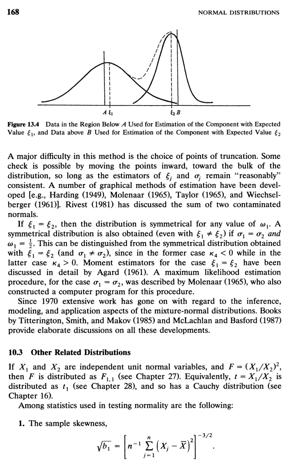
/


![TABLE 13.4 Multipliers an, a'n such that E[anS] = a = E[a'JV] 128](https://djvu.online/jpg/G/I/p/GIpGFve5Mnr8K/148.webp)


![TABLE 17.4 Values of Pr[Ur s > u] forn = 5, r = 1, 5 = 2 373](https://djvu.online/jpg/G/I/p/GIpGFve5Mnr8K/393.webp)


![TABLE 20.2 ARE for x^ compared to X^]+l 592
5.9 Censored Data, 592](https://djvu.online/jpg/G/I/p/GIpGFve5Mnr8K/612.webp)


Author: Norman L.J. Kotz S. Balakrishnan N.
Tags: теория вероятностей математический анализ
ISBN: 0-471-58495-9
Year: 1994


Text
Continuous
Univariate
Distributions
Volume 1
WILEY SERIES IN PROBABILITY AND MATHEMATICAL STATISTICS
Established by WALTER A. SHEWHART and SAMUEL S. WILKS
Editors: Vic Barnett, Ralph A. Bradley, Nicholas /. Fisher, /. Stuart Hunter,
/. B. Kadane, David G. Kendall, Adrian F. M. Smith, Stephen M. Stigler,
Jozef L. Teugels, Geoffrey S. Watson
A complete list of the titles in this series appears at the end of this volume
Continuous
Univariate
Distributions
Volume 1
Second Edition
NORMAN L. JOHNSON
University of North Carolina
Chapel Hill, North Carolina
SAMUEL KOTZ
University of Maryland
College Park, Maryland
N. BALAKRISHNAN
McMaster University
Hamilton, Ontario, Canada
A Wiley-Interscience Publication
JOHN WILEY & SONS, INC.
New York • Chichester • Brisbane • Toronto • Singapore
This text is printed on acid-free paper.
Copyright © 1994 by John Wiley & Sons, Inc.
All rights reserved. Published simultaneously in Canada.
Reproduction or translation of any part of this work beyond
that permitted by Section 107 or 108 of the 1976 United
States Copyright Act without the permission of the copyright
owner is unlawful. Requests for permission or further
information should be addressed to the Permissions Department,
John Wiley & Sons, Inc., 605 Third Avenue, New York, NY
10158-0012.
Library of Congress Cataloging in Publication Data:
Johnson, Norman Lloyd.
Continuous univariate distributions / Norman L. Johnson, Samuel
Kotz, N. Balakrishnan.—2nd ed.
p. cm.—(Wiley series in probability and mathematical
statistics. Applied probability and statistics.)
“A Wiley-Interscience publication.”
Includes bibliographical references and index.
ISBN 0-471-58495-9 (v. 1)
1. Distribution (Probability theory) I. Kotz, Samuel.
II. Balakrishnan, N., 1956- . III. Title. IV. Series.
QA273.6.J6 1994 93-45348
519.2'4—dc20
Printed in the United States of America
10 9 8 7 6 5
To
Regina Elandt-Johnson
Rosalie Kotz
Colleen Cutler and Sarah Balakrishnan
Contents
Preface
List of Tables
12 Continuous Distributions (General)
1 Introduction, 1
2 Order Statistics, 6
3 Calculus of Probability Density Functions, 14
4 Systems of Distributions, 15
4.1 Pearson System, 15
4.2 Expansions, 25
4.3 Transformed Distributions, 33
4.4 Bessel Function Distributions, 50
4.5 Miscellaneous, 53
5 Cornish-Fisher Expansions, 63
6 Note on Characterizations, 67
Bibliography, 68
13 Normal Distributions
1 Definition and Tables, 80
2 Historical Remarks, 85
3 Moments and Other Properties, 88
4 Order Statistics, 93
5 Record Values, 99
6 Characterizations, 100
7 Approximations and Algorithms, 111
CONTENTS
viii
8 Estimation, 123
8.1 Estimation of £, 123
8.2 Estimation of a, 127
8.3 Estimation of Functions of £ and a, 139
8.4 Estimation from Censored Data, 146
9 Simulational Algorithms, 152
9.1 Box-Muller Method, 152
9.2 Marsaglia-Bray’s Improvement, 153
9.3 Acceptance-Rejection Method, 153
9.4 Ahrens-Dieter Method, 155
10 Related Distributions, 156
10.1 Truncated Normal Distributions, 156
10.2 Mixtures, 163
10.3 Other Related Distributions, 168
Bibliography, 174
14 Lognormal Distributions 207
1 Introduction, 207
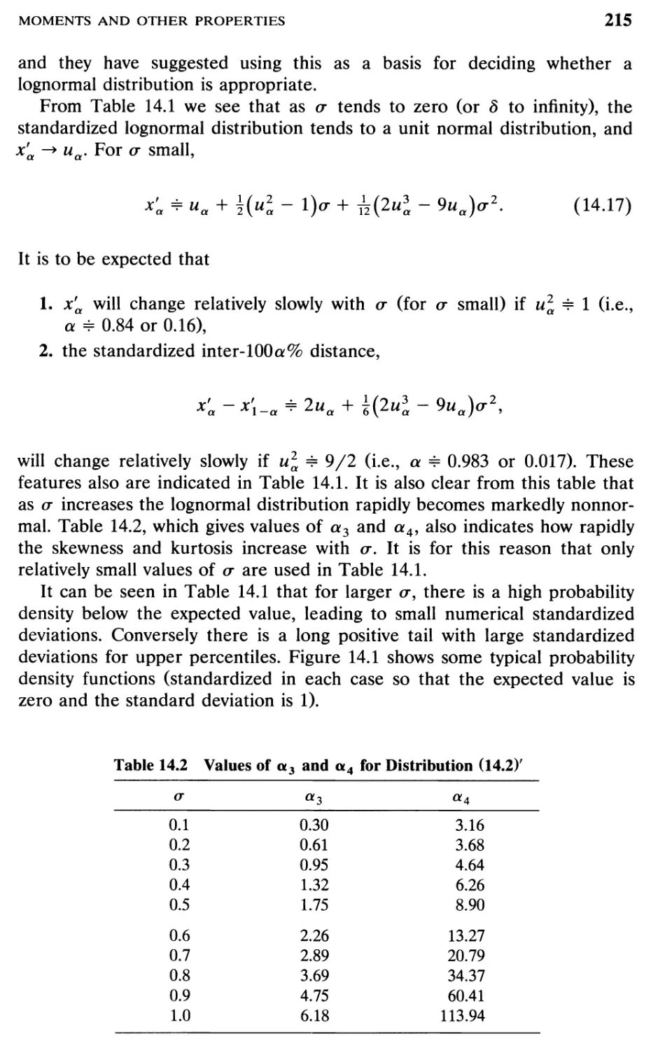
2 Historical Remarks, 209
3 Moments and Other Properties, 211
4 Estimation, 220
4.1 0 Known, 220
4.2 0 Unknown, 222
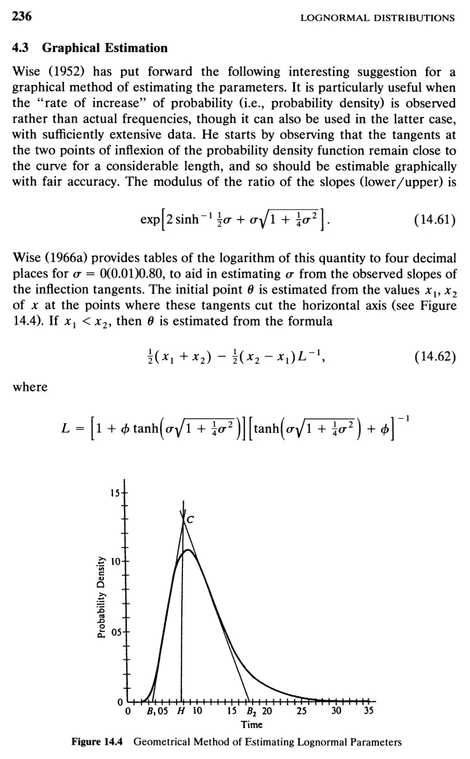
4.3 Graphical Estimation, 236
5 Tables and Graphs, 237
6 Applications, 238
7 Censoring, Truncated Lognormal and Related
Distributions, 240
8 Convolution of Normal and Lognormal Distributions, 247
Bibliography, 249
15 Inverse Gaussian (Wald) Distributions 259
1 Introduction, 259
2 Genesis, 260
3 Definition, 261
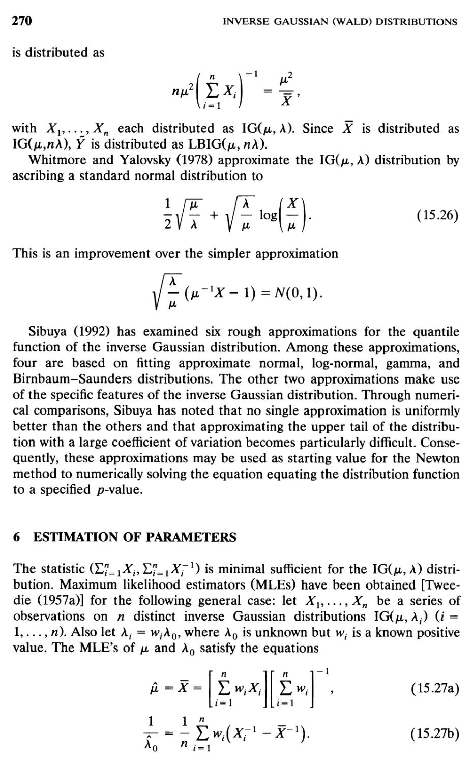
4 Moments, 262
5 Properties, 266
6 Estimation of Parameters, 270
CONTENTS
7 Truncated Distributions—Estimation of Parameters, 276
7.1 Doubly Truncated Distribution, 277
7.2 Truncation of the Lower Tail Only, 278
7.3 Truncation of the Upper Tail Only, 279
8 Conditional Expectations of the Estimators
of the Cumulants, 279
9 Related Distributions, 281
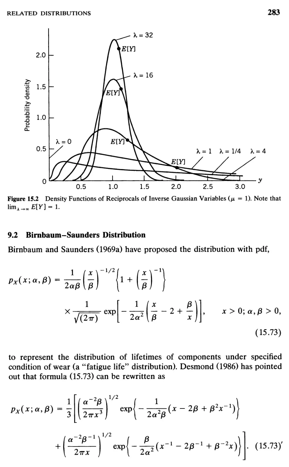
9.1 Reciprocal of an Inverse Gaussian Variate, 281
9.2 Birnbaum-Saunders Distribution, 283
9.3 Generalized Inverse Gaussian Distributions, 284
9.4 Mixtures of IGK/i, A) with Its Complementary
Reciprocal, 285
9.5 Other Related Distributions, 287
10 Tables, 289
11 Applications, 290
Bibliography, 292
16 Cauchy Distribution
1 Historical Remarks, 298
2 Definition and Properties, 299
3 Order Statistics, 303
4 Methods of Inference, 306
4.1 Methods Based on Order Statistics, 306
4.2 Maximum Likelihood Inference, 310
4.3 Conditional Inference, 314
4.4 Bayesian Inference, 315
4.5 Other Developments in Inference, 317
5 Genesis and Applications, 318
6 Characterizations, 321
7 Generation Algorithms, 323
7.1 Monahan’s (1979) Algorithm, 323
7.2 Kronmal and Peterson’s (1981) Acceptance-Complement
Method, 324
7.3 Ahrens and Dieter’s (1988) Algorithm, 326
8 Related Distributions, 327
Bibliography, 329
17 Gamma Distributions
1 Definition, 337
2 Moments and Other Properties, 338
CONTENTS
X
3 Genesis and Applications, 343
4 Tables and Computational Algorithms, 344
5 Approximation and Generation of Gamma
Random Variables, 346
6 Characterizations, 349
7 Estimation, 355
7.1 Three Parameters Unknown, 356
7.2 Some Parameters Unknown, 360
7.3 Estimation of Shape Parameter
and y Known), 368
7.4 Order Statistics and Estimators Based
on Order Statistics, 370
8 Related Distributions, 379
8.1 Truncated Gamma Distributions, 380
8.2 Compound Gamma Distributions, 381
8.3 Transformed Gamma Distributions, 382
8.4 Convolutions of Gamma Distributions, 384
8.5 Mixtures of Gamma Distributions, 386
8.6 Reflected Gamma Distributions, 386
8.7 Generalized Gamma Distributions, 388
Bibliography, 397
18 Chi-Square Distributions Including Chi and Rayleigh 415
1 Historical Remarks, 415
2 Definition, 416
3 Moments and Other Properties, 420
4 Tables and Nomograms, 422
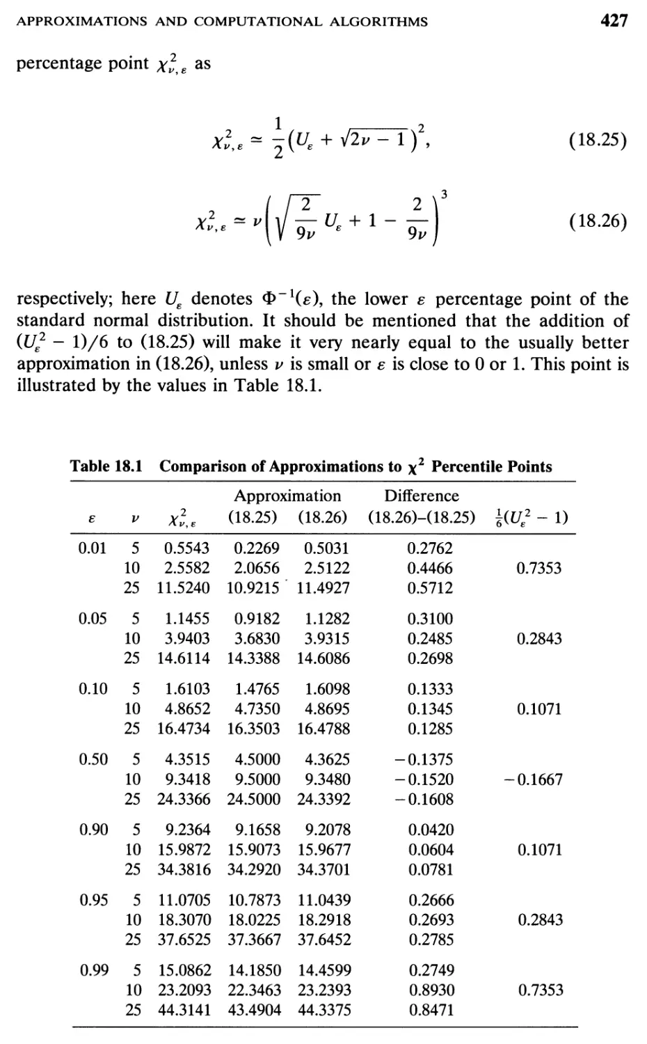
5 Approximations and Computational Algorithms, 426
6 Characterizations, 441
7 Simulational Algorithms, 443
8 Distributions of Linear Combinations, 444
9 Related Distributions, 450
10 Specific Developments in the Rayleigh Distribution, 456
10.1 Historical Remarks, 456
10.2 Basic Properties, 456
10.3 Order Statistics and Properties, 459
10.4 Inference, 461
10.5 Prediction, 474
10.6 Record Values and Related Issues, 475
CONTENTS
10.7 Related Distributions, 479
Bibliography, 481
19 Exponential Distributions
1 Definition, 494
2 Genesis, 494
3 Some Remarks on History, 497
4 Moments and Generating Functions, 498
5 Applications, 499
6 Order Statistics, 499
7 Estimation, 506
7.1
Classical Estimation, 506
7.2
Grouped Data, 509
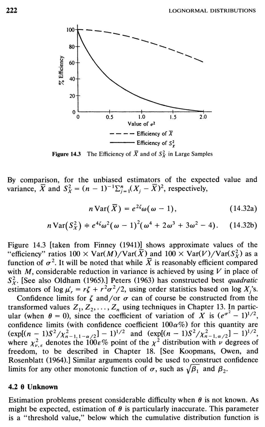
7.3
Estimators Using Selected Quantiles, 510
7.4
Estimation of Quantiles, 521
7.5
Bayesian Estimation, 522
7.6
Miscellaneous, 526
Characterizations, 534
8.1
Characterizations Based on Lack of Memory
and on Distributions of Order Statistics, 536
8.2
Characterizations Based on Conditional
Expectations (Regression), 540
8.3
Record Values, 544
8.4
Miscellaneous, 544
8.5
Stability, 545
9 Mixtures of Exponential Distributions, 546
10 Related Distributions, 551
Bibliography, 556
20 Pareto Distributions,
1 Introduction, 573
2 Genesis, 573
3 Definitions, 574
4 Moments and Other Indices, 577
4.1 Moments, 577
4.2 Alternative Measures of Location, 577
4.3 Measures of Inequality, 578
5 Estimation of Parameters, 579
5.1
Least-Squares Estimators, 580
5.2
Estimators from Moments, 580
5.3
Maximum Likelihood Estimation, 581
5.4
Estimation Based on Order Statistics, 584
5.5
Sequential Estimation, 588
5.6
Minimax Estimation, 588
5.7
Estimation of Pareto Densities, 589
5.8
Estimation of Pareto Quantiles, 590
5.9
Censored Data, 592
5.10
Bayesian Estimation, 594
6 Estimation of Lorenz Curve and Gini Index, 595
7 Miscellaneous, 596
8 Order Statistics and Record Values, 599
8.1 Order Statistics, 599
8.2 Record Values, 601
9 Characterizations, 603
10 Product and Ratios of Pareto Random Variables, 605
11 Applications and Related Distributions, 607
12 Generalized Pareto Distributions, 614
Bibliography, 620
Weibull Distributions
1 Historical Remarks, 628
2 Definition, 629
3 Order Statistics, 637
4 Methods of Inference, 641
4.1 Moment Estimation, 641
4.2 Best Linear Unbiased Estimation, 644
4.3 Asymptotic Best Linear Unbiased Estimation, 647
4.4 Minimum Quantile Distance Estimation, 651
4.5 Modified Moment Estimation, 652
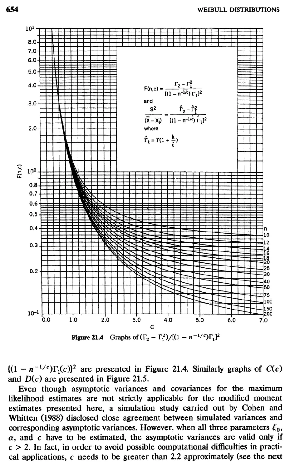
4.6 Maximum Likelihood Estimation, 656
4.7 Modified Maximum Likelihood Estimation, 660
4.8 Bayesian Estimation and Shrinkage Estimation, 661
5 Tolerance Limits and Intervals, 663
6 Prediction Limits and Intervals, 667
7 Record Values, 671
8 Tables and Graphs, 675
CONTENTS
9 Characterizations, 679
10 Simulation Algorithms, 682
11 Applications, 684
12 Related Distributions, 686
Bibliography, 695
Abbreviations
Author Index
Subject Index
Preface
As a continuation of Univariate Discrete Distributions, second edition,
this book is the first of two volumes to discuss continuous univariate
distributions. The second edition of Continuous Univariate Distributions differs
from the first, published in 1970, in two important aspects: (1) Professor
N. Balakrishnan has joined the two original authors as a coauthor. (2)
Because of substantial advances in theory, methodology, and application of
continuous distributions, especially gamma, Weibull, and inverse Gaussian
during the last two decades, we have decided to move the chapter on extreme
value distributions to the next volume. The chapter on gamma distributions
has been split into two chapters, one dealing only with chi-squared
distributions. Even so, as in the revision of the volume on Discrete Distributions, the
great amount of additional information accruing since the first edition has led
to a substantial increase in length.
In accordance with the principle stated in the original General Preface, we
continue to aim at “excluding theoretical minutiae of no apparent practical
importance,” although we do include material on characterizations that some
may regard as being of doubtful practical value. The more general Chapter
12 has been expanded relatively less than the other chapters that deal with
specific distributions.
Even with omission of the extreme value distribution chapter, the great
amount of new information available has forced us to be very selective for
inclusion in the new work. One of our main preoccupations has been to assist
the struggle against fragmentation, the necessity for which has been elegantly
expressed by Professor A. P. Dawid, new editor of Biometrika [Biometrika,
80, 1 (1993)]. We realize that some authors may be affronted at omission of
their work, but we hope that it will not be regarded as unfriendly action, or at
“best” a consequence of ignorance. These volumes are intended to be useful
to readers, rather than an “honor roll” of contributors.
We acknowledge with thanks the invaluable assistance of Mrs. Lisa Brooks
(University of North Carolina), Mrs. Cyndi Patterson (Bowling Green State
University), and Mrs. Debbie Iscoe (Hamilton, Canada) in their skillful
typing of the manuscript. We also thank the Librarians of the University of
xv
PREFACE
xvi
North Carolina, Bowling Green State University, McMaster University,
University of Waterloo, and the University of Maryland for their help in library
research. Samuel Kotz’s contribution to this volume was, to a large extent,
executed as a Distinguished Visiting Lukacs Professor in the Department of
Mathematics and Statistics at Bowling Green State University (Bowling
Green, Ohio) during September-December 1992. Likewise N. Balakrishnan’s
work for this volume was carried out mostly in the Department of Statistics
and Actuarial Science at the University of Waterloo where he was on
research leave during July 1992—June 1993.
Special thanks are also due to Mrs. Kate Roach and Mr. Ed Cantillon at
John Wiley & Sons in New York for their sincere efforts in the fine
production of this volume. We also thank Ms. Dana Andrus for all her efforts
in copy-editing the long manuscript.
Thanks are offered to the Institute of Mathematical Statistics, the
American Statistical Association, the Biometrika Trustees, the Institute of
Electrical and Electronics Engineerings, the Association for Computing Machinery,
Marcel Dekker, Inc., the Royal Statistical Society, the American Society for
Quality Control, the Australian Statistical Society, Gordon and Breach
Science Publishers, Blackwell Publishers, and the editors of Biometrical
Journal, Sankhya and Tamkang Journal of Mathematics, for their kind
permission to reproduce previously published tables and figures.
Authors of this kind of informational survey—designed primarily for
nonspecialists—encounter the problem of having to explain results that may
be obvious for a specialist but are not part and parcel of the common
knowledge, and still have enough space for information that would be new
and valuable for experts. There is a danger of “high vulgarization” (over
simplification) on the one hand and an overemphasis on obscure “learned”
points—which many readers will not need—on the other hand. We have
tried to avoid these pitfalls, to the best of our ability.
It is our sincere hope that these volumes will provide useful
facts—coherently stated—for a “lay reader,” and also arouse perceptions and memories
among well-informed readers, stimulating introspection and further research.
Norman L. Johnson
Samuel Kotz
N. Balakrishnan
List of Tables
TABLE 12.1 Values of À giving maximum or minimum j82 43
TABLE 13.1 Percentile points of normal distribution, as
standardized deviates (values of Ua) 84
TABLE 13.2 Standardized percentile points of distribution (13.42)
and the normal distribution 112
TABLE 13.3 Efficiency of trimmed means, relative to X 124
TABLE 13.4 Multipliers an, a'n such that E[anS] = a = E[a'JV] 128
TABLE 13.5 Values of v, A, and log c such that first three
moments of (T/a)x and agree 130
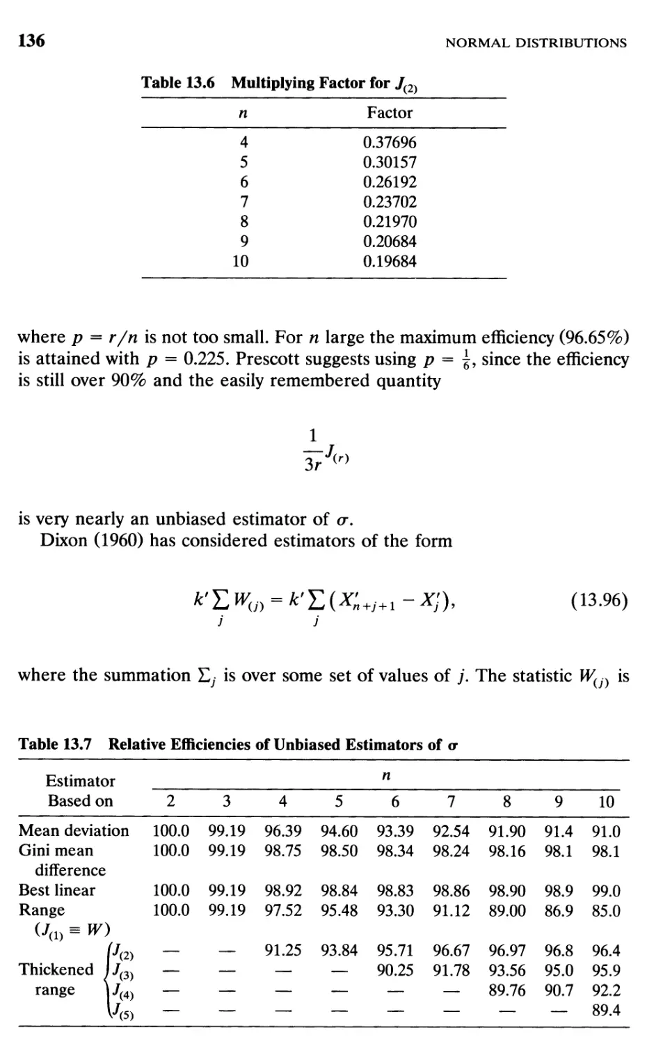
TABLE 13.6 Multiplying factor for /(2) 136
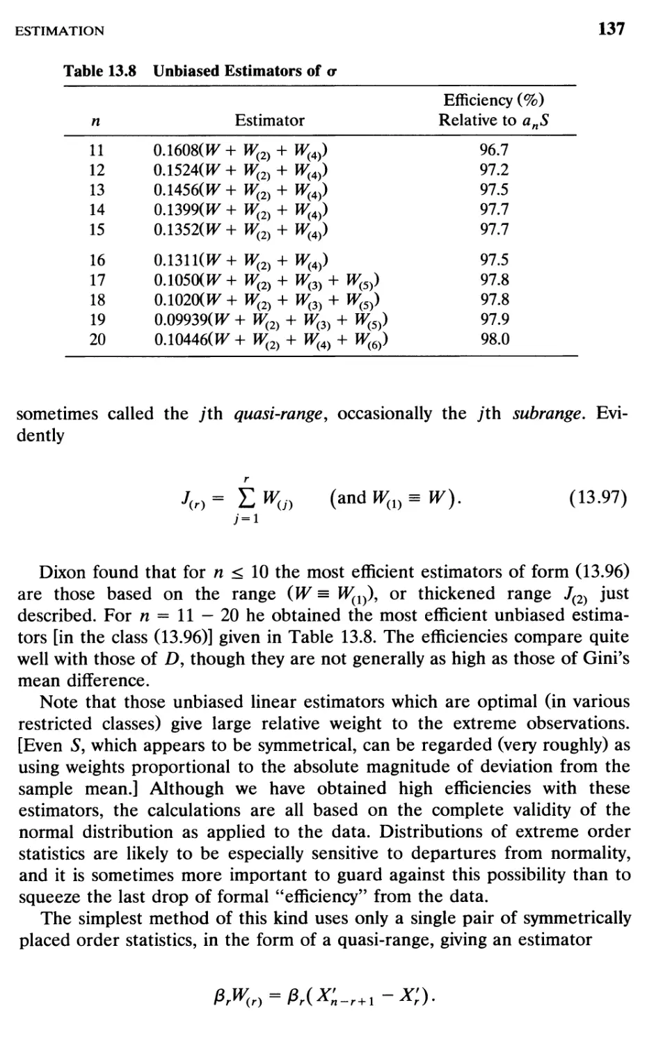
TABLE 13.7 Relative efficiencies of unbiased estimators of a 136
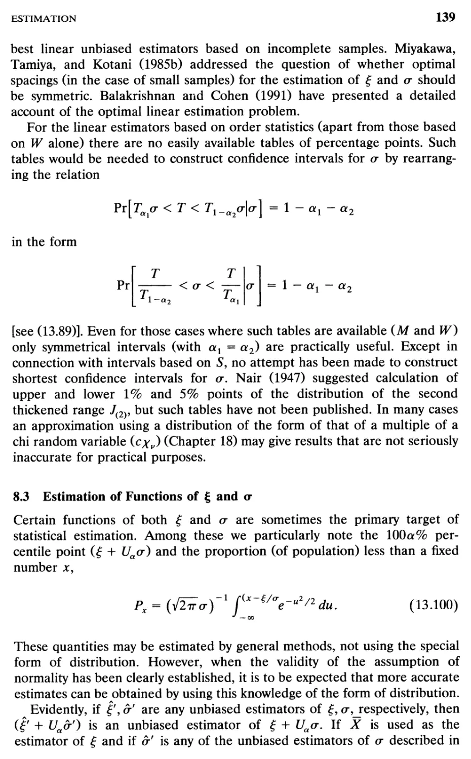
TABLE 13.8 Unbiased estimators of a 137
TABLE 13.9 Efficiency (%) of Winsorized mean based on
Xj+1,..., X'n_j relative to the best linear unbiased
estimator of f based on X], Xj+l9 ...,X'n_j 149
TABLE 13.10 Expected value, standard deviation, and
(mean deviation)/(standard deviation) for
truncated normal distributions 159
TABLE 13.11 Asymptotic values of n X (variance)/cr2 for
maximum likelihood estimators 160
xvii
xviii
Standardized 100a% points (x'a) of lognormal
distributions (a = S1־)
Values of a3 and a4 for distribution (14.2y
Percentile points of standardized lognormal
distributions
Values of -u 1/in + 1) and -E(Ul n)
Variances and covariances of maximum likelihood
estimators for censored three-parameter lognormal
distribution
Maximum likelihood estimators for censored
three-parameter lognormal distribution where
value of 0 is supposed known
Comparison of Cauchy and normal distributions
Percentage points of standard Cauchy distribution
Results of simulation of à and à
Details of available tables on moments of gamma
order statistics
Comparison of the percentage points of rth-order
statistics from standard gamma distribution with
values from Tiku and Malik’s (1972) approximation
(with a = 2, sample size n = 6)
Values of Pr[Ur s > u] for n = 5, r = 1, s = 2
Comparison of approximations to \2 percentile
points
Accuracy of several chi-squared approximation
formulas
Maximum absolute error in approximations of Fx!{x)
in (18.22), (18.23), (18.24), and (18.51)
Comparisons of the cube root and the fourth root
transformations
TABLE 14.1
TABLE 14.2
TABLE 14.3
TABLE 14.4
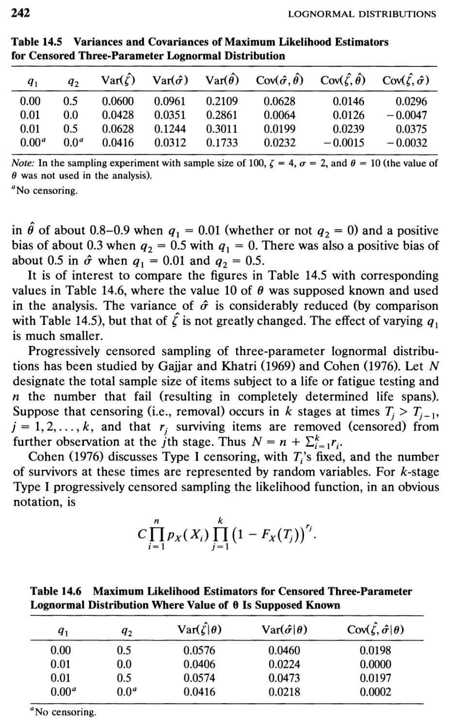
TABLE 14.5
TABLE 14.6
TABLE 16.1
TABLE 16.2
TABLE 17.1
TABLE 17.2
TABLE 17.3
TABLE 17.4
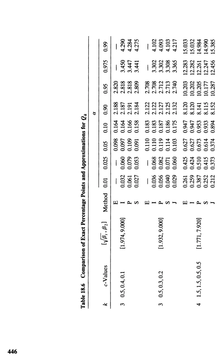
TABLE 18.1
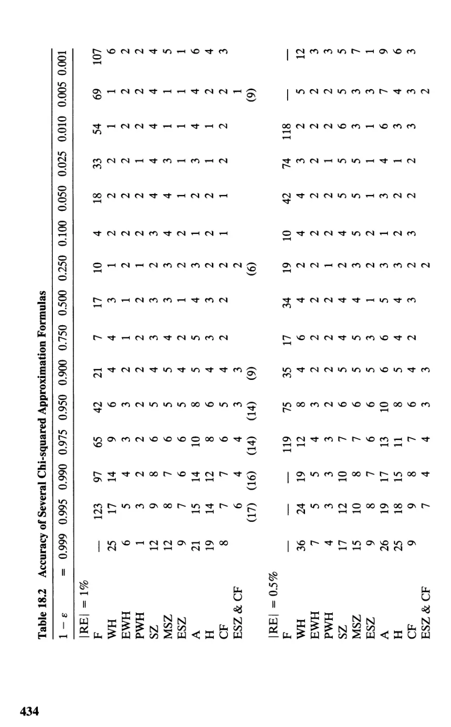
TABLE 18.2
TABLE 18.3
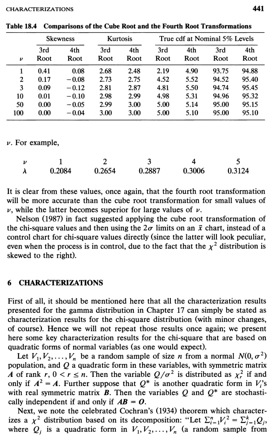
TABLE 18.4
xix
444
446
449
464
466
535
591
592
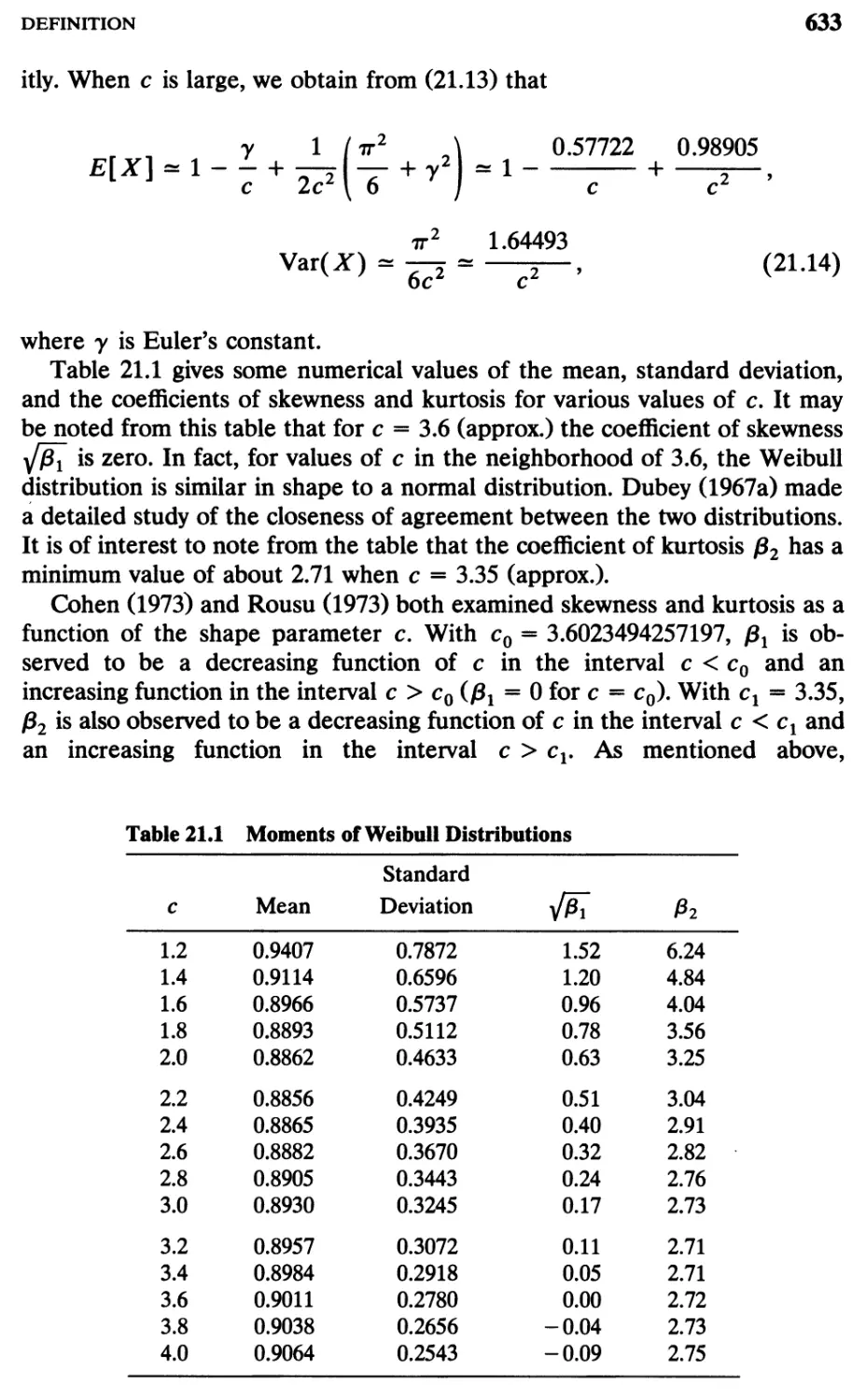
633
646
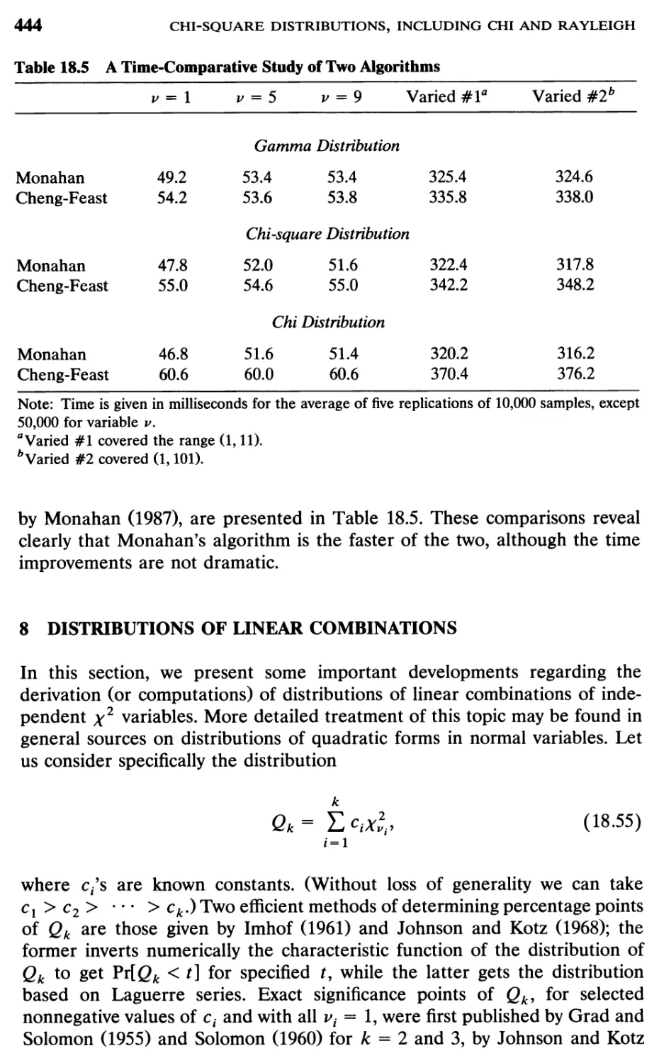
A time-comparative study of two algorithms
Comparison of exact percentage points and
approximations for Qk
Percentage points using Imhof s method (I),
Solomon and Stephens’ method (S), and mixture
approximation (M)
Coefficients at of the BLUE of a and efficiency
relative to the BLUE based on complete sample for
n = 2(1)10, r = 0, and s = 0(l)n - 2
Optimum spacings {A,}, corresponding coefficients
bt, and the value of K2 for the ABLUE o־**
(complete samples)
A dictionary of characterizations of the exponential
distribution
Values of Pu j for specific estimator of x^ of
the form (20.64)
ARE for compared to
Moments of Weibull distributions
Values of gn = log10 w1/2 such that
g״(log10 X'n - log10 X[)1־ is a median-unbiased
estimator of c
Continuous
Univariate
Distributions
Volume 1
CHAPTER 1 2
Continuous Distributions (General)
1 INTRODUCTION
Chapters 1 and 2 (of Volume 1) contain some general results and methods
that are also useful in our discussion of continuous distributions. In this
chapter we will supplement this information with techniques that are relevant
to continuous distributions. As in Chapter 2, some general systems of
(continuous) distributions will be described.
Continuous distributions are generally amenable to more elegant
mathematical treatment than are discrete distributions. This makes them especially
useful as approximations to discrete distributions. Continuous distributions
are used in this way in most applications, both in the construction of models
and in applying statistical techniques. Continuous distributions have been
used in approximating discrete distributions of discrete statistics in Volume 1.
The fact that most uses of continuous distributions in model building are as
approximations to discrete distributions may be less widely appreciated but is
no less true. Very rarely is it more reasonable, in an absolute sense, to
represent an observed value by a continuous, rather than a discrete, random
variable. Rather this representation is a convenient approximation,
facilitating mathematical and statistical analysis.
An essential property of a continuous random variable is that there is zero
probability that it takes any specified numerical value, but in general a
nonzero probability, calculable as a definite integral of a probability density
function (see Section 1.4) that it takes a value in specified (finite or infinite)
intervals. When an observed value is represented by a continuous random
variable, the recorded value is, of necessity “discretized.” For example, if
measurements are made to the nearest 0.01 units, then all values actually in
the interval (8.665, 8.675) will be recorded as 8.67. The data are therefore
grouped. Adjustments in the estimation of population moments, to correct
(on average) for this effect, were proposed by Sheppard (1896). These may be
summarized for the case of equal group widths h (with /j!r,g/j!r denoting the
1
2
CONTINUOUS DISTRIBUTIONS (GENERAL)
rth original moment and rth grouped moment, respectively):
(12.1a)
M2 =gß'2-^h2, (12.1b)
Ms 3 - (12.1c)
M4 + ^/»4. (12.1d)
The general formula is [Sheppard (1896); Wold (1934)]
l£r = i (21~J — 1) ( y ) Bj giir-jh>, (12.2)
where Bj is the jth Bernoulli number (see Chapter 1, Section A9).
These results depend on the assumption that if the centers of groups are
..., a — h, a, a + h,... (|fl| <
then a has a uniform distribution (Chapter 26) between - \h and + \h [see
also Haitovsky (1983)]. Effects of invalidity of this assumption have been
evaluated by Tricker (1984), who showed that the characteristic function
(Chapter 1, Section B8) of gX (the grouped variable corresponding to a
random variable X) is
* sin(hh+jv)
<Psx(t) = E —1, . exp(l - i • 2irjh) ■ <px(th + 2irj), (12.3)
j= -oo 2in “I" J17
where i = V- 1 and cpx(t) is the characteristic function of X.
In the same paper, effects of rounding when the distribution of X is
normal (Chapter 13), Laplace (Chapter 24), or gamma (Chapter 17) are
evaluated numerically for selected cases. For a given group width h, the
magnitude of the correction for grouping tends to increase with the
magnitude of the skewness, as measured by | yfß[ I; it is quite small for symmetrical
distributions.
Some concepts that have great value for discrete distributions are
much less valuable in the discussion of continuous distributions. Probability-
generating functions, in particular, are little used in this part of the book.
Factorial moments also rarely offer the advantages of conciseness and
simplicity that they do for discrete distributions, although they can be calculated.
INTRODUCTION
3
On the other hand, standardization (use of the transformed variable
(X-E[X])
^var(X)
to produce a distribution with zero mean and unit standard deviation) is
much more useful for continuous distributions. In particular, the shape of a
distribution can be conveniently summarized by giving standardized values of
a number of quantiles (i.e., values of the variable for which the cumulative
distribution function has specified values). Care should be taken to
distinguish between standardized and standard forms of distributions. The latter
are usually convenient ways of writing the mathematical formulas for
probability density functions. They may happen to be standardized, but this is not
essential.
MacGillivray (1992) has introduced the skewness function
F~\u) + F~\ 1 - u) - 2F~\\)
F~\u) - F-1(l - u)
Note that F~x{\) = median (X) and y^(f) is Gabon’s measure of skewness:
(Upper quartile - Median) - (Median - Lower quartile)
Interquartile distance
MacGillivray proposes
sup 17*0)1 (12.4b)
\ <U< 1
as “a measure of overall asymmetry for the central 100(1 — 2a)% of the
distribution.”
At this point we introduce indices that are applied more commonly to
continuous than to discrete distributions:
1. GinVs mean differences, y(X), for the distribution of X is the expected
value, E[\Xl - X2\] of the absolute value of the difference between two
independent variables Xv X2, each distributed as X.
If Xv ...,Xn are i.i.d., then the statistic
8= (") * H \X,-Xj\ (12.5)
i<j
is an unbiased estimator of
y{X) =£[!*, -X2\\.
(12.6)
4
CONTINUOUS DISTRIBUTIONS (GENERAL)
2. The Lorenz curve, for a positive random variable A", is defined as the
graph of the ratio
.,rn, ElXIX<x]Fx(x)
Em <12'7>
against Fx(x). If X represents annual income, L(p) is the proportion
of total income that accrues to individuals having the 100/?% lowest
incomes.
It is easy to see that
L(p) <p,
L( 0) = 0,
L( 1) = 1.
A typical Lorenz curve is shown in Figure 12.1. If all individuals earn the
same income, L(/?) = /?. The area between the line L(/?) = p and the
Lorenz curve may be regarded as a measure of inequality of income, or more
generally, of variability in the distribution of X. There is extensive discussion
of Lorenz curves in Gail and Gastwirth (1978), and a concise account of their
properties in Dagum (1985).
Gastwirth (1971) has given the following definition of the Lorenz function
L(p):
L(p) = {E[X]}-l(PFxl(t)dt, (12.8)
Jo
where
Fxl(t) = inffx-.Fj^O > r}.
X
This equation is equivalent to (12.7) for continuous distributions, but it also
applies to discrete distributions.
Lorenz ordering is sometimes used to compare the amounts of inequality
in two or more distributions. It is based on comparisons of the values of L( p)
for the distributions. If their difference is of the same sign for all p, the
distributions are Lorenz ordered appropriately. If the sign changes, Lorenz
ordering does not apply. There is a useful description of Lorenz ordering in
Arnold (1987); see also Chapter 33.
The area between the line L(p) = p and the actual Lorenz curve is called
the area of concentration. The Gini concentration index C(X) is twice this
INTRODUCTION
5
area. It is related to GinVs mean difference, defined as in (12.5):
C(X) = 2[\p - L{p)} dp = 1 -2(XL{p) dp.
Jc\ Jr\
Now
f1L(p)dp = -^—jXE[X\X<x)Fx(x)dFx(x)
E[X]J0
1
nx\L{L.'Px('>JTAx>‘b
ElX^X, <X2]Pr[X, < X2],
E[X]
with Xx, X2 independently distributed as X. Since X1 and X2 are
continuous and independent,
thus
?r[X1<X2] = Pr[Xl>X2] = h
E[Xx\Xx <X2]
C(X) = 1 -
E[X]
6
CONTINUOUS DISTRIBUTIONS (GENERAL)
Since
12[e[xx\xx<x2] +E[X1\X1 >x2]} = E[X]
and
y{X) =E[\Xl-X2\] =E[X1\X1 >X2] -E[Xx\Xx <X2],
we have
E[Xx\Xx<X2] =E[X]-{ y(X).
Hence
h(X)
C^) = W- (12-9a)
The ratio y(X)/E[X] = E[\Xx - X2\]/E[X] is analogous to the coefficient
of variation. Tziafetas (1989) obtains the alternative form:
Cov( *,/>(*))
c{x) =— ' (12'9b)
Order statistics are of much greater use, and simpler in theoretical
analysis, for continuous than for discrete distributions. The next section will
be devoted to a general discussion of order statistics for continuous variables,
with particular reference to their use in statistical analysis.
2 ORDER STATISTICS
If Xv X2,..., Xn are random variables, and X[ < X2< * * * < Xfn are the
same variables arranged in ascending order of magnitude [so that X[ =
min(Xv X2,..., Xn\ X'n = max(X1? X2,..., Xn)\ then X[, X2,...,Xfn are
called the order statistics corresponding to Xv X2,..., Xn (see also Chapter
1, Section BIO). If it is necessary to indicate the total number of variables
explicitly, the symbols X[ ;n,..., X'n:n will be used.
If the differences {Xt - X-i are continuous random variables, then the
events {Xt = X}) all have zero probability. Being finite in number, they can be
neglected in probability calculations. We will suppose, from now on, that this
is the case, so we can assume that X[ < X2 • • • < X'n, without altering any
probabilities that relate to the joint distribution of X[, X2,..., X’n.
ORDER STATISTICS
7
The cumulative distribution function of X'n is defined by
Pr[<x] = Pr
If Xx, X2,..., Xn are mutually independent, then
n (*/**)
>=i
(12.10)
Pr[Z' <x] = IlPr[^^*],
y=i
and the probability density function of X’n is equal to
(12.11)
(Cumulative distribution\ A
function of X'n j X ^
Probability density '
function of X{
Cumulative distribution
function of X{
(12.12)
If all X/s have identical distributions with Pr[Xj < x] = F(x), and
dF(x)/dx = p(x), then the probability density function of X'n is
n[F(x)]n p(x).
(12.13a)
Similarly (again assuming that all X/s are independent and identically
distributed) the probability density function of X[ is
n[l-F(*)]” p(x).
(12.13b)
More generally, in this case, with 1 < ax < a2 < • • • < as <n (and setting
a0 = 0, as + l = n, F(xaQ) = 0, F(xa ) = 1), the joint probability density
function of X'ai, X'a2,..., X' is (in an obvious notation)
n\
- Oj_l) !
5 + 1
Y\p{xa)
i-1
(xai <xa2< ••• <xa). (12.14)
In particular, the joint probability density function of X[ and X'n is
n(n - l)p(Xl)p(xn)[F(xn) - F^)]
n — 2
(*,<*„). (12.15)
8
CONTINUOUS DISTRIBUTIONS (GENERAL)
From this joint distribution it is possible to evaluate the cumulative
distribution function of the range (W = Xfn — X[). The formulas
Pr[W < w] = n f p(x)[F(x) — F(jc - w)\n~x dx (12.16)
J — 00
and
E[W] = C {l - [F(x)]" - [1 - F(x)n dx (12.17)
J — oo
are of interest.
If n = 2m + 1 is odd (i.e., m is an integer), then X'm + l represents the
(sample) median of Xv X2,..., Xn. Its probability density function is
(2m + 1)!
V [F(*){1-/=■(*)}) p(x). (12.18)
(ml)
Generally the 100p% sample percentile is represented by X^n + l)p and is
defined only if (n + 1 )p is an integer. The median corresponds to p = }; we
have the lower and upper quartile for p = f, respectively.
Often under certain conditions of regularity, it is possible to obtain useful
approximations to the moments of order statistics in terms of the common
probability density function of the A"’s. This approach makes use of the fact
that the statistics Yx = F(Ar1), Y2 = F(X2\..., Yn = F(Xn) are
independently distributed with common rectangular distribution (see Chapter 26)
over the range 0 to 1. The corresponding order statistics Y(, Y2,..., Y„ have
the joint probability density function
PY[,...,Y^y\^-^yn) = nl (0^y1<y2< ••• <y„<l).
The joint probability density function of any subset Y^,...,Y^ (1 < ax <
a2< * * • < as < n) is [using (12.14)]
*<”•. ■ n;:,K‘
(12.19)
with a0 — 0, ai + 1 = n; yao = 0; ya j+] = 1, and where Y^,YJs is denoted
by {Ya'}. The moments and product moments of the Y”s are given by the
ORDER STATISTICS
9
formula
n ^
y=i
n\
Idj + E r, - 1 !
i = 1
(fly + U-lrl ~ !)!
(12.20)
We now expand X'r, as a function of Yr', about the value E[Y’] = r/(n + 1);
thus
X'r —r) + (Yr
\ n + 1 / I n \ I
dF~l(y)
dy
y = r/(n + 1)
d F~ (y)
dy2
y = r/(n +1)
(12.21)
So we can take expected values of each side of (12.13) (using the method of
statistical differentials, described in Chapter 1). Note that since
y = F(x) = f p(t) dt,
J — oo
dF~l dx 1 1
dy dy dy/dx p{x)
and
dF~\y)
dy
y=r/(n + 1)
p(C)
where £' satisfies the equation
—!—=fcp(x\dX' (12.22)
n + 1 J-a,
Similarly d2F~x/dy2 = -[p(x)]~2[dp(x)/dy] = -[p(x)]~3[dp(x)/dx], and
so on.
David and Johnson (1954) found it convenient to arrange the series so
obtained in descending powers of (n + 2). Some of their results follow. [In
10
CONTINUOUS DISTRIBUTIONS (GENERAL)
these formulas, ps = s/(n + 1); qs = 1 - ps; (F = dF l/dy\
(F-lTr = d2F-l/dy2\y^r/(n + 1), etc.]
y=r/(n + 1)’
2 (n + 2)
(n + 2)
(12.23a)
Vzr(X')
PrQr
n + 2
(n + 2)
+Pr^|(F_1)'r(F-1)"' + ~ [(F_1)r]2|
[2(gr-pr)(F-1)'r(F-1):
+...,
(12.23b)
+ ■
PrQs
(n + 2)
(qr - pr)(F-l)”r(F-l)'s + (q, - pMF-VAF-1)*,
+ 2P'qAF 1)^F 1)s+2Psq^F ^F *)”
1
+ -prqs(F-l)r(F-l)"s
+ ... , r < s, (12.23c)
ß^Xp) = 7~T^ bUr-Pr){{F-%f
(n + 2) 1
+ 3prgr{(F-1)'r}2(F-1)';}] + • • • , (12.23d)
3/>,V
(n + 2)
p4(K)
2{(F-l)'r}4
(n + iy
\6{(qr-pr)2 -prqr}{(F-')'r}4
+ 36prqr(qr ~ pr){(F l)'r)3(F 1)'"
+ 5prV{2{(F-1),r}3(F-1)'; + 3{(F-1)'r(F-1)';}2}] + ... . (12.23e)
ORDER STATISTICS
11
By inserting the values of (F-1)'r, (F-1)^, and so on, appropriate to the
particular distribution, approximate formulas can be obtained that
correspond to any absolutely continuous common distribution of the original
independent variables. These formulas generally tend to be more accurate
for large n, and for larger min(pr,qr) [with Cov(X'r, X's) for larger
min(pr, ps,qr,qs)\- David (1981) and Arnold and Balakrishnan (1989)
provide detailed discussions on bounds and approximations for moments of
order statistics.
If the distribution of X is such that Fr[X < x] is a function of only
(x - Q)/<j> so that 0 and <f> ( > 0) are location and scale parameters, then
it is easy to see that Z = (X — 0)/</> has a distribution that does not
depend on 0 or f Denoting the order statistics corresponding to
independent random variables Z1? Z2,..., Zn, each distributed as Z, by
Z[:n, Z'2:n,..., Z'n:n it is easy to see that
E[X’r:n) = 6 + <j>E[Z'rn], (12.24a)
and further that
Var(*;;„) =4>2Var
Cov(X'r:n,X's:n) =t2Cov(Z'r:n,Z's:n). (12.24b)
Hence it is possible to obtain best linear unbiased estimators of 0 and (f>,
based on the order statistics X[:n, X2:n,..., X'n:n, by minimizing the quadratic
form:
E Lcrs(x'r:n - e - <t>E[z'r,n]){x's,n - e - <t>E[z's:n]),
r s
where the matrix (cr5) is the inverse of the matrix of variances and
covariances of the Z'r:n’s [Lloyd (1952)].
In later chapters a number of results obtained by this method will be
presented. The method is of particular value when not all the Xr.^s are
used. For example, when data are censored (as described in Chapter 1,
Section BIO), not all the order statistics are available. Even if they were
available, we would want to use only a limited number based on robustness
considerations. It is useful, in such cases, to know which sets of a fixed
number of order statistics will minimize the variance of the best linear
unbiased estimator of 0 or cf> (or perhaps some function of these parameters).
Exact calculation is usually tedious, but approximate calculation, using only
the first terms of formulas (12.23a), (12.23b) is less troublesome.
In using these results, it is desirable to bear in mind that (1) there may be
nonlinear estimators that are (in some sense) more accurate, (2) “best” is
defined in terms of variance which is not always appropriate, and (3) the
constraint of unbiasedness may exclude some good estimators. However, it
12
CONTINUOUS DISTRIBUTIONS (GENERAL)
does appear that the best linear unbiased estimators of location and scale
parameters, based on order statistics, usually offer accuracy close to the
utmost attainable from the data.
Bennett (1952) developed a general method for determining
“asymptotically efficient linear unbiased estimators.” These are estimators of the form
where /(•) is a “well-behaved” function; that is, the limiting distribution of
available. The following results are quoted from Chernoff, Gastwirth, and
Johns (1967) who have also demonstrated the asymptotic normality (as
n -> oo) of these estimators.
Relatively simple formulas for /(•) are available for the special case when
the parameters dv02 are location and scale parameters so that (for each
unordered X)
The corresponding density function is 02 1g'[(x — dx)/d2], and the Fisher
information matrix is
[Note that /21 = /12 provided that g"(y) exists and that limy_ ±00 yg'(y) = 0.]
Then for estimating 0X with 02 known, we can use
j: n
(12.25)
4n(Ln — 6) is normal with expected value zero. Bennett’s thesis is not easily
?v[X<x]=g
e2 > o.
(12.26)
(
where
(12.28)
ORDER STATISTICS
13
To make the estimator unbiased, InlIi202 must be subtracted. For estimating
02 with 0X known, we can use
J{u) = I22'U2(F~\u)).
To make the estimator unbiased, I22li201 must be subtracted.
If neither 6X nor 02 is known, then for estimating 0V
J(u) =/11L',(F-1(M)) +/12L'2(F-1(u))
and for estimating 02,
J(u) = Il2L\(F-\u)) + I22L2(F-\u)),
where
(/n /12\
\/12 I22]
is the inverse of the matrix I. These estimators are unbiased. Chernoff,
Gastwirth, and Johns (1967) also obtain formulas to use when the data are
censored. Balakrishnan and Cohen (1991) discuss this, and related methods
of estimation, in considerable detail.
The limiting distributions of order statistics as n tends to infinity have been
studied by a number of writers. It is not difficult to establish that if r — no)
tends to zero as n tends to infinity, the limiting distribution of n(X'r:n - Xj)
(where Pr[A" < XM] = <o) is normal with expected value zero and standard
deviation yJ<o( 1 — a>) /piX^). However, other limiting distributions are
possible. Wu (1966) has shown that a lognormal limiting distribution may be
obtained.
Books by Galambos (1987), Resnick (1987), and Leadbetter, Lindgren, and
Rootzen (1983) include discussions of asymptotic results for extreme order
statistics, while those by Shorack and Wellner (1986) and Serfling (1980) have
dealt with central order statistics and linear functions of order statistics.
Reiss (1989) has discussed convergence results for all order statistics.
Recently Arnold, Balakrishnan, and Nagaraja (1992) have presented a useful
summary of many of these developments on the asymptotic theory of order
statistics.
Chan (1967) has shown that the distribution function is characterized by
either of the sets of values {E[X[. J} or [E[X'n:n]} (for all n) provided that
the expected value of the distribution is finite. Many characterization results
involving order statistics are reviewed in Galambos and Kotz (1978) and
Arnold, Balakrishnan, and Nagaraja (1992).
14
CONTINUOUS DISTRIBUTIONS (GENERAL)
3 CALCULUS OF PROBABILITY DENSITY FUNCTIONS
The reader may have noted that many of the results of the preceding section
were expressed in terms of probability density functions. Although these are
only auxiliary quantities—actual probabilities being the items of real
importance—they are convenient in the analysis of continuous distributions. In this
section we briefly describe techniques for working with probability density
functions that will be employed in later chapters. More detailed discussions,
and proofs, can be found in textbooks; see, for example, Mood, Graybill, and
Boes (1974), Bickel and Doksum (1977), Hogg and Craig (1978), Dudewicz
and Mishra (1988), and Casella and Berger (1990).
If Xv X2,..., Xn are independent random variables with probability
density functions px[x\)i Px£x2^ • • • > Px(xn)> ^en i°^nt probability
density function may be taken as
If the variables are not independent, conditional probability density functions
must be used. Then in place of (12.29) we have
Of course (12.30) includes (12.29), since, if Xv..., Xn are a mutually
independent set of variables, then
If p(xv ..., xn) is known, then the joint probability density function of any
subset of n random variables can be obtained by repeated use of the formula
To find the joint distribution of n functions of Xu ...,Xn (statistics) when
n
Pxux2 x„(x1,x2,...,x„) = TIpx(xj). (12.29)
; 1 J
p(x1,x2,...,xn) = p{xl)p(x2\xl)p{x3\xx, x2) ... p{xn\xx, x2,..., xn_x) *
(12.30)
p(x2\xl) =p{x2),
p(x3\xt,x2) =p(x3) ... .
/oo
p(x u..., xn) dxp=p(x 1,.
— oo
— 00
• • > xp -1J xp +1J •
(12.31)
Tx = Xx,..., Xn), ...,Tn = Tn(Xx,..., Xn) and the transformation from
(Xv ..., Xn) to (7\,..., Tn) is one to one, then the formula
*In the remainder of this and succeeding sections of this chapter, subscripts following p will
often be omitted for convenience. In succeeding chapters the subscripts will usually appear.
SYSTEMS OF DISTRIBUTIONS
15
may be used [tx,...,tn and xx,...,xn are related in the same way as
Tv...,Tn and Xv...,Xn; Xj(t) means that Xj is expressed in terms of
and d(xx,..., xn)/d(ti,..., tn) is the Jacobian of (xx, ..., xn) with
respect to in that it is a determinant of n rows and n columns
with the element in the ith row and the jth column equal to dx{/dtf].
If the transformation is not one to one, the simple formula (12.32) cannot
be used. In special cases, however, straightforward modifications of (12.32)
can be employed. For example, if k different sets of values of the x’s
produce the same set of values of the Vs, it may be possible to split up the
transformation into k separate transformations. Then (12.32) is applied to
each, and the results added together.
Having obtained the joint distribution of 7\, T2,..., Tn, the joint
distribution of any subset thereof can be obtained by using (12.21) repeatedly. The
conditional distribution of Xx, given X2,..., Xn is sometimes called the
array distribution of Xx (given X2,..., Xn). The expected value of this
conditional distribution (a function of X2,..., Xn) is called the regression of
Xx on X2,...,Xn. The variance is called the array variance (of Xx, given
X2,..., Xn); if it does not depend on X2,..., Xn, the variation is said to be
homoscedastic.
4 SYSTEMS OF DISTRIBUTIONS
Some families of distributions have been constructed to provide
approximations to as wide a variety of observed distributions as possible. Such families
are often called systems of distributions, or, more often, systems of frequency
curves. Although theoretical arguments may indicate the relevance of a
particular system, their value should be judged primarily on practical, ad hoc
considerations. Particular requirements are ease of computation and facility
of algebraic manipulation. Such requirements make it desirable to use as few
parameters as is possible in defining an individual member of the system.
How few we may use, without prejudicing the variety of distributions
included, is a major criterion in judging the utility of systems of distributions.
For most practical purposes it is sufficient to use four parameters. There is
no doubt that at least three parameters are needed; for some purposes this is
enough. Inclusion of a fourth parameter does produce noticeable
improvement, but it is doubtful whether the improvement obtained by including a
fifth or sixth parameter is commensurate with the extra labor involved. Here
we will describe some systems of frequency curves. Among these systems
there should be at least one that suffices for practical needs and possibilities
in most situations.
4.1 Pearson System
Between 1890 and 1895 Pearson (1895) designed a system whereby for every
member the probability density function p(x) satisfies a differential equation
16
CONTINUOUS DISTRIBUTIONS (GENERAL)
of form
1 dp a + x
p dx c0 + clx + c2x
(12.33)
The shape of the distribution depends on the values of the parameters a, c0,
cu and c2. If —a is not a root of the equation
c0 + cxx + c2x2 = 0,
p is finite when x = —a and dp/dx is zero when x = — a. The slope
(dp/dx) is also zero when p = 0. But, if x ¥= -a and p # 0, then
dp(x)/dx # 0. Since the conditions p(x) > 0 and
/oo
p(x) dx = 1
— 00
must be satisfied, it follows from (12.33) that p(x) must tend to zero as x
tends to infinity, and likewise must dp/dx. This may not be true of formal
solutions of (12.33). In such cases the condition p(x) > 0 is not satisfied, and
it is necessary to restrict the range of values of x to those for which p(x) > 0
and to assign the value p(x) = 0 when x is outside this range.
The shape of the curve representing the probability density function varies
considerably with a, c0, cv and c2. Pearson classified the different shapes
into a number of types. We will give a resume of his classification. We follow
his system of numbering because it is well-established, but it does not have a
clear systematic basis.
The form of solution of (12.33) evidently depends on the nature of the
roots of the equation
c0 + cxx + c2x2 = 0, (12.34)
and the various types correspond to these different forms of solution. We first
note that if c1 = c2 = 0, equation (12.33) becomes
d log p(x)
dx
x + a
whence
p( x) = K exp
(x + a)
2 Cn
SYSTEMS OF DISTRIBUTIONS
17
where K is a constant, chosen to make
-00
/ p(x) dx = 1.
^ — oo
It is clear that c0 must be positive and that K = tc0 . As a result the
corresponding distribution is normal with expected value —a and standard
deviation ifc^. The next chapter is devoted to this distribution.
The normal curve is not assigned to particular type. It is in fact a limiting
distribution of all types. From now on we will suppose that the origin of the
scale of X has been chosen so that E[X] = 0.
Type I corresponds to both roots of (12.33) being real, and of opposite
signs. Denoting the roots by av a 2, with
ax < 0 < a2,
we have
c0 + cxx + c2x2 = —c2(x — al)(a2 — x).
Equation (12.33) can be written
1 dp a + x
p dx (x - al)(a2 - x)
the solution of which is
p{x) = K(x - al)m\a2 - x)mi, (12.35)
with
a + ax
m\ = —7 r,
C2\a2 al)
a + a2
m2 = : r-
c2\a2 ai)
For both x — ax and a2 — x to be positive, we must have a{ < x < a2, so we
limit the range of variation to these values of x. Equation (12.35) can
represent a proper probability density function provided mx> — 1 and
m2> — 1. This is a general form of beta distribution, which will be discussed
further in Chapter 25. Here we briefly note a few points relating to the
function p(x).
The limiting value of p(x), as x tends to aj is zero or infinite depending
on whether ra; is positive or negative (for j = 1,2). If mx and m2 have the
same sign, p(x) has a single mode or antimode (according as the ra’s are
18
CONTINUOUS DISTRIBUTIONS (GENERAL)
positive or negative, respectively). Type I distributions can be subdivided
according to the appearance of the graph of p(x) against x. Thus we have
Type I(U): if mx < 0 and ra2 < 0.
Type I(J): if mx < 0 and m2 > 0, or if mx > 0 and ra2 < 0.
If ffij is zero, then p(x) tends to a nonzero limit as x tends to aj (j = 1
The symmetrical form of (12.35), with mx = ra2, is called a Type II
distribution. If the common value is negative, the distribution is U-shaped,
which is sometimes described as Type II(U). Type III corresponds to the case
c2 = 0 (and cx # 0). In this case (12.33) becomes
with m = cfHcoCf1 - a). If c1 > 0, we take the range of x as x > -c0/cx;
if c1 < 0, the range is taken to be x < — c0/cx. Type III distributions are
gamma distributions and are discussed further in Chapter 17.
Type IV distributions correspond to the case in which the equation
or 2).
d log p{x)
x + a
1 a - c0/cl
dx
c0 + cxx
C1 C0 + C1X
whence
(12.36)
c0 4- cxx 4- c2x2 = 0
does not have real roots. Then we use the identity
c0 4- cxx 4- c2x2 = C0 4- c2(x 4- Cj)2,
with C0 = c0 - }cxc2\ Cx = \c1c21. We write (12.33) as
d log p(x)
-(x 4- Cx) - (a - Cx)
C0 4- c2(x 4- Cx)
dx
From this it follows that
SYSTEMS OF DISTRIBUTIONS
19
(Note that since c0 + cxx + c2x2 = 0 has no real roots, cf < 4c0c2, and so
c2C0 = c0c2 - \c\ is positive.)
Since no common statistical distributions are of Type IV form, it will not
be discussed in a later chapter, but we devote a little space here to this type.
Formula (12.37) leads to intractable mathematics if one attempts to calculate
values of the cumulative distribution function. As we will see later, it is
possible to express the parameters a, c0, c1? and c2 in terms of the first four
moments of the distribution, so it is possible to fit by equating actual and
fitted moments. Fitting Type IV by maximum likelihood is very difficult (with
unknown accuracy in finite-sized samples) and rarely attempted.
The tables in Pearson and Hartley (1972) give standardized quantiles
(percentiles) of Pearson system distributions to four decimal places for
y/ßi = 0.0(0.1)2.0 and for ß2 increasing by intervals of 0.2. With some
interpolation these tables can provide approximate values of the cumulative
distribution function, without the need to evaluate K (for Type IV). To evaluate K
for Type IV, special tables must be used or a special quadrature of K~lp(x)
[according to (12.37)] carried out.
Amos and Daniel (1971) and Bouver and Bargmann (1974) provide more
extensive tables of quantiles, to four and five decimal places, respectively.
Also Bouver (1973) gives values of the cdf for Type IV distributions, to nine
decimal places.
Bowman and Shenton (1979a, b) obtained rational fraction approximations
to percentile points of standardized Pearson distributions. Davis and Stephens
(1983) utilized these approximations to construct a computer algorithm to
determine approximate 0.01, 0.025, 0.05, 0.10, 0.25, 0.50, 0.75, 0.90, 0.95,
0.975, and 0.99 percentiles, for 0 < \Jßx\ < 2 and values of ß2 (between 1.5
and 15.8) depending on jßx and the percentile being evaluated.
On account of the technical difficulties associated with the use of Type IV
distributions, efforts have been made to find other distributions with simpler
mathematical forms and with circumstances close enough to Type IV
distributions to replace them. More information on this point will be given later in
this chapter.
Approximations for the cdfs of Type IV distributions, especially aimed at
accuracy in the tails of the distributions, have been developed by Woodward
(1976) and Skates (1993). Woodward (1976), taking the pdf in the form
2
— m
(12.37)'
obtained the approximation
Fx(x) = l-Kia2 1 + ^r
m + 1 exp{-A:tan l(x/a)\
(12*38)
2 mx + ak
a
20
CONTINUOUS DISTRIBUTIONS (GENERAL)
Skates (1993), using techniques for approximating integrals developed by
Reid and Skates (1986) and Barndorff-Nielsen (1990), formulated the pdf as
1 + P2 ,
px{x) = K2 1 + \x + p
l+p2
Xexp
vp tan 1 ( I x + p
l+p2
l+p2
, (12.39)
which can be obtained from (12.37)' by putting
(v + 1)(1 +p2)
2\ ’
Ci = p
l+p2
C2= (v + l)“1,
pi V
v+1y l+p
J2 *
He derived a sequence of “secant approximations,” whose initial
approximation is
Fx(x) = ^(rVv) - <£(>>)|-^/{l + (x +p)2} "7}^ (12.40)
with
r2 = \og\
1 + ( x + p)
1+P2
- 2p{tan x(x + p) - tan 1 p},
and also an approximation based on Barndorff-Nielsen’s (1990) analysis,
Fx(x) =4>|r^- +-log[^{l + (^+P)2}])- (12-41)
SYSTEMS OF DISTRIBUTIONS
21
Type V corresponds to the case where c0 + clx + c2x2 is a perfect square
(c2 = 4c0c2). Equation (12.33) can be rewritten
d\og p(x) x + a
dx c^x + crf
1 a -C1
c2(x + Cl) c2(x + C1)2’
whence
p(x) = K( x + Cx)
-1/C2
exp
a — Cx
C2(x + CJ
(12.42)
If (a - C{)/c2 < 0, then x > —C{, if (a - C,)/c2 > 0, then x < —Cv [The
inverse Gaussian distribution (Chapter 15) belongs to this family.] If a = Cx
and |c2| < 1, then we have the special case
p(x) = K( x + Ct)
-1/C2
which is sometimes called Type VIII and Type IX provided that c2 > 0 or
c2 < 0. From (12.42) it can be seen that (X + Cx)~l has a Type III
distribution.
Type VI corresponds to the case when the roots of c0 + cxx + c2x2 = 0
are real and of the same sign. If they are both negative (e.g., al < a2 < 0),
then an analysis similar to that leading to equation (12.35) can be carried out,
with the result written in the form
p(x) = K(x - ax)m\x — a2)m2. (12.43)
Since the expected value is greater than a2, it is clear that the range of
variation of x must be x > a2. [Formula (12.43) can represent a proper
probability density function provided that m2 < — 1 and m1 + m2 < 0.]
Finally, Type VII corresponds to the case where cx = a = 0, c0 > 0, and
c2 > 0. In this case equation (12.33) becomes
d log p(x) x
dx Cq ~h c2x2 ’
whence
p(x) = X(c0 + c2x2) (2c2> . (12.44)
A particularly important distribution belonging to this family is the (central)
t distribution, which will be discussed further in Chapter 28. Distribution
22
CONTINUOUS DISTRIBUTIONS (GENERAL)
(12.44) can be obtained by a simple multiplicative transformation from a t
distribution with “degrees of freedom” (possibly fractional) equal to c2l - 1.
The parameters a, c0, cl9 and c2 in (12.33) can be expressed in terms of
the moments of the distribution. Equation (12.33) may be written (after
multiplying both sides by xr)
dp(x)
xr(c0 + cl + c2x )——-—h xr(a + x)p(x) = 0. (12.45)
7 a(x)
Integrating both sides of (12.45) between -oo and +o°, and assuming that
xrp(x) -> 0 as x -> ±oo for r < 5, we obtain the equation
-rc0/i'r_l + [ — (r + l)c! + a]*/r + [-(r + l)c2 + l]/4+1 = 0. (12.46)
Putting r = 0,1,2,3 in (12.46), and noting that p!0 = 1 and (in the present
context) /x'_1 = 0, we obtain four simultaneous linear equations for a, c0, cv
and c2 with coefficients which are functions of p!v p!2, /x'3, and /x'4. The
expected value of the variable can always be arranged (as we have done
above) to be zero. If this be done, then = 0 and p!r = fir for r > 2. The
formulas for a, c0, cv and c2 are then
c0 = (4/32 - 3ßl)(10ß2 - Uß, - 18)~ V2, (12.47a)
a = ci = + 3)(10/82 - 12/3! - 18)_1 (12.47b)
c2 = (2M4M2 _ 3^3 - 6m|)(10^4/a2 - 12m23 - 18*4)
= (2ß2 - 3ß, - 6)(\0ß2 - \2ßx -18r1. (12.47c)
From the definitions of the various types of distributions, it is clear that
equations (12.47) yield
Type I: k = \c\{c0c2)~l = \ßx{ß2 + 3)2(4/32 - 3ß1)~\2ß2 - 3/3j -
6)_1 < 0.
Type II: ßx = 0, ß2 < 3.
Type III: 2ß2 - 3ßl - 6 = 0.
Type IV: 0 < k < 1.
Type V: k = 1.
Type VI: k > 1.
Type VII: ßx = 0, ß2> 3.
The division of the (ßv ß2) plane among the various types is shown in
Figure 12.2. (Note that it is impossible to have ß2 — ßt — 1 < 0.)
SYSTEMS OF DISTRIBUTIONS 23
Figure 12.2 A Chart Relating the Type of Pearson Frequency Curve to the Values of ßv ß2
The upside-down presentation of this figure is in accordance with well-
established convention. Note that only Types I, VI, and IV correspond to
areas in the (ßx,ß2) diagram. The remaining types correspond to lines and
are sometimes called transition types. Other forms of diagrams have been
proposed by Boetti (1964) and Craig (1936). The latter uses (2ß2 — 3ßx —
6)/(02 + 3) in place of ß2 for one axis.
Examples of fitting Pearson curves to numerical data are given in Elderton
and Johnson (1969). Computer programs for producing values of random
variables having Pearson type distributions have been described by Cooper
et al. (1965). We conclude this subsection by noting a few general properties
of Pearson type distributions.
Glänzel (1991) has shown that if E[X2] is finite, and E[X\X > x] and
E[X2\X > x] are differentiable functions of x, the distribution of X belongs
to the Pearson system if
E[X2\X > x] = Lx(x)E[X\X > x] + L2(x)
24
CONTINUOUS DISTRIBUTIONS (GENERAL)
where Lx and L2 are linear functions with real coefficients. But this is not a
necessary condition. Necessary conditions can be established by addition of
the conditions
(c0 + cxx + c2x2)xp(x) -> 0 [see (12.33)]
as x tends to the upper limit of its support.
Nair and Sankaran (1991) have obtained the following characterization of
the Pearson system. If X is a continuous random variable over (a, b) with
hazard rate hx(x), then it has a distribution belonging to the Pearson system
if and only if
E[X\X > x] = f + (<z0 + axx + a2x2}hx(x)
with real £, aQ, ax, and a2, for all x in (a, b) where a may be -oo? and b may
be -I-oo. Korwar (1991) gives a rather more complicated characterization of
the Pearson system.
By an analysis similar to that leading to equations (12.47), it can be shown
that
I 1-3c2\
Mean deviation = 2 — A*2P(aA) (12.48)
\ 1 - 2 c2)
for all Pearson type distributions [Pearson (1924); Kamat (1966); Suzuki
(1965)]. Note that
1 — 3c2 ^ 4^2 ~ ^
1-2c2 = 6(ß2-ßl-l) >
As mentioned earlier, the derivative dp(x)/dx equals zero at x = -a. There
is a mode, or an antimode, of the distribution at this value of x, so
Mode (or antimode) — Expected value = —a.
Finally, we have
d2p(x) x + a dp(x) c2x2 + 2ac2x + acx — cc
dx2 c0 + cxx + c2x2 dx 4- CiX + c2jc2)2
p(x)
p(x) r ? ? i
[(* + a) + c2(x + a) + a2( 1 - c2) - c0J,
(c0 + cxx + C2x2)2
since cx = a. Provided that a2(l - c2) < co, there are points of inflexion
SYSTEMS OF DISTRIBUTIONS
25
equidistant from the mode at
x = Mode ± ^{c0 - a2(l - c2)}(l + c2) 1
Hansmann (1934) investigated distributions for which the pdf satisfied a
modified form of equation (12.33):
1 dp
p dx
2 . 4 ’
c0 + c1x + c2 x
(12.49)
where the equation c0 + cxx + c2x2 = 0 has two positive roots b2 > a2. The
pdfs so obtained [including a correction due to Pawula and Rice (1989)] are
b2 - x2
P(X) =K\ x2_a2
Ul < b;
(12.50a)
p(x) =
b2-x2
a2 — x2
K
b2 -x2
Ul < a,
a < \x\ < b;
(12.50b)
p(x) = K expj — j{c2(b2 — x2)} XJ, \x\<b,a=b. (12.50c)
Here k = \{c2(b2 — a2)}-1, and K, Kx, K2 are normalizing constants. Note
that K{ and K2 have to satisfy the conditions
Jp(x) dx = 1,
jX2p(x) dx =
All the distributions are symmetric about zero.
4.2 Expansions
For a wide class of continuous distributions it is possible to change the values
of the cumulants by a simple application of an operator to the probability
26
CONTINUOUS DISTRIBUTIONS (GENERAL)
density function. If p(x) is a probability density function with cumulants
kv k2, ..., then the function
will have cumulants ky + eu k2 + e2> • • • • ^ necessary to explain the
meaning of (12.51) rather carefully. The operator
is to be understood in the sense described in Chapter 1. That is, the
exponential must be formally expanded as
and then applied to p{x). [As in Chapter 1, Section A4, D is the
differentiation operator and Djp(x) = dip(x)/clxi.] It should be clearly understood
that g(x) may not satisfy the condition g(x) > 0 for all x. Note that the
cumulants of g(x) are defined as coefficients of tr/r\ in the expansion of
whether or not g(x) > 0.
Despite this limitation it is often possible to obtain useful approximate
representation of a distribution with known moments (and known cumulants)
in terms of a known pdf p(x). By far the most commonly used initial family
of distributions is the normal distribution. The representations arising from
this choice of initial distribution are called Gram-Charlier series. From (12.51)
we find (formally)
(12.51)
+ ~^{£i + ^eie2 + 4£i£3 + £a)D4P(X) + ... . (12.52)
SYSTEMS OF DISTRIBUTIONS
27
For the approximation to the cumulative distribution function, we have
f g(t) = f p(t) dt - + Hei + ei)Dp{x) + ■ • • . (12.53)
J — 00 ^ —00
In many cases [including the case when p(x) is a normal probability density
function]
Djp(x) = Pj(x)p(x),
where Pj(x) is a polynomial of degree j in x. Then (12.52) can be written in
the form
1 1
1 - + -(ej + e2)P2{x) - -(e? + 3eie2 +
+ — (ef + 6efe2 + 4ßle3 + e4)P4(x)
p(x) (12.52)'
with a corresponding form for (12.53).
If the expected values and standard deviations of p(x) and g(x) have
been made to agree, then ex = e2 = 0, and (12.52)' becomes
g(*) =
i
i
1 - -^e3P3(x) + -^e4P4(x)
p(x) (12.54)
and also
f g(t) dt = f p(t) dt
j — J — m
PAX) 24£4^3^x^
p(x),
(12.55)
assuming that Pj(x)p(x) -> 0 at the extremes of the range of variation of x.
A common way of ensuring this agreement in the expected value and the
standard deviation is to use standardized variables and to choose p(x) so
that the corresponding distribution is standardized. If desired, the actual
expected value and standard deviation can be restored by an appropriate
linear transformation.
Suppose that we use a standardized variable. In taking p(x) =
(]/27r)~1e~x2/2 (normal), we have (-l)jPj(x) as the Hermite polynomial
Hj(x) described in Chapter 1. Then, since Kr = 0 when r is greater than 2 for
the normal distribution, e3, eA,..., are equal to the corresponding cumulants
of the distribution that we want to approximate. Further, since this function
28
CONTINUOUS DISTRIBUTIONS (GENERAL)
is standardized, we have
3 = ß2 ~ 3,
where the shape factors refer to this distribution. Thus we have
= as
£a = CL a
g(*) =
1 + ^yfßlH.ix) + ^(ß2 - 3)//4(x) + ...
(\Z2ir) 1e xI/2,
(12.56)
and by integrating both sides of (12.56), we obtain
f g(t)dt = <f>(x) -
^ — 00
= <D(x)-
~-^yfW\H2{x) +
1
24
()82-3)//3(x) +
<H*)
where
_ 24^2 ” “ 3xW(x) + •••>
$(x) = (V5ir) 1 T e~‘2/2dt,
J — oo
<H*) =
(12.57)
(12.58)
Equations (12.56) and (12.57) are known as Gram-Charlier expansions
(1905); some earlier writers refer to them as Bruns-Charlier expansions
(1906). In these expansions the terms occur in sequence determined by the
successive derivatives of <f>(x). This is not necessarily in decreasing order of
importance, and a different ordering is sometimes used. The ordering is
based on the fact that for a sum of n independent, identically distributed
standardized random variables, the rth cumulant is proportional to nl~r/2
(r > 2). This means that, in our notation, er a nl~r/2. Collecting terms of
equal order in n~l/2, and rearranging in ascending order, gives an Edge-
worth expansion [Edgeworth (1896, 1907)] whose leading terms are
g(x) =
l + ^^H^x) +^(ß2-3)H4(x) +^ß1H6(x) + ...
12’
<t>(x)
(12.59)
SYSTEMS OF DISTRIBUTIONS
29
ß2
Figure 12.3 ß\,ß2 Plane Showing Regions of Unimodal Curves and Regions of Curves
Composed Entirely of Nonnegative Ordinates
from which we obtain
f g(t) dt = 4>(x) - -Jß[(x2 - 1)<H*) - ~ 3)(*3 - 3x)<t>(x)
- -/3i(*5 - IOjc3 + 15jc)^(x) + ... . (12.59)'
As we noted at the beginning of this subsection, the mathematical
expression obtained by applying a cumulant modifying function will not, in general,
represent a proper probability density function because there are many
intervals throughout which it is negative. This is also true when only a finite
number of terms of the expansion is used. Figure 12.3 presents the results of
an investigation by Barton and Dennis (1952) and shows the regions in the
(ßi, ßi> plane where the expressions (12.56) and (12.59) are never negative.
The shaded region should be excluded from the Edgeworth unimodal region,
as was shown by Draper and Tierney (1972). [See also Balitskaya and
Zolotuhina (1988).]
Figure 12.3 also shows the region where the curves corresponding to
(12.56) and (12.59) are unimodal. Multimodality in expansions like (12.56) or
(12.59), fitted to empirical data, often indicates an unnecessary fidelity to
more or less accidental features of the data, in the form of “humps” in the
30
CONTINUOUS DISTRIBUTIONS (GENERAL)
tails. This kind of phenomenon is more likely to be encountered as more
terms are used in the expansion.
In most applications only the first four moments are used, and the
following terminating expressions are used:
Note that the Edgeworth has no general theoretical superiority over the
Gram-Charlier expansion—it depends on a particular assumption about the
orders of magnitude of successive cumulants which may, or may not, be a
good approximation to actual conditions.
Although the expansions (12.60) and (12.61) terminate, and so the general
theory at the beginning of this paragraph does not apply, it can be seen, from
the orthogonality (with normal weight function) of Hermite polynomials that
they are functions with the correct values for the first four moments, and that
they also satisfy the condition fZ.00g(x)dx = 1. Since
g(*) = 1 + ~ 3x) + -^(ßi ~ 3)(*4 - 6x2 + 3) <f>(x)
(Gram-Charlier), (12.60)
or
£(*) = 1 + g ~ 3*) + ^(02 - 3)(*4 - 6x2 + 3)
+—ßY(x5 — IOjc3 + 15jc) <f>(x) (Edgeworth). (12.61)
for j odd,
and for j even
or
7krCMx'e"'/2dx - °'even)'
SYSTEMS OF DISTRIBUTIONS
31
it follows that for the Gram-Charlier (finite term) distribution as given by
(12.45) the mean deviation is
2 27 - ß2
77 ~~24 '
This is also the ratio of mean deviation to standard deviation for this
Gram-Charlier expansion, with general values for the expected value and
variance. Note that for ß2 > 27 the mean deviation is negative. This is
because the probability density function is negative for some values of x.
However, for 1 < ß2 < 7,
Mean deviation
13
<
77 Standard deviation 12
Similar results can be obtained for the Edgeworth expansion (12.61). For this,
Bhattacharjee (1965) and Singh (1967) have obtained the distributions of
extreme values and ranges, and they have given numerical values for
expected values and variances in random samples of size up to 12. Subrahma-
niam (1966) has obtained the distributions of linear functions of independent
sample values, and of sample variance for random samples for this
distribution.
It is possible to derive expansions of Gram-Charlier form by arguments
similar to those used in deriving certain central limit theorems (Chapter 13).
Cramer (1928) gives a general discussion; Longuet-Higgins (1964) gives an
analysis from a physicist’s point of view.
Some theoretical results of Bol’shev (1963) are relevant here. Starting
from the normalizing transformation
y(x) = ^[PrfS < *]] (12.62)
one can expand the argument Pr[S < x] about <j>(xX as a power series in
Pr[S < x] — <F(jc). If this difference, in turn, be expanded as a power series
in x, then (12.62) gives a power series (in x) expression for y(jc). [See also
equation (12.21) et seq. of this chapter.)
In the particular case where S = Sn is the standardized sum of n
independent identically distributed variables Xu X2,..., Xn with finite expected
value £ and standard deviation cr, respectively (and finite cumulants of all
orders) [i.e., Sn = (na2)~1/2'Lj=i(Xj - £)], there is an expansion
Pr [Sn<x]-<S>(x) =Q(x), (12.63)
where Q(x) is a polynomial with coefficient depending on the common
32
CONTINUOUS DISTRIBUTIONS (GENERAL)
moment ratios of each Xt. Inserting (12.62) in (12.63), we obtain
y(x) = x + + 0(n_(r_2)/2), (12.64)
with
P2(X) = - Jßl{x2 ~ 1),
Ps(x) = ^^i(4x3 _ lx) ~ ^(^2 - 3)(*3 - 3x).
Bol’shev shows that of all functions u(x, n) satisfying the conditions that
(1) dr~2u/dxr~2 exists and is continuous with respect to n on the line n = 0
and (2) du/dx exists in a domain
|*| < Cn“(r_2)(r - 1), C > 0, r > 3,
the only one for which
Pr[u(x,n) < u0] = <f>(u0) + 0(n~(r~2)/2)
is the function given by (12.64). Bol’shev has applied this result in a number
of special cases.
It will be appreciated that it is not essential that p(x) in (12.52y must be a
normal probability density function. In particular, if p(x) is a standard
gamma probability density function, expansions in terms of Laguerre
polynomials are obtained. Such expansions have been discussed by Khamis (1958)
and applied to approximate the distribution of noncentral F (Chapter 30) by
Tiku (1965). If p(x) is a standard beta distribution, expansions in terms of
Jacobi polynomials are obtained, but these have not been much used.
Woods and Posten (1968) have made a systematic study of the use of
Fourier series expansions in calculating cumulative distribution functions.
Their methods are based on the following theorem: If X is a random variable
with Fx(x) = 0, 1 for * < 0, * > 1, respectively, then for 0 < * < 1,
00
Fx{ x) = 1 - Ott~1 — E bj sin jd, (12.65)
7 = 1
where
6 = cos_1(2* - 1)
and
bj = 2(777-) 1£’[cos(7*cos l(2X - 1))].
SYSTEMS OF DISTRIBUTIONS
33
(The function of which the expected value is to be taken is the ;th Chebyshev
polynomial 7}(jc); see Chapter 1, Section Al.)
Woods and Posten also use a generalized form of this theorem which
expresses Fx(x) in terms, of any conveniently chosen “distribution function”
G(x), with G(x) = 0, 1 for x < 0, x > 1, respectively. For 0 < x < 1,
00
Fx(x) = G(x) - sin 70, (12.66)
j= 1
with
di = bf-2(jTT)-1fo1TJ(x)dG(x).
Appropriate choice of G(x)—usually close to Fx(x)—can increase the rate
of convergence of the infinite series, though the d’s are not so easily
computed as the ft’s. There are similar results for the case when Fx(x) = 0,
1 for x < -1, x > 1.
Computer programs based on these theorems are given in Woods and
Posten (1968) for evaluating the cumulative distribution and percentage
points of the beta, F and chi-square distributions (Chapters 25, 27, and 18,
respectively) and of the noncentral forms of these distributions (Chapters 30
and 29). In Chapter 25 (Section 6) some further details are given in regard to
the application of these series to the beta distributions.
A book by Hall (1992) contains an excellent exposition of Edgeworth
expansions and their properties. It includes the use of tilted Edgeworth
expansions, designed for use when greater accuracy is required in certain
parts (e.g., in upper or lower tails) of the distribution.
4.3 Transformed Distributions
If the distribution of a random variable X is such that a simple explicit
function f(X) has a well-known distribution, it becomes possible to use the
results of research on the latter—including published tables—in studying the
former distribution. The best known of such distributions is the lognormal
distribution (Chapter 14) where lo^X — £) has a normal distribution. Other
well-known families of distributions correspond to cases in which (X - £)c or
e-(x-o exponential distributions [Type II (or Weibull) and Type III
extreme value distributions, respectively; see Chapters 21 and 22].
Edgeworth (1916, 1917) considered the possibility of polynomial
transformations to normality. To make sure the transformation is monotonic, it is
necessary to impose restrictions on the coefficients in the polynomial. This
analysis is rather complicated and this kind of transformation is not often
used at present.
34
CONTINUOUS DISTRIBUTIONS (GENERAL)
Plotting on probability paper* will indicate the form of the
transformation. One of the earliest papers on this method is Kameda (1928). Further
references include Flapper (1967) and Chambers and Fowlkes (1966). Sets of
“model plots” of quantiles of various distributions against those of the unit
normal distribution contained in the latter reference can be helpful in
deciding on suitable transformations.
By analogy with the Pearson system of distributions, it would be
convenient if a simple transformation to a normally distributed variable could be
found such that, for any possible pair of values y[ß[,ß2 there is just one
member of the corresponding family of distributions. No such single simple
transformation is available, but Johnson (1949, 1954) and Tadikamalla and
Johnson (1982, 1989) have described sets of three such transformations
which, when combined, do provide one distribution corresponding to each
pair of values Jß[ and ß2. We now describe the sets presented in 1949 in
some detail.
One of the three transformations is simply
Z = y + 5 \og(X - f), X>^ (12.67a)
which corresponds to the family of lognormal distributions. The others are
+ £<X<£+ A, (12.67b)
Z = y + 5sinh-1j—T~}‘ (12.67c)
The distribution of Z is, in each case, unit normal. The symbols y, 8, £, and
A represent parameters. The value of A must be positive, and we
conventionally make the sign of 8 positive also.
The range of variation of X in (12.67b) is bounded and the corresponding
family of distributions is denoted by SB; in (12.67c) the range is unbounded,
and the symbol Sfj is used. For lognormal distributions the range is bounded
below (if 8 < 0, it would be bounded above).
It is clear that the shapes of the distribution of X depends only on the
parameters y and 8 (8 only, for lognormal). Writing Y = (X - £)/A, we
have
Z = y' + 8 log y, for lognormal (y' = y - 8 log A), (12.68a)
Z = y + 8 logj} ’ f°r S»’ (12.68b)
Z = y + 8 sinh“1 Y, for SUt (12.68c)
* Probability paper is graph paper designed so that a plot of the cumulative frequency against the
variable value would give a linear relation for a specified distribution—often the normal
distribution.
SYSTEMS OF DISTRIBUTIONS
35
and Y must have a distribution of the same shape as X. The moments of Y
in (12.68a) are given in Chapter 14.
For SB, from (12.68b),
lx'r(Y) = f [1 + e-(z~y)/s]re-zl/2dz.
^ — oo
Although it is possible to give explicit expressions for p!r(Y) (not involving
integral signs) [see Johnson (1949), equations (56) and (57)], they are very
complicated.
It is interesting to note that for SB distributions,
^ = (12.69a)
<Vr r r(r + 1)
^ ~ - M'r+i) + g3 Vr+1 - mV+2)- (12.69b)
For Sa, however, we obtain from (12.68a),
l£r(Y) = {^)~X2-rf [e(z~y)/s - e-(z-y)/s]re~z2/2dz (12.70)
J — oo
and this can be evaluated in a straightforward manner, yielding the following
values for the expected value, and lower central moments of Y:
Il\(Y) = (o1/2 sinh ft, (12.71a)
fJL2(Y) = i(w — 1)(ö> cosh2ft + 1), (12.71b)
M3(Y) = -\a)l/2((o - l)2{co(co + 2)sinh3ft + 3sinh ft}, (12.71c)
fJL4(Y) = |(co — 1 )2{co2(co4 + 2 co3 + 3 co2 — 3)cosh4ft + 4co2( co + 2)
Xcosh2ft + 3(2co + 1)}, (12.71d)
where co = exp(3-2), ft = y/8. Note that co > 1 and that ju3, so a3( = ^fß^)
has the opposite sign to y. For y = 0, the shape factors (for both X and Y)
are
a\ ~ ßi =
a4 = ß2 = \ (co4 + 2 co2 + 3).
As y increases both ßj and ß2 increase, and the (ßl9 ß2) point approaches
the point with coordinates [(co — 1X^ + 2)2, co4 + 2co3 + 3co2 — 3] as y -> oo.
The latter point is on the “lognormal line” (see Chapter 14). It corresponds
to a lognormal distribution defined by (12.67a).
36
CONTINUOUS DISTRIBUTIONS (GENERAL)
ßl
The variation of (ßu ß2) with y and 8 is shown diagrammatically in Figure
12.4. This figure can be used to obtain approximate values of y and 8, for
given ßx and ß2 (note that the sign of y must be opposite to that of 5 see
above). More accurate values can be obtained using tables in Johnson (1965),
possibly combined with methods of iterative calculation described in that
reference. Methods of fitting based on order statistics have been described by
Mage (1982), Slifker and Shapiro (1980), and Wheeler (1980). Siekierski
(1992) contains a useful comparative study of methods of fitting.
It can be seen from Figure 12.4 (and proved analytically) that for any
(ßvß2) point “below” the lognormal, line, there is an appropriate Su
distribution. Similarly for any possible point “above” the lognormal line there
is an appropriate SB distribution. In fact the lognormal, Su and SB families
(or systems) cover the whole possible (ßl9 ß2) plane uniquely—namely there
is just one appropriate distribution corresponding to each (ßu ß2) point. The
normal distribution, corresponding to the point (0,3), has to be considered as
the limiting form of all three families as 8 -> oo.
Some typical probability density functions belonging to the SB and Su
families are shown in Figures 12.5a-/ (SB) and 12.6a-c (S^) [taken from
SYSTEMS OF DISTRIBUTIONS
System Sn
Y = 0; 6 = 0.5
ß! =0.00; ß2= 1.63
(a)
(c)
System SB
Y = 1; Ö = 1
ßi =0.53; ß2 = 2.91
System SB
Y = 0; 6 = 1/V2
ßi = 0.00; ß2= 1.87
1.0
0.5
(b)
(d)
System SB
(e)
(f)
Figure 12.5 System SB Density Functions
38
CONTINUOUS DISTRIBUTIONS (GENERAL)
System Sv System Sv
y = 1; 6 = 2 y = 1; 6 = 2
Pi = 0; p2 = 4.51 ß! = 0.76; P2 = 5.59
Figure 12.6 System Sa Density Functions
Johnson (1949)]. All Sa curves are unimodal; SB curves may be unimodal, or
they may have two modes, with an antimode between them. The latter case
occurs if
8 < l/i/2,
|y| < 8~l \/l - 282 - 28 tanh“1 Vl - 282 . (12.72)
There are transition cases in which one mode and the antimode coalesce into
a point of inflection (see Figures 12.5a, c). If y = 0 and 8 = 1/ yfl (Figure
12.5ft), a flat-topped distribution is obtained.
For all SB and Sfj (and also lognormal) distributions there is “high
contact” at the extremities of the range of variation. That is to say, not only
does the probability density function tend to zero as the extremity is
approached, but so do all derivatives. (This applies as Y -> ± oo, as well as when
the extremities are finite.) This property is not shared by all Pearson system
distributions.
Numerical comparisons of the cumulative distribution functions of the
Pearson Type IV and Sv distributions corresponding to the same pair of
values of ßx and ß2 indicate remarkably close agreement. Distributions of
either system may often be used in place of their counterpart in the other
systein with low risk of errors of practical importance being incurred.
Agreement is poorest in the lower tails for large ßx and/or ß2. Rieck and
SYSTEMS OF DISTRIBUTIONS
39
Nedelman (1991) introduce a sort of reverse Sa system, wherein X is
distributed as a linear function of sinh-1((Z - y)/8\ with Z having a unit
normal distribution. Thus
Analogous sets of three transformations, with Z [in equations (12.68)]
having (1) a standard Laplace distribution (S'L, SB, S'v) or (2) a standard
logistic distribution (Ll, Lb, Lv) have been described by Johnson (1954) and
Tadikamalla and Johnson (1982), respectively. These two sets possess similar
properties to SL,SB,Su. Among these properties are the following:
1. They cover the (ßx, ß2) plane uniquely with SB(LB) “above” and
SyiLfj) “below” the dividing log-Laplace (log-logistic) line.
2. The SB and LB curves are bimodal for (ßv ß2) “above” a line in the
Sb(Lb) area, while all the S'v and Lv curves are unimodal.
Transformations of a standard uniform variable U whose pdf is
(see Chapter 26) have the useful feature that it is very easy to simulate
observed values.
Tukey lambda distributions [Hastings et al. (1947); Tukey (1962)] are
defined by the transformation
(12.73)
Pu(u) = 1> 0 < u < 1
aUK - (1 - t/)A
X= —
a > 0, A # 0; -A-1 <X < A“1 for A > 0,
(12.74a)
with the transitional A = 0 transformation
(12.74b)
Transformations (12.74a) and (12.74b) are each monotonic increasing, so if
A ¥= 0,
40 CONTINUOUS DISTRIBUTIONS (GENERAL)
since F^u) = u, 0 < u < 1. Also Fx(X) has a standard uniform
distribution, so the transformations (12.74a) and (12.74b) can be regarded as
expressions for X corresponding to a specified value F of Fx(x). Expressed
differently,
aFK - (1 - F)k
x(F) = x = , a > 0, A =£ 0, (12.74a)'
A
and
X=l0g{~i~:l/}, a>°' (12.74b)'
Originally attention was mainly directed at the symmetrical Tukey lambda
distributions a = 1, defined by
Uk - (1 - U)k
X= —, A*0, (12.75a)
A
and
X = j (corresponding to A -> 0). (12.75b)
The lower quartile, median and upper quartile for (12.74a) are obtained by
putting U = \, and f, which yields
(a - 3a)(4aA)~\ (a - 1)(2aA)_1 and (3A - 1)(4aA)"\
respectively. The value of Gabon’s skewness index
Lower quartile + Upper quartile - 2(Median)
Upper quartile - Lower quartile
is given by
a - 1 3A - 2A + 1 + 1
a + 1 3A - 1
For (12.74a) the rth moment about zero of X is
tfAX) = 77 f{auk - (1 - u)A} du
A •/o
(12.76)
= ^ E(-l)y(y)«r^(A(r-)) + 1.A/+ 1). (12.77)
SYSTEMS OF DISTRIBUTIONS
41
In particular, the expected value and variance are
E[X] = A_1(A + l)-1(a — 1) (12.78a)
and
Var(Z) = (A + 1)_1(2A + 1 )~\a2 + 1)
— 2A_2{ß(A + 1, A + 1) — (A + 1 )_2}a. (12.78b)
Joiner and Rosenblatt (1971) provide a detailed analysis for the
symmetrical distributions (12.75a). They point out that although explicit formulas for
the pdf of X are not generally available, the values A = 1 and A = 2 both
correspond to uniform distributions for X [over range (— 1,1), (— j,j),
respectively]. Also, for appropriate values of A, very good approximations to
normal and t distributions (Chapter 13) can be obtained. They suggest that
A = 0.135 for normal approximation. (Of course location and scale
parameters can be introduced to give any required expected value and standard
deviation.) The least possible value of ß2 is 1.75 (approx.). For any value
greater than this, there are two possible values of A. Thus for ß2 = 3 (as for
a normal distribution) the values of A are 0.135 (as suggested above) and also
5.2. The two corresponding pdfs (standardized to have expected value zero
and standard deviation 1) are shown in Figure 12.7 [taken from Joiner and
Rosenblatt (1971)]. The pdfs of X are slightly U-shaped for 1 < A < 2; they
are unimodal for A < 1 or A > 2.
Figure 12.7 Probability Density Functions for Standardized Lambda Distributions, Each
Having ß2 = 3.00 (and ßx = 0)
42
CONTINUOUS DISTRIBUTIONS (GENERAL)
Ramberg (1975) deals with distributions defined by a slight modification of
(12.74a), namely
aU** - (1 - U)A3
AT = A! + —. (12.74c)
A2
He shows that the (ßv ß2) points cover the whole plane except those
“above” a line joining the uniform (0,1.8) and exponential (4,9) points [in the
Pearson Type I (beta) area]. He gives tables of values of Aj, A2, and A3
producing specified values for ßx and ß2 for a standardized variable.
Skew distributions for X can be obtained in other ways than by putting
a ¥= 1 in (12.74a). Johnson and Kotz (1973) replace U in (12.75a) by T, where
T has a standard beta (0, </>) distribution. The resulting pdf of X is
px(x) = {ß(ö,</>)}_1{f(^)}ö l{l - ft*)}''’“1
x[{'(*)}A_1 + {l-f(*)}A~T\ (12-79)
where t(x) satisfies the equation
{/(*)}A - {1 - /(*)}A
x = \_v_Af ± \_n_ (12M)
In general there is no explicit formula for px(x), as we have already noted.
The rth moment about zero is
MX) = {B(9,*)}-1A-' E |yJ(-l)yB(9 + (r-j)x,4> + A).
(12.81)
Clearly px(x) -> 0 or » at the extremes of the range of variation of X,
according as pT(t) -> 0 or oo, for A > 1.
We now consider the variation in shape of the distribution of X with
changes in A, the parameters 0 and </> having fixed values. Since X — (1 -
X) = 2X — 1 = X2 — (1 - X)2, we see that the values of yjßx and ß2 must
be the same for A = 1 and A = 2. In each one of these two cases we have a
beta distribution with the same parameters, though different range, as that of
the original variables. By virtue of the continuity of the function involved, ß2
must take a maximum or minimum value for some value of A between 1 and
2. It is in fact a minimum when 0 = </>, but can be a maximum when 0 ¥= </>,
and occurs for a value of A in a remarkably narrow range about A = 1.45; see
Table 12.1 for a few examples. By considering neighboring loci of (y/ßi,ß2)
for varying A, with slightly different values of 0 and </> it can be seen that at
SYSTEMS OF DISTRIBUTIONS 43
Table 12.1 Values of A Giving Maximum or Minimum ß2
0
A
\/ß\
ß2
0
</>
A
✓0i
02
0.5
0.5
1.44
0
1.469°
2
2
1.46
0
2.086°
0.5
1.0
1.47
0.662
2.134°
2
5
1.48
0.661
2.944
0.5
2.0
1.44
1.318
3.987
2
10
1.46
1.035
4.090
0.5
5.0
1.43
2.109
8.171
2
15
1.44
1.195
4.752
0.5
10.0
1.41
2.549
11.69
5
5
1.48
0
2.489°
1
1
1.45
0
1.753
5
10
1.51
0.380
2.836
1
2
1.44
0.604
2.401
5
15
1.48
0.551
3.155
1
5
1.45
1.299
4.549
10
10
1.49
0
2.705°
1
10
1.43
1.688
6.573
10
15
1.48
0.179
2.804°
"Minimum.
least for some values oijßx and 02> there will be more than one set of values
(0, </>, A) giving these values for the shape parameters.
This might be expected, since there are three parameters available to give
two specified values jßx and ß2. Another way of looking at the situation is to
consider what happens when A is fixed, but 0 and </> vary. It is known that for
A = 1, the region between the boundary ß2 — Qßi)2 - 1 = 0, and the Type
III line 2ß2 - l^ß^)2 - 6 = 0 is covered. For A > 0, generally, the region
covered is that between the line ß2 — Qß^2 -1 = 0, and the line [Johnson
and Kotz (1972)] corresponding to (Type III variable)A. The latter is
approached as (f) -> oo, with 0 remaining constant.
From (12.79) we see that dpx(x)/dx = 0 if
a | 1 - Ay + (<f>y - 6)
■> " - J. - A - (^y - a) -*(>■), say, (12.82)
where y = K*){1 - K*)}_1. If 0 = </> = 1, we find that g(y) = y. Then the
only possible modal values are y = 0, 1, or oo [i.e., t(x) = 0, \ or 1
corresponding to x = -A, 0, or A].
For A < 1 < min(0, </>), g(y) increases from 0 to oo as y increases from
(0 - l)/(</> - A) to (0 - A)/(</> - 1), while yA_1 decreases as u increases.
Equation (12.82) thus has just one root, since for y outside this range g(y) is
negative, and so the distribution of X is unimodal.
A similar situation, in reverse, holds if 1 < A < min(0, </>). If </> < min(l, A)
and 0 > max(l, A), then g(y) is always negative for u > 0, and (12.82) has no
solution. In this case, since 0 > 1 and </> < 1, /?*(*) -> 0 as y -> —1 and
-> oc as y -> 1. The density function of X is J-shaped, as is that of T.
Related results hold similarly if > max(l, A) and 0 < min(l, A). For <f> > 1
and 0 > 1, py(y) = 0 at t = 0 or 1; hence, the slope of px(x) is also zero at
these points.
44
CONTINUOUS DISTRIBUTIONS (GENERAL)
An interesting special case corresponds to A = 0 + </> — 1. Then (12.82)
becomes
/ 0 - 1 \(0+^-2)_1
Hft) ' (12'83)
In the symmetrical case 0 = </>, (12.82) is satisfied by yA_1 = 1, whence t = \
and the corresponding modal value for X is 0, as is to be expected. The
distribution can, however, be bimodal, with antimode at 0. This is so, for
example, if A > 1 and 0 = </> < |(A2 - A + 2). Moments of order statistics
are easily obtained. Joiner and Rosenblatt (1971) give formulas for the rth
moment of X[ and for the expected value and variance of the range in
random samples of size n.
Other systems that include asymmetric distributions are
I-A,(A, - U)x\ A2>U,
X = ( 1V 2 / 2 (12.84)
\\tiU- A2)a\ k2< u
[Schmeiser and Deutsch (1977), quoted by Butterworth (1987)],
X = {/A‘ - (1 - U)k2 (A!#A2) (12.85)
[Ramberg and Schmeiser (1974); Ramberg et al. (1979)]. As in all cases,
location and scale parameters can be introduced to give desired values for
expectation and variance. Transformation (12.84) has the attractive feature
that it has a simple explicit inverse.
Lam, Bowman, and Shenton (1980) discuss (12.85). They note, as did
Joiner and Rosenblatt (1971) for the symmetrical distribution, that the
equations for At and A2 obtained by requiring y/ßx and ß2 to have specified
values may not have unique solutions. Figure 12.8, taken from Lam, Bowman,
and Shenton (1980), indicates loci of constant Jßx and of constant ß2 as
functions of A2 and Aj/A^ This paper also includes comparisons of 1%, 5%,
95%, and 99% points for standardized curves of various systems with
common values y/ßv ßv indicating quite close agreement. Similar more extensive
comparisons are available in several other papers [e.g., Pearson, Johnson,
and Burr (1979)]. The closeness of results is often due to the fact that the
different systems can have similar features of smoothness that increase
comparability beyond that to be expected from just equality of first four
moments. Mallows (1956) provides an interesting study of these possibilities
(see also Chapter 33).
Another system of this kind, ascribed to H. A. Thomas by Hosking (1986),
quoting Houghton (1978), is defined by the relation
* = * + (i)l1 " (1 " u)ß} ~ (i)t1 " (1 " (12'86)
SYSTEMS OF DISTRIBUTIONS
45
x2
-10 12 3 4
Figure 12.8 Contours of yjßx and ß2 for Distribution (12.85). constant yjßx
constant ß2
Essentially AT = 0(1 — U)~s - 6(1 - U)ß + k with (f> = y/«, 6 = a/ß; k =
f + 6 - (f>.
If a, ß, y, and 8 are each positive, X is already a monotonic increasing
function of U. Since (12.86) is unchanged if a and y, and ß and -8 are
interchanged, it can be assumed, without loss of generality, that ß + 8 > 0.
The following further conditions ensure uniqueness of the relation between
X and U [i.e., equation (12.86) has only one solution]:
1. Either ß + 8 > 0, or ß = y = 8 = 0.
2. If a = 0, then ß = 0.
3. If y = 0, then 8 = 0.
4. y > 0.
5. a + y > 0.
These distributions have been used in hydrology to model flood and stream
flow data. They are called Wakeby distributions.
The range of variation of X is from f up to infinity if 8 > 0 and y > 0.
If either 8 < 0 or y = 0, the range is finite, from f to f + a/ß - y/8
46 CONTINUOUS DISTRIBUTIONS (GENERAL)
(= f + 0 - (f>). The pdf p(x) of X is related to the cdf F(x) by the formula
p(x) = [a{l - F(x)}ß~l + y{ 1 - F(*)}~s_1]
= {1 - F(*)}s+1(af + y)-1
(12.87)
with
As r
ß + 8
p(x)
r = {1-F(*)}
oo if a + y = 0,
(a + y) 1 if a + y > 0.
As X -» 00,
p(x) ~ \ -1
1 y exp
y 1/s(Sx) 1 1/5 if 5 > 0,
if 8 = 0, y > 0.
(12.88a)
If 6 < 0 so that the range is from £to<o = f + 0 — $, then as x -> co,
p(*) ~ (-8 *)(-©) (to -x)
k-S'1-!
(12.88b)
Pdfs of some Wakeby distributions are shown in Figures 12.9, for
parameter values shown below (£ = 0 in all cases):
Pdf
Number
a
ß
y
8
Pdf
Number
a
ß
y
8
1
30
20
9
5
2
1
5
l
0.3
10
0.5
5
l
-0.8
3
1
2
11
0.01
4
1
0.5
12
-0.5
5
10
10
13
5
6
1
3
l
14
0.5
10
7
1
2
-0.3
15
0.01
l
-1.1
8
1
1
3
16
-0.5
5
17
-0.9
1.12
10
18
-1.1
1.11
l.ii
The fact that the distributions have three disposable shape parameters (plus
location and scale parameters) gives the system considerable flexibility. See
also generalized Pareto distributions (Chapter 20, Section 8).
Figure 12.9 Wakeby Probability Density Functions
Hoaglin (1984) describes the Tukey g- and h-system obtained by the
transformations
(i + Ag“1 expUhZ2 + gZ - 1), g # 0,
*= (12.89)
+ AZexp(2^Z2), g = 0,
where Z is a unit normal variable. This system covers a large part of the
(ßj, ß2) diagram, excluding some symmetrical U-shaped distributions.
Combining the Pearson and Tukey lines of approach, Voit (1992) defines a
system of S-distributions by the differential equation
(12.90)
48
CONTINUOUS DISTRIBUTIONS (GENERAL)
There are three parameters a, g, and h in (12.90). A fourth (location)
parameter £ is introduced by the condition
F(0) =FX(0-
a is a scale parameter; g and h determine the shape. This system includes a
few standard distributions—notably logistic distributions (g = 1, h = 2)—and
gives good approximations to many others. It is especially well suited for
computational work.
The condition pix) > 0 requires that g < h [if g = h, we have pix) = 0
for all x] and a =£ 0. Voit (1992) notes that the distribution of X is
symmetric about zero if
{F(x)}g - {F(x)}h = {1 - F(x)}8 — {1 - F(x)}h for all x,
or
{F(*)}* - {1 - F(x)}g = {F(jc)}A - {1 - F(jc)}'1 for all F{x)
in [0,1], which leads to g = 1, h = 2 (logistic). [Equation clearly holds if
F{x) = \ at the median of X but not, in general, for other values of x.]
At a mode, with dp(x)/dx = 0, we have
gp(x){F(.r)}g_1 = hp(x){F(x)}h~l.
So, if pix) # 0,
g{F(jc)}s-’ =h{F(x)}h~'. (12.91)
Since {F(jc)}g_/I is a monotonic function of Fix), there is a single mode, at
F-lHg/h)l/^-g)l
Pdfs of three 5-distributions are shown in Figure 12.10, taken from Voit
(1992).
Power transformations have generally been the subject of several studies.
We will encounter some special cases in later chapters including power
transformations of gamma and Pareto variables (generalized gamma and
generalized Pareto) in Chapters 17 and 20, respectively. For power
transformations to normality, Box and Cox (1964) is a standard reference, though
there are several others. They discussed transformations of the form
(12.92)
SYSTEMS OF DISTRIBUTIONS 49
p(x)
x
Figure 12.10 Densities of Three 5-Distributions. From left to right: g = 0.25, h = 0.5; g = 0.75,
h = 1.5; g = 1.2, h = 5. In all three cases a = 1 and F(0) = 0.01.
(The A = 0 of course leads to lognormal distributions; see Chapter 14.) This
approach is limited to variables X that have support excluding negative
values. In particular, X cannot have a normal distribution. Attempts at
overcoming this constraint include papers by Moore (1957) and Goto, Inoue,
and Tsuchiya (1983, 1987).
Moore (1957) approached the problem by seeking to find numbers r, m,
and c such that
Xr -m
Z =
c
is approximately normal, with a very small probability that Z is negative (i.e.,
m /c is large).
Goto, Matsubara, and Tsuchiya (1983) define a power-normal distribution
having pdf,
0(s8n(A)uI+ll/A.)^,~l~A'‘)’ A*°- <12'93>
where
<!>(«) = (yJlTr) '/looexp(-\t2) dt;
= <!>'(«) = (iJItt) 'exp(-5«2).
50
CONTINUOUS DISTRIBUTIONS (GENERAL)
4.4 Bessel Function Distributions
McKay (1932) described a system of distributions that would provide (at
least) one distribution corresponding to any pair of values (ßx, ß2) for which
(ß2 — 3)/ßi > 1.5 (i.e., “below” the Type III line). In fact for the narrow
strip
ß2-3
1.5 < < 1.57735, (12.94)
there are three possible distributions of this system corresponding to a single
(ßv ßi) point- Although most of the formulas presented below were derived
by McKay, we will first mention a possible genesis of the system constructed
by Bhattacharyya (1942). The distributions can in fact be obtained as
distributions of Xxax ± X2a2 where Xl9 X2 are mutually independent random
variables, each distributed as x2 with v degrees of freedom (see Chapter 18).
The distribution of Y = Xx(rx + X2a2 is the first of McKay’s forms. It has
probability density function
y > 0, (12.95)
with
b = 4 of of (of - ct22)
c = (of + of)(of - of) 1 > 1,
m = 2v + 1.
The distribution of Z = XxvI — X2a2 is the second of McKay’s forms. It has
probability density function
Pz(z) = ~i
II -c
ir1/22mbm + ir(m + i)
(12-96)
with
b = 4<712<722(of + cr2 ) 1,
C = ~(<Ti - of)(of + 0-22) \ |c| < 1,
m = 2v + 1.
In (12.95) and (12.96), /m(*) and Km{') are modified Bessel functions (of
the first and second kind, respectively) of order m (see Chapter 1, Section 3).
SYSTEMS OF DISTRIBUTIONS
51
For both kinds of distributions (12.95) and (12.96) the moment-generating
function is
(with of course appropriate values of b and c, depending on which kind of
distribution is being considered).
It follows that the rth cumulant is
Kr = (r - l)!(m + \)br{c2 - l)"r[(c - l)r + (c + l)r]. (12.97)
(This can be established directly from Bhattacharyya’s approach.) In
particular
jßx has the opposite sign to c. From the last two equations of (12.98) it can
be shown that
Regarded as a cubic equation in c2, (12.99) has a single positive root for
and three positive roots for (ß2 - 3)/ßx > 1.5. [The three positive roots are
given by McKay (1932) to 5 significant figures for (ß2 — 3)/ßx =
1.502(0.002)1.576.] For the region between the line
(termed the Bessel line by McKay) and the axis of ß2 there is a unique
“Bessel distribution” corresponding to any given (ßv ß2) point. Figure 12.11
[taken from Bhattacharyya (1942)] shows how the values of m and c2 vary
over this region, which was called the K-region by McKay [because only
distributions of form (12.96) can be used here]. This diagram also shows how
ft\ = (2m + 1 )bc(c2 - 1) \
/i2 = (2m + 1 )b2(c2 + 1 )(c2 — 1) 2,
ßx = 4c2(c2 + 3)2(2m + l)_1(c2 + 1) 3,
ß2 = 3 + 6(c4 + 6c2 + l)(2m + l)_1(c2 + 1)~2. (12.98)
02-3
— > 1.57735,
l
ß2 - 1.57735^! -3 = 0
(12.100)
52
CONTINUOUS DISTRIBUTIONS (GENERAL)
1.0 ßl
Figure 12.11 Bessel Distribution Regions in (ßv ß2) Plane
narrow is the K and I region, where there are two distributions of form
(12.95) and one of form (12.96) for each pair of values (ßv ß2).
It would seem that the AT-form (12.96) is likely to be more generally useful
than the /-form (12.95). Indeed, it has been suggested that (12.96) would lead
to less troublesome computation than the Pearson Type IV distributions that
have the same (ßv ß2) values. However, the I-form (12.95) has been used
[Bose (1938)] for graduating an observed frequency distribution. Also the
SYSTEMS OF DISTRIBUTIONS
53
family of /-distributions include the noncentral x2 distributions [see Laha
(1953) and Chapter 29] and the distribution of the Mahalanobis D2-statistic.
A generalization of the K-form, with probability density function
proportional to \z\mKm(\z/b\), mf # m, has been studied by Sastry (1948).
McNolty (1967) has described the application of Bessel function
/-distributions to the distributions of signal or noise in output processed by a radar
receiver under various sets of conditions. This paper contains interesting
accounts of how the Bessel distribution might be expected to arise in each
case. McLeish (1982) suggests the family of symmetrical distributions (of T)
generated by T = Gl/2Z, where G has a gamma (a, 2) distribution (see
Chapter 17) and Z is a unit normal variable, independent of G, as “robust
alternatives” to the normal distribution, in the sense of possessing robust
maximum likelihood estimators. The resulting distribution has pdf,
\t I
a-1/2
If a is an integer, we have
e
-|*l a — l
8a(0 22“-1,.?0\ a — l J jl
2a - 1 -j\ I2'l'
Location and scale parameters may be introduced in the usual way. McLeish
(1982) notes that this distribution was defined by Pearson, Jeffery, and
Elderton (1929) and studied in Pearson, Stouffer, and David (1932), and that
a more general family with pdf,
Pt(0 = 0 - a2)aea,ga(t)
is “closely” related to McKay’s Bessel-function distributions.
4.5 Miscellaneous
Burr (1942) has suggested a number of forms of cumulative distribution
function that might be useful for purposes of graduation. In choosing one of
these forms of distribution, the principal aim is to facilitate the mathematical
analysis to which it is to be subjected, while attaining a reasonable
approximation.
The forms for the cumulative distribution function (Fy(y)) listed by Burr
are shown below (the first corresponds to a uniform distribution and is
54
CONTINUOUS DISTRIBUTIONS (GENERAL)
included because it is in the original list):
(I) y for 0 < y < 1.
(II) (e~y + I)"*.
(III) (y-c + 1)-* for 0 <y.
(IV) [((c — y)/y)1/c + I]-* for 0 < y < c.
(V) (ce~tany + 1 )“* for —tt/2 < y < tt/2.
(VI) (ce~ksinhy + l)~k.
(VII) 2_*(1 + tanh y)k.
(VIII) [(2/ir)tan_1 ey]k.
(IX) 1 - 2/{c[(l + ey)k - 1] + 2}.
(X) (1 - e~y2)k for 0 < y.
(XI) [y - (l/2ir)sin2iry]A: for 0 < y < 1.
(XII) 1 - (1 + yc)~k for 0 < y.
Here k and c are positive parameters. Setting y = (x — we can
introduce two extra parameters.
Burr (1942) devoted special attention to the family (XII) of distributions.
The probability density function of Z = Yc is
it(l + z)~ik+l\ z > 0. (12.101)
and the rth moment of X is
E[Zr/c] = kß\^ + \,k - ^), r<ck. (12.102)
Burr gives, for c = 1(1)10 and k = 1(1)11, tables of mean and standard
deviation to 5 decimal places, and of ^fß7 and ß2 to 3 decimal places or 4
significant figures. In Burr (1968) and Burr and Cislak (1968) there is further
discussion of properties of this family, with special reference to the
distributions of sample median and range. There is a thorough analysis of Type XII
distributions in Rodriguez (1977). [See also Vodä (1982).] Wingo (1993) has
discussed the maximum likelihood estimation of the parameters of Type XII
distributions based on progressively censored samples.
It should be noticed that it is possible to relate some of the above forms of
distribution by simple transformations. Thus (III) can be obtained from (II)
by replacing y by c log y. Fry (1993) has recently provided a detailed survey
of the univariate and multivariate Burr distributions.
Mielke’s (1973) kappa distributions have cdfs of form
{1 -(l+y-)-1}17“.
(12.103)
SYSTEMS OF DISTRIBUTIONS
55
Fattorini and Lemmi (1979) describe applications and provide graphs of some
pdfs. Ferreri (1964) has described a system of distributions with probability
density functions of form
px(x) = Jb[G(-\,a)\ ‘[exp{a + b(x - £)2} + c] \ c=± 1,
(12.104)
where
00
G(p,a) = T(p + 1) £ (-0''Vyflr<p+1).
j= 1
This distribution depends on four parameters a, b, c, and £. The rth
absolute moment about £ (the mean) is
,, G(\(r - 1), a)
b~r/2 t \ ■ (12.105)
G(~2 ,a)
For c = 1, ß2 < 3; for c = -1, ß2 > 3. As a increases, the distribution
approaches normality.
Among other systems of distributions we note those described by Toranzos
(1952) and Laha (1961). Toranzos describes a class of bell-shaped frequency
distributions with probability density functions of form
(Constant) • xc exp[ -\{a + /3%)2], x > 0. (12.106)
Laha considers distributions for which there is a standard form having
characteristic function (1 + UD-1 for some value of a in range 0 < a < 2.
This distribution, known as the Linnik distribution, is discussed in Chapter
24.
There are some very broad classes of distributions, including most of the
common distributions. We will not devote much attention to these, as we are
concerned more with properties of specific distributions than with broad
classification. The exponential-type class includes all density functions that
can be written in the form
p(x) = exp[A(x)B{0) + C(x) +D(0)], (12.107)
where A(-\ B(-), C( ), and D(-) are arbitrary functions. This class was
recognized nearly simultaneously by Darmois (1935) and Koopman (1936) (as
the form taken by the density function if a single sufficient statistic for 0
exists, given values of n independent identically distributed random
variables). It is often called the Darmois-Koopman (or Koopman-Darmois) class.
A subclass of these distributions, still very broad, is thoroughly discussed in
Morris (1983).
56
CONTINUOUS DISTRIBUTIONS (GENERAL)
An even broader class is that of the Polya-type distributions, introduced
by Karlin (1957). A frequency function A(x) is said to be a Pölya-type
frequency function if for every positive integer n and every pair of sets of
increasing numbers xx < x2< * * * < >>1 < >>2 < ’** <yn the determinant
IIA(— yjAH > 0. A characterization of Pölya-type frequency functions by
means of the structure of their characteristic functions was given by Lukacs
(1968).
Mathai and Saxena (1966) have pointed out that the formula for the
density function
d*‘'T(*)T(ß)r(, - c/d) r_, „
pAx) ~ F(V7rf)r(ör(« - c/imß - c/d)x
(12.108)
(with x > 0, c > 0, a - c/d > 0, ß - c/d > 0) and the limiting form
obtained by letting a tend to infinity, and a to zero in such a way that aa tends
to af:
da'c/äY(ß)Y(r - c/d)
- Tic/Wm - ,/*)*" 'W’r: -“'X ) (U m
can be made to represent a considerable variety of commonly used
distributions by appropriate choice of values for the parameters; the confluent
hypergeometric functions 2FX and lFl are defined in Chapter 1, Sections A6
and A7, respectively.
The class of stable distributions has very considerable importance in
probability theory, though statistical applications appear to be rather limited.
Nevertheless, Mandelbrot (1963) and Fama (1965) have applied stable laws to
stock market data, though this application was criticized by Nicklin and
Paulson (1975). See also Fielitz and Smith (1972), and, more recently,
Akgiray, Booth, and Loistl (1989). Holtsmark (1919) applied them to
modeling electrical fields; see also DuMouchel (1973). Informally speaking, a
location scale family is stable if the convolution of two distributions belonging
to the family also belongs to the family. More formally if the pdf of Xt is
1 [x-OA
-f\ -I i - 1,2,
and Xx and X2 are independent, then the pdf of (Xx + X2) is of form
f[(x — 0)/cr]/cr for some 9 and cr.
An alternative definition [Monrad and Stout (1988)] is that if X, Xx,..., Xn
are i.i.d. and there exist constants an> 0 and bn such that HrJ=xXj/an - bn
has the same distribution as X, the common distribution is stable (excluding
the case of degenerate one-point distributions).
SYSTEMS OF DISTRIBUTIONS
57
All stable distributions have characteristic functions (Chapter 1, Section
B8) of form
<Px(0 = exp[i>f - c|tr{l + iß sgn(r)w( |f|, a)}], (12.110)
where
,,,, x /tanQira), a# 1,
co( \t , a) = {
y } \2n"1log(0, a = h
and i = ]/- 1 (0 < a < 2; —1</3<1). /xisa location parameter and c is
a scale parameter. If c = 0, the distribution is degenerate. The shape of the
pdf is determined by the parameters a and ß. The latter is a skewness
parameter. If ß = 0, the distribution is symmetric. When ß = 0,
a = 2 gives normal distributions (Chapter 13) for any value of ß,
a = 1 gives Cauchy distributions (Chapter 16),
a = ^ gives distributions with the same shape as (x2 with 1 degree of
freedom)-1, a special case of Pearson Type III (Section 4.2).
For other values of a (and/or ß =£ 0) we do not have simple expressions
for the pdfs. There are a few special cases [Zolotarev (1954)]:
1
a = —, ß = 1 (the Macdonald distribution)
ß = 0 or 1
(in terms of Whittaker functions)
[Kropac (1982) has a discussion of distributions involving Macdonald
functions.]
There are explicit formulas for the pdfs of standardized stable
distributions as convergent series, although they are rather complicated. For 0 <
a < 1,
1 “ (~1)7 lT'(ja + 1) sin[;{^7ra - tan l(ß tan
Px(x) = — £ ;i
vx i J- xia(l + jß2 tan2 ^Ti-a)
(12.111a)
58
CONTINUOUS DISTRIBUTIONS (GENERAL)
For 1 < a < 2,
jc711 + ß2 tan2
j/(2 a)
(12.111b)
Chernin and Ibragimov (1959) have shown that all stable pdfs are unimodal.
Figures 12.12a-c show pdfs of stable distributions for a = 0.5, 1.0, and
1.5 each for various values of ß, taken from Holt and Crow (1973), which
further contains figures and tables of the pdf to 4 decimal places, for
a = 0.25(0.25)1.75,
ß = -1.00(0.25)1.00,
x = 0.000(0.001)0.010(0.01)2.00(0.1)M(1)M*(5 or 10);
the values of M, M* were chosen to allow for easy interpolation out to value
0.0001 for the pdf.
Tables of the cdf [to four decimal places, when x =
0.05(0.05)1.00(0.1)2.0(0.2)4.0(0.4)6.0(1)8,10,15,20] and percentile points [to 3
decimal places, with p = 0.52(0.02)0.94(0.01)0.97(0.005)0.995,0.9975] for
symmetric stable distributions (ß = 0) with a = 1.0(0.1)1.9,1.95,2.0 had
already been given by Fama and Roll (1968). Soon after Holt and Crow (1973),
additional tables of the cdfs of standardized symmetric distributions were
given by Worsdale (1975). Included were values for a = 0.6(0.1)2.0 with
x = 0(0.05)3.00, and also with log10 x = 0.40(0.05)2.50. Values were given to
five decimal places, though there is a warning of possible round-off error in
the fourth place.
Tables calculated by Worsdales’s method, for a = 1.0(0.1)1.9,1.95,2.0 and
x = 0.00(0.05)1.00(0.1)2.0(0.2)4.0(0.4)6.0,7,8,10,15,20 are presented in
Panton (1992). There has been some reluctance to include tables for smaller
values of a, presumably associated with the somewhat unusual shapes of the
corresponding distributions, already becoming apparent in Figure 12.12a
(where a = 0.5).
Properties of symmetric stable distributions have been studied by Gawron-
ski (1984) and Nagaer and Shkol’nik (1989). Gawronski (1984) showed that all
stable densities are “bell-shaped”—that is, px(x) is infinitely differentiable
(for x real), and dkpx(x)/dxk has exactly k zeros (all simple) on the support
of the distribution varying with a and chosen so as to make interpolation
feasible. An unusual feature is that for a =£ 1, the heavier tail is in the
negative direction (negative skewness in the ordinary sense) for ß > 0, and
conversely for ß < 0; the situation is reversed for a = 1. (See Figure 12.12b).
de Haan and Resnick (1980) presented a simple asymptotic estimate for
the index of a stable distribution. Saniga, Pfaffenberger, and Hayya (1975)
(a) when a = 0.5
0.4
0.3
0.2
0.1
f" 1 1 1
i i
!—ß = .00
■sy/—ß= 25
ß = l.oo—.
ß= .75 \j///
ß= .50
...i. . j ...
i i _i i. i
-2
(b) when a = 1.0
(c) when a=1.5
Figure 12.12 Stable Probability Density Functions. In (b) note the reversal of location of
heavier tail from that for a =£ 1.
59
60
CONTINUOUS DISTRIBUTIONS (GENERAL)
discussed small-sample properties of the maximum likelihood estimator of
the index a by means of Monte Carlo simulations. These authors also
examined the power of various goodness-of-fit tests for stable versus normal
and normal versus stable distributions.
Barndorff-Nielsen (1978) observed that from observational data, plots of
log (frequency) against value of the variable will often show approximately
hyperbolic formula. This implied that the pdf would be of form
{2Vl + a2X1(f)}_1exp[A/(l + a2)( 1 + x2) - ax}], (12.112)
where £ < 0 and Kx(0 is the Bessel function (Chapter 1, Section A5).
Location and scale parameters, 0 and cr, respectively, can be introduced,
making four parameters in all. Equation (12.112) defines the hyperbolic
system of distributions. Barndorff-Nielsen and Blaesild (1983) give a succinct
account of this system. The expected value for (12.112) is
E[x] - w 112113a>
and the variance is
, I K2U) ) a2\K,U)KAC) ~ Ki<n)
Var(*)-r (gfiyr *?co (12'mb)
Sargan pdfs [Goldfield and Quandt (1981), ascribed to D. Sargan] are of
form
L(j'-ßjyl)e~aW P
W=o I j=o
This is a p-order Sargan density. The distributions are symmetrical about
zero. Goldfield and Quandt (1981) recommend (12.114) as a viable
alternative to normal distributions in econometric modeling. For p = 0 we have
Laplace distributions (Chapter 24). Missiakoulis (1983) notes that the pdf of
the arithmetic mean of p + 1 independent Laplace variables is a p-order
Sargan density, and he discusses the choice of order when fitting a Sargan
distribution. Tse (1987) also considers this question and indicates a
preference for higher orders than those recommended by Missiakoulis (1983).
E ßj<xj\x\J, 00 = 1; a > 0, ß. > 1. (12.114)
SYSTEMS OF DISTRIBUTIONS
61
Azzalini (1985) noted that if X and Y are independent random variables,
each having a pdf symmetric about zero, then for any A,
\ = Pr[X - AF < 0] = I pY(y)Fx(\y) dy.
J — oo
Hence 2pY(y)Fx(\y) is a pdf. Taking X and Y each to be unit normal
variables, we obtain Azzalini’s “skew-normal” class of distributions, with
pdfs,
2<f>(x)<t>(kx). (12.115)
These distributions have a single parameter A. (A = 0 gives a unit normal
distribution.) Location and scale parameters can be added, in the usual way.
It is interesting to note that if X has pdf (12.115), then X2 is distributed as
X2 with one degree of freedom (for all values of A).
To increase coverage of the (ßx, ß2) plane Azzalini (1985) introduced a
further parameter, £, and defined densities
\x + £)
<I>{^(1 + A2)_1/2}
Px(x |A,0= . 2n-!/2\~ (12.116)
Henze (1986) showed that if Xx and X2 are independent standard normal
variables (MO, 1)), then
*= (1 + A2)_1/2{A|Ar1| +X2}
has pdf (12.115). Also, extending Azzalini’s original approach, he showed that
the distribution of X2, conditional on Xt < \X2 + £ has pdf (12.116).
Mallows (1983) constructed a system of distributions that would cover the
whole (jß1,jß2) plane in a smooth manner, without the sharp transitions of
the Pearson and Johnson systems. The system is defined as distributions of
the random variable
+ A(*y„+ 0ZJ, (12.117)
where £, A, if/, co, 0, and a are parameters, YM and Za are mutually
independent, Yw is a continuous variable with pdf
62
CONTINUOUS DISTRIBUTIONS (GENERAL)
with R(a>) = {1 - <t>(w)}/{0(&))} (Mills’s ratio; see Chapter 13). Za is a
two-point Bernoulli variable with
[E[ZJ = 0, Var(Za) = 1, n3(Zj = {a(l - a)r2(l - 2a), and fi4(Za) =
{a(l - a)}“1 - 3.]
Although there are six parameters in (12.117), the scale factor (A) is
redundant. Mallows suggested fitting by the first four moments, introducing
the relationship
{ß2(yj - ß2(X)}{ßz(YJ - 3} = 2/31(AQ. (12.118)
From (12.118) the value of
<ü37?(w)[{w7?(w)} J {w/?0)} “ 1
and hence of co, is determined. Then 0 is determined from
ß2(X) = e-%(x) + 04 + 602(i - e2) + ß2(yj(i - e2)2. (12.120)
Finally, the values
•/'={(!- 02)[<o/?(<d)} 1 - l]}
1/2
(12.121)
and
{ßi(x)(ß2(x))
+ 406)
1/2I
(12.122)
are calculated.
CORNISH-FISHER EXPANSIONS
63
The standard slash distribution is the distribution of the ratio of a unit
normal variable to an independent standard uniform (0,1) variable. Its pdf is
l (<ft(Q) - *K*)}
p(x) = *2 ’ X (12.123)
[^(0), *»0,
where </>(*) = (V^7r )_1 exp(- \x2). Equation (12.123) is mainly of use in
simulation studies. General slash distributions can be obtained by replacing
the unit normal variable by a general normal N(ij, a2) random variable.
Properties of this family of distributions have been discussed by Rogers and
Tukey (1972) and Mosteller and Tukey (1977). Their applications to
robustness studies through Monte Carlo simulations have been well illustrated by
Andrews et al. (1972) and Gross (1973). The maximum likelihood estimation
of location and scale parameters for this family has been described by
Kafadar (1973).
Albert, Delampady, and Polasek (1991) have proposed the use of an
extended-power family of distributions in robustness studies. These are
symmetric distributions with pdf,
Px(x) = K0l/2 exp
IcA_1 1 + ^T
-ij
A, 0 > 0; c > 1, (12.124a)
where K depends on c and A but not on 0. For A = 0,
px(x) = K01/2 exp
(12.124b)
is suggested. This is a Cauchy distribution (Chapter 16), since the right hand
side of (12.124b) can be written as
KeW2{1 + ~
-c/2
5 CORNISH-FISHER EXPANSIONS
If any distribution is fitted by making the first s moments of the fitted and
actual distributions agree, it is, in principle, possible to calculate quantiles of
64
CONTINUOUS DISTRIBUTIONS (GENERAL)
the fitted distribution and to regard these as approximations to the
corresponding quantiles of the actual distribution. In fact the fitted quantiles are
functions of the s fitted moments. So we have estimators of the actual
quantiles which are functions of these s moments.
Usually these functions are very complicated and not easily expressible in
explicit form. However, in the case of the Gram-Charlier and Edgeworth
expansions, described in Section 4.2, it is possible to obtain explicit
expansions for standardized quantiles as functions of corresponding quantiles of
the unit normal distributions. In these expansions the terms are polynomial
functions of the appropriate unit normal quantile, with coefficients that are
functions of the moment-ratios of the distribution. We now outline the
method of derivation of these expansions, using an argument propounded by
Cornish and Fisher (1937). [The argument has been reformulated in Fisher
and Cornish (1960) and extended by Finney (1963).]
From (12.51) we have formally
and if p(x) = </>(*) = ) xe x2/1, then DJp(x) = ( -1 )jHj(x)<l>(x). Now
suppose that Xa and Ua are defined by
Using the expansion (12.125)
(12.126)
We now expand the right-hand side as
CORNISH-FISHER EXPANSIONS
65
Inserting this in (12.126) gives the identity
, {r-.M-py/i'}1
ZD
* = 0
l\
4>(xa)-
(12.128)
Expanding the left-hand side and dividing both sides by <t>(Xa) gives an
identity, of polynomial form, between (Xa — Ua) and Xa. By straightforward,
though tedious, algebra it is possible to rearrange (12.118) to obtain either Ua
as a function of Xa [i.e., Ua = U(Xa)] or Xa as a function of Ua [i.e.,
= X(Ua)l
Cornish and Fisher (1937) gave detailed formulas for U(Xa) and X(Ua),
and they extended these in Fisher and Cornish (1960). They collected terms
according to Edgeworth’s system (see Section 4.3). Based on their formula we
have (to order n~l if Kr is of order n1~r/2 with the distribution
standardized)
X(Ua) = Ua + l(t/„2 - 1 )k3
+ T(C/a3 _ Wa)K^ _ JL(2£/<3 _ 5Ua)K2
+ ^(U*4 - 61/„2 + 3)k5 - T([/a4 _ 5U2 + 2}k3k4
+ X(nu:-53ua2 + n)Kl
+ X{U! - 10Ua3 + 15Ua)K6 (12.129)
~M(2^5_17C/“+21C/“)k3K5
~3^4 (3t/« - 24C/«3 + 29W
+ i(14C/“ " 103t/“ + 107t/“)K3K4
- X^(252Ua5 - 1688t/„3 + 1511 Ua)K\ + • • • .
66
CONTINUOUS DISTRIBUTIONS (GENERAL)
Also
U{Xa)=Xa-l-{Xl-\)K,
- - 3Xa)K4 + ^(4*3 - ixayi
~ + 3)*5 + 1*4 1(11X* ~ A2X* + 15)*3*4
-^(69*a4-187*a2 + 52)/c33
“ 7^X$a " 10*“ + X5Xa)K6 (12'130)
+ ^(7*« “48*« +51*>3*5
+ 3^4 ~~ 32^"« + 35^«)k4
^(lllZa5 - 547*3 + 456Ara)/c|/c4
^(948Za5 - 3628*3 + 24732Q*4 + * * * .
864
+
The formulas given in the 1937 and 1960 papers include terms adjusting the
mean and variance. In formulas (12.129) and (12.130), however, it has been
assumed that the distribution to be fitted has been standardized, so no
correction is needed.
Numerical values of the coefficients in formula (12.129) of Fisher and
Cornish (1960) are given to 5 decimal places for a = 0.5, 0.75, 0.9, 0.95,
0.975, 0.99, 0.995, 0.999, and 0.9995. This paper also gives the values of the
first seven Hermite polynomials, to 12 decimal places, for the same values of
a. It is especially to be noted that the functional forms U( ) and AX*) do not
depend on the value of a. The function U(X) may be regarded as a
normalizing transformation of the random variable X. The function X(-)
expresses the quantiles of the (standardized) distribution of A" as a function
of corresponding quantiles of the unit normal distribution.
In practice only a finite number of terms of the expansions U(-) or X(-)
are used. It is important to recognize that the results obtained are not
equivalent to those obtained by retaining a similar number (or indeed any
specified number) of terms in the Gram-Charlier expansions. They may be (in
NOTE ON CHARACTERIZATIONS
67
favorable cases) good approximations to the quantiles of the “distributions”
represented by the complete expansions.
Even though the Cornish-Fisher expansions are directly related to the
Edgeworth form of distribution, there is a difference in the way these two are
used. It is unusual to use moments higher than the fourth in fitting an
Edgeworth (or Gram-Charlier) expansion. This is partly because the
possibility of negative values (and multimodality) becomes more serious as further
terms are added and partly because, with observed data, estimation of higher
moments is often of low accuracy. Cornish-Fisher expansions, on the other
hand, are more usually applied to theoretically determined distributions (with
known moments), and it is quite usual to use moments of order as high as six,
or even greater.
As Finney (1963) has pointed out, it would be possible to obtain analogues
of Cornish-Fisher expansions by operating on Laguerre series (or other)
forms of distribution in the same way as described (for Edgeworth series) at
the beginning of this section. Use of Cornish-Fisher expansions to calculate
percentiles of Pearson distributions has been reported by Bowman and
Shenton (1979a, b) and Davenport and Herring (1979). Modifications of the
expansion have been described by McCune (1977). Lee and Lin (1992)
present a computer program for extending the Cornish-Fisher expansion to
terms of order n~9. (It can be adjusted to give any required order, provided
the computer has sufficient capacity.) They note that the expansion is
ultimately divergent and suggests, as a practical stopping rule, that the odd
order and even order series of terms be considered separately, and that the
summation be terminated immediately before either series increases in
absolute value.
6 NOTE ON CHARACTERIZATIONS
Characterizations of specific distributions will be described at appropriate
places in the text. However, the two following types of characterization,
which apply to all distributions in this volume, will not usually be mentioned
individually, since this would lead to tautological repetition.
If Xv ..., Xn are i.i.d., their common distribution is determined by
1. that of their sum, or, a fortiori their arithmetic mean (X), or
2. that of any one order statistic X'r:n (the rth smallest of the A"’s).
In case 1, which applies to all distributions (continuous or discrete), the
common characteristic function is equal to the (l/n)th power of that of the
sum and thus determines the common distribution. In case 2 for absolutely
68
CONTINUOUS DISTRIBUTIONS (GENERAL)
continuous distributions, the cdf of X'r. n is
Fx’Jx) = Wir,n-r+ 1), (12.131)
where F(x) is the common cdf of Xu ..., Xn, and Ip(a, b) is the incomplete
beta function ratio (Chapter 1, Section 5). The right-hand side of (12.131) is a
monotonic-increasing function of F(x) and so determines F(x), given
Fxt (jc). [See Johnson and Kotz (1990).]
'xr\n
BIBLIOGRAPHY
Akgiray, V., Booth, G. G., and Loistl, O. (1989). Stable laws are inappropriate for
describing German stock returns, Allgemeine Statistische Archivefe, 73, 115-121.
Albert, J., Delampady, M., and Polasek, W. (1991). A class of distributions for
robustness studies, Journal of Statistical Planning and Inference, 28, 291-304.
Amos, D. E., and Daniel, S. L. (1971). Tables of percentage points of standardized
Pearson distributions, Record Report SC-RR-710348, Sandia Laboratories,
Albuquerque, New Mexico.
Andrews, D. F., Bickel, P. J., Hampel, F. R., Huber, P. J., Rogers, W. H., and Tukey,
J. W. (1972). Robust Estimates of Location: Survey and Advances, Princeton:
Princeton University Press.
Arnold, B. C. (1987). Majorization and the Lorenz order, Lecture Notes in Statistics
No. 43, New York and Berlin: Springer-Verlag.
Arnold, B. C., and Balakrishnan, N. (1989). Relations, bounds and approximations for
order statistics, Lecture Notes in Statistics No. 53, New York: Springer-Verlag.
Arnold, B. C., Balakrishnan, N., and Nagaraja, H. N. (1992). A First Course in Order
Statistics, New York: Wiley.
Azzalini, A. (1985). A class of distributions which includes the normal ones,
Scandinavian Journal of Statistics, 12, 171-178.
Balakrishnan, N., and Cohen, A. C. (1991). Order Statistics and Inference: Estimation
Methods, San Diego: Academic Press.
Balanda, K. P., and MacGillivray, H. L. (1990). Kurtosis and spread, Canadian Journal
of Statistics, 18, 17-30.
Balitskaya, E. O., and Zolotuhina, L. A. (1988). On the representation of a density by
an Edgeworth series, Biometrika, 75, 185-187.
Barndorff-Nielsen, O. (1978). Hyperbolic distributions and distributions on
hyperbolae, Scandinavian Journal of Statistics, 5, 151-157.
Barndorlf-Nielsen, O. E. (1990). A note on the standardized signed log-likelihood
ratio, Scandinavian Journal of Statistics, 17, 157-160.
Barndorff-Nielsen, O., and Blaesild, P. (1983). Hyperbolic distributions, Encyclopedia
of Statistical Sciences, 3, S. Kotz, N. L. Johnson, and C. B. Read (editors), New
York: Wiley.
Barndorff-Nielsen, O. E., and Cox, D. R. (1989). Asymptotic Techniques for Use in
Statistics, London: Chapman and Hall.
BIBLIOGRAPHY
69
Barton, D. E., and Dennis, K. E. R. (1952). The conditions under which Gram-
Charlier and Edgeworth curves are positive definite and unimodal, Biometrika,
39, 425-427.
Bennett, C. A. (1952). Asymptotic Properties of Ideal Linear Estimators, Unpublished
thesis, Ann Arbor, MI: University of Michigan.
Benson, F. (1949). A note on the estimation of mean and standard deviation from
quantiles, Journal of the Royal Statistical Society, Series B, 11, 91-100.
Berry, K. J., Mielke, P. W., and Wong, R. K. W. (1986). Approximate MRPP P-values
obtained from four exact moments, Communications in Statistics—Theory and
Methods, 15, 581-589.
Bhat, B. R. (1988). On exponential and curved exponential families in stochastic
processes, Mathematical Scientist, 13, 121-134.
Bhattacharjee, G. P. (1965). Distribution of range in non-normal samples, Australian
Journal of Statistics, 7, 127-141.
Bhattacharyya, B. C. (1942). The use of McKay’s Bessel function curves for graduating
frequency distributions, Sankhyä, 6, 175-182.
Bhattacharyya, B. C. (1943). On an aspect of Pearsonian system of curves and a few
analogies, Sankhyä, 6, 415-418.
Bickel, P. J., and Doksum, K. A. (1977). Mathematical Statistics: Basic Ideas and
Selected Topics, San Francisco: Holden Day.
Birnbaum, A., and Saunders, S. C. (1969). A new family of life distributions, Journal
of Applied Probability, 6, 319-327.
Boetti, G. (1964). Una rappresentazione grafica per la determinazione del tipo di
curva, tra le curve del sistema di Pearson, corrispondente a dati valori numerici
dei momenti 3° e 4° delle distribuzioni, Giomale delV Istituto Italiano degli
Attuari, 27, 99-121.
Bol’shev, L. N. (1963). Asymptotic Pearsonian transformations, Teoriya Veroyatnostei i
ee Primeneniya, 8, 129-155. (In Russian)
Bortolotti, G. (1965). Nuove vedute sulle distribuzioni di frequenze e sui loro rapporti
con la legge normale delle probabilita. I & II, Statistica, Bologna, 25, 197-288
and 329-362.
Bose, S. S. (1938). On a Bessel function population, Sankhyä, 3, 253-261.
Bouver, H. (1973). Table of the cumulative standardized Pearson Type IV
distribution, Themis Report No. 28, Dept, of Statistics, Athens: University of Georgia.
Bouver, H. (1974). Tables of the standardized percentage points of the Pearson
system of curves in terms of ßx and ß2, Themis Report No. 32, Dept, of
Statistics, Athens: University of Georgia.
Bouver, H., and Bargmann, R. E. (1977). The Pearsonian distribution package: An
application in curve-fitting, ASA Proceedings in Statistical Computation, 127-132.
Bowman, K. O., and Shenton, L. R. (1979a). Approximate percentage points for
Pearson distributions, Biometrika, 66, 147-155.
Bowman, K. O., and Shenton, L. R. (1979b). Further approximate Pearson percentage
points and Cornish-Fisher, Communications in Statistics—Simulation and
Computation, 8, 231-244.
70
CONTINUOUS DISTRIBUTIONS (GENERAL)
Box, G. E. P., and Cox, D. R. (1964). An analysis of transformations, Journal of the
Royal Statistical Society, Series B, 26, 211-243.
Bruns, H. (1906). Wahrscheinlichkeitsrechnung und, Kollektivmasslehre, Leipzig:
Teubner.
Burr, I. W. (1942). Cumulative frequency functions, Annals of Mathematical Statistics,
13, 215-232.
Burr, I. W. (1968). On a general system of distributions III. The sample range,
Journal of the American Statistical Association, 63, 636-643.
Burr, I. W., and Cislak, P. J. (1968). On a general system of distributions, I. Its
curve-shape characteristics, II. The sample median, Journal of the American
Statistical Association, 63, 627-635.
Butterworth, N. J. (1987). A fast and flexible family of distributions for simulation
studies, AIIE Transactions, 19, 439-444.
Casella, G., and Berger, R. L. (1990). Statistical Inference, Pacific Grove, California:
Brooks/Cole.
Castoldi, L. (1963). A continuous analogon of Poisson’s distribution, Rendiconti del
Seminario della Facoltä di Scienze della Universita di Cagliari, 33, 1-5.
Chambers, E., and Fowlkes, E. B. (1966). A Dictionary of Distributions: Comparisons
with the Standard Normal, Murray Hill, NJ: Bell Telephone Laboratories.
Chan, L. K. (1967). On a characterization of distributions by expected values of
extreme order statistics, American Mathematical Monthly, 74, 950-951.
Charlier, C. V. L. (1905). Uber die Darstellung willkürlicher Funktionen, Arkiv ßr
Matematik, Astronomi och Fysik, 2, No. 20, 1-35.
Charlier, C. V. L. (1914). Contributions to the mathematical theory of statistics, Arkiv
für Matematik, Astronomi och Fysik, 9, 1-18.
Chernin, K. E., and Ibragimov, I. A. (1959). On the unimodality of stable laws, Theory
of Probability and Its Applications, 4, 417-419.
Chernoff, H., Gastwirth, J. L., and Johns, M. V. (1967). Asymptotic distribution of
linear combinations of functions of order statistics with applications to
estimation, Annals of Mathematical Statistics, 38, 52-72.
Cooper, J. D., Davis, S. A., and Dono, N. R. (1965). Pearson Universal Distribution
Generator (PURGE), Proceedings of the 19th Annual Conference, American
Society for Quality Control, 402-411.
Cornish, E. A., and Fisher, R. A. (1937). Moments and cumulants in the specification
of distributions, Review of the International Statistical Institute, 5, 307-320.
Craig, C. C. (1936). A new exposition and chart for the Pearson system of curves,
Annals of Mathematical Statistics, 7, 16-28.
Cramer, H. (1928). On the composition of elementary errors, Skandinavisk Aktuari-
etidskrift, 11, 13-74 and 141-180.
Dagum, C. (1985). Lorenz Curve, Encyclopedia of Statistical Sciences, 5, S. Kotz, N. L.
Johnson, and C. B. Read (editors), 156-161, New York: Wiley.
Darmois, G. (1935). Sur les lois de probabilites ä estimation exhaustif, Comptes
Rendus de VAcademie des Sciences, Paris, 200, 1265-1267.
Davenport, J. M., and Herring, T. A. (1979). On the use of curve fitting to model the
error of the Cornish-Fisher expansion of the Pearson Type VI distribution,
Communications in Statistics—Simulation and Computation, 8, 311-333.
BIBLIOGRAPHY
71
David, F. N., and Johnson, N. L. (1954). Statistical treatment of censored data, Part I:
Fundamental formulae, Biometrika, 41, 228-240.
David, H. A. (1981). Order Statistics (Second edition), New York: Wiley.
Davis, C. S., and Stephens, M. A. (1983). Approximate percentage points using
Pearson curves, Algorithm AS 192, Applied Statistics, 32, 322-327.
de Feriet, J. K. (1966). The Gram-Charlier approximation of the normal law etc.,
Report 2013, Applied Mathematics Laboratory, David Taylor Model Basin,
Department of the Navy, Washington, DC.
de Haan, L., and Resnick, S. I. (1980). A simple asymptotic estimate for the index of a
stable distribution, Journal of the Royal Statistical Society, Series B, 42, 83-87.
Dershowitz, A. F. (1966). Polynomial fit to percentiles of Pearson curves, T. I. S.
Report 66-Ch-SD-511, General Electric Company.
Draper, N. R., and Tierney, D. E. (1972). Regions of positive and unimodal series
expansion of the Edgeworth and Gram-Charlier expansion, Biometrika, 59,
463-465.
Draper, N. R., and Tierney, D. E. (1973). Exact formulas for additional terms in some
important series expansions, Communications in Statistics, 1, 495-524.
Dudewicz, E. J., and Mishra, S. N. (1988). Modern Mathematical Statistics, New York:
Wiley.
DuMouchel, W. H. (1971). Stable Distributions in Statistical Inference, Ph.D. Thesis,
Yale University, New Haven, CT.
DuMouchel, W. H. (1973). 1. Stable distributions in statistical inference: 2.
Information from stably distributed sample, Journal of the American Statistical
Association, 70, 386-393.
Edgeworth, F. Y. (1896). The asymmetrical probability curve, Philosophical Magazine,
5th Series, 41, 90-99.
Edgeworth, F. Y. (1907). On the representation of statistical frequency by a series,
Journal of the Royal Statistical Society, Series A, 70, 102-106.
Edgeworth, F. Y. (1914). On the use of analytic geometry to represent certain kinds of
statistics, Journal of the Royal Statistical Society, Series A, 11, 838-852.
Edgeworth, F. Y. (1916). On the mathematical representation of statistical data,
Journal of the Royal Statistical Society, Series A, 79, 455-500.
Edgeworth, F. Y. (1917). On the mathematical representation of statistical data,
Journal of the Royal Statistical Society, Series,A, 80, 65-83; 80, 266-288; 80,
411-437.
Elderton, W. P., and Johnson, N. L .(1969). Systems of Frequency Curves, London:
Cambridge University Press.
Fama, E. F. (1965). The behavior of stock market prices, Journal of Business,
University of Chicago, 38, 34-105.
Fama, E. F., and Roll, R. (1968). Some properties of symmetric stable distributions,
Journal of the American Statistical Association, 63, 817-836.
Fama, E. F., and Roll, R. (1971). Parameter estimates for symmetric stable
distributions, Journal of the American Statistical Association, 66, 331-338.
Fattorini, L., and Lemmi, A. (1979). Proposta di un modello alternativo per l’analisi
della distribuzione personale del reditto, Atti delle Giornate di Lavoro AIRO,
1-28.
72
CONTINUOUS DISTRIBUTIONS (GENERAL)
Ferreri, C. (1964). A new frequency distribution for single variate analysis, Statistica
{Bologna), 24, 223-251. (In Italian)
Fielitz, B. D., and Smith, E. W. (1972). Asymmetric stable distribution of stock price
changes, Journal of the American Statistical Association, 67, 813-814.
Finney, D. J. (1963). Some properties of a distribution specified by its cumulants,
Technometrics, 5, 63-69.
Fisher, R. A., and Cornish, E. A. (1960). The percentile points of distributions having
known cumulants, Technometrics, 2, 209-226.
Flapper, P. (1967). Transformatie van niet-normale verdelingen, Statistica Neer-
landica, 21, 151-155.
Freimer, M., Kollia, G., Mudholkar, G. S., and Lin, C. T. (1988). A study of the
generalized Tukey lambda family, Communications in Statistics—Theory and
Methods, 17, 3547-3567.
Fry, T. R. L. (1993). Univariate and multivariate Burr distributions: A survey,
Pakistan Journal of Statistics, Series A, 9, 1-24.
Gail, M. H., and Gastwirth, J. L. (1978). A scale-free goodness-of-fit test for the
exponential distribution based on the Lorenz curve, Journal of the American
Statistical Association, 73, 786-793.
Galambos, J. (1987). The Asymptotic Theory of Extreme Order Statistics (Second
edition), Malabar, FL: Kreiger.
Galambos, J., and Kotz, S. (1978). Characterizations of Probability Distributions,
Lecture Notes in Mathematics No. 675, New York: Springer-Verlag.
Gastwirth, J. L. (1971). A general definition of the Lorenz curve, Econometrica, 39,
1037-1038.
Gastwirth, J. L. (1972). The estimation of the Lorenz curve and Gini index, Review of
Economics and Statistics, 54, 306-316.
Gawronski, W. (1984). On the bell-shape of stable distributions, Annals of Probability,
12, 232-242.
Gawronski, W., and Weissner, M. (1992). Asymptotics and inequalities for the mode
of stable laws, Statistics and Decisions, 10, 183-197.
Glänzel, W. (1991). Characterization through some conditional moments of Pearson-
type distributions and discrete analogues, Sankhya, Series B, 53, 17-24.
Goldfield, S. M., and Quandt, R. E. (1981). Econometric modelling with non-normal
disturbances, Journal of Econometrics, 17, 141-155.
Goto, M., Inoue, T., and Tsuchiya, Y. (1983). On estimation of parameters for
power-normal distribution, Bulletin of Information and Systematics, 21(1-2), 41-53.
Goto, M., Inoue, T., and Tsuchiya, Y. (1987). Double power-normal transformation
and its performance—An extensive version of Box-Cox transformation, Journal
of the Japan Statistical Society, 17, 149-163.
Goto, M., Matsubara, Y., and Tsuchiya, Y. (1983). Power-normal distribution and its
application, Reports of Statistics Application Research, JUSE, 30(3), 8-28.
Groeneveld, R. A. (1986). Measurement of skewness and kurtosis for the generalized
Tukey lambda distributions, Communications in Statistics—Theory and Methods,
15, 329-343.
BIBLIOGRAPHY
73
Gross, A. M. (1973). A Monte Carlo swindle for estimators of location, Applied
Statistics, 22, 347-353.
Haitovsky, Y. (1983). Grouped Data, Encyclopedia of Statistical Sciences, 3, S. Kotz,
N. L. Johnson, and C. B. Read (editors), 527-536, New York: Wiley.
Hall, P. (1992). The Bootstrap and Edgeworth Expansion, New York and Berlin:
Springer-Verlag.
Hansmann, G. H. (1934). On certain non-normal symmetric frequency distributions,
Biometrika, 26, 129-135.
Harris, E. K., and DeMets, D. L. (1972a). Effects of intra- and inter-individual
variation on distributions of single measurements, Clinical Chemistry, 18, 244.
Harris, E. K., and DeMets, D. L. (1972b). Estimation of normal ranges and
cumulative proportions by transforming observed distributions to Gaussian form,
Clinical Chemistry, 18, 605-612.
Harter, H. L. (1968). The use of order statistics in estimation, Operations Research, 16,
783-798.
Hastings, C., Mosteller, F., Tukey, J. W., and Winsor, C. P. (1947). Low moments for
small samples: A comparative study of order statistics, Annals of Mathematical
Statistics, 18, 413-426.
Henze, N. (1986). A probabilistic representation of the “skew-normal” distribution,
Scandinavian Journal of Statistics, 13, 271-275.
Hoadley, A. B. (1968). Use of the Pearson densities for approximating a skew density
whose left terminal and first three moments are known, Biometrika, 55, 559-563.
Hoaglin, D. C. (1984). Summarizing shape numerically: The g- and /i-distributions,
Data Analysis for Tables, Trends and Shapes: Robust and Exploratory Techniques,
D. C. Hoaglin, F. Mosteller, and J. W. Tukey (editors), New York: Wiley.
Hogg, R. V., and Craig, A. T. (1978). Introduction to Mathematical Statistics (Fourth
edition), New York: MacMillan.
Holt, D. R., and Crow, E. L. (1973). Tables and graphs of the stable probability
density functions, Journal of Research, National Bureau of Standards, 77B,
144-198.
Holtsmark, J. (1919). Uber der Verbreitering von Spektrallinien, Annalen der Physik,
58, 577-630.
Houghton, J. E. (1978). Birth of a parent: The Wakeby distribution for modeling flood
flows, Water Resources Research, 14, 1105-1110.
Hougaard, P. (1986). Survival models for heterogeneous populations derived from
stable distributions, Biometrika, 73, 387-396.
Janssen, A. (1986). Scale invariant exponential families and one-sided test procedures,
Statistics and Decisions, 4, 147-174.
Johnson, N. L. (1949). Systems of frequency curves generated by methods of
translation, Biometrika, 36, 149-176.
Johnson, N. L. (1954). Systems of frequency curves derived from the first law of
Laplace, Trabajos de Estadistica, 5, 283-291.
Johnson, N. L. (1965). Tables to facilitate fitting Sy frequency curves, Biometrika, 52,
547-558.
74
CONTINUOUS DISTRIBUTIONS (GENERAL)
Johnson, N. L., and Kotz, S. (1973). Extended and multivariate Tukey distributions,
Biometrika, 60, 655-661.
Johnson, N. L., and Kotz, S. (1990). Characterization of an absolutely continuous
distribution by the distribution of any order statistic, Indian Journal of
Mathematics, 32, 193-194.
Johnson, N. L., Nixon, E., Amos, D. E., and Pearson, E. S. (1963). Table of
percentage points of Pearson curves, for given ßl and ß2, expressed in standard
measure, Biometrika, 50, 459-498.
Joiner, B. L., and Rosenblatt, J. R. (1971). Some properties of the range in samples
from Tukey’s symmetric lambda distribution, Journal of the American Statistical
Association, 66, 394-399.
Kafadar, K. (1982). A biweight approach to the one-sample problem, Journal of the
American Statistical Association, 11, 416-424.
Kafael, M.-A. and Schmidt, P. (1985). On the adequacy of the “Sargan distribution”
as an approximation to the normal, Communications in Statistics—Theory and
Methods, 14, 509-526.
Kamat, A. R. (1966). A property of the mean deviation for the Pearson type
distributions, Biometrika, 53, 287-289.
Kameda, T. (1928). On the reduction of frequency curves, Skandinavisk Aktuarietid-
skrift, 11, 112-118.
Karlin, S. (1957). Polya-type distributions II, Annals of Mathematical Statistics, 28,
281-308.
Khamis, S. H. (1958). Incomplete gamma functions, Bulletin of the International
Institute of Statistics, 37, 385-396.
Kokonendji, C. C. (1992). Caracterisation des functions variances de Seshadri des
families exponentielles sur U, Comptes Rendus, Academie des Sciences, Paris, 314,
1063-1068.
Koopman, B. O. (1936). On distributions admitting a sufficient statistics, Transactions
of the American Mathematical Society, 39, 339-409.
Korwar, R. M. (1991). On characterizations of distributions by mean absolute
deviation and variance bounds, Annals of the Institute of Statistical Mathematics, 43,
287-295.
Krieger, A. M. (1979). Bounding moments, the Gini index and Lorenz curve from
grouped data for unimodal density functions, Journal of the American Statistical
Association, 74, 375-378.
Kropäc, O. (1982). Some properties and applications of probability distributions based
on the Macdonald function, Aplikace Matematiky, 27, 285-301.
Laha, R. G. (1953). On some properties of the Bessel function distributions, Bulletin
of the Calcutta Mathematical Society, 46, 59-72.
Laha, R. G. (1961). On a class of unimodal distributions, Proceedings of the American
Mathematical Society, 12, 181-184.
Lam, H.-K., Bowman, K. O., and Shenton, L. R. (1980). Remarks on the generalized
Tukey’s lambda family of distributions, Proceedings of the ASA Statistical
Computing Section, 134-139.
BIBLIOGRAPHY
75
Leadbetter, M. R., Lindgren, G., and Rootzen, H. (1983). Extremes and Related
Properties of Random Sequences and Processes, New York: Springer-Verlag.
Lee, Y. -S., and Lin, T. -K. (1992). Higher-order Cornish-Fisher expansion, Algortihm
AS269, Applied Statistics, 41, 233-240. Correction, Ibid., 42, 268-269.
Leitch, R. A., and Paulson, A. S. (1975). Estimation of stable law parameters: Stock
price application, Journal of the American Statistical Association, 70, 690-697.
Levy, P. (1927). Theorie des erreurs—La loi de Gauss et les lois exceptionelles,
Bulletin de la Societe Mathematique de France, 52, 49-85.
Linnik, Yu. V. (1953). Linear forms and statistical criteria. II, Ukrainskii Matemati-
cheskii Zhurnal, 5, 247-290. (In Russian)
Lloyd, E. H. (1952). Least squares estimation of location and scale parameters using
order statistics, Biometrika, 39, 88-95.
Longuet-Higgins, M. S. (1964). Modified Gaussian distribution for slightly non-linear
variables, Journal of Research of The National Bureau of Standards, 68D,
1049-1062.
Lukacs, E. (1968). Contributions to a problem of D. van Dantzig, Teoriya Veroyatnos-
tei i ee Primeneniya, 13, 114-125.
Lukacs, E. (1969). Stable distributions and their characteristic functions, Jahresbericht
der Deutschen Mathematischen Vereinigung, 71, 84-114.
MacGillivray, H. L. (1992). Shape properties of the g- and h- and Johnson families,
Communications in Statistics—Theory and Methods, 21, 1233-1250.
Mage, D. T. (1980). An explicit solution for SB parameters using four percentile
points, Technometrics, 22, 247-251.
Mallows, C. L. (1956). Generalizations of TchebychefFs inequalities, Journal of the
Royal Statistical Society, Series B, 18, 139-176.
Mallows, C. L. (1983). A new system of frequency curves, Contributions to Statistics:
Essays in Honour of Norman L. Johnson, P. K. Sen (editor), 329-338,
Amsterdam: North-Holland.
Mandelbrot, B. (1963). The variation of certain speculative prices, Journal of Business,
University of Chicago, 36, 394-519.
Mardia, K. V. (1965). Tippett’s formulas and other results on sample range and
extreme, Annals of the Institute of Statistical Mathematics, 17, 85-91.
Martinez, J., and Iglewicz, B. (1984). Some properties of the Tukey g- and /i-family of
distributions, Communications in Statistics—Theory and Methods, 13, 353-359.
Martins, E. G., and Pestansa, D. (1982). The tabulation of stable density functions
with small characteristic exponent, Acta V. Jornade de Luso-Espaha Mathemat-
ica, 9, 665-668.
Mathai, A. M., and Saxena, R. K. (1966). On a generalized hypergeometric
distribution, Metrika, 11, 127-132.
McCune, D. (1977). On Cornish-Fisher expansion as a ratio of determinants, without
cumulants, Communications in Statistics—Theory and Methods, 6, 243-250.
McKay, A. T. (1932). A Bessel function distribution, Biometrika, 24, 39-44.
McLeish, D. L. (1982). A robust alternative to the normal distribution, Canadian
Journal of Statistics, 10, 89-102.
76
CONTINUOUS DISTRIBUTIONS (GENERAL)
McNolty, F. (1967). Applications of Bessel function distributions, Sankhya, Series B,
29, 235-248.
Mehran, F. (1976). Linear measures of income inequality, Econometrica, 44, 805-809.
Mendoza, G. A., and Iglewicz, B. (1983). A comparative study of systems of univariate
frequency distributions, ASA Proceedings of Statistical Computing Section,
249-254.
Mielke, P. W. (1973). Another family of distributions for describing and analyzing
precipitation data, Journal of Applied Meteorology, 12, 275-280.
Missiakoulis, S. (1983). Sargan densities, which one?, Journal of Econometrics, 23,
223-233.
Monrad, D., and Stout, W. (1988). Stable Distributions, Encyclopedia of Statistical
Sciences, 8, S. Kotz, N. L. Johnson, and C. B. Read (editors), 617-621, New
York: Wiley.
Mood, A. M., Graybill, F. A., and Boes, D. C. (1974). Introduction to the Theory of
Statistics (Third edition), New York: McGraw-Hill.
Moore, P. G. (1957). Transformations to normality using fractional powers of the
variable, Journal of the American Statistical Association, 52, 237-246.
Morris, C. N. (1983). Natural exponential families with quadratic variance function,
Annals of Statistics, 11, 515-529.
Mosteller, F., and Tukey, J. W. (1977). Data Analysis and Regression: A Second Course
in Statistics, Reading, MA: Addison-Wesley.
Müller, P. -H., and Vahl, H. (1976). Pearson’s system of frequency curves whose left
boundary and first three moments are known, Biometrika, 63, 191-194.
Nagaev, A. V., and Shkol’nik, S. M. (1989). Some properties of symmetric stable
distributions close to the normal distribution, Theory of Probability and Its
Applications, 33, 139-144.
Nair, N. U., and Sankaran, P. G. (1991). Characterization of the Pearson family of
distributions, IEEE Transactions on Reliability, 40, 75-77.
Nicklin, F. H., and Paulson, A. S. (1975). The stable law in security analysis, Research
Report 37-75-P2, School of Management, Troy, NY: Rensselaer Polytechnic
Institute.
O’Hagan, A., and Leonard, T. (1976). Bayes’ estimation subject to uncertainty about
parameter constraints, Biometrika, 63, 201-202.
Panton, D. B. (1992). Cumulative distribution function values for symmetric
standardized stable distributions, Communications in Statistics—Simulation and
Computation, 21, 485-492.
Paulson, A. S., Holcomb, E. A., and Leitch, R. A. (1975). The estimation of the
parameters of the stable laws, Biometrika, 62, 163-174.
Pawula, R. F., and Rice, S. O. (1989). A note on Hansmann’s 1934 family of
distributions, IEEE Transactions on Information Theory, 35, 910-911.
Pearson, E. S., and Hartley, H. O. (eds.) (1972). Biometrika Tables for Statisticians, 2,
Cambridge: Cambridge University Press.
Pearson, E. S., Johnson, N. L., and Burr, I. W. (1979). Comparisons of the percentage
points of distributions with the same first four moments, chosen from eight
different systems of frequency curves, Communications in Statistics—Simulation
and Computation, 8, 191-229.
BIBLIOGRAPHY
77
Pearson, K. (1895). Contributions to the mathematical theory of evolution. II. Skew
variations in homogeneous material, Philosophical Transactions of the Royal
Society of London, Series A, 186, 343-414.
Pearson, K. <1924). On the mean error of frequency distributions, Biometrika, 16,
198-200.
Pearson, K., Jeffery, G. B., and Eiderton, E. M. (1929). On the distribution of the first
product moment-correlation, in samples drawn from an indefinitely large normal
population, Biometrika, 21, 164-193.
Pearson, K., Stouffer, S. A., and David, F. N. (1932). Further applications in statistics
of the Tm(x) Bessel function, Biometrika, 24, 292-350.
Proctor, J. W. (1987). Estimation of two generalized curves covering the Pearson
system, Proceedings of ASA Section on Statistical Computing, 287-292.
Ramberg, J. S. (1975). A probability distribution with applications to Monte Carlo
simulation studies, Statistical Distributions in Scientific Work, 2 G. P. Patil,
S. Kotz, and J. K. Ord (editors), 51-64, Dordrecht: Reidel.
Ramberg, J. S., Dudewicz, E. J., Tadikamalla, P. R., and Mykytka, E. F. (1979). A
probability distribution and its use in fitting data, Technometrics, 21, 201-214.
Ramberg, J. S., and Schmeiser, B. W. (1974). An approximate method for generating
asymmetric random variables, Communications of the Association for Computing
Machinery, 17, 78-82.
Reid, W. H., and Skates, S. J. (1986). On the asymptotic approximation of integrals,
SIAM Journal on Applied Mathematics, 46, 351-358.
Reiss, R. D. (1989). Approximate Distributions of Order Statistics: With Applications to
Nonparametric Statistics, Berlin: Springer-Verlag.
Resnick, S. I. (1987). Extreme Values, Regular Variation, and Point Processes, New
York: Springer-Verlag.
Rieck, J. R., and Nedelman, J. R. (1991). A log-linear model for the Birnbaum-
Saunders distribution, Technometrics, 33, 51-60.
Rigo, P. (1987). Two inequalities for the Gini index, Statistica (Bologna), 47, 531-541.
Rocke, D. M. (1993). On the beta transformation family, Technometrics, 35, 72-75.
Rodriguez, R. N. (1977). A guide to the Burr Type XII distributions, Biometrika, 64,
129-134.
Rogers, W. H., and Tukey, J. W. (1972). Understanding some long-tailed symmetric
distributions, Statistica Neerlandica, 26, 211-226.
Rust, P. F. (1991). Modeling approximately normal distributions with S-systems,
Proceedings of ASA Section on Statistical Computing, 162-166.
Saniga, E. M., Pfaffenberger, R. C., and Hayya, J. C. (1975). Estimation and good-
ness-of-fit tests for symmetric stable distributions, ASA Proceedings of Business
and Economic Statistics Section, 530-534.
Sastry, K. V. K. (1948). On a Bessel function of the second kind and Wilks’
Z-distribution, Proceedings of the Indian Academy of Sciences, Series A, 28,
532-536.
Sathe, Y. S., and Lingres, S. R. (1979). Bounds for the Pearson Type IV tail
probabilities, Communications in Statistics—Theory and Methods, 8, 533-541.
Schmeiser, B. W., and Deutsch, S. J. (1977). A versatile four parameter family of
probability distributions suitable for simulation, AIIE Transactions, 9, 176-180.
78
CONTINUOUS DISTRIBUTIONS (GENERAL)
Serfling, R. J. (1980). Approximation Theorems of Mathematical Statistics, New York:
Wiley.
Shapiro, S. S., and Gross, A. J. (1981). Statistical Modeling Techniques, New York:
Marcel Dekker.
Shenton, L. R., and Carpenter, J. A. (1965). The Mills ratio and the probability
integral for the Pearson Type IV distribution, Biometrika, 52, 119-126.
Sheppard, W. F. (1896). On the calculation of the most probable values of frequency
constants for data arranged according to equidistant divisions of a scale,
Proceedings of the London Mathematical Society, 29, 353-380.
Shorack, G. R., and Wellner, J. A. (1986). Empirical Processes with Applications to
Statistics, New York: Wiley.
Siekierski, K. (1992). Comparison and evaluation of three methods of estimation of
the Johnson SB distribution, Biometrical Journal, 34, 879-895.
Singh, C. (1967). On the extreme values and range of samples from non-normal
populations, Biometrika, 54, 541-550.
Skates, S. J. (1993). On secant approximations to cumulative distribution functions,
Biometrika, 80, 223-235.
Slifker, J. F., and Shapiro, S. S. (1980). The Johnson system: Selection and parameter
estimation, Technometrics, 22, 239-246.
Steiner, F. (ed.) (1991). The Most Frequent Value: Introduction to a Modern Conception
of Statistics, Budapest: Akadämiai Kiadö.
Stok, J. P. van der (1908). On the analysis of frequency curves according to a general
method, Koninklijke Nederlandse Akademie van Wetenschappen, Series A,
Mathematical Sciences, 10, 799-817.
Subrahmaniam, K. (1966). Some contributions to the theory of non-normality. I.
(univariate case), Sankhyä, Series A, 28, 389-406.
Suzuki, G. (1965). A consistent estimator for the mean deviation of the Pearson type
distribution, Annals of the Institute of Statistical Mathematics, 17, 271-285.
Tadikamalla, P. R., and Johnson, N. L. (1982). Systems of frequency curves generated
by transformations of logistic variables, Biometrika, 69, 461-465.
Thiele, T. N. (1903). Theory of Observations, London: Layton.
Thionet, P. (1966). Note sur les melanges de certaines distributions de probabilites,
Publications de TInstitut de Statistique de TUniversite de Paris, 15, 61-80.
Tiku, M. L. (1965). Laguerre series forms of non-central chi-squared and F
distributions, Biometrika, 52, 415-427.
Tippett, L. H. C. (1925). On the extreme individuals and the range of the samples
taken from the normal population, Biometrika, 17, 364-387.
Toranzos, F. I. (1952). An asymmetric bell-shaped frequency curve, Annals of
Mathematical Statistics, 23, 467-469.
Tricker, A. R. (1984). Effects of rounding on the moments of a probability
distribution, The Statistician, 33, 381-390.
Tse, Y. K. (1987). A note on Sargan densities, Journal of Econometrics, 34, 349-354.
Tukey, J. W. (1962). The future of data analysis, Annals of Mathematical Statistics, 33,
1-67.
BIBLIOGRAPHY
79
Tziafetas, G. N. (1989). A formula for the Gini coefficient and its decomposition,
Biometrical Journal, 8, 961-967.
Vodä, V. G. (1982). Burr distribution revisited, Revue Roumaine de Mathematiques
Pures et Appliquees, 27, 885-893.
Voit, E. O. (1992). The ^-distribution: A tool for approximation and classification of
univariate, unimodal probability distributions, Biometrical Journal, 34, 855-878.
Wheeler, R. E. (1980). Quantile estimators of Johnson curve parameters, Biometrika,
67, 725-728.
Williams, E. J. (1977). Some representations of stable random variables as products,
Biometrika, 64, 167-169.
Wingo, D. R. (1993). Maximum likelihood methods for fitting the Burr Type XII
distribution to multiply (progressively) censored life test data, Metrika, 40,
203-210.
Winterborn, K. B. (1978). Determining parameters of the Johnson 5^ distributions,
Communications in Statistics—Simulation and Computation, 7, 223-226.
Wold, H. (1934). Sulla correzione di Sheppard, Giornale delV Istituto Italiano degli
Attuari, 5, 304-314. (In Italian)
Wood, J. T. (1974). An extension of the analysis of transformations of Box and Cox,
Applied Statistics, 3, 278-283.
Woods, J. D., and Posten, H. O. (1968). Fourier series and Chebyshev polynomials in
statistical distribution theory, Research Report No. 37, Department of Statistics,
Storrs, CT: University of Connecticut.
Woodward, G. J. (1976). Approximations of Pearson Type IV tail probabilities,
Journal of the American Statistical Association, 71, 513-514.
Worsdale, G. J. (1975). Tables of cumulative distribution functions for symmetric
stable distributions, Applied Statistics, 24, 123-131.
Wu, C. -Y. (1966). The types of limit distributions for some terms of variational series,
Scientia Sinica, 15, 749-762.
Zolotarev, V. M. (1954). Expression of the density of a stable distribution with
exponent a greater than one by means of a frequency with exponent I/a,
Doklady Akademii Nauk SSSR, 98, 735-738. [In Russian. English translation in
Selected Translations AMS-IMS, 1, 163-167 (1961).]
Zolotarev, V. M. (1966). On representation of stable laws by integrals, Selected
Translations in Mathematical Statistics and Probability, 6, 84-88.
CHAPTER 1 3
Normal Distributions
1 DEFINITION AND TABLES
A random variable X is normally distributed if it has the probability density
function:
1
V2tt
exp
cr > 0.
The probability density function of U = (X - £)/a is
Pu(u) = (v^) 1exp(-i«2),
(13.1)
(13.2)
which does not depend on the parameters a. This is called the standard
form of normal distribution. (It is also the standardized form.) The random
variable U is called a standard, or unit, normal variable.
Since
Pr[X<x] = Pr
U <
x - £
(13.3)
such probabilities can be evaluated from tables of the cumulative distribution
function of U, which is
<D(u) = Pr[l/< u] = (i/5ir) lfe~x2/2dx. (13.4)
^ — oo
The notation 4>( •) is widely used, so it will be used in this book. Further it is
convenient to have a systematic notation for the quantiles of the distribution
of U. We use the system defined by
80
DEFINITION AND TABLES
81
so that Ul_a is the upper 100a% point, and Ua (= -Ul_a) is the lower
100a% point of the distribution.
There are other forms of notation that are much less frequently
encountered in statistical work. The parameter in (13.1) is sometimes replaced by
the precision modulus
h — (oV2)
Other functions are
erf(jc) = 2tt"1/2 fe'^dt = 23>(W2) - 1,
Jo V ' (13.5)
erfc(jc) = 1 - erf(jc)
(erf is the error function, or Cramp function, and erfc the error function
complement). Other names for the distribution are second law of Laplace,
Laplace, Gaussian, Laplace-Gauss, de Moiure; 3>(-) is also called the
Laplace-Gauss integral, or simply the probability integral, and erf(-) is also
known by this last name and is sometimes called the error integral.
Tables relating to the unit normal distribution are a necessary ingredient
of any textbook in statistical theory or its applications. This is because for
many decades the normal distribution held a central position in statistics. As
pointed out, tables of the unit normal distribution suffice for calculations
relating to all normal distributions. Some care is necessary in using these
tables; for example, putting
(\/2rr ) li
-x2/2 _
Z(x),
(13.6)
it is necessary to remember the multiplier a 1 in
(\/27t a) 1 exp
-I—li
2 1 a
= a~lZ
x - £
(13.7)
But no real difficulties are presented by the extended use of tables of the unit
normal distribution. [The symbols <p(x), cf>(x) are often used in place of
Z(x).]
In most of the tables only positive values of the variable are given. This is
all that is necessary, since
Z(x)=Z(-x) and <J>(jc) = 1 — <J>(—jc). (13.8)
Here we give a list of only the more easily available tables. Fuller lists are
given in the National Bureau of Standards (1952) (up to 1952) and
Green82
NORMAL DISTRIBUTIONS
wood and Hartley (1962) (up to 1958). The functions most often tabulated
are <F(jc), Z(jc), and Ua, but there are many variants for special uses.
Pearson and Hartley (1948) give tables based on values originally
computed by Sheppard (1903, 1907). These contain
1. <F(jc) and Z(jc) to 7 decimal places for x = 0.00(0.01)4.50; and to 10
decimal places for x = 4.50(0.01)6.00.
2. Ua to 4 decimal places for a = 0.501(0.001)0.980(0.0001)0.9999.
3. Z(JJa) to 5 decimal places for a = 0.500(0.001)0.999.
Pearson and Hartley (1970) have also provided these tables.
Fisher and Yates (1963) give Ua to 6 decimal places for a =
0.505(0.005)0.995, and to 5 decimal places for 1 - a = 0.0rl [r = 2(1)8].
These tables include values of “probits”—(5 + Ua)—to 4 decimal places for
a = 0.001(0.001)0.980(0.0001)0.9999 and of Z(u) to 4 decimal places for
u = 0.00(0.01)3.00(0.1)3.9.
Owen (1962) gives Z(jc) and <F(jc) to 6 decimal places, Z(1)(jc), Z(2)(jc),
Z(3)(jc), and {1 - 3>(jt)}/Z(jt) to 5 decimal places, and <F(jc)/Z(jc) to 4
decimal places, for x = 0.00(0.01)3.99; also {1 - <£(*)} to 5 significance
figures for jc = 3.0(0.1)6.0(0.2)10.0(1)20(10)100(25)200(50)500, and Ua and
Z(Ua) to 5 decimal places for a = 0.500(0.001)0.900(0.005)0.990.
Kelley (1948) gives Ua to 8 decimal places for a = 0.5000(0.0001)0.9999.
Hald (1952) gives Z(jc) and <F(jt) to 4 significant figures for
jc = ±0.00(0.01)4.99,
and probits (5 + Ua) to 3 decimal places for
a = 0.0001(0.0001)0.0250(0.001)0.9750(0.0001)0.9999.
We next describe some tables containing larger number of decimal places,
useful for special calculations.
In Zelen and Severo (1964) there are tables of Z(jc), <&(*) and Z(1)(jc) to
15 decimal places, Z(2)(jc) to 10, and Z(r\x) (r = 3,4,5,6) to 8 decimal
places for x = 0.00(0.02)3.00. For the values x = 3.00(0.05)5.00, <&(*) is
given to 10 decimal places, Z(x) to 10 significant figures, and Z(r)(jc)
(r = 2, ...,6) to 8 significant figures. A further table gives Z(r)( jc) (r =
7,..., 12) to 8 significant figures for x = 0.0(0.1)5.0. There are also tables
[based on Kelley (1948)] of Ua and Z(Ua) to 5 decimal places for a =
0.500(0.001)0.99, and of Ua to 5 decimal places for a = 0.9750(0.0001)0.9999.
In the National Bureau of Standards tables (1953) there are given tables of
Z(x) and 2<F(jt) — 1 [= erf(jc/V^2)] to 15 decimal places for x =
0(0.0001)1.0000(0.001)7.800; and also of 2[1 - <&(*)] to 7 significant figures
for jc = 6.00(0.01)10.00.
DEFINITION AND TABLES
83
Pearson (1931) gives tables [calculated by Kondo and Elderton (1931),
and Mills and Camp in Mills (1926)] of Ua, Z(Ua\ a/Z(Ua\ (1 -
a)/Z(Ua\ Z(Ua)/a and Z(Ua)/(l - a) to 10 decimal places for a =
0.500(0.001)0.999 and of [1 - <I>(jc)]/Z(jc) to 5 decimal places for jc =
0.00(0.01)4.00(0.05)5.00(0.1)10.0. (This last quantity “ratio of area to
bounding ordinate” is known as Mills ratio.) Wichura (1990) has made some
comments on approximating this Mills ratio.
In Emersleben (1951) there are tables of erf jc, and 23/2Z(jcv^2) to 10
decimal places for x = 0(0.01)2.00, and also of xex erfc(jc) to 7 decimal
places for x = 0.000(0.005)0.250 and erfc(V^7r) to 15 decimal places for
n = 1(1)10.
Bol’shev and Smirnov (1965) give tables of <F(jc) to six decimal places for
x = 0.000(0.001)3.000 and to five decimal places for x = 3.00(0.01)5.00; Z(jc),
Z(r)(x) (r= 1,2,3,4,5) for jc = 0.000(0.004)3.00(0.02)4.00(0.04)5.0(0.1)6.0
and Ua to 6 decimal places for jc = 0.500(0.001)0.9700(0.0001)0.9990.
Harvard University Computation Laboratory Tables (1952) give values of
3>(jc) to six decimal places for jc = 0.000(0.004)4.892; of Z(jc) to six decimal
places for jc = 0.000(0.004)5.216 and of Z(r)(jc) (r = 1,2,..., 20) for
r = 1(1)4 to six decimal places for jc = 0.000(0.004)6.468;
r = 5(1)10 to six decimal places for jc = 0.000(0.004)8.236;
r = 11(1)15 to six decimal places for jc = 0.000(0.002)6.198 and seven
significant figures for jc = 6.2(0.002)9.61;
r = 16(1)20 to seven significant figures for jc = 0(0.002)8.398 and to six
decimal places for jc = 8.4(0.002)10.902.
The set of tables of the Advanced Series of Mathematics and Engineering
(1961) contains values of Z(jc) for
jc = 0.0000(0.001)2.7000 to 8 decimal places,
jc = 2.7000(0.0001)3.4500 to 9 decimal places,
jc = 3.4500(0.0001)4.1000 to 10 decimal places,
jc = 4.1000(0.0001)4.6500 to 11 decimal places,
jc = 4.6500(0.0001)5.0000 to 12 decimal places.
Values of 3>(x) are given according to the same scheme, except that only 7
decimal places are given for 0.0000 < jc < 1.0000, while 11 places are given
for 4.0500 < jc < 4.1000. There are also values of Z(2)(jc), Z(3)(jc) and Z(4)(jc),
to six decimal places, for jc = 0.000(0.001)5.000. Extremely detailed tables of
the error function and its first 20 derivatives have been published in the
U.S.S.R.; see Smirnov (1960, 1965) and Tables of Probability Functions
(1959).
84
NORMAL DISTRIBUTIONS
Table 13.1 Percentile Points of Normal Distribution,
as Standardized Deviates (Values of Ua)
a
ua
0.5
0.000000
0.6
0.253347
0.7
0.524401
0.75
0.674490*
0.8
0.841621
0.9
1.281552
0.95
1.644854
0.975
1.959964
0.99
2.326348
0.995
2.575829
0.9975
2.807034
0.999
3.090232
*The value of U015 (= 0.6745), the upper quartile of the unit
normal distribution, is occasionally called the probable error of
the distribution, though this nomenclature is seldom used at
present. The probable error of distribution (1) is, of course,
^0.75'<T'
There are many other publications containing various forms of tables of
the normal distribution. Further tables of special functions associated with
the normal distribution are used in connection with probit analysis. There is
no need for extensive tables of the normal distribution to be given here. We
confine ourselves, in Table 13.1, to a few commonly used values of Ua.
Tables of random unit normal deviates (representing values of a random
variable having a unit normal distribution) have been constructed from tables
of random numbers (representing values of a random variable having a
discrete rectangular distribution over the integers 0-9). In 1948 Wold (1948)
published a set of 25,000 random unit normal deviates (to 3 decimal places),
based on Kendall and Babington Smith’s (1942) tables of random numbers. A
set of 10,400 random unit normal deviates (also to 3 decimal places), based
on Tippett’s (1927) table of random numbers, was published by Sengupta and
Bhattacharya (1958). These replaced an earlier set of tables, first appearing
in 1936 [Mahalanobis et al. (1934)] which were found to contain a number of
errors.
A set of 100,000 random unit normal deviates, to 3 decimal places, based
on the first half-million random numbers produced in 1947, was published by
RAND (1955). In Buslenko et al. (1966) there is a table of 1000 random unit
normal deviates, to 4 decimal places. These were calculated from the values
of five independent random variables Rx,..., R5 each randomly distributed
HISTORICAL REMARKS
85
over the range 0 to 1 (see Chapter 26), using the formulas
U = X — 0.01(3X-X3),
where
[This formula was suggested by Bol’shev (1959). Note that \/3 (2Rj - 1) has a
standardized rectangular distribution.]
2 HISTORICAL REMARKS
Because of the importance of the normal distribution, considerable attention
has been paid to its historical development. The earliest workers regarded
the distribution only as a convenient approximation to the binomial
distribution. At the beginning of the nineteenth century appreciation of its broader
theoretical importance spread with the work of Laplace and Gauss. The
normal distribution became widely and uncritically accepted as the basis of
much practical statistical work, particularly in astronomy. Around the
beginning of the present century, a more critical spirit developed with more
attention being paid to systems of “skew (nonnormal) frequency curves” (see
Chapter 12). This critical spirit has persisted, but it is offset by developments
in both theory and practice. The normal distribution has a unique position in
probability theory, and it can be used as an approximation to other
distributions. In practice, “normal theory” can frequently be applied, with small risk
of serious error, when substantially nonnormal distributions correspond more
closely to observed values. This allows us to take advantage of the elegant
nature and extensive supporting numerical tables of normal theory.
The earliest published derivation of the normal distribution (as an
approximation to a binomial distribution) seems to be that in a pamphlet of
de Moivre dated 12 November 1733. This pamphlet was in Latin; in 1738
de Moivre published an English translation, with some additions. [See also
Archibald (1926) and Daw (1966).]
In 1774 Laplace obtained the normal distribution as an approximation to
hypergeometric distribution, and four years later he advocated tabulation of
the probability integral [<&(*), in our notation]. The work of Gauss in 1809
and 1816 established techniques based on the normal distribution, which
became standard methods used during the nineteenth century.
Most theoretical arguments for the use of the normal distribution are
based on forms of central limit theorems. These theorems state conditions
under which the distribution of standardized sums of random variables tends
86
NORMAL DISTRIBUTIONS
to a unit normal distribution as the number of variables in the sum increases,
that is, with conditions sufficient to ensure an asymptotic unit normal
distribution. Gauss’s (1816) derivation of the normal distribution, as the
resultant of a large number of additive independent errors, may be regarded
as one of the earliest results of this kind.
Formal rigorous mathematical discussion of central limit theorems (for
independent random variables) may be said to start with the work of
Lyapunov (1900). A useful theorem associated with his name states that if
Xx, X2,..., Xn are independent, identically distributed random variables
with finite mean and standard deviation then the distribution of the
standardized sum
Euxj - nEW
y/nV&r(X)
tends to the unit normal distribution as n tends to infinity. Lyapunov also
obtained an upper bound for the magnitude of the difference between the
cumulative distribution functions of the standardized sum and the unit
normal. This upper bound was of the form Cn~l/2 log n9 where C is a
constant depending on the variances and third moments of the X/s. It has
subsequently been considerably improved by Cramer (1928), Berry (1941),
Esseen (1942), Zahl (1966), and Zolotarev (1967). For the case when the
variables {A^} are identically distributed the upper bound obtained by
Zolotarev (1967) is
°-82Dk‘/2
where
<r2 = Var(Z,.),
This result was an improvement on an earlier result of Wallace (1959)
[correcting a result of Berry (1941)]. Zahl (1966) has shown that the upper
bound
can be obtained, provided v3/(t3 > 3/ y/2 = 2.22.
HISTORICAL REMARKS
87
It can be shown by consideration of particular cases that the upper bound
must be at least
with
VT3
6\/2tt
0.40974.
Zolotarev (1967) has shown that if the variance and absolute third central
moment of Xj are aj2, v3j, respectively (/ = 1,2,..., n), then an upper bound
for the magnitude of the difference between cumulative distribution
functions is
For the general case of independent (but not necessarily identically
distributed) variables, Lindeberg (1922) showed that putting Var(A^) = of
and
°(»)= E o-,2,
(=i
if
arf E(Pr{|^-£[^]| Z ta(n)}
, = iv
xe[{*(. - ElxtfllX, - E[Xt]| £ = 0
for all t > 0, the distribution of the standardized sum
E (Xi - E[X,])
1 = 1
tends to the unit normal distribution as n tends to infinity. The necessity of
Lindeberg’s condition was established by Feller (1935). Since then attention
has moved to consideration of conditions under which a limiting normal
distribution applies to sums of nonindependent random variables. An
account of some such conditions can be found in a book by Loeve (1963).
A comprehensive account of the central limit theorem and related
problems (up to the early 1950s) has been given by Gnedenko and Kolmogorov
88
NORMAL DISTRIBUTIONS
(1954). Multidimensional extensions of central limit theorems have been
investigated by Bergström (1945), Esseen (1958), Sadikova (1966), and Sazanov
(1967) among others.
Porter (1985), while discussing the historical details of the concepts of
variation and error in Quetelet’s statistics, has brought out the vital role that
the normal distribution plays in the mathematics of society. Wilf (1988) has
commented briefly on the general quest for normality. Read (1985) has
provided a fine review of the various important developments on the normal
distribution. Stigler (1982) has proposed a new standard for the normal
distribution.
As one would expect, there has been a phenomenal development on
various aspects of the normal distribution. Consequently several books and
monographs have appeared dealing specifically with inference,
characterizations, tolerance limits, prediction, goodness-of-fit, and so on. It is therefore
neither feasible nor necessary to discuss all these developments in detail.
Fortunately there is a handbook prepared by Patel and Read (1981) available
on the distribution; the second edition of this book is currently under
preparation. We are hopeful and confident that this volume will provide a
comprehensive treatment to the distribution, and hence we have
concentrated on adding only those results that are primarily of distributional nature
(rather than specific inferential aspect). We refer the readers to the above-
mentioned handbook and other books/monographs (listed for specific topics)
for an elaborate discussion.
3 MOMENTS AND OTHER PROPERTIES
If U has the unit normal distribution, then, since the distribution is
symmetrical about U = 0,
E[U] = 0, (13.9)
and so
nr = Ijlr = E(Ur) = (i/2ir) 1 f Xre~x2/2dx. (13.10)
* — CO
If r is odd,
fir = 0.
MOMENTS AND OTHER PROPERTIES
89
If r is even,
/xr = (v/2A) fxre-x2/2dx
= (v'27^r)2(r+1)/2 jV“1)/2e-' dt
= 2r/T(i(r+ 1))/^
= (r - l)(r - 3) ...3.1. (13.11)
Hence
Var (U) =fi2= 1,
a3(U) = 0,
ß2(U) = a4(U) = 3.
This, as pointed out in Section 1, reveals that the unit normal is also the
standardized normal distribution. If X has the general normal distribution
(13.1), then
X=£ + (tU, (13.12)
where U is a unit normal variable.
Some normal probability density functions are shown in Figure 13.1. The
nine curves shown correspond to all possible combinations of £ = —1, 0, 1
and cr = {,1,2. The curve in the center represents the unit normal
distribution (£ = 0, a = 1). The distribution is symmetrical about X = £; the
probability density function has points of inflexion at X = £ ± cr. The distribution
is unimodal with mode at X = £ (which is also the median of the
distribution). The modal value of the probability density function is (v^27r)-1 =
0.3979.
The moment generating function of2f(=£ + o-L0is
E[etx] = et€+(t2a2/2) (13.13)
and the characteristic function is elti-(t2<r2/2)m For all r > 2, the cumulants Kr
are zero. This property characterizes normal distributions.
Standard Deviation (<r)
(5) sn [E/y pajoadxg
90
Figure 13.1 Normal Density Functions
MOMENTS AND OTHER PROPERTIES
91
The mean deviation of X is a^jl/ir = 0.798o\ For all normal
distributions
Mean deviation
Standard deviation
The information-generating function of X is
(ifair a)
The entropy is
log(v^27rcr) + (13.16)
It is of some interest to note that the probability density function (13.1)
can be expressed in the numerical form
0.3979(0.6065)[(jr^)/tr]2. (13.17)
The derivatives of the function Z( •) are also of some interest. They are used,
for example, in the Gram-Charlier expansion (see Chapter 12). We have
already discussed them in Chapter 1, and Section 1 of Chapter 12 contains
some references to tables of their numerical values.
If Xl9 X2,..., Xn are independent, normally distributed random variables,
then any linear function of these variables is also normally distributed. It is of
interest to note that if Xx and X2 are independent, and each is normally
distributed with zero expected value, then X1X2(X? + X2)~1/2 is also
normally distributed. If further var(A^) = var(^2X then (X? - X2)/(X\ +
X2) is also normally distributed [Shepp (1964)].
If Xv X2,..., Xn are independent random variables each distributed as
(13.1), then by applying the transformation
v27T <T
(13.15)
- = 0.798.
IT
(13.14)
Jf1=^+(l-2)-;^t/2<r+(2-3)-;^t/3<r +
2)~ U2cr+ (2, ■ 3)~ *U3cr +
-2(2 • 3)~ U3a+
X2=X-(l
x3 = x
+ [(« - l)n] ' Un(T,
+ [(« “ i)»] _./7Una’
+ [(«-l)n] 7 Un(T,
X=X
~(n - \)[{n - \)n\ 1/2Una,
(13.18)
it can be shown that
1. X (= n 1Y,”=lXj) has a normal distribution with expected value f and
standard deviation a/ yfn .
92
NORMAL DISTRIBUTIONS
2. Each Uj (j = 2,..., /i) is a unit normal variable.
3. X, U2,..., Un are a mutually independent set of variables, and hence
4. EJ=1(A"y — ^T)2 = cr2Ey=2^2 is distributed as cr2 (*2 with (/i - 1)
degrees of freedom).
This last result was obtained by Helmert in 1875-76. The transformation
(13.18) is called Helmert's transformation.
Since any function
of the deviations {Xj — X) alone is a function of {Uj} alone, we further note
that by (13.18) and by property 3,
5. X and any function g(Xx — X,..., Xn — X) are mutually independent.
This result_is helpful in calculatingjnoments and distributions of statistics
such as X[R3ngd(Xl,...,Xn)]-l;X[n-1LJ„1\Xj-X\]-\ It can also be
shown that
6. Ej=\(Xj - X)2 and any function of the ratios
are mutually independent.
Zehna (1991) has recently given a simple proof for the result that X and
S2 are statistically independent. Bondesson (1981) discussed a normal sample
with given sample mean and variance. Szekely (1985) established the
multiplicative infinite divisibility of a standard normal distribution, while Chernoff
(1981) presented an inequality involving the normal distribution function.
Berg (1988) showed that the distribution of the cube (or, indeed, any odd
power) of a normal random variable is not determined by its moments.
Hawkins (1975) has made a comment on the computation of noncentral t
and normal integrals. Hawkins and Wixley (1986) have made some
observations on the transformation of chi-squared variables to the normal
distribution (see also Chapter 18). Aroian, Taneja, and Cornwell (1978) have derived
the mathematical forms of the distribution of the product of two normal
variables, while Cornwell, Aroian, and Taneja (1977) have discussed the
numerical evaluation of that distribution. Hayya, Armstrong, and Gressis
(1975) have considered the distribution of the ratio of two normal variables.
Karhunen and Narula (1989) have similarly derived the distribution of the
ratio of the absolute values of two normal variables. Anscombe and Glynn
g(Xl-X,...,Xn-X)
ORDER STATISTICS
93
(1983) have discussed the distribution of the kurtosis statistic b2 based on
normal samples. Owen (1980) has presented a valuable table giving formulas
for various integrals related to the normal distribution. Some additions to this
table have been made by Chou (1981).
Recently, for the U.S. population of men and women aged 17-84 years,
Brainard and Burmaster (1992) showed that the normal distribution fits the
marginal histograms of height (in cells representing 1-in. intervals) for both
genders. Further, they demonstrated that the bivariate histogram for men is
fit well by the bivariate normal distribution between the height and the
natural logarithm of weight (in cells representing 10-lb intervals).
4 ORDER STATISTICS
Let X[ < X’2 < • • • < X'n be the order statistics obtained from a random
sample of size n from the standard normal distribution (13.4). Then the
density of X'r (1 < r < ri) is
P^X) ' l)l(„— r)'1*«*»"’!1 - 4>(*>r'Z(A0.
— 00 < X < 00, (13.19)
and the joint density of X'r and X's (1 < r < s < n) is
Px’r,x'( x> y)
X{1 - <&(y)}n~sZ(x)Z(y), -00 < JC <y < 00. (13.20)
From (13.19) and (13.20), the single and the product moments of order
statistics may be derived. Derivations of these quantities explicitly in terms of
some elementary functions have been attempted by numerous authors,
including Jones (1948), Godwin (1949a), Ruben (1954, 1956), Watanabe et al.
(1957, 1958), Bose and Gupta (1959), and David (1963). These authors
have been successful in their attempts at least for small sample sizes. By
adopting a differential equation approach and using the characterizing
differential equation (of the standard normal density function) Z(1)(x) =
dZ(x)/dx = -xZ(x), Bose and Gupta (1959) have shown, for example, that
when n = 2,
E[XA = -E[X[] = X.t
V7T
94
NORMAL DISTRIBUTIONS
when n = 3,
E[X£ = -E[X[] = E[X'2] = 0;
when n - 4,
6 , /-
E[X'a] = -E[X[\ = —-j= tan-1 ^2 ,
TTyTT
6 18 , _
£[^] = -£[*£] = tan- i/l;
V7T TTyTT
and when n = 5,
£[^] = -£[*i] =-^Ltan-1^ --L
TTyTT lyv
10 30 , _
E[X'a] = -E[X'2] = -= = tan"1 a/2, E[X'2] = 0.
V77 TTyTT
This method, however, fails to give explicit expressions in terms of
elementary functions for expected values of order statistics in samples of size 6 or
more. It is of interest to mention that Ruben (1954), who has shown that the
single moments of order statistics can be expressed as linear functions of the
contents of certain hyperspherical simplices, noted that for dimension greater
than three these contents cannot be expressed in terms of elementary
functions. This possibly explains why the method of Bose and Gupta fails at
sample size 6. Renner (1976) has discussed the evaluation of expected values
by means of power series for sample sizes six and seven.
Similar explicit formulas may be derived for the product moments of order
statistics from small sample sizes. First, it is clear that when n = 2,
E[X[X’2] = E[XxX2] = E[Xx]E[X2] = 0.
Following the differential equation approach, it can be shown that when
n = 3,
E[X[X'2] = E[X'2X'2] = —, E[X[X'2] = ,
2 77 77
ORDER STATISTICS
95
and when n = 4,
^3 ^
E[X[X'2] = E[X'3XA = —, E[X'2X'3] = —(2 - 73),
IT IT
E[X[X'3}=E[X'2X'4} = (2-V3), £[*;*']=
7T 7T
A general approach, given by Godwin (1949a), is to express the product
moments in terms of integrals of the form
Jn= f •• f e QU" -'Xn)dx1...dxn,
•'n •'n
(13.21)
where Q(xl9..., xn) is a quadratic form in the x/s. For n = 1,2,3, can be
expressed explicitly in terms of elementary functions as follows:
n = 1, 0(*i) = auxi> Ji =
2^’
where
n = 2, ß(*2) = auxj + a22x\ + 2a12x1x2,
'2'7st(2 ““""(7^)}’
an an
an a22
n = 3, Q(xux2,x3)
= anx\ + a22x| + a33x\ + 2a12x,*2 + 2al3x1x3 + 2a23x2x3,
/jr [ 77
_ 2
— «HÖ22 a12*>
•^3 =
4/Ä7 \ 2
, ^ _ j I al2al3 alla23 1 _!
f- tan I , I + tan
}/a 11^3
fl12ß23 fl13fl22
y] a 22^ 2
-tan"
_l[ a13a23 al2a33
^a33^3
96
NORMAL DISTRIBUTIONS
where
«11
a\2
al3
>
II
al2
a22
a 23
al3
a 23
a33
— ^11^22^33 alla23 ^22^13 a33a12 + ^al2al3a23'
The values of means of order statistics have been tabulated to five decimal
places by Harter (1961a) for n = 2(1)100(25)250(50)400, and also by Harter
(1970) for some more choices of n. The mean and variance of the ith
quasi-range have been tabulated by Harter (1959) for n up to 100. Tippett
(1925) has computed the expected value of the sample range for n < 1000,
while Harter (1960) presented tables of the mean, variance, and the
coefficients of skewness and kurtosis for n < 100. Teichroew (1956) has presented
tables of means and product moments of order statistics for sample sizes up
to 20. By making use of Teichroew’s tables, Sarhan and Greenberg (1962)
have tabulated the variances and covariances of order statistics (to 10
decimal places) for n < 20. These tables have been extended by Tietjen et al.
(1977) for sample sizes up to 50. The values of the mean and standard
deviation of order statistics prepared by Yamauti (1972) for sample sizes up
to 50 are contained in the tables of Tietjen et al. (1977). For the largest order
statistic X'n, Ruben (1954) has tabulated the first ten moments for n < 50
and Borenius (1965) has presented the first two moments for n < 120.
Parrish (1992a, b) has presented tables of means, variances and covariances
of order statistics (up to 25 decimal places) for some selected sample sizes up
to 50. Miyakawa, Tamiya, and Kotani (1985a) have discussed the numerical
evaluation of moments of order statistics through an orthogonal inverse
expansion. Öztürk and Aly (1991) have proposed some simple
approximations for the moments of order statistics.
Royston (1982) has given an algorithm for computing the expected values
of normal order statistics. This algorithm will compute and present the exact
values for sample sizes up to 1000 and will also present an approximate value
for the quantity for larger sample sizes [see Koeniger (1983) for an additional
remark on this algorithm]. Balakrishnan (1984) has presented an algorithm,
based on an orthogonal inverse expansion, to approximate the sum of squares
of normal scores, namely S = E"=1{^[Y/]}2. This quantity arises often in
nonparametric statistics. Dansie (1986) described the normal order statistics
as permutation probability models, while Nelson (1983) discussed the
usefulness of normal scores as a transformation.
For the standard normal distribution, an interesting property satisfied by
order statistics is that
n n
E e[x;x;] = E cov(x;, x;) = 1, 1 < i < n. (13.22)
1 j = 1
ORDER STATISTICS
97
That is, every row (or column) of the product-moment matrix or the
variance-covariance matrix adds up to 1. This follows easily from the fact that
X and X't — X are statistically independent. Some relationships between
moments of order statistics have also been established by various authors,
and almost all of them have been derived by exploiting the characterizing
differential equation Z(1)(x) = —xZ(x). For example, Govindarajulu (1963)
has shown that for 1 < i < n,
e\X’2\ = 1+«("!/)n£(-l)j[n J l)j^-E[X'1:i+JX^:i+j]. (13.23)
If we set i = n in (13.23), we obtain the relation
e[x,2\ = e[x'2] = 1 + E[X[X'2]. (13.24)
The results in (13.22), (13.23), and (13.24) have been used for checking the
computation of the product moments. Furthermore Davis and Stephens
(1977, 1978) have applied (13.22) and (13.24) to improve the David-Johnson
approximation of the variance-covariance matrix (see Chapter 12). Reference
may also be made to Shea and Scallon (1988) for further remarks in this
regard.
By noting that the condition Z(1)(x) = — xZ(x) is satisfied by both the
standard normal and the half-normal (see Section 10) distributions, Joshi and
Balakrishnan (1981) established the following results satisfied by order
statistics from both these distributions:
n
Ze[x;x;] =1+ ££[*;_ ,*;]
j=i j=i
L e[x;x;] = E E[x;2]-(n-i)
j = i+l
y-i + 1
E E[x;x;\ = 1 +
j=i
for 1 < i < n, (13.25)
for 1 < i < n — 1,
(13.26)
for 1 < i < n, (13.27)
and
E coV(x;,x;) = 1 - (#. -/ + i)e[x'1:1]{e[xi] -eix;^]}
for 1 < i < n. (13.28)
98
NORMAL DISTRIBUTIONS
Joshi and Balakrishnan (1981) have used these relations to derive a
convenient expression for the_variance of th£ selection differential or reach
statistic, defined as A* = Xk - X, where Xk is the average of the k largest
order statistics, X'n_k + 1,..., X'n. For example, Joshi and Balakrishnan (1981)
have shown that
E[x?}=^ E (2i - 2n + 2k - 1)e[aT/2] — ~r~ ■ (13.29)
K i=n-k+1 K
Consequently the mean and variance of Xk (and hence of A*) can be
determined from the first two raw moments of X[ alone. These quantities
have been tabulated for sample sizes up to 50 by Joshi and Balakrishnan
(1981). Some properties of Xk have also been discussed by Schaeffer, van
Vleck, and Velasco (1970) and Burrows (1972, 1975). In particular, they
observed that kVax(Xk) remains almost constant for the selected fraction
k/n. While Schaeffer, van Vleck, and Velasco (1970) tabulated the values of
kVar(Xk) for n < 20_and all choicesof k, Burrows (1972, 1975) provided
approximations to E[Xk] and k Var(A^) for large values of n. But, Joshi and
Balakrishnan (1981) have pointed out that Burrows’ approximation for
kVar(Xk) is not satisfactory for small values of k even when n is 50, and
that the approximation improves when k increases. The statistic A*, is
related to Murphy’s test statistic for outliers; for details, see Hawkins (1980)
and Barnett and Lewis (1994).
The cumulative distribution function of the extreme X'n was tabulated by
Tippett (1925) for n = 3,5,10,20,30,50,100(100)1000. Percentage points for
n < 30 were given by Pearson and Hartley (1970), and the cumulative
distribution function of X'n was tabulated by Pearson and Hartley (1972), to 7
decimal places, for n = 3(1)25(5)60, 100(100)1000 and for x in steps of 0.1.
Gupta (1961) and Govindarajulu and Hubacker (1964) have presented
percentage points of all order statistics for n < 10 and n < 30, respectively.
Eisenhart, Deming, and Martin (1963) have tabulated percentage points of
the sample median. Pearson and Hartley (1942, 1970) have provided tables
for the distribution function of the sample range X’n - X[. Harter and
Clemm (1959) have given extensive tables of the cumulative distribution
function (to 8 decimal places) and also of the percentage points (to 6 decimal
places) of the range for n = 2(1)20(2)40(10)100 and the argument in steps of
0.01, and 23 different percentage points for each n, respectively. Besides
reproducing these tables, Harter (1970) has presented tables of the
probability density function of the sample range (to 8 decimal places) for n up to 16
and the argument in steps of 0.01. The cumulative distribution function of
the /th quasi-range, X’n_iJtl — X', is presented by Harter (1970) to 8 decimal
places for n = 2(1)20(2)40(10)100, i = 1,2,..., 9, and the argument in steps
of 0.05. Harter (1970) has also presented tables of corresponding percentage
RECORD VALUES
99
points to 6 decimal places. Currie (1980) has discussed the distribution of the
studentized range. An algorithm for calculating the probability integral of the
sample range has been presented by Barnard (1978); see El Lozy (1982) for
some additional remarks on this computational algorithm.
David, Kennedy, and Knight (1977) have provided tables of means,
variances, and covariances of order statistics arising from a standard normal
sample with one outlier. These values are presented for all n up to 20, for
the two cases: (1) location-outlier, the outlier being MA, 1) for A = 0(0.5)3,
4; and (2) scale-outlier, the outlier being MO, t2) for r = 0.5,2,3,4. These
tables have since been used in many robustness studies because they can be
utilized to determine exactly the bias and the mean square error of any linear
estimator when there is a single outlier present in the sample.
In addition to the numerous tables listed here, there are also several
tables pertaining tests for outliers. The recently published third edition of
Barnett and Lewis (1994) provides a complete list of all the available tables.
5 RECORD VALUES
Let XU(l), XU(2),... be the upper record values arising from a sequence {X^
of i.i.d. standard normal variables. That is, with T0 = 0 and
Tn = min[j:j > Tn_u Xj > XThJ
denoting the upper record times, the record value sequence is
defined by XU(n) = XTn i, n = 1,2,... . Then the density of *</<„) is
PxUinix) = ("M1 - *(*))rlz(*), -«<* <
(13.30)
and the joint density of XU(^m) and XU(n) is given by
Px^x.J^y)
= (m - 1)!(n - m- l)!^“108^1 ~ 1 - <D(x)
x{ -log(l - $(y)) + log(l - <S>(x))}n~m~lZ(y),
-oo <jc<y<oo?l<m<n. (13.31)
From (13.30) and (13.31), Houchens (1984) and Balakrishnan and Chan
(1994) have determined (by numerical methods) the values of E[XU{n)\
VaKA^)), and Cov(XU(m), XU(n)). By making use of these values, these
100
NORMAL DISTRIBUTIONS
authors have also derived the best linear unbiased estimators of f and or
based on the first n upper record values. Balakrishnan and Chan (1994) have
also discussed the prediction of a future record and a test for spuriosity of a
current record value. They have also established that
E[XU(n_d*^)] = E[X^\ - 1 for n > 2, (13.32)
and consequently that
Cov(Art/(n_1), XUM)
= Var(XVM) + E[Xuw]{E[XUin)] - E[XU(n_n]} - 1. (13.33)
Suppose that
XL(2)i • • • j denote the lower record values arising from
a sequence {X^} of i.i.d. standard normal variables; that is, with T* = 1 and
T* = min{; :; > T*_1? Xi < XT*J
denoting the lower record times, the lower record value sequence [XL{n$l = l
is defined by XL{n) = XT* , n = 1,2,... . Then, due to the symmetry of the
standard normal distribution, it may be easily observed that
(XL(m), XL(n)) — ( XU(m), XU{n^).
With this property, moments of the lower record values (and inference based
on the lower record values) can be easily obtained from the corresponding
results for the upper record values.
6 CHARACTERIZATIONS
We first summarize normal characterizations presented in the first edition of
this book [Johnson and Kotz (1970)]. In all cases Xu ..., Xn are i.i.d. random
variables, unless explicitly stated otherwise.
1. X = n~1'Lj=iXj has a normal distribution. [See Chapter 12, Section 6.
Janson (1988) expresses this in the form dk<j>x(t)/dtk|,=0 = 0 f°r
k > 2, where <f>x(t) is the characteristic function of the common
distribution of the A^s.]
A more sophisticated characterization based on properties of X is
due to Fieger (1971). If the distribution of the X’s belongs_to a location
family, with Fx(x) = g(x - 0), if E[\Xt\] is finite, and if X is the best
translation invariant estimator of 0 for any convex loss function
CHARACTERIZATIONS
101
W(0*9 0) = W(\d* - 0\) with W{u) > W(0) for all w, then the common
distribution is normal.
2. X and g({Xt — Xj}, i # j) mutually independent, given one of three
conditions:
a. g(-) = YJ]=x(Xj — X)2 (= nS). [Lukacs_(1942); weakened to X and
S which have joint pdf of form h(X, S)Sn~2, with dh/dX and
dh/dS existing, by Kaplansky (1943).]
b. g( ) is a ^-statistic [i.e., g(-) is a polynomial in the X’s and
£[#(*)] = Kr, which is the rth cumulant of the common distribution
of the X’s for some integer r > 2]. [Basu and Laha (1954); Lukacs
(1955). See also Geary (1936) and Kawata and Sakamoto (1949).]
c. g{ •) = 0 if and only if Xj - X for all j; and
g(cX) = \c\g(X)
[Paskevich (1958), Rao (1958), Zinger (1958)].
3. Conditions on conditional expected values:
a. E[X\{Xt - Xj}, i # j] = E[X] (for n > 2) [Kagan, Linnik, and Rao
(1965, 1973)]. Note that for n = 3, this condition is satisfied by any
symmetric distribution with finite expected value. Rao (1967)
extended this condition to
e[x,\Xj -x\= E[X] for all i # j.
b. The common distribution has zero mean and finite variance, and
there exist (n — 1) linearly independent statistics Yj =
(/ = 1,..., n - 1) such that
E
Yj
E b,X,
= 0 for all j = 1,..
.,n — 1
< = i
and some {6,} ({aJl9..., ajn} not all zero). Kagan, Linnik, and Rao
(1973, p. 156) improve this result by requiring only j = 1 in (13.34)
and not finite variance, but restricted to n > 3. [Cacoullos (1967b)].
c. = 0, where a}, # 0 (j = 1,..., n)9 {bj} are not all zero, and
/ " \2
n
I n \2
E “,X,
j =1
= E
[Cacoullos (1967a)].
02
NORMAL DISTRIBUTIONS
4. Conditions based on identity of distributions:
a. 'Lnj=xdjXj (dj # 0, j = 1,..., n) and each Xt (i = 1,..., n) for some
{dj} [Shimizu (1962), referring to Linnik (1952)].
b. and where djbj =£ 0 (for all j)9 and {bj} is not
just a rearrangement of {dj}9 provided the common distribution has
finite moments of all order [Marcinkiewicz (1939)]. [Linnik (1952)
showed that this result is not valid if some moments are infinite.]
c. (n = 2) of Xx and (Xx + X2)/ [Polya (1923), referred to by Bryc
(1990)].
5. Characterizations based on order statistics [Govindarajulu (1966)]:
a. Provided the common distribution has a finite variance, the
condition
E[x? - = <r2
ensure that the common distribution is either normal (with variance
a2) or truncated (from above) normal.
b. If the expected value of the common distribution is zero, the
condition
nE[X'X] = a2, j=l,...,n; n> 2, (13.35)
ensures that the common distribution is normal. [Note that if it be
assumed that the common distribution has zero probability for
negative values, condition (13.35) ensures that it is hdlf-normdl (see
Section 10).]
6. Conditions based on distributions of specific statistics:
a. Lt}=xX2 and {X2/(L”=xX2)} (i = 1, ...9n) are mutually
independent [Tamhankar (1967)].
b. The distribution of YJ]=x(Xj + d})2 depends on the parameters {dj}
only through YJ]=xd2 [Kagan and Shalayevskii (1967)].
c. Provided that djbj ^ 0 (/ = 1,..., n)9 and "Lnj=xbjXj are
mutually independent for some {dj9 bj}. [Darmois (1951), Skitovich
(1953). The result is known as the Ddrmois-Skitovich theorem.
Another proof was given by Tranquilli (1968).]
This condition and the following one do not require assumption
of finite variance—or indeed, identity of distributions of Xl9..., Xn
—though mutual independence is still a necessary property.
d. Extending condition 1 to cases of not necessarily identically
distributed variables, if (Xx + X2) has a normal distribution, so do each
CHARACTERIZATIONS
103
of Xx and X2. [Cramer (1936), extended to n > 2 random variables
by Lukacs (1956).]
e. If each Xj is distributed symmetrically about zero, the condition that
the statistics
are mutually independent and distributed as t with j — 1 degrees of
freedom (7 = 2,...,«) is necessary and sufficient to ensure that
each Xj has the same normal distribution [Kotlarski (1966)].
Books by Kagan, Linnik, and Rao (1973) and Mathai and Pederzoli (1977),
as well as a survey by Kotz (1974), provide a useful, and reasonably adequate,
basis for more mathematically inclined readers desiring to understand
derivations of the above results. Ghurye and Olkin (1973) include a clear exposition
of the work of Polya (1923) and Linnik (1953), and they illustrate the
application of Linnik’s results.
In the two decades following publication of the first edition of this book,
there has been substantial growth in literature on characterizations, in which
characterization of normal distributions has played a prominent part. In fact,
to some extent, characterization of normal distributions has become a branch
of mathematics, with emphasis on functional equations and characteristic
functions but with only limited impact on applied statistics. We are unable to
provide a comprehensive, or even fully representative, account due in part to
space restriction but also to our feeling that a sizable proportion of the more
recent results are of little value in applied work. Exploitation of earlier
results has not occurred to the extent that one might have expected, or hoped
for. This is true even for results of type 2 above (p. 101).
A possible exception is the following characterization initially due to
Csörgö and Seshadri (1971) and Csörgö, Seshadri, and Yalovsky (1975). It
was used to develop tests of normality. An early version is as follows: Given
Xl9..., Xn (n = 2k + 3, k > 2) which are i.i.d. with expected value £ and
variance a2, and
y-i \i/2
^ E UXi-jXi
i= yfJUny
j = - 1,
(13.36)
n
104
NORMAL DISTRIBUTIONS
and given
Yg = Z\g_x + Z\g9 *= 1,+ 1 = \{n - 1),
and the statistics
Zr8-iY8
y* = g— _r = 1 ? k
Lr rJt + ly ’ ' a, z,, . . . , a,,
which have the joint distribution of order statistics for k mutually
independent standard uniform variables, then the common distribution of Xu ..., Xn
is normal.
A parallel result, applicable for n = 2/c, if E[Xj\ = £ is known, and it can
be assumed that the common distribution is symmetrical, is that if the
statistics
Y'* = - 1 - -g. r = 1 2 At — 1
^g=lrg
where Yg = (^2g-i " O2 + “ O2 (s = 1» • • • > have the joint
distribution of order statistics for k — 1 mutually independent standard uniform
variables, the common distribution of the X’s is normal. Further extensions
have been obtained in later work.
A typical result of this class due to Pakshirajan and Mohan (1971), which
states that if Xu X2, and X3 are mutually independent random variables
each symmetric about zero, with cdf continuous at 0 (i.e., Pr[Xj = 0] = 0),
then the joint characteristic function of the ratios Xx/X3 and X2/X3 is
exp(- ^tx + *f ) ^ and only if the X’s have a common normal distribution
with zero expected value. However, as noted in the first edition (p. 53), the
distribution of the ratio Xx/X2 of two i.i.d. variables does not characterize a
normal distribution [Fox (1965)].
Bryc (1990) has extended Polya’s (1923) result (4c above) as follows: If Xx
and X2 are i.i.d. random variables with finite variance such that, for some a
and ß (> 0), (a + ßXx) and {Xx + X2) have identical distributions, then Xx
has a normal distribution.
A further generalization [Wesolowski (1990)] is this: If Xx,..., Xn (n > 2)
are square integrable random variables and {al9...,an} are real numbers
with ax # -1, 0, or 1 and Xx and have identical distributions,
then Xx has a normal distribution [compare 3a; Shimizu (1962) requires a
similar condition for each Xj]. Arnold and Isaacson (1978) give a simpler
proof. See also Lukacs and Laha (1964), who relaxed the condition of square
integrability.
CHARACTERIZATIONS
105
Kagan, Linnik, and Rao (1973) contains some extensions and refinements
of results already mentioned. These include
1. If Xl9 ..., Xn are i.i.d. and
LajXji^aj-l) and ^Xf-i^aA
y=i w=i I j=i w=i )
are mutually independent, the X’s are normally distributed (pp.
105-106) (cf. 2a).
2. If Xl9..., Xn (n > 3) are mutually independent, with E[Xt] = 0, if
n
Li - E auXj, i =
j= i
are linearly independent, and if
= 0,
then the X’s each have a normal distribution (p. 419).
3. If Xl9...,Xn are mutually independent and {fly},{bj} are nonzero real
numbers satisfying the conditions
fly, bj # 0 for all j,
cijbf1 + &kbk 1 ^ 0 f°r all j ^ k,
then each AT,- has a normal (possibly degenerate) distribution provided
that the conditional distribution of Ey=1fl; A"; and LJ=1bjXj is
symmetric.
We also note the following:
4. If Xx and X2 are i.i.d., they are unit normally distributed if and only if,
for some al9 a2 # 0 each of (a1X1 + a2X2)2/(a\ + a\) and (fljA'j -
a2X2)2/(a\ + a\) has a *2 distribution with 1 degree of freedom
[Geisser (1973, pp. 492-494)].
5. Kelker and Matthes (1970) considered location-scale families. These
are families with cdf of form
where 0, a are the location and scale parameters, respectively.
106
NORMAL DISTRIBUTIONS
According_to Kelker and Matthes, “Within the location and scale
parameter families (X9 5) is a sufficient statistic [for (0, cr)] if and only if the family is
the normal distribution family.” This is indeed correct, but Bondesson (1977)
has pointed out that their proof required Fx(x) to represent a continuous
distribution. He amended the proof to avoid this assumption. Kelker and
Matthes (1970) also showed that
3
p~
E
E OjXj
y=i
6. If Xl9...9Xn are independent and nondegenerate random variables
with location family cdfs Fx(x) = gt(x — 0) (j = 1,..., n), then a
necessary and sufficient condition for Erj=lbjXj (b1,...,bn¥= 0) to be a
sufficient statistic for 0 is that Xj have a normal distribution with
variance proportional to bj~l.
7. \f_Xl9... 9 Xn (n = 4) are i.i.d. and (Xx — X2)/S is independent of
(X9 S), then the common distribution of the X’s is normal.
Braverman (1985) has obtained characterizations in terms of unconditional
expected values. These include the following characterizations:
1. If Xl9 X2, and X3 are i.i.d. random variables with finite moments of
odd order, and there are constants C_ such that
(13.37)
for all a = (al9 a2, a3) and all odd p, then each of the three variables
has a normal distribution.
This result is not true for even integers p.
2. If Xx and X2 are i.i.d., with a symmetric common distribution, with
Z?[exp(A|A}|2)] <oo for some A > 0
and
£[!*/]#() for alls
real or complex, with Re s > 0, and
E[\aiX1 + a2X21] = C(a\ + aj)1/2 (13.38)
for suitable C, then the common distribution is normal.
Braverman (1989) has also shown that
3. If Xx and X2 are i.i.d. (not necessarily symmetric) and there are two
odd numbers, px and p2, such that
E[\aiX, + a2X2\p>] = Cy(af + a\)P', j = 1,2, (13.39)
CHARACTERIZATIONS
107
for all real al9 a2 and suitable Cy, then the common distribution of the
X’s is normal.
Next we present a few notes on “stability” (or “robustness”) of
characterizations—namely, how far small departures from exact characterization
conditions can affect size of departure from the characterized form.
Defining the distance between two cdfs as
8(G(x), F( jc)) = sup |G(x) - F(x) \
Meshalkin (1968) described the two distributions as e-coincident if
8(G(x), F(x)) < e, and termed a random variable X, with cdf Fx(x),
e-normal if
*),<*>
x-S
a
< e
for some pair (£, a).
Sapogov (1956) showed that if Xx and X2 are independent, with
^Y,(0) = 2’
jgM xdFx(x) =
-g(e)
fse x2dFx(x) = of + i\,
J-g(e)
where
g(e) = (—2log e)1/2 + 1, 0 < e < 1,
then, if Xx + X2 is e-normal, Xx is /3(e)-normal with
ß(e) = Co’1_3( — log e) 1/2,
where C is some constant (not depending on e), because
sup
X
Fx(x) - <D
< Cert 3( - log e)
-1/2
(13.40)
108
NORMAL DISTRIBUTIONS
Using the concept of e-independence of Xx and X2, defined by
for all (aj9 bj, c;), Nye (1966) showed that
1. if Xx and X2 are mutually independent, and (Xx + X2) and (Xx — X2)
are e-independent, Xx and X2 are both /^(e^normal,
2. if Xl9..., Xn are i.i.d. random variables and X and S2 are
e-independent, then the common distribution of the X’s is /32(e)-normal.
Both ßx(e) and ß2(e) were of order (-log e)“1/2, and so was /3(e).
Meshalkin (1968) obtained an improved order of magnitude in the
following results: If Xx and X2 are i.i.d., with expected value zero and variance 1,
and EUX^l2] is bounded, then (1') e-independence of (Xx + X2) and (Xx -
X2) implies /33e1/2-normality of the common distribution, and (2') e-coinci-
dence of the distribution functions of (Xx + X2)/\^2 and Xi implies
jß4e1/2-normality of Xx and X2. The multipliers ß3 and /34 depend on the
bound of E[\Xi\3], but not on e.
Yanushkyavichyus (1989) in his doctoral dissertation at Vilnius University
provided the following stability theorem, improving on the above results: Let
Xu...,Xn be independent identically distributed random variables. If X
and S2, defined by the formulas,
- 1 A
x = - E xjt
S2=-£ (Xj ~ xf, n> 2
n j=\
are (5, e)-independent [i.e., 8(F(X YyFxFY)<s, where F(X Y)(x,y)
Pr(X < x, Y < y), Fx(x) = PrCZ < x)], then
n-i/2
S(Xj, N) < c|ln 1 j (13.41)
[i.e., there exists a normal r.v. N, such that (13.41) is valid, where C is an
absolute constant].
CHARACTERIZATIONS
109
Yanushkyavichyus (1989) also improved on Nye (1966) and Meshalkin’s
result by showing that if Xx and X2 are independent identically distributed
random variables and if S = Xx + X2 and T = Xx — X2 are (8,
^-independent, then there exists a normal r.v. N, such that
/ J \(2/3)log23
8(Xj, N) < Ce1/3 ln-
Note that the loss of order from e to e1/3 with a logarithm factor is due to
passage from the functional equations, in terms of distribution functions
F{SD)(x, y) = Es(x)FD(y) + r(x, y), (\r(x, y)I < e, for all (x, y) e R2) to a
functional equation in terms of characteristic functions. Yanushkyavichyus’s
results do not involve any restrictions on moments or on possible degeneracy
of the r.v. under consideration.
Stability in regression models was studied by Lukacs (1942) and
Yanushkyavichyus (1989), among others. Yanushkyavichyus’s result is as
follows: Let /a be a distance defined on the space of random variables. A r.v.
X (with a finite expectation E[X]) has (/a, e)-regression on r.v. Y if
ß\E[X\YlE[X]\<e.
Yanushkyavichyus (1989) selects /a|Z1?Z2| =E\Zl—Z2\ and proves the
following theorem: If Xl9 X2 are i.i.d. random variables with E[Xj] = 0,
E[Xj2] = a-2, E[\Xj\2+8] < M < oo for some 8 > 0 and Lx = axXx + a2X2
has (/a, e)-regression on L2 = bxXx + b2X2 (and axbx + a2b2 # 0; \b2\,
I bx\ < 1), then there is a normal distribution [G(jc)] with parameter (0, a-2)
such that
sup |F(x) — G(jc)| < C]/- log e ,
*
where F(x) = Pr[Xj < x] and C depends on M and (al9 a2, bl9 b2) only.
Numerous other characterizations of normal are available in the literature.
Gabovich (1974) has discussed the stability of certain characterization results.
Khatri (1975a, b) has characterized the normal distribution by the constancy
of regression; see Gyires (1975). Sampson (1975) has characterized the
general exponential family of distributions by moment generating functions.
Ruben (1974, 1975) has presented some characterizations through the
distribution of the sample variance (see also Chapter 18). A characterization of
normal distribution, through the general linear model, has been given by
Ruben (1976). Parthasarathy (1976) characterized the normal law through the
local independence of some statistics. Several weak sense analogues of
characteristic properties were given by Kagan (1976). Zinger (1977) presented
110
NORMAL DISTRIBUTIONS
a characterization through identically distributed linear statistics. Many of
these characterizations have been reviewed in the book on this topic by
Mathai and Pederzoli (1977).
Some characterization results were also developed based on some
properties of estimators. For example, Klebanov and Melamed (1976) provided a
characterization through properties of Bayesian estimators. Klebanov and
Melamed (1978) also characterized the normal distribution through
properties of Fisher information amount. Fieger (1976) characterized the
distribution based on a homogeneous Pitman estimator. Bondesson (1976), by
starting with the question when the sample mean is BLUE, established a
characterization result. Bondesson (1974, 1975, 1978) also proved some
characterizations of the normal law through properties of distributions of
some statistics. In particular, in the 1978 paper Bondesson has shown that
the sample variance, when properly normalized, is distributed as chi-square
only for the normal distribution (also see Chapter 18). In an interesting note,
Goel and DeGroot (1980) established that only normal distributions have
linear posterior expectations in linear regression. Ahmad (1978) and
Wesolowski (1987) have provided further characterizations based on
regression. Bischoff, Cremers, and Fieger (1987) used the sufficiency of the least-
squares estimation for characterization. Eberl (1986) has characterized the
normal distribution in translation classes through properties of Bayes
estimators. Stadje (1988) provided a characterization through maximum likelihood
estimation. Klebanov and Neupokoeva (1990) recently proved an interesting
characterization by a property of the expected values of order statistics. A
characterization of the normal law in the Gauss-Markov model has been
given by Stepniak (1991).
Fieger (1977) discussed transformations that characterize the normal
distribution. Arnold and Isaacson (1978) presented some characterizations
through the distribution of linear forms (assuming finite variance). Prakasa
Rao (1979) used some identities for characterizations. Lukacs (1976, 1977,
1980) presented stability theorems for many characterizations. Some more
assorted characterization results for the normal distribution are due to
Talwalker (1980), Lajko (1980), Joshi (1982), Borovkov and Utev (1983),
Ramasubramanian (1985), Viskov (1985), Ahsanullah and Hamedani (1988),
and Ahsanullah (1990). Letac (1981) proved some interesting
characterizations via the concepts of isotropy and sphericity. Findeisen (1982) has
discussed Gauss’s characterization of the normal distribution. Hombas (1985)
has characterized the normal density function as the solution of a differential
equation. Ahsanullah (1989) has used properties of linear statistics as well as
chi-squared in order to characterize the normal distribution. It is important
to mention that the finiteness of the variance is a critical assumption in many
of the above mentioned characterization results; see Lancaster (1987) for
some comments in this regard. Quite recently, Cacoullos, Papathanasiou, and
Utev (1993) discussed a characterization of the normal distribution and also
presented a proof of the central limit theorem connected with it.
APPROXIMATIONS AND ALGORITHMS
111
7 APPROXIMATIONS AND ALGORITHMS
The most common use of the normal distribution is as an approximation
where either normality is ascribed to a distribution in the construction of a
model or a known distribution is replaced by a normal distribution with the
same expected value and standard deviation. Examples of such replacement
are the Fisher and Wilson-Hilferty approximations to the ^-distribution
(Chapter 18), the normal approximation to the (central) ^-distribution
(Chapter 28), and the use of normal distribution to approximate the
distribution of the arithmetic mean of a number (often not very large, around 8 or
more) of independent and identically distributed random variables. But now
we are concerned with approximations to the normal distribution. It is
possible to regard the distributions that are approximated by the normal
distribution as being, themselves, approximations to normal distributions.
However, they are usually more complex than the normal distribution, and
we would like to study approximations that are simpler than the normal
distribution.
From the point of view of replacement of a normal distribution by another
distribution we note that:
1. A lognormal distribution can give a good representation of a normal
distribution that has a small absolute value (say, less than 0.25) of the
coefficient of variation.
2. A particular form of logistic distribution is very close to a normal
distribution (see Chapter 23).
3. A form of the Weibull distribution with the shape parameter ~ 3.25
is almost identical with the unit normal distribution (see Chapter 21).
4. Raab and Green (1961) have suggested that the distribution with
probability density function
(27r) ^l+COSJC), — 7T<X<7T, (13.42)
can be used to replace a normal distribution. The correspondence is
not very precise (see Table 13.2 comparing standardized percentile
deviates of the two distributions) but will sometimes give useful
analytical results. The replacement would only be used if substantial
simplification in analysis were effected thereby.
The expected value and standard deviation of a random variable
with distribution (13.42) are zero and (jrr2 - 2)1/2 = 1.14. The
standardized range of the distribution (-77*, 7r) is thus from -2.77 to
+ 2.77 standard deviations, and obviously the replacement gives a
poor fit in the tails.
5. Bell (1962) has described even simpler approximations, using
triangular distributions (Chapter 26). He pointed out that such
approximations can be regarded as the second stage in a series of approximations
112
NORMAL DISTRIBUTIONS
Table 13.2 Standardized Percentile Points of Distribution (13.42)
and the Normal Distribution
Cumulative
Probability
Standardized Value
Normal
Distribution (13.42)
0.5
0.000
0.000
0.6
0.253
0.279
0.75
0.674
0.732
0.9
1.282
1.334
0.95
1.645
1.649
0.975
1.960
1.888
0.99
2.326
2.124
ßi
3.000
2.406
by distributions of means of increasing numbers of independent
rectangularly distributed variables (see the method of construction of
“random normal deviates” used by Buslenko et al. (1966) described in
Section 1).
Chew (1968) includes 2, 4, and 5 in a list of five possible
replacements for normal distributions. The two other distributions he
suggests are uniform (Chapter 26) and Laplace (Chapter 24). These also
will be very crude approximations.
6. Hoyt (1968) has suggested using the distribution of the sum of three
mutually independent random variables each uniformly distributed
over the interval — 1 to +1 as an approximation to the unit normal
distribution. The density function is
|(3 — x2) for |jc| < 1,
^(3 - \x\)2 for 1 < \x\ < 3.
This gives an error not exceeding 0.01 in the cumulative distribution
function.
7. Steffensen (1937) has suggested the use of the distribution of a
multiple of a chi random variable (i.e., cxv\ with v sufficiently large.
He called this a “semi-normal” distribution.
8. A different kind of approximation has been developed in connection
with calculation of the functions 4>( •), Z( •) in computers. These
approximations usually employ polynomial expressions. They give quite
high accuracy, sometimes only within definite limits on the values of
the variable. Outside these limits they may give quite poor
approximation.
APPROXIMATIONS AND ALGORITHMS
113
Zelen and Severo (1964) quote, among other things, the following
formulas, which are based on formulas given by Hastings (1955):
4>(x) = 1 — (axt + a2t2 + a3t3)Z( x), (13.43)
with t = (1 + 0.33267*)-1, ax = 0.4361836, a2 = -0.1201676, and
a3 = 0.9372980. The error in <&(*), for x > 0, is less than 1 X 10⁻⁵.
4>(jc) = 1 — \{\ + axx + a2x2 + a3x3 + a4x4) 4, (13.44)
with ax = 0.196854, a2 = 0.115194, a3 = 0.000344, and a4 = 0.019527.
The error in 4>(jc), for x > 0, is less than 2.5 X 10⁻⁴.
Z( x) = (a0 + aix2 + a4x4 + a6x6) 9
(13.45)
with a0 = 2.490895, a2 = 1.466003, a4 = -0.024393, and a6 =
0.178257. The error in Z(x) is less than 2.7 X 10⁻³.
Very accurate results can be obtained with the formula [Hart
(1966)]
1 - ^(x) = (x^) l[exp(—x2/2)]
1 -
(1 + bx2)l/1
(1 + ax2)
IT
XM~
1 (1 +bx2)l/2
27TX + (1 +ax2) ‘
-x2/2
V2\
(13.46)
with
a = 2^[l + (1 + 6tr - 2tt2)1/2\ = 0.212024,
b = ——|l + (1 + 6 77 — 2772)1/2j = 0.
282455.
For x > 2, Schucany and Gray (1968) have constructed the simpler
formula
1 - <£(*) = [(x2 + 2)]/2tt]
-l
Xjc
exp
—x
x6 4- 6x4 + 14jc2 - 28
x + 5x - 20jc - 4
, (13.47)
114
NORMAL DISTRIBUTIONS
which is even better than (13.46) for x > 3. [The proportionate error
of (13.46) for 5 < x < 10 is about 0.5 X 10“5; that of (13.47) decreases
from 0.39 X 10“5 for x = 5 to 0.42 X 10“7 for x = 10.]
By use of rather elaborate formulas, quite remarkable accuracy can
be attained. Strecock (1968) gives formulas for values of erf(x) [see
(13.5)] and of the inverse function [inverf(y) where erf(inverf(y)) = y],
correct to 22 decimal places for |jc| (or |inverf(y)|) less than 7.85.
9. Burr (1967) has considered approximations to <&(*) of form
He suggests taking a = 0.644693, ß = 0.161984, c = 4.874, and k =
-6.158. An even better approximation is obtained by using
which is a symmetrical function of x. The discrepancy \H(x) - <Kx)|
reaches its maximum value of about 0.00046 when x = ± 0.6.
10. McGillivray and Kaller (1966) have considered the discrepancy
between 4>(jt) and 0(jt) + a2rZ(x)H2r_x(x), where H2r_1(x) is the
Hermite polynomial of order 2r — 1 and a2r is a. constant chosen so
that 1 + a2rH2r(x) cannot be negative. This means that a2r must be
between zero and
The second function <&(*) + a2rZ(x)H2r_l(x) is the cumulative
distribution function of a symmetrical distribution having the first r even
central moments (and of course all odd moments), the same as those
for a unit normal distribution. The discrepancy cannot exceed
The values of this quantity, for r = 2, 3, and 4 are 0.10, 0.03, and
0.005, respectively. [Of course other distributions with the same (zero)
odd central moments and first r even central moments might have
greater discrepancies, but these results do give a useful idea of the
accuracy obtained by equating moments.]
G(x) = 1 - [l + (a +ßx)c] \
H(x) = j[G(x) + 1 — G(— *)]
A2r sup{Z(x)|^2r_1(jt)|}.
X
APPROXIMATIONS AND ALGORITHMS
115
11. Riffenburgh (1967) has suggested that a symmetrical truncated unit
normal distribution be approximated by the density function
l(Z(x) — Z(c))
\ 1 7( \ ’ c ^ x < c,
<D(c) - 2 - cZ(c)
where —c,c are the points of truncation. Use of this approximation is
recommended only when c exceeds 1 (preferably c > 1.5). Tables of
the variance (to 3 decimal places) of the approximate distribution are
given by Riffenburgh (1967) for c = 0.8(0.1)1.2(0.05)4.00, and also of
Fr[X < x] - \ (to 4 decimal places) for c = 1.2(0.1)3.0 and x at
intervals of 0.05. (Riffenburgh has also developed test procedures
based on this distribution.)
We now discuss some bounds on the value of 4>(jc). Various inequalities
for Mills’s ratio can also be interpreted as bounds for <&(*) or Z(x). Using a
simple geometrical argument (based on the joint distribution of two
independent unit normal variables) it can be shown that
1 + 0
-e~x2'2)X/2
< 4>(jc) <
1 + 0
1/2
(13.48)
[e.g., see D’Ortenzio (1965)]. By a refinement of the argument, on the
left-hand side of (13.48), (1 — e~xl/2) can be replaced by
1 - e“*2/2 + (2
7T
and on the right-hand side, (1 - e *2) can be replaced by
1 - e~*2 - (1 - 2tt~1)2e~*2.
The approximation
1 + {1 - exp
— 2x
IT
1/2
(13.49)
was obtained by Polya (1945). This has a maximum error of 0.003, when
x = 1.6. Cadwell (1951) modified (13.49) to
<*>(*) = i[l + {l - exp( — 27t_1x2 - §v~2(tt - 3)jc4)}1/2] . (13.50)
116
NORMAL DISTRIBUTIONS
Over the range 0 < x < 3.5, the maximum error of (13.50) is 0.0007, when
x = 2.5. Formula (13.50) should not be used for large values of x. Cadwell
suggested, on empirical grounds, the addition of the terms
-0.0005*6 4- 0.00002jc8
to the exponent in (13.50). This reduces the maximum error to 0.00005.
Carta (1975) developed approximations, similar to that of Hastings in
(13.44), of the form
<F(jt) = 1 - \(al + a2x + • • • +anxn l) 2 , for x > 0. (13.51)
Note the added flexibility of a variable first coefficient, as opposed to the
fixed value of 1 in (13.44). For different choices of n and q, Carta (1975) has
presented the coefficients a- s that yield the minimum absolute error. For
example, from Carta’s table, we have the coefficients corresponding to n = 6
and q = 4 as
0.9999998582, 0.0487385796, 0.02109811045,
0.003372948927, - 0.00005172897742, 0.00008569579420.
The absolute error for this approximation (for all x > 0) is less than 1.2 X
10-6. Note that in this case (and also for some other choices of n,q), the
leading coefficient is very nearly 1 [as in (13.44)]. Carta also has presented
similar approximations for x restricted in the intervals [0,3.09], [0,4.00], and
[0,5.20].
Badhe (1976) presented the following approximation which is easily imple-
mentable on a hand calculator:
<F(jt) = 1
Z(x)
_ 1 ( 3745Q,{x)
Y1 + Y
(13.52)
where Y = x2 + 10 and
Qx(x) = 8.5(*2 - 0.4284639753*“2 + 1.240964109) 1 + 1.
Badhe (1976) has pointed out that the approximation in (13.52) is good when
x > 4, but certainly not suitable when x < 2. For the case where x < 2,
Badhe has presented a seventh degree polynomial approximation (obtained
APPROXIMATIONS AND ALGORITHMS
117
by Chebyshev economization) given by
<D(x) = \ +x{ö + Y[b + y(c + Y{d + Y[e + Y(f+Y(g + /iY))]})]},
(13.53)
where
Y = x2/32,
a = 0.3989422784,
b = -2.127690079,
c = 10.2125662121,
d = -38.8830314909,
e = 120.2836370787,
/= -303.2973153419,
g = 575.073131917,
h = -603.9068092058.
The maximum absolute error for this approximation, for x e [0,2], is 0.2 X
10“8.
By making use of the Hermite expansion
oo ^
^fXZ(t)dt = 2e-2/8 E (x/2)2n + lH2n(x/2), (13.54)
Jo w = 0(2n + l)!
where Hn(x) is the nth Hermite polynomial, and the known recurrence
relation
Hn + i(x) =*Hn(x) - nHn_l(x) for n = 1,2,...,
with H0(x) = 1 and Hx(x) = x, Kerridge and Cook (1976) suggested using
the series
^ fz(t) dt = xe~*2/8 E —±—e2n(x/2) (13.55)
J0 n = 0 2n + 1
for computing 4>(jc) on a computer. In (13.55), 6n(x) = xnHn(x)/nl, which is
easily computed using the recurrence relation
118
NORMAL DISTRIBUTIONS
Beasley and Springer (1977) have provided an algorithm for computing the
percentage point xp, for a specified value of p, such that
/Xpz(t)dt.
* — oo
Their Fortran subroutine replaces p by q = p — \ and then compares \q\
with 0.42; if \q\ < 0.42, xp is determined by a rational approximation
qAtf)
XP B(q2j ’ (13‘56)
where A and B are polynomials of degrees 3 and 4, respectively, while if
\q\ > 0.42 an auxiliary variable, r = {ln(| — \q| )}1/2 is first formed and then
xp as
C(r)
x--±dU)’ <13'57)
where C and D are polynomials of degrees 3 and 2, respectively, the sign
being taken that of q. See also an earlier algorithm given by Odeh and Evans
(1974).
Page (1977) considered simple approximations of the form
(13-58)
where y = axx{\ + a2x2), and determined ax = 0.7988 and a2 = 0.04417 to
provide an approximation with maximum error 0.14 X 10 “3. Page has also
presented a similar simple approximation for the percentage point that gives
two decimal accuracy.
Derenzo (1977) provided an approximation to the unit normal cdf as
1 ( (83* + 351) jc + 562 \
4>(*) = 1 - — exp{ ——■— >, * > 0, (13.59)
v } 2 \ (703/*) + 165 / v }
with a maximum absolute error of 0.042% for * e (0,5.5]. Another
approximation that Derenzo presented is
1 / *2 0.94 \
) (13'60)
with a maximum absolute error of 0.040% for * > 5.5. Derenzo (1977) also
provided an approximation for the percentage point xp (for a given p) as
I f(4y + 100) y + 205] y2 \1/2
[(2^56), llMlyl 131 ' (13'61)
APPROXIMATIONS AND ALGORITHMS
119
where y = — log(l - p/2), with a maximum absolute error of 1.3 X 10 4 for
x e (0,5.2). For x e [5.2,22.6), Derenzo has given the approximation
with a maximum absolute error of 4 X 10⁻⁴.
Some more simple (but not necessarily more accurate for all x)
approximations for the cumulative distribution function 4>(jt) have been given
by Parsonson (1978), Easingwood (1979), Heard (1979), Martynov (1981),
Monahan (1981), Allasia and Giordano (1982), Hawkes (1982), Fearn (1983),
Edgeman (1988), and Abernathy (1988). Pugh (1989) has made a survey of
many of the algorithms available for computing the cdf <F(x).
Moran (1980), by slightly modifying a formula of Strecock (1968) given for
the error function, came up with the approximation
Compared to the 38-term approximation given by Strecock, this
approximation is simpler to use and is also accurate to nine decimal places for |x| <7.
Shore (1982), by using a “betalike” cumulative distribution G(x) [with
G(-oo) = 0, G(oo) = 1, G(0) = I and
where kx > 0] to approximate O(jt), derived the following three
approximations for the percentage point xp:
(13.62)
p>-, (13.64)
1
x
p
P \ P
P
1, p>-, (13.65)
1
1
x
p
P
+ 6,
p>-, (13.66)
where a and b should satisfy
b = [1 - 1.3682a2]1/2 - 1.3862a
120
NORMAL DISTRIBUTIONS
or its approximate simpler form b = 1.3086 — 2.3735a (which is easier to use
when a value of a is sought that gives the best fit for any desired range of x).
The approximation in (13.64) is the most accurate of the three with a
maximum absolute difference of 0.0073 (0.5%) for 0 < x < 2.3. It is
interesting to note that for h = 0, we have a = 0.5513 = y[3 /ir, in which case the
simple approximation in (13.66) becomes the logistic approximation (with
location parameter 0 and shape parameter y/3 /ir); see Chapter 23. For
-0.5 <x < 2.2, the best approximation of (13.66) is with a = 0.495 and
b = 0.1337; for x > 2.2, the best approximation is obtained with a = 0.4506
and b = 0.2252.
Shore (1982) has also obtained a good approximation for the standard
normal pdf as
Z(x) = 1.4184(1 - p)°'8632p,
V } V } (13.67)
p = $(*) > j.
This approximation immediately yields an approximation for the Mills’s ratio
(hazard rate-see Chapter 33, Section 2) as
2(x)
l - <i>(x)
[ 1.4184p08632] \ p <\,
[ 1.4184(1 -p)“0 1368p]_1,
p>\.
(13.68)
Shore has also discussed the accuracy of this approximation.
Shah (1985) suggested the following approximation for <£(*) - j, x > 0:
x(4A-x)
0 < x < 2.2
(13.69)
2.2 < x < 2.6
x > 2.6.
Even though this approximation is simple to use, it is clear from (13.69) that
it is not designed to approximate right tail areas for x > 2.6. For this reason
Norton (1989) proposed the approximations for 1 — <F(x) as
ie-(*2+x)/29 o <x < 2.6, (13.70)
ie-(x2+i.2x°*)/29 o < x < 2.7, (13.71)
Z(x)/x, x > 2.7. (13.72)
A number of comments and criticisms have been made on these
approximations given by Norton; see Hoaglin (1989), Pratt (1989), Cox (1989), Shore
APPROXIMATIONS AND ALGORITHMS
121
(1990), Sharp (1990), Revfeim (1990), and McConnell (1990), and also the
replies to these comments by Norton (1990a, b).
Schonfelder (1978) discussed further on Chebyshev expansions for the
error and related functions, including <F(x). Hamaker (1978) presented
simple approximations for the cdf <F(x) as well as for the percentage point
xp. Lin (1988) discussed alternatives to Hamaker’s approximations. Schmeiser
(1979) gave easy approximations for the percentage point xp that could be
used on hand calculators. Bailey (1981) proposed alternatives to Hastings’s
approximation to xp. Lew (1981) presented an approximation to <F(x) with
simple coefficients. Wichura (1988) and Guirguis (1991) have discussed
approximations to the percentage point xp. While Heffernan (1988) gave a
simple formula for the cdf <F(x), Lin (1989) presented approximations for the
normal tail probability as well as its inverse which are easy to use even on a
hand calculator. Lin (1990) has also proposed a simpler logistic
approximation to <i>(x) and to xp [also see the comment after (13.66)]. Even though all
these approximations are quick and easy to use, their relative accuracies may
vary dramatically, and therefore their use should be adjudged for the
particular situation one intends to use. The modern personal computer with its great
power and memory does make some of the work (if not all) unnecessary, as
the following remarks indicate.
Fleming (1989) has advocated the use of numerical integration for
approximating <F(x), for it can be easily demonstrated using a spreadsheet program
and a personal computer. For example, <F(x) can be computed using Lotus
1-2-3 by approximating the area under the standard normal pdf Z(x).
Fleming (1989) has noted that a rectangular integration gives results accurate
to four decimal places for 0 < x < 3, with the interval width being taken as
0.01. As he has pointed out, other methods of integration (like the
trapezoidal rule, Simpson’s rule, Newton’s three-eighths rule) are also easily
adaptable and will be even more accurate in evaluating <t>(x). When a
powerful personal computer with a spreadsheet program is available, it
should be put to use rather than relying on simple-to-use approximations.
A mechanical method of drawing a normal probability density curve has
been described by Edwards (1963). Normal probability paper is graph paper
with a natural scale in the horizontal (abscissa) direction, while the distances
on the vertical (ordinate) scale are proportional to the corresponding normal
deviates. The vertical scale is usually marked in percentages. Thus 50%
correspond to the horizontal axis, 25% and 75% are at distances 0.6745
below and above this line, 5% and 95% are at distances 1.9600 below and
above this line, and so on (see Figure 13.2). Barnett (1976) has discussed
convenient probability plotting positions, while Nelson (1976) has elaborated
the construction of normal probability paper. Recently Nelson (1989) put
forward a stabilized normal probability plotting technique; Rouncefield
(1990), among many others, explained how one could use the normal
probability paper to assess the validity of the assumption of normal distribution for
a sample.
122
NORMAL DISTRIBUTIONS
0.999
0.998
0.995
0.99
0.98
0.97
0.96
0.95
0.94
0.92
0.90
0.84
0.80
§ 0.75
'? 0.70
O 0.65
O 0.60
p2 0.55
ü 0.50
0.45
«3 0.40
3 U.JU
U 0.25
0.20
0.16
0.10
0.08
0.06
0.04
0.02
0.01 ;
0.005
0.002
0.001«
Figure 13.2 Normal Probability Paper
If X has the distribution (13.1) and Fr[X < x] is plotted (as the ordinate)
against x (as the abscissa), then a straight line is obtained. The slope of this
line is a~l and its intercept on the horizontal axis is at x = If observed
frequencies of the events (X < x) are used in place of the actual
probabilities, an approximately straight-line plot may be expected. A straight line
fitted to these observed points gives estimates of a and Such graphical
methods of estimation can give good practical accuracy.
If the horizontal scale is logarithmic, we have lognormal probability paper
(see Chapter 14). Half-normal probability paper is simply normal probability
paper with negative abscissas omitted. It is used in connection with analysis
of variance techniques developed by Daniel (1959).
ESTIMATION
123
8 ESTIMATION
The theory of estimation of £ and a has been fully worked out. To facilitate
comprehension, this section is divided into four subsections. Subsections 8.1
through 8.3 describe techniques primarily appropriate to a complete sample
(though some apply also to censored data) corresponding to values of n
independent random variables each having distribution (13.1). Subsection 8.4
describes techniques suitable when the data have been censored by omission
of certain order statistics. (Truncated normal distributions will be discussed
in Section 10.) Subsection 8.5 lists various books/monographs available on
specific topics relating to inference for the normal distribution.
The variety of applicable methods can be bewildering. To judge rapidly
between them, it is necessary to bear in mind accuracy, sensitivity to
variations from normality, and ease of calculation. The relative importance of
these factors varies with circumstance, but they should always be taken into
account. As mentioned earlier in Section 2, there are numerous volumes
available on specific topics relating to inference for the normal distribution
(as listed in Section 8.5). This is understandable of course, due to the volume
of literature. Because of the availability of all these volumes and the
upcoming revised edition of “Handbook of the Normal Distribution” by Patel and
Read, we only present briefly the recent developments, referring the readers
to appropriate volumes for a comprehensive treatment of the topic of
interest.
8.1 Estimation of $
The arithmetic_mean X = n~lYJ]=lXj and the mean square deviation S2 =
n~xY/j=i{Xj — X)2 are jointly sufficient for £ and er, and X is sufficient for £
alone. For most practical purposes X is the best estimator for £, whether or
not a is known. It is the maximum likelihood estimator and is unbiased.
The only circumstances under which this estimator would not be used are
(1) when not all observations are available (as will be discussed more fully in
Section 8.4), or (2) when the accuracy of some values (e.g., outlying values) is
doubtful. In either case estimation may be based on a central block of order
statistics. As an extreme case (when n is odd), a single order statistic, the
median, may be used to estimate £. This is an unbiased estimator of £, and
has standard deviation approximately equal to
\irn2n~x — 1.5708er2/!“1
compared with
Var(JT) = a2n~l.
124
NORMAL DISTRIBUTIONS
The efficiency of the median, relative to X, is thus approximately
100 X (1.5708) l% = 63.7%.
Alternatively, the Jth Winsorized mean
£(/
O')
—
jx;+1+ E
=; + i
(13.73)
may be used (j < [(/i — l)/2]). It can be seen that hi) is obtained by
replacing each of X[, X^,..., Xj by and X'n_j+i, ..., by AT'_y. This
is also an unbiased estimator of f. It is interesting to note that Chernoff,
Gastwirth, and Johns (1967) obtain a formula of the type (13.73), if only
Xj+l,..., X'n_j are available, with the multipliers (j) of X-+l and X’n_j
replaced by
[Z{Ue)]2s-1 + U'Z(U.)
l-2e + 2UeZ(Ue) + 2[Z(Ue)]2e~1 ’
where e = j/(n + 1), and n~l replaced by (n - 2j + 2a)-1. In fact a is
slightly less than j.
Rather than replace the values of extreme observations by more central
values, we can simply omit them. The resulting unbiased estimator of £ is the
Jth trimmed mean
^«(n-2;)"1 E XI. (13.74)
i=j+1
Some relative efficiencies of iuy compared with X, are shown in Table 13.3.
(For efficiencies of £0), see Table 13.9.)
Table 13.3 Efficiency of Trimmed Means, Relative to X
n
j
Relative Efficiency
off('y) (%)
5
2
69
10
2
89
10
3
81
15
2
92
15
4
83
15
6
73
ESTIMATION
125
It is apparent that the Winsorized mean £</) is more efficient than i[jy In
fact, compared with the best linear unbiased estimator using the same order
statistics, its efficiency never falls below 99.9% for n < 20 [Sarhan and
Greenberg (1962)]. Meeden (1976) has pointed out a special property of
linear estimates of £, while Mehran (1975) has derived relationships between
the UMVUEs of the mean and median of a function of a normal distribution.
Knowledge of a is of no help in calculating point estimators of £. It is,
however, used in calculating the standard deviations of such estimators and
in constructing confidence intervals for £. If a is known, 100(1 - a)%
confidence limits for £ are
Although the similar formulas
do not give exact limits (since £('y) do not have normal distributions), they
give limits that are useful provided that n is not too small (e.g., n > 15).
If er is not known, the above formulas cannot be used. It is natural to
replace a by an estimator of a. If the sample size is large and a good
(efficient) estimator of a is used, this can be done with little serious effect on
the confidence coefficient. The “estimator” of a most often employed is
although this is not an unbiased estimator of a. If this estimator is used, then
Ul_a/2 in (13.75) should be replaced by tn_l l_a/2, the upper 50a% point of
the t distribution with (n — 1) degrees of freedom (see Chapter 28). The
effect of replacement of a by (1 — n~x)~1/2S in formulas (13.76) is not so
clear, but there should be comparable increase in the multiplying factor
It can be shown (see Section 3) that X and any function of the deviations
{Xj - X}, only, are mutually independent. This facilitates computation of
percentage points of distributions of statistics of form
Sfl±U,.„/2^V a.(|;(>)
(13.76)
yfn(X-%)/<r
126
NORMAL DISTRIBUTIONS
say, with various functions f(Xx - X,..., Xn - X) in the denominator,
subject to the restrictions that /(•) is positive with probability one and that
f(ay1,ay2,...,ayn) = af(yu y2,..., yn)
for any a > 0. For example, we might have
= range
= max(Xl -X,...,Xn-X)
-min(^1 -X,...,Xn - X)
= W
or
f(Xt - X,..., Xn — X} = mean deviation
= n~1 £ \Xj-X\
7 = 1
= M.
Indeed, any of the estimators of a to be described in Section 8.2 might be
used as /(•).
Under the conditions stated, the distribution of a~1f(Xl - X,...,
Xn - X) does not depend on a. The distribution of T{n therefore does not
depend on £ or a. As a result it is possible, in principle, to construct tables of
percentage points of this distribution, defined by /(•) and a alone. The
relation
Pr
m'ai f(Xt -X,...,Xn-X) ^
= !-(«!+ «2)
can be arranged to show that the limits
<rTifhaif(X1-X,...,Xn-X)
X yfc
(13.77)
^ <rr{/u_a2/(
* a -
form a 100(1 — ax — a2)% confidence interval for £.
ESTIMATION
127
To calculate such limits it is necessary to have tables of percentage points
of the distribution of T{f), among which the following are available:
For /(•) = (1 — n~1)~1/2S, as described in Chapter 28 (tables of
distribution).
For /( •) = W [in Lord (1947)].
For /( •) = M [in Herrey (1965)].
If such tables are not available, approximations may be used, for example,
the approximations to the distributions of M and W to be described in
Section 8.2; alternatively, they may be determined through Monte Carlo
simulations.
8.2 Estimation of <r
The maximum likelihood estimator of a (£ not being known) is
1/2
5 =
n~l L(*,.-*)2
;'=i
(13.78)
If £ is known, the maximum likelihood estimator is
ll/2
n-1 E (X, - €Y
j=i
= [s2 + (x-if
1/2
(13.79)
It is, however, very unusual to know £ exactly, and we will not discuss this
estimator further, except to note that neither (13.78) nor (13.79) is an
unbiased estimator of a. In fact
E[S] =
<r(2/n)l/2r(n/2)
T[(n - l)/2]
O'
a„
(13.80)
and
{s2 + (*-£)2}
2\ >/2
a(2/n)1/2r[(n + l)/2]
T(n/2)
To obtain an unbiased estimator of <x, we must multiply S by a„. A few
values of an are shown in Table 13.4. Values of a’n = an)/1 — n_1, such that
a’nE[{(n - 1)_1E(^, - X)2}1/2] = a, are also shown.
128
NORMAL DISTRIBUTIONS
Table 13.4 Multipliers an9a'n Such That E[anS] =
a = Elajv]
n
an
<
2
1.77245
1.25331
3
1.38198
1.12838
4
1.25331
1.08540
5
1.18942
1.06385
6
1.15124
1.05094
7
1.12587
1.04235
8
1.10778
1.03624
9
1.09424
1.03166
10
1.08372
1.02811
For n greater than 10, the formulas
«„ = ! + !(«- 1)_1>
< = 1 + i(n - I)”1
give quite good approximations.
V= n(n - 1 )~'s2 = (n - l)'1 E (Xj ~ (13.81)
; = i
is an unbiased estimator of or2. Jarrett (1968) has given an interesting
historical account of tables of these multiplying factors. [See also Cureton
(1968) and Bolch (1968).] Note that the value of a minimizing the mean
square error of aS2 as an estimator of a2 is (n"1 + I)-1. The value of b
minimizing the mean square error of bS as an estimator of a is arn + l
[Markowitz (1968)]. Iliescu and Voda (1974) have discussed the estimation of
or in detail.
The variance of the unbiased estimator, anS, of a is
Var(a„S) = [a2n( 1 - n“1) - 1 ]a2. (13.82)
The variance of V is
Var(K) = 2(n - 1 )~V. (13.83)
Unbiased estimator of a can also be obtained by multiplying the mean
deviation (M) and the range (W) by appropriate factors (depending of
course on n). The resulting unbiased estimators bnM, cnW are identical with
anS for n = 2, and have greater variances than anS for n > 2. Values of bn
ESTIMATION
129
can
be calculated from the simple formula bn = Tr/2)n(n-l) l.
Values of cn for n = 2(1)20 are given in Pearson and Hartley (1948).
Relative efficiencies (inverse ratio of variances) of bnM,cnW and other
unbiased estimators of cr compared with anS, are shown in Table 13.7 on
page 136. From this table it can be seen that the estimator based on range is
(slightly) more efficient than that based on mean deviation for n = 4,5, but
less efficient for n > 6. (For n = 2,3 the two estimators give identical
estimators of a.)
The formula for bn, quoted above, follows from
For n > 5, a very good approximation (error no more than about 0.00001) is
Godwin and Hartley (1945) calculated a table of the probability integral of
the distribution of Af, giving Pr[M < ma] to 5 decimal places for m =
0.00(0.02)3.00 and n = 2(1)10, and also multipliers Ma for percentile points
such that
to 3 decimal places, for n = 2(1)10 and a = 0.001, 0.005, 0.01, 0.025, 0.05,
0.1, 0.9, 0.95, 0.975, 0.99, 0.995, and 0.999. For n = 10 there are also given
approximate values calculated from the formula
(13.84)
The variance of M is
2°-2/ 1\(1 , _i 1
Var<M) = —(-„ + si„- —
(13.85)
a2 Var(M) = n~\ 1 - 2ir"1)(l - 0.12«-1). (13.86)
Approximate formulas for the moment ratios of M are
ßi(M) = 1.05b-1,
ß 2(M) = 3 + 0.91«-1.
Pr[ M < Macr] = a
(13.87)
Although the upper and lower 2.5%, 5% and 10% values are not too
inaccurate, approximation is poor for the more extreme values. A better
130
NORMAL DISTRIBUTIONS
approximation was obtained by Cadwell (1953), by regarding (M/a)18 as
having (approximately) a cxl distribution with
log c = — log 2 — 1.8
0.617[£[M]]:
Var(M)
5 v
v = v0 + 0.196 - 0.159^0 \
(13.88)
The approximation was obtained by first finding values of A, c, and v to
make (M/crY and have the same first three moments. The values of
course depend on n\ they are shown in Table 13.5 [based on Cadwell (1953)].
This table also gives the results of similar calculations for the range W. It can
be seen that for M, the values of A do not vary much, once n exceeds 5, say.
An “average” value of 1.8 was chosen; the values of v and c were then
adjusted to make the first two moments of (M/a)18 and agree. It might
Table 13.5 Values of v, A, and log c Such That First Three Moments of (T/ a)x
and c\l Agree
n
T = Range
T =
Mean Deviation
V
A
log io c
V
A
log io c
2
1.00
2.00
0.3010
1.00
2.00
1.6990
3
2.05
1.96
0.2368
2.05
1.96
1.4234
4
3.20
1.90
0.1547
3.35
1.84
1.2370
5
4.5
1.83
0.0607
4.6
1.80
1.1149
6
6.0
1.75
1.9588
5.9
1.77
2.0177
7
7.7
1.67
1.8574
7.2
1.74
2.9388
8
9.5
1.60
1.7685
8.4
1.74
2.8765
9
12.0
1.51
1.6457
9.6
1.74
2.8222
10
14.0
1.46
1.5785
11.0
1.72
2.7674
12
19.0
1.36
1.4252
13.0
1.74
2.6964
14
26.0
1.24
1.2479
16.0
1.70
2.6126
16
34.0
1.14
1.0964
18.0
1.72
2.5617
18
46.0
1.03
2.9142
21.0
1.70
2.4988
20
60.0
0.94
2.7569
23.0
1.71
2.5491
ESTIMATION
131
be thought that A = 1.7 would have been a better choice, but the chosen
value of A (= 1.8) does give closer approximation for smaller values of n,
without affecting the accuracy too severely for larger values of n.
In the same paper Cadwell discussed approximations to the distributions
of the arithmetic mean of a number (k) of (independent) (M/a)’s or
(W/er)9s. He also considered the distributions of the ratios
max;(M;) J ma Xy(^)
;—- and ; ;—-,
miny(Afy) mm;(W^)
which are analogous to the ratios of maximum to minimum of a number of
independent mean square deviations (S^, , S%\ each based on the
same number of observed values. Cadwell gives tables of approximate upper
5% and 1% points of these statistics for n = 3(1)10 and k = 2(1)12 (for the
5% points, n = 12,15,20,30,60 are also included for the mean deviation
ratio, and n = 12,15,20 for the range ratio). Similar tables for the statistics
max/(5/)
min j(Sf)
are given by Pearson and Hartley (1948). They also provide some useful
tables of values connected with the distribution of (M/er), including the
expected value, variance, ßu and ß2 for n = 2(1)20, 30, 60, and the upper
and lower 0.1, 0.5, 2.5, 5, and 10 percentage points for n = 2(1)10.
Among the few simple exact results concerning the distribution of range,
we note the following:
For n = 2, E[W] = 2a/ Vw; Var(W) = 2o-2(l - 277“1).
For n = 3, E[W] = 3a/ yfc; Var(fF) = cr2[2 - (9 - 3i/3 )ir-1].
For n = 4, E[W] = (3a/ VirXl + 2ttsin_1(j)X
Godwin (1949a) gives a number of other exact values of first and second
moments.
Subsequently, quite extensive tables of the distribution and moments of
(W/cr) have become available. A historical survey (up to 1960) of these tables
has been given by Harter (1960), who also provided tables of percentage
point multipliers, Wa, to 6 decimal places for n = 2(1)20(2)40(10)100 and
a = 0.0001, 0.0005, 0.001, 0.005, 0.01, 0.025, 0.05, 0.1(0.1)0.9, 0.95, 0.975,
0.99, 0.995, 0.999, 0.9995, and 0.9999. There are also tables of the expected
value, variance, and ßx and ß2 of (W/cr) to 8 (or more) significant figures for
n = 2(1)100 in Harter (1960). Pearson and Hartley (1948) give tables of
Pr[W < wer] to 4 decimal places for n = 2(1)20 and w = 0.00(0.05)7.25. They
also give the upper and lower 0.1, 0.5, 2.5, 5, and 10 percentage points of the
132
NORMAL DISTRIBUTIONS
distribution of (W/cr) to 2 decimal places, and expected value and variance
(5 decimal places), ßx (4 decimal places), and ß2 (3 decimal places) for
n = 2(1)20, 30, and 60. More elaborate tables are also available in this
context, and some numerical algorithms have also been developed; see
Section 4 for details.
From Table 13.5 it can be seen that a single value of A might not be found
such that (W/a)x is well approximated by a distribution of ext (for suitably
chosen c and v) for a range of values of n < 20. Pearson (1952) and Cox
(1949) have investigated this kind of approximation in some detail. From
their investigations it appears that for smaller values of n (e.g., n < 8), an
approximation of the form c\v is preferable (indeed, it is exact for n = 2); an
approximation of the form ext *s better for larger values of n.
Using tables of percentage points of (M/cr), (W/cr), and x2 (see Chapter
18), it is possible to construct confidence intervals for cr by rewriting the
equation
Pr[T«lCr < T < = 1 - «1 - «2
in the form
Pr
T^0
< <T <
= 1
(13.89)
which shows that (T/Tl_ai, T/Ta) is a 100(1 — — a2)% confidence
interval for <t. Here T can be replaced by M, W, or /n S, and Ta by
(M/a)a,(W/a)a, or {nXn-ha, respectively.
The maximum likelihood estimator S of cr (like its unbiased counterpart
anS) is not a linear function of the observed values of Xl9 X2,..., Xn. It is,
however, possible to construct a best linear unbiased estimator of cr, using the
order statistics X[, X2,..., X'n. Such estimators (using all the sample values)
are of form
[n/2]
*>= E a}(X^_j+1 - Xj). (13.90)
; = 1
Values of have been calculated for n = 2(1)20; they have been published
in Sarhan and Greenberg (1962). Balakrishnan (1990) has presented similar
tables for n = 21(1)30(5)40. The efficiency of D relative to anS is always
greater than 98%. Although this is very satisfactory, these estimators are not
used often because it is just as easy to calculate anS if all values are to be
used, and this does not require such extensive auxiliary tables. If a linear
estimator is desired (e.g., to reduce effects of inaccurate outlying
observations), there are other linear estimators, nearly as efficient as D, but with
simpler formulas for the coefficients.
ESTIMATION
133
We take especial note of Gini's mean difference
-1 n n
2) EE I*,-*, I
i<j
4 ln/2] 1 I n
* L [>(« + i)- at;). (U.9i)
We have
I ^ Ier’
Var[G] = 4[n(« - 1)] 1
— (n + 1) + 27t l{n — 2)y/3
-2ir~\2n - 3)
cr
The statistic \{ttG is an unbiased estimator of cr. The first three lines of
Table 13.7 [taken from Nair (1949)] show the efficiencies of M^jir/2, \yfrrG
and D, the best linear unbiased estimator of cr, for n = 2(1)10. It can be
seen that \^frrG is very nearly as efficient as D. As n tends to infinity, the
efficiency of \ JrrG, relative to anS, tends to
(f + 4>/3 - 8) 1 = 97.8%.
The asymptotically efficient estimator obtained by the method of Chernoff,
Gastwirth, and Johns (1967) (see Section 2 of Chapter 12) is obtained by
putting a ■ in (13.90) equal to Uj/(n + l) for all j.
We also mention an estimator of cr suggested by Gupta (1952) as an
approximation to D. This is obtained by replacing the coefficients aj in
(13.90) by
where U[ < <
< t/n' are order statistics corresponding to n indepen-
134
NORMAL DISTRIBUTIONS
dent unit normal variables so that the estimator is
(13.93)
For large n this estimator is very nearly the same as the asymptotically
efficient estimator just described. Shapiro and Wilk (1965) described
estimators similar to D', except that the ratio of a\ to the remaining ans is
modified.
In view of the accuracy attainable with \^frrG, it does not seem necessary
to consider the use of £>'. However, we note an estimator proposed by Mead
(1966) which is based on the same general idea as Gupta’s estimator and may
be convenient to apply in special circumstances (e.g., using certain kinds of
rapid measuring apparatus). Suppose that the number of observations (n) is a
multiple of m, say, km. The data are then sorted into k groups so that the m
least values are in the first group, the next m least values in the second
group, and so on; the last group consists of the m greatest values. If the unit
normal distribution is truncated between ui_l and U, (>«,•_ j), then (see
Section 10.1) the expected value of the truncated distribution is
(Note thaj) = k 1 for all /.) Denoting the mean of the ith
group by Yi9 the_estimators are as follows: for k = 2, 0.62666 (Y2 —_Yx);for
k = 3, 0.45838 (Y3 - YJ; for k = 4, 0.36927 (YA_- Yj + 0.09431 (Y3 - ?2);
for k = 5, 0.31213 (Y5_- YL) + 0.11860 (Y4_- Y2)\ and for k = 6, 0.27177
(Y6 - Yj) + 0.12373 (Y5 - Y2) + 0.03844 (Y4 - Y3). Mead obtained these
Mead’s estimator is then
D"=iA nf the ith group]
(13.94)
with
ui = Vi/k> i 1)
ESTIMATION 135
values for the asymptotic efficiency of this estimator (n large) relative to anS:
k 2 3 4 5 6
Asymptotic
87.6 93.3
95.6
96.8
97.8
Efficiency (%)
Yet another class of linear estimators has been studied by Oderfeld and
Pleszczynska (1961) and Pleszczynska (1965). These are linear functions of
the order statistics Y/,..., Y„ corresponding to the random variables Y- =
IXj — X\. These authors estimated the values of the coefficients in
on an empirical basis, using result of sampling experiments. In the first paper
the only value used for n was 5, and the suggested estimator was
In the second paper the smallest absolute deviate was omitted (i.e., ax taken
equal to zero). Coefficients (ay) were estimated for n = 3(1)10. In all cases
the largest coefficient was an, indicating the relative importance of extreme
observations in estimating cr. These estimators appear (from empirical
evidence) to have quite high (over 95%) efficiencies relative to anS, though they
are no higher than, for example, estimators based on Gini’s mean difference.
For n < 10 (at least) there are even simple unbiased estimators of cr that
are not much less efficient than \JrrG or D. These are based on the
thickened ranges
[Jones (1946)]. Values of the multiplying factor to be applied to /(2) to make
it an unbiased estimator of cr are shown in Table 13.6 [taken from Jones
(1946)]. Relative efficiencies of these estimators (compared with anS) are
also shown in Table 13.7. It can be seen that if /(1) (= W) be used for n < 5
and /(2) for 6 < n < 10, the relative efficiency never falls below 98%.
For large n Prescott (1968) has given the approximate formulas
n
— 0.065 Y/ + 0.150Y2 + 0.175 Y3' + 0.312Y4' + 0.405Y5'.
r
J(r)= EPS-,■+!-*;)
/=1
(13.95)
2r cr
- ~^r[p + {pur - Z(U,)){<1 - ip)vr + 2Z(t/„)}],
136
NORMAL DISTRIBUTIONS
Table 13.6 Multiplying Factor for /(2)
n
Factor
4
0.37696
5
0.30157
6
0.26192
7
0.23702
8
0.21970
9
0.20684
10
0.19684
where p = r/n is not too small. For n large the maximum efficiency (96.65%)
is attained with p = 0.225. Prescott suggests using p = since the efficiency
is still over 90% and the easily remembered quantity
1
is very nearly an unbiased estimator of cr.
Dixon (1960) has considered estimators of the form
k'I'Wu) = kX(X'n+j+i-X;), (13.96)
j j
where the summation £; is over some set of values of j. The statistic JT(;) is
Table 13.7 Relative Efficiencies of Unbiased Estimators of cr
Estimator
n
Based on
2
3
4
5
6
7
8
9
10
Mean deviation
100.0
99.19
96.39
94.60
93.39
92.54
91.90
91.4
91.0
Gini mean
100.0
99.19
98.75
98.50
98.34
98.24
98.16
98.1
98.1
difference
Best linear
100.0
99.19
98.92
98.84
98.83
98.86
98.90
98.9
99.0
Range
100.0
99.19
97.52
95.48
93.30
91.12
89.00
86.9
85.0
a„ - w)
r(2>
—
—
91.25
93.84
95.71
96.67
96.97
96.8
96.4
Thickened l/(3)
—
—
—
—
90.25
91.78
93.56
95.0
95.9
range W(4)
89.76
90.7
92.2
Us)
89.4
ESTIMATION
137
Table 13.8
Unbiased Estimators of a
n
Estimator
Efficiency (%)
Relative to anS
11
0.1608(1T + W(2) + W{4))
96.7
12
0.1524(JF + W(2) + W(4))
97.2
13
0.1456(W + W(2) + W(4))
97.5
14
0.1399(JF + W(2) + W(4))
97.7
15
0A352(W + W(2) + W(4))
97.7
16
0.1311(1T+ W(2) + W(4))
97.5
17
0.1050(JF+ W(2) + W0) + W(5))
97.8
18
0.1020(W + W(2) + W(3) + W(5))
97.8
19
0.09939(W + W(2) + W(3) + W(5))
97.9
20
0.10446(JT+ W(2) + W(4) + W(6))
98.0
sometimes called the jth quasi-range, occasionally the jth subrange.
Evidently
J(r)= t (and W(l) = W). (13.97)
j= i
Dixon found that for n < 10 the most efficient estimators of form (13.96)
are those based on the range (W = W^, or thickened range /(2) just
described. For n = 11 - 20 he obtained the most efficient unbiased
estimators [in the class (13.96)] given in Table 13.8. The efficiencies compare quite
well with those of D, though they are not generally as high as those of Gini’s
mean difference.
Note that those unbiased linear estimators which are optimal (in various
restricted classes) give large relative weight to the extreme observations.
[Even S, which appears to be symmetrical, can be regarded (very roughly) as
using weights proportional to the absolute magnitude of deviation from the
sample mean.] Although we have obtained high efficiencies with these
estimators, the calculations are all based on the complete validity of the
normal distribution as applied to the data. Distributions of extreme order
statistics are likely to be especially sensitive to departures from normality,
and it is sometimes more important to guard against this possibility than to
squeeze the last drop of formal “efficiency” from the data.
The simplest method of this kind uses only a single pair of symmetrically
placed order statistics, in the form of a quasi-range, giving an estimator
ßrWir) = ßr{X'n_r+l-X’r).
138
NORMAL DISTRIBUTIONS
For « large it is best to take r = 0.069«. The efficiency (relative to anS) of
the corresponding unbiased estimator of <t is about 65% [Pearson (1920)].
[For estimating f by a statistic of form
ßr/2(X'n-r+ 1 +*,')>
the best choice is r = 0.270«, and the efficiency is about 67%.]
Kulldorff (1963, 1964) has studied the construction of estimators of this
kind in some detail. He found that if estimators of form
EW,, (13.98)
1 = 1
were considered, quite good results could be obtained by taking ßr
proportional to /, giving estimators of form
k
yZiWiriY (13.99)
i= 1
For k = 2 Kulldorff found that the best values of rx and r2 [subject to an
estimator of form (13.99) being used] to take are 0.0235« and 0.1279«,
respectively, with y = 0.1174; for k = 3 optimal values are rx = 0.0115«,
r2 = 0.0567«, and r3 = 0.1704«, with y = 0.0603. The corresponding relative
efficiencies are approximately 82% for k = 2 and 89% for k = 3. Note that
these results apply to “large” samples (large values of «) and cannot be
expected to apply when « < 20, as in the discussion of other estimators.
Using the large-sample approximations, Eisenberger and Posner (1965)
have constructed “best linear unbiased estimators” of mean and standard
deviation using only a fixed number (A:) of quantiles, and excluding quantiles
more extreme than 1 and 99%, or 2.5 and 97.5%, for k = 2(2)20. They also
give (for the same values of A:) pairs of linear estimators minimizing
(Variance of estimator of mean)
+ A(Variance of estimator of standard deviation)
for A = 1, 2, and 3. Formulas appropriate for censored samples (described in
Section 8.4) can also be used for complete samples if certain observed values
must be ignored.
Ogawa (1976) has commented on the optimal spacing of the systematic
statistics for the estimation of normal parameters. Ogawa (1977) later
presented optimal spacings for the simultaneous estimation of £ and <t based on
selected two sample quantiles. Cheng (1980) discussed the asymptotic best
linear unbiased estimator of £ from a censored sample. Fattorini (1978) gave
percentile estimators for £ and a, while Cheng and Ling (1983) discussed the
ESTIMATION
139
best linear unbiased estimators based on incomplete samples. Miyakawa,
Tamiya, and Kotani (1985b) addressed the question of whether optimal
spacings (in the case of small samples) for the estimation of £ and cr should
be symmetric. Balakrishnan and Cohen (1991) have presented a detailed
account of the optimal linear estimation problem.
For the linear estimators based on order statistics (apart from those based
on W alone) there are no easily available tables of percentage points. Such
tables would be needed to construct confidence intervals for a by
rearranging the relation
Pr[ra10’ <T < = 1 - «1 - «2
in the form
T T
Pr
m < cr <
cr
= 1
1 —a2 Tai
[see (13.89)]. Even for those cases where such tables are available (M and W)
only symmetrical intervals (with ax = a2) are practically useful. Except in
connection with intervals based on S, no attempt has been made to construct
shortest confidence intervals for cr. Nair (1947) suggested calculation of
upper and lower 1% and 5% points of the distribution of the second
thickened range /(2), but such tables have not been published. In many cases
an approximation using a distribution of the form of that of a multiple of a
chi random variable (cxv) (Chapter 18) may give results that are not seriously
inaccurate for practical purposes.
8.3 Estimation of Functions of £ and a
Certain functions of both f and cr are sometimes the primary target of
statistical estimation. Among these we particularly note the 100a%
percentile point (f + Ua(r) and the proportion (of population) less than a fixed
number x,
Px = (\Z27o-)“1 (ix~i/ae-“2/2du. (13.100)
J — oo
These quantities may be estimated by general methods, not using the special
form of distribution. However, when the validity of the assumption of
normality has been clearly established, it is to be expected that more accurate
estimates can be obtained by using this knowledge of the form of distribution.
Evidently, if are any unbiased estimators of £, <7,Respectively, then
(£' + Ua&') is an unbiased estimator of £ + Ua<r. If X is used as the
estimator of £ and if &' is any of the unbiased estimators of cr described in
140
NORMAL DISTRIBUTIONS
Section 8.2, then, since X and &' are independent,
Var(* + Ua&’) = a2n~x + U2 Var(<x'). (13.101)
Combination of X with the best linear unbiased estimator of a (or one of
the other, nearly as efficient, linear estimators of a) will give a good linear
estimator of £ + Uacr.
_If anS is used as an estimator of a, the distribution of the estimator
(X + UaanS) may be evaluated in the following way:
Pt[x + UaanS < K]
= Pr
Ua \ I U„a„(T
= Pr
&(£-K)\( Xn-i r1 „ / r
U + } | , — . | < - Uaajn - 1
a
w-T
= Pr
C-il 1 ^ -U„ajn - 1
O’
(13.102)
where t'n_ i(A) denotes a noncentral t variable (see Chapter 31) with n - 1
degrees of freedom and a noncentrality parameter A.
If other estimators of a are used, approximate results of similar form can
be obtained by approximating the distribution of &' by that of cxv, with
suitable values of c and v. It will usually be troublesome to assess the
accuracy of these approximations. If effects of unreliable outlying
observations are to be specially avoided, then estimators of £ and cr not using such
observations may be used. However, if the reason for this precaution is that
lack of normality is suspected, it is doubtful that £ + Uacr should be
estimated at all.
Coming now to the estimation of quantities like
J*r[X <x] = (v^7t) 1 f(x ^/(Te~u2/2 du,
J — 00
it is clear that the maximum likelihood estimator is obtained by replacing £
by X, and cr by S. The resulting estimator is, in general, biased. (It is
unbiased if it so happens that x = f.)
ESTIMATION
141
To obtain the minimum variance unbiased estimator, the Blackwell-Rao
theorem may be used. The estimator
T =
1 iiXx<x,
0 if X1 > x
(13.103)
is an unbiased estimator of Pr[X < x] and X and S are jointly complete
sufficient statistics for £ and or. Hence the minimum variance unbiased
estimator of Pr[X < x] is
£[r|X,s] = Pr^ <xpr,s]
= Pr
- X x-X
<
x,s
Since the conditional distribution of (Xx — X)/S is independent of both A" and
5, it is the same as the unconditional distribution of (Xx — X)/S. Making an
orthogonal transformation with one new variable ^n/(n — 1) (Xx — X), and
one equal to 4nX, it can be seen that (Xt — X)/S is distributed symmetrically
about zero as the signed square root of (n — 1) times a beta variable with
parameters f — 1 (see Chapter 25). Hence the minimum variance unbiased
estimator of Pr[X <x] is
for x < X — S^n — 1 ,
for x > X + S^n - 1 .
(13.104)
(Numerical evaluation can be effected using tables of the incomplete beta
function, as described in Chapter 25.)
At this point we note that if A^rt + 1 is independent of, and has the same
distribution as each Xj9 (Xn + 1 - X)/S is distributed as [(n + 1 )/{n — 1)]1/2
times t with n — 1 degrees of freedom. Hence the interval
contains on average a proportion 1 — ax — a2 of the population values. It is
thus a form of tolerance interval for the normal distribution. Unlike the
tolerance intervals described in Chapter 12, the construction of this interval
\X+ t
n — 1,
142
NORMAL DISTRIBUTIONS
makes use of knowledge of the form of population distribution. It cannot be
used for other populations without the possibility of introducing bias.
Wald and Wolfowitz (1946) have shown that a good approximation to
tolerance limits, such that there is a probability equal to 1 — a that the limits
include at least a specified proportion y of the population, is
_ A yfnS
X± — , (13.105)
Xn — 1, a
where Xy satisfies the equation
<l>(n~1/2 + Ar) - - Ar) = y.
The construction of exact one-sided tolerance limits can be simply
effected, using the noncentral t distribution (see Chapter 31). We note that the
population proportion less than (X + kS) is
/ X + kS - £
and this is at least y if
X + kS - £
1 > a
This inequality can be rearranged in the form
Vn{(^-f)/o-} - VnC/,
{n {S/a-)/^n - 1
> — k}Jn — 1 . (13.106)
The statistic on the left-hand side of (13.106) has a noncentral t distribution
with (n - 1) degrees of freedom and noncentrality parameter (- }fnUy). In
order that the probability that at least a proportion y of the population is
less than (X + kS), should be equal to (1 — a), we make (-ky/n - 1) equal
to the lower 100a% point of the noncentral t distribution, i.e.
~ln- 1 a{~ JnUy)
k = — (13.107)
vn — 1
Nelson (1977) has discussed tolerance factors for the normal distribution.
Odeh and Owen (1980) have presented elaborate tables of normal tolerance
limits. Gerisch, Struck, and Wilke (1987) determined one-sided tolerance
limit factors in the case of censored samples through Monte Carlo Simula-
ESTIMATION
143
tions. Mee (1988) discussed the estimation of the percentage of a normal
distribution lying outside a specified interval. Eberhardt, Mee, and Reeve
(1989) determined factors for exact two-sided tolerance limits for the normal
distribution.
Sometimes it is desired to estimate the mean square error (£ — £0)2 + o2,
where £0 is a specified number. The mean square
n~l E (Xj - £0)2
;= i
is an unbiased estimator of this quantity. It is distributed as
n lcr2 X
9 \
Noncentral x with
n degrees of freedom and
noncentrality parameter
«(£ - £o)2/<r2 ,
(see Chapter 29) and has variance
2 n 2cr4
2n{Z-Z0f
n + ■ ■ 2 ' ' "
= 2n V4
’ , 2(^-^0)2'
O’
O
A natural estimate of^he coefficient of variation (o/£) is the rati° anS/X,
or more generally a'nS/X, with a!n being suitably chosen. Since the expected
value of S/X is infinite, it is not possible to obtain an unbiased estimator of
this form. We can, however, construct an approximate confidence interval for
cr/£. We will suppose that Pr[X < 0]_can be neglected (i.e., a/g sufficiently
small—less than say). Then, since X/S is distributed as (n — I)-1/2 times
noncentral t with n — 1 degrees of freedom and noncentrality parameter
it follows that (in the notation of Chapter 31)
Pr
= 1 — a1 — a2
or
Pr
n l/2g i-
«2
Vn - IX\ £
O’
< — < n 1/2g,
«1
\!n - 1 X
= 1 — ax — a
(13.108)
144
NORMAL DISTRIBUTIONS
where ga(z) is the solution (for g) of the equation
t'n-Uaig) =Z
(13.109)
(assuming that X is not too small). Assuming now that £ > 0, (13.108) can be
rewritten
Pr
._ I \fn — IX\ a _ tyfr^lXX
*/«.,(—j—) < j < j—)
= 1 — ax — a2.
It is necessary to use tables of the noncentral t distribution (see Chapter 31,
Section 7) to calculate even these approximate limits.
More easily calculable, but rather rough, approximate limits are obtained
from the formula
Lower limit = F[l - n~l/2Ua^\ + F2] \
Upper limit = F[l - + F2]’
(13.110)
where V=S/X. These are based on the assumption that (S - kX) is
approximately normally distributed with expected value (a - k£) and
variance 1 + \k2) so that (since £ » a)
Pr
S
— < k
X
= <D
i-^
or
that is, ^n/il + jV2) (1 — Vtj/<r) has approximately a unit normal
distribution. A similar argument indicates that if Xu X2 are independent normal
random variables and E[Xj] = Var(Xj) = erf (j = 1,2) with £2 ^
then putting X1/X2 = R, the distribution of
(R2*i + -!2)
1/2
is approximately unit normal.
Koopmans, Owen, and Rosenblatt (1964) have pointed out that if the
distribution of each of the independent variables is lognormal (see Chapter
14), then construction of exact confidence intervals for the coefficient of
variation is straightforward. Since it is possible to approximate a normal
distribution quite closely by a lognormal distribution (see Chapter 14, Section
3), it is likely that the same formulas will give good results for normal
variables (though they will not of course give exactly specified values for
ESTIMATION
145
confidence coefficients). The (approximate) confidence limits, in terms of the
original variables Xv ..., Xn obtained by this method, are
exp<
and
exp<
E^log*,- log*)2
Xn — 1,1 —aj
E'Ujlog Xj - log xf
Xn — 1, a2
- 1
1/2
(13.111)
- 1
1/2
where log *= w"1 E,"=1 log *,-.
The cumulative distribution function of the rth quasi-range for random
samples from a unit normal distribution is [Jones et al. (1969)]
Alr — i + 1) r-i n — 2r + i — l
1 = 0 r*v l) * j = 0 k = 0
n — 2r + i—l—j + k ,
w > 0,
where
and 8h = 0, 1 for h < 0, >0, respectively; the Y9s are standardized
multinormal variables (Chapter 35) with all correlations equal to
Estimates for the reliability function of the normal distribution has been
considered by Hurt (1980). Sinha (1985) has discussed Bayes’s estimations of
the reliability function.
Owen and Hua (1977) have presented tables of confidence limits on the
tail area of the normal distribution. Fertig and Mann (1977) have discussed
one-sided prediction intervals for at least p out of m future observations.
Nelson and Schmee (1981) have given prediction limits for the last failure
time of a normal sample from early failures. Lingappaiah (1983) has
discussed prediction problems in normal samples. Along the lines of Fertig and
Mann (1977), Chou and Owen (1986) have studied one-sided simultaneous
lower prediction intervals for / future samples from a normal distribution.
Whitmore (1986) has made some interesting comments on the prediction
limits for a single normal observation. Odeh (1989a) has developed
simultaneous two-sided prediction intervals to contain at least / out of k future
means. Similarly Odeh (1989b) has also discussed simultaneous one-sided
prediction intervals to contain all of k future means.
146
NORMAL DISTRIBUTIONS
8.4 Estimation from Censored Data
We will consider situations in which the rx least, and r2 greatest,
observations are censored (i.e., not recorded) leaving only X'ri + l,..., Xfn_r2. Best
linear unbiased estimators, based on these order statistics, are particularly
useful in these circumstances, since the maximum likelihood estimators of £
and a are much more difficult to calculate than they are for complete
samples. We will, first, discuss maximum likelihood estimators and then
possible approximations.
The joint probability density function of X' +l,..., X'n_ is
p(xri + 1,...,X„_r2) =
n!
r,!r2!
1
+
r\
-»(*-'■ "*)1
\ a 1
I a I.
(13.112)
x Y\ zl—
= r, + l \ or I
The maximum likelihood estimators £, <x of £, a, respectively satisfy the
following equations [using the notation UJ = (Xj — £)/&]:
z(4',+.)
n — r2
+ E 0;
; = r,+ 1
-0,
n-r2
+ E u;2
j = rl +1
(13.113)
+ r,
1 +
UL.
A0'—,)
= n.
(13.114)
From equations (13.115) below it can be seen that in (13.113) the censored
“observations” are replaced by the expected value of the appropriate tail of
the normal distribution truncated at Xrr +1 or X^_r2, as the case may be, and
that in (13.114) the squared standardized deviates of these “observations”
ESTIMATION
147
are replaced by the corresponding expected values for the tails. With this in
mind, we obtain approximate solutions of equations (13.113) and (13.114) by
replacing (X'ri + 1 - £)/& and (X'n_ri - £)/& by Uai and £/i_tt2, respectively
(except in the summations) with = (r; + 1 )/(n + 1) for j = 1,2. By
introducing the following notation for the moments of the tails (of singly
truncated normal distributions, Section 10),
Z(Ug) , Z(U«) ,
1 - <&(£/„)
(13.115)
UgZ(Ua) , UaZ{Ua) _ t
*{U„) 1 - <D({7J
we obtain the approximate equations
X' + {n-rx-r2) ViM'u«,-) + r2/A(i-«2+>)* = £ (13.116)
rt-r2
— \2
_;=rj + l
\n rl^2,(«!-) r2At'2,(l-a2 + )
-(n-ri-r2) ViM'u«,-) + ^m'ui-«^))2] * = o-2, (13.117)
with 2C = (n - rl - r2) lT,nj=^+\Xj- Values of fi\tCt± and tf2ya± can be
obtained from tables mentioned in Section 1 [also in Harter and Moore
(1966)].
Having obtained first approximations to £ and or from (13.116) and
(13.117), these can be used to calculate new values of now using
(Xfri + 1 - £)/& and (X'n_r2 - £)/& in place of Uai and Ux_a2, respectively.
Then (13.113) and (13.114) give new approximations to £, <x, and so on.
Cohen (1957) has given a chart that may be used in the solution of (13.113)
and (13.114).
Approximations (for large values of n) to the variances and covariance of
| and a are the same as for the corresponding truncated distributions, with
truncation points corresponding to = rj/n (j = 1,2). Some numerical
values are given in Section 10. Detailed discussions of these developments
and corresponding tables and graphs may be found in the volumes of Harter
(1970), Nelson (1982), Schneider (1986), Cohen and Whitten (1988), Cohen
(1991), and Balakrishnan and Cohen (1991). Although solution of the
maximum likelihood equations is practicable if the techniques described above or
variants thereof are used, it is often convenient to use simpler estimating
formulas.
148
NORMAL DISTRIBUTIONS
Making the further approximation rj/n = <&(Ua) (j = 1,2), equations
(13.116) and (13.117) can be written
X' + ^[Z(U^a2) - Z(uai)\[ 1 - a, - a2r‘ = I (13.118)
n~r2
n"1 E (X'i-X')
Tj + 1
X 1 - a, - a2 + UaZ(Uai) - U^aZ{Ux_a2)
-{Z(Uai) - Z(t/1_„2)}2( 1 - - a,)“1] = «X2. (13.119)
Tiku (1967) has suggested that the approximate formulas
= ax + bxx,
= U2 +
z(*)
*(*)
Z(x)
1 - <!>(*)
be used to simplify equations (13.113) and (13.114). (The values of ax, bu a2,
and b2 are chosen to give good fits over the range U < x < Ux .) This
leads to the following equations for the estimators of £ and a (denoted here
by arf):
!' =K + Lcr',
(l- ay- a2)a’2 - {a2a2X’n_r2 - ayüyX’^ j - (a2a2 - a^K.}?2
n — r2
- n“1 E X? + a2b2X’n2_r2-aybyX',2'
I j-ry + l )
— (1 — a1 — a2 + a2b2 + axbx)K2 = 0,
with
K
n-'VJI^X; + a2b2X'n_r2 - a^X’^
[1 - ax - a2 + a2b2 - axbx]
and
a2a2 ~ aiai
1 — ax — a2 + a2b 2 — <x1b1
(the quadratic in <x' has only one positive root).
ESTIMATION
149
For symmetrical censoring (ax = a2 = a), we have a2 = ax = a, say, and
= ~t>i = b, leading to
p, + qfe(^;+1 + ^_r)
* 1 - 2a + lab
and
n-1 E -X? + aö(^2-r + ^;+i) - (1 - 2a + 2ab)K2
j = r+ 1
= 0.
Note that is of similar form to the Winsorized mean (13.73). Tiku gives
tables to assist in obtaining good values for a and b. These simplified
estimators, referred to as the modified maximum likelihood estimators, have
been utilized to develop several robust inference procedures (robust to
departures from normality); see Tiku, Tan, and Balakrishnan (1986).
For symmetrical censoring, the Winsorized mean (13.73) described in
Section 8.1 is a natural choice as estimator of £. For a moderate degree of
asymmetry in censoring (i.e., | rx — r21 small), it may be worthwhile to set
aside the excess observations and use the Winsorized mean of the largest
available symmetrically censored set of sample values. Table 13.9 [from
Table 13.9 Efficiency (%) of Winsorized Mean Based on Xj; +1,..., X'n_j
Relative to the Best Linear Unbiased Estimator of $ Based on X'j9 Xj + 1,..., X'n _j
1
2
3
4
5
6
3
100.0
4
96.2
5
96.4
100.0
6
96.9
96.4
7
97.3
96.3
100.0
8
97.7
96.7
96.7
9
98.0
97.1
96.5
100.0
10
98.2
97.4
96.8
97.1
12
98.6
97.9
97.4
97.0
97.4
14
98.8
98.3
97.9
97.5
97.1
97.6
16
99.0
98.6
98.2
97.9
97.5
97.3
18
99.1
98.8
98.5
98.2
97.9
97.6
20
99.2
98.9
98.7
98.4
98.2
98.0
150
NORMAL DISTRIBUTIONS
Dixon (I960)] gives the efficiency of the Winsorized mean
£(;) = + 1)^/+1 + Xj + 2 + * ' * +X'n-j-1 + 0 + 1 )Xn-j]
relative to the best linear unbiased estimator of £ based on
X-, Xj+l,..., X'n_j. It can be seen that the loss in efficiency from ignoring the
value X- is trifling.
Even if one of rx and r2 is zero, the Winsorized mean can still be used
with little loss of efficiency. Even this can be reduced by using a modified
Winsorized mean of form (for rx = 0, r2 = r)
(n + a- 1 )~l\aX[ +X'2+ ••• +(r+ l)X'n_r] (13.120)
with a chosen to make this an unbiased estimator of f. Minimum values of
the efficiency of this estimator (relative to the best linear unbiased estimator)
are shown below:
Minimum
Relative
r Efficiency
1 99.8%
2 99.2%
3 98.5%
4 97.7%
5 96.9%
6 96.0%
Values of a are given in Dixon (1960, table II), but they can easily be
calculated from tables of expected values of ordered normal variables (see
Section 4).
Estimation of a is more seriously, and adversely, affected by omission of
extreme values, than is estimation of £. However, there is the compensating
feature that the estimates are generally less sensitive to departures from
exact normality of distribution (as already noted in Section 8.2). Rhiel (1986),
for example, has examined the effect of nonnormality on the use of the
sample range in estimating the population standard deviation a. The
simplest estimators of a that may be used when analyzing censored samples are
those based on the quasi-ranges
wa) = x'n_j+1-x;.
(13.121)
ESTIMATION
151
Dixon found that for symmetrical censoring with rx = r2 = r < 6, and
n < 20, estimators based on
!• W(r+1) + fV(r+2) for r = 1, 11 < n < 15, and r = 2, 16 < n < 19,
2* ^r+i) + ^(r+3) f°r r = 1, 16 < n < 20, and r = 2, n = 20,
3. W^r+1) for all other r < 6, n < 20,
have efficiencies relative to the best linear unbiased estimators of a of at
least 96.5%. A similar situation exists when \rl — r2\ = 1. Dixon also gives
simple formulas for linear unbiased estimators for single censoring with
rx = 0, r2 < 6, n < 20, that have a minimum efficiency of 93.7% relative to
the best linear unbiased estimators.
Selvin (1976) has discussed a graphical estimate of £ based on censored
samples. Custer and Pam (1976) have provided correction for bias in the
maximum likelihood estimator of a in a right-censored sample. Persson and
Rootzen (1977) have proposed some simple and highly efficient estimators for
£ and cr when the available sample is Type-I censored. Healy (1978) has
given a mean difference estimator of cr in the case of symmetrically censored
samples; see Prescott (1979) for a similar estimator of cr in the case of
asymmetrically censored samples. A linear estimator of a has also been
provided by Healy (1982) for symmetrically censored samples. Schneider
(1984) presented some simple and very efficient estimators for both £ and cr
for censored samples; also see Schneider (1986) for a detailed discussion on
various estimators of £ and cr under censored sampling. Wolynetz (1979) has
developed an algorithm for determining the maximum likelihood estimates of
£ and a from truncated and censored data. Hill (1987) and Swan (1977) have
discussed algorithms for the maximum likelihood estimation from grouped
and censored data. Schader and Schmid (1984) compared some algorithms
available for the computation of the maximum likelihood estimates of £ and
cr from a grouped sample. Schader and Schmid (1988) have also discussed
small-sample properties of these maximum likelihood estimates from a
grouped data.
Sobel and Tong (1976) have described the estimation of a normal
percentile by grouping. Kabe (1976) has constructed confidence bands for the
quantiles. Dyer, Keating, and Hensley (1977) have compared different point
estimators of normal percentiles. Durrant (1978) has presented a nomogram
for confidence limits on quantiles of the normal distribution. In continuation
of the work of Dyer, Keating, and Hensley (1977), a further look at the
comparison of different point estimators of normal percentiles has been given
by Dyer and Keating (1979). Hassanein, Saleh, and Brown (1986) have
tabulated the best linear unbiased estimators of normal quantiles for sample
sizes up to 20. Oppenlander, Schmee, and Hahn (1988) have proposed some
simple robust estimators of normal tail percentiles and then examined their
performance.
152
NORMAL DISTRIBUTIONS
Rukhin (1986) has provided an interesting discussion on the estimation of
normal tail probabilities. Gertsbakh and Winterbottom (1991) have examined
both point and interval estimation of normal tail probabilities.
Shapiro (1986) has elaborated on how to test for normality, while
D’Agostino and Stephens (1986) have presented different types of goodness-
of-fit tests for the normal distribution, examined their comparative
performance, and presented necessary tables of percentage points for these tests.
Barnett and Lewis (1994) have discussed in some detail various methods of
testing for the presence of outliers in normal samples and have also
presented several tables to facilitate the use of such tests.
9 SIMULATIONAL ALGORITHMS
Many algorithms for generating pseudorandom numbers from a normal
population have been developed over the years. Of course any uniform
random number generating algorithm can be successfully used with the
inverse cumulative distribution function (or an efficient approximation of it,
as discussed in Section 7) to generate pseudorandom normal observations.
But simpler, more efficient, and faster methods of simulation have been
developed, and we describe a few of them here.
9.1 Box-Muller Method
By starting with two independent standard normal variables Xl and X2, Box
and Muller (1958) considered the transformation
and showed that the variables Yx and Y2 are independently uniformly
distributed in (0,1). Since Y2 is uniformly distributed in (0,1), it readily
follows that Xx/X2 has a standard Cauchy distribution (see Chapter 16).
Hence, after generating two pseudorandom uniform (0,1) observations Yx
and Y2, (13.122) may be used to obtain the required pseudorandom normal
observations Xx and X2.
Alternatively, if we consider the polar transformation
(13.122)
Xx = r sin 0 and X2 = r cos 0,
(13.123)
it can be easily verified that the joint density of r and 0 is
p(r, 0) = —e~r2/2r, 0 < r < oo, 0 < 0 < 2tt. (13.124)
277
SIMULATIONAL ALGORITHMS
153
By factorization theorem, we immediately have the variables r and 0 to be
statistically independent. Further the variables
1
Ux = e~r /2 and U2 = —6 (13.125)
27T
are independently uniformly distributed in (0,1). [These are exactly same as
Yx and Y2 in (13.122).] Inverting the transformation, we get
Xt = yj- 2 In U1 cos(2irt/2),
(13.126)
X2 = yj- 2 In U1 sin(2irU2)
to be a pair of pseudorandom standard normal observations; see also Golder
and Settle (1976).
9.2 Marsaglia-Bray’s Improvement
Marsaglia and Bray (1964) improved Box-Muller method as follows: Let Ul
and U2 be uniformly distributed on (-1,1), subject to the condition that
+ ^2 ^ ^at is, pUhu£ui> u2) a disc °f uniform height and radius 1,
centered at the origin, and is given by
PuuuiU l’Ul) = — - -1 ?£ u1; w2 < 1,0 < m? + u| < 1.
IT
Then by direct transformation of variables it can be verified that the variables
I+ Ui)]''2
x' ^ Uf + Ui
(13.127)
' — 21n(l/12 + U?)\1/2
X2 = U2
t/2 + ui
are independently distributed as standard normal. After simulating a
pseudorandom observation (w1? u2) from a uniform circular disc of radius 1,
centered at the origin, (13.127) can be used to generate a pair of pseudorandom
standard normal observations. Atkinson and Pearce (1976) have
demonstrated that this method is faster than the Box-Muller method.
9.3 Acceptance-Rejection Method
The acceptance-rejection method is a fast method (certainly faster than the
inverse cumulative distribution function method mentioned earlier) of
gener154
NORMAL DISTRIBUTIONS
ating pseudorandom normal observations; see Kinderman and Ramage (1976).
In this method the normal density is represented as a mixture of densities
over which a variety of acceptance-rejection methods due to Marsaglia
(1964), Marsaglia and Bray (1964), and Marsaglia, MacLaren, and Bray
(1964) are applied.
Suppose that the pdf p{x) is bounded above by a function cq(x), where
c > 0 and q(x) is a density function for all x. Generally q(x) is taken to be
an easily computable function. The “rejection method” generates
pseudorandom numbers from p(x) as follows:
1. Provides a pair of independent uniform (0,1) random numbers, ux and
u2.
2. Provides a random number from q(x) using ux, say, xq.
3. Accepts xq as a pseudorandom observation from p(x) if
p{xq)
Uo < •
2" cq(xq)
4. If xq is rejected, returns to step (1).
The constant c is to be selected as the smallest number such that
p(x) < cq(x) for all x. For example, with p(x) being the standard normal
density function and q(x) being the Laplace density function (Chapter 24)
q(x) = -e~aW,
xq may be generated (by inverse cdf method) as
1
-log (2ux)
a
Xq~ \ 1
— — log{2(l - Mj)}
The inequality in step 3 becomes in this case
x2
log m2 < Cj + a I*,| - y, (13.129)
where cx = f log{2/(7rc2a2)}. If we consider the Laplace distribution with
mean 0 and variance 1, then a2 = 2, and in this case we have c = e/ ]frr and
Cj = -1. Consequently (13.129) reduces to
if 0 < ux <
if \ < ux < 1.
(13.128)
X2 1 2
logu2 < -1 + Jl\xq\ - y - - 2O**1 - ^2) • (13-130)
SIMULATIONAL ALGORITHMS
155
9.4 Ahrens-Dieter Method
From the Box-Muller transformation in (13.122) or (13.126), observe that the
variables
are independently distributed as Cauchy and exponential with mean 2,
respectively. Thence the inverse of this transformation yields
The snag in using this transformation is that the signs of the square roots are
undetermined. However, as Ahrens and Dieter (1988) have pointed out,
these signs must be positive and negative independently and with equal
probability So Xx may receive a random sign, and sign(A"2) becomes
sign(C). Thus the pseudorandom standard normal observations Xx and X2
may be generated from (13.132) by using directly the Cauchy generator (see
Chapter 16) and the exponential generator (see Chapter 19) with S = E + E.
For this algorithm Ahrens and Dieter (1988) have pointed out that (for
generating a pair of pseudorandom standard normal observations) 1.023195
is the average consumption of uniform (0,1) random variables (with 1.039921
uniform variables for the exponential algorithm and 1.006469 for the Cauchy
algorithm).
Several other simulational algorithms are also available for generating
normal observations. Kinderman, Monahan, and Ramage (1975), Marsaglia,
Ananthanarayanan, and Paul (1976), Atkinson and Pearce (1976), Sakasegawa
(1978), Best (1979), and Deak (1980, 1981) have all presented simple and
economical methods of generating normal observations. Gates (1978)
presented a modified Butler algorithm for this purpose. Burford and Willis
(1978) carried out a comparative study of unit normal variables generated by
the Box-Muller algorithm using alternative standard uniform generators.
Kronmal, Peterson, and Hutchinson (1979) discussed the generation of
normal random variables using the uniform alias-rejection mixture method.
Schuster (1983) made some comments on the method of generating normal
variates by summing three uniforms. Dagpunar (1988) has presented a
method of generating random variates from the tail of a normal distribution.
Dagpunar (1987) has also given a nomogram to enable the manual sampling
of random variates from a normal distribution.
Generating a normal sample with given sample mean and variance has
been considered by Pullin (1979), Marsaglia (1980), and Jones (1985).
C = — and 5 = Xf +
(13.131)
and
(13.132)
156
NORMAL DISTRIBUTIONS
10 RELATED DISTRIBUTIONS
In Section 8 we provided references for the distributions of arithmetic mean,
median, variance, range, mean deviation, and so on, in “random samples
from normal populations.” Many chapters of this volume discuss other
distributions related to the normal distribution. In the present section we will
confine ourselves to discussion of truncated normal distributions and
mixtures of normal distributions, together with some brief references to some
other distributions related to the normal.
10.1 Truncated Normal Distributions
A random variable X has a doubly truncated normal distribution if its
probability density function is
e-(x-£)2/2 <r:
yj'l'TT (T J A
-1
= <T~lZ
X ~ £
b - n (A-t
4>| - O'
A < x < B.
(13.133)
The lower and upper truncation points are A, B, respectively; the degrees of
truncation are 4>((^4 — £)/er) (from below) and 1 - <K(ß - f)/cr) (from
above). If A is replaced by - oo? or B by oo? the distribution is singly truncated
from above, or below, respectively. More elaborate forms of truncation (e.g.,
omission of a number of intervals of X) will not be considered here.
Some typical doubly and singly truncated normal probability density
functions are shown in Figure 13.3. These are classified according to the degrees
of truncation. It can be seen that when the truncations are large, the
distribution bears little resemblance to a normal distribution. It is indeed
more like a rectangular or trapezoidal distribution (Chapter 26). The case
A = £, B = oo produces a half-normal distribution. This is actually the
distribution of £ + <r\U\ where U is a unit normal variable. We will discuss,
in detail, only doubly truncated normal distributions. Treatment of singly
truncated normal distributions follows on similar lines.
The expected value of X [from (13.133)] is given by
Z((/l-0/.)-Z((B-{)/.)
£[Jrl (+ -Of«)-Hi. A-OM' ( *
157
158
NORMAL DISTRIBUTIONS
and the variance of X by
Var(2f)
1 +
((A - £)/*)Z({A - £)/*) - ((B - £)A)Z((B - £)/°0
Z((A-Q/a) -Z((B-Q/a)
Q((B-e)/v)-<t>((A-€)/*)
Note that if A - £ = -(B - £) = — 8a, then
<r2. (13.135)
E[X] = i,
Var(X) =
k
2 8Z(8)
1 2<D(S) - 1
a
The mean deviation of X is
B
Z(J) - Z
S'-WB
-*(/)/
x
\ O'
where
J =
Z((A-Q/a) -Z((B-Q/a)
*((B - £)/a) - *((A - £)/a)
(13.136)
(13.137)
Some values of E[X], )/Var(AQ and the ratio of the mean deviation to the
standard deviation are given in Table 13.10.
The moments of the truncated distribution can also be expressed in terms
of the Hh functions [Fisher (1930)] defined by
Hhn(y) = (n!) */ {t-y)"e ,2/1dt.
(13.138)
(Note that Hhn(y) = f;Hhn_l(t) dr, Hh0(y) = i/2^(l - <F(y)); Hh.^y) =
e y2/2.)
Sugiura and Gomi (1985) have given Pearson diagrams (of the coefficients
of skewness and kurtosis) for the truncated normal distributions. Nakamura
(1980) has discussed the moments of positively truncated normal distribution.
Hall (1979) has also derived inverse moments for a class of truncated normal
distributions.
RELATED DISTRIBUTIONS
159
Table 13.10 Expected Value, Standard Deviation, and
(Mean Deviation) / (Standard Deviation) for Truncated Normal Distributions
Degrees of Truncation
(Below) (Above)
[-f +
(Expected
Value)]
X a-"1
(Standard
Deviation)
X a--1
(Mean
Deviation)/
(Standard
Deviation)
0
0.1
-0.195
0.844
0.814
0
0.2
-0.350
0.764
0.812
0
0.3
-0.497
0.702
0.809
0
0.4
-0.644
0.650
0.805
0
0.5
-0.798
0.603
0.801
0
0.6
-0.966
0.558
0.795
0
0.7
-1.159
0.514
0.791
0
0.8
-1.400
0.468
0.785
0
0.9
-1.755
0.4^11
0.777
0.1
0.1
0.000
0.662
0.844
0.1
0.2
-0.149
0.566
0.850
0.1
0.3
-0.287
0.489
0.853
0.1
0.4
-0.422
0.420
0.854
0.1
0.5
-0.559
0.355
0.856
0.2
0.2
0.000
0.463
0.856
0.2
0.3
-0.135
0.382
0.859
0.2
0.4
-0.266
0.309
0.861
0.2
0.5
-0.397
0.239
0.863
0.3
0.3
0.000
0.297
0.862
0.3
0.4
-0.129
0.222
0.864
0.3
0.5
-0.256
0.151
0.865
0.4
0.4
0.000
0.146
0.865
0.4
0.5
-0.126
0.073
0.866
The values of A and B are usually known, at least fairly closely. If A and
B are known, the maximum likelihood estimation of £ and a is equivalent to
estimation by equating first and second sample and population moments. The
equations satisfied by the estimators £ and a are similar in form to those for
censored samples, with X'+l,X'n_ replaced by A,B, respectively, and
with the multipliers rxn~l, r2n~l replaced by the degrees of truncation
4>((^4 - O/a), 1 - <£((# — f)/er), respectively.
Harter and Moore (1966) have given a table of asymptotic variances of,
and correlation between, £ and a (for large n). Table 13.11 is based on their
figures and includes the asymptotic variance of the maximum likelihood
estimator of £ when a is known and of a when £ is known. If <&(M - £)/er)
is greater than [1 - <K(# - £)/er)], the variable X can be replaced by —X,
160 NORMAL DISTRIBUTIONS
Table 13.11 Asymptotic Values of n X (Variance) / a2 for Maximum Likelihood Estimators
Proportions Censored
f and cr
Unknown
ct Known
f Known
*
Variance
of
£ *
Correlation
between
£,&
Variance
of
£
Variance
of
a
0.0
0.0
1.00
0.50
0.000
1.00
0.50
0.0
0.1
1.02
0.59
0.053
1.02
0.58
0.0
0.2
1.06
0.69
0.125
1.05
0.68
0.0
0.3
1.14
0.82
0.214
1.09
0.78
0.0
0.4
1.27
0.99
0.320
1.14
0.89
0.0
0.5
1.52
1.24
0.441
1.22
1.00
0.0
0.6
1.99
1.62
0.572
1.34
1.09
0.0
0.7
3.02
2.25
0.700
1.53
1.14
0.0
0.8
5.78
3.54
0.822
1.87
1.15
0.0
0.9
17.79
7.51
0.918
2.78
1.18
0.1
0.1
1.04
0.70
0.000
1.04
0.70
0.1
0.2
1.07
0.85
0.075
1.06
0.84
0.1
0.3
1.14
1.04
0.172
1.11
1.01
0.1
0.4
1.27
1.32
0.293
1.17
1.20
0.1
0.5
1.54
1.74
0.417
1.25
1.41
0.1
0.6
2.13
2.46
0.597
1.37
1.58
0.1
0.7
3.67
3.95
0.757
1.57
1.69
0.1
0.8
9.77
8.66
0.896
1.94
1.71
0.2
0.2
1.10
1.05
0.000
1.10
1.05
0.2
0.3
1.15
1.34
0.103
1.14
1.32
0.2
0.4
1.28
1.78
0.239
1.20
1.68
0.2
0.5
1.56
2.54
0.413
1.29
2.10
0.2
0.6
2.30
4.09
0.618
1.42
2.53
0.2
0.7
5.18
8.93
0.827
1.64
2.82
0.3
0.3
1.19
1.79
0.000
1.19
1.80
0.3
0.4
1.29
2.57
0.150
1.26
2.51
0.3
0.5
1.57
4.16
0.368
1.35
3.59
0.3
0.6
2.69
9.04
0.665
1.50
5.04
0.4
0.4
1.33
4.17
0.000
1.33
4.17
0.4
0.5
1.57
9.09
0.286
1.44
8.35
£ by A by —B and B by —A, then <!>((-# + £)/er) will be less than
[1 - <£((— A + £)/cr)], and the tables may be applied.
The tables by Harter and Moore (1966) give 6 decimal places. Earlier
tables by Gupta (1952) give the first three columns to 5 decimal places for
singly truncated distributions (A = — oo and so 4>((^4 - £)/er) = 0), for
<P((B - £)/er) = 0.05(0.05)0.95(0.01)0.99. The values given in these tables
also give the asymptotic variances for estimators of £ and a from singly and
doubly censored sets of independent identically distributed normal variables.
RELATED DISTRIBUTIONS
161
They are, however, only asymptotic values, and some care is needed in using
them when the sample size n is not large (e.g., less than 50).
Sampling experiments [Harter and Moore (1966)] with n = 10 and n = 20
with the degree of truncation. For a moderate degree of truncation (or
censoring) knowledge of either parameter does not result in much reduction
of variance of the estimator of other parameter. Occasionally, the points of
truncation (A and B) are not known and must be estimated from the data, as
well as £ and cr. With sufficiently large samples it will probably be good
enough to take A equal to a value slightly less than the least observed value,
and B slightly larger than the greatest observed value, but sometimes more
elaborate methods may be needed.
The maximum likelihood estimation of the four parameters A, B, £, and
cr has been described by Cohen (1950a). An estimation using the first four
moments has been described by Shah and Jaiswal (1966). There are marked
similarities between the equations obtained by the two methods. Cohen gives
tables of auxiliary quantities useful in solving the maximum likelihood
equations. These tables have been extended by Lifsey (1965).
Cohen (1950b) also has described how the parameters £ and a can be
estimated when there is a single truncation (i.e., A = — oo or B = °°), using
the first three sample moments. As the point of truncation is supposed
known, it is not really necessary to use the third moment. However, by
introducing the third moment, simple explicit formulas are obtained.
Supposing that B = oo (i.e., left truncation only), the estimators of £ and a2 are
respectively, where m'r is the rth sample moment about the point of
truncation A. Cohen found that the asymptotic efficiency of these estimators
(relative to maximum likelihood estimators) is never less than 77% for £,
72% for o-2. For very small or very large degrees of truncation the efficiencies
are greater.
The use of the third moment may be expected to introduce unnecessary
inaccuracies. Pearson and Lee (1908) gave formulas from which estimators
can be obtained, equating only first and second sample and population
moments; the estimators are also maximum likelihood estimators. The
equations for the estimators |, & are (again assuming B = oo)
have indicated that there is a negative bias in both | and & that increases
(13.139)
162
NORMAL DISTRIBUTIONS
where 8 = (A — £)_/d- (= estimate of lower truncation point as a
standardized deviate) and X = n~lLTJ=lXj. Using (13.140), (13.141) can be solved for
8, and then & is calculated from (13.140).
Cohen and Woodward (1953) give tables of the functions
y<ä)=it^ä)-s) '•
$Y(8)[Y(8) -8]
[to 8 significant figures for 8 = — 4.0(0.1)3.0 to aid in the solution of (13.140)
and (13.141)]. Since (13.141) can be written in the form
inverse interpolation suffices to determine 8, and then the table of Y(5) is
used to calculate a.
Crain (1979) has discussed further the estimation of parameters of a
truncated normal distribution. Chiu and Leung (1981) have presented a
graphical method of estimating the parameters, and Mittal and Dahiya (1987)
and Hegde and Dahiya (1989) have provided further discussions on the
estimation of parameters from a doubly truncated normal distribution.
Detailed discussions on the estimation of parameters from truncated normal
distributions may be found in the volumes by Harter (1970), Schneider
(1986), Cohen and Whitten (1988), Cohen (1991), and Balakrishnan and
Cohen (1991).
DePriest (1983) has used the singly truncated normal distribution to
analyze satellite data. Levedahl (1989) has found an application for the
truncated normal distribution in evaluating the effect of commodity
donation programs. Ord and Bagchi (1983) have suggested the truncated
normal-gamma mixture as a distribution for lead time demand.
Distributions of functions of truncated normal variables cannot usually be
expressed in mathematically elegant forms. In Francis (1946) there are some
tables (calculated by Campbell) of the distribution of the sums of n
independent identically distributed truncated normal variables. The tables are not
extensive, but they do give a useful idea of the effects of truncation on the
distribution of arithmetic means, even for nonnormal distributions. Values of
the cumulative distribution, to 4 decimal places, are given for values of the
argument at intervals of 0.1, and for n = 2 and 4.
As an example of special problems that can sometimes arise, we mention
the derivation of the distribution of the sum of two independent random
variables, one normal and the other truncated normal. This has been
discussed in Weinstein (1964).
RELATED DISTRIBUTIONS
163
10.2 Mixtures
Compound normal distributions are formed by ascribing a distribution to one,
or both, of the parameters £, a in (13.1). There are two distinct kinds of
distributions: those obtained by treating £ and/or a as continuous random
variables are of methodological and theoretical interest, while when (£, a)
takes only a finite (usually small) number of possible values, the fitting of
corresponding distributions is usually regarded as the “dissection” of a
heterogeneous population into more homogeneous “parts.”
Using the notation introduced in Chapter 8, we remark that the
distribution*
Normal(£,o-) /\ Normal(ju, a')
£
is also a normal distribution, with expected value p and standard deviation
+ cr'2. This can be demonstrated by direct integration, or simply by
regarding the compound distribution as that of (p + U'cr') + Ua, where
U, U' are independent unit normal variables.
It can also be shown that
Normal(£,o-) /\ Gamma(c^2)
is equivalent to a Pearson Type VII distribution (Chapter 12, Section 4.1). In
fact
(2c)
Xexp[ — (2c<x2) 1 - (2a2) \x - £)2] da~2 (13 142)
(*-£)2
,1/2
£(l/2,i;/2)
1 +
-G/+D/2
(It may be noted that the distribution ascribed to a~2 is of a kind sometimes
called fiducial, which is obtained by formal inversion of the statement 66 V is
distributed as xl**2” to become “a~2 is distributed as V~lx2”)
Teichroew (1957) has studied the distribution
Normal(0, a2) /\ Gamma(c^).
* In the notation introduced in Chapter 8, £ is a random variable.
164
NORMAL DISTRIBUTIONS
The distribution has a complicated form, although its characteristic function
is simply (1 + ct2)~v/1.
The distribution
Normal(£,<r) f\ Rectangular
£
has been studied by Bhattacharjee et al. (1963). Clow, Hansen, and McNolty
(1974) have considered this distribution as the distribution for the pulse-
plus-stationary Gaussian noise (under a constant amplitude).
Coming now to mixtures of a finite number (&) of normal components, a
general form for the probability density function is
k -l
Y (Ot{j2rr(Tt) exp
t = i
The quantities (ol9 (o2,..., cok (0 < cot; Lk=1cot = 1) are called the weights of
the component normal distributions. We will consider in detail only the case
k = 2. With increasing number of components the general case rapidly
becomes extremely complicated, though simplifications (e.g., supposing all
o'/s to be equal) can sometimes be used to render the analysis more
manageable.
With k = 2, and and £2 sufficiently different, it is possible for (13.143)
to represent bimodal distributions [Helguero (1904); Prasad (1955);
Teichroew (1957)]. A systematic study of conditions under which this is so has
been made by Eisenberger (1964) [see also Wessels (1964)]. He summarizes
his results as follows:
(13.143)
1. If
7 Herder}
< 4(al + ori) ’
the distribution cannot be bimodal (in particular, if = £2)-
2. If
(€l-(2)2>
&crlcr2
a? +
there are values of col and a)2 (= 1 — <ox) for which the distribution is
bimodal.
3. For any set of values £1? £2> anc* a2 there are values of col and a>2
for which the distribution is unimodal. (This is fairly evident, on
considering that if a>l = 0 or col = 1, a normal distribution, which is
unimodal, is obtained.)
RELATED DISTRIBUTIONS
165
Tables of moments of (13.143) with k = 2 [(standard deviation) o--1, a3
and (a4 - 3) to 3 decimal places for a)2/<ox = 0.1, 0.9, and 1.0; <t2/<tx =
1.0(0.5)3.0 and (£2 ~ ^i)/cri = 0.0(0.5)3.0] have been given by Linders (1930).
If (ol is nearly 1, and so a>t (for t > 1) is small, the mixture distribution
(13.143) is sometimes called a contaminated normal distribution [Tukey
(1949)]. It has been used as a model to assess tests for rejection of outlying
observations obtained in samples from a supposedly normal distribution, and
also in robustness studies for various inference procedures.
In the general case (13.143), the rth moment of X about zero is
k k
MX) = ZE[Xr\Zt,<rt] = ££[(£ + Ua,Y]
1 = 1 t=i
[r/2] I r \ k
= L[2j)Elu2i]Z'i€r2Wi, (13-144)
where U is a unit normal variable (remember that E[Uj] = 0 if j is odd).
Suppose that k is equal to 2, and that we want to estimate the 5
parameters a)l (= 1 — a)2), £i, crv anc* °2 by the method of moments.
Five moments will be needed. From the equations
Mi ~ + (1 — ^1)^2?
A2 = "l(fl + °f) + (1 - <*>l)(£f + °22)>
A3 = E “>,(£? + 3f,<r,2),
(13.145)
A4 = E w,(£,4 + 6^,2a-,2 + 3a-,4),
t= 1
2
A5 = E *>,(£ + 10f,V + 15^o-r4),
t= 1
we try to find values for £2, anc* °2*
This problem was considered by Pearson in 1894. Subsequently a number
of improvements have been effected [e.g., Charlier and Wicksell (1924);
Helguero (1905)]. Papers by Molenaar (1968) and Cohen (1967) give a useful
account of this work. The following summary is based on information in these
papers.
Putting 0j = £j — (j = 1,2) the central moments fi2, i±3, /jl4, and /x,5
are obtained from (13.145) by replacing ijt by 0, (t = 1,2). From the resulting
equations can be derived an equation of ninth degree for (/> = 0X02:
9
E atf = 0,
;=o
(13.146)
166
NORMAL DISTRIBUTIONS
where
Uq = — 24/i 3,
al = — 96/4*4,
a2 = 3K4 — 72/4*5,
a3 = 288/4 — 108/i,3Ac4Ac5 + 27ac4,
ö4 — 444/i 3 ac 4 18ac5,
a5 = 90/c4 + 12/jl3k5,
a6 = 36/tl,
fly == 84ac4,
flg = 0,
fl9 = 24,
with
*4 = M4 - 3/4,
*5 = Ms “ 10m2M3-
In application, values of /x,r are replaced by sample values of these moments.
Since equation (13.146) might have as many as nine roots, there may be
difficulty in choosing the “right” root. Since /i\ lies between and f2, h
follows (unless = £2) that 0j and 02 are of opposite signs, and so
(/> = 0t02 < 0. Hence only negative roots of (13.146) need be considered. For
ease of computation the following method appears to be convenient.
If the value of </>' = 0j + 02 is known then <f> is a negative root of the
cubic equation
6</>3 - 2<j>’2<!>2 + (3k4 - 4</>'m3)</> + m! = 0, (13.147)
and this equation has only one such root. Using (/>', and the value of <f>
obtained from (13.147), values of 0t and 02 can be determined, and from
these f!, £2 are estimated as
£,.=*+0y, y=l,2 (13.148)
(X being the sample mean), and <ox as
RELATED DISTRIBUTIONS
167
Finally, we have
a2 = j0y(2<f>' - + n3 - 92, j = 1,2. (13.150)
Using the parameter values so obtained, a value for ji5 can be calculated
such as /i5(<f>'). By inverse interpolation from a series of such values of
a value for (and hence a set of values for all five parameters) can
be estimated. [This does not exclude the possibility that more than one value
of <f>' may make equal to the sample value, so it may still be necessary
to distinguish among such values. Pearson (1894) suggested that the value
giving closest agreement between sample and population sixth moments be
chosen. It is easy, however, to think of other criteria, e.g., choosing the value
giving the least value of *2 or some other goodness-of-fit criterion.]
In view of the likely inaccuracy in estimating the sixth central moment, it
seems preferable to use the first and third absolute central moments, vx
(mean deviation) and v3, together with the variance ijl2. From the equations
Vt = [«!«■! + (1 - 0>!)o-2]
jJL2 = + (1 — (13.151)
v3 = [w^i3 + (1 - 12
we obtain (tx, cr2 as roots of the equation
M2 - 27r"‘)z2 “ ( 2 ][~5V3 ~ + 417*'1*'3 - ^2 = °-
(13.152)
Sometimes simpler procedures can give adequate results. If the difference
between the means \£l — g2\ is large enough, then the left-hand and right-
hand tails of the distribution come almost entirely from single (and different)
components of the mixture. Figure 13.4 typifies such a situation, with < £2
(and ctj > (r2). In such cases a truncated normal distribution may be fitted to
each tail separately (as described, for single truncation, in Section 1). This
gives estimates of £1? £2, and a2. Finally, cox is determined from the
equation
+ (1 “ ^1)^2 = X-
168
NORMAL DISTRIBUTIONS
Figure 13.4 Data in the Region Below A Used for Estimation of the Component with Expected
Value £1? and Data above B Used for Estimation of the Component with Expected Value £2
A major difficulty in this method is the choice of points of truncation. Some
check is possible by moving the points inward, toward the bulk of the
distribution, so long as the estimators of ^ and cr; remain “reasonably”
consistent. A number of graphical methods of estimation have been
developed [e.g., Harding (1949), Molenaar (1965), Taylor (1965), and Wiechsel-
berger (1961)]. Rivest (1981) has discussed the sum of two contaminated
normals.
If tjx = then the distribution is symmetrical for any value of <ov A
symmetrical distribution is also obtained (even with £x =£ €2) if crx = cr2 and
<ox = This can be distinguished from the symmetrical distribution obtained
with = £2 (and <r1 =£ <^2), since in the former case k4 < 0 while in the
latter case k4 > 0. Moment estimators for the case = £2 have been
discussed in detail by Agard (1961). A maximum likelihood estimation
procedure, for the case orx = a2, was described by Molenaar (1965), who also
constructed a computer program for this procedure.
Since 1970 extensive work has gone on with regard to the inference,
modeling, and application aspects of the mixture-normal distributions. Books
by Titterington, Smith, and Makov (1985) and McLachlan and Basford (1987)
provide elaborate discussions on all these developments.
10.3 Other Related Distributions
If Xx and X2 are independent unit normal variables, and F = (Xx/X2)2,
then F is distributed as Fx x (see Chapter 27). Equivalently, t = Xx/X2 is
distributed as tx (see Chapter 28), and so has a Cauchy distribution (see
Chapter 16).
Among statistics used in testing normality are the following:
1. The sample skewness,
-3/2
RELATED DISTRIBUTIONS
169
2. The sample kurtosis,
b2 =
— \4
n-1 E (*, -*)
; = i
n-1 E(*y-*)2
[Considerable attention has been devoted to obtaining formulas for the
higher moments (up to eight) of these two statistics. See Fisher (1930),
Geary (1933, 1947), Geary and Worlledge (1947), Hsu and Lawley
(1940), and Wilkinson (1961). Tables of approximate percentiles are
available in Pearson (1965).]
3. The ratio (sample mean deviation)/(sample standard deviation) [Geary
(1935, 1936)].
4. The ratio (best linear unbiased estimator of a) X (sample variance)“1
[Shapiro and Wilk (1965)].
5. Ratios of symmetrical differences between order statistics,
Xn-rl+l-X'ri
K-r2+l-K2
[David and Johnson (1954)].
6. The ratio (sample range)/(sample standard deviation) [Pearson,
Hartley, and David (1954); Pearson and Stephens (1964)].
As mentioned earlier in Section 8, a complete account of the goodness-of-fit
tests for the normal distribution (along with detailed tables of percentage
points, approximations for large samples, comparative power studies, etc.)
can be had from the books by Shapiro (1986) and D’Agostino and Stephens
(1986). In the construction of tests for outlying observations, distributions of
the following statistics have been studied:
1. (X'n - X)/cr, (X - X[)/(r and the same statistics with or replaced by
the sample standard deviation [David (1956); Nair (1947); Sarhan
(1954); Pearson and Chandra Sekar (1936)].
2. Ratios of order statistics of form
X’r -X[ X^-X^_r_,
for r = 2,3,4,
\rt
Ar+1 A1 An An
[Dixon (1950)].
Since 1970 the literature on outliers and related issues has expanded
significantly. This is clearly evident from the third edition of Barnett and Lewis
(1994). Many new tests have been proposed, their performance have been
170
NORMAL DISTRIBUTIONS
Original normal
density function
Folded part
e
Folded normal
density function
Figure 13.5 Folded Normal Distribution
evaluated, comparative studies have been carried out, and several tables have
been constructed to facilitate the users. All these developments have been
discussed in great detail in Barnett and Lewis (1994).
If X has a normal distribution as in (13.2), then \X\ is said to have a
folded normal distribution. As the name suggests, the distribution can be
regarded as being formed by folding the part corresponding to negative X
about the vertical axis (see Figure 13.5) and then adding it to the positive
part.
The folded normal distribution is identical with the distribution of
and, as such, will be described in Chapter 29. If the folding is about the
mean, then £ = 0 and a central x *s obtained. This is also the half-normal
distribution referred to earlier in this chapter (Section 10.1). Leone, Nelson
and Nottingham (1961) and Nelson (1980) have discussed various properties
and applications of the folded normal distribution. Sinha (1983) has derived
Bayesian estimates for the parameters of this distribution.
In Chapter 12 we discussed Johnson's system of distributions (as three
different transformations of normal random variables). Shenton and Bowman
(1975) have used the ^distributions to examine the sample skewness and
kurtosis statistics. Hill (1976) has given an algorithm for normal-Johnson and
Johnson-normal transformations. Olsson (1979) has explained the fitting of
Johnson’s SB and Sa systems of curves using the maximum likelihood
method. Hill and Wheeler (1981) have commented on the algorithm of Hill
(1976) and also on the fitting of Johnson curves by the method of moments;
also see Dodgson and Hill (1983). The logistic-normal distribution, in
particular, has received considerable attention from many authors. Aitchison and
Shen (1980) have discussed some properties and uses of this distribution,
while Lenk (1988) used this distribution for Bayesian and nonparametric
predictive densities. Titterington (1989) has provided a review of the logistic-
normal distribution. Crouch and Spiegelman (1990) recently considered
integrals of the form f°lO0f(t)e~t dt and applied them to the study of logistic-
normal models.
Noncentral \ with
a X one degree of freedom and
^ noncentrality parameter (i/o-)2
RELATED DISTRIBUTIONS
171
Azzalini’s (1985) skewed-normal distributions was described in Chapter 12.
This family of distributions, including the normal (when A = 0) and the
half-normal (when A = oo), has been discussed further by Azzalini (1986).
Henze (1986) has provided a probabilistic representation of this family of
distributions. Kotz and Johnson (1988) have provided a brief review of this
distribution, while Liseo (1990) has recently discussed inferential aspects of
this distribution from a Bayesian viewpoint.
A robust alternative to the normal distribution proposed by McLeish
(1982) has already been pointed out in Chapter 12. Tardiff (1980) and Canal
(1981) have discussed a generalized normal distribution, while Vianelli (1983)
has defined families of normal and lognormal distributions of order r. Goto
and Hatanaka (1985) have studied power-normal transformations. The
Sargan distribution was introduced in Chapter 12. Kafael and Schmidt (1985)
have examined the adequacy of the Sargan distribution as an approximation
to the normal distribution.
When X has a Mf, o2) distribution, then it is easily seen that Y = 1/X
has the density function
py(y|f,cr) = . g-((i/y)-tf/(2^)> (13.153)
^J2iroyz
Robert (1991), in generalizing the density in (13.153), has proposed the family
of generalized inverse normal distributions with density
pY(y\a,i,<r) = /C(“’^°')e~((1/y)^)2/(2<r2), a > 1, <r > 0, (13.154)
where K(a, £, o) is the normalizing constant. The distribution is always
bimodal, with modes at
£ + + 4 acr2 ^2 + 4aor2 — £
y\ = ~—2 and y 2 = ~—2 •
Lao Lao
The constant K(a, £, o) can be expressed explicitly in terms of confluent
hypergeometric functions. The k th moment exists only if a > k + 1. For
example, when a > 2, the mean of the distribution is given by
€ iFi{(a ~ l)/2; 3/2; f2/2<r2)
cr2 ^((a- l)/2;l/2;f2/2<r2)-
Kanji (1985) and Jones and McLachlan (1990) have considered
Laplace-normal mixture distribution with density function
p(x;€,a,a,ß) = + :L=V<-*)2/(2<r2) (13.155)
2p yjLiro
and applied the distribution to fit wind shear data.
172
NORMAL DISTRIBUTIONS
A random variable X is said to have a circular normal distribution if its
probability density function is [Kotz and Johnson (1982)]
1
Px^X^ = 2ttI (k)ekC°*iX~e)y ° “ * < 27r? 0 < * < 277 ’ (13-156)
where I0(k) = L<J=0(k/2)2j/(J!)2 is the modified Bessel function of first kind
and order 0. The parameters of the distribution are 0 and k\ as k increases,
the distribution becomes more and more concentrated around the pole
x = 0. Sometimes a bivariate normal distribution with equal marginal
standard deviations is also referred as a circular normal distribution; see Dyer
(1974). In fact Dyer considered a truncated form of that distribution,
discussed an estimation method for the parameters, and illustrated the method
with ballistic applications.
A random variable X is said to have a lineo-normal distribution if its cdf is
given by
Fx(x) = v—2 fX Ctl/2e-y2/(2,,T2)dtdy (13.157)
V 7TCT •'-oo-'o
[Kotz and Johnson (1985a)]. The distribution is symmetric about 0 and has
variance 2a2/3. This distribution is a member of the modified normal
distributions constructed by Romanowski. The cdf of this family is [Kotz and
Johnson (1985c)]
Fx(x) = f f1ta~l/2e~y2/(2(<t2)dtdy. (13.158)
\2ir CT */-oo*/0
Formula (13.158) is in fact a compound (or mixture) distribution obtained by
ascribing the power function distribution with density (a + 1 )ta, 0 < t < 1
and a > — 1, to the distribution N(0,a2)/a2. This distribution is also
symmetric about 0, has variance a2(a + 1 )/(a + 2) and kurtosis 3(a +
2)2/{(a + 1 Xa + 3)}. The lineo-normal distribution in (13.157) is a special
case of (13.158) with a = 1. When a = 0, the distribution in (13.158) is
referred to as equi-normal distribution. When a = f, (13.158) is called as a
radico-normal distribution. When a = 2, (13.158) is called as a quadri-normal
distribution.
The lagged normal density function is the convolution of a normal density
function and a descending exponential function, and is given by
= f‘ Pl(r)p2(t-r)dr, (13.159)
J — oo
where pfx) is the density function of Mf, o'2) and p2(x) is the exponential
density Aexp(-Ax), x > 0. The mean and variance of the density (13.159)
are simply £ + 1/A and a2 + 1/A2, respectively. A generalized lagged normal
density function may similarly be defined by convoluting the normal density
function with two or more exponentials. Realizing that the convolution of two
or more exponentials is the generalized Erlangian distribution, the general-
RELATED DISTRIBUTIONS
173
ized lagged normal density function simply becomes the convolution of a
normal density function and a generalized Erlangian density function. Davis
and Kutner (1976) have applied this generalized lagged normal density
function to fit indicator-dilution curves.
The alpha distribution has its cdf as
Fx(x) = 4>|a - j j A>(a), a, ß > 0,
(13.160)
and pdf as
The distribution has its mode at ß(}/a2 + 8 - a)/4, and it moves to the left
(right) as a(ß) increases. This distribution has been applied to tool wear
problems and has also been suggested for use in modeling lifetimes under
accelerated test condition. Salvia (1985) has provided a characterization of
the distribution, some other inferential results, and further pointed out the
reliability application of the distribution. Note the similarity between (13.161)
and the inverse normal density function (13.153). The similarity is due to the
fact that (13.161) is nothing but the density function of X = 1/Y when Y has
a Mf, o'2), truncated to the left of 0, distribution (with a = g/a and
ß = l/o-).
A random variable X is said to have a two-piece normal distribution with
parameters £, a1 and cr2 if it has its pdf,
f /(2<r l2) r < t
Px(x)=[ 2 2’ (13-162)
' \Ae-^2^2\ x>g,
where A = + a2)~1 / yfrr. John (1982) investigated the fitting of this
distribution by the method of moments as well as the maximum likelihood
method, and he discussed a number of properties of the distribution. In
addition John has suggested a test of normality against a two-piece normal
alternative. The distribution was originally introduced by Gibbons and
Mylroie (1973) by joining two half-normal distributions; they then applied it
to fit impurity profiles data in ion-implantation research. Kimber (1985) has
examined this distribution further, and discussed methods of estimation and
testing. Kimber has also considered the truncated two-piece normal
distribution and derived maximum likelihood estimates of its three parameters.
Kimber and Jeynes (1985) have applied the truncated two-piece normal
distribution to an analysis of the depth measurements of arsenic implants in
silicon.
174
NORMAL DISTRIBUTIONS
BIBLIOGRAPHY
Abernathy, R. W. (1988). Finding normal probabilities with a hand-held calculator,
Mathematics Teacher, 81, 651-652.
Agard, J. (1961). Melange de deux populations normales et etude de quelques
fonctions /(x, y) de variables normales x, y, Revue de Statistique Appliquee, 9,
No. 4, 53-70.
Ahmad, R. (1978). A characterization of the normal distribution based on the sample
mean and the residual vector, Trabajos de Estadistica, 29/2, 77-80.
Ahrens, J. H., and Dieter, U. (1988). Efficient table-free sampling methods for the
exponential, Cauchy, and normal distributions, Communications of the ACM, 31,
1330-1337.
Ahsanullah, M. (1989). Characterizations of the normal distribution by properties of
linear statistics and chi-squared, Pakistan Journal of Statistics, Series B, 5,
267-276.
Ahsanullah, M. (1990). Some characteristic properties of normal distribution,
Computational Statistics and Data Analysis, 10, 117-120.
Ahsanullah, M., and Hamedani, G. G. (1988). Some characterizations of normal
distribution, Bulletin of the Calcutta Statistical Association, 37, 95-99.
Aitchison, J., and Shen, S. M. (1980). Logistic-normal distributions: Some properties
and uses, Biometrika, 67, 261-272.
Aitkin, M. (1966). The correlation between variate-values and ranks in a doubly
truncated normal distribution, Biometrika, 53, 281-282.
Alam, K. (1971). A characterization of normality, Annals of the Institute of Statistical
Mathematics, 23, 523-525.
Allasia, G., and Giordano, C. (1982). Bilateral approximation of the normal
distribution function, Statistica, 42, 389-396.
Anscombe, F. J., and Glynn, W. J. (1983). Distribution of the kurtosis statistic b2 for
normal samples, Biometrika, 70, 227-234.
Archibald, T. C. (1926). A rare pamphlet of Moivre and some of his discoveries, Isis,
8, 671.
Arnold, B. C., and Isaacson, D. L. (1978). On normal characterizations by the
distribution of linear forms, assuming finite variance, Stochastic Processes and
Their Applications, 1, 227-230.
Aroian, L. A., Taneja, V. S., and Cornwell, L. W. (1978). Mathematical forms of the
distribution of the product of two normal variables, Communications in Statistics
—Theory and Methods, 1, 165-172.
Athreya, K. B. (1986). Another conjugate family for the normal distribution, Statistics
& Probability Letters, 4, 61-64.
Atkinson, A. C., and Pearce, M. C. (1976). The computer generation of beta, gamma
and normal random variables (with discussion), Journal of the Royal Statistical
Society, Series A, 139, 431-460.
Azzalini, A. (1985). A class of distributions which includes the normal ones,
Scandinavian Journal of Statistics, 12, 171-178.
BIBLIOGRAPHY
175
Azzalini, A. (1986). Further results on a class of distributions which includes the
normal ones, Statistica, 46, 199-208.
Badhe, S. K. (1976). New approximation of the normal distribution function,
Communications in Statistics—Simulation and Computation, 5, 173-176.
Bailey, B. J. R. (1981). Alternatives to Hastings’ approximation to the inverse of the
normal cumulative distribution function, Applied Statistics, 30, 275-276.
Baker, G. A. (1930). Random sampling from non-homogeneous populations, Metron,
8, 67-87.
Balakrishnan, N. (1984). Approximating the sum of squares of normal scores, Applied
Statistics, 33, 242-245.
Balakrishnan, N. (1990). Best linear unbiased estimates of the mean and standard
deviation of normal distribution for complete and censored samples of sizes
21(1)30(5)40, McMaster University Report, Hamilton, Canada.
Balakrishnan, N., and Chan, P. S. (1994). On the normal record values and associated
inference, Submitted for publication.
Balakrishnan, N., and Cohen, A. C. (1991). Order Statistics and Inference: Estimation
Methods, San Diego: Academic Press.
Barnard, J. (1978). Probability integral of the normal range, Applied Statistics, 27,
197-198.
Barnett, V. (1976). Convenient probability plotting positions for the normal
distribution, Applied Statistics, 25, 47-50.
Barnett, V., and Lewis, T. (1994). Outliers in Statistical Data (Third edition), New
York: Wiley.
Barton, D. E. (1961). Unbiased estimation of a set of probabilities, Biometrika, 48,
227-229.
Basu, D., and Laha, R. G. (1954). On some characterizations of the normal
distribution, Sankhyä, 13, 359-362. (Addendum, 14, 180).
Beasley, J. D., and Springer, S. G. (1977). The percentage points of the normal
distribution, Applied Statistics, 26, 118-121.
Bell, S. (1962). Approximating the normal distribution with the triangular, Sandia
Corporation Report No. 494.
Benson, F. (1949). A note on the estimation of mean and standard deviation from
quantiles, Journal of the Royal Statistical Society, Series B, 11, 91-100.
Berg, C. (1988). The cube of a normal distribution is indeterminate, Annals of
Probability, 16, 910-913.
Bergström, H. (1945). On the central limit theorem in the space Rk, k > 1, Skandi-
navisk Aktuarietidskrift, 28, 106-127.
Bernstein, S. N. (1941). On a characteristic property of the normal law, Trudy
Leningrad Polytekhn. Instituta, 3, 21-22.
Berry, A. C. (1941). The accuracy of the Gaussian approximation to the sum of
independent variates, Transactions of the American Mathematical Society, 49,
122-136.
Best, D. J. (1979). Some easily programmed pseudo-random normal generators,
Australian Computer Journal, 11, 60-62.
176
NORMAL DISTRIBUTIONS
Bhattacharjee, G. P., Pandit, S. N. N., and Mohan, R. (1963). Dimensional chains
involving rectangular and normal error-distributions, Technometrics, 5, 404-406.
Bhattacharya, N. (1959). An extension of Hald’s table for one-sided censored normal
distribution, Sankhyä, 21, 377-380.
Billingsley, P. (1963). Limit theorems for randomly selected partial sums, Annals of
Mathematical Statistics, 33, 85-92.
Bischoff, W., Cremers, H., and Fieger, W. (1987). A characterization of the normal
distribution by sufficiency of the least squares estimation, Metrika, 34, 259-273.
Bland, R. P., Gilbert, R. D., Kapadia, C. H., and Owen, D. B. (1966). On the
distributions of the range and mean range for samples from a normal
distribution, Biometrika, 53, 245-248.
Bliss, C. I., and Stevens, W. L. (1937). The calculation of the time-mortality curve,
Annals of Applied Biology, 24, 815-852.
Blum, J. R. (1956). On a characterization of the normal distribution, Skandinauisk
Aktuarietidskrift, 39, 59-62.
Bolch, B. W. (1968). More on unbiased estimation of the standard deviation, The
American Statistician, 22, No. 3, 27.
Bol’shev, L. N. (1959). On the transformations of random variables, Teoriya Veroyat-
nostei i ee Primeneniya, 4, 136-149. (In Russian. English translation, 129-141.)
Bol’shev, L. N., and Smirnov, N. V. (1965). Tables of Mathematical Statistics, Moscow:
Nauka.
Bondesson, L. (1974). A characterization of the normal law, Sankhyä, Series A, 36,
321-324.
Bondesson, L. (1975). Normal distribution, gamma distribution, and quadratic
polynomial statistics, Scandinavian Journal of Statistics, 2, 138-144.
Bondesson, L. (1976). When is the sample mean BLUE? Scandinavian Journal of
Statistics, 3, 116-120.
Bondesson, L. (1977a). The sample variance, properly normalized, is *2-distributed
for the normal law only, Sankhyä, Series A, 39, 303-304.
Bondesson, L. (1977b). A note on sufficiency and independence, Technical Report
NFMS-3046, Department of Statistics, Lund University, Sweden.
Bondesson, L. (1981). A normal sample with given sample mean and variance, Journal
of Statistical Computation and Simulation, 14, 51-52.
Borenius, G. (1958). On the distribution of extreme values in a sample from a normal
distribution, Skandinavisk Aktuarietidskrift, 41, 131-166.
Borenius, G. (1965). On the limit distribution of an extreme value in a sample from a
normal distribution, Skandinavisk Aktuarietidskrift, 48, 1-16.
Borovkov, A. A., and Utev, S. A. (1983). On an inequality and a related
characterization of the normal distribution, Theory of Probability and Its Applications, 28,
219-228.
Bose, R. C., and Gupta, S. S. (1959). Moments of order statistics from a normal
population, Biometrika, 46, 433-440.
Box, G. E. P., and Muller, M. E. (1958). A note on the generation of random normal
deviates, Annals of Mathematical Statistics, 29, 610-611.
BIBLIOGRAPHY
177
Brainard, J., and Burmaster, D. E. (1992). Bivariate distributions for height and
weight of men and women in the United States, Risk Analysis, 12, 267-275.
Braverman, M. S. (1985). Characteristic properties of normal and stable distributions,
Theory of Probability and Its Applications, 30, 465-474.
Braverman, M. S. (1989). On a characterization of the normal distribution, Preprint,
Khabarovsk University, Khabarovsk, Russia.
Breakwell, J. V. (1953). On estimating both mean and standard deviation of a normal
population from the lowest r out of n observations (Abstract), Annals of
Mathematical Statistics, 24, 683.
Bryc, W. (1990). Normal distributions and characterizations, Unpublished manuscript,
Cincinnati, OH: University of Cincinnati.
Bryc, W., and Szablowski, P. J. (1990). Some characteristics of normal distribution by
conditional moments, Bulletin of the Polish Academy of Sciences: Mathematics,
38, 209-218.
Burford, R. L., and Willis, J. E. (1978). The comparative quality of unit normal
variates generated by the Box-Muller algorithm using alternative unit uniform
generators, ASA Proceedings of Statistical Computing Section, 84-89.
Burr, I. W. (1967). A useful approximation to the normal distribution function, with
application to simulation, Technometrics, 9, 647-651.
Burrows, P. M. (1972). Expected selection differentials for directional selection,
Biometrics, 28, 1091-1100.
Burrows, P. M. (1975). Variances of selection differentials in normal samples,
Biometrics, 31, 125-133.
Buslenko, N. P., Golenko, D. I., Shreider, Yu. A., Sobol, I. M., and Sragovich, V. G.
(1966). The Monte Carlo Method, Oxford: Pergamon. (Original Russian edition
published 1962.)
Cacoullos, T. (1967a). Some characterizations of normality, Sankhyä, Series A, 29,
399-404.
Cacoullos, T. (1967b). Characterizations of normality by constant regression of linear
statistics on another linear statistic, Annals of Mathematical Statistics, 38,
1894-1898.
Cacoullos, T., Papathanasiou, V., and Utev, S. (1993). Another characterization of the
normal law and a proof of the central limit theorem connected with it, Theory of
Probability and Its Applications, 37, 581-588.
Cadwell, J. H. (1951). The bivariate normal integral, Biometrika, 38, 475-479.
Cadwell, J. H. (1953a). Approximating to the distributions of measures of dispersion
by a power of x2, Biometrika, 40, 336-346.
Cadwell, J. H. (1953b). The distribution of quasi-ranges in samples from a normal
population, Annals of Mathematical Statistics, 24, 603-613.
Cadwell, J. H. (1954). The statistical treatment of mean deviation, Biometrika, 41,
12-18.
Canal, L. (1981). On the generalized normal distribution, Quademi di Statistica e
Matematica Applicata alle Scienze Economico-Sociali, 4, 97-107. (In Italian)
Carta, D. G. (1975). Low-order approximations for the normal probability integral
and the error function, Mathematics of Computation, 29, 856-862.
178
NORMAL DISTRIBUTIONS
Charlier, C. V. L., and Wickseil, S. D. (1924). On the dissection of frequency
functions, Arkiu for Matematik, Astronomi och Fysik, 18, No. 6, 1-64.
Cheng, S. W. (1980). On the ABLUE of the normal mean from a censored sample,
Journal of Statistical Planning and Inference, 4, 259-265.
Cheng, S. W., and Ling, K. D. (1983). On the BLUE’s of location and scale
parameters based on incomplete samples, Soochow Journal of Mathematics, 9,
35-45.
Chernoff, H. (1981). A note on an inequality involving the normal distribution, Annals
of Probability, 9, 533-535.
Chernoff, H., Gastwirth, J. L., and Johns, M. V. (1967). Asymptotic distribution of
linear combinations of order statistics with application to estimation, Annals of
Mathematical Statistics, 38, 52-71.
Chew, V. (1968). Some useful alternatives to the normal distribution, The American
Statistician, 22, No. 3, 22-24.
Chiu, W. K., and Leung, M. P. Y. (1981). A graphical method for estimating the
parameters of a truncated normal distribution, Journal of Quality Technology, 13,
42-45.
Chou, Y.-M. (1981). Additions to the table of normal integrals, Communications in
Statistics—Simulation and Computation, 10, 537-538.
Chou, Y.-M., and Owen, D. B. (1986). One-sided simultaneous lower prediction
intervals for / future samples from a normal distribution, Technometrics, 28,
247-251.
Chu, J. T. (1955). On bounds for the normal integral, Biometrika, 42, 263-265.
Chu, J. T., and Ya’Coub, K. (1966). Quadratic order estimates and moments of
normal order statistics, Annals of the Institute of Statistical Mathematics, 18,
337-341.
Clark, C. E. (1966). Random Numbers in Uniform and Normal Distribution, San
Francisco: Chandler.
Clow, R., Hansen, E., and McNolty, F. (1974). Bayesian density functions for
Gaussian pulse shapes in Gaussian noise, Proceedings of the IEEE, 62, 134-136.
Cohen, A. C. (1949). On estimating the mean and standard deviation of truncated
normal distributions, Journal of the American Statistical Association, 44, 518-525.
Cohen, A. C. (1950a). Estimating the mean and variance of normal populations from
singly truncated and doubly truncated samples, Annals of Mathematical Statistics,
21, 557-569.
Cohen, A. C. (1950b). On estimating the mean and variance of singly truncated
normal frequency distributions from the first three sample moments, Annals of
the Institute of Statistical Mathematics, 3, 37-44.
Cohen, A. C. (1955). Censored samples from truncated normal distributions,
Biometrika, 42, 516-519.
Cohen, A. C. (1957). On the solution of estimating equations for truncated and
censored samples from normal populations, Biometrika, 44, 225-236.
Cohen, A. C. (1961). Tables for maximum likelihood estimates: Singly truncated and
singly censored samples, Technometrics, 3, 535-540.
BIBLIOGRAPHY
179
Cohen, A. C. (1963). Progressively censored samples in life testing, Technometrics, 5,
327-339.
Cohen, A. C. (1967). Estimation in mixtures of two normal distributions,
Technometrics, 9, 15-28.
Cohen, A. C. (1991). Truncated and Censored Samples: Theory and Applications, New
York: Marcel Dekker.
Cohen, A. C., and Whitten, B. J. (1988). Parameter Estimation in Reliability and Life
Span Models, New York: Marcel Dekker.
Cohen, A. C., and Woodward, J. (1953). Tables of Pearson-Lee-Fisher functions of
singly truncated normal distributions, Biometrics, 9, 489-497.
Cornwell, L. W., Aroian, L. A., and Taneja, V. S. (1977). Numerical evaluation of the
distribution of the product of two normal variables, ASA Proceedings of
Statistical Computing Section, 163-168.
Cox, D. R. (1949). Use of range in sequential analysis, Journal of the Royal Statistical
Society, Series B, 11, 101-114.
Cox, D. R. (1960). Notes on the analysis of mixed frequency distributions, British
Journal of Mathematical and Statistical Psychology, 19, 39-47.
Cox, S. H. (1989). Comment on “Pocket-calculator approximation for areas under the
standard normal curve,” The American Statistician, 43, 290.
Craig, C. C. (1928). An application of Thiele’s semi-invariants to the sampling
problem, Metron, 1, No. 4, 3-74.
Crain, B. R. (1979). Estimating the parameters of a truncated normal distribution,
Applied Mathematics and Computation, 5, 149-156.
Cramer, H. (1928). On the composition of elementary errors, Skandinavisk Aktuari-
etidskrift, 11, 13-74, 141-180.
Cramer, H. (1936). Uber eine Eigenschaft der normalen Verteilungsfunktion,
Mathematische Zeitschrift, 41, 405-414.
Crouch, E. A. C., and Spiegelman, D. (1990). The evaluation of integrals of the form
/* oo/(f)exp( —f2)df: Application to logistic-normal models, Journal of the
American Statistical Association, 85, 464-469.
Csörgö, M., and Seshadri, V. (1971). Characterizing the Gaussian and exponential law
via mappings onto the unit interval, Zeitschrift für Wehrscheinlichkeitstheorie und
ihre Verwendte Gebiete, 18, 333-339.
Csörgö, M., Seshadri, V., and Yalovsky, M. (1975). Application of characterizations in
the area of goodness-of-fit, In Statistical Distributions in Scientific Work (G. P.
Patil, ed.), Dordrecht, Netherlands: Reidel, 2, 79-90.
Cureton, E. E. (1968). Unbiased estimation of the standard deviation, The American
Statistician, 22, No. 1, 22. (Priority correction, Ibid., 22, No. 3, 27.)
Currie, I. D. (1980). On the distribution of the studentized range in a single normal
sample, Scandinavian Journal of Statistics, 7, 150-154.
Custer, S. W., and Pam, S. H. (1976). Correction for bias in maximum likelihood
estimators of a in a right-censored normal distribution, Communications in
Statistics—Simulation and Computation, 5, 15-22.
D’Agostino, R. B., and Stephens, M. A. (editors) (1986). Goodness-of-fit Techniques,
New York: Marcel Dekker.
180
NORMAL DISTRIBUTIONS
Dagpunar, J. S. (1987). Nomograms for the manual sampling of random variates from
gamma, normal and associated distributions, The Statistician, 36, 31-36.
Dagpunar, J. S. (1988). Computer generation of random variates from the tail of t
and normal distributions, Communications in Statistics—Simulation and
Computation, 17, 653-661.
Daly, J. F. (1946). On the use of the sample range in an analogue of Student’s Mest,
Annals of Mathematical Statistics, 17, 71-74.
Daniel, C. (1959). Use of half-normal plots in interpreting factorial two-level
experiments, Technometrics, 1, 311-341.
Dansie, B. R. (1986). Normal order statistics as permutation probability models,
Applied Statistics, 35, 269-275.
Darmois, G. (1951). Sur une propriete caracteristique de la loi de probability de
Laplace, Comptes Rendus de TAcademie des Sciences, Paris, 232, 1999-2000.
Darmois, G. (1953). Analyse generale des liasons stochastiques. Etude particuliaire de
l’analyse factorielle lineaire, Revue de TInstitut Internationale de Statistique, 21,
2-8.
David, F. N., and Johnson, N. L. (1954). Tests for skewness and kurtosis with ordered
variables, Proceedings of the International Congress of Mathematics, 2, 286.
David, H. A. (1956). Revised upper percentage points of the extreme studentized
deviate from the sample mean, Biometrika, 43, 449-451.
David, H. A. (1957). Estimation of means of normal populations from observed
minima, Biometrika, 44, 282-286.
David, H. A. (1968). Gini’s mean difference rediscovered, Biometrika, 55, 573-575.
David, H. A., Kennedy, W. J., and Knight, R. D. (1977). Means, variances, and
covariances of the normal order statistics in the presence of an outlier, Selected
Tables in Mathematical Statistics, 5, 75-204.
David, H. T. (1963). The sample mean among the extreme normal order statistics,
Annals of Mathematical Statistics, 34, 33-55.
Davis, C. S., and Stephens, M. A. (1977). The covariance matrix of normal order
statistics, Communications in Statistics—Simulation and Computation, 6, 75-82.
Davis, C. S., and Stephens, M. A. (1978). Approximating the covariance matrix of
normal order statistics, Applied Statistics, 27, 206-211.
Davis, G. C., Jr. and Kutner, M. H. (1976). The lagged normal family of probability
density functions applied to indicator-dilution curves, Biometrics, 32, 669-675.
Daw, R. H. (1966). Why the normal distribution, Journal of the Institute of Actuaries
Students Society, 18, 2-15.
Deak, I. (1980). A fast normal random number generator, Alkalmazott Matematikai
Lapok, 6, 83-92. (In Hungarian)
Deak, I. (1981). An economical method for random number generation and a normal
generator, Computing, 27, 113-121.
DePriest, D. J. (1983). Using the singly truncated normal distribution to analyze
satellite data, Communications in Statistics—Theory and Methods, 12, 263-272.
Derenzo, S. E. (1977). Approximations for hand calculators using small integer
coefficients, Mathematics of Computation, 31, 214-225.
BIBLIOGRAPHY
181
Dixon, W. J. (1950). Analysis of extreme values, Annals of Mathematical Statistics, 21,
488-506.
Dixon, W. J. (1960). Simplified estimation from censored normal samples, Annals of
Mathematical Statistics, 31, 385-391.
Dixon, W. J. (1962). Rejection of observations, Contributions to Order Statistics, A. E.
Sarhan and B. G. Greenberg (editors), 299-342, New York: Wiley.
Dodgson, J. H., and Hill, I. D. (1983). A remark on Algorithm AS100: Normal-
Johnson and Johnson-normal transformations, Applied Statistics, 32, 345.
Doeblin, W. (1937). Sur les proprietes asymptotiques de mouvements regis par certains
types de chaines simples, Thesis, University of Paris.
Doornbos, R. (1956). Significance of the smallest of a set of estimated normal
variances, Statistica Neerlandica, 10, 117-126.
D’Ortenzio, R. J. (1965). Approximating the normal distribution function, Systems
Design, 9, 4-7.
Durrant, N. F. (1978). A nomogram for confidence limits on quantiles of the normal
distribution with application to extreme value distributions, Journal of Quality
Technology, 10, 155-158.
Dyer, D. D. (1974). Estimation in a truncated circular normal distribution with
ballistic applications, Operations Research, 22, 197-201.
Dyer, D. D., and Keating, J. P. (1979). A further look at the comparison of normal
percentile estimators, Communications in Statistics—Theory and Methods, 8,
1-16.
Dyer, D. D., Keating, J. P., and Hensley, O. L. (1977). Comparison of point estimators
of normal percentiles, Communications in Statistics—Simulation and
Computation, 6, 269-284.
Easingwood, T. (1979). Approximation to the normal distribution function,
Mathematical Gazette, 63, 40-42.
Eaton, M. L. (1966). Characterization of distributions by the identical distribution of
linear forms, Journal of Applied Probability, 3, 481-494.
Eberhardt, K. R., Mee, R. W., and Reeve, C. P. (1989). Computing factors for exact
two-sided tolerance limits for a normal distribution, Communications in Statistics
—Simulation and Computation, 18, 397-413.
Eberl, W., Jr. (1986). Characterizations of normality in translation classes by
properties of Bayes estimators, Metrika, 33, 111-119.
Edgeman, R. L. (1988). Normal distribution probabilities and quantiles without
tables, Mathematics of Computer Education, 22, 95-99.
Edwards, A. W. F. (1963). A linkage for drawing the normal distribution, Applied
Statistics, 12, 44-45.
Eisenberger, I. (1964). Genesis of bimodal distributions, Technometrics, 6, 357-363.
Eisenberger, I., and Posner, E. C. (1965). Systematic statistics used for data
compression in space telemetry, Journal of the American Statistical Association, 60,
97-133.
Eisenhart, C., Deming, L. S., and Martin, C. S. (1963). Tables describing small-sample
properties of the mean, median, standard deviation, and other statistics in
182
NORMAL DISTRIBUTIONS
sampling from various distributions, National Bureau of Standards, Technical
Note No. 191.
Elfving, G. (1947). The asymptotical distribution of range in samples from a normal
population, Biometrika, 34, 111-119.
El Lozy, M. (1982). A remark on Algorithm AS 126: Probability integral of the normal
range, Applied Statistics, 31, 99.
Emersleben, O. (1951). Numerische Werte des Fehlerintegrals für yjrvrr, Zeitshrift für
Angewandte Mathematik und Mechanik, 31, 393-394.
Esseen, C. -G. (1942). On the Liapounoff limit of error in the theory of probability,
Arkiv för Matematik, Astronomi och Fysik, 28A, 1-19.
Esseen, C. -G. (1945). Fourier analysis of distribution functions. A mathematical study
of the Laplace-Gauss law, Acta Mathematica, 77, 1-125.
Esseen, C. -G. (1958). On mean central limit theorems, Kunglige Tekniska Högskolans
Handlingar, No. 121, 1-30.
Evans, I. G. (1964). Bayesian estimation of the variance of a normal distribution,
Journal of the Royal Statistical Society, Series B, 26, 63-68.
Fattorini, L. (1978). Percentile estimators for the parameters of the normal
distribution, Metron, 36/3, 151-158.
Fearn, D. (1983). Elementary methods for approximating the cumulative distribution
of beta, F, t, and normal variables, Computer Science and Statistics: Proceedings
of the Fifteenth Symposium on the Interface, J. E. Gentle (editor), 344-346,
Amsterdam: North-Holland.
Feller, W. (1935). Über den zentralen Grenzwertsatz der
Wahrscheinlichkeitsrechnung, Mathematische Zeitschrift, 40, 521-559.
Feller, W. (1945). The fundamental limit theorems in probability, Bulletin of the
American Mathematical Society, Series £, 51, 800-832.
Feller, W. (1966). An Introduction to Probability Theory, 2, New York: Wiley.
Fertig, K. W., and Mann, N. R. (1977). One-sided prediction intervals for at least p
out of m future observations from a normal population, Technometrics, 19,
167-178.
Fieger, W. (1971). A statistical characterization of the normal distribution, Zeitschrift
für Wahrscheinlichkeitstheorie und Ihre Verwendte Gebiete, 19, 330-344.
Fieger, W. (1976). On a characterization of the normal law based on a homogeneous
Pitman estimator, Sankhyä, Series A, 38, 394-396.
Fieger, W. (1977). Transformations that characterize the normal distribution, Metrika,
24, 7-22. (In German)
Fields, R. I., Kramer, C. Y., and Clunies-Ross, C. W. (1962). Joint estimation of the
parameters of two normal populations, Journal of the American Statistical
Association, 57, 446-454.
Findeisen, P. (1982). Gauss’ characterization of normality, Metrika, 29, 55-63.
Fisher, R. A. (1925). Theory of statistical estimation, Proceedings of the Cambridge
Philosophical Society, 22, 700-706.
Fisher, R. A. (1930). The moments of the distributions of normal samples of measures
of departure from normality, Proceedings of the Royal Society of London, 130,
16-28.
BIBLIOGRAPHY
183
Fisher, R. A. (1931). The truncated normal distribution, British Association for the
Advancement of Science, Mathematical Tables, 5, xxxiii-xxxiv.
Fisher, R. A., and Yates, F. (1963). Statistical Tables for Biological, Agricultural and
Medical Research, London and Edinburgh: Oliver & Boyd.
Fleming, N. S. (1989). Approximating the normal cumulative distribution function
using a spreadsheet program, The American Statistician, 43, 68. Reply, Ibid., 43,
290-291.
Fox, C. (1965). A family of distributions with the same ratio property as normal
distribution, Canadian Mathematical Bulletin, 8, 631-636.
Francis, V. J. (1946). On the distribution of the sum of n sample values drawn from a
truncated normal population, Journal of the Royal Statistical Society, Series B, 8,
223-232.
Gabovich, Yu. R. (1974). On the stability of certain characteristic properties of the
normal distribution, Theory of Probability and Its Applications, 19, 365-370. (In
Russian)
Galambos, J., and Kotz, S. (1978). Characterizations of Probability Distributions,
Lecture Notes in Mathematics, 675, Heidelberg: Springer-Verlag.
Gates, C. E. (1978). Generating random normal deviates using a modified Butler
algorithm, ASA Proceedings of Statistical Computing Section, 111-114.
Gauss, C. F. (1809). Theoria Motus Corporum Coelestium, Hamburg: Perthes &
Besser. (English translation by C. H. Davis, published 1857, Boston: Little,
Brown.)
Gauss, C. F. (1816). Bestimmung der Genauigkeit der Beobachtungen, Zeitschrift
Astronomi, 1, 185-197.
Gautschi, W. (1964). Error function and Fresnel integrals, Handbook of Mathematical
Functions, M. Abramowitz and I. A. Stegun (editors) 295-309, U.S. Department
of Commerce, Applied Mathematics Series, 55.
Geary, R. C. (1933). A general expression for the moments of certain symmetrical
functions of normal samples, Biometrika, 25, 184-186.
Geary, R. C. (1935). The ratio of the mean deviation to the standard deviation as a
test of normality, Biometrika, 27, 310-332.
Geary, R. C. (1936). Moments of the ratio of the mean deviation to the standard
deviation for normal samples, Biometrika, 28, 295-305.
Geary, R. C. (1947). The frequency distribution of ^b^ for samples of all sizes drawn
at random from a normal population, Biometrika, 34, 68-97.
Geary, R. C. (1947). Testing for normality, Biometrika, 34, 209-242.
Geary, R. C., and Worlledge, J. P. G. (1947). On the computation of universal
moments of tests of statistical normality derived from samples drawn at random
from a normal universe. Application to the calculation of the seventh moment of
b2, Biometrika, 34, 98-110. (Correction, Ibid., 37, 189.)
Geisser, S. (1956). A note on the normal distribution, Annals of Mathematical
Statistics, 27, 858-859.
Geisser, S. (1973). Normal characterization via the squares of random variables,
Sankhyä, Series A, 35, 492-494.
184
NORMAL DISTRIBUTIONS
Gerisch, W., Struck, W., and Wilke, B. (1987). One-sided Monte Carlo tolerance limit
factors for normal distributions in the case of censored samples, Computational
Statistics Quarterly, 3, 265-288.
Gertsbakh, I., and Winterbottom, A. (1991). Point and interval estimation of normal
tail probabilities, Communications in Statistics—Theory and Methods, 20,
1497-1514.
Ghosh, J. K. (1969). Only linear transformations preserve normality, Sankhyä, Series
A, 31, 309-312.
Ghurye, S. G., and Olkin, I. (1973). Identically distributed linear forms and the
normal distribution, Advances in Applied Probability, 5, 138-152.
Gibbons, J. F., and Mylroie, S. (1973). Estimation of impurity profiles in ion-
implanted amorphous targets using joined half-Gaussian distributions, Applied
Physics Letters, 22, 568-569.
Gjeddebaek, N. F. (1949). Contribution to the study of grouped observations.
Applications of the method of maximum likelihood in case of normally distributed
observations, Skandinavisk Aktuarietidskrift, 42, 135-150.
Glänzel, W. (1988). A characterization of the normal distribution, Studia Scientiarum
Mathematicum Hungarica, 23, 89-91.
Gnedenko, B. V. (1948). On a theorem of S. N. Bernstein, Izvestiya Akademii Nauk
SSSR, Seria Matematicheskaya, 12, 97-100. (In Russian)
Gnedenko, B. V., and Kolmogorov, A. N. (1954). Limit distributions for sums of
independent random variables, Reading, MA: Addison-Wesley.
Godwin, H. J. (1945). On the distribution of the estimate of mean deviation obtained
from samples from a normal population, Biometrika, 33, 254-256.
Godwin, H. J. (1948). A further note on the rpean deviation, Biometrika, 35, 304-309.
Godwin, H. J. (1949a). On the estimation of dispersion by linear systematic statistics,
Biometrika, 36, 92-100.
Godwin, H. J. (1949b). Some low moments of order statistics, Annals of Mathematical
Statistics, 20, 279-285.
Godwin, H. J., and Hartley, H. O. (1945). Tables of the probability integral and the
percentage points of the mean deviation in samples from a normal population,
Biometrika, 33, 254-265.
Goel, P. K., and DeGroot, M. H. (1980). Only normal distributions have linear
posterior expectations in linear regression, Journal of the American Statistical
Association, 75, 895-900.
Golder, E. R., and Settle, J. G. (1976). The Box-Muller method for generating
pseudo-random normal deviates, Applied Statistics, 25, 12-20.
Gosslee, D. G., and Bowman, K. O. (1967). Evaluation of maximum likelihood
estimates of parameters in mixtures of normal distributions, Oak Ridge National
Laboratory, Report ORNL-TM-2110.
Goto, M., and Hatanaka, S. (1985). On power-normal transformation diagnostics,
Japanese Journal of Applied Statistics, 14, 69-80. (In Japanese)
Govindarajulu, Z. (1963). On moments of order statistics and quasi-ranges from
normal populations, Annals of Mathematical Statistics, 34, 633-651.
BIBLIOGRAPHY
185
Govindarajulu, Z. (1966). Characterizations of normal and generalized truncated
normal distributions using order statistics, Annals of Mathematical Statistics, 37,
1011-1015.
Govindarajulu, Z., and Hubacker, N. W. (1964). Percentiles of order statistics in
samples from uniform, normal, chi (1 d.f.) and Weibull populations, Reports in
Statistical Applied Research, JUSE, 11, 64-90.
Graybill, F. A., and Kingman, A. (1970). A survey of characterizations of normal
distribution by identical distribution of linear forms from Polya (1923), Annals of
Mathematical Statistics, 41, 1889-1895.
Greenwood, J. A., and Hartley, H. O. (1962). Guide to Tables in Mathematical
Statistics, Princeton, NJ: Princeton University Press.
Grubbs, F. E. (1950). Sample criteria for testing outlying observations, Annals of
Mathematical Statistics, 21, 27-58.
Grubbs, F. E., and Weaver, C. L. (1947). The best unbiased estimate of population
standard deviation based on group ranges, Journal of the American Statistical
Association, 42, 224-241.
Grundy, P. M. (1952). The fitting of grouped truncated and grouped censored normal
distribution, Biometrika, 39, 252-259.
Guirguis, G. H. (1991). A rational approximation of the inverse normal probability
function, Computational Statistics and Data Analysis, 11, 199-201.
Gupta, A. K. (1952). Estimation of the mean and standard deviation of a normal
population from a censored sample, Biometrika, 39, 260-273.
Gupta, S. S. (1961). Percentage points and modes of order statistics from the normal
distribution, Annals of Mathematical Statistics, 32, 888-893.
Gupta, S. S. (1962). Life-test sampling plans for normal and lognormal distributions,
Technometrics, 4, 151-175.
Guttman, I. (1960). Tests for the scale parameter of the truncated normal, Canadian
Mathematical Bulletin, 3, 225-236.
Gyires, B. (1975). A characterization of the normal distribution, Statistical
Distributions in Scientific Work, 3, 211-220, Dordrecht: D. Reidel.
Hahn, G. J. (1969). Finding an interval for the next observation from a normal
distribution, Journal of Quality Technology, 1, 168-171.
Hahn, G. J. (1970a). Statistical intervals for a normal population, Part I. Tables,
examples and applications, Journal of Quality Technology, 2, 115-125.
Hahn, G. J. (1970b). Statistical intervals for a normal population, Part II. Formulas,
assumptions, some derivations, Journal of Quality Technology, 2, 195-206.
Hald, A. (1949). Maximum likelihood estimation of the parameters of a normal
distribution which is truncated at a known point, Skandinauisk Aktuarietidskrift,
32, 119-134.
Hald, A. (1952). Statistical Tables and Formulas, New York: Wiley.
Hall, R. L. (1979). Inverse moments for a class of truncated normal distributions,
Sankhyä, Series B, 41, 66-76.
Halperin, M. (1952). Maximum likelihood estimation in truncated samples, Annals of
Mathematical Statistics, 23, 226-238.
186
NORMAL DISTRIBUTIONS
Halperin, M. (1952). Estimation in the truncated normal distribution, Journal of the
American Statistical Association, 47, 457-465.
Halperin, M. (1961). Confidence intervals from censored samples, Annals of
Mathematical Statistics, 32, 828-837.
Halperin, M. (1966). Confidence intervals from censored samples, II, Technometrics,
8, 291-301.
Hamaker, H. C. (1978). Approximating the cumulative normal distribution and its
inverse, Applied Statistics, 27, 76-77.
Harding, J. P. (1949). The use of probability paper for the graphical analysis of
polynomial frequency distributions, Journal of Marine Biology Association, United
Kingdom, 28, 141-153.
Harris, H., and Smith, C. A. B. (1949). The sib-sib age of onset correlation among
individuals suffering from a hereditary syndrome produced by more than one
gene, Annals of Eugenics, London, 14, 309-318.
Hart, R. G. (1966). A close approximation related to the error function, Mathematics
of Computation, 20, 600-602.
Harter, H. L. (1959). The use of sample quasi-ranges in estimating population
standard deviation, Annals of Mathematical Statistics, 30, 980-999. Correction,
Ibid., 31, 228.
Harter, H. L. (1960). Tables of range and studentized range, Annals of Mathematical
Statistics, 31, 1122-1147.
Harter, H. L. (1961). Expected values of normal order statistics, Biometrika, 48,
151-157.
Harter, H. L. (1963). Percentage points of the ratio of two ranges and power of the
associated test, Biometrika, 50, 187-194.
Harter, H. L. (1964). Criteria for best substitute interval estimators, with an
application to the normal distribution, Journal of the American Statistical Association, 59,
1133-1140.
Harter, H. L. (1970). Order Statistics and Their Use in Testing and Estimation, 1 and 2,
Washington, DC: Government Printing Office.
Harter, H. L., and Clemm, D. S. (1959). The probability integrals of the range and of
the Studentized range—probability integrals, percentage points, and moments of
the range, 1, Wright Air Development Center Technical Report No. 58-484.
Harter, H. L., and Moore, A. H. (1966). Iterative maximum likelihood estimation of
the parameters of normal populations from singly and doubly censored samples,
Biometrika, 53, 205-213.
Hartley, H. O. (1942). Numerical evaluation of the probability integral (of range),
Biometrika, 32, 309-310.
Hartley, H. O. (1945). Note on the calculation of the distribution of the estimate of
mean deviation in normal samples, Biometrika, 33, 257-258.
Hartley, H. O., and Pearson, E. S. (1951). Moment constants for the distribution of
range in small samples, Biometrika, 38, 463-464.
Hassanein, K. M., Saleh, A. K. Md. E., and Brown, E. F. (1986). Best linear unbiased
estimators for normal distribution quantiles for sample sizes up to 20, IEEE
Transactions on Reliability, 35, 327-329.
BIBLIOGRAPHY
187
Hasselblad, V. (1966). Estimation of parameters for a mixture of normal distributions,
Technometrics, 8, 431-444. (Discussion by A. C. Cohen, 445-446.)
Hastings, C. (1955). Approximations for Digital Computers, Princeton, NJ: Princeton
University Press.
Hastings, C., Mosteller, F., Tukey, J. W., and Winsor, C. P. (1947). Low moments for
small samples: A comparative study of order statistics, Annals of Mathematical
Statistics, 18, 413-426.
Hawkes, A. G. (1982). Approximating the normal tail, The Statistician, 31, 231-236.
Hawkins, D. M. (1975). From the noncentral t to the normal integral, The American
Statistician, 29, 42.
Hawkins, D. M. (1980). Identification of Outliers, London: Chapman & Hall.
Hawkins, D. M., and Wixley, R. A. J. (1986). A note on the transformation of
chi-squared variables to normality, The American Statistician, 40, 296-298.
Hayya, J., Armstrong, D., and Gressis, N. (1975). A note on the ratio of two normally
distributed variables, Management Sciences, 21, 1338-1341.
Healy, M. J. R. (1978). A mean difference estimator of standard deviation in
symmetrically censored normal samples, Biometrika, 65, 643-646.
Healy, M. J. R. (1982). A linear estimator of standard deviation in symmetrically
trimmed normal samples, Applied Statistics, 31, 174-175.
Heard, T. J. (1979). Approximation to the normal distribution function, Mathematical
Gazette, 63, 39-40.
Heath, D. F. (1967). Normal or lognormal: Appropriate distributions (Letter), Nature,
London, 213, 1159-1160.
Heffernan, P. M. (1988). New measures of spread and a simple formula for the
normal distribution, The American Statistician, 42, 100-102.
Hegde, L. M., and Dahiya, R. C. (1989). Estimation of the parameters in a truncated
normal distribution, Communications in Statistics—Theory and Methods, 18,
4177-4195.
Helguero, F. de (1904). Sui massima delle curve dimorfiche, Biometrika, 3, 84-98.
Helguero, F. de (1905). Per la risoluzione delle curve dimorfiche, Biometrika, 4,
230-231.
Helmert, F. R. (1875). Über die Berechnung des wahrscheinlichen Fehlers aus einer
endlichen Anzahl wahrer Beobachtungsfehler, Zeitschrift für angewandte
Mathematik und Physik, 20, 300-303.
Helmert, F. R. (1876). Über die Wahrscheinlichkeit der Potenzsummen der
Beobachtungsfehler und über einige damit im Zusammenhänge stehende Frangen,
Zeitschrift für angewandte Mathematik und Physik, 21, 192-218.
Henze, N. (1986). A probabilistic representation of “skew-normal” distribution,
Scandinavian Journal of Statistics, 13, 271-275.
Herrey, E. M. J. (1965). Confidence intervals based on the mean absolute deviation of
a normal sample, Journal of the American Statistical Association, 60, 257-269.
Hill, B. M. (1963). Information for estimating the proportions in mixtures of
exponential and normal distributions, Journal of the American Statistical Association, 58,
918-932.
188
NORMAL DISTRIBUTIONS
Hill, I. D. (1976). Normal-Johnson and Johnson-normal transformations, Applied
Statistics, 25, 190-192.
Hill, I. D. (1987). A remark on Algorithm AS 16. Maximum likelihood estimation
from grouped and censored normal data, Applied Statistics, 36, 119-120.
Hill, I. D., and Wheeler, R. E. (1981). A remark on Algorithms AS99: Fitting Johnson
curves by moments and AS 100: Normal-Johnson and Johnson-normal
transformations, Applied Statistics, 30, 106.
Hoaglin, D. C. (1989). Comment on “Pocket-calculator approximation for areas under
the standard normal curve,” The American Statistician, 43, 289.
Hojo, T. (1931). Distribution of the median, quartiles and interquartile distance in
samples from a normal population, Biometrika, 23, 315-360.
Hombas, V. C. (1985). Characterizing the normal density as a solution of a differential
equation, Statistica Neerlandica, 39, 387-388.
Houchens, R. L. (1984). Record value theory and inference, Doctoral dissertation,
Riverside, CA: University of California.
Hoyt, J. P. (1968). A simple approximation to the standard normal probability density
function, The American Statistician, 22, No. 2, 25-26.
Hsu, C. T., and Lawley, D. N. (1940). The derivation of the fifth and sixth moments of
the distribution of b2 in samples from a normal population, Biometrika, 31,
238-248.
Hurt, J. (1980). Estimates of reliability for the normal distribution, Aplikace Matem-
atiky, 25, 432-444.
Hyrenius, H. (1949). Sampling distributions from a compound normal parent
population, Skandinavisk Aktuarietidskrift, 32, 180-187.
Ibragimov, I. A. (1965). On the rate of convergence to normality, Doklady Akademii
Nauk SSSR, 161, 1267-1269. (In Russian)
Iliescu, D. V., and Voda, V. Gh. (1974). On the estimation of standard deviation for a
normal population, Trabajos de Estadistica, 25, 71-98.
Irwin, J. O. (1925). The further theory of Francis Gabon’s individual-difference
problem, Biometrika, 17, 100-128.
Janson, S. (1988). Normal convergence by higher semi-invariants with applications to
sums of dependent variables and random graphs, Annals of Probability, 16,
305-312.
Jarrett, R. F. (1968). A minor exercise in history, The American Statistician, 22, No. 3,
25-26.
Jilek, M., and Likar, O. (1960). Tolerance limits of the normal distribution with
known variance and unknown mean, Australian Journal of Statistics, 2, 78-83.
John, S. (1982). The three-parameter two-piece normal family of distributions and its
fitting, Communications in Statistics—Theory and Methods, 11, 879-885.
Jones, A. E. (1946). A useful method for the routine estimation of dispersion in large
samples, Biometrika, 33, 274-282.
Jones, G. M., Kapadia, C. H., Owen, D. B., and Bland, R. P. (1969). On the
distribution of the quasi-range and mid-range for samples from a normal
population, Technical Report No. 20, THEMIS Contract, Department of Statistics,
Dallas, TX: Southern Methodist University.
BIBLIOGRAPHY
189
Jones, H. L. (1948). Exact lower moments of order statistics in small samples from a
normal distribution, Annals of Mathematical Statistics, 19, 270-273.
Jones, M. C. (1985). Generating normal variates with given sample mean and
variance, Applied Statistics, 34, 295.
Jones, P. N., and McLachlan, G. J. (1990). Laplace-normal mixtures fitted to wind
shear data, Journal of Applied Statistics, 17, 271-276.
Joshi, P. C., and Balakrishnan, N. (1981). An identity for the moments of normal
order statistics with applications, Scandinavian Actuarial Journal, 203-213.
Joshi, V. M. (1982). A characterization of the normal population, Journal of the
Indian Statistical Association, 20, 85-88.
Kabe, D. G. (1976). On confidence bands for quantiles of a normal population,
Journal of the American Statistical Association, 71, 417-419.
Kac, M. (1939). On a characterization of the normal distribution, American Journal of
Mathematics, 61, 726-728.
Kafael, M. A., and Schmidt, P. (1985). On the adequacy of the “Sargan distribution”
as an approximation to the normal, Communications in Statistics—Theory and
Methods, 14, 509-526.
Kagan, A. M. (1976). Several weak sense analogues of characteristic properties of the
normal distribution, Journal of Soviet Mathematics, 61, 59-67. (In Russian)
Kagan, A. M., Linnik, Yu. V., and Rao, C. R. (1965). On a characterization of the
normal law based on a property of the sample average, Sankhyä, Series A, 27,
405-406.
Kagan, A. M., Linnik, Yu. V., and Rao, C. R. (1973). Characterization Problems of
Mathematical Statistics, New York: Wiley.
Kagan, A. M., and Shalayevskii, O.V. (1967). Characterization of the normal law by a
property of the non-central ^-distribution, Lietuvos Matematikos Rinkinys, 1,
57-58. (In Russian)
Kamat, A. R. (1953). The third moment of Gini’s mean difference, Biometrika, 40,
451-452.
Kamat, A. R. (1954a). Distribution theory of two estimates for standard deviation
based on second variate differences, Biometrika, 41, 1-11.
Kamat, A. R. (1954b). Moments of the mean deviation, Biometrika, 41, 541-542.
Kamat, A. R., and Sathe, Y. S. (1957). Approximations to the distributions of some
measures of dispersion based on successive differences, Biometrika, 44, 349-359.
Kanji, G. K. (1985). A mixture model for wind shear data, Journal of Applied
Statistics, 12, 49-58.
Kaplansky, I. (1943). A characterization of the normal distribution, Annals of
Mathematical Statistics, 14, 197-198.
Karhunen, P. J., and Narula, S. C. (1989). The probability distribution of the ratio of
the absolute values of two normal variables, Journal of Statistical Computation
and Simulation, 33, 173-182.
Katti, S. K., and Khan, B. A. (1988). A proof of a characterization of normality,
Revista Brasilea Probabilitade Estadistica, (REBRAPE), 2, 1-5.
Kawata, R., and Sakamoto, H. (1949). On the characterization of the normal
population by the independence of the sample mean and the sample variance, Journal
of the Mathematical Society of Japan, 1, 111-115.
190
NORMAL DISTRIBUTIONS
Kelker, D., and Matthes, R. K. (1970). A sufficient statistics characterization of the
normal distribution, Annals of Mathematical Statistics, 41, 1086-1090.
Kelley, T. L. (1948). The Kelley Statistical Tables, Cambridge: Harvard University
Press.
Kendall, M. G., and Babington Smith, B. (1942). Random Sampling Numbers, Tracts
for Computers, xxiv. Cambridge: Cambridge University Press.
Kerridge, D. F., and Cook, G. W. (1976). Yet another series for the normal integral,
Biometrika, 63, 401-403.
Keyfitz, N. (1938). Graduation by a truncated normal, Annals of Mathematical
Statistics, 9, 66-67.
Khatri, C. G. (1975a). Characterization of normal law by constancy of regression,
Statistical Distributions in Scientific Work, 3, 199-210, Dordrecht: D. Reidel.
Khatri, C. G. (1975b). A characteristic property of normal distribution, Gujarat
Statistical Review, 2/2, 24-27.
Kimber, A. C. (1985). Methods for the two-piece normal distribution,
Communications in Statistics—Theory and Methods, 14, 235-245.
Kimber, A. C., and Jeynes, C. (1985). An application of the truncated two-piece
normal distribution to the measurement of depths of arsenic implants in silicon,
Technical Report No. 51, Department of Mathematics, University of Surrey,
England.
Kinderman, A. J., Monahan, J. F., and Ramage, J. G. (1975). Computer generation of
random variables with normal and Student’s t distributions, ASA Proceedings of
Statistical Computing Section, 128-131.
Kinderman, A. J., and Ramage, J. G. (1990). Computer generation of normal random
variables, Journal of the American Statistical Association, 71, 893-896.
(Correction, Ibid., 85, 272.)
King, E. P. (1953). Estimating the standard deviation of a normal population,
Industrial Quality Control, 10, No. 2, 30-33.
Kingman, A., and Graybill, F. A. (1970). A non-linear characterization of the normal
distribution, Annals of Mathematical Statistics, 41, 1889-1895.
Klebanov, L. B., and Melamed, I. A. (1976). The characterization of the normal and
gamma distributions by properties of their Bayesian estimates, Litovskii Matem-
aticheskii Sbomik, 16/1, 123-137. (In Russian)
Klebanov, L. B., and Melamed, I. A. (1978). Characterization of normal and gamma
distributions by properties of Fisher information amount, Journal of Soviet
Mathematics, 9, 881-886.
Klebanov, L. B., and Melamed, I. A. (1982). Stability of some problems of
characterization of the normal and related distributions, Studia Scientiarum Mathemati-
carum Hungarica, 17, 367-378.
Klebanov, L. B., and Neupokoeva, M. V. (1990). A characterization of a distribution
by a property of the mean values of order statistics, Theory of Probability and Its
Applications, 34, 715-720.
Koeniger, W. (1983). A remark on AS177. Expected normal order statistics (exact and
approximate), Applied Statistics, 32, 223-224.
BIBLIOGRAPHY
191
Kondo, T., and Eiderton, E. M. (1931). Table of functions of the normal curve to ten
decimal places, Biometrika, 22, 368-376.
Koopmans, L. H., Owen, D. B., and Rosenblatt, J. I. (1964). Confidence intervals for
the coefficient of variation for the normal and log-normal distributions,
Biometrika, 51, 25-32.
Kotlarski, I. (1966). On characterizing the normal distribution by Student’s law,
Biometrika, 53, 603-606.
Kotz, S. (1974). Characterizations of statistical distributions: A supplement to recent
surveys, International Statistical Review, 42, 39-45.
Kotz, S., and Johnson, N. L. (1982). Circular normal distribution, Encyclopedia of
Statistical Sciences, 1, S. Kotz, N. L. Johnson, and C. B. Read (editors), 479, New
York: Wiley.
Kotz, S., and Johnson, N. L. (1985a). Lineo-normal distribution, Encyclopedia of
Statistical Sciences, 5, S. Kotz, N. L. Johnson, and C. B. Read (editors), 73, New
York: Wiley.
Kotz, S., and Johnson, N. L. (1985b). Normal-gamma (prior) density, Encyclopedia of
Statistical Sciences, 6, S. Kotz, N. L. Johnson, and C. B. Read (editors), 362, New
York: Wiley.
Kotz, S., and Johnson, N. L. (1985c). Modified normal distributions, Encyclopedia of
Statistical Sciences, 5, S. Kotz, N. L. Johnson, and C. B. Read (editors), 590-591,
New York: Wiley.
Kotz, S., and Johnson, N. L. (1986). Radico-normal distribution, Encyclopedia of
Statistical Sciences, 7, S. Kotz, N. L. Johnson, and C. B. Read (editors), 500-501,
New York: Wiley.
Kotz, S., and Johnson, N. L. (1988). Skew-normal distributions, Encyclopedia of
Statistical Sciences, 8, S. Kotz, N. L. Johnson, and C. B. Read (editors), 507, New
York: Wiley.
Kronmal, R. A., Peterson, A. V., Jr., and Hutchinson, F. (1979). Generating normal
random variables using the uniform alias-rejection mixture method, ASA
Proceedings of Statistical Computing Section, 250-255.
Krutchkoff, R. G. (1966). The correct use of the sample mean absolute deviation in
confidence intervals for a normal variate, Technometrics, 8, 663-673.
Kulldorff, G. (1958a). Maximum likelihood estimation of the mean of a normal
random variable when the sample is grouped, Skandinavisk Aktuarietidskrift, 41,
1-17.
Kulldorff, G. (1958b). Maximum likelihood estimation of the standard deviation of a
normal random variable when the sample is grouped, Skandinavisk
Aktuarietidskrift, 41, 18-36.
Kulldorff, G. (1963, 1964). On the optimum spacing of sample quantiles from a
normal distribution, Part I, Skandinavisk Aktuarietidskrift, 46, 143-161. Part II,
Skandinavisk Aktuarietidskrift, 47, 71-87.
Laha, R. G. (1956). On the stochastic independence of a homogeneous quadratic
statistic and the sample mean, Vestnik Leningrad University, 1, 23-32.
Laha, R. G. (1957). On a characterization of the normal distribution from properties
of suitable linear statistics, Annals of Mathematical Statistics, 28, 126-139.
192
NORMAL DISTRIBUTIONS
Lajko, K. (1980). A characterization of generalized normal and gamma distributions,
Analytic Function Methods in Probability Theory, No. 21, 199-225, Amsterdam:
North-Holland.
Lancaster, H. O. (1987). Finiteness of the variances in characterizations of the normal
distribution, Australian Journal of Statistics, 29, 101-106.
Laplace, P. S. (1774). Determiner le milieu que Ton doit prendre entre trois
observations donnees d’un meme phenomene, Memoires de Mathematique et Physique
presentees ä VAcademie Royale des Sciences par divers Savans, 6, 621-625.
Laplace, P. S. (1778). Memoire sur les probabilites, Histoire de VAcademie Royale de
Sciences, Annee 1778 (published 1781), 227-332.
Lee, A. (1914). Tables of the Gaussian “tail” functions when the “tail” is longer than
the body, Biometrika, 10, 208-214.
Lenk, P. J. (1988). The logistic normal distribution for Bayesian, nonparametric,
predictive densities, Journal of the American Statistical Association, 83, 509-516.
Leone, F., Nelson, L. S., and Nottingham, R. B. (1961). The folded normal
distribution, Technometrics, 3, 543-550. Correction, Ibid., 22, 452.
Leslie, R. T., and Brown, B. M. (1966). Use of range in testing heterogeneity of
variance, Biometrika, 53, 221-227.
Letac, G. (1981). Isotropy and sphericity: Some characterizations of the normal
distribution, Annals of Statistics, 9, 408-417.
Levedahl, J. W. (1989). Evaluating the effect of commodity donation programs using
the truncated normal distribution, Proceedings of the Kansas State University
Conference on Applied Statistics in Agriculture, G. A. Milliken and J. R. Schwenke
(editors), 176-185, Lawrence: Kansas State University.
Levy, H., and Roth, L. (1936). Elements of Probability, Oxford: Oxford University
Press.
Levy, P. (1935). Proprietes asymptotiques des sommes de variables aleatoires indepen-
dantes ou enchainees, Journal de Mathematiques Inures et Appliquees, 14, 347-402.
Lew, R. A. (1981). An approximation to the cumulative normal distribution with
simple coefficients, Applied Statistics, 30, 299-301.
Lifsey, J. D. (1965). Auxiliary estimating functions for doubly truncated normal
samples, NASA Technical Memo. TM X-53221.
Lin, J. -T. (1988). Alternatives to Hamaker’s approximations to the cumulative normal
distribution and its inverse, The Statistician, 37, 413-414.
Lin, J. -T. (1989). Approximating the normal tail probability and its inverse for use on
a pocket calculator, Applied Statistics, 38, 69-70.
Lin, J. -T. (1990). A simpler logistic approximation to the normal tail probability and
its inverse, Applied Statistics, 39, 255-257.
Lindeberg, J. W. (1922). Einie neue Herleitung des Exponentialgesetzes in der
Wahrscheinlichkeitsrechnung, Mathematische Zeitschrift, 15, 211-225.
Linders, F. J. (1930). On the addition of two normal frequency curves, Nordic
Statistical Journal, 2, 63-73.
Lingappaiah, G. S. (1983). Prediction in samples from a normal population, Journal of
Statistical Research, 17, 43-50.
BIBLIOGRAPHY
193
Linnik, Yu. V. (1952). Linear statistics and the normal distribution law, Doklady
Akademii Nauk SSSR, 83, 353-355. (In Russian. English translation published by
American Mathematical Society, 1961.)
Liseo, B. (1990). The skew-normal class of densities: Inferential aspects from a
Bayesian viewpoint, Statistica, 50, 59-70. (In Italian)
Lloyd, E. H. (1952). Least squares estimation of location and scale parameters using
order statistics, Biometrika, 39, 88-95.
Loeve, M. (1950). Fundamental limit theorems of probability theory, Annals of
Mathematical Statistics, 21, 321-338.
Loeve, M. (1963). Probability Theory (Third edition), New York: Van Nostrand.
Looney, S. W., and Gulledge, T. R., Jr. (1985). Probability plotting positions and
goodness of fit for the normal distribution, The Statistician, 34, 297-303.
Lord, E. (1947). The use of range in place of standard deviation in the Mest,
Biometrika, 34, 41-67. Correction, Ibid., 39, 442.
Lukacs, E. (1942). A characterization of the normal distribution, Annals of
Mathematical Statistics, 13, 91-93.
Lukacs, E. (1955). Applications of Faä di Bruno’s formula in mathematical statistics,
American Mathematical Monthly, 62, 340-348.
Lukacs, E. (1956). Characterization of populations by properties of suitable statistics,
Proceedings of the Third Berkeley Symposium on Mathematical Statistics and
Probability, 2, 195-214.
Lukacs, E. (1960). Characteristic Functions, London: Griffin.
Lukacs, E. (1962). On tube statistics and characterization problems, Zeitschrift für
Wahrscheinlichkeitstheorie und verwandte Gebiete, 1, 116-125.
Lukacs, E. (1976). On the stability of a characterization of the normal distribution,
österreichische Akademie de Wissenschaften, 185, 167-179.
Lukacs, E. (1977). Stability theorems for characterizations of the normal and of the
degenerate distributions, In Recent Developments in Statistics, Proceedings of the
1976 European Meeting of Statisticians, September 6-11,1976, Grenoble, France,
pp. 535-536, Amsterdam: North-Holland.
Lukacs, E. (1980). Stability theorems for characterizations of the normal and of the
degenerate distributions, Asymptotic Theory of Statistical Tests and Estimation,
205-229, New York: Academic Press.
Lukacs, E., and King, E. P. (1954). A property of the normal distribution, Annals of
Mathematics Statistics, 25, 389-394.
Lukacs, E., and Laha, R. G. (1964). Applications of Characteristic Functions, New
York: Hafner.
Lyapunov, A. (1900). Sur une proposition de la theorie des probabilites, Izvestiya
Akademii Nauk SSSR, Series V, 13, 359-386. [Also Lyapunov, A. (1954). Collected
Works, 1, 125-151, Moscow: Akademia Nauk SSSR. (In Russian)]
Lyapunov, A. (1901). Nouvelle forme du theoreme sur la limite de probability,
Memoire Academia St. Petersbourg, Series VII, 12, 1-24. [Also Lyapunov, A.
(1954). Collected Works, 1, 157-176. Moscow: Akademia Nauk SSSR. (In
Russian)]
194
NORMAL DISTRIBUTIONS
Mahalanobis, P. C., Bose, S. S., Roy, P. R., and Banerjee, S. K. (1934). Tables of
random samples from a normal distribution, Sankhyä, 1, 289-328.
Marcinkiewicz, J. (1939). Sur une propriete de la loi de Gauss, Mathematische
Zeitschrift, 44, 612-618.
Markowitz, E. (1968). Minimum mean-square-error estimation of the standard
deviation of the normal distribution, The American Statistician, 22, No. 3, 26.
Marsaglia, G. (1964). Generating a variable from the tail of a normal distribution,
Technometrics, 6, 101-102.
Marsaglia, G. (1980). Generating a normal sample with given sample mean and
variance, Journal of Statistical Computation and Simulation, 11, 71-73.
Marsaglia, G., Ananthanarayanan, K., and Paul, N. J. (1976). Improvements on fast
methods for generating normal random variables, Information Processing Letters,
5, 27-30.
Marsaglia, G., and Bray, T. A. (1964). A convenient method for generating normal
variables, SIAM Review, 6, 260-264.
Marsaglia, G., MacLaren, D., and Bray, T. A. (1964). A fast procedure for generating
normal random variables, Communications of the ACM, 1, 4-10.
Martynov, G. V. (1981). Evaluation of the normal distribution function, Journal of
Soviet Mathematics, 17, 1857-1876.
Mathai, A. M., and Pederzoli, G. (1977). Characterizations of the Normal Probability
Law, New York: Wiley.
McConnell, C. R. (1990). Comment on “Pocket-calculator approximation for areas
under the standard normal curve” (43, 24-26), The American Statistician, 44,
63-64.
McGillivray, W. R., and Kaller, C. L. (1966). A characterization of deviation from
normality under certain moment assumptions, Canadian Mathematical Bulletin, 9,
509-514.
McKay, A. T. (1933a). The distribution of Jß^ in samples of four from a normal
universe, Biometrika, 25, 204-210.
McKay, A. T. (1933b). The distribution of ß2 in samples of four from a normal
universe, Biometrika, 25, 411-415.
McKay, A. T. (1935). The distribution of the difference between the extreme
observation and the sample mean in samples of n from a normal universe, Biometrika,
27, 466-471.
McLachlan, G. J., and Basford, K. E. (1987). Mixture Models: Inference and
Applications to Clustering, New York: Marcel Dekker.
McLeish, D. L. (1982). A robust alternative to the normal distribution, Canadian
Journal of Statistics, 10, 89-102.
Mead, R. (1966). A quick method of estimating the standard deviation, Biometrika,
53, 559-564.
Mee, R. W. (1988). Estimation of the percentage of a normal distribution lying
outside a specified interval, Communications in Statistics—Theory and Methods,
17, 1465-1479.
Meeden, G. (1976). A special property of linear estimates of the normal mean,
Annals of Statistics, 4, 649-650.
BIBLIOGRAPHY
195
Meeker, W. Q., and Hahn, G. J. (1982). Sample sizes for prediction intervals, Journal
of Quality Technology, 14, 201-206.
Mehran, F. (1975). Relationships between the UMVU estimators of the mean and
median of a function of a normal distribution, Annals of Statistics, 3, 457-460.
Meshalkin, L. D. (1968). On the robustness of some characterizations of the normal
distribution, Annals of Mathematical Statistics, 39, 1747-1750.
Mills, J. F. (1926). Table of the ratio: Area to bounding ordinate for any portion of
normal curve, Biometrika, 18, 395-400.
Mittal, M. M., and Dahiya, R. C. (1987). Estimating the parameters of a doubly
truncated normal distribution, Communications in Statistics—Simulation and
Computation, 16, 141-159.
Miyakawa, K., Tamiya, T., and Kotani, K. (1985a). Some comments on the numerical
evaluation of moments of order statistics from the normal distribution:
Applications of the orthogonal inverse expansion, TRU Mathematics, Science University
of Tokyo, 21/1, 147-159.
Miyakawa, K., Tamiya, T., and Kotani, K. (1985b). Are the optimum spacings
symmetric? In the case of normal distribution for small samples, TRU
Mathematics, Science University of Tokyo, 21/1, 161-171.
Moivre, A. de (1733). Approximatio ad Summam Ferminorum Binomii (a + b)n in
Seriem expansi, Supplementum II to Miscellanae Analytica, 1-7.
Moivre, A. de (1738). The Doctrine of Chances (Second edition). (First edition 1718,
third edition 1756; new impression of second edition, with some additional
material, 1967. London: Frank Cass and Co.)
Molenaar, W. (1965). Survey of separation methods for two normal distributions ,
Statistica Neerlandica, 19, 249-263. (In Dutch)
Monahan, J. F. (1981). Approximating the log of the normal cumulative, Computer
Science and Statistics: Proceedings of the Thirteenth Symposium on the Interface
W. F. Eddy (editor), 304-307, New York: Springer-Verlag.
Monk, D. T., and Owen, D. B. (1957). Tables of the Normal Probability Integral,
Sandia Corporation. (Publications of the U.S. Department of Commerce, Office
of Technical Services.)
Moore, P. G. (1956). The estimation of the mean of a censored normal distribution by
ordered variables, Biometrika, 43, 482-485.
Moran, P. A. P. (1980). Calculation of the normal distribution function, Biometrika,
67, 675-676.
Muhammad, F., Ahmad, S., and Abiodullah, M. (1993). Use of probability weighted
moments in the analysis of means, Biometrical Journal, 35, 371-378.
Muller, M. E. (1959). A comparison of methods for generating normal deviates on
digital computers, Journal of the Association of Computing Machinery, 6, 376-383.
Nair, K. R. (1947). The distribution of the extreme deviate from the sample mean and
its studentized form, Biometrika, 34, 118-144.
Nair, K. R. (1949). The efficiency of Gini’s mean difference, Bulletin of the Calcutta
Statistical Association, 2, 129-130.
Nair, K. R. (1950). Efficiencies of certain linear systematic statistics for estimating
dispersion from normal samples, Biometrika, 37, 182-183.
196
NORMAL DISTRIBUTIONS
Nair, K. R. (1952). Tables of percentage points of the studentized extreme deviate
from the sample mean, Biometrika, 39, 189-191.
Nair, U. S. (1936). The standard error of Gini’s mean difference, Biometrika, 28,
428-438.
Nakamura, T. (1980). On the moment of positively truncated normal distribution,
Journal of the Japan Statistical Society, 10, 139-144.
National Bureau of Standards (1952). A Guide to Tables of the Normal Probability
Integral, U.S. Department of Commerce, Applied Mathematics Series, 21.
National Bureau of Standards (1953). Tables of Normal Probability Functions, U.S.
Department of Commerce, Applied Mathematics Series, 23. (Original edition,
1942.)
Nelson, L. S. (1976). Constructing normal probability paper, Journal of Quality
Technology, 8, 56-57.
Nelson, L. S. (1977). Tolerance factors for normal distributions, Journal of Quality
Technology, 9, 198-199.
Nelson, L. S. (1980). The folded normal distribution, Journal of Quality Technology,
12, 236-238.
Nelson, L. S. (1983). Expected normal scores, a useful transformation, Journal of
Quality Technology, 15, 144-146.
Nelson, L. S. (1989). A stabilized normal probability plotting technique, Journal of
Quality Technology, 21, 213-215.
Nelson, W. (1982). Applied Life Data Analysis, New York: Wiley.
Nelson, W., and Schmee, J. (1981). Prediction limits for the last failure time of a (log)
normal sample from early failures, IEEE Transactions on Reliability, 30, 461-463.
Newman, D. (1939). The distribution of range in samples from a normal population,
expressed in terms of an independent estimate of standard deviation, Biometrika,
31, 20-30.
Norton, R. M. (1989). Pocket-calculator approximation for areas under the standard
normal curve, The American Statistician, 43, 24-26. Reply, Ibid., 43, 290.
Norton, R. M. (1990a). Reply to “Comments on ‘Pocket-calculator approximation for
areas under the standard normal curve’ ” (43, 24-26), The American Statistician,
44, 64.
Norton, R. M. (1990b). Reply to “Comments on ‘Pocket-calculator approximation for
areas under the standard normal curve’ ” (43, 24-26), The American Statistician,
44, 262.
Nye, H. H. (1966). On the stability of certain theorems characterizing normal
distribution, International Congress of Mathematicians: Information Bulletin, 6, 5.
Odeh, R. E. (1989a). Simultaneous two-sided prediction intervals to contain at least ^
out of k future means from a normal distribution, Communications in
Statistics—Simulation and Computation, 18, 429-457.
Odeh, R. E. (1989b). Simultaneous one-sided prediction intervals to contain all of k
future means from a normal distribution, Communications in
Statistics—Simulation and Computation, 18, 1557-1585.
Odeh, R. E., and Evans, J. O. (1974). Algorithm AS 70. The percentage points of the
normal distribution, Applied Statistics, 23, 96-97.
BIBLIOGRAPHY
197
Odeh, R. E., and Owen, D. B. (1980). Tables for Normal Tolerance Limits, Sampling
Plans, and Screening, New York: Marcel Dekker.
Oderfeld, J., and Pleszczynska, E. (1961). Liniowy estymator odchylenia sredniego w
populacji normalnej, Zastosowania Matematyki, 6, 111-117.
Ogawa, J. (1951). Contributions to the theory of systematic statistics, I, Osaka
Mathematics Journal, 3, 175-213.
Ogawa, J. (1962). Determination of optimum spacings in the case of normal
distributions, Contributions to Order Statistics, A. E. Sarhan and B. G. Greenberg
(editors), 272-283, New York: Wiley.
Ogawa, J. (1976). A note on the optimal spacing of the systematic statistics—Normal
distribution, Essays in Probability and Statistics, pp. 467-474, Tokyo, Japan:
Shinko Tsuko Company.
Ogawa, J. (1977). Optimal spacings for the simultaneous estimation of the location
and scale parameters of a normal distribution based on selected two sample
quantiles, Journal of Statistical Planning and Inference, 1, 61-72.
Olsson, D. M. (1979). Fitting Johnson’s SB and Sa systems of curves using the
method of maximum likelihood, Journal of Quality Technology, 11, 211-217.
Oppenlander, J. E., Schmee, J., and Hahn, G. J. (1988). Some simple robust
estimators of normal distribution tail percentiles and their properties,
Communications in Statistics—Theory and Methods, 17, 2279-2301.
Ord, J. K., and Bagchi, U. (1983). The truncated normal-gamma mixture as a
distribution for lead time demand, Naval Research Logistics Quarterly, 30,
359-365.
Owen, D. B. (1962). Handbook of Statistical Tables, Reading, MA: Addison-Wesley.
Owen, D. B. (1980). The table of normal integrals, Communications in
Statistics—Simulation and Computation, 9, 389-419. Correction, Ibid,, 10, 541.
Owen, D. B., and Hua, T. A. (1977). Tables of confidence limits on the tail area of the
normal distribution, Communications in Statistics—Simulation and Computation,
1, 183-201.
Öztürk, A., and Aly, E. E. A. A. (1991). Simple approximation for the moments of
normal order statistics, The Frontiers of Statistical Computation, Simulation, and
Modeling, 1, P. R. Nelson, E. J. Dudewicz, A. Öztürk, and E. C. van der Meulen
(editors), pp. 151-170, Syracuse, NY: American Sciences Press.
Pachares, J. (1959). Tables of the upper 10% points of the studentized range,
Biometrika, 46, 461-466.
Page, E. (1977). Approximations to the cumulative normal function and its inverse for
use on a pocket calculator, Applied Statistics, 26, 75-76.
Pakshirajan, P., and Mohan, N. C. (1971). A characterization of the normal law,
Annals of the Institute of Statistical Mathematics, 21, 529-532.
Parrish, R. S. (1992a). Computing expected values of normal order statistics,
Communications in Statistics—Simulation and Computation, 21, 57-70.
Parrish, R. S. (1992b). Computing variances and covariances of normal order
statistics, Communications in Statistics—Simulation and Computation, 21, 71-101.
Parsonson, S. L. (1978). An approximation to the normal distribution function,
Mathematical Gazette, 62, 118-121.
198
NORMAL DISTRIBUTIONS
Parthasarathy, K. R. (1976). Characterization of the normal law through the local
independence of certain statistics, Sankhyä, Series A, 38, 174-178.
Paskevich, V. S. (1953). On a property of control charts used in quality control,
Prikladnaya Matematika i Mekhanika, 17, 49-57. (In Russian)
Patel, J. K., and Read, C. B. (1981). Handbook of the Normal Distribution, New York:
Marcel Dekker.
Patil, G. P. (1964). On certain compound Poisson and compound binomial
distribution, Sankhyä, Series A, 26, 293-294.
Patil, S. A. (1961). Monotonicity property of indices of information functions of
samples censored below and samples censored above from normal distribution,
Bulletin of the Calcutta Statistical Association, 10, 153-162.
Pearson, E. S. (1930). A further development of tests for normality, Biometrika, 22,
239-249.
Pearson, E. S. (1931). Note on tests for normality, Biometrika, 22, 423-424.
Pearson, E. S. (1932). The percentage limits for the distribution of range in samples
from a normal population, Biometrika, 24, 404-417.
Pearson, E. S. (1936). Note on probability levels for }/b^, Biometrika, 28, 306-307.
Pearson, E. S. (1942). The probability integral of the range in samples of n
observations from a normal population. Part I: Foreword and tables, Biometrika, 32,
301-308.
Pearson, E. S. (1945). The probability integral of the mean deviation (Editorial Note),
Biometrika, 33, 252-253.
Pearson, E. S. (1952). Comparison of two approximations to the distribution of the
range in small samples from normal populations, Biometrika, 39, 130-136.
Pearson, E. S. (1965). Tables of percentage points of Jb^ and b2 in normal samples;
a rounding off, Biometrika, 52, 282-285.
Pearson, E. S., and Chandra Sekar, C. (1936). The efficiency of statistical tools and a
criterion for the rejection of outlying observations, Biometrika, 28, 308-320.
Pearson, E. S., and Hartley, H. O. (1942). The probability integral of the range in
samples of n observations from a normal population, Biometrika, 32, 301-310.
Pearson, E. S., and Hartley, H. O. (1943). Tables of the probability integral of the
‘Studentized’ range, Biometrika, 33, 89-99.
Pearson, E. S., and Hartley, H. O. (1948). Biometrika Tables for Statisticians (Second
edition), 1, Cambridge: Cambridge University Press.
Pearson, E. S. and Hartley, H. O. (1970). Biometrika Tables for Statisticians (Third
edition), 1, Cambridge: Cambridge University Press.
Pearson, E. S., and Hartley, H. O. (1972). Biometrika Tables for Statisticians, 2,
Cambridge: Cambridge University Press.
Pearson, E. S., Hartley, H. O., and David, H. A. (1954). The distribution of the ratio,
in a single normal sample, of range to standard deviation, Biometrika, 41,
482-493.
Pearson, E. S., and Stephens, M. A. (1964). The ratio of range to standard deviation
in the same normal sample, Biometrika, 51, 484-487.
Pearson, K. (1894). Contributions to the mathematical study of evolution,
Philosophical Transactions of the Royal Society of London, Series A, 185, 71-110.
BIBLIOGRAPHY
199
Pearson, K. (1920). On the probable errors of frequency constants, Part III, Biometrika,
13, 112-132.
Pearson, K. (1924). Historical note on the origin of the normal curve of errors,
Biometrika, 16, 402-404.
Pearson, K. (ed.) (1931). Tables for Statisticians and Biometricians, Part II, Cambridge:
Cambridge University Press.
Pearson, K. (1931). Historical note on the distribution of the standard deviations of
samples of any size drawn from an indefinitely large normal parent population,
Biometrika, 23, 416-418.
Pearson, K., and Lee, A. (1908). On the generalized probable error in multiple
normal correlation, Biometrika, 6, 59-68.
Pepper, J. (1932). The sampling distribution of the third moment coefficient—an
experiment, Biometrika, 24, 55-64.
Persson, T., and Rootzen, H. (1977). Simple and highly efficient estimators for a type
I censored normal sample, Biometrika, 64, 123-128.
Pillai, K. C. S. (1952). On the distribution of “studentized” range, Biometrika, 39,
194-195.
Pleszczynska, E. (1963). Tabela wag liniowego estymatora odchylenia sredniego w
populacji normalnej, Zastosowania Matematyki, 7, 117-124.
Plucinska, A. (1965). O pewnych zagadieniach zwiazanych z podzialem populacji
normalnej na czesci, Zastosowania Matematyki, 8, 117-125.
Polya, G. (1932). Verleitung des Gauss’chen Fehlergesetzes aus einer
Funktionalgleichung, Mathematische Zeitschrift, 18, 96-108.
Polya, G. (1945). Remarks on computing the probability integral in one and two
dimensions, Proceedings of the 1st Berkeley Symposium on Mathematical Statistics
and Probability, 63-78.
Porter, T. M. (1985). The mathematics of society: variation and error in Quetelet’s
statistics, The British Journal for the History of Science, 18, 51-69.
Prakasa Rao, B. L. S. (1979). Characterizations of distributions through some
identities, Journal of Applied Probability, 16, 902-908.
Prasad, A. (1955). Bi-modal distributions derived from the normal distribution,
Sankhyd, 14, 369-374.
Pratt, J. W. (1989). Comment on “Pocket-calculator approximation for areas under
the standard normal curve,” The American Statistician, 43, 289-290.
Prescott, P. (1968). A simple method of estimating dispersion from normal samples,
Applied Statistics, 17, 70-74.
Prescott, P. (1979). A mean difference estimator of standard deviation in
asymmetrically censored normal samples, Biometrika, 66, 684-686.
Proschan, F. (1953). Confidence and tolerance intervals for the normal distribution,
Journal of the American Statistical Association, 48, 550-564.
Pugh, G. A. (1989). Computing with Gaussian distribution: A survey of algorithms,
ASQC Technical Conference Transactions, 496-501.
Pullin, D. I. (1979). Generation of normal variates with given sample mean and
variance, Journal of Statistical Computation and Simulation, 9, 303-309.
200
NORMAL DISTRIBUTIONS
Raab, D. H., and Green, E. H. (1961). A cosine approximation to the normal
distribution, Psychometrika, 26, 447-450.
RAND Corporation (1955). A Million Random Digits with 100,000 Normal Deviates,
Glencoe, IL: Free Press.
Ramasubramanian, S. (1985). A characterization of the normal distribution, Sankhyä,
Series A, 47, 410-414.
Rao, C. R. (1967). On some characterizations of the normal law, Sankhyä, Series A,
29, 1-14.
Rao, C. R., Mitra, S. K., and Mathai, A. (1966). Formulae and Tables for Statistical
Work, Calcutta: Statistical Publishing Society.
Rao, J. N. K. (1958). A characterization of the normal distribution, Annals of
Mathematical Statistics, 29, 914-919.
Rao, M. M. (1963). Characterizing normal law and a nonlinear integral equation,
Journal of Mathematics and Mechanics, 12, 869-880.
Read, C. B. (1973). An application of a result of Watson to estimation of the normal
standard deviation, Communications in Statistics, 1, 183-185.
Read, C. B. (1985). Normal distribution, Encyclopedia of Statistical Sciences, 6,
S. Kotz, N. L. Johnson, and C. B. Read (editors), 347-359, New York: Wiley.
Renner, R. M. (1976). Evaluation by power series of the means of normal order
statistics of samples of sizes six and seven, Mathematical Chronicle, 4, 141-147.
Revfeim, K. J. A. (1990). Comment on “Pocket-calculator approximation for areas
under the standard normal curve” (43, 24-26), The American Statistician, 44, 63.
Rhiel, G. S. (1986). The effect of non-normality on the use of the range in estimating
the population standard deviation, Journal of Statistical Computation and
Simulation, 24, 71-82.
Riffenburgh, R. H. (1967). Transformation for statistical distribution approximately
normal but of finite sample range, Report NUWC-TP-19, Naval Undersea
Warfare Center, San Diego, CA. [Abbreviated version Technometrics, 11, (1969),
47-59.]
Rivest, L. -P. (1981). On the sum of contaminated normals, The American Statistician,
35, 155-156.
Robert, C. (1991). Generalized inverse normal distributions, Statistics & Probability
Letters, 11, 37-41.
Rouncefield, M. (1990). Is it normal? How to use probability (or normal) graph paper,
Teaching Statistics, 12, 6-8.
Royston, J. P. (1982). Expected normal order statistics (exact and approximate),
Applied Statistics, 31, 161-165.
Ruben, H. (1954). On the moments of order statistics in samples from normal
populations, Biometrika, 41, 200-227.
Ruben, H. (1956). On the moments of the range and product moments of extreme
order statistics in normal samples, Biometrika, 43, 458-460.
Ruben, H. (1960). On the geometrical significance of the moments of order statistics,
and of deviations of order statistics from the mean in samples from Gaussian
populations, Journal of Mathematics and Mechanics, 9, 631-638.
BIBLIOGRAPHY
201
Ruben, H. (1962). The moments of the order statistics and of the range in samples
from normal populations, Contributions to Order Statistics, A. E. Sarhan and
B. G. Greenberg (editors), 165-190, New York: Wiley.
Ruben, H. (1974). A new characterization of the normal distribution through the
sample variance, Sankhyä, Series A, 36, 379-388.
Ruben, H. (1975). A further characterization of normality through the sample
variance, Sankhyä, Series A, 37, 72-81.
Ruben, H. (1976). A characterization of normality through the general linear model,
Sankhyä, Series A, 38, 186-189.
Rukhin, A. L. (1986). Estimating normal tail probabilities, Naval Research Logistics
Quarterly, 33, 91-99.
Sadikova, S. M. (1966). On two-dimensional analogs of an inequality of C. -G. Esseen
and their application to the central limit theorem, Teoriya Veroyatnostei i ee
Primeneniya, 11, 370-380. (In Russian)
Sakasegawa, H. (1978). On a generation of normal pseudo-random numbers, Annals
of the Institute of Statistical Mathematics, 30, 271-280.
Salvia, A. A. (1985). Reliability application of the alpha distribution, IEEE
Transactions on Reliability, 34, 251-252.
Sampson, A. R. (1975). Characterizing exponential family distributions by moment
generating functions, Annals of Statistics, 3, 747-753.
Sandelius, M. (1957). On the estimation of the standard deviation of a normal
distribution from a pair of percentiles, Skandinavisk Aktuarietidskrift, 40, 85-88.
Sapogov, N. A. (1956). Stability problem for Cramer’s theorem, Leningrad Universitet
Vestnik (II), 60-64.
Sarhan, A. E. (1954). Estimation of the mean and standard deviation by order
statistics, Part I, Annals of Mathematical Statistics, 25, 317-328.
Sarhan, A. E., and Greenberg, B. G. (1962). The best linear estimates for the
parameters of the normal distribution, Contributions to Order Statistics, A. E.
Sarhan and B. G. Greenberg, (editors), 206-269, New York: Wiley.
Sarkadi, K. (1960). On testing for normality, Matematikai Kutato Intezetenet
Közlemenyei, Hungarian Academy of Science, 5, 269-275.
Saw, J. G., and Chow, B. (1966). The curve through the expected values of ordered
variates and the sum of squares of normal scores, Biometrika, 53, 252-255.
Sazanov, V. V. (1967). On the rate of convergence in the multidimensional central
limit theorem, Teoriya Veroyatnostei i ee Primeneniya, 12, 82-95. (In Russian)
Schader, M., and Schmid, F. (1984). Computation of maximum likelihood estimates
for jji and o- from a grouped sample of a normal population: A comparison of
algorithms, Statistische Hefte, 25, 245-258.
Schader, M., and Schmid, F. (1988). Small sample properties of the maximum
likelihood estimators of the parameters p and <r from a group sample of a
normal population, Communications in Statistics—Simulation and Computation,
17, 229-239.
Schaeffer, L. R., van Vleck, L. D., and Velasco, J. A. (1970). The use of order
statistics with selected records, Biometrics, 26, 854-859.
202
NORMAL DISTRIBUTIONS
Schay, G. (1965). Approximation of sums of independent random variables by normal
random variables, Zeitschrift für Wahrscheinlichkeitstheorie und verwandte
Gebiete, 4, 209-216.
Schmeiser, B. W. (1979). Approximations to the inverse cumulative normal function
for use on hand calculators, Applied Statistics, 28, 175-176.
Schneider, H. (1984). Simple and highly efficient estimators for censored normal
samples, Biometrika, 71, 412-414.
Schneider, H. (1986). Truncated and Censored Samples from Normal Populations, New
York: Marcel Dekker.
Schonfelder, J. L. (1978). Chebyshev expansions for the error and related functions,
Mathematics of Computation, 32, 1232-1240.
Schucany, W. R., and Gray, H. L. (1968). A new approximation related to the error
function, Mathematics of Computation, 22, 201-202.
Schuster, E. F. (1983). Generating normal variates by summing three uniforms,
Computer Science and Statistics: Proceedings of the Fifteenth Symposium on the
Interface, J. E. Gentle (editor), 324-327, Amsterdam: North-Holland.
Selvin, S. (1976). A graphical estimate of the population mean from censored normal
data, Applied Statistics, 25, 8-11.
Sengupta, J. M., and Bhattacharya, N. (1958). Tables of random normal deviates,
Sankhyä, 20, 250-286.
Shah, A. K. (1985). A simpler approximation for areas under the standard normal
curve, The American Statistician, 39, 80. Correction, Ibid., 39, 327.
Shah, S. M., and Jaiswal, M. C. (1966). Estimation of parameters of doubly truncated
normal distribution from first four sample moments, Annals of the Institute of
Statistical Mathematics, 18, 107-111.
Shapiro, S. S. (1986). How to Test Normality and Other Distributional Assumptions,
ASQC Press, Milwaukee, Wisconsin.
Shapiro, S. S., and Wilk, M. B. (1965). An analysis of variance test for normality
(complete samples), Biometrika, 52, 591-611.
Sharp, W. E. (1990). Comment on “Pocket-calculator approximation for areas under
the standard normal curve” (43, 24-26), The American Statistician, 44, 261.
Shea, B. L., and Scallon, A. J. (1988). Approximating the covariance matrix of normal
order statistics, Applied Statistics, 37, 151-155.
Shenton, L. R., and Bowman, K. O. (1975). Johnson’s Su and the skewness and
kurtosis statistics, Journal of the American Statistical Association, 70, 220-228.
Shepp, L. (1964). Normal functions of normal random variables, SIAM Review, 6,
459-460.
Sheppard, W. F. (1903). New tables of the probability integral, Biometrika, 2,
174-190.
Sheppard, W. F. (1907). Table of deviates of the normal curve, Biometrika, 5,
404-406.
Sheppard, W. F. (1939). The Probability Integral, British Association for the
Advancement of Science, Mathematical Tables, 7.
Shimizu, R. (1961). A characterization of the normal distribution, Annals of the
Institute of Statistical Mathematics, 13, 53-56.
BIBLIOGRAPHY
203
Shimizu, R. (1962). Characterization of the normal distribution, Part II, Annals of the
Institute of Statistical Mathematics, 14, 173-178.
Shore, H. (1982). Simple approximations for the inverse cumulative function, the
density function and the loss integral of the normal distribution, Applied
Statistics, 31, 108-114.
Shore, H. (1990). Comment on “Pocket-calculator approximation for areas under the
standard normal curve” (43, 24-26), The American Statistician, 44, 261.
Sinha, S. K. (1983). Folded normal distribution: A Bayesian approach, Journal of the
Indian Statistical Association, 21, 31-34.
Sinha, S. K. (1985). Bayes estimation of the reliability function of normal distribution,
IEEE Transactions on Reliability, 34, 360-362.
Skitovich, V. P. (1953). On a property of the normal distribution, Doklady Akademii
Nauk SSSR, 89, 217-219. (In Russian)
Skitovich, V. P. (1954). Linear Forms of Independent Random Variables and the
Normal Distribution, Izvestiya Akademii Nauk SSSR, Series Mathematics 18,
185-200.
Smirnov, N. V. (ed.) (1960). Tables of the Normal Integral, Normal Density and Its
Normalized Derivatives, Moscow: Akademia Nauk SSSR. (In Russian)
Smirnov, N. V. (ed.) ([I960] 1965). Tables of the Normal Probability Integral, Normal
Density and Its Normalized Derivatives, New York: Macmillan. (Translation)
Sobel, M., and Tong, Y. L. (1976). Estimation of a normal percentile by grouping,
Journal of the American Statistical Association, 71, 189-192.
Stadje, W. (1988). A generalized maximum likelihood characterization of the normal
distribution, Metrika, 35, 93-97.
Steffensen, J. F. (1937). On the semi-normal distribution, Skandinavisk Aktuarietid-
skrift, 20, 60-74.
Stepniak, C. (1991). On characterization of the normal law in the Gauss-Markov
model, Sankhyä, Series A, 53, 115-117.
Stigler, S. M. (1982). A modest proposal: A new standard for the normal, The
American Statistician, 36, 137-138.
Strecock, A. J. (1968). On the calculation of the inverse of the error function,
Mathematics of Computation, 22, 144-158.
Subramanya, M. T. (1965). Tables of two-sided tolerance intervals for normal
distribution N(ix,a) with ji unknown and cr known, Journal of the Indian Statistical
Association, 3, 195-201.
Sugiura, N., and Gomi, A. (1985). Pearson diagrams for truncated normal and
truncated Weibull distributions, Biometrika, 72, 219-222.
Swamy, P. S. (1963). On the amount of information supplied by truncated samples of
grouped observations in the estimation of the parameters of normal populations,
Biometrika, 50, 207-213.
Swan, A. V. (1977). A remark on Algorithm AS 16: Maximum likelihood estimation
from grouped and censored normal data, Applied Statistics, 26, 122.
Szekely, G. (1985). Multiplicative infinite divisibility of standard normal and gamma
distribution, Proceedings of the Seventh Conference on Probability Theory, 1982,
Brasov, Romania, Editura Academiei, Bucharest IVNU Science Press, Utrecht,
pp. 579-581.
204
NORMAL DISTRIBUTIONS
Tables of the Error Function and Its First Twenty Derivatives (1952). Cambridge:
Harvard University Computation Laboratory.
Tables of Normal Distribution (1961). Advanced Series of Mathematics and
Engineering Tables, 3, Tokyo: Corona.
Tables of Probability Functions (1959). 2, Computing Center, Moscow: Akademia
Nauk SSSR.
Tallis, G. M., and Young, S. S. M. (1962). Maximum likelihood estimation of
parameters of the normal, log-normal, truncated normal and bivariate normal
distributions from grouped data, Australian Journal of Statistics, 4, 49-54.
Talwalker, S. (1980). On characterizing the normal and Poisson distributions,
Communications in Statistics—Theory and Methods, 9, 347-354.
Tamhankar, M. V. (1967). A characterization of normality, Annals of Mathematical
Statistics, 38, 1924-1927.
Tardiif, R. M. (1980). Generalized normal distribution, Stochastica, 4, 221-225.
Taylor, B. J. R. (1965). The analysis of polymodal frequency distributions, Journal of
Animal Ecology, 34, 445-452.
Teicher, H. (1961). Maximum likelihood characterization of distributions, Annals of
Mathematical Statistics, 32, 1214-1222.
Teichroew, D. (1956). Tables of expected values of order statistics and products of
order statistics for samples of size twenty and less from the normal distribution,
Annals of Mathematical Statistics, 27, 410-426.
Teichroew, D. (1957). The mixture of normal distributions with different variances,
Annals of Mathematical Statistics, 28, 510-512.
Teichroew, D. (1962). Tables of lower moments of order statistics for samples from
the normal distribution, Contributions to Order Statistics, A. E. Sarhan and B. G.
Greenberg, (editors), New York: Wiley.
Thompson, W. R. (1935). On a criterion for the rejection of observations and the
distribution of the ratio of deviation to sample standard deviation, Annals of
Mathematical Statistics, 6, 214-219.
Tietjen, G. L., Kahaner, D. K., and Beckman, R. J. (1977). Variances and covariances
of the normal order statistics for sample sizes 2 to 50, Selected Tables in
Mathematical Statistics, 5, 1-74.
Tiku, M. L. (1967). Estimating the mean and standard deviation from a censored
normal sample, Biometrika, 54, 155-165.
Tippett, L. H. C. (1925). On the extreme individuals and the range of samples taken
from a normal population, Biometrika, 17, 364-387.
Tippett, L. H. C. (1927). Random Sampling Numbers (Tracts for Computers XV),
Cambridge: Cambridge University Press.
Titterington, D. M. (1989). Logistic-normal distribution, Encyclopedia of Statistical
Sciences, Supplementary volume, S. Kotz, N. L. Johnson, and C. B. Read
(editors), 90-91, New York: Wiley.
Titterington, D. M., Smith, A. F. M., and Makov, U. E. (1985). Statistical Analysis of
Finite Mixture Distributions, New York: Wiley.
Tranquilli, G. B. (1966). Sul teorema di Basu-Darmois, Giornale delTIstituto Italiano
degli Attuari, 29, 135-152.
BIBLIOGRAPHY
205
Trotter, H. F. (1959). An elementary proof of the central limit theorem, Archiv der
Mathematik, 10, 226-234.
Truax, D. R. (1953). An optimum slippage test for the variances of k normal
distributions, Annals of Mathematical Statistics, 24, 669-674.
Tukey, J. W. (1949). Comparing individual means in the analysis of variance,
Biometrics, 5, 99-114.
Tukey, J. W. (1962). The future of data analysis, Annals of Mathematical Statistics, 33,
1-67.
Vianelli, S. (1983). The family of normal and lognormal distributions of order r,
Metron, 41/1, 3-10.
Viskov, O. V. (1985). An algebraic characterization of the normal distribution, Theory
of Probability and Its Applications, 30, 141-143.
Wald, A., and Wolfowitz, J. (1946). Tolerance limits for a normal distribution, Annals
of Mathematical Statistics, 17, 208-215.
Walker, H. M. (1924). Studies in the History of Statistical Methods, Baltimore: William
and Wilkins.
Wallace, D. (1959). A corrected computation of Berry’s bound for the central limit
theorem error, Statistics Research Center, University of Chicago.
Watanabe, Y., Isida, M., Taga, S., Ichijo, Y., Kawase, T., Niside, G., Takeda, Y.,
Horisuzi, A., and Kuriyama, I. (1957). Some contributions to order statistics,
Journal of Gakugei, Tokushima University, 8, 41-90.
Watanabe, Y., Yamamoto, T., Sato, T., Fujimoto, T., Inoue, M., Suzuki, T., and Uno,
T. (1958). Some contributions to order statistics (continued), Journal of Gakugei,
Tokushima University, 9, 31-86.
Weichselberger, K. (1961). Uber ein graphisches Verfahren zur Ternnung von
Mischverteilungen und zur Identifikation kapierter Normalverteilungen bei
grossem Stichprobenumfang, Metrika, 4, 178-229.
Weinstein, M. A. (1964). The sum of values from a normal and a truncated normal
distribution (Answer to Query), Technometrics, 6, 104-105. (See also answers by
M. Lipow, N. Mantel, and J. W. Wilkinson, Technometrics, 6, 469-471.)
Weissberg, A., and Beatty, G. H. (1960). Tables of tolerance-limit factors for normal
distributions, Technometrics, 2, 483-500.
Wesolowski, J. (1987). A regressional charcterization of the normal law, Statistics &
Probability Letters, 6, 11-12.
Wesolowski, J. (1990). Personal communication (to W. Bryc).
Wessels, J. (1964). Multimodality in a family of probability densities, with application
to a linear mixture of two normal densities, Statistica Neerlandica, 18, 267-282.
Wetherill, G. B. (1965). An approximation to the inverse normal function suitable for
the generation of random normal deviates on electronic computers, Applied
Statistics, 14, 201-205.
White, J. S. (1970). Tables of normal percentile points, Journal of the American
Statistical Association, 65, 635-638.
Whitmore, G. A. (1986). Prediction limits for a univariate normal observation, The
American Statistician, 40, 141-143.
Wichura, M. J. (1988). The percentage points of the normal distribution, Applied
Statistics, 37, 477-484.
206
NORMAL DISTRIBUTIONS
Wichura, M. J. (1990). A note on Das’s approximation to Mill’s ratio, Statistics &
Probability Letters, 10, 297-299.
Wilf, H. S. (1988). The quest for normality, Educational and Psychological
Measurement, 48, 711-712.
Wilkinson, G. N. (1961). The eighth moment and cumulant of the distribution for
normal samples of the skewness coefficient, y = k3k2 3/2, Australian Journal of
Statistics, 3, 108-109.
Wishart, J. (1930). The derivation of certain high order sampling product moments
from a normal population, Biometrika, 22, 224-238.
Wold, H. (1948). Random Normal Deviates (Tracts for Computers, XXV), Cambridge:
Cambridge University Press. (Also Statistica Uppsala, 3.)
Wolfowitz, J. (1946). Confidence limits for the fraction of a normal population which
lies between two given limits, Annals of Mathematical Statistics, 17, 483-488.
Wolynetz, M. S. (1979). Maximum likelihood estimation from confined and censored
normal data, Applied Statistics, 28, 185-195.
Yamauti, Z. (ed.) (1972). Statistical Tables and Formulas with Computer Applications,
JSA-1972, Tokyo, Japan: Japanese Standard Association.
Yanushkyavichyus, R. V. (1988). Convolution equations in problems of the stability of
characterization of probability laws, Teoriya Veroyatnostei i ee Primeneniya, 33,
720-734. (English translation: Theory of Probability and Its Applications, 33,
668-680.
Yanushkyavichyus, R. V. (1989). Doctoral thesis, Abstracts, Vilnius, Lithuaniya:
Vilnius University.
Zackrisson, U. (1959). The distribution of “Student’s” t in samples from individual
nonnormal populations, Publications of the Statistical Institute, Gothenburg,
University of Gothenburg, No. 6.
Zacks, S. (1966). Unbiased estimation of the common mean of two normal
distributions based on small samples of equal size, Journal of the American Statistical
Association, 61, 467-476.
Zahl, S. (1966). Bounds for the central limit theorem error, SIAM Journal of Applied
Mathematics, 14, 1225-1245.
Zehna, P. W. (1991). On proving that X and 52 are independent, The American
Statistician, 45, 121-122.
Zeigler, R. K. (1965). A uniqueness theorem concerning moment distributions,
Journal of the American Statistical Association, 60, 1203-1206.
Zelen, M., and Severo, N. C. (1964). Probability functions, Handbook of Mathematical
Functions, M. Abramowitz and I. A. Stegun (editors), 925-995, U. S. Department
of Commerce, Applied Mathematics Series, 55.
Zinger, A. A. (1958). New results on independent statistics, Trudy Soveshchaniya
Teorii Veroyatnostei i Matematicheskoi Statistike, Erevan, AN ArmSSR, 103-105.
(In Russian)
Zinger, A. A. (1977). On the characterization of the normal law by identically
distributed linear statistics, Sankhyä, Series A, 39, 232-242.
Zinger, A. A., and Linnik, Yu. V. (1964). On a characterization of the normal
distribution, Teoriya Veroyatnostei i ee Primeneniya, 9, 692-695. (In Russian)
Zolotarev, V. M. (1967). A sharpening of the inequality of Berry-Esseen, Zeitschrift
für Wahrscheinlichkeitstheorie und verwandte Gebiete, 8, 332-342.
CHAPTER 14
Lognormal Distributions
1 INTRODUCTION
The idea of a transformation such that the transformed variable is normally
distributed was encountered in Chapter 12. In Section 4.3 of that chapter
some specific transformations were introduced. Of these the most commonly
used, and the only one of sufficient importance to merit a separate chapter, is
the simple logarithmic transformation.
If there is a number 0 such that Z = log(A" — 0) is normally distributed,
the distribution of X is said to be lognormal. For this to be the case, it is
clearly necessary that X take any value exceeding 0 but have zero probability
of taking any value less than 0. The term “lognormal” can also be applied to
the distribution of X if log(0 - X) is normally distributed, X having zero
probability of exceeding 0. However, since replacement of X by —X (and 0
by -0) reduces this situation to the first, we will consider only the first case.
The distribution of X can be defined by the equation
U = y + 8log(X-6) (14.1)
where U is a unit normal variable and y, 8 and 0 are parameters. From
(14.1) it follows that the probability density function of X is
px(x) = S[(* - 6)^2tt ] 1 exp[ - ^{y + 8 log(x — 0)}2], x > 0.
(14.2)
(We take 8 > 0, without loss of generality, since — U has the same
distribution as U.) An alternative notation replaces y and 8 by the expected value £
and standard deviation o- of Z = logfA" - 0). The two sets of parameters are
related by the equations
207
208
LOGNORMAL DISTRIBUTIONS
so that (14.1) becomes
^ iog( x- e) -£
(14.1)'
<7
and (14.2) becomes
Px(x) = [(x ~ 0)]/2tt(t] exp
{log(x - 0) - I}2
(x > 0). (14.2)'
The lognormal distribution is sometimes called the antilognormal
distribution. This name has some logical basis in that it is not the distribution of the
logarithm of a normal variable (this is not even always real) but of an
exponential—that is, antilogarithmic—function of such a variable. However,
“lognormal” is most commonly used, and we will follow this practice. The
minor variants logarithmic- or logarithmico-normal have been used, as have
the names of pioneers in its development, notably Galton (1879) and
McAlister (1879), Kapteyn (1903), van Uven (1917a), and Gibrat (1930) (see
Section 2). When applied to economic data, particularly production
functions, it is sometimes called the Cobb-Douglas distribution [e.g., Dhrymes
It can be seen that a change in the value of the parameter 0 affects only
the location of the distribution. It does not affect the variance or the shape
(or any property depending only on differences between values of the
variable and its expected value). It is convenient to assign 0 a particular value
for ease of algebra, with the understanding that many of the results so
obtained can be transferred to the more general distribution. In many
applications 0 is “known” to be zero (so that Pr[A" < 0] = 0 or X is a
“positive random variable”). This important case has been given the name
two-parameter lognormal distribution (parameters y, 8 or £, a). For this
distribution (14.1) becomes
(1962)].
U = y + 8 log X
(14.3)
and (14.1)' becomes
log X - £
(14.4)
U =
The general case (with 0 not necessarily zero) can be called the three-
parameter lognormal distribution (parameters y, 6, 0 or £, a, 0).
HISTORICAL REMARKS
209
A so-called four parameter lognormal distribution has been defined by
ix-e\
U = y + Slogj—— . (14.5)
Since (14.5) can be rewritten
U = y' + 8 \og(X- 0) (14.5)'
with y' = y — 8 log A, it is really only a three-parameter lognormal that is
defined by (14.1).
2 HISTORICAL REMARKS
Galton (1879) pointed out that, if Xl9 X2,..., Xn are independent positive
random variables and
Tn= flXj,
j=i
then
n
log T„ = E log Xj,
j= 1
and if the independent random variables log Ays are such that a central limit
type of result applies, then the standardized distribution of log Tn would tend
to a unit normal distribution as n tends to infinity. The limiting distribution
of Tn would then be (two-parameter) lognormal. In an accompanying paper
McAlister (1879) obtained expressions for the mean, median, mode, variance,
and certain percentiles of the distribution.
Subsequent to this, little material was published relating to the lognormal
distribution until 1903 when Kapteyn again considered its genesis on the lines
described above. [Fechner (1897) mentioned the use of the distribution in the
description of psychophysical phenomena but gave little emphasis to this
topic.] Kapteyn and van Uven (1916) gave a graphical method (based on the
use of sample quantiles) for estimating parameters, and in the following years
there was a considerable increase in published information on the lognormal
and related distributions. Wicksell (1917) obtained formulas for the higher
moments (in a study of the distribution of ages at first marriage), while van
Uven (1917a, b) considered transformations to normality from a more general
point of view; Nydell (1919) obtained approximate formulas for the standard
deviations of estimators obtained by the method of moments. Estimation
from percentile points was described by Davies (1925, 1929) and tables to
210
LOGNORMAL DISTRIBUTIONS
facilitate estimation from sample moments were published by Yuan (1933).
Unbiased estimators based on sample moments were constructed by Finney
(1941).
From 1930 onward fields of application of the lognormal distribution have
increased steadily. Gibrat (1930, 1931) found the distribution usefully
representing the distribution of size for varied kinds of ‘natural’ economic units.
Gibrat’s “law of proportional effect” can be expressed as
Xj = Xj_l(l+Zj), (14.6)
where X0, Xl9 X2,..., Xn is a sequence of random variables and {Z;} is a set
of mutually independent random variables, statistically independent of {Xj}.
Formula (14.6) leads to
xn = x0U{i+Zj).
y=i
For Zj small compared to 1, we have
log = log Y0 + £ Zj.
j=i
Using a multiplicative analogue to the additive central limit theorem, we
arrive at the conclusion that Xn is asymptotically lognormally distributed
with two parameters. Variations and extensions of Gibrat’s argument have
appeared in the literature. Kalecki (1945) assumed that the regression of
log(l + Zj) on log Xj_l is linear, with
log(l + Zj) = -ctj log Xj_x + Yj with E[Yj] = 0,
leading to
^ofl(l-«y)+^fl(l-«y)+ +Yn_x(l-an)+Yn\.
j=i y-2 )
Soon after Gibrat’s work, Gaddum (1933) and Bliss (1934) found that
distributions of critical dose (dose just causing reaction) for a number of
drugs could be represented with adequate accuracy by a (two-parameter)
lognormal distribution. On the basis of these observations, a highly developed
method of statistical analysis of “quantal” (all-or-none) response data has
been elaborated. (The term “probit analysis” has been given to such
analyses, although “probit” is often understood to apply to a special transformed
value, 0-1(/3) + 5, where p is an observed proportion.)
Lognormal distributions have also been found to be applicable to
distributions of particle size in naturally occurring aggregates [Hatch (1933), Hatch
log Xn = log
MOMENTS AND OTHER PROPERTIES
211
and Choute (1929), and Krumbein (1936), with Bol’shev, Prohorov, and
Rudinov (1963), Herdan (1960), Kalinske (1946), Kolmogorov (1941), Kottler
(1950), and Wise (1952) among many others]. It is possible to give a general
theoretical basis for this application on lines similar to those of Gibrat’s
arguments. Consider a quantity A, subjected to a large number of successive
independent subdivisions, the yth resulting in a proportion Xj of the quantity
surviving, so that after n divisions the surviving quantity is AX1X2 • • • Xn. If
Xl9..., Xn are each uniformly distributed (see Chapter 26) over the interval
0 to 1, then the distribution of this quantity will be approximately lognormal.
[See Halmos (1944) and Herdan (1960) for more complete accounts of this
argument.]
Further applications, in agricultural, entomological, and even literary
research were described by Cochran (1938), Williams (1937, 1940), Grundy
(1951), Herdan (1958, 1966), and Pearce (1945). Koch (1966, 1969) discussed
mechanisms that might generate lognormal distributions in a variety of
biological and pharmacological situations.
This broadening of areas of practical usefulness of the distribution was
followed by (and presumably associated with) renewed interest in estimation
of its parameters. (Section 4 of this chapter contains technical accounts of
estimation procedures.) Even in 1957 there were so many doubtful points in
this regard that Aitchison and Brown (1957) devoted a substantial part of
their book to discussion of problems of estimation, on account of
“unresolved difficulties.” Many of these difficulties, especially those concerning
maximum likelihood estimation, have now been solved, or at least clarified. A
recent paper [Nakamura (1991)] contains a description of construction of an
adequate theoretical framework. Wu (1966) has shown that lognormal
distributions can arise as limiting distributions of order statistics when order and
sample size increase in certain relationships.
The book by Aitchison and Brown (1957) was very useful to us when
organizing material for this chapter in the first edition. It can still be
recommended for supplementary reading together with a more recent
compendium on lognormal distributions, edited by Crow and Shimizu (1988),
containing contributions from several experts. In revising the present chapter,
we have tended to include topics which are less thoroughly covered in this
compendium.
3 MOMENTS AND OTHER PROPERTIES
Most of the following discussion will be in terms of the two-parameter
distribution, using (14.4) rather than (14.3). The rth moment of X about zero
is
fj!r = E[Xr] = £[exp r(£ + Ucr)\ = exp(r£ + \r2cr2). (14.7)
212
LOGNORMAL DISTRIBUTIONS
The expected value of X is
fi!l = exp(£ + {or2) = ec(ol/2, (14.8a)
where co = exp(or2), and the variance is
fi2 = y^2 ~ Mr = e2^(fc>2 — (*>1/2)2) = e2^o)(a) — 1). (14.8b)
The rth central moment of X [Wartmann (1956)] is
vr-E^x-^y] = r(-i)y[y)^-y^
i^-l)J^expl^r-j){+^(r-j)2<r2+j(+^ja2
i (_i)T lexp
y=o
r£+-{(r-j)2+j}o-
= *>r/2| E (-1)1 / I <oir-jXr-j~l)/2\er!
In particular
fi3 = (o3/2((o — l)2(co + 2)e3^,
fjl4 = o)2(o) — l)2((o4 + 2 (o3 + 3 co2 — 3)e4(\
The shape factors are
«3 = yfßl = (<o - l)1/2(o) + 2)
and
a4 = ß2 = (o4 + 2 (o3 + 3 co2 — 3.
(14.8c)
(14.8d)
(14.8e)
(14.9a)
(14.9b)
Neither of these depends on f. Note that a3 > 0 and a4 > 3—that is, the
distributions are positively skewed and are leptokurtic.
Equations (14.9a) and (14.9b) may be regarded as parametric equations of
a curve in the (ßt, ß2) plane. This curve is called the lognormal line and is
MOMENTS AND OTHER PROPERTIES
213
shown in Figure 12.1 of Chapter 12, where it separates the regions for
Johnson 5^ and SB distributions. The coefficient of variation is (co - 1)1/2. It
also does not depend on The distribution of X is unimodal; the mode is at
(14.10)
Mode (A") =oi"V
From (14.4) it is clear that the value xa, such that Pr[X < xa] = a, is
related to the corresponding percentile ua of the unit normal distribution by
the formula:
= exP(£ + uaa).
In particular
=
Median (X) = x05 = ec (since uQ5 =
Comparison of (14.8a), (14.10), and (14.11b) shows that
E[X] > Median (2f) > Mode (X)
0).
and
Mode(A')
E[X]
The Theil coefficient is
= 6>-3/2 =
Median (X )
X
rlogf
E[X]
2er
(14.11a)
(14.11b)
(14.12a)
(14.12b)
(14.13)
E[X] &\£[2T]/j
Since the coefficient of variation is (to — 1)1/2, the asymmetry index is
(from (14.9a))
2
——— :—:— = (o + 2 = (Coefficient of variation) + 3. (14.14)
Coefficient of variation
In hydrological literature special attention has been devoted to relations
between fih Median (20 and [Burges, Lettenmeier, and Bates (1975);
Charbeneau (1978); Burges and Hoshi (1978)].
The standardized 100a% deviate is, for example,
xa-n\(X)
X ' --
yfclx)
ft)-1/2 exp(wacr) - 1
s{ua)
(14.15)
(« - 1)1/2
[compare (14.11a), (14.8a) and (14.8b)]. Some values of x'a are shown in
Table 14.1.
Slifker and Shapiro (1980) have noted that for lognormal distributions
{2(3*0 -«(“«)} - {«(-«„) ~«(“3««)}
{«(«„) -g(~ua)}2
1 for all a, (14.16)
o
c
.2
o
o
o
04
o
O
CO
o
o
o
o
m
o
o
VO
o
as
so
o
as
r-
o
os
00
o
00
os
o
CO
Tf
m
00
H
o
04
04
o
o
CO
m
<D
S
Ö
1
Ö
1
Ö
1
Ö
1
Ö
1
Ö
1
Ö
1
Ö
1
Ö
1
Ö
1
Ö
1
Ö
1
Ö
1
o
1
in
in
Os
vo
SO
o
00
VO
CO
VO
VO
o
00
SO
r-
in
SO
os
00
SO
o
in
vo
CO
as
so
CO
vo
r-
as
vo
in
CO
SO
o
o-
00
04
SO
Tf
o
r-
O
04
SO
SO
O
SO
00
o
o-
CO
o
vo
Tf
o-
m
in
in
Tf
o-
04
O
as
o
o-
in
as
vo
in
o»
04
in
(N
Ö
©
1
O
©
1
Ö
©
1
©
Ö
1
Ö
Ö
1
Ö
Ö
1
Ö
Ö
1
Ö
Ö
1
C>
Ö
1
Ö
Ö
1
Ö
Ö
1
Ö
Ö
1
Ö
Ö
1
Ö
d
1
q
as
p
r-
p
as
p
p
o
p
SO
p
o
CO
in
04
CO
O)
CO
CO
04
rH
p
CO
p
04
p
04
04
04
p
<N
04
p
Tf
04
p
Tf
o
p
r-
p
p
o
p
o
OS
CO
VO
os
1
rH
1
rH
1
1
1
1
1
1
1
H
1
1
1
Ö
o
95
m
SO
sq
CO
sq
00
vq
OS
vq
as
in
p
i>
in
04
P
SO
in
P
Tf
un
in
p
04
p
r-
p
O
p
00
p
00
p
Os
P
SO
p
P
SO
p
00
p
in
04
as
p
in
rH
CO
p
i>
P
rH
1
i
1
1
T“H
1
T“H
1
1
T“H
1
1
1
1
r-H
rH
1
1
d
1
in
in
as
as
CO
as
04
p
o
Os
p
QC
r-
p
m
00
O
rH
04
00
CO
as
p
in
SO
t>
00
CO
t>
04
o
p
CO
04
p
in
CO
CO
p
in
Tf
as
p
in
in
p
04
in
00
OS
VO
K
os
04
rH
1
c\i
1
04
rH
1
04
1
04
1
04
1
04*
1
04
1
04
1
04
1
oi
1
04
1
04
1
04
d
1
66
o-
CO
00
p
04
Tf
p
VO
p
o
04
O
in
in
in
in
o
SO
o-
o
SO
CO
o
OS
p
00
p
CO
P
Tf
P
00
o
p
o
p
04
p
CO
p
04
p
VO
p
00
as
oo
o-
04*
04
1
04
04
1
04
04
1
04
<N
i
04
04
1
04
04
I
04*
04
I
oi
1
04
t-H
1
04
1
CO*
1
CO
1
CO
rH
1
CO
d
1
in
in
CO
VO
04
in
as
vo
SO
t|-
in
00
SO
CO
00
o
CO
CO
as
in
04
as
as
o
04
in
p
in
r-H
o
I>
in
p
as
p
04
p
p
p
CO
04
p
04
p
00
04
r-
os
On
Ö
04
04
1
04
oi
1
04
04
1
04
04
1
04
04
1
oi
04
1
04
04
1
CO
04
1
CO
04
1
CO
04*
1
CO
1
CO
H
1
Tt-
1
in
o
1
in
in
04
00
00
in
r-
in
as
SO
04
P
VO
as
p
Tf
p
00
Tf
04
04
Tf
04
p
SO
CO
o
p
o
CO
00
p
04
SO
p
00
p
04
p
p
00
p
SO
p
r-
p
o
OS
m
CO
Os
On
Ö
04
04
1
04
04
1
CO
04
1
CO
oi
1
CO
04
1
CO
04
1
CO
04
1
CO
04
1
CO
04
1
CO
04*
1
CO
1
t—H
1
Tf
1
SO
d
1
On
00
P
0-
p
04
as
SO
p
''tf'
QC
in
p
SO
t>
Tf
in
as
p
Tf
p
SO
P
p
00
in
p
O
p
in
p
CO
CO
p
CO
o
CO
p
SO
P
OS
p
04
p
Tf
04
r-
Os
Os
Ö
CO
CO
1
CO
04
1
CO
04
1
CO
04
1
CO
04
1
CO
04
1
CO
04
1
CO
04
1
CO
04
1
ti-
04
1
Tf-
04
1
in
1
in
1
OS
d
1
in
as
in
o
OS
CO
OS
OS
p
O
o
vq
p
P
OS
04
04
QC
CO
00
CO
as
in
in
p
SO
as
in
Os
p
in
04
p
Tf
o
o
SO
p
p
rH
r-
SO
p
SO
p
SO
0-
os
Os
Ö
CO
cn
i
CO
CO
1
CO
CO*
1
CO
04
1
CO
04
1
CO
04
1
04
1
04
1
04
1
^t*
04
1
in
04
1
in
1
sd
1
rH
d
1
*c3
H
*c3
H
H H
<D <D
a £
a o
^ d
ö
b
0.02
o
Ö
SO
O
Ö
80*0
oro
zvo
0.14
0.16
00
Ö
0.20
0.30
o
Ö
0.50
o
p
214
MOMENTS AND OTHER PROPERTIES
215
and they have suggested using this as a basis for deciding whether a
lognormal distribution is appropriate.
From Table 14.1 we see that as a tends to zero (or 8 to infinity), the
standardized lognormal distribution tends to a unit normal distribution, and
xa Ua- For a* small,
*« * ua + Hul - 1)or + iH2m« ~ 9ua)<r2- (14-17)
It is to be expected that
1. x'a will change relatively slowly with a (for a small) if u\ == 1 (i.e.,
a = 0.84 or 0.16),
2. the standardized inter-100a% distance,
K ~X1 -a 4= 2ua + 1(2ul - 9ua)(T2,
will change relatively slowly if u\ == 9/2 (i.e., a = 0.983 or 0.017). These
features also are indicated in Table 14.1. It is also clear from this table that
as a increases the lognormal distribution rapidly becomes markedly
nonnormal. Table 14.2, which gives values of a3 and a4, also indicates how rapidly
the skewness and kurtosis increase with a. It is for this reason that only
relatively small values of a are used in Table 14.1.
It can be seen in Table 14.1 that for larger a, there is a high probability
density below the expected value, leading to small numerical standardized
deviations. Conversely there is a long positive tail with large standardized
deviations for upper percentiles. Figure 14.1 shows some typical probability
density functions (standardized in each case so that the expected value is
zero and the standard deviation is 1).
Table 14.2
Values of a3 and a4
for Distribution (14.2)'
cr
«3
a 4
0.1
0.30
3.16
0.2
0.61
3.68
0.3
0.95
4.64
0.4
1.32
6.26
0.5
1.75
8.90
0.6
2.26
13.27
0.7
2.89
20.79
0.8
3.69
34.37
0.9
4.75
60.41
1.0
6.18
113.94
216
LOGNORMAL DISTRIBUTIONS
Figure 14.1 Standardized Lognormal
Distribution
-3 -2 -I
0
2
x
Wise (1952) has shown that the probability density function of the two-
parameter distribution has two points of inflection at
Just as the sum of two independent normal variables is also normally
distributed, so the product of two independent (two-parameter) lognormally
distributed variables is also lognormally distributed. If
is a unit normal variable. In particular, if Xv X2,..., Xn is a random sample
from the distribution (14.2)' (with 0 = 0) so that log Xj is distributed
normally with expected value f and variance cr2, then «_1Ey=1 log X}r =
log(G(;c)), where G(x) is the sample geometric mean of Xv..., Xn, is
distributed normally with expected value f and variance cr2/n. The sample
geometric mean G(x) therefore has a lognormal distribution with parameters
f, n~lcr2 [in (14.2)'], or y = — Jn£/(r, 8 = yfn /cr.
We introduce the notation A(f, a2) to denote a distribution defined by
(14.4) so that XxX2 has the distribution A(£\ + f2, a2 + a2) if Xj has
the distribution A(f;-, cr2) (for any j) and Xl9 X2 are mutually independent.
Then the distribution of cijXj, where a} is any positive constant, is
(14.18)
Uj^yj + SjlogXj, J= 1,2,
are independent unit normal variables, then
log(*,*2) = Sf't/, + SilU2 - (yjSf1 + y2«2-‘),
and so
(Sf2 + 52-2)"1/2[ \og{XxX2) + yjSf1 + yA'1]
MOMENTS AND OTHER PROPERTIES
217
A(f;. + log fly, Oy2). Clearly, if Y2,..., Xk are a mutually independent set,
then ny=1flyAy is distributed as A(Ey=1{£y + log fly}, Ey=ior2).
Distributions of sums of independent random variables, each having
lognormal distribution, have received special attention in the literature.
These distributions are of importance in many areas of telecommunication,
statistical detection problems, multihop scatter systems, and so on.
Fenton (1960) approximates the distribution of sum by a lognormal
distribution with the same first two moments. Barakat (1976) considers the sum
S = YJj=iXi of N i.i.d. X/s distributed as A(f, a2). He expresses the
characteristic function of each Xj in the form
<£a-(0 =
njlv
/:
-y2 /lcr2eicrt(ey -y - l)eity ^y
He then uses the expansion
00 y n
exp{i(Tt{ey - y - 1)} = £ an(i<rt) —
n = 0 n'
to obtain the characteristic function in the form
<M0 = exp11orf - ~{<Tt) £ —— an{iat)hn{i(Tt). (14.19)
V 1 I n= 0 n'
Values of the coefficients an(s) are given in Barakat’s Table 1; the hn(x) are
“quasi-Hermite” polynomials. The pdf is obtained by inverting (14.19) using
quadrature.
The somewhat less ambitious target of obtaining the distribution of the
sum of two independent lognormal variables was considered by Naus (1969).
He obtained the moment-generating function of the distribution of the sum
of two independent A(0, a2) variables. Schwartz and Yeh (1982) consider the
same problem when the two lognormal variables are not necessarily
identically distributed.
The following (condensed) analysis of the problem indicates the difficulties
involved: Suppose that Xj is distributed A(£y, a2) (j = 1,2) and that X1 and
X2 are mutually independent. The joint pdf of Xx and X2 is
218
LOGNORMAL DISTRIBUTIONS
Changing to variables Yx = Xx X2, Y2 = X2, we have the Jacobian
KXx,X2)
1 -1
d(YuY2)
0 1
= 1,
and the joint pdf of Yx and Y2 is
1
2'77<t1ct2( y, - y2)y2
exp
11 >og(yi ~ y2) ~ £i
o-,
1 (log y2 - C2
2
<r,
0 < y2 < y,.
Hence
pYi(y i) = S_fy^y i’ y2) ^2 = /n ‘py„K2(yi> y2)
= 1 /•* 1
2ir<r1<r2^o ( y i — y2) >^2
exp
£ (log( y, - y2) -
2
£ / log y2 - i2
2
cr7
dy2.
Setting y2 = yxt, we obtain
177^/„'7(1^7) exp
1 | log( 1 - 0 + logy! - C\
(T,
U logf + log y, - t2
2
dt.
(14.20)
The integral in (14.20) may be evaluated by quadrature.
The preceding discussion has been limited to variables with two-parameter
lognormal distributions. The extra parameter, 0 in (14.2) or (14.2)' moves
(“translates”) the whole distribution by an amount 0 in the direction of
increasing X. Many properties—particularly variance and shape—remain
unchanged, but the reproductive property does not hold if 0 =£ 0 for either
Xx or X2.
MOMENTS AND OTHER PROPERTIES
219
TIME
Figure 14.2 Hazard Rate of the Lognormal Distribution, with E[log7] = 0; <r = S.D.Uog T) =
0.3,0.5,0.7
The information-generating function corresponding to (14.2) is
k u — 1
exp
V2tt
1
-(u - 1)2(h52) 1 + (u - 1)T
(14.21)
The entropy is
A recent reference for the characteristic function of A(£, a2) is Leipnik
(1991). The distribution is not determined by its moments. A result of
Bondesson (1979) is that any distribution with pdf of form
cxß *£(.*;), ß > 0, g(0) = 1,
with g( ) completely monotone on (0, oo)5 satisfying some mild regularity
conditions is infinitely divisible (see Chapter 1). This result enables us to
deduce that lognormal distributions are infinitely divisible.
Sweet (1990) has studied the hazard rate of lognormal distributions.
Figure 14.2, taken from that paper, exhibits some of his results for A(f, a2).
From this figure it can be seen that h(0) = 0 and that h(t) runs to a
maximum and thereafter decreases slowly to zero. The value tM of t that
maximizes h(t) is
fM = exp(£ + zMa),
(14.23)
220 LOGNORMAL DISTRIBUTIONS
where (zM + or)-1 = { 1- <b(zM)}/<f>(zM) = R(zM), which is Mills’s ratio
(see Chapter 13).
From (14.23), -a < zM < -a + or~\ and hence
(14.24)
As a -> oo, tM -> exp(£ - a2), and so for large a,
exp(£ - a2/2)
max/i(t) = /= . (14.25a)
t ayjlir
AS Or -> exp(£ — o-2 + 1), and so for small or,
max/i(t) = [a2 exp(£ - a2 + 1)} \ (14.25b)
4 ESTIMATION
4.1 0 Known
If the value of the parameter 0 is known (it is often possible to take 0 equal
to zero), then estimation of the parameters £ and a (or y and 8) presents
few difficulties beyond those already discussed in connection with the normal
distribution. In fact, by using values of Z, = log(A"/ - 0), the problem is
reduced to that of estimation of parameters of a normal distribution. Many
specialized problems, such as those relating to truncated distributions or
censored samples, or the use of order statistics, may be reduced to
corresponding problems (already discussed in Chapter 13) for the normal
distribution. Maximum likelihood estimation is exactly equivalent to maximum
likelihood estimation for normal distributions, so that the maximum likelihood
estimators f, & for f and a, respectively, are
<j =
n~' E (Z, - zf
7 = 1
1/2
(14.26a)
(14.26b)
where Z = n~lL’j=lZj (assuming of course that XvX2,...9Xn are
independent random variables each having the same lognormal distribution with 0
known).
There are a few situations where techniques appropriate to normal
distributions cannot be applied directly. One is the construction of best linear
unbiased estimators, using order statistics of the original variables Xj. An-
ESTIMATION
221
other is that where the original values [Xj] are not available, but the data are
in groups of equal width. While the results can immediately be written down
in the form of grouped observations from a normal distribution, the groups
appropriate to the transformed variables will not be of equal width. In such
circumstances methods of the kind described in Chapter 12, Section 2, might
be applied.
Sometimes it may be desired to estimate not £ or cr but rather the
expected value_exp(£ + cr2/2) and the variance_ea (ea - l)e2C of the
variable X. Since Z and S2 = (n - 1)_1E"=1(Z; - Z)2 are jointly complete and
sufficient statistics for £ and cr, if cr is known the UMVU estimator of
0a b = exp(aC + ba2) is
I - i Q> <* \
0U = explaY + ba2 — >. (14.27)
If a function /(Z, S2) has expected value h(£, cr), it is the minimum variance
unbiased estimator of h(£, cr). Finney (1941) obtained such estimators of the
expected value and variance in the form of infinite series
M = exp(Z)g|—52J (14.28a)
K=exp(2Z)|g(252) -g|—(14.28b)
respectively, where
n - 1 " (n - l)2y_1 tJ
g(0 ~ 1 + n ' + n/(n + i)(„ + 3)...(n + 2/- 3)/! ‘ (14-29)
Unfortunately, the series in (14.29) converges slowly (except for very small
values of t). Finney recommends using the approximation
( t(t + 1) t2(3t2 + 22t + 21) )
m _ __ + } (14.30)
which (he states) should be safe for n > 50 in (14.28a) and n > 100 in
(14.28b) provided that the coefficient of variation [(ea — 1)1/2] is less than 1
(corresponding to cr < 0.83).
Finney showed that [with oj = exp(cr2)]
ft Var(M) = cr2euo){l + ^cr2), (14.31a)
nVar(K) = 2a2eHo>2{2(o> - l)2 + a2(2<o - l)2}. (14.31b)
222
LOGNORMAL DISTRIBUTIONS
Efficiency of X
Efficiency of S2X
Figure 14.3 The Efficiency of X and of Sx in Large Samples
By comparison, for the unbiased estimators of the expected value and
variance, X and S\ = (n - 1)-1E- X)2, respectively,
nVar(Z) = e2^((o - 1), (14.32a)
nVar(Sj-) = e4^co2((o - 1 )2(a>4 + 2a>3 + 3co2 - 4). (14.32b)
Figure 14.3 [taken from Finney (1941)]_ shows approximate values of the
“efficiency” ratios 100 X VaKAO/VaKA')_and 100 X Var(K)/Var(,SjO as a
function of a2. It will be noted that while X is reasonably efficient compared
with Af, considerable reduction in variance is achieved by using V in place of
Sx. [See also Oldham (1965).] Peters (1963) has constructed best quadratic
estimators of log [ir = r£ + r2cr2/2, using order statistics based on log X- s.
Confidence limits for £ and/or a can of course be constructed from the
transformed values Zv Z2,..., Zn using techniques in Chapter 13. In
particular (when 0 = 0), since the coefficient of variation of X is (ea - 1)1/2,
confidence limits (with confidence coefficient 100a%) for this quantity are
(exp[(n - 1)S2/xl-hl-a/1\ ~ D1/2 and (exp[(n - 1)S2/xl-Ua/1\ ~ 1)1/2,
where xl,e denotes the 100e% point of the x2 distribution with v degrees of
freedom, to be described in Chapter 18. [See Koopmans, Owen, and
Rosenblatt (1964).] Similar arguments could be used to construct confidence
limits for any other monotonic function of cr, such as yfß[ and jß2.
4.2 0 Unknown
Estimation problems present considerable difficulty when 8 is not known. As
might be expected, estimation of 8 is particularly inaccurate. This parameter
is a “threshold value,” below which the cumulative distribution function is
ESTIMATION
223
Table 14.3 Percentile Points of Standardized Lognormal Distributions
a
0
Lower
Median
Upper
10%
25%
25%
10%
0.02
-49.995
-1.275
-0.680
-0.010
0.669
1.288
0.04
-24.990
-1.268
-0.685
-0.020
0.663
1.293
0.06
-16.652
-1.260
-0.689
-0.030
0.657
1.299
0.08
-12.480
-1.252
-0.693
-0.040
0.650
1.303
0.10
-9.975
-1.244
-0.697
-0.050
0.643
1.307
0.12
-8.303
-1.235
-0.700
-0.060
0.635
1.311
0.14
-7.108
-1.225
-0.703
-0.069
0.628
1.314
0.16
-6.210
-1.216
-0.706
-0.079
0.620
1.316
0.18
-5.511
-1.206
-0.708
-0.089
0.611
1.318
0.20
-4.950
-1.195
-0.710
-0.098
0.603
1.320
zero and above which it is positive. Such values are often—one might say
“usually” difficult to estimate.
However, estimation of parameters is often not as important as estimation
of probabilities—in particular, of cumulative distribution functions.
Table 14.3 shows the median and upper and lower 10% and 25% points of
lognormal distributions with widely differing values of 0, but with f and cr so
chosen that each distribution is standardized (i.e., has zero expected value
and unit standard deviation; see also Table 14.1).
There can be considerable variation in 0 with little effect on the
percentiles and little effect on values of the cumulative distribution functions for
fixed values of X. Insensitivity to variation in 0 is most marked for large
negative values of 0. These observations and Table 14.3 should correct any
feeling of depression caused by the inaccuracy of estimation of 0. Of course
there can be situations where the accuracy of estimation of 0 itself is a
primary consideration. In these cases special techniques, both of
experimentation and analysis, may be needed. These will be briefly described at the end
of this section.
Maximum likelihood estimation of 0, £, and cr might be expected to be
attained by the following tedious, but straightforward, procedure. Since for
given 0, the likelihood function is maximized by taking
i=i(6)=n~l Elog(Xj-8),
(14.33a)
/= i
& = <r( 0) =
E {iog(A} - e) - c\d)}2
1/2
(14.33b)
[cf. (14.26a), (14.26b)],
224
LOGNORMAL DISTRIBUTIONS
one might take a sequence of values of 8, calculate the maximized likelihood
corresponding to each, and then try to estimate numerically the value 8 of 8
by maximizing the maximized likelihood. However, Hill (1963) has shown that
as 8 tends to min(Xu X2,..., Xn)* the maximized likelihood tends to
infinity. Formally this would seem to indicate that we should accept the
“estimates”: 8 = mm(Xv X2,..., Xn), £= — oo, & = oo. Hill resolved this
difficulty by introducing a prior joint distribution for 8, £, and cr, and then
using Bayes’s theorem. This leads to the conclusion that solutions of the
formal maximum likelihood equations should be used, with 8 satisfying
where Zj = [log(A} - 8) - £(0)]/<j(0) and £(0), a(8) satisfy (14.33), with 8
replaced by 8.
Formal calculation of limiting variances gives
«Var(^) = a2[a)(l + cr2) — 2cr2][cu(l + cr2) — 2cr2 — l] \ (14.35b)
nVar(cr) == cr2[c*j( 1 + cr2) — l][w(l + cr2) — 2 cr2 — l] \ (14.35c)
Formulas equivalent to these have been given by Cohen (1951) and Hill
(1963), but (14.35c) is unlikely to be valid [see Hill (1963) and below].
We may note that Harter and Moore (1966) carried out a sampling
experiment, with f = 4, cr = 2, and 8 = 10. Their results can be represented
approximately, for sample size n in the range 50 to 200 by
(note the factor n2 in the last formula). If 8 is known, their results give
n Var(^) = 4.1—not much less than if 8 is not known—but n Var(<j) is now
only about 2.1.
Tiku (1968) has suggested an approximate linearization of the maximum
likelihood equations based on the approximate formula
i (xj - 0T1 + kw] (*, - »T'2;) = o. (14.34)
«Var(0) = <j2e2^w ’[w(l + <r2) — 2<r2 — l] *,
(14.35a)
ft Var(^) = 4.2,
ft Var(<r) = 3.2,
ft2 Var(0) = 1800
Z(x)[ 1 — $(*)] 1 = a + ßx
(14.36)
*It is clear that we must take 6 < minCA^, X2,..., Xn).
ESTIMATION
225
for Mills’s ratio. Appropriate values of a and ß depend on the range of
values of x. (See discussion of a similar technique in Chapter 13, Section 8.4.)
Over the last 20 years there has been further consideration of maximum
likelihood estimation for the three-parameter lognormal and its difficulties.
We are inclined to agree with the opinion expressed by Griffiths (1980), that
“the method of maximum likelihood has been wrongly discredited because of
supposed computational difficulties and theoretical uncertainties.”
Calitz (1973) suggests using Cohen’s (1951) method to solve the maximum
likelihood equations. He solves (14.34) numerically using the Newton-
Raphson method, which will converge provided the initial value of 8 is
chosen so that d log L(8)/d8 < 0. Using the value 8 = max^.öA^,
X(l) — 0.1), where X(1) is the least of the observed values of X, provided
satisfactory results. Lambert’s (1964) failure to solve this problem—which
triggered many denunciations of the maximum likelihood method—was due
to his choice of method of iteration. He tried to iterate on all three maximum
likelihood equations simultaneously.
Wingo (1976) proposed using penalty functions, maximizing the function
The constant c is chosen to be a large positive number (although its value
can be problem dependent). Hawkins (1991) points out that a necessary
condition for the maximum likelihood equations to “degenerate” so that they
cannot be solved is that
where St = £"=1[{log(Xj + a)Y/n] (i = 1,2) be a decreasing function of a.
Noting that all data are in fact subject to grouping (and so are, in reality,
discrete), Giesbrecht and Kempthorne (1976) have shown that the problem of
an unbounded likelihood function can be removed by taking a suitable
discretized model. Griffiths (1980) utilizes the discretization procedure to
obtain a confidence interval for the threshold parameter 0. Provided that the
group width is sufficiently small, the likelihood will be practically of the same
form for both the (approximate) continuous and (correct) discrete models,
except in the neighborhood of the singularity in the continuous model.
Griffiths (1980) also discusses construction of approximate confidence
intervals for 8.
Dahiya and Guttman (1982) construct a “shortest prediction interval” of
level 1 - a for a two-parameter lognormal variable. [This is not an estimated
-n{£(0) + log <7(0)},
with £(0), <r(0) given by (14.33), subject to constraints of form
(14.37)
25, + log(52 - 5,2),
226
LOGNORMAL DISTRIBUTIONS
interval, it is simply the interval {a, b) such that b — a is minimized subject to
Pr[a < X < b] = 1 - a.] Clearly we must have a = exp(£ + Aa) and b =
exp(£ + Ba\ with
®(B) - ®(A) = 1 - a (14.38)
(to provide level 1 — a). Subject to (14.38) we have to minimize b — a, or
equivalently
eBa-eAa. (14.39)
From (14.38), </)(BXdB/dA) - = 0, whence
dB (f>{A)
dA (f>(B)
To minimize (14.39), we equate
(14.40a)
d I dB \
~^(eBa ~ eAa) = - eAa\ (14.40b)
to zero.
Inserting the value of dB/dA from (14.40a), we obtain
eBar • (f>(A) = eAa(f>{B),
whence Ba — A2/! = Act — B2/2; that is,
A +B = -2(j. (14.41)
The values of A and B are easily determined from (14.38) and (14.41), but
Dahiya and Guttman (1982) provide tables to facilitate the process. These
authors also consider construction of shortest confidence intervals for the
median (e0. [Of course, if it is known that 6 = 0, confidence intervals for f
(= £[log X ]) are easily constructed using normal theory results (see Chapter
13).]
Since
ESTIMATION 111
are sufficient for the parameters of A(£, cr2), a minimum variance unbiased
estimator of
li\ = \ogE[X]=£+ ±cr2
is
ß\ = WX+ \S2\ (14.42a)
a minimum variance unbiased estimator of the variance of ß\,
Var(/?1) = Var(iög^) + ± Var(52),
(since log X and S2 are independent) is [Land (1972)]
y2 = Vzr(ß\) = n^S2 + \{n + 1)_1S4. (14.42b)
Among other proposed modifications of maximum likelihood estimation
we note the suggestions of Cohen and Whitten (1980) based on introduction
of order statistics: They propose replacing the maximum likelihood equation
d log L/d$ = 0 by
log(Z; - 6) = £ + *E[U;] (14.43)
where X' is the rth order statistic among Xl9...,Xn and U' is the rth order
statistic among n mutually independent unit normal variables, or by
log(*;-0) =£ + 0-4>-1(^j-). (14.44)
Other modifications include: the equation is replaced by
E[X] =X
or by
, zz.Ax, -x)2
Var(X) = 5 with S2 = V .
n — 1
The actual estimating equations for 0 are
0 = X - el{u
and
S2 = e2Co){o) — 1).
228
LOGNORMAL DISTRIBUTIONS
Nevertheless, uncertainties and difficulties in the use of (14.33) and (14.34)
lead us to consider methods other than maximum likelihood.
If the first three sample moments are equated to the corresponding
population values, we obtain the formulas
X = 0 + exp(£ + (14.45a)
m2 = n-1 £ [Xj - xf = e2i+ä\e&2 - 1), (14.45b)
1=i
m3 = n~l £ [Xj - xf = e3f+3^/2(e<?2 _ i)2(e<?2 + 2), (14.45c)
whence
bl = m\m^ = (^°"2 - l)(ea2 + 2)
= (<ü - 1)(<5 + 2)2. (14.46)
From (14.46), a> and then a can be determined. From (14.45b),
C= \ log[m2<«j_1(<ü - I)-1],
and finally 0 can be determined from (14.45a).
Yuan (1933) provided a table of values of the right-hand side of (14.46) to
aid in the solution of that equation. Aitchison and Brown (1957) give a table
for dr2 directly to four decimal places for = 0.0(0.2)10.0(1)24. Without
using such tables, an iterative method using equation (14.46) in the form
<w = l + (w + 2 )~2bl (14.46)'
is quite easy to apply, or the explicit solution
(O
= [1 + 5*1 ++ )2-i
1 +11bl- y/(l + i&j)2- l]1/3 - 1
can be used.
This method is easy to apply but liable to be inaccurate because of
sampling variation in bx. [However, Sinha (1981) found it to be quite
reliable.] Even when 6 is known, estimation of population variance by sample
variance is relatively inaccurate (see Figure 14.3). Approximate formulas for
ESTIMATION
229
the variances of the estimators were obtained by Nydell (1919). They are
nVar(f) = £[4 u~l + 54 + 306w + 895w2 + 1598w3 + 1753.5w4 + 1242.7w5]
Var((j) = £wcr_2{8 + 106w + 332w2 + 479w3 + 404w4 + 216w5},
where u = a) — 1 = e*2 — 1 = (square of coefficient of variation).
A modification of the method of moments is to estimate 8 by this method
and then use Finney’s estimators M, V [see (14.28a) and (14.28b)] of
expected value and variance, applied to the variables {Xt — 8}.
Alternatively, if one is prepared to accept some loss in efficiency, it might
be possible to use a relatively simple method of calculating estimates. Certain
special forms of the method of percentile points give very simple formulas for
the estimators. Using the relationship [see (14.1) and (14.11a)]
uaj = 7 + 8 log(xa. - e), j = 1,2,3,
the following formula can be obtained:
u — u
CL\ «2
iog[(*g, - e)/(xa2 ~ 9)]
l°g[(*a2 - »)/(*«, “ A)] ’
(14.47)
(14.48)
If estimated values Xa. of the xa ,’s are inserted in (14.48), the solution of the
resulting equation for 8 must be effected by trial and error. However, if we
choose a2 = \ (corresponding to the median) and a1 = 1 — a3, then (noting
that ul/2 = 0, and ux_ai = — u) the equations are (asterisk denoting
“estimated value”):
* = 0* +e-r*/r
exp
*1/2 = 0* +
exp
ai
8*
(14.49a)
(14.49b)
(14.49c)
whence
230
LOGNORMAL DISTRIBUTIONS
so that no solution by trial and error is needed. Aitchison and Brown (1957)
suggest taking ax = 0.95, but it is likely that any value between 0.90 and 0.95
will give about the same accuracy. Lambert (1970) suggested using values of
the parameters obtained by this method as a starting point for an iterative
formal solution of the maximum likelihood equations. He used the value
ax = 61/64 = 0.953.
It is possible for (14.50) to give a negative value of 5*, but this happens
only if
which is very unlikely to be the case if the distribution has substantial positive
skewness.
If the sample median Xl/2 is replaced by the sample arithmetic mean X
and equation (14.49b) by
From this equation 8* can be found numerically. Aitchison and Brown
(1957) give graphs of the function on the right-hand side of (14.51), for
ax = 0.95, 0.90, and 0.80, which helps to give an initial value for the solution.
This method of estimation is called Kemsley’s method (1952). It can also give
a negative value for 5*, though this is unlikely to occur.
A method suggested by Boswell, Ord, and Patil (1979) is easy to apply:
Consider the 100 a th lower, 50th and 100 a th upper percentiles of the normal
variable Z = log(A" - 0). These are f - zcr, £, and f + zcr, respectively,
where a = <F(-z) = 1 — ^(z). The corresponding (unknown) percentiles of
X will be x(l) = exp(£ - zcr) + 0, x(2) = exp(£) + 0, and jc(3) = exp(£ + zcr)
+ 0. Solving for 0, from these three equations we obtain
Estimating *(1), x(2), and x(3) from the corresponding percentiles of
lognormal data we obtain an estimator of 0.
Boswell, Ord, and Patil (1979) recommended choosing z in the range of
1.5 to 2. Aitchison and Brown (1957) made an experimental comparison of
results of using the method of moments (14.46), the method of quantiles
■«! xl/2 < xl/2 xl_ai,
X=0* +e-**/«*exp(iS*-2^
then from (14.49a), (14.49c), and (14.49d),
(14.49d)
= exp(la*-2)-exp(—^g*-1)
Xai - X exp(uaiS*_1) - exp(|5*-2)
(14.52)
ESTIMATION
231
(14.50), and Kemsley’s method (14.51) to estimate 0. They came to the
conclusion that (14.50) with ax = 0.95 is slightly better than (14.51) and that
both are considerably better than the method of moments.
Other methods of estimating 0 have been suggested. Cohen's method
(1951) is based on the idea that in a large sample at least one observed value
of X should be not much greater than the threshold value 0. The least
sample value Xmin is equated to the formula for the 100(n + 1)-1% point of
the distribution, giving the relationship
^min = 0* + /5* eXP
or
*min = 0* + e(* exp[M1/(n + 1)o-*]. (14.53)
This is then combined with the first two maximum likelihood equations
(14.33).
There are natural modifications of this method, to allow for cases when
there are several equal (or indistinguishable, as in grouped data) minimum
values. Using a variant of this method, an initial value of 0 (for use in some
iterative process) may be chosen as Xmin minus some arbitrary (usually rather
small) value.
Cohen, Whitten, and Ding’s (1985) modified moment estimation method
uses the equations (in an obvious notation)
E[X] = X, (14.54a)
Var(JT) = S2, (14.54b)
0 + exp {£ + aE[Uh „]} = *min. (14.54c)
Equation (14.54c) is obtained from (14.53) by replacing w1/(n + 1) =
<t>~l((n + I)-1) by E[Ul n]. Table 14.4 gives values of —w1/(n + 1) and
-E[Ul n\. [More detailed tables of E[Ul n] are available in Harter (1961);
see also Tippett (1925) and Chapter 13, Section 4.]
Table 14.4 Values of —ul/(n+l) and —E(Ul n)
n
5
10
20
30
40
50
60
70
~ Ul/(n + l)
~E(Uhn)
0.967
1.163
1.340
1.539
1.671
1.867
1.848
2.043
1.970
2.161
2.062
2.249
2.135
2.319
2.195
2.377
n
80
90
100
150
200
300
400
1000
~ Ul/(n + \)
~E(Uhn)
2.246
2.427
2.291
2.470
2.330
2.508
2.477
2.649
2.578
2.746
2.714
2.878
2.808
2.968
3.093
3.241
Ul/(n+l)
8*
232
LOGNORMAL DISTRIBUTIONS
The explicit form of the estimating equations is
0* + efV1/2 = X, (14.54a)'
e2l*(o*((o* - 1) = S2, (14.54b)'
6* + el* expjv/log u>* £[t/1>n]} = *min. (14.54c)'
The above three equations give
a>*(a>* - 1) S2
/("*) = 7 ~l=zr = 2- (14-55)
- exp{v/log w*E[UUn]}] (* - Xmin)
From (14.55), (and so cr* = y^log co* ) can be determined numerically.
Cohen, Whitten, and Ding (1985) and Cohen and Whitten (1988) provide
graphs of /(o>*) as a function of cr* for n = 10, 15, 20, 30, 50, 100, and 400.
A pioneering paper by Cheng and Amin (1982) introduced a new method
of estimation—maximum product-of-spacings (MPS). This overcomes
difficulties involved in maximum likelihood estimation for the three-parameter
lognormal distribution. The authors claim that Giesbrecht and Kempthorne’s
(1976) grouping and discretization method does not appear to identify the
essential difficulty. “Whether it is possible in practice or not, it is still
legitimate to hypothesize a situation where the observations are truly
continuously distributed, when discretization is merely an approximation to the
actual situation.” The authors contend that in maximum likelihood
estimation for a continuous density px(x\<j)\ one maximizes, approximately
flPr{*,. < + M)l<£} = fl fX‘+(SXl)px(x\<l>) dx, (14.56)
i= 1 i=\JXl
replacing the probabilities on the right-hand side by the first-order
approximations
f*'+(SX)Px(x\4>) dx = PxiX^iSXi).
The quantities
Dt = Yi — = fX‘ px(x\<j>) dx, i = 1,2, ...,n + 1, (14.57)
JX'i-1
where Xq = — o° < X[ < X'2 < • • • < X'n < X'n + l = oo constitute an ordered
random sample of size n, are called spacings of {y}. The MPS method
ESTIMATION
233
chooses <!> that maximizes
n + i \ l/(n + 1)
n A • (14.58)
Under certain assumptions on px(x\(f>) the MPS estimators are consistent.
For the three-parameter lognormal distribution, if the true parameter =
(£, cr, 0) lies in any set in {<£: — oo < 0, £ < oo, 0 < cr < oo}, then the estimators
are consistent as n -> <», which is a stronger result than is available for
maximum likelihood estimators.
For the lognormal model we have to maximize
<W,X) =
h{(,*,0\Xl,...,Xn) = Elogl^Z.) -HZi-x)}, (14.59)
where Zt = a~l{\og(Xi - 0) - £}, Z0 = -oo, Zn + l = + oo. Instead of direct
maximization Cheng and Amin (1982) obtained the restricted maximum of
/*(•) with respect to f and o- for a sequence of values of 0, and then
maximized with respect to 0. They used £a + x = Za= and cra + l
= {/i_1E(Zö/ - Zö)2}1/2, with Zfll- = - 0) - £a}, in an iterative
procedure, and reported fast convergence, usually in three or four iterations,
using the stopping rule
\KL+i^a+ue) -h(ca,aa,0)\ < io-6.
Evans and Shaban (1974) discuss estimation of parameters of the form
y = exp (a£ + bo-2),
where a and b are arbitrary constants. Other papers on this subject by
Neyman and Scott (1960), Mehr an (1973), Bradu and Mundlak (1970), Likes
(1980), Shimizu and Iwase (1981), and Shimizu (1983) are summarized in
Crow and Shimizu (1988).
Zellner (1971), Sinha (1979), and Rukhin (1986) studied Bayesian
estimation of parameters of the two-parameter lognormal distribution. The first two
authors utilized improper priors p(£, a) a l/crc, c > 0. Rukhin utilizes
generalized prior density which is also “uniform” in £. Wang, Ma, and Shi
(1992) discuss, among other things, Bayesian estimation of the mean 6 =
exp(£ + a2/2) of lognormal distribution A(£, cr2). Using g(£, cr) a cr-1 as a
joint noninformative prior on (£, cr), they derive the marginal posterior for 6
234
LOGNORMAL DISTRIBUTIONS
in the form
g(0U) a e(n-2)/2 f+CC(Tn-'
X exp{ -
(n — 1 )sz + «(log 6 — Z) no2
2 o2
do,
0 < 0 + oo?
where Z = (l/«)Elog Xt and = EQog Xt — Z)2/(n - 1) [which is
Zellner’s (1971) result].
For censored samples X[ < • • • < X'r (r < n) with o known and using
prior normal distribution MA0, iff I) on £, they obtain
C-\ogX’r
Kt\X’r) =
O
Xexp
o
r2 + <r2/*olx,_ X'r + \0a2/^2y
where
'-CM
Xexp
2a
C - log X'r
o
y.2 , _2 /,/ 2
r + «7 V'/'o
- r
rL + az/<Ao / + AqO’V'/'o
2cr
The integral / has no closed form solution and must be numerically
evaluated. These authors use two-parameter lognormal distributions A(£/? o2) for
independent variables Xt (i = 1,2) with independent “noninformative prior”
distributions for £/s and o- s in analysis of environmental data.
The reliability function for two parameter lognormal distributions is given
by
log t — £
t > 0.
The Bayesian estimator based on a sample of observations Xv X2,..., Xn is
given by [cf. Padgett and Wei (1977)]:
/a' (log t — m')
ß' Y1 + l/(r-1 + n)
where tla! is a random variable with ^-distribution with 2 a' degrees of
freedom, provided that (£, o2) has the “normal-gamma prior” [i.e., prior
(f|cr) is N(m,ro2) and prior (o~2) is G(a, ß\ with density g(y) =
RB(t) = 1 - Pr
ESTIMATION
235
{ßa/T(a)}va xe ßv, v > 0]. The joint prior is
p(£,ct) a a1 a exp
-ßa2
2 T(T2
Here
m =
t lm + riY
r~l 4- n
1 " _ 2 r ^(Y- m)2
O'-O + jEpi-i') + 2(T- + n) ■
where Yj = log Xt ~ N(£, a2) and a' = a + n/2. As a -* 0, ß -* 0, and
t“1 -»0, corresponding to Jeffreys’s “vague” prior, we have
Pr
ha’ <
Pr
log t — rri
ß' + 1/(t 1 + n)
log t - y
t„ <
(14.60)
Sinha (1989) obtains a very similar result directly assuming the joint prior:
p(£, <t) a 1 /er.
Comparison with the maximum likelihood estimator
log t — £
and with the minimum variance unbiased estimator
R
MVU'
(0 =
1,
o,
1 -L
n — 2 n
w < 0,
w > 1,
0 < w < 1,
where Iz(a, b) is the incomplete beta function ratio and w = \ +
4n [(log t - X)/{2Sjn - 1}], t > 0, with* = T.l_lXl/n and S2 = E"=1(^, -
X)2/(n - 1), shows, as might be expected, that the Bayes’s estimator has the
smallest variance when the assumed priors are actually the true priors. The
estimator is, however, slightly biased.
236
LOGNORMAL DISTRIBUTIONS
4.3 Graphical Estimation
Wise (1952) has put forward the following interesting suggestion for a
graphical method of estimating the parameters. It is particularly useful when
the “rate of increase” of probability (i.e., probability density) is observed
rather than actual frequencies, though it can also be used in the latter case,
with sufficiently extensive data. He starts by observing that the tangents at
the two points of inflexion of the probability density function remain close to
the curve for a considerable length, and so should be estimable graphically
with fair accuracy. The modulus of the ratio of the slopes (lower/upper) is
Wise (1966a) provides tables of the logarithm of this quantity to four decimal
places for a = 0(0.01)0.80, to aid in estimating cr from the observed slopes of
the inflection tangents. The initial point 0 is estimated from the values xv x2
of x at the points where these tangents cut the horizontal axis (see Figure
14.4). If X! < x2, then 0 is estimated from the formula
(14.61)
±(*1 +X2) - j(x2-x1 )L \
(14.62)
where
\(
c
rrw 1111111
0 5,05 H 10 15 B2 20 25 30 35
Time
Figure 14.4 Geometrical Method of Estimating Lognormal Parameters
TABLES AND GRAPHS
237
with
$ = (1 + W)[(ryß^W\ ■
Wise (1966a) also provides values of L to four decimal places for cr =
0.(0.01)0.80.
Finally f is estimated from the formula
t = l<T2 + \ log[0, - 6)(x2 - 0)]. (14.63)
Sequential estimation and testing have been discussed by Zacks (1966) and
Tomlinson (1957).
Issues of testing normality versus lognormality has received attention in
the literature for the last 20 years. See Kotz (1973), Klimko, Rademaker, and
Antle (1975), and more recently Al-Khalidi and Hwang (1991).
5 TABLES AND GRAPHS
Aitchison and Brown (1957) give values of the coefficient of variation, a3,
(a4 - 3), the ratios [from (14.12b)] of mean to median (ea /2) and mean to
mode (e3<r2/2), and the probability that X does not exceed E[X] for
(7 = 0.00(0.005)1.00(0.1)3.0.
(When cr = 0, values appropriate to the unit normal distribution are shown.)
All values [except for coefficient of variation and (a4 — 3) when a = 0.05]
are given to four significant figures.
Tables of percentile points of (two-parameter) lognormal distributions
have been published by Moshman (1953): Upper and lower 10%, 5%, 2.5%,
1%, and 0.5% values to 4 decimal places, for a3 = 0(0.05)3.00; and by
Broadbent (1956): ratios of upper and lower 5% and 1% values to the
expected value, to 4 decimal places, for coefficient of variation [(e* — 1)1/2]
equal to 0(0.001)0.150. (Note that this corresponds to 0 < a < 0.15
approximately.)
Tables of random lognormal deviates have been published by Hyrenius
and Gustafsson (1962). These were derived from tables of random normal
deviates (see Chapter 13) and are given to 2 decimal places for distributions
with skewness a\ = 0.2, 0.5, 1.0, and 2.0 (corresponding approximately to
o- = 0.006, 0.16, 0.31, and 0.55).
Graph paper with the horizontal (abscissa) scale logarithmic and the
vertical (ordinate) scale normal [marked with proportion P at a distance
from the origin equal to x where P = <Hx)] is called lognormal probability
paper. If X has a two-parameter lognormal distribution, plotting P =
Pr[X < x] as ordinate against x as abscissa will give a straight-line plot. The
238
LOGNORMAL DISTRIBUTIONS
slope of the line is 8 (= cr~l)\ it meets the horizontal axis at —y/8 (= £)•
From sample plots these parameters may be estimated by observing the slope
of a fitted line and its intersection with the horizontal axis. If a third
parameter (0) is needed, the plotted points tend to curve up, away from a
straight line, as x decreases. It is possible, with some patience, to obtain a
graphical estimate of 0 by trial and error [as suggested by Gibrat (1930)],
changing the value of 0 until a plot using (x - 0) in place of x can be most
closely fitted by a straight line. For a subjective method of this kind, it is not
possible to obtain even an approximate formula for the standard deviation of
the estimator of 0. However, the method seems to give quite useful results
and can certainly be used to obtain initial values for use in iterative
processes.
Graph paper of the kind described above is useful in probit analysis of
quantal response data. Moments, product moments, and percentage points of
various order statistics for standard lognormal distribution A(0,1) have been
computed and tabulated for all samples of size 20 or less by Gupta,
McDonald, and Galarneau (1974).
6 APPLICATIONS
Section 2 of this chapter indicates several fields in which lognormal
distributions have been found applicable, and the references in the present section
contain further examples. Application of the distribution is not only based on
empirical observation but can, in some cases, be supported by theoretical
argument—for example, in the distribution of particle sizes in natural
aggregates (see Section 2), and in the closely related distribution of dust
concentration in industrial atmospheres [Kolmogorov (1941); Tomlinson (1957);
Oldham (1965)]. Geological applications have been described by Ahrens
(1954-57), Chayes (1954), Miller and Goldberg (1955), and Prohorov (1963).
Thebault (1961) gives a number of examples of such applications and
includes some further references.
The three-parameter lognormal distribution was introduced to geology by
Krige (1960) for modeling gold and uranium grades, and it is now widely
regarded as the “natural” parametric model for low-concentration deposits.
The lognormal model for minerals present in low concentrations has been
experimentally verified for many minerals [Krige (1971); Harbaugh and
Ducastaing (1981)]. Its use for gold deposits was pioneered by Sichel (1947).
Further applications, mentioned by Oldham (1965), include duration of
sickness absence and physicians’ consultation time. Wise (1966) has described
application to dye-dilution curves representing concentration of indicator as
a function of time. Hermanson and Johnson (1967) found that it gives a good
representation of flood flows, although extreme value distributions (see
Chapter 22) are more generally associated with this field. Medical
applications are summarized by Royston (1992), who mentions, in particular, model-
APPLICATIONS
239
ing the weights of children [Rona and Altman (1977)] and construction of
age-specific reference ranges for clinical variables [Royston (1991)]. Royston
(1992) fits lognormal distributions to observations of antibody concentration
in jjig/ml of type III group B streptococcus (BGS).
Leipnik (1991) mentions applications of sums of independent lognormal
variables in telecommunication and studies of effects of the atmosphere on
radar signals. Molecular particles are modeled in radar noise theory as
having normal velocity distribution, while dust particles of a given type are
assigned lognormal distributions.
The lognormal distribution has also been found to be a serious competitor
to the Weibull distribution (Chapter 21) in representing lifetime distributions
(for manufactured products). Among our references, Adams (1962), Epstein
(1947, 1948), Feinlieb (1960), Goldthwaite (1961), Gupta (1962), and Nowick
and Berry (1961) refer to this topic. Other applications in quality control are
described by Ferrell (1958), Morrison (1958), and Rohn (1959). Aitchison and
Brown (1957) cite various applications such as the number of persons in a
census occupation class and the distribution of incomes in econometrics, the
distribution of stars in the universe, and the distribution of the radical
component of Chinese characters.
The 1974 distribution of wealth in the United Kingdom was studied by
Chester (1979) who fitted a two-parameter lognormal distribution to data
reported in the Inland Revenue Statistics (1977). Theoretical grounds for this
application of lognormal distributions are developed by Sargan (1957) and
Pestieau and Possen (1979) [see also Gibrat (1930, 1931)].
The two-parameter distribution is, in at least one important respect, a
more realistic representation of distributions of characters like weight, height,
and density than is the normal distribution. These quantities cannot take
negative values, but a normal distribution ascribes positive probability to such
events, while the two-parameter lognormal distribution does not.
Furthermore, by taking cr small enough, it is possible to construct a lognormal
distribution closely resembling any normal distribution. Hence, even if a
normal distribution is felt to be really appropriate, it might be replaced by a
suitable lognormal distribution. Such a replacement is convenient when
obtaining confidence limits for the coefficient of variation. Koopmans, Owen,
and Rosenblatt (1964) pointed out that if the normal distribution is replaced
by a lognormal distribution, then confidence limits for the coefficient of
variation are easily constructed (as described in Section 4 of this chapter).
Wise (1966) has pointed out marked similarities in shape between
appropriately chosen lognormal distributions and inverse Gaussian (Chapter 15) and
gamma (Chapter 17) distributions.
The lognormal distribution is also applied, in effect, when certain
approximations to the distribution of Fisher’s z = \ log F are used (see Chapter 27).
It is well known that the distribution of z is much closer to normality than is
that of F [e.g., Aroian (1939)]. Logarithmic transformations are also often
used in attempts to “equalize variances” [Curtiss (1943); Pearce (1945)]. If
240
LOGNORMAL DISTRIBUTIONS
the standard deviation of a character is expected to vary (e.g., from locality to
locality) in such a way that the coefficient of variation remains roughly
constant (i.e., with standard deviation roughly proportional to expected
value), then application of the method of statistical differentials (as described
in Chapter 1) indicates that by use of logarithms of observed values, the
dependence of standard deviation on expected value should be substantially
reduced. Very often the transformed variables also have a distribution more
nearly normal than that of the original variables.
Ratnaparkhi and Park (1986)—starting from Yang’s (1978) deterministic
model for the rate of change in the residual strength with respect to the
number of fatigue cycles
dX(n) f(n)
—7—— = - c*0, (14.64)
dn c(X(n))c~l V '
where X(n) is the residual strength at cycle n9 f(n) is a nonnegative function
of n, and c is a physical parameter—proposed using a lognormal distribution
for Y(0), the initial (or “ultimate”) strength. They deduced from this that the
random variable N (the fatigue failure cycle) has a three-parameter
lognormal distribution.
The relationship between leaving a company and employees tenure has
been described by two-parameter lognormal distributions with great success
[Young (1971); McClean (1976)]. It was found that the lognormal model
accurately defines the leaving behavior for any “entry cohort” (defined as a
group of people of about the same quality, performing roughly the same work
and joining the company at about the same time). Agrafiotis (1985) estimated
the early leavers for each entry cohort of a company based on the lognormal
hypothesis by fitting an appropriate unweighted least-squares regression.
O’Neill and Wells (1972) point out that recent work in analyzing
automobile insurance losses has shown that the lognormal distribution can be
effectively used to fit the distribution for individual insurance claim
payments. Many applications in biochemistry, including mechanisms generating
the lognormal distribution can be found in Masuyama (1984) and its
references.
Recently, for the U.S. population of men and women aged 17-84 years,
Brainard and Burmaster (1992) showed that the lognormal distribution fits
the marginal histograms of weight (in cells representing 10-lb intervals) for
both genders.
7 CENSORING, TRUNCATED LOGNORMAL
AND RELATED DISTRIBUTIONS
As pointed out in Section 4, estimation for the two-parameter lognormal
distribution, and the three-parameter distribution with known value for 0,
CENSORING, TRUNCATED LOGNORMAL AND RELATED DISTRIBUTIONS
241
presents no special difficulties beyond those already encountered with normal
distributions in Chapter 13. The same is true for censored samples from
truncated forms of these distributions [see, e.g., Gajjar and Khatri (1969)].
If log X has a normal distribution with expected value £ and standard
deviation cr, truncated from below at log X0, then the rth moment of X
about zero is
I 1 - O(t/0 - rcr) \
( rth moment if not truncated) — — , (14.65)
\ 1 - *(l/o) J
with U0 = (log X0 - O/cr [Quensel (1945)]. For the three-parameter
distribution, with 0 not known, when censoring or truncation has been applied,
estimation presents considerable difficulty.
Tiku (1968) has used his approximate linearization formula (described in
Section 4) to simplify the maximum likelihood equations for the truncated
lognormal; Tallis and Young (1962) have considered estimation from grouped
data.
Thompson (1951) gives details of fitting a “truncated lognormal
distribution” that is a mixed distribution defined by
Pr[log X = a] = <d| j
Pr[a < log X < z] = cD| —-) — <d(—- | for z > a. (14.66)
cr
Tables are provided to assist estimation by moments.
Harter and Moore (1966) gave the results of some sampling experiments in
which values of parameters were estimated for lognormal distributions
censored by omission of proportions qx at the lower and q2 at the upper limits of
the range of variation, with qx = 0 or 0.01 and q2 = 0 or 0.5. (The case
= #2 = 0 corresponds to a complete, untruncated lognormal distribution.
These results have already been noted in Section 4.)
Taking £ = 4, cr = 2, and 0 = 10, Table 14.5 shows the values that were
obtained for the variances of estimators determined by solving the maximum
likelihood equations. Although the results are applicable to a censored
sample from lognormal distribution they should give a useful indication of
the accuracy to be expected with truncated lognormal distributions. The
substantial increase in Var(0) with even a small amount of censoring (qx =
0.01) at the lower limits is notable. It would seem reasonable to suppose that
variances and covariances are approximately inversely proportional to sample
size, if estimates are needed for sample sizes larger than 100. The arithmetic
means of the estimators were also calculated. They indicated a positive bias
242
LOGNORMAL DISTRIBUTIONS
Table 14.5 Variances and Covariances of Maximum Likelihood Estimators
for Censored Three-Parameter Lognormal Distribution
Q\
#2
Var(<f)
Var(cf)
Var(0)
Cov(<x, 6)
Cov(<f, e)
Cov(£ <j)
0.00
0.5
0.0600
0.0961
0.2109
0.0628
0.0146
0.0296
0.01
0.0
0.0428
0.0351
0.2861
0.0064
0.0126
-0.0047
0.01
0.5
0.0628
0.1244
0.3011
0.0199
0.0239
0.0375
0.00a
0.0a
0.0416
0.0312
0.1733
0.0232
-0.0015
-0.0032
Note: In the sampling experiment with sample size of 100, £ = 4, a = 2, and 6 = 10 (the value of
0 was not used in the analysis).
flNo censoring.
in 0 of about 0.8-0.9 when qx = 0.01 (whether or not q2 = 0) and a positive
bias of about 0.3 when q2 = 0.5 with qx = 0. There was also a positive bias of
about 0.5 in & when qx = 0.01 and q2 = 0.5.
It is of interest to compare the figures in Table 14.5 with corresponding
values in Table 14.6, where the value 10 of 0 was supposed known and used
in the analysis. The variance of & is considerably reduced (by comparison
with Table 14.5), but that of £ is not greatly changed. The effect of varying qx
is much smaller.
Progressively censored sampling of three-parameter lognormal
distributions has been studied by Gajjar and Khatri (1969) and Cohen (1976). Let N
designate the total sample size of items subject to a life or fatigue testing and
n the number that fail (resulting in completely determined life spans).
Suppose that censoring (i.e., removal) occurs in k stages at times Ti > tj-i>
j = 1,2, ...,&, and that r- surviving items are removed (censored) from
further observation at the ;th stage. Thus N = n +
Cohen (1976) discusses Type I censoring, with T’s fixed, and the number
of survivors at these times are represented by random variables. For A:-stage
Type I progressively censored sampling the likelihood function, in an obvious
notation, is
cflPxmh(l-Fx(Tj))ri.
i=1 j=1
Table 14.6 Maximum Likelihood Estimators for Censored Three-Parameter
Lognormal Distribution Where Value of 0 Is Supposed Known
#2
Var(<f|0)
Var(<r|0)
Cov(<f,cr|0)
0.00
0.5
0.0576
0.0460
0.0198
0.01
0.0
0.0406
0.0224
0.0000
0.01
0.5
0.0574
0.0473
0.0197
0.00a
0.0a
0.0416
0.0218
0.0002
flNo censoring.
CENSORING, TRUNCATED LOGNORMAL AND RELATED DISTRIBUTIONS
243
For the lognormal distribution (14.2)' the local maximum likelihood
estimating equations are
Cohen suggests selecting trial values 0t for 0, solving the first two
equations with 0 = 0i for t)i and o^, using standard Newton-Raphson procedure,
and then substituting these values into the third equation. If the third
equation is not satisfied for any value of 0 in the permissible interval
0 < xmin, he recommends application of a modified maximum likelihood
method (which has proved satisfactory in many applications) in which the
third equation is replaced by
where <t>(fr) = r/(N + 1), and X'r is the rth order statistic among the X’s
for some r > 1.
The discretized form of the (truncated) lognormal distribution has been
found to offer a competitive alternative to logarithmic series distributions in
some practical situations (see Chapter 7). Quensel (1945) has described the
logarithmic Gram-Charlier distribution in which log X has a Gram-Charlier
distribution.
Kumazawa and Numakunai (1981) introduced a hybrid lognormal
distribution H(a, ß, y) defined by the cdf,
k
E[log(*i-0) -£] +o-Er,.z,. = o,
1 1
] (14.67)
where Z, = Z(T*) = <f>(T*)/[l - <6(7,*)], with
T,* = {log(r, - 6) - £cr/d)/cr.
Hx(x\a,ß,y) J^j—{x+ß Jexp
rx 1 (a
(a log x + ßx + y)2
2
0<jc<oo?a>0, ß > 0, a + ß > 0. (14.68)
For a = 0, the equation (14.68) represents a normal distribution with
parametrs -yß"1, ß~2, and for ß = 0 it gives the lognormal distribution
244
LOGNORMAL DISTRIBUTIONS
Figure 14.5 Frequency Curves of the Normal, Lognormal, and Hybrid Lognormal Distribution,
MO, 1), A(0,1), and H( 1,1,0), Respectively
A(-ya~l,a~2) [or N(\og x\ -ya_1, a-2)]. Thus (14.68) can be viewed as
the cdf of a hybrid normal-lognormal distribution. Figure 14.5 provides
comparison of the three curves for standard values of these parameters.
For small x 1 the curve of H( 1,1,0) approaches that of A(0,1), and for
x > 1.5 it decreases faster than both A(0,1) and MO, 1). Data of
occupational radiation exposures, as reported in the late 1970s by the U.S. Nuclear
Regulatory Commission, are shown to be far better fitted by the hybrid
lognormal distribution than by lognormal or normal.
Based on the relation
H(x\a, ß,y) = N(log px + px\/i, cr2), (14.69)
where n = log(j3/a) - (y/a), cr2 = 1/a2, and p = ß/a, Kumazawa and
Numakunai (1981) designed hybrid lognormal probability paper that provides
a quick method of judging whether given data can be fitted by a hybrid
lognormal distribution.
The and SB systems of distributions [Johnson (1949)], discussed in
Chapter 12, are related to the lognormal distribution in that the lognormal
distribution is a limiting form of either system and in that the “lognormal
line” is the border between the regions in the (ßl9 ß2) plane corresponding to
the two systems.
CENSORING, TRUNCATED LOGNORMAL AND RELATED DISTRIBUTIONS
245
The distribution corresponding to the SB transformation, defined by
which has four parameters y, 8, f, and A, was considered by van Uven as
early as 1917. It has been termed the four-parameter lognormal distribution
by Aitchison and Brown (1957). This name is not so well recognized as the
two-parameter or three-parameter lognormal nomenclature. In view of the
existence of other four-parameter transformations (e.g., (14.5)], the
usefulness of this name is doubtful.
Lambert (1970) uses the form of pdf,
which is a reparametrization of Johnson’s SB distribution (Chapter 12,
Section 4.3). The random variable log[(A" - r)/(0 — X)] has the ß)
distribution. Johnson (1949) carried out estimation of 0 and r using quantiles
and a method based on quantiles and points of the range. (See also Chapter
12.)
Estimation becomes a difficult problem when all four parameters must be
estimated from observations. Lambert (1970) tackles maximum likelihood
estimation of the parameters. The difficulties associated with the behavior of
the likelihood function at r = min Xt or 0 = max Xt are overcome by
assuming that observations are multiples of some unit 8 (i.e., a recorded
observation may differ from its true value by up to 8/2). The likelihood
equation is
U = y + 8 log
x-z
(14.70)
T < X < 0,
Ll(Xl,X2,...,X„\fj,,ß,T,0)
I (e-r)n
n(xt - r)n(0 - xw^2
2
if r < Xx and Xn < 9,
0
if either Xx < r or Xn > 9
(14.71)
(The parameter space is defined by -oo < ^ <oo;0</3<°o; -oo<T< Xx\
246
LOGNORMAL DISTRIBUTIONS
< 0 < oo.) At any maximum of Lx the following equations are satisfied:
51ogL, 1
o = ——1 = -E {log( xt - r) - log(0 - xt) - /* ,
dfi ß
d log Lx n 1 ^
o = = -^ + ^E{log(*, - T) - log(0 - X,) - m}2,
' aiogL, n 1 1 log(*, -r) -log(0-Z,)
dT 0-T+^Xi-T+ß^ Xt-T
5log L\ n 1 1 log(Z, -r) -log(0-Z,-) -p
30 0 — t ^ 0 - Xt + ß ^ 0 - Xj
(14.72)
Solving the first two equations for fi and ß yields
A/ ^ E{log(^-r)-log(0-^)}
m(t,0) = ,
£{log(Xt - r) - log(0 - Xt) - /i(r, 0)}2
ß(r,e) = - .
Then
L**(t,0) s supL(n,ß,r,e)
V,ß
.. 1
mx, - r)U(e -X,.){^(r,0)}"/2 (2ire)"/2
If the values t and 0 that maximize L**(r, 6) are found, then the set
(/2,jß, t, 0) will be the solution of equations (14.72), and as long as f <
Xx - 8/2 and 0 > Xn + 8/2, these may be taken as the maximum likelihood
estimates.
To locate the greatest value of the likelihood, Lambert (1970) recommends
that “the function log L**(r, 0) be plotted over a range of values of r and 0.
Examination of such a plot enables one either to locate a region in which the
greatest value of log L**(r, 0) lies or to observe in which direction to shift to
find this value; in this case the function was recalculated over a suitable new
region. Once a region containing the greatest value is found, changing the
intervals in r and 9 at which log L** is calculated enables one to locate the
greatest value with any desired accuracy and so to obtain r and 0.” Lambert
concludes that “although techniques have been developed for estimating,
from the likelihood, the parameters of the four-parameter lognormal
distriCONVOLUTION OF NORMAL AND LOGNORMAL DISTRIBUTIONS
247
bution, and these appear to provide satisfactory estimates with artificial
samples, the method has not so far yielded useful estimates.”
We are unaware of any further development along these lines in
estimating the Johnson four-parameter lognormal distribution using maximum
likelihood method. Wasilewski (1988) studied mixtures of several two parameter
lognormal distributions A(£/? cr2) O' = 1,..., k), with pdf
px(x\a,£l,...,£k,pl,...,pk)
= px(x\a,£,p)
1 * I — (log x — Ci)2 \
= ,5Pi eXP( 2a* ) ’ * > °’ (14'73)
where p, > 0, Ef=1p, = 1, and 0 < ■ < £k.
The rth moment about zero of (14.73) is
k k
E[Xr] = XI Pi exP(r£i + \r2a2) = er2<r2/2 X) P,erf‘. (14.74)
(=i i=i
Wasilewski (1988) discusses estimation of the parameters (cr, £,/?) by the
method of moments, equating for r = — k, — k + 1,..., k — 1, k the values
of E[Xr] to the observed values
n
mr = n~l £ Xf.
/ = l
8 CONVOLUTION OF NORMAL AND LOGNORMAL DISTRIBUTIONS
Hawkins (1991) investigated, in detail, convolutions of normal and lognormal
distributions. His work was motivated by application of lognormal
distributions—namely, in measuring lognormally distributed quantities with
instruments that give quick and inexpensive readings but have substantial random
measurement errors. If log(Z + a) is distributed as N(£, a2) and X is a
measurement of Z with an unbiased normally distributed error Y [Y ~
MO, r2)] independent of Z so that X = Z + Y and X\Z ~ MZ, r2), then
Px(x\ol,t,C, a)
248
LOGNORMAL DISTRIBUTIONS
(using the transformation t = log z). The parameters a and r are the
location and scale parameters of the convolution.
The canonical form (a = 0, r = 1) is
px(x\0,l,i;,(r) = j
1
1
,^expri
——2— + (* -e )
The moments of (14.74)' are easily calculated from the relation
k
where U denotes a unit normal variable. In particular,
E[X] = -a + exp(£ + jcr2),
Var(^) = t2 + exp(2£ + cr2){e<r2 - 1}.
(14.76)
(14.77)
Compare these equations with (14.8a) and (14.8b). The sequence of moments
of X increases even more rapidly than that of Z, and (similarly to the
lognormal distribution) the distribution of X is also not determined by its
moments. Any normal distribution N(£, d2\ say, can be obtained as a
degenerate limiting case of the convolution, letting a oo, a -> 0, and
keeping the mean and the variance equal to £ and 82, respectively.
Unlike the three-parameter lognormal distribution, the likelihood of the
lognormal-normal convolution has no singularities, and the distribution is
infinitely differentiable with respect to all its parameters. However, it is still
possible that data may conform better to a normal than to a lognormal-
normal distribution. Hawkins (1991) finds that his nondegeneracy test (see
Section 4) is equally applicable in the lognormal-normal case with Z£
replaced by Xt. _
_ Moment estimation is straightforward. Let X = 'LXi/n and S2 = E(Arl- -
X)2/n, and let M3 = E(Arl- - X)3/n and Bx = Af32/56, then utilizing
equation (14.46)' or its explicit solution when estimating moments of the three-
parameter lognormal, we have
& = log co,
{ — log
d>( d> — 1)
(14.78)
a = exp(£* + 2) - X.
BIBLIOGRAPHY
249
However, Hawkins (1991) finds that this modified method of moments in the
case of lognormal-normal distribution is by far less effective than the
conventional one. Moment estimators turn out to be highly biased, but still they may
provide a useful starting point for maximum likelihood estimation. This
approach is a very time-consuming routine operation for the lognormal-
normal distribution, since it involves numerous evaluations of the density and
its derivatives for each value in the sample. Especially undesirable are
situations where the initial a is large and the initial a close to zero (cases
close to degeneracy). Hawkins recommends a hybrid algorithm behaving like
steepest descent method in the initial steps and like Newton’s method close
to the optimum.
BIBLIOGRAPHY
Adams, J.-D. (1962). Failure time distribution estimation, Semiconductor Reliability, 2,
41-52.
Agrafiotis, G. K. (1985). Fitting the lognormal distribution to censored labour wastage
data, Mathematics of Social Science, 10, 269-279.
Ahrens, L. H. (1954-57). The lognormal distribution of the elements, Geochimica et
Cosmochimica Acta, 5, 49-73; 6, 121-131; 11, 205-212.
Aitchison, J., and Brown, J. A. C. (1957). The Lognormal Distribution, Cambridge:
Cambridge University Press.
Al-Khalidi, H. R., and Hwang, L. J. (1991). Some pitfalls of tests of separate families
of hypotheses: Normality vs. lognormality, Communications in Statistics—Theory
and Methods, 20, 2505-2528.
Aroian, L. A. (1939). A study of Fisher’s z distribution, Annals of Mathematical
Statistics, 12, 429-438.
Bain, A. D. (1964). The Growth of Television Ownership in the United Kingdom since
the War, Cambridge: Cambridge University Press.
Balakrishnan, N., and Cohen, A. C. (1991). Order Statistics and Inference: Estimation
Methods, San Diego: Academic Press.
Barakat, R. (1976). Sums of independent lognormally distributed variables, Journal of
the Optimization Society of America, 66, 211-216.
Bliss, C. I. (1934). The method of probits, Science, 79, 38-39.
Bol’shev, L. N., Prohorov, Yu. V., and Rudinov, D. A. (1963). On the
logarithmic-normal law in geology (Abstract), Teoriya Veroyatnostei i ee Primeneniya, 8, 114. (In
Russian. English translation, 107.)
Bondesson, L. (1979). A general result on infinite divisibility, Annals of Probability, 1,
965-979.
Borges, R. (1966). A characterization of the normal distribution, Zeitschrift für
Wahrscheinlichkeitstheorie und Verwandte Gebiete, 5, 244-246.
Boswell, M. T., Ord, J. K., and Patil, G. P. (1979). Normal and lognormal distributions
as models of size, Statistical Distributions in Ecological Work, J. K. Ord, G. P.
250
LOGNORMAL DISTRIBUTIONS
Patil, and C. Taillie (editors), 72-87, Fairland, MD: International Cooperative
Publishing House.
Bradu, D., and Mundlak, Y. (1970). Estimation in lognormal linear models, Journal of
the American Statistical Association, 65, 198-211.
Brainard, J., and Burmaster, D. E. (1992). Bivariate distributions for height and
weight of men and women in the United States, Risk Analysis, 12, 267-275.
Broadbent, S. R. (1956). Lognormal approximation to products and quotients,
Biometrika, 43, 404-417.
Bulmer, M. G. (1974). On fitting the Poisson lognormal distribution to species-
abundance data, Biometrics, 30, 101-110.
Burges, S. J., and Hoshi, K. (1978). Approximation of a normal distribution by a
three-parameter log normal distribution, Water Resources Research, 14, 620-622.
Burges, S. J., Lettenmeier, D. P., and Bates, C. L. (1975). Properties of the three-
parameter lognormal probability distribution, Water Resources Research, 11,
229-235.
Calitz, F. (1973). Maximum likelihood estimation of the parameters of the three
parameter lognormal distribution—A reconsideration, Australian Journal of
Statistics, 15, 229-235.
Camp, B. H. (1938). Notes on the distribution of the geometric mean, Annals of
Mathematical Statistics, 9, 221-226.
Carelman, T. (1926). Les Fonctions Quasi-analytiques, Paris: Gauthier-Villars.
Charbeneau, R. J. (1978). Comparison of the two- and three-parameters lognormal
distributions used in stream-flow analysis, Water Resources Research, 14, 149-160.
Chayes, F. (1954). The lognormal distribution of the elements: A discussion, Geochim-
ica et Cosmochimica Acta, 6, 119-120.
Cheng, R. C. H., and Amin, N. A. K. (1982). Maximum product-of-spacings
estimation with application to the lognormal distribution, Journal of the Royal Statistical
Society, Series B, 44, 394-403.
Cheng, R. C. H., and lies, T. C. (1990). Embedded models in three parameter models
and their estimation, Journal of the Royal Statistical Society, Series B, 52,
135-149.
Chester, A. (1979). Efficient estimation of income and wealth distribution, Discussion
paper, Faculty of Commerce and Social Science, University of Birmingham,
England.
Cochran, W. G. (1938). Some difficulties in the statistical analysis of replicated
experiments, Empire Journal of Experimental Agriculture, 6, 157-163.
Cohen, A. C. (1951). Estimating parameters of logarithmic-normal distributions by
maximum likelihood, Journal of the American Statistical Association, 46, 206-212.
Cohen, A. C. (1963). Progressively censored samples in life-testing, Technometrics, 18,
99-103.
Cohen, A. C., and Whitten, B. J. (1980). Estimation in the three-parameter
lognormal distribution, Journal of the American Statistical Association, 75, 399-404.
Cohen, A. C. and Whitten, B. J. (1988). Parameter Estimation in Reliability and Life
Span Models, New York: Marcel Dekker.
BIBLIOGRAPHY
251
Cohen, A. C., Whitten, B. J., and Ding, Y. (1985). Modified moment estimation for
the three-parameter lognormal distribution, Journal of Quality Technology, 17,
92-99.
Crow, E. L. (1988). Applications in Atmospheric Sciences, Chapter 13 in Lognormal
Distributions: Theory and Applications, E. L. Crow and K. Shimizu, (editors), pp.
331-356, New York: Marcel Dekker.
Crow, E. L., and Shimizu, K. (eds.) (1988). Lognormal Distributions: Theory and
Applications, New York: Marcel Dekker.
Curtiss, J. H. (1943). On transformations used in the analysis of variance, Annals of
Mathematical Statistics, 14, 107-122.
Dahiya, R. C., and Guttman, I. (1982). Shortest confidence and prediction intervals
for the log-normal, Canadian Journal of Statistics, 10, 277-291.
Davies, G. R. (1925). The logarithmic curve of distribution, Journal of the American
Statistical Association, 20, 467-480.
Davies, G. R. (1929). The analysis of frequency distributions, Journal of the American
Statistical Association, 24, 349-366.
Dennis, B., and Patil, G. P. (1988). Applications in Ecology, Chapter 12 in Lognormal
Distributions: Theory and Applications, E. L. Crow and K. Shimizu (editors), New
York: Marcel Dekker.
Dhrymes, P. J. (1962). On devising unbiased estimators for the parameters of the
Cobb-Douglas production function, Econometrica, 30, 297-304.
Eltetö, Ö. (1965). Large sample lognormality tests based on new inequality measures,
Bulletin of the International Statistical Institute, 41(1), 382-385.
Epstein, B. (1947). The mathematical description of certain breakage mechanisms
leading to the logarithmico-normal distribution, Journal of the Franklin Institute,
244, 471-477.
Epstein, B. (1948). Statistical aspects of fracture problems, Journal of Applied Physics,
19, 140-147.
Evans, I. G., and Shaban, S. A. (1974). A note on estimation in lognormal models,
Journal of the American Statistical Association, 69, 779-781.
Evans, I. G., and Shaban, S. A. (1976). New estimators (of smaller M.S.E.) for
parameters of a lognormal distribution, Biometrische Zeitschrift, 18, 453-466.
Fechner, G. T. (1897). Kollektiumasslehre, Leipzig: Engelmann.
Feinlieb, M. (1960). A method of analyzing log-normally distributed survival data with
incomplete follow-up, Journal of the American Statistical Association, 55, 534-545.
Fenton, L. F. (1960). The sum of log-normal probability distributions in scatter
transmission systems, IRE Transactions in Communication Systems, CS8, 57-67.
Ferrell, E. B. (1958). Control charts for log-normal universes, Industrial Quality
Control, 15(2), 4-6.
Finney, D. J. (1941). On the distribution of a variate whose logarithm is normally
distributed, Journal of the Royal Statistical Society, Series B, 1, 155-161.
Gaddum, J. H. (1933). Reports on biological standards III. Methods of biological
assay depending on a quantal response, Special Report Series, Medical Research
Council, London, 183.
252
LOGNORMAL DISTRIBUTIONS
Gaddum, J. H. (1945). Lognormal distributions, Nature, 156, 463-466.
Gajjar, A. V., and Khatri, C. G. (1969). Progressively censored samples from
lognormal and logistic distributions, Technometrics, 11, 793-803.
Galton, F. (1879). The geometric mean in vital and social statistics, Proceedings of the
Royal Society of London, 29, 365-367.
Gibrat, R. (1930). Une loi des repartitions economiques: L’effet proportioneile,
Bulletin de Statistique General, France, 19, 469ff.
Gibrat, R. (1931). Les Inegalites Economiques, Paris: Libraire du Recueil Sirey.
Giesbrecht, F., and Kempthorne, O. (1976). Maximum likelihood estimation in the
three-parameter lognormal distribution, Journal of the Royal Statistical Society,
Series B, 38, 257-264.
Goldthwaite, L. R. (1961). Failure rate study for the lognormal lifetime model,
Proceedings of the Seventh National Symposium on Reliability and Quality Control
in Electronics, 208-213.
Griffiths, D. A. (1980). Interval estimation for the three-parameter lognormal
distribution via the likelihood function, Applied Statistics, 29, 58-68.
Grundy, P. M. (1951). The expected frequencies in a sample of an animal population
in which the abundances of species are log-normally distributed, Part I,
Biometrika, 38, 427-434.
Gupta, S. S. (1962). Life test sampling plans for normal and lognormal distributions,
Technometrics, 4, 151-175.
Gupta, S. S., McDonald, G. C., and Galarneau, D. I. (1974). Moments, product
moments and percentage points of the order statistics from the lognormal
distribution for samples of size twenty and less, Sankhyä, Series B, 36, 230-260.
Haimos, P. R. (1944). Random alms, Annals of Mathematical Statistics, 15, 182-189.
Harbaugh, J., and Ducastaing, M. (1981). Historical changes in oil-field populations as
method of forecasting field sizes of undiscovered populations. A comparison of
Kansas, Wyoming and California, Subsurface Geology Series, Kansas Geological
Survey, Lawrence, KS.
Harter, H. L. (1961). Expected values of normal order statistics, Biometrika, 48,
151-166.
Harter, H. L., and Moore, A. H. (1966). Local-maximum-likelihood estimation of the
parameters of three-parameter log-normal populations from complete and
censored samples, Journal of the American Statistical Association, 61, 842-851.
Hatch, T. (1933). Determination of average particle size from the screen-analysis of
non-uniform particulate substances, Journal of the Franklin Institute, 215, 27-37.
Hatch, T., and Choute, S. P. (1929). Statistical description of the size properties of
non-uniform particulate substances, Journal of the Franklin Institute, 207,
369-388.
Hawkins, D. M. (1991). The convolution of the normal and lognormal distributions,
South African Statistical Journal, 25, 99-128.
Herdan, G. (1958). The relation between the dictionary distribution and the
occurrence distribution of word length and its importance for the study of quantitative
linguistics, Biometrika, 45, 222-228.
BIBLIOGRAPHY
253
Herdan, G. (1960). Small Particle Statistics (Second edition), London: Butterworth.
Herdan, G. (1966). The Advanced Theory of Language as Choice and Chance, New
York: Springer-Verlag.
Hermanson, R. E., and Johnson, H. P. (1967). Generalized flood-frequency
relationships, Iowa State Journal of Science, 41, 247-268.
Heyde, C. C. (1963). On a property of the lognormal distribution, Journal of the Royal
Statistical Society, Series B, 25, 392-393.
Hill, B. M. (1963). The three-parameter lognormal distribution and Bayesian analysis
of a point-source epidemic, Journal of the American Statistical Association, 58,
72-84.
Hyrenius, H., and Gustafsson, R. (1962). Tables of Normal and Log-normal Random
Deviates: I, II, Stockholm: Almqvist and Wiksell.
Iwase, K., and Kanefuji, K. (1992). Estimation for 3-parameter lognormal distribution
with unknown shifted origin, Technical Report No. 92-D5, Department of Applied
Mathematics, Hiroshima University, Japan.
Johnson, N. L. (1949). Systems of frequency curves generated by methods of
translation, Biometrika, 36, 149-176.
Jones, C. F. (1971). A confidence interval for the lognormal hazard, Technometrics,
13, 885-888.
Kalecki, M. (1945). On the Gibrat distribution, Econometrica, 13, 161-170.
Kalinske, A. A. (1946). On the logarithmic probability law, Transaction American
Geophysical Union, 27, 709-711.
Kapteyn, J. C. (1903). Skew Frequency Curves in Biology and Statistics, Groningen:
Astronomical Laboratory, Noordhoft.
Kapteyn, J. C., and van Uven, M. J. (1916). Skew Frequency Curves in Biology and
Statistics, Groningen: Hotsema Brothers, Inc.
Kemsley, W. F. F. (1952). Body weight at different ages and heights, Annals of
Eugenics, London, 16, 316-334.
Klimko, L. A., Rademaker, A., and Antle, C. E. (1975). A test for normality versus
lognormality, Communications in Statistics, 4, 1009-1019.
Koch, A. L. (1966). The logarithm in biology, I. Mechanisms generating the lognormal
distributions exactly, Journal of Theoretical Biology, 12, 276-290.
Koch, A. L. (1969). The logarithm in biology, II. Distributions simulating the
lognormal, Journal of Theoretical Biology, 23, 251-268.
Kolmogorov, A. N. (1941). Uber das logarithmisch normale Verteilungsgesetz der
Dimensionen der Teilchen bei Zerstückelung, Doklady Akademii Nauk SSSR, 31,
99-101.
Koopmans, L. H., Owen, D. B., and Rosenblatt, J. I. (1964). Confidence intervals for
the coefficient of variation for the normal and lognormal distributions, Biometrika,
51, 25-32.
Kottier, F. (1950). The distribution of particle sizes, I, Journal of the Franklin
Institute, 250, 339-356.
Kotz, S. (1973). Normality vs. lognormality with applications, Communications in
Statistics, 1, 113-132.
254
LOGNORMAL DISTRIBUTIONS
Krige, D. G. (1960). On the departure of one value distributions from the lognormal
model in South African gold mines, Journal of the South African Institute for
Mining and Metallurgy, 61, 231-244.
Krige, D. G. (1971). Geostatistical case studies of the advantages of lognormal-
deWijsian Kriging with mean for a base metal mine and a gold mine, Journal of
the International Association for Mathematical Geology, 14, 547-555.
Krumbein, W. C. (1936). Application of logarithmic moments to size frequency
distributions of sediments, Journal of Sedimentary Petrology, 6, 35-47.
Kumazawa, S., and Numakunai, T. (1981). A new theoretical analysis of occupational
dose distributions indicating the effect of dose limits, Health Physics, 41, 465-475.
Lambert, J. A. (1964). Estimation of parameters in the three-parameter lognormal
distribution, Australian Journal of Statistics, 6, 29-32.
Lambert, J. A. (1970). Estimation of parameters in the four parameter lognormal
distribution, Australian Journal of Statistics, 12, 33-43.
Land, C. E. (1972). An evaluation of approximate confidence interval estimation
methods for lognormal means, Technometrics, 14, 145-158.
Laurent, A. G. (1963). The lognormal distribution and the translation method:
description and estimation problems, Journal of the American Statistical
Association, 58, 231-235. (Correction, Ibid., 58, 1163.)
Lawrence, R. J. (1988a). The lognormal as event-time distribution, Chapter 8 in
Lognormal Distributions: Theory and Applications, E. L. Crow and K. Shimizu
(editors), pp. 211-228, New York: Marcel Dekker.
Lawrence, R. J. (1988b). Applications in economics and business, Chapter 9 in
Lognormal Distributions: Theory and Applications, E. L. Crow and K. Shimizu
(editors), pp. 229-266, New York: Marcel Dekker.
Leipnik, R. B. (1991). Lognormal random variables, Journal of the Australian
Mathematical Society, Series B, 32, 327-347.
Likes, J. (1980). Variance of the MVUE for lognormal variance, Technometrics, 22,
253-258.
McAlister, D. (1879). The law of the geometric mean, Proceedings of the Royal Society
of London, 29, 367-375.
McClean, S. (1976). A comparison of the lognormal and transition models for
wastage, The Statistician, 25, 281-294.
Masuyama, M. (1984). A measure of biochemical individual variability, Biometrical
Journal, 26, 327-346.
Mehran, F. (1973). Variance of the MVUE for the lognormal mean, Journal of the
American Statistical Association, 68, 726-727.
Michelini, C. (1972). Convergence pattern of the scoring method in estimating
parameters of a lognormal function, Journal of the American Statistical
Association, 67, 319-323.
Miller, R. L., and Goldberg, E. D. (1955). The normal distribution in geochemistry,
Geochimica et Cosmochimica Acta, 8, 53-62.
Morrison, J. (1958). The lognormal distribution in quality control, Applied Statistics, 1,
160-172.
BIBLIOGRAPHY
255
Moshman, J. E. (1953). Critical values of the log-normal distribution, Journal of the
American Statistical Association, 48, 600-609.
Mosimann, J. E. (1970). Size allometry: Size and shape variables with
characterizations of the lognormal and generalized gamma distributions, Journal of the
American Statistical Association, 65, 930-945.
Mosimann, J. E., and Campbell, G. (1988). Applications in biology: Simple growth
models, Chapter 11 in Lognormal Distributions: Theory and Applications, E. L.
Crow and K. Shimizu (editors), pp. 287-302, New York: Marcel Dekker.
Nakamura, T. (1991). Existence of maximum likelihood estimates for interval-censored
data from some three-parameter models with a shifted origin, Journal of the
Royal Statistical Society, Series B, 53, 211-220.
Naus, J. I. (1969). The distribution of the logarithm of the sum of two log-normal
variates, Journal of the American Statistical Association, 64, 655-659.
Nelson, W., and Schmee, J. (1979). Inference for (log) normal life distributions from
small singly censored samples and BLUEs, Technometrics, 21, 43-54.
Neyman, J., and Scott, E. (1960). Correction for bias introduced by a transformation
of variables, Annals of Mathematical Statistics, 31, 643-655.
Nowick, A. S., and Berry, B. S. (1961). Lognormal distribution function for describing
anelastic and other relaxation processes, IBM Journal of Research and
Development, 5, 297-311, 312-320.
Nydell, S. (1919). The mean errors of the characteristics in logarithmic-normal
distribution, Skandinavisk Aktuarietidskrift, 1, 134-144.
Oldham, D. D. (1965). On estimating the arithmetic means of lognormally distributed
populations, Biometrics, 21, 235-239.
O’Neill, B., and Wells, W. T. (1972). Some recent results in lognormal parameter
estimation using grouped and ungrouped data, Journal of the American Statistical
Association, 69, 76-79.
Padgett, W. J., and Wei, L. J. (1977). Bayes estimation of reliability for the two-
parameter lognormal distribution, Communications in Statistics—Theory and
Methods, 6, 443-457.
Patterson, R. L. (1969). Difficulties involved in the estimation of a population mean
using transformed sample data, Technometrics, 8, 535-537.
Pearce, S. C. (1945). Lognormal distribution, Nature, 156, 747.
Pestieau, P., and Possen, U. M. (1979). A model of wealth distribution, Econometrica,
47, 701-722.
Peters, S. (1963). Multi-quantile estimates of the moments of a lognormal distribution,
Working Memo No. 142, Arthur D. Little, Inc.
Preston, F. W. (1948). The commonness, and rarity of species, Ecology, 29, 254-283.
Prohorov, Yu. V. (1963). On the lognormal distribution in geo-chemistry, Teoriya
Veroyatnostei i ee Primeneniya, 10, 184-187. (In Russian)
Quensel, C.-E. (1945). Studies of the logarithmic normal curve, Skandinavisk
Aktuarietidskrift, 28, 141-153.
Ratnaparkhi, M. V., and Park, W. J. (1986). Lognormal distribution—Model for
fatigue life and residual strength of composite material, IEEE Transactions on
Reliability, R-35, 312-315.
256
LOGNORMAL DISTRIBUTIONS
Reid, D. D. (1981). The Poisson lognormal distribution and its use as a model of
plankton aggregation, Statistical Distributions in Scientific Work, C. O. Taillie,
G. P. Patil, and B. A. Baldessari (editors), 303-316, Dordrecht: Reidel.
Rendu, J.-M. M. (1988). Applications in geology, Chapter 14 in Lognormal
Distributions: Theory and Applications, E. L. Crow and K. Shimizu (editors), pp. 357-366,
New York: Marcel Dekker.
Rohn, W. B. (1959). Reliability prediction for complex systems, Proceedings of the
Fifth National Symposium on Reliability and Quality Control in Electronics,
381-388.
Rona, R. J., and Altman, D. G. (1977). National study of health and growth:
Standards of attained height, weight and triceps skinfold in English children 5 to
11 years old, Annals of Human Biology, 4, 501-523.
Royston, P. (1991). Constructing time-specific reference ranges, Statistics in Medicine,
10, 675-690.
Royston, P. (1992). Estimation, reference ranges and goodness of fit for the three-
parameter log-normal distribution, Statistics in Medicine, 11, 897-912.
Rukhin, A. L. (1986). Improved estimation in lognormal models, Journal of the
American Statistical Association, 81, 1041-1049.
Sargan, J. D. (1957). The distribution of wealth, Econometrica, 25, 568-590.
Sartwell, P. E. (1950). The distribution of incubation periods of infectious diseases,
American Journal of Hygiene, 51, 310-318.
Schwartz, S. C., and Yeh, Y. (1982). On the distribution function and moments of
power-sums with log-normal components, Bell System Technical Journal, 61,
1441-1462.
Severo, N. C., and Olds, E. G. (1956). A comparison of tests on the mean of a
logarithmico-normal distribution, Annals of Mathematical Statistics, 27, 670-686.
Shaban, S. A. (1988a). Poisson-lognormal distributions, Chapter 7 in Lognormal
Distributions: Theory and Applications, E. L. Crow and K. Shimizu (editors), pp.
195-210, New York: Marcel Dekker.
Shaban, S. A. (1988b). Applications in industry, Chapter 10 in Lognormal
Distributions: Theory and Applications, E. L. Crow and K. Shimizu (editors), pp. 267-286,
New York: Marcel Dekker.
Shimizu, K. (1986). Estimation in lognormal distribution, Proceedings of the Second
Japan-China Symposium on Statistics, 237-240, Kyushi University, Fukanoka,
Japan.
Shimizu, K., and Iwase, K. (1981). Uniformly minimum variance unbiased estimation
in lognormal and related distributions, Communications in Statistics—Theory and
Methods, 10, 1127-1147.
Sichel, H. S. (1947). Experimental and theoretical investigations of the bias error in
mine sampling with special reference to narrow gold reefs, Transactions of the
Institute of Mining and Metallurgy, 56, 403-473.
Sichel, H. S. (1967). Application of statistical techniques to the evaluation of mineral
deposits, Bulletin of the International Statistical Institute, 42, 245-268.
Sinha, S. K. (1979). A note on Bayes estimators and robustness of lognormal
parameters, Journal of the Indian Society of Agricultural Statistics, 31(3), 49-53.
BIBLIOGRAPHY
257
Sinha, S. K. (1981). On the moment estimation of lognormal parameters, Journal of
the Indian Association for Productivity, Quality and Reliability (IAPQR
Transactions), 6, No. 2, 83-88.
Sinha, S. K. (1989). Bayesian inference about the prediction/credible intervals and
reliability function for lognormal distribution, Journal of the Indian Statistical
Association, 27, 73-78.
Sinnott, E. W. (1937). The relation of gene to character in quantitative inheritance,
Proc. National Academy of Science, Washington, 23, 224-227.
Slifker, J. F., and Shapiro, S. S. (1980). The Johnson system: Selection and parameter
estimation, Technometrics, 22, 239-246.
Sweet, A. L. (1990). On the hazard rate of the lognormal distribution, IEEE
Transactions on Reliability, 39, 325-328.
Szajnowski, W. J. (1977). Estimators of log-normal distribution parameters, IEEE
Transactions on Aerospace and Electronic Systems, AES-13, 533-536.
Tallis, G. M., and Young, S. S. Y. (1962). Maximum likelihood estimation of
parameters of the normal, the log-normal, truncated normal and bivariate normal
distributions from grouped data, Australian Journal of Statistics, 4, 49-54.
Thebault, J. Y. (1961). Distribution lognormale de certains caracteres de quelques
phenomenes geologiques et ses applications, Revue de Statistique Appliquee, 9(2),
37-87.
Thompson, H. R. (1951). Truncated lognormal distributions, I. Solution by moments,
Biometrika, 38, 414-422.
Thöni, H. (1969). A table for estimating the mean of a lognormal distribution, Journal
of the American Statistical Association, 64, 632-636.
Thorin, O. (1977). On the infinite divisibility of the lognormal distribution,
Scandinavian Actuarial Journal, 121-148.
Tiku, M. L. (1968). Estimating the parameters of log-normal distribution from
censored samples, Journal of the American Statistical Association, 63, 134-140.
Tippett, L. H. C. (1925). On the extreme individuals and the range of samples taken
from a normal population, Biometrika, 17, 364-387.
Tokoko, K. (1966). On the mode and median of Gibrat distribution, Bulletin of the
Faculty of Arts and Sciences, Ibaraki University, (Natural Sciences), 17, 11-15.
Tomlinson, R. C. (1957). A simple sequential procedure to test whether average
conditions achieve a certain standard, Applied Statistics, 6, 198-207.
Uven, M. J. van (1917a). Logarithmic frequency distributions, Proceedings of the Royal
Academy of Sciences, Amsterdam, 19, 533-546.
Uven, M. J. van (1917b). Logarithmic frequency distributions, Proceedings of the Royal
Academy of Sciences, Amsterdam, 19, 670-694.
Wang, H. Z., Ma, B.-H., and Shi, J.-S. (1992). Estimation of environmental factors for
the log normal distribution, Microelectronics & Reliability, 32, No. 5, 679-685.
Wartmann, R. (1956). Anwendung der logarithmischen Normalverteilung,
Mitteilungsblatt für Mathematische Statistik, 8, 83-91.
Wasilewski, M. (1988). Estimation of the parameters of the mixture (k > 1) of
logarithmic-normal variables, Trabajos de Estadistica, 3, 167-175.
258
LOGNORMAL DISTRIBUTIONS
Weiss, L. L. (1957). A nomogram for log-normal frequency analysis, Transactions of
the American Geophysical Union, 38, 33-37.
Wicksell, S. D. (1917). On the genetic theory of frequency, Arkiu för Mathematik,
Astronomi och Fysik, 12, No. 20.
Williams, C. B. (1937). The use of logarithms in the interpretation of certain
entomological problems, Annals of Applied Biology, 24, 404-414.
Williams, C. B. (1940). A note on the statistical analysis of sentence length, Biometrika,
31, 356-361.
Wilson, E. G., and Worcester, J. (1945). The normal logarithmic transformation,
Review of Economics and Statistics, 27, 17-22.
Wingo, D. R. (1976). Moving truncations barrier-function methods for estimation in
three-parameter lognormal models, Communications in Statistics—Simulation
and Computation, 1, 65-80.
Wise, M. E. (1952). Dense random packing of unequal spheres, Philips Research
Reports, 7, 321-343.
Wise, M. E. (1966a). The geometry of log-normal and related distributions and an
application to tracer-dilution curves, Statistica Neerlandica, 20, 119-142.
Wise, M. E. (1966b). Tracer-dilution curves in cardiology and random walk and
lognormal distributions, Acta Physiologica Pharmacologica Neerlandica, 14,
175-204.
Wu, C.-Y. (1966). The types of limit distribution for some terms of variational series,
Scientia Sinica, 15, 745-762.
Yang, J. N. (1978). Fatigue and residual strength degradation for graphite/epoxy
composite under tension-compression cyclic loadings, Journal of Composite
Materials, 12, 19-39.
Young, A. (1971). Demographic and ecological models for manpower planning,
Aspects of Manpower Planning, D. J. Bartholomew and R. B. Morris (editors),
London: English Universities Press.
Yuan, P. T. (1933). On the logarithmic frequency distribution and the
semi-logarithmic correlation surface, Annals of Mathematical Statistics, 4, 30-74.
Zacks, S. (1966). Sequential estimation of the mean of a log-normal distribution
having a prescribed proportional closeness, Annals of Mathematical Statistics, 37,
1688-1695.
Zellner, A. (1971). Bayesian and non-Bayesian analysis of the lognormal distribution
and lognormal regression, Journal of the American Statistical Association, 66,
327-330.
CHAPTER 15
Inverse Gaussian
(Wald) Distributions
1 INTRODUCTION
The name “inverse Gaussian” was first applied to a certain class of
distributions by Tweedie (1947), who noted the inverse relationship between the
cumulant generating functions of these distributions and those of Gaussian
distributions. The same class of distributions was derived by Wald (1947) as
an asymptotic form of distribution of average sample number in sequential
analysis. The name “Wald distribution” is also used for members of this
class. Wasan (1968b) calls these distributions first passage time distributions of
Brownian motion with positive drift and uses the abbreviation T.B.M.P.
distribution.
Inverse Gaussian distributions have attracted considerable attention
during the last 20 years. A major influence was the Ph.D. dissertation of R. S.
Chhikara, under J. L. Folks at Oklahoma State University, in 1972. This work
was followed by several joint publications by Chhikara and Folks culminating
in a review paper [Folks and Chhikara (1978)]. This paper attracted many
discussants—including probabilists and both theoretical and applied
statisticians—and continuing interest in the topic, resulting eventually in a book
devoted to inverse Gaussian distributions [Chhikara and Folks (1989)]. In the
early 1980s B. J0rgensen,s M.Sc. thesis, under the direction of O.
Barndorff-Nielsen, appeared as J0rgensen (1982). Tables of percentile points
of inverse Gaussian distributions became available in a CRC Handbook
(1988). Books by A. C. Cohen and B. J. Whitten (1989) and N. Balakrishnan
and A. C. Cohen (1991) contain a chapter devoted to estimation of
parameters in a three-parameter inverse Gaussian distributions.
In view of this partial consolidation of recent research on inverse Gaussian
distributions, and to keep the length of this chapter with reasonable limits,
we include here mostly results that are not emphasized in the above
references and concentrate on post-1988 results as much as possible. Readers are
advised to consult Chhikara and Folks (1989) and J0rgensen (1982) for
259
260
INVERSE GAUSSIAN (WALD) DISTRIBUTIONS
additional details. The bibliography of this chapter is, however, more
comprehensive and contains some references that are not explicitly mentioned in
the text but might be viewed as important contributions in regard to
particular aspects of the distributions.
2 GENESIS
Suppose that a particle moving along a line tends to move with a uniform
velocity v. Suppose also that the particle is subject to linear Brownian
motion, which causes it to take a variable amount of time to cover a fixed
distance d. It can be shown that the time X required to cover the distance is
a random variable with probability density function
where ß is a diffusion constant [Schrödinger (1915)]. Several heuristic and
some more or less rigorous derivations of this result have been published
[Huff (1974); Whitmore and Seshadri (1987, and references therein)].
Alternatively, when the time x is fixed, the distance D over which the
particle travels is a random variable with the normal distribution
Po(d) = j2^ßTe~'d~vxf/(2ßx)- (152)
While examining the cumulant generating functions of (15.1) and (15.2),
Tweedie (1956) noticed the inverse relationship between these functions and
suggested the name “inverse Gaussian” for the distribution (15*1).
Distributions of this kind were derived by Wald (1947) as a limiting form
of distribution of sample size in certain sequential probability ratio tests. In a
more general form, the distribution can be obtained as a solution to the
following problem: Given that Z1? Z2,... are independent random variables,
each having the same distribution with finite expected value E[Z] > 0 and
nonzero variance V(Z), what is the limiting distribution of the random
variable N, defined by
Px(x) = -T=J==de-(d~ux)2/(2ßx\ 0<x, (15.1)
\2irßx
with K > 0?
Note that Efl ^ is the first of the sums Zx, Zx + Z2, Zx + Z2 + Z3,..., to
be not less than K, with K > 0.
It can be shown that E[N] = K/E[Z] and that
lim Fr[N <xE(N)]
DEFINITION
261
is given by the integral up to x of
Px(x) =
±_
2tt
e*x-3/2 exp
--<f>(x + x ‘)
x>0, (15.3)
with
KE[Z]
*= nzf>0'
This is the standard form of probability density function of the Wald
distribution. It is a special inverse Gaussian distribution.
3 DEFINITION
On substituting v = d/k and ß = d2/k into (15.1), we obtain the standard
(“canonical”) form of the two-parameter inverse Gaussian distribution:
px(xIm, A) =
2ttx3
A
277 X3
1/2
exp -
2p2x
(x - py
1/2
A / x fji
exp{ 2 + —
2p\p x
x > 0. (15.4a)
We will denote this distribution by IG(^t, A). As we will see below, ^ is the
expected value and p?/A is the variance of lG(p, A); p/k is the square of
the coefficient of variation.
Alternatively, the distribution can be written in any of the three following
equivalent forms [Tweedie (1957a)]:
p4>
2irx3
1/2 . / 1 / x II
e exp| --<£ — + —
1 2 \ p x
(15.4b)
px{x\a, A) =
A
1/2
2ttx3 _
e^expj-
A
1/2
A
. 277JC3
exp
~2
1 I 4>2x A
H
A x
.1/2
2x
(15.4c)
■Gly.A).
(15.4d)
262
INVERSE GAUSSIAN (WALD) DISTRIBUTIONS
Figure 15.1 Inverse Gaussian Density Functions, E[X] = jjl = 1
In these equations (/> = A/ju,, a = y/(2ix); A, jx, (/>, and a are all positive. The
Wald distribution (15.3) is obtained by taking = 1 (and A = (/>); in our
notation it is IG(1, 0). Our distinction between standard Wald
(one-parameter) and standard inverse Gaussian (two parameters) is arbitrary, but we find
it to be convenient.
Note that if X is distributed as IGi/x, A), then aX (a > 0) is distributed as
IG(flju, a\). Some graphs of px(jc|/x, A) are shown in Figure 15.1. The cdf
corresponding to (15.4a) is
MxI*. A) - ♦{/? (f - >))+•“'**(-^(^ + >)) <^-4«)
where <!>(•) is the standard normal distribution function [Shuster (1968);
Chhikara and Folks (1977)].
4 MOMENTS
From (15.4a) we obtain the cumulant generating function
MOMENTS
263
The corresponding characteristic function is
A I
exp
The cumulant generating functions corresponding to (15.4b), (15.4c), and
(15.4e) are
2 nt\l/2\
* ) I
2Af'1/2'
Vx(t; a, A) = - (a - 1)
=<£jl - ^
¥*(*;*, A) = 4> 1 - 1
1/2
respectively.
The first four cumulants corresponding to (15.5a) are
( = E[X]),
(= Var(*)),
«1
= ß
3
k2
A
3m5
k3
A2 ’
15/a7
k4
A3
Generally, for integer r > 2,
2r — 1
Kr =1x3x5... X (2r — 3) ——j-
A
[Tweedie (1957a)]. The first two moment-ratios are
^ = a3 = 3/x (=3<^-1/2),
ß2 = a4 = 3 +
15/a
(15.5b)
(15.5c)
(15.5d)
(15.6)
(15.7)
(15.8a)
(15.8b)
264 INVERSE GAUSSIAN (WALD) DISTRIBUTIONS
In the Pearson (ßl9 ß2) plane the inverse Gaussian points fall on the straight
line ß2 = 3 + 5ßx/3 which lies between the gamma (Type III) and lognormal
lines.
The first three negative moments about zero of lG(p, A) are
p'_i = /a — 1 + A-1, (15.9a)
m'_2 = p~2 + 3p~l\~l + 3A“2, (15.9b)
p'_3 = p~3 + 6p~2X~l + 15p~1X~2 + 15A-3. (15.9c)
Note that for the Wald distribution, kx = 1 whatever the value of 0, and that
Kr = 1 X 3 X 5 ... X (2r - 3
From (15.4b) the density function of Y = X~x is
pY(y\p,<f>) =
2iry3
-1/2
p<f>y <f> \
y exp — + 0 -
2py j
It follows that
E[X-r\p,4>]=E[Y'\p,<l>]=pE[Xr+t\n-l,(l>].
In particular for the standard Wald distribution (p = 1), we have the
remarkable relation between negative and positive moments
p!_r = p'r+l. (15.10)
For the standard Wald distribution, the mean deviation is
4e2*<D(-2v^). (15.11)
For <f> large (whatever be the value of p)
Mean deviation
. . A-Jijie -2M)
Standard deviation v '
= 4^’e2,#’[(v/2ir) 'e-2*^^) *|l - (2^) 2}]
~2 t 1
1 - 7* • (1512>
Since taking /a = 0 (to make E[X] = 0) also makes Var(X) = 0, a
standardized form of the distribution has to be obtained circuitously. By taking the
MOMENTS
265
variable
Y = X + £, £ < 0,
so that E[Y] = p + Var(y) = ju,3/A; ^ßx(Y) = 3^(\/p) and then
taking p = — A = — £3, we have
£[y] = o,
Var(y) = 1,
The distribution of Y is a three-parameter inverse Gaussian IG(ju,A,£).
Its pdf is given in (15.45).
A one-parameter inverse Gaussian [different from Wald (15.3)], obtained
by taking A = p2 in (15.4a), has been discussed by Vodä (1973). [See also
Iliescu and Vodä (1977, 1981).] Its pdf is
Px(xIaO = p(2irx3) 1/2exp[ —|jc_1(jc — p)2}, x > 0, p > 0. (15.14)
In our notation it is an lG(p, p2) distribution.
Yet another one-parameter inverse Gaussian distribution is obtained as a
limiting form of IG(p, A) as p -> oo. The pdf is
The expected value and variance (and indeed E[Xa] for a > \) are infinite.
This is the distribution of first passage time of drift-free Brownian motion,
which is the one-sided stable law (see Chapter 12) with exponent Letac
and Seshadri (1989) point out that this distribution is also a member of a
natural exponential family.
In the discussion following Folks and Chhikara (1978), Whitmore (1978)
[see also Whitmore (1979)] introduced a class of modified inverse Gaussian
distributions, which he termed defective inverse Gaussian distributions. They
}/ßi(Y) = 3|£|.
The cdf of Y is
-1/2
jc > 0, A > 0. (15.15)
266
INVERSE GAUSSIAN (WALD) DISTRIBUTIONS
have densities of form
Px(x) = a2(2irx3v) 1/2exp
(a - Sx)2
for 0 < x < », S < 0,
2i'je
(15.16)
together with a nonzero probability
-2 aS
Pr[X = oo] = l - exp
Note the reparametrization \x = a/ |8|, A = a2/v.
The genesis of distribution (15.16) is as follows: Consider a Wiener process
{W(t)\ t > 0} with W(0) = 0, having drift and volatility parameters S (< 0)
and v, respectively—namely for any interval of time (tx, t2), W(t2) — W(tx) is
normally distributed with expected value S(t2 — tx) and variance v(t2 - tx).
There is an absorbing barrier at a (> 0). The probability of eventual
absorption is exp(2aS/v), and the distribution of first passage time,
conditional on absorption occurring in finite time is IG(a/ |8|, a2/v).
Over part of the parameter space (for a2\8\/v > 10, 8 < 0) the inverse
Gaussian distribution is approximately lognormal (see Chapter 14). However,
when a2\b\/v is small, the two distributions differ.
5 PROPERTIES
As $ tends to infinity (with fixed) the standardized distribution tends to a
unit normal distribution (see Figure 15.1). More precisely, there is the
following relation between corresponding quantiles of the standard Wald
distribution Xp((f)) and the normal distribution Up, obtained by Sigangirov
(1962):
where
PROPERTIES 267
For small <f> (<j> < U^/16),
772^2* <W)< 7^-- (15-17)'
P/2 Up/2
As p tends to infinity (A remaining fixed), the distribution of Y = 1 tends
to the gamma distribution:
pY(y) =A(217-)-1/V1/2exp( —|Ay), y>0 (15.18)
[Wasan and Roy (1967)].
Krapivin (1965) notes the following equations, satisfied by the Wald
probability density function px(x) [as given in (15.3)]:
%(*) = Fx(x) = / PxO) dt = / tPx(t) dt
J0 Jl/X
= 1 - f1/Xtpx(t) dt. (15.19)
Jo
This enables one to calculate the expected value of a Wald distribution from
tables of W^(x). From (15.4e) with p = 1 and A = <f>, we have the cdf
Fx(x) = <I>|(jc - 1)^^J + e2<#,<J>|-(* + J- (15.20a)
For jc large
F^(jc) = 1 - e-+x/2e+Qog jc). (15.20b)
If A'j,., Xn are independent IGK/i,-, A,) variables 0’ = 1,..., n), then the
distribution of
is lG(p, A) with
It is thus a one-parameter inverse Gaussian distribution of the type described
by Vodä (1973) with pdf given in (15.14).
268
INVERSE GAUSSIAN (WALD) DISTRIBUTIONS
If fjL; = jx and A, = A for all i = 1,..., n, we have
distributed as lG(n\/p, n2\2/p2), whence
A" is distributed as IG(ju,, «A)
(15.21)
[since has an IG(flju,,<zA) distribution if X has an IG(/x, A) distribution;
see Section 3, following (15.4d)]. Property (15.21) is termed a reproducibility
property.
The inverse Gaussian distribution may be characterized by the fact that if
Xv X2,..., Xn are mutually independent IG(p, A) variables, then X =
(Eni^xX^/n and F = n~lYJl=^X^x - A'-1) are statistically independent
[Tweedie (1957a)]. The converse is also true; that is, if the expected values of
X, X2, 1/X, andJl/E^i^) exist and are different from zero, and if X and
n~l'L?=1(X^1 — X~l) are independently distributed, then the distribution of
each variate Xt is inverse Gaussian [Khatri (1962)].
Letac and Seshadri (1985) have provided a short proof of this
characterization, replacing the hypothesis on moments by the assumption that X is
positive. Seshadri (1983) extended Khatri’s result by jmposing constancy of
expected values of suitable statistics, conditional on X. One of his results is
as follows: If Xv X2,..., Xn are independent and identically distributed, and
does not depend on E"=1^, then the common distribution of the X/s is
inverse Gaussian. Taking at= 1 (i = 1,..., n), we obtain Khatri’s result.
Letac, Seshadri, and Whitmore (1985) have shown that if Xx, X2,..., Xn
are mutually independent IG(p, A) variables, then
are mutually independent and Q — Qx is distributed as x2 with n — 1
degrees of freedom.
The distribution is unimodal and its shape depends only on the value of
$ = \/fi [see Figure 15.1]. The location of the mode is
2
and
x
PROPERTIES 269
Shuster (1968) has pointed out that if X has distribution (15.4a), then
\(X - n)2(ix2X)~x has a x2 distribution with one degree of freedom
(Chapter 18). Some further details are given by Wasan (1968a, b).
Folks and Chhikara (1978) suggest the algebraic formulas
\e^-2 £ xr\xt - (if = \e £ (x~' -x~l) + \ne^x-^x - ßf,
1 i=i z (=i z
(15.22a)
E E(xj-x:})- £ni{x-'-x:')+ £ £ (V-*r!),
i = 1 j = 1 i — 1 / = i y = 1
(15.22b)
where w^EyL^-y and X..= (LThese are
analogues, for IG parent populations, to the standard decompositions of sums of
squares, used in analysis of variance for data in one-way classification by
groups for normal parent populations.
They show that for the analogue of a standardized normal variable
U = (ne)l/2(X - X1/2)~\ (15.23)
U2 is distributed as \2 with one degree of freedom but U is not normally
distributed.
More recently there has been some attention in the literature to the
“length biased” pdf of IG(y, A), which is generally defined as
ypx(y)
^ - w- <15-24)
For the length-biased inverse Gaussian—denoted LBIG(y, A)—we have
A \1/2 / A(,-m)2
2nyfi2 j eXP( 2ß2y
= exp ~ o..2.. - • (15-25)
We note that if X is distributed as IG(y, A), then y2/X is distributed as
LBIG(y, A); conversely, if Y is distributed as LBIG(y, A), then y2/Y is
distributed as lG(y, A).
If YUY2,... ,Yn are mutually independent LBIG(/x,,A) variables, then
their harmonic mean
270
INVERSE GAUSSIAN (WALD) DISTRIBUTIONS
is distributed as
ny2
X’
with Xv..l,Xn each distributed as IG(y, A). Since X is distributed as
lG(y,n\), Y is distributed as LBIG(ji, /iA).
Whitmore and Yalovsky (1978) approximate the lG(y, A) distribution by
ascribing a standard normal distribution to
Sibuya (1992) has examined six rough approximations for the quantile
function of the inverse Gaussian distribution. Among these approximations,
four are based on fitting approximate normal, log-normal, gamma, and
Birnbaum-Saunders distributions. The other two approximations make use
of the specific features of the inverse Gaussian distribution. Through
numerical comparisons, Sibuya has noted that no single approximation is uniformly
better than the others and that approximating the upper tail of the
distribution with a large coefficient of variation becomes particularly difficult.
Consequently, these approximations may be used as starting value for the Newton
method to numerically solving the equation equating the distribution function
to a specified p-value.
6 ESTIMATION OF PARAMETERS
The statistic (L?=iXi,'L?=1Xj~l) is minimal sufficient for the lG(y, A)
distribution. Maximum likelihood estimators (MLEs) have been obtained [Twee-
die (1957a)] for the following general case: let Xl9..., Xn be a series of
observations on n distinct inverse Gaussian distributions lG(y, A,) (i =
1,..., n). Also let A, = w{\0, where A0 is unknown but wt is a known positive
value. The MLE’s of y and A0 satisfy the equations
(15.26)
This is an improvement over the simpler approximation
(15.27a)
(15.27b)
ESTIMATION OF PARAMETERS
271
When the w/s are all equal to unity, (15.27a) and (15.27b) become
fi=X = 11 (15.28a)
1 n _
_ = «-1 E (JTf1 -*“1). (15.28b)
/ = i
It is apparent _that in this case X is a sufficient statistic for /i. The
distribution of is IG(^i,«A0). Tweedie (1957a) has shown that X and A0
are independent. An elementary proof of this basic property is given by
Schwarz and Samanta (1991). It can be shown that
K(= Aq *) is distributed as (A0«)_1 X (x2 with n — 1 degrees of freedom).
(15.29)
Combining (15.27b) and (15.29), the following relation is obtained:
n
X) w^Xf1 — X~l>) is distributed as
/ = l
Aq 1 X (x2 with n — 1 degrees of freedom). (15.30)
Confidence intervals for A0 may be constructed using (15.30) [Tweedie
(1957a)]. We also note that
(n- I)“1 Em^AT1-*-1) (15-31)
1 = 1
is an unbiased estimator of 1/A0. It is in fact the uniform minimum variance
unbiased estimator [Roy and Wasan (1968)]. Note that the distribution of this
estimator is the same form as that of the usual unbiased estimator of variance
of a normal distribution [Tweedie (1957a)]. _
An approximately unbiased estimator of 1/A0 is S2/X3, where
, z^AXi-x)2
5 = _ x—— • (15.32)
It is a consistent estimator and has asymptotic efficiency of </>/(</> + 3). Some
further notes on estimators of the cumulants will be found in Section 9.
If the value of p, is known, we may, by a suitable choice of scale, take it to
be equal to 1. We are then in the situation of having to estimate the single
parameter </>, of a standard Wald distribution.
If Xv X2,.. •, Xn are independent random variables, each having
distribution (15.3), then the maximum likelihood estimator </> of </> satisfies the
272
INVERSE GAUSSIAN (WALD) DISTRIBUTIONS
equation
whence
+n-\f:(Xi+X-l) = 0,
z zi = i
4> =
^E(A-,+AT')-2
n i = 1
-1
For « large
nVar(<£) = 2<£2.
We note that if <f> be estimated by equating observed and expected values
of m2 = n~1 E”= j(Xt - X)2, the resultant estimator is
(15.33)
(15.34)
4> = m2l.
For n large
nVar(<£) = 2<f>2 + 15$.
The asymptotic efficiency of <f>, relative to $, as an estimator of <f> is
(1 + 7.50-1)"1.
From (15.10) it follows that
= E[X + X~l - 2] = 1 + (1 + (f>~l) -2 = 4>~l,
that is, $~l is an unbiased estimator of </>-1 and m2 is also an unbiased
estimator </>_1. Further
Var(<£_1) = 2 4>-2n-\
Var(m2) = (2 </>-2 + 15</>_3)«_1.
(15.35a)
(15.35b)
It is of interest to compare these results with those when fi is unknown. The
maximum likelihood estimators are then
</> =
A =n_1 E
i = 1
HMIH-1
(15.36a)
(15.36b)
ESTIMATION OF PARAMETERS
273
Evidently
(15.37a)
Also
ft Var(<£) = 2(f)2 + </>,
Corr (ß,4>) = -(1 + 2(f>)~v2
(15.37b)
(15.37c)
The increase in variance of $, arising from ignorance of the value of /j.,
should be noted.
Moment estimators are
ß=X
(15.38a)
4> = z~
zu{xt-x)
nX2
2
j = (sample coefficient of variation) . (15.38b)
Note that </> 1/2 is the coefficient of variation. The variance of ß is of
course the same as that of ß and
More recently moment and maximum likelihood estimation have been
discussed by Padgett and Wei (1979) and maximum likelihood estimation by
Cheng and Amin (1981), with special attention to consistency and asymptotic
efficiency. The two methods of estimation have been compared by Jones and
Cheng (1984) who find maximum likelihood to be clearly superior. Modified
maximum likelihood and moment estimation, in which the equation obtained
by equating expected and observed values of the first (least) order statistic
replaces the maximum likelihood equation equating dlog (likelihood)/d£ to
zero, or the moment equation between sample and population values of the
third moment about zero, are discussed by Chan, Cohen, and Whitten (1984).
Cohen and Whitten [(1985), (1988)] and Balakrishnan and Cohen (1991)
provide tables to assist in computation of the solution of the newly
introduced equation for £ in terms of fi and A (for the three-parameter case
discussed in Section 4).
A uniform minimum variance unbiased estimator of the variance (a2 =
H3/A) of IG(n, A) was derived by Korwar (1989) as
ft Var(</>) = 10(f>2 + 19(f) [cf. (15.34)]. (15.39)
where
00 a[j]b[j] zj
2F1(a,b;c;z) = £
274
INVERSE GAUSSIAN (WALD) DISTRIBUTIONS
is the Gaussian hypergeometric function discussed in Chapter 1, and V is
defined in (15.28b).
Hsieh and Korwar (1990) have shown that
(n — 1)<72
&2 = — (15.41)
n + 1 V '
has mean square error never greater than that of &2, as an estimator of a2.
The maximum likelihood estimator of a2 is VX^_/n\ the mean square error
of VX3/(n + 1) is never greater than that of VX3/n.
In further work Hsieh, Korwar, and Rukhin (1990) have shown that the
mean square error of X, the maximum likelihood estimator of /i, is never
less than that of an estimator of form
( an
1 - 2e exp< =—
\ 2XV
(15.42)
for suitably chosen (positive) values of e and a. In fact, for any given a (> 0),
this will be true for
0 < e < min(infg(jt),0.5j,
where
^[(Vl + aY~l + x - l)expj-(Vl + aY~x - l)/y}]
g(x) =
with Y distributed as (n — I)-1 X (^2 with n — 1 degrees of freedom) and
y = To obtain an “optimal” choice for the values of e and a, it is
suggested to use e = f, and the following table, with y = for a:
y 0.1 0.5 1 5 10 20 50
a 0.46 1.75 3.19 13.84 26.64 51.80 126.25
A uniform minimum variance unbiased estimator of the squared coefficient
of variation (/jl/A) is
T = n(n-iy1XV. (15.42)
Seshadri (1989) derives the distribution of T in terms of modified Bessel
function of the third kind. Despite the complicated form of the distribution
the variance of T is_quite a simple expression. Since X and V are mutually
independent and X has a N(/jl, n~l/i3/A) distribution, while V has a
ESTIMATION OF PARAMETERS 275
n\~lXn-1 distribution,
E[T2] = n2(n - 1 )~2 E[X~2]E[V2]
= rt2(n — 1) 2(fJ? + n_1/i3A_1)n2A_2|2(n — 1) + (« — l)2]
and
Var(r) = E[T2] - [E[T]}2 = E[T2] - ix2X~2
~(n~ 1>_'(a)12 + ”T“(l)}' <15'43>
For large n, \/n — 1 (T — /iA-1) has an approximately normal distribution
with zero expected value and variance [2 + (/a/A)](/a/A)2.
Seto and Iwase (1985) obtained a complicated formula for an UMVU
estimator of the mode of an IG(/a, A) distribution. For n = 3 this estimator is
Y = X{1F2(-\;l,l;-\W2) - W), (15.44)
where
i_ \i/2
W=2\\1+3XV' ~1}’
xF2 (a;b,c\z) = £
“ fl[/1 zy
j-o b[i]cU] j'- ■
Estimation of the parameters of the three-parameter IG(jul, A, £)
distribution with pdf
eXP(-A2^"-«^ )'
y > £; fi, A > 0, (15.45)
has been discussed by Padgett and Wei (1979), Cheng and Amin (1981),
Jones and Cheng (1984), Chan, Cohen, and Whitten (1984), Cohen and
Whitten (1985, 1988), and Balakrishnan and Cohen (1991). Putting A =
H3/o-2, (15.45) can be written as
y > fi,a > 0. (15.46)
276
INVERSE GAUSSIAN (WALD) DISTRIBUTIONS
Recent books by Cohen and Whitten (1988) and Balakrishnan and Cohen
(1991) discuss estimation problems for distribution (15.45) in great detail. We
do not present these in full here. It should, however, be noted that MLEs are
not available if the sample third central moment is negative.
For the special case when the value of a = E[X]/Var(X) is known—the
corresponding distribution being IG(/i, afi2)—procedures for statistical
inference on fi have been constructed by Iwase (1987) and Joshi and Shah
(1991). Iwase (1987) showed that the uniform minimum variance unbiased
estimator of /a, based on n independent IG(/a, c/i2) variables Xv..., Xn is
fi = T
n > 2,
where T = {n-1E"_1^T1}-1 's the harmonic mean of the A"s, and
. “ — c + 1)[;1
ij/(a,c-,x) = xa 2 L (-1) ^ x 1
j=o }•
(15.47)
(15.48)
is the confluent hypergeometric function. (See Chapter 1, Section A7.)
The maximum likelihood estimator of /j. is
A 1 ryi
P = 2T
1 + {l + 4(cT) '}
1/2
n > 1.
(15.49)
Iwase (1987) showed that
ß = /2{1 + o(n *)}
(15.50)
as n -> oo. Joshi and Shah (1991) consider (from a Bayesian viewpoint)
another special case, namely c~2jjl), where c = E[X]/y/w&r(X) is
the coefficient of variation of X, and the value of c is known.
Bayesian analysis for the general IG(jjl, A) distribution has been
considered by Betro and Rotondi (1991) and by Banerjee and Bhattacharyya (1979).
Joshi and Shah (1991) consider Bayesian estimation of the expected value n
of IG(/i, c~2/jl), where the value of c (the coefficient of variation) is known.
7 TRUNCATED DISTRIBUTIONS—ESTIMATION OF PARAMETERS
It is frequently desirable to estimate the parameters of a truncated inverse
Gaussian distribution. Estimators of the parameters and their asymptotic
variances have been obtained [Patel (1965)] for both the singly and doubly
truncated cases.
TRUNCATED DISTRIBUTIONS ESTIMATION OF PARAMETERS
277
7.1 Doubly Truncated Distribution
The density function of the doubly truncated distribution may be written as
/ Ajc A \
px(x\n,X;x1,x2) = Kx exP|“^2_^|’ (15.51)
where
xx < x < x2.
The values of xl and x2 denote the lower and upper points of truncation,
respectively, of the distribution of X (0 < xx < x2)\ the parameters ji and A
are positive.
A recurrence relation for the moments may be obtained by differentiating
(15.51) partially with respect to x and multiplying both sides by xr to give,
after integration by parts:
ap-'r - Xrfr-2 - 2(x'iP\ - x2Pi) = (2r ~ 3)mV-v (15.52)
where
a = A/ /i2,
Pi = PX(XM’ A; xv x2) for i = 1,2,
My = /rX,2jfrPx(Jf Im. A; xx, x2) dx for r = 0, ± 1, + 2,... .
px and p2 are of course values of the density at the truncation points xx and
X2‘
If the population moments (p!r) are replaced by the sample moments (m'r)
in the recurrence relation (15.52), the following set of equations results:
Mb = c, (15.53)
where
A
a
' 1
-m'_2
-2
2
' — 3m'_ j'
A
m\
— m'_!
— 2xx
2x2
-1
h =
Pi
, M =
m'2
-1
— 2x\
2 x\
, C =
m\
A,
m\
*
-m\
-2xf
2x2,
3 m2
(h is a vector of estimators of functions of the parameters.) Provided that M
is nonsingular, (15.53) may be solved as
h = M-1c
(15.54)
278 INVERSE GAUSSIAN (WALD) DISTRIBUTIONS
from which ß may be derived as yjk/a .
The asymptotic variances and covariances of the estimators (h) of the
parameters may be obtained in matrix form by using a differential method
[Patel (1965)]. The elements of this symmetric matrix are as follows:
n Var(fl) = (14 + Aa)p!_2 + 0/a_i - P-1 - AP_2, (15.55a)
n Cov(<J, A) == 2\fj!_2 - AP_x + 3a, (15.55b)
n Cov(a, px) = kp!_x + 3ap!x — ak - 3, (15.55c)
nCov(a, p2) =f AV_i - (9 + ak)p!x 4- 3aß2, (15.55d)
n Var(A) = k2p!_2 + «V2 “ 2aA, (15.55e)
« Cov(a, Pj) = a2p!3 - a/a2 - aA/a^ + A, (15.55f)
n Cov^A, p2) ^ 2ap!3 — akp!2 + 3kßx + öP4 + A2, (15.55g)
n Var( px) = 3aß3 + (1 + aA)/a'2 + aP4, (15.55h)
nCov(px, p2) = I8/A3 + ß2 + 3P4 + aP5, (15.55i)
30
tiVar(p2) == —(5p!3 + kp!2 + P4) + 4kp!3 — kP4 + 3P5 + aP§, (15.55j)
where Pr = (2x[px — x2p2).
Two other useful general relations are
Var(/2) = ~2 4 [a2 Var(A) +A2Var(fl) — 2ak Cov(a, A)], (15.56)
^ / C a\ flVar(A) — ACov(fl,A)
C°v(A, /a) = —2; . (15.57)
7.2 Truncation of the Lower Tail Only
If the truncation point is at x0 where 0, then the estimators hx of the
parameters are
hx = Mf^j, (15.58)
where Mi is a matrix of order 3 (obtained by deleting the last row and
column of M and putting xx = jc0). The vectors hx and cx are obtained from
h and c, respectively, by deleting the last element and putting px = p0.
The asymptotic variance of A can be obtained from (15.55e) and that of ß
and the covariance between A and ß from (15.56) and (15.57), respectively.
CONDITIONAL EXPECTATIONS OF THE ESTIMATORS OF THE CUMULANTS
279
7.3 Truncation of the Upper Tail Only
This case may be dealt with in a similar manner. The general relations (15.53)
of the first case are again applicable with xx = 0, x0 = x2, p0 = p2, and
omitting the last row and column of M. The asymptotic variances and
covariances of the estimators are obtained in the same way as in the second
case.
8 CONDITIONAL EXPECTATIONS OF THE ESTIMATORS
OF THE CUMULANTS
We now return to study the untruncated distribution. The section is of less
general interest than Section 7, but contains some useful results. It may be
shown that, given the arithmetic mean X, the conditional expectation of any
unbiased estimator kr of the rth cumulant must be
E[kr\x] = 2x[^k«2) exp^cj/V - I)2'“3
II \ du
X“p(-2°" )(7T2ji- <I5W)
where G = An/X. Since the distribution of X has the same form as (15.4c)
with </> replaced by <f>n, then the probability density function of G is
cxp[-(e2/2g) + e - (g/2)}
Pg(s) = Ix= , S>0, (15.60)
y2vg
where 9 = <t>n. The moments of G may be obtained using the formulas
developed for the inverse Gaussian variate X [see (15.7) and (15.10)].
The first few moments of G are
E[G] = 0 + 1,
E[G2] = 02 + 30 + 3,
£[G3] = 03 + 602 + 150 + 15,
£[G4] = 04 + 1O03 + 4502 + 1050 + 105,
£[G5] = 05 + 1504 + 1O503 + 42O02 + 9450 + 945,
E[G6] = 06 + 2105 + 21O04 + 126O03 + 472502 + 103950 + 10395.
(15.61)
280
INVERSE GAUSSIAN (WALD) DISTRIBUTIONS
It can be shown [Tweedie (1957b)] that conditional expectations of unbiased
estimators of the cumulants, calculated from (15.59) are
E[k2\X; A,«] = A2n3G~2/, (15.62a)
£[jt3|.Y;A,n] = ±n2X3{(G + 3)J - 1}, (15.62b)
E[k4\X;A,n] = (|)/i3*4{(G2 + 10G + 15)/- G - 7}, (15.62c)
where
/ = 1 - GeG/2 f°°e~Gu2/2 du. (15.63)
Ji
J has a maximum value of 1 and decreases monotonically to 0 as G increases
to oo.
An asymptotic series expansion of (15.63) yields
/ = G_1 - 3 G~2 + ••• +( - l)f+13 X 5... X (2 r- l)G~r
+ (-l)r3 X 5... X (2r - 1) X (2r + 1 )G~re~G/2 (V2'-VG“2/2du
h
(15.64a)
[Tweedie (1957b)]. A relatively large number of significant figures is required
in J in order to yield accurate results when evaluating (15.62) numerically.
Tables of J and eG/2f™e~Gu2/2 du (= I) were compiled [National Bureau
of Standards (1942)]. Tweedie (1957b) gives tables of / and / for G = 1(1)10.
Tweedie also gives “a useful expansion for moderately large values of G” in
the form of the continued fraction
1
J= G + 3
1 + 2
GT5 <15‘64b)
T+4
G + ...,
where the sequence of positive integers in the partial numerators is 1; 3, 2; 5,
4; 7, 6; 9, 8; and so on. For large values of G, asymptotic expansions of
RELATED DISTRIBUTIONS
281
Hermite polynomials may be used, giving
r_ _ ! 4A I X2 \ r " (2i + 2r — 3)!
E\kr\X;A,n ~ -=- — £ — (15.65)
lr J X \2A/ ,-oi!(r-2)!(-2G)' 1 1
On using (15.65), or by applying the asymptotic series expansion (15.64a)
of J to (15.62), the expected values of the estimators of the cumulants
become
E[k2\X;X,n] ~ A-'*3(l - 3G~l + 15G"2 - 105G"3 + 945G"4 -...),
(15.66a)
£[^3|^; A,«] ~ 3A“2Z5(1 - 10G-1 + 105G"2 - 1260G“3
+ 17325G-4 - ...), (15.66b)
E[k4\X;X,n] ~ 15A“3Z7(1 - 21G“1 + 378G~2 - 6930G“3
+ 135135G-4 — ... ) (15.66c)
[Tweedie (1957b)]. Experimental data involving the inverse Gaussian
distribution exhibit a high correlation between changes in sample means and changes
in sample variances in different sets of data. This fact can be accounted for
theoretically by the relationship between the first and second cumulants
[k2 = k\/k, as can be seen from (15.6)]. The regression function of the
sample variance S2 on the sample mean X is
r , _ , GJX3
E[S2\X; A, n] = = JnX2 (15.67)
A
[Tweedie (1957b)].
9 RELATED DISTRIBUTIONS
9.1 Reciprocal of an Inverse Gaussian Variate
Sometimes it may be convenient to use the reciprocal of a variate X having
an inverse Gaussian distribution. [In terms of the moving particle (see
Section 2) this corresponds to average velocity.] The probability density
function of Y (= 1/X) is (see also Section 3)
(Ay A AHA 11/2
. y>0. (15.68)
282
INVERSE GAUSSIAN (WALD) DISTRIBUTIONS
This distribution is called the random walk distribution [Wise (1966); Wasan
(1968b)].
The positive moments about zero for Y are the same as the negative
moments about zero for the inverse Gaussian variate X and are given by
(15.9) and (15.10). The cumulant generating function of Y is
= A/n-1{l - (1 + 2rA_1)1/2} - |log(l + 2fA_1). (15.69)
The first two cumulants are
k,(Y) = - + 7, (15.70a)
l± A
“><y) - i + T (,5'70b)
The bias of Y as an estimator of /x 1 is A The mean square error in using
Y as an estimator of 1 /ju. is
Y-
-1 -L 1\-2
= (A/u,) + 3A
(15.71)
The mode of the density function of Y is located at
Mode(y) = -
ß
1 +
2 \V2
n \ IX
4A
2A
(15.72)
Wise (1966) has shown that the density function has two points of inflection,
at values of y, satisfying the equation
A \2 1
where
u4 + 2 u3 + u = — H—,
>/ 4
Figure 15.2 presents plots of the density function of Y for different values of
A [reproduced from Tweedie (1957a)].
RELATED DISTRIBUTIONS
283
Figure 15.2 Density Functions of Reciprocals of Inverse Gaussian Variables (/i = 1). Note that
lim.^oo E[Y] = 1.
9.2 Bimbaum-Saunders Distribution
Birnbaum and Saunders (1969a) have proposed the distribution with pdf,
'Mf)
X
yf&r)
exp
1 I x ß
2 + -
2a \ ß
x > 0; a, ß > 0,
(15.73)
to represent the distribution of lifetimes of components under specified
condition of wear (a “fatigue life” distribution). Desmond (1986) has pointed
out that formula (15.73) can be rewritten as
px(x;a,ß) = -
a~ ß
2vx3
1/2
exp
2a ß
(x-2ß + ß2x-1)
1 /2
+(^^r) w{-~ 2ß~'+ß~2x)] - <15'73)’
284
INVERSE GAUSSIAN (WALD) DISTRIBUTIONS
Comparison with equations (15.4a) and (15.68) shows that the
Birnbaum-Saunders distribution is a mixture, in equal proportions, of an
lG(ß,a~2ß) distribution and a reciprocal IG(ß,a~2ß~l) distribution.
Desmond (1985) provided a more general derivation of this distribution
based on a biological model. In his derivation, Desmond has strengthened
the physical justification for the use of this distribution by relaxing some of
the assumptions made by Birnbaum and Saunders (1969a). Birnbaum and
Saunders (1969b) derived the maximum likelihood estimators for the
parameters a and ß. They also presented a mean mean estimator for ß. Ahmad
(1988) discussed a jackknife estimator for ß based on the mean mean
estimator. Tests of hypotheses and interval estimation of parameters, based
on the maximum likelihood estimates, have been developed by Engelhardt,
Bain, and Wright (1981). Rieck and Nedelman (1991) discussed a log-linear
model for this distribution, which is applicable in accelerated life-testing.
Estimation of parameters based on symmetrically Type-II censored samples
has been considered by Rieck (1994). Bhattacharyya and Fries (1982) have
also studied reciprocal inverse Gaussian distributions. They emphasize the
exponential family structure of the distributions. More details on the
Birnbaum-Saunders distribution may be found in Chapter 33, Section 2.
9.3 Generalized Inverse Gaussian Distributions
An important generalization of inverse Gaussian distributions, introduced by
Good (1953) and studied by Wise (1971, 1975), has attracted considerable
attention, exemplified especially by an exhaustive and interesting monograph
by J0rgensen (1982). He uses parameters if/, *, and 0, and defines the pdf of
a generalized inverse Gaussian distribution [GIG(i/f, *,0)] as
*>0;<A,*>0, (15.74)
where K0( •) is a modified Bessel function of the third kind. If 0 = - \ we
have an IGi^/xXx) Pdf. Other special cases are
0 = \ — reciprocal IG( ) distribution,
X = 0,0 > 0 — gamma distribution (Chapter 17),
ij/ = 0,0 < 0 — reciprocal gamma distribution (Chapter 17)
0 = 0 — hyperbolic distribution of Barndorff-Nielsen, Blaesild, and Hal-
green (1978) and Rukhin (1974) (Chapter 12).
J0rgensen (1982) also uses an alternative form for (15.74), more symmetrical
RELATED DISTRIBUTIONS
285
in appearance, obtained by putting co = V(<Aa) and v = ^/(x/$)• This gives
px(x\w,r},0) = {2r}eKe(<o)ylx*-1 exp{ - + -tjjc“1)},
a: > 0, <o, 17 > 0. (15.74)'
If x = 0 or if/ = 0 so that = 0, equation (15.4a) for IG(/i, A) corre-
sponds to (15.74?, with 0 = - 5, = A//i, and Tf = fi (and K_1/2(a>)
= ^jTT(o~l/2e~ü}). Jprgensen (1982) also reports an approximation based on
supposing that
-e3/2X~\2X + e-\) (15.75)
has a standard normal [MO, 1)] distribution and suggests that even better
approximation might be secured by taking log X to have an approximate
normal distribution (i.e., by approximating the GIG distribution by a
lognormal distribution). He also shows that GIG distributions can be regarded as
limiting cases of generalized hyperbolic distributions.
Barndorff-Nielsen, Blaesild, and Halgreen (1978) have shown that GIG
distribution with 0 < 0 can arise as first passage times of a
time-homogeneous diffusion process. The well-known analogy between analysis of data
based on normal and IG parent distributions (see Section 6)—wherein the
maximum likelihood estimators of and A for IG(/i, A) are
ß =X,
A = (X-X~l)~l (see (15.27a), (15.27b)),
with ß having an lG(fi,n\) distribution and nk/k having a Xn-i
distribution—does not extend to GIG distributions. However, the set
[LZ,, flog*,) (15.76)
w=i ;=i /=1 I
is minimally sufficient for GIG distributions. Embrechts (1983) has shown
that the GIG distribution belongs to a class of subexponential distributions.
9.4 Mixtures of IG(|i, A) with Its Complementary Reciprocal
If Xx is distributed as IG(ju, a~2) and Xjl is distributed as IG(ju-1, a~2ii2),
we call X2 the complementary reciprocal of Xv Jprgensen, Seshadri, and
Whitmore (1991) introduced a mixture of the distributions of Xx and X2 in
proportions 1 — p and p, respectively (0 <p < 1). They denote this
distribu286 INVERSE GAUSSIAN (WALD) DISTRIBUTIONS
tion by M-IG(p, a~2, p). The pdf of this distribution is
px(x\p.,<r~2,p) = (27t<t2x3) I/2(l -p + ^-jexpj- |’
x > 0; fi,(r > 0;0 < p < 1. (15.77)
We have
E[X] = p +p(T2p2, (15.78a)
Var(X) = o-V + P(3 - p)o-V- (15.78b)
Introducing y = /x(l - p)/p, (15.77) can be written as
Px(x\*,<r-',p) - (2^^>)-‘/2(^-)exp|- U2^x J. (15.77)'
If y is known, this is a two parameter exponential family. The cdf is
- *(^£) + op(^)*(^)- 0579)
For both lG(p, o'-2) and M-IG(/i, a--2, p), the statistic (Z - p)2/(p2X) has
a *i distribution; (see page 269).
A M-KX/x, a~2, p) random variable ^ can be represented as
X = Xx + Y, (15.80)
where Xx and Y are mutually independent, has an lG(p, cr~2)
distribution, and Pr[Y = 0] = 1 — p, while Y is distributed as p2cr2X\ if Y =£ 0. Thus
M-IG(/z, (t~2, p) is a convolution of an inverse Gaussian and a compound
Bernoulli distribution.
Also if X is distributed as M-IG(/x, o-“2, p\ then
cX is distributed as M-IG(/x, C(r~2, p)
and
X~l is distributed as M-IG(/x_1, p?cr~2, \ - p).
Thus the M-IG family is “closed under reciprocation.”
Figure 15.3 from J0rgensen, Seshadri, and Whitmore (1991) provides
graphs of some M-IG(1,1, p) pdfs, and Figure 15.4 plots graphs of M-IG
distribution with common expected value 1, y = 1 [i.e., p =p/(l — p)],
RELATED DISTRIBUTIONS
287
1.2
0.9
g 0.6
Q>
Q
0.3
0.0
0 1 2 3 4 5
x
Figure 15.3 Density Functions of Af-IG(1,1, p) for p = 0, 0.2, 0.4, 0.6, 0.8, and 1. From
J0rgensen, Seshadri, and Whitmore (1991).
jjL = 0.1(0.2)0.9,0.95, and a chosen so that the variance is 1 [i.e., (1 - p)p3(r2
+ (3 - p)p5cr4 = 1]. The Birnbaum-Saunders distribution is a particular case
of the Af-IG(/x, o-2, p).
Abd-El-Hakim and Ahmad (1992) have recently considered a mixture of
two inverse Gaussian distributions and discussed its modal properties.
9.5 Other Related Distributions
Al-Hussaini and Abd-El-Hakim (1990) studied estimation of parameters of a
inverse Gaussian-Weibull mixture of the form
(15.81)
They derived equations for both maximum likelihood and weighted maximum
likelihood estimators. In an earlier paper (1989) the same authors proposed
this mixture as a failure model and investigated its failure rate function.
/ A x1/2
288
INVERSE GAUSSIAN (WALD) DISTRIBUTIONS
X
Figure 15.4 Density Functions of M-lGlp, <r2) Having Mean Value m = 1, y = 1, and ji = 0.1,
0.3, 0.5, 0.7, 0.9, and 0.95. From J0rgensen, Seshadri, and Whitmore (1991).
Holla (1966) has described a (discrete) compound Poisson distribution:
Poisson(0) A Inverse Gaussian (see Chapter 9)
e
Robert (1991) proposes another form of generalized inverse normal as a
generalization of the distribution of 1/X, when X is distributed as M0, a2).
The pdf of Z = 1/X is
Pz(2|0,<7) = 72^? eXP{~ 2^(l "*)
Robert’s family TN(a, r, /x) is defined by
K(a,ii, r) I (z 1 -fi) \
pz(z\a,n,T) = 7-r^ exp< —-5 >, a > 1, r > 0,
TABLES
289
where K is a normalizing constant expressed in terms of a confluent
hypergeometric function. The distribution is bimodal with modes at
l± 4- [i2 4- Aar2
Z1 ~ 9 2
2ar
and
^/I2 4- Aar2 — p
Z2= w •
For a = ii = 2 (r = 1) the distribution is indistinguishable from a
distribution with positive support. The case a = 2 corresponds to the original
inverse normal transformation. The k th moment is defined only if a > k 4- 1.
This distribution generates a conjugate prior family for the parameters of
N(0, (r202) distribution.
10 TABLES
Tables of the cumulative distribution function corresponding to (15.4a) have
been constructed by Wasan and Roy (1967). They give values of Pr[X <x] to
four decimal places for = 5 and
A = 0.25(0.25)1.00(1)10,16(8)32.
For A < 0.25 they suggest using a reciprocal gamma approximation, and for
A > 32, a normal approximation (see section 5). If it is desired to evaluate
Pr[X < x] for a value of ii different from 5, then one can evaluate
Pr [Y=lßX<^x],
since Y has distribution (15.4a) with p, equal to 5, and A equal to 5 X
(original A)/ju.. The intervals of x in the tables vary between 0.005 and 0.5.
They were chosen so that the differences between successive tabulated values
of Prt^ < jc] rarely exceed 0.005.
Tables of the standard Wald probability density function (15.3) and
cumulative distribution function (15.16) have been published by Krapivin
(1965). They contain values of each function to six significant figures for
<f> = 0.01(0.01)0.1(0.1)4.0(0.2)5.0(0.5)10
and for various values of x. The coverage of x decreases with the increase in
290
INVERSE GAUSSIAN (WALD) DISTRIBUTIONS
the values of <£. For example, when = 0.01, one has
* = 0(0.0001)0.01(0.01)1(0.05)6(0.1)31(0.5)81(1)231(25)1181,
and when = 2.0, x = 0(0.01)2(0.05)7(0.2)12.0. These tables also contain
the modal values to six significant figures for
= 0.0001(0.0001)0.0100(0.01)1.00(0.1)6.0(1)55,
60(10)550,800(100)5700,60000(10000)550000.
Chan, Cohen, and Whitten (1983) give tables of Fx(x) to 6 decimal places for
x— -3.0(0.1)5.9 with a3 = 0.0(0.1)1.2 and x= -1.5(0.1)7.4 with a3 =
1.3(0.1)2.5. Extensive tables of percentage points of the IG(A, A2) distribution
indexed by parameter A for
A = 0.02(0.02)4(0.04)6(0.2)35(1)100(2)150(4)250(10)300(20)
600(40)2000(80)4000
and for cumulative probability 0.001,0.005,0.01(0.01)0.99,0.995,0.999, are
presented to eight significant figures in a CRC Handbook (1989) (J. A.
Koziol, editor).
11 APPLICATIONS
Inverse Gaussian distributions have been used to explain the motion of
particles influenced by Brownian motion [Wasan (1968b)]. In particular, they
have been used to study the motion of particles in a colloidal suspension
under an electric field [Tweedie (1947)].
It has been suggested [Tweedie (1957a)] that because of the statistical
independence between X and 1/A, an analogue of the analysis of variance
for nested classifications can be performed. This analogue uses the tables of
X2 and F developed for the analysis of variance where the measure of
dispersion is given by (15.22b).
The main, and the most familiar, applications of Wald distributions are in
sequential analysis [e.g., Wald (1947); Bartlett (1956)]. Some authors have
used this distribution in various physical applications connected with
diffusion processes with boundary conditions. It appears in the calculation of the
distribution of time of first hitting the boundary in a random walk.
In Russian literature on electronics and radiotechnique, the Wald
distribution is often used, and several studies on this distribution have been
published in these journals [e.g., Basharinov, Fleishman, and Samochina
(1959); Sigangirov (1962)]. [The Krapivin (1965) extensive tables described
above have also been published by the Soviet Institute of Radiotechnique
and Electronics.]
APPLICATIONS
291
Marcus (1975) has suggested that an inverse Gaussian distribution might
be used in place of a lognormal distribution when a longtailed distribution is
expected to be appropriate—for example, in distribution of particle size in
aggregates [see Bardsley (1980) for a related application in meteorology and
also Lawrence (1984) in business applications]. If distributions of sums of
independent random variables (convolutions) are to be studied, it may be
useful to remember that if the mutually independent random variables Xt
(i = 1,..., n) are distributed as IG(/x/? erf), respectively, then (Xl + X2
+ * • • +Xn) has an IG(E"=1/x,p c(E"=1/x,;)2) distribution (see page 267).
In recent years the inverse Gaussian distribution has played versatile roles
in models of stochastic processes including the theory of generalized linear
models [McCullagh and Neider (1983)], reliability and lifetime data analysis
[Padgett and Tsai (1986)], accelerated life testing [Bhattacharyya and Fries
(1982)], and repair time distributions, especially in cases of preponderance of
early failures [Chhikara and Folks (1977)]. In industrial quality control
Edgeman (1989a, b) has developed control charts and sampling plans based
on inverse Gaussian process distributions.
More recently Dhulesia, Bernicet, and Deheuvels (1991) have provided
theoretical justification, based on the properties of Brownian motion with
drift, for preferring inverse Gaussian to lognormal or gamma distributions to
describe distributions of slug lengths in pipelines, and verified this conclusion
by fitting data. (The fit often breaks down for very short slug lengths, which
are likely to be produced by special physical phenomena.)
Hougaard (1984) and Feaganes and Suchindran (1991) advocates the use
of the inverse Gaussian distribution for distribution of “frailty” [a concept
recently developed in survival analysis; e.g., see Hougaard (1984)]. Frailty
occurs in models of heterogeneity. Ordinary life table analyses implicitly
assume that population is homogeneous. If z is frailty, then the hazard rate
(or death rate) at age t for a person with frailty z is assumed to be of the
multiplicative form
0(t; z) = z0(t)9
where 0(f) is independent of z and describes the age effect.
An advantage of using inverse Gaussian to represent the distribution of
frailty is its closure property. If frailty in the population is distributed as an
inverse Gaussian at the formation of the cohort (e.g., birth), then frailty will
still have an inverse Gaussian distribution among survivors at any time after
the formation of the cohort. In fact, if the frailty is distributed as IG (ja, A),
then the distribution of z given T > t is IG(jit, A), where jit =
rf\ — 2Aii~2{q0(u) du}~l/2.
Another advantage is that the coefficient of variation for this conditional
distribution of heterogeneity decreases with age (unlike the case of the
gamma distribution where it remains constant); that is to say, the survivors
become more identical with the passage of time.
292
INVERSE GAUSSIAN (WALD) DISTRIBUTIONS
BIBLIOGRAPHY
Abd-El-Hakim, N. S., and Ahmad, K. E. (1992). On the modes of a mixture of two
inverse Gaussian distributions, Egyptian Statistical Journal, 36, 226-233.
Ahmad, I. A. (1988). Jackknife estimation for a family of life distributions, Journal of
Statistical Computation and Simulation, 29, 211-223.
Akman, O., and Gupta, R. C. (1992). A comparison of various estimators of the mean
of an inverse Gaussian distribution, Journal of Statistical Computation and
Simulation, 40, 71-81.
Al-Hussaini, E. K., and Abd-El-Hakim, N. S. (1989). Failure rate of the inverse
Gaussian-Weibull mixture model, Annals of the Institute of Statistical
Mathematics, 41, 617-622.
Al-Hussaini, E. K., and Abd-El-Hakim, N. S. (1990). Estimation of parameters of the
inverse Gaussian-Weibull mixture model, Communications in Statistics—Theory
and Methods, 19, 1607-1622.
Al-Hussaini, E. K., and Abd-El-Hakim, N. S. (1992). Efficiency of schemes from the
inverse Gaussian-Weibull mixture model, Communications in Statistics—Theory
and Methods, 21, 3143-3169.
Balakrishnan, N., and Cohen, A. C. (1991). Order Statistics and Inference: Estimation
Methods, San Diego: Academic Press.
Banerjee, A. K., and Bhattacharyya, G. K. (1979). Bayesian results for the inverse
Gaussian distribution, with an application, Technometrics, 21, 247-251.
Bardsley, W. E. (1980). Note on the use of the inverse Gaussian distribution for wind
energy applications, Journal of Applied Meteorology, 19, 1126-1130.
Barndorff-Nielsen, O. E., Blaesild, P., and Halgreen, C. (1978). First hitting time
models for the generalized inverse Gaussian distribution, Stochastic Processes
and their Applications, 7, 49-54.
Barndorff-Nielsen, O. E., and J0rgensen, B. (1989). Some parametric models on the
simplex, Journal of Multivariate Analysis, 39, 106-116.
Bartlett, M. S. (1956). Introduction to Stochastic Processes, Cambridge: Cambridge
University Press.
Basharinov, A. E., Fleishman, B. S., and Samochina, M. A. (1959). Binary
accumulating systems with two threshold analyzers, Radiotekhnika i Elektronika, 4,
1419-1426. (In Russian).
Betro, B., and Rotondi, R. (1991). On Bayesian inference for the inverse Gaussian
distribution, Statistics & Probability Letters, 11, 219-224.
Bhattacharyya, G. K., and Fries, A. (1982). Fatigue failure models—Birnbaum-
Saunders vs. Inverse Gaussian, IEEE Transactions in Reliability, 31, 439-440.
Birnbaum, Z. W., and Saunders, S. C. (1969a). A new family of life distributions,
Journal of Applied Probability, 6, 319-327.
Birnbaum, Z. W., and Saunders, S. C. (1969b). Estimation for a family of life
distributions with applications to fatigue, Journal of Applied Probability, 6,
328-347.
Chan, M. Y., Cohen, A. C., and Whitten, B. J. (1983). The standardized inverse
Gaussian distribution-tables of the cumulative distribution function,
Communications in Statistics—Simulation and Computation, 12, 423-442.
BIBLIOGRAPHY
293
Chan, M. Y., Cohen, A. C., and Whitten, B. J. (1984). Modified maximum likelihood
and modified moment estimators for the three-parameter inverse Gaussian
distribution, Communications in Statistics—Simulation and Computation, 13,
47-68.
Cheng, R. C. H., and Amin, N. A. K. (1981). Maximum likelihood estimation of
parameters in the inverse Gaussian distribution with unknown origin,
Technometrics, 23, 257-263.
Chhikara, R. S. (1972). Statistical Inference Related to the Inverse Gaussian
Distribution, Ph.D. dissertation, Stillwater, OK: Oklahoma State University.
Chhikara, R. S., and Folks, J. L. (1977). The inverse Gaussian distribution as a
lifetime model, Technometrics, 19, 461-468.
Chhikara, R. S., and Folks, J. L. (1989). The Inverse Gaussian Distribution, New York:
Marcel Dekker.
Cohen, A. C., and Whitten, B. J. (1985). Modified moment estimation for the
three-parameter inverse Gaussian distribution, Journal of Quality Technology, 17,
147-154.
Cohen, A. C., and Whitten, B. J. (1988). Parameter Estimation in Reliability and Life
Span Models, New York: Marcel Dekker.
CRC Handbook. (1988). Percentile Points of the Inverse Gaussian Distribution, J. A.
Koziol (editor), Boca Raton, FL: CRC Press.
Desmond, A. F. (1985). Stochastic models of failure in random environments,
Canadian Journal of Statistics, 13, 171-183.
Desmond, A. F. (1986). On relationship between two fatigue-life models, IEEE
Transactions on Reliability, 35, 167-169.
Dhulesia, H., Bernicet, M., and Deheuvels, P. (1991). Statistical analysis and
modelling of slug lengths, Multi-phase Production, 80-112, A. P. Burns (editor), New
York: Elsevier.
Edgeman, R. L. (1989a). Inverse Gaussian control charts, Australian Journal of
Statistics, 31, 294-296.
Edgeman, R. L. (1989b). Control of inverse Gaussian processes, Quality Engineering,
1, 265-276.
Edgeman, R. L. (1989c). Sample Plans for the Inverse Gaussian Distribution, College
of Business Working Papers Series, No. 89-10, Fort Collins, CO: Colorado State
University.
Embrechts, P. (1983). A property of the generalized inverse Gaussian distribution
with some applications, Journal of Applied Probability, 20, 537-544.
Engelhardt, M., Bain, L. J., and Wright, F. T. (1981). Inferences on the parameters of
the Birnbaum-Saunders fatigue life distribution based on maximum likelihood
estimation, Technometrics, 23, 251-256.
Feaganes, J. R., and Suchindran, C. M. (1991). Weibull regression with unobservable
heterogeneity, an application, ASA Proceedings of Social Statistics Section, pp.
160-165.
Folks, J. L., and Chhikara, R. S. (1978). The inverse Gaussian distribution and its
statistical applications—A review, Journal of the Royal Statistical Society, Series
B, 40, 263-289.
294
INVERSE GAUSSIAN (WALD) DISTRIBUTIONS
Good, I. J. (1953). The population frequencies of the species and the estimation of
population parameters, Biometrika, 40, 237-260.
Holla, M. S. (1966). On a Poisson-inverse Gaussian distribution, Metrika, 11, 115-121.
Hougaard, P. (1984). Life table methods for heterogeneous populations: Distributions
describing the heterogeneity, Biometrika, 71, 75-83.
Hsieh, H. K. (1990). Inferences on the coefficient of variation of an inverse Gaussian
distribution, Communications in Statistics—Theory and Methods, 19, 1589-1605.
Hsieh, H. K., and Korwar, R. M. (1990). Inadmissibility of the uniformly minimum
variance unbiased estimator of the inverse Gaussian variance, Communications in
Statistics—Theory and Methods, 19, 2509-2516.
Hsieh, H. K., Korwar, R. M., and Rukhin, A. L. (1990). Inadmissibility of the
maximum likelihood estimator of the inverse Gaussian mean, Statistics &
Probability Letters, 9, 83-90.
Huff, B. W. (1974). A comparison of sample path properties for the inverse Gaussian
and Bessell processes, Scandinavian Actuarial Journal, 157-166.
Iliescu, D. V., and Vodä, V. G. (1977). Some inferences on alpha distribution, Revue
Roumaine de Mathematiques Pures et Appliquees, 22, 1433-1439.
Iliescu, D. V., and Vodä, V. G. (1981). On the inverse Gaussian distribution, Bulletin
Mathematique de la Societe des Sciences Mathematiques de la Republique Socialiste
de Roumaine (N.S.), 25, 281-293.
Iwase, K. (1987). UMVU estimation for the inverse Gaussian distribution I(n,cfi2)
with known c, Communications in Statistics—Theory and Methods, 16, 1315-1320.
Iwase, K., and Kanefuji, K. (1991). Estimation for 3-parameter inverse Gaussian
distribution with unknown origin, Technical Report No. 92-04, Department of
Applied Mathematics, Hiroshima University, Japan.
Iwase, K., and Seto, N. (1983). Uniformly minimum variance unbiased estimation for
the inverse Gaussian distribution, Journal of the American Statistical Association,
78, 660-663.
Jones, G., and Cheng, R. C. H. (1984). On the asymptotic efficiency of moment and
maximum likelihood estimators in the three-parameter inverse Gaussian
distribution, Communications in Statistics—Theory and Methods, 13, 2307-2314.
J0rgensen, B. (1982). Statistical Properties of the Generalized Inverse Gaussian
Distribution, Lecture Notes in Statistics, No. 9, New York: Springer-Verlag.
J0rgensen, B., Seshadri, V., and Whitmore, G. A. (1991). On the mixture of the
inverse Gaussian distribution with its complementary reciprocal, Scandinavian
Journal of Statistics, 18, 77-89.
Joshi, S., and Shah, M. (1991). Estimating the mean of an inverse Gaussian
distribution with known coefficient of variation, Communications in Statistics—Theory
and Methods, 20, 2907-2912.
Khatri, C. G. (1962). A characterization of the inverse Gaussian distribution, Annals
of Mathematical Statistics, 33, 800-803.
Kingman, J. F. C. (1978). Discussion of “The inverse Gaussian distribution and its
statistical applications—a review” by J. L. Folks and R. S. Chhikara, Journal of
the Royal Statistical Society, Series B, 40, 263-289.
BIBLIOGRAPHY
295
Korwar, R. M. (1980). On the uniformly minimum variance unbiased estimators of the
variance and its reciprocal of an inverse Gaussian distribution, Journal of the
American Statistical Association, 75, 734-735.
Krapivin, V. F. (1965). Tables of Wald's Distribution, Moscow: Nauka. (In Russian).
Lancaster, A. (1978). A stochastic model for the duration of a strike, Journal of the
Royal Statistical Society, Series A, 135, 257-271.
Lawrence, R. J. (1984). The log normal distribution of the duration of strikes, Journal
of the Royal Statistical Society, Series A, 147, 464-483.
Letac, G., and Seshadri, V. (1985). On Khatri’s characterization of the inverse
Gaussian distribution, Canadian Journal of Statistics, 13, 249-252.
Letac, G., and Seshadri, V. (1989). The expectation of X~l as a function of E(X) for
an exponential family on the positive line, Annals of Statistics, 17, 1735-1741.
Letac, G., Seshadri, V., and Whitmore, G. A. (1985). An exact chi-squared
decomposition theorem for inverse Gaussian variates, Journal of the Royal Statistical
Society, Series B, 47, 476-481.
Marcus, A. H. (1975). Power-sum distributions: An easier approach using the Wald
distribution, Journal of the American Statistical Association, 71, 237-238.
McCullagh, P., and Neider, J. A. (1983). Generalized Linear Models, London:
Chapman and Hall.
National Bureau of Standards (1942). Tables of Probability Functions, 2, Washington,
DC: Government Printing Office.
Newby, M. (1985). A further note on the statistics of strike duration, Journal of the
Royal Statistical Society, Series A, 148, 350-356.
Nonnenmacher, T. F. (1990). Fractional and differential equations for a class of
Levy-type probability densities, Journal of Physics A23, L697S-L700S.
O’Reilly, F. J., and Rueda, R. (1992). Fit for the inverse Gaussian, Canadian Journal
of Statistics, 20, 387-398.
Padgett, W. J., and Tsai, S. K. (1986). Prediction intervals for future observations
from the inverse Gaussian distribution, IEEE Transactions on Reliability, 35,
406-408.
Padgett, W. J., and Wei, L. J. (1979). Estimation for the three-parameter inverse
Gaussian distribution, Communications in Statistics, 8, 129-137.
Patel, R. C. (1965). Estimates of parameters of truncated inverse Gaussian
distribution, Annals of the Institute of Statistical Mathematics, 17, 29-33.
Rieck, J. R. (1994). Estimation of parameters of the Birnbaum-Saunders distribution
based on complete and symmetrically censored samples (Preprint).
Rieck, J. R., and Nedelman, J. (1991). A log-linear model for the Birnbaum-Saunders
distribution, Technometrics, 33, 51-60.
Robert, C. (1991). Generalized inverse normal distributions, Statistics & Probability
Letters, 11, 37-41.
Roy, L. K. (1977). Estimation of parameters of a truncated log-inverse Gaussian,
Trabajos de Estadistica, 28, 161-165.
Roy, L. K., and Wasan, M. T. (1968). The first passage time distribution of Brownian
motion with positive drift, Mathematical Biosciences, 3, 191-204.
296
INVERSE GAUSSIAN (WALD) DISTRIBUTIONS
Schrödinger, E. (1915). Zür Theorie der Fall—und Steigversuche an Teilchenn mit
Brownsche Bewegung, Physikalische Zeitschrift, 16, 289-295.
Schwarz, C. J., and Samanta, M. (1991). An inductive proof of the sampling
distribution for the MLEs of parameters in an inverse Gaussian distribution, The
American Statistician, 45, 223-225.
Seal, H. L. (1978). From aggregate claims distribution to probability of ruin, ASTIN
Bulletin, 10, 47-53.
Seshadri, V. (1983). The inverse Gaussian distribution: Some properties and
characterizations, Canadian Journal of Statistics, 11, 131-136.
Seshadri, V. (1989). A U-Statistic and estimation for the inverse Gaussian
distribution, Statistics & Probability Letters, 7, 47-49.
Seshadri, V. (1992). General exponential models on the unit simplex and related
multivariate inverse Gaussian distributions, Statistics & Probability Letters, 14,
385-391.
Seto, N., and Iwase, K. (1985). UMVU estimators of the mode and limits of an
interval for the inverse Gaussian distribution, Communications in
Statistics—Theory and Methods, 14, 1151-1161.
Shuster, J. (1968). On the inverse Gaussian distribution function, Journal of the
American Statistical Association, 63, 1514-1516.
Sibuya, M. (1992). Numerical calculation of quantiles of the inverse Gaussian
distribution, Japanese Journal of Applied Statistics, 22, 113-127. (In Japanese.)
Sichel, H. S. (1974). On a distribution representing sentence-length in written prose,
Journal of the Royal Statistical Society, Series A, 137, 25-34.
Sichel, H. S. (1975). On a distribution law for word frequencies, Journal of the
American Statistical Association, 70, 542-547.
Sigangirov, K. Sh. (1962). Representation of Wald’s distribution by means of a normal
distribution, Radiotekhnike Elektronika, 1, 164-166. (In Russian)
Tweedie, M. C. K. (1947). Functions of a statistical variate with given means, with
special reference to Laplacian distributions, Proceedings of the Cambridge
Philosophical Society, 43, 41-49.
Tweedie, M. C. K. (1956). Some statistical properties of inverse Gaussian
distributions, Virginia Journal of Science (New Series), 1, 160-165.
Tweedie, M. C. K. (1957a). Statistical properties of inverse Gaussian distributions, I,
Annals of Mathematical Statistics, 28, 362-377.
Tweedie, M. C. K. (1957b). Statistical properties of inverse Gaussian distributions, II,
Annals of Mathematical Statistics, 28, 696-705.
Vodä, V. G. (1973). A note on the one-parameter inverse Gaussian distribution,
Revista de Ciencias Matemäticas, Universidade de Louringo Marques, Serie A, 4,
47-55.
Wald, A. (1947). Sequential Analysis, New York: Wiley.
Wasan, M. T. (1968a). On an inverse Gaussian process, Skandinavisk Aktuarietid-
skrift, 69-96.
Wasan, M. T. (1968b). First Passage Time Distribution of Brownian Motion,
Monograph, Department of Mathematics, Kingston, Ontario: Queen’s University.
BIBLIOGRAPHY
297
Wasan, M. T., and Roy, L. K. (1967). Tables of inverse Gaussian probabilities
(Abstract), Annals of Mathematical Statistics, 38, 299.
Whitmore, G. A. (1976). Management applications of inverse Gaussian distributions,
International Journal of Management Science, 4, 215-223.
Whitmore, G. A. (1978). Discussion of “The inverse Gaussian distribution and its
statistical applications—a review” by J. L. Folks and R. S. Chhikara, Journal of
the Royal Statistical Society, Series B, 40, 263-289.
Whitmore, G. A. (1979). An inverse Gaussian model for labour turnover, Journal of
the Royal Statistical Society, Series A, 142, 468-478.
Whitmore, G. A. (1983). A regression method for censored inverse Gaussian data,
Canadian Journal of Statistics, 11, 305-315.
Whitmore, G. A., and Seshadri, V. (1987). A heuristic derivation of the inverse
Gaussian distribution, The American Statistician, 41, 280-281.
Whitmore, G. A., and Yalovsky, M. (1986). Inverse Gaussian ratio estimation, Applied
Statistics, 35, 8-15.
Wise, M. E. (1971). Skew probability curves with negative powers of the time and
related random walks in series, Statistica Neerlandica, 25, 159-180.
Wise, M. E. (1975). Skew distributions in biomedicine, including some with negative
powers of time, Statistical Distributions in Scientific Work, 2, G. P. Patil, S. Kotz,
and J. K. Ord (editors), 241-262, Dordrecht: Reidel.
CHAPTER 16
Cauchy Distribution
1 HISTORICAL REMARKS
The density function + jc2)-1, that is commonly referred to as the
Cauchy density, or rather curves proportional to (x2 + a2)-1—have been
studied in the mathematical world for over three centuries. An excellent
historical account of the distribution has been prepared by Stigler (1974). As
he points out, the curve seems to have appeared first in the works of Pierre
de Fermat in the midseventeenth century and was subsequently studied by
many including Sir Isaac Newton, Gottfried Leibniz, Christian Huygens,
Guido Grandi, and Maria Agnesi; interestingly the curve had acquired the
name the “Witch of Agnesi” derived from the name of the last-mentioned
Italian mathematician who lived from 1718 to 1799. She had discussed the
properties of the Cauchy curve and referred to it as la Versiera (Italian for
“witch”), following the term introduced by Grandi (1718). Grandi’s
construction and interpretation of the Cauchy density is very simply the locus of
points C in Fig. 16.1 as K goes from — oo to oo with the angle at C remaining
a right angle.
Simeon Denis Poisson (1824) was the first to notice that the distribution
with density 7r_1(l + x2)~l has some peculiar properties and could provide
counterexamples to some generally accepted results and concepts in
statistics. For example, by presenting the characteristic function of the Cauchy
distribution, Poisson showed that a proof given by Laplace for the
large-sample justification for Legendre’s principle of least squares through the central
limit theorem breaks down as the second term in Laplace’s expansion of the
characteristic function would not be negligible for large n (the sample size).
As Eisenhart (1971) indicated, it is this simple form of the characteristic
function that may have led Poisson to consider this heavy-tailed density
function. But this distribution, known as the “Cauchy distribution,” became
associated with Augustin Louis Cauchy (1853) when he, in response to an
article by I. J. Bienayme (1853) criticizing a method of interpolation
suggested earlier by Cauchy, considered the density function and showed that
Legendre’s least-squares does not provide the “most probable results” in this
case as it does in the case of normally distributed errors. More elaborate
historical details in this regard are in Stigler (1974).,
298
DEFINITION AND PROPERTIES
299
K
2 DEFINITION AND PROPERTIES
The special form of the Pearson Type VII distribution, with probability
density function
(ttA)
1 +
x — 6
A > 0,
(16.1)
is called the Cauchy distribution [Cauchy (1853) eq. (25), p. 206]. The
cumulative distribution function is
1
2
— + v 1 tan 1
e
(16.2)
The parameters 0 and A are location and scale parameters, respectively.
The distribution is symmetrical about x = 0. The median is 0; the upper and
lower quartiles are 0 ± A. The probability density function has points of
inflexion at 0 ± A/^3. It may be noted that the values of the cumulative
distribution at the points of inflexion are 0.273 and 0.727, as compared with
the corresponding values 0.159 and 0.841 for the normal distribution.
If X has pdf (16.1), then the probability density function of Y = A + BX
is of the same form as that of X, with 0 replaced by A + B0 and A replaced
by |£|A. The distribution does not possess finite moments of order greater
than or equal to 1, and so does not possess a finite expected value or
standard deviation. (However, 0 and A are location and scale parameters,
respectively, and may be regarded as being analogous to mean and standard
deviation.) Goria (1978) derived expressions for the fractional absolute
moments of a Cauchy variable. The most notable difference between the normal
and Cauchy distributions is in the longer and flatter tails of the latter. These
differences are illustrated in Tables 16.1 and 16.2.
It should be mentioned here that Balanda (1987) carried out a kurtosis
comparison of the Cauchy and Laplace distributions. Although the coefficient
300
CAUCHY DISTRIBUTION
Table 16.1 Comparison of Cauchy and Normal Distributions
X
?r[X < x]
X
?r[X<x]
Cauchy
Normal
Cauchy
Normal
0.0
0.5000
0.5000
2.2
0.8642
0.9311
0.2
0.5628
0.5537
2.4
0.8743
0.9472
0.4
0.6211
0.6063
2.6
0.8831
0.9602
0.6
0.6720
0.6571
2.8
0.8908
0.9705
0.8
0.7148
0.7053
3.0
0.8976
0.9785
1.0
0.7500
0.7500
3.2
0.9036
0.9845
1.2
0.7789
0.7919
3.4
0.9089
0.9891
1.4
0.8026
0.8275
3.6
0.9138
0.9924
1.6
0.8222
0.8597
3.8
0.9181
0.9948
1.8
0.8386
0.8876
4.0
0.9220
0.9965
2.0
0.8524
0.9113
Note: The Cauchy distribution is in standard form (16.3); the normal distribution has expected
value zero and standard deviation (0.67445) _1 = 1.4827. The two distributions have the same
median (x = 0) and upper and lower quartiles (x = ± 1). Since both distributions are
symmetrical about x = 0, there is no need to tabulate negative values of x.
of kurtosis ß2 is infinite for Cauchy and 6 for the double exponential,
Balanda noted that this moment-based comparison is inadequate, since it
fails to recognize the dominant features of the two distributions: the Cauchy’s
long tail and the double exponential’s dramatic peak (see Chapter 24). For
example, Horn (1983) classified the double exponential as being more peaked
than the Cauchy distribution, while Rosenberger and Gasko (1983) classified
the Cauchy as having heavier tails than the double exponential distribution.
Since the moment-based orderings are not helpful because none of the
Cauchy’s moments are finite as mentioned earlier, Balanda made a kurtosis
comparison using kurtosis orderings following the lines of van Zwet (1964)
(see Chapter 33).
Table 16.2 Percentage Points
of Standard Cauchy Distribution
?r[X<x]
X
0.5
0.0000
0.6
0.3249
0.7
0.7265
0.75
1.0000
0.8
1.3764
0.85
1.9626
0.9
3.0777
0.95
6.3138
0.975
12.7062
DEFINITION AND PROPERTIES
301
There is no standardized form of the Cauchy distribution, as it is not
possible to standardize without using (finite) values of mean and standard
deviation, which do not exist in this case. However, a standard form is
obtained by putting 0 = 0, A = 1. The standard pdf is
7T_1(1 + *2)_1 (16.3)
and the standard cdf is
— + tt~ 1 tan-1*. (16.4)
(Note that this is the t-distribution with 1 degree of freedom; see Chapter 28.)
Values of (16.4) are shown in Table 16.1. Percentage points [values Xa such
that Vr[X < Xa] = a] are shown in Table 16.2.
The characteristic function corresponding to (16.1) is
E[eltX] = exp[/f0 - U|A]. (16.5)
If Xl9 X2,..., Xn are independent random variables with pdfs
Pxj<x) = (ttA,.)-1
1 +
Aj > 0; j = l,2,...,n, (16.6)
then the characteristic function of Sn = Enj=\Xj is
exp
it E ej ~ U\ E Ay
/= l y-i
Hence Sn has a Cauchy probability density function, as in (16.1), with
A = Ey=1Ay; 0 = Ey=10y. More generally, JLtl=lajXj has a Cauchy probability
density function, as in (16.1) with A = Ey=1|öy|Ay; 0 = Ey=1«y0y. In
particular, putting
Ai — A2 — * ’ * — An — A,
0l = 02= ... =en = e,
«1 = «2 = ’ = an = «_1»
we see that the arithmetic mean n ~1 E'L [ X; of n independent random
variables each having probability density function (16.1) has the same Cauchy
distribution as each of the Xfs. It should be pointed out here that Dwass
(1985), Nelsen (1985), and Blyth (1986) derived the distribution of a sum of
302
CAUCHY DISTRIBUTION
independent Cauchy random variables using the convolution formula (instead
of the more advanced characteristic function approach described above).
Thus the Cauchy distribution is a “stable” distribution and is also
“infinitely divisible.” Puglisi (1966) has shown that a variable with a
Cauchy distribution can be represented as the sum of two independent
random variables, each having infinitely divisible, but not stable, distributions.
Dugue (1941) presented a decomposition of Cauchy using Raikov theorem.
Bondesson (1987) has shown that the half-Cauchy (or folded-Cauchy)
distribution is infinitely divisible. Similarly Rohatgi, Steutel, and Szekely (1990)
have proved that the product and quotient of two i.i.d. standard Cauchy
random variables, with density as in (16.3), are infinitely divisible too.
Springer and Thompson (1966) have obtained explicit formulas for the
probability density function of the product of n (< 10) independent and
identically distributed Cauchy variables (each with 0 = 0, A = 1).
If Xx and X2 are independent, and each has a standard Cauchy
distribution, then (bxXx + b2X2) has a Cauchy distribution and is in fact distributed
as (|bx\ + |b2\)Xv Pitman and Williams (1967) have extended this result,
obtaining [in a form suggested by Williams (1969)]:
“Suppose that the sets of numbers {w;} and {fly} are such that Wj > 0, E“=1w/ = 1,
and {fly} possesses no limit point. Then, if X has a standard Cauchy distribution,
so does
00
Zwjil+ajX^aj-Xy1.”
y-1
Similarly, when X has a standard Cauchy distribution, Kotlarski (1977) has
shown that for n = 2,3,..., the random variables
2X 3X -X3 4X — X3
Zl~ 1 - X2 ’ Zs _ 1 - 3X2 ’ Za = 1- 6X2 + X4 ’
all have the same standard Cauchy distribution.
Gupta and Govindarajulu (1975) derived the distribution of the quotient
of two independent Hotelling’s T2-variates in terms of a hypergeometric
function of the second kind, which includes the distribution of the quotient of
two independent Cauchy variates as a special case. Eicker (1985) proved that
ORDER STATISTICS
303
sums of independent squared Cauchy variables grow quadratically, that is,
/ * n2 \
Pr n2o( 1) < £ X2 < 1 as n -* oo
\ «=l "C1) /
for any positive o( 1) sequence; see Bose (1987) for some further remarks in
this direction. Zhang (1990) has discussed the distribution of the squared sum
of independent Cauchy variables. Salama (1983) has discussed additional
problems associated with the Cauchy distribution.
3 ORDER STATISTICS
If Xl9 X2,..., Xn are independent random variables each with standard
Cauchy density function (16.3), and X[ <X2< • • • X'n are the
corresponding order statistics, then the density function of X'r (1 < r < n) is
n\ /I 1 \r-1/1 1
P»-{x) - (r - 1) !(/t - r)! \ 2 + i X) (2 “ i ta”" *
x^(TT^y -»<*<"- <w-7>
and the joint density function of X'r and X's (1 < r < s < n) is
n\ /II
Px’,x'(*,y) = (r _ l)!(s — r — !)!(« — s)! \ 2 + ^
1 1
— H tan 1 x
r- 1
I1 1 1 1 r~r"1/1 1 1 \
X — tan y tan x\ I — tan y
\ TT TT I \ 2 77 /
X
7t2(1 + *2)(l + y2)9
— oo < x < y < oo.
(16.8)
Since the standard Cauchy random variable does not possess finite moments
of order > 1, an application of Sen’s (1959) theorem immediately reveals
that expected values of X[ and X'n, and the variances of X[, X’2, X'n_l and
X'n are infinite; interested readers may also refer to Stoops and Barr (1971)
for some insight into this existence-of-moments problem.
By employing numerical integration methods, Barnett (1966b) computed
from (16.7) and (16.8) values of means, variances, and covariances of order
statistics for sample size n = 5(1)16(2)20. Explicit expressions (involving
infinite series) can be derived for the single and the product moments of
order statistics as shown recently by Vaughan (1993). For example, one may
304 CAUCHY DISTRIBUTION
write from (16.7) that
E[X'r} = f yPx,{y)dy
J — oo
n- fir/2 I™ I'"1/17 \"~r
' (r-l)!(n - r»*-LJ.1 + >) [l^)
where Ix and I2 are integrals over the ranges [0, it/2] and [-7t/2, 0] with the
same integrand. Using Gradshteyn and Ryzhik’s (1965) integral formula that
for |y| < 7T and for any a > 1,
00 ?2iR va + 2i
/,-co.+
where B2i is the Bernoulli number given by
*0=1,
*« = (-l)i_1(2i)!f(2/)/(22'-1ir2i), i > h
with £(2/) = E“=1r2' [see Gradshteyn and Ryzhik (1965)], we get
'■“Ä( M I r (« - r + > + 2i)(2i)! ' (1610)
Similarly we find
iln-r\ ■ A (-l)'22'R2,(^/2)r_1+J'+2i
Substitution of the expressions of Ix and I2 in (16.10) and (16.11),
respectively, into (16.9) yields
ORDER STATISTICS
305
Similar explicit expressions for the second moment and the product moment
have been derived by Vaughan (1993).
For large n, of course, one may use David and Johnson’s (1954)
approximation to derive approximate expressions for the means, variances and
covariances of order statistics as
<1613)
V„(Jr;) , i„:(I)(i - ^)cosec4(~), (16.14)
and
Cov(jr;,x;) ± (16.15)
Writing, for example,
*(“) = Fx\u) = cot{7r( 1 - «)} = £ (-1 )'22V2'-1 2'^ - ^
;=o \Al)-
00
= EM1 - w)2i_1, (16.16)
i = 0
Hall (1978) has derived an asymptotic formula for mean of X'n_r (for
1 < r < n — 2) as
n\ n (r + 2i - 1)!
*g--1-7r,s»*(. + «-i)i+,,,i <1617)
the error term eN is always negative and is bounded by
n!(r + 2N + 1)! I r + IN + 2
M <b — < 1 -
rl(n + 2N)\(n — r — 1) \ 2(n + 2N + I)
where b = sup(2N+i\b2i\. By using inequalities for B2j [see Abramowitz and
Stegun (1965, p. 208)], Hall has also shown that
| * j(1 _22,-;i) <0,^1,
so that b2i -> -2/7r as i -> oo, and the error \b2i + 2/7t| is less than
4 X 10“7 if i > 10. Approximate expressions for the second single moment
306
CAUCHY DISTRIBUTION
and the product moment similar to that in (16.17) have also been derived by
Hall (1978). Mention should also be made of Joshi (1969), who has modified
the orthogonal inverse expansion method of Sugiura (1962) to derive bounds
and approximations for moments of order statistics from the Cauchy
distribution.
The asymptotic distribution of the largest order statistic X'n can be
obtained from the general formulas of Frechet (1927), Fisher and Tippett
(1928), and von Mises (1936) [see Galambos (1987)]. The Cauchy distribution
belongs to the class for which
lim {l - Fx(x))x2 = A > 0. (16.18)
Jt—>00
The asymptotic distribution of the extremal quotient (= X’n/ \X[\) has been
discussed by Gumbel and Keeney (1950).
4 METHODS OF INFERENCE
It is not possible to use the method of moments to estimate 0 and A by
equating sample and population first and second moments. (It may be
remembered, incidentally, that it wasshown in Section 2 of this chapter that
the arithmetic mean, n~l'L'j=iXJ = X, has the same distribution as any one
of the X’s. Thus X is no more informative than any single one of the X's,
although one might feel it could be a useful estimator of 0.) It is possible to
derive methods of estimation using moments of fractional order, but these
are not used here.
4.1 Methods Based on Order Statistics
The simple form of cumulative distribution function (16.2) makes it possible
to obtain simple estimators by equating population percentage points (quan-
tiles) and sample estimators thereof. The 100/?% quantile Xp of the
distribution satisfies the equation
?r[X<Xp] =p;
a convenient estimator from the sample is the rth-order statistic, X'r, with
r = (n + l)p. We will denote this estimator by Xp. The value of Xp depends
on 0 and A.
If px and p2 are distinct numbers between 0 and 1, then the equations
XPj=xPi, j = 1,2,
METHODS OF INFERENCE
307
lead to the estimators
A = (xpi -Xp^(cotirp2 - cot ttPj)'1, (16.19)
6 = cot irp2 — Xpi cot Trpx j(cot irp2 — cot irpx) l. (16.20)
[Note that tan[7r(p - \)\ = -cot irp as in (16.13).]
In the symmetrical case with px= p > 1/2 > 1 - p = p2,
Ä = - ^.Jtan^l - p)], (16.21)
9 = \(xp+Xl_p). (16.22)
If the available observations can be represented by values of n
independent random variables, X^ X2,..., Xn, each with probability density
function of form (16.1), and Xp,Xx_p are appropriate order statistics [so that
E(Xp) = Xp, E{X,_p) = Xx_p\ then
nVar(A) = A2[27t2(1 — p)(2p — l)]cosec2 27rp, (16.23)
nWar(O) = A2[^7t2(1 - p)\cosec4 7rp. (16.24)
The estimators A and § are uncorrelated; A is an unbiased estimator of 6.
The approximate variance [by (16.24)] of 0 is minimized by taking p =
55.65%; the corresponding value of the right-hand side of (16.24) is 2.33A2.
The Cramer-Rao lower bound for the variance of an unbiased estimator of 0
is 2\2/n, so the asymptotic efficiency of 0 is 86%. (The quoted lower bound
applies whether A is known or not.) Putting r = n/2 in (16.14), we see that
the variance of the median is approximately ^7r2A2/n = 2.47A2/n. The
median is an unbiased estimator of 0 with asymptotic efficiency 81%.
Rothenberg, Fisher, and Tilanus (1964) obtained an approximation to the
variance of the symmetrical censored arithmetic mean, 0', say, where the
censoring causes omission of the \pn (approx.) lowest and \pn (approx.)
highest observed values in a random sample of size n. The formula they
obtained is
nVar(0') = A2[p(l — p) 2cot2(^7rp)
+ 2tt-1(1 - p)~2cot(\irp) - (1 -p)-1]. (16.25)
The statistic O' is an unbiased estimator of 0. By taking p = 0.76 the
right-hand side of (16.25) attains its minimum value 2.28A2. The asymptotic
efficiency of the estimator 0' is then 88%. [See also Bloch (1966).]
308
CAUCHY DISTRIBUTION
This “optimum” & uses the values of only the central 24% of the
observations, while the “best” pair of order statistics to use in 6 are
separated by only the central 11% of observations. For the normal
distribution (see Chapter 13, Section 8) considerably larger central groups of
observations give “optimum” results. This reflects the greater variability in the
“tails” of the Cauchy distribution.
Bloch (1966) discussed the asymptotic best linear unbiased estimation of 6
based on k optimally selected quantiles, by following the method of Ogawa
(1951). Let X'nx < X'n2 < • • • < X'nk be the A>order statistics of interest, and
let , Xg2,..., Xg be the corresponding population quantiles, that is,
F(Xg) = for i = 1,2,..., k. It is then known from Ogawa (1951) that the
asymptotic relative efficiency of the BLUE of 0 is
with p. =px(Xii\p0 =Pk + 1 = 0,f0 = 0,f* + 1 = 1. The optimal value of
£ = (£1?..., €k) may be obtained by minimizing Kx in (16.27) with respect to
..., gk. The corresponding ABLUE is then given by
We note here that Kariya, Sinha, and Subramanyam (1981) derived nearly
efficient estimators for 0 based on 3 or 5 optimally determined order
statistics. Chan (1970) discussed the asymptotic best linear unbiased
estimation of the parameters 0 and A based on k optimally selected order statistics,
when one or both parameters are unknown. For example, by assuming the
spacing to be symmetric, he determined the optimal spacings for the
estimation of 0 when A is known. Chan also showed that the asymptotic best linear
unbiased estimates of 0 and A, when both are unknown, determined by the
spacings ijt = i/(k + 1), i = 1,2,..., k, have joint asymptotic relative
efficiency of at least 65% for all k > 2.
Balmer, Boulton, and Sack (1974) showed however that in the case of the
estimation of 9, when A is known, optimal A>spacings (corresponding to the
maximum asymptotic relative efficiency) are asymmetric when k = Am — 1,
e = —f f TT = 2Ki>
e[{p'(X)/p(X)}2\
(16.26)
where
i = l £i'-l
(16.27)
k
(16.28)
Pi
{
METHODS OF INFERENCE
309
which is in contrast to Chan’s assumption of symmetric spacing. By
combining a dynamic programming procedure and Newton-Raphson iteration
methods, they determined accurately the optimal spacings for k — 3, 7, and 11.
They also proved that the spacings ^ = i/(k + 1), / = 1,2,..., k, is in fact
the optimal spacing for the joint estimation of 0 and A; see also Chan, Chan
and Mead (1973) and Cane (1974). Furthermore the joint asymptotic relative
efficiency of the ABLUEs 0** and A**, based on the aforementioned k
optimal spacings, is given by
k + 1
JARE = { sin I
Mitt) • (1630)
and 6** and A** are given by
k k
0** = £ atX’nt and A** = £ b,X'nt, (16.31)
where
1 = 1 /=l
4 / iti \ I 2iri
a; = — sm2| I cos, ,
k 1 \ + 1 / \/c+l
4 / ui \ ( 2iri
b; = — sin sin
k 1 \ k 1 ) \fc+l
[For details, see Sarhan and Greenberg (1962).] Tests of hypotheses
concerning 0 = 0O and (0, A) = (0O, A0) have been considered by Chan and Cheng
(1971) and Saleh, Hassanein, and Brown (1985), respectively, based on these
A>optimal ABLUEs.
Among estimators of form (i.e., linear functions of order
statistics) the following values of give asymptotically optimum estimators:
For 0,
„ -l
For A,
sin 477(/(« + 1) 1 “ i)
tan 7r(/(ft + l)-1 -
8tan7r(/(ft + 1) 1 - f)
sec4 7r(/(ft + l)”1 - i)
[See Chernoff, Gastwirth and Johns (1967).] Barnett (1966b) determined the
310
CAUCHY DISTRIBUTION
BLUE of 0 given by
n-2
o*= irE-lt = Lc.Jf', (16.32)
and its variance given by
Var(0*)
lrE_1l ’
(16.33)
where 1T = (1,1,..., 1) and E is the variance-covariance matrix of n — 4
central order statistics. He has tabulated the coefficients ci in (16.32) and
Var(0*) in (16.33) for sample sizes up to 20. Weiss and Howlader (1988)
extended Barnett’s work by tabulating the BLUEs of 0 and A for sample
sizes up to 20 (since 0* and A* are uncorrelated due to the symmetry of the
Cauchy distribution, they had to present tables only for A*). Weiss and
Howlader (1988) also presented a simple linear estimator for A to be
Ä = L Cix; = -- E tan(irqjx;, (16.34)
*<=/A r ie/A
where r = n — 4 for even n (/A = {3,4,..., n - 2}) and r = n — 5 for odd n
(/A = {3,4,...,(n - l)/2, (n + 3)/2,...,n - 2}) and qt = (i - 2 + \)/
(n - 1) for i < n/2 with <?„_; +x = 1 - They show that the
estimator A in (16.34) has almost minimum mean squared error even for small
samples. Some simplified linear estimators for 0 and A based on
quasi-midranges and quasi-ranges, respectively, were proposed earlier by
Raghunandanan and Srinivasan (1972) for the complete sample case as well
as in the case of symmetrically Type-II censored samples [also see Haq
(1971)].
4.2 Maximum Likelihood Inference
Based on n observations xl9 x2,..., xn from the Cauchy density in (16.1), we
have the likelihood equations for 0 and A to be
dlogL = » 2(x, - e) =
09 i=\ A2 + (Xj — 0)2
and
d log L n ” 2A
—— = - - E 2 =0
<?A A ,= j A + (Xj — 0)
For the problem of estimating 0 when A is known, the likelihood function
is occasionally multimodal. In fact, for a sufficiently small A, it will have n
(16.35)
(16.36)
METHODS OF INFERENCE
311
local maxima—one close to each of the n observations [see Edwards (1972)].
In general, the MLE of 0 when A is fixed is a root of a polynomial of degree
2n — 1 [refer also to Reeds (1985)]. Barnett (1966a) discussed a numerical
method of finding a global maximum of 0. For this global optimization
problem, given an easily derived upper bound on the second derivative of the
negative of the log-likelihood function, Wingo (1983) prescribed the usage of
Brent’s (1973) univariate numerical global optimization method to locate the
absolute maximum among several relative maxima, instead of performing an
exhaustive search over the entire real line. In this case, even though the
likelihood equation for 0 has multiple roots, Bai and Fu (1987) proved that
the maximum likelihood estimator 0 (the global maximum) converges to 0
exponentially and is an asymptotically efficient estimator in the Bahadur
sense. Haas, Bain, and Antle (1970) developed numerical methods for solving
the likelihood equations in (16.35) and (16.36). Hinkley (1978) conducted
large-scale simulations (based on 40,000 samples of size 20 and 20,000
samples of size 40) and very rarely observed the Newton-Raphson procedure
to fail to converge. Copas (1975) and Gabrielsen (1982) showed that the joint
likelihood function for 0 and A is unimodal. Hence the two-parameter
situation is easier to handle than just the location-parameter case in that
even simple schemes, such as the steepest ascent, will enable to determine
the MLEs of 0 and A.
For a sample of size 2, Haas, Bain, and Antle (1970) showed that the MLE
A A
of (0, A) is not unique and that all MLEs (0, A) for observations xx and x2
with xx < x2 are given by
xx < 0 < x2 and Ä2 = (0 - xx}(x2 - 0). (16.37)
For an arbitrary sample size, Copas (1975) showed that the only time the
MLE of (0, A) is not unique is when half the observations are at a point xx
and the other half at a point x2, when the MLE (0, A) is again given by
(16.37). When otherwise half or more of the observations are at a point xx,
the maximum of the likelihood function occurs at 0 = xx and A = 0, a
singular point for the likelihood equations in (16.35) and (16.36). However, in
all other cases, the MLE of (0, A) is the unique root of the likelihood
equations in (16.35) and (16.36). Curiously enough, Ferguson (1978) showed
that closed-form expressions exist for the MLE (0, A) for samples of size 3
and 4.
Based on a sample of size 3 denoted by xx, x2 and x3 with xx < x2 < x3,
Ferguson (1978) presented the MLEs of 0 and A as
* *i(x3 -x2)2 +x2(x3 -*i)2 + x3(x2 -Xj)2
0 = —; 7 72—7 72—> (16-38)
(*3-*2) +(*3-*l) + (*2“*l)
1/3 (Jt3 -X2)(x3 - Xl)(x2 -*1)
A = 5^-= j. (16.39)
(*3-*2) + (*3_*l) +(*2-*l)
312
CAUCHY DISTRIBUTION
Observe that 0 in (16.38) is a weighted average of the three observations with
weights proportional to the squares of the differences of the other two. A
direct substitution of the expressions of 0 and A in (16.38) and (16.39) into
formulas (16.35) and (16.36) will readily reveal that these estimates are in fact
the MLEs (due to the uniqueness of the MLE established by Copas).
Based on a sample of size 4 denoted by xv x2, x3, and x4 with
xx < x2 < x3 < x4, Ferguson (1978) similarly presented the MLEs of 0 and A
as
x2x4-x1x3
0 = — ——, (16.40)
X4 — X3 + X2 — Xx
(x4 - x3)(x3 - X2)(x2 - Xl)(x4 - xx)
A2 = — . (16.41)
(x4 -X3 +X2-X!)
Observe that 0 in (16.40) is a weighted average of the two middle-order
statistics with weights proportional to the distance of the opposite outlier
from its neighbor, if we write 0 = ax2 + (1 — a)x3, where a =
(x4 — x3)/{(x4 —x3) + (x2 — Xj)}. Once again, a direct substitution of the
expressions of 0 and A in (16.40) and (16.41) into formulas (16.35) and
(16.36) will readily reveal that (0, A) is in fact the MLE.
The fact that 0 is a weighted average of the sample values can be
established easily for any sample size n. To do this, let us first rewrite the
likelihood equations in (16.35) and (16.36) as
-11 + {(*, - 6)A}2
1 n
2’
(16.42)
n
E : A m2 = 7«. (16-43)
i-n + {(Xl-e)/\} 2
Upon dividing (16.43) by (16.42), we see immediately that 6 is a weighted
average of the sample observations xt (a result we have seen already
explicitly for n = 3 and 4).
An interesting property of 0 in (16.38) and (16.40) is that outlying
observations have a negative effect. To be precise, changes in the values of
observations in the lower and upper extreme values have the effect of
pushing the estimate in the opposite direction. As Ferguson pointed out, this
occurs even for equally spaced observations in a sample of size 3. To see this
effect, let xx = — 1, x2 = 0 and x3 > 0 in (16.38) so that
x3(l - x3)
e(x3) =
2(xj + x3 + 1) '
At x3 = 1, we have d(x3) = 0 as it should be, due to the symmetry, but for
x3 > 1 we see that d(x3) < 0. In fact (d/dx3)0(x3) < 0 for all x3 > (\/3 -
l)/2 = 0.366 This interesting property had been noticed earlier by
METHODS OF INFERENCE
313
Barnett (1966b), Bloch (1966), Chan (1970) and Balmer, Boulton, and Sack
(1974) in the best linear unbiased estimator of 0.
Quite recently McCullagh (1992a, b, c; 1993) established some remarkable
results on properties of the MLEs. First of all, he considers n i.i.d. variables
from a Cauchy population with density function
|A |
Px(x;v) = 72 (16.44)
ir\x - r\\
in which r is a real number and 77 = 0 + iX is the Cauchy parameter
represented as a complex number. The parameter space here should be
taken as the complex plane in which complex conjugate pairs of points are
identified; this set is isomorphic to the upper half-plane. He then proved that
for any function A(-) analytic on the upper half-plane, h(fj) is unbiased for
h(ri) provided that the expectation exists. For example, it immediately
implies that E(rj) = 17 for n > 3, E(fjk) = 77* for integer k < n — 2,
£(log 77) = log 77 for n > 3, and so on. Furthermore the Cauchy family has
the property (as mentioned earlier in Section 2) that if X -> Cauchy^), then
aX + 6 / ari + b \
— -> Cauchy (16.45)
cX + d \C7] + d )
for all real numbers a, b, c, and d with ad — be ^ 0. That is, the Cauchy
family of distributions is closed under the action of the real Möbius group G,
and the parameter is equivariant. Let T = Tx + iT2 be the MLE of 77 = 6 +
i\ based on sample observations xi9 i = 1,..., n. It then immediately follows
from (16.45) that
I ax + b\ aT(x) + b
T\ 7 = 7- (16.46)
\ cx + d ) cT(x) + d
That is, if the components of x are transformed by h e G, the MLE derived
from hx will be the same as the transformation h applied to the MLE based
on x. In other words, T is equivariant under G. Upon exploiting this
equivariance feature, McCullagh proved that the joint density of T has the
form
1
P(h’h^v) = (16.47)
where ^ = k — 1712/(4f2A). He derived explicit expressions for p3(x) and
pA(x) and also the asymptotic large-sample limit. Note that in this derivation
of the distribution of T, explicit closed-form expression of T is not required
although the closed form expressions of the MLEs given earlier for n = 3
and 4 offer no help in obtaining the joint density function. It is the form of
the density in (16.47) that is used by McCullagh to establish the remarkable
property that E[h(T)\ = hirf) if h{•) is harmonic and the expectation is
finite. As an immediate consequence, of course, we have the result that both
components of the MLE are unbiased for n > 3.
314
CAUCHY DISTRIBUTION
Further, by using the explicit expressions of
3/3
pAx) =
Ptix) =
+ 3*(1 + ^)} ’
12 log( 1 + 2X)
tt2x(x + 1)(2* + 1) ’
McCullagh derived fairly simple forms for the marginal densities of Tx = 0
and T2 = A for sample sizes 3 and 4. For example, when n = 3,
2/3 ]/2
ir(l + ff) ^ Vl + £ {l + Vl + £ }
Pr2(h) - ,, -,.3/2 x /- . f- .1/2’ {2 > O’
where e = 4 £|/{3C 1 + tj)2}. Interestingly the density of T2 given above is
approximately the positive half of a Student’s ^-distribution on two degrees of
freedom (see Chapter 28), since the second factor is bounded between 0.83
and 1.0 as ß is between 0 and j.
4.3 Conditional Inference
Suppose that Xv X2,..., Xn, are i.i.d. random variables from Cauchy
population with density as in (16.1). Fisher (1934) observed that the configuration
statistic A with components at = (Xt — §)/A is ancillary in the sense that the
distribution of A does not depend on the parameter (0, A) as is evident from
the invariance of A under location and scale transformations. Here 0 and A
need not be the maximum likelihood estimators. In fact, any pair of equivari-
ant estimators for (0, A) will suffice. The basic philosophy behind this method
of inference [Fisher (1934)] is that the precision with which the parameters 0
and A are estimated depends on the configuration observed, some
configurations being more informative than others; as a result the appropriate
distribution that should be used for inferential purposes is the conditional
distribution of (0, A) given the observed value of the configuration ancillary.
Lawless (1972) discussed conditional confidence interval estimation
procedures for 0 and A. He discussed three cases separately: (1) 0 unknown, A
known; (2) 0 known, A unknown; and (3) both 0 and A unknown. After
discussing the computational aspects of using this conditional inference
approach, he made some numerical comparisons of the conditional
confidence interval procedures and the unconditional confidence interval
procedures. We will describe this method of inference by considering case (3).
A A
First, we have the conditional joint density function of 0 and A, given A = a,
METHODS OF INFERENCE
315
as
^ Yt 2
p(0,\\al,...,an_2) = C—- fl
' A i= 1
(l + [(0 - 6 + a,Ä)/A] I
77"
, (16.48)
where C = C(av... ,jin_2) is the nomalizing constant. It is clear that z, =
(0 - 0)/A and z2 = A/A are pivotal quantities, with joint conditional density
p(zl,z2\al,...,an_2) = Cz% 2Yl
i = 1
1
irjl + (zj + a,z2)2}
. (16.49)
From (16.49) it is of interest to consider the joint conditional density of
z3 = zx/z2 and z2, which is given by
p(z3,z2|a1,...,a„_2) = Cz£ ^
1
tt{1 + zf(a, + z3)2}
. (16.50)
To make inferences about 6 when A is unknown, z2 should be integrated out
of (16.50) to obtain the marginal distribution of z3 = (0 — 0)/A, conditional
on the observed al9...,an_2- Similarly, to make inferences about A when 0
is unknown, z3 should be integrated out of (16.50) to obtain the marginal
distribution of z2 = A/A, conditional on the observed al9..., an_2.
Computing probabilities for the marginal distributions of z3 and z2 is too
complicated and quite time-consuming. So Lawless (1972) suggested either looking
at a plot of contours of (16.50) or at plots of the conditional densities
p(z3\z2) and p(z2\z3) for a few selected values of the conditioning variable.
Recently McCullagh (1992a, b) gave a nice discussion on the choice of
ancillary in reference to the Cauchy case. He specifically showed that the
configuration ancillary is not unique and that the choice of ancillary has some
effect on conditional probability calculations. For moderate deviations he
showed that the choice of ancillary has very little effect on probability
calculations with the asymptotic effect being at most of order Op(n~x). In
case of large deviations, the relative or logarithmic difference between the
two conditional densities is Op(nl/2) and unbounded in probability as n -> 00.
McCullagh (1992b) showed that there exist moderate deviation
approximations with absolute error 0(n~x) that are independent of the choice of
ancillary, given that (r), A) is sufficient.
4.4 Bayesian Inference
Starting with the “vague prior”
g(0,A) a -
(16.51)
and combining it with the likelihood function based on the sample xl9...,xn,
316
CAUCHY DISTRIBUTION
we obtain the joint posterior density of 6 and A as
0(0, A|x) a A”-1 fl - / fl.2- (16.52)
i= 1 X + (xt ~ 0)
Then, the Bayesian estimators of 6 and A, under the squared-error loss
function, are the posterior means given by
dB = E(6|x) = J jdH(6, X\x)d(6, X)
= //flA^nr.jA2 + (*,- - Ö)2}~1f/(Ö, A)
//An-1nr=1{A2 + (x,.-0)2}“1rf(0,A) ’
(16.53)
//A"n;=1{A2 +(xi- 0)2} d(8, A)
\B = — — ' . (16.54)
//A"-1nr=1{A2 + (^.-0)2} d(e,A)
Note that these estimators, unlike in the case of a location parameter 0
alone, do not minimize the squared-error loss among equivariant estimates.
One needs to start with the prior density dO dX/X3 in order to derive such
estimates.
In deriving a best invariant test for the normal distribution against a
Cauchy alternative, Franck (1981) evaluated integrals similar to those in
(16.53) and (16.54). Spiegelhalter (1985) obtained closed-form expressions for
the Bayesian estimators of 0 and A which, for odd values of n larger than 3,
are
. 1 EE,<,w,.,(*, + x,)log du
“b ~ o VX'* 1 A ’ (ID.DjJ
2 EE, <; jWjj log djj
TT EE, < .Wi/d;,-
Afl = - ,<; ‘ 11 , (16.56)
4 EE,- < jWu log du
where
d ij \x i x j j,
(~i )i+id?r'
WiJ nu,dikdik •
Refer to Spiegelhalter (1985) for similar expressions for the Bayesian
estimators of 0 and A for even values of n.
Howlader and Weiss (1988a) pointed out that the exact formulas given
above are difficult to compute and require great computational precision as
these estimates are very unstable and often blow up in values. Through an
empirical Monte Carlo study that they carried out, they also observed that
the exact method often grossly overestimated A, especially for small values of
n. It is for this reason that Howlader and Weiss (1988a) derived some
approximate Bayesian estimators by using a method of approximating ratios
METHODS OF INFERENCE
317
of integrals [e.g., (16.53) and (16.54)] due to Lindley (1980). They then
showed that these approximate Bayesian estimators perform very well in
comparison to the MLEs. It should be mentioned here that Lindley’s (1980)
expansion, a method similar to the one employed by Hinkley (1978) in
correcting for the bias of the MLE and the method of Efron (1975) on
second-order efficiency, has been compared by Howlader and Weiss (1987) to
another method of approximating ratios of integrals due to Tierney and
Kadane (1986). In comparing the performance of the two methods under the
Cauchy model, Howlader and Weiss (1987) observed that the former (even
though is computationally more tedious) remains quite stable even for small
sample sizes (unlike the latter). It is of interest to add here that the Bayesian
estimation of the reliability function Rx(t) of the Cauchy density in (16.1)
has been discussed by Howlader and Weiss (1988b).
4.5 Other Developments in Inference
Efron and Hinkley (1978), when making an excellent assessment of the
normal approximations to the distribution of the maximum likelihood
estimator in one-parameter families (with the variance approximation by either the
expected total Fisher information or the observed information), used Cauchy
distribution as an example. Barnard (1974), in response to an article by
Bailey (1973), pointed out that in the problem of data reduction one’s
interest is typically to reduce a number of independent observations whose
distribution involves an unknown parameter 0 to an equivalent single
observation (ESO), whose distribution also involves 0, in such a way that the
information about 0 in the set of observations is exactly (or at least nearly)
equivalent to that in the ESO. When 0 is the location parameter, it so
happens that the form of the distribution of the ESO is the same (apart from
a scaling factor) as that of the original observations in the case of normal and
uniform distributions. However, Barnard (1974) mentioned that this property
is rather exceptional and cited the Cauchy distribution in which case for
n = 2 the distribution differs from Cauchy in being bimodal.
Higgins and Tichenor (1977) proposed “window estimates” for 0 and A,
and also established the consistency and asymptotic normality of these
estimates. They further showed that the asymptotic distribution of these
window estimates is the same as that of the MLEs. Through an empirical
comparative study, Higgins and Tichenor (1978) showed that the window
estimate of 0 is nearly optimal for n > 40 and is as efficient as many other
estimates for n > 20; further they displayed that the window estimate of A is
nearly optimal even for samples of size 10.
Kadiyala and Murthy (1977) considered the problem of estimation of a
linear regression with Cauchy disturbances. They compared the performance
of the ML method and the minimum sum of absolute errors method for this
specific estimation problem.
Koutrouvelis (1982) discussed a method of estimation of 0 and A using the
empirical characteristic function. Interestingly enough, the determination of
318
CAUCHY DISTRIBUTION
optimum values at which the empirical characteristic function needs to be
evaluated for this method of estimation reduces to the determination of the
asymptotically optimum quantiles for the parameter estimation of an
exponential distribution by linear functions of order statistics; the latter has a
known solution by Ogawa (1960) (also see Chapter 19). These estimators are
shown to be asymptotically independent and normally distributed, achieving
high asymptotic efficiencies. Feuerverger and McDunnough (1981a, b) also
considered this empirical characteristic function approach but restricted it to
the determination of the optimum uniform spacing between the points.
Beckman and Johnson (1987) discussed the fitting of the Cauchy
distribution (Student ^-distribution, more generally) to grouped experimental data by
means of a grouped MLE approach. A final mention has to be made to the
asymptotically optimal tests proposed by Philippou (1988) based on the
concept of contiguity.
5 GENESIS AND APPLICATIONS
The standard Cauchy distribution with 0 = 0, A = 1, as in (16.3), is the
distribution of central t with one degree of freedom (Chapter 28). It is thus
the distribution of the ratio U/V, where U and V are independent unit
normal variables. An interesting application of this distributional result was
illustrated by Stigler (1989); he used this result to derive an explicit
expression for bivariate normal orthant probabilities, namely Pr[Zx < 0, Z2 < 0],
where (Zx, Z2)T has a standard bivariate normal distribution with correlation
coefficient p, as follows. Define V = (Z2 — pZx)/ \/l - p2; then V is
standard normal and independent of Zx (since the covariance is 0). Noting now
that Z2 < 0 is equivalent to V < - cZx, where c = p/ ^1 - p2, we have
Pr[Zx < 0, Z2 < 0] = Pr[Zx < 0, V < -cZx]
= Pr[Z, < 0, K < c|Zj].
Now by the symmetry of the distribution of Zx (and since Pr[Zx = 0] = 0)
Pr[Zx < 0,V < c\Zx\] = Pr[Zj > 0,K< c\Zx\]
= -?r[V<c\Zx\]
1
' V
= —
Pr
-—- < c
2
lzJ
1
(1
1
= —
{ —
H tan
2
\2
TT
1
f 1
1
== —
H sin
2
\ 2
TT
from the fact that V/ \ZX\ has a standard Cauchy distribution.
GENESIS AND APPLICATIONS
319
However, it should be mentioned that the common distribution of U and
V need not be normal. For example, the ratio U/V has a Cauchy
distribution if
-l
Pu(u) = yflir *(1 + h4)
(16.57)
pv(v) = yflTT~x{\ + vA)
[Laha (1959b)]. Other examples have been given by Laha (1959a), Mauldon
(1956), Fox (1965), Steck (1958), Kotlarski (1960), and Roslonek (1970). Note
that since U and V have identical distributions, V/U and U/V must have
identical distributions. Hence, if X has the probability density function
(16.3), so does X~l.
Since, provided bx and b2 are not both zero,
\ \_1 -Ab.U-b.V] _i
)+s2) -»,(»?+»!)- bi + +b2(b‘ + biy,
b*v.
it follows that if X has a Cauchy distribution, so does (bxX + b2)~x. This
result was obtained in this way by Savage (1966), and by direct calculation by
Menon (1966). [Note that if U and V are independent standard normal
variables, so are (bxU - b2VXbl + b|)_1/2 and (b2U + bxV)(bj + b\)~l/2
(see Chapter 13, Section 3).] When X and Y are independent normal
variables with means and /x2 anc* variances of and a2, respectively, then
Kamerud (1978) derived the density function of the random variable X/Y
which, for the special case when px = p2 = 0 and ax = a2 = 1, reduces to
the standard Cauchy density.
Arnold and Brockett (1992) proved by simple arguments that, when
U = (Ul9..., Un)T has a spherically symmetric distribution, then for i # j,
Ui/Uj has a standard Cauchy distribution [see also DeSilva (1979)]. More
generally, Arnold and Brockett (1992) also established that when V =
(Vl9..., Vn)T has an elliptically symmetric distribution, then for i j, VJVj
has a general Cauchy distribution.
The Cauchy distribution is obtained as the limiting distribution of
n~lYJ]=xX/1 as n -> oo, where Xx, X2,... are independent identically
distributed random variables with common density function px(x) satisfying the
conditions [Pitman and Williams (1967)]
1. p*(0) > 0,
2. px(x) continuous at x = 0,
3. px(x) possesses left-hand and right-hand derivatives at x = 0.
Since the reciprocal of a Cauchy variable also has a Cauchy distribution, it
follows that the limiting distribution of the harmonic mean, under these
conditions, is Cauchy. Shapiro (1978) discussed the rate of convergence of
distribution functions of sums of reciprocals of random variables to the
320
CAUCHY DISTRIBUTION
A
Figure 16.2 Geometric Description.
Cauchy distributions; the limit distributions in this case have also been
discussed by Shapiro (1988).
The Cauchy distribution also arises in describing the distribution of the
point of intersection P of a fixed straight line with another variable straight
line, randomly oriented in two dimensions through a fixed point A. The
distance OP of the point of intersection from the pivot (0) of the
perpendicular from A to the fixed line has a Cauchy distribution with 0 = 0. The
situation is represented diagrammatically in Figure 16.2. The angle Z.OAP
has a uniform (rectangular) distribution (Chapter 26) between —ir/2
(corresponding to OP = — oo) and 7t/2 (corresponding to OP = +oo).
On the basis of this kind of model, the Cauchy distribution may be used to
describe the distribution of points of impact of particles from a point-source
A with a fixed straight line. It may be noted that if the space is of s + 1
dimensions instead of two dimensions, then the distance r, say, of the point
of intersection with a fixed hyperplane from the foot of the perpendicular
from A to the hyperplane is distributed as a multiple of central t with s
degrees of freedom (Chapter 28).
Spitzer (1958) has shown that if (R(t\6(t)) are the polar coordinates of a
random point under standard Brownian motion at time t (with R{0) > 0),
then the distribution of {A0(f)}(| log t)~x tends to a Cauchy distribution as t
tends to infinity, where (A0(O) denotes the total algebraic angle turned
through up to time t [so that (A0(f)} = [0(f) - 0(0)] mod27r]. Berman
(1967) established that if t is the first time that /?(t) = rv then
{A0(r)}|log(r1/R(O))|-1 has a Cauchy distribution with 0 = 0, A =
llogfrj//?«)))!.
Mukherjea, Nakassis, and Miyashita (1986) established an interesting
property regarding the identification of Cauchy parameters by the
distribution of the maximum random variable. Specifically, consider two sets of
Cauchy distributions with cdf s given by
1 1
Fi(x) = ö + “tan \aix)> 1 =
Z 77
Fj*(x) = ^ tan l(bjx)> j=l,2,...,m
Z 77
CHARACTERIZATIONS
321
for - oo < x < oo. Suppose that
F,F2 • • • Fn = F*F* ■■■ F*.
They then proved in this case that the a’s are simply a rearrangement of the
V s.
6 CHARACTERIZATIONS
Menon (1962, 1966), gave several characterizations of the Cauchy
distribution. Among them is the following (from (1966)):
If Xv X2,..., Xn are independent, identically distributed random variables, then
the common distribution is a Cauchy distribution if and only if, for any set of real
numbers {bj # 0, fly) (j = 1,2,..., n) there exist real numbers B (=£ 0) and A such
that Ey=1(fl; + bjXj)~l has the same distribution as A(B -I- Xx)~l.
Obretenov (1961) has given the following characterization:
If X and Y are independent and have the same distribution, then a necessary and
sufficient set of conditions for this to be a Cauchy distribution is (i) the
characteristic function </>(f) = E(eltX) = E(eltY) has a finite non-zero righthand derivative at
t = 0, i.e., </>'(0) = A =£ 0, and (ii) for any pair of positive real numbers a, b there is
a positive real number c (depending on a and b) such that aX -I- bY has the same
distribution as cX (or cY).
Note that the normal distribution satisfies condition (ii), but not condition
(i), when a and b are chosen so that E(aX + bY) = 0. A further remarkable
characterization, due to Williams (1969), is: “If (1 + aX\a — X)~l has the
same distribution as X, and 7r-1 tan-1 a is not a rational number, then X
has a standard Cauchy distribution.” A related characterization, also due to
Williams (1969), is “If (02 + A2X20 — X)~l has the same distribution as X
and 7r~1 tan-1(0/A) is not a rational number, then X has a Cauchy
distribution with parameters 0, A.”
As mentioned earlier in Section 5, it is known that if X and Y are
independent standard normal variables, then X/Y has a standard Cauchy
distribution. But the converse is not true [refer to Letac (1981) for some
additional insight]. In an attempt to provide an additional condition that will
guarantee the normality of X and Y, Ahsanullah and Hamedani (1988) prove
the result that “if {Min(Af, y)}2 and X/Y are distributed as chi-square with 1
degree of freedom and standard Cauchy, respectively, where X and Y are
i.i.d. random variables from an absolutely continuous distribution, then X
and y are distributed as standard normal.”
Knight (1976) proved the characterization result that a random variable X
is of Cauchy type iff (aX + b)/(cX + d) has a distribution with the same
shape as X for every a, b, c, d, with ad — be ^ 0. This result was extended
by Knight and Meyer (1976) to the standard Cauchy distribution in the
322
CAUCHY DISTRIBUTION
Euclidean space R". Dunau and Senateur (1987) provided a simple proof for
this characterization result.
Kotlarski (1979) showed that if X has a standard Cauchy distribution,
then so does 2X/(\ - X2). By making use of some characterization results
for the uniform distribution and the fact that X = tan U, where U is a
uniform random variable on the interval [0, tt), has a standard Cauchy
distribution, Arnold (1979) established some characterization results for the
Cauchy distribution. Specifically, he proved that if X and Y are independent
absolutely continuous random variables, then any one of
1. Y and (X + Y)/( 1 - XY) are independent,
2. X and (X + Y)/(l - XY) are identically distributed,
3. X and 2X/(1 - X2) are identically distributed,
imply that X has a standard Cauchy distribution. Norton (1983) then proved
the following characterization result: For X and Y i.i.d. symmetric random
variables, X has a standard Cauchy distribution iff
4. X and X2/(l + X2) are distributed as 2X/(1 - X2) and 1/(1 + X2),
respectively, or
5. X and X2/(l + X2) are distributed as (X + Y)/(l - XY) and
1/(1 + X2), respectively.
It should be noted that Norton’s characterization based on condition 4 or 5
requires one further condition than Arnold’s characterization based on
condition 3 or 2, respectively. But the latter is under the stronger assumption
that the random variables X and Y are both absolutely continuous.
Kamps (1991) showed that a recurrence relation satisfied by the single
moments of order statistics established by Barnett (1966b) given by
is in fact a characterization of the Cauchy distribution. He also proved that a
generalization of Barnett’s relation to the case of a doubly truncated Cauchy
distribution with density function
established by Khan, Yaqub, and Parvez (1983) characterizes this doubly
truncated Cauchy distribution.
Bell and Sarma (1985) and Glänzel (1987) have given some additional
characterizations, with the last author basing one on truncated moments.
Further characterization results are presented by Kagan, Linnik, and Rao
(1973).
E[(X'r:n)2} =-{E[X'r,n_x\-E[X'r
TT
]} - 1, 3 < r < n — 2,
1
PxT(X) ^tan 1 £ _ tan 1 + x2j ’
a < x < b, (16.58)
GENERATION ALGORITHMS
323
7 GENERATION ALGORITHMS
A convenient method of sampling from a Cauchy distribution is based on the
inversion of the distribution function F(x); that is, if U is a uniform (0,1)
variate, then tan(7t(JJ — ^)) is distributed as standard Cauchy. This method
of course uses the tan function and needs one uniform (0,1) deviate per
observation from the Cauchy distribution. Even though this method can be
programmed easily in high-level languages, it may be relatively slow. Some
efficient generation algorithms have been proposed for the Cauchy case;
three of these are discussed below.
7.1 Monahan’s (1979) Algorithm
Let yl5y2,...be i.i.d. random variables from an arbitrary distribution
function F (usually chosen to be standard uniform). Let Zx = 1 and Z2, Z3,... be
independent Bernoulli variates with Pr[Z/ = 1] = ai/ai_1 = pt for i > 1 and
given constants 1 = ax > a2> a3 > >0. Further let En be the event
that max(y1?..., Yn) = Yx and Zx = Z2 = • • • = Zn = 1. Then the
algorithm in its generality involves the following steps:
1. Generate X with distribution function P (chosen to be a simple
distribution, for convenience, like uniform), and let Y0 = G(X). G is an
appropriately chosen function, with the only condition on it being that
it maps the support of P onto the support of F.
2. Continue to generate Yv Y2,..., Z1? Z2,... if max(yl? Y2,..., Yn) < Y0
and Zj = Z2 = • • • = Zn = 1.
3. If yn + 1 > y0 or Z„ + 1 = 0, stop.
4. If n is even, deliver X, else go to step 1.
Then
?x[X <x,Y,<G(x),En\ = f Pr[y, < G(y),En\dP{y), (16.59)
— oo
Pr [X<x,Yx<G{x),En,EUx]
= f [anF(G(y))n - a„ + 1F(G(y))n + 1] dP(y). (16.60)
J — oo
Let h(w) = T%=0anwn with 1 = a0 > ax > • • • >0. Convergence is implied
for w e [-1,1) by an -> 0. Summing (16.60) over even n beginning with 0,
we get the distribution function of X as
j^h{-F{G(y)))dP(y)
r-M-F(G(y)))dP(y). ( ' >
The denominator of (16.61) is the probability that X will be “delivered,” pD,
324
CAUCHY DISTRIBUTION
say; the expected number of Y’s needed to produce a single X, ENF, is
I-MnG(y)))dP(y)
1 ,] r-J>(-F(0(y)))dP(y); ( ' *
the expected number of samples from the distribution P, ENP, is the
reciprocal of the probability that X will be delivered.
For the Cauchy case, we have
3 , * + 1
h(w) = (1 - w/2)~2 = 1 + w + -w2 + • • • + ~n + * ’ ’ ’
F(u) = u, u e (0,1),
P(x) = (1 + x)/2,
G(x) = 2[Vl + *2 - 1].
Algorithm
0. Generate u.
1. * <- 2w - 1; n <- 0; y0 <- G(X).
2. Generate uv yn + 1 <- Wj.
3-If y«+i >pn+i>,o; g°to s.
4. « <- n + 1; go to 2.
5. u <- (y„+1 -p„+iy0)/d -p»+iy0)-
6. If n is odd, go to 1.
7. w <- 2w; if w < 1, deliver A".
8. Otherwise, w <- u — 1, and deliver X <- 1/X.
Monahan (1979) determined that pD = 7t/4 and ENF ~ 1.88. This method
hence requires \ fewer uniform deviates than the synthetic tangent
algorithm’s [Kinderman, Monahan, and Ramage (1977)] 8/77 « 2.56.
7.2 Kronmal and Peterson’s (1981) Acceptance-Complement Method
This method is a variant of the commonly used acceptance-rejection method
for generating random variables [Knuth (1968)] that avoids rejection. In
general, to generate random variables from the density p(x) defined on
— cc<a<x<b<™, the method is as follows:
1. Choose a decomposition of the density /(•) into subdensities g^*) and
g2(*) such that /?(•) = g^*) + g2( ), with the mass of the subdensity
g2(•) being q = f*g2(x)dx.
2. Choose a dominating density /i*(-) > g^*).
GENERATION ALGORITHMS
325
Then:
3. a. Generate X ~ /**(•).
b. Generate U ~ uniform (0,1), independent of X.
4. a. If U < g1(^)//i*(AT), then accept X.
b. Otherwise, generate Y, independent of (X,U) from the density
g2( *)/<?, and return Y.
It may then be easily verified that
Pr[ X < t, acceptance in step 4a] = f gi(x) dx,
J a
Pr[Y < t, nonacceptance in step 4a] = Cg2{y) dy
J a
with the consequence that
Pr[random variable returned < t] = Cp{x) dx,
"'a
as desired. Now, for generating standard Cauchy random variables, Kronmal
and Peterson (1981) observe that if X is distributed as a truncated Cauchy
with density
P(x) = UI < 1], (16.63)
2
tt( l+x2)
then the random variable Z defined by
1
Z = X with probability —
1 1
= — with probability — (16.64)
will have a standard Cauchy distribution. Hence generation of X from
(16.63) can be used in conjunction with the transformation in (16.64) to
generate Cauchy random variables. Kronmal and Peterson use the
decomposition
Si(*) =
1
/[Ul < l],
ir( 1 + x2) \ tt 2
g2(x) = [l - ^)7[W < (16-65)
326
CAUCHY DISTRIBUTION
with the dominating density
h*(x) = \l[\x| < 1].
(16.66)
With this choice (as well as some other choices), they found this algorithm to
be much more time efficient than the inverse distribution function method as
well as the synthetic tangent method.
7.3 Ahrens and Dieter’s (1988) Algorithm
This simple and efficient table-free method is based on the “exact
approximation” method by Marsaglia (1984). The idea of an exact approximation is
as follows: Let x(t) be a monotonic differentiable function in r e [0,1]. Then
the transformed random variable X <- x(T) has the desired density p(x) if
the density of the T-variates is g(t) = p(x(t))\x'(t)\. As mentioned in the
beginning of this section, the inversion method is based on the
transformation x(t) = F~l(t) resulting in g(t) = 1 Vr e [0,1]. Now, if x(t) is only an
easy-to-calculate approximation to F~\t\ g(t) may still be close to 1, and
then the approximation can be made exact in a statistical sense in the
following way. Supposing that Vr e [0,1], g(t) is such that p < g(t) < r,
where p < 1 < r, and that the function x(t) is chosen so that h = r — p is
small. Then generate a U -> uniform (0,1) deviate, and if U < p return
X <- x(U/p). Otherwise, use a new pair U, U' of uniform (0,1) deviates for
an acceptance-rejection procedure: Return X *- x(U) if Uf < (g(JJ) - p)/h
or else try again with another (£/, U’).
For the standard Cauchy distribution, Ahrens and Dieter (1988) suggested
and found that the choice of a = 0.638063 and b = 0.595949 brought the
function
a
=t\TZ^ +b)’
4
(16.67)
g(t) =p(x)x’(t) =
even closer to 1 in (- 5, j).
RELATED DISTRIBUTIONS
327
Then the exact approximate algorithm is as follows:
0. Constants:
a =0.6380631366077803
b =0.5959486060529070
c =0.9339962957603656
W =0.2488702280083841
A =0.6366197723675813
B =0.5972997593539963
H =0.0214949004570452
P =4.9125013953033204
1. Generate U. Set T <- U — \ and S <- W — T2. If S < 0, go to 3.
2. Return * T(A/S + B).
3. Generate U. Set T «- U - s «- \ - T2, and X <- T(a/s + b).
4. Generate U\ If s2{{ 1 + X2XHU' + P) - q) + 5 > go to 3.
5. Return X.
Ahrens and Dieter (1988) have shown that p = 0.997738 and h = 0.004366,
and that the overall consumption of uniform variables is N = p + 2h =
1.006429 per pseudorandom observation from the standard Cauchy
distribution.
8 RELATED DISTRIBUTIONS
We have already noted, in Section 2, that the Cauchy distribution is a central
t distribution (Chapter 28) with one degree of freedom. It is related to other
distributions in the same way as the ^-distributions. Rider (1957) has studied
the properties of a system that he has named the generalized Cauchy
distributions. The probability density function of a random variable X with
such a distribution is of the form:
kY{h) 1
pAx) = 2Ar(*-‘)r(A - k-') [1 + \{x-e)/x\>]h’ k,k,h> °’
hk> 1. (16.69)
For k = 2 and 0 = 0, X is distributed as A(2h - I)-1/2 times a central t
variable with (2h - 1) degrees of freedom, and for k = 2, h = 1, X is
distributed according to (16.1).
Symmetrically truncated Cauchy distributions, with density function (in
standard form)
[2(1 + jc2)tan_1 A] \ -A<jc<A, (16.70)
have been discussed in Derman (1964). The distribution is symmetrical about
328
CAUCHY DISTRIBUTION
zero and has variance
A - tan-1 A
tan-1 A
so the variance of the arithmetic mean of n independent variables having this
distribution is
n *(A — tan *A)
tan_1A
(16.71)
while for large n the variance of the median is approximately
n_1(tan_1A)2. (16.72)
Formula (16.71) is larger than (16.72) for A > 3.41, so the median is
asymptotically more efficient, as an estimator of the center of a symmetrically
truncated Cauchy distribution, provided not more than \ - 7r~ Han“ *(3.41)
= 0.0908 of the distribution is truncated at either end.
The standard half-Cauchy distribution has density function
2ir_1(l +x2)~\ 0<x. (16.73)
The analogy with the half-normal distribution (Chapter 13, Section 7.1) is
clear. Mijnheer (1968) has carried out sampling experiments to investigate
methods of estimating parameters of the general half-Cauchy distribution in
which extreme observations are rejected.
The folded-Cauchy distribution [obtained by folding the distribution (16.1)
about x = 0] has density function
OA)
'(
X - 0
1 +
.1
A
-l
+ 1 +
x + 0
y‘l
A
) .
= 2(77 A) 1
1 +
1 +
x + 0
-1
(16.74)
x > 0.
For 0 < A/ v^3, the mode is at x = 0; for 0 > A/ v^3 it is at
I A \ 1
1/2
X = 0
1 + -
\e
-1/2
- 1
1/2
(16.75)
The wrapped-up Cauchy distribution is obtained by wrapping a Cauchy
distribution around a circle and adding up the probability densities
coinciding at each point. With mean angle 0 and mean vector length p, the density
BIBLIOGRAPHY
329
function of a wrapped-up Cauchy random variable T is given by
1 1 - p2
P(t) = — 2—Ö 71 ZÖ"’ 0 < f < 277, (16.76)
277 1 + pz — 2p cos(t — 6)
where 0 represents a location parameter and p a scale parameter with
0 < p < 1. Thus this is a location-scale family of distributiosn. When p = 0,
(16.76) is simply the uniform distribution on the circle, and as p -> 1 (16.76)
approaches a point mass distribution at 0. In general, the wrapped-up
Cauchy distribution is unimodal and symmetric about 0. This distribution
serves as an alternative to the Fisher-von Mises distribution for modeling
symmetric data on the circle. For further discussion, one may refer to Mardia
(1972) and Batschelet (1981). Kent and Tyler (1988) discussed the maximum
likelihood estimation of the parameters 0 and p. They showed that for
n > 3, the MLEs exist and are unique and can be computed from the
likelihood equations by means of a simple algorithm. Thus they noted that
the two-parameter wrapped-up Cauchy distribution behaves just like the
two-parameter Cauchy distribution as far as the maximum likelihood
estimation of parameters is concerned. Reference should also be made to Best and
Fisher (1979) who have used the wrapped-up Cauchy density as an envelope
to present an acceptance-rejection method of simulation from the von Mises
distribution.
BIBLIOGRAPHY
Abramowitz, M., and Stegun, I. A. (eds.). (1965). Handbook of Mathematical
Functions with Formulas, Graphs and Mathematical Tables, New York: Dover.
Ahrens, J. H., and Dieter, U. (1988). Efficient table-free sampling methods for the
exponential, Cauchy, and normal distributions, Communications of the ACM, 31,
1330-1337.
Ahsanullah, M., and Hamedani, G. G. (1988). Some characterizations of normal
distribution, Calcutta Statistical Association Bulletin, 37, 95-99.
Arnold, B. C. (1979). Some characterizations of the Cauchy distribution, Australian
Journal of Statistics, 21, 166-169.
Arnold, B. C., and Brockett, P. L. (1992). On distributions whose component ratios
are Cauchy, The American Statistician, 46, 25-26.
Bai, Z. D., and Fu, J. C. (1987). On the maximum-likelihood estimator for the
location parameter of a Cauchy distribution, Canadian Journal of Statistics, 15,
137-146.
Bailey, B. J. R. (1973). Estimation from first principles, Mathematical Gazette, 57,
169-174.
Balanda, K. P. (1987). Kurtosis comparisons of the Cauchy and double exponential
distributions, Communications in Statistics—Theory and Methods, 16, 579-592.
330
CAUCHY DISTRIBUTION
Balmer, D. W., Boulton, M., and Sack, R. A. (1974). Optimal solutions in parameter
estimation problems for the Cauchy distribution, Journal of the American
Statistical Association, 69, 238-242.
Barnard, G. A. (1974). The two aspects of statistical estimation, Mathematical
Gazette, 58, 116-123.
Barnett, V. D. (1966a). Evaluation of the maximum likelihood estimator when the
likelihood equation has multiple roots, Biometrika, 53, 151-165.
Barnett, V. D. (1966b). Order statistics estimators of the location of the Cauchy
distribution, Journal of the American Statistical Association, 61, 1205-1217.
Correction, Ibid., 63, 383-385.
Batschelet, E. (1981). Circular Statistics in Biology, San Diego: Academic Press.
Beckman, R. J., and Johnson, M. E. (1987). Fitting the Student-f distribution to
grouped data, with application to a particle scattering experiment, Technometrics,
29, 17-22.
Bell, C. B., and Sarma, Y. R. (1985). A characterization of the Cauchy distribution
(Spanish), Trabajos de Estadistica y de Investigacion Operativa, 36, 3-7.
Berman, S. M. (1967). An occupation time theorem for the angular component of
plane Brownian motion, Annals of Mathematical Statistics, 38, 25-31.
Best, D. J., and Fisher, N. I. (1979). Efficient simulation of the von Mises distribution,
Applied Statistics, 28, 152-157.
Bienayme, I. J. (1853). Remarques sur les differences qui distinguent l’interpolation
de M. Cauchy de la methode des moindres carres et qui assurent la superiorite
de cette methode, Comptes Rendus Hebdomadaires des Seances de TAcademie des
Sciences Paris, 37, 5-13.
Bloch, D. (1966). A note on the estimation of the location parameter of the Cauchy
distribution, Journal of the American Statistical Association, 61, 852-855.
Blyth, C. R. (1986). Convolutions of Cauchy distributions, American Mathematical
Monthly, 93, 645-647.
Bondesson, L. (1987). On the infinite divisibility of the half-Cauchy and other
decreasing densities and probability functions on the non-negative line,
Scandinavian Actuarial Journal, 225-249.
Bose, A. (1987). Some remarks on the paper “Sums of independent-squared Cauchy
variables grow quadratically: Applications” by F. Eicker, Sankhya, Series A, 49,
138-140.
Brent, R. P. (1973). Algorithms for Minimization without Derivatives, Englewood
Cliffs, NJ: Prentice-Hall.
Cane, G. J. (1974). Linear estimation of parameters of the Cauchy distribution based
on sample quantiles, Journal of the American Statistical Association, 69, 243-245.
Cauchy, A. L. (1853). Sur les resultats moyens d’observations de meme nature, et sur
les resultats les plus probables, Comptes Rendus de TAcademie des Sciences,
Paris, 37, 198-206.
Chan, L. K. (1970). Linear estimation of location and scale parameters of Cauchy
distribution based on sample quantiles, Journal of the American Statistical
Association, 65, 851-859.
BIBLIOGRAPHY
331
Chan, L. K., Chan, N. N., and Mead, E. R. (1973). Linear estimation of the
parameters of the Cauchy distribution using selected order statistics, Utilitas
Mathematica, 3, 311-318.
Chan, L. K., and Cheng, S. W. H. (1971). On the Student’s test based on sample
percentiles from the normal, logistic and Cauchy distributions, Technometrics, 13,
127-137.
Chernoff, H., Gastwirth, J. L., and Johns, M. V. (1967). Asymptotic distribution of
linear combinations of functions of order statistics with applications to
estimation, Annals of Mathematical Statistics, 38, 52-72.
Copas, J. B. (1975). On the unimodality of the likelihood for the Cauchy distribution,
Biometrika, 62, 701-704.
David, F. N., and Johnson, N. L. (1954). Statistical treatment of censored data. I.
Fundamental formulae, Biometrika, 41, 228-240.
Derman, C. (1964). Some notes on the Cauchy distribution, National Bureau of
Standards Technical Note, Nos. 3-6, Washington, DC.
DeSilva, B. M. (1979). The quotient of certain stable random variables, Sankhyä,
Series B, 40, 279-281.
Dugue, M. D. (1941). Sur certaines composantes des lois de Cauchy, Comptes Rendus
de VAcademie des Sciences, Paris, 718-719.
Dunau, J.-L. and Senateur, H. (1987). An elementary proof of the Knight-Meyer
characterization of the Cauchy distribution, Journal of Multivariate Analysis, 22,
74-78.
Dwass, M. (1985). On the convolution of Cauchy distributions, American
Mathematical Monthly, 92, 55-57.
Edwards, A. W. F. (1972). Likelihood, Cambridge: Cambridge University Press.
Efron, B. (1975). Defining the curvature of a statistical problem (with application to
second-order efficiency), with discussion, Annals of Statistics, 3, 1189-1242.
Efron, B., and Hinkley, D. V. (1978). Assessing the accuracy of the maximum
likelihood estimator: Observed versus expected Fisher information, Biometrika,
65, 457-487.
Eicker, F. (1985). Sums of independent-squared Cauchy variables grow quadratically:
Applications, Sankhyä, Series A, 47, 133-140.
Eisenhart, C. (1971). The development of the concept of the best mean of a set of
measurements from antiquity to the present day, 1971 A.S. A. Presidential
Address, Fort Collins, Colorado.
Ferguson, T. S. (1978). Maximum likelihood estimates of the parameters of the
Cauchy distribution for samples of size 3 and 4, Journal of the American
Statistical Association, 73, 211-213.
Feuerverger, A., and McDunnough, P. (1981a). On the efficiency of empirical
characteristic function procedures, Journal of the Royal Statistical Society, Series B, 43,
20-27.
Feuerverger, A., and McDunnough, P. (1981b). On efficient inference in symmetric
stable laws and processes, Proceedings of the International Symposium on
Statistics and Related Topics, M. Csörgö, D. A. Dawson, J. N. K. Rao, and
A. K. Md. E. Saleh (editors), Amsterdam: North-Holland.
332
CAUCHY DISTRIBUTION
Fisher, R. A., and Tippett, L. H. C. (1928). Limiting forms of the frequency
distributions of the smallest and the largest member of a sample, Proceedings of
the Cambridge Philosophical Society, 24, 180-190.
Fox, C. (1965). A family of distributions with the same ratio property as normal
distribution, Canadian Mathematical Bulletin, 8, 631-636.
Franck, W. E. (1981). The most powerful invariant test of normal vs. Cauchy with
applications to stable alternatives, Journal of the American Statistical Association,
76, 1002-1005.
Frechet, M. (1927). Sur la loi de probability de l’ecart maximum, Annales de la Societe
Polonaise de Mathematique, Cracow, 6, 93-116.
Fulvio, A. (1965). Sulla decomposizione de una variabile casuale seguent e la legge di
Cauchy, Bolletino della Unione Matematica Italiana, 20, 177-180.
Gabrielsen, G. (1982). On the unimodality of the Cauchy distributions: Some
comments, Biometrika, 69, 677-678.
Galambos, J. (1987). The Asymptotic Theory of Extreme Order Statistics (Second
edition), Melbourne, FL: Kreiger.
Glänzel, W. (1987). A characterization theorem based on truncated moments and its
application to some distribution families, Mathematical Statistics and Probability
Theory B, P. Bauer, et al. (editors), 75-84, Dordrecht: Reidel.
Goria, M. (1978). Fractional absolute moments of the Cauchy distribution, Quaderni
di Statistica e Matematica Applicata alle Scienze Economico-Sociali, University of
Trento, Trento {Italy), 1/2, 89-96.
Gradshteyn, I. S., and Ryzhik, I. M. (1965). Tables of Integrals, Series, and Products,
San Diego: Academic Press.
Grandi, G. (1718). Note al trattato del Galileo del moto naturale accellerato, Opere
Di Gallileo Galilei Tomo Terzo, p. 393. Florence.
Gumbel, E. J., and Keeney, R. D. (1950). The extremal quotient, Annals of
Mathematical Statistics, 21, 523-537.
Gupta, A. K., and Govindarajulu, Z. (1975). Distribution of the quotient of two
independent Hotelling’s T2-variates, Communications in Statistics, 4, 449-453.
Haas, G., Bain, L. J., and Antle, C. (1970). Inferences for the Cauchy distribution
based on maximum likelihood estimators, Biometrika, 57, 403-408.
Hall, P. (1978). Some asymptotic expansions of moments of order statistics, Stochastic
Processes and their Applications, 1, 265-275.
Haq, M. (1971). Estimation of the scalar parameter in a Cauchy population, Journal
of Sciences—Physical Section, 1, 67-68.
Higgins, J. J., and Tichenor, D. M. (1977). Window estimates of location and scale
with applications to the Cauchy distribution, Applied Mathematics and
Computation, 3, 113-126.
Higgins, J. J., and Tichenor, D. M. (1978). Efficiencies for window estimates of the
parameters of the Cauchy distribution, Applied Mathematics and Computation, 4,
157-166.
Hinkley, D. V. (1978). Likelihood inference about location and scale parameters,
Biometrika, 65, 253-261.
Horn, P. S. (1983). A measure for peakedness, The American Statistician, 37, 55-56.
BIBLIOGRAPHY
333
Howlader, H. A., and Weiss, G. (1987). Considerations on the approximation of
Bayesian ratios of integrals, Computer Science and Statistics: Proceedings of the
Nineteenth Symposium on the Interface, 406-409.
Howlader, H. A., and Weiss, G. (1988a). On Bayesian estimation of the Cauchy
parameters, Sankhyä, Series B, 50, 350-361.
Howlader, H. A., and Weiss, G. (1988b). Bayesian reliability estimation of a two-
parameter Cauchy distribution, Biometrical Journal, 30, 329-337.
Joshi, P. C. (1969). Bounds and approximations for the moments of order statistics,
Journal of the American Statistical Association, 64, 1617-1624.
Kadiyala, K. R., and Murthy, K. S. R. (1977). Estimation of regression equation with
Cauchy disturbances, Canadian Journal of Statistics, 5, 111-120.
Kagan, A. M., Linnik, Yu. V., and Rao, C. R. (1973). Characterization Problems of
Mathematical Statistics, New York: Wiley.
Kamerud, D. B. (1978). Solution to Problem 6104: The random variable X/Y,X,Y
Normal, American Mathematical Monthly, 85, 206.
Kamps, U. (1991). A characterizing property of Cauchy, doubly truncated Cauchy and
related distributions, Technical Report, Institut für Statistik und
Wirtschaftsmathematik, RWTH, Aachen, Germany: Aachen University of Technology.
Kariya, T., Sinha, B. K., and Subramanyam, K. (1981). Nearly efficient estimators
based on order statistics, Technical Report No. 81-05, Pittsburgh: University of
Pittsburgh.
Kendall, M. G., and Stuart, A. (1961). The Advanced Theory of Statistics, 2. London:
Griffin.
Kent, J. T., and Tyler, D. E. (1988). Maximum likelihood estimation for the wrapped
Cauchy distribution, Journal of Applied Statistics, 15, 247-254.
Khan, A. H., Yaqub, M., and Parvez, S. (1983). Recurrence relations between
moments of order statistics, Naval Research Logistics Quarterly, 30, 419-441.
Corrigendum, Ibid., 32, 693.
Kinderman, A. J., Monahan, J. F., and Ramage, J. G. (1977). Computer methods for
sampling from Student’s t distribution, Mathematics of Computation, 31,
1009-1018.
Knight, F. B. (1976). A characterization of the Cauchy type, Proceedings of the
American Mathematical Society, 55, 130-135.
Knight, F. B., and Meyer, P. A. (1976). Une Caracterisation de la loi de Cauchy,
Zeitschrift fuer Wahrscheinlichkeitstheorie und Verwandte Gebiete, 34, 129-134.
Knuth, D. E. (1968). The Art of Computer Programming: Fundamental Algorithms, 1,
Reading, MA: Addision-Wesley.
Kotlarski, I. I. (1960). On random variables whose quotient follows the Cauchy law,
Colloquium Mathematicum, 7, 277-284.
Kotlarski, I. I. (1977). Problem 6164, American Mathematical Monthly, 84, 575.
Kotlarski, I. I. (1979). An exercise involving Cauchy random variables, American
Mathematical Monthly, 86, 229.
Koutrouvelis, I. A. (1982). Estimation of location and scale in Cauchy distributions
using the empirical characteristic function, Biometrika, 69, 205-213.
334
CAUCHY DISTRIBUTION
Kronmal, R. A., and Peterson, A. V., Jr. (1981). A variant of the acceptance-rejection
method for computer generation of random variables, Journal of the American
Statistical Association, 76, 446-451.
Laha, R. G. (1959a). On the law of Cauchy and Gauss, Annals of Mathematical
Statistics, 30, 1165-1174.
Laha, R. G. (1959b). On a class of distribution functions where the quotient follows
the Cauchy law, Transactions of the American Mathematical Society, 93, 205-215.
Lawless, J. F. (1972). Conditional confidence interval procedures for the location and
scale parameters of the Cauchy and logistic distributions, Biometrika, 59, 377-386.
Letac, G. (1981). Isotropy and sphericity: some characterizations of the normal
distribution, Annals of Statistics, 9, 408-417.
Lindley, D. V. (1980). Approximate Bayesian methods (with discussion), Trabajos de
Estadistica y de Inuestigacion Operatiua, 31, 232-245.
Mardia, K. V. (1972). Statistics of Directional Data, San Diego: Academic Press.
Marsaglia, G. (1984). The exact-approximation method for generating random
variables in a computer, Journal of the American Statistical Association, 79, 218-221.
Mauldon, J. H. (1956). Characterizing properties of statistical distributions, Quarterly
Journal of Mathematics, Oxford, 1, 155-160.
McCullagh, P. (1992a). Conditional inference and Cauchy models, Biometrika, 79,
247-259.
McCullagh, P. (1992b). On the choice of ancillary in the Cauchy location-scale
problem, Bahadur Festschrift, S. K. Mitra (editor), To appear.
McCullagh, P. (1992c). Some examples of harmonic measures in statistics, Preprint.
McCullagh, P. (1993). On the distribution of the Cauchy maximum-likelihood
estimator, Proceedings of the Royal Society of London, Series A, 440, 475-479.
Menon, M. V. (1962). A characterization of the Cauchy distribution, Annals of
Mathematical Statistics, 33, 1267-1271.
Menon, M. V. (1966). Another characteristic property of the Cauchy distribution,
Annals of Mathematical Statistics, 37, 289-294.
Mijnheer, J. L. (1968). Steekproeven uit de halve Cauchy verdeling, Statistica Neer-
landica, 22, 97-101.
Mises, R. von (1936). La Distribution de la plus grande de n valeurs, Revue
Mathematique de VUnion Interbalkanique, 1, 1-20.
Monahan, J. F. (1979). Extensions of von Neumann’s methods for generating random
variables, Mathematics of Computation, 33, 1065-1069.
Mukherjea, A., Nakassis, A., and Miyashita, J. (1986). The problem of identification
of parameters by the distribution of the maximum random variable, Journal of
Multivariate Analysis, 18, 178-186.
Nelsen, R. B. (1985). Letter to the editor, American Mathematical Monthly, 92, 679.
Norton, R. M. (1983). A characterization of the Cauchy distribution, Sankhyä, Series
A, 45, 247-252.
Obretenov, A. (1961). A property characterizing the Cauchy distribution, Fiziko-
Mathematichesko Spisaniye, BiXlgarska Akademiya na Naukite, 4, No. 37, 40-43.
(In Bulgarian)
Ogawa, J. (1951). Contributions to the theory of systematic statistics, I, Osaka
Mathematical Journal, 3, 175-213.
BIBLIOGRAPHY
335
Ogawa, J. (1960). Determination of optimum spacings for the estimation of the scale
parameter of an exponential distribution based on sample quantiles, Annals of
the Institute of Statistical Mathematics, 12, 135-141.
Philippou, A. N. (1988). Asymptotically optimal tests for the logarithmic, logistic and
Cauchy distributions based on the concept of contiguity, Asymptotic Statistics 2:
Proceedings of the Third Prague Symposium of Asymptotic Statistics, P. Mandl and
M. Huskova (editors), 379-386, Amsterdam: North-Holland.
Pitman, E. J. G., and Williams, E. J. (1967). Cauchy-distributed functions of Cauchy
variates, Annals of Mathematical Statistics, 38, 916-918.
Poisson, S. D. (1824). Sur la probability des resultats moyens des observations,
Connaissance des Terns pour Van 1827, 273-302.
Puglisi, A. (1966). Sulla decomposizione della legge di probabilitä di Cauchy, Bolletino
della Unione Matematica Italiana, 21, 12-18.
Raghunandanan, K., and Srinivasan, R. (1972). Simplified estimation of parameters in
a Cauchy distribution, Statistica Neerlandica, 26, 25-27.
Reeds, J. A. (1985). Asymptotic number of roots of Cauchy likelihood equations,
Annals of Statistics, 13, 775-784.
Rider, P. R. (1957). Generalized Cauchy distributions, Annals of the Institute of
Statistical Mathematics, 9, 215-223.
Rider, P. R. (1960). Variance of the median of samples from a Cauchy distributions,
Journal of the American Statistical Association, 55, 322-323.
Rohatgi, V. K., Steutel, F. W., and Szekely, G. J. (1990). Infinite divisibility of
products and quotients of i.i.d. random variables, Mathematical Scientist, 15,
53-59.
Rosenberger, J. L., and Gasko, M. (1983). Comparing location estimators: Trimmed
means, medians and trimean, Understanding Robust and Exploratory Data
Analysis, D. C. Hoaglin, F. Mosteller, and J. W. Tukey (editors), 297-338, New York:
Wiley.
Roslonek, E. (1970). On pairs of random variables whose sum follows the Cauchy
distribution, Demonstratio Mathematica, 2, 223-230.
Rothenberg, T. J., Fisher, F. M., and Tilanus, C. B. (1964). A note on estimation from
a Cauchy sample, Journal of the American Statistical Association, 59, 460-463.
Salama, I. A. (1983). On some distributional properties of Cauchy random variables,
Technical Report.
Saleh, A. K. Md. E., Hassanein, K. M., and Brown, E. F. (1985). Optimum spacings
for the joint estimation and tests of hypothesis of location and scale parameters
of the Cauchy distribution, Communications in Statistics—Theory and Methods,
14, 247-254.
Sarhan, A. E., and Greenberg, B. G. (eds.). (1962). Contributions to Order Statistics,
New York: Wiley.
Savage, L. J. (1966). A geometrical approach to the special stable distributions,
Technical Report No. 1, Department of Statistics, New Haven, Connecticut: Yale
University.
Sen, P. K. (1959). On the moments of the sample quantiles, Calcutta Statistical
Association Bulletin, 9, 1-19.
Shapiro, J. M. (1978). On the rate of convergence of distribution functions of sums of
reciprocals of random variables to the Cauchy distribution, Houston Journal of
336
CAUCHY DISTRIBUTION
Mathematics, 4, 439-445.
Shapiro, J. M. (1988). Limit distributions for sums of reciprocals of independent
random variables, Houston Journal of Mathematics, 14, 281-290.
Spiegelhalter, D. J. (1985). Exact Bayesian inference on the parameters of a Cauchy
distribution with vague prior information, Bayesian Statistics 2: Proceedings of the
Second Valencia International Meeting on Bayesian Statistics, J. M. Bernardo,
M. H. DeGroot, D. V. Lindley, and A. F. M. Smith (editors), 743-749,
Amsterdam: Elsevier.
Spitzer, F. (1958). Some theorems concerning 2-dimensional Brownian motion,
Transactions of the American Mathematical Society, 87, 187-197.
Springer, M. D., and Thompson, W. E. (1966). The distribution of products of
independent random variables, SIAM Journal of Applied Mathematics, 14,
511-526.
Steck, G. P. (1958). A uniqueness property not enjoyed by the normal distribution,
Annals of Mathematical Statistics, 29, 604-606.
Stigler, S. M. (1974). Studies in the history of probability and statistics. XXXIII.
Cauchy and the witch of Agnesi: An historical note on the Cauchy distribution,
Biometrika, 61, 375-379.
Stigler, S. M. (1989). Letter to the Editor: Normal orthant probabilities, The American
Statistician, 43, 291.
Stoops, G., and Barr, D. (1971). Moments of certain Cauchy order statistics, The
American Statistician, 25, 51.
Sugiura, N. (1962). On the orthogonal inverse expansion with an application to the
moments of order statistics, Osaka Mathematical Journal, 14, 253-263.
Tierney, L., and Kadane, J. (1986). Accurate approximations for posterior moments
and marginals, Journal of the American Statistical Association, 81, 82-86.
van Zwet, W. R. (1964). Convex Transformations of Random Variables, Mathematical
Centre Tracts 7, Amsterdam: Mathematisch Centrum.
Vaughan, D. C. (1993). The exact values of the expected values, variances and
covariances of the order statistics from the Cauchy distribution, Preprint.
Weiss, G., and Howlader, H. (1988). Linear scale estimation, Journal of Statistical
Computation and Simulation, 29, 117-126.
Weiss, L. (1966). The relative maxima of the likelihood function. II, Skandinavisk
Aktuarietidskrift, 119-121.
Williams, E. J. (1969). Cauchy-distributed functions and a characterization of the
Cauchy distribution, Annals of Mathematical Statistics, 40, 1083-1085.
Wingo, D. R. (1983). Estimating the location of the Cauchy distribution by numerical
global optimization, Communications in Statistics—Simulation and Computation,
12, 201-212.
Zhang, H. -C. (1990). Distribution of the squared sum of the independent Cauchy
variables, Statistical Inference in Elliptically Contoured and Related Distributions,
K. -T. Fang and T. W. Anderson (editors), 193-200, New York: Allerton Press.
CHAPTER 1 7
Gamma Distributions
1 DEFINITION
A random variable X has a gamma distribution if its probability density
function is of form
This distribution-denoted gamma (a, ß, y)—is Type III of Pearson’s system
(Chapter 12, Section 4). It depends on three parameters a, ß, and y. If
y = 0, the distribution is termed a two-parameter gamma distribution,
denoted gamma (a, ß); see equation (17.23).
The standard form of distribution is obtained by setting ß = 1 and y = 0.
This gives
If a = 1, we have an exponential distribution (see Chapter 19). If a is a
positive integer, we have an Erlang distribution.
The distributions of Y = —X, namely
(x - y)a 1 exp[ — (x - y)/ß]
a > 0, ß > 0; x > y.
(17.1)
(17.2)
. . (~y - y)a 1 exp[(y + y)/ß]
Py(y) = x
y < -y, (17.1)'
and
(17.2)'
337
338
GAMMA DISTRIBUTIONS
are also gamma distributions. But such distributions rarely need to be
considered, and we will not discuss them further here.
The probability integral of distribution (17.2) is
Pr[X<x] = [r(a)]-1 (Xta-le-‘dt. (17.3)
•'o
This is an incomplete gamma function ratio. The quantity
r■(«) = fr-'e-'dt (17.4)
•'o
is sometimes called an incomplete gamma function, but this name is also quite
commonly applied to the ratio (17.3) (Chapter 1, Section 3).
This ratio depends on x and a, and it would be natural to use a notation
representing it as a function of these variables. However, Pearson (1922)
found it more convenient to use u = xa~l/2 in place of x for tabulation
purposes, and he defined the incomplete gamma function as
*(«.«-1)=T7~~\ dt- (i7-5)
i(a) •'o
The main importance of the (standard) gamma distribution in statistical
theory is the fact that if Ux, U2,..., Uv are independent unit normal variables,
the distribution of Hvj=lU2 is of form (17.1) with a = v/2, ß = 2, and y = 0.
This particular form of gamma distribution is called a chi-square distribution
with v degrees of freedom. The corresponding random variable is often
denoted by x2, and we will follow this practice. It is clear that \Hvj=lU2 has a
standard gamma distribution with a = v/2. Expressed symbolically:
pxl{x2) = [2v/2T(\v)} l{x2)iv/2)~l exp(- |x2), x2 > 0. (17.6)
Although in the definition above v must be an integer, the distribution (17.6)
is also called a “x2 distribution with v degrees of freedom” if v is any
positive number. This distribution is discussed in detail in Chapter 18.
2 MOMENTS AND OTHER PROPERTIES
The moment generating function of the standard gamma distribution (17.2) is
E[etX] = {Y{a)}~1 ( xa~l exp[-(1 - t)x\ dx = (1 - t) “, t < 1.
Jo
(17.7)
The characteristic function is (1 — it)~a.
MOMENTS AND OTHER PROPERTIES 339
Since distributions of form (17.1) can be obtained from those of form
(17.2) by the linear transformation X = (X' - y)/ß, there is no difficulty in
deriving formulas for moments, generating functions, and so on, for (17.1)
from those for (17.2).
The formula for the rth moment about zero of distribution (17.2) is
-1 r00 , r (a + r)
= {r(a)} j x“+'-'e-*dx= \ . (17.8)
■'o Ha)
From (17.8) cumulants can be obtained. These are very simple:
Kr = (r — 1) !a. (17.9)
Hence for distribution (17.2)
E[X] = Var(X) = a,
= 2a, (17.10)
H4 = 3 a2 + 6a,
so
«3 = yfßi = 2a_1/2,
a4 = ß2 = 3 + 6a
The mean deviation of distribution (17.2) is
2aa<ra
(17.11)
r(a) ‘
(17.12)
The standard distribution (17.2) has a single mode at x = a - 1 if a > 1.
[Distribution (17.1) has a mode at x = y + ß(a - 1).] If a < 1, px{x) tends
to infinity as x tends to zero; if a = 1 (the standard exponential distribution),
lim^oP^x) = 1.
There are points of inflexion, equidistant from the mode, at
Jt = a - 1 ± va - 1 (17.13)
(provided that the values are real and positive). The standardized variable
X-a
W = —j=— (17.14)
ya
is referred to as the frequency factor by hydrologists in flood frequency
analysis [see, e.g., Phien (1991) or Chow (1969)].
340
GAMMA DISTRIBUTIONS
Vodä (1974) studies a reparametrized version of the gamma distribution
(17.1), with y = 0, whose pdf is
px(x;a,6) = |-j x )’ * > 0; a, 0 > 0.
(17.15)
Some typical probability density functions are shown in Figures 17.1 and 17.2.
Figure 17.2 shows three different gamma distributions (17.1), each having the
same expected value (zero) and standard deviation (unity).
a = 1; p(x) = exp[ — (jc + 1)] (jc > —1) Mode at -1
8
a = 4; p(x) = — (jc + 2)3exp[-2(jc + 2)] (jc > -2) Mode at
2187
a = 9; p(x) = ^ (jc + 3)8exp[ — 3(jc + 3)] (jc > -3) Mode at -3
It can be seen from Figure 17.1 that, as a increases, the shape of the curve
becomes similar to the normal probability density curve. In fact the
standardized gamma distribution tends to the unit normal distribution as the value of
the parameter a tends to infinity:
lim Pr[(X — a)a~l/2 < u] = 4>(w) (17.16)
a —► 00
for all real values of u, where <F(w) = (27r)-1/2/“00exp(— \t2)dt.
A similar result holds for the general distribution (17.1), namely
lim Pr
a—>00
X-y
ß
— a)a 1/2 < u
= *(«).
(17.17)
For xl,
lim Pr[(*J - v)(2v) 1/2 < u] = <!>(«). (17.18)
It can be checked from (17.10) and (17.11) that a3 -> 0, a4 -» 3 (the values
for the normal distribution) as a, v, respectively, tend to infinity.
One of the most important properties of the distribution is the
reproductive property: If Xv X2 are independent random variables each having a
distribution of form (17.1), with possibly different values a', a" of a, but with
common values of ß and y, then (Xx + X2) also has a distribution of this
form, with the same value of ß9 double the value of y, and with a = a' + a".
MOMENTS AND OTHER PROPERTIES
341
Figure 17.1 Gamma Density Functions
For distribution (17.2) Gini’s concentration ratio is
T(a + j)
G = (17.19a)
>/irr(a + 1)
The Lorenz concentration ratio is
L = 2B05(a,a + 1), (17.19b)
342
GAMMA DISTRIBUTIONS
Figure 17.2 Standardized Type III Density Functions
a = 1; p(x) = exp[-(x + 1)] (x > -1) Mode at -1
ol = 4; p(x) = (8/3X* + 2)3exp[ — 2(x + 2)] (x > -2) Mode at -1/2
a = 9; p(x) = (2187/4480X* + 3)8 exp[ - 3(* + 3)] (x > - 3) Mode at -1/3
where Bp(a, b) = f£ya l(l — y)b 1 dy is the incomplete beta function. The
Pietra ratio is
<17'20)
The Theil entropy measure of inequality is
T = 1- a) — log a (17.21)
a
[^P(a) = d log T(a)/da] [Salem and Mount (1974); McDonald and Jensen
(1979)]. Saunders and Moran (1978) show that the e-quantile of the gamma
distribution (17.1), denoted by ye)a, where
f £i°‘e~yya~1 dy/T(a) = e (17.22)
JQ
has the property that when 1 > e2 > > 0, the ratio ya = yE2\a/yex\a is a
decreasing function of a and thus the equation
7a = b
has a unique solution, c/)(b) for any b e (l,oo). Moreover ya -> 1 as a -> oo.
The reproductive property is utilized, among other things, for
determination of gamma priors in Bayesian reliability analysis [see Waller and
Waterman (1978)]. Also ye^a - ye, ja increases with a, implying that the
gamma distributions are “ordered in dispersion” (see Chapter 33).
GENESIS AND APPLICATIONS
343
3 GENESIS AND APPLICATIONS
Lancaster (1966) quotes from Laplace (1836) in which the latter obtains a
gamma distribution as the posterior distribution of the “precision constant”
(h = (Chapter 13, Section 1) given the values of n independent
normal variables with zero mean and standard deviation a (assuming a
“uniform” prior distribution for h). Lancaster (1966) also states that
Bienayme (1838) obtained the (continuous) x2 distribution as the limiting
distribution of the (discrete) random variable Ef=1(A/; - np^2(np^~l, where
(A/j, . . . , Nk) have a joint multinomial distribution with parameters
P\> P2’ * * * 9 Pk-
The gamma distribution appears naturally in the theory associated with
normally distributed random variables, as the distribution of the sum of
squares of independent unit normal variables. (See Chapter 18.) The use of
the gamma distribution to approximate the distribution of quadratic forms
(particularly positive definite quadratic forms) in multinormally distributed
variables is well established and widespread. One of the earliest examples
was its use, in 1938, to approximate the distribution of the denominator in a
test criterion for difference between expected values of two normal
populations with possibly different variances [Welch (1938)]. It has been used in this
way many times since. The use of gamma distributions to represent
distributions of range and quasi-ranges in random samples for a normal population
has been discussed in Chapter 13. In most applications the two-parameter
form (y = 0),
x a ^e x ^ ^
Px(x) = ßaT(a) » x > 0; a > 0, /3 > 0, (17.23)
is used (this is equivalent to approximating by the distribution of ^ßxia)-
However, the three-parameter form has also been used with good effect [e.g.,
see Pearson (1963)].
The gamma distribution may be used in place of the normal distribution as
“parent” distribution in expansions of Gram-Charlier type (Chapter 12,
Section 4.2). Series with Laguerre polynomial multipliers rather than Her-
mite polynomial multipliers are obtained in this situation. Formulas for use
with such expansions and their properties have been described by Khamis
(1960). These Laguerre series have been used by Barton (1953) and Tiku
(1964a, b) to approximate the distributions of “smooth test” (for goodness-of-
fit) statistics and noncentral F (Chapter 30).
In applied work, gamma distributions give useful representations of many
physical situations. They have been used to make realistic adjustments to
exponential distributions in representing lifetimes. The “reproductive”
property (mentioned in Section 1) leads to the appearance of gamma distributions
in the theory of random counters and other topics associated with random
344
GAMMA DISTRIBUTIONS
processes in time, in particular in meteorological precipitation processes
[Kotz and Neumann (1963); Das (1955)]. Some other applications from
diverse fields are described in papers cited in references. Among the latter
papers Salem and Mount (1974) provide a comparison of the gamma and
lognormal distributions and demonstrate that the gamma distributions
provides a better fit for personal income data in the United States for the years
1960 to 1969.
Dennis and Patil (1984) discuss applications of gamma distribution in
statistical ecology (standard model for sampling dispersion). Among more
recent applications we note Costantino and Desharnais’s (1981) empirical fit
of the steady-state abundances of laboratory flour beetle (Tribolium)
populations. Dennis and Patil (1984) generalize this result and show that a gamma
distribution is an approximate stationary distribution for the abundance of a
population fluctuating around a stable equilibrium. Starting from the
stochastic model of population growth
dn
— = n[g(u) + h(n)z(t)],
where n is population density at time t, g(u) is the specific growth rate, z(t)
is a Gaussian process (noise) with variability a2, and h(n) is a function
specifying the density dependence on the effects of the noise, Dennis and
Patil (1984) approximate Wright’s formula for the equilibrium pdf by a
gamma distribution emphasizing its right-skewness in the distribution of
single-species abundances at equilibrium and its positive range. Then,
modifying their deterministic model from du/dt = ng(u) to du/dt = n[g(u) -
p(u)\, where p(u) is a specific rate describing the effects of predation,
harvesting and other forces, Dennis and Patil (1984) arrive at a weighted
gamma distribution for the equilibrium pdf.
Gamma distributions share with lognormal distributions (Chapter 14) the
ability to mimic closely a normal distribution (by choosing a large enough)
while representing an essentially positive random variable (by choosing
y > 0).
4 TABLES AND COMPUTATIONAL ALGORITHMS
In 1922 there appeared a comprehensive Tables of the Incomplete T-Function,
edited by Pearson (1922). This contains values of I(u,p) [see (17.5) with
a = p + 1] to seven decimal places for p = -1(0.05)0(0.1)5(0.2)50 and u at
intervals of 0.1. These are supplemented by a table of values of
log I(u, p) - (p + l)log u
for p = -1(0.05)0(0.1)10 and u = 0.1(0.1)1.5. This function was chosen to
make interpolation easier, particularly for low values of p (Section 5).
TABLES AND COMPUTATIONAL ALGORITHMS
345
Harter (1964) published tables of I(u, p) to nine decimal places for
p = -0.5(0.5)74(1)164 and u at intervals of 0.1. In this work he covers a
greater range of values of p and has two extra decimal places, although
Pearson (1922) has p at finer intervals. Harter (1969) published further tables
places for yfß^ = 0.0(0.1)4.8(0.2)9.0. Harter (1971) extends his 1969 tables
and provides percentage points of the one-parameter gamma distribution
(Pearson Type III) corresponding to cumulative probabilities 0.002 and 0.998
as well as 0.429624 and 0.570376. The first pair is used for determination of
the magnitude of an event (flood) corresponding to 500-year return period,
while the second corresponds to a return period of 32,762 years (the so-called
mean annual flood according to the guidelines of the U.S. Department of
Housing and Urban Development). These are the most important direct
tables of I(u, p).
Pearson (1922) gave the more general formula for distribution (17.1):
Salvosa (1929, 1930) published tables of the probability integral, probability
density function and its first six derivatives for distribution (17.1), with ß and
y so chosen that X is standardized (i.e., ß = a3/2; y = —2/a3). Values are
given to six decimal places for a3 (= 2a~1/2) = 0.1(0.1)1.1 at intervals of
0.01 for x. Cohen, Helm, and Sugg (1969) have calculated tables of the
probability integral to nine decimal places for a3 = 0.1(0.1)2.0(0.2)3.0(0.5)6.0
at intervals of 0.01 for x. Bobee and Morin (1973) provide tables of
percentage points of order statistics for gamma distributions.
Thom (1968) has given tables to four decimal places of the distribution
function Tx(a)/T(a):
1. for a = 0.5(0.5)15.0(1)36 and * = 0.0001, 0.001,
0.004(0.002)0.020(0.02)0.80(0.1)2.0(0.2)3.0(0.5)—the tabulation is
continued for increasing x until the value of the tabulated function
exceeds 0.9900;
2. values of x satisfying the equation
of Type III distributions, giving the 0.01, 0.05, 0.1, 0.5, 1, 2, 2.5, 4, 5, 10(10)90,
95, 96, 97.5, 98, 99, 99.5, 99.9, 99.95, and 99.99 percentage points to 5 decimal
for y = (x - y)/ß > 0. (17.24)
L(«)
———— = £
r (a)
for a = 0.5(0.5)15.0(1)36 and e = 0.01,0.05(0.05)0.95,0.99. Bürgin
(1975) provides some interesting numerical computations of the gamma
and associated functions. He cites the following representation for the
346
GAMMA DISTRIBUTIONS
incomplete gamma function ratio:
un + i
Lau (1980) uses a series expansion similar to Wilk, Gnanadesikan, and
Huyett (1962a) to calculate the incomplete gamma function ratio. Moore
(1982) finds this series expansion not always satisfactory. Bhattacharjee
(1970) provides an alternative algorithm. Phien (1991) presents an algorithm
for computing the quantile ye)a. Newton’s method seems to be appropriate to
solving the equation
I(ys\a, a + 1) = 6.
Efficient computation requires a powerful algorithm for computing the
incomplete gamma function ratio and a good initial value y0. Phien used
Moore’s algorithm (1982) for calculation of the incomplete gamma function
ratio and the approximate value provided by Hoshi and Burges (1981) is used
for the initial value y0.
Moore’s algorithm is highly accurate. In the experiment conducted by
Phien (1991) Moore algorithm’s value agreed with those values tabulated by
E. S. Pearson (1963) up to the sixth decimal place.
5 APPROXIMATION AND GENERATION OF GAMMA RANDOM
VARIABLES
The best-known approximations for probability integrals of gamma
distributions have been developed in connection with the x2 distribution.
Modifications to apply to general gamma distributions are direct, using the linear
transformation y = 2(x - y)/ß. The reader should consult Section 5 of
Chapter 18.
From (17.25) it may be observed that for u small, u~(p+1)I(u, p) is very
approximately, a linear function of u. It is for this reason that the values
log I(u, p) - (p + l)log u
tabulated by Pearson (1922) lead to relatively easy interpolation. Gray,
APPROXIMATION AND GENERATION OF GAMMA RANDOM VARIABLES
347
Thompson, and McWilliams (1969) have obtained the relatively simple
approximation:
1 r°° x
nr- / ta~ e~f dt = „
xa e Jx x — a + 1
a — 1
1 -
(x - a 4- l)2 + 2x
(17.26)
which gives good results when x is sufficiently large.
If Y has the standard uniform distribution (Chapter 26, Section 1)
pY(y) = 1, 0 < y < 1, (17.27)
then (-2logT) is distributed as x2 with 2 degrees of freedom. If
yl,y2,...,yj each have distribution (17.27) and are independent then
Ej=1(-21og Yj) is distributed as x\s\ that is, it has a gamma distribution with
a = s, ß = 2, and y = 0. Using this relation, it is possible to generate gamma
distributed variables from tables of random numbers. Extension to cases
when a is not an integer can be effected by methods of the kind described by
Bänkövi (1964).
If X has distribution (17.2), then the moment generating function of log X
is
, v r(a + o
E[et{ogX] = E[Xl] = ' ■■ . (17.28)
T(a)
Hence the rth cumulant of log X is
Kr(log X) = iA(r_1)(«). (17.29)
Note that for a large
ß^logX) =a~\
ß2(logX) =3 + 2 a~\
which may be compared with
ßl(X)=4a~\
ß2(X) = 3 + 6a~l.
The distribution of log X is more nearly normal than the distribution of X.
Although this approximation is not generally used directly, it is often very
useful when approximating the distributions of functions of independent
gamma variables.
For example, suppose that Xl7 X2,Xk are independent variables,
each distributed as x1 with v degrees of freedom. Then the distribution of
(17.30)
max(XuX2,...,Xk)
min(Xl,X2,...,Xk)
Rk = _:_/v v ~ (17-31)
348
GAMMA DISTRIBUTIONS
may be approximated by noting that
log Rk = max(log Xl9...9 log Xk) - min(log Xl9..., log Xk)
is approximately distributed as the range of k independent normal variables
each having the same expected value, and standard deviation
[See also (17.107).]
Gray and Schucany (1968) and Gray and Lewis (1971) apply the method of
H- and /^-transforms (see Chapter 12, Section 4) to approximate the tail
probabilities of chi-squared (and hence of gamma) distributions. Alfers and
Dinges (1984) sought an approximate normalizing transformation. They
obtained a polynomial expression.
A recent survey of approximations for gamma distribution quantiles is
contained in a paper by Phien (1991). He notes that for a variable X with pdf
given by (17.2), the standardized variable is W = (X — a)/yja (for which
E[W] = 0, Var(JF) = 1, and yfßjwj = 2/y/a). The Wilson-Hilferty chi-
squared approximation (see Chapter 18, Section 5) gives
where 4>(ze) = e. When a is small (skewness is large), the values of We given
by (17.33) are too low.
Kirby (1972) modifies (17.33) and obtains the following approximation:
where A = max^a, 0.40), B = 1 + 0.0144 [max(0,2a 1/2 - 2.25)]2, and
Kirby (1972) provides tables to assist in the calculation of A, B, and D.
Kirby’s approximation was in turn modified by Hoshi and Burges (1981) who
express A, B, B — AJa, and D as polynomials of degree 5 in a~l/2. Phien
(1991) reproduces the values given by Hoshi and Burges (1981). Harter (1969)
provided tables of exact values of We, to which Bobee (1979) fitted
polynomials in a-1/2 of degree four. For vißi = 2/^a < 4 (i.e., a> \) Bobee’s
(17.32)
We = yfc\{l - la-1 + la-1/^}3 - l], (17.33)
We=A(U-B),
(17.34)
U = max
with
D = 2a 1/2 - 0.063{max(0,2a 1/2 - l)}185.
CHARACTERIZATIONS
349
approximation is superior to those of Hoshi and Burges (1981) and Kirby
(1979), but it is not satisfactory for smaller values of a.
Tadikamalla and Ramberg (1975), Wheeler (1975), and Tadikamalla (1977)
approximate the gamma distribution (17.2) by a four-parameter Burr
distribution (see Chapter 12, Section 4.5) by equating the first four
moments—expected value, variance, skewness, and kurtosis.
For the Burr distribution with cdf,
the 100/?% points of the largest and smallest order statistics from a random
sample of size n are
respectively. These equations give good approximations to the corresponding
value for the appropriate gamma distributions. Tables are available from
Tadikamalla (1977) to facilitate calculation of appropriate values for a, b, k,
and c.
Values of c and k for given values of a are given in Tadikamalla and
Ramberg (1975) and Wheeler (1975). These two papers were published in the
same issue of the same journal, and yet they do not cross-reference each
other. (Fortunately the values of c and k given in the two papers agree.)
Many papers on generation of gamma random variables have been written
in the years 1964 to 1990. It is impossible to survey them in detail. We draw
attention to Ahrens and Dieter (1974, “GO algorithm”), Fishman (1976),
Jöhnk (1964), Odell and Newman (1972), Wallace (1974), and Whittaker
(1974)—all are based on the general von Neumann rejection method. Cheng
and Feast (1979, 1980) use the ratio of uniform random variables on the lines
suggested by Kinderman and Monahan (1977).
Bowman and Beauchamp (1975) warn of pitfalls with some gamma
distribution simulation routines. They note that an algorithm given by Phillips and
Beightler (1972) does not actually generate random variables with gamma
distributions, but rather with Weibull distributions (see Chapter 21).
a+b{(l-py1Ank)-l}1/C
(17.35a)
(17.35b)
6 CHARACTERIZATIONS
If X1 and X2 are independent standard gamma random variables [i.e.,
having distributions of form (17.2), possibly with different values of a; au a2,
350
GAMMA DISTRIBUTIONS
say], then the random variables
Xx + X2 and
Xx +X2
are mutually independent. [Their distributions are, respectively, a standard
gamma with a = ax + a2 and a standard beta (Chapter 25) with parameters
a 1, a
-•]
Lukacs (1965) showed that this property characterizes the gamma
distribution in that, if Xx and X2 are independent positive random variables, and
Xx 4- X2 and Xx/(Xx + X2) are mutually independent, then Xx and X2
must each have gamma distributions of form (17.1) with y = 0, common ß,
but possibly different values of a. If it be assumed that Xx and X2 have
finite second moments and identical distributions, it is sufficient to require
that the regression function
axxXx + laX2XxX2 4- a22X2
(x1+x2y
Xx + x2
*11 a22 ^ 2fl12,
be independent of Xx 4- X2 to ensure that the common distribution is a
gamma distribution [Laha (1964)].
Marsaglia (1974) extended Lukacs’s result by removing the condition that
Xx and X2 should be positive. He shows that “If Xx and X2 are independent
nondegenerate random variables, then Xx 4- X2 is independent of Xx/X2 if
and only if there is a constant c such that cXx and cX2 have standard gamma
distributions.” Marsaglia (1989) provides a simpler proof of this result. He
uses a method of deriving Lukacs’s (1965) result, which was developed by
Findeisen (1978), without use of characteristic functions (although a
disclaimer, suggested by the referees of the Findeison paper, claims that
characteristic functions are implicit in the argument). Marsaglia (1989) also
remarks that the “Xx 4- X2, Xx/X2” characterization has been used in
developing computer methods for generating random points on surfaces by
projections of points with independent (not necessarily positive) components.
Earlier Marsaglia (1974) had obtained the following result “Let
Xx, X2,..., Xn (n > 2) be independent random variables. Then the vector
\s„’ sHy
where Sn = E]^xXj, is independent of Sn if and only if there is constant c
such that cXx, cX2,..., cXn are gamma.” Wang and Chang (1977) used this
result to develop several sensitive nonparametric tests of exponentiality.
Many multivariate generalizations of these results are surveyed in Wang
(1981).
CHARACTERIZATIONS
351
On the one hand, the distribution of Xx/X2 is not sufficient to establish
that each \Xj\ has a gamma distribution. If Xj is distributed as standard
gamma (a;), (j = 1,2) and Xx and X2 are mutually independent then the
probability density function of G = Xx/X2 is
pG(g) = +g)-(“1+“2>, g>0, (17.36)
which is a Pearson Type VI distribution (see Chapter 12 and also Chapter
25). However, it is possible for Xx and X2 to be independent, identically
distributed positive random variables, and for G = Xx/X2 to have
distribution (17.36), without each X}- having a gamma distribution [Laha (1954);
Mauldon (1956); Kotlarski (1962, 1965)]. However, Kotlarski (1967) showed
that the joint distribution of ratios Xx/X3, X2/X3 (in a similar situation)
does characterize the distribution (up to a constant multiplier).
It follows that any result depending only on the distribution (17.36) of the
ratio Xx/X2 cannot characterize the distribution of each Xj. In particular, it
ca^n be shown that if Xx and X2 are independent and identically distributed
as in (17.2), then
has a t2a distribution (as defined in Chapter 28), although this property is not
sufficient to establish the form of the common distribution of Xx and X2
(given they are positive, independent, and identically distributed).
However, if X3 is a third random variable (with the same properties
relative to Xx and X2), then the joint distribution of
is sufficient to establish that common distribution is a gamma distribution
with y = 0. [Kotlarski (1967).]
Khatri and Rao (1968) have obtained the following characterizations of
the gamma distribution, based on constancy of various regression functions:
1. If Xv X2,..., Xn (n > 3) are independent positive random variables
and
Y1=tbuXi, bu*0,i = l,2,...,n,
i=i
n
Yj = n^", j — 2,... ,n,
i = 1
352
GAMMA DISTRIBUTIONS
with the (n - 1) X n matrix (fy,) (/ = 2,..., n, i = 1,2,..., n)
nonsingular, then the constancy of
E[Yx\Y2,...,Yn]
ensures that the X’s must have a common gamma distribution (unless
they have zero variances).
Setting bn = bl2= • • • = bln = 1 and bj J_l = -1, bj y = 1, with
all other b’s zero, the condition becomes the constancy of
n
T X:
x2
X3
xn'
J
J-1
Xi"
' xy
xi
2. In the conditions of 1, if E[Xj l] ^ 0 (j = 1,2,, n) and
Zi= ZbuX~\
i= 1
n
zi= E bji Xi > j = 2,... ,n,
1 = 1
with the fe’s satisfying the same conditions as in 1, then the constancy of
E[ZiIZ2, Z3,..., Zn]
ensures that each Xj has a gamma distribution (not necessarily the
same for all j), unless they have zero variances. Choosing special values
of b’s as in 1, we obtain the condition that E\E,nj=lXjl\X2 —
Xx,,,.,Xn — Xx\ should be constant.
3. Under the same conditions as in 1, if E[Xx log Xx\ is finite, then the
constancy of
n
n
E
E ajXj
Uxh
j*1
i = l
with E"= lüjbj = 0, \bn\ > max(|bx\, \b2\,..., \bn_x\\ and ajbj/anbn <
0 for all ; = 1,2,..., n — 1 ensures that Xx has a gamma distribution
(unless it has zero variance).
As a special case, setting ax = a2 = * * * = an = 1, bn = n — 1, bx
= b2 = • • • = bn_x = — 1, we obtain the condition as the constancy of
CHARACTERIZATIONS
353
4. If Xv..., Xn are independent, positive, and identically distributed
random variables, and if E[Xe1] =£ 0 0* = 1,2,..., n) and
7 = i
I«
7 = 1
is constant with the same conditions on the a9s and b’s as in 3, the
common distribution of the X’s is a gamma distribution (unless it has a
zero variance).
Giving the a9s and ft’s the same special values as in 3, we obtain the
condition of constancy of
7 = 1
xm
where X = n~lZnj=lXj.
Khatri and Rao (1968) have also obtained a number of further conditions
characterizing gamma distributions. Hall and Simons (1969) have shown that
if X and Y are mutually independent and nondegenerate, and if
e[x\X + Y)~2\x + y\ and e[y\X + Y)~2\x + y]
do not depend on X + Y, then either X and Y or —X and — Y have
two-parameter gamma distributions with a common value of the scale
parameter ß.
The following characterization based on conditional expectation was
suggested by Wang (1972): “If ß = (bjk) be a n X n real matrix satisfying
E bjj = 1 and E^ = c^0,
7 = 1 i,k
X = (Xv X2,..., Xny is a n X 1 random vector, Q* = X'ßX, and L = C'X,
where C = (cv c2,..., cn)' is an n X 1 real vector such that Ly=1c; = 1 and
Cj = ck =£ 0 for some /, k, then provided the distribution F of ^
(i = 1,2, ...,n) is nondegenerate, the conditional expectation £[Q*|L] is
zero almost everywhere if and only if each Xt has a gamma distribution.” If
N is a random variable defined by
N = 0 if Xx > x
and
N = n if X± + • • • +Xn < x < X± + • • • -\~Xn + i,
354
GAMMA DISTRIBUTIONS
where Xl9 X2,..., Xn are independent random variables each having
distribution (17.1) with a an integer and with y = 0 (Erlang distribution), then N
has the generalized Poisson distribution (Chapter 9, Section 3)
Pr[N<n]=e~x/ß jf j-
Nabeya (1950) showed that for a = 1, the converse is true. That is to say,
it is a characterization of the common distribution of Xl9 ..., Xn (exponential
in this case) given that they are positive, independent, identically distributed,
and continuous. Goodman (1952) extended the result to apply to any positive
integer value of a < 2, thus providing a characterization of a gamma
distribution.
Under conditions (4), Linnik, Rukhin, and Stzelic (1970) characterize the
gamma distribution by the property
Sn > does not depend on Sn = £ Xj9
I J=i
where Pk is a polynomial of degree k, n > 2, and n > k. Some conditions on
the behavior of the cdf of the positive i.i.d. Xt and its derivative in an interval
[0, e] were required to prove the validity of this result.
If Xl9 X2,..., Xn are independent gamma variables with the same scale
parameter ßj9 and S(Xl9 X2,..., Xn) is a statistic invariant under the scale
transformation X -> cX (for all c ¥= 0), then U = Y!-=lXj and S =
S(^1? X2,, Xn), are independent [Wang (1981)]. However, whether the
gamma distribution can be characterized by the independence of U and S
seems still to be an open problem.
The following characterization has been proved by Wang (1981): Let
Xv..., Xn (n > 2) be nondegenerate i.i.d. positive random variables and Ix
and I2 be arbitrary nonempty subsets of (1,2,..., n) of size k < n/2. Define
7\ = nJeIlXj and t2 = njel2Xj. If
E[T?\U] = + T2)2,
then the X’s have a (two-parameter) gamma distribution (17.23).
Characterization of gamma distributions by the negative binomial has
been provided by Engel and Zijlstra (1980):
Let events A occur independently and at random so that the number of events
occurring in a given interval is a Poisson random variable with rate 6. The waiting
time between events has a negative exponential distribution with mean 0-1, and
the total time T between r + 1 events has a gamma (r, 0_1) distribution.
ESTIMATION
355
Consider now a second process independent of the first in which events B occur at
an average rate ß. If we start from a specified instant and count the number NB of
B events occurring before the rth A event, the distribution of NB is negative
binomial with parameters r and p = a/(a + ß).
Engel and Zijlstra (1980) have shown that T has a gamma (r, a) distribution
if and only if NB has a negative binomial distribution.
Letac (1985) characterizes the gamma distributions as follows: Given two
positive independent random variables X and Y, if the distribution of Y is
defined by its moments
E[YS] = II + - 1 for s > 0
and a fixed given positive a, then X exp{(-X/a)Y} and X have the same
distribution if and only if the distribution of X is gamma with shape
parameter a [as in (17.2)]. Motivation for this characterization is that (UV)UV
and Uu have the same distribution provided U and V are independent
uniform [0,1] variables.
She (1988) has proved several theorems dealing with characterizations of
the gamma distribution based on regression properties; see also Wesolowski
(1990) for a characterization result based on constant regression, and Yeo
and Milne (1991) for a characterization based on a mixture-type distribution.
7 ESTIMATION
Estimation of parameters of gamma distribution has also received extensive
attention in the literature in the last two decades. The contributions of
Bowman and Shenton and of A. C. Cohen and his coworkers should be
particularly mentioned. Bowman and Shenton’s (1988) monograph provides
detailed analysis of maximum likelihood estimators for two-parameter gamma
distributions with emphasis on the shape parameter and presents valuable
information on distributions and moments of these estimators, including their
joint distributions. Careful discussion of estimation problems associated with
the three-parameter gamma density is also presented. The major emphasis of
the monograph is on the distribution of sample standard deviation, skewness
and kurtosis in random samples from a Gaussian density. The authors also
deal with the moments of the moment estimators. The list of references in
the monograph covers the development of the authors’ work on this area
from 1968 onwards.
A. C. Cohen’s contributions to estimation of parameters of the gamma
distribution are covered in the monographs by Cohen and Whitten (1988)
and Balakrishnan and Cohen (1991) with an emphasis on modified moment
estimators and censored samples. As in Chapters 14 and 15 we will concen-
356
GAMMA DISTRIBUTIONS
träte on results not available in monographic literature and especially those
discussed in less easily available sources.
7.1 Three Parameters Unknown
We will first consider estimation for the three parameter distribution (17.1),
although in marly cases it is possible to assume y is zero, and estimate only a
and ß in (17.1). Given values of n independent random variables
Xv X2,..., Xn, each distributed as in (17.1), the equations satisfied by the
maximum likelihood estimators a, ß, and y of a, ß, and y, respectively, are
y=i
n
E (xi - y) - näß = 0,
j-1
E (X, - »)-'
y=i
0,
(17.37a)
0,
(17.37b)
0.
(17.37c)
From (17.37c) it can be seen that if a is less than 1, then some X/s must be
less than y. This is anomalous, since for x < y the probability density
function (17.1) is zero. It is also clear that equations (17.37) will give rather
unstable results if ä is near to 1, even though it exceeds 1. It is best,
therefore, not to use these equations unless it is expected that a is at least
2.5, say.
It is possible to solve equations (17.37) by iterative methods. A convenient
(but not the only) method is to use (17.37a) to determine a new value for ß,
given a and y. Then (17.37b) for a new y, given a and ß, and (17.37c) for a
new a, given ß and y.
The asymptotic variance-covariance matrix of yfnä, yfnß, and yfn y is the
inverse of the matrix
ifß'(a)
ß~l
\ß~l(a ~ 1) 1 ß
The determinant of this matrix is
ß~l ß-\a-l)~l
aß~2 ß~2
-2
ß-2(a-2)~ll
ßA
l+’ia)
a
2a-3
(a - 1 )\a - 2)
ESTIMATION
357
Hence
Var(a) = 2«“1 [2i/r'(«) “ (2a ~ 3)(« “ !) 1 > (17.38a)
Var(jö) = n_1/32[(a — 1 )2i/r'(a) — a + 2] [2(a — 1 )2i/r'(a) — 2a + 3] ,
(17.38b)
Var(y) = n~lß2(a — 2){at/r'(a) — l}[2t/r'(a) — (2a — 3)(a — 1) 2]
(17.38c)
Using the approximation
i{/'(a) = a“1 + \a~2 + |a“3,
we obtain the simple formulas
Var(a) = 6n~la3,
Var(/3) = 3n~lß2a,
Var(y) = f n~lß2a3,
(17.39)
(17.38a)'
(17.38b)'
(17.38c)'
giving the orders of magnitude of the variances when a is large. Fisher (1922)
obtained the more precise approximation:
Var(a) = 6n *[(a — l)3 + }(a — 1)]
(17.40)
by using more terms in the expansion (17.39).
If the method of moments is used to estimate a, ß, and y, the following
simple formulas are obtained:
where
y + äß = X,
aß2 = m2,
2äß3 = m3,
n
X = n~l
7 = l
-»r1
(17.41a)
(17.41b)
(17.41c)
m
m
7 = 1
— \3
= n 1 E (xj~x)
7 = 1
358
GAMMA DISTRIBUTIONS
are the sample mean, second, and third central moments. (Since this method
would be used only when n is rather large, there is no need to attempt to
make the estimators unbiased; it is also not clear whether this would improve
the accuracy of estimation.) Note that (17.41a) and (17.37by are identical.
From equations (17.41) the following formulas for the moment estimators
a, ß, and y are obtained:
a
Am\
m\
>3
£ (where = “57J J <17'42a)
ß= (17.42b)
m2
_ 2 m\
y=X . (17.42c)
m.
Although these are simple formulas, the estimators are often, unfortunately,
considerably less accurate than the maximum likelihood estimators ä, ß,
and y.
It can be shown that if n and a are large
Var(a) = 6 a(a + l)(a + 5 )n~l (17.43)
[Fisher (1922)]. Comparing (17.40) and (17.43), it can be seen that the ratio of
approximate values Var(a)/Var(a) is substantially less than 1 unless a is
rather large. The ratio
(a - l)3 + j(a - 1)
a(a + l)(a + 5)
increases with a and reaches the value 0.8 at a = 39.1.
On the other hand, we have already noted that when a is less than 2.5, the
maximum likelihood estimators are of doubtful utility. It then becomes
necessary to consider yet other methods of estimation. When a is less than 1,
the distribution is shaped like a reversed /, with the probability density
function tending to infinity as x tends to y (see Figure 17.1). If n is large (as
it usually is if a three-parameter distribution is being fitted), it is reasonable
to estimate y as the smallest observed value among Xv X2,..., Xn, or a
value slightly smaller than this. Estimation of a and ß then proceeds as for
the two-parameter case, to be described later. Using the value of a so
estimated, a new value for y can be estimated, and so on.
As in the case of the lognormal and inverse Gaussian distributions
(Chapters 14 and 15), Cohen and Whitten (1988) advocate the use of
ESTIMATION
359
modified moment estimators
E[X] = X = y + äß, (17.44a)
Var( X) = s2 = äß2, (17.44b)
E[F(x[:n)} = ^ (17-44c)
Tables and graphs to facilitate solution of (17.44c) are given by Cohen and
Whitten (1986, 1988), Bai, Jakeman, and Taylor (1990). Note that (17.37b)
and (17.37c) can be written as
n / X — y \
^5hr)' (17-45a)
ß= l(^) - (17.45b)
i-1 V n ) ZU^-y)
respectively. Assuming a value for y, a(y), and ß(y) can be computed, the
corresponding likelihood L(y) calculated. The value of y maximizing L(y) is
then found numerically. [See Bai, Jakeman, and Taylor (1990).]
Cheng and Amin (1983) applied their maximum product of spacings (MPS)
estimator method (see Chapters 12, 14, and 15) to provide consistent
estimators of a, ß, and y. This method yields the following first-order equations:
d log G = "+1 /;$_,[-(« ~ 1) + ß~\x - y)](x - y)a~2e-ix~y)/ß dx
dy , = i (n + - y)a~ie~<'x~y)/ß dx
(17.46a)
5 log G a 1 " + 1 fx{_^x ~ y)° ß~2e~{x~y)/ß dx
dß ß n + 1 i=1 !x(_[x ~ y)a le~(x~y)/ß dx
(17.46b)
d log G
= -log ß - log i/r(a)
n + 1 Sx'1 (x ~~ y)a~le~(x~y)/ß log(x - y) dx
+ £ ^ j— -— = 0, (17.46c)
where X[ < X'2 < • • • < X'n are the order statistics corresponding to
xlt...,xn.
da
360
GAMMA DISTRIBUTIONS
7.2 Some Parameters Unknown
We now consider estimation when the value of one of the three parameters
a, ß, and y is known. The commonest situation is when the value of y is
known (usually it is zero). Occasionally a is known (at least approximately)
but not ß or y. Inadmissibility of standard estimators of gamma parameters
in the case when y = 0 has received attention in the literature.
Let Xu X2,..., Xk be independent random variables with two-parameter
gamma distributions with parameters a£, ßt (i = 1,..., k) where the values
of the a/s are known but the /3/s (> 0) are unknown. Berger (1980)
considered weighted quadratic losses Ef=1)Ö“m(ölj8“1 — l)2 for m =
0,2,1, -1, and showed that the standard estimator of (ßv ß2, ..., ßkX namely
(Xl/(al + 1),..., Xk/(ak + 1)) is inadmissible for k > 2 except when m =
0, in which case it is inadmissible for k > 3. Ghosh and Parsian (1980) also
discussed this problem for the same weighted quadratic losses. Gupta (1984)
has shown that inadmissibility also holds for the loss function
k k
L{ß’,8) = £S,ft- £ log Sißi-k.
; = i i=i
The vector of natural estimators (Xx/av ..., Xk/ak) is an inadmissible
estimator of (ßl9..., ßk) for k > 3. It would seem, however, that the critical
dimension for inadmissibility is typically 2; three dimensions are required
only in special cases. The problem whether the natural estimator is
admissible for k = 2 is an open question. Zubrzycki (1966) has considered the case
when ß is known to exceed some positive number /30. He has shown that with
a loss function (/3* - ß)z/ßz, where ß* denotes an estimator of ß, and given
a single observed value of X, estimators
ß* = (a + iylX + b, (17.47)
with
ß0(a + l)~l <b<2ß0(a + iy\
have minimax risk [equal to (a + l)“1] and are admissible in the class of
estimators linear in X.
If y is known, the maximum likelihood estimators of a and ß might be
denoted a(y), jS(y) to indicate their dependence on y. We will, however,
simply use a and ß; no confusion between this use and that in Section 7.1
should arise.
If y is known to be zero, the probability density function is of form
(17.23). If Xv X2,..., Xn are independent random variables each having
ESTIMATION
361
distribution (17.23), then equations for the maximum likelihood estimators
a,ß are
n 1 E logXjf = log ß + ^(a),
7 = 1
(17.48a)
X=äß.
(17.48b)
From (17.48b), ß = X/a. Inserting this in (17.48a), we obtain the following
equation for «:
n~l E log Xj ~ log X = tfr(a) - log a; (17.48c)
7 = 1
that is,
Rn = log
Arithmetic mean ( Xx, X2,..., Xn)
Geometric mean ( Xx, X2,..., Xn)
= log a — i(s(a).
(Note that > 0.)
It is readily seen that the estimator «, of « the shape parameter, and the
ratio ß/ß are distributed independently of ß. In particular, the variance of
ß/ß does not depend on the parent population value of ß. The value of a
can be determined by inverse interpolation in a table of the function
[log a — Such a table has been published by Masuyama and Kuroiwa
(1952). Chapman (1956) has published a table giving the results of such
inverse interpolation (i.e., values of a) corresponding to a few values of the
ratio of arithmetic to geometric mean. (He reported that a more complete
table was available from the Laboratory of Statistical Research, University of
Washington.)
Greenwood and Durand (1960) pointed out that the function «[log a —
il/(a)\ progresses much more smoothly than does [log a - and so is
more convenient for interpolation. They gave a table of values of «[log « —
t/r(«)] as a function of a to eight decimal places for argument values
0.00(0.01)1.40, and to seven decimal places for argument values 1.4(0.2)18.0.
This method eliminates the necessity of inverse interpolation and assures
high accuracy using linear interpolation. Bain and Engelhardt (1975) show
that 2na log Rn is approximately distributed as c\l for appropriate values of
c and v (depending on n and «). For «>2 we have 2 na log Rn
approximately distributed as Xn-v t^ee a^so (17.107).]
362
GAMMA DISTRIBUTIONS
Wilk, Gnanadesikan, and Huyett (1962a, b) noted that the solution of
equation (17.48c) is very nearly a linear function of
Arithmetic mean
__
Arithmetic mean - Geometric mean ’
except when a is less than about 2. They give a table of solutions of equation
(17.48c) to five decimal places for
H = 1.000(0.001)1.010(0.002)1.030(0.005)1.080(0.01)1.16(0.02)1.40(0.05)
2.00(0.1)3.0(0.2)5.0(0.5)7.0(1)10(2)20(10)50.
For H > 1.001, linear interpolation gives four decimal place accuracy for a.
If a is large enough, the approximation t/r(a) = log(a - \) may be used.
Then from (17.48c) we have
Arithmetic mean a
Geometric mean a — \ ’
that is,
Arithmetic mean
& * T7T-rr : 7; : r = \H. (17.49)
2( Arithmetic mean - Geometric mean)
For a better approximation 1/12 (= 0.083) should be subtracted from the
right-hand side.
Thom (1968) suggests the approximation
ar=X_1(1 + V1 + K)- (17-5°)
Thom further suggests adding the correction [{aT - 1X24 - 96ar)-1 +
0.0092] if aT > 0.9, and gives a table of corrections for aT < 0.9. It is stated
that with these corrections the value of aT should be correct to three decimal
places.
Asymptotic formulas (as n -> oo) for the variances of 4n a and 4n ß, and
the correlation between these statistics, are
Var(\/na) =f a{ail/'(a) — 1} l,
Var(^’jS) = - l}“1, (17.51)
Corr(a,j8)= — (ai/r'(a)} 1/2.
ESTIMATION
363
Masuyama and Kuroiwa (1952) give tables with values of a{ai//(a) - l}-1
and — l}-1. If the approximation iff’(a) = (a — useful
for a large, is used, we have
Var(v^a) =f 2a(a — ^),
Var(Vrcß) = ß2a,
Corr(a,ß) = -yj 1 - |a_1 .
(17.52)
Bowman and Shenton (1968) investigated the approximate solutions [due to
Greenwood and Durand (I960)]
a = 00876 + 0.1648852/?„ - 0.0544274/?;;), 0 < Rn < 0.5772,
(17.53a)
a = i?;'(17.79728 + 11.968477/? „ + /?^)“'(8.898919 + 9.059950/?„
+ 0.9775373R2n), 0.5772 < /?„ < 17. (17.53b)
The error of (17.53a) does not exceed 0.0088% and that of (17.53b) does not
exceed 0.0054%.
If a is known but not ß or y, maximum likelihood estimators ß = ß(a),
y = y(a) satisfy equations (17.37b)' and (17.37c)' with a replaced by a. From
(17.37b)',
7 = X - aß,
and hence (17.37b)' can be written as an equation for ß,
(a - l)ß
n~l E (Xj-X + aß)
j= 1
(17.37c)"
Alternatively, using the first two sample moments, we have for moment
estimators ß = ß(a) and y = y(a),
y = X - aß,
aß2 = m2 [cf. (17.41a) and (17.41b)],
whence
(17.54)
= X- •/
am
2 *
364
GAMMA DISTRIBUTIONS
In this case (a known) for n large,
while
Var(jS) = ß2n~1,
Var(f) = jß2a(a - 2)n~\
/ - \ (a + 1)
Con(ß,y) = -
+ 3
Var(/3) = |/32(1 + 3a“1)«"1,
Var(f) = \ß2a(a + 3)/i_1,
/ - x (a + 1)
Co^ß.y)*--^-
(17.55)
(17.56)
The advantage of the maximum likelihood estimators is not so great in this
case as when all three parameters have to be estimated.
Glaser (1976a) observes that the distribution of Rn is the same as that of
where the V’s are independently distributed beta random variables
with parameters a and i/n (i = 1,..., n - 1). Various methods for
calculation of the distribution of Rn and its lower critical values are available in the
literature.
Provost (1988) provides expression for the ;th moment of Rn and provides
an expression for its probability density function by inverting the Mellin
transform. In their seminal paper and book Bowman and Shenton (1983,
1988) provide an approximation to the distribution of Rn, along with a new
approximation to the inverse function ä = <f>~l(Rn), namely
1
a
1 Rn
+ 6 18
4 Rl AlRl
+
2 Rn 6 18 135 810
This can be used when Rn is not too small; if Rn is small, the formula
(17.57a)
ä ~ (Rn + logf?„)
-1
(17.57b)
is suggested. They also suggest using Thom’s formula (17.50) as a starting
value for an iterative procedure, calculating the mth iterate, am from the
formula
R„
(17.58)
They observe that about ten iterations suffices for reasonable accuracy.
ESTIMATION 365
Bowman and Shenton (1983) also obtain the formula
Ks(Rn) = (-1) V“VJ_1)(«) - 4>u~l\na)} (17.59)
for the 5th cumulant of Rn. As n -> o°,
(17-60a)
*i{Rn) ~ (17.60b)
n,{Rn)~ -2y^r> (17-60c)
ß4(Rn)~ 3+^j. (17.60d)
These values suggest that for n large is approximately distributed as
Xn-iA2na). For n large
na 2 n — 1 7(n2 — 9)
£[<*] ~ 7 T “ TT + TwT TT777" + r,./^ _ o\„2 2
n — 3 3(n — 3) 9(n — 3)na 54(n — 9)rt a
(n2 - l)(26n3 + 33n2 - 324n - 707)
810(n2 — 9)(n + 5)n3a3 ' (17'61a)
2n2a2 2 n(n + 1 )a
Var(a) = 2
(n — 3) (n — 5) 3(n — 3) (n — 5)
2(n2 - 3n + 5)
H 2 + • • • (17.61b)
9{n - 3)\n - 5)
, V(2n -10)/ (n - 3)2 \
V^)' n — 1 [‘-W*-)' <17'61C)
3(n + 9)(n - 5) ( 4(n - 3)2 \
ß2^ ~ (n - 7)(n - 9) j1 “ 3(n + 9)n2a2 ~ '" }
[Bowman and Shenton (1988)]. (17.61d)
Bowman and Shenton (1982) give tables of coefficients of series expansions
for the expected value, variance and third and fourth central moments
of a and ß (terms up to n~6) for a = 0.2(0.1)3(0.2)5(0.5)15 and n =
6(1)50(5)100(10)150.
366
GAMMA DISTRIBUTIONS
Choi and Wette (1969) present results of sampling investigations. As an
example, with a = 2 and ß = 1 they obtain the average values (arithmetic
means of 100 repetitions) shown below:
n
a
ß
40
2.10
1.03
120
2.04
1.02
200
2.03
1.01
The positive bias in ä is to be expected from the expansion (17.61a). Note
that the next term in the expansion is
(n2 — 1)7r(n)
17010(n2 - 9)(n + 5)(n + l)n4a4 ’
where
7r(n) = 1004«5 + 9363«4 + 13358«3 - 82019«2 - 296760« - 288472.
The expansion is asymptotic in nature, so only limited accuracy can be
expected from it’s use. It is more accurate than an expansion simply in
descending powers of n.
Anderson and Ray (1975), noting that the bias in a can be considerable
when n is small, suggest using the following, less biased estimator based on
(17.61a):
n - 3 2
-a + —. (17.62)
n 3 n
For estimating 6 = ß~l, these authors suggest /3-1/(cf*X where
Shenton and Bowman (1973) introduce the “almost unbiased” estimators
. 2nRn 2nR2„ 4n(n + 1 )R3n
a = Xl - — — +
n- 1 2(n — 1) 9(n — l)(n + 3)
2n{ln2 + 60n + 7 )R*
135(n - l)(n + 3)(n + 5) (’
(17.64a)
n-3 n + l (n + 1 )Rn {An2 - lOn + 4)R2n
2 nRn 6n 18n 135n(n + 3)
ESTIMATION
367
Dahiya and Gurland (1978) develop generalized minimum chi-squared
estimators of a and ß. Stacy (1973) proposed “quasimaximum likelihood”
estimators for 1 /a and ß,
(!)=«(«-i) 1 E(Z, - n_1)logZ;., (17.65a)
(17.65b)
Mi)’-
where Z, = XJnX 0 = 1,..., n).
These estimators arise from the maximum likelihood estimators for Stacy
and Mihram’s (1965) generalized gamma distribution (see Section 8). The
estimators are unbiased and
1
(n - 1 )a2
1 +
na2 + (/f'(a + 1)
na + 1
Var(/3) =
ß
(n — 1 )a
The asymptotic efficiencies are for (1 /a)'
{l + a + -f 1)}.
n - 1
{1 + a2il/'(a + !)}<! +
na + 1)
na + 1
-l
(17.66a)
(17.66b)
(17.67a)
and for ß
n — 1
{l + a + a2i/j'(a + 1)}
(17.67b)
Grouped data can be tested by standard methods. Rosaiah, Kantam, and
Narasimham (1991) give a detailed analysis for fitting a two-parameter
gamma distribution. They provide tables for optimum group length d, in the
sense of (1) minimum asymptotic generalized variance or (2) minimum sum of
asymptotic variances, for a = 2(1)5 and number of groups, k = 2(1)10 for the
cases when neither a nor ß are known or when only a or only ß is known.
The group boundaries are 0, dß, 2dß,..., (k - 1) dß, oo. Since it is necessary
to know both a and ß to use the tables, they can be regarded as only
providing a basis for intelligent selection of group length. Tables are also
provided for use when group lengths may vary.
368
GAMMA DISTRIBUTIONS
7.3 Estimation of Shape Parameter (ß and 7 Known)
Bowman and Shenton (1970) carried out an extensive study of the
distributional properties of two different estimators of the shape parameters, a, of
the gamma distribution (17.2). These were as follows:
1. The maximum likelihood estimator (MLE) a.
2. Thom’s (1968) estimator aT [see (17.50)].
We recall that a is the solution of the equation
The estimator (17.68) is much easier to compute than either ä or aT. All
three estimators are unaffected by the value of the scale parameter (0).
Dusenberry and Bowman (1977) compare these three estimators. In regard to
a, they apply the techniques of David and Johnson (1951) to calculate the cdf
of ä by noting that
It is not difficult to determine the moments of (X2 - aS2). These are then
used to approximate the required probability. Dusenberry and Bowman
(1977) use the Cornish-Fisher expansion to evaluate percentage points of the
distribution of a. They plot values of Pr[a < a] for
Figure 17.3 is the plot for a = 2.0.
The estimator aT is quite close to a. Although aT has a slight systematic
bias, this is offset by a somewhat lower variance and greater ease of
calculation. The moment estimator a is much easier to compute than either
R„ = log a - ift(a),
(17.48c)'
while
(17.50)
which is applicable when aT is not too small.
3. The moment estimator
a
tn\2 X2
m2 S2 '
(17.68)
X2
Pr[a < a] = Pr -y < a = Pr[Z2 - aS2 < 0].
ü
a = 0.5(0.5)3.0(1)5(5)20,
n = 50,75,100,150,200,300,750,1000.
ESTIMATION
369
Figure 17.3 Pr[a < a] for a = 2.0.
a or aT but has a greater bias and variance than either of these two
estimators. As measured by Jßx and ß2, the distribution of a is closer to
normality than that of either a or aT for nearly all the values of a and n
considered by Dusenberry and Bowman (1977).
Blischke (1971) constructed a BAN (best asymptotically normal) estimator
of a, when ß is known, as
a' = a +
n-'LU'ogiXi/ß) -</,(<*)
Iy(a)
Since ä is a consistent estimator of a and
(17.69)
, X
M-
the estimator a' is asymptotically unbiased.
Results from 50 simulated samples of sizes n = 11, 31, and 51 are set out
in Table 17.1, comparing values of a and a'. Note that ä has a positive bias,
except for the case where a = 2.00 and n = 31. Huque and Katti (1976) and
Bar-Lev and Reiser (1983) discuss maximum conditional likelihood
estimation of a. There is little to choose between the two estimators. Note the
generally positive bias of the maximum likelihood estimator.
370
GAMMA DISTRIBUTIONS
Table 17.1 Results of Simulation for a and a
BAN Estimator (a')
ML Estimator (a)
Arithmetic Sample
Arithmetic Sample
a
n
Mean
Variance
Mean
Variance
0.25
11
0.234"
0.00565"
0.269
0.0067
31
0.243
0.00214
0.258
0.0020
51
0.238
0.00088
0.252
0.0010
0.50
11
0.530
0.0271
0.543
0.0219
31
0.476
0.0059
0.498
0.0052
51
0.494
0.0025
0.506
0.0045
0.75
11
0.760
0.0480
0.773
0.0339
31
0.743
0.0101
0.765
0.0135
51
0.745
0.0063
0.747
0.0069
1.25
11
1.228
0.0678
1.301
0.0879
31
1.195
0.0204
1.257
0.0221
51
1.253
0.0171
1.260
0.0172
1.50
11
1.533
0.0958
1.537
0.1010
31
1.487
0.0362
1.508
0.0355
51
1.529
0.0233
1.525
0.0199
2.00
11
2.063
0.121
2.036
0.1270
31
1.965
0.067
1.996
0.0514
51
1.979
0.031
2.004
0.0321
" Based on 48 values; in two cases negative estimates were obtained.
7.4 Order Statistics and Estimators Based on Order Statistics
A considerable amount of work has been done in evaluating the lower
moments of order statistics X[ < X'2< • • • < X'n corresponding to sets of
independent random variables Xt,..., Xn having a common standard gamma
distribution of form (17.2). Since y and ß are purely location and scale
parameters, the results are easily extended to the general form (17.1).
[Moments of order statistics of the exponential distribution (a = 1) are
discussed in some detail in Chapter 19, Section 6.] Tables of moments of
order statistics from random samples of size n from the standard gamma
distribution (17.2) are summarized in Table 17.2.
We next note that Kabe (1966) has obtained a convenient formula for the
characteristic function of any linear function E"=1öyAJ of the order statistics.
The characteristic function is
ESTIMATION
371
Applying the transformation
n
*r = FI”',
J=r
so that 0 < Wj < 1 for j = 1,2,..., (n - 1), and wn > 0, we obtain the
formula
rt![r(a)] "f1/1---/1/ fl< l\exp{-wnD(w)]dwndwn_l...dwl
J0 J0 J0J1 \j= 1 I
= ff-- f[ V[wf~l)[D(w)rna dwn_1...dwl,
ir(a)J Jo Jo Jo \ j=i j
(17.71)
where
D(w) = (1 - iant) + w„_!( 1 - + w’„_2wn_1( 1 - ian_2t) + • • •
+ w^wv.-HViO -WiO-
Table 17.2 Details of Available Tables on Moments of Gamma Order Statistics
Reference
Values
of n
Shape
Parameter
a
Order of
Moments
Serial
Number (;')
of Order
Statistics
Number
Figures0
Gupta (1961)a
11(1)10
1(1)5
1(1)4
1(1)« \
6 s.f.
i
111(1)15
1(1)5
7(1)4
1 /
Breiter and
1(1)16
0.5(1)5.5
1(1)4
1(1)«
5 s.f.
Krishnaiah (1968)
(0.5)10.5
Harter (1970)
1(1)40
0.5(0.5)4.0
1
1(1)«
5 d.p.
Prescott (1974)
2(1)10
2(1)5
1
1(1)«
4 d.p.
Walter and Stitt
(1(1)25
1(1)10(5)20
1
l,n )
(1988) <
1(1)5
1,5(5)20
1
1(1)« /
4 d.p.
I 10(5)25
1,5(5)20
1
1,5(5)«/
Balasooriya and
1(1)10
5(1)8
1(1)5
1(1)2
5 d.p.
Hapuarachchi (1991)*
(5)40
aThe values of BS (1992) occasionally differ from those of Gupta (1961) by more than 0.00001.
frThe last of these references also includes covariances for n = 15(5)25, a = 2(1)5, extending
Prescott (1974) which includes covariances for n = 2(1)10 and the same values of a. More
extensive tables of expected values of order statistics for n = 15(1)40, a = 5(1)8, and covariances
for n = 2(1)25 and a = 2(1)8 are available on request from Balasooriya and Hapuarachchi
(Memorial University of Newfoundland, St. John’s).
cs.f. = significant figures; d.p. = decimal places.
372
GAMMA DISTRIBUTIONS
The multiple integral can be expanded as a series of beta functions. Although
we will not use it here directly, equation (17.71) is very convenient as a
starting point for studying the distributions of linear functions of order
statistics from gamma distributions.
The distribution of X'r, the rth smallest among n independent random
variables each having distribution (17.2), has the probability density function
n!
Px'r(X) = (r - 1)!(« - r)\
[r,(a)j
r- 1
[ r,(«)l
r(a) J
r(a) J
n~r a-1 -
x e
r (a)
* > 0. (17.72)
In general, this expression does not lend itself to simple analytic treatment.
However, if a is a positive integer,
Tv(«) 1 rr ,
TTT = rTT / *dt = 1 ~ c * ^ 77
r(a) r(a)-\> y=0 \ J-
and so (17.72) becomes
[cf. (17.24a)]
M*) ~ (r — 1) !(n — r)!
1 — 6
a- 1
E , ,
y=o \ }■
a- 1
E 77
;=o
Xa-le~(n-r+l)x
(a- 1)1
x>0. (17.73)
In this case it is possible to express all moments (of integer order) of X'r and
all product moments (of integer orders) of order statistics as finite sums of
terms involving factorials, although these expression will usually be
cumbersome.
Johnson (1952) has obtained an approximation to the distribution of range
(X'n - X[) for random samples from (17.2). Tiku and Malik (1972) provide ßx
and ß2 values of the rth-order statistic X'r for the gamma distribution and
compare them with approximate values obtained by equating the first three
moments of xj with those of (X'r + a)/g. Numerical comparisons are
presented in Table 17.3. The agreement is excellent except for a = 0.01. It is,
however, doubtful whether any method of approximation based on moments
can provide accurate values for the extreme lower tail, as the classical paper
of E. S. Pearson (1963) indicated.
Lingappaiah (1974) obtained the joint density of X'r and X’s (s > r), from
the standard gamma distribution (17.1), and he derives from it that of the
difference Ur s = X’s — X'. More recently Lingappaiah (1990) has obtained
the distribution of Urs in the presence of a single outlier—when n — 1
observations are from a standard gamma a distribution but one observation
is from a gamma a + 8 distribution. Typical values of Pr[f/r ,s>"] under
these conditions are shown in Table 17.4.
ESTIMATION
373
Table 17.3 Comparison of the Percentage Points of rth-Order Statistics
from Standard Gamma Distribution with values from Tiku and Malik’s
(1972) Approximation (with a = 2, sample size n = 6)
r — 21 ^xact
~~ \ Approximate
. (Exact
y — 4<
( Approximate
r _ 21 Exact
— \ Approximate
r = f Exact
\ Approximate
Upper Percentage Points
50
75
90
95
99
1.135
1.536
1.963
2.250
2.854
1.135
1.535
1.962
2.249
2.854
2.376
3.036
3.744
4.225
5.254
2.370
3.040
3.754
4.234
5.245
Lower Percentage Points
25
10
05
01
0.807
0.570
0.453
0.280
0.808
0.571
0.453
0.276
1.829
1.423
1.214
0.885
1.821
1.423
1.224
0.924
As is to be expected, in Table 17.4 Pr[Ur s > u] increases with 8. Note that
the values depend only on au, so a single table (with a = 1) might suffice.
Lingappaiah (1991) also provides tables (to 5 d.p.) with negative moments
E[X'r~l] of the standard gamma a distribution for n = 2(1)5 with i = -(a -
1),-(a - 2),..., -1. As far as we know, the most general recurrence
relationship in the literature for moments of order statistics from gamma a
samples are those in Thomas and Moothathu (1991).
These formulas relate values of (descending) factorial moments
= E[X™] =E[X'n{X'n-\)-{X'n-i + 1)]
of the greatest X in a random sample of size n from the standard gamma
distribution (17.1). The recurrence formula is
T(A: + an — n + 1) 1 "
V 1_ y _ y A u(fc-n+j)
k + n(a-1) *1n-l,jhLn,n ’
;' = i
n ä: 2; k ä: max[l - a, n( 1 - a)], (17.74)
Table 17.4 Values of Pr lUr s > u] for n = 5, r = 1, s = 2
u
a —
0.5
a —
1.0
0.25
0.5
0.75
1.0
0.25
0.5
0.75
1.0
8
0
0.6065
0.3679
0.2231
0.1353
0.3679
0.1353
0.0498
0.0183
1
0.6672
0.4414
0.2901
0.1895
0.4414
0.1895
0.0796
0.0329
2
0.6831
0.4654
0.3161
0.2138
0.4654
0.2138
0.0968
0.0432
Note: Included are four observations from gamma a, one from gamma a + 8.
374
GAMMA DISTRIBUTIONS
where
^0,1 =
Arl = -r~l{k - r + 1 + (n - r)(a - \)}Ar_lx,
Arj = r~\n - r)Ar_1J_1 - r~l{k - r + j + (n - r)(a - 1 )}Ar_hj
(y = 2,3,...,/- - 1),
Ar,r = r~l(n - r)Ar_l r.
If a is an integer, expected values and moments of the other order
statistics can be evaluated using Joshi’s (1979) formula:
a-1 ( \
4'?„ = 4-,:*-, + oi-T(a) L (^77—J’ (17-75)
with n'%}n = E[X£:n\, = 1; = 0 f°r * ^ 1- Prescott (1974) shows
that
*[W\ - -TrpEE£££(-D‘"(r; 1)(51)
{r(a)j b C U V j \ ° )\ c 1
r(w + « + i)r(u + ck + y + i)
XtfM(a,t - 1 )av(a,q - 1)-
'U+c-J+H'+qy+a+J+lj, ’
(17.76)
where t = n—s + c + l9 q = b + s — r — c, and summation is over 0 <
b < r — 1, 0<c<r — s — 1, 0 < w < (a — l)(t — 1), 0 < v <
(a — \\q — 1), 0 < j < u + a, and
n\
^ (a* — 1)1(5' — Y — 1)!(/1 — S') !
and where ag(h, /) is the coefficient of z8 in the expansion of {'Ljl{(zj/j\)Y.
Gupta (1962) obtained recurrence formulas for the crude moments p!k]n
= E[X'kl:n] of the fcth-order statistic (Xk:n). These are
n (n-\)(oL-\) Y(a + i+j)
^‘»"rT^T L a^n~^ ’ (17-77a>
1 y = 0 n
'“»■ (k - !)!(« - *)! ( J )»-*+>+!• (17'77b)
where tf/a, p) is as defined in (17.76); see Balakrishnan and Cohen (1991).
Prescott (1974) provided a table of variances and covariances of all order
statistics for n = 2(1)10 with a = 2(1)5 to four decimal places. (He used a
log-gamma computer routine, accurate to about ten decimal places, to avoid
errors occurring in tables prepared by Gupta (1962)—which have been
ascribed to the way in which ratios of gamma functions were calculated.)
ESTIMATION
375
Using Gupta’s tables (1962), it is possible to construct best linear unbiased
estimators of the parameter ß if a and y are known. Coefficients of such
estimators have been given by Musson (1965). Coefficients for best linear
unbiased estimators, not using all of the sample values have been given by
1. Karns (1963) using only one-order statistic,
2. Bruce (1964) using the least M values out of n,
3. Hill (1965) using only the least number of order statistics (from a
complete or censored sample) to give a specified efficiency relative to
the best linear unbiased estimator using all available order statistics,
4. Särndal (1964) using the best /c-order statistics. (Särndal also considers
estimation of ß and y, a being known.)
Returning now to situations where it is necessary to estimate all three
parameters a, ß, and y, we consider maximum likelihood estimation when
the least rl and greatest r2 of the X’s have been censored. The maximum
likelihood equations are [introducing Z; = (X- — y)/ß for convenience]
. r'(«) - r* (*) r'z jä)
E log Z - nil,'(a) + —— — r2 + —= 0,
j-rl+1 r(«) - rinja) r^+i(«)
(17.78a)
-(n - rx - r2)a + £ Z;+
Z“_rje-z-2
r2
v U >
r2
J-Z+1 J r(«) - r±n_r2{a)
7®- p ^ri+1
-rj = 0, (17.78b)
n-r2 £a-l e-Zn_r2
-(a-l) £ Z/1 + (n - rx - r2) +
j = r i + l
r(“) -
'2
Zf-\e~zn-1
; ... >-! = 0. (17.78c)
TZrJa)
The equations simplify if either rt = 0 or r2 = 0. For the case rx = 0
(censoring from above) a method of solving the equations is given by Harter
and Moore (1965); also see Balakrishnan and Cohen (1991).
Estimation is simplified if the value of y is known. Without loss of
generality it may be arranged (if y is known) to make y = 0 (by adding, if
necessary, a suitable constant to each observed value). For this case, with
data censored from above (rx = 0), Wilk, Gnanadesikan, and Huyett
(1962a, b) have provided tables which considerably facilitate solution of the
376
GAMMA DISTRIBUTIONS
maximum likelihood equations. They express these equations in terms of
P =
S =
(n;w)
*'n-r2
(n - r2)X'n_r
(17.79)
(17.80)
that is, the ratios of the geometric and arithmetic means of the available
observed values to their maximum. The maximum likelihood equations for a
and ß are
(n - r2)log P = n
iIf'(a) - log
SX'n-r2
ß
= a —
X'n-r2
ß
e-X'„.,2/ß
A«) ’
d log /( a)
->*? “, (17.81a)
da
(17.81b)
where
J(a) = dt. (17.82)
Note that r2 and n enter the equations only in terms of the ratio r2/n,
and X'n_ and ß only as the ratio X'n_r2/ß. Wilk, Gnanadesikan, and
Huyett (1962b) provide tables, giving a and äß/X’n_r2 to three decimal
places for
— = 1.0,1.1,1.2(0.2)2.0,23,2.6,3.0,
r2
P = 0.04(0.04)1.00, and S = 0.08(0.04)1.00.
The values for n/r2 = 1 of course correspond to uncensored samples. A
special table, which we have already mentioned in Section 7.2, is provided for
this case. Wilk, Gnanadesikan, and Lauh (1966) discuss generalizations and
modifications of these techniques for estimation of an unknown common
scale parameter based on order statistics from a sample of gamma random
variables with known shape parameters not necessarily all equal.
If a is known, it is possible to use “gamma probability paper,” as
described by Wilk, Gnanadesikan, and Huyett (1962a) to estimate ß and y
graphically. This entails plotting the observed order statistics against the
corresponding expected values for the standard distribution (17.2) (which of
course depends on a) or, if these are not available, the values satisfying
ESTIMATION
377
the equations
—= [r(a)]_1 (6lxa-'e-xdx. (17.83)
n + 1 •'o
In the case of progressively censored sampling, Cohen and Norgaard (1977)
and Cohen and Whitten (1988) suggest the following procedure for solving
the maximum likelihood equations (in the case when a > 1): Let n denote
the total sample size and D, the number of failing items, for which there are
completely determined life spans. Suppose that censoring occurs in k stages
at times TX<T2< • • • < Tk and that Cy surviving items are selected
randomly and withdrawn (censored) from further observation at time T-.
Then
k
n=D+ £Cy. (17.84)
y=i
The sample data consist of the ordered life span observations {X,} (/ =
1,2,..., D), the censoring times {7}} and the numbers of censored items {C;}
(/ = 1,2,..., k). The likelihood function is
L = KY\Pxm n {1 - Fx(Tj))C>, (17.85)
*■=1 j=1
where K is a constant, and px(') and Fx(-) are the pdf and cdf of the
lifetime distribution, respectively.
For the three-parameter gamma lifetime distribution (17.1), we have
D
log L = -D log T(a) - na log ß - ß~l £ {Xi ~ y)
;=i
D k
+ (« - 1) L log(X,. - y) + E Cj log(l - Fj) + log K, (17.86)
i=1 j=1
where
Fj = {ßaT(a)} 1 f*J yya dy.
(17.87)
378
GAMMA DISTRIBUTIONS
The corresponding maximum likelihood equations are
d log L £ * C, dFi
= -D*(a) -D log/3 + £ log(*, - y) - E = 0,
i-i y=l ~ j
da
l — A J — * 7
(17.88a)
aiogL Da 1 ° * C, <9F,.
= + “9 E (*«■ - y) - E ^—~r — = o, (17.88b)
dß ß ß2 i=i yri 1 -Fjdß v 7
<9 log L £> £ i £ C, <9Fy
-—- = --(«-1)E(^-y)"1- ET-2TT72=0 (17.88c)
^y ß i=1 y-1 !-*;■
[cf. (17.37a)-(17.37c) for the case of uncensored samples].
Evaluation of the partial derivatives of Fj with respect to a, ß, and y and
computational details are given in Cohen and Whitten (1988). They caution
that convergence problems may arise in iterative solution of equations (17.88)
unless a » 1 (in our opinion, a > 2.5). Cohen and Norgaard (1977) assert
that for a > 4, the formulas can be used “without any hesitation.”
When a is less than 1, the likelihood function tends to infinity as y -> X[.
Cohen and Norgaard (1977) suggest setting an initial value y = X[ - {17,
where 17 is “the precision with which observations are made,” and then
proceeding iteratively. They also provide computational details for
calculation of the asymptotic variance-covariance matrix of a, ß, and y.
The maximum likelihood estimator ä is the solution of
n~l t log(j) =*(«)• (17-9°)
A median estimator a* is the solution of
/ Median(^) \
log - J- \ = *(«*). (17.91)
Harner, Shyu, and Trutzer (1991) carried out simulation studies of robustness
of these estimators with respect to contamination of a gamma (a, 1)
distribution by a gamma (a0,1) distribution. They took sample sizes n = 25,75, with
a = 1,2,5 and a0 = 0.1,1,5,10; the proportions of contaminant [gamma
(a0,1)] were p = 0,0.01,0.05, and 0.1. They concluded the following:
1. The moment estimator (a) “greatly overestimates” the value of a.
2. The maximum likelihood estimator (a) “is competitive except when
a0 = 0.1.”
3. The median estimator (a*) is “fairly stable over all combinations of the
simulation parameters,” with positive bias for small a, decreasing to
“negligible amounts” as a or n increase.
RELATED DISTRIBUTIONS
379
Harner, Shyu, and Trutzer (1991) also consider trimmed mean estimators
(a0i 02) satisfying the equation
E‘ik,iog(x;/ß)
„ _ [»,„ + i] _ [M] _ j - *<«>■ (17-92)
where A"/ is the ith order statistic among Xl9...,Xn, kx = [0xn + \] + 1
and k2 = n — [d2n] — 1. Simulations were carried out for the same values of
the parameters as for a, a, and a*, with
(0i, 02) = (0.025,0.075) and (0.0,0.1).
The trimmed means gave good results with (01? 02) = (0.025,0.075), and it
was suggested that a trimmed mean, omitting the first few order statistics,
might be used in place of the maximum likelihood estimator if a is thought
to be small (giving rise to observations near zero).
8 RELATED DISTRIBUTIONS
If Y has the standard uniform (rectangular) distribution
py(y) = 1, 0 < y < 1, (17.93)
then Z = - log Y has the exponential distribution
pz(z)=e~z, 0 < z, (17.94)
which is a special form of gamma distribution. If Yv Y2,..., Yk are
independent random variables, each distributed as Y, and Z; = -logl} (j =
1, ...,&), then Z(k) = Ey=1Z; has a gamma distribution with parameters
a = k, ß = 1, y = 0. [2Z(k) is distributed as x\k* see Chapter 18.]
Relationships between gamma and beta distributions are described in Chapter 25 (see
also Section 6 of this chapter).
Apart from noting these interesting relationships, we will devote this
section to an account of classes of distributions that are related to gamma
distributions, in particular
1. truncated gamma distributions,
2. compound gamma distributions,
3. transformed gamma distributions especially the generalized gamma
distributions (which are assigned a special section of their own),
4. distributions of mixtures, sums, and products of gamma variables.
380
GAMMA DISTRIBUTIONS
8.1 Truncated Gamma Distributions
The most common form of truncation of gamma distributions, when used in
life-testing situations, is truncation from above. This is omission of values
exceeding a fixed number t, which is usually (though not always) known. If r
is not known, and the distribution before truncation is of the general form
(17.1), there are four parameters (a, jS, y, r) to estimate, and technical
problems become formidable. However, it is not difficult to construct fairly
simple (but quite likely not very accurate) formulas for estimating these
parameters.
Fortunately it is often possible to assume that y is zero in these situations
[see Parr and Webster (1965) for examples], and we will restrict ourselves to
this case. We will suppose that we have observations that can be regarded as
observed values of independent random variables Xv X2, • •., Xn, each
having the probability density function
This may be denoted as a gamma (a, ß |r) distribution. Estimation of the
parameters a and ß has been discussed by Chapman (1956), Cohen (1950,
1951), Das (1955), Des Raj (1953), and Iyer and Singh (1963).
The moments of distribution (17.95) are conveniently expressed in terms
of incomplete gamma functions:
Gross (1971) notes that this is an increasing function of both a and ß and,
further, that fi'r+1/jj!r is an increasing function of a for r > 0.
The preceding results imply that
Xa-ie-x/ß
0 < X < T.
(17.95)
MX) =ßrrT/ß(a + r)/rT/ß(a).
(17.96)
0 < ß\ < for all a > 0,
ß + 1
ßr
(17.97)
ß + r + s
for all a >0. (17.98)
Nath (1975) obtained the minimum variance unbiased estimator of the
reliability function (R(t) = Pr[X > f ]) for the gamma (a, /3|r) distribution
with integer a. In his analysis he showed that the sum of n independent
RELATED DISTRIBUTIONS
381
gamma(a, ß\r) variables, Yn = Xx + • • • +Xn has cdf
C"{r(a)}"
k
X E C — l)r(”)(y - rr)"“ ‘öfna - 1, ——
r=o \r> \ y~rr,
for kyr < y < (A:y + 1 )t; k = 0,1,..., n — 1, (17.99)
with
0 na - 1,
y — rr
= E*
r!s(r)!
na — 1
s(r)
y — rr
s( r)
(17.100)
where 5(r) = £y=0the multinomial summation £* is over all nonnegative
r = (rv satisfying L"Iorj = r-
The formula for the MVU estimator of R(t) appears to be extremely
cumbersome, although Nath (1975) claims that “it is not so in practical
application, particularly when the sample size is small.”
As t oo, the distribution of Yn tends to gamma (na, ß), as is to be
expected. The MVU estimator of R(t) tends to the incomplete beta function
ratio It/Y(oL, (n — l)a), corresponding to Basu’s (1964) MVU estimator of
R(t), with corrected factorial term. [See also Wani and Kabe (1971), and for
exponential distributions, Pugh (1963).]
8.2 Compound Gamma Distributions
Starting from (17.1), compound gamma distributions can be constructed by
assigning joint distributions to a, ß, and y. The great majority of such
distributions used in applied work start from (17.2) (i.e., with y = 0) and
assign a distribution to one of a and ß (usually ß).
If ß~x itself be supposed to have a gamma (5, b~x) distribution with
b8x8~le~xb
pß-'(x) = — , 0<t, (17.101)
the resulting compound distribution has probability density function
r(<* +
= rr\ri*\x (x + J) ’ 0 -*• (17-102)
1(a)l(8)
382
GAMMA DISTRIBUTIONS
This belongs to Type VI of Pearson’s system (Chapter 12, Section 4). It can
be expressed formally as
Gamma (a, ß,0) /\ Gamma (8, b~l, 0) = Type VI.
ß~l
See Dubey (1970) for further details and extensions.
The noncentral x2 distribution (Chapter 29) is a mixture of gamma
distributions, each with ß equal to 2 and a distributed as v + 2;, where j is a
Poisson variable. Formally
Gamma (a, 2,0) A Poisson(^A) = ^2(A),
(a-u)/2
or equivalently
xl A Poisson (±A) s*'2(A).
(ct-v)/2
Bhattacharya (1966) has considered the distribution
Gamma (a, ß,0) A Gamma (a, jß',0).
ß
This distribution is considerably more complicated than when ß 1 has a
gamma distribution. The probability density function is
2[/3T(a)r(a')]_1(^)2(a+a> 0<*’ O7'103)
where Ka'_a(2yjx/ß’) is the modified Bessel function of the third kind, of
order a' — a [see Abramowitz and Stegun (1965)].
8.3 Transformed Gamma Distributions
Olshen (1937) published an account of a systematic investigation into the
distribution of log X when X has a standard gamma distribution (17.2). The
moment-generating function of log X is
. . T(> + 0
E[e<^x] =E[X‘) = V '
r(a)
(17.104)
RELATED DISTRIBUTIONS
383
and the cumulant generating function is
log T(a + t) - log T(a).
Hence
Kr(logX) = (A(r_1)(«). (17.105)
Introducing the approximation
ilf(s\a) = (-l)*_1(s - l)!(a - |) *, s>l,
we see that the shape factors of log X are approximately
a3(log X) = -(a - \) 1/2,
a4(log X) = 3 + 2(a - ±)~\ (17.106)
By comparison with a3(X) and a4(X) [see (17.11)], it can be seen that these
are closer to the “normal values” 0 and 3 than are the moment ratios of the
original distribution of X. The approximation “log X is normally distributed
with expected value t/r(a) and variance ^'(<*)” is likely to be fairly accurate
for a sufficiently large. The accuracy of this approximation has been studied
by Bartlett and Kendall (1946).
If the approximation is accepted, it provides an approximation to the
distribution of
max(Xl9...,Xn)
Rn=-r-YY (17.107)
mm( ..., Xn)
where the X/s are independent chi squared random variables with v degrees
of freedom. For
log Rn = max(log Xl9..., log Xn) - min(log Xl9..., log Xn)
= range(log X1,..., log Xn)
is approximately distributed as
\/V(v/2) X (range of n independent unit normal variables).
The log-gamma distribution is defined as the distribution of a random
variable Y when -log Y has a gamma (a, ß) distribution. The pdf is
1 (~logy)a 1
pY(y\a,ß) = X —^TTT?ii , 0 <y < 1. (17.108)
384
GAMMA DISTRIBUTIONS
[See Consul and Jain (1971).] The rth moment about zero is
E[Yr\ = E[erX\
= {/3°T(a)} 1 t“-1 exp{ —(/3_1 + r)x}dx = (^7) •
(17.109a)
In particular,
E[Y] = (/s"+t) ’ (17.109b)
ß r / ß '2a
y*Y'-\JT2} ~ \/ir+7J ’ (17‘109c>
Generalized gamma distributions with Zc distributed as gamma (a, ß, y) will
be described in Section 8.7.
8.4 Convolutions of Gamma Distributions
The distribution of 7= with Xt ~ gamma (a,-, j3f-) has received
special attention in recent literature. The most recent result is due to Sim
(1992) who shows that Y has pdf
Pr(y\«,ß) - r^(nft-')y'-'«p(-^)
V V f/p-1 _ 0-1 \ V /i 7 Iin\
0 (a(r))r! ^ ßn-i)y} ’ (1^.110)
where a = £"=1q7,
1, i = 2,
0)
Y *~z/v———cJ- i = 3 4 in
y_o *S-V' >
MO - { f t.-tJX-aX-O0’.,
a^Krl
RELATED DISTRIBUTIONS
385
for r = 0,1,2 and
c, =
ßf-2 ~ ßi-\
ßß1 - ßß~\
Sim (1992) claims that this result is easily obtained by mathematical
induction. Moschopoulos (1985) gives the alternative expression
py(y|a,ß) = C£
( = 0
Siya+i-le-y/ß‘
ßf+T (a + i)
(17.110)'
where
*+i
8i+1 = (*’ + i) 1 E
i=i
1,44
8/c + l-i-
His derivation is based on inversion of the moment generating function
n?=1(l - ßit)~ai. Further expressions have been given by Mathai (1982), for
cases when (1) all a/s are equal and (2) all a/s are integers.
Ratios of independent gamma (ai9 ßt) variables (/ = 1,2) are distributed
as Pearson Type VI [see also F distributions (Chapter 27)]. Distributions of
products (and ratios) of gamma variables have been discussed in Malik (1967,
1968a), Lee, Holland, and Flueck (1979), and Springer (1979).
As an example, here is a derivation of the distribution of Y = X1X2,
where X1 and X2 are mutually independent random variables and Xj has a
gamma (ay, 1) distribution (j = 1,2). The joint density of Xx and X2 is
Pxl,x£xi> xi) ~
FK)r (a2)
-lYa 2-i
xx, x2 > 0.
(17.110a)
Making the one-to-one transformation
y = xxx2, z = xx or inversely xx = z, x2 = y/z
with Jacobian
9(xl,x2)
d(y,z)
0 1
l/z -y/z2
1/z,
386
GAMMA DISTRIBUTIONS
the joint density of Y = XxX2 and Z = Xj is
Hence, the density function of Y = XxX2 is
1
,00
ya2-l f zai-a2-le-z-(y/z}dz
0
1
yJ(“1+“2) 1 j (ai “2 (' + ' l)i/y dt ^2 — tyjy ^
o
2
yl2(a'+a2)-lKai-a2{2fi), y > 0, (17.110b)
r(«i)r(a2)
where Kg(h) is the modified Bessel function of the third kind [see Abramowitz
and Stegun (1965)].
Kotz and Srinivasan (1969) have obtained this result by the use of Mellin
transforms.
The distribution of the ratio Xx/X2 will be discussed in Chapter 27. The
book by Springer (1979) contains many examples of distributions of products
and sums of gamma (and beta) variables.
8.5 Mixtures of Gamma Distributions
A A>component mixture, in proportions pl \ p2 - ' *' 'Pk Pi = 1 b °f
Kanno (1982) has described an iterative procedure for fitting a
two-component distribution of type (17.111). He emphasizes that the choice of initial
values for (av a2\ ßx, ß2\ Pi) substantially affects the convergence of the
procedure.
8.6 Reflected Gamma Distributions
Borghi (1965) introduced a “reflected version of the gamma distribution”
derived by reflecting the three-parameter distribution (17.1) about y. It has
gamma (a, ß) distributions has pdf,
/^(xk.ßjp) =
(17.111)
RELATED DISTRIBUTIONS
387
pdf,
lUr-yl““1 ( |x-y|\
PAx)-J ß.na) e*p( —), a,ß > 0. (17.112)
The standard form has y = 0, ß = 1 [cf. (17.2)] with pdf,
1 Ul““1
Px(x) = öTTTexp(_|x|)- (17.113)
2 1 (a)
Kantam and Narasimham (1991) have given tables of the BLUEs of ß and
y (when a is known) for a = 2(1)5 and sample size n = 2(1)10 for complete
and censored (symmetric- and right-) samples. They also studied the
properties of the quasi-midrange [\(X[ + X'n_i+1)\, the sample median, trimmed
mean, and Winsorized mean as alternative estimators for y, and the mean
deviation from the median, and the quasi-range (X'n_i+1 — X[) as bases for
alternative estimators for ß. Among their conclusions they note that although
the median is a good alternative to the BLUE of y when a = 1 [the double
exponential, or Laplace, distribution (see Chapter 24)], this is not the case for
larger values of a.
Harvey (1967) has considered a more general form of reflected
distribution, with pdf
I \x - y\ \a_1 f |r-y||
K\a + 1 exp| j, a,b,a> 0, (17.114)
where
= l[f>^{r(a)-ra(a)}].
An attractive feature of this class of distributions, as compared with that of
Borghi, is that the density is not, in general, zero at the point of symmetry
(y).
If a, b, and a are known, the maximum likelihood estimator y satisfies the
equation
n 11 \X- - y| \ \ n
(« - 1) E ^ Jsgn(X; - y)J = E sgn(*; - y). (17.115)
388
GAMMA DISTRIBUTIONS
Wesolowski (1993) presented a characterization for the reflected
generalized gamma distribution. His result is that, for two i.i.d. random variables X
and Y, symmetric distribution of X/Y is independent of \X\y + \Y\y (y > 0)
if and only if the random variables have the reflected generalized gamma
distribution.
8.7 Generalized Gamma Distributions
Generalized gamma distributions were discussed by Amoroso (1925), who
fitted such a distribution to an observed distribution of income rates.
Between 1925 and 1962, however, there appeared to be little interest in this
family of distributions. An interesting physical model generating generalized
gamma distributions was described by Lienhard and Meyer (1967).
If it be supposed that {(Z — y)/ßY = X (with c > 0) has the standard
gamma distribution (17.2), then the probability density function of Z is
This was defined (with y = 0) by Stacy (1962) as the family of generalized
gamma distributions [see also Cohen (1969)]. It includes Weibull distributions
(a = 1), half-normal distributions (a = c = 2, y = 0), and of course
ordinary gamma distributions (c = 1). In addition the lognormal distribution
is a limiting special case when a -> oo. If y = 0, the cdf can be expressed as
where G(a, a) is the incomplete gamma function ratio Ya(a)/Y(a).
Since {(Z - y)/ß}c has a standard gamma distribution, it is clear that
[from (17.8)]
z - y
ß
c
zizy. (17.116)
(17.117)
T(a + r/c)
r(a)
(17.118)
The moments and shape factors of Z can be deduced from (17.118). We may
note, in particular, that if c = 2, then (Z — y)2 has a gamma distribution,
and that if c = 2, y = 0, ß = 2, and a = \v, then Z is distributed as xv-
RELATED DISTRIBUTIONS
389
If y = 0, the incomplete rth moment (up to £) of Z is
dz
ßhcxp[-U/ß)c}
(17.119)
(a + r/c)T{a) \ ß
where is the confluent hypergeometric function, which is a special
case of the generalized hypergeometric function |jcJ (see
Chapter 1).
The generalized gamma distribution has two shape parameters, a and c.
Taguchi (1980) suggested an alternative parametrization, introducing
parameters h = a-1, d = ca in place of a and c. He refers to d and h as skewness
and “sharpness” parameters, respectively, and suggests that they be
estimated using a generalized concentration curve (closely related to the Gini
concentration coefficient).
If y = 0, we have
with X having a standard gamma (a) distribution. Hence the shape factors
(a3 and aA) of log Z are the same as those of log X, and they depend only on
a, not on c. The distribution is bell-shaped for ca > 1 and reverse J-shaped
otherwise. If the values of c and y are known, problems of estimation can be
reduced to similar problems for ordinary gamma distributions by using the
transformed variable (Z — y)c.
The two parameters c and a define the shape of the distribution (17.116).
These distributions cover an area in the (ßl9 ß2) plane. Note that, as for the
Weibull distribution, there is a value c = c(a) for which ßx = 0. For c < c(a\
ifßl > 0; for c > c(a), yß7 < °-
Roy (1984) presented a characterization of the generalized gamma
distribution based on a conditional distribution along the lines of Patil and
Seshadri (1964). Mees and Gerard (1984) applied the generalized gamma
distribution to model the distributional shape of seed germination curves,
and also discussed the estimation of the three parameters as well as the
germination capacity through the maximum likelihood estimation method.
Johnson and Kotz (1972) studied power transformations of gamma (a, ß)
variables, which generate the (Stacy) generalized gamma distributions. They
provide a diagram (Figure 17.4) showing regions of the (yfß^, ß2) plane
corresponding to distributions of [gamma (a)]A variables [i.e., (Stacy)
generalized gamma distributions with c = A-1]. (As A -> 0, and so c -> °°, the
distribution tends to that of the logarithm of a gamma variable.)
log Z = c l(\og X + log ß),
(17.120)
390
GAMMA DISTRIBUTIONS
Vß7
-2.0 -1.5 -1.0 -0.5 0.5 1.0 1.5 2.0
1
\
- 11
ß2
Figure 17.4 Region of Existence of (Gamma)A Distributions, Shaded; Region Where Two
Distributions Exist, Cross-hatched.
In the figure the region is bounded by the lines A = 0+, the power-func-
tion line [pz(z) = Oz0~l (0 < z < 1, 6 > 0)] the log Type III line, and
A = -0.54. There are two distributions for each point between the A =
-0.54 and A = 0 lines. This area is cross-hatched. Cammilleri (1971) calls
the generalized gamma with y = 0, x > 0 the generalized seminormal density.
He studies the distribution of the product XY, where X and Y are two
independent random variables having generalized seminormal distributions
with distinct values of the parameters a and ß but the same parameter c.
Pakes and Khattree (1992) show that the distribution of Z is determined
by the moments only if c > (Compare with a related result for the
lognormal distribution in Section 3 of Chapter 14.) Indeed, if c < any
distribution with pdf
has the same moments for — 1 < e < 1, including e = 0.
Roberts (1971) shows that a necessary and sufficient condition for \ W\l/c
(c =£ 0) to have a gamma (a, ß) distribution is that the pdf is of form
pz(z\a, ß,0, c){l — e sin( — 2irca + zctan27rc)} (17.121)
(17.122)
RELATED DISTRIBUTIONS
391
with
h(w) + h(—w) = \c\{ßaT(a)} 1 for all w.
[Roberts and Geisser (1966) had previously obtained this result for c = 2.]
Jakuszenkowa (1973) further extended this result, obtaining a
characterization in terms of the joint distribution of variables
yJZ,ZQx - i]Zf'ZQ , i=l,...,n,
where Z0, Zv ..., Zn are mutually independent positive random variables.
Lefante and Turner (1985) calculated an “average likelihood” for
distribution (17.116) with y = 0 by integrating the likelihood (based on sample values
Z2,..., Zn):
c"(n?_,zf)“-1/c na f »
' [ , (/3'c) exp -(/3"c) EZf
{r(«)} I <-1
with respect to ß~c (from zero to infinity), obtaining the value
|c|T(na + 1) / " \“(,,a+1)
ire,)- (n,z'J \BZf) ■ <17123)
They describe the use of this statistic in a form of Bayesian estimation.
The essential difficulty in estimation for generalized gamma distributions
with y = 0 is estimation of c. In fact, if c is known, one can apply the
transformation X = Zc and use the methods appropriate to gamma
distributions.
Maximum likelihood estimation of c, a, and ß (assuming y to be known)
was described by Parr and Webster (1965). Taking y = 0, the maximum
likelihood equations are [Hager and Bain (1970)]:
-na + £ J5j =0, (17.124a)
(17124b>
-nift(a) + c £ log 4 =0. (17.124c)
1=1 \ ß 1
Equation (17.124a) yields ß = ß(ä, c) = j Yh j(n^)| • Substituting
this expression for ß into (17.124b) we have
a = a(c) =
1
(E?_, log Z,/n) - j £ Zf log Z,J/| E Zf J
. (17.125)
392
GAMMA DISTRIBUTIONS
Substituting into (17.124c) yields an equation in the single unknown c, and
then the problem is to solve H(c) = 0 for c, where
i log Z /" \
H(c) = -</,(<*) + “ log| £ Zf J + log /i<5, (17.126)
and a is given by (17.125).
Extensive investigation of H(c) conducted by Hager (1970) in his doctoral
dissertation indicated that it is not always possible to determine if H(c) = 0
has a root. The complication is that as c -> 0, a becomes quite large. There
are conflicting reports in the literature as to the possibility of solving the
equation H(c) = 0. Hager and Bain (1970) and Lawless (1980) report
persistent divergence of their iterative numerical methods. Their experience led
them to conclude that MLE may not exist unless n > 400, say. Stacy (1973),
on the other hand, reports on multiple distinct solutions to H(c) = 0 for
sample sizes as small as 20. It has been found that the Newton-Raphson
method does not work well and that the existence of solutions to the
log-likelihood equations is sometimes in doubt. When maximum likelihood
estimates could be found, the asymptotic normal distribution of a was not in
effect even for samples of size 400 when sampling with a values of 1 and 2.
Lawless’s (1980) method maximizes the likelihood function over a subset
of the parameters with the remaining parameters temporarily held fixed at
some initial values. This is then followed by a heuristic interpolation scheme
that refines further values of the fixed parameter. This approach guarantees
only a local maximum of the likelihood function and is not very efficient
computationally.
Wingo (1987b) recommends the root isolation method developed by Jones,
Waller, and Feldman (1978) which assures globally optimal maximum
likelihood estimators of generalized gamma distribution parameters. See also
Wingo (1987a) for additional justification of the method.
Cohen and Whitten (1988) recommend the reparametrization 0 = ßc,
which results in the three equations:
0=£^r, (17.127a)
1 = 1
na
" A na£"=1Zf log Z
£ Z'C " , , ' = 0, (17.127b)
, = i (n/c) +aE"=1logZ,
n
c £ log Z, - n log § - ifj(a) = D(0, a, c) = 0. (17.127c)
i = l
They suggest, for example, starting with a first approximation cv for c,
substituting it into (17.127b) and solving this equation for ä — av substituting
RELATED DISTRIBUTIONS
393
ax and cx into (17.127a) and solving for 0 - 01? and then substituting the
three approximation into (17.127c). The cycle is to be repeated until a pair ai
and ci of successive approximations are sufficiently close to each other, and
then interpolating for the final estimates. They do not address directly the
convergence problem.
We note two possible parametrizations of the three-parameter generalized
gamma distribution (with y = 0): the form
originally suggested by Stacy (1962), and another obtained by introducing
k = d/b allowing the power parameter to be negative
The second form was suggested by Stacy and Mihram (1965) and is commonly
used in practice. Straightforward moment estimation of parameters based on
moments of log Z was proposed by Stacy and Mihram (1965) (see pages
395-396).
Estimation in Four-parameter Generalized Gamma Distribution
Harter (1966) studied maximum likelihood estimation of all four parameters
a, jS, y, and c. He gives tables of asymptotic variances and covariances and
includes an extract from these tables in Harter (1967), which also contains
the results of a number of applications of the method of maximum likelihood
to complete samples of size 40, and also to such samples censored by
exclusion of the greatest 10, 20, or 30 observed values [also see Harter
(1970)]. From the evidence of some sampling experiments, it appears that
1. maximum likelihood estimates have a definite bias in samples of this
size,
2. estimators of a and c have high negative correlations.
The generalized gamma distribution is not recommended as a model for
analysis of sample data, unless the sample size is large enough to group the
data in a frequency table. Cohen and Whitten (1988) suggest a minimum
sample size of 100 observations—even more if a four-parameter model is
employed.
They recommend a modified moment estimation procedure, equating
sample and population values for the first three moments but equating the
cdf at the first-order statistic to (n + l)“1, in place of equating fourth sample
and population moments (which can involve large sampling errors). First,
b
Zd-\e-(z/af^ a,d,b > 0; 2 > 0,
pz(z;a,d,b) =
adT(d/b)
(17.128a)
Zbk-ie-(z/a)^ a,k > 0, b + 0; 2 > 0.
(17.128b)
394
GAMMA DISTRIBUTIONS
assuming a trial value cx for c, solve the fourth equation for the moment-ratio
<x3 (== y[ß[) and proceed iteratively until a final value c, say, is obtained
producing close agreement with the sample value of a3. Using this value for
c, the estimators for a, ß, and y are calculated from the remaining
equations.
Cohen and Whitten (1988) provide extensive tables of a3 as a function of
c and a for c = 0.2,0.5(0.5)3.5, and also of the corresponding cdf for
c = 0.5(0.5)3.5. Rao, Kantam, and Narasimham (1991) has derived Lloyd-type
(1952) BLUE of the location y and scale ß parameters of the four-parameter
generalized gamma distribution. They give coefficients of BLUEs based on
order statistics (Z'i + 1,..., Z'n_r2)—that is, excluding the rx least and the r2
greatest—for c = 0.25,0.5,2,4, a = 2(1)4, and n = 3(1)10, together with
their variances. This paper also includes analyses (for three-parameter
generalized gamma) for (1) Gupta-type BLUEs, and /3£, of y and ß,
respectively, in which the order statistics are treated as if they were uncorrelated
and had a common variance (see Chapter 13), (2) “trimmed-type” estimators
E*(z;-z' x)
(3) Winsorized-type estimators
r,z; + E*z; + r2Z'r - nZ' +1
and (4) median-type estimators
ß*M =
7' — 7'
Zj(n +1)/2 ^rj + 1
if n is odd,
E*\Z{n + xy2 - z; jl/3 = l]
Z' + Z' -2 Z' ^17-131)
z'(n + 2)/2 ^ «/2 L/^rx + 1
—7 ; r ^ w is even.
E*[Z’(n+2)/2 + Z’n/2- 2Z’ri+l\ß = l]
In each of equations (17.129)-(17.131) the expected values (E*) are
calculated on the basis ß = 1; in (17.29) and (17.130), E* denotes summation from
i = rx + 1 to i = n — r2. Rao, Kantam, and Narasimham (1991) report that
in all patterns of censoring Gupta-type BLUEs (y£ and ߣ) perform well,
with minimum relative efficiencies of 84% for c = 2 and 87% for c = 4. In
decreasing order of preference for the other estimators of ß we have
ßw, ß*’ßp’ but for °*25 ^ ^ < 1, is preferable to /3^.
Some investigations have been aimed at estimation of reliability—that is,
the survival function Pr[Z > z] = 1 - Fz(z). Since this is just a particular
function of the parameters, one would expect difficulties to arise when there
RELATED DISTRIBUTIONS
395
are difficulties in estimation of a, ß, and y. So it is not surprising that Hager,
Bain, and Antle (1971) and Hager and Bain (1970) found that no MLE of
reliability may exist for small sample sizes or when c is small.
Log (Generalized) Gamma Distribution Estimation
Stacy and Mihram (1965) were first to propose a method estimation based on
the moments of log Z. [Of course if the known value of y is not zero,
log(Z - y) would be used.] The moment-generating function of 7 =
log(Z//3) is
Hence the cumulant generating function of T is
Kr{T) = c-Wr~l\a),
so that
(
Kl(logZ)=c V(a) + log/3
Kr(logZ) = c->(r-1)(a), r> 2.
(17.132)
The equations
(17.133)
can be written in the form
ix 3 <T(a)
(17.133a)
/4/2 W(a)]V2
lx2>P"(a)
c =
IXj^'(a)
ß = exp|Vi - c~lil>(a)].
(17.133b)
(17.133c)
Replacing population moments in (17.133) by sample moments and solving
successively for a, c, and ß gives the required moment estimators.
396
GAMMA DISTRIBUTIONS
Lawless (1980) has illustrated the usefulness of the log-gamma distribution
as a life-test model. The maximum likelihood estimation of the parameters
has been discussed by Lawless (1980) and Prentice (1974). More recently,
Balakrishnan and Chan (1994a) studied order statistics from the log-gamma
distribution and developed best linear unbiased estimators for the
parameters. The asymptotic best linear unbiased estimation of the location and scale
parameters based on general Type II censored samples is discussed by
Balakrishnan and Chan (1994b). By using the maximum likelihood estimates,
Balakrishnan and Chan (1994c) determined tolerance limits (both upper and
lower) based on Type II censored samples. The maximum likelihood
estimation for the three-parameter case is considered by Balakrishnan and Chan
(1994d). Young and Bakir (1987) discuss the log-gamma regression model
and associated issues.
Generalized Gamma Convolutions and Related Families
The concept of a generalized gamma convolution (GGC) was introduced by
Thorin (1977a) and used by him to establish infinite divisibility of Pareto
distributions, and later [Thorin (1977b)] of lognormal distributions. It was,
however, Bondesson (1979) who refined the notion; he provided a deep
analysis of this family of distributions and its relationships to other families.
His recent book [Bondesson (1992)] contains a consolidated account of
current work in the field, including an extensive although “not exhaustive”
bibliography. As yet GGC distributions have not found much application in
statistical work. Here we give only a brief summary of GGC theory; we refer
the reader to Bondesson’s book for a more extensive discussion.
The concept of GGC arose in the context of establishing infinite
divisibility, but we will be mainly interested in the distributions themselves—
in particular, in the facts that several well-known distributions are
included in the class of GGC. The moment-generating function (mgf) of the
gamma(a, ß) distribution is (1 — ßt)~a and the convolution of
k gamma(a„ ßß variables (i = 1,..., k) has mgf
I! (! - ßiO = exp| - L «, l°g(l - ßit) J. (17.134)
The class of GGC distributions is defined to include limits of convolutions of
generalized gamma distributions as k -> oo? with the ß’s following a mixed
nonnegative distribution with possible probability greater than zero of taking
a specific value.
A formal definition is that the class of GGC distributions has mgf of form
<p(t) = expjaf - /log(l - ßt)U(dß)}, (17.135)
BIBLIOGRAPHY
397
where U(dß) is a nonnegative measure over ß > 0, satisfying
f\log ß\U(dß) < 00,
•'o
fß~lU(aß) < oo.
J\
All GGCs enjoy the following properties:
1. They are unimodal.
2. They are infinitely divisible.
3. They are (of course) closed with respect to convolution.
4. If X and Y are independent, X is a GGC variable, and Y has a gamma
distribution, then X/Y is a GGC variable.
5. All pdfs of form
M
Kxß~l FI (! + cix)y>- ß’cj>yj >
y=i
are GGC.
6. If fix) is the pdf of a GGC distribution, so is Kf{x) (1 + cx)~y for any
y > 0. (In particular Kx~lf(x) is the pdf of a GGC.)
The class of GGC distributions includes Pareto, lognormal, inverse Gaussian
and Type VI Pearson (beta of second kind) distributions.
An important tool in identifying a distribution as a GGC distribution is the
result that if its pdf f(x) satisfies the condition “f(xy)f(x/y) is a strictly
monotonic function of y + y_1 for every x” [termed “hyperbolically
completely monotone” by Bondesson (1992)], then it must be a GGC distribution.
This is a sufficient, but not a necessary, condition for a distribution to belong
to the GGC class.
BIBLIOGRAPHY
Abramowitz, M., and Stegun, I. A. (editors) (1965). Handbook of Mathematical
Functions with Formulas, Graphs and Mathematical Tables, New York: Dover.
Abu Salih, M. S. (1987). Bayesian estimation of a generalized gamma distribution,
Arabian Journal for Science and Engineering (Saudi Arabia), 225-230.
Achcar, J. A., and Bolfarine, H. (1986). The log-linear model with a generalized
gamma distribution for the error: A Bayesian approach, Statistics & Probability
Letters, 4, 325-332.
398
GAMMA DISTRIBUTIONS
Ahrens, J. H., and Dieter, U. (1974). Computer methods for sampling from gamma,
beta, Poisson and binomial distributions, Computing, 12, 223-246.
Alexander, G. N. (1962). The use of the gamma distribution in estimating regulated
output from storages, Transactions in Civil Engineering, Institute of Engineers,
Australia, 4, 29-34.
Alfers, D., and Dinges, H. (1984). A normal approximation for beta and gamma tail
probabilities, Zeitschrift fuer Wahrscheinlichkeitstheorie, 65, 399-419.
Amoroso, L. (1925). Ricerche intorno alia curva dei redditi, Annali di Mathematica,
Series IV, 2, 123-159.
Anderson, C. W., and Ray, W. D. (1975). Improved maximum likelihood estimators
for the gamma distribution, Communications in Statistics, 4, 437-448.
Atkinson, A. C., and Pearce, M. C. (1976). The computer generation of beta, gamma
and normal random variables, Journal of the Royal Statistical Society, Series A,
139, 431-461.
Bai, J., Jakeman, A. J., and Taylor, J. A. (1990). Percentile estimation of the
three-parameter gamma and lognormal distributions: methods of moments versus
maximum likelihood, Mathematics and Computers in Simulation, 32, 167-192.
Bain, L. J., and Engelhardt, M. (1975). A two-moment chi-square approximation for
the statistic log(x/x), Journal of the American Statistical Association, 70, 948-950.
Balakrishnan, N., and Chan, P. S. (1994a). Log-gamma order statistics and linear
estimation of parameters, Computational Statistics & Data Analysis (to appear).
Balakrishnan, N., and Chan, P. S. (1994b). Asymptotic best linear unbiased estimation
for log-gamma distribution, Sankhyä, Series B (to appear).
Balakrishnan, N., and Chan, P. S. (1994c). Maximum likelihood estimation for the
log-gamma distribution under Type-II censored samples and associated
inference, In Recent Advances in Life-testing and Reliability, N. Balakrishnan (editor),
Boca Raton, FL: CRC Press (to appear).
Balakrishnan, N., and Chan, P. S. (1994d). Maximum likelihood estimation for the
three-parameter log-gamma distribution, In Recent Advances in Life-testing and
Reliability, N. Balakrishnan (editor), Boca Raton, FL: CRC Press (to appear).
Balakrishnan, N., and Cohen, A. C. (1991). Order Statistics and Inference: Estimation
Methods, San Diego: Academic Press.
Balasooriya, U., and Hapuarachchi, K. P. (1992). Extended tables for the moments of
gamma distribution order statistics, IEEE Transactions on Reliability, 41, 256-264.
Bänkövi, G. (1964). A note on the generation of beta distributed and gamma
distributed random variables, Mathematical Proceedings of the Hungarian
Academy of Science, Series A, 9, 555-562.
Bar-Lev, S. K., and Reiser, B. (1963). A note on maximum conditional likelihood
estimation for the gamma distribution, Sankhyä, Series B, 45, 300-302.
Bartlett, M. S., and Kendall, D. G. (1946). The statistical analysis of variance
heterogeneity and the logarithmic transformation, Journal of the Royal Statistical
Society, Series B, 8, 128-138.
Barton, D. E. (1953). The probability distribution function of a sum of squares,
Trabajos de Estadistica, 4, 199-207.
Basu, A. P. (1964). Estimates of reliability for some distributions useful in life testing,
Technometrics, 6, 215-219.
BIBLIOGRAPHY
399
Basu, A. P. (1981). The estimation of P(X < Y) for distributions useful in life testing,
Naval Research Logistics Quarterly, 28, 383-392.
Beard, R. E. (1948). Some experiments in the use of the incomplete gamma function
for the approximate calculation of actuarial functions, Proceedings of the
Centennial Assembly, Institute of Actuaries, 2, 89-107.
Berger, J. (1980). Improving on inadmissible estimators in continuous exponential
families with applications to simultaneous estimation of gamma scale parameters,
Annals of Statistics, 8, 545-571.
Berger, R. L., and Casella, G. (1992). Deriving generalized means as least squares and
maximum likelihood estimates, The American Statistician, 46, 279-282.
Berman, M. (1981). The maximum likelihood estimators of the parameters of the
gamma distribution are always positively biased, Communications in
Statistics—Theory and Methods, 10, 693-697.
Berndt, G. D. (1958). Power functions of the gamma distribution, Annals of
Mathematical Statistics, 29, 302-306.
Bhattacharya, S. K. (1966). A modified Bessel function model in life testing, Metrika,
11, 133-144.
Bhattacharjee, G. P. (1970). Algorithm AS 32. The incomplete gamma integral,
Applied Statistics, 9, 285-287.
Bienayme, I. J. (1838). Memoire sur la probability des resultats moyens des
observations; demonstration directe de la regle de Laplace, Memoires de TAcademie de
Sciences de TInstitute de France, Paris, Series Etrangers, 5, 513-558.
Bienayme, I. J. (1852). Memoire sur la probability des erreurs d’apres la methode de
moindres carres, Liouville’s Journal de Mathematiques Pures et Appliquees, 17,
33-78.
Birnbaum, Z. W., and Saunders, S. C. (1958). A statistical model for life-length of
materials, Journal of the American Statistical Association, 53, 151-160.
Blischke, W. R. (1971). Further results on estimation of the parameters of the
Pearson Type III distribution, Report ARL 71-0063, Wright-Patterson Air Force
Base, OH.
Blischke, W. R., Glinski, A. M., Johns, M. V., Mundle, P. B., and Truelove, A. J.
(1965). On non-regular estimation, minimum variance bounds and the Pearson
Type III distribution, Report ARL 65-177, Wright-Patterson Air Force Base,
OH.
Block, H. W., and Rao, B. Raja (1974). Some generalized distributions based on
Stacy’s generalized gamma distribution, Scandinavian Actuarial Journal, 185-189.
Bobee, B., and Morin, G. (1973). Statistique d’ordre de la loi Pearson III et de sa
forme derivee ä asymetrie negative, Revue de Statistique Appliquee, 21, 4.
Bondesson, L. (1979). A general result on infinite divisibility, Annals of Probability, 1,
965-979.
Bondesson, L. (1992). Generalized Gamma Convolutions and Related Classes of
Distributions and Densities, New York: Springer-Verlag.
Borghi, O. (1965). Sobre una distribuciön de frecuencias, Trabajos de Estadistica, 16,
171-192.
Bowman, K. O., and Beauchamp, J. J. (1975). Pitfalls with some gamma variate
simulation routines, Journal of Statistical Computation and Simulation, 4,141-154.
400
GAMMA DISTRIBUTIONS
Bowman, K. O., and Shenton, L. R. (1968). Properties of estimators for the gamma
distribution, Report CTC-1, Union Carbide Corp., Oak Ridge, Tennessee.
Bowman, K. O., and Shenton, L. R. (1970). Small sample properties of estimators for
the gamma distribution, Report CTC-28, UCCND, Oak Ridge, Tennessee.
Bowman, K. O., and Shenton, L. R. (1978). Coefficient of variation on sampling from
a gamma universe, ICQC'78, Tokyo, D1-19-D1-24.
Bowman, K. O., and Shenton, L. R. (1982). Properties of estimators for the gamma
distribution, Communications in Statistics—Simulation and Computation, 11,
377-519.
Bowman, K. O., and Shenton, L. R. (1983). Maximum likelihood estimators for the
gamma distribution revisited, Communications in Statistics—Simulation and
Computation, 12, 697-710.
Bowman, K. O., and Shenton, L. R. (1988). Properties of Estimators for the Gamma
Distribution, New York: Marcel Dekker.
Box, G. E. P., and Tiao, G. C. (1962). A further look at robustness via Bayes’s
theorem, Biometrika, 49, 419-432.
Breiter, M. C., and Krishnaiah, P. R. (1967). Tables for the Moments of Gamma
Order Statistics, Report ARL 67-1066, Wright-Patterson Air Force Base, OH.
(Also Sankhyä, Series B, 30, 59-72.)
Broeder, G. G. den (1955). On parameter estimation for truncated Pearson type III
distributions, Annals of Mathematical Statistics, 26, 659-663.
Bruce, R. A. (1964). Estimation of the scale parameter of the gamma distribution by
the use of M order statistics, Unpublished thesis, Air Force Institute of
Technology, Wright-Patterson Air Force Base, OH.
Bürgin, T. A. (1975). The gamma distribution and inventory control, Operations
Research Quarterly, 26, 507-525.
Cammilleri, G. (1972). Di una distribuzione del prodotto di variabili stocastiche,
Uniuersita di Palermo, Annali della Facolta di Economia e Commercio, 25, No. 4,
87-97.
Cantor, A. K., and Knapp, R. G. (1985). A test of the equality of survival
distributions, based on paired observations from conditionally independent exponential
distributions, IEEE Transactions on Reliability, R-34, 342-346.
Chapman, D. G. (1956). Estimating the parameters of a truncated gamma
distribution, Annals of Mathematical Statistics, 27, 498-506.
Cheng, R. C. H. (1977). The generation of gamma variables with non-integral shape
parameters, Applied Statistics, 26, 71-75.
Cheng, R. C. H., and Amin, N. A. K. (1983). Estimating parameters in continuous
univariate distributions with a shifted origin, Journal of the Royal Statistical
Society, Series B, 45, 394-403.
Cheng, R. C. H., and Feast, G. M. (1979). Some simple gamma variate generators,
Applied Statistics, 28, 290-295.
Cheng, R. C. H., and Feast, G. M. (1980). Gamma variate generators with increased
shape parameter range, Communications of the ACM, 23, 389-394.
Choi, S. C., and Wette, R. (1969). Maximum likelihood estimation of the parameters
of the gamma distribution and their bias, Technometrics, 11, 683-690.
BIBLIOGRAPHY
401
Chow, V. T. (1969). Handbook of Applied Hydrology, New York: McGraw-Hill.
Clark, C. (1951). Urban population densities, Journal of the Royal Statistical Society,
Series A, 114, 490-496.
Cobb, L. (1981). The multimodal exponential families of statistical catastrophe theory,
Statistical Distributions in Scientific Work, 4, C. Taillie, G. P. Patil, and B.
Baldessari (editors), 67-90, Dordrecht: Reidel.
Cohen, A. C. (1950). Estimating parameters of Pearson type III populations from
truncated samples, Journal of the American Statistical Association, 45, 411-423.
Cohen, A. C. (1951). Estimation of parameters in truncated Pearson frequency
distributions, Annals of Mathematical Statistics, 22, 256-265.
Cohen, A. C. (1969). A Generalization of the Weibull Distribution, NASA Contractor
Report, No. 61293, Cont. NAS 8-11175, Marshall Space Flight Center, Alabama.
Cohen, A. C., Helm, F. R., and Sugg, M. (1969). Tables of Areas of the Standardized
Pearson Type III Density Function, Report NASA CR-61266, NASA, Marshall
Space Flight Center, Alabama.
Cohen, A. C., and Norgaard, M. J. (1977). Progressively censored sampling in the
three-parameter gamma distribution, Technometrics, 9, 333-340.
Cohen, A. C., and Whitten, B. J. (1986). Modified moment estimation for the
three-parameter gamma distribution, Journal of Quality Technology, 17, 147-154.
Cohen, A. C., and Whitten, B. J. (1988). Parameter Estimation in Reliability and Life
Span Models, New York: Marcel Dekker.
Constantine, K., Karson, M., and Tse, S. K. (1986). Estimation of P(Y < X) in the
gamma case, Communications in Statistics—Simulation and Computation, 15,
365-388.
Constantine, K., Karson, M., and Tse, S. K. (1989). Bootstrapping estimators of
P(X < Y) in the gamma case, Journal of Statistical Computation and Simulation,
33, 217-231.
Constantine, K., Karson, J., and Tse, S. K. (1990). Confidence interval estimation of
P(Y < X) in the gamma case, Communications in Statistics—Simulation and
Computation, 19, 225-244.
Consul, P. C., and Jain, G. C. (1971). On the log-gamma distribution and its
properties, Statistische Hefte, 12, 100-106.
Costantino, R. F., and Desharnais, R. A. (1981). Gamma distributions of adult
numbers for Tribolium populations in the regions of their steady states, Journal
of Animal Ecology, 50, 667-681.
Czuber, E. (1981). Theorie der Beobachtungsfehler, Leipzig: Teubner.
Dahiya, R. C., and Gurland, J. (1978). Estimating the parameters of a gamma
distribution, Trabajos de Estadistica, 29/2, 81-87.
Damsleth, E. (1975). Conjugate classes for gamma distributions, Scandinavian Journal
of Statistics, 2, 80-84.
Das, S. C. (1955). The fitting of truncated type III curves to daily rainfall data,
Australian Journal of Physics, 7, 298-304.
Das Gupta, A. (1984). Admissibility in the gamma distribution: Two examples,
Sankhyä, Series A, 395-407.
402
GAMMA DISTRIBUTIONS
David, F. N., and Johnson, N. L. (1951). The effect of non-normality on the power
function of the F-test in the analysis of variance, Biometrika, 38, 43-57.
Dennis, B., and Patil, G. P. (1984). The gamma distribution and the weighted
multimodal gamma distributions as models of population abundance,
Mathematical Biosciences, 68, 187-212.
Des Raj, S. (1953). Estimation of the parameters of type III populations from
truncated samples, Journal of the American Statistical Association, 48, 336-349.
DiCiccio, T. J. (1987). Approximate inference for the generalized gamma distribution,
Technometrics, 29, 33-40.
Dubey, S. D. (1970). Compound gamma, beta and F distributions, Metrika, 16, 27-31.
Dusenberry, W. E., and Bowman, K. O. (1977). The moment estimator for the shape
parameter of the gamma distribution, Communications in Statistics—Simulation
and Computation, 6, 1-19.
Elderton, W. P. (1902). Tables for testing the goodness of fit of theory to observation,
Biometrika, 1, 155-163.
Ellis, R. L. (1844). On a question in the theory of probabilities, Cambridge
Mathematical Journal, 4, 127-132.
Engel, J., and Zijlstra, M. (1980). A characterisation of the gamma distribution by the
negative binomial distribution, Journal of Applied Probability, 17, 1138-1144.
Esteban, J. (1981). Income-share elasticity, density functions and the size distribution
of income, Manuscript, University of Barcelona.
Ferreri, C. (1984). On the hypergeometric birth process and some implications about
the Gamma distribution representation, Journal of the Royal Statistical Society,
Series B, 46, 52-57.
Findeisen, P. (1978). A simple proof of a classical theorem which characterizes the
gamma distribution, Annals of Statistics, 6, 1165-1167.
Fisher, R. A. (1921). On the mathematical foundations of theoretical statistics,
Philosophical Transactions of the Royal Society of London, Series A, 222, 309-368.
Fisher, R. A., and Cornish, E. A. (1960). The percentile points of distributions having
known cumulants, Technometrics, 2, 209-225.
Fishman, G. S. (1976). Sampling from the gamma distribution on a computer,
Communications of the Association for Computing Machinery, 1, 407-409.
Fraser, D. A. S. (1990). Tail probabilities from observed likelihood, Biometrika, 77,
65-76.
Galambos, J., and Kotz, S. (1978). Characterizations of probability distributions,
Lecture Notes in Mathematics, 675, New York: Springer-Verlag.
Garti, Y., and Consoli, T. (1954). Sur la densite de probability du produit de variables
aleatoires de Pearson du Type III, Studies in Mathematics and Mechanics,
301-309, Presented to R. von Mises, San Diego: Academic Press.
Geldston, S. (1962). Probability Distribution at the Output of a Logarithmic Receiver,
Research Report PIBMRI-1087-62, Microwave Research Institute, Polytechnic
Institute of Brooklyn, NY.
Ghosh, J. K., and Singh, R. (1970). Estimation of the reciprocal of the scale
parameters of a gamma density, Annals of the Institute of Statistical Mathematics,
22, 51-55.
BIBLIOGRAPHY
403
Ghosh, M., and Parsian, A. (1980). Admissible and minimax multiparameter
estimation in exponential families, Journal of Multivariate Analysis, 10, 551-564.
Glaser, R. E. (1973). Inferences for a gamma distributed random variable with both
parameters unknown with applications to reliability, Technical Report 154,
Department of Statistics, Palo Alto: Stanford University.
Glaser, R. E. (1976a). The ratio of the geometric mean to the arithmetic mean for a
random sample from a gamma distribution, Journal of the American Statistical
Association, 71, 480-487.
Glaser, R. E. (1976b). Exact critical values for Bartlett’s test for homogeneity of
variances, Journal of the American Statistical Association, 71, 488-490.
Goodhardt, G. J., and Chatfield, C. (1973). Gamma distribution in consumer
purchasing, Nature, 244, 316.
Goodman, L. A. (1952). On the Poisson-gamma distribution problem, Annals of the
Institute of Statistical Mathematics, 3, 123-125.
Gray, H. L., and Lewis, T. O. (1971). Approximation of tail probabilities by means of
the /^-transformation, Journal of the American Statistical Association, 66,
897-899.
Gray, H. L., and Schucany, W. R. (1968). On the evaluation of distribution functions,
Journal of the American Statistical Association, 63, 715-720.
Gray, H. L., Thompson, R. W., and McWilliams, G. V. (1969). A new approximation
for the chi-square integral, Mathematics of Computation, 23, 85-89.
Greenwood, J. A., and Durand, D. (1960). Aids for fitting the gamma distribution by
maximum likelihood, Technometrics, 2, 55-65.
Grice, J. V., and Bain, L. J. (1980). Inferences concerning the mean of the gamma
distribution, Journal of the American Statistical Association, 75, 929-933.
Gross, A. J. (1971). Monotonicity properties of the moments of truncated gamma and
Weibull density functions, Technometrics, 13, 851-857.
Gupta, A. D. (1984). Admissibility in the gamma distribution, Sankhyä, Series A, 46,
395-407.
Gupta, S. S. (1960). Order statistics from the gamma distribution, Technometrics, 2,
243-262.
Gupta, S. S. (1962). Gamma distribution, In Contributions to Order Statistics, A. E.
Sarhan and B. G. Greenberg (editors), 431-450, New York: Wiley.
Gupta, S. S., and Groll, P. A. (1961). Gamma distribution in acceptance sampling
based on life tests, Journal of the American Statistical Association, 56, 942-970.
Hager, H. W. (1970). Statistical Inference for the Generalized Gamma Distribution,
Ph.D. dissertation, Department of Statistics, Rolla: University of Missouri.
Hager, H. W., and Bain, L. J. (1970). Inferential procedures for the generalized
gamma distribution, Journal of the American Statistical Association, 65,1601-1609.
Hager, H. W., Bain, L. J., and Antle, C. E. (1971). Reliability estimation for the
generalized gamma distribution and robustness of the Weibull model,
Technometrics, 13, 547-557.
Hall, W. J., and Simons, G. (1969). Characterizations of the gamma distribution,
Sankhyä, Series A, 31, 385-390.
404
GAMMA DISTRIBUTIONS
Harner, E. J., Shyu, H. -R., and Trutzer, V. (1991). A simulation study of the
robustness of estimators for the shape parameter of the gamma distribution, The
Frontiers of Statistical Computation, Simulation, and Modeling (Vol. 1 of the
Proceedings of ICOSCO-1), 317-322.
Harter, H. L. (1964). New Tables of the Incomplete gamma Function Ratio and of
Percentage Points of the Chi-square and Beta Distributions, Washington, DC:
Government Printing Office.
Harter, H. L. (1966). Asymptotic variances and covariances of maximum-likelihood
estimators, from censored samples, of the parameters of a four-parameter
generalized gamma population, ARL Report 66-0158, Wright-Patterson Air
Force Base, OH.
Harter, H. L. (1967). Maximum likelihood estimation of the parameters of a four-
parameter generalized gamma population from complete and censored samples,
Technometrics, 9, 159-165.
Harter, H. L. (1969). A new table of percentage points of the Pearson type III
distribution, Technometrics, 11, 177-187.
Harter, H. L. (1970). Order Statistics and their Use in Testing and Estimation, 1 and 2,
Washington, DC: Government Printing Office.
Harter, H. L. (1971). More percentage points of the Pearson type III distribution,
Technometrics, 13, 203-204.
Harter, H. L., and Moore, A. H. (1965). Maximum likelihood estimation of the
parameters of gamma and Weibull populations from complete and from censored
samples, Technometrics, 7, 639-643.
Harvey, H. (1967). A Family of Averages in Statistics, Morrisville, PA: Annals Press.
Henery, R. J. (1983). Permutation probabilities for gamma random variables, Journal
of Applied Probability, 20, 822-834.
Hill, T. D. (1965). Estimation of the scale parameter of the gamma distribution by the
use of L order statistics, Unpublished thesis, Air Force Institute of Technology,
Wright-Patterson Air Force Base, OH.
Hobbs, J. R., Moore, A. H., and James, W. (1984). Minimum distance estimation of
the three parameters of the gamma distribution, IEEE Transactions on
Reliability, R33, 237-240.
Hoshi, K., and Burges, S. J. (1981). Approximate estimation of the derivative of a
standard gamma quantile for use in confidence interval estimates, Journal of
Hydrology, 53, 317-325.
Hsu, Y. S., and Amunrud, L. R. (1981). A generalization of the Poisson and
general-gamma distributions with application, American Journal of Mathematical
and Management Sciences, 1, 167-188.
Huang, W. J., and Cheng, L. -S. (1989). Note on a characterization of gamma
distributions, Statistics & Probability Letters, 8, 485-487.
Huque, F., and Katti, S. K. (1976). A note on maximum conditional likelihood
estimators, Sankhyä, Series B, 38, 1-13.
Ismail, R., Jeyaratnam, S., and Panchapakesan, S. (1986). Estimation of Pr[X > Y]
for gamma distributions, Journal of Statistical Computation and Simulation, 26,
253-267.
BIBLIOGRAPHY
405
Iyer, P. V. K., and Singh, N. (1963). Estimation of the mean and the standard
deviation of a type III population from censored samples, Journal of the Indian
Statistical Association, 1, 161-166.
Jackson, O. A. Y. (1969). Fitting a gamma or log-normal distribution to fibre-diameter
measurements of wool tops, Applied Statistics, 18, 70-75.
Jakuszenkowa, H. (1973). On some property of the generalized gamma-distribution,
Prace Matematyczne, 17, 237-243.
Jensen, J. L. (1986). Inference for the mean of a gamma distribution with unknown
shape parameter, Scandinavian Journal of Statistics, 13, 135-151.
Jensen, J. L., and Kristensen, L. B. (1991). Saddlepoint approximations to exact test
and improved likelihood ratio tests for the gamma distribution, Communications
in Statistics—Theory and Methods, 20, 1515-1532.
Johnson, N. L. (1952). Approximations to the probability integral of the distribution
of range, Biometrika, 39, 417-419.
Johnson, N. L., and Kotz, S. (1972). Power transformation of gamma variables,
Biometrika, 59, 226-229.
Jöhnk, M. D. (1964). Erzeugung von betaverteilten und gammaverteilten
Zufallszahlen, Metrika, 8, 5-15.
Jones, B., Waller, W. G., and Feldman, A. D. (1978). Root isolation using function
values; BIT: Nordisk Tidskrift for Informationsbehandlung, 18, 311-319.
Joshi, P. C. (1979). On the moments of gamma order statistics, Naval Research
Logistics Quarterly, 26, 675-679.
Kabe, D. G. (1966). Dirichlet’s transformation and distributions of linear functions of
ordered gamma variates, Annals of the Institute of Statistical Mathematics, 18,
367-374.
Kagan, A. M., and Rukhin, A. L. (1967). On the estimation theory of the scale
parameter, Teoriya Veroyatnostei i ee Primeneniya, 12, 735-741. (In Russian)
Kaluszka, M. (1986). Admissible and minimax estimators of Ar in the gamma
distribution with truncated parameter space, Metrika, 33, 363-375.
Kanno, R. (1982). Maximum likelihood estimation of parameters for a mixture of two
gamma distributions, Reports of Statistical Application Research, JUSE, 29, No. 3,
14-24.
Kantam, R. R. L., and Narasimham, V. L. (1991). Linear estimation in reflected
gamma distribution, Sankhyä, Series B, 53, 25-47.
Karns, R. C. (1963). Scale parameter estimation of the gamma probability function
based on one order statistic, Unpublished thesis, Air Force Institute of
Technology, Wright-Patterson Air Force Base, OH.
Keating, J. P., Glaser, R. E., and Ketchum, N. S. (1990). Testing hypotheses about the
shape parameter of a gamma distribution, Technometrics, 32, 67-82.
Khamis, S. H. (1960). Incomplete gamma function expansions of statistical
distribution functions, Bulletin of the International Statistical Institute, 37, 385-396.
Khan, A. H., and Khan, R. U. (1983). Recurrence relation between the moments of
order statistics from generalized gamma distribution, Journal of Statistical
Research (Bangladesh), 17, 75-82.
406
GAMMA DISTRIBUTIONS
Khatri, C. G., and Rao, C. R. (1968). Some characterizations of the gamma
distribution, Sankhya, Series A, 30, 157-166.
Kinderman, A. J., and Monahan, J. F. (1977). Computer generation of random
variables using the ratio of uniform deviates, Association for Computing
Machinery, Monograph Transactions, Mathematical Software, 3, 257-260.
Kirby, W. (1972). Computer-oriented Wilson-Hilferty transformation that preserves
the first three moments and the lower bound of the Pearson type 3 distribution,
Water Resources Research, 8, 1251-1254.
Klebaner, F. C. (1989). Stochastic difference equations and generalized gamma
distribution, Annals of Probability, 17, 178-188.
Klinken, J. van (1961). A method for inquiring whether the T-distribution represents
the frequency distribution of industrial accident costs, Actuariele Studien, 3,
83-92.
Kotlarski, I. (1962). On pairs of independent variables whose quotients follow some
known distribution, Colloquium Mathematicum, 9, 151-162.
Kotlarski, I. (1965). A certain problem connected with the gamma distribution,
Zeszyty Naukowe Politechniki Warszawskiej, 6, 21-28. (In Polish)
Kotlarski, I. (1967). On characterizing the gamma and the normal distribution, Pacific
Journal of Mathematics, 20, 69-76.
Kotz, S., and Neumann, J. (1963). On distribution of precipitation amounts for the
periods of increasing length, Journal of Geophysical Research, 68, 3635-3641.
(Addendum, 69, 800-801.)
Kotz, S., and Srinivasan, R. (1969). Distribution of product and quotient of Bessel
function variates, Annals of the Institute of Statistical Mathematics, 21, 201-210.
Kotz, S., and Steutel, F. W. (1988). Note on a characterization of exponential
distribution, Statistics & Probability Letters, 6, 201-203.
Kruskal, W. H. (1946). Helmert’s distribution, American Mathematical Monthly, 53,
435-438.
Kübler, H. (1979). On the fitting of the three parameter distributions: Lognormal,
gamma, Weibull, Statistische Hefte, 20, 68-123.
Laha, R. G. (1954). On a characterization of the gamma distribution, Annals of
Mathematical Statistics, 25, 784-787.
Laha, R. G. (1964). On a problem connected with beta and gamma distributions,
Transactions of the American Mathematical Society, 113, 287-298.
Lancaster, H. O. (1966). Forerunners of the Pearson *2, Australian Journal of
Statistics, 8, 117-126. (See also W. Kruskal’s review in Mathematical Reviews, 36,
916.)
Laplace, P. S. (1836). Theorie Analytique des Probabilites (Supplement to third edition).
Lau, C. L. (1980). A simple series for the incomplete gamma integral, Applied
Statistics, 29, 113-114.
Lavender, D. E. (1967). On the Distribution of the Sum of Independent Doubly
Truncated Gamma Variables, Report NASA CR-61184.
Lawless, J. F. (1980). Inference in the generalized gamma and log gamma
distributions, Technometrics, 22, 409-419.
BIBLIOGRAPHY
407
Lee, M. -L. T., and Gross, A. J. (1989). Properties of conditionally independent
generalized gamma distributions, Probability in the Engineering and Informational
Sciences, 3, 289-297.
Lee, R. Y., Holland, B. S., and Flueck, J. A. (1979). Distribution of a ratio of
correlated Gamma random variables, SIAM Journal Applied Mathematics, 36,
304-320.
Lefante, J. J., Jr., and Turner, M. E., Jr. (1985). The average likelihood and a fiducial
approximation: One parameter members of the generalized gamma distributions,
Communications in Statistics—Theory and Methods, 14, 419-436.
Leslie, R. T., and Khalique, A. (1980). A note on bias reduction in moment estimators
of the gamma distribution, Pakistan Journal Statistics, Series A, 2, 33-40.
Letac, G. (1985). A characterization of the gamma distribution, Advances in Applied
Probability, 17, 911-912.
Lienhard, H. J., and Meyer, P. L. (1967). A physical basis for the generalized gamma
distribution, Quarterly of Applied Mathematics, 25, 330-334.
Lingappaiah, G. S. (1974). Prediction in samples from the gamma distribution as
applied to life testing, Australian Journal of Statistics, 16, 30-32.
Lingappaiah, G. S. (1976). Effect of outliers on the estimation of parameters, Metrika,
23, 27-30.
Lingappaiah, G. S. (1991). Prediction in samples from a gamma population in the
presence of an outlier, Bulletin of the Malaysian Mathematical Society (Second
Series), 14, 1-14.
Linnik, Yu. V., Rukhin, A. L., and Stzelic, S. I. (1970). Gamma distribution and
partial sufficiency of polynomials, Proceedings of the Steklov Institute of
Mathematics, 111, 45-58.
Lloyd, E. H. (1952). Least-squares estimation of location and scale parameters using
order statistics, Biometrika, 39, 88-95.
Lukacs, E. (1965). A characterization of the gamma distribution, Annals of
Mathematical Statistics, 26, 319-324.
Lwin, T., and Singh, N. (1974). Bayesian analysis of the gamma distribution model in
reliability estimation, IEEE Transactions in Reliability, R-23, 314-319.
Malik, H. J. (1967). Exact distribution of the quotient of independent generalized
gamma variables, Canadian Mathematical Bulletin, 10, 463-465.
Malik, H. J. (1968a). Exact distribution of the product of independent generalized
gamma variables with the same shape parameter, Annals of Mathematical
Statistics, 39, 1751-1752.
Malik, H. J. (1968b). A characterization of the generalized gamma distribution,
Metron, 27(3-4), 41-45.
Malik, H. J. (1976). Distribution of a linear function and the ratio of two independent
linear functions of independent generalized gamma variables, Naval Research
Logistics Quarterly, 23, 339-343.
Marsaglia, G. (1974). Extension and application of Lukacs’ characterization of the
gamma distribution, Proc. Symposium Statistics & Related Topics, Carleton
University, Ottawa.
408
GAMMA DISTRIBUTIONS
Marsaglia, G. (1989). The X + Y, X/Y characterization of the gamma distribution, In
Contributions to Probability and Statistics, L. J. Bleier, M. D. Perlman, S. J. Press,
and A. R. Sampson (editors), 91-98, New York: Springer-Verlag.
Masuyama, M., and Kuroiwa, Y. (1952). Table for the likelihood solutions of gamma
distribution and its medical applications, Reports of Statistical Application
Research, (JUSE), 1, 18-23.
Mathai, A. M. (1972). Products and ratios of generalized gamma variates, Skandi-
navisk Aktuarietidskrift, 192-198.
Mathai, A. M. (1982). Storage capacity of a dam with gamma type inputs, Annals of
the Institute of Statistical Mathematics, 34, 591-597.
Mauldon, J. G. (1956). Characterizing properties of statistical distributions, Quarterly
Journal of Mathematics (Oxford, 2nd Series) 27, 155-160.
McDonald, J. B. (1984). Some generalized functions for the size distribution of
income, Econometrica, 52, 647-663.
McDonald, J. B., and Jensen, B. C. (1979). An analysis of estimators of alternative
measures of income inequality associated with the gamma distribution function,
Journal of American Statistical Association, 74, 856-860.
Mees, E., and Gerard, G. (1984). The generalized gamma distribution: A model for
seed germination curves, Biometrie-Praximetrie, 24, 101-115.
Menon, M. V. (1966). Characterization theorems for some unimodal distributions,
Journal of the Royal Statistical Society, Series B, 28, 143-145.
Miller, R. B. (1980). Bayesian analysis of the two-parameter gamma distribution,
Technometrics, 22, 65-69.
Moore, R. J. (1982). Algorithm AS 187: Derivatives of the incomplete gamma
integral, Applied Statistics, 31, 330-335.
Moschopoulos, P. G. (1985). The distribution of the sum of independent gamma
random variables, Annals of the Institute of Statistical Mathematics, 37, 541-544.
Mosleh, A., and Apostolakis, G. (1982). Some properties of distributions useful in the
study of rare events, IEEE Transactions on Reliability, R-31, 87-94.
Musson, T. A. (1965). Linear estimation of the location and scale parameters of the
Weibull and gamma probability distributions by the use of order statistics,
Unpublished thesis, Air Force Institute of Technology, Wright-Patterson Air
Force Base, OH.
Nabeya, S. (1950). On a relation between exponential law and Poisson’s law, Annals
of the Institute of Statistical Mathematics, 2, 13-16.
Nath, G. B. (1975). Unbiased estimates of reliability for the truncated gamma
distribution, Scandinavian Actuarial Journal, 181-186.
Norris, N. (1966). Maximum-likelihood estimators of the relative scale parameters of
Type III and Type IV populations, Presented at Institute of Mathematical
Statistics Meeting, August, 1966, New Brunswick, NJ.
Odell, P. L., and Newman, T. G. (1972). The Generation of Random Variates, London:
Charles Griffin.
Oginski, L. (1991). Estimation of parameters of a mixture of an arbitrary number of
generalized gamma distributions, Zeszyti Naukowe Matematiyczne, Lodz, 22,
5-12.
BIBLIOGRAPHY
409
Olshen, A. C. (1937). Transformation of the Pearson type III distributions, Annals of
Mathematical Statistics, 8, 176-200.
Osaki, S., and Li, X. (1988). Characterization of gamma and negative binomial
distributions, IEEE Transactions on Reliability, R-37, 379-382.
Pakes, A. G. (1992). On characterizations through mixed sums, Australian Journal of
Statistics, 34, 323-339.
Pakes, A. G., and Khattree, R. (1992). Length-biasing characterizations of laws and
the moment problem, Australian Journal of Statistics, 34, 307-326.
Parr, Van B., and Webster, J. T. (1965). A method for discriminating between failure
density functions used in reliability predictions, Technometrics, 1, 1-10.
Patil, G. P., and Seshadri, V. (1964). Characterization theorems for some univariate
probability distributions, Journal of the Royal Statistical Society, Series B, 26,
286-292.
Paul, S. R., and Thiagarajah, K. (1992). Multi-sample test of equal gamma distribution
scale parameters in presence of unknown common shape parameter,
Communications in Statistics—Theory and Methods, 21, 1633-1650.
Pearson, E. S. (1963). Some problems arising in approximating to probability
distributions using moments, Biometrika, 50, 95-111.
Pearson, E. S., and Hartley, H. O. (1954). Biometrika Tables for Statisticians, 1,
Cambridge: Cambridge University Press.
Pearson, K. (1900). On a criterion that a given system of deviations from the probable
in the case of a correlated system of variables is such that it can be reasonably
supposed to have arisen from random sampling, Philosophical Magazine, 5th
Series, 50, 157-175.
Pearson, K. (ed.). (1922). Tables of the Incomplete T-Function, H. M. Stationery Office,
London. (Reprint 1934, Cambridge University Press.)
Pearson, K. (1931). Historical note on the distribution of the standard deviation of
samples of any size drawn from an indefinitely large normal parent population,
Biometrika, 23, 416-418.
Phien, H. N. (1991). On the computation of gamma quantiles, In The Frontiers of
Statistical Computation, Simulation and Modeling (Vol. 1 of the Proceedings of
ICOSCO-I), 253-269.
Phillips, D. T., and Beightler, C. S. (1972). Procedures for generating gamma variates
with non-integer parameter sets, Journal of Statistical Computation and
Simulation, 1, 197-208.
Pitman, E. J. G. (1939). Tests of hypotheses concerning location and scale parameters,
Biometrika, 31, 200-215.
Plucinska, A. (1965). On certain problems connected with a division of a normal
population into parts, Zastosowania Matematyki, 8, 117-125. (In Polish)
Plucinska, A. (1966). On a general form of the probability density function and its
application to the investigation of the distribution of rheostat resistance,
Zastosowania Matematyki, 9, 9-19. (In Polish)
Plucinska, A. (1967). The reliability of a compound system under consideration of the
system elements prices, Zastosowania Matematyki, 9, 123-134. (In Polish)
410
GAMMA DISTRIBUTIONS
Podolski, H. (1972). The distribution of a product of n independent random variables
with generalized gamma distribution, Demonstratio Mathematica, 4, 119-123.
Pogurova, V. I. (1965). On the calculation of quantiles of the T-distribution, Teoriya
Veroyatnostei i ee Primeneniya, 10, 746-749. (In Russian. English translation,
677-680).
Prentice, R. L. (1974). A log-gamma model and its maximum likelihood estimation,
Biometrika, 61, 539-544.
Prescott, P. (1974). Variances and covariances of order statistics from the gamma
distribution, Biometrika, 61, 607-613.
Provost, S. B. (1988). The exact density of a statistic related to the shape parameter of
a gamma variate, Metrika, 35, 191-196.
Pugh, E. L. (1963). The best estimate of reliability in the exponential case, Operations
Research, 11, 57-61.
Pusz, J., and Wesolowski, J. (1992). A non-Lukacsian regressional characterization of
the gamma distribution, Applied Mathematics Letters, 5, 81-84.
Radhakrishna, C., Rao, A. V. D., and Anjaneyulu, G. V. S. R. (1992). Estimation of
parameters in a two component mixture generalized gamma distribution,
Communications in Statistics—Theory and Methods, 21, 1799-1805.
Raja Rao, B., and Garg, M. L. (1969). A note on the generalized (positive) Cauchy
distribution, Canadian Mathematical Bulletin, 12, 865-868.
Rao, A. V., Kantam, R. R., and Narasimham, V. L. (1991). Linear estimation of
location and scale parameters in the generalized gamma distribution,
Communications in Statistics—Theory and Methods, 20, 3823-3848.
Reiser, B., and Rocke, D. M. (1991). Inference for stress-strength problems under the
gamma distribution, preprint.
Revfeim, K. J. A. (1991). Approximation for the cumulative and inverse gamma
distribution, Statistica Neerlandica, 45, 328-331.
Roberts, C. D. (1971). On the distribution of random variables whose rath absolute
power is gamma, Sankhyä, Series A, 33, 229-232.
Roberts, C., and Geisser, S. (1966). A necessary and sufficient condition for the
square of a random variable to be gamma, Biometrika, 53, 275-277.
Rosaiah, K., Kantam, R. R. L., and Narasimham, V. L. (1991). Optimum class limits
for ML estimation in two-parameter gamma distribution from a grouped data,
Communications in Statistics—Simulation and Computation, 20, 1173-1189.
Roy, D. (1984). A characterization of the generalized gamma distribution, Calcutta
Statistical Association Bulletin, 33, 137-141.
Roy, J. (1972). Evaluation of gamma score, Sankhyä, Series B, 34, 27-32.
Salem, A. B., and Mount, T. D. (1974). A convenient descriptive model of income
distribution: the gamma density, Econometrica, 42, 1115-1127.
Salvosa, L. R. (1929). Generalizations of the Normal Curve of Error, Ann Arbor:
Edwards Brothers.
Salvosa, L. R. (1930). Tables of Pearson’s type III function, Annals of Mathematical
Statistics, 1, 191-198.
BIBLIOGRAPHY
411
Sarma, P. V. S., Srinivasa Rao, K. S., and Prabhakara Rao, R. (1990). On a family of
bimodal distributions, Sankhya, Series B, 52, 287-292.
Särndal, C. -E. (1964). Estimation of the parameters of the gamma distribution by
sample quantiles, Technometrics, 6, 405-414.
Saunders, I. W., and Moran, P. A. P. (1978). On the quantiles of the gamma and F
distributions, Journal of Applied Probability, 15, 426-432.
She, S. Y. (1988). A class of characterization theorems for determining whether a
population has a T-distribution, Huaihua Shizhuan Xuebao, 7, 30-35.
Shenton, L. R., and Bowman, K. O. (1972). Further remarks on m.l.e. for the gamma
distribution, Technometrics, 14, 725-733.
Shenton, L. R., and Bowman, K. O. (1973). Comments on the gamma distribution and
uses in rainfall data, The Third Conference on Probability and Statistics in
Atmospheric Science, 8 pp.
Shiue, W. K., Bain, L. J., and Engelhardt, M. (1988). Test of equal gamma
distribution means with unknown and unequal shape parameters, Technometrics, 30,
169-174.
Siddiqui, M. M., and Weiss, G. H. (1963). Families of distributions for hourly median
power and instantaneous power of received radio signals, Journal of Research;
National Bureau of Standards, 67D, 753-762.
Sim, C. H. (1992). Point process with correlated gamma interarrival times, Statistics
& Probability Letters, 15, 135-141.
Simpson, J. (1972). Use of the gamma distribution in single-cloud rainfall analysis,
Monthly Weather Review (100), 4, 309-312.
Singh, R. (1972). Admissible estimators of Ar in gamma distribution with quadratic
loss, Trabajos de Estadistica, 23, 129-134.
Singh, S. K., and Maddala, G. S. (1976). A function for the size distribution of
incomes, Econometrica, 44, 963-970.
Slutskii, E. E. (1950). Tablitsi dlya Vichisleniya Nepolnoi T-funktsii i Veroyatnosti x2,
(Tables for Computing the Incomplete Gamma Function and \2 Probabilities),
A. N. Kolomogorov (editor), Moscow: Akademia Nauk SSSR.
Springer, M. D. (1979). Algebra of Random Variables, New York: Wiley.
Stacy, E. W. (1962). A generalization of the gamma distribution, Annals of
Mathematical Statistics, 33, 1187-1192.
Stacy, E. W. (1973). Quasimaximum likelihood estimators for two-parameter gamma
distributions, IBM Journal of Research and Development, 17, 115-124.
Stacy, E. W., and Mihram, G. A. (1965). Parameter estimation for a generalized
gamma distribution, Technometrics, 7, 349-358.
Stammberger, A. (1967). Über einige Nomogramme zur Statistik, Wissenshaftliche
Zeitschrift der Humboldt-Universität Berlin, Mathematisch-Naturwissenschaftliche
Reihe, 16, 1, 86-93.
Tadikamalla, P. R. (1977). An approximation to the moments and the percentiles of
gamma order statistics, Sankhya, Series B, 39, 372-381.
Tadikamalla, P. R. (1978). Computer generation of gamma random variables,
Communications of the Association for Computing Machinery, 21, 419-422.
412
GAMMA DISTRIBUTIONS
Tadikamalla, P. R., and Ramberg, J. S. (1975). An approximate method for
generating gamma and other variates, Journal of Statistical Computation and Simulation,
3, 275-282.
Taguchi, T. (1980). On an interpretation and an estimation of shape parameters of
the generalized gamma distribution, Metron, 38, 27-40.
Taillie, C. (1981). Lorenz ordering within the generalized gamma family of income
distributions, In Statistical Distributions in Scientific Work, 6, C. Taillie, G. P.
Patil, and B. Balderssari (editors), 181-192, Dordrecht: Reidel.
Thom, H. C. S. (1968). Direct and Inverse Tables of the Gamma Distribution, Silver
Spring, MD; Environmental Data Service.
Thomas, P. Y., and Moothathu, T. S. K. (1991). Recurrence relations for moments of
different orders of extremes from gamma distribution, Communications in
Statistics—Theory and Methods, 20, 945-950.
Thorin, O. (1977a). On the infinite divisibility of the ratio distribution, Scandinavian
Actuarial Journal, 31-40.
Thorin, O. (1977b). On the infinite divisibility of the lognormal distribution,
Scandinavian Actuarial Journal, 121-148.
Thorin, O. (1978). An extension of the notion of a generalized T-convolution,
Scandinavian Actuarial Journal, 141-149.
Tiku, M. L. (1964). Approximating the general non-normal variance ratio sampling
distribution, Biometrika, 51, 83-95.
Tiku, M. L., and Malik, H. J. (1972). On the distribution of order statistics, Australian
Journal of Statistics, 14, 103-108.
Tricomi, F. G. (1950). Sulle funzione gamma incomplete, Annali di Matematica Pura
ed Applicata, 31, 263-279.
Vodä, V. G. (1974). The study of a certain gamma-type distribution, Studii si Cenetäri
Matematice, 26, 311-322.
Wallace, N. D. (1974). Computer generation of gamma random variates with
nonintegral shape parameters, Communications of the Association for Computing
Machinery, 7, 691-695.
Waller, R. A., and Waterman, M. S. (1978). Percentiles for the gamma distribution,
SIAM Review, 20, 856.
Walter, S. D., and Stitt, L. W. (1988). Extended tables for moments of gamma
distribution order statistics, Communications in Statistics—Simulation and
Computation, 17, 471-487.
Wang, Y. H. (1972). On characterization of certain probability distribution,
Proceedings of the Cambridge Philosophical Society, 71, 347-352.
Wang, Y. H. (1981). Extension of Lukacs’ characterization of the gamma distribution,
Analytical Methods in Probability Theory, D. Dugue, E. Lukacs, and V. K. Rohatgi
(editors), New York: Springer-Verlag.
Wang, Y. H., and Chang, S. A. (1977). A new approach to the nonparametric tests of
exponential distribution with unknown parameters, In The Theory and
Applications of Reliability II, 235-258, San Diego: Academic Press.
BIBLIOGRAPHY
413
Wani, J. K., and Kabe, D. G. (1971). Point estimation of reliability of a system
comprised of K elements from the same gamma model, Technometries, 13,
859-864.
Wasilewski, M. J. (1967). Sur certaines proprietes de la distribution gamma generalisee,
Revue de Statistique Appliquee, 15, No. 1, 95-105.
Welch, B. L. (1938). The significance of the difference between two means when the
population variances are unequal, Biometrika, 29, 350-361.
Wesolowski, J. (1990). A constant regression characterization of the gamma law,
Advances in Applied Probability, 22, 488-490.
Wesolowski, J. (1993). Some characterizations connected with properties of the
quotient of independent random variables (preprint).
Wheeler, D. J. (1975). An approximation for simulation of gamma distributions,
Journal of Statistical Computation and Simulation, 3, 225-232.
Whittaker, J. (1974). Generating gamma and beta random variables with non-integral
shape parameters, Applied Statistics, 23, 210-214.
Wilk, M. B., and Gnanadesikan, R. (1964). Graphical methods for internal
comparisons in multiresponse experiments, Annals of Mathematical Statistics, 35,
613-631.
Wilk, M. B., Gnanadesikan, R., and Huyett, M. J. (1962a). Probability plots for the
gamma distribution, Technometrics, 4, 1-20.
Wilk, M. B., Gnanadesikan, R., and Huyett, M. J. (1962b). Estimation of parameters
of the gamma distribution using order statistics, Biometrika, 49, 525-545.
Wilk, M. B., Gnanadesikan, R., and Lauh, E. (1966). Scale parameter estimation from
the order statistics of unequal gamma components, Annals of Mathematical
Statistics, 37, 152-176.
Wilson, E. B., and Hilferty, M. M. (1931). The distribution of chi-square, Proceedings
of the National Academy of Sciences, Washington, 17, 684-688.
Wingo, D. R. (1987a). Computing globally optimal maximum likelihood estimates of
generalized gamma distribution parameters—Some new numerical approaches
and analytical results, In Proceedings of the Nineteenth Symposium on Interface of
Computer Science and Statistics.
Wingo, D. R. (1987b). Computing maximum-likelihood parameter estimates of the
generalized gamma distribution by numerical root isolation, IEEE Transactions
on Reliability, R-36, 586-590.
Wishart, J. (1927). On the approximate quadrature of certain skew curves, with an
account of the researches of Thomas Bayes, Biometrika, 19, 1-38. (Correction,
Ibid., 19, 442.)
Wong, A. C. M. (1992). Inferences on the shape parameter of a gamma distribution:
A conditional approach, Technometrics, 34, 348-351.
Wong, A. C. M. (1993). A note on inference for the mean parameter of the gamma
distribution, Statistics & Probability Letters, 17, 61-66.
Yehia, A. Y., and Ahmed, A. N. (1987). A characterization of the generalized gamma
distribution using residual moments, Manuscript, Department of Mathematics,
Cairo University.
414
GAMMA DISTRIBUTIONS
Yeo, G. F., and Milne, R. K. (1991). On characterizations of beta and gamma
distributions, Statistics & Probability Letters, 11, 239-242.
Young, D. H. (1971). Moment relations for order statistics of the standardized gamma
distribution and the inverse multinomial distribution, Biometrika, 58, 637-640.
Young, D. H., and Bakir, S. T. (1987). Bias correction for a generalized log-gamma
regression model, Technometrics, 29, 183-191.
Zubrzycki, S. (1966). Explicit formulas for minimax admissible estimators in some
cases of restrictions imposed on the parameter, Zastosowania Matematyki, 9,
31-52.
CHAPTER 1 8
Chi-Square Distributions,
Including Chi and Rayleigh
1 HISTORICAL REMARKS
As we noted in Chapter 17, the standard chi-square distribution with v degrees
of freedom is in fact a gamma distribution with shape parameter v/2 and
scale parameter 2. As a result many properties and results discussed for the
gamma distribution in Chapter 17 will continue to hold (with suitable
changes) for the chi-square distribution. In this chapter, however, we present
specific developments that have taken place on the chi-square distribution
and related issues. It is important to mention here the book by Lancaster
(1969) which, even though it is more than 20 years old, gives a fine account of
this distribution and will still serve as a good basic reference source.
Lancaster (1966) noted that Bienayme (1838) obtained the chi-square
distribution as the limiting distribution of the random variable
£f=1(A/; - npiY/inPi), where Nv N2, ...,Nk have a joint multinomial
distribution with parameters n, pv p2, Pk (see Chapter 11 of the first edition).
It is also well-known that if Ux, U2,..., Uv are independent standard normal
variables, then Y/i=lU2 has a chi-square distribution with v degrees of
freedom (here v has to be an integer by definition, but the distribution is
defined for any real v > 0 as can be seen in the next section). Lancaster
(1966) also pointed out that the result, that if Vv V2,...,Vk are independent
chi-square random variables each with two degrees of freedom (i.e., they are
exponential random variables), then £f= is distributed as chi-square with
2k degrees of freedom, was demonstrated by Ellis (1844). The general
reproductive property of chi-square distributions was proved by Bienayme
(1852) and also by Helmert (1875) using a different method. Helmert (1876a, b)
also established the result that if Xv X2,..., A^_are independent normal
Nip, a2) variables then E fl=fXi - X)2/cr2 (with X being the sample mean)
is distributed as a chi-square variable with n — 1 degrees of freedom and that
this variable is statistically independent of X. Because of this historical fact
415
416
CHI-SQUARE DISTRIBUTIONS, INCLUDING CHI AND RAYLEIGH
Kruskal (1946) recommended calling the joint distribution of the two random
variables Helmert's distribution; this recommendation was also supported by
Lancaster (1966).
Kendall (1971), through his investigations, concluded that Abbe (1863) was
the first to deduce the chi-square law; interested readers may also refer to
Sheynin (1966, 1971, 1988), Matsunawa (1981), and Plackett (1983) for
additional illuminating details on the history of the chi-square distribution. In
1860 Maxwell derived the chi-square distribution for the case v = 3; during
the years 1878 to 1881, Boltzmann used the chi-square distribution first with
v = 2 and then with v = 3 (in 1878) and published a general formula later in
1881. The formula provided by Boltzmann (1878) for the case v = 3,
however, contained an error. Quite interestingly, Sheynin (1988) (following a clue
from Bol’shev) discovered that Gauss (1816), in one of his papers in geodetics
(the branch of applied mathematics that determines the shape and area of
large tracts of land, the exact position of geographical points, and the
curvature, shape, and dimensions of the earth), presented a derivation of the
asymptotic distribution of the chi-square (as v -> oo) which (in modern day
notation) is the well-known normal distribution with mean v and standard
deviation Jlv. Sheynin (1971, 1988) also pointed out that Herschel came
close to deriving chi-square for v = 2 in the year 1869 [as was discovered
earlier by Kruskal (1946)].
The chi-square distribution also appeared in Pearson (1900) as the
approximate distribution for the chi-square statistics used for various tests in
contingency tables (of course the exact distribution of this statistic is discrete).
The use of chi-square distribution to approximate the distribution of quadratic
forms (particularly positive definite ones) in multinormally distributed
variables is well established and widespread. One of the earliest ones in this
direction is the work of Welch (1938) who used a chi-square approximation
for the distribution of the denominator in a test criterion for difference in
means of two normal populations with possibly different variances. Interested
readers may refer to the commentaries of Lancaster (1982), Koch and
Bhapkar (1982), and Koch and Stokes (1982) to see many other situations
where the chi-square distribution plays a vital role.
2 DEFINITION
Let us denote a chi-square random variable with v degrees of freedom by xt-
Then the probability density function of xl *s
*,;(*> - 2-^(v/2)e~'/v"n~'' •ta0' <18'1)
where IX •) is the complete gamma function. As mentioned in the last
section, this is precisely the density function of when U/s are
DEFINITION
417
independent standard normal variables. Although in this derivation of the
density, v must be an integer, the distribution in (18.1) is referred to as a x2
distribution with v degrees of freedom for any positive v.
From (18.1) we find
- 2^Ä){-k/a-‘+ (5 - >k/2i <18-2>
which immediately reveals that for v < 2 the mode of the distribution is at 0
while for v > 2 the mode is at v — 2. For any v > 0, we can also find the
cumulative distribution function from (1) to be
fx2Sx) = prU,2M = ry(2l%)2)’ *>0,
(18.3)
where F^a) denotes the incomplete gamma function defined by
r,(a) = fe-'t*-1 dt, x>0. (18.4)
Jo
Of course, for even values of v, by repeated integration it can be shown from
(18.3) that 1 - Fxi(x) is equal to the probability that a Poisson random
variable with mean jc/2 does not exceed (v/2) — 1. For the purpose of
illustration, plots of pxi(x) are presented in Figure 18.1 for v = 1(1)8. Gulli
(1989) recently made an analogy between the xt density function in (18.1)
and the impulse response of a fractional system.
The distribution of the positive square root of a variable having a chi-square
distribution with v degrees of freedom is called a chi-distribution with v
degrees of freedom, and the corresponding variable denoted by xv- From
(18.1) we then obtain the pdf of xv as
px.(y) - 2^^r(p/2)e~y2/2yU l’ y>0^>0- (18-5)
This includes as special cases the half-normal (v = 1), Rayleigh (v = 2), and
Maxwell-Boltzmann (v = 3) density functions. From (18.5), we immediately
find that for v < 1 the mode of the distribution is at 0, while for v > 1 the
mode is at y/v — 1. One can also find the cumulative distribution of xv easily
from (18.3) to be
T 2/2(v/2)
FAy) = Mx^y] = -~^/2) y>o,^>o. (is.6)
For the purpose of illustration, plots of px(y) are presented in Figure 18.2
for v = 1(1)8.
1 d.f.
2 d.f.
3 d.f.
4 d.f.
5 d.f.
6 d.f.
7 d.f.
8 d.f.
Figure 18.1 Plots of Chi-square Density in (18.1)
418
1 d.f
2 d.f.
3 d.f.
4 d.f.
y
5 d.f.
y
6 d.f.
7 d.f.
8 d.f.
y y
Figure 18.2 Plots of Chi Density in (18.5)
419
420 CHI-SQUARE DISTRIBUTIONS, INCLUDING CHI AND RAYLEIGH
3 MOMENTS AND OTHER PROPERTIES
From (18.1) we find the moment-generating function of xl to
= —75— [ e~x(-1~2,)/2x(-v/2)~1 dx
1 J 2v/2Y(v/2) Jo
= (1-2 t)~v/\ t<(18.7)
and, similarly, the characteristic function to be (1 - 2it)~v/1. From (18.7),
one may obtain the raw moments of xl- Instead, one can derive the rth raw
moment of xl directly from (18.1) to be
E\Y2Y = u! (y2\ = - [°° ~(x/2) (v/2) + r-l fa
^ MM 2^2Y(v/2)Jo
= VY[(v/2) + r]
T(v/2)
= p(v + 2) ■■■{v + 2(r- 1)}. (18.8)
From (18.7) we also find the cumulant generating function of xl to
— (i//2)log(l - 21), from which we find the rth cumulant to be
Kr(xl) = vT~\r- 1)!, r= 1,2,3,... . (18.9)
Thus for the xl distribution we find that
E[xl] = V, Var(^) = 2v,
A (xl) = » ßiixl) = 3 + y (18.10)
and the mean deviation to be
e-v/2yv/2
(18.11)
It can be seen from the plots of the xl density function in Figure 18.1 that as
v increases, the shape of the curve becomes similar to that of the normal
density curve. As a matter of fact, the xl distribution (after standardization)
MOMENTS AND OTHER PROPERTIES
421
tends to the unit normal distribution; that is,
= $(*), (18.12)
lim Pr
p —» 00
Xv - V
< x
where 4>(*) denotes the cumulative distribution function of a unit normal
variable. It can also be checked from (18.10) that ^ßi(xl) 0 and ß2(Xp)
-> 3 (the values for the unit normal distribution) as v -> ».
One of the important properties of the chi-square distribution is its
reproductive property (described for the gamma distribution in Chapter 17): If
Xx and X2 are independently distributed as and Xv2> resPectively, then
Xx + X2 is distributed as Xpl + p2-
Causey (1986) derived a formula for he expected absolute departure of xl
variable from its median, that is, Disp(^) = E[\xl - Median (*2)|]. Since
for any continuous random variable X, the measure E[ |X — c | ] (as a
function of c) is minimum when c = Median (X), this measure can be regarded
as a measure of dispersion of the variable X. For the xl distribution, for
example, Causey reported the values of the median and this measure of
dispersion as
v 1 2 3 4
Median(*2) 0.4549 1.386 2.366 3.357
Disp(*2) 0.8573 1.386 1.779 2.103
The moments of a xv random variable can be derived easily from (18.8).
For example, the rth raw moment is given by
E[XV]' = tfriXv) = ^r([XuY/2)
2r/T[(iz + r)/2]
= T(u/2) ’
Specifically, we have
r = 1,2,... . (18.13)
r., , ^r[(. + i)/2] /r[(. + i)/2]\2
EU] - J2 r(i>/2) and Var(*„) - - “ r(„/2) ) ■
(18.14)
Johnson and Welch (1939) gave formulas for computing the first six cumu-
lants of they also presented a series expansion for E[xJ in (18.14) as:
r f— f 1 1 5 21
E[xv] — 1 - H — — +
Av 32v2 l2Sv3 2048
399 869
+ ««*..6 + • (18.15)
8192v5 65536v6
422
CHI-SQUARE DISTRIBUTIONS, INCLUDING CHI AND RAYLEIGH
They also presented the following recurrence relations for the cumulants
Kr(xJ (with k^) = £[*„]):
k2(Xv) = v - {*i(*„)}2,
*3(*„) = Ki(ArJ{l - 2k2(*„)},
«Uv**) = I - (2v - 1){1 - 2k2(x„)} ~ |{1 ~ 2k2(x„)}2,
Ks(xv) = ki(x„)\~2k4(xv) + 3(! - 2k2(xv)}2],
and
k6(xv) = 2(2r - 1)k4(*„) + 3{1 - 2k2(xv)}
- 12(2„ - 1){1 - 2k2(Xv)}2 ~ 15{1 - 2k2(x„)}3.
Deutler (1984) pointed out correctly that the terms in the formula for Kr(xv)
are each of the same order and hence a dangerous numerical cancellation
results for large v, since the ^-distribution tends to normal for large v and
as a result Kr(xv/ Jv) 0 for r > 3 as v -> ». Therefore by making use of
Luke’s (1969) series expression for the ratio of two gamma functions, Deutler
(1984) derived series expansions for the cumulants Kr(xv) similar to the one
in (18.15) for E[xJ. For example,
1 1 13 75 1215
* K^Xv^ = 2V + 2V " 2V “ 2V +
17403 122101
+ _2TV " W +
-2 3 3 45 57 4875
V = ^4 + ~ 2V ~ 2V + 2*V + ‘ ‘ •
These series expressions demonstrate how quickly Kr(xv/ Jv) -> 0 for r > 3
as v increases, giving a rough criterion for the convergence rate of
(Xv/ \^) — 1 to standard normality. Keiding, Jensen, and Ranek (1972),
among others, studied properties of the \v distribution and observed that it
quickly approaches normal distribution as v gets large.
4 TABLES AND NOMOGRAMS
One of the earliest tables of probability integrals of chi-square distributions
was published in 1902. It contained values of Pr[*^ > x] to six decimal places
for v = 2(1)29 and x = 1(1)30(10)70, and was prepared by Elderton (1902).
In 1922 Pearson edited a comprehensive Tables of the Incomplete T-Function.
TABLES AND NOMOGRAMS
423
These tables contained values of the function I(u,p) defined by (also see
Chapter 17)
1 /WFTT + i)
= Tijnjl = r(P - tis-w»
to seven decimal places for p = -1(0.05)0(0.1)5(0.2)50 and u at intervals of
0.1. These values were also supplemented by a table of values of
log I(u, p) - (pH- l)log u (18.17)
for p = -1(0.05)0(0.1)10 and u = 0.1(0.1)1.5. This function was chosen to
make interpolation easier, particularly for low values of p. Harter (1964a, b)
published tables of I(u,p) to nine decimal places for p = -0.5(0.5)74(1)164
and u at intervals of 0.1 (thus covering a greater range of values of p than
that considered by Pearson (1922), although not at such fine intervals, and
also with a higher accuracy) and a table of percentage points of the xl
distribution. As mentioned earlier in Section 2, special values of the survival
function (or the cumulative distribution function) of a chi-square distribution
can be obtained from tables of the cumulative Poisson distribution using the
formulas (for integral values of v)
V— 1
Hxl * *] = c_JC/2 E (*/2)'/*'! (18.18)
1 = 0
and
Pr[xi„-i >x] = e x/2 £ {(x/2)'+Vr(i + §)} + 2{l - $(/*)}•
i = 0
(18.19)
Khamis and Rudert (1965) published extensive tables of Prt^f,, > x] to ten
decimal places for
r = 0.05(0.05)10(0.1)20(0.25)70,
x = 0.0001(0.0001)0.001(0.001)0.01(0.01)1.00(0.05)6.0(0.1)
16.0(0.5)66(1)166(2)250.
The varied intervals for x were chosen to make interpolation easier just as
Pearson (1922) used equal intervals for u =x/(2}/v) for the same reason.
Thompson (1941) and Pearson and Hartley (1954) presented tables of lower e
percentage points of viz-> suc^ ^at
Pr[*,2 ^ xU = Fxi(Xl') = s (18.20)
424
CHI-SQUARE DISTRIBUTIONS, INCLUDING CHI AND RAYLEIGH
to six significant figures for v = 1(1)30(10)100 and e = 0.005,0.01,0.025,
0.05,0.10,0.25,0.50,0.75,0.90,0.95,0.975,0.99,0.995. Pearson and Hartley
(1954) also presented values for e = 0.999. Vanderbeck and Cooke (1961)
used the same values of e, with the addition of the value 0.80, and tabulated
xl9e t0 f°ur decimal places or significant digits, whichever turned out to be
more accurate (except for v = 1), for v = 1(1)300; an approximation was
used by them when v > 30. The less easily accessible tables prepared by
these authors give values of 1 - Fxi(x) for x = 0.1(0.1)3.2 with v =
0.05(0.05)0.2(0.1)6.0, and for * = 3.2(0.2)7.0(0.5)10(1)35 with =
0.1(0.1)0.4(0.2)6.0. The noninteger choices of v in these tables is a valuable
feature. To facilitate interpolation for small values of x, tables of
Fx2(x)/(x/2)v/2 were also presented for x = 0.05(0.05)0.2(0.1)1.0 with
v = 0.05(0.05)0.2(0.1)6.0. For large values of x, another table presented
values of 1 — Fxi(x) for Jlx - Jlv = -4.0(0.1)4.8 with yj2/v =
0.02(0.02)0.22(0.01)0.25.
Hald and Sinkbaek (1950) presented tables of xl,e t0 three decimal places
or significant digits, whichever turned out to be more accurate, for v = 1(1)100
and e = 0.0005, 0.001, 0.005, 0.01, 0.025, 0.05, 0.1(0.1)0.9, 0.95,
0.975,0.99,0.995,0.999,0.9995. Harter (1964a) presented tables of xl,e t0 six
significant figures for v = 1(1)150(2)330 and the above choices of e and also
e = 0.0001 and 0.9999. Part of these tables corresponding to v = 1(1)100 was
published by Harter (1964b). As pointed out by Bol’shev in his review of
these tables, the correct values for xio,o.6’ *?4,o.8> and Xso,oa are 62.1348,
83.9965, and 76.1879, respectively. Russell and Lai (1969) tabulated values of
1 — F i(x) to five decimal places for v = 1(1)50 and x =
0.001(0.001)0.01(0.01)0.1(0.1)10.0. Slustskii (1950) compiled the first
comprehensive tables of the xl distribution in the Soviet Union.
A nomogram produced by Boyd (1965) connects values of P = Pr[^ > ]
with those of v and Xo by means of a straight-edge. Boyd’s nomogram is
presented here in Figure 18.3. Stammberger (1967) produced another
nomogram for the Xv distribution. Krauth and Steinebach (1976) produced
extended tables of percentage points of the chi-square distribution with at most
ten degrees of freedom. Specifically they tabulated the percentage points
corresponding to
£ = 0.0000001,0.0000005,0.000001,0.000005,0.00001,0.00005,
0.0001(0.0001)0.001(0.001)0.01(0.005)0.1(0.01)0.2,0.8(0.1)0.9
(0.005)0.99(0.001)0.999(0.0001)0.9999,0.99995,0.99999,
0.999995,0.999999,0.9999995,0.9999999.
Gilbert (1977) provided a simple formula for interpolating tables of xl- He
implemented an approximation of the form
Xv,s - a0 + a\v + a2p2 + «3 l°g *'»
(18.21)
TABLES AND NOMOGRAMS
425
*Sh
xlO-
1-6.
xlO
<10~5 -
xicr4
xio-
o.i
0.2
0.3
.05
.10
.20
D.F.
'$r
4-
6 -
8 ■
10-
20
30
40
50
60
70
80
90
100
120
■5
-7
-9
15
D.F.
2
x0 H
.1
.4
.6
1.0
2
3
4
5
6
8
10
12
14
16
18
20
25
30
35
40
50
60
70
80
90
100
120
130
Figure 18.3 Boyd’s \2 Nomogram
426
CHI-SQUARE DISTRIBUTIONS, INCLUDING CHI AND RAYLEIGH
where the coefficients a{ depend only on e (or the significance level 1 — e).
By employing Dwyer’s (1951) method of pivotal condensation to solve the
normal equations obtained from (18.21) for v = 1(1)30 and the tabled values
of xl,e f°r e = 0.95, 0.99 and 0.999, Gilbert determined the following values
for the coefficients a{\
SIGNIFICANCE LEVEL, 1—6
0.05
0.01
0.001
a0
2.518232
5.174627
9.205913
«i
1.282189
1.402766
1.542498
«2
-0.00211427
-0.00303260
-0.00411568
a3
1.371169
1.858993
2.314035
Gilbert has discussed the maximum error incurred while using the
interpolation formula in (18.21); he has shown that this interpolation method provides
quite reasonable values (often correct to two decimal places or more) for v
small and even nonintegral for the values of e considered.
5 APPROXIMATIONS AND COMPUTATIONAL ALGORITHMS
As mentioned earlier in Section 3, the standardized xl distribution tends to
the unit normal distribution as v -> oo [see (18.12)]. The simple
approximation obtained from (18.12) given by
jYv )’ (18.22)
however, is not very accurate unless v is rather large. Better approximations
may be obtained by using the asymptotic normality of various functions of xh
even though only approximate standardization is effected. Among the best-
known simple approximations are Fisher’s (1922) approximation given by
Fxl(x) ® <P(y/2x - y/2v - 1 ) (18.23)
and the Wilson-Hilferty (1931) approximation given by
Of these two approximations the second one is definitely more accurate, but
both the approximations are better than the one in (18.22). From the
approximations in (18.23) and (18.24), one may obtain approximations to the
APPROXIMATIONS AND COMPUTATIONAL ALGORITHMS
percentage point xl, e as
427
xl,. = \{Ue +
(18.25)
(18.26)
respectively; here Ue denotes <f>-1(e), the lower e percentage point of the
standard normal distribution. It should be mentioned that the addition of
(f/e2 - l)/6 to (18.25) will make it very nearly equal to the usually better
approximation in (18.26), unless v is small or e is close to 0 or 1. This point is
illustrated by the values in Table 18.1.
Table 18.1 Comparison of Approximations to x2 Percentile Points
e
V
v2
Ai/,6
Approximation
(18.25) (18.26)
Difference
(18.26)—(18.25)
W -1)
0.01
5
0.5543
0.2269
0.5031
0.2762
10
2.5582
2.0656
2.5122
0.4466
0.7353
25
11.5240
10.9215
11.4927
0.5712
0.05
5
1.1455
0.9182
1.1282
0.3100
10
3.9403
3.6830
3.9315
0.2485
0.2843
25
14.6114
14.3388
14.6086
0.2698
0.10
5
1.6103
1.4765
1.6098
0.1333
10
4.8652
4.7350
4.8695
0.1345
0.1071
25
16.4734
16.3503
16.4788
0.1285
0.50
5
4.3515
4.5000
4.3625
-0.1375
10
9.3418
9.5000
9.3480
-0.1520
-0.1667
25
24.3366
24.5000
24.3392
-0.1608
0.90
5
9.2364
9.1658
9.2078
0.0420
10
15.9872
15.9073
15.9677
0.0604
0.1071
25
34.3816
34.2920
34.3701
0.0781
0.95
5
11.0705
10.7873
11.0439
0.2666
10
18.3070
18.0225
18.2918
0.2693
0.2843
25
37.6525
37.3667
37.6452
0.2785
0.99
5
15.0862
14.1850
14.4599
0.2749
10
23.2093
22.3463
23.2393
0.8930
0.7353
25
44.3141
43.4904
44.3375
0.8471
428
CHI-SQUARE DISTRIBUTIONS, INCLUDING CHI AND RAYLEIGH
Vanderbeck and Cooke (1961) used the Cornish-Fisher expansion to give
2 . . . 1
.2
= v + ^u,+ -(u? - 1) + ~ ™.)
1
(1061/84 - 486Ue2 + 168)
405^
+56öbr(w/-5 + ^ <18-27>
[also see Goldberg and Levine (1946); Peiser (1943)]. They also presented a
table comparing exact values of xl e whh those given by (18.27) for v =
10(10)100 and e = 0.005, 0.010, 0.025, 0.05, 0.10, 0.25, 0.50, 0.75, 0.90,
0.95,0.975,0.99,0.995. For v > 60 the difference was only occasionally greater
than 0.0001. In fact, even when v = 30, the difference exceeded 0.0001 only
for e outside the range 0.1-0.9.
A power series expression for Fxi(x) can be derived in the following way:
F i(x) = —75— f e t/2t<^v/2) 1 dt
xvy ) 2v/1Y(v/2\ J0
= —pz \ fX f;(-l),V/2)+,’"1/(2ii!)}*
2v/2T(v/2)J0 M V
2(x/2)r/2 “ .
- <18-28)
The above series converges to all x > 0, and the true value will lie between
E"l0 and ETlo1. The series expression in (18.28) may be used as a basis for
evaluating Fx2.(x) approximately when x is small (e.g., x < v). Pearson and
Hartley (1954) suggested an iterative procedure for calculating hased on
(18.28). Since Fxj(^>e) = e, (18.28) can be written in the form
-2/v
{v + 2i)2H\
■ <i8-29)
By inserting a trial value of on the right-hand side of (18.29), a new
value can be obtained. The first term of the series could be used for the
initial value, while one additional term could be included at each successive
iteration. Harter (1964a, b) used this iterative method in the construction of
his tables.
APPROXIMATIONS AND COMPUTATIONAL ALGORITHMS
429
Gray, Thompson, and McWilliams (1969) used an approximation for the
incomplete gamma integral, together with Stirling’s approximation, to get
This approximation gives an accuracy of three decimal places when 1 — Fxi(x)
is of order 0.1, even for v as small as 2.
Wallace (1959) derived definite bounds for the survival function of the xl
distribution and for the corresponding equivalent standard normal deviate.
He showed that
From Stirling’s formula it is easily noted that dv is very nearly equal to 1.
Defining the equivalent normal deviate by the equation
with the lower limit being valid for v > 0.37 and the max can be replaced by
0.6y[v. While the bounds in (18.33) are less precise than the Wilson-Hilferty
approximation in (18.24) for most of the distribution, the upper bound in
(18.33) gives useful approximation in the extreme upper tail. Hill (1969)
(x — v + 2)2 + Av
2(v - 2)
(18.30)
dv{\ - <D(w(*))} > 1 - Fxi(x) > dve^\ 1 - *(w2(x))}, (18.31)
where
(v — l)/2 e-v/2y[2^
V
I>/2) ’
w(x) = — V — V log
ft
W2(x) = w(x) +
1 - Fxi{x) = 1 - Q>(u(x)),
(18.32)
Wallace also proved that
430 CHI-SQUARE DISTRIBUTIONS, INCLUDING CHI AND RAYLEIGH
presented an expansion of u(x) in terms of w(x) as
7
(6(w(jc))3 + 17w(jt)} + • • •
+ 9720v2
(18.34)
which gives <J>(w(jc)) to five decimal places for v > 20 (in fact, to eight
decimal places if terms up to order v~A are retained). Cornish (1969)
reported high accuracy for Hill’s expansion in (18.34). Hill also presented a
Cornish-Fisher type expansion for the chi-square percentiles as
standard normal distribution (as before). The approximation in (18.35) is
much more accurate than Vanderbeck and Cooke’s (1961) Cornish-Fisher
expansion in (18.27) for e values close to 0 or 1.
In his algorithm for the computation of *2-quantiles, Goldstein (1973)
used the extended formula
(18.35)
where cv = yJ(v/2) - (1/3) and Ue is the lower e percentage point of the
2
— +
I215v2
1
(4a:4 + 16a:2 - 28)
1
+ 7873200t’3
(301a:7 - 1519a:5 - 32769a:3 - 79349a:) , (18.36)
APPROXIMATIONS AND COMPUTATIONAL ALGORITHMS
to which the following polynomial was fitted:
431
,. 0.2237368 0.01513904 \
xl. = v{ (1.0000886 - -2
x I 0.02607083 0.008986007 \
+ -j=-10.4713941 +
■Jv \ V V2 )
x2 1 0.01128186 0.02277679 \
+ — 0.0001348028 + + -
V \ V v2 )
x3 / 0.01153761 0.01323293 \
+ —=t -0.008553069 5
vyv \ v j
x4 ( 0.005169654 0.006950356 \
+ —~ 0.00312558 +
V2 I V v2 )
x5 I 0.00253001 0.001060438 \
-0.0008426812 + + 5
v^y/v \ v v J
x6 ( 0.001450117 0.001565326\)3
+ -r 0.00009780499 +
V \ V V
(18.37)
where x = Ue is the lower e percentage point of the standard normal
distribution. Goldstein’s approximation in (18.36) seems to be quite good
even for extreme significance limits. The polynomial fit in (18.37) is slightly
better than (18.36), but is unwieldy and is useful primarily for computer
implementation.
Severo and Zelen (1960) considered the approximation to the normal
distribution function 4>(jc + h) as given by the Taylor series expansion about
x, and the following terms of the Gram-Charlier series
Fxl{x) = <*>(*) - y<D(3)(;c) + ||<I>(4)(t),
where 4>(A:)(jc) is the fcth derivative of 4>(jc) and yx and y2 are the measures
of skewness and kurtosis, respectively, given by
y/128 4 64
7i = ■ r and y2 = -
llvypv 9v 81v2
432 CHI-SQUARE DISTRIBUTIONS, INCLUDING CHI AND RAYLEIGH
to propose a modification to the Wilson-Hilferty formula in (18.26) as
l
9v
{ue-K) \ ,
where
2 l2ft(U?-\) _ (£// - 3Ua)
21v ( 3ft 4
(18.38)
(18.39)
In obtaining the correction factor hv in (18.39), Severo and Zelen (1960) used
only the first term in the above expression of y2. By using both terms of y2
and proceeding similarly, Zar (1978) proposed a modified Severo-Zelen
approximation as
9v
{Ue-h'v) \ ,
(18.40)
where
h'
486v
;{(9i> + 16)([// - 3UB) - 24ftv(Ue2 - 1)}. (18.41)
Another simple approximation to the percentage points of the xl distribu-
tion is the time-honored Haldane’s (1937) approximation given by
v2
A i/, j
13
I2v
5 Uc
6 1
18^
+ 1
— I —
18^ 1 48v
13/5
+ V
(18.42)
Aroian (1943) used the coefficient of skewness (= y/S/v) of the xl
distribution to determine empirically a relationship
X2V'E^v + ft;\lJe + bx^ +*>2(;)} (18-43)
reporting values of bx and b2 for various choices of e.
Hoaglin (1977), upon examining the tables of percentage points for v = 3
to 30, gave an approximation for the right-tail of the xl distribution to be
xle = {l.00991^ + 1.95188/- log10(l - e) - 1.14485}2, (18.44)
APPROXIMATIONS AND COMPUTATIONAL ALGORITHMS
433
which he called the “additive” fit. A better approximation, which he called
the “extended” fit, is
xle - {l.06807^ + 2.13161 V- log10(l - e)
— 0.04589^v[ — log10( 1 - e)] - 1.37266j2,
and a “simplified” fit was given as
xl,e ~ + 2/- log10(l - e) - -J .
Similarly, for the left-tail, Hoaglin provided the “additive” fit to be
xle = |o.97657\/v + 1.46049y — log10(l - e) + 0.59025}2, (18.47)
the “extended fit” to be
xl. « {l.l4309Vv - 0.94591-\/- log10(l - e)
-O.13138^[-log10(l - e)] - 0.06198}2, (18.48)
and a “simplified fit” to be
xls = - 1-5^/— log10(l — e) - 0.6}2. (18.49)
A very interesting comparative study of all these approximation formulas
was carried out by Zar (1978) at a number of different significance levels. He
also included in this study an improved approximation derived from Severo
and Zelen’s approximation in (18.38) and its modification in (18.40) given by
where K = H = chc — vhv or K = Hf = ch!c = vh!v whichever provides the
better approximation, where hv and h'v are as given in (18.39) and (18.41),
respectively. The values of c, and H or Hf that were found empirically to
yield the most accurate approximation using (18.50) have been tabulated by
Zar (1978).
Zar (1978) assessed the accuracy of all the above described approximation
formulas by determining the minimum value of v necessary to achieve a
specified absolute relative error for various values of e. These are reported in
Table 18.2. The relative error defined by (Approximate value - Actual
(18.45)
(18.46)
Table 18.2 Accuracy of Several Chi-squared Approximation Formulas
1 - s = 0.999 0.995 0.990 0.975 0.950 0.900 0.750 0.500 0.250 0.100 0.050 0.025 0.010 0.005 0.001
oc<n<n<nvoco^hvococo
CO
(N (N M in r-iror^CN
OV<N(Ni—i<NcO(NcOCO(N<N
Tt’Tt’CNC^Tt’Tt’r—(lO^CO
CO
h'TtHnto^NmtocJ
t^VOfNN^i^COVOTtN
UOTtCNCNlOlOiOVOiOTtCO
<N Q CO
CMVOCOCNUOIOIOOOVOIOCO
IOOOCOCNVOVOVOOOOVOCO
^ r-
ino\fOM'0^voooo'0^t
VO
ONM^COhhVDCOHhTl-
r-^-^-(Noor-vo^-(Nr^^-
Ov t—( t-h t—(
OM^COOMhMnOO^-
cor-uocooooi^uoTtr-vo
CN t—( v-H v-H
TtUOCOCNOOOOvOOOvr^
CN v—l t—I I I
a
^ot^Tj-r'ioovvoinov
CO v-H H <N <N
u
§ 3^n8SSL„,*S
”pL,^w5ütflSw<csuw
IS
io
Ö
§
g?|JNgM
tiH^pq&.SSpq<:KU
434
ESZ & CF
I RE | = 0.1%
tJ" ( CN *-h
OinnO\H^)0\0000
00 (N <N <N
CN i—I 1—I i—(
I coco(NTj-mr^Tj-a\t^m
| ^ t—i (N t-h
TtnmHh(NTto\in
vOTtcomOf^ON^tvo
0s! ^“H t-H t-H rH
mcocoi—i©<N©«nco
r'-^coincococooc^
a\co(NO©i—ir-'coco
(NNrONOOOMn(N^tr<l
00
I ©COCN^HCOVOCOVOCO
I CN t—( t—I
cooncococovo^-i>vo^-C'I
ON
u^mmTtoo^-ONoou^m
<N
(NtJ-cOOvOncOCNOnio
ONintN^-r^ON^-©^^-
00 i"H t—I
i^Tj-m'OHTtc^O'O
fN| T—( T—( T—I T—(
'Oinmmt^O\'OONtNfs-lD
CO
OO^tnMO^HOOHin
^-^-(NOvONl^VOCOOOVO
OOVOVOUO©©(NVO©ON
t—( t—( t—( t—I 0s! t-H *-H
'omindH^Nooox
CN *—I *—I CN *-H I
t^vommcocNr^iOT—ion
CO *"H t-H H CN O'! t-H
covoTtvoTt©oovocNON
Tf *“H t-H t-H (N CN ’-H
I Mh^ooooro^inino
I NO (N H H Tt CO rH H
^^^■HOONOMCOH
in M H H CO CO H H
cooNvovocommco mcN
00 N Cl H CO H H
hO\^HOO(SHinco
00 CO CN H Tt Tt H
HOMfNh(N00H\O
CO^-H CO rH Tt O rH
S N
PU|
U
<%
N W
N M
on L-
u
N
HH^pqcLiSSpq<ffiupq ~plh£wclhJ5§w<Euw
435
Note: Shown is the minimum ^ necessary to achieve the indicated accuracy (RE = relative error). F = Fisher (18.25); WH = Wilson-
Hilferty (18.26); EWH = extended Wilson-Hilferty (18.36); PWH = polynomial extension of Wilson-Hilferty (18.37); SZ = Severo-Zelen
(18.38); MSZ = modified Severo-Zelen (18.40); ESZ = empirically modified Severo-Zelen (18.50); A = Aroian (18.93); H = Haldane
(18.42); CF = Cornish-Fisher (18.27); ESZ & CF = mean of ESZ and CF, use for v up to that in parentheses, with CF alone used for
higher v. The — indicates that the indicated accuracy was not reached for v up to 140.
436
CHI-SQUARE DISTRIBUTIONS, INCLUDING CHI AND RAYLEIGH
1.3
1.2
1.1
1.0
0.9
0.8
0.7
0.6
0.5
0.4
0.3
0.2
0.1
0
• Cornish-Fisher
• Empirically modified Severo-Zelen
• Extended Wilson-Hilferty
• Wilson-Hilferty
■ Severo-Zelen
■ Fisher
20
25
30
Degrees of freedom
Figure 18.4 The Accuracy of Several Formulas for Approximating x2 at the 5% Significance
Level (e = 0.95). Fisher (18.25), Wilson and Hilferty (18.26); extended Wilson-Hilferty (18.36),
Severo and Zelen (18.38), Cornish-Fisher expansion (18.27), empirically modified Severo-Zelen
formula (18.50). On this plot, Haldane’s approximation (18.42) would appear very near the
Cornish-Fisher approximation, the modified Severo-Zelen (18.40) would appear very near the
Severo-Zelen, and the Aroian (18.43) would lie between the Wilson-Hilferty and the Cornish-
Fisher. Relative error = (Approximation — Actual value)/(Actual value)
value)/(Actual value) is presented in Figure 18.4, for example, for the
various approximation formulas at the 5% significance level (i.e., e = 0.95). It
is clear from Table 18.2 and Figure 18.4 that Fisher’s approximation in
(18.25) is the poorest. The Wilson-Hilferty approximation in (18.26) is
impressively good, especially for e no more extreme than 0.05 or 0.995. The
Severo-Zelen approximation in (18.38) and its modification in (18.40) do not
differ much from the Wilson-Hilferty, except when e is more extreme than
0.10 or 0.99, at which they become better. The extended Wilson-Hilferty
formula in (18.36) is even better, and the polynomial fit in (18.37) improves a
bit on that. Hence these two approximations are quite appropriate for
computer implementation. The direct approximations of Gilbert in (18.21)
and of Hoaglin in (18.44)-(18.49) do not provide asymptotically improving
approximations to xl,e as v increases as do the other procedures. This is to
be expected after all, since these approximations were developed based on
tabulated values for v up to 30. Further these approximations as well as that
of Aroian in (18.43) are not decided improvements over the Wilson-Hilferty
approximation in (18.26) and hence are not as good as the Cornish-Fisher
approximation in (18.27) or the modified Severo-Zelen approximation in
APPROXIMATIONS AND COMPUTATIONAL ALGORITHMS
437
(18.50). The Haldane approximation in (18.42), as simple as it may be,
provides good results and generally just a little inferior to the approximations
secured by the Cornish-Fisher formula in (18.27) for e in the range 0.025 to
0.999, but it does become poor at extreme levels of significance. In
conclusion, the Wilson-Hilferty approximation in (18.26) will perform quite
satisfactorily for many routine uses, except when v is very small. Should more
accuracy be required, the Cornish-Fisher approximation in (18.27) could be
used. For computer implementation, the extended Wilson-Hilferty
approximations in (18.36) or (18.37) could be used. One may instead use the
algorithm of Best and Roberts (1975) that is described below in order to
achieve greater accuracy. Interestingly Zar (1978) also noted that the average
of the Cornish-Fisher approximation in (18.27) and the formula in (18.50)
provided better approximations than either of them in many cases as one
tended to overestimate and the other tended to underestimate.
Similar comparative studies have also been carried out by Sahai and
Thompson (1974), Ling (1977, 1978), and on a very minor scale by Liddell
(1983). In the former the authors concluded that for v > 40 the four-term
Cornish-Fisher expansion considered by Peiser (1943) [see (18.27)] is accurate
enough with an error less than 0.1%; however, for small v and values of e
quite close to 1, one may need to use additionally seventh and eighth terms in
the approximation in (18.27) which are given by
respectively.
Ling (1977, 1978), on the other hand, compared the asymptotic—the
Fisher and Wilson-Hilferty approximations of Fxi{x) in (18.22), (18.23), and
(18.24), respectively—with the approximation due to Peizer and Pratt (1968)
given by
? (12 t/6 - 243f/4 - 923Ue2 + 1472)
25515*/ v '
and
1
(3153U7 + 4353Ue5 - 289517Ue3 - 289717Ue),
9185400
if x — v — 1,
x-v + (2/3) - (0.08»
I*-O'-1)1
1/2'
X (v — l)logl
if x # v — 1.
(18.51)
438
CHI-SQUARE DISTRIBUTIONS, INCLUDING CHI AND RAYLEIGH
Table 18.3 Maximum Absolute Error in Approximations
of Fi(x) in (18.22), (18.23), (18.24), and (18.51)
X»
V
(18.22)
(18.23)
(18.51)
(18.24)
5
8.4( — 2)a
2.(X — 2)
3.3( —4)
2.6( — 3)
6
7.7( — 2)
1.9( —2)
2.1(-4)
2.2( — 3)
7
7.1(-2)
1.7( —2)
1.4( —4)
1.8( —3)
8
6.7( — 2)
1.6( —2)
l.CK —4)
1.6( —3)
9
6.3( —2)
1.5( —2)
7.5( — 5)
1.4( —3)
10
6.0( — 2)
1.5( —2)
5.8( —5)
1.3(-3)
11
5.7( —2)
1.4( —2)
4.6( — 5)
l.K-3)
12
5.4( — 2)
1.3( —2)
3.7( —5)
1.0( —3)
13
5.2( —2)
1.3( —2)
3.1(-5)
9.6( — 4)
14
5.0(-2)
1.2( —2)
2.6( —5)
8.9( — 4)
15
4.9( — 2)
1.2( —2)
2.2( — 5)
8.2( - 4)
20
4.2( — 2)
1.0( —2)
1.2( — 5)
6.1(-4)
25
3.8( — 2)
9.3( — 3)
7.3( — 6)
4.8( — 4)
30
3.4( — 2)
8.5( — 3)
5.0( — 6)
3.9( — 4)
40
3.0( — 2)
7.4( — 3)
2.9( — 6)
2.9( - 4)
50
2.7( — 2)
6.6( - 3)
1.9( —6)
2.3( — 4)
60
2.4( — 2)
6.1(-3)
1.4( —6)
1.9( — 4)
100
1.9( — 2)
4.7( — 3)
5.5(-7)
l.K-4)
120
1.7( —2)
4.3( — 3)
4.1(-7)
9.2( — 5)
150
1.5( —2)
3.8( — 3)
2.8( — 7)
7.3( —5)
200
1.3( —2)
3.3( — 3)
1.8( —7)
5.4( —5)
240
1.2( —2)
3.0( — 3)
1.3( —7)
4.5( — 5)
add) = cX 10d.
Ling determined the maximum absolute error in these approximations of
Fv2(jc) in the interval (0.0001,0.9999) with x in increments of 0.001 for
X v
integral values of v between 5 and 240. These values are presented in Table
18.3 from which it is quite evident that the Peizer-Pratt approximation in
(18.51) is even better than the good Wilson-Hilferty approximation in (18.24)
in the range studied and probably beyond.
El Lozy (1982), through a similar study, determined that Hill’s modified
Cornish-Fisher expansion in (18.35) performs better than the Peizer-Pratt
approximation in (18.51), but that this greater accuracy is achieved at the cost
of involving considerably more mathematical operations. One may also refer
to Narula and Li (1977) to get an idea about the computational effort
involved (in terms of number of arithmetic and special function operations)
in the different methods of approximating the distribution function Fxi{x)
and of approximating the percentage points xl,e-
Best and Roberts (1975) provided an algorithm (along with a Function
Subprogram in Fortran) for computing quite accurately the percentage points
APPROXIMATIONS AND COMPUTATIONAL ALGORITHMS
439
of the xl distribution. This algorithm is both more general and more
accurate than an algorithm given earlier by Goldstein (1973). In this method,
for a given value of e, xl,e ls found from the Taylor series expansion [Hill
and Davis (1968)] given by
where xl ls a suitable starting approximation,
cx{u) = 1,
i(*0 = \ r
1 1 (v \
I-;!»-1
For many choices of v and s, the Wilson-Hilferty approximation in (18.26) is
used for xl (say> Toi)- However, better starting approximations than this one
are used for the three limiting cases e -> 0, e -> 1, and v -> 0:
1. e -> 0 (small *£e): T02 = {ev2(l'/2)~lr(v/2)}2/v.
2. e 1 (large *£e): = -2{log(l - e) - K^/2) - l]log(^oi/2) +
log T(^/2)}.
3. -> 0: For the special case v < 0.32, e is expressed in terms of
Hastings’s (1955) approximation to the exponential integral, and in this
case *04 is determined by Newton-Raphson iteration.
In this vein, it should be added here that Shea (1988) has presented an
algorithm (along with a Function Subprogram in Fortran 77) for computing
accurately the incomplete gamma integral and hence the cumulative
distribution function of xl- This algorithm performs more effectively than the
ones given earlier by Hill and Pike (1967), Bhattacharjee (1970),
El Lozy (1976), Gautschi (1979a, b), and Lau (1980) [also see Rice and
Gaines Das (1985)].
Further discussions have been made by Acock and Stavig (1976), Gander
(1977), Fettis (1979), Watts (1979), Bukac and Burstein (1980), Cheng and Fu
(1983), Chernick and Murthy (1983), and Haines (1988) regarding some other
approximations for the percentage points of xl distribution. Similarly
Dunlap and Duffy (1975), Weintraub (1979), Sletten (1980), Craig (1984),
Knüsel (1986), and Terrell (1987) have all discussed the computation of
the distribution function of xl distribution. Interestingly, for even integral
values of v, Terrell (1987) noted that the following continued fraction
440
CHI-SQUARE DISTRIBUTIONS, INCLUDING CHI AND RAYLEIGH
approximation
fx2Sx) = 2P*2Xx)
x vx 2x (v + 2)jc 4x
(18.53)
converges significantly faster than the Poisson series expression in (18.18) for
the left-tail of the distribution. Lin (1988) presented a very simple
approximation to the cumulative distribution (for large v) as
where z = {x - {v, ax = -0.9911, bx = 0.8055, a2 = -0.6763, and b2 =
-1.2451. As Lin (1988) noted, a simple approximation for xl,e can so ^>e
secured from (18.54) by equating the right-hand side to e, taking logs, and
then solving for z from a quadratic equation.
Tables to facilitate the construction of shortest confidence intervals for a
parameter 0 based on a pivotal quantity Q having distribution have been
prepared by many authors including Tate and Klett (1959), Guenther (1969),
and Akhlagi and Parsian (1986). These tables give the values of a and b such
that Pr [a <Q<b] = l- a which yields the shortest confidence interval for
the parameter 0, for various choices of v and a.
It must be remarked here that the Wilson-Hilferty approximation in
(18.24) or (18.26) is essentially based on the fact that the cube root
transformation of chi-square brings it close to normality. Hawkins and Wixley (1986)
showed that the fourth root transformation transforms the chi-squared
distribution to very near normality for all degrees of freedom. The fourth root
transformation turns out to be also superior than the cube root
transformation for small degrees of freedom like v = 1 and 2. The fourth root
transformation also provides very close approximations to the tail percentage points.
However, for large degrees of freedom, the cube root transformation turns
out to be better, but both transformations are very accurate as measured by
the moments and percentage points and even more so by the coverage
probabilities. These points are well illustrated in Table 18.4 which shows, for
each selected value of v the coefficients of skewness and kurtosis, and the
actual left- and right-tail areas at a nominal two-sided 90% of both the fourth
root and the cube root transformations, fitted by the method of moments to
the transformed variable.
Mention should also be made here to the work of Hernandez and Johnson
(1980) and Taylor (1985) who used the Kullback-Leibler information to
determine optimal values of A (power of the transform) for certain choices of
(18.54)
CHARACTERIZATIONS 441
Table 18.4 Comparisons of the Cube Root and the Fourth Root Transformations
V
Skewness
Kurtosis
True cdf at Nominal 5% Levels
3rd
Root
4th
Root
3rd
Root
4th
Root
3rd
Root
4th
Root
3rd
Root
4th
Root
1
0.41
0.08
2.68
2.48
2.19
4.90
93.75
94.88
2
0.17
-0.08
2.73
2.75
4.52
5.52
94.52
95.40
3
0.09
-0.12
2.81
2.87
4.81
5.50
94.74
95.45
10
0.01
-0.10
2.98
2.99
4.98
5.31
94.96
95.32
50
0.00
-0.05
2.99
3.00
5.00
5.14
95.00
95.15
100
0.00
-0.04
3.00
3.00
5.00
5.10
95.00
95.10
v. For example,
v 1 2 3 4 5
A 0.2084 0.2654 0.2887 0.3006 0.3124
It is clear from these values, once again, that the fourth root transformation
will be more accurate than the cube root transformation for small values of
v, while the latter becomes superior for large values of v.
Nelson (1987) in fact suggested applying the cube root transformation of
the chi-square values and then using the 2 a limits on an x chart, instead of a
control chart for chi-square values directly (since the latter will look peculiar,
even when the process is in control, due to the fact that the x2 distribution is
skewed to the right).
6 CHARACTERIZATIONS
First of all, it should be mentioned here that all the characterization results
presented for the gamma distribution in Chapter 17 can simply be stated as
characterization results for the chi-square distribution (with minor changes,
of course). Hence we will not repeat those results once again; we present
here some key characterization results for the chi-square that are based on
quadratic forms of normal variables (as one would expect).
Let Vl9 V2,..., Vn be a random sample of size n from a normal M0, a2)
population, and Q a quadratic form in these variables, with symmetric matrix
A of rank r, 0 < r < n. Then the variable Q/a2 is distributed as x2 tf and
only if A2 = A. Further suppose that Q* is another quadratic form in V^s
with real symmetric matrix B. Then the variables Q and Q* are
stochastically independent if and only if ALB = O.
Next, we note the celebrated Cochran’s (1934) theorem which
characterizes a x2 distribution based on its decomposition: “Let 'L^iVi2 = Ey=1ö;,
where Qj is a quadratic form in Vl9 V2,..., Vn (a random sample from
442
CHI-SQUARE DISTRIBUTIONS, INCLUDING CHI AND RAYLEIGH
MO, o-2)) with associated matrix Aj of rank rj = 1,2,...,/:. Then, the
random variables Qj/o-2, / = 1,2,...,/:, are mutually independent with
Qj/cr2 distributed as x2 if and only if Ey= xrj =
Dykstra and Hewett (1972) presented two interesting examples of
absolutely continuous bivariate distributions which shed further light in this
regard. One example simply illustrates the fact that the sum of two random
variables can be distributed as x2 with one of the variables also distributed
as x2 and the other variable positive but not necessarily distributed as \2-
Their other example illustrates the fact that the sum of two variables can be
distributed as *2, with each variable also distributed as x2 anc* their degrees
of freedom adding up properly, but still the two variables need not be
independent.
Ruben (1974, 1975) characterized the normal distribution through the
sample variance; the relevance of these results to this chapter comes from the
chi-square distribution of the sample variance. Ruben’s (1975)
characterization is as follows: “Let Xx,X2'> • • • > he i.i.d. random variables. Define
Qn = E"=1(^ — Xn)2, where Xn = YJl^XJn, Let p and q be distinct
integers > 2. Then constants \p and \q exist such that Qp and Qq are
distributed as kpxl-\ anc* kqxq-i, respectively, if and only if Xx is normally
distributed.” A simpler proof for this characterization result was provided by
Bondesson (1977).
Khatri (1963, 1978), Shanbhag (1968), and Good (1969) all presented
necessary and sufficient conditions for a quadratic form in multinormal
random variables to be distributed as chi-square. Let X ~ MVN(Q, 2),
where £ is nonnegative definite and can be written as £ = BBT, B being an
n X s matrix of rank s = rank(£). Then the quadratic form Q = XTAX is
distributed as chi-square if and only if (1) £/!£>!£ = £>!£ [Khatri (1963)],
(2) (4£)3 = (Ah)2 or trace(4£) = trace((,4£)2) = rank(£4£) [Shanbhag
(1968)], (3) the eigenvalues of Ah are zeros and ones only or trace(4£) =
trace((>l£)2) = • • • = trace((>l£)n) [Good (1969)]. [Refer to Khatri (1978)
for some comments on all these results.]
In trying to interpret what is so unique about the sum of squares in the
definition of “a chi-square distribution with n degrees of freedom as the
probability distribution of the sum of squares of n independent standard
normal variates,” Mitra (1974) presented an interesting uniqueness result
concerning the sum of squares. Let Vv V2,..., Vn be i.i.d. normal variables
with mean 0 and an unknown variance 0efl, where the parameter space ü
is sufficiently rich so that E"=1l^2 is a complete sufficient statistic for 0. Then,
if g(V) is a statistic such that g(\)/6 is distributed as x2 f°r every 0eO,
Mitra proved that g(V) = E"=1l^2 a.e. It should be mentioned here that the
degrees of freedom being n is very crucial in this result, for there is no
dearth of examples of statistics distributed as x2 with less than n degrees of
freedom that are not even second degree functions in l^’s. Mitra (1974) also
conjectured that the result may be true when the parameter space fl is a set
of finite cardinality.
SIMULATIONAL ALGORITHMS
443
Hussain (1986) has shown that a x2 random variable with even degrees of
freedom can be decomposed and expressed as a sum of two identically
distributed random variables each with a mixed chi-square distribution. More
specifically, if X ~ x\n-> then there exists a representation X = U + V with
U and V being identically distributed, each as a mixture of x2 distributions
with degrees of freedom 2 j - 1, j = 1,2,...,«; further the random variables
U and V are negatively correlated with the coefficient of correlation puv =
-(n - 1)/(« + 1). For the special case n = 1, we have X ~ x\ and Puv = 0
which is also evident from the fact that U and V are independent random
variables each having x\ distribution in this case (due to Cochran’s theorem
stated in the beginning of this section).
7 SIMULATIONAL ALGORITHMS
First of all, it should be mentioned that a pseudorandom observation from a
chi-square distribution with integer v can be generated as the sum of squares
of v standard normal observations (generated by one of the efficient
algorithms discussed in Chapter 13). This naturally can be quite time-consuming
even for moderately large v. One could also use an accurate approximation
of F~2l(-) (discussed earlier in Section 5) along with an efficient standard
uniform random generator to produce an observation from xl distribution
via the usual inverse cumulative distribution function method.
On the other hand, one could use one of the many algorithms for
generating gamma observations discussed earlier in Chapter 17 to produce a
xl observation by appropriately scaling the simulated gamma deviate (with
shape parameter a = v/2 and ß = 2). Of course this requires the gamma
algorithm to be able to cover an extended range (a > 1/2) instead of the
usual lower bound of 1 (since v > 1). For example, the gamma simulational
algorithms due to Best (1978) and Kinderman and Monahan (1980) are valid
only for a > 1. But the algorithm given by Cheng and Feast (1980) meets the
minimum requirement of a > 1/2 and hence may be utilized for the purpose
of simulating pseudo-random observations from xl distribution.
If one requires to simulate random observations from xv distribution, one
could do this by first simulating random observations from xl distribution
and then taking the positive square roots of these observations. One could
also simulate random observations from xv distribution directly by using the
algorithm of Monahan (1987), which is essentially a ratio of uniforms
algorithm [Kinderman and Monahan (1977)]. Of course Monahan’s algorithm can
be used to generate observations from xl distribution (by taking squares of
the simulated xv observations) or to generate random observations from the
gamma distribution with shape parameter a = v/2 (by taking squares of the
simulated xv observations and then dividing by 2). Monahan (1987) also
carried out a time-comparative study of his algorithm against that of Cheng
and Feast (1980). The time-comparisons of these two algorithms, as reported
444 CHI-SQUARE DISTRIBUTIONS, INCLUDING CHI AND RAYLEIGH
Table 18.5 A Time-Comparative Study of Two Algorithms
i/ = 1
v = 5 v = 9 Varied #1“
Varied #2*
Gamma Distribution
Monahan
49.2
53.4 53.4
325.4
324.6
Cheng-Feast
54.2
53.6 53.8
335.8
338.0
Chi-square Distribution
Monahan
47.8
52.0 51.6
322.4
317.8
Cheng-Feast
55.0
54.6 55.0
342.2
348.2
Chi Distribution
Monahan
46.8
51.6 51.4
320.2
316.2
Cheng-Feast
60.6
60.0 60.6
370.4
376.2
Note: Time is given in milliseconds for the average of five replications of 10,000 samples, except
50,000 for variable v.
“Varied #1 covered the range (1,11).
b Varied #2 covered (1,101).
by Monahan (1987), are presented in Table 18.5. These comparisons reveal
clearly that Monahan’s algorithm is the faster of the two, although the time
improvements are not dramatic.
8 DISTRIBUTIONS OF LINEAR COMBINATIONS
In this section, we present some important developments regarding the
derivation (or computations) of distributions of linear combinations of
independent x2 variables. More detailed treatment of this topic may be found in
general sources on distributions of quadratic forms in normal variables. Let
us consider specifically the distribution
Qk= E%2,, (18-55)
;=l
where c/s are known constants. (Without loss of generality we can take
Cj > c2 > * * * > ck.) Two efficient methods of determining percentage points
of Qk are those given by Imhof (1961) and Johnson and Kotz (1968); the
former inverts numerically the characteristic function of the distribution of
Qk to get PrfQfc < t] for specified t, while the latter gets the distribution
based on Laguerre series. Exact significance points of Qk, for selected
nonnegative values of c, and with all vt = 1, were first published by Grad and
Solomon (1955) and Solomon (1960) for k = 2 and 3, by Johnson and Kotz
DISTRIBUTIONS OF LINEAR COMBINATIONS
445
(1968) for k = 4 and 5, and by Solomon and Stephens (1977) for k = 6, 8,
and 10.
Davis (1977) showed that the distribution of Qk in (18.55), with ct
nonnegative and any specified values of vi9 is derivable from a fcth-order
linear differential equation. The computation of percentage points of Qk by
analytic continuation of the series solution at the origin becomes feasible by
this method for a useful range of parameter values. This method thus avoids
the slow convergence of the power series for large values of t (since the
power series is about t = 0 and is effective only for small values of t).
For the case when all f/s are equal to 1, Jensen and Solomon (1972)
proposed a Wilson-Hilferty type approximation by taking Z = (Qk/E[Qk])h
to be approximately a normal distribution with mean and variance depending
on the first three cumulants of Qk. Proceeding similarly, Solomon and
Stephens (1977) proposed two more approximations, one by fitting a Pearson
curve with the same first four moments as Qk, and the other by fitting
Qk = A(xpY where A, p, and r are determined by the first three moments
of Qk. To evaluate the performance of these approximations, they carried
out a study comparing the exact (E) values taken from Solomon’s (1960) and
Johnson and Kotz’s (1968) tables, Imhof s (I) approximate value, the Jensen-
Solomon (J) approximate value, the four-moment Pearson (P) approximate
value, and the three-moment \2 (S) approximate value, of the a percentage
points for different choices of c/s. These values are presented in Table 18.6.
From Table 18.6 it is clear that the Imhof method gives quite accurate
values (to be expected since the method is essentially exact) at all levels of a.
All three approximations P, J, and S give excellent accuracy in the upper tail,
while S performs better than the other two in the lower tail. However, all
(except Imhof s) approximations become relatively less accurate in the lower
tails as the coefficients of skewness and kurtosis of Qk increase.
For the positive definite case (ck > 0), Oman and Zacks (1981) used
Robbins and Pitman’s (1949) method of mixtures to derive a very good
approximation for the distribution function of Qk for any specified values of
c/s and f/s. For example, for a > 1 using this mixture method, it is
well-known that [Neuts and Zacks (1968)] the distribution of axl can be
represented as a negative binomial mixture of central chi-squared
distributions:
axl ~ Xv+2J>
(18.56)
where J ~ NB(ik, p) with its probability mass function
g(j\if),ß) =
r(M +j)
y = 0,1,..., (18.57)
roor(y + i)
O)
I
(A
S3
O
S
a
s
Od
*
£
01)
A
I
a>
Cu
u
9
w
S3
O
A
Od
E
o
U
so
ae
a
H
O
Tj-
m
CN
co
co
r-
co
CN
o
m
Os
On
00
r-
O
On
o
rH
CO
CO
00
On
00
On
I
(N
CN
CN
1
rH
©
rH
CN
p
p
os
OS
CO
©
1
Tf
1
TT
Tt
in
in
Tt-
in
rH
rH
rH
rH
rH
m
O
r-
rH
CN
CN
00
in
CO
CN
r-
VO
r-
m
O
O
o
VO
00
00
VO
m
On
tj-
tj-
co
co
co
CO
CN
CN
CN
CN
©
I
co
co
co
1
co
co
co
co
CN
CN
CN
CN
CN
rH
rH
rH
rH
o
00
00
On
00
00
CN
co
o
CO
CN
m
r-
r-
m
CN
rH
rH
O
o
o
rH
rH
o
O
o
r-
00
On
00
00
00
00
CN
CN
CN
CN
Ö
CN
CN
CN
CN
CN
CN
CN
CN
CN
©
d
d
d
d
rH
rH
rH
00
r-
rH
CN
CN
r-
m
CN
o
o
rH
in
CN
O
00
00
On
00
CN
CN
CN
CN
co
CN
CN
N-
rH
m
On
rH
rH
rH
rH
rH
rH
rH
rH
rH
rH
rH
rH
rH
rH
O
CN
CN
CN
CN
CN
CN
CN
CN
CN
00
00
00
00
00*
VO
00
co
co
C"~
VO
m
r-
r-
CO
CO
Tfr
O
vo
VO
VO
m
00
00
00
00
r-
m
CO
On
H
rH
rH
rH
rH
rH
rH
rH
rH
rH
On
On
On
On
00
Ö
©
©
Ö
©
Ö
Ö
Ö
Ö
Ö
d
d
d
d
d
00
r-
On
rH
o
o
On
co
r-
r-
CO
■*fr
in
On
On
O
On
rH
rH
rH
T“H
o
CN
CN
C"~
rH
r-
o
O
O
rH
O
rH
rH
rH
rH
rH
VO
VO
VO
VO
CO
Ö
Ö
Ö
Ö
©
©
Ö
©
©
©
d
d
d
d
d
m
o
On
co
00
CN
o
m
o
m
CO
(N
I
VO
C"~
m
I
VO
00
r-
VO
CN
CN
rH
rH
r-
o
1
o
o
o
1
O
o
o
o
N-
N-
in
CO
o
o
o
©
©
©
©
©
d
d
d
d
d
CN
C"~
VO
VO
o
On
rH
On
C"~
CN
CN
rH
I
co
VO
CN
I
co
in
N-
CN
VO
m
00
m
rH
o
1
o
O
o
1
o
o
O
O
CN
CN
CO
CN
CN
©
©
©
©
o
©
©
Ö
d
d
d
d
d
TD
O
J3
+->
<D
s
<u
>
W H d, w w M Oh 73 H, [L] M dn 73 ^
O
Os
?
On
O
Ö
in
ö
s
o
Os
CN
co
Os
CN
©
co"
©
in
Ö
o
CN
On
r-
r-
in
ö
in
ö
in
446
r-
On
CM
M"
ON
CM
m
cn
t-H
o
00
On
M-
On
O
00
00
H
00
rH
Ö
CM
iH
00
(N
ON
CM
I
t-H
m
©
rH
M-
rH
rH
H
1
tj-
rH
in
rH
m
M-
cn
CM
cn
©
CM
m
CM
VO
VO
r">
rH
t-H
t-H
t-H
o
M-
in
s
in
rH
VO
VO
s
in
00
00
00
00
00
VO
CM
00
VO
CM
00
ON
m
ON
m
VO
r-
m
00
VO
©
Ö
Ö
©
©
m
m
m
M-
in
©
00
m
§
o
M-
Tt
Ö
Ö
Ö
Ö
Ö
On
VO
m
00
VO
m
1
m
m
m
On
CM
Ö
Ö
Ö
©
VO
CM
CM
m
CM
CM
CM
CM
8
O
00
©
Ö
©
Ö
©
M-
CM
m
CM
cn
M-
rH
o
cn
rH
rH
o
00
00
rH
00
rH
00
rH
00
rH
00
M-
rH
ON
m
rH
ON
ON
r-
00
e'en
00
00
o
CM
rH
M-
tj-
rH
in
rH
ON
rH
ON
rH
ON
rH
M"
00
m
cn
r-
VO
in
CM
t-H
CM
CM
rH
CM
rH
CM
rH
rH
CM
On
rH
CM
On
rH
m
On
CM
O
ON
en
00
ON
On
On
On
On
ON
r-
M-
cn
r-
M"
cn
m
cn
CM
e'en
en
m
CM
rH
rH
rH
m
M-
ON
cn
M-
ON
rH
©
§
ON
o
m
00
Ö
Ö
rH
Ö
©
r-
r-
VO
r-
r-
VO
m
rH
00
o
3
On
00
m
©
©
©
Ö
©
00
M-
Tt
On
M-
Tt
r-
VO
VO
m
rH
M-
en
©
©
©
©
©
On
3
r-
CM
On
rH
ON
m
p
en
rH
00
CM
CM
CM
CM
rH
CM
rH
CM
M-
CM
e~-
o
en
00
o
en
I
00
m
ON
00
VO
m
rH
rH
1
vd
00
H
00
r-
e'00
r-
e-;
t>
3
rH
ON
in
m
00
CM
en
rH
en
en
rH
en
t-H
1
r-
§
CM
VO
m
00
VO
Ö
rH
Ö
rH
©
rH
©
rH
Ö
rH
rH
CM
rH
CM
m
m
en
©
rH
CM
ON
ON
rH
rH
©
00
M-
00
00
M-
00
rH
o
CM
o
o
00
vq
Ö
Ö
rH
©
Ö
On
O
VO
ON
o
VO
1
00
CM
in
m
00
M-
©
©
©
Ö
en
o
M-
3
M-
O
rH
M-
en
3
m
Ö
Ö
rH
©
o
in
o
in vo in
Ö Ö o
in oo in m
Ö h © o o
in co Tt o' in
(M h o co ©
m in
447
448
CHI-SQUARE DISTRIBUTIONS, INCLUDING CHI AND RAYLEIGH
with ifr = (a - l)/a and y = v/2. As a result one can write
00
Pr[a*v2 <x] = L 8U\^>^)Fxl+2J(x), 0<Zx<°°. (18.58)
j=o
Using this method, Oman and Zacks (1981) obtained the mixture
representation for the distribution function of Qk as
00
Pr[ö, <x] = E Fxl+2j(x) Pr[/=;], (18.59)
7 = 0
where v = vx + v2 + • • • + vk and / = Jx + J2 + * * * +Jk, and the
probability mass function of J can be obtained as a A>fold convolution of the
corresponding mass functions of which incidentally is not
negative binomial since the i/f/s are not equal. These authors have also suggested
an approximation for the distribution of J in order to reduce the amount of
computation required for (18.59). The formula in (18.59) provides quite an
accurate approximation for the percentage points of Qk both in lower and
upper tails, as is illustrated in Table 18.7 for some selected choices of k, c/s,
and v/s.
It is of interest to add here that for the special case when all v’s are 1,
Buckley and Eagleson (1988) [based on earlier work of Hall (1983)] derived
an approximation for the distribution function of Qk, and they also derived
an explicit upper bound for the error involved in this approximation. Wood
(1989) proposed a three-parameter F approximation to the distribution of Qk
and showed that this approximation has clear superiority in the lower tail
over both the Buckley and Eagleson approximation as well as the classical
Satterthwaite (1946) approximation; but, the S approximation of Solomon
and Stephens (mentioned earlier) seems to have an overall edge over Wood’s
F-approximation.
Generalizing the method of mixtures due to Robbins and Pitman (1949),
Ruben (1962) considered a linear combination of noncentral chi-squares
(with noncentrality parameters Sf) as
Qt= £ciX*(8f), (18.60)
i = l
and presented an infinite series expression for its distribution function as
Pf[Qt <x]= £ajFxh^, (18.61)
where v = vx + v2 + • • • +vk and ß is an arbitrary positive constant; Ruben
has also shown that (18.61) converges uniformly on every finite interval of
DISTRIBUTIONS OF LINEAR COMBINATIONS
449
Table 18.7 Percentage Points Using Imhof s Method (I), Solomon and Stephens’s
Method (S), and Mixture Approximation (M)
ck^vk>
Method
N
0.01
0.025
0.05
0.10
0.90
0.95
0.975
0.99
0.5(1), 0.4(1),
I
0.032
0.060
0.097
0.164
2.187
1.818
3.450
4.290
0.1(1)
S
0.027
0.053
0.091
0.158
2.184
2.809
3.441
4.275
M
29
0.031
0.059
0.098
0.164
2.187
2.818
3.451
4.292
0.5(1), 0.3(1),
I
0.036
0.068
0.110
0.183
2.122
2.708
3.302
4.102
0.2(1)
S
0.040
0.071
0.114
0.186
2.125
2.713
3.308
4.103
M
12
0.036
0.067
0.110
0.183
2.121
2.708
3.303
4.105
1.5(2), 0.5(2)
I
0.259
0.424
0.627
0.947
8.120
10.202
12.282
15.032
S
0.252
0.415
0.614
0.933
8.115
10.177
12.247
14.990
M
18
0.259
0.425
0.627
0.947
8.120
10.203
12.283
15.040
2.5(1), 0.5(3)
I
0.225
0.368
0.545
0.826
8.540
11.342
14.279
18.294
S
0.202
0.331
0.495
0.765
8.564
11.232
14.051
17.980
M
26
0.224
0.368
0.545
0.826
8.540
11.343
14.280
18.296
1.8(2), 0.6(1),
I
0.449
0.677
0.943
1.347
9.921
12.419
14.913
18.213
0.4(2)
S
0.415
0.640
0.904
1.372
9.902
12.358
14.837
18.130
M
29
0.447
0.677
0.943
1.347
9.921
12.419
14.915
18.216
3.0(1), 0.5(4)
I
0.404
0.609
0.848
1.211
10.407
13.778
17.308
22.127
S
0.344
0.528
0.750
1.103
10.428
13.591
16.958
21.735
M
31
0.403
0.609
0.848
1.211
10.407
13.778
17.307
22.129
0.2(4), 0.1(2)
I
0.135
0.197
0.263
0.356
1.800
2.147
2.483
2.914
S
0.139
0.198
0.263
0.355
1.801
2.148
2.484
2.912
M
14
0.139
0.198
0.263
0.355
1.801
2.148
2.484
2.916
0.4(1), 0.2(1),
I
0.122
0.178
0.238
0.324
1.879
2.332
2.799
3.429
0.1(4)
S
0.135
0.186
0.242
0.324
1.885
2.335
2.794
3.420
M
20
0.125
0.178
0.237
0.323
1.879
2.333
2.798
3.434
0.3(1), 0.2(1),
I
0.208
0.268
0.331
0.416
1.741
2.101
2.463
2.950
0.1(2),
S
0.213
0.270
0.330
0.413
1.741
2.096
2.454
2.937
0.05(6)
M
33
0.209
0.268
0.330
0.414
1.746
2.105
2.464
2.940
0.4(1), 0.1(3),
I
0.199
0.257
0.317
0.398
1.786
2.228
2.630
3.336
0.05(6)
S
0.204
0.256
0.312
0.389
1.794
2.214
2.655
3.274
M
40
0.201
0.258
0.317
0.398
1.787
2.229
2.694
3.334
x > 0. If (18.61) is actually a mixture representation, that is, cij > 0 and
ai = 1, then the truncated series (up to / - 1) will necessarily lie
0 uj
between 0 and 1, and the truncation error will be bounded above by
7-1
<
l - E «,•
; = 0
F 2 ( —
(18.62)
450
CHI-SQUARE DISTRIBUTIONS, INCLUDING CHI AND RAYLEIGH
If some a/s are negative, the truncation error will not necessarily satisfy
(18.62).
Based on Ruben’s formulas, Sheil and O’Muircheartaigh (1977) and
Farebrother (1984a, b, c) have provided algorithms for determining the
distribution of a linear combination of chi-square (not necessarily central) random
variables. Following the lines of Imhof, Davies (1980) presented an algorithm
for computing the distribution of a variable
k
ß = E CiXlffi) + $X0, (18.63)
i= 1
where X0 is an independent standard normal variable, by employing the
method of numerical inversion of the characteristic function developed
earlier by Davies (1973).
Field (1993) has recently used a uniform saddlepoint approximation to
obtain extreme tail areas for a linear combination of independent chi-square
variables. This approximation uses a transformation of the tail area coming
out of the Fourier inversion of the characteristic function which yields a
quadratic in the exponent. The Jacobian of the transformation, when
expanded in a Taylor series, leads to this approximation. Field has displayed
that the approximation is quite accurate in extreme tails.
Finally, mention should be made of the works of Charnet and Rathie
(1985), Shirahata (1988), and Provost (1986), with the last author deriving the
exact distribution of the ratio of a linear combination of x2 variables over
the root of a product of x2 variables. Gordon and Ramig (1983) discussed
the distribution of the sum of correlated x2 variables (components of a
multivariate chi-square distribution), while Hanumara and Barry (1978)
discussed the distribution of a difference between independent \2 variables.
9 RELATED DISTRIBUTIONS
As mentioned earlier in Section 1 and also in Chapter 17, xl distributions
are special gamma distributions. In fact xl is distributed as gamma with
shape parameter a = v/2 and scale parameter ß = 2. As pointed out in
Sections 2 and 4, the chi-square distribution is also related to the Poisson
distribution. Specifically, for even values of v, the survival function of a xl
distribution at x is same as the cumulative distribution function of a Poisson
random variable (with mean x/2) at (v/2) - 1. It has also been seen earlier
in Chapter 15 that chi-square distributions arise naturally in the
decomposition of inverse Gaussian variates.
Just as the sum of squares of v independent standard normal variables has
a xl distribution, the sum of squares of v independent N(fij91), j =
RELATED DISTRIBUTIONS
451
1,2,... ,v, variables has a noncentral chi-square distribution with v degrees of
freedom and noncentrality parameter 82 = Ej=1^y. Han (1975) has expressed
the cdf of a noncentral chi-square distribution with odd degrees of freedom
as functions of the cdf and pdf of the standard normal distribution. For more
details and a discussion on this noncentral x2 distribution, refer to Chapter
29. One may also similarly define noncentral chi distributions.
Dion and Fridshal (1982) published an interesting conjecture that relates
the quantiles of two independent x2 random variables with the quantiles of
an appropriate F distribution. Specifically, let x2(i+y)/2 an^ X2(i-y)/2
denote the lower (1 + y)/2 and (1 - y)/2 percentage points of xl distribu-
tion, that is, Pr[*2 < *Mi+y)/2] = (1 + r>/2 and Pr[*2 <; *2,(i_y)/2] = (1 -
y)/2, for any y e [0,1). Similarly, let Xv',(i+y)/2 and *2,(i-7)/2 denote the
lower (1 + y)/2 and (1 - y)/2 percentage points of xl' distribution. Finally,
let F„> (1+y)/2 and Fv.yV,(1_r)/2 denote the lower (1 + y)/2 and (1 - y)/2
percentage points of the F-distribution with (z/, v) degrees of freedom. Then
Dion and Fridshal (1982) conjectured the quantile inequalities
Burk et al. (1984) proved the above conjecture for the case of equal degrees
of freedom (i.e., v = z/). In this case they also proved that (18.63)' holds for a
broader class of distributions than x2 and gave sufficient conditions on the
density functions in order for (18.63)' to hold. It is also of interest to mention
here that Burk et al., through numerical studies, showed that the conjecture
in (18.63)' is false in some small interval 0 < y < y0 but holds in the interval
y0 < y < 1.
Ghosh (1973) proved some monotonicity theorems for x2 and related
F-distributions. He then remarked that the adequacy of interpolation
formulae for x2,e (discussed in Section 5) and Fv,ve can be judged by using his
theorems regarding increasing or decreasing property of these quantities.
Following this work, Sarkar (1983) proved that x2e ^ave log-concave
property in v > 0 for fixed e e (0,1). He also proved that Fv' v>e have the
log-concave (log-convex) property in v* > 0 (y > 0) for fixed v > 0 (v' > 0)
and e e (0,1). Incidentally he also established that xl,E possess the total
positivity of order 2 property in (v, e), and similarly the related Fv>ve possess
the same property in both (v, e) and (v', e). Sarkar (1980) has also derived
similar results for the distribution functions of xl (central as well as
noncentral) and Fv,v.
The distribution of the product (IT) of two independent variables,
distributed as xtx anc* Xv2 respectively, can be obtained from (17.110.b) as the
x*,a-v)/2/v’
4(l + y)/2A ’
^V,F,(l+y)/2 ^
X2,(\+y)/2/v'
X2,(l-y)/2A ’
(18.63)'
452
CHI-SQUARE DISTRIBUTIONS, INCLUDING CHI AND RAYLEIGH
distribution of 4Y with ax = vx/2 and a2 = v2/2. The resulting density of
w = x\xl2 is given by
Pw(w) 2^+v^-1T(vl/2)T(v2/2)y* 1 2 K*Vl v
w > 0, (18.64)
where Kg(h) is the modified Bessel function of the third kind.
The probability distribution of the distance from the origin to a point
(YuY2,...,Yn) in TV-dimensional Euclidean space, where the 17s are normal
variables gives rise to the generalized Rayleigh distribution. Specifically, when
17s are i.i.d. MO, or2) variables, the probability density function of
X = y/LftiYi2 is given by
2
px(x; TV, or) = jtjz xN le x /(2<r ), x > 0, cr > 0.
' (2<r2)N/1T(N/2)
(18.65)
This generalized form of the Rayleigh distribution is also referred in
literature as the “chi distribution with N degrees of freedom and scale parameter
or.” The density function in (18.5) thus corresponds to the standard chi
distribution (cr = 1) with v degrees of freedom. The density function in
(18.65) is unimodal and the mode is easily seen to be at //V — 1 or. The &th
moment of X is given by
E[Xk] = Trp: re-x2/(2a2)xN+k-l fa
(2<t^N/2T(N/2-\ Jo
(18.66)
(2<r2) T( Af/2)
2k/2akT[(N + k)/2]
T(N/2)
From the expression of the raw moment in (18.66), one may easily obtain the
mean, variance, and the coefficients of skewness and kurtosis of the
distribution in (18.65) for any specified value of TV, the degrees of freedom. It is also
clear from the form of the density function in (18.65) that for a fixed value of
TV, the distribution belongs to the one-parameter exponential family of
distributions; further, based on a sample of size n, namely Xl9 X2,..., Xn, a
sufficient statistic for cr is Eni=lX2. The likelihood function based on this
RELATED DISTRIBUTIONS
453
sample is
2 1 (18.67)
2Nn/2{r(N/2)}n<rNn \t-i
which immediately yields the maximum likelihood estimator of cr to be
/ 1 « \ !/2
• (18.68)
The special case of N = 2 in (18.65) is the Rayleigh density function,
which has been studied quite extensively in the statistical and engineering
literature. Due to its importance and also the great deal of attention it has
received over the years, specific developments with regard to the Rayleigh
distribution are described in some length in Section 10 of this chapter.
It should also be mentioned here that the function in (18.65), for the
special case of N = 1, reduces to
er V tt
-x2 /(la2) ^ x > o, > 0,
which is the density function of a half-normal or folded normal random
variable. This distribution is discussed in Chapter 13. Furthermore, for the
special case of N = 3, (18.65) reduces to
23/2
-*2e-'*2/(2a’2), jc > 0, o- > 0,
ör3/jr
which is the density function known in the statistics and physics literatures as
“Maxwell-Boltzmann density function.” This distribution arises as the
distribution of the magnitude of the velocity of a randomly chosen molecule of a
gas in a closed container under the assumption that the gas is not flowing and
that the pressure in the gas is the same in all directions. Classical estimation
and tests of hypotheses for the parameter cr have been discussed by Iliescu
and Vodä (1974). Tyagi and Bhattacharya (1989) have developed a Bayesian
estimator of the average velocity and of the distribution function, under the
squared error loss function.
It should be mentioned here that for the chi distribution in (18.65), with N
being assumed to be known, estimation of the parameter cr has been
considered by several authors. For example, Stacy and Mihram (1965) dis-
454
CHI-SQUARE DISTRIBUTIONS, INCLUDING CHI AND RAYLEIGH
cussed the estimation based on a complete sample while Dyer (1973)
considered the BLU estimation of cr based on k optimally selected quantiles for
various choices of N. By considering the two-parameter form of the chi
distribution with probability density function
x > ß, cr > 0, (18.69)
Harter (1970) dealt with the maximum likelihood estimation of the
parameters fi and cr based on complete and Type II censored samples. For this
two-parameter chi distribution with N degrees of freedom, Hassanein, Saleh,
and Brown (1989) worked out the asymptotic best linear unbiased estimators
of fi and cr based on k optimally selected sample quantiles and presented
the necessary tables of optimum spacings and the corresponding coefficients
and the variances and covariance of these estimates for N = 3(1)30 and
k = 2(1)6. Ali, Umbach, and Saleh (1992) recently carried out a similar study
on the asymptotic linear estimation of life functions such as the quantile,
survival and hazard functions.
Azzalini (1985) considered a random variable Z with density function
<f>(z; A) = 2<&(Az)<f)(z), -oo <z < oo, (18.70)
where $( •) and 4>( •) are standard normal density and distribution functions,
respectively. He called Z as a skew-normal random variable with parameter A.
This density is related to the chi density in (18.5) as it can be shown that
(18.70), in the limiting case of A -> oo, tends to the half-normal density
function which, as mentioned earlier, is a chi distribution with v = 1 degree
of freedom.
Chi-bar-square distributions are simply mixtures of chi-square distributions,
mixed over their degrees of freedom. They often arise when testing
hypotheses that involve inequality constraints [Barlow et al. (1972)]. Suppose that {Pn}
is a sequence of probability distributions, each of which has support
contained in the nonnegative integers and has nonzero finite mean pn and finite
variance cr£. Then Yn, the random variable having the chi-bar-square
distribution associated with Pn, has its survival function to be
00
Pr[Y„>*] = Y,pHjPr[xf>x],
j-o
(18.71)
RELATED DISTRIBUTIONS
455
where pn ; = Pn(j). It may then be easily verified that
00
00
E[Yn} = 'LPnJE[xf] = T.JPnJ^Pn* (18.72)
j = 0
E[Yn] = £ Pn,JE[{Xjf = E (l2 + V)Pn,j
j-0 y=o
P*n "1"
(18.73)
and consequently
Var(Y„) = <r2 + 2/in.
(18.74)
Recently Dykstra (1991) has determined necessary and sufficient
conditions on the distributions {Pn}™=i that will ensure that Zn =
(Yn - ixn)/(a2 + 2jin)l/2 converges in distribution to the standard normal.
Specifically, he has shown that the asymptotic normality occurs for the
chi-bar-square distribution if either the ratio of the mean to the variance of
the mixing distribution goes to oo or the weighting distribution itself is
asymptotically normal; these are the only ways for asymptotic normality to
hold, other than a combination of the two phenomena. As an example, if we
consider the earlier described (see also Chapter 29) noncentral chi-square
random variable a^(32), with v degrees of freedom and 82 as noncentrality
parameter, then we can write
where ^(A) is the probability that a Poisson (A) random variable takes on the
value i (see Chapter 4). The weight distribution in (18.71) for this distribution
will be that of 2X + v when X has a Poisson (82/2) distribution. Of course
this weighting distribution has mean 82 + v and variance 282; also 2X + v is
asymptotically normal as 52 -» 00. Hence we have the asymptotic normality of
a noncentral chi-square distribution in the case when v is fixed and 82 -> oo.
This result will continue to hold even when v is allowed to vary.
By considering the one-parameter exponential family of distributions with
pdf [Barndorff-Nielsen (1978)]
Rahman and Gupta (1993) called the subfamily, having -2a(X)b(0) to be
distributed as chi-square with appropriate degrees of freedom, as the family
of transformed chi-square distributions. They show that a necessary and
Pr[^2(S2) > *] = PrU22/+„ > *], (18.75)
f(x;0) = exp[a(x)b(0) + c(0) + h(x)],
456 CHI-SQUARE DISTRIBUTIONS, INCLUDING CHI AND RAYLEIGH
sufficient condition for belonging to this subfamily is
2 c'(6)b(e)
rrrr: = k,
where k is positive and free from 6. It may be easily verified that
distributions like the normal, log-normal, gamma, exponential, Rayleigh, Pareto,
Weibull, Erlang, inverse Gaussian, and Maxwell all (discussed in this volume)
belong to this transformed chi-square family. Rahman and Gupta (1993) have
also discussed some inference problems with regard to this family of
distributions.
10 SPECIFIC DEVELOPMENTS IN THE RAYLEIGH DISTRIBUTION
10.1 Historical Remarks
The Rayleigh distribution was originally derived by Lord Rayleigh (J. W.
Strutt) (1880, 1919) in connection with a problem in the field of acoustics.
Miller (1964) derived the Rayleigh distribution as the probability distribution
of the distance from the origin to a point (Yl5 Y2,..., YN) in Af-dimensional
Euclidean space, where the Y/s are independent and identically distributed
MO, o-2) variables. Siddiqui (1962) showed that the Rayleigh amplitude
distribution (the distribution of the power or amplitude of electronic waves
received through a scattering medium) is the asymptotic distribution of a
two-dimensional random walk. Polovko (1968) noted that some types of
electrovacuum devices have the feature that they age rapidly with time even
though they may have no manufacturing defects. The Rayleigh distribution is
quite appropriate for modeling the lifetimes of such units as it possesses a
linearly increasing hazard rate [see (18.79)]. Quoting the early works of Hertz
(1909) and Skellam (1952), Cliff and Ord (1975) point out the remarkable
property that the Rayleigh distribution arises as the distribution of the
distance between an individual and its nearest neighbor when the spatial
pattern is generated by a Poisson process. Hirano (1986) has presented a
brief account of the history and properties of this distribution.
10.2 Basic Properties
A Rayleigh random variable X has probability density function [with N = 2
from (18.65)]
Px(x) = ~~2e x2/(2(r2\ 0 < x < oo, or > 0, (18.76)
SPECIFIC DEVELOPMENTS IN THE RAYLEIGH DISTRIBUTION
457
cumulative distribution function
Fx(x) = 1 - e~x2/(2a2\ 0 < jc < oo, a > 0, (18.77)
survival or reliability function
Rx(x) = 1 - Fx(x) = e-x2/(la2\ 0 < x < oo, a > 0, (18.78)
and hazard function
Px(x) x
M*) = ^7-T = —, 0 < * < oo, o- > 0. (18.79)
KX(X) a
The mean residual life or the life expectancy of a Rayleigh component is
obtained from (18.78) as
= rRM du = eS/(2a') rc-„V(2<r2) fa
x K rx(x) K
Raja Rao and Talwalker (1989) derived lower and upper bounds for this
function ex.
As mentioned earlier, it is the linearly increasing hazard or failure rate in
(18.79) that makes the Rayleigh distribution a possible model for the
lifetimes of components that age rapidly with time. From (18.78) we observe that
for small enough values of x the reliability of a component having the
Rayleigh distribution decreases with time more slowly than the reliability of a
component having an exponential distribution (whose hazard rate is constant);
see Chapter 19. However, for larger values of x the reliability of the Rayleigh
component decreases with time more rapidly than in the case of an
exponential component [see Kodlin (1967)].
It should be mentioned here that the Rayleigh survival function in (18.78)
has been generalized by Bradley, Bradley, and Naftel (1984) who have
studied a survival function of the form
R(t) = exp|-/i(l - e ßt)V - a0t - axt2}
which is appropriately referred to as the generalized Gompertz-Rayleigh
model. This general model includes the Makeham-Gompertz model studied
earlier by Bailey, Homer, and Summe (1977) and Bailey (1978) as a special
case.
Plots of the density function px(x) are presented for a = 0.5(0.5)3.0 in
Figure 18.5 and for a = 4.0(1.0)8.0 in Figure 18.6. The case when or = 1 is
referred to as the standard Rayleigh density function.
458
CHI-SQUARE DISTRIBUTIONS, INCLUDING CHI AND RAYLEIGH
Figure 18.5 Rayleigh Densities for a = 0.5(0.5)3.0
From (18.76) and (18.77), it is readily noted that the mode of the
distribution is at cr [also see the comment after (18.65)] and that the pth
percentile of the distribution is
x = Fxl(p) = cr{ -21og(l - p)}l/2, 0 < p < 1. (18.80)
Further, the coefficient of variation of this distribution is y/4ir — 1 and the
median of the distribution is <r/log4 = 1.17741or. Furthermore we obtain
immediately from (18.66) the rth raw moment of X to be
n!r = E[Xr] =a'V/2r^- + l),
(18.81)
SPECIFIC DEVELOPMENTS IN THE RAYLEIGH DISTRIBUTION
459
Figure 18.6 Rayleigh Densities for a = 4.0(1.0)8.0
Equation (18.81) yields specifically the mean, variance and the coefficients of
skewness and kurtosis of X to be
Mean = E[X] = <rfir/2 = 1.25331o-,
Variance = Var(Z) = <t2(4 - tt)/2 = 0.42920o-2,
Skewness = yJß^X) = 2(ir - 3)i/ir/(4 - tt)3/2 = 0.63111,
Kurtosis = ß2(X) = (32 - 3tt2)/(4 - v)2 = 3.24509.
10.3 Order Statistics and Properties
Let Xl9 X2,..., Xn be random variables each having the Rayleigh
distribution in (18.76). Let X[ < X’2 < • • • < X'n denote the order statistics ob-
460 CHI-SQUARE DISTRIBUTIONS, INCLUDING CHI AND RAYLEIGH
tained by arranging the above sample in increasing order of magnitude. Then
Lieblein (1955) has shown that for 1 < r < n,
jTo -
[W n\ (-1)f 1 '(r j *)
and
- (r-mn-rvO' -
n’.
(r - l)!(n - r)! (n - if
= TTT7Z I\7 £ ; 777” • (18-83)
Similarly Dyer and Whisenand (1973a) have shown that for 1 < r < s < n,
™ - (,-„K
x{e-xV(2<r2) _ e-y2/(2<rY_r“1{e-^/(2a2)j"_I+1 —Lg-AT2/(2<72) fady
n\
s — r—1 r— 1 / . \ / 1 \
^.5, ~ i )( > )
(r - l)!(s - r - l)!(n - s)! /=0 y=0
X H(s - r — i + j, n - s + i + 1), (18.84)
where the function H(a, b) is defined as
H(a,b) = f" fyx2y2e-ax2/2e~by2/2dxdy, a,b> 0. (18.85)
0 ■'o
SPECIFIC DEVELOPMENTS IN THE RAYLEIGH DISTRIBUTION
461
Integration by parts immediately yields
H(a,b) - + f^3 Erf(/|,)}
where Erf(-) denotes the error function (see Chapter 13). Now upon using
the integral formulas
f 3e-(a+b)yl/2d =
Jo (a + b)
2
2 :
y\e by2/2y2 dy = i/ —r I — - tan 1 \[- + ^
7Tb I 2 V a a + b
[see Ng and Geller (1969)], we obtain
1 (77 [~lr 4ab(a—b)\
2 ",an" V« + (a + 6)2 • ^
As pointed out by Dyer and Whisenand (1973a), formula (18.84) can
effectively be used along with formula (18.86) in computing the product moments
of order statistics. It should be mentioned here that an alternate formula for
the product moments in terms of the incomplete beta function was derived by
Lieblein (1955); reference may also be made to Shoukri (1982).
10.4 Inference
Let Xl,X2,-..,Xn be a random sample from the Rayleigh population with
probability density function as in (18.76). Let X[ < • • • < X’n be the
corresponding order statistics. In this section we present the various results on
inference for the parameter cr.
Best Linear Unbiased Estimation
Suppose that X'r+l < X'r+2 < • • • < X’n_s is the available Type II censored
sample, where the smallest r and the largest s observations were not
observed due to experimental restrictions. Then, by using the generalized
least-squares approach originally due to Aitken (1934) and Lloyd (1952), one
may obtain the best linear unbiased estimator (BLUE) of the scale parameter
462
CHI-SQUARE DISTRIBUTIONS, INCLUDING CHI AND RAYLEIGH
a of the Rayleigh distribution in (18.77) as
(18.87)
where
1
1
a = -E[X] and E = — Var(X).
Further the variance of the BLUE in (18.87) is
(18.88)
For details, one may refer to David (1981) and Balakrishnan and Cohen
(1991). Dyer and Whisenand (1973a) have computed the coefficients at and
Var(<r*) for n up to 15 and all possible choices of r and s (i.e., r + s < n - 1).
Balakrishnan and Ambagaspitiya (1993) have recently tabulated the
coefficients ai and values of Var(<r*)/o-2 for n up to 30 for the case of right-
censored samples (r = 0). These values are presented in Table 18.8 for
sample sizes up to 10 with r = 0; the efficiency of <r* based on censored
samples relative to the complete sample are also reported. More elaborate
tables have also been presented by Adatia (1994).
It should be mentioned here that Hirai (1972) has used Downton’s (1966)
general approach to derive quadratic coefficients estimators for the two-
parameter Rayleigh distribution. This method, applicable only for complete
samples, is shown to yield highly efficient estimators even in the case of small
sample sizes [also see Hirai (1976)].
Asymptotic Best Linear Unbiased Estimation
The asymptotic best linear unbiased estimate (ABLUE) of a based on k
optimally selected order statistics has been discussed by Dyer and Whisenand
(1973b), Dyer (1973), and Cheng (1980). By following the steps of Ogawa
(1951) [also see Balakrishnan and Cohen (1991)], these authors have shown
that the ABLUE of a based on the spacing {A1? A2,..., A^} is
k
a** = E btX!
I [rtA,]+ 1 >
(18.89)
SPECIFIC DEVELOPMENTS IN THE RAYLEIGH DISTRIBUTION
463
where
£= {-21og(l -Ä,)}1/2 and /, = £,(1 — Af),
with
A0 — 0, A^ + 1 — 1, and /0£0 — 0 — fk+\€k + i-
(Note that the A/s do not depend on n.) Further the asymptotic variance of
the ABLUE in (18.89) is
From (18.90) it is readily seen that the spacing which maximizes K2 is the
optimal spacing. These optimal spacings have been numerically determined
by Dyer and Whisenand (1973b), Dyer (1973), and Cheng (1980). It should be
mentioned here that Cheng has shown that the optimal spacing {Aj satisfies
the relation
where {A*} is the optimal spacing for the ABLUE ju,** (when a is known) for
the extreme-value distribution of the largest values determined earlier by
Chan and Kabir (1969). An optimal r-test [based on <r** in (18.89)] has also
been proposed by Cheng (1980) for testing hypotheses regarding a. In Table
18.9, the values of the optimal A;, the corresponding coefficients and K2
are presented for k up to 10; Adatia (1994) has recently prepared tables of
optimal BLUE based on k selected order statistics for sample sizes n =
20(1)40 and k = 2(1)4.
It is also of interest to mention here that D’Agostino and Lee (1975) have
used the technique of Chernoff, Gastwirth and Johns (1967) to derive the
ABLUE of a based on Type II censored samples. They show that this
estimator, in addition to having a simple closed form, possesses good
efficiency even for samples as small as 5.
,4Var(o-**) =
yiK2
(18.90)
A, = 1 - A*
k-i+ 1>
c*
II
st
u
a
a
a
£
si
a
a
a
£
o
U
a
0Q
W
3
PQ
&
&
c
•m
*S
s
w
TS
c
si
©
W
3
0Q
©
o
co
o>
04
o>
00
04
00
o
1-H
1-H
1
$
00
o
O'
CO
SO
CO
04
sg
SO
Os
O-
CO
04
CO
CO
00
©
SO
O
o-
o
s
©
©
s
£
S
SO
CO
Ö
Ö
Ö
Ö
Ö
Os
VO
Ö
Ö
©
Ö
Ö
Ö
fl 1
.2* «
6 3
© o
U II
Co
oc -o
°® 5
iH w
JS o
CÜ
H
II
s s
s s
Ö Ö
^ co
so t"~
o o
r-
Tf
00
O
Ö
s
SO
00 os so
co co so
O'
00
O
co
Os
O O
04 Tf
oo sn
o* »-I
O
Ö Ö
m oo t-h co co os
oo
o
$
Tj-
Os
co
$
O-
VO
Os
Os
Tj-
SO
Os
CO
r-
O'
O'
Os
O'
04
SO
S
co
VO
s;
00
$
©
£
04
O
3
co
o
SO
©
00
©
Os
©
CO
*-•
K
04
©
Ö
©
©
©
©
©
©
8
»3
o
s
&
©
©’
04
CO
Os
04
©
SO
SO
Os
04
CO
Os
O'
CO
©
CO
Os
CO
CO
CO
o-
00
OS
Os
©
©
©
©
©
©
©
©
©
©
©
H 04
io r-
pi <3
o o
04
O'
Os
CO
04
Os
CO
©
CO
Os
CO
CO
VO
r-
©
©
©
©
©
©
©
©
00
04
CO
O'
O'
CO
04
Os
00
©
04
©
i-H
H
CO
©
©
©
©
O'
CO
Os
CO
O'
O'
$
CO
Os’
8
SO
VO
©
$
©
Os’
Os
Os
CO
Os
SO
Os
04
co
VO
co
04
Os
04
04
$
©
8
Os
©
©
CO
©
SO
©’
■'3-
©
co
©
s
©
SO
©
©
S
©’
©
©
8
©
CO
CO
CO
00
©
©
Os
©
CO
Tf
co
CO
t-H
04
CO
©
©
©
O 00
00 00
O
O t-H
h o>
© ©
o
464
o
ö
t"~ co
r-
Ov H
o r-
ö ö
$
rH f" rH
o r- 04
n h oo
IT) h
o o
Ö ©
8
o
r-
00
o
04
Ov
04
r-
VO
O
uo
o
rH
rH
Ö
Ö
$
vO 0" 00 ON
o
Ö
o o
Ö Ö
O
uo
00
VO
Ov
uo
Ov
co
©
co
co
8
O
Ov
o
VO
co
o
04
Ov
O'
$
ON
VO
VO
o
00
uo
04
o
co
o
©
r-
o
00
o
Ov
o
co
co
co
o
s
Ö
Ov
Ö
Ö
Ö
Ö
Ö
Ö
Ö
Ö
On
O-
Ö
Ö
r-
^t-
VO
VO
o
©
vO t
vn co on
^t- ^ 04
00 0 Tt
© H VO
Ö Ö Ö
co vo t"~
rl- rH un
0" 00 O
VO h ON
Tf 04
vo
O 04
rH 00
o o
Ö Ö
o o
Ö Ö
VO
Ov
CO
VO
I/o
uo
uo
VO
I/O
co
^t-
uo
O'
uo
VO
O'
00
o
O
O
o
Ö
Ö
Ö
Ö
$
$
04
rH
O CO
H 00
H 04
Ö Ö
$
00
00
Ov
l/o
co
Ov
l/o
VO
00
04
04
04
00
00
8
$
00
P
0-
04
Ov
o
Ov
t-"
o
3
§
Ov
00
04
©
©
r-
o
Ov
o
O
5-
s
t-"
o
Ov
o
VO
l/o
o^
Ö
Ö
Ö
Ö
Ö
Ö
Ö
©
Ö
©
Ö
00
r-
CO O
O Tj-
H vo
r-
VO
00
Ov
s
Tf
uo
04
g
9
co
00
r-
tj-
00
04
04
UO
$
VO
VO
r-
co
3
VO
r-
g
04
l/o 0"
o o
Ö ©
s
©
04
©
r-
©
s
©
ON
©
©
04
©
I/O
VO
©
00
©
©
04
©
Ov
00
©
0-
uo
04
04
Ov
VO
r-
Ov
1/0
CO
Ov
UO
VO
1/0
00
©
co
VO
©
©
co
©
©
©
©
©
$
co ^ oo
VO Ov O
O U0 CO
Ov CO Ov
© rH o-
© © ©
<. .
0" CO
04 00
CO uo
Ov
©
VO
©
00
Ov
00
00
04
r-
$
04
co
$
CO
r-
04
Ov
©
'«fr
0"
co
VO
00
vo
vo
rH
uo
uo
rH
00
©
©
©
rH
rH
©
©
©
r-
©
©
Ov
■'3-
©
©
©
©
8
uo
co
04
©
04
^ 00
04 U0
co co
m co
H Tf
© ©
465
466
CHI-SQUARE DISTRIBUTIONS, INCLUDING CHI AND RAYLEIGH
Table 18.9 Optimum Spacings {X, }, Corresponding Coefficients bi9
and the Value of K2 for the ABLUE a** (Complete Samples)
k =
2
3
4
5
6
7
8
9
10
Ai
0.63853
0.52953
0.45143
0.39306
0.34790
0.31198
0.28274
0.25848
0.23805
^2
0.92655
0.82994
0.74192
0.66705
0.60421
0.55134
0.50651
0.46814
0.43500
a3
0.96545
0.90671
0.84336
0.78288
0.72769
0.67820
0.63407
0.59475
a4
0.98105
0.94338
0.89785
0.85062
0.80469
0.76138
0.72118
As
0.98850
0.96308
0.92972
0.89286
0.85517
0.81818
a6
0.99250
0.97460
0.94959
0.92055
0.88965
a7
0.99484
0.98178
0.96262
0.93946
As
0.99630
0.98649
0.97152
a9
0.99726
0.98971
Aio
0.99791
h
0.37319
0.27489
0.21407
0.17305
0.14374
0.12191
0.10512
0.09187
0.08120
^2
0.20462
0.21326
0.19429
0.17201
0.15167
0.13419
0.11942
0.10696
0.09640
b3
0.10061
0.13013
0.13495
0.13040
0.12251
0.11376
0.10517
0.09714
b4
0.05759
0.08501
0.09630
0.09920
0.09784
0.09440
0.09002
b5
0.03628
0.05861
0.07084
0.07664
0.07856
0.07819
h
0.02443
0.04217
0.05356
0.06024
0.06371
bi
0.01728
0.03139
0.04147
0.04814
^8
0.01270
0.02402
0.03276
b9
0.00962
0.01881
^10
0.00747
k2
3.28105
3.56419
3.70764
3.79029
3.84224
3.87702
3.90144
3.91924
3.93263
Maximum Likelihood Estimation
Based on a complete sample Xv X2,..., Xn of size n from the Rayleigh
population with pdf as in (18.76), the likelihood function is [see (18.67)]
L(Xl,Xn;a) = (18.91)
from which we immediately obtain the maximum likelihood estimator (MLE)
of a as [see (18.68)]
(1 " \1/2
■ (18-92)
Of course from (18.81) we can also propose a simple moment estimator for a
as Xyfl/TT. As Cohen and Whitten (1988) and Balakrishnan and Cohen
(1991) point out, since X2 ~ <r2x\ (i = 1,.. •, n), 2n&2/a2 has a chi-square
distribution with 2n degrees of freedom. By making use of this exact
SPECIFIC DEVELOPMENTS IN THE RAYLEIGH DISTRIBUTION
467
distributional result, we can construct a 100(1 - a)% confidence interval for
cr as
I 2n&2
(18.93)
where x\n, * and x\nare respectively the lower and upper § percentage
points of the chi-square distribution with 2n degrees of freedom. Further,
since the Rayleigh density in (18.76) belongs to the general exponential
family of distributions, it immediately follows from (18.91) that TJJ=xX2 is
both complete and sufficient, and that the MLE of a2 given by YTi=xXf /i2n)
is unbiased and also the uniformly minimum variance unbiased estimator
(UMVUE) of a2. Now upon using the fact that 2n&2/a2 ~ x\n anc* the
asymptotic expansion IXx + a)/F(x) ~ xa [1 + (a2 + a)/(2x)], as done by
Sinha and Howlader (1983), the MLE & in (18.92) can be shown to be
asymptotically unbiased for a. This fact can alternatively be verified by using
Kendall, Stuart, and Ord’s (1991) series expression for the mean of the chi
distribution; for example, refer to Balakrishnan and Cohen (1991, p. 143).
Furthermore it is easily observed that the MLE of the reliability function
Rx(t) in (18.78) is given by
Rx(t) = exp
-nr
Also, following Basu (1964), we have the UMVUE of Rx(t) as
RxO) =
l -
n- 1
for 0 < t < £ X2,
i = 1
for t > E*;2-
i=l
It is of interest to note here that
lim Rx(t) = lim 1
= ^(0-
Hence the UMVUE of the reliability function Rx(t) tends asymptotically to
the MLE.
Suppose that the available sample is singly right censored at time T. That
is, out of a total of N items placed on test n are completely observed (< T)
and c are censored (> T) so that N = n + c. Note that T is a fixed constant
468
CHI-SQUARE DISTRIBUTIONS, INCLUDING CHI AND RAYLEIGH
in the case of Type I censoring and that T = X'n in the case of Type II
censoring. For samples of this type the MLE of a may be explicitly derived
to be [Cohen and Whitten (1988)]
H 2n } • <18'94>
Suppose that the independent sample Xi9 i = 1,2,..., n, arises from a
singly right-truncated Rayleigh distribution (truncated at x = T). That is, the
sample consists of n random observations each of which is in the time
interval [0, T ]. Then, by introducing the unknown parameter T0 = T/a,
Cohen and Whitten (1988) have shown that the MLE of T0 satisfies the
equation
= (18.95)
where
2 4>(z)
WO)-Hz)’
hi*) = -i - I,.;; (18.96)
<f>( •) is the pdf of the standard normal distribution. To facilitate the
calculation of f0 and hence of & (= T/f0), Cohen and Whitten (1988) presented
tables and a graph of the function J2(z) [see also Balakrishnan and Cohen
(1991, p. 142)]. A graph of the function J2(z) is presented here in Figure
18.7. To use this method of estimation in a practical situation, we first need
z
Figure 18.7 Graph of the Function J2(z) in (18.96) for the Determination of the MLE of a in
the Singly Right-Truncated Rayleigh Distribution
SPECIFIC DEVELOPMENTS IN THE RAYLEIGH DISTRIBUTION 469
to find the value of J2(f0) in (18.95) from the observed data, read the
corresponding value of T0 from Figure 18.7, and then determine the MLE of
a as & = T/T0.
It should be mentioned here that by considering a doubly Type II
censored sample X'r+1 < X'r+2 < • • * < X’n_s from (18.76) (with r smallest
and s largest observations censored from a sample of size n), Lee, Kapadia,
and Brock (1980) derived the modified maximum likelihood estimator of the
parameter a. Specifically, by considering the likelihood function
L = ■ - n'n_ — (^r+1)} {l -*■(*„-,)}' H P(zi) (18.97)
risia i=r+1
and the likelihood equation for a given by
d log L 1
der cr
P(Zr+l)
2(n - r-s) +rzr+1 — -
t\Zr+1)
P(z„-s) "~S 2
L zr
1 -Hzn-s)
i = r+ 1
= 0, (18.98)
where zt = X[/(t are the standardized order statistics and p(z) and F(z) are
the standard pdf and cdf given by
p{z) = ze~z2/1 for z > 0,
F{z) = 1 - e~z2/1 for z > 0,
Lee, Kapadia, and Brock (1980) derived a modified maximum likelihood
estimator for cr by approximating the likelihood equation in (18.98). Upon
using the linear approximation
p(zr+1) zr+le~z2+l/2
where a and ß are such that
s(h2) - g(hi)
and a=g(Ai) _hißy (18.100)
n2 nl
with hx and h2 being chosen so that
470 CHI-SQUARE DISTRIBUTIONS, INCLUDING CHI AND RAYLEIGH
Lee, Kapadia, and Brock (1980) derived the modified maximum likelihood
estimator for a to be
&= ^{-D + )/Dr+~4GB}, (18.101)
where
G = 2(n - r — s),
D = raX'r+1,
B = rßX'X, + x?_s + "e x;2.
i = r+1
These results have been reported by Tiku, Tan, and Balakrishnan (1986)
(with an algebraic error). It is of interest to mention here that Lee, Kapadia,
and Brock (1980) also suggested an estimator based on linear approximation
twice in order to achieve greater accuracy in the approximation in case of
small sample sizes.
Based on a complete sample Xv X2,..., Xn from a two-parameter
Rayleigh population with pdf,
Px(x) = —x>fi,o->0, (18.102)
we have the likelihood function as
L(Xu...,Xn^,a) = (18.103)
a , = i
from which the likelihood equations for <j and ß are immediately obtained as
d log L In 1 _ ,
— = -— + — „x2
der er er
and
dlogL " / 1 \ 1 "
-T— = -E +-iE(^-m)=°. (18.105)
m , = l
Upon writing (18.104) as
SPECIFIC DEVELOPMENTS IN THE RAYLEIGH DISTRIBUTION 471
and then eliminating er2 from (18.105), we obtain the likelihood equation for
II as
n(X — 11) 1 A 2
<18107)
As mentioned by Balakrishnan and Cohen (1991, pp. 140-141), one may
solve for /2 iteratively from (18.107) and then determine & from (18.106).
From (18.81) we can also employ the estimating equations E[X] = X (the
sample mean) and Var(A") = s2 (the sample variance) and derive simple
moment estimators for cr and /i as & = 2/(4 — it) and fi = X — &yjir/2 .
Alternatively, we can employ the estimating equations E[X[\ = X[ and
E[X] = A" and derive the following modified moment estimators [see
Balakrishnan and Cohen (1991) for more details] for cr and p as
a”d (18'108)
Bayesian Estimation
Let us consider the one-parameter Rayleigh distribution with pdf as in
(18.76). In situations where very little is known about the parameter cr of
interest, it is customary to use Jeffreys’s (1961) noninformative (or vague)
prior
g(<r) a|/(cr)|1/2 = - (18.109)
O'
[since /(cr) = E{-(d2/do2)log px(x\o)} = 1/cr2 is the Fisher’s information
based on a single observation] due to its invariance under parametric
transformations [see Box and Tiao (1973)]. Combining the likelihood function in
(18.91) with the vague prior in (18.109), we obtain the posterior density of cr
as
2(-Tn X2)n
= W rU; e-z>='x‘/<2lr2). (18.110)
r (n)
cr
In estimating a parameter, the squared-error loss function can be used when
decisions become gradually more damaging for larger error. Under this
squared-error loss function, as shown by Sinha and Howlader (1983), the
Bayesian estimator of cr is the mean of the posterior density in (18.110) and
472
CHI-SQUARE DISTRIBUTIONS, INCLUDING CHI AND RAYLEIGH
is given by
Note that the Bayesian estimator &B in (18.111) tends to the MLE & in
(18.92) as n ->
Similarly the posterior density of a2 is
H(^2|X) = ^^Le~ZUXl/a<r2) (18-112)
r(n)(<r2)
from which the Bayesian estimator of a2, under the squared-error loss
function, may be obtained as
For large n, the Bayesian estimator of cr2 in (18.113) becomes YI[=xXf /(2n),
which is the MLE of a2.
Next, upon substituting a2 = t2/{ — 2lof£Rx(t))} in (18.112), we obtain
the posterior density of the reliability function Rx(t) as
xf-log^O)}0"072, 0 < Rx(t) < 1, (18.114)
from which the Bayesian estimator of Rx(t), under the squared-error loss
function, is obtained as
t2 \ ~n/2
(/?*(*))* = £[**(0IX] = 1 + • (18-115)
It is easy to note that the Bayesian estimator (Rx(t)) in (18.115) tends to the
MLE Rx(t) = exp{—nt2/E"= iX2}.
SPECIFIC DEVELOPMENTS IN THE RAYLEIGH DISTRIBUTION
473
Proceeding in a similar manner, Sinha and Howlader (1983) obtained the
posterior density of the hazard function hx(t) in (18.79) to be
and the Bayesian estimator of hx(t), under the squared-error loss function,
to be
which is exactly the same as the MLE of hx(t).
Sinha and Howlader (1983) also developed Bayesian intervals for the
parameter a. Since E"=1^2/a2 has a chi-square distribution with 2n
degrees of freedom, the interval in (18.93) simply becomes the 100(1 - a)%
equal-tail credible interval for a [Edwards, Lindman, and Savage (1963)].
After observing that the posterior density of a in (18.110) is unimodal, the
highest posterior density interval (HL, Hv) of <t satisfies the following two
equations simultaneously:
Similarly, by noting from the posterior density of Rx(t) in (18.114) that
-2E"=1A"£2 log(Rx(t))/t2 has a chi-square distribution with 2n degrees of
freedom, the highest posterior density interval (HL(t\ Hv(t)) of the
reliability Rx(t) satisfies the following two equations simultaneously:
(18.116)
(18.117)
(18.118)
(18.119)
Pr - E X? MW„(0) < < - 7i £ Xf \og{HL(t)) = 1 - a,
(18.120)
(
(18.121)
Mention has to be made of the work of Ariyawansa and Templeton (1984)
who considered the problem of statistical inference on the parameter a
474
CHI-SQUARE DISTRIBUTIONS, INCLUDING CHI AND RAYLEIGH
based on a doubly Type II censored sample using Fraser’s (1968) structural
inference approach. Mention should also be made to Bühler (1983), Corotis,
Sigl, and Klein (1978), and Barros and Estevan (1983) who have implemented
methods of estimation and fitted Rayleigh distributions in some practical
situations. While the first paper introduced the Rayleigh distribution in the
analysis of blurred photographs due to camera shake, the last two papers
make use of the Rayleigh distribution in the evaluation of wind power from
short wind records.
10.5 Prediction
When X has a one-parameter Rayleigh distribution with density as in
(18.76), then it is easy to see that X2 has a one-parameter exponential
distribution (since X2 ~ cr2*f). Due to this fact, some of the known results
on the prediction limits and prediction intervals in the one-parameter
exponential distribution can be suitably adopted for the Rayleigh distribution.
Specifically the prediction problems that are of interest are of the following
types [Aitchison and Dunsmore (1975)]:
1. After observing the first r failure times out of n items placed on a
lifetest, one wants to construct a prediction interval for X', the sth
failure time, for r < s <n.
2. After observing a sample size n (or even a Type II censored sample),
one may be interested in constructing a prediction interval for failure
times from a “future sample” of items to be placed on a life test.
Balakrishnan and Ambagaspitiya (1993) and Raqab (1992) discussed the
prediction problems for the Rayleigh distribution in great detail. While the
former discusses prediction based on the BLUE discussed in Section 10.4.1,
the latter discusses predictors based on maximum likelihood method,
conditional median approach, and linear method; it also compares these various
predictors through Monte Carlo simulations.
Howlader (1985) constructed prediction intervals for problem (2) from the
Bayesian viewpoint. Given the data X, with the posterior density of a as in
(18.110), we have the conditional joint density of a future independent
observation y and a as
h(y,*\X) = f(y\cr,X)U(cr\X)
= /(y|cr)II(cr|X) since y is independent of X
SPECIFIC DEVELOPMENTS IN THE RAYLEIGH DISTRIBUTION
475
Integrating out a in (18.122), we obtain the predictive density of y to be
n(y X) = , , (18.123)
(y2 + Ef=12f;2)
from which it is easy to see that y2 has a beta distribution of the second kind.
Under the squared-error loss function, the Bayesian predictive estimator of y
is simply
P. -£[HX1 - ^ ~ h) (E X’f. (18.124,
From (18.93), Howlader (1985) also derived the 100(1 - a)% highest
posterior density prediction interval (c1? c2) for y to be the simultaneous solution
of
n=lx2 \ I n=lx2
cf + L^X2} \cj + L"=lX2
/ci + Lr.1xrn+l
cf + L^X?
= 1 - a, (18.125)
(18.126)
It should also be added here that Howlader (1985) further discussed the
prediction of the /cth order statistic y'k from a future sample of m
observations. Sinha (1990) developed Bayesian prediction limits for a future
independent observation y under the asymptotically locally invariant prior due to
Hartigan (1964) which assigns a prior distribution for a as g(cr) and satisfies
the equation
d E(IJ2)
= <18127>
where It = (d'/fifcrOlog f(x\a) if E(Ix) = 0 and E(I2) + E(I2) = 0; for the
case of the Rayleigh distribution in (18.76), it yields the prior g(a) a 1/cr3.
10.6 Record Values and Related Issues
Distributions and Moments
Let XU{1), XU(2),... be the upper record values arising from a sequence {^}
of independent and identically distributed Rayleigh random variables with
pdf and cdf as in (18.76) and (18.77), respectively. Balakrishnan and Chan
(1993) have studied the properties of record values and also discussed some
related issues. Let us denote E[Xfr(n)] by «<*>, E[XU(m)XU(n)] by am n,
476
CHI-SQUARE DISTRIBUTIONS, INCLUDING CHI AND RAYLEIGH
VaK^t/(B)) by E„„, and Cov(XU(m), XU(n)) by Em>„. Then for n > 1 and
k > 0 we obtain
= T(n)fo •r*{_,og(1 “ Fx(x)))n 'Px(x)
1 r°° , I x2 \n 1 x 2 2
= —— f xk -—2 X —re x /(2<r }
r(n)J0 \2o-2/ o-2
ak2k/2T
k
n + —
2
r(n)
Similarly we obtain for 1 < m < n,
1
(18.128)
m — 1
,2 v-2
r00 /-y I \ x_ _r_ _ X
r(m)r(n — m) Jo Jo^l 2a2 ) o-2 \ 2cr2 2a2
X -^-je~y2/(2(r2) dxdy
= 2c72-r(m + ^r(n + 1)
i —ra — 1
r(m)r(n +
From (18.128) and (18.129), for example, we get
W2r(„ + i)
(18.129)
S«,/. = Var(-X’t/(„)) = 2<r2|n
r(n + l)
r(n)
T(m + i) (r(n + 1)
x,„ - cov(jfw„,, xnn) =
(18.130)
(18.131)
r(n + \) \
r(») /'
(18.132)
These results can be used to develop some inference procedures based on
record values, as demonstrated by Balakrishnan and Chan (1993).
SPECIFIC DEVELOPMENTS IN THE RAYLEIGH DISTRIBUTION
477
Estimation
Suppose the first n upper record values from the Rayleigh population are
available. Then, by proceeding along the lines in Section 10.4 and denoting
X = XU(2),..., A"t/(„)) ,
a = ~(a1,a2,...,an)T and £ = ^((X,„)),. j=v
we derive the best linear unbiased estimator (BLUE) of the scale parameter
a of the Rayleigh distribution as
n
a* = —f=—f~X = £ CiXU0) (18.133)
« L a i = 1
and its variance as
Var(<7*) =
Jr-l
a
a
(18.134)
By noting that j is of the specific form p^j (for i </), and that
therefore the matrix X is invertible and its inverse a simple tridiagonal
matrix, Balakrishnan and Chan (1993) have simplified the expression in
(18.133) in order to derive the BLUE as
yf2T{n + I)
and its variance to be
r(n)
Xuw (18.135)
I nV2(n) \
Var(<'*>-‘'{r>Ti)-1)' <18'136>
Based on the first n upper record values, the likelihood function is then given
by
PX(X i) Px(x2) Px(xn-1) .
1 — Fx(xl) 1 — ^x{Xl) 1 — Fx(xn-l)
= (n*,)o-“2"e_J;"2/<2<72)> 0<x1<x2< ••• <*„<°°. (18.137)
478
CHI-SQUARE DISTRIBUTIONS, INCLUDING CHI AND RAYLEIGH
Equation (18.137) yields the maximum likelihood estimator of a as
& = ^2^ ^u(n) (18.138)
and its variance is given by
J r2(n + ±)\
v^> v - }• (18139)
Since limn_n~1/2[F(n + \)/Y(n)\ = 1 [e.g., Abramowitz and Stegun(1973,
p. 257)], it is quite clear from (18.135) and (18.138) that the BLUE and the
MLE are asymptotically identical.
Prediction
Suppose the first m upper records XU(l),..., XU(m) have been observed.
Then the BLU predicted value of the nth record XU(n), n > m + 1, is given
by
v*
U(n)
r (m) r(n + i)
r(m + \) r(n)
Xn
(18.140)
We can also construct a prediction interval for XU(n) by considering the
pivotal quantity
r(m)
xt
U(m)
(18.141)
Since A"2/(2cr2) ~ *1/2 *s distributed as a standard exponential random
variable, we can show that X^m)/X^n) is distributed as a beta(m, n — m)
variate [see Chapter 25 and Dunsmore (1983)]. Using this property, the
100(1 — a)% prediction interval for Xuw has been derived by Balakrishnan
and Chan (1993) to be
Xx
U(m)
U(m)
’ ]/ba(m,n - m)
(18.142)
where ba(m, n — m) is the lower a percentage point of the beta(m, n - m)
distribution. Balakrishnan and Chan (1993) have extended all these results to
the case where the upper record values arise from a sequence of i.i.d.
variables from a two-parameter Rayleigh distribution with density function
as in (18.102). For more details on related work, interested readers should
refer to Ahsanullah (1988), Arnold and Balakrishnan (1989), and Arnold,
Balakrishnan, and Nagaraja (1992).
SPECIFIC DEVELOPMENTS IN THE RAYLEIGH DISTRIBUTION
479
10.7 Related Distributions
As indicated earlier in Section 9, the Rayleigh distribution is simply the chi
distribution with two degrees of freedom and scale parameter cr. The inverse
Rayleigh distribution with probability density function
has been considered by Iliescu and Vodä (1973) and Vodä (1972). Similarly
the log-Rayleigh distribution has been discussed by Shepherd (1975).
It is of interest to point out here that Vodä (1976a) considered a
distribution with probability density function
and termed it the “generalized Rayleigh distribution.” The Rayleigh density
in (18.76) is obtained as a special case of (18.143) when k = 0. One should
bear in mind that while the chi distribution in (18.65) is defined for positive
integral values of the parameter N, the generalized Rayleigh distribution in
(18.143) is defined for nonnegative real values of the parameter k. Vodä
(1976a) has discussed some properties of this generalized distribution and
also studied the maximum likelihood estimate and the best linear estimate of
the parameter 0 under complete and censored samples [also see Vodä
(1977)]. Further Vodä (1975, 1976a) considered the left-truncated form of the
distribution in (18.143) given by
where xT is the truncation point, and discussed the maximum likelihood
estimation of the parameter 0. Vodä (1976b) also considered a
two-component mixture of generalized Rayleigh distributions of the form vpx(x; k,0x)
+ (1 - ir)px(x; k, 02) and discussed the method of moments estimation of
the parameters 0l9 02, and 7r. This work is an extension of the work by
Krysicki (1963) who had earlier discussed the problem of estimation for a
two-component mixture of Rayleigh distributions.
The Rayleigh density function in (18.76) is also a special case of the
Weibull distribution with density function
jc > 0, 0 > 0,
20* + 1
J£2&+ lg-0X2
px(x;k,6) =
r(k + 1)
x > 0, 0 > 0, k > 0, (18.143)
px(x;k,e) =
PxT(x;k,0)
x > xT, 0 > 0, k > 0,
C \e Xc/<TC^ 0 < x < 00, C > 0, cr > 0.
This distribution is discussed at great length in Chapter 21.
480
CHI-SQUARE DISTRIBUTIONS, INCLUDING CHI AND RAYLEIGH
Many suggestions have been made regarding the use of a distribution with
its hazard function being a lower-order polynomial in the fields of life testing
and reliability; for example, see Bain (1974), Gross and Clark (1975), and
Lawless (1982). The linear-exponential distribution with density
px(x) = (A + vx)e~ax+vx2/2\ x > 0, (18.144)
and its hazard function varying as a linear function is one such distribution.
This distribution and its applications have been discussed in detail by
Broadbent (1958), Carbone, Kellerhouse and Gehan (1967), Gehan and
Siddiqui (1973), and Balakrishnan and Malik (1986).
Balakrishnan and Kocherlakota (1985) considered the double Rayleigh
distribution with probability density function
|jC — /x\ 2 2
Px(x) = —2—2—/2(r , —00 < x < oo, -00 < fi < oo, a > 0
(18.145)
[the two-parameter Rayleigh distribution in (18.102) is simply the density
function in (18.145) folded at x = fx, and hence the distribution in (18.145) is
appropriately termed as the double Rayleigh]. They studied the order
statistics from this distribution and constructed the best linear unbiased estimators
of the parameters fx and cr. Balakrishnan and Kocherlakota also carried out
a similar work on a more general double Weibull distribution.
Another interesting distribution to which Rayleigh is related is the Rice
distribution. In the data transmission theory the Rice distribution function
plays a fundamental role in topics concerned with normally derived processes
as the first-order statistics of the envelope of additive narrowband signal and
normal noise processes [e.g., see Rice (1944, 1945, 1948); Middleton (1960);
Levin (1973); and Dozio, Taute, and Hein (1991)]. The Rice density function
of kind (/x, cr) is the two-parameter density function given by
-00 < M < 00, o- > 0, (18.146)
where H is the Heaviside unit step and I0 is the modified Bessel function of
the first kind and order zero [Watson (1944)]. It is clear that (18.146) reduces
to the Rayleigh density in (18.76) in the particular case when fx = 0. In the
context of statistical properties of additive narrowband signal and normal
noise processes, cr2 in (18.146) represents the mean-squared value of the
cosine and sine components of the real stationary normal narrowband noise
process, while fx in (18.146) represents the amplitude of the narrowband
signal ensemble. When jx/a is small, the Rice density function in (18.146) is
very close to the Rayleigh density function, and when x is far out on the tail
BIBLIOGRAPHY
481
of the curve or when p is large, the Rice density function in (18.146) behaves
like a normal density with mean p and variance a2 [see Dozio, Taute and
Hein (1991)].
Barnett, Clough, and Kedem (1993) have considered the fitting of Rayleigh
and left-truncated Rayleigh distributions to model high peak distributions
while studying the phenomenon of acoustic emission. It was Ono (1976) who
earlier studied the peak distribution of continuous and burst-type acoustic
emission signals and displayed that the Rayleigh distribution serves as an
adequate model for the peak magnitude observed in continuous-type acoustic
emission regardless of bandwidth.
BIBLIOGRAPHY
Abbe, E. (1863). Über die Gesetzmässigkeit der Vertheilung der Fehler bei
Beobachtungsreihen, Gas. Abh., 2, 55-81.
Abramowitz, M., and Stegun, I. A. (eds.) (1973). Handbook of Mathematical Functions
with Formulas, Graphs and Mathematical Tables (Second edition), New York:
Dover Publications.
Acock, A. C., and Stavig, G. R. (1976). Normal deviate approximations of *2,
Perceptual and Motor Skills, 42, 220-221.
Adatia, A. (1994). Best linear unbiased estimator of the Rayleigh scale parameter
based on fairly large censored samples, IEEE Transactions on Reliability (to
appear).
Ahsanullah, M. (1988). Introduction to Record Statistics, Needham Heights, MA: Ginn
Press.
Aitchison, J., and Dunsmore, I. R. (1975). Statistical Prediction Analysis, Cambridge:
Cambridge University Press.
Aitken, A. C. (1934). On least squares and linear combination of observations,
Proceedings of the Royal Society of Edinburgh, 55, 42-48.
Akhalgi, M. R. A., and Parsian, A. (1986). A note on shortest confidence intervals,
Communications in Statistics—Simulation and Computation, 15, 425-433.
Ali, M. M., Umbach, D., and Saleh, A. K. Md. E. (1992). Estimating life functions of
chi distribution using selected order statistics, IEEE Transactions on Industrial
Engineering Research and Development, 24, 88-98.
Ariyawansa, K. A., and Templeton, J. G. C. (1984). Structural inference on the
parameter of the Rayleigh distribution from doubly censored samples,
Statistische Hefte, 25, 181-199.
Arnold, B. C., and Balakrishnan, N. (1989). Relations, Bounds and Approximations for
Order Statistics, Lecture Notes in Statistics, 53, New York: Springer-Verlag.
Arnold, B. C., Balakrishnan, N., and Nagaraja, H. N. (1992). A First Course in Order
Statistics, New York: Wiley.
Aroian, L. A. (1943). A new approximation to the levels of significance of the
chi-square distribution, Annals of Mathematical Statistics, 14, 93-95.
482
CHI-SQUARE DISTRIBUTIONS, INCLUDING CHI AND RAYLEIGH
Azzalini, A. (1985). A class of distributions which includes the normal ones,
Scandinavian Journal of Statistics, 12, 171-178.
Bailey, R. C. (1978). Limiting forms of the Makeham model and their use for survival
analysis of transplant studies, Biometrics, 34, 725-726.
Bailey, R. C., Homer, L. D., and Summe, J. P. (1977). A proposal for the analysis of
kidney graft survival, Transplantation, 24, 309-315.
Bain, L. J. (1974). Analysis for the linear failure rate distribution, Technometrics, 16,
551-559.
Balakrishnan, N., and Ambagaspitiya, R. S. (1993). Best linear unbiased estimate and
associated inference for the Rayleigh distribution (submitted for publication).
Balakrishnan, N., and Chan, P. S. (1993). Record values from Rayleigh and Weibull
distributions and associated inference, Presented at the International Conference
on Extremes and Applications held at Gaithersburg, Maryland, May 1993.
Balakrishnan, N., and Cohen, A. C. (1991). Order Statistics and Inference: Estimation
Methods, San Diego: Academic Press.
Balakrishnan, N., and Kocherlakota, S. (1985). On the double Weibull distribution:
Order statistics and estimation, Sankhyä, Series B, 47, 161-178.
Balakrishnan, N., and Malik, H. J. (1986). Order statistics from the linear-exponential
distribution, Part I: Increasing hazard rate case, Communications in
Statistics—Theory and Methods, 15, 179-203.
Barlow, R. E., Bartholomew, D. J., Bremner, J. M., and Brunk, H. D. (1972).
Statistical Inference under Order Restrictions, New York: Wiley.
Barndorff-Nielsen, O. (1978). Information and Exponential Families in Statistical
Theory, New York: Wiley.
Barnett, J. T., Clough, R. B., and Kedem, B. (1993). Power considerations in acoustic
emission (Preprint).
Barros, V. R., and Estevan, E. A. (1983). On the evaluation of wind power from short
wind records, Journal of Climate and Applied Meteorology, 22, 1116-1123.
Basu, A. P. (1964). Estimates of reliability for some distributions useful in life tests,
Technometrics, 6, 215-219.
Best, D. J. (1978). Letter to the editor, Applied Statistics, 27, 181.
Best, D. J., and Roberts, D. E. (1975). Algorithm AS 91. The percentage points of the
X2 distribution, Applied Statistics, 24, 385-388.
Bhattacharjee, G. P. (1970). The incomplete gamma integral, Applied Statistics, 19,
285-287.
Bienayme, I. J. (1838). Memoire sur la probability des resultats moyens des
observations; demonstration directe de la regle de Laplace, Memoires de TAcademie de
Sciences de TInstitut de France, Paris, Series Etrangers, 5, 513-558.
Bienayme, I. J. (1852). Memoire sur la probability des erreurs d’apres la methode de
moindres carres, Liouville’s Journal de Mathematiques Pures et Appliquees, 17,
33-78.
Boltzmann, L. (1878). Weitere Bemerkungen über einige Probleme der mechanischen
Wärmetheorie, Wiss. Abh., 2, 250-288.
Boltzmann, L. (1881). Über einige das Wärmegleichgewicht betreffende Sätze, Wiss.
Abh., 2, 572-581.
BIBLIOGRAPHY
483
Bondesson, L. (1977). The sample variance, properly normalized, is ^-distributed for
the normal law only, Sankhya, Series A, 39, 303-304.
Box, G. E. P., and Tiao, G. C. (1973). Bayesian Inference in Statistical Analysis,
Reading, MA: Addison-Wesley.
Boyd, W. C. (1965). A nomogram for chi-square, Journal of the American Statistical
Association, 60, 344-346.
Bradley, D. H., Bradley, E. L., and Naftel, D. C. (1984). A generalized Gompertz-
Rayleigh model as a survival distribution, Mathematical Biosciences, 70, 195-202.
Broadbent, S. (1958). Simple mortality rates, Applied Statistics, 7, 86-95.
Buckley, M. J., and Eagleson, G. K. (1988). An approximation to the distribution of
quadratic forms in normal random variables, Australian Journal of Statistics, 30,
150-159.
Blihler, E. (1983). Eine Anwendung der Rayleigh-Verteilung auf ein Problem der
Photographie, Statistische Hefte, 24, 155-159.
Bukac, J., and Burstein, H. (1980). Approximations of Student’s t and chi-square
percentage points, Communications in Statistics—Simulation and Computation, 9,
665-672.
Burk, F., Dion, L., Fridshal, D., Langford, E., O’Cinneide, C., and Parsons, T. (1984).
On a conjecture relating \2 and F quantiles, Communications in
Statistics—Theory and Methods, 13, 661-670.
Carbone, P. O., Kellerhouse, L. E., and Gehan, E. A. (1967). Plasmacytic myeloma: A
study of the relationship of survival to various clinical manifestations and
anomolous protein type in 112 patients, American Journal of Medicine, 42,
937-948.
Causey, B. D. (1986). Expected absolute departure of chi-square from its median,
Communications in Statistics—Simulation and Computation, 15, 181-183.
Chan, L. K., and Kabir, A. B. M. L. (1969). Optimum quantiles for the linear
estimation of the parameters of the extreme value distribution in complete and
censored samples, Naval Research Logistics Quarterly, 16, 381-404.
Charnet, R., and Rathie, P. N. (1985). The distribution of linear combination of
independent random variables, Gujarat Statistical Review, 12, 17-26.
Cheng, R. C. H., and Feast, G. M. (1980). Gamma variate generators with increased
shape parameter range, Communications of the Association of Computing
Machinery, 23, 389-394.
Cheng, S. W. (1980). On the ABLUE and optimum Mest of the parameter of
Rayleigh distribution, Tamkang Journal of Mathematics, 11, 11-17.
Cheng, S. W., and Fu, J. C. (1983). An algorithm to obtain the critical values of the t,
X2 and F distributions, Statistics & Probability Letters, 1, 223-227.
Chernick, M. R., and Murthy, V. K. (1973). Chi-square percentiles: Old and new
approximations with applications to sample size determination, American Journal
of Mathematical and Management Sciences, 3, 145-161.
Chernoff, H., Gastwirth, J. L., and Johns, M. V., Jr. (1967). Asymptotic distribution of
linear combinations of functions of order statistics with applications to
estimation, Annals of Mathematical Statistics, 38, 52-72.
484
CHI-SQUARE DISTRIBUTIONS, INCLUDING CHI AND RAYLEIGH
Cliff, A. D., and Ord, J. K. (1975). Model building and the analysis of spatial pattern
in human geography (with discussion), Journal of the Royal Statistical Society,
Series B, 37, 297-348.
Cochran, W. G. (1934). The distribution of quadratic forms in a normal system, with
applications to the analysis of covariance, Proceedings of the Cambridge
Philosophical Society, 30, 178-191.
Cohen, A. C., and Whitten, B. J. (1988). Parameter Estimation in Reliability and Life
Span Models, New York, Marcel Dekker.
Cornish, E. A. (1969). Fisher Memorial Lecture, 37th International Statistical Institute
Session, London, England.
Corotis, R. B., Sigl, A. B., and Klein, J. (1978). Probability models of wind velocity
magnitude and persistence, Solar Energy, 20, 483-493.
Craig, R. J. (1984). Normal family distribution functions: FORTRAN and BASIC
programs, Journal of Quality Technology, 16, 232-236.
D’Agostino, R. B., and Lee, A. F. S. (1975). Asymptotically best linear unbiased
estimation of the Rayleigh parameter for complete and tail-censored samples,
IEEE Transactions on Reliability, 24, 156-157.
David, H. A. (1981). Order Statistics (Second edition), New York: Wiley.
Davies, R. B. (1973). Numerical inversion of a characteristic function, Biometri/ca, 60,
415-417.
Davies, R. B. (1980). Algorithm AS 155. The distribution of a linear combination of
X2 random variables, Applied Statistics, 29, 323-333.
Davis, A. W. (1977). A differential equation approach to linear combinations of
independent chi-squares, Journal of the American Statistical Association, 72,
212-214.
Deutler, T. (1984). A series expansion for the cumulants of the ^-distribution and a
Cornish-Fisher expansion for the noncentrality parameter of the noncentral
^-distribution, Communications in Statistics—Simulation and Computation, 13,
507-513.
Dion, L., and Fridshal, D. (1982). A relationship between chi-square and F critical
values, Communications in Statistics—Simulation and Computation, 11, 233-235.
Downton, F. (1966). Linear estimates with polynomial coefficients, Biometrika, 53,
129-141.
Dozio, M., Taute, R., and Hein, H. -J. (1991). Topics of Rice-statistics: The problem
of decomposition of superpositions, Wissenschaft. Zeitschrift, Martin-Luther
Universität Halle-Wittenberg, Mathematik-Naturwissenschaft, 40, 73-86.
Dunlap, W. P., and Duffy, J. A. (1975). FORTRAN IV functions for calculating exact
probabilities associated with z, *2, t and F values, Behavior Research Methods
and Instrumentation, 7, 59-60.
Dunsmore, I. R. (1983). The future occurrence of records, Annals of Institute of
Statistical Mathematics, 35, 267-277.
Dwyer, P. S. (1951). Linear Computations, New York: Wiley.
Dyer, D. D. (1973). Estimation of the scale parameter of the chi distribution based on
sample quantiles, Technometrics, 15, 489-496.
BIBLIOGRAPHY
485
Dyer, D. D., and Whisenand, C. W. (1973a). Best linear unbiased estimator of the
parameter of the Rayleigh distribution. Part I: Small sample theory for censored
order statistics, IEEE Transactions on Reliability, 22, 27-34.
Dyer, D. D., and Whisenand, C. W. (1973b). Best linear unbiased estimator of the
parameter of the Rayleigh distribution. Part II: Optimum theory for selected
order statistics, IEEE Transactions on Reliability, 22, 229-231.
Dykstra, R. (1991). Asymptotic normality for chi-bar-square distributions, Canadian
Journal of Statistics, 19, 297-306.
Dykstra, R. L., and Hewett, J. E. (1972). Examples of decompositions of chi-squared
variables, The American Statistician, 26, 42-43.
Edwards, W., Lindman, H., and Savage, L. J. (1963). Bayesian statistical inference for
psychological research, Psychology Reviews, 70, 193-242.
Elderton, W. P. (1902). Tables for testing the goodness of fit of theory to observation,
Biometrika, 1, 155-163.
Ellis, R. L. (1844). On a question in the theory of probabilities, Cambridge
Mathematical Journal, 4, 127-132.
El Lozy, M. (1976). Remark on Algorithm 299. Chi-squared integral, ACM
Transactions on Mathematical Software, 2, 393-395.
El Lozy, M. (1982). Efficient computation of the distribution functions of Student’s t,
chi-squared and F to moderate accuracy, Journal of Statistical Computation and
Simulation, 14, 179-189.
Farebrother, R. W. (1984a). Algorithm AS 204. The distribution of a positive linear
combination of \2 random variables, Applied Statistics, 33, 332-339.
Farebrother, R. W. (1984b). Remark AS R52. The distribution of a linear
combination of central \2 random variables. A remark on AS 153: Pan’s procedure for
the tail probabilities of the Durbin-Watson statistic, Applied Statistics, 33,
363-366.
Farebrother, R. W. (1984c). A remark on Algorithms AS 106, AS 153 and AS 155.
The distribution of a linear combination of x2 random variables, Applied
Statistics, 33, 366-369.
Fettis, H. E. (1979). An asymptotic expansion for the upper percentage points of the
^-distribution, Mathematics of Computation, 33, 1059-1064.
Field, C. (1993). Tail areas of linear combinations of chi-squares and non-central
chi-squares, Journal of Statistical Computation and Simulation, 45, 243-248.
Fisher, R. A. (1922). On the interpretation of \2 from contingency tables and
calculation of P, Journal of the Royal Statistical Society, Series A, 85, 87-94.
Fraser, D. A. S. (1968). The Structure of Inference, New York: Wiley.
Gander, W. (1977). A machine independent algorithm for computing percentage
points of the ^-distribution, Zeitschrift für angewandte Mathematik und Physik,
28, 1133-1136.
Gauss, C. F. (1816) (1880). Bestimmung der Genauigkeit der Beobachtungen, Werke
4, Göttingen, 109-117.
Gautschi, W. (1979a). A computational procedure for incomplete gamma functions,
ACM Transactions on Mathematical Software, 5, 466-481.
486
CHI-SQUARE DISTRIBUTIONS, INCLUDING CHI AND RAYLEIGH
Gautschi, W. (1979b). Incomplete gamma functions, ACM Transactions on
Mathematical Software, 5, 482-489.
Gehan, E. A., and Siddiqui, M. M. (1973). Simple regression methods for survival
time studies, Journal of the American Statistical Association, 68, 848-856.
Ghosh, B. K. (1973). Some monotonicity theorems for x2, F and t distributions with
applications, Journal of the Royal Statistical Society, Series B, 35, 480-492.
Gilbert, R. I. (1977). A simple formula for interpolating tables of x2, Biometrics, 33,
383-385.
Goldberg, H., and Levine, H. (1946). Approximate formulas for the percentage points
and normalization of t and x2> Annals of Mathematical Statistics, 17, 216-225.
Goldstein, R. B. (1973). Algorithm 451: Chi-square quantiles, Communications of the
Association of Computing Machinery, 16, 483-485.
Good, I. J. (1969). Conditions for a quadratic form to have a chi-square distribution,
Biometrika, 56, 215-216. Correction, 57, 225.
Gordon, N. H., and Ramig, P. F. (1983). Cumulative distribution function of the sum
of correlated chi-squared random variables, Journal of Statistical Computation
and Simulation, 17, 1-9.
Grad, A., and Solomon, H. (1955). Distribution of quadratic forms and some
applications, Annals of Mathematical Statistics, 26, 464-477.
Gray, H. L., Thompson, R. W., and McWilliams, G. V. (1969). A new approximation
for the chi-square integral, Mathematics of Computation, 23, 85-89.
Gross, A. J., and Clark, V. A. (1975). Survival Distribution: Reliability Applications in
the Biomedical Sciences, New York: Wiley.
Guenther, W. C. (1969). Shortest confidence intervals, The American Statistician, 23,
22-25.
Gulli, C. (1989). Analogy between the chi-squared density function and the impulse
response of a fractional system, Signal Processing, 17, 129-140.
Haines, P. D. (1988). A closed form approximation for calculating the percentage
points of the F and t distributions, Applied Statistics, 37, 95-100.
Hald, A., and Sinkbaek, S. A. (1950). A table of percentage points of the x2
distribution, SkandinaviskAktuarietidskrift, 33, 168-175.
Haldane, J. B. S. (1937). The approximate normalization of a class of frequency
distributions, Biometrika, 29, 392-404.
Hall, P. (1983). Chi-squared approximations to the distribution of a sum of
independent random variables, Annals of Probability, 11, 1028-1036.
Han, C.-P. (1975). Some relationships between noncentral chi-squared and normal
distributions, Biometrika, 62, 213-214.
Hanumara, R. C., and Barry, E. P. (1978). A table of some percentage points of the
distribution of a difference between independent chi-square variables, Journal of
Statistical Computation and Simulation, 6, 169-181.
Harter, H. L. (1964a). New Tables of the Incomplete Gamma Function Ratio and of
Percentage Points of the Chi-square and Beta Distributions, Washington, DC:
Government Printing Office.
BIBLIOGRAPHY
487
Harter, H. L. (1964b). A new table of percentage points of the chi-square distribution,
Biometrika, 51, 231-239.
Harter, H. L. (1970). Order Statistics and Their Use in Testing and Estimation, Vol. 2,
Washington, DC: Government Printing Office.
Hartigan, J. A. (1964). Invariant prior distributions, Annals of Mathematical Statistics,
35, 836-845.
Hassanein, K. M., Saleh, A. K. Md. E., and Brown, E. F. (1989). Simultaneous
estimation of the location and scale parameters of the chi-distribution by selected
order statistics, Soochow Journal of Mathematics, 15, 55-64.
Hastings, C., Jr. (1955). Approximations for Digital Computers, Princeton: Princeton
University Press.
Hawkins, D. M., and Wixley, R. A. J. (1986). A note on the transformation of
chi-square variables to normality, The American Statistician, 40, 296-298.
Helmert, F. R. (1875). Über die Berechnung der wahrscheinlichen Fehlers aus einer
endlichen Anzahl wahrer Beobachtungsfehler, Zeitschrift für angewandte
Mathematik und Physik, 20, 300-303.
Helmert, F. R. (1876a). Die Genauigkeit der Formel von Peters zue Berechnung des
wahrscheinlichen Beobachtungsfehlers directer Beobachtungen gleicher
Genauigkeit, Astronomische Nachrichten, 88, columns 113-120.
Helmert, F. R. (1876b). Über die Wahrscheinlichkeit der Potenzsummen der
Beobachtungsfehler und über einige damit in Zusammenhänge stehende Fragen,
Zeitschrift für angewandte Mathematik und Physik, 21, 192-218.
Hernandez, F., and Johnson, R. A. (1980). The large-sample behavior of
transformations to normality, Journal of the American Statistical Association, 75, 855-861.
Herschel, J. F. W. (1869). Familiar Lectures on Scientific Subjects, 496-507, New
York: Routledge.
Hertz, P. (1909). Über die gegenseitigen durchshnittlichen Abstand von Punkten, die
mit bekannter mittlerer Dichte im Raum angeordnet sind, Mathematische
Annalen, 67, 387-398.
Hill, G. W. (1969). Progress results on asymptotic approximations for Student’s t and
chi-squared, Personal communication.
Hill, G. W., and Davis, A. W. (1968). Generalized asymptotic expansions of Cornish-
Fisher type, Annals of Mathematical Statistics, 39, 1264-1273.
Hill, I. D., and Pike, M. C. (1967). Algorithm 299. Chi-squared integral,
Communications of the Association of Computing Machinery, 10, 243-244.
Hirai, A. S. (1972). Estimation of scale and location parameters, using quadratic
coefficients, Australian Journal of Statistics, 14, 222-226.
Hirai, A. S. (1976). Estimation of the scale-parameter from the Type II censored
Rayleigh distribution, Punjab University Journal of Mathematics, 9, 61-67.
Hirano, K. (1986). Rayleigh distribution, In Encyclopedia of Statistical Sciences, 1,
S. Kotz, N. L. Johnson, and C. B. Read (editors), 647-649, New York: Wiley.
Hoaglin, D. C. (1977). Direct approximation for chi-squared percentage points,
Journal of the American Statistical Association, 72, 508-515.
Howlader, H. A. (1985). HPD prediction intervals for Rayleigh distribution, IEEE
Transactions on Reliability, 34, 121-123.
488
CHI-SQUARE DISTRIBUTIONS, INCLUDING CHI AND RAYLEIGH
Hussain, A. (1986). A note on a decomposition of ^-distribution, Pakistan Journal of
Statistics, 2, 41-42.
Iliescu, D. V., and Vodä, V. Gh. (1973). Studiul variabilei aleatoare repartizate invers
Rayleigh, Studii si Cercetari Matematica, Academia Republicii Socialiste Romania,
Bucharest, 25, 1507-1521.
Iliescu, D. V., and Vodä, V. Gh. (1974). Asupra variabilei aleatoare repartizate dupä
legea Lui Maxwell, Studii si Cercetari Matematica, Academia Republicii Socialiste
Romania, Bucharest, 26, 169-178.
Imhof, J. P. (1961). Computing the distribution of quadratic forms in normal
variables, Biometrika, 48, 417-426.
Jeffreys, H. (1961). Theory of Probability, Oxford: Clarendon Press.
Jensen, D. R., and Solomon, H. (1972). A Gaussian approximation to the distribution
of a definite quadratic form, Journal of the American Statistical Association, 67,
898-902.
Johnson, N. L., and Kotz, S. (1968). Tables of distributions of positive definite
quadratic forms in central normal variables, Sankhyä, Series B, 30, 303-314.
Johnson, N. L., and Welch, B. L. (1939). On the calculation of the cumulants of the
^-distribution, Biometrika, 31, 216-218.
Keiding, N., Jensen, S. T., and Ranek, L. (1972). Maximum likelihood estimation of
the size distribution of liver cell nuclei from the observed distribution in a plane
section, Biometrics, 28, 813-829.
Kendall, M. G. (1971). The work of E. Abbe, Biometrika, 58, 369-373.
Kendall, M. G., Stuart, A., and Ord, J. K. (1991). Advanced Theory of Statistics (Sixth
edition), 1, New York: Oxford University Press.
Khamis, S. H., and Rudert, W. (1965). Tables of the incomplete gamma function ratio:
chi-square integral, Poisson distribution, Darmstadt: Justus von Liebig.
Khatri, C. G. (1963). Further contribution to Wishartness and independence of
second degree polynomials in normal vectors, Journal of the Indian Statistical
Association, 1, 61-70.
Khatri, C. G. (1978). A remark on the necessary and sufficient conditions for a
quadratic form to be distributed as chi-squared, Biometrika, 65, 239-240.
Kinderman, A. J., and Monahan, J. F. (1977). Computer generation of random
variables using the ratio of uniform deviates, ACM Transactions on Mathematical
Software, 3, 257-260.
Kinderman, A. J., and Monahan, J. F. (1980). New methods for generating Student’s t
and gamma variables, Computing, 25, 369-377.
Knüsel, L. (1986). Computation of the chi-square and Poisson distribution, SIAM
Journal of Scientific and Statistical Computation, 7, 1022-1036.
Koch, G. G., and Bhapkar, V. P. (1982). Chi-square tests, In Encyclopedia of
Statistical Sciences, 1, S. Kotz and N. L. Johnson (editors), 442-457, New York:
Wiley.
Koch, G. G., and Stokes, M. E. (1982). Chi-square tests: Numerical examples, In
Encyclopedia of Statistical Sciences, 1, S. Kotz and N. L. Johnson (editors),
457-472, New York: Wiley.
BIBLIOGRAPHY
489
Kodlin, D. (1967). A new response time distribution, Biometrics, 23, 227-239.
Krauth, J., and Steinebach, J. (1976). Extended tables of the percentage points of the
chi-square distribution for at most ten degrees of freedom, Biometrische Zeitschift,
18, 13-22.
Kruskal, W. H. (1946). Helmert’s distribution, American Mathematical Monthly, 53,
435-438.
Krysicki, W. (1963). Application de la methode des moments a l’estimation des
parametres d’un melange de deux distributions de Rayleigh, Revue de Statistique
Appliquee, 11, 25-45.
Lancaster, H. O. (1966). Forerunners of the Pearson *2, Australian Journal of
Statistics, 8, 117-126.
Lancaster, H. O. (1969). The Chi-Squared Distribution, New York: Wiley.
Lancaster, H. O. (1982). Chi-square distribution, In Encyclopedia of Statistical
Sciences, 1, S. Kotz and N. L. Johnson (editors), 439-442, New York: Wiley.
Lau, C. L. (1980). A simple series for the incomplete gamma integral, Applied
Statistics, 29, 113-114.
Lawless, J. F. (1982). Statistical Models and Methods for Lifetime Data, New York:
Wiley.
Lee, K. R., Kapadia, C. H., and Brock, D. B. (1980). On estimating the scale
parameter of the Rayleigh distribution from doubly censored samples,
Statistische Hefte, 21, 14-29.
Levin, B. R. (1973). Fondaments Theoriques de la Radiotechnique Statistique, Moscow:
Editions mir.
Liddell, D. (1983). On the distributions of \2 and Bulletin in Applied Statistics, 10,
240-243. Correction, Journal of Applied Statistics, 11, 119.
Lieblein, J. (1955). On moments of order statistics from the Weibull distribution,
Annals of Mathematical Statistics, 26, 330-333.
Lin, J. -T. (1988). Approximating the cumulative chi-square distribution and its
inverse, The Statistician, 37, 3-5.
Ling, R. F. (1977). On the maximum absolute errors of some approximations for t,
chi-squared, and F tail probabilities, ASA Proceedings on Statistical Computing,
299-304.
Ling, R. F. (1978). A study of the accuracy of some approximations for t, x2, and F
tail probabilities, Journal of the American Statistical Association, 73, 274-283.
Lloyd, E. H. (1952). Least-squares estimation of location and scale parameters using
order statistics, Biometrika, 39, 88-95.
Luke, Y. L. (1969). The Special Functions and Their Approximations, 1, San Diego:
Academic Press.
Matsunawa, T. (1981). Some reflexions and historical reviews on the chi-square
distribution, Proceedings of the Institute of Statistical Mathematics, 29, 109-127.
(In Japanese)
Maxwell, J. C. (1860, 1927). Illustrations of the dynamical theory of gases, Scientific
Papers, 1, 377-410. Paris: Librairies Scientifiques Hermann.
490
CHI-SQUARE DISTRIBUTIONS, INCLUDING CHI AND RAYLEIGH
Middleton, D. (1960). An Introduction to Statistical Communication Theory, New
York: McGraw-Hill.
Miller, K. S. (1964). Multidimensional Gaussian Distributions, New York: Wiley.
Mitra, S. K. (1974). On a definition of the chi-square distribution, Gujarat Statistical
Review, 1, 33-36.
Monahan, J. F. (1987). An algorithm for generating chi random variables, ACM
Transactions on Mathematical Software, 13, 168-172.
Narula, S. C., and Li, F. S. (1977). Approximations to the chi-square distribution,
Journal of Statistical Computation and Simulation, 5, 267-277.
Nelson, L. S. (1987). A chi-square control chart for several proportions, Journal of
Quality Technology, 19, 229-231.
Neuts, M. F., and Zacks, S. (1967). On mixtures of x2 and F-distributions which yield
distributions of the same family, Annals of the Institute of Statistical Mathematics,
19, 527-536.
Ng, E. W., and Geller, M. (1969). A table of integrals of the error function, Journal of
Research of National Bureau of Standards, B. Mathematical Sciences, 73, 1-20.
Ogawa, J. (1951). Contributions to the theory of systematic statistics, I, Osaka
Mathematical Journal, 3, 175-213.
Oman, S. D., and Zacks, S. (1981). A mixture approximation to the distribution of a
weighted sum of chi-squared variables, Journal of Statistical Computation and
Simulation, 13, 215-224.
Ono, K. (1976). Amplitude distribution analysis of acoustic emission signals, Materials
Evaluation, 34, 177-184.
Pearson, E. S., and Hartley, H. O. (1954). Biometrika Tables for Statisticians, 1,
Cambridge: Cambridge University Press.
Pearson, K. (1900). On a criterion that a given system of deviations from the probable
in the case of a correlated system of variables is such that it can be reasonably
supposed to have arisen from random sampling, Philosophical Magazine, 5th
Series, 50, 157-175.
Pearson, K. (ed.) (1922). Tables of the Incomplete Y-Function, H. M. Stationery Office,
London, England (Reprint 1934, Cambridge University Press).
Peiser, A. M. (1943). Asymptotic formulas for significance levels of certain
distributions, Annals of Mathematical Statistics, 14, 56-62.
Peizer, D. B., and Pratt, J. W. (1968). A normal approximation for binomial, F, beta
and other common, related tail probabilities I, Journal of the American Statistical
Association, 63, 1416-1456.
Plackett, R. L. (1983). K. Pearson and the chi-squared test, International Statistical
Review, 51, 59-72.
Polovko, A. M. (1968). Fundamentals of Reliability Theory, San Diego: Academic
Press.
Provost, S. B. (1986). The exact distribution of the ratio of a linear combination of
chi-square variables over the root of a product of chi-square variables, Canadian
Journal of Statistics, 14, 61-67.
Rahman, M. S., and Gupta, R. P. (1993). Family of transformed chi-square
distributions, Communications in Statistics—Theory and Methods, 22, 135-146.
BIBLIOGRAPHY
491
Raja Rao, B., and Talwalker, S. (1989). Bounds on life expectancy for the Rayleigh
and Weibull distributions, Mathematical Biosciences, 96, 95-115.
Raqab, M. Z. (1992). Predictors of Future Order Statistics from Type-II Censored
Samples, Unpublished Ph.D. thesis, Columbus: Ohio State University.
Rayleigh, J. W. S. (1880). On the resultant of a large number of vibrations of the same
pitch and of arbitrary phase, Philosophical Magazine, 5th Series, 10, 73-78.
Rayleigh, J. W. S. (1919). Philosophical Magazine, 6 th Series, 37, 321-347.
Rice, L. R., and Gaines Das, R. E. (1985). A remark on algorithms AS 32 and AS 147:
The incomplete gamma integral, Applied Statistics, 34, 326.
Rice, S. O. (1944). Mathematical analysis of random noise, I, Bell System Technical
Journal, 23, 282-332.
Rice, S. O. (1945). Mathematical analysis of random noise, II, Bell System Technical
Journal, 24, 46-156.
Rice, S. O. (1948). Statistical properties of a sine wave plus random noise, Bell System
Technical Journal, 27, 109-157.
Robbins, H. E., and Pitman, E. J. G. (1949). Applications of the method of mixtures
to quadratic forms in normal variates, Annals of Mathematical Statistics, 20,
552-560.
Ruben, H. (1962). Probability content of regions under spherical normal distributions.
IV. The distribution of homogeneous and non-homogeneous quadratic functions
of normal variables, Annals of Mathematical Statistics, 33, 542-570.
Ruben, H. (1974). A new characterization of the normal distribution through the
sample variance, Sankhyä, Series A, 36, 379-388.
Ruben, H. (1975). A further characterization of normality through the sample
variance, Sankhyä, Series A, 37, 72-81.
Russell, W., and Lai, M. (1969). Tables of Chi-square Probability Function,
Department of Mathematics, St. Johns: Memorial University of Newfoundland.
(Reviewed in Mathematics of Computation, 23, 211-212.)
Sahai, H., and Thompson, W. O. (1974). Comparisons of approximations to the
percentiles of the t, x2> and F distributions, Journal of Statistical Computation
and Simulation, 3, 81-93.
Sarkar, S. K. (1980). Inference from incomplete multivariate samples—Some testing
and related problems, Doctoral dissertation, Pittsburgh: University of Pittsburgh.
Sarkar, S. K. (1983). Some results on x2 and a related distribution, Sankhyä, Series A,
45, 253-255.
Satterthwaite, F. E. (1946). An approximate distribution of estimates of variance
components, Biometrika, 33, 110-114.
Severo, N. C., and Zelen, M. (1960). Normal approximation to the chi-square and
non-central F probability function, Biometrika, 47, 411-416.
Shanbhag, D. N. (1968). Some remarks concerning Khatri’s result on quadratic forms,
Biometrika, 55, 593-596.
Shea, B. L. (1988). Algorithm AS 239. Chi-squared and incomplete gamma integral,
Applied Statistics, 37, 466-473.
Sheil, J., and O’Muircheartaigh, I. (1977). Algorithm AS 106: The distribution of
non-negative quadratic forms in normal variables, Applied Statistics, 26, 92-98.
492
CHI-SQUARE DISTRIBUTIONS, INCLUDING CHI AND RAYLEIGH
Shepherd, W. L. (1975). Computation of moments of a log-Rayleigh distributed
random variable, Proceedings of Twentieth Conference on Design of Experiments in
Army Research Development and Testing, Parts 1 and 2, ARO Report No. 75-2,
441-448.
Sheynin, O. B. (1966). Origin of the theory of errors, Nature, 211, 1003-1004.
Sheynin, O. B. (1971). On the history of some statistical laws of distribution,
Biometrika, 58, 234-236.
Sheynin, O. B. (1988). C. F. Gauss and the ^-square distribution, NTM-Schriftenr.
Gesch. Naturwiss., Technik, Med.-Leipzig, 25, 21-22.
Shirahata, S. (1988). Computation of the exact distribution of a weighted sum of
chi-square variables, Bulletin of the Computational Statistics of Japan, 1, 37-44.
(In Japanese)
Shoukri, M. M. (1982). A note on estimation and test for the Rayleigh amplitude
distribution, Communications in Statistics—Theory and Methods, 11, 1919-1934.
Siddiqui, M. M. (1962). Some problems connected with Rayleigh distributions,
Journal of Research of National Bureau of Standards, Series D, 66, 167-174.
Sinha, S. K. (1990). On the prediction limits for Rayleigh life distribution, Calcutta
Statistical Association Bulletin, 39, 104-109.
Sinha, S. K., and Howlader, H. A. (1983). Credible and HPD intervals of the
parameter and reliability of Rayleigh distribution, IEEE Transactions on
Reliability, 32, 217-220.
Skellam, J. G. (1952). Studies in statistical ecology: I, Spatial pattern, Biometrika, 39,
346-362.
Sletten, O. (1980). Algorithms for hand calculators to approximate Gaussian and
chi-square probabilities, Educational and Psychological Measurement, 40, 899-910.
Slutskii, E. E. (1950). Tablitsi dlya Vichisleniya Nepolnoi T-funktsii i Veroyatnosti
(Tables for Computing the Incomplete Gamma function and x2 probabilities),
A. N. Kolmogorov (editor), Moscow: Akademia Nauk SSSR.
Solomon, H. (1960). Distribution of quadratic forms—Tables and applications,
Applied Mathematics and Statistics Laboratories, Technical Report 45, Stanford, CA:
Stanford University.
Solomon, H., and Stephens, M. A. (1977). Distribution of a sum of weighted
chi-square variables, Journal of the American Statistical Association, 72, 881-885.
Stacy, E. W., and Mihram, G. A. (1965). Parameter estimation for a generalized
gamma distribution, Technometrics, 1, 349-358.
Stammberger, A. (1967). Über einige Nomogramme zur Statistik, Wissenshaftliche
Zeitschrift der Humboldt-Universität Berlin, Mathematisch-Naturwissenschaftliche
Reihi, 16, 186-193.
Tate, R. F., and Klett, G. W. (1959). Optimal confidence intervals for the variance of
a normal distribution, Journal of the American Statistical Association, 54, 674-682.
Taylor, J. M. G. (1985). Power transformations to symmetry, Biometrika, 72, 145-152.
Terrell, G. R. (1987). Chi-squared left-tail probabilities, Journal of Statistical
Computation and Simulation, 28, 264-266.
Thompson, C. M. (1941). Tables of percentage points of the chi-square distribution,
Biometrika, 28, 187-191.
BIBLIOGRAPHY
493
Tiku, M. L., Tan, W. Y., and Balakrishnan, N. (1986). Robust Inference, New York:
Marcel Dekker.
Tyagi, R. K., and Bhattacharya, S. K. (1989). Bayes estimator of the Maxwell’s velocity
distribution function, Statistica, 49, 563-566.
Vanderbeck, J. P., and Cooke, J. R. (1961). Extended Table of Percentage Points of the
Chi-Square Distribution, Nauweps Report 7770, U.S. Naval Ordnance Test
Station, China Lake, CA.
Vodä, V. Gh. (1972). On the “inverse Rayleigh” distributed random variable, Reports
in Statistical Applied Research JUSE, 19, 13-21.
Vodä, V. Gh. (1975). Note on the truncated Rayleigh variate, Revista Colombiana de
Matematicas, 9, 1-7.
Vodä, V. Gh. (1976a). Inferential procedures on a generalized Rayleigh variate, I,
Aplikace Matematiky, 21, 395-412.
Vodä, V. Gh. (1976b). Inferential procedures on a generalized Rayleigh variate, II,
Aplikace Matematiky, 21, 413-419.
Vodä, V. Gh. (1977). Some inferences on Rayleigh distribution, ASQC Technical
Conference Transactions, 588-589.
Wallace, D. L. (1959). Bounds on normal approximations to Student’s t and the
chi-square distributions, Annals of Mathematical Statistics, 30, 1121-1130.
Watson, G. N. (1944). A Treatise on the Theory of Bessel Functions (Second edition),
Cambridge: Cambridge University Press.
Watts, D. G. (1979). Simple revealing approximations to F and x2 percentage points,
The Statistician, 28, 141-142.
Weintraub, S. (1979). Non-linear least squares fit of the chi-square and t distributions,
Journal of Statistical Computation and Simulation, 10, 79-84.
Welch, B. L. (1938). The significance of the difference between two means when the
population variances are unequal, Biometrika, 29, 350-361.
Wilson, E. B., and Hilferty, M. M. (1931). The distribution of chi-square, Proceedings
of the National Academy of Sciences, 17, 684-688.
Wood, A. T. A. (1989). An F approximation to the distribution of a linear
combination of chi-squared variables, Communications in Statistics—Simulation and
Computation, 18, 1439-1456.
Zar, J. H. (1978). Approximations for the percentage points of the chi-squared
distribution, Applied Statistics, 27, 280-290.
CHAPTER 19
Exponential Distributions
1 DEFINITION
The random variable X has an exponential (or negative exponential)
distribution if it has a probability density function of form
px{x) = o- 1 exp
(x - 6)
(19.1)
Figure 19.1 gives a graphical representation of this function, with 0 > 0. This
is a special case of the gamma distribution, the subject of Chapter 17. The
exponential distribution has a separate chapter because of its considerable
importance and widespread use in statistical procedures.
Very often it is reasonable to take 0 = 0. The special case of (19.1) so
obtained is called the one-parameter exponential distribution. If 0 = 0 and
cr=l, the distribution is called the standard exponential distribution. The
pdf is
Px(>c)=exp(—*), x > 0. (19.2)
The mathematics associated with the exponential distribution is often of a
simple nature, and so it is possible to obtain explicit formulas in terms of
elementary functions, without troublesome quadratures. For this reason
models constructed from exponential variables are sometimes used as an
approximate representation of other models that are more appropriate for a
particular application.
2 GENESIS
There are many situations in which one would expect an exponential
distribution to give a useful description of observed variation. One of the most widely
quoted is that of events recurring “at random in time.” In particular, suppose
that the future lifetime of an individual has the same distribution, no matter
494
GENESIS
495
Figure 19.1 Exponential Density Function
how old it is at present. This can be written formally (X representing
lifetime)
Pr[X < x0 + x\X > x0] = Pr[X < x] for all x0 > 0, x > 0.
X must be a continuous positive random variable. If it has a probability
density function px(x), then the conditional probability density function,
given that X is greater than x0, is
Px(x)
1-Fx(x0)’ X X° •
Since the conditional distribution of the future lifetime (X - x0) is the same
as the (unconditional) distribution of X, we have, say,
Px(x o)
1 “ Fx(x0)
Px( 0) =
Polt follows that if Fx(x0) #1, p0 > 0 and Fx(x) satisfy the differential
equation
x)
dx
— Po[l Fx(x)]’
whence 1 - Fx(x) a e p°x. Introducing the condition lim^0 Fx(x) = 0, we
find that
1 -Fx(x) =e~
Pox
(19.3)
496
EXPONENTIAL DISTRIBUTIONS
that is,
Fx(x) = 1 - e~p*x = p0(Xe~Pot dt.
Jo
This shows that the probability density function of X is of form (19.1) with
0 = 0, a =P01-
There are other situations in which exponential distributions appear to be
the most natural. Many of these do, however, have as an essential feature the
random recurrence (often in time) of an event.
In applying the Monte Carlo method it is often required to transform
random variables from a standard rectangular distribution to exponential
random variables. An ingenious method was suggested at an early date by
von Neumann (1951). Let {Xt\ i = 0,1,...} be a sequence of independent
random variables from the standard rectangular distribution, and define a
random variable N taking positive integer values through {A"f} by the
inequalities
2 N-1 N
x,<x0, Y,*j<xo,..., E Xj<x0, LXj>x0.
j=i j=i i
We “accept” the sequence {Xt} if N is odd, otherwise we “reject” it and
repeat the process until N turns out odd. Let T be the number of sequences
rejected before an odd N appears (T = 0,1,...) and X0 be the value of the
first variable in the accepted sequence. Then Y = T + X0 is an exponential
random variable with the standard density e~x.
A rather more convenient method was suggested by Marsaglia (1961). Let
N be a nonnegative random integer with the geometric distribution [Chapter
5, Section 2, equation (5.8)]
Pr[N = n] = (1 - e~A)e~n\ n = 0,1,...,
and let M be a positive random integer with the zero-truncated Poisson
distribution [Chapter 4, Section 10, equation (4.73)]
e~Akm
Pr[M = m] = (1 - e~A) 1 —, m = l,2,....
Finally let {Xt\ i = 1,2,...} be a sequence of independent random variables
each having a standard rectangular distribution (Chapter 26). Then
Y = A{N + min( *M)}
has the standard exponential distribution.
SOME REMARKS ON HISTORY
497
Sibuya (1962) gave a statistical interpretation of the procedure,
recommended that the value of the parameter A be taken as 0.5 or log 2, and
extended the technique to the chi-square distribution. Bänkövi (1964)
investigated a similar technique. A table of 10,000 exponential random numbers is
given by Barnett (1965).
3 SOME REMARKS ON HISTORY
Over the last 40 years the study of estimators based on samples from an
exponential population has been closely associated with the study of order
statistics. Lloyd (1952) described a method for obtaining the best linear
unbiased estimators (BLUEs) of the parameters of a distribution, using order
statistics. Epstein and Sobel (1953) presented the maximum likelihood
estimator of the scale parameter a, of the one-parameter exponential
distribution in the case of censoring from the right. Epstein and Sobel (1954)
extended the foregoing analysis to the two-parameter exponential
distribution. Sarhan (1954) employed the method derived by Lloyd to obtain the
BLUEs of a and 0 for the two-parameter exponential distribution in the
case of no censoring. Sarhan (1955) extended his results to censoring. Sarhan
noted that in the special case of the one-parameter exponential distribution,
his results agreed with those of Epstein and Sobel, and therefore his
estimator of a was not only the best linear unbiased estimator but also the
maximum likelihood estimator of a. Epstein (1960) extended his own results
to estimators of a and 0 for the one- and two-parameter exponential
distributions in the cases of censoring from the right and/or left. For the
two-parameter exponential distribution his maximum likelihood estimators
coincided with the BLUEs of Sarhan (1960), but for the one-parameter
exponential distribution there was agreement only in the case of censoring
from the right. Many other contributions by Epstein and Sobel are included
in the references.
In the light of the applicability of order statistics to the exponential
distribution it became quite natural to attempt estimation of the parameter
by use of the sample quasi-ranges. Rider (1959) derived the probability
density function and the cumulants of the quasi-range of the standardized
exponential distribution and Fukuta (1960) derived “best” linear estimators
of a and 0 by two sample quasi-ranges. The next step would quite reasonably
be that of determining the two order statistics that would supply the best
linear unbiased estimator of a and 0 for the two-parameter distribution; this
was in fact done numerically by Sarhan, Greenberg, and Ogawa (1963). They
employed the method of Lloyd to obtain the best linear estimators of a and
0 based on the two-order statistics X[.n and X'm:n, and then compared
numerically the relative efficiencies of the estimators for various pairs
of values (/, m). Harter (1961), using a similar approach to that of Sarhan
and his coworkers, presented the best linear estimators of a for the one-
498
EXPONENTIAL DISTRIBUTIONS
parameter distribution based on one- and two-order statistics. Harter
mentioned in this paper that he was not aware of any analytical process by which
the optimum pair of order statistics X’ln and can be determined.
Siddiqui (1963) presented an analytical method based on the Euler-Mac-
laurin formula for obtaining the optimum pair of BLUE order statistics.
Since 1963 a considerable number of additional, more refined, results have
been obtained. Some of these results are presented in Section 7.
4 MOMENTS AND GENERATING FUNCTIONS
The moment generating function of a random variable X with probability
density function (19.1) is
E[e,x] = (1 - at)~le,e (= (1 - aty1 if 6 = 0). (19.4)
The characteristic function is (1 — iat)~1e"e.
The central moment generating function is
The cumulant generating function is log E[e,x] = td — log(l — at). Hence
the cumulants are
Setting r = 2,3,4, we find that
Var(X) = ß2 = a2
H3 = 2 a3
H4 = 9a4.
Note that if d = 0 and a = 1, then £[*] = 1 = VaK*).
The first two moment ratios are
E[e«x-e~^] = (1 -atyXe-‘°.
= 0 + a ( = E[X])
Kr=(r-l)lar, r> 1.
(19.5)
yfß7 = 2, ß2 = 9.
The mean deviation is
(19.6)
ORDER STATISTICS
499
Note that
Mean deviation
2
- = 0.736.
Standard deviation
e
(19.7)
The median of the distribution is 0 + o- loge 2. The mode of this distribution
is at the lowest value 0 of the range of variation.
The information generating function [(w - l)-th frequency moment] is
al~uu~l. The entropy is 1 + log o\ The hazard rate (er-1) is constant. This is
an important property of exponential distributions.
5 APPLICATIONS
As has already been mentioned in Section 1, the exponential distribution is
applied in a very wide variety of statistical procedures. Currently among the
most prominent applications are in the field of life-testing. The lifetime (or
life characteristic, as it is often called) can be usefully represented by an
exponential random variable, with (usually) a relatively simple associated
theory. Sometimes the representation is not adequate; in such cases a
modification of the exponential distribution [often a Weibull distribution
(Chapter 21) is used].
Another application is producing usable approximate solutions to difficult
distributional problems. An ingenious application of the exponential
distribution to approximate a sequential procedure is due to Ray (1957). He wished
to calculate the distribution of the smallest n for which E"=1Lf2 < Kn, where
Ul9U29.-- are independent unit normal variables and Kx, K2,... are
specified positive constants. By replacing this by the distribution of the smallest
even n, he obtained a problem in which the sums E"=1Lf2 are replaced by
sums of independent exponential variables (actually *2,s with two degrees of
freedom each).
Vardeman and Ray (1985) investigated the average sum lengths for
CUSUM schemes when observations are exponentially distributed. They
show that in this case the Page (1954) integral equation whose solution gives
average sum lengths for one-sided CUSUM schemes can be solved without
resorting to approximation. They provide tables of average run lengths for
the exponential case.
6 ORDER STATISTICS
Let X[ < X'2 < * * • < X'n be the order statistics obtained from a sample of
size n from the standard exponential distribution in (19.2). Then, the joint
500
EXPONENTIAL DISTRIBUTIONS
density of all n order statistics is
we obtain from (19.8) the joint density function of Yv Y2,...,Yn to be
That is, the Yt’s (termed normalized spacings) are independent and identically
distributed standard exponential random variables. This result is originally
due to Sukhatme (1937). Also from (19.9),
From (19.11) it is clear that the exponential order statistics form an additive
Markov chain as shown originally by Renyi (1953).
The additive Markov chain representation in (19.11) makes it possible to
write down explicit expressions for the single and product moments of X[.
For example, we have
This special structure of the variance-covariance matrix of exponential order
statistics makes it possible to derive the best linear unbiased estimators of the
parameters in an explicit form (see Section 7).
Interestingly the result that the normalized spacings Y’s defined in (19.9)
are i.i.d. standard exponential random variables has been generalized by
i = 1,2,..., n.
(19.11)
Var( X
i = 1,2,...,«, (19.13)
Cov( X
= Var(A7) fori <i<k<n. (19.14)
501
ORDER STATISTICS
Viveros and Balakrishnan (1994) to the case of a Type II progressively
censored sample. To be precise, let m be the number of failures observed
before termination of a life test of n individuals and X[ < X2 < • • • < X'm
be the observed ordered life lengths. Let Rt designate the number of units
removed at the time of the ith failure (Type II censoring),
1 — 1
0 <Rt<n- E (Rj? + 1) 1 ־, i = 2,3,..., m — 1,
j=i
with
0 < Rx < n - 1,
m — 1
*n = n- E (Hy+l)־־l.
7 = 1
The resulting data are referred to as a Type II progressively censored
sample [e.g., see Nelson (1982); Lawless (1982); Cohen and Whitten (1988);
Balakrishnan and Cohen (1991); Cohen (1991)]. Defining the ith normalized
spacing between X[, Xr2,..., X'm as
Y, = |n ־ E (Rj + 1)J(*/ -*־/_,), i = 1,2,...,m, (with X'0 = 0),
(19.15)
Viveros and Balakrishnan (1994) have proved that Y?s are i.i.d. exponential
random variables. Sukhatme’s result, presented earlier, is a particular case of
this general result corresponding to Rx = R2 = * * * = Rm = 0. In this
general case an additive Markov chain representation for X[ similar to the one
in (19.11) is possible; it can then be used in writing down explicit expressions
for the means, variances, and covariances of X\ that are similar to those in
(19.12)-(19.14). The special structure of the variance-covariance matrix of
exponential order statistics observed earlier in (19.13)-(19.14) occurs in this
general case of Type II progressively censored sample and enables the best
linear unbiased estimators of the parameters to be derived in an explicit form
(as described in Section 7c).
Due to the close relationship between the geometric and the exponential
distributions, there also exists a close relationship between the dependence
structure of order statistics from the geometric distribution and those from
the exponential distribution. Steutel and Thiemann (1989) showed some of
these similarities. For example, by introducing a second subscript to denote
EXPONENTIAL DISTRIBUTIONS
502
sample size, (19.11) can be written as
(19.16)
XL = E
where the X[:n_jJrl’s are independent. Steutel and Thiemann (1989)
established the following parallel relationship for the geometric order statistics:
(19.17)
z׳i:n= Ez1+/_„:1׳ +
7 = 1
where Z\:n denotes the ith order statistic from a random sample of size n
from a geometric (p) distribution, the Yf s are independent exponential (a)
random variables with a = 1 /[ — log(l — /?)], [y] denotes the integer part of
y, and <y> denotes the fractional part of Y. Further, all the random
variables on the right-hand side of (19.17) are independent.
Arnold and Villasenor (1989) and Arnold and Nagaraja (1991) discussed
the Lorenz order relationships among order statistics from exponential
samples. The Lorenz curve associated with X is
(19.18)
0 < u < 1
SFx\t)dt!
^ 0)1 ׳/d-^x
Lx(u) ־־
(see Chapter 12, Section 1). Given two nonnegative random variables X and
y (with finite positive mean), we say X exhibits less inequality (or variability)
than y in the Lorenz sense, and write X <L y, if Lx(u) > Ly(w) for all
u e [0,1]; if the inequality is an equality, we write X =L Y. If Lx{u) and
Ly(w) cross, X and Y are not comparable in the Lorenz sense. Arnold and
Nagaraja (1991) proved that for i < j,
X’j,m <LX'i:n iff(n-i+ \)E[X'in\ £(m-j + l)E[x;:m\. (19.19)
As direct consequences of this result, they established for the exponential
order statistics that
1• */:1+ ״ <LX!:n,
2• ^7+l:n + l <L^i:n^
3• x;+1:n <LX[.n iff E[X!:n] < 1; otherwise, X-:n and X!+lzn are not
Lorenz ordered.
These authors have also discussed the Lorenz ordering of linear functions of
exponential order statistics.
503
ORDER STATISTICS
By making use of the underlying differential equation of a standard
exponential distribution, given by px(x) = 1 - Fx(x), Joshi (1978, 1982)
derived the following recurrence relations:
m r il
E[*un ־ C l , n^l, m = 1,2,, (19.20a)
n
E[x;mn] =£[*;״:״-,] + ^[x;?-1],
and
2 <,i^n, m = 1,2,..., (19.20b)
E[x;:nx׳i+1:n] = E[x!?n] + -^—E[Xi:n], l*izn-l, (19.20c)
and
E[x;:nx;:n\ =E[x!:nx;_1:n] + —L—E[x;:n],
1 < i < j < n, j — i > 2. (19.20d)
These recurrence relations can be used in a simple recursive manner in order
to compute all the single and product moments (in particular, the means,
variances, and covariances) of all order statistics. Balakrishnan and Gupta
(1992) extended these results and derived relations that will enable one to
find the moments and cross-moments (of order up to 4) of order statistics.
They then used these results to determine the mean, variance, and the
coefficients of skewness and kurtosis of a general linear function of
exponential order statistics and approximate its distribution. Through this approach
Balakrishnan and Gupta (1992) justify a chi-square approximation for the
distribution of the best linear unbiased estimator of the mean lifetime based
on doubly Type II censored samples (see Section 7). Interestingly the
relations in (19.20a)-(19.20d), under certain conditions, can also be shown to
be characterizations of the exponential distribution [Lin (1988, 1989)] (see
Section 8). Balakrishnan and Malik (1986) derived similar recurrence
relations for the single and product moments of order statistics from a linear-
exponential distribution with increasing hazard rate. Sen and Bhattacharyya
(1994) have discussed inferential issues relating to this distribution.
By making use of the facts that X = — log U has a standard exponential
distribution, when U has a uniform (0,1) distribution (see Chapter 26), and
that ־־־ log U is a monotonic decreasing function of U, we have
X'i:n± — logl/׳-,.+I;n, 1 zi<n,
EXPONENTIAL DISTRIBUTIONS
504
and hence
where Y/s are the normalized exponential spacings defined in (19.9). Since
Y/s are i.i.d. exponential, as seen earlier, it immediately follows from (19.21)
that
are i.i.d. uniform (0,1) random variables. This result was derived originally by
Malmquist (1950) and is now used effectively to simulate order statistics from
uniform distribution without resorting to any ordering.
Joshi (1978, 1982) also considered order statistics from a right-truncated
exponential population with density
where Px = - log(l - P) and 1 - P (0 < P < 1) is the proportion of
truncation on the right of the standard exponential distribution. By making use of
the underlying differential equation given by
and proceeding along the lines used to prove relations (19.20a)-(19.20d),
Joshi (1978, 1982) established the following recurrence relations:
(19.22)
(19.23)
0 < x < Pl9
otherwise,
E[X[7n] = jE[x[m,1־I
n > 2, m = 1,2,
(19.24a)
E[Xl"n\ = jE[X'™Un_x\ + ^[^r1־״]
2<i<n- l,m = 1,2,...,
(19.24b)
505
ORDER STATISTICS
E[X'nmn\ = jE[X'nm_Un_!] + ^E[x׳nm-1]
־(■^-)*T’ n ^ 2, m = 1,2,..., (19.24c)
E[X'n_ 1:nX'n:n] = E[X'״ l1:״;1_^]£ + [״]
n > 2, (19.24d)
£[x;:nx;+1:n]=E[x;?n] +-^
x|£[z/;n] -
-!?[*;?„-!]}j, I < i £ n — 2, (19.24e)
£[*;:n*;:n] =E[x׳i:nx;_ 1:„] +
1 ^ i < j < n — 1; j ־־ i > 2, (19.24f)
and
E[X'i:nX'n:n] = E[X'i:nX'n_Un] + E[X\,n)
-n(^A){piE[x!.n-i] - E[x;:n-,X’
l<i<n-2. (19.24g)
Saleh, Scott, and Junkins (1975) derived exact (but somewhat cumbersome)
explicit expressions for the first two single moments and the product
moments of order statistics in this right-truncated exponential case.
Balakrishnan and Gupta (1992) extended the results of Joshi and established
recurrence relations that will enable one to find the moments and
crossmoments (of order up to four) of order statistics.
EXPONENTIAL DISTRIBUTIONS
506
By considering the doubly truncated exponential distribution with density
(1925)
\0, otherwise,
where Q and 1 - P (0 < Q < P < 1) are the proportions of truncation on
the left and right of the standard exponential distribution, respectively, and
Q! = — log(l - Q) and Px = -log(l — P\ Joshi (1979) and Balakrishnan
and Joshi (1984) derived several recurrence relations satisfied by the single
and the product moments of order statistics. Khan, Yaqub, and Parvez (1983)
tabulated these quantities for some value of P, Q, and n. Distributions of
some systematic statistics like the sample range and quasi-range were derived
in this case by Joshi and Balakrishnan (1984).
7 ESTIMATION
Before 1959 a considerable amount of work had been done on inference
procedures for the exponential distribution with both censored and
uncensored data. (See numerous references at the end of this chapter.) It was
realized, in the 1960s and 1970s, that although the exponential distribution
can be handled rather easily, the consequent analysis is often poorly robust
[e.g., see Zelen and Dannemiller (1961)]. Nevertheless, the study of
properties of this distribution, and especially construction of estimation and testing
procedures has continued steadily, during the last 30 years, with some
emphasis on Bayesian analysis and order statistics methodology, and an
explosion of results on characterizations. To keep this chapter within
reasonable bounds, it was necessary to be very selective in our citations and
descriptions of results. We first discuss classical estimators.
7.1 Classical Estimation
If XvX2,...,Xn are independent random variables each having the
probability density function (19.1), then the maximum likelihood estimators of 0
and a are
0 = min(Xl,X2,...,Xn),
(19.26)
*«״i1־ E (*/־־*־ (»־*•
1 = 1
If 0 is known, the maximum likelihood estimator of a is (X — 0). Even with
a known, 0 above is still the maximum likelihood estimator of 0.
507
ESTIMATION
(19.27)
t > 8,
The probability density function of 8 is
n(t — 8)
Pe(0 = (~)exP
which is of the same form as (19.1) but with a replaced by a/n. The variance
of 0 is therefore <r2/n2, and its expected value is 0 4־ o־/n. It is interesting to
note that the variance is proportional to n~2 and not to n1־.
The expected value of & [= X — 0] is o־(l — n1־), and its variance is
(72[«1־+n2-2־n3־].
The expected value of (X - 0) is o־ and its variance is o2־n_1.
A function of special interest in some applications is the value of the
probability that X exceeds a value jc0; the reliability function R(x0). If 6 = 0
so that (19.1) becomes
Px(x) = a 1 exp| j> x > 0, <r > 0, (19.28)
then
R(x0) ־e19.29) .'»/"*־)
Inserting the maximum likelihood estimator, & = in place of a,
would give the estimator exp(-x0n/E"=1^). This is the maximum likelihood
estimator of the reliability i?(jt0). It is biased, but a minimum variance
unbiased estimator can be obtained by using the Blackwell-Rao theorem.
The statistic
T = 11 if Xi > *0’
\0 ifX^Xo,
is an unbiased estimator of exp(-x0/(r). Since is a complete
sufficient statistic for a [and so also for exp( —x0/a)], the required minimum
variance unbiased estimator is
n
n
T
LXi
= Pr
V
X
o
LXi
<׳=i
i= 1
The ratio X1/T.^iXi has a beta distribution with parameters 1, n 1 ־־, and
EXPONENTIAL DISTRIBUTIONS
508
is independent of E"= ! X! (Chapter 17, Section 6). Hence
— z)" 2 dz
(19.30)
*o < ZXi
n
n
X0> T.X,
0,
which is the required minimum variance unbiased estimator. This formula
was obtained by Pugh (1963). (Pugh claims this is the “best” estimator but
does not compare its mean square error with that of competing estimators.)
The sampling distribution of the maximum likelihood estimator of parameter
a in (19.28), based on a “time-censored” sample, was derived by Bartholomew
Moment estimators (0, dr) of (0, a) can be obtained by equating sample
and population values of the mean and variance. They are
Cohen and Helm (1973) discuss modified moment estimators obtained by
replacing (19.31b) by an equation that puts the first-order statistic X[ equal
to its expected value. This gives
(1963).
(19.31a)
(19.31b)
â = sample standard deviation.
0 =X-&
(19.31c)
0* +n~lâ* =X[,
which leads to
(19.31d)
and
(19.31e)
n(X-X[)
n - 1
They show that these are minimum variance unbiased estimators (and
509
ESTIMATION
a fortiori BLUEs). Also
o•2
Var(0*) = — —, (19.32a)
n(n — 1)
a2
Var(<r*) -, (19.32b)
n — 1
o•2
Cov(0*,<?*) ־ 19.32) ,-c)
n(n - 1)
so that Corr(0*, dr*) = 1 /Jn. Further, since cr* is distributed as
a 100(1 - a)% confidence interval for a is (in the obvious
notation)
I 2(1 - ״)2 (1 - ״)
I 2 ^ ’ 2 a I * (19.33)
2 ’ 2
^ Xh^n — V), 1 —f A2׳(n-1),
7.2 Grouped Data
In a monograph Kulldorff (1961) discussed a general theory of estimation
based on grouped or partially grouped samples. By grouped we mean that in
disjoint intervals of the distribution range, only the numbers of observed
values that have fallen in the intervals are available, and not the individual
sample values. The distribution of the observed numbers is a multinomial
distribution with probabilities that are functions of the parameter. If
individual observations are available in some intervals, the sample is partially
grouped.
Kulldorff devoted a large part of his book to the estimation of the
exponential distribution because of its simplicity. The cases studied included
completely or partially grouped data, 6 unknown, a unknown, both 6 and a
unknown, a finite number of intervals, an infinite number of intervals,
intervals of equal length, and intervals of unequal length. Here we describe
only the maximum likelihood estimator of o־ when 0 is known, the intervals
are not of equal length, and the number of intervals is finite.
Let 0 = x0 < xx < • • ־ < xk_t < oo be the dividing points and Nv..., Nk,
(E?=1^ = n) the numbers of observed values in the respective intervals.
Then the maximum likelihood estimator & is the unique solution of
EXPONENTIAL DISTRIBUTIONS
510
(19.35)
which exists if and only if < n and Nk < n. For large n,
For a given k, the dividing points that minimize the asymptotic variance
are
^ ־ *E (19.36)
a j=k-i
where
8! = *8 ,(2)1־t = g2}1־ + - g(8,_!)},
g(x) = x(l - e1־(*־.
For example,
k = 2, — = 1.5936;
or
k = 3, — = 1.0176, — = 2.6112.
0־ or
The simplicity of mathematical analysis for the exponential distribution
permits us to construct convenient Bayesian estimators of parameters of
(19.1). Some initial results in this area (for censored samples) are presented
in Varde (1969), who also compared their performance with more natural (at
least in this case) and efficient maximum likelihood and minimum variance
unbiased estimators.
7.3 Estimators Using Selected Quantités
In life-test analysis it is often supported that lifetime can be represented by a
random variable with probability density function
Px(x) = o1-־ exp| j, x > 0, a > 0. (19.28)'
If a number n of items are observed with lifetimes commencing
simultaneously, then, as each life concludes, observations of lifetime become available
sequentially, starting with the shortest lifetime X[ of the n items, followed by
the 2nd, 3rd... shortest lifetimes respectively. Clearly it will be
advantageous if useful inferences can be made at a relatively early stage,
without waiting for completion of the longer lifetimes. This means that
511
ESTIMATION
inference must be based on observed values of the k, say, shortest lifetimes,
or in more general terms, the first k-order statistics (see Section 6). On
account of the practical importance of these analyses, statistical techniques
have been worked out in considerable detail. Here we will describe only
methods of estimation, but a considerable range of test procedures is also
available.
From (19.8) we find that if
V2 = X^-X', V3 = X3 — X2,... ,Vn = X'n — X'n_l9
then
1. X[, F2, V3,...,Vn are mutually independent,
2. the distribution of X[ is exponential (19.1) with 0 = 0, a = n-1,
3. the distribution of Vj is exponential (19.1) with 0 = 0,
a = (n - j + l)1־, j = 2,..., n.
Since Xj = X[ + V2 + • • • +Vj (; > 2), it follows that all linear functions of
the order statistics can be expressed as linear functions of the independent
random variables X[, V2,..., Vn. This form of representation [suggested by
Sukhatme (1937) and Renyi (1953); see also Epstein and Sobel (1954) for a
similar result] is very helpful in solving distribution problems associated with
methods described in the remainder of this section. A similar kind of
representation can be applied to gamma distributions, though the results are
not so simple.
It is necessary to distinguish between censoring (often refered as Type II
censoring), in which the order statistics that will be used (e.g., the r smallest
values) are decided in advance, and truncation (or Type I censoring) in which
the range of values that will be used (e.g., all observations less than T0) is
decided in advance (regardless of how many observations fall within the
specific limits). Truncation (or Type I censoring) by omission of all
observations less than a fixed value T0 (> 0) has the effect that observed values may
be represented by a random variable with probability density function
x > T0, cr > 0, (19.37)
x~T0
a 1 exp
which is again of form (19.1) [with T0 (known) replacing 0], and so presents
no special difficulties. However, if (as is more commonly the case) truncation
is by omission of all values greater than T0 (> 0), then the corresponding
probability density function is
EXPONENTIAL DISTRIBUTIONS
512
If m observations are obtained, they can be represented by independent
random variables Xv X2,..., Xm, each with distribution (19.38). The
maximum likelihood equation for an estimator &Tq of a is
-if (M 1
*To = m L Xj + T0 eXP — 1 ־
y = l \aT0J
(19.39)
This equation may be solved by an iterative process. In this work the table of
Barton, David, and Merrington (1963) is useful.
Wright, Engelhardt, and Bain (1978) and Piegorsch (1987) studied
inference on 0 and (T for distribution (19.1) under Type I censoring. Wright,
Engelhardt, and Bain (1978) presented procedures based on the conditional
distribution of “failure״ times, given the number D of failures occurring
before the censoring time r. They distinguished between testing with and
without replacement. In the first case X[ and D are sufficient statistics, and
in the second D and S = Ef^AJ are sufficient.
Assuming testing without replacement, they utilized the facts that given
D = d, the conditional distribution of [(X - X[)/(X - 0)]d is uniform on
(0,1), and that for fixed 0, D is sufficient and complete for o־, while for fixed
o־, X[ is sufficient and complete for 0.
Assuming testing without replacement leads to a rather complicated
conditional density for X'v given D and 5. However, Wright, Engelhardt, and
Bain (1978) provide a table of exact percentage points of X[ for small and
moderate D and an approximation for large D. [In the case where 0 = 0,
Bartholomew (1963) developed confidence intervals based on the maximum
likelihood estimator
+ (n — D)t TDn
& = 1-^ }- = (19.40)
where r is the termination time, (provided that D > 0)].
Piegorsch (1987) uses somewhat simpler methods, based on the
approximate distribution of the likelihood ratio (LR) test statistic and some other
approximations reviewed in Lawless (1982, Sec. 3.5.2). He discusses small
sample performance of these procedures, based on Monte Carlo evaluation.
He introduces the sets
A = {/: min(^, r) = ti9 i = 1,..., n)
and
T = {/: min(^,r) = r, i = 1,...,«}
513
ESTIMATION
and proposes estimators
§ = X' (19.41a)
and
<f= + Xrmax(r-0,0)], D > 0, (19.41b)
and observed lifetimes tt and fixed censoring time at r.
The LR statistic for testing a = a0 is
2D{a<To 1 - log(<r<r019.42) .{1 ־ (1־)
The asymptotic distribution of this statistic is x2 with one degree of freedom
if 6 = 60. To construct approximate 100(1 — a)% confidence limits for 6,
Piegorsch (1987) suggests solving the equations
da1־ - log((ro■1 = (1־ + xh-a(2D)1־.
This equation always has two solutions, one for a/a < 1 and the other for
a/a > 1. These solutions La and Ua are then used to construct an
asymptotic 100(1 — a)% confidence interval on a of the form
<»*>
A similar approach yields asymptotic 100(1 — a)% confidence limits for 0.
For smaller sample sizes (n < 10), the conditional inference on a given by
Wright, Engelhardt, and Bain (1978) may be preferred. However, Piegorsch’s
method for 0 performs well even for n = 5 with an F-based approximation
providing errors closer to nominal than the LR-based values particularly at
a = 0.05.
Joint regions for (a0 ,־) can be constructed using Bonferroni’s approach,
with a rectangular region corresponding to the cross-product of univariate
1 - f confidence intervals on 0 and a (the elliptic procedure using the
asymptotic normality of the MLEs breaks down, yielding a hyperbolic rather
than an elliptic region). Ranking and subset selection procedures for
exponential population with Type I (and Type II) censored data are discussed in
Berger and Kim (1985).
We will now restrict ourselves to Type II censored samples only. We will
give details only for the case where 0 = 0 [so that the probability density
function is as in (19.28)] and where censoring results in omission of the
largest n — k values (i.e., observation of the k smallest values, where k is
specified prior to obtaining the observations). The joint probability density
EXPONENTIAL DISTRIBUTIONS
514
function of the k (> 1) smallest observations in a random sample of size n is
This statistic is distributed as (\v/k) X (x2 with 2k degrees of freedom).
The expected value of Y’k is therefore a, and its variance is cr2/k. The limits
define a confidence interval for cr with confidence coefficient 100(1 — a)%.
A wide variety of estimators of a and 0 based on order statistics is
available. Many references at the end of this chapter contain discussions of
such estimators. Among the problems discussed are estimation
1. by linear functions of a limited number (usually not more than about
five) of order statistics—this includes both the choice of coefficients in
the linear function, and of the order statistics to be used;
2. when only the k largest values are observed;
3. when predetermined numbers of both the smallest and largest values
are omitted;
4. conversely, when only these values are known—that is, the middle
group of observations is omitted.
In all cases formulas have been obtained appropriate to estimation of a,
knowing 0; of 0, knowing a; and of both 0 and a, neither being known. We
now discuss some of the more useful of these formulas.
The variance-covariance matrix of the order statistics X[ < X'2 < • • • <
X’n has elements
)
Xj + (n — k + 1) jca
(T
0<jc!<a:2< (19.44)
The maximum likelihood estimator of cr is
= k~lTk:n. (19.45)
Y׳k = k-1 x; + (n-k + 1)*;
and
2 kv;
Var(*;) = O■2 È (n-/ +l)2־ = Cov(*;,*;), r<s. (19.46)
7 = 1
515
ESTIMATION
Also
(19.47)
£[*;] 0־ +a £(#1+/-ו).
7-1
From these relationships it is straightforward to construct best linear
unbiased estimators based on fc-selected order statistics XX’ni,..., X'nk with
<nk.
nx < n2 <
It will be convenient to use the notation
*׳mi = E (19.48)
with n0 = 0, and wl0/w20, w;1,a:+1/w;2,*+1 each defined to be zero.
If 0 is known, the best linear unbiased estimator of a is
(19.49)
-1
11
w
XL -
21
W
l,i + l
EP-
O’ =
./=11^21 ”>2,1 + 1/
The variance of & is ^2(Ef1־(1^•^!־. Some special cases are
1. nt = i, k = n (complete sample):
1 E4־מ-
1 = 1
Var(<?) =
2. ־/ = ,מ! + /, k = n - rt - r2 (censoring r! smallest and r2 largest
values):
!(*;,+! - 0) - (« -rj)z;1+1
glV(n-1 + 1)־
E^1(« ־ I + 1)
-1
& = K
T! + &
+ (,.-!•,-*)*;,+* + E x\ (19.50)
i — r1 +1
EXPONENTIAL DISTRIBUTIONS
516
with
1־I {rE(n-/ + i)־*+ {2־!.
f 1+1־׳
K = | E (n - i + 1)
(If rx = 0, this is the case of omission of the r2 largest values only,
already discussed. If r2 = 0, it is the case of omission of the rx
smallest values only.) Balakrishnan (1990) and Balasubramanian and
Balakrishnan (1992) have derived similar linear estimators for the case
when the available sample is multiply Type־II censored. Fei and Kong
(1994) have discussed the interval estimation of parameters in this case,
while Kong and Fei (1994) have established limit theorems for the
maximum likelihood estimators based on multiply censored samples.
3. nt = 1 for i = 1,2,..., rv rij = n — r2 + j — rx for j = rx 41 ־,...,
rx 4־ r2, k = rx 4־ r2. This corresponds to censoring by omission of a
central group of values, retaining only the rx smallest and r2 largest
values. In this case
w
7*1 4־ T2 — 1 4־
w
x j Ez; + (n-r1 + i-^)x;
+(^ -2־׳ + i)^;2+i+ £*;-״«),
v w t i=r+2 )
a =
(19.51)
where
-l
-2
n — r2 +1 ׳
w' = 52 (n - i + 1)
i=*rl +1
n — r2 +1
h52 = ׳ (« - * + i)
i = rl +1
4. k = 1 (estimation from a single order statistic X^). In this case
-l
(19.52a)
52 (n - i + 1) 1
1 = 1
CT =
-2
. (19.52b)
-l
52 (n - i + 1)
i= 1
52 (׳I ־ i + 1)■
i = 1
Var((;1) = o2־
The variance is a minimum (with respect to «!), when nl is the nearest
integer to 0.79681(« 4־4 »)1.16312 ־4 0.39841 — (1 ־ l)“1 [Siddiqui
ESTIMATION 517
(1963)]. Epstein (1962) has noted that the efficiency of the unbiased
estimator based on X'r — 0 is never less than 96% if r/n < 5, or 90%
if r/n < §.
5. k = 2 (estimation from two order statistics X' , X’n2). The variance of
a is a minimum when nx is the nearest integer to 0.6386(n 4־ \) and n2
is the nearest integer to 0.9266(« 4־ \) [Siddiqui (1963)].
For small samples Sarhan and Greenberg (1958) give the following optimal
choices:
Sample Size (n)
2-4 5-7 8-11
12-15
16-18
19-21
!«׳
n — 1 n — 2 n — 3
n - 4
n — 6
n - 7
n2
n n n
n
n — 1
n — 1
If 0 is not known, the optimal choices are different. Sarhan and Greenberg
(1958) give the following optimal choices for nx and n2 (with k = 2):
Sample Size (n)
2-6
7-10
11-15
16-20
21
«i
1
1
1
1
1
n2
n
n — 1
n — 2
n — 3
n - 4
The best (in fact only) linear unbiased estimator of cr, using only X’ni and
XL, is
n!
(19.53)
•\ -i
n2 — 1
E (» -J)
j = n i
and its variance is
1־2»'
n2— 1
-2
E (« -i)2־
E (« ~ J) 1
o19.54) .2־)
J=n i
The optimal value of nx is always 1, whatever the values of n and n2.
Kulldorff (1962) considered the problem of choosing nl9 n2,..., nk to
minimize Var(^) or Var(0) for k fixed. He tabulated the optimal «/s and
coefficients for small values of k and «. Earlier, Sarhan and Greenberg
(1958) treated the asymptotic (large n) case (for 0 known) giving the optimal
percentiles nx/n, n2/n,..., nk/n, for k fixed. These tables are reproduced
by Ogawa (1962). Saleh and Ali (1966) and Saleh (1966) proved the
uniqueness of the optimal selection and extended the results to censored cases.
The table of Zabransky, Sibuya, and Saleh (1966) is most exhaustive and
covers uncensored and censored samples, finite and asymptotic cases for a
wide range. Sibuya (1969) gave the algorithms for computing their tables, and
unified previous results in simpler form.
EXPONENTIAL DISTRIBUTIONS
518
Epstein (1962) gave a number of useful results. He pointed out that
X'r — 0 is approximately distributed as \(<r/r) X (x2 with 2r degrees of
freedom). Approximate confidence intervals for o־ can be constructed on this
basis. Epstein also gave formulas for the minimum variance unbiased
estimators of 0 and o־ for the two-parameter distribution (19.1), based on
X[, *2> •. •, X’k- These are
l)1־ *E (1 ♦;*)(/־ ״ -Xj), (19.55a)
y-1
0* =X[ -n־V*; (19.55b)
o־* is distributed as |o־(fc - I)-1 X [\2 with 2(k - 1) degrees of freedom].
100(1 ־ a)% confidence limits for o־ are
2(* - l)o2 *־(k - l)o־*
2 an(J 2 ־
A2׳(Jfc - 1), 1 - f A2׳(fc -1), f
100(1 - a)% confidence limits for 0 are
*i-^,2(*-!),!-^*"1־ and X[ (19.56)
(using the notation of Chapter 27, Section 1).
If only X'k +l9 ...,X’n_k are to be used, the minimum variance unbiased
estimators are
n — k2— 1
<r* = (n - kx- k2- iyl E (n-j + l)(A1+;־-A19.57) ,(;׳a)
;=*1 + 1
*i
»*״־!^־*E(«19.57) ;1־(;־b)
7 = 0
o■* is distributed as 50■(/! — kl — k2 — l)-1 X [x2 with 2(n - k! - k2 - 1)
degrees of freedom] and
j)
+ (n-k1-k2 - 1)
L (1- ״)
j-o
(19.58)
Var( 0* ) = o2־
The minimum variance unbiased estimator (MVUE) of the reliability func-
519
ESTIMATION
1־^ ,
(19.59)
I1 Tk:n)
0 if t>Tk:n.
tion based on X[, ...,Xk is
R(t) =
[Tk.n is defined in (19.45)].
The mean square error of R(t) is
oo/ C \2r~2
MSE(R(t)) = JT ^1 — -j y(u;r)du
where
y(u;r) = le "»
t
C = —
a
[Basu (1964)]. Based on past data, one may have a prior (guessed) value of a,
cr0, say, that can be utilized for statistical inference. The so-called shrinkage
estimators arising in this situation perform better than the MVUE if the value
cr0 is close to o־. A preliminary test can be conducted to check the closeness
of cr0 to <r. Chiou (1987) proposes incorporating a preliminary test on a,
using an estimator of type
exp( 1 if H0: a = o0־ is not rejected,
I ״b/ 0 0 (19.60)
RPT(t) -
R(t) otherwise.
Since 2Tk:n/a has a \2 distribution with 2k degrees of freedom, H0 is not
rejected if
2Tfc.n
C! < < C2,
°־o
where Cx (C2) are the § lower (upper) percentage points of xlk- Thus
( ( M 2Tk:n
exp if Cx < — < C2,
RpAt) = l I 1 *o (19.61)
l-R(f) otherwise.
EXPONENTIAL DISTRIBUTIONS
520
Chiou (1987) provides optimal critical values for the preliminary test and
their corresponding level of significance, based on the minimax regret
criterion.
where <o is a shrinkage coefficient suitably specified. Chiou provides a table
of optimum values of shrinkage coefficient a> for t/a0 = 0.25(0.25)2.0 and
k = 4(2)10 as well as critical values Cx and C2 for the preliminary test.
Zacks and Even (1966) compared the performance of MVUE and the
maximum likelihood estimator in terms of mean square error for small
samples. The MLE is more efficient than MVUE over the interval 0.5 <
t/a < 3.5. Over the “effective intervals where (r0/a is in the vicinity of 1
[(0.7, 1.4) for r = 4 and t/a0 = 2 as an example], Chiou’s (1992) shrinkage
estimators are more efficient, but none of the estimators for R(t) investigated
so far is uniformly better than others over the whole possible range of o-/cr0.”
Cohen and Whitten (1988) discuss estimation of parameters in the case of
progressively censored samples. Censoring is progressively carried out in k
stages at times rx < r2 < • • • < r; < • • • < rk. At jth stage of censoring,
Cj sample specimens, selected randomly from the survivors at time r;, are
removed. In addition we have n full-term observations and our sample
consists of (Xu X2,..., Xn) plus k partial term observations {C;t,} (j >
1,..., k). Thus N = n 4־ r, where r = Ef Cj (Cj > 1 corresponds to
censoring and Cj = 0 to noncensoring), and the sum total (ST) term of all N
The modified maximum likelihood estimators (MMLEs) of a and 6 in the
case of progressive censoring, obtained by solving
din L
Alternatively, Chiou (1992) proposes the “shrinkage estimator’
(19.62)
otherwise,
*2(0 =
U(o
observations in the sample is
k
n
ST= £*, + E CjTj.
i=1 /=1
= 0 and E[X[]=X[
dcr
are given by
ST-N6
ô =
n
(19.63a)
_ ST - NXJ
0 =
521
ESTIMATION
Explicitly
ST - NX[
(19.63b)
lST־nX[-N .
—: — = 0
(For the uncensored case C; = 0, n = N, and ST = nX.)
Estimation of parameters from general location-scale families (of which
the two-parameter exponential distribution is a member) under progressive
censored sampling was studied by Viveros and Balakrishnan (1994). They
follow the classical arguments for conditional inference for location and scale
parameters as expounded, for example, in Lawless (1982).
A modified hybrid censoring model was investigated by Zacks (1986). Let
to be the fixed time at which the (Type I) censoring occurs. Let X'k: n denote
the A:th-order statistic of a sample of n i.i.d. random variables from the
one-parameter exponential distribution (19.28).
Let X* = min(A^:n,r0). The recorded random variable is the time-
censored fcth-order statistic. Let X*u...,X*m denote m i.i.d. random
variables distributed as X*. Zacks (1986) shows the existence and uniqueness
of a MLE of o' based on the sample X* m = (X&,..., X£m).
He also investigates the properties of the moment estimator (ME) that is
the root of the equation in a
where B(j; n; p) is the cdf of the binomial distribution with parameters
Numerical comparisons show that in the case of MLE “censoring has a
dramatic effect on the possibility of estimating cr efficiently. The efficiency of
the MLE drops to almost zero when a is in the neighborhood of t0.” The
asymptotic relative efficiency of ME relative to MLE is an increasing function
of t0/(t = 77. When 17 = 1, the ARE of the ME is about 62%, whereas at
rj = 3 it is 99%. On the other hand, under censoring, the MLE is consider-
Robertson (1977), in an important paper, develops estimation procedures for
quantiles of the exponential distribution (19.28) such that mean square errors
in the predicted distribution function is minimized. For complete random
samples of size n, a particular quantile, represented as Ka, has estimators of
the form K*X. The optimal estimator of Kcr (with squared error loss) is in
[l - B(j; n; e־To/°־)] = X* = m1־ £ X?j, (19.64)
m
(n, p).
ably more efficient than the ME when 77 is close to 1.
7.4 Estimation of Quantiles
EXPONENTIAL DISTRIBUTIONS
522
fact K0X, where
(19.65)
exp{K/(n + 1)} - 1
2 — exp{.#C/(n 4- 1)}
n+ 1
(19.66)
K
n + 1
2 — exp
Kn = n
Its mean square error is
e-2K_e-K
For a linear estimator Y.?=laiXi, the mean square error is
f • • • f {e~K — eXa׳Xi}2e~Xx‘ dx1 dx2 • ■ • dxn
Jo Jo
= e~2K - 2e~K ft (1 + fl;)1־ + ft (1 + 2a,.)19.67) 1־)
1=1 1=1
where a = 1 for convenience, yielding minimizing values
[exp{A:/(n + 1)} - 1]
(19.68)
for all i.
2 — exp{ZC(w + 1)}
a: =
For n < (Aylog 2) - 1, this estimator will break down, and the optimum
choice will be A0 = a>. [Indeed one cannot reasonably expect to estimate the
99% point (K = 4.605) using a sample of size 5_[( < (A/log 2) 1 ־־).]
Comparison of K0X with KX (the natural A) and K2X [chosen to make exp(~A2Ar)
an unbiased estimator of exp(—Ao־)] has been carried out by Robertson
(1977). For small n or large A (extreme percentiles) there are considerable
differences among the three estimators.
To estimate Ao־ by means of a single order statistic the estimator is of the
form K3X'r, where the optimal choice for large n turns out to be r = an with
a = 0.79681213 (the positive root of equation e2־a = 1 - a) and
(19.69)
+ 0{n~2).
3K2 - 2(1 - a)K
16a2(l — a)n
K
K’“ 2a
For large n, K3X'r has efficiency approximately 65% [= 4a(l - a)%\
relative to K0X, the optimal estimator based on the complete sample.
7.5 Bayesian Estimation
One-Parameter Exponential Distributions
In Bayesian estimation prior distributions are often assigned to the hazard
rate (A = o1“־) rather than to the expected value (o־). We therefore use the
523
ESTIMATION
pdf
px(x|A)=Ae־A* (* > 0; A > 0). (19.28)״
If the prior on A is uniform over (0, M), then the posterior density of A,
given a random sample Xv X2,..., Xn is
A" exp( -AE”=1Af,)
V ' 0 < A <M. (19.70)
/0MA״ exp(-AE”_,Af,) dX ’
For large M this is approximately a gamma (n + 1, {E"=1AT(•}-1) distribution
with pdf
(E1 + ״()*1=׳׳ A״ / - \
expl -A }^XA. (19.71)
1-1
T(n + 1)
If this posterior pdf is used as a new prior, and a random sample
Yv Y2,...,Ym obtained, the new posterior is of the same form as (19.71), with
n increased to (n + m) and E"־!^ increased by EJL\Yj. Thus the gamma
prior is a “natural conjugate” prior for A [see Barlow and Proschan (1979)].
Waller et al. (1977) develop an interesting and potentially fruitful
approach to determination of the parameters of a gamma (a, /3) prior on A in
the pdf (19.28)", based on values of
Pr[A < A;•] — Pj, } = 1,2; A! < A2,
decided upon by a researcher. Extensive tables and graphs are provided
giving values of a and !3 for selected values A0 and p0 for which
Pr[A <A0] =p0• (19.72)
By overlapping transparencies of graphs for (Al9px) and (A2,p2X
appropriate values of a and /3 can be determined. If (19.72) is satisfied then A0//3
is constant for given a. For small values of a, Waller et al. (1977)
recommended the approximation A ~ /3p1/a.
For situations where only the first k “failures” are observed, with k
specified in advance (Type II censoring), the MLE of A is
A = kTj^1, (19.73)
with Tk = Ef= xXl + 0! — k)X'k. With a gamma (a,b~l) prior on A, we
arrive at a posterior gamma (a + k,(b + T*.)-1) distribution of A. Similar
results are obtained for truncated sampling (Type I censoring), and also for
inverse binomial sampling (when a failed or truncated unit is replaced).
EXPONENTIAL DISTRIBUTIONS
524
If A 1 (= 0•) is ascribed a “uniform” distribution, the posterior
distribution for <7־ would have pdf
(־) exp|-l <r > 0, (19.74)
T(n - 1)
which is called the inverted gamma distribution.
Since an inverted gamma prior on a also results in an inverted gamma
posterior distribution for o־, it is a natural conjugate in this situation. This is
not surprising since, if A has a gamma distribution, a (= A ”l) has an
inverted gamma distribution.
Bayesian estimation of the reliability function
R(t) = Pr[*> r] = exp|-^J (19.29)׳
has been studied by Sinha and Guttman (1976). Assuming a so-called vague
Jeffreys’s prior density (proportional to a1־) on a, and using only the first k
order statistics, they show that the posterior density of R(t) is
Sk
"{־log R(t)}{R(t)}Sk־\ R(t)z 0, (19.75)
V(k)
where Sk = Tk/t, which can be regarded as the “cumulative life per unit
time״ up to time t. The posterior density for a in this situation is
exp I. (19.76)
T (k)
See also Shoukri (1983) for further discussions.
Villen-Altamizano (1990) used a gamma (p, a1־) prior for A (= o1-־),
obtaining the posterior density of R( 1) = exp(-o1_־) given the results (Wj9 7;)
0* = 1,..., n) from a randomly censored sample of size n with lifetimes {Xj}
and censoring times {Ty}, where
Wj = min(XJ9Yj)
525
ESTIMATION
and
j 1 if Xj z Yj,
W(W,)״ ־ ■dx>Y
(a + W)
pR{r\W,I)=y \ ra+w-\-\ogr)p+I-\ 0 < r < 1, (19.77)
r(p + 1)
in the form
U/\P+I
a + W \P+I
where W= L]=lWJ and I = E1=־׳/;.
The posterior expected value is
Rt - E[R\W, /] - |^Tj*׳TT) ' <19•78»
This is the Bayesian estimator (optimal for quadratic loss). The mode of the
posterior distribution is
«,-pi /1-׳« + ־ 19.79) ׳ )
10 otherwise.
Two-Parameter Exponential Distributions
For the two-parameter distribution
Px(x) = a 1 exp| 1> x > 6 > 0; a > 0, (19.1)'
Sinha and Guttman (1976) ascribed a joint prior to 0 and a that is
proportional to a~a (a > 0), and obtained the following results for Type I
censoring using the first k order statistics in a random sample of size n. The
posterior expected values (Bayes estimators) of 0 and a are
Ck[n(k + a -3)X’x- CfcijSO
E[0|X1 = * , (19.80)
1 J n(k + a - 3) v '
EXPONENTIAL DISTRIBUTIONS
526
where
i=l
For the reliability function
t - 0
R(t) = exp
we have
n (( t _x;\(2־,,+*)־
־[««)« - : + —
k J
(k+a — 2)\
I t + nX[\
1־ +——M , />^.(19.82)
\ Sk j j
This estimator was found to be reasonably robust with respect to a. The
posterior distribution of R(t) is quite complicated [see also Pierce (1973)].
Trader (1985) used a truncated normal prior.
7.6 Miscellaneous
Maximum probability estimation (MPE) is a method of estimation proposed
by Weiss and Wolfowitz (1967) [see also Weiss (1985)]. The essential idea is
to seek an interval of predetermined length /, say, that maximizes the integral
of the likelihood function over the interval. In the case of the two-parameter
exponential distribution (19.1), the analysis for estimation of 6 takes an
especially simple form. Given a random sample of size n with values
Xv ..., Xn, the likelihood function is
( ( £?=! №1(»־
KW..) - r exp{ ;—/8•° < ״ ־ s min ־*־
(O, 0>X[.
(19.83)
527
ESTIMATION
Since L = 0 for 6 > X{ and L is an increasing function of 6 for 8 <, X[,
the MPE interval of length / is
(X[-l,X[) (19.84)
(whatever the value of o־). Blyth (1982) followed this analysis by considering
choice of attractive values for /, if (X[ - \l) is used as a point estimator of 0.
He found that
1. for minimum mean square error, \l = n V,
2. for minimum absolute error, \l = n~l(r log2.
Introducing a quadratic loss function, Arnold (1970), and independently
Zidek (1973) and Brewster (1974), derived optimal estimators of o־ for cases
where 6 is unknown. The MLE of cr, â = X - X[, is also the best affine
equivariant estimator (BAEE) of a. However, the estimator is inadmissible
for a wide class of loss functions satisfying conditions of differentiability and
bowl-shapedness. Modified estimators, aimed at reducing this drawback,
were suggested by the above authors.
Estimators of the ratio (5 = c^/o־!) of scale parameters of two
distributions ttvtt2 of form (19.1) with values (cry, 0;) ( j = 1,2) for the parameters
(a0 ,־), respectively, were investigated by Madi and Tsui (1990). Suppose that
there are two independent ordered random sample values
X'n < X[2 < * ״ * < X[ from 7r1
and
< X'2 from tt 2
— X22׳ ^
æ2î
With loss function 8*) whence 8* is an estimator of 8, the statistics
- V / X'n X2׳l \
(*,-*;„*,-a•;,) r_r,F_r
\ A1 A11 2 21 I
are sufficient for the four parameters a!, <r2, Bv and 02. Assuming that
8*) = W(8*/8\ the BAEE estimator is
(19.85)
if X’u > 0,
if X'n < 0,
Xi
*1-X't
C0 > c!
11
Xi-X’n .
— mm
^2-^21
Xl-X’u
־= Co
Y — Yf
Æ2 a21
8* =
EXPONENTIAL DISTRIBUTIONS
528
where c0 minimizes /q!"1 2W(ctX 1 + n1t/n2) ("1+"2 2)<fr and c! minimizes
/“!׳«1־'1׳(c/Xl + ׳i1f/n2)_("1+"2_1) dt provided that
1. W is differentiable,
2. W(y) is bowl-shaped [i.e., W(y) decreases with y for y < y0, increases
for y > y0l attaining its minimum value at y = 1,
3. if o־j = o1 = 2־, then
is finite for all c > 1.
I *i־*n
W'\c=
X2 -X'n
_A “smooth’^ version of 8* can be obtained by replacing the multiplier of
(Xx — X'n)/(X2 — X21) by a more refined function. The resulting estimator
has
-l
cn = 1 3 ־־«
-i l8*\ (8*\
ci = n2 (ni + 1) n\(n2 3 ־־) for n2> 3 and — I = 1 - I — I ;
(19.86a)
for - log(^) - 1. (19.86b)
c0 = nj1(«! - 1)־ n!(«2 2 ־),
(8*
\T,
Effects of Outliers
The effects of outliers on the estimation of a in the one-parameter case
(19.28) has received considerable attention in the literature since the early
1970s. Among the first studies were those of Kale and Sinha (1971) and Joshi
(1972). They initially studied situations where n — 1 independent random
variables each had distribution (19.28), while one further random variable
(the “outlier”) has a pdf of the same form, but with a replaced by a/a.
For situations where the identity of the outlier is not known (and the
probability that Xj is the outlier is n“1 for j = 1,..., n\ Kale and Sinha
(1971) suggest consideration of the class of estimators (for a):
־‘״ITT' "9•87»
where Tk is defined as in (19.73). Joshi (1972) tabulates optimum values for
k, minimizing the mean square error. If k = n [with an = £ ^iAn + DL we
have i=zl
MSE (dn/a) = (n + l)2 + 1־ (a2( 1 - 1־(n + l)19.88) ,2־)
where a/a is the mean of the outlier.
529
ESTIMATION
Generally, the optimum k has to be found numerically. Joshi (1972) found
that for 0.55 < a <, 1 the optimal value of k is n. Later [Joshi (1988)] he
found that the optimal value of k is fairly stable over wide ranges of values of
a and suggested, as a rule of thumb,
Take k = n for 0.5 ^ a < 1.0
Take k — n - 1 for 0.25 ^ a < 0.5
Take k = n - 2 for 0.05 <,<*<> 0.25.
Chikkagoudar and Kunchur (1980) suggest the estimator
׳L / 1 2 j \
V = E 27 77 \Xi■ (19.89)
/-i\ n n2(n + l)J ' v '
Comparison between &k and V shows that neither estimator dominates the
other (in terms of mean square error loss). [Tk (for optimal A:) is superior for
values of a near 0 or 1.] Balakrishnan and Barnett (1994) have recently
proposed some generalized estimators of this form and discussed their
properties.
From (1991) has studied robust estimators that are general linear
functions of order statistics, aiming to obtain optimal (or near-optimal) values for
the coefficients c; in 'L’j=1cjXj, for various values of a and n. Optimal choice
calls for rather complicated calculations, so From advocates use of simplified
estimators with very nearly optimal mean square error, which is always less
than those of &k and V. This estimator uses
d1 for 1 < j < m,
d2 for m + 1 < j < n,
with dx > d2 and appropriate integer m. Tables are provided giving optimal
values of (dv d2, m) for n = 2(1)15(5)30(10)50 and a = 0.05, 0.15.
If the value of a is known, Joshi (1972) suggests using the estimator
(n - 1 + <x~1)crn_1/n. (19.90)
He also suggests estimating a (if it is unknown) by an iterative procedure,
solving the equation
nan = (n - 1 + a1־)a19.91) 1_״)
to estimate a, and then using optimal k to get a new estimator crn of <j, and
so on; see also Jevanand and Nair (1993).
Through a systematic study of order statistics from independent and
non-identically distributed exponential random variables, Balakrishnan (1994)
EXPONENTIAL DISTRIBUTIONS
530
has established several recurrence relations for the single and the product
moments of order statistics. These results will enable the computation of all
the single and product moments of order statistics arising from a sample
containing p outliers (recursively in p by starting with p = 0 or the i.i.d.
case). Through this recursive computational process, Balakrishnan (1994) has
extended the work of Joshi (1972) to the p-outlier case and determined the
optimal trimmed and Winsorized estimators. The robustness properties of
various linear estimators, including the Chikkagoudar-Kunchur estimator in
(19.89), have also been examined by Balakrishnan (1994).
Veale (1981) has investigated cases where the identity of the outlier is
known. This of course leads to much simpler analysis.
Returning to uncontaminated (no-outliers) data, the estimation of a in
the standard (one-parameter) case (19.28), subject to the condition that a is
no less than o0־, was studied by Gupta and Basu (1980). [Related cases
a < o0־, or a in (o0־, o־!) can be analyzed similarly by using appropriate
transformations.]
Natural estimators of a (given a > a0) are
& = max(*, Oq) (the MLE) (19.92)
or
n
a* = n~l £ max(*y,o19.93) .(0־)
>=1
Numerical studies show that the mean square error (MSE) of o־* is less than
that of & for small n, when o0־/o־ is small. Indeed, even for n = 30, o־* has
the smaller MSE if cT0/a < 0.3.
Estimation of the probability P = Pr[y < *], where * and Y are
independent exponential variables, has received prominent attention in the
literature. The common interpretations of this probability is a measure of the
reliability or performance of an item of strength Y subject to a stress *, or
probability that one component fails prior to another component of some
device.
Tong (1974, 1975) obtained the uniformly minimum variance unbiased
estimator (UMVUE) of P when * and Y are independent one-parameter
exponential (19.28) variables. Kelley, Kelley, and Schucany (1976) derived the
variance of the UMVUE of P. Beg (1980) obtained the UMVUE of P when
* and y have two-parameter exponential (19.1) distributions with unequal
scale and location parameters. Gupta and Gupta (1988) obtained the MLE,
the UMVUE, and a Bayesian estimator of P when the location parameters
are unequal but there is a common scale parameter. Bartoszewicz (1977)
tackled the problem in the exponential case for different types of censoring.
Reiser, Faraggi, and Guttman (1993) discuss the choice of sample sizes for
the experiments dealing with inference on Pr[y < *} in an acceptance
531
ESTIMATION
sampling theory framework with exponential variables. Most recently Bai and
Hong (1992) revisited the problem, obtaining the UMVUE of P with
unequal sample sizes when X and Y are independent two-parameter
exponential random variables with an unknown common location parameter.
Kocherlakota and Balakrishnan (1986) have discussed one-sided as well as
two-sided acceptance sampling plans based on Type-II censored samples.
If X and Y are independent one-parameter exponential (19.28) random
Given two independent random samples Xv..., Xm and Yv..., Yn, the
[Tong (1974)] where aSb) = a(a - 1) • ״ ״ (a - b + 1), a[b] ־ a(a + 1) • • •
(a + b - 1).
If is known so that there is no need to sample for Y values, the MVUE
is
If there is Type II censoring, with only the first g order statistics X[, ...,X'g
of X and the first h order statistics Y{,..., Y’h of Y being available, the
UMVUE of P is
(19.94)
variables with hazard rates (o1 ־)A and fi, respectively, then
P = Pr[Y<X] =fi(\ +!it)1־.
MVUE of P is
V')
if riY < mX,
(19.95)
P* =
n-1
if riY > mX.
i- E(-i)״
(19.97)
if H < G,
/1-1
l- E (-i)
where G = + On - g)X'g, H = + (n - h)Y'h. For g = m and
h = n, (19.97) reduces to (19.95). If each failed item is replaced immediately
EXPONENTIAL DISTRIBUTIONS
532
by a new item having the same lifetime distribution, the UMVUE of P is
obtained from (19.97) by replacing G by mX'g and H by nY^
The maximum likelihood estimator of P (given complete sample values) is
If m = n the MLE is unbiased (£[P] = /1(A 4־ /a)"1), and hence it is also the
UMVUE of P, as noted by Chious and Cohen (1984). Expressions for the
UMVUE of P for the general case of two-parameter exponential random
variables are complex, even in the case of common (unknown) location
where T = min(X,Y) = min(X[,Y{) is the maximum likelihood estimator of
the common location parameter. As m,n ־־» oo5 with m/n ־־» y,
asymptotically
where o2־ = P2( 1 - P)2{y(l — y)} and the P and the UMVUE are
asymptotically equivalent in this case.
In view of (19.94), the problem of choice of sample sizes for estimating P
with specified accuracy is equivalent to the solution to the sample size
problem provided by Reiser, Faraggi, and Guttman (1993) for the ratio of
two exponential scale parameters. Given Pv a, P2, P with 0 < P2 < Px < 0,
0 < a < 1, 0 < p < 1, it is required to find an acceptance rule of the form
P > Pc, with m and n such that (1) if P = Pv the probability of acceptance is
1 - a, and (2) if P = P2, the probability of acceptance is /3. In this case m
X
(19.98)
parameter.
However, the MLE of P is given by
(19.99)
X+Y-2T’
X-T
P = ——=—
(19.100)
yfn(P-P) ^*N(0,(T2),
and n must satisfy
(19.101)
F P
x 2n,2m; a 2
where F2ny2m,a is t^le a percentage point of the F2n 2m distribution.
When a random sample of size n has been censored by omission of the
greatest n — k observed values, it may be of interest to estimate (predict) the
533
ESTIMATION
value of a specific one of the omitted values X'r, say (r > k). Lawless (1971)
in place of Gl9 noting that these would lead to simpler calculations and that
X'k contains “all the prior information” about X^ However, Kaminsky (1977)
pointed out that this is only true if o־ is known. He also noted that the
probability that the UPL based on Gx exceeds that based on G2 is close to
(but below) 0.5 in a number of representative cases. Furthermore he showed
that the asymptotic probability (as n ־־» oo) that the length of predictor
For the two-parameter distribution (19.1) similar procedures can be
followed, noting that the variables X[ — X[ are distributed as order statistics
from a random sample of size n — 1 from the distribution (19.28). Likes
(1974) extends Lawless’s (1971) treatment to this case, using the statistic
used the pivotal variable
G! T k [Tk as defined in (19.73)] (19.102)
Tl.
k
to obtain the upper 100(1 - a)% prediction limit (UPL),
(19.103)
UPL (X'r)=X'k + g1A_aTk
where Pr[G! < £!!_1 = [״ — a. The cdf of G! is
-l
x L, [ f )(-l)'(»-r + i + l)
(19.104)
X{1 + (n - r + i + l)g} *.
Lingappaiah (1973) suggested using
(19.105)
interval based on G2 exceeds that based on G! is zero.
(19.106)
with T'k = Ef=2^7 + (n ־־ k)X'k - (n - \)X[. Tables of quantiles of G\ were
constructed by Likes and Ned&lka (1973). Further results on these lines were
obtained by Lawless (1977), and later incorporated in his important textbook,
EXPONENTIAL DISTRIBUTIONS
534
Lawless (1982). Prediction intervals under “hybrid censoring”—termination
when either k “failures” have occurred, or at a fixed time T, whichever
comes first—have been studied by Ebrahimi (1992).
Sometimes, it is desired to “predict” statistics based on a future random
sample from the same exponential population. If all observed values in the
original sample (X[ < ״ • • < X^) are available the (minimum variance
unbiased) estimator of the sth order statistic (Ys') in a future sample of size
n2 is in fact the best linear unbiased estimator.
A predicted interval for the range of a future sample has been constructed
by Colangelo and Patel (1992), using the cdf of the ratio (W2/W1) of ranges
of independent random samples of sizes nx and n2. We have
<y
W,
w,
Pr
= (n! - 1)/V*(l - e־J)״r2(l - e~yx)1~2״ dx
/=0 /=0 \ * /\ J )
(19.107)
The authors provide tables of value Ky such that J*r[(W2/Wf) < Ky\ = y for
nu n2 = 5(5)25 and y = 0.005, 0.001, 0.025, 0.05, 0.1, 0.9, 0.95, 0.975,
0.99,0.995. From these tables 100(1 - a! - a2)% prediction intervals
(KaW, K1_aW) can be constructed.
Evans and Nigm (1980) [see also Dunsmore (1974)] use Bayesian methods
to obtain a predicted interval for X's, based on a Type I censored data
(X[,..., X'k) (k < s). They point out that with the Bayesian approach it is
easy to take into account prior information on the value of 0 [in (19.1)] such
as 0 > 0.
Dunsmore’s (1974) result, which does not allow for the condition 6 > 0,
may serve as a reasonably good approximation even when the true underlying
distribution is the left-truncated exponential, since in typical life-testing
situations the amount of probability given to negative ^,s using Dunsmore’s
approach is small. Dunsmore’s (1974) results, which do not impose positivity
constraint, can be used as starting values in an iterative solution and in many
cases may provide an adequate approximation.
8 CHARACTERIZATIONS
In the preparation of this section, some 200 works published on this subject
during the last 35 years [from Fisz (1958) onward] have been studied. These
include three monographs—Galambos and Kotz (1978), Azlarov and Volodin
535
CHARACTERIZATIONS
(1986) and Kakosyan, Klebanov, and Melamed (1984)—and the survey of
Kotz (1974). The stream of publications shows no signs of drying up. We are
highly impressed by the ingenuity displayed in much of the work on this
topic, though we must admit to having some doubts on adequate justification
for publishing some of it. It is of course impossible to mention all the
published results, and the inevitable choices presented considerable
difficulties. We would like to make it clear that lack of citation of a result is not
necessarily indicative of assessment of lesser value, on our part, and certainly
not in any objective sense.
The main criteria for inclusion were chronological novelty (post 1978) and
evidence of development of the four basic types of characterization
delineated in the Galambos and Kotz (1978) monograph. We believe the latter is
the clearest (most “transparent”) available system of classification, enabling
us to distinguish, in many cases, among overlapping, albeit independent,
results. Our sincere apologies go to researchers whose names are not
mentioned or whose contributions are included only in part.
We have also attempted to include new types of characterizations,
developed since 1978, although, in our opinion, these constitute only a minority in
the flood of recently published results. For readers’ convenience we produce
here—with minor modifications—the four distinct types of characterizations
presented in Galambos and Kotz (1978), ignoring some mathematical niceties.
See Table 19.1.
Table 19.1 A Dictionary of Characterizations of the Exponential Distribution
Mathematical Properties
Statistical Interpretation
I.
F(x1 + x2) = F(x1)F(x2) for xv x2 > 0
Lack of memory property
II.
F(rtx) = {F(x)}n for n > 1, x > 0
nX\ = X (characterization
in terms of the minimum
value in random sample
of size n)
III.
j F(x) dx = F(z) for z > 0
Characterizations in terms of
and successive iterations
truncated distributions, the
of this integral equation
constancy of conditional
expectations, conditional
variances, and conditional
higher moments
IV.
F'(x) = cF(x) for x > 0
Constancy of the hazard rate
Remark
In a substantial number of papers, characterizations in terms of
independence of order statistics and some other relations between them are directly
EXPONENTIAL DISTRIBUTIONS
536
reduced to property I in Table 19.1 via the property
( F(x + u) \ n
< —= > is independent of x for all n > 1, u ^ 0.
1 F(x) j
The underlying tool (in many cases) is the logarithmic version of the
celebrated Cauchy functional equation
f(x + y) =f(x)f(y), V x,y > 0 (19.108)
or its more abstract equivalent, the Choquet-Deny equation. This is
especially true in type I characterizations.
The major part of the edifice of characterizations of exponential
distributions is rooted, in the final analysis, in this equation, or in its integral form,
although very often in a hardly recognizable guise. Once again we note that
what follows is a condensed account of a selective catalog of
characterizations, motivated by two (occasionally conflicting) aims—emphasizing the
more recent results and assessing the (potential) applicability of these results
in practical situations.
There are quite severe restraints on size, since this is just one section of a
volume containing ten chapters. We have also kept in mind the aim of
reflecting, and reporting objectively on, the “state of the art” in statistical
distribution theory in the last decade of the twentieth century. The results
are presented, more or less, in chronological order, and we have tried to hint
at mathematical tools used in their derivation. The close relationship
between exponential and Poisson distributions is glossed over in this section.
Some relevant characterizations are sited in Chapter 4 (on Poisson
distributions), and other results relating to exponential distributions appear in
Chapter 6 (on negative binomial, including geometric, distributions).
8.1 Characterizations Based on Lack of Memory
and on Distributions of Order Statistics
The lack of memory property is identical with the constancy of hazard rate
property (group IV) provided that the existence of a density [absolute
continuity of Fx(x)] is assumed, so we will not treat the latter separately. We
will, however, include in this subsection characterizations based on
distributions of order statistics. We now consider extensions of the simple lack of
memory property as characterizations of exponential distributions.
537
CHARACTERIZATIONS
We first discuss conditions in terms of relevation functions. The earliest
concept of this kind introduced by Krakowski (1973) in order to represent the
distribution of the time T to failure of the second component in a system,
where each item is replaced on failure by an item of the same age. If the
lifetime cdf of each item is Fx(x\ with F*(()) = 0, and the density px(x) =
Fx(x) exists, the relevation cdf is
FT(t) = Pr[T ^ t] = /W(*)|l ־ dx. (19.109)
The similarity is apparent to the cdf of the convolution of two X’s
(corresponding to replacement by a new item), which is
J^W(*){1 ~Fx(t- *)} dx. (19.110)
The two cdf s are in fact identical if Fx(x) is of form (19.28). Under certain
mild assumptions on Fx(x\ the converse is also true.
In fact, if (19.109) and (19.110) are identical, or equivalently if
Fx(t) f^Px(x){Fx(x)} 1 dx = f^Px(x)Fx(t - x) dx, (19.111)
then provided that Fx(x) is absolutely continuous Fx(x) = 1 - e~x/tr.
For the case where the replacement item has lifetimes X2 with a cdf
Fx£x) differing from Fx[x), Grosswald, Kotz, and Johnson (1980) and
Westcott (1981), among others, extend (19.111) to
Fx,(*) f^Px(x){FX2(x)} 1 dx = f^Px(x)FX2(t - x) dx. (19.112)
If Fx(.x) is continuous and Fx{x) is absolutely continuous, then Fx{x) =
1 - e~x/<T whatever Fx(,x) may be. Rao and Shanbhag (1986) show that this
result holds even under less stringent conditions than continuity of Fx£x).
Ahsanullah (1976, 1977, 1978a, b) considers the following equation:
(19.113)
dx = 0.
-F(z)
' Fx(x + z)
, Fx(x)
( Px(x)
Jo
This can be regarded as an “integrated” lack of memory condition. It is
EXPONENTIAL DISTRIBUTIONS
538
clearly satisfied for exponential distributions of type (19.28) since Fx(x) =
e~x/<r results in Fx(x + z)/Fx(x) = e~z/<T = Fx(z). Conditions under which
the converse also holds are more difficult to establish than those sufficing for
(19.111) and (19.112). Grosswald and Kotz (1981), and also Shimizu (1978),
found that satisfaction of the condition
lim e־bxF"(x) = 0 for some b > 0
*00*־־
is sufficient. Further refinements were obtained by Yanushkyavichyus (1989).
A theorem of Lau and Rao (1982, 1984) reveals that integrated lack of
memory properties generally lead to solutions of type
Fx(x)=g(x)e~kx, (19.114)
where
g(x + w) = g(x) for some w.
[This generally does reduce to e~kx provided the support of w is not a
lattice.]
In this subsection it will be convenient, in our study of characterizations
using order statistics, to denote the rth order statistic in a random sample of
size n by the symbol X'r. n because we will need to refer to different sample
sizes in the same equation. Puri and Rubin (1970) showed that the condition
X2.-2׳-X'U2 = X, (19.115)
which is equivalent to
2f F(x+y)px(y)dy = F(x), (19.115)׳
Jo
characterizes a (nonlattice) exponential distribution. Ahsanullah (1976)
claimed that the conditions
X's.n-X'r..n^X'Si_r:n_r, 1 = 1,2, \<r<Sl<s2<n (19.116)
characterize exponential distribution (provided the distribution is absolutely
continuous). [Gather (1989) pointy out that Ahsanullah’s proof involves the
assumption that F(x 4־ u)/{F(u)F(x)} - 1 has the same sign (always
positive or always negative) for all u > 0 and any fixed x > 0.]
539
CHARACTERIZATIONS
Another result of Ahsanullah’s (1977)—that
(n - l)(X'i+l n-X'i:n) for some i and n (19.117)
characterizes an exponential distribution—is effectively based on the
functional equation
F(mx) = {F(*)}19.118) \״)
In fact property II of Table 19.2 can be derived from I. Since
F(s1 + s2 + S3) = F(sl + s2)F(s3) = F(s!)F(s2)F(s3)
and generally
(m \ m
Es,J = FI F(sy), (19.119a)
by taking st = s2 = • ״ • sm = x, we have
F(mx) = {F(jc)}m. (19.119b)
We therefore do not assign a separate subsection to property II, and proceed
to property III.
Recently, Liang and Balakrishnan (1992) proved a characterization result
for exponential distributions with possibly different scale parameters. Their
result is as follows: “Let Xl9 X2, •••>Xn be mutually independent
nonnegative random variables having absolutely continuous distribution functions
Ft(x) over its support [0,00) and the corresponding density function pt(x) > 0
for x > 0. Let A denote the event that Xt - Xi+l > 0 for all / = 1,2,...,
n - 1. Then, conditional on the event A, Xt — Xi+1 and Xi+1 are
independent for all i = 1,2,..., k if and only if Xt (i = 1,2,..., k) are exponentially
distributed random variables (possibly with different scale parameters), where
1 <k<n- 1.”
A similar characterization of geometric distributions has also been
established by Liang and Balakrishnan (1993). Fosam and Shanbhag (1994) have
shown that these characterization results can be proved through Lau and
Rao’s (1982, 1984) theorem mentioned above under weaker assumptions.
EXPONENTIAL DISTRIBUTIONS
540
8.2 Characterizations Based on Conditional Expectation (Regression)
If AT is a nonnegative random variable, and h(z) is a real-valued measurable
function for z > 0, such that the expected value of IMA')! is finite, we have
the following characterizations based on the condition
for all nonnegative values of y. If h(z) is linear, the corresponding condition
characterizes the exponential distributions [Shanbhag (1970); Dallas (1973)].
With h(z) a polynomial in z the same result was derived by Sahobov and
Geshev (1974). An even more general result was obtained by Klebanov
(1980). His characterization of exponential distributions is set out formally
below.
The cdf Fx(x) is of form (19.28) if and only if for some absolutely
continuous h(z) and for some value of cr,
1. E[e~x\X ^ y] = e~)'E[X] for all y ^ 0.
2. E[exp{- j(X - y)2}\X S: y] = £[exp(- \X2)\ for all y > 0.
3. E[(X — y)a\X > y] = E[Xa] for all y > 0 and for 0 < a <, 4 provided
Introducing the further condition on Fx{x) [in addition to Fx(0) = 0] that
E[X2] is finite, we have
(19.120)
E[h(X-y)\X>y] =E[h(X)]
(19.121)
E[X\X^y] = y + E[X]
(19.122)
for z ^ 0,
for z < 0,
is integrable in Lebesgue measure, and also
1. !™,.,״{^(*)expGT■*)} = 0,
"2 dz <, 1.
2. - — log 1-
We have the following characterizations as corollaries:
that limJ_0־e8;t{l - Fx(x)} = 0 for some S > 0.
(19.123)
Va^AflA■ > y) = c for all y > 0
which characterizes distribution (19.28), as does
for all y > 0. (19.124)
[Azlarov, Dzamirzaev, and Sultanova (1972); Laurent (1974)].
541
CHARACTERIZATIONS
Dallas (1979) showed that if F^O) = 0 and E[Xr\ is finite for some
positive integer r, then
E[(X - y)r\X > y] = c for all y ^ 0 (19.125)
characterizes (19.28). Nagaraja’s (1975) characterization avoids introducing
constancy of conditional expectation directly. The condition is
{E[X-y\X>y])2 = \&r(X\X>y) for all y > 0. (19.126)
The condition
E[{h(X) - h(y)}m\X >y]=c, (19.127)
where h{ •) is strictly increasing and differentiable characterizes
p ! \ i ( \
Fx(x) = 1 - exp I —I,
as does the condition
E[h(X)\X >y] =h(y) + c. (19.128)
Kotlarski (1972) obtained a generalization of this case.
Characterizations due to Guerrieri (1965), Reinhardt (1968), Hoang (1968),
Shanbhag (1970), Obretenov (1970), Azlarov, Dzamirzaev, and Sultanova
(1972), Laurent (1974), Vartak (1974), Dallas (1974), Deryagin and Polesit-
skaya (1975), and Gupta (1975) are all equivalent to, or included in Sahobov
and Geshev’s (1974) result (see the following paragraph).
As an indication of the mathematical tools employed in Sahobov and
Geshev’s (1974) work, note that their equation [see also Dallas (1974)]
E[(X - y)r\X > y] = E[Xr] (19.129)
for all y > 0 and some integer r > 0 is mathematically equivalent to the
functional equation
f(u - y)rlF(u) du = crF(y), (19.129)׳
Jy
which leads to an equation of form
(19.130)
drF(y)
EXPONENTIAL DISTRIBUTIONS
542
The general solution of this equation is
n — 1
(19.131)
F(y)=c0e y/(r" + £c,exp(z,y)
1 = 1
where an> 0 and the z/s_ are (possibly) complex numbers.
The conditions that F(y) is bounded, nonincreasing, and nonnegative
ensure that ct = 0 for i = 1,..., n — 1 so that
F(y) = c0exp(-y/an)
—that is, it is the survivor function of an exponential distribution. Similarly
the condition Var(* — y\X >y) = c for all y > 0 is equivalent to
f^(x-y)2F(x)dx- = c,
Hy)
leading to
(19.132)
<A׳(y)
r(y)
2 Hy)
r(y)
where = fy(x - y)F(x) dx, and iff"(y) = F(y). Solutions of (19.132)
are
1. i/f(y) = Cq exp(± yfy /K),
2. \jf{y) = quadratic function of y.
However only e/r(y) = i/f0 exp(- yfy /K) satisfies the boundary conditions.
Wang and Srivastava (1980) obtained a characterization in terms of order
statistics. If X has a continuous cdf and has finite expected value, then
= c for all y > 0
(n-k)-1 £ (X’i:n- X’k:n)\Xi„=y
i = k + l
characterizes a exponential distribution. Mukheijee and Roy (1986) noted
that since
= E[X-y\X>y],
(n-k)1־ £ (X’i:n-X’k:n)\X’k:n=y
i = k +1
543
CHARACTERIZATIONS
this result is equivalent to the results of Reinhardt (1968) and Shanbhag (1970).
They also showed that the exponential distribution is characterized by
constancy of the conditional coefficient of variation of (n - k)~l'L?=k+1(X'i:n -
X'k,״), givenX'k.n.
In a later paper Roy and Mukherjee (1991) show that among distributions
with finite variance and monotone 2?[£"_2(^/:n = *1 =
the condition Cov(X[:n, E"_2(Ay:n - X[:n)) = 0 characterizes exponential
(19.1) distributions [see also Swanepoel (1991)]. Kotz and Shanbhag (1980)
pointed out that any distribution with Fx(0) = 0—as is typical for lifetime
distributions—is uniquely determined by its mean residual life function
E[X - u\X > u], and many of the results cited above can be derived from
this fact.
The following example of a stable characterization is appealing. Van Beek
and Braat (1973) showed that if E[X] = 1 and the residual lifetime at a
randomly chosen “age” is distributed as X/q, then if q = 1,
[ q“2/2 exp(-*«?“ (1/2))v(du)
J — 00
( qu2/1v(du)
* — er>
while if 0 < q < 1,
Fx(x) = 1
for any periodic measure v of period 1. [It is straightforward to allow for
E[X] * 1.]
All distributions of the above class have the same moments
fi!r = rq2/(1 ־־׳)־׳־-
Although the moments do not determine (“characterize”) the distributions,
Vardi, Shepp, and Logan (1981) have shown that they differ little unless q is
very small. In fact for q > e~2ir = 0.001867, the maximum absolute
difference between the cdfs of any two distributions in the class is less than
yjlira1־ exp( 2!־a'1] , 7 ,
, —~8exp --TT2**1־ ,
(yllira 1)sinh(׳^^ J) I 8 /
where a = —log q.
Vardi, Shepp, and Logan (1981) note that for q > 0.8, the absolute
difference cannot exceed 10" 15. This may be regarded as a remarkable
example of “stability” in a characterization. Vardi and his coworkers also
showed that it is not possible to have q > 1.
EXPONENTIAL DISTRIBUTIONS
544
Suppose Xit i = 1,2,3, are i.i.d., nonnegative continuous random variables
that are square-integrable such that E[Xt] = Var(^,) = 1 for i = 1,2,3. Let
11 11
U = -X2 Xl and W = -X3 X!.
b a b a
Then, Pusz (1993) has proved that Xt'% are exponentially distributed if and
only if
\w+~,—־־T7T־ if IT ^ 0 ,
I (a + b)b (a ־+־ b) 4־ b
E[U\W] = l fl and Var((/|fT) = 2 2 .
if IT > 0 (a+b)b
(a +b)b
8.3 Record Values
Characterization based on record values has been a fashionable topic during
the last 15 years. A record value in a sequence Xl9 X2,-- - is defined as any
Xj that is greater than the preceding values (Xv..., Xj_xX [Lower record
values (e.g., time to run 100 m.) may similarly be defined as any Xj that is
smaller than the preceding values (Xv..., Xj_1).]
The record times are the values of j for which Xj is a record value. In
terms of order statistics (X[:n < X’2.n < ... < X^:n), if the wth record time
is /z(M), then
«(1) = 1, «(״) = mHm > xn> > (19-133)
and the wth record value is
*00 (19-134)
The starting point of much research in this field was Tata’s (1969)
theorem, which states that if Fx(x) is absolutely continuous, it is an
exponential cdf if and only if /?(1) and /?(2) — R(1) are mutually independent.
[Galambos and Kotz (1978) provide a detailed discussion.] A flood of
generalizations, extensions, and variants followed the original work. These are well
summarized in Deheuvels (1984).
8.4 Miscellaneous
Another line of development started from results obtained by Ferguson
(1964) and Crawford (1966), stating that quite generally if X[:2 and
X2:2 — X[:2 are mutually independent, then either Fx(x) is a geometric cdf
(see Chapter 5) or
Fx{x) = 1 — exp{ — b{x — a)}, x > a, b > 0.
545
CHARACTERIZATIONS
An independent flood of generalizations followed, the most notable being
due to Rossberg (1972a, b). Among his results, we quote the following:
1. If Fxix) is neither degenerate nor a lattice distribution, the condition
Pr [X'k+Un-X'k:n>x] = {F(*)}"19.135) *־)
characterizes distributions of form (19.28).
2. If F{x) and Gix) are cdfs, such that limJC_0+F(^) = 0 and
lim^o+G(*) = 1, Fix) not being a lattice distribution, then the
condition
aFix) + j3G(x) = Fix) * Gix) (19.136)
[the convolution of independent variables with cdfs Fix), Gix),
respectively] is equivalent to Fix) being of form (19.28) and Gix) being the
cdf of the negative of a variable of the same form (19.28), with the ratio
of the parameters i(rF/aG) being /3/a.
8.5 Stability
The “stability” of certain characterizations of the exponential
distribution—namely the closeness of a distribution to an exponential distribution
consequent upon near (but not exact) satisfaction of a characterization
condition—has been studied by Shimizu (1980, 1981). He showed, among
other things, that if Xv ...,Xn are i.i.d. with survival function F(jc), and
Prfmin(«!^ anXn) <x] = [l - R(x)]F(x) (19.137)
n
for 0 <, x < x0 with x0 > 0, Oj >0, £ aj1 < <» where
7-1
R(x) = leCx2’
K X > 1, |£| < 1,0 <6,5 < i
then
[e~x/a(i + e^x2), 0^x<l,
Fix) = _ 7 ; ' „ (19.138)
x/a{l + <f>^x exp(tf>x)}, l<x<x0,
where limx_t0+[F(x)/x} = o1-־, e! = 2e(l — a)-1, <j> = 2(e + SXl — a)1־,
and a~l = max(af \..., a'1). [See also Yanushkyevichene (1983).]
From Yanushkyevichene (1983) and Yanushkyavichyus (1989) we have
another stability theorem: If Fx(x) is continuous and strictly monotone over
the domain 0 < Fx(x) < 1 and has a finite first moment, and if for some
1 < j < K there exists a positive constant y such that for F-almost all x > 0,
\E[Xj+l:n-Xj:n\Xj:n=x]-y\<e,
EXPONENTIAL DISTRIBUTIONS
546
then for all x > 0,
If*(*) - exp(-A **)I < Ce1/(n~J) exp( —Ax),
where A *, A, and C depend only on y and n — j.
The following result gives stability theorem for record value
characterizations. Let be record values of a sequence of i.i.d. nonnegative random
variables with a continuous distribution function F(x), possessing a finite
first moment and also strictly monotonic over 0 < F(x) < 1. If for some fixed
j there exists a positive constant y such that for all x > 0,
|£[f?y+1-K,.|/?,=*] -y|<s,
then
1^(*) - exp(-A0*)| < Ceexp(A*), * > 0,
where A = y_1 — 8 > 0, 8 a fixed positive constant, and C and A0 depend
only on y and 8.
Before leaving the topic of characterizations we note the following simple
transformations [for distribution (19.2)] that relate the exponential
distribution to other commonly employed distributions.
Transformation FY(y) = 1 - FY(y) Distribution
Y = log X exp(-ey) Extreme value (Chapter 22)
Y = expiX/r) (1 /y)r (y > 1) Pareto (Chapter 20)
Y = \ - e־־x 1 - )0) ׳ < y < 1) Uniform (Chapter 26)
Y = Xl/C (c > 0) exp(-yc) (y > 0) Weibull (Chapter 21)
Characterizations of these distributions can be used (with appropriate
transformation) to characterize exponential distributions, and conversely.
9 MIXTURES OF EXPONENTIAL DISTRIBUTIONS
Mixtures of exponential distributions have important life-testing applications.
A batch of electronic tubes may consist of two subpopulations, with each
subpopulation having its own characteristic mean life and the two
subpopulations being in proportions <o1 and <o2 = 1 - (ov (Each unit of the population
may be regarded as if it contains a “tag״ that indicates the subpopulation to
which it belongs and hence defines the way in which that particular item will
fail.) Finally, the failure times for the ith subpopulation are assumed to be
independently distributed with probability density function (19.28) with <7 = 0•
.(1,2 ־ /)
547
MIXTURES OF EXPONENTIAL DISTRIBUTIONS
If a)1 is the proportion of units belonging to subpopulation i = 1, then the
cumulative distribution function of T, the time to failure, is
*>0, (19.139a)
I ־*
1 — exp —
I °2־
-t
1 - exp
<o 1
and the density function is
+ (1 - (ot)cj^e־t/a\ t > 0. (19.139b)
(0
This distribution has also been applied (under the name Schuhl distribution)
to the distances between elements in traffic [Petigny (1966)]. Mixtures of
exponential distributions have been found to represent some demographic
distributions [Susarla and Pathala (1965)].
Gumbel (1939) gave a method for fitting a mixture of two exponential
distributions, using the first two sample moments. Cases where a has a
continuous distribution have been studied by Bhattacharya and Holla (1965)
and Bhattacharya (1966). In the latter paper it is shown that if a has an
exponential distribution (with parameters 0, fi) the probability density
function of T is 2/3_1.K0(2(*/73)1/2) (0 < t), where Kq() is a modified Bessel
function of the third kind of zero order (see Chapter 1, Section A12). If a
has a beta distribution (Chapter 25) over the range (0,0) the probability
density function can be expressed in terms of a Whittaker function. In the
earlier paper the special case where a has a uniform distribution is
considered.
We now consider methods of estimating the parameters a>l9 and <r2 in
(19.139a) and (19.139b).
Case A: Relative Magnitude of Subpopulation Parameters Not Known
Mendenhall and Hader (1958) derived the following equations for the
maximum likelihood estimators, expressed in terms of
(19.140a)
(19.140b)
(19.140c)
A R, (n-R)
o>i = — + k ,
n n
j8i=^, + A:L——L,
02 =*2+ £
A,
where
EXPONENTIAL DISTRIBUTIONS
548
1 + (Чг)иф[(1/А)"
and
к =
Here
n = the number of units on test,
t0 = the time at which test is terminated,
R = the total number of failures during test,
Rx = the number of failures from subpopulation 1,
R2 = the number of failures from subpopulation 2 (note that Rx + R2 =
R\
Xu = Ty/t0, Ty being the time at which the /th failure from the ith
population occurs,
Pi is the estimator of pt = at/t0 (i = 1,2).
The estimators of pv p2, and (o1 must be obtained by solving the
simultaneous equations (19.140). A method of solving these approximately was given by
Mendenhall and Hader (1958).
Case B: Relative Magnitude of Subpopulation Parameters Known
In the special case px = p2 = p the maximum likelihood estimators become
<S!=y. (19.140a)׳
rxXx + r2X2 + (n - r)
p = — —r (19.140b)'
In general, we have to use the method in case A to obtain estimators, but if
we have crossover, that is,
px > p2 while pt < p2
or
px<p2 while px>p2,
we use case B estimators corresponding to the special case pt = p2 = p.
Rider (1961) used the “method of moments” to obtain rather involved
estimators of mixture exponential parameters. Proschan (1963) also discussed
the problem of mixture of several exponential distributions and derived some
549
MIXTURES OF EXPONENTIAL DISTRIBUTIONS
interesting results concerning the resulting mixed population. For the case of
mixture distributions with pdf
exp(־“)’
x > 0, 00 < ־, a > 0, 0 < < 1
(the number of “outliers” in the sample not being specified), Willemain et al.
(1992) carried out extensive Monte Carlo comparisons of seven estimators of
a, using the relative closeness (difference of absolute values of errors of
estimation) as a criterion. More details on mixtures of exponential
distributions can be found in books by Everitt and Hand (1981) and Titterington,
Smith, and Makov (1985).
Mixed distributions with
Fx(x) = w 41) ־ - <o)(l - e־i/a), t > 0, 0 < < 1, o19.141) ,0 < ־)
can arise in clinical trial situations where there is a probability <o of
immediate failure but survivors have a lifetime distribution as in (19.28).
Kleyle and Dahiya (1975) have considered estimation of the parameters <o
and <r.
McClean (1986) studied estimation for the mixed exponential distribution
where the failure time data is grouped. The problem originated from the data
of job status of university graduates in the Northern Ireland collected
quarterly for various grades over 5 \ year period on whether or not they were
still in service. Bartholomew (1982) has shown that a mixed exponential
distribution provides a good fit to these data.
Mixtures of generalized exponential distributions have also found
application in “mine dust” analysis [Tallis and Light (1968)]. In particular, a problem
that arises is that of estimating the parameters a, /3, and y of the distribution
with density function
Px(x) = yAe-*x + (1 -־ y)Be-№, x > a,
whereA, B, and a are known constants.
The method of maximum likelihood is often regarded as the standard
method of estimating parameters. In this case, however, we would obtain
rather complicated equations, and methods using half-moment equations
have been developed [Joffe (1964)]. Half-moment equations are less
complicated. Although they must be solved iteratively, they can be handled on a
pocket calculator. The three half-moment equations are
(19.142)
m\ = y4,« + (1 1,2,3=־׳ ־,
EXPONENTIAL DISTRIBUTIONS
550
where
1 n
ra'r = — E^r/2 (n is the number of elements)
1=1
and
a2earoo
!j!l & = — 7=7 / xr/ e dx.
^*1)2 ״ +a^)K
D/2g afcdx.
Use may be made of the recurrence relationship
,00 2 fl(r+1)/2e־^ r + 1 ,oo
/ xr/ e dx = 1 / jc(r
•7a a a Ja
One can express j8 as a function of a and y, and the three half-moments
as follows:
P-yQ
0= D (19.143a)
R-(y/*)Q’
where
P = 4m! — 3-Janti ,
Q = Vi,« 3 ־\/a4,« >
R = m’i — yJam\ .
y may be written as a function of a, and the three half-moments as
PU-SR
7 = Q[U-(S/a)]-r[R-(P/a)]’ (19143b)
where
U = m\ — ^Jam\
S = 3mi - 2{a
r = - 2{a .
A solution of these equations can be obtained iteratively by choosing a value
of a and consequent values /3 and y from (19.143a) and (19.143b).
551
RELATED DISTRIBUTIONS
Considerable work has also been done on the generalized mixed
exponential form (often denoted by GH) in the last decade; for example, see Botta
and Harris (1986), Botta, Marchal, and Harris (1987), Harris and Sykes
(1987), Harris and Botta (1988), and Harris, Marchal, and Botta (1992).
These generalized mixed exponential forms are linear but not necessarily
convex combinations of negative exponential distribution functions (unlike
the mixture form). The cumulative distribution function is given by
k
F(x) = 1 ~ LPit6־iX>
/=1
with 0, > 0, Eki=iPi = 1, < Pi < and 0! < 02 < 6 > ״ ״ ״k (without
loss of any generality). Botta and Harris (1986) showed that the above class is
dense in the set of all distribution functions relative to an appropriate metric.
Harris, Marchal, and Botta (1992) have recently reviewed the relationship of
these generalized hyperexponential distributions to other types of
distribution functions in the Coxian family, particularly the phase types.
Interestingly, by assuming the claim amount distribution to be of the generalized
hyperexponential form given above, Gerber, GoovaertS, and Kaas (1987) have
considered the probability and the severity of ruin in terms of the usual
model of the collective risk theory in insurance.
10 RELATED DISTRIBUTIONS
There are many important distributions closely related to the exponential
distribution. (See also the end of Section 8.)
If a variable X (> 0) is such that Y = (AT - 0)c has the exponential
distribution (19.28), then X is said to have a Weibull distribution with shape
parameter c. It is necessary that c be greater than — 1, for otherwise the
integral of
x> 0, (19.144)
between x = 0 and x = 0' > 0 will be infinite. (See Chapter 21 for a detailed
discussion of this distribution.) If c and 0 are known (and often 0 is known to
be zero) the transformed variable Y = (X — 0)c may be used, and the
well-developed techniques associated with the exponential distribution
become applicable. If c is not known, special techniques are needed; these
techniques are discussed in Chapter 21.
If Y = e־x has an exponential distribution of form (19.28), then X has a
distribution of extreme value form (Chapter 22).
-(x-ey
exp
c — 1
Px(x) = °0 - ־)
EXPONENTIAL DISTRIBUTIONS
552
Another distribution of theoretical, and some practical, importance is the
double (or bilateral) exponential distribution. This is the distribution of a
random variable X with probability density function
-l I ־־־ *1־ o\ \
Px(x) = (2a־) expl I, a19.145) .0 < ־)
It is also known as Laplace's first law of error. (Laplace's second law of error
is the normal distribution.) The exponential distribution might be regarded as
a double exponential “folded” about x = 0. The double exponential
distribution is the subject of Chapter 24.
The fact that the exponential distribution belongs to the class of gamma
distributions has been mentioned in Section 1. Taking 0 = 0 and o2 = ־ in
(19.1), we obtain the distribution of \2 with two degrees of freedom. From
this it can be seen that if Xv X2,..., Xn are independent random variables
each with probability density function (19.1), then their arithmetic mean is
distributed as 0 + \n־xa X (\2 with 2n degrees of freedom). We further
note that if the quadratic form E";=1ai;L^ in independent unit normal
variables Uv U2,..., Un has a matrix A with eigenvalues A1? A2,..., An, then
applying an appropriate linear transformation of the U's,
E (*,№ = E XjU*2, (19.146)
i,j= 1 /= 1
where U*, U*, • •., U* are independent unit normal variables. If the nonzero
A’s are equal in pairs, then E”=1A;t^*2 can be expressed as a linear function
of independent variables each distributed as \2 with two degrees of freedom,
and so exponentially. The distribution theory of such a variable is much
simpler than that of a general quadratic form in normal variables.
In fact, if Xv...,Xn are independent standard exponential variables,
then the linear form
n
Y = E a,■A}, Aj # \k,
j-1
has the probability density function
PyU) = E ( n.(A, ־ A*)1־)a־*2־״^, y > 0. (19.147)
1 \k*j )
This is a special type of mixture of exponential distributions and called the
general gamma or the general Erlang distribution. It is used in queueing
theory, reliability theory, and psychology. Some special patterns of A’s have
been discussed by Likes (1967, 1968), McGill and Gibbon (1965), and others.
553
RELATED DISTRIBUTIONS
Kaminsky, Luks, and Nelson (1984) derived a recursive formula that is
easily programmable for the evaluation of the distribution function of ratios
of linear combinations of independent exponential random variables. The
result is based on a generalization of the lack of memory property for the
exponential distribution.
Let a = (flj,..., am)f, b = (bl9..., bny be vectors of positive constants, and
let X = (Xl9 X2,..., Xmf9 Y = (Y!, Y2,..., Yny be independent vectors of
independent exponential random variables, each with density px(x) = e~x9
x > 0. For any vector U = (Ul9..., Umy, let U* = (t/2,..., Then the
functions Gm n: ((R+)m X (R+)n) -0,1] <־] given by
Gm>n(a,b) = Pr[a'X £ b׳Y]
satisfy
g-<*־ (־,׳ (^)g-׳'־)״׳,,)+(^)G--(*־b,)■
(19.148)
with boundary conditions,
G0,0)״,b) = 0,
Gm,0(a,0) = 1.
The relationship between the exponential and rectangular distributions is
discussed in more detail in Chapter 26. Here we note only the following
property: If Xl9 X2,..., Xn each have probability density function (19.28),
then Yj = for j = 1,...,(n - 1) are distributed as the
order statistics of a random sample of size n — 1 from a rectangular
distribution over the range 0 to 1.
The following relation between Poisson and exponential distributions is of
importance in applications (see also Chapter 4, Sections 2 and 9): If Tl9 T2,...
are a succession of independent random variables each having the same
density function (19.28) and the random variable N is defined by the
inequalities
+ ^2 + ’ ’ ’ + TN < r < Tx + T2 + • • • + TN+!,
then N has a Poisson distribution with expected value r/o־.
An exponential distribution truncated from below is still an exponential
distribution with the same scale parameter.
EXPONENTIAL DISTRIBUTIONS
554
An exponential distribution truncated by exclusion of values exceeding x0
has the density function
, x0 > x > 0.
(19.149)
x - e
-l
exp
x0- d
px(x) =<T 1{l - exp
The expected value of this distribution is
xo-0'
,r‘l
./1־
(T
exp
x0- e
O
־ 1
0 + o
If Xu X2,..., Xn are independent random variables, each having the
distribution (19.149), then the statistic is sufficient for o, if 0 be
known. Bain and Weeks (1964) have shown that the density function of
Y = Tfj-iXj - n0 is
xn - 0
oil — exp
1_ [! (1 — jjj e~y/a[(n-^
(1 (19.150a־״[(0 ־ o*);־־ ׳<](”)'(!־)^x E
Pr(y) =
for j0(xQ - 0) < y < (;0 + lX^o 0 ־X Jo = 0,1,2,...,(« - 1). The
cumulative distribution function is
e-j(xo-0)/a
J° ( rt
E(-i)y •
j = 0 \J
x0 - 0
Fr(y) = {l ־ exp
(19.150b)
2(j0 +d-j)(x0-0)
Xin <
x Pr
where y = (x0 - 0XJO + d), j0 being an integer and 0 < < 1.
Deemer and Votaw (1955) showed that if 0 be known to be zero, then the
maximum likelihood estimator o of o is the solution of the equation
(19.151)
-1
Ajcô1 =àxô1 - (ex^& - 1)
555
RELATED DISTRIBUTIONS
provided that X < \x0. If X > i*0, then & is infinite; this result may be
taken to mean that a truncated exponential distribution is inappropriate.
[Formally, it indicates that a rectangular distribution (Chapter 26) over the
range 0 to x0 should be used.] In Deemer and Votaw (1955) there is a table
of X/x0 to four decimal places as a function of &~l for &_1 = 0.01(0.01)0.89.
For n large,
n Var(<r-1) ־= [o■2 V - g־*o/19.152) 1 [2-(״)
Estimation of 0 for the cumulative distribution function
1 -e־x/e{l -F(x)},
[where F(x) is the cumulative distribution function of a non-negative random
variable] was treated by Gercbah (1967). He suggested an estimator based on
a random sample of size n = km. Divide the sample into m groups at
random, with *io) the smallest value in the /th group. Then under certain
monotonicity conditions on F(x)
0 = km 1 £ X[( j)
; = 1
is a consistent estimator of 0 as k and m tend to infinity.
In extending the Marshall-Olkin bivariate exponential distribution to an
absolutely continuous and not necessarily possessing memoryless property
model, Ryu (1993) has recently presented a generalization of the exponential
distribution derived as a marginal distribution of this generalized bivariate
model. The new generalized distribution with density function
Px(x) = {A! + A12(l - (19.153)
has an increasing failure rate in general. Note that when s ־־» oo, the density
in (19.153) becomes the exponential density function with constant hazard
rate of A! + A12. In Figure 19.2, plots of the exponential density function and
the generalized exponential density function are presented. While the
exponential density function is monotonically decreasing, the density in (19.153) is
initially increasing and then decreasing.
EXPONENTIAL DISTRIBUTIONS
556
density
Figure 19.2 Plots of the Generalized Exponential Density in (19.153) and the Exponential
Density for the Case A! = 0.1, A12 = 0.2 and s = 0.5, and At = 0.1, A12 = 0.2 and s = oo,
Respectively. The Dashed Line Is the Exponential Density and the Solid Line Is the Generalized
Exponential Density.
BIBLIOGRAPHY
Ahsanullah, M. (1976). On a characterization of the exponential distribution by order
statistics, Journal of Applied Probability, 13, 818-822.
Ahsanullah, M. (1977). A characteristic property of the exponential distribution,
Annals of Statistics, 5, 580-582.
Ahsanullah, M. (1978a). Record values and the exponential distribution, Annals of the
Institute of Statistical Mathematics, 30, 429-433.
Ahsanullah, M. (1978b). A characterization of the exponential distribution by spac-
ings, Journal of Applied Probability, 15, 650-653. (Similar paper in Annals of the
Institute of Statistical Mathematics, 30, 163-166.)
Ahsanullah, M. (1979). Characterization of the exponential distribution by record
values, Sankhya, Series B, 41, 116-121.
Ahsanullah, M. (1981a). Record values of exponentially distributed random variables,
Statistische Hefte, 22, 121-127.
Ahsanullah, M. (1981b). On characterizations of the exponential distribution by
spacings, Statistische Hefte, 22, 316-320.
Ahsanullah, M. (1988). On a conjecture of Kakosyan, Klebanov, and Melamed,
Statistische Hefte, 29, 151-157.
557
BIBLIOGRAPHY
Alzaid, A. A., Rao, C. R., and Shanbhag, D. N. (1987). Solution of the integrated
Cauchy functional equation on a half line using exchangeability, Sankhya, Series
A, 49, 189-194.
Arnold, B. C. (1970). Inadmissibility of the usual scale estimate for a shifted
exponential distribution, Journal of the American Statistical Association, 65, 1260-1264.
Arnold, B. C., and Nagaraja, H. N. (1991). Lorenz ordering of exponential order
statistics, Statistics & Probability Letters, 11, 485-490.
Arnold, B. C., and Villasenor, J. A. (1989). Lorenz ordering of order statistics,
Presented at the Workshop on Stochastic Orders and Decision Under Risk,
Hamburg, Germany.
Azlarov, T. A. (1972). Stability of characteristic properties of the exponential
distribution, Lietuvos Matematikos Rinkinys, 12, No. 2, 5-9. [In Russian. English version
in Translations in Mathematical Statistics, 14, 33-38 (1978).]
Azlarov, T. A., Dzamirzaev, A. A., and Sultanova, M. M. (1972). Characterization
properties of the exponential distribution, and their stability, Random Processes
and Statistical Inference, No. II, Izdat. “Fan” Uzbek. SSR, Tashkent, 10-19. (In
Russian)
Azlarov, T. A., and Volodin, N. A. (1986). Characterization Problems Associated with
the Exponential Distribution, Berlin: Springer-Verlag.
Bai, D. S., and Hong, Y. W. (1992). Estimation of Pr(.Y < Y) in the exponential case
with common location parameter, Communications in Statistics—Theory and
Methods, 21, 269-282.
Bain, L. J., and Weeks, D. L. (1964). A note on the truncated exponential
distribution, Annals of Mathematical Statistics, 35, 1366-1367.
Balakrishnan, N. (1990). On the maximum likelihood estimation of the location and
scale parameters of exponential distribution based on multiply Type II censored
samples, Journal of Applied Statistics, 17, 55-61.
Balakrishnan, N. (1994). Order statistics from non-identical exponential random
variables and some applications (with discussion), Computational Statistics &
Data Analysis (to appear).
Balakrishnan, N., and Barnett, V. (1994). Outlier-robust estimation of the mean of an
exponential distribution (submitted for publication).
Balakrishnan, N., and Cohen, A. C. (1991). Order Statistics and Inference: Estimation
Methods, San Diego: Academic Press.
Balakrishnan, N., and Gupta, S. S. (1992). Higher order moments of order statistics
from exponential and right-truncated exponential distributions and applications
to life-testing problems, Technical Report No. 92-07C, Department of Statistics,
Purdue University, West Lafayette, IN.
Balakrishnan, N., and Joshi, P.C. (1984). Product moments of order statistics from
doubly truncated exponential distribution, Naval Research Logistics Quarterly, 31,
27-31.
Balakrishnan, N., and Malik, H. J. (1986). Order statistics from the linear-exponential
distribution, Part I: Increasing hazard rate case, Communications in
Statistics—Theory and Methods, 15, 179-203.
EXPONENTIAL DISTRIBUTIONS
558
Balasubramanian, K., and Balakrishnan, N., (1992). Estimation for one- and two-
parameter exponential distributions under multiple type־II censoring, Statistische
Hefte, 33, 203-216.
Bankovi, G. (1964). A decomposition-rejection technique for generating exponential
random variables, Mathematical Proceedings of the Hungarian Academy of
Science, Series A, 9, 573-581.
Barlow, R. E., and Proschan, F. (1979). Inference for the Exponential Life
Distribution, Report ORC 79-16, Operations Research Center, University of California,
Berkeley.
Barnett, V. D. (1965). Random Negative Exponential Deviates, Tracts for Computers,
27, Cambridge: Cambridge University Press.
Bartholomew, D. J. (1963). The sampling distribution of an estimate arising in life
testing, Technometrics, 5, 361-374.
Bartholomew, D. J. (1982). Stochastic Models for Social Processes (Third edition), New
York: Wiley.
Barton, D. E., David F. N., and Merrington, M. (1963). Table for the solution of the
exponential equation, exp(b) - b/(X - p) = 1, Biometrika, 50, 169-176.
Bartoszewicz, J. (1977). Estimation of P(Y < X) in the exponential case, Zastosowa-
nia Matematyki, 16, No. 1, 1-8.
Basu, A. P. (1964). Estimates of reliability for some distributions useful in life testing,
Technometrics 6, 215-219.
Basu, A. P. (1965a). On some tests of hypotheses relating to the exponential
distribution when some outliers are present, Journal of the American Statistical
Association, 60, 548-559.
Basu, A. P. (1965b). On characterizing the exponential distribution by order statistics,
Annals of the Institute of Statistical Mathematics, 17, 93-96.
Beg, M. A. (1980). Estimation of P(Y < X) for truncation parameter distributions,
Communications in Statistics—Theory and Methods, 9, 327-345.
Beg, M. I., and Balasubramanian, K. (1990). Distributions determined by conditioning
on a single order statistic, Metrika, 37, 37-43.
Beg, M. I., and Kirmani, S. N. U. A. (1974). On a characterization of exponential and
related distribution, Australian Journal of Statistics, 16, 163-166 (Correction,
Ibid., 1976, 18, 85).
Bell, C. B., and Sarma, Y. R. K. (1980). A characterization of exponential
distributions based on order statistics, Metrika, 27, 263-269.
Berger, R. L., and Kim, J. S. (1985). Ranking and subset selection procedures for
exponential populations with Type-I and Type-II censored data, In Frontiers of
Modem Statistical Inference Procedures, E. J. Dudewicz (editor), 425-448,
Syracuse, New York: American Sciences Press.
Bhattacharya, S. K. (1966). A modified Bessel function model in life testing, Metrika,
11, 133-144.
Bhattacharya, S. K., and Holla, M. S. (1965). On a life test distribution with stochastic
deviations in the mean, Annals of the Institute of Statistical Mathematics, 17,
97-104.
559
BIBLIOGRAPHY
Blyth, C. R. (1982). Maximum probability estimation in small samples, In A Festschrift
for Erich L. Lehmann, P. Bickel et al. (editors), 83-96, Belmont, CA: Wadsworth.
Botta, R. F., and Harris, C. M. (1986). Approximation with generalized
hyperexponential distributions: Weak convergence results, Queueing Systems, 2, 169-190.
Botta, R. F., Marchai, W. G., and Harris, C. M. (1987). Characterizations of
generalized hyperexponential distribution functions, Communications in
Statistics-Stochastic Models, 3, 115-148.
Brewster, J. F, (1974). Alternative estimators for the scale parameter of the
exponential distribution with unknown location, Annals of Statistics, 2, 553-557.
Brewster, J. F., and Zidek, J. V. (1974). Improving on equivariant estimators, Annals
of Statistics, 2, 21-38.
Bulgren, W. G., and Hewett, J. E. (1974). Double sample tests for hypotheses about
the mean of an exponential distribution, Technometrics, 15, 187-192.
Carlson, P. G. (1958). Tests of hypothesis on the exponential lower limit, Skandi-
navisk Aktuarietidskrift, 41, 47-54.
Chikkagoudar, M. S., and Kunchur, S. H. (1980). Estimation of the mean of an
exponential distribution in the presence of an outlier, Canadian Journal of
Statistics, 8, 59-63.
Chiou, P. (1987). A preliminary test estimator of reliability in a life-testing model,
IEEE Transactions on Reliability, R-36, 408-410.
Chious, W. J., and Cohen, A. (1984). Estimating the common location parameter of
exponential distribution with censored samples, Naval Research Logistics
Quarterly, 31, 475-482.
Choquet, D., and Deny, J. (1960). Sur l’equation de convolution p = p * a, Comptes
Rendus de TAcadémie des Sciences, Paris, 250, 799-801.
Cohen, A. C. (1963). Progressively censored samples in life testing, Technometrics, 5,
327-339.
Cohen, A. C. (1991). Truncated and Censored Samples: Theory and Applications, New
York: Marcel Dekker.
Cohen, A. C., and Helm, F. R. (1973). Estimators in the exponential distribution,
Technometrics, 15, 415-418.
Cohen, A. C., and Whitten, B. J. (1988). Parameter Estimation for Reliability and Life
Span Models, New York: Marcel Dekker.
Colangelo, L., and Patel, J. K. (1992). Prediction intervals based on ranges and
waiting times for an exponential distribution, IEEE Transactions on Reliability,
41, 469-472.
Crawford, G. B. (1966). Characterization of geometric and exponential distributions,
Annals of Mathematical Statistics, 37, 1790-1795.
Csôrgô, M., Seshadri, V., and Yalovsky, M. (1975). Applications of characterizations,
in the area of goodness of fit, In Statistical Distributions in Scientific Work, 2, G.
P. Patil, S. Kotz, and J. K. Ord (editors), 70-90, Dordrecht: Reidel.
Dallas, A. C. (1974). A characterization of the exponential distribution, Bulletin de la
Société Mathématique de Grèce, 14, 172-175.
Dallas, A. C. (1979). On the exponential law, Metrika, 26, 105-106.
EXPONENTIAL DISTRIBUTIONS
560
Dallas, A. C. (1981). Record values and the exponential distribution, Journal of
Applied Probability, 18, 949-951.
David F. N., and Johnson, N. L. (1948). The probability integral transformation when
parameters are estimated from the sample, Biometrika, 35, 182-190.
Deemer, W. L., and Votaw, D. F. (1955). Estimation of parameters of truncated or
censored exponential distributions, Annals of Mathematical Statistics, 26,498-504.
Deheuvels, P. (1984). The characterization of distributions by order statistics and
record values—a unified approach, Journal of Applied Probability, 21, 326-334.
Deny, J. (1960). Sur l’equation de convolution !x — p * cr, Séminaire de Théorie de
Potentiel Secretariat Mathématique, Faculté des Sciences, Paris, 4 Ann.
Deryagin, Yu. V., and Polesitskaya, N. A. (1975). A characterization of the
exponential distribution by the absence of after-effect property, Trudy Moskovskogo
Instituta Elektronicheskogo Mashinostroyeniya, 44, 192-198.
Dufour, R. (1982). Tests d’adjustement pour des échantillons tronques ou censures,
Ph.D. thesis, Université de Montréal.
Dufour, R., Maag, U. R., and Eeden, C. van (1984). Correcting a proof of a
characterization of the exponential distribution, Journal of the Royal Statistical
Society, Series B, 46, 238-241.
Dunsmore, I. R. (1974). The Bayesian predictive distribution in life testing models,
Technometrics, 16, 455-460.
Ebrahimi, N. (1992). Prediction intervals for future failures in the exponential
distribution under hybrid censoring, IEEE Transactions on Reliability, 41,
127-132.
Elewa, S. A., Nagarsenker, B. N., and Nagarsenker, P. B. (1991). On a test of equality
of exponential populations based on censored samples, Communications in
Statistics—Simulation and Computation, 21, 909-917.
Elperin, T., and Gertsbakh, I. (1988). Estimation in a random censoring model with
incomplete information: Exponential lifetime distribution, IEEE Transactions on
Reliability, 37, 223-229.
El-Sayyad, G. M. (1967). Estimation of the parameter of an exponential distribution,
Journal of the Royal Statistical Society, Series B, 29, 525-532.
Epstein, B. (1954). Truncated life tests in the exponential case, Annals of
Mathematical Statistics, 25, 555-564.
Epstein, B. (1957). Simple estimators of the parameters of exponential distributions
when samples are censored, Annals of the Institute of Statistical Mathematics, 8,
15-26.
Epstein, B. (1958). Exponential distribution and its role in life testing, Industrial
Quality Control, 15, 4-9.
Epstein, B. (1960a, b). Tests for the validity of the assumption that the underlying
distribution of life is exponential, Parts I and II, Technometrics, 2, 83-101 and
167-183.
Epstein, B. (1960c). Estimation of the parameters of two parameter exponential
distributions from censored samples, Technometrics, 2, 403-406.
561
BIBLIOGRAPHY
Epstein, B. (1960d). Statistical life test acceptance procedures, Technometrics, 2,
435-446.
Epstein, B (1960e). Estimation from life test data, Technometrics, 2, 447-454.
Epstein, B. (1961). Estimates of bounded relative error for the mean life of an
exponential distribution, Technometrics, 3, 107-109.
Epstein, B. (1962). Simple estimates of the parameters of exponential distributions, In
Contributions to Order Statistics, A. E. Sarhan and B. G. Greenberg (editors),
361-371, New York: Wiley.
Epstein, B., and Sobel, M. (1953). Life testing, Journal of the American Statistical
Association, 48, 486-502.
Epstein, B., and Sobel, M. (1954). Some theorems relevant to life testing from an
exponential distribution, Annals of Mathematical Statistics, 25, 373-381.
Epstein, B., and Sobel, M. (1955). Sequential life tests in the exponential case, Annals
of Mathematical Statistics, 26, 82-93.
Epstein, B., and Tsao, C. K. (1953). Some tests based on ordered observations from
two exponential distributions, Annals of Mathematical Statistics, 24, 458-466.
Evans, I. G., and Nigm, A. H. M. (1980). Bayesian prediction for the left truncated
exponential distribution, Technometrics, 22, 201-204.
Everitt, B. S., and Hand, D. J. (1981). Finite Mixture Distributions, London: Chapman
and Hall.
Fairbanks, K. (1988). A two-stage life test for the exponential parameter,
Technometrics, 30, 175-180.
Fei, H., and Kong, F. (1994). Interval estimations for one- and two-parameter
exponential distributions under multiply Type II censored samples,
Communications in Statistics—Theory and Methods (to appear).
Ferguson, T. S. (1964). A characterization of the exponential distribution, Annals of
Mathematical Statistics, 35, 1199-1207.
Ferguson, T. S. (1967). On characterizing distributions by properties of order
statistics, Sankhya, Series A, 29, 265-278.
Fisz, M. (1958). Characterization of some probability distributions, Skandinavisk
Aktuarietidskrift, 41, 65-70.
Fosam, E. B., and Shanbhag, D. N. (1994). Certain characterizations of exponential
and geometric distributions, Journal of the Royal Statistical Society, Series B, 56,
157-160.
From, S. G. (1991). Mean square error efficient estimation of an exponential mean
under an exchangeable single outlier model, Communications in Statistics—
Simulation and Computation, 20, 1073-1084.
Fukuta, J. (1961). The use of sample quasi-ranges from the exponential population,
Research Reports of the Faculty of Engineering, Gifu University, No. 11, 40-45.
Gajek, L., and Gather, U. (1989). Characterizations of the exponential distribution by
failure rate and moment properties of order statistics, In Lecture Notes in
Statistics, 51, J. Hulser and R.-D. Reiss (editors), 114-124, Berlin: Springer-
Verlag.
EXPONENTIAL DISTRIBUTIONS
562
Gajek, L., and Gather, U. (1991). Moment inequalities for order statistics with
application to characterizations of distributions, Metrika, 38, 357-367.
Galambos, J. (1972). Characterization of certain populations by independence of
order statistics, Journal of Applied Probability, 9, 224-230.
Galambos, J. (1975a). Characterizations of probability distributions by properties of
order statistics, I (continuous case), In Statistical Distributions in Scientific Work,
3, G. P. Patil, S. Kotz, and J. K. Ord (editors), 71-88, Dordrecht: Reidel.
Galambos, J. (1975b). Characterizations of probability distributions by properties of
order statistics, II (discrete case), In Statistical Distributions in Scientific Work, 3,
G. P. Patil, S. Kotz, and J. K. Ord (editors), 89-101, Dordrecht: Reidel.
Galambos, J., and Kotz, S. (1978). Characterizations of Probability Distributions,
Lecture Notes in Mathematics, 675, Berlin: Springer-Verlag.
Gather, U. (1989). On a characterization of the exponential distribution by properties
of the order statistics, Statistics & Probability Letters, 1, 93-96.
Gerber, H. U., Goovaerts, M. J., and Kaas, R. (1987). On the probability and severity
of ruin, ASTIN Bulletin, 17, 151-163.
Gercbah (Gertsbach), I. B. (1967). On estimation of parameters of a distribution with
an exponential factor, Teoriya Veroyatnostei i ee Primeneniya, 1, 121-123. (English
translation: Theory of Probability and Its Applications, 12, 110-111.)
Ghosh, M., and Razmpour, A. (1984). Estimation of common location parameters of
several exponentials, Sankhyâ, Series A, 46, 383-394.
Gnedenko, B. V., Belyaev, Yu. K., and Solovev, A. D. (1965). Mathematical Methods
in Reliability Theory, Moscow. (English translation, San Diego: Academic Press,
1968.)
Govindarajulu, Z. (1966). Characterization of the exponential and power
distributions, Skandinavisk Aktuarietidskrift, 49, 132-136. (Correction, Scandinavian
Actuarial Journal, 1978).
Grosswald, E., and Kotz, S. (1981). An integrated lack of memory characterization of
the exponential distribution, Annals of the Institute of Statistical Mathematics, 33,
205-214.
Grosswald, E., Kotz, S., and Johnson, N. L. (1980). Characterizations of the
exponential distribution by relevation-type equations, Journal of Applied Probability, 17,
874-877.
Guenther, W. C. (1971). On the use of best tests to obtain best /8-content tolerance
intervals, Statistica Neerlandica, 25, 191-202.
Guenther, W. C., Patil, S. A., and Uppuluri, V. R. R. (1976). One-sided /8-content
tolerance factors for the two parameter exponential distribution, Technometrics,
18, 333-340.
Guerrieri, G. (1965). Some characteristic properties of the exponential distribution,
Giomale degli Economisti e Annali di Economica, 24, 427-437.
Gumbel, E. J. (1939). La dissection d’une répartition, Annales de l'Université de Lyon,
3-me Series, Section A, 2, 39-51.
Gupta, A. K., and Basu, A. D. (1980). Estimation of restricted scale parameters of the
exponential distribution, Sankhyâ, Series B, 42, 1-10.
563
BIBLIOGRAPHY
Gupta, R. C. (1975). On characterization of distributions by conditional expectations,
Communications in Statistics, 4, 99-103.
Gupta, R. D., and Gupta, R. C. (1988). Estimation of P(Yp > Max(Y1, Y2,..., Yp_l))
in the exponential case, Communications in Statistics—Theory and Methods, 17,
911-924.
Hamdan, M. A. (1972). On a characterization by conditional expectations,
Technometrics, 14, 497-499.
Harris, C. M., and Botta, R. F. (1988). A note on phase-type, almost phase-type,
generalized hyperexponential and Coxian distributions, Technical Report No.
GMU/22461 /102, Department of Operations Research and Applied Statistics,
Fairfax, VA: George Mason University.
Harris, C. M., Marchal, W. G., and Botta, R. F. (1992). A note on generalized
hyperexponential distributions, Communications in Statistics—Stochastic Models,
8, 179-191.
Harris, C. M., and Sykes, E. A. (1987). Likelihood estimation for generalized mixed
exponential distributions, Naval Research Logistics, 34, 251-279.
Harter, H. L. (1961). Estimating the parameters of negative exponential populations
from one or two order statistics, Annals of Mathematical Statistics, 32,1078-1090.
Harter, H. L. (1964). Exact confidence bounds, based on one order statistic, for the
parameter of an exponential population, Technometrics, 6, 301-317.
Hawkins, D. M., and Kotz, S. (1976). A clocking property of the exponential
distribution, Australian Journal of Statistics, 8, 170-172.
Hoang, H. N. (1968). Estimate of stability of a characterization of the exponential
distribution, Lietuvos Matematikos Rinkinys, 8, No. 1, 175-177. (In Russian)
Homan, S. M., and Lachenbruch, P. A. (1986). Robust estimation of the exponential
mean parameter for small samples: Complete and censored data,
Communications in Statistics—Simulation and Computation, 15, 1087-1107.
Hsieh, H. K. (1981). On testing the equality of two exponential distributions,
Technometrics, 23, 265-269.
Hsieh, H. K. (1986). An exact test for comparing location parameters of k exponential
distribution with unequal scales based on type II censored data, Technometrics,
28, 157-164.
Huang, J. S. (1974a). Characterizations of the exponential distribution by order
statistics, Journal of Applied Probability, 11, 605-608.
Huang, J. S. (1974b). On a theorem of Ahsanullah and Rahman, Journal of Applied
Probability, 11, 216-218.
Huang, J. S. (1975). Characterization of distributions by the expected values of the
order statistics, Annals of the Institute of Statistical Mathematics, 27, 87-93.
Huzurbazar, V. S. (1955). Confidence intervals for the parameter of a distribution
admitting a sufficient statistic when the range depends on the parameter, Journal
of the Royal Statistical Society, Series B, 17, 86-90.
Jevanand, E. S., and Nair, N. U. (1993). Estimation of exponential parameters in the
presence of outliers, Biometrical Journal, 35, 471-478.
Joffe, A. D. (1964). Mixed exponential estimation by the method of half moments,
Applied Statistics, 13, 93-98.
EXPONENTIAL DISTRIBUTIONS
564
Joshi, P. C. (1972). Efficient estimation of the mean of an exponential distribution
when an outlier is present, Technometrics, 14, 137-144.
Joshi, P. C. (1978). Recurrence relations between moments of order statistics from
exponential and truncated exponential distributions, Sankhyd, Series B, 39,
362-371.
Joshi, P. C. (1979). A note on the moments of order statistics from doubly truncated
exponential distribution, Annals of the Institute of Statistical Mathematics, 31,
321-324.
Joshi, P. C. (1982). A note on the mixed moments of order statistics from exponential
and truncated exponential distributions, Journal of Statistical Planning and
Inference, 6, 13-16.
Joshi, P. C. (1988). Estimation and testing under exchangeable exponential model
with a single outlier, Communications in Statistics—Theory and Methods, 17,
2315-2326.
Joshi, P. C., and Balakrishnan, N. (1984). Distribution of range and quasi-range from
doubly truncated exponential distribution, Trabajos de Estadistica y de Investiga-
ciones Operationes, 35, 231-236.
Kakosyan, A. V., Klebanov, L. B., and Melamed, I. A. (1984). Characterization of
Distributions by the Method of Intensively Monotone Operators, Lecture Notes in
Mathematics 1088, New York: Springer-Verlag.
Kale, B. K., and Sinha, S. K. (1971). Estimation of expected life in the presence of an
outlier observation, Technometrics, 13, 755-759.
Kambo, N. S., and Awad, A. M. (1985). Testing equality of location parameters of K
exponential distributions, Communications in Statistics—Theory and Methods, 14,
567-583.
Kaminsky, K. S. (1977). Comparison of prediction intervals for failure times when life
is exponential, Technometrics, 19, 83-86.
Kaminsky, K. S., Luks, E. M., and Nelson, P. I. (1984). Strategy, non-transitive
dominance and the exponential distribution, Australian Journal of Statistics, 26,
111-118.
Kelley, G. D., Kelley, J. A., and Schucany, W. R. (1976). Efficient estimation of
P(Y < X) in the exponential case, Technometrics, 18, 359-360.
Khan, A. H., Yaqub, M., and Parvez, S. (1983). Recurrence relations between
moments of order statistics, Naval Research Logistics Quarterly, 30, 419-441.
Corrigendum, 32, 693 (1985).
Kleyle, R. M., and Dahiya, R. C. (1975). Estimation of parameters of mixed failure
time distribution from censored samples, Communications in Statistics, 4, 873-882.
Knight, W. (1965). A method of sequential estimation applicable to the
hypergeometric, binomial, Poisson, and exponential distributions, Annals of Mathematical
Statistics, 36, 1494-1503.
Kocherlakota, S., and Balakrishnan, N. (1986). One- and two-sided sampling plans
based on the exponential distribution, Naval Research Logistics Quarterly, 33,
513-522.
Kong, F., and Fei, H. (1994). Limit theorems for the maximum likelihood estimators
under multiple Type II censoring, Communications in Statistics—Theory and
Methods (to appear).
565
BIBLIOGRAPHY
Kopocinski, B. (1988). Some characterizations of the exponential distribution
function, Probability and Mathematical Statistics, 9, 105-111.
Kotlarski, I. I. (1972). On a characterization of some probability distributions by
conditional expectations, Sankhyâ, Series A, 34, 461-466.
Kotz, S. (1974). Characterizations of statistical distributions, a supplement to a recent
survey, International Statistical Review, 42, 39-65.
Kotz, S., and Johnson, N. L. (1974). A characterization of exponential distributions by
a waiting time property, Communications in Statistics, 3, 257-258.
Kotz, S., and Shanbhag, D. N. (1980). Some new approaches to probability
distribution, Advances in Applied Probability, 12, 903-921.
Kotz, S., and Steutel, F. W. (1988). Note on a characterization of exponential
distributions, Statistics & Probability Letters, 6, 201-203.
Krakowski, M. (1973). The relevation transform and a generalization of the gamma
distribution function, Revue Française, Automatique et Informatique Recherche
Operationelle 7, Series V-2, 107-120.
Krishnaji, N. (1970). Characterization of the Pareto distribution through a model of
unreported incomes, Econometrica, 38, 251-255.
Krishnaji, N. (1971). Note on a characterizing property of the exponential
distribution, Annals of Mathematical Statistics, 42, 361-362.
Kulldorff, G. (1961). Contributions to the Theory of Estimation from Grouped and
Partially Grouped Samples, Stockholm: Almqvist and Wiksell (New York: Wiley).
Kulldorff, G. (1962). On the asymptotic optimum spacings for the estimation of the
scale parameter of an exponential distribution based on sample quantiles,
Mimeographed report, University of Lund.
Kulldorff, G. (1963). Estimation of one or two parameters of the exponential
distribution on the basis of suitably chosen order statistics, Annals of Mathematical
Statistics, 34, 1419-1431.
Kumar, S., and Patel, J. K. (1971). A test for comparison of two exponential
distributions, Technometrics, 13, 183-189.
Lau, K, and Rao, C. R. (1982). Integrated Cauchy functional equation and
characterization of the exponential law, Sankhyâ, Series A, 44, 72-90.
Lau, K, and Rao, C. R. (1984). Solution to the integrated Cauchy functional equation
on the whole line, Sankhyâ, Series A, 46, 311-318.
Laurent, A. G. (1974). On characterization of some distributions by truncation
properties, Journal of the American Statistical Association, 69, 823-827.
Laurent, A. G., and Gupta, R. C. (1969). A characterization of the exponential
distribution, Annals of Mathematical Statistics, 40, 1865.
Lawless, J. F. (1977). Prediction intervals for the two-parameter exponential
distribution, Technometrics, 19, 469-472.
Lawless, J. F. (1982). Statistical Models and Methods for Lifetime Data, New York:
Wiley.
Leslie, J., and van Eeden, C. (1991). On a characterization of the exponential
distribution based on a type 2 right censored sample, Quebec University at
Montreal Technical Report, No. 154.
EXPONENTIAL DISTRIBUTIONS
566
Liang, T.-C., and Balakrishnan, N. (1992). A characterization of exponential
distributions through conditional independence, Journal of the Royal Statistical Society,
Series B, 54, 269-271.
Liang, T.-C., and Balakrishnan, N. (1993). A characterization of geometric
distributions through conditional independence, Australian Journal of Statistics, 35,
225-228.
Lieberman, A. (1959). Sequential life testing plans for the exponential distribution,
Industrial Quality Control, 16, 14-18.
Likes, J. (1967). Distributions of some statistics in samples from exponential and
power-function populations, Journal of the American Statistical Association, 62,
259-271.
Likes, J. (1968). Differences of two ordered observations divided by standard
deviation in the case of negatively exponential distribution, Metrika, 12, 161-172.
Likes, J. (1974). Prediction of s-th ordered observation for the two-parameter
exponential distribution, Technometrics, 16, 241-244.
Likes, J., and Nedelka, S. (1973). Note on studentized range in samples from an
exponential population, Biometrishche Zeitschrift, 15, 545-555.
Lin, G. D. (1987). On characterizations of distributions via moments of record values,
Probability Theory and Related Fields, 74, 479-483.
Lin, G. D. (1988). Characterizations of distributions via relationships between two
moments of order statistics, Journal of Statistical Planning and Inference, 19,
73-80.
Lin, G. D. (1988). Characterizations of uniform distributions and of exponential
distributions, Sankhya, Series A, 50, 64-69.
Lin, G. D. (1989). The product moments of order statistics with applications to
characterizations of distributions, Journal of Statistical Planning and Inference,
21, 395-406.
Lingappaiah, G. S. (1973). Prediction in exponential life testing, Canadian Journal of
Statistics, 1, 113-117.
Lloyd, E. H. (1952). Least-squares estimation of location and scale parameters using
order statistics, Biometrika, 39, 88-95.
Madi, M., and Tsui, K.-W. (1990). Estimation of the ratio of the scale parameters of
two exponential distributions with unknown location parameters, Annals of the
Institute of Statistical Mathematics 42, 77-87.
Malmquist, S. (1950). On a property of order statistics from a rectangular distribution,
Skandinavisk Aktuarietidskrift, 33, 214-222.
Marsaglia, G. (1961). Generating exponential random variables, Annals of
Mathematical Statistics, 32, 899-900.
Marsaglia, G., and Tubilla, A. (1975). A note on the “lack of memory״ property of the
exponential distribution, Annals of Probability, 3, 353-354.
McClean, S. (1986). Estimation for the mixed exponential distribution using grouped
follow-up data, Applied Statistics 15, 31-37.
McGill, W. J., and Gibbon, J. (1965). The general-gamma distribution and reaction
time, Journal of Mathematical Psychology, 2, 1-18.
567
BIBLIOGRAPHY
Mendenhall, W., and Hader, R. J. (1958). Estimation of parameters of mixed
exponentially distributed failure time distributions from censored life test data,
Biometrika, 45, 504-520.
Menon, M. V., and Seshadri, V. (1975). A characterization theorem useful in
hypothesis testing, Contributions libre, 40 ieme Session de VInstitut International
de Statistique, 586-590.
Mukheijee, S. P., and Roy, D. (1986). Some characterizations of the exponential and
related life distributions, Calcutta Statistical Association Bulletin, 35, 189-197.
Nadler, J. (1960). Inverse binomial sampling plans when an exponential distribution is
sampled with censoring, Annals of Mathematical Statistics, 31, 1201-1204.
Nagaraja, H. N. (1977). On a characterization based on record values, Australian
Journal of Statistics, 19, 71-74.
Nagaraja, H. N. (1988). Record values and related statistics. A review,
Communications in Statistics—Theory and Methods, 17, 2223-2238.
Nelson, W. (1982). Applied Life Data Analysis, New York: Wiley.
Neumann, J. von (1951). Various techniques in connection with random digits, Monte
Carlo methods, National Bureau of Standards, Applied Mathematics Series, 12,
36-38. Washington, DC: Government Printing Office.
Obretenov, A. (1970). On a property of exponential distribution, Fiziko Matemat-
icesko Spisanie, Bolgarskie Akademija na Naukita, Fiziceskie Institut, 13, No. 1,
51-53.
Ogawa, J. (1951). Contributions to the theory of systematic statistics, I, Osaka
Mathematical Journal, 3, 175-213.
Ogawa, J. (1960). Determination of optimum spacings for the estimation of the scale
parameters of an exponential distribution based on sample quantiles, Annals of
the Institute of Statistical Mathematics, 12, 135-141.
Ogawa, J. (1962). Optimum spacing and grouping for the exponential distribution, In
Contributions to Order Statistics, A. E. Sarhan and B. G. Greenberg (editors),
371-380, New York: Wiley.
Page, E. S. (1954). Continuous inspection schemes, Biometrika, 41, 100-114.
Patil, G. P. (1963). A characterization of the exponential-type distribution, Biometrika,
50, 205-207.
Patil, G. P., and Seshadri, V. (1964). Characterization theorem for some univariate
probability distributions, Journal of the Royal Statistical Society, Series B, 26,
286-292.
Paulson, E. (1941). On certain LRT associated with exponential distribution, Annals
of Mathematical Statistics, 12, 301-306.
Perng, S. K. (1978). A test for equality of two exponential distributions, Statistica
Neerlandica, 32, 93-102.
Petigny, B. (1966). Extension de la distribution de Schuhl, Annales des Ponts et
Chaussées, 136, 77-84.
Pfeifer, D. (1982). Characterizations of exponential distributions by independent
nonstationary record increments, Journal of Applied Probability, 19, 127-135.
(Corretion, Ibid., 19, 906.)
EXPONENTIAL DISTRIBUTIONS
568
Piegorsch, W. W. (1987). Performance of likelihood based internal estimates for
two-parameter exponential samples subject to type 1 censoring, Technometrics,
29, 41-49.
Pierce, D. A. (1973). Fiducial, frequency, and Bayesian inference for the two
parameter negative exponential distribution, Technometrics, 15, 249-253.
Proschan, F. (1963). Theoretical explanation of observed decreasing failure rate,
Technometrics, 5, 375-383.
Pudeg, A. (1990). Charakterisierung von Wahrscheinlichkeitsverteilungen durch
Verteilungseigenschaften der Ordnungsstatistiken und Rekorde, Ph.D.
Dissertation, Rheinisch-Westfalischen Technischen Hochschule Aachen, Germany.
Pugh, E. L. (1963). The best estimate of reliability in the exponential case, Operations
Research, 11, 57-61.
Puri, P. S., and Rubin, H. (1970). A characterization based on absolute differences of
two i.i.d. random variables, Annals of Mathematical Statistics, 41, 2113-2122.
Pusz, J. (1992). Characterization of exponential distributions by conditional moments,
Teoriya Voryantnostei i Primeneniya, 37, No. 3, 599-601. [In Russian. English
translation in Theory of Probability and Its Applications, 37, 557-560 (1993).]
Raghavachari, M. (1965). Operating characteristic and expected sample size of a
sequential probability ratio test for the simple exponential distribution, Bulletin
of the Calcutta Statistical Association, 14, 65-73.
Ramachandran, B. (1979). On the strong memorylessness property of the exponential
and geometric probability laws, Sankhyâ, Series A, 41, 244-251.
Ramachandran, B. (1982). On the equation: /(x) =0]/ ־,oo)/(* +y)d/i(y), Sankhyâ,
Series A, 44, 364-371.
Ramachandran, B., and Rao, B. L. S. P. (1984). On the equation /(x) = /0I«/(* +
y)dp(y), Sankhyâ, Series A, 46, 326-338.
Rao, C. R., and Shanbhag, D. N. (1986). Recent results on characterization of
probability distributions: A unified approach through extensions of Deny’s
theorem, Advances in Applied Probability, 18, 660-678.
Ray, W. D. (1957). Sequential confidence intervals for the mean of a normal
population with unknown variance, Journal of the Royal Statistical Society, Series
B, 19, 133-143.
Reinhardt, H. E. (1968). Characterizing the exponential distribution, Biometrics, 24,
437-439.
Reiser, B., Faraggi, D., and Guttman, I. J. (1993). Choice of sample size for testing
the P{X > Y), Communications in Statistics—Theory and Methods, 21, 559-569.
Reiser, B., and Guttman, I. J. (1986). Statistical inference for Pr(Y > X): The normal
case, Technometrics, 28, 253-257.
Reiser, B., and Guttman, I. J. (1989). Sample size choice for reliability verification in
strength stress models, Canadian Journal of Statistics, 17, 253-259.
Rényi, A. (1953). On the theory of order statistics, Acta Mathematica Academiae
Scientarium Hungaricae, 4, 191-232.
Richards, D. St. P. (1981). Stability theorems for some characterizations of the
exponential distribution, Annals of the Institute of Statistical Mathematics, 33,
199-204.
569
BIBLIOGRAPHY
Rider, P. R. (1959). Quasi-ranges of samples from an exponential population, Annals
of Mathemtical Statistics, 30, 252-254.
Rider, P. R. (1961). The method of moments applied to a mixture of two exponential
distributions, Annals of Mathematical Statistics, 32, 143-147.
Robertson, C. A. (1977). Estimation of quantiles of exponential distributions with
minimum error in predicted distribution function, Journal of the American
Statistical Association, 72, 162-164.
Rossberg, H.-J. (1966). Charakterisierungsprobleme, die sich aus der von A. Renyi in
die Theorie der Ranggrossen eingefuhrten Methode ergeben, Monatsberichte der
Deutschen Akademie der Wissenschaften zu Berlin, 8, 561-572.
Rossberg, H.-J. (1972a). Characterization of distribution functions by the
independence of certain functions of order statistics, Sankhya, Series A, 34, 111-120.
Rossberg, H.-J. (1972b). Characterization of the exponential and the Pareto
distributions by means of some properties of the distributions which the differences and
quotients of order statistics are subject to, Mathematische Operationsforschung
und Statistik, 3, 207-216.
Roy, D., and Mukheijee, S. P. (1991). Revival of a life-time distribution, Economic
Quality Control, 6, 164-173.
Ryu, K. (1993). An extension of Marshall and Olkin’s bivariate exponential
distribution, Journal of the American Statistical Association, 88, 1458-1465.
Sahobov, O. M., and Geshev, A. (1974). Characteristic property of the exponential
distribution, Natura Universita Plovdiv, 1, 25-28. (In Russian)
Saleh, A. K. Md. E. (1966). Estimation of the parameters of the exponential
distribution based on optimum statistics in censored samples, Annals of Mathematical
Statistics, 37, 1717-1735.
Saleh, A. K. Md. E., and Ali, M. M. (1966). Asymptotic optimum quantiles for the
estimation of the parameters of the negative exponential distribution, Annals of
Mathematical Statistics, 37, 143-151.
Saleh, A. K. Md. E., Scott, C., and Junkins, D. B. (1975). Exact first and second order
moments of order statistics from the truncated exponential distribution, Naval
Research Logistics Quarterly, 22, 65-77.
Sarhan, A. E. (1954). Estimation of the mean and standard deviation by order
statistics, Annals of Mathematical Statistics, 25, 317-328.
Sarhan, A. E. (1955). Estimation of the mean and standard deviation by order
statistics, Part III, Annals of Mathematical Statistics, 26, 576-592.
Sarhan, A. E., and Greenberg, B. G. (1958). Estimation problems in the exponential
distribution using order statistics, In Proceedings in Statistics for the Technical
Missile Evaluation Symposium, 123-173, Blacksburg, VA.
Sarhan, A. E., and Greenberg, B. G. (Editors) (1962), Contributions to Order Statistics,
New York: Wiley.
Sarhan, A. E., Greenberg, B. G., and Ogawa, J. (1963). Simplified estimates for the
exponential distribution, Annals of Mathematical Statistics, 34, 102-116.
Sen, A., and Bhattacharyya, G. K. (1994). Inference procedures for the linear failure
rate model (preprint).
Seshadri, V., Csorgo, M., and Stephens, M. A. (1969). Tests for the exponential
distribution using Kolmogorov-type statistics, Journal of the Royal Statistical
Society, Series B, 31, 499-509.
EXPONENTIAL DISTRIBUTIONS
570
Shanbhag, D. N. (1970). The characterizations for exponential and geometric
distributions, Journal of the American Statistical Association, 65, 1256-1259.
Shanbhag, D. N. (1977). An extension of the Rao-Rubin characterization of the
Poisson distribution, Journal of Applied Probability, 14, 640-646.
Shimizu, R. (1978). Solution to a functional equation and its application to some
characterization problems, Sankhya, Series A, 40, 319-332.
Shimizu, R. (1979). A characterization of the exponential distribution, Annals of the
Institute of Statistical Mathematics, 31, 367-372.
Shimizu, R. (1980). Functional equation with an error term and the stability of some
characterization of the exponential distributions, Annals of the Institute of
Statistical Mathematics, 32, 1-16.
Shimizu, R. (1981). On the stability of characterizations of the exponential
distributions, Annals of the Institute of Statistical Mathematics, 33, 339-346.
Shoukri, M. (1983). Some remarks on the Bayesian inference for the exponential
model, Metron, 41/1, 77-85.
Sibuya, M. (1962). On exponential and other random variable generators, Annals of
the Institute of Statistical Mathematics, 13, 231-237.
Siddiqui, M. M. (1963). Optimum estimators of the parameters of negative
exponential distributions from one or two order statistics, Annals of Mathematical
Statistics, 34, 117-121.
Sinha, S. K., and Guttman, I. (1976). Bayesian inference about the reliability function
for the exponential distribution, Communications in Statistics, 5, 471-479.
Spinelli, J. J., and Stephens, M. A. (1987). Tests for exponentiality when origin and
scale parameters are unknown, Technometrics, 29, 471-476.
Spurrier, J. D. (1984). An overview of tests for exponentiality, Communications in
Statistics-Theory and Methods, 13, 1635-1654.
Srivastava, M. S. (1967). A characterization of the exponential distribution, American
Mathematical Monthly, 74, 414-416.
Srivastava, R. C. (1978). Some characterizations of the exponential distribution based
on record values, Abstract, Bulletin of the Institute of Mathematical Statistics, 1,
283.
Srivastava, R. C. (1981). Some characterizations of the exponential distribution based
on record values, In Statistical Distributions in Scientific Work, 4, C. Taillie, G. P.
Patil, and B. Baldessari (editors), 417-418, Dordrecht: Reidel.
Srivastava, R. C., and Wang, Y. H. (1980). A characterization of the exponential and
related distributions by linear regression, Annals of Statistics, 8, 217-220.
Stephens, M. A. (1986). “Tests based on EDF Statistics,״ and “Tests based on
regression,” In Goodness-of-fit Techniques, R. B. d’Agostino and M. A. Stephens
(editors), 97-234, New York: Marcel Dekker.
Steutel, F. W., and Thiemann, J. G. F. (1989). On the independence of integer and
fractional parts, Statistica Neerlandica, 43, 53-59.
Sukhatme, P. V. (1936). On the analysis of k samples from exponential population
with special reference to the problem of random intervals, Statistical Research
Memoirs, 2, 94-112.
571
BIBLIOGRAPHY
Sukhatme, P. V. (1937). Tests of significance for samples of x2־population with two
degrees of freedom, Annals of Eugenics, 8, 52-56.
Susarla, V., and Pathala, K. S. (1965). A probability distribution for the time of first
birth, Journal of Scientific Research, Banaras Hindu University, 16, 59-62.
Swanepoel, J. W. H. (1991). A note on the characterization of the exponential
distribution by the covariance of spacings, South African Statistical Journal, 25,
73-78.
Swartz, G. B. (1975). A short proof of a characterization by conditional expectations,
IEEE Transactions on Reliability, R-24, 76-77.
Tallis, G. M., and Light, R. (1968). The use of fractional moments for estimating the
parameters of a mixed exponential distribution, Technometrics, 10, 161-175.
Talwalker, S. (1977). A note on characterization by the conditional expectation,
Metrika, 24, 129-136.
Tanis, E. A. (1964). Linear forms in the order statistics from an exponential
distribution, Annals of Mathematical Statistics, 35, 270-276.
Tata, M. N. (1969). On outstanding values in a sequence of random variables,
Zeitschrift fur Wahrscheinlichkeitstheorie und Ihre Verwandte Gebiete, 12, 9-20.
Tiku, M. L. (1981). Testing equality of location parameters of two exponential
distribution, Aligarh Journal of Statistics, 1, 1-7.
Titterington, D. M., Smith, A. F. M., and Makov, U. E. (1985). Statistical Analysis of
Finite Mixture Distributions, New York: Wiley.
Tong, H. (1974). A note on the estimation of P(Y < X) in the exponential case,
Technometrics, 16, 625.
Tong, H. (1975). Letter to Editor, Technometrics, 17, 395.
Trader, R. L. (1985). Bayesian inference for truncated exponential distributions,
Communications in Statistics—Theory and Methods, 14, 585-592.
Van Beek, P., and Braat, J. (1973). The limit of sequences of iterated overshoot
distribution functions, Stochastic Processes and Their Applications, 1, 307-316.
Varde, S. D. (1969). Life testing and reliability estimation for the two parameter
exponential distribution, Journal of the American Statistical Association, 64,
621-631.
Vardeman, S., and Ray, D. (1985). Average run lengths CUSUM schemes when
observations are exponentially distributed, Technometrics, 27, 145-150.
Vardi, Y., Shepp, L. A., and Logan, B. F. (1981). Distribution functions invariant
under residual-lifetime and length-biased sampling, Zeitschrift fur
Wahrscheinlichkeitstheorie und Ihre Verwandte Gebiete, 56, 415-426.
Vartak, M. N. (1974). Characterization of certain classes of probability distributions,
Journal of the Indian Statistical Association, 12, 67-72.
Veale, J. R. (1975). Improved estimation of expected life when one identified spurious
observation may be present, Journal of the American Statistical Association, 70,
398-401.
Villen-Altamizano, J. (1990). Confidence intervals for reliability functions of an
exponential distribution under random censorship, Kybemetika, 26, 462-472.
Viveros, R., and Balakrishnan, N. (1994). Interval estimation of parameters of life
from progressively censored data, Technometrics, 36, 84-91.
EXPONENTIAL DISTRIBUTIONS
572
Waller, R. A., Johnson, M. M., Waterman, M. S., and Martz, H. F., Jr. (1977).
Gamma prior distribution selection for Bayesian analysis of failure rate and
reliability, Los Alamos Scientific Laboratory, Report 6A-UR-155.
Wang, Y. H. (1971). On characterization of some probability distributions and
estimation of the parameters of the Pareto distribution, Ph.D. dissertation,
Columbus: Ohio State University.
Wang, Y. H., and Srivastava, R. C. (1980). A characterization of the exponential and
related distributions by linear regression, Annals of Statistics, 8, 217-220.
Weiss, L. (1985). Maximum Probability Estimation, In Encyclopedia of Statistical
Sciences, S. Kotz, N. L. Johnson, and C. B. Read (editors), 5, 351-357, New
York: Wiley.
Weiss, L., and Wolfowitz, J. (1967). Maximum probability estimators, Annals of the
Institute of Statistical Mathematics, 19, 193-206.
Westcott, M. (1981). Letter to the Editor, Journal of Applied Probability, 18, 568.
Willemain, T. R., Allahvardi, A., De Sautels, P., Eldridge, J., Gur, O., Miller, M.,
Panos, G., Srinivasan, A., Surithadi, J., and Topal, E. (1992). Robust estimation
methods for exponential data: A Monte-Carlo comparison, Communications in
Statistics—Simulation and Computation, 21, 1043-1075.
Witte, H.-J. (1988). Some characterizations of distributions based on the integrated
Cauchy functional equation, Sankhya, Series A, 50, 59-63.
Witte, H.-J. (1990). Characterizations of distributions of exponential or geometric
type by the integrated lack of memory property and record values, Computational
Statistics & Data Analysis, 10, 283-288.
Witte, H.-J. (1991). Some characterizations of exponential or geometric type
distributions in a nonstationary record value model, Unpublished manuscript.
Wright, F. T., Engelhardt, M., and Bain, L. J. (1978). Inferences for the
two-parameter exponential distribution under type I censored sampling, Journal of the
American Statistical Association, 73, 650-655.
Yanushkyevichene, O. L. (1983). Estimate of stability of a characterization of the
exponential law, Theory of Probability and Its Applications, 28, 116-128.
Yanushkyavichyus, R. L. (1989). Investigation of stability of characterization problems
of mathematical statistics (Abstract) Ph.D. dissertation, Vilnius University,
Lithuania (appeared as a monograph in 1991).
Yeo, G. F., and Milne, R. K. (1989). On characterizations of exponential distributions,
Statistics & Probability Letters, 1, 303-305.
Zabransky, F., Sibuya, M., and Saleh, A. K. Md. E. (1966). Tables for the estimation
of the exponential distribution (Review of an unpublished Mathematical Table,
File No. 92), Mathematics of Computation, 20, 621.
Zacks, S., and Even, M. (1966). The efficiencies in small samples of the maximum
likelihood and best unbiased estimators of reliability functions, Journal of the
American Statistical Association, 61, 1033-1051.
Zelen, M., and Dannemiller, M. C. (1961). The robustness of life testing procedures
derived from the exponential distribution, Technometrics, 3, 29-49.
Zidek, J. V. (1973). Estimating the scale parameter of the exponential distribution
with unknown location, Annals of Statistics, 1, 264-278.
CHAPTER 20
Pareto Distributions
1 INTRODUCTION
Since the publication of the first edition of this book, the literature on Pareto
distributions has grown, perhaps faster than for any other continuous
univariate distribution. To survey comprehensively the new material would require
much more space than is available for this distribution. Fortunately, the
availability of an excellent text by B. C. Arnold (1983), devoted solely (except
for the last chapter) to the univariate Pareto and related distributions allows
us to concentrate on topics that are only briefly discussed in that text (e.g.,
estimation using order statistics) and also to emphasize developments since
1982. Besides a thorough discussion of characterization and measures of
inequality that are closely associated with Pareto distributions, Arnold’s
monograph provides a comprehensive historical overview.
2 GENESIS
The Pareto distribution is named after an Italian-born Swiss professor of
economics, Vilfredo Pareto (1848-1923). Pareto’s law, as formulated by him
(1897), dealt with the distribution of income over a population and can be
stated as follows:
N = Ax־a
where N is the number of persons having income > x, and A, a are
parameters (a is known both as Pareto’s constant and as a shape parameter).
It was felt by Pareto that this law was universal and inevitable—regardless of
taxation and social and political conditions. “Refutations” of the law have
been made by several well-known economists over the past 60 years [e.g.,
Pigou (1932); Shirras (1935); Hayakawa (1951)]. More recently attempts
have been made to explain many empirical phenomena using the Pareto
573
PARETO DISTRIBUTIONS
574
distribution or some closely related form [e.g., Steindl (1965); Mandelbrot
(1960, 1963, 1967); Hagstroem (1960); Ord (1975)].
Harris (1968) has pointed out that a mixture of exponential distributions,
with parameter в1־ having a gamma distribution, and with origin at zero,
gives rise to a Pareto distribution. [See also Maguire, Pearson, and Wynn
(1952).] In fact, if
Pr[X<x\6] = 1
and !л = 0_1 has a gamma distribution [(17.2) of Chapter 17], then
Pr[X <*] = - e~tx) dt
= 1
/3״Г(а) J0
= l-(/3* + l )־“,
which is of the form (20.4) below.
3 DEFINITIONS
The Pareto distribution has survived in its original form as
Fx(x) = Pr[Zs:x] = | jJ , k > 0, a > 0, x > k, (20.1)
where Fx(x) is the probability that the income is equal to or greater than x
and k represents some minimum income. As a consequence of (20.1), the
cumulative distribution function of X, representing income, may be written
as
■H!)־
Fx(x) = 1 — ^ — j , k > 0, a > 0, x > k, (20.2)
and the corresponding pdf is
Px(x) = akax~(a + l\ k > 0, a > 0, x ^ k. (20.3)
This is a special form of Pearson Type VI distribution; we will denote it by
X ~ PUXk, a). The relation given by (20.2) is now more properly known as
the Pareto distribution of the first kind.
For Bayesian analysis a slightly different parametrization is sometimes
found to be convenient (see Section 6). In economic literature, special
575
DEFINITIONS
attention is given to determination of an appropriate value of the parameter
a. For income distributions, the assumption that a > 1 seems to be quite
realistic. In Bresciani-Turroni (1939) we find the comment:
The actual values of “a” ... fall within comparatively narrow limits. They oscillate
about 1.5, and deviations from this value appear to be caused [more] by
imperfections of statistical material than by the real cause.
Some 30 years later, Cramer (1971, p. 57) remarked
The values of “a” have increased from between 1.6 and 1.8 in the nineteenth
century to between 1.9 and 2.1 in the developed countries at the present time.
Two other forms of this distribution were proposed by Pareto. One, now
referred to as the Pareto distribution of the second kind (sometimes Lomax
distribution), is given by
F*(*) = 1־־r־T7^’ <20•4)
(x + C)
This is also a Pearson Type VI distribution. It will be denoted by X ~
P(IIXC, a). Lomax (1954) used this distribution in the analysis of business
failure data.
The standard P(II) distribution has C = 1; its pdf is
px(x) = a{\ + x)־a~l, x > 0, a > 0, (20.5a)
and the survival function is
Fx(x) = (1 +x)־a, jc>0, a >0. (20.5b)
Introducing a location parameter /!, the P(II) distribution’s survival
function can be represented as
Fx(x) = |l + , X>n;C,a> 0. (20.4)׳
In most applications /1 is nonnegative. The shape parameter a is often
assumed to exceed 1, so as to ensure that the expected value is finite. We will
denote this distribution by P(IIX/x, C, a).
The third distribution proposed by Pareto—the Pareto distribution of the
third kind—has the cdf
Fx(x) = 1 7~־7 ־T^6•20) •0<* <־)
(x + C)
PARETO DISTRIBUTIONS
576
It can be denoted P(IIlXfl, b\ C).
In this chapter we will concentrate mainly on the simple Pareto (I) and
Pareto (II) distributions. Arnold (1983) defines a Pareto distribution by the
cdf
Fx(x) = f1 + (^^1(־/Y] * x> lx,a,y,<r> 0. (20.7)
We will denote this distribution as P(IVXm> 7> «)• Note that
P(I)(o־,a) = P(IV)(o־, a, 1, a) and
P(II)(M,c7,a) ^P(IV)(M,c7,l,a).
Feller (1971) defines a Pareto distribution as the distribution of W = Y~l 1 ־־
when Y has a standard beta (yv y2) distribution. The pdf of Y is
Pv(y) = {6(Ti.ya)}"1!־ 1)1-1׳1׳y)720 .1־ <y < 1; •y!,y2 > 0.
(20.8)
If ׳y2 = 1 the distribution of IP is a Lomax distribution (20.4). Arnold (1983)
pointed out that the variable
!x + <r(Y~l - l)r
is a generalization of the Pareto (IV) variable. This in turn is called a
generalized F variable if !x = 0 [Kalbfieisch and Prentice (1980)]; see
Chapter 27.
A basic property of a standard (PGXfc, a)) Pareto variable X is that
X — k exp|-^ j, (20.9)
where V is a standard exponential variable (pv(v) = exp(-i0, v > 0).
[Equivalently 2a log(X/k) has a \2 distribution with two degrees of
freedom.]
This intimate relationship between P(I) and exponential distributions
permits us to obtain a wide range of properties of the former—in particular,
characterizations—from properties of the latter. (See Chapter 19, Section 8,
for characterizations of exponential distributions.) Takano (1992) has
discussed recently a relationship between the Pareto distribution and a
differential equation. An expression for the U-measure of the Pareto density has
also been given by Takano (1992), where it is considered as a generalized
gamma convolution (see Chapter 17, Section 8.4).
577
MOMENTS AND OTHER INDICES
4 MOMENTS AND OTHER INDICES
4.1 Moments
Provided that r is less than a, the rth moment about zero of a P(IX&, a)
variable is
fi'r = akr(a — r) 1 = fcr|l — — j , r<a. (20.10)
In particular the expected value is
E[X] = ak{a - l)1־, a > 1, (20.11a)
and the variance is
Var(Z) =ak2(a - l)2־(a -2)־\ a > 2. (20.11b)
Also
a + 1 j a — 2
a3(X) = V/3!(^) = V ־7־ > a > 3> (20.11c)
3(a - 2)(3a2 + a + 2)
״»־) a(a — 3)(a - 4) ■ 11'20* -4 ״d*
As c ־> oo, a3(jc) 2 <־־, and a/A") 9 «־־. The mean deviation is
2k(a - !)1־(I - a1 ־)a~1 (a > 1) and
Mean deviation , 1/2 ,
= 2(1 — 2c~ ) (1 — a~ ) \ a> 2. (20.12)
Standard deviation
The value of this ratio is 0.513 when a = 3, and 0.597 when a = 4. As a
tends to infinity, the ratio tends to 2e~l = 0.736. Cohen and Whitten (1988)
provide tables of the skewness [a3(X)] and kurtosis [a/^)] of PGXfc, a) as
functions of a for a = 4.1,4.2(0.2)19.0,20,30,50,100, and the expected value
and variance as functions of a and k.
4.2 Alternative Measures of Location
Although the expected value does not always exist, the following alternative
measures of location do exist. The population geometric mean is
578 PARETO DISTRIBUTIONS
The population harmonic mean ({/?[A"-1]}-1) is
(20.14)
h = k(l + a 1).
The population median is
(20.15)
= 2 l/ak.
m
One might also use the mode k, though this index does not take into
account the value of a. [The mode of P(IlX/x, C, a) is at /!.]
4.3 Measures of Inequality
Arnold (1983) emphasizes that the value of the variance is of little
importance in the context of modeling income distributions, as compared with
some other measures of inequality. We note the Gini index, which for
P(lXJt, a) is
G = (2a — l)-1, a > 1. (20.16)
Also the Lorenz curve is
L(w) = 1 - (1 - w)(o1־)/a, a > 1. (20.17)
An alternative expression for G is
E[X'i 2]
1 ־ w• f20•16»
from which an extension to a generalized nth-order Gini index
(20.16)"
E[X'l:n+l]
E[X[.״]
has been made. [Here X[:m denotes the first order statistic (least value) in a
579
ESTIMATION OF PARAMETERS
(20.18)
random sample of size m.] For the P0X&, a) distribution
G״ = {n(n + l)a — n)1־.
Other classical measures of inequality are the average income of poorer-
than-average individuals
(20.20)
(20.21)
(20.22)
[E\X] Jr , x
(E[X\)h XdFAx)
■iriiHrini-iFi)׳
mr =
for P(I)(fc, a) (20.19)
and the average income of richer-than-average individuals
1 /.00
1—F V pfviv/, ;xdFx(x)
1 ~ FxKE\.x\) JEIX]
(= (t^t)2 for P(I)(A:, a)
rrijj =
The hazard rate is
r{x) — ax ,
and the cumulative hazard rate is
R(x) = fkr(0dt = olo g(^).
Note that the hazard rate is a decreasing function of x. However, the
elasticity [d log F(x)/d log jc] is constant (equal to a).
Ahmed, Haq, and Khurshid (1990) have discussed the peakedness of the
Pareto distribution through a slight modification of a measure of peakedness
given by Horn (1983). The modification has been made in order to take into
account the skewness of the Pareto distribution.
5 ESTIMATION OF PARAMETERS
In this section we will suppose (unless otherwise explicitly stated) that
Xv X2,..., Xn are independent random variables each distributed as in
(20.2).
PARETO DISTRIBUTIONS
580
5.1 Least-Squares Estimators
Rearranging (20.2) and taking logarithms of both sides, we obtain
log[l 7/ ־־y(jc)] = a log k - a log x. (20.23)
The parameters a and k may be estimated by least-squares from sample
estimates of Fx(x), using as the dependent variable the logarithm of 1 minus
the cumulative distribution of the sample. The least-squares estimator of a is
then
, -nZU log Xt log[l - Fx(X!)] + (EjL! log log[l - Fx(Xt)])
«£״- !(log Xf - (E"_! log Xf
(20.24)
The corresponding least-squares estimator of k may be obtained by
substituting into (20.23) the arithmetic mean values of the dependent and
independent variables along with the estimator a and solving for k. Estimators of the
parameters obtained by least-squares methods have been shown to be
consistent [Quandt (1966)].
5.2 Estimators from Moments
Provided that a > 1, the mean of the Pareto distribution exists and is given
by (20.11a). By equating this to the sample mean X and rearranging, we
obtain the relation
(20.25)
X - k*
between estimators a*, k* of a and k. A formula for k* may be found by
the following argument [Quandt (1966)]: The probability that all n of the X/s
are greater than a particular value x is (k/x)an. Let Fx^x) be the cumulative
distribution function of the smallest sample value. Then
I k\an
Fx[{*) = 1 ־ I “I , x>k. (20.26)
The corresponding density function is
(20.27)
ankan
Px!(x) = xan +1 *
ESTIMATION OF PARAMETERS 581
From (20.27) the expected value of X[ (the smallest sample value) is
ank
E[X[] = -—-. (20.28)
an — 1
Equating X[ to E[X[\ in (20.28), the estimator of k is found to be
_ (a*n- l)X[
(20.29)
and substituting this in (20.25), we obtain
nX-XJ
(״3•20> ־ *“
The estimators a* and fc* are consistent [Quandt (1966)].
5.3 Maximum Likelihood Estimation
The likelihood function for a sample (Xv ..., Xn) from a Pareto distribution
is
n aJça
(20•31)
j-! xj
Taking logarithms of both sides, differentiating partially with respect to the
parameter a, and setting the result to zero we find the relation
(20.32)
a = n
between the maximum likelihood estimators a, k of a, k, respectively.
A second equation (corresponding to d log L/dk = 0) cannot be obtained
in the usual way, since log L is unbounded with respect to k. Since A: is a
lower bound on the random variable X, log L must be maximized subject to
the constraint
k < min*;. (20.33)
i
By inspection, the value of k that minimizes (20.31) subject to (20.33) is
(20.34)
k = minA", = X[;
PARETO DISTRIBUTIONS
582
a may be expressed as a function of k and the geometric mean by
substituting g = ffl,״17(^!.״ into (20.32) to yield
(20.35)
(20.36a)
(20.36b)
(20.36c)
(20.37a)
(20.37b)
(20.37c)
-l
Ml)
a =
We have
nka 1
E[k] = n >
na - 1 a
2
n > —;
a
2
n > —.
a
nka2
(na 1 ־־־) (na — 2)
Var(A:) =
2k2
(na — l)(na — 2) 9
MSE(k) =
hence
Also
n > 2,
n > 3;
n > 3.
na
n- 2’
E[a] =
(n — 2) (n — 3)
a2(n2 + 4n - 12)
(/! — 2)(n — 3)
Var(a) =
MSE(a) =
hence
It has been shown by Quandt (1966) that both a and k are consistent
estimators of a and k, respectively.
Note that 2na/a is distributed as x2 with 2(n — 1) degrees of freedom. A
100(1 — a)% confidence interval for a is given by
(«^n-1),f(2n)-1,aAr2„_1)>1_f(2n)-1). (20.38)
The pdf of k is
y > 0.
na., — na — 1
Pk(y) = naknay
The set (k, a) is jointly sufficient for (k, a), and k and a are mutually
independent [Malik (1970)]. Also k is sufficient for k when a is known and a
is sufficient for a when k is known.
583
ESTIMATION OF PARAMETERS
From (20.37a) and (20.37b),
a* = (1 - 2n1־)a (20.39)
and
k* = {l - (n - I)20.40) )({1־*»1־)
are unbiased estimators of a and k, respectively. The variance of A:* is
Var(fc*) = a־l(n - 1 )~l(na - 2)~lk2, n > —. (20.41)
Since (a, k) is a sufficient statistic for (a, k), and (a*, A:*) is a function of
(a,k), (a*, A:*) is the uniform minimum variance estimator of (a,k). Its
ellipse of concentration is contained within the ellipse of concentration of
every other unbiased estimator of (a, k). From this point of view it may be
called the “best” unbiased estimator of (a, k), though some biased estimators
might be “better” in terms of appropriate loss functions.
If k is known the maximum likelihood estimator of a is
(20.42)
Hi
a =
Note that 2na/a! is distributed as \2 with 2n degrees of freedom. A
100(1 - a)% confidence interval for a is given by
(«״2*׳,f(2«) 1’6'xin, i-f(2«) 1). (20.43)
[Compare with (20.38) to assess the greater accuracy accruing from
knowledge of the value of &.] Also
na
E[a[׳ 20.44)a)
n — I
Va'№ ״ ־i.: 20.44) • ״b)
(n — 1) (n — 2)
Maximum likelihood estimation from grouped data for P(IXA:, a) when k
is known (i.e., estimation of a when k is known) has been discussed by Fisk
(1961) and Aigner and Goldberger (1970). Aigner and Goldberger apply a
general method of Kulldorff (1961) for maximum likelihood estimation from
grouped data, to estimation of a from P(I) distributions with k = 1 [P(IX1, a)
distributions].
PARETO DISTRIBUTIONS
584
Let jc0 = 1 < x2 < x2 < • • • <xT < xT+l = oo be the boundaries of the
(T + 1) groups, and denote the number of observations, in a random sample
of size n, falling into the group bounded by x, and x,+!, by Nt (t = 0,1,..., T;
Y.J=()Nt = n). The maximum likelihood estimator of a is the solution of the
equation
T1־ I *,־־+! log xt+l- xja log x, \
L A, — 1 + NT log xT = 0. (20.45)
t — 0 \ *t +1 x
Although the left-hand side of (20.45) is highly nonlinear in a, Aigner and
Goldberger (1970) assert that it is usually amenable to iterative solution, or
simply to trial-and-error search over a relevant range of values for a. It
should be noted, however, that zero values of Nt pose problems for
maximum likelihood estimation. It is recommended that such group intervals be
disregarded (though this is likely to lead to bias in the estimator).
If the group boundaries are in equal ratios, with xt = cxt _! for t = 1,..., T
(and xQ = k), then the maximum likelihood estimator of a is
7־— lQg(1 + ^46•20) ־ ( 77־־)
log c \ Ef=0tN,)
(The grouped data have a truncated log-geometric distribution; see Chapter
5, Section 11).
5.4 Estimation Based on Order Statistics
For P(IX*, a) distribution both the moment estimation (Section 5.2) and the
maximum likelihood estimation (Section 5.3) may be modified by using the
equation
X[ (= £[*!]) = nak{na - l)20.47) 1־)
together with (20.25) or (20.32), respectively. Estimation of k and a, using
estimators of two quantiles, is simple to apply, in the way described below.
Select two numbers P! and P2 between 0 and 1 and obtain estimators of
the respective quantiles XP and Xp2. [In large samples it is possible to take
XP = Ar('n + 1)P .] Estimators of a and k are then obtained by solving the two
simultaneous equations
585
ESTIMATION OF PARAMETERS
(20.49)
The estimator of a is
log [(1-P1)/(1~P2)}
log(xP2/XPi)
The corresponding estimator of k can be obtained from (20.48). It has been
shown that the estimators of a and k obtained by this method are consistent
[Quandt (1966)] (see also Section 5.8).
Koutrouvelis (1981) extends the quantile method of estimation to the use
of suitably chosen order statistics X״p X'2״,X'״k from a random sample of
(large) size n from a P(IX*, a) distribution (see also Section 5.8). The idea is
to reduce the problem to an exponential distribution by noting that Yj, =
log X'n is an order statistic from a population with cdf FY(y) — 1 —
exp(-(y - rj)/cr\ where tj = log k and <x = 1/a. The estimators fj and &
are obtained from the weighted linear regression fit to £[log X'n] = r! —
a log(l - #,.) (i = 1,..., k), where f, = n,/n. They are given by
<?= £ 6, log X'nr (20.50a)
/=1
= \ogX'ni -&ux, (20.50b)
where
(u2 - «!)/{exp(«^ - exp(«!)}
bl L ’
{(“, ־ «,-i)/[exp(«,) - exp(«,״!)]} - {(Mi+! - M,)/[exp(M1+i) - exp(«,)]}
L
i = 2,3,...,* - 1,
(w* - «*-!)/{exp(«*) - exp(«t_!)}
bk j ,
b,=
with
m, = -log(l - t,), i = l,2,...,*,
L-j ,.
i=2 exp(«,) - exp(«,_!)
These estimators are asymptotically BLUEs of 17 and cr, respectively [Ogawa
(1962)], while the estimators k = exp(rj) and a = \/& (with 77 and & given
above) remain asymptotically unbiased but no longer linear. Koutrouvelis
PARETO DISTRIBUTIONS
586
(1981) has shown that k and a״ are consistent and asymptotically normal with
means k and a and variances
k2(u\L 1 -1־ exp(ut) - 1)
Var(A:) ^ -, (20.51a)
naL
Var(a) ~ a2/(nL). (20.51b)
Since the determinant of the variance-covariance matrix of k and a is
A:2{exp(w!) - l}/(n2D, the optimal values for ul,...,uk are obtained by
maximizing the function {exp(M!) 1-{1 ־־L with respect to ul,u2,...,uk
subject to the constraint 0 < ux < u2 < • ־ ־ < uk < oo. The values of tx and
of ux = -log(l — tx) must be positive. Saleh and Ali (1966) propose to first
take the optimal nj = 1 and t! = n\/(n -1־ for fixed t2,...,tk. Thus
w? = log{l - l/(n + f)}_1. The optimal choice of w2> • • • > uk determined
after replacing ux by u\. Koutrouvelis (1981) provides additional details.
Simulation investigations carried out by Koutrouvelis (1981) show that for
parameter k, his method using two optimal sample quantiles performs almost
as well as using five optimal quantiles (for n = 25, 100, and 500), while for
parameter a the estimator based on five sample quantiles is substantially
more efficient than the two quantile procedure, and competes in efficiency
with the maximum likelihood estimator. For all the cases considered RE(a)
> 0.697 for the five quantile procedure and RE(5) > 0.584 for two quantile
procedure (n = 25,100,500, k = 1, and a = 0.5, 1.5, and 4.5). He also
discovered that even a slight change of the definition of sample quantile has a
significant effect on the values of moments of a.
For the three-parameter P(IIXfi, C, a) distribution (20.4)\ the
construction of BLUEs for !i and C, when a is known has received much attention.
Kulldorff and Vannman (1973) and Vannman (1976) pioneered this work.
Charek, Moore, and Coleman (1988) compared BLUEs with six minimum
distance estimators of !i and C [based on Kolmogorov (D) distance, Cramer-
von Mises distance and the Anderson-Darling statistic, each applied with two
different minimization routines]. They found that for the values a = 1(1)4
and sample sizes n = 6(3)18, the BLUE for C had the smallest mean square
error, and that the BLUE for !x also has advantageous properties.
The BLUEs developed by Kulldorff and Vannman (1973) for the case
a > 2, are calculated from the equations
p. = X[ - Y[(na - 1 ){na - 2) - naD] (20.52a)
(20.52b)
C = (X[ -p)(na - 1),
587
ESTIMATION OF PARAMETERS
where
B0 = 1, B,; = {l - 2a 1(n-i + l) 1}B,•-!, 1 = 1,2, ...,n,
D = (« + l)LBf + (a-l)Bn,
i = l
Y = (a + 1) E BtX; + (a - 1 )BnX'n - £>*!. (20.52c)
Vannman’s (1976) estimators, developed for the case a <2, are given by
(20.53a)
na — 1 ’
(a + 1) Z B,Xl + (2a - !)B^X^
i-1
C =
(20.53b)
/ na - 1 \
№״־2־“׳>( — ־
where
(na — 2)(na — a — 2) ־־ na(a 2 ־־)Bn_l
(na — 1 )(a + 2)
t/ =
and the B/s are as defined in (20.52c). For 2/n < a < 2, with 2/a an integer,
Vannman’s estimators simplify to
(20.53a)׳
(20.53b)׳
C = (na - 1)(AT| - A)
(a + l)(a + 2)
(na — 2)(na — a — 2)
Note that in (20.53bX only the first n - (2/a) order statistics are used.
Asymptotically BLUEs of C, when a is known, have been considered by
Chan and Cheng (1973), who also dealt with censored cases.
For small sample sizes, calculation of BLUEs is fairly simple, but it
becomes tedious as n increases. Vannman (1976) suggests using BLUEs
based on the first k order statistics, with k considerably less than n. Arnold
(1983) notes that the latter order statistics may be unstable.
PARETO DISTRIBUTIONS
588
5.5 Sequential Estimation
Hamdy and Pallotta (1987) constructed a three-stage procedure for
estimating the parameters of PGX&, a). From a random sample Xl9 X2,-•-,Xn of
size n, we have estimators
k* = X[ = min(^, ...,*20.54) ,(״a)
= e log(^)j . (20.54b)
of k and a, respectively. Hamdy and Pallotta (1987) assume that the optimal
sample size needed to estimate k is of the form
n0 = pa־v, p,y > 0, (20.55)
where ft and y are known constants. If a also were known, then n0 would be
determined. If a is not known, the following three-stage procedure is
proposed: Start with a sample of size m ( > 2), and take an “appropriate” constant
0. If [0j8a*”7] + 1 > m take an additional sample of size [0/3fl*"r] + 1 ־־־ m
so that the total sample size is R* = max(m, [0/3a*~y] + 1). In the third stage
we make the final sample size to be
N* = mzx(R*,[pa*^] + 1)
by taking N* — R* additional observations. Hamdy and Pallotta suggest
taking 0 = \, and assert that their method is a practical alternative to
one-at-a-time sequential sampling.
5.6 Minimax Estimation
Kaluszka (1986) has shown that for the P(lXfc, a) distribution, a minimax and
admissible estimator (with mean square error loss function) of ar, if k is
known, is
r(n ~ r) I " \_r n
, r< 1. (20.56)
[See also Iliescu and Voda (1979).] The result is obtained by noting that the
distribution of E"=1 log{Xt/k) is gamma (n, a~l) and then applying a general
method of Kaluszka (1986). [See also Chapter 17, Section 8.]
589
ESTIMATION OF PARAMETERS
5.7 Estimation of Pareto Densities
Asrabadi (1990) discusses estimation of the PGXfc, a) pdf
aka
Px(x) = -^7T> x S: k > 0, a > 0, (20.57)
using the popular method of finding the UMVUE of this simple function of
the parameters. If k is known, then T = is a complete sufficient
statistic for the parameter a. Thus the conditional pdf of Xt, given T, is a
function of T only, px(x\T), say, and this is the UMVUE of px(x). We have
(n - l){log T - log x - (n - l)log k}2־״
Px(x) = r״I ’ k<x<,Tk n+1.
V *(log T - n log k)
The corresponding estimate of the cdf
Fx(x) = 1 ־־| ־j , x^k> 0, (20.2)׳
(20.58)
is
0 for x < k,
{log T- log*-(« -!)logit}1־״
**(*) = {1-־־ ־ r~i— for k <* < Tk~H+1,
V ' I (log T - n log k)
ll for n ;> Tk~n+1.
(20.59)
This is the UMVUE of Fx(x). Similarly the rth moment of px(x) is the
UMVUE of the rth moment of the P(IX&, a) distribution.
After successive integrations by parts we find
, ^־77 = (['*]£)
(log T - n log k)
t r~2 (log T — n log k)lrl
I i = 1
I 1׳* A^& /vif 1
X j Tk~rn ־ 1 ־ E — |. (20.60)
We emphasize that these simple expressions are due to the especially simple
form of the pdf and cdf of the classical PGXfc, a) distribution (see analogous
results for the exponential distribution in Chapter 19).
PARETO DISTRIBUTIONS
590
Both px(x) and px(x) are decreasing functions of x for x > k (and equal
to zero for x < k). The value of px(x) at x = k is (n - l)/c_1{log T -
n log A:}-1, which is the UMVUE of k~1a, the value of px(x) at x = k. Note
that
n — 1
(20.61)
n log k
is the UMVUE of a and that the distribution of a*-1 is gamma
(n,a~\n — I)-1), so 2(n - 1 )a/a* has a xln distribution (see Chapter 18).
Also
Var(«*) = a2(n — 2)_1 (20.62)
and a*2(n — I)-1 is an unbiased estimator of Var(a*).
Reduction to a problem involving exponentially distributed variables is
employed by Hassanein, Saleh, and Brown (1991) to estimate the survivor
function
Fx(x) = (־) > x>k, (20.63)
for PdXfc, a) using just m (< n) of the order statistics from a random sample
of size n. Choice of the appropriate order statistics is discussed in their
paper.
5.8 Estimation of Pareto Quantiles
Umbach, Ali, and Hassanein (1981) consider the P(IIIXju׳, C, a) distribution
(20.4y, with known shape parameter a. They wish to estimate the
f-quantile of P(IIIXju׳, C, a) by the estimator
X;(l,u) = btX! + buX'u, (20.64)
where X}, X'u are the /th and wth order statistics (/ < u) in a random sample
of size n, and bt and bu are chosen so that x^l, u) will be asymptotically
unbiased and minimum variance.
Suppose that I = [npt] + 1, u = [npu] + 1 (pt < pu). The asymptotic
expected values of X\ and X'u are
^[^/1 ^xPl = p +zpik,
(20.65)
E[X'U] = xPu = fi + zpk,
where is the £-quantile of P(!Xl, a).
ESTIMATION OF PARAMETERS 591
Table 20.1 Values of I I for Specific Estimator of jr.
\ ״/» bu )
of the Form (20.64)
f-0.1
II
p
£ = 0.75
a = 0.5
0 ,0.3596
0.4374,0.6397
0 ,0.3596
0.8369,0.1631
0.8151,0.1849
-9.4279,10.4279
a — 1
0 ,0.5000
0.4000,0.7000
0 ,0.5000
0.8889,0.1111
0.8000,0.2000
-3.0000,4.0000
a - 2
0 ,0.6180
0.3572,0.7545
0.6786,0.8772
0.9125,0.0875
0.7835,0.2165
0.7835,0.2165
a = 3
0 ,0.6695
0.3333,0.7796
0.6667,0.8898
0.9199,0.0801
0.7745,0.2255
0.7745,0.2255
The asymptotic variance of x€(l, u) is
Var(^(/,u))
k2
/
na2(zPu־zpfX
(ZPu - Z()2zl, (ZP, ־
1)
+ 2zpizPu (zPu ~ zg)(
zp-zd(z*pr x)
+ (zt-zpfz2Pu (zaPu
- 1)}. (20.66)
If optimal values of / and u (minimizing the asymptotic variance) include
pt = 0, then pu = I - k־a, bt = (ka - z^)/(ka - 1), and bu = (z^ - 1)/
(ka — 1), where
(20.67)
Expressions for the optimal values of ph pu, bh and bu are more complex
in the general case. Optimal sets of values are shown in Table 20.1 for a few
special cases. Of course one needs to have a good idea of the value of a to
use these tables. Values of the ARE of x^, compared to the nonparametric
estimator X^]+1, is presented in Table 20.2 which indicates that x^
performs far better than X^]+1 especially for values of £ close to 0 or 1.
A different approach to estimation of quantiles was adopted by Asrabadi
(1990), using formula (20.59) for the UMVUE, Fx(x) of Fx(x). The £-quan-
tile of F$(x\ viz., Xf = /7J-1(^) is not a UMVUE of xthe £־quantile of
PQXfc, a). However, from the distribution of X* an approximate 100(1 - a)%
PARETO DISTRIBUTIONS
592
Table 20.2 ARE for x! Compared to +1.
£ = 0.1 f - 0.5 £ - 0.75
a = 0.5
191%
111%
5288%
a = 1
277
117
133
a = 2
380
126
116
0 = 3
438
130
167
confidence interval for x^ is given by
n — 1
(20.68)
2d log(X*/k)
n-1
Xln,
1-1-
2a log( z; A)
xln, 1-
1 -
Saleh, Ali, and Umbach (1985) investigated nonlinear estimators of the
quantiles of P(lX&, a) based on a few selected order statistics, using the
approach developed by Koutrouvelis (1981) (see Section 5.4). The quantile
^ = ^1a)=*(W)1־/fl (20.69)
is estimated by exploiting the relationship between Pareto and exponential
distributions [see (20.9)]. If Xfr is the rth-order statistic in a random sample
of size n from a P(IX£, a) distribution, then Z' = log(X'r/k) is the
corresponding order statistic in a sample from the exponential distribution with
pdf
a1־ exp( — a~lz), z > 0. (20.70)
Asymptotic BLUEs log k and a~l, for log k and a1־־, respectively, for the
latter situation have been thoroughly investigated [e.g., see Saleh and Ali
(1966) and Koutrouvelis (1981) for a corrected version]. The corresponding
estimator of is
xg = expjlog k - a1־ log(l - f)}. (20.71)
The estimator is quite efficient even for a small number (2-4) of selected
order statistics and highly efficient for moderate numbers ( > 8). It is superior
to the nonparametric estimator X^]+l, and far superior if f is near 0 or 1.
5.9 Censored Data
For censored samples of size n, with only values less than a (known) value r
recorded, suppose that exact values Xl9 ...,Xn_c are known for only n - c
individuals, while for the other c individuals it is only known that the value
593
ESTIMATION OF PARAMETERS
exceeds r. If k is known, the MLE of a is
a = (n - c) | £ l°g ־ n log k + c log r j . (20.72)
If k is not known, Cohen and Whitten (1988) recommend modified maximum
likelihood estimators, obtained by solving the equations
X[ = E[X[\ = kan(an - l)20.73) ,1־a)
a = (n - c) | £ log Xt - n log k + c log r j , (20.73b)
iteratively, starting with k slightly less than X[.
Rohatgi and Saleh (1987) discuss the case where r is not known, but only
the least n - c among the n sample values (X[ < X'2 < • • • < X'n_c) are
known. All that is known of the remaining c values is that they are not less
than X'n_c. Extending results of Saksena and Johnson (1984), they obtain the
maximum likelihood estimators
k=X[, (20.74a)
« = (« - c) | E log X\ + c log X’n_c - n log j . (20.74b)
The UMVUEs are
/ n - c 1 \ *
k*= 1 ־ -T *, (20.75a)
\ n(n - c - 1) a )
n - c — 2
a* = a. (20.75b)
n - c
If we have independent samples of sizes nv n2 from P(IXA:, ax) and
P(IXA:, a2X respectively, of which only the nl - cl9 n2 - c2 least values are
known, UMVUE of the common value of k is
k, (20.76)
£ «,(«, - Cj - l)dj \
i ; = 1 nJ~cJ
k =
where subscripts refer to estimators based on the ;th sample values, and
PARETO DISTRIBUTIONS
594
k = min(kl9 k2). The variance of this UMVUE of k is estimated by
The following prior distributions for the parameters a and k in P(IX£, a)
have been studied [* denotes natural conjugate, and (Pareto)-1 signifies
distribution of the reciprocal of a PGXA:, a) variable]:
Gamma distributions are natural conjugates for a; power-function distribu-
Geisser (1984, 1985) has provided extensive analysis of the application of
Bayesian methods in predicting future values of PGXA:, a) distributed random
variables from observed values in a complete random sample. Nigm and
Hamdy (1987) have Considered a similar problem where only the r least
values (first r order statistics) in a random sample of size n are available, and
it is desired to predict the remaining n — r values. Geisser (1985) and
Arnold and Press (1989) are of the opinion that it is more natural to assess
prior belief about k first and then to consider the conditional prior
distribution of 0, given k, than conversely. Arnold and Press (1989) also point out
that Nigm and Hamdy’s (1987) analysis can be performed for the case where
(20.77)
5.10 Bayesian Estimation
a
k
Reference
Gamma*
a a1־
Known
kma-\am *
m(m - l)m(־log n)m
fw
Known
Known
Power Function
Lwin (1972)
!!dependent)
Nigm and Hamdy (1987)
Arnold and Press
tions are natural conjugates for k.
for the P(DU, a) distribution
. (20.78)
595
ESTIMATION OF LORENZ CURVE AND GINI INDEX
By considering the Pareto density function in (20.3) when the shape
parameter a is known and the scale parameter k is unknown, Liang (1993)
has discussed the problem of estimating the scale parameter k under a
squared-error loss through the nonparametric empirical Bayes approach. He
has then derived an empirical Bayes estimator of k and discussed the
corresponding asymptotic optimality. Under some mild conditions, Liang
(1993) has shown that this empirical Bayes estimator is asymptotically
optimal and that the associated rate of convergence is of order 0(n2/3־).
6 ESTIMATION OF LORENZ CURVE AND GINI INDEX
The Lorenz curve is
L(p,a) = 1 - (1 —p)120.79) ,'־‘־)
and the Gini index is
G(fl) = (2a - l)1־
(see Section 4.3).
The maximum likelihood estimators of these two quantities are obtained by
replacing a by a (if k is known) or by a' (if k is unknown) and then
introducing the condition L(p,a) > 0. Moothathu (1985, 1990) has
investigated the sampling distributions of the estimators (L) of L{p,a), showing
them to be asymptotically consistent. The distribution is mixed, with
(20.80a)
Pr[L = 1] = Pr[(MLE of a) <, l]
-tt— S + 1
(1 - *)1־״(logw20.80) ," ”(׳b)
T(n -5-1- 1)(1 — p)
and density
pL(w) = -
with t] = na/log(l - p\ and s = 1 (2) according as k is (is not) known.
An unbiased estimator of L(p, a) is
{-S! log( 1 -p)}J
1+ E
j-!
L = 1 - (1 -p)
= 1 - (1 — p)0F1( — ;n; —S1 log(l - p)), (20.81a)
PARETO DISTRIBUTIONS
596
where 0F£ — \n\x) is defined in Chapter 1, Section A7, and a minimum
variance unbiased estimator is
L* = 1 — (1 -/?)oF,(-;« - 1;S2log(l -p)). (20.81b)
In (20.81a) and (20.81b) 0F!(...) stands for a confluent hypergeometric
function (Chapter 1, Section A7), and
(20.81c)
The maximum likelihood estimator G of the Gini index has pdf
(2 na)"~s+1 ( w \"~s , I—2naw\
',°<>־ (״ r(n -»+ i) (iT») (1 + b,) “״(tT^t)'
T(n -s + 1)
0 < w < 1, (20.82)
where again s = 1 (2) according as k is (is not) known.
Uniform minimum variance unbiased estimators of G are
!F!( 1; n; jSx) - 1 if A: is known, (20.83a)
jF!( 1; n — 1; ^S2) “ 1 if Ac is unknown, (20.83b)
where
00 a[r] xr
iFi(a-,b;x) = I ^77
i-0 u '•
with a[r) = a(a + 1) • • • (a + r — 1), b[r) = b(b + 1) • • • (b + r — 1); see
Chapter 1, Section A7.
7 MISCELLANEOUS
The distribution of Y = E"_! log Ay has density function
Py(y) = 7rr~r(y - nl°8 &)" a(y 108״*\ y>n\ogk (20.84)
T(n)
597
MISCELLANEOUS
[Malik (1966)]. The probability density function of Z = eY = XxX2 ... Xn is
(־^r)]" V(‘+1), Z>kn. (20.85)
log
na
ank
r (׳»)
Pz(*) =
The distribution of the sample geometric mean G* = Z1/n has probability
density function
Pg*(8) = -^ye108}^7—)־(f)} , k < g < <*>. (20.86)
2an log(G*/A:) is distributed as x2 with In degrees of freedom [Malik
(1970a)]. The distributions of h and m can be directly derived from that
of G*, where h and m are the estimators of h and m in (20.14) and (20.15).
A measure of dispersion has been suggested by Muniruzzaman (1957). It is
termed geometric standard deviation. This is
A - expj|/£[(log X - log y)2] }. (20.87)
where y = k exp(l/a) is the population geometric mean. The moment-
generating function of log X is
*'(l-te20.88) ,1-(1־)
from which
Var(log X) = a2־ = [log( J)] • (20.89)
Thus the geometric standard deviation of X is y/k (= A), and the Pareto
distribution can be completely specified by the location parameter y and
scale parameter A. The maximum likelihood estimator of A is G*/X[.
The probability density function of the sample median M in samples of
size n = 2p + 1 is
־ 1
(2 p + l)\aka(p+l)
Pm(™) = 7^772 m~(ap + a + l)
(PO
, k < m < oo.
(20.90)
The rth moment of M is
r<» + l)r[((» + l)/2) - (r/a)\
׳*'(M) r[(n + l)/2]r[/i + 1 - (r/a)] (2°-91)
PARETO DISTRIBUTIONS
598
Note that
r(n + l)rU(n + 1) - «1־I
£[M1 ־ r[I(iT +־l)]'r(־nT'l~"p■) x *• <20-92>
[Note also from (20.15) that the population median value is 21/ak.]
Applying Stirling’s formula to (20.92), using logarithmic expansion, and
retaining terms to the order of 1/n, we obtain
a + 1
E[M] = k2l/a{\ +
2na2 )’
Var(Af) = k222/°a~2n~1. (20.93)
It is apparent from (20.93) that
lim E[M] = 21/ak = m; [cf (20.15)]
It-* oo
Further, we see that
V(m)
4= 1,
V(M)
where m = 2 l/&k is the MLE of the median (m).
On setting the parameter k in (20.2) equal to 1, we obtain
F*(*) = 1 -x־a, x >: 1. (20.94)
This may be regarded as a standard form of the Pareto distribution. A
location parameter e can be introduced to yield
Fx(x) = 1 - (x - e)־°, ril + E. (20.95)
It can be shown [Gumbel (1958)] that if T has an exponential distribution
with scale parameter d, then X = exp(7) + e has the Pareto distribution
(20.95) with
1
a = —, a > 1,
e
x > 1 + e, e ^ 0.
A single-order statistic estimator using only X'm of a, given e, is
s]e = i= —7’ <20•96)
o Cmn log( Xm - e)
599
ORDER STATISTICS AND RECORD VALUES
where
1
Cmn ׳!£ ־li(n - i + I)-1
[Moore and Harter (1967)]. a\e and 0 are consistent estimators of the shape
parameter of the Pareto distribution and the scale parameter of the
exponential distribution, respectively [Moore and Harter (1967)].
It can be shown [Moore and Harter (1967)] that an exact confidence
interval for a based on X'm alone, if e is known, is
{D/iOT>״log(^ - e)}1־ > a > {Dmlog(X׳m - e)}~\ (20.97)
where the coefficients Dt m ״ and Du m n have been tabulated [Harter (1964)]
when n = 1(1)20(2)40 for m optimal. (In the sense that the value of m
selected maximizes the efficiency of the confidence interval.)
8 ORDER STATISTICS AND RECORD VALUES
8.1 Order Statistics
We have already noted the distribution of the median of n (= 2p + 1)
independent random variables, each having the Pareto distribution. The /th
smallest order statistic X■ has density function
. a \ j ~ 1
k <, x,
(20.98)
(20.99)
u \ a(n —j +1) / / l.
Mi
n\ ta\(k
Px!(x)= (j — l)!(n — j)! lx)\x
and its rth moment about zero is
T(n + l)T(n — j H- 1 — ra l)
[see (20.91) which is obtained by putting j = \{n + 1) in (20.99).] The joint
probability density function of two order statistics Xfr, Xfs (r < s) is
n\a2k2a
Px׳r,x׳(xr>xs) = (r_ 1)1(, - r - l)!(n -s)!
s — r— 1
k<xr<xs, (20.100)
־(a + l)
r — 1
־ 1
*r
a(n— s)
X
x - (IA)
PARETO DISTRIBUTIONS
600
and their covariance can be calculated from
T(n + l)T(n — r - 2a~l + l)T(n — s - a-1 + 1) _
Fi y y 1 = —- —- —- - k2
1 r îJ T(n-s + l)T(n - r - a1־ + l)r(n - 2a1 + 1־)
(20.101)
Malik (1966) showed that the characteristic function of the kth smallest
order statistic X'k in a random sample of size n is
r(n + l)“ T(*+/<*-») (it)j
T(k) /ror(n+ya1 + 1־) jt ’
and obtained the interesting recurrence relationships
(k - l)E[(*i)1 = (A: + ra1 - 1־)E[( *;_,)'] (k > 1) (20.102a)
(2a1 - / + 1־ )E[XIX,'] = (a1־ + / - l)E[X'kXU-\ (k < I).
(20.102b)
He has provided tables of:
1. ElX'j] for n < 12,
2. E[X'rX's] for n <S 12,
3. VaKXj) and Cav(X'r, X’) for n < 8
to four decimal places.
Huang (1975) showed that for P(IX&, a)
£(־׳)n(׳•)
E{xr} = ~for a>i(n-r + l)20.103) .1־)
(n-ia V
Balakrishnan and Joshi (1982) derived further recurrence relations among
single and product moments of order statistics for different sample sizes, with
= E[(X'r:nY] and nr>s:n = E[X'.״X':n], namely
(na — = nak\ n > 1, (20.104a)
(na - t)$}n = nan^il:n-i, 2 <,r <n, (20.104b)
{a(n -r) - 1}/*,= a(n - r)/r2?״,
1 < r <, n - 1, (20.104c)
601
ORDER STATISTICS AND RECORD VALUES
and
{a(n - s + 1) - l}fir s:n = a(n — s + l)fir s_1:n,
l<r<s<n,s — r > 2. (20.104d)
8.2 Record Values
Pareto distributions arise as limiting distributions of the waiting time Wv the
number of new observations needed to obtain a value exceeding the ath
greatest among n observations already available. Formally,
W=min(h,h> 1, Xn+h >X'n_a+Un). (20.105)
It can be shown that if the parent distribution is continuous
lirn PrlW1) = 1* < 1־+ x)-״, x^O. (20.106)
,!->oo
This is the P(IX1, a) distribution. This is a general result for any continuous
parent distribution.
For cases where the parent distribution itself is Pareto, Ahsanullah and
Houchens (1989) and Balakrishnan and Ahsanullah (1994a, b) have obtained
several results: Let Xn (n > 1) be a sequence of i.i.d. random variables,
possessing a pdf. Define
Yn = max(*!,...,*״), n> 1.
Then Xj is a (upper) record value of the sequence [X„} if Xs > Yj_x (j > 1).
(By definition, Xx is a record value.)
The indices Tn at which the record values occur are the record times.
Formally,
Tn = min(j : Xj > XTnJ, (20.107)
with T0 = 1. A characteristic property of the Pareto distribution is that the
ratios XTJXTn are independent and identically distributed as P(IX1, a).
The pdf of Xjn is
{*(*)}"
pxT(x) = nl Px(x), (20.108)
where R(x) is the cumulative hazard rate alogix/k) (see Section 4.3). It
follows that XTn is the product of n — 1 mutually independent PQXA:, a)
variables.
PARETO DISTRIBUTIONS
602
Ahsanullah and Houchens (1989) provide tables of the variances and
covariances of XT and XT for a = 2.5(0.5)5.0, 0 < m < n <, 3.
Balakrishnan and Ahsanullah (1994a) derive recurrence relations for single
and product moments of (upper) record values for standardized Lomax,
P(II), distributions with cdf
Fx(x) = 1 1) ־ +x)־a, x>0,a> 0. (20.109)
They show that the pdf of XTn is
PxTSx) ־־ ] ־I°g{l - Fx(x)}]nPx(x)• (20.110)
Using direct calculations, they show that
. ,,(־׳ + l)E\XrT 1 +aE\Xp'\
E[x£+\] = 2 Lfl _ ! » r < a - 1. (20.111a)
1 1 + aE\XT ,
(20•111b) ״!7T E\xrn+]
In particular,
Also
Cow(XTm, XTJ = Var(zO> 0 < m < n - 1. (20.111c)
Ahsanullah (1991) has carried out a detailed study of a generalized
Pareto (II) (Lomax) distribution, with pdf
l , (x^t if0*o'
Px(x) = k\1+P k } > 0<*<£-^ if j8 < 0
k )
(20.112)
In this case XT is distributed as
1n
K K JL
f־T + Tn^ (20.113)
P P i=0
where the V/s are i.i.d. as P(lXl, /3“1). For this case, Balakrishnan and
Ahsanullah (1994b) have established recurrence relations for single and
product moments of upper record values generalizing the results given above
[equations (20.111)] for the Lomax distribution.
603
CHARACTERIZATIONS
9 CHARACTERIZATIONS
The close relationship between the exponential and Pareto distributions
emphasized in Section 3 allows us to simply translate various
characterizations of the exponential distribution to Pareto. These characterizations are
however of limited intrinsic value for understanding the models that can be
generated by and/or admit a Pareto distribution fit. Galambos and Kotz
(1978) provide a detailed discussion of characterizations of the exponential
and Pareto distributions; some of these characterizations are presented in
Chapter 19. Most characterizations of Pareto distribution are essentially
based on the mean residual life property (Hagstroem (1925)). More rigorous
proofs have been developed by Arnold (1971) and Huang (1974).
A typical, more recent, result along these lines, due to Morrison (1978),
states that the Pareto distribution of the second kind (with range x > 0) is
the unique gamma mixture of exponential distributions that yields a linearly
increasing mean residual lifetime E[X\X > t] regardless of the mixing
process. (Recall that Pareto is generated by a gamma mixing of exponentials—see
Section 2). There is an extensive discussion of characterizations based on
mean residual lifetime in Kotz and Shanbhag (1980). A second class of
characterizations is based on the property connecting truncation to rescaling.
A typical result, due to Bhattacharya (1963), is that under certain conditions
on the support of the distribution, the relationship
Рг[Х>у|Х>л:0] = PrjyAr>yJ, for all у > х0^к, (20.114)
characterizes P(IX&, a) distributions with scale parameter к.
Under the assumption of the existence of moments, this characterization is
equivalent to the linearity of the mean residual lifetime as a function of x0
[Kotz and Shanbhag (1980), Dallas (1976)].
The property (20.114) can be interpreted in the following (“underreported
income property”) way:
If the distribution of Y = 6X, where 0 < в < 1, truncated from below at k0, is the
same as the distribution of X, then X must have a P(II) distribution with scale
parameter к [Krishnaji (1970, 1971)]. Y may be regarded as reported and X as
actual income.
Refinements of this interpretation have been provided by Huang (1978) and
Marsaglia and Tubilla (1975). However, the assumption that underreported
income has this relation to actual income is very doubtful.
Characterizations based on truncation invariance of the Gini index [Ord,
Patil, and Taillie (1981)] and on a linear relation between log x and
log{l - Fx(x)} [Moothathu (1984)] have similar bases.
PARETO DISTRIBUTIONS
604
Schmittlein and Morrison (1981) claimed that the median residual lifetime
is of form a 4־ bx0 if and only if X has a P(II) distribution. However, Gupta
and Langford (1984) showed that non-Paretian distributions with cdf of form
where c = (log2)/{log(b 41 ־)}, also have M(x0) of this form.
Many characterizations are based on distributions of order statistics,
usually involving the least observed value, X'v
A typical result is
Let X[ < X’2 < * * * < X'n be the order statistics from an absolutely continuous
distribution function Fx(x) where the lower bound on the random variable X is
given by k, that is, Fx(k) = 0. It can then be shown for a sample of size n from
this distribution that the statistics X[ and (X[ + • • • +Xfn)/X[, or equivalently X[
and (X’2 + • • • +X,n)/X'1, are independent if and only if the random variable X
Dallas (1976) provides an essentially equivalent theorem “Under the
assumption of existence of the r־th moment
[Beg and Kirmani (1974), Khan and Khan (1987)] are simply restatements of
the characterizing equation
(20.115)
M( jc0) = median(^ - xQ\X > *0)
Fx(x) = 1 - [a“bx] S(log(a + bx))
with g(״) a periodic function of period log(b 41 ־) such that
c
has the Pareto distribution. [Srivastava (1965)]
n
E 53 Xl\X'i = x = cxr implies that X is Pareto (I)(20.116)
Characterizations of the type:
E[ X'/+l\X's = x] =cxrfoil^s<n (20.117)
(20.118)
Px(x) a
1 ~Fx(x) x
of the Pareto distribution (see Section 4).
605
PRODUCT AND RATIOS OF PARETO RANDOM VARIABLES
James’s (1979) characterization based on the independence
(Xx/X[y X2/X[,... XJX{) and X[, falls within the general framework of
shape-size analysis in Mosimann (1970).
Arnold (1983) provides an alternative, very illuminating interpretation of
these results. The reader is referred to his book for further characterizations
of Pareto distributions of various kinds. In our opinion most of the
characterizations of Pareto (and exponential) distributions are in essence variants of
the memoryless property of the exponential and are eventually reduced
to solving a Cauchy-type functional equation or its integral variants (see
Chapter 19).
10 PRODUCT AND RATIOS OF PARETO RANDOM VARIABLES
The product of n independent Pareto random variables Xi9 distributed as
PQXfc,-, (/ = 1,... n) can be expressed in the form
| fpijexp j i iVi/a,)J (20.119)
where the V/s are independent standard exponential variables.
If the a{s are all distinct but kt = k for all j, the distribution of
is given in terms of the survival function as
,׳«״׳■’׳«־’■slrBlr;))׳ y>k■(20120)
' /#/ *
Pederzoli and Rathie (1980), using the method of Mellin transforms,
obtained an expression for the distribution of Y when the a/s are not all
distinct.
Castellani (1950) and Malik (1970a) have analyzed the special case when
a! = a2= ••• = an = a.
In this case,
£(*//«)
i=i
is distributed as a gamma (n, a-1) variable, and the distribution of the
product has pdf
{mlog(y/m))n~l(y/m) “(a/y)
Pr(y) - V(n) (y *m)’ (20,121)
where m =
PARETO DISTRIBUTIONS
606
The distribution of the quotient Z = Xx/X2 of two independent Pareto
random variables with parameters (kv ax) and (k2, a2) respectively, was also
tackled by Pederzoli and Rathie (1980). The corresponding pdf is
(20.122)
for z < kxk2 1
for z > kxk2 1
a2- 1
-a,-I
a,a
1M2
kxk2 1(ax + a2) \ kxk2 1
a,a
1M2
kxk2 1(ax + a2) \ kxk2 1
Pz(z) =
(20.123)
The cdf is
for z < kxk2 1
for z > kxk2 1.
a2
ax -f a2 \ kxk2 1
a2 I kxk
a, 4־ an
1 -
Fz(*) =
Given a random sample of size n from P(IXA:, a) with order statistics
X[ <, X'2 < • • • < X'n, the pdf of the ratio
Wm% (*■<•׳)
is
(0 < w < 1)
(20.124)
a B(n — j + l,j— 1)
pw(w) =
[see, e.g., Springer (1979)].
The pdf of the product T = XftXj was also obtained in a closed, albeit
cumbersome, form, using the Mellin transform. The exact expression involves
summations with respect to r and s of terms of the type:
n\ak2a(r+n~j+l)
(i 1 ־־־)!(j ־־ i — 1)\{n — j) !(2r + n + i — 2j — s + 1)
\ — a(2r+n+i-2,/-s + l)
I = h(t,a,k;i,j,s,r), (20.125)
with appropriate weights.
607
APPLICATIONS AND RELATED DISTRIBUTIONS
Explicitly:
PtO) = E E (-l)r+i_1(; 1 M(1 ־־ l\h(t,a,k\i,j,s,r)
r0־ J0־ V r J\ s /
(0 < t) (20.126)
where 1 < i < j < n, [see, e.g., Springer (1979)].
Distribution of products of independent Pareto (IV) variables can be
derived from the distribution of products of powers of independent gamma
variables (generalized gamma variables)—see Chapter 17, Section 8.7. Blum
(1970) has discussed the distribution of the sum of independent Pareto
variables.
If X has a P(IX&, a) distribution, then Y = X1־ has the density function
pY(y) = akaya0) 1־ < y < AT1). (20.127)
This distribution, which is a special Pearson Type I distribution, is called the
power-function distribution. Its moments are, of course, simply the negative
moments of the corresponding Pareto distribution, so that
ak~r
M׳r(Y) = —20.128) .־)
a + r
Moments of order statistics for this distribution were calculated by Malik
(1967), while recurrence relations for these quantities have been derived by
Balakrishnan and Joshi (1981). Rider (1964) has obtained the distribution of
products and quotients of maximum values of sets of independent random
variables having distribution (20.127). He suggests such distributions might be
used in approximate representation of the lower tail of the distribution of a
random variable having a fixed lower bound (as in a gamma distribution, for
example).
11 APPLICATIONS AND RELATED DISTRIBUTIONS
The discrete form of the Pareto distribution (Zipf-Estoup’s law) has been
discussed in Chapter 11. In many cases the Pareto distribution may be used
as an approximation to the Zipf distribution. Xekalaki and Panaretos (1988)
consider the Yule distribution discussed in Chapter 6, Section 10.3 to be the
discrete analog of the Pareto distribution and provide a mutual
characterization of these distributions. Many socioeconomic and other naturally occurring
quantities are distributed according to certain statistical distributions with
very long right tails. Examples of some of these empirical phenomena are
distributions of city population sizes, occurrence of natural resources, stock
PARETO DISTRIBUTIONS
608
price fluctuations, size of firms, personal incomes, and error clustering in
communication circuits. Many distributions have been developed in an
attempt to explain these empirical data. As Arnold (1985) points out:
The bald fact remains that in the upper tail, income distributions are reasonably
well approximated by Pareto distributions and, certainly for predictive purposes,
the lack of a compelling explanatory model should not deter one from capitalizing
on the appealing simplicity of Pareto’s distribution.
The lognormal distribution has emerged as the main competitor for
Pareto. It has been observed that while the fit of the Pareto curve may be
rather good at the extremities of the income range, the fit over the whole
range is often rather poor. On the other hand, the lognormal (Gibrat)
distribution (Chapter 14) fits well over a large part of the income range but
diverges markedly at the extremities [Fisk (1961)].
Ferguson (1962) and James (1979) discuss the Pareto distributions as
limiting distributions of the generalized gamma distribution (Chapter 17)
when the parameter c ־־> — ».
Truncated Pareto distributions, with an upper limit (&') as well as a lower
limit (k\ have been found by Goldberg (1967) to fit the distribution of oil
fields, in a specified area, by size. A truncated P(IX&, a) distribution has
density function of the form
Px(x) = j־[l ־ (k/k')a]־\k/x)a+1 (k<x<k') (20.129)
and cumulative distribution function
'0 (x<k)
Fx(x) = [l - (k/k')1־[״ [l - (k/x)״\ (k<x<z k') (20.130a)
1 (*>*׳).
or equivalently
(o (x < K(1 - Q)~l/a)
Fx(x) = I (1 ־ Q ~ kax~a)/(P - Q) (tf(l - Q)־l/a zxzK( 1 - P)־l/a)
(l (x > K(l -P)~1/a)
(20.130b)
with K = k(l ־־ Q)l/a, where Q and 1 — P (Q < P) are the proportions
truncated on the left and right, respectively. Moments of order statistics
E[Xfr\n] = i/p:n from this distribution exist for all r, n and i because the
range of the distribution is finite.
Balakrishnan and Joshi (1982) derived recurrence relations for these
moments. Taking, without loss of generality, the scale parameter k = 1, a
typical relation is:
609
APPLICATIONS AND RELATED DISTRIBUTIONS
For n >2, 1 <, r < n — 1 and i = 1,2,...
{(n - r + l)a -
= a[(n - r + 1)M<0 1:n + nP2{^f,n.x - /*Vi,20.131) [{,-«־)
where
P — 1
= P-Q'
(Compare with similar relationship for the nontruncated case in Section 8.)
Similar relations were obtained by Khurana and Jha (1985) based on
expressions for i&?.n in terms of hypergeometric functions 2F^a,b\c\t). A
typical relation is
- ryp:n = _ rM(0 1:20.132) (״)
which follows from
Mr:״ = fc'O - Q) (/fl2Fi|i/a,r;n + 1; t _ q ).
since (a - b)2Fx(a, b\ c; z) = a2F^a + 1, b; c; z) - b2Fl(a, b + 1; c; z).
Cohen and Whitten (1988) discuss estimation of parameters for
distributions truncated on the right (at point jc0). When k is known, the MLE of a is
the solution (in a) of the equation
l (*a0)4M*Ao) i£
1 + —;—7TTT*— = 1 ^ ״og X.i - log *• (20.133)
a l-(k/x0) n i=1
Cohen and Whitten recommend the use of
*'-׳Ik■״*(^l
as the initial value in an iterative procedure, which would be the MLE of a if
the distribution were not truncated.
A mixture of two Pareto distributions is sometimes called a double Pareto
distribution.
Modifications of the Pareto distribution have been developed to give
better representation of income distributions.
One of the best known income distributions is the Champemowne
distribution [Champemowne (1952)]. It is supposed that the random variable X,
termed “income-power,” and defined by X = log T, where T is the actual
PARETO DISTRIBUTIONS
610
income, has a density function of the form
Px(x) = —TT7־ o > (20.134)
cosh{a(x - x0)} + A
where n, a, x0 and A are parameters (n is, of course, a function of a
and A). This is included in Perks’s family of distributions, described in
Chapter 23. We have retained the unusual notation (n) used by
Champernowne. This symbol does not have anything to do with “sample
size” in the present context.
The curve given by (20.134) is symmetrical and x0 is the median value of
the income-power. If we let log t0 = x0 then the density function of income
(r = ex) is
Ml) ~ ׳U(־(«׳/׳“+ A + K׳/׳o>“] <20 135)
and t0 is the median value of the income.
In order to find the proportion of persons with income greater than t, we
integrate (20.135). The form that the integral takes will depend on the value
of A. For — 1 < A < 1 the cumulative distribution function is
Fr(01־-^<a.-{^/+in*A|).} (20.136) .(0 <׳)
0 < 0 < it and cos 0 = A.
ta
lo
(137•20) •(0<׳) =
ts + r
1 ( ta + e'tz
(20.138) .(0 <׳) 10--! = (^
where
For A = 1
For A > 1
where
cosh 77 = A.
In (20.136)^(20.138), a is equal to Pareto’s constant (Section 2), and t0 is the
median value of the income. No simple interpretation exists for the
parameters 6 and 77. The latter may be regarded as a parameter used for adjusting
the kurtosis of the fitted density function (20.134) along the income power
scale [Champernowne (1952)].
611
APPLICATIONS AND RELATED DISTRIBUTIONS
The three forms of the density function corresponding to (20.136)-(20.138)
may be obtained by differentiation and are, respectively
(20.139)
(20.140)
(20.141)
a sin 6
6*{OAo)“ + 2cos 6 + (t0/t)a} ’
a
2 ’
t[{t/t0)a/2 + (׳o/02/״}
a sinh 7]
'nt{0/to)a + 2 cosh tj + (t0/t)a}
[These are all of form (20.135), of course.] Methods of fitting are described in
Champernowne (1952).
In general, it is possible to improve the fit of a distribution by the
incorporation of extra parameters. To this end Champernowne (1952)
proposed a five parameter model of the form:
for 0 < t < t0,
for t > tQ.
(20.142)
sin 0
cos 0 + (t/t 0)
(a2 ־4 0(1 — ־ tan 1
sin 0
+ 0/t0)
\ COS 0
tan
(1 + <r)0
2a־
(1 +<t)0
FA*) ~
1 -
The fifth parameter a may be considered as a measure of skewness, in that
when cr > 1 the curve exhibits positive skewness, and when a < 1 the curve
is negatively skewed. When a = 1, the distribution (20.136) is obtained.
The limiting form of the density function of the Champernowne
distribution as 0 0 <־־ is
a— l
(20.143)
(t/h)
On making the transformation (T/t0)a = e*, the logistic or sech square
density function
(20.144)
[1 +*'] [1+«־T
MO =
is obtained [see Chapter 23] [Fisk (1961)]. The shape of this distribution is
quite similar to that of the normal density function. However, in the tails the
sech square density is greater than the normal. For economists concerned
PARETO DISTRIBUTIONS
612
with the upper tails of distributions, the Pareto, Champernowne, and sech
square distributions are probably more useful than the lognormal, which
generally gives a poor fit in the tails [Aitchison and Brown (1957)].
The cumulative distribution function corresponding to (20.143) is
(t/t0)a
^77 ־ <׳W <20 145>
that is,
FT(t) = 1 . (20.146)
rW 1 + (t/t0) K }
For small t, (20.146) is close to the Pareto distribution (20.2).
A number of papers [Mandelbrot (1960, 1963, 1967)] discuss a class of
distributions that has been termed “stable Paretian.” In the development of
the theory, two forms of the Pareto law are distinguished [Mandelbrot
(I960)]:
Strong Law of Pareto. The distribution is of the form given by (20.2); that
is,
1 = (]־) *s:*;
= 1 X < k.
Weak or Asymptotic form of the law of Pareto, The form of this distribution
is
1 - Fx(x) ~ |^) as jc -»oo. (20.147)
This implies that if log[l — /^(jc)] is plotted against log jc, the resulting curve
should be asymptotic to a straight line with slope equal to -a as jc
approaches infinity (see Section 9). It has been shown [Levy (1925)] that there
is a class of distributions that follow the asymptotic form of the law of Pareto
and are characterized by the fact that 0 < a < 2. These are known as the
stable Paretian or stable non-Gaussian distributions. The normal distribution
(a = 2) is also a member of the family of stable laws and has the property
that it is the only one with a finite variance. A further property of the
non-Gaussian stable laws when 1 < a < 2 is that the expected value is finite.
It has been shown by Levy (1925) that the logarithm of the characteristic
function of the stable Paretian distribution is
log <£(0 = i8t — y\t\a[l — ifi(t/ U|)tan(a7720.148) .[(2/־)
The parameters of (20.148) are a, y and S, The location parameter is 8;
and if a > 1, then 8 is the mean of the distribution. 0 is an index of
613
APPLICATIONS AND RELATED DISTRIBUTIONS
Pv(y) = — E(־l); ' y2’ (20.149)
7 = 0 \ J) ״
skewness such that when equal to zero the curve is symmetric; when /3 > 0
the curve is skewed to the right, and when )8 < 0 it is skewed to the left. The
scale parameter is y; a is intimately related to the Pareto exponent (in the
sense that the limit of xa~l Pr[A" > x] is finite and non-zero) and controls
the amount of probability found in the tails of the distribution. When
0 < a < 2, the extreme tails of the stable distributions are higher than those
of the normal, with the total probability in the tails increasing as a moves
from 2 to 0. Explicit expressions for the density functions of stable Paretian
distributions are known for only three cases; the Cauchy (a = 1, /3 = 0), the
normal (a = 2), and the “coin tossing״ (Bernoulli) case (a = )8 = 1,
S = 0, y = 1) [Fama (1963)].
Putting )8 = 0 in (20.148), we have
log = iSt - y\t\a.
For the variable Y = (X - S)y~1/a we have the “standard form״ of
symmetric stable distribution with
iog<M0 = -ur.
Bergstrom (1952) has shown that, for a > 1,
Pr(y) --L.
17a j = 0
so that
Fy(y) = \+ £ (-1)'1־ ]y272°-150) •1־)
For large y, the asymptotic series
1 00 . IY ja)
i + - E (-!)'־hrMb«151•20) (״)
" i-i J-y
is useful for calculating FY(y\ when a > 1.
Fama and Roll (1968) give tables of values of Fr(y\ to four decimal
places, for
a = 1.0(0.1)1.9(0.05)2.00
and
y = 0.05(0.05)1.00(0.1)2.0(0.2)4.0(0.4)6.0(1)8,10,15,20.
They also give values of yP satisfying FY(yP) = P, to three decimal places,
for the same values of a and P = 0.52(0.02)0.94(0.01)0.97(0.005)0.995,0.9995.
It is notable that y0 72 varies but little with a. Its value increases from 0.827
when a = 1 (Cauchy) to about 0.830 (a = 1.3 — 1.6) and then decreases to
0.824 for a = 2 (normal).
PARETO DISTRIBUTIONS
614
Fama and Roll (1968) suggest that this stability may be used to construct
an estimator of y1/a as
(0.827) _1 X [upper 28% order statistic-lower 28% order statistic],
which should be robust with respect to changes in a.
The Pareto distribution has been applied by astronomers to model the
brightness (equivalent to magnitude) distribution of comets. Donnison (1990)
used the Pareto power-law model for the distribution of the long-period
comets (those that take more than 200 years to complete an orbit) and the
short-period comets (those that take less than 15 years to complete an orbit).
Donnison analyzed some data by assuming a Pareto distribution for the
distribution of brightness. By hypothesizing that brightness indices have
increased with discovery date, Donnison and Peers (1992) subsequently
analyzed the same data in terms of trend analysis. Pettit (1993) has recently
provided an alternative Bayesian solution to the problem by using Gibbs
sampling.
12 GENERALIZED PARETO DISTRIBUTIONS
1. A class of “generalized Pareto” distributions was described by Ljubo
(1965). The cumulative distribution function is
Fx(x) = j1 ” (r+^) 6 ^ (X ־ k) (20.152)
[0 (x<k)
with /3 > 0.
2. A class more extensively studied within the framework of extreme-value
distributions and used in applications is originally due to Pickands
(1975) but more recently propagated by Hosking and his co-workers.
Hosking and Wallis (1987) and Dargahi-Noubary (1989), among others,
investigate a generalized Pareto distribution (GPD) with the cdf
Fx(x; c, k) = 1 - (1 - cx/k)l/c. (20.153)
Special cases, c = 0 and c = 1, correspond respectively to exponential
distribution with mean k and the uniform distribution on (0, k), while Pareto
distributions correspond to negative values of c. This distribution is
extensively used in the analysis of extreme events (Pickands (1975) was apparently
the first to use this distribution in this context), especially in hydrology
[van Montfort and Witter (1985)], as well as in reliability studies when
615
GENERALIZED PARETO DISTRIBUTIONS
Figure 20.1 Probability Density Function of the Generalized Pareto Distribution for Different
Values of the Shape Parameter c [Source: Hosking and Wallis (1987)]
robustness is required against heavier tailed or lighter tailed alternatives to
an exponential distribution. Typical forms of these distributions are depicted
in Figure 20.1.
The pdf is
Px(x) = fc־ 1)1־ cx/kY1־1־ (c * 0), (20.154a)
or
px(x) = it1־ exp( -x/k) (c = 0). (20.154b)
The support of the distribution is x > 0 for c < 0 and 0 <x < k/c for
c > 0.
Dargahi-Noubary (1989) recommends GPD for use as the distribution of
the excess of observed values over an arbitrarily chosen “threshold.” He
points out that, “the GPD arises as a class of limit distribution for the excess
over a threshold, as the threshold increases toward the right-hand end of the
distribution (tail).”
Moreover, “Direct connection between the GPD and extreme value
distributions is as follows: If N is a Poisson random variable with mean A and
yvy2,...yn are independent excesses with the distribution function
[(20.153)], then
Pr[max(Y1,Y2,...,Y7V) <jc] =exp[-A(l - cx/k)l/€\” (20.155)
(an extreme value distribution; see Chapter 22).
If X has a GPD with parameters (k,c) then the conditional distribution
of X — y' given X > yf is GPD with parameters k - cy\ c provided k — cy'
> 0. (Compare with the memoryless property of the exponential distribution.)
This property of GPD is called “threshold stability.” Dargahi-Noubary
(1989) also advocates use of GPD (and threshold methods) for fitting a
PARETO DISTRIBUTIONS
616
distribution of annual maxima of the wind speed (gusts) using the data
provided by Cook (1982), and that of maximum floods of the Feather River
for the years (1962-1980). He finds the fit based on GPD to be much better
than one using classical extreme value methods.
The hazard rate rx(x) = px(x)/{l - Fx(x)} of the GPD is l/(k - cx),
which is a monotonic function of x, decreasing for c < 0, constant for c = 0,
and increasing for c > 0 [see Xekalaki (1983), who characterizes this
distribution by its hazard rate].
Generalized Pareto distributions with c > \ have finite endpoints with
Px(*) > 0 at each end (see Figure 20.1). Such distributions seldom occur in
statistical application. (The variance of generalized Pareto for c > \ is
infinite.)
With £[( 1 - cX/k)r] = (1 + re)1־ for 1 4 rc > 0, we have
!! = E[X] = k/( 1 + c) (20.156a)
and
Var(2f) = o■2 = k2/{( 1 + c)2( 1 + 2c)}. (20.156b)
The skewness is
= a3 = 2(1 - c)(l + 2c)1/2/(1 + 3c), (20.156c)
and the kurtosis is
3(1 + 2c)(3 - c + 2c2)
^ (1 + 30(1 + 40 ■ (20156d)
In general the r-th moment exists if c > -1 /r.
Also, since — c“1 log(l - cX/k) has a standard exponential distribution,
= cT(s + 1) for integer s. (20.156e)
-K)}'
Davison (1984) has observed that if X has a GPD (k, c) distribution, then
k — cu
E[X — u\X > u] = — , for all u > 0
14c
if c > -1. Thus the plot of mean “excess” over u, versus u, should be
roughly linear with the slope — c/(l 4 c) and intercept k/( 1 4 c).
Hosking and Wallis (1987) provide a detailed investigation of estimation
procedures for the GPD. Their general conclusion is that “maximum
likeli617
GENERALIZED PARETO DISTRIBUTIONS
hood estimation, although asymptotically the most efficient method, does not
clearly display its efficiency even in samples as large as 500, while the method
of moments is generally reliable except when c < — 2.״
The maximum likelihood equations are:
= 1; (20.157a)
(20.157b)
n 1 £ (l + ck 1X^
1 +«-1 Ë log(l - ck־%)
1=1
c — n 1 £ log(l - cîc
i=l
Since log L approaches infinity when c > lAand k/c approaches max(^)
= X'n, the MLEs are taken as the values k and c which yield a local
maximum of log L (unless the Giesbrecht and Kempthorne (1976) approach
of maximizing grouped-data. likelihood function is used—as described in
Chapter 14 for the lognormal distribution).
Maximum likelihood estimation of parameters works well if c < but not
otherwise. For c < \ the asymptotic normal distribution of the maximum
likelihood estimates based on a sample of size n has the mean value (c, k)
and variance-covariance matrix
(1 - c)2 k( 1 - c)
(20.158)
2k2(l-c).J V }
The estimators are consistent, asymptotically normal, and asymptotically
efficient for c < The nonregular case is discussed by Smith (1985).
Grimshaw (1993) describes an algorithm for solution of equations (20.157).
He points out that ck1־ can be determined from (20.157a), and this value
can then be inserted in (20.157b) to obtain c. If no local minimum is found in
the space
{c < 0, k > 0} U {0 < c < 1, k/c > X,
there is no maximum likelihood estimator. In such cases, Grimshaw (1993)
recommends using “alternative estimators given by Hosking and Wallis
״.(1987)
The moment estimators are easily computed from the formulas
k = \X(X2S20.159) (1 + 2־a)
and c = \{X2/S2 - 1) (20.159b)
where X and S2 are the sample mean and variance respectively.
PARETO DISTRIBUTIONS
618
Since Var(S2) is infinite for c < -1/4, these estimators are not
asymptotically normal (of order n“1). For c = 0, we have exponential distributions
and the moment estimators coincide with the maximum likelihood ones. For
c > “1/4, (fc, c) is asymptotically bivariate normal with variance-covariance
matrix
(1 + c)2
n var
(1 + 2c)(l + 3c)(l + 4c)
2k2{\ + 6 c + 12c2) fc(l + 2c)(l + 4c + 12c2) ’
[k(l + 2c)(l + 4c + 12c2) (1 + 2c)2(l + c + 6c2)
(20.160)
Hosking and Wallis (1987) also suggest use of probability-weighted moments
(PWM)
Mp<r<s = E[x”{Fx(X)}r{ 1 - F*(*)}‘]
for estimation of GPD parameters. In particular,
k
(20.161)
(20.162)
(s + l)(s + 1 4־ k)
,2־
as = MUs = £[A{l-P(A)}s] =
exists for c > ־־־I and the identities
2a!
c =
ao 2 al
k =
are valid. They recommend substituting a0 and ax in (20.162) by the
estimators
1-.. ־ £ (n 1־'׳■־ ”)(׳•־) ■■■(n-j-r + 1) v׳ __A i
ar ^ L / i\/ ׳)\ / \ j9 ^ I»
j-1 (n - l)(n - 2)...(n - r)
(20.163a)
or
zr = n~l £(i-pJ:n)rx;, r = 0,1, (20.163b)
where pj.n = (j + y)/(n + 8), where y and 8 are suitable constants (often
y = “0.375 and 8 = 0.25).
The estimators ar and ar are asymptotically equivalent.
619
GENERALIZED PARETO DISTRIBUTIONS
Shape parameter c
Figure 20.2 Asymptotic Efficiency, Relative to the Maximum Likelihood Estimator, of Moment
and PWM Estimators of the Shape Parameter of the Generalized Pareto Distribution
Asymptotic efficiency of moment and probability-weighted moment
estimators of the shape parameter of the GPD are presented in Figure 20.2.
Simulations carried out by Hosking and Wallis (1987) have shown that the
estimators with the smallest mean squared error (MSE) are moment
estimators when c > 0 and PWM estimators when c < -0.2, while PWM have
overall lower bias. The theoretical and simulated standard deviations of the
estimators differed by less than 10% provided n > 50 and c > 0.4.
Quantile estimators of GPD are easily obtained from the relation
x(F) = *:{1 - (1 - F)c}/c, c * 0
= -k log( 1 - F), c = 0 (20.164)
by substituting k and c by their estimators k and c.
Since
x(F) = kF{ 1 + |(1 - c)F + 0(F2)} as F -> 0,
the accuracy of x(F), for small F, is essentially determined by the accuracy
of k.
Smith (1987) estimates the tail of a distribution that covers all three limit
laws of classical extreme value theory. Given a large number of independent
observations Xly..., Xn with a common density /, fix a high threshold u and
let N denote the number of exceedance of u and let be the
excesses. Namely Yj = Xj — U when j is the index of the i-th exceedance.
PARETO DISTRIBUTIONS
620
Conditionally on N the excesses are i.i.d. with the definition
Fu(y) = iF(u +y) - F(u)}/{ 1 - F(u)},u <x0, 0 <y <x0 - u,
(20.165)
where jc0 is the upper end point of F.
Smith (1987) proposes to estimate Fu by the GPD G(;k, c), estimating k
and c by maximum likelihood estimates. A similar approach has been taken
by Hall (1982) and Joe (1987).
The justification of these approximations is based on Pickands’s (1975)
result stating
lim sup \Fu(y) - G(u; k(u), c) | = 0 (20.166)
M->*o o<y<x0-u
for some fixed c and function k(u) if and only if F is in the domain
of attraction of one of the three limit extreme value laws. (See
Chapter 22.)
BIBLIOGRAPHY
Ahmed, S. A., Haq, M. -U., and Khurshid, A. (1990). Measure of peakedness in
Pareto model, The Philippine Statistician, 39, 61-70.
Ahsanullah, M. (1991). On record values from the generalized Pareto distribution,
Pakistan Journal of Statistics, Series A, 1, 129-136.
Ahsanullah, M., and Houchens, R. L. (1989). A note on record values from a Pareto
distribution, Pakistan Journal of Statistics, Series A, 5, 51-57.
Aigner, D. J., and Goldberger, A. S. (1970). Estimation of Pareto’s law from grouped
observations, Journal of the American Statistical Association, 65, 712-721.
Aitchison, J., and Brown, J. A. C. (1957). The Lognormal Distribution, Cambridge:
Cambridge University Press.
Arnold, B. C. (1971). Two characterizations of the exponential distribution,
Unpublished manuscript, Ames: Iowa State University.
Arnold, B. C. (1983). Pareto Distributions, Fairland, MD: International Cooperative
Publishing House.
Arnold, B. C. (1985). Pareto distributions, In Encyclopedia of Statistical Sciences, S.
Kotz, N. L. Johnson and C. B. Read (editors), 568-574, New York: Wiley.
Arnold, B. C., and Press, S. J. (1983). Bayesian inference for Pareto populations,
Journal of Econometrics, 21, 287-306.
Arnold, B. C., and Press, S. J. (1986). Bayesian analysis of censored or grouped data
from Pareto populations, In Bayesian Inference and Decision Techniques, P.
Gores and A. Zellner (editors), 157-173, Amsterdam: North-Holland.
Arnold, B. C., and Press, S. J. (1989). Bayesian estimation and prediction for Pareto
data, Journal of the American Statistical Association, 84, 1079-1084.
621
BIBLIOGRAPHY
Asrabadi, B. R. (1990). Estimation in the Pareto distribution, Metrika, 37, 199-205.
Balakrishnan, N., and Ahsanullah, M. (1994a). Relations for single and product
moments of record values from Lomax distribution, Sankhya, Series B (to
appear).
Balakrishnan, N., and Ahsanullah, M. (1994b). Recurrence relations for single and
product moments of record values from generalized Pareto distribution,
Communications in Statistics—Theory and Methods (to appear).
Balakrishnan, N., and Joshi, P. C. (1981). Moments of order statistics from doubly
truncated power function distribution, Aligarh Journal of Statistics, 1, 98-105.
Balakrishnan, N., and Joshi, P. C. (1982). Moments of order statistics from doubly
truncated Pareto distribution, Journal of the Indian Statistical Association, 20,
109-117.
Beg, M. I., and Kirmani, S. N. U. A. (1974). On a characterization of exponential and
related distributions, Australian Journal of Statistics, 16, 163-166.
Benjamin, J. R., and Cornell, C. A. (1970). Probability, Statistics and Decision for Civil
Engineers, New York: McGraw-Hill.
Berger, J. M., and Mandelbrot, B. (1963). A new model for error clustering in
telephone circuits, IBM Journal of Research and Development, 1, 224-236.
Bergstrom, H. (1952). On some expansions of stable distributions, Arkiv for Matem-
atik, 2, 375-378.
Bhattacharya, N. (1963). A property of the Pareto distribution, Sankhya, Series B, 25,
195-196.
Blum, M. (1970). On the sums of independently distributed Pareto variates, SIAM
Journal of Applied Mathematics, 19, 191-198.
Bresciani-Turroni, C. (1939). Annual survey of statistical data: Pareto’s law and index
of inequality of incomes, Econometrica, 1, 107-133.
Brillinger, D. (1963). Necessary and sufficient conditions for a statistical problem to
be invariant under a Lie group, Annals of Mathematical Statistics, 34, 492-500.
Castellani, M. (1950). On multinomial distributions with limited freedom: A stochastic
genesis of Pareto’s and Pearson’s curves, Annals of Mathematical Statistics, 21,
289-293.
Champernowne, D. G. (1952). The graduation of income distribution, Econometrica,
20, 591-615.
Chan, L. K., and Cheng, S. W. (1973). On the optimum spacing for asymptotically best
linear estimate of the scale parameter of the Pareto distribution, Tamkang
Journal of Mathematics, 4, 9-21.
Charek, D. J., Moore, A. H., and Coleman, J. W. (1988). A comparison of estimation
techniques for the three parameter Pareto distribution, Communications in
Statistics—Simulation and Computation, 17, 1395-1407.
Cohen, A. C., and Whitten, B. J. (1988). Parametric Estimation in Reliability and Life
Span Models, New York: Marcel Dekker.
Cook, N. J. (1982). Towards better estimation of extreme winds, Journal of Wind
Engineering and Industrial Aerodynamics, 9, 295-323.
Cramer, J. S. (1971). Empirical Econometrics, Amsterdam: North-Holland.
PARETO DISTRIBUTIONS
622
Dallas, A. C. (1976). Characterizing the Pareto and power distributions, Annals of the
Institute of Statistical Mathematics, 28, 491-497.
Dargahi-Noubary, G. R. (1989). On tail estimation: An improved method,
Mathematical Geology, 21, 829-842.
Davison, A. C. (1984). Modelling excesses over high thresholds, with an application,
In Statistical Extremes and Applications, J. Tiago de Oliveira (editor), 461-482,
Dordrecht: Reidel.
Donnison, J. R. (1990). The distribution of cometary magnitudes, Monthly Notices of
the Royal Astronomical Society, 245, 658-663.
Donnison, J. R., and Peers, H. W. (1992). An approach to trend analysis in data with
special reference to cometary magnitudes, Monthly Notices of the Royal
Astronomical Society, 256, 647-654.
Fama, E. F. (1963). Mandelbrot and the stable Paretian hypothesis, Journal of
Business, University of Chicago, 36, 420-429.
Fama, E. F., and Roll, R. (1968). Some properties of symmetric stable distributions,
Journal of the American Statistical Association, 63, 817-836.
Feller, W. (1971). An Introduction to Probability Theory and its Applications, 2 (Second
edition), New York: Wiley.
Ferguson, T. S. (1962). Location and scale parameters in exponential families of
distributions, Annals of Mathematical Statistics, 33, 986-1001 (Correction, Ibid.,
34, 1603).
Fisk, P. R. (1961). The graduation of income distributions, Econometrics, 29,171-185.
Freiling, E. C. (1966). A Comparison of the Fallout Mass-Size Distributions Calculated
by Lognormal and Power-Law Models, San Francisco: U.S. Naval Radiological
Defense Laboratory.
Galambos, J., and Kotz, S. (1978). Characterization of Probability Distributions,
Lecture Notes in Mathematics, 675, Berlin: Springer-Verlag.
Geisser, S. (1984). Predicting Pareto and exponential observables, Canadian Journal
of Statistics, 12, 143-152.
Geisser, S. (1985). Interval prediction for Pareto and exponential observables, Journal
of Econometrics, 29, 173-185.
Giesbrecht, F., and Kempthorne, O. (1976). Maximum likelihood estimation of the
3-parameter log-normal distribution, Journal of the Royal Statistical Society,
Series B, 38, 257-264.
Goldberg, G. (1967). The Pareto Law and the Pyramid Distribution, Publication No.
505, Houston, TX: Shell Development.
Grimshaw, S. D. (1993). Computing maximum likelihood estimates for the generalized
Pareto distributions, Technometrics, 35, 185-191.
Gumbel, E. J. (1958). Statistics of Extremes, New York: Columbia University Press.
Gupta, R. C., and Langford, E. S. (1984). On the determination of a distribution by its
median residual life function: a functional equation, Journal of Applied
Probability, 21, 120-128.
Hagstroem, K. -G. (1925). La loi de Pareto et la reassurance, Skandinavisfc Aktuari-
etidskrift, 8, 65-88.
623
BIBLIOGRAPHY
Hagstroem, K. -G. (1960). Remarks on Pareto distributions, Skandinavisk Aktuarietid-
skrift, 43, 59-71.
Hall, P. (1982). On estimating the end point of a distribution, Annals of Statistics, 10,
556-568.
Hamdy, H. I., and Pallotta, W. J. (1987). Triple sampling procedure for estimating the
scale parameters of Pareto distributions, Communications in Statistics—Theory
and Methods, 16, 2155-2164.
Harris, C. M. (1968). The Pareto distribution as a queue service discipline, Operations
Research, 16, 307-313.
Harter, H. L. (1964). Exact confidence bounds based on one order statistic, for the
parameter of an exponential population, Technometrics, 6, 301-317.
Hassanein, K. M., Saleh, A. K. Md. E., and Brown, E. F. (1991). Estimating survivor
function using optimally selected order statistics, Metrika, 38, 99-115.
Hayakawa, M. (1951). The application of Pareto’s law of income to Japanese data,
Econometrica, 19, 174-183.
Hogg, R. V., and Klugman, S. A. (1984). Loss Distributions, New York: Wiley.
Horn, P. S. (1983). A measure of peakedness, The American Statistician, 37, 55-56.
Hosking, J. R. M., and Wallis, J. R. (1987). Parameter and quantile estimation for the
generalized Pareto distribution, Technometrics, 29, 339-349.
Houchens, R. L. (1984). Record value theory and inference, Ph.D. dissertation,
Riverside: University of California.
Huang, J. S. (1974). On a theorem of Ahsanullah and Rahman, Journal of Applied
Probability, 11, 216-218.
Huang, J. S. (1975). A note on order statistics from the Pareto distribution,
Scandinavian Actuarial Journal, 2, 187-190.
Huang, J. S. (1978). On a “lack of memory” property, Technical Report No. 84,
Statistical Series, Ontario, Canada: University of Guelph.
Iliescu, D., and Voda, K. (1979). Some notes on Pareto distribution, Revue Roumaine
des Mathemetiques Pures et Appliquees, 4, 328-337.
James, I. R. (1979). Characterization of a family of distributions by the independence
of size and shape variables, Annals of Statistics, 1, 869-881.
Joe, H. (1987). Estimation of quantiles of the maximum of N observations, Biometrika,
74, 347-354.
Kabe, D. G. (1972). On moments of order statistics from the Pareto distribution,
Skandinavisk Aktuarietidskrift, 55, 179-181.
Kalbfleisch, J. D., and Prentice, R. L. (1980). The Statistical Analysis of Failure Time
Data, New York: Wiley.
Kaluszka, M. (1986). Admissible and minimax estimators of ar in the gamma
distribution with truncated space, Metrika, 33, 363-375.
Kern, D. M. (1983). Minimum variance estimation in the Pareto distribution, Metrika,
30, 15-19.
Khan, A. H., and Ali, M. M. (1987). Characterizations of probability distributions
through higher order gap, Communications in Statistics—Theory and Methods, 16,
1281-1287.
PARETO DISTRIBUTIONS
624
Khan, A. H., and Khan, S. A. (1987). Moments of order statistics from Burr
distribution and its characterizations, Metron, 45, 21-29.
Khurana, A. P., and Jha, V. D. (1985). Order statistics of a sample and of an extended
sample from discrete distributions, Journal of the Indian Society for Agricultural
Statistics, 37, 63-70.
Kotz, S., and Shanbhag, D. N. (1980). Some new approaches to probability
distributions, Advances in Applied Probability, 12, 903-921.
Koutrouvelis, I. A. (1981). Large-sample quantile estimation in Pareto laws,
Communications in Statistics—Theory and Methods, 10, 189-201.
Krishnaji, N. (1970). Characterization of the Pareto distribution through a model of
under-reported incomes, Econometrica, 38, 251-255.
Krishnaji, N. (1971). Note on a characterizing property of the exponential
distribution, Annals of Mathematical Statistics, 42, 361-362.
Kulldorff, G. (1961). Contributions to the Theory of Estimation from Grouped and
Partially Grouped Samples, Uppsala, Sweden: Almqvist and Wiksall.
Kulldorff, G., and Vannman, K. (1973). Estimation of the location and scale
parameters of a Pareto distribution by linear function of order statistics, Journal of the
American Statistical Association, 68, 218-227.
Lévy, P. (1925). Calcul des Probabilités, Paris: Gauthier-Villars.
Liang, T. -C. (1993). Convergence rates for empirical Bayes estimation of the scale
parameter in a Pareto distribution, Computational Statistics & Data Analysis, 16,
35-45.
Ljubo, M. (1965). Curves and concentration indices for certain generalized Pareto
distributions, Statistical Review, 15, 257-260. (In Serbo-Croatian, English
summary.)
Lomax, K. S. (1954). Business failures. Another example of the analysis of failure
data, Journal of the American Statistical Association, 49, 847-852.
Lwin, T. (1972). Estimation of the tail of the Paretian law, Skandinavisk Aktuarietid-
skrift, 55, 170-178.
Maguire, B. A., Pearson, E. S., and Wynn, H. A. (1952). The time intervals between
industrial accidents, Biometrika, 39, 168-180.
Malik, H. J. (1966). Exact moments of order statistics from the Pareto distribution,
Skandinavisk Aktuarietidskrift, 49, 144-157.
Malik, H. J. (1967). Exact moments of order statistics for a power-function
population, Skandinavisk Aktuarietidskrift, 50, 64-69.
Malik, H. J. (1968). Estimation of the parameters of the power-function population,
Metron, 27, 196-203.
Malik, H. J. (1970a). Distribution of product statistics from a Pareto population,
Metrika, 15, 19-22.
Malik, H. J. (1970b). Estimation of the parameter of the Pareto distribution, Metrika,
15, 126-132.
Malik, H. J., and Trudel, R. (1976). Distribution of Product and Quotient of Order
Statistics, Technical Report No. 30, Ontario, Canada: University of Guelph.
Mandelbrot, B. (1960). The Pareto-Levy law and the distribution of income,
International Economic Review, 1, 79-106.
625
BIBLIOGRAPHY
Mandelbrot, B. (1963). The variation of certain speculative prices, Journal of Business,
University of Chicago, 36, 394-419.
Mandelbrot, B. (1967). The variation of some other speculative prices, Journal of
Business, University of Chicago, 40, 393-413.
Marsaglia, G., and Tubilla, A. (1975). A note on the “lack of memory” property of the
exponential distribution, Annals of Probability, 3, 353-354.
Moore, A. H., and Harter, H. L. (1967). One-order statistics conditional estimators of
the shape parameter of the limited and Pareto distributions and the scale
parameters of Type II asymptotic distributions of smallest and largest values,
IEEE Transactions on Reliability, 16, 100-103.
Moothathu, T. S. K. (1981). On Lorenz curves of lognormal and Pareto distributions,
Journal of the Indian Statistical Association, 19, 103-108.
Moothathu, T. S. K. (1984). Characterizations of power function and Pareto
distributions in terms of their Lorenz curves, Research Review, 3, 118-123.
Moothathu, T. S. K. (1985). Sampling distributions of Lorenz curve and Gini index of
the Pareto distribution, Sankhya, Series B, 47, 247-258.
Moothathu, T. S. K. (1990). The best estimator and a strongly consistent,
asymptotically normal, unbiased estimator of Lorenz curve, Gini index and Theil entropy
index of Pareto distribution, Sankhya, Series B, 52, 115-127.
Morrison, D. G. (1978). On linearly increasing mean residual lifetimes, Journal of
Applied Probability, 15, 617-620.
Mosimann, J. E. (1970). Size allometry: Size and shape variables with
characterizations of the lognormal and generalized gamma distributions, Journal of the
American Statistical Association, 65, 930-945.
Muniruzzaman, A. N. M. (1950). On some distributions in connection with Pareto’s
law, Proceedings of the First Pakistan Statistical Conference, 90-93.
Muniruzzaman, A. N. M. (1957). On measures of location and dispersion and tests of
hypotheses on a Pareto population, Bulletin of the Calcutta Statistical Association,
1, 115-123.
Nigm, A. M., and Hamdy, H. I. (1987). Bayesian prediction bands for the Pareto
lifetime model, Communications in Statistics—Theory and Methods, 16,
1761-1772.
Ogawa, J. (1962). Optimum spacing and grouping for the exponential distribution, In
Contributions to Order Statistics, A. E. Sarhan and B. G. Greenberg (editors),
371-380, New York: Wiley.
Ord, J. K. (1975). Statistical models for personal income distributions, In Statistical
Distributions in Scientific Work, 2, G. P. Patil, S. Kotz, and J. K. Ord (editors),
151-158, Dordrecht: Reidel.
Ord, J. K., Patil, G. P., and Taillie, C. (1981). Relationships between income
distributions for individuals and for households, In Statistical Distributions in
Scientific Work, 6, C. Taillie, G. P. Patil and B. A. Baldessari (editors), 203-210,
Dordrecht: Reidel.
Pareto, V. (1987). Cours d'Economie Politique, Paris: Rouge et Cie.
Pederzoli, G., and Rathie, P. N. (1980). Distribution of product and quotient of
Pareto variables, Metron, 21, 165-169.
PARETO DISTRIBUTIONS
626
Pettit, L. I. (1993). Inferences about ordered parameters—an astronomical problem,
The Statistician, 42, 491-496.
Pickands, J. (1975). Statistical inference using extreme order statistics, Annals of
Statistics, 3, 119-131.
Pigou, A. C. (1932). The Economics of Welfare, London: Macmillan.
Porter, J. E., Coleman, J. W., and Moore, A. H. (1992). Modified KS, AD and C-VM
tests for the Pareto distribution with unknown location and scale parameters,
IEEE Transactions on Reliability, 41, 112-117.
Quandt, R. E. (1964). Statistical discrimination among alternative hypotheses and
some economic regularities, Journal of Regional Science, 5, 1-23.
Quandt, R. E. (1966). Old and new methods of estimation and the Pareto
distribution, Metrika, 10, 55-82.
Rider, P. R. (1964). Distribution of product and quotient of maximum values in
samples from a power-function population, Journal of the American Statistical
Association, 59, 877-880.
Rohatgi, V. K., and Saleh, A. K. Md. E. (1987). Estimation of the common scale
parameter of two Pareto distributions in censored samples, Naval Research
Logistics, 34, 235-238.
Rytgaard, M. (1990). Estimation in Pareto distribution, ASTIN Bulletin, 20, 201-216.
Saksena, S. K., and Johnson, A. M. (1984). Best unbiased estimators for the
parameters of a two-parameter Pareto distribution, Metrika, 31, 77-83.
Saleh, A. K. Md. E., and Ali, M. M. (1966). Asymptotic optimum quantiles for the
estimation of the parameter of the negative exponential distribution, Annals of
Mathematical Statistics, 37, 143-152.
Saleh, A. K. Md. E., Ali, M. M., and Umbach, D. (1985). Large sample estimation of
Pareto quantiles using selected order statistics, Metrika, 32, 49-56.
Schmittlein, D., and Morrison, D. (1981). The median residual time: A
characterization theorem and an application, Operations Research, 29, 392-399.
Shirras, G. F. (1935). The Pareto law and the distribution of income, Economic
Journal, 45, 663-681.
Smith, R. L. (1984). Threshold methods for sample extremes, In Statistical Extremes
and Applications, J. Tiago de Oliveira (editor), 621-638, Dordrecht: Reidel.
Smith, R. L. (1985). Maximum likelihood estimation in a class of non-regular cases,
Biometrika, 72, 67-90.
Smith, R. L. (1987). Estimating tails of probability distributions, Annals of Statistics,
15, 1174-1207.
Springer, M. D. (1979). The Algebra of Random Variables, New York: Wiley.
Srivastava, M. S. (1965). A characterization of Pareto’s distribution and
(k + l)xk/dik + 1\ Annals of Mathematical Statistics, 36, 361-362.
Steindl, J. (1965). Random Processes and the Growth of Firms, New York: Hafner.
Takano, K. (1992). On relations between the Pareto distribution and a differential
equation, Bulletin of the Faculty of Science of Ibaraki University, Series A, 24,
15-30.
627
BIBLIOGRAPHY
Umbach, D., Ali, M. M., and Hassanein, K. H. (1981). Estimation of Pareto quantiles
using two order statistics, Communications in Statistics—Theory and Methods, 10,
1933-1941.
Van Montfort, M. A. J., and Witter, J. V. (1985). Testing exponentiality against
generalized Pareto distribution, Journal of Hydrology, 78, 305-315.
Vannman, K. (1976). Estimators based on order statistics from a Pareto distribution,
Journal of the American Statistical Association, 71, 704-708.
Xekalaki, E. (1983). Hazard functions and life distributions in discrete time,
Communications in Statistics—Theory and Methods, 12, 2503-2509.
Xekalaki, E., and Panaretos, J. (1988). On the association of the Pareto and the Yule
distribution, Theory of Probability and Its Applications, 33, 191-195.
CHAPTER 21
Weibull Distributions
1 HISTORICAL REMARKS
The Weibull distribution is named after the Swedish physicist, Waloddi
Weibull, who (1939a, b) used it to represent the distribution of the breaking
strength of materials and in 1951 for a wide variety of other applications. The
close agreement that Weibull demonstrated between his observed data and
those predicted with the fitted Weibull models was quite impressive. He used
the distribution to model data secured from problems dealing with yield
strength of Bofors’ steel, fiber strength of Indian cotton, length of syrtoideas,
fatigue life of an ST-37 steel, statures of adult males born in the British
Isles, and breadth of beans of Phaseolus vulgaris. Interestingly Rosen and
Rammler had used this distribution earlier in 1933 to describe the “laws
governing the fineness of powdered coal.” In the Russian statistical literature
this distribution is often referred to as the WeibulUGnedenko distribution,
since it is one of the three types of limit distributions for the sample
maximum established rigorously by Gnedenko (1943) [e.g., see Gnedenko,
Belyaev, and Solov’ev (1965)]. The name Frechet distribution is also used
sometimes due to the fact that it was Frechet (1927) who first identified this
distribution to be an extremal distribution [later on shown to be one of three
possible solutions by Fisher and Tippett (1928)].
The Weibull distribution includes the exponential and the Rayleigh
distributions as special cases (see Chapters 19 and 18). Since the hazard function
(or the failure rate) of this distribution is a decreasing function when the
shape parameter c is less than 1, a constant when c equals 1 (the exponential
case), and an increasing function when c is greater than 1, the use of the
distribution in reliability and quality control work was advocated by many
authors following Weibull (1951), Kao (1958, 1959), and Berrettoni (1964).
Due to the nature of the hazard function described above, the distribution
often becomes suitable where the conditions for “strict randomness” of the
exponential distribution are not satisfied, with the shape parameter c having
a characteristic or predictable value depending upon the fundamental nature
of the problem being considered. Unlike in the case of the exponential
628
629
DEFINITION
distribution, probabilistic bases for the Weibull distribution are not
commonly encountered in situations where the distribution is actually employed.
However, Malik (1975) and Franck (1988) have assigned some simple physical
meanings and interpretations for the Weibull distribution, thus providing
natural applications of this distribution in reliability problems particularly
dealing with wearing styles [see also Harter (1986)]. The distribution, being a
power transformation of the exponential, presents a convenient way of
introducing some flexibility in the model through the power (or the shape
parameter) c. Some situations where the Weibull distribution will likely arise
have been mentioned by Gittus (1967). Hallinan (1993) has recently provided
an excellent review of the Weibull distribution by presenting historical facts,
and the many different forms of this distribution as used by practitioners and
possible confusions and errors that arise due to this non-uniqueness.
The Weibull distribution is undeniably the distribution that has received
maximum attention during the past 23 years since the first edition of this
volume was published. This is clearly evident from the large number of
references (most of which have been published since 1970) at the end of this
A random variable X has a Weibull distribution if there are values of the
has the standard exponential distribution with probability density function
The probability density function of the Weibull random variable X is then
chapter.
2 DEFINITION
parameters c ( > 0), a ( > 0), and f 0 such that
(21.1)
Y =
a
(21.2)
Pr(y) =e y > 0.
c — 1
e-((*-«o)/״r * > £0. (21.3)
The cumulative distribution function is
(21.4)
Fx(x) = 1 - e 1<-X x > ij0,
and the survival (or the reliability) function is
(21.5)
Rx(x) = 1 - Fx(x) = e {(* «o)/״}c־ x > £0.
630 WEIBULL DISTRIBUTIONS
From (21.3) and (21.5) we get the hazard function
Px(x) c [ x - tjo \c 1
**<*>׳ ־ *>f»• (21-6)
As mentioned earlier, it is clear that the hazard function in (21.6) is
decreasing for c < 1, constant for c = 1, and increasing for c > 1. The mean
residual life or the life expectancy of a Weibull component is obtained from
(21.5) as
/.00 Ry(u) ״ roc
ex = ( n"; 'V du — e^x~^o)/a] f e־Kw־־£°)/«] dUm
x Jx Rx(x) Jx
Raja Rao and Talwalker (1989) derived lower and upper bounds for this
function.
For c > 1 the Weibull density function in (21.3) tends to 0 as x ־־■> f0, and
there is a single mode at
(c - 1 \1/c
x = a\ +f0. (21.7)
This value tends to a + f 0 very rapidly as c -»<». For 0 < c < 1 the mode is
at £0 and the density is a decreasing function of x for all x > £0.
From (21.4) we observe that the median of the distribution is
a(log2)1/c + £0. (21.8)
It is also of interest to note that for all values of c,
F*r(fo + a) = 1 ־־ e21.9) .0.63 = 1־)
The standard form of the distribution will have £0 = 0 and a = 1 so that
the standard density function is
Px(x) = cxc~1e~xC\ x > 0, c > 0 (21.10)
and the corresponding cumulative distribution function is
(21.11)
Fx(x) = 1 - e x\ x > 0, c > 0.
631
DEFINITION
The distribution of X now depends on the shape parameter c alone. The
plots of the standard density function in (21.10) for c = 0.25,0.5,
1,1.5,2,3,4,5 are presented in Figure 21.1. The moment ratios, coefficient of
variation, and standardized cumulants kt/k\/1 of the standard distribution
are of course the same as those of the distribution in (21.3), which depend
only on c and not on £״ or a (as they are location and scale parameters).
Moments corresponding to the three-parameter distribution in (21.3) are
easily derived from those corresponding to the standard distribution in
(21.10) by using the transformation X' = $0 + aX.
Since Xc has the standard exponential distribution in (21.2), the rth raw
moment of X is also the (r/c)th moment about zero of the standard
c = 0.5
CO
©
CM
o
o
o
x
c = 1.0
CO
o
co
o
£ +•
^ o
CM
o
o
o
x x
Figur4"21.1 Plots of Standard Weibull Density Function in (21.10)
WEIBULL DISTRIBUTIONS
632
c = 3.0
C as 2.0
X
c 5.0 ־־
in
o
o
o
x
4.0־=:
CD
o
CM
o
o
o
ID
o
o
o
Figure 21.1 (Continued.)
(21.12)
(21.13)
exponential random variable (see Chapter 19). Hence
M׳r=£m = r^ + i)
from which we get
£w־r|;״)
Var(*)־r(l + l)-{r(i + l)}.
Similar expressions for the moment ratios can easily be written down explic-
633
DEFINITION
itly. When c is large, we obtain from (21.13) that
1 Itt2 \ 0.57722 0.98905
c 2c2 \ 6 I c c2
E[X] ■1 — +
tv- 1.64493
6c2
Var(Jf) = —2 — 21.14) , 2־)
where y is Euler’s constant.
Table 21.1 gives some numerical values of the mean, standard deviation,
and the coefficients of skewness and kurtosis for various values of c. It may
be noted from this table that for c = 3.6 (approx.) the coefficient of skewness
is zero- fact> for values of c in the neighborhood of 3.6, the Weibull
distribution is similar in shape to a normal distribution. Dubey (1967a) made
a detailed study of the closeness of agreement between the two distributions.
It is of interest to note from the table that the coefficient of kurtosis /32 has a
minimum value of about 2.71 when c = 3.35 (approx.).
Cohen (1973) and Rousu (1973) both examined skewness and kurtosis as a
function of the shape parameter c. With c0 = 3.6023494257197, /3! is
observed to be a decreasing function of c in the interval c < c0 and an
increasing function in the interval c > c0 (/3! = 0 for c = c0). With c! = 3.35,
/32 is also observed to be a decreasing function of c in the interval c < Cj and
an increasing function in the interval c > cv As mentioned above,
Table 21.1 Moments of Weibull Distributions
c
Mean
Standard
Deviation
1Jßi
02
1.2
0.9407
0.7872
1.52
6.24
1.4
0.9114
0.6596
1.20
4.84
1.6
0.8966
0.5737
0.96
4.04
1.8
0.8893
0.5112
0.78
3.56
2.0
0.8862
0.4633
0.63
3.25
2.2
0.8856
0.4249
0.51
3.04
2.4
0.8865
0.3935
0.40
2.91
2.6
0.8882
0.3670
0.32
2.82
2.8
0.8905
0.3443
0.24
2.76
3.0
0.8930
0.3245
0.17
2.73
3.2
0.8957
0.3072
0.11
2.71
3.4
0.8984
0.2918
0.05
2.71
3.6
0.9011
0.2780
0.00
2.72
3.8
0.9038
0.2656
-0.04
2.73
4.0
0.9064
0.2543
-0.09
2.75
634
VO О
635
DEFINITION
Dubey (1967a) has studied the behavior of the Weibull distribution in
considerable detail for values of c in the vicinity of c0 and cv Graphs of both
j8x and j32 as functions of c are presented in Figure 21.2.
When p2 is plotted as a function of f}u two distinct lines or branches are
observed intersecting at (j3x = 0, j32 = 2.72). The point of intersection
corresponds to c — c0, while the two separate branches correspond to the
intervals c < c0 and c > c0. These two (pl9 j32) lines for the Weibull distribution
along with the corresponding lines for the log-normal distribution and for the
Pearson Type III (gamma) and Type V distributions (see Chapter 12) have
been plotted in Figure 21.3. As shown in Figure 21.3, the (j8X, j32) line for the
Weibull distribution with c < c0 lies in the Type I region (region below Type
III) and extends approximately parallel to the Type III line until the two lines
intersect off the graph at (j3x = 4.0, j32 = 9.0). The Weibull line for c > c0
originates in the Type I region and extends approximately parallel to the
Type V line. It crosses the Type III line into the Type VI region (region
between Types III and V) at a point where = 0.5 and then moves in close
to the log-normal line. Hence the Weibull distribution with c > c0 will
closely resemble the Pearson Type VI distribution when )8! > 0.5, and for
values px - 1 or greater it will also closely resemble the lognormal
distribution. The skewness factor of the Weibull family has been studied at great
length by Groeneveld (1986).
From (21.12) we obtain the moment generating function of log X to be
E[e,Xo*x] =E[Xl] = r|l + lj. (21.15)
Hence the rth cumulant of log AT is ^(r)(l)/cr, where ^(r)(״) are the
“polygamma functions״ (derivatives of logarithm of gamma function); see
Chapter 1, Section A2. In particular, we have
£[log X] = - -
c
TT2
Var(log X) = ^2• (21.16)
The variable log X has an extreme value distribution which is discussed in
detail in Chapter 22.
The information generating function for the standard distribution in
(21.10) is
(21.17)
T(u) = e[(px(X))״\ = cuf°°xu(c~1)e־uxC dx.
636
637
ORDER STATISTICS
Setting uxc = v (taking u > 0 and noting that c > 0), we obtain
(21.18)
from which the entropy of the distribution is
(21.19)
A detailed account of these and other properties of the Weibull distribution
has been presented by Lehman (1963).
Let Xv X2,..., Xn be independent and identically distributed Weibull
random variables with density function in (21.3) and cumulative distribution
function (21.4); further, let X[ < X’2 < • • • < X’n denote the order statistics
obtained from these n variables. The density function of the smallest order
It is readily observed from (21.20) that X[ is also distributed as a Weibull
random variable, except that a is replaced by an1־/c. In other words, the
Weibull distribution is “closed under minima.”
From the density function and joint density function of order statistics,
exact explicit expressions for the single and the product moments of order
statistics can be derived. For this purpose it is convenient to work with order
statistics for a random sample from the standard Weibull distribution (21.10),
since the corresponding results for the three-parameter distribution (21.3)
3 ORDER STATISTICS
statistic X[ is
Px[(x) = n{ 1 - F*(*)}״ lpx(x)
x>£0. (21.20)
can be obtained by using the linear transformation £0 + aX'r.
The density function of X'r (1 ^ r ^ n) is
(1 — e *c)r 1e xC(n r+1)cxc x, x > 0.
n\
Px׳rix)~ (r_1)!(n_r)!
(21.21)
WEIBULL DISTRIBUTIONS
638
From (21.21), we obtain the fcth raw moment of X'r to be
£[(*;)*] =
(k/c) *
r
(r - 1)!(n - r)!
n\
(21.22)
Using (21.22), which is due to Lieblein (1955), Weibull (1967b) tabulated
means and variances of order statistics for n = 5(5)20 and c-1 = 0.1(0.1)1.0.
Govindarajulu and Joshi (1968) similarly tabulated means and variances of all
order statistics for n up to 10 and c = 1,2,2.5,3(1)10. Harter (1970)
presented a more extensive table of means of order statistics for samples of sizes
up to 40 and c = 0.5(0.5)4(1)8. Recently Balakrishnan and Chan (1993a) have
tabulated means and variances of all order statistics for n up to 20 and
An alternate simple recursive method of computing the single moments
has been proposed by Balakrishnan and Joshi (1981). David and Shu (1978)
showed that for an arbitrary distribution with distribution function Fx(x),
with Fx, = 1 for all x so that (21.23) is true for r = 1 as well. Further, for
^0:«
any arbitrary distribution we have the relation [David (1981, pp. 46-47);
Arnold, Balakrishnan, and Nagaraja (1992, pp. 111-112)]
i,i, 1.5(0.5)3,4(2)10.
.1111
(21.23) <1+r "{(*)׳7A*־ 1U "{(*)׳r ” !){^A) ־ (r.1:n(x׳Fx= (*),
which, together with (21.23), readily yields
Then, using [Parzen (1960, p. 212)]
ORDER STATISTICS 639
and substituting for Fx, {x) from (21.25), we get
E[{X'r.,n)k] =E[{X'r_Un_l)k]+k[nrZ\)jk{n-r + \,r-\), (21.26)
where
Jk(n - r + \,r - 1) = rxk-le-xC(n-r+1)[ 1 - e~xY 1 dx. (21.27)
Jo
These quantities can be computed recursively using
״ m r(*A)
Cpk/c ’
Jk(p,m) = Jk(p,m - 1) -Jk(p + l,m - 1), m > 1, (21.28)
and then the single moments may be computed recursively from (21.26).
The joint density function of X'r and X's (1 ^ r < s < n) is
x{e־xC - e־^)s־r־VIac1־c־J<<־״,+V1־,
0 < x < y < oo. (21.29)
From (21.29) we obtain the product moment of X'r and X's as
E[X'rX's] = f fxypx.x,{x, y) dxdy
Jo Jo
ft\r^ T— 1 s — r— 1
E E (-i)s־r־l~J+t
(r-l)!(s-r-l)!(n-s)l J=0
X r fye-W+»xCe-(n-r-J)yCxcyc dxdy
s—r—1—j+i
ЛУe-(i+i + l)xce-(n-r-jУycxCyC fcrfy
I
n\ r~1s r 1
E E (-i)
(r-l)!(s-r-l)!(n-s)! (.=0 J=0
X■ 4>c(i + j + l,n - r - j), (21.30)
WEIBULL DISTRIBUTIONS
640
where 4>c(a, b) is Lieblein’s «^-function defined by
4>c(a, b) = c2 C fye~axC-byCxcyc dxdy. (21.31)
Jo Jo
Through a differential equation approach, Lieblein (1955) has shown that for
a s: b,
, . (r[i + (1A)1)2, I l n
<t>c(a’b) (ab)1+a/c) a/<a+fe)[ c c / (21-32)
where 7p(a, fe) is incomplete beta function ratio defined by (see Chapter 1,
Section A5)
= A־ 1)1־׳ o60 .*1־ <p < 1. (21.33)
D(a,o)-׳o
When a < b, <f>c(a, b) may be computed from the identity
{r[l + (1/c)]}2
<f>c{a,b) +4>c(b,a) = 1 • (21-34)
(ab)
After computing the (^־function from (21.32) and (21.34), the product
moments (and hence the covariances) of Weibull order statistics may be
computed from the formula in (21.24). Weibull (1967b) presented covariances
of all order statistics for n = 5(5)20 and c1.0(0.1)0.1 = 1־. Govindarajulu
and Joshi (1968) tabulated covariances of order statistics for sample sizes up
to 10 and c = 1,2,2.5,3(1)10. Balakrishnan and Chan (1993a) prepared
tables of covariances of all order statistics for n up to 20 and c
= j, j, 1.5(0.5)3,4(2)10; see also Adatia (1994) for some extended tables
of covariances.
The tables of means, variances, and covariances of order statistics are
necessary for the determination of best linear unbiased estimators of the
parameters £0 and a (when c is assumed to be known), as explained in the
following section. We note here that Patel and Read (1975) and Patel (1975)
discussed bounds on moments of linear functions of order statistics. Malik
and Trudel (1982) derived the density function of quotient of two order
statistics. Recurrence relations satisfied by the product moments of order
statistics were derived by Khan et al. (1983). By noting from (21.12) that
negative moments (of order r > — c) do exist for the standard Weibull
random variable, Khan, Khan, and Parvez (1984) discussed the negative
moments of all Weibull order statistics (of order greater than -c). Further
relevant discussions on order statistics have been provided by Miller (1976),
Harter (1988), and Shor and Levanon (1991).
641
METHODS OF INFERENCE
4 METHODS OF INFERENCE
For the two-parameter Weibull distribution (with f0 = 0) with probability
density function
P (x) = S-xc-ie-tx/ar9 x > 0, a > 0, c > 0, (21.35)
a
numerous papers have appeared over the years dealing with exact or
approximate methods of inference for the shape parameter c and the scale
parameter a. In this case the transformed variable Y = log X is easily seen to have
the probability density function
pY(y) = cec(y'° -oo<y<oo, «>0, c>0, (21.36)
which is a Type 1 extreme-value distribution (a member of the location-scale
family of distributions) with the location parameter r! = log a and the scale
parameter 5 = 1/c. Due to this fact, given a sample from the two-parameter
Weibull distribution (21.35), after using the logarithmic transformation on
the data and estimating the parameters r! and 5 using some method or
criterion, one can obtain estimators of the parameters a and c through the
relationships a = ev and c = 1/5. Of course some properties of the
estimators of the parameters and 6 will be passed on to the transformed
estimators of the parameters a and c (e.g., the maximum likelihood
property), while some other properties may not be inherited by the transformed
estimators of a and c (e.g., the unbiasedness property). Almost all the papers
that deal with inference for the two-parameter Weibull distribution are based
on this transformation idea. Since these results, in principle, were derived
primarily in developing inference for the location and scale parameters 17
and 6 of the Type 1 extreme-value distribution, they will be discussed in
detail in Chapter 22. Other inference-related topics like tolerance limits and
intervals and prediction limits and intervals are handled in Sections 5 and 6,
respectively. Once again, most of the developments in these topics are also
based on the transformation idea. As a result our primary focus in this
section will be on methods of inference developed for the three-parameter
Weibull distribution, or those results that do not hinge upon the
transformation of the Weibull data to the extreme-value form.
4.1 Moment Estimation
By equating the first three moments of X to the first three sample moments
and solving, it is possible to determine the moment estimators of f0, a,
and c. The value of the first moment ratio depends only on c, and
once }[p[ is estimated from the sample coefficient of skewness (yfb[\ c can
be determined numerically. Using this estimated value of c, a is determined
WEIBULL DISTRIBUTIONS
642
from the standard deviation, and finally £0 is determined from the sample
mean. If £0 is known, then c can be estimated from the ratio (standard
deviation)/(mean — £0). A nomogram provided by Kotel’nikov (1964) for this
purpose is presented in Section 8, Figure 21.6. Dubey (1966f, 1967b) provided
tables of asymptotic relative efficiency of moment estimators.
Using the formula for the moments of X, it is possible to construct simple
estimators of c1־, applicable when is known. Menon (1963) proposed the
estimator
~ yf6
(c *) = — X {Sample standard deviation of log Xl9 log X2,..., log Xn}
V6 / 1 "2
= V x V ^ (1og *2) ’ (* 108־ ׳L37)
which is an asymptotically normal and unbiased estimator of c1־. Its variance
is {1.1 + 0(n~1)}(c~2/n), and its asymptotic efficiency, relative to the
Cramer-Rao lower bound, is 55%. Kagan (1965) constructed a generalization
of Menon’s estimator with a higher asymptotic efficiency.
Weibull (1967b) proposed that estimation of the parameters can be based
on the first and second moments about the smallest sample value
Ri = -Z (X'i - X[)‘, i = 1,2. (21.38)
n j=l
As n -* oo, the expected value of R2/R\ tends to a function /(c) of the
shape parameter c. By solving the equation
f(c*) = -j(21.39)
an asymptotically unbiased estimator of c can be derived. The table
presented below, taken from Weibull (1967b), gives some values of /(c):
c /(c)
0.0
1.0000
0.1
1.0145
0.2
1.0524
0.3
1.1093
0.4
1.1831
0.5
1.2732
0.6
1.3801
0.7
1.5045
0.8
1.6480
0.9
1.8124
1.0
2.0000
643
METHODS OF INFERENCE
For c > 0.5, this estimator is markedly more accurate than the estimator
based on central moments. The asymptotic efficiency (compared with MLEs)
decreases from 97.6% when c = 0.5 to 60.8% when c = 1.0, while that of a
central moment estimator (obtained by equating Jp[ to the sample value
yfb[) decreases from 17.1% to 7.6% over the same range of values of c. Of
course the moment estimator uses the third central moment, while R2/R\ in
(21.39) uses only the first two moments, so one might expect the former to be
relatively inaccurate.
The statistic
— I log a — — 27 log A}} (21.40)
y I n j-i I
is an unbiased estimator of c1־־, with variance
(21.41)
n — 2
־77׳ 1-
(c2") 74.93 = 2־־ ,
6yz n
where y is Euler’s constant. Menon (1963) pointed out that this estimator,
apart from its unbiasedness, does not have very many desirable properties;
for example, its efficiency is as low as 12%. On the other hand, the estimator
of a derived from (21.40), given by
a = exp| - £ log Xt + y(c_1)|, (21.42)
is asymptotically unbiased, with variance
c2־
Var(a) = 1.2 + c20־(n21.43) .(3/2־)
n
This estimator has an asymptotic efficiency of 95%.
Moment estimation of the shape parameter c was also discussed by
Mihram (1977). The properties of moment estimators for the
three-parameter case have been discussed by many authors, including Newby (1980, 1984)
and Cran (1988). A nomogram for estimating all three parameters has been
prepared by Sen and Prabhashanker (1980). Tables that would facilitate the
method of moments estimation of all three parameters have been presented
by Blischke and Scheuer (1986). Bowman and Shenton (1983) have given
series expressions for moments of these moment estimators.
WEIBULL DISTRIBUTIONS
644
4.2 Best Linear Unbiased Estimation
Let X'r+1, X’r+2,..., X’n_s be a doubly Type II censored sample from the
three-parameter Weibull distribution in (21.3), where the smallest r and the
largest s lifetimes (out of n components based on a life test) were not
observed. Let Z'+1, Z'+2,..., Z'n_s be the corresponding doubly Type II
censored sample from the standard Weibull distribution (21.10), where
Z\ = (X־! - i;0)/a for r־l־l<i</i — s. Further, let us denote £[Z'] by fih
Var(Z') by aj״J■, Cov(Z•, Zp by eru, and write
(tr= (Mr+l.Mr + 2.•••.^״-,).
lr = (1> 1> • • • > l)lx(n-r-»)i
£ = ((o•r + \ <,i,j <n - s)).
Explicit expressions for these quantities have already been presented in
Section 3, wherein the available tables for these quantities have also been
listed. Realize, however, that these depend on the value of the shape
parameter c. With the assumption that the shape parameter c is known the
BLUEs of the location (or threshold) and scale parameters £0 and a can be
derived as shown below.
With XT = (X'r+l9 X'r+2> • • • > upon minimizing the generalized
variance
(21.44)
(X - i0l - avfz-'ix - f0l - ail.)
with respect to the unknown parameters £0 anc* we obtain the BLUEs of
£0 and a as
M,7’2־yi7S1־ -
(lr£1־l)(|iT£־V) - (i/S2(!1־,
£o* =
(21.45)
= L atXl,
I = /1 + ־
(21.46)
n—s
= L b,xi.
i = r +1
645
METHODS OF INFERENCE
= a2Vu (21.47)
The variances and covariance of these estimators are given by
M׳rs־V
2 =a2K2, (21.48)
(lrS1־l)((iri:1־n) - (|irS־'l) )
( i/E1־! \
Cov(^q »«*) = 2»־ ־ 2»= 2l/3• (21-49)
The coefficients a( and bt and the values of Vv V2, and V3 have been
tabulated by various authors for different choices of the sample size n and
values of the shape parameter c. For example, Weibull (1967a) presented
tables for n = 5(5)20 and c1.0(0.1)0.1 = 1־. Govindarajulu and Joshi
(1968) presented tables for sample size n up to 10 and c = 1,2,2.5,3(1)10.
Balakrishnan and Chan (1993b) prepared tables for n up to 20 and
C = I, i 1,1,1.5(0.5)3,4(2)10.
Musson (1965) provided early discussion on the determination of the
BLUEs of i0 and a. Stump (1968) proposed nearly best unbiased estimators
of £0 and a as functions of order statistics. Further discussion and
developments on the best linear unbiased estimators of the parameters £0 and a
obtained through least-squares theory have been provided by Friedman
(1981), Friedman and Gertsbakh (1981), Engeman and Keefe (1982), and
Yildirim (1990).
For the case when £0 can be assumed to be zero, Vogt (1968) has
constructed a median-unbiased estimator of c. Since Yf = (XJ/a)c (j =
1,2,..., n) are order statistics corresponding to independent standard
exponential variables, it can be shown that
= n j 1 ){/(»•־ ׳ i) + «} 1-
Y'
n
Pr
There is a unique value of w0 <) ׳), say h1/2׳, such that the probability is
equal to Then, since the events Y^/Y{ < w1/2 and
c < (log X'n - log *{)1־(log w1/2)
are identical, it follows that c is the median of the distribution of
(log X'n - log *;)1־(log w1/2).
Some values of log10 wl/2, based on Vogt (1968), are shown in Table 21.2.
WEIBULL DISTRIBUTIONS
646
Table 21.2 Values of gn = log10 w1/2 such that gn(log10 X'n - log10 X[) 1
is a Median-Unbiased Estimator of c
n 2
3
4
5
6
7
8
9
10
gn 0.477
0.802
1.009
1.159
1.278
1.375
1.458
1.530
1.594
For large samples, when £0 is known to be zero, Dubey (1967c) suggested
using the estimated 16.7% and 97.4% quantiles, yl9 y2, respectively, and
estimating c by the formula
log ?
\y!
c* = 2.989
This estimator is asymptotically unbiased and normal, with approximate
variance 0.916c2/w•
The construction of best linear unbiased estimators for c1־ and log a
using the first k order statistics has been studied by White (1965). For the
special case when k = 2, the following estimators have been suggested by
Leone, Rutenberg, and Topp (1960):
1. If £0 is known to be zero, c is estimated by solving the equation
*2 ( n \VC
^־־b) - + ‘•
2. If the value of £0 Is not known but that of c is known, then £0 Is
estimated as
-l
(b!r-
X[-n-\X'2-X'x)
3. If the values of both a and c are known, then £0 is estimated as
X[ — a(n + l)1־/c.
This is an unbiased estimator of £0-
4. If the value of c is known, a is estimated as
l/c
(n - 1)
1 -n1־/c(n - l)1/T(c1 + 1־)
Ux2׳-x[)
647
METHODS OF INFERENCE
5. Finally, if the values of both £0 and c are known, a may be estimated
as
(K+1 ־ fo)[Iog{(» + 1)/(" - M)}]1־/c
using the single order statistic A^ + !, where p is the largest integer not
exceeding n(l - e~l).
Note that a linear function of order statistics {Xfi is also a linear function
of c_1-th powers {Zj1/C} or order statistics corresponding to n independent
exponentially distributed variables. If all the sample were available, then it
would be best to use a linear function of the Z'-’s (i.e., of XjC9s). While this
may not be so when incomplete sets of order statistics are used, it appears
quite likely that if c is known, functions of form £AjX]c will be more useful
than those of form LkjXj.
4.3 Asymptotic Best Linear Unbiased Estimation
By making use of the asymptotic approximations (see Chapter 12), we have
+ (21.50)
and
A,(l - A,) / 1
np(F~1(Ai))p^F~1(AJ)J ' "\n
<51•21) -i +°b-«/,. ־ i».*״
where p( ) and F“1(•) are the density function and the inverse cumulative
distribution function of the standard Weibull distribution (with £0 = 0 and
a = 1), and ni = [nAf] + 1. Then the asymptotic best linear unbiased
estimators (ABLUEs) of £0 and a may be derived, based on k optimally selected
order statistics (or quantiles), by determining the optimal values of
Aj, A2,..., A*., subject to 0 < Ax < A2 < ־ ־ ־ < A*. < 1, that minimize some
norm of the variance-covariance matrix of the estimates.
Using the approximations in (21.50) and (21.51), we can write the
asymptotic approximations for the variances and covariances of the BLUEs and
a* in (21.47) through (21.49) as
Var(£o ) = — X 77־J7־^—TTj, (21.52)
a2
n VnV22 -
a2 Vn
Var(«*) = - X —-r, (21.53)
« vnv22 ~ V&
Cov( a*) = ־ - X —-ii—. (21.54)
a2 V,
n VnV22 - V&
WEIBULL DISTRIBUTIONS
648
In the above formulas
t,״.»£|p(f-'|A,,)־p(F-(A.-,)))■ (2U5)
i. l *i ^i-l
y22= L : T 21.56) ׳)
i = l I AI-1
1־,*)*} ״(A,)) -p(i?1־(A״-i»}{F־,(AJ)p(F1־(AJ» -F1־(Ai_1)p(F1־(A,_1))}
12 2- A — A ’
, = ! Ai Ai-1
(21.57)
with A0 = 0, A*+1 = 1, p(F~\A0)) = F~ 1(A0)p(F~ 1(Aq)) -p(F1־(Aifc+1» =
F1־(At+1)p(F1־(Aft+1)) = 0. Then the ABLUEs ££* and a** are derived
by determining the optimal spacing (Ax, A2,..., A*), subject to 0 < A, < A2
< • • • < Ak, which minimizes the determinant or the trace of the variance-
covariance matrix of afld a*. For example, if the determinant norm is
used for this purpose, then we will need to determine Ax, A2,..., \k that
maximize the quantity (K״F22 - K12).
Similarly, if the threshold parameter f 0 is unknown but the scale
parameter a is known, then the ABLUE £q* is derived by determining Ax, \2,...,\k
to maximize Vn since in this case the asymptotic approximation for the
variance of the BLUE giyen by
Var(£j)--^21-58) .־)
nVn
On the other hand, if the threshold parameter £0 *s known but the scale
parameter a is unknown, then the ABLUE a** is derived by determining
A1? A2,..., Ak that maximize ^22- since in this case the asymptotic
approximation for the variance of the BLUE a* is given by
a2
Var («*) = -—. (21.59)
Estimation of the scale parameter a by the use of one optimally selected
order statistic has been discussed by Quayle (1963) and Moore and Harter
(1965). Clark (1964) has discussed the estimation of a by the use of k
optimally selected order statistics. Moore and Harter (1966) have discussed
the interval estimation of the parameter a based on one optimally selected
order statistic. Murthy and Swartz (1975) discussed the estimation of
parameters based on two order statistics. Chan, Cheng, and Mead (1974) discussed
the simultaneous estimation of the parameters £0 and a based on k
optimally selected order statistics [also see Hassanein (1971)]. Hassanein, Saleh,
649
METHODS OF INFERENCE
and Brown (1984) provided estimators based on k optimally selected order
statistics from complete as well as Type II censored samples. Zanakis and
Mann (1982) proposed a simple percentile estimator for the shape parameter
c when all three parameters are unknown.
For distribution (21.2), the cumulative distribution function is
X - So
a
Fx(x) = 1 - exp
This equation can be written
* = fo + «[-log(1 -P’a:(*)}]1/C•
Suppose that Xp., XPj, XPk are estimators of the values of X
corresponding to Fx(x) = Pi,Pj,pk, respectively. (In a large sample Xp. would be the
[(n + DpJ-th order statistic.) Then the three equations
Xps = io + «* [ -log(l 1[(,</ ־/c*, S = i, j, k,
could be solved, yielding the estimators £*, a*, and c*.
The equation for c* is
[-log(l -p,)]1/c* - [-log(l -Pj)]l/C*
[-log(l -Pj)]1/C* - [-log(l -Pk)]1/C*
Xr, ~ XPi
K~xPk
If it can be arranged that
log(l - Pj) = ^{־log( 1 )}{ log( 1 -Pk)} ,
then the above equation for c* simplifies to
\{log[{ log( 1 Pk)}/{ log(l -Py)}]}
toi\{xri-xr)/(xr,-x^\
Dubey (1967c) has discussed the optimal choice of ph pj9 and pk.
If the value of £0 known (e.g., zero), then a variety of methods of
estimating c and a is available. The function Yj = 1 - exp[-(Xj/a)c] is the
probability integral transform of Xj if Xj has distribution (21.2) with £0 = 0.
If Y[ <Y2< ״ ־ ־ < y״ are the corresponding order statistics, then
j = 1,2,...,«,
Y! = 1 - exp
WEIBULL DISTRIBUTIONS
650
and the Y/9s are distributed as order statistics in a random sample from the
standard uniform distribution over the interval 0 to 1 [see (26.1) of Chapter
26 with a = h = and so E[Y/] = j/(n + 1).
Estimators a*,c* of a,c, obtained by minimizing
L [log{-log(l - Y/)} - log{-log( 1 - £[*7])}f
7 = 1
- £
7 = 1
with respect to c and a, are
^ - ^)(log x; - iojT)
E;=1(log X) - i5i*)2
where
n - j + 1
n + 1
-log
= log
£ 1־»־:A
1 = 7
log x = E logz;
7 = 1
In \!/"
=(jf)
These estimators were proposed by Gumbel (1958).
Estimators of similar form, with Kj replaced by logE/«!(/! — i ־hi)-1],
were proposed by Bain and Antle (1967), and with K, replaced by
n-j + (3/2)
n-j
-log
log
by Miller and Freund (1965). [A further estimator was obtained by Bain and
Antle (1967), replacing K} by minus expected value of the (/!—,/ + l)-th
order statistic of random samples of size n from the standard Type 1 extreme
value distribution (22.26) of Chapter 22; see also Kimball (1960) and Mann
(1968). Bain and Antle (1967) show that for all estimators of this form the
distribution of c*/c does not depend on any parameter (and so confidence
651
METHODS OF INFERENCE
intervals of c can be constructed from an observed value of c*). They further
found, from a Monte Carlo investigation, that all the estimators (with various
values of Kj) just described are comparable with (and rather better than)
Menon’s estimator (21.40).
The c*’s are biased estimators of c, but the bias could be removed by an
appropriate corrective multiplier (equal to {£״[<:*/c]}1־). Bain and Antle give
values for this multiplier.
Sometimes it is desired to estimate the “reliability,״ that is,
x- to
a
R(x) = Pr[X>x] = exp
or, if £0 be known to be zero, exp[ — (x/a)c]. Of course, if a, c are maximum
likelihood estimators of a, c, respectively, then exp[־־(x/a)c] is a maximum
likelihood estimator of R(x).
4.4 Minimum Quantile Distance Estimation
In the case of the three-parameter Weibull distribution, the method
proposed by Carmody, Eubank, and LaRiccia (1984) provides a minimum
quantile distance estimator for the parameter 0 = (£0, a, c). Parr
and Schucany (1980) presented a useful discussion on minimum distance
estimation using the empirical cumulative distribution function, while
LaRiccia (1982) gave a lucid account of the quantile domain approach.
Let (3(A) = -log(l ־־ A), 0 < A < 1, denote the quantile function of the
standard exponential distribution. Then the quantile function corresponding
to the three-parameter Weibull distribution in (21.3) is
0(A;6) =£0 + «{<2(A)}1/c. (21.60)
Define the sample quantile function as
Q(A)=Z/, < A < —, i — 1,2,...,«. (21.61)
n n
For a given set of k < n percentile points A. = {A!, A2,..., A*} with 0 < A! <
A2 < • • • < \k < 1, let
ex==(e(A1),e(A2),...,G(A*))r
WEIBULL DISTRIBUTIONS
652
and
fix( 0) = (0(A1;e),j2(A2;e),...,0(A*;e))r,
where Q{A; 0) and 0(A) are as defined in (21.60) and (21.61), respectively.
Then the minimum quantile distance estimator of 0 is the vector that
minimizes the quadratic form
(Cx - ex(*))V(0)(ek - fix(»)) (21.62)
as a function of 0, where fT(0) is a user-defined k X k matrix of weights that
may be chosen to depend on 0. Thus (21.62) provides an entire family of
estimators 0x(fT), indexed by both X and W. A good choice of W, suggested
by Carmody, Eubank, and LaRiccia (1984), is
W*(c) = HK(c)R;'Hx(c), (21.63)
where R^1 = min(Aj, A,-) - A,Ay and H^c) is the k X k diagonal matrix
having its ith diagonal element to be c(l - Since Rx 1 has a
tridiagonal inverse whose typical row has nonzero entries
1 ^1+1 ~ ^i-l 1
"a/־־ A,_/ (A/+1 ־־ Ai_1)(Ai — ki-i) 9 ־Al+1-A/
the elements of W*(c) in (21.63) can easily be evaluated.
Although the estimator 0X(WO will not have a closed form, the estimator
can be computed without much difficulty, using a standard minimization
routine. The interesting thing about this method of estimation is that it
requires no modifications if the sample is Type II right censored, left
censored, or doubly censored. Carmody, Eubank, and LaRiccia (1984) have
established some asymptotic properties of the estimator including the
uniqueness, consistency, and asymptotic normality. Further they have made
some suggestions on the selection of A, since the variance-covariance matrix
of the estimator is a function of the specific quantiles selected, even though
the estimator 0x(IT*) is optimal for any given A.
4.5 Modified Moment Estimation
For the three-parameter Weibull distribution, Cohen, Whitten, and Ding
(1984) suggested the use of the traditional method of moments equations
E[X] = X and Var(JO = S2 along with the equation E[X[] = X[ for the
simultaneous estimation of the parameters £0, a, and c, and this is the
653
METHODS OF INFERENCE
method of modified moment estimation. Realizing from (21.13) and (21.22)
that
E[X] = £0 + art(c)
Var(A) = a2{r2(c) - r2(c)}
E[X[] = U+-£rcUc),
the estimating equations readily become
£o + «r!(c) = X
a2{r2(c) - r2(c)} = S2
^ + ^7^(0)=^,
where Tfc(c) = T[1 4־ (k/c)\_X = (1 /ri)Y?i=yXi is the observed sample mean,
S2 = [1 /in - ־־־ X)2 is the observed sample variance, and X[ is
the observed smallest order statistic. After a few simple algebraic
manipulations, the three equations of (21.65) reduce to
S2 f2 - f2
(x-xD2 " {(I-h2{^/1־
ni/£X[ - X
£() “ l/£ 1
ni/c - 1
n1/e(X- X[)
OL A a. ,
(»/c ־ i)r!
where 1} = I}(c) = T[1 4־ (j/c)]. Equivalent expressions for £0 and a that
are convenient for use are
a = SC(c) and £0 = X- SD(c), (21.67)
where C(c) = 1/ ^T2 - r2 and D(c) = TJ ,Jt2 - r2.
With A׳, S2, and A׳{ available from the sample data, (21.66a) need to be
solved for c, and subsequently and a can be determined from (21.66b) and
(21.66c), respectively. Although this method of estimation is applicable for all
values of the shape parameter c, Cohen, Whitten, and Ding (1984) pointed
out that some computational difficulties may be encountered when c < 0.5 (a
case not of great practical importance). Graphs of (r2(c) - r2(c)}/
(21.66a)
(21.66b)
(21.66c)
(21.64)
(21.65)
WEIBULL DISTRIBUTIONS
654
c
Figure 21.4 Graphs of (r2 - !,,2)/[(I - n~1/c)I\]2
{(1 — n~1/c)r1(c)}2 are presented in Figure 21.4. Similarly graphs of C(c)
and Die) are presented in Figure 21.5.
Even though asymptotic variances and covariances for the maximum
likelihood estimates are not strictly applicable for the modified moment
estimates presented here, a simulation study carried out by Cohen and
Whitten (1988) disclosed close agreement between simulated variances and
corresponding asymptotic variances. However, when all three parameters £0,
a, and c have to be estimated, the asymptotic variances are valid only if
c > 2. In fact, in order to avoid possible computational difficulties in
practical applications, c needs to be greater than 2.2 approximately (see the next
655
METHODS OF INFERENCE
6.0
C(c)
Z
Z
7
D(c)
5.0
Z
z
7
Z
7
׳׳7
Z
C(c) = (r2 ־ rf)־i'2
D(c) = rj(r2 - r2)2'1־
and
a = S״C(c)
£0 = X־S-D(£)
7
7
Z
Z
J
1.0 2.0 3.0 4.0
c
Figure 21.5 Graphs of C(c) and Die)
6.0•
5.0
4.0
3.0
2.0
1.0
Q
־a
0.0
0.0
Section). For more details on this method of estimation, readers are referred
to the books by Cohen and Whitten (1988) and Balakrishnan and Cohen
(1991).
Instead of the simple modified moment equation E[X[\ = X[, Cohen and
Whitten (1982) considered some other possible equations:
(21.68)
(21.69)
E[Fx(X[)] =Fx{X[)
giving -log[n/(n + 1)] = [(A'J - £0)/a]c, and
median( X) = Sample median, xMed
giving £״ + a(log 2)1/c = JcMed. Cohen and Whitten (1982) have compared
the performance of these estimators with the MLEs (discussed in Section 4.6)
and some modified maximum likelihood estimators (discussed in Section 4.7).
WEIBULL DISTRIBUTIONS
656
4.6 Maximum Likelihood Estimation
The most usual situation is £0 known (e.g., zero, without loss of generality)
but c unknown, so both c and a must be estimated. Given sample values
from a random sample of size n from the two-parameter Weibull distribution
the maximum likelihood estimators c and a of c and a, respectively, satisfy
the equations
If £0 is not equal to zero, then each Xt is replaced by Xt — £0 in the above
equations. The value of c needs to be obtained from (21.72) and then used in
(21.71) to obtain d. It should be noted that if c were in fact known to be
equal to c, then d in (21.71) would be the maximum likelihood estimator
of a.
If the parameter £0 is also unknown, then the maximum likelihood
estimates c, d, and £0 satisfy the equations
If the value £0 satisfying (21.73)-(21.75) is larger than X[, then it is the MLE
of £0. Otherwise, the MLE is i0 = X[ in which case (21.73) and (21.74) must
be solved for a and c. It should be noted that the MLEs are “regular” (in the
sense of having the usual asymptotic distribution) only for c > 2. If c is
with probability density function
(21.70)
(21.71)
and
c = log*,- . (21.72)
-l
-l
־ ־ E log(*, - i0) , (21.74)
n ; = !
l ”
and
(c - 1) t (Xi - i־(״’ = câ~ê E (*,- - (of1. (21.75)
i=1 i=l
657
METHODS OF INFERENCE
known to be in the interval (0,1), then X[ is a “superefficient” estimator for
£0. If the MLEs are regular, then Dubey (1965) has given for large n (when
£0 is known)
Section A2).
Haan and Beer (1967) suggested that (21.74) be solved for c, for each of a
series of trial values of £0. The value of a is then easily obtained from (21.73)
and the value of the likelihood can be calculated. An alternative method
would be to compare the values of a obtained from (21.73) and (21.75).
Monte Carlo studies conducted by Aroian (1965) and Miller (1966)
established that c is a biased estimator of c, the relative bias depending on sample
size but not on c. For sample size 170, for example, the bias is about 0.8%.
Based on a Type II censored sample X[ < X'2 < • • • X'k with the largest
n - k observations censored, Cohen (1965) has given the maximum
likelihood equations for estimators of £0, a, and c. For example, if £0 is known to
be 0, then the equations are of form similar to (21.71) and (21.72) but with
respectively. For samples of size 10, censored by omission of the five largest
values, McCool (1966) presented estimated percentile points of the
distribution of c/c, based on sampling experiments. The estimates are based on five
sets of 1000 samples each, for c = 0.9,1.1,1.3,1.5,1.7, respectively. It is
noteworthy that the estimated value of E[c/c] is 1.37, indicating that c
should be divided by 1.37 to obtain an approximately unbiased estimator of c.
McCool also showed that the distribution of c log(Xp/Xp), where Xp is the
wVar(a) = 1 +
n Var(c) = c2[t/r'(l)] 1 = —20.608 = ־c2,
7T
/A .X • ^(2) ״,״
where if/(•) and i/r'(*) are digamma and trigamma functions (see Chapter 1,
n
n
n
n~\ E xf, E xf log x״ E log xt
1=1 1=1 1=1
replaced by
k
k־\ + {n-k)X'k\
1 = 1
k
E xf log X[ + (n - k)Xf log x׳k9
k
E log*;,
1 = 1
WEIBULL DISTRIBUTIONS
658
maximum likelihood estimator of
Xp = a[ — log(l -P)]1/c
does not depend on any of the parameters.
Since (21.73)-(21.75) do not yield explicit solutions for the estimates,
Cohen (1965) suggested eliminating a° from the first two equations to give
(21.76)
EM*, ־ iof iog(^ ־ £>)
eM*׳ - ioy
־ ־ E log(*, - i0) = 0.
n 1 = 1
When is known, (21.76) can be easily solved for c. When £0 is unknown,
Cohen suggested the following approach: Select a first approximation £0 < X[,
and solve (21.76) and (21.73) for c and a; then verify whether the likelihood
equation for £0 in (21.75) is satisfied for these values of the estimates, and
iterate until a pair of estimates for £0 is attained that is sufficiently close.
The asymptotic variance-covariance matrix for the MLEs /0, a and c can
be shown to be
(21.77)
a2
a
$12
~$13
n
n
a2
a
T*22
~4>23
C2
~4>33
a
ii
where
(21.78)
<ft'(l) KC-J2
c2M ’ ^22 c2M ’
C - T2[2 - (1/c)]
M
J*(2) + KT[2 - (l/c)]
c2M
J + ^(2)r[2 - (1/c)]
M
— /r[2 — (1/c)]
M
4>u =
4> 33 =
4*12 =
4*13 =
4>23 =
659
METHODS OF INFERENCE
Here
M = КС - Ыф(2)т[г - -Сф2(2) - ЛТ2|2 - -J2,
C= Ml ־ ~\ +crh- ^ ^
with
'-־ИМ’--)■
К=ф'(1) + {ф(2)}\
а = 1 + фЬ - i
The variance-covariance factors in (21.78) have been tabulated by Cohen and
Whitten (1988, p. 48) and Balakrishnan and Cohen (1991, p. 125) for various
values of the shape parameter c > 2.
Harter (1970, pp. 104-106) has presented similar expressions for the case
where the available sample is doubly Type II censored. Harter has also given
some tables of the variance-covariance factors for selected values of c and
different levels of censoring at both ends. Lawless (1982) and Bain and
Engelhardt (1991a) have also discussed iterative methods of determining the
maximum likelihood estimates of the parameters. Cohen (1975), Lemon
(1975), and Wingo (1973) have discussed the maximum likelihood estimation
of parameters where the available sample is progressively censored.
Escobar and Meeker (1986a) presented the Fisher information matrix
based on complete and censored data. Pertinent discussion on the maximum
likelihood estimation for this case may also be seen in the paper by Smith
(1985) discussing the problem in general for the class of nonregular cases.
Zanakis and Kyparisis (1986) reviewed various maximum likelihood
estimation methods available in literature for the three-parameter case. Zanakis
(1979) also carried out a simulation study comparing various simplified
estimators proposed for the three-parameter case.
By adapting Fisher’s conditional approach to inference, Lawless (1978,
1980, 1982) has developed procedures for exact inference concerning the
parameters and some functions of them such as quantiles. Although these
exact conditional procedures have the advantage of not requiring extensive
tables like the unconditional procedures, numerical integration is usually
necessary for their application. For this reason DiCiccio (1987) proposed a
method of approximate conditional inference based on normal
approximaWEIBULL DISTRIBUTIONS
660
tions to the distributions of signed square roots of likelihood ratio statistics.
By comparing the results with those of Lawless (1982), DiCiccio has shown
that his approximate conditional method provides fairly accurate
approximations to the exact method even in case of small samples. DiCiccio, Field, and
Fraser (1990) have described two tail probability approximations for this
problem in order to avoid high-dimensional integrals.
4.7 Modified Maximum Likelihood Estimation
Cohen and Whitten (1982) proposed modified maximum likelihood
estimators (MMLEs) of f0, a, and c as alternatives for use when the MLEs are
likely to be unsatisfactory (when c < 2 or perhaps 2.2); these estimators also
possess some advantages with respect to ease of computation, bias, and
variance for all values of c. The various MMLEs proposed by Cohen and
Whitten (1982) are based on replacing the likelihood equation for £0 in
(21.75) with alternate functional relationships of the following forms:
(21.79)
(21.80)
(21.81)
(21.82)
(21.83)
reducing to
(*1-fo)‘
1
E[Fx(X{)] =
a
n + 1
׳)108־TTf) -
E [ X[ ] = X[ reducing to
fo+ (n^)1"(1 + 7) ~X"
E\X] = X reducing to £0 + o!r|l + — j = X,
Var(X) = S2 reducing to
= S2,
r(1 + 7)־r11 + 7
a
E[ *Med 1 = *Med reducing to
£0 + a(log2)1/c=XMed.
Here, -A'Med denotes the sample median. Then (21.73), (21.74), and one of
(21.79)-(21.83) are solved jointly to obtain the MMLEs. Through a simula-
tional study, Cohen and Whitten (1982) have also shown that the entries in
the asymptotic variance-covariance matrix of the MLEs in (21.77) and (21.78)
provide a reasonable approximation to variances and covariances of the
MMLEs (when c > 2). Further discussion on the MMLEs may be found in
Cohen and Whitten (1988), Balakrishnan and Cohen (1991), and Cohen
(1991).
661
METHODS OF INFERENCE
Wyckoff, Bain, and Engelhardt (1980) proposed the following procedure
for estimating the parameters £0, a, and c. X[ is used as an initial estimate
of £0. An initial estimate of c is obtained by taking £0 = X[ and using the
estimator of c proposed by Dubey (1967c) given by [see Section 4.2]
2.989
Cl = log(**-*{) ־log(**84־ 21> ’ (]*־)
where Xk and Xh are the 94th and 17th sample percentiles, respectively. £״
is reestimated from (21.80), with a replaced by (* — £0)/T[l + (1/c)] [from
(21.81)]; c\ is substituted for c, and the resulting equation is solved for £0.
The solution is the new estimate for £0, denoted by £0. The parameters a
and c are then estimated by assuming £0 = /0 and using the estimators given
by Engelhardt and Bain (1977). Proceeding somewhat similarly, Kappenman
(1985b) proposed the following estimators of £0, a, and c:
_ Xj - *״(r[l + (1 /c,))/n•'‘•}
(° [l - (r[l + (I/*,)]/»1"■)] ־ '
nk״
[s/(n - *)]E?_,+1 log(*; - io) - LUi log(*/ - to) ’ (2L86)
and
10.5772 1 » , . \
a = exp|—— + - £ log(*/ - f0) J, (21.87)
where cx is given by (21.84), s = [0.84n] with [•] denoting the integer part,
Xm is the 63rd sample percentile, and kn is a constant that depends upon the
sample size [Engelhardt and Bain (1977)]. Through a simulation study
Kappenman (1985b) has displayed that the mean squared errors for the
estimators of and c in (21.85) and (21.86) are always considerably smaller than
those for the corresponding MMLEs; the same is true for the estimators of
a, except for the case where c = 0.5.
4.8 Bayesian Estimation and Shrinkage Estimation
Considerable amount of work dealing with Bayes, empirical Bayes, and
shrinkage estimation methods for the parameters of the Weibull distribution
has been done since 1970. Volumes by Tsokos and Shimi (1977) and Martz
and Waller (1982) will provide interested readers with many details and
developments in this direction.
Soland (1966, 1967) initiated the Bayesian estimation of the Weibull
parameters. Papadopoulos and Tsokos (1975) derived Bayesian confidence
bounds for the Weibull model. By considering a two-parameter form under
stochastic variation of the shape and scale parameters c and a, Tsokos and
WEIBULL DISTRIBUTIONS
662
Rao (1976) described the Bayesian analysis. While Kamat (1977) discussed
the Bayesian estimation of the system reliability using Monte Carlo
simulation, Martz and Lian (1977) considered the Bayes and empirical Bayes point
as well as interval estimation of the reliability; see Bennett (1977) for further
results on empirical Bayes estimates. Lingappaiah (1977) presented the
Bayesian approach to the prediction problem based on complete and
censored samples; also see Tziafetas (1987) for further discussion on this issue.
By considering the two-parameter Weibull distribution, Erto (1982) derived
practical Bayesian estimators for the parameters a and c. Bayesian
estimation of the parameters as well as the reliability function for the
three-parameter case has been discussed by Sinha (1986), Sinha and Guttman (1988), and
Sinha and Sloan (1988). Similar discussions have been made by Sinha (1982,
1987) and Sinha and Sloan (1989) for mixtures of Weibull distributions.
Singpurwalla (1988) and Singpurwalla and Song (1988) have presented a
discussion on how to incorporate expert opinion in the reliability analysis
based on Weibull distributions. Smith and Naylor (1987) compared the
performance of the Bayesian estimators of the parameters £0, a, and c with
the corresponding maximum likelihood estimators. Canavos (1983) similarly
compared the performance of the Bayesian and empirical Bayesian
estimators of the parameters. Abdel-Wahid and Winterbottom (1987) proposed
approximate Bayesian estimates for the reliability function and the hazard
rate based on complete and censored data, while Dey and Kuo (1991) gave a
new empirical Bayesian estimator based on censored data.
An experimenter involved in life-testing experiments becomes quite
familiar with failure data and hence may often develop knowledge about some
parameters of the distribution. In the case of Weibull distribution, for
example, knowledge on the shape parameter c can be utilized to develop
improved inference for the other parameters. If an initializing value 0O of a
parameter 9 is available, say, the shrunken estimator k0 + (1 — k)90 (0 <
k < 1) for 0 as proposed by Thompson (1968) is more efficient than the
estimator 0 only if 9 is close to 90 and is less efficient otherwise. This
shrinkage estimation of the Weibull parameters has been discussed by a
number of authors, including Singh and Bhatkulikar (1978), Pandey (1983,
1988), Pandey, Malik, and Srivastava (1989), Pandey and Singh (1984),
Pandey and Upadhyay (1985, 1986), and Pandey and Singh (1993). For
example, Singh and Bhatkulikar (1978) suggested performing a significance
test of the validity of the prior value of c (which they took as 1). Pandey
(1983) also suggested a similar preliminary test shrunken estimator for c. In a
recent paper Pandey and Singh (1993) derived a test based on !type II
censored data for the hypothesis H0:c = c0 versus H1:c # c0 (by
minimizing the sum of the probabilities of the two types of error) and used it to
propose another preliminary test shrunken estimator for c. The authors have
shown that this estimator has higher efficiency and also Pitman’s closeness
than other shrunken estimators even in case of small sample sizes.
663
TOLERANCE LIMITS AND INTERVALS
5 TOLERANCE LIMITS AND INTERVALS
For any arbitrary continuous distribution function Fx(x), the proportion of
the population that falls in the interval (/, u) is Fx(u) — Fx(l). Suppose that
L and U are random variables such that L < U with probability 1. Then the
proportion of the population that falls in the random interval (L, U) will also
be random and is equal to FX(U) - FX{L). Suppose that L and U are
chosen in such a way that
Pr[Fx(U)-Fx(L)>f}]=y. (21.88)
That is, L and U are chosen so that at least 100j8% of the population falls in
the random interval (L,U) with probability y. This interval is called a
100y% tolerance interval with proportion j8, and L and U are called the
tolerance limits. The difference between a tolerance interval and a confidence
interval is quite apparent. However, as in the case of confidence intervals,
one can define one-sided tolerance limits and intervals. From (21.88) we
define L to be a lower y tolerance limit for proportion j8 (setting U = ») if
Pr[l ~Fx{L) >P] =y
or, equivalently,
Ft[Fx(L) <l־j3] = y. (21.89)
For a general location-scale family of distributions (Weibull distributions
belong to this class when c is known), Dumonceaux (1969) demonstrated that
tolerance limits can be constructed based on the pivotal quantity
A
T = £o^jo _ «F_1(1 _
a a
where F-1(l - f$) is the inverse of the distribution function Fx(x) (in the
standardized form); that is, F_1(l ־־ P) = [-log j8]1/c, and £0 and a are the
chosen estimates of £0 and respectively, determined from the given
sample. In this case the pivotal quantity T in (21.90) becomes
A
T= _ (_logj8)l/c“ (2191)
a a
Now, suppose that ty is the lower y percentage point of the distribution of
the pivotal quantity T in (21.91); that is,
(21.92)
Pr[7^rr] =y.
WEIBULL DISTRIBUTIONS
664
Then it is easily verified from (21.89) that
L = i0- tya (21.93)
forms a lower y tolerance limit for proportion )8.
Similarly from (21.88) we may define the tolerance limit U to be an upper
y tolerance limit for proportion /3 (setting L = £0) if
Pr[F^(t/) £/3] = y. (21.94)
It can be constructed based on the pivotal quantity
T*=-^A+“f~ i(/3)
a a
= + “{ —log(l -J3)}1/c. (21.95)
a a
Suppose that t* denotes the lower y percentage point of the distribution of
the pivotal quantity T* in (21.95); that is,
Pr[T* < t*] = y.
Then it is easily verified from (21.94) that
U = io + t*a (21.96)
forms an upper y tolerance limit for proportion j8.
Tables of lower tolerance limits can also be used to determine lower
confidence limits for the reliability function as originally observed by Lloyd
and Lipow (1962, p. 204) in the case of normal distributions. Let Rx(t) =
Pr[X > t] = 1 - Fx(t) denote the reliability at a specified time t. Then a
lower confidence limit for the reliability function Rx(t) can be obtained by
setting t = L and then determining for a specified y the value of )8 that
would make the statement in (21.92) to be true. The value of )8 thus
determined would then be the lower confidence limit for the reliability
function Rx(t). To see this, let Rx denote the observed value of the chosen
estimate Rx(t) for the given sample. Then, by setting
L = io ־־ *y“ =
665
TOLERANCE LIMITS AND INTERVALS
we obtain
A
= -f־)־ = (!*־ 1)1־logA)1/C• (21.97)
Now, we need to choose ß so as to satisfy
Pr È2——É2. _ ^(-Iogj8)1/c <; -(-log*!)17‘ = y (21.98)
[see (21.91) and (21.92)]. If the reliability function Rx(t) = ft, then F 1(l —
fi) = (-log p)1/c = (t - £0)/« so that (21.98) becomes
Thus we have Rx(t) = to be the value of the reliability function which
makes (21.99) to be true, and hence ft is the lower confidence limit for Rx(t).
Such a value exists and is independent of the unknown parameters £0 and «
(for the case when the shape parameter c is known), since Dumonceaux
(1969) has shown that the distribution of Rx(t) depends only on the
unknown parameter Rx(t).
Thoman, Bain, and Antle (1970) discussed the determination of tolerance
limits and the estimation of the reliability Rx(t) and also confidence intervals
for the reliability function using the maximum likelihood method. This
discussion is for the two-parameter Weibull distribution (with £0 = 0 or
assumed to be known). Tables are also provided for the lower confidence
limits of the reliability and hence the lower tolerance limits. Mann and Fertig
(1973) presented similar tables based on the best linear invariant estimates of
a and c (when f 0 = 0 or assumed to be known). The results of Thoman,
Bain, and Antle (1970) were extended to the case of Type II censored
samples by Billman, Antle, and Bain (1972), who also presented some
or iff
iff
or iff Pr 1 - F
WEIBULL DISTRIBUTIONS
666
necessary tables for the lower confidence limits of the reliability Rx(t) when
the censoring on the right is either 25% or 50%. For the two-parameter
Weibull distribution, Lawless (1975) discussed the same issues using the
conditional approach which does not require the construction of any tables
and is applicable for complete as well as Type II censored samples. Mann
and Fertig (1977) discussed the construction of tolerance limits and lower
confidence limits on the reliability using the asymptotic linear estimators
based on k optimally selected order statistics for the parameters a and c
(when £0 = 0). Mann (1977) also examined the adequacy of an
/7־approximation for a statistic involved in the derivation of lower confidence bounds on
the percentiles of the distribution discussed earlier by Mann, Schafer, and
Singpurwalla (1974), for Type II censored data. Mann (1978a, b) has made
further investigation on calculating simple approximate small-sample lower
tolerance bounds or confidence bounds for percentiles of the distribution
based on a two-parameter Weibull accelerated life-testing model. Bain and
Engelhardt (1981) provided some simple approximations for the distributions
of pivotal quantiles (based on the MLEs) for the two-parameter Weibull
model that are useful for construction of approximate confidence limits for
the parameters a and c, and also in determining approximate tolerance
limits and confidence limits on reliability. These involve the chi-square, t, and
noncentral t distribution (see Chapters 18, 28, 31) approximations for the
pivotal quantities. Based on the least-squares method and median plotting
positions, Erto and Guida (1985) determined lower confidence limits for
reliability (also useful for finding lower confidence limits for population
quantiles), and presented the necessary tables for various sample sizes and
different choices of Type II right censoring.
All of these developments are based on the two-parameter Weibull
distribution (taking £0 = 0) and hence, not surprisingly (as explained in the
beginning of Section 4), use the logarithmic transformation of the Weibull
data into the extreme-value form and then proceed with the location
parameter rj = log(a) and the scale parameter S = 1/c. As mentioned earlier in
Section 4, the Weibull distribution with unknown scale and shape parameters
is rewritten in the familiar and convenient “location-scale form” of the
extreme-value distribution that made all the above-mentioned derivations
possible [with tj and S appearing in (21.90)-(21.99) in place of £0 and a].
Johnson and Haskell (1984) considered the three-parameter Weibull
distribution in (21.3) and discussed a large-sample approach for deriving lower
tolerance bounds. This is based on a large-sample approximation for the
distribution of the maximum likelihood estimates established by Johnson and
Haskell (1983). By means of a simulation study, they observed that n = 70 is
even too small for obtaining a good approximate normal distribution for the
proposed approximate tolerance limits. The approximation is observed to be
particularly weak when is large (e.g., 0.95), with great improvement taking
place when is around 0.75.
667
PREDICTION LIMITS AND INTERVALS
6 PREDICTION LIMITS AND INTERVALS
For the two-parameter Weibull distribution (with g0 = 0), Mann and
Saunders (1969) used three specially selected order statistics to predict the
minimum of a single future sample. Suppose that X'r, X'p, and X'q are the
three selected order statistics from the available sample of size n. Further
suppose that Y[ is the smallest in a future sample of size N. Mann (1970) has
for y = 0.95 and selected values of n, N, r, p, and q. If denotes the
minimum in the ith future sample, Hewett and Moeschberger (1976) showed
that
where the sizes Nu N2, of the future samples all equal N.
In a repairable system suppose that n breakdowns have occurred and that
the times of occurrence follow a Weibull process (see Section 12 for details).
Engelhardt and Bain (1978) discussed the prediction of the time of the next
breakdown, say, Tn+V and in general the time Tn+k of the k th future
breakdown. In the case of the prediction of Tn+1, they derived an exact
closed-form prediction limit; for the general case of Tn+k, they discussed the
exact limit and also an approximate prediction limit. The y level lower
presented tables for the factor v in the probability statement
(21.100)
Pr\Y[>X'r + v{X'p-X'q)\=y
k
Pr n {Y'm>X'r + v{X'p-X'qj\ ^yk, (21.101)
1 = 1
confidence limit for Tn+k is a statistic TL = TL(n, k, y) such that
(21.102)
Pr[TL(n,k,y) < Tn+k] = y.
The form of TL(n, k, y) is
(21.103)
where
WEIBULL DISTRIBUTIONS
668
and y1_y satisfies the equation in y:
1
with
m> (n-1)!(A:
For the case k = 1, (21.103) can be written as
(21.104)
TL(n, l,y) = tn exp
Assuming that a Type II right-censored sample is available from the
two-parameter Weibull distribution (with £0 = 0), Engelhardt and Bain (1979)
used the logarithmic transformation to change to the Type 1 extreme-value
distribution form (as explained in the first paragraph of Section 4) and then
discussed the construction of prediction limits for the minimum and, in
general, the jth smallest in a future sample of size N. These intervals are
based on some closed-form estimates of the extreme-value parameters 77
(= log a) and 8 (= 1 /c) and F-approximations to the resulting pivotal
quantities. Engelhardt and Bain (1982) subsequently presented a simplified
approximation for the lower prediction limit for the smallest in a future
sample of size N; this simplified limit is an explicit form in terms of the
estimates of the extreme-value parameters 77 and 8 and the variances and
covariance of these estimates. Sherif and Tan (1978) have discussed this
prediction problem when the available sample is Type II progressively
censored. Fertig, Meyer, and Mann (1980), along the lines of Engelhardt and
Bain (1979), discussed the prediction of a single future observation through
pivotal quantities based on the best linear invariant estimators of the
extreme-value parameters 77 and 8 and presented the necessary tables of
percentage points for different sample sizes and levels of censoring.
Wright and Singh (1981) considered the problem of predicting the 5th-
order statistic X', having observed the first r order statistics in a sample of
size n from a two-parameter Weibull distribution (with £0 = 0) when (1) n is
fixed and (2) n is randomly distributed as a binomial variable. The strong
assumption that the shape parameter c is known is made in this analysis.
With the assumption that c is known, the prediction problem considered
here becomes equivalent to that in the case of the scaled exponential
Adatia and Chan (1982) used the maximin estimator and the adaptive
estimator of a, both of which are robust as explained briefly in Section 4, to
distribution (see Chapter 19).
669
PREDICTION LIMITS AND INTERVALS
construct prediction intervals for an order statistic X's, having observed the
first r order statistics X[,...,X'r from a sample of size n from the two-
parameter Weibull distribution (with £0 = 0). These authors assume that the
shape parameter c is known to lie in the interval [cL, c^] and then use the
maximin or the adaptive estimator to propose “robust” predictors of X's.
These predictors are taken to be linear functions of the observed order
statistics X[, X'2,..., X'r with weights determined from the guaranteed
efficiency required. Necessary tables have also been provided by Adatia and
Chan (1982). Under the same setup Balasooriya and Chan (1983) carried out
a robustness study of four types of predictors of X's, given X[,X'r,
assuming that it is only known that the shape parameter c lies in an interval.
For this comparative study they considered the following four predictors:
1. Best linear unbiased predictor
X
—
c
a
E[Z's\c] - ta(c)1 V(c) E
X's(c) = <a(c)TV(c)~lX + â(c)
(21.105)
where â(c) is the BLUE of a (see Section 4), Z\ is the ith standardized
order statistic (= X\■/a), X denotes the column vector consisting of the
given r order statistics, F(c) is the variance-covariance matrix of
(Z'j,..., Z'), and w(c) is the r X 1 covariance matrix of (Z\,..., Z')
and Z' (1 <, r < s < n).
2. Best linear invariant predictor
X
—
c
a
£[Z'|c] - w(c) F(c) E
X's(c) =X’s(c)+a(c)
(21.106)
Var(â(c)/a)
1 + Var( â(c)/a)
X
3. Final linear unbiased predictor
*;*(c) = X'r + a(c){£[z;|c] - £[z;|c]}. (21.107)
4. Cross-validatory predictive function
X;cross(c;a) =X'r + a{£[z;|c] - £[Z;|c]}, (21.108)
WEIBULL DISTRIBUTIONS
670
where a depends on the sample and is given by
-■r;_״_״)(E[z;k] - £[z;_״.r)k])
Balasooriya and Chan (1983) showed that the cross-validatory predictive
function is the best in the sense of guaranteed efficiency; in addition this
method does not require the knowledge of the covariances of Weibull order
statistics or the inverse of an r X r matrix.
Pandey and Upadhyay (1986) considered the prediction of the smallest or
the ith order statistic from a future sample of size N having observed a Type
II right-censored sample X[9...9X'r from a sample of size n from the
two-parameter Weibull distribution (with £0 = 0). They assume that the scale
parameter a is known and then develop prediction limits by using the
preliminary test estimator of the unknown shape parameter c proposed by
Pandey (1983) (also see Section 4).
As mentioned in Section 4.8, Tziafetas (1987) considered the Bayesian
prediction of a single future observation, having observed a Type II right-
censored sample from the two-parameter Weibull distribution (with £0 = 0).
Bayesian predictive intervals are derived after assigning Weibull and uniform
(cl9 c2) prior distributions for the scale parameter a and the shape parameter
c, respectively. Nigm (1990) derived similar Bayesian prediction bounds for
order statistics from the same sample and also for order statistics from a
future sample, having observed a Type I censored sample up to time t. Based
on a Type II censored sample X[, from a sample of size n, Nigm
(1989) had earlier discussed the derivation of Bayesian prediction bounds for
the order statistic X’s (r < s < n) from the same sample, and also for the
order statistic Y{ in a future sample of size N. For this development Nigm
(1989) used an informative prior family for the parameters a* and c of the
bivariate form
n(a*,c) = c2“(a*)“+v*e>e־c*e־fc״״*e>, a> -1, g, h, b > 0, c, a* > 0,
where <j>( *) and if/( *) are increasing functions of c. Here the parameter a* is
given by a1־/c and the reparametrized Weibull density is ca*xc־le־a*xC.
The same Bayesian prediction problem had earlier been discussed by Evans
and Nigm (1980a, b) but using the noninformative prior for the parameters
a* and c given by
1
n(a*,c) a —r, c > 0, a* > 0.
a*cz
671
RECORD VALUES
Dellaportas and Wright (1991) have described a numerical approach to this
Bayesian prediction problem and the method of evaluating the posterior
expectations. These authors, in addition to constructing prediction bounds
for future lifetimes, also discuss the construction of the posterior distribution
of the median lifetime.
This section deals only with the two-parameter Weibull distribution (with
£0 = 0 or known). The prediction problems for the three-parameter Weibull
model in (21.3) seem to be unresolved and is certainly worth looking into.
7 RECORD VALUES
Let Xl3 X2,... be an i.i.d. sequence of standard Weibull random variables
with density function in (21.10), and let XU(X), XU(2)3... be the upper record
values arising from this sequence (see Chapter 13, Section 5, for definitions).
Then the density function of the nth upper record value XU(n) is
1 -
־}^ ־M1 ־ Fat(*)]}" Px(x)
X>0, w = 1’2’•••• (21-HO)
Similarly the joint density function of XU(m) and XU(n) is
pxU(m),xU(n)(x: y)
= r(m)T(n - m) {-108t1 ־ F*(*)]}
x{-log[l -Fx(y)\ +log[l-fx(t)]r־״־V(^)
= w J r(xe')m1־cxe-l(y'-xe)n-m-ie-'ccye-\
r(m)T(n - m)
0 < x < y, m = l,2,...,n - 1. (21.111)
From (21.110), the kth raw moment of XU(n) is obtained to be
E[xkw\ =r|n + ^)y/r(«), k> 1, n = 1,2,.... (21.112)
WEIBULL DISTRIBUTIONS
672
In particular, we have
_.״ . r[n 4- (1/C)1
tl־t№)| ־ r(״) ■
vwv ^ r[”+ (2/c)] |r[״ + (l/c)H־
Var(*„„,) ( )• (21.113)
Observe also from (21.110) that Xy(n) is distributed as standard gamma with
shape parameter n. Dallas (1982) has discussed some further distributional
results on upper record values from the Weibull population.
Next, from the joint density function of XU(m) and XU(n) in (21.111), we
obtain the product moment to be
I0 f*xyfm,»(x>y)dxdy
r[/n + (1/c)] r[n + (2/c)]
r(׳n) X r[n + (1/c)] ’
From (21.113) and (21.114) we immediately obtain
^ v ^ ^ rfm + (1/0)I I rl2) +״/C)J r[1/0) +״)I \
(-׳OV(A[/(m), XU(״y) r(״j) |r[„ + (1/c)] r(n) /■
(21.115)
It is of interest to note here that the variance-covariance matrix ((at •)) is of
the form y = a^bj, i < j; this will make the inversion of the matrix possible
explicitly (see Section 4.4) which will enable us to derive the best linear
unbiased estimators of the parameters f 0 and a (when c is known) in an
explicit form.
In addition to deriving the above results, Balakrishnan and Chan (1993c)
also established the following simple recurrence relations satisfied by the
1 < m < n — 1.
(21.114)
RECORD VALUES 673
single and the product moments of Weibull upper record values:
£[*£(״+,)] = (l + ^)£[*£(1*״ .[(״. k = 1,2,, (21.116)
me
E[X^m)XlU(m+1)] = ——rE[X*£+n], m> 1, k,l = 1,2,...,
TfXC I AC
(21.117)
- -£^TiE
\ <,m <.n — 2, k,l = 1,2,..., (21.118)
E\Xy(m)Xu(m+2)] = ~ j+1)]
- m{E[X^m+1)X‘J(m+2)] ~E[X^+1)]},
m^l, k,l = 1,2,..., (21.119)
־ (i + ^,;.))«1^41
- 1!,!■■"),yi-
l^m^n-2, *:,/=1,2,.... (21.120)
Suppose that the original sequence of variables arise from the three-
parameter Weibull population with density function in (21.3). Then the
likelihood function based on the first n upper records is
Pxi* 1) Px(*2) Px(x1-״)
1 — ^(•^1) 1 — Ex(x2) 1-^(at״_i) x
£0 <*1 <*2 < ••• <*„• (21.121)
Suppose the threshold parameter £0 is known. If the shape parameter c is
WEIBULL DISTRIBUTIONS
674
also known, then the MLE of a is easily observed to be
(21.122)
(21.123)
Xu(n) fo
«1/c
a =
with the variance [from (21.113)]
T[n + (2/c)] I r[n + (1/c)] V
T(n) f
r (n)
X
a
Var(a) =
Suppose that the shape parartieter c is unknown. Then the MLE’s of a and c
may be determined numerically from the likelihood function in (21.121), or
from the likelihood function based on the first n record values from the
extreme value distribution (for details, see Chapter 22). If the threshold
parameter £0 is also unknown, then the MLE’s of £0, a and c have to be
determined numerically by solving simultaneously the three likelihood
equations obtained from (21.121).
For the case when the shape parameter c is known, Balakrishnan and
Chan (1993c) derived the BLUE’s explicitly by making use of the explicit
expressions of the means, variances, and covariances of record values
presented earlier in (21.113) and (21.115). Because of the form of the variance-
covariance matrix elements <rf j = a,b;, i < j (as mentioned earlier), where
r[«• + (1/c)]
a, =
(21.124)
F(0
T [j + (2/c)] r [j + (1/c)]
' r[y + (1/c)] TO)
the inverse of ((o־l>;)) can be explicitly written as [Graybill (1983, p. 198)]
(c + 1)2
T[1 + (2/c)] ’
r(0
(T1’1 =
= f[f+ (2/c)] {c2(21'2 1 + 21 ־)+ C(4i 1 + (2 ־}’
i = 2,3,...,« - 1,
־(nc — c + l)(nc — c + 2),
T(n)
ic(ic + 1), i = 1,2,..., n — 1,
F[n + (2/c)] b,
T (i)
(21.125)
r[i + (2/c)]
r‘0 = <־, |; - i| > 2.
675
TABLES AND GRAPHS
For the case when £0 and c are known, the BLUE of a becomes
“,= r[/+((i>/c)l№'->21126> •(^־)
Its variance is
2 ״,״(r(״)r[2) + ״/c)]
<“ > r2[n + (1/c)] /' (21-127)
For large n, these are easily seen to be equivalent to the MLE in (21.122) and
its variance in (21.123). Proceeding similarly for the case where both £0 and
a are unknown but the shape parameter c is known, Balakrishnan and Chan
(1993c) derived the BLUE’s of £0 and a in explicit form, and also presented
the variances and covariance of these estimators.
8 TABLES AND GRAPHS
Several tables and graphs relating to different methods of inference for the
Weibull parameters have already been listed in Section 4. These will not be
repeated here. Although the Weibull cumulative distribution function is
available in an exact explicit form [(21.4)] that is easily computable, it is often
convenient to have tables, or graphs, from which values can be obtained
quickly without direct calculations.
For the standard Weibull case [£0 = 0 and a = 1 in (21.3)], Plait (1962)
presented tables giving values of the probability density function (cxc־le~x°)
to eight decimal places for c = 0.1(0.1)3(1)10 and also of the cumulative
distribution function (1 - e~xC) to seven decimal places for c = 0.1(0.1)4.0.
Dourgnon and Reyrolle (1966) also tabulated the cumulative distribution
function (less extensively). Harter and Dubey (1967) presented values of the
mean, variance, and first six standardized cumulant ratios Kr/Kr1/2, r =
3,..., 8, to eight decimal places for c = 1.1(0.1)10.0.
For the case where the threshold parameter £0 is zero, by noting that
E[X] = fi\ = aT[l + (1/c)], the cumulative distribution function of X in
(21.4) can be rewritten as
* > 0. (21.128)
*r[l + (1/c)]
Mi
Fx(x) = 1 - exp{ -
As it was indicated in Section 4, Kotel’nikov (1964) used (21.128) in
constructing a nomogram for finding Fx(x\ given the mean and the standard
deviation o־. This nomogram is presented in Figure 21.6. One part of the
676
677
TABLES AND GRAPHS
nomogram determines the shape parameter c from given values of !i\ and o־.
This is done by finding the intersection of the straight line joining the
appropriate points on the p\ and 0־ scales with the c scale. Then it is
necessary to place the scale at the foot of the figure along the appropriate
line and move it till the dotted line on the nomogram passes through the
appropriate 0־ value on the scale. (Note that the edge of the scale to be used
depends on c.) Then for any given value of x, the value of the cumulative
distribution function Fx(x) is the “Fx(x) curve” passing through the value x
on the appropriate edge of the scale. It is convenient in practice for the
movable scale to be transparent.
Weibull probability paper can be constructed in several different ways [e.g.,
see Kao (1959); Nelson (1967); Plait (1962)]. Starting with the form of the
cumulative distribution function in (21.4), we observe that
loglogjl - F*(*)} = c log|x > £o>
or
log log | t _ F ^ | = c log(* - £0) - c log a, x> £0,
Setting loglog{l/[l - Fx(x)]} as w and log(* - £0) as v, we obtain the linear
relationship
w = cv — c log a, c > 0.
Therefore, if 1 - Fx(x) or 1/{1 - F^(*)} is plotted against * - £0 on a
log log versus log paper, a straight line is observed. The slope of the line is
-c or c, and the intercept with the y־axis is clog a or -clog a. This
Weibull probability paper, as presented by Nelson (1967), is given in Figure
21.7.
Nelson and Thompson (1971) have provided a detailed discussion on the
many different probability papers available for the Weibull analysis. Nelson
(1972) also discussed the theory and application of hazard plotting based on
censored data. The volume by D’Agostino and Stephens (1986) provides an
authoritative account of graphical analysis of Weibull data and also of many
formal goodness-of-fit methods such as EDF tests. Fowlkes (1987) has also
presented theoretical quantile-quantile plots that provide some insight for
users working with real-life data regarding the usage of the Weibull model
for the data at hand.
Harter and Dubey (1967) used Monte Carlo simulations to
construct extensive tables of the distribution of sample variances, s2 =
£7=!(*/ - x)2/(n - 1), calculated from random samples from Weibull popu-
WEIBULL DISTRIBUTIONS
678
1 2.34567891 2 34567891
x
Figure 21.7 Weibull Probability Paper
lations, and also of the “Weibull-t” defined by
Jn(x- n'!)
s
constructed from i.i.d. samples from the Weibull distribution. They also
constructed tables of the distribution of the sample mean x using a Cornish-
Fisher expansion (see Chapter 12).
Details of tables relating to order statistics from Weibull populations have
been presented in Section 3. As mentioned earlier, tables and graphs have
been prepared by several authors in order to simplify the different methods
of inference proposed in the literature; for the benefit of readers and users, a
description of such tables and graphs may be seen in Section 4. Tables
prepared for the determination of Weibull tolerance limits have been
de679
CHARACTERIZATIONS
scribed in Section 5. Finally, tables relating to the prediction problems
concerning the Weibull distribution are detailed in Section 6.
9 CHARACTERIZATIONS
It was already shown in Section 3 that when Xv X2,..., Xn are independent
and identically distributed Weibull random variables, then the smallest order
statistic X[ is also distributed as Weibull. Dubey (1966a) established this to
be a characterizing property of a Weibull distribution by showing that if X[
is distributed as Weibull, then the common distribution of the Xt has to be a
Weibull distribution. The proof is straightforward if one looks at the survival
function of X[ (see Chapter 12, Section 6).
By assuming that X and Y are independent nonnegative random
variables, Arnold and Isaacson (1976) have shown that, for some pair (0, b) such
that 0 < a, b < 1,
min( Z, Y) =aX=bY
if and only if X and Y have Weibull distributions. More generally, Arnold
and Isaascon have proved the following characterization result:
Let Xl9 X2,..., Xm be independent non-degenerate non-negative random
variables. Suppose that
min(X1,X2,...,Xm)*a1X1*a2X2i ••• 4 amXm,
where 0 < ai < 1, i * 1, 2,..., m. If, for that a for which ET=\a? = 1>
lim^^o^. F(x)/xa ־= c, then the X/s have Weibull distributions.
By generalizing the Cauchy functional equation <I>(* + y) = O(jc) + 0(y)
to the form
O((*0 + yc)l/c) = $(*) 4׳()$ ־), c # 0,
assuming <I> to be left- or right-continuous, Wang (1976) established a
characterization of the Weibull distribution as follows:
Let c # 0 and X be a non-degenerate non-negative random variable. Then, X has
a two-parameter Weibull distribution if and only if X satisfies
Pr(Ar>(xc + yc)1/c|x > y) = Pr(AT>*) for all x, y > 0 (21.129)
with c > 0. If c < 0, there is no random variable possessing property (21.129).
Note that this characterization is in the spirit of the memoryless property of
the exponential distribution [see Chapter 19 for details and also Janardan
(1978)].
WEIBULL DISTRIBUTIONS
680
Let Xv X2,..., Xn by n positive real random variables. For a;• > 0 and
c > 0, let
׳־׳/ , (XJ ־ ar xl>ai’
A J) \0, Xj < dj,
and suppose that for some r between 1 and n 1 ־־, (Zv..., Zr) and
(Zr+1,..., Zn) are independent. Then Cook (1978) proved a characterization
result that for all ^ 0, ElUj^^jiaj)] depends on the parameters only
through a function of E"=1a; if and only if all Xj are mutually independent
two-parameter Weibull random variables.
Let Xl:n, X2:n,..., Xn:n be the order statistics obtained from n i.i.d.
random variables with absolutely continuous strictly increasing distribution
function F(x). Janardan and Taneja (1979a) characterized the
two-parameter Weibull distribution based on the following statements:
1. For any fixed r and two distinct numbers Sx and S2 and 1 < r <
5! < S2 < n, the distributions of
K = Wr.n - XCr-.n)l/C and ^ = ^(_r;n_r
are identical for i = 1 and 2.
2. The statistics Dx = Xl:n and D2 = (X2:n - X{:r)i/C are independent.
3. The statistics Uj = (Xj+l:n - Xf.n)l/c, 1 <j < n 1 ־־־, and Xi:n (1 <
i <j) are independent [also see Janardan and Schaeffer (1978)].
4. X, Xl9 ...,Xk are random variables satisfying Pr[^ - > 0] is
positive, and
* /
k \x/c
Pr
X- E*, > \ac
+ L*,c
(=i I
< = 1 /
i-1 \l-l /
= Pt[X> a],
c > 0.
Notice the similarity of condition 4 to (21.129).
Janardan and Taneja (1979b) have provided some further characterization
results. One of these is based on the conditional expectation as follows: Let
A" be a nonnegative random variable with distribution function F(x).
Suppose that E[X] < oo and that y is a positive number. Then F(x) is a
two-parameter Weibull distribution if and only if
E[Xc\X>y] =yc + E[X] for all y,c> 0.
Another condition based on which they characterize the Weibull distribution
is
£[(x-(5c + lc)1/c)+] =«£[(*-s) + ]£[(Z-0 + ]
for all s, t belonging to a dense subset of (0,»), where (X - u)+ denotes
681
CHARACTERIZATIONS
max{Y — u, 0}. Roy (1984) established some characterization results for the
generalized gamma distribution based on the Fisher-information-minimiza-
tion and entropy-maximization principles which gives as a special case results
for the Weibull distribution. Further, denoting the cumulative hazard
function -log[l - Fix)] by Hix) and the hazard function by hix) = H'(x) =
pix)/[l - F(x)], Roy and Mukheijee (1986) presented some
characterizations for the two-parameter Weibull distribution based on the following
statements:
1. H(xy)Hil) = H(x)H(y) for all *, y > 0.
2. H(xy)Hil) = H(x)Hiy), with Hi 1) > 0, for at least one value of
y > 0 (and not equal to 1), for all * > 0, and xhix)/Hix) is
nondecreasing for * > 0.
3. hix) is strictly increasing with hiO) = 0 and hiX) is distributed as
two-parameter Weibull (shape parameter d > 1) where (1/c) +
(1/cO = 1.
Khan and Beg (1987) proved that the simple condition that
VariXr+1:n\Xr:n = *) does not depend on * characterizes the
two-parameter Weibull distribution. This is, in principle, a direct consequence of a
characterization of the exponential distribution based on the condition that
VariXr+l:n\Xr:n = *) is a constant, a result due to Beg and Kirmani (1978)
(see also Chapter 19). Along similar lines Khan and Ali (1987) have
characterized the Weibull distribution through the condition that
E[Xf+1:n\Xr:n =*] =xc + constant
[see also El-Din, Mahmoud, and Youssef (1991)].
Ouyang (1987), Beg and Ali (1989), Moothathu (1990), and Chaudhuri and
Chandra (1990) have provided some other characterizations of the Weibull
distribution. For example, the characterization result presented by the first
author is based on the conditional expectation of the function giX), given
that X < x. Kamps (1991) has provided a characterization result for the
Weibull distribution based on inequalities for moments of record values, with
equality being satisfied if and only if the parent distribution is two-parameter
Weibull. The proof follows easily from a simple application of Holder’s
inequality.
Scholz (1990) established an interesting characterization of the three-
parameter Weibull density function in (21.3): Let C = [iu,v, w): 0 < u < v
< w < 1, log(l ־־ w)log(l - w) = (log(l - v))2), and F-1(״) denote the
inverse of the distribution function in (21.4). Then it is easily verified from
(21.4) that for some fixed t, namely t = f0, the quantile relation
r^HjrV) - (r1(2((״ = t{F־\u) + F~\w) - 2F~1(v))
holds for every (w, v, w) e C. Scholz proves that this in fact is a
characterizing relation for the three-parameter Weibull distribution in (21.4). He also
has made some suggestions with regard to the usage of this characterization
WEIBULL DISTRIBUTIONS
682
result in developing a goodness-of־fit procedure for the three-parameter
Weibull distribution.
Shimizu and Davies (1981) have established the following two
characterization results:
1. Let N be an integer valued random variable (independent of the ^’s)
such that N >2 with probability 1 and the distribution of log N has a
finite mean and is not concentrated on a lattice p, 2p,... for any p > 0.
Then the random variable Y = N1/c • X1:N is distributed as X if and
only if X’s are distributed as Weibull.
2. Let m > 2 be a fixed positive number, and let Zv..., Zm be a set of
positive random variables (independent of the ^’s) satisfying
= 1,
Pr
> 0.
is irrational for some i and j
log Z,
log Zj
Pr
Then the random variable Y = min{Xx/Zv..., Xm/Zm} is distributed
as X if and only if the ^’s have Weibull distributions.
Roy (1984) presented a characterization of the generalized gamma (or
generalized Weibull; see Section 12) for two independent nonnegative
random variables X and Y based on the conditional distribution of X, given
Z = X/Y, being also a generalized gamma distribution.
10 SIMULATION ALGORITHMS
Since the cumulative distribution function F of a three-parameter Weibull
variable is of a closed explicit form [see (21.4)], it is easy to generate
pseudorandom observations through the probability integral transformation
approach. Specifically, letting
U = F(X;£0,a,c) = 1 - e-[(X~^)/a]C (21.130)
and inverting this transformation, we obtain
* = £״ + «{—log(l - U))l/C. (21.131)
Thus, after generating a pseudo-random observation U from the uniform
(0,1) population, the required Weibull observation X can be generated from
(21.131) for the specified values of the parameters, f0, a, and c. This simple
simulational process is easily programmable in languages such as Fortran.
However, within the context of GPSS, (21.131) cannot be directly
implemented because GPSS does not contain any built-in functions, and in
particular contains no logarithmic function and no exponentiation operator.
Tadikamalla and Schriber (1977) have proposed a simulational algorithm in
683
SIMULATION ALGORITHMS
GPSS that involves the following process:
1. A piecewise linear approximation to the inverse of the cdf (21.131) is
formed.
2. This piecewise linear approximation is expressed in GPSS by defining a
C־type (“continuous”) function consisting of ordered pairs of points
corresponding to the piecewise linear approximation.
3. When a random observation is needed, the function is invoked; in
response, the GPSS processor evaluates the function’s argument (which
is a value returned by a 0-1 random number generator), then does a
table lookup in the function defining set of ordered pairs, performs a
linear interpolation across the interval that brackets the argument, and
returns the interpolant value as the value of the function.
To improve the piecewise linear approximation involved, they suggested
writing (21.131) equivalently as
(21.132)
11 )log{-log( 1 - t/)}
X = f o + a exp
and using a GPSS C־type function to determine a value for log{ —log(l — £/)}
and another GPSS C־type function to determine a value for exp {argument).
Of course the process described above can be used for any distribution by
introducing an appropriate piecewise linear approximation (even when the
cdf is not available in an explicit form). In languages wherein the logarithmic
function and the exponentiation operator are available, (21.132) can be
implemented directly to simulate the required Weibull observation.
Another natural way to simulate a Weibull observation is to make
use of any efficient exponential simulational algorithm. By realizing that
[(X - f0)/a]c is distributed as standard exponential, we can simulate the
required Weibull observation X by
(21.133)
where Z denotes the standard exponential pseudo-random observation
already simulated. Note that the transformation in (21.133) is equivalent to the
transformation in (21.132), since -log(l - U) when U ~ uniform((), 1), is
distributed as standard exponential Z (see Chapter 19).
Ishioka (1990) has discussed the generation of Weibull random numbers
using the ratio of uniform pseudorandom observations. Ramberg and Tadika-
malla (1974) have shown how gamma variates can be generated by using
Weibull sampling mechanisms.
WEIBULL DISTRIBUTIONS
684
11 APPLICATIONS
As mentioned earlier in Sections 1 and 2, the fact that the hazard rate of the
Weibull distribution is decreasing, constant, and increasing according as
c < 1, c = 1, and c > 1 has made this distribution highly useful as a lifetime
model. Naturally numerous articles appeared dealing with this particular type
of application and the analysis of data resulting from such life tests.
Despite a warning issued by Gorski (1968) on the “Weibull euphoria,״
many more papers have appeared since 1970 exploring several new and
interesting applications of the Weibull distribution. Van der Auwera,
de Meyer, and Malet (1980), Barros and Estevan (1983), Dixon and Swift
(1984), Conradsen, Nielsen, and Prahm (1984), and Tuller and Brett (1984)
have all discussed the Weibull distribution in the analysis of wind speed.
Pavia and O’Brien (1986) used the Weibull distribution to model wind speed
over the ocean, while Carlin and Haslett (1982) applied the distribution to
model wind power from a dispersed array of wind turbine generators. The
Weibull distribution also found applications in analyzing rainfall and flood
data. Zhang (1982), Boes (1989), and Nathan and McMahon (1990)
considered the Weibull distribution in the analysis of flood data, while Wilks (1989)
and Selker and Haith (1990) applied the distribution to model the rainfall
intensity data.
The Weibull model was utilized in many analyses relating to health
sciences. For example, Berry (1975) discussed the design of carcinogenesis
experiments using the Weibull distribution. Dyer (1975) applied the
distribution to analyze the relationship of systolic blood pressure, serum cholesterol,
and smoking to 14־year mortality in the Chicago Peoples Gas Company;
coronary and cardiovascular-renal mortality were also compared in two
competing risk models in this study. Whittemore and Altschuler (1976) used
the model in the analysis of lung cancer incidence in cigarette smokers by
considering Doll and Hill’s data for British physicians. Aitkin, Laird, and
Francis (1983) applied the Weibull model in analyzing the Stanford heart
transplant data. Christensen and Chen (1985) proposed a general
noninteractive multiple toxicity model including the Weibull. While carrying out a
Bayesian analysis of survival curves for cancer patients following treatment,
Chen et al. (1985) utilized the Weibull distribution. Portier and Dinse (1987)
made use of the Weibull distribution in their semiparametric analysis of
tumor incidence rates in survival/sacrifice experiments. Rao, Talwalker, and
Kundu (1991) applied the model to study the relative relapse rate of placebo
versus 6-Mercaptopurine group of acute leukemia patients. Some further
uses of the Weibull distribution in analysis relating to health issues may be
found in Goldman (1984), Achcar, Brookmeyer, and Hunter (1985), Struthers
and Farewell (1989), and Koehler and McGovern (1990). Ellingwood and
Rosowsky (1991), while studying the duration of load effects in Load and
Resistance Factor Design (LRFD) for wood construction, used the Weibull
685
APPLICATIONS
distribution function for short-term modulus of rupture, obtained by loading
the beam to failure over a period of approximately 5 to 10 minutes.
In addition to the above-mentioned applications, the Weibull distribution
also found important uses in a variety of other problems. For example, Fong,
Rehm, and Graminski (1977) applied the distribution as a microscopic
degradation model of paper. The uses of the distribution in analyzing
hydrometeorological, metrological, and pharmacokinetic data have been
illustrated by Wong (1977), Voda (1978), and Schwenke (1987), respectively. A
Weibull shelf life model for pharmaceutical problems was proposed by
Ogden (1978). Rink et al. (1979) used the three-parameter Weibull
distribution to quantify sweetgum germination data in genetic research. The
application of the Weibull distribution to the analysis of the reaction time data has
been introduced by Ida (1980). A role for the Weibull distribution in offshore
oil/gas lease bidding problems has been demonstrated by Dyer (1981). While
Berry (1981) used the distribution as a human performance descriptor,
Newby and Winterton (1983) applied it to model the duration of industrial
stoppages. Applications of the Weibull distribution in lumber industry have
been discussed by Johnson and Haskell (1983). Rawlings and Cure (1985)
introduced the Weibull function as a dose-response model to describe ozone
effects on crop yields. Kanaroglou, Liaw, and Papageorgiou (1986) used the
distribution in the analysis of migratory systems. The application of the
Weibull model in the analysis of thunderstorm data has been displayed by
Schuette, Salka, and Israelsson (1987). Homan, Pardo, and Trudeau (1987)
discussed an application of Weibull modeling and discriminant analysis of
alcoholism relapse among veterans. In order to evaluate the effect of
temperature on cumulative germination of alfalfa, Bahler, Hill, and Byers (1989)
considered both Weibull and logistic functions and compared the
performance of the two. Lalla (1990) used the distribution to model the spell
duration data. Gates (1985) and Braennaes (1986) have illustrated some
further applications of the Weibull distribution. Quite interestingly Papas-
tavridis (1987, 1988) and Chryssaphinou and Papastavridis (1990) established
Weibull distribution as the limiting distribution for the reliability of
consecutive &-out-of-«, consecutive &-within-m-out-of-«, and consecutive A:-out-of-n:
F systems, respectively.
It is of interest to mention here the works of Revfeim (1983, 1984) and
Leese (1973). By assuming that the number of occurrences of an event in a
fixed period of time has a Poisson distribution, with probability of r events in
a fixed time T given by
(PT)re~»T
'־־־־׳Ti—
where p is the mean rate of occurrence of the event per unit of time in which
T is measured, and then using a two-parameter Weibull distribution, Revfeim
WEIBULL DISTRIBUTIONS
686
(1984) obtained the maximum value distribution (in a stochastic form) as
I I -xc w
G(x) — exp< —pT exp
a
He used this stochastic model to analyze extreme annual rainfall data.
Some other applications of the Weibull distribution have been described
earlier in Section 1.
12 RELATED DISTRIBUTIONS
As pointed our earlier, the Weibull distribution in (21.4), when c = 1,
becomes the two-parameter exponential distribution
Fx(x) = 1 - e־1'־«/*, x > f0,
which has been discussed in Chapter 19. For the case where c = 2, the
Weibull distribution in (21.4) becomes the two-parameter Rayleigh
distribution
Fx(x) = 1-r^2^־, *>f0,
which has already been discussed in Chapter 18.
If X has a Weibull distribution in (21.4), then the probability density
function of y = — c log[(* - i0)/a] is given by
Pr(y) = e־e־ye־y, 00־ < y < oo,
which is one of the extreme value distributions that will be discussed in detail
in Chapter 22. As mentioned on several occasions in this chapter, this
transformation forms a basis for some methods of estimation of the
parameters c and a (when f 0 IS known).
When = 0, the probability density function of the random variable *
can be conveniently written in the form
px(x) = cexc־le־dxC, x > 0, c> 0, (21.134)
where 6 = a~c. If c is fixed but a varies so that the parameter 6 has a
gamma probability density function
687
RELATED DISTRIBUTIONS
then the probability density function of the random variable X can be written
as
Note that the transformation Xc (of this compound Weibull random variable)
has a Pareto distribution (see Chapter 20). This was observed by Dubey
(1968). It is also of interest to note that the density in (21.135) is Burr’s Type
III distribution with a scale parameter 8 (see Chapter 12, Section 4).
Proceeding on similar lines, Harris and Singpurwalla (1968) derived
compound Weibull distributions by assigning for the parameter 0 = a־c (1)
uniform, (2) two-point, and (3) two-parameter gamma distributions. Harris
and Singpurwalla (1969) discussed the estimation of parameters in such
Weibull distributions with random scale parameters.
Rodriguez (1977) made an interesting connection between Burr’s Type
XII distribution (see Chapter 12) and the Weibull family. Specifically, he
observed that the Weibull curve is the lower bound for Burr’s Type XII
distribution in the Pearson (y/js^, /32) plane, and he explained it as follows:
He also noted that Burr’s Type XII distribution can be obtained as a smooth
mixture of Weibull distributions.
On reflecting the Weibull distribution with density (21.3) about the vertical
axis x = f0, the density function and the distribution function of the
reflected distribution become [Cohen (1973)]
(21.135)
p8pcxc~1
For a Burr Type XII random variable X9 we have
+
(xc 1 (X
1 — exp —k\ — — I —
1 - e as k -► oo.
WEIBULL DISTRIBUTIONS
688
respectively. When any skewed distribution is reflected about a vertical axis,
the sign of the skewness is reversed. Accordingly, the “reflected Weibull
distribution״ will be positively skewed for c > c0 and negatively skewed for
c < c0 (see Section 2). With the Weibull distribution in (21.3) being the third
asymptotic distribution of smallest values as discussed by Gumbel (1958), the
reflected Weibull distribution given above is actually the third asymptotic
distribution of largest values or the Fisher-Tippett Type III distribution of
largest values.
By reflecting the Weibull density function in (21.3) onto the left of (a
mirror image of the function on the right), Balakrishnan and Kocherlakota
(1985) defined the double Weibull distribution with probability density func-
The density function in (21.136) is symmetric about f0. [For the case c = 1 it
becomes the Laplace or double exponential density, which will be studied in
Chapter 24.] For this distribution Balakrishnan and Kocherlakota (1985)
discussed the properties of order statistics and derived, in particular, explicit
expressions for means, variances, and covariances of order statistics. Using
these quantities, they derived the BLUEs of the parameters £0 and a,
assuming the shape parameter c to be known, based on complete samples
and presented the necessary tables for sample sizes up to 10. These results
were extended by Dattatreya Rao and Narasimham (1989) to the case of
Type II censored sample. Vasudeva Rao, Dattatreya Rao, and Narasimham
(1991) have also derived optimal linear estimators for a based on absolute
values of order statistics (when f 0 is known).
Zacks (1984) introduced a three-parameter Weibull-exponential
distribution having a distribution function
where Y+= max(0, Y\ A > 0 (scale parameter), c > 1 (shape parameter),
and r > 0 (change-point parameter). This family possesses a nondecreasing
hazard rate function given by
which is simply a superposition (for x > r) of a Weibull hazard rate on the
constant hazard rate of an exponential distribution. It is clear that as the
change-point parameter r ־־> oo, the distribution approaches the exponential
distribution with parameter A. As Zacks (1984) aptly pointed out, this family
tion
Fx{x\A,c,r) = 1 — e Xx [A(* T)+]C, x ^ 0,
if 0 < x < r,
if x > r,
A
A + Acc(x — r)c_1
hx(x;\9c9t) =
689
RELATED DISTRIBUTIONS
is suitable for modeling systems that, after a certain length of time, enter a
wear-out phase in which components of the system have an increasing hazard
rate. Adaptive Bayesian inference has also been developed by Zacks for the
parameter t.
Mention should be made here of the piecewise Weibull model discussed
by Nelson (1982).
Stacy and Mihram’s (1965) generalized gamma distribution with the
probability density function
where IXjS; y) = /0ye“'^-1 dt is the incomplete gamma function, is a
generalization of the three-parameter Weibull distribution in (21.3); the three-
parameter Weibull pdf in (21.3) is a special case of this distribution when the
second shape parameter = 1. A discussion of this distribution is presented
in Chapter 17 (as it is a generalization of the three-parameter gamma
distribution as well). Cohen (1969) discussed this distribution as the four-
parameter generalized Weibull distribution, while Arora (1974) studied in
detail various characteristics of this generalized Weibull family.
Suppose that Xi (i = 1,2,..., k) are independently distributed as three-
parameter Weibull (f0, at, ct) with probability density function (21.3); then a
random variable X that is distributed as Xt with probability tt, (such that
7r! + it2 + * * * +׳n1 = *־) is said to have a finite-mixture Weibull distribution.
x>£0>0,
and cumulative distribution function
The density function of X is given by
x > f0; ai9ct > 0, (21.137)
and the cumulative distribution function is given by
k k
i=1 i=l
(21.138)
WEIBULL DISTRIBUTIONS
690
The case when k = 2 is commonly referred to as a two-component mixture
Weibull distribution and has received considerable attention over the years
from numerous researchers. For example, Kao (1959) suggested the use of
this model in life-testing experiment involving electron tubes and proposed a
graphical method of estimation of the parameters involved in this model.
Rider (1961) discussed the method of moments estimation of the parameters
of this mixed-Weibull model. Kaylan and Harris (1981) developed efficient
numerical algorithms to derive the maximum likelihood estimates of the
parameters involved in the finite-mixture Weibull model. Cheng and Fu
(1982) have discussed further on estimation of mixed Weibull parameters.
Bayesian inference has been developed for a variety of problems involving
the two-component mixture Weibull distribution by many researchers
including Ashour and Rashwan (1981), Ashour, Shoukry, and Mohamed (1983),
Ashour (1987a), Sinha (1987), and Sinha and Sloan (1989). Of these, the first
and the last articles dealt with the prediction problem, while Sinha (1987)
dealt with the Bayesian estimation of the parameters and the associated
reliability function of the model; see also Sinha (1982). Dykacz and
Hennessey (1989) have explained how a two-component Weibull model can
arise due to some natural features of a process. The usage of mixtures of
Weibull distributions in order to estimate mixing proportions has been
elaborated by Woodward and Gunst (1987). The special case of mixed
Weibull-exponential model (a two-component mixture Weibull distribution in
which one of the components has an exponential distribution, i.e., ct = 1)
has also been studied in detail by Ashour (1985, 1987b). This author has
discussed estimation of parameters from censored samples secured from this
model and also the Bayesian estimation of the parameters involved. Mixtures
of exponential distributions also could be considered as a special case of
mixture Weibull distribution in (21.137) [Jewell (1982)], but more details on
this specific case may be seen in Chapter 19. An interesting discussion of
general mixture models and their role in survival analysis has been made by
Farewell (1986).
In a similar effort Al-Hussaini and Abd-El-Hakim (1989) proposed the
Inverse Gaussian-Weibull mixture distribution with density function
Px(x>Q) = vp^x) + (1 - tr)p2(x), 0 < tt < 1, (21.139)
where px(x) is the IG(/x, A) density (see Chapter 15) given by
x > 0; /x, A > 0,
A(x — p)2
and p2(x) is the two-parameter Weibull density given by
x > 0; a, c > 0.
691
RELATED DISTRIBUTIONS
The parameter 0 in (21.139) is the vector of all five parameters involved in
the mixture model. The density in (21.139) can be either unimodal or
bimodal. Since the hazard rate of the IG distribution is either upside-down
bathtub or increasing and the hazard rate of the Weibull distribution is
decreasing, constant, or increasing, the mixture model yields six different
combinations of hazard rates; see Al־Hussaini and Abd־El־Hakim (1989).
Thus the mixture model in (21.139) provides a very flexible model for
reliability studies. Estimation of parameters for this model has been
considered by Al־Hussaini and Abd-El־Hakim (1990).
The Weibull distribution in (21.3) can be restricted to lie in the interval
(L, U); that is, the distribution is truncated below L and above U. In this
case the distribution is referred to as the doubly truncated Weibull
distribution, and its density function is given by
c I x - f
px(x) = a{e־[(W0)/«r - e-ltu-€o)/*T] ( ־^־
< L < x <U;c,a> 0. (21.140)
The special case of L = £0 is referred as the right-truncated Weibull
distribution, and its pdf is
v = - (*_Z ^2 ) e-[(x-to)/<*lc
Px{) a{ l-*-K־״M/0״l a I 6
go<x<U;c,a>0. (21.141)
Similarly the special case of U ־־» o° is referred as the left-truncated Weibull
distribution, and its pdf is
Px(x) = — J e־K*־fo)/“Ie+Kt־«o)/״r>
< L < x < oo; c, a > 0. (21.142)
These truncated Weibull distributions have also been suggested for use in
life-test analysis. Sugiura and Gomi (1985) presented the Pearson diagram of
()[Pi’P2) f°r truncated Weibull distributions, while McEwen and Parresol
(1991) presented expressions for the moments and summary statistics. Wingo
(1988) described methods for fitting the right-truncated Weibull distribution
in (21.141) to life-test and survival data; see also Martinez and Quintana
(1991). Wingo (1989) discussed the role and properties of the left-truncated
Weibull distribution in (21.142). A mention should be made of Mittal and
Dahiya (1989) who have discussed the problem of estimation of parameters
of a truncated Weibull distribution.
\c_1
WEIBULL DISTRIBUTIONS
692
Nakagawa and Osaki (1975) defined a discrete Weibull distribution as a
distribution {/*.}*=0 such that
In this case the probability mass function and the hazard rate are given by
It is clear from (21.145) that this distribution has decreasing hazard rate if
0 < c < 1, constant hazard rate if c = 1 (in fact it becomes the geometric
distribution in this case), and increasing hazard rate if c > 1. Thus this
distribution mimics the property of the continuous Weibull distribution and
hence becomes a natural analogue of it. It is also easy to verify that if X has
the discrete Weibull distribution in (21.143), then Xc has a geometric
distribution (a property similar to the continuous Weibull distribution).
Nakagawa and Osaki (1975) appropriately pointed out that this discrete
Weibull distribution will be useful in modeling failures of some devices that
often depend more on the total number of cycles than on the total time that
they have been used (switching devices, rail tracks, tires, etc.). Stein and
Dattero (1984) introduced another discrete Weibull distribution as the distri-
This discrete Weibull distribution has the following appealing properties:
(1) the hazard rate behaves similarly to that of the continuous Weibull
distribution, (2) it provides the exact lifetime distribution of a specific system,
and (3) the lifetime converges in limit to that given by the continuous Weibull
distribution. Ali Khan, Khalique, and Abouammoh (1989) have recently
proposed a simple method of estimation of the parameters of these two
discrete Weibull distributions and compared its efficiency with the method of
00
£/>;(<?,c) =qk\ A: = 0,1,2,..., c>0,0<<7<1. (21.143)
(21.144)
and
= 1 - qVt+V'-k'' it - 0,1,... . (21.145)
bution whose hazard rate is given by
(21.146)
where m is given by
moments estimates.
693
RELATED DISTRIBUTIONS
When X has a Weibull distribution with density function as in (21.3), the
distribution of 1/X is referred as the inverse Weibull distribution. Its density
function or distribution function can be written down easily from (21.3) and
(21.4). Erto (1989) has discussed the properties of this distribution and its
potential use as a lifetime model. The maximum likelihood estimation and
the least-squares estimation of the parameters of the inverse Weibull
distribution are discussed by Calabria and Pulcini (1990).
Starting with the Weibull density with unit median given by
Pw(x) “ c(log2)xc~1e~log2 xC, (21.147)
Ekstrom (1973) used the usual Rice procedure [e.g., see Whalen (1971, pp.
103-105)] to derive the density function of the Weibull-Rician distribution as
,2*I log2\ f exp[( —log2)(y2 - 2Ay cos <f> + A2)c/2\ \
PwR(y)=l b־׳; { r Z ,1(2—c)/2 )d4>■
•׳o \ 2tt ) ^ [y2 - 2Ay cos <f> + A ] j
(21.148)
Here y is the envelope, A is the peak signal-to-median clutter ratio, and c is
the parameter of the unit median Weibull density in (21.147). The integration
on the RHS of (21.148) is not difficult to do numerically. Nilsson and Glisson
(1980) derive this density function and the corresponding cumulative
distribution function using conditional probability arguments, and in this method the
cumulative distribution function is also expressed as a single integral.
A Weibull process is a useful model for phenomena that are changing over
time. As noted by Ascher (1979), it is important to distinguish between a
Weibull process, which models a repairable system, and the Weibull
distribution (discussed so far), which models a nonrepairable system. Crow (1974)
proposed a stochastic model in which the number of system failures is
assumed to occur according to a nonhomogeneous Poisson process, {MO:
t > 0}, with mean value function of the form m(0 = /?[MO] = Atc and
intensity function of the form v(t) = dm(t)/dt = Act01־. This is consistent
with the empirical finding of Duane (1964) that the number of system failures
and operating time are approximately linearly related (in the logarithmic
scale), since log m(0 = log A + c log t is a linear function of log t. Another
commonly used parametrization is m(0 = (t/0)c, with c < 1 corresponding
to improvement of the system and c > 1 corresponding to its deterioration.
The Weibull process inherits its name due to the fact that in the sequence of
successive failure times TVT2,..., the time to first failure Tl has the
Weibull distribution with hazard rate function v(t) = c(t/0)c~l/0.
Furthermore the conditional failure time Tn, given 7\ = tv..., Tn_l = tn_l, also has
a Weibull distribution truncated below at tn_v More details on various
results regarding Weibull processes can be obtained from a review article by
WEIBULL DISTRIBUTIONS
694
Engelhardt (1988). Moeller (1976) has presented a similar discussion on the
Rasch-Weibull process.
Based on the Griffith theory of brittle fracture and the statistical theory of
extreme values, Black et al. (1989) proposed the brittle fracture distribution,
which is a three-parameter distribution that includes the Weibull and the
exponential distributions as special cases. The cumulative distribution
function of this distribution is
Fx(x;a,p,r) = 1 - e״"־»'2"־*, x > 0, a > 0,/3 > 0, r > 0.
(21.149)
Here, X represents the breaking stress or strength. The corresponding
probability density function is
Px(x;a,p,r) = 2ax2r1־|^ + rJe־WA2)-«2,«־(,/x2> * > 0. (21.150)
Black, Durham, and Padgett (1990) observed that the value of /3 affects the
scale and that a and r both increase the variance as they increase.
For the case when /3 = 0 and 8 = 2r, (21.149) reduces to the Weibull
distribution with shape parameter 8 and scale parameter a. If )8 = 0 and
r = 1/2, then (21.149) becomes an exponential distribution with mean 1/a.
Since a closed-form expression does not exist for the moment generating
function or the characteristic function of the brittle fracture distribution in
(21.149), Gulati, Durham, and Padgett (1993) derived bounds for the kth
moment (k > 1). While the lower bound turns out to be sharp, the upper
bound does not. Black, Durham, and Padgett (1990) discussed estimation of
the three parameters by a simple least-squares procedure and also by the
maximum likelihood method. These authors have noted that the least-squares
estimates could be used as good initial values for an iterative procedure for
obtaining the maximum likelihood estimates; they also examined the
behavior of these estimators by means of simulations.
Kopaev (1990, 1993) has considered a modified Weibull distribution with
cumulative distribution function
F(x) = 1 - e־Kx/c)expl±<x/c))P/A}B, (21.151)
where +(x/c) is taken for p > 0 and -(x/c) for p < 0. Kopaev has
discussed many properties of this distribution and also some methods of
estimation of the parameters in (21.151).
695
BIBLIOGRAPHY
BIBLIOGRAPHY
Abdel-Wahid, A. R., and Winterbottom, A. (1987). Approximate Bayesian estimates
for the Weibull reliability function and hazard rate from censored data, Journal
of Statistical Planning and Inference, 16, 277-283.
Achcar, J. A., Brookmeyer, R., and Hunter, W. G. (1985). An application of Bayesian
analysis to medical follow-up data, Statistics in Medicine, 4, 509-520.
Adatia, A. (1994). Extended tables of covariances of order statistics from the Weibull
distribution, Preprint, University of Regina, Regina, Saskatchewan.
Adatia, A., and Chan, L. K. (1982). Robust procedures for estimating the scale
parameter and predicting future order statistics of the Weibull distribution,
IEEE Transactions on Reliability, 31, 491-498.
Adatia, A., and Chan, L. K. (1985). Robust estimators of the 3־parameter Weibull
distribution, IEEE Transactions on Reliability, 34, 347-351.
Aitkin, M., Laird, N., and Francis, B. (1983). A reanalysis of the Stanford heart
transplant data (with discussion), Journal of the American Statistical Association,
78, 264-292.
Al-Baidhani, F. A., and Sinclair, C. D. (1987). Comparison of methods of estimation
of parameters of the Weibull distribution, Communications in
Statistics—Simulation and Computation, 16, 373-384.
Al-Hussaini, E. K., and Abd-El-Hakim, N. S. (1989). Failure rate of the inverse
Gaussian-Weibull mixture model, Annals of the Institute of Statistical
Mathematics, 41, 617-622.
Al-Hussaini, E. K., and Abd-El-Hakim, N. S. (1990). Estimation of parameters of the
inverse Gaussian-Weibull mixture model, Communications in Statistics—Theory
and Methods, 19, 1607-1622.
Ali Khan, M. S., Khalique, A., and Abouammoh, A. M. (1989). On estimating
parameters in a discrete Weibull distribution, IEEE Transactions on Reliability,
38, 348-350.
Antle, C. E., and Bain, L. J. (1988). Weibull distribution, In Encyclopedia of Statistical
Sciences, 9, S. Kotz, N. L. Johnson, and C. B. Read (editors), 549-556, New
York: Wiley.
Archer, N. P. (1980). A computational technique for maximum likelihood estimation
with Weibull models, IEEE Transactions on Reliability, 29, 57-62.
Archer, N. P. (1982). Maximum likelihood estimation with Weibull models when the
data are grouped, Communications in Statistics—Theory and Methods, 11,
199-207.
Arnold, B. C., Balakrishnan, N., and Nagaraja, H. N. (1992). A First Course in Order
Statistics, New York: Wiley.
Arnold, B. C., and Isaacson, D. (1976). On solutions to min(X,Y) = aX and
min(Y, Y) = aX = bY, Z. Wahrscheinlichkeitstheorie verw. Gebiete, 35, 115-119.
Aroian, L. A. (1965). Some properties of the conditional Weibull distribution,
Transactions of the Nineteenth Technical Conference of the American Society for Quality
Control, 361-368.
WEIBULL DISTRIBUTIONS
696
Arora, M. S. (1974). The 4-parameter generalized Weilbull family and its derivatives,
Abstract 711-62-6, Notices of the Institute of Mathematical Statistics, A-240.
Ascher, H. (1979). Comments on “Models for Reliability of Repaired Equipment,״
IEEE Transactions on Reliability, 28, 119.
Ashour, S. K. (1985). Estimation of the parameters of mixed Weibull-exponential
models from censored samples, Tamkang Journal of Mathematics, 16, No. 4,
103-111.
Ashour, S. K. (1987a). Multi-censored sampling in mixed Weibull distribution, Journal
of the Indian Association for Productivity, Quality and Reliability, 12, No. 2, 51-56.
Ashour, S. K. (1987b). Bayesian estimation of mixed Weibull exponential in life
testing, Applied Stochastic Models and Data Analysis, 3, 51-57.
Ashour, S. K., and Jones, P. W. (1977). Shortest confidence intervals for the shape
parameter of a Weibull distribution based on two adjacent failure times,
Technometrics, 19, 201-204.
Ashour, S. K., and Rashwan, D. R. (1981). Bayesian predictions for compound
Weibull model, Communications in Statistics—Theory and Methods, 10,
1613-1624.
Ashour, S. K., and Shalaby, O. A. (1982). Estimating sample size with Weibull failure,
Mathematische Operationsforschung und Statistik, Series Statistics, 14, 263-268.
Ashour, S. K., Shoukry, E., and Mohamed, T. (1983). Bayesian estimation for
compound Weibull model, Mathematische Operationsforschung und Statistik,
Series Statistics, 14, 381-386.
Bahler, C., Hill, R. R., Jr., and Byers, R. A. (1989). Comparison of logistic and
Weibull functions: The effect of temperature on cumulative germination of
alfalfa, Crop Science, 29, 142-146.
Bain, L. J. (1972). Inferences based on censored sampling from the Weibull or
extreme-value distribution, Technometrics, 14, 693-702.
Bain, L. J., and Antle, C. E. (1967). Estimation of parameters in the Weibull
distribution, Technometrics, 9, 621-627.
Bain, L. J., and Engelhardt, M. (1980a). Inferences on the parameters and current
system reliability for a time truncated Weibull process, Technometrics, 22,
421-426.
Bain, L. J., and Engelhardt, M. (1980b). Probability of correct selection of Weibull
versus gamma based on likelihood ratio, Communications in Statistics—Theory
and Methods, 9, 375-381.
Bain, L. J., and Engelhardt, M. (1981). Simple approximate distributional results for
confidence and tolerance limits for the Weibull distribution based on maximum
likelihood estimators, Technometrics, 23, 15-20.
Bain, L. J., and Engelhardt, M. (1986). Approximate distributional results based on
the maximum likelihood estimators for the Weibull distribution, Journal of
Quality Technology, 18, 174-181.
Bain, L. J., and Engelhardt, M. (1991a). Statistical Analysis of Reliability and Life-
testing Models (Second edition), New York: Marcel Dekker.
Bain, L. J., and Engelhardt, M. (1991b). Reliability test plans for one-shot devices
based on repeated samples, Journal of Quality Technology, 23, 304-311.
697
BIBLIOGRAPHY
Balakrishnan, N., and Chan, P. S. (1993a). Extended tables of means, variances and
covariances of Weibull order statistics, Report, McMaster University, Hamilton,
Ontario.
Balakrishnan, N., and Chan, P. S. (1993b). Extended tables of the best linear unbiased
estimators of the location and scale parameters of the Weibull distribution based
on complete and Type־II censored data, Report, McMaster University, Hamilton,
Ontario.
Balakrishnan, N., and Chan, P. S. (1993c). Record values from Rayleigh and Weibull
distributions and associated inference, Presented at the International Conference
on Extremes and Applications, Gaithersburg, MD.
Balakrishnan, N., and Cohen, A. C. (1991). Order Statistics and Inference: Estimation
Methods, San Diego: Academic Press.
Balakrishnan, N., and Joshi, P. C. (1981). A note on order statistics from Weibull
distribution, Scandinavian Actuarial Journal, 121-122.
Balakrishnan, N., and Kocherlakota, S. (1985). On the double Weibull distribution:
Order statistics and estimation, Sankhya, Series B, 47, 161-178.
Balasooriya, U., and Chan, L. K. (1983). The prediction of future order statistics in
the two-parameter Weibull distributions—A robust study, Sankhya, Series B+ 45,
320-329.
Barlow, R. E., and Hsiung, J. H. (1983). Expected information from a life test
experiment, The Statistician, 32, 35-45.
Barlow, R. E., and Proschan, F. (1988). Life distribution models and incomplete data,
In Handbook of Statistics, 7, P. R. Krishnaiah and C. R. Rao (editors), 225-250,
Amsterdam: North-Holland.
Barros, V. R., and Estevan, E. A. (1983). On the evaluation of wind power from short
wind records, Journal of Climate and Applied Meteorology, 22, 1116-1123.
Beg, M. I., and Ali, M. M. (1989). Characterization of the exponential and Weibull
distributions, Pakistan Journal of Statistics, Series B, 5, 287-291.
Beg, M. I., and Kirmani, S. N. U. A. (1978). Characterization of the exponential
distribution by a weak homoscedasticity, Communications in Statistics—Theory
and Methods, 7, 307-310.
Bennett, G. K. (1977). Basic concepts of empirical Bayes methods with some results
for the Weibull distribution, In Theory and Applications of Reliability: With
Emphasis on Bayesian and Nonparametric Methods, 2, C. P. Tsokos and I. N.
Shimi (editors), 181-202, New York: Academic Press.
Berrettoni, J. N. (1964). Practical applications of the Weibull distribution, Industrial
Quality Control, 21, 71-79.
Berry, G. (1975). Design of carcinogenesis experiments using the Weibull distribution,
Biometrika, 62, 321-328.
Berry, G. L. (1981). The Weibull distribution as a human performance descriptor,
IEEE Transactions on Systems, Man, Cybernetics, 11, 501-504.
Bhattacharya, S. K. (1962). On a probit analogue used in a life-test based on the
Weibull distribution, Australian Journal of Statistics, 4, 101-105.
Bhattacharyya, G. K., and Soejoeti, Z. (1989). A tampered failure rate model for
step-stress accelerated life test, Communications in Statistics—Theory and
Methods, 18, 1627-1643.
WEIBULL DISTRIBUTIONS
698
Billman, B. R., Antle, C. E., and Bain, L. J. (1972). Statistical inference from censored
Weibull samples, Technometrics, 14, 831-840.
Black, C. M., Durham, S. D., Lynch, J. D., and Padgett, W. J. (1989). A new
probability distribution for the strength of brittle fibers, Fiber-Tex 1989, The
Third Conference on Advanced Engineering Fibers and Textile Structures for
Composites, NASA Conference Publication 3082, 363-374.
Black, C. M., Durham, S. D., and Padgett, W. J. (1990). Parameter estimation for a
new distribution for the strength of brittle fibers: A simulation study,
Communications in Statistics—Simulation and Computation, 19, 809-825.
Blischke, W. R., Johns, M. V., Truelove, A. J., and Mundle, P. B. (1965). Estimation
of the location parameters of the Pearson Type III and Weibull distributions in
the non-regular case and other results in non-regular estimation, Aerospace
Research Laboratories ARL 6-0233, Wright-Patterson Air Force Base, OH.
Blischke, W. R., and Scheuer, E. M. (1986). Tabular aids for fitting Weibull moment
estimates, Naval Research Logistics Quarterly, 33, 145-153.
Blom, G. (1958). Statistical Estimates and Transformed Beta Variables, New York:
Wiley.
Boes, D. C. (1989). Regional flood quantile estimation for a Weibull model, Water
Resources Research, 25, 979-990.
Boland, P. J., Proschan, F., and Tong, Y. L. (1989). Crossing properties of mixture
distribution, Probability in the Engineering and Informational Sciences, 3, 355-366.
Bowman, K. O., and Shenton, L. R. (1983). Moment series for moment estimators of
the parameters of a Weibull density, In Proceedings of the Fourteenth Symposium
on the Interface, K. W. Keiner, R. S. Sacher, and J. W. Wilkinson (editors),
174-186, Berlin: Springer-Verlag.
Braennaes, K. (1986). Prediction in a duration model, Journal of Forecasting, 5,
97-103.
Brown, G., and Wingo, D. R. (1975). Comments on “MLE of Weibull parameters by
quasilinearization,” IEEE Transactions on Reliability, 24, 158-159.
Brownlee, J. (1923). Tracts for Computers 9, Cambridge: Cambridge University Press.
Bugaighis, M. M. (1988). Efficiencies of MLE and BLUE for parameters of an
accelerated life-test model, IEEE Transactions on Reliability, 37, 230-233.
Bunday, B., and Al-Mutwali, I. (1981). Direct optimization for calculating maximum
likelihood estimates of parameters of the Weibull distribution, IEEE
Transactions on Reliability, 30, 367-369.
Bury, K. V. (1975). Statistical Models in Applied Science, New York: Wiley.
Cacciari, M., and Montanari, G. C. (1985). An approximative method for calculating
parameters and tolerance limits for percentiles of a Weibull distribution valid for
progressive censored tests, Metron, 43, No. 2, 67-84. (In Italian)
Cacciari, M., and Montanari, G. C. (1987). A method to estimate the Weibull
parameters for progressively censored tests, IEEE Transactions on Reliability, 36,
87-93.
Calabria, R., and Pulcini, G. (1990). On the maximum likelihood and least squares
estimation in the inverse Weibull distribution, Statistica Applicata, 2, 53-66.
Canavos, G. C. (1983). A performance comparison of empirical Bayes and Bayes
estimators of the Weibull and gamma scale parameters, Naval Research Logistics
Quarterly, 30, 465-470.
699
BIBLIOGRAPHY
Carlin, J., and Haslett, J. (1982). The probability distribution of wind power from a
dispersed array of wind turbine generators, Journal of Climate and Applied
Meteorology, 21, 303-313.
Carmody, T. J., Eubank, R. L., and LaRiccia, V. N. (1984). A family of minimum
quantile distance estimators for the three-parameter Weibull distribution, Statis-
tische Hefte, 25, 69-82.
Chan, L. K., Cheng, S. W. H., and Mead, E. R. (1974). Simultaneous estimation of
location and scale parameters of the Weibull distribution, IEEE Transactions on
Reliability, 23, 335-341.
Chandra, N. K., and Chaudhuri, A. (1990a). On testimating the Weibull shape
parameter, Communications in Statistics—Simulation and Computation, 19,
637-648.
Chandra, N. K., and Chaudhuri, A. (1990b). On the efficiency of a testimator for the
Weibull shape parameter, Communications in Statistics—Theory and Methods, 19,
1247-1259.
Chao, A., and Hwang, S. -J. (1986). Comparison of confidence intervals for the
parameters of the Weibull and extreme value distributions, IEEE Transactions
on Reliability, 35, 111-113.
Charernkavanich, D., and Cohen, A. C. (1984). Estimation in the singly truncated
Weibull distribution with an unknown truncation point, Communications in
Statistics—Theory and Methods, 13, 843-857.
Chaudhuri, A., and Chandra, N. K. (1989). A test for Weibull populations, Statistics
& Probability Letters, 7, 377-380.
Chaudhuri, A., and Chandra, N. K. (1990). A characterization of the Weibull
distribution, Journal of the Indian Association for Productivity, Quality and
Reliability, 15, 69-72.
Chen, W. C., Hill, B. M., Greenhouse, J. B., and Fayos, J. V. (1985). Bayesian analysis
of survival curves for cancer patients following treatment, In Bayesian Statistics,
2, J. M. Bernardo, M. H. DeGroot, D. V. Lindley, and A. F. M. Smith (editors),
299-328, Amsterdam: North-Holland.
Chen, W. W. S. (1987). Testing gamma and Weibull distribution: A comparative
study, Estadistica, 39, 1-26.
Cheng, K. F., and Chen, C. H. (1988). Estimation of the Weibull parameters with
grouped data, Communications in Statistics—Theory and Methods, 17, 325-341.
Cheng, K. F., and Shun, J. Y. (1989). Testing equality of two Weibull distributions
with jointly type II censored samples, Bulletin of the Institute of Mathematics,
Academia Sinica, 17, 143-155.
Cheng, R. C. H., and Amin, N. A. K. (1983). Estimating parameters in continuous
univariate distributions with a shifted origin, Journal of the Royal Statistical
Society, Series B, 45, 394-403.
Cheng, R. C. H., and lies, T. C. (1983). Confidence bands for cumulative distribution
functions of continuous random variables, Technometrics, 25, 77-86.
Cheng, R. C. H., and lies, T. C. (1987). Corrected maximum likelihood in non-regular
problems, Journal of the Royal Statistical Society, Series B, 49, 95-101.
Cheng, R. C. H., and lies, T. C. (1988). One-sided confidence bands for cumulative
distribution functions, Technometrics, 30, 155-159.
Cheng, S. W., and Fu, J. C. (1982). Estimation of mixed Weibull parameters in life
testing, IEEE Transactions on Reliability, 31, 377-381.
WEIBULL DISTRIBUTIONS
700
Christensen, E. R., and Chen, C. -Y. (1985). A general noninteractive multiple toxicity
model including probit, logit, and Weibull transformations, Biometrics, 41,
711-725.
Christofferson, R. D., and Gillette, D. A. (1987). A simple estimator of the shape
factor of the two-parameter Weibull distribution, Journal of Climate and Applied
Meteorology, 26, 323-325.
Chryssaphinou, O., and Papastavridis, S. G. (1990). Limit distribution for a consecu-
tive-fc-out-of-n: F system, Advances in Applied Probability, 22, 491-493.
Clark, E. C., and Williams, G. T. (1958). Distribution of the members of an ordered
sample, Annals of Mathematical Statistics, 29, 862-870.
Clark, L. J. (1964). Estimation of the scale parameter of the Weibull probability
density function by the use of one order and of M order statistics, Unpublished
thesis, Air Force Institute of Technology, Wright-Patterson Air Force Base,
Dayton, OH.
Cobb, E. B. (1989). Estimation of the Weibull shape parameter in small-sample
bioassay, Journal of Statistical Computation and Simulation, 31, 93-101.
Cohen, A. C. (1965). Maximum likelihood estimation in the Weibull distribution
based on complete and on censored samples, Technometrics, 7, 579-588.
Cohen, A. C. (1969). A four-parameter generalized Weibull distribution and its
inference, NASA Contractor Report No. 61293, Contract NAS 8-11175, Marshall
Space Flight Center, Huntsville, AL.
Cohen, A. C. (1973). The reflected Weibull distribution, Technometrics, 15, 867-873.
Cohen, A. C. (1975). Multi-censored sampling in the three parameter Weibull
distribution, Technometrics, 17, 347-352.
Cohen, A. C. (1991). Truncated and Censored Samples: Theory and Applications, New
York: Marcel Dekker.
Cohen, A. C., and Whitten, B. J. (1982). Modified maximum likelihood and modified
moment estimators for the three-parameter Weibull distribution,
Communications in Statistics—Theory and Methods, 11, 2631-2656.
Cohen, A. C., and Whitten, B. J. (1988). Parameter Estimation in Reliability and Life
Span Models, New York: Marcel Dekker.
Cohen, A. C., Whitten, B. J., and Ding, Y. (1984). Modified moment estimation for
the three-parameter Weibull distribution, Journal of Quality Technology, 16,
159-167.
Conradsen, K., Nielsen, L. B., and Prahm, L. P. (1984). Review of Weibull statistics
for estimation of wind speed distributions, Journal of Climate and Applied
Meteorology, 23, 1173-1183.
Cook, L. (1978). Characterization of exponential and Weibull distributions through
truncated statistics, Scandinavian Actuarial Journal, 165-168.
Couture, D. J., and Martz, H. F., Jr. (1972). Empirical Bayes estimation in the
Weibull distribution, IEEE Transactions on Reliability, R-21, 75-83.
Cran, G. W. (1988). Moment estimators for the 3-parameter Weibull distribution,
IEEE Transactions on Reliability, 37, 360-363.
Crow, L. H. (1974). Reliability analysis for complex, repairable systems, In Reliability
and Biometry: Statistical Analysis of Life Lengths, F. Proschan and R. J. Serfling
(editors), 379-410, Philadelphia: SIAM.
701
BIBLIOGRAPHY
Crow, L. H. (1982). Confidence interval procedures for the Weibull process with
applications to reliability growth, Technometrics, 24, 67-72.
Crowder, M. (1985). A distributional model for repeated failure time measurements,
Journal of the Royal Statistical Society, Series B, 47, 447-452.
Crowder, M. (1990). On some nonregular tests for a modified Weibull model,
Biometrika, 77, 499-506.
D’Agostino, R. B., and Stephens, M. A. (eds.) (1986). Goodness-of-fit Techniques, New
York: Marcel Dekker.
Dallas, A. C. (1982). Some results on record values from the exponential and Weibull
law, Acta Mathematica of Academy of Sciences of Hungary, 40, 307-311.
Dattatreya Rao, A. V., and Narasimham, V. L. (1989). Linear estimation in double
Weibull distribution, Sankhyâ, Series B, 51, 24-64.
David, H. A. (1981). Order Statistics (Second edition), New York: Wiley.
David, H. A., and Moeschberger, M. L. (1978). The Theory of Competing Risks, New
York: Macmillan.
David, H. A., and Shu, V. S. (1978). Robustness of location estimators in the presence
of an outlier, In Contributions to Survey Sampling and Applied Statistics: Papers in
Honor of H. O. Hartley, H. A. David (editor), 235-250, New York: Academic
Press.
De Braganca Pereira, B. (1984). On the choice of a Weibull model, Estadistica, 36,
157-163.
Dellaportas, P., and Wright, D. E. (1991). Numerical prediction for the
two-parameter Weibull distribution, The Statistician, 40, 365-372.
Dey, D. K., and Kuo, L. (1991). A new empirical Bayes estimator with type II
censored data, Computational Statistics & Data Analysis, 12, 271-279.
DiCiccio, T. J. (1987). Approximate inference for the generalized gamma distribution,
Technometrics, 29, 33-40.
DiCiccio, T. J., Field, C. A., and Fraser, D. A. S. (1990). Approximations of marginal
tail probabilities and inference for scale parameters, Biometrika, 11, 77-95.
Dixon, J. C., and Swift, R. H. (1984). The directional variation of wind speed and
Weibull probability parameters, Atmospheric Environment, 18, 2041-2047.
Dourgnon, F., and Reyrolle, J. (1966). Tables de la fonction de répartition de la loi de
Weibull, Revue de Statistique Appliquée, 14, No. 4, 83-116.
Duane, J. T. (1964). Learning curve approach to reliability monitoring, IEEE
Transactions on Aerospace, 2, 563-566.
Dubey, S. D. (1965). Asymptotic properties of several estimators of Weibull
parameters, Technometrics, 1, 423-434.
Dubey, S. D. (1966a). Characterization theorems for several distributions and their
applications, Journal of Industrial Mathematics, 16, 1-22.
Dubey, S. D. (1966b). Comparative performance of several estimators of the Weibull
parameters, Proceedings of the Twentieth Technical Conference of the American
Society for Quality Control, 723-735.
Dubey, S. D. (1966c). Some test functions for the parameters of the Weibull
distributions, Naval Research Logistics Quarterly, 13, 113-128.
Dubey, S. D. (1966d). On some statistical inferences for Weibull laws, Naval Research
Logistics Quarterly, 13, 227-251.
WEIBULL DISTRIBUTIONS
702
Dubey, S. D. (1966e). Hyper-efficient estimator of the location parameter of the
Weibull laws, Naval Research Logistics Quarterly, 13, 253-264.
Dubey, S. D. (1966f). Asymptotic efficiencies of the moment estimators for the
parameters of the Weibull laws, Naval Research Logistics Quarterly, 13, 265-288.
Dubey, S. D. (1966g). Transformations for estimation of parameters, Journal of the
Indian Statistical Association, 4, 109-124.
Dubey, S: D. (1967a). Normal and Weibull distributions, Naval Research Logistics
Quarterly, 14, 69-79.
Dubey, S. D. (1967b). Revised tables for asymptotic efficiencies of the moment
estimators for the parameters of the Weibull laws, Naval Research Logistics
Quarterly, 14, 261-267.
Dubey, S. D. (1967c). Some percentile estimators for Weibull parameters,
Technometrics, 9, 119-129.
Dubey, S. D. (1967d). Monte Carlo study of the moment and maximum likelihood
estimators of Weibull parameters, Trabajos de Estadistica, 18, 131-141.
Dubey, S. D. (1968). A compound Weibull distribution, Naval Research Logistics
Quarterly, 15, 179-188.
Dumonceaux, R. H. (1969). Statistical inferences for location and scale parameter
distributions, Ph.D. thesis, Rolla, MO: University of Missouri.
Dyer, A. R. (1975). An analysis of the relationship of systolic blood pressure, serum
cholesterol, and smoking to 14-year mortality in the Chicago Peoples Gas
Company Study. Part I: Total mortality in exponential—Weibull model, Part II:
Coronary and cardiovascular-renal mortality in two competing risk models,
Journal of Chronic Diseases, 28, 565-578.
Dyer, D. (1981). Offshore oil/gas lease bidding and the Weibull distribution, In
Statistical Distributions in Scientific Work, 6, C. Taillie, G. P. Patil, and B. A.
Baldessari (editors), 33-45, Dordrecht: Reidel.
Dykacz, J. M., and Hennessey, J. C. (1989). An example of a two-part Weibull model
prompted by some natural features of a process, ASA Proceedings of Social
Statistics Section, 79-83.
Ekstrom, J. (1973). The detection of Steady Targets in Weibull Cluster, Presented at
IEEE Conference on Radar—Present and Future, London, Publication No. 105.
El-Din, M. M. M., Mahmoud, M. A. W., and Youssef, S. E. A. (1991). Moments of
order statistics from parabolic and skewed distributions and a characterization of
Weibull distribution, Communications in Statistics—Simulation and Computation,
20, 639-645.
Ellingwood, B., and Rosowsky, D. (1991). Duration of load effects in LRFD for wood
construction, Journal of Structural Engineering, 117, 584-596.
Ellis, W. C., and Rao Tummala, V. M. (1983). Bayesian approach to maximum
likelihood estimation of parameters of Weibull distribution, ASA Proceedings of
Business & Economic Statistics Section, 574-575.
Ellis, W. C., and Rao Tummala, V. M. (1986). Minimum expected loss estimators of
the shape & scale parameters of the Weibull distribution, IEEE Transactions on
Reliability, 35, 212-213.
Emoto, S. E., and Matthews, P. C. (1990). A Weibull model for dependent censoring,
Annals of Statistics, 18, 1556-1577.
703
BIBLIOGRAPHY
Engelhardt, M. (1975). On simple estimation of the parameters of the Weibull or
extreme-value distribution, Technometrics, 17, 369-374.
Engelhardt, M. (1988). Weibull processes, In Encyclopedia of Statistical Sciences, 9,
S. Kotz, N. L. Johnson, and C. B. Read (editors), 557-561, New York: Wiley.
Engelhardt, M., and Bain, L. J. (1973). Some complete and censored sampling results
for the Weibull or extreme-value distribution, Technometrics, 15, 541-549.
Engelhardt, M., and Bain, L. J. (1974). Some results on point estimation for the
two-parameter Weibull or extreme-value distribution, Technometrics, 16, 49-58.
Engelhardt, M., and Bain, L. J. (1977). Simplified statistical procedures for the
Weibull or extreme-value distribution, Technometrics, 19, 323-332.
Engelhardt, M., and Bain, L. J. (1978). Prediction intervals for the Weibull process,
Technometrics, 20, 167-170.
Engelhardt, M., and Bain, L. J. (1979). Prediction limits and two-sample problems
with complete or censored Weibull data, Technometrics, 21, 233-238.
Engelhardt, M., and Bain, L. J. (1982). On prediction limits for samples from a
Weibull or extreme-value distribution, Technometrics, 24, 147-150.
Engeman, R. M., and Keefe, T. J. (1982). On generalized least squares estimation of
the Weibull distribution, Communications in Statistics—Theory and Methods, 11,
2181-2193.
Engeman, R. M., and Keefe, T. J. (1985). Two-step estimators of the scale parameter
of the Weibull distribution, Computers and Biomedical Research, 18, 391-396.
Erto, P. (1982). New practical Bayes estimators for the 2-parameter Weibull
distribution, IEEE Transactions on Reliability, 31, 194-197.
Erto, P. (1989). Genesis, properties and identification of the inverse Weibull lifetime
model, Statistica Applicata, 1, 117-128. (In Italian)
Erto, P., and Guida, M. (1985). Tables for exact lower confidence limits for reliability
and quantiles, based on least-squares of Weibull parameters, IEEE Transactions
on Reliability, 34, 219-223.
Escobar, L. A., and Meeker, W. Q., Jr. (1986a). Elements of the Fisher information
matrix for the smallest extreme value distribution and censored data, Applied
Statistics, 35, 80-86.
Escobar, L. A., and Meeker, W. Q., Jr. (1986b). Planning accelerated life tests with
Type II censored data, Journal of Statistical Computation and Simulation, 23,
273-297.
Evans, I. G., and Nigm, A. M. (1980a). Bayesian prediction for two-parameter
Weibull lifetime models, Communications in Statistics—Theory and Methods, 9,
649-658.
Evans, I. G., and Nigm, A. M. (1980b). Bayesian 1-sample prediction for the
2-parameter Weibull distribution, IEEE Transactions on Reliability, 29, 410-413.
Farewell, V. T. (1986). Mixture models in survival analysis: Are they worth the risk?
Canadian Journal of Statistics, 14, 257-262.
Farewell, V. T., and Prentice, R. L. (1977). A study of distributional shape in life
testing, Technometrics, 19, 69-76.
Feam, D. H., and Nebenzahl, E. (1991). On the maximum likelihood ratio method of
deciding between the Weibull and gamma distributions, Communications in
Statistics—Theory and Methods, 20, 579-593.
WEIBULL DISTRIBUTIONS
704
Fertig, K. W., and Mann, N. R. (1980). Life-test sampling plans for two-parameter
Weibull populations, Technometrics, 22, 165-177.
Fertig, K. W., Meyer, M. E., and Mann, N. R. (1980). On constructing prediction
intervals for samples from a Weibull or extreme value distribution,
Technometrics, 22, 567-573.
Fisher, R. A., and Tippett, L. H. C. (1928). Limiting forms of the frequency
distribution of the largest or smallest member of a sample, Proceedings of the
Cambridge Philosophical Society, 24, 180-190.
Flygare, M. E., Austin, J. A., and Buckwalter, R. M. (1985). Maximum likelihood
estimation for the 2-parameter Weibull distribution based on interval-data, IEEE
Transactions on Reliability, 34, 57-59.
Fong, J. T., Rehm, R. G., and Graminski, E. L. (1977). Weibull statistics and a
microscopic degradation model of paper, Journal of the Technical Association of
the Pulp and Paper Industry, 60, 156-159.
Fowlkes, E. B. (1987). Folio of Distributions: A Collection of Theoretical Quantile-
Quantile Plots, New York: Marcel Dekker.
Franck, J. R. (1988). A simple explanation of the Weibull distribution and its
applications, Reliability Review, 8, No. 3, 6-9.
Fréchet, M. (1927). Sur la loi de probabilité de l’écart maximum, Annales de la Société
Polonaise de Mathématique, Cracovie, 6, 93-116.
Freimer, M., Mudholkar, G. S., and Lin, C. T. (1989). Extremes, extreme spacings and
outliers in the Tukey and Weibull families, Communications in Statistics—Theory
and Methods, 18, 4261-4274.
Freudenthal, A. M., and Gumbel, E. J. (1954). Minimum life in fatigue, Journal of the
American Statistical Association, 49, 575-597.
Friedman, L. (1981). Parameter estimation in a minimum-type model by the least-
squares method—A Monte Carlo study, Communications in Statistics—Theory
and Methods, 10, 463-487.
Friedman, L., and Gertsbakh, I. B. (1980). Maximum likelihood estimation in a
minimum-type model with exponential and Weibull failure models, Journal of the
American Statistical Association, 75, 460-465.
Friedman, L., and Gertsbakh, I. B. (1981). Parameter estimations in a minimum-type
scheme, Communications in Statistics—Theory and Methods, 10, 439-462.
Fukuta, J. (1963). Estimation of parameters in the Weibull distribution and its
efficiency, Research Report No. 13, Faculty of Engineering, Gifu University,
Japan.
Fuller, W. A. (1991). Simple estimators for the mean of skewed populations, Statistica
Sinica, 1, 137-158.
Galambos, J. (1981). Failure time distributions: Estimates and asymptotic results, In
Statistical Distributions in Scientific Work, 5, C. Taillie, G. P. Patil, and B. A.
Baldessari (editors), 309-317, Dordrecht: Reidel.
Galetto, F. (1988). Comment on “New practical Bayes estimators for the 2-parameter
Weibull distribution,” IEEE Transactions on Reliability, 37, 562-565.
Gallagher, M. A., and Moore, A. H. (1990). Robust minimum-distance estimation
using the 3-parameter Weibull distribution, IEEE Transactions on Reliability, 39,
575-580.
705
BIBLIOGRAPHY
Gates, D. J. (1985). On the optimal composition of electricity grids with unreliable
units: Solvable models, Advances in Applied Probability, 17, 367-385.
Gibbons, D. I., and Vance, L. C. (1981). A simulation study of estimators for the
2־parameter Weibull distribution, IEEE Transactions on Reliability, 30, 61-66.
Gibbons, D. I., and Vance, L. C. (1983). Estimators for the 2-paraméter Weibull
distribution with progressively censored samples, IEEE Transactions on
Reliability, 32, 95-99.
Gittus, J. H. (1967). On a class of distribution functions, Applied Statistics, 16, 45-50.
Glaser, R. E. (1984). Estimation for a Weibull accelerated life testing model, Naval
Research Logistics Quarterly, 31, 559-570.
Gnedenko, B. V. (1943). Sur la distribution limite du terme maximum d’une série
aléatoire, Annals of Mathematics, 44, 423-453.
Gnedenko, B. V., Belyaev, Yu. K., and Solov’ev, A. D. (1965). Mathematical Methods
in Reliability Theory, Moscow. (In Russian. English Translation, New York:
Academic Press, 1968.)
Goldman, A. I. (1984). Survivorship analysis when cure is a possibility: A Monte Carlo
study, Statistics in Medicine, 3, 153-163.
Gorski, A. C. (1968). Beware of the Weibull euphoria, IEEE Transactions on
Reliability, 17, 202-203.
Govindarajulu, Z., and Joshi, M. (1968). Best linear unbiased estimation of location
and scale parameters of Weibull distribution using ordered observations,
Statistical Applications Research, JUSE, 15, 1-14.
Graybill, F. A. (1983). Matrics with Applications in Statistics (Second edition),
Belmont, CA: Wadsworth.
Groeneveld, R. A. (1986). Skewness for the Weibull family, Statistica Neerlandica, 40,
135-140.
Gross, A. J., and Clark, V. A. (1975). Survival Distributions: Reliability Applications in
the Biomedical Sciences, New York: Wiley.
Gross, A. J., and Lurie, D. (1977). Monte Carlo comparisons of parameter estimators
of the 2־parameter Weibull distribution, IEEE Transactions on Reliability, 26,
356-358.
Gulati, S., Durham, S. D., and Padgett, W. J. (1993). C401. On bounds for moments
of the brittle fracture distribution, Journal of Statistical Computation and
Simulation, 47, 105-108.
Gumbel, E. J. (1958). Statistics of Extremes, New York: Columbia University Press.
Haan, C. T., and Beer, C. E. (1967). Determination of maximum likelihood estimators
for the three parameter Weibull distribution, Iowa State Journal of Science, 42,
37-42.
Hahn, G. J., Godfrey, J. T., and Renzi, N. A. (1960). Weibull density computer
programs, General Electric Company Report No. 60GL235.
Hahn, G. J., and Meeker, W. Q., Jr. (1983). Product life data analysis and some of its
hazards, Chemical Technology, 13, 282-284.
Hallinan, A. J., Jr. (1993). A review of the Weibull distribution, Journal of Quality
Technology, 25, 85-93.
WEIBULL DISTRIBUTIONS
706
Harris, C. M., and Singpurwalla, N. D. (1968). Life distributions derived from
stochastic hazard functions, IEEE Transactions on Reliability, 17, 70-79.
Harris, C. M., and Singpurwalla, N. D. (1969). On estimation in Weibull distributions
with random scale parameters, Naval Research Logistics Quarterly, 16, 405-410.
Harter, H. L. (1970). Order Statistics and Their Use in Testing and Estimation, 2,
Washington, DC: Government Printing Office.
Harter, H. L. (1986). Realistic models for system reliability, In Reliability and Quality
Control, A. P. Basu (editor), 201-207, Amsterdam: North-Holland.
Harter, H. L. (1988). Weibull, log-Weibull and gamma order statistics, In Handbook
of Statistics, 7, P. R. Krishnaiah and C. R. Rao (editors), 433-466, Amsterdam:
North-Holland.
Harter, H. L., and Dubey, S. D. (1967). Theory and tables for tests of hypotheses
concerning the mean and the variance of a Weibull population, Aerospace
Research Laboratories ARL 67-0059, Wright-Patterson Air Force Base, OH.
Harter, H. L., and Moore, A. H. (1965a). Point and interval estimators, based on m
order statistics, for the scale parameter of a Weibull population with known
shape parameter, Technometrics, 7, 405-422.
Harter, H. L., and Moore, A. H. (1965b) Maximum-likelihood estimation of the
parameters of gamma and Weibull populations from complete and from censored
samples, Technometrics, 1, 639-643. (Correction, Ibid., 9, 195.)
Harter, H. L., and Moore, A. H. (1967). Asymptotic variances and covariances of
maximum likelihood estimators, from censored samples, of the parameters of
Weibull and gamma populations, Annals of Mathematical Statistics, 38, 557-570.
Harter, H. L., and Moore, A. H. (1976). An evaluation of exponential and Weibull
test plans, IEEE Transactions on Reliability, 25, 100-104.
Harter, H. L., Moore, A. H., and Wiegand, R. P. (1985). Sequential tests of
hypotheses for system reliability modeled by a 2-parameter Weibull distribution,
IEEE Transactions on Reliability, 34, 352-355.
Hassanein, K. M. (1971). Percentile estimators for the parameters of the Weibull
distribution, Biometrika, 58, 673-676.
Hassanein, K. M., and Legler, W. K. (1975). On minimum variance stratification for
estimating the mean of a Weibull population, Scandinavian Actuarial Journal,
207-214.
Hasssanein, K. M., Saleh, A. K. Md. E., and Brown, E. F. (1984). Quantile estimates
in complete and censored samples from extreme-value and Weibull distributions,
IEEE Transactions on Reliability, 33, 370-373.
Haugh, L. D., and Delano, J. (1984). The effect of successive censoring and truncation
on inference for the Weibull distribution: A Monte Carlo study, ASA Proceedings
of Statistical Computing Section, 233-238.
Hentzschel, J. (1989). Parametric estimation of censored samples: The Weibull
distribution, Mathematische Operationsforschung und Statistik, Series Statistics,
20, 383-395. (In German)
Hewett, J. E., and Moeschberger, M. L. (1976). Some approximate simultaneous
prediction intervals for reliability analysis, Technometrics, 18, 227-230.
Hirose, H. (1991). Percentile point estimation in the three-parameter Weibull
distribution by the extended maximum likelihood estimate, Computational Statistics &
Data Analysis, 11, 309-331.
707
BIBLIOGRAPHY
Hobbs, J. R., Moore, A. H., and Miller, R. M. (1985). Minimum-distance estimation
of the parameters of the 3־parameter Weibull distribution, IEEE Transactions on
Reliability, 34, 495-496.
Homan, S. M. (1989). A comparison of plotting rules under Lx and L2 estimation of
the Weibull scale and shape parameters in situations of small samples with
possible censoring and outliers, Communications in Statistics—Simulation and
Computation, 18, 121-143.
Homan, S. M., Pardo, E. S., and Trudeau, M. (1987). An application of Weibull
modeling and discriminant analysis of alcoholism relapse among veterans, ASA
Proceedings of Social Statistics Section, 222-224.
Hsieh, P. I., Lu, M. -W., and Frohman, T. F. (1987). Simulation study on the Weibull
distribution, Reliability Review, 7, No. 4, 53-56.
Husler, J., and Schuepbach, M. (1986). On simple block estimators for the parameters
of the extreme-value distribution, Communications in Statistics—Simulation and
Computation, 15, 61-76.
Ida, M. (1980). The application of the Weibull distribution to the analysis of the
reaction time data, Japanese Psychological Research, 22, 207-212.
Ishioka, T. (1990). Generating the Weibull random numbers using the ratio of
uniform deviates, Journal of the Japanese Society for Quality Control, 20, 127-129.
(In Japanese)
Ishioka, T., and Nonaka, Y. (1991). Maximum likelihood estimation of Weibull
parameters for two independent competing risks, IEEE Transactions on
Reliability, 40, 71-74.
Jaech, J. L. (1964). Estimation of Weibull distribution shape parameter when no more
than two failures occur per lot, Technometrics, 6, 415-422.
Jaech, J. L. (1968). Estimation of Weibull parameters from grouped failure data,
Presented at the American Statistical Association Annual Meeting at Pittsburgh,
August 1968.
Janardan, K. G. (1978). A new functional equation analogous to Cauchy-Pexider
functional equation and its application, Biometrical Journal, 20, 323-328.
Janardan, K. G., and Taneja, V. S. (1979a). Characterization of the Weibull
distribution by properties of order statistics, Biometrical Journal, 21, 3-9.
Janardan, K. G., and Taneja, V. S. (1979b). Some theorems concerning
characterization of the Weibull distribution, Biometrical Journal, 21, 139-144.
Janardan, K. G., and Schaeffer, D. J. (1978). Another characterization of the Weibull
distribution, Canadian Journal of Statistics, 6, 77-78.
Jewell, N. P. (1982). Mixtures of exponential distributions, Annals of Statistics, 10,
479-484.
Johns, M. V., and Lieberman, G. J. (1966). An exact asymptotically efficient
confidence bound for reliability in the case of the Weibull distribution, Technometrics,
8, 135-175.
Johnson, L. G. (1968). The probabilistic basis of cumulative damage, Transactions of
the Twenty-second Technical Conference of the American Society of Quality
Control, 133-140.
Johnson, N. L. (1966). Cumulative sum control charts and the Weibull distribution,
Technometrics, 8, 481-491.
WEIBULL DISTRIBUTIONS
708
Johnson, R. A., and Haskell, J. H. (1983). Sampling properties of estimators of a
Weibull distribution of use in the lumber industry, Canadian Journal of Statistics,
11, 155-169.
Johnson, R. A., and Haskell, J. H. (1984). An approximate lower tolerance bound for
the three parameter Weibull applied to lumber property characterization,
Statistics & Probability Letters, 2, 67-76.
Kagan, A. M. (1965). Zamechaniya o razdyelyayushchikh razbyeniakh, Trudy Mate-
matichskogo Instituta imeni Steklova, 79, 26-31 (In Russian. English translation
by the American Mathematical Society, 1968.)
Kalbfleisch, J. D., and Lawless, J. F. (1988). Estimation of reliability in field-perfor-
mance studies (with discussion), Technometrics, 30, 365-836.
Kamat, S. J. (1977). Bayesian estimation of system reliability for Weibull distribution
using Monte Carlo simulation, In Theory and Applications of Reliability: With
Emphasis on Bayesian and Nonparametric Methods, 2, C. P. Tsokos and I. N.
Shimi (editors), 123-132, New York: Academic Press.
Kamps, U. (1988). Distance measures in a one-parameter class of density functions,
Communications in Statistics—Theory and Methods, 17, 2013-2019.
Kamps, U. (1991). Inequalities for moments of order statistics and characterizations
of distributions, Journal of Statistical Planning and Inference, 27, 397-404.
Kanaroglou, P., Liaw, K. -L., and Papageorgiou, Y. Y. (1986). An analysis of
migratory systems. II: Operational framework, Environment and Planning, Series
A, 18, 1039-1060.
Kao, J. H. K. (1958). Computer methods for estimating Weibull parameters in
reliability studies, Transactions of IRE—Reliability and Quality Control, 13,15-22.
Kao, J. H. K. (1959). A graphical estimation of mixed Weibull parameters in
life-testing electron tubes, Technometrics, 1, 389-407.
Kappenman, R. F. (1981). Estimation of Weibull location, Journal of Statistical
Computation and Simulation, 13, 245-254.
Kappenman, R. F. (1982). On a method for selecting a distributional model,
Communications in Statistics—Theory and Methods, 11, 663-672.
Kappenman, R. F. (1983). Parameter estimation via sample reuse, Journal of
Statistical Computation and Simulation, 16, 213-222.
Kappenman, R. F. (1985a). A testing approach to estimation, Communications in
Statistics—Theory and Methods, 14, 2365-2377.
Kappenman, R. F. (1985b). Estimation for the three-parameter Weibull, lognormal,
and gamma distributions, Computational Statistics & Data Analysis, 3, 11-23.
Kappenman, R. F. (1988). A simple method for choosing between the lognormal and
Weibull models, Statistics & Probability Letters, 7, 123-126.
Kapur, K. C., and Lamberson, L. R. (1977). Reliability in Engineering Design, New
York: Wiley.
Kaylan, A. R., and Harris, C. M. (1981). Efficient algorithms to derive maximum-like-
lihood estimates for finite exponential and Weibull mixtures, Computers and
Operations Research, 8, 97-104.
Keating, J. P. (1984). A note on estimation of percentiles and reliability in the
extreme-value distribution, Statistics & Probability Letters, 2, 143-146.
709
BIBLIOGRAPHY
Khan, A. H., and Ali, M. M. (1987). Characterization of probability distributions
through higher order gap, Communications in Statistics—Theory and Methods, 16,
1281-1287.
Khan, A. H., and Beg, M. I. (1987). Characterization of the Weibull distribution by
conditional variance, Sankhya, Series A, 49, 268-271.
Khan, A. H., Khan, R. U., and Parvez, S. (1984). Inverse moments of order statistics
from Weibull distribution, Scandinavian Actuarial Journal, 91-94.
Khan, A. H., Parvez, S., and Yaqub, M. (1983). Recurrence relations between product
moments of order statistics, Journal of Statistical Planning and Inference, 8,
175-183.
Khirosi, S., and Mieko, N. (1963). On the graphical estimation of the parameter of the
Weibull distribution from small samples, Bulletin of the Electrotechnical
Laboratory, 27, 655-663.
Khirosi, S., Sideru, T., and Minoru, K. (1966). On the accuracy of estimation of the
parameters of the Weibull distribution from small samples, Bulletin of the
Electrotechnical Laboratory, 30, 753-765.
Kimball, B. F. (1960). On the choice of plotting positions on probability paper,
Journal of the American Statistical Association, 55, 546-560.
Kingston, J. V., and Patel, J. K. (1981). Interval estimation of the largest reliability of
k Weibull populations, Communications in Statistics—Theory and Methods, 10,
2279-2298.
Klein, J. P., and Basu, A. P. (1981). Weibull accelerated life tests when there are
competing causes of failure, Communications in Statistics—Theory and Methods,
10, 2073-2100.
Klein, J. P., and Basu, A. P. (1982). Accelerated life tests under competing Weibull
causes of failure, Communications in Statistics—Theory and Methods, 11,
2271-2286.
Kleyle, R. (1978). Approximate lower confidence limits for the Weibull reliability
function, IEEE Transactions on Reliability, 27, 153-160.
Koehler, K. J., and McGovern, P. G. (1990). An application of the LFP survival model
to smoking cessation data, Statistics in Medicine, 9, 409-421.
Kopaev, B. V. (1990). A modified Weibull distribution and its properties, NadezhnosV
i Kontrol Kachestva, 4, 48-51.
Kopaev, B. V. (1993). Applications of the weighing method for determination of
estimators of parameters of a distribution law, Zavodskaya Laboratoria, 10,
53-57.
Kotel’nikov, V. P. (1964). A nomogram connecting the parameters of Weibull’s
distribution with probabilities, Teoriya Veroyatnostei i ee Primeneniya, 9, 743-746.
(in Russian. English translation, 9, 670-673.)
Kiibler, H. (1979). On the fitting of the three parameter distributions lognormal,
gamma and Weibull, Statistische Hefte, 20, 68-125.
Lalla, M. (199,0). Parameter estimation of the cumulative distribution function of spell
duration, Statistica, 50, 269-284. (In Italian)
Lamberson, L. R., and DeSouza, D. I., Jr. (1987). Bayesian Weibull estimation,
ASQC Technical Conference Transactions, 497-506.
WEIBULL DISTRIBUTIONS
710
LaRiccia, V. N. (1982). Asymptotic properties of weighted L2 quantile distance
estimators, Annals of Statistics, 10, 621-624.
Lawless, J. F. (1972). Confidence intervals for the paramétrés of the Weibull
distribution, Utilitas Mathematica, 2, 71-87.
Lawless, J. F. (1973a). On the estimation of safe life when the underlying life
distribution is Weibull, Technometrics, 15, 857-865.
Lawless, J. F. (1973b). Conditional versus unconditional confidence intervals for the
parameters of the Weibull distribution, Journal of the American Statistical
Association, 68, 665-669.
Lawless, J. F. (1975). Construction of tolerance bounds for the extreme-value and
Weibull distributions, Technometrics, 17, 255-262.
Lawless, J. F. (1978). Confidence interval estimation for the Weibull and extreme-value
distributions (with discussion), Technometrics, 20, 355-368.
Lawless, J. F. (1980). Inference in the generalized gamma and log gamma
distributions, Technometrics, 22, 409-419.
Lawless, J. F. (1982). Statistical Models and Methods for Lifetime Data, New York:
Wiley.
Lawrence, K. D., and Shier, D. R. (1981). A comparison of least squares and least
absolute deviation regression models for estimating Weibull parameters,
Communications in Statistics—Simulation and Computation, 10, 315-326.
Lee, L., and Lee, S. K. (1978). Some results on inference for the Weibull process,
Technometrics, 20, 41-46.
Lee, S. M., Bell, C. B., and Mason, A. L. (1988). Discrimination, signal detection, and
estimation for Weibull-type Poisson processes, IEEE Transactions on Information
Theory, 34, 576-580.
Leese, M. N. (1973). Use of censored data in the estimation of Gumbel distribution
parameters for annual maximum flood series, Water Resources Research, 9,
1534-1542.
Lehman, E. H. (1963). Shapes, moments and estimators of the Weibull distribution,
IEEE Transactions on Reliability, 12, 32-38.
Lemon, G. H. (1975). Maximum likelihood estimation for the three parameter
Weibull distribution based on censored samples, Technometrics, 17, 247-254.
Lemon, G. H., and Wattier, J. B. (1976). Confidence and “A” and “B” allowable
factors for the Weibull distribution, IEEE Transactions on Reliability, 25, 16-19.
Leone, F. C., Rutenberg, Y. H., and Topp, C. W. (1960). Order Statistics and
Estimators for the Weibull Distribution, Case Statistical Laboratory Publication
No. 1026, Cleveland, OH: Case Institute of Technology.
Lieblein, J. (1955). On moments of order statistics from the Weibull distribution,
Annals of Mathematical Statistics, 26, 330-333.
Lingappaiah, G. S. (1977). Bayesian approach to prediction in complete and censored
samples from the Weibull population, Metron, 35, 167-180.
Lingappaiah, G. S. (1983). A study of shift in parameter of a Weibull life test model,
Industrial Mathematics, 33, 139-148.
Lingappaiah, G. S. (1990). Inference in life tests based on a Weibull model when an
outlier is present, Journal of the Indian Association for Productivity, Quality and
Reliability, 15, 1-10.
711
BIBLIOGRAPHY
Lloyd, D. K., and Lipow, M. (1962). Reliability: Management, Methods, and
Mathematics, Englewood Cliffs, NJ: Prentice-Hall.
Looney, S. W. (1983). The use of the Weibull distribution in bioassay, ASA
Proceedings of Statistical Computing Section, 272-277.
Makino, T. (1984). Mean hazard rate and its application to the normal approximation
of the Weibull distribution, Naval Research Logistics Quarterly, 31, 1-8.
Malik, H. J., and Trudel, R. (1982). Probability density function of quotient of order
statistics from the Pareto, power and Weibull distributions, Communications in
Statistics—Theory and Methods, 11, 801-814.
Malik, M. A. K. (1975). A note on the physical meaning of the Weibull distribution,
IEEE Transactions on Reliability, 24, 95.
Mandelbaum, J., and Harris, C. M. (1982). Parameter estimation under progressive
censoring conditions for a finite mixture of Weibull distributions, In Optimization
in Statistics, S. H. Zanakis and J. S. Rustagi (editors), 239-260, Amsterdam:
North-Holland.
Mann, N. R. (1966). Exact three-order-statistics confidence bounds on reliability
parameters under Weibull assumptions, Aerospace Research Laboratories
Report ARL 67-0023, Wright-Patterson Air Force Base, OH.
Mann, N. R. (1967). Tables for obtaining the best linear invariant estimates of
parameters of the Weibull distribution, Technometrics, 9, 629-645.
Mann, N. R. (1968). Point and interval estimation procedures for the two-parameter
Weibull and extreme-value distributions, Technometrics, 10, 231-256.
Mann, N. R. (1970). Warranty periods based on three ordered sample observations
from a Weibull population, IEEE Transactions on Reliability, 19, 167-171.
Mann, N. R. (1971). Best linear invariant estimation for Weibull parameters under
progressive censoring, Technometrics, 13, 521-533.
Mann, N. R. (1977). An F approximation for two-parameter Weibull and lognormal
tolerance bounds on possibly censored data, Naval Research Logistics Quarterly,
24, 187-196.
Mann, N. R. (1978a). Calculation of small-sample Weibull tolerance bounds for
accelerated testing, Communications in Statistics—Theory and Methods, 7, 97-112.
Mann, N. R. (1978b). Weibull tolerance intervals associated with moderate to small
survival proportions for use in a new formulation of Lanchester combat theory,
Naval Research Logistics Quarterly, 25, 121-128.
Mann, N. R., and Fertig, K. W. (1973). Tables for obtaining Weibull confidence
bounds and tolerance bounds based on best linear invariant estimates of
parameters of the extreme-value distribution, Technometrics, 15, 87-101.
Mann, N. R., and Fertig, K. W. (1975). Simplified and efficient point and interval
estimators for Weibull parameters, Technometrics, 17, 361-368.
Mann, N. R., and Fertig, K. W. (1977). Efficient unbiased quantile estimators for
moderate-size complete samples from extreme-value and Weibull distributions;
confidence bounds and tolerance and prediction intervals, Technometrics, 19,
87-94.
Mann, N. R., and Saunders, S. C. (1969). On evaluation of warranty assurance when
life has a Weibull distribution, Biometrika, 59, 615-625.
WEIBULL DISTRIBUTIONS
712
Mann, N. R., Schafer, R. E., and Singpurwalla, N. D. (1974). Methods for Statistical
Analysis of Reliability and Life Data, New York: Wiley.
Marquina, N. (1979). A simple approach to estimating Weibull parameters, ASA
Proceedings of Statistical Computing Section, 365-367.
Martinez, S., and Quintana, F. (1991). On a test for generalized upper truncated
Weibull distributions, Statistics & Probability Letters, 12, 273-279.
Martz, H. F., Jr., and Lian, M. G. (1977). Bayes and empirical Bayes point and
interval estimation of reliability for the Weibull model, In Theory and
Applications of Reliability: With Emphasis on Bayesian and Nonparametric Methods, 2,
C. P. Tsokos, and I. N. Shimi (editors), 203-234, New York: Academic Press.
Martz, H. F., Jr., and Waller, R. A. (1982). Bayesian Reliability Analysis, New York:
Wiley.
McCool, J. I. (1966). Inference on Weibull percentiles and shape parameter from
maximum likelihood estimates, SFK Industries Research Laboratory Report No.
AL68P023, King of Prussia, PA.
McCool, J. I. (1974). Inferential techniques for Weibull populations, Aerospace
Research Laboratories ARL 74-0180, Wright-Patterson Air Force Base, OH.
McCool, J. I. (1976). Estimation of Weibull parameter with competing-mode
censoring, IEEE Transactions on Reliability, 25, 25-31.
McCool, J. I. (1979). Estimation of Weibull shape parameter for samples of size 2,
IEEE Transactions on Reliability, 28, 158-160.
McEwen, R. P., and Parresol, B. R. (1991). Moment expressions and summary
statistics for the complete and truncated Weibull distribution, Communications in
Statistics—Theory and Methods, 20, 1361-1372.
McWilliams, T. P. (1989). Economic control chart designs and the in-control time
distributions: A sensitivity study, Journal of Quality Technology, 21, 103-110.
Meeker, W. Q., Jr. (1984). A comparison of accelerated life test plans for Weibull and
lognormal distributions and type I censoring, Technometrics, 26, 157-171.
Meeker, W. Q., Jr. (1986). Planning life tests in which units are inspected for failure,
IEEE Transactions on Reliability, 35, 571-578.
Meeker, W. Q., Jr. (1987). Limited failure population life tests: Application to
integrated circuit reliability, Technometrics, 29, 51-65.
Meeker, W. Q., Jr., and Nelson, W. (1976a). Weibull percentile estimates and
confidence limits from singly censored data by maximum likelihood, IEEE
Transactions on Reliability, 25, 20-24.
Meeker, W. Q., Jr., and Nelson, W. (1976b). Optimum accelerated iife-tests for the
Weibull and extreme value distributions, IEEE Transactions on Reliability, 25,
321-332.
Meeker, W. Q., Jr., and Nelson, W. (1977). Weibull variances and confidence limits by
maximum likelihood for singly censored data, Technometrics, 19, 473-476.
Mendenhall, W. (1958). A bibliography on life testing and related topics, Biometrika,
45, 521-543.
Mendenhall, W., and Lehman, E. H. (1960). An approximation to the negative
moments of the positive binomial useful in life testing, Technometrics, 2, 227-242.
Menon, M. V. (1963). Estimation of the shape and scale parameters of the Weibull
distribution, Technometrics, 5, 175-182.
713
BIBLIOGRAPHY
Mihram, G. A. (1975). A generalized extreme-value density, South African Statistical
Journal, 9, 153-162.
Mihram, G. A. (1977). Weibull shape parameter: Estimation by moments, ASQC
Technical Conference Transactions, 315-322.
Miller, D. R. (1976). Order statistics, Poisson processes and repairable systems,
Journal of Applied Probability, 13, 519-529.
Miller, D. W. (1966). Degree of normality of maximum likelihood estimates of the
shape parameter of the Weibull failure distribution, Unpublished thesis,
St. Louis, MO: Washington University.
Miller, I., and Freund, J. E. (1965). Probability and Statistics for Engineers, Englewood
Cliffs, NJ: Prentice-Hall.
Mittal, M. M., and Dahiya, R. C. (1989). Estimating the parameters of a truncated
Weibull distribution, Communications in Statistics—Theory and Methods, 18,
2027-2042.
Moeller, S. K. (1976). The Rasch-Weibull process, Scandinavian Journal of Statistics,
3, 107-115.
Moore, A. H., and Harter, H. L. (1965). One-order-statistic estimation of the scale
parameters of Weibull populations, IEEE Transactions on Reliability, 14,100-106.
Moore, A. H., and Harter, H. L. (1966). Point and interval estimation, from one-order
statistic, of the location parameter of an extreme-value distribution with known
scale parameter, and of the scale parameter of a Weibull distribution with known
shape parameter, IEEE Transactions on Reliability, 15, 120-126.
Moore, A. H., Harter, H. L., and Antoon, D. F. (1981). Confidence intervals and tests
of hypotheses for the reliability of a 2-parameter Weibull distribution, IEEE
Transactions on Reliability, 30, 468-470.
Moothathu, T. S. K. (1990). A characterization property of Weibull, exponential and
Pareto distributions, Journal of the Indian Statistical Association, 28, 69-1A.
Mukheijee, S. P., and Roy, D. (1987). Failure rate transform of the Weibull variate
and its properties, Communications in Statistics—Theory and Methods, 16,
281-291.
Mukheijee, S. P., and Sasmal, B. C. (1984). Estimation of Weibull parameters using
fractional moments, Calcutta Statistical Association Bulletin, 33, 179-186.
Murthy, V. K., and Swartz, G. B. (1975). Estimation of Weibull parameters from
two-order statistics, Journal of the Royal Statistical Society, Series B, 37, 96-102.
Musson, T. A. (1965). Linear estimation of the location and scale parameters of the
Weibull and gamma distributions by the use of order statistics, Unpublished
Thesis, Air Force Institute of Technology, Wright-Patterson Air Force Base,
Dayton, OH.
Nakagawa, T. (1986). Periodic and sequential preventive maintenance policies,
Journal of Applied Probability, 23, 536-542.
Nakagawa, T., and Osaki, S. (1975). The discrete Weibull distribution, IEEE
Transactions on Reliability, 24, 300-301.
Nathan, R. J., and McMahon, T. A. (1990). Practical aspects of low-flow frequency
analysis, Water Resources Research, 26, 2135-2141.
Nelson, L. S. (1967). Weibull probability paper, Industrial Quality Control, 23,
452-453.
WEIBULL DISTRIBUTIONS
714
Nelson, P. R. (1979). Control charts for Weibull processes with standards given, IEEE
Transactions on Reliability, 28, 283-288.
Nelson, W. (1972). Theory and application of hazard plotting for censored failure
data, Technometrics, 14, 945-966.
Nelson, W. (1982). Applied Life Data Analysis, New York: Wiley.
Nelson, W. (1985). Weibull analysis of reliability data with few or no failures, Journal
of Quality Technology, 17, 140-146.
Nelson, W., and Meeker, W. Q., Jr., (1978). Theory for optimum accelerated censored
life tests for Weibull and extreme value distributions, Technometrics, 20, 171-178.
Nelson, W., and Thompson, V. C. (1971). Weibull probability papers, Journal of
Quality Technology, 3, 45-50.
Newby, M. J. (1980). The properties of moment estimators for the Weibull
distribution based on the sample coefficient of variation, Technometrics, 22, 187-194.
(Correction, Ibid., 24, 90.)
Newby, M. J. (1984). Properties of moment estimators for the 3־parameter Weibull
distribution, IEEE Transactions on Reliability, 33, 192-195.
Newby, M. J., and Winterton, J. (1983). The duration of industrial stoppages, Journal
of the Royal Statistical Society, Series A, 146, 62-70.
Nigm, A. M. (1989). An informative Bayesian prediction for the Weibull lifetime
distribution, Communications in Statistics—Theory and Methods, 18, 897-911.
Nigm, A. M. (1990). Prediction bounds using type I censoring for the Weibull
distribution, Mathematische Operationsforschung und Statistik, Series Statistics,
21, 227-237.
Nilsson, A. A., and Glisson, T. H. (1980). On the derivation and numerical evaluation
of the Weibull-Rician distribution, IEEE Transactions on Aerospace and
Electronic Systems, 16, 864-867.
Ofosu, J. B. (1990). Design of experiments for selection from gamma and Weibull
populations, Pakistan Journal of Statistics, Series A, 6, 71-84.
Ogden, J. E. (1978). A Weibull shelf-life model for pharmaceuticals, ASQC Technical
Conference Transactions, 574-580.
Ostrouchov, G., and Meeker, W. Q., Jr. (1988). Accuracy of approximate confidence
bounds computed from interval censored Weibull and lognormal data, Journal of
Statistical Computation and Simulation, 29, 43-76.
Ouyang, L. Y. (1987). On characterizations of probability distributions based on
conditional expected values, Tamkang Journal of Mathematics, 18, 113-122.
Ôztürk, A., and Korukoglu, S. (1988). A new test for the extreme value distribution,
Communications in Statistics—Simulation and Computation, 17, 1375-1393.
Padgett, W. J., and Spurrier, J. D. (1990). Shewhart-type charts for percentiles of
strength distributions, Journal of Quality Technology, 22, 283-288.
Palisson, F. (1989). Determination of the parameters of the Weibull model using an
actuarial method, Revue de Statistique Appliquée, 37, No. 4, 5-39. (In French)
Panchang, V. G., and Gupta, R. C. (1989). On the determination of three-parameter
Weibull MLE’s, Communications in Statistics—Simulation and Computation, 18,
1037-1057.
715
BIBLIOGRAPHY
Pandey, B. N., Malik, H. J., and Srivastava, R. (1989). Shrinkage testimators for the
shape parameter of Weibull distribution under Type II censoring,
Communications in Statistics—Theory and Methods, 18, 1175-1199.
Pandey, B. N., and Singh, K. N. (1984). Estimating the shape parameter of the
Weibull distribution by shrinkage towards an interval, South African Statistical
Journal, 18, 1-11.
Pandey, M. (1983). Shrunken estimators of Weibull shape parameter in censored
samples, IEEE Transactions on Reliability, 32, 200-203.
Pandey, M. (1987). Bayes estimator of survival probability from randomly censored
observations with Weibull distribution of time to death, Biometrical Journal, 29,
491-496.
Pandey, M. (1988). A Bayesian approach to shrinkage estimation of the scale
parameter of a Weibull distribution, South African Statistical Journal, 22, 1-13.
Pandey, M., Ferdous, J., and Uddin, Md. B. (1991). Selection of probability
distribution for life testing data, Communications in Statistics—Theory and Methods, 20,
1373-1388.
Pandey, M., and Singh, U. S. (1993). Shrunken estimators of Weibull shape parameter
from Type-II censored samples, IEEE Transactions on Reliability, 42, 81-86.
Pandey, M., and Upadhyay, S. K. (1983). Selection of Weibull shape parameter, based
on adaptive estimation, IEEE Transactions on Reliability, 32, 205-208.
Pandey, M., and Upadhyay, S. K. (1985). Bayes shrinkage estimators of Weibull
parameters, IEEE Transactions on Reliability, 34, 491-494.
Pandey, M., and Upadhyay, S. K. (1986). Approximate prediction limit for Weibull
failure based on preliminary test estimator, Communications in Statistics—Theory
and Methods, 15, 241-250.
Papadopoulos, A. S., and Tsokos, C. P. (1975). Bayesian confidence bounds for the
Weibull failure model, IEEE Transactions on Reliability, 24, 21-26.
Papastavridis, S. G. (1987). A limit theorem for the reliability of a consecutive-A>out-
of-n system, Advances in Applied Probability, 19, 746-478.
Papastavridis, S. G. (1988). A Weibull limit for the reliability of a consecutive
A>within־ra־out־of־n system, Advances in Applied Probability, 20, 690-692.
Park, W. J. (1983). Percentiles of pooled estimates of Weibull parameters, IEEE
Transactions on Reliability, 32, 91-94.
Parr, W. C., and Schucany, W. R. (1980). Minimum distance and robust estimation,
Journal of the American Statistical Association, 75, 616-624.
Parzen, E. (1960). Modem Probability Theory and Its Applications, New York: Wiley.
Patel, J. K. (1975). Bounds on moments of linear functions of order statistics from
Weibull and other restricted families, Journal of the American Statistical
Association, 70, 670-674.
Patel, J. K., and Read, C. B. (1975). Bounds on conditional moments of Weibull and
other monotone failure rate families, Journal of the American Statistical
Association, 70, 238-244.
Patel, S. R., and Patel, N. P. (1989). On shrinkage type Bayes estimators of the scale
parameter of Weibull distribution, Metron, 47, 351-360.
WEIBULL DISTRIBUTIONS
716
Pavia, E. J., and O’Brien, J. J. (1986). Weibull statistics of wind speed over the ocean,
Journal of Climate and Applied Meteorology, 25, 1324-1332.
Pinder, J. E., Ill, Wiener, J. G., and Smith, M. H. (1978). The Weibull distribution: A
new method of summarizing survivorship data, Ecology, 59, 175-179.
Plait, A. (1962). The Weibull distribution—with tables, Industrial Quality Control, 19,
17-26.
Portier, C. J., and Dinse, G. E. (1987). Semiparametric analysis of tumor incidence
rates in survival/sacrifice experiments, Biometrics, 43, 107-114.
Quayle, R. J. (1963). Estimation of the scale parameter of the Weibull probability
density function by use of one-order statistic, Unpublished thesis, Air Force
Institute of Technology, Wright-Patterson Air Force Base, Dayton, OH.
Quesenberry, C. P., and Kent, J. (1982). Selecting among probability distributions
used in reliability, Technometrics, 24, 59-65. (Correction, Ibid., 24, 171.)
Raja Rao, B., and Talwalker, S. (1989). Bounds on life expectancy for the Rayleigh
and Weibull distributions, Mathematical Biosciences, 96, 95-115.
Ramberg, J. S., and Tadikamalla, P. R. (1974). An algorithm for generating gamma
variates based on the Weibull distribution, American Institute of Industrial
Engineers Transactions, 6, 257-260.
Rao Tummala, V. M. (1980). Minimum expected loss estimators of reliability and
shape parameter of Weibull distribution, Industrial Mathematics, 30, 61-67.
Rao, B. R., Talwalker, S., and Kundu, D. (1991). Confidence intervals for the relative
relapse rate of placebo vs. 6-Mercaptopurine group of acute leukemia patients,
Biometrical Journal, 33, 579-598.
Ratnaparkhi, M. V., and Park, W. J. (1986). Lognormal distribution: Model for
fatigue life and residual strength of composite materials, IEEE Transactions on
Reliability, 35, 312-315.
Rawlings, J. O., and Cure, W. W. (1985). The Weibull functions as a dose-response
model to describe ozone effects on crop yields, Crop Science, 25, 807-814.
Revfeim, K. J. A. (1983). On the analysis of extreme rainfalls, Journal of Hydrology,
22, 107-117.
Revfeim, K. J. A. (1984). Generating mechanisms of, and parameter estimators for,
the extreme value distribution, Australian Journal of Statistics, 26, 151-159.
Rider, P. R. (1961). Estimating the parameters of mixed Poisson, binomial, and
Weibull distributions by the method of moments, Bulletin de TInstitut
International de Statistique, 39, 225-232.
Rigdon, S. E. (1990). The effect of assuming a homogeneous Poisson process when
the true process is a power law process, Journal of Quality Technology, 22,
111-117.
Rigdon, S. E., and Basu, A. P. (1988). Estimating the intensity function of a Weibull
process at the current time: Failure truncated case, Journal of Statistical
Computation and Simulation, 30, 17-38.
Rigdon, S. E., and Basu, A. P. (1989). The power law process: A model for the
reliability of repairable systems, Journal of Quality Technology, 21, 251-260.
Rigdon, S. E., and Basu, A. P. (1990). Estimating the intensity function of a power law
process at the current time: Time truncated case, Communications in
Statistics—Simulation and Computation, 19, 1079-1104.
717
BIBLIOGRAPHY
Ringer, L. J., and Sprinkle, E. E., III. (1972). Estimation of the parameters of the
Weibull distribution from multicensored samples, IEEE Transactions on
Reliability, R-21, 46-51.
Rink, G., Dell, T. R., Switzer, G., and Bonner, F. T. (1979). Use of the
[three-parameter] Weibull function to quantify sweetgum germinating data, Silvae Genetica, 28,
9-12.
Robinson, J. A. (1983). Bootstrap confidence intervals in location-scale models with
progressive censoring, Technometrics, 25, 179-187.
Rodriguez, R. N. (1977). A guide to the Burr type XII distribution, Biometrika, 64,
129-134.
Rosen P., and Rammler, B. (1933). The laws governing the fineness of powdered coal,
Journal of the Institute of Fuels, 6, 29-36.
Rousu, D. N. (1973). Weibull skewness and kurtosis as a function of the shape
parameter, Technometrics, 15, 927-930.
Roy, D. (1984). A characterization of the generalized gamma distribution, Calcutta
Statistical Association Bulletin, 33, 137-141. (Correction, Ibid., 34, 125.)
Roy, D., and Mukheijee, S. P. (1986). A note on characterizations of the Weibull
distribution, Sankhya, Series A, 48, 250-253.
Salvia, A. A. (1979). Consonance sets for 2-parameter Weibull and exponential
distribution, IEEE Transactions on Reliability, 28, 300-302.
Saylor, F. (1977). A Monte Carlo comparison of the method-of-moments to the
maximum-likelihood estimates of Weibull parameters for CAS data, In Theory
and Applications of Reliability: With Emphasis on Bayesian and Nonparametric
Methods, 2, C. P. Tsokos and I. N. Shimi (editors), 517-530, New York:
Academic Press.
Schafer, D. B. (1975). A note on a simple test function for the Weibull distribution
location parameter, Scandinavian Actuarial Journal, 1-5.
Schafer, R. E., and Angus, J. E. (1979). Estimation of Weibull quantiles with
minimum error in the distribution function, Technometrics, 21, 367-370.
Schneider, H. (1989). Failure-censored variables-sampling plans for lognormal and
Weibull distributions, Technometrics, 31, 199-206.
Schneider, H., and Weissfeld, L. A. (1989). Interval estimation based on censored
samples from the Weibull distribution, Journal of Quality Technology, 21,179-186.
Scholz, F. -W. (1990). Characterization of the Weibull distribution, Computational
Statistics & Data Analysis, 10, 289-292.
Schuepbach, M., and Huesler, J. (1983). Simple estimators for the parameters of the
extreme-value distribution based on censored data, Technometrics, 25, 189-192.
Schuette, T., Salka, O., and Israelsson, S. (1987). The use of the Weibull distribution
for thunderstorm parameters, Journal of Climate and Applied Meteorology, 26,
457-463.
Schulz, W. (1983). The planning of sample sizes for maximum likelihood estimation of
the parameters of the Weibull distribution, Biometrical Journal, 25, 783-789.
Schwenke, J. R. (1987). Using the Weibull distribution in modeling pharmacokinetic
data, ASA Proceedings of the Biopharmaceutical Section, 104-109.
Selker, J. S., and Haith, D. A. (1990). Development and testing of single-parameter
precipitation distributions, Water Resources Research, 26, 2733-2740.
WEIBULL DISTRIBUTIONS
718
Sen, I., and Prabhashanker, V. (1980). A nomogram for estimating the three
parameters of the Weibull distribution, Journal of Quality Technology, 12, 138-143.
Sherif, A., and Tan, P. (1978). On structural predictive distribution with type II
progressively censored Weibull data, Statistische Hefte, 19, 247-255.
Shier, D. R., and Lawrence, K. D. (1984). A comparison of robust regression
techniques for the estimation of Weibull parameters, Communications in
Statistics—Simulation and Computation, 13, 743-750.
Shimizu, R., and Davies, L. (1981). General characterization theorems for the Weibull
and the stable distributions, Sankhya, Series A, 43, 282-310.
Shor, M., and Levanon, N. (1991). Performances of order statistics CFAR, IEEE
Transactions on Aerospace and Electronic Systems, 27, 214-224.
Singh, J., and Bhatkulikar, S. G. (1978). Shrunken estimation in Weibull distribution,
Sankhya, Series B, 39, 382-393.
Singh, V. P., Cruise, J. F., and Ma, M. (1990). A comparative evaluation of the
estimators of the Weibull distribution by Monte Carlo simulation, Journal of
Statistical Computation and Simulation, 36, 229-241.
Singpurwalla, N. D. (1988). An interactive PC-based procedure for reliability
assessment incorporating expert opinion and survival data, Journal of the American
Statistical Association, 83, 43-51.
Singpurwalla, N. D., and Song, M. S. (1988). Reliability analysis using Weibull
life-time data and expert opinion, IEEE Transactions on Reliability, 37, 340-347.
Sinha, S. K. (1982). Reliability estimation with Type I censoring of a mixture of
Weibull distributions, Publications of Institute of Statistics, University of Paris
IV, 27, No. 2, 75-92.
Sinha, S. K. (1986). Bayes estimation of the reliability function and hazard rate of a
Weibull failure time distribution, Trabajos de Estadistica, 37, 47-56.
Sinha, S. K. (1987). Bayesian estimation of the parameters and reliability function of a
mixture of Weibull life distributions, Journal of Statistical Planning and Inference,
16, 377-387.
Sinha, S. K., and Guttman, I. (1988). Bayesian analysis of life-testing problems
involving the Weibull distribution, Communications in Statistics—Theory and
Methods, 17, 343-356.
Sinha, S. K., and Sloan, J. A. (1988). Bayes estimation of the parameters and
reliability function of the 3-parameter Weibull distribution, IEEE Transactions
on Reliability, 37, 364-369.
Sinha, S. K., and Sloan, J. A. (1989). Prediction inverval for a mixture of Weibull
failure-time distributions: A Bayesian approach, South African Statistical Journal,
23, 119-130.
Sirvanci, M. (1984). An estimator for the scale parameter of the two parameter
Weibull distribution for type I singly right-censored data, Communications in
Statistics—Theory and Methods, 13, 1759-1768.
Sirvanci, M., and Yang, G. (1984). Estimation of the Weibull parameters under Type I
censoring, Journal of the American Statistical Association, 79, 183-187.
Smith, R. L. (1985). Maximum likelihood estimation in a class of nonregular cases,
Biometrika, 72, 67-90.
719
BIBLIOGRAPHY
Smith, R. L., and Naylor, J. C. (1987). A comparison of maximum likelihood and
Bayesian estimators for the three-parameter Weibull distribution, Applied
Statistics, 36, 358-369.
Smith, R. M. (1977). Some results on interval estimation for the two parameter
Weibull or extreme-value distribution, Communications in Statistics—Theory and
Methods, 6, 1311-1322.
Soland, R. M. (1966). Use of the Weibull distribution in Bayesian decision theory,
Research Analysis Corporation Technical Paper RAC-TP-225, McLean, VA.
Soland, R. M. (1967). Bayesian analysis of the Weibull process with unknown scale
parameter, IEEE Transactions on Reliability, 17, 84-90.
Splitstone, D. (1967). Estimation of the Weibull shape and scale parameters, Masters
thesis, Ames: Iowa State University, Iowa.
Srinivasan, R., and Wharton, R. M. (1975). Confidence bands for the Weibull
distribution, Technometrics, 17, 375-380.
Srivastava, J. N. (1987). More efficient and less time-consuming censoring designs for
life testing, Journal of Statistical Planning and Inference, 16, 389-413.
Srivastava, J. N. (1989). Advances in the statistical theory of comparison of lifetimes
of machines under the generalized Weibull distribution, Communications in
Statistics—Theory and Methods, 18, 1031-1045.
Stacy, E. W., and Mihram, G. A. (1965). Parameter estimation for a generalized
gamma distribution, Technometrics, 7, 349-358.
Stauffer, H. B. (1979). A derivation for the Weibull distribution, Journal of Theoretical
Biology, 81, 55-63.
Stein, W. E., and Dattero, R. (1984). A new discrete Weibull distribution, IEEE
Transactions on Reliability, 33, 196-197.
Stone, G. C., and Rosen, H. (1984). Some graphical techniques for estimating Weibull
confidence intervals, IEEE Transactions on Reliability, 33, 362-369.
Struthers, C. A., and Farewell, V. T. (1989). A mixture model for time to AIDS data
with left truncation and an uncertain origin, Biometrika, 76, 814-817.
Stump, F. B. (1968). Nearly best unbiased estimation of the location and scale
parameters of the Weibull distribution by the use of order statistics, Master’s
thesis, Air Force Institute of Technology, Wright-Patterson Air Force Base,
Dayton, OH.
Sugiura, N., and Gomi, A. (1985). Pearson diagrams for truncated normal and
truncated Weibull distributions, Biometrika, 72, 219-222.
Suzuki, K. (1985). Estimation of lifetime parameters from incomplete field data,
Technometrics, 27, 263-271.
Suzuki, Y. (1988). On selection of statistical models, In Statistical Theory and Data
Analysis, 2, K. Matusita (editor), 309-325, Amsterdam: North-Holland.
Tadikamalla, P. R., and Schriber, T. J. (1977). Sampling from the Weibull and gamma
distributions in GPSS, Simuletter, 9, No. 1, 39-45.
Tang, D. (1989). Confidence interval estimation for the coefficient of variation of the
Weibull distribution, Chinese Journal of Applied Probability and Statistics, 5,
276-282. (In Chinese)
WEIBULL DISTRIBUTIONS
720
Tate, R. F. (1959). Unbiased estimation: Functions of location and scale parameters,
Annals of Mathematical Statistics, 30, 341-366.
Taylor, J. A., and Jakeman, A. J. (1985). Identification of a distributional model,
Communications in Statistics—Simulation and Computation, 14, 497-508.
Thoman, D. R., Bain, L. J., and Antle, C. E. (1970). Reliability and tolerance limits in
the Weibull distribution, Technometrics, 12, 363-371.
Thompson, J. R. (1968). Some shrinkage techniques for estimating the mean, Journal
of the American Statistical Association, 63, 113-123.
Tiago de Oliveira, J. (1981). Statistical choice of univariate extreme models, In
Statistical Distributions in Scientific Work, 6, C. Taillie, G. P. Patil, and B. A.
Baldessari (editors), 367-387, Dordrecht: Reidel.
Tiago de Oliveira, J., and Littauer, S. B. (1976). Mean square invariant forecasters for
the Weibull distribution, Naval Research Logistics Quarterly, 23, 487-512.
Tseng, S. -T., and Wu, H. -J. (1990). Selecting, under type-II censoring, Weibull
populations that are more reliable, IEEE Transactions on Reliability, 39,193-198.
Tsokos, C. P., and Rao, A. N. V. (1976). Bayesian analysis of the Weibull failure
model under stochastic variation of the shape and scale parameters, Metron, 34,
201-218.
Tsokos, C. P., and Shimi, I. N. (eds.) (1977). Theory and Applications of Reliability:
With Emphasis on Bayesian and Nonparametric Methods, 1 and 2, New York:
Academic Press.
Tuller, S. E., and Brett, A. C. (1984). The characteristics of wind velocity that favor
the fitting of a Weibull distribution in wind speed analysis, Journal of Climate
and Applied Meteorology, 23, 124-134.
Tziafetas, G. N. (1987). On the construction of Bayesian prediction limits for the
Weibull distribution, Mathematische Operationsforschung und Statistik, Series
Statistics, 18, 623-628.
Vance, L. C. (1979). Estimating parameters of a Weibull distribution, ASQC
Technical Conference Transactions, 113-118.
Van der Auwera, L., de Meyer, F., and Malet, L. M. (1980). The use of the Weibull
three-parameter model for estimating mean wind power densities, Journal of
Applied Meteorology, 19, 819-825.
Vasudeva Rao, A., Dattatreya Rao, A. V., and Narasimham, V. L. (1991). Optimum
linear unbiased estimation of the scale parameter by absolute values of order
statistics in the double exponential and the double Weibull distributions,
Communications in Statistics—Simulation and Computation, 20, 1139-1158.
Voda, V. G. (1978). Concerning an application of the Weibull distribution to
reliability aspects in metrology, Metrologia Aplicata, 25, 123-124.
Vogt, H. (1968). Zur Parameter- und Prozentpunktschatzung von Lebens-
dauerverteilungen bei kleinem Stichprobenumfang, Metrika, 14, 117-131.
Wallenius, K. T., and Korkotsides, A. S. (1990). Exploratory model analysis using
CDF knotting with applications to distinguishability, limiting forms, and moment
ratios to the three parameter Weibull family, Journal of Statistical Computation
and Simulation, 35, 121-133.
721
BIBLIOGRAPHY
Wang, Y. H. (1976). A functional equation and its application to the characterization
of the Weibull and stable distributions, Journal of Applied Probability, 13,
385-391.
Weibull, W. (1939a). A statistical theory of the strength of material, Report No. 151,
Ingeniors Vetenskaps Akademiens Handligar, Stockholm.
Weibull, W. (1939b). The phenomenon of rupture in solids, Report No. 153, Ingeniors
Vetenskaps Akademiens Hadligar, Stockholm.
Weibull, W. (1951). A statistical distribution of wide applicability, Journal of Applied
Mechanics, 18, 293-297.
Weibull, W. (1967a). Estimation of distribution parameters by a combination of the
best linear order statistics and maximum likelihood, Air Force Materials
Laboratory Technical Report AFML-TR-67-105, Wright-Patterson Air Force Base,
Dayton, OH.
Weibull, W. (1967b). Moments about smallest sample value, Air Force Materials
Laboratory Technical Report AFML-TR-67-375, Wright-Patterson Air Force
Base, Dayton, OH.
Whalen, A. D. (1971). Detection of Signals in Noise, New York: Academic Press.
White, J. S. (1964). Least-squares unbiased censored linear estimation for the log
Weibull (extreme value) distribution, Journal of Industrial Mathematics, 14,
21-60.
White, J. S. (1965). Linear estimation for the log Weibull distribution, General
Motors Research Publication GMR-481.
White, J. S. (1966). A technique for estimating Weibull percentage points, General
Motors Research Publication GMR-572.
White J. S. (1967). Estimating reliability from the first two failures, General Motors
Research Publication GMR-669.
Whittemore, A., and Altschuler, B. (1976). Lung cancer incidence in cigarette
smokers: Further analysis of Doll and Hill’s data for British physicians, Biometrics, 32,
805-816.
Whitten, B. J., and Cohen, A. C. (1981). Percentiles and other characteristics
of the four-parameter generalized gamma distribution, Communications in
Statistics—Simulation and Computation, 10, 175-219. (Correction, Ibid., 10, 543.)
Wilks, D. S. (1989). Rainfall intensity, the Weibull distribution, and estimation of
daily surface runoff, Journal of Applied Meteorology, 28, 52-58.
Wingo, D. R. (1973). Solution of the three-parameter Weibull equations by
constrained modified quasilinearization (progressively censored samples), IEEE
Transactions on Reliability, 22, 96-102.
Wingo, D. R. (1988). Methods for fitting the right-truncated Weibull distribution to
life-test and survival data, Biometrical Journal, 30, 545-551.
Wingo, D. R. (1989). The left-truncated Weibull distribution, Statistische Hefte, 30,
39-48.
Wilson, R. B. (1965). Two notes on estimating shape parameters, RAND Corporation
Memorandum RM-4459-PR.
WEIBULL DISTRIBUTIONS
722
Wong, P. G., and Wong, S. P. (1982). A curtailed test for the shape parameter of the
Weibull distribution, Metrika, 29, 203-209.
Wong, R. K. W. (1977). Weibull distribution, iterative likelihood techniques and
hydrometeorological data, Journal of Applied Meteorology, 16, 1360-1364.
Woo, J., and Lee, K. H. (1983). Estimation of the scale parameter in the Weibull
distribution based on the quasi-range, Journal of the Korean Statistical Society,
12, 69-80.
Woodward, W. A., and Gunst, R. F. (1987). Using mixtures of Weibull distributions to
estimate mixing proportions, Computational Statistics & Data Analysis, 5,
163-176.
Wright, W. P., and Singh, N. (1981). A prediction interval in life-testing: Weibull
distribution, IEEE Transactions on Reliability, 30, 466-467.
Wyckoff, J., Bain, L. J., and Engelhardt, M. (1980). Some complete and censored
sampling results for the three-parameter Weibull distribution, Journal of
Statistical Computation and Simulation, 11, 139-151. (Correction, Ibid., 13, 149.)
Yildirim, F. (1990). Least squares estimation of the Weibull parameters, Pakistan
Journal of Statistics, Series A, 6, 93-104.
Zacks, S. (1984). Estimating the shift to wear-out systems having exponential-Weibull
life distributions, Operations Research, 32, 741-749.
Zanakis, S. H. (1979). A simulation study of some simple estimators for the three-
parameter Weibull distribution, Journal of Statistical Computation and
Simulation, 9, 101-116.
Zanakis, S. H., and Kyparisis, J. (1986). A review of maximum likelihood estimation
methods for the three-parameter Weibull distribution, Journal of Statistical
Computation and Simulation, 25, 53-73.
Zanakis, S. H., and Mann, N. R. (1982). A good simple percentile estimator of the
Weibull shape parameter for use when all three parameters are unknown, Naval
Research Logistics Quarterly, 29, 419-428.
Zhang, Y. (1982). Plotting positions of annual flood extremes considering
extraordinary values, Water Resources Research, 18, 859-864.
Abbreviations
ABLUE
asymptotically best linear unbiased estimator
ARE
asymptotic relative efficiency
BAEE
best affine equivariant estimator
BAN
best asymptotically normal
BLIE
best linear invariant estimator
BLUE
best linear unbiased estimator
cdf
cumulative distribution function
GGC
generalized gamma convolution
GIG
generalized inverse Gaussian distribution
GPD
generalized Pareto distribution
IG
inverse Gaussian distribution
LBIG
length biased inverse Gaussian distribution
MLE
maximum likelihood estimator
MME
(method of) moments estimator
MMME
modified (method of) moments estimator
MPE
maximum probability estimator
MPS
maximum product-of-spacings
MSE
mean square error
MVUE
minimum variance unbiased estimator
N(/x,o■2)
normal distribution with mean ju and variance o2־
P(XX.)
Pareto distribution of X-th kind (X = I, II, or III)
pdf
probability density function
Pr[£]
probability of event E
PWM
probability-weighted moment
UMVUE
uniform(ly) minimum variance unbiased estimator
723
Author Index
The purpose of this Index is to provide readers with quick and easy access to the contributions
(pertinent to this volume) of any individual author, and not to highlight any particular author’s
contribution.
Akman, O., 292
Alam, K., 174
Al-Baidhani, F. A., 695
Albert, J., 63, 68
Alexander, G. N., 398
Alfers, D., 348, 398^
Al-Hussaini, E. K., 287, 292, 690, 691, 695
Ali, M. M., 517, 569, 586, 592, 626
Ali, M. Masoom, 454, 481, 590, 592, 623, 626,
627, 681, 697, 709
Ali-Khalidi, H. R., 237, 249
Ali Khan, M. S., 692, 695
Allahvardi, A., 549, 572
Allasia, G., 119, 174
Al-Mutwali, I., 698
Altman, D. G., 239, 256
Altschuler, B., 684, 721
Aly, E. E. A. A., 96, 197
Alzaid, A. A., 557
Ambagaspitiya, R. S., 462, 474, 482
Amin, N. A. K., 232, 233, 250, 273, 275, 293,
359, 400, 699
Amoroso, L., 388, 398
Amos, D. E., 19, 68, 74
Amunrud, L. R., 404
Ananthanarayanan, K., 155, 194
Anderson, C. W., 366, 398
Anderson, T. W., 586
Andrews, D. F., 63, 68
Angus, J. E., 717
Anjaneyulu, G. V. S. R., 410
Anscombe, F. J., 92, 174
Abbé, E., 416, 481
Abd־El־Hakim, N. S., 287, 292, 690, 691, 695
Abdel-Wahid, A. R., 662, 695
Abernathy, R. W., 119, 174
Abiodullah, M., 195
Abouammoh, A M., 692, 695
Abramowitz, M., 305, 329, 382, 386, 397, 478,
481
Abu Salih, M. S., 397
Achcar, J. A., 397, 684, 695
Acock, A. C., 439, 481
Adams, J. ־D., 239, 249
Adatia, A., 462, 463, 481, 640, 668, 669, 695
Agard, J., 168, 174
Agnesi, M., 298
Agrafiotis, G. K., 240, 249
Ahmad, I. A., 284, 292
Ahmad, K. E., 287, 292
Ahmad, R., 110, 174
Ahmad, S., 195
Ahmed, A. N., 413
Ahmed, S. A., 579, 620
Ahrens, J. H., 155,174, 326, 327, 329, 349, 398
Ahrens, L. H., 238, 249
Ahsanullah, M., 110, 174, 321, 329, 478, 481,
537-539, 556, 557, 601, 602, 620
Aigner, D. J., 583, 584, 620
Aitchison, J., 170, 174, 211, 228, 230, 237, 239,
245, 249, 474, 481, 612, 620, 621
Aitken, A. C., 461, 481
Aitkin, M., 174, 684, 695
Akgiray, V., 56, 68
Akhlagi, M. R. A., 440, 481
725
AUTHOR INDEX
726
Balmer, D. W., 308, 313, 330
Baneijee, A. K., 276, 292
Baneijee, S. K., 84, 194
Bankovi, G., 347, 398, 497, 558
Barakat, R., 217, 249
Bardsley, W. E., 291, 292
Bargmann, R. E., 19, 69
Bar-Lev, S. K., 369, 398
Barlow, R. E., 454, 482, 523, 558, 697
Barnard, G. A., 317, 330
Barnard, J., 99, 175
Barndorff-Nielsen, O. E., 20, 60, 68, 259, 284,
285, 292, 455, 482
Barnett, J. T., 481, 482
Barnett, V. D., 98, 99, 121, 152, 169, 170, 175,
303, 309-311, 313, 322, 330, 497, 529, 557,
558
Barr, D., 303, 336
Barros, V. R., 474, 482, 684, 697
Barry, E. P., 450, 486
Bartholomew, D. J., 454, 482, 508, 512, 549,
558
Bartlett, M. S., 290, 292, 383, 398
Barton, D. E., 29, 69, 175, 343, 398, 512, 558
Bartoszewicz, J., 530, 558
Basford, K. E., 168, 194
Basharinov, A. E., 290, 292
Basu, A. D., 530, 562
Basu, A. P., 381, 398, 399, 467, 482, 519, 558,
709, 716
Basu, D., 101, 175
Bates, C. L., 213, 250
Batschelet, E., 329, 330
Beard, R. E., 399
Beasley, J. D., 118, 175
Beatty, G. H., 205
Beauchamp, J. J., 349, 399
Beckman, R. J., 96, 204, 318, 330
Beek, P. van, 543, 571
Beer, C. E., 657, 705
Beg, M. A., 530, 558
Beg, M. I., 558, 604, 621, 681, 697, 709
Beightler, C. S., 349, 409
Bell, C. B., 322, 330, 558, 710
Bell, S., Ill, 175
Belyaev, Yu. K., 562, 628, 705
Benjamin, J. R., 621
Bennett, C. A., 12, 69
Bennett, G. K., 662, 697
Benson, F., 69, 175
Berg, C, 92, 175
Berger, J., 360, 399
Berger, J. M., 621
Berger, R. L, 14, 70, 399, 513, 558
Antle, C. E., 237, 253, 311, 332, 395, 403, 650,
651, 665, 695, 696, 698, 720
Antoon, D. F., 713
Apostolakis, G., 408
Archer, N. P., 695
Archibald, T. C., 85, 174
Ariyawansa, K. A., 473, 481
Armstrong, D., 92, 187
Arnold, B. C., 4, 11, 13, 68, 104, 110, 174, 319,
322, 329, 478, 481, 502, 527, 557, 573, 576,
578, 587, 594, 603, 605, 608, 620, 638, 679,
695
Aroian, L. A., 92, 174, 179, 239, 249, 432, 435,
436, 481, 657, 695
Arora, M. S., 689, 696
Ascher, H., 693, 696
Ashour, S. K., 690, 696
Asrabadi, B. R., 589, 591, 621
Athreya, K. B., 174
Atkinson, A. C., 153, 155, 174, 398
Austin, J. A., 704
Awad, A. M., 564
Azlarov, T. A., 534, 540, 541, 557
Azzalini, A., 61, 68, 171, 174, 175, 454, 482
Babington Smith, B., 84, 190
Badhe, S. K., 116, 175
Bagchi, U., 162, 197
Bahler, C., 685, 696
Bai, D. S., 531, 557
Bai, J., 359, 398
Bai, Z. D., 311, 329
Bailey, B. J. R., 121, 175, 317, 329
Bailey, R.C., 457, 482
Bain, A. D., 249
Bain, L. J., 284, 293, 311, 332, 361, 391, 392,
395, 398, 403, 411, 480, 482, 512, 513, 554,
557, 572, 650, 651, 659, 661, 665-668, 695,
696, 698, 703, 720, 722
Baker, G. A., 175
Bakir, S. T., 396, 414
Balakrishnan, N., 11, 13, 68, 96-100, 132, 139,
147, 149, 162, 175, 189, 249, 259, 273, 275,
276, 292, 355, 374, 375, 396, 398, 462,
466-468, 470, 471, 474-478, 480-482, 493,
501, 503, 505, 506, 516, 521, 529, 530, 531,
539, 557, 558, 564, 566, 571, 600-602, 607,
608, 621, 638, 640, 645, 655, 659, 660, 672,
674, 675, 688, 695, 697
Balanda, K. P., 68, 299, 300, 329
Balasooriya, U., 371, 398, 669, 670, 697
Balasubramanian, K., 516, 558
Baldessari, B., 625
Balitskaya, E. O., 29, 68
ni
AUTHOR INDEX
Bondesson, L., 92, 106,110,176, 219, 249, 302,
330, 396, 397, 399, 442, 483
Bonner, F. T., 685, 717
Booth, G. G., 56, 58
Borenius, G., 96, 176
Borges, R., 249
Borghi, O., 386, 387, 399
Borovkov, A. A., 110, 176
Bortolotti, G., 69
Bose, A., 303, 330
Bose, R. C., 93, 94, 176
Bose, S. S., 52, 69, 84, 194
Boswell, M. T., 230, 249
Botta, R. F., 551, 559, 563
Boulton, M., 308, 313, 330
Bouver, H., 19, 69
Bowman, K. O., 19, 44, 67, 69, 74, 170, 184,
202, 349, 355, 363-366, 368, 369, 399, 400,
402, 411, 643, 698
Box, G. E. P., 48, 70, 152, 153, 155, 176, 400,
471, 483
Boyd, W. C., 424, 425, 483
Braat, J., 543, 571
Bradley, D. H., 457, 483
Bradley, E. L., 457, 483
Bradu, D., 233, 250
Braennaes, K., 685, 698
Brainard, J., 93, 177, 240, 250
Braverman, M. S., 106, 177
Bray, T. A., 153, 154, 194
Breakwell, J. V., 177
Breiter, M. C., 371, 400
Bremner, J. M., 454, 482
Brent, R. P., 311, 330
Bresciani-Turroni, C., 575, 621
Brett, A. C., 684, 720
Brewster, J. F., 527, 559
Brillinger, D., 621
Broadbent, S. R., 237, 250, 480, 483
Brock, D. B., 469, 470, 489
Brockett, P. L., 319, 329
Broeder, G. G. den, 400
Brookmeyer, R., 684, 695
Brown, B. M., 192
Brown, E. F., 151,186, 309, 335, 454, 487, 590,
623, 649, 706
Brown, G., 698
Brown, J. A. C., 211, 228, 230, 237, 239, 245,
249, 612, 620
Brownlee, J., 698
Bruce, R. A., 375, 400
Brunk, H. D., 454, 482
Bruns, H., 28, 70
Bryc, W., 102, 104, 177
Bergström, H., 88, 175, 613, 621
Berman, M., 399
Berman, S. M., 320, 330
Berndt, G. D., 399
Bernicet, M., 291, 294
Bernstein, S. N., 175
Berrettoni, J. N., 628, 697
Berry, A. C., 86, 175
Berry, B. S., 239, 255
Berry, G., 684, 697
Berry, G. L., 685, 697
Berry, K. J., 69
Best, D. J., 155, 175, 329, 330, 437, 438, 443,
482
Betro, B., 276, 292
Bhapkar, V. P., 416, 488
Bhat, B. R., 69
Bhatkulikar, S. G., 662, 718
Bhattachaijee, G. P., 31, 69, 164, 176, 346,
399, 439, 482
Bhattacharya, N., 84, 176, 603, 621
Bhattacharya, S. K., 382, 399, 453, 493, 547,
559, 697
Bhattacharyya, B. C., 50, 51, 69
Bhattacharyya, G. K., 276, 284, 291, 292, 503,
569, 697
Bickel, P. J., 14, 63, 68, 69
Bienayme, I. J., 298, 330, 343, 399, 415, 482
Billingsley, P., 176
Billman, B. R., 665, 698
Birnbaum, A., 69
Birnbaum, Z. W., 283, 284, 292, 399
Bischoff, W., 110, 176
Black, C. M., 694, 698
Blaesild, P, 60, 68, 284, 285, 292
Bland, R. P., 145, 176, 188
Blackwell, D., 141, 507
Blischke, W. R., 369, 399, 643, 698
Bliss, C. I., 176, 210, 249
Bloch, D., 307, 308, 313, 330
Block, H. W., 399
Blom, G., 698
Blum, J. R., 176
Blum, M., 607, 621
Blyth, C. R., 301, 330, 527, 559
Bobee, B., 345, 348, 399
Boes, D. C., 14, 76, 684, 698
Boetti, G., 23, 69
Boland, P. J., 698
Bolch, B. W., 128, 176
Bolfarine, H., 397
Bol’shev, L. N., 31, 32, 69, 83, 85, 176, 211,
249, 416, 424
Boltzmann, L., 416, 482
AUTHOR INDEX
728
Chandra, N. K., 681, 699
Chandra Sekar, C., 169, 198
Chang, S. A., 350, 412
Chao, A., 699
Chapman, D. G., 361, 380, 400
Charbeneau, R. J., 213, 250
Charek, D. J., 586, 621
Charernkavanich, D., 699
Charlier, C. V. L., 27-30, 64, 66, 67, 70, 165,
178, 243
Charnet, R., 450, 483
Chatfield, C., 403
Chaudhuri, A., 681, 699
Chayes, F., 238, 250
Chen, C. H., 699
Chen, C. ־Y., 684, 700
Chen, W. C., 684, 699
Chen, W. W. S., 699
Cheng, K. F., 699
Cheng, L. -S., 404
Cheng, R. C. H., 232, 233, 250, 273, 275, 293,
294, 349, 359, 400, 443, 444, 483, 699
Cheng, S. W. H., 138, 178, 309, 331, 439, 462,
463, 483, 587, 621, 648, 690, 699
Chernick, M. R., 439, 483
Chemin, K. E., 58, 70
Chernoff, H, 12,13, 70, 92,124, 133, 178, 309,
331, 463, 483
Chester, A., 239, 250
Chew, V., 112, 178
Chhikara, R. S., 259, 262, 265, 269, 291, 293
Chikkagoudar, M. S., 529, 530, 559
Chiou, P., 519, 520, 559
Chious, W. J., 532, 559
Chiu, W. K., 162, 178
Choi, S. C., 366, 400
Choquet, D., 559
Chou, Y. -M., 93, 145, 178
Choute, S. P., 211, 252
Chow, B., 201
Chow, V. T., 339, 400
Christensen, E. R., 684, 700
Christofferson, R. D., 700
Chryssaphinou, O., 685, 700
Chu, J. T., 178
Cislak, P. J., 54, 70
Clark, C., 401
Clark, C. E., 178
Clark, E. C., 700
Clark, L. J., 700
Clark, V. A., 480, 486, 705
Clemm, D. S., 98, 186
Cliff, A. D., 456, 484
Clough, R. B., 481, 482
Buckley, M. J., 448, 483
Buckwalter, R. M., 704
Bugaighis, M. M., 698
Bühler, E., 474, 483
Bukac, J., 439, 483
Bulgren, W. G., 559
Bulmer, M. G., 250
Bunday, B., 698
Burford, R. L., 155, 177
Burges, S. J., 213, 250, 346, 348, 349, 404
Bürgin, T. A., 345, 400
Burk, F., 451, 483
Burmaster, D. E., 93, 177, 240, 250
Burr, I. W., 44, 53, 54, 70, 76, 114, 177, 687
Burrows, P. M., 98, 177
Burstein, H., 439, 483
Bury, K. V., 698
Buslenko, N. P., 84, 112, 177
Butterworth, N. J., 44, 70
Byers, R. A., 685, 696
Cacciari, M., 698
Cacoullos, T., 101, 110, 177
Cadwell, J. H., 115, 116, 130, 131, 177
Calabria, R., 693, 698
Calitz, F., 225, 250
Cammilleri, G., 390, 400
Camp, B. H., 83, 250
Campbell, G., 255
Canal, L., 171, 177
Cane, G. J., 309, 330
Canavos, G. C., 662, 698
Cantor, A. K., 400
Carbone, P. O., 480, 483
Carelman, T., 250
Carlin, J., 684, 699
Carlson, P. G., 559
Carmody, T. J., 651, 652, 699
Carpenter, J. A., 78
Carta, D. G., 116, 177
Casella, G., 14, 70, 399
Castellani, M., 605, 621
Castoldi, L., 70
Cauchy, A. L., 298, 299, 330
Causey, B. D., 421, 483
Chambers, E., 34, 70
Champernowne, D. G., 609-611, 621
Chan, L. K., 13, 70, 308, 309, 313, 330, 331,
463, 483, 587, 621, 648, 668-670, 695, 697,
699
Chan, M. Y., 273, 275, 290, 292, 293
Chan, N. N., 309, 331
Chan, P. S., 99, 100, 175, 396, 398, 475-478,
482, 638, 640, 645, 672, 674, 675, 697
729
AUTHOR INDEX
Custer, S. W., 151, 179
Czuber, E., 401
D’Agostino, R. B., 152,169,179, 463, 484, 677,
701
Dagpunar, J. S., 155, 180
Dagum, C., 4, 70
Dahiya, R. C., 162, 187, 195, 225, 226, 251,
367, 401, 549, 564, 691, 713
Dallas, A. C., 540, 541, 560, 603, 604, 622, 672,
701
Daly, J. F., 180
Damsleth, E., 401
Daniel, C., 122, 180
Daniel, S. L., 19, 68
Dannemiller, M. C., 506, 572
Dansie, B. R., 96, 180
Dargahi-Noubary, G. R., 614, 615, 622
Darling, D. A., 586
Darmois, G., 55, 70, 102, 180
Das, S. C., 344, 380, 401
Das Gupta, A., 401
Dattatreya Rao, A. V., 688, 701, 720
Dattero, R., 692, 719
Davenport, J. M., 67, 70
David, F. N., 9, 53, 71, 77, 169, 180, 305, 331,
368, 401, 512, 558, 560
David, H. A..-H, 71, 99, 169, 180, 198, 462,
484, 638, 701
David, H. T., 93, 180
Davies, G. R., 209, 251
Davies, L., 682, 718
Davies, R. B., 450, 484
Davis, A. W., 439, 445, 484, 487
Davis, C S., 19, 71, 97, 180
Davis, G. C., 173, 180
Davis, S. A., 23, 70
Davison, A. C., 616, 622
Daw, R. H., 85, 180
Deak, I., 155, 180
De Braganca Pereira, B., 701
Deemer, W. L., 554, 560
DeFériet, J. K., 71
de Fermat, P., 298
DeGroot, M. H., 110, 184
de Haan, L., 58, 71
Deheuvels, P., 291, 294, 544, 560
Delampady, M., 63, 68
Delano, J., 706
Dell, T. R., 685, 717
Deilaportas, P., 671, 701
DeMets, D. L., 73
Deming, L. S., 98, 181
Dennis, B., 251, 344, 402
Clow, R., 164, 178
Clunies-Ross, C. W., 182
Cobb, E. B., 700
Cobb, L., 401
Cochran, W. G., 211, 250, 441, 443, 484
Cohen, A., 532, 559
Cohen, A. C., 13, 68, 139, 147, 161, 162, 165,
175, 178, 179, 224, 225, 227, 231, 232, 242,
249-251, 259, 273, 275, 276, 290, 292, 293,
345, 355, 358, 359, 374, 375, 377, 378, 380,
388, 392-394, 398, 401, 462, 466-468, 471,
482, 484, 501, 508, 520, 557, 559, 577, 593,
609, 621, 633, 652-655, 657-660, 687, 689,
697, 699, 700, 721
Colangelo, W. L., 534, 559
Coleman, J. W., 586, 621, 626
Conradsen, K., 684, 700
Consoli, T., 402
Constantine, K., 401
Consul, P. C., 384, 401
Cook, G. W., 117, 190
Cook, L., 680, 700
Cook, N. J., 616, 621
Cooke, J. R., 424, 428, 430, 493
Cooper, J. D., 23, 70
Copas, J. B., 311, 312, 331
Cornell, C. A., 621
Cornish, E. A., 64-67, 70, 72, 402, 430,
435-438, 484, 678
Cornwell, L. W., 92, 174, 179
Corotis, R. B., 474, 484
Costantino, R. F., 344, 401
Couture, D. J., 700
Cox, D. R., 48, 68, 70, 132, 179
Cox, S. H., 120, 179
Craig, A. T., 14, 73
Craig, C. C., 23, 70, 179
Craig, R. J., 439, 484
Crain, B. R., 162, 179
Cramer, H., 31, 70, 86, 103, 179, 586, 642
Cramer, J. S., 575, 621
Cran, G. W., 643, 700
Crawford, G. B., 544, 559
Cremers, H., 110, 176
Crouch, E. A. C., 170, 179
Crow, E. L., 58, 73, 211, 233, 251
Crow, L. H., 693, 700, 701
Crowder, M., 701
Cruise, J. F., 718
Csorgo, M., 103, 179, 559, 569
Cure, W. W., 685, 716
Cureton, E. E., 128, 179
Currie, I. D., 99, 179
Curtiss, J. H., 239, 251
AUTHOR INDEX
730
Dwass, M., 301, 331
Dwyer, P. S., 426, 484
Dyer, A. R., 684, 702
Dyer, D., 685, 702
Dyer, D. D., 151, 172, 181, 454, 460-463, 484
Dykacz, J. M., 690, 702
Dykstra, R. L., 442, 455, 485
Dzamirzaev, A. A., 540, 541, 557
Eagleson, G. K., 448, 483
Easingwood, T., 119, 181
Eaton, M. L., 181
Eberhardt, K. R., 143, 181
Eberl, W., 110, 181
Ebrahimi, N., 534, 560
Edgeman, R. L., 119, 181, 291, 293
Edgeworth, F. Y., 28-30, 33, 64, 67, 71
Edwards, A. W. F., 121, 181, 311, 331
Edwards, W., 473, 485
Eeden, C. van, 560, 565
Efron, B., 317, 331
Eicker, F., 302, 331
Eisenberger, I., 138, 164, 181
Eisenhart, C., 98, 181, 298, 331
Ekstrom, J., 693, 702
Eiderton, E. M., 53, 77, 83, 191
Eiderton, W. P., 23, 71, 402, 422, 485
El-Din, M. M. M., 681, 702
Eldridge, J., 549, 572
Elewa, S. A., 560
Elfving, G., 182
Ellingwood, B., 684, 702
Ellis, R. L., 402, 415, 485
Ellis, W. C., 702
El Lozy, M., 99, 182, 438, 439, 485
Elperin, T., 560
El-Sayyad, G. M., 560
Eltetö, Ö., 251
Embrechts, P., 285, 293
Emersleben, O., 83, 182
Emoto, S. E., 702
Engel, J., 354, 355, 402
Engelhardt, M., 284, 293, 361, 398, 411, 512,
513, 572, 659, 661, 666-668, 694, 696, 703,
722
Engeman, R. M., 645, 703
Epstein, B., 239, 251, 497, 511, 517, 518, 560,
561
Erto, P., 662, 666, 693, 703
Escobar, L. A., 659, 703
Esseen, C. -G., 86, 88, 182
Esteban, J., 402
Estevan, E. A., 474, 482, 684, 697
Eubank, R. L., 651, 652, 699
Dennis, K. E. R., 29, 69
Deny, J., 559, 560
DePriest, D. J., 162, 180
Derenzo, S. E., 118, 119, 180
Derman, C., 327, 331
Dershowitz, A. F., 71
Deryagin, Yu.V., 541, 560
DeSautels, P., 549, 572
Deshamais, R. A., 344, 401
DeSilva, B. M., 319, 331
Desmond, A. F., 283, 284, 293
DeSouza, D. I., 709
Des Raj, S., 380, 402
Deutler, T., 422, 484
Deutsch, S. J., 44, 77
Dey, D. K., 662, 701
Dhrymes, P. J., 208, 251
Dhulesia, H., 291, 294
DiCiccio, T. J., 402, 659, 660, 701
Dieter, U., 155, 174, 326, 327, 329, 349, 398
Ding, Y., 231, 232, 251, 652, 653, 700
Dinges, H., 348, 398
Dinse, G. E., 684, 716
Dion, L., 451, 483, 484
Dixon, J. C., 684, 701
Dixon, W. J., 136, 137, 150, 151, 169, 181
Dodgson, J. H., 170, 181
Doeblin, W., 181
Doksum, K. A., 14, 69
Donnison, J. R., 614, 622
Dono, N. R., 23, 70
Doornbos, R., 181
D’Ortenzio, R. J., 115, 181
Dourgnon, F., 675, 701
Downton, F., 462, 484
Dozio, M., 480, 481, 484
Draper, N. R., 29, 71
Duane, J. T., 693, 701
Dubey, S. D., 382, 402, 633, 635, 642, 646, 649,
657, 661, 675, 677, .679, 687, 701, 702, 706
Ducastaing, M., 238, 252
Dudewicz, E. J., 14, 44, 71, 77
Duffy, J. A., 439, 484
Dufour, R., 560
Dugué, M. D., 302, 331
Dumonceaux, R. H., 663, 665, 702
DuMouchel, W., 56, 71
Dunau, J. ־L., 322, 331
Dunlap, W. P., 439, 484
Dunsmore, I. R., 474, 478, 481, 484,,534, 560
Durand, D., 361, 363, 403
Durham, S. D., 694, 698, 705
Durrant, N. F., 151, 181
Dusenberry, W. E., 368, 369, 402
731
AUTHOR INDEX
Francis, V. J., 162, 183
Franck, J. R., 629, 704
Franck, W. E., 316, 332
Fraser, D. A. S., 402, 474, 485, 660, 701
Frechet, M., 306, 332, 628, 704
Freiling, E. C., 622
Freimer, M., 72, 704
Freudenthal, A. M., 704
Freund, J. E., 650, 713
Fridshal, D., 451, 483, 484
Friedman, L., 645, 704
Fries, A., 284, 291, 292
Frohman, T. F., 707
From, S. G., 529, 561
Fry, T. R. L., 54, 72
Fu, J. C., 311, 329, 439, 483, 690, 699
Fujimoto, T., 93, 205
Fukuta, J., 497, 561, 704
Fuller, W. A., 704
Fulvio, A., 332
Gabovich, Yu. R., 109, 183
Gabrielsen, G., 311, 332
Gaddum, J. H., 210, 251, 252
Gail, M. H., 4, 72
Gaines Das, R. E., 439, 491
Gajek, L., 561, 562
Gajjar, A. V., 241, 242, 252
Galambos, J., 13, 72, 183, 306, 332, 402, 534,
535, 544, 562, 603, 622, 704
Galarneau, D. I., 238, 252
Galetto, F., 704
Gallagher, M. A., 704
Galton, F., 3, 40, 208, 209, 252
Gander, W., 439, 485
Garg, M. L., 410
Garti, Y., 402
Gasko, M., 300, 335
Gastwirth, J. L., 4, 12, 13, 70, 72, 124, 133,
178, 309, 331, 463, 483
Gates, C. E., 155, 183
Gates, D. J., 685, 705
Gather, U., 538, 561, 562
Gauss, C. F., 81, 85, 86, 183, 416, 485
Gautschi, W., 183, 439, 485, 486
Gawronski, W., 58, 72
Geary, R. C., 101, 169, 183
Gehan, E. A., 480, 483, 486
Geisser, S., 105, 183, 391, 410, 594, 622
Geldston, S., 402
Geller, M., 451, 490
Gerard, G., 389, 408
Gerber, H. U., 551, 562
Gercbah, I. B., 555, 562 (also see Gertsbakh,
I.)
Evans, I. G., 182, 233, 251, 534, 561, 670, 703
Evans, J. O., 118, 196
Even, M., 520, 572
Everitt, B. S., 549, 561
Fairbanks, K., 561
Fama, E. F., 56, 58, 71, 613, 614, 622
Faraggi, D., 530, 532, 568
Farebrother, R. W., 450, 485
Farewell, V. T., 684, 690, 703, 719
Fattorini, L., 55, 71, 138, 182
Fayos, J. V., 684, 699
Feaganes, J. R., 291, 293
Fearn, D., 119, 182, 703
Feast, G. M., 349, 400, 443, 444, 483
Fechner, G. T., 209, 251
Fei, H., 516, 561, 564
Feinlieb, M., 239, 251
Feldman, A. D., 392, 405
Feiler, W., 87, 182, 576, 622
Fenton, L. F., 217, 251
Ferdous, J., 715
Ferguson, T. S., 311, 312, 331, 544, 561, 608,
622
Ferrell, E. B., 239, 251
Ferreri, C., 55, 72, 402
Fertig, K. W., 145, 182, 665, 666, 668, 704, 711
Fettis, H. E., 439, 485
Feuerverger, A., 318, 331
Fieger, W., 100, 110, 176, 182
Field, C. A., 450, 485, 660, 701
Fields, R. I., 182
Fielitz, B. D., 56, 72
Findeisen, P., 110, 182, 350, 402
Finney, D. J., 64, 67, 72, 221, 222, 229, 251
Fisher, F. M., 307, 335
Fisher, N. I., 329, 330
Fisher, R. A., 64-67, 70, 72, 82, 111, 158, 169,
182, 183, 306, 314, 329, 332, 357, 358, 402,
430, 435-438, 471, 485, 628, 659, 678, 704
Fishman, G. S., 349, 402
Fisk, P. R., 583, 608, 611, 622
Fisz, M., 534, 561
Flapper, P., 34, 72
Fleishman, B. S., 290, 292
Fleming, N. S., 121, 183
Flueck, J. A., 385, 407
Flygare, M. E., 704
Folks, J. L., 259, 262, 265, 269, 291, 293
Fong, J. T., 685, 704
Fosam, E. B., 539, 561
Fowlkes, E. B., 34, 70, 677, 704
Fox, C., 104, 183, 319, 332
Francis, B., 684, 695
AUTHOR INDEX
732
Grandi, G., 298, 299, 332
Gray, H. L., 113, 202, 346, 348, 403, 429, 486
Graybill, F. A., 14, 76, 185, 190, 674, 705
Green, E. H., Ill, 200
Greenberg, B. G., 96, 125, 132, 201, 309, 335,
497, 517, 569
Greenhouse, J. B., 684, 699
Greenwood, J. A., 81, 82, 185, 361, 363, 403
Gressis, N., 92, 187
Grice, J. V., 403
Griffiths, D. A., 225, 252
Grimshaw, S. D., 617, 622
Groeneveld, R. A., 72, 635, 705
Groll, P. A., 403
Gross, A. J., 78, 380, 403, 407, 480, 486, 705
Gross, A. M., 63, 73
Grosswald, E., 537, 538, 562
Grubbs, F. E., 185
Grundy, P. M., 185, 211, 252
Guenther, W. C., 440, 486, 562
Guerrieri, G., 541, 562
Guida, M. A., 666, 703
Guirguis, G. H., 121, 185
Gulati, S., 694, 705
Gulledge, T. R., 193
Gulli, C., 417, 486
Gumbel, E. J., 306, 332, 547, 562, 598, 622,
650, 688, 704, 705
Gunst, R. F., 690, 722
Gupta, A. D., 360, 403
Gupta, A. K., 133, 134, 160, 185
Gupta, Aijun K., 302, 332, 530, 562
Gupta, R. C., 292, 530, 541, 563, 565, 604, 622,
714
Gupta, R. D., 530, 563
Gupta, R. P., 455, 456, 490
Gupta, S. S., 93, 94, 98, 176, 185, 238, 239,
252, 371, 374, 375, 403, 503, 505, 557
Gur, O., 549, 572
Gurland, J., 367, 401
Gustafsson, R., 237, 253
Guttman, I., 185, 225, 226, 251, 524, 525, 530,
532, 568, 570, 662, 718
Gyires, B., 109, 185
Haan, C. T., 657, 705
Haas, G., 311, 332
Hader, R. J., 547, 548, 567
Hager, H. W., 391, 392, 395, 403
Hagstroem, K. -G., 574, 603, 622, 623
Hahn, G. J., 151, 185, 195, 197, 705
Haith, D. A., 684, 717
Haines, P. D., 439, 486
Haitovsky, Y., 2, 73
Haid, A., 82, 185, 424, 486
Gerisch, W., 142, 184
Gertsbakh, I., 152, 184, 560, 562, 645, 704
(also see Gercbah, I. B.)
Geshev, A., 540, 541, 569
Ghosh, B. K., 451, 486
Ghosh, J. K, 184, 402
Ghosh, M., 360, 403, 562
Ghurye, S. G., 103, 184
Gibbon, J., 552, 566
Gibbons, D. I., 705
Gibbons, J. F., 173, 184
Gibrat, R., 208, 210, 211, 238, 239, 252
Giesbrecht, F., 225, 232, 252, 617, 622
Gilbert, R. D., 176
Gilbert, R. I., 424, 426, 436, 486
Gillette, D. A., 700
Giordano, C., 119, 174
Gittus, J. H., 629, 705
Gjeddebaek, N. F., 184
Glänzel, W., 23, 72, 184, 322, 332
Glaser, R. E., 364, 403, 405, 705
Glinski, A. M., 399
Glisson, T. H., 693, 714
Glynn, W. J, 92, 174
Gnanadesikan, R., 346, 362, 375, 376, 413
Gnedenko, В. V., 87, 184, 562, 628, 705
Godfrey, J. T., 705
Godwin, H. J., 93, 95, 129, 131, 184
Goel, P. K., 110, 184
Goldberg, E. D., 238, 254
Goldberg, G., 608, 622
Goldberg, H., 428, 486
Goldberger, A. S., 583, 584, 620
Golder, E. R., 153, 184
Goldfield, S. M., 60, 72
Goldman, A. I., 684, 705
Goldstein, R. B., 430, 431, 439, 486
Goldthwaite, L. R., 239, 252
Golenko, D. I., 84, 112, 177
Gomi, A, 158, 203, 691, 719
Good, I. J., 284, 294, 442, 486
Goodhart, G. J., 403
Goodman, L. A., 354, 403
Goovaerts, M. J., 551, 562
Gordon, N. H., 450, 486
Goria, M., 299, 332
Gorski, A. C., 684, 705
Gosslee, D. G., 184
Goto, M., 49, 72, 171, 184
Govindarajulu, Z., 97, 98, 102, 184, 185, 302,
332, 562, 638, 640, 645, 705
Grad, A., 444, 486
Gradshteyn, I. S., 304, 332
Graminski, E. L., 685, 704
733
AUTHOR INDEX
Healy, M. J. R., 151, 187
Heard, T. J., 119, 187
Heath, D. F., 187
Heffernan, P. M., 121, 187
Hegde, L. M, 162, 187
Hein, H. -J., 480, 481, 484
Helguero, F. de, 164, 165, 187
Helm, F. R., 345, 401, 508, 559
Helmert, F. R., 92, 187, 415, 416, 487
Henery, R. J., 404
Hennessey, J. C., 690, 702
Hensley, O. L., 151, 181
Hentzschel, J., 706
Henze, N., 61, 73, 171, 187
Herdan, G., 211, 252, 253
Hermanson, R. E., 238, 253
Hernandez, F., 440, 487
Herrey, E. M. J., 127, 187
Herring, T. A., 67, 70
Herschel, J. F. W, 416, 487
Hertz, P., 456, 487
Hewett, J. E., 442, 485, 559, 667, 706
Heyde, C. C., 253
Higgins, J. J., 317, 332
Hilferty, M. M, 111, 413, 426, 429, 432,
435-440, 445, 493
Hill, B. M., 187, 224, 253, 684, 699
Hill, G. W., 429, 430, 438, 439, 487
Hill, I. D., 151, 170, 181, 188, 439, 487
Hill, R. R., 685, 696
Hill, T. D., 375, 404
Hinkley, D. V., 311, 317, 331, 332
Hirai, A. S., 462, 487
Hirano, K., 456, 487
Hirose, H., 706
Hoadley, A. B., 73
Hoaglin, D. C., 47, 73, 120, 188, 432, 433, 436,
487
Hoang, H. N., 541, 563
Hobbs, J. R., 404, 707
Hogg, R. V., 14, 73, 623
Hojo, T., 188
Holcomb, E. A., 76
Holla, M. S., 288, 294, 547, 559
Holland, B. S., 385, 407
Holt, D. R., 58, 73
Holtsmark, J., 56, 73
Homan, S. M., 563, 685, 707
Hombas, V. C., 110, 188
Homer, L. D., 457, 482
Hong, Y. W., 531, 557
Horisuzi, A., 93, 205
Horn, P. S., 300, 332, 579, 623
Haldane, J. B. S., 432, 435-437, 486
Halgreen, C., 284, 285, 292
Hall, P., 33, 73, 305, 306, 332, 448, 486, 620,
623
Hall, R. L., 158, 185
Hall, W. J., 353, 403
Hallinan, A. J., 629, 705
Haimos, P. R., 211, 252
Halperin, M., 185, 186
Hamaker, H. C., 121, 186
Hamdan, M. A., 563
Hamdy, H. I., 558, 594, 623, 625
Hamedani, G. G., 110, 174, 321, 329
Hampel, F. R., 63, 68
Han, C. -P., 451, 486
Hand, D. J., 549, 561
Hansen, E., 164, 178
Hansmann, G. H., 25, 73
Hanumara, R. C., 450, 486
Hapuarachchi, K. P., 371, 398
Haq, M., 310, 332
Haq, M. -Ü., 579, 620
Harbaugh, J., 238, 252
Harding, J. P., 168, 186
Harner, E. J., 378, 379, 404
Harris, C. M., 551, 559, 563, 574, 623, 687,
690, 706, 708, 711
Harris, E. K., 73
Harris, H., 186
Hart, R. G., 113, 186
Harter, H. L., 73, 96, 98, 131, 147, 159-162,
186, 224, 231, 241, 252, 345, 348, 371, 375,
393, 404, 423, 425, 428, 454, 486, 487, 497,
563, 599, 623, 625, 629, 638, 640, 648, 659,
675, 677, 706, 713
Hartigan, J. A., 475, 487
Hartley, H. O., 19, 76, 82, 98, 129, 131, 169,
184-186, 198, 409, 423, 424, 428, 490
Harvey, H., 387, 404
Haskell, J. H., 666, 685, 708
Haslett, J., 684, 699
Hassanein, K. M., 151, 186, 309, 335, 454, 487,
590, 623, 627, 648, 706
Hasselblad, V., 187
Hastings, C., 39, 73, 113, 116, 121, 187, 439,
487
Hatanaka, S., 171, 184
Hatch, T., 210, 252
Haugh, L. D., 706
Hawkes, A. G., 119, 187
Hawkins, D. M., 92, 98, 187, 225, 247-249,
252, 440, 487, 563
Hayakawa, M., 573, 623
Hayya, J. C., 58, 77, 92, 187
AUTHOR INDEX
734
Jaiswal, М. C., 161, 202
Jakeman, A. J., 359, 398, 720
Jakuszenkowa, H., 391, 405
James, I. R., 605, 608, 623
James, W., 404
Janardan, K. G., 679, 680, 707
Janson, S., 100, 188
Janssen, A., 73
Jarrett, R. F., 128, 188
Jeffery, G. B., 53, 77
Jeffreys, H., 471, 488
Jensen, В. C., 342, 408
Jensen, D. R., 445, 488
Jensen, J. L., 405
Jensen, S. T., 422, 488
Jevanand, E. S., 529, 563
Jewell, N. P., 690, 707
Jeyaratnam, S., 404
Jeynes, C., 173, 190
Jha, V. D., 609, 624
Jilek, M., 188
Joe, H., 602, 623
Joffe, A. D., 549, 563
John, S., 173, 188
Jöhnk, M. D., 349, 405
Johns, M. V., 12, 13, 70, 124, 133, 178, 309,
331, 399, 463, 483, 698, 707
Johnson, A. M., 593, 626
Johnson, H. P., 238, 253
Johnson, L. G., 707
Johnson, M. E., 318, 330
Johnson, M. M., 523, 572
Johnson, N. L., 9, 23, 34-36, 38, 39, 42-44, 68,
71, 73, 74, 76, 78, 100, 169-172, 180, 191,
213, 244, 245, 247, 253, 305, 331, 368, 372,
389, 401, 405, 421, 444, 445, 488, 537, 560,
562, 565, 707
Johnson, R. A., 440, 487, 666, 685, 708
Joiner, В. L., 41, 44, 74
Jones, A. E., 135, 188
Jones, B., 392, 405
Jones, C. F., 253
Jones, G., 273, 275, 294
Jones, G. M., 145, 188
Jones, H. L., 93, 189
Jones, M. C., 155, 189
Jones, P. N., 171, 189
Jones, P. W., 696
Jorgensen, B, 259, 284-288, 292, 294
Joshi, M., 638, 640, 645, 705
Joshi, P. C., 97, 98, 189, 306, 333, 374, 405,
503, 504, 506, 528-530, 558, 564, 600, 607,
608, 621, 638, 697
Joshi, S., 276, 294
Hoshi, K., 213, 250, 346, 348, 349, 404
Hosking, J. R. M., 44, 614-619, 623
Houchens, R. L., 99, 188, 601, 602, 620, 623
Hougaard, P., 73, 291, 294
Houghton, J. E., 44, 73
Howlader, H. A., 310, 316, 317, 333, 336, 467,
471, 473-475, 487, 492
Hoyt, J. P., 112, 188
Hsieh, H. K., 274, 294, 563
Hsieh, P. I., 707
Hsiung, J. H., 697
Hsu, C. T., 169, 188
Hsu, Y. S., 404
Hua, T. A., 145, 197
Huang, J. S., 563, 600, 603, 623
Huang, W. J., 404
Hubacker, N. W., 98, 185
Huber, P. J., 63, 68
Huesler, J., 717
Huff, B. W., 260, 294
Hunter, W. G., 684, 695
Huque, F., 369, 404
Hurt, J., 145, 188
Hüsler, J., 707
Hussain, A., 443, 488
Hutchinson, F., 155, 191
Huyett, M. J., 346, 362, 375, 376, 413
Huygens, C., 298
Huzurbazar, V. S., 563
Hwang, L. J., 237, 249
Hwang, S. -J., 699
Hyrenius, H., 188, 237, 253
Ibragimov, I. A., 58, 70, 188
Ichijo, Y., 93, 205
Ida, M., 685, 707
Iglewicz, B., 75, 76
lies, T. C., 250, 699
Iliescu, D. V., 128, 188, 265, 294, 453, 479,
488, 588, 623
Imhof, J. P., 444, 445, 449, 450, 488
Inoue, M., 93, 205
Inoue, T., 49, 72
Irwin, J. O., 188
Isaacson, D. L., 104, 110, 174, 679, 695
Ishioka, T, 683, 707
Isida, M., 93, 205
Ismail, R., 404
Israelsson, S., 685, 717
Iwase, K., 233, 253, 256, 275, 276, 294, 296
Iyer, P. V. K., 380, 405
Jackson, O. A. Y., 405
Jaech, J. L., 707
Jain, G. C., 384, 401
735
AUTHOR INDEX
Kelley, G. D., 530, 564
Kelley, J. A., 530, 564
Kelley, T. L., 82, 190
Kempthorne, O, 225, 232, 252, 617, 622
Kemsley, W. F. F., 230, 231, 253
Kendall, D. G., 383, 398
Kendall, M. G, 84,190, 333, 416, 467, 488
Kennedy, W. J., 99, 180
Kent, J., 716
Kent, J. T., 329, 333
Kern, D. M, 623
Kerridge, D. F., 117, 190
Ketchum, N. S., 405
Keyfitz, N., 190
Khalique, A, 407, 692, 695
Khamis, S. H., 32, 74, 343, 405, 423, 488
Khan, A. H., 322, 333, 405, 506, 564, 604, 623,
624, 640, 681, 709
Khan, B. A., 189
Khan, R. U., 405, 640, 709
Khan, S. A., 604, 624
Khatri, C. G., 109, 190, 241, 242, 252, 268, 294,
351, 353, 406, 442, 488
Khattree, R., 390, 409
Khirosi, S., 709
Khurana, A. P., 609, 624
Khurshid, A., 579, 620
Kim, J. S., 513, 558
Kimball, B. F., 650, 709
Kimber, A. C., 173, 190
Kinderman, A. J., 154, 155, 190, 324, 333, 349,
406, 443, 488
King, E. P., 190, 193
Kingman, A., 185, 190
Kingman, J. F. C., 294
Kingston, J. V., 709
Kirby, W., 348, 349, 406
Kirmani, S. N. U. A., 558, 604, 621, 681, 697
Klebaner, F. C., 406
Klebanov, L. B., 110, 190, 535, 540, 564
Klein, J., 474, 484, 709
Klett, G. W., 440, 492
Kleyle, R. M., 549, 564, 709
Klimko, L. A., 237, 253
Klinken, J. van, 406
Klugman, S. A., 623
Knapp, R. G., 400
Knight, f. B., 321, 333
Knight, R. D, 99, 180
Knight, W., 564
Kniisel, L., 439, 488
Knuth, D. E., 324, 333
Koch, A. L., 211, 253
Koch, G. G., 416, 488
Kocherlakota, S., 480, 482, 531, 564, 688, 697
Joshi, V. M., 110, 189
Junkins, D. B., 505, 569
Kaas, R., 551, 562
Kabe, D. G., 151, 189, 370, 381, 405, 413, 623
Kabir, A. B. M. L., 463, 483
Kac, M., 189
Kadane, J., 317, 336
Kadiyala, K. R., 317, 333
Kafadar, K., 63, 74
Kafael, M. -A., 74, 171, 189
Kagan, A. M., 101-103, 105, 109, 189, 322,
333, 405, 642, 708
Kahaner, D. K., 96, 204
Kakosyan, A. V., 535, 564
Kalbfleisch, J. D., 576, 623, 708
Kale, B. K., 528, 564
Kalecki, M., 210, 253
Kalinske, A. A., 211, 253
Kaller, C. L., 114, 194
Kaluszka, M., 405, 588, 623
Kamat, A. R., 24, 74, 189
Kamat, S. J., 662, 708
Kambo, N. S., 564
Kameda, T., 34, 74
Kamerud, D. B., 319, 333
Kaminsky, K. S., 533, 553, 564
Kamps, U., 322, 333, 681, 708
Kanaroglou, P., 685, 708
Kanefuji, K., 253, 294
Kanji, G. K., 171, 189
Kanno, R., 386, 405
Kantam, R. R. L., 367, 387, 394, 405, 410
Kao, J. H. K., 628, 677, 690, 708
Kapadia, C. H., 145, 176, 188, 469, 470, 489
Kaplansky, I., 101, 189
Kappenman, R. F., 661, 708
Kapteyn, J. C., 208, 209, 253
Kapur, K. C., 708
Karhunen, P. J., 92, 189
Kariya, T., 308, 333
Karlin, S., 56, 74
Karns, R. C., 375, 405
Karson, M., 401
Katti, S. K., 189, 369, 404
Kawase, T., 93, 205
Kawata, R., 101, 189
Kaylan, A. R., 690, 708
Keating, J. P, 151, 181, 405, 708
Kedem, B., 481, 482
Keefe, T. J., 645, 703
Keeney, R. D., 306, 332
Keiding, N., 422, 488
Kelker, D., 105, 106, 190
Kellerhouse, L. E., 480, 483
AUTHOR INDEX
736
Lachenbruch, P. A., 563
Laha, R. G., 53, 55, 74,101,104,175,191,193,
319, 334, 350, 351, 406
Laird, N., 684, 695
Lajko, K., 110, 192
Lai, M., 424, 491
Lalla, M., 685, 709
Lam, H. -K., 44, 74
Lamberson, L. R., 708, 709
Lambert, J. A., 225, 230, 245, 246, 254
Lancaster, A., 295
Lancaster, H. O., 110, 292, 343, 406, 415, 416,
489
Land, C. E., 227, 254
Langford, E., 451, 483
Langford, E. S., 604, 622
Laplace, P. S., 81, 85, 192, 298, 343, 406
LaRiccia, V. N., 651, 652, 699, 710
Lau, C. L., 346, 406, 439, 489
Lau, K., 538, 539, 565
Lauh, E., 376, 413
Laurent, A. G., 254, 540, 541, 565
Lavender, D. E., 406
Lawless, J. F., 314, 315, 334, 392, 396, 406,
480, 489, 501, 512, 521, 533, 534, 565, 659,
660, 666, 708, 710
Lawley, D. N., 169, 188
Lawrence, K. D., 710, 718
Lawrence, R. J., 254, 291, 295
Leadbetter, M. R., 13, 75
Lee, A., 161, 192, 199
Lee, A. F. S., 463, 484
Lee, K. H., 722
Lee, K. R., 469, 470, 489
Lee, L., 710
Lee, M. -L. T., 407
Lee, R. Y., 385, 407
Lee, S. K., 710
Lee, S. M., 710
Lee, Y. -S., 67, 75
Leese, M. N., 685, 710
Lefante, J. J., 391, 407
Legier, W. K., 706
Lehman, E. H., 637, 710, 712
Leibniz, G., 298
Leipnik, R. B., 219, 239, 254
Leitch, R. A., 75, 76
Lemmi, A., 55, 71
Lemon, G. H., 659, 710
Lenk, P. J., 170, 192
Leonard, T., 76
Leone, F. C., 170, 192, 646, 710
Leslie, J., 565
Leslie, R. T., 192, 407
Kodlin, D., 457, 489
Koehler, K. J., 684, 709
Koeniger, W., 96, 190
Kokonendji, C. C., 74
Kollia, G., 72
Kolmogorov, A. N., 87, 184, 211, 238, 253, 586
Kondo, T., 83, 191
Kong, F., 516, 561, 564
Koopman, B. O., 55, 74
Koopmans, L. H., 144, 191, 222, 239, 253
Kopaev, B. V., 694, 709
Kopocinski, B., 565
Korkotsides, A. S., 720
Korukoglu, S., 714
Korwar, R. M., 24, 74, 273, 274, 294, 295
Kotani, K., 96, 139, 195
Kotel’nikov, V. P., 642, 675, 676, 709
Kotlarski, I. I., 103, 191, 302, 319, 322, 333,
351, 406, 541, 565
Kottier, F., 211, 253
Kotz, S., 13, 42, 43, 68, 72, 74, 100, 103, 171,
172, 183, 191, 237, 253, 344, 386, 389, 402,
405, 406, 444, 445, 488, 534, 535, 537, 538,
543, 544, 562, 563, 565, 603, 622, 624
Koutrouvelis, I. A., 317, 333, 585, 586, 592,
624
Koziol, J. A., 290
Krakowski, M., 537, 565
Kramer, C. Y., 182
Krapivin, V. F., 267, 289, 290, 295
Krauth, J., 424, 489
Krieger, A. M., 74
Krige, D. G., 238, 254
Krishnaiah, P. R., 371, 400
Krishnaji, N., 565, 603, 624
Kristensen, L. B., 405
Kronmal, R. A., 155, 191, 324, 325, 334
Kropäc, O., 57, 74
Krumbein, W. C., 211, 254
Kruskal, W. H., 406, 416, 489
Krutchkoff, R. G., 191
Krysicki, W., 479, 489
Kübler, H., 406, 709
Kulldorff, G., 138, 191, 509, 517, 565, 583, 586,
624
Kumar, S., 565
Kumazawa, S., 243, 244, 254
Kunchur, S. H., 529, 530, 559
Kundu, D., 684, 716
Kuo, L., 662, 701
Kuriyama, I., 93, 205
Kuroiwa, Y., 361, 363, 408
Kutner, M. H., 173, 180
Kyparisis, J., 659, 722
737
AUTHOR INDEX
Longuet-Higgins, M. S., 31, 75
Looney, S. W., 193, 711
Lord, E., 127, 193
Lu, M. -W., 707
Lukacs, E., 56, 75,101,103, 104, 109,110,193,
350, 407
Luke, Y. L., 422, 489
Luks, E. M., 553, 564
Lurie, D., 705
Lwin, T., 407, 594, 624
Lyapounov, A., 86, 193
Lynch, J. D., 694, 698
Ma, B. *H., 233, 257
Ma, M., 718
Maag, U. R., 560
MacGillivray, H. L., 3, 68, 75
MacLaren, D., 154, 194
Maddala, G. S., 411
Madi, M., 527, 566
Mage, D. T., 36, 75
Maguire, B. A., 574, 624
Mahalanobis, P. C, 53, 84, 194
Mahmoud, M. A. W., 681, 702
Makino, T., 711
Makov, U. E., 168, 204, 549, 571
Malet, L. M., 684, 720
Malik, H. J., 372, 373, 385, 407, 412, 480, 482,
503, 558, 582, 597, 600, 605, 607, 624, 640,
662, 711, 715
Malik, M. A. K., 629, 711
Mallows, C. L., 44, 61, 75
Malmquist, S., 504, 566
Mandelbaum, J., 711
Mandelbrot, B., 56, 75, 574, 612, 621, 624, 625
Mann, N. R., 145, 182, 649, 650, 665-668, 704,
711, 712, 722
Marchai, W. G., 551, 559, 563
Marcinkiewicz, J., 102, 194
Marcus, A. H., 291, 295
Mardia, K. V., 75, 329, 334
Markowitz, E., 128, 194
Marquina, N., 712
Marsaglia, G., 153-155, 194, 326, 334, 350,
407, 408, 496, 566, 603, 625
Marshall, A. W., 555
Martin, C. S., 98, 181
Martinez, J., 75
Martinez, S., 691, 712
Martins, E. G., 75
Martynov, G. V., 119, 194
Martz, H. F., 523, 572, 661, 662, 700, 712
Mason, A. L., 710
Masuyama, M., 240, 254, 361, 363, 408
Letac, G., 110, 192, 265, 268, 295, 321, 334,
355, 407
Lettenmeier, D. P., 213, 250
Leung, M. P. Y., 162, 178
Levanon, N., 640, 718
Levedahl, J. W., 162, 192
Levin, B. R., 480, 489
Levine, H., 428, 486
Levy, H., 192
Levy, P., 75, 192, 612, 624
Lew, R. A., 121, 192
Lewis, T., 98, 99, 152, 169, 170, 175
Lewis, T. O., 348, 403
Li, F. S., 438, 490
Li, X., 409
Lian, M. G., 662, 712
Liang, T. -C., 539, 566, 595, 624
Liaw, K. -L., 685, 708
Liddell, D., 437, 489
Lieberman, A., 566
Lieberman, G. J., 707
Lieblein, J., 460, 461, 489, 638, 640, 710
Lienhard, H. J., 388, 407
Lifsey, J. D., 161, 192
Light, R., 549, 571
Likar, O., 188
Likes, J., 233, 254, 533, 552, 566
Lin, C. T., 72, 704
Lin, G. D., 503, 566
Lin, J. -T., 121, 192, 440, 489
Lin, T. -K., 67, 75
Lindeberg, J. W., 87, 192
Linders, F. J., 165, 192
Lindgren, G., 13, 75
Lindley, D. V., 317, 334
Lindman, H., 473, 485
Ling, K. D., 138, 178
Ling, R. F, 437, 438, 489
Lingappaiah, G. S., 145, 192, 372, 373, 407,
533, 566, 662, 710
Lingres, S. R., 77
Linnik, Yu. V., 55, 75, 101-103, 105, 189, 193,
206, 322, 333, 354, 407
Lipow, M., 664, 711
Liseo, B., 171, 193
Littauer, S. B., 720
Ljubo, M., 614, 624
Lloyd, D. K., 664, 711
Lloyd, E. H., 11, 75, 193, 407, 461, 489, 497,
566
Lloyd, M., 87, 193
Logan, B. F., 543, 571
Loistl, O., 56, 68
Lomax, K. S., 575, 624
AUTHOR INDEX
738
Miller, D. R., 640, 713
Miller, I., 650, 713
Miller, K. S., 456, 490
Miller, M., 549, 572
Miller, R. B., 408
Miller, R. L., 238, 254
Miller, R. M., 708
Mills, J. F., 83, 195
Milne, R. K., 355, 414, 572
Minoru, K., 709
Mises, R. von, 306, 329, 334, 586
Mishra, S. N., 14, 71
Missiakoulis, S., 60, 76
Mitra, S. K., 200, 442, 490
Mittal, M. M., 162, 195, 691, 713
Miyakawa, K, 96, 139, 195
Miyashita, J., 320, 334
Moeller, S. K., 713
Moeschberger, M. L., 667, 701, 706
Mohamed, T., 690, 696
Mohan, N. C., 104, 197
Mohan, R., 164, 176
Moivre, A. de, 81, 85, 195
Molenaar, W., 165, 168, 195
Monahan, J. F., 119, 155, 190, 195, 323, 324,
333, 334, 349, 406, 443, 444, 488, 490
Monk, D. T., 195
Monrad, D., 56, 76
Montanari, G. C., 698
Montfort, M. A. J. van, 614, 627
Mood, A. M., 14, 76
Moore, A. H., 147, 159-161, 186, 224, 241,
252, 375, 404, 586, 599, 621, 625, 627, 648,
704, 706, 707, 713
Moore, P. G., 49, 76, 195
Moore, R. J., 346, 408
Moothathu, T. S. K, 373, 412, 595, 603, 625,
681, 713
Moran, P. A. P., 119, 195, 342, 411
Morin, G., 345, 399
Morris, C. N., 55, 76
Morrison, D. G., 603, 604, 625, 626
Morrison, J., 239, 254
Moschopoulos, P. G., 385, 408
Moshman, J. E., 237, 255
Mosimann, J. E., 255, 605, 625
Mosleh, A., 408
Mosteller, F., 39, 63, 73, 76, 187
Mount, T. D., 342, 344, 410
Mudholkar, G. S., 72, 704
Muhammad, F., 195
Mukheijea, A., 320, 334
Mukheijee, S. P., 542, 543, 567, 569, 681, 713,
717
Muller, M. E., 152, 153, 155, 176, 195
Mathai, A. M., 56, 75, 103, 110, 194, 200, 385,
408
Matsubara, Y., 49, 72
Matsunawa, Т., 416, 489
Matthes, R. K., 105, 106, 190
Matthews, P. C., 702
Mauldon, J. G., 319, 334, 351, 408
Maxwell, J. C., 416, 489
McAlister, D., 208, 209, 254
McClean, S., 240, 254, 549, 566
McConnell, C. R., 121, 194
McCool, J. I., 657, 712
McCullagh, P., 291, 295, 313-315, 334
McCune, D., 67, 75
McDonald, G. C., 238, 252
McDonald, J. B., 342, 408
McDunnough, P., 318, 331
McEwen, R. P., 691, 712
McGill, W. J., 552, 566
McGillivray, W. R., 114, 194
McGovern, P. G., 684, 709
McKay, A. T, 50, 51, 75, 194
McLachlan, G. J, 168, 171, 189, 194
McLeish, D. L, 53, 75, 171, 194
McMahon, T. A., 684, 713
McNolty, F., 53, 76, 164, 178
McWilliams, G. V., 347, 403, 429, 486
McWilliams, T. P., 712
Mead, E. R., 309, 331, 648, 699
Mead, R., 134, 194
Mee, R. W., 143, 181, 194
Meeden, G., 125, 194
Meeker, W. Q., 195, 659, 703, 705, 712, 714
Mees, E., 389, 408
Mehran, F., 76, 125, 195, 233, 254
Melamed, I. A., 110, 190, 535, 564
Mendenhall, W., 547, 548, 567, 712
Mendoza, G. A., 76
Menon, M. V., 319, 321, 334, 408, 567, 642,
643, 712
Merrington, M., 512, 558
Meshalkin, L. D., 107-109, 195
Meyer, F. de, 684, 720
Meyer, M. E., 668, 704
Meyer, P. A., 321, 333
Meyer, P. L., 388, 407
Michelini, C., 254
Middleton, D., 480, 490
Mieko, N., 709
Mielke, P. W., 54, 69, 76
Mihram, G. A, 367, 393, 395, 411, 453, 492,
643, 689, 713, 719
Mijnheer, J. L., 328, 334
Miller, D. W., 657, 713
739
AUTHOR INDEX
Nigm, A. H. M, 534, 561, 594, 625, 670, 703,
714
Nillsson, A. A., 693, 714
Niside, G., 93, 205
Nixon, E., 74
Nonnenmacher, T. F., 295
Nonaka, Y., 707
Norgaard, M. J., 377, 378, 401
Norris, N., 408
Norton, R. M., 120, 121, 196, 322, 334
Nottingham, R. B., 170, 192
Nowick, A. S., 239, 255
Numakunai, T., 243, 244, 254
Nydell, S., 209, 229, 255
Nye, H. H., 108, 109, 196
Obretenov, A., 321, 334, 541, 567
O’Brien, J. J., 684, 716
O’Cinneide, C., 451, 483
Odeh, R. E., 118, 142, 145, 196, 197
Odell, P. L., 349, 408
Oderfeld, J., 135, 197
Ofosu, J. B., 714
Ogawa, J., 138, 197, 308, 318, 334, 335, 462,
490, 497, 517, 567, 569, 585, 625
Ogden, J. E., 685, 714
Oginski, L., 408
O’Hagan, A., 76
Oldham, P. D., 222, 238, 255
Olds, E. G., 256
Olkin, I., 103, 184, 555
Olshen, A. C., 382, 409
Olsson, D. M., 170, 197
Oman, S. D., 445, 448, 490
O’Muircheartaigh, I., 450, 491
O’Neill, B., 240, 255
Ono, K., 481, 490
Oppenlander, J. E., 151, 197
Ord, J. K., 162, 197, 230, 249, 456, 467, 484,
488, 574, 603, 625
O’Reilley, F. J., 295
Osaki, S., 409, 692, 713
Ostrouchov, G., 714
Ouyang, L. Y., 681, 714
Owen, D. B., 82, 93, 142, 144, 145, 176, 178,
188, 191, 195, 197, 222, 239, 253
Öztürk, A., 96, 197, 714
Pachares, J., 197
Padgett, W. J., 234, 255, 273, 275, 291, 295,
694, 698, 705, 714
Page, E., 118, 197, 499, 567
Pakes, A. G., 390, 409
Pakshirajan, P., 104, 197
Palisson, F., 714
Müller, P. -H., 76
Mundlak, Y., 233, 250
Mundle, P. B., 399, 698
Munirazzaman, A. N. M., 597, 625
Murphy, R. B., 98
Murthy, K. S. R., 317, 333
Murthy, V. K., 439, 483, 648, 713
Musson, T. A., 375, 408, 645, 713
Mykytka, E. F., 44, 77
Mylroie, S., 173, 184
Nabeya, S., 354, 408
Nadler, J., 567
Naftel, D. C., 457, 483
Nagaev, A. V., 58, 76
Nagaraja, H. N., 13, 68, 478, 481, 502, 541,
557, 567, 638, 695
Nagarsenker, B. N., 560
Nagarsenker, P. B., 560
Nair, K. R., 133, 139, 169, 195, 196
Nair, N. U., 24, 76, 529, 563
Nair, U. S., 196
Nakagawa, T., 692, 713
Nakamura, T., 158, 196, 211, 255
Nakassis, A., 320, 334
Narasimham, V. L., 367, 387, 394, 405, 410,
688, 701, 720
Narula, S. C., 92, 189, 438, 490
Nath, G. B., 380, 381, 408
Nathan, R. J., 684, 713
Naus, J. I., 217, 255
Naylor, J. C., 662, 719
Nebenzahl, E., 703
Nedëlka, S., 533, 566
Nedelman, J. R., 39, 77, 284, 295
Neider, J. A., 291, 295
Nelsen, R. B., 301, 334
Nelson, L. S., 96, 121, 142, 170, 192, 196, 441,
490, 677, 713
Nelson, P. I., 553, 564
Nelson, P. R., 714
Nelson, W., 145, 147, 196, 255, 501, 567, 677,
689, 712, 714
Neumann, J. von, 344, 349, 406, 496, 567
Neupokoeva, M. V., 110, 190
Neuts, M. F., 445, 490
Newby, M., 295
Newby, M. J., 643, 685, 714
Newman, D., 196
Newman, T. G., 349, 408
Newton, I., 298
Neyman, J., 233, 255
Ng, E. W., 461, 490
Nicklin, F. H., 56, 76
Nielsen, L. B., 684, 700
AUTHOR INDEX
740
Peers, W. H., 614, 622
Peiser, A. M., 428, 437, 490
Peizer, D. B., 437, 438, 490
Pepper, J., 199
Perks, W. F., 610
Perng, S. K., 567
Persson, T., 151, 199
Pestansa, D., 75
Pestieau, P., 239, 255
Peters, S., 222, 255
Peterson, A. V., 155, 191, 324, 325, 334
Petigny, B., 547, 567
Pettit, L. I., 614, 626
Pfaffenberger, R. C., 58, 77
Pfeifer, D., 567
Phien, H. N., 339, 346, 348, 409
Philippou, A. N., 318, 335
Phillips, D. T., 349, 409
Pickands, J., 614, 620, 626
Piegorsch, W. W., 512, 513, 568
Pierce, D. A., 526, 528
Pigou, A. C., 573, 626
Pike, M. C., 439, 487
Pillai, K. C. S., 199
Pinder, J. E., 716
Pitman, E. J. G., 302, 319, 335, 409, 445, 448,
491, 662
Plackett, R. L., 416, 490
Plait, A., 675, 677, 716
Pleszczynska, E., 135, 197, 199
Plucinska, A., 199, 409
Podolski, H., 410
Pogurova, V. I., 410
Poisson, S. D., 298, 335
Polasek, W., 63, 68
Polesitskaya, N. A., 541, 560
Polovko, A. M., 456, 490
Pölya, G., 102-104, 115, 199
Porter, J. E., 626
Porter, T. M., 88, 199
Portier, C. J., 684, 716
Posner, E. C., 138, 181
Possen, U. M., 239, 255
Posten, H., 32, 33, 79
Prabhakara Rao, R., 411
Prabhashanker, V., 643, 718
Prahm, L. P., 684, 700
Prakasa Rao, B. L. S., 110, 199, 568
Prasad, A., 164, 199
Pratt, J. W., 120, 199, 437, 438, 490
Prentice, R. L., 396, 410, 576, 623, 703
Prescott, P., 135, 136, 151, 199, 371, 374, 410
Press, S. J., 594, 620
Pallotta, W. J., 588, 623
Pam, S. H., 151, 179
Panaretos, J., 607, 627
Panchang, V. G., 714
Panchapakesan, S., 404
Pandey, B. N., 662, 715
Pandey, M., 662, 670, 715
Pandit, S. N. N., 164, 176
Panos, G., 549, 572
Panton, D. B., 58, 76
Papadopoulos, A. S., 661, 715
Papageorgiou, Y. Y., 685, 708
Papastavridis, S. G., 685, 700, 715
Papathanasiou, V., 110, 177
Pardo, E. S., 685, 707
Pareto, V., 573, 625
Park, W. J., 240, 255, 715, 716
Parr, Van B., 380, 391, 409
Parr, W. C., 651, 715
Parresol, B. R., 691, 712
Parrish, R. S., 96, 197
Parsian, A., 360, 403, 440, 481
Parsons, T., 451, 483
Parsonson, S. L., 119, 197
Parthasarathy, K. R., 109, 198
Parvez, S., 322, 333, 506, 564, 640, 709
Parzen, E., 638, 715
Paskevich, V. S., 101, 198
Patel, J. K., 88, 123, 198, 534, 559, 565, 640,
709, 715
Patel, N. P., 715
Patel, R. C., 276, 278, 295
Patel, S. R., 715
Pathala, K. S., 547, 571
Patil, G. P., 198, 230, 249, 251, 344, 389, 402,
409, 567, 603, 625
Patil, S. A., 198, 562
Patterson, R. L., 255
Paul, N. J., 155, 194
Paul, S. R., 409
Paulson, A. S., 56, 75, 76
Paulson, E., 567
Pavia, E. J., 684, 716
Pawula, R. F., 25, 76
Pearce, M. C., 153, 155, 174, 398
Pearce, S. C., 211, 239, 255
Pearson, E. S., 19, 44, 74, 76, 82, 83, 98, 129,
131, 132, 169, 186, 198, 343, 346, 372, 409,
423, 424, 428, 490, 574, 624
Pearson, K., 15, 16, 19, 23, 24, 47, 52, 53, 77,
138, 158, 161, 163, 165, 167, 198, 199, 299,
337, 338, 344-346, 409, 416, 422, 423, 445,
490
Pederzoli, G., 103, 110, 194, 605, 606, 625
741
AUTHOR INDEX
Reeve, C. P., 143, 181
Rehm, R. G., 685, 704
Reid, D. D., 256
Reid, W. H., 20, 77
Reinhardt, H. E., 541, 543, 568
Reiser, B., 369, 398, 410, 530, 532, 568
Reiss, R. D., 13, 77
Rendu, J. ■M. M., 256
Renner, R. M., 94, 200
Renyi, A., 500, 511, 568
Renzi, N. A., 705
Resnick, S. I., 13, 58, 71, 77
Revfeim, K. J. A., 121, 200, 410, 685, 716
Reyrolle, J., 675, 701
Rhiel, G. S., 150, 200
Rice, L. R., 439, 491
Rice, S. O., 25, 76, 480, 491
Richards, D. St. P., 568
Rider, P. R, 327, 335, 497, 548, 569, 607, 626,
690, 716
Rieck, J. R., 38, 77, 284, 295
Riffenburgh, R. H., 115, 200
Rigdon, S. E., 716
Rigo, P., 77
Ringer, L. J., 717
Rink, G., 685, 717
Rivest, L. -P., 168, 200
Robbins, H. E., 445, 448, 491
Robert, C., 171, 200, 288, 295
Roberts, C. D., 390, 391, 410
Roberts, D. E., 437, 438, 482
Robertson, C. A., 521, 522, 569
Robinson, J. A., 717
Rocke, D. M., 77, 410
Rodriguez, R. N., 54, 77, 687, 717
Rogers, W. H., 63, 68, 77
Rohatgi, V. K, 302, 335, 593, 626
Rohn, W. B., 239, 256
Roll, R., 58, 71, 613, 614, 622
Rona, R. J., 239, 256
Rootzen, H., 13, 75, 151, 199
Rosaiah, K., 367, 410
Rosen, H., 719
Rosen, P., 717
Rosenberger, J. L., 300, 335
Rosenblatt, J. I., 144, 191, 222, 239, 253
Rosenblatt, J. R., 41, 44, 74
Roslonek, E., 319, 335
Rosowsky, D., 684, 702
Rossberg, H. -J., 545, 569
Roth, L., 192
Rothenberg, T. J., 307, 335
Rotondi, R., 276, 292
Rouncefield, M., 121, 200
Preston, F. W., 255
Proctor, J. W., 77
Prohorov, Yu. V., 211, 238, 249, 255
Proschan, F., 199, 523, 548, 558, 568, 697, 698
Provost, S. B., 364, 410, 450, 490
Pudeg, A., 568
Pugh, E. L., 381, 410, 508, 568
Pugh, G. A., 119, 199
Puglisi, A., 302, 335
Pulcini, G., 693, 698
Pullin, D. I., 155, 199
Puri, P. S., 538, 568
Pusz, J., 410, 544, 568
Quandt, R. E., 60, 72, 580-582, 585, 626
Quayle, R. J., 648, 716
Quensel, C. -E., 241, 243, 255
Quesenberry, C. P., 716
Quintana, F., 691, 712
Raab, D. H., Ill, 200
Rademaker, A., 237, 253
Radhakrishna, C., 410
Raghavachari, M., 568
Raghunandanan, K., 310, 335
Rahman, M. S., 455, 456, 490
Ramachandran, B., 568
Ramage, J. G., 154, 155, 190, 324, 333, 349
Ramasubramanian, S., 110, 200
Ramberg, J. S., 42, 44, 77, 412, 683, 716
Ramig, P. F., 450, 486
Rammler, B., 717
Ranek, L., 422, 488
Rao, A. N. V., 662, 720
Rao, A. V., 394, 410
Rao, A. V. D., 410
Rao, B. Raja, 399, 410, 457, 491, 630, 684, 716
Rao, C. R., 101, 103, 105, 141, 189, 200, 322,
333, 351, 353, 406, 507, 537-539, 557, 565,
568, 642
Rao, J. N. K., 101, 200
Rao, M. M., 200
Rao Tummala, V. M., 702, 716
Raqab, M. Z., 491
Rashwan, D. R., 690, 696
Rathie, P. N., 450, 483, 605, 606, 625
Ratnaparkhi, M. V., 240, 255, 716
Rawlings, J. O., 685, 716
Ray, D., 499, 571
Ray, W. D., 366, 398, 499, 568
Rayleigh, J. W. S., 456, 491
Razmpour, A., 562
Read, C. B., 88, 123, 198, 200, 640, 715
Reeds, J. A., 311, 335
AUTHOR INDEX
742
Sasmal, B. C., 713
Sastry, K. V. K., 53, 77
Sathe, Y. S., 77, 189
Satö, T., 93, 205
Satterthwaite, F. E., 448, 491
Saunders, I. W., 342, 411
Saunders, S. C., 69, 283, 284, 292, 399, 667,
711
Savage, L. J., 319, 335, 473, 485
Saw, J. G., 201
Saxena, R. K., 56, 75
Saylor, F., 717
Sazanov, V. V., 88, 201
Scallon, A. J., 97, 202
Schader, M., 151, 201
Schaeffer, D. J., 680, 707
Schaeffer, L. R., 98, 201
Schafer, D. B., 717
Schafer, R. E., 666, 712, 717
Schay, G., 202
Scheuer, E. M., 643, 698
Schmee, J., 145, 151, 196, 197, 255
Schmeiser, B. W., 44, 77, 121, 202
Schmid, F., 151, 201
Schmidt, P., 74, 171, 189
Schmittlein, D., 604, 626
Schneider, H., 147, 151, 162, 202, 717
Scholz, F. -W., 681, 717
Schonfelder, J. L., 121, 202
Schriber, T. J., 682, 719
Schrödinger, E., 260, 296
Schucany, W. R., 113, 202, 348, 403, 530, 564,
651, 715
Schuepbach, M., 707, 717
Schuette, T., 685, 717
Schulz, W., 717
Schuster, E. F., 155, 202
Schwartz, S. C., 217, 256
Schwarz, C. J., 271, 296
Schwenke, J. R., 685, 717
Scott, C., 505, 569
Scott, E., 233, 255
Seal, H. L., 296
Selker, J. S., 684, 717
Selvin, S., 151, 202
Sen, A., 503, 569
Sen, I., 643, 718
Sen, P. K., 303, 335
Senateur, H., 321, 331
Sengupta, J. M., 84
Serfling, R. J., 13, 78
Seshadri, V., 103, 179, 260, 265, 268, 274,
285-288, 294-297, 389, 409, 559, 567, 569
Setö, N., 275, 294, 296
Rousu, D. N., 633, 717
Roy, D., 389, 410, 542, 543, 567, 569, 681, 682,
713, 717
Roy, J., 410
Roy, L. K., 267, 271, 289, 295, 297
Roy, P. R., 84, 194
Royston, J. P., 96, 200
Royston, P., 238, 239, 256
Rüben, H., 93, 94, 96, 109, 200, 201, 442, 448,
449, 491
Rubin, H., 538, 568
Rudert, W., 423, 488
Rudinov, D. A., 211, 249
Rueda, R., 295
Rukhin, A. L., 152, 201, 233, 256, 274, 284,
294, 354, 405, 407
Russell, W., 424, 491
Rust, P. F., 77
Rutenberg, Y. H., 646, 710
Rytgaard, M., 626
Ryu, K., 555, 569
Ryzhik, I. M., 304, 332
Sack, R. A., 308, 313, 330
Sadikova, S. M., 88, 201
Sahai, H., 437, 491
Sahobov, O. M., 540, 541, 569
Sakamoto, H., 101, 189
Sakasegawa, H., 155, 201
Saksena, S. K., 593, 626
Salama, I. A., 303, 335
Saleh, A. K. Md. E., 151, 186, 309, 335, 454,
481, 487, 505, 517, 569, 572, 586, 590, 592,
593, 623, 626, 648, 706
Salem, A. B., 342, 344, 710
Salka, O., 685, 717
Salvia, A. A., 173, 201, 717
Salvosa, L. R., 345, 410
Samanta, M., 271, 296
Samochina, M. A., 290, 292
Sampson, A. R., 109, 201
Sandelius, M., 201
Saniga, E. M., 58, 77
Sankaran, P. G., 24, 76
Sapogov, N. A., 107, 201
Sargan, J. D., 60, 171, 239, 256
Sarhan, A. E., 96, 125, 132,169, 201, 309, 335,
497, 517, 569
Sarkadi, K., 201
Sarkar, S. K., 451, 491
Sarma, P. V. S., 411
Sarma, Y. R. K., 322, 330, 558
Särndal, C. -E., 375, 411
Sartwell, P. E., 256
743
AUTHOR INDEX
Sim, C. H., 384, 385, 411
Simons, G., 353, 403
Simpson, J., 411
Sinclair, C. D., 695
Singh, C., 31, 78
Singh, J., 662, 718
Singh, K. N., 662, 715
Singh, N., 380, 405, 407, 668, 722
Singh, R., 402, 411
Singh, S. K., 411
Singh, U. S., 662, 715
Singh, V. P., 718
Singpurwalla, N. D., 662, 666, 687, 706, 712,
718
Sinha, B. K., 308, 333
Sinha, S. K., 145, 203, 228, 233, 235, 256, 257,
467, 471, 473, 475, 492, 524, 525, 528, 564,
570, 662, 690, 718
Sinkbaek, S. A., 424, 486
Sinnott, E. W., 257
Sirvanci, M., 718
Skates, S. J., 19, 20, 77
Skellam, J. G., 456, 492
Skitovich, V. P., 102, 203
Sletten, O., 439, 492
Slifker, J. F., 78, 213, 257
Sloan, J. A., 662, 690, 718
Slutskii, E. E., 411, 424, 492
Smirnov, N. V., 83, 176, 203
Smith, A. F. M., 168, 204, 549, 571
Smith, C. A. B., 186
Smith, E. W., 56, 72
Smith, M. H., 716
Smith, R. L., 617, 619, 620, 626, 659, 662, 718,
719
Smith, R. M., 719
Sobel, M., 151, 203, 497, 511, 561
Sobol, I. M., 84, 112, 177
Soejoeti, Z., 697
Soland, R. M., 661
Solomon, H., 444, 445, 448, 449, 486, 488, 492
Solov’ev, A. D., 562, 628, 705
Song, M. S., 662, 718
Spiegelhalter, D. J., 316, 336
Spiegelman, D., 170, 179
Spinelli, J. J., 570
Spitzer, F., 320, 336
Splitstone, D., 719
Springer, M. D., 302, 336, 385, 386, 411, 606,
607, 626
Springer, S. G., 118, 175
Sprinkle, E. E., 717
Spurrier, J. D., 570, 714
Sragovich, V. G., 84, 112, 177
Settle, J. G., 153, 184
Severo, N. C., 82,113, 206, 256, 431-433, 435,
436, 491
Shaban, S. A., 233, 251, 256
Shah, A. K., 120, 202
Shah, M., 276, 294
Shah, S. M., 161, 202
Shalaby, O. A., 696
Shalayevskii, O. V., 102, 189
Shanbhag, D. N., 442, 491, 537, 539-541, 543,
557, 561, 565, 568, 570, 603, 624
Shapiro, J. M., 319, 320, 335, 336
Shapiro, S. S., 36, 78, 134, 152, 169, 202, 213,
257
Sharp, W. E., 121, 202
She, S. Y., 355, 411
Shea, B. L., 97, 202, 439, 491
Sheil, J., 450, 491
Shen, S. M., 170, 174
Shenton, L. R., 19, 44, 67, 69, 74, 78, 170, 202,
355, 363-366, 368, 400, 411, 643, 698
Shepherd, W. L., 479, 492
Shepp, L., 91, 202, 543, 571
Sheppard, W. F., 1, 2, 78, 82, 202
Sherif, A., 668, 718
Sheynin, O. B., 416, 492
Shi, J. -S. 233, 257
Shier, D. R., 710, 718
Shimi, I. N., 661, 720
Shimizu, K., 211, 233, 251, 256
Shimizu, R., 102, 104, 202, 538, 545, 570, 682,
718
Shirahata, S., 450, 492
Shirras, G. F., 573, 626
Shiue, W. K., 411
Shkol’nik, S. M., 58, 76
Shor, M., 640, 718
Shorack, G. R., 13, 78
Shore, H., 119, 120, 203
Shoukri, M. M., 461, 492, 524, 570
Shoukry, E., 690, 696
Shreider, Yu. A., 84, 112, 177
Shu, V. S., 638, 701
Shun, J. Y., 699
Shuster, J., 262, 269, 296
Shyu, H. -R., 378, 379, 404
Sibuya, M., 270, 296, 497, 517, 570, 572
Sichel, H. S., 256, 296
Siddiqui, M. M., 411, 456, 480, 486, 492, 498,
516, 517, 570
Sideru, T., 709
Siekierski, K., 36, 78
Sigangirov, K. Sh., 266, 290, 296
Sigl, A. B., 474, 484
AUTHOR INDEX
744
Suzuki, Y., 719
Swamy, P. S., 203
Swan, A. V., 151, 203
Swanepoel, J. W. H., 543, 571
Swartz, G. B., 571, 648, 713
Sweet, A. L., 219, 257
Swift, R. H., 684, 701
Switzer, G., 685, 717
Sykes, E. A., 551, 563
Szablowski, P. J., 177
Szajnowski, W. J., 257
Székely, G., 92, 203, 302, 335
Tadikamalla, P. R., 34, 39, 44, 77, 78, 349, 411,
412, 682, 683, 716, 719
Taga, S., 93, 205
Taguchi, T., 389, 412
Taillie, C., 412, 603, 625
Takano, K., 576, 626
Takeda, Y., 93, 205
Tallis, G. M., 204, 241, 257, 549, 571
Talwalker, S., 110, 204, 457, 491, 571, 630, 684,
716
Tamhankar, M. V., 102, 204
Tamiya, T., 96, 139, 195
Tan, P., 668, 718
Tan, W. Y., 149, 470, 493
Taneja, V. S., 92, 174, 179, 680, 707
Tang, D., 719
Tanis, E. A., 571
Tardiff, R. M., 171, 204
Tata, M. N., 544, 571
Tate, R. F., 440, 492, 720
Taute, R., 480, 481, 484
Taylor, В. J. R., 168, 204
Taylor, J. A., 359, 398, 720
Taylor, J. M. G., 440, 492
Teicher, H., 204
Teichroew, D., 96, 163, 164, 204
Templeton, J. G. C., 473, 481
Terrell, G. R., 439, 492
Thébault, J. Y., 238, 257
Thiagarajah, K., 409
Thiele, T. N., 78
Thiemann, J. G. F., 501, 502, 570
Thionet, P., 78
Thom, H. C. S., 345, 362, 364, 368, 412
Thoman, D. R., 665, 720
Thomas, H. A., 44
Thomas, P. Y., 373, 412
Thompson, C. M., 423, 492
Thompson, H. R., 241, 257
Thompson, J. R., 662, 720
Thompson, R. W., 347, 403, 429, 486
Srinivasan, A., 549, 572
Srinivasan, R., 310, 335, 386, 406
Srinivasa Rao, K. S., 411
Srivastava, J. N., 719
Srivastava, M. S., 570, 604, 626
Srivastava, R., 662, 715, 719
Srivastava, R. C., 542, 570, 572
Stacy, E. W., 367, 388, 392, 393, 395, 411, 453,
492, 689, 719
Stadje, W., 110, 203
Stammberger, A., 411, 424, 492
Stauffer, H. B., 719
Stavig, G. -B., 439, 481
Steck, G. P., 319, 336
Steffensen, J. F., 112, 203
Stegun, I. A., 305, 329, 382, 386, 397, 478, 481
Stein, W. E., 692, 719
Steindl, J., 574, 626
Steinebach, J., 424, 489
Steiner, F., 78
Stephens, M. A., 19, 71, 97,152, 169, 179, 180,
198, 445, 448, 449, 492, 569, 570, 677, 701
Stepniak, C., 110, 203
Steutel, F. W., 302, 335, 406, 501, 502, 565,
570
Stevens, W. L., 176
Stigler, S. M., 88, 203, 298, 318, 336
Stitt, L. W., 371, 412
Stok, J. P. van der, 78
Stokes, M. E., 416, 488
Stone, G. C., 719
Stoops, G., 303, 336
Stouffer, S. A., 53, 77
Stout, W., 56, 76
Strecock, A. J., 114, 119, 203
Struck, W., 142, 184
Struthers, C. A., 684, 719
Stuart, A., 333, 467, 488
Stump, F. B., 645, 719
Stzelic, S. I., 354, 407
Subrahmaniam, K., 31, 78 (also see
Kocherlakota, S.)
Subramanya, M. T., 203
Subramanyam, K., 308, 333
Suchindran, C. M., 291, 293
Sugg, M., 345, 401
Sugiura, N., 158, 203, 306, 336, 691, 719
Sukhatme, P. V., 500, 501, 511, 570, 571
Sultanova, M. M., 540, 541, 557
Summe, J. P., 457, 482
Surithadi, J., 549, 572
Susarla, V., 547, 571
Suzuki, G., 24, 78
Suzuki, K., 719
Suzuki, T., 93, 205
745
AUTHOR INDEX
Uddin, Md. B., 715
Umbach, D., 454, 481, 590, 592, 626, 627
Uno, T., 93, 205
Upadhyay, S. K., 662, 670, 715
Uppuluri, V. R. R., 562
Utev, S. A., 110, 176, 177
Uven, M. J. van, 208, 209, 245, 253, 257
Vaderbeck, J. P., 424, 428, 430, 493
Vahl, H., 76
Vance, L. C., 705, 720
Van der Auwera, L., 684, 720
Vännman, K., 586, 587, 624, 627
Van Vleck, L. D., 98, 201
Varde, S. D., 510, 571
Vardeman, S., 499, 571
Vardi, Y., 543, 571
Vartak, M. N., 541, 571
Vasudeva Rao, A., 688, 720
Vaughan, D. C., 303, 305, 336
Veale, J. R., 530, 571
Velasco, J. A., 98, 201
Vianelli, S., 171, 205
Villasenor, J. A., 502, 557
Villen-Altamizano, J., 524, 571
Viskov, O. V., 110, 205
Viveros, R., 501, 521, 571
Vodä, V. G., 54, 79, 128, 188, 265, 267, 294,
296, 340, 412, 453, 479, 488, 493, 588, 623,
685, 720
Vogt, H., 645, 720
Voit, E. O., 47-49
Volodin, N. A., 534, 557
Votaw, D. F., 554, 560
Wald, A., 142, 205, 259, 260, 265, 290, 296
Walker, H. M., 205
Wallace, D. L., 86, 205, 429, 493
Wallace, N. D., 349, 412
Wallenius, K. T., 720
Waller, R. A., 342, 412, 523, 572, 661, 712
Waller, W. G., 392, 405
Wallis, J. R., 614-619, 623
Walter, S. D., 371, 412
Wang, H. Z., 233, 257
Wang, Y. H., 350, 353, 354, 412, 542, 570, 572,
679, 721
Wani, J. K., 381, 413
Wartmann, R., 212, 257
Wasan, M. T., 259, 267, 269, 271, 282, 289,
290, 295-297
Wasilewski, M. J., 247, 257, 413
Watanabe, Y., 93, 205
Thompson, V. C., 677, 714
Thompson, W. E., 302, 336
Thompson, W. O., 437, 491
Thompson, W. R., 204
Thöni, H., 257
Thorin, О., 257, 396, 412
Tiago de Oliveira, J., 720
Tiao, G. C., 400, 471, 483
Tichenor, D. M., 317, 332
Tierney, D. E., 29, 71
Tierney, L., 317, 336
Tietjen, G. L., 96, 204
Tiku, M. L., 32, 78, 148, 149, 204, 224, 241,
257, 343, 372, 373, 412, 470, 493, 571
Tilanus, C. B., 307, 335
Tippett, L. H. C., 78, 84, 96, 98, 204, 231, 257,
306, 332, 628, 704
Titterington, D. M., 168, 170, 204, 549, 571
Tokoko, K., 257
Tomlinson, R. C., 237, 238, 257
Tong, H., 530, 531, 571
Tong, Y. L., 151, 203, 698
Topal, E., 549, 572
Topp, C. W., 646, 710
Toranzos, F. I., 55, 78
Trader, R. L., 526, 571
Tranquilli, G. B., 102, 204
Tricker, A. R., 2, 78
Tricomi, F. G., 412
Trotter, H. F., 204
Truax, D. R., 205
Trudeau, M., 685, 707
Trudel, R., 624, 640, 711
Truelove, A. J., 399, 698
Trutzer, V., 378, 379, 404
Tsai, S. K., 291
Tsao, C. K., 561
Tse, S. K., 401
Tse, Y. K., 60, 78
Tseng, S. -T., 720
Tsokos, C. P., 661, 715, 720
Tsuchiya, Y., 49, 72
Tsui, K. -W., 527, 566
Tubilla, A., 566, 603, 625
Tukey, J. W., 39, 40, 47, 63, 68, 73, 76-78,165,
187, 205
Tuller, S. E., 684, 720
Turner, M. E., 391, 407
Tweedie, M. C. K., 259-261, 263, 268, 270,
271, 280-282, 290, 296
Tyagi, R. K., 453, 493
Tyler, D. E., 329, 333
Tziafetas, G. N., 6, 79, 662, 670, 720
AUTHOR INDEX
746
Williams, E. J., 79, 302, 319, 321, 335, 336
Williams, G. T., 700
Willis, J. E., 155, 177
Wilson, E. B., Ill, 413, 426, 429, 432, 435-440,
445, 493
Wilson, E. G., 258
Wilson, R. B., 721
Wingo, D. R., 54, 79, 225, 258, 311, 336, 392,
413, 659, 691, 698, 721
Winsor, C. P., 39, 73, 187
Winterbom, K. B., 79
Winterbottom, A., 152, 184, 662, 695
Winterton, J., 685, 714
Wise, M. E., 211, 216, 236-239, 258, 282, 284,
297
Wishart, J., 206, 413
Witte, H. -J., 572
Witter, J. V., 614, 627
Wixley, R. A. J., 92, 187, 440, 487
Wold, H., 2, 79, 84, 206
Wolfowitz, J., 142, 205, 206, 526, 572
Wolynetz, M. S., 151, 206
Wong, A. C. M., 413
Wong, P. G., 722
Wong, R. K. W., 69, 685, 722
Wong, S. P., 722
Woo, J., 722
Wood, A. T. A., 448, 493
Wood, J. T., 79
Woods, J. D., 32, 33, 79
Woodward, G. J., 19, 79
Woodward, J., 162, 179
Woodward, W. A., 690, 722
Worcester, J., 258
Worlledge, J. P. G., 169, 183
Worsdale, G. J., 58, 79
Wright, D. E., 671, 701
Wright, F. T., 284, 293, 512, 513, 572
Wright, W. P., 668, 722
Wu, C. -Y., 13, 79, 211, 258
Wu, H. -J., 720
Wyckoff, J., 661, 722
Wynn, H. A., 574, 624
Xekalaki, E., 607, 616, 627
Ya’Coub, K., 178
Yalovsky, M., 103, 179, 270, 297, 559
Yamamoto, T., 93, 205
Yamauti, Z., 96, 206
Yang, G., 718
Yang, J. N., 240, 258
Yanuskyavichene, O. L., 545, 572
Waterman, M. S., 342, 412, 523, 572
Watson, G. N., 480, 493
Wattier, J. B., 710
Watts, D. G., 439, 493
Weaver, C. L., 185
Webster, J. T., 380, 391, 409
Weeks, D. L., 554, 557
Wei, L. J., 234, 255, 273, 275, 295
Weibull, W., 628, 638, 640, 642, 645, 721
Weichselberger, K., 168, 205
Weinstein, M. A., 162, 205
Weintraub, S., 439, 493
Weiss, G., 310, 316, 317, 333, 336
Weiss, G. H., 411
Weiss, L., 258, 336, 526, 572
Weissberg, A., 205
Weissfeld, L. A., 717
Weissner, M., 72
Welch, B. L., 343, 413, 416, 421, 488, 493
Wellner, J. A., 13, 78
Wells, W. T., 240, 255
Wesolowski, J., 104, 110, 205, 355, 388, 410,
413
Wessels, J., 164, 205
Westcott, M., 537, 572
Wetherill, G. B., 205
Wette, R., 366, 400
Whalen, A. D., 693, 721
Wharton, R. M., 719
Wheeler, D. J., 349, 413
Wheeler, R. E., 36, 79, 170, 188
Whisenand, C. W., 460-463, 485
White, J. S., 205, 646, 721
Whitmore, G. A., 145, 205, 260, 265, 268, 270,
285-288, 294, 295, 297
Whittaker, J., 349, 413
Whittemore, A., 684, 721
Whitten, B. J., 147, 162, 179, 227, 231, 232,
250, 251, 259, 273, 275, 276, 290, 292, 293,
355, 358, 359, 377, 378, 392-394, 401, 466,
468, 484, 501, 520, 559, 577, 593, 609, 621,
652-655, 659, 660, 700, 721
Wichura, M. J., 83, 121, 205
Wicksell, S. D., 165, 178, 209, 258
Wiegand, R. P., 706
Wiener, J. G., 716
Wilf, H. S., 88, 206
Wilk, M. B., 134, 169, 202, 346, 362, 375, 376,
413
Wilke, B., 142, 184
Wilkinson, G. N., 169, 206
Wilks, D. S., 684, 721
Willemain, T. R., 549, 572
Williams, C. B., 211, 258
747
AUTHOR INDEX
Zahl, S., 86, 206
Zanakis, S. H., 649, 659, 722
Zar, J. H., 432, 433, 437, 493
Zehna, P. W., 92, 206
Zeigler, R. K., 206
Zelen, M., 82, 113, 206, 431-433, 435, 436,
491, 506, 572
Zellner, A., 233, 234, 258
Zhang, H. -C, 303, 336
Zhang, Y., 684, 722
Zidek, J. V., 527, 559, 572
Zijlstra, M., 354, 355, 402
Zinger, A. A., 101, 109, 206
Zolotarev, V. M., 57, 79, 86, 87, 206
Zolotuhina, L. A., 29, 68
Zubrzycki, S., 360, 414
Zwet, W. R. van, 300, 336
Yanuskyavichyus, R. L., 108, 109, 206, 538,
545, 572
Yaqub, M., 322, 333, 506, 564, 640, 709
Yates, F., 82, 183
Yeh, Y., 217, 256
Yehia, A. Y., 413
Yeo, G. F., 355, 414, 572
Yildirim, F., 645, 722
Young, A., 240, 258
Young, D. H., 396, 414
Young, S. S. M., 204
Young, S. S. Y., 241, 257
Youssef, S. E. A., 681, 702
Yuan, P. T., 210, 228, 258
Zabransky, F., 517, 572
Zackrisson, U., 206
Zacks, S., 206, 237, 258, 445, 448, 490, 520,
521, 572, 688, 689, 722
Subject Index
For readers’ convenience, lists of all continuous and discrete distributions that are referred to in
this volume have also been included in this Index.
income distribution, 4, 239
indicator-dilution curves, 238
industrial stoppages, 685
ion-implantation, 173
lead time demand, 162
life testing, 291, 534
literary research, 211
load effects, 684
lumber industry, 684, 685
lung cancer incidence, 684
medical research, 238, 684
meteorology, 291, 685
metrology, 685
occupational radiation exposure, 685
oil/gas lease bidding, 685
particle motion, 290
particle size distribution, 210, 238, 291, 628
pharmaceutical data, 211
physicians’ consulting times, 238
production functions, 208
psychophysical phenomena, 209
quality control, 239, 291, 628
radiotechnique, 290
rainfall intensity, 684
repair time, 291
satellite data, 162
sequential analysis, 290
sickness absence duration, 238
slug length in pipe lines, 291
survival analysis, 291
telecommunications, 239
weight distributions, 93, 239, 240
wind power, 684
ABLUE, 12, 308, 462, 585, 647
Acceptance-complement method, 324
Acceptance-rejection method, 153, 324
Acceptance sampling plans, 531
Alpha distributions, 173
Analysis of variance, 122
Ancillary statistics, 314
Antimode, 24
Applications:
age at marriage, 209
agricultural research, 211
alcoholism recovery, 685
antibody concentration, 239
assessing grade of ores, 238
automobile insurance losses, 240
biochemistry, 240
brightness of comets, 614
brittle fracture, 694
commodity donation programs, 162
critical dose, 210
dust concentration, 238
dye-dilution curves, 238
ecology, 345
econometric modeling, 60
electronics, 290
entomological research, 211
flood flows, 45, 238, 339, 614, 684
geodetics, 416
geological research, 238
germination data, 685
heart transplant data, 684
height distribution, 93, 239
hydrology, 45, 210, 339, 614, 684
implants (arsenic/silicon), 173
749
SUBJECT INDEX
750
Characteristic function, 2, 89, 219, 444, 600
empirical, 318
Characterization, 67, 88, 100, 268, 321,
349-355, 441-443, 503, 534-546, 576,
603-605, 679-682
approximate, 543
stability of, 107, 545
Chebyshev polynomials, 33
Chi distributions, 112, 421, 479
Chi-bar-square(d) distributions, 454
Chi-square(d) distributions, 269, 338, 383,
415-493, 582
reproductive property, 421
Choquet-Deny equation, 536
Circular normal distribution, 172
Clutter ratio, 693
Cochran’s theorem, 441
Coefficient of variation, 143, 213, 239, 273,
291, 458
Computational algorithms, 346. See also
Computer generation
Computer generation, 117, 152
acceptance-complement, 324
acceptance-rejection, 153, 324
Ahrens-Dieter, 155
Box-Muller, 152
Cauchy, 152, 323
chi-square(d), 443
exponential, 496, 497
Marsaglia-Bray, 153
normal, 152
Weibull, 682
Conditional expectation, 101, 279, 540
Conditional inference, 314, 659
Conditional likelihood, 315
Confidence intervals, 125, 139, 222, 226, 239,
315, 509, 512, 661, 665
Continuous distributions:
alpha
antilognormal (see Lognormal)
Azzalini
Bessel (function) I- and K־forms
beta
Birnbaum-Saunders
bivariate normal
brittle fracture
Burr
Cauchy
Champernowne
chi
chi-bar-square(d)
chi-square(d)
circular normal
Applications: (continued)
wind shear data, 684
wind speed, 684
Approximations, 1, 11, 20, 85, 111-121, 171,
270, 305, 346, 383, 416, 426-441, 448,
494, 620, 647, 683
Haldane, 432
Hoaglin, 432
Peizer-Pratt, 438
Severo-Zelen, 431, 432
Wilson-Hilferty, 348, 426
Array distribution, 15
Array variance, 15
Azzalini distributions, 61, 171, 454
^־״transforms, 348
Bayesian inference, 233, 276, 316, 391, 471,
510, 522, 524, 574, 594, 614, 661, 668, 684
Bernoulli distributions, 613
Bessel (function) distributions, 50, 547
I־form, 50, 51
K־form, 50, 51
Bessel line, 51
Best linear unbiased estimator, see BLUE
(/31? p2) diagram, 23, 29, 36, 52, 158, 634, 635,
691
Beta distributions, 17, 32, 478, 507, 547
“Betalike” cdf, 119
Binomial variable, 521, 668
Birnbaum-Saunders distribution, 283
Bivariate normal distributions, 93, 319
Blackwell-Rao theorem, 141, 507
BLUE, 11, 132, 149, 151, 394, 461, 498, 503,
515, 586, 640, 644, 645
Brittle fracture distributions, 694
Brownian motion, 259
Burr distributions (Types I-XII), 53, 54
Type XII, 687
Cauchy distributions, 57, 63,168, 298-336, 613
convolution, 302
folded, 302
generalized, 327
standard form, 301
truncated, 322, 327, 328
wrapped-up, 328, 329
Cauchy functional equation, 679
Censoring, 11, 54, 146, 234, 242, 307, 310, 375,
461, 463, 511, 515, 592, 652, 657
progressive, 377, 501, 520, 659, 668
time508 ,־
Central limit theorem, 31, 85, 87, 110
Champernowne distribution, 609
751
SUBJECT INDEX
Maxwell-Boltzmann
modified normal
noncentral chi-square(d)
noncentral F
noncentral t
normal
normal-gamma
Pareto
Pearson
Perks
Polya-type
power function
power-gamma
power-normal
quadri-normal
radico-normal
random walk
Rayleigh
rectangular (see Uniform)
Rice (see Noncentral chi-square(d))
S-
$B> *^L> $U
Sargan
Schuhl
semi-normal
skew(ed)-normal
slash
Stacy-Mihram (see Generalized gamma)
subexponential
t
Toranzos
trapezoidal
triangular
Tukey g- and h-
Tukey lambda
uniform
Weibull
Weibull-exponential
Weibull-Gnedenko (see Weibull)
Weibull-Rician
Zipf
Convolution:
generalized gamma (GGC), 396
lognormal, 217
normal-lognormal, 247
Cornish-Fisher expansions, 63, 364, 428
Cramér-Rao lower bound, 307, 642
Cramp function, 81
Cross-validatory predictive function, 669
Cumulants, 299
CUSUM (cumulative sum) schemes, 499
Darmois-Koopman distributions, 55
Darmois-Skitovich theorem, 102
Continuous distributions: (continued)
Cobb-Douglas (see Lognormal)
Cramp function
Darmois-Koopman
De Moivre (see Normal)
Edgeworth series
equi-normal
Erlang
exponential
exponential-type
extended-power
extreme value
F
Ferreri
Fisher’s z
Frechet (see Weibull)
Galton-McAlister (see Lognormal)
gamma
Gaussian (see Normal)
generalized F
generalized gamma
generalized gamma convolution
generalized hyperbolic
generalized hyperexponential
generalized inverse gamma
generalized inverse Gaussian
generalized lognormal
generalized Pareto
generalized Weibull
Gompertz-Rayleigh
Gram-Charlier series
Hansmann
half-normal
hybrid lognormal
hyperbolic
hyperexponential
inverse Gaussian
inverse Gaussian-Weibull
inverted gamma
Johnson
kappa (Mielke)
Koopman-Darmois
lagged normal
Laha
Laplace
Laplace-normal
lineo-normal
log-gamma
lognormal
logistic
Lomax
Macdonald
Makeham-Gompertz
Mallows
Marshall-Olkin (bivariate exponential)
SUBJECT INDEX
752
maximum likelihood, see Maximum
likelihood
median, 378
minimax, 588
minimum distance, 586
minimum variance unbiased (MVUE), 221,
235, 508, 519, 586, 596
modified moment, 231, 249, 273, 652-655
shrinkage, 519, 661
uniformOy) minimum variance unbiased
(UMVUE), 221, 271, 273, 467, 530, 589,
590, 593, 594, 596
Winsorized, 530
Expansions, 25
Chebyshev, 121
Cornish-Fisher, 63, 66, 67, 364, 428
Edgeworth, 28, 64
Gram-Charlier, 26, 64, 66, 67, 91
Laguerre, 67
orthogonal inverse, 306
Exponential distributions, 337, 415, 457,
494-572, 576, 589, 598, 603, 688
constant hazard rate, 535
lack of memory property, 535, 553, 605, 679
mixtures, 546
reproductive property, 415
Ryu’s generalization, 555
truncated, 504
Exponential family, 109
Exponential-type class of distributions, 55
Exponentiality, test of, 350
Extremal quotient, 306
Extreme value distributions, 238, 551, 635, 641,
666, 668, 686
Extreme value theory, 619
F distributions, 451
generalized, 576
Ferreri distributions, 55
Fiducial distribution, 163
Final linear unbiased predictor, 669
Fisher information (matrix), 110, 659, 681
Fisher’s z distributions, 239
Folded Cauchy distributions, 302
Folded normal distributions, 170
Fourier series, 32
Frailty, 291
Frequency factor, 339
Functions (mathematical):
Bernoulli numbers, 2, 304
Bessel functions, 60, 547
confluent hypergeometric, 276
erf, 81
Euler’s constant, 633
De Moivre distribution, see Normal
distribution
Degrees of freedom, 22, 417
Delta method (statistical differentials), 9
Differential equations, 15, 93, 504
Discrete distributions:
Bernoulli
binomial
discrete Weibull
hypergeometric
negative binomial
Poisson
Zipf-Estoup
Double exponential distributions, see Laplace
distributions. See also Extreme value
distributions
Double Pareto distributions, 609
Edgeworth expansions, 28
tilted, 33
Elasticity, 579
Empirical Bayes, 595
Entropy, 637
e-coincident, e-normal, 107
e-independence, 108
Erlang distribution, 172, 552
Error function, 81, 119
Error integral, 81
Estimation:
graphical, 168, 209, 236, 666
least-squares, 580
maximin, 668
maximum likelihood, see Maximum
likelihood
maximum probability, 526
median-unbiased, 645
minimax, 588
minimum absolute error, 527
minimum mean square error, 527
modified moment-method, 231, 249, 273,
652-655
moment-method, 273, 548, 580, 641
probability-weighted moment-method, 619
quantile method, 585
Estimator:
“almost unbiased,” 366
asymptotically best linear unbiased, see
ABLUE
best linear invariant, 668
best linear unbiased, see BLUE
best quadratic, 222, 462
equivariant, 314
least-squares, 580
753
SUBJECT INDEX
//־transforms, 348
Half-moment equations, 549
Half-normal distributions, 97
Hansmann distributions, 25
Hazard rate, 120, 219, 531, 628, 691
Heterogeneity, 291
History:
Cauchy distributions, 298
chi-square(d) distributions, 415
exponential distributions, 497
gamma distributions, 343
inverse Gaussian distributions, 260
lognormal distributions, 209
normal distributions, 85-88
Pareto distributions, 573
Rayleigh distributions, 456
Weibull distributions, 628
Homoscedastic, 15
Hotelling’s T2, 302
Hyperbolic distributions, 60
generalized, 60
Hyperbolically completely monotone, 397
Hypergeometric distributions, 85
Index:
Gal ton’s skewness, 40
Gini concentration, 4, 596
Gini mean difference, 3, 133
of a stable distribution, 58
Theil entropy, 213
Infinite divisibility, 92, 219, 302, 397
Interquartile distance, 3
Inverse Gaussian distributions, 239, 259-297,
397
defective, 265
generalized, 284
length-biased, 269
reciprocal, 281
reproducibility, 268
Inverse Gaussian-Weibull distributions, 287,
690
Inverse Weibull distributions, 693
Inverted gamma distributions, 524
Jacobian, 15, 385
Johnson system, 34, 170
Kappa (Mielke) distributions, 54
Kolmogorov distance, 586
Koopman-Darmois distributions, 55
Kurtosis, 610
ordering, 299
sample, 169
Functions (mathematical): (continued)
Euler-Maclaurin formula, 498
Hh function, 158
hypergeometric, 302
incomplete beta, 141, 461
incomplete beta function ratio, 235, 640
incomplete gamma, 417, 689
incomplete gamma function ratio, 345, 388
Lieblein’s ^־function, 640
modified Bessel functions, 50, 51
polygamma, 635
polynomials, see Polynomials
Whittaker functions, 57, 547
Gamma distributions, 18, 53, 337-414, 450,
523, 552, 594, 672, 686
compound, 381, 607, 682
convolution, 384
general, 552
generalized, 48, 384, 387, 607, 689
mixtures, 386
reflected, 386
reproductive property, 340
standardized, 340
Gaussian distribution, see Normal distribution
General(ized) linear model, 291
Generalized gamma convolution (GGC), 396,
576
Generalized hyperexponential distributions,
551
Generalized inverse Gaussian distributions
(GIG), 284
Generalized inverse normal distributions, 171,
288
Generating functions:
cumulant, 395, 420, 498
information, 219
moment, 89, 109, 395, 420, 498
Geometric distributions, 496, 501, 692
Geometric standard deviation, 597
Gibrat’s law (of proportional effect), 210
Gini’s concentration index, 4, 595
nth order, 578
Gini mean difference, 3, 133
Gompertz-Rayleigh model, generalized, 457
Goodness-of־fit, 88, 169
Gram-Charlier distributions, 243
logarithmic, 243
Gram-Charlier expansions, 64
Gram-Charlier series, 26, 431
Graphical methods, 147, 151, 236, 662
Grouped data, 2, 151, 225, 367, 509, 583, 617
Sheppard’s adjustments, 2
SUBJECT INDEX
754
Mean deviation/standard deviation ratio, 31,
91, 159, 169, 264, 577
Mean square error, 128, 316
Median, 3, 8, 307, 421, 598, 655
Mellin transform, 605
Minimum quantile distance estimator, 651
Mixtures, 165, 247, 285, 546, 609
Mobius group, 313
Mode, 24, 213, 282
Moment-ratios, 212. See also ()8!, j32) diagram
Moments, 44, 88
central, 212
existence of, 303
fractional, 299, 306
probability-weighted, 618
Multimodality, 29, 38, 164, 310
Multinomial distributions, 343, 415
Multinormal distributions, 442
Multivariate chi-square(d) distributions, 450
Natural conjugate distributions, 594
Negative exponential distributions, see
Exponential Distributions
Newton-Raphson iteration, 243, 309, 311
Nomograms, 425, 675, 676
Noncentral chi-square(d) distributions, 53,143,
382, 451
Noncentral F distributions, 343
Noncentral t distributions, 142, 666
Noncentrality parameter, 142, 151
Normal distributions, 27, 80-206, 611
characterizations, 100-110
compound, 163
contaminated, 165
sample range, 383
truncated, 156-162
Normal-gamma prior, truncated, 162
Optimal spacing, 138, 308, 463, 591, 649, 666
Order statistics, 6, 44, 93, 125, 234, 309, 370,
459, 469, 500, 511, 536, 584, 599, 604,
637, 645
limit distributions, 13
Ordering
kurtosis, 299
Outliers, 99, 169, 372, 528, 549
Murphy’s test, 98
Pareto:
strong law of, 612
weak law of, 612
Pareto distributions, 397, 573-627, 687
double, 609
first kind, 574
Laguerre series, 32, 67, 343
Laha distributions, 55
Laplace,
first law, 552. See also Laplace distributions
second law, 552. See also Normal
distributions
Laplace distributions, 39, 60, 154, 299
Laplace-normal distributions, 171
Least-squares, 298, 580, 666
generalized, 461
regression, 240
Lifetime distributions, 239, 283, 377, 456, 499,
629, 684
Likelihood, 246
Likelihood ratio, 512
Lindeberg’s condition, 87
Linnik distributions, 55
Location parameter, 12
Location-scale family, 12, 521, 641, 666
Log-concave property, 451
Logistic distributions, 39, 48, 111, 611
Logistic-normal distributions, 170
Log-logistic line, 39
Lognormal distributions, 33, 111, 144, 207-258,
266, 397, 608
Cohen’s estimators, 231
convolution, 217
Finney’s estimators, 229
hybrid, 243
Kemsley’s estimators, 230
line, 35, 212, 244, 635
mixtures, 247
Lomax distributions, 575, 602
Lorenz curve, 4, 502, 595
function, 4
ordering, 4, 502
Loss function, squared error, 316, 471, 527
Lyapunov condition, 86
Macdonald distributions, 57
Mahalanobis’s D2, 53
Makeham-Gompertz distributions, 457
Mallows distributions, 61
Markov chain, additive, 500
Marshall-Olkin (bivariate exponential)
distributions, 555
Maximum likelihood, 54, 140, 211, 220, 223,
245, 270, 287, 310, 387, 466, 506, 514,
547, 581, 593, 595, 656
conditional, 369
modified, 149, 227, 520, 655, 660
weighted, 287
Maximum product-of-spacings, 232
Maxwell-Boltzmann distributions, 417, 453
755
SUBJECT INDEX
Quartile, 3, 8
Quasi-midrange, 310
Quasi-range, 137, 145, 150, 310, 343, 497
Random deviates, 84, 237
Random numbers, 84
Random walk, 290
Range, 92, 150, 245, 372
interquartile, 3
quasi-, 137, 145, 150, 310, 343, 497
thickened, 137
Rayleigh distributions, 686. See also Chi
distributions
Record values, 99, 475, 544, 601, 671
Rectangular distributions, see Uniform
distributions
Regression, 110, 240, 540
Reliability function, 234, 380, 394, 457, 467,
478, 507, 662, 664, 665
Residual lifetime:
mean, 457, 603
median, 604
Rice distributions, see Noncentral
chi-square(d) distributions
Rounding, 2
5-distributions, 47
Sargan distributions, 60, 171
Scale parameter, 12
Schuhl distributions, 547
Sech square(d) distributions, see Logistic
distributions
Semi-normal distribution, 112
generalized, 390
Sequential analysis, 260, 290, 499
Sheppard’s adjustment for grouping, 2
Shrinkage estimator, 519, 661
Skewness coefficient (index):
Galton, 40
MacGillivray, 3
Pearson (^37), 19
Skewness, sample, 168
Skew(ed)-normal distributions, 171, 454
Skitovich-Darmois theorem, 102
Slash distributions, 63
Spacings, 232, 500, 504
optimal, 138, 308, 463, 591, 649, 666
Stable distributions, 56
index, 57
Stable non-Gaussian distributions, 612
Stable Paretian distributions, 612
Pareto distributions: (continued)
generalized, 46, 48, 602, 614
second kind, 575
standard form, 598
third kind, 574
Pareto’s constant, 573, 610
Pearson system:
Types I-VII, 15-25, 67
Type III, 57, 635
Type IV, 38
Type V, 635
Type VI, 397, 574, 635
Type VII, 163
Types VIII and IX, 21
Penalty function, 225
Perks’s distributions, 610
Pitman “nearness” (closeness), 662
Poisson distributions, 354, 382, 423, 450, 455,
553, 615, 685
zero-truncated, 496
Polya-type distributions, 56
Polynomials:
Chebyshev, 33
Hermite, 27, 64, 114, 117
Jacobi, 32
Laguerre, 32, 343
quasi-Hermite, 217
Power, 169
Power-function distribution, 594, 607
Power-gamma distributions, see Generalized
gamma distributions
Power-normal distributions, 49
Pr[y < X] estimators, 530
Prediction interval, 225
Predictors, 669
Probability density functions, 1
calculus, 14
joint, 8
Probability integral, 81
Probability paper, 34, 121
Cauchy, 299
gamma, 376
half-normal, 122
hybrid lognormal, 224
lognormal, 122, 237
normal, 121
Weibull, 677
Probit analysis, 210
Quadratic forms, 343, 416, 442, 444, 499
Quadrature, 121, 218
Quality control, 239, 291, 628
Quantal data, 210, 238
Quantile, 3, 138, 266, 306, 510, 584, 590, 651,
681
SUBJECT INDEX
756
Uniform distributions, 8, 85, 320, 496, 503
Uniform(ly) minimum variance unbiased
estimator (UMVUE), 221, 271, 273, 467,
530, 589, 590, 593, 596
Unimodality, 29, 39, 41, 397
Wakeby distributions, 45
Wald distributions, see Inverse Gaussian
distributions
Weibull distributions, 111, 388, 479, 499, 551,
628-722
double, 688
Menon’s estimator, 642
mixture, 689
modified, 694
reflected, 687
truncated, 691
Weibull-exponential distributions, 688
Weibull-Rician distributions, 693
Weighting distribution, 455
Window estimates, 317
Winsorized estimator, 530
Winsorized mean, 149, 387
Witch of Agnesi, 298
Wrapped־up Cauchy distribution, 329
Zipf distributions, 607
Zipf-Estoup distributions, 607
Standardization, 3, 80
Statistical differentials (delta method), 9
Stochastic processes:
Gaussian, 344
Poisson, 693
Weibull, 667, 693
Wiener, 266
t distributions, 21, 234, 301
Tests, 309, 454
Theil entropy coefficient, 213
Threshold value, 222, 615, 644, 648, 675
Tolerance intervals, 141, 663
Toranzos distributions, 55
Total positivity, 451
Transformations, 33, 110, 641, 666, 683, 687
Helmert, 92
normalizing, 31, 33, 48, 66, 209
power629 ,440 ,48 ,־
probability integral, 682
variance equalizing, 239
Transformed chi-square(d) distributions, 455
Triangular distributions, 111
Trimmed mean, 124, 379
Truncation, 115, 156, 240, 276, 380, 468, 511,
553, 603, 608, 691
Tukey g- and /!־distributions, 47
Tukey lambda distributions, 39