/
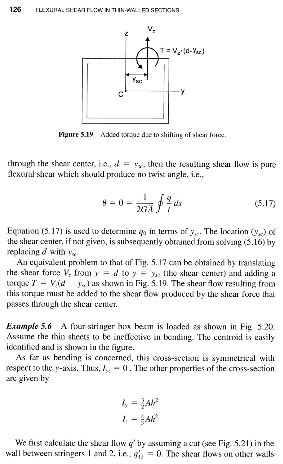
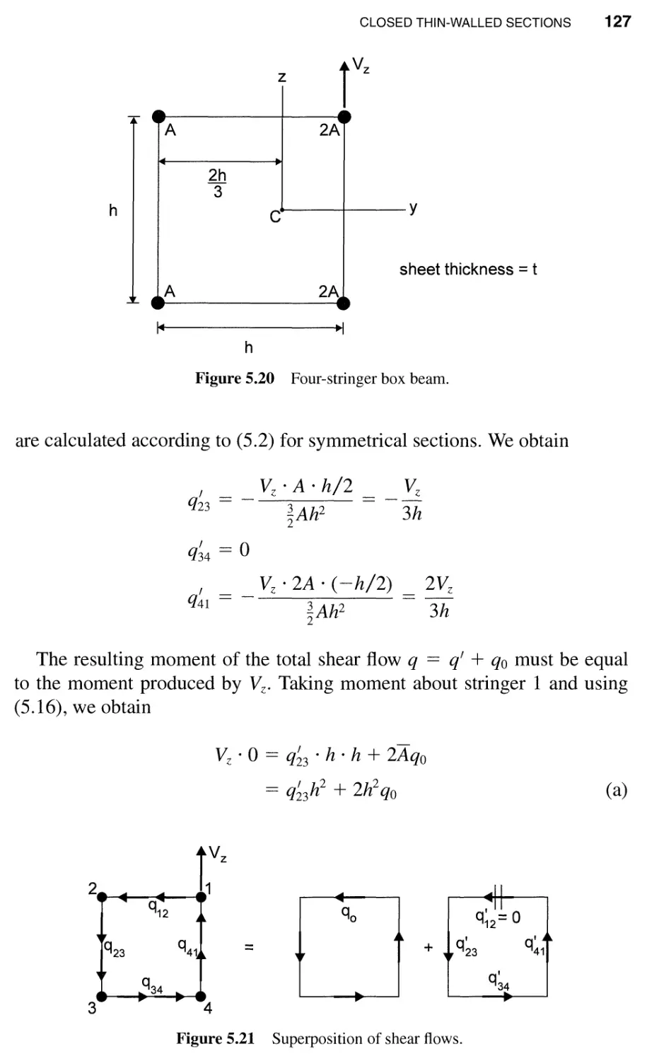

Author: Sun C.T.
Tags: physics mathematical physics aircraft mechanics of aircraft structures spacecraft
ISBN: 0-471-17877-2
Year: 1998


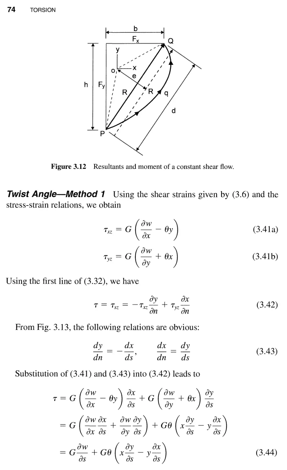
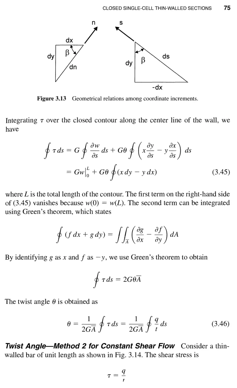
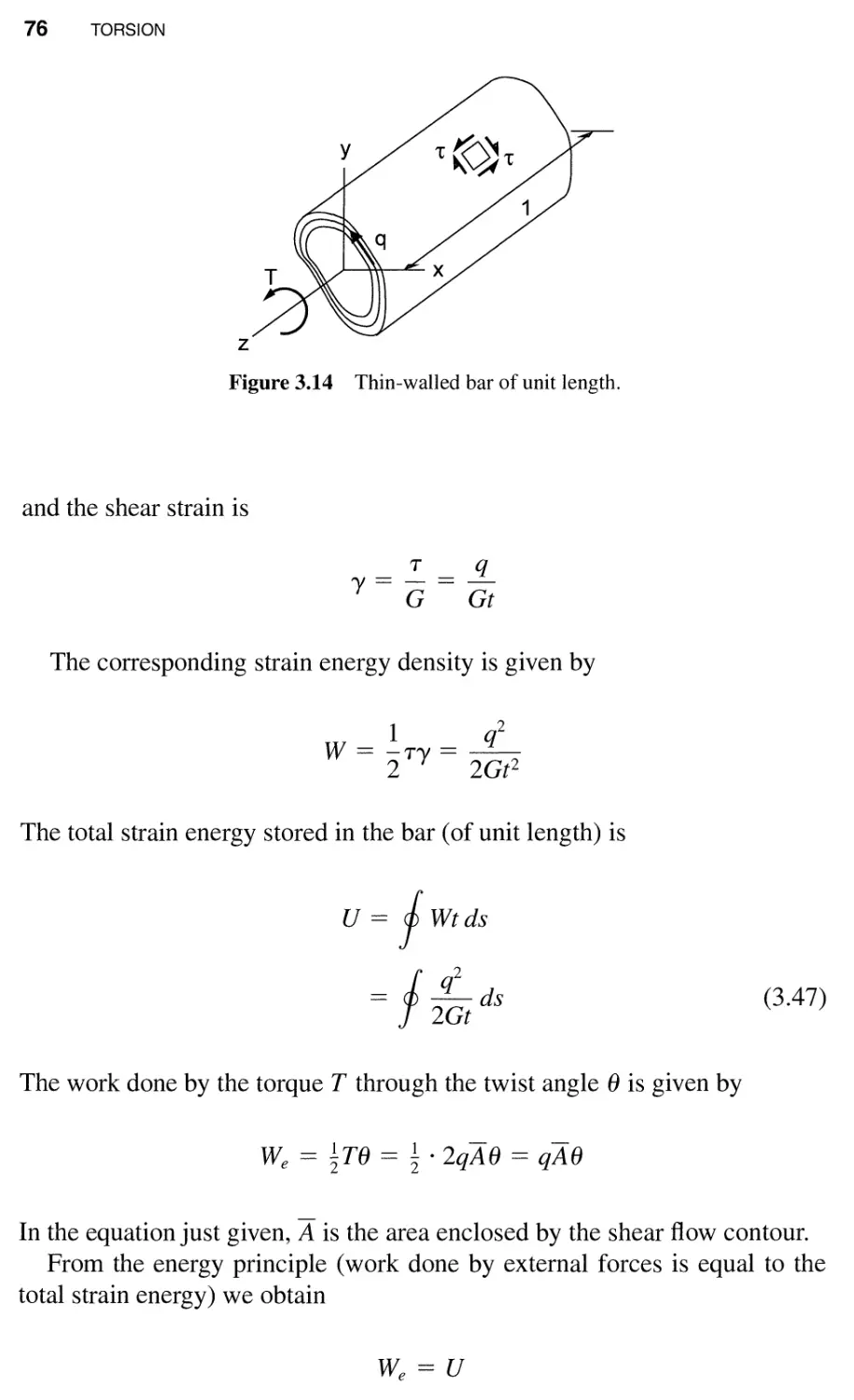
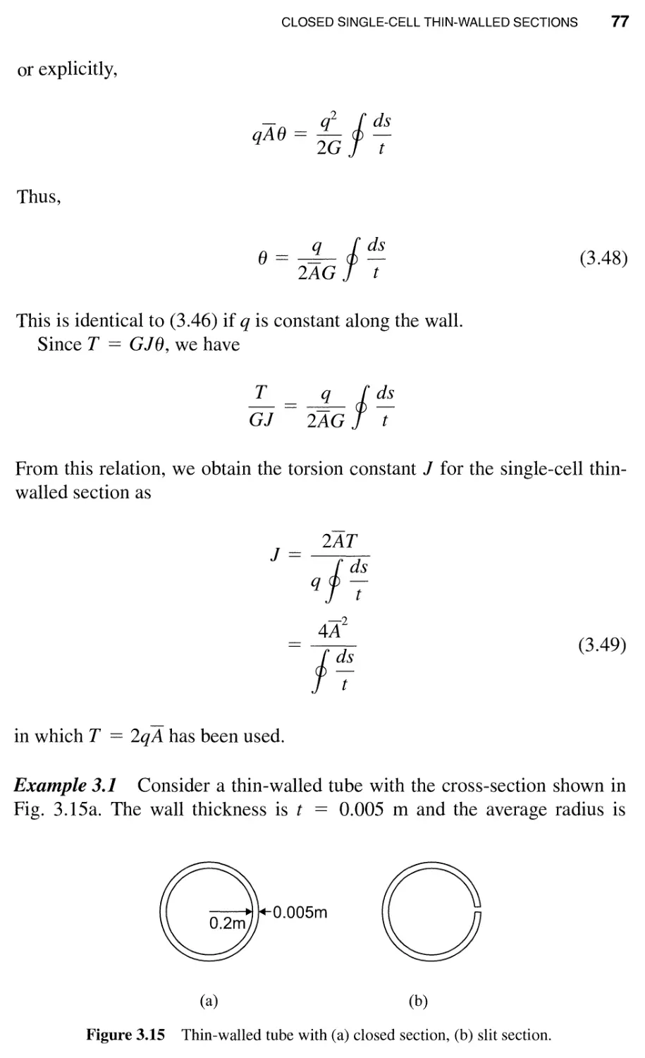
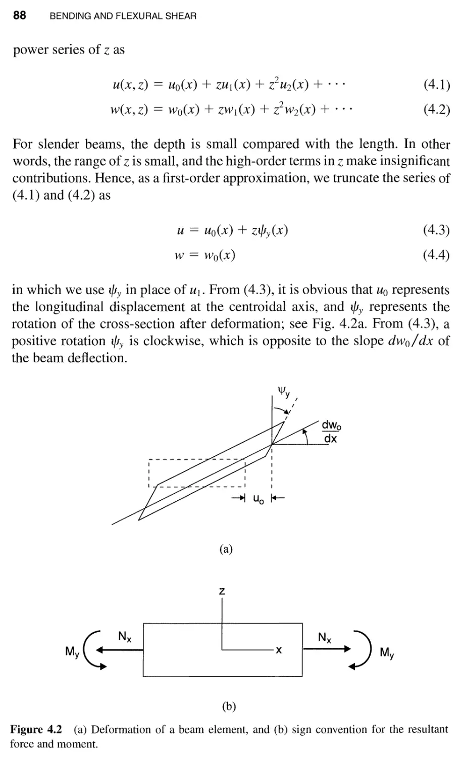
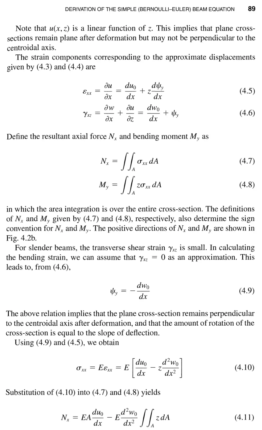
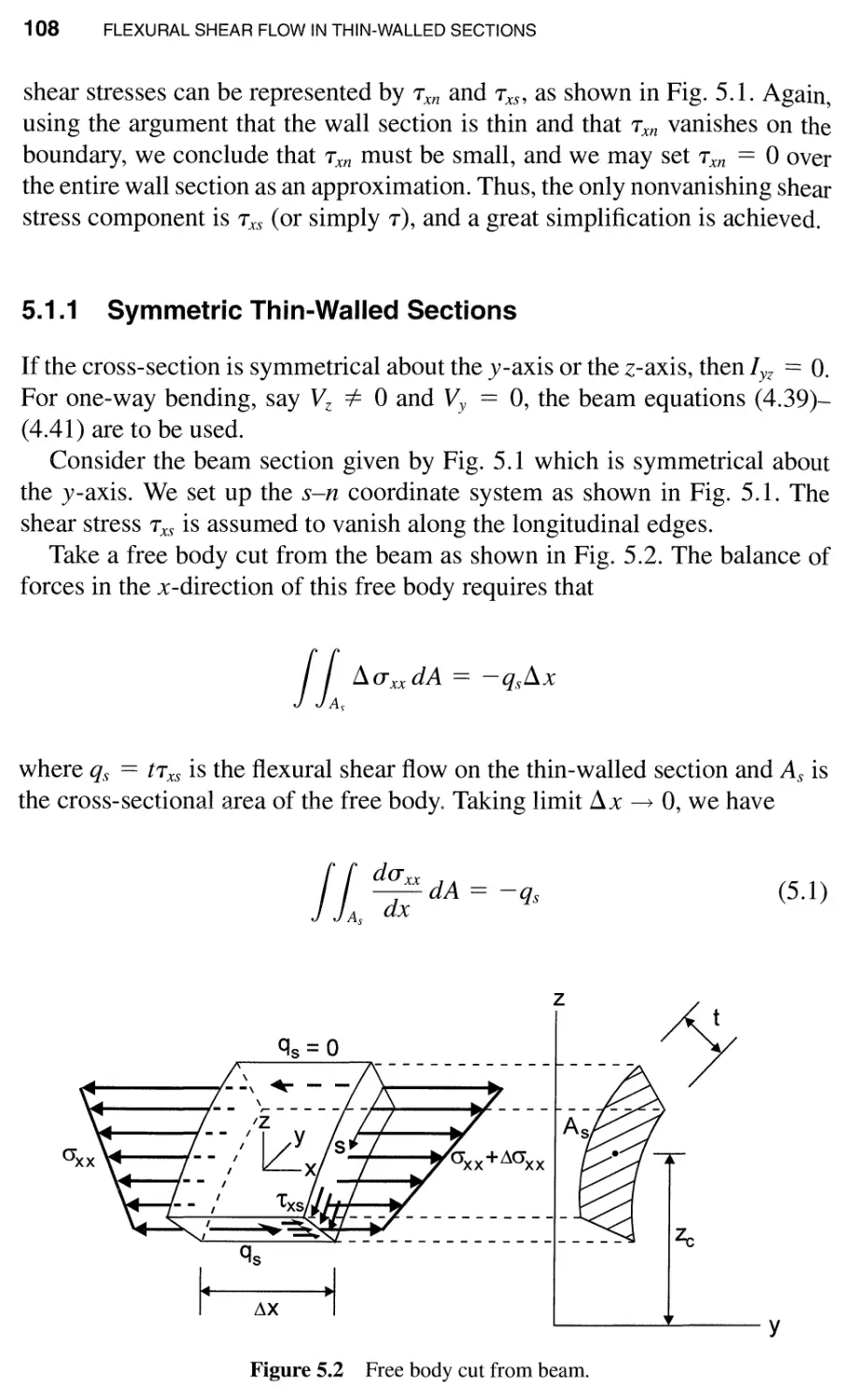
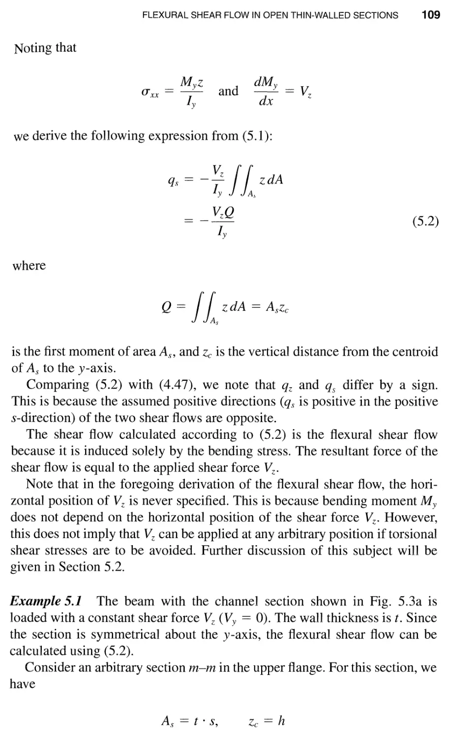
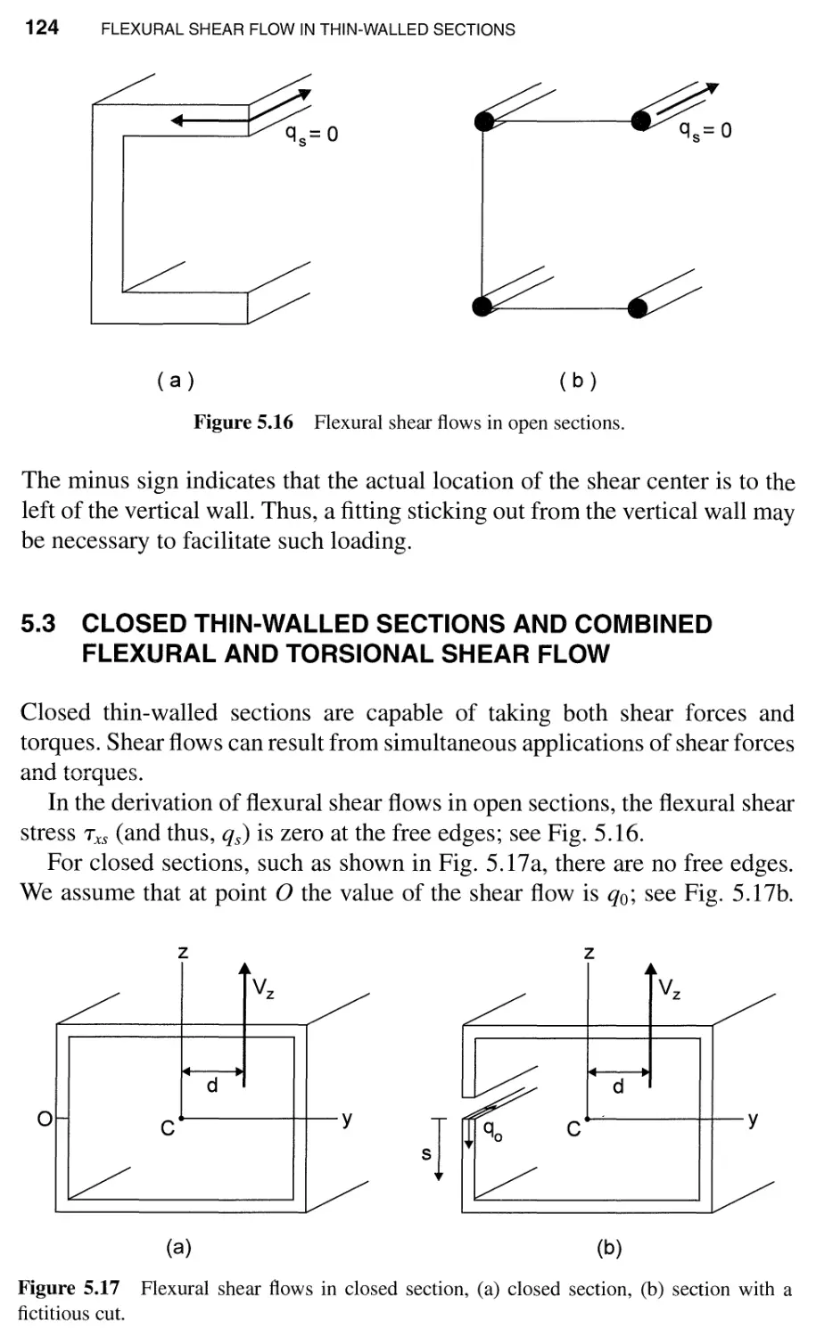
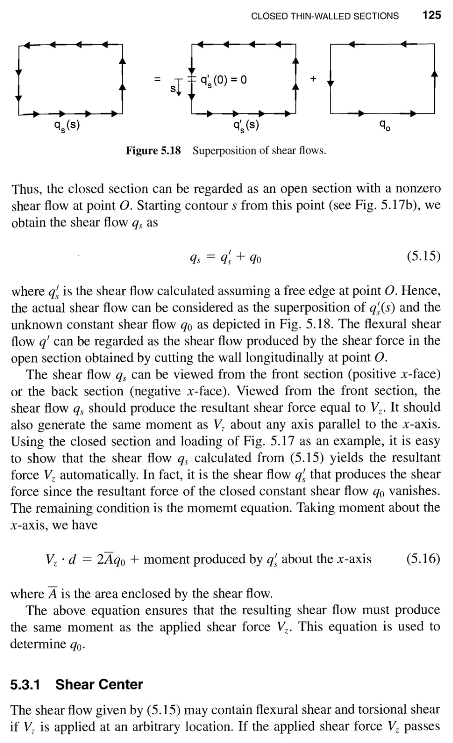
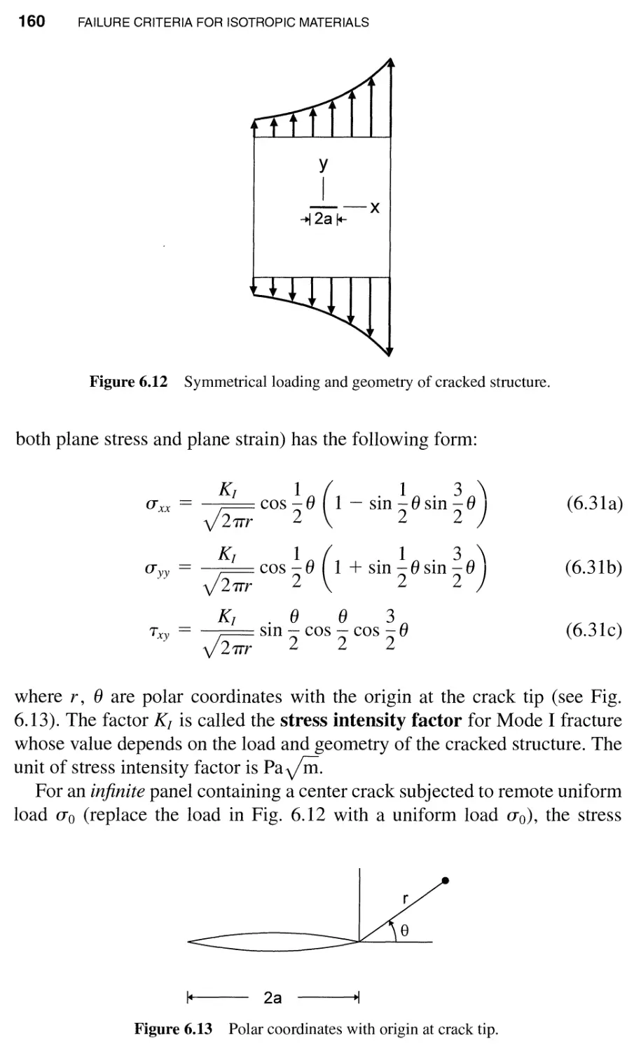
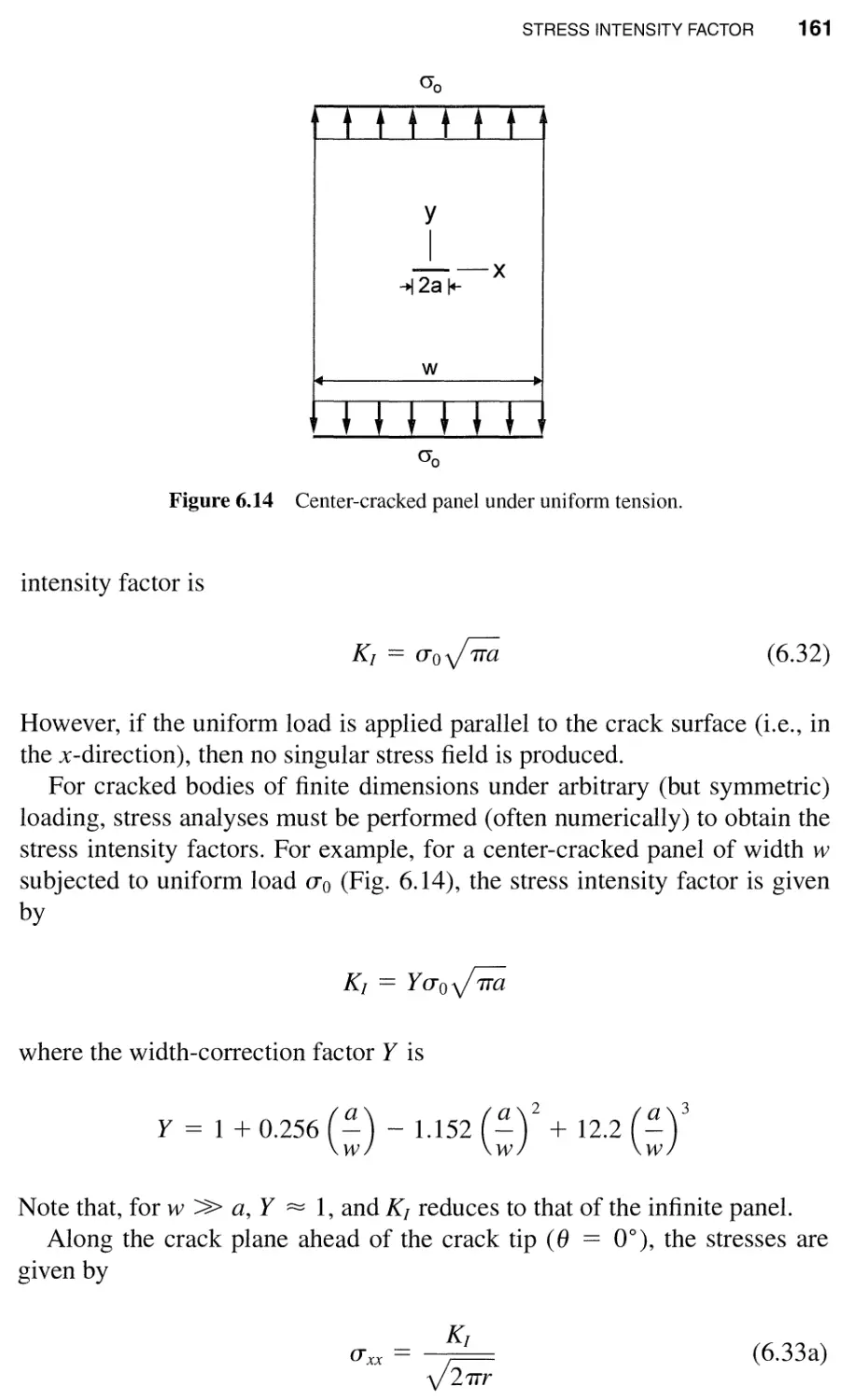
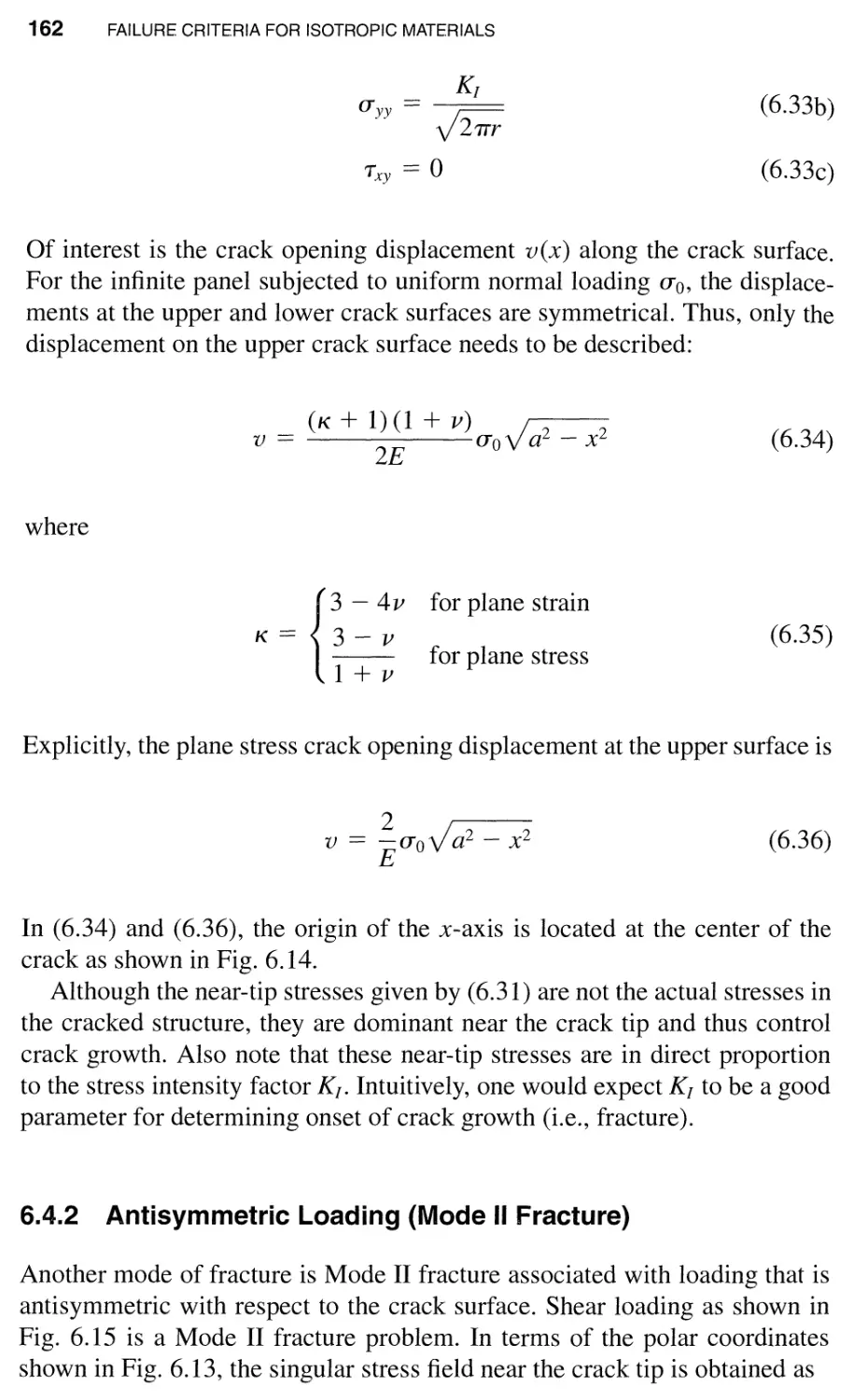
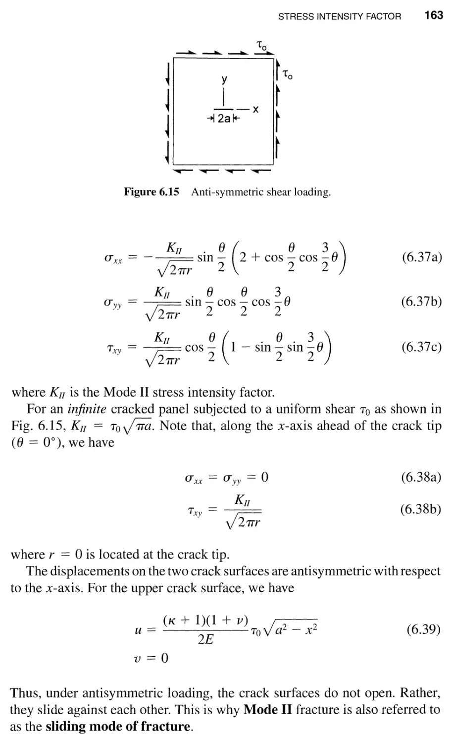
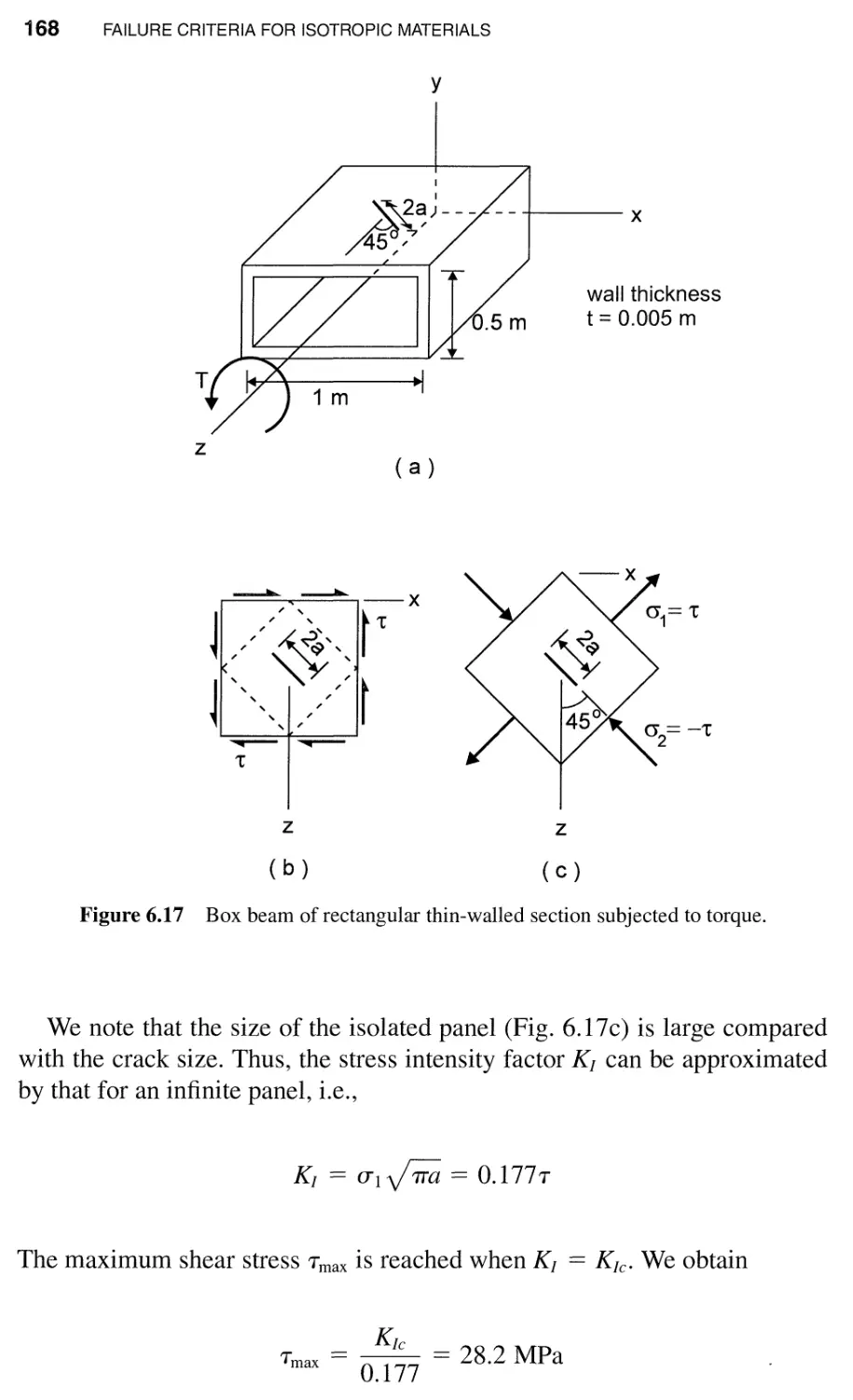
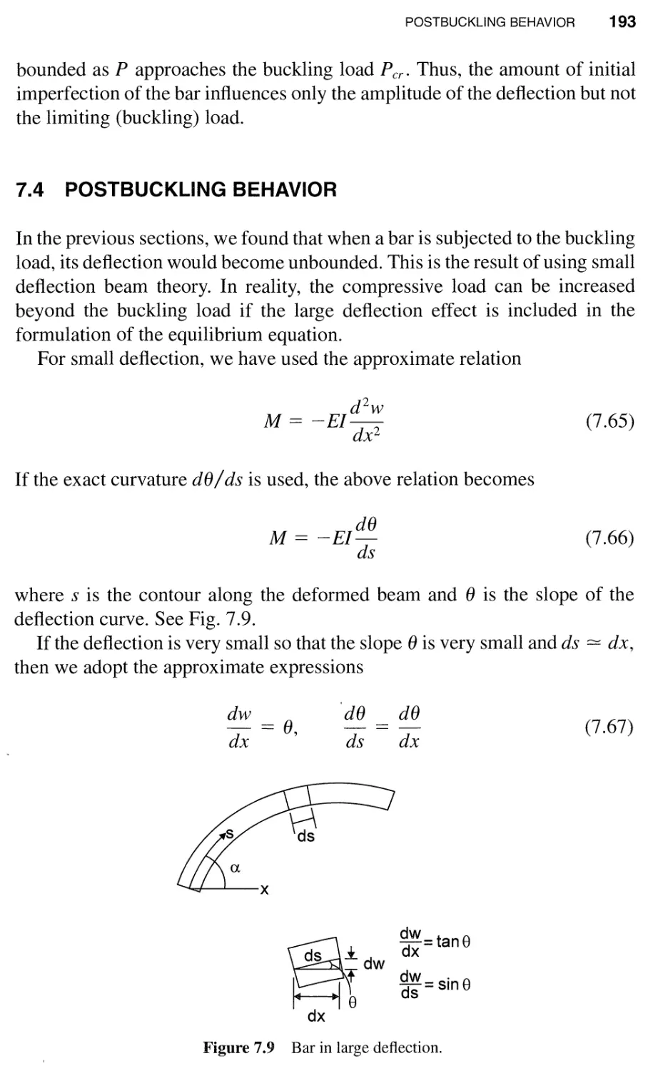
Text
r
An accessible, state-of-the-art introduction to the most
important topics in aerospace engineering today
This combined text and professional reference presents what every struc-
tural engineer needs to
now about modern aircraft structures. Covering
the latest developments in the field, it explores the role of commercial
finite element codesLnstructural analysis, demonstrates the use of fracture
mechanics to s?lve
damage tolerance and durability problems in aircraft
structures, and' examines the penetration of composite materials into areas
tradi
iQnally dominated by metals. Clear and accessible throughout, this
c
ook assumes only an introductory background in the mechanics of solids
while explaining subjects typically found only in much more advanced texts.
It offers ample examples; emphasizes concepts of mechanics rather than
problem solving,and helps foster an in-depth understanding of the subject.
Mechanics of Aircraft Structures provides concise introductions to:
.
Aerospace'material
ad\fdnceCi'composites as weWas metals
· The concept of anisotropy in material properties and properties of fiber composites
· A new approach for deriving the shear flow on thin-waned sections
· Methods for calculating strain energy release rates and stress intensity
factors for simple structures
r Pfcttmre
lCSfoplcs:-: fafi guecraC1{ -gr6vith'''and'1iber - reinforced composItes
· The concept of postbuckling of thin rods
· Mechanics of composite materials and laminates
Mechanics of Aircraft Structures combines classical and state-of-the-art
topics into an excellent one-semester introductory course in structural
mechanics and aerospace engineering at the undergraduate or graduate
level. It is also an extremely useful resource for aerospace or mechanical
engineers-especially in aerospace, automotive, and defense-related industries.
c. T. SUN is the Neil Armstrong Distinguished Professor at Purdue University. His
experience spans three decades, and he has received a number of teaching and
research awards in aeronautics and composite materials.
Cover Design: Watts Design? Inc
Cover Illustration: The Boeing Company
ISBN 0-471-17877-2
111111111111 "111/1 Ilr"al
lIal
i
i
(1), .
n;:,
SlJ "
. ,
, ,
.,.
......
,......,.
, ,1\'-
cn
0,...
r ..
I
.....;
H
n
P1
:..::"
,'; "
J
I-i.
P-
(J;
'F;
--t
< '
(
t;r
..
"
,. Ih,
I' echanics of
o
o [/(
[/@
!
stru." ures
I
This book is printed on acid-free paper. 0
Copyright @ 1998 by John Wiley & Sons, Inc. All rights reserved.
Published simultaneously in Canada.
No part of this publication may be reproduced, stored in a retrieval system or transmitted in any
form or by any means, electronic, mechanical, photocopying, recording, scanning or otherwise,
except as permitted under Sections 107 or 108 of the 1976 United States Copyright Act, without
either the prior written permission of the Publisher, or authorization through payment of the
appropriate per-copy fee to the Copyright Clearance Center, 222 Rosewood Drive, Danvers, MA
01923, (508) 750-8400, fax (508) 750-4744. Requests to the Publisher for permission should be
addressed to the Permissions Department, John Wiley & Sons, Inc., 605 Third Avenue, New Yor
NY 10158-0012, (212) 850-6011, fax (212) 850-6008, E-Mail: PERMREQ@WILEY.COM.
This publication is designed to provide accurate and authoritative information in regard to the
subject matter covered. It is sold with the understanding that the publisher is not engaged in
rendering legal, accounting, or other professional services. If legal advice or other expert
assistance is required, the services of a competent professional person should be sought.
Library of Congress Cataloging-in-Publication Data:
Sun, C. T. (Chin- Teh), 1939-
Mechanics of aircraft structures / C.T. Sun.
p. cm.
Includes index.
ISBN 0-471-17877-2 (cloth: alk. paper)
1. Airframes. 2. Fracture mechanics. I. Title.
TL671.6.S82 1998
629.134/31-dc21 97-29337
Printed in the United States of America
10 9 8 7 6 5 4 3 2 1
CONTENTS
Preface
xi
1 Characteristics of Aircraft Structures and Materials 1
1 .1 Introduction / 1
1.2 Basic Structural Elements in Aircraft Structure / 2
1.2.1 Axial Member / 2
1.2.2 Shear Panel / 3
1.2.3 Bending Member (Beam) / 4
1.2.4 Torsion Member / 5
1.3 Wing and Fuselage / 7
1.3.1 Load Transfer / 7
1.3.2 Wing Structure / 9
1.3.3 Fuselage / 10
1.4 Aircraft Materials / 11
Problems / 15
v
vi CONTENTS
2 Introduction to Elasticity 17
2.1 Concept of Displacement / 17
2.2 Strain / 19
2.3 Stress / 24
2.4 Equations of Equilibrium in a Nonuniform
Stress Field / 26
2.5 Principal Stresses / 27
2.5.1 Shear Stress / 32
2.5.2 Revisit of Transformation of Stress / 34
2.6 Linear Stress-Strain Relations / 36
2.6.1 Strains Induced by Normal Stress / 36
2.6.2 Strains Induced by Shear Stress / 39
2.6.3 3-D Stress-Strain Relations / 40
2.7 Elastic Strain Energy / 44
2.8 Plane Elasticity / 46
2.8.1 Stress-Strain Relations for Plane Isotropic
Solids / 47
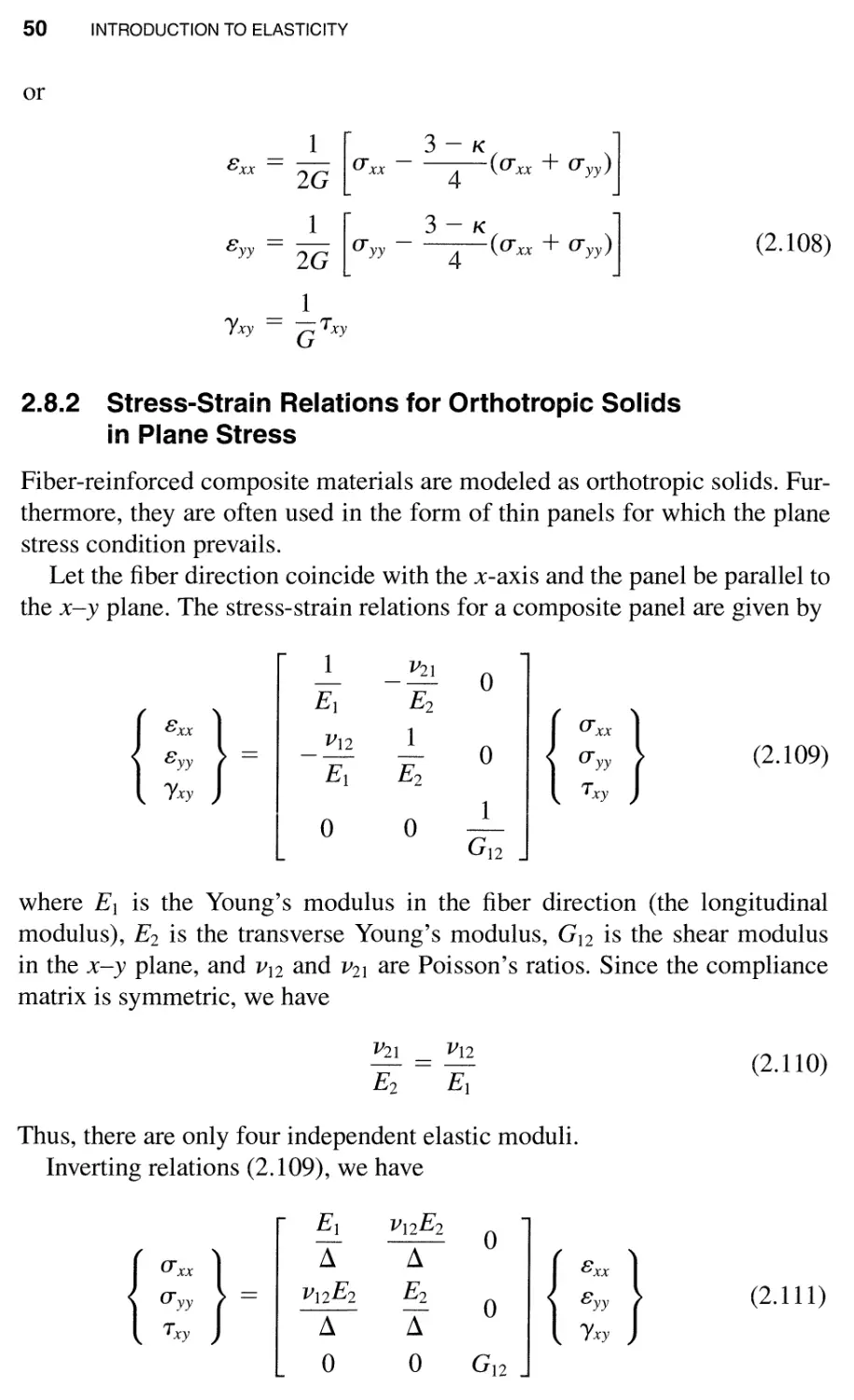
2.8.2 Stress-Strain Relations for Orthotropic Solids in
Plane Stress / 50
2.8.3 Governing Equations / 51
2.8.4 Solution by Airy Stress Function for Plane
Isotropic Solids / 52
Problems / 53
3 Torsion
3.1 Torsion of Uniform Bars / 57
3.2 Bars with Circular Cross-Sections / 63
3.3 Bars with Narrow Rectangular Cross-Sections / 65
57
CONTENTS vii
3.4 Closed Single-Cell Thin-Walled Sections / 69
3.5 Multicell Thin-Walled Sections / 79
Problems / 83
4 Bending and Flexural Shear 87
4.1 Derivation of the Simple (Bernoulli-Euler)
Beam Equation / 87
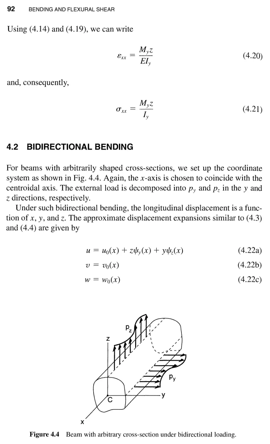
4.2 Bidirectional Bending / 92
4.3 Transverse Shear Stress due to Transverse Force in
Symmetric Sections / 97
4.3.1 Narrow Rectangular Cross-Section / 98
4.3.2 General Symmetric Sections / 100
4.3.3 Wide-Flange Beam / 102
4.3.4 Stiffener-Web Sections / 103
Problems / 104
5 Flexural Shear Flow in Thin-Walled Sections 107
5.1 Flexural Shear Flow in Open
Thin-Walled Sections / 107
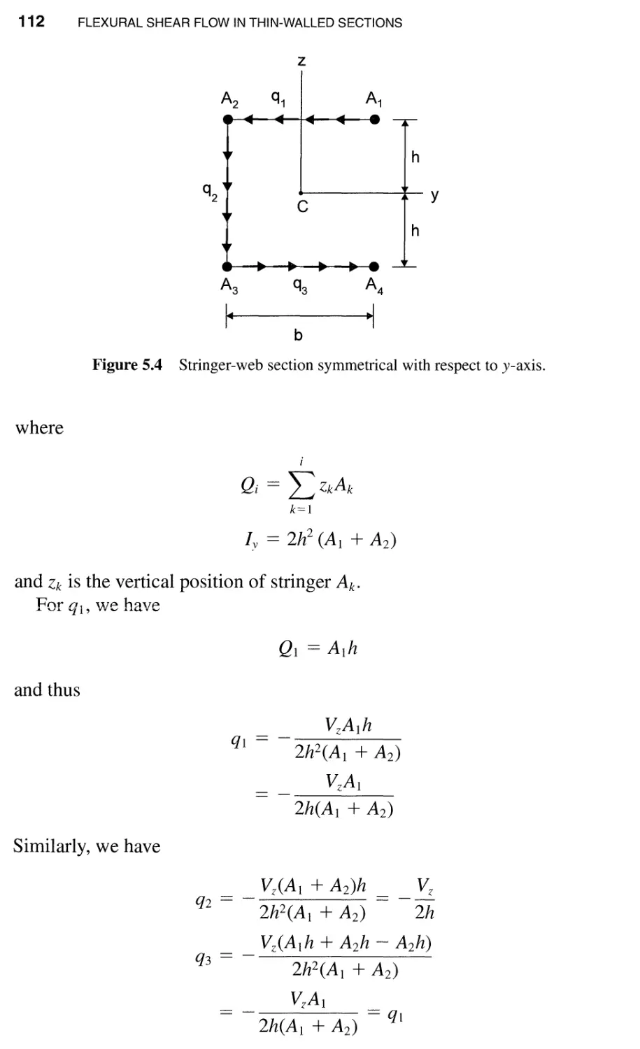
5.1.1 Symmetric Thin-Walled Sections / 108
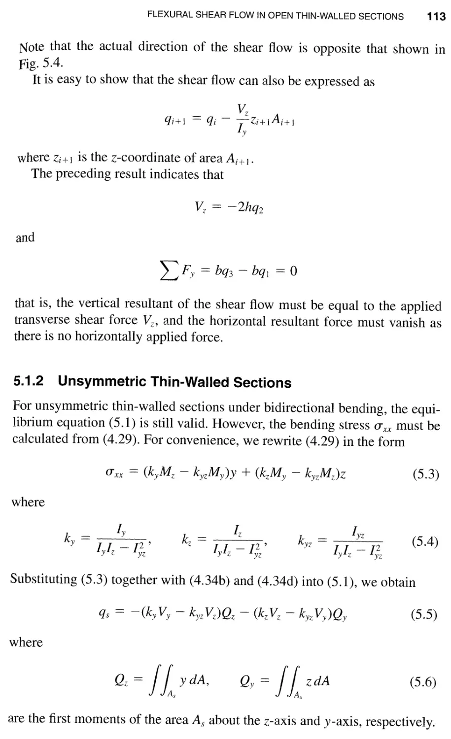
5.1.2 Unsymmetric Thin-Walled Sections / 113
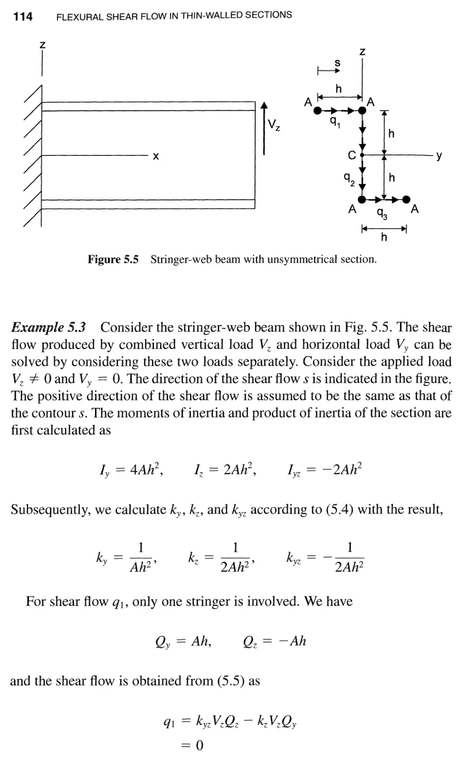
5.1.3 Multiple Shear Flow Junctions / 115
5.1.4 Selection of Shear Flow Contour / 117
5.2 Shear Center in Open Sections / 117
5.3 Closed Thin-Walled Sections and Combined Flexural
and Torsional Shear Flow / 124
5.3.1 Shear Center / 125
5.3.2 Statically Determinate Shear Flow / 129
viii CONTENTS
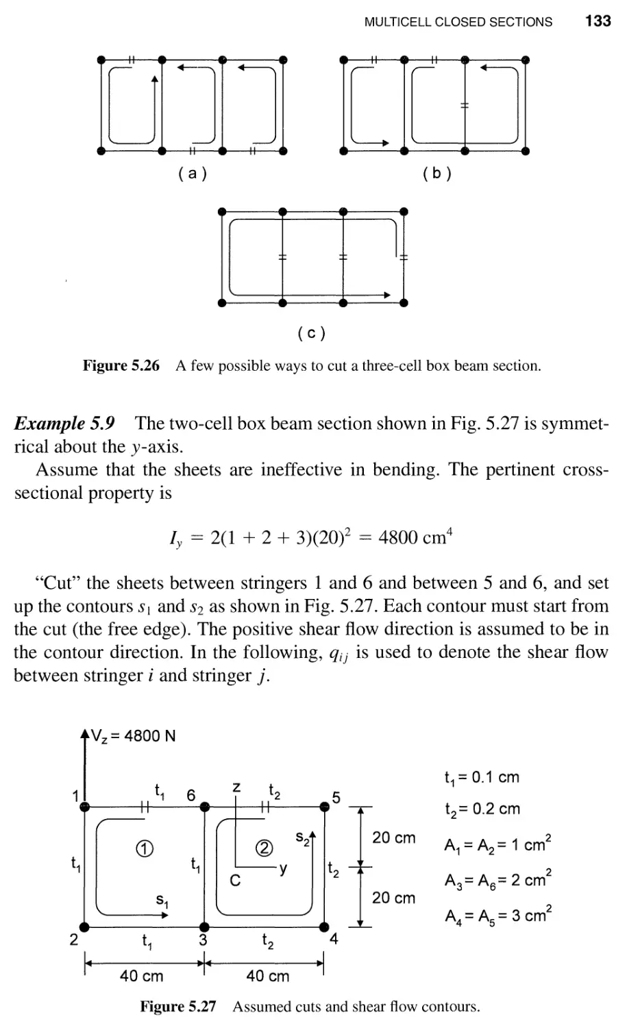
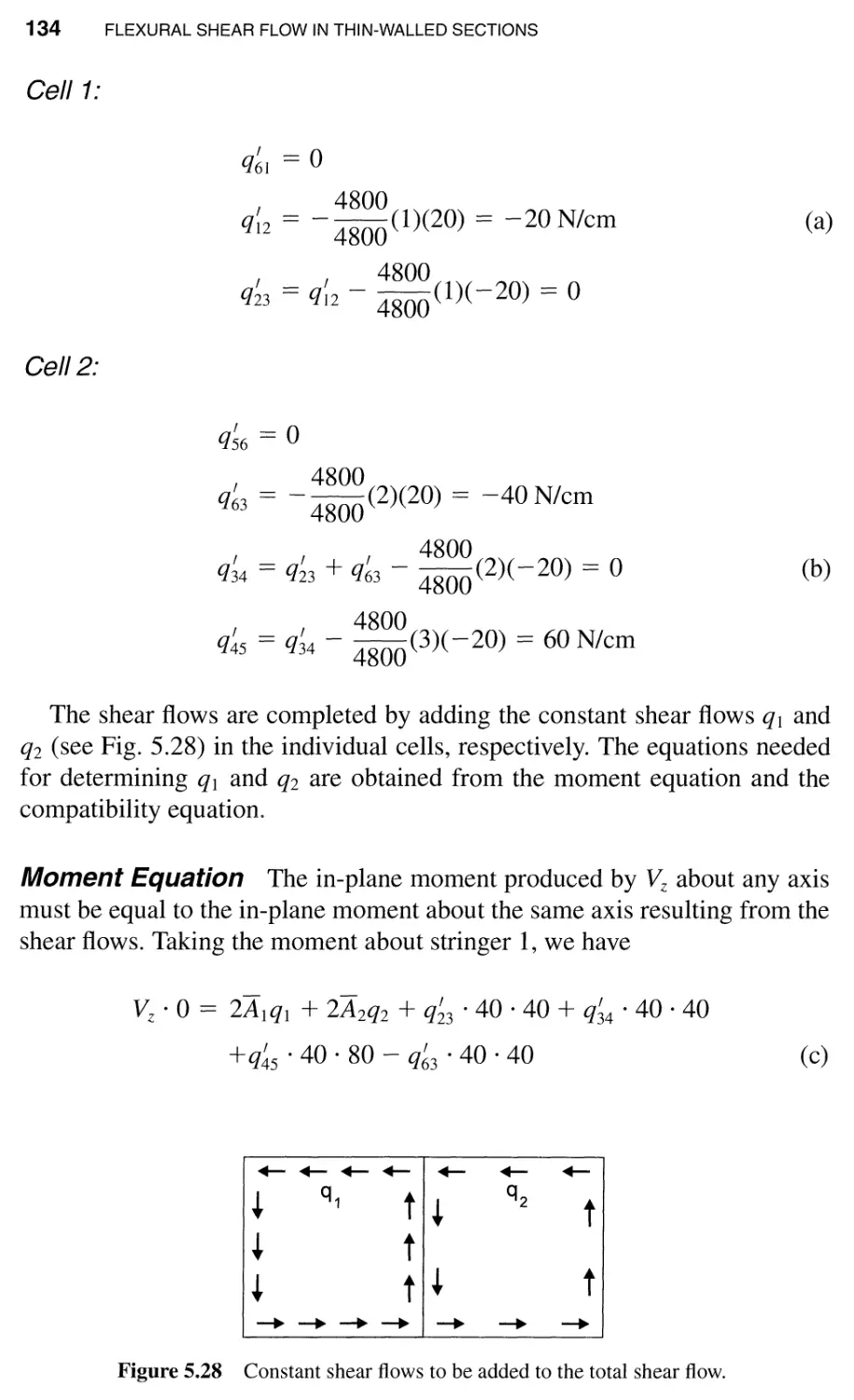
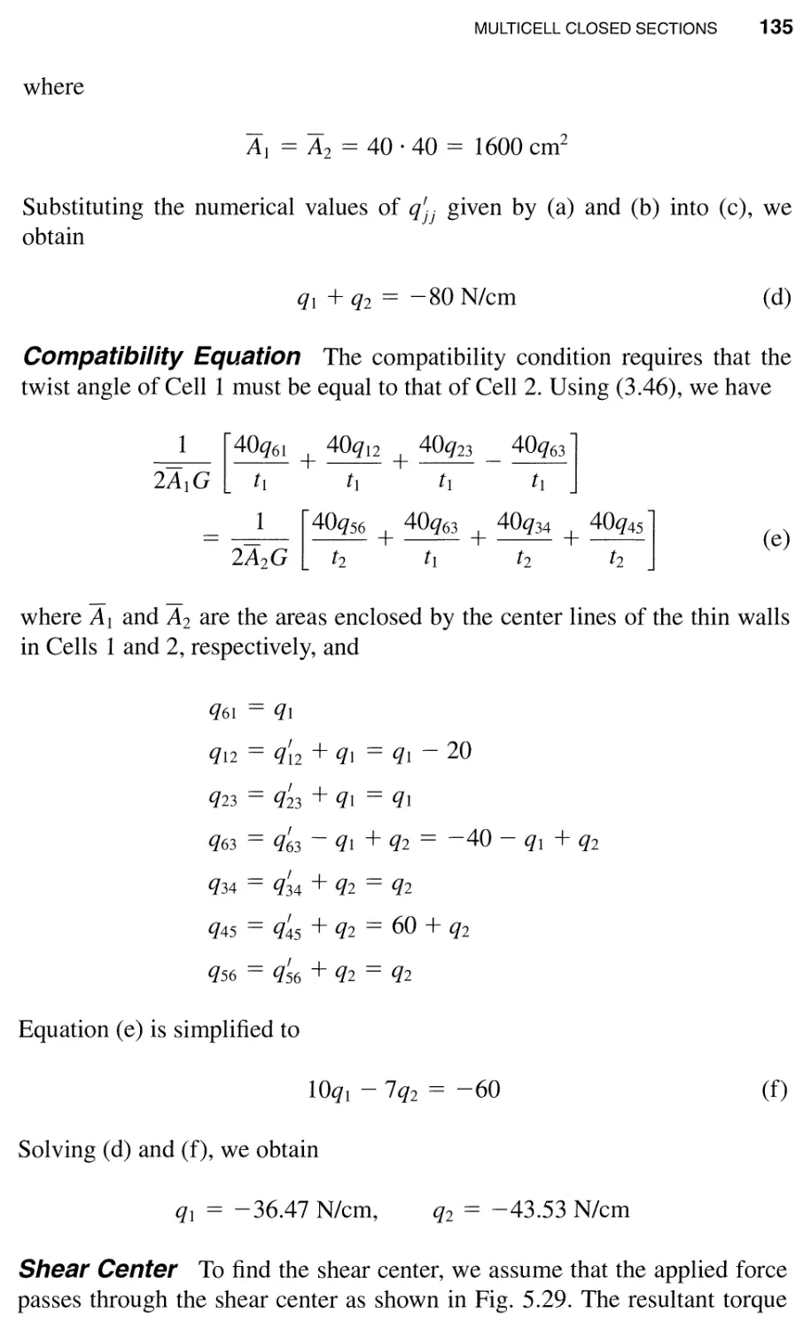
5.4 Multicell Closed Sections / 132
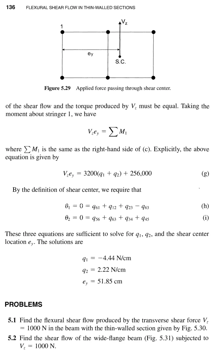
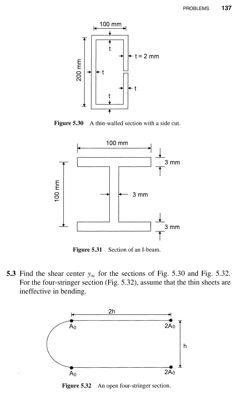
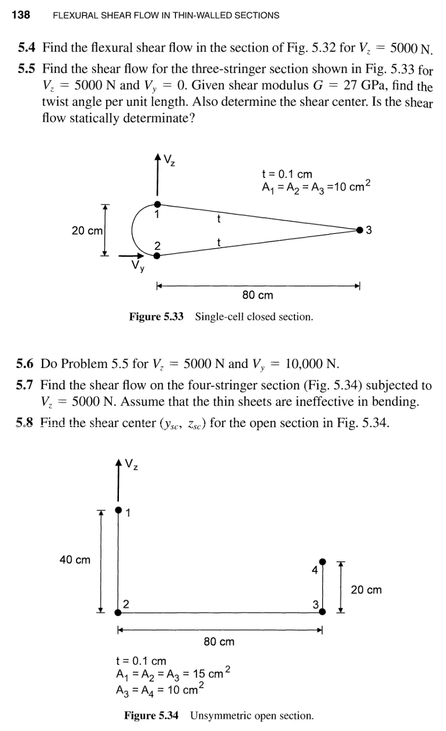
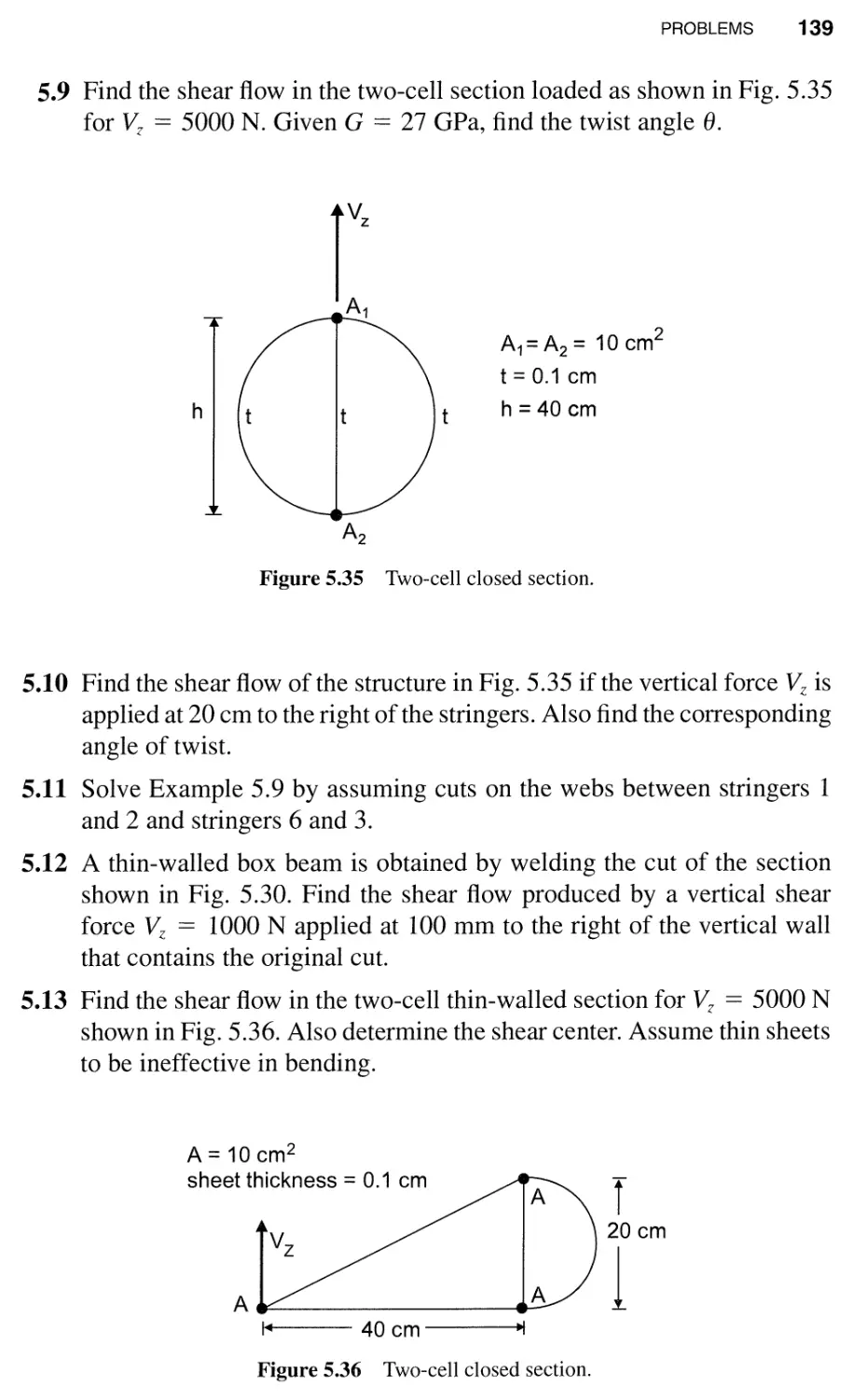
Problems / 136
6 Failure Criteria for Isotropic Materials 141
6.1 Strength Criteria for Brittle Materials / 141
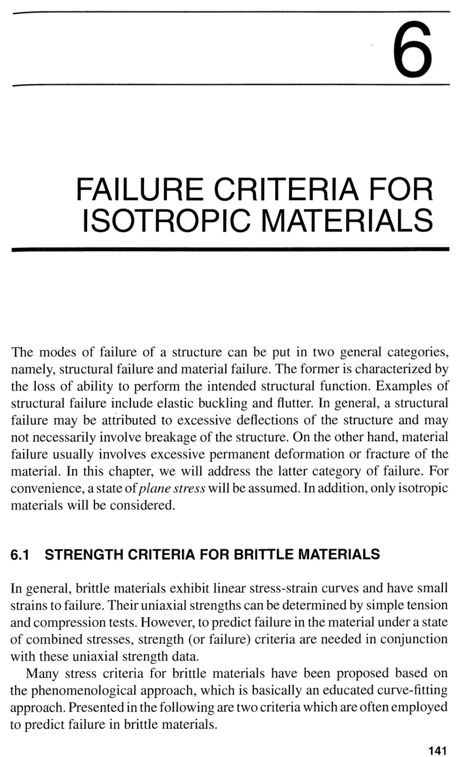
6.1.1 Maximum Principal Stress Criterion / 142
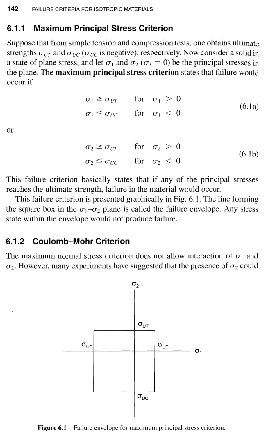
6.1.2 Coulomb-Mohr Criterion / 142
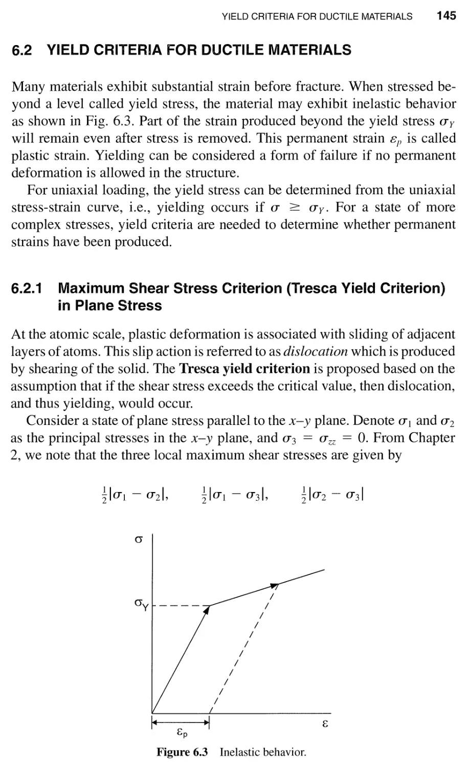
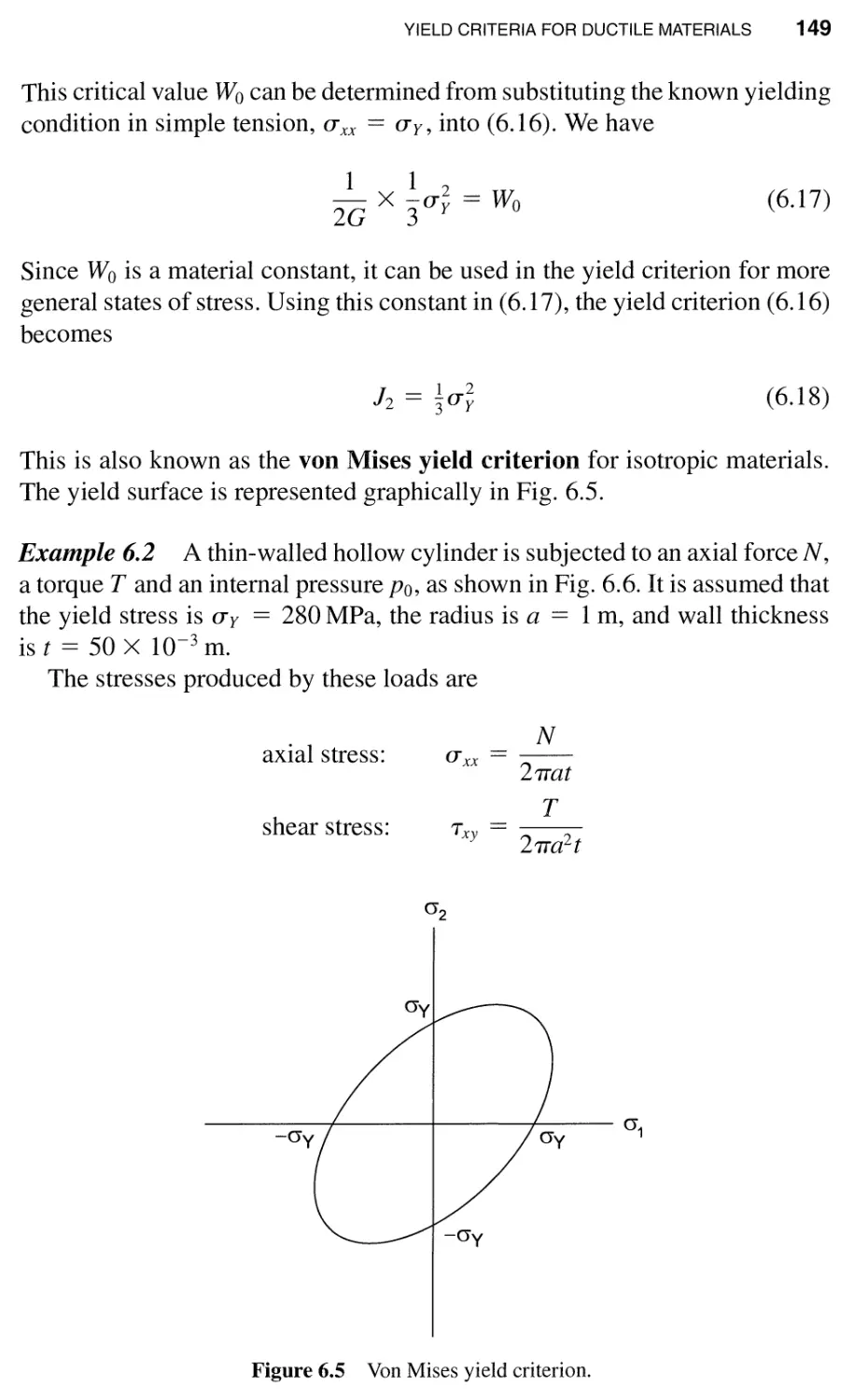
6.2 Yield Criteria for Ductile Materials / 145
6.2.1 Maximum Shear Stress Criterion (Tresca Yield
Criterion) in Plane Stress / 145
6.2.2 Maximum Distortion Energy Criterion (von
Mises Yield Criterion) / 147
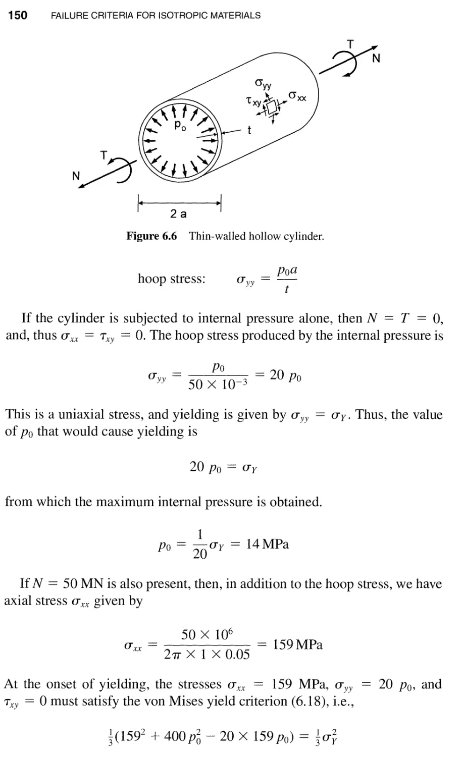
6.3 Fracture Mechanics / 151
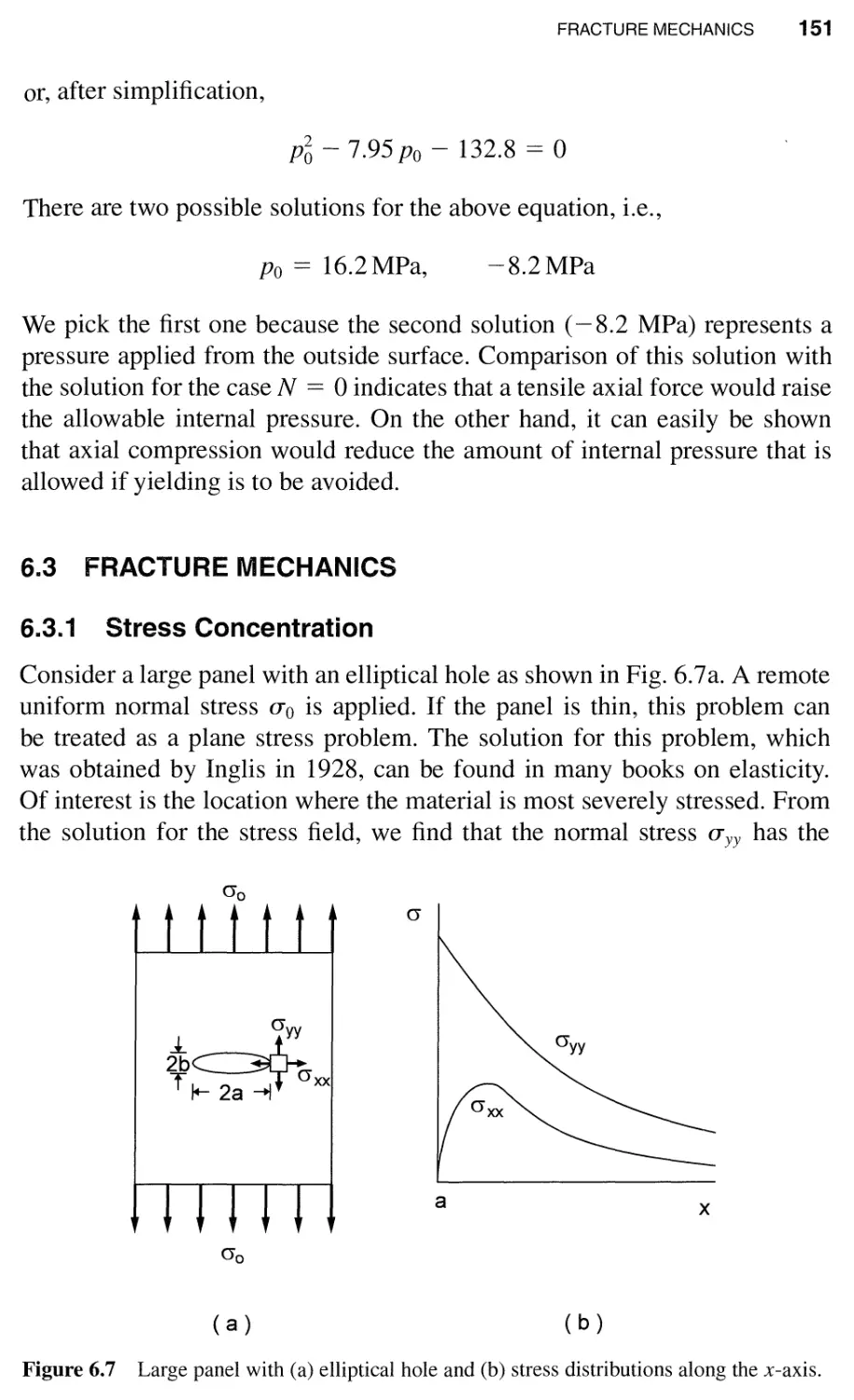
6.3.1 Stress Concentration / 151
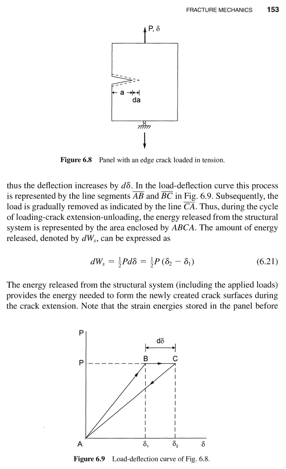
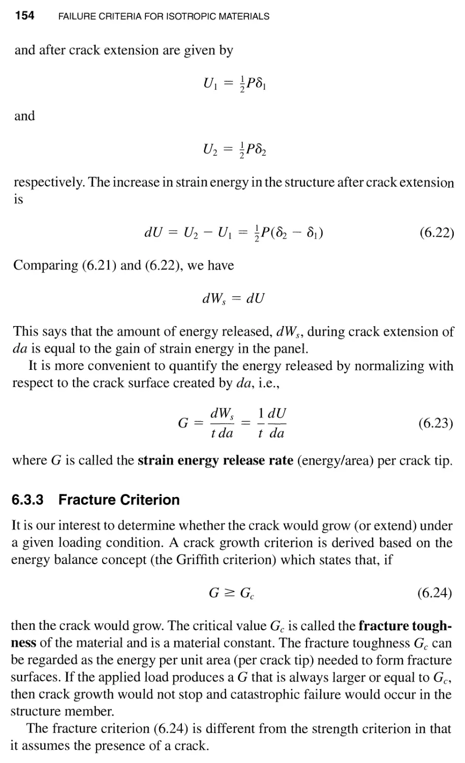
6.3.2 Concept of Cracks and Strain Energy Release
Rate / 152
6.3.3 Fracture Criterion / 154
6.4 Stress Intensity Factor / 159
6.4.1 Symmetric Loading (Mode I Fracture) / 159
6.4.2 Antisymmetric Loading (Mode II
Fracture) / 162
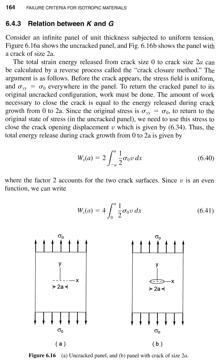
6.4.3 Relation between K and G / 164
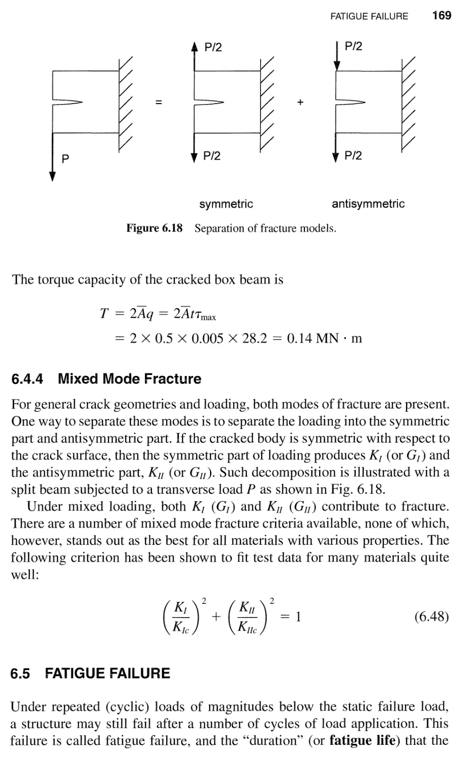
6.4.4 Mixed Mode Fracture / 169
6.5 Fatigue Failure / 169
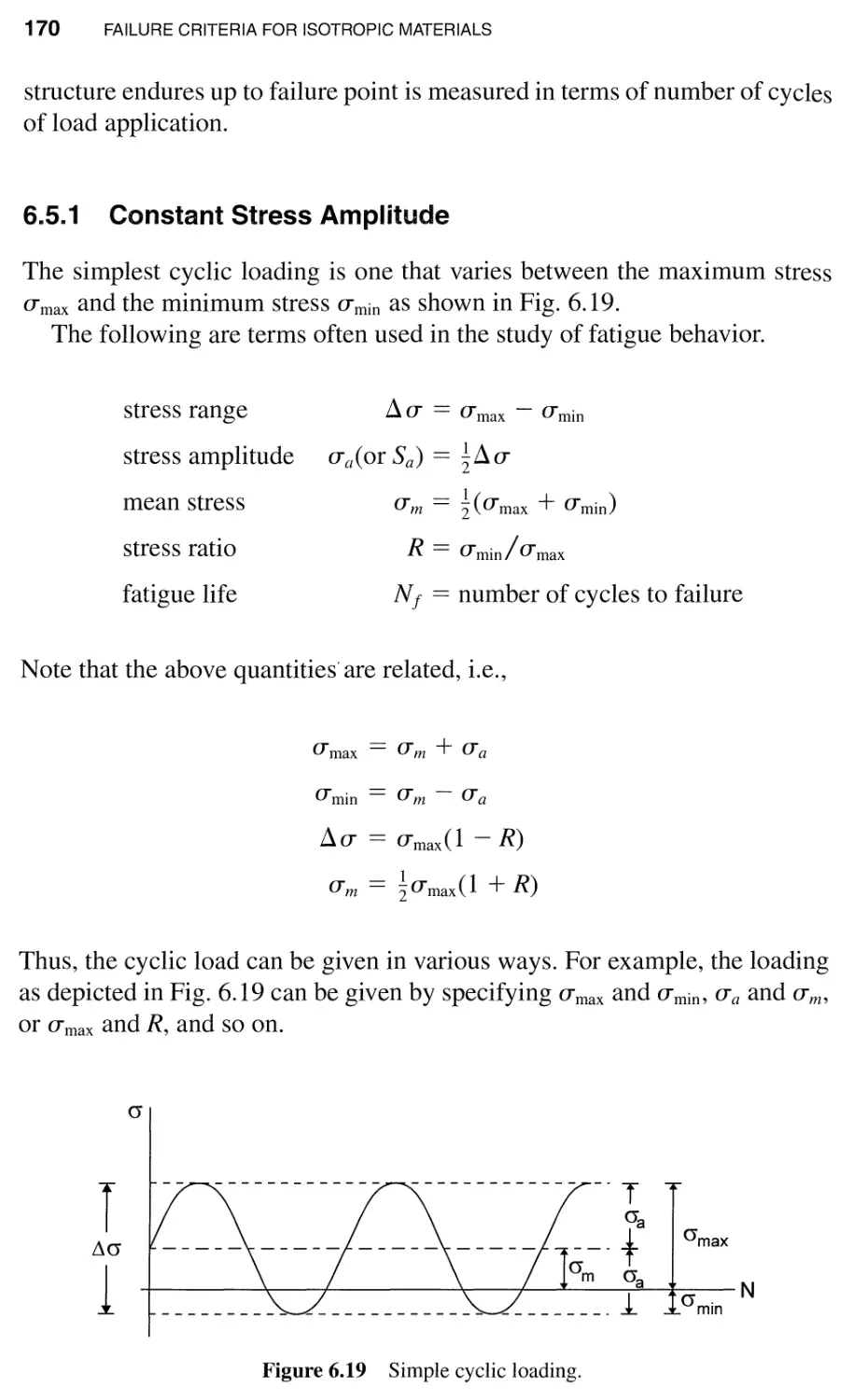
6.5.1 Constant Stress Amplitude / 170
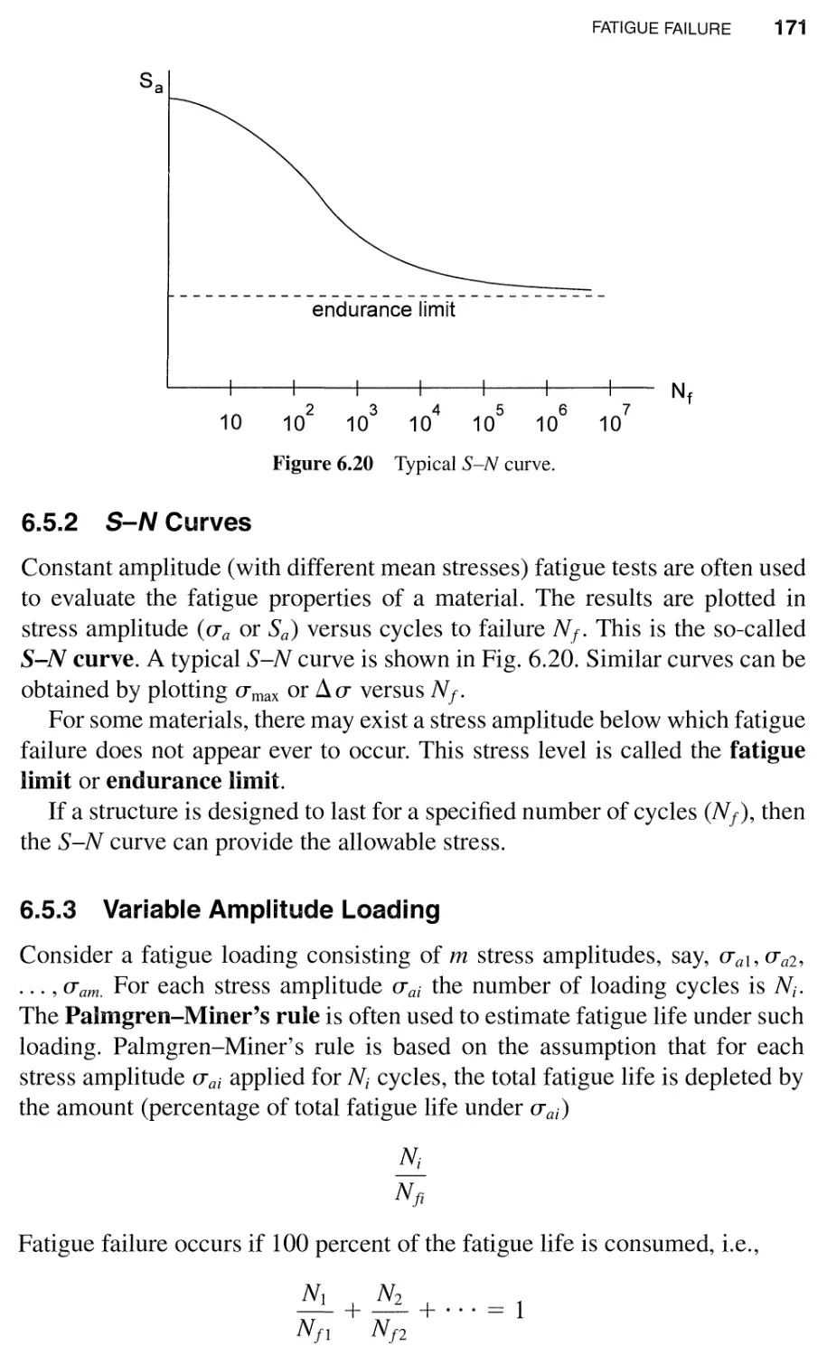
6.5.2 S-N Curves / 171
6.5.3 Variable Amplitude Loading / 171
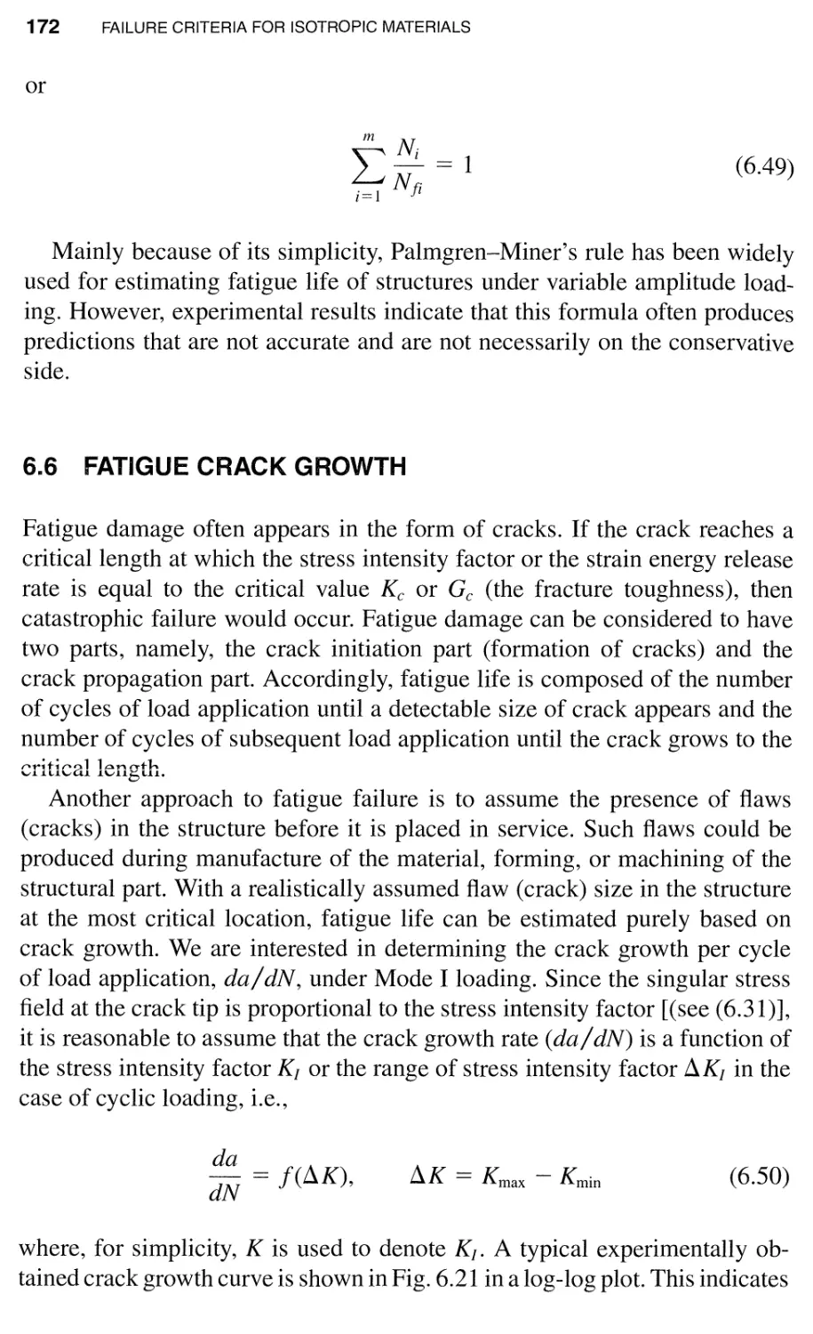
6.6 Fatigue Crack Growth / 172
Problems / 174
CONTENTS ix
7 Elastic Buckling 179
7.1 Eccentrically Loaded Beam-Column / 179
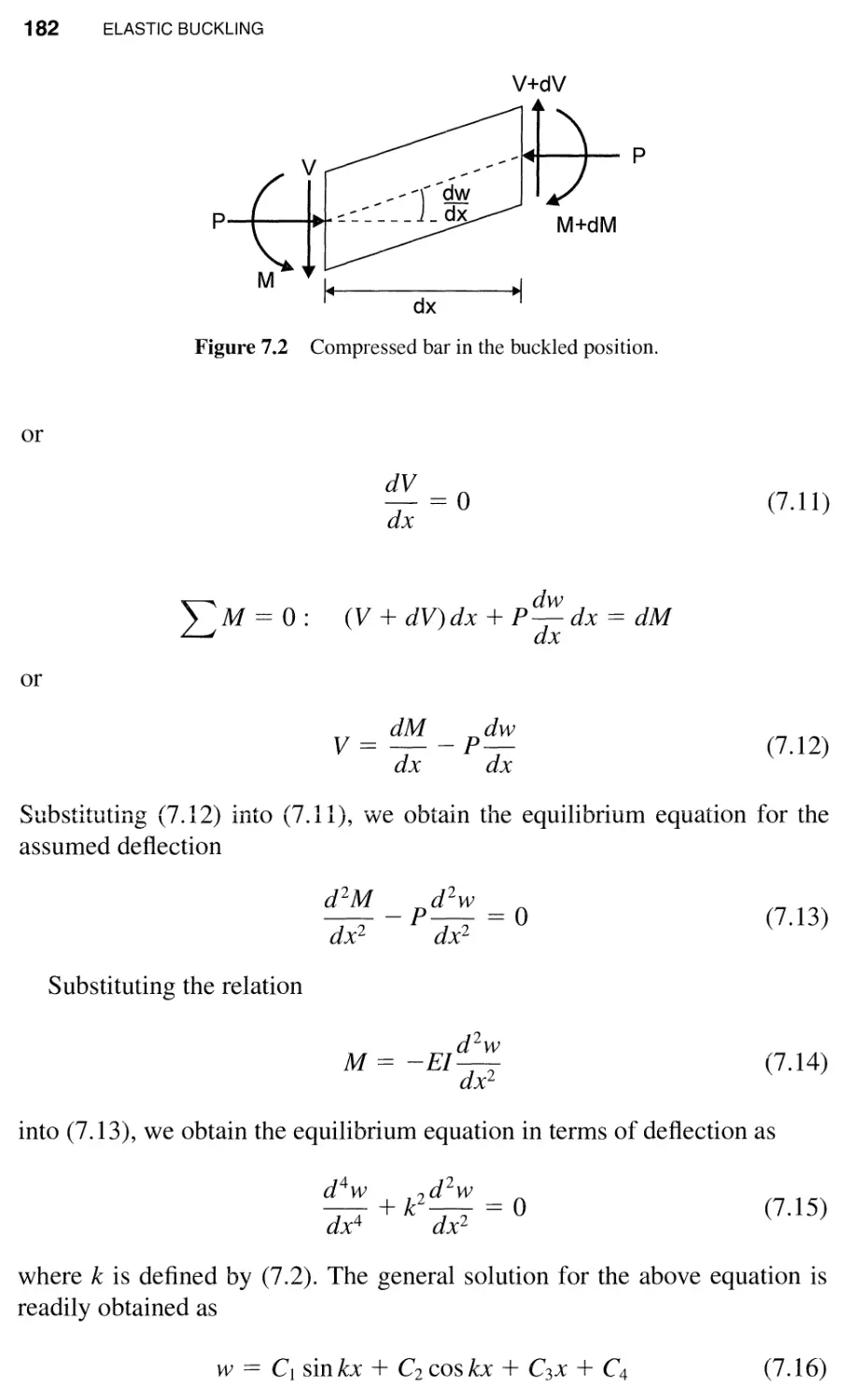
7.2 Elastic Buckling of Straight Bars / 181
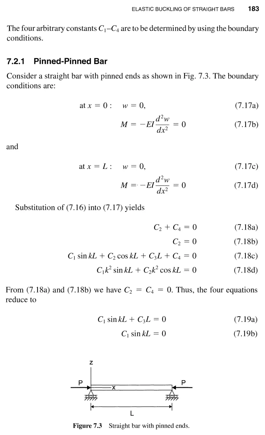
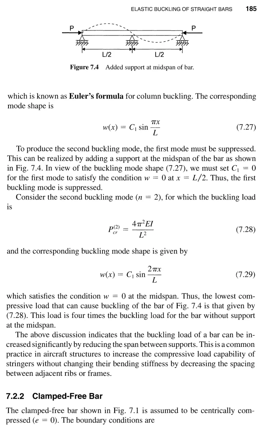
7.2.1 Pinned-Pinned Bar / 183
7.2.2 Clamped-Free Bar / 185
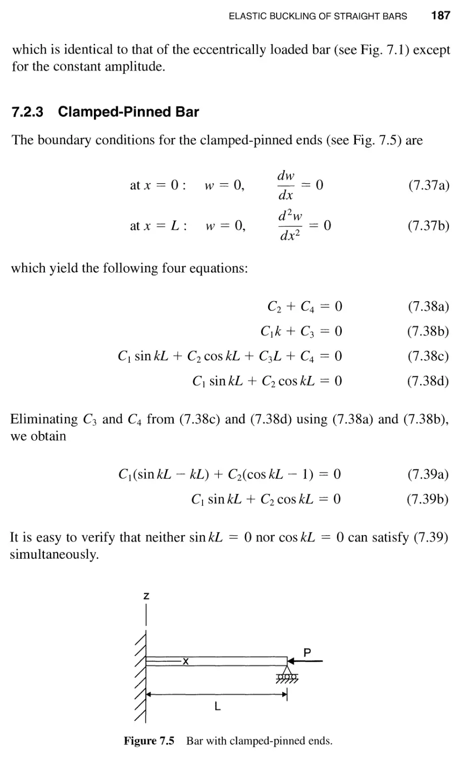
7.2.3 Clamped-Pinned Bar / 187
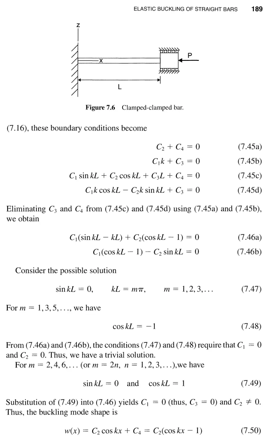
7.2.4 Clamped-Clamped Bar / 188
7.2.5 Effective Length of Buckling / 190
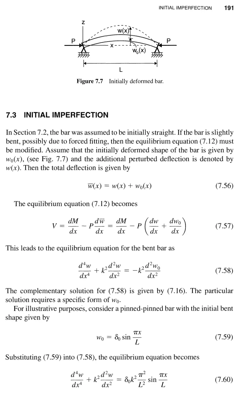
7.3 Initial Imperfection / 191
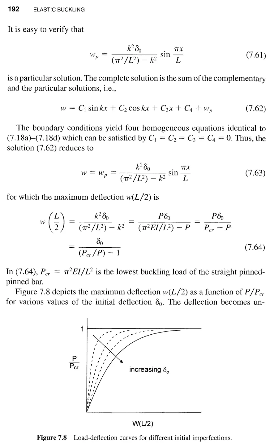
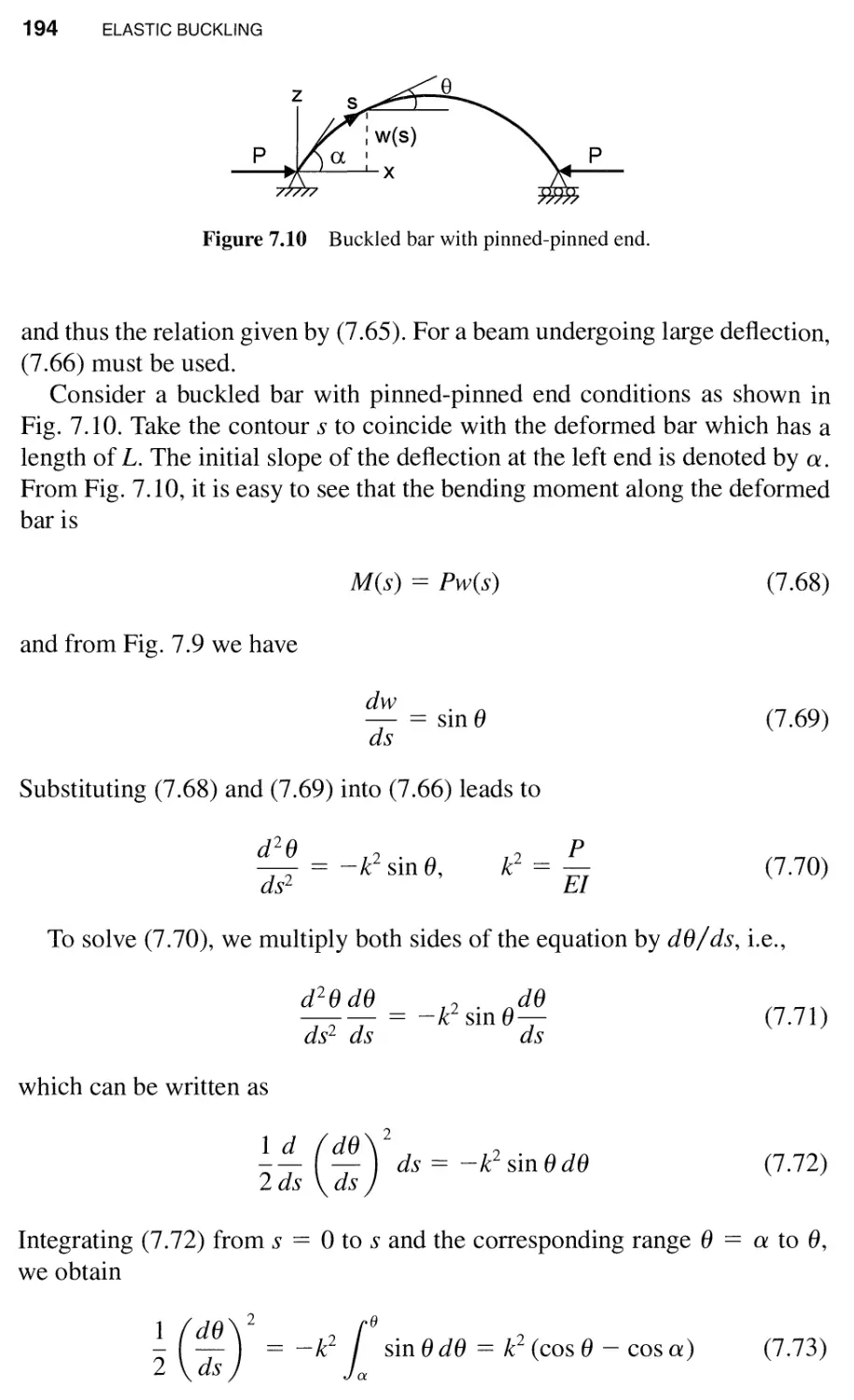
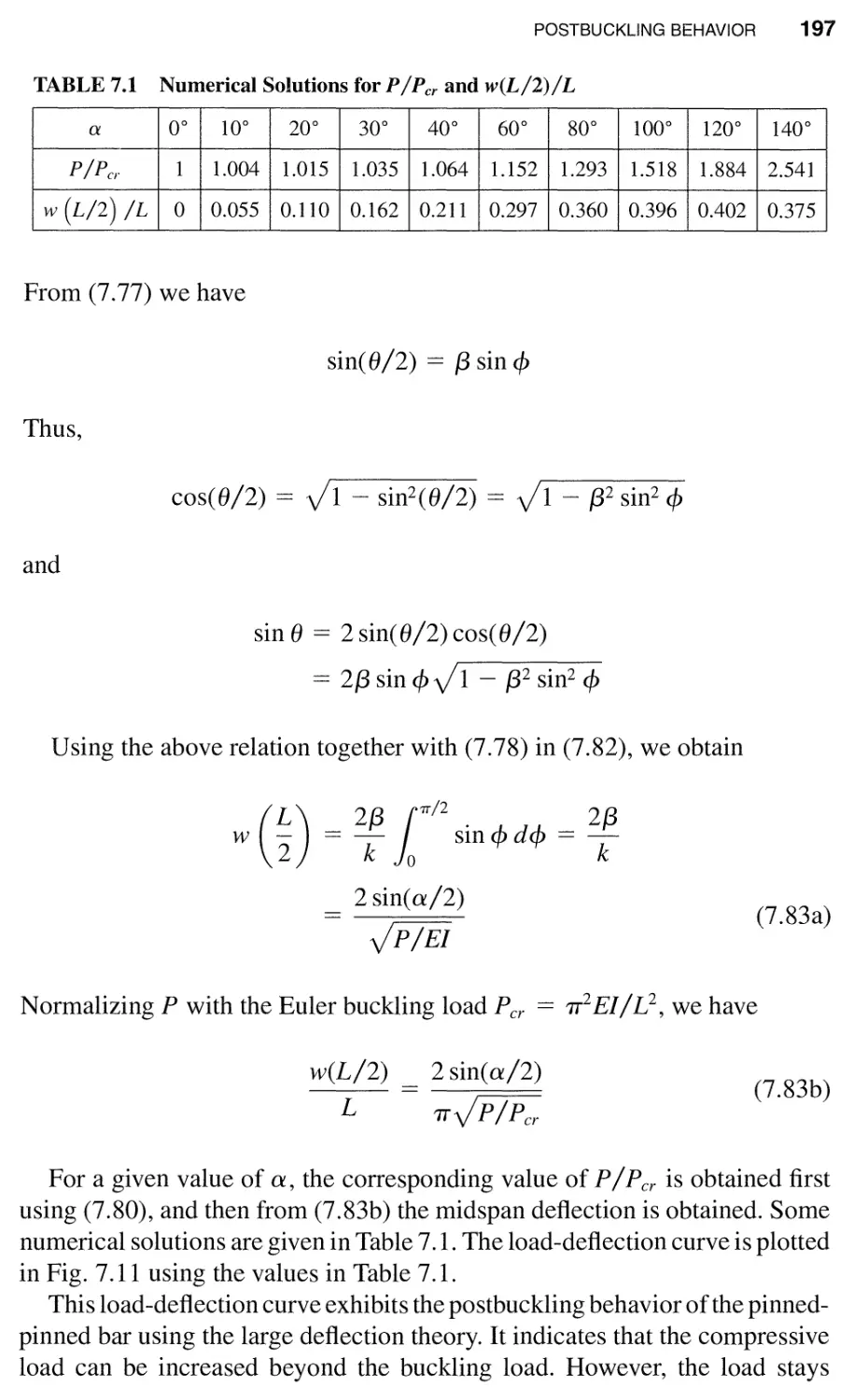
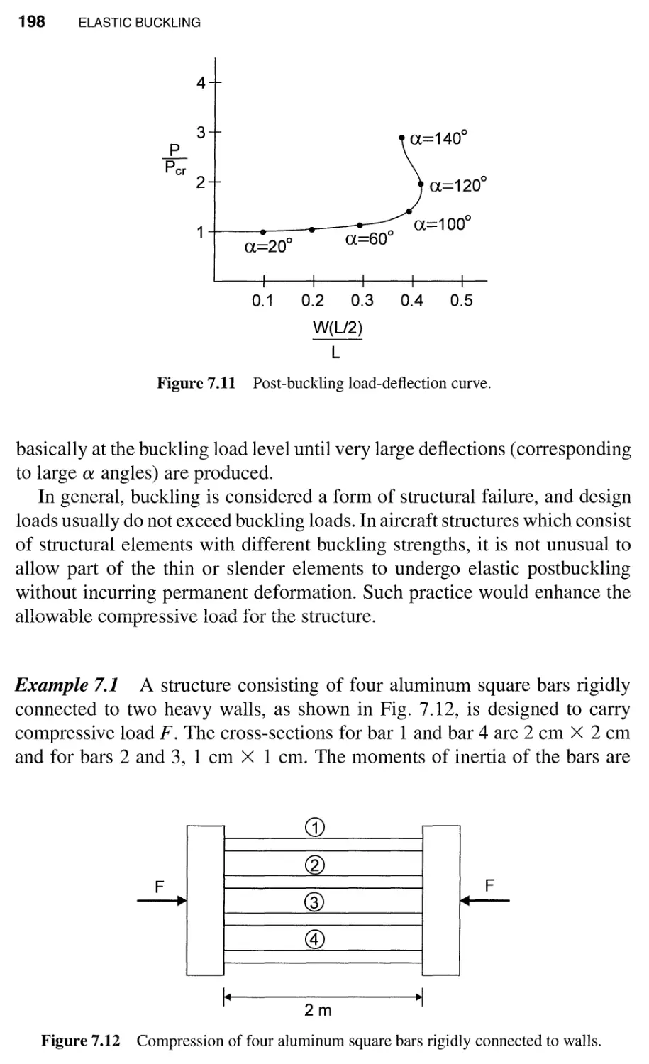
7.4 Postbuckling Behavior / 193
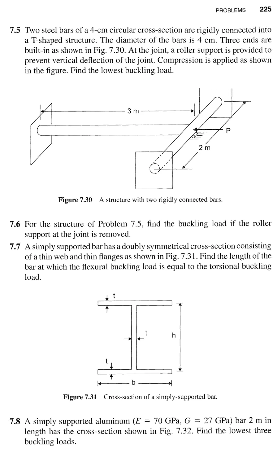
7.5 Bar of Unsymmetric Section / 199
7.6 Torsional-Flexural Buckling of Thin-Walled Bars / 202
7.6.1 Nonuniform Torsion / 202
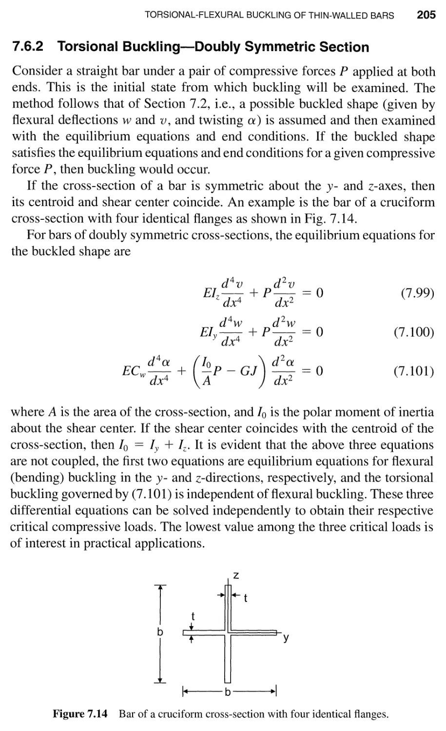
7.6.2 Torsional Buckling-Doubly Symmetric
Section / 205
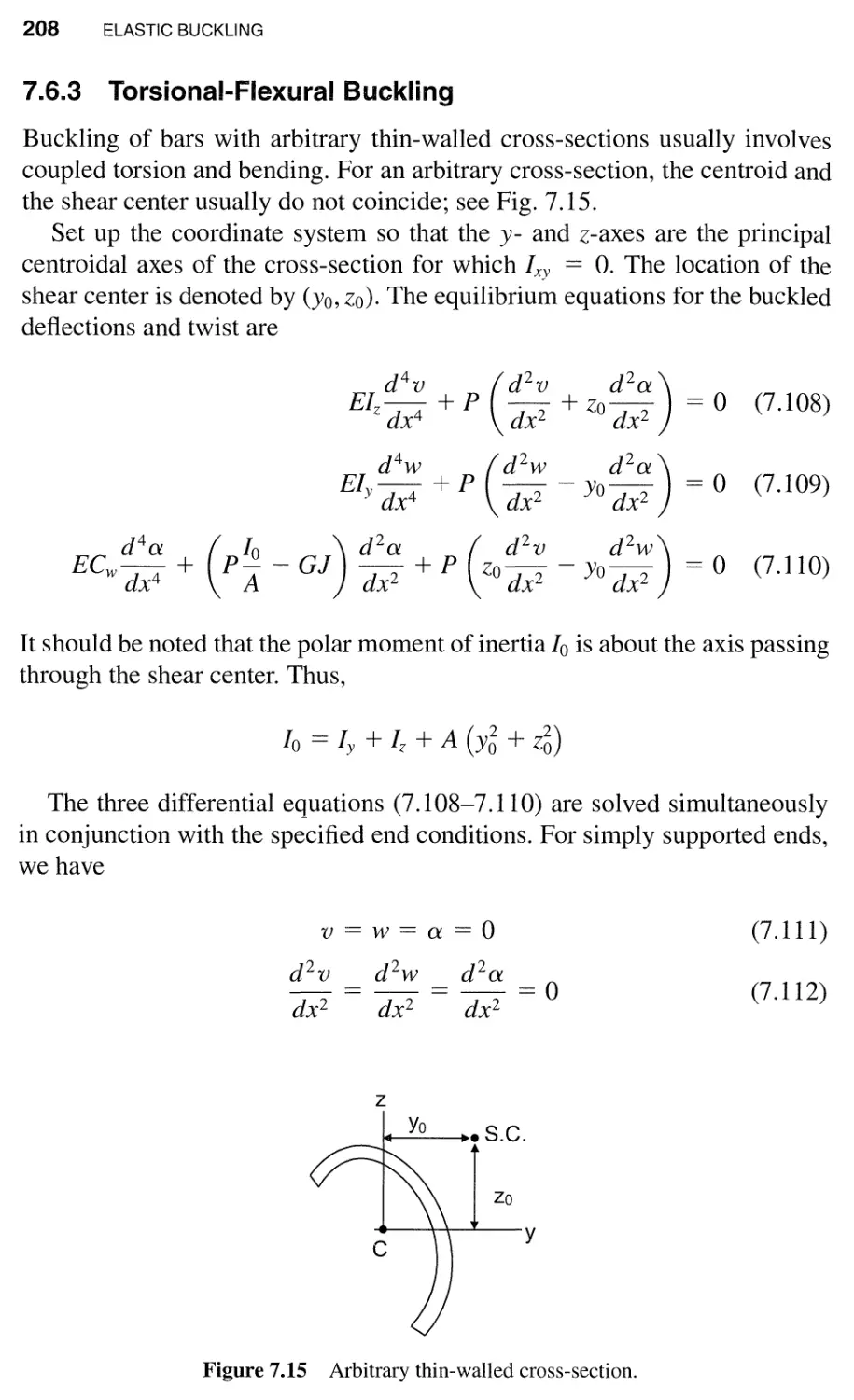
7.6.3 Torsional-Flexural Buckling / 208
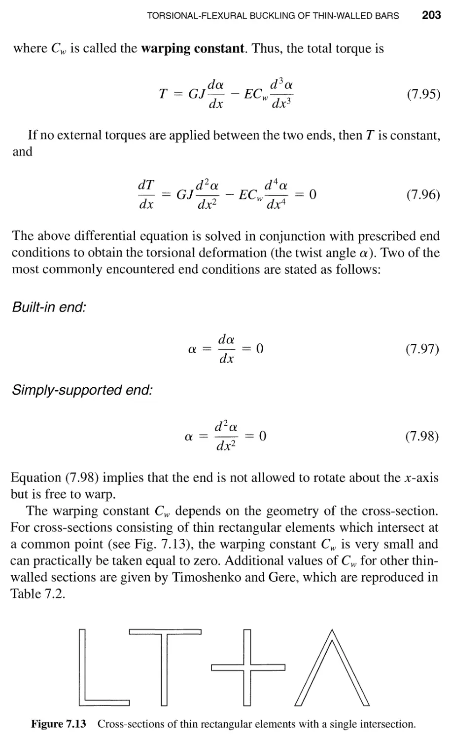
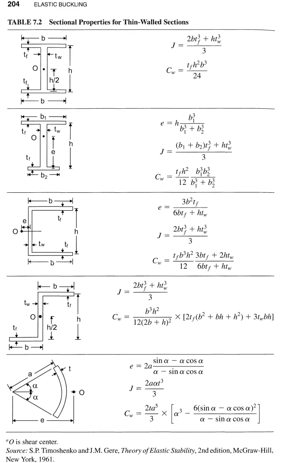
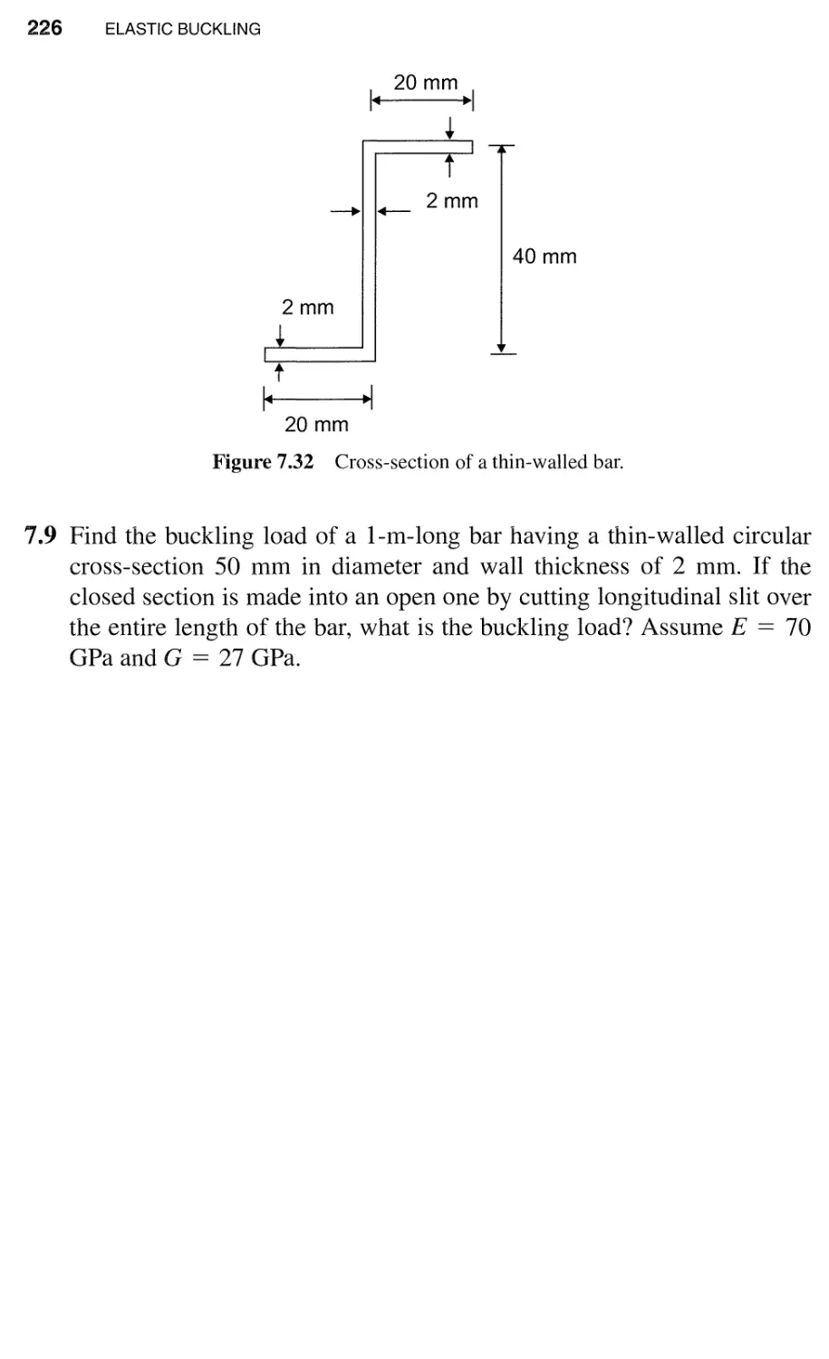
7.7 Elastic Buckling of Flat Plates / 212
7.7.1 Governing Equation for Flat Plates / 212
7.7.2 Cylindrical Bending / 215
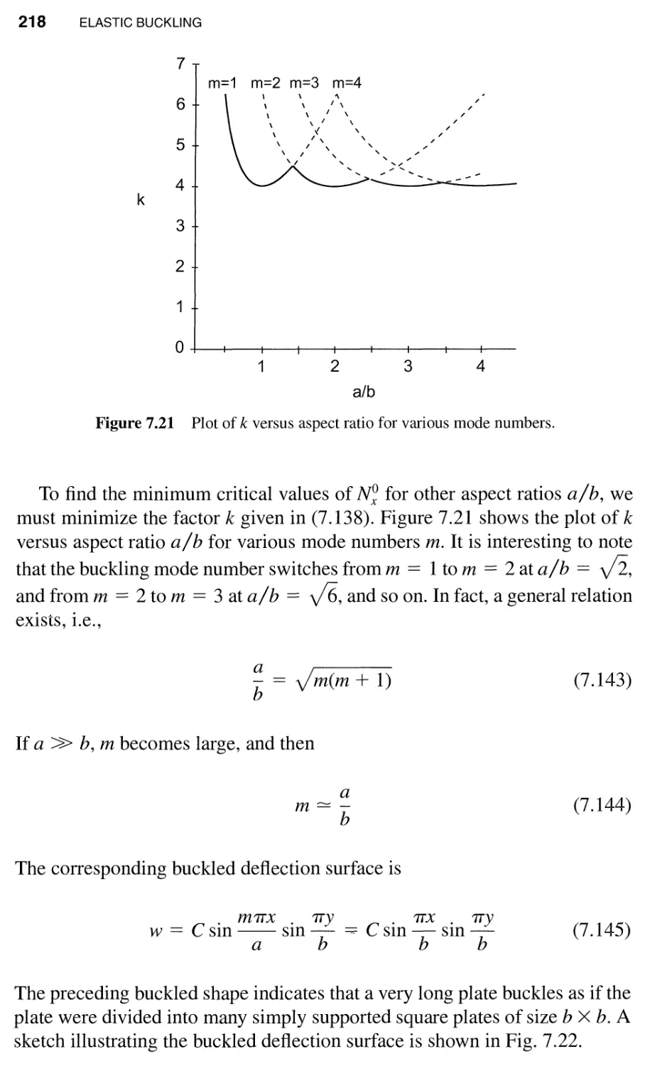
7.7.3 Buckling of Rectangular Plates / 216
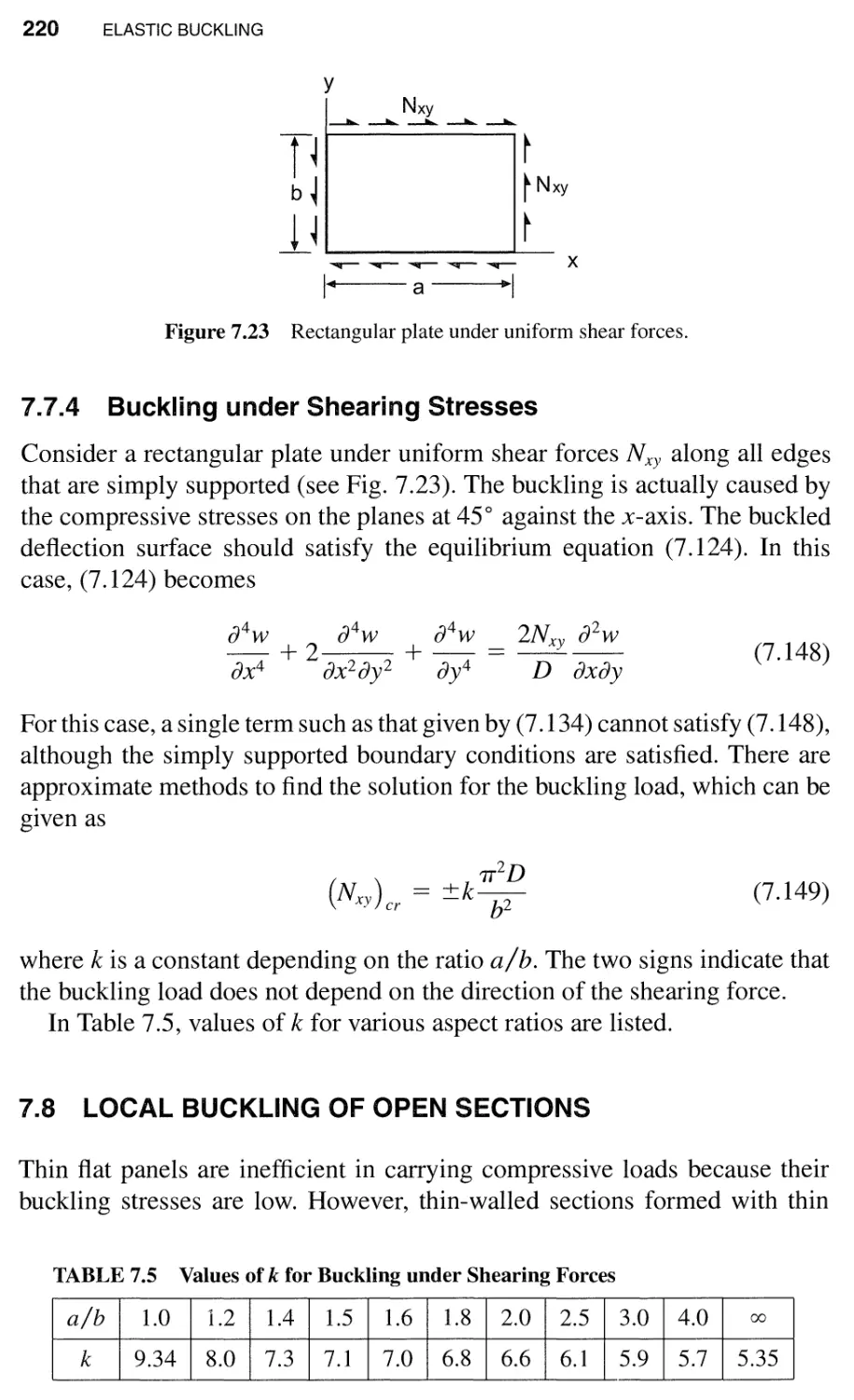
7.7.4 Buckling under Shearing Stresses / 220
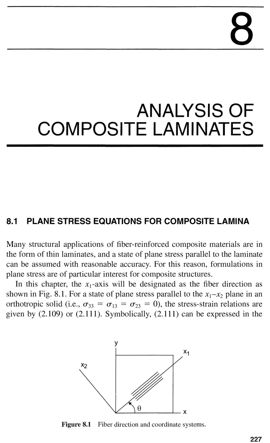
7.8 Local Buckling of Open Sections / 220
Problems / 223
8 Analysis of Composite Laminates 227
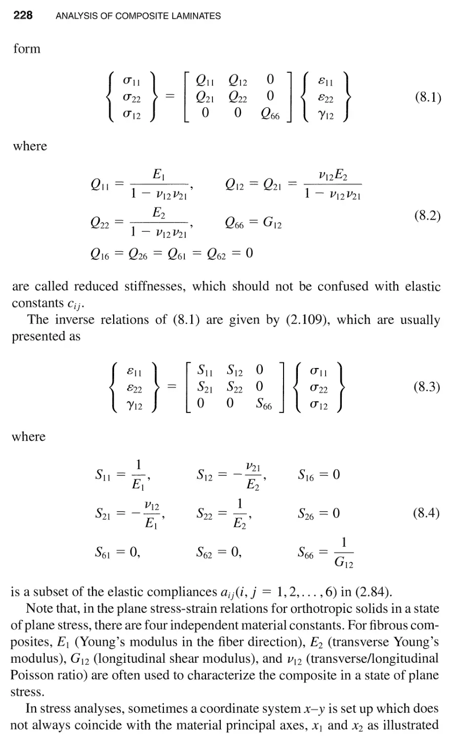
8.1 Plane Stress Equations for Composite Lamina / 227
8.2 Off-Axis Loading / 233 -
8.3 Notation for Stacking Sequence in Laminates / 236
8.4 Symmetric Laminate under In-Plane Loading / 238
X CONTENTS
8.5 Effective Moduli for Symmetric Laminates / 241
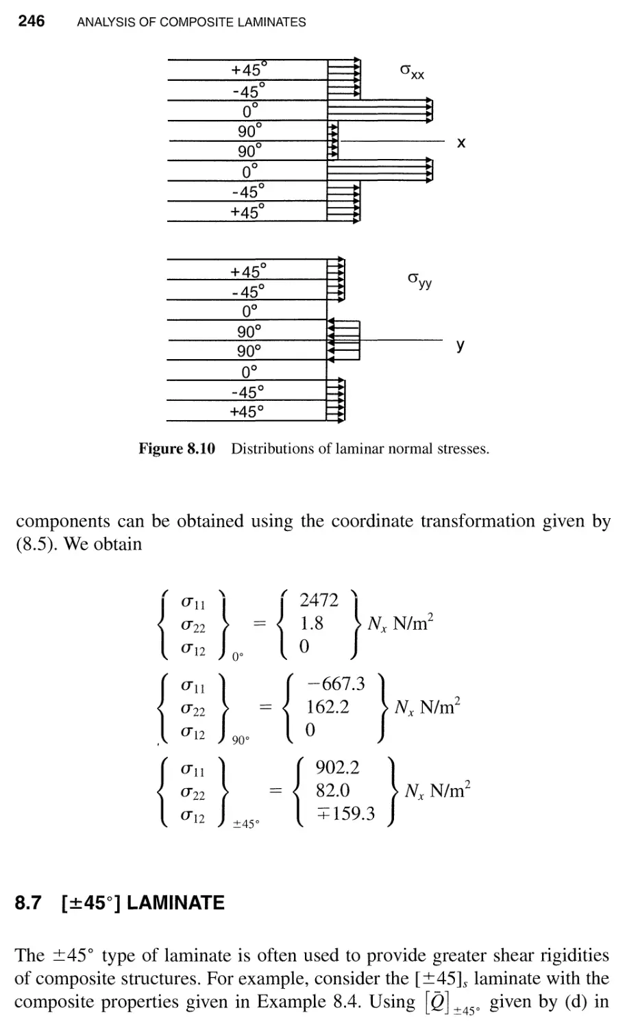
8.6 Laminar Stresses / 243
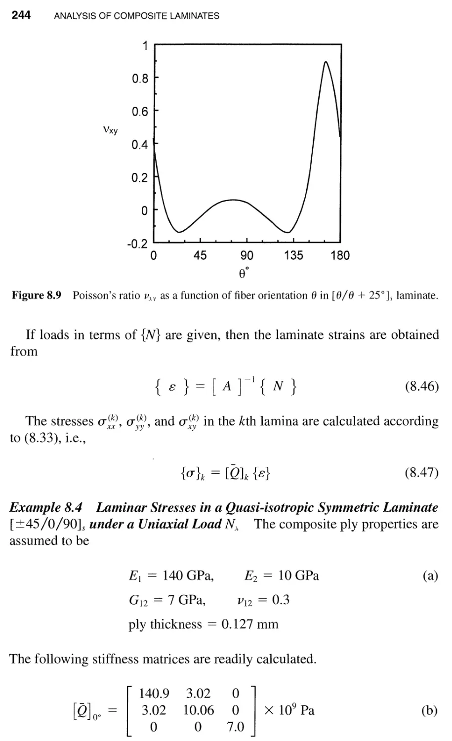
8.7 [:!:45°] Laminate / 246
Problems / 248
Index 251
PREFACE
This book is intended for junior or senior level aeronautical engineering
students with a background in the first course of mechanics of solids. The
contents can be covered in a semester at a normal pace.
The selection and presentation of materials in the course of writing this
book were greatly influenced by the following developments. First, commer-
cial finite element codes have been used extensively for structural analyses
in recent years. As a result, many simplified ad hoc techniques that were
important in the past have lost their useful roles in structural analyses. This
development leads to the shift of emphasis from the problem-solving drill to
better understanding of mechanics, developing the student's ability in formu-
lating the problem, and judging the correctness of numerical results. Second,
fracture mechanics has become the most important tool in the study of air-
craft structure damage tolerance and durability in the past thirty years. It
seems highly desirable for undergraduate students to get some exposure to
this important subject, which has traditionally been regarded as a subject for
graduate students. Third, advanced composite materials have gained wide
acceptance for use in aircraft structures. This new class of materials is sub-
stantially different from traditional metallic materials. An introduction to the
characteristic properties of these new materials seems imperative even for
undergraduate students.
In response to the advent of the finite element method, consistent elasticity
approach is employed. Multidimensional stresses, strains, and stress-strain
relations are emphasized. Displacement, rather than strain or stress, is used
in deriving the governing equations for torsion and bending problems. This
xi
xii PREFACE
approach will help the student understand the relation between simplified
structural theories and 3-D elasticity equations.
The concept of fracture mechanics is brought in via the original Griffith's
concept of strain energy release rate. Taking advantage of its global nature
and its relation to the change of the total strain energies stored in the struc-
ture before and after crack extension, the strain energy release rate can be
calculated for simple structures without difficulty for junior and senior level
students.
The coverage of composite materials consists of a brief discussion of their
mechanical properties in Chapter 1, the stress-strain relations for anisotropic
solids in Chapter 2, and a chapter (Chapter 8) on analysis of symmetric
laminates of composite materials. This should be enough to give the student
a background to deal correctly with composites and to avoid regarding a
composite as an aluminum alloy with the Young's modulus taken equal to the
longitudinal modulus of the composite. Such a brief introduction to composite
materials and laminates is by no means sufficient to be used as a substitute
for a course (or courses) dedicated to composites.
A classical treatment of elastic buckling is presented in Chapter 7. Besides
buckling of slender bars, the postbuckling concept and buckling of structures
composed of thin sheets are also briefly covered without invoking an advanced
background in solid mechanics. Postbuckling strengths of bars or panels are
often utilized in aircraft structures. Exposure, even very brief, to this concept
seems justified, especially in view of the mathematics employed, which should
be quite manageable for student readers of this book.
The author expresses his appreciation to Mrs. Marilyn Engel for typing
the manuscript and to James Chou and R. Sergio Hasebe for making the
drawings.
C.T.SUN
MECHANICS OF
AIRCRAFT STRUCTURES
CHARACTERISTICS OF
AIRCRAFT STRUCTURES
AND MATERIALS
1.1 INTRODUCTION
The main difference between aircraft structures and materials and civil engi-
neering structures and materials lies in their weight. The main driving force
in aircraft structural design and aerospace material development is to reduce
weight. In general, materials with high stiffness, high strength, and light
weight are most suitable for aircraft applications.
Aircraft structures must be designed to ensure that every part of the mate-
rial is used to its full capability. This requirement leads to the use of shell-like
structures (monocoque constructions) and stiffened shell structures (semi-
rnonocoque constructions). The geometrical details of aircraft structures are
much more complicated than those of civil engineering structures. They usu-
ally require the assemblage of thousands of parts. Technologies for joining
the parts are especially important for aircraft construction.
The size and shape of an aircraft structural component are usually de-
termined based on nonstructural considerations. For instance, the airfoil is
chosen according to aerodynamic lift and drag characteristics. Then the so-
lutions for structural problems in terms of global configurations are limited.
Often, the solutions resort to the use of special materials developed for appli-
cations in aerospace vehicles.
Because of their high stiffness/weight and strength/weight ratios, alu-
minum and titanium alloys have been the dominant aircraft structural materi-
als for many decades. However, the recent advent of advanced fiber-reinforced
composites has changed the outlook. Composites may now achieve weight
savings of 30-40 percent over aluminum or titanium counterparts.
2 CHARACTERISTICS OF AIRCRAFT STRUCTURES AND MATERIALS
1.2 BASIC STRUCTURAL ELEMENTS IN
AIRCRAFT STRUCTURE
Major components of aircraft structures are assemblages of a number of basic
structural elements, each of which is designed to take a specific type of load,
such as axial, bending, or torsional load. Collectively, these elements can
efficiently provide the capability for sustaining loads on an airplane.
1.2.1 Axial Member
Axial members are used to carry extensional or compressive loads applied
in the direction of the axial direction of the member. The resulting stress is
uniaxial:
u == EB
(1.1)
where E and B are the Young's modulus and normal strain, respectively, in
the loading direction. The total axial force F provided by the member is
F == Au == EAB
(1.2 )
where A is the cross-sectional area of the member. The quantity EA is termed
the axial stiffness of the member, which depends on the modulus of the
material and the cross-sectional area of the member. It is obvious that the axial
stiffness of axial members cannot be increased (or decreased) by changing
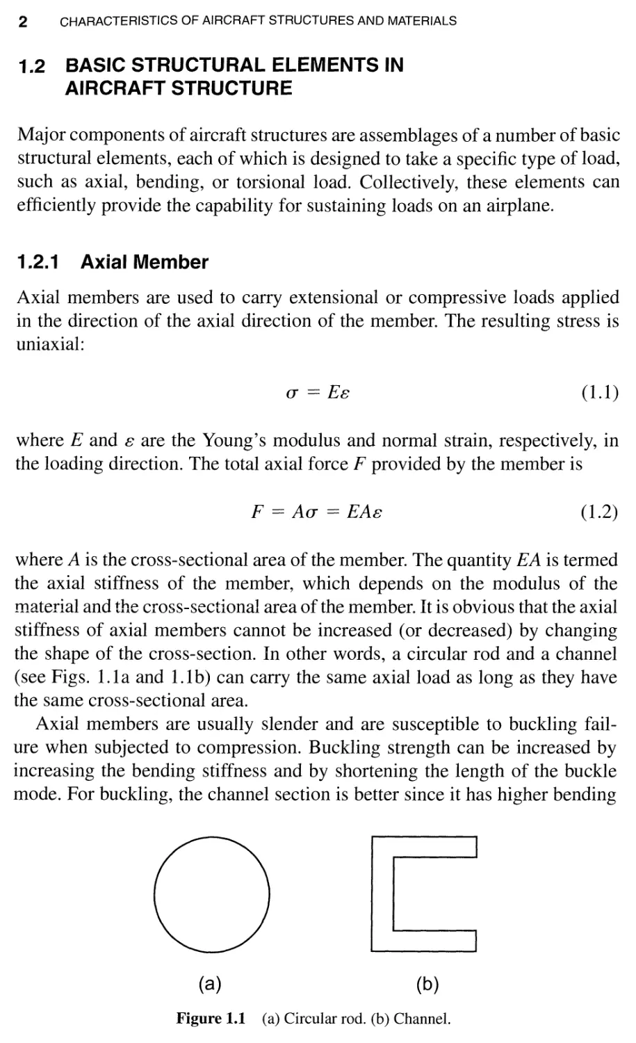
the shape of the cross-section. In other words, a circular rod and a channel
(see Figs. 1.1 a and 1.1 b) can carry the same axial load as long as they have
the same cross-sectional area.
Axial members are usually slender and are susceptible to buckling fail-
ure when subjected to compression. Buckling strength can be increased by
increasing the bending stiffness and by shortening the length of the buckle
mode. For buckling, the channel section is better since it has higher bending
(a)
(b)
Figure 1.1 (a) Circular rod. (b) Channel.
BASIC STRUCTURAL ELEMENTS IN AIRCRAFT STRUCTURE 3
stiffness than the circular section. However, because of the slenderness of
most axial members used in aircraft (such as stringers), the bending stiffness
of these members is usually very small and is not sufficient to achieve the
necessary buckling strength. In practice, the buckling strength of axial mem-
bers is enhanced by providing lateral supports along the length of the member
with more rigid ribs (in wings) and frames (in fuselage).
1.2.2 Shear Panel
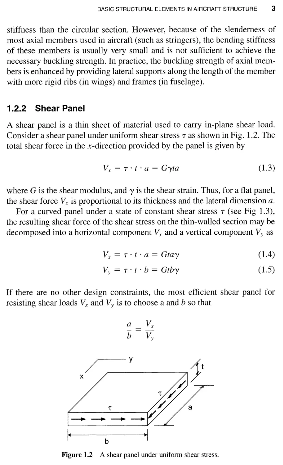
A shear panel is a thin sheet of material used to carry in-plane shear load.
Consider a shear panel under uniform shear stress T as shown in Fig. 1.2. The
total shear force in the x-direction provided by the panel is given by
V x == T . t . a == G)lta
(1.3)
where G is the shear modulus, and )I is the shear strain. Thus, for a flat panel,
the shear force V x is proportional to its thickness and the lateral dimension a.
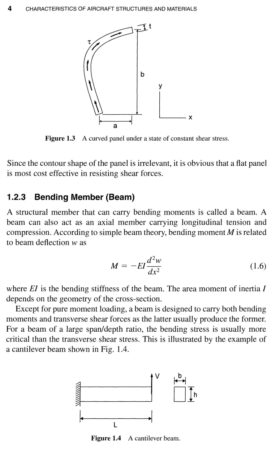
For a curved panel under a state of constant shear stress T (see Fig 1.3),
the resulting shear force of the shear stress on the thin-walled section may be
decomposed into a horizontal component V x and a vertical component V y as
V x == T . t . a == Gta)l
V y == T . t . b == Gtb)l
(1.4 )
( 1.5)
If there are no other design constraints, the most efficient shear panel for
resisting shear loads V x and V y is to choose a and b so that
a V x
- --
b V y
y
/
L
I b -I
x
Figure 1.2 A shear panel under uniform shear stress.
4 CHARACTERISTICS OF AIRCRAFT STRUCTURES AND MATERIALS
;;:It
b
a
.1
y
Lx
Figure 1.3 A curved panel under a state of constant shear stress.
Since the contour shape of the panel is irrelevant, it is obvious that a flat panel
is most cost effective in resisting shear forces.
1.2.3 Bending Member (Beam)
A structural member that can carry bending moments is called a beam. A
beam can also act as an axial member carrying longitudinal tension and
compression. According to simple beam theory, bending moment M is related
to beam deflection w as
d 2 w
M == -EI-
dx 2
(1.6)
where EI is the bending stiffness of the beam. The area moment of inertia I
depends on the geometry of the cross-section.
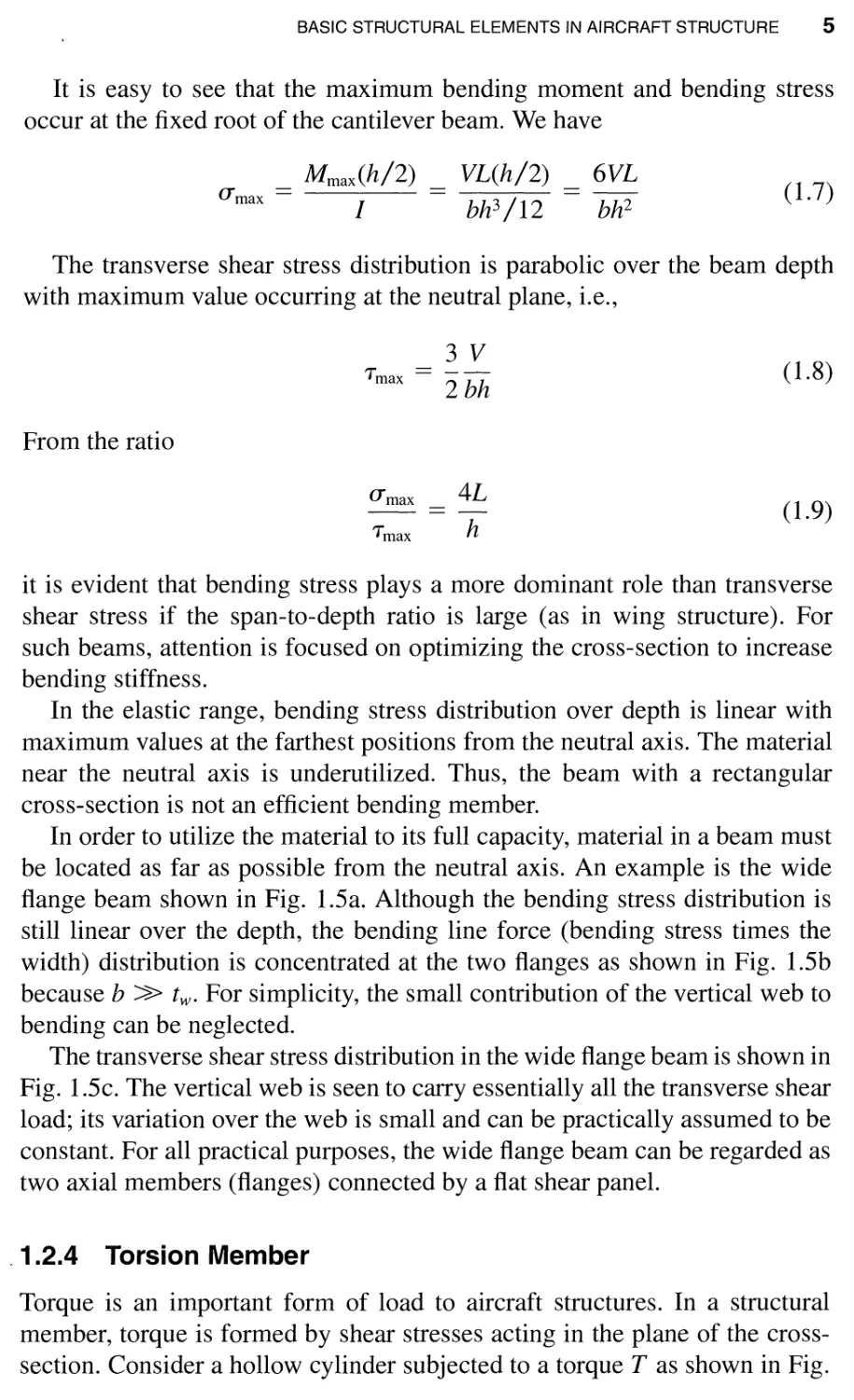
Except for pure moment loading, a beam is designed to carry both bending
moments and transverse shear forces as the latter usually produce the former.
For a beam of a large span/depth ratio, the bending stress is usually more
critical than the transverse shear stress. This is illustrated by the example of
a cantilever beam shown in Fig. 1.4.
v
Dlh
I.
L
.1
Figure 1.4 A cantilever beam.
BASIC STRUCTURAL ELEMENTS IN AIRCRAFT STRUCTURE 5
It is easy to see that the maximum bending moment and bending stress
occur at the fixed root of the cantilever beam. We have
U max ==
M max (h/2)
I
VL(h/2)
bh 3 /12
6VL
--
bh 2
( 1.7)
The transverse shear stress distribution is parabolic over the beam depth
with maximum value occurring at the neutral plane, i.e.,
3 V
Tmax == 2 bh
( 1.8)
From the ratio
U max 4L
---
Tmax h
(1.9)
it is evident that bending stress plays a more dominant role than transverse
shear stress if the span-to-depth ratio is large (as in wing structure). For
such beams, attention is focused on optimizing the cross-section to increase
bending stiffness.
In the elastic range, bending stress distribution over depth is linear with
maximum values at the farthest positions from the neutral axis. The material
near the neutral axis is underutilized. Thus, the beam with a rectangular
cross-section is not an efficient bending member.
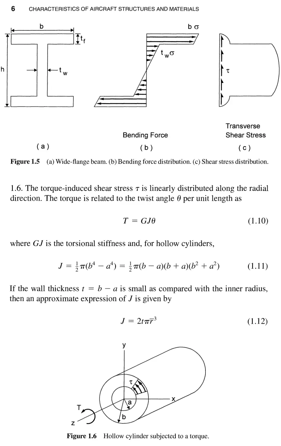
In order to utilize the material to its full capacity, material in a beam must
be located as far as possible from the neutral axis. An example is the wide
flange beam shown in Fig. I.Sa. Although the bending stress distribution is
still linear over the depth, the bending line force (bending stress times the
width) distribution is concentrated at the two flanges as shown in Fig. 1.5b
because b » two For simplicity, the small contribution of the vertical web to
bending can be neglected.
The transverse shear stress distribution in the wide flange beam is shown in
Fig. 1.5c. The vertical web is seen to carry essentially all the transverse shear
load; its variation over the web is small and can be practically assumed to be
constant. For all practical purposes, the wide flange beam can be regarded as
two axial members (flanges) connected by a flat shear panel.
,1.2.4 Torsion Member
Torque is an important form of load to aircraft structures. In a structural
member, torque is formed by shear stresses acting in the plane of the cross-
section. Consider a hollow cylinder subjected to a torque T as shown in Fig.
6 CHARACTERISTICS OF AIRCRAFT STRUCTURES AND MATERIALS
,-
b
.,
It f
ba
h
t w
twa
t
t
t-c
t
t
Bending Force
Transverse
Shear Stress
( a )
( b )
( c )
Figure 1.5 (a) Wide-flange beam. (b) Bending force distribution. (c) Shear stress distribution.
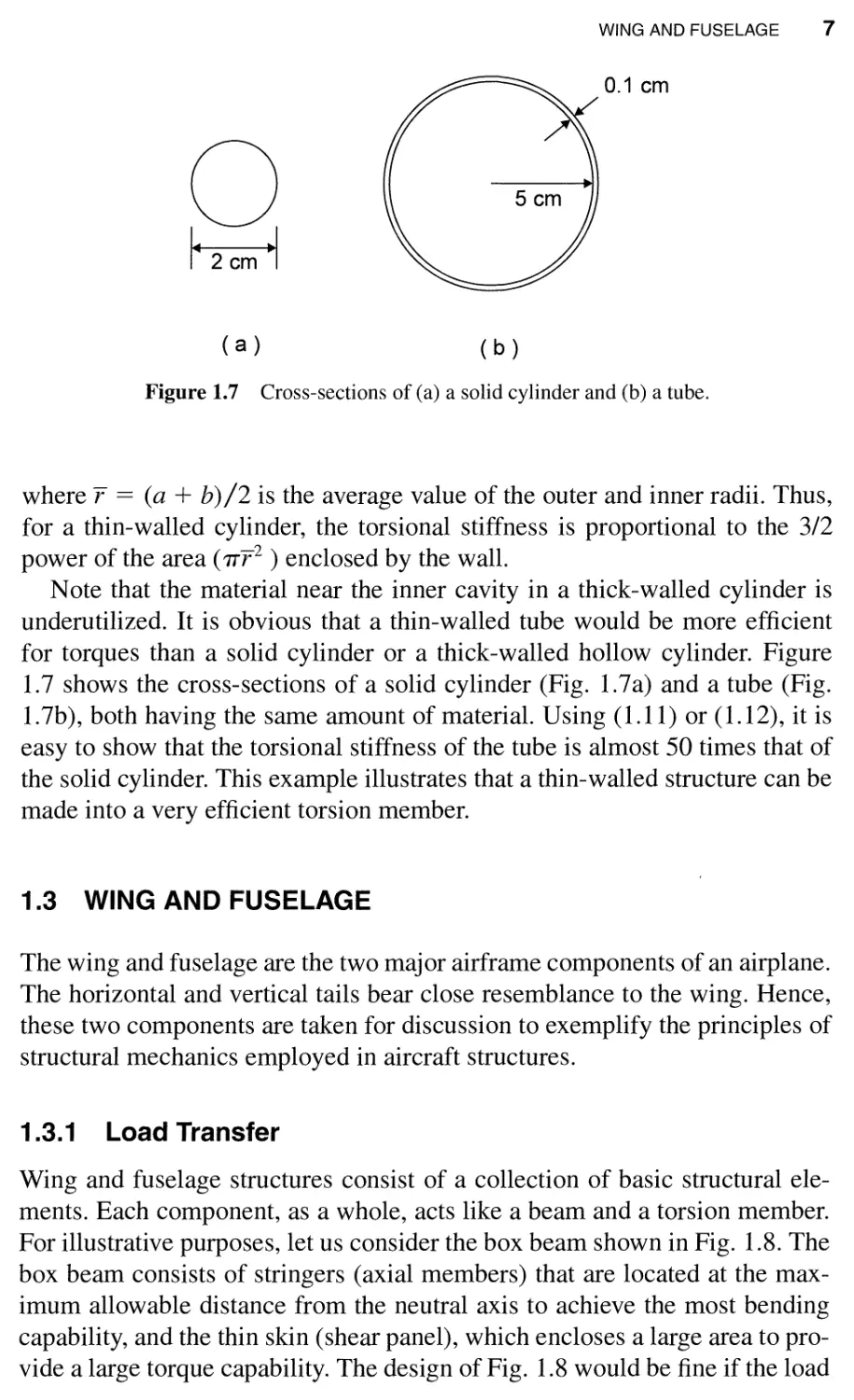
1.6. The torque-induced shear stress T is linearly distributed along the radial
direction. The torque is related to the twist angle e per unit length as
T == GJe
(1.10)
where GJ is the torsional stiffness and, for hollow cylinders,
J == 7T(b4 - a 4 ) == 7T(b - a)(b + a)(b 2 + a 2 )
(1.11)
If the wall thickness t == b - a is small as compared with the inner radius,
then an approximate expression of J is given by
J == 2t 7Tr 3
( 1.12)
z
Figure 1.6 Hollow cylinder subjected to a torque.
WING AND FUSELAGE 7
o
1 4 2 em .1
0.1 em
( a )
( b )
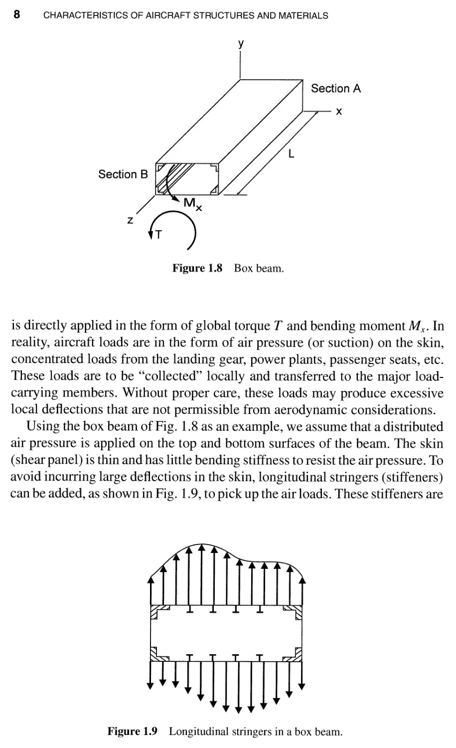
Figure 1.7 Cross-sections of (a) a solid cylinder and (b) a tube.
where r == (a + b)/2 is the average value of the outer and inner radii. Thus,
for a thin-walled cylinder, the torsional stiffness is proportional to the 3/2
power of the area (7T r 2 ) enclosed by the wall.
Note that the material near the inner cavity in a thick-walled cylinder is
under utilized. It is obvious that a thin-walled tube would be more efficient
for torques than a solid cylinder or a thick-walled hollow cylinder. Figure
1.7 shows the cross-sections of a solid cylinder (Fig. 1.7 a) and a tube (Fig.
1. 7b), both having the same amount of material. Using (1.11) or (1.12), it is
easy to show that the torsional stiffness of the tube is almost 50 times that of
the solid cylinder. This example illustrates that a thin-walled structure can be
made into a very efficient torsion member.
1.3 WING AND FUSELAGE
The wing and fuselage are the two major airframe components of an airplane.
The horizontal and vertical tails bear close resemblance to the wing. Hence,
these two components are taken for discussion to exemplify the principles of
structural mechanics employed in aircraft structures.
1.3.1 Load Transfer
Wing and fuselage structures consist of a collection of basic structural ele-
ments. Each component, as a whole, acts like a beam and a torsion member.
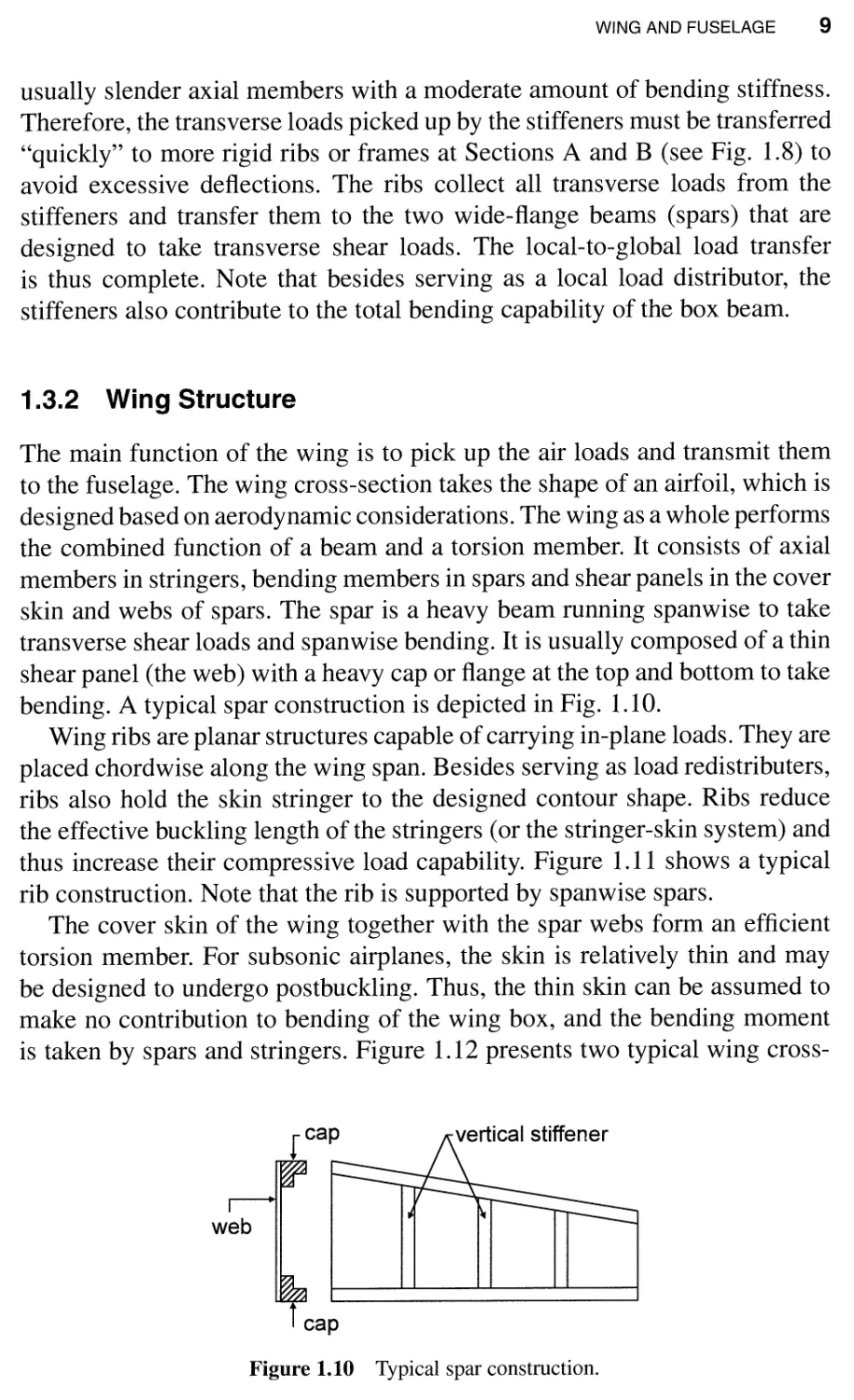
For illustrative purposes, let us consider the box beam shown in Fig. 1.8. The
box beam consists of stringers (axial members) that are located at the max-
imum allowable distance from the neutral axis to achieve the most bending
capability, and the thin skin (shear panel), which encloses a large area to pro-
vide a large torque capability. The design of Fig. 1.8 would be fine if the load
8 CHARACTERISTICS OF AIRCRAFT STRUCTURES AND MATERIALS
y
Section 8
Section A
x
/ Mx
Zh)
Figure 1.8 Box beam.
is directly applied in the form of global torque T and bending moment Mx. In
reality, aircraft loads are in the form of air pressure (or suction) on the skin,
concentrated loads from the landing gear, power plants, passenger seats, etc.
These loads are to be "collected" locally and transferred to the major load-
carrying members. Without proper care, these loads may produce excessive
local deflections that are not permissible from aerodynamic considerations.
Using the box beam of Fig. 1.8 as an example, we assume that a distributed
air pressure is applied on the top and bottom surfaces of the beam. The skin
(shear panel) is thin and has little bending stiffness to resist the air pressure. To
avoid incurring large deflections in the skin, longitudinal stringers (stiffeners)
can be added, as shown in Fig. 1.9, to pick up the air loads. These stiffeners are
Figure 1.9 Longitudinal stringers in a box beam.
WING AND FUSELAGE 9
usually slender axial rl1embers with a moderate amount of bending stiffness.
Therefore, the transverse loads picked up by the stiffeners must be transferred
"quickly" to more rigid ribs or frames at Sections A and B (see Fig. 1.8) to
avoid excessive deflections. The ribs collect all transverse loads from the
stiffeners and transfer them to the two wide-flange beams (spars) that are
designed to take transverse shear loads. The local-to-global load transfer
is thus complete. Note that besides serving as a local load distributor, the
stiffeners also contribute to the total bending capability of the box beam.
1.3.2 Wing Structure
The main function of the wing is to pick up the air loads and transmit them
to the fuselage. The wing cross-section takes the shape of an airfoil, which is
designed based on aerodynamic considerations. The wing as a whole performs
the combined function of a beam and a torsion member. It consists of axial
members in stringers, bending members in spars and shear panels in the cover
skin and webs of spars. The spar is a heavy beam running spanwise to take
transverse shear loads and spanwise bending. It is usually composed of a thin
shear panel (the web) with a heavy cap or flange at the top and bottom to take
bending. A typical spar construction is depicted in Fig. 1.10.
Wing ribs are planar structures capable of carrying in-plane loads. They are
placed chordwise along the wing span. Besides serving as load redistributers,
ribs also hold the skin stringer to the designed contour shape. Ribs reduce
the effective buckling length of the stringers (or the stringer-skin system) and
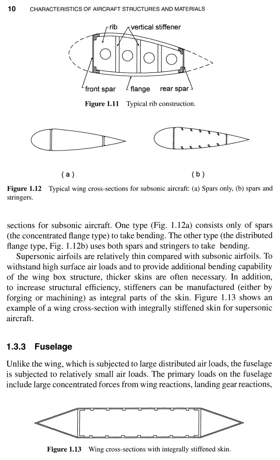
thus increase their compressive load capability. Figure 1.11 shows a typical
rib construction. Note that the rib is supported by spanwise spars.
The cover skin of the wing together with the spar webs form an efficient
torsion member. For subsonic airplanes, the skin is relatively thin and may
be designed to undergo postbuckling. Thus, the thin skin can be assumed to
make no contribution to bending of the wing box, and the bending moment
is taken by spars and stringers. Figure 1.12 presents two typical wing cross-
cap
Figure 1.10 Typical spar construction.
10 CHARACTERISTICS OF AIRCRAFT STRUCTURES AND MATERIALS
/'
/"
/
(
\
"-
"-
.......
00
-
-
Iflange
rear spar
Figure 1.11 Typical rib construction.
G:
( a )
( b )
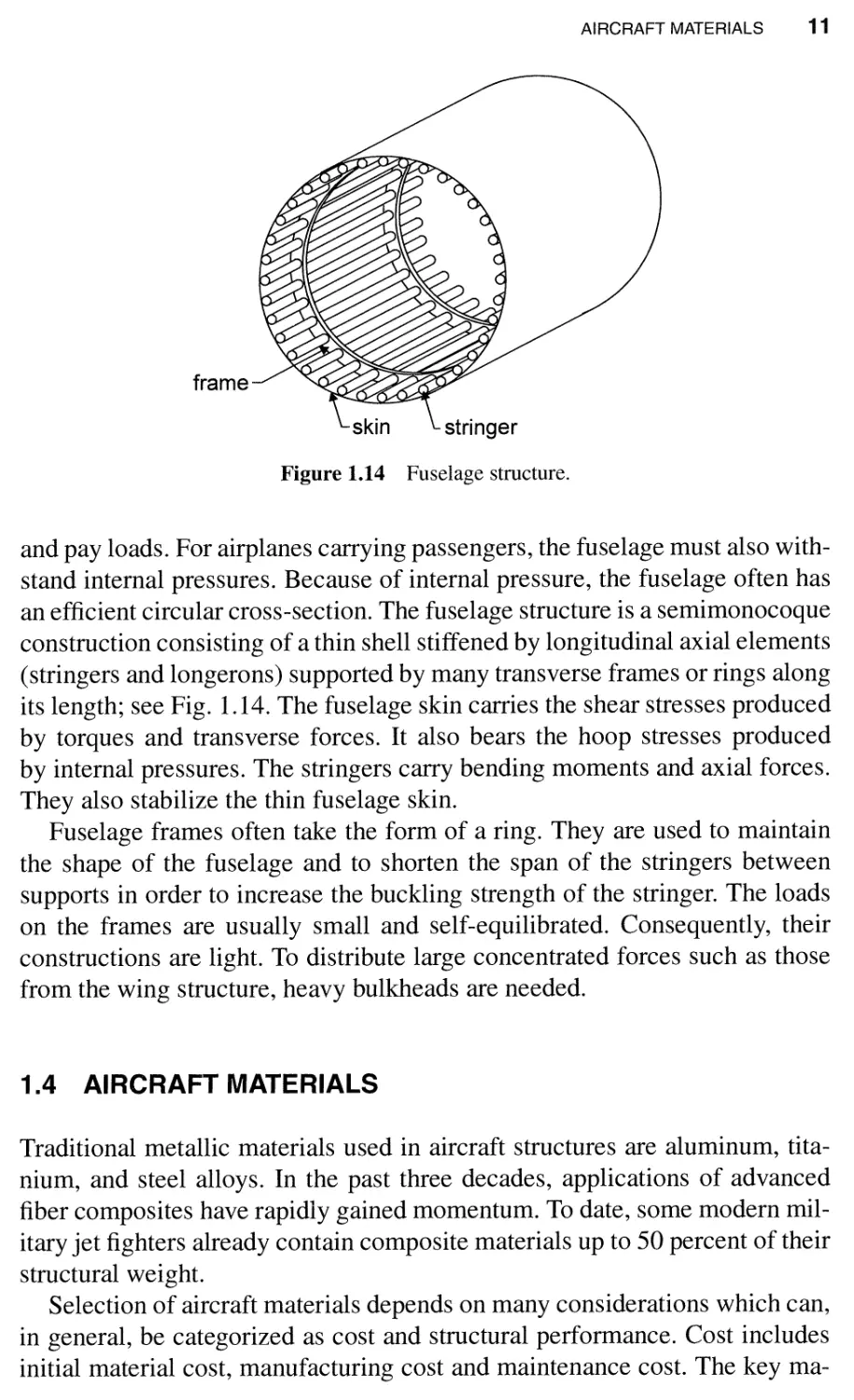
Figure 1.12 Typical wing cross-sections for subsonic aircraft: (a) Spars only, (b) spars and
stringers.
sections for subsonic aircraft. One type (Fig. 1.12a) consists only of spars
(the concentrated flange type) to take bending. The other type (the distributed
flange type, Fig. 1.12b) uses both spars and stringers to take bending.
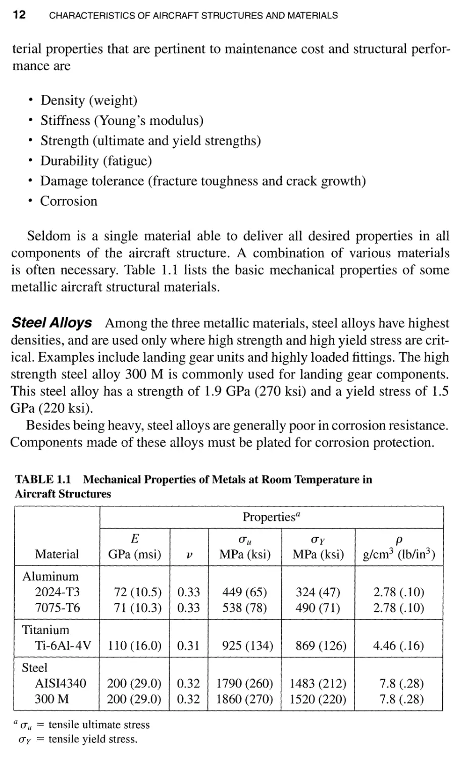
Supersonic airfoils are relatively thin compared with subsonic airfoils. To
withstand high surface air loads and to provide additional bending capability
of the wing box structure, thicker skins are often necessary. In addition,
to increase structural efficiency, stiffeners can be manufactured (either by
forging or machining) as integral parts of the skin. Figure 1.13 shows an
example of a wing cross-section with integrally stiffened skin for supersonic
aircraft.
1.3.3 Fuselage
Unlike the wing, which is subjected to large distributed air loads, the fuselage
is subjected to relatively small air loads. The primary loads on the fuselage
include large concentrated forces from wing reactions, landing gear reactions,
<
Figure 1.13 Wing cross-sections with integrally stiffened skin.
AIRCRAFT MATERIALS 11
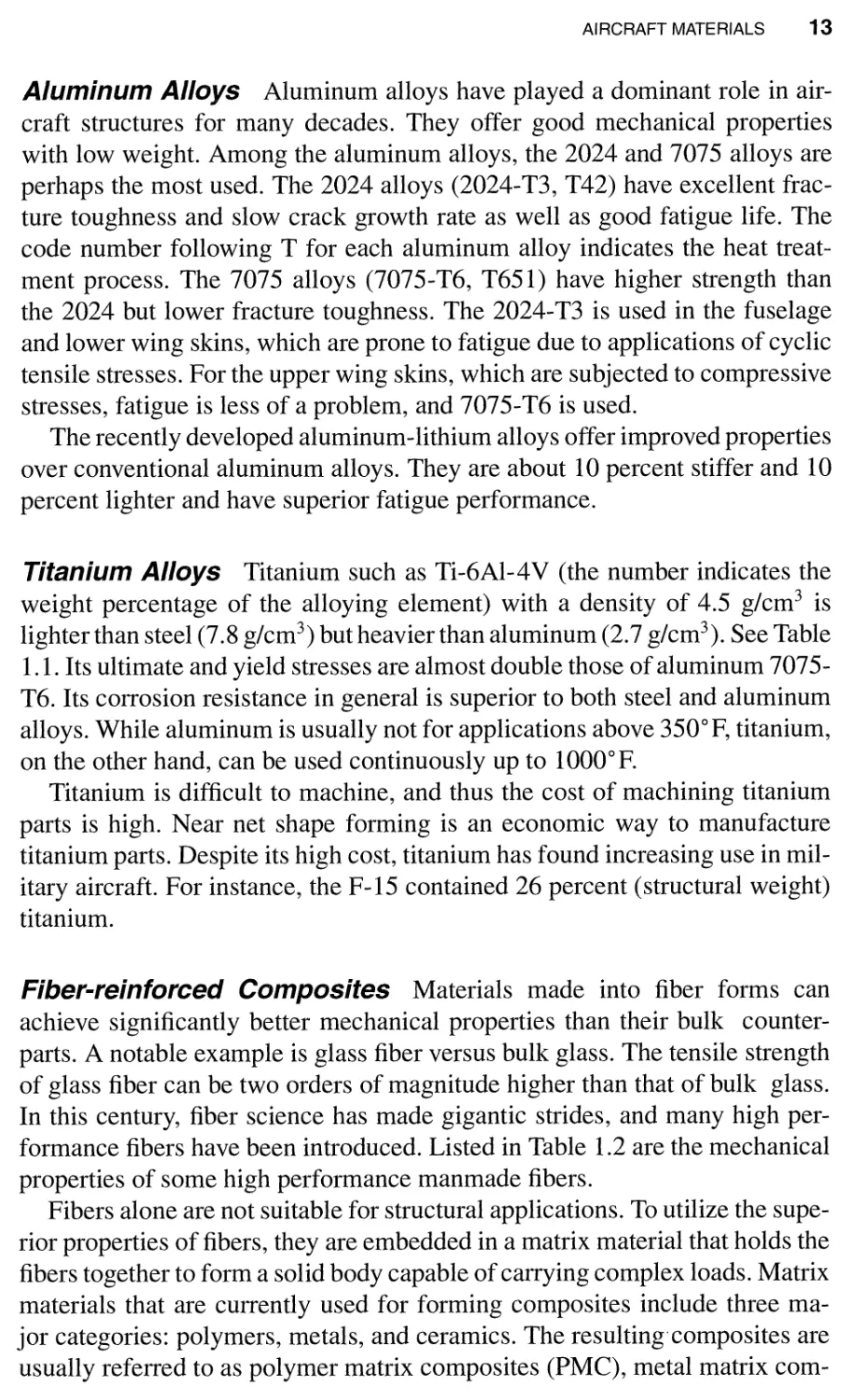
frame
Figure 1.14 Fuselage structure.
and pay loads. For airplanes carrying passengers, the fuselage must also with-
stand internal pressures. Because of internal pressure, the fuselage often has
an efficient circular cross-section. The fuselage structure is a semimonocoque
construction consisting of a thin shell stiffened by longitudinal axial elements
(stringers and longerons) supported by many transverse frames or rings along
its length; see Fig. 1.14. The fuselage skin carries the shear stresses produced
by torques and transverse forces. It also bears the hoop stresses produced
by internal pressures. The stringers carry bending moments and axial forces.
They also stabilize the thin fuselage skin.
Fuselage frames often take the form of a ring. They are used to maintain
the shape of the fuselage and to shorten the span of the stringers between
supports in order to increase the buckling strength of the stringer. The loads
on the frames are usually small and self-equilibrated. Consequently, their
constructions are light. To distribute large concentrated forces such as those
from the wing structure, heavy bulkheads are needed.
1.4 AIRCRAFT MATERIALS
Traditional metallic materials used in aircraft structures are aluminum, tita-
nium, and steel alloys. In the past three decades, applications of advanced
fiber composites have rapidly gained momentum. To date, some modern mil-
itary jet fighters already contain composite materials up to 50 percent of their
structural weight.
Selection of aircraft materials depends on many considerations which can,
in general, be categorized as cost and structural performance. Cost includes
initial material cost, manufacturing cost and maintenance cost. The key ma-
12 CHARACTERISTICS OF AIRCRAFT STRUCTURES AND MATERIALS
terial properties that are pertinent to maintenance cost and structural perfor-
mance are
· Density (weight)
· Stiffness (Young's modulus)
· Strength (ultimate and yield strengths)
· Durability (fatigue)
· Damage tolerance (fracture toughness and crack growth)
· Corrosion
Seldom is a single material able to deliver all desired properties in all
components of the aircraft structure. A combination of various materials
is often necessary. Table 1.1 lists the basic mechanical properties of some
metallic aircraft structural materials.
Steel Alloys Among the three metallic materials, steel alloys have highest
densities, and are used only where high strength and high yield stress are crit-
ical. Examples include landing gear units and highly loaded fittings. The high
strength steel alloy 300 M is commonly used for landing gear components.
This steel alloy has a strength of 1.9 GPa (270 ksi) and a yield stress of 1.5
GPa (220 ksi).
Besides being heavy, steel alloys are generally poor in corrosion resistance.
Components made of these alloys must be plated for corrosion protection.
TABLE 1.1 Mechanical Properties of Metals at Room Temperature in
Aircraft Structures
Properties a
E (J"u (J"y P
Material GPa (msi) v MPa (ksi) MPa (ksi) g/cm 3 (lb/in 3 )
Aluminum
2024- T3 72 (10.5) 0.33 449 (65) 324 (47) 2.78 (.10)
7075-T6 71 (10.3) 0.33 538 (78) 490 (71) 2.78 (.10)
Titanium
Ti-6AI-4V 110 (16.0) 0.31 925 (134) 869 (126) 4.46 (.16)
Steel
AISI4340 200 (29.0) 0.32 1790 (260) 1483 (212) 7.8 (.28)
300M 200 (29.0) 0.32 1860 (270) 1520 (220) 7.8 (.28)
a O"u = tensile ultimate stress
O"y = tensile yield stress.
AIRCRAFT MATERIALS 13
Aluminum Alloys Aluminum alloys have played a dominant role in air-
craft structures for many decades. They offer good mechanical properties
with low weight. Among the aluminum alloys, the 2024 and 7075 alloys are
perhaps the most used. The 2024 alloys (2024- T3, T42) have excellent frac-
ture toughness and slow crack growth rate as well as good fatigue life. The
code number following T for each aluminum alloy indicates the heat treat-
ment process. The 7075 alloys (7075- T6, T651) have higher strength than
the 2024 but lower fracture toughness. The 2024- T3 is used in the fuselage
and lower wing skins, which are prone to fatigue due to applications of cyclic
tensile stresses. For the upper wing skins, which are subjected to compressive
stresses, fatigue is less of a problem, and 7075- T6 is used.
The recently developed aluminum-lithium alloys offer improved properties
over conventional aluminum alloys. They are about 10 percent stiffer and 10
percent lighter and have superior fatigue performance.
Titanium Alloys Titanium such as Ti-6Al-4V (the number indicates the
weight percentage of the alloying element) with a density of 4.5 g/cm 3 is
lighter than steel (7.8 g/cm 3 ) but heavier than aluminum (2.7 g/cm 3 ). See Table
1.1. Its ultimate and yield stresses are almost double those of aluminum 7075-
T6. Its corrosion resistance in general is superior to both steel and aluminum
alloys. While aluminum is usually not for applications above 350°F, titanium,
on the other hand, can be used continuously up to 1000°F.
Titanium is difficult to machine, and thus the cost of machining titanium
parts is high. Near net shape forming is an economic way to manufacture
titanium parts. Despite its high cost, titanium has found increasing use in mil-
itary aircraft. For instance, the F-15 contained 26 percent (structural weight)
titanium.
Fiber-reinforced Composites Materials made into fiber forms can
achieve significantly better mechanical properties than their bulk counter-
parts. A notable example is glass fiber versus bulk glass. The tensile strength
of glass fiber can be two orders of magnitude higher than that of bulk glass.
In this century, fiber science has made gigantic strides, and many high per-
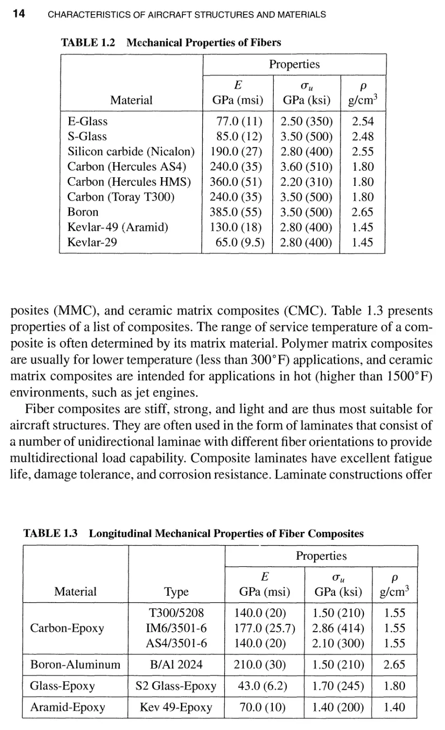
formance fibers have been introduced. Listed in Table 1.2 are the mechanical
properties of some high performance manmade fibers.
Fibers alone are not suitable for structural applications. To utilize the supe-
rior properties of fibers, they are embedded in a matrix material that holds the
fibers together to form a solid body capable of carrying complex loads. Matrix
materials that are currently used for forming composites include three ma-
jor categories: polymers, metals, and ceramics. The resulting'composites are
usually referred to as polymer matrix composites (PMC), metal matrix com-
14 CHARACTERISTICS OF AIRCRAFT STRUCTURES AND MATERIALS
TABLE 1.2 Mechanical Properties of Fibers
Properties
E (J"u P
Material GPa (msi) GPa (ksi) g/cm 3
E-Glass 77.0 (11) 2.50 (350) 2.54
S-Glass 85.0 (12) 3.50 (500) 2.48
Silicon carbide (Nicalon) 190.0 (27) 2.80 (400) 2.55
Carbon (Hercules AS4) 240.0 (35) 3.60 (510) 1.80
Carbon (Hercules HMS) 360.0 (51) 2.20 (310) 1.80
Carbon (Toray T300) 240.0 (35) 3.50 (500) 1.80
Boron 385.0 (55) 3.50 (500) 2.65
Kevlar-49 (Aramid) 130.0 (18) 2.80 (400) 1.45
Kevlar-29 65.0 (9.5) 2.80 (400) 1.45
posites (MMC), and ceramic matrix composites (CMC). Table 1.3 presents
properties of a list of composites. The range of service temperature of a com-
posite is often determined by its matrix material. Polymer matrix composites
are usually for lower temperature (less than 300°F) applications, and ceramic
matrix composites are intended for applications in hot (higher than 1500°F)
environments, such as jet engines.
Fiber composites are stiff, strong, and light and are thus most suitable for
aircraft structures. They are often used in the form of laminates that consist of
a number of unidirectional laminae with different fiber orientations to provide
multidirectional load capability. Composite laminates have excellent fatigue
life, damage tolerance, and corrosion resistance. Laminate constructions offer
TABLE 1.3 Longitudinal Mechanical Properties of Fiber Composites
Properties
E (J"u P
Material Type GPa (msi) GPa (ksi) g/cm 3
T300/5208 140.0 (20) 1.50 (210) 1.55
Carbon-Epoxy IM6/3501-6 177.0 (25.7) 2.86 (414) 1.55
AS4/3501-6 140.0 (20) 2.10(300) 1.55
Boron-Aluminum B/ Al 2024 210.0 (30) 1.50 (210) 2.65
Glass-Epoxy S2 Glass-Epoxy 43.0 (6.2) 1.70 (245) 1.80
Aramid-Epoxy Kev 49-Epoxy 70.0 (10) 1.40 (200) 1.40
PROBLEMS 15
the possibility of tailoring fiber orientations to achieve optimal structural
performance of the composite structure.
PROBLEMS
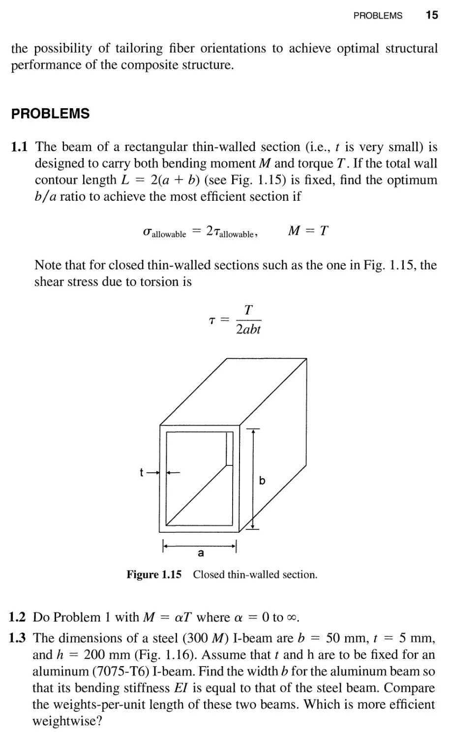
1.1 The beam of a rectangular thin-walled section (i.e., t is very small) is
designed to carry both bending moment M and torque T. If the total wall
contour length L == 2(a + b) (see Fig. 1.15) is fixed, find the optimum
b / a ratio to achieve the most efficient section if
U allowable == 2 Tallowable,
M == T
Note that for closed thin-walled sections such as the one in Fig. 1.15, the
shear stress due to torsion is
T
T== -
2abt
t
I
a
- I
Figure 1.15 Closed thin-walled section.
1.2 Do Problem 1 with M == aT where a == 0 to 00.
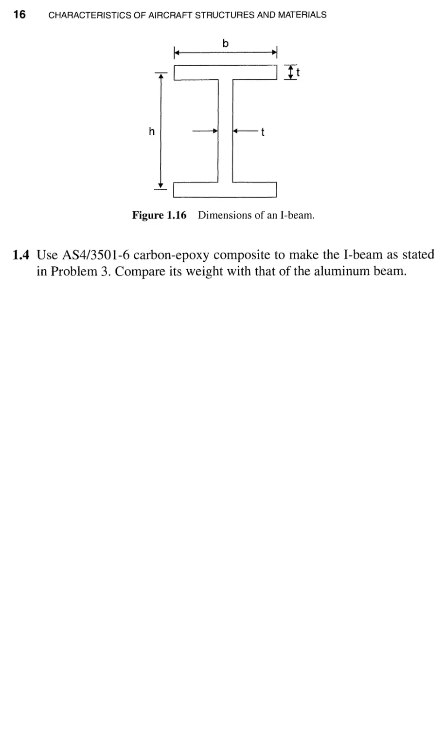
1.3 The dimensions of a steel (300 M) I-beam are b == 50 mm, t == 5 mm,
and h == 200 mm (Fig. 1.16). Assume that t and h are to be fixed for an
aluminum (7075- T6) I-beam. Find the width b for the aluminum beam so
that its bending stiffness EI is equal to that of the steel beam. Compare
the weights-per-unit length of these two beams. Which is more efficient
weightwise?
16 CHARACTERISTICS OF AIRCRAFT STRUCTURES AND MATERIALS
I.
b
.1
It
h t
Figure 1.16 Dimensions of an I-beam.
1.4 Use AS4/3501-6 carbon-epoxy composite to make the I-beam as stated
in Problem 3. Compare its weight with that of the aluminum beam.
INTRODUCTION
TO ELASTICITY
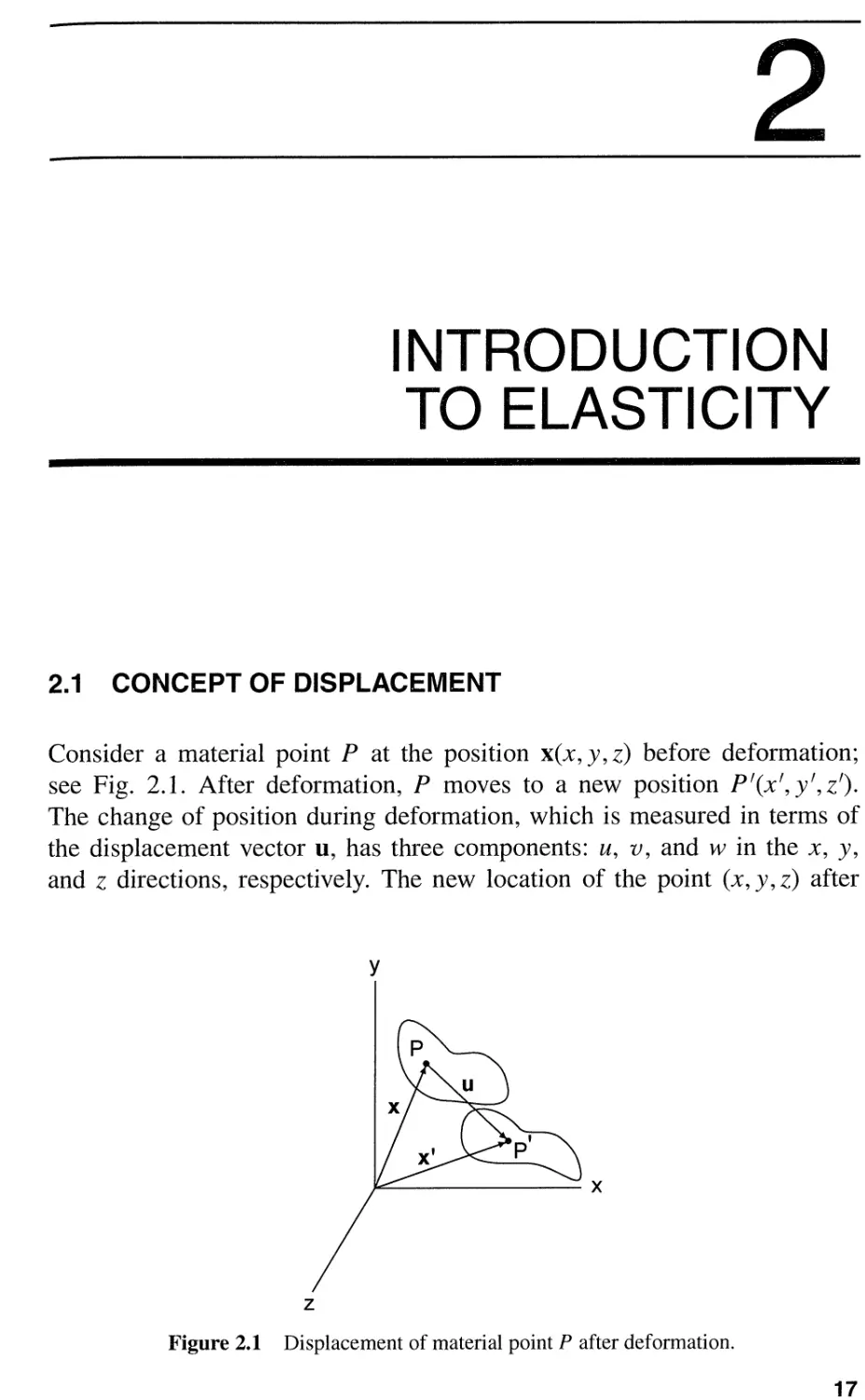
2.1 CONCEPT OF DISPLACEMENT
Consider a material point P at the position x(x, y, z) before deformation;
see Fig. 2.1. After deformation, P moves to a new position Pf(Xf, yf, Zf).
The change of position during deformation, which is measured in terms of
the displacement vector u, has three components: u, v, and w in the x, y,
and z directions, respectively. The new location of the point (x, y, z) after
y
x
z
Figure 2.1 Displacement of material point P after deformation.
17
18 INTRODUCTION TO ELASTICITY
deformation is given by
Xf == x + U or U == Xf - X
yf == y + v
Zf == Z + w
v == yf - Y
w == Zf - Z
(2.1 )
Thus, the deformed configuration is uniquely defined if the displacement
components u, v, and ware given everywhere in the body of interest.
Consider an axial member [i.e., a one-dimensional (I-D) body] of original
length La. Assume the axial strain to be uniform in the member. Then the
axial strain everywhere in the member is calculated by
I1L
B ==-
La
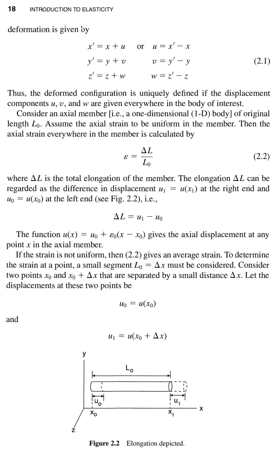
where I1L is the total elongation of the member. The elongation I1L can be
regarded as the difference in displacement Ul == U(X1) at the right end and
Uo == u(xo) at the left end (see Fig. 2.2), i.e.,
(2.2)
I1L == Ul - Uo
The function u(x) == Uo + BO(X - xo) gives the axial displacement at any
point x in the axial member.
If the strain is not uniform, then (2.2) gives an average strain. To determine
the strain at a point, a small segment La == I1x must be considered. Consider
two points Xo and Xo + I1x that are separated by a small distance x. Let the
displacements at these two points be
Uo == u(xo)
and
U1 == u(xo + I1x)
y
I
( (
!.ua 1
Xa
La
.1
o I
I u 1
x 1
x
z
Figure 2.2 Elongation depicted.
STRAIN 19
respectively. The difference in displacement between these two points is
f1u == U1 - Uo == U(XO + f1X) - U(XO)
(2.3)
which can also be regarded as the elongation of the material between these
two points. The axial strain in this segment (or at point xo) is defined as
. f1u du
B == 11m - == -
8x-+O Llx dx
(2.4)
Thus, axial strain can be obtained from the derivative of the displacement
function.
If a rod is subjected to a uniform tension and B == Bo == constant, then
du
dx == Bo,
xo < x < xo+Lo
Integrate the above equation to obtain
u == BoX + C
Let u(xo) == uo; then, from the above equation, C
displacement function is given by
Uo - BoXo, and the
u == BO(X - xo) + Uo
(2.5)
2.2 STRAIN
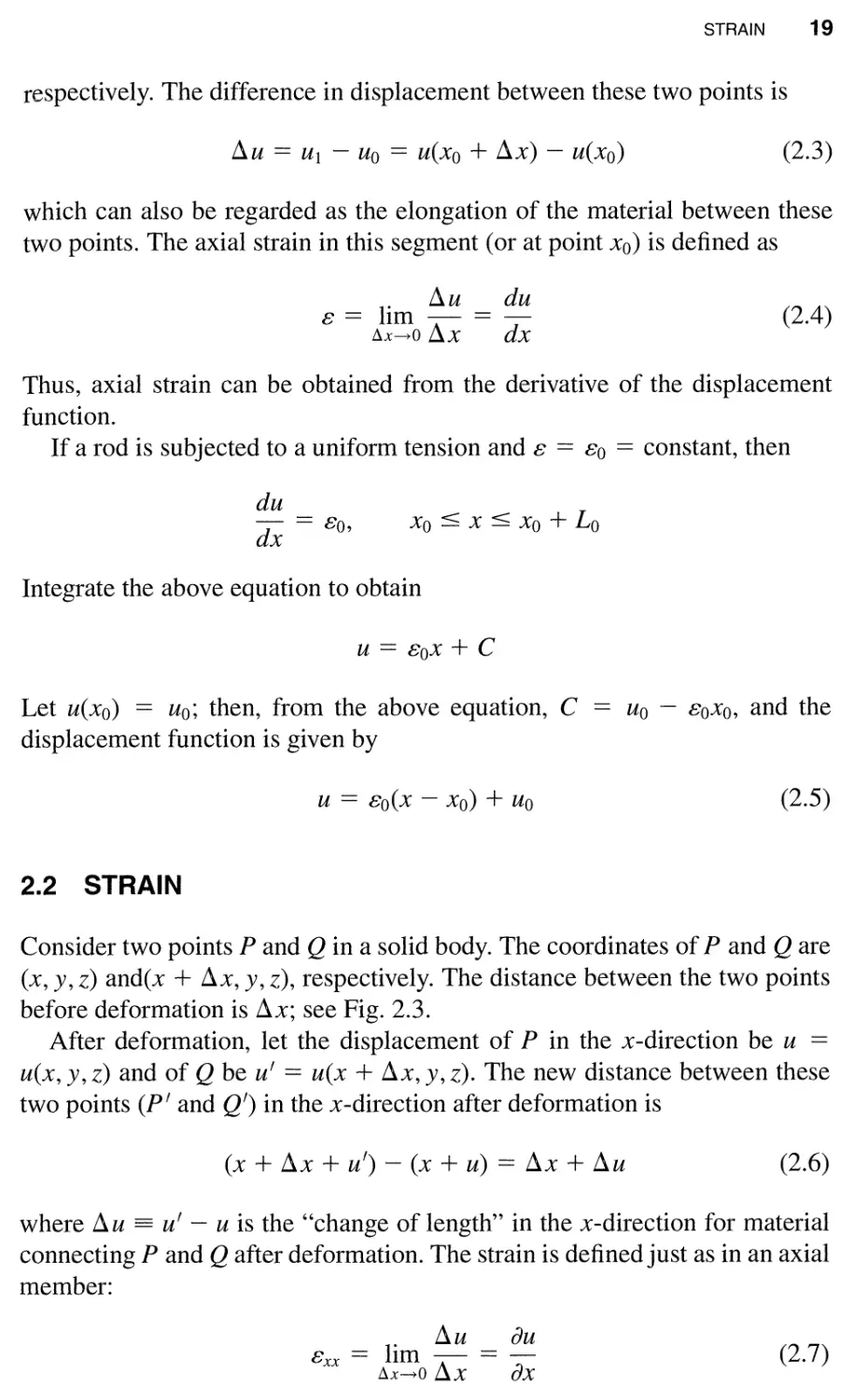
Consider two points P and Q in a solid body. The coordinates of P and Q are
(x, y, z) and(x + f1x, y, z), respectively. The distance between the two points
before deformation is f1x; see Fig. 2.3.
After deformation, let the displacement of P in the x-direction be u ==
u(x, y, z) and of Q be u f == u(x + f1x, y, z). The new distance between these
two points (P f and Qf) in the x-direction after deformation is
(x + f1x + u f ) - (x + u) == f1x + f1u
(2.6)
where f1 u u f - u is the "change of length" in the x-direction for material
connecting P and Q after deformation. The strain is defined just as in an axial
member:
. f1 u au
B == 11m - - -
xx A
8x-+O L.lX ax
(2.7)
20 INTRODUCTION TO ELASTICITY
y
I
=Lo
.1
. . . . .. .
P(x,y,z) P'(x+u,y,z) Q(x+ ,y,z) Q'(x+ +u',y,z)
x
z
Figure 2.3 Neighboring points P and Q in a solid body.
This is the x-component of the normal strain, which measures the "deforma-
tion in the x-direction" at a point (x, y, z).
Similarly, the y-component and z-component of the normal strain at the
point are given by
Jv (2.8)
E ==-
YY Jy
and
Jw (2.9)
E ==-
zz Jz
respectively. Comparing the strain component Exx with the strain in the I-D
case (or in an axial member), we may interpret Exx as the elongation per unit
length of an "infinitesimal" axial element of the material at a point (x, y, z) in
the x-direction. Similar interpretations can be given to Eyy and Ezz.
The three normal strain components are not sufficient to describe a general
state of deformation in a 3-D body. Additional shear strain components are
needed to describe the distortional deformation.
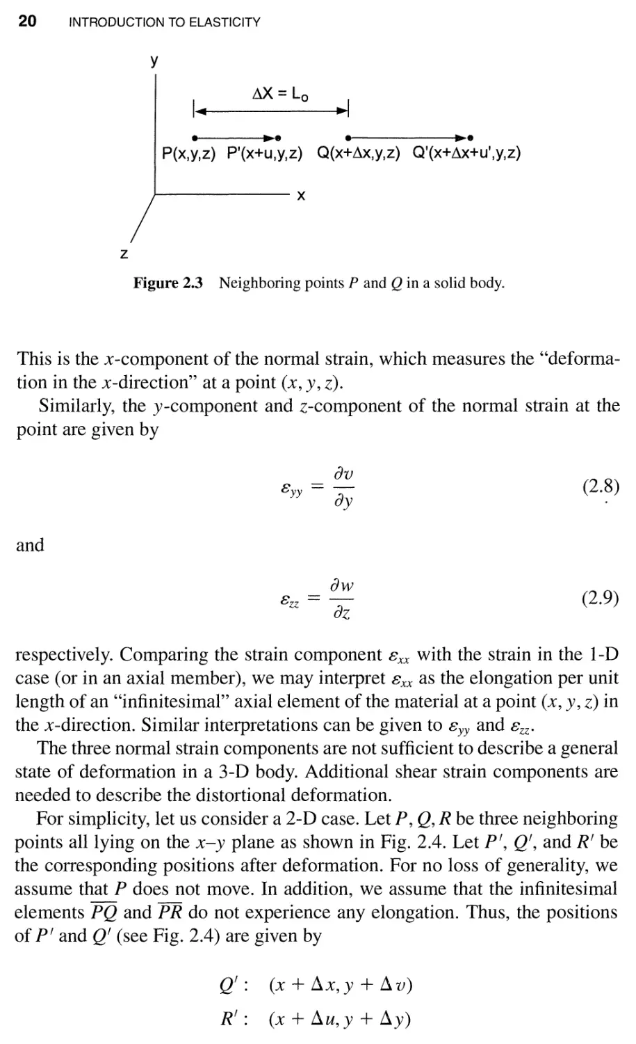
For simplicity, let us consider a 2-D case. Let P, Q, R be three neighboring
points all lying on the x-y plane as shown in Fig. 2.4. Let p f , Qf, and R f be
the corresponding positions after deformation. For no loss of generality, we
assume that P does not move. In addition, we assume that the infinitesimal
elements PQ and PR do not experience any elongation. Thus, the positions
of p f and Qf (see Fig. 2.4) are given by
Qf: (x + Llx,y + Llv)
R f : (x+Llu,y+Lly)
STRAIN 21
ilu
,... I
R(x,y+ily)- t R'(x+ilu,y+ily)
/
8 2 /
y
ily /
/
/
/ ---
Q'(x+ilx,y+ilv)
-e------: I Iw
ilx Q(x+ilx,y)
x
P(x,y),P'(x,y)
Figure 2.4 Rotations of material line elements in the x-y plane.
For Qf, the displacement increment Ll v is
Llv == vex + Llx,y) -
'-- j
displacement at Q
v(x,y)
'--v--/
displacement at P
(2.10)
Similarly for R f , the displacement increment Llu can be written as
Llu == u(x, y + Lly) - u(x, y)
(2.11 )
- -
The rotations e 1 and e 2 of elements PQ and PR are assumed to be small
and are given by
. Ll v av
e 1 == 11m - - -
8x-+0 Ll x ax
and
. Ll u au
e 2 == 11m - - -
8x-+0 Ll y ay
respectively. The 0tal change of angle between PQ and PR after deformation
is defined as the shear strain component in the x-y plane:
av au
'V == 'V = e 1 + e 2 == - + -
IXY IYX ax ay
(2.12)
Similar shear strain components in the y-z plane and x-z plane are defined
as
aw av
)'zy = )'yz = ay + az
(2.13)
22 INTRODUCTION TO ELASTICITY
aw au
'Yzx = 'Yxz = ax + az
(2.14 )
Thus, a general state of deformation at a point in a solid is described by
three normal strain components Bxx, Byy, Bzz and three shear strain components
)lxy, )lyZ' )lxz.
Rigid Body Motion If a body undergoes a displacement without inducing
strains in the body, then the motion is a rigid body motion. For instance, the
following displacements
u == uo == constant
v == va == constant
w == wo == constant
represent a rigid body translational motion and do not yield any strains.
Another rigid body motion is the rigid body rotation. The following dis-
placements represent a rigid body rotation in the x-y plane.
u == - ay
v==ax
(2.15)
w==O
It is easy to verify that no strains are associated with the above displacement
field.
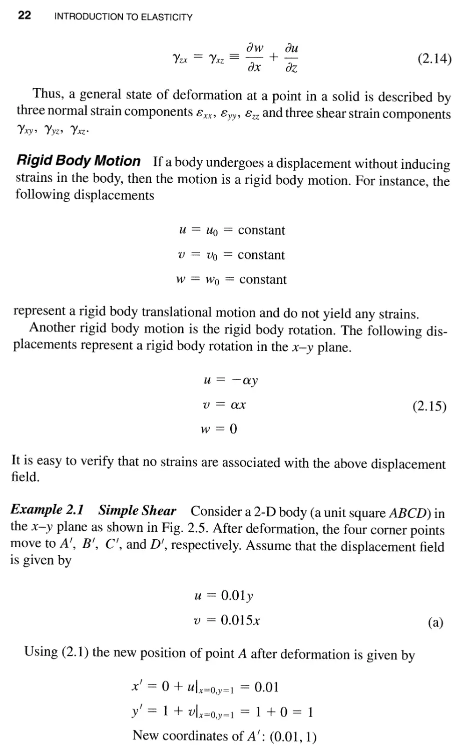
Example 2.1 Simple Shear Consider a 2-D body (a unit square ABCD) in
the x-y plane as shown in Fig. 2.5. After deformation, the four corner points
move to A f , B f , C f , and D f , respectively. Assume that the displacement field
is given by
u == O.Oly
v == 0.015x
(a)
Using (2.1) the new position of point A after deformation is given by
Xf == 0 + ul x =o,y=l == 0.01
yf == 1 + vl x =o,y=l == 1 + 0 == 1
New coordinates of A f : (0.01,1)
STRAIN 23
y
A
_ _ I . 81
A I --
--
---
8 I
I
I
I
I
I
I
I
I
I
I
I
I
I
I
" _------- D'
C,C 1 14
1
1
I D
x
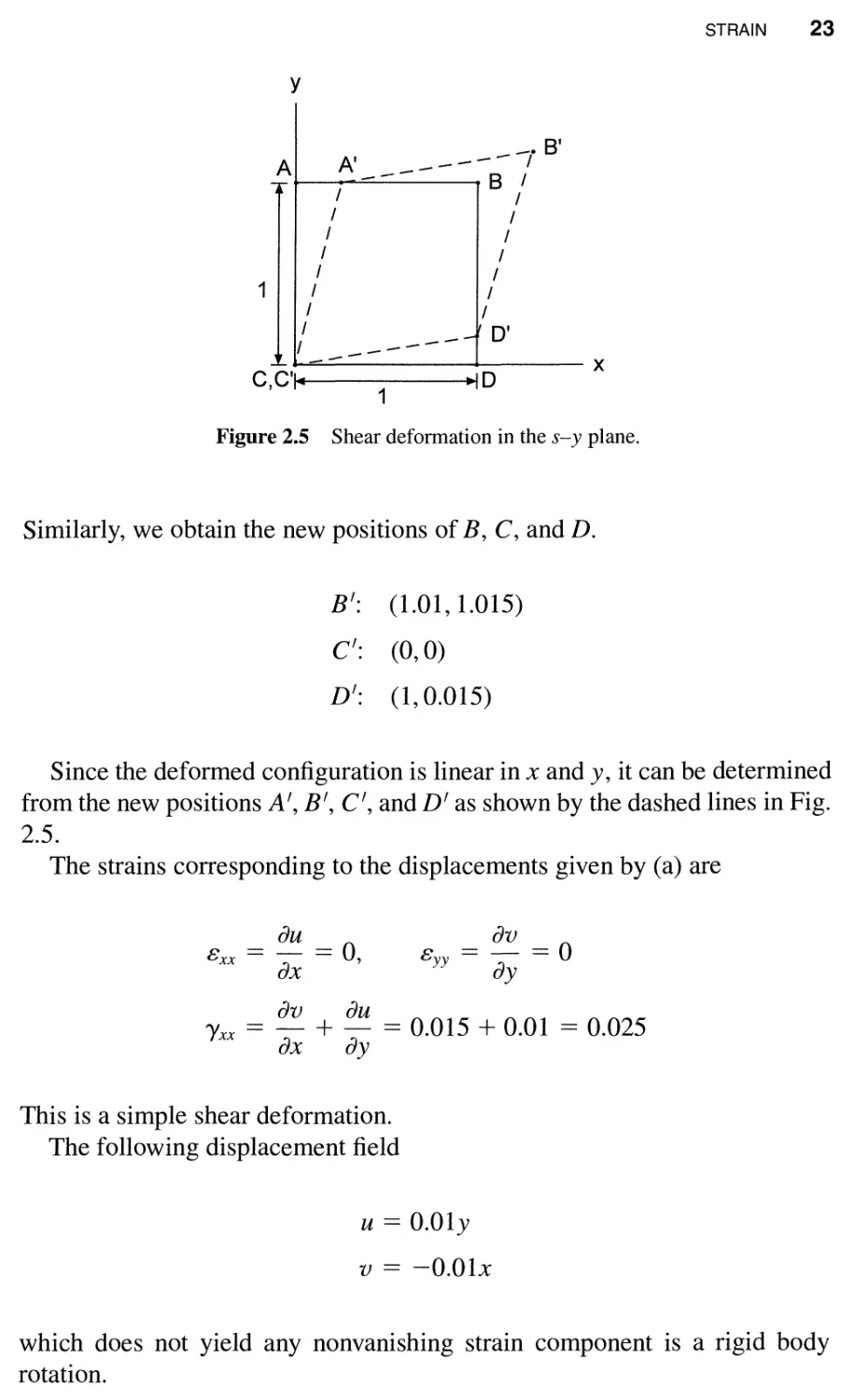
Figure 2.5 Shear deformation in the s- y plane.
Similarly, we obtain the new positions of B, C, and D.
B f : (1.01,1.015)
C f : (0, 0)
D f : (1,0.015)
Since the deformed configuration is linear in x and y, it can be determined
from the new positions A f , B f , C f , and D f as shown by the dashed lines in Fig.
2.5.
The strains corresponding to the displacements given by (a) are
au av
B ==-==0 B ==-==0
xx ax ' YY ay
av au
)lxx == - + - == 0.015 + 0.01 == 0.025
ax ay
This is a simple shear deformation.
The following displacement field
u == O.Oly
v == -O.Olx
which does not yield any nonvanishing strain component is a rigid body
rotati on.
24 INTRODUCTION TO ELASTICITY
2.3 STRESS
For an axial member, the force is always parallel to the member, and the stress
is defined as
p
u==-
A
(2.16)
where A is the cross-sectional area. If A == 1 unit area, then u == P.
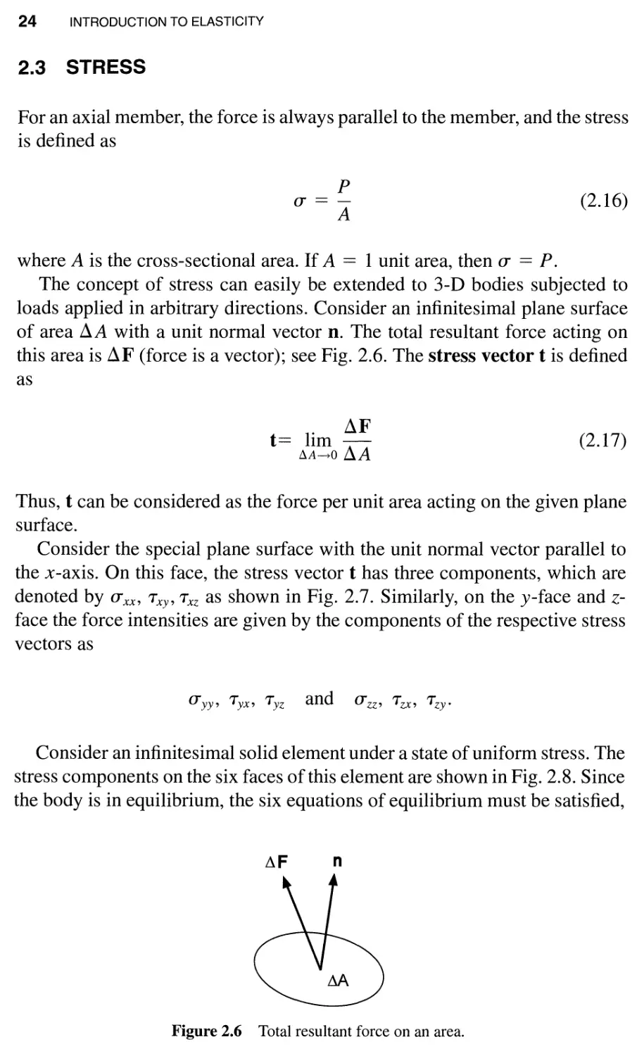
The concept of stress can easily be extended to 3-D bodies subjected to
loads applied in arbitrary directions. Consider an infinitesimal plane surface
of area A with a unit normal vector ll. The total resultant force acting on
this area is F (force is a vector); see Fig. 2.6. The stress vector t is defined
as
1 . F
t== 1m-
A-tO A
(2.17)
Thus, t can be considered as the force per unit area acting on the given plane
surface.
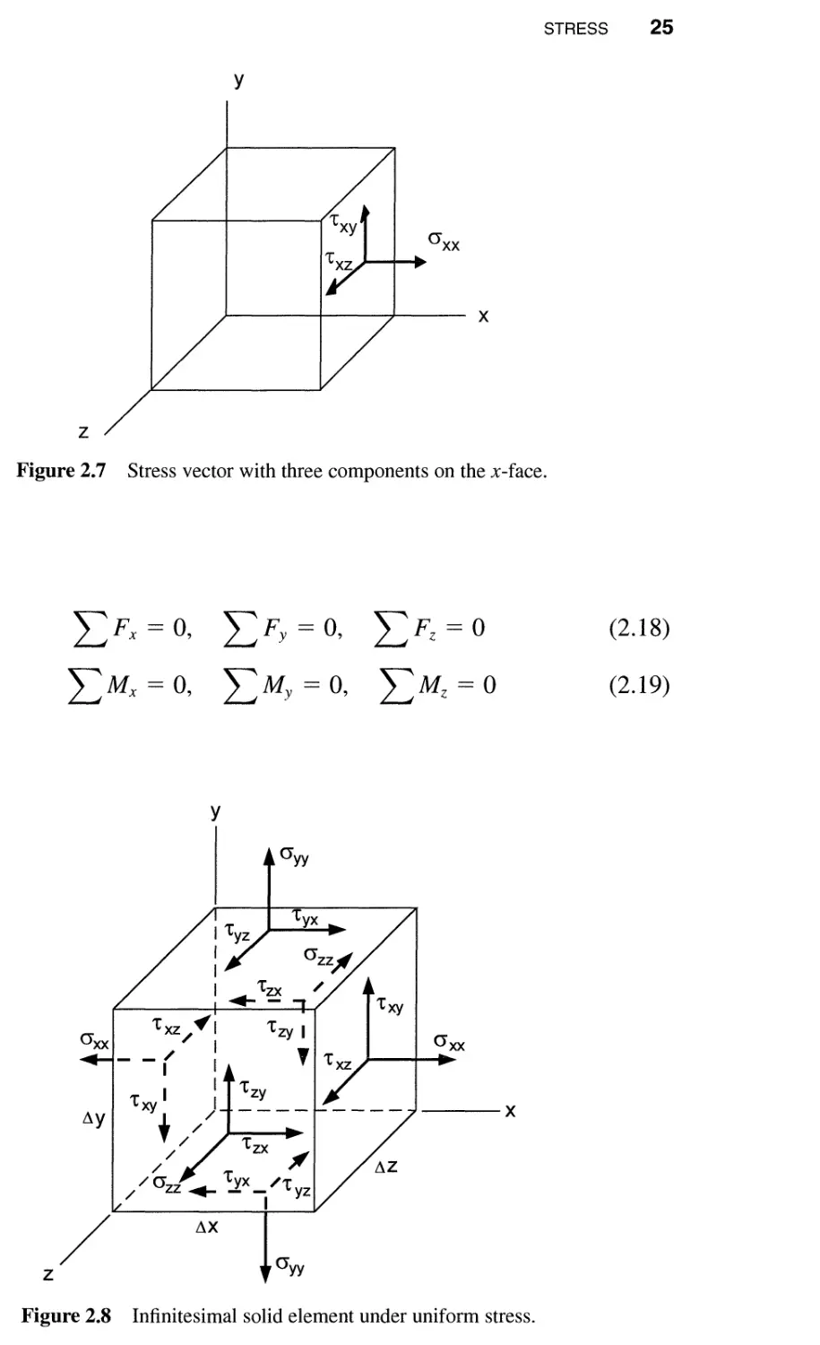
Consider the special plane surface with the unit normal vector parallel to
the x-axis. On this face, the stress vector t has three components, which are
denoted by U xx , Txy, Txz as shown in Fig. 2.7. Similarly, on the y-face and z-
face the force intensities are given by the components of the respective stress
vectors as
u yy, Tyx, TyZ and U ZZ ' Tzx, Tzy.
Consider an infinitesimal solid element under a state of uniform stress. The
stress components on the six faces of this element are shown in Fig. 2.8. Since
the body is in equilibrium, the six equations of equilibrium must be satisfied,
F n
Figure 2.6 Total resultant force on an area.
STRESS 25
y
a xx
x
z
Figure 2.7 Stress vector with three components on the x-face.
L Fx = 0,
L Mx = 0,
L Fy = 0,
L My = 0,
L Fz = 0
L M z = 0
(2.18)
(2.19)
y
fly
xz I
/ I
- ( I
I
I I
XV + //
/ zx
/
/
/ (J ZZ ....oIIIII...- yx /
/ .........- - yz
I
xy
a xx
a xx
x
/
flX
z
a yy
Figure 2.8 Infinitesimal solid element under uniform stress.
26 INTRODUCTION TO ELASTICITY
The force equations (2.18) are obviously satisfied automatically. To satisfy
(2.19), the following relations among the shear stress components are neces-
sary.
Txy == Tyx,
Tyz == Tzy,
T xz == Tzx
(2.20)
Thus, only six stress components are independent, including three normal
stress components u xx , U yy , U zz and three shear stress components, say, Tyz,
Txz, Txy.
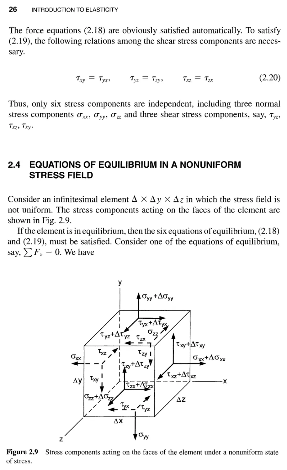
2.4 EQUATIONS OF EQUILIBRIUM IN A NONUNIFORM
STRESS FIELD
Consider an infinitesimal element d X dy X dz in which the stress field is
not uniform. The stress components acting on the faces of the element are
shown in Fig. 2.9.
If the element is in equilibrium, then the six equations of equilibrium, (2.18)
and (2.19), must be satisfied. Consider one of the equations of equilibrium,
say, I: Fx == O. We have
y
I
I 't yx + L1 't yx
a /.,
't yz+L1 yz 't zz
I zx /
-
'txz / I 't zy I
a xx
- - ( : 't Zy +L1't zy '
I I
l1y 'txy + ,,/
azz+fa ,
/ 't yx /'t
/ ... - I yz
a xx +L1a xx
x
/
x
z
a yy
Figure 2.9 Stress components acting on the faces of the element under a nonuniform state
of stress.
PRINCIPAL STRESSES 27
(u xx + duxx)dydz - (uxx)dydz
+ (Tyx + d Tyx)dxdZ - (Tyx)dxdZ
+ (T zx + d Tzx)dxdy - (Tzx)dxdy
==0
Dividing the above equation with dxdydz, we obtain
do-xx + dTyx + dT zx = 0
dx dy dz
Taking the limit dx, dy, dz 0, the above equilibrium equation becomes
au xx aT yx aT zx
-+-+-==0
ax ay az
(2.21 )
Similarly, equations L: Fy == 0 and L: Fz == 0 lead to
aT xy au yy aT zy _
-+-+--0
ax ay az
(2.22)
and
aT xz aT yz au zz
-+-+-==0
ax ay az
(2.23)
respectively.
It can easily be verified that the moment equations L: Mx
L: M z == 0 lead to
L:My
Txy == Tyx, Tyz == TZy, T xz == Tzx
(2.24)
which are identical to the relation given by (2.20).
Equations (2.21)-(2.24) are the equilibrium equations of a point in a body.
If a body is in equilibrium, the stress field must satisfy these equations
everywhere in the body.
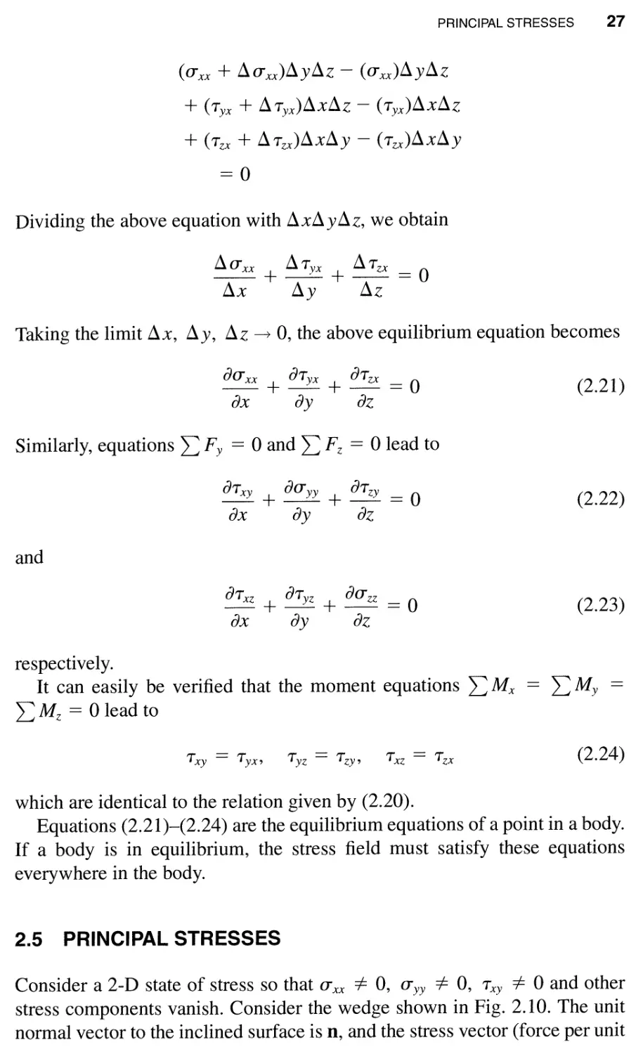
2.5 PRINCIPAL STRESSES
Consider a 2-D state of stress so that U xx *- 0, U yy *- 0, Txy *- 0 and other
stress components vanish. Consider the wedge shown in Fig. 2.10. The unit
normal vector to the inclined surface is ll, and the stress vector (force per unit
28 INTRODUCTION TO ELASTICITY
y
cr xx .---1
xy
I/nll = 1
x
't yx
a yy
Figure 2.10 2-D state of stress in a wedge element.
area) acting on this surface is t. From the equilibrium equations L Fx == 0
and L Fy == 0 for the wedge, we obtain
t x l1s == u xx l1y + T yx l1X
(2.25)
t y l1s == T xy l1y + U yy l1x
By noting
l1y
- == cos e == n
I1s x
I1x .
- == SIn e == n
I1s y
(2.26)
(2.25) can be expressed in the form
t x == uxxn x + Tyxny
(2.27)
t y == Txynx + u yyny
Equations (2.27) can be expressed in matrix form as
[ :; ;:] { : } {: }
(2.28)
where the relation Tyx == Txy has been invoked.
PRINCIPAL STRESSES 29
Using the same method, one can easily derive the equations for the 3-D
case with the result
[ u xx Txy
Txy U yy
T xz T yz
3;]{::} { }
(2.29)
Symbolically, (2.29) can be written as
[u]{n} == {t}
(2.30)
Equation (2.30) indicates that the stress matrix [u] can be viewed as a
transformation matrix that transforms the unit normal vector {n} into the stress
vector {t}, which acts on the surface with the unit normal {n}.
If we are interested in finding surfaces for which t is parallel to ll, i.e.,
{t} == u{n}
(2.31 )
where u is a scalar, then (2.29) yields a typical eigenvalue problem:
[ u ]{n} == {t} == u{n} (2.32)
or
([ u] - u [ I ]){ n} == 0 (2.33)
where [I] is the identity matrix. In order for (2.33) to have a nontrivial solution
for {n}, we require
I[ u] - u[I]1 == 0
or
u xx - U Txy Txz
Txy U yy - U TyZ ==0
Txz Tyz U zz - U
(2.34)
Expanding the determinantal equation (2.34) yields a cubic equation in u.
Since [u] is real and symmetric, there are three real roots, say U1, U2, U3 (see
any book on linear algebra or matrix theory for the proof). The corresponding
eigenvectors, {n(l)}, {n(2)}, {n(3)}, can be shown to be mutually orthogonal.
30 INTRODUCTION TO ELASTICITY
These three directions are called principal directions of stress, and U1, U2,
and U3 are the corresponding principal stresses.
On the surfaces perpendicular to these directions, we have
{t(i)} == Ui{ n(i)},
i == 1, 2, 3
(2.35)
This says that on the surface with the unit normal {n(i)}, the stress vector is
also normal to that surface, and its magnitude is Ui. In other words, there are
no shearing stresses on these surfaces.
Without loss of generality, we assume U1 ::> U2 ::> U3. Then it can be shown
that U1 and U3 are the maximum and minimum normal stresses, respectively,
on all surfaces at a point. The proof is given as follows.
On an arbitrary surface with unit normal vector {n}, let the stress vector
be {t}. The normal component (projection) of {t} on {n} is given by
Un == t . n == {t}T{n}
== ([ U ]{n})T{n}
== {n}T[ U ]T{n} == {n}T[ U ]{n}
(2.36)
where superscript T indicates the transposed matrix.
Choose a coordinate system so that X-, y-, and z-axes are parallel to the
principal directions of stress, respectively. Then [ (J" ] has a simple form as
[ U1
[a] =
2 :3]
(2.37)
Substituting (2.37) into (2.36), we obtain
_ 2 + 2 + 2
Un - U1 n x U2 n y U3 n z
(2.38)
If U1 ::> U2 ::> U3, then we have
22222 2
U1 n x + U1 ny + U1 n z ::> Un ::> U3 n x + U3 n y + U3 n z
Since n; + n; + n; == 1 (n is a unit vector), it is obvious that
U1 ::> Un ::> U3
(2.39)
PRINCIPAL STRESSES 31
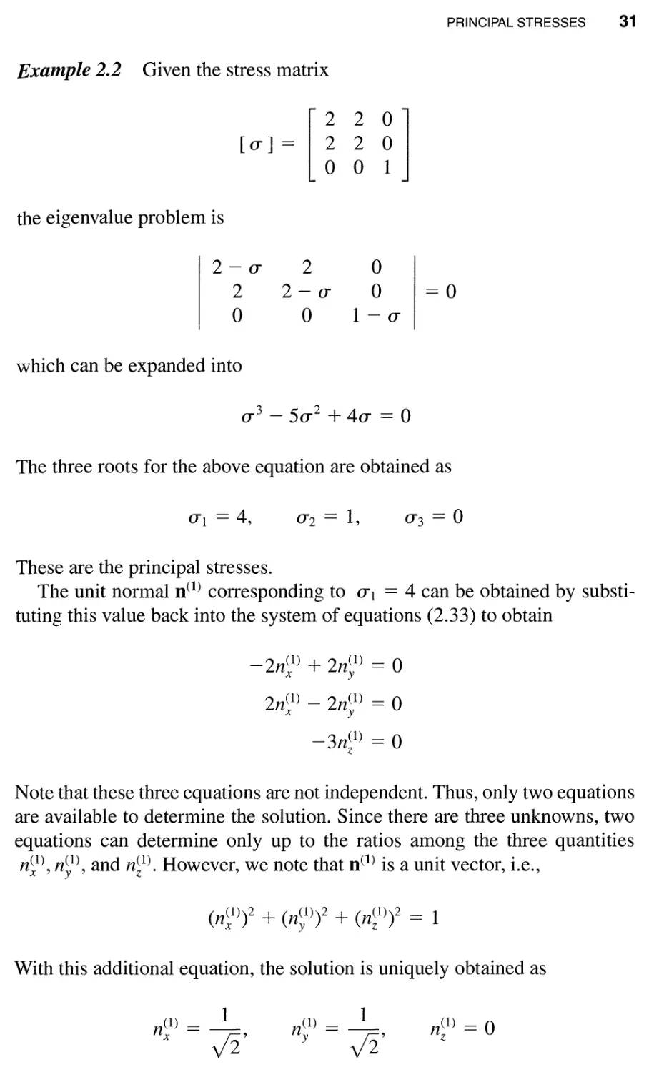
Example 2.2 Given the stress matrix
[a]= [ ]
the eigenvalue problem is
2-u
2
o
2
2-u
o
o
o
l-u
==0
which can be expanded into
u 3 - 5u 2 + 4u == 0
The three roots for the above equation are obtained as
U1 == 4,
U2 == 1,
U3 == 0
These are the principal stresses.
The unit normal n(l) corresponding to U1 == 4 can be obtained by substi-
tuting this value back into the system of equations (2.33) to obtain
- 2n(1) + 2n(1) == 0
x y
2n(1) - 2n(1) == 0
x y
- 3n(1) == 0
z
Note that these three equations are not independent. Thus, only two equations
are available to determine the solution. Since there are three unknowns, two
equations can determine only up to the ratios among the three quantities
n 1) , n 1), and n 1). However, we note that n(l) is a unit vector, i.e.,
(n 1))2 + (n 1))2 + (n 1))2 == 1
With this additional equation, the solution is uniquely obtained as
1
n(1) == -
x J2'
1
n(1) == -
Y J2'
n(1) == 0
z
32 INTRODUCTION TO ELASTICITY
Following similar rnanipulations, the unit vectors 0(2) and 0(3) correspond-
ing to U2 and U3, respectively, can be determined. We have
n(2) == 0 n(2) == 0 n(2) == 1
x , y , z
and
1 1 nO) == 0
n(3) == _ n(3) == -_
x J2' Y J2' z
It is easy to verify that these three eigenvectors are mutually orthogonal.
2.5.1 Shear Stress
The stress vector t can be decomposed into a normal vector UnO and a
tangential vector T that is lying on the surface with the unit normal 0, i.e.,
t == UnO + T (2.40 )
Thus,
T== t - UnO (2.41)
Denoting the magnitude of the shear stress vector by T, we have
T 2 == IItll 2 - u == (t; + t + t;) - u
(2.42)
Let us choose the coordinate system (x, y, z) to be parallel to the principal
directions with corresponding principal stresses UI, U2, and U3, respectively.
With respect to this coordinate system, the stress matrix [u] assumes the
diagonal form as in (2.37). From (2.29) we obtain
t x == uln x
t y == U2 n y
(2.43)
t z == U3 n z
Using (2.43), the magnitude of the stress vector can be written as
IItll 2 == t; + t + t;
== (uln x )2 + (U2ny)2 + (U3 n z)2
(2.44)
PRINCIPAL STRESSES 33
Substituting (2.44) and (2.38) into (2.42), we obtain
i2 == (0"1n x )2 + (0"2ny)2 + (0"3n Z )2 - (O"ln; + 0"2n + 0"3 n ;)2
== n 2 ( 1 - n 2 ) 0"2 + n 2 ( 1 - n 2 ) 0"2 + n 2 ( 1 - n 2 ) 0"2
x xl y y 2 z z 3
2 22 2 2 2 2 2 2
- 0"10"2 n x n y - 0"20"3 n y n z - 0"10"3 n x n z
(2.45)
Equation (2.45) can be further simplified by using the relation 1 - n;
n; + n;. We obtain
T 2 == n 2 n 2 ( 0" - 0" ) 2 + n 2 n 2 ( 0" - 0" ) 2
xy 1 2 yz 2 3
+ n 2 n 2 ( 0" - 0" ) 2
z x 3 1
(2.46)
Consider all surfaces that contain the y-axis, namely surfaces with unit
normal vector perpendicular to the y-axis. For any of these surfaces, we have
n x =1= 0,
ny == 0,
n z =1= 0
(2.47)
The magnitude of the shear stress is
i2 == n 2 n 2 ( 0" - 0" ) 2
z x 3 1
== (1 - n;)n;( 0"3 - 0"1)2
(2.48)
In deriving (2.48), the equation n; + n; == 1 has been used.
The extremum of I TI occurs at
a( T2)
== 0 == (2n x - 4n )(0"3 - 0"1)2
an x
(2.49)
This yields the solutions
n x == 0
1
and n x = + .J2
(2.50)
It can easily be shown that n x == 0 leads to the minimum value of T 2 and
n x == + 1/-)2 yields the maximum shear stress.
Since ny == 0, and n; + n; == 1, the solution n x == + 1/ -)2 gIves
n z == + 1/ -)2. These represent two surfaces making, respectively, +450
and -45 0 with respect to the x-axis.
34 INTRODUCTION TO ELASTICITY
Substituting n x == + 1/ J2 into (2.48), the maximum shear stress is ob
tained as
2 _ 1 ( ) 2
T max - 4: 0"3 - 0"1
or I T max I == i I 0" 3 - 0" Ii
(2.51 )
Similar considerations of surfaces containing the x-axis and the z-axis,
respectivel y, yield
I T max I == i I 0"2 - 0" 31
I T max I == i I 0" 1 - 0"21
(2.52)
(2.53)
Among these three shear stresses given by (2.51)-(2.53), the one given by
(2.51) is the true maximum shear stress if we assume, with no loss of gener-
ality,
0"1 > 0"2 > 0"3
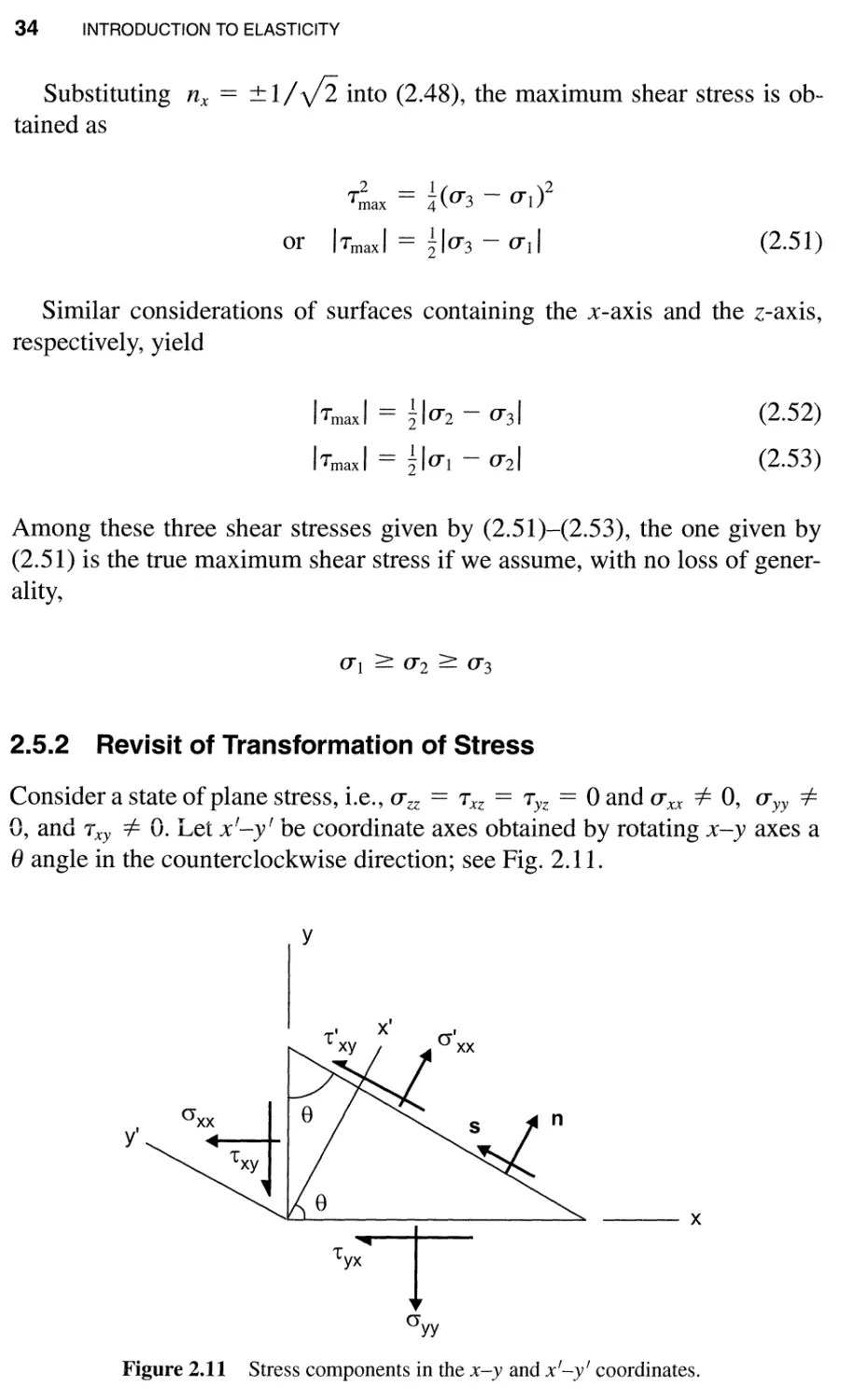
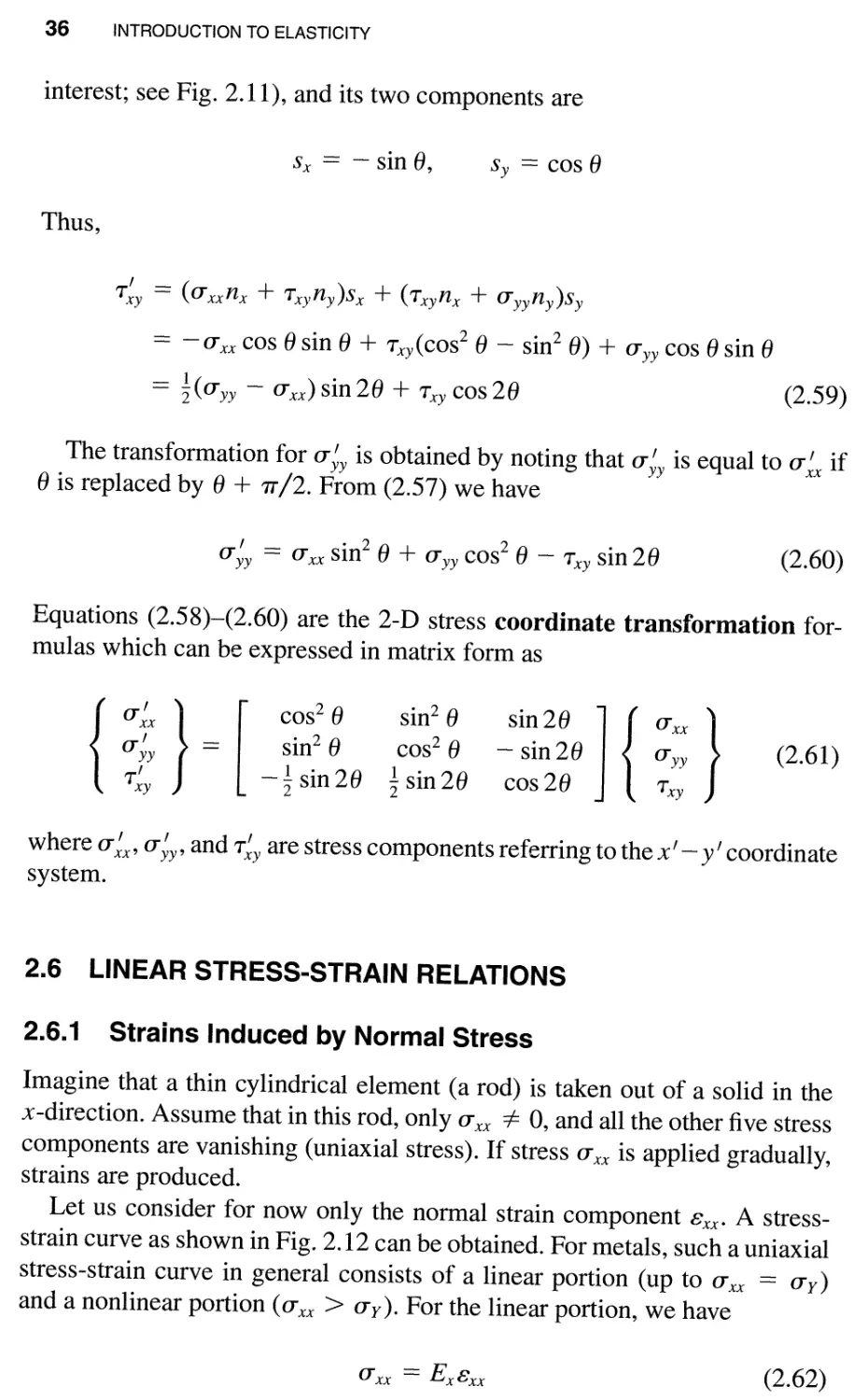
2.5.2 Revisit of Transformation of Stress
Consider a state of plane stress, i.e., O"zz == Txz == TyZ == 0 and O"xx =1= 0, O"yy =1=
0, and Txy =1= O. Let xf_yf be coordinate axes obtained by rotating x-y axes a
e angle in the counterclockwise direction; see Fig. 2.11.
y
yl
Xl
I
a xx
n
X
'ryx
a yy
Figure 2.11 Stress components in the x-y and x'-y' coordinates.
PRINCIPAL STRESSES 35
Consider the surface perpendicular to the xf-axis. On this surface, the stress
vector t is given by
{ ::} [ ::::] { :: }
(2.54)
where n == (n x , ny) is the unit vector parallel to the xf-axis.
Let u;x, U;y, and T;y be the stress components in reference to the xf_yf
coordinates. Noting that u;x == Un, we have
U;x == Un == t . n == txn x + tyny
(2.55)
Substituting the following relations
t x == uxxn x + Txyny
t y == Txynx + Uyyny
into (2.55) yields
f _ 2 + + + 2
U xx - uxxn x Txynxny Txynxny Uyyny
== uxxn; + 2nxnyTxy + Uyyn
(2.56)
Noting n x == cos e, and ny == sin e, we rewrite (2.56) in the form
f _ 2 l) . 2 l) . 2 l)
U xx - U xx cos u + U yy sIn u + Txy sIn u
(2.57)
Further use of
cos 2 e == (1 + cos 2e),
sin 2 e == (1 - cos 2e)
in (2.57) leads to
U;x == ( U xx + U yy) + ( U xx - U yy) cos 2 e + T xy sin 2 e
(2.58)
The shear stress component T y can be regarded as the tangential component
of the stress vector, i.e.,
T;y == t · s == txs x + tyS y
where s is the unit vector parallel to the yf-axis (or parallel to the surface of
36 INTRODUCTION TO ELASTICITY
interest; see Fig. 2.11), and its two components are
S x == - sin e,
S y == cos e
Thus,
rr.;y == (O"xxnx + Txyny)sx + (Txyn x + O"yyny)sy
== - 0" xx cos e sin e + Txy (cos 2 e - sin 2 e) + 0" yy cos e sin e
== (O"yy - O"xx) sin 2e + Txy cos 2e (2.59)
The transformation for a;y is obtained by noting that a;y is equal to a:X if
e is replaced by e + 7T /2. From (2.57) we have
f - . 2 l) + 2 l) . 2 l)
O"yy - O"xx sIn U O"yy cos U - Txy sIn u
(2.60 )
Equations (2.58)-(2.60) are the 2-D stress coordinate transformation for-
mulas which can be expressed in matrix form as
{ j;} [
cos 2 e
sin 2 e
- sin2e
sin 2 e
cos 2 e
sin 2e
sin 2e ] { O"xx }
- sin 2e O"yy
cos 2e Txy
(2.61 )
where O";x' O";y, and T;y are stress components referring to the x f - Y f coordinate
system.
2.6 LINEAR STRESS-STRAIN RELATIONS
2.6.1 Strains Induced by Normal Stress
Imagine that a thin cylindrical element (a rod) is taken out of a solid in the
x-direction. Assume that in this rod, only O"xx =1= 0, and all the other five stress
components are vanishing (uniaxial stress). If stress O"xx is applied gradually,
strains are produced.
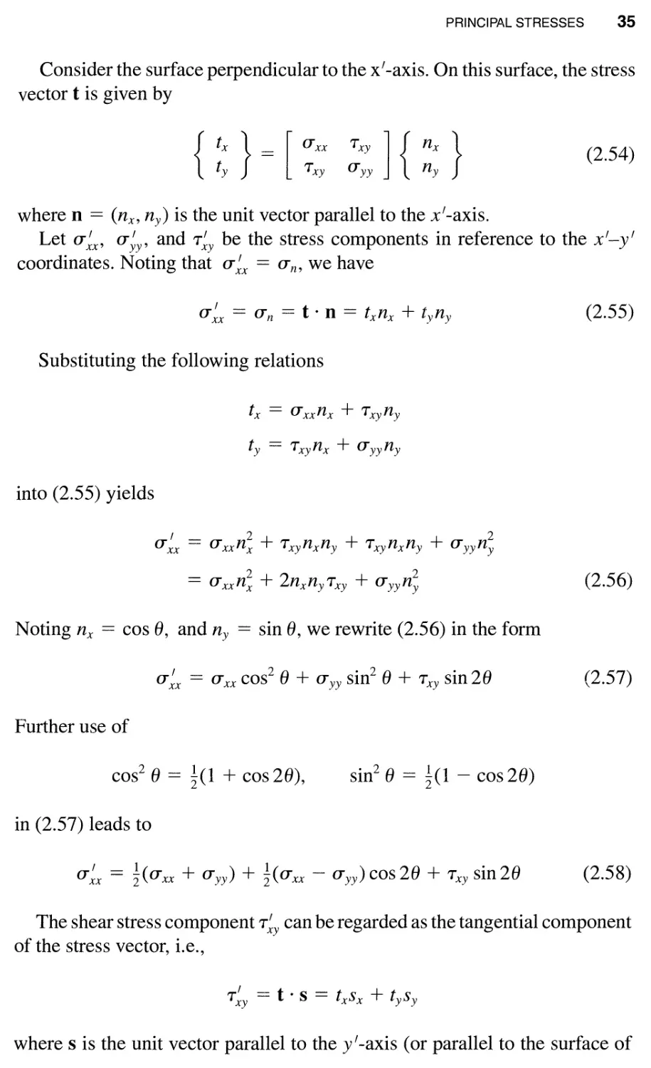
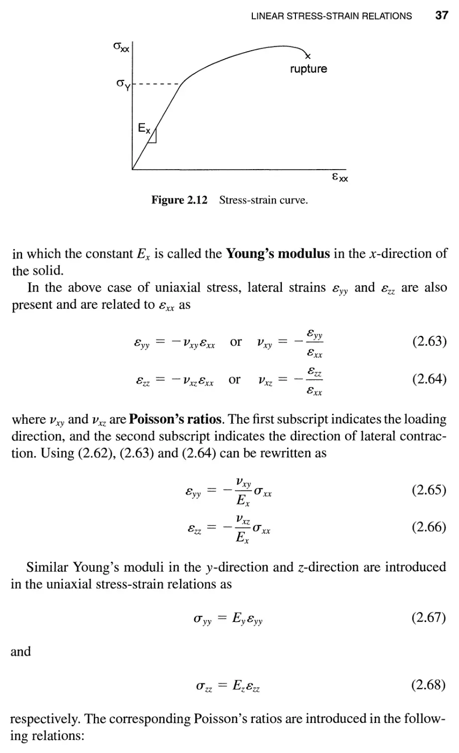
Let us consider for now only the normal strain component 8xx. A stress-
strain curve as shown in Fig. 2.12 can be obtained. For metals, such a uniaxial
stress-strain curve in general consists of a linear portion (up to O"xx == O"y)
and a nonlinear portion (O"xx > O"y). For the linear portion, we have
0" xx == Ex8xx
(2.62)
LINEAR STRESS-STRAIN RELATIONS 37
a xx
a y
ru ptu re
Exx
Figure 2.12 Stress-strain curve.
in which the constant Ex is called the Young's modulus in the x-direction of
the solid.
In the above case of uniaxial stress, lateral strains Byy and Bzz are also
present and are related to Bxx as
Byy == - vxyBxx or v xy == Byy (2.63)
Bxx
Bzz (2.64 )
Bzz == - VxzBxx or V xz == --
Bxx
where v xy and V xz are Poisson's ratios. The first subscript indicates the loading
direction, and the second subscript indicates the direction of lateral contrac-
tion. Using (2.62), (2.63) and (2.64) can be rewritten as
_ v xy
Byy - - Ex O"xx
V xz
Bzz == - -O"xx
Ex
(2.65)
(2.66)
Similar Young's moduli in the y-direction and z-direction are introduced
in the uniaxial stress-strain relations as
O"yy == EyByy (2.67)
and
O"zz == EzBzz (2.68)
respectively. The corresponding Poisson's ratios are introduced in the follow-
ing relations:
38 INTRODUCTION TO ELASTICITY
Bxx == - VyxByy == V yx
- -O"yy
Ey (2.69
v yz
Bzz == - VyzByy == - -O"yy
Ey
and
V zx
Bxx == - VzxBzz == --O"zz
Ez (2.70)
v zy
Byy == - v zy Bzz == - -O"zz
Ez
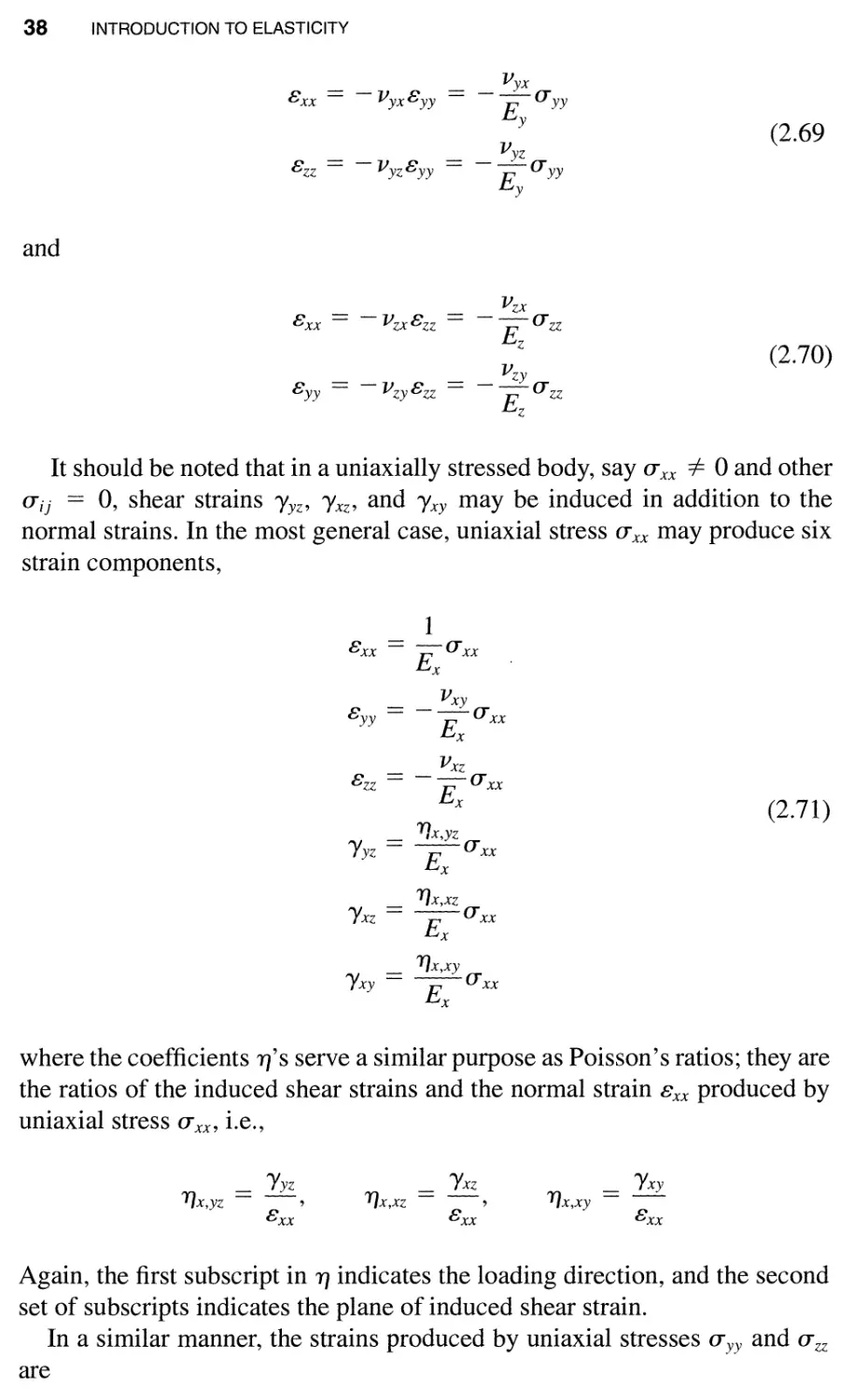
It should be noted that in a uniaxially stressed body, say O"xx =1= 0 and other
O"ij == 0, shear strains )lyz, )lxz, and )lxy may be induced in addition to the
normal strains. In the most general case, uniaxial stress O"xx may produce six
strain components,
1
Bxx == -O"xx
Ex
_ v xy
B yy - --0"
Ex xx
V xz
Bzz == - E 0" xx
x
_ Y]x,YZ
)lyz - TO"xx
x
(2.71)
'lx,xz
)lxz == Ex 0" xx
_ 'lx,xy
)lxy - TO"xx
x
where the coefficients 'l's serve a similar purpose as Poisson's ratios; they are
the ratios of the induced shear strains and the normal strain Bxx produced by
uniaxial stress 0" xx, i.e.,
)lyZ
'lx,YZ == ,
Bxx
'lx,xz ==
Bxx
)lxz
)lxy
'lx,xy ==
Bxx
Again, the first subscript in 'l indicates the loading direction, and the second
set of subscripts indicates the plane of induced shear strain.
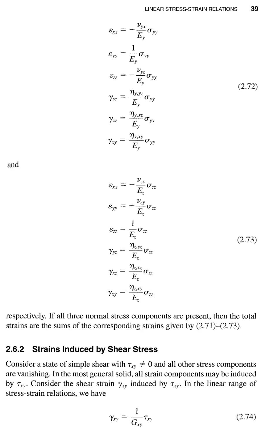
In a similar manner, the strains produced by uniaxial stresses 0" yy and 0" zz
are
LINEAR STRESS-STRAIN RELATIONS 39
_ V yx
8xx - - E O"yy
y
1
Byy == E 0" yy
y
_ v yz
Bzz - - E O"yy
y
_ YJy,yz
)lyZ - TO" yy
y
YJ v ,xz
)lxz == EO"YY
y
_ YJy,xy
)lxy - TO"YY
y
(2.72)
and
V zx
Bxx == --O"zz
Ez
_ V Zy
Byy - - E O"zz
z
1
Bzz == - O"zz
Ez
_ YJz,yz
)lyz - TO"zz
z
YJz,xz
)lxz == T O"zz
z
(2.73 )
_ YJz,xy
)lxy - TO"zz
z
respectively. If all three normal stress components are present, then the total
strains are the sums of the corresponding strains given by (2.71)-(2.73).
2.6.2 Strains Induced by Shear Stress
Consider a state of simple shear with Txy =1= 0 and all other stress components
are vanishing. In the most general solid, all strain components may be induced
by Txy. Consider the shear strain )lxy induced by Txy. In the linear range of
stress-strain relations, we have
1
)lxy == - G - Txy
xy
(2.74)
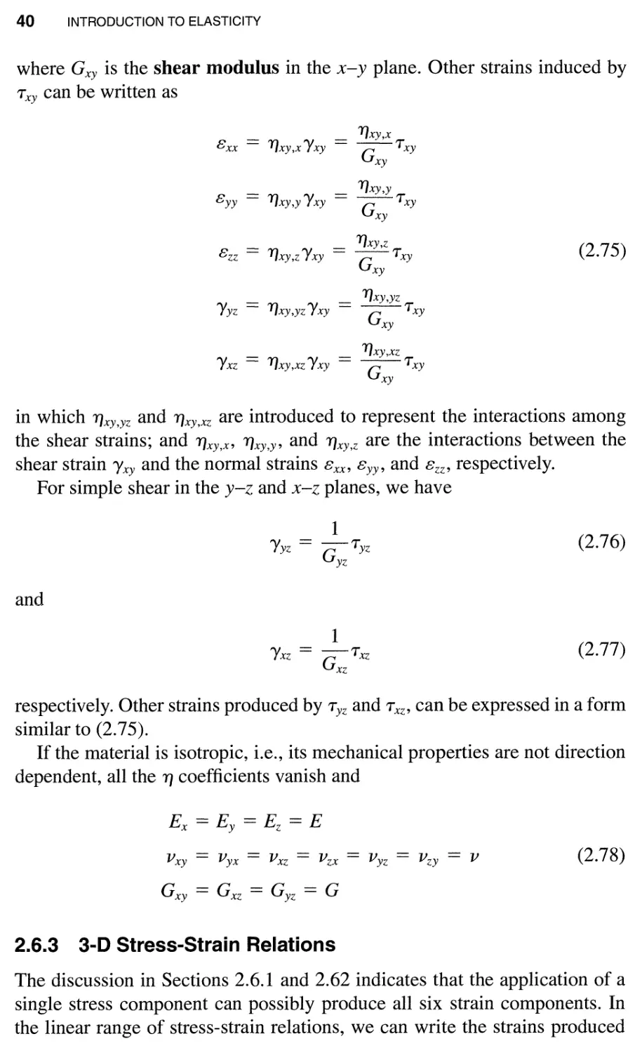
40 INTRODUCTION TO ELASTICITY
where G xy is the shear modulus in the x-y plane. Other strains induced by
Txy can be written as
_ _ 'lxy,x
Bxx - 'lxy,x)lxy - - G Txy
xy
_ _ 'lxy,y
Byy - 'lxy,y)lxy - - G Txy
xy
_ _ 'lxy,Z
Bzz - 'lxy,z)lxy - - G Txy
xy
(2.75)
'lxy,yz
)lyz == 'lxy,yz )lxy == G Txy
xy
'l xy ,xz
)lxz == 'lxy,xz )lxy == G Txy
xy
in which 'lxy,yz and 'lxy,xz are introduced to represent the interactions among
the shear strains; and 'lxy,x, 'lxy,y, and 'lxy,z are the interactions between the
shear strain )lxy and the normal strains Bxx, Byy, and Bzz, respectively.
For simple shear in the y-z and x-z planes, we have
1
)lyZ == GTyZ
yz
(2.76)
and
1
)lxz == GTxz
xz
(2.77)
respectively. Other strains produced by Tyz and Txz, can be expressed in a form
similar to (2.75).
If the material is isotropic, i.e., its mechanical properties are not direction
dependent, all the 'l coefficients vanish and
E==E==E==E
x y z
v xy == v yx == v xz == v zx == v yZ == v Zy == v
(2.78)
G xy == G xz == G yZ == G
2.6.3 3-D Stress-Strain Relations
The discussion in Sections 2.6.1 and 2.62 indicates that the application of a
single stress component can possibly produce all six strain components. In
the linear range of stress-strain relations, we can write the strains produced
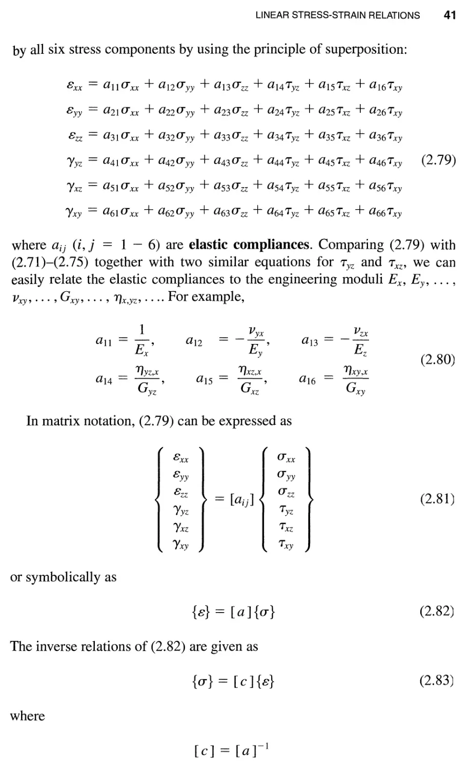
LINEAR STRESS-STRAIN RELATIONS 41
by all six stress components by using the principle of superposition:
B xx == all 0" xx + a 12 0" yy + a 13 0" zz + a 14 T yz + a 15 T xz + a 16 T xy
Byy == a210" xx + a22 0" yy + a23 0" zz + a24 TyZ + a25 T xz + a26 Txy
Bzz == a310"xx + a320"yy + a330"zz + a34 Tyz + a35 T xz + a36 T xy
)lyz == a410"xx + a420"yy + a430"zz + a44 T yz + a45 T xz + a46 T xy (2.79)
)lxz == as 1 O"xx + a520"yy + a530" zz + a54 Tyz + a55 T xz + a56 T xy
)lxy == a6lO" xx + a620" yy + a63 0" zz + a64 Tyz + a65 Txz + a66 Txy
where aij (i, j == 1 - 6) are elastic compliances. Comparing (2.79) with
(2.71)-(2.75) together with two similar equations for Tyz and Txz, we can
easily relate the elastic compliances to the engineering moduli Ex, Ey, . . . ,
v xy , . . . , G xy, . . . , YJx,yz, . . .. For example,
1 v yx V zx
all -- a12 al3 ==
E' Ey , Ez
x (2.80)
YJYZ,x YJxz,x YJxy,x
a14 == -, a15 == - a16
G yZ G xz , G xy
In matrix notation, (2.79) can be expressed as
Bxx
O"xx
Byy
Bzz
)lyz
)lxz
)lxy
== [ aij ]
O"yy
0" zz
Tyz
T xz
Txy
(2.81 )
or symbolically as
{B} == [a]{O"}
(2.82)
The inverse relations of (2.82) are given as
{O"} == [C]{B}
(2.83)
where
[C] == [a]-l
42 INTRODUCTION TO ELASTICITY
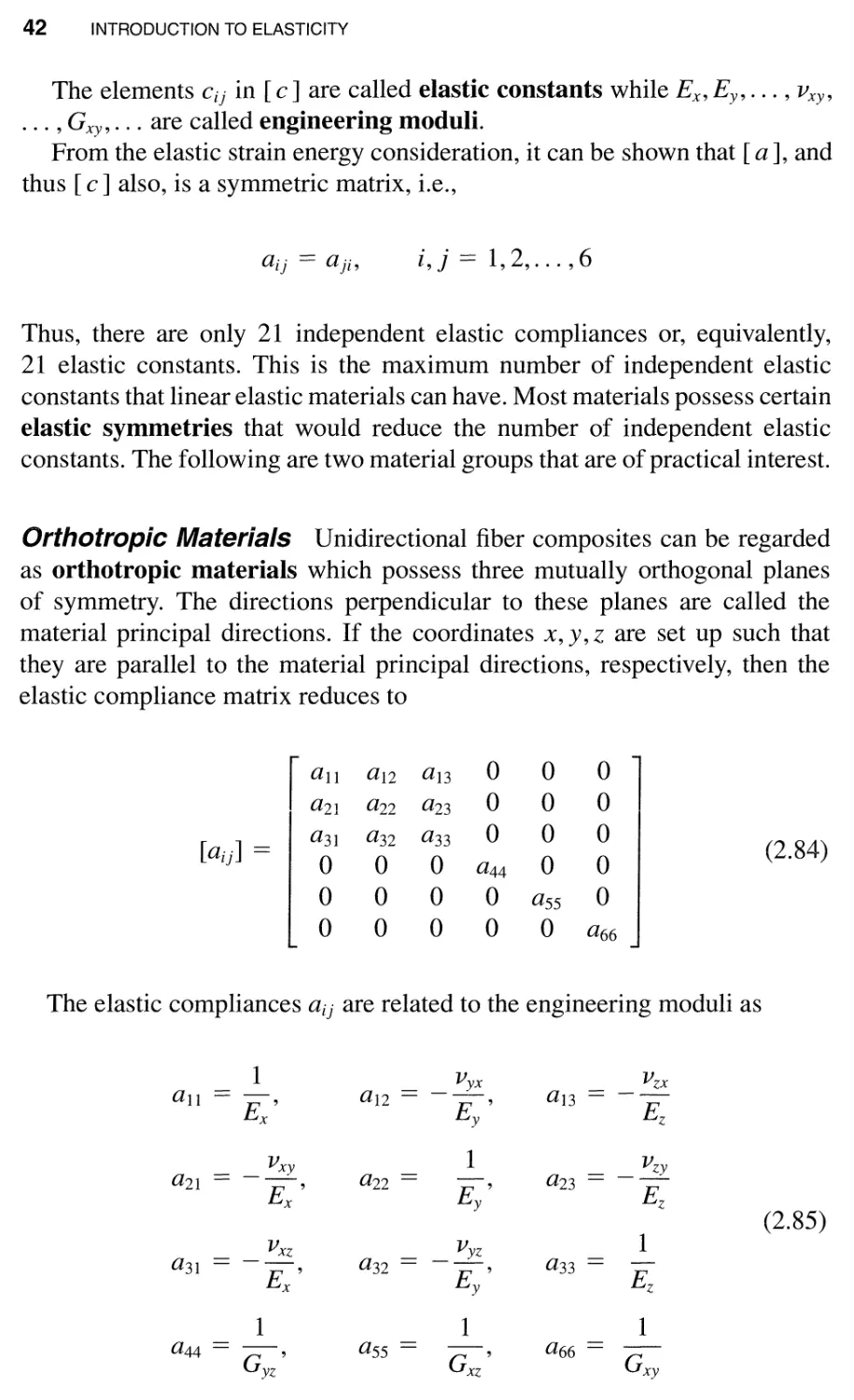
The elements cij in [c] are called elastic constants while Ex, Ey,. . . , v xy ,
. . . , G xy, . . . are called engineering moduli.
Prom the elastic strain energy consideration, it can be shown that [a], and
thus [c] also, is a symmetric matrix, i.e.,
a.. == a..
IJ JI'
l, ] == 1, 2, . . . , 6
Thus, there are only 21 independent elastic compliances or, equivalently,
21 elastic constants. This is the maximum number of independent elastic
constants that linear elastic materials can have. Most materials possess certain
elastic symmetries that would reduce the number of independent elastic
constants. The following are two material groups that are of practical interest.
Orthotropic Materials Unidirectional fiber composites can be regarded
as orthotropic materials which possess three mutually orthogonal planes
of symmetry. The directions perpendicular to these planes are called the
material principal directions. If the coordinates x, y, z are set up such that
they are parallel to the material principal directions, respectively, then the
elastic compliance matrix reduces to
r a]] a12 al3 0 0 0 l
a2l a22 a23 0 0 0
[aij] == a31 a32 a33 0 0 0 (2.84)
0 0 0 a44 0 0
0 0 0 0 ass 0
0 0 0 0 0 a66
The elastic compliances aij are related to the engineering moduli as
1 v yx V zx
all -- a12 == al3 ==
E' Ey , Ez
x
v xy 1 v zy
a2l Ex , a22 == E' a23 == Ez
y (2.85)
1
V xz v yz
a31 - a32 == a33 ==
E' Ey , Ez
x
1 1 1
a44 == -, ass == G xz , a66 == G xy
G yZ
Since au == a ji, we have
_ Ey
v yx - - v xy ,
Ex
LINEAR STRESS-STRAIN RELATIONS 43
Ez
v zy == - v yZ
Ey
Ez
V zx == E V xz ,
x
(2.86)
Thus, there are nine independent elastic constants for orthotropic elastic
materials.
Fiber-reinforced composites are regarded as orthotropic solids. It is cus-
tomary to denote the fiber direction as xl-axis, and the transverse directions
as X2 and X3. The elastic moduli are referenced to this particular coordinate
system and denoted by E 1 , E 2 , E 3 , V12, Vl3, V23, G 23 , G l3 , and G 12 .
The following are the in-plane engineering moduli for some polymeric
composites.
A54/3501-6 Carbon-epoxy (AS4 carbon fiber in 3501-6 epoxy):
E 1 == 140 GPa,
G 12 == 7.0 GPa,
Boron-epoxy:
E 1 == 205 GPa,
G 12 == 5.5 GPa,
52-Glass-epoxy:
E 1 == 43 GPa,
G 12 == 4.5 GPa,
E 2 == 10 GPa
V12 == 0.3
E 2 == 21 GPa
V12 == 0.17
E 2 == 9 GPa
V12 == 0.27
Note that the Young's modulus in the fiber direction (E 1 ) for AS4/3501-6
is 14 times the transverse Young's modulus (E 2 ).
Isotropic Materials The elastic properties of isotropic materials are in-
variant with respect to directions. Thus, isotropy is a special case of orthotropy.
By requiring the conditions given by (2.78), we obtain
1
all == a22 == a33 == -
E
v
a12 == a13 == a23 == --
E
(2.87)
1
a44 == a55 == a66 == -
G
44 INTRODUCTION TO ELASTICITY
The corresponding elastic constants cij can also be expressed in terms of
engineering moduli as
C11 == C22 == C33 == A + 2G
C12 == C13 == C23 == A
C44 == C55 == C66 == G
(2.88)
where A == vE/(1 + v)(1 - 2v).
It is evident that the stress-strain relations for isotropic materials can be
expressed in terms of the Young's modulus E, Poisson's ratio v, and shear
modulus G. Moreover, it can be shown that these three quantities are related
by
E == 2(1 + v)G
(2.89)
Thus, there are only two independent elastic constants for isotropic materials.
Aluminum alloys are usually considered isotropic materials. Typical values
of their elastic moduli are
E == 70 GPa,
v == 0.33
2.7 ELASTIC STRAIN ENERGY
An elastic body can store energy in the form of deformation. This strain
energy is completely released when loads are removed. Since the strain energy
is stored solely in the form of deformation, it can be expressed in terms of
strain components or stress components.
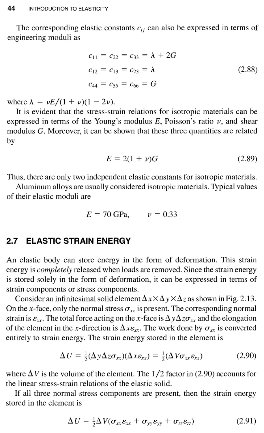
Consider an infinitesimal solid element dx X d y X dz as shown in Fig. 2.13.
On the x-face, only the normal stress O"xx is present. The corresponding normal
strain is Bxx. The total force acting on the x-face is dy dzO"xx and the elongation
of the element in the x-direction is dXB xx . The work done by O"xx is converted
entirely to strain energy. The strain energy stored in the element is
d U == 1(dydzO"xx)(dxB xx ) == 1(d VO"xxBxx)
(2.90)
where d V is the volume of the element. The 1/2 factor in (2.90) accounts for
the linear stress-strain relations of the elastic solid.
If all three normal stress components are present, then the strain energy
stored in the element is
d U == 1d V( O"xxBxx + O"yyByy + O"zzBzz)
(2.91 )
I
I
I
I
I
I
I
I
I
I
L__________
/
/
/
/
/
/
/
/
y
a xx
y
/
z
x
ELASTIC STRAIN ENERGY 45
a xx
x
Figure 2.13 Infinitesimal solid element subjected to normal stress (J" xx.
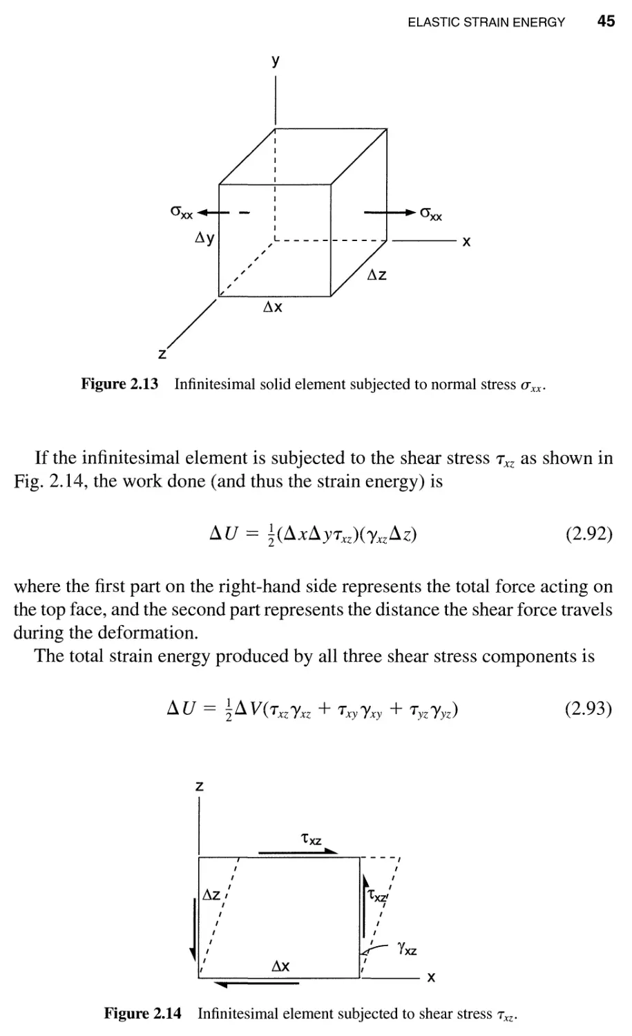
If the infinitesimal element is subjected to the shear stress T xz as shown in
Fig. 2.14, the work done (and thus the strain energy) is
d U == (dxdYTxz)( )lxzdz)
(2.92)
where the first part on the right-hand side represents the total force acting on
the top face, and the second part represents the distance the shear force travels
during the deformation.
The total strain energy produced by all three shear stress components is
d U == d V ( T xz )I xz + T xy )I xy + T yz )lyz)
z
,
,
j;>
......
(2.93)
'txz
.....
----,
,
rTf'
Yxz
,
,
x
Figure 2.14 Infinitesimal element subjected to shear stress Txz.
46 INTRODUCTION TO ELASTICITY
The total strain energy stored in d V due to normal and shear stresses is the
sum of (2.91) and (2.93). The strain energy density W is defined as
dU 1
W == == -( O"xxBxx + O"yyByy + O"zzBzz
L.lV 2
+ T xz )lxz + Txy)lxy + Tyz )lyz)
(2.94)
U sing the matrix representations of the stress-strain relations (2.82) and
(2.83), the strain energy density can be expressed in various forms as
W == 1{0"}T{B} == 1{B}T{0"}
== 1{B}T[ C ]{B}
== 1{ 0" }T[ a]{ O"}
(2.95)
Since W > 0, the above quadratic forms imply that [c] and [a] must
be positive definite. Consequently, all the diagonal terms cu(i == 1 - 6) and
aii(i == 1 - 6) must be positive. For orthotropic materials, this implies that all
the major engineering moduli Ex, Ey, Ez, G yZ ' G xz , and G xy cannot assume
negative values.
2.8 PLANE ELASTICITY
Many structures under certain types of loading may yield strain and stress
fields that are independent of, say, the z-direction and have
Bzz == )lyz == )lxz == 0
(2.96)
or
O"zz == T xz == Tyz == 0
(2.97)
over the entire structure. The state of deformation with (2.96) is called a state
of plane strain parallel to the x-y plane, while that with (2.97) is called a
state of plane stress parallel to the x-y plane.
From the strain-displacement relations, the conditions of (2.96) can be
described in terms of the displacement field as
u == u(x, y)
v == vex, y)
w==O
(2.98)
PLANE ELASTICITY 47
where u, v, and ware displacement components in the X-, y- and z- directions,
respectively.
To produce a state of plane strain parallel to the x-y plane, the structure
must be uniform in shape in the z-direction, and loading must be indepen-
dent of the z-axis. An example is a hollow cylinder subjected to uniform
internal pressure with both ends constrained to suppress its movement in the
z-direction.
The plane stress condition given by (2.97), in general, cannot be exactly
realized. It is often used to approximate the state of stress in a thin panel sub-
jected to only in-plane (x-y plane) loading. The corresponding displacement
field is given by
u == u(x, y)
v == vex, y)
(2.99)
w == BzzZ
where normal strain Bzz is independent of the z-axis.
2.8.1 Stress-Strain Relations for Plane Isotropic Solids
Plane strain and plane stress conditions lead to simplification in stress-strain
relations. Recall that the 3-D stress-strain relations for isotropic solids can be
expressed in the following forms:
{O"} == [c ]{B}
(2.100)
or
{B} == [a ]{O"}
(2.101)
where
E(1 - v)
C11 == C22 == C33 == A + 2G ==
(1 + v)(1 - 2v)
Ev
C12 == C21 == C13 == C31 == C23 == C32 == A ==
(1 + v)(1 - 2v)
C44 == C55 == C66 == G
other cij == 0
1
all == a22 == a33 == -
E
48 INTRODUCTION TO ELASTICITY
v
a12 == a21 == a13 == a31 == a23 == a32 == --
E
1
a44 == a55 == a66 == -
G
other au == 0
Plane Strain Using the plane strain conditions, (2.100) reduces to
E
O" xx == [( 1 - V ) B xx + VB yy]
(1 + v)(1 - 2v)
E
U yy = (1 + v)(1 _ 2v) [ve xx + (1 - v)e yy ]
vE
0" == [ B + B ]
zz (1 + v)(1 - 2v) xx yy
Ty7. == 0
T xz == 0
(2.102)
Txy == G)lxy
It is easy to see that
O"zz == v( 0" xx + 0" yy)
Thus, O"zz is a dependent quantity. The remaining nontrivial equations in
(2.102) are usually considered the stress-strain relations for a state of plane
strain. Inverting these equations, we obtain
1 + v
Bxx == E [(1 - v)O"xx - vO"yy]
1 + v
Byy == E [ - VO"xx + (1 - v)O"yy]
1
)lxy == G Txy
(2.103)
Plane Stress The reduced stress-strain relations for a state of plane stress
are readily derived from the 3-D relations given by (2.101). We have
1
B xx == E ( 0" xx - VO" yy )
PLANE ELASTICITY 49
1
Byy == -( - VO"xx + O"yy)
E
v
B zz == - - ( 0" xx + 0" yy)
E
)lyz == 0
)lxz == 0
1
)lxy == G Txy
(2.104)
Again, from (2.104) we note that
v
Bzz == - 1 (Bxx + Byy)
-v
(2.105)
is a dependent quantity. Inverting the first two and last equations in (2.104),
we obtain
E
O"xx == 1 _ v 2 (Bxx + VB yy )
E
O"yy == 1 _ v 2 (VB xx + Byy)
Txy == G)lxy
(2.106)
These relations are different from the corresponding plane strain relations
given by (2.102). However, the two sets of stress-strain relations can be put
in a single expression by introducing the following parameter defined by
for plane strain:
K == 3 - 4v
3-v
K==
1 + v
for plane stress:
In terms of parameter K, the stress-strain relations for both plane strain and
plane stress can be expressed in the form:
[ 3 - K ]
O"xx == 2G Bxx + 2K _ 2 (Bxx + Byy)
[ 3 - K ]
O"yy == 2G Byy + 2K _ 2 (Bxx + Byy)
(2.107)
Txy == G)lxy
50 INTRODUCTION TO ELASTICITY
or
1 [ 3-K ]
B xx == 2 G 0" xx - 4 ( 0" xx + 0" yy )
1 [ 3-K ]
Byy == 2G O"yy - 4 (O"xx + O"yy)
1
)lxy == G Txy
(2.108)
2.8.2 Stress-Strain Relations for Orthotropic Solids
in Plane Stress
Fiber-reinforced composite materials are modeled as orthotropic solids. Fur-
thermore, they are often used in the form of thin panels for which the plane
stress condition prevails.
Let the fiber direction coincide with the x-axis and the panel be parallel to
the x-y plane. The stress-strain relations for a composite panel are given by
1 V21
0
{ } E 1 E 2 { }
Bxx V12 1 O"xx
Byy E 2 0 O"yy (2.109)
)lxy E 1 Txy
1
0 0
G 12
where E 1 is the Young's modulus in the fiber direction (the longitudinal
modulus), E 2 is the transverse Young's modulus, G 12 is the shear modulus
in the x-y plane, and V12 and V21 are Poisson's ratios. Since the compliance
matrix is symmetric, we have
V21 V12
(2.110)
E 2 E 1
Thus, there are only four independent elastic moduli.
Inverting relations (2.109), we have
E 1 V12 E 2 0
-
{ O"xx } d d
O"yy V12 E 2 E 2 0
-
Txy d d
0 0 G 12
{ Bxx }
Byy
)lxy
(2.111 )
PLANE ELASTICITY 51
where
Ll == 1 - V12 V21
2.8.3 Governing Equations
To solve plane elasticity problems, three sets of conditions must be satis-
fied, i.e., the equilibrium equations, boundary conditions, and compatibility
equations.
Equilibrium Equations For plane problems, it is easy to show that the
3-D equilibrium equations (2.21)-(2.23) reduce to
aO" xx aT xy
-+- ==0
ax ay
aT xy + aO" yy == 0
ax ay
(2.112)
Boundary Conditions For plane problems, the loading stress vector t
on the boundary is in the x-y plane, i.e., t z == O. On the boundary contour,
the applied traction ( stress vector) is given and the stresses must satisfy the
following boundary conditions:
{ : } = [ ; ;:] { : }
(2.113)
where n == (n x , ny) is the unit normal vector to the boundary contour of the
plane body.
Compatibility Equation The three strain components Bxx, Byy, and )lxy
are derived from the two displacement components u and v as
au
Bxx == -,
ax
av
Byy == -,
ay
au av
l' ==-+-
xy ay ax
(2.114)
Using the strain-displacement relations in (2.114), we can derive the following
compatibility equation:
a 2 Bxx a 2 Byy
+
ay2 ax 2
a 2 )I xy
axay
(2.115)
Thus, the three strain functions Bxx, Byy, and )lxy cannot be arbitrarily specified;
they must satisfy the compatibility equation (2.115). Otherwise, we may not
be able to find a unique displacement field.
52 INTRODUCTION TO ELASTICITY
For isotropic solids, the compatibility equation (2.115) can be written in
terms of stresses by using the stress-strain relations and equilibrium equations.
We have
yr2(O"xx + O"yy) == 0
(2.116)
where
a 2 a 2
yr2 == _ + _
aX 2 ay2
2.8.4 Solution by Airy Stress Function for Plane
Isotropic Solids
Consider the possibility of the existence of a function e/> (x, y) such that
a 2 e/>
O"xx ==
ay
a 2 e/>
0" ==-
yy ax 2
a 2 e/>
T ==-
xy axay
(2.117)
With the relations given by (2.117), it is easy to verify that the equilibrium
equations (2.112) are satisfied automatically. Substitution of (2.117) into
(2.116) yields
yr2yr2e/> == 0
or, explicitly,
a 4 e/> a 4 e/> a 4 e/>
-+2 +-==0
ax 4 ax 2 ay2 ay4
(2.118)
The above is the compatibility equation in terms of e/> which is called the
Airy stress function. In this form, the solution to a plane elasticity problem is
reduced to solving (2.118) for e/> from which stresses are derived from (2.117).
These stresses are required to satisfy the boundary conditions. Note that, in
using the Airy stress function, one need not worry about equilibrium equations
since they are automatically satisfied. The solution procedure involves solving
the partial differential equation (2.118) and satisfying the boundary conditions
(2.113).
PROBLEMS 53
PROBLEMS
2.1 Consider a unit cube of a solid occupying the region
o < x < 1,
o < Y < 1,
O < z < 1
After loads are applied, the displacements are given by
u == ax
v == f3y
w==O
(a) Sketch the deformed shape for a == 0.03, f3 == -0.01.
(b) Calculate the six strain components.
(c) Find the volume change Ll V [Ll V == V (the volume after defor-
mation) - Va (the original volume)] for this unit cube. Show that
Bxx + Byy + Bzz Ll V.
2.2 Consider the following displacement field:
u == ay
v == -ax
w==O
Sketch the displaced configuration of a unit cube with the faces originally
perpendicular to the axes, respectively. This displacement field does not
yield any strains; it only produces a rigid body rotation. Show that the
angle of rotation is
( - : ) = -a
2.3 Consider the displacement field in a body
u == 0.02x + 0.02y - O.Olz cm
v == O.Oly - 0.02z cm
w == - O.Olx
+ O.Olz cm
Calculate the strains in the body. What is the distance after deformation
between the two points that are located at (0,0,0) and (5,0,0) before
54 INTRODUCTION TO ELASTICITY
deformation? Check the solution obtained from the definition of strain
Bxx with that using the "geon1etrical" method.
2.4 Consider the problem of simple shear in Example 2.1 and Fig. 2.5. From
the deformed shape, find the normal strain for material along the line CB
by comparing the deformed length CfBf and undeformed length CB .
Set up new coordinates (Xf, yf) so that the xf-axis coincides with CB ,
and yf is perpendicular to the xf-axis. The relation between (x, y) and
(Xf, yf) is given by
Xf == X cos e + y sin e
y f == - x sin e + y cos e
where e == 45 0 is the angle between Xf and the x-axis.
Write the displacements u f and v f in the Xf and yf directions, respec-
tively, in terms of the new coordinates Xf and yf. The relation between
(u f , v f ) and (u, v) is the same as between (Xf, yf) and (x, y). Then calcu-
late the strains using u f and v f, i.e.,
dUf
B f ==-
xx dX f
dv f
B f ==-
YY dy f
dU f dV f
Y y = ay' + ax'
Compare B x with the normal strain (along CB ) obtained earlier.
2.5 A cantilever beam of a rectangular cross-section is subjected to a shear
force V as shown in Fig. 2.15. The bending stress is given by
Mz
0" ==-
xx I
where M == - VeL - x). Assume a state of plane stress parallel to
the x-z plane, i.e., O"yy == Txy == Tyz == O. Find the transverse shear
stress Txz(== T zx ) by integrating the equilibrium equations over the beam
thickness and applying the boundary conditions Txz == 0 at z == + h/2.
Hint: From equilibrium equation
dO"xx + dT xz == 0
dX dZ
PROBLEMS 55
z
V b
H
x O}
I I
L
Figure 2.15 Cantilever beam subjected to a shear force.
we have
aT xz aO"xx z aM
- - - - --
az ax I ax
2.6 The state of stress in a body is uniform and is given by
0" xx == 4 MPa,
0" xy == 2 MPa,
0" yy == 3 MPa,
0" yz == 0,
0" xz == 0
0" zz == 0
Find the three components of the stress vector t on the surface ABCD as
shown in Fig. 2.16. Find the normal component 0" n of the stress vector.
A
/
/
/
/
/
/
/
/
-x
C
/
z
Figure 2.16 Shape of a wedge.
2.7 Find the principal stresses and corresponding principal directions for the
stresses given in Problem 2.6. Check the result with other methods such
as Mohr's circle.
56 INTRODUCTION TO ELASTICITY
2.8 A state of hydrostatic stress is given by
[ 0"0 0
[0"] == 0 0"0
o 0
o ]
Show that on any surface the force (or stress vector) is always perpen-
dicular to the surface and that the magnitude of the stress vector is equal
to 0"0.
2.9 An isotropic solid with Young's modulus E and Poisson's ratio v is
under a state of hydrostatic stress as given in Problem 2.8. Find the
corresponding strain components.
2.10 For small strains, the volume change Ll V /V is identified to be equal to
Bxx + Byy + Bzz. The bulk modulus K of an isotropic solid is defined as
the ratio of the average stress and the volume change, i.e.,
1 LlV
3 (O"xx + O"yy + O"zz) == K V
Derive K in terms of E and v.
2.11 Derive the compatibility equation for plane elasticity problems in terms
of stresses, i.e.,
V 2 ( 0" xx + 0" yy) == 0
2.12 Consider a thin rectangular panel loaded as shown in Fig. 2.17. Show
that the Airy stress function
cP == C1 X2 + C2 X Y + C3y 2
solves the problem. Find the constants CI, C2, C3.
y
cr o
- ...
--
- ... cr o
--
-
.... ..
-
.... ..
-
.... ..
-
.... ..
--
... ...
--
... ...
x
b
1--
.1
a
Figure 2.17 Thin rectangular panel subjected to uniform tension.
--
--
TORSION
3.1 TORSION OF UNIFORM BARS
Torque is an important load on aircraft structures. The resulting shear stresses
and twist angle are to be determined.
There are two main approaches for solving the torsion problem, i.e., the
Prandtl stress function method and the St. Venant warping function method.
Here, we will use the Prandtl stress function method.
Consider a straight bar of a constant cross-section subjected to equal and
opposite torques T at each end; see Fig. 3.1. The origin of the coordinate
system is located at the center of twist of the cross-section, about which the
cross-section rotates during twisting. This implies that the in-plane displace-
ments u and v vanish along the z-axis. Note that the location of the center of
twist is a function of the shape of the cross-section. In the formulation and
solution of the torsion problem, the explicit location of the center of twist is
not needed. Let a denote the total angle of rotation (twist angle) at z relative
to the end at z == O. The twist angle per unit length is denoted by
e == a/z
St. Venant assumed that during torsional deformation, the plane sections
warp, but the projections on the x-y plane rotate as a rigid body. Consider
an arbitrary point P on the cross-section at z that moves through a rotation of
a small angle a to P f after the torque is applied. For clarity in illustration,
we select P to locate on the lateral boundary of the bar as shown in Fig. 3.2.
Assume that the cross-section at z == 0 remains stationary. If the rotation
57
58 TORSION
y
T
x
z
Figure 3.1 Straight bar of a constant cross-section.
angle a is small, then the displacement components at point P are given by
u == - ra sin f3 == - ay == - ezy
v == ra cos f3 == ax == ezx
(3.1 )
(3.2)
This displacement field represents a rigid rotation of the cross-section through
angle e in the x-y plane.
y
,--
I
I
I
I
I
T:
y
x
x
y
z
Figure 3.2 Rotation of the cross-section of a bar under torsion.
TORSION OF UNIFORM BARS 59
The displacement w in the z-direction is assumed to be independent of z,
i.e. ,
w(x, y) == elfi(x, y)
(3.3)
where lfi(x, y) is the warping function.
The displacement field given by (3.1)-(3.3) yields
Bxx == Byy == Bzz == )lxy == 0
Prom the stress-strain relations we conclude that
0" xx == 0" yy == 0" zz == T xy == 0
Thus, Tyz and Txz are the only two nonvanishing stress components. In view of
the displacement field, it is easy to see that Tyz and Txz are independent of z. In
the absence of body forces, the equations of equilibrium (2.21 )-(2.23) reduce
to
aT xz + aT yz == 0
ax ay
(3.4)
Prandtl introduced a stress function ct> (x, y) such that
act>
T ==-
xz ay ,
act>
T ==--
vz a
- x
(3.5)
It is easy to verify that Tzx and Tyz, derived from ct> in this manner, satisfy the
equations of equilibrium automatically.
Prom (3.1) and (3.2) and the strain-displacement relations,
aw au
)I xz == ax + az '
aw av
)1==-+-
yz ay az
we obtain
aw
)lxz == ax - ey
aw
'V == - + ex
I yz ay
(3.6a)
(3.6b)
Using (3.6), it is easy to derive the following equation:
a)lyZ _ a)lxz - 2 l)
- -- u
ax ay
(3.7)
60 TORSION
This is the compatibility equation for torsion. Using the stress-strain relations
1
)lyz == G Tyz,
1
)lxz == G T xz
we obtain from (3.7)
aT yz _ aT xz == 2Ge
ax ay
(3.8)
In terms of the Prandtl stress function, (3.8) becomes
a 2 1> + a 2 1> = -2GB
ax 2 ay2
(3.9)
The torsion problem now reduces to finding the stress function ct> and requir-
ing that the stresses derived from this stress function satisfy the boundary
conditions.
On the lateral surface of the bar, no loads are applied. Thus, the stress
vector t must vanish. Using (2.30), i.e.,
{I} == [0" ]{n}
the stress vector can be evaluated on the lateral surface by specifying the unit
normal vector ll. On the lateral surface, n z == O. Thus,
{%} [£ J,z :]{ }
(3.10)
Explicitly, we have
Ix == 0,
I == 0
y
(3.11a)
act> act>
Iz == Txznx + Tyzn y == -n x - -ny
ay ax
(3.11 b)
Referring to Fig. 3.3, it is easy to derive
. dy
n x == SIn YJ == ds
dx
n == cos YJ == --
y ds
(3.12a)
(3.12b)
TORSION OF UNIFORM BARS 61
y
x
Figure 3.3 Tangential (s) and normal (n) directions of the boundary contour of the bar
cross-section.
Using the relations in (3.12), (3.11b) can be expressed as
ae/> dy ae/> dx
t == -- + --
z ay ds ax ds
de/>
--
ds
(3.13 )
The stress free boundary condition t z == 0 is now given by
de/> == 0
ds
or
e/> == constant
(3.14a)
on the lateral surface. For solid sections with a single contour boundary,
this constant is arbitrary and can be chosen to be zero. Thus, the boundary
condition can be expressed as
e/> == 0 on the lateral surface of the bar
(3.14b)
Of interest are the shear stresses Txz and Tyz on the cross-section (see Fig.
3.4) and their resultant torque. Consider a differential area dA == dx dYe The
torque produced by the stresses in this area is
dT == XTyZ dA - YTxz dA
== [ _ x JcP _ Y JcP ] dA
ax ay
62 TORSION
y
x
z
Figure 3.4 Shear stresses on the cross-section.
The total resultant torque is obtained by integrating dT over the entire cross-
section, i.e.,
T == - J ' r [ X Jcf> + Y Jcf> ] dx dy
JA ax ay
= - J 1 [ :x (xcf» - cf> ] dx dy - J 1 [ ; (ycf» - cf> ] dx dy
= 2 J 1cf> dx dy - J [xcf> ] dy - J [ycf> ] dx
where Xl, X2, Y1, and Y2 are integration limits on the boundary. Since cp van-
ishes on the boundary contour, the last two terms in the above equation vanish.
Thus,
T = 2 J 1cf> dx dy
(3.15)
The above derivations clearly indicate that the solution of the torsion
problem lies in finding the stress function cp(x, y) that vanishes along the
lateral boundary of the bar. Once cp(x, y) is determined, the location of the
center of twist (x == 0, y == 0) is also defined.
For bars of arbitrary cross-section, warping (out-of-plane displacement) of
the cross-section occurs when twisted. The induced warping can be obtained
by integrating aw/ax and aw/ay, using (3.6).
BARS WITH CIRCULAR CROSS-SECTIONS 63
3.2 BARS WITH CIRCULAR CROSS-SECTIONS
Consider a uniform bar of circular cross-section. If the origin of the coordi-
nates is chosen to coincide with the center of the cross-section, the boundary
contour is given by the equation
x 2 + y2 == a2
where a is the radius of the circular boundary. Assume the stress function as
( x2 y2 )
cfJ==C -+--1
a 2 a 2
(3.16)
This stress function satisfies the boundary condition (3.14).
Substituting (3.16) into the compatibility equation (3.9), we have
C == -la 2 Ge
2
(3.17)
Thus, the stress function of (3.16) with C given by (3.17) solves the problem.
It also indicates that the center of the circular section is the center of twist.
From (3.15), we have the torque as
T = 2C J 1 ( : + : - 1) dx dy
= 2C J 1 ( :: - 1) dA
= 2C ( - A )
where
J = J 1 r 2 dA = 7Ta 4
is the polar moment of inertia of the cross-section, and
A == 7Ta 2
is the cross-sectional area. Since a 2 A == 2J, thus,
2CJ
T == -- == eGJ
a 2
(3.18)
64 TORSION
where GJ is called the torsional rigidity. The shear stresses are
acfJ y
T == - == 2C- == -Gey
ay a 2
_ acfJ _ x
T - -- - -2C- == Gex
yz ax a 2
(3.19)
(3.20)
Consider a cylinder of a circular cross-section of radius r cut from the
circular bar of radius a. On the lateral surface of this cylinder of radius r (see
Fig. 3.5a), the stress vector is given by (3.11). Thus,
t ==t == 0
x y
t z == Txzn x + Tyzn y
Also note that
x
n x == cos (3 == -
r
. Q y
n == SIn fJ == -
y r
Using (3.19), (3.20), and the above relations, we obtain
xy xy
t == -Ge- + Ge- == 0
z
r r
y
x
x
z
z
(a)
(b)
Figure 3.5 Shear stresses on (a) a cylinder of radius r(a > r) cut out of the original cylinder,
and on (b) surface cut along the radial direction of the cylinder.
BARS WITH NARROW RECTANGULAR CROSS-SECTIONS 65
As shown in Fig. 3.5a, the radial shear stress Trz on the cross-section vanishes
since it is equal to lz.
Now, consider the surface exposed by cutting along the radial direction of
the cylinder as shown in Fig. 3.5b. The unit normal vector to the surface is
given by
n z == 0,
. {3 y
n == SIn ==-
x ,
r
x
n == - cos {3 == --
Y r
(3.21)
Substituting (3.19) and (3.20) together with (3.21) into (3.11b) yields the only
nonvanishing component of the stress vector in the z-direction as
lz == -Ger
On the z-face (the cross-section), the tangential shear stress T (that is perpen-
dicular to the radial direction) is equal to lz in magnitude. Adjusting the sign
for direction, we have
T == - l == Ger
z
Using (3.18) to eliminate e, the above relation can be expressed in terms of
the torque as
Tr
T ==-
J
It is evident that the magnitude of T is proportional to r. This is the well-known
result for torsion of circular bars.
Using (3.6), (3.19), and (3.20), we can also show that
w==O
Thus, for bars with circular cross-sections under torsion, there is no warping.
3.3 BARS WITH NARROW RECTANGULAR CROSS-SECTIONS
The result for circular cross-sections cannot be automatically extended to
noncircular cross-sections. For example, for a square cross-section, the resul-
tant shear stress cannot be assumed to be perpendicular to the radial direction,
and its magnitude is not proportional to the radial distance. Further, warping
may be present. For bars with certain noncircular cross-sections, solutions
can be found in books on the theory of elasticity. In aircraft structures, many
66 TORSION
y
So
tI X
I b .1
( a )
L XZ
( b )
Figure 3.6 Bar with a narrow rectangular cross-section.
components are large in lateral dimensions compared with the thickness. For
such narrow sections, simplifications can be achieved.
Consider a bar with a narrow rectangular cross-section as shown in Fig.
3.6a. It is assumed that b » t. On the top and bottom faces (y == + t/2), the
boundary condition requires that
T yz == 0
In terms of the stress function, this says that
acp
- == -T == 0
ax yz
(3.22)
on the top and bottom faces. Since t is very small, and Tyz must vanish at
y == + t /2, it is unlikely that the shear stress Tyz would build up across the
thickness. Therefore, we can assume that Tyz 0 through the thickness.
Consequently, we assume that cp is independent of x.
In view of the foregoing, the governing equation (3.9) reduces to
d 2 <fy = -2GB
dy2
(3.23)
Twice integrating (3.23), we obtain
cp == -Ge y 2 + C 1 y + C 2
BARS WITH NARROW RECTANGULAR CROSS-SECTIONS 67
The boundary condition requires
cfJ==o
t
at y == + -
2
(3.24)
which leads to
C 1 == 0
t 2
C 2 == Ge-
4
and, subsequently,
cp = - GO [i - ]
(3.25)
The corresponding shear stresses are obtained from (3.5) and (3.25) as
Txz == - 2Gey,
T yz == 0
(3.26)
The shear stress Txz acts parallel to the x-axis and is distributed linearly
across the width, as shown in Fig. 3.6b. The maximum shear stress occurs at
-+ /2 .
y - -t , I.e.,
(Txz)max == Get
(3.27)
The torque is obtained by substituting (3.25) into (3.15):
j b/2 j t/2 ( t2 )
T == -2Ge y2 - - dxdy
-b/2 -t/2 4
bt 3
== -Ge
3
Define the torsion constant J as
bt 3
J ==-
3
(3.28)
Then
T == GJe
where G J is the torsional rigidity.
68 TORSION
From (3.6a) and (3.26), we have
aw Txz
- == 'V + e y == - + e y == -e y
ax IXI G
The amount of warping on the cross-section can be obtained from integrating
the above expression. We obtain
w == -xye
The integration constant is set equal to zero because w == 0 at the center of
twist.
The results obtained here can be used for sections composed of a number
of thin-walled members. For example, the T-section shown in Fig. 3.7a can be
considered as a section consisting of two rectangular sections. The combined
torsional rigidity is given by
GJ == G(J I + J 2 )
where
J 1 == b1ti
J 2 == b 2 ti
The formula given by (3.28) can also be applied to curved open thin-walled
sections by interpreting b as the total arc length as depicted by Fig. 3. 7b.
I
b 1
I
b 2
b
1-
T-
It 1
H
t 2
( a )
( b )
Figure 3.7 Examples of open thin-walled sections.
CLOSED SINGLE-CELL THIN-WALLED SECTIONS 69
y
x
Figure 3.8 Wall section enclosed by an inner contour S 1 and an outer contour So.
3.4 CLOSED SINGLE-CELL THIN-WALLED SECTIONS
Members with closed thin-walled sections are quite common in aircraft struc-
tures. Figure 3.8 shows a closed thin-walled section with a single cell. The
wall thickness t is assumed to be small compared with the total length of the
complete wall contour. In general, the wall thickness t is not a constant but is
a function of s.
The wall section is enclosed by the inner contour Sl and the outer contour
So as shown in Fig. 3.8. Using the Prandtl stress function cp, the stress-free
boundary conditions are given by (see (3.14))
d1> = 0 on 51 and 50
ds
(3.29)
Thus,
cp == Co on So
cp == Cion S 1
(3.30)
(3.31 )
where Co and C 1 are two different constants and cannot be set equal to zero
simultaneously as in the case of solid sections with a single boundary contour.
Consider the shear stresses at an arbitrary point on the wall section. Let us
set up a coordinate system s-n so that s coincides with the center line of the
wall and n is perpendicular to s as shown in Fig. 3.9a. Take an infinitesimal
prismatic element of unit length in the z-direction as shown in Fig. 3.9b. The
active shear stresses on the side faces are shown in the figure. Note that the
70 TORSION
( a )
dy
z--
z--
-dx
(b) (c)
Figure 3.9 Shear stresses at a point on a wall section.
inclined surface is perpendicular to the s-direction. The equilibrium condition
(balance of forces in the z-direction) gives
T sz dn == - Txz dy + Tyz dx
ay ax
Tsz == - Txz an + Tyz an
a1J ay
--
ay an
a1J
an
a1J ax
--
ax an
(3.32)
Similarly, using the free body of Fig. 3.9c and the equilibrium condition,
we have
Tnz ds == Txz dy - TyZ dx
ay ax
Tnz == Txz- - TyZ-
as as
CLOSED SINGLE-CELL THIN-WALLED SECTIONS 71
acp ay acp ax
== -- + --
ay as ax as
_ acfJ (3.33)
as
Note that a negative sign is added in front of Tyz dx to account for the fact that
an increment ds is accompanied by a decrement -dx. Since Tnz == acp/ as == 0
on So and Sl, and t is small, the variation of Tnz across the wall thickness is
negligible. Hence, a reasonable approximation is to assume Tnz 0 over the
entire wall section. As a result of this assumption, the 'Tsz is retained as the
only nonvanishing stress component.
Let cp be expressed in terms of the coordinates sand n and expand cp in
series of n as
cp(s, n) == cpo(s) + ncp1 (s) + n 2 CP2(S) + . · .
(3.34)
where
t t
-- < n < -
2 2
in which t(s) is wall thickness and, in general, is a function of the wall contour.
Since the range of n is small, the high-order terms of n in (3.34) can be
neglected without causing much error. Retaining the linear term in (3.34), we
have
cp(s, n) == cpo(s) + ncp1 (s)
(3.35)
The boundary conditions require that
cfJ (s, )
cfJ (s, - )
t
== CPo + - CP1 == Co
2
t
== CPo - - CP1 == C 1
2
on So
on Sl
Solving the two equations, we obtain
1
CPo == -(Co + C 1 )
2
1
CP1 == -(Co - C 1 )
t
72 TORSION
Figure 3.10 Shear stress on a wall section in the s-direction.
The shear stress T on the wall section in the s-direction (see Fig. 3.10) is
given by
acP 1
T == 'T.5Z == - an == - cP1 == t ( C 1 - Co)
(3.36)
Thus, the shear stress T on the thin-walled section is uniform over the thick-
ness. Nevertheless, T is still a function of the contour s if the wall thickness t
is not constant.
Define the shear flow q (force/contour length) as
q == 71 == C 1 - Co
(3.37)
This indicates that, regardless of the wall thickness, the shear flow is constant
along the wall section.
The shear stress T along the wall is usually represented by the shear flow q
along the center line of the wall. Since the shear flow forms a closed contour,
the force resultants are equal to zero, i.e., 2:= Fx == 0 and 2:= Fy == O. However,
the shear flow produces a resultant torque.
Consider a constant shear flow q on a closed thin-walled section as shown
in Fig. 3.11. The resultant torque produced by the shear flow is given by
T = f rq ds
CLOSED SINGLE-CELL THIN-WALLED SECTIONS 73
y
x
Figure 3.11 Constant shear flow on a closed thin-walled section.
Noting that r ds == 2 dA, we rewrite the above integral as an area integral:
T = J fx 2q dA = 2q A
(3.38)
where A is the area enclosed by the shear flow or, equivalently, the area
enclosed by the center line of the wall section.
Consider a shear flow q as shown in Fig. 3.12. It can easily be shown that
the resultant force R is oriented parallel to the line connecting the two end
points P and Q of the shear flow, and the magnitude of the resultant force is
given by
R == qd
(3.39a)
The components of the resultant force are
Fx == qb
Fy == qh
(3.39b)
(3.39c)
The torque about the z-axis is
T == 2Aq
(3.39d)
where A is the area bounded by the contour q and lines OP and OQ . The
actual location e (see Fig. 3.12) of the resultant force can be obtained from
the torque equivalence condition, i.e.,
R e == T == 2Aq
(3.40 )
74 TORSION
I
b
h
p
Figure 3.12 Resultants and moment of a constant shear flow.
Twist Angle-Method 1 Using the shear strains given by (3.6) and the
stress-strain relations, we obtain
T xz = G ( :: - Oy )
T == G ( aw + ex )
yz ay
(3.41 a)
(3.41b)
Using the first line of (3.32), we have
ay ax
T == Tsz == -T xz - + Tyz-
an an
(3.42)
From Fig. 3.13, the following relations are obvious:
dy dx
--
dn ds'
dx dy
---
dn ds
(3.43)
Substitution of (3.41) and (3.43) into (3.42) leads to
( aw ) ax ( aw ) ay
T == G - - ey - + G - + ex -
ax as ay as
( awax away ) ( ay ax )
== G -- + -- + Ge x- - y-
ax as ay as as as
aw ( ay ax )
== G- + Ge x- - y-
as as as
(3.44 )
CLOSED SINGLE-CELL THIN-WALLED SECTIONS 75
n
/
s
"
dx
dy
dy
-dx
Figure 3.13 Geometrical relations among coordinate increments.
Integrating T over the closed contour along the center line of the wall, we
have
f f aw f ( ay ax )
Tds==G -ds+Ge x--y- ds
as as as
= Gwl + GO feXdY - ydx)
(3.45)
where L is the total length of the contour. The first term on the right-hand side
of (3.45) vanishes because w(O) == w(L). The second term can be integrated
using Green's theorem, which states
f (I dx + g dy) == J ' { ( ag - a I ) dA
JA ax ay
By identifying g as x and 1 as -y, we use Green's theorem to obtain
f rds = 2GO A
The twist angle e is obtained as
e == 1 _ f T ds == 1 - f q ds
2GA 2GA t
(3.46)
Twist Angle-Method 2 for Constant Shear Flow Consider a thin-
walled bar of unit length as shown in Fig. 3.14. The shear stress is
q
T == -
t
76 TORSION
z
Figure 3.14 Thin-walled bar of unit length.
and the shear strain is
_ T _ q
)1----
G Gt
The corresponding strain energy density is given by
1 q2
W == -T)I ==
2 2Gt 2
The total strain energy stored in the bar (of unit length) is
u = f Wt ds
== f L ds
2Gt
(3.47)
The work done by the torque T through the twist angle e is given by
w == 1.Te == 1. . 2 q A e == q A e
e 2 2
In the equation just given, A is the area enclosed by the shear flow contour.
From the energy principle (work done by external forces is equal to the
total strain energy) we obtain
We == U
CLOSED SINGLE-CELL THIN-WALLED SECTIONS 77
or explicitly,
- q2 f ds
qAe == 2G t
Thus,
e == i f ds
2AG t
(3.48)
This is identical to (3.46) if q is constant along the wall.
Since T == GJe, we have
T q f ds
GJ - 2 A G t
Prom this relation, we obtain the torsion constant J for the single-cell thin-
walled section as
2AT
J == f ds
q -
t
4 A 2
f S
(3.49)
in which T == 2qA has been used.
Example 3.1 Consider a thin-walled tube with the cross-section shown in
Pig. 3.15a. The wall thickness is t == 0.005 m and the average radius is
O.OOSm
(a)
(b)
Figure 3.15 Thin-walled tube with (a) closed section, (b) slit section.
78 TORSION
0.2025 m. Thus,
A == 1T(0.2025)2 == 0.129 m 2
f ds == 1T X 0.405 == 254
to.005
From (3.49), the torsion constant is obtained as
-2 2
1 1 = 4A = 4 X (0.129) = 2.62 X 10- 4 m 4
f s 254
If the tube is cut open as shown in Fig. 3.15b, then the torsion constant is
given by (3.28) as
1 2 = b 3 = 'TT X 0.4 ; (0.005)3 = 5.24 X 10- 8 m 4
The ratio of torsional rigidities of these two tubes is
1 1 == 5000
1 2
It is evident that the tube \vith the closed section has a much higher torsional
rigidity than the slit tube.
Example 3.2 Consider a three-stringer thin-walled beam with the cross-
section as shown in Fig. 3.16. The contribution of individual stringers to
the overall torsional rigidity of the thin-walled structure is small and can
be neglected. Hence, this structure can be considered as a single-cell closed
section with a nonuniform wall thickness and the shear flow is constant along
the wall.
1.2 m
t1 = O.OOS m
t2 = t3= 0.007 m
t2
, ..
2m
,
Figure 3.16 Three-stringer thin-walled bar.
MULTICELL THIN-WALLED SECTIONS 79
If the torque T (N.m) is given, then the shear flow is obtained from the
- -
relation T == 2Aq. The area A is readily obtained as
A == 1T(0.6)2 + (2 . 1.2) == 1.765 m 2
thus,
T T
q == -== == - N/m
2A 3.53
This twist angle is obtained using (3.46). We obtain
e == 1 f ds
2 A G q t
q ( 1.21T 2 2.33 )
= 2 X 1.765G. 2tl + t2 +----;;-
T
== 79 - rad/m
G
Because of its smaller thickness, the shear stress in the curved wall is
higher than that in the straight walls. The shear stress in the curved wall is
T == q == T == 56.66T
t1 0.005 X 3.53
If the allowable shear stress of the material is 200 MPa, then the maximum
torque that this structure can take is
T. = Tallow = 200 X 10 6 = 3.53 X 10 6 N. m
max 56.66 56.66
3.5 MULTICELL THIN-WALLED SECTIONS
Wing sections are often composed of airfoil skin supported by thin vertical
webs to form multicell constructions. Figure 3.17 shows a two-cell skin-web
section. In addition, stiffeners are used to carry bending loads. The individual
stiffeners, although having large concentrated cross-sectional areas, do not
make a significant contribution to the torsional rigidity of the wing box and
are often neglected in the consideration of torsional stiffness of the wing box.
For torsion of a single-cell section, the Prandtl stress function must be
constant along each boundary contour. For the two-cell section, there are
80 TORSION
skin
"
" " I "
" "
" "
" "
Figure 3.17 Two-cell stringer-skin-web section.
three boundary contours, i.e., So, Sl, and S2 (see Fig. 3.18). Thus, we have
c{J(So) == Co
c{J(SI) == C 1
c{J (S2) == C 2
where Co, C 1 , and C 2 are three different constants.
From the result of (3.37), we note that the shear flow between two boundary
contours is equal to the difference between the values of c{J along these
contours. Specifically, for each cell, the shear flow is considered positive if it
forms a counterclockwise torque about the cell and its value is equal to the
value of c{J on the inside contour minus that on the outside contour, i.e.,
q1 == C 1 - Co
q2 == C 2 - Co
q12 == C l - C 2
(3.50a)
(3.50b)
(3.50c)
Note that the direction of ql2 assumed in Fig. 3.18 is positive for cell 1 and
negative for cell 2.
So t 2
+- +--
i "'-s
2
(2)
t
--+ -+ --+ --+
t 1
Figure 3.18 Two-cell thin-walled section.
MULTICELL THIN-WALLED SECTIONS 81
Figure 3.19 Superposition of two constant shear flows.
From (3.50), we obtain
ql2 == q1 - q2
(3.51 )
In view of this relation, the shear flow system of Fig. 3.18 can be viewed as
the superposition of two shear flows ql and q2 as depicted in Fig. 3.19. Thus,
the torque contributed by each cell can be calculated by using T == 2 A q. The
total torque of the two-cell section is
T == 2A 1 q1 + 2A 2 q2
(3.52)
- -
where Al and A 2 are the areas enclosed by the shear flows qI and q2, respec-
tively.
The twist angles e 1 and e 2 of the cells are obtained using (3.46):
1 J q ds
0 1 = 2A 1 G !cellI t
1 J q ds
O 2 = 2 A 2 G !cell 2 t
(3.53a)
(3.53b)
It is important to note that for each cell, the shear flow (and twist angle) is
taken positive if it flows (rotates) in the counterclockwise direction. For the
shear flow in Fig. 3.18, q12 == q1 - q2 should be used for cellI, while for cell
2, -q12 == q2 - q1 should be used.
Since the entire thin-wall section must rotate as a rigid body in the plane,
we require the compatibility condition
e 1 == e 2 == e
(3.54)
Equations (3.52) and (3.54) are solved to find the two unknown shear flows
q1 and q2.
Sections with more than two cells can be treated in a similar way. Additional
equations provided by the compatibility condition are available for solving
84 TORSION
3.3 Consider the straight bar of a uniform elliptical cross-section. The semi-
major and semiminor axes are a and b, respectively. Show that the stress
function of the form
( x2 y2 )
cp==C -+--1
a 2 b 2
provides the solution for torsion of the bar.
Find the expression of C and show that
7Ta 3 b 3
J==
a 2 + b 2
-2Ty
7Tab 3 '
Tzx ==
Tzv ==
2Tx
7Ta 3 b
and the warping displacement
w==
T(b 2 - a 2 )
xy
7Ta 3 b 3 G
3.4 A thin aluminum sheet is to be used to form a closed thin-walled section.
If the total length of the wall contour is 100 cm, what is the shape that
would achieve the highest torsional rigidity? Consider elliptical (includ-
ing circular), rectangular, and equilateral triangular shapes.
3.5 The two-cell section in Fig. 3.23 is obtained from the single-cell section
of Fig. 3.22 by adding a vertical web of the same thickness as the skin.
Compare the torsional rigidities of the structures of Fig. 3.22 and Fig.
3.23 with L 1 == L 2 == 10 cm and Ll == 5 cm and L 2 == 15 cm, respectively.
i
0.3 em
10 em
1 4
I
20 em
Figure 3.22 Single-cell thin-walled section.
PROBLEMS 85
3.6 Find the torsional rigidity if the side wall of one of the two cells in Fig.
3.23 (with L 1 == L 2 == 10 cm) is cut open. What is the reduction of
torsional rigidity as compared with the original intact structure?
I
10 em
1-- I-- I
L 1 L 2
Figure 3.23 Two-cell section.
3.7 Find the torque capability of the thin-walled bar with the section shown
in Fig. 3.22. Assume shear modulus G == 27 GPa and the allowable shear
stress of Tallow == 187 MPa.
3.8 A two-cell thin-walled member with the cross-section shown in Fig. 3.24
is subjected to a torque T. The resulting twist angle e is 3 0 . Find the
shear flows, the applied torque, and the torsion constant. The material is
aluminum alloy 2024- T3.
50 em
t 2
t 1 = 0.1 em
t 2 = 0.3 em
t 12 = 0.2 em
Figure 3.24 Two-cell section.
3.9 For the bar of Fig. 3.24, find the maximum torque if the allowable shear
stress is Tallow == 187 MPa. What is the corresponding maximum twist
angle e?
3.10 Find the shear flow and twist angle in the two-cell three-stringer thin-
walled bar with the cross-section shown in Fig. 3.25. The material is Al
2024- T3. The applied torque is 2 X 10 5 N. m.
86 TORSION
1.2 m
t1 = O.OOS m
t2= t3= 0.007 m
t1
t2
,..
2m
I
Figure 3.25 Two-cell three-stringer thin-walled section.
3.11 What is the maximum torque for the structure of Fig. 3.25 if the allowable
twist angle e is 2 0 /m?
BENDING AND
FLEXURAL SHEAR
4.1 DERIVATION OF THE SIMPLE (BERNOULLI-EULER)
BEAM EQUATION
Consider a straight beam (bar) of a uniform cross-section that is symmetrical
with respect to a vertical line. The coordinates are set up such that the x-axis
coincides with the centroidal axis of the cross-sections along the beam, and
the z-axis coincides with the vertical line of symmetry; see Fig. 4.1. The
resultant transverse load pz (N/m) is applied in the x-z plane.
Of interest are displacements in the x- and z-directions, u and w, respec-
tively. If the width of the beam is small, then the state of stress due to transverse
loading can be approximated by plane stress parallel to the x-z plane, and u
and w can be assumed to be functions of x and z only. Expand u and w in
z
z
h
y
x
T
Figure 4.1 Straight beam of a uniform and symmetrical cross-section.
87
88 BENDING AND FLEXURAL SHEAR
power series of z as
u(x, z) == uo(x) + ZU1 (x) + Z2 U2 (X) + . . .
w(x, z) == wo(x) + ZW1 (x) + Z2 W2 (X) + . . .
(4.1 )
(4.2)
For slender beams, the depth is small compared with the length. In other
words, the range of z is small, and the high-order terms in z make insignificant
contributions. Hence, as a first-order approximation, we truncate the series of
( 4.1) and (4.2) as
U == uo(x) + zl/iy(x)
w == wo(x)
(4.3)
(4.4)
in which we use l/iy in place of U1. From (4.3), it is obvious that Uo represents
the longitudinal displacement at the centroidal axis, and l/iy represents the
rotation of the cross-section after deformation; see Fig. 4.2a. From (4.3), a
positive rotation l/iy is clockwise, which is opposite to the slope dwo/ dx of
the beam deflection.
\Vy
I
I
I
dw o
dx
---.j U o I+-
(a)
z
MyC:
N x N x
X .
) My
(b)
Figure 4.2 (a) Deformation of a beam element, and (b) sign convention for the resultant
force and moment.
DERIVATION OF THE SIMPLE (BERNOULLI-EULER) BEAM EQUATION 89
Note that u(x, z) is a linear function of z. This implies that plane cross-
sections remain plane after deformation but may not be perpendicular to the
centroidal axis.
The strain components corresponding to the approximate displacements
given by (4.3) and (4.4) are
au duo dt/Jy
B == - == - + z-
xx ax dx dx
aw au dwo
)lxz == - + - == - + t/J 1
ax az dx )
( 4.5)
(4.6)
Define the resultant axial force N x and bending moment My as
N x = J1UxxdA
My = J 1 zuxxdA
(4.7)
(4.8)
in which the area integration is over the entire cross-section. The definitions
of N x and My given by (4.7) and (4.8), respectively, also determine the sign
convention for N x and My. The positive directions of N x and My are shown in
Fig. 4.2b.
For slender beams, the transverse shear strain )lxz is small. In calculating
the bending strain, we can assume that )lxz == 0 as an approximation. This
leads to, from (4.6),
dwo
t/J == --
y dx
(4.9)
The above relation implies that the plane cross-section remains perpendicular
to the centroidal axis after deformation, and that the amount of rotation of the
cross-section is equal to the slope of deflection.
Using (4.9) and (4.5), we obtain
[ duo d2WO ]
O"xx == EBxx == E dx - Z dx 2
(4.10)
Substitution of (4.10) into (4.7) and (4.8) yields
N = EA duo - E d2WO 11 dA
x d d 2 Z
X X A
(4.11 )
90 BENDING AND FLEXURAL SHEAR
My = E duo J ' { zdA - E d2 0 J ' { i dA
dx JA dx JA
( 4.12)
Since the origin of the coordinates coincides with the centroid of the cross-
section, we have
J 1 zdA = 0
Thus, (4.11) and (4.12) reduce to
duo
N == EA-
x dx
d2wo
My == -Ely 2
dx
( 4.13)
(4.14)
where
Iy = J 1 i dA
is the moment of inertia of the cross-sectional area about the y-axis.
If no axial force is applied, i.e., N x == 0, then duo/ dx == O. From (4.5), this
means that Bxx == 0 along the x-axis (or, more precisely, in the x-y plane).
Thus, the x-axis is the neutral axis and the x-y plane is the neutral plane.
After adopting the approximation of (4.9), we note that )lxz == 0, and, as a
result, the transverse shear stress Txz cannot be obtained from the shear strain
(which is approximated to be zero). The resultant transverse shear force
V z = J 1 Txz dA
( 4.15)
should be obtained from considering the equilibrium of a beam element as
shown in Fig. 4.3.
The force equilibrium in the z-direction gives
V z + Pz x == 0
Taking the limit x -t 0, we have
dV z
dx == -pz
( 4.16)
DERIVATION OF THE SIMPLE (BERNOULLI-EULER) BEAM EQUATION 91
p
Z
AL JL AL AL A
M y ( 1
V z +I1V z
1 )My+ My
V z
x
Figure 4.3 Equilibrium of a beam element.
The moment equilibrium yields
- My + pz. x .1 x + (V z + Vz) x == 0
After taking x 0 (and thus V z -t 0), we obtain
dMy
- ==v
dx z
( 4.17)
It is evident that the transverse shear force V z can be derived from the bending
moment using (4.17).
If the beam is subjected to a pure constant moment, then
v == dMy == 0
z dx
This is satisfied by setting Txz == 0 [see (4.15)]. Evidently, the assumption
)lxz == 0 is exact in this case when moment is constant along the beam.
Substituting (4.14) into (4.17) and then into (4.16), we obtain
d4wo
Ely 4 == pz
dx
( 4.18)
This is the Bernoulli-Euler beam (simple beam) equation.
In the absence of axial force, i.e., N x == 0, we have duo/ dx
(4.13), and the bending strain reduces to
o from
d2wo
Bxx == -z dx 2
( 4.19)
92 BENDING AND FLEXURAL SHEAR
Using (4.14) and (4.19), we can write
MyZ
B ==-
xx EI
y
( 4.20)
and, consequently,
MyZ
0" ==-
xx I
y
(4.21 )
4.2 BIDIRECTIONAL BENDING
For beams with arbitrarily shaped cross-sections, we set up the coordinate
system as shown in Fig. 4.4. Again, the x-axis is chosen to coincide with the
centroidal axis. The external load is decomposed into py and pz in the y and
Z directions, respectively.
Under such bidirectional bending, the longitudinal displacement is a func-
tion of x, y, and z. The approximate displacement expansions similar to (4.3)
and (4.4) are given by
u == uo(x) + zt/fy (x) + yt/fz(x)
v == vo(x)
w == wo(x)
( 4.22a)
(4.22b)
(4.22c)
x
Figure 4.4 Beam with arbitrary cross-section under bidirectional loading.
BIDIRECTIONAL BENDING 93
where t/Jy and t/Jz are rotations of the cross-section about the y-axis and z-axis,
respectively. The positive direction of t/Jy is the right-hand rotation about the
positive y-axis, and t/Jz is about the negative z-axis.
The corresponding strains are
au duo dt/Jy dt/Jz
Bxx == - == - + z- + y-
ax dx dx dx
av au dvo
'Y ==-+-==-+t/J
xy ax ay dx z
aw au dwo
)lxz == - + - == - + t/J
ax az dx y
( 4.23a)
(4.23b)
(4.23c)
Again, the simplifying assumption )lxy == )lxz == 0 yields the relations
dvo
t/Jz == - dx
dwo
t/J == --
y dx
which are substituted into (4.23a) to obtain
duo d2vo d2wo
B xx == dx - Y dx 2 - Z dx 2
( 4.24)
Using the argument that duo/ dx == 0 if N x == 0, the bending strain is reduced
to
d2vo d2wo
Bxx == -y dx 2 - Z dx 2
( 4.25)
The bending moments about the y-axis and z-axis, respectively, are defined
as
- J 'r - J 'r [ d2VO 2 d2WO ]
My - JA zCTxxdA - -E JA yz dx 2 + Z dx 2 dA
d2vo d2wo
== -Elyz - Ely 2
dx dx
J ' r d2vo d2wo
M z = JA YCTxxdA = -Elz dx2 - Elyz dx 2
( 4.26)
( 4.27)
94 BENDING AND FLEXURAL SHEAR
where
Iy = J 1 Z2 dA moment of inertia about y-axis
Iz = J I I dA moment of inertia about z-axis
Iyz = J 1 yz dA product of inertia
( 4.28a)
(4.28b)
(4.28c)
From the definitions of (4.26) and (4.27), the sign convention for My and M z
is determined as illustrated in Fig. 4.5.
Solving (4.26) and (4.27), we obtain
d 2 VA 1
-E == 2 (-IyzM y + IyM z )
dx Iylz - IyZ
d 2 w 1
- E a == 2 (IzM y - IyzM z )
dx 2 Iylz - IyZ
Using (4.25), we write the bending stress as
d2vo d2wo
G"xx == E£xx == -yE dx 2 - zE dx 2
_ IyM z - IyzM y y + IzM y - IyzM z z
Iylz - I;z Iylz - I;z
( 4.29)
x
Figure 4.5 Sign convention of My and M z .
BIDIRECTIONAL BENDING 95
z
.....
...............
.....
"-
.....
"-
.....,,- y
c .............../.....a , -z
...............,
.....
y
...............
.....
...............
N.A.
Figure 4.6 Neutral axis by angle ex.
The location of the neutral axis (neutral plane) along which O"xx == 0 can
be found from (4.29), i.e.,
IyM z - IyzM y _ IzM y - IyzM z
Iylz - I;z Y - - Iylz - I;z Z
Defining the neutral plane by angle a as shown in Fig. 4.6, we have
tan a -== _ Z == IyM z - IyzM y
y IzM y - IyzM z
( 4.30)
If the y-axis or z-axis is an axis of symmetry for the cross-section, then
Iyz == 0 and (4.29) reduces to
M z My
0" == - y + -z
xx I I
z y
(4.31 )
Further, if M z == 0, the bending stress becomes
M
0" xx == -----L z
Iy
( 4.32)
This is what was derived in Section 4.1 for symmetric sections.
If Iyz "* 0 and M z == 0, then from (4.29) we have
IyzM y IzM y
O"xx == - 2 Y + 2 z
Iylz - IyZ Iylz - IyZ
(4.33)
96 BENDING AND FLEXURAL SHEAR
Z
A 1
0.4m
_ _ _ c_ _ y
y
0.3m
1
1-
1Zc
1
0.5m
I A3
-
y
A2 14
Figure 4.7 Single-cell box beam with four stringers.
Therefore, for beams with an arbitrary cross-section under one-way bending,
say My "* 0 and M z == 0, the simple beam bending stress formula (4.32) is
not valid, and (4.33) must be used.
From the equilibrium considerations of a differential beam element, it is
easy to derive the following relations for bidirectional bending.
dV z
dx == -pz
dM
----Z == V
dx z
dV y _
---p
dx y
dM z
- ==v
dx y
(4.34a)
(4.34b)
(4.34c)
( 4.34d)
Example 4.1 The cross-section of a single-cell box beam with four stringers
is shown in Fig. 4.7. The contribution of the thin sheets to bending is assumed
to be negligible. Thus, only the areas of the stringers are considered in the
bending analysis. The areas of the stringers are Al == 6 X 10- 4 m 2 , A 2 ==
5 X 10- 4 m 2 , A3 == A4 == 4 X 10- 4 m 2 .
First, the centroid of the effective cross-sectional areas (i.e., those of the
stringers) must be determined. Denoting the coordinates of the stringers by
( y j ' Zi) with respect to the y-z system, we have the coordinates of the centroid:
2:: Y iAi
Y c ==
2:: Ai
OA I + OA 2 + 0.5A 3 + 0.5A 4
Al + A 2 + A3 + A4
4 X 10- 4
== 0.21 m
19 X 10- 4
TRANSVERSE SHEAR STRESS DUE TO TRANSVERSE FORCE IN SYMMETRIC SECTIONS 97
2:: ZiAi
Zc ==
2:: Ai
0.4A 1 + OA 2 + OA 3 + 0.3A 4 3.6
== _ 19 == 0.19m
Al + A 2 + A3 + A4
Thus, the location of the centroid is (0.21, 0.19) in the y-z system.
This cross-section consisting of four stringers is not symmetric with respect
to either the y- or the z-axis. Hence, the general bending equations must be
used. The moments of inertia of the effective cross-sectional area of the box
beam with respect to the coordinate system y-z are calculated according to
(4.28). Denoting the coordinates of each stringer by (Yi, Zi) with respect to
the y-z system, we have
I y = LA Z 7
== Al (0.4 - 0.19)2 + (A 2 + A 3 )(0.19)2 + A 4 (0.3 - 0.19)2
== 0.63 X 10- 4 m 4
Iz = LAl
== (AI + A 2 )(0.21)2 + (A 3 + A 4 )(0.29)2 == 1.16 X 10- 4 m 4
Iyz = L AYizi
== Al (-0.21)(0.21) + A 2 ( -0.21)( -0.19) + A 3 (0.29)( -0.19)
+ A 4 (0.29)(0.11)
== -0.15 X 10- 4 m 4
Consider the loading M z == 0 and My "* O. The neutral plane is given by
l y zM y
tan a == - .
IzM y
0.15 X 10- 4 = 0.13
1.16XI0- 4
which yields a == 7 0 measured clockwise from the y-axis.
The bending stresses in the stringers can be calculated easily using (4.29).
4.3 TRANSVERSE SHEAR STRESS DUE TO TRANSVERSE
FORCE IN SYMMETRIC SECTIONS
In deriving the Bernoulli-Euler beam equation, the transverse shear strain l'xz
was neglected while the transverse shear stress Txz (and, thus, the transverse
shear force V z ) was kept in the equilibrium equation. Such contradictions are
98 BENDING AND FLEXURAL SHEAR
z
x
h/2
Y
h/2
I.
b
I
Figure 4.8 N arrow rectangular section.
often found in simplified structural theories. The assumption l'xz == 0 is quite
good for slender beams (i.e., the depth is small compared with the span). In
fact, it is exact if the loading is a pure bending moment. However, for short
beams under transverse loads, significant shear stress (strain) may result.
The exact distribution of T xz on the cross-section of a beam subjected to
transverse forces is generally not easy to analyze. An exception is the narrow
rectangular section as shown in Fig. 4.8. If h » b, the plane stress assumption
adopted in the derivation of the simple beam theory is valid. In other words,
Txz can be assumed to be uniform across the width of the section. Otherwise,
Txz is a function of y, as depicted in Fig. 4.9.
4.3.1 Narrow Rectangular Cross-Section
Consider a beam with a narrow rectangular cross-section as shown in Fig 4.8.
The resultant transverse shear force V z is
z
h
L XZ
-y
I"
b
-I
Figure 4.9 Distribution of Txz across the width of a wide beam section.
TRANSVERSE SHEAR STRESS DUE TO TRANSVERSE FORCE IN SYMMETRIC SECTIONS 99
j h/2
V z == b T xz dz
-h/2
This definition alone is not sufficient to recover the distribution of T xz in the
vertical (z-) direction. We resort to the equilibrium equation,
aO" xx + aT xz == 0
ax az
( 4.35)
Substituting (4.21) into (4.35), we obtain
aMy + aT xz == 0
Iy ax az
( 4.36)
Using the relation
aMy
- == v
ax z
in (4.36) we have
aT xz zV z
--
az Iy
Integrating the above equation from z == -h/2 to z, we obtain
( h ) Vz ( 2 h 2 )
'Txz(z) - 'Txz - 2 = - 2Iy z -"4
( 4.37)
Since the shear stress vanishes at the top and bottom faces, i.e.,
Txz( + h/2) == 0
(4.37) reduces to
_ V z c 2 ( Z2 )
T -- 1--
xz 2Iy c 2
( 4.38)
where
h
c == -
2
100 BENDING AND FLEXURAL SHEAR
From (4.38), it is evident that Txy has a parabolic distribution over z, and the
maximum value which occurs at z == 0 is
Ve 2
(Txz)max = 2
y
4.3.2 General Symmetric Sections
For uniform beams with general symmetric (with respect to the z-axis) cross-
sections, the simple beam results are valid, i.e.,
Myz
B ==-
xx EI
y
Myz
0" ==-
xx I
y
dMy
V ==-
z dx
( 4.39)
( 4.40)
(4.41 )
However, the transverse shear stress T xz distribution over the cross-section is
difficult to analyze. For symmetrical sections under a transverse shear force
V z , the only thing we know is that the distribution of Txz is symmetrical with
respect to the z-axis.
Since the variation of T xz in the y-direction is unknown, it is more convenient
to consider the transverse shear flow qz defined as
qzCz) = J Txz dy
( 4.42)
If T xz is uniform across the width t, then
qz == tT xz
( 4.43)
If Txz is not uniform in the y-direction, the average value is introduced as
- qz
T==-
xz t
( 4.44)
The transverse shear flow qz can be determined from the equilibrium of a
differential beam element as shown in Fig. 4.10.
In Fig. 4.10a, the side view of the beam element of length dx is shown with
the bending stresses acting on the two neighboring cross-sections. Consider
the free body of the beam element above the B-B plane (i.e., z > Zl ) as
TRANSVERSE SHEAR STRESS DUE TO TRANSVERSE FORCE IN SYMMETRIC SECTIONS 101
Z
W
a xx - qz qz qz a xx + ,1 a xx
I I
I I
I I
I I
I I
I I
I I
I I
I I
B
Z1
Zc
I
I
I
I
I
I
I
I
I '
L _ _ _ _ _ _ _ _ _ _ _ _,
c
,
\
,
y
LlX
(a) (b)
Figure 4.10 Differential beam element with bending stresses.
shown in Fig. 4.1 Ob. The shear flow qz on the cross-section at z == Zl is equal
to the shear force acting on the bottom face of the free body as depicted in
Fig. 4.10a. For the free body above z == Zl, equilibrium equation L: Fx == 0
is given by
J 1, duxxdA = qzdx
( 4.45)
where Al is the cross-sectional area above z == Zl. Dividing both sides of
(4.45) by dx and taking the limit dx -7 0, we have
J ' { du xx dA = qz
JA I dx
( 4.46)
By using (4.40) in (4.46) we obtain the transverse shear flow as
J1 dMy Z
qz == --dA
AI dx Iy
== dMy ! J ' { z dA
dx Iy JA I
VzQ
--
Iy
( 4.47)
where
Q = J 1, zdA
( 4.48)
102 BENDING AND FLEXURAL SHEAR
z
A B
C' - - D' - - E' - - - F'
C D E F
xz
qz
( a )
( b )
( C )
Figure 4.11 (a) Wide-flange beam, (b) distribution of Txz, (c) distribution of shear flow qz.
is the first moment of the area A 1. If the centroid of A 1 is at z == Zc, then Q
can also be expressed as
Q == AI. Zc
(4.49)
4.3.3 Wide-Flange Beam
Consider the wide-flange beam shown in Fig. 4.11a. The transverse shear
stress is usually represented by the average value T xz as shown in Fig. 4.11 b. A
jump in T xz is noted at plane CDEF due to the sudden change of width. If the
transverse shear flow qz is plotted as shown in Fig. 4.11 c, then no such jump
exists.
In the free-hung portion of the wide flange (e.g., the portions CD and EF),
the actual transverse shear stress Txz is much smaller than the average value
Txz. It is noted that Txz must vanish along AB, CD, and EF. If the thickness
of the flange is small, then Txz cannot build up significantly except for the
portion connected to the vertical web. A more accurate distribution of Txz
along CfDfEfF f is depicted in Fig. 4.12.
C'
D' E'
F'
l' xz
Figure 4.12 Distribution of T xz in wide-flange beam.
TRANSVERSE SHEAR STRESS DUE TO TRANSVERSE FORCE IN SYMMETRIC SECTIONS 103
A 1
,
c 1 => t qz
t
c
C
c 2 t
.
A 2
c 1
c 2
Figure 4.13 Concentration area for wide flange.
4.3.4 Stiffener-Web Sections
From Fig. 4.11, it is seen that for wide-flange beams, the transverse shear
stress is small in the flange and that the web carries the majority of the
transverse shear load. An approximate model for such a wide-flange beam
is obtained by lumping the total area of the flange into a concentrated area
as shown in Fig. 4.13. In addition, we may assume that the web does not
contribute to resisting bending. Thus, for the web section we have
Q == A 1 C 1
which remains unchanged with location. As a result qz is constant along the
web.
In aircraft structures, stringers are often used to provide bending stiffness,
and thin webs are used to carry shear flows. To maximize the bending capacity
of the structure, we place stringers at the greatest distance from the neutral
axis. The thin web is usually assumed ineffective in bending. Consequently,
the shear flow in the web between two adjacent stringers is constant.
Example 4.2 A uniform cantilever beam consisting of two stringers and a
thin web is loaded as shown in Fig. 4.14.
In this case, transverse shear flow q can be found in two ways. First, we
use the fact that the resultant force of the shear flow should be equal to the
applied shear force V z , i.e.,
2hqz == V z
V z
:. qz == 2h
104 BENDING AND FLEXURAL SHEAR
V z
A
h
qz
t
h
A
Figure 4.14 Uniform cantilever beam with two stringers.
The same result can be obtained using (4.47), with
Q == Ah
I == 2Ah 2
y
Thus,
VzAh V z
qz ==
2Ah 2 2h
PROBLEMS
4.1 A uniform beam of a triangular section as shown in Fig. 4.15 is subjected
to a shear force V z . Find the distribution of the transverse shear stress Txz
on the cross-section.
h
y
I-
-I
b
Figure 4.15 Uniform beam of a triangular section.
PROBLEMS 105
4.2 The stringer-web sections shown in Figs. 4.16, 4.17, and 4.18 are sub-
jected to the shear force V z "* 0 , while V.V == O. Find the bending stresses
in the stringers for the same bending moment My. Which section is most
effective in bending?
2A
2h
2A
Figure 4.16 Stringer-web section.
A A
2h
A A
I..
h
I
Figure 4.17 Stringer-web section.
I"
h
I
A A
2h
A A
I"
h
.1
Figure 4.18 Stringer-web section.
106 BENDING AND FLEXURAL SHEAR
4.3 Compare the bending capabilities of the two sections of Figs. 4.17 and
4.18 if My == 0, M z "* o.
4.4 Figure 4.19 shows the cross-section of a four-stringer box beam. Assume
that the thin walls are ineffective in bending and the applied bending
moments are
My == -500,000 N . cm
M z == 200,000 N . cm
Find the bending stresses in all stringers.
4.5 Find the neutral axis in the thin-walled section of Fig. 4.19 for the loading
given in Problem 4.4.
2
4em
z
y
Iso em
2
. 1 2em
2
4 em I "
200 em
Figure 4.19 Thin-walled section.
4.6 Find the bending stresses in the stringers at the fixed end of the box beam
loaded as shown in Fig. 4.20. Assume that the thin sheets are negligible
in bending.
A = 4 em 2
P = 200 N
40 e mT :
80 em
Figure 4.20 Loaded box beam.
FLEXURAL SHEAR FLOW IN
THIN-WALLED SECTIONS
5.1 FLEXURAL SHEAR FLOW IN OPEN
THIN-WALLED SECTIONS
Bending stresses in beams with open thin-walled sections subjected to bending
loads can be analyzed using the beam equations derived in the previous
sections with excellent accuracy if the beam span-to-depth ratio is large.
In contrast, the transverse shear stresses Txz and Txy are very difficult to
obtain. In fact, for a thin-walled section, T xz and Txy, in general, are not
the most convenient stress components to consider. For instance, it is more
advantageous to set up the s-n coordinate system for the thin-walled section
shown in Fig. 5.1. The s-axis follows the center line of the wall, and the n-
axis is perpendicular to the s-axis. Referring to the s-n coordinate system, the
z
't xn
n 'txs)i>
I
I
xi l vz
I
I
x
Figure 5.1 Thin-walled section symmetrical with respect to y-axis.
107
108 FLEXURAL SHEAR FLOW IN THIN-WALLED SECTIONS
shear stresses can be represented by Txn and Txs, as shown in Fig. 5.1. Again,
using the argument that the wall section is thin and that Txn vanishes on the
boundary, we conclude that Txn must be small, and we may set Txn == 0 over
the entire wall section as an approximation. Thus, the only nonvanishing shear
stress component is Txs (or simply T), and a great simplification is achieved.
5.1.1 Symmetric Thin-Walled Sections
If the cross-section is symmetrical about the y-axis or the z-axis, then Iyz == O.
For one-way bending, say V z "* 0 and V y == 0, the beam equations (4.39)-
(4.41) are to be used.
Consider the beam section given by Fig. 5.1 which is symmetrical about
the y-axis. We set up the s-n coordinate system as shown in Fig. 5.1. The
shear stress Txs is assumed to vanish along the longitudinal edges.
Take a free body cut from the beam as shown in Fig. 5.2. The balance of
forces in the x-direction of this free body requires that
J 1, du xx dA = -q,dx
where qs == tT xs is the flexural shear flow on the thin-walled section and As is
the cross-sectional area of the free body. Taking limit dx 0, we have
J ' r du xx dA = -qs
JA s dx
(5.1)
z
qs = 0
\
- -\
\
-- ----- -
qs
Zc
I
x
I
y
Figure 5.2 Free body cut from beam.
FLEXURAL SHEAR FLOW IN OPEN THIN-WALLED SECTIONS 109
Noting that
Mv z
£T - .
V --
xx I
y
and
dMy
- ==v
dx Z
we derive the following expression from (5.1):
q, = - z J 'r zdA
y JA
VzQ
Iy
(5.2)
where
Q = J 1, z dA = AsZc
is the first moment of area As, and Zc is the vertical distance from the centroid
of As to the y-axis.
Comparing (5.2) with (4.47), we note that qz and qs differ by a sign.
This is because the assumed positive directions (qs is positive in the positive
s-direction) of the two shear flows are opposite.
The shear flow calculated according to (5.2) is the flexural shear flow
because it is induced solely by the bending stress. The resultant force of the
shear flow is equal to the applied shear force V z .
Note that in the foregoing derivation of the flexural shear flow, the hori-
zontal position of V z is never specified. This is because bending moment My
does not depend on the horizontal position of the shear force V z . However,
this does not imply that V z can be applied at any arbitrary position if torsional
shear stresses are to be avoided. Further discussion of this subject will be
given in Section 5.2.
Example 5.1 The beam with the channel section shown in Fig. 5.3a is
loaded with a constant shear force V z (V y == 0). The wall thickness is t. Since
the section is symmetrical about the y-axis, the flexural shear flow can be
calculated using (5.2).
Consider an arbitrary section m-m in the upper flange. For this section, we
have
As == t . s,
Zc == h
110 FLEXURAL SHEAR FLOW IN THIN-WALLED SECTIONS
-:fh
h
1 4
J
b
(a)
q1
q1 --. --.
t
t
t
t
q1
q1
(b)
Figure 5.3 Beam with channel section symmetrical with respect to y-axis.
Thus,
Vzths
qs == - I '
y
O < s < b
This indicates that the shear flow is linearly distributed along the upper flange,
and the negative sign means that its direction is opposite that of the contour
s, as shown in Fig. 5.3b. The maximum value occurs at s == b, i.e.,
(qs)max ==
Vztbh
Iy
-q1
"
In a similar manner, the shear flow on the vertical web is obtained as
qs ==
Vz[tbh + tsf(h - Sf /2)]
Iy
where Sf is measured starting from the top end of the web. At the top of the
web, Sf == 0 and
qs ==
Vztbh
Iy
== -q1
FLEXURAL SHEAR FLOW IN OPEN THIN-WALLED SECTIONS 111
At the midsection of the web, Sf == h, and
qs ==
Vzth(b + h/2)
Iy
V z th 2
== -ql - == -q2
2Iy
At the bottom of the web, Sf == 2h, and
qs == -q1
Again, the negative value of q s indicates that the actual direction of q s is
opposite that of Sf.
The shear flow on the lower flange can be calculated using the same
counterclockwise shear flow contour. Alternatively, we may choose a new
clockwise contour S" as shown in Fig. 5.3a. We have
A == ts"
s ,
Zc == - h
and
qs ==
V t hs II
Z
Iy
o < S" < b
The shear flow along the lower flange given by the preceding equation is
positive, indicating that its direction is the same as contour S".
It can be verified that the resultant force of the shear flow is equal to V z .
Stringer-Web Sections For stringer-web constructions such as the one
with the cross-section shown in Fig. 5.4, stringers are used to take bending.
Often the web can be assumed to be ineffective in bending, and its area
neglected in the calculation of Q. As a result, the shear flow between two
adjacent stringers becomes constant.
Example 5.2 Consider a four-stringer thin-walled channel beam with cross-
section shown in Fig. 5.4. Assume that A3 == A 2 and A4 == AI; then the section
is symmetric about y-axis, and the shear flow equation (5.2) can be used. Thus,
shear flow qi produced by a vertical shear force V z is obtained as
VzQi
qi == - I
y
112 FLEXURAL SHEAR FLOW IN THIN-WALLED SECTIONS
z
A 2
q1
A 1
q2
h
y
h
A3
q3
A4
I
b
-I
Figure 5.4 Stringer-web section symmetrical with respect to y-axis.
where
Qi = LZkAk
k=l
Iy == 2h 2 (AI + A 2 )
and Zk is the vertical position of stringer Ak.
For ql, we have
Q1 == A 1 h
and thus
q1
V z A 1 h
2h 2 (A l + A 2 )
V z Al
2h(A l + A 2 )
Similarly, we have
V z (Al + A 2 )h V z
q2 == - 2h2(Al + A 2 ) 2h
Vz(A1h + A 2 h - A 2 h)
q3 == - 2h 2 (Al + A 2 )
V z Al
== - 2h(A l + A 2 ) == ql
FLEXURAL SHEAR FLOW IN OPEN THIN-WALLED SECTIONS 113
Note that the actual direction of the shear flow is opposite that shown in
Fig. 5.4.
It is easy to show that the shear flow can also be expressed as
V z
qi+ I == qi - _ I Zi+ l A ;+ I
y
where Z; + I is the z-coordinate of area Ai + 1 .
The preceding result indicates that
V z == - 2hq2
and
L Fy = bq3 - bq] = 0
that is, the vertical resultant of the shear flow must be equal to the applied
transverse shear force V z , and the horizontal resultant force must vanish as
there is no horizontally applied force.
5.1.2 Unsymmetric Thin-Walled Sections
For unsymmetric thin-walled sections under bidirectional bending, the equi-
librium equation (5.1) is still valid. However, the bending stress O"xx must be
calculated from (4.29). For convenience, we rewrite (4.29) in the form
O"xx == (kyM z - kyzMy)Y + (kzM y - kyzMz)z
(5.3)
where
_ Iy
ky - 2 '
Iylz - lyZ
Iz
k z == 2 '
Iylz - lyZ
_ Iyz
k yz - 2
Iylz - lyZ
(5.4)
Substituting (5.3) together with (4.34b) and (4.34d) into (5.1), we obtain
qs == -(kyV y - kyzVz)Qz - (kzV z - kyzVy)Qy
(5.5)
where
Qz = J 1, y dA,
Qy = J 1, zdA
(5.6)
are the first moments of the area As about the z-axis and y-axis, respectively.
114 FLEXURAL SHEAR FLOW IN THIN-WALLED SECTIONS
z
I
x
IVz
z
J
A A
y
A
q3
A
I h I
Figure 5.5 Stringer-web beam with unsymmetrical section.
Example 5.3 Consider the stringer-web beam shown in Fig. 5.5. The shear
flow produced by combined vertical load V z and horizontal load V y can be
solved by considering these two loads separately. Consider the applied load
V z =I=- 0 and V y == O. The direction of the shear flow s is indicated in the figure.
The positive direction of the shear flow is assumed to be the same as that of
the contour s. The moments of inertia and product of inertia of the section are
first calculated as
I == 4Ah 2
y ,
I == 2Ah 2
z ,
I == -2Ah 2
yz
Subsequently, we calculate ky, k z , and k yz according to (5.4) with the result,
1
ky == Ah 2 '
1
k z == 2Ah 2 '
1
k yz == - 2Ah 2
For shear flow ql, only one stringer is involved. We have
Qy == Ah,
Qz == -Ah
and the shear flow is obtained from (5.5) as
ql == k yz VzQz - k z VzQy
==0
FLEXURAL SHEAR FLOW IN OPEN THIN-WALLED SECTIONS 115
For q2, we have
Qy == 2Ah,
Qz == -Ah
and
q2 = ( - 2 h2 ) (-Ah) V z - ( 2 h2 ) (2Ah)V z
1
==--v
2h z
In the same manner, we obtain
q3 == 0
Of course, in this case, constant shear flow q2 can be obtained from the
fact that the resultant transverse shear force must be equal to V z , i.e.,
2hq2 == - V z
Again, the negative sign in the above equation indicates that the actual direc-
tion of the shear flow is opposite that assumed in Fig. 5.5.
5.1.3 Multiple Shear Flow Junctions
In multicell thin-walled sections, there are junctions where three or more
shear flows meet. For example, consider the junction of three walls as shown
in Fig. 5.6. We have shown that for shear flows produced by a torque,
q3 == q1 - q2 or q1 == q2 + q3
(5.7)
..
q1
q2
Figure 5.6 Junction of three walls.
116 FLEXURAL SHEAR FLOW IN THIN-WALLED SECTIONS
This relation is valid for flexural shear flows produced by transverse forces
for sections without concentrated areas. Relation (5.7) is obvious from the
consideration of balance of force (in x-direction) for the free body of Fig. 5.6.
For sections consisting of stringers and thin sheets, the relation (5.7) is not
valid. Consider the junction of three sheets and a stringer as shown in Fig. 5.7.
The equilibrium equation in the x-direction is
L Fx = 0 : (CT xx + LlCTxx)A - CTxxA + q1Llx - q2 Llx - Q3 Llx = 0
Taking Llx --7 0, we have
dO" xx
q1 == q2 + q3 - A-
dx
(5.8)
For example, consider a symmetrical section subjected to transverse force V Z .
We have
_ Myzc
0" xx - ,
Iy
dMy == V
dx Z
(5.9)
where Zc is the vertical position of the stringer. Substitution of (5.9) into (5.8)
yields
VzAzc
q1 == q2 + q3 -
Iy
(5.10)
which is different from (5.7).
#
/cr
;fi
q2
q1 · ·
:
Figure 5.7 Junction of three sheets anad a stringer.
SHEAR CENTER IN OPEN SECTIONS 117
S1m
82
83
84 85
Figure 5.8 Five possible contours for shear flow.
5.1.4 Selection of Shear Flow Contour
In using (5.2) or (5.5) to calculate flexural shear flows, it is important to
specify the shear flov'v' contour s since it indicates the assumed direction of the
shear flow. Other than the requirement that a contour must begin from a free
edge, the choice can be arbitrary. For simple sections, such as those shown in
Figs. 5.4 and 5.5, a single contour is sufficient, and we may select the contour
to start from either the top free edge or the bottom free edge.
For some sections, it is convenient to set up different shear flow contours
for different portions of the section. For example, consider the wide flange
beam as shown in Fig. 5.8. Five contours are selected (see Fig. 5.8). Con-
tours Sl, S2, S4, and S5 can be used to calculate the shear flows in the flanges
independently. Contour S3 should be considered as the combined contour of
Sl and S2. When calculating the shear flow in the vertical web (along S3), the
areas of both top flanges must be included. Using the relation q3 == q1 + q2
at the junction, the shear flow along the vertical web can be calculated by
adding the contribution of the additional area of the vertical web to the shear
flows q 1 and q2 in the top flanges at the junction.
5.2 SHEAR CENTER IN OPEN SECTIONS
In calculating the shear flow in an open section produced by shear forces, only
the magnitude of the shear force is used. The position of the applied force in
the y-z plane is not specified. However, the flexural shear flow resulting from
the shear force has a definite resultant force location. This location is called
the shear center of the cross-section. The shear center is sometimes called
the center of twist. If a torque is applied about the shear center, the beam will
twist without bending. Conversely, if the shear force is applied through the
shear center, the beam will bend without twisting.
To illustrate the procedure of finding the location of shear center, let us
consider a thin-walled bar with two heavy flanges as shown in Fig. 5.9.
Assume that the curved web is ineffective in bending. Consequently, the
118 FLEXURAL SHEAR FLOW IN THIN-WALLED SECTIONS
R=V
t-:-1
T
h
1
Figure 5.9 Thin-walled bar with two heavy flanges.
shear flow is constant between the flanges, and is obtained as
V z
q ==-
h
(5.11)
Using (3.40) and (5.11), it can be easily verified that the resultant R of the
shear flow is qh which is equal to the applied shear force V z . In fact, shear
flows calculated from the shear flow formulas (5.2) and (5.5) always give the
applied shear forces.
The location of the resultant force R( == V z ) of the shear flow q is also
the location of the shear center. The applied shear force V z must be applied
through this location in order to avoid additional torsional deformation.
Assuming that the shear center is at a distance e to the left of the top flange
(see Fig. 5.9), and requiring that the moment produced by R(== V z ) about the
top flange be the same as by the shear flow, we have
- -V z
V e == 2A q == 2A-
z h
(5.12)
where
A = 7T ( ) 2 = 7Th2
(5.13)
is the area enclosed by the curved web and the straight line connecting the
two flanges. From (5.12), we obtain
2A 7Th
e==-==-
h 4
(5.14)
SHEAR CENTER IN OPEN SECTIONS 119
The positive sign of e indicates that the location of the shear center is to the
left of the flanges. Also note that the shear center location does not depend
on the magnitude of the shear force.
In general, the location of a shear center is determined by its horizontal
position and vertical position. The horizontal position is obtained from the
loading condition V z * 0 and V y == 0, and the vertical position is determined
using V y * 0 and V z == O.
Example 5.4 The four-stringer thin-walled channel section of Fig. 5.10 is
a special case of the section given in Fig. 5.4. To determine the horizontal
position of its shear center, we consider the loading of V z * 0 and V y == O.
The resulting shear flow has been obtained in Example 5.2. We have
q1
V z Al
2h(A l + A 2 )
V z
q2 == -
2h
VZAI
q3 == 2h(A l + A 2 )
Note that the shear flow direction in Fig. 5.10 is the actual direction.
Let the resultant force of the shear flow be Rz which is obviously equal to
V z in magnitude and should pass through the shear center (see Fig. 5.10). The
resultant force Rz must also produce the same moment about the x-axis (or
z
q2
q1 A 1
S.c. y
A 2
q3
I-
h
.1
Figure 5.10 Shear-flow direction.
120 FLEXURAL SHEAR FLOW IN THIN-WALLED SECTIONS
any other axis) as does the shear flow, i.e.,
RzYsc == -q1 (h)(h) - q2(2h)(yc) - q3(h)(h)
(a)
where
A1h
Yc == Al + A 2
is the horizontal distance between the centroid and the vertical web. Using
Rz == V z and the expressions for q1, Q2, and Q3, we obtain the distance Ysc from
(a) as
2hA I
Ysc == - Al + A 2
(b)
The location Y == Ysc is the horizontal position of the shear center for this
section for the shear force applied in the vertical (z) direction. The negative
sign of Ysc in (b) indicates that the actual shear center is to the left of the
centroid.
If the shear force V z is applied through the shear center, this shear flow
is the complete response of the structure. If the shear force V z is not applied
through the shear center as shown in Fig. 5.11 a, then an additional torque
load results. As shown in Fig. 5.11 b, the shear force V z can be translated to
the shear center, resulting in a torque Vzd. In such cases, the shear stresses
produced by the torque must be added to the flexural shear stresses. Since
open thin-walled sections are generally weak in torsion, it is desirable to apply
the shear force through the shear center.
z z
V z
v: A
I
Vzd I
I
Y I Y
S.C. C S.C. C
( a )
( b )
Figure 5.11 Location of shear force; (a) actual location, (b) shifted to shear center.
SHEAR CENTER IN OPEN SECTIONS 121
A2
A1
Ry = V y
.
zs
z
L y
c
A2
qo
A1
Figure 5.12 Shear flow for a horizontal shear force.
To find the vertical position Zsc of the shear center, we consider the section
of Fig. 5.10 subjected to loading V y * 0 and V z == O. For this section k yz == 0,
and from (5.5) we have
qs == -k y VyQz
(c)
The location of the centroid is indicated in Fig. 5.10 with
A 1 h
Yc ==
(AI + A 2 )
The shear flow is easily obtained from (c):
A 1 A 2 h
q1 == -k y V y A 1 (h - Yc) == -kyV y == -qo
Al + A 2
q2 == q1 - ky V y A 2 ( -Yc) == 0
A 1 A 2 h
q3 == q2 - ky V y A2(-Yc) == ky V y == -q1 == qo
Al + A 2
The shear flow, after adjusting the sign for direction, is shown in Fig. 5.12. The
shear flow is seen to be symmetrical with respect to the y-axis. The resultant
Ry thus coincides with the y-axis and, consequently, the vertical location of
the shear center is Zsc == O.
Simple Rule for Determining Shear Center The following rule can
be used to locate the shear center for sections possessing symmetries. If a
section (including both stringers and thin webs) is symmetric about an axis,
then the shear center lies on this axis. For example, the sections of Figs. 5.13a
and 5.13b are symmetrical with respect to the y-axis and thus Zsc == O. This
cannot be said about the section of Fig. 5.14. Although it is considered a
122 FLEXURAL SHEAR FLOW IN THIN-WALLED SECTIONS
z
z
y
A 2
c
y
A 1
A 2
(a)
(b)
Figure 5.13 Symmetric sections.
z
A 1
A 2
c
y
A 1
A 2
Figure 5.14 Unsymmetric section.
symmetrical section for bending when the thin webs are assumed ineffective
in bending, the shear flow cannot be symmetric about the y-axis because oj
the unsymmetric webs.
Example 5.5 The beam with a channel section shown in Fig. 5.3 is sym-
metrical about the y-axis. Thus Zsc == O. To determine the horizontal position
of the shear center, we consider the loading case V z * 0, V y == 0 for which
the shear flow has already been obtained in Example 5.1 and is reproduced in
Fig. 5.15b.
Assume that V z passes through the shear center which is assumed to be at
e y to the right of the vertical well. Then the moment produced by V z and the
shear flow about any axis (that is parallel to the x-axis) must be equal. By
selecting the axis location at the lower left corner of the channel, the shear
flows on the vertical wall and the lower flange produce no moment; and only
the shear flow on the upper flange does. The shear flow on the upper flange
SHEAR CENTER IN OPEN SECTIONS 123
m
5
hI
h 1- t C
5"
I
-I
b
(a)
q1
q1
q1
---+ ---+
t
t
t
t
q1
(b)
Figure 5.15 Reproduction of shear flow in Example 5.1.
can be written in the form
s
q == -q1
b
The moment of this shear flow about the selected axis is clockwise and is
given by
l b hb2q1 hbq1
hqds == == -
a 2b 2
For the assumed loading position, (see Fig. 5.15), the moment produced
by V z about the same axis is VZe y , which is counterclockwise. Hence
Vze y ==
Noting that
q1
Vztbh
Iy
we obtain
tb 2 h 2
e ==-
y r.
hbq1
2
124 FLEXURAL SHEAR FLOW IN THIN-WALLED SECTIONS
q = 0
s
(a) (b)
Figure 5.16 Flexural shear flows in open sections.
The minus sign indicates that the actual location of the shear center is to the
left of the vertical wall. Thus, a fitting sticking out from the vertical wall may
be necessary to facilitate such loading.
5.3 CLOSED THIN-WALLED SECTIONS AND COMBINED
FLEXURAL AND TORSIONAL SHEAR FLOW
Closed thin-walled sections are capable of taking both shear forces and
torques. Shear flows can result from simultaneous applications of shear forces
and torques.
In the derivation of flexural shear flows in open sections, the flexural shear
stress Txs (and thus, qs) is zero at the free edges; see Fig. 5.16.
For closed sections, such as shown in Fig. 5.17a, there are no free edges.
We assume that at point 0 the value of the shear flow is qo; see Fig. 5.17b.
z
z
V z
c
y
51
V z
d
d
c
y
(a)
(b)
Figure 5.17 Flexural shear flows in closed section, (a) closed section, (b) section with a
fictitious cut.
CLOSED THIN-WALLED SECTIONS 125
= s1" q (0) = 0
+
qs(s) q (s)
qo
Figure 5.18 Superposition of shear flows.
Thus, the closed section can be regarded as an open section with a nonzero
shear flow at point O. Starting contour s from this point (see Fig. 5.17b), we
obtain the shear flow qs as
- f+
qs - qs qo
(5.15)
where q. is the shear flow calculated assuming a free edge at point O. Hence,
the actual shear flow can be considered as the superposition of q. (s) and the
unknown constant shear flow qo as depicted in Fig. 5.18. The flexural shear
flow qf can be regarded as the shear flow produced by the shear force in the
open section obtained by cutting the wall longitudinally at point O.
The shear flow qs can be viewed from the front section (positive x-face)
or the back section (negative x-face). Viewed from the front section, the
shear flow qs should produce the resultant shear force equal to V z . It should
also generate the same moment as V z about any axis parallel to the x-axis.
Using the closed section and loading of Fig. 5.17 as an example, it is easy
to show that the shear flow qs calculated from (5.15) yields the resultant
force V z automatically. In fact, it is the shear flow q that produces the shear
force since the resultant force of the closed constant shear flow qo vanishes.
The remaining condition is the momemt equation. Taking moment about the
x-axis, we have
V z . d == 2 A qo + moment produced by q about the x-axis
(5.16)
where A is the area enclosed by the shear flow.
The above equation ensures that the resulting shear flow must produce
the same moment as the applied shear force V z . This equation is used to
determine qo.
5.3.1 Shear Center
The shear flow given by (5.15) may contain flexural shear and torsional shear
if V z is applied at an arbitrary location. If the applied shear force V z passes
126 FLEXURAL SHEAR FLOW IN THIN-WALLED SECTIONS
z
V z
T = V z. (d-Y sc )
Y sc
c
Y
Figure 5.19 Added torque due to shifting of shear force.
through the shear center, i.e., d == Yse, then the resulting shear flow is pure
flexural shear which should produce no twist angle, i.e.,
e == 0 == 1 - f q ds
2GA t
( 5.1 7)
Equation (5.17) is used to determine qo in terms of Yse. The location (Y.wJ of
the shear center, if not given, is subsequently obtained from solving (5.16) by
replacing d with Y se.
An equivalent problem to that of Fig. 5.17 can be obtained by translating
the shear force V z from Y == d to Y == Yse (the shear center) and adding a
torque T == Vz(d - Yse) as shown in Fig. 5.19. The shear flow resulting from
this torque must be added to the shear flow produced by the shear force that
passes through the shear center.
Example 5.6 A four-stringer box beam is loaded as shown in Fig. 5.20.
Assume the thin sheets to be ineffective in bending. The centroid is easily
identified and is shown in the figure.
As far as bending is concerned, this cross-section is symmetrical with
respect to the y-axis. Thus, Iyz == 0 . The other properties of the cross-section
are given by
I == lAh 2
y 2
I == iAh 2
Z 3
We first calculate the shear flow qf by assuming a cut (see Fig. 5.21) in the
wall between stringers 1 and 2, i.e., q 2 == O. The shear flows on other walls
CLOSED THIN-WALLED SECTIONS 127
z
r vz
A
2A
2h
3
h
c
y
sheet thickness = t
A
2A
I'"
.1
h
Figure 5.20 Four-stringer box beam.
are calculated according to (5.2) for symmetrical sections. We obtain
I V z . A · h/2 V z
q23 == - 'lAh 2 == - 3h
2
q l == 0
34
f _ V z .2A.(-h/2)
q41 - - 'lAh 2
2
2V z
--
3h
The resulting moment of the total shear flow q == qf + qo must be equal
to the moment produced by V z . Taking moment about stringer 1 and using
(5.16), we obtain
V z · 0 == q 3 . h · h + 2 A qo
== q 3h2 + 2h 2 qo
(a)
2
t Vz
qo
,
q12= 0
, ,
+ q23 q41
=
,
q34
3
Figure 5.21 Superposition of shear flows.
128 FLEXURAL SHEAR FLOW IN THIN-WALLED SECTIONS
Thus,
_ 1 f _ V z
qo - - 2 q23 - 6h
The total shear flows are
f V z
ql2 == q12 + qo == 6h
_ f _ V z
q23 - q23 + qo - - 6h
f V z
q34 == q34 + qo == 6h
f 5V z
q41 == q41 + qo == 6h
To determine the horizontal location of the shear center, we assume that the
shear force V z is applied through the shear center (assumed to be at distance
e from stringer 1 as shown in Fig. 5.22). Then the moment equation (a) is
replaced by
V . e == q f h2 + 2h 2 q
z 23 a
Thus,
Vze q 3 V z
qo == 2h 2 - 2 == 6h 2 (h + 3e)
(b)
2
q12
1
V z
ZL e
q41
q23 C Y
1.- -.
3 q34 4
Figure 5.22 Assuming shear force passes through the shear center.
CLOSED THIN-WALLED SECTIONS 129
and
V z
q12 == qo == -(h + 3e)
6h 2
V z
q23 == 6h 2 ( - h + 3e)
V z
q34 == 6h 2 (h + 3e)
V z
q41 == 6h 2 (5h + 3e)
Since V z passes through the shear center, the twist angle is equal to zero.
Using (5.17), we have
e == 1 _ [ q12 . h + q23 . h + q34 . h + q41 . h ] == 0
2GA t t t t
This equation reduces to
ql2 + q23 + q34 + q41 == 0
Solving the above equation for e, we obtain
e == -l.h
2
The negative sign indicates that the shear center is located to the left of the
vertical wall between stringers 1 and 4. It is obvious from Fig. 5.22 that
h h
Ysc == 3 + e == - 6
The vertical location Zsc of the shear center can be determined in a similar
manner by applying a horizontal shear force V y . The result is Zsc == 0, i.e., the
shear center lies on the axis of symmetry of the cross-section.
5.3.2 Statically Determinate Shear Flow
At any cross-section of a thin-walled beam, the shear flow must result in the
same resultant forces and moment as the applied ones, i.e.,
LFy = V y
(5.18a)
130 FLEXURAL SHEAR FLOW IN THIN-WALLED SECTIONS
L Fz = V z
( 5. 18b )
L M = Vye Z + VZe y
( 5. 18c )
where e z and e y are the distances of V y and V z from the axis about which the
moments are taken. For some sections, the shear flow can be determined from
these equations alone. This type of shear flow is statically determinate. In this
case, the sectional properties (Iy, Iz, and Iyz) are not involved.
Example 5.7 Consider the three-stringer single-cell section loaded as shown
in Fig. 5.23. The three equations on the equivalent resultants are given by
L Fy = 0 :
L Fz = V z :
hq1 - hq2 == 0
(a)
2hq3 - hql - hq2 == V z
(b)
LM 1 = VZe y : 1Th2q! = VZe y [ql = q2 from (a) is used] (c)
Solving the above equations, we obtain
VZe y
q1 == q2 == -
'Trh 2
_ ('Trh + 2e y )V z
q3 - 2'Trh 2
If V z passes through the shear center, then the twist angle e == 0, i.e.,
q1 · 'Trh/2 q2 · 'Trh/2 q3(2h) 0
+ + ==
t t t
2
h
thickness of
all sheets = t
y
h
Figure 5.23 Three-stringer single-cell section.
CLOSED THIN-WALLED SECTIONS 131
T Ph
h
1
Vy = 3P h
h/3
I.
2P h
2P v
Pv
V z = 3P v
(a) (b)
Figure 5.24 Resultant shear forces.
This leads to
'Trh
e ==-
y 2+'Tr
The negative sign indicates that the shear center is located to the left of the
vertical web.
Example 5.8 The cross-section of a three-stringer thin-walled beam and the
applied loads are shown in Fig. 5.24a. This problem can be solved by first
converting the loads into the resultant shear forces as shown in Fig. 5.24b and
then using the method of cutting the closed cell into an open cell to find q .
Alternatively, by recognizing that the shear flow is statically determinate,
we can use (5.18) to determine the shear flow. Assuming the constant shear
flows in the thin-wall segments as shown in Fig. 5.25, we have
3P h == bq23 - bq31
3P v == -hq12 + hq31
2P h h + Pv b == 2A 1 q12 + 2A 2 q23
(a)
(b)
(c)
The left-hand side and right-hand side of (c) represent moments of the applied
forces and the shear flow about stringer 1, respectively. In deriving the above
q12
q23
Figure 5.25 Assumed shear flows.
132 FLEXURAL SHEAR FLOW IN THIN-WALLED SECTIONS
equations, the relation given by (3.40) has been used. Also, the areas Al and
A 2 are
A l = 1T ( ) 2 = 1Th 2
- 1
A 2 == -hb
2
The shear flows q12, q23, and q3l are obtained by solving the three equations
(a), (b), and (c).
5.4 MULTICELL CLOSED SECTIONS
As discussed in the previous section, the shear flow in a single-cell beam
can be analyzed by making a fictitious cut so that it can be treated as an
open section with an existing constant shear flow qo. The shear flow qf is
unambiguously obtained from (5.2) or (5.5) for the "open section" subjected
to the applied shear forces. The unknown shear flow qo is determined from
the requirement that the moment produced by the total shear flow qf + qo
must be equal to the moment produced by the applied shear forces.
The aforementioned procedure can be employed for the analysis of shear
flows in beams with multicell thin-walled cross-sections. For instance, con-
sider an n-cell section. Make a "cut" in the wall in each cell to make the entire
section "open." For each cell, a constant shear flow qj (i == 1, 2, . . . , n) must
be added to the shear flow qf calculated for the "open section." It requires n
equations to solve for the n unknowns qi. These n equations are provided by
the n - 1 compatibility equations,
e 1 == e 2 == . . · == en
(5.19)
where e j is the twist angle per unit length of the ith cell. An additional equation
is provided by equating the moment of the applied shear forces to the total
resultant moment of all the shear flows in the cells.
In making the cuts, no part of the section should be completely cut off.
In setting up the shear flow contours for the resulting "open" section, it is
more convenient to begin each contour from the cut location where qf == O.
Moreover, each wall can be covered by only a single contour. Figure 5.26
shows a few possible ways to cut a three-cell box beam section. Apparently,
the cut depicted in Fig. 5.26c is the most convenient because a single contour
is sufficient.
MULTICELL CLOSED SECTIONS 133
( a )
( b )
- -
..
....
( e )
Figure 5.26 A few possible ways to cut a three-cell box beam section.
Example 5.9 The two-cell box beam section shown in Fig. 5.27 is symmet-
rical about the y-axis.
Assume that the sheets are ineffective in bending. The pertinent cross-
sectional property is
Iy == 2(1 + 2 + 3)(20)2 == 4800 cm 4
"Cut" the sheets between stringers 1 and 6 and between 5 and 6, and set
up the contours Sl and S2 as shown in Fig. 5.27. Each contour must start from
the cut (the free edge). The positive shear flow direction is assumed to be in
the contour direction. In the following, qij is used to denote the shear flow
between stringer i and stringer j.
1 r vz = 4800 N z t 2 t 1 = 0.1 em
5
t 2 = 0.2 em
CD C?) S2 20em 2
A 1 = A 2 = 1 em
t 1 t 1 Y t 2 2
C A = A = 2 em
3 6
S1 20em
A = A = 3 em 2
4 5
2 t 1 3 t 2 4
I 40em I 40 em I
Figure 5.27 Assumed cuts and shear flow contours.
134 FLEXURAL SHEAR FLOW IN THIN-WALLED SECTIONS
Cell 1:
q f == 0
61
4800
q;2 = - 4800 (1 )(20) = - 20 N/cm
f f 4800
q23 == q12 - 4800 (1)( -20) == 0
(a)
Cell 2:
q f == 0
56
4800
q 3 = - 4800 (2)(20) = -40 N/cm
f _ f f 4800 _
q34 - q23 + q63 - 4800 (2)( -20) - 0
q f == q f - 4800 ( 3 )( _20 ) == 60 N/cm
45 34 4800
(b)
The shear flows are completed by adding the constant shear flows q1 and
q2 (see Fig. 5.28) in the individual cells, respectively. The equations needed
for determining ql and q2 are obtained from the moment equation and the
compatibility equation.
Moment Equation The in-plane moment produced by V z about any axis
must be equal to the in-plane moment about the same axis resulting from the
shear flows. Taking the moment about stringer 1, we have
V z . 0 == 2 A l ql + 2 A 2 q2 + q 3 .40. 40 + q 4 · 40. 40
+q 5 .40 · 80 - q 3 .40 .40 (c)
+- +- +- +- +- +- +-
q1 t q2 t
t
t t
--+ --+ --+ --+ --+ --+ --+
Figure 5.28 Constant shear flows to be added to the total shear flow.
MULTICELL CLOSED SECTIONS 135
where
A l == A 2 == 40 · 40 == 1600 cm 2
Substituting the numerical values of q j given by (a) and (b) into (c), we
obtain
q1 + q2 == -80 N/cm
(d)
Compatibility Equation The compatibility condition requires that the
twist angle of Cell 1 must be equal to that of Cell 2. Using (3.46), we have
1 [ 40 q 61 40q12 40q23 40 q 63 ]
- + + -
2A 1 G tit 1 tIt 1
1 [ 40 q 56 40q63 40q34 40 q4 5 ]
== - + + +
2A 2 G t2 t1 t2 t2
(e)
- -
where Al and A 2 are the areas enclosed by the center lines of the thin walls
in Cells 1 and 2, respectively, and
q61 == q1
q12 == q 2 + ql == q1 - 20
q23 == q 3 + q1 == q1
q63 == q 3 - q1 + q2 == -40 - ql + q2
q34 == q 4 + q2 == q2
q45 == q 5 + q2 == 60 + q2
q56 == q 6 + q2 == q2
Equation (e) is simplified to
10q1 - 7q2 == -60
(f)
Solving (d) and (f), we obtain
ql == - 36.47 N/cm,
q2 == -43.53 N/cm
Shear Center To find the shear center, we assume that the applied force
passes through the shear center as shown in Fig. 5.29. The resultant torque
136 FLEXURAL SHEAR FLOW IN THIN-WALLED SECTIONS
1
V z
ey
s.c.
Figure 5.29 Applied force passing through shear center.
of the shear flow and the torque produced by V z must be equal. Taking the
moment about stringer 1, we have
VZe y = LMI
where 2: M} is the same as the right-hand side of (c). Explicitly, the above
equation is given by
VZe y == 3200(q1 + q2) + 256,000
(g)
By the definition of shear center, we require that
8 1 == 0 == q 61 + q 12 + q23 - q 63
e 2 == 0 == q56 + q63 + q34 + q45
(h)
(i)
These three equations are sufficient to solve for q1, q2, and the shear center
location eye The solutions are
q1 == -4.44 N/cm
q2 == 2.22 N/cm
e y == 51.85 cm
PROBLEMS
5.1 Find the flexural shear flow produced by the transverse shear force V z
== 1000 N in the beam with the thin-walled section given by Fig. 5.30.
5.2 Find the shear flow of the wide-flange beam (Fig. 5.31) subjected to
V z == 1000 N.
PROBLEMS 137
I_ 100mm 1
t
t = 2 mm
E
E
a t
a
N
t
t
Figure 5.30 A thin-walled section with a side cut.
I"
100 mm
.1
3mm
T
E
E
a
a
3mm
3mm
T
Figure 5.31 Section of an I-beam.
5.3 Find the shear center Ysc for the sections of Fig. 5.30 and Fig. 5.32.
For the four-stringer section (Fig. 5.32), assume that the thin sheets are
ineffective in bending.
I"
2h
I
Ao
2Ao
h
Ao 2Ao
Figure 5.32 An open four-stringer section.
138 FLEXURAL SHEAR FLOW IN THIN-WALLED SECTIONS
5.4 Find the flexural shear flow in the section of Fig. 5.32 for V z == 5000 N.
5.5 Find the shear flow for the three-stringer section shown in Fig. 5.33 for
V z == 5000 Nand V y == O. Given shear modulus G == 27 GPa, find the
twist angle per unit length. Also determine the shear center. Is the shear
flow statically determinate?
r vz
t = 0.1 em
A 1 = A 2 = A3 =10 em 2
20 em
3
I.
80 em
I
Figure 5.33 Single-cell closed section.
5.6 Do Problem 5.5 for V z == 5000 Nand V y == 10,000 N.
5.7 Find the shear flow on the four-stringer section (Fig. 5.34) subjected to
V z == 5000 N. Assume that the thin sheets are ineffective in bending.
508 Find the shear center (Ysc, z.wJ for the open section in Fig. 5.34.
r vz
1
40 em
4
I 20 em
2
3
,.
I
80 em
t = O. 1 em
A 1 = A 2 = A3 = 15 em 2
A3 = A4 = 10 em 2
Figure 5.34 U nsymmetric open section.
PROBLEMS 139
5.9 Find the shear flow in the two-cell section loaded as shown in Fig. 5.35
for V z == 5000 N. Given G == 27 GPa, find the twist angle e.
r vz
A 1
2
A 1 = A 2 = 10 em
t = 0.1 em
h t t h = 40 em
A 2
Figure 5.35 Two-cell closed section.
5.10 Find the shear flow of the structure in Fig. 5.35 if the vertical force V z is
applied at 20 cm to the right of the stringers. Also find the corresponding
angle of twist.
5.11 Solve Example 5.9 by assuming cuts on the webs between stringers 1
and 2 and stringers 6 and 3.
5.12 A thin-walled box beam is obtained by welding the cut of the section
shown in Fig. 5.30. Find the shear flow produced by a vertical shear
force V z == 1000 N applied at 100 mm to the right of the vertical wall
that contains the original cut.
5.13 Find the shear flow in the two-cell thin-walled section for V z == 5000 N
shown in Fig. 5.36. Also determine the shear center. Assume thin sheets
to be ineffective in bending.
A=10em 2
sheet thickness = 0.1 em
f
20 em
1
A
1 4
40 em
I
Figure 5.36 Two-cell closed section.
140 FLEXURAL SHEAR FLOW IN THIN-WALLED SECTIONS
5.14 Find the shear flow in the five-stringer thin-walled section produced by
the loads shown in Fig. 5.37.
5000 N
3000 N
T
h
1
A
A
A = 10 cm 2
sheet thickness = 0.1 cm
h = 40 cm
A
A
1 4
h
I
h
I
Figure 5.37 Three-cell closed section.
FAILURE CRITERIA FOR
ISOTROPIC MATERIALS
The modes of failure of a structure can be put in two general categories,
namely, structural failure and material failure. The former is characterized by
the loss of ability to perform the intended structural function. Examples of
structural failure include elastic buckling and flutter. In general, a structural
failure may be attributed to excessive deflections of the structure and may
not necessarily involve breakage of the structure. On the other hand, material
failure usually involves excessive permanent deformation or fracture of the
material. In this chapter, we will address the latter category of failure. For
convenience, a state of plane stress will be assumed. In addition, only isotropic
materials will be considered.
6.1 STRENGTH CRITERIA FOR BRITTLE MATERIALS
In general, brittle materials exhibit linear stress-strain curves and have small
strains to failure. Their uniaxial strengths can be determined by simple tension
and compression tests. However, to predict failure in the material under a state
of combined stresses, strength ( or failure) criteria are needed in conjunction
with these uniaxial strength data.
Many stress criteria for brittle materials have been proposed based on
the phenomenological approach, which is basically an educated curve-fitting
approach. Presented in the following are two criteria which are often employed
to predict failure in brittle materials.
141
142 FAILURE CRITERIA FOR ISOTROPIC MATERIALS
6.1.1 Maximum Principal Stress Criterion
Suppose that from simple tension and compression tests, one obtains ultimate
strengths O"UT and O"UC (O"uc is negative), respectively. Now consider a solid in
a state of plane stress, and let 0"1 and 0"2 (0"3 == 0) be the principal stresses in
the plane. The maximum principal stress criterion states that failure would
occur if
0"1 :> O"UT for 0"1 > 0
for 0 (6.1 a)
0"1 -< O"uc 0"1 <
or
0"2 :> O"UT for 0"2 > 0
for 0 (6.1 b)
0"2 -< O"uc 0"2 <
This failure criterion basically states that if any of the principal stresses
reaches the ultimate strength, failure in the material would occur.
This failure criterion is presented graphically in Fig. 6.1. The line forming
the square box in the 0"1-0"2 plane is called the failure envelope. Any stress
state within the envelope would not produce failure.
6.1.2 Coulomb-Mohr Criterion
The maximum normal stress criterion does not allow interaction of 0"1 and
0"2. However, many experiments have suggested that the presence of 0"2 could
a 2
aUT
a uc aUT
a uc
a 1
Figure 6.1 Failure envelope for maximum principal stress criterion.
STRENGTH CRITERIA FOR BRITTLE MATERIALS 143
reduce the ultimate value of 0"1. The Coulomb-Mohr criterion is among
many criteria that attempt to account for the effect of stress interaction.
The Coulomb-Mohr failure envelope for a state of plane stress (0"3 == 0)
is shown in Fig. 6.2. The envelope is given by the following equations.
First quadrant (0"1 > 0, 0"2 > 0) :
Third quadrant (0"1 < 0, 0"2 < 0) :
Second quadrant (0"1 < 0, 0"2 > 0) :
Fourth quadrant (0"1 > 0, 0"2 < 0) :
0" I == 0" VT , 0"2 == 0" VT
(6.2a)
(6.2b)
(6.2c)
0"2 == O"vc , 0"2 == O"vc
0"2 + == 1
O"VT O"vc
+ 0"2 == 1
O"VT O"vc
(6.2d)
For a pure shear produced by 0"2 == -0"1 (assume 0"1 > 0), the maximum
shear stress is Tv == 10"1 - 0"21 == 0"1. From (6.2d) we have
TV == 0"1 ==
O"VT O"vc
O"vc - O"VT
which is the shear stress at failure under pure shear loading.
Example 6.1 A thin-walled tube is made of a brittle material having O"VT ==
200 MPa and O"vc == - 500 MPa. The mean radius is a == 0.2 m and the wall
thickness t == 0.004 m. Of interest is to find the maximum torque T that the
tube can carry.
cr 2
cr uc
crUT
cr 1
Figure 6.2 Coulomb-Mohr failure envelope.
144 FAILURE CRITERIA FOR ISOTROPIC MATERIALS
Under a torque, the state of the stress in the tube is pure shear. The shear
stress T can be obtained from the shear flow q which is related to the torque.
We have
T == 2 A q == 2 A tT == 2TTa 2 tT
== 2TT(0.2)2 X (0.004) X T == 0.001 T
(a)
It is easy to show that for pure shear, the principal stresses are 0"1 ==
-0"2 == T. Without loss of generality, we assume T > O.
According to the maximum principal stress criterion, there are two possible
failure loads, i.e.,
T == 0" I == 0" UT == 200 MPa
and
T == -0"2 == -O"uc == 500 MPa
It is obvious that
T max == 200 MPa
Thus, the maximum torque is, from (a),
Tmax == 0.001 Tmax == 200 kN.m
(b)
If the Coulomb-Mohr criterion is used, then the maximum shear stress
is obtained from (6.2d). We have
T max ==
O"UT O"uc
O"uc - O"UT
143 MPa
and the corresponding maximum torque
Tmax == 143 kN.m
(c)
The significant discrepancy between the predictions of these two strength
criteria in this example serves to emphasize that the applicability of these
strength criteria may vary from material to material and that great caution
must be exercised in using these criteria.
YIELD CRITERIA FOR DUCTILE MATERIALS 145
6.2 YIELD CRITERIA FOR DUCTILE MATERIALS
Many materials exhibit substantial strain before fracture. When stressed be-
yond a level called yield stress, the material may exhibit inelastic behavior
as shown in Fig. 6.3. Part of the strain produced beyond the yield stress O"y
will remain even after stress is removed. This permanent strain Bp is called
plastic strain. Yielding can be considered a form of failure if no permanent
deformation is allowed in the structure.
For uniaxial loading, the yield stress can be determined from the uniaxial
stress-strain curve, i.e., yielding occurs if 0" > O"y. For a state of more
complex stresses, yield criteria are needed to determine whether permanent
strains have been produced.
6.2.1 Maximum Shear Stress Criterion (Tresca Yield Criterion)
in Plane Stress
At the atomic scale, plastic deformation is associated with sliding of adjacent
layers of atoms. This slip action is referred to as dislocation which is produced
by shearing of the solid. The Tresca yield criterion is proposed based on the
assumption that if the shear stress exceeds the critical value, then dislocation,
and thus yielding, would occur.
Consider a state of plane stress parallel to the x-y plane. Denote 0"1 and 0"2
as the principal stresses in the x-y plane, and 0"3 == O"zz == O. From Chapter
2, we note that the three local maximum shear stresses are given by
10"1 - 0"2/'
10"1 - 0"31,
10"2 - 0"31
cr
cry _ _ _ _
/
/
/
/
/
/
/
/
/
/
/
/
,..
Gp
I
G
Figure 6.3 Inelastic behavior.
146 FAILURE CRITERIA FOR ISOTROPIC MATERIALS
Let the critical value of shear stress be Ty. Then, noting that 0"3
plane stress, the yield criterion can be expressed as
o from
10"1 - 0"21 > 2Ty
10"11 > 2Ty
10"21 > 2Ty
(6.3a)
(6.3b)
(6.3c)
Yielding occurs if any of the above inequalities is satisfied.
For simple tension, 0"1 =I=- 0, 0"2 == 0, we know that yielding occurs at
0"1 == O"y. Substituting 0"1 == O"y into (6.3a) or (6.3b), we obtain
O"y == 2Ty
Thus, the Tresca yield criterion can also be written as
10"1 - 0"21 > O"y
10"11 > O"y
10"21 > O"y
(6.4a)
(6.4b)
( 6. 4c )
The yield surface ( envelope) shown in Fig. 6.4 is constructed by the minimum
values of the left-hand side of (6.4). Stresses inside the envelope produce no
plastic strains.
cr 2
cry
-a:
y
cry
0'1
Figure 6.4 Yield surface for Tresca yield criterion.
YIELD CRITERIA FOR DUCTILE MATERIALS 147
6.2.2 Maximum Distortion Energy Criterion
(von Mises Yield Criterion)
In an isotropic material, deformation can be separated into two parts, i.e.,
dilatation (or volume change) and distortion (or shape change). Plastic defor-
mation resulting from dislocation accompanies distortion but not dilatation.
From Chapter 2, we note that dilatation is given by
V
BO == Bxx + Byy + Bzz == -
V
(6.5)
\
With the aid of the stress-strain relations, (6.5) can be expressed in terms of
stresses as
BO ==
3(1 - 2v)
0"0
E
(6.6)
where
0"0 == j (0" xx + 0" yy + O"zz)
(6.7)
is the average stress. Equation (6.6) can be written in terms of the bulk
modulus K as
0"0 == KBo
(6.8)
where
E
K==
3(1 - 2v)
For a state of plane stress, we have
O"zz == 0,
Bzz == - V(Bxx + Byy)
(6.9)
Thus,
BO == (1 - V)(Bxx + Byy)
0"0 == i ( 0" xx + 0" yy )
The strain energy density (energy per unit volume) associated with the volume
dilatation is given by
148 FAILURE CRITERIA FOR ISOTROPIC MATERIALS
1
W == -0" 0 8 0
7) 2
1
== _0"2
2K a
1 2
== 18K ( 0" xx + 0" yy )
(6.10)
The total strain energy density for plane stress is
W == (0" xxBxx + O"yy Byy + Txy )lxy)
(6.11a)
Alternatively, using the stress-strain relations,
_ 1 ( 2 2 ) 1 2
W - 2E O"xx + 0" yy - 2vO"xxO"yy + 2G Txy
(6.11b)
The strain energy associated with distortional deformation is obtained as
W d == W - W7)
( 6.12)
which can be explicitly expressed in the form
1
W -.r
d == -J2
2G
(6.13)
where
J 2 == i [( 0" xx - 0" yy)2 + O";x + O". y + 6T;y]
(6.14)
If x- and y-axes are chosen parallel to the principal directions of stress, then
Txy == 0 and J 2 can be expressed in terms of the principal stresses as
J 2 == i[(O"I - 0"2)2 + O" + O"i]
_ 1 ( 2 + 2 )
- 3 0"1 - 0"10"2 0" 2
( 6.15)
The maximum distortion energy criterion states that yielding begins if
the distortion energy reaches a critical value, i.e.,
1
W d == -J 2 == W o
2G
( 6.16)
YIELD CRITERIA FOR DUCTILE MATERIALS 149
This critical value W o can be determined from substituting the known yielding
condition in simple tension, O"xx == O"y, into (6.16). We have
1 1 2
2G X 3 0"Y == W o
( 6.17)
Since W o is a material constant, it can be used in the yield criterion for more
general states of stress. Using this constant in (6.17), the yield criterion (6.16)
becomes
J - 1 n- 2
2 - '3 v y
( 6.18)
This is also known as the yon Mises yield criterion for isotropic materials.
The yield surface is represented graphically in Fig. 6.5.
Example 6.2 A thin-walled hollow cylinder is subjected to an axial force N,
a torque T and an internal pressure Po, as shown in Fig. 6.6. It is assumed that
the yield stress is O"y == 280 MPa, the radius is a == 1 m, and wall thickness
ist == 50 X 10- 3 m.
The stresses produced by these loads are
shear stress:
N
0" xx == 2TTat
T
Txy == 2TTa 2 t
axial stress:
a 2
a 1
Figure 6.5 Yon Mises yield criterion.
150 FAILURE CRITERIA FOR ISOTROPIC MATERIALS
N
I
2a
I
Figure 6.6 Thin-walled hollow cylinder.
hoop stress:
poa
O"yy == -
t
If the cylinder is subjected to internal pressure alone, then N == T == 0,
and, thus 0" xx == Txy == O. The hoop stress produced by the internal pressure is
Po - 20
O"yy == 50 X 10- 3 - Po
This is a uniaxial stress, and yielding is given by 0" yy == O"y. Thus, the value
of Po that would cause yielding is
20 Po == O"y
from which the maximum internal pressure is obtained.
1
Po == -O"y == 14 MPa
20
If N == 50 MN is also present, then, in addition to the hoop stress, we have
axial stress O"xx given by
0" xx ==
50 X 10 6
== 159 MPa
27T X 1 X 0.05
At the onset of yielding, the stresses 0" xx == 159 MPa, 0" yy
Txy == 0 must satisfy the von Mises yield criterion (6.18), i.e.,
20 Po, and
! ( 159 2 + 400 p 2 - 20 X 159 p ) == !0"2
3 a a 3 y
FRACTURE MECHANICS 151
or, after simplification,
P6 - 7.95 Po - 132.8 == 0
There are two possible solutions for the above equation, i.e.,
Po == 16.2 MPa,
- 8.2 MPa
We pick the first one because the second solution (- 8.2 MPa) represents a
pressure applied from the outside surface. Comparison of this solution with
the solution for the case N == 0 indicates that a tensile axial force would raise
the allowable internal pressure. On the other hand, it can easily be shown
that axial compression would reduce the amount of internal pressure that is
allowed if yielding is to be avoided.
6.3 FRACTURE MECHANICS
6.3.1 Stress Concentration
Consider a large panel with an elliptical hole as shown in Fig. 6.7a. A remote
uniform normal stress (To is applied. If the panel is thin, this problem can
be treated as a plane stress problem. The solution for this problem, which
was obtained by Inglis in 1928, can be found in many books on elasticity.
Of interest is the location where the material is most severely stressed. From
the solution for the stress field, we find that the normal stress (T yy has the
a o
j j A
2b a
T I+- 2a --+I xx
, 1
a
a
x
a o
( a )
( b )
Figure 6.7 Large panel with (a) elliptical hole and (b) stress distributions along the x-axis.
152 FAILURE CRITERIA FOR ISOTROPIC MATERIALS
maximum value at the ends of the major axis (x == + a):
U yy = Uo (1 + 2 : )
( 6.19)
The distributions of (T yy and (T xx along the x-axis are shown in Fig. 6.7b.
The stress concentration factor Kt is defined as
(T a
Kt == == 1 + 2-
(To b
( 6.20)
For a circular hole, a == band
Kt == 3
Apparently, for elliptical holes with a > b, the stress concentration factor is
larger than 3. In fact, theoretically, Kt -+ 00 as b / a -+ 0 .
The presence of stress concentrations in a material may cause premature
failure. If the material contains defects such as elliptical holes, its strength
definitely would depend on the magnitude of stress concentration resulting
from the defects. Our ability to predict failure of the material evidently relies
on our understanding of the results of these defects.
6.3.2 Concept of Cracks and Strain Energy Release Rate
Many defects and damage in materials and structures have the form of a crack.
An ideal crack (or Griffith crack) can be viewed as the limiting case of an
elliptic hole with the minor axis b -+ O. This limiting case results in unbounded
stresses at the crack tip. As a result, stress-based failure criteria such as the
maximum principal stress criterion and the Coulomb-Mohr criterion are not
suitable for failure prediction for structures containing ideal cracks because
of the singular stresses.
A. A. Griffith was the first researcher to propose an energy balance concept
to determine whether a crack would grow or not. The growth of the crack
signifies the onset of failure.
According to Griffith's argument, new crack surfaces are formed during
crack extension; the creation of crack surfaces requires a supply of energy
from the system (applied forces and the material). When the supply meets the
demand, crack growth is realized.
In order to put Griffith's energy concept in mathematical terms, let us
consider a panel of thickness t with a crack at an edge as shown in Fig.
6.8. Assume that the crack extends the amount da after the load reaches P.
During the crack extension, the load is kept at the constant value of P and
FRACTURE MECHANICS 153
P, 8
Figure 6.8 Panel with an edge crack loaded in tension.
thus the deflection increases by d8. In the load-deflection curve this process
- -
is represented by the line segments AB and BC in Fig. 6.9. Subsequently, the
load is gradually removed as indicated by the line CA. Thus, during the cycle
of loading-crack extension-unloading, the energy released from the structural
system is represented by the area enclosed by ABCA. The amount of energy
released, denoted by dW , can be expressed as
dW s == Pd8 == P (8 2 - 8 1 )
(6.21)
The energy released from the structural system (including the applied loads)
provides the energy needed to form the newly created crack surfaces during
the crack extension. Note that the strain energies stored in the panel before
P
d8
.1
c
A
8 1
8 2
8
Figure 6.9 Load-deflection curve of Fig. 6.8.
154 FAILURE CRITERIA FOR ISOTROPIC MATERIALS
and after crack extension are given by
VI == P81
and
V 2 == P82
respectively. The increase in strain energy in the structure after crack extension
IS
dV == V 2 - VI == P(82 - 8 1 )
( 6.22)
Comparing (6.21) and (6.22), we have
dW5 == dV
This says that the amount of energy released, dW , during crack extension of
da is equal to the gain of strain energy in the panel.
It is more convenient to quantify the energy released by normalizing with
respect to the crack surface created by da, i.e.,
dW s 1 dV
G - -
- - - --
t da t da
(6.23)
where G is called the strain energy release rate (energy/area) per crack tip.
6.3.3 Fracture Criterion
It is our interest to determine whether the crack would grow (or extend) under
a given loading condition. A crack growth criterion is derived based on the
energy balance concept (the Griffith criterion) which states that, if
G > G c
( 6.24)
then the crack would grow. The critical value G c is called the fracture tough-
ness of the material and is a material constant. The fracture toughness G c can
be regarded as the energy per unit area (per crack tip) needed to form fracture
surfaces. If the applied load produces a G that is always larger or equal to G n
then crack growth would not stop and catastrophic failure would occur in the
structure member.
The fracture criterion (6.24) is different from the strength criterion in that
it assumes the presence of a crack.
FRACTURE MECHANICS 155
Strain Energy in Structural Members From (6.23) we note that the
strain energy release rate of a crack in a structure is related to the rate of
change of the total strain energy in the structure with respect to crack length.
It is then useful to review some of the strain energy expressions in structural
members.
Axial Element In an axial element of a uniform cross-section, the axial
stress is O"xx == P / A where P is the total applied axial force, and A is the
cross-sectional area. From the strain energy density function (2.94) we have
1 1 O";x
W==-O" B ==--
2 xx xx 2E
p2
N . m/m 3
2EA2
(6.25a)
The total strain energy stored in an axial member of length L is
i L P2L
U == W . A dx == -
a 2EA
(6.25b)
Beam Element For beams of a symmetric section subjected to a bending
moment M about the y-axis, the bending stress is given by
Mz
0" ==-
xx I
The strain energy density can be expressed in the form
0"2 M 2 z 2
W== ==
2E 2EI2
The strain energy per unit length of the beam is obtained from integrating the
strain energy density over the cross-section, i.e.,
J 1 W dA = 2 ;2 J 1 i dA
M 2
2EI
( 6.26)
Since bending moment M may be a function of x, the total strain energy
stored in the beam is obtained by integrating (6.26) over the entire length. We
156 FAILURE CRITERIA FOR ISOTROPIC MATERIALS
have
l L M2
U == - dx
a 2EI
( 6.27)
Torsion Member For a bar of a solid circular section, the shear stress T is
related to the torque T as
Tr
T ==-
J
Using the shear stress-strain relation
T == G)I
the strain energy density is obtained from (2.91) as
1 T 2 T 2 r 2
W == - T)I == - ==
2 2G 2GJ2
(6.28)
The total strain energy stored in the bar of a circular cross-section and length
Lis
u = 111 W dV = l L (1 1 ; : dA ) dx
= 2 2 1L (J 1 r 2 dA) dx
T 2 .L
2GJ
( 6.29)
For a thin-walled bar of single closed section, the strain energy stored in
the bar of unit length is given by (3.47). For a bar of length L, the total strain
energy IS
L f q 2
U == 2G t ds
( 6.30)
where the contour integration is along the center line of the wall.
Example 6.3 Consider an equally split beam loaded as shown in Fig. 6.10.
There are three beam segments, among which segment 3 is not loaded and
FRACTURE MECHANICS 157
P
-+It!+-
T
Q) 2h
CD 1
p
a 14 b
L
x
Figure 6.10 Loaded split beam.
has no strain energy stored. Because of symmetry, beam 1 and beam 2 have
the same amount of strain energy.
Consider beam 1. The bending moment is
M == Px
and the strain energy stored in the beam is
u = t M 2 dx = t p 2 X 2 dx = p 2 a 3
1 Jo 2EI Jo 2EI 6EI
where
th 3
1==-
12
is the moment of inertia of beam 1 (and beam 2). The total strain energy
stored in the entire split beam is
p 2 a 3 p 2 a 3
V == VI + V 2 == 2 6EI 3EI
from which we obtain the strain energy release rate
1 dV p 2 a 2
G - -
--- -
t da tEl
Suppose that the crack would start to grow at P == PI and a == a1 . Thus,
p 2 a 2
G == 1 1
C tEl
(a)
158 FAILURE CRITERIA FOR ISOTROPIC MATERIALS
If a2 == 2a1, then the P 2 required to grow the crack is
p 2 a 2 _ 4Pi(a1)2
G == 2 2
C tEl tEl
(b)
Comparing (a) and (b), we conclude that
P 2 == 1 P 1
That is, it takes half the load to grow the crack if the initial crack size is twice
as large.
Of course, the above conclusion may not be true for other loading and
structural configurations. For instance, if the transverse loads are replaced
with two constant moments Mo, the strain energy release rate can be readily
obtained as
G = M5
tEl
which is obviously independent of crack length.
Example 6.4 Consider the split beam of Fig. 6.10. Change the loads to
horizontal forces as shown in Fig. 6.11. In this case, both segment 1 and
segment 2 are subjected to an axial force P, and segment 3 is subjected to
a bending moment M == Ph produced by the pair of axial forces. The strain
energy stored in segments 1 and 2 are computed using (6.25), i.e.,
VI
p 2 a
2EA 1 '
p 2 a
U -
2 - 2EA 2
(a)
a
(
CID
I
b
P
P
CD
Ph
x
Figure 6.11 Split beam subjected to horizontal forces.
STRESS INTENSITY FACTOR 159
The strain energy stored in segment 3 is obtained using (6.27).
V 3 == l L (Ph)2 dx = P 2 h 2 b
a 2EI3 2EI3
(b)
The total strain energy in the split beam is
p 2 a (Ph)2b
V == VI + V 2 + V 3 == - +
EA 1 2EI3
(c)
where Al == A 2 == th and 13 == t(2h)3/12.
Before differentiating (c) to obtain the strain energy release rate, we should
recognize the fact that b == L - a is a function of a. In view of this, we have
1 dV 1 [ p2 p2 h2 ]
G - -
- -- - - --
t da tEAl 2EI3
Consider the case in which the axial forces applied to segments 1 and 2,
respectively, are in the same direction. For such a loading condition, segment
3 is under an axial force of 2P. The total strain energy in the split beam
becomes
p 2 a (2P)2b p 2 a 2p 2 (L - a)
V==-+ ==-+
EA 1 2EA3 EA 1 E(2A 1 )
It is easy to verify that
1 dV
G == -- == 0
t da
This implies that the crack cannot be propagated under such loads.
6.4 STRESS INTENSITY FACTOR
Within the framework of linear elasticity, stresses near the tip of an ideal
crack in a panel subjected to in-plane loads are singular. In fact, the singular
stress field near the crack tip has a known functional form.
6.4.1 Symmetric Loading (Mode I Fracture)
If the loading and geometry of the cracked structure are symmetric with
respect to the crack surface (e.g., Fig. 6.12), then the singular stress field (for
160 FAILURE CRITERIA FOR ISOTROPIC MATERIALS
y
I
--X
-.j 2a I+-
Figure 6.12 Symmetrical loading and geometry of cracked structure.
both plane stress and plane strain) has the following form:
T xy ==
K[ 1 ( . 1 . 3 )
cos - e 1 - SIn - e SIn - e
V 21Tr 2 2 2
K[ 1 ( 1. 3 )
cos - e 1 + sin - e SIn - e
V 21Tr 2 2 2
K[ . e e 3
SIn - cos - cos-e
V21Tr 2 2 2
(6.31a)
0" xx ==
0" yy ==
(6.31b)
(6.31c)
where r, e are polar coordinates with the origin at the crack tip (see Fig.
6.13). The factor K[ is called the stress intensity factor for Mode I fracture
whose value depends on the load and geometry of the cracked structure. The
unit of stress intensity factor is Paylffi.
For an infinite panel containing a center crack subjected to remote uniform
load 0"0 (replace the load in Fig. 6.12 with a uniform load 0"0), the stress
1 4
2a
I
Figure 6.13 Polar coordinates with origin at crack tip.
STRESS INTENSITY FACTOR 161
cr o
y
I
--x
-.j 2a
w
cr o
Figure 6.14 Center-cracked panel under uniform tension.
intensi ty factor is
K[ == O"o
(6.32)
However, if the uniform load is applied parallel to the crack surface (i.e., in
the x-direction), then no singular stress field is produced.
For cracked bodies of finite dimensions under arbitrary (but symmetric)
loading, stress analyses must be performed (often numerically) to obtain the
stress intensity factors. For example, for a center-cracked panel of width w
subjected to uniform load 0"0 (Fig. 6.14), the stress intensity factor is given
by
K[ == yO"o
where the width-correction factor Y is
Y = 1 + 0.256 ( : ) - 1.152 ( : r + 12.2 ( : r
Note that, for w » G, Y 1, and K[ reduces to that of the infinite panel.
Along the crack plane ahead of the crack tip (e == 0 0 ), the stresses are
given by
0" xx ==
K[
J 21Tr
(6.33a)
162 FAILURE CRITERIA FOR ISOTROPIC MATERIALS
0" yy ==
K[
J27TT
(6.33b)
Txy == 0
(6.33c)
Of interest is the crack opening displacement vex) along the crack surface.
For the infinite panel subjected to uniform normal loading 0"0, the displace-
ments at the upper and lower crack surfaces are symmetrical. Thus, only the
displacement on the upper crack surface needs to be described:
(K + 1) (1 + v) J 2 2
V == 2E 0"0 a - x
(6.34 )
where
{ 3 - 4v for plane strain
K== 3-v
for plane stress
1 + v
( 6.35)
Explicitly, the plane stress crack opening displacement at the upper surface is
v = 2 (To J a 2 - x 2
E
( 6.36)
In (6.34) and (6.36), the origin of the x-axis is located at the center of the
crack as shown in Fig. 6.14.
Although the near-tip stresses given by (6.31) are not the actual stresses in
the cracked structure, they are dominant near the crack tip and thus control
crack growth. Also note that these near-tip stresses are in direct proportion
to the stress intensity factor K[. Intuitively, one would expect K[ to be a good
parameter for determining onset of crack growth (i.e., fracture).
6.4.2 Antisymmetric Loading (Mode II Fracture)
Another mode of fracture is Mode II fracture associated with loading that is
antisymmetric with respect to the crack surface. Shear loading as shown in
Fig. 6.15 is a Mode II fracture problem. In terms of the polar coordinates
shown in Fig. 6.13, the singular stress field near the crack tip is obtained as
STRESS INTENSITY FACTOR 163
'to
----Il1o.. ----Il1o.. ----Il1o.. ----Il1o..
y
I
--x
-.j 2a I+-
t -Co
t
t
t
Figure 6.15 Anti-symmetric shear loading.
(Txx = - Kll sin () ( 2 + cos e cos 3 e )
V27TT 2 2 2
KII . e e 3
O"yy == SIn - cos - cos - e
V27Tr 2 2 2
Txy = cas () ( 1 - sin e sin 3 e )
27Tr 2 2 2
(6.37a)
(6.37b)
(6.37c)
where KII is the Mode II stress intensity factor.
For an infinite cracked panel subjected to a uniform shear TO as shown in
Fig. 6.15, KII == TOV7ffi. Note that, along the x-axis ahead of the crack tip
(e == 0 0 ), we have
0" xx == 0" yy == 0
KII
Txy = V2nr
(6.38a)
(6.38b)
where r == 0 is located at the crack tip.
The displacements on the two crack surfaces are anti symmetric with respect
to the x-axis. For the upper crack surface, we have
_ (K + 1)(1 + v) V 2 2
U - TO a - x
2£
v==O
(6.39)
Thus, under anti symmetric loading, the crack surfaces do not open. Rather,
they slide against each other. This is why Mode II fracture is also referred to
as the sliding mode of fracture.
164 FAILURE CRITERIA FOR ISOTROPIC MATERIALS
6.4.3 Relation between K and G
Consider an infinite panel of unit thickness subjected to uniform tension.
Figure 6.16a shows the uncracked panel, and Fig. 6.16b shows the panel with
a crack of size 2a.
The total strain energy released from crack size 0 to crack size 2a can
be calculated by a reverse process called the "crack closure method." The
argument is as follows. Before the crack appears, the stress field is uniform,
and O"yy == 0"0 everywhere in the panel. To return the cracked panel to its
original uncracked configuration, work must be done. The amount of work
necessary to close the crack is equal to the energy released during crack
growth from 0 to 2a. Since the original stress is O"yy == 0"0, to return to the
original state of stress (in the uncracked panel), we need to use this stress to
close the crack opening displacement v which is given by (6.34). Thus, the
total energy release during crack growth from 0 to 2a is given by
j a 1
W (a) == 2 -O"ov dx
-a 2
( 6.40)
where the factor 2 accounts for the two crack surfaces. Since v is an even
function, we can write
fa 1
W,(a) = 4 Jo 2 (To V dx
(6.41 )
(jo
(jo
j j j j j
y
I
------x
1+ 2a +/
1 1 1 r r r
j j j j j
y
-x
1+ 2a +/
, 1 , . . .Ir .
(jo
(jo
( a )
( b )
Figure 6.16 (a) Uncracked panel, and (b) panel with crack of size 2a.
STRESS INTENSITY FACTOR 165
Substituting (6.34) into (6.41), we have
W ( ) O" (K + 1)(1 + v) l a J 2 2 d
"a== a-x x
,) E
a
O" (K + 1)(1 + v) [ X J 2 2 1 2 . -1 ( X )] a
- a - x + -a Sin -
E 2 2 2 a
7T0" a2(K + 1)(1 + v)
4E
( 6.42)
The strain energy release rate (per crack tip) for Mode I is
G 1 = ! aw,
2 aa
_ 7TO" a(K + 1)(1 + v)
4E
_ KJ(K + 1)(1 + v)
4E
(6.43)
In (6.43), the 1/2 factor accounts for two crack tips in the panel.
Using the definition of K, we can easily show that, for symmetric (Mode I)
loading,
K 2
G - I
1--
E
for plane stress
( 6.44)
and
1 - v 2
G 1 = E K; for plane strain
( 6.45)
Following the same procedure, we can derive the strain energy release rate
for antisymmetric (Mode II) loading. We have
Kh
G II == - for plane stress
E
(6.46)
and
1 - v 2
G II == K for plane strain
E
(6.47)
Although the relations (6.44)-(6.47) are derived for an infinite panel under
either uniform normal stress 0"0 or shear stress TO, they are valid for finite
166 FAILURE CRITERIA FOR ISOTROPIC MATERIALS
dimensions and arbitrary loading. Of course, in general cases, K 1 and KIJ
must be solved for the specific problem.
In view of these relations, the fracture toughness of a material can be
given by either G c or Kc. It should be noted that fracture toughness depends
on the thickness of the panel. Thin panels that are closer to the ideal plane
stress condition have higher fracture toughness than thick panels that are
closer to the state of plane strain. Most standard fracture toughness tests are
performed using thick specimens (compact tension specimens), and thus they
give fracture toughness under the plane strain condition. Table 6.1 lists the
plane strain values of KJc for some engineering materials.
Example 6.5 Consider the split beam of Example 6.3. It is obvious that
the loading is a symmetric (Mode I) loading. Assume a plane strain fracture
condition so that
1 - v 2
G 1 == K 2
E I
Since the strain energy release rate for the split beam is
p 2 a 2
G 1 ==
tEl
we have
E p 2 a 2
K; == X
1 - v 2 tEl
p 2 a 2
(1 - v 2 )tl
TABLE 6.1 Material Properties of Aluminum and Steel Alloys
Plane Strain UI timate UI timate
Toughness Yield Stress Elongation
KJc O"y O"UT BUT
Material MPa vm MPa MPa %
i\l Alloys
2024- T651 24 415 485 13
2024- T351 34 325 470 20
6061-T651 34 275 310 11
7075-T651 29 505 570 12
Steel
AISI 1144 66 540 840 5
AISI4130 110 1090 1150 14
Data source: N. E. Dowling, Mechanical Behavior of Materials,
Prentice-Hall, 1993, p. 282.
STRESS INTENSITY FACTOR 167
Thus,
K 1 == Pa
1
(1 - V 2 )t!
Suppose the split beam has the following dimensions:
h == 1 X 10- 2 m
,
t == 2 X 10- 2 m
,
a == 5 X 10- 2 m
For 2024- T651 aluminum, we have (see Table 6.1)
KJc == 24 X 10 6 pavID,
v == 0.3
The critical load Per that would cause fracture (crack extension) is obtained
using the fracture criterion, i.e.,
K 1 == Pcr a
1
== K ' == 24 X 10 6
(1 - v2)t! Ie
Solving the above equation for Per and substituting the numerical values for
the parameters, we obtain
Per = KIc J (1 - p2)t! = 2.64 X 10 3 N
a
It is easy to verify that a split beam of aluminum alloy 2024- T351 could
withstand the same load with a == 7.08 cm.
Example 6.6 A box beam of a rectangular thin-walled section is subjected
to a counterclockwise torque as shown in Fig. 6.17a. The material is brittle,
having a fracture toughness KIc == 5 MPaym. After a period of service, a
through-the-thickness crack appears in the top panel. The crack makes an
angle 45 0 against the z-axis. Because of the crack, the torque capacity of the
box beam will be reduced.
Assume a == 0.01 m. Cut out the 1 m X 1 m panel that contains the crack.
This panel is subjected to a pure shear loading as shown in Fig. 6.17b. It is
easy to show that the principal stresses are 0"1 == T and 0"2 == - T , and the
corresponding principal directions make 45 0 and -45 0 against the x-axis as
shown in Fig. 6.17c. In terms of 0"1 and 0"2 as loading, we recognize this as a
lVlode I fracture problem.
Since 0"2 is applied parallel to the crack surface, it does not open the crack
surfaces and does not contribute to the near-tip singular stresses. Hence, 0"1
is the only loading that is relevant to fracture of the panel.
168 FAILURE CRITERIA FOR ISOTROPIC MATERIALS
y
2 j__-
5 ;'
;'
x
wall thickness
t = 0.005 m
1 m
z
( a )
l'
;' . ,----lfII,... t - x
;', l'
/' >,
1<"":""" t
, ;'
z
z
( b )
( c )
Figure 6.17 Box beam of rectangular thin-walled section subjected to torque.
We note that the size of the isolated panel (Fig. 6.17 c) is large compared
with the crack size. Thus, the stress intensity factor K 1 can be approximated
by that for an infinite panel, i.e.,
K 1 == 0"1 yfim == 0.177 T
The maximum shear stress Tmax is reached when K 1 == KIe. We obtain
T max ==
K
Ie == 28.2 MPa
0.177
FATIGUE FAILURE 169
P/2
P/2
=
+
P
P/2
P/2
symmetric
antisymmetric
Figure 6.18 Separation of fracture models.
The torque capacity of the cracked box beam is
T == 2Aq == 2AtT max
== 2 X 0.5 X 0.005 X 28.2 == 0.14 MN · m
6.4.4 Mixed Mode Fracture
For general crack geometries and loading, both modes of fracture are present.
One way to separate these modes is to separate the loading into the symmetric
part and antisymmetric part. If the cracked body is symmetric with respect to
the crack surface, then the symmetric part of loading produces K 1 (or G 1 ) and
the anti symmetric part, K II (or G II ). Such decomposition is illustrated with a
split beam subjected to a transverse load P as shown in Fig. 6.18.
Under mixed loading, both K 1 (G 1 ) and K II (G II ) contribute to fracture.
There are a number of mixed mode fracture criteria available, none of which,
however, stands out as the best for all materials with various properties. The
following criterion has been shown to fit test data for many materials quite
well:
( ) 2 ( ) 2
K 1 + K II - 1
KJc K IIc
(6.48)
6.5 FATIGUE FAILURE
Under repeated (cyclic) loads of magnitudes below the static failure load,
a structure may still fail after a number of cycles of load application. This
failure is called fatigue failure, and the "duration" (or fatigue life) that the
170 FAILURE CRITERIA FOR ISOTROPIC MATERIALS
structure endures up to failure point is measured in terms of number of cycles
of load application.
6.5.1 Constant Stress Amplitude
The simplest cyclic loading is one that varies between the maximum stress
0" max and the minimum stress 0" min as shown in Fig. 6.19.
The following are terms often used in the study of fatigue behavior.
stress range Ll 0" == 0" max - 0" min
stress amplitude O"a( or Sa) == Ll 0"
mean stress 0" m == (0" max + 0" min)
stress ratio R == 0" mini 0" max
fatigue life N f == number of cycles to failure
Note that the above quantities' are related, i.e.,
0" max == 0" m + 0" a
0" min == 0" m - 0" a
Ll 0" == 0" max( 1 - R)
0" m == 0" max (1 + R)
Thus, the cyclic load can be given in various ways. For example, the loading
as depicted in Fig. 6.19 can be given by specifying 0" max and 0" min, O"a and 0" m,
or 0" max and R, and so on.
a
T
a
1
------------- -. T
aa
-_of
am (J.
a
__________ ______________ _________ 1
a max
N
a min
Figure 6.19 Simple cyclic loading.
FATIGUE FAILURE 171
Sa
endurance limit
10
23456 7
10 10 10 10 10 10
N f
Figure 6.20 Typical S-N curve.
6.5.2 S-N Curves
Constant amplitude (with different mean stresses) fatigue tests are often used
to evaluate the fatigue properties of a material. The results are plotted in
stress amplitude (0" a or Sa) versus cycles to failure N.f. This is the so-called
S-N curve. A typical S-N curve is shown in Fig. 6.20. Similar curves can be
obtained by plotting 0" max or Ll 0" versus N f .
For some materials, there may exist a stress amplitude below which fatigue
failure does not appear ever to occur. This stress level is called the fatigue
limit or endurance limit.
If a structure is designed to last for a specified number of cycles (N f ), then
the S-N curve can provide the allowable stress.
6.5.3 Variable Amplitude Loading
Consider a fatigue loading consisting of m stress amplitudes, say, O"a1, O"a2,
. . . ,O"am. For each stress amplitude O"ai the number of loading cycles is N i .
The Palmgren-Miner's rule is often used to estimate fatigue life under such
loading. Palmgren-Miner's rule is based on the assumption that for each
stress amplitude 0" ai applied for N i cycles, the total fatigue life is depleted by
the amount (percentage of total fatigue life under 0" ai)
N.
1
Nfi
Fatigue failure occurs if 100 percent of the fatigue life is consumed, i.e.,
N l N 2
-+-+...==1
Nfl N.f2
172 FAILURE CRITERIA FOR ISOTROPIC MATERIALS
or
In
N i == 1
Nr
i= 1 ./1
( 6.49)
Mainly because of its simplicity, Palmgren-Miner's rule has been widely
used for estimating fatigue life of structures under variable amplitude load-
ing. However, experimental results indicate that this formula often produces
predictions that are not accurate and are not necessarily on the conservative
side.
6.6 FATIGUE CRACK GROWTH
Fatigue damage often appears in the form of cracks. If the crack reaches a
critical length at which the stress intensity factor or the strain energy release
rate is equal to the critical value Kc or G c (the fracture toughness), then
catastrophic failure would occur. Fatigue damage can be considered to have
two parts, namely, the crack initiation part (formation of cracks) and the
crack propagation part. Accordingly, fatigue life is composed of the number
of cycles of load application until a detectable size of crack appears and the
number of cycles of subsequent load application until the crack grows to the
critical length.
Another approach to fatigue failure is to assume the presence of flaws
(cracks) in the structure before it is placed in service. Such flaws could be
produced during manufacture of the material, forming, or machining of the
structural part. With a realistically assumed flaw (crack) size in the structure
at the most critical location, fatigue life can be estimated purely based on
crack growth. We are interested in determining the crack growth per cycle
of load application, da/ dN, under Mode I loading. Since the singular stress
field at the crack tip is proportional to the stress intensity factor [(see (6.31)],
it is reasonable to assume that the crack growth rate (da/ dN) is a function of
the stress intensity factor K/ or the range of stress intensity factor ilK/ in the
case of cyclic loading, i.e.,
da
dN = f(!lK),
ilK == Kmax - K min
( 6.50)
where, for simplicity, K is used to denote K/. A typical experimentally ob-
tained crack growth curve is shown in Fig. 6.21 in a log-log plot. This indicates
FATIGUE CRACK GROWTH 173
10- 4
-5
10
da -6
dN 10
-7
10
-8
10
-9
10
5 10 20 100
L\K
Figure 6.21 Typical experimentally obtained crack growth curve.
that the power law
da = C(I1K)m
dN
(6.51)
fits the data very well except for the two ends of the ilK range. This crack
growth equation is credited to P. C. Paris and is usually called Paris Law (or
more correctly, Paris model) of crack growth.
In log-log scale, (6.51) can be expressed as
log ( :; ) = log C + m log(I1K)
( 6.52)
Thus, in the log-log plot, the relation between da/ dN and ilK appears linear.
Equation (6.51) can be integrated to find the relation between crack length
and load cycles. To do this, the relation between K and crack length a must
be obtained first. For example, consider a large panel (treated as an infinite
panel) containing initially a center crack of 2ao. If the cyclic loading is uniform
normal stress with
then
0" max == 0"0
0" min == 0
il K == 0"0 yfiiG
174 FAILURE CRITERIA FOR ISOTROPIC MATERIALS
TABLE 6.2 Values of C and m for K in MPa · ill 1 /2
and da/ dN in m1cycle
Material C m
2024T3 (R == 0.1) 1.60X 10- 11 3.59
2024T3 (R == 0.5) 3.15xl0- ll 3.59
Martensitic Steel (R == 0) 1.36x 10- 10 2.25
Austenitic Steel (R == 0) 5.60X 10- 12 3.25
From (6.51) we have
da r:::
- == C(O"oy na)m
dN
or
da /
- == c(0"2 n )'n 2dN
a m / 2 0
Integrating the above equation, i.e.,
1 (1 da == 1 N C(a27r)t11/2dN
a m / 2 a
(10 a
we obtain
1
(a -m/2+ 1 - a m/2+ 1) == C( 0"5 n )m/2 N
-m/2 + 1
Thus, the current half crack length after N cycles is
[( m ) ] 1/(-m/2+1)
a = -2 + 1 C( a 5 7r )t11/2N + a t11/2+1
In the Paris model, coefficients C and m are independent of dK (or equiva-
lently, the stress range) but are influenced by the R-ratio. Table 6.2 lists values
of C and m for some metals.
PROBLEMS
6.1 Derive the distortional energy expression for plane stress.
6.2 A thin-walled hollow sphere 2 m in diameter is subjected to internal
pressure Po. The wall thickness is 5 mm and the yield stress of the material
PROBLEMS 175
is 250 MPa. Use both Tresca and von Mises yield criteria to determine
the maximum internal pressure Po that does not cause yielding.
6.3 Consider the problem of Example 6.1. Find the maximum Po without
causing yielding if N == - 50 X 10 6 N (compression).
6.4 An aluminum alloy 2024- T651 (see Table 6.1) panel is subjected to
biaxial loading as shown in Fig. 6.22. Assume 0"1 == 300 MPa and 0"2
can be either tension or compression. Find the maximum values of 10"21
in tension and compression that the panel can withstand before yielding
according to von Mises yield criterion.
(j'2
(j' 1 .
(j'1
(j'2
Figure 6.22 Material under biaxial stress.
6.5 Find the total strain energy release rate for the split beam loaded as shown
in Figs. 6.23 and 6.24.
h
1..
-+lt
T
2h
1
p
a
L
x
Figure 6.23 Split beam subjected to shear force.
176 FAILURE CRITERIA FOR ISOTROPIC MATERIALS
(M O
h
1..
p
-+lt
T
2h
1
Figure 6.24 Split beam subjected to extension and bending.
6.6 Consider the split beam with loading shown in Fig. 6.25. Both loadings in
Figs. 6.11 and Fig. 6.25 are antisymmetric, and both are Mode II fracture
problems. For the same value of P, which loading is more efficient in
cracking the beam? Assume that the material is aluminum 2024-T651
with
E == 70 GPa,
a == 10 X 10- 2 m
,
L == 15 X 10- 2 m
,
v == 0.3
t == 2 X 10- 2 m
h == 1 X 10- 2 m
p
p
a
L
x
-+lt
n 2 1
UI
Figure 6.25 Split beam subject(,d to shear forces.
6.7 To further split the beam of Fig. 6.25, a rigid cylinder of diameter d == 0.5
cm is inserted as shown in Fig. 6.26. How far does one have to drive the
cy linder in order to split the beam? Assume plane strain fracture condition
with K/c == 50 MPa yffi.
6.8 Consider the thin-walled cylinder of Fig. 6.6. The material is aluminum
2024- T651. Estimate the maximum pressure Po (assume T == N == 0)
if there is a through-the-thickness crack 1 cm long. The crack surface
is parallel to the longitudinal axis of the cylinder. If K Ilc == K/c, find the
maximum torque T (assume Po == N == 0).
PROBLEMS 177
d-
T
2h
C1
Figure 6.26 Split beam opened by cylinder.
6.9 Consider the thin-walled box beam in Fig. 6.17. The top wall contains a
crack parallel to the x-axis. The crack length is 0.02 m (i.e., a == 0.01 m).
Assume KIc == K Ilc == 5 MpaJill. If the box beam is subjected to a torque
T == 100 kN . m, estimate the maximum additional axial force N by using
the mixed mode fracture criterion.
6.10 The split beam of Fig. 6.10 is subjected to a pair of cyclic opening forces
P with
Pmax == 2000 N,
P min == 0
The initial crack length ao is 40 mm. The material is 2024- T651 AI, and
t == 2 X 10- 2 m, h == 1 X 10- 2 m. The crack growth rate is given by
da
- == 1 6 X 10-ll( KI)3.59 mlcycle
dN .
in which K 1 is in MpaJill. Find the number of cycles to failure (at which
the crack becomes unstable under the load P max).
6.11 Consider Example 6.6. Instead of a static torque, a cyclic torque with
Tmax == 0.1 MN. m,
T min == 0
is applied. The Paris law for the material is
da
- == 5 X 10-ll( KI)3
dN
mlcycle
Find the number of cycles for the crack of initial length ao == 0.01 m to
grow to a length a == 0.02 m.
ELASTIC BUCKLING
Failure in a structure can be classified in two general categories, i.e., material
failure and structural failure. The former includes plastic yielding, rupture,
fatigue, and unstable crack growth (fracture). In the latter category examples
include flutter (excessive dynamic deflection of a structure in air flow) and
buckling. Structural failure results in the loss of the designed structural func-
tions and may lead to eventual material failure. In this chapter, we will study
an important mode of structural failure-buckling.
In this chapter, for the sake of brevity, the transverse displacements of the
bar will be denoted by wand v instead of Wo and va used in Chapter 4.
7.1 ECCENTRICALLY LOADED BEAM-COLUMN
A bar is called a beam-column if it is subjected to bending moments and
compressive axial forces. An example is the cantilever bar subjected to an
eccentricalload as shown in Fig. 7.1. The vertical arm attached to the free
end is assumed to be rigid.
Referring to the deformed configuration shown in Fig. 7.1, the bending
moment at section x is
M== -P(8+e-w)
where w(x) is the transverse deflection of the bar and 8 is the deflection at the
free end. Using the bending equation (4.14), we have
179
180 ELASTIC BUCKLING
z
e+o-{ .;
+-
,
,
"
8
,." w(x)
- -
x
x
L
Figure 7.1 Cantilever bar subjected to eccentricalload.
d 2 w
EI - == - M == P( 8 + e - w)
dx 2
which can be expressed as
d 2 w
- + k 2 w == k 2 ( 8 + e)
dx 2
(7.1 )
where
k= J;
(7.2)
The general solution for the nonhomogeneous linear ordinary differential
equation (7.1) is easily obtained as
w(x) == C 1 sinkx + C 2 coskx + 8 + e
(7.3)
The three unknowns C 1 , C 2 , and 8 are determined using the boundary condi-
tions, i.e.,
at x == 0, w == 0 :
dw == 0 .
dx .
C 2 == - 8 - e
(7.4)
(7.5)
C 1 == 0
and
at x == L, w == 8: C 1 sin kL + C 2 cos kL + 8 + e == 8 (7.6)
ELASTIC BUCKLING OF STRAIGHT BARS 181
Solving the above three equations, we obtain
e
C 2 == - C 1 == 0
coskL'
8 == e ( 1 - 1 )
coskL
(7.7)
(7.8)
with which we have the deflection as
( 1 - cos kx )
w(x) == e
coskL
(7.9)
From (7.8) we see that the tip deflection 8 is proportional to the eccentricity
e, and that 8 00 as kL 7T' /2 no matter how small e( * 0) is. The
compressive force corresponding to kL == 7T' /2 is
7T' 2 EI
Per == 4L2
(7.10)
At this load, a straight bar under axial compression would suffer excessive
deflection (or buckling). This critical load as given by (7.10), which is inde-
pendent of the eccentricity e, is called the buckling load for a "straight" bar
with one end clamped and the other free.
7.2 ELASTIC BUCKLING OF STRAIGHT BARS
For the eccentrically compressed bar discussed in the previous section, the
deflection given by (7.9) vanishes if e == 0 and P < Per. That is, no transverse
deflection can be produced by the compressive force. However, when e == 0
and P == Per (or equivalently cos kL == 0), the solution (7.9) for the deflection
is not determined. Hence, to consider the axially loaded (e == 0) bar, a
different formulation of the problem is needed. Consider a centrically (e == 0)
compressed straight bar. The boundary conditions at the two ends are arbitrary.
We want to examine for a given P whether it is possible to maintain a
transverse deflection w(x). If such deflection is possible, then it must satisfy
the equilibrium equation and the specified boundary conditions.
Take a differential element from the compressed bar in the (assumed)
buckled position as shown in Fig. 7.2. The equilibrium equations for this free
body are
L Fz = 0 : (V + dV) - V = 0
182 ELASTIC BUCKLING
V+dV
p
p
I..
dx
./
Figure 7.2 Compressed bar in the buckled position.
or
dV == 0
dx
(7 .11 )
LM = 0 :
dw
(V + dV)dx + P- dx == dM
dx
or
dM dw
V == - - P-
dx dx
(7.12)
Substituting (7.12) into (7.11), we obtain the equilibrium equation for the
assumed deflection
d 2 M d 2 w
- P- == 0
dx 2 dx 2
(7 . 13)
Substituting the relation
d 2 w
M == -EI-
dx 2
(7.14 )
into (7.13), \ve obtain the equilibrium equation in terms of deflection as
d 4 w + k 2 d2W = 0
dx 4 dx 2
(7.15)
where k is defined by (7.2). The general solution for the above equation is
readily obtained as
w == C 1 sinkx + C 2 coskx + C 3 x + C 4
(7.16)
ELASTIC BUCKLING OF STRAIGHT BARS 183
The four arbitrary constants C 1-C4 are to be determined by using the boundary
conditions.
7.2.1 Pinned-Pinned Bar
Consider a straight bar with pinned ends as shown in Fig. 7.3. The boundary
conditions are:
at x == 0 : w==O (7.17a)
,
d 2 w (7.1 7b)
M == - EI - == 0
dx 2
and
at x == L : w==O (7.1 7 c )
,
d 2 w (7.17 d)
M ==. -EI- == 0
dx 2
Substitution of (7.16) into (7.17) yields
C 2 + C 4 == 0
C 2 == 0
C 1 sinkL + C 2 coskL + C 3 L + C 4 == 0
C 1 k 2 sin kL + C 2 k 2 cos kL == 0
(7.18a)
(7.18b)
(7.18c)
(7.18d)
From (7.18a) and (7 .18b) we have C 2 == C 4 == O. Thus, the four equations
reduce to
C 1 sinkL + C 3 L == 0
C l sinkL == 0
(7.19a)
(7 .19b )
z
p
p
x
I"
L
-I
Figure 7.3 Straight bar with pinned ends.
184 ELASTIC BUCKLING
from which we obtain C 3 == 0 and
C 1 sin kL == 0
(7.20)
Since C l * 0 (otherwise we have a trivial solution, i.e., w == 0 everywhere),
we must require
sin kL == 0
(7.21 )
Equation (7.21) is satisfied if
kL == n7T',
n == 1, 2, 3, . . .
(7.22)
The corresponding P's that satisfy (7.22) are
Cn) _ n 2 7T'2 EI
Per - L2 '
n == 1, 2, 3, . . .
(7 . 23)
The deflection (buckling mode shape) for each critical load p ) (also called
buckling load) is
WCn)(x) == C l sin kCn)x
(7.24)
where
fi cn)
kCn) ==
EI
(7.25)
Hence, there are infinitely many possible deformed configurations given
by (7.24) that are associated with the axial loads given by (7.23). In other
words, at the compressive load P: ), besides the straight position, the bar can
also assume a deformed position given by (7.24) for any value of C 1 . These
values of P, the critical loads, are also called bifurcation points.
Among all the critical loads, the lowest one with n == 1 is of particular
importance because as compression is applied to the bar the lowest buckling
load is reached first. The lowest buckling load (for the first buckling mode
with n == 1) is
7T' 2 EI
P == p(l) ==
er er L 2
(7.26)
ELASTIC BUCKLING OF STRAIGHT BARS 185
P .,./
+
.,..----......
" p
"--------
.I .1
L/2
L/2
Figure 7.4 Added support at midspan of bar.
which is known as Euler's formula for column buckling. The corresponding
mode shape is
( ) . 7TJC
W X == C l SIn -
L
(7.27)
To produce the second buckling mode, the first mode must be suppressed.
This can be realized by adding a support at the midspan of the bar as shown
in Fig. 7.4. In view of the buckling mode shape (7.27), we must set C 1 == 0
for the first mode to satisfy the condition w == 0 at x == L /2. Thus, the first
buckling mode is suppressed.
Consider the second buckling mode (n == 2), for which the buckling load
IS
(2) _ 47T 2 EI
Per - L2
(7.28)
and the corresponding buckling mode shape is given by
27TX
w(x) == C 1 sin -
L
(7.29)
which satisfies the condition w == 0 at the midspan. Thus, the lowest com-
pressive load that can cause buckling of the bar of Fig. 7.4 is that given by
(7.28). This load is four times the buckling load for the bar without support
at the midspan.
The above discussion indicates that the buckling load of a bar can be in-
creased significantly by reducing the span between supports. This is a common
practice in aircraft structures to increase the compressive load capability of
stringers without changing their bending stiffness by decreasing the spacing
between adjacent ribs or frames.
7.2.2 Clamped-Free Bar
The clamped-free bar shown in Fig. 7.1 is assumed to be centrically com-
pressed (e == 0). The boundary conditions are
186 ELASTIC BUCKLING
at x == 0 :
w==O
dw
- == 0
dx
d 2 w
M == - EI - == 0
dx 2
dM dw
V == - - P- == 0
dx dx
(7.30a)
(7 .30b)
at x == L :
(7.30c)
The last equation can be written as
d 3 w + k 2 dw = 0
dx 3 dx
(7.30d)
Substituting the general solution (7.16) into (7.30), we obtain
C 2 + C 4 == 0
Clk + C 3 == 0
C 1 k 2 sin kL + C 2 k 2 cos kL == 0
C 3 k 3 == 0
(7.31a)
(7.31b)
(7.31c)
(7.31d)
From (7.31b) and (7.31d) we have C l == C 3 == O. From (7.31c) we obtain
C 2 coskL == 0
(7.32)
For a nontrivial solution C 2 =1= 0, and we require
n7T
cos kL == 0 or k == -
2L'
n == 1,3,5,...
(7.33)
which yields the buckling loads:
(n) _ n 2 7T 2 EI
Per - 4L2 '
n == 1, 3, 5, . . .
(7.34)
The lowest buckling load is
7T 2 EI
Per ==
4L2
(7.35)
which is only one-fourth that for the pinned-pinned bar.
The lowest buckling mode shape is
w(x) == C 2 cos kx + C 4 == C 2 (cos kx - 1)
(7.36)
ELASTIC BUCKLING OF STRAIGHT BARS 187
which is identical to that of the eccentrically loaded bar (see Fig. 7.1) except
for the constant amplitude.
7.2.3 Clamped-Pinned Bar
The boundary conditions for the clamped-pinned ends (see Fig. 7.5) are
at x == L :
w==O
,
dw == 0
dx
d 2 w
- ==0
dx 2
(7.37 a)
at x == 0 :
w==O
,
(7.37b)
which yield the following four equations:
C 2 + C 4 == 0
C 1 k + C 3 == 0
C 1 sinkL + C 2 coskL + C 3 L + C 4 == 0
C 1 sinkL + C 2 coskL == 0
(7.38a)
(7 .38b)
(7 .38c)
(7.38d)
Eliminating C 3 and C 4 from (7.38c) and (7.38d) using (7.38a) and (7.38b),
we obtain
C 1 (sinkL - kL) + C 2 (coskL - 1) == 0
C 1 sinkL + C 2 coskL == 0
(7.39a)
(7 .39b)
It is easy to verify that neither sin kL == 0 nor cos kL == 0 can satisfy (7.39)
simultaneousl y.
z
I
p
L
x
Figure 7.5 Bar with clamped-pinned ends.
188 ELASTIC BUCKLING
From (7.39b), we have
sin kL
C 2 == - k C l
cos L
(7.40)
Substituting (7.40) into (7.39a) yields
C l (tan kL - kL) == 0
(7.41 )
For a nontrivial solution, we require
tan kL - kL == 0
(7.42)
The solution for kL to the above equation can only be solved numerically.
The lowest value that satisfies (7.42) is approximately
kL == 4.49
(7.43)
from which the lowest buckling load is obtained as
(4.49)2E/ 20. 16E/
P - -
- -
cr L2 L2
(7.44 )
From (7.40), (7.38a) and (7.38b) we have
C 2 == -4.49 C 1
4.49
C 3 == -kC l == --C 1
L
C 4 == 4.49 C 1
Thus, the buckling shape is not a pure sinusoid. The buckling load is about
twice that for the pinned-pinned bar.
7.2.4 Clamped-Clamped Bar
The boundary (end) conditions for the clamped-clamped bar (Fig. 7.6) are
w == 0, and dw / dx == 0 at both ends (x == 0, L). Using the general solution
ELASTIC BUCKLING OF STRAIGHT BARS 189
z
I
x
p
L
Figure 7.6 Clamped-clamped bar.
(7.16), these boundary conditions become
C 2 + C 4 == 0
Clk + C 3 == 0
C 1 sinkL + C 2 coskL + C 3 L + C 4 == 0
C 1 k cos kL - C 2 k sin kL + C 3 == 0
(7.45a)
(7 .45b )
(7.45c)
(7.45d)
Eliminating C 3 and C 4 from (7 .45c) and (7.45d) using (7.45a) and (7 .45b),
we obtain
C 1 (sin kL - kL) + C 2 (cos kL - 1) == 0
C 1 (coskL - 1) - C 2 sinkL == 0
(7.46a)
(7 .46b)
Consider the possible solution
sin kL == 0,
kL == m7T,
m == 1, 2, 3, . . .
(7.47)
For m == 1, 3, 5, . . ., we have
cos kL == - 1
(7.48)
From (7.46a) and (7.46b), the conditions (7.47) and (7.48) require that C 1 == 0
and C 2 == O. Thus, we have a trivial solution.
Form == 2,4,6,... (orm == 2n, n == 1,2,3,...),wehave
sin kL == 0 and cos kL == 1
(7.49)
Substitution of (7.49) into (7.46) yields C 1 == 0 (thus, C 3 == 0) and C 2 =1= O.
Thus, the buckling mode shape is
w(x) == C 2 coskx + C 4 == C 2 (coskx - 1)
(7.50)
190 ELASTIC BUCKLING
with
2n71'
k== -
L'
n == 1, 2, 3, . . .
Thus, the buckling loads are
4n 2 71'2EI
pen) _
er L2'
n == 1, 2, 3, . . .
(7.51 )
The lowest buckling load
471' 2 EI
Per ==
L2
(7.52)
is four times the buckling load for the pinned-pinned bar.
78255 Effective Length of Buckling
One common feature among all buckling loads is that they can be expressed
in a single form as
Per ==
71' 2 EI
L2
e
(7.53)
where Le is the effective length of buckling whose value depends on the
boundary conditions. For example, for the pinned-pinned bar, Le == L; for the
clamped-pinned bar, Le == 0.7 L; for the clamped-free bar, Le == 2L; and for
the clamped-clamped bar Le == 0.5L.
The buckling load is directly proportional to the bending stiffness and
inversely proportional to the square of the effective length. It is thus more
efficient to increase the buckling strength of a bar by reducing its effective
length of buckling.
Since the moment of inertia I of the bar cross-section is, like Le, a geometric
quantity, (7.53) is often expressed as
71'2 EA
P ==
er (Le/ p)2
(7.54)
where p is the radius of gyration defined by
I == p2 A (A == cross-sectional area)
(7.55)
The quantity Lei P is referred to as the effective slenderness ratio of the bar.
INITIAL IMPERFECTION 191
z
p
p
x----
1--
.1
L
Figure 7.7 Initially deformed bar.
7.3 INITIAL IMPERFECTION
In Section 7.2, the bar was assumed to be initially straight. If the bar is slightly
bent, possibly due to forced fitting, then the equilibrium equation (7.12) must
be modified. Assume that the initially deformed shape of the bar is given by
wo(x), (see Fig. 7.7) and the additional perturbed deflection is denoted by
w(x). Then the total deflection is given by
w (x) == w(x) + wo(x)
(7.56)
The equilibrium equation (7.12) becomes
v == dM _ p d w == dM _ P ( dW + dWo )
dx dx dx dx dx
(7.57)
This leads to the equilibrium equation for the bent bar as
d 4 w + e d2w = _k2 d2WO
dx 4 dx 2 dx 2
(7.58)
The complementary solution for (7.58) is given by (7.16). The particular
solution requires a specific form of W00
For illustrative purposes, consider a pinned-pinned bar with the initial bent
shape given by
. 7TX
Wo == vo SIn -
L
(7.59)
Substituting (7.59) into (7.58), the equilibrium equation becomes
d 4 w d 2 w 7T 2 7TX
- + k 2 - == Dok2- sin-
dx 4 dx 2 L2 L
(7.60)
192 ELASTIC BUCKLING
It is easy to verify that
k280 . 7TX
W == SIn -
P (7T 2 /L2) - k 2 L
(7.61 )
is a particular solution. The complete solution is the sum of the complementary
and the particular solutions, i.e.,
W == C l sinkx + C 2 coskx + C 3 x + C 4 + w p
(7.62)
The boundary conditions yield four homogeneous equations identical to
(7. 18a)-(7. 18d) which can be satisfied by C 1 == C 2 == C 3 == C 4 == O. Thus, the
solution (7.62) reduces to
k280 . 7TX
w == W == SIn -
p (7T 2 /L2) - k 2 L
(7.63)
for which the maximum deflection w(L/2) is
w ( ) =
k280
(7T 2 /L2) - k 2
8 0
(Per/P) - 1
P80
(7T 2 EI/L2) - P
P80
Per - P
(7.64 )
In (7.64), Per == 7T 2 EI/L2 is the lowest buckling load of the straight pinned-
pinned bar.
Figure 7.8 depicts the maximum deflection w(L/2) as a function of P /P er
for various values of the initial deflection 8 0 . The deflection becomes un-
1
increasing Do
P
Per
W(L/2)
Figure 7.8 Load-deflection curves for different initial imperfections.
POSTBUCKLING BEHAVIOR 193
bounded as P approaches the buckling load Per. Thus, the amount of initial
imperfection of the bar influences only the amplitude of the deflection but not
the limiting (buckling) load.
7.4 POSTBUCKLING BEHAVIOR
In the previous sections, we found that when a bar is subjected to the buckling
load, its deflection would become unbounded. This is the result of using small
deflection beam theory. In reality, the compressive load can be increased
beyond the buckling load if the large deflection effect is included in the
formulation of the equilibrium equation.
For small deflection, we have used the approximate relation
d 2 w
M == -EI-
dx 2
(7.65)
If the exact curvature de / ds is used, the above relation becomes
de
M == -EI-
ds
(7.66)
where s is the contour along the deformed beam and e is the slope of the
deflection curve. See Fig. 7.9.
If the deflection is very small so that the slope e is very small and ds dx,
then we adopt the approximate expressions
dw == e
dx '
de de
---
ds dx
(7.67)
dW =tane
ds 1.. dx
dw
I \f dW =sine
r----+I e ds
dx
Figure 7.9 Bar in large deflection.
194 ELASTIC BUCKLING
p
p
Figure 7.10 Buckled bar with pinned-pinned end.
and thus the relation given by (7.65). For a beam undergoing large deflection,
(7.66) must be used.
Consider a buckled bar with pinned-pinned end conditions as shown in
Fig. 7.10. Take the contour s to coincide with the deformed bar which has a
length of L. The initial slope of the deflection at the left end is denoted by a.
From Fig. 7.10, it is easy to see that the bending moment along the deformed
bar is
M(s) == Pw(s)
(7.68)
and from Fig. 7.9 we have
dw . l)
- == SIn lJ
ds
(7.69)
Substituting (7.68) and (7.69) into (7.66) leads to
d 2 e
- == - k 2 sin e
ds 2 '
k 2 ==
EI
(7.70)
To solve (7.70), we multiply both sides of the equation by del ds, i.e.,
d 2 e de = -k2 sin e de
ds 2 ds ds
(7.71 )
which can be written as
( ) 2
1 d de _ 2.
- - - ds - - k sIn e de
2 ds ds
(7.72)
Integrating (7.72) from s == 0 to s and the corresponding range e == a to e,
we obtain
1 ( de ) 2 1 8
- - == - k 2 sin e de == k 2 (cos e - cos a)
2 ds a
(7.73)
POSTBUCKLING BEHAVIOR 195
Thus,
de
ds = + ky 2 J cos e - cos a
(7.74)
Prom Pig. 7.10, we note that de / ds is negative for the entire bar. Thus, the
negative sign is taken.
Prom (7.74) we have
ds == _ de
kV2 J cos e - cos a
(7.75)
Since the deflection is symmetrical about the midspan at which e == 0, we
can integrate over half of the bar and obtain
L 1 0 de
2 = - (X k V2 J cos e - cos a
1 {a de
V2k Jo J cos e - cos a
1 (a de
- 2k Jo J sin2(a/2) - sin 2 (e/2)
(7.76)
Define the new variable cp as
. A-. 1. e
SIn '¥ == - sIn -
f3 2
(7.77)
where
. a
f3 == SIn-
2
Prom the relation (7.77) it is seen that when e varies from 0 to a, the quantity
sin cp varies from 0 to 1; hence cp varies from 0 to 7T /2. Differentiate (7.77)
to obtain
_1 e _1 ) .2e
cos cp dcp - - cos - de - - 1 - SIn - de
2f3 2 2f3 2
= J1 - /32 sin 2 cP de
2f3
196 ELASTIC BUCKLING
Thus,
de == 2f3 cos cp dcp
V I - f32 sin 2 cp
(7.78)
Using (7.78) together with (7.77), the integral (7.76) takes the form
L 1 j Tr/2 dcp 1
- == - == -F(f3)
2 k a V I - f32 sin 2 cp k
(7.79)
The integral F(f3) is the elliptic integral of the first kind. For a given value of
f3, the value of F can be found in many mathematical tables.
Recalling the definition of k and the buckling load Per for the pinned-pinned
bar, we rewrite (7.79) in the form
7Tff (7.80a)
- - == F(f3)
2 Per
or
P 4 2 (7.80b)
- == -F (f3)
Per 7T'2
The numerical solution for P / Per is given in Table 7.1 for a range of value a.
From (7.69) and (7.75), we have
. sin e de
dw == SIn e ds == -
kV2 v cos e - cos a
(7.81 )
The deflection at the midspan w(L/2) is
w(L/2) = J dw
1 1 0
= - V2 k ex V cas e - cas a
1 j a sin ede
- 2k a v sin2(a/2) - sin 2 (e/2)
1 j a sin e de
- 2k a f3 V l - sin 2 cp
sin e de
(7.82)
POSTBUCKLING BEHAVIOR 197
TABLE 7.1 Numerical Solutions for P /P cr and w(L/2)/L
ex 0° 10° 20° 30° 40° 60° 80° 100° 120° 140°
PIPer 1 1.004 1.015 1.035 1 .064 1.152 1.293 1.518 1.884 2.541
w(L/2)/L 0 0.055 0.110 0.162 0.211 0.297 0.360 0.396 0.402 0.375
From (7.77) we have
sine e /2) == f3 sin cp
Thus,
cos(e/2) == V I - sin 2 (e/2) == V I - f32 sin 2 cp
and
sine == 2 sin(e/2) cos(e/2)
== 2f3 sin cp V I - f32 sin 2 cp
Using the above relation together with (7.78) in (7.82), we obtain
w ( )
2f3 1 Tr/2 . 2f3
== - SIn cp d cp == -
k a k
2 sin(a/2)
V P/EI
(7.83a)
Normalizing P with the Euler buckling load Per == 7T 2 EI/L2, we have
w(L/2)
L
2 sin(a/2)
7T V P/P er
(7 .83b)
For a given value of a, the corresponding value of P / Per is obtained first
using (7.80), and then from (7.83b) the midspan deflection is obtained. Some
numerical solutions are given in Table 7.1. The load-deflection curve is plotted
in Fig. 7.11 using the values in Table 7.1.
This load-deflection curve exhibits the postbuckling behavior of the pinned-
pinned bar using the large deflection theory. It indicates that the compressive
load can be increased beyond the buckling load. However, the load stays
198 ELASTIC BUCKLING
4
3
1
o
a=120
P
Per
2
a=20°
a=60 0
0.1 0.2 0.3 0.4 0.5
W(L/2)
L
Figure 7.11 Post-buckling load-deflection curve.
basically at the buckling load level until very large deflections (corresponding
to large a angles) are produced.
In general, buckling is considered a form of structural failure, and design
loads usually do not exceed buckling loads. In aircraft structures which consist
of structural elements with different buckling strengths, it is not unusual to
allow part of the thin or slender elements to undergo elastic postbuckling
without incurring permanent deformation. Such practice would enhance the
allowable compressive load for the structure.
Example 7.1 A structure consisting of four aluminum square bars rigidly
connected to two heavy walls, as shown in Fig. 7.12, is designed to carry
compressive load F. The cross-sections for bar 1 and bar 4 are 2 cm X 2 cm
and for bars 2 and 3, 1 cm X 1 cm. The moments of inertia of the bars are
@
F F
... @ ...
..... ......
@)
CD
,-
2m
I
Figure 7.12 Compression of four aluminum square bars rigidly connected to walls.
BAR OF UNSYMMETRIC SECTION 199
readily obtained as
II = 14 = 0.02 X 0.02 3 = 1.33 X 10- 8 m 4
12
1 2 = h = 0.01 X 0.01 3 = 8.3 X 10- 10 m 4
12
The buckling loads for the bars are
47T'2EIl 47T'2 X 70 X 10 9 X 1.33 X 10- 8
Perl == P er4 == L2 4 == 9189 N
47T'2 X 70 X 10 9 X 8 3 X 10- 10
P er2 == P er3 == . == 573 N
4
Before buckling occurs, the compressive strains in the bars are equal and
their loads are proportional to their respective cross-sectional areas. Thus, the
loads carried by bars 1 and 4 when bars 2 and 3 have just buckled are
PI == P 4 == A A 2 1 Per2 = 0.02: X 573 = 2292 N
0.01
At this stage the total load F is
F == PI + P 4 + P er2 + P er3 == 5730 N
If postbuckling in bars 2 and 3 is allowed, then the load is increased to
the level at which bars 1 and 4 would buckle. Recall that, in the post buckled
state, the loads carried by bar 2 and bar 3 are basically equal to P er2 and P er3 ,
respectively. Thus, the total load capacity of this structure is
F == Perl + P er2 + P er3 + P er4 == 19542 N
which is more than three times the total load if no postbuckling is allowed.
7.5 BAR OF UNSYMMETRIC SECTION
Consider a straight bar of unsymmetric section under compression. The as-
sumed perturbed deflection consists of displacement components vex) in the
y-direction and w(x) in the z-direction.
200 ELASTIC BUCKLING
Take a free body of a small bar element similar to that of Fig. 7.2. The
consideration of balance of forces in the y- and z-directions yields
dV. v == 0 (7.84a)
dx
and
dV z == 0 (7.84b)
dx
respectively. The balance of moments yields
dM z dv
V == - - p-
y dx dx
_ dMy dw
V - - - p-
z dx dx
(7.85a)
(7.85b)
Substituting [see (4.26) and (4.27)]
d 2 v d 2 w
My == - Elyz dx 2 - Ely dx 2
d 2 v d 2 w
M z == - Elz dx 2 - Elyz dx 2
into (7.85) and then (7.84), we obtain the equilibrium equations as
d 4 v d 4 w d 2 v
Elz + Elyz + p == 0
dx dx dx
d 4 w d 4 v d 2 w
Ely + Elyz + p == 0
dx dx dx
(7.86a)
(7.86b)
For illustration, we consider a pinned-pinned bar. It is easy to show that
the displacements
C . 7TX
V == 1 sIn -
L
. 7TX
W == C 2 sIn -
L
(7.87a)
(7.87b)
satisfy the boundary conditions. Thus, they represent a possible buckling
mode. Substitution of (7.87) into (7.86) yields
BAR OF UNSYMMETRIC SECTION 201
C 1 (Elz ;: - p ;: ) + C 2 El yz ;: = 0 (7.88a)
C1El yz ;: + C 2 (El y ;: - p ;: ) = 0 (7.88b)
Eliminating C 2 from these equations, we obtain
C [ ( EI - P ) - yz X 71" ] == 0
1 z ;: Ely( 7r;; 2) - P L:
For a nontrivial solution, C l *- 0, and we have
(Elz ;: - P ) (El y ;: - P ) - E21 z ;: = 0
which can be rewritten as
71"2 E ( I + I ) 71"4 E 2
p2 - y z P + ( I I - 1 2 ) == 0
L 2 L 4 Y z yz
(7.89)
Two solutions for P are obtained:
_71"2E [ 1 \/ 2_ _2 ]
P - V 2 (Iy + Iz) + 2 (Iy + Iz) 4 (Iy Iz Iyz)
The buckling load is the smaller of the two solutions, i.e.,
71"2Elp
Per ==
L2
(7.90)
where
_ 1 _ 1 J ( _ ) 2 2
Ip - 2 (Iy + Iz) 2 Iy Iz + 41yZ
(7.91 )
The quantity Ip is readily recognized as the smaller moment of inertia about
the principal axes of the cross-sectional area. In fact, Ip is the minimum value
of the moment of inertia of the cross-section about any axis passing through
the centroid. This indicates that buckling deflection takes place in the direction
perpendicular to the principal axis about which the moment of inertia is the
mInImum.
202 ELASTIC BUCKLING
7.6 TORSIONAL-FLEXURAL BUCKLING OF
THIN-WALLED BARS
In the previous sections, we considered only lateral deflection (flexure) for
possible buckling modes. For bars with low torsional rigidities, buckling may
also occur by twisting, or by combined twisting and bending. This type of
buckling failure is very important to aircraft structures because they often
consist of thin-walled bars with open sections.
A full treatment of torsional-flexural buckling is beyond the scope of this
book. In this section, we will adopt governing equations without detailed
derivations and use them to perform some buckling analyses of thin-walled
structures. For additional details, the reader is referred to the book by S. P.
Timoshenko and J. M. Gere, Theory of Elastic Stability, second edition,
McGraw-Hill, New York, 1961.
7.6.1 Nonuniform Torsion
In Chapter 3, we discussed pure torsion, i.e., the torque is applied at the end
of a bar, the ends of which are free to warp. The torque T is related to the
twist angle per unit length e as
da
T == GJe == GJ-
dx
(7.92)
where G is the shear modulus, J is the torsion constant, and a is the total
twist angle. Since e (and thus T also) is constant, we have the differential
equation
d 2 a
- ==0
dx 2
(7.93)
which implies that the twist angle a is a linear function of x.
In pure torsion, only shearing stresses on cross-sections are produced, and
the torque is the resultant couple of these shearing stresses. If the cross-
sections are not free to rotate (e.g., a built-in end), then warping would
be completely or partially suppressed, resulting in normal axial stresses (0" xx)
distributed over the cross-section. Additional shearing stresses are induced by
the normal stresses in order to satisfy equilibrium equations. These shearing
stresses produce an additional torque T f which can be related to the twist
angle a as:
d 3 a
T f == -EC -
w dx 3
(7.94)
TORSIONAL-FLEXURAL BUCKLING OF THIN-WALLED BARS 203
where C w is called the warping constant. Thus, the total torque is
da d 3 a
T == GJ - - EC -
dx w dx3
(7.95)
If no external torques are applied between the two ends, then T is constant,
and
dT d 2 a d 4 a
- == GJ- - EC - == 0
dx dx 2 w dx4
(7.96)
The above differential equation is solved in conjunction with prescribed end
conditions to obtain the torsional deformation (the twist angle a). Two of the
most commonly encountered end conditions are stated as follows:
Built-in end:
da
a==-==O
dx
(7.97)
Simply-supported end:
d 2 0L
a==-==O
dx 2
(7.98)
Equation (7.98) implies that the end is not allowed to rotate about the x-axis
but is free to warp.
The warping constant C w depends on the geometry of the cross-section.
For cross-sections consisting of thin rectangular elements which intersect at
a common point (see Fig. 7.13), the warping constant C w is very small and
can practically be taken equal to zero. Additional values of C w for other thin-
walled sections are given by Timoshenko and Oere, which are reproduced in
Table 7.2.
I
I
Figure 7.13 Cross-sections of thin rectangular elements with a single intersection.
204 ELASTIC BUCKLING
TABLE 702 Sectional Properties for Thin-Walled Sections
I..
b
.1
2bt 3 + ht 3
J == f w
3
t h 2 b 3
C == f
w 24
t f
o .
I
h/2
t w I
h
1
I+-;-- b1 .1 b 3
i e == h 1
tf t w b 3 + b 3
I 2
o · f
h ] = (b 1 + b 2 )t} + ht
e 1
3
t h 2 b 3 b 3
C == L I 2
w 12 b 3 + b 3
1 2
I.. b .1 3b 2 t
e== f
tf I 6btf + ht w
e
2bt 3 + ht 3
0 h J == f w
tw tf 1 3
C == t fb 3 h 2 3btf + 2ht w
I b >1
I w 12 6btf + ht w
b 2bt 3 + ht 3
J == f w
tl T 3
t w
b 3 h 2
o. f h C w == 2 X [2t f(b 2 + bh + h 2 ) + 3t w bh]
tf h/2 1 12(2b + h) .
1
b
SIn a - a cos a
t e == 2a .
a - SIn a cos a
2aat 3
J;::::
3
2ta 5 [a 3 _ 6(sina a cos a)2]
C ==-X
w 3 a - SIn a cos a
a 0 is shear center.
Source: S.P. Timoshenko and"1.M. Gere, Theory of Elastic Stability, 2nd edition, McGraw-Hill,
New York, 1961".
TORSIONAL-FLEXURAL BUCKLING OF THIN-WALLED BARS 205
7.6.2 Torsional Buckling-Doubly Symmetric Section
Consider a straight bar under a pair of compressive forces P applied at both
ends. This is the initial state from which buckling will be examined. The
method follows that of Section 7.2, i.e., a possible buckled shape (given by
flexural deflections wand v, and twisting a) is assumed and then examined
with the equilibrium equations and end conditions. If the buckled shape
satisfies the equilibrium equations and end conditions for a given compressive
force P, then buckling would occur.
If the cross-section of a bar is symmetric about the y- and z-axes, then
its centroid and shear center coincide. An example is the bar of a cruciform
cross-section with four identical flanges as shown in Fig. 7.14.
For bars of doubly symmetric cross-sections, the equilibrium equations for
the buckled shape are
d 4 v d 2 v
EI - + P- == 0
z dx4 dx 2
d 4 w d 2 w
Ely + P == 0
dx dx
d 4 a ( /0 ) d2a
EC - + -P - GJ - == 0
w dx4 A dx2
(7.99)
(7.100)
(7. 101 )
where A is the area of the cross-section, and 10 is the polar moment of inertia
about the shear center. If the shear center coincides with the centroid of the
cross-section, then 10 == Iy + Iz. It is evident that the above three equations
are not coupled, the first two equations are equilibrium equations for flexural
(bending) buckling in the y- and z-directions, respectively, and the torsional
buckling governed by (7.101) is independent of flexural buckling. These three
differential equations can be solved independently to obtain their respective
critical compressive loads. The lowest value among the three critical loads is
of interest in practical applications.
z
T
b
1
t
t
y
I..
b
I
Figure 7.14 Bar of a cruciform cross-section with four identical flanges.
206 ELASTIC BUCKLING
The equilibrium equation (7.101) for torsional buckling is of the same form
as that for flexural buckling. Defining
2 _ (/o/A)P - GJ
p - EC w
(7.102)
we can rewrite (7.101) in the form
d 4 a d 2 a
_ + p2_ == 0
dx 4 dx 2
(7.103 )
which is, in form, identical to (7.15). Thus, for a simply supported bar, the
critical load for torsional buckling satisfies [see (7.22)]
pL == n7T',
n == 1, 2, 3, ...
The corresponding torsional buckling load (for n == 1) is given by
A ( 7T'2 )
P; == - GJ + 2ECw
/0 L
(7.104)
Similarly, for a bar with built-in ends, the torsional buckling load is
A ( 47T'2 )
P; == - GJ + ECw
/0 L
(7.105)
Using the concept of effective length of buckling, Le, torsional buckling
loads for different end conditions can be expressed in the form
1 ( 7T'2 )
P; == 2 GJ + 2ECw
R Le .
(7.106)
where
R= fi
(7.107)
is the polar radius of gyration of the cross-section.
Example 7.2 Buckling of a thin-walled bar with a cruciform cross-section
as shown in Fig. 7.14 is studied. Assume that b » t. The following properties
TORSIONAL-FLEXURAL BUCKLING OF THIN-WALLED BARS 207
are easily obtained:
A == 2bt
tb 3
1==1==-
z y 12
J == 2 bt 3
3
tb 3
10 == I + I == -
y z 6
2 _ 10 _ b 2
R----
A 12
From the discussion in Section 7.6.1, we have C w == 0 for this cross-section
if b » t. For simply supported ends, the torsional buckling load is obtained
from (7.104):
T GJ 8t 3 G
p ==-==
cr R2 b
(a)
The torsional buckling load is noted to be independent of the length of the
bar.
Since the bending rigidities of the cross-section of the bar are identical
about both y- and z-axes, the flexural buckling load for the simply supported
bar is obtained from (7.26) by recognizing Iy == Iz == I. We have
7T' 2 EI
Per ==
L2
7T'2 Etb 3
12L2
(b)
For the torsional buckling to occur preceding the flexural buckling, we
require
7T'2 Etb 3
12L2
8t 3 G
>
b
or
L 7T'b fE
b < 4tV 6G
The above result indicates that torsional buckling occurs in stubby bars.
208 ELASTIC BUCKLING
7.6.3 Torsional-Flexural Buckling
Buckling of bars with arbitrary thin-walled cross-sections usually involves
coupled torsion and bending. For an arbitrary cross-section, the centroid and
the shear center usually do not coincide; see Fig. 7.15.
Set up the coordinate system so that the y- and z-axes are the principal
centroidal axes of the cross-section for which I xy == O. The location of the
shear center is denoted by (Yo, zo). The equilibrium equations for the buckled
deflections and twist are
d 4 a
EC w dx 4 +
d 4 v ( d 2 V d 2 a )
Elz +p +zo
dx dx dx
d 4 w ( d 2 W d 2 a )
Ely dx 4 + p dx 2 - Yo dx 2
( 10 ) d2a ( d2V d 2 W )
p- - GJ - + p Zo- - Yo-
A dx 2 dx 2 dx 2
==0
(7.108)
==0
(7.109)
==0
(7.110)
It should be noted that the polar moment of inertia 10 is about the axis passing
through the shear center. Thus,
10 == Iy + Iz + A (y + z )
The three differential equations (7.108-7.110) are solved simultaneously
in conjunction with the specified end conditions. For simply supported ends,
we have
v==w==a==O
d 2 v d 2 w d 2 a
-==-==-==0
dx 2 dx 2 dx 2
(7.111 )
(7.112)
z
Yo . s.c.
Zo
C Y
Figure 7.15 Arbitrary thin-walled cross-section.
TORSIONAL-FLEXURAL BUCKLING OF THIN-WALLED BARS 209
and for built-in ends we have
v==w==a==O
dv == dw == da == 0
dx dx dx
(7.113)
(7.114 )
Consider the case of a bar of length L with simply supported ends. It can
readily be verified that the following buckling shape functions
. 7TX
V == C 1 sIn-
L'
. 7TX
a == C 3 sIn-
L
. 7TX
W == C 2 sIn -
L'
(7.115)
satisfy the end conditions (7.111) and (7.112). Substituting the buckling shape
functions of (7.115) into (7.108)-(7.110) yields
PZ O C 1 - pY O C 2 -
(p - El z ;: ) C[ + PZ O C 3 = 0
(p - El y ;: ) C 2 - pY O C 3 = 0
( 7T2 10 )
EC - + GJ - -P C 3 == 0
w L2 A
The above equations can be expressed in the form
(P - Pz) C 1 + PZ O C 3 == 0
(p - Py) C 2 - pY O C 3 == 0
10
PZ O C 1 - pY O C 2 + - (P - poJ C 3 == 0
A
where
7T 2 EI
P - y
Y L2'
7T 2 EI
Pz = £2 z ,
A ( 7T2 )
P == - GJ + EC -
a 10 w L2
(7.116)
(7.11 7)
(7.118)
(7.119)
(7.120)
(7.121 )
(7.122)
It is noted that Py and Pz are the Euler critical loads for buckling about the y-
and z-axes, respectively, and Pais the critical load for pure torsional buckling.
Equations (7.119)-(7.121) are homogeneous, and a nontrivial solution for
C 1 , C 2 , and C 3 exists only if the determinant of the coefficient matrix vanishes,
1.e. ,
210 ELASTIC BUCKLING
p-p
z
o
PZo
o
P-P
y
-Pya
PZo
-Pya
10 (P - P oJ / A
==0
(7.123)
Expanding the determinant of (7.123), we obtain a cubic equation for P,
which yields three possible roots. These are the critical loads of buckling.
The lowest value is of practical interest.
Example 7.3 An aluminum bar of length L == 1 m is subjected to axial
compression. The cross-section of the bar is shown in Fig. 7.16. The ends
of the bar are simply supported. The material properties are given by E ==
70 OPa and G == 30 OPa; the dimensions are t == 2 mm, h == 0.05 m and
b == 0.1 m.
Since the cross-section is symmetrical about the y-axis, the centroid must
lie on the y-axis.
The horizontal distance y of the centroid from the vertical wall is deter-
mined by taking moments of the cross-sectional area about the vertical wall,
1.e.,
A y == 2 (0.002 X 0.1 X 0.05) == 2 X 10- 5
where
A == 3 X 0.002 X 0.1 == 6 X 10- 4 m 2
is the total cross-sectional area. Thus,
y == 0.0333 m
Z t I
(Yo,zo)
s.c. C Y 2h
1
t
Figure 7.16 Cross-section of a bar subjected to axial compression.
TORSIONAL-FLEXURAL BUCKLING OF THIN-WALLED BARS 211
Prom the result of Example 5.5, we obtain the horizontal position, Yo, of the
shear center as
( tb 2 h 2 )
Yo = - Iy + Y = -0.076 m
in which ly is
t ( 2h ) 3
I == + 2tbh 2 == 1.17 X 10- 6 m 4
y 12
Other sectional properties are
tb 3
lz == 2th y 2 + 2 X - + 2tb X (0.05 - y )2 == 0.67 X 10- 6 m 4
12
1 == I + I + A (y 2 + Z 2 ) == 5 32 X 1 0 - 6 m4
a y z a a .
J = [3 (b + 2h + b) = 8 X 10- 10 m4
3
The warping constant C w is found from Table 7.2. We have
C w == 11.9 X 10- 10 m 6
Prom (7.122), we have
Py == 8.08 X 10 5 N, Pz == 4.63 X 10 5 N, Pa == 9.54 X 10 4 N (a)
Noting that Yo == -0.076 m and Zo == 0, we see that the three equilibrium
equations, (7.119) to (7.121), become
(P - Pz)C 1 == 0
(P - P y )C 2 + 0.076 PC 3 == 0
0.076 PC 2 + 0.0089 (P - Pa) C 3 == 0
(b)
(c)
(d)
It is evident that (b) is not coupled with the other two equations. The solution
for (b) is
Per == Pz == 4.63 X 10 5 N
(e)
212 ELASTIC BUCKLING
In order to have a nontrivial solution for (c) and (d) we require
P - Py 0.076 P
0.076 P 0.0089 (P - Pa)
==0
After expanding the determinant, we obtain
p2 - 25.74 X 10 5 P + 21.97 X 10 10 == 0
(f)
The two possible roots for Pare
Pcr == 0.89 X 10 5 N
(g)
and
Pcr == 24.8 X 10 5 N
(h)
Among the three critical loads, the lowest value is Pcr == 0.89 X 10 5 N which
is lower than any of the uncoupled buckling loads given by (a). Thus, the
buckling load of the bar is reduced by the coupling of torsion and bending.
7.7 ELASTIC BUCKLING OF FLAT PLATES
Thin panels under cOll1pression would also buckle. Since aircraft structures are
composed of thin-walled components, buckling of thin sheets is an important
subject of study to aeronautical engineers. Unlike buckling of slender bars,
buckling analysis of thin sheets requires knowledge of advanced structural
mechanics such as theories of plates and shells as well as more advanced
mathematics. These subjects are usually covered in graduate level courses
and are thus beyond the scope of this book.
The objective of this section is to provide the student with some exposure
to the subject of buckling of thin plates. To achieve this without requiring an
advanced background of the student, many derivations of the equations and
formulas will be skipped. Whenever possible, the column buckling results
discussed in the previous sections will be used to provide some qualitative
explanations.
7.7.1 Governing Equation for Flat Plates
Consider a flat plate of thickness h under in-plane line loads (force/length)
as shown in Fig. 7.17. This is considered the initial state of the flat plate. If
ELASTIC BUCKLING OF FLAT PLATES 213
d
dx
Figure 7.17 Flat plate under in-plane loads.
additional deformation is produced in terms of transverse deflection w, then
transverse shear forces Qx and Qy (force/length), bending moments Mx and
My, and twisting moment M xy (moment/length) are induced in the plate. The
positive directions of these plate resultant forces and moments are shown in
Fig. 7.18. These ind'.1ced plate resultant shear forces and moments together
with the existing in-plane resultant forces N x , Ny, and N xy (force/length)
must satisfy the equilibrium equations. Since the initial state under in-plane
forces is already in a state of equilibrium, the only equilibrium equation to
be satisfied is the balance of forces in the z-direction. Following a procedure
similar to that used in Section 7.2 for straight bars, we obtain the equilibrium
equation for the differential plate element of Fig. 7.18 as
a 4 w a 4 w a 4 w 1 ( a2w a 2 w a 2 w )
-+2 +-==- N-+N-+2N
ax 4 ax 2 ay2 ay4 D x ax 2 y ay2 xYaxay
(7.124 )
z
x
N x
x
Ny Qy
Figure 7.18 Resultant forces and moments.
214 ELASTIC BUCKLING
where
Eh 3
D==
12(1 - v 2 )
(7.125)
is the bending rigidity of the plate.
Boundary Conditions The general solution to the differential equation
(7.124) contains arbitrary constants which are to be determined from the
boundary conditions of the plate. For illustration, we consider the boundary
conditions along the edge x == o.
Clamped Edge A clamped edge means that the deflection (w) and rotation
(aw / ax) along this edge are not allowed during plate deformation. Thus, the
boundary conditions are given by
(w)x=O == 0,
( aw ) == 0
ax x=o
(7.126)
Simply Supported Edge The deflection along a simply supported edge is
zero, but the edge is allowed to rotate freely about the y-axis; i.e., there are
no bending moments Mx along this edge. These conditions are expressed in
terms of plate displacement in the form
(w)x=o == 0,
( a 2 w a2w )
M == -D - + v- == 0
x ax 2 ay2 x=o
(7.127)
Free Edge If the edge x == 0 is free from external loads, then the shear force
and bending moment must vanish along this edge. Since aM xy / ay produces
an equivalent shear force action, the total shear force acting on this edge must
include Qx and aM xy / ay. Thus, the conditions for a free edge are
( a 2 w a2w )
M == -D - + v- == 0
x ax 2 ay2 x=o
(7.128)
( Qx - a;x y ) == 0
y x=o
(7.129)
By using the relations
a 2 w
M xy == D(1 - v)
axay
and
ELASTIC BUCKLING OF FLAT PLATES 215
a ( a2W a 2 w )
Q == -D- - + -
x ax ax 2 ay2
the condition (7.129) can be written as
[ a 3 w a3w ]
- + (2 - v) == 0
ax 3 axa y 2 x=O
(7.130)
7.7.2 Cylindrical Bending
In general, buckling of flat plates is a 2-D problem. The deflection surface of
a buckled plate is a function of both x and y coordinates. A special case of
a rectangular plate under uniform compression N == - N x as shown in Fig.
7.19 may be treated approximately as a 1-D problem if b » a. For such a
case, the deflection w can be assumed to be independent of the y-axis. The
deformed plate forms a cylindrical surface about the y-axis and thus the name
cylindrical bending. Such an assumption is good except for the regions near
the edges y == 0 and y == b. Neglecting this edge effect and assuming that
w(x) is a function of x only, the governing equation (7.124) reduces to
d 4 w d 2 w
D- +N o - == 0
dx 4 x dx 2
Multiplying (7.131) by b, we have
(7 .131 )
d 4 w d 2 w
Db- +P- == 0
dx 4 dx 2
(7.132)
where P == N b is the total compressive force. Comparing (7.132) with
(7.15), we note that, if the bending rigidity EI of the bar is replaced by the
N
+---
+---
+---
+---
+---
+---
+---
+---
+---
+---
+---
+---
+---
N
x
Figure 7.19 Rectangular plate under uniform compression.
216 ELASTIC BUCKLING
total bending rigidity Db of the plate, then the buckling of a plate in cylindrical
bending is identical to buckling of a straight bar.
From (7.125) we note that
Eh 3 b
Db ==
12(1 - v 2 )
EI
1 - v 2
(7 .13 3)
Thus the only difference between a bar and a plate in cylindrical bending is
a factor of 1 - v 2 . This is the result of the assumption that the bending stress
in the plate is in a state of plane strain parallel to the x-z plane while in the
bar a state of plane stress is assumed.
7.7.3 Buckling of Rectangular Plates
Simply Supported Edges Consider a rectangular plate compressed by
uniform in-plane forces N along the edges x == 0 and x == a as shown in
Fig. 7.20. The four edges are assumed to be simply supported. The deflection
surface of the buckled plate is given by
. m1TX . n1TY
w == C mn Sin sin-,
a b
m, n == 1, 2, 3, . . .
(7.134 )
It is easy to verify that this deflection function satisfies the simply supported
boundary conditions (7.127) along all four edges. It must also satisfy the
equilibrium equation (7.124). Substitution of (7.134) in (7.124) leads to
m 4 1T4 m 2 n 2 n 4 1T4 1 m 2 1T2
+ 2--1T 4 + == -No
a 4 a 2 b 2 b 4 D x a 2
(7.135)
from which we obtain the critical value of the compressive force
a == 1T 2 a 2 D ( m2 + n 2 ) 2
N x m 2 a 2 b 2
(7.136)
y
I
N
a
N
.
x
Figure 7.20 Simply supported rectangular plate compressed by uniform in-plane forces.
ELASTIC BUCKLING OF FLAT PLATES 217
The solution given by (7.136) represents the buckling force associated with
the buckling mode shape in the form of (7.134) with a combination of m and
n. From (7.136), it is obvious that among all the possible values of n, n == 1
will make N the smallest. Thus the critical value of the compressive force
becomes
tf1 = 7T 2 D ( m b + ! a ) 2 = k 7T 2 D
x b 2 a mb b 2
(7.137)
where
k== ( m b +! a ) 2
a mb
(7.138)
If b » a, then N can be approximated by the expression
7T 2 D
NO == -m 2
x a 2
(7.139)
which can easily be verified as the solution to the buckling equation (7.131)
for the cylindrical bending problem. In such cases, m == 1 yields the lowest
critical force; i.e.,
7T 2 D
( NO ) -
x cr a 2
(7 .140)
For plates with general aspect ratios, the minimum critical force N depends
on the ratio a/b and the mode number m. If a is smaller than b, the second
term in the parenthesis of (7.138) is always smaller than the first term. Then
the minimum value of N can be obtained by taking the minimum value of
the first term, i.e., m == 1. Thus for a < b, we have
a 7T 2 D ( b a ) 2
(NxL = a + b
(7.141 )
whose minimum value occurs when a == b for a constant b. This conclusion
can easily be obtained by setting J (N ) cr / J(a/b) == O. This result indicates
that the buckling load for a plate of a given width is the smallest if the plate
is square and is given by
4 7T 2 D
( NO ) -
x cr a 2
(7.142)
This is four times the buckling load for plates under cylindrical bending.
218 ELASTIC BUCKLING
7
m=1 m=2 m=3 m=4
6
\
\
\
\
\
\
\ '\
\ I \
\ I \
\ I \
-( ,
1 , '
I, '
\ 1 , '
'I , '.....;.;
.; .....
/
/
/
/
/
/
/
.;
5
.;
4
""""---- .... .... -- - -
k
3
2
1
o
1
2
3
4
a/b
Figure 7.21 Plot of k versus aspect ratio for various mode numbers.
To find the minimum critical values of N for other aspect ratios a/b, we
must minimize the factor k given in (7.138). Figure 7.21 shows the plot of k
versus aspect ratio a/b for various mode numbers m. It is interesting to note
that the buckling mode number switches from m == 1 to m == 2 at a/b == yI2,
and from m == 2 to m == 3 at a/b == )6, and so on. In fact, a general relation
exists, i.e.,
a == yl m(m + 1)
b
(7.143)
If a » b, m becomes large, and then
a
m -
b
(7.144)
The corresponding buckled deflection surface is
. m7TX . TTY . TTX . 7TY
w == C SIn sIn - -:- C sIn - sIn -
a b b b
(7.145)
The preceding buckled shape indicates that a very long plate buckles as if the
plate were divided into many simply supported square plates of size b X b. A
sketch illustrating the buckled deflection surface is shown in Fig. 7.22.
ELASTIC BUCKLING OF FLAT PLATES 219
T
l b
I
b
-I
b
-I
Figure 7.22 Buckled deflection surface a » b.
Other Boundary Conditions
Simply Supported Edges along x == 0, x == a, and y == 0, and the Free
Edge along y == b We now change the edge of the plate (see Fig. 7.20)
along y == b to the free edge condition while keeping all other three edges
simply supported. The lowest critical compressive force N is given by the
general form
( 0 ) _ k 7T2D
N --
x cr b 2
(7.146)
The value of the buckling coefficient k depends on the aspect ratio a/b and
Poisson's ratio v. Table 7.3 lists the values of k for various aspect ratios and
v == 0.25. For long plates, i.e., a » b, the value of k can be calculated using
the approximate formula
b 2
k == 0.456 + 2
a
(7.147)
Simply Supported Edges along x == 0, x == a, Clamped Edge y == 0
and the Free Edge y == b For a rectangular plate with these boundary
conditions, the values of k for a/b ratios up to 2.4 are listed in Table 7.4.
TABLE 7.3 Values of k for Simply Supported Edge along y = 0 and Free Edge along
y = b, v = 0.25
a/b 0.50 1.0 1.2 1.4 1.6 1.8 2.0 2.5 3.0 4.0 5.0
k 4.40 1.440 1.135 0.952 0.835 0.755 0.698 0.610 0.564 0.516 0.506
TABLE 7.4 Values of k for Clamped Edge along y = 0 and Free Edge along y = b,
v = 0.25
a/b 1.0 1.1 1.2 1.3 1.4 1.5 1.6 1.7 1.8 1.9 2.0 2.2 2.4
k 1.70 1.56 1.47 1.41 1.36 1.34 1.33 1.33 1.34 1.36 1.38 1.45 1.47
220 ELASTIC BUCKLING
y
Nxy
--liII... --liII... --liII... --liII...
Nxy
T
b
JJ
......--
1 4 a I
x
Figure 7.23 Rectangular plate under uniform shear forces.
7.7.4 Buckling under Shearing Stresses
Consider a rectangular plate under uniform shear forces N xy along all edges
that are simply supported (see Fig. 7.23). The buckling is actually caused by
the compressive stresses on the planes at 45 0 against the x-axis. The buckled
deflection surface should satisfy the equilibrium equation (7.124). In this
case, (7.124) becomes
a 4 w a 4 w a 4 w 2N a 2 w
2 xy
-+ +-==-
ax 4 ax 2 ay2 ay4 D axay
For this case, a single term such as that given by (7.134) cannot satisfy (7.148),
although the simply supported boundary conditions are satisfied. There are
approximate methods to find the solution for the buckling load, which can be
gIven as
(7.148)
7T 2 D
( N ) == +k-
xy cr - b 2
(7.149)
where k is a constant depending on the ratio a/b. The two signs indicate that
the buckling load does not depend on the direction of the shearing force.
In Table 7.5, values of k for various aspect ratios are listed.
7.8 LOCAL BUCKLING OF OPEN SECTIONS
Thin flat panels are inefficient in carrying compressive loads because their
buckling stresses are low. However, thin-walled sections formed with thin
TABLE 7.5 Values of k for Buckling under Shearing Forces
a/h 1.0 1.2 1.4 1.5 1.6 1.8 2.0 2.5 3.0 4.0 00
k 9.34 8.0 7.3 7.1 7.0 6.8 6.6 6.1 5.9 5.7 5.35
LOCAL BUCKLING OF OPEN SECTIONS 221
sheets such as angles, channels, etc., can provide much improved compressive
buckling strengths.
The global buckling of slender bars of thin-walled sections has been dis-
cussed in Section 7.6. For short open-section members, local buckling may
occur before global buckling. Local buckling often takes the form of buckling
of flat plates.
Let us consider an open section composed of flat sheet elements. It has been
found that the buckling load of the open section can be approximated reason-
ably well by summing the individual buckling loads of the sheet elements.
The rationale for the above approach is similar to that used in Example 7.1.
Denoting the buckling load for sheet element "i" by P2 , the total buckling
load of the composite section is estimated as
p == pO) + p(2) + p(3) + . . .
er cr er er
(7.150)
The (average) crippling stress 0" er of the section is
O"er == Per / A
(7.151 )
where A is the total cross-sectional area.
To estimate the local buckling load, boundary conditions for each sheet
element must be specified. This is usually a rather difficult task because
restraints from the adjacent sheet elements, in general, do not fall into the
usual category of edge conditions for flat plates. Approximate but conservative
boundary conditions are usually used. For example, the angle section shown
in Fig. 7.24 has two identical flanges which would buckle under the same
Figure 7.24 Angle section with two identical flanges.
222 ELASTIC BUCKLING
compressive load. In this case, there is no restraint from one flange on the other.
Hence, the edge along the junction can be assumed to be simply supported. For
more general sections, the simply supported edge is often used to approximate
the boundary conditions along the junction of two sheet elements.
Example 7.4 We will estimate the crippling load for a channel section
shown in Fig. 7.25. The material is an aluminum alloy with E == 69 GPa
and v == 0.3.
The channel is assumed to be the assembly of three flat plate elements.
The loading edges (top and bottom) are simply supported; the edges along
the junctions between elements are approximated as simply supported edges;
the free edges in elements "1" and "3" are obvious. The local buckling load
for each element is calculated as follows.
Elements "1" and "3" These two plate elements are simply supported along
three sides and free on one side. The aspect ratio a/b is 5.0 which gives the
buckling coefficient k == 0.506 (see Table 7.3). The bending rigidity of the
plate element is given by (7.125). We have
Eh 3 69 X 10 9 X (0.002)3
D == == == 50.5 N. m
12(1 - v 2 ) 12(1 - 0.09)
Thus, the buckling (line) load for plate elements "1" and "3" is
( 0 ) = k 7T 2 D = 0.506 X 7T 2 X 50.5 = 6 0 5 N / m
N x cr b2 0.04 3
0.3 m
1 m
Figure 7.25 Channel section.
PROBLEMS 223
The local buckling load for both elements is
p ;) == p ;) == 6305 X 0.2 == 1261 N
Element "2" Plate element "2" is simply supported along the four edges.
The aspect ratio is a/b == 3.33. The corresponding buckling coefficient k can
be picked up from Fig. 7.21. We have k 4.0. Thus, the local buckling (line)
load for element "2" is
( NO ) = k 7T 2 D = 4.0 X 7T 2 X 50.5 = 22 155 N
x cr b 2 0.09 '
The buckling load for element "2" is
p ;) == 22,155 X 0.3 == 6646 N
Using (7.150), the total crippling load for the channel section is
p == pO) + p(2) + pO) == 9168 N
cr cr cr cr
PROBLEMS
7.1 The truss structure consists of two bars connected by a pin-joint (which
allows free rotation of the bars). The other ends of the bars are hinged as
shown in Fig. 7.26. A weight W is hung at the joint. Find the maximum
weight the truss can sustain before buckling occurs.
Figure 7.26 A two-bar truss.
224 ELASTIC BUCKLING
7.2 A bar is built-in at the left end and supported at the right end by a linear
spring with spring constant a. Find the equation for buckling loads. [Hint:
The boundary conditions are w == 0 and dw / dx == 0 at the left end; and
M == 0 and V == - aw at the right end.]
L
-I
p
EI
a
Figure 7.27 A bar with a built-in end and an elasticially supported end.
7.3 Two steel bars (E == 210 OPa) are connected by a hinge as shown in
Fig. 7.28. The square cross-section of the bar is 5 cm X 5 cm. Find the
buckling load for the bar with a built-in end.
3m
Figure 7.28 A two-bar structure.
7.4 Find the buckling load equation for the bar with the left end built-in and
the right end simply supported but constrained by a rotational spring (see
Fig. 7.29). The spring constant {3 relates the bending moment M and the
rotation e == dw / dx by M == {3e.
L
p
EI
Figure 7.29 A bar with a built-in end and a rotationally constrained end.
PROBLEMS 225
7.5 Two steel bars of a 4-cm circular cross-section are rigidly connected into
a T-shaped structure. The diameter of the bars is 4 cm. Three ends are
built-in as shown in Fig. 7.30. At the joint, a roller support is provided to
prevent vertical deflection of the joint. Compression is applied as shown
in the figure. Find the lowest buckling load.
3m
2m
/
/
/
/ /
/- /
/ '//
\
'-
Figure 7030 A structure with two rigidly connected bars.
7.6 For the structure of Problem 7.5, find the buckling load if the roller
support at the joint is removed.
787 A simply supported bar has a doubly symmetrical cross-section consisting
of a thin web and thin flanges as shown in Fig. 7.31. Find the length of the
bar at which the flexural buckling load is equal to the torsional buckling
load.
t
t
t h
+-
b I
Figure 7.31 Cross-section of a simply-supported bar.
7.8 A simply supported aluminum (E == 70 OPa, G == 27 OPa) bar 2 m in
length has the cross-section shown in Fig. 7.32. Find the lowest three
buckling loads.
226 ELASTIC BUCKLING
20mm
I I
+
---. +-
2mm
40mm
2mm
t
I I
20 mm
Figure 7.32 Cross-section of a thin-walled bar.
7.9 Find the buckling load of a I-m-Iong bar having a thin-walled circular
cross-section 50 mm in diameter and wall thickness of 2 mm. If the
closed section is made into an open one by cutting longitudinal slit over
the entire length of the bar, what is the buckling load? Assume E == 70
OPa and G == 27 OPa.
ANALYSIS OF
COMPOSITE LAMINATES
8.1 PLANE STRESS EQUATIONS FOR COMPOSITE LAMINA
Many structural applications of fiber-reinforced composite materials are in
the form of thin laminates, and a state of plane stress parallel to the laminate
can be assumed with reasonable accuracy. For this reason, formulations in
plane stress are of particular interest for composite structures.
In this chapter, the xl-axis will be designated as the fiber direction as
shown in Fig. 8.1. For a state of plane stress parallel to the X1-X2 plane in an
orthotropic solid (i.e., 0"33 == 0"13 == 0"23 == 0), the stress-strain relations are
given by (2.109) or (2.111). Symbolically, (2.111) can be expressed in the
y
X1
,
X2
e
x
Figure 8.1 Fiber direction and coordinate systems.
227
228 ANALYSIS OF COMPOSITE LAMINATES
form
{ 0"11 } [ Q11 Ql2 0 ] { Bll }
0"22 Q2l Q22 0 B22 (8.1 )
0"12 0 0 Q66 )112
where
El
Qll ==
1 - V 12 V2l '
E 2
Q22 ==
1 - V 12 V2l '
Vl2 E 2
Ql2 == Q2l ==
1 - V 12 V21
Q66 == G l2
(8.2)
Q 16 == Q26 == Q61 == Q62 == 0
are called reduced stiffnesses, which should not be confused with elastic
constants Cij.
The inverse relations of (8.1) are given by (2.109), which are usually
presented as
{ Bl1 }
B22
)112
[ 511
5 21
o
66] { :: }
(8.3)
where
1
Sll = E 1 '
V2l
Sl2 = - E 2 '
1
S22 = E 2 '
5 16 == 0
V12
S21 = - El '
5 26 == 0
(8.4 )
5 61 == 0,
5 62 == 0,
1
5 66 == -
G 12
is a subset of the elastic compliances aij(i, j == 1, 2, . . . , 6) in (2.84).
Note that, in the plane stress-strain relations for orthotropic solids in a state
of plane stress, there are four independent material constants. For fibrous com-
posites, E 1 (Young's modulus in the fiber direction), E 2 (transverse Young's
modulus), G 12 (longitudinal shear modulus), and Vl2 (transverse/longitudinal
Poisson ratio) are often used to characterize the composite in a state of plane
stress.
In stress analyses, sometimes a coordinate system x-y is set up which does
not always coincide with the material principal axes, Xl and X2 as illustrated
PLANE STRESS EQUATIONS FOR COMPOSITE LAMINA 229
in Fig. 8.1. The two sets of stress components with respect to these two
coordinates systems are related by the transformation matrix [To-] [see (2.61)]:
{ :: } = [Tu] { :; }
where
[ COS2 e
[To-] == sin 2 e
- sin e cos e
sin 2 e
cos 2 e
sin e cos e
(8.5)
2 sin e cos e ]
- 2 sin e cos e
cos 2 e - sin 2 e
(8.6)
In the same manner, the strains with respect to the two coordinate systems
are related by
{ Bl1 }
B22
)112
where
[ COS2 e
[T E ] == sin 2 e
- 2 sin e cos e
== [T E ]
{ Bxx }
Byy
)lxy
(8.7)
sin 2 e
cos 2 e
2 sin e cos e
sin e cos e ]
- sin e cos e
cos 2 e - sin 2 e
(8.8)
Note that the inverses [To- ]-1 and [TE]-l can be obtained by replacing e in
(8.6) and (8.8) with - e.
Using the transformation matrices [To-] and [T E ], we have
{ :; } = [Tur 1 { :: } = [Tur 1 [Q] { :: }
{ Bxx }
== [To-] -1 [Q] [T E ] Byy
)lxy
Thus, the stress-strain relations for the state of plane stress parallel to x-y
(X1-X2) plane become
{ :;} [Q] { ; }
(8.9)
230 ANALYSIS OF COMPOSITE LAMINATES
where
[Q] == [To-]-l [Q] [T£]
(8.10)
The explicit expressions for the elements in [Q] are given by
Q11 == Q11 cos 4 e + 2(Q12 + 2Q66) sin 2 e cos 2 e + Q22 sin 4 e
Ql2 == Q21 == (Q11 + Q22 - 4Q66) sin 2 e cos 2 e + Q12 (sin 4 e + cos 4 e)
Q22 == Qll sin 4 e + 2 (Q12 + 2Q66) sin 2 e cos 2 e + Q22 cos 4 e (8.11)
- -
Q16 == Q61
== (Q11 - Q12 - 2Q66) sin e cos 3 e + (Q12 - Q22 + 2Q66) sin 3 e cos e
- -
Q26 == Q62
== (Q11 - Q12 - 2Q66) sin 3 e cos e + (Q12 - Q22 + 2Q66) sin e cos 3 e
Q66 == (Qll + Q22 - 2Q12 - 2Q66) sin 2 e cos 2 e + Q66 (sin 4 e + cos 4 e)
The fact that [Q] is a full matrix indicates that the in-plane shear deformation
)lxy is coupled with the normal deformations Bxx and Byy. This behavior is
called shear-extension coupling.
Following a similar procedure, we obtain
{ Bxx } = [s] { O"xx }
Byy O"yy (8.12)
)lxy O"xy
where
[s] = [Tsr 1 [S] [To-] (8.13 )
and
S 11 == 5 11 cos 4 e + (25 12 + 5 66 ) sin 2 e cos 2 e + 5 22 sin 4 e
S12 == 5 21 == 5 12 (sin 4 e + cos 4 e) + (5 11 + 5 22 - 5 66 )sin 2 ecos 2 e
S22 == 5 11 sin 4 e + (25 12 + 5 66 ) sin 2 e cos 2 e + 5 22 cos 4 e (8.14)
- - . 3 . 3
516 == 561 == (25 11 - 25 12 - 5 66 ) SIn e cos e + (25 12 - 25 22 + 5 66 ) SIn e cos e
- _- _ .3 . 3
526 - 562 - (25 11 - 25 12 - 5 66 ) SIn e cos e + (25 12 - 25 22 + 5 66 ) SIn e cos e
S66 == 2(25 11 + 25 22 - 45 12 - 5 66 ) sin 2 e cos 2 e + 5 66 (sin 4 e + cos 4 e)
PLANE STRESS EQUATIONS FOR COMPOSITE LAMINA 231
By using the definitions of engineering moduli, the stress-strain relations
in an arbitrary coordinate system (x, y) can also be expressed in the form
1 v yx 'lxy,x
Ex Ey G xy
{ Bxx } v xy 1 'lxy,y { O"xx }
Byy - O"yy (8.15)
Ex Ey G xy
)lxy O"xy
'lx,xy 'l y ,xy 1
Ex Ey G xy
Since the x- or y-axis may not coincide with the principal (fiber) direction,
the engineering moduli Ex, Ey, v xy , G xy , and 'lxy,x. . . are called the apparent
engineering moduli. Comparing (8.12) and (8.15), we have
- 1 - v yx - _ 'lxy,x
Sll S12 - - S16
-- - --
E' Ey , G xy
x
- v xy - 1 - 'l xy,y
S21 S22 -- S26 -- (8.16)
Ex , E' G xy
y
- 'l x ,xy - _ 'ly,xy - 1
S6l -- S62 -- S66 --
Ex , Ey , G xy
For an orthotropic material, the apparent engineering moduli can be ex-
pressed in terms of the principal engineering moduli through the use of (8.16),
(8.14), and (8.4). The relations are
[ ( ) J -1
1 1 2 V12 . 1 .
Ex == - cos 4 e + - - - sIn 2 e cos 2 e + - sIn 4 e
El G 12 E 1 E 2
[ V12 ( 1 1 2 V12 1 ) . 2 2 J
v xy == Ex - - - + - + - - - SIn e cos e
E 1 El E 2 E 1 G 12
E == [ sin4 e + ( - 2V 12 ) sin2 e cos 2 e + cos 4 e J l (8.17)
y E 1 G 12 E 1 E 2
G xy ==
[ ( ) J -1
1 1 1 2 V12 1 . 2 2
- + 4 - + - + - - - SIn e cos e
G l2 E 1 E 2 E 1 G 12
[ ( 2 2 V12 1 ) . 3
'lx,xy == Ex - + - - - SIn ecos e
El E 1 G 12
( 2 2 V12 1 ) . 3 J
- - + - - - sIn e cos e
E 2 El G l2
232 ANALYSIS OF COMPOSITE LAMINATES
_ [ ( 2 2 V12 1 ) . 3
'Y) - E - + - - - SIn e cos e
',y,xy y E E G
I 1 12
( 2 2 Vl2 1 ) . 3 ]
- - + - - - SIn e cos e
E 2 El G 12
Variations of the apparent moduli Ex, G xy , v xy , and 'lx,xy against fiber
orientation e for three composites are given in Pig. 8.2.
In the plots, the following material constants were used.
Carbon-epoxy:
El == 1400Pa,
G 12 == 7.0 OPa,
Boron-aluminum:
E 1 == 235 OPa,
G 12 == 45 OPa,
Glass-epoxy:
E 1 == 43 OPa,
G 12 == 4.5 OPa,
E 2 == 100Pa
V12 == 0.3
E 2 == 135 OPa
V12 == 0.3
E 2 == 9.0 OPa
V12 == 0.27
Among the three composites, carbon-epoxy is the most anisotropic with
the largest E1/E2 ratio, and boron-aluminum is the least anisotropic. The
following behaviors are noticed.
· The longitudinal stiffness represented by Ex drops sharply as the loading
direction deviates from the fiber direction, expecially for carbon-epoxy.
Thus, the fiber orientation in composite structures must be precisely
aligned during manufacturing.
· The shear stiffness represented by G xy attains a maximum value at e ==
45 0 . This means that placing fibers in the 45 0 direction in a composite
can achieve the best in-plane shear property.
· The maximum coupling between extension and shear occurs between
e == 10 0 and 20 0 . Prom the results for 'lx,xy shown in Pig. 8.2, a unit
of axial strain (Bx == 1) applied in the x-direction can induce two units
of shear strain )lxy in carbon-epoxy composite if the fiber orientation is
12 0 .
OFF-AXIS LOADING 233
14 1.4
12 -a- Carbon/Epoxy 1.2 -a- Carbon/Epoxy
-h:- Boron/Aluminum
-h:- Boron/Aluminum -e- Glass/Epoxy
10 -e- Glass/Epoxy 1
Ex
E2 8 E2 0.8
6 0.6
4 0.4
2 0.2
0 0
0 10 20 30 40 50 60 70 80 90 0 10 20 30 40 50 60 70 80 90
eO eO
0.6 1
-a- Carbon/Epoxy -a- Carbon/Epoxy
0.5 -ft- Boron/Aluminum 0.5 -ft- Boron/Aluminum
-e- Glass/Epoxy -e- Glass/Epoxy
0.4 0
V xy 1lx, xy
0.3 -0.5
0.2 -1
0.1 -1.5
0 -2
0 10 20 30 40 50 60 70 80 90 0 10 20 30 40 50 60 70 80 90
eO eO
Figure 8.2 Variations of apparent moduli against fiber orientation for three composites.
8.2 OFF-AXIS LOADING
Consider a state of uniform deformation in a composite panel produced by
applying a uniaxial stress O"xx == 0"0 in the x-direction; see Pig. 8.3. Prom
(8.12), the uniform state of deformation is given by the strains
234 ANALYSIS OF COMPOSITE LAMINATES
y
\--
,
,
,(J'o
x
'---------
Figure 8.3 Deformation of off-axis composite under tension.
-
B xx == 5 II 0"0
-
Byy == 512 0"0
(8.18)
-
)I xy == 516 0"0
It is seen that shear deformation can result from application of a normal load,
except when x- and y-axes coincide with the material principal axes, Xl and
X2 (in that case 516== 5 16 == 0). Coupling between normal deformation and
shear deformation does not exist in isotropic solids.
Integrating the strain-displacement relations for Bxx and Byy [see (2.7) and
(2.8)] yields the displacement components:
u == Bxx X + fey)
v == Byyy + g (x)
(8.19)
(8.20)
where f(y) and g(x) are arbitrary functions of variables y and x, respectively.
Substituting (8.19) and (8.20) into shear strain
au av
)I ==-+-
xy ay ax
(8.21)
we obtain
)I xy == f f (y) + g f (x) == S 16 0"0
(8.22)
where a prime indicates differentiation with respect to the argument. Prom
(8.22), it is obvious that f(y) and g(x) must be linear functions of y and x,
respectively, i.e.,
fey) == C 1 y + C 3
g(x) == C 2 x + C 4
(8.23)
(8.24 )
OFF-AXIS LOADING 235
Thus, the displacements (8.19) and (8.20) can be expressed as
u == Sll O"Ox + C1Y + C 3
v == S12 O"oY + C 2 X + C 4
(8.25)
(8.26)
Removing the rigid body translations from the above displacements, we
set C 3 == C 4 == O. To suppress the rigid body rotation, we assume that the
horizontal edges of the panel remain horizontal after deformation, i.e.,
av
- == C 2 == 0
ax
(8.27)
The remaining constant C 1 is obtained from (8.22) in conjunction with (8.21).
We have
C l ==S16 0"0
(8.28)
Thus, the displacement field in the composite panel under the uniform stress
0" xx == 0"0 IS
- -
u == S 11 O"ox+ S 16 O"oY
(8.29)
(8.30)
-
v == S 12 O"oY
For the AS4/3501-6 carbon-epoxy composite, the elastic moduli are
E 1 == 140 GPa
E 2 == 10 GPa
G 12 == 6.9 GPa
V12 == 0.3
(8.31 )
If the off-axis angle e is 45 0 , then
Sll == 0.615 X 10- 10 m 2 fN
S12 == -0.245 X 10- 10 m 2 /N
S16 == -0.47 X 10- 10 m 2 fN
(8.32)
The deformed shape of the panel can be determined from the displacement
field given by (8.29) and (8.30), which is depicted in Fig. 8.3.
236 ANALYSIS OF COMPOSITE LAMINATES
--.... --.... --.... --.... --.... T
I
I
I
I
Figure 8.4 Composite panel under shear load.
Example 8.1 Off-axis Composite Panel under Shear Load A composite
panel with e == 45 0 is under shear load T, as shown in Fig. 8.4. The elastic
moduli of the composite are given by (8.31). From (8.12), the strains produced
by the shear load are
-
B xx == S 16 T (a)
-
Byy == S26 T (b)
-
)lxy == S66 T (c)
Using the elastic moduli (8.31) and the transformed compliances (8.14), we
have
- _ - - -10 2
S16 - S26- -0.47 X 10 m IN
S66 == 1.45 X 10- 10 m 2 /N
(d)
(e)
It is interesting to note from (d) that a positive shear load produces negative
normal strains in Bxx and Byy. In other words, a positive shear load would
shorten the composite panel in both x- and y-directions. On the other hand, a
negative shear load would enlarge the size of the panel.
8.3 NOTATION FOR STACKING SEQUENCE IN LAMINATES
Unidirectionally reinforced fiber composites have superior properties only
in the fiber direction. In practical applications, laminas with various fiber
orientations are combined together to form laminated composites that are
capable of carrying loads of multiple directions. Due to the lamination, the
material properties of a laminate become heterogeneous over the thickness.
Further, due to the arbitrary fiber orientations of the laminas, the laminate
may not possess orthotropy as each constituent lamina does.
NOTATION FOR STACKING SEQUENCE IN LAMINATES 237
A laminate consists of a number of laminas of different fiber orientations.
A composite ply is the basic element in constructing a laminate. Each lamina
may contain one or more plies of the same fiber orientation. The laminate
properties depend on the lamina fiber orientation as well as its position in the
laminate (the stacking sequence). To describe a laminate, the fiber orientation
and position of each lamina must be accurately specified.
To achieve the above purpose, a global coordinate system, (x, y, z), must
be established. Let the x-y plane be parallel to the plane of the laminate and
the z-axis be in the thickness direction. The fiber orientation (e) is measured
relative to the x-axis as shown in Fig. 8.1. The positions of the plies are listed
in sequence starting from one face of the laminate to the other face along the
positive z-direction. An example is shown in Fig. 8.5 for [0/0/45/-45].
In practice, lay-up is not arbitrary; it often possesses certain repetitions and
symmetry. To avoid lengthy expressions, abbreviated notations are used to
specify the stacking sequence. The following are some abbreviated notations
introduced to indicate ply or sublaminate repetition and symmetry in the
lay-up.
Symmetry If the lay-up is symmetric with respect to the midplane of the
laminate, then only half of the plies are specified; the other half is included by a
subscript "s" indicating symmetric lay-up. An example is [0/90/ + 45 / - 451
or [0/90/ + 45]s which stands for [0/90/ +45/ -45/ -45/ +45/90/0].
Repetition If a ply or sublaminate contiguously repeats itself n times in
a laminate, then a subscript n is attached to the ply angle or the sublami-
nate group angles to indicate the repetitions. For example, [0 2 /90 2 ] stands
for [0/0/90/90], and [(0/90)2/ + 452] stands for [0/90/0/90/45/45/
-45/-45].
z
x/
y
Figure 8.5 Position of plies in laminate.
238 ANALYSIS OF COMPOSITE LAMINATES
Additional examples are:
[0/ + 45 /0 1 stands for [0/45/-45/0/-45/45/0] where an underline is
used to indicate the ply right on the plane of symmetry.
[(0/90)21 or [0/90]2s stands for [0/90/0/90/90/0/90/0].
[(0/90)s]2 stands for [0/90/90/0/0/90/90/0].
Special names are often given to laminates with particular lay-ups. For
instance, a laminate consisting of only 0 0 and 90 0 plies is referred to as a
cross-ply laminate. If a laminate consists of only + e and - e plies, it is
called an angle-ply laminate. A balanced laminate is a laminate in which
there is a - e ply for every + e ply.
8D4 SYMMETRIC LAMINATE UNDER IN-PLANE LOADING
Laminates with symmetric lay-ups are most popular in applications mainly
because they are free from warping induced by thermal residual stresses
resulting from curing at elevated temperatures. Laminates provide excellent
stiffness and strength properties for in-plane loading. They can be used with
great structural efficiency in skins and stiffeners in aircraft structures.
Consider a laminated panel consisting of a number of fiber-reinforced
laminas, as shown in Fig. 8.6. The x-y plane is located at the midplane of the
laminate.
In a well made laminate, the laminas are perfectly bonded. Under in-plane
loading, laminas deform, and the displacements are continuous across the ply
boundaries. If the laminate is thin, then we can assume with good accuracy
that the strain components Bxx, Byy, and )lxy in all the laminas are the same over
the thickness of the laminate. In other words, we assume that the laminate
deforms uniformly over the thickness if it is under in-plane loading.
z
----r h/2
Y
h/2
x
Figure 8.6 Laminated panel.
SYMMETRIC LAMINATE UNDER IN-PLANE LOADING 239
z
y
N xy
Ny
-
x
N x
N xy
Figure 8.7 Resultant forces.
Although the strains are uniform and continuous over the thickness of the
laminate, the stresses in the laminas are, in general, discontinuous across the
interfaces due to different material properties resulting from different fiber
orientations. For the kth lamina, the stress components are calculated using
the transformed stress-strain relations
{ } == [ :
0" xy k Q16
Q12
Q22
Q26
:: t { }
(8.33)
It is conceivable that analyzing each layer individually is a cumbersome
task. Consistent with the beam theory in Chapter 4 and the plate theory in
Chapter 7, in-plane resultant forces are introduced. These resultant forces are
defined as
{ E } = 1 : { :; } dz
(8.34 )
where h denotes the thickness of the plate, and the stress components O"xx,
d h I f (k) (k) d (k). f . I d . h k h
0" YY' an 0" xy assume t e va ues 0 0" xx , 0" YY , an 0" xy I Z IS ocate In t e t
lamina. The resultant forces, which have the unit of force per unit length, are
depicted in Fig. 8.7.
Let the kth lamina occupy the region from Z == Zk-1 to Z == Zk (see Fig. 8.8).
Then the integral in (8.34) can be broken up into integrals over the individual
laminas as
{ E } = t 1 1 { :; } k dz
(8.35)
240 ANALYSIS OF COMPOSITE LAMINATES
z
T
h/2
_Ju_
t
h/2
+ tk
kth lamina - - - - - - - - -
x
Zo II
1
Figure 8.8 Positions of laminas.
where n is the total number of laminas in the laminate. Substituting (8.33)
into (8.35), we obtain
{ Nx } n i Zk { Bxx }
Ny = L [Q L e yy dz
N k = 1 Zt. - I 'V
xy I xy
(8.36)
Note that the quantities Bx, By, and )lxy are independent of z. Hence, the
integrations in (8.36) can be performed to yield
{ z; }
N xy
[ All A 12 A16 ] { B }
== A 12 A 22 A 26
A 16 A 26 A66 .. ;
(8.37)
where
j h/2
A ij == (2 ) dz
-h/2
(i,j == 1,2,6)
(8.38)
or, explicitly,
n
n
_ '"" - (k) _ _ '"" - (k)
A ij - Qij (Zk Zk-l) - Qij tk
k=l k=l
(8.39)
Coefficients A ij are called extensional stiffnesses.
EFFECTIVE MODULI FOR SYMMETRIC LAMINATES 241
8.5 EFFECTIVE MODULI FOR SYMMETRIC LAMINATES
A symmetric laminate under in-plane loading can be treated as an equivalent
homogeneous anisotropic solid in plane stress by introducing the average
stresses
o-xx== Nx/h,
o-yy== Ny/h,
o-xy== Nxy/h
(8.40)
In terms of these average stresses, (8.37) can be written as
{ :: } = [A] { }
(8.41 )
Equation (8.41) indicates that the laminate is effectively a 2-D anisotropic
solid inplane stress and [A]/h is the effective elastic constant matrix.
The inverse relation of (8.41) is
{ B} == h [A f] {o-}
(8.42)
where
[ A f] == [A] - 1
The components A:) are given by
A l == (A22 A 66 - A 6) / d
A 2 == (A 16 A 26 - A 12 A 66 )/ d
A 2 == (AllA66 - AT6) / d
A 6 == (A 12 A 26 - A 22 A 16 )/ d
A 6 == (A 12 A 16 - A ll A 26 )/ d
A 6 == (AllA22 - AT2) / d
(8.43 )
where
d == IAi)1
Comparing (8.42) with (8.15), we can relate the components A:) to the effec-
tive engineering moduli for the laminate as
242 ANALYSIS OF COMPOSITE LAMINATES
1
E ==-
x hA f '
II
A 2
V xy == - A f '
11
1
E ==-
Y hAf
22
A f
V ==-
yx Af
22
(8.44 )
A 6
'lxy,x == A f '
66
_ A 6
'lxy,y - A f
66
1
G xy == hAf
66
If a symmetric laminate also possesses the property A 16 == A 26 == 0 (e. g.,
[0/90]s and [ + 451 ), then the effective moduli can be explicitly expressed as
Ex == (AllA22 - Ai2)/hA 22
Ey == (AllA22 - Ai2)/hA ll
v xy == A 12 / A 22
v yx == A 12 / All
G xy == A66/ h
(8.45)
'lxy,x == 'lxy,y == 0
Quasi-isotropic Laminate Although each lamina is anisotropic, some
laminates may possess isotropic in-plane stiffness properties. These laminates
are called quasi-isotropic laminates because their bending properties are still
anisotropic.
A quasi-isotropic laminate is characterized by an in-plane stiffness matrix
[A] that is invariant with respect to in-plane rotations of the coordinate system.
In other words, the laminate stiffnesses are independent of direction just
like an isotropic homogeneous solid. A symmetric quasi-isotropic laminate
is constructed as follows. Let n( > 3) be the number of fiber orientations
in the laminate. The angle between two adjacent fiber orientations is 7T / n.
The number of plies for each fiber orientation is identical. Examples for
quasi-isotropic laminates are 7T/3 laminate [0/ + 60]s and 7T/4 laminate
[ + 45 /0/901 . Other quasi-isotropic laminates corresponding to higher values
of n can be constructed in the same manner.
Example 8.2 Effective Modulifor Quasi-isotropic Laminate [ + 45 /0/901
Assume that the elastic moduli of the composite are
LAMINAR STRESSES 243
E 1 == 180 GPa, E 2 == 10 GPa,
ply thickness
laminate thickness h
G 12 == 7 GPa,
0.127 mm
1.02 mm
V12 == 0.3
The laminate in-plane stiffnesses Ai} are obtained as
All == A 22 == 61.84 X 10 6 N/m
A 12 == A 21 == 17.92 X 10 6 N/m
A 16 == A 26 == 0
A66 == 21.96 X 10 6 N/m
The effective moduli for the laminate are calculated using (8.45). We obtain
Ex == Ey == (AllA22 - Ai2)/hA 22 == 55.5 GPa
v xy == v yx == A 12 / A 22 == 0.29
G xy == A66/h == 21.5 GPa
Note that the relation E == 2(1 + v)G for isotropic materials holds for the
quasi - isotropic laminate.
Example 8.3 Negative Poisson's Ratio in Laminates When a symmetric
laminate is treated as a 2-D homogeneous solid in plane stress, it may exhibit
some unusual properties that are not observed in other homogeneous solids.
One of these is negative Poisson's ratios.
Consider the symmetric but unbalanced laminates [e/e + 25°]s where
e == 0 0 to 180 0 . The ply properties are
E 1 == 180 GPa,
E 2 == 10 GPa,
G 12 == 7 GPa
V12 == 0.28, ply thickness == 0.13 mm
The apparent Poisson's ratio v xy can be calculated using (8.44). Figure 8.9
shows v xy as a function of e. It is seen that negative values of v xy are possible.
Also note that unusually high positive values of v xy can be produced.
8.6 LAMINAR STRESSES
The in-plane resultant forces provide a convenient way to formulate the
global governing equations for thin laminates. However, for the prediction of
laminate strength, stresses in each lamina must be recovered.
244 ANALYSIS OF COMPOSITE LAMINATES
1
0.8
0.6
Vxy
0.4
0.2
o
-0.2
o
45
90
eO
135
180
Figure 8.9 Poisson's ratio VA\' as a function of fiber orientation 8 in [8/8 + 25°L laminate.
If loads in terms of {N} are given, then the laminate strains are obtained
from
{ B } == [ A ] -I { N }
(8.46)
The stresses 0"5 ), O" ;), and 0"5;) in the kth lamina are calculated according
to (8.33), i.e.,
-
{O"}k == [Q]k {B}
(8.47)
Example 8.4 Laminar Stresses in a Quasi-isotropic Symmetric Laminate
[ + 45/0/901 under a Uniaxial Load N;. The composite ply properties are
assumed to be
El == 140 GPa,
G l2 == 7 GPa,
E 2 == 10 GPa
V12 == 0.3
(a)
ply thickness == 0.127 mm
The following stiffness matrices are readily calculated.
[ 140.9
[ Q ] 0 0 = 3.g2
3.02
10.06
o
] X 10 9 Pa
7.0
(b)
LAMINAR STRESSES
245
[(2]90 0 == [ 13 ; {4 9 ] X 10 9 Pa
o 0 7.0
[ 46.25 32.25 + 32.71 ]
[(2] 2::45 0 == 32.25 46.25 + 32.71 X 10 9 Pa
+ 32.71 + 32.71 36.23
[ 61.84 1 7.92 0 ]
[A] == 17.92 61.84 0 X 10 6 N/m
o 0 21.96
[ 17.65 - 5.11 0 ]
[A]-l == -5.11 17.65 0 X 10- 9 m/N
o 0 45.53
(c)
(d)
(e)
(f)
The strains are
{ i } = [Ar 1 { 1 } = { 51 } X 10- 9 N x
in which N x is in N/m. The laminar stresses are
{ O"xx } { 2472 }
O"yy 0 0 = [Q]oo{e} = 10 8 N x N/m 2
O"xy
{ O"xx } 90 0 [Q]90 0 {e} = { 162.2 }Nx
O"yy -667.3 N/m 2
O"xy 0
{ O"xx } 45 0 [Q] 45o{e} = { 651.5 }Nx
O"yy 332.8 N/m 2
O"xy + 410.1
The distributions of the laminar normal stresses are shown in Fig. 8.10. It
is evident that the stress distribution from lamina to lamina is not continuous.
Also note the large compressive stress O"yy developed in the 90 0 lamina due
to its inability to contract in the y-direction.
It is easy to verify that the resultant force Ny == O.
The stress components in reference to the material principal axes (Xl, X2)
in each lamina are of particular interest in strength analysis. These stress
246 ANALYSIS OF COMPOSITE LAMINATES
+45 0 - cr xx
-45°
0° :::1
:::1
:::I
90° ;
90° t
0° .1
:::1
:::1
-45°
+45°
x
+45°
_45°
0°
90°
90°
0°
-45°
+45°
cr yy
y
Figure 8.10 Distributions of laminar normal stresses.
components can be obtained using the coordinate transformation given by
(8.5). We obtain
{ \ { 2472 '\
0"11 } 0 0 .8 } N x N/m 2
0"22
0"12
{ O"ll } 90 0 { -667.3 } N x N/m 2
0"22 162.2
0"12 0
{ O"ll } 45° { 902.2 } N x N/m 2
0"22 82.0
0"12 + 159.3
8.7 [ + 45 0 ] LAMINATE
The + 45 0 type of laminate is often used to provide greater shear rigidities
of composite structures. For example, consider the [ + 45]s laminate with the
composite properties given in Example 8.4. Using [(2] 2::45 0 given by (d) in
[2::45°] LAMINATE 247
Example 8.4, we have
[ 23.50 16.38 0 ]
[A] == 16 0 .38 23 0 .50 0 X 10 6 N/m
18.40
(8.48)
By treating this laminate as an equivalent homogeneous orthotropic solid in
plane stress, the equivalent elastic moduli can be obtained from (8.45). We
have
Ex == Ey == 23.8 GPa,
G xy == 36.2 GPa
(8.49)
V xy == v yx == 0.70,
'lx,xy == 'lxy,x == 0
Comparing these moduli with those of the unidirectional composite, we
note a significant increase in the shear rigidity. However, this is achieved at
the expense of the longitudinal modulus Ex.
Determination of G 12 Using + 45 0 Laminates Consider the [ + 451
laminate subjected to a uniform uniaxial stress o-xx( == Nx/h) == 0"0 and
0- yy == 0- xy == O. Based on the symmetry of the laminate, it is not difficult to
see that, in both +450 and -45 0 laminas,
0" xx == 0" a
O"yy == 0
( 0" xy ) -450 == - (0" xy) +450
(8.50)
From the coordinate transformation (8.5) for stress, we have
0"12 == -sin e cos e O"xx + sin e cos e O"yy + (cos 2 e - sin 2 e) O"xy
== -sin e cos e 0"0 + (cos 2 e - sin 2 e) O"xy (8.51)
For e == -45 0 , (8.51) yields
_1
0"12 - 20"0
(8.52)
Since the [ + 451 laminate is balanced with respect to the uniaxial load, we
have )lxy == O. From the coordinate transformation on strains,
248 ANALYSIS OF COMPOSITE LAMINATES
{ :: } = [Ts] { ; }
(8.53)
we obtain
)112 == -2 sin e cos e(B xx - Byy)
(8.54 )
In the -45° lamina, (8.54) gives
)112 == Bxx - Byy
(8.55)
With respect to the material principal coordinate system (Xl, X2), the shear
stress-strain relation for an orthotropic composite is (T12 == G 12 )112. Thus,
G - (T12 _ (T12
12 - - -
)112 Bxx - Byy
(8.56)
In view of (8.52), we conclude that
(To
G 12 ==
2(B xx - Byy)
Ex
2(1 + V xy )
(8.57)
In deriving the above relation, the definitions Ex == (To/ Bxx and v xy ==
-Byy/ Bxx have been used. Here Ex and v xy are the effective Young's modulus
and Poisson's ratio, respectively, of the [ + 45]s laminate under uniaxial load
in the x-direction. The relation (8.57) can be used to determine G 12 from the
tension test of a [ + 45]s laminate specimen.
PROBLEMS
8.1 Given a carbon-epoxy composite panel under uniaxial loading, i.e., (Txx ==
(To, (Tyy == (Txy == 0, plot )lxy as a function of the fiber orientation e. The
composite properties are
E 1 == 140 GPa,
E 2 == 10 GPa,
G 12 == 7 GPa,
V12 == 0.3
8.2 Consider a rectangular composite panel with e == 45° (material prop-
erties are given in Problem 8.1) subjected to (Txx == 10 MPa, (Tyy == 0,
(Txy == T. Find T that is necessary to keep the deformed shape rectangular.
8.3 Plot the extension-shear coupling coefficients 'lx,xy and 'lxy,x versus e for
the composite given in Problem 8.1. Find the e f s that correspond to the
maximum values of 'lx,xy and 'lxy,x, respectively.
PROBLEMS 249
8.4 If the carbon-epoxy composite panel is subjected to a shear stress Txy,
find
(a) the fiber orientation at which UII is maximum
(b) the fiber orientation at which )lxy is minimum.
Compare the result with that of Problem 8.3.
8.5 Consider a [ + 451 laminate. If the constituent composite material is
highly anisotropic, i.e.,
EI »E2 and EI» G I2
show that the effective engineering moduli for the laminate can be ex-
pressed approximately as
Ex 4Q66 4G I2
G ___ QII ___ EI
x Y -4-4
QII - 4Q66
v xy
Qll + 4Q66
EI - 4G I2
EI + 4G I2
Compare these approximate values with the exact values for AS4 /3501-6
carbon-epoxy composite.
8Q6 Compare the in-plane longitudinal stiffnesses in the x-direction for
[ + 30/01 and [30 2 /O]s laminates of AS4/3501-6 carbon-epoxy com-
posite. Which is stiffer?
8.7 Plot the effective moduli Ex, G xy , and v xy versus e for the angle-ply
laminate [ + el of AS4/3501-6 carbon-epoxy composite.
8.8 Find the shear strains ()lxy) in the AS4/3501-6 carbon-epoxy composite
[ + 451 and [0 /901 laminates subjected to the shear loading N xy == 1000
N/m. Also find the lamina stresses Ull, U22, and U12. If the maximum
shear strength of the composite is IUI21 == 100 MPa, what are the shear
loads (N xy ) the two laminates can carry?
INDEX
A
for unsymmetrical section,
94-96
Bending member, 4
Bending moments, 89, 93
Bending rigidity of plate,
214
Bending stiffness of beam, 4
Bending stress, 5, 94
Bernoulli-Euler beam, 87, 91
Bifurcation points, 184
Boundary conditions, 51
for plates, 214
Buckling:
of bars of unsymmetric section,
199
effective length of, 190
of flat plate, 212
load, see Critical load
local, 220
mode shape, 184
of open section, 290
of rectangular plate,
216-220
of straight bar, 179-190
torsional, 205-206
torsional- flexural, 208
Aircraft materials, 11-15
Airy stress function, 52
Aluminum alloys, 12, 13, 166
Angle of twist, in torsion, 57,
74-77,202
multicell sections, 81
narrow rectangular section, 67
single-cell section, 69
Apparent engineering moduli, 231
Average stress, 147
Axial force, 89
Axial member, 2, 18, 24
Axial stiffness, 2
Axial stress, 24
B
Beam, 4, 87
Beam column, 179
Bending, bidirectional, 92-97
Bending equations:
for symmetrical section,
91-92
251
252 INDEX
c
Effective length of buckling,
190
Effective slenderness ratio, 190
Elastic compliances, 41, 228
Elastic constants, 42
Elastic symmetry, 42
Endurance limit, 171
Equilibrium equations, 26, 51
for buckling of flat plates, 212
for torsional buckling, 205
for torsional-flexural buckling,
208
Euler's formula, 185
Carbon-epoxy, 14
Center of twist, 57, 62
Centroidal axis, 87
Compatibility equation, 51, 60, 81,
135
Composites 11, 13-14, 42-43
ceramic matrix, 14
metal matrix, 14
polymer matrix, 13, 43
Coulomb-Mohr criterion, 142
Coupling, shear-extension, 230, 232
Crack growth rate, 172
Crack surface displacement, 162, 163
Crack, Griffith, 152
Crippling stress, 221
Critical load:
for clamped-clamped bar, 188-190
for clamped-free bar, 185, 186
for clamped-pinned bar, 187, 188
for flat plate, 216-220
for pinned-pinned bar, 184
for torsional buckling, 205, 206,
209
Critical strain energy release rate,
154
Critical stress intensity factor, 166
Cylindrical bending, 215
F
D
Fatigue, 169-174
crack growth rate, 172
failure, 169-172
life, 169
limit, 171
Fibers, mechanical properties of,
14
Fiber-reinforced composites,
13-14,43,227
Flat plates:
elastic shear buckling of, 220
equilibrium equations of, 212
Flexural shear flow, 109
in closed sections, 124
in multicell sections,
132-136
in open sections, 107-115
Fracture criterion, 154
for mixed mode fracture, 169
Fracture mechanics, 151-159
Fracture toughness, 154, 166
Fuselage, basic structure, 10
Dilatation, 147
Dislocation, 145
Displacement, concept of, 17-19
Distortional energy, 148
Doubly symmetric section, 205
Dowling, N. E., 166
E
G
Eccentrically loaded bars, buckling
of, 179
Gere, J. M., 202, 204
Griffith, A. A., 152
INDEX 253
H
longitudinal Young's, 50
shear, 40
transverse Young's, 50
Young's, 37
Moments of inertia, 94
Hydrostatic stress, 56
I
Inglis,N.P.,151
Initial imperfection of bar, 191
Isotropic materials, 40, 43-44,
141-177
N
Neutral axis, 90, 95
Neutral plane, 90, 95
Normal strains, 20
Normal stresses, 26, 30, 36
J
1 2 , 148
o
L
Off-axis loading, 233,
Orthotropic solids, 42-43
Lamina, 236
Laminar stress, 243
Laminate, composite, 14,
236
angle-ply, 238
balanced, 238
cross-ply, 238
quasi- isotropic, 242
symmetric, 238, 241
Longitudinal modulus, 50
p
M
Palmgren-Miner rule, 171
Paris fatigue model, 173
Plane strain, definition of, 46
Plane stress, definition of, 46
Plastic strain, 145
Ply, composite, 237
Poisson's ratios, definition of
,
37
Polar moment of inertia, 63,
205
Postbuckling of bar, 193-198
Prandtl stress function, 59
Principal axes (directions), 30
Principal stresses, 27-32
Product of inertia, 94
Maximum principal stress criterion,
142
Maximum shear stress, 34
Mean stress, 170
Metallic materials, 11-13
Modes of loading for fracture,
159, 162
Modulus:
bulk, 56, 147
effective, 241-242
engineering, 41-42
Q
Quasi-isotropic laminates,
242
254 INDEX
R
s
maximum principal stress,
142
Stress concentration factor, 152
Stress, definition of, 24
Stress intensity factor, 159-169
mode I, 160
mode II, 163
Stress range, 170
Stress ratio, 170
Stress-strain relations, 36-44
for orthotropic solids 42, 50,
228-230
for plane strain, 48-50
for plane stress, 48-50
for 3-0,40
S tress vector, 24
Radius of gyration, 190
polar, 206
Resultant force, 89, 90, 239
Resultant moment, 89
Rigid body motion, 22
Shear center, 135
in closed sections, 125-126
definition of, 117
in open sections, 117-122
Shear flow, 72, 107-140 (See also
Flexural shear flow and
Torsional shear flow)
junction, 115-116
statically determinate, 129-132
transverse, 100-101
Shear force, 90, 98
Shear panels, 3
Shear strains, 21
Shear stress, 26, 32-34, 97-103
Singular stress field at crack tip, 160,
163
S-N curve, 171
Stacking sequence, 236-237
Steel alloys, 12, 166
Stiffnesses:
extensional, 240
reduced, 228
Strain, definition of, 18-22
Strain-displacement relations,
19-22
S train energy, 44-46
in axial member, 155
in beam, 155
in torsion member, 156
Strain energy density, 46
Strain energy release rate,
152-154
Strength criteria, 141-144
Coulomb-Mohr, 142
T
Timoshenko, S. P., 202, 204
Titanium alloys, 12, 13
Torsion constant, 67, 77, 82
Torsion member, 5, 156
Torsion, nonuniform, 202
Torsion of bars of circular section,
63-65
Torsion of thin-wall bars, 69-83
multicell sections, 74-83
narrow rectangular section,
65-68
single-cell section, 69-79
Torsional shear flow, 72
Torsional stiffness (rigidity), 6, 64
Transformation, coordinate:
of lamina stiffnesses and
compliances, 230
of strain, 229
of stress, 34-36, 229
of stress-strain relations, 239
u
U nidirectionallamina, 236
INDEX 255
v
y
Variable amplitude loading, 171
w
Yield criterion:
maximum distortion energy, 148
maximum shear stress, 149
Tresca, 145
von Mises, 149
Yield stress, 145
Young's modulus, 37
Warping in thin-walled bar, 202
Warping constant, 203
Warping function, 59, 65, 68
Wing,7-10
ri b, 9
Wing spar, 9