THE
INTERNATIONAL SERIES
OF
MONOGRAPHS ON PHYSICS
GENERAL EDITORS
R. J. ELLIOTT J. A. KRUMHANSL D. H. WILKINSON

THE
MATHEMATICAL THEORY
OF BLACK HOLES
S. CHANDRASEKHAR
University of Chicago
Clarendon Press • Oxford
Oxford University Press • New York
1983

Oxford University Press, Walton Street, Oxford 0X2 6DP
London Glasgow New York Toronto
Delhi Bombay Calcutta Madras Karachi
Kuala Lumpur Singapore Hong Kong Tokyo
Nairobi Dar Es Salaam Cape Town
Melbourne Wellington
and associate companies in
Beirut Berlm Ibadan Mexico City
© Oxford University Press, 1983
Published in the United States by
Oxford University Press, New York
All rights reserved. No part of this publication may be
reproduced, stored in a retrieval system, or transmitted, in any
form or by any means, electronic, mechanical, photocopying,
recording, or otherwise, without the prior permission of
Oxford University Press.
Library of Congress Cataloging in Publication Data
Chandrasekhar, S. (Subrahmanyan), 1910—
The mathematical theory of black holes.
(The International series of monographs on physics)
1. Black holes (Astronomy) I. Title.
IL.'JSefles.
QB843.B55C48 1982 523 82-7920
ISBN 0-19-851291-0 AACR2
British Library Cataloguing in Publication Data
Chandrasekhar, S. (Subrahmanyan)
The mathematical theory of black holes.—(The
International series of monographs on physics)
1. Black holes (Astronomy)
I. Title II. Series
523 QB843.B55
ISBN 0-19-851291-0
(y

TO THE READER
First, my fear; then, my curtsy; last, my
speech. My fear is, your displeasure; my curtsy, my
duty; and my speech, to beg your pardons. If you
look for a good speech now, you undo me; for what
I have to say is of mine own making; and what
indeed I should say will, I doubt, prove mine own
marring. But to the purpose, and so to the venture.
W. Shakespeare
(Henry IV, Part II)
Contents. The table of contents has been made sufficiently detailed that the
topics covered and their organization can be gathered from it. Also, the
opening section of each chapter provides the prospect and the closing section, often,
a retrospect.
Arrangement. The section numbers run serially through the entire book; and
so do those of the tables and the figures. References to equation numbers are
to those in the same chapter unless qualified by the prefix of the number of the
chapter to which it belongs.
Notation. The choice of a notation which will be strictly consistent
throughout the book proved to be impossible: all the alphabets that are available are
simply not adequate. Besides, one is constrained not to mar the appearance of
an equation or a formula and obscure its meaning by a random assortment of
symbols. A compromise had to be made. While certain symbols, easily
recognizable from the context, maintain their meanings throughout, many are
transient. It is hoped that going to the beginning of the chapter (if not the section)
will resolve most of the ambiguities.
Bibliographical Notes. Since the entire subject matter (including the
mathematical developments) has been written (or, worked out) ab initio,
independently of the origins, the author has not made any serious search of the
literature. The bibliographical notes at the end of each chapter provide no more than
the sources of his information.
The book is an expression of the author's perspective with the limitations
which that implies.

ACKNOWLEDGMENTS
In my study of the mathematical theory of black holes, I have greatly benefited
from my association with several colleagues. I am particularly indebted
to John L. Friedman, for his critical judgement, perceptive comments, and
constant encouragement, besides his help with Chapter 10 (§ 102) and 11 (§
114);
to Steven Detweiler, for his active collaboration in several investigations
(incorporated in the book) and for his ever-readiness to be helpful both in
matters requiring clarification and in matters requiring computations—Tables IV,
VI, IX, X, and XI, as well as the tables included in the Appendix, are due to
him;
to Garret Toomey, for his assistance with the sections dealing with the
geodesies in the Schwarzschild, the Reissner-Nordstrom, and the Kerr space-times
and for providing the beautiful illustrations included in Chapters 3,5, and 7;
and
to Robert Wald, Robert Geroch, and James Hartle, for acting as referees on
diverse matters.
Of my indebtedness to Basilis Xanthopoulos, I can make no adequate
acknowledgement. He undertook, gladly, the formidable task of reading the
entire book in several stages of the manuscript and checking the mathematical
developments. But his help went much beyond that: besides his original
contributions included in Chapters 4 (§ 25), 5 (§ 42), 6 (§ 57), 7 (§ 60), and 11 (§
109), his critical appraisal was always invaluable.
I am also grateful to Ms. Mavis Takeuchi-Lozano for her assistance in the
preparation of the manuscript and in its passage through the press.
The writing of this book (during the period March 1980-January 1982)
was supported in part by the National Science Foundation under grant PHY-
78-24275 with the University of Chicago. Also, during the three-month period
(March-June 1980) I had the support of a Regents Fellowship of the
Smithsonian Institution (Washington, D.C.) at the Center for Astrophysics, Harvard
College Observatory.
And finally, I am grateful to the Clarendon Press for bringing to this book
(as to two earlier books of mine) that excellence of craftsmanship and
typography which is characteristic of all their work.
S.C.

CONTENTS
Prologue 1
1. MATHEMATICAL PRELIMINARIES 3
1. Introduction 3
2. The elements of differential geometry 3
(a) Tangent vectors 4
(b) One-forms (or, cotangent or covariant vectors) 5
(c) Tensors and tensor products 8
3. The calculus of forms 10
(a) Exterior differentiation 12
(b) Lie bracket and Lie differentiation 14
4. Covariant differentiation 16
(a) Parallel displacements and geodesies 19
5. Curvature forms and Cartan's equations of structure 21
(a) The cyclic and the Bianchi identities in case the torsion is
zero 25
6. The metric and the connection derived from it. Riemannian
geometry and the Einstein field-equation 26
(a) The connection derived from a metric 28
(b) Some consequences of the Christoffel connection for the
Riemann and the Ricci tensors 30
(c) The Einstein tensor 31
(d) The Weyl tensor 31
(e) Space-time as a four-dimensional manifold; matters of
notation and Einstein's field equation 32
7. The tetrad formalism 34
(a) The tetrad representation 35
(b) Directional derivatives and the Ricci rotation-coefficients 36

k CONTENTS
(c) The commutation relations and the structure constants 38
(d) The Ricci and the Bianchi identities 39
(e) A generalized version of the tetrad formalism 40
8. The Newman-Penrose formalism 40
(a) The null basis and the spin coefficients 41
(b) The representation of the Weyl, the Ricci, and the
Riemann tensors 42
(c) The commutation relations and the structure constants 45
(d) The Ricci identities and the eliminant relations 45
(e) The Bianchi identities 48
(/) Maxwell's equations 51
(g) Tetrad transformations 53
9. The optical scalars, the Petrov classification, and the
Goldberg-Sachs theorem 55
(a) The optical scalars 56
(b) The Petrov classification 58
(c) The Goldberg-Sachs theorem 62
Bibliographical notes 63
2. A SPACE-TIME OF SUFFICIENT GENERALITY 66
10. Introduction 66
11. Stationary axisymmetric space-times and the dragging of
inertial frames 66
(a) The dragging of the inertial frame 69
12. A space-time of requisite generality 70
13. Equations of structure and the components of the Riemann
tensor 73
14. The tetrad frame and the rotation coefficients 80
15. Maxwell's equations
Bibliographical notes
82
84

CONTENTS xi
3. THE SCHWARZSCHILD SPACE-TIME 85
16. Introduction 85
17. The Schwarzschild metric 85
(a) The solution of the equations 88
(b) The Kruskal frame 90
(c) The transition to the Schwarzschild coordinates 92
18. An alternative derivation of the Schwarzschild metric 93
19. The geodesies in the Schwarzschild space-time: the time-like
geodesies 96
(a) The radial geodesies 98
(b) The bound orbits (£2<1) 100
(i) Orbits of the first kind 103
(a) The case e = 0 106
(/3) The case 2/t (3 + e) = 1 107
(8) The post-Newtonian approximation 107
(ii) Orbits of the second kind 108
(a) The case e = 0 109
(/3) The case 2/t (3 + e) = 1 110
(iii) The orbits with imaginary eccentricities 111
(c) The unbound orbits (£2>1) 113
(i) Orbits of the first and second kind 113
(ii) The orbits with imaginary eccentricities 115
20. The geodesies in the Schwarzschild space-time: the null
geodesies 123
(a) The radial geodesies 123
(b) The critical orbits 124
(i) The cone of avoidance 127
(c) The geodesies of the first kind 130
(i) The asymptotic behaviours of <px for P/3M—* 1 and
P»3M 132
(d) The geodesies of the second kind 133
(e) The orbits with imaginary eccentricities and impact
parameters less than (3J3)M 133
21. The description of the Schwarzschild space-time in a
Newman-Penrose formalism 134
Bibliographical notes 136

4. THE PERTURBATIONS OF THE SCHWARZSCHILD BLACK-
HOLE 139
22. Introduction 139
23. The Ricci and the Einstein tensors for non-stationary
axisymmetric space-times 139
24. The metric perturbations 142
(a) Axial perturbations 143
(b) The polar perturbations 145
(i) The reduction of the equations to a one-dimensional
wave equation 149
(ii) The completion of the solution 150
25. A theorem relating to the particular integrals associated with
the reducibility of a system of linear differential equations 152
(a) The particular solution of the system of equations (52)-
(54) 158
26. The relations between Vi+) and F(~> and Z<+) and Z(~> 160
27. The problem of reflexion and transmission 163
(a) The equality of the reflexion and the transmission
coefficients for the axial and the polar perturbations 164
28. The elements of the theory of one-dimensional potential-
scattering and a necessary condition that two potentials yield
the same transmission amplitude 166
(a) The Jost functions and the integral equations they satisfy 169
(b) An expansion of lgT(o-) as a power series in o--1 and a
condition for different potentials to yield the same
transmission amplitude 171
(c) A direct verification of the hierarchy of integral equalities
for the potentials V[±) = ±/3/' +/32/2 + k/ 173
29. Perturbations treated via the Newman-Penrose formalism 174
(a) The equations that are already linearized and their
reduction 175
(b) The completion of the solution of equations (237)-(242)
and the phantom gauge 180
30. The transformation theory 182
(a) The conditions for the existence of transformations with
f = 1 and /3= constant; dual transformations 185

(b) The verification of the equation governing F and the
values of k and /32
188
31. A direct evaluation of ^0 in terms of the metric perturbations 188
(a) The axial part of ^0 190
(b) The polar part of ^0 192
32. The physical content of the theory 193
(a) The implications of the unitarity of the scattering matrix 197
33. Some observations on the perturbation theory 198
34. The stability of the Schwarzschild black-hole 199
35. The quasi-normal modes of the Schwarzschild black-hole 201
Bibliographical notes 203
5. THE REISSNER-NORDSTROM SOLUTION 205
36. Introduction 205
37. The Reissner-Nordstrom solution 205
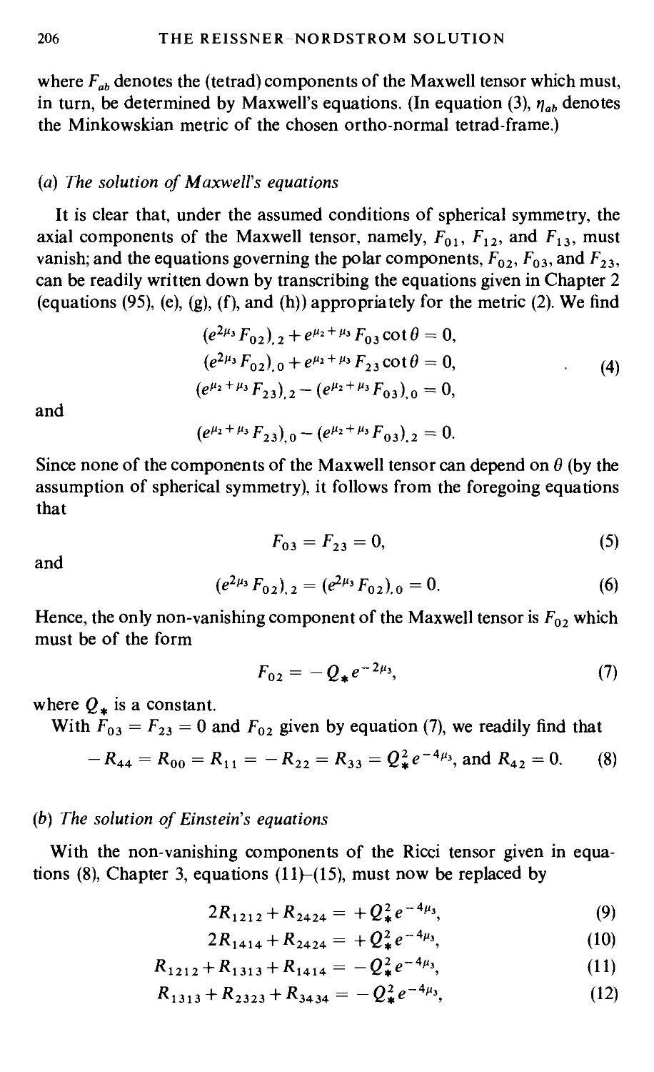
(a) The solution of Maxwell's equations 206
(b) The solution of Einstein's equations 206
38. The nature of the space-time 209
39. An altemative derivation of the Reissner-Nordstrom metric 214
40. The geodesies in the Reissner-Nordstrom space-time 215
(a) The null geodesies 216
(b) Time-like geodesies 219
(c) The motion of charged particles 224
41. The description of the Reissner-Nordstrom space-time in a
Newman-Penrose formalism 224
42. The metric perturbations of the Reissner-Nordstrom solution 226
(a) The linearized Maxwell equations 226
(b) The perturbations in the Ricci tensor 227
(c) Axial perturbations 228
(d) Polar perturbations 230
(i) The completion of the solution 234

43. The relations between Viw and Vty and Zj<+) and Zf
235
44. Perturbations treated via the Newman-Penrose formalism 238
(a) Maxwell's equations which are already linearized 238
(b) The 'phantom' gauge 240
(c) The basic equations 241
(d) The separation of the variables and the decoupling and
reduction of the equations 242
45. The transformation theory 245
(a) The admissibility of dual transformations 246
(b) The asymptotic behaviours of Y±i and X±j 248
46. A direct evaluation of the Weyl and the Maxwell scalars in
terms of the metric perturbations 249
(a) The Maxwell scalars <\>o and <t>2 252
47. The problem of reflexion and transmission; the scattering
matrix 254
(a) The energy-momentum tensor of the Maxwell field and
the flux of electromagnetic energy 257
(b) The scattering matrix 258
48. The quasi-normal modes of the Reissner-Nordstrom black-
hole 261
49. Considerations relative to the stability of the Reissner-
Nordstrom space-time 262
50. Some general observations on the static black-hole solutions 270
Bibliographical notes 271
6. THE KERR METRIC 273
51. Introduction 273
52. Equations governing vacuum space-times which are stationary
and axisymmetric 273
(a) Conjugate metrics 276
(b) The Papapetrou transformation 277
53. The choice of gauge and the reduction of the equations to
standard forms
278

(a) Some properties of the equations governing X and Y 281
(b) Alternative forms of the equations 282
(c) The Ernst equation 284
54. The derivation of the Kerr metric 286
(a) The tetrad components of the Riemann tensor 290
55. The uniqueness of the Kerr metric; the theorems of Robinson
and Carter 292
56. The description of the Kerr space-time in a Newman-Penrose
formalism 299
57. The Kerr-Schild form of the metric 302
(a) Casting the Kerr metric in the Kerr-Schild form 306
58. The nature of the Kerr space-time 308
(a) The ergosphere 315
Bibliographical notes 317
7. THE GEODESICS IN THE KERR SPACE-TIME 319
59. Introduction 319
60. Theorems on the integrals of geodesic motion in type-D
space-times 319
61. The geodesies in the equatorial plane 326
(a) The null geodesies 328
(b) The time-like geodesies 331
(i) The special case, L=aE 331
(ii) The circular and associated orbits 333
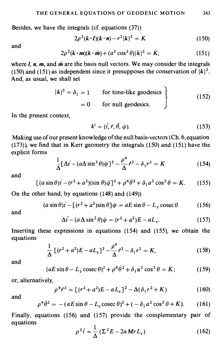
62. The general equations of geodesic motion and the separability
of the Hamilton-Jacobi equation 342
(a) The separability of the Hamilton-Jacobi equation and an
alternative derivation of the basic equations 344
63. The null geodesies 347
(a) The 0-motion 349
(i) -rj > 0 349
(ii) -q = 0 349
(iii)i7<0 349

(b) The principal null-congruences 349
(c) The r-motion 350
(d) The case a=M 357
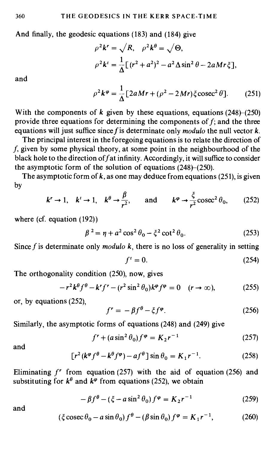
(e) The propagation of the direction of polarization along a
null geodesic 358
64. The time-like geodesies 361
(a) The 0-motion 362
(b) The r-motion 363
65. The Penrose process 366
(a) The original Penrose process 368
(b) The Wald inequality 370
(c) The Bardeen-Press-Teukolsky inequality 371
(d) The reversible extraction of energy 373
66. Geodesies for a2>M2 375
(a) The null geodesies 375
(b) The time-like geodesies 376
(c) Violation of causality 377
Bibliographical notes 379
8. ELECTROMAGNETIC WAVES IN KERR GEOMETRY 382
67. Introduction 382
68. Definitions and lemmas 383
69. Maxwell's equations: their reduction and their separability 384
(a) The reduction and the separability of the equations for ¢0
and ¢2 385
70. The Teukolsky-Starobinsky identities 386
71. The completion of the solution 392
(a) The solution for (/> 1 393
(b) The verification of the identity (80) 394
(c) The solution for the vector potential 395
72. The transformation of Teukolsky's equations to a standard
form 397
(a) The r^r)-relation 399

73. A general transformation theory and the reduction to a one-
dimensional wave-equation
400
74. Potential barriers for incident electromagnetic waves 404
(a) The distinction between Z, + 0>) and Z<-0>) 406
(b) The asymptotic behaviour of the solutions 408
75. The problem of reflexion and transmission 410
(a) The case <t>&c (= -aim) and a2>0 410
(b) The case &s<&<o*c 412
(c) The case 0 s£ & < o^ 414
76. Further amplifications and physical interpretation 417
(a) Implications of unitarity 419
(b) A direct evaluation of the flux of radiation at infinity and
at the event horizon 421
(c) Further amplifications 425
77. Some general observations on the theory 427
Bibliographical notes 428
9. THE GRAVITATIONAL PERTURBATIONS OF THE KERR
BLACK-HOLE 430
78. Introduction 430
79. The reduction and the decoupling of the equations governing
the Weyl scalars ^0, *i, ¥3, and ¥4 431
80. The choice of gauge and the solutions for the spin coefficients
k, a, A, and v 434
(a) The phantom gauge 435
81. The Teukolsky-Starobinsky identities 436
(a) A collection of useful formulae 441
(b) The bracket notation 442
82. Metric perturbations; a statement of the problem 443
(a) A matrix representation of the perturbations in the basis
vectors 444
(b) The perturbation in the metric coefficients 445
(c) The enumeration of the quantities that have to be
determined, the equations that are available, and the
gauge freedom that we have 446

XV111
CONTENTS
83. The linearization of the remaining Bianchi identities 447
84. The linearization of the commutation relations. The three
systems of equations 448
85. The reduction of system I 453
86. The reduction of system II: an integrability condition 454
87. The solution of the integrability condition 458
88. The separability of ¥ and the functions *3l and &~ 464
(a) The expression of £% and Sf in terms of the Teukolsky
functions 465
89. The completion of the reduction of system II and the
differential equations satisfied by £% and & 467
90. Four linearized Ricci-identities 470
91. The solution of equations (209) and (210) 472
(a) The reduction of equations (233)-(236) 475
(b) The integrability conditions 478
92. Explicit solutions for Zi and Z2 479
(a) The reduction of the solutions for Zi and Z2 482
(b) Further implications of equations (211) and (212) 484
93. The completion of the solution 485
94. Integral identities 487
(a) Further identities derived from the integrability condition
(263) 489
95. A retrospect 497
96. The form of the solution in the Schwarzschild limit, a —»0 500
97. The transformation theory and potential barriers for incident
gravitational waves 502
(a) An explicit solution 503
(b) The distinction between Z< + ot)and ZI-** 506
(c) The nature of the potentials 507

CONTENTS
xix
(d) The relation between the solutions belonging to the
different potentials 512
(e) The asymptotic behaviours of the solutions 513
98. The problem of reflexion and transmission 514
(a) The expression of R and l in terms of solutions of
Teukolsky's equations with appropriate boundary
conditions 517
(b) A direct evaluation of the flux of radiation at infinity 520
(c) The flow of energy across the event horizon 523
(d) The Hawking-Hartle formula 526
99. The quasi-normal modes of the Kerr black-hole 528
100. A last observation 529
Bibliographical notes 529
10. SPIN-'/i PARTICLES IN KERR GEOMETRY 531
101. Introduction 531
102. Spinor analysis and the spinorial basis of the Newman-
Penrose formalism 531
(a) The representation of vectors and tensors in terms of
spinors 535
(b) Penrose's pictorial representation of a spinor £A as a 'flag' 537
(c) The dyad formalism 538
(d) Covariant differentiation of spinor fields and spin
coefficients 539
103. Dirac's equation in the Newman-Penrose formalism 543
104. Dirac's equations in Kerr geometry and their separation 544
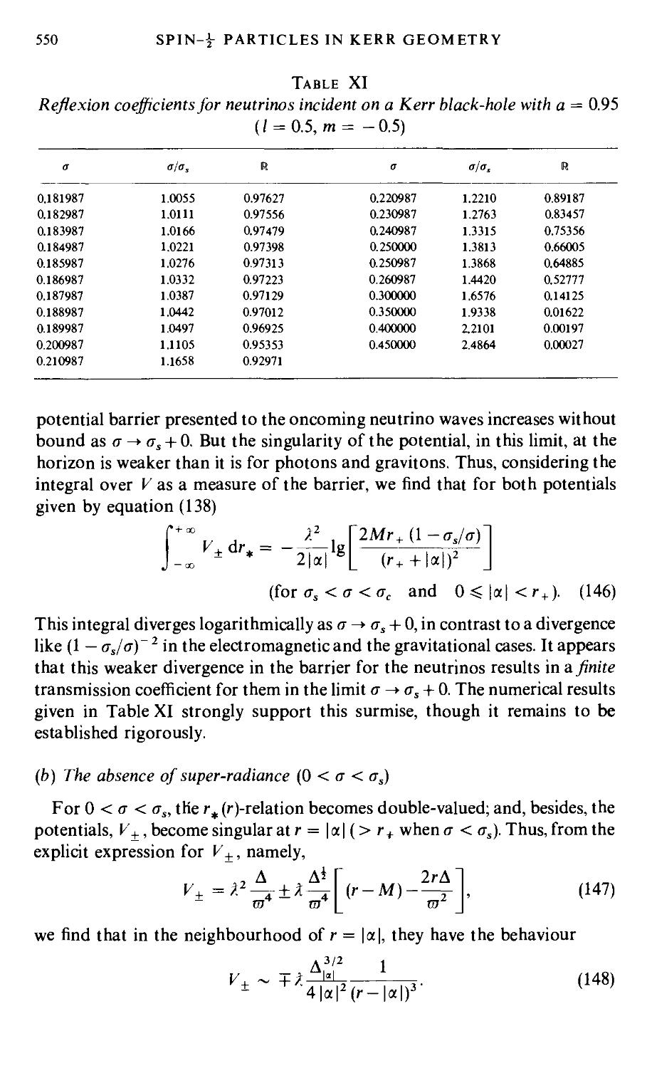
105. Neutrino waves in Kerr geometry 546
(a) The problem of reflexion and transmission for cr> <rs ( =
-am/2Mr+) 548
(b) The absence of super-radiance (0< cr< crs) 550
106. The conserved current and the reduction of Dirac's equations
to the form of one-dimensional wave-equations 552

CONTENTS
(a) The reduction of Dirac's equations to the form of one-
dimensional wave-equations 553
(b) The separated forms of Dirac's equations in oblate-
spheroidal coordinates in flat space 555
107. The problem of reflexion and transmission 556
(a) The constancy of the Wronskian, [Z±,Z%~\, over the
range of r, r+<r< °° 557
(b) The positivity of the energy flow across the event horizon 558
(c) The quantal origin of the lack of super-radiance 560
Bibliographical notes 561
11. OTHER SOLUTIONS; OTHER METHODS 563
108. Introduction 563
109. The Einstein-Maxwell equations governing stationary
axisymmetric space-times 564
(a) The choice of gauge and the reduction of the equations to
standard forms 566
(b) Further transformations of the equations 567
(c) The Ernst equations 569
(d) The transformation properties of the Ernst equations 570
(e) The operation of conjugation 572
110. The Kerr-Newman solution: its derivation and its description
in a Newman-Penrose formalism 573
(a) The description of the Kerr-Newman space-time in a
Newman-Penrose formalism 579
111. The equations governing the coupled electromagnetic-
gravitational perturbations of the Kerr-Newman space-time 580
112. Solutions representing static black-holes 583
(a) The condition for the equilibrium of the black hole 586
113. A solution of the Einstein-Maxwell equations representing an
assemblage of black holes 588
(a) The reduction of the field equations 590
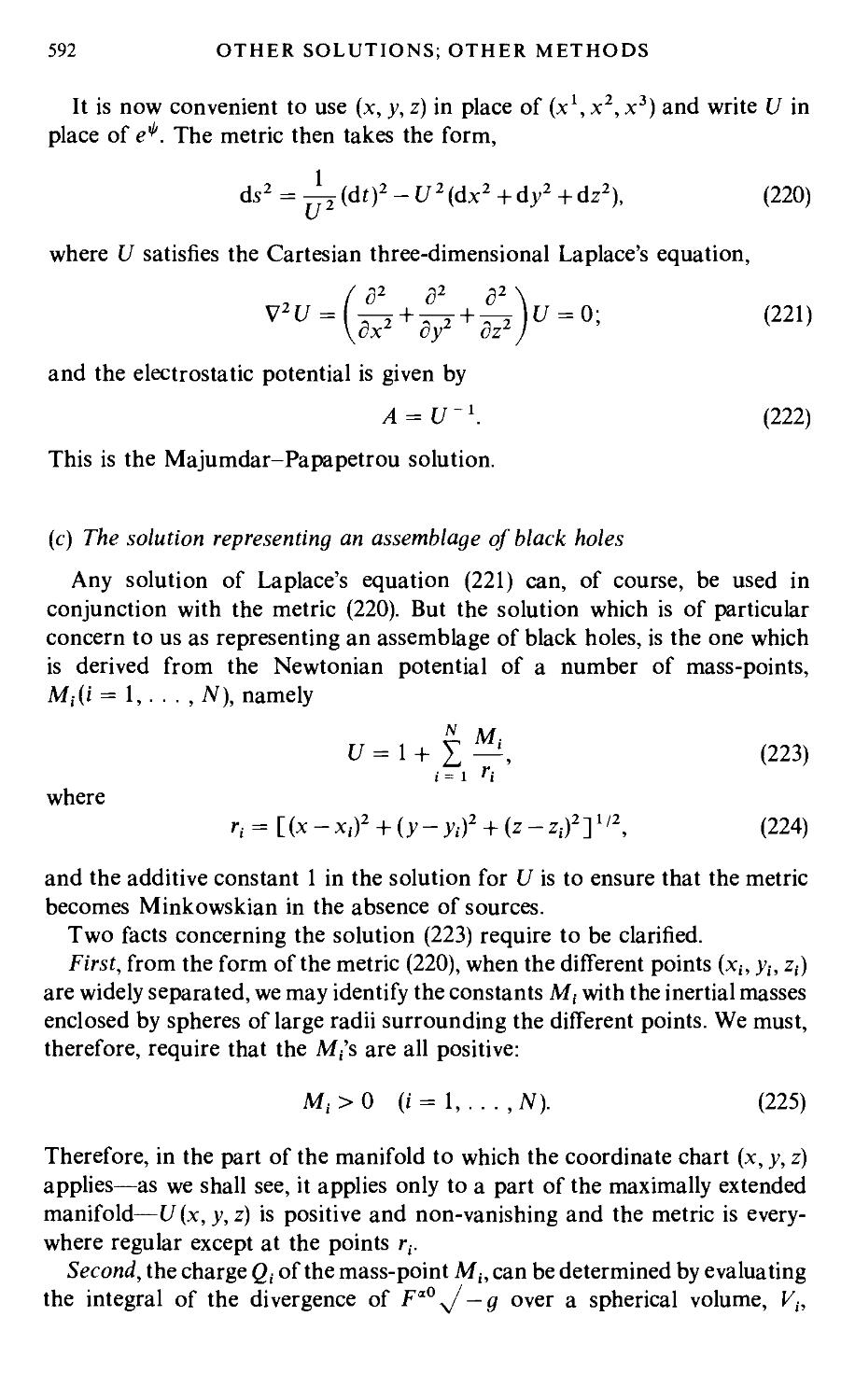
(b) The Majumdar-Papapetrou solution 591
(c) The solution representing an assemblage of black holes 592

CONTENTS
xxi
114. The variational method and the stability of the black-hole
solutions 596
(a) The linearization of the field equations about a stationary
solution; the initial-value equations 603
(b) The Bianchi identities 606
(c) The linearized versions of the remaining field equations 608
(d) Equations governing quasi-stationary deformations;
Carter's theorem 609
(e) A variational formulation of the perturbation problem 614
(i) A variational principle 619
(ii) The stability of the Kerr solution to axisymmetric
perturbations 620
Bibliographical notes 622
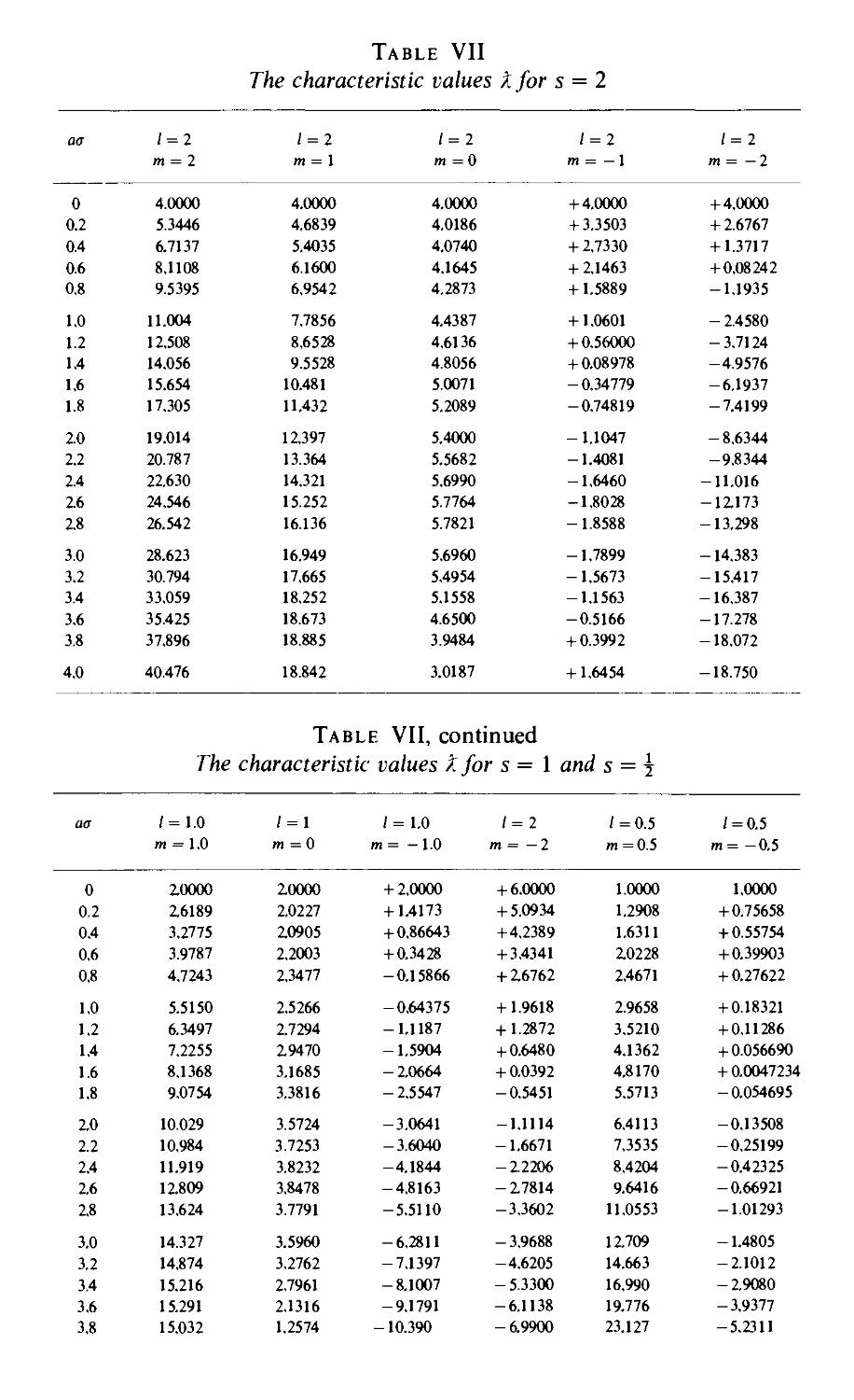
Appendix. Tables of Teukolsky and Associated Functions 625
Epilogue 637
Index 639

Roy Patrick Kerr (1934- )
A-4
Karl Schwarzschild (1873-1916)

PROLOGUE
The black holes of nature are the most perfect macroscopic objects there are in
the universe: the only elements in their construction are our concepts of space
and time. And since the general theory of relativity provides only a single
unique family of solutions for their descriptions, they are the simplest objects
as well.
The unique two-parameter family of solutions which describes the space-
time around black holes is the Kerr family discovered by Roy Patrick Kerr in
July, 1963. The two parameters are the mass of the black hole and the angular
momentum of the black hole. The static solution, with zero angular
momentum, was discovered .by Karl Schwarzschild in December, 1915. A
study of the black holes of nature is then a study of these solutions. It is to this
study that this book is devoted.

1
MATHEMATICAL PRELIMINARIES
1. Introduction
In this chapter, we shall provide an account of the analytical methods that lie at
the base of much of the developments that are to be described in this
book.These consist of Cartan's calculus of differential forms and the tetrad
and the Newman-Penrose formalisms. While none of these matters are novel
in themselves, they cannot all be found in a coherent treatment in one place;
and the account is included to make the book as self-contained as is possible.
The presentation of the elements of differential geometry in §§2-6 is, however,
not intended to replace the standard accounts of the subject available
elsewhere: the presentation is confined to the barest essentials leading to
Cartan's equations of structure.
2. The elements of differential geometry
Differential geometry deals with manifolds. Manifolds are essentially spaces
that are locally Euclidean in a sense which we shall first make precise.
We recall that an Euclidean space of n-dimensions, R„, is the set of all
n-tuples, (x1,. . . , x") (- oo < x' < + go), with open and closed sets (or,
neighbourhoods) defined in the usual way. A manifold, M, is locally identical to
Euclidean space in the sense that M is covered (i.e., a union of)
neighbourhoods, 11^, and that associated with each <^a there is a one-one map, (/>„, which
images each point p e 91^, to a point in an open neighbourhood of R„ (onto
which <^a is imaged by fa) with the coordinates (x1,..., x"). Further, if two
neighbourhoods, 11^, andf^, of M, intersect and have points in common (i.e.,
^a <^^"a =/= 0), and if fa and fa are the associated maps onto neighbourhoods
in U„, then the map fa0^/^1 images a point fa(p) (pef,nfa) with the
coordinates (x1, ..., x"), say, to the point fa(p) with the coordinates
(x1, ..., x"), then as a part of the definition of M, it is required that x'
(i — 1,. . . , n) are smooth functions of (x1, ..., x"). (Smooth functions are
those which have continuous partial derivatives of all orders.)
The Cartesian product M x N of two manifolds M and N is, in the first
instance, the ordered pair of points, (p, q), where peM and q e N; further, if ^fa
and f~x are neighbourhoods in M and in N, t/>a and \j/e are the associated maps,
and <px(p) = (x1,. . . , x") and i/^(<?) = (y1, ■ . • , /") (m not necessarily equal to
n), then the map,
(fax ipe) (p,q) = (x1, . . . ,x",y\ . . . , f),

4
MATHEMATICAL PRELIMINARIES
suffices to complete the definition of M x N as a manifold of (m + «)-
dimensions.
We now consider a function f on M defined by a map /: M -» R1. We shall
suppose that the combined map f° <j>~1 which images a point (x1, . . . , x") in
W on to the reals, IR^isasmooth function of the coordinates (x1, . . . ,x").We
define a smooth curve X on M by the map
X: an interval I (a <t < b) in U1 -* X(t) = peM
such that
((/)^)(0 = ^(0,-. .,x"(t)]; (1)
and we require that x'(f) (i = 1, . . ., n) are smooth functions off. Finally, we
may note that a function f, defined on the manifold, enables us to define the
function, f° X on the curve X. With the aid of the map (/>a ° X we are led to
consider the function f(X (t)) =f(x1(t), . . . , xn(t) (where (x*(0> • • • ,x"(t))are
the coordinates of p = X(t) by the map t/>a.
(a) Tangent vectors
With the definition of/(x1 (f), ..., x"(f)) on a curve X on M, which we have
just given, consider
"A
dt Jut)
= limit -{f(X(t0 + e))-f(X(t0))
= " dxJ(0
,= i dt
t0\dxS)uto) \dt 8x>
(2)
where, in the last step, summation over repeated indices is assumed. (This
summation convention will be adopted throughout the book.)
It is now clear that by considering various curves X passing through a given
point p, we can define a linear vector-space (at p) consisting of linear
combinations of the coordinate derivatives djdx' of the forms
x=x'L- (3)
where the XJ,s are any set of n numbers. These tangent vectors arise by
considering the curves X defined by
x>(t)^x'(p) + X>t 0-=1,...,/1) (4)
for t in some small interval — e < t < + e.
The tangent vectors at p form a linear vector-space over U1 spanned by the
coordinate derivatives, since the requirement for a linear vector-space, namely,
(«X+pY)f=«(Xf) + p(Yf), (5)

THE ELEMENTS OF DIFFERENTIAL GEOMETRY
5
is satisfied for all vectors X and Y, numbers a and ft, and functions f.
Moreover, the vectors (d/dxJ')p are linearly independent; for, otherwise, there
should exist numbers X'(j = 1, . . . , ri), not all zero, such that X = X'd/dx'
applied to any smooth function is identically zero; but the application of X to
the coordinate functions xk(k = 1, . . . , n) would lead to Xk = 0 for all k; and
this is a contradiction.
Finally, the definition of X by
Xf=Xl]jJ = xJf.J> (6>
for every smooth function f clearly satisfies the Leibnitz rule when operating
on products of functions, thus
X(fg)\m=(fXg + gXf)\Mt). (7)
Tangent vectors may, in fact, be considered as directional derivatives. (In
equation (6) we have introduced the notation of denoting derivatives with
respect to x' by the index), following a comma, both as subscripts.)
The space of tangent vectors (or contravariant vectors, as they are also
called) to an n-dimensional manifold M at p, denoted by Tp(M) or simply Tp, is
an n-dimensional vector-space. This space, which may be visualized as the set
of all 'directions' at p, is called the tangent space at p.
Instead of a basis determined by local coordinates, we may choose any other
n linearly independent vectors ea(a = 1, . . . , n) (say). There must, then, exist
linear relations of the form
where the determinant of the matrix formed by <!>„* must be non-zero. The
inverse relation is then given by
^=*V* (9)
where [¢^] is the inverse of the matrix [¢/]:
$ak$'j = 5kj and $.k$bk = dab. (10)
Given any basis (ej), we can express any tangent vector at p in the form
X=XJe;. (11)
The XJ,s are the components of X relative to the basis (ej).
(b) One-forms (or, cotangent or covariant vectors)
A one-form, a>, at p is a linear mapping of the tangent space Tp on to the reals:
a>. Tp^U\ (12)

6
MATHEMATICAL PRELIMINARIES
In other words, given any tangent vector X at p, the one-form <o associates
uniquely with it a number <o{X) which is also written as
a>(X)=(a>,X}. (13)
The required linearity of the map is expressed by the relation
(a>,otX+pY> = a(a,,X> + p(a>,Y>, (14)
where X and Y are any two tangent vectors and a and /? are any two real
numbers. We, further, define multiplication of forms by real numbers and
sums of forms by the rules that, for any XeTp and any real number a,
(<xo})(X) = <x((o,X} and (a) +n)(X) = (<o,X) + (it, X), (15)
where <o and n are two one-forms. By these rules, one-forms span a vector
space which we denote by T*p; it is called the cotangent space at p and the dual
of the tangent space. For this reason one-forms are also called cotangent
vectors (or, covariant vectors).
We shall now verify that a basis for T*p, associated with a basis (e}) for Tp, is
provided by the one-forms (e')(i = 1, . . . , n) which map any tangent vector
X = X'e} to its components; thus,
e'(X)=(e',XJeJ) = Xi (i= 1,..., n). (16)
From this last equation it follows that
el(ej)=W,e}y=6lj. (17)
The expression of any arbitrary one-form <o as a linear combination of the
e"s is obtained by observing that
(a>,X)=(a>,Xiei) = Xi(a>,eiy. (18)
Now letting
co;= (a>, ety =<o(ei), (19)
be the numbers to which a> maps the basis vectors (e;) of the tangent space Tp at
p, we may write
(<o,X} = tOtX' = «(<>', X^j)
= <a^',X>. (20)
Since this last equation is valid for any XeTp, it follows that
a> = a>ie'; (21)
and this is the required expression of a> as a linear combination of the e"s. That
the vectors ei are linearly independent is manifest from its definition. The bases
(¢() and (e') are said to provide dual bases for the tangent and the cotangent
spaces at p.

THE ELEMENTS OF DIFFERENTIAL GEOMETRY
7
If in place of the dual bases (e;) and (e') we should choose different bases,
ev = d>; ;*; and ey = &' se\ (22)
obtained by non-singular linear transformations represented by 3>;>J and Q>}'s,
then the condition, that the new bases (er) and (e3) continue to be dual,
requires
= cDJ>rk^=cDJ>V; (23)
in other words, the matrices [<&;-'] and [3>j;] are the inverses of one another.
Finally, we may note that if we change from one set of local coordinates (x;)
to another set (xl'), then the corresponding expressions for 3>r' and ¢-^ are
Associated with any function f on the manifold, one defines a one-form d/
by requiring that
df(X)=(df,X} = Xf, (25)
for any vector XeTp. In a local coordinate basis,
and by definition,
in particular,
X=X>1; (26)
(dlXy^X'^^X'fj; (27)
<dx^,£7> = ^i. (28)
Hence, the one-forms (dxj) provide a local coordinate basis for the cotangent
vectors which is dual to the local coordinate basis provided by the tangent
vectors (dj = d/dx}) for the tangent space. The bases (dj) and (dxJ) are
sometimes referred to as the canonical bases for the tangent and the cotangent
spaces.
We note that if
d/= ajdxJ, (29)
then it follows from
Xi/i=<d/,^>=<aJdxJ,X'ai>
= a,X'<dx',S, > = «,*', (30)
that
a, =/, and d/ = /;dx<; (31)

8 MATHEMATICAL PRELIMINARIES
and this last equation is consistent with the conventional meaning one attaches
tod/
(c) Tensors and tensor products
LCt nsr = T*p x T*p x ... x T% x Tp x Tp x ... x Tp (32)
v. ■> v /
r factors s factors
represent the Cartesian product or r cotangent spaces and s tangent spaces at
some point p of a manifold, i.e., the space of ordered sets of r one-forms and
s tangent vectors: (to1, . . . , a/, Xlt . . . ,XS). And consider a multilinear
mapping, T, of the manifold nsr to the reals:
T: ff^R1. (33)
Precisely, what the mapping provides is an association (in some unique
manner) of any given ordered set of r one-forms and s tangent vectors to a real
number:
T{(ol, . . . ,(or, Xu ..., Xs) = a real number. (34)
The condition that the map is multilinear requires that
nm\...,ar,aX+pY,X2,...,XM)
= a7>\ . ..,&', X,X2, ..., Xs) + pT{a>\ . . . , wT, Y, X2, . . . , Xs), (35)
for all a, /JelR1 and X, YeTp; and for similar replacements of all the other
forms and vectors. A multilinear mapping so defined is said to be a tensor of
type (r, s). Linear combinations of tensors of a given type (r, s) are defined by
the rule
(a7+ /?S)K, ...,<*„...,*,)
= a7>\ ...,wr,Xu.. . ,^,) + 0,5(0.1. ...,aT,Xu.. .,XS), (36)
for all a./JeR1, <o'eT*p, and XjeTp (i = I, . . . ,r; j = I, . . . ,s). By these
rules, tensors of a given type (r, s) span a linear vector-space of dimension nr+s.
And the space of such tensors is called the space of tensor products and denoted
by
Trs(P) = rp® ... ®rp® r*p®... ®r% (37)
r factors s factors
We shall presently verify that a basis for tensor products of type (r, s) is
provided by the nr+s special mappings
<?,,...,/'• ;'-K, ...,ar,Xlt...,X.)
= 'u ...,/'' ■ H^kie\ ..., afKe\ 1,% ..., Xs'-e,)
= <o1il...cfirX1i'...X.J: (38)

THE ELEMENTS OF DIFFERENTIAL GEOMETRY
9
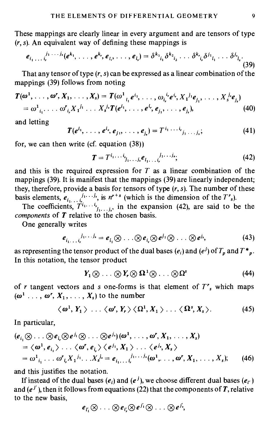
These mappings are clearly linear in every argument and are tensors of type
(r, s). An equivalent way of denning these mappings is
«,,... ,/' ■■■ V', • • -,e\eh,. . .,et) = 8\d\ . . . 5\S\ . . . 5\.
(39)
That any tensor of type (r, s) can be expressed as a linear combination of the
mappings (39) follows from noting
T(a>\ ...,a>',Xu...,Xs) = Tip1 ^, . . . ,co,.V%X>A, . . . , A>Js)
= co1,,. . . . a/, X,* . . . Xj-T(e\ ..., e\ eh, ..., eh\ (40)
and letting
T(e\..., e\ eJlt ...,^) = 7^---^ ...j,; (41)
for, we can then write (cf equation (38))
r= ^--¾....;.««,. V,,"i"; (42)
and this is the required expression for T as a linear combination of the
mappings (39). It is manifest that the mappings (39) are linearly independent;
they, therefore, provide a basis for tensors of type (r, s). The number of these
basis elements, e^ /'■ ■ ■>', is nr+s (which is the dimension of the Trs).
The coefficients, T'1- l'Si ^, in the expansion (42), are said to be the
components of T relative to the chosen basis.
One generally writes
'(,... .'/V ■ ''' = «i, ® ■ ■ ■ ® eK®eh ® ■ ■ ■ ® e''> (43>
as representing the tensor product of the dual bases (et) and (e>) of Tp and T*p.
In this notation, the tensor product
Y1®...®Yr®£l1® ...®QS (44)
of r tangent vectors and s one-forms is that element of Trs which maps
(to1 . . . , (or, Xt,. . . , Xs) to the number
W.Y.y ... (o/.ijxtf,^)... <ns,*s>. (45)
In particular,
(<?,. <g>. . . ®eir®ej' <g>. . . ®ej') K, . . - , < Xu . . . , X.)
= (^,^)... ««t><^, *,>... <e\X.>
= a;1,- . . . a>W'. . .*,'■ = ^...,./"' -'-(a.1,. ..,a>',Xu..., Xs); (46)
and this justifies the notation.
If instead of the dual bases (e;) and (e'), we choose different dual bases (ev)
and (eJ ), then it follows from equations (22) that the components of T, relative
to the new basis,
efl® ■ ■ ■ ®eVr®e>'i® . . . ®e>\

10
MATHEMATICAL PRELIMINARIES
are given by
7"1"-^,.../. = ^, ■■■^V---^-^-^,...v (47)
The contraction of a tensor of type (r, s) with the components P1 ■ ■ ■ trjt ...^,
with respect to a chosen contra variant index ip and a chosen covariant index;,,
is defined as the following tensor of type (r - 1, s - 1):
7-(,... «,.,«,♦,...,;._ Vi^<+i A<?ii® . . . ®elpi®eip+i® ■ ■ ■ ®<?,v
®eh® . . . ®<?'«->(x)<?Vi(g) . . . ®eA (48)
where, as the notation indicates, summation over all values of k (of the i„-
contravariant index and of the ;4-covariant index) is to be effected. It can be
readily verified, with the aid of equations (23) and (47), that the process of
contraction is independent of the chosen basis.
A tensor of type (0,2) is said to be symmetric or antisymmetric if
T(X, Y) = T(Y, X) or T(X, Y) = -T(F, X)
for all X and Y in T„. (49)
In terms of components, in an arbitrary basis, symmetry or antisymmetry
implies _ _ _ _ ....
Tls = Tn or T,j=-Tj,. (50)
More generally, a tensor of type (r, s) is said to be symmetric or antisymmetric
in its covariant indices i and j if
7>\. ..,a>',... ,ta>,. ..,wr,Xu...X,) =
±T(a>\ . . ,a>\ . . ,a>1, . . .,a>r,Xu . . . , Xs), (51)
for all co's and ^'s. Symmetry or antisymmetry with respect to chosen
contravariant indices are similarly defined.
3. The calculus of forms
A particularly important class of tensors of type (0, s) is the class of totally
antisymmetric tensors, i.e., covariant tensors which are antisymmetric in every
pair of their arguments, i.e.,
T(Aj, ..., Xj, ..., Xj, ..., Xs) = — 1 \X\, ..., Xj, ..., A;, ..., As),
(52)
for all pairs of indices i and j and for all a"s. Tensors of this kind can be
constructed out of a general tensor T of type (0, s) by applying to it the
alternating operator A whose effect on it is to give the linear combination
defined by
,47-(^,,...,^) = 4 I sgnU,, ...,;s)r(A-;.,, ..., A";.), (53)

THE CALCULUS OF FORMS
11
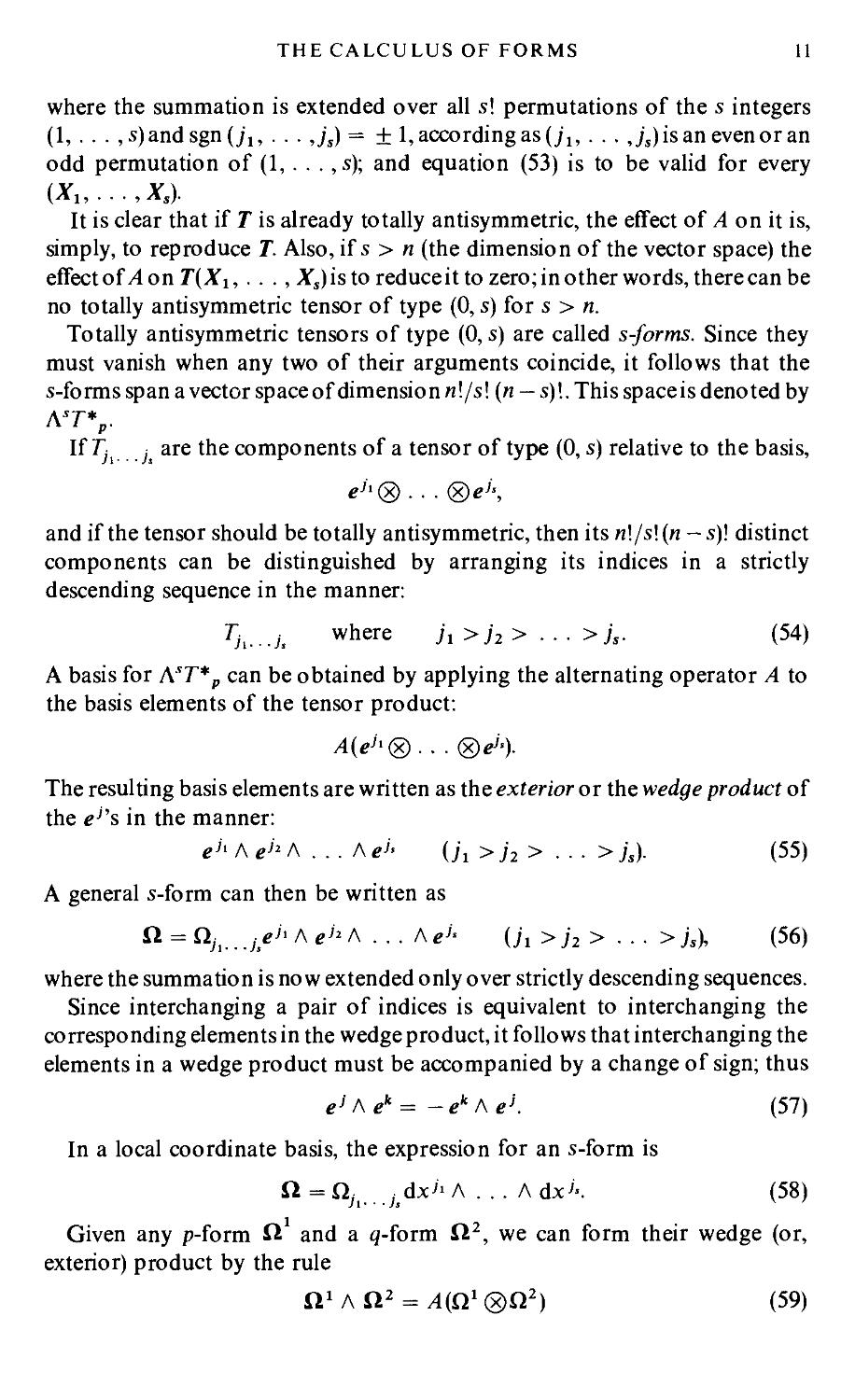
where the summation is extended over all s! permutations of the s integers
(1, . . . ,s)andsgn(;!, . . . ,js) = + 1, according as (ju . . . Js) is an even or an
odd permutation of (1, . . . , s); and equation (53) is to be valid for every
(X j ,..., As).
It is clear that if T is already totally antisymmetric, the effect of A on it is,
simply, to reproduce T. Also, if s > n (the dimension of the vector space) the
effect of/4 on T(Xi, . . ., Xs) is to reduce it to zero; in other words, there can be
no totally antisymmetric tensor of type (0, s) for s > n.
Totally antisymmetric tensors of type (0, s) are called s-forms. Since they
must vanish when any two of their arguments coincide, it follows that the
s-forms span a vector space of dimension n\/s\ (n — s)!. This space is denoted by
at%.
If Tj _j are the components of a tensor of type (0, s) relative to the basis,
eh® ■ ■ ■ ®e>\
and if the tensor should be totally antisymmetric, then its n\/s\{n — s)! distinct
components can be distinguished by arranging its indices in a strictly
descending sequence in the manner:
Th.-.j. where Ji >^> ■ ■ ■ >■/'»• (54)
A basis for AST*P can be obtained by applying the alternating operator A to
the basis elements of the tensor product:
A(eh® . . . ®e>-).
The resulting basis elements are written as the exterior or the wedge product of
the eJ,s in the manner:
«>' A «>'» A . . . A «>■ (ji >j2> ■■■ > j,). (55)
A general s-form can then be written as
SI = Q;i.. .,/>' A e1* A . . . A e>- (ji >j2> ..-> Js), (56)
where the summation is now extended only over strictly descending sequences.
Since interchanging a pair of indices is equivalent to interchanging the
corresponding elements in the wedge product, it follows that interchanging the
elements in a wedge product must be accompanied by a change of sign; thus
e> Aek = -ekAej. (57)
In a local coordinate basis, the expression for an s-form is
" = £V .jdx'^A . .. Adx^. (58)
Given any p-form il and a q-form il2, we can form their wedge (or,
exterior) product by the rule
il1 A il2 = A(Q* ®Q2) (59)

12
MATHEMATICAL PRELIMINARIES
to obtain a (p + g)-form. (It must accordingly vanish identically if p + q > n.)
Wedge products of forms clearly obey the associative and the distributive
laws, but they are not in general commutative. For, by definition,
ft1 A ft2 = (ft1^ jeh A . . . AeJ-)A (Q2k] ktek> A . . . A <?*.), (60)
where (j\, ■ ■ ■ ,jp) and (/cl5 . . . , kq) are strictly descending sequences.
Accordingly,
ft1 A ft2 = (-l)M(n2fcl...fc<<?fc'A . . . A«k.)A(Q1.]Jf''A .. . Ae'<)
= (-i)wn2An1, ' (61)
since each of the q basis elements ek', . . ., ek* must suffer p interchanges before
il1 A il2 can be brought to the form required of ft2 A ft1.
So far, we have considered tensors and forms defined at a point on the
manifold. We shall now enlarge the basic definitions in a way which enables us
to envisage fields defined on M. Thus, a smooth tensor-fieldT' S(M) (or, simply
Trs) of type (r, s) on M is an assignment of an element of T's(p) at each point
p e M in such a way that the components of Trs relative to any local coordinate
basis are smooth functions of the coordinates. This enlargement of the basic
definitions is necessary if we are to formulate notions of differentiation.
In the future we shall be concerned only with smooth tensor fields; and this is
to be understood even if the qualifying words 'smooth' and 'field' are omitted.
(a) Exterior differentiation
Exterior differentiation is effected by an operator d applied to forms. It
converts p-forms to (p+ l)-forms consistently with the following rules:
(a) The operator d, applied to functions (or zero-forms) f, yields a one-form
d/ defined by
df(X)=(df,xy = xf
for every Xe T10. In particular, in a local coordinate basis
^^
(b) If Ax and A2 are two p-forms,
d(otA1+PA2) = otdA1 + pdA2 (a^eR1).
(c) If A is a p-form and B is a q-form,
d(A A B) = dA A B + (- 1)" A A dB.
(d) Poincare's lemma, which requires that
d(d/l) = 0,
for every p-form A.

THE CALCULUS OF FORMS
13
To clarify that the operator d subject to the foregoing rules is well-defined,
consider, first, the exterior derivative
dA = d(A, i dx3' A . . . A dx>>)
of a p-form A. By rules (a), (b), and (d)
dA =dA: -, Adx^'A . . . AdxJ*
dA: ,
= Jl: 'dx*AdxJ-A . .. AdxV (62)
dx
It is important to verify at this point that dA, as given by equation (62), is
independent of the choice of the local coordinate system. For, if instead of the
local coordinates (x3') we had chosen a different set of local coordinates (x1'),
then by equations (24) and (47),
dx3' dx >'
Ai\...i=Ah.-U^'"^J,i (63»
and we should conclude that
d (/1,, j.dx3' A . . .Adx^)
v Ji---jp '
( dx'' dx3'
= d[Aj i ——. . .—— dx^'A . . . AdxJ*
\ 3'-3' dx3' dx3'
dx3' dx3'
= —- . • • ^r-rd^i j A dx;i A . . . A dx3'
dx3' dx3' 3'--3'
d2x3' dxh dx3' 4 v , ? , /•
dxkdx3' dx3' dx3' 3'-3'
dx3' dx3'-' d2x3' .,
■ ■■ + v~r- --^-^- -, t-, fAi idxk Adx3' . .. Adx3'. (64)
dx3' dx3'-' dxkdx3' 3'--3' v '
All the terms on the right-hand side of equation (64) involving the second
derivatives of x3<(i = 1, . . . ,n) vanish on account of their symmetry in/c'and./;
and the antisymmetry of the basis elements, in these same indices, in the wedge
product; and the sole surviving term is the first one which is clearly the same as
dAi , Adx3' A . . . Adx3' = d(Ai , dx3' A . . . A dxM.
Accordingly,
d(An j.pdx3' A . . . A dx3'-) = d(Ah jdx3' A . . . A dx^); (65)
and this is what we set out to verify.
We next verify that the rule (c) is consistent with the expression (62) for dA.

14
MATHEMATICAL PRELIMINARIES
For, by the rules (a), (b), and (d)
d(A A B) = d(Aji j^dx'' A . . . A dxj- A Bki k^dxk> A . . . A dx*')
dA, ,
= —-^dx' A dx'' A . . . A dx'- A Bk k dxk> A . . . A dx^
dxi kt...k,
SBk k
+ A, f ^-?dx! A dxJl A . . . A dx'- A dxk' A . . . A dx*1*
;,...;„ dx,
/dBk k \
= dA AB + (-l)M;-_ ..jdxJ'A . . . A dx'- Al '"," ' dx1' A dx k> A ... Adxfc. I
= dA AB + (-l)"A AdB. (66)
And finally, to establish the consistency of rule (d), we need only observe that
dxk
rdA: ,
d{dA) = d( a t dx* A d*;'' A . . . A dx^
d2A-
= ^-^dx' A dxk A dx^'' A . . . A dx'- = 0. (67)
This completes the demonstration that the operation d is, indeed, well-defined.
(b) Lie bracket and Lie differentiation
Given any two vector fields, Xand Y, their Lie bracket, \_X, Y~\, is defined by
its action on any function /; and it is given by
IX, F]/= (XY- YX)f= X(Yf)- Y(Xf). (68)
The Lie bracket of any two tangent vectors is, again, a tangent vector, since
IX, F] («/■+ fig) = «[*, Ylf+ fi\_X, Y]g (69)
and
\_X, F](fg) = g[X, Y1f+f\_X, Y^g, (70)
where f and g are any two functions and a and fi are any two real numbers. The
first of these relations is manifest while the second follows quite readily:
\.X,Y2<Jg) = X(Yfg)-Y(Xfg)
= X(gYf+fYg)- Y(gXf+fXg)
= gXYf+ (Xg)(Yf)+(Xf)(Yg)+fXYg
-{gYXf+(Xf)(Yg)+(Yf)(Xg)+fYXg}
= g[X, Yy+flX, Y]g. (71)
The relation (69) establishes the Lie bracket as a linear operator while the
relation (70) establishes it as a differentiation.

THE CALCULUS OF FORMS
15
As may be readily verified, the Lie bracket satisfies the Jacobi identity,
[[*, F], Z] + [[F, Z], XI + [[Z, XI, Y] = 0. (72)
We have seen that the Lie bracket of X and Y is a tangent vector. Its
components, relative to a local coordinate basis, can be obtained by its action
on x'. Thus,
IX, Yy = (AT- YX)x> = XY'-YX'
= XkY\k-YkX\k, (73)
where (as indicated earlier) a comma preceding an index denotes partial
differentiation with respect to the local coordinate with that same index.
In a local coordinate basis, the Lie bracket \_dk, df\ clearly vanishes.
Considered as a differentiation, \_X, Y~\ is called the Lie derivative of Y in the
direction X and is written as
SexY = IX, F] = - \Y, XI = - <£YX. (74)
More generally, we define the Lie derivative, if XT, of a tensor field T of a given
type, as a tensor of the same type which satisfies the following rules:
(a) Its action on a scalar field f is given by
&xf= Xf= df(X). (75)
(b) Its action on a tangent vector Y, as we have already defined, is given by
<£XY=\X,Y\ (76)
And (c) it operates linearly on tensor fields and satisfies the Liebnitz rule when
acting on tensor products:
^X(S®T) = ^XS®T+S®^XT, (77)
where S and T are arbitrary tensor fields.
The last of the foregoing rules enables us to derive the effect of Z£x on a
tensor of arbitrary type. Thus, its effect on a one-form <o can be determined by
considering, for any arbitrary vector-field Y, the contracted version of the
relation
2>x(<o®Y) = (tfx<D)®Y + a>®{2>xY\ (78)
namely,
^<a.,F> = <^a.,y>+<a.,^y>. (79)
Writing out this last equation explicitly, we have
Xk(<o,Y'\k = {tfxa>)jY> + a>,{#xY)' (80)
or, making use of equation (73), we obtain
(^xa)tY' = Xk(a>J,kY> + a>iY>,k)-a>i(XkY1,k-YkX1,k)
= (Xk(oJ,k + (okXktJ)Y'. (81)

16
MATHEMATICAL PRELIMINARIES
Since this last equation is valid for an arbitrary Y, we conclude that
(Sexm)l^(0l,kXk + <okX\J. (82)
We may write equation (79) alternatively in the form
&x\a>W\ = (&x«>){Y) + «>(&xV)- (83)
By rule (c), equation (83) admits of generalization to a tensor of type (r, s). We
have
^x\_T(<o\..., c/, y„..., ys>] = (sexT)(m\..., w, y„..., ys)
+ nsexa>\ a>2,...,a>',Yu...,Y,)+ ■■■
+ 7-(^,...,^,1^,...,^}¾ (84)
where all the terms in this equation, except the first one on the right-hand side,
can be evaluated in terms of the known results (73), (75), and (82). The
components of ifXT can, therefore, be deduced from equation (84).
For later use, we shall derive here a simple identity relating the exterior
derivative of a one-form to Lie derivatives. By making use of equation (82), we
have
<i?,a»,y>-y<a»,*>
= ((Oj,kXk + cokXkj)Y>-Y'(cokJXk + cokXkj)
= (a>j,k-a>kJ)XkY> = 2da>(X, Y). (85)
Now, substituting for (yx<o,Yy from equation (79), we obtain the required
result:
da>(X, Y) = ${X(a>, Y} - Y(a>, X} - <o», \_X, F] >} (86)
where we have written the Lie bracket \_X, Y~\ in place i£xY.
4. Covariant differentiation
We shall now define a type of differentiation which, unlike exterior and Lie
differentiation, requires that the manifold be endowed with an additional
structure. This additional structure is an affine connection, V, which assigns to
each vector field Xon M a differential operator, V*, which maps an arbitrary
vector-field, Y, into a vector field VXY. Consistent with these requirements, we
impose the conditions,
(a) VXY is linear in the argument X, i.e.,
Vfx+gYZ=fVxZ+gVYZ (X,Y,ZeT\\ (87)
where/and g are any two arbitrary functions defined on M;
(b) VXY is linear in the argument Y, i.e.,
VX(Y+Z) = VXY+VXZ (X,Y,ZeT\), (88)
(c) Vxf=Xf, (89)

COVARIANT DIFFERENTIATION
17
where/is any function on M; and, finally,
(d) Vx(fY)=(Vxf)Y+fVxY. (90)
It should be noted that, according to equation (89), in a local coordinate
basis (dk), Vdk, when acting on functions, coincides with partial differentiation
with respect to x\
With the action of V^ on vector fields YieT1^ specified by the rules (a)-(d),
we now define the covariant derivative, V F, of F as a tensor field of type (1,1)
which maps the contravariant vector-field X to V^F, i.e.,
VF(*)=<VF,*> = V*F, (91)
for every XeT V In this notation, we can rewrite equation (90) in the form
V(/F) = d/®F+/VF (92)
To clarify what the assignment of a connection precisely means, it will be
useful to rewrite VXY relative to some chosen dual bases (et) and (e'). Thus,
making use of the rules (a)-(d), we have
V*F = Vx(Y'ej) = (X Y>)e} + y'V^. (93)
Since Vxes, for a particular e3, is a tensor field of type (1,1) we must have a
representation, in the chosen basis, of the form
Vxej = a>'j (X)e„ (94)
where <olj (depending on I and;') are one-forms. Accordingly, we may write
VxY^iXY^ej+ro'jiX)^. (95)
Alternatively, we may also rewrite equation (93) in the form
VxY=(XY')ej+YJVx^ej
= (XP)ej+PXkVetej, (96)
or, in conformity with the definition (94),
VXY = (XYJ)eJ+YJXka>'J(ek)el. (97)
Letting
0-,.(^) = 0^ (98)
be the coefficient of ek in the expansion of <o'j in the basis (ek), we conclude that
a connection V is specified by the n2 one-forms a>';. or, equivalently, by the n3
scalar fields to'Jk.
Returning to equation (95) and rewriting it in the form
VXY=\_XY> + e>;,(*)y']<?;, (99)
we infer that
(VXY)J = XYi + (D\(X)Yl. (100)

18
MATHEMATICAL PRELIMINARIES
In a local coordinate basis (dk, dX'), equation (100) gives
(V^YV^YJ + Y'o^Y^ + y'coV (101)
In a local coordinate basis, it is customary to write
F}lk in a place of (x)'lk; (102)
and using semicolons to indicate covariant derivatives (in contrast to commas
which indicate ordinary partial derivatives), we obtain the standard formula
y^ = y^ + y'rv (103)
The definition of covariant derivatives of vector fields can be extended to
tensor fields, in general, by requiring that the operation of V satisfies the
Leibnitz rule when acting on tensor products. Thus, we require that
V(S®T) = VS®T + S®VT, (104)
where S and T are two arbitrary tensor-fields. An immediate consequence of
this requirement is (cf. equation (84))
Vx{T(a>\ . . . ,a»', Ylt . . ., Ys)} = (VxT)(a>\ . . . ,a»', Yu . . ., Y.)
+ T(Vxa>\a>2, ...,a.', ^,,...,^)+ ...
+ T(a>\ . . . , a.', Yu . . ., YS^,VXYS). (105)
Thus, if il is a one-form, then, for every vector field Y, the foregoing equation
gives
Vx(il(Y)) = (Vxil)(Y) + il(VxY), (106)
or, in terms of a local basis (et) and {e1), we have
V*(QjYj) = (Vx^jY' + QjiVxYy. (107)
Now making use of rule (c) and equation (100), we find
(Vxil)jY' = (XQj)Y^ + Qj(XY')-QJ\_XY^ + YW,(*)]
= (XQj)YJ^Qi(o'j(X)YK (108)
We conclude that
{vxn)} = xn,-a,a>l,(X), (i09)
or, alternatively,
Vxil = \_Xnj-n,o}'j(X)^e}. (110)
Specializing this last equation to the case when SI = e', we obtain the formula
v*<?;=-«>;,(*),?', (in)
which is to be contrasted with the earlier formula (94). Equation (111) shows
that a knowledge of the n2 one-forms <olj suffices to determine the covariant
derivatives of one-forms, as well, once we accept the Leibnitz rule for tensor
products.

COVARIANT DIFFERENTIATION
19
Also, we may note that in a local coordinate basis, equation (109) gives
Q;,, = QM-Q,rV (112)
An important result follows from equations (109) and (112) when applied to
the one-form d/ Since the components of d/ in a local coordinate basis are/,-,
we obtain from equation (112), in this case,
f,j;k=fj,k-fjr'jk; (113)
and by permuting the indices) and k in this equation, we obtain
Since partial differentiations applied to functions permute, we find, on taking
the difference of equations (113) and (114),
fj;k-f*J= -fAr'fi-r'y). (115)
The right-hand side of equation (115) is non-vanishing only for non-symmetric
connections. On this account, it is customary to write
7"'*= -(r'/k-r'm). (116)
From the occurrence of this quantity in equation (115), it is clear that T'jk are
the components of a tensor of type (1, 2). It is called the torsion tensor. We
define the torsion tensor more generally in §5; meantime, we may note that in
terms of it, we can write equation (115) in the form
fj:k-f.k-j = TlJkftl. (117)
Returning to equation (105), we now observe that, with the aid of equations
(99) and (109), we can readily write down the covariant derivative of an
arbitrary tensor-field. Thus,
s\, = s%+s^kr'ml + s^r^ - sW (i is)
(a) Parallel displacements and geodesies
Let Y represent a contravariant vector-field. Consider its variation along a
curve Aon M. The change 5 Y in Y caused by a displacement along A resulting
from an increment 5t in t (which parametrizes A) is, in a local coordinate
system, given by
(Syy = YJk^miSt (119)
at
In Euclidean geometry and in a Cartesian system of coordinates, one would
say that Yis 'parallely propagated' along A if SY = 0. In a general differentiable
manifold with a connection, one defines, analogously, that a vector Y is

20
MATHEMATICAL PRELIMINARIES
parallely propagated along X, if
{Dyy = ,^ ^mi„ = YK/^piit = 0, „20,
1 at at
or, alternatively, if
(1^+1^)^^ = 0. (121)
In other words, for parallel propagation of Y along X, we require that (cf.
equation (119))
(6Y)> = - Ylr'lkdxk(j(t)) 5t. (122)
at
In particular, for the tangent vector to the curve X, dxJ(X(t))/dt parallely
propagated along X,
J4*!wm\ = _ d^(t))d,»Wt))^
\ df / df df
A curve A on M is said to be a geodesic if the tangent vector to A, parallely
propagated, remains a multiple of itself. This condition, for X to be a geodesic,
is, clearly,
dx'(A(t)) , dx\X(t))dx\X{t))
j 1 Ik ~j j of
where t/>(f) is some function of t. In the limit (5 f -> 0, the equation for a geodesic
becomes
d2xj . dx'dx* ,, dxj
ip-+rJ*dTdT-*(t)dr- (125)
It can be readily verified that if we reparametrize the curve X by the variable
df"exp
dt'4(t')\, (126)
equation (125) becomes
d2xj . dx'dx* n
-r^+r^ —— = 0; (127
ds ds ds
and when the equation for a geodesic is reduced to this form, we say that it is
ajfinely parametrized. It should be noticed that the only freedom we have in the
choice of s is its origin and its scale.

CURVATURE FORMS AND CARTAN'S EQUATIONS 21
5. Curvature forms and Cartan's equations of structure
For a manifold endowed with a connection, we define the two mappings
T(X, Y) = VXY-VYX-\_X, F] (128)
and
*(*,r) = V,Vy-VyV,-V[xy] (129)
where Xand Fare two contravariant vector-fields. These mappings are called
torsion and curvature, respectively. As defined, both are antisymmetric in their
arguments.
Considering torsion first, we readily verify that T is linear in the arguments
X and Y; thus
T(X+Y,Z) = T(X,Z) + T(Y,Z) (X, Y, ZeT\); (130)
also
T(fX,Y)=fT(X,Y\ (131)
where /is any function. (In proving the second of these relations, we must
make use of identity
UX,Y~\=f\.X,Y-\-(Yf)X.)
The relations (130) and (131) clearly imply that the mapping
T: T'oxT'o^T'o (132)
is multilinear. Accordingly, T is a tensor field of type (1, 2).
Let (ej) and (el) provide dual bases for T„ and T*p. Then, as we have shown
(equation (100)),
(VxYy = XY}+Y'(o',(X) = Xes(Y) + e'(Y)(o',(X). (133)
Therefore,
VxY-VyX=\_XeJ(Y) + a>sl(X)e'(Y)-YeJ(X)-a>Jl(Y)e'(X)']eJ:
(134)
Hence,
P(X, Y) = <e\VxY-VYX-\_X,Yiy
= X(e\ Y> - Y(e\X}- <«', \_X, F] >
+ <0'l{X)e\Y)-<0il{Y)e\X), (135)
or, making use of the general identity (86), we have
\TS{X, Y) = (de' + a,1, A el)(X, Y). (136)
Since this equation is valid for arbitrary X and X we conclude that
ir^' = deJ + co^Ae' = SlJ (say). (137)

22
MATHEMATICAL PRELIMINARIES
This is the first of Cartan's equations of structure. In the important special case,
when the torsion is zero, equation (137) reduces to
deJ! + a)', A el = 0. (137')
In a local coordinate basis, de> — 0 (since e' = dx') and equation (137)
reduces to
T> = 2T\k dxk A dx' = (rjlk - r^dx* a dx', (138)
in agreement with our earlier definition of this quantity in equation (116).
Turning next to the curvature, by definition, we have
R(X,Y)Z = VXVYZ- vyV,Z- Vw y]Z. (139)
The expression on the right-hand side of equation (139) is manifestly linear in
X, Y, and Z And, moreover, it can also be verified that
R (fX, Y )Z = R (X, fY )Z = fR (X, Y )Z )
and > (140)
R(X,Y)fZ=fR(X,Y)Z, J
where/is an arbitrary function. Hence, the mapping
R: T\xT\xT\^T\, (141)
is a multilinear function of the arguments. Consequently, R is a tensor field of
type (1,3): it is called the Riemann tensor.
Now, making use of known relations, we obtain
S/XVYZ= Vx{Yei{Z) + a>Sk(Y)ek(Z)}ej
= \_Ye,(Z) + <olk(Y)ek(Zn\/xel + \XYe\Z) + *{o»',(lV(Z)}>,
= [_Ye,(Z) + <olk(Y)ek(Z)^l(X)eJ
+ \_XYe' (Z) + e> (Z)X(o', (Y) + a>\ (Y)Xe' (Zftej
= \_XYeJ(Z) + <o\ (Y)Xe1 (Z) + e1 (Z)Xoj', (Y)
+ ©>, (X)Yel (Z) + a,', (X)w'k {Y)t* (Z)]<?,.. (142)
Consequently,
VXVYZ- VYVXZ = {lXa>i,(Y)- Ya>\(X) + m\(X)a>k,(Y)
-to\{Y)(ok,(X)y(Z)+\_X,Y^(Z)}eJ. (143)
We also have
VwnZ= {\_X,Yle'(Z) + a>\i\_X,Yl)e'(Z)}ej. (144)
Now combining equations (143) and (144), we obtain
R(X, Y)Z={X( m\ Y > - Y < m\ X > - < <o'u \_X, Y] >
+ a>lk(X)at,{Y)-a>\(Y)at,{X)}J{Z)ej, (145)

CURVATURE FORMS AND CARTAN'S EQUATIONS 23
or, making use of the identity (86), we have
\R(X, Y)Z= (do.', + a>\ A a>\)(X, Y)el(Z)ej. (146)
Accordingly, if a> is any one-form,
R(a>,Z,X, Y) = Rilkmlej®el®{ek A em)-]{e>,Z,X, Y)
= {R\kmek A em) (X, Y^(Z)ej(<D). (147)
From a comparison of equations (146) and (147), we obtain the relation
Wikm^ A «m = dcoJ, +e>\Ae>\. (148)
Denning the two-form,
il1, = &a>\ + to'k A a>\, (149)
we have Carton's second equation of structure:
W^e* A *" = HV (150)
In a local coordinate basis
©', = T\mAxm; (151)
therefore
d«>j, = rv„dx« a dxm = i(rv„ - rj,„,m)dx" a dxm. (152)
Also,
o^Ao^r^r^dx^dx"-
= i[r^„rk,m-rJkmrk,„)dx"Adx"'. (153)
Accordingly, Cartan's second equation of structure is equivalent to the
definition
R^nn, = r v „ - r\, m + rv,r\m - rjkmr\„; (154)
and this is the Riemann tensor as conventionally defined.
It is of interest to relate the foregoing treatment of the Riemann tensor,
following Cartan, to the more customary treatment of it, by evaluating the
right-hand side of equation (139), ab initio, in a local coordinate basis. Thus, by
making use of equation (103), we have
S/XS/YZ = Vx(YkZ\kej) = Yk V*(Z V,.) + Z>,ke-^xYk
= YkXlZ>,k.le)+Yk.lXlZ',kej. (155)
Accordingly,
VXVYZ-VYVXZ = YkX\Zlku- Zll.k)eJ+[Yk.lX' - XkuY'lZ>.ke}
= YkX\ZKM-ZKA,k)eJ+lX,Yyz\ke1 + XlY»{Tknl-Ykln)Z-'.ke}- (156)

24
MATHEMATICAL PRELIMINARIES
or, since
v[xy]z=[*,y]kzv,, (157)
R(X, Y)Z= (ZJ.k.l-Z}.l.k + T»lkZ'.n)X,YkeJ
= RJilkZiXlYkej. (158)
We thus obtain the relation
ZAt:/-ZA/;t= -K^,Z! + r"wZ^„. (159)
This is the Ricci identity; it is the customary starting point for the introduction
of the Riemann tensor when the torsion is zero.
It is of interest to contrast equation (159) with the equation,
f,ku-f,i;k = T"uf,n, (160)
which we derived earlier in §4 (equation (117)).
A further result of some importance which follows from equation (129) is
(cf. equation (114))
R(X, Y)/= v,(y'/,) - VYX%) - ix, y-\%
= (xiY>.t- rx'.o/j+Y>xi (fju-iu)- ix, nj'fj
= x'r(p„,-r;,„)// + x'YVr^ + r",,.)/„ = o. (iei)
So far, we have considered the effect of R(X, Y) on contravariant vector-
fields and scalar fields only. We shall now consider its effect on arbitrary
tensor-fields.
By virtue of the Leibnitz rule satisfied by covariant differentiation of tensor
products, we readily verify that
R(X,Y)(P®Q)=R(X,Y)P®Q + P®R(X,Y)Q, (162)
where P and Q are arbitrary tensor-fields. With the aid of equation (162) we
can, for example, find the effect of R(X, Y) on a one-form ft. Thus, if Zis any
contravariant vector-field, it follows from equation (162) that
R(X,Y)(RjZ>)= \_R(X,Y)£ll-Z* + £lj\_R(X,Y)zy. (163)
Since R(X,Y) acting on a scalar field vanishes (by equation (161)), we
conclude:
IR{X,Y)S11jZ'= -njR'utZ'X'Y"
= -SliR'^ZlX'Y1'. (164)
Hence,
\_R(X, Y)ill = - R'pOtX'Y*. (165)
On the other hand, by evaluating the effect of R(X, Y) on il by the same
procedure that was followed in deriving equation (158), we now obtain
R(X, Y)il = XlYk[Qj.k.nQJ.l.k + r'lkQj.H]e>. (166)

CURVATURE FORMS AND CARTAN'S EQUATIONS 25
Now combining equations (165) and (166), we have
n,-;t;/-ty;/;t = ^ j,,^ +^,,^. „. (167)
Again, considering the effect of R(X, Y) on a tensor of type (2,0), we have
(on making use of equations (161) and (162))
*(*, y)[S^®<g = *(*, Y)S"el®ej + el®R(X, Y)SlU}
= (R^SV + U>Illll,Sa)X"Y-«i ®«j; (168)
and we conclude that
SlJ;kii-s'J;i;k= -Rlm»SmJ-RJMS-+^8^,,. (169)
In a similar fashion, we find
It is now manifest how we can write down corresponding formulae for
tensors of arbitrary type.
Finally, we note that by contracting the Riemann tensor (154) with respect
to the second (or, the third) co variant index, we obtain the Ricci tensor (or, its
negative); thus K^ = -*'*, = *■• (171)
In a local coordinate basis, the expression for the components of the Ricci
tensor is (cf. equation (154))
Rlm = rvpr^+r^rl - r\mrk,j. (172)
(a) The cyclic and the Bianchi identities in case the torsion is zero
In case the torsion is zero (cf. equation (128)),
VxQ-VqX=\.X,Q] (X,QeT\), (173)
the curvature tensor satisfies two important identities which we shall now
establish.
First, we verify that by virtue of the relation (173),
vx\y, z] + vy[z, *] + wzix, r\
= (V,Vy-VyV,)Z+(VzV,-V,Vz)y+(VyVz-VzVy)*. (174)
Therefore,
R(X,Y)Z+ R(Z,X)Y+ R(Y,Z)X
= v,[y,z] + Vy[z,jf] + vz[jf,y]-vWy]z-v[yZ]jf-v[zfly.
(175)
On the other hand, by writing Q = [Y,Z~\ in equation (173), we obtain
V*[F, Z] - V[y>z]* = IX, \Y,Z\ ]. (176)

26
MATHEMATICAL PRELIMINARIES
Accordingly, equation (175) reduces to
R(X, Y)Z+R(Z,X)Y+ R(Y,Z)X
= \X, [Y,ZH + [Y, [Z, XI ] + [Z, IX, Y] ] = 0, (177)
by the Jacobi identity. In a local coordinate basis, equation (177) provides the
cyclic identity
K'ita + KJtai + KJ»» = 0. (178)
Next, consider the exterior derivative of Cartan's two-form Q;, (cf. equation
(149)). We have
dil'i = dco \ A <okl — e> -^ A dco'',
= (il^-a^Ac^Aa^-a^A^-a^Aa.",). (179)
The triple wedge-products of the one-forms which occur in the second line of
equation (179) are seen to cancel; and we are left with
dilJ,- £ljkA<ok, + o>'\ Ailk, = 0; (180)
and this equation expresses the Bianchi identities. We can obtain them in their
standard forms by rewriting equation (180) in a local coordinate basis when
";i = i^JiMdxpAdx« and e>\ = r\rdxr. (181)
With these substitutions, equation (180) gives
(R}lpt,r- R}kptrklr + rVK'Wdx" Adx" Adx' = 0. (182)
Since the connection F'kr is symmetric in k and r, when the torsion is zero, the
additional terms we include in the following equation do not affect its validity:
Wipn.r — R'kpqT lr + rjkrR lpq
- R'mT^r- RJlpkrkv)dx> A dx" A dx' = 0. (183)
But the quantity in parentheses in equation (183) is precisely the covariant
derivative of R\pq with respect to xr. We conclude that
RJlPq;r+Rilqr;p + Rilrp;q = ^ (184)
and this is the Bianchi identity in its standard form.
6. The metric and the connection derived from it. Riemannian geometry and
the Einstein field-equation
A metric tensor g is a non-singular symmetric tensor-field of type (0,2). Thus,
(a) tif.xf^R1;
(b) ^FH^JJOforevery^Fer0,; \ (185)
(c) g(X, Y) = 0 for every YeT0! implies that X = 0.

THE METRIC AND THE CONNECTION DERIVED FROM IT 27
The condition (b) ensures the symmetry of g while the condition (c) its non-
singular nature.
In a local basis, we may write
g = gije'®e} and gt} = g}i; (186)
and, similarly, in a local coordinate basis,
g = giJdxi®dxi and gi} = g}i. (187)
In terms of its components, the requirement that the metric tensor be non-
singular is equivalent to the requirement that the determinant g of the matrix
[#;,] is non-zero at every point of the manifold. The matrix [#;;] has then a
unique inverse. We denote the elements of the inverse matrix by g1' so that
g,Jg}k = slk. (188)
This last equation guarantees that we may, in fact, regard gij as the
components of a tensor field, g'1, of type (2,0) whose representation in the
basis e;®£, (dual to the basis used in equation (186)) is given by
g'1=gi}ei®eJ. (189)
One uses the metric tensor to define a path length L, along a curve X on M,
from X (a) to X (b) (for example) by the formula
L =
dx< (X (t))dx' (/1(f))
9u
1/2
dt. (190)
df df
In conformity with this definition, it is customary to write
ds2 =0i,-dx;dx'' (191)
and consider ds2 as giving the square of the interval ds between neighbouring
points of the manifold.
Given a tensor field T of type (r, s), we may contract g ® T and g~1 ® T
with respect to one of the indices of the metric tensor (or its inverse) to obtain
tensors of ty pes (r— l,s+ l)and (r+ l,s — Irrespectively. The components of
the contracted tensor are written as
a-Tah■••'••" . = Tab••■.-••? . ^1
iJ ij cd . . . q ' j ca. . . q ]
and I (192)
nij-rab...p _-rab...p j J
g ' cd . ..i.. .q — ' cd q- J
The process can clearly be repeated. We regard tensors derived by such raising
and lowering of indices as representing the same geometric quantity since by
raising an index and subsequently lowering it, we recover the original tensor.
An important notion concerning the metric tensor is its signature. It is
defined as the difference in the number of coefficients that are positive and the

28
MATHEMATICAL PRELIMINARIES
number of coefficients that are negative when gi} (at some point) is brought to
its diagonal form. It can be shown that the signature so defined is the same at
all points of a (connected) manifold. An Euclidean metric is one for which the
signature is, numerically, equal to the dimension of the manifold. And the
metric is said to be Lorentzian or Minkowskian if the signature is + (n —2)-,
the plus or minus sign being a matter of convention.
(a) The connection derived from a metric
So far, we have considered the introduction of the metric as independent of
whatever connection we may or may not have endowed the manifold. We shall
now show that, associated with a metric, we can endow the manifold with a
unique torsion-free connection by the requirement that
V* = 0. (193)
With such a connection
v(*®r) = *®vr, (194)
where 7" is any tensor field. The principal advantage of such a connection is that
the operation of raising or lowering of indices commutes with the operation of
covariant differentiation.
To deduce the torsion-free connection which follows from the requirement
(193), we evaluate ¥xg with g expressed in the form (186). Thus, we require
VxQije'®^ = Xgt,l ® e> + gtjl(Wxe') ® e> + e1® (V*«'")] = 0, (195)
or, making use of equation (111), we have
\.Xgij-glj<o,i(X)-gil<o'J(X)-]ei®eJ = 0. (196)
We conclude that
(dgtj-g^af, - gu<o';)(X) = 0. (197)
Letting X = dk in a local coordinate basis, we obtain from equation (197) the
requirement
gis,k=gijTllk + gllTlSk% (198)
where by our assumption of zero torsion, the T -symbols are symmetric in their
'covariant' indices. From equation (198) we derive, in the usual fashion, that
9allk~2\dxk+-dJ dx'J' (199)
or, equivalently,
The connection is thus uniquely specified; and this connection underlies
Riemannian geometry.

THE METRIC AND THE CONNECTION DERIVED FROM IT 29
The T-symbols (200), appropriate to a metric g, are called the Christoffel
symbols; and the connection itself is called the Christoffel connection.
Two elementary consequences of the Christoffel connection are the
following.
The first is that the scalar product, (X- Y), of two contra variant vector-fields,
X and Y, defined by
g(X,Y)={XY) = gijXlYK (201)
remains unchanged as A'and Fare parallely propagated along a curve X on M.
For (by equations (120) and (121))
0^^)= (DgrfX'Y' + gulYiDX' + X'DY^^O, (202)
since Dgtj vanishes by virtue of the condition Vg = 0 (from which the
connection was derived) and DX1 and DX' vanish by the assumption of
parallel propagation along X.
A second consequence is that the geodesic equation (127), derived in §4 from
the requirement that the tangent vector to the curve X, as it is parallely
propagated along X, remains a multiple of itself, now emerges as the Euler-
Lagrange equation of an extremal problem. Thus, consider the integral
(cf. equation (190))
I
^l(X{s))dx'(X(s)) „M^
Lds, where L = gl}—^-^-—^^, (203)
and the curve X is parametrized by the arc length, s, along X. The Euler-
Lagrange equation, for the extremal problem associated with the integral /, is
Af8L\ dL n , dxUX(s))
3- tt- -v-7 = 0 where *'= r-^- (204)
ds\dx>J dx' ds y
Since
dL . dL
-^=2gi}xl and ^ = ff«M*'*. (205)
the Euler-Lagrange equation reduces to
M' + tey>jk-±0tti .,)*'** = 0, (206)
or, alternatively,
ffy3e' + itoy.* + 0ui-ff«M)*'*k = °- (207)
Contracting this last equation with g'\ we obtain
3c' + r'ikxix'' = 0. (208)
An alternative form of the foregoing equation, which we shall find useful, is to
express it in terms of the 'velocity''
. dx>
W = x> = —. (209)
ds

30
MATHEMATICAL PRELIMINARIES
Then
xJ=u\kuk, (210)
and the equation for the geodesic takes the form
(<k + n'iku'V = "j;X = 0. (211)
If the geodesic is not affinely parametrized, it will take the form (cf. equation
(125)) u'.^ = <puJ, (212)
where <j> is some scalar function.
As may be directly verified(by contracting with u,), equation (211)allows the
integral («•«) = constant, consistently with the fact that u is parallely
propagated along the geodesic.
(b) Some consequences of the Christoffel connection for the Riemann and
the Ricci tensors
When the connection is that compatible with a metric, the Riemann and the
Ricci tensors have additional symmetries. Thus, equation (170) with gi}
substituted for Stj gives
g!n,Rmjk, + gn,jRm!k,=0; (213)
or, with the index m lowered, we have
RiJkl + RjM = 0. (214)
Hence, the completely covariant Riemann-tensor is antisymmetric in the first
pair of indices, as well. We deduce a further symmetry by the following
sequence of transformations. Starting from the cyclic identity (cf. equation
(178)),
Rjkmn + Rjmnk + Rjnkm = 0, (215)
making use of the known antisymmetry in the first and the second pair of
indices and of the cyclic identity as well, we find successively,
Rjkmn = ~~ ("jmnk + Rjnkm) = "mjnk + R-njkm
= ~ (Rmnkj + ^mk/n) ~ (Rnkmj + Rnmjk )
= 2 Rmnjk + (Rkmjn + Rknmj)
= 2 Rmnjk — R-kjnm = 2 Rmnjk ~ Rjkmn- (216)
Hence
Rjkmn = Rmnjk- (217)
The Riemann tensor is therefore unchanged by the simultaneous interchange
of the first pair with the second pair of its covariant indices. From these various
symmetries, one concludes that the number of independent components of the
Riemann tensor is n2(n2 — 1)/12 (i.e., 20 for the Riemann tensor of a four-
dimensional manifold).

THE METRIC AND THE CONNECTION DERIVED FROM IT 31
From the symmetries of the Riemann tensor, the symmetry of the Ricci
tensor follows; for
Ru^fRw^fRm^Rji- (218)
We may note in this connection the explicit expression for the Ricci tensor in a
local coordinate basis. But first we observe that
rJ;k = igJI (g,3,k + g,kJ- gjk,i) = hg*gXj, k
= (WlfflU (219)
where \g\ denotes the absolute value of the determinant of [#;;]■ With the
foregoing expression for the contracted Christoffel symbol, equation (172)
gives
„ _r; S2\gy/\g\ d\gyf\g\
R,m-r"-;~ dSdx™ +^^r "-~r k™r »■ (220)
(c) The Einstein tensor
The Einstein tensor G;j is related to the Ricci tensor by
Gn^Ru-hgtjR, (221)
where
R = Rl, = gilRu (222)
is the contracted Ricci tensor (or, as it is usually called, the scalar curvature).
The most important property of the Einstein tensor is that its covariant
divergence vanishes:
G'J:,= 0. (223)
This identity follows from the Bianchi identity (184). Thus, contracting the
relation,
*ljkl:- - eiPRipln.;k + Rijmk;l = °' (224)
with respect to the indices i and k, we obtain
K;/:.-0*'V.:it-Kj-;/ = O. (225)
Now raising the index; and contracting it with m, we obtain
KJ/:j + K\:it-K/ = 0> (226>
or
(#,-^,11)., = 0, (227)
which is the required identity.
(d) The Weyl tensor
We have seen that the Reimann tensor, R{Jkl, is antisymmetric in both pairs
of indices (y) and (kl) and it is, moreover, unchanged by a simultaneous
interchange of the two pairs of indices (y) and (kl). By virtue of these

32
MATHEMATICAL PRELIMINARIES
symmetries, the only non-trivial contraction we can make, by raising one of its
indices and contracting it with any one of the three remaining covariant
indices, is that leading to the Ricci tensor. Accordingly, it will be convenient to
separate the Riemann tensor into a 'trace-free' part and a 'Ricci' part. This
separation is accomplished by the Weyl tensor,
Cijki = R-ijki — tn_2\ ^ik ^A + Qj' ^ik ~ ®>k ^" ~~ &" ^ik'
+ fr-iHW-2)(gftgj,~gflg't)Jt- (228)
This tensor has manifestly all the symmetries of the Riemann tensor; but
0y,CyH = O in contrast to gilRiJkl = Rik- (229)
A further distinction is that while the Riemann tensor can be denned in a
manifold endowed only with a connection, the Weyl tensor can be denned only
when a metric is also denned.
The importance of the Weyl tensor for the deeper problems of differential
geometry (and of general relativity) is the conformal invariance of Cljkl, i.e., its
invariance to thetransformationg -»Q2g where Q is some scalar function; but
we shall not be concerned with those problems in this book.
(e) Space-time as a four-dimensional manifold; matters of notation and
Einstein's field-equation
In our account of differential geometry, we have, up to the present, made no
restrictions on the dimensionality of the manifold (or, of its signature). But
space-time, in the general theory of relativity, is considered as a four-
dimensional differentiable manifold with a Lorentzian signature; and our
subsequent discussion in this chapter (as in the rest of the book) will be
restricted to this case. In this section, we shall recapitulate the basic equations
of the theory in the notation and with the conventions (regarding signs) we
shall adopt.
First, with regard to the signature, our convention will be that when the
metric is brought to its diagonal form (at any point of space-time), the
difference in the number of coefficients that are positive and the number of
coefficients that are negative is — 2; in particular, in flat space, the
Minkowskian metric will be taken to have the form
ds2 = c2 dt2 - dx2 - dy2 - dz2, (230)
where c denotes the velocity of light (which we shall generally set equal to 1 by
a choice of units).
With its Lorentzian signature, the metric of space-time is not positive-

THE METRIC AND THE CONNECTION DERIVED FROM IT 33
definite in the sense that g(X,X) can be positive, zero, or negative. And we call
vectors as time-like, null, or space-like according as g(X,X) > 0, = 0, or < 0.
Material particles (with finite rest-mass) can describe only time-like trajectories
(i.e., curves along which the tangent vector is always time-like), while massless
particles (such as photons, gravitons, and neutrinos) describe null trajectories
(i.e., curves along which the tangent vector is always null).
Freely falling particles describe geodesies—time-like if they have finite rest-
mass and null if they are massless. Null geodesies cannot clearly be
parametrized by the arc length even though they can be affinely parametrized
by a change of variables (as shown in §4, equation (126)). The equations for the
geodesies (time-like or null), when expressed in terms of the four-velocity, u,
can always be reduced to the forms given in equations (211) and (212). Along
time-like geodesies («• «) = 1, while along null geodesies («•«) = 0.
We note that by our definition of the Riemann tensor, the Ricci identity has
the form
^^ = ^1-¾^ (231>
Further, the Ricci tensor is obtained by the contraction
gJlRiJU = Rit- (232)
And the Weyl tensor is now related to the Riemann and the Ricci tensors by
Ciju = Run — i (Sik Rji + Gji Rtk — Qjk R-u — Gu Rjk)
+ i(gikgfl-gjk9u)R- (233)
The Riemann tensor has twenty distinct components while the Weyl and the
Ricci tensors have ten components each. And the Bianchi identity,
R.;[W,m] = %(R ijkl;m + Rijlm:k + Rijmk;l) = °> (234)*
includes 24 distinct equations corresponding to the six distinct index-pairs
(i,j, i j= j), each of which can be associated with the four choices for k ^= I ± m.
However, only 20 of these 24 equations are linearly independent since, as may
be directly verified, the following four linear combinations identically vanish
by virtue of the various symmetries of the Riemann tensor (including that of
the cyclical relation):
^12[34,1]~ ^13[4l;2] + ^14[12;3] = 0,
^23[4l;2]~ ^24 [12; 3] + ^21 [23; 4] = 0,
^34[12;3]—^3l[23;4] + ^32[34;1] = 0, I ^ '
an<I R 41 [23; 4] ~ R 42 [34; 1] + R 43 [41; 2] = 0.
* We are here adopting the notation that enclosing a group of indices in square brackets signifies that the
quantity in question has been 'antisymmetrized' by applying the alternating operator A to them in the manner of
equation (S3).

34
MATHEMATICAL PRELIMINARIES
Einstein's equation governing the geometry of space-time is
SnG
Gu = RtJ -i»u«=-y 7-y, (236)
where TVj denotes the energy-momentum tensor of the matter and of the fields
(other than gravitational) which may be present and G is the constant of
gravitation (which, like c, we shall generally set equal to 1 by a choice of units).
An alternative form of equation (236) is
Ris = - ^r Vu - ^SijT) (T = gUTu). (236')
In a vacuum (i.e., in regions of space-time in which TtJ = 0), Einstein's
equation reduces to
Gu = 0, or, equivalently, K;, = 0; (237)
and the Riemann and the Weyl tensors coincide.
One generally considers Einstein's equation as an equation for determining
the metric (more particularly, the ten metric coefficients gtj). In view of the
identity (equation (223)),
G'jj = 0, (238)
it is clear that any solution of Einstein's equation must involve four arbitrary
functions. The freedom we thus have in the choice of these functions is
described as gauge freedom and traced to the 'general covariance' of the theory.
And this gauge freedom allows us to impose four coordinate conditions on the
metric.
And finally, it should be noted that, in the vacuum, the number of Bianchi
identities is reduced from 20 to 16 since four of the identities included in
equation (238) are identically satisfied by virtue of the field equation (237).
7. The tetrad formalism
The standard way of treating problems in the general theory of relativity
used to be to consider the Einstein field-equation in a local coordinate basis
adapted to the problem on hand. But in recent years, it has appeared
advantageous, in some contexts, to proceed somewhat differently by choosing
a suitable tetrad basis of four linearly independent vector-fields, projecting the
relevant quantities on to the chosen basis, and considering the equations
satisfied by them. This is the tetrad formalism.
In the applications of the tetrad formalism, the choice of the tetrad basis
depends on the underlying symmetries of the space-time we wish to grasp and
is, to some extent, a part of the problem. Besides, it is not always clear what the
'relevant' equations are and what the relations among them may be. On these

THE TETRAD FORMALISM
35
accounts, we shall present the basic ideas of the theory without any prior
commitments and derive the various equations which will later appear as the
relevant ones of the formalism for the applications we have in view.
(a) The tetrad representation
We set up at each point of space-time a basis of four contravariant vectors,
e(a)( (a =1,2,3,4), (239)
where enclosure in parentheses distinguishes the tetrad indices from the tensor
indices (which are not so enclosed). (Also, we shall reserve the earlier letters of
the Latin alphabet (a, b, etc.,) for the tetrad indices and the later letters (i,j, etc.)
for the tensor indices.) Associated with the contravariant vectors (239) we have
the covariant vectors,
e(a)i = 9 ike(a)k, (240)
where g;k denotes the metric tensor. In addition, we also define the inverse, eib\,
of the matrix [«(„>'] (with the tetrad index labelling the rows and the tensor
index labelling the columns) so that
eMlJb), = SmM and eMitPJ = 5,}, (241)
where the summation convention with respect to the indices of the two sorts,
independently, is assumed (here and elsewhere). Further, as a part of the
definitions, we shall also assume that
e(a)'em = riiam, (242)
where
r/(a)(fc) is a constant symmetric matrix. (243)
One most often supposes that the basis vectors, e(a)', are orthonormal in
which case rj(am represents a diagonal matrix with the diagonal elements, + 1,
— 1, — 1, — 1. We shall not make this assumption though it should be stated
that a formalism, more general than the one we shall describe in detail, can be
developed in which the f/(a)(h)'s are allowed to be functions on the manifold. In
some contexts this further generalization may commend itself. We consider it
briefly in §(e) below; but, for the present, we shall proceed on the assumption
that the r)(a)(b)'s are constants.
Returning to equation (242), let ri("m be the inverse of the matrix [^(j,)];
then
'/""'"W) = <5<V (244)
As a consequence of the various definitions,
»Z(.x« ela)i = elbV, r/<a)<fc) ew = tf\; (245)

36
MATHEMATICAL PRELIMINARIES
and most importantly,
*<„>,• ^,- = ^,, (246)
Given any vector or tensor field, we project it onto the tetrad frame to
obtain its tetrad components. Thus,
AM=eMJA' =e(a)JAj,
and A' = eM'AM = «<■>' A(o);
and more generally,
1 ij— e ie j1 (b)(W — C i ' (B)/-
(247)
(248)
It is clear from equations (241), (242), (244), and (245) that (a) we can pass
freely from the tensor indices to the tetrad indices and vice versa; (b) raise and
lower the tetrad indices with riia)ib) and r/(a)(fc) even as we can raise and lower the
tensor indices with the metric tensor; (c) there is no ambiguity in having
quantities in which the indices of both sorts occur; and (d) the result of
contracting a tensor is the same whether it is carried out with respect to its
tensor or tetrad indices.
(b) Directional derivatives and the Ricci rotation-coefficients
The contravariant vectors eM, considered as tangent vectors, define the
directional derivatives (cf. equation (8))
. d
I
dxl
and we shall write
(249)
^,(.) = e<->'|? =<W </>■<' (250>
where <j> is any scalar field. More generally, we define
A(„),(b) - eib)' —{ A(a) - e(b)'^; e(a)J A}
d . .. d
\eto'Aj
= e(bjVdilejAJ = emlleMU}.t + Akela)k;i-]. (251)
We thus obtain
A (a), <(,) = e(a)' A j .,«,„' + eMk;, e(b; e(c)k Alc), (252)
making use of the various rules enunciated at the end of the preceding section
and of the fact that the raising and the lowering of tensor indices permutes with
the operation of covariant differentiation.

THE TETRAD FORMALISM
37
With the definition
?(c) (a) (t)=eW* «(<,)*;I«(*)'. (253)
we can rewrite equation (252) in the form
A {a), (ft) = <W Ai; i e(b) + 7 (c) („) (ft) Alc)- (254)
The quantities, 7(c)(a),(,), which we have defined in equation (253) are called the
Ricci rotation-coefficients. An equivalent definition of these coefficients is
e(a)k;i = e{c\y[c)[a)(b/b\. (255)
The Ricci rotation-coefficients are antisymmetric in the first pair of indices:
y (c)(a) (b)= -y(a)(c)(b) (256)
—a fact which follows from expanding the identity
0= 1(a)(b),i= [«(<,)*«(*)*];£. (257)
(Notice that we could not have deduced this antisymmetry if the ri(a)(b)'s had
not been constants.) By virtue of this antisymmetry, equation (255) can also be
written in the form
«M;i=-y(fl)\. (258)
Returning to equation (254), we write it in the alternative form
e«M;;e(ft/ = A(a),(b)~ »Z^7<„)(a)(ft)A(m)■ (259)
The quantity on the right-hand side of this equation is called the intrinsic
derivative of A(a) in the direction e(b) and written Aia)^b):
A(a)m = e[a{ A,-Se(h> (or, A,j = «<■>, A^/"^). (260)
We thus have the formula,
A(a)\(b) = A(a);(b)-1(n)(m)y(nHaHb)A(m), (261)
relating the directional and the intrinsic derivatives.
It is clear from the definitions (260) that we can pass freely from intrinsic
derivatives to covariant derivatives and vice versa.
The notion of the intrinsic derivative of vector fields is readily extended to
tensor fields in an obvious fashion. Thus, the intrinsic derivative of the
Riemann tensor is given by
R(a)(b)(c)(d)\(/) = Rijki;me(a)'e(b)Jeic) e(d)e(f)m. (262)
Now expanding
R(a)(b)(c)(d)\(f) = LR ijkle(a)1 e(b)3 C(c) e(d) ],me(/)m' (263)
and replacing the covariant derivatives of the different basis-vectors by the
respective rotation-coefficients (in accordance with the relation (258)) we find

38 MATHEMATICAL PRELIMINARIES
(analogous to equation (261))
R[a)[b)[c)(d)\(f) = R [a){b){c){dUf)
-l" m \_y{„)[a)[f)R {m)[b){c){d) + y{n)ib){f)R{a)(m){c){d)
+ 7in)ic)(f)Ria)ib)im)id) + V(n)(d)(/1R (a)(fc)(c)(m)]- (264)
Finally, it is important to observe that the evaluation of the rotation
coefficients does not require the evaluation of covariant derivatives (and,
therefore, of the Christoffel symbols). For, denning
^(fl) (fc) (c) = e[byj [<W e(c)J - e(a)> e<c)'], (265)
and rewriting in the form
^(<i) (fc) (c) = [e(fc)i,; - e{b]j,i] e[a) c(c/> (266)
we observe that we can replace the ordinary derivatives of c(fc)i and e(fcy by the
corresponding covariant derivatives (in accordance with equation (115) for
symmetric connections) and write
-*(a)(6)(c) = \-e(b)i;j- e(by-,i] «(«)'«(()'
= y(fl)(fc)(c)-r(c)(fc)(fl)- (267)
By virtue of this relation, we have
V(B)(*)(C) = l[^(B)(*)(c) + ^(C)(B)(fc) — ^(*)(C)(B)] (268)
and as is manifest from equation (266) the evaluation of A(a)(fc)(c) requires only
the evaluation of ordinary derivatives. Notice also that the A-symbols are
antisymmetric in the first and the third indices:
^•(B)(*)(C) = — ^(C)(*)(B)- (269)
(c) The commutation relations and the structure constants
The Lie bracket, \_e(a), eih)~\, plays an important role in the theory; and being a
tangent vector itself, can be expanded in terms of the same basis, e(a). Thus, we
must have an expansion of the form
le(a),e(b)-] = Cic\ame(c). (270)
The coefficients, C(c\a)(b), in this expansion are called the structure constants;
they are antisymmetric in the indices (a) and (b) and there are 24 of them.
The structure constants can be expressed in terms of the rotation coefficients
as follows. Consider the effect of the Lie bracket on a scalar field/. We have
I><b), «<*)]/= C(b/[C(*//;], i - <Wl><«///],i
= [-W(«i + Wn)K;
= [-WC,(B, + 7(B,<C,,fc)]^/'/;- (271)

THE TETRAD FORMALISM
39
Comparison with equation (270) now yields the relation
C C\a)(b) = 7 C\b)(a) — 7 C\a)(b)- (272)
Equation (270), written out explicitly with the structure constants expressed
in terms of the rotation coefficients, provides the commutation relations; there
are twenty-four of them.
(d) The Ricci and the Bianchi identities
Projecting the Ricci identity (equation (231)),
e(a)i;kJ — e[a)i;l;k= ^mitt^a)"1* (273)
on to the tetrad frame, we have
R(a)(b)(c)(d) = R-mikle(a) e(b) e(c) e(d)
= {-[y(.,(/,to,*(/V«VI;«
+ LyMlf^f)i^lk}elbilee^eld)'. (274)
Now expanding the quantities in the square brackets, on the right-hand side,
and replacing, once again, the co variant derivatives of the basis vectors by the
respective rotation-coefficients, we obtain
K<<oa»<c)(d) = — y<<oa»<o, (<f) + V(<D(*)(<i), <o
+ V(*)(<d(/)[V(o '(d)-7(d) V)]
+ V(/-)(b)(0V(*) (d)-7(/)(a)(d)7(fc) (c).
(275)
Because of the antisymmetry of the rotation coefficients in the first pair of
their indices and the manifest antisymmetry of the operation by which the
tetrad components of the Riemann tensor are constructed from them, it is clear
that there are 36 equations of the kind (275).
And finally, the Bianchi identity (234), expressed in terms of intrinsic
derivatives and tetrad components, takes the form
R{a)[b)Uc){d)\{f)1 = £ X {K(a)(fc)(c)(d), (/)
ucwnm
— 11nm [V(n)(B)(/-)^(m)(*)(c)(d) +V(n)(*)(/-)^(B)(m)(c)(d)
+ V(n)(c)(/-)^(B)(*)(m)(d) + V(n)(d)(/-)^(B)(*)(c)(m) ]}; (276)
and, as we have noted earlier in §6(e), there are 20 linearly-independent
equations of this kind.
The basic equations of the tetrad formalism are the 24 commutation
relations (270), the 36 Ricci identities (275), and the 20 linearly-independent
Bianchi identities. It is not clear how many of these equations are independent,
how they are to be ordered or used and, indeed, what they are for. These are all
questions which we shall confront in due course.

40
MATHEMATICAL PRELIMINARIES
(e) A generalized version of the tetrad formalism
In the foregoing account of the tetrad formalism, we have explicitly assumed
that f/(a)(!,), as denned in equation (242), represents a constant symmetric
matrix. If this should not be the case and the rj(am's are functions in
space-time, then (as we have already noted) we cannot infer the antisymmetry
of the rotation coefficients in their first two indices; instead, we shall have (cf.
equation (257))
V(b)(W(c) — V(W(b)(c) = 1(a)(b), <<:)• (277)
And even more important, the process of raising and lowering of tetrad indices
by riia)(b) and rimb) does not permute with the operation of directional or of
intrinsic differentiation. A careful scrutiny of the analysis of the preceding
sections shows that while the correct expression for the structure constant, in
place of equation (272), is
C^a><w = W%-)VV (278)
the Ricci and the Bianchi identities as written in equations (275) and (276)
continue to be valid.
8. The Newman-Penrose formalism
The Newman-Penrose formalism is a tetrad formalism with a special choice
of the basis vectors. The choice that is made is a tetrad of null vectors I, n, m,
and m of which I and n are real and m and m are complex conjugates of one
another. The novelty of the formalism, when it was first proposed by Newman
and Penrose in 1962, was precisely in their choice of a null basis:* it was a
departure from the choice of an orthonormal basis which was customary till
then. The underlying motivation for the choice of a null basis was Penrose's
strong belief that the essential element of a space-time is its light-cone
structure which makes possible the introduction of a spinor basis. And it will
appear that the light-cone structure of the space-times of the black-hole
solutions of general relativity is exactly of the kind that makes the
Newman-Penrose formalism most effective for grasping the inherent
symmetries of these space-times and revealing their analytical richness. But it may
be stated, here already, that the special adaptability of the Newman-Penrose
formalism to the black-hole solutions of general relativity derives from their
"type-D" character and the Goldberg-Sachs theorem—matters which will be
considered later in this chapter (§9) and subsequently.
* Penrose was originally led to consider the introduction of a null basis from his interest in incorporating in
general relativity spinor analysis in an essential way. We briefly consider this alternative approach to the
Newman-Penrose formalism in Chapter 10 (§102).

THE NEWMAN-PENROSE FORMALISM
41
(a) The null basis and the spin coefficients
As we have already stated, underlying the Newman-Penrose formalism is
the choice of a null basis consisting of a pair of real null-vectors, /and n, and a
pair of complex-conjugate null-vectors m and in. They are required to satisfy
the orthogonality conditions,
/• m = /• in = nm = »■ m = 0, (279)
besides the requirements,
/• /= »• n = m- m = m- m = 0, (280)
that the vectors be null. It is customary to impose on the basis vectors the
further normalization conditions,
/ ii=1
and
m- m = — 1.
(281)
It is strictly not necessary to impose these further conditions (cf. § 7(e)). Indeed,
in some of Penrose's later work, he prefers not to impose the conditions (281)
as more in harmony with his views on the null-cone structure of space-time.
But for the purposes of this book, this additional freedom in the choice of the
basis vectors does not have any advantage that overcomes the disadvantage of
having rotation coefficients which are not antisymmetric in their first two
indices, and the still more serious disadvantage of not being able to permute
the operation of the raising and the lowering of the tetrad indices with the
operation of directional and intrinsic differentiations. On these accounts, in
this book, we shall retain the normalization conditions (281). Then, the
fundamental matrix represented by r/(a)(fc) is a constant symmetric matrix of the
form
[»/<.><«] = lV"""] =
0
1
0
0
1
0
0
0
0
0
0
-1
0
0
-1
0
(282)*
with the correspondence (cf. §7(a)),
e\ = I, e2 = n, e3 = m, and e4 = m. (283)
The corresponding covariant basis is given by
el = e2 = n; e2 = e^ = /; e3 = —e*= —m, and e* = —e3= —m.
(284)
The basis vectors, considered as directional derivatives, are designated by
* In the sequel, we shall dispense with the distinguishing parentheses for the tetrad indices so long as there is no
ambiguity as to what is intended.

42
MATHEMATICAL PRELIMINARIES
special symbols:
ei = e2 = D; e2 = el = A; e3 = —e* = 5; and e4 = — e3 = 5*.
(285)
The various Ricci rotation-coefficients, now called the spin coefficients, are,
similarly, designated by special symbols:
K = y3iu p = y3i*, £ = 3(7211+7341);
^ = 7313; /* = 7243; 7 = 3(7212+7342);
^ = 7244; T = y312; a = 5(7214 + 7344); (286)
v = 7242; 7t = y241; /^ = 3(7213+7343)-
It is clear that the complex conjugate of any quantity can be obtained by
replacing the index 3, wherever it occurs, by the index 4, and conversely. This is
a general rule.
(b) The representation of the Weyl, the Ricci, and the Riemann tensors
The Weyl tensor is the trace-free part of the Riemann tensors; and its tetrad
components are given by (cf. equation (233))
R-abcd = C abed-lilac R-bd — 7/bc^ad — Had^-bc + Ibd^-ac)
+ Ulac1bd-riadribc)R, (287)
where KM denotes the tetrad components of the Ricci tensor and R the scalar
curvature:
Rac = rib''Rabcd and R = „">Rab = 2(Rl2 - RM). (288)
The fact that Cabcd is trace-free requires that
if Cabcd = Clbc2 + ^2bcl — C3bcA. — C^bci = 0. (289)
Besides, we must also require that
Cl234+Ci342+C1423=0. (290)
The condition (289), written out explicitly for b = c, gives
£-1314 = C2324 = £-1332 = C1442 = 0, (291)
while the condition for b± c together with the cyclic requirement (290) give
^1231 = C1334; C124i = C1443; C1232 = C2343; C1242 = (-2434)
C1212 — C3434; and C1342 — 3(Ci2i2 —C1234> = 3^3434 — Ci 234)-J
Making use of the foregoing results, we find that the various components of

THE NEWMAN-PENROSE FORMALISM
43
the Riemann tensor are related to those of the Weyl and the Ricci tensors by
^1212 = ^1212+^12 — 5^; ^1324 = £-1324 + 12^1 ^1234 = £-1234i
3434
= ^-3434- ^34-S^i ^1313 = Ci3i3; R2
R
^1314 = ?R-1U ^2324 = 3^22; ^3132 = — 2^33i
^1213 = ^1213 +3^13; ^1334 = £-1334+2^13^
= c.
^1223 — C\223 _ 3^23»
R
2334
= c
2334
+ *K,
(293)
and the additional complex-conjugate relations obtained by replacing the
index 3 by the index 4, and vice versa.
In the Newman-Penrose formalism, the ten independent components of the
Weyl tensor are represented by the five complex scalars,
*o= -C1313= -CpqJ»mH'ms.}
^ = -c1213=-V»'W,
^2= -C1342= -Cppl'WiS'ir,
™3 = — £-1242 =
VA= -c
■CpqJ<>n*rffns
2424
= — c «p
rfnfin'rfC.
(294)
While it is clear on general grounds that the Weyl tensor is completely
specified by the five complex scalars *P0, . . . , *F4, it will be convenient to have
a general formula which expresses the different components of the Weyl tensor
explicitly in terms of the five scalars. Such a formula can be obtained in the
following manner.
First, we shall introduce a symbol which indicates the construction out of
products of four quantities a linear combination of them which will have all the
principal symmetries of the Riemann and the Weyl tensors. Thus, we shall let
{wpxtyrzs} = wpxqyrzs-wpxtzrys-xpwtyrzs + xpwqzrys
+ ypzqwrxs-ypzqxrws- zpyqwrxs + zpyqxrws. (295)
The linear combination so constructed is manifestly antisymmetric in (p,q)
and in (r, s)and unchanged for the simultaneous interchange of the index pairs
(p, q) and (r, s). In this notation, it is clear that the tensor components, Cpqrs, of
the Weyl tensor must have the representation
Cpirs = G1212 {lPnqlrns} + Q3A3A{mpmllmrms} + Qi23*{lpntmrms}
+ Qi3i*{lpmtlrms} + Q232^{npmtnrms}
+ LQ1313 {lP™tlrms} +Q2323 {nP™tnrms} +Q1213 {lPntlrms}
+ Qi223{lPnqnrms} + Ql323{lpmllnrms} +Ql32^{lpmqtirms}
+ Qi33*{ipmtmrms} + Q233^{npmqmrms} + complex conjugates],
(296)

44
MATHEMATICAL PRELIMINARIES
where Q are coefficients, unspecified for the present, and the 'complex
conjugates' of the eight quantities in the square brackets on the right-hand side
are to be obtained by writing m wherever m occurs and index 4 wherever the
index 3 occurs and vice versa.
The coefficients Q in the representation (296) can be obtained by
contracting both sides of the equation by appropriate products of the
components of/, n, m, and m. Thus, by contracting with lpmqlrms, the left-hand
side, by definition, yields — *P0» while the only surviving term on the right-
hand side has the coefficient 62424; and, accordingly, 62424= — *P0.
Similarly, by contracting the equation with l"mqlrms, the only surviving term
on the right-hand side has the coefficient 62423; and this coefficient must vanish
since the left-hand side yields C1314 which we have shown to be zero (cf.
equation (291)). Proceeding in this fashion, systematically making use of the
various definitions and requirements included in equations (291), (292), and
(294), we find
61324 = ^2; 61212 = 63434= -(^2+^2*); 61234 = ^2-^2*);
6l313 = — ^4-1 62424 = ~^0l 6l213 = — 6l334 = ^3;
61224 = 62443=-^1: and 6l314 = 62324 = 6l323 =6l424=0.
(297)
The required formula is, therefore,
C„„ =-(^2 + *2*)[{ Wr«.} + {mpmqmrms}] + (*2 -^2*){lPntmrms}
+ l-^o{npmqtirms} -vVA{lpmqlrms} +^211^^^}
-*\Wpninrfns} + {npm,m,.ms}]
+ ^3l{lpnqlrms} -{lpmqmrms}'\ + complex conjugates]. (298)
In particular,
C1334 = *Pi; £2443 = 4^ Ct2i2 = C3434 = — (*P2 + ^2*);
and ^234 = (^2-^). (299)
Including the four components which vanish and allowing for complex
conjugation, we have specified in equations (294) and (299) all the distinct
components of the Weyl tensor.
And finally, the ten components of the Ricci tensor are defined in terms of
the following four real and three complex scalars:
¢00 = —3^11; ¢22 = —3^22; ¢02 = —3^33; ¢20 = —3^44;!
¢11 = -i(*i2 + «34); ¢01 = -3*13; ¢10 = -3*14; f (300)
A =&R = MRi2 -K34); ¢12 = -i^23; ¢21 = -3^24- J

THE NEWMAN-PENROSE FORMALISM 45
(c) The commutation relations and the structure constants
We shall now proceed to write down the explicit forms of the various
equations of the theory.
We consider first the commutation relation (cf. equations (270) and (272))
[«(«).«<*)] = (ycba-7cab)ec = Ccabec. (301)
As an example, consider
[A,£>] = [»,/] = l>2, *i] = (yci2-yC2iK
= - 7l21 el +7212*2 +(7312- 7321 )*3 +(7412- 7421 )<?*
= -7121 A +7212£)-(7312-732l)^*-(7412-742l)^
(302)
or, giving the spin coefficients their designated symbols, we obtain
AD-DA = (y + y*)D + (e + e*)A-(r* + n)5-(r + n*)5*. (303)
In similar fashion, we obtain:
SD~DS = (<x* + P~ii*)D + kA -(p* + e-e*)5-a5*, (304)
<5a-A,5= -v*D + (r-<x*-p)A + (fi-y + y*)S + t*S*, (305)
5*5-55* = (jj.* - n)D + (p* - p)A +(ot-p*)5 + (P-ot*)5*. (306)
By expressing the foregoing relations in the manner of equation (301), we
find that the structure constants are related to the spin coefficients as in the
accompanying tabulation:
Cl2l=+(y + y*);Cl3l = +(«* + p-n*);Cl32 = -v*; C\3 = n*~n,
C22l = +(£ + £*); C231 = +k; C232 = T-oi*-p;C\3 = p*-p,
C\l=-(T* + ny,C33l = -(p* + £-£*);C332=fi-y + y*;C\3 = at-p*,
C*21 =-(* + «*); C*31 = -<r, C*32=+X*; C\3=p-ot*.
(307)
(d) The Ricci identities and the eliminant relations
We shall now write down the explicit forms which the Ricci identities take in
the Newman-Penrose formalism. Considering the (1313)-component of
equation (275), for example, we have (making use of the relations (293))
— M) = £-1313 = ^1313 = 7l33,l _7l31,3
+ 7133(7121 +7431 -7413 +7431 +7134»
-7l31 (7433+7123-7213+7231 +7132»; (308)
or, substituting for the directional derivatives and the spin coefficients their
designated symbols, we obtain
Do-5k = o(3£-e* + p + p*) + K(n*-z-3p-tx*) + x¥0. (309)

46
MATHEMATICAL PRELIMINARIES
[K1314]
[K1313]
[K1312]
(a)
(b)
(c)
As we have noted in the context of the standard tetrad formalism in §7(d),
we can write down a total of 36 equations by considering the various different
components of equation (275). But in the context of the Newman-Penrose
formalism, it will suffice to write down only half the number of equations (by
omitting to write down the complex conjugate of an equation). We list below a
set of 18 equations, as originally derived by Newman and Penrose in 1962; and
we have indicated in each case the component of the Riemann tensor which
gives rise to the equation.
Dp-S*K = (p2 + aa*) + p(e + e*)
- k*z - k(3cc + /?* - n) + 0>00,
Da -5k = o(p + p* + 3e-£*)
-K(T-rc*+a* + 3/?) + ¥0,
Dz- Ak = p(z + n*) + a(r* + n) + r(e-e*)
-^ + ^) + ^+¢01,
Da -6*£ = (x(p + E*- 2e) + /?<7* - /?*£ - kX
-K*y + n(£ + p) + <t>l0, [i(K3*i*-Ki2i*)] (d)
Dp-5e = a(a + n) + P(p*-e*)-K(n + y)
-£(«*-**) + *!, Cl(«i2i3-«34i3)] (e)
Dy- Ae = <x(t + 7t*) + /?(t* + n)-y(e+£*)
-ely+y^ + rn-VK + Vt+Qu-A, [^1212-^3412)] (0
DX-S*n = {pX + o*ix) + n(n + a-fl)-vK*
-A(3£-£*) + (D20,
Dn-5n= (p*n + aX) + n(n* - a* + /?)
-H(£ + £*)-VK + V2+2A,
Dv - An = n(n + t*) + X(n* + t) + n(y-y*)
-v(3£ + £*) + ^3+(D21,
AX-5*v= -X(n + n* + 3y-y*)
+ v(3a + /?*+rc-T*)-¥4,
^p-^*ff = p(a* + /?)-ff(3a-/?*) + T(p-p*)
+ ^-^)-^+(1)0,,
5a - 5*0 = (up - Xa) + aa* + /?/?* - 2a/?
+ y(p-p*) + £(H-H*)-x¥2+(I>ll+A,
[1(^1234-^3434)] 0)
[^244l]
[^243l]
[^242l]
[^2442]
[^3143]
(g)
(h)
(i)
(J)
(k)

THE NEWMAN-PENROSE FORMALISM
47
6A- 6*p = v(p - p*) + n(p- p*) + p(<x + P*)
+ X[a*-3fi)-V3 + <b21, [R2443] (m)
6v- Ap = (p2 + M*) + p(y + y*)-v*n
+ v(T-3/?-a*) + 0>22, [R2423] (n)
Sy — A/? = y(z — a* — /}) + pz — av — ev*
-p{y-y*-H)+*X* + 4>l2, [i(«l232-*3*32)] (0)
Sz- Aa = (po+X*p) + z(z + p-(x*)
-a(3y-y*)-Kv* + %2, [«1332] (P)
Ap-S*z = -(pp* + oA) + z(P*-a-z*)
+ p(y + y*) + vK-V2-2\, [R132*] (q)
Aa- 5*y = v(p + e)- Hz + 0) + a(y* - p*)
+ y(P*~Z*)-V3. [1(^,242-^3442)] W
(310)
While each of the foregoing equations contains one or more of the Weyl and
the Ricci scalars, it is clear that one should be able to obtain from them a total
of sixteen real equations which are independent of them and involve only the
spin coefficients. The reason is that, while the right-hand side of equation (275)
(from which all of the foregoing equations were derived) is antisymmetric in
the first pair and in the second pair of indices, it has not the in variance of the
Riemann tensor (on the left-hand side) for the simultaneous interchange of the
first and the second index of pairs. It is precisely this latter in variance (together
with the cyclic identity) which reduces the number of independent components
of the Riemann tensor from thirty-six to twenty. For this same reason, we must
be able to eliminate the Riemann tensor, altogether, from sixteen of the thirty-
six equations included in equation (275) (and (310)). This elimination can be
carried out directly from the equations listed. Thus, the imaginary part of
equation (310,a) will not contain d>00 since it is real. Similarly, from equations
(310,c), (310,e), and the complex conjugate of equation (310,d) we can readily
eliminate 4^ and d>01 (=d>01*), and obtain a single complex equation
involving only the spin coefficients. By such systematic eliminations, we obtain
the following set of four real and six complex eliminant relations:
D(p-p*) + 5k*-S*k = (p-p*)(p + p* + £ + e*)+K(z* + n-3ot-p*)
-K*(z + n*-3a*-P), (a)
D(p-p*) + 5(<x + p*-n)-5*((x*+p-n*)=(y + y*)(p-p*)
+ a(n* -2P)-ot*(n-2p*) + K*v* -kv + fin-P*n*+ (p+ p*)(p-p*)(b)
D(p-p*-y + y*)+ A(£-£*)-Sn + S*n* = (£ + £*)(p*-p)

48
MATHEMATICAL PRELIMINARIES
+ t*(a* + n* - /J)-r(a + 7r- /?*) + Xa - X*o* + p*p- pp.* + 2(ey-£*y*),
(c)
A(p*-p) + <5v-c5*v* = (p-p*)(p + p*+y + y*) + v(T-3/?-a* + 7r*)
-v*(t*+rt-3/?*-a), (d)
D(T-a*-/J)- A/C + ^(£+£*) = p(T*+rt) + K*/l*+ff(T*-a-/?*)
+ £(T-rt*)-p*(/? + a* + rt*) + £*(2a*+2/?-t-rt*) + »c(/i-27), (e)
^(p-£ + £*)-^*ff +£»(/?-a*) = p(a* + /? + T)-p*(t-/? + a* + rt*)
+ (e*-e)(2<x*-n*) + a(n-2<x) + K(y*-y-n*) + K*A*, (f)
+ /l(p-p*-3£ + £*)-/?7T-T*/?*, (g)
Dv + A (a + /J* - rc) - c5*(y + y*) = v(p - 2e) + /1(tc* - a* - /J) + p(rc + t*)
-/i*(a + /?* + T*) + y(»-T*) + y*(2a + 2/?*-w-T*) + ff*v*, (h)
A(/?*-a) + 5A + 5*(y-y*-/i) = v(e*-e-p*)+A(T-2/?) + a(/i + /i*)
-p*(rt + T*+/?*) + p(rt + /?*)+(7-7*)(T*-2/?*) + ff*v*, (i)
£>p+ Ap-^-^*T = p*p-pp* + rt(rt*-a* + /?) + t(/?*-a-T*)
+ p(y + y*)-p(£ + £*). (J)
(311)
(e) The Bianchi identities
As we have stated earlier in § 7(d), there are, altogether, twenty linearly-
independent Bianchi-identities. A complete set is provided by the eight
complex identities
^13[13|4] = °; Kl3[21|4] = CI; ^13[13|2] = 0; ^13[43|2] = °! j -^
^42[13|4] = 0; ^42[21|4] = 0; ^42[13|2] = 0; #42[43|2] = 0; i
and the four real identities which follow from
»/*"(«*-WKJlc-O. (313)
Explicitly written out, equation (313) provides the two real equations,
^ll|2+^34|l—^13|4—^14|3 = 0, ]
and I (314)
^22|l + ^34|2 —-^2314--^2413 = 0> J
and the one complex equation
^33|4+^12|3_^31|2_^32|l = 0- (315)
We shall now write down the explicit forms of the various identities in terms
of the spin coefficients and the Weyl and the Ricci scalars. As an example,

THE NEWMAN-PENROSE FORMALISM
49
consider the first of the identities listed in equation (312). We have
^1313|4+^133411+^1341|3 = °- (316)
By making use of the relations given in equations (293), we can write instead,
^131314+(^1334 + 3^13)11-3^1113 = 0- (317)
Considering the terms in the Weyl tensor, we have
^- 131314 = ^1313,4- I"™ (7nl4Cm3i3 + 7„34^-imi3
+ 7nl4^-13m3 + 7n34Cl31m)
= ^1313,4- 2(7214 + 7344)^-1313 + 273i4(Ci2i3 + C4313)
= -6*V0 + 4aV0-4pVl, (318)
and
C 1334|1 = ^1334,1- '/""I[7nllCm334 + 7n3l(Clm34 + Ci3m4)
+ 7n4lCi33m]
= ^-1334,1—C 0*211 + 7341 ) Cl334 + 7l 3 l(Cl 234-C3434)
+ 7231C1314 + 7141C1332 + 7131^-1324 + ^241^--1331]
= Dx¥l-2ex¥l + 3K'i>2-n'V0. (319)
Similarly, we find
i(K13|1-KU|3)= -/^0i+ <5<D00 + 2(£ + p*)<I>0i+2<T<I>10
-2/cd)ii-»c*(I)02 + (rt*-2a*-2/?)(I)00. (320)
Combining equations (318), (319), and (320), we obtain the required explicit
form of the identity (316). The remaining identities can be derived in similar
fashion. We give below the explicit forms of the eight complex identities (312):
-5*X¥0 + Dx¥l + (4a - rt)»P0 - 2 (2p + e)x¥l + 3kV2
+ [Ricci] = 0;
+ d*xVl-DV2-mi0 + 2(n-a.)xVl + 2>pxV2-2KV3
+ [Ricci] = 0;
-5*X¥2 + DX¥3 + 2Wl - 2>nV2 + 2(e- p)¥3 + k¥4
+ [Ricci] = 0;
+ 5*V3 - DXVA- 3/1*2 + 2(2n + a)*3 - (4e- p)¥4
+ [Ricci] = 0;
-A^o + ,5^ + (4y- fi)V0-2(2r + p)V t +3aV2
+ [Ricci] = 0;
^13[13|4]
^13[21|4]
^42[13|4]
^42[21|4]
^13[13|2]
= 0,
= 0,
= 0,
= 0,
= 0,
(a)
(b)
(c)
(d)
(e)

50
MATHEMATICAL PRELIMINARIES
- A*! + 5XV2 + vV0 + 2(y-/*)¥,- 3t¥2 + 2oV3
+ [Ricci] = 0; Ki3[43|2] = 0, (f)
- A¥2 + 6>¥3 + 2v¥, - 3/*¥2 + 2(0-t)^3 + <t¥4
+ [Ricci] = 0; «42[13|2] = 0, (g)
- A¥3 + <5¥4 + 3v¥2 - 2(7 + 2/^)^3 - (t - 4/?)*4
+ [Ricci] =0; «42[43|2] = 0, (h)
(321)
where the terms in the Ricci tensors (enclosed in square brackets), in the
respective equations, are:
- £>0>01 + (5<I>00 + 2(e + p*)O01 + 2a®l0 - 2KOn - k*%2
+ (n*-2a*-2p)d>00, (a)
+ ^*(D01- A(D00-2(a + T*)d)01+2p(I)1 ,+ff*O02
-(/i*-2y-2y*)«»00-2T<I»10-2DA, (b)
-£)<D2! + ^<D20 + 2(p* -£)0>21 - 2/*0>10 + 2710),, - k*0>22
-(2a*-2/?-7c*)0)20-2^*A, (c)
- A0>20 + <5*0>21 + 2(a -t*)<D21 + 2vd>10 + ff*0)22 -21^,
-(fi* + 2y-2y*)(t>20, (d)
- £)(D02 + 5% ,+2(7^-0)4)0,-2^- A *0)00 + 2a<t>, t
+ (p* + 2£-2£*)<D02, (e)
A0)0i - <5*<D02 + 2(/i* - y)<D0i - 2pO)12 - v*a)00 + 2t<D, ,
+ (T*-2/?* + 2a)<D02 + 2<5A, (f)
- £>0>22 + M>2, + 2(tc* + /?)0>2, -2/iO),, -/l*0>20 + 2tc<I)12
+ (p*-2£-2£*)0)22-2AA, (g)
Ad>2, -c5*a>22 + 2(/i* + y)0>2! -2V0)!, - v*0>20 + 2X<t>l2
+ (T*-2a-2/?*)(D22. (h)
(321')
The explicit forms of the contracted identities (314) and (315) are:
<5*<D01 +^0-0(4^ +3A)-A<I>oo
= k*0>12 + k<D21 + (2a + 2t* - 7c)<D0i + (2a* + 2t - 7t*)0>10
-2(p + p*)<D11-ff*«»02-ff<I»20 + |> + /i*-2(y + y*)]<I»00, (i)
(5*<I>12+c5<I>21- A^n+SAJ-D^z
= -v(DOi-v*a)1o + (T*-20*-27c)(I)12 + (T-20-27c*)(I)21
+ 2(/i + /i*)(D11-(p + p*-2£-2£*)(I)22 + A(I)o2+A*a)2o, (j)

THE NEWMAN-PENROSE FORMALISM
51
5(CD1S -3A)-DCD12- &<b01+6*<b02
= K<t>22 -v*<t>00 + (z*-n + 2(x-2/?*)4>02 - ff021 + A*4>10
+ 2(t-«*)«), 1-(2p + p*-2e*)<D12 + (2/i*+/i-2y)<D01. (k)
(322)
In the vacuum, the Ricci scalars vanish and the relevant Bianchi identities
are given by the eight complex equations (321, a-h) with the Ricci terms set
equal to zero; also, in this case, we need not concern ourselves with the
contracted identities (322). In general, however, the Ricci terms in equations
(321, a-h) must be included; and in this formalism they are replaced by the
components of the energy-momentum tensor in accordance with Einstein's
equation,
8nG
Ru= —^-(Tij-tgijT). (323)
The basic equations of the Newman-Penrose formalism are comprised in
the commutation relations (303)-(306), the Ricci identities (310, a-r), the
eliminant relations (311, a-j), and the Bianchi identities (equations (321) and
(322)). As we have remarked earlier, it is not clear what these equations are for
and in what sense they replace Einstein's equation or are equivalent to it.
(f) Maxwell's equations
In the Newman-Penrose formalism, the antisymmetric Maxwell-tensor, Fy,
is replaced by the three complex scalars
</>o = -Fi3 = Fijlimi,
</>i = i(*"12 + F«) = iFy(/V + iii'm>),
and </>2 = f42 = FlJmln>;
and Maxwell's equations,
Fum = 0 and gikFij;k = 0, (325)
expressed in terms of tetrad components and intrinsic derivatives, namely,
F[ofc|c] = 0 and >TFo„|m = 0, (326)
are replaced by the equations
</>l|l-</>0|4 = 0> </>2|l-</>l|4 = 0>
0113-0012 = °. </>2|3-</>l|2 = °-.
The explicit forms of these equations are readily found. Thus,
</>i|i = KFi2, i - nnm (y„.. Fm2 +yn2l Flm)
+ F43,! - nnm (7„41 Fm3 + yn3l F4m)]
= 01,1-(7131^42+7241^13)
= D0i+K02-rc0o; (328)
(324)
(327)

52
MATHEMATICAL PRELIMINARIES
and, similarly,
</>0|4= <5*(/>0-2<x(/>o + 2p<j)l. (329)
The first of Maxwell's equations (327), therefore, takes the form
D^-S*<p0 = (n-2a)<p0 + 2p$l-K$2. (330)
And the remaining equations are
D(j)2-5*(j)l= -/1(/)0 + 2710! + (p-2e)(j)2, (331)
<5</>i- A </)0 = (/*- 2y)(/)o + 2t(/)1-ff(/)2, (332)
^</>2-A (/)1= -v(/)0 + 2^(/)^(1-2/^)(/)2. (333)
Turning next to the energy-momentum tensor of the Maxwell field, we have
^ = if JV FM - ir/ofc F„ F"; (334)
and in terms of the Maxwell scalars (/>0, (/>i, and (/>2, we readily find that
-iTu = </>o</>o*; -i^i3 = </>o</>i*;
-i(7"i 2+^34) = (/)1 </>!*; -2^23 = </>i</>2*; (335)
-?T22 = <p2<p2*; -iT33 = <p0<p2*;
and the trace of rafc is, of course, zero. In accordance with equations (300) and
(323), we can, therefore
set A = 0 and replace <Sm„ by (/>„,(/>„*, (336)
apart from the constant of proportionality, — SnG/c*.
In the Bianchi identities listed in equations (321, a-h), the Ricci terms
(.321', a-h) simplify considerably when use is made of Maxwell's equations
(330)-(334). Thus, considering the terms in the derivatives of the Ricci scalars
in equation (321', a), we have
-D<t>0l+d<t>00^ -0(^^) +d(<fi0$0*)
= -(^0(/)^-^)-(/)1^0 + (/^^0
= -<fi0{(n* -2«*)(t>0* + 2p*<j>l* -K*(t>2*}
-(/),*£>(/)o+(/)o*<5(/>o; (337)
and inserting this last expression in (321', a), we find that we are left with
- (/>i*0(/>o + (/>o*<5(/>o + 2(£(/>o(/>i* + ff(/>i (/>o* - *(/>! (/>i* -/?(/>o(/>o*)-
(338)
The other terms listed in (321') allow of similar simplifications; and the Ricci
terms to be included in equations (321, a-h) for an Einstein-Maxwell field take
the following forms (apart from a constant of proportionality):

THE NEWMAN-PENROSE FORMALISM
53
- </>i*0</>o + </>o*<5</>o + 2(£(/>0(/>i* +o<pi <p0* - K(/>, (/>,*-/? (/)0 (/>o*), (a)
+ <pl*S*<p0-<p0*A<po + 2(-a<p0<pl*+p<pl<pl*+y^^*-^^0*), (b)
-(/),-0(/)2 + (/)o*^2+ 2(-£(/)2(/)^ -/*(/), (/)0*+/?(/)2</>0*+™/), </>!*), (C)
-(/)0* A (/)2 + (/),*^*(/)2+ 2(a</)2(/),* + v(/)l(/)o*-7(/)2(/)0*-^</>i </>i*), (d)
-</>2*£></>0 + </), *<5</)o + 2(-K(/),(/)2*-/J(/)o</>,* + ^(/), </), * + £</)0 (/)2 *), (e)
+ (/),* A (/)o-</>2*^*</>o + 2(-p(/),(/)2*-7(/)o(/>i* + T(/), (/),*+a</)0(/)2*), (f)
-(/)2*£»(/)2+(/),*^(/)2+2(-£(/)2(/)2* -/"/>, </>,* +/?</>2</>, * + ™/), </>2*), (g)
+ (/),* A(/)2-</>2*<5*</>2 + 2(-a(/)2(/)2*^v(/), (/),*+7</)2</),* + ^</>i</>2*)- (h)
(339)
And since the vanishing of the covariant divergence of the energy-momentum
tensor is automatically guaranteed by Maxwell's equations, we need not
concern ourselves with equations (322).
(g) Tetrad transformations
Having chosen a tetrad frame—either an orthonormal frame, as in the
conventional tetrad formalism, or a null frame, as in the Newman-Penrose
formalism—we can subject the frame to a Lorentz transformation at some
point and extend it continuously through all of space-time. Corresponding to
the six parameters of the group of Lorentz transformations, we have six
degrees of freedom to rotate a chosen tetrad frame. In considering the effect of
such Lorentz transformations on the various Newman-Penrose quantities, we
shall find it convenient to regard a general Lorentz transformation of the basis
vectors l,n,m, and m as made up of the following three classes of rotations:
(a) rotations of class I which leave the vector / unchanged;
(b) rotations of class II which leave the vector n unchanged; and
(c) rotations of class III which leave the directions of/and n unchanged and
rotate m (and m) by an angle 6 in the (m, /w)-plane.
Associated with these three classes of rotations, we have the following explicit
transformatiqns (which, as may be readily verified, preserve the underlying
orthogonality and normalization conditions):
I: /-» /, »i-» m + al, wi-nw+ a*7, and, n -* n + a*m + am + aa*l;
II: n-^n,m-^m + bn,m-^m + b*n, and, / -> l + b*m + bm + bb*n;
HI: /-> A~ll,n^> An,m-^eiem, and m-^e-®m\
where a and b are two complex functions and A and 6 are two real functions on
the manifold.
The effect of a rotation of class I on the various Newman-Penrose

54
MATHEMATICAL PRELIMINARIES
quantities is readily found. Thus, considering the Weyl scalars *P0 and *?[, we
have
— *P0 — C1313
■CpqrslI'(rrf + al'i)lr(rrf + als
--Cpvsl"mnrms= -*0,
and
4», = C1213 ->Cp.„/"(«* + a*m'> + am* + aa*l*)lr(ms + als)
= CMrsl<>{n* + a*m«)l'ms
= C1213 + a*C1313 = -(^!+a*^0),
(340)
(341)
where in the reduction for x¥l, apart from the obvious symmetries of the Weyl
tensor, the fact that C1413 = 0 (cf, equation (291)) has been used. The effects
of the transformation on the remaining Weyl scalars are similarly found; and
the result is
*o-»*o,*i-»*i + a**o,*2-»*2 + 2fl**1 + (fl*)2*0.
¥3 -> 4>3 + 3a*¥2 + 3(a*)2^! + (a*)3¥0,
vP4^-vP4 + 4a*vP3 + 6(a*)2vP2 + 4(a*)3vP1 + (a*)4vP4.
(342)
In a similar fashion, we find that the spin coefficients transform as follows:
k -* k; a -* o + cik; p -* p + a*K; e -* s + a*K;
x -* z + ap + a*a + aa*K; n-* n+2a*e+ (a*)2K + Da*;
cc-+ a + a*(p + e) + (a*)2k; fi ->/? + ae + a*a + aa*K,
y-^y + aa + a*(P+T)+aa*(p + E)+(a*)20 + a(a*)2K;
X -> X + a* (2a + n) + (a*)2 (p + 2s) + (a*)3K + 6* a* + a*Da*;
H->H + an+ 2a* /J + 2aa*s + (a*)2 a + a(a*)2K + da* + aDa*;
v->v + aX + a*(n + 2y) + (a*)2 (t + 2/?) + (a*)3a + aa* (n + 2a)
+ a(a*)2 (p + 2e) + a(a*)3K + (A + a*5 + ad* + aa*D)a*. (343)
And the scalars representing the Maxwell field become
</>o -»</>o, </>i -»</>i + a*</>o, </>2 -»</>2 + 2a*(/)! + (a*)2(/>0.
(344)
The corresponding effects of a rotation of class II on the various
Newman-Penrose quantities can be readily written down from the foregoing
formulae, since the effect of interchanging /and n results in the transformation
4>0 * 4>4*, *1 **3*, *2 * ^2*, </>0 * ~ </>2*, </>. * -</>!*, I
k «± — v*, p *± — /x*, a *± — X*, a «± — /?*, £ +± — y*, and rc+±—t*.J
(345)

OPTICAL SCALARS, CLASSIFICATION, AND THE THEOREM 55
In particular, the effect of a rotation of class II on the Weyl scalars is
^0-^0 + 4^1+6^2+4^3+^4, 1
V i -> Vl + 3bV2 + 3b2 ^3+^4, [ (346)
^2 - ^2 + 2bV3 + b2¥4, ¥3 -> ^3 + b¥4, ¥4 - ¥4. J
And finally, we write down the effects of a rotation of class HI on the
Newman-Penrose quantities.
^3-..^-^3, and ^4-^^-^4-,
(/>o->;4~V0(/>o, </>i -*(j)i,<p2^Ae-w(f)2;
k -> A'2ewK, a -^ A'1 e2i6a, p -> A'1 p,z-^ ei6z,
% ->e'wn, X -> 4e~2'"/l, /i -> ^, v -» ^2e"''ev,
E-^A'1e-^A'2DA + $iA~lD6,
tx->e-w<x + $ie-ie6*6-$A-le-ie6*A,
P->eiep + $ieie66-±A-leie6A. (347)
This completes our account of the Newman-Penrose formalism.
9. The optical scalars, the Petrov classification, and the Goldberg-Sachs
theorem
The physical significance of the spin coefficients that were formally
introduced in §8 in the context of the Newman-Penrose formalism becomes
apparent when we consider the propagation of the basis vectors along / or n.
Thus, the first-order change in a basis vector e(a), when it suffers an
infinitesimal displacement £, is, by definition,
Sew = e{a)l;jZ} = e<w»y(fc,(.,(C,e<c)y^
= -y<„><»<c>*V. (348)
Therefore, the change, Se(a) (c) in e(a), per unit displacement along the direction
c, is given by
SeM(c)=-ymbmelb\ (349)
In particular, for the change in /, per unit displacement along /, we have
(cf. equation (284))
^/(1)=-71,,,,1^=-7121^-7131^-7141^
= -7i2i/+7i3i« + 7i4i»», (350)

56
MATHEMATICAL PRELIMINARIES
or, giving to the spin coefficients their designated symbols, we have
81(1)= (e + e*)l-tern-K*m. (351)
Similarly, we find
<5n(l)= -y2meib)= -(e + e*)n + nm + n*m (352)
and
c5»i(l)= -y3meih)= +(e-e*)m + n*l-Kn. (353)
Several important conclusions follow from equations (351)-(353). Thus,
rewriting equation (351) in the alternative form (cf. equation (348)),
I..JJ =(e + £*)/, - Knii - K*mh (354)
we conclude from equations (211) and (212) that the l-vectors form a
congruence of null geodesies if, and only if, k — 0; and, further, that they are
affinely parametrized if, and only if, in addition e = 0. If k = 0 the latter
requirement for affine parametrization (namely, £ = 0) can always be met by a
rotation of class III described in §7(g) (cf, equations (347)) which will not
affect the direction of I nor of an initially vanishing k.
If the vectors I should initially be defined as a congruence of null geodesies
affinely parameterized, so that k = e = 0, then by a rotation of class I (which
will not affect I nor the initial vanishing of k and e), we can arrange that n = 0.
After such a rotation, the newly oriented vectors n, m, and m will, according to
equations (352) and (353), suffer no change for displacements along I. In other
words, under these circumstances, all the basis vectors I, n, m, and m will remain
unchanged as they are parallely propagated along I.
(a) The optical scalars
Some further properties of a congruence of null geodesies can be derived by
writing out explicitly the summations on the right-hand side of the equation,
'.;; = e<°\y(an(b)e<»j. (355)
We find
/,;j =(e + e*)linj+(y + y*)lilj- (a* +fi)limj-(a + fi*)hmj
— Kifiinj — /c*mjM;- + amiifij + ff*m,m;-
— rrfiilj — T*m,/j + p mimj + p* mirhj. (356)
First, we observe that if we contract this equation with V we recover equation
(354). Since the /'s form a congruence of null geodesies affinely parametrized,
k = e = 0, and equation (356) becomes
',;; = (7 + 7*) hh- («* + P)Um,- (a + /?*) /,my- rmjj
+ orhirhj + o*mimj + pmimj + p*mimj — z*milj. (357)

OPTICAL SCALARS, CLASSIFICATION, AND THE THEOREM 57
From this last equation, we find
kan= -(a* + ^-T)/[jm;]-(a + ^*-T*)/[im;] + (p-p*)m[im;] (358)
and
kuM =(P~ P*)™[im;4]- (359)
From the standard theorems of the subject (see the references in the
Bibliographical Notes at the end of the chapter) it follows that the congruence
of the null geodesies will be hyper-surface orthogonal (i.e. I will be proportional
to the gradient of a scalar field) if, and only if, the spin coefficient p is real; and I
will be equal to the gradient of a scalar field if, and only if, in addition a* + /? = x.
From equations (357), (358), and (359) we find
*/';.-=-i(P + P*) = 0 (say), (360)
i/ti:j]/'y'= -i(P-P*)2 = o)2 (say), (361)
and
iW':''=02 + M2. (362)
The quantities 0, to, and a, as defined by the foregoing equations, were first
introduced by R. Sachs and are called the optical scalars. Alternative
definitions of 6 and co are
6 = — Rep and co = Imp. (363)
The geometrical meanings of p and a are as follows. But first, we recall that I
is the tangent vector to a null ray, say, N, and m is a complex vector orthogonal
to I. At a point P on N, the real part of m spans with /a 2-plane. Now consider a
small circle with its centre at a point P on N and lying in the 2-plane orthogonal
to I. If we follow the rays of the congruence I, which intersect the circle, into the
future null-direction, the circle may become contracted or expanded, rotated
or sheared (into an ellipse). The expansion (or contraction), the rotation, and
the shear are measured, respectively, by — Rep, Imp, and a (see Fig. 1); and \a\
measures the magnitude of the shear and j arg a the angle the minor axis of the
ellipse makes with the assigned 2-plane.
The fact that Imp is a measure of the rotation is consistent with the
requirement that this quantity vanish for the congruence to be hypersurface
orthogonal.
The essential roles which the spin coefficients p and a play in describing the
behaviour of bundles of light-rays as they traverse a gravitational field, are,
further, manifested by the change experienced by I, in the orthogonal direction
m, as it propagates. This change, in accordance with equation (349), is given by
<5/(3) = - y i (fc,3 em = («• + /?)/- p*m - am. (364)
The equations governing the variation of p and a, along the geodesic, are
given by equations (310, a) and (310, b) in which we can now set k = £ = 0.

58
MATHEMATICAL PRELIMINARIES
Fig. 1. The geometrical interpretation of the optical scalars in terms of the effect of propagation
of a small circle perpendicular to the beam.
Thus
£>p = (p2 + M2) + <I>oo- (365)
and
Da = a(p+p*) + V0, (366)
where it may be recalled that
¢00= -3K11 = -iV'/y and ^0= -Confirm?. (367)
Some useful alternative forms of the foregoing equations governing the
optical scalars may be noted here. Thus, equation (366) may be rewritten in the
form
£)(7=-20(7 + ^0- (368)
An analogous equation for co follows from taking the imaginary part of
equation (365) and remembering that <S0o ls real- Thus,
Deo = i (p + p*) (p - p*) = - 200). (369)
And the real part of equation (365) gives
DO = o)2 -62 -I (712- (Dqo- (370)
Equations (368), (369), and (370) are the standard forms in which they are
commonly used.
(b) The Petrov classification
We have seen how, with respect to a chosen null tetrad-frame, the Weyl
tensor is completely specified by the five complex scalars, *P0, *?!, ..., *P4. But
the values which these scalars take are dependent on the choice of frame and on
the six-parameter group of Lorentz transformations to which it is subject. The
question now arises as to which of these scalars and how many of them can be
made to vanish by a suitable orientation of the frame. The answer to this
question gives rise to an algebraic classification of the Weyl tensor into types
called the Petrov classification and the Petrov types.

OPTICAL SCALARS, CLASSIFICATION, AND THE THEOREM 59
Let *P4 ± 0. (If *P4 should happen to be zero in the chosen frame, then by a
rotation of class I, we can make it non-zero so long as space is not flat
conformally and not all of the Weyl scalars vanish.) Consider now a rotation of
class II with a parameter b. The Weyl scalars 4*o, ^, etc., become (cf. equation
(346))
^d) = 4\> + 4^4*! + 6b2 4»2 + 4b3 4»3 + bA 4<4,
4/^)=4^+3^2 + 3^3 + ^4, (371)
4>2(1>= 4*2 + 2bx¥3 + b2 4»4, 4V1' = *P3 + bVA, 4V1' = ^4,
where the superscript "(1)" distinguishes the new values of the scalars from the
old. It is clear that by a rotation of class II, 4,0<1) can be made to vanish if b is
chosen as a root of the equation
4\ b* + 44V3 + 6¾^2 + 4*! b + V0 = 0. (372)
This equation has always four roots and the corresponding new directions of/,
namely, l+b*m + bm + bb*n, are called the principal null-directions of the
Weyl tensor. If one or more of the roots coincide, the tensor is said to be
algebraically special; otherwise, it is said to be algebraically general. And the
various ways in which the roots can coincide, or be distinct, leads to the Petrov
classification.
(a) Petrov type I—In this case, all four roots of equation (372) are distinct.
Let them be bl,b2,b3, and b4. Then by a rotation of class II with parameter
b = bl (say) we can make *P0 = 0. Then by a rotation of class I (which does not
affect 4*0) we can make ¥4 vanish.* With 4*0 and 4*4 made to vanish in this
manner, 4%, 4*2,and 4*3 will be left non-vanishing and of these scalars 4% 4*3
and 4*2 are invariant to the remaining rotations of class HI (which cannot,
however, affect the vanishing of 4*0 and 4*4).
(/?) Petrov type II—Let equation (372) allow two coincident roots bx = b2
(=^ b3± b4 and b3± bA). In this case, besides equation (372), its derivative
(with respect to b), namely
4^ + 34^ + 34^ + ^1=0, (373)
will also be satisfied when b = b2. Therefore, by a rotation of class II with
parameter b = bl (= b2), *Po and *i will vanish. Then by a rotation of class I
(which will not affect the initial simultaneous vanishing of 4*0 and 4%) (see
equations (342)) we can make *P4 vanish. Only x¥2 and 4*3 will be left non-
vanishing; and of them only *P2 will be invariant to rotations of class III.
(7) Petrov type D—Let equation (372) allow two distinct double roots bl
* Note that the roots of the equation (cf. equation (342))
T0(a*)4 + 4T1(a*)3 + 6T2(a*)2+4T3a* + T4 = 0 (372)
are the reciprocals of the roots of equation (372).

60
MATHEMATICAL PRELIMINARIES
and b2. In this case, we shall show how, by a rotation of class II followed by a
rotation of class I, we can make *P0» ^1.^3. and ^4 vanish simultaneously and
leave *F2 as the only remaining non-vanishing scalar.
By assumption, *P0» after a rotation of class II with parameter b, will have the
value
*o(1) = **(*-*i)2(*-*2)2- (374)
The values of the remaining scalars can be obtained by successively
differentiating the expression for ^V1' and renormalizing, at each stage, to have
the same coefficient *F4 for the highest power of b. We, thus, find
V/l) = ^t(b-bl)(b-b2)(2b-bl-b2) ]
V2W = $V4l(b-bl)(b-b2) + H2b-bl-b2)2l (375)
^>3^ = ^A(2b-bl-b2), and ¥4a) = ¥4.J
With the choice, b = bu
^ = ^ = 0, *2a) = ^(^-¼)2. 1
\ (376)
V3ll)=$V4(bl-b2), and *P4(1) = »P4J
Now subject the frame to a rotation of class I with a parameter a*. Then, the
new values of the Weyl scalars are (cf. equation (342))
*2<2) = ^2'U = i**(*i-*2)2,
*P3<2> = »P3<1> + 3a*»P2<1)=|vP4(fc1-fc2)+^4a*(fc1-fc2)2
= \VA{bl-b2)[_\+a*{bl-b2)-], (378)
and
»P4<2> = vp4 + 4a*.|»P4(fc1-fc2) + 6(a*)2.^4(fc1-fc2)2
= »P4[l + a*(fc1-fc2)]2. (379)
Accordingly, with the choice
a* = (b2-bl)~\ (380)
we can make *P3<2) and »F4<2) also vanish. Thus, by a rotation of class
II with parameter bx followed by a rotation of class I with parameter
a* = {b2—bl)'l,xV0,yVl,xV3, and *P4 have been reduced to zero and *P2 is the
only non-vanishing scalar. And *P2 is invariant to rotations of class III.
(5) Petrov type HI—If three roots of equation (372) coincide and bx = b2
= b3 ^= bA, then by a rotation of class II with parameter b = bl(= b2 = b3)v/e
can make *P0, ^Vand *P2 vanish simultaneously; and by a subsequent rotation
of class I we can make *P4 vanish (without affecting the vanishing of *P0' *i >
and *P2). And *P3 will be the only non-vanishing scalar whose magnitude can
be altered by rotations of class III.
(377)

OPTICAL SCALARS, CLASSIFICATION, AND THE THEOREM 61
(e) Petrov type N—If all four roots coincide and there is only one distinct
root b (say), then, by a rotation of class II with parameter b, we can make *P0,
*?!, *P2, and *P3 vanish simultaneously and *P4 will be the only non-vanishing
scalar.
We shall now derive some simple conditions for / to be a principal null-
direction of the Weyl tensor and for the occurrence of the various Petrov types.
Using the general expression (298) for Cpqrs, we find that
CpqJqlr = (¥2 + V2*)lpls + V0mpms + V0*mpms
-4M/pm, + /,»»p)-¥i* (/,«, + ',«,)■ (381)
Accordingly,
C^t,/,]/'/^ (*o*«p-*i*/p)«[s/(]+(*o'»p-*i'p)'S[,',] (382)
and
kuCpwW*1' = *<>/[,,«,]«[,/,] + Vo*ku*Pl*isitr (383)
Consequently, the condition, that / is a non-degenerate principal null-direction
belonging to a Weyl tensor of type I, is
^,^/,^ = 0, if and only if *o = 0; (384)
and the condition, that / is a doubly-degenerate principal null-direction
belonging to a Weyl tensor of type II, is
C^lqP V = 0, if and only if V0 = ¥, = 0. (385)
And when 4*0 and x¥l vanish,
CM„/'/r=(*2 + *2*)/p/,. (386)
If the Weyl tensor is of type D and n is the second doubly-degenerate null-
direction, then, besides the condition (385), we must also have
^[^,:^ = 0-, (387)
and when ¥4 = ¥3 = 0,
C„„n<nr=iV2+V2*)npni. (388)
If the Weyl tensor is of type III and »P0 = x¥l = *P2 =0, then it follows from
equation (298) that
<WS= [*3 (lpmq-lqmp) + V3*(lpmq -/,mp)]/P; (389)
and we conclude that
CMr[s/t]/' = 0, if and only if 4>0 = ¥, = ¥2 = 0. (390)
And, finally, if the tensor is of type N and ¥0 = 4», = *¥2 = *P3 = 0, then
CM„= -**{/pm,/rm,}-***{/pm,tm,}, (391)

62
MATHEMATICAL PRELIMINARIES
and
C„„l' = 0, if and only if 4>0 = 4>, = 4>2 = ¥3 = 0. (392)
(c) The Goldberg-Sachs theorem
We restrict ourselves to the vacuum when the Ricci tensor vanishes and the
Riemann and the Weyl tensors coincide. With this restriction the theorem
states:
If the Riemann tensor is of type II and a null basis is so chosen that I is the
repeated null direction and *P0 = 4*, = 0, then k = a = 0; and, conversely,
if k = a = 0, then 4^ = 4*, = 0 and the Riemann tensor is of type II.
The importance of the theorem consists in its relating, reciprocally, the
type-II character of a field with the existence of a congruence of shear-free null
geodesies.
To prove that, when *P0 = 4*, = 0, the congruence formed by the vector /is
geodesic (k = 0) and shear-free (a = 0), is straightforward. Thus, when
*P0 = 4*, = 0, the Bianchi identities (equations (321, a, b, c, e, f, and g)) are
3k4>2=0, (a);£>¥2= -2kV3 + 3PV2, (b); ^
D>¥3-5*>¥2 = -^-2(8-^3 + 3^2, (c);
I (393)
3aV2 = 0, (e); -8V2= -3zV2 +2aV3, (f);
M>2 -SV3= -3nV2-2(r-fi)V3+aV4,{g).
If space is not flat (i.e., not all of *P0, 4^, 4^. *3» an(^ ^4 are zero), then it
follows from equations (393,a,b,c) that k = 0 and from equations (393,e,f,g)
that (7 = 0.
To prove the converse, namely, that if k = a = 0 then 4*0 = x¥l = 0, is
somewhat less direct. First, we shall suppose that by a rotation of class III
(which will not affect the vanishing of k and a), s has been made to vanish. Then
the Ricci identities (310,a,b,c,e, and k) for k = a = 0 give
Dp = p2, (a); 4>0 = 0, (b); Dx = (t* +7^ + 4-, (c); }
> (394)
Dp = p*p +^^ (e); dp = (a* +p)p + (p-p*)r-Vl, (k);\
and the Bianchi identities (equations (321,a and e), with 4*0 set equal to zero in
accordance with equation (394,b)) are
D*,=4p*1,(a); and 5^,=2(21 + 0)^,,(6). (395)
And finally, the commutation relation (304) gives
DS-SD = (it*- a* -/?)£» +p*S. (396)
From equations (343) it is clear that by a rotation of class I (which will not
affect 4*0 nor the vanishing of k, a, or e), we can arrange that t = 0 provided

BIBLIOGRAPHICAL NOTES
63
p ± 0. (If on the other hand p = 0, it would follow from equation (394, k) that
*Pj = 0, which is the result that we wish to prove.) Assuming then, that z has
been made to vanish (and p ± 0), we have by equations (395)
Dlg^l=4p and 5lgx¥l=2^. (397)
Accordingly,
(DS-SD)lg'¥l =2£>/?-4c5p. (398)
Now, using the relations (394,e and k) and remembering that z has been made
to vanish, we have
(DS-SD)lg'¥l =2p*/?-4(a*+/?)p+6*,. (399)
On the other hand, by applying the commutation relation (396) to lg 4%, and
making use of equations (395,a and e), we obtain
(D6-5D)\g'Vl = (7r*-a*-/J)Dlg4'1 +p*dlgx¥l
= 4(rc*-a*-/?)p + 2/?p*. (400)
Equating now the right-hand sides of equations (399) and (400), we obtain
¥, =!**p, (401)
whereas, equation (394,c) with z = 0 requires
4», = -n*p. (402)
Since we have assumed that p ^= 0 it follows from equations (401) and (402)
that x¥l = 0; and the proof of the theorem is completed.
A corollary to the Goldberg-Sachs theorem is that if the field is algebraically
special and of Petrov type D, then the congruences formed by the two principal
null-directions, I and n, must both be geodesic and shear-free, i.e., k = a = v
= A=0 when 4*0 = x¥l = *P3 = *P4 = 0; and conversely.
It is a remarkable fact that the black-hole solutions of general relativity are
all of Petrov type D and, therefore, enable their analysis in a null tetrad-frame
in which the spin coefficients k, a, X, and v and all the Weyl scalars, except *P2»
vanish. It is this circumstance which accounts for the special effectiveness of
the Newman-Penrose formalism for their consideration.
BIBLIOGRAPHICAL NOTES
§§ 1-6. There are many good books on differential geometry; but most of them are
either more advanced or more extensive than is strictly necessary for our purposes. The
account in these sections is adapted to our particular needs. In style and outlook, it is
similar to the accounts in:
1. D. Lovelock and H. Rund, Tensors, Differential Forms, and Variational
Principles, Appendix, 331-52, John Wiley & Sons, Inc., New York, 1975.

64 MATHEMATICAL PRELIMINARIES
2. S. W. Hawking and G. F. R. Ellis, The Large-Scale Structure of Space-Time,
chapter II, 19-55, Cambridge, England, 1973.
§ 7. Brief accounts of the tetrad formalism will be found in:
3. L. D. Landau and E. M. Lifschitz, Classical Fields, §98, 291-94, Pergamon
Press, Oxford, 1975.
4. S. Chandrasekhar in General Relativity—An Einstein Centenary Survey,
chapter 7,371-91, edited by S. W. Hawking and W. Israel, Cambridge, England, 1979.
§ 8. The Newman-Penrose formalism is central to the book; and as we shall see in
Chapters 8, 9, and 10, it is peculiarly well adapted to the study of the black-hole
solutions of general relativity. The basic paper on the subject is:
5. E. T. Newman and R. Penrose, J. Math. Phys., 3, 566-79 (1962).
An account which more fully motivates the underlying concepts is:
6. R. Penrose, An Analysis of the Structure of Space-Time, Cambridge University
Adams Prize Essay, Cambridge, England, 1966.
An alternative version of the formalism which exploits the underlying symmetry with
respect to the basis vectors I and n and with respect to m and m is given in:
7. R. Geroch, A. Held, and R. Penrose, J. Math. Phys., 14, 874-81 (1973).
For certain practical considerations (explained in the Bibliographical Notes for
Chapter VIII) we have preferred to adhere to the original less symmetric version.
For other accounts of the Newman-Penrose formalism see:
8. F. A. E. P irani in Lectures on General Relativity, Brandeis Summer Institute in
Theoretical Physics, I, 249-373, Prentice Hall, Inc., Englewood, New Jersey,
1964.
9. R. A. Breuer, Gravitational Perturbation Theory and Synchotron Radiation,
Lecture Notes in Physics, 44, Springer Verlag, Berlin, 1975.
See also reference 4.
§ 9(a). The optical scalars were introduced by Sachs:
10. R. K. Sachs, Proc. Roy. Soc. {London) A, 264, 309-37 (1961).
11. , ibid. 270, 103-26 (1962).
See also:
12. R. K. Sachs, Relativity, Groups, and Topology, 523-62, Les Houches Summer
School in Theoretical Physics, Gordon and Breach Science Publishers, New
York, 1964.
For a condensed and an illuminating account see:
13. R. Penrose in Perspectives in Geometry and Relativity, 259-74, edited by B.
Hoffmann, Indiana University Press, Bloomington, Indiana, 1966.
The significance of the optical scalars, as spin coefficients, emerged, of course, only after
the Newman-Penrose formalism had been developed. (See also reference 6.)
§ 9{b). The original papers in which the Petrov classification (sometimes also called the
Petrov-Pirani classification) is described are:
14. A. Z. Petrov, Sci. Nat. Kazan State University, 114, 55-69 (1954).
15. F. A. E. Pirani, Phys. Rev., 105, 1089-99 (1957).
For more extensive accounts see:
16. A. Z. Petrov, Einstein Spaces, translated by R. E. Kelleher and J. Woodrow,
Pergamon Press, Oxford, 1969.
17. F. A. E. Pirani in Gravitation: An Introduction to Current Research, 119-226,
edited by L. Witten, John Wiley & Sons, Inc., New York, 1962.
See also reference 8.

BIBLIOGRAPHICAL NOTES
65
The account in the text is an elaboration of the one gven in reference 5. (See also
reference 4.)
§ 9(c). The Goldberg-Sachs theorem is proved in:
18. J. N. Goldberg and R. K. Sachs, ActaPhys. Polonica, Supp. 13, 22,13-23 (1962).
But the proof given follows reference 5.

2
A SPACE-TIME OF SUFFICIENT GENERALITY
10. Introduction
The black-hole solutions of general relativity are static and spherically
symmetric (as the Schwarzschild and the Reissner-Nordstrom solutions are)
or stationary and axisymmetric (as the Kerr and the Kerr-Newman solutions
are). The perturbed state of these solutions, which are of equal concern to us,
will be neither stationary nor axisymmetric. As a basis for the treatment of the
various problems that are suggested in these latter contexts, it will be
convenient to have on hand the Einstein and the Maxwell equations in a
space-time of sufficient generality which will encompass the different
situations we shall encounter in the course of our study. In this chapter, we shall
consider a space-time which appears to have the requisite generality; and we
shall provide expressions for the basic tensors which will enable us to write
down, without any ado, the relevant equations appropriate to the different
contexts.
11. Stationary axisymmetric space-times and the dragging of
inertial frames
We consider first the metric appropriate to stationary axisymmetric space-
times as a preliminary to our consideration of more general space-times which
are neither stationary nor axisymmetric.
For the description of a stationary axisymmetric space-time, it is convenient
to take as two of the coordinates the time t( = x°) and the azimuthal angle
<p( = x1) about the axis of symmetry. The stationary and the axisymmetric
character of the space-time require that the metric coefficients be independent
of t and <p and that
gu = gu(x2>x3)> (1)
where x2 and x3 are the two remaining spatial coordinates.
Besides stationarity and axisymmetry, we shall also require that the space-
time is invariant to the simultaneous inversion of the time t and the angle <p, i.e.,
to the transformation, t -> —t and <p -* — (p. The physical meaning of this
additional requirement is that the source of the gravitational field, whatever
that may be, has motions that are purely rotational about the axis of symmetry;
for, in that case, the energy-momentum tensor of the source will have the stated
invariance. In other words, the space-time we are considering is that associated

STATIONARY AXISYMMETRIC SPACE-TIMES
67
with a 'rotating body'. In any event, the assumed invariance requires that
002 = 003 = 012 = 013 = 0, (2)
since the terms in the metric with these coefficients change sign under the
inversion, t-* —t and q> -> — (p. Therefore, under the assumptions made, the
metric must have the form
ds2 = g00(dx0)2 + 2g0ldx°dxl +gil(dx1)2
+ [022 (d*2)2 +2023 dx2dx3+033 (dx3)2]- (3)
where all the metric coefficients are functions of x2 and x3 only.
A further reduction in the form of the metric can be achieved by making use
of the following theorem.
THEOREM. The metric
ds2= 011(dx1)2 + 2gl2dxldx2 + g22(dx2)2 (4)
of a two-dimensional space, (x1, x2), with a positive- or a negative-definite
signature ( + ,+ or —, —) can always be brought to the diagonal form,
ds2= +e2"[(dx1)2 + (dx2)2] (5)
by a coordinate transformation, where e2)i is some function ofx1 and x2.
Proof To prove the theorem, it will clearly suffice to show that there exist
transformations,
xl' = $(x\x2) and x2'= ^(x1, x2), (6)
which will reduce the contravariant form of the metric,
ds2 = »11(dx1)2 + 2&12dx1dx2 + &22(dx2)2, (7)
to a diagonal form with equal coefficients for (dxt)2 and (dx2)2.
For a transformation to achieve the stated ends, it is necessary and sufficient
that
01'2' =011 </>,ifi+012(</>,i<A,2 + </\2f i) + 022</>,2«A,2 = O (8)
and
011'-02'2' = 0^(^-^) + 20^((/),1(/^-^,2)
+ 022(</>,22-«A,22) = O (9)
We readily verify that equation (8) is identically satisfied by the substitutions
(/^=^(0^,1+022^) and </>>2= -K(0u<A,i+012f 2), (10)
where k is any arbitrary function. But the same substitutions in equation (9)

68
A SPACE-TIME OF SUFFICIENT GENERALITY
yield the condition
[k2{&11»22-(&12)2}-i][»1V,i2 + 231V,i'A,2 + 32V,22] = o (li)
For a positive- or a negative-definite metric, the term in square brackets in
equation (11) cannot vanish; and the equation can be satisfied only by the
choice
*2 = gllg22_(gl2)2=gllg22-(gl2)2 =g, (12)
where g denotes the determinant of the covariant form of the metric. We
conclude that equations (8) and (9) are satisfied by the substitutions
¢.1 = +0%2>,i + 022f2)= +g*g2k>P,k
and (13)
¢.2 = -aHgll^.i +012f 2) = -0W.k.
The integrability condition for these equations requires
(0W,k)., = O. (14)
In other words, \p can be any solution of Laplace's equation in the 2-space
considered. The existence of transformations which will reduce the metric to a
diagonal form with equal coefficients for (dxt)2 and (dx2)2 (and, therefore,
also for (dx1)2 and (dx2)2 in the covariant form of the metric) is established.
It is worth noticing that by rewriting equations (13) in the covariant form,
¢.1 = 9^9^^^, (15)
(where £i;is the alternating symbol in two indices), the gradients of (/) and of ip
appear as 'duals' of one another.
It follows from the theorem we have proved that the part of the metric in
square brackets in equation (3) can be reduced to the form
+ e2"[(dx2)2 + (dx3)2], (16)
where fi is some function of x2 and x3.
With the various simplifications available, we shall write the metric
appropriate to a stationary axisymmetric space-time in the form
ds2 = e2v(dt)2 -e2*(d<p -codt)2 -e2^(dx2)2 -e2^(dx3)2, (17)
where v, \j/, co, fi2, and /x3 are functions of x2 and x3. It will be noticed that we
have not specialized the metric as fully as we might have, within the
requirements of our basic assumptions of stationarity, axisymmetry, and
invariance under simultaneous inversion of t and <p, sinee we have left the
functions /i2 and fi3 to be different. We have done so in order that we may, at a
later stage, avail ourselves of this gauge-freedom to restrict \i2 and /i3 by a
coordinate condition which may appear advantageous.

STATIONARY AXISYMMETRIC SPACE-TIMES
69
(a) The dragging of the inertial frame
Associated with the metric (17), we can define a tetrad frame by the basis
vectors:
= (*"
0
e(0)i
eav = (<oe*, -e*
0
0
e(2)i
c(3)i
(0
= (0
0
0
0),
0),
-«"», 0),
0 , -e^).
(18)
The corresponding contravariant basis-vectors are:
e{0j = (e-v , coe-* ,0 , 0),
0
0),
-<2)
' = (0
«(3)' = (0
e""2, 0),
0 , e~
(19)
For a tetrad frame so defined
e{a) £(fc)i — '/(BXfc) —
0
-1
0
0
0
0
-1
0
(20)
Thus, in the chosen frame, the metric is Minkowskian: it, therefore, represents
locally an inertial frame.
Now consider a point in space-time which is assigned the four-velocity,
u° =
where
and
df e v , d</> „ dxa „
d(p
dx"
~dT
(a = 2,3),
(21)
(22)
(/2 =c2^-2v(fi_ajj2 + c2^,-2v(1;2j2+c2^3-2v(1;3j2_ (23.)
The same point will be assigned, in the local inertial frame, the four-velocity,
M<"> = e{a\ul = n^memu\
(24)
or, as one readily finds,
1
,(0) _
~Jv-v2y
^-v(fi-to)
7(1 - ^2)
«(1) = ,.. ..,/, and u(a) = //t T/2
To"-172)
(a = 2,3). (25)

70
A SPACE-TIME OF SUFFICIENT GENERALITY
Therefore, a point, considered as describing a circular orbit (with the proper
circumference ne^) with an angular velocity Q in the chosen coordinate frame,
will be assigned an angular velocity,
e*-v(fi-co), (26)
in the local inertial frame. Accordingly, a point which is considered as at rest in
the local inertial frame (i.e., ua) = ui2) = u|3) = 0), will be assigned an angular
velocity co in the coordinate frame. On this account, the non-vanishing of co is
said to describe a 'dragging' of the inertial frame. In Chapter 6, we shall show
that in an asymptotically flat space-time with the metric (17),
a)->2Jr"3 (27)
where J is a constant which will be interpreted as the angular momentum of
the source.
12. A space-time of requisite generality
We now wish to generalize the line element (17) to encompass situations
which are non-stationary and non-axisymmetric. Our principal interest in
these generalizations is to be able to treat, in full generality, perturbations of
space-times which are either static and spherically symmetric or stationary and
axisymmetric.
In the first instance, we shall restrict ourselves to space-times which retain
their axisymmetry at all times, i.e., we shall allow the metric to be dependent on
t but restrict it to be independent of (p. Let the contravariant form of the metric
be
g = gtJdtd,. (28)
Then by assumption, all the components, g'J, of the metric are functions only
of x°, x2, and x3. We shall now show how, by a local coordinate-
transformation involving only x°, x2, and x3, we can bring the 3 x 3-matrix,
[0U']> (i,j — 0,2,3), to a diagonal form.
THEOREM (COTTON-DARBOUX). The metric
g = giididj (i,j = 0,1,2), (29)
in a three-dimensional space, (x^x^x2), can always be brought to a diagonal
form by a local coordinate-tranformation.
Proof. First, we observe that by the choice of a geodesic system of
coordinates, the metric can be brought to the form
g = e°d0 + q<*t>Jdf (e° = + 1; a, p = 1, 2). (30)
[A geodesic system of coordinates is constructed by considering a surface

A SPACE-TIME OF REQUISITE GENERALITY
71
f(x°,xl,x2) such that g'jfti fj}J= 0, letting the geodesies, normal to f= 0, be the
coordinate lines x°, and choosing the coordinates x1 and x2 on the surfaces
geodesically parallel to /]
Consider the coordinate transformation,
x1' = tf'{x°,x\x2) (f = 0,1,2), (31)
where (/>' are functions of x°, x1, and x2 which we wish to determine by the
conditions that the metric (30), in the new coordinate system, is diagonal. The
conditions clearly are
<?' = <°%%^'%% = « ^/. = (0,1,.(..2,,^, (32,
or, written out explicitly,
yw2 fl„aW _Ko ,_>
' ^^--° -W^ ~K '(Say)'
(33)
Hence,
3(/)° /KlK2V12 d<j)1 /K2K°V12 d<j)2 /K°KlV12
and
dx° \ K° J ' dx° \ Kl J ' dx° V K'
(34)
Now, suppose that t/>°, t/)1, and t/>2, as functions of the two variables x1 and
x2, are specified on a surface x° = 0 (say); and, further, that K°, Kl, and K2 are
nowhere zero on the surface and satisfy the usual conditions of smoothness.
Then, by the Cauchy-Kowalewski theorem, there exist unique functions, t/>°,
(/)1, and (/)2 which satisfy the system of equations (33) and which reduce to the
values specified on x° = 0. The existence of local coordinate-transformations,
which will bring the metric in a 3-space to the diagonal form, is thus
established.
Returning to the consideration of a metric appropriate for a non-stationary
axisymmetric space-time, we can, in accordance with the theorem we have
established, set
g02 = g03 = g23 = 0. (35)
And we shall write the diagonal coefficients in the forms
g00 = e-2\ g22=-e~2"\ and g33 = -e~2^, (36)

72
A SPACE-TIME OF SUFFICIENT GENERALITY
where v, /i2, and fi3 are functions of x°,x2, and x3. Let the remaining
coefficients of g1' be
and a0l=coe-2\ g12 = -q2e~2^, g13 = -q3e~2^) (3?)
g11 = co2e~2v - e~2* - q22e~2^ - q23e~2^, J
where u>, q2, q3, and ij/ are further functions of x°, x2, and x3.
With the contravariant form of the metric, chosen in the manner we have
described, the covariant form of the metric is
ds2 = e2v(dt)2 -e2*(d(p - q2dx2 - q3dx3 -codt)2
- e2^(dx2)2 - e2^(dx3)2. (38)
Comparison with the metric (17) shows that the metric (38) is, in some sense, a
natural generalization of it to allow for non-stationarity. Also, it should be
noted that we do not now have the freedom of gauge to impose on fi2 and fi3
any additional coordinate condition—a freedom we did have in the context of
the stationary metric (17).
The chosen form of the metric (38) involves seven functions, namely, v,{j/,fi2,
/x3,u),q2, and q3. On the other hand, since Einstein's equation is covariant and
provides only six independent equations for the metric coefficients, it should
be the case that these seven functions occur in the field equations only in six
independent combinations. As to how this might arise can be inferred from
considering the coordinate transformation
x1 =x1'+/(x°',x2',x3') and x' = xv (/=0,2,3). (39)
Under this transformation, only the metric coefficients gn(i =0,2,3) will
change; thus,
gvv = gn+9iif,i or i0vv-9ti)l9ii=f.i (» = 0,2,3). (40)
From the integrability conditions of these relations, it follows that
«.2-42,0» «3-93,0, and ^2,3-^3,2, (41)
are invariant to the transformation (39). And it is a fact, which we shall verify,
that the functions to, q2, and q3 occur in the field equations only in the
combinations (41). But among the combinations (41), we have the identity,
(^,2-92,0),3-(^,3-93,0),2 + (92,3-^3,2),0 = 0- (42)
In this manner, the seven functions, in terms of which we have expressed the
metric coefficients, occur in the field equations (as we have indicated) only as
six independent quantities.
The form of the metric (38), which we have derived for non-stationary
axisymmetric space-times, can be applied to a class of non-axisymmetric space-

EQUATIONS AND COMPONENTS OF RIEMANN TENSOR 73
times whose metric coefficients are separable in the variable x1 (= <p), i.e., when
0u(x°, x1, x2, x3) = gli{x°, x2, x3)h(xl), (43)
where ^(x1) is some function of x1. For, in this case, it is clear that by a
coordinate transformation, involving only x°, x2, and x3 and leaving xl
unchanged, we can make g02, g03, and g23 vanish: the common factor, ^(x1),
which will occur in equation (33) will not, of course, make any difference. To
allow for this possible generalization, we shall formally let the seven functions,
v, \p, fi2, fi3, q2, q3, and w be functions of x1 as well. It will appear in later
chapters that the form of the metric has the requisite flexibility and generality
to encompass all the situations to which we shall apply the equations and the
expressions appropriate for the metric (38) with the metric coefficients allowed
to be functions of all four variables x°, x1, x2, and x3. Also, it should be
remarked that, even with this generalization, the seven functions in terms of
which the metric coefficients are expressed occur in the field equations only in
six independent combinations (see §§13 and 14).
The remaining sections of this chapter are devoted to writing down the basic
expressions and equations which should be used in conjunction with the
chosen form of the metric.
13. Equations of structure and the components of the Riemann tensor
For the purposes of writing down the explicit form of Einstein's equation
for the most general form of the metric chosen in §12, we shall obtain the
components of the Riemann tensor via Cartan's equations of structure. In
deriving the relevant equations, we can preserve maximum symmetry by
writing
dt=—idx4, <3, = i<34, v =/i4, and to = iq4. (44)
The metric (38) then takes the form
ds2= -Jje2^(dxA)2-e2,''(dxl-JjqAdxA)2, (45)
A A
where the capital Latin indices (/1, B,. . .) and summations over them are
restricted to the values 2, 3, and 4. In the form (45), the metric is entirely
symmetric in the indices 2,3, and 4. But it should be noted that in this complex
version, its signature is ( — ,—,—, —). Also, it should be recalled that ip, nA,
and qA are functions of all four variables x1 and xA(A = 2, 3,4).
To avoid ambiguity, summation over a repeated capital Latin index
(restricted to its range) will not be assumed: summation will be explicitly
indicated (as in equation (45)) whenever it is needed,
In applying Cartan's method, we shall take
coA = e^dxA and ml = e^(dxl-^qAdxA) (46)
A

74 A SPACE-TIME OF SUFFICIENT GENERALITY
as our basis of one-forms (denoted by el in Ch. 1, §5). These forms correspond
to the choice of an orthonormal tetrad-frame with signature ( —, —, —, —).
The inverse relations expressing the one-forms dxA and dx1 in terms of co^and
to1 are
dxA = e-^coA and dx1 = e'^o)1 +Jje-^qAcoA. (47)
A
The first step in deriving Cartan's equations of structure (Ch. 1,
equations (137) and (149)) is to express the exterior derivatives of the ofs in terms of
the basis of the two-forms, namely, a/ A co1 (i j=j, i,j = 1, 2, 3, 4). We find
dcoA = £ e**iiA BdxB A dxA + e»«nA1dxl A dxA
B
= Xe-"«/iAiBcoB A aA + nA ![e-^co1 + I>~"B<JBa)B] A a/
B B
= le-^{^AB + qBflAl)(0BA(0A+e-<pflAitoiAcoA (48)
B
In writing compactly equations such as the foregoing, we shall find it
convenient to define a colon derivative of a function f(xl,x2,x3,x4) with
respect to xA (A = 2,3,4) by
f:A=f,A + qAf,i- (49)
It is a differentiation, since it satisfies the Leibnitz rule:
(fg):A=f9:A + gf:A- (50)
In this notation, equation (48) takes the form
dtoA= -Y^e-^BHA-B^ /\mB-e-'1' nAlmA r\ml. (51)
B
Similarly, we find
dm1 =Jje-»«(il/.A + qAA)coAAcol- £ e* ~"A-"BqB:A^A A «B- (52)
A ' A,B
Now, when the torsion is zero, Cartan's first equation of structure
(Ch. 1, equation (137)) gives
dtol= -Jj(olAA(oA (53)
A
and
da>A= -JjcoABA(oB-(oAlA(ou, (54)
B

EQUATIONS AND COMPONENTS OF RIEMANN TENSOR 75
and these equations determine the connection one-forms co1 A and co^gfrom
our knowledge of do;1 and dcoA. Also, since the one-forms co1 and coA provide
the basis for an orthonormal tetrad-frame, it follows from Ch. 1,
equation (197) that
co'j=-coJt (i,; = l,2,3,4). (55)
From a comparison of equations (51) and (52) with equations (53) and (54), we
conclude that
<o1a= -a>Ai =e-»A(\l>;A + qA,\W -e'*Va,iO>A
+ lle*-K*-K°QAB(oB (56)
B
and
coAB = ~(oBA= -^e*-"*-i"QAB(o1+e-il'>liA:B(oA-e-il*iiB.A(oB, (57)
where
Q.AB = lA:B-lB;A- (58)
Now, letting
^ = ^ + 4,4,1, (59)
we have the following explicit expressions for the different connection forms.
a,l2 =e-^xV1ojl -e-^ 11^^ + ^-^-^Q^w3 +^-^-^Q^o/,
(ol3 =e-x>x¥3col -e-*n3Aco3 + ^-10-^()340)4 + ^-^-^632^,
0^ = ^-^^4^-^-^/14^^+^^-^-^642^ + ^-^-^6430)3.
a,23 = -^^-^-^6230)1 +e-^ii2W -e-^^.2co3,
o)34= -^-^-"'Qs^oo1 +e-"*nyA(o3 -e-"'n4.3(o\
0)42= -^^-^-^642^^^-^^4:2^-^-^^2:40)2. (60)
To obtain the components of the Riemann tensor from Cartan's second
equation of structure, namely,
^R'juco1' A co' = n'j = do/,- + o/k A tokh (61)
we have to evaluate the exterior derivatives of the connection forms listed in
equations (60). (Actually, it will appear that, by taking into account the
underlying symmetry of the metric in the indices 2,3, and 4, we can write down
all the components of the Riemann tensor from a knowledge only of, for
example, Cll2 and fi23.)
The required exterior derivatives of o/,- can be written down with the aid of
the following readily verifiable lemmas.

76 A SPACE-TIME OF SUFFICIENT GENERALITY
LEMMAS. If F is any function of xl,x2,x3, and x4, then
A
+ $YjFe*-K*-x>>QABcoAAcoB, (62)
A,B
and
d(FcoA) = Jje-^-"B(e^FyB(j0BA wa
B
+ c-^-^(e^F)>1aj1AtoA, (63)
where Q A is an operator, which acting on any function f (x1, ..., x4), yields
®Af=f:A + qA,J=f,A + (qAf),l- (64)
(Note that SiA is not a differentiation; and also that (cf. equation (59))
e-*9A{e*)=*xA + qA,l = 'VA. (65)
Now making use of the foregoing lemmas in conjunction with the
connection forms (60), we find that
dcol2 = ^-^-^^4(^-^^2)0/^ 0^-6-^-^(^-^2.1).1^ m2
A
-ie-*-"'(e*-feG23).i«3A 0/-2^-^-^(^-^24)^0/^ co1
+ 031 A ^{^-^-^^2^23+^-^-^(^-^623):2
+ e-K>-K>(e-* + K>»2,lh}
+ co2A ^{^-^-^^2624 + ^-^-^(^-^624):2
+ e-^-"*(e-*+^2,l):4}
+ t03A ^{^-^-^-^^634+^-^-^(^-^2^).3
_|e- «.-ft (e* -^623):4), (66)
0,^ A C023 = [e-2"3VP3^2:3-|e2'/'"2''2"2''3e23]«,A ^
-[e-^-"^3W:2+^-^-"^3.lG23]«lA«3
+ ^-^-^-^634623^ A ^-^^-^-^634^2:3^2 A «0*
+ 1^-^-^-^634/^:20/^0/, (67)
co\A co\ = [¢-^4^2:4-1^-^-^624]^ «2

EQUATIONS AND COMPONENTS OF RIEMANN TENSOR 77
-^-2"*-"'043/i2:4G>2A CO3 + ^ ~ "^ "'~ "'Q43 m:2(0* A ft)3
and
dco23 = -^e-*-**S>A(e2,l/-^-^Q23)toA A to1
A
-e-*-K(e^-*>H2:3),i(j°2a a>1 +6-*-">(<*>-^h3:2),i<o3/\ ft)1
_e-K2-K3(eK3-^3:2):2}
+ ft)2A ^{-^-^-^-^623624-6-^-^(^-^/12:3):4}
+ ft)3A ^{-^-^-^-^623634 + ^-^-^^3-^^^)^}.
(69)
(Ol2A C0l3 = 1^-^-^-^^^3^-^-^-^-^^^2^(0^ 0)4
+ ^-^-^^2632 + 6-^-^^^.l]^1 A ^2
+ 1:-2-^-^-^3 023-^-^2^3 ,l]«lA«3
+ [i6^-2^-2"3Q23+e-2^2>1/l3,l]0)2AO)3
+ [i6^-2^-"3-^Q24Q23-2-6-"3-"4e34^2,l]«2AO)4
+ [ie2*-2"3-to-/«4e23e34+ie-fc-/«.e24/,3il]a)3A o)4, (70)
0)34A 0)42 = [-1^-^-^-^634^:2-^^^^642^4:3]^ 0)4
+ 1^-^ -^^34/12:4^1 A ft)2+^-^^^642/^3:4^1 A ft)3
+ 6-^/^3:4/12:4¾)2 A ft)3 - e ~^3 ~*'H4.3 H2-A<>>2 A ft)4
+ e-^-^/i3.4/i4.2ft)3A ft)4. (71)
Now (cf. equations (55) and (61))
\Ri2U(Ok/\(o' = ill2 =dft)12-ft)13 Aft)23-ft)14Aft)24. (72)
Therefore, combining equations (66), (67), and (68) in accordance with the
foregoing expression for Qi2t we can read of the components of Rl2kl of the
Riemann tensor by simply collecting the coefficients of mk A o)'. Thus, Rl2l2,
which is the coefficient of ft)1 A o)2 in ili2, is given by
Rl2l2 = -r*-^2(^-^2)-c-2^3to-r*-^-V2,i),.
+ ^-2^-^623+^^-^^^624-^-^^4^2:4: (73)
and, lowering the index, we obtain equation (a) in the list of equations (75)

78 A SPACE-TIME OF SUFFICIENT GENERALITY
given below. Equations (g), (j), and (s) in the list are, similarly, the coefficients
of co1 A co3, co2 A co3, and co3 A co4 in £ll2. In the same way, equations (d)and
(p) are obtained by combining equations (69), (70), and (71) in accordance with
the definition
^R23klcok A co' = Q23 = dco23 - co12 ^ co13 - co34 A a>42. (74)
The remaining components of the Riemann tensor are obtained by suitable
permutations of the indices in equations (a), (d), (j), (p), and (s) by making use
of the underlying symmetry in the indices (2), (3), and (4).
-e-*-">(e">-V2.i).i+4«2,''"2''2[«"2''3G23 + «"2''4G24]; (a)
-U1313 = -^-^-^^3(^-^^3)-^-^^2^3:2-^-^^4^3:4
-c-^^^-^^.o.i+i^-^tr^Q^ + r^e^]; (b)
-*1414 = -^-^04(^-^4)-^-^2^4:2-^-^3^4:3
-e^-^ie^-tnt^+ieW-^le-^Qlt + e-^QW]; (c)
-^2323 = -^-"2-"3 [(^-^^2:3):3+ (^3-"^3:2):2]-^-2>3:4^2:4
_le2*-2,2-2,}Q23_e-2^2 ^3i. (d)
-^2424= -^-"2-^C(^-^2:4):4 + (^-"^4:2):2]-^-2"^4:3^2:3
-V^-^-^ei*-*-2^,!^,!; (e)
-^3434 = -^-^-^:(^-^^3:4):4+(^-^^4:3):31-^-^^4:2^3:2
_l^-2,3-2,4G24_e-2^3^4i. (f)
-*i2i3 = -e-t-^g^-^J+e-^-^i^a
+^-^-^:623.1+623(^3-^2+^,1]; (g)
-K1214 = -^-^-^^4(^-^^2)+^-^-^^4^:2
+^^-^-^-^634632
+ ie-"'-^[624.1+624(^4-^2 + ^,1]; (h)
-«1314 = -^-^-^^(^-^^3) + ^-^-^^4^4:3
+ le2*-2fc-ft-«4g24g23
+ ^""'-^[634.1+ 634(^4-^3 + ^.1]; (i)
-«1223 = ^-^-^623(^2-^3:2) + ^-^-^(^-^623):2
+ ^-^-^643/^2:4

EQUATIONS AND COMPONENTS OF RIEMANN TENSOR 79
+ ^-^-^^2,1):3-^-^3,1/^ (J)
^1224 = ^-^-^224(^2-^4:2) + ^-^-^(^-^224):2
+ ^-^-^634^2:3
+ e-ft-^(«-* + "^2,1):4-«"*~'<4^.1^2:4; (k)
«1334 = ^-^-^634(^3 -^4:3) + ^-"3-"4(^-"3e34);3
+ ^-^-^624/^3:2
+ e-^-^(e-* + ^3tl).A-e-*-i^^1^.A; (1)
«1332 = ^-^-^632(^3 -^2:3) + ^-^-^(^-^632):3
+ ^-^-^642/^3:4
+ ^-^-^^3,1):2-^-^2,1/^3:2; (m)
^1442 = ^-^-^642(^4-^2:4) + ^-^-^(^-^642):4
+ ^-^-^632/^3
+ e-^-"2(e-^ + "^4,l):2-^-^-"^2,1^4:2; (")
^1443 = ^-^-^643(^4-^3:4) + ^-^-^(^-^643)..4
+ ^-^-^623^2
+ «-"*-'"(e-* + ^4.i):3-e"*-''^3.1/^4:3: (°)
«2334 = e-"2""4 [/^3:2:4 + /^3:2(/^3 -/^2):4-/^3:4/^4:2]
-1^-^-^-^623634-^-^-^624/^3,^ (P)
«3224 = e -"3 " "' [/^2:3:4 + /^2:3 (/½ ~ /^):4 ~ /^2:4/^4:3]
-^-^-^-^632624-^-^-^634/^2,1: (q)
«3442 = e-"3_"2 [/^4:3:2+ /^4:3 (/^4-/^3 ):2-/^4:2/^2:3]
-^-^-^-^634642-2^^-^632/^4,1: W
«1234 =^-"3-"4 [(^-^624):3-(^-^623):4]
+ ^-^-^-^634(2^2-/^3:2-/^4:2): (S)
«1423=^-fe-"3C(^-^643):2-(^-'Ue42):3]
+ ^-"'-«»-«.623(2*4-^2:4-^3:4); (*)
«1342 =^-^-^^(^-^632):4-(^-^634):2]
+ i^-«2-«3-^Q (2vp3 -^3-^:3)- (U)

80
A SPACE-TIME OF SUFFICIENT GENERALITY
It should be noted that we can obtain formally different expressions for the
same component of the Riemann tensor (modulo its symmetries) by differently
ordering the permutations of the indices 2, 3, and 4. For example, by
combining equations (68), (70), and (71), as required by the definition of Q23,
we obtain
-R23i3=U'*~"'S3{.e2,l'-^-i1'Q23)-e-*-i"{.eil'-^ii3.2ll
+ ±e*-K>-2^3Q23 + e-*-^2Li3A-y<l>-2>"-KiQ42Li3.A,(76)
as the coefficient of co1 A a)3.Itisnotmanifestthatthisexpressionfor#23l3 is,
apart from sign, the same as the expression for Rl332 given in equation (75, m).
Nevertheless, by expanding the two expressions, we can verify that, in fact, they
agree as required if proper use is made of our definitions of the colon derivative
and of the operator Q)A. The establishment of other similar equalities is not
always easy: they often depend on identities which are not obvious, as the
following:
2[23:4]-G[23<74],l = 0. (77)
Turning next to the components of the Ricci and the Einstein tensors, we can
obtain them by combining appropriately the components of the Riemann
tensor. Thus,
-#n = #1212 + Ki3i3 + #i4i4, etc.,
+ #12 = + Gi2 = #1332 + #1442, etc.,
-# — #1212 + #1313 + #1414 + #2323 + #2424 + #3434,
2
and
^11 = #2323+ #2424+#3434, etc.
(78)
We shall not write out these expressions explicitly: we shall have occasions to
consider various special cases in later chapters.
Finally, we may note that we can revert from the (complex) coordinate x4 to
the (real) space-time coordinate x°(= t) by the correspondence
-i4->0,; ,4-» -',o, /U->v; and qA-+-iw. (79)
14. The tetrad frame and the rotation coefficients
In some contexts, as in obtaining the explicit forms of Maxwell's equations
in §15, it is convenient to apply the tetrad formalism to the space-time with the
metric chosen in §12. For such applications, a knowledge of the Ricci rotation-
coefficients in a suitable tetrad-frame is, of course, essential. The tetrad frame
we shall select is the real version, with a signature ( + , —, —, —), of the
complex frame with the signature ( —, —, —, —), used in §13. Explicitly, the

TETRAD FRAME AND THE ROTATION COEFFICIENTS 81
covariant vectors, which provide the basis for the orthonormal frame selected,
are (cf. equations (18) and (19))
(80)
e(o„ = («v , 0 , 0 ,
«(i,i =ifoe* , -e* , q2e* ,
«(2,« = (0 , 0 , -e»> ,
e(3„ = (0 , 0 , 0 ,
The corresponding contravariant vectors are
«(o,' = («-v ,o»«-v ,0
«(!,' = (0 ,e-* , 0
«(2)! = (0 , q2e-"2 , e'K>
«(3)i = (0 - «3«~"3 , 0
0),
q*e*
, 0),
, -«"')•
, 0),
,0),
,0),
,e-"3).
(81)
As explained in Chapter 1 §8(b), the most convenient method of evaluating
the rotation coefficients is via the symbols (Ch. 1, equation (266))
^•(b,(*,(c, = e(a) le{b)i,j~ e{b) j,i:Je(c) ■ (82)
The evaluation of these symbols is direct and straightforward. The results can
be expressed in compact forms in the notation of'colon derivatives' introduced
in §13. However, since we do not wish to introduce the imaginary coordinate,
x4 = ix°, we shall now restrict the capital Latin letters (A, B, etc.) to the indices
0, 2, and 3. Also we shall write
q0 = to. (83)
DEFINITIONS. (1) The colon derivative ofa function f(x°,x\ x2, x3) with
respect to xA(A = 0,2,3) is given by
f:A=f.A + qAf.l. (84)
(2) The operator Q)A acting onf(x°, xl, x2, x3) gives
®Af = f.A + qA,if = f,A + (qAf),u (85)
(3) QAB = qA:B~qB:A, (86)
and
(4) %VA~^.A + qA,i~e-*3A(e*). (87)
It is of interest to notice in this connection that the colon derivatives are
simply related to the directional derivatives along the tangent vectors e(0).
Thus,
emf=e~vf:0, ewf=e~^f2, e{3)f=e~^f,3
and (88)
W=«-*/!i.

82
A SPACE-TIME OF SUFFICIENT GENERALITY
With the foregoing definitions we find that the A-symbols have the values
listed below;
■fi
^110 ^0e V> ^223 — ~^2:3e"
^112 = ~Vie-»\ A233 = +/*3:2e~"2,
Aii3=-*3e-"', A21o = G2o^-fe-v, (89)
^220= ~fi2:0e-\ A31o = G30^-"3-V,
^330 = ~M:0e-\ ^213 = Q23e*-^-l".
The rotation coefficients ymb)(C)are now determined in terms of A{oKW{c) by the
formula (cf. Ch. 1, equation (268))
7(B)(fc)(c> = 2 [^(b)(W(c) + A(c)(b)(*) — A(k)(c)(B)]• (90)
We find:
^100
^200
^300
^122
^133
=
=
=
=
=
-
-
-
/<2
V3
V,le
v.2e
v:3e
Ae~
Ae~
-^
-fi
-¾
*,
7ioo
7200
7300
7l22
7133
7233
7102
7103
=
=
=
=
=
=
=
=
-v Ae
— v.2e
— v;3e
V2,le~
H3,\e~
V3:2e~
7201 =
7301 =
-0
-V;
-e
fl
-
-
, 7ioi
. 7121
, 7131
7202
73 03
7232
7120 =
7130 =
=
=
=
=
=
=
ie
ie
-V0e~
-V2e-
-V3e~
-/*2:0e
-/*3:0«~
-/^2:3^
20«*-"J
30«*-"'
V
P-2
9
^3
— V
9
- V
9
~Hs
— V
— V
(91)
7132 = 7231= -7123=^23^-^3.
15. Maxwell's equations
We conclude this chapter by deriving Maxwell's equations in the space-time
with the metric we have chosen. The derivation is most conveniently carried
out in the tetrad frame of §14.
Maxwell's equations,
1WWf<*,|W = 0 ^d F[(fl)(D)|(c)] = 0, (92)
in the orthonormal frame of §14, become
c ' a0:0 c '«1,1 c ' «2:2 c * a3:3
= - -foi (7obi - 7ibo) ~-F02 (7ob2 - 72bO> - Foi (70b3 - 73bO>
+ ^12(71b2-72bi) + ^23(72b3-73b2)+^3i(73b1-7ib3)
+ ^Bl(-7lOO+7l22+7l33) + ^B2(-7200+7211 +7233»
+ ^b3 ( - 7300 + 73 11 + 7322» + ^bo(7i01 + 7202 + 7303» (93)

MAXWELL'S EQUATIONS
83
and
F[a,b,c-]+ Z (_ 70acF0b + 7 lac F\b + 7lacF2b + 7lacF3b
[a Ac]
~7obcFaO + 7lbcFal + 72bc Fa2 + 7ibc Fa3 ) = 0. (94)
The particular form of the left-hand side of equation (93) derives from the fact
that the directional derivatives, along the contravariant basis-vectors (81), are
simply related to the colon derivatives (as we have noted in equations (88)).
Now, substituting in equations (93) and (94) the values for the rotation
coefficients given in equations (91), we find, after some lengthy but
straightforward reductions, the following set of eight equations:
^3(^ + ^12)-^2(^+^13) + (^+^23),1=0, (a)
^2(^ + ^01) + ^0(^ + ^12)-(^+^02),1 =0, (b)
®3^ + ,foi) + @o^+^i3)-(«' + "Jfo3),i=0, (c)
= e*^F02Q02 + e*^^F03Q03-e1'^F23Q23, (d)
1^^+^02) + ^3(^+^03) + (^+^01),1 =0, (e)
-1^ + ^3) + 1^+^03)-(^ + ^13),1 = (), (f)
+ ^^ + ^23) + ^0(^+^02)-(^ + ^12),1 =0, (g)
(^ + ^2):3-(^+^03):2+(^+^23):0
= ^ + V^0lG23+^+^12G03-^+^l3G02- (") (95)
The foregoing eight equations are not all linearly independent; and that they
are not depends on the following commutation rules (which are readily
verified):
®A<J.l)=f:A,l ]
and [ (96)
(SA@B-@B@A)f=-(QABf\l.\
Thus, by applying the operators QJ0, — Qs3, and &2 to equations (a), (b), and
(c), respectively, adding and simplifying with the aid of the commutation rules,
we obtain
\.-Q<*e* + »>Fl2 + Q02e*+i»Fl3-Q23e* + "FQl
+ (^+^23):0+(^ + ^02):3-(^+^03):211 =0. (97)
But this equation is identically satisfied by virtue of equation (h). Similarly, by
applying the operators Qj0, — &3, and — &2 to equations (e), (f), and (g),
respectively, adding and simplifying with the aid of the commutation rules
(96), we find that the resulting equation is identically satisfied by virtue of
equation (d).
We have now the means to write down the explicit forms of the Einstein and

84 A SPACE-TIME OF SUFFICIENT GENERALITY
the Einstein-Maxwell equations for the non-stationary non-axisymmetric
space-time with the metric (38).
BIBLIOGRAPHICAL NOTES
§11. Bardeen appears to have been the first to recognize the special appropriateness of
the form of the metric chosen in this section to describe stationary axisymmetric space-
times:
1. J. M. Bardeen, Astrophys. J., 161, 103-9 (1970).
See also:
2. J. M. Bardeen, W. H. Press, and S. A. Teukolsky, ibid., 178, 347-69 (1972).
§12. In spite of its elementary character, the theorem (which we have designated as the
Cotton-Darboux theorem) that in a 3-space one can always set up locally, i.e., in finite
open neighbourhoods, a triply orthogonal system of curvilinear coordinates, seems to
have escaped mention in any of the standard sources on differential geometry. Indeed,
the reference to
3. E. Cotton, Ann. Fac. Sci. Toulouse, Ser. 2, 1, 385^138 (1899) (see particularly
p. 410)
was traced by Professor A. Trautman to an 'example' in:
4. A. Z. Petrov, Einstein Spaces, translated by R. E. Kelleher and J. Woodrow,
Pergamon Press, Oxford, 1969. See Example 5 on p. 44.
We have adjoined Darboux's name with that of Cotton, in designating the theorem,
since Cotton's proof is modelled on one given by Darboux for Euclidean spaces:
5. G. Darboux, Lecons sur les Systemes Orthogonaux et les Coordinriees Curvilignes,
Gauthier-Villars, Paris, 1898. See pp. 1-2.
I am grateful to Professor Trautman for his interest and advice in these and related
questions.
§13. The tetrad components of the Riemann tensor for a metric of the same form but
under conditions of axisymmetry are given in:
6. S. Chandrasekhar and J. L. Friedman, Astrophys. J., 175, 379-405 (1972).
§§14-15. The analysis in these sections generalizes the treatment in:
7. S. Chandrasekhar and B. C. Xanthopoulos, Proc. Roy. Soc. (London) A, 367,1-14
(1979).

3
THE SCHWARZSCHILD SPACE-TIME
16. Introduction
A full understanding of the Schwarzschild space-time, as consisting of an
event horizon and an essential singularity at the centre, was achieved only
comparatively recently. In this chapter, we shall bypass the common
historical route and provide, instead, a derivation of the Schwarzschild metric
(in essence, due to Synge) which addresses itself directly to the essential
features of the space-time. Also, since the geodesies in the Schwarzschild
space-time illuminate some basic aspects of space-times with event horizons,
we shall include an account of them —perhaps more complete than is strictly
necessary. We conclude the chapter with a description of the Schwarzschild
space-time in a Newman—Penrose formalism and a proof of its type-D
character.
17. The Schwarzschild metric
The Schwarzschild metric is a spherically symmetric solution of Einstein's
equation for the vacuum. Following Synge, we shall define a spherically
symmetric space-time as a manifold which is the Cartesian product, S2 x U2, of
a unit two-dimensional sphere S2 and a two-dimensional manifold U2 with an
indefinite metric. On S2, we take the usual polar coordinates, (0, <p), with the
metric
dQ2 = (d0)2 + (d<p)2 sin2 0. (1)
On U2, since it is characterized by an indefinite metric, null lines
u = constant and v = constant (2)
must exist. We shall take them as a basis for a coordinate system on U2. With
this choice of coordinates on S2 and U2, we can write the most general metric
for a spherically symmetric space-time in the form
ds2 =4/dudt;-e2"3[(d0)2 + (d(/>)2sin20], (3)
where/and fi3 are functions of u and v.
The metric (3) can be brought to a form in which it becomes a special case of
the general metric considered in Chapter 2 by the substitutions
u=±(x° + x2) and v = ^(x°-x2); (4)

86
THE SCHWARZSCHILD SPACE-TIME
for, the metric, then, takes the form
ds2 = /[(dx0)2 - (dx2)2] - e2^ [(d0)2 + (d<p)2 sin2 0]. (5)
In order that we may transcribe the formulae of Chapter 2 directly, it is
convenient to write
f= e2"\ e2* = e2^ sin2 0, dx1 = d<p, dx3 = d0, and dx4 = idx°, (6)
when the metric becomes
-ds2 = e^^dx*)2 + e2<l'(dx1)2 + e2^(dx2)2 +e2^(dx3)2. (7)
The metric is now of the form considered in Chapter 2, §13 with
1i = 13 = «4 = 0, /U = /<2, and e* = e^ sin 0. (8)
Accordingly, for the present choice of the metric,
^4=/0,4, ^2=/0,2, and y3=cot0, (9)
and /i2 and /x3 are functions of x2 and x4 only.
We can now run down the list of the components of the Riemann tensor
given in Chapter 2 (equations (67)) for the special case we are presently
considering. We find that the only non-vanishing components of the Riemann
tensor are:
-R1212= -^2323= -^-^(^-^3,2),2-^^3,4^2,4
= -e_2"2|> 3,2,2 +^3,2(^3-^2),2 + ^3,4^2,4], (a)
-^1414= -^3434= -^-^(^-^3,4),4-^-^3,2^2,2
= -e"2"2[^3,4,4+/^3,4(/^3-^2),4 + ^3,2/^2,2]. (b)
-K1214 = +R23M= -e-"'-"1(«'""''^3.2).4 + «"2''^3.4^2.2
= -e_2"2[/i3,2,4+^3,2(^3-/^2),4-/^3,4/^2,2], (c)
-Rl3l3=e-2K>-e-2»>l(n3,2)2 + (n3,4)2l (d)
-^2424= -e"2"2(/i2,4,4+ /^2,2,2)- (e)
(10)
The field equations now require that the components of the Ricci tensor
vanish. These conditions give (cf. Ch. 2, equations (70))
— ^22 = ^1212 + ^2323 + ^2424 = 2^1212 + ^2424 = 0. (H)
— K44 = K1414 + K2424 + K3434 = 2K1414 + ^2424 = 0. (12)
-^11=^1212+^1313 + ^1414 = 0, (13)
-«33=^1313 + ^2323 + ^3434 = 0; (14)
and the only non-diagonal component of the Ricci tensor, which does not

THE SCHWARZSCHILD METRIC 87
vanish identically, is
#24 = #2114+ #2334 = 0. ^5)
Equations (10, b) and (11)-(15) are readily seen to require
#1212 = #1414 = — 2#2424 = — 2#1313
and \ (16)
#2334 = #1214 = 0-
Reverting to the space-time variable x°, we have
#1212 = — #1010 = 2#2020 = _I#1313
and \ (17)
#1210 = 0,
where
K1212 = e"2"2[/i3,2,2+/^3,2(/^3-/^2),2-/^3,0/^2,0], (a)
#1010 = ^^[^3,0,0 + /^3,0(/^3-/^2),0-/^3,2/^2,2]. (b)
#1210 = e~2"2|>3,2,0+^3,2(/i3-^2).0-^3,0^2.2]. (C)
#1313= -e-2"3 + e-2"2C(/<3,2)2-(/<3,o)2], (d)
#2020 = e_2"2(/^2,0,0-/^2,2,2)- (e)
(18)
We consider equations (17) in the combinations
#1212 + #1010 = 0, #1210 = 0,
#1212 + #1313 —#1010 = 0, an(I #0202 + #1313 = 0-
(19)
Inserting from equations (18), for the components of the Riemann tensor, in
the foregoing equations, we find that they can be reduced to the forms
[(e"3),2 e~fc]i2 + [(«">) 0e-">).„ + («">) 0 (e -*).<> + (e>"\2 (e-*).2 = 0,
(20)
(«"').o.2 - («"').2^2.o - (^),0/^2,2 = 0, (21)
^2+{^3(^3),o,o-^3(^3),2,2 + CK3),o]2-C(^3),2]2} = 0, (22)
and
^2"2(/^2,0,0-/^2,2,2)-^2"3+^2''2~2''3{C(^3),2]2-C(^3),o]2}=0.
(23)
Reverting to the variable
f= e2^ and letting Z = e">, (24)
we can rewrite equations (20)-(24) in the forms
/(Z 2.2 + Z 0,0)-(Z2/2+Z o/o) = 0, (25)

88 THE SCHWARZSCHILD SPACE-TIME
2/Z o.2-(Z 2/0 + 2.0/2) = 0, (26)
/+ Z(Z 0,0 - 2,2.2) + (Z,o)2 ~ (Z,2)2 = 0, (27)
^C(lg/).o,o-(lg/),2.2]-^2- + ^yC(2,2)2-(2,o)2]=0. (28)
Equations (25) and (26) can be combined to give
/(Zo.o±2Zo,2 + Z2,2)-(Z2±Z0)(/.2±/o) = 0; (29)
while equation (28) can be simplified, with the aid of equation (27), to give
K(lg/),o,o-(lg/),2,2] +^(Z 0,0-2,2,2) = 0. (30)
Finally, reverting to the original variables u and v, we have the equations
/Z,„,„-Z„/„ = 0, (31)
/Z,,,-Z,/, = 0, (32)
/+ZZ,„„ + Z,„Z, = 0, (33)
and
i(lgAu.„ + |2„„ = 0. (34)
(a) The solution of the equations
Rewriting equation (31) in the form
2^, =4 (35)
•^.u J
we conclude that
f=B(v)Z,u, (36)
where B(v) is an arbitrary function of 1;. Similarly, from equation (32), we
conclude that
f=A(u)Z,v, (37)
where A (u) is an arbitrary function of u. Now writing equation (33) in the two
alternative forms,
/+(ZZ,,),„ = 0 and /+(ZZ„),, = 0, (38)
and substituting for/from equations (36) or (37), we obtain
[B(t;)Z + ZZ,,],„ = 0 and [>1(U)Z + ZZ,„],, = 0. (39)
Therefore,
Flu) G(v)
Z_u=-A(u)+-^- and Z, = -B(v)+-^-, (40)

THE SCHWARZSCHILD METRIC
89
where F(u) and G(v) are further arbitrary functions of the arguments specified.
By making use of equations (36), (37), and (40), we obtain
Z,UZV= -A(u)Z.„ + F(u)^= -f+F(u)^
= -B(i;)Z, + G(»)|=-/+G(i))|!. (41)
Accordingly,
F(u)^ = G(v)^. (42)
Together with equations (36) and (37), equation (42) requires
Z„ F(u) A(u)
Z.v G(v) B(vY
Therefore,
F(u) G(v)
-~ = —^ = a constant = 2M
A(u) B(v)
Thus, we obtain the solution
Z..= -A(u)U-^f) and Zv=-
and
( 2M\
f=-A(u)B(v)ll- — \.
(say).
-B(v)(l-
\
2M~
(43)
(44)
(45)
(46)
It can now be verified that the solution of equations (31)-(33) expressed by
equations (45) and (46) satisfies the remaining equation (34).
The meaning of the solution for Z given by equation (45) becomes clearer in
the form
( 2M\
dZ=- 1—— \[A(u)du + B(v)dv]. (47)
According to this equation, Z is not a function of u and of v independently: it
depends jointly on them in the sense that we can draw curves of constant Z in
the (u, y)-plane. The latter statement is essentially the content of Birkhoff's
theorem to which we shall return in §(c) below and also in §18.
Finally, we may note that the solution for the metric itself is given by
ds2 = -4[ 1--^- jA(u)B(v)dudv-Z2dil2. (48)

90 THE SCHWARZSCHILD SPACE-TIME
(b) The Kruskal frame
The occurrence of the two arbitrary functions, A (u) and B(v), in the solution
(48) for the metric, is entirely consistent with the freedom we have in defining,
as coordinates in U2, u and v or some function of u and some function of v. The
availability of this gauge freedom is in accord with the fact that the two
arbitrary functions, A(u) and B(v), occur in the combinations A(u)du and
B(v)dv both in the metric (48) and in the solution (47) for Z. However, some
care must be exercised in the choice of the functions of u and v which we wish to
designate as coordinates in U2 if we are not to introduce spurious coordinate-
singularities in the metric (particularly at Z = 2M, as is manifest from the
form of the metric). The occurrence of singularities might only signify that the
coordinate functions chosen are valid in certain well-defined neighbourhoods
of the manifold and not valid globally.
A choice of the coordinate functions that avoids spurious singularities is
obtained b} letting
- A(u)du-^2Md\gu and - B(v)dv -> 2Mdlgi;
Then
dZ = 2Mil-—\d[\g(uv)l
and
16M2 f 2M\ , ,
ds2 = 1 dudt;-Z2dQ2.
uv \ Z J
On integration, equation (50) gives
\uv\ = C\Z-2M\ez>2M,
where C is a constant of integration. With the choice
C = (2M)~\ (53)
and replacing Z by the customary radial-coordinate r, the metric (51) takes the
Kruskal form
32M3
ds2 = - -^- e ~r'2M du dv - r2 dQ2, (54)
r
where r is related to uv by
uv = (l-r/2M)er/2M. (55)
We shall now examine the domain in the (u, t;)-plane in which the metric is
well-defined.
First, we observe that the (r, ut;)-relation (55) is double-valued if we allow
negative values for r. The two branches of the relation, for r > 0 and for r < 0,
must, therefore, refer to entirely distinct physical situations. Since reversing the
sign of r has the same effect as reversing the sign of M, it is clear that the branch
(49)
(50)
(51)
(52)

THE SCHWARZSCHILD METRIC 91
Singularity
Fig. 2. The Schwarzschild geometry in the u- and v- coordinates (equivalent to the Kruskal
coordinates). The light cones at any point are defined by the null geodesies, u = constant and
v — constant, passing through that point. The curves of constant t and constant r are the radial
lines from the origin and the hyperbolae, respectively. The dashed line is a possible time-like
trajectory crossing the horizon.
of the relation (55) for r < 0 is that appropriate to a negative value of M; it is,
therefore, not of much interest for, as we shall presently see, M has the physical
meaning of mass. We shall, accordingly, restrict ourselves to r > 0 and M > 0.
In the (u, t;)-plane, the curves of constant r are rectangular hyperbolae with
the coordinate axes as asymptotes. Also, the 'iso-radial' curves for r > 2M are
confined to the quadrants I and III (in Fig. 2), while the curves for r < 2M are
confined to the quadrants II and IV; and the axes themselves define the loci for
r = 2M. The light cones at any point are defined by the null geodesies,
u = constant and v = constant, passing through that point. It is clear from the
disposition of the light cones in Fig. 2 that no time-like (or, null) trajectory, in
the direction of increasing r in the quadrant II, can ever emerge into the
quadrant I. These geometrically obvious facts imply (as we shall see more
explicitly in §§19 and 20 below) that the surface r = 2M is an event horizon.
A further essential feature of the space-time which Fig. 2 exhibits, is that a

92
THE SCHWARZSCHILD SPACE-TIME
future-directed time-like trajectory (in the direction of decreasing r), once it
crosses the horizon (at r = 2M) into the quadrant II, cannot avoid intersecting
the locus r = 0 where the element of proper volume vanishes. In other words,
anything which crosses the horizon cannot escape being crushed to 'nothing' at
r = 0. For this reason, the centre emerges as a singular line of the
Schwarzschild space-time—a fact which is further exemplified by all the non-
vanishing components of the Riemann tensor (in a local inertial-frame)
diverging at r = 0 and nowhere else (see equations (75) below).
(c) The transition to the Schwarzschild coordinates
Let
u/v = e"2M. (56)
This substitution is strictly valid in the quadrants I and III. In these
quadrants, the curves of constant t are straight lines through the origin. In
particular, t = 0 along u = +v, and t-* + oo along the y-axis (approached in
the counter-clockwise direction) and t-* — oo along the u-axis (approached
in the clockwise direction).
Restricting our considerations to the quadrants I and III, we have
/du diA
df=2M(v-vJ- (57)
We also have (replacing Z by r in equation (50))
r&r -,., /du diA
= 2M —+— . (58)
r — 2M \u vr
From these equations, it follows that
r2 (dr)2 , du di;
and the expression (51) for the metric becomes
ds2 = (l -™^J (At)2 - i {^/r -r2[(dfl)2 + (d<p)2sin2fl]. (60)
This is the Schwarzschild metric in its most familiar form; it is also the form in
which Schwarzschild originally wrote it. The present derivation, however,
emphasizes that it is strictly applicable only in the quadrants I and III. But the
form (60) has several advantages. It makes it manifest, for example, that the
radial coordinate r is a 'luminosity distance' in the sense that the surface area of
a sphere of 'radius' r is Anr2 and that t is a measure of the proper time for an
observer at rest at infinity. Further, the asymptotic form of the metric for
r -> oo shows that it represents the space-time external to a spherical distri-

ALTERNATIVE DERIVATION OF SCHWARZSCHILD METRIC 93
bution of inertial mass M. And finally, since the metric coefficients are
explicitly independent of time and there is, in addition, no dragging of the
inertial frame (cf. Ch. 2, §11(a)) the space-time is static as experienced by an
observer external to the horizon. And this is Birkhoff's theorem as commonly
stated.
Returning to the (u, t;)-plane, we now observe that any time-like or null
trajectory, crossing into quadrant II from quadrant I, will, according to any
observer stationed in quadrant I, take an infinite time to do so. (We shall
provide illustrations of this phenomenon in §§19 and 20.) Also, since no
timelike or null trajectory can ever emerge from quadrant II into quadrant I, events
in the space interior to r = 2M are inaccessible to all observers in quadrant I:
the events taking place interior to r = 2M are incommunicable to the space
outside. It is in this sense that the surface r = 2M is an event horizon; and it is
also the sense in which the Schwarzschild metric represents the space-time of a
black hole.
18. An alternative derivation of the Schwarzschild metric
In view of the important role which the Schwarzschild metric in its standard
form (60) plays in subsequent developments, it will be useful to have an ab
initio derivation of it starting with the coordinates r and t as they eventually
emerged in §17(c). Besides, it will provide the occasion to obtain directly the
various components of the Riemann tensor, in these coordinates, which we
shall need.
The arguments, which led us to postulate a metric of the form (1) for a
spherically symmetric space-time, will permit us to write
ds2 = f00(dt)2 + 2f02drdt+f22(dr)2 + gdil2 (61)
where/oo>/o2>/22» and S are functions of the variables r and t only. By a
coordinate transformation involving these variables, we can arrange that/02
vanishes and g is replaced by the square of the luminosity distance r. Such a
transformation is clearly possible in some open neighbourhood; but it is not
evident that it may be possible globally. Indeed, as our discussion in §17 has
shown, such a transformation is not, in fact, possible for the entire space-time.
With this understanding, the metric can be reduced to the form
ds2 = e2v(df)2-e2^(dr)2-r2[(d0)2 + (d(p)2sin20], (62)
where v and \i2 are functions off (= x° = — ix4)andr( = x2). The metric (62) is
again of the general form considered in Chapter 2. In the present instance
v = /^4, /½ = lgr, iA = lgr+ lgsin0, n32 = r~l, |
I (63)
¥4 = 0, VP1 = 0, V2 = r~l, and ¥3 = cot0. J

94
THE SCHWARZSCHILD SPACE-TIME
Running down the list of the components of the Riemann tensor given in
Chapter 2 (equations (67)), we find that the only non-vanishing components
of the Riemann tensor are
e ~ 2^
~ *M212 = — #2323 = "I ^2,r'
— #1414 ~ —#3
#2334 — + #1214 —
-2|j2
"V.r.
. -V-V2
-/^2,4.
(64)
■K,3,3 = >-2(l-e-H
and
-#2424 = -e-^-V[(e"^V2,4),4+(eV-fcV,r),r],
where it should be remembered that these are the tetrad components in a frame
with the basis vectors
c(a)i
e" 0 0 0
0 -rsinfl 0 0
0 0 -e^ 0
0 0 0 -r
(65)
The field equations now follow from setting the various components of the
Ricci tensor equal to zero. Thus,
— #42 _ #1412 + #3432 ~ 2-
-/^2,4 = 0.
Hence,
(66)
(67)
V-2 = Hl(r)-
Considering next the equation,
-#44+ #22 = #1414+ #3434-(#1212 + #2323> = 0' (68)
we find
Therefore,
e-2»>(v + fi2\r = 0.
v= -ii2(r)+f(t\
(69)
(70)
where/(f) is an arbitrary function of f. There is no loss of generality in setting
/(f) = 0, since it can be 'absorbed' in the definition off, i.e., by replacing e/("df
by df. With this redefinition of the time coordinate
V = ~H2,
(71)

ALTERNATIVE DERIVATION OF SCHWARZSCHILD METRIC 95
and both v and /x2 are functions of r only. The fact that the metric coefficients,
originally allowed to be functions of t as well, are now seen to be independent
of t is a further demonstration of Birkhoff's theorem: the space-time external
to a spherical mass is necessarily static.
The solution can now be completed by considering the equation
— «33 = «1313 + «2323 + «4343 = 0. (72)
Substituting for the components of the Riemann tensor from equations (64),
we find
e ~ 2^ 1
^2
-2^r- = (i_e-2^). (73)
The solution of this equation is
e~2^ = i_2M/r(=e2v), (74)
where M is a constant. It can now be verified that the vanishing of the
remaining components of the Riemann tensor is ensured by the solution (74).
We have thus recovered the solution (60) for the metric.
Finally, we note that, with the solution for /*2 and v given by equation (74),
the non-vanishing components (64) of the Riemann tensor reduce to
_-^(1)(3)(1)(3) = -^(2)(0)(2)(0) = 2Mr J
and V (75)
«(1)(2)(1)(2) = «(2)(3)(2)(3) = _«(1)(0)(1)(0) = _ «(3)(0)(3)(0) = Mr > J
where we have enclosed the indices in parentheses to emphasize that these are
tetrad components in a local inertial-frame specified by the basis vectors (65).
We observe that all these components of the Riemann tensor diverge at
r = 0—a manifestation of the singular nature of the Schwarzschild space-time
at r = 0.
To obtain the covariant tensor-components, in the coordinate frame in
which the Schwarzschild metric is expressed, we must subject the tetrad
components (with respect to each of the indices) to the transformation (65);
and applying this transformation to the components listed in equation (75), we
find
«oioi = -Mr~le2v sin20, R0303 = -Mr~le2\
Rl2l2= + Mr~ le~2v sin2 6, R2323 = + Mr~ le~2\\ (76)
Rl3l3= -2Mrsin20, K0202 = 2Mr"3,
where it may be recalled that
e2v = 1 - 2M/r, (77)
and, further, that the indices 0,1,2, and 3 refer to the coordinates t, q>, r, and 6,
respectively.

96
THE SCHWARZSCHILD SPACE-TIME
19. The geodesies in the Schwarzschild space-time:
the time-like geodesies
We have shown in Chapter 1 (§6(a), equation (203)) that the equations
governing the geodesies in a space-time with the line element,
ds2 = gijdxidx\ (78)
can be derived from the Lagrangian
dx;dxj
2* = '«**> (79)
where t is some affine parameter along the geodesic. For time-like geodesies,
t may be identified with the proper time, s, of the particle describing the
geodesic.
For the Schwarzschild space-time, the Lagrangian is
2
I1-™)*-!^-^-^2'*2
(80)
where the dot denotes differentiation with respect to t. The corresponding
canonical momenta are
d£> ( 2M\. d£> 2 .
pr= -- = ^1--) r, and Pe=--^^r6.
(81)
The resulting Hamiltonian is
je=pti-{prf + ped + pil,M-& = &. (82)
The equality of the Hamiltonian and the Lagrangian signifies that there is no
'potential energy' in the problem: the energy is derived solely from the 'kinetic
energy' as is, indeed, manifest from the expression (79) for the Lagrangian. The
constancy of the Hamiltonian and of the Lagrangian follows from this fact:
jt = £> = constant. (83)
By rescaling the affine parameter t, we can arrange that 2I£ has the value + 1
for time-like geodesies. For null geodesies, if has the value zero. (We shall not
be concerned with space-like geodesies.)
Further integrals of the motion follow from the equations
^ = ^ = 0 and ^=-^ = 0. (84)
dt dt dx dep

THE TIME-LIKE GEODESICS
97
Thus,
( 2M\dt
p. = 1 — = constant = E (say) (85)
V r /dT
and
p„ = r"1 sin"10— = constant. (86)
v dt
Moreover, from the equation of motion,
it follows that if we choose to assign the value n/2 to 6 when 0 is zero, then 0 will
also be zero; and 6 will remain constant at the assigned value. We conclude that
the geodesic is described in an invariant plane which we may distinguish by
0 = n/2. Equation (86) then gives
7d<»
p9 = ir -7- = constant = L (say), (88)
where L denotes the angular momentum about an axis normal to the invariant
plane.
With i and ip given by equations (85) and (88), the constancy of the
Lagrangian gives
F.2 r2 L2
--^ = 2^= +1 or 0, (89)
l-2M/r \-2Mjr r
depending on whether we are considering time-like or null geodesies.
In this section we shall restrict ourselves to time-like geodesies. (Null
geodesies are considered in the following section.) For time-like geodesies,
equations (88) and (89) can be rewritten in the forms
£)' + (.-^)(.+£)-E.
and
d<p L
dt r
(91)
By considering r as a function of q> (instead of t), we obtain the equation
drV , r4 2M , ,
dW =(£-^Vr-r+m (92)
Letting
u = r'\ (93)
as in the analysis of the Keplerian orbit in the Newtonian theory, we obtain the

98
THE SCHWARZSCHILD SPACE-TIME
basic equation of the problem:
du\2 , , 2M l-£2
-J =2MU3-^+_u-_. (94)
This equation determines the geometry of the geodesies in the invariant plane.
Once equation (94) has been solved for u(<p), the solution can be completed by
direct quadratures of the equations,
dt _ 1 df
d<p~Lui an Aq> Lu2(l-2Mu)
2 and 77=,,.2,, ,„..,■ (95>
(a) The radial geodesies
The radial geodesies of zero angular momentum, while simple, illustrate
some essential features of the space-time to which references were made in §17.
The equations governing these geodesies are (cf. equations (85) and (90))
drV 2M , „, dt E
1-)= l-£ ) and — = -———. 96)
Ax J r ' dt \-2Mjr '
We shall consider the trajectories of particles which start from rest at some
finite distance r, and fall towards the centre. The starting distance is related to
the constant E by
2M
\^E'
r, = ^-^2 (r = r> when ^ = 0)- (97)
The equations of motion are most conveniently integrated in terms of a
variable r] where
M 2M
r = 1_£2(1 + cosr/) = 1_£2cos2i>? = r;cos2ir/. (98)
Clearly, rj = 0 when r = r;; and the values of r\ when r crosses the horizon at
r = 2M and arrives at the singularity at r = 0 are
rj = r/H = 2 sin-1 E when r = 2M
and (99)
r] = n when r = 0.
In terms of r\, the equations to be integrated are
'-) =(l-£2)tan2^ and ^ = „„27.7^2... » (100)
together with
dr\2 2 21 df Ecos2^r/
dt/ 2 dt cos2 ^-cos2 ^H'
dr .
— =— r sin^r/cos^r/. (101)
dr/

THE TIME-LIKE GEODESICS
99
Since we are considering infalling particles,
dr /2M\1/2
— = -(1-E2)itan|r/= - tan^. (102)
dr V r, /
From equations (101) and (102), we now obtain
dt / r? \1/2 / r3 \1/2
sr(js) -^-(si) (1+CMrt ,103'
Therefore,
/ r3 \ 1/2
T = V8m) {r,+Sinr])' (104)
where we have assumed that t = 0 at the starting point r] = 0. From equation
(104) it follows that the particle crosses the horizon and arrives at the
singularity at the finite proper times,
<°-w-
8M ' ('/H + sin'/H) and To = ( ^77 I n- (105>
The situation, as we shall see presently, is very different when we consider the
equation of the trajectory in coordinate time, t. The equation to be integrated
to obtain t is (cf. equations (100) and (103))
jj = £fzLV/2 «****, t , (106)
drj \2M/ cos \r\ -cos \r]H
On integration, this equation gives
v2m;
1 = £(;fbY L^+sinr/J + U-E2),/]
+ 2Mlg
tanir/H+tanjr/
(107)
tan jrjH- tan ^r\
According to this equation,
f->oo as rj -frjn — 0, (108)
in sharp contrast with the behaviour of the proper time t. This is an example of
what we concluded on general grounds in §17(c), namely, that with respect to
an observer stationed at 'infinity', a particle describing a time-like trajectory
will take an infinite time to reach the horizon even though by its own proper
time it will cross the horizon in a finite time. And after crossing the horizon, the
particle will arrive at the singularity, again, at finite proper time. These facts are
illustrated in Fig. 3 in terms of the solutions (104) and (108).

100
THE SCHWARZSCHILD SPACE-TIME
6
5
4
r/M 3
2
1
0 5 10 15 20 25 30
time/A/
Fig. 3. The variation of the coordinate time (r) and the proper time (t) along a time-like radial-
geodesic described by a test particle, starting at rest at r - 6M and falling towards the singularity.
(b) The bound orbits (E2 < 1)
The consideration of equation (94), governing the geometry of the orbits
described in the invariant plane, is conveniently separated into two parts,
pertaining, respectively, to E2 < 1 and E2 > 1. These two classes of orbits are
characterized by energies (exclusive of the rest energy) which are negative or
positive (and zero). As we should expect, this distinction is one which will
determine whether the orbits are bound or unbound (i.e., whether along the
orbits r remains bounded or not). In this section (b), we shall restrict ourselves
to bound orbits (E2 < 1). These orbits are governed by the equation
(£)' =f(u), (109)
where
2M l-£2
f(u) = 2Mu3-u2 + -^u jj- (£2<1). (110)
It is clear that the geometry of the geodesies will be determined by the
disposition of the roots of the equation/(u) = 0. Since/(u) is a cubic in u, there
are two possibilities: either, all the roots are real or one of them is real and the
two remaining are a complex-conjugate pair. Letting uu u2, and u3 denote the
roots of the cubic equation/(u) = 0, we have
ulu2u3 = (l-E2)/2ML2 (111)
and
ul + u2 + u3 = l/2M. (112)
Since we have assumed that (1 — E2) > 0, the equation/(u) = 0 must always
allow a positive real root. From the further facts,/< 0 for u = 0 and/(u) ->
t, Schwarzschild time

THE TIME-LIKE GEODESICS
101
Fig. 4. The disposition of the roots of a cubic/(u) = 0 for E1 > 1. The various cases (a), (/!), etc.,
are distinguished in the text.
+ ooforu-> + oo,itfollows that wemust consider the fivecases distinguished
in Fig. 4. These different cases lead to the following possibilities.*
Case (a): For every pair of values E and L, which allows for u three real roots
0 < ul < u2 < u3, there exist two distinct orbits confined, respectively, to the
intervals ul ;% u < u2 and u ^ u3, i.e., an orbit which oscillates between two
extreme values of r( = u^1 and u2 l) and an orbit, which, starting at a certain
aphelion distance (=U3X), plunges into the singularity at r = 0 (i.e., as
u -> oo). We shall call these two classes of orbits as of the^zrsf and second kinds,
respectively. The orbits of the first kind are the relativistic analogues of the
Keplerian orbits and to which they tend in the Newtonian limit. The orbits of
the second kind have no Newtonian analogues. However, we shall find that the
orbits of both kinds (and the unbound orbits, as well, as we shall see in §(c)
below) are most conveniently parametrized by an eccentricity, e ^ 0 and a latus
rectum, I, even as the Newtonian orbits are.
Case (/?): In this case the orbit of the first kind is a stable circular orbit (of
zero eccentricity) while the orbit of the second kind, even though labelled as of
zero eccentricity, still plunges into the singularity.
Case (y): In this case, the orbit of the first kind starts at a certain aphelion
distance, uj-1, and approaches the circle of radius u3l, asymptotically, by
spiralling around it an infinite number of times. The orbit of the second kind is,
in some sense, a continuation of the orbit of the first kind in that it spirals away
from the same circle (towards the centre) to plunge eventually into the
singularity.
Case (5): In this case all three roots coincide; and the principal difference
with case (e) below is that the equations also allow an unstable circular orbit of
radius u\ l( = u2 l = u3 l).
* By combining the relations (111) and (112) with the further relation
uiu1 + u1u1 + u1ui = l/L2,
it can be shown that the equation / (u) — 0 for £2 < 1 does not allow two negative real roots beside a positive
root. All the allowed possibilities are distinguished in Fig. 4.

102
THE SCHWARZSCHILD SPACE-TIME
1.04
1.02
1.00
Y
0.98
0.96
0.94
0.92
-r/M
Fig. 5. The effective potentials appropriate for time-like trajectories (cf. equation (113)). The
minima in the potentials correspond to the stable circular orbits while the maxima correspond to
unstable circular orbits. At the point of inflexion the last stable circular orbit occurs.
Case (e): In this case, we have only one class of orbits: they all plunge into
the singularity after starting from certain finite aphelion distances. We shall
find that these orbits are most conveniently parametrized by an imaginary
eccentricity; otherwise, they are similar to the radial geodesies.
The different cases we have distinguished can also be inferred by
interpreting
r'.(x-2-^U*K\ 013,
which occurs on the left-hand side of equation (90), as a 'potential energy' in
the sense that, together with f2, interpreted as 'kinetic energy', it is a constant of

THE TIME-LIKE GEODESICS
103
the motions. (See Fig. 5 in which we have displayed the potential-energy curves
for some typical values of the parameters E and L.)
(i) Orbits of the first kind
Orbits of the first kind occur in the cases (a), (/?), (y), and (5); and these cases
require that/(u) = 0 allows three real roots, all of which are positive; and we
shall write them as
11 12
M,=T(l-e), u2=-(l+e), and "3=777-7. (H4)
where the latus rectum, I, is some positive constant and the eccentricity e is less
than 1 for ux > 0, as required by the condition E2 < 1:
0<e<l for E2 < 1. (115)
(We have assigned to u3 the value consistent with the requirement (112)).
It is important to note that to be in conformity with the ordering, ux ^ u2
^ u3, we must require
^7-7^7(1+8) or l>2M(3 + e). (116)
2M I I
Defining
li = M/l, (117)
we have the important inequality
^^TTT or l-6/*-2/ie^0. (118)
2 (3 + e)
The condition, that
'w-'K-^X-^X-^t) <»"
agrees with its definition (110), yields the relations,
Ml , 1 - E2 1
73 = ^[/-M(3 + e2)] and -^E^(|-4M)(l-e2), (120)
or, in terms of fi,
7^ = 7^1-^(3 + ^2)] and ^#^ =^(1-4^)(1-^2). (121)
It follows from these relations that
/*<(3 + e2)-1 and n<l (122)
It can be verified that these inequalities are guaranteed by (118).

104 THE SCHWARZSCHILD SPACE-TIME
An alternative expression for E2 may be noted here:
fJ = y^[(2^-l)2-Ve2]. (123)
Returning to equation (109), we now make the substitution
u = -(1+ecosx), (124)
where ^ is a new variable which we may call the 'relativistic anomaly', following
Darwin. According to equation (124)
at aphelion, where u = (1 — e)/l, x = n )
and > (125)
at perihelion, where u = (1 + e)/l, # = 0. J
We readily verify that the substitution (124) reduces equation (109) to the
simple form
= [1-2/43 + ecosx)]
d(p J
= [(1 - 6 /i + 2 fie) -4 fie cos2 &], (126)
or, alternatively,
+ -^=(1-6/^ + 2fie)i/2 (1 - /c2 cos2 ;h)1/2, (127)
d<p
where
*2= X ■ (128)
1 —Ofi + z/xe
The inequality (118) guarantees that
/c2 < 1 and 1 - 6/i + 2/*e > 0. (129)
It is now apparent that the solution for q> can be expressed in terms of the
Jacobian elliptic integral
* Ay
F(ip,k) =
where
(130)
0 ^/(1-fc2 sin2?)'
* = ±(«-X). (131)
Thus, we may write
2
(l-6/* + 2/*e)'
where the origin of <p has been chosen at aphelion passage where % = n. The
» = /i «... 1..,.11/2 F(**-**,fc). (132)

THE TIME-LIKE GEODESICS
105
perihelion passage occurs at x = 0 where \j/ = n/2. (Orbits derived on the basis
of equation (132) are illustrated in Fig. la, (a), (b), (c), pp. 116 and 117.)
The solution can now be completed by direct integration of the
equations (95) for t and t. Thus,
and
t =
1
L %
E
L
*d<p 1 Cdcp dx
u2 L dv u2
*d<p dx
dXu2(l-
-2Mu)
(133)
(134)
By making use of equations (121), (123), (124), and (126), we obtain
dx(1 + ecosx)~2 [1-2/i(3 +ecos*)]~1/2
^[1-/,(3 + ^)]1^
M
(135)
and
/3/2
' = T7T72[(2/<-l)2-Ve2]
2^11/2
d^(l +ecos^)"
x [1 -2/i(3 + ecosx)T112 [1-2/^(1 +ecos^)]_1.
Expressing t and t in units of the Newtonian period,
4n2l3
Newton
(l-e2)3GM
1/2
(136)
(137)
of a Kepler orbit with the same eccentricity and latus rectum, we find that the
factors in front of the integrals on the right-hand sides of equations (135) and
(136) are, respectively,
1
2%
^,0,,(1-^1:1-/43+^)]^
and
2%
^Newton (l-^2)3/2 [(2/1-l)2-4/.2 e2]
(138)
(With rNewton given by equations (137), the integrals on the right-hand side of
equations (135) and (136), with the foregoing factors, give t and t in seconds:
the units in which c = 1 and G = 1, which we have adopted hitherto, is
abandoned in this instance for comparison with the results of the Newtonian
theory.)
We now consider two special cases: the case e = 0 when the two roots u t and
u2 coincide (the case (/?) of Fig. 4) and the case 2/^(3 + e) = 1 when the two
roots u2 and u3 coincide (the case (y) of Fig. 4).

106
THE SCHWARZSCHILD SPACE-TIME
(a) The case e = 0: In this case the orbit is a circle with the radius
rc = I and n = M/rc. (139)
Equations (121) and (123), relating the angular momentum L and the energy E
of the orbit to the parameters e and I of the orbit, now give
1 l-3M/r, E2 (2M/rc-l)2
-^ = — and —, = - — -. (140)
L2 rcM L2 rcM V '
Rewriting the first of these equations in the form
r2-^rc + 3L2=0, (141)
we conclude (as is evident from Fig. 5) that an orbit of zero eccentricity is
compatible with the one or the other of the two roots,
rc = ^ll±(l-12M2/L2)l'2l, (142)
and, further, that no circular orbit is possible for
LjM < 2^3. (143)
For the minimum allowed value of LjM,
rc = 6M and E2 = f for LjM = 2^3. (144)
It is clear that the larger of the two roots of equation (142) (for
LjM > 2 ,/3) locates the minimum of the potential-energy curve y(r)
defined by equation (113), while the smaller root locates the maximum of the
potential-energy curve. Therefore, the circular orbit of the larger radius will be
stable in contrast to the circular orbit of the smaller radius which will be
unstable. The allowed ranges for the radii of these two classes of orbits are
6M < rc(stable) < oo and 3M ^ rc (unstable) ^ 6M. (144')
Of the two orbits of zero eccentricity allowed for LjM > 2,/3, it is the
stable o ne with the larger radius (smaller u) that is included among the orbits of
the first kind we are presently considering.
The periods for one complete revolution of these circular orbits, measured
in proper time and in coordinate time, are (cf. equations (136)-(138))
/1-3/A1'2 _ _1/2
Tperiod — ^Newton! , _ , ) and fperiod — ^Newton(1 — fyi)
(145)
(Notice that r^od -> oo when \i ->^ and r,-»6M.)

THE TIME-LIKE GEODESICS
107
(/?) The case 2/^(3 + e) = 1: In this case, the perihelion, rp, and the
aphelion rap, distances are given by
I 3 + e 3 + e
r„ = -— = 2M—- and r ap = 2M-^~. (146)
1 + e 1 +e 1 — e
It follows that the perihelion distances for these orbits are restricted to the
range
AM «5 rp < 6M. (147)
Also, for these orbits
L2 =1 (3 + e)2
M2 (3-e)(l+e)
2 =4^ v wi^ and l-E2=- r (148)
The modulus, /c, of the elliptic integral, in terms of which the solution (132) is
expressed, becomes l in this case and it is convenient to go back to
equation (126); it gives
^J =4^sin2|Z or ^ = -2(^e)l/2smh, (149)
where the negative sign has been chosen so that <p may increase (from zero)
when x decreases from its aphelion value n (to its perihelion value 0). The
required solution of equation (149) is
<P= ~ i, lg(tanix) («>=0 when x = n). (150)
Equation (150) shows that <p -> oo when #->0 and the perihelion is
approached. In other words, the orbit approaches the circle at rp,
asymptotically, spiralling around it (in the counter-clockwise direction) an infinite
number of times. In §(ii, /?) below, we shall show that this orbit 'continues' into
the interior of the circle as an orbit of the second kind to plunge eventually into
the singularity. (See Fig. la, (d), p. 117.)
(y) The post-Newtonian approximation: The first-order correction, of
relativistic origin, to the Keplerian orbits of the Newtonian theory can be
readily deduced from equation (126) by noting that under conditions of
normal occurrence, \i = M/l is a very small quantity, it is essentially the ratio of
the Schwarzschild radius (~ 2 km) to the major axis of a planetary or a binary-
star orbit ( ~ 106-108 km). Expanding, then, equation (126), to the first order
in ix, we obtain
-dcp = dx(l +3/^ + ^e cos x)', (151)
or, in integrated form,
— <p = (1 + 3/i)x + l^esinx +constant. (152)

108
THE SCHWARZSCHILD SPACE-TIME
From equation (152) we infer that the change in q>, after one complete
revolution during which x changes by In, is 2(1 + 3/*)tl Therefore, the advance
in the perihelion, A<p, per revolution is
Acp
6n— = 6n—
I a{\
M
(153)
where a denotes the semi-major axis of the Keplerian ellipse; and this is the
standard result (first derived by Einstein).
(ii) Orbits of the second kind
As we have already explained, orbits of the second kind have their aphelions
at u Jl and eventually plunge into the singularity at r = 0. It is important to
observe that, since ul + u2+u3 = 1/2M and ul + u2> 0, u3 < 1/2M; and
that, therefore, all these orbits start outside the horizon.
To obtain the solution for these orbits, we now make the substitution
in place of (124). By this substitution,
1 2
« = «•» =
2M~ 1 WhCn
£ = 0
and
(155)
(156)
u -> oo as £ -»• n.
We further find that equation (109) now reduces to
d£ V
-^ =(l-6/* + 2^)(l-/c2sin2!0,
d<p/
with the same definition of k2 as for the orbits of the first kind. The solution for
<p can, accordingly, be expressed in terms of the same elliptic integral (130).
Thus, we may now write (cf. equation (132))
2
<P
(l-6n + 2ne)1'2
FQZ.k).
(157)
At aphelion, £ = 0 and q> = 0; and at the singularity £ -> n and q> takes the
finite value
^ = (1-6^2^/^^ (158>
where K(k) denotes the complete elliptic integral,
K(k) =
o y(l-/c2sin27)'
(159)

THE TIME-LIKE GEODESICS
109
(Examples of orbits derived on the basis of equation (157) are illustrated in
Fig. la, (a), (b), (c), pp. 116 and 117.)
The solution for the proper time t and the coordinate time t can be obtained
by integrating the equations
dr _ 1 dcp dt _ E dcp
di~Lu2di and d£~ Lu2(l-2Mu)df (16U)
The occurrence of the factor (1 — 2Mu)~l on the right-hand side of the
equation for df/d<^ shows that the integral for t diverges as«-» 1/2M. The
parts of these orbits for r < 2M are, therefore, inaccessible to an observer
stationed outside the horizon; and this is a manifestation of the same
phenomenon which occurred in the case of the radial geodesies: it is a further
example of what was deduced on general grounds in §§17(£>) and (c). It is also
important to observe that all these orbits which cross the horizon necessarily
end at the centre—a manifestation of the singular nature of the space-time at
this point.
We now consider the two special cases, e = 0 and 2/^(3 + e) = 1.
(a) The case e = 0: In this case (since k2 is also zero) equation (156)
integrates to give
¢ = (1-6^(^.-^0), (161)
where cp0 is a constant of integration. The corresponding solution for u is
« = j + (^r-|)sec2[|(l-6/i)1'2(<p-<p0)]. (162)
This orbit of'zero eccentricity' is not a circle! Starting at an aphelion distance
u Jl (in the range 3 M ^ u^l < 6M), when <p = <p0, it arrives at the singularity
at r = 0, when
<p-<Po = w/(l- 6/*)1'2, (163)
after circling one or more times depending on how close \i is to 1/6. The circle
at u^l is the envelope of these solutions, so that the circular orbit, predicted for
this radius, is a singular solution of the equations of motion. (See Fig. la,
(e),p. 118.)
The case e = 0 and /x = 1/6 must be treated separately. In this case, all three
roots of/(u) = 0 coincide (case (S) of Fig. 4) and ut = u2 = 1/6M. As we have
shown in §(i, a), a circular orbit of radius 6M is allowed by the equations of
motion as a special solution; it is, in fact, the lower bound for the radii of stable
circular orbits (see equations (144') and (146)). The general solution can be
obtained from the equation appropriate to this case, namely,
(^-(-^

110
THE SCHWARZSCHILD SPACE-TIME
and the solution of this equation is
1 2
6M M((p — (p0
U = -ZT7 + Tm——3- (165)
This orbit approaches the circle at 6M, asymptotically, by spiralling around it
an infinite number of times (see Fig. la, (f), p. 118).
(/?) The case 2/i(5 + e)= 1: We cannot obtain the solution for this case by
simply letting \i = 1/2(3 + e) in the analysis leading to equation (156): the
coefficient of tan2 ^, in the initial substitution (152), vanishes. We must,
therefore, consider this case ab initio.
When 2/^(3 + e)= 1, the roots of/(u) = 0 are
l~e a \ \-e \+e
«i = — and "2 = "3 = 4M—2T=-r; (166)
and the substitution that is suggested is
u = -(l + e + 2etan2K). (167)
By this substitution,
u = u2 = u3 = (1 + e)/l when £ = 0, and u-»oo when £ = n. (168)
We further find that equation (109) reduces to
^-J =4/*esin2if. (169)
We observe that this is exactly the same equation we obtained when
considering the orbits of the first kind in the same context, u2 = u3 (see
equation (149)). And, as before, we shall write
<P= T^--lg(tanK). (170)
Along this orbit, <p = 0 when ^ = n and r -> 0; and <p -> oo as ^ -»• 0 and we
approach the aphelion at r = //(1 + e). In other words, the orbit approaches
the circle at //(1 + e), asymptotically, by spiralling around it (in the
counterclockwise direction) an infinite number of times. This behaviour is the same as
of the orbits of the first kind. But there is one important difference: the circle at
//(1 + e) is the perihelion for the orbits of the first kind, while it is the aphelion
for the orbits of the second kind. If we wish to consider the orbits of the two
kinds as continuations of one another (when u2 = u3), we must suppose that
the circle at //(1 + e) is approached by the orbit of the first kind by spiralling
around it an infinite number of times and then spiralling inwards before its
ultimate fall into the singularity. (See Fig. la, (d), p. 117.)

THE TIME-LIKE GEODESICS
111
(iii) The orbits with imaginary eccentricities
Finally, we have to consider the case when/(u) = 0 allows only one real root
(which is necessarily positive for the bound orbits we are presently
considering) and a pair of complex-conjugate roots (the case (e) of Fig. 4). It is evident
that the corresponding orbits, while starting at some finite aphelion distances,
will fall into the singularity though they may circle the origin one or more times
before doing so. We shall characterize these orbits by an imaginary eccentricity
ie (e > 0) and write the roots of/(u) = 0 as
"1 = 2^-? "2=7(1 + /e)'
and
"3 =y(l-ie).
(171)
It is manifest that with the present definitions, we can obtain the equations
which replace equations (121) and (123) by simply writing — e2 wherever + e2
occurs and conversely. We thus obtain
and
1
1
Tm
[1-/.(3-e2)],
\-E
1
L2 =^(1-4/^)(1+e2),
— = J-l(2n-l)2+4n2e2l
(172)
The last of these equations shows, incidentally, that I must be taken to be
positive. Moreover, the fact that we are presently considering bound orbits
with (1 — E2) > 0, requires that \i < 5; and this inequality guarantees
l-3fi + /ie2 > 0.
(173)
Also, we observe that we can set no upper limit to e2.
With the assumption (171) regarding the roots of/(u) = 0, the equation we
have to consider is
d"V „ ( 1 2
— =2M u-:— + - .
d<p) \ 2M I
And the substitution we now make is
1\2 e2'
u =-(l+etan^).
Since the range of u is
1
< u < 00,
2M I
the corresponding range of £ is
(174)
(175)
(176)
(177)

112
THE SCHWARZSCHILD SPACE-TIME
where
or, equivalently,
,1^=-.^-1
tan|£0 = ^ , (178)
2\xe
. , 6u — 1 . 2ue
smHo=—^ and cos|^0=^, (179)
where
A = \_(6fi-l)2+4fi2e2y<2. (180)
We find that with the substitution (175), equation (174) reduces to
-~= + Jl[ (6^ - 1) + 2/^sin £ + (6/^-1)cos£]1/2- (181)
By a standard formula in the theory of elliptic integrals, the solution for <p can
be expressed in terms of the Jacobian elliptic integral. Thus,
where
> dy
(182)
and
,/(1 -k2 sin2 y)'
^2=^(A + 6/i-l), (183)
sin2 \p = —— { A —2/iesin^ -(6/^- l)cos<^)}
= A + 6 _1 { A + 6p - 1 - 2[2/*e sinK + (6/* - l)cos±{]cos^}.
(184)
From equations (179) and (184), it follows that
sin2 ij/ = 1 both when £ = £o (at aphelion)
and £ = n (at the singularity). (185)
Moreover,
sin2i^=0 when £ = tan_1——. (186)
Therefore, ip assumes the value zero within the range (177) of £. We conclude
that the range of \p associated with the range of £ is
- w/2 < \j/ < + w/2 (io^i^ w). (187)
Accordingly, we may write the solution for <p as
<p=-lK{K(k)-FW,k)}, (188)

THE TIME-LIKE GEODESICS
113
where K(k) denotes the complete elliptic integral and F(^i, k) (as usual) the
incomplete Jacobian integral. In writing the solution for q> in the form (188),
we have assumed that q> = 0 at the singularity where £ = n and \j/ = n/2. The
value of <p at aphelion, where £ = £0 and \p = — n/2, is
<pap = 2K(k)/s/A. (189)
(See Fig. la, (g), (h), p. 119, where examples of orbits derived on the basis of
equation (188) are illustrated.)
This completes our discussion of the bound orbits. We now turn to the
unbound orbits with E2 ^ 1.
(c) The unbound orbits (E2 > 1)
When E2 > 1, the constant term in/(u) is positive. The equation/(u) = 0
must, therefore, allow a negative root; and the cases we must distinguish (fewer
than for bound orbits) are those shown in Fig. 6. [Again, it can be shown that
the case of all three real roots being negative cannot arise (see footnote on
p. 101).]
So long as there are three real roots and two of them are positive (distinct or
coincident), we must continue to distinguish between orbits of two kinds:
orbits of the first kind restricted to the interval, 0 < " < u2 (which are the
analogues of the hyperbolic orbits of the Newtonian theory) and the orbits of
the second kind with u ^u3 (which are, in essence, no different from the bound
orbits of the second kind). When u2 = u3, the two kinds of orbits coalesce as
they approach, asymptotically, a common circle from opposite sides by
spiralling round it an infinite number of times. And finally, when the equation
f(u) = 0 allows a pair of complex-conjugate roots (besides a negative real
root), the resulting orbits can be considered as belonging to imaginary
eccentricities; and they differ from the bound orbits considered in §(b, iii) only
in that they are not bound!
(i) Orbits of the first and second kinds
When all three roots are real, we shall continue to express them in terms of
an eccentricity e as in the case of the bound orbits, with the only difference that
now e#:l. Thus, we shall write (cf. equation (114))
u,= -l-{e-\), u2 = l-{e+\), and "3=^7-7 (*>!)• (190)
The inequality (118), namely,
1-6/^-2/w >0, (191)
continues to hold, since it is a consequence only of the assumed ordering of the
roots: ut < u2 ^ u3. The relations (121) also continue to hold, again with the

114
THE SCHWARZSCHILD SPACE-TIME
/(")
Fig. 6. The disposition of the roots of the cubic equation/(u) = 0 for E1 > 1.
difference that now e^l. We, therefore, write
and
^ = ^D-M3 + ,2)]
^1 = 1(1-4/,)(^-1). (192)
Since L2 > 0 and E2 — 1 > 0 (by assumption),
l-H(3 + e2)> 0
and
^
(193)
(194)
The requirement, n ^ £, is guaranteed by both the inequalities (191) and (193).
With regard to these latter two inequalities, one readily verifies that (193)
ensures (191) for e < 3 while (191) ensures (193) for e > 3. In this connection,
we may note that when 2/^(3 + e) = 1 (i.e., when the two roots u2 and u3
coincide) the relations (192) become (cf. equation (148))
L2 A (3 + e)2 e2-l
—7 = 4—^ —— and E2 - 1 = j.
M2 (3-e)(e+l) 9-e2
(195)
Accordingly, for these special orbits, the allowed range of e is
1 ^ e < 3:
(196)
and the corresponding perihelion-distances must lie in the range (cf. the range
(147) for the bound orbits)
3M < rp ^ AM.
(197)
Quite generally, we may also note that since the orbits of the first kind (and
the orbits belonging to imaginary eccentricities, as well) 'arrive from infinity',
we can associate with them an impact parameter, D, and a velocity at infinity,
V; these are related to L and E by
D2 =
L2£2
E2 =
1
(198)
V2 E2-\ V" 1-V2
Turning to the analytical representation of these orbits, we shall make the

THE TIME-LIKE GEODESICS
115
same substitution as before, namely,
u=-(l+ecosx)- (199)
However, since e > 1,
u = 0 when x = cos"1 (-e"1) = xx (say)- (200)
But the perihelion passage still occurs when x = 0. The allowed range of x is,
therefore,
0<X<X„ =cos-1(-e"1). (201)
Apart from this restriction on the range of x, the analysis in § (b, i) is applicable
as it stands; and the solution for x can be expressed in terms of the elliptic
integral (130) with the same modulus k. Keeping in mind the restriction in the
range of x, we may now write the solution for <p in the form (cf. equation (132))
^ = (1-6, + 2^^^^-^^-^^^ (2°2)
In writing the solution for q> in the form (202), we have taken the origin of q> at
perihelion passage where x = 0. The trajectory goes off to infinity,
asymptotically, along the direction
V = ^°° = (i -6, + 2/^2 [K(fe)~f (l^' fe)] («Aoo=icos-1e-1). (203)
The limiting case of these orbits, when the two roots u2 and u3 coincide, is
described by the same equation (150) (except, again, for the restriction in the
range of x )• And as was stated in the context of the bound orbits, the unbound
orbits approach the circle at rp, asymptotically, by spiralling around it an
infinite number of times.
The discussion of the bound orbits of the second kind in §(b, ii) applies to the
unbound orbits without any change; only we are now concerned with values of
e>l.
(ii) The orbits with imaginary eccentricities
As we have shown in §(b, iii), the bound orbits which fall into the singularity
are best characterized by imaginary eccentricities. The unbound orbits, which
similarly fall into the singularity, can likewise be characterized by imaginary
eccentricities; and the analysis of §(b, iii) can be adapted to the present context
with only minor changes to allow for the orbits arriving from infinity rather
than from finite aphelion-distances.
The relations (172) for unbound orbits are
J__ ! -- ~ -- . £ -i 1
1?~Tm
2- [1-,(3-^)] and -3- = -(4^-1)(1+^). (204)

-24 -18 -12 -6 0
(a) e=Vi,(=\\,M=
6 12 18 24
3_
14
(b) e='/2, (=7.5, M

6
4
-2
-4
-6
-8
-8
-6 -4
(c) e=Vi,t=3,M=-^
3
2
1
0
1
2
3
1
-
-
-
-
I
1 1 1
/^ ""
fs~\
vC J
V^/
1 1 1
1
■\
-
-
-
1
-3-2-1 0 l :
(d) e=Vi, 1=-^, M=^
117

2.0
1.5
1.0
0.5
0
-0.5
-1.0
-1.5
-2.0
i i i i i i i
_L
_L
-2.0 -1.5 -1.0 -0.5 0 0.5 1.0 1.5 2.0
(e) e = 0, (=j-,M=^
(f) e=0)M=— M=^

(g) e = 0.01/,f=l,M=-^
(h) e = OM, t=l,M=
14
Fig. la. Various classes oftime-like geodesies described by a test particle with E2 < 1: (a), (b), (c):
geodesies of the first and the second kind with eccentricity e = 1/2 and latera recta, I = 11,7.5 and
3 respectively; (d): an example of a trajectory in which the orbits of the first and the second kind
coalesce (e — 1/2, I — 3/2) for which 2fi (3 + e) = 1); (e): an example of a circular orbit (e = 0,
I = 3/2) and the associated orbit of the second kind; (f): the last unstable circular orbit when the
orbit of the second kind spirals out of the orbit of the first kind (e = 0, ft — 1/6); (g), (h): bound
orbits with I = 1 and imaginary eccentricities e = 0.01 i and 0.1 i. (In all these figures M = 3/14 in
the scale along the coordinate axes.)
119

3
2
1
0
-1
-2
-3
-4.
-4 -3 -2 -1
(a) e = Y> (=4.5, M =^
(b), = f^=f,M=-i
120

3
2
1
0
-1
-2
-3
-4
(c) e = Y> l= !-94> M=u
(d) e = 0.0011, i'=l,M=0.3
(e) e = 0.1i, i'=l,M=0.3
Fig. lb. Various classes of time-like geodesies described by a test particle with E2 > 1: (a), (b), (c):
orbits of the first and the second kind with eccentricity e = 3/2 and laterarecta, 4.5,2.5, and 1.94
respectively (Af = 3/14 in the scale along the coordinate axes); (d), (e): unbound orbits with I = 1
and with imaginary eccentricities e = 0.001 i and 0.1 i (Af = 0.3 in the scale along the coordinate
axes).
121

122
THE SCHWARZSCHILD SPACE-TIME
Accordingly, we must now require
\i^\ and 1 - 3/i + y.e2 > 0. (205)
For 3 > n > i, the second inequality imposes no restrictions on e2; but for
/x > 3, it is necessary to impose the restriction
e2> 3-1//1 (,*>$). (206)
For obtaining the solution for these orbits, we make the same substitution
(175) as before. However, in view of present requirement, \x ^ \, the range of t,
must be terminated at £x (before £<, as denned in equation (179)) where
tan i ^ = -e~\
or, (207)
sin" ^ = -7(17^) and cosH-=7(iT?)-
For, when £ = £^, u becomes zero and when £ < £x, u becomes negative.
Therefore, as ¢-+^+ 0, u -> 0 and r -> oo. But the upper limit on £, namely n
(when u -* oo and r -> 0), is unaffected. The allowed range of £ is, therefore,
£00 < ^ «. (208)
Apart from these changes, the solution for <p can again be written as (cf.
equations (183), (184), and (188))
q>=-j-K{K(k)-FW,k)}. (209)
The origin of q> (as in the earlier solution) is at the singularity (where £ = n and
\j/ = + n/2). But the lower limit on ip, say ^w, as the orbit goes off to infinity,
can be obtained from equation (184) by inserting for sin \^ and cos \£ the
values appropriate for ^ given in equations (207). We find
sin2^ = ^h^{A+6"-l-2e24^r) (210)
(Note that for fi > i, the right-hand side of equation (210) is less than 1; and
that it is equal to 1 for \i = \, and ^/^=- n/2 as in the case for the bound
orbits.)
In Fig. lb, a number of examples of the different classes of unbound orbits
are illustrated.
This completes our discussion of the time-like geodesies in the
Schwarzschild space-time.

THE NULL GEODESICS
123
20. The geodesies in the Schwarzschild space-time:
the null geodesies
As we have already explained in §19, the Lagrangian must be equated to zero
for the null geodesies. Therefore, equation (89) must now be replaced by
E2 f2 L2
= 0, (211)
+ -r 1 ) = £■ (212)
(213)
l-2M/r l-2M/r r
or
dr\2 L2 ( 2AA
*) +A ~)
This equation must be considered together with
' 2M\dt dw L
l--j-=E and -1 = -,.
Again, by considering r as a function of <p and replacing r by u = 1/r as the
independent variable, we obtain the equation (cf. equation (94))
-J = 2Mu>-u2+-2
where
D = L/E (215)
denotes the impact parameter. We observe that in contrast to the earlier
definition, f(u), as now defined, has no term linear in u; and, in addition, the
constant term is always positive.
(a) The radial geodesies
We begin our consideration of the null geodesies with the radial geodesies.
The relevant equations are (cf. equations (212) and (213))
dr _ - (\ 2M\dt_
:) =2Af«3-«2+-j=/(«) (say), (214)
, =±E and 1 — = E. (216)
dt \ r Jdz
Accordingly,
d
dt
7-±('-™}
or, in the integrated form,
t = +r+ + constant ±, (218)
where
r+ = r + 2Mlg(^-l). (219)
The variable r+ to which we have now been led plays an extremely important

124
THE SCHWARZSCHILD SPACE-TIME
role in subsequent developments. It is customarily defined by the equation
(cf. equation (74))
d Ad
h- = -*;P (220)
dr+ r ar
where
A = r2-2Mr = rVv (221)
is the horizon function. With r+ as defined in equation (219)
/■„ -> - oo as r -» 2M + 0 and /■„ -* r as r -> + oo.
(222)
dt r2
— = —E,
dt A '
Ar
dr~
±E,
de
— = o,
dt
The importance of the variable r+ arises from this fact: its range from — oo to
+ oo exhausts the entire part of the space-time that is accessible to observers
outside the horizon.
Equation (218) must be contrasted with the equation
r= +£t +constant ± (223)
which relates r to the proper time t. Equations (218) and (223) show that while
the radial geodesic crosses the horizon in its own proper time without ever
noticing it, it takes an infinite coordinate-time even to arrive at the horizon: its
'crossing the bar' is not within the realm of experience of a mere observer
outside the horizon. All of this is made manifest in Fig. 8 where the null cones
included between the geodesies (217) are illustrated.
The tangent vectors associated with the radial geodesies (217) are
and -r- = 0. (224)
dt
We shall find in §21, that these null vectors provide the basis for constructing a
null tetrad-frame towards a description of the Schwarzschild space-time in a
Newman-Penrose formalism.
(b) The critical orbits
Returning to the general equation (214), we first consider the different cases
that must be distinguished. They clearly relate to the disposition of the rootsof
the cubic equation
f(u) = 2Mu3-u2+^ = 0. (225)
The sum and the product of the roots u1, u2, and u3 of this equation are given
by
U! + u2 + u3=— and Ul"2"3= "^MD1' ^226'

THE NULL GEODESICS
125
/■ = 0 r=2M r
Fig. 8. Illustrating the ingoing and outgoing radial null-geodesies in the Schwarzschild
coordinates.
Clearly the equation/(u) = 0 must allow a negative real root; and the two
remaining roots may either be real (distinct or coincident) or be a complex-
conjugate pair. The different cases that must be distinguished are, therefore,
essentially the same as those for the unbound time-like geodesies. In the
present instance, the case when two of the positive real roots* coincide plays a
specially decisive role in the discrimination of the null geodesies. On this
account, we shall consider this critical case first.
The conditions for the occurrence of two coincident roots can be obtained as
follows. The derivative of equation (225), namely,
/'(u) = 6Mu2-2u = 0, (227)
allows u = (3M)~' as a root; and u = (3M)"' will be a root of equation (225)
(indeed, a double root) if
D2 = 27M2 or D = (3 J3)M. (228)
* The impossibility of three real negative roots follows from the equation ui+u2 + ui = 0.

126
THE SCHWARZSCHILD SPACE-TIME
From the condition on the product of the roots, we infer that the roots of
/(h) = 0 are
u, = - 1/6M and u2 = u3 = 1/3 M and D = (3y/3)M.
(229)
Moreover when D has the value (288), du/d<p vanishes when u = (3M)_1.
Therefore, a circular orbit of radius 3M is an allowed null-geodesic. This circular
orbit cannot, however, be a stable one. Its place in the family of the null
geodesies can be understood by considering the full equation, appropriate to
this case, namely,
We verify that this equation is satisfied by the substitution
U= -^ + ^4^^-^ (231)
where <p0 is a constant of integration. If <p0 is so chosen that
tanh2i<p0=i, (232)
then
-> oo when <p = 0. (233)
But
we
u=0
also notice that
u
and
1
~3M
when q> -* oo. (234)
Therefore, a null geodesic arriving from infinity with an impact parameter
D = (3 y/3)M approaches the circle of radius 3M, asymptotically, by
spiralling around it.
Associated with the orbit (231), we must have an 'orbit of the second kind'
which, originating at the singularity, approaches, from the opposite side, the
same circle at r = 3M, asymptotically, by spiralling around it. Such an orbit
can be obtained by the substitution
in the same equation (230). We find that the equation then reduces to
j|)2=sin^; (236)
and we may take
p = 21g(tanif) or tani{ = e*/2 (237)

THE NULL GEODESICS
127
as the appropriate solution. Inserting this solution in equation (235), we obtain
1 lef
3~M + M(ef-l)2
Along this orbit
U = WT~. + .,,., M2- (238>
u -* oo and r ->0 when <p -* 0 "]
and > (239)
u-»(3M)_1 as (p -* oo; J
it has accordingly the attributes that were stated. As we have explained in a
similar context in §19(4», ii), the solution (239) with the sign of q> reversed may
be considered as a 'continuation' of the solution (231).
In Fig. 9 the various classes of null geodesies that can occur are illustrated.
(i) The cone of avoidance
At any point we can define a 'cone of avoidance' whose generators are the null
rays, described by the solution (231) of equation (230), passing through that
point, since, as is clear on general grounds and as we shall establish analytically
in §(e) below, light rays, included in the cone, must necessarily cross the
horizon and get trapped.
If \p denotes the half-angle of the cone (directed inward at large distances),
then
ldr
cot ^= +-3-, (240)
ra<p
where
dr = (l-2M/r)"1/2dr (241)
is an element of proper length along the generators of the cone. Therefore,
1 dr 1 du
C°t{l/~ +r(l-2M/r)ll2d(p~ «(1 -2Mu)1/2 d<p' ( '
where u = l/r. In equation (242) we may substitute for du/d<p from
equation (230). In this manner we obtain
(r/2M-l)ll2\l 3m)\1+6m)
co^ = -,■„., ,,./2( 1-TT7 )( ! +ZT7 J (243>
or
tan^ MM-I)1'2 (244)
tan[p-(r/3M-l)(r/6M+1)1^ (244)
From this last equation it follows that
3x/3
d/ ' ^-M as r -* oo; \l/ = \% for r = 3M,
r
and \p = 0 for r = 2M.
(245)

3
2
1
0
1
2
3
4
U \
\
\
r>)
J
/
/
i /
-4
-3 -2 -1
(a) P=l,M=y^
(c) e = 0.001 /, f=l,M=y
Fig. 9. Various classes of null geodesies in the Schwarzschild metric (a): a null geodesic with
P — 1 (cf. equation (251)) illustrating orbits of the first and the second kind; (ft): the critical null-
geodesic, with D = Dc — 3 ,/3. M, for which the orbits of the two kinds spiral towards the unstable
128

2.0
1.5
1.0
0.5
0
-0.5
-1.0
-1.5
-2.0
i r
j_
j_
_L
(b) D = Dc = 3y/3.M, M=
J_
-2.0 -1.5 -1.0 -0.5 0 0.5 1.0 1.5 2.0
3
14
(d) e = 0.01 /, £=1, M=y
circular orbit at 3M (M = 3/14 in the scale along the coordinate axes for (a)and (ft)); (c), (d): orbits
with imaginary eccentricities (e — 0.001 i and 0.01 i with I = 1) (M = 1/3 in the scale along the
coordinate axes).

130
THE SCHWARZSCHILD SPACE-TIME
2.25M 3M 5M 6M
Fig. 10. The cone of avoidance at different distances from the Centre.
Therefore, the cone of avoidance is narrow and, at large distances, its angle is
that subtended by a disc of radius (3 ^/3) M. The cone opens out fully at
r = 3M; and for r < 3M, it is directed outward and becomes narrower
asr-> 2M; and at r = 2M, everything is blotted out (see Fig. 10).
(c) The geodesies of the first kind
We now consider the case when all the roots of the cubic equation/(u) = 0
are real and the two positive roots are distinct. Let the roots be
P-2M-Q, ^ 1 J P-2M + Q , „
where P denotes the perihelion distance and Q is a constant to be specified
presently. The sum of the roots has been arranged to be equal to 1/2 M as
required (cf. equation (226)). Also, it should be noted that the ordering of the
roots, u, < u2 < u3, requires that
Next, evaluating
Q + P - 6M > 0.
f(u) =2M(u-u1)(u- u2)(u - u3)
(247)
(248)
with «i, u2, and u3 as specified in equations (246), and comparing the result
with the expression (225), we obtain the relations
Q2 = (P-2M)(P + 6M)
and
1
D1
8MP:
[g2-(P-2M)2].
(249)
(250)

THE NULL GEODESICS
131
With the aid of the first of these relations, the second simplifies to give
P3
D' =
(251)
(252)
(253)
P-2M
Combined with the relation (249), the inequality (247) gives
(P-2M)(P + 6M) > (P-6M)2,
or, after simplification,
P>3M.
From equation (251), we now obtain the further inequality
£>>(3v"3)M = £>c (say). (254)
Therefore, the orbits we are now considering have impact parameters in excess
of the critical value leading to the special solutions considered in §(b) above.
Moreover, they are entirely outside the circle r = 3M.
We now make the substitution
1 Q-P+6Mn ,
U~P= SMP—{1+C°SX)'
or, equivalently,
0-P+2M Q-P+6M
u + * ,,.„ = * „,jr> (1-cosx).
AMP
8MP
By this substitution,
u = — when x = ^. and
u = 0 and r -» oo when sin2 \x =
Q-P+2M .
= sm 1X«> (say).
(255)
(256)
(257)
2A Q-P + 6M
We further find that the substitutions (255) and (256) reduce equation (214) to
(258)
where
(¾ -?a-*'-'h>.
k2=— (Q-P + 6M).
2Q
(259)
The solution for q> can, therefore, be expressed in terms of the Jacobian elliptic
integral in the form
/p\l/2
¢ = 2(-) LK(k)-F(h,k)l
(260)

132
THE SCHWARZSCHILD SPACE-TIME
where the origin of q> has been chosen at perihelion passage when i = n (see
equations (257)). The asymptotic value of <p, as r -> oo, is given by
<Poo=2[^\ LK(k)-F(±Xx,k)-\,
(261)
where x<x> is specified in (257). (See Fig. 9(a), p. 128.)
(i) The asymptotic behaviours of (pwfor P -> 3M and for P/3M > 1
It is of interest to obtain the asymptotic behaviours of <px for P -* 3M and
for P/3M -> oo.
First, we observe that
when P = 3M, Q = 3M, D = (3y/3)M, k2 = 1,
and F(}Zk,1)
sin2koo = i,
(262)
Next, we find from equations (249), (251), and (259) that
if P = M(3 + S), Q = M(3 + |c5), k'2 = 1 -k2 = f<5,
and
D=DC + SD where 3D = {\J3)M52.
Also, we have the known asymptotic relation,
K(fc)-»lg(4/fc') = lg6-±lg5 (/c'^0).
Inserting these various relations in equation (261), we find that
or
c5£>
6^3(^3-1)
2 (73 + 1}
llg
Letting
we obtain
6*j3{j3-\)2
(73TTF
M 2
,(73-1)
7J-^^^---3^823^
(263)
(264)
(265)
(266)
(267)
(268)
and this is the required relation.
It should be noted that geodesies, that are deflected by an angle © given by
equation (268), include not only the one that has suffered this deflection, but
also the ones which have been deflected by © + Inn (n = 1,2, . . .): they derive
from geodesies with the impact parameters
Dn = Dc + 3.4823 Afr(0 + 2""). (269)
By similar (and simpler) arguments, it can be shown that for P |> 3M, the

THE NULL GEODESICS
133
deflection © (as defined in equation (267)) is given by
0^_ and £,^P(i+__j. (270)
The first of these relations is the celebrated one which provided the basis for
one of the early (and spectacular) confirmations of the general theory of
relativity.
(d) The geodesies of the second kind
To obtain the null geodesies, whose ranges are u3 ^ u < oo, we make the
substitution
1 Q + P-6M ,,
U = P+ 4MP Sech> (271)
in place of (255). By this substitution,
u is at aphelion when u = u3 = (Q + P — 2M) and y = 0
4MP \ (272)
and u -* oo and r ->0 when x = n-
The substitution (271) reduces equation (214) to the same form (258) and with
the same value of k2; and we may now write (cf. equation (260))
<P = 2[q) Fi-2X,k), (273)
where the origin of <p is now at aphelion passage.
(e) The orbits with imaginary eccentricities and impact parameters
less than (3,/3) M
Finally, we consider the orbits when the equation/(u) = 0 has a pair of
complex-conjugate roots, besides a negative real root. As in §19(4», iii), we shall
now write the roots in terms of an imaginary eccentricity ie as in
equations (171). On evaluating
f(u) = 2M[ u —+-
Jy ' l 2M I
IV e2
(274)
and comparing it with/(u) given in equation (214), we obtain the relations
/-M(3-e2) = 0 and —L— = (- -^^^- (275)
v ' 2MB2 \\ 2M) I2 v '
or, alternatively, in terms of n = M/l, we have
7 1 D2 1
e2=-(3u-l) and —, = ^. (276)

134
THE SCHWARZSCHILD SPACE-TIME
These relations require
fi>^ and £»<(3v/3)M. (277)
Therefore, these orbits have impact parameters less than the value which
distinguishes the orbits considered in §(c) above.
The analysis of §19(4», iii) applies equally to the present with the only proviso
that e2 and \i are no longer to be considered as independent parameters but
related: e2 = 3 — \x~'. Since these orbits are unbounded, the solution for <p is
given by the same equation (209) as in §19(c, ii). In particular,
<p„=-j-K{K(k)-FW„,k)}, (278)
where \px (on substituting for e2 its present value, 3 —/i-1) is now given by
A + l
sln^=AT6^T' (279)
where it should be remembered that fi> h and further that
A = (48/i2-16/i + l)1/2. (280)
Examples of orbits derived on the basis of equations (230), (238), (260),
(273), and (278) are illustrated in Fig. 9, (c) and (d) p. 129.
This completes our considerations relating to the geodesies in the
Schwarzschild space-time.
21. The description of the Schwarzschild space-time
in a Newman-Penrose formalism
We shall conclude our consideration of the Schwarzschild space-time by a
description of it in a Newman-Penrose formalism. For the construction of a
null-tetrad frame needed for such a description, we start with the null vectors
(224) representing radial null-geodesies. Precisely, for the real null-vectors /
and n of the Newman-Penrose formalism we shall take
and
/' = (/', /',/fl,/*) = ^(r2, +A, 0, 0)
n' = («', nr, ne, n<0) = —^ (r2, - A, 0, 0),
(281)
where the vector, associated with the negative sign for dr/dt in (224), has been
multiplied by A/2r2 to satisfy the required orthogonality condition
I n = 1. (282)
On this account, the vector n, unlike the vector /, is not affinely parametrized.

THE NULL GEODESICS
135
We now complete the tetrad basis by adjoining to / and n the complex null-
vector,
rri1 = (rri, rrf, me, m*) = —7-(0, 0, 1, i cosec 0), (283)
which is orthogonal to /and n and satisfies the further normalization condition
m m= -1. (284)
The contravariant vectors /', n', m', and m' provide the required basis. The
corresponding covariant vectors are
7 "N
/,. = (1,--,0,0),
1
ni = ^(\ + r2, 0,0),
1
(285)
m, = —^(0, 0, -r2, - jr2sin 6).
The spin coefficients (as defined in Chapter 1, equations (286)) with respect
to the chosen basis are most conveniently evaluated via the A-symbols
(Chapter 1, equation (266)) even as the rotation coefficients (in a different
basis) were evaluated in Chapter 2, §14. We now find that the non-vanishing X
symbols are
M r-2M 1 _cot0
^122--^2- ^243- 2P~' 341__r' and 334_7V2'
(286)
and the spin coefficients, derived with their aid, are
K = a = X = v = e = n = r=0, (287)
and
1 „ 1 cot0 r-2M M
- 2,/2 r 2r2 2r2
(288)
r
The fact that the spin coefficients k, a, X, and v vanish shows that the
congruences of the null geodesies, / and n, are shear-free as is, indeed, obvious
from the purely radial character of these null geodesies in a spherically
symmetric background. From the shear-free character of these congruences,
we can conclude on the basis of the Goldberg-Sachs theorem that the
Schwarzschild space-time is of Petrov type-D.
The Goldberg-Sachs theorem also allows us to conclude that in the chosen
basis, the Weyl scalars, *P0, x¥1, *P3, and *P4 vanish; and that the only non-
vanishing scalar is *P2. These conclusions can be directly verified by

136
THE SCHWARZSCHILD SPACE-TIME
contracting the non-vanishing components of the Riemann tensor listed in
equations (76) with the vectors I, n, m, and m in accordance with the definitions
of the Weyl scalars in Chapter 1, equations (294) (remembering that the tensor
indices 0, 1, 2, and 3 correspond to the coordinate indices t, <p, r, and 9,
respectively). The vanishing of the scalars *P0, 4*,, *P3, and 4*4 is readily
verified. Considering the scalar *P2, we have
xV2 = Rij\illiminkrhl
r2
= ^(Rojo,-e2vRo}2i-e2vR2jo,-e*vR2j2l)mJm'
e~2v
= ^r(RoioiCosec2e + R0303-e4vR2323-e*vR1212cosec26), (289)
or, inserting for the components of the Riemann tensor their values given in
equations (76), we find
4>2 = -Mr'3. (290)
With the specification of the null basis, the spin coefficients, and the Weyl
scalars, we have completed the description of the Schwarzschild space-time in a
Newman-Penrose formalism which exemplifies its special algebraic character.
BIBLIOGRAPHICAL NOTES
K. Schwarzschild's (1873-1916) original derivation of the solution, known by his name,
was published in:
1. K. Schwarzschild, Berliner Sitzungsbesichte (Phys. Math. Klasse), 189-96,
3 Feb. 1916 (Mitt. Jan. 13).
See also:
2. K. Schwarzschild, Berliner Sitzungsbesichte (Phys. Math. Klasse), 424-34,
23 Mar. 1916 (Mitt. Feb. 24).
There can hardly be a book on general relativity which does not include some
discussion of Schwarzschild's solution. Nevertheless, the heroic circumstances under
which the solution was discovered seem hardly to be known. The first published
account (so far as the present author is aware) is in:
3. S. Chandrasekhar, Notes and Records of the Royal Society of London, 30,249-60
(1976).
And the story is retold in:
4. W. Sullivan, Black Holes, 61-2, Anchor Press, Doubleday, Garden City,
New York, 1979.
Since these accounts may easily have been overlooked by most students of relativity, the
account given in reference 3 is briefly abstracted below:
Schwarzschild's paper, in which he derived his solution, was communicated to the
Berlin Academy by Einstein on 13 January 1916just about two months after Einstein
himself had published the basic equations of his theory in a short communication. In
acknowledging the manuscript of Schwarzschild's paper on 9 January 1916, Einstein
wrote: 'Ihre Arbeit habe ich mit grossten Interesse durchgesehen. Ich hatte nicht

BIBLIGRAPHICAL NOTES
137
erwartet, dass man so einfach die strenge Lossung der Aufgabe formulieren konnte.
Die rechenrische Behandlung des Gegenstandes gefiilt mir ausgezeichnet' [I have
read your paper with the greatest interest. I had not expected that one could
formulate the exact solution of the problem so simply. The analytical treatment of
the problem appears to me splendid.]
The circumstances under which Schwarzschild derived his now famous solution are
the following:
During the spring and summer of 1915, Schwarzschild was serving in the German
army at the eastern front. While at the eastern front with a small technical staff,
Schwarzschild contracted pemphigus—a fatal disease; and he died on 11 May 1916.
It was during this period of illness that Schwarzschild wrote his two papers on
relativity [besides a fundamental one on the Bohr-Sommerfeld theory].
Among the many books which discuss Schwarzschild's solutions, the reader can find
excellent accounts in:
5. L. D. Landau and E. M. Lifschitz, Classical Fields, §§100-1,299-321, Pergamon
Press, Oxford, 1975.
6. C. W. Misner, K. S. Thorne, and J. W. Wheeler, Gravitation, chapter 25,655-78,
and chapters 31-32, 819-41, W. H. Freeman and Co., San Francisco, 1970.
Figs. 3 and 5 in the text are taken from reference 6.
§§17-18. It is customary (as, for example, in references 5 and 6) to derive
Schwarzschild's solution in the coordinate system (t, r,d,<p) (of §18) and then transform
it to the 'Eddington-Finklestein' or the 'Kruskal' frame to show that there is no real
singularity at the Schwarzschild-radius, Rs = 2GM/c2, and to clarify the nature of
the surface at R s as an event horizon. We have inverted this common procedure and
obtained the solution ab initio in the Kruskal frame and then transformed it to the
Schwarzschild frame as a matter of convenience. The manner of presentation is due to
Synge:
7 J. L. Synge, Annali di Matematica pura ed Applicata, 98, 239-55 (1974).
As Synge remarks: "If the problem of spherical symmetry had been attacked originally
in this way, it would never have occurred to anyone to think of a singularity here [i.e., at
r = Rs]-" However, the basic idea that the nature of the Schwarzschild space-time is
best clarified in a system of null coordinates is due to:
8. A. S. Eddington, Nature, 113, 192 (1924).
9. D. Finklestein, Phys. Rev., 110, 965-7 (1958).
10. M. D. Kruskal, ibid., 110, 1743-5 (1960).
For fuller references to the literature see reference 6.
§§19-20. The geodesies in the Schwarzschild space-time have been discussed widely in
the literature ever since Einstein's first evaluation, in a post-Newtonian approximation,
of the deflection of light and the precession of the Kepler orbit in the field of a central
spherically symmetric source of gravitation. The interest in the geodesies as a means of
understanding the nature of the space-time itself is, however, relatively recent; and the
accounts in references 5 and 6 are adequate.
On the purely analytical side, an exceptionally complete treatment of the geodesies is
contained in an early investigation by:
11. Y. Hagihara, Jap. J. Astron. Geophys, 8, 67-175 (1931).
But Hagihara's treatment makes the subject much more complicated than is necessary.
The account in the text is essentially a completion of the program set out by:
12. C. G. Darwin, Proc. Roy. Soc. (London) A, 249, 180-94 (1958).
13. , ibid., 263, 39-50 (1961).

138
THE SCHWARZSCHILD SPACE-TIME
In particular, by classifying the orbits into those of 'the first kind' and those of 'the
second kind,' and allowing the eccentricity to be imaginary, we are able to treat all cases
in a coherent and a unified manner.
The geodesies illustrated in Figs. 7, 8, and 9 have all been evaluated and drawn by
Mr. Garret Toomey to whom the author is most grateful.
For a complete listing of references bearing on geodesies in the Schwarzschild space-
time see:
14. N. A. Sharp, General Relativity and Gravitation, 10, 659-70 (1979).
For a beautiful pictorial visualization of the Schwarzschild black-hole with a luminous
accretion disc see:
15. J. P. Luminet, Astron. Astrophys., 75, 228-35 (1979).
§21. The first applications of the Newman-Penrose formalism for a study of the
Schwarzschild space-time are due to:
16. R. H. Price, Phys. Rev. D, 5, 2419-38 and 2439-54 (1972).
17. J. M. BARDEENand W. H. Press, J. Math. Phys., 14, 7-19 (1972).
The actual applications considered in these papers, however, are in the context of the
next chapter.

4
THE PERTURBATIONS OF THE
SCHWARZSCHILD BLACK-HOLE
22. Introduction
This chapter is devoted to the study of the perturbations of the Schwarzschild
black-hole. On the physical side, the principal question to which the study is
addressed is the manner in which gravitational waves, incident on the black-
hole, are scattered and absorbed. The answer to this question has clearly some
astrophysical interest. On the theoretical side, the answer has a more
transcendent interest: it provides insight, in its simplest and purest context,
into the deeper aspects of space and time as conceived in general relativity; and
it reveals the analytical richness of the theory.
There are, at present, two avenues of approach to the study of the
perturbations of space-times. One can either study, directly, the perturbations
in the metric coefficients via the Einstein or the Einstein-Maxwell equations
linearized about the unperturbed space-times; or, one can study the
perturbations in the Weyl and in the Maxwell scalars via the equations of the
Newman-Penrose formalism. While the latter avenue appears specially
suitable to the study of the perturbations of the space-times around black
holes (on account of their special algebraic character), it will emerge that the
theories developed along both avenues complement each other very effectively
in disclosing inner relationships which will have remained shrouded otherwise.
23. The Ricci and the Einstein tensors for non-stationary
axisymmetric space-times
In studying the perturbations of any spherically symmetric system, one can,
without any loss of generality, restrict oneself to axisymmetric modes of
perturbations. For, non-axisymmetric modes of perturbations with an elmv-
dependence on the azimuthal angle <p (where m is an integer positive or
negative) can be deduced from modes of axisymmetric perturbations with
m = 0 by suitable rotations since there are no preferred axes in a spherically
symmetric background. Thus, an axisymmetric mode, evaluated at a point
(6, <p) on the sphere with respect to a chosen polar axis, when expressed in
another frame with its polar axis pointing in a direction (6', <p') will be assigned
a polar angle © given by
cos© = cos 6 cos 6' + sin OsinO' cos (</>' — <p). (1)

140 PERTURBATIONS OF SCHWARZSCHILD BLACK-HOLE
When the chosen axisymmetric mode is subjected to this transformation, it will
be decomposed into non-axisymmetric components, each of which may be
considered as representing different non-axisymmetric modes; and we may do
this by virtue of the linearity of the underlying perturbation theory.
In practice, the above mentioned decomposition will occur in the following
way. The equations governing the perturbations of a spherically symmetric
system will be separable in all four of the variables t, r, 0, and <p. Ignoring the
dependence on t and r, we may expect the dependence of an axisymmetric
mode on the angle 0 to be expressible in terms of the Legendre functions
P, (cos0). When a mode belonging to a particular P, (cos0) is subjected to the
transformation (1), it will become
m= +1
P,(cos0) = ^ ^(0080)^^^080^-^, (2)
m= -l
where P™ (cos0) are the associated Legendre functions. Thus an axisymmetric
mode belonging to a particular / is decomposed into a complete set of (2/ + 1)
modes with angular dependences given by Pi,(cosO)e"mp. The functions
describing the radial dependence will, of course, be unaffected by this
decomposition. It is this same reason which ensures the independence of the
radial wave-function of an electron in a central field on the magnetic quantum
number m and its dependence only on the orbital angular momentum specified
by/.
In considering the perturbations of the Schwarzschild black-hole, we shall,
in accordance with the foregoing remarks, restrict ourselves to time-dependent
axisymmetric modes. It will suffice then to consider the Schwarzschild solution
as a special, spherically symmetric time-independent solution of the field
equations appropriate to the line element (Ch. 2, equation (38)),
ds2 =e2v(dt)2-e2'l'(d<p-codt-q2dx2-q3dx3)2
-e2">(dx2)2-e2^(dx3)2, (3)
and obtain the relevant perturbation equations by linearizing the field
equations about the Schwarzschild solution. For this purpose (and other
purposes, as well) it will be convenient to have the explicit expressions for the
various components of the Ricci and the Einstein tensors for the line element
(3) when v, \j/, /*2, /*3, u>, %2, and <?3 are functions only of t, x2, and x3. These
components can be readily obtained by suitable contractions of the Riemann
tensor whose components (when the metric functions are dependent on q>, as
well) are listed in Chapter 2 (equations (75)). The results of such contractions
are given below.

THE RICCI AND THE EINSTEIN TENSORS
141
-R00 =e-2vl(ij/ + n2+ /i3),0,0 + "A,o(<A-v),o+ ^2.0(/½ -v),o
+ /^3,0(¾-v),0]
-e-2"2[v,2,2 + v2(^ + v-/i2 + /i3)i2]
-e-2"3[v, 3,3 +V,3 ("A+ V+ ^-/^3),3]
+ ^-2v[e-2,2Q2o+e-2,3Q2o]) (a)
-Kn =e-2^[f2,2 + f2(^ + v + ^3-^2)>2]
+ e-2"3[f3, 3 +f 3(^ + V + /<2-/<3 ),3]
-^-2vCf0,0 + «A,0(«A-V + /^2+/^3),0] -^2^-2"2-2"3G223
+ ^-2v[e-2,3G2o+e-2,2Q2o]) (b)
- «22 = e-^W + V + ¾ ),2,2 +<A,2(«A -/^2),2
+ /^3,2(/^3 -/^2),2 + v,2(v-/*2),2]
+ ^-2"3 [/^2,3,3 +/^2,3 (>A + V+ /^2 -/^3),3]
-e-2VC/^2,0,0 + /^2,o(>A-V +/^2 +/^3),0]
+ le2^-2fe[e-2ftG23_e-2vQ2o]) (c)
-R01 =^-^-^-^^(^-^^ + ^220),2 + (^^-^^^30).3]. (d)
-^12=^-^-^^^(^^-^-^632),3-(^-^^-^602),0]. (e)
-K02 = e~"2~v[(iA + /^3),2,0 + ^,2(^-/^2),0 + /^3,2(/^3 -/^2),0
-W +/^3).0 V,2)]-|^-V-2"3-"2G23G30, (f)
- K23 = «-"!-"> [(^ + V)i2>3 -(^ + V),2^2,3 -(^ + V),3 H3<2 + f 2 f 3
+ V,2V3]-l^-2v-^-^G2oG30, (g)
Goo = -^-2"2[("A+/^3),2,2 + >A,2(lA-^2+^3),2+^3,2(/^3-/^2),2]
-e^ttf + ftb.a + filf-ft+ftb + ft.afe-ftb]
+ e-2vC«A,o(/^2+ /^3),0+ /^3,0/^2,0]-i^-2vC^-2"2G22o + ^-2"3G32o]
(h)
.le2,A-2^-2ftQ23)
Gn = e~2"2[(v +113),2.2+v,2(v -/^2 + /^3),2 +/^3,2 (/^3- /^2),2]
+ e-2"3[(v + /i2),3,3+V,3(v-^3+/i2),3+/i2i3(/i2 -^3).3]
- e"2v[ (/½ + /*3 ),0.0 + /*2,0 (/*2 ~v),0 + /*3. o(/*3~ V>, 0 +/*2.0/*3 ,0]
+ ie2*le-2^-2^Q223-e-2^-2vQ220-e-2^-2vQ230l (i)

142 PERTURBATIONS OF SCHWARZSCHILD BLACK-HOLE
G22=e-2"3[(1A+V),3,3 + (>A + V),3(v -ll3),3 +f3f3]
+ e-2"»[v2W+/*3),2 + f 2/*3i2]
-e~2v[(i^ +H3\0,0 + (>A +/^3).0(^3 -v),o + >A,o>A,o]
-i^[e-2^-2^Q223-e-^-^Q|0+e-2"3-2vG2o]) (j)
(4)
where
Qab = (Ia,b-(Ib,a and £40 = <Uo-«,4 U, B = 2,3). (5)
The components R33,Rl3,R03, and G33 are not listed; they can be obtained by
interchanging the indices 2 and 3 in the components R22, K12, R02, and G22
which are listed.
24. The metric perturbations
The Schwarzschild line-element considered as a special case of the line
element (3) has the metric coefficients
e2v = e-2ni = i_2M/r = A/r2, e^ = r, e* = rsin0, (6)
and
co = q2 = q3=0 (A = r2 - 2Mr; x2 = r; x3 = 0). (7)
Consequently, a general perturbation of the Schwarzschild black-hole will
result in
co,q2, and q3 (8)
becoming small quantities of the first order and the functions v, fi2, fi3, and ^
experiencing small increments,
5v,Sfi2,5fi3, and 5$. (9)
It is clear that the perturbations leading to non-vanishing values of co, q2, and
q3 and perturbations leading to increments in v, ^2, /i3, and ip are of very
different kinds: the former induce a dragging of the inertial frame and impart a
rotation to the black hole while the latter impart no such rotation. For this
reason we shall call them axial and polar perturbations, respectively. The
terminology is justified when we consider the effect of a reversal in the sign of </>
on the metric. It has no effect when the perturbations are polar while, when the
perturbations are axial, the signs of co, q2, and q3 must also be reversed if the
metric is to remain unchanged. As one may expect from these different
behaviours of the perturbations of the two kinds, they must decouple in the
sense that they can be considered independently of each other. We shall find
that this is indeed the case.

THE METRIC PERTURBATIONS
143
(a) Axial perturbations
As we have stated, axial perturbations are characterized by the non-
vanishing of co, q2, and q3. The equations governing these quantities are given
by
Rl2 = R13=0. (10)
From the expression (4, e) for Rl2, for example, it is apparent that in equations
(10), we may insert for v, /i2, ix3, and ip their unperturbed values (6). The
resulting equations are
(<3*+'-ft-'"eM)13 = -<3'-,+',s-,"eo21o (5*12 = 0), (ii)
{e^ + v-^-^Q2i).2= +e3*~v + "2-"3Go3,o (5*13=0). (12)
Letting
Q(t, r, 9) = AQ23 sin3 6 = A(q2,3 -q3,2)sin3 9, (13)
and substituting for v, ix2,ix3, and ty their unperturbed values (6), we obtain the
pair of equations
1 8Q = -(«, 2-¢2.0).0, (14)
r4 sin3 6 d6
A 8Q
r4 sin3 6 dr
=+(«,3-93,o).o- (I5)
In our further considerations, we shall assume that the perturbations have
the time-dependence
eiat, (16)
where a is a constant (generally real). This assumption corresponds to a
Fourier analysis of the perturbations and considering the Fourier component
with the frequency — a. Retaining the same symbols for the amplitudes of the
perturbations with the foregoing time-dependent factor, we can rewrite
equations (14) and (15) in the forms
1 5Q .
r4sin30 30
and
= +1(760,3 + ff q3.
r4sin30 dr
Eliminating co from these equations, we obtain
(17)
'^£)+-'4U£K«- <18>

144 PERTURBATIONS OF SCHWARZSCHILD BLACK-HOLE
The variables r and 0 in equation (18) can be separated by the substitution
Q(r,e) = Q(r)C,-+3{2(8), (19)
where C"n denotes the Gegenbauer function governed by the equation
-^sin2v0— + n(n + 2v)sin2vo
da da
c;m = o. (20)
4(4^W<We=0, ,23,
It may be noted here that the Gegenbauer function C,+32/2 (o) is related to the
Legendre function Pi(0) by the formula
r-^™-,i„3fld 1 dP,(6) on*
Cl + 2 (0)-sin <>__-_ (21)
or
Cf+32/2 (0) = (Pus- P,,e cot o) sin2 6. (22)
With the substitution (19) in equation (18), we obtain the radial equation
d /AdQ\_ 2A
^d7^~d7j_^ r~^
where
/i2 = 2« = (/-1)(/ + 2) (24)
specifies the associated angular dependence.Changing to the variable (cf. Ch. 3,
equation (219))
>. = r + 2MW2M-l) (£-££) (25)
and further letting
Q(r) = rZ<-\ (26)
we find that Z(_) satisfies the one-dimensional Schrodinger wave-equation
A2
where the potential V{~) is given by
V{"l=^l(n2 + 2)r-6Ml (28)
Equation (27) governing the axial perturbation was first derived (though by an
entirely different procedure) by Regge and Wheeler; and it is often referred to
as the Regge-Wheeler equation.
* With the usual normalization of the Gegenbauer and the Legendre functions, there is an additional factor
3[((-1)((( + 1)(( + 2)]1 on the right-hand side of this equation.
2 +ff2 )Z(->= K(_)Z(_), (27)
*

THE METRIC PERTURBATIONS
145
Table I
The potential barrier, V{~\for axial perturbations/or different values of I and n
rjM
2.0
2.1
2.2
2.3
2.4
2.5
2.6
2.7
2.8
2.9
3.0
3.2
3.4
3.6
/ = 2;
n = 2
0.
0.03394
0.06147
0.08362
0.10127
0.11520
0.12605
0.13435
0.14057
0.14506
0.14815
0.15106
0.15086
0.14861
/=3;
n = 5
0.
0.09872
0.17417
0.23156
0.27488
0.30720
0.33087
0.34773
0.35923
0.36647
0.37037
0.37079
0.36458
0.35437
/ = 4,-
n = 9
0.
0.18511
0.32443
0.42881
0.50637
0.56320
0.60397
0.63224
0.65077
0.66169
0.66667
0.66376
0.64954
0.62871
r/M
3.8
4.0
4.5
5.0
6.0
7.0
8.0
9.0
10.0
12.0
14.0
16.0
18.0
20.0
/ = 2,-
n = 2
0.14503
0.14063
0.12803
0.11520
0.09259
0.07497
0.06152
0.05121
0.04320
0.03183
0.02436
0.01923
0.01555
0.01283
/ = 3;
n = 5
0.34185
0.32813
0.29264
0.25920
0.20370
0.16243
0.13184
0.10882
0.09120
0.06655
0.05060
0.03973
0.03201
0.02633
/ = 4,-
n = 9
0.60428
0.57813
0.51212
0.45120
0.35185
0.27905
0.22559
0.18564
0.15520
0.11285
0.08559
0.06708
0.05396
0.04433
In our subsequent work, we shall find it convenient to introduce the
operators
d d2
A±=—±io and A2 = A+A_ = A_ A+=-^ + (72. (29)
.T , -+ia and A2 = A+A_ = A_ A+=—T + a2.
- drt dr2
In this notation, the equation satisfied by Z( 'is
A2Z(-)= yi-)Zl-)
(30)
Table I provides a brief tabulation of the potential V'' for I = 2, 3, and 4; and
they are exhibited in Fig. 11.
(b) The polar perturbations
Polar perturbations are characterized by non-vanishing increments in the
metric functions v, /*2, /*3, and i//. Examining the expressions (4/, g, b, and j) for
#02, #23» #i i, and G22, we find that the Q^b's occur quadratically in them; they
can, accordingly, be ignored in a linear perturbation-theory. Thus, as expected,
the equations governing the axial and the polar perturbations do decouple.
Linearizing the expressions for R02, R03, #23» #11» and G22 about the
Schwarzschild values, we obtain the equations
(^+^3).,+
1
vr l(^ + fy3)--fy2 = 0
(<5#02 = 0),
(31)
(a* + ty2).fl+W-fy3)cot0 = O (<5KO3 = 0), (32)

146 PERTURBATIONS OF SCHWARZSCHILD BLACK-HOLE
V(-
Fig. 11. The potential barriers surrounding the Schwarzschild black-holes for axial
perturbations. The curves are labelled by the values of I to which they belong.
(Sip + 5v\rtg+ (dip-5fl3\rCOt0 + ( v,-- )Svt8
-2|j2
V,+ - )^2.0 = 0 05*23=0),
^V,r + (;+V,rW + ^),r-2W-V,r+^
+ -3 [ (Sij/ + dv\6tg +(2Sij/ + Sv-Sn3 ),0COt 0 + 2<5/i3 ]
-e~2*(5ip + ^3).0.0=0 (SG22=0),
and
(33)
(34)
e+2vj^.r.r + 2[-+v,r)^,r + -(# + ^v-^2 + ^3).r
-2^^ + 2v.r^|+l{5ffl>fl+(25^ + 5v + ^2-^3)|flcot0 + 25/i3}
-e-2Mf0,o=0 (5*11=0). (35)
We shall assume once again that the perturbations have a time-dependence
e"" so that "0" is replaced by the factor ia; and we shall suppress the factor e""
in our subsequent considerations.

THE METRIC PERTURBATIONS 147
The variables r and 6 in equations (31)-(35) can be separated by the
substitutions (due to J. Friedman)
5v = N(r)Pl (cos 6), (36)
8p2 = L{r)Pl (cos 0), (37)
Sfi3 = [T(r)P,+ V(r)PIAel (38)
and
5^ = [T(r)Pl+V(r)Pltecotei (39)
We may note that, according to these substitutions,
Sil/ + S^ = l2T-l(l+l)V^P„ (40)
6tfi + W-6n3)cotO = (T-V)Pl,e, (41)
and
fyAe + (2^ - 5fi3 \e cot 9 + 26^ = [2-/(/ + l)]rP,
= -2rt77>,. (42)
Returning to a consideration of equations (31)-(35), we first observe that
equation (32), by the substitutions (37) and (41), leads to the relation
T-V+L = 0 (5R03=0). (43)
Accordingly, only three of the four radial functions we have defined are
linearly independent. We shall choose N, L, and V as the independent
functions.
Making use of equations (40) and (41), the (0,2)- and the (2,3)-components
of the field equations—equations (31) and (33)—give
^- + 1-vr)[2r-/(/ + l)K]--L = 0 (44)
ar r ' J r
and
(T-V + N\,-(^-v\n-(^ + v\l = Q, (45)
or, after the elimination of T, we have
JVr-Lr = (J-v,rW(^ + viP)L (46)
and
Lr + (--vr)L =
X,+ (i-v,U
(47)
where we have replaced V by
X = nV = \(l-\)(l + 2)V. (48)

148 PERTURBATIONS OF SCHWARZSCHILD BLACK-HOLE
Similarly, we find that by making use of equations (40) and (42),
equation (34) gives
-N r+ - + v
r • \r
2T-l(l+\)V
2/1
r\r
+ 2v,r)L
e~2v.. . e~2v
-1(1+ 1)^-JV - 2n—r-T + o2e~4v[2T-1(1 + 1) V\ = 0,
r r
or, after the elimination of T, we have
^-/(/+1)1^ JV-;(J + 2vrJL-2^ + vrj(L + «C).r
e~2v
-272^-(^-/.)-2^-^ + ^) = 0.
(49)
(50)
Finally, considering equation (35), we find that it consists of terms in P, and
P/_e cot 6. These terms vanish separately by virtue of the preceding equations;
and the terms in P( e cot 0 give
1 \ e~2
Vrir + 2[- + vtr)Vr + —r-(N+L) + <T2e-*,V = 0.
(51)
This equation, as we have stated, is not independent of equations (46), (47), and
(50); it is, nevertheless, useful in this form in our further reductions.
It will be observed that equations (46), (47), and (50) provide three linear
first-order equations for the three radial functions L, N, and V (or X). By
suitably combining them, we can express the derivatives of each of them as
linear combinations of themselves. Thus, we find
N<r=aN + bL + cX,
Lr = (a — + v,)JV + (b v, IL + cX,
x,r= -(a-^ + v./W-N» + --2vr JL- (c+--vir )X,
where, for the sake of brevity, we have written
n + 1 M
a =
V r =
r-2M' 'r r(r-2M)'
b =
1
■ +
M
- +
M-
+ a'
r r-2M r(r-2M) r(r-2Mf (r-2M)
1 1
C = + ^TT +
M
+ oA
r r-2M r(r-2Mf (r-2M)
(52)
(53)
(54)
(55)

THE METRIC PERTURBATIONS
149
We shall find the following alternative forms of equations (47) and (54) useful:
(L + X) =-(^-v,rV-f--vr )X
i -Vr7rC(2r-5M)L + (r-3M)Z] (56)
r(r — 2M)
and
nr + 3M
X = -- —-N-
_ __\. M M2 + <r2r4
r(r-2M) \_r-2M ~ r(r-2M) + r(r-2M)2
(L + X)
n+\
+ ^2ML <57>
(i) The reduction of the equations to a one-dimensional wave equation
It is a remarkable fact that
Z<+>= T\ (—X-l\ (58)
nr + 3M \nr J
by virtue of equations (52)-(54), satisfies a one-dimensional wave equation
similar to Z(_). This reduction of the third-order system of equations (52)-(54)
to a single second-order equation emerged empirically. Its origin must,
however, lie in some deeper fact at the base of equations (52)-(54). As to what
this may be is clarified in §25 below. But first, we shall verify that Z(+), as
defined in equation (58), does in fact satisfy a one-dimensional wave equation.
Rewriting Z(+) in the form
r2
Zl+) = rV —-(L + X), (59)
nr + 3M ' v '
differentiating it with respect to r+ and substituting for (L + X) r from
equation (56), we find
r(nr + 5M) (nr + 5M)
Differentiating this expression with respect to r and making use, once again, of
equation (56), we obtain
Z^ = (r-2M)V,r,r+V,r+™{r-2^V,r
• r(nr + iM)
-nr2+4Mnr + 6M2 3Mn
r2(nr+3M)2 + (nr+ 3M
nr2-3Mnr-3M2
— in -T hm ni-\-vm Jivin _ ,_ -,,..,
+ 3M .2/..,,,^2 ^ + ,...,, „«W + n)r-MUL + X)
r(r-2M)(nr + 3M)
T[(2r-5M)L + (r-3M)Z]. (61)

150 PERTURBATIONS OF SCHWARZSCHILD BLACK-HOLE
On substituting for Kr r from equation (51), we shall be left with an expression,
which, besides L, X, and N, involves only the derivative of V for which we can
substitute from equation (57). After making these substitutions and
simplifying, we find that we are left with (after some remarkable cancellations)
(d^+ff2)z<+)= J/<+)z<+)' (62)
where
K(+> = ^- r[n2(n+l)r3+3Af«V + 9M2nr + 9M3]. (63)
rs(nr + 3M)2
Equation (62) was first derived (by an entirely different procedure) by Zerilli;
and it is often called the Zerilli equation.
We shall rewrite equation (62) in the alternative form (cf. equation (30))
A2Z(+>= J/(+>Z( + >. (64)
Table II provides a brief tabulation of the potential V{+) for I = 2, 3, and 4;
and they are exhibited in Fig. 12. A comparison of the tabulations of V{ + ) and
V{') shows that they differ remarkably little over the entire ra.nge of r+ even
though their analytical forms (28) and (63) are so different.
(ii) The completion of the solution
With the reduction of the third-order system of equations (52)-(54) to the
single second-order equation (61) for Z(+), it is clear that the solution for L, X,
Table II
The potential barrier, V{ + \for polar perturbations for different values of land n
r/M
2.0
2.1
2.2
2.3
2.4
2.5
2.6
2.7
2.8
2.9
3.0
3.2
3.4
3.6
1 = 2;
n = 2
0.
0.04183
0.07311
0.09647
0.11383
0.12660
0.13584
0.14235
0.14673
0.14946
0.15089
0.15094
0.14848
0.14452
/= 3;
n = 5
0.
0.10289
0.18018
0.23805
0.28106
0.31263
0.33536
0.35122
0.36171
0.36802
0.37106
0.37003
0.36272
0.35172
1 = 4;
n = 9
0.
0.18766
0.32809
0.43272
0.51004
0.56639
0.60656
0.63420
0.65211
0.66246
0.66691
0.66314
0.64827
0.62355
rjM
3.8
4.0
4.5
5.0
6.0
7.0
8.0
9.0
10.0
12.0
14.0
16.0
18.0
20.0
1 = 2;
n = 2
0.13970
0.13443
0.12079
0.10787
0.08617
0.06974
0.05734
0.04786
0.04050
0.03002
0.02310
0.01832
0.01487
0.01231
/ = 3
n = 3
0.33866
0.32458
0.28876
0.25542
0.20054
0.15993
0.12988
0.10728
0.08997
0.06575
0.05005
0.03934
0.03172
0.02611
/ = 4;
n = 9
0.60225
0.57591
0.50974
0.44891
0.34997
0.27758
0.22444
0.18475
0.15449
0.11239
0.08527
0.06685
0.05379
0.04420

THE METRIC PERTURBATIONS
151
j/( + >
3.0
2.5
2.0
1.5
1.0
0.5
Fig. 12. The potential barriers surrounding the Schwarzschild black-holes for polar
perturbations. The curves are labelled by the values of I to which they belong.
and N will require a further quadrature. Thus, rewriting equation (47) in the
form
d , d
— (r2e_vL)= -nr~(re'vV)
dr dr
and replacing V by
2>Mr 3M
we obtain the equation
(l+^)^:(^-^) =-^7A[e-v(nr + 3M)Z<+)].
'drv " ' 3Mdr
This equation yields the integral relation
2 -v f nr d
~ ~ J(nr + 3M)dr
or, after an integration by parts
[e"v(nr + 3M)Z(+)]dr,
r2e'vL= -nre"vZ(+) + 3Mn
nr+3M
Z( + >dr.
(65)
(66)
(67)
(68)
(69)

152 PERTURBATIONS OF SCHWARZSCHILD BLACK-HOLE
Defining
we have the solution
d> = nev
■vZ( + )
nr + 3M
3M
dr,
r{ + )
+ —¢.
r
With this solution for L, equation (66) gives
Z = -(Z<+» + (D).
r
As a consequence of these solutions for L and X,
L + Z=-T(nr + 3M)0).
(70)
(71)
(72)
(73)
To obtain the solution for N, we return to equation (60) and substitute for
V,r{— X,r/n) on the right-hand side from equation (57). In this manner, we
obtain
Zrt = -(r-2M)
n
nr + 3M
' r(r-2M)
N-
1
M
+
M2 + <tV
r-2M r(r-2M) r(r-2M)2
,, v, " + 1 J 3M{r-2M)v nr2-3Mnr-3M2 tl vx
X (L + X) + r-rrLV +--^ ^#+ ——= (L + X).
r-2M
nr(nr + 3M)
(nr + 3Mf
(74)
Simplifying this last equation and substituting for L and L + X their solutions
(71) and (72), we find
N= nr Z<+> n
nr + 3M ,r* (nr + 3M)2
"6M2
+ 3Mn + n(n+ \)r
r{ + )
+ M-
M2+ff2r4\0)
r-2M
f (75)
This completes the formal solution of the basic equations. We shall return to
a consideration of the wave equations for Z(+) and Z(_) in §§26 and 27.
25. A theorem relating to the particular integrals
associated with the reducibility of a system of
linear differential equations
In our treatment of the polar perturbations in §24, we saw that the system of
three linear equations (equations (52)-(54)) governing N, L, and X could be
reduced to a single second-order equation for a particular combination of
them which we denoted by Z(+). This reducibility of the system was a verifiable

REDUCIBILITY OF A SYSTEM OF LINEAR EQUATIONS 153
but an empirically discovered fact; and in view of the complexity of the
potential in the wave equation for Z(+), this is a remarkable coincidence
shrouded in mysterious cancellations. In this section, we shall try to locate the
origin of the mystery.
In principle, the reducibility of a system of linear equations to one of lower
order is, of itself, nothing extraordinary: it can always be achieved if one has a
prior knowledge of some particular solutions of the equations. The reduction
in §24 was, however, achieved without any such prior knowledge. A general
question which occurs is whether, from a knowledge of the reducibility of a
system of linear equations to one of lower order, we can, conversely, devise an
algorism for deriving the particular solutions which made the reduction, in the
first place, possible. Such an algorism was recently devised by Xanthopoulos.
We shall give an account of it, since the procedure has applications in other
contexts which we shall encounter.
We consider a system of n linear equations,
d^=AjkXk (j= 1,..., «), (76)
where the Ajks are some known functions of x and summation over repeated
indices is assumed. Letting Xdenote the column vector (with components Xj)
and A the (n, n)-matrix (whose elements are AJk) we can write equation (76) in
the form
AX
— = AX. (77)
We define the associated adjoint system of equations by
AX .-( AX: - \
-=-^ ^ot_L^_AkiXky (78)
where At denotes the transposed of the matrix A.
If Xj and Xj are solutions of equations (77) and (78), then it readily follows
that
— (XjXj) = 0 or XjXj = constant. (79)
dx
We define the adjoint of the operators
Ai and A&- (80>
in the customary manner by
Jf A AA* J Jf A2 AA* A A2A^
~A a -a— and A a-^ + 2-a—a- + ^-^> 81
dx dx dx^ dx dx dx2

154 PERTURBATIONS OF SCHWARZSCHILD BLACK-HOLE
respectively. Also, we shall find it convenient to write equation (76) in the form
d \„ /„ d
EX=\ITx~A)x= \3jkdx~Ajk)Xk = 0' (82)
where I denotes the unit (diagonal) matrix.
Suppose that there exists a linear combination,
Z = LjXj =LX, (83)
of the Xfs which, by virtue of equation (77), satisfies the second-order
equation
OZ=(d^ + ^ + C)L^ = 0' (84)
where B and C are some known functions of x. The problem now is to devise an
algorism which will enable us to discover the particular solutions of
equations (77) which made this reduction possible.
More generally, one may suppose that there are m combinations
Za = LxJXj (a = 1, . . . m; j = 1, . . . n; 2m < n) (85)
which satisfy the set of m equations
d2 d
'dx^^'dx
t«l>T^ + B°l>^- + C°l>)Zl> = 0 («=1, ■■■,«), (86)
where Bxfi and CaP are certain known functions of x. We shall, however, restrict
ourselves to the simpler case when we have only one combination to consider.
No essentially new ideas are required to treat the general case; but a suitable
notation must be devised.
The fact that equation (84) is satisfied, by virtue of equation (82), implies a
certain operator identity which can be derived as follows:
^ = ~tLiXj=(^t+LkAkJ)Xj=r,Xj (Say)' (8?)
where
T, = ^ + LkAkj, or r = ^+ LA. (88)
Differentiating equation (87), we find
d2Z (AT
^ Vd,2 + r^'J*'- (89)
Inserting the foregoing expressions for the derivatives of Z in equation (84), we
obtain
oz = (^+ rkAkj+bt j+clAxj = o;
(90)

REDUCIBILITY OF A SYSTEM OF LINEAR EQUATIONS 155
and we infer the identity
dr
— + rA + Br + CL=0. (91)
dx
We now seek an operator S which will satisfy the identity
SE = OL, (92)
or, explicitly,
d
'dx "*>)"' Vdx2 " "dx
S«\*<<J7Z-A«j)XJ = \7Z2+B7Z + C)LJXJ- (93>
Then
and
(cf. equation (87))
d2Z /
dr,
dx
dZ
dx7 ~
+ rkA
Wj
U,V
+ LjAj,
f+rtAt
To determine S, we evaluate the right-hand side of equation (93) when X}
satisfies the inhomogeneous equation
-^-=AJkXk + \j. (94)
(95)
^(LjAj). (96)
Therefore, by making use of the identity (91), we now find
OZ-OL^-^+L^ + BLj+rty,
={^+L<£+BL<+r>){s»£-A»)x>-(97)
Comparison with equation (92) now shows that
d AL
S=L — + — +BL + r. (98)
dx dx
The adjoint of this operator, S, is
5+= -L+ — + BLt + Tt. (99)
dx
Now consider
Xj = Sj</, = - Lj^-+ (BLj + r})4 (j = 1, . . . , ri), (100)
where <j> is some function of x. We shall now suppose that the foregoing n

156 PERTURBATIONS OF SCHWARZSCHILD BLACK-HOLE
equations determine <f> and <j>tX uniquely. This is possible if, and only if, the
(3. nl-matrix
(3, n)-matrix
*i
+ Ll
+ L2
■(BLi + ro
(BL2 + r2)
X„ +L„ -(BL„+r„)
or, equivalently, the matrix,
x, lx r\
x2 l2 r2
*„ l„ r„
is of rank 2, i.e., all the third-order determinants
(101)
(102)
Dijk =
x, u r,
{i+) + k + i\
(103)
formed out of any three rows selected from the matrix (102) vanish. We shall
now show that the vanishing of these determinants is preserved for the X/s
varying in accordance with the adjoint system of equations
dX,
dx
— AkJXt
(104)
To show that this is the case, we differentiate the determinant Dijk and replace
the derivatives of X, L, and T in accordance with equations (104), (88), and (91),
respectively. We thus obtain
d
d~xD^ =
+
An Xi
A-ikXi
Xi L,
X; L,
Lt
Lj
Lk
+
Xi (Ti-LiAh) Ti
Xj (Tj-LiAu) Tj
{TiAn + BTi + CLi)
(riA,j+Brj+CLj)
Lk -(r,Alk + Brk + CLk)
= -An
x, l, r,
Xj Lj Tj
Xk Lk rk
-A>J
X;
xt
xk
Lt
L,
Lk
r<
r,
rk
— Aik
x> u r<
X; Lj Tj
xt ^ r,
-BDijk.
(105)

REDUCIBILITY OF A SYSTEM OF LINEAR EQUATIONS 157
Therefore,
— Dijk= -AliDIJk-AIJDilk-AlkDiJl-BDijk. (106)
We conclude that if all the third-order determinants, £)i;k's, vanish, their
derivatives also vanish.
Without loss of generality, we may assume that <j> and (/> x are determined by
the first pair of equations, j = 1 and 2, in (100). Consider the (n — 2)
determinants
£>12a (a = 3,..., n). (107)
Since any determinant DiJk can be expressed as a linear combination of the
^i2a's (with coefficients independent of the X/s), we can rewrite equation
(106) in the form
^£>i2a= /a/,^12/, (a = 3,..., n), (108)
where /ap are coefficients which are independent of the X/s and are explicitly
known. Equation (108) guarantees that the vanishing of all the Dl2/s is
preserved by the adjoint system (104).
Equation (108) provides a linear system of (n — 2) first-order equations for
the Dl2/s. We shall suppose that the integrating factors for these equations
can be found and the solutions expressed in the forms
QJX = kxpDl2p = Ca = constant (a = 3, . . . , n), (109)
where the /cap's are some known functions. Since the determinants, Dt 2p, are
themselves linear combinations of the X/s, the solutions (109), written out
explicitly in terms of the X/s, will be of the forms
@. = XmiJt, = C. (a = 3,..., n), (110)
where the Xm/s are determinate linear combinations of the k^^s. Equation
(79) now enables us to conclude that X(0l)J(j = 1, . . . , n), for each a, represents
a particular solution of the original system of equations (77). It is the existence
of these particular solutions that underlies the original reducibility of the
system. We have thus solved the problem, in principle, which we set ourselves.
It is of interest to note that in the particular case of an initial third-order
system, reducible to a second-order equation, equation (106) takes the
particularly simple form
^1=-(B + All+A22 + A33)Dl23 (111)
—an equation which allows of immediate integration.

158
PERTURBATIONS OF SCHWARZSCHILD BLACK-HOLE
(a) The particular solution of the system of equations (52)-(54)
We have seen in §24 that the system of equations (52)-(54) for N, L, and X is
reducible to an equation of the second order for
Z< + ) =
3M ,
L + X |.
nr
nr + 3M<
To apply the algorism we have developed, we let
x -> r, and Xu X2, X3 -> N, L, X.
With this correspondence
L1=0, L2 =
and
U =
3M
(112)
(113)
(114)
nr + 3M' " J nr + 3M nr
Also, the wave equation satisfied by Z( + ), in terms of the variable r, is
d27( + ) 1M A7( + ) r2
^^+ 2M dZ + ,(tr2-J/< + »)Z< + » = 0. (115)
dr2 r(r-2M) dr (r-2M)2V ' V '
We next consider equation (111) satisfied by
,2
£»123 =
nr + 3M
According to equations (52)-(54) and (114)
n o r\
l -l r2
X 3M/nr T3
2 5M-2r
^11 + ^22 + ^33 =a + fc-c— = - ——,
r r(r — 2M)
and
B =
2M
r(r-2M)
The equation for Dl2i, therefore, becomes
d£)123 _ 2r-lM
dr ~r(r-2M)
The integrated form of this equation is
£>12
-£)123 = constant (e2v = 1 -2M/r).
(116)
(117)
(118)
(119)
(120)
It remains to express Dl23 in terms of N, L, and X. By equation (116),
-2 r x 3M_ \.~. _ /3M
£»123 =
nr + 3M
r3+—r2 N + rw^^L+x
nr \ nr
(121)

REDUCTIBILITY OF A SYSTEM OF LINEAR EQUATIONS
where (cf. equation (88))
I\ = L2A2l + L3A3l,
T2 = L2<r+ L2A22 + L3A32,
and
r, = L3r + L2A23 +L3A
J3,r
2^23 + ^3 A33->
159
(122)
The coefficients A2l, etc., in the foregoing equations can be read off from
equations (52)-(54). On evaluating the various expressions, we find that we are
finally left with
0123= —
PN + 3ML + nrX),
where
M2 + a2r*
r — 2M
The integral (120) now takes the form
:(pN + 3ML + nrX) = constant.
Therefore
N=/=p3, L = g = 3M^,
r r
and
X =h = nr-
(123)
(124)
(125)
(126)
represent particular solutions of equations (52)-(54) which were discovered by
Xanthopoulos by this method.
With the aid of the particular solution (126), equations (52)-(54) can be
reduced to one of order two by the substitutions,
N=fv, L = gX,
and
X = hX,
(127)
when they become
v.r = Al2-().-v) + Al3-(x-v),
^,r = A2lJ-(v~k)+A23-(X-k),
9 9
f 9
X,r = A3l-(v-x)+A32~(k-x).
(128)
By letting
P = v-A, Q = k-x, and R = x~v (P + Q + R=0), (129)

160 PERTURBATIONS OF SCHWARZSCHILD BLACK-HOLE
the equations take the forms
dP ( 9 /\„ h h
-7-= -(Al2-f+A2lJ- )P + A23-Q + Al3-R,
dr \ f gj g f
dQ f h g\ f fn
~T= -[A23-+A32l)Q + A3iJ-rR + A2lJ-P,
dr \ g hj h g
dK ( f h\ a g
(130)
and these equations are consistent with the requirement (cf. equation (129))
P + Q + R = 0. (131)
The reducibility of the system to one of second order is now manifest.
Since
nr + 3M\nr J nr+5M nr+3M
it is clear that the solution can be completed and expressed in terms of Z<+) and
its derivative in the manner of §24(ii).
26. The relations between K<+) and K<~> and Z<+) and Z<_)
In §24, we reduced the equations governing the polar and the axial
perturbations to one-dimensional Schrodinger equations for two functions
Z<_) and Z<+) with potentials Vi~) and V(+). It is a remarkable fact that, in
spite of appearance, the two potentials Vi~) and V{ + ), given by equations (28)
and (63), are very simply related. They are in fact given by (as one may directly
verify)
Vi±)=±p£L + p2f2 + Kft (133)
where
/J = constant = 6M, k = constant = An(n + 1) = \x2 (n2 + 2), (134)
and
A _ A
r3(fi2r + 6M) ~2r3(nr + 3M)'
/=.3,,,2,.^=^3, ,.„• (135>
It should be particularly noted that in equation (133) P and k: are constants
and/is a function which vanishes both at the horizon (r = 2M) and at infinity
(with an inverse-square r~2-behaviour).
There is no obvious reason, at this stage, to have expected (or, indeed, to
expect) that the potentials V{+) and Vi~) are simply related in this fashion. The
origin of the relation will emerge when we come to treat the perturbation
problem via the Newman-Penrose formalism in §§28 and 29. Meantime, we

RELATIONS BETWEEN ^(t|AND K1"1 AND Z1*1 ANDZ1"1 161
shall accept the relation (133) as a directly verifiable fact and show that it
implies a very simple relation between the solutions Z< + ) and Z<_).
Quite generally, we shall consider the two wave equations
d'Zl + a2Zl = V,Z, = (+p?£+P2f2 + Kf)zi (136)
dx2 l l l \' rdx
and
d^ + a2Z2 = y2Z2 = (-li^+li2f2 + Kf]z2, (137)
where /? and k are some real constants and/is an arbitrary smooth function
which, together with its derivatives of all orders, vanish for both x -* + oo and
x -> — oo, and whose integral over the entire range of x is finite. (For
convenience of notation, we are temporarily replacing r„, by x and Z< + ) and
Z'-'byZi andZ2.)
There is clearly no restriction to supposing that, given a solution Z2 of
equation (137),
Zx = pZ2 + qZ'2 (138)
is a solution of equation (136) where Z'2 denotes the derivative of Z2 (with
respect to x) and p and q are certain suitably chosen functions. The equations
that must govern p and q in order that Zu given by equation (138), is a solution
of equation (136), can be derived as follows.
Differentiating equation (138) and making use of equation (137) satisfied by
Z2, we obtain
Z\ = \_p' + q(V2-a2ftZ2 + (p + q')Z'2. (139)
Differentiating this equation, once again, we similarly obtain
Z'l = \_p" + (p + 2q')(V2-<T2) + qV'2lZ2
+ [p' + q(J/2-^2) + p' + q"]Z'2; (140)
and this expression must identically be the same that follows from equations
(136) and (138), namely,
Z'l={pZ2 + qZ'2)(Vl-a2). (141)
Equating the coefficients of Z2 and Z2 on the right-hand sides of
equations (140) and (141), we find
q{Vl-a2) = 2p' + q" + q{V2-a2) (142)
and
P{V,-o2) = p" + (p + 2q')(V2-G2) + qV'2; (143)
or, alternatively,
q(J/i-J/2) = 2p' + q" (144)
and
p{Vl-V2) = p" + 2q'{V2-a2) + qV2. (145)

162 PERTURBATIONS OF SCHWARZSCHILD BLACK-HOLE
Eliminating (Vl — V2) between these two equations, we obtain
2pp'+pq"-p"q-2qq'(V2-a2)-q2Vi=0. (146)
This equation provides the integral
p2 + (pq' -p'q)-q2{V2-a2) = constant = C2 (say). (147)
Equations (144) and (147) are the equations which p and q must satisfy if the
combination pZ2 +qZ'2 is to be a solution of equation (136). In general (i.e.,
for arbitrarily specified Vx and V2) one cannot expect to solve these equations
explicitly. But for the case on hand, we can! Indeed, for Vx and V2 of the forms
specified, one can readily verify that
q = 2/? ( = constant) and p = k + 2/?2/, (148)
do satisfy equations (144) and (147) with
C2 = k2+4/?2<t2. (149)
Accordingly, the solutions Zt and Z2 of equations (136) and (137) are related
in the manner
(k + 2iap)Zl = (k + 2p2f)Z2 + 2pZ'2,
(150)
where we have chosen a relative normalization of Zy and Z2 such that the
inverse relation in the same normalization is given by
(K-2iop)Z2 =(»c + 2/?2/)Z1-2/?Z'1. (151)
For the particular case of Z( + ) and Z(_) when /?, k, and/are given by
equations (134) and (135), the relations (150) and (151) take the forms
|>2(/<2 + 2) + 12ktM]Z< + ) =
and
\_fi2(fi2 + 2)-l2iaM'\Z{-) =
H2(fi2+2)+J2M2
fi2(fi2+2) + 12M2
rJ(/i2r + 6M)
Z<~>
+ 12MZ!;#» (152)
rJ(^r + 6M)
Z( + )
12MZ<+)
(153)
We shall return in §27 to the implications of the foregoing relations and to the
further consequences of the potentials being of the forms (133).
An interesting consequence of the relations (152) and (153) is the following.
By inserting for L, X, and N their solutions (71), (72), and (75) in the expression
&=-(nr + 3M)
r
(n + l)r
+
(/1+1)-
(L + X), (154)

THE PROBLEM OF REFLEXION AND TRANSMISSION 163
we find that the terms in <$> cancel (which is the reason for considering the
expression 2£ in the first place) and we are left with
Therefore,
V(n + 1) ,,, r-2M
y +3Mn-
3M r2(nr + 3M)
Z(+). (155)
—&= -12MZ< + > +
4n(n+l) + 36M2
r>r + 3M)
r{+)
(156)
From a comparison of this last equation with equation (153) (and
remembering that ix2 = In), we conclude that the expression for 2£, formed out of the
radial functions describing the polar perturbations, will satisfy the wave
equation appropriate to the axial perturbations]
27. The problem of reflexion and transmission
We return to the wave equations satisfied by Z( + ) and Z(_) to consider the
nature of the solutions of these equations and the quantities of physical
interest which they determine.
We first observe that the potentials V{ + ) and V{~) are smooth functions,
integrable over the range of r#, ( + oo, — oo), and positive everywhere. Besides,
they have an inverse-square behaviour for r„, -> + oo and vanish exponentially
as we approach the horizon and /■„,-> — oo. Thus,
J/'±)^-2(n+l)r-2 as r-^r^-^ + oo "]
and \ (157)
K<±)-» (constant) ±er*l2M as r#-»—oo.J
Since K(±' fall off more rapidly than r~l for r% -» + oo, the asymptotic
behaviour of the solutions, Z(±), for /■„,-> + oo, is given by
e±ior. (^-,.+00). (158)
For real a, the solutions, therefore, represent ingoing and outgoing waves at
+ oo. The underlying physical problem is, therefore, one of reflexion and
transmission of incident waves (from + or — oo) by the one-dimensional
potential-barriers, V(±\ This is the problem of the penetration of one-
dimensional potential-barriers with which we are familiar in elementary
quantum theory. Precisely, in the context of the problem on hand, we must
seek solutions of the wave equations which satisfy the boundary conditions,
Z(±) -> e + iar' + R{±\o)e-iar' (/■„,-> + oo),
-> T^\a)e + iar' (r„, -> - oo).
* ' " (159)

164 PERTURBATIONS OF SCHWARZSCHILD BLACK-HOLE
These boundary conditions correspond to an incident wave of unit amplitude
from + oo giving rise to a reflected wave of amplitude Ri:t\a) at + oo and a
transmitted wave of amplitude r(±'((7) at — oo. (Note that, in conformity with
physical requirements, the boundary conditions we have imposed do not allow
for waves emerging from the horizon.)
Since the potentials are real, the complex conjugate of the solution,
satisfying the boundary conditions (159), will satisfy the complex-conjugate
boundary conditions,
Z(±)*^e-'<"-. + K<±)*(ff)e + ''ffr. (^-+00),
r<±>»e-ffr. (r^-oo). (lW)
Since the Wronskian,
[Z<±>,Z<±>*] =Z<±>Z<±>*-Z<±>Z<±>; (161)
of the two (independent) solutions, Z(±' and Z(±'*, must be a constant, we
obtain by evaluating at + oo and — oo,
-2«t(|K(±V)|2-1)= +2ia\T^\a)\2, (162)
or,
0^)((7) + 1^)((7) = 1, (163)
where
03^)((7) = 1^)((7)12 and J^\a) = \T^(a)\2 (164)
are the reflexion and the transmission coefficients.
(a) The equality of the reflexion and the transmission coefficients
for the axial and the polar perturbations
Consider, quite generally, the problem of reflexion and transmission
associated with the pair of wave equations (136) and (137). From equations
(150) and (151) relating the solutions of these two equations, it follows, from
our assumption that/vanishes for x -* + oo, that solutions for Zt, derived
from solutions for Z2 having the asymptotic behaviours
Z2^e + iax and Z2-><r,ffX (x-»+oo), (165)
have, respectively, the asymptotic behaviours
Zl^e + iax and Zt -> *" „ e~iffx (x -> + oo). (166)
Accordingly, for the associated problems of reflexion and transmission of
incident waves by the potential barriers Vx and V2,
7^((7) = ^((7) and ^i(t7) = K~^K2((7). (167)
K + 2iap

poopooppooooop
<^a>a><z>c>c>c>c>c>c>c>c>c>
© o — ■& K>
N V) ^ .¾ *P *
«8
o o o o
— ^-1 s* K>
oo 4a. K> 4a-
O O p O p O
k) Ift OO « VO SO
si oc 4^ u oo «
* * ^4 a oo ^
Ui O " w oo w
O O O p p O
x o> S
P P P
* w w
O oo a\
O O O p p
U> U> l»J k> N*
4a. K> O O O
P O p p O O O
8"© ©©■-■- "u> 4a.
" K) 7i O 00 "
OO U. XI Ui w ^ O
■- 4a. U> U> sj n- K>
s| » 1^1 w
o
4a.
<_/i
4a.
O
2
VO
O
K>
v©
P
OO
oo
v©
<_/l
O
4a.
<_/i
p r
*s
VO Q
— ©
^
a_
(¾
V
Ifl ^ \C U w 0i s| O Is) l/i U| Q w "si Q A * b 4a bo h 4a.'"-
©4a.l*>sj^4K><^isJOSu>— — OOK>*sJ— 4a. OO K> K>
wwWMMwwww^^^^wiUiyip
O -J a ^ w w '
u> \© © o^ oo <_/»
O k) 0i bo ■•
■- O U> K> 4a.
' p p n* *- K> U>
8 4a. "oo -- 4a. "o K>
— © sj \© ©■> sj
"st>
c
§
o
<5'
Oo *>j
T *^
1 (¾
^
2-¾
-! J*
a a
a o
y o
^¾
-! Q_
<-. (¾
a- a
(¾ <-►
» S
X <Z-
a' a
— a
a *■
a a.
»■ r
3.¾
"O rS
the reflected amplitudes,
waves for I = 2 and fo\
H
>
03
r
tn
5
H
X
tn
*a
50
O
03
r
tn
2
o
50
tn
r
tn
x
O
Z
>
z
o
H
50
>
z
2
o
z

166 PERTURBATIONS OF SCHWARZSCHILD BLACK-HOLE
Thus, while the amplitudes of the transmitted waves are identically the same for
the two potentials, Vl and V2, the reflected amplitudes differ only in their phases:
^(0) = ^^(0) where eu = K~l\ap (168)
K + 2iap
The equality of the reflexion and the transmission coefficients follows from
these facts.
For the particular case of Z'+' and Z' -' on hand, the phase difference in the
reflected amplitudes is given by (cf. equation (134)).
H (/r+ 2) + 12ioM
In Table III we provide a brief listing of the reflexion and transmission
coefficients (common for both the axial and the polar perturbations) and the
difference in phase of the reflected waves given by equation (169).
It should be further noted that, from the relations (150) and (151) between
the solutions Zt and Z2, it also follows that should Vx allow a discrete set of
states (with solutions falling off exponentially as x -* + 00), then V2 will also
allow the same set of discrete states. However, since the potentials, K,+' and
Vl~\ are positive everywhere, they do not allow any discrete states.
28. The elements of the theory of one-dimensional potential-scattering
and a necessary condition that two potentials yield the same
transmission amplitude
In §27 we have seen how the pair of potentials (133) yield the same
transmission amplitude for all a. The question arises whether there are some
necessary conditions that will characterize potentials with this property. The
question is related to the theory of'inverse scattering' dealing with the problem
of determining the potential from a knowledge of the S-matrix (see
equation (178) below) and its ramifications in the theory of solitons and the
Korteweg-de Vries equation. Besides, it will emerge from our study of the
associated problem in the context of the Kerr black-hole in Chapter 9 that we
shall have to deal with cases of complex potentials and potentials with
singularities. For these cases there is, as yet, no comprehensive theory. For this
reason, we shall give a brief account of the elements of the extant theory and
obtain necessary conditions for two potentials to yield the same transmission
amplitude.
The theory of one-dimensional potential-scattering is concerned with the
solution of Schrodinger's wave-equation
—- + a2)f=Vf (-oo<x< +00), (170)
>dx I

ONE-DIMENSIONAL POTENTIAL SCATTERING
167
where V(x) is a smooth function of x. We shall also suppose that all
polynomials, constructed out of V and of its derivatives of all orders, are
integrable over the entire range, (-00,+ 00), of x. With these restrictions on
V, the asymptotic behaviours of the solutions of equation (170), for x -* + 00,
are given by
e±iax. (171)
We now consider two particular solutions, fx (x, a) and f2 (x, a), with the
asymptotic behaviours
/i(x,ff)-KJ-ta (x^+00)
and (172)
f2(x,a)^e + iax (x->_oo).
Now/,(x,i7) and/i(x, — a) are two solutions of equation (170) which are
independent, since their Wronskian
[/1 (x, o\ A (x, - ff)] = f/i' (x, a)fx (x, - a) -ft (x, a)^ ' (x, - a)} = constant
= lim {eb'x(-ia)e-iax-e-iax(ia)e + btx}
= -2io±0. (173)
Similarly,
Ui {x, a\f2 (x, - «7)] = + 2i«7 ( ^ 0); (174)
and/2(x, ff) and/2(x, —°) are also independent solutions of equation (170).
It follows that there exist unique functions ^i(ff), R2{o), 7\(<r), and T2(a) such
that
/2 (x, ff) = ^1 A (x, «7) + -J- /1 (x, - a) (175)
and
/1 (x, ff) = ^ /2 (x, ^) + ^-/2 (x, - a\ (176)
for a ± 0. From the assumed asymptotic behaviours/t(x, <r) and/2(x, a), it
follows from the foregoing representations that
K,(ff) 1
lim /2(x, .7) = -¾"»* + ——« + "»< (177)
x-+oo 7\(<r) 7\(<r)
and
lim /i (x, a) = *^fl e + i°* + -±-e- •". (178)
Accordingly, 7\(<t)/2 (x, a) corresponds to an incident wave of unit amplitude
from + 00 (cf. equation (159)) giving rise to a reflected wave of amplitude
Ri{o) and a transmitted wave of amplitude 7\(<r). Similarly, T2(a)fi (x, a)

168 PERTURBATIONS OF SCHWARZSCHILD BLACK-HOLE
corresponds to an incident wave of unit amplitude from — oo giving rise to
reflected and transmitted waves of amplitudes R2(o) and T2(a), respectively.
We define
T,(a) R2{a)
Rd°) T2(a)
S(a) =
(179)
for a j= 0, as the scattering or the S-matrix.
From the representations (175) and (176) and the relations (173) and (174), it
follows that
^r— = -XT-[/i {x, o\f2 (x, ff)] = ——,
and
Therefore,
^r—- = -T^[/2(x,ff),/1(x, -(7 ],
/ t ((7) 2i(7
T2 ((7) 2iff
(180)
^((7) = ^(.7) = ^(7) (say),
Jtt((7)= Jt2(-(7) Jtl(-g)
r(ff) r(-ff) ' ^ 7-(-(7)
RAa)
7"((7)
(181)
(182)
Besides,
T* ((7) = 7(-(7), 7^((7) = 7^(-^), and Rf (-a) = 7?2((7). (183)
Next, inserting fovf2(x,a) its representation (175) in equation (176) for
fi (x, a) and equating the coefficients of/\ (x, a) and/! (x, — a) in the resulting
expression (which we may since fx (x, a) and /t (x, — ff) are independent
solutions) we find
l=R2(a)R1(a) +
1
7-((7)7-((7) 7-((7)7-(-(7)5
(184)
in addition to the relation (182). Making use of the relation s (182) and (183), we
can rewrite equation (184) in the alternative forms
\Rl(a)\2 + \T(a)\2 = \R2(a)\2 + \T(a)\2 = \.
From equation (185) it follows that
l*i (ff) I, 1*2 HI, and
17» I
are
<i;
(185)
(186)
and further that 7?t((7) and R2(o)can differ only in phase. The relations (181),
(182), and (183) establish the symmetry and the unitarity of the S-matrix.

ONE-DIMENSIONAL POTENTIAL SCATTERING 169
(a) The Jost functions and the integral equations they satisfy
In the theory of potential scattering one defines the Jost functions,
m1(x,(7) = e + iffYi(x,ff) and m2 (x, a) = e - ">xf2 (x, a), (187)
which satisfy the boundary conditions (cf. equation (172))
mt(x, <t)-»1 as x -> + oo and m2(x, <r)-> 1 as x -> — oo. (188)
Also, we shall now let a be a complex variable with Imff < 0 so that the
functions,/t (x, <r) and f2(x,a), as defined in equation (172), vanish for
x -* + oo and x -* — oo, respectively.
In terms of the Jost functions, we can rewrite equations (175) and (176) in
the forms
T(o)m2(x,o) = Rl(o)e-2i<!Xml(x,o) + mi(x, -a) (189)
and
r^Jm^x.ff) = R2(a)e+2iaxm2(x,a) + m2(x, -a). (190)
From the behaviours (188) it follows in particular that
m2{x,a) = R^-e-2i"x + ~ + o{\) as x -» + oo (191)
T{a) T(a)
and
«i(x,ff) = ^^ e + 2iffX + J- + o(l) as x^-oo. (192)
/ (a) / (a)
We also note that the Jost functions satisfy the differential equations
d2mt dml
dx2 '" dx
and
— 2ht—— = Km^
d2m2 dm2
(193)
We shall now obtain an integral equation for m2(x, <r). Letting
f2(x,o) = eiax + ip(x,o) (ip-^O as x -» - oo), (194)
we find that t// satisfies the differential equation
d2 \
-^ +a2 U = (eiax + ¢)V. (195)
dx J
Solving this equation with the aid of the Green function,
G(x-x') = -sinff(x-x')0(x-x'), (196)
a

170 PERTURBATIONS OF SCHWARZSCHILD BLACK-HOLE
where 0(x — x') is the step function,
0(x — x') = 1 for x > x' and =0 for x < x', (197)
we obtain (remembering that i^ -> 0 as x -> —oo),
1
^/(x, a) =
2ia
ry<r(x-x')_e-;ff(x-x')-j j/(x')[eiffX' + ^(x',ff)]dx'. (198)
Rewriting this equation in terms of the Jost function,
m2(x, a) = e-iaxf2(x, a) = 1 + e-iax\j/(x, a),
we obtain
m2(x, a) = 1
1
2io
(e2iff(x' -x) _ j j v(x')m2 (x'5 ff) dx'
(199)
(200)
Equation (200), for a ± 0, is a Volterra integral-equation for m2 (x, <r); and,
for Im a < 0, its solution obtained by repeated iterations always converges for
any smooth V which is integrable. It is also apparent that the solution obtained
by such iterations provides an expansion for m2(x, a) in a power series in
inverse a. Based on these facts, it can be shown that m2(x, a) is an analytic
function in the lower-half complex <r-plane (i.e., for Im a < 0); and, further,
that it is continuous for Im a < 0 (a ± 0).
From equation (200) it follows that
m2(x, a) = — e
— liax
1
2io
+
1 +
2ia
= —e
-liax
2ia
e + 2iax'V(x')m2(x',a)dx
- OO
V(x')m2(x\ ff)dx'
°° e+2iax'V(x')m2(x\a)dx'
+
1 +
2ia
V(x')m2(x', ff)dx'
+ 0(1) for x->oo. (201)
Comparison of this last result with equation (191) shows that
*i(g) = __L "'
2io
and
7»
1
e2,ffXK(x)m2(x,ff)dx
1
= 1 +
T(a) 2ia
V(x)m2(x, a) Ax.
(202)
(203)
It is clear that similar equations for R2 (a)/T(a) and 1 /T(a) can be written down
in terms of the Jost function mt(x, a).
From equation (203), we may draw one important conclusion. For Im<7 < 0,

ONE-DIMENSIONAL POTENTIAL SCATTERING
171
we can obtain a convergent expansion for 1/T(a), by inserting for the Jost
function, m2(x, a), its solution obtained from the Volterra integral-
equation (200) by repeated iterations. An expansion for 1 /T(o), obtained in this
fashion, will be a power series in inverse a with coefficients which will be
bounded so long as V(x) satisfies the requirements we have imposed on it,
namely, the boundedness of integrals of all polynomials constructed out of V
and its derivatives. In particular, it follows from equation (203) that
r^=1"i
V(x)dx + 0((7-2). (204)
(b) An expansion of\gT{a) as a power series in a 1 and a condition for
different potentials to yield the same transmission amplitude
We have seen how, by combining equations (200) and (203), we can obtain
an expansion for 1/T(a) as a power series in a~l. But it appears that to obtain
the coefficients in this expansion explicitly, it is more convenient to follow a
different route due to Faddeev.
With the substitution,
m2 (x, a) = ew<x' "\ (205)
equation (193) satisfied by m2(x, a) becomes
w" + Haw' + (w'f - V = 0, (206)
where primes are used to denote differentiations with respect to x. From the
fact that m2 -* 1 as x -> — oo, we conclude that
w->0 as x-» -oo. (207)
Also, from equation (191) we similarly conclude that
w-> — \gT(a) as x -* + oo for lm<r<0. (208)
Now letting
w(x, a) =
we obtain the equation
v(x',a)dx (w' = v), (209)
v' + 2iov + v2- V = 0. (210)
The requirement (208) now implies that
lg?» =
v(x, a) Ax. (211)
We now seek a solution of equation (210) by expanding v in a power series
i a~l; thus
v = ) , (212)

172 PERTURBATIONS OF SCHWARZSCHILD BLACK-HOLE
where, according to equations (204) and (211),
Vl = v.
Inserting the expansion (212) in equation (211), we obtain
\gT(a) = - ^ c„<x-\
where
(2i)aca =
v„(x)dx.
(213)
(214)*
(215)
Now substituting the expansion (212) in equation (210) and equating the
coefficients of the different powers of l/a, we obtain the recurrence relation,
V„= ~v'n-l- X ^1^-1-1-
(216)
Using this recurrence relation, we can solve for the t;„'s successively starting
with
»!= V.
We find
v2= -v\ = - V,
v3= -v'2-vl= V"-V2,
vA= -v'3-2Vlv2= -V'" + 2(V2)',
v5 = -v'A-2Vlv3-v2 = V""-3(V2)" + (V')2+2V\ etc. J
(217)
(218)
The coefficients of odd orders, c2n+l, in the expansion for \gT(a) are,
therefore,
2icl =
Vdx; -(2i)3c3
V2dx;
(205c5 =
(2K3+K'2)dx;etc,
(219)
while all the coefficients of even order vanish.
Now if two different potentials should yield the same T{a\ then the derived
series expansions for \gT{o) (convergent for Im<7 < 0) for the two potentials
must coincide term by term. In this manner, we find that the integrals of the
* 1 am grateful to Dr. Roza Trautman for pointing out to me that this result follows directly for the following
alternative expansion for lg7"(<r) due to V. E. Zakharov and L. D. Faddeev, Funct. Anal. Appl., 5, 280 (1971):
^^) = ^ f ^rj Vr'lg|7>')l2d<r'-

ONE-DIMENSIONAL POTENTIAL SCATTERING 173
following quantities for the two potentials should be the same:
(i) V; (ii) V2\ (iii) 2V3 + V'2; (iv) 5VA + WVV'2+ V"2;
(v) UV5 + 10V2V'2+UVV"2 + V'"2; etc.
The integrals we encounter here are formally the same as the conserved
quantities of the Korteweg-de Vries equation,
",r-6"",x+",x,x,x = 0- (221)
This coincidence is not an accident; but it will take us too far afield to state the
reasons. The interested reader may wish to consult the relevant literature
quoted in the Bibliographical Notes at the end of the chapter.
(c) A direct verification of the hierarchy of integral equalities
for the potentials K<±) = + /?/' + /?2/2 + «f
The various integral equalities required of the potentials V{ + ) and V{~), as
given in equations (136) and (137), can be verified, individually, by evaluating
the expressions (220) for
V = pf' + P2f2 + Kf (222)
and showing that the terms odd in /? are expressible as derivatives of
combinations of/and its derivatives and, therefore, vanish on integration (by
virtue of our assumption that/and all its derivatives vanish for x-» + oo).
The equality of the integrals of V{+) and K'"' follows, for example, from the
fact that the integral of /?/' vanishes.
Considering next V2, for the terms odd in /?, we have
2/?(/?2/2 + Kf)f = lp3(f3y+Kp(f2y. (223)
The integral of this expression clearly vanishes; and the remaining terms, even
in /?, are the same for K< + ) and V{~). In the same way, the terms odd in /?, in the
expression for 2V3 + V'2, can be reduced to the form
2(}3(ff'2)' + Kp(f'2)' + 6/?(/?2/2 + «f)2f; (224)
and the integral of this expression also vanishes. The equality of the integrals of
the two remaining quantities listed in (220) can be similarly verified, although
the complexity of the reduction rapidly increases.
A direct evaluation of the integrals of the expressions (220) fbr the potentials
Vi+) and V{~) appropriate for the Schwarzschild black-hole yields the
(220)

174 PERTURBATIONS OF SCHWARZSCHILD BLACK-HOLE
following results:
® i(2p"3);
(H) ^(V-18P + 18);
(ni)^l^(16p3_83p2+l50p-87);
. 1 / 1 4 53_ 3 j263_ 2_}4T_ 444 \
(1V) 128M71V168P ~1386P + 2772P 1430P + 10010/
1 ( 14 , 41 . 56 , 2557 ,
(v) 77^779 77^P-^^rP+' " -
512M9\6435K 2574 K 1155F 34320*
1203 723 \ /#v_
+ 19448p-38896j' (225)
where p = 2(n+ 1).
29. Perturbations treated via the Newman-Penrose formalism
The treatment of the metric perturbations in the previous sections leaves one
with a sense of bafflement: relations have emerged whose origins are not clear.
Thus, why should the polar and the axial perturbations define the same
reflexion and transmission coefficient? Why should the solutions describing
them be related as simply as they are? And why, indeed, should the potentials
V{ +' and V{ ~' be derivable from the same formula with only a change of sign in
one of the terms? While the deeper physical origins of these relations are still
obscure, they emerged, first, from the alternative treatment of the
perturbations via the Newman-Penrose formalism. And to this study we now turn.
We shall assume that the perturbations in the various quantities have a time
(t) and an azimuthal angle (<p) dependence given by
eHot + m<p)^ (226)
where a is a constant and m is an integer positive, negative, or zero. The
directional derivatives D, A, S, and S* along the basis null-vectors set up in
Chapter 3 (equation (281)), when acting on functions with a t- and a <p-
dependence given by (226), become
1 1
m^(5=—/r-i?,1,, and m = 5* -—xr^o.
ryj2 r^/2
(227)

PERTURBATIONS VIA NEWMANN-PENROSE FORMALISM 175
where
ir2a r — M
£#„ = or+ —— + 2« —-—, i£n = 8e + n cot 6 + m cosec 6,
t ir2a r — M t
Si I = d,—— + 2n—-—, and i£ \ = de + ncot6-mcosec0.
(228)
It will be noticed that while Qin and 3s\ are purely radial operators, y„ and Z£\
are purely angular operators.
The differential operators (228), which we have defined, satisfy a number of
identities which we shall find useful; they are
Si = (&.)*; <el(6)=-Sen{n-6\
AS>„+1 = S>„A, sin 0 ifn+1 = if „ sin 0.
(229)
Consistent with the type-D character of the Schwarzschild space-time (and
as we have verified directly in Chapter 3, §21), the Weyl scalars 1*0,1^, T3, and
1*4 and the spin coefficients, k, a, A, and v vanish in the background. The only
non-vanishing Weyl scalar is 1*2; and it has the value (Ch. 3, equation (290))
¥2= -Mr'3; (230)
and the non-vanishing spin-coefficients have the values (Ch. 3, equation (288))
A r-M _ M
2?'
1 „ cot e
r r2s/2
2,.3- 7 = ^+--,.2
2r2
(231)
(a) The equations that are already linearized and their reduction
Among the various equations of the Newman-Penrose formalism listed in
Chapter 1 (§8(c), (d), and (e)) there are six equations—the four Bianchi
identities (Ch. 1, equation (321) (a), (d), (e), and (h)) and the Ricci identities
(Ch. 1 equation (310) (b) and (j))—which are linear and homogeneous in the
quantities which vanish identically in the background. The equations are
and
(5* - 4a + w)4»0 - (D - 2e - 4p)4*! = 3k¥2,
(A - Ay + /*)4»0 - (5 - 4t - 2/?)^ = 3<r¥2,
(D - p - p* - 3e + e* )a - (S - x + n* - a* - 3p> = T0;
(D + 4e - p)T4 - (<5* + An + 2a)¥3 = - 3/14»2,
(^ + 4/?-t)T4-(A + 27 + 4^),I'3 = -3vT2,
(A + ^ + ^*+3y-7*)/l-(^*+3a+/?*+rt-T*)v = -T4.
(232)
(233)
The foregoing equations are already linearized in the sense that since Tq, IV
1*3,1*4, k, ff, A, and v, as perturbations, are to be considered as quantities of the
first order of smallness (with a t- and a (^-dependence given by (226)). We may

176
PERTURBATIONS OF SCHWARZSCHILD BLACK-HOLE
accordingly, replace all the other quantities (including the basis vectors and,
therefore, also the directional derivatives) which occur in them by their
unperturbed values given in equations (227), (230), and (231). We thus obtain
^(^o + 2cot0)¥o-(^o + *V = "7^'
2r
A rJ-° V^l
'o+r)ff-^^(^o-cot0)»c = To;
(234)
and
^0 + -)^4
r I r
1 (i?0-cot 0)¥3= +^ A,
r
7~2
^(*J+2ca.*)*4+£(*l-^ + J)p,-
^
3M
2(r-M) 4
(235)
These equations take simple and symmetrical forms if we write them in terms
of the variables
(236)
In this manner, we obtain the following basic set of equations:
3N
and
i?2O0-1 ^0 + -)01 = -6Mk,
d®\—jOo + ifliO! = +6Ms,
0--|(D4-i?-i$3 = 6M/,
if^4 + A(®t_1+-j*3 = 6Mn,
a(V-i+^)/ + ^^=^.
(237)
(238)
(239)
(240)
(241)
(242)

PERTURBATIONS VIA NEWMANN-PENROSE FORMALISM 177
We can eliminate $t between equations (237) and (238) by applying the
operator if t1 to equation (237) and the operator (3i0 + 3/r) to equation (238)
and adding. The right-hand side of the resulting equations, apart from a factor
6M, is precisely the quantity which occurs on the left-hand side of
equation (239). We thus obtain the decoupled equation
seU&i + (®o+\\4®\-\
(D0=_ (D0. (243)
Similarly, we obtain from equations (240)-(242) (by the elimination of ¢3) the
decoupled equation
if _ t if I + a(V_ t + ^) (^0-;)
0>4= ¢4. (243')
r
The identity,
6A 6M
.2 r
a(®!+-)(^5--)-- = h®^l+'l-ir20 + (r -M)-]
= A@l@l-6ior, (244)
reduces equation (243) to the form
1^-^2 + (A^i@\ - 6KTr)]d>0 = 0. (245)
Similarly, equation (243') reduces to the form
[if _t if ^ +(A® 1^0 + 6^)] ¢4 = 0. (246)
Equations (245) and (246) allow a separation of the variables. Thus, by the
substitutions,
®0 = R + 2(r)S+2(6) and ¢4 = K_2(r)S_2(0), (247)
where R±2 and S±2 are functions, respectively, of r and 0 only, we obtain the
two pairs of equations
ifttif2S + 2= -,<2S+2, (248)
(AS!lSil-6iar)R + 2= +fi2R + 2; (249)
and
^.^1$^ = -^$.^ (250)
(A$ll@0 + 6ior)R-2= +n2R.2, (251)
where fi2 is a separation constant.
It will be noticed that we have not distinguished the separation constants
that derive from equations (245) and (246). The reason is the following:
considering equation (248), we first observe that fi2 is a characteristic-value
parameter that is to be determined by the requirement that S + 2(0) is regular at

178 PERTURBATIONS OF SCHWARZSCHILD BLACK-HOLE
0 = 0 and 0 = n. On the other hand, since the operator acting on S_2 on the
left-hand side of equation (250) is the same as the operator acting on S+2 in
equation (248), if we replace 0 by n — 0, it follows that a proper solution,
S + 2 (0; \x2), of equation (248), belonging to a characteristic value ix2, provides a
proper solution of equation (250), belonging to the same value /i2, if we replace
0 by % — 0 in S + 2(0; n2). In other words, equations (248) and (250) determine
the same set of characteristic values for \i2.
The characteristic values of \x2 can be ascertained, without loss of generality,
by considering the case m = 0. (The reasons are the same that allow us to
restrict ourselves to axisymmetric perturbations of an initially spherically
symmetric system.) On expanding the equation governing S + 2, for m = 0, we
find
d S+2 , „„,Qd5+2 -,,„^2 a , 2mc _ _ „2
do2 de
By the substitution,
+ cot0~7^-2(cot20 + cosec20)S + 2 = -fi2S + 2. (252)
S+2(0) = C(0)cosec20, (253)
the equation becomes
Sin3^sin^^^2C = 0- (254)
Comparison with equations (20) and (21) shows that
C(0) = C^212 (0) and fi2 = In = (I - 1) (I + 2). (255)
Therefore,
S+2(0) = Cr+T (9) cosec2 0 = sin 0 A J*£
d0 sin 0 d0
= pi,e,e-pi,ecote (m = °>' (256>
where Ph as usual, denotes the Legendre function. When m ± 0, S+2(0)
becomes a 'spin-weighted' spherical harmonic; but the value of fi2 is
unaffected.
Returning to the radial equation (249), we observe that A2R + 2 satisfies the
equation
(A2-M-6i<rr)A2R + 2 = fi2(A2R + 2); (257)
and this is the complex conjugate of equation (251) satisfied by R-2.
We shall transform equation (257) to a standard recurrent form in the
theory. First, we observe that
2 r2
£>0 = -r A+ and ®\ = ~r A- (258)
A A

PERTURBATIONS VIA NEWMANN-PENROSE FORMALISM 179
where (cf. equation (29))
d d A d
— ±ia and =-=- —
dr+ dr+ r dr
A+ = —+ jff and - = ^-. (259)
(260)
Accordingly,
A2-M = &2®o\®l = r2AA+ (^-)-
Also, replacing A2R + 2 by
Y+2 = r~3A2R + 2, (261)
we can rewrite equation (257) in the form
A +
T2A-(r3r+2)
■6ia~Y+2=fi2^Y+2. (262)
On further simplification, equation (262) can be brought to the form
A2Y+2 + PA_Y+2-Gy+2=0, (263)
where
d r8 4
^ = 3^72= 121'-3**) (264>
and
drt °A2 r2
S=4(A + 6M). (265)
Equation (263) is the form in which we shall mostly use the equation for l^;
and it is a form which we shall encounter frequently.
A similar reduction of equation (251), governing R-2, will lead to the
complex conjugate of equation (263). Thus, with the substitution
Y_2 = r-3K_2, (266)
we find
A2Y_2+PA + Y_2-eY-2 =0- (267)
With Y+2 and Y*2 satisfying the same equation, we readily deduce that
r8
-2(7*2A- Y+2 - Y+2 A_ Yf2) = constant. (268)
Since
y_*2A_y+2-y+2A_y_*2 = y+2.,.y*2-y+2y*2.,,, (269)
it follows that the Wronskian, [Y+2, Y-2], of the-solutions Y+2 and Y*2, is
given by
IT+2, y-2] = constant r-8A2; (270)

180 PERTURBATIONS OF SCHWARZSCHILD BLACK-HOLE
or, in view of the substitutions (261) and (266),
\_A2R + 2,R*-2~\ = constant r 2 A2. (271)
This last relation must clearly imply a 'conservation law', even as the constancy
of the Wronskian, [Z(±), Z(±)*], led to the conservation law incorporated in
equation (163). Indeed, we shall find in §32 that the implications of
equation (271) are the same as those of equation (163).
(b) The completion of the solution of equations (237)-(242)
and the phantom gauge
While we shall not pursue in this chapter the complete solution of all the
relevant equations of the Newman-Penrose formalism—we shall do so in
Chapter 9 in the more general context of the Kerr black-hole—we shall,
nevertheless, complete the solutions of equations (237)-(242) since they will be
needed in some of the considerations of Chapter 5.
Two preliminary observations:^'^, we are provided with only six equations
for the eight unknowns which they involve—a fact which implies that their
solution must involve two arbitrary functions; and second, equations
(237)-(239) governing 3>0, $t, k and s and equations (240)-(242) governing 3>4,
¢3,I, and n are decoupled. This latter decoupling of the two sets of equations
has far-reaching implications—implications whose consideration we shall
again postpone to Chapter 9.
Returning to equations (237)-(242), we have shown how these equations
lead to independent equations for <S>0 and ¢4. Clearly, the solutions for the
remaining quantities must involve two arbitrary functions. The origin of this
arbitrariness is clear. From our discussion of the effect of tetrad rotations on
the various Newman-Penrose quantities in Chapter 1 (§8(3)), it follows that
To and T4 are affected only in the second order by first-order infinitesimal
rotations of the tetrad basis in a background in which *¥0, IV ¥3, and ¥4
vanish. But this is not the case with 1^ and ¥3: they are affected in the first
order (see particularly Ch. 1, equations (342) and (346)). In other words, in a
linear perturbation-theory, Tq and ¥4 are gauge-invariant quantities while 1^
and T3 are not. Consequently, we may, for instance, choose a gauge (i.e.,
subject the tetrad basis to an infinitesimal rotation) in which 1^ and ¥3 vanish
(without affecting ¥0 and ¥4).
If a choice of gauge, in which 1^ and ¥3 are zero, is made, then the
corresponding solutions for k, s, I, and n can be directly read off from
equations (237), (238), (240), and (241);
-6Mk= R + 2y2S+2, 6Ms = S + 2A(@l-3/r)R + 2C\
and \ (272)
+ 6Mn=R_2y\S-2, 6M/ = S_2(S>0-3/r)K_2. J

PERTURBATIONS VIA NEWMANN-PENROSE FORMALISM 181
One important piece of information is, however, missing in the foregoing
solutions: we do not, as yet, know the relative normalization of the radial
functions A2R + 2 and R-2. We shall obtain this information in §32.
Other choices of gauge, besides the one in which 1^ and ¥3 are zero, can be
made; and one in particular which brings to equations (237)-(242) a symmetry
which they lack. Thus, considering equations (237)-(239), the symmetry of
these equations in 3>0, k, and s is only partially present in 4>u k, and s.
Equation (239) is, for example, the 'right' equation which allows us to obtain a
decoupled equation for 3>0 after the elimination of $t between equations (237)
and (238). But a similar elimination of <t>0 does not lead to a decoupled
equation for ¢^ since we do not have a 'right' fourth equation. However,
exercising the freedom we have to subject the tetrad frame to an infinitesimal
rotation, we can rectify the situation by supplying (ad hoc?) the needed fourth
equation. Thus, with the additional equation,
3\ 2
i\—)k + S'2s = -^l, (273)
r J r
we can eliminate <t>0 between equations (237) and (238) to obtain the decoupled
equation
>J-*Vs0+^) + ^2^-1
$! = 12 — d>t. (274)
r
On expanding this equation, we find
\_(&9\20-6ier) +#2^-^1 =0. (275)
Similarly, supplementing equations (240)-(242) by the additional equation
^0-^/1-^1/ = ^3, (276)
and eliminating ¢4 between equations (240) and (241), we obtain the
decoupled equation
[(A®i®t_1+6iffr) + i?Ji?'_1]O3=0. (277)
Equations (275) and (277) are clearly separable: by the substitutions
<i>,=R + l{r)S+l{Q) and ¢3 = /^(1-)5^(6) (278)
—we justify the designation of these functions with the subscripts + 1
and — 1 presently—we obtain the pair of equations
and
(A®t@0-6ior)R + l = +fi2R + u &2&tiS+1 = ~n2S+l; (279)
(A®!®^+6^)/^ = +/^2K_1,if^if_1S_1 = -/i2S_i. (280)

182 PERTURBATIONS OF SCHWARZSCHILD BLACK-HOLE
It will be noticed that in equations (279) and (280), we have used the same
separation constant ix2 as in equations (248) and (250). The reason is the
functions S+1 and S_ t are simply related to the functions S + 2 and S_2. The
following relations are manifestly true if the functions are suitably normalized:
&2S + 2=+nS+1, ^t1S+1=-liS + 2; (281)
and
SetS.2=-iiS.lt ^-,S.,= +/iS_2; (282)
and the regularity of S±2 at 6 = 0 and n guarantees the regularity of S±l as
well.
We shall find (cf. Chapter 5, §46) that the functions ¢^ and ¢3, as defined by
equations (278)-(280), describe Maxwell's field in Schwarzschild's geometry*.
Thus, we have, in effect, derived Maxwell's equations (appropriate for photons
with spin+ 1) by finding a gauge which rectifies the truncated symmetry of
equations (237)-(242) in the quantities which occur in them. The designation
of the relevant radial and angular functions by the subscripts + 1 is, therefore,
justified.
Because of the apparent veiled 'awareness' of Schwarzschild's geometry to
the existence of Maxwell's field, we shall call the gauge, in which
equations (273) and (276) are true, the phantom gauge.
Finally, we may note that the solutions for the spin coefficients in the
phantom gauge are
-6Mk = S+ll + i*R + 2-{S0 + 3/r)R + l],
+ 6Ms = S + 2l-pR + l+A(Dt-3/r)R + 2], I
+ 6M/ = S_2[-^_1 + (^0-3/r)K_2], J
+ 6Mn = S_ t[ -fiR-2 + A(S>t t + 3/r)K_ J.,
We notice that by virtue of the relations (281) and (282), the foregoing
solutions for the spin coefficients continue to be separable in r and 6. We shall
find that this separability plays an important role in the treatment of the
perturbation of the Reissner-Nordstrom black-hole in Chapter 5.
30. The transformation theory
In the preceding section, we have shown how the Newman-Penrose
formalism leads to a pair of complex-conjugate equations for the radial
functions, A2R + 2 and K_ 2. As we shall see in detail in §32, there is, associated
with equations (263) and (267) and the Wronskian (271), a problem of
reflexion and transmission of incident gravitational waves which has the same
physical content as that associated with the equations governing Z(±) and the
Wronskian (161) leading to the conservation law (163). Indeed, the require-
* We treat Maxwell's equation, in the more general context of the Kerr geometry, in Chapter 8.

THE TRANSFORMATION THEORY
183
ment, that the theories developed along the two avenues—the
Newman-Penrose formalism and the linearized Einstein equation—be
consistent with one another, is ultimately the reason why the axial and the polar
perturbations determine the same reflexion and transmission coefficients. A
corollary to this inference is that it should be possible to express the functions
Y±2 and Z(±), explicitly, in terms of one another. This possibility—rather, the
certainty—that a solution, Y+2, of equation (263) can be transformed,
simultaneously, to provide solutions of either of the equations governing Z(+)
or Z(""\ implies that there is a special feature of equation (263) which will make
this possible. We shall now set out to find what this special feature is.
The problem is to express the solution of an equation of the form
A2Y+PA_Y-QY=0 (284)
in terms of the solution of a one-dimensional wave-equation
A2Z = VZ, (285)
where
n d f, r
drA BA
lg72 I- (286)
and Q and V are certain functions which we shall, for the present, leave
unspecified.
Since Y and Z both satisfy equations of the second order, there is no
restriction to assuming that Yis a linear combination of Z and its derivative.
But instead of making this assumption simply as we did in §26 when
considering a similar problem, we shall now assume that
Y= /A + A + Z+WA+Z, (287)
or, equivalently,
Y= fVZ + (W + 2iaf)A + Z, (288)
where f and Ware certain functions of r+ to be determined. It may appear odd
that the-expression of Y, as a linear combination of Z and its derivative, is made
in this oblique fashion. That it is the most appropriate one to make in the
context of equations (284) and (285) emerged in a different context which will
be clarified in §31 below.
Applying the operator A _ to both sides of equation (287) and making use of
the fact that Z has been assumed to satisfy equation (285), we find
A_Y=
or, with the definitions,
A-{fV)+WV
z +
dr*
A + Z; (289)
.p^. = A-(fV)+WV (290)

184 PERTURBATIONS OF SCHWARZSCHILD BLACK-HOLE
and ,
R= fV + — {W+2iaf), (291)
dr*
we can write
A2
A_y= -p-jrZ + RA + Z. (292)
r°
Next, applying the operator A _ to equation (292), we obtain (again making
use of the equation satisfied by Z)
A2 dB A2 d /A2
A_A_y= -p-^-wz-JL^z-pz-f^
+ RVZ + -R-\ + Z. (293)
On the other hand, by equation (284),
A_A_y= - (P + 2kt) A _y+Qy, (294)
or, substituting for Y and A_yfrom equations (287) and (292), we have
(cf. equation (286))
( d r8\/ A2
A_A_y= -(^ + - lg^-^Z + KA + Z
+ QlfVZ + (W+2iaf)\ + Z-\. (295)
Since the right-hand sides of equations (293) and (295) must identically be the
same, we can equate the coefficients of Z and A + Z. In this manner, we obtain
RV-^^- = QfV, (296)
r drt
and
dR A2 ( d r8\
— -p- = Q{W+2iaf)-(2ia + — lg-^JR. (297)
We shall rewrite equations (296) and (297) in the forms
-%■¥- = (Qf-RW, (298)
r° dr+
and
^r(^R) = ^lQ(W+2iaf)-2i<TRl + p. (299)
It can now be verified that equations (290), (291), (298), and (299) allow the
integral
r8
j-jRf V + P(W+ 2io f ) = K = constant. (300)

THE TRANSFORMATION THEORY
185
This integral is the present analogue of the integral (147) which was found in
§26 in a similar context.
The integral (300) enables us to write the inverse of the relations (288) and
(292) in the forms
KZ=~RY-^(W+2iof)A-Y,
r8
KA + Z=pY+jIfV\_Y.
(301)
(a) The conditions for the existence of transformations with
f = 1 and p = constant; dual transformations
We may formally consider any four of the five equations (290), (291),
(298)-(300) as equations governing the five functions p, f, R, V, and W. We
now ask for the conditions when the transformation equations will be
compatible with
P = constant and / = 1. (302)
We shall find that transformations compatible with the requirements (302) are
possible only if Q satisfies a certain non-linear second-order differential
equation even in p. By virtue of this last fact it will emerge that the
requirements (302) are precisely those which will permit transformations of
the equations governing Y, simultaneously, to either of the equations
governing Z( + ) and Z(_) with V{ + ) and V{') of the forms stated in §26
(equation (133)).
When P is a constant and / = 1, equation (298) requires that
R = Q. (303)
Equation (291) then gives
AW
V = Q-—. (304)
ul *
The remaining equations—which we may take to be (299) and (300
d r8 \ (r
2R = [ Q)W+P (305)
and
Letting
dr+\A2 / IA
^jQ)V + pW=K- 2iap = co nstant = k (say). (306)
F = ^G, (307)

186 PERTURBATIONS OF SCHWARZSCHILD BLACK-HOLE
we can rewrite equations (305) and (306) in the forms
and
W=l-i^--P) (308)
FV + PW=F[Q-—) + PW=k. (309)
Eliminating W between these last two equations, we obtain
d/ldF A JJiF_ \
or, after some simplifications, we have
1/dFV d2F A2 . p2 ,„((1
F{dr-J-*i+SF =T + K- (3U)
Since F must be assumed as given, equation (311) provides a necessary and
sufficient condition for the transformation equations to be compatible with the
requirements (302): there must exist constants P and k such that equation (311) is
satisfied by the given Q = A2F/rB. Since P occurs as p2 in equation (311), two
transformations, associated with + P and — /?, are possible when the equation
is satisfied. We shall call them dual transformations; and, as we shall presently
verify, they lead directly to the equations governing the axial and the polar
perturbations.
Distinguishing the transformations associated with +P and — P by
superscripts ( + ), we can write
and
J/(±) = Q-^—. (313)
dr+
Rewriting this last equation in the form
and making use of equation (310), we obtain
r{±) = i;*-*i\Z-*ri (315)
1 T-P-(—
F F2\dr,
Letting
f=F~\ (316)

THE TRANSFORMATION THEORY
187
we obtain the formula
dr„
The explicit forms of the associated transformations are
Y = J/<±»Z<±»+(H^<±» + 2Jff)A+Z<±),
and
where
A_y= + fi-s-Z^ + QA + Z^\
K'i'Z**' = -I[Qy-(^<±» + 2iff)A_ Y],
8
K<±)A + Z(±»= +)3Y+-1K<±»A_Y,
K(±>=K + 2iffjS.
(317)
(318)
(319)
(320)
And finally, we may note that by making use of the relations (318) and (319),
we can relate the solutions for Z( + ) and Z(_). Thus, letting Z(-) denote a
solution of the wave equation with the potential V{'\ we may use the first of
the equations (319) to express it in terms of Y and A _ Y and then express these
in terms ofZ( + ) and A+Z(+) with the aid of equations (318). By this procedure,
we obtain
A2
K(-)Z(-) = Gy_(^(-) + 2jff)A_y
= Q[l/( + ,Z( + , + (^( + , + 2Jff)A+Z( + )]
-(W^ + lio)
-jS-8-Z( + , + eA+Z<+>
(321)
or, after some regrouping of the terms, we have
K(-)Z(-) =
QV{ + ) + p{W<> + ) + 2ia) + P{W^)- W<> + ))
Z( + )
+ f(H/( + >_H/(->)A+z< + >. (322)
The expression on the right-hand side of equation (322) can be simplified by
making use of equations (306), (312), (316), and (320); and we find
(k- 2/(7)3) Z<-> = (K + 2p2f)Z{ + )-2p
dZ< + >
dr* "
The inverse of this relation is
(K + 2iaP)Z{ + ) = {K + 2p2f)Z{')+ip
dz<->
dr*
(323)
(324)

188 PERTURBATIONS OF SCHWARZSCHILD BLACK-HOLE
We have thus recovered the relations (150) and (151) which we derived earlier
by the transformation directly relating the solutions of equations (136) and
(137).
(b) The verification of the equation governing F and the values of k and p2
For the case on hand, Q is denned in equation (265). Therefore,
F = ^Q=j(n2r + 6M) = ~. (325)
We shall now verify that this expression for F satisfies equation (311) for certain
determinate values of fi2 and k. Thus, considering the left-hand side of
equation (311), we find
-F
r2 dr \r2 dr J r8
= fi2 (fi2 +2) + 36M2
r3(fi2r + 6M)
= ^(^+2) + ^--, (326)
and this must equal k + p2/F. Therefore, F as defined in equation (325) does
satisfy equation (311) with
P2 = 36M2 and k = ^2 (n2 + 2). (327)
Therefore, equation (263) governing Y allows the dual transformations
considered in §(a) above: and the expression (317) for K(±) with P = 6M and/
as defined inequation (325) are what was quoted in §26, equations (133)-(135).
Besides, with k, P, and F as presently defined, the relations (323) and (324) are
the same as those derived earlier on the assumption that V{ + ) and V{~) have
the forms that we have now derived for them.
And finally, we may note that for F given by equation (325),
2 ,_ ,.., „_, „„ + , ^2r2-3»2Mr-6M2
r2(n2r + 6M)
W^) = ^(r-3M) and W^ + ) = 2M \ ^t^ . (328)
31. A direct evaluation of T0 in terms of the metric perturbations
In the preceding section, we have related the Weyl scalar,
%> = ^+2(r)S + 2(0), (329)
to the metric perturbations by showing how the function Y+ 2 can be expressed
in terms of Z(+) and Z(-) by the dual transformations incorporated in

EVALUATION OF "F0 IN TERMS OF METRIC PERTURBATIONS 189
equations (318) and (319). We shall now complete the full circle by evaluating
To directly in terms of the metric perturbations.
By definition
,^'o = K<P><,><r>w'(P,»I(,,'(r,»I(s,•- (330)
We have already shown in Chapter 2 (§21) that ¥0 (as well as 1^, ¥3, and ¥4),
for the Schwarzschild space-time vanishes as required by its type-D character.
Therefore, in evaluating the perturbed value of Tq, it will suffice to contract the
perturbed Riemann-tensor with the unperturbed basis-vectors since the
contributions arising from the contractions of the unperturbed Riemann-
tensor with the perturbed basis-vectors I and m (expressed, in turn, as linear
combinations of the unperturbed basis-vectors) vanish by virtue of the
vanishing of unperturbed Weyl-scalars Tq, IV ¥3 and IV Thus, we may write
T0 =-SR
(p)(«)(r)(s)
/(P)m(«)/(r)mW
(331)
where we have enclosed the indices in parentheses to emphasize that they
signify tetrad components in the frame in which we have evaluated the
Riemann tensor in Chapter 2 (equations (75)).
The tetrad components of the basis vectors can be obtained by applying to
the tensor components (given in Chapter 3, equation (281)) the transformation
represented by
„(«> _
ev
0
0
0
0
r sin0
0
0
0
0
e~*
0
0
0
0
r
(332)
where e2v = A/r2 = (1 -2M/r). We find
IIP) = (/<o /W /w /(«)) = (e-»f0,e'\0),
n<p> = („«>,„{<p\„M „(«)) = \(e + \0,-e + \0),
m(P) = (mW m(9\ mw m(0)) = _L (o, if 0, 1).
(333)
Contraction of the Riemann tensor with these vectors gives
T0 = -ie-2*(5R030l +SR232l +5R230l+5R032l)
-$e-2*(5R0303+25R0323+5R2323
-SR0l0l-2SR0l2l-SR2l2l). (334)
It will be observed that Tq is decomposed into an axial part—the first group of
terms, odd in the index 1, which reverses in sign with a reversal in the sign of <p,
and a polar part—the second group of terms, even in the index 1, which is
invariant to a reversal in the sign of <p.

190 PERTURBATIONS OF SCHWARZSCHILD BLACK-HOLE
(a) The axial part of Tq
The relevant perturbed components of the Riemann tensor that are included
in the axial part of Tq can be read off directly from the list given in Chapter 2.
We find
^0301=^-^-^603.0-^-^-^623^,
^2301 =^-V-"2-"3
(;+5vr)g23 + ±g23..
6o3.2-6o2,3+ 6o3(--V.r )-602 COt0
5*o32i = -ie*-"-"'-'"
620.3 + 620 cot 6 - Q23.0 + Q30l — v.
, (335)
where it may be recalled that we are now restricting ourselves to axisymmetric
perturbations (which, as we have explained in §23, implies no loss of
generality). Inserting the expressions (335) in the terms which occur with the
factor — j in equation (334), we find
.ImTn = ^ + ^G23r+le-2vQ23o
1
+ 2e~
6o3,r + 2(^-V.r ]Q03
+ 2e-4v6o3.ohin0-
(336)
On the other hand, according to equations (13), (14), (15), and (19),
623 =
Q(r)cr+y2(Q) ia
Asm3 6 e
and
203.0=^^^0.^,-^(^.
(337)
(338)
Inserting these expressions in equation (336), we find
-----^(1) + ½^
+ ^T
2ioA
d/AdQ\ A/1
sin20
(339)
where we have suppressed the common factor e"". Simplifying this last

EVALUATION OF "F0 IN TERMS OF METRIC PERTURBATIONS 191
equation with the aid of equation (23), we obtain
"1 d
- Im ¥n = 1 ia
= <ia
2dr\AJ rA 2A dr
n n r-3MdQlCf+32/2(0)
^A" drj ia sin2 6
IdQ Q r-M
A dr rA A2 W
-ffVG
+ 3TG +
'Ve
| /i r-3Mdg|Cr+32/2(e)
r2A r2A dr J iff sin2 0 "
Now letting
e = »-z«->,
(340)
(341)
as in equation (25), we find, after some further simplifications, that equation
(340) becomes
, r/ r-3M\dZ(-»
+
A'
(H2 + 2)r-6M . r(r-3M)
2r2A
- + ia -
'(-)
cr+y2(0)
ia sin2 8
■ (342)
Recalling the definitions (27) and (328), namely,
0 A
W{~)=^(r-3M) and V{') = -^[(n2 +2)r-6M], (343)
r r
we can now rewrite equation (342) in the form
- 2ia Im ¥n =
(2i<7+ W(->)
dZ< >
dr*
+ (K(_)+i<7 H^(-,-2ff2)Z(-)
or, alternatively,
c(-+32/2(0)
sin20
,cr+32/2(e)
-2iffIm¥0=^[F<->Z(-> + (^(-> + 2iff)A + Z<->]-^
(344)
(345)
In view of the substitutions (256) and (261), the foregoing equation is in
complete accord with equation (318) which we arrived at via the
Newman-Penrose formalism and the transformation theory.

192 PERTURBATIONS OF SCHWARZSCHILD BLACK-HOLE
(b) The polar part of Tq
The relevant perturbed components of the Riemann tensor, which are
included in the polar part of Tq in equation (334), can be obtained by
linearizing the corresponding components listed in Chapter 2 about the
unperturbed Schwarzschild-metric. We find
2v /z \ i
-<5K0303 = -2^2^rvir + e2vf-^ + vir^3>rJ + -I^vee + e"2vff2^3,
-<5Koioi = -2&n2 — vr + e2v^+e2vvr5il/ r + C^-5v() + a2e-2v5il/,
1 v
<W,r + ( " + V,r )dn3,r ^
-SRl2i2 =2(5¾ — v,r-e2v
r
W,rM-r + \)w,rJjf
COt0
-^2-^2,(
-^^0323 = ~'°
— <5^0121 1"'
$H3.r + ~ (<5/*3 - dUl) - V,r<5/*3
-^,r+ -(^2 -Sil/) + vrStl/
(346)
Inserting these expressions in the terms which occur with the factor — \e 2v in
equation (334), we find
Re¥0=:h?
(5il/-5fi3)
\^-rTr) + 2l\Tr+-r-V')
-ff2e-2.W_^3) + _/__cot0_j(5v_^2)
(347)
In accordance with equations (36)-(39), we may substitute in these equations
^-^3 = - V(PlAe-PL9cot6) = - V—^f1
and
dv-dn2 = (N-L)Pl
We thus obtain
1
(348)
-Re ^0 =
d2 2d „. .(A 1
-~ + -— + 2iae 2v —
arA rar \dr
+ — vr |-e"4V
V
^(N-L)|C-(0)
,-2v
~r~2
sin2 6
(349)

THE PHYSICAL CONTENT OF THE THEORY
193
or, making use of equation (51) and rearranging the terms, we have
-2v
-Re¥0='
v.rVtr + o2e-*vV + -—N
-Viae
Kr + |~v, W
cr+V2(0)
sin2 6
(350)
Simplifying the first group of terms (without the factor ia) with the aid of
equation (57), we find
Re¥0 =
lar
r-2M
r-3M
V r + - ^r-V
+
•r ' r(r-2M)
M
(r-2M)2
n(r-2M)
(L + X)-V
+
nr2-3Mnr-3M2 M[nr2 -M(2n- l)r-3M2]
nr2(r-2M)2 nr2(r-2M)3
M (r2 - 3Mr + 3M 2) , 1 Cf+32/2 (0)
r2(r-2M)3
K
sin20
(351)
After some further reductions in which we make use of equations (57) and (60),
the foregoing equation can be brought to the form
1 f2n2(n+l)r3 + 6Mn2r2 + 18M2nr+18M3
-Re^o-^| r2(nr + 3M)2
+
2ia
: + 2
nr2-3Mnr-3M2
r-2M (r-2M){nr + 3M)
(Z^ + i°Z)
cr+y2(Q)
sin2 6 '
(352)
or, recalling the definitions (63) and (328) of V{ + ) and W{ + \ we have
-ReT0=-T[l/(+,Z( + , + (^( + , + 2Jff)A+Z( + )]
sin20 '
(353)
again, in complete accord with what we derived earlier via the
Newman-Penrose formalism and the transformation theory.
We have now come the full circle.
32. The physical content of the theory
We stated at the outset (in §22) that, on the physical side, our principal
concern in this study of the perturbations is to elucidate the manner in which
incident gravitational-waves are reflected and absorbed by the black hole.

194 PERTURBATIONS OF SCHWARZSCHILD BLACK-HOLE
While it would appear on general grounds that the reflexion (R) and the
transmission (T) coefficients, derived from the equations governing Z(±), are
precisely the quantities which are sought, the matter requires clarification,
since at no point in the analysis or in the arguments was there an occasion to
mention the incidence of gravitational waves. And the matter is not a very
simple one either: it will require us, as we shall find, to relate the theories,
developed on the basis of the linearized Einstein-equations and the
Newman Penrose formalism, at a deeper level than we have done hitherto.
First, we observe that the 'constant' in the Wronskian relation (270) is simply
related to the Wronskian [Z, Z*], whose constancy led to the conservation
law, U + J = 1 in §27. Thus, considering the Wronskian,
K2[Z1,Z2]=K2(Z2A + Z1-Z1A + Z2), (354)
of any two independent solutions, Zl and Z2, of equation (285), substituting
for KZ and KA + Z from equations (301), and making use of the integral (300),
we find
K2[Zt,Z2]= A2
A2
\2
~RfV + P(W+2iaf^(Y2A^Yl-YlA^Y2)
KIYUY2]. (355)
Accordingly,
tiITi-^] =KlZuZ2-\ = constant. (356)
This last relation clearly implies that we should be able to determine the
reflexion and the transmission coefficients from the equations governing Y+2
and Y_2 (or, equivalently, from the equations governing A2R + 2 and R-2).
However, with our present knowledge, we cannot obtain any useful
information from the Wronskian [Y+2, Y*2~\ since V+2and V_2 satisfy independent
equations—a fact to which attention was drawn, already, in §29(b). In
Chapter 9, we shall find, in the more general context of the Kerr black-hole,
that the equations of the Newman-Penrose formalism, which we have not so
far considered, do in fact determine the relative normalizations of the
functions Y+2 and V_2 so that the Wronskian of Y+2 and Y*2 can, indeed, be
used to determine U andT. But in the present context, we shall circumvent the
need for that analysis, by obtaining the requisite relations directly from the
equations provided by the transformation theory of §30.
We know that the solutions for Z( + ) and Z(_) have the asymptotic
behaviours e±,ar* both for /■„ -► + oo and for /■„ -> — oo. We may use this
knowledge to obtain the associated asymptotic behaviours of Y+2 and V_2
with the aid of equations (318) and (319) and their complex conjugates.

THE PHYSICAL CONTENT OF THE THEORY
195
Remembering that V(±\ W(±\ and Q all vanish for r+ -► + oo, we find, from
the first of each of the pairs of equations (318) and (319), that for
Z<±>-
and z'i'-ve-1'"-. (r+ -► + oo), (357)
the asymptotic behaviours of Y+ 2 and Y_ 2 are
Y+2-> -4ff2e + Iffr.,
K<±)*
4ff2 r4
4ff2 r4
-4a2e -'""*.
(358)
Similarly, remembering that I7'1' and Q vanish on the horizon and that (cf.
equation (328))
W<±)-» -(2M)-1 for r = 2M, (359)
we find that, for
Z(±)_>c + «f. and z(±)->e-'<"■« (r+ -► -
the behaviours of Y+ 2 and Y_ 2 are
K(±)*A2e + i<"'«
■oo ,
(360)
Y+2--4/(7(/(7-l/4M)e+""-.; Y_2 -►
n2-
K'i'A2^-""''
(2M)"4(i(7- 1/2M) (/(7- 1/4M)
(2M)B4(/(7+ 1/2M) (/(7+ 1/4M)
; y_2 -► 4/(7(/(7 + l/4M)e-""■•.
(361)
Making use of the asymptotic behaviours of Y+2 and Y_2, we can write
down the boundary conditions for the Weyl scalars,
Q0 = ei°t + i»"eR+2S+2=ei°t + im^Y+2S+2 (= 4»0) (362)
and
<l>4 = eu" + >"vi>R_2s_2=ei'n + imi>r3Y_2S-.2 (=r4T4), (363)
corresponding to the boundary conditions (cf. equation (159))
Z(±)->e + i^. + K<±»((7)e-''<"'' (/■„-► +00)
-► r(±V)c+"r* (^---oo),
(364)
appropriate for determining the reflexion and the transmission amplitudes
K<±'((7) and r<±>((7); thus,
<l>o->e"" + imi>S+2(0)[ y|
■eiat + im^S+2(e)Y^:
?ml
r
e+ior.
, y(ref)4
'+ '+2 —J-
(r„ -+ + oo)
(r+ -► - oo)
(365)

196 PERTURBATIONS OF SCHWARZSCHILD BLACK-HOLE
and
<D4->c«rt+ »«<(> S_2(0) yUni
^(■n)
+ Y(_re/ V3 e - ^. (^-+00)
where
Y<i"]=-4<T2; y(«f)=_^-ii(±)(ff);
4tr2
y(in]= -^-j y(Ie2f)= -4o2RM{p);
4ff
Y^\ = (2M)Hia{ia - l/4M)T(a);
K(±)Y(ff)
y(?) = .
(2M)54(i<7 + 1/2M) (iff + 1/4M)
(366)
(367)
Now, it is clear that the coefficients of the leading terms, with an
r~ ^behaviour in the asymptotic expansions of the Weyl scalars Tq and ¥4 at
infinity, will determine the flux of energies in the incoming and the outgoing
gravitational waves. The relationships are established in Chapter 9 (98(b)).
The result of the analysis is that the flux of energies, per unit time and unit
solid-angle (Q), in the incoming (incident) and the outgoing (reflected) waves
are given by
d2£<in> (S+2)2 1
dfdQ
2n 2ff
y('n)i2
2 I ' +2 I
and
d2£(ref) (5_2)2 j
dfdQ
2% 2ff2
ir'ifl2,
(368)
(369)
where the angular functions, S+2 and S_2, are assumed to be normalized to
unity. From the expressions given in equations (367), we find that, in
agreement with equations (368) and (369),
= l*(±V)|2 =
y_
(ref)
or
256ff8
y(in)
1 +2
y(ref)
'(ref)
y(in)
y(ref) y(ref)
1 -7 ' +7
y(in)y(in)
IK**'!2
y,in)
|K'±)|2
256ff8
y(ref)
1 -2
y(ta)
(370)
(371)
The expressions for IR given in equations (371) will enable us to determine the
reflexion coefficient directly from the equations governing Y+2 or Y_2 (or,
equivalently, from the equations governing R + 2 or K_ 2); and it will, of course,
be in agreement with that determined by the equations governing Z(±).

THE PHYSICAL CONTENT OF THE THEORY
197
The corresponding expressions for the transmission coefficient,!, are
(2M)6(ff2+l/16M2
y(tr)
1 +2
y(in)
1 +2
(2M)1
a2 +
1
16M2
a2 +
1
4M2
y[tr>
y(in)
= (2M)2
y(tr) y(tr)
(<72 + l/4M2)1/2
(372)
y(in) v(in)
1 +2 ' -2
While the physical meaning of T, as the fraction of the incident flux of
energy that is absorbed by the black hole, is manifest from the conservation law
IR + T = 1, a direct proof requires some sophisticated arguments which we
postpone to Chapter 9.
(a) The implications of the unitarity of the scattering matrix
The unitarity of the scattering matrix (179) established in §28 requires,
among other things, that the solution for Z satisfying the boundary conditions,
r* + R{-a)e+iar* (r*->-oo)
T(-a)e'iar* (^-^+00)
(373)
determines the same reflexion and transmission coefficients, IR and T, as the
solution satisfying the boundary conditions (364). Making use of the same
relations (358) and (361), we find that the corresponding boundary conditions
for the Weyl scalars 3>0 and 3>4 are
(J)0 _> eiot + im<PS + 2 yOn)e-.ffr, + y<ref)
eiet + imVS+l y(tr)«
and
(r+ -► - oo),
(r+ -► + oo),
(J)4 _> eM + im<P S __ 2 (yOn)e - iar, + y(ref)^ + iar, ) (^ _, _ ^
(374)
where
. e<<x + <»«f>S-2(Y{±Ilr3e-i'"'*)
K
(r+ -> + oo),
(375)
y(in)
+ 2 (2M)54(fff - 1/2M) (ia - 1/4M)'
7¾ = (2M)34ia(ia- 1/4M);
Y%f = (2M)34ia(ia- l/4M)R(-a);
v(tr) _
1 +2 —
2n-°\
K
~4o
yLtr2» = -4a2T(-a),
} (376)

198 PERTURBATIONS OF SCHWARZSCHILD BLACK-HOLE
From these relations, we obtain
\R(-o)\2 =
\T(-a)\2
y(ref)
y(in)
1 +2
y(ref) 2
n
(ref)
y(in)
1 +2
IKI
(2M)lb256(72 (ff2 + 1/16M2)2 (a2 + 1/4M2)
y(in)
m
256
IKI2
(2M)16ff2(ff2 + l/16M2)2(ff2 + 1/4M2)
(377)
(2M)10 (a2 + 1/16M2) (ff2 + 1/4M2)
fM 2(2M)6(ff2 + l/16M2)
y(in)
(378)
33. Some observations on the perturbation theory
The theory of the perturbations of the Schwarzschild black-hole, described
in the preceding sections, has so many intertwining strands that it is difficult to
unravel them and reveal a coherent pattern. But certain elements of the pattern
do emerge.
The centre from which the pattern seems to radiate is the equation provided
by the Newman-Penrose formalism for the radial function Y+2 (or Y_2)
belonging to the Weyl scalar Tq (or V4). As we have seen in §32, we can
determine, in terms of the function Y+ 2 (or Y_ 2), without any ambiguity, the
reflexion and the transmission coefficients for incident gravitational waves.
And every strand of the theory must lead to these same coefficients.
When we turn to the metric perturbations, their separation into an axial and
a polar part is a directly manifest aspect—an aspect which is concealed in the
Newman-Penrose formalism.
The axial perturbations are described by a single scalar function, Z(_),
which satisfies a one-dimensional Schrodinger wave-equation with a potential,
V{~)—the Regge-Wheeler equation. The reflexion and the transmission
coefficients one can derive by elementary methods from this equation must of
course agree with what one derives from the equation governing Y+ 2. Clearly,
a transformation must exist which relates the function Y+2 and Z{~\
The polar perturbations are described by three radial functions, L, N, and X,
which satisfy a coupled system of three first-order linear equations. Since these
equations must also inform on the reflexion and transmission of incident
gravitational-waves, they must be reducible to a wave equation of the second
order. The reducibility must be guaranteed by the existence of a special integral
of the equations: this is the Xanthopoulos integral (126). But, if a reduction is
guaranteed, it can be effected in numerous ways. There is, for example, the
combination Z( + ) (given by equation (59)) which satisfies the wave equation
with the potential, V(+'—theZerilli equation. However, there is another linear

STABILITY OF THE SCHWARZSCHILD BLACK-HOLE 199
combination 2£ (given by equation (154)) which satisfies the Regge-Wheeler
equation. This ambiguity is really a consequence of the necessity that, whatever
wave equation one derives for the polar perturbation, it must lead to the same
reflexion and transmission coefficients as does the Regge-Wheeler equation;
and that, therefore, its solutions must be expressible, explicitly, as linear
combinations of Z(_) and its derivative.
Can one, on the foregoing grounds, dismiss the wave equation governing
Z(+)? It would not seem that one can. For, when we seek for the
transformation relating the solutions for Y+ 2 and for Z(~', we find that it is one
of a dual pair with potentials of the form (cf. equation (133))
V(±)= ±P-r~ + P2f2 + Kf (Pand kconstants), (379)
dr+
where the minus sign leads to the Regge-Wheeler potential and the plus sign
leads to the Zerilli potential. Besides, the potentials are manifestly of the forms
which guarantee the equality of the reflexion and the transmission coefficients
and provide simple reciprocal relations between the solutions for Z(+) and
z<->.
There is a further strand in the theory. The Newman-Penrose formalism is
not, in its inception, concerned with the decomposition of the Weyl scalars Tq
and 1*4 into their axial and polar parts. The decomposition becomes possible
only if we express them, explicitly, in terms of the perturbed components of the
Rjemann tensor. When the decomposition is made, the two parts decouple—as
they must. The two parts must, then, of necessity, satisfy the same equation—
as in fact they do!
There is yet another facet to the perturbation theory which we shall consider
in Chapter 10. But from the present vantage point, it would appear that the two
central facts of the theory are the admissibility of the equation governing Tq to
dual transformations and the associated decomposition of the perturbations
into an axial and a polar part.
34. The stability of the Schwarzschild black-hole
The stability of the Schwarzschild black-hole to external perturbations—the
only kind we need consider—has been the subject of extensive discussions. The
question one addresses in this context is the following: given any initial
perturbation confined to a finite interval of r+ (i.e., of'compact support'), will it
remain bounded, at all times, as it evolves?
We have seen that the perturbations are governed by single one-
dimensional wave-equations of the form
d2Z ,
—5- + ff2Z= VZ, (380)

200 PERTURBATIONS OF SCHWARZSCHILD BLACK-HOLE
with smooth real potentials, independent of a, and of short range (i.e., one
with a bounded integral). It would appear then that the standard theorems of
the quantum theory are applicable. These theorems guarantee that the wave
functions, belonging to any observable, form a complete set and that any
square-integrable function that can describe a state of the system can be
expanded in terms of them; and, further, that the integral of the absolute
square of any state function must remain constant with time.
For the problem on hand, the solutions Z (r+, a) of equation (380) for real a,
satisfying the boundary conditions (159), provide the basic complete set of
wave functions; and any initial perturbation that is smooth and confined to a
finite interval of r+ can be expressed as an integral over the functions Z (r+, a)
in the form
1 C+ °°
$(o;0) Z(r„; a) do; (381)
*K,0) =
(2w
,1/2
and the evolution of the perturbation, at later times, is given by
1
<M»V) =
We are guaranteed that
(2n
,1/2
^(ff;0)eifftZ(r+; a) da.
(382)
l"Mr*;0)|2drt =
\4>(a;0)\2da =
IWiVOfdv (383)
Also the boundedness of ^(r^, t), for all t > 0, follows directly from a
comparison of equations (381) and (382).
A weaker result, but one of general interest, follows from the time-
dependent version of equation (380), namely,
d2 Z d2Z
dt2
dr\
VZ.
(384)
(We should have derived this equation, had we not, in the analysis of §24,
replaced d/dt by ia, in accordance with our assumption (16) that the time-
dependence of the perturbations is represented by the factor eiat.) Multiplying
equation (384) by dZ */dt, we obtain, after an integration by parts,
dZ* d2Z dZ d2Z* dZ*
dt dt2
dr^ dtdr^
dt
dr+ = 0,
(385)
provided the various integrals converge. Adding to equation (385) its complex
conjugate, we obtain the energy integral
•+ 00 /
- CO \
dZ
dt
2
+
dZ
dr^
+ V\Z\* dr+ = constant.
(386)

THE QUASI-NORMAL MODES
201
The existence of this energy integral bounds the integral of \dZ/dt\2; it,
therefore, excludes an exponential growth of any bounded solution of equation
(383).
35. The quasi-normal modes of the Schwarzschild black-hole
In this last section of this chapter we shall consider what we may describe as
the pure tones of the black hole. The situations we have in mind are the
following.
A black hole can be perturbed in a variety of ways, other than by the incidence
of gravitational waves: by an object falling into it, or by the accretion of matter
surrounding it. Or, we may consider a black hole being formed by a slightly
aspherical collapse of a star settling towards a final state described by the
Schwarzschild solution. In all these cases, the evolution of the perturbations—
if they can be considered as 'small'—can, in principle, be followed by
expressing them as superpositions of the basic solutions, Z (r+; a), considered
in §34. However, we may expect on general grounds that any initial
perturbation will, during its last stages, decay in a manner characteristic of the
black hole and independently of the original cause. In other words, we may
expect that during the very last stages, the black hole will emit gravitational
waves with frequencies and rates of damping, characteristic of itself, in the
manner of a bell sounding its last dying pure notes. These considerations
underlie the formulation of the concept of the quasi-normal modes of a black
hole.
Precisely, quasi-normal modes are defined as solutions of the perturbation
equations, belonging to complex characteristic-frequencies and satisfying the
boundary conditions appropriate for purely outgoing waves at infinity and
purely ingoing waves at the horizon. The problem, then, is to seek solutions of
the equations governing Z(±> which will satisfy the boundary conditions
Z<±>-»,4<±>(ff)e-<<" (r,-+ooO (387)
_> e + i'r. (r+_,. -oo). J
This is clearly a characteristic-value problem for a; and the solutions belonging
to the different characteristic values define the quasi-normal modes.
First, we may observe that exponentially growing unstable quasi-normal
modes, with Imff < 0, are excluded by the energy integral (386). For, if such
modes should exist, solutions satisfying the boundary conditions (387) will
vanish exponentially for r+ -► + oo; the integrals, over r+ in equations (386),
converge and we shall be led to a contradiction. We can, therefore, have only
damped stable quasi-normal modes; but the solutions belonging to them will
diverge for r+ —»■ + oo—a fact which we must accept as corresponding to an
implicit assumption of an 'infinite' perturbation in the remote past.

202 PERTURBATIONS OF SCHWARZSCHILD BLACK-HOLE
Next, we observe that the characteristic frequencies a are the same for Z(_)
and Z( + ): for, if a is a characteristic frequency and Z{~](o) is the solution
belonging to it, then the solution Z( + ) (a) derived from Z(_) (a) in accordance
with the relation (152), will satisfy the boundary conditions (387) with
(cf. equation (169))
A< + » = ,4<-V)^ (388)
It will suffice, then, to consider only the equation governing Z(_).
Letting
Z(~> = exp( i
</>drtl, (389)
we find that the equation we have to solve is
i<P rt + o2-<p2-yi-) = 0; (390)
and the appropriate boundary conditions are
<j>-* — a as r+->+oo and <p^+a as r+ -► — oo. (391)
Solutions of equation (390), satisfying the boundary conditions (391), exist
only when a assumes one of a discrete set of values. It is not known, in general,
whether the set of characteristic values is finite or an enumerable infinity.
A useful identity, which follws from integrating equation (390) and making
use of the boundary conditions (391), is (cf. equation (225))
-2ia +
(<r2-</>2)drt =
V{')dr* = 2~M(^ + & (392)
In Table IV we list the complex characteristic-frequencies a for different
values of I.
Table IV
The complex characteristic-frequencies belonging to the quasi-normal modes of
the Schwarzschild black-hole (a is expressed in the unit (2M)_1)
( 1Mb I 2Mb
2
3
0.74734 +0.17792i
0.69687 + 0.54938i
1.19889+ 0.1854U
1.16402 + 0.56231i
0.85257 + 0.74546i
4
5
6
1.61835 + 0.18832(
1.59313+ 0.56877i
1.12019 + 0.84658i
2.02458 + 0.18974i
2.42402 + 0.190531
(The entries in the different lines for 1 — 2,3, and 4 correspond to the characteristic values belonging to different
modes.)

BIBLIOGRAPHICAL NOTES
203
Detailed calculations, pertaining to slightly aspherical collapse of dust
clouds and to particles of finite mass falling into black holes along geodesies,
do exhibit the phenomenon of the ringing of black holes with the frequencies
and rates of damping of these quasi-normal modes.
BIBLIOGRAPHICAL NOTES
The theory of the perturbations of the Schwarzschild space-time was initiated in a
classic paper by T. Regge and J. A. Wheeler:
1. T. Regge and J. A. Wheeler, Phys. Rev., 108, 1063-9 (1957).
Following Regge and Wheeler, several investigations along the same lines were
published during the early seventies, e.g.:
2. C. V. Vishveshwara, Phys. Rev. D, 1, 2870-9 (1970).
3. F. J. Zerilli, ibid, 2, 2141-60 (1970).
4. , Phys. Rev. Letters, 24, 737-8 (1970).
5. J. M. Bardeen and W. H. Press, J. Math. Phys., 14, 7-19 (1972).
But certain essential features of the theory remained unrecognized: for example, it was
not even known that the axial and the polar perturbations (rather, the 'odd' and the
'even' parity perturbations as they were then called) are characterized by the same
reflexion and transmission coefficients. Many of the other relations emerged only
gradually and often in the context of the Kerr black-hole. For this reason, in this
chapter we bring together the results and methods scattered through the following
papers to present a self-contained, coherent, and unified treatment of the theory of the
perturbations of the Schwarzschild black-hole:
6. S. Chandrasekhar, Proc. Roy. Soc. {London) A, 343, 289-98 (1975).
7. and S. Detweiler, ibid, 344, 441-52 (1975).
8. , ibid, 345, 145-67 (1975).
9. S. Chandrasekhar, ibid, 358, 421-39 (1978).
10. , ibid, 441-65 (1978).
11. , ibid, 365, 453-65 (1979).
12. and B. C. Xanthopoulos, ibid, 367, 1-14 (1979).
13. , ibid, 369, 425-33 (1980).
See also:
14. S. Chandrasekhar in General Relativity—An Einstein Centenary Survey, edited
by S. W. Hawking and W. Israel, Cambridge, England, 1979.
§24. The treatment in this section is essentially the same as in reference 6. The basic
relations (36)-(39), which enable a separation of the variables, were discovered by
J. L. Friedman:
15. J. L. Friedman, Proc. Roy. Soc. (London) A, 335, 163-90 (1973).
§25. In this section we present a somewhat simplified version of a theory developed by:
16. B. C. Xanthopoulos, Proc. Roy. Soc. (London) A, 378, 61-71 (1981).
§§26-27. The relations discussed in these sections emerged only gradually. They
explicitly occur for the first time in reference 13; but several related aspects of them were
partially known earlier. See references 7 and 11 and:
17. J. Heading, J. Phys. A. Math. Gen., 10, 885-97 (1977).
§28. The theory of inverse scattering and its ramifications for the theory of the
Korteweg-de Vries equation are far too extensive to allow an account of any depth in
the brief section we have allocated to it. But the relations we have found between V{+)

204 PERTURBATIONS OF SCHWARZSCHILD BLACK-HOLE
and V{~) (and similar relations we shall find in subsequent chapters in the contexts of
the Reissner-Nordstrom and the Kerr black-holes) are far too reminiscent of the theory
to simply ignore it. The account in this section (inclusive of §(a)) is largely based on the
following paper by Deift and Trubowitz:
18. P. Deift and E. Trubowitz, Communications on Pure and Applied Math., 32,
121-251 (1979).
I am grateful to Professor Deift for critical comments on this section.
The analysis in §(b) follows closely:
19. L. D. Faddeev, Soviet Physics Dokl, 3, 747-51 (1958).
For the explicit form of the relations of orders higher than those listed in equation (220)
see:
20. R. M. Miura, C. S. Gardner, and M. D. Kruskal, J. Math. Phys., 9, 1204-9
(1968).
General references to the classical theory of the solitons and of the Korteweg-de Vries
equation in particular are:
21. G. B. Whitham, Linear and Non-Linear Waves, §§16.14-16.16 and 17.2-17.4,
John Wiley & Sons, Inc., New York, 1974.
22. A. C. Scott, F. Y. F. Chu, and D. W. McLaughlin, Proc. IEEE, 61, 1443-83
(1973).
23. R. M. Miura, SIAM Rev., 18, 412-59 (1976).
§29. In this section, the treatment in reference 9 in the context of the Kerr space-time is
adapted to the Schwarzschild space-time.
§30. The transformation theory was originally developed in reference 8 (and
subsequent papers not listed here) in the context of the perturbations of the Kerr black-
hole. It is adapted here for the Schwarzschild space-time. The basic ideas are implicit in
reference 6.
§31. The polar part of 4% was evaluated by J. L. Friedman (reference 15); the axial part
is evaluated here to complete the analysis.
§34. For alternative treatments of the stability of the Schwarzschild black-hole see:
24. V. Moncrief, Ann. Phys., 88, 323-42 (1973).
25. R. M. Wald, J. Math. Phys., 20, 1056-8 (1979).
The basic theorems used in the discussion in the text are stated in:
26. L. D. Landau and E. M. Lifschitz, Quantum Mechanics (Non-Relativistic
theory), §21, 60-3, Pergamon Press, Oxford, 1977.
§35. The treatment of the quasi-normal modes in this section follows reference 7. In
Table IV, the numerical results given in reference 7 are supplemented by some further
results in:
27. D. L. Gunter, Phil. Trans. Roy. Soc. (London) A, 296, 497-526 (1980).
The appearance of these quasi-normal modes during the last stages of the collapse of
stellar masses is examined in:
28. C. T. Cunningham, R. H. Price, and V. Moncrief, Astrophys. J., 224, 643-67
(1978).
29. , ibid., 230, 870-92 (1979).

5
THE REISSNER-NORDSTROM SOLUTION
36. Introduction
A spherically symmetric solution of the coupled equations of Einstein and of
Maxwell is that of Reissner and Nordstrom. It represents a black hole with a
mass M and a charge Q^. Since one does not expect any macroscopic body to
possess a net charge, the consideration of a charged black-hole would appear
to be outside the realm of reality. Nevertheless, the study of the
Reissner-Nordstrom solution contributes to our understanding of the nature
of space and time. Thus, we shall find that the scattering of incident
electromagnetic and gravitational waves by the Reissner-Nordstrom black
hole is described by a symmetric unitary scattering-matrix of order four and
allows for the partial conversion of energy of one kind (electromagnetic or
gravitational) into energy of the other kind. Besides, the Reissner-Nordstrom
solution provides a more general framework for the many surprising analytical
features which we encountered in the study of the Schwarzschild solution in
Chapter 4. And finally, the fact that the Reissner-Nordstrbm solution has two
horizons, an external event horizon and an internal "Cauchy horizon,"
provides a convenient bridge to the study of the Kerr solution in the
subsequent chapters.
37. The Reissner-Nordstrom solution
Since the Reissner-Nordstrom solution, like the Schwarzschild solution,
represents a spherically symmetric space-time, we can, as in Chapter 3, write
the line-element in either of the two forms (Ch. 3, equations (3) and (5)),
ds2 = 4/dudu-e2"3[(d0)2 + (d<p)2sin20], (1)
or
ds2 = e2^[(dx°)2-(dx2)2]-e2"3[(d0)2+(d<p)2sin20], (2)
where/= e2^2 and n3 are functions solely of u and v (or, equivalently, of x° and
x2). Accordingly, the expressions for the non-vanishing (tetrad) components of
the Riemann tensor (appropriate to the metric (2)) given in Chapter 3,
equations (10), continue to be valid. However, since we are now considering,
not a vacuum field, but one in which an electromagnetic field prevails, we
cannot set the Ricci tensor to be zero, as we did in Chapter 3,
equations (11)-(14). Instead we must now set
Kt= -2(ticdFacFbd-ir,abFefF"), (3)

206
THE REISSNER NORDSTROM SOLUTION
where Fab denotes the (tetrad) components of the Maxwell tensor which must,
in turn, be determined by Maxwell's equations. (In equation (3), nab denotes
the Minkowskian metric of the chosen ortho-normal tetrad-frame.)
(a) The solution of Maxwell's equations
It is clear that, under the assumed conditions of spherical symmetry, the
axial components of the Maxwell tensor, namely, F01, F12, and F13, must
vanish; and the equations governing the polar components, F02, F03, and F23,
can be readily written down by transcribing the equations given in Chapter 2
(equations (95), (e), (g), (f), and (h)) appropriately for the metric (2). We find
(e2,,1F02),2 + e^ + i"F03 cot 6 = 0,
(e2"3 ^02). o + e»> + "> F23 cot 6 = 0, . (4)
(^ + "3F23),2-(^ + "3Fo3))0 = 0,
and
(^ + "3F23))0-(^ + "3F03).2 = 0.
Since none of the components of the Maxwell tensor can depend on 6 (by the
assumption of spherical symmetry), it follows from the foregoing equations
that
^03 = F23 = 0, (5)
and
(^^02).2 = (^^02).0 = 0. (6)
Hence, the only non-vanishing component of the Maxwell tensor is F02 which
must be of the form
^02 =-Q*e-2"\ (7)
where Q% is a constant.
With F03 = F23 = 0 and F02 given by equation (7), we readily find that
-^44 = ^00 = ^11 = -i?22 = ^33 = e^-^3,andi?42 = 0. (8)
(b) The solution of Einstein's equations
With the non-vanishing components of the Ricci tensor given in
equations (8), Chapter 3, equations (11)-(15), must now be replaced by
2*1212+ ^2424 =+<2^-4"3, (9)
2*1414 + ^2424= +Qle-4«>, (10)
*1212+*1313+*1414= -Qle-4"', (11)
*1313+*2323+*3434= -e^-4^, (12)

THE REISSNER NORDSTROM SOLUTION
207
and
«2114 + «2334 = «24 = 0. (13)
From equations (9) and (10), it follows that
«1212+ «1010 = 0; (14)
and from equations (13) and Chapter 3, equation (10b), we conclude that
*i2io = 0. (15)
Next, adding equations (9) and (10), we obtain
«i2i2-«ioio-«2020= +e*e~4"3; (16)
and rewriting equation (11) in the form
*i2i2+*i3i3-*ioio=-Gie-4ft, (17)
we can combine it with equation (16) to give
«i3i3+«202o= -2Qle-4»>. (18)
We observe that equations (14) and (15) are the same as the first pair of
equations in Chapter 3, equation (19), while equations (17) and (18) replace the
second pair. Treating these equations in the same fashion, we obtain the basic
set of equations
/Z„,„-Z„/„ = 0, (19)
/Z ,,,-Z,/, = 0, (20)
01
z2
/(1-¾ +ZZU), + ZuZ, = 0, (21)
(22)
Equations (19)-(22) replace equations (31)-(34) of Chapter 3; and their
solution can be accomplished in similar fashion. Thus, equations (19) and (20)
enable us to conclude, as before, that
/=yi(u)Z, and f=B{v)Z,u, (23)
where A(u) and B(v) are functions only of the arguments specified. Next
writing equation (21) in the alternative forms,
A(u)[Z + ^-)+ZZ„
and
Ql
B(v)[Z + ^-) + ZZ,v
- 0 (24)
0, (25)

208
THE REISSNER-NORDSTROM SOLUTION
we deduce that
and
A(u)[ 1+||) +
F{u)
Z
Ql\ , G(v)
B(v)\ 1+^- +
(26)
(27)
where F (u) and G (v) are further arbitrary functions of the arguments specified.
Equations (23), (26), and (27) can be combined to give
Ql
z2
z„z
-/(1+.2
+
F(u)Z_v
-/(1 + .2
Ql
z
+
z
G(v)Z,u
z,
Therefore,
and we conclude that
F(u) _ G(v)
A(u) B(v)
Thus, we obtain the solutions
F{u)_A{u)
G(v) B(v)'
a constant = 2M (say).
(28)
(29)
(30)
and
f-
2M Ql
2M O2
■A(u)B(v)[ 1-^ + P
(31)
(32)
It can now be verified that the solution of equations (19)-(21), expressed by
equations (31) and (32), satisfies the remaining equation (22).
The meaning of the solution for Z given by equations (31) becomes clearer
in the form
2M , Ql
dZ = - 1
Z+Z2
lA(u)du + B(v)dv1;
(33)
and the form of this solution again establishes, as in Chapter 3, 17(b), that a
spherically symmetric solution of the coupled Einstein-Maxwell equations is
necessarily static (outside the event horizon), i.e., a generalization of Birkhoff's
theorem.

THE NATURE OF THE SPACE-TIME
209
Finally, we may note that the solution for the metric itself is given by
( 2M O2 \
ds2= -4(1—— + ^\A{u)B{v)dudv-Z2dil2. (34)
The occurrence of the two arbitrary functions A (u) and B(v) in the solution (34)
(as in the corresponding solution of Chapter 3, equation (48) for the
Schwarzschild metric) is entirely consistent with the freedom of choice we have
in defining, as coordinates in U2, u and v, or some function of u and some
function of v.
38. The nature of the space-time
In accordance with customary usage, we shall replace Z by r, with its
meaning of 'luminosity distance,' and write equations (33) and (34) in the
forms
A
dr= --1\_A(u)du + B(v)dv'] (35)
and
where
Let
ds2 = -4-rA(u)B(v)dudv-r2dCl2, (36)
A=r2-2Mr + Ql. (37)
r+=M + V(M2-e2)andr_ = M-V(M2-e2J, (38)
be the roots of A = 0. These roots will be real and distinct if M2 > Q2,. We
shall assume that this inequality obtains. Since
A > 0 for r >r+ and 0 < r < r_
and A<0 for r_<r<r + , (39)
it is clear that we must distinguish the three regions:
A: 0 < r < r_; B: r_ < r < r + ; and C: r > r+. (40)
We shall find that, while the surface r — r+ is an event horizon in the same
sense that r = 2M is an event horizon in the Schwarzschild space-time, the
surface r = r_ is a 'horizon' in a different sense which we shall clarify presently.
We shall find it convenient to rewrite equation (35) in the form
dr„= -[/l(u)du + B(u)du] (41)
where
* 2 2 2
Ldr = r + _^_lg|r_r+| ^—lg|r_r_ |. (42)
A r,-r_ r+-r_

210 THE REISSNER-NORDSTROM SOLUTION
As defined,
— °° < r* < + °° f°r r+ < r < + oo
and + oo > r„ > — oo for r-<r<r + . (43)
To clarify the nature of the space-time described by the metric (36), we shall
make different choices for the functions A(u) and B(v) in the regions A and C
and in the region B. In the regions A and C we shall choose
A(u)= -B(v)=l (44)
and let
dt = i(du + du). (45)
Then,
u = t — rif and v = t + r^; (46)
and the metric takes the form
ds2 = 3dudu-r2dQ2, (47)
or, equivalently,
ds2 =4(dO2-^(dr)2-r2[(d0)2 + (d<p)2sin20]. (48)
rz A
It is in this last form that the Reissner-Nordstrbm metric is generally written
and commonly known.
In the region B, we shall choose instead
A(u) = B{v)=-l (49)
and let
dt = ±(du-dv). (50)
Then
u = rit, + t and v = r^ — t, (51)
and
ds2 = ^dudt;-r2dn2. (52)
With the foregoing choices, the parts of the manifold in the three regions can
be represented by the 'blocks' in Fig. 13 for constant values of the angular
coordinates 6 and </>. The edges of the blocks are identified as indicated. Also, to
the regions A, B, and C there correspond further regions A',B', and C obtained
by applying the transformation, u-+ —u and v -»• — v, which reverses the light-
cone structure. A maximal analytic extension of the Reissner-Nordstrom
solution may then be obtained by piecing together copies of the six blocks in an
analytic fashion so that an overlapping edge is covered by either a u(r)- or a
u(r)-system of coordinates (with the exception of the corners of each block).

c
o
qs
qs kl -
o
U-
S
:0
TJ
o
Z
j
I
c ,, a
o V ...
u V k
qs o i
211

/ \ '
Fig. 14. The maximum analytic extension of the Reissner-Nordstrom space-time. The different
regions A, B, and C of Fig. 13 are pieced together contiguously; regions A', B', and C are obtained
from A, B, and C by applying the transformation u -> —u and v -> — u. The full extension is
obtained by piecing together copies of the six blocks so that an overlapping edge is covered by a
u (r) or a i! (r)-chart. A time-like geodesic from region C crossing both horizons and a possible
timelike path an observer may take, to be emancipated of the past, are shown.
212

THE NATURE OF THE SPACE-TIME
213
The resulting 'ladder' is shown in Fig. 14; it can be extended, indefinitely, in
both directions. The principal reason for this extension is to make the manifold
geodesically complete, i.e., to ensure that all geodesies, except those which
terminate at the singularity, have infinite affine lengths both in the past and in
the future directions.
An analytic representation of the maximally extended space-time can be
obtained as follows. In the regions A and C, we set
tanl/= -e~«u= -e-*«-',)
= -e-«{e+«'|p-r+ l^lr-r-l-A2} (53)
and
tanK= +e+av = + e+a{, + r^
= + e + "t{e+ar\r-r+\1'2\r-r-\-f'2}, (54)
where
a = (r+-r-)/2r2+ and P = rl /r+2 (> 0 and < 1). (55)
In the region B, we set
tan 1/= +e+au= + e + ^t + r^
= +e+at{e+"\r-r+ |1/2 |r-r_ |-^2} (56)
and
tanK= +e+clv= + e + a{-, + r^
= +e-"t{e + "\r-r+\l'2\r-r.\-fl2}. (57)
By these substitutions, the metric takes the 'universal' form
4
ds2 = —2 |r —r+1 |r —r_ |cosec 2 U cosec 2 V dU dV-r2 dft2, (58)
where r is implicitly defined in terms of U and V by
tanl/tan^= -^1^-^+11^-^-1-^ (r > r+ and 0<r<r_)
= +e2ar\r-r+\\r-r-\-tl (r-<r<r+). (59)
The values of U and V, along the different edges of the blocks in Fig. 13, are
indicated. The metric, as defined by equation (58), is analytic everywhere
except at r = r_, since \r — r_ | is raised to a negative power in equation (59);
but it is at least C2 at r = r_.
The delineation of the coordinate axes by null geodesies enables us to
visualize, pictorially, the nature of the underlying space-time. It is clear, for
example, that the space-time external to r+ (in the region C) is very similar to
the Schwarzschild space-time external to the surface r = 2M: any observer,
who crosses the surface r = r+ (represented by CD in Fig. 13), following a
future-directed time-like trajectory, is forever 'lost' to an external observer
(in C). Besides, any radiation transmitted by such an observer, at the instant of
his crossing, will be infinitely red-shifted (because dt/dx -*■ + oo; see equa-

214 THE REISSNER-NORDSTROM SOLUTION
tion (70) below) to an external observer. The surface at r = r+ is, therefore, an
event horizon in exactly the same sense that the surface r = 2M is, in the
Schwarzschild space-time. However, for one who has crossed the event
horizon in the Reissner-Nordstrom geometry, there would appear to exist an
infinite range of rich possibilities for experience, that are denied to one who
crosses the event horizon in the Schwarzschild geometry. For the latter person,
there is, as we have seen, no alternative to being inexorably propelled towards
the singularity at r = 0. In contrast, the corresponding person, in region B in
the Reissner-Nordstrom geometry, has, for example, the option to follow a
future-directed time-like trajectory and cross the surface r = r_ (represented
by C'E) into the region A'. At the instant of such crossing, the person will
witness, in a flash, a panorama of the entire history of the external world, in
infinitely blue shifted (because dt/dr -* — oo for r -*■ r_ + 0; see equation (70)
below) null rays arriving in the direction BCC'E. Once in the region A', the
person's future is no longer determined by his (or her) past history: the region
A' is outside the domain of dependence of the spatial slice y extending across
the regions C and C in Fig. 14. For this reason, the surface at r = r_ is called a
'Cauchy" horizon.
Alternatively, an observer in the region B has the option of following a
timelike geodesic and entering the region A by crossing the surface r_ (represented
by EF = E'F'). All such geodesies (except the purely radial null geodesies) skirt
the singularity at r = 0 and cross the surface r = r_ (across E'G') to emerge,
eventually, into a 'wonderfully' new asymptotically flat universe. It is clear that
all these rich and varied prospects, for one who has crossed the event horizon
at r = r+, are essentially a consequence of the time-like character of the
singularity at r = 0 (in contrast to the space-like character of the singularity in
the Schwarzschild geometry). But a word of warning: crossing the Cauchy
horizon is fraught with danger (as we shall see in §49).
39. An alternative derivation of the Reissner-Nordstrom metric
A derivation of the Reissner-Nordstrom metric, similar to the one for the
Schwarzschild metric given in Chapter 3, §18, can be given. Thus, with a metric
of the form Chapter 3, equation (62), we have the same expressions (Ch. 3,
equation (64)) for the non-vanishing components of the Riemann tensor. And
since, moreover, (cf. equations (8))
R42 = 0 and R22 ~ ^44 = 0, (60)
the conclusions expressed in Chapter 3, equations (67) and (72) continue to
hold in the present context. However, in place of Chapter 3, equation (73), we
now have (see equation (8))
2»2,r +^(1-^^) = ^33=% (61)
r ir r

GEODESICS IN REISSNER-NORDSTROM SPACE-TIME 215
The solution of this equation is
1 + ^f
r r
„2v
(62)
and we recover the solution in its standard form given in equation (48).
With the solution for fi2 and v given in equation (62), we find that the non-
vanishing components of the Riemann tensor are (cf. Ch. 3, equation (75))
*<i
(1)(3)(1)(3)
2Mr-Ql
R
2Mr-3Ql,
(2)(0)(2)(0)
and
(63)
*<i
)(2)(1)(2)
R
(2)(3)(2)(3)
*<i
(1)(0)(1)(0)
R
Mr-Ql
(3)(0)(3)(0)
where we have enclosed the indices in parentheses to emphasize that these are
the tetrad components in a local inertial frame. These expressions show that
r = 0 is, indeed, a genuine space-time singularity. The corresponding tensor-
components are given by (cf. Ch. 3, equations (76))
)2
and
^0101
^0303
*M212
^2323
^1313
Rfttm ■
+ Rtipup -
+ Rtete =
+ Rr0r6 =
+ R<p0Ve
+ Rtrt, =
Mr-Ql ^ ■ 2fl
5—- e^v sin 0,
rM
+ ^e"»
sin20,
+ ^e-»
- -(2Mr-Ql)sm2er
, 2Mr-3Ql
I A *
(64)
where e2* = A/r2.
40. The geodesies in the Reissner-Nordstrom space-time
Since the Reissner-Nordstrom metric differs from the Schwarzschild metric
only in the definition of the 'horizon function' A, it follows that the basic
equations governing geodesic motion are, with the redefinition of A, the same
as those considered in Chapter 3, §§18 and 19. Thus, the equations governing
the time-like geodesies are (Ch. 3, equations (85), (90), and (91))
dr , _ , ,
,d./M1 + r»
£2;
df
'A'
and ^.
at
L
~2'
(65)

216
THE REISSNER NORDSTROM SOLUTION
where
A = r2-2Mr + Ql. (66)
By considering r as a function of </> and replacing r by u = 1/r as the
independent variable, we obtain the equation (cf. Ch. 3, equation (94))
(£)'--«*+«"'-"'(,+£)+£"-1^-'M ,sart
(67)
The corresponding equations governing the null geodesies are (cf. Ch. 3,
equations (212)-(215))
drV ,A ,,, dt r2 J d</> L
*)+L> = £: * = £a; and d7 = ^ (68)
and
^Y=-e2X + 2Mu3-u2+-^=/(u) (say), (69)
where L>( = L/E) is, as before, the impact parameter.
Equations (67) and (69) differ from the equations considered in Chapter 3
by/(u) being a biquadratic instead of a cubic. We shall find that this fact makes
an essential difference only for the orbits which cross the horizon at r = r+, i.e.,
for the orbits, which in the Schwarzschild geometry terminated at the
singularity at r = 0; and this is in accord with the differences in the
Schwarzschild and the Reissner-Nordstrom geometries interior to the
respective event horizons.
(a) The null geodesies
As in the Schwarzschild space-time, the radial null-geodesies in the
Reissner-Nordstrom geometry provide the base for constructing a null tetrad-
frame for use in a Newman-Penrose formalism. The equations governing the
radial null-geodesies can be obtained by setting L = 0 in equations (68); thus,
0. (70)
(71)
(72)
where r„ is defined in equation (42). Therefore, for an in-going null-ray, the
coordinate time t incrccises from — oo to -+- oo a.s v decreases from -+- oo to r+,
dr dt r2
dr — ' dr A
Accordingly,
dr
The solution of this equation is
'=+'*
and — =
ax
A
+ constant,
d</>
= d7

GEODESICS IN REISSNER NORDSTROM SPACE-TIME 217
decreases from + oo to — oo as r further decreases from r+ to r_, and increases
again from — oo to a finite limit as r decreases from r _ to zero. All the while, the
proper time decreases at a constant rate E (as behoves light!). From a finite
distance r > r+, a co-moving observer will arrive at the singularity in a finite
proper time. (We shall see, presently, that these are the only class of geodesies
that terminate at the singularity: all others skirt it.) It should also be noted that
as dt/dx tends to + oo for r -*■ r+ + 0 and to — oo as r -»• r_ + 0, any radiation
received from infinity (in the region C) will appear infinitely red-shifted at the
crossing of the event horizon and infinitely blue-shifted at the crossing of the
Cauchy horizon.
Turning to the consideration of equation (69) and the null geodesies in
general, we first observe that the quartic equation, f(u) = 0, always allows
two real roots: one negative (which has no physical significance) and one
positive (which, one can show, occurs for r < r_). We shall be concerned only
with cases when the two remaining roots are either both real (distinct or
coincident) or a complex-conjugate pair. Let the value of the impact parameter,
D, for which/(u) = 0 has a double root, be denoted by Dc. Then, for all values
of D > Dc, we shall have orbits of two kinds (as in the Schwarzschild space-
time): orbits of the first kind which lie entirely outside the event horizon,
coming from + oo and receding again to + oo after a perihelion passage; and
orbits of the second kind which have two turning points, one outside the event
horizon and one inside the Cauchy horizon. For values of the impact
parameter D < Dc (when/(u) = 0 allows only one real root, > 1 /r _, along the
positive real u-axis) the orbit coming from + oo will cross both horizons and
have a turning point for a finite value of r < r_. Thus, all these orbits skirt the
singularity at r = 0. However, from our remarks in §39, it follows that orbits
which have turning points inside the Cauchy horizon cannot be assumed to
continue along the symmetrically reflected time-reversed orbits: they should be
considered, instead, as continuing up the 'ladder' in Fig. 14: e.g., A-y B' ->C
(where C is now a different asymptotically-flat universe).
The value of the impact parameter for which/(u) = 0 allows a double root is
determined by the equations
/(ii) = ^ - u2 (Ql u2-2Mu +1) = 0 (73)
and
/'(u)= -2u(l-3Mu + 2{)2u2) = 0. (74)
Besides u = 0, equation (74) allows the roots
3M r i wiyi2i
At the larger of these two roots,/(u) has a maximum. The double root we are

218
THE REISSNER-NORDSTROM SOLUTION
seeking must occur at the minimum of/(u) where
3M
4<22*
1-1
m
9M:
2 \l/2"
uc (say).
(76)
The corresponding value of r is
rc = 1.5M[l+(l-8^/9M2)"2]- (77)
It is clear that at this radius rc, the geodesic equations allow an unstable circular
orbit.
The value of the impact parameter, Dc, associated with the double root rc
follows from equation (73). We find
Dc = r2/VAc, Ac = r2- 2Mrc + Q* = Mrc - Q\.
When D = Dc,
f{u)={u-uc)2l-Qlu2+2{M-Qluc)u + uc(M-Qluc)];
and the solution for cp is given by
(78)
(79)
<P = ±
l-Qlu2+2{M-Qluc)u + uc{M-Qluc)l
du
u — ur
The substitution, _.
£ = (u-uc) \
reduces cp to the elementary integral,
9
(-Qi+bi+ce)112'
where
b = 2(M-2Qluc) and c = uc(3M-4{)2uc).
We thus obtain the solution
1
+ <p = ■
Tc
lg{2[c(-e*+^ + ^2)]1/2+2c<^ + fc} (c>0)
1
V-
-sin
2c£+b
(4(22 c + fc2)
2\l/2
(c<0)
(80)
(81)
(82)
(83)
(84)
The orbits of the two kinds are described by this same solution for values of the
arguments in the following ranges:
oo > r > rc, 0 < u < uc
for orbits of the first kind, and
rr>r>r„
and
uc 1 > ^ > — oo,
(85)
"c< "** "max (= 1/fmin).
and + oo > £ > £min( = (un
(86)

GEODESICS IN REISSNER NORDSTROM SPACE-TIME 219
Fig. 15. The null geodesic for the critical impact-parameter Dc given by equation (78) for
2» = 0.8. The inner and the outer horizons are shown by the dashed circles; the dotted circle
represents the unstable circular-orbit. The trajectory actually crosses the inner horizon, but only
just barely, before it terminates. The unit of length along the coordinate axes is M.
for orbits of the second kind where rmin is the positive root of the equation
(cf. equation (79)),
uc(M-Qluc)r2+2{M-Qluc)r-Ql=0.
(87)
Both these orbits approach the unstable circular orbit at r = rc, asymptotically
from opposite sides, by spiralling around it an infinite number of times.
An example of the solution derived from equation (84) is illustrated in
Fig. 15 (cf. Fig. 9, (b) which illustrates the corresponding orbits in the
Schwarzschild space-time). We can now readily visualize the nature of the null
geodesies for other values of the impact parameter.
(b) Time-like geodesies
Considering first the radial geodesies, we have the governing equations
'dA2
drj
£2-^
and
— = E-
dr A
(88)

220
THE REISSNER-NORDSTROM SOLUTION
Since A > 0 in the interval 0 < r < r _, it is clear that (E2 r2 — A) will vanish for
some finite value of 0 < r < r _. We conclude that the trajectory will have a
turning point inside the Cauchy horizon. Thus, even the radial time-like
geodesies do not reach the singularity at r = 0: they skirt it only to emerge in
other domains. It is also clear from equations (88) that the variation of the
coordinate time, t, with r will exhibit singularities both for r -* r + (+ 0) and for
r -y r_ (+ 0) consistently with the horizon character of these surfaces.
The formal solutions of equations (88) can be readily written down in terms
of elementary integrals. We shall not write them since they are too complicated
to exhibit in any more manifest manner what can be deduced from a simple
inspection of the equations.
Turning next to equation (67) and to a consideration of time-like geodesies
in general, we can classify and analyze the different cases, as we did in
Chapter 3, §19 in the context of the Schwarzschild geometry. It is, however, clear
that the essential difference between the geodesies in the Reissner-Nordstrom
and the Schwarzschild geometries will be in the orbits which cross the event
horizon: in the Schwarzschild geometry all such orbits must terminate in the
singularity; in the Reissner-Nordstrom geometry they will formally terminate
at some point inside the Cauchy horizon. The differences which arise on this
account can be illustrated sufficiently by considering the orbits of the second
kind associated with stable and unstable circular orbits.
The conditions for the occurrence of circular orbits are
/(«)= -Qlu4 + 2Mu3-(l + Ql/L2)u2 + [_2Mu-(l-E2)1/L2=0, (89)
and
/'(u)= -4Q%u3 +6Mu2 -2{l + Ql/L2)u + 2M/L2 = 0. (90)
From these equations, it follows that the energy E and the angular momentum
L of a circular orbit of radius rc = l/uc is given by
, (l-2Muc + Qiu2)2
and
l-3Muc+2Qlu2
M-Qlue
(92)
uc(l-3Muc+2<22»"c2)'
These equations require, in particular, that
l-3Muc+2Qlu2 >0. (93)
Comparison of this inequality with equation (74) shows that the minimum
radius for a time-like circular orbit is the radius of the unstable circular
photon-orbit. In Fig. 16 we exhibit the dependences of E and L on the radius of
the circular orbit.

GEODESICS IN REISSNER-NORDSTROM SPACE-TIME 221
L2/M2
10 12
(a)
r/M
r/M
(b)
Fig. 16. The variations of E2 (figure (a)) and L2 (figure (6)) with the radius of the circular orbit.
The curves are labelled by the values of Ql to which they belong.
When E and L have the values (91) and (92), appropriate for a circular orbit
of radius rc = l/uc, equation (67) becomes (cf. equation (79))
du
(u-uc)2l~Qlu2+2(M-Qluc)u + {M-Qluc-M/L2u?)ucl
(94)
Therefore, besides the circular orbit of radius rc = l/uc, equation (94) provides
an orbit of the second kind determined by (cf. equation (80))
<p = +
1-Qlu2+2(M-Qluc)u + (M-Qluc-M/L2u2)uj
1-1/2
du
u — uc
(95)
With the substitution
{ = (11-10-1 (96)
we obtain the same solution (84) with, however,
b = 2(M-2Qluc) and c = uc(3M-4Qluc-M2/L2uf). (97)
An example of an orbit of the second kind associated with a stable circular
orbit is illustrated in Fig. 17a. When the circular orbit is unstable, the orbits of
both kinds can be derived from the same formula (84) (the case c < 0). An
example of such orbits is illustrated in Fig. 17b.
The minimum radius for a stable circular orbit will occur at a point of
inflexion of the function/(u), i.e., we must supplement equations (89) and (90)
with the further equation
/"(u) = - \2Q\u2 + l2Mu-2(l+Q2JL2) = 0.
(98)

-6 -4 -2
0
(a)
-6 -4 -2
(b)
222

GEODESICS IN REISSNER-NORDSTROM SPACE-TIME 223
-6 -4 -2
Fig. 18. The last time-like unstable circular orbit which occurs at radius 4.89 M for g„ =0.8. The
horizons are indicated by the dashed circles; and the unit of length along the coordinate axes is M.
Eliminating L2 in this equation with the aid of equation (92), we obtain the
equation
4Qtu*-9MQlu2c+6M2uc-M = 0, (99)
or, alternatively,
r3c-6Mr2+9Qlrc-4Qt/M = 0. (100)
(It may be noted here that equation (100) gives rc — 6M when Q\ = 0, in
agreement with the value for the Schwarzschild geometry.)
When all three equations, (89), (90), and (98), are satisfied, equation (67)
takes the form
^Y = (u-uc)3 (2M-3Qluc-Qlu);
and the solution of this equation is (cf. Ch. 3, equation (165))
2{M-2Qluc)
U~Uc+(M-2Qlucf(<p-<p0f+Ql-
An example of this orbit is illustrated in Fig. 18.
(101)
(102)
Fig. 17. (a) Theorbit of the second kind associated with a stable time-like circular-orbit with a
reciprocal radius uc = 0.15 for Qt = 0.8. (b) The case of a time-like unstable circular-orbit (with a
reciprocal radius uc = 0.2225) when the orbits of the two kinds coalesce. In both cases illustrated,
the orbits of the second kind cross the inner horizon and, again, only just barely. The horizons are
indicated by the dashed circles; and the unit of length along the coordinate axes is M.

224
THE REISSNER-NORDSTROM SOLUTION
(c) The motion of charged particles
A test particle with a net charge will not, of course, describe a geodesic in the
Reissner-Nordstrom geometry. Since, in this geometry, the only non-
vanishing component of the vector potential isA0( — Q^/r), its motion will be
determined, instead, by the Lagrangian
2JSf =
"A/dA2_r^/dr
dey
to)
(r2sin20)
dcp
d7
, 2<iQ*
r
dt
d?
(103)*
where q denotes the charge per unit mass of the test particle. The equations of
motion which follow from this Lagrangian are readily written down. They are
(cf. equations (65))
A dt qQ*
rz ax r
constant,
2d(P ,
constant,
and
/dr\2 A
{dx)+7
1+-
AdA2
r^dx)
E-
iQ<
(104)
(105)
and in place of equation (67) we now have
2
g2u4 + 2Mu3
+ 72 (M -«&£)«■
i+Gi
l-£2
L2-
(l-?2)"
(106)
The only novel feature these equations present is that if a particle should
have a turning point as it arrives at theevent horizon, then its energy, according
to equation (105), will be
E = qQJr,
(107)
and this will be negative if qQ% < 0. This fact gives rise to the possibility of
extracting energy from the black hole, energy that is associated with its charge.
We shall consider processes of this kind in Chapter 7.
41. The description of the Reissner-Nordstrom space-time
in a Newman-Penrose formalism
For constructing a null tetrad-frame for a description of the
Reissner-Nordstrom space-time in a Newmann-Penrose formalism, we start
* This expression for the Lagrangian follows from Lorentz's equation of motion, namely,

DESCRIPTION OF R-N SPACE-TIME IN A N-P FORMALISM 225
with the vectors (70) specified by the radial null geodesies. Precisely, we shall
take
/'■ = (/',r,/e,/*>) = i(r2, +A,0,0),
and
1
2r
(ri, rf, n6, n<<>) = ^j(r2,-A, 0,0),
(108)
as the two real null-vectors of the basis and adjoin to them the complex null-
vector,
m1' = {rri, mr, m6, mv) = —j- (0,0, 1, i cosec 6), (109)
orthogonal to / and n. These vectors satisfy the required normalization
conditions
/n=l and m-m= -1. (110)
The basis vectors, (l,n,m,m), differ from the ones defined in the
Schwarzschild space-time (Ch. 3, equations (281)-(283)) only in the definition
of A. The evaluation of the spin coefficients proceeds exactly as before with
only minor changes resulting from the present definition of A. We now find
(cf. Ch. 3, equations (287) and (288))
0 (111)
and
and
1 1 cot0 A
r-M Mr-Ql
The fact, that the spin coefficients, k, a, X, and v vanish, confirms the type-D
character of the space-time. The Weyl scalars, ^0,^,^3, and ¥4 must,
therefore, vanish in the chosen basis as can, indeed, be directly verified by
contracting the Riemann tensor (whose non-vanishing components are listed
in equations (64)) in accordance with the definitions of the scalars. The Weyl
scalar yV2 does not, however, vanish. We find (cf. Ch. 3, equation (289))
V2 = Rpqrsl'm'>nrms
(i?oioiCOsec20 + i?o3O3 ~e4yR2323 -e4yR12i2cosec26), (113)
4r2
or, inserting for the components of the Riemann tensor their values given in
equations (64), we find
V2=-{Mr-Ql)r-\ (114)

226
THE REISSNER-NORDSTROM SOLUTION
The description of the Reissner-Nordstrom geometry in the
Newman-Penrose formalism is completed by noting that the value of the only
non-vanishing Maxwell-scalar is given by
(115)
42. The metric perturbations of the Reissner-Nordstrom solution
As in the case of the Schwarzschild solution, the perturbations in the metric
coefficients of the Reissner-Nordstrom solution can be analyzed by
linearizing, about this solution, the Einstein and the Maxwell equations appropriate
for the non-stationary axisymmetric metric,
ds2 = e2v(dt)2-e2'l'(d<p-codt-q2dx2-q3dx3)2
-e2^{dx2)2-e2^{dx3)2. (116)
But in contrast to the treatment of the Schwarzschild perturbations in Chapter
4, §24, we must now consider the linearization of the Maxwell equations as
well. We start with Maxwell's equations.
(a) The linearized Maxwell equations
Maxwell's equations, listed in Chapter 2 (equations (95)) when specialized
to the simpler case (116), take the forms
(e^+^F12).3 + (^+"3F31),2=0,
(^ + vFoi),2 + (e*+"2F12),o = 0,
(^ + ^01),3 + (^ + ^13),0=0, \ (117)
(^ + ^01),0 + (^ + ^12),2 + (^+^13),3
and
where
^ + "3 F02 &>2 + ^ + "2 ^03 <2o3 -e* + v F23 Q
23V23
(^ + ^02),3 + (^+^03),3=0,
-(^ + ^23),2+(^ + ^03),/)=0,
+ (^+V ^23),3+ (^+"3 ^02),0=0,
(^+^02).3-(^+^03),2 + (^+^23),0
= e"' + "F01Q23+e*+«>F12Q03-e*+«>F13Q02,
(118)
QaB — lA,B —<lB,A
and
IA0
qA,o-co,A (A,B = 2,3). (119)
It will be observed that the first set of equations (117) involves only
quantities (or, products of quantities) which reverse their signs when </> is

METRIC PERTURBATIONS OF R-N SOLUTION
227
replaced by — <p, while the second set of equations (118) involves only
quantities which are invariant to the reversal in the sign of <p. They correspond,
respectively, to what we have described as axial and polar quantities in
Chapter 4, §24. Besides, in each of the two groups of equations, we can
dispense with the first equation since it provides only the integrability
condition for the two following equations.
Remembering that F02 (— — Q*r~2)ls the only non-vanishing component
of the Maxwell tensor and also that the QAbS are quantities of the first order of
smallness, we readily find that the linearized versions of equations (117) and
(118) (dispensing with the first equation in each case) are
{re" F01 sin0),r + re~v F12>0 sin0 = 0, (120)
rev (F01 sin0)>e + r2 F13j0 sin0 = 0, (121)
re-vF01,o + (revF12)ir+F13,e= - <2* («,2 -fe.o)sin 6, (122)
^-vF03,0 = (r^F23),r, (123)
<5^02,0-% (^ + ^3),0 + -^ (F2i sin0),e = O, (124)
r rsmv
and
SF.
02
%(<5v + <5^2)
,e
+ (r^F3o),r + re-*F23io = 0. (125)
(b) The perturbations in the Ricci tensor
In contrast to the Schwarzschild space-time, we cannot in our treatment of
the Reissner-Nordstrom space-time set the perturbed components of the Ricci
tensor to be equal to zero. Instead, we must set
-*.,(», G. * JWr2]- (126)
From this equation, we find
SRoo^SRu
5R22 = 3R33 = -2^-3 F02,
r2
-± F
2 r2 3>
^01=-2% F12, <5K03=+2-
5R12 =+2% F01, SR23 =+2% F03,
and
SR02 = SR13 = 0.
(127)

228
THE REISSNER-NORDSTROM SOLUTION
(c) Axial perturbations
The perturbation equations, which follow from the linearization of
Einstein's equations about the Reissner-Nordstrom solution, can be obtained
exactly as in the treatment of the Schwarzschild perturbations in
Chapter 4, §24. In particular, the axial perturbations can be treated
independently of the polar perturbations.
As in the context of the Schwarzschild solution, the axial perturbations of
the Reissner-Nordstrom solution are characterized by the non-vanishing of a>,
q2, and q3; and in place of Chapter 4, equations (11) and (12), we now have
(r2e2v{223sin30),3+r4{2o2,osin30 = 2(rVsin20)<5K12
= 4e„revFolsin20, (128)
and
(r2e2yQ23sm30\2-r2e-2yQO3,osm36= -2{r2sm26)5R13 = 0, (129)
where we have substituted for SR12 and SR13 from equations (127).
Equations (128) and (129) must be supplemented by equations (120)-(122).
These latter equations can be reduced to a single equation for F01 by
eliminating F12 and F13 from equation (122) with the aid of equations (120)
and (121). We thus obtain
[>2*(re*B),r],r + -(-?^ sinB-re- B.0.0
r \sm6Je
= e*K2,o-42,o,o)sin20, (130)
where
B = Folsin0. (131)
With the substitution (cf. Ch. 4, equations (13)-(15)),
Q{r, 6, t) = r2e2*Q23sm36 = A{q2t3-q3,2)sm38, (132)
equations (128) and (129) take the forms
^f =-(-,-,,0).0 + ^^ (133)
and
A dQ
r4sin30 dr
+ ((0,3 -,3.o),o- (134)
Eliminating co from these equations and assuming (as we always do) that the
perturbations have a time-dependence e'"', we obtain the equations (cf. Ch. 4,

METRIC PERTURBATIONS OF R-N SOLUTION 229
equation (18))
d {AdQ\i.3od ( 1 dQ
, r
A
Similarly, eliminating (co2-q2,o),o from equation (130) with the aid of
equation (133), we obtain the equation
[e2v(revB) r] ,+ -(-¾] sin0 + ( a1re-'-&ev ]B
■ ' r\sin0/e V r3 J
= -<**&§■ (136)
The variables r and 6 in equations (135) and (136) can be separated by the
substitutions (cf. Ch. 4, equations (19) and (20))
Q(r,e) = Q(r)Cl-+y2(6), (137)
and
B(r, 9) = 4^^- = 3B(r)C,-+Y2 (6), (138)
sin u au
where, in writing the alternative form for B(r, 9), we have made use of the
recurrence relation,
1 dCv
-wThF= ~2vCn-l (I39)
sin0 a6
By making use of the equations satisfied by the Gegenbauer functions C,+32/2
and C,+V2, we find that the substitutions (137) and (138) in equations (135)
and (136) yield the radial equations (cf. Ch. 4, equation (23))
A d /AdQ\ , A , 4CL«2
Ad7<7d7 )-^Q^Q= --^-^b (140)
and
[i2'(«'ll),r],p-(^ + 2)yB+fff2«-'-^«'JB= ~Q*% (141)
where
^=2n = (1-1)(1 + 2). (142)
Changing to the variable r„ (defined in equation (42)) and further letting
//(-)
Q(r) = rH{i) and re"B = —, (143)
2n

230
THE REISSNER-NORDSTROM SOLUTION
we find that H2 ' and H\ > satisfy the pair of coupled equations,
A
A2//<-'-r5
2H(-I
O2
(H2 + 2)r-3M + 4^±
H<T>-3MHi2-' + 2Q,nH\-A,
A2H\
(H2 + 2)r-3M + 4
Qi
H<r)+2e*^H(2~)+3M//(r)
where, in accordance with our standard usage,
^-sT*
Equations (144) and (145) can be decoupled by the substitutions
and
where
Z<r»= +gifl<f>+ (-qiq2)ll2H
(-)
7(-)
z,2
(-^)^//^ + 41^
(144)
(145)
(146)
(147)
(148)
q1=3M+s/(9M2 + 4Q2n2) and q2 = 3M- j(9M2+ 4Qln2). (149)
We find that Z\~) and Z2_) satisfy the one-dimensional Schrodinger-type
wave-equations,
A^Z}-' = K}-»Z}-» (i = 1, 2), (150)
where
H-»
(^ + 2)1--^(1+^
(i,j=l,2ii±j) (151)
qt+q2 = 6M, and -<h<?2 = 46iU2-
(152)
The reduction of the equations governing the axial perturbations to the pair of
one-dimensional wave equations (150) was first accomplished by Moncrief
and by Zerilli (though by very different procedures).
It will be observed that in the limit <2„ = 0, when q1 = 6M and q2 — 0, the
equation governing Z2~) reduces to the Regge-Wheeler equation (Ch. 4,
equations (27) and (28)).
(d) Polar perturbations
Polar perturbations are characterized by non-vanishing increments in the
metric functions v, fi2, ^3, and \j/. Linearizing the expressions for R02, R03, R23,
Rlt, and G22 given in Chapter 4 (equations (4)) and substituting from
equations (127) for the perturbations in these quantities, we find that, in place

METRIC PERTURBATIONS OF R-N SOLUTION
231
of Ch. 4, equations (31)-(35), we now have
W + ^3),r+(;-V,r")W + ^3)-;^2= -«02 = 0, (153)
l(dil, + dH2\e + (dil,-5n3)cotei0= -ev + x>5R03 = -2Q.-F23, (154)
r
1
{5\l/ + 5v)r6 + {5\l>-5n3\rcot0+ vr— <5ve
v.r +;We = -e»> + >"5R23 = -2qJ-^-F03, (155)
1
+ -=- [(<ty + <5v)e e + (2(5^ + <5v - <5^3 )e cot 0 + 2fy3]
rz
e~2vW + ^3),0,0 = SG22 = <5K22 = 2^-SF02 (156)
and
»2v
+ ^-[^ee + ^^ecot0 + (^ + ^v-^3+^2)ecot0 + 2^3]
r
-e~2v^.o.o = -«11=2%5F02. (157)
r
These equations must be considered along with equations (123)-(125)
obtained from the linearization of Maxwell's equations.
The variables r and 0 in equations (123)-(125) and (153)-(157) can be
separated by the substitutions
<5v = N(r)P,(0); ty2 - L(r)P,(0);
ty3 = [T(r)P,+ ^^:1,
^ = [T(r)P,+ K(r)Pw cot 0],
re
^02 = 2g~ B°2 (r)P" F°3 = ~ 2<r B°3 (r)P'-<"
and
re
^23 = -io^-B23(r)Pitg,
(158)
(159)
(160)

232 THE REISSNER-NORDSTROM SOLUTION
if proper use is made of the relations in Chapter 4, equations (40)-(42). We thus
obtain the following equations for the various radial functions we have
introduced:
^+(7-^) [2r-/(/+l)K]-?L = 0, (161)
(T-V+L) = B23, (162)
(T-V+NXr-(-r-vAN-(^ + v^L=B0i, (163)
;Nr+0 + v.r)[2r-/(/+l)K]-^i + 2v,r)L
and
-4^e~2viV-^e-2vr+(T2e-4v[2r-/(/+l)K] = B02 (164)
B03 = -^B^),, = B2Xr + -B23, (165)
r r
rVvB02 = 2e*[2r-/(/ + l)l/]-/(/+l)r2B23, (166)
(rV'Bb3).r + rVvB02 +ffV*-2'B23 = 2^^4^- (167)
We observe that two of these equations (namely, equations (162) and (166)) are
algebraic.
We shall find it convenient to write
X = nV = $(1-1) (l + 2)V, (168)
in which case (by virtue of equation (162))
2T-l(l + l)V= -2(L + X-B23). (169)
By making use of this last relation, we can rewrite equation (161) in the form
(L+X-B2i\r= -(^-vA(L + X-B23)-l-L. (170)
Similarly, by combining equations (162), (163) and (165)
Nr-Lr=0-vrW0+vr)L + ^B23. (171)
Finally, we may note that by separating the variables in equation (157) by
the substitutions (158), we are led to the equation
Kr>r+2(-+v>rVr + ^-(iV + L) + (T2e-4vK = 0. (172)

METRIC PERTURBATIONS OF R N SOLUTION
233
We observe that this is the same equation that we obtained in the context of
the Schwarzschild perturbations (Ch. 4, equation (51)).
Equations (164), (170), and (171) provide three linear first-order equations
for the three functions L, N, and V(— X/n). By suitably combining these
equations, we can express each of them as linear combinations of L, N, V,B23,
and B03. Thus, (cf. Ch. 4, equations (52)-(55))
N,r = aN + bL + c{X-B23\
a hvr W + lfc v.
L + c{X-B23)--B23,
r
(173)
(174)
1
+ v,r )N
fc + J-2v„
where
n + 1
-2v
r
1 n
L-\c + — v
e-2v + vr + rv2r + (T2re-4v-2 ,
r r r
e*„-2v
(X — B23) + B03,
(175)
(176)
1 n , M ,
-e~2v + —e~2v +
M2
02
,. , ,-e"4v + (T2re-4v -^-(1 +2e2v)e~4v,
r r r r rJ
(177)
1 e~2v O2
- + + rv2+ff2re-4v-2-^-e-2v
1 e~2v M2
= — + +
r r r
O2
3 e~4v + (T2re-4v-^f (l + e2v)e~4v.
(178)
The following alternative form of equation (175) may be noted:
1
nr + 3M - 2
Ql
-2v
N
+
1 , M , 1
r r r
(M2-Ql)e-
+ aL + B03.
(L + X-B23)
(179)
It is a remarkable fact that the system of eq uations of order five, represented
by equations (165)-(167) and (173)-(175), can be reduced to two independent
equations of the second order. Thus, it can be directly verified that the
functions H2+) and H[+), denned in the manner (cf. Ch. 4, equation (59))
H2+) = -X--(L + X-B23),
n td
(180)

234
THE REISSNER-NORDSTROM SOLUTION
and
H\
( + )
1
l
r2B23+2Ql-{L + X-B23)
m
r2B23 + 2
Qlfr
where
m=nr + 3M-2Ql/r,
-X-H2+)
satisfy the pair of equations (cf. equations (144) and (145)),
\*H2+) = 4 \_UH2+) + W{- 3MH2+) + 2Q,nH{+))],
A2H[+) = ~lUH[+)+W( + 2QtHH2+) + 3MH[+))l
where
and
U = {2nr + 3M)W + {tn-nr-M)-
2nA
W-
A 1
— {2nr + 3M) + -{nr+M).
(181)
(182)
(183)
(184)
(185)
rm
Equations (183) and (184) can be decoupled by the same substitutions (147)
and (148) that were used to decouple equations (144) and (145) obtained in the
context of the axial perturbations. Thus, the functions
r<+>
,(+)
1/2H( + )
and
ZY'=+qiH\-' + (-qiq2f^H
7< + > _ ( r, r, U/2 1/(+) , _ //(+)
z2 =-(-^1¾) Hi +qi"2 ,
(186)
(187)
with the same definitions of qx and q2, satisfy the one-dimensional wave-
equations
A2Z|+)= K! + )Zp (i=l,2), (188)
where
V[+) = *IU+±(91-q2W] and V2+) = ^U-Hqi -q2Wl
(189)
These decoupled equations were first derived by Moncrief and Zerilli (though
by very different methods).
Also, it can be verified that in the limit <2„ = 0, the equation governing Z2 '
reduces to Zerilli's equation (Ch. 4, equations (62) and (63)).
(i) The completion of the solution
From our discussion in Chapter 4 (§25) of the reduction of the equations
governing the polar perturbations of the Schwarzschild black-hole to Zerilli's

RELATIONS BETWEEN V\; +> AND V\C ' AND Z\ + ) AND Z\~
235
equation, it is clear that the present reducibility of a system of equations of
order five to the pair of equations (183) and (184) must be the result of the
system allowing a special solution. By applying an extension of the algorism
described in Chapter 4, §25, to the more general case, when the reduction of a
linear system of differential equations to more than one second-order equation
has been accomplished, Xanthopoulos discovered that the present system of
equations (165), (167), and (173)-(175) allows the special solution (cf. Ch. 4,
equation (126))
Ml
Nm
M--(M2-Ql+<j2r4)-2-
A * r
Lm = r-iev(3Mr-4Ql),Xi0) = ne"r-1,
B
(0)
23
2Qlr~3e\ and B(0U3' = 2Qlr~6e-y(IQl + r2 -3Mr).^
(190)
The completion of the solution for the remaining radial functions with the
aid of the special solution (190) is relatively straightforward. Xanthopoulos
finds
JV = JV<0)$ + 2n H
(+)
< + h
m
(nrffr + G.W').
+ ^02v(n7-2nr-3M)-(n + l)ro](nr//2' + Q^liH\ '), (191)
rw
L = L^<b—j(nrHi+) + Q^H\^\
X=X(0)(D + -//< + ),
B23=Bi>-%H<+»,
#03
where
r ' r m
(nrH^> + QmnHV>).
$
/< + ).
r< + )>
(nrH^' + Q^nHY')—dr.
mr
(192)
(193)
(194)
(195)
(196)
It may be noted here that in the limit <2„ = 0, $ as denned in equation (196)
differs from <b as denned in Chapter 4, equation (70) by a factor e~v.
43. The relations between V\+) and V{i~) and Z\+) and z!_)
As in the case of the Schwarzschild perturbations, the potentials V^
(i = 1,2), associated with the polar and the axial perturbations, are related in a

236 THE REISSNER-NORDSTROM SOLUTION
v2
2.00
1.75
1.50
1.25
1.00
0.75
0.50
0.25
Kj+) (0.9)—►/
/
0.6%\—Ki"'(0.9)
-10 -8 -6 -4 -2
2 4
r./M
10
Fig. 19. The potential barriers l-']*' surrounding the Reissner-Nordstrom black-hole: the full-
line curves are appropriate for axial perturbations for ¢, = 0,0.4,0.6,0.8, and 0.9. The curves are
labelled by the values of Qt to which they belong. The potential barriers for the polar
perturbations differ very little from those for the axial perturbations: cf. the neighbouring full-line
and dashed-line curves belonging to the axial and polar perturbations for Qt = 0.9.
manner which guarantees the equality of the reflexion and the transmission
coefficients determined by the equations governing ZJ*'. Thus, it can be
verified (and as we shall later deduce in §45), the potentials are, in fact, given by
(197)
where
k = n2 (H2 + nPi = qP and / =
rJ(nzr+qj)
(i,j=l,2;i±j\
(198)
and the q/s have the same meanings as hitherto. The solutions, z[+) and Z\ '
of the respective equations are, therefore, related in the manner (cf. Ch. 4,

RELATIONS BETWEEN V\ + ) AND V\T > AND Z] + t AND Zj"1 237
0.4
0.3 —
Vt
0.2 —
0.1
-10 -
Fig. 20. The potential barriers V}- 'surrounding the Reissner-Nordstrom black-hole: the full-
line curves are appropriate for axial perturbations for Qt = 0,0.4,0.6,0.8, and 0.9. The curves are
labelled by the values of Qt to which they belong. The potential barriers for the polar
perturbations cannot be distinguished from those for the axial perturbations in the scale of the
diagrams: cf. the neighbouring full-line and dashed-line curves belonging to the axial and polar
perturbations for g„ = 0.9.
equations (152) and (153))
lH2{H2+2)±2iaq]^z\±) =
H2(H2+2) +
2q]A
^(^r+qj)
Z
(+)
dZ|+>
(199)
It is the existence of this relation which guarantees the equality of the reflexion
and the transmission coefficients determined by the wave equations governing
Z\+) and Z\~\ We shall return in §47 to a consideration of the implications of
the solutions of these equations to the problem of reflexion and transmission
of gravitational and electromagnetic waves simultaneously incident on the
Reissner-Nordstrom black-hole. Meantime, we exhibit in Figs. 19 and 20 the
potentials V\^ for a range of values of Q^.

238
THE REISSNER-NORDSTROM SOLUTION
44. Perturbations treated via the Newman-Penrose formalism
The solution for the Weyl scalars, ^Fq and ¥4, via the Newman-Penrose
formalism, in the context of the Schwarzschild perturbations, was readily
possible only because four of the Bianchi identities and two of the Ricci
identities (listed in Chapter 4, equations (232) and (233)) are already linearized
in the sense that they are homogeneous in the quantities which vanish in the
background geometry (by virtue of its type-D character). This fact meant that
these equations could be considered without a knowledge of the perturbations
in the basis vectors—a problem of an altogether different order of magnitude
(as we shall find in Chapter 9). While this favoured situation persists with
regard to the Bianchi and the Ricci identities in the Reissner-Nordstrom
geometry (again, by virtue of its type-D character) it is not present in Maxwell's
equations (see equations (200)-(203) below)—they include terms in the
Maxwell scalar <j>1, which do not vanish in the background. But equations can
be derived which are already linearized in the same sense that the Bianchi and
the Ricci identities are. We begin by deriving these equations.
(a) MaxwelFs equations which are already linearized
Equations governing the Maxwell scalars, <f>0, <f>1, and <f>2 m the
Newman-Penrose formalism are (Ch. 1, equations (330)-(333))
(D-2p)4>1-(5* + n-2<x)4>0 + K$2 = 0, (200)
(<5-2t)0!-( A+n-2y)4>0 + <j<t>2 = 0, (201)
(5* + 2n)<f>1 -(D-p + 2e)4>2-l<t>0=0, (202)
( A+2h)4>1-{6-t + 2P)4>2-v$0=0. (203)
Since 4>i(= Qm/2r2) is non-vanishing in the background geometry, the
linearized version of these equations will involve the perturbations in the basis
vectors (acting as directional derivatives on 4>i) as well as of the spin
coefficients p, t, n, and fi (which are also non-vanishing in the background). To
rectify this situation we proceed as follows.
Applying the operator (<5-2t-oc* -[S + n*) to equation (200) and the
operator (D — e + e* — 2p — p*) to equation (201) and subtracting one from
the other of the resulting equations, we obtain
[(<5-2T-a*-/? + 7t*)(<5* + 7t-2a)
-(D-e + e*-2p-p*)(A + n-2yn$0
= [(5-2x-x*-P + n*)K-(D-£ + e*-2p-p*)<j]4>2
+ k54>2 -<jD<t>2 + (3D-D5)(j>y - (25p)¢^ + (2Dt)^1
-(a* + ^-7t*)D^1+2p(a*-l-^-7t*)^1
-{-z + E*-p*)d<i>l+2x(-z + z*-p*)<}>l. (204)

PERTURBATIONS TREATED VIA N-P FORMALISM 239
On the right-hand side of this equation, we replace the commutator (SD — D6)
operating on <j>u by its value given in Chapter 1, equation (304) and also
substitute for Dx and dp from the Ricci identities (Ch. 1, equation (310), (c)and
(k), respectively). Considerable simplification results and we are left with
[(<5-2T-a*-/? + 7t*)(<5* + 7t-2a)
-(D-e + e*-2p-p*)(A + Ai-2y)]4>0
= [{5-2x-oi*-P + n*)K-{D-z + E*-2p-p*)o~\<}>2 + K5<}>2-oD<j)2
+ 24>l\_(A-3y-y*-n + n*)K-(5*-3<x + p*--t*-n)o]
+ 4$lv¥l+KA4>l-<jd*4>l. (205)
Similarly, by the application of the operators — (A + p* — y* + y + 2fi) and
+ (<5* — x* + <x + fi* + 2n) on equations (202) and (203), addition, and
subsequent simplification in like manner, we obtain the further equation
[ (3 * - x * + a + p * + 2 n) (6 - x + 2 /?)
- (A + n* - y * + y + 2(i) (D - p + 2e)] <f>2
= [(A + H*-y* + y + 2n)X-(d*-x* + <x + p* + 2n)v]$0
+ X A(j>0 —v3*4>0
+ 2$l[-(D + 3e + e* - p+p*)v+(S + n*+ x - a* + 3/2)2]
+ 44>lv¥3-vD4>l+134>l. (206)
It will be observed that equations (205) and (206) are already 'linearized' in
the sense we have been using that term. Indeed, the terms in 4>i m equation
(205) and in (j>0 in equation (206) are quantities of the second order of smallness
and can be ignored in a linear perturbation theory. Also, the terms A(j>y and
6 * 4> i (in equation (205)) and D 4> i and <5 4> i (in equation (206)) can be replaced,
respectively, by —2fi4>l, —2n<t>u 2p<pl, and 2x(pl as required by equations
(200)-(203) for the background. We thus obtain the following equations
appropriate for a linear perturbation theory:
[(<5-2T-a*-/} + 7t*)(<5* + 7t-2a)
-(D-e + e*-2p-p*)(A + H-2y)]<t>0
= 2(j)y[( A-3y-y*-2ti + n*)K-(S*-3ot. + p*-x*-2n)<j + 2y¥l]
(207)
and
[(<5*-T* + a + /?* + 27r)(<5-T + 2/?)
-(A + n*-y* + y+2n)(D-p + 2e)]$2
= 2(j)yl(d + 7t* + 2x-<x* + 3P)X-(D + 3e + e*-2p + p*)v + 2v¥3J
(208)

240
THE REISSNER-NORDSTROM SOLUTION
(b) The 'phantorri gauge
It is clear that it would not be a simple matter to consider equations (207)
and (208), as they stand, along with the other equations derived from the
Bianchi and the Ricci identities. A gauge that would manifestly simplify the
equations considerably is one in which
4>o = 4>2 = 0. (209)
For, in this gauge, equations (207) and (208) simply become equations relating
the spin coefficients, k, <j, 1, and v, with the Weyl scalars v¥l and ¥3; thus, we
shall have
( A-3y-y*-2n + n*)K-(S*-3<x + P*-x*-2n)o + 2*i'l =0 (210)
and
(5 + n* + 2-c-<x* + 3P)l-(D + 3e + e*-2p + p*)v + 2*i>3 = 0. (211)
It is a remarkable fact that equations (210) and (211) survive even in the limit
4> 1 = 0; and in the limit 4> 1 = 0, they may be said to describe a 'phantom gauge'.
Indeed, we shall find that it is, in fact, the phantom gauge to which we were led
in Chapter 4, §29(fc) (see equations (217) and (218) below).
It follows from our discussion of the effect of tetrad rotations on the various
scalars and spin coefficients in Chapter 1 (§8(3)) that a gauge in which c£0 and
4>2 vanish can be chosen. An infinitesimal rotation of class II, for example, will
change the Weyl and the Maxwell scalars, to the first order in b, according to
the scheme (cf Ch. 1, equations (345) and (346))
^0-^0 + 4^1, ¥i->¥i + 3byV2, ¥2->¥2 + 2W3, ^3-^^3 + ^4,
¥4 -»*4; 4>0 -+4>o + 2b4>u 01-^1 + ^02. and <i>i^<t>2- (212)
Since *¥0, *Ft, ¥3, ¥4, 4>0, and 4>2 vanish in the unperturbed
Reissner-Nordstrom space-time, it is clear that *P0, *¥2, ¥3, ¥4, ¢1, and <f>2 are
unaffected to the first order by the infinitesimal rotation. But v¥l and 4>0 are
not: they are affected to the first order in b since ^2 and 4>i are non-vanishing
in the background. It may, however, be noted, parenthetically, that while a
gauge, in which v¥l and ¢1 vanish simultaneously, cannot be chosen, the
combination
2y¥l<f>l -3(^0^2 is invariant to the first order (213)
for the infinitesimal rotations.
In like manner, a gauge in which <p2 or ¥3 is zero can be chosen.
Returning to equations (210) and (211) and substituting for the non-
vanishing spin-coefficients their values given in equations (112), we obtain
_Ay~* 5\ 1
2?
Y^_£V + _L_if2(T = 2Ti (214)

PERTURBATIONS TREATED VIA N-P FORMALISM 241
and
*&\l.-(90-% =-2^3, (215)
where the operators Q>„, 3s\, Z£n, and S£\ have the same meanings as in
Chapter 4, equations (228) with a difference only in the definition of A. In
terms of the variables (cf Ch. 4, equations (236))
k = (r2 y/2)k, a = sr, X = 2l/r, v = n y/2/r2,
*! = *JrJl, and ^3 = *3 V2/r3,
equations (214) and (215) take the simpler forms,
(216)
t 3\ $!
*>2—)k + £e2s = 2— (217)
r
and
-\n-Se\l = 2 —. (218)
r / r
It will be observed that equations (217) and (218) are exactly those that were
introduced in Chapter 4 (equations (273) and (276)) to rectify the 'truncated
symmetry' of equations Chapter 4, (237)-(242); they represent in fact the
phantom gauge.
(c) The basic equations
The Ricci and the Bianchi identities we shall consider are the same as the
ones we considered in the context of the Schwarzschild perturbations, namely,
Chapter 1, equations (310), (b) and (j) and Chapter 1, equations (321), (a), (e),
(d), and (h). The Ricci identities are the same in the present context as well: they
are the third in each of the two groups of three equations (Ch. 4,
equations (232) and (233)). But in the first pair of equations, which represent the
Bianchi identities, we must include the 'Ricci terms' listed in Chapter 1,
equation (339). In the chosen gauge, 4>o = 4>2 = 0' these additional terms are,
respectively,
-4/c^.n, (a); 4(74)^, (e); -410^?, (d); and 4v^^f (h).
(219)
By the inclusion of these terms, the right-hand sides of the first pair of
equations in Chapter 4, equations (232) and (233), become:
+ k(3¥2 -40!0f )= -K(3Mr-2Ql)r-*,
+ (7(3y2+4,^?)= -o(3Mr-4Ql)r-\
-A(3'F2 + 4^10f)= +H3Mr-4Ql)r-\
-v(34P2-4^)1^f)= +v(3Mr-2Ql)r-\
(220)

242 THE REISSNER-NORDSTROM SOLUTION
on substituting for ¥2 and 4>i their values given in equations (114) and (115),
namely,
y2= -{Mr-Ql)r-4 and ¢, = QJ2r2. (221)
With the terms (220) on the right-hand sides, our present basic set of equations
(including equations (217) and (218)) are (cf. Ch. 4, equations (237)-(242))
if2<D0-(®o+^)*i = -2fc(3A#-2^M, (222)
a(®2— W + JSPt^! = + 2s HM-4^), (223)
(^0+-)5-^-1^ = -, (224)
M@\ — )k+^2s = 2 — (225)
r I r
and
(a0 — W-JSP.^j = +2/(3M-4^
JZ,5** + A(si1+-J4>3=2n(3A#-2^j (227)
A(V_t +- )/ + :?_!„ = *♦, (228)
^o-^V-^S' = ;«3, (229)
where
<D0 = ¥0 and <D4 = ¥4r4, (230)
and the remaining variables have already been denned in equation (216).
(d) The separation of the variables and the decoupling
and reduction of the equations
Considering the first group of equations (222)-(225), we find that the
variables can be separated by the substitutions (cf. Ch. 4, equations (247),
(278), and (283)),
O>o(r,0) = K + 2(r)S + 2(0); 9^,0) = R + l(r)S + l{6);\
k(r,6) = k(r)S + l(6); s(r,8) = s(r)S + 2(8), J
where the angular functions S + 2(0) and S + 1(0) are the normalized proper

PERTURBATIONS TREATED VIA N-P FORMALISM 243
solutions of the equations
^^2S + 2=-n2S + 2 and J?2J?ttS+l=-n2S+l, (232)
where
,/2 = 2n = (/-1)(/+ 2). (233)
Besides, the functions S+2(9) and S+1(6) are related in the manner (cf. Ch. 4,
equations (281) and (282))
y2S + 2=nS+l and ^tlS+l = ~nS + 2. (234)
The substitutions (231) effect a separation of the variables in
equations (222)-(225) by virtue of the relations (234) among the angular functions;
and we obtain the following coupled system of equations for the radial
functions we have denned:
//K + 2-(®o + -V+i = -2fc(3M-2^M, (235)
a(91-1)R + 2-hR+1= +2s\3M-4^A, (236)
?o + -V+^ = —• (237)
(238)
a(®1-% + Hs = 2^-.
The system of equations (235)-(238) can be decoupled to provide a pair of
independent equations of the second order by considering the functions
F+l = R + 2+qik/n; G+l = R+l + qls/li, j
F + 2 = R + 2+q2k/n; G + 2 = R+l+q2s/n, J
where qi and q2 have the same meanings as in §42 (equation (149)). Thus, by
adding equation (236) to ql/^i times equation (238), we obtain
A(®i-3)F+l=uR+l+2s(3M + ^p-)-qis + 2^
n— F+l =nR+l+2s 3M + ^ )-qis + 2— R+l
= HR+l+q2s + -^-[R+l+^s
=Ki+?-:)(K*'+7s)-(i+?j)G"' ,240)
where, in the reductions, we have made use of the relations (152) among qt and
q2. The relation obtained by interchanging the indices 1 and 2 in
equation (240) is manifestly also true. Both these relations can be expressed in the

244
THE REISSNER-NORDSTROM SOLUTION
single equation
AUlA\F + . = Jl+^L\G+j (i,j = 1,2; i±j). (241)
The convention that i andj take the values 1 and 2 but i ± j will be adhered to,
strictly, in the rest of this chapter; it will not be restated on every occasion.
By combining equations (235) and (237) in a similar fashion, we obtain the
equation
i0+iy+i=n(i+-^y+j. (242)
Now letting
1
A2"T' ~T' r
F + i = 1^Y+i and G+i = ^X + h (243)
we find that equations (241) and (242) become
2lY+i = n^l+^y+j (244)
and
&oX+, = ^(l+^y+l. (245)
Since
Ad A + d
-T^o = 3— +i<r = A+ and -^S>1=- «r = A_, (246)
r dr,, rz dr„
we can rewrite equations (244) and (245) in the forms
A-y+i = /v(!+^)*+; (247)
and
A + X-=4(1+^)y-
(248)
Finally, eliminating the X's in favour of the Fs, we obtain the pair of basic
equations,
A2y+i + p;A_y+i-eiy+; = o (i = 1,2), (249)
where
'•-£"(0 ">-<»%)•
and

THE TRANSFORMATION THEORY
245
By a similar sequence of reductions, we obtain from the second group of
equations, (226)-(229), the conjugate pair of equations,
A2y_; + pa + y_; - fty_, = o, (252)
by the substitutions
<D4(r,0) = K_2(r)S_2(0), 93(r,0) = R.^S.^U
n(r, 0) = ,,(^^(0), /(r,0) = /(r)S_2(0), J
A
F_; = r3y_i, and G_; = ^.,. (254)
The angular functions, S_t(0) and S_2(0), are now defined by the 'adjoint
equations'
if_!if2S_2= -|i2S_2 and ^5^..^ = -//¾..^ (255)
and they are related in the manner
<e\S.2= -/zS_! and if^S^ = +/*S_2. (256)
Thus, the Newman-Penrose equations, governing the Weyl and the
Maxwell scalars describing the perturbations of the Reissner-Nordstrom
black-hole, have been reduced to the same standard equation that we
considered in Chapter 4 in the context of the Schwarzschild black-hole.
45. The transformation theory
The pair of equations, (249) and (252), to which the Newman-Penrose
equations were reduced in §44, differ from the equations considered in §30
(Ch. 4, equation (284) and its complex conjugate) only in one inconsequential
respect: A2, in the definition of Ph is replaced by Dr The transformation theory
developed in §30 will, therefore, apply in the present context with only very
minor modifications.
The problem to which we now address ourselves is the transformation of
equations (249) and (252) to a pair of one-dimensional wave equations of the
form
A2Zf = VtZt (257)
for some suitably defined potential.
We shall, in the first instance, restrict our consideration to the
transformation of equation (249). Also for the sake of convenience, we shall write Yt in
place of y+i. The analysis appropriate to equation (252) will proceed along
exactly the same lines with the only difference that the sign of a should be
changed and, in particular, A_, wherever it occurs, must be replaced by A+ ,
and conversely.

246
THE REISSNER-NORDSTROM SOLUTION
As in §30, we start with a substitution of the form (cf Ch. 4, equation (287))
Y, = /,^,+(^ + 2ia/,)A + Z„ (258)
and obtain the equations (cf. Ch. 4, equations (290)-(292))
A_yf= -^/?;Zf + KfA + Z;, (259)
r
r8^ dr.
—rA-l^(/«^)+^^, (260)
and
^=/,^ + -(^ + 2^/,). (261)
The compatibility of equations (249) and (257), then, leads to the equations
(Ch. 4, equations (298)-(300))
j^r=(Qifi-Ri)V; (262)
^r(^R^ = ,^\.Qi^i + 2ia(Qifi-Ri^ + ph (263)
and the integral
r8
— Ri fiVi + Pi(Wi + 2ia f.)=K, = constant. (264)
(a) The admissibility of dual transformations
We shall now verify that, as in the case of the Schwarzschild perturbations,
equations (260)-(264) are compatible with
Pi = constant and /, = 1, (265)
and allow dual transformations with two values for /?, of opposite signs.
As in §30 (Ch. 4, equations (307) and (311)) the condition for existence of
dual transformations is that
F, = r8^ = ~(n2r + qj) (i, j = 1, 2; i + j) (266)
satisfies the differential equation
l/dF,V d2F, D, Pf
Y\4r-)-K+SFf = J;+K> (26?)
for some suitably chosen constants,
Pf and Kt = K,-2iaPi. (268)

THE TRANSFORMATION THEORY
247
We find that Fh as defined in equation (266), does satisfy equation (267) with
fif=qf (i,j = l,2;i^j) and *, = k = n2(n2 + 2). (269)
The potentials, KJ*', associated with the dual transformations belonging to
±qj are (cf Ch. 4, equation (317))
V\±)=±qi^- + qfff + Kft (i,j=\,2;i+j\ (270)
fi=!T= 3, 2 . , (U=l,2;i^). (271)
where
1
Ff H(^2r + ^-)
Comparison with equation (197) shows that the potentials (270) are in fact the
same that occur in the wave equations which determine the axial and the polar
perturbations.
Also, we may note that (cf. Ch. 4, equation (312))
^=-^/^/., (272)
or, explicitly,
W\^=W^)=\(r-2,M + 2^L) (273)
and
^ + )=^(-)-2^. 3 A (i,j =1,2; i^j). (274)
Jr3(n2r + qj)
The explicit forms of the associated transformations are (cf. Ch. 4,
equations (318) and (319))
Yi= KS±)zS±)+(^±) + 2i(T)A + zS±), (275)
A_ Y^T^qjZ^ + QiA + Z\±\ (276)
K\Vz\V=^Q,Yt~(lV\V + 2io)A-Yh (277)
KP'A + ZP- + ^+^^-^-, (278)
where it may be recalled that
4(1+$y1+4.)_„>.*(1+4.
and
KS±) = |i2(|i2 + 2)±2i(T^. (280)
a-^S'+£•+& -^'+&• <2*»

248
THE REISSNER-NORDSTROM SOLUTION
Making use of equation (247), we obtain from equations (276) and (277) the
further relations
liXj= T^.Z^ + ^^l+^A+ZP, (281)
K^ZW = ^'-t I+-^^,-(^ + 21(7)^]. (282)
As we have stated earlier, in the foregoing equations, we have written Yt and
Xj for y+( and X+j. To obtain the corresponding equations relating y_f
and X_j to ZJ*' we need only to change the sign of cr and write A + wherever
A_ occurs, and conversely.
(b) The asymptotic behaviours ofY±i and X±j
The short range character of the potentials, V^K ensure that the solutions
Zp* have the asymptotic behaviours, e±iar* both for r„ -> + oo and for rm ->
— oo (cf §47 below). We can use this knowledge (as we did in a similar context
in §32) to deduce the associated asymptotic behaviours of Y±i and X±j with
the aid of equations (275)-(278), (281), and (282). In making these deductions,
we need only to know that
V^, Qhfh and A all tend to 0 for r„ -► ± oo, (283)
and that
1^-.-0 for r„ -.-+00
and
W\±]^ --r(Mr+-Ql) for r^ -► - oo.
f +
(284)
Notice that the limiting value of H^'at the horizon is independent of i and of
the distinguishing superscript (±).
To avoid the ambiguity of " + " used both as superscripts (to distinguish the
axial from the polar in Z^') and as subscripts (to distinguish Y+i from Y-t
which satisfies the complex-conjugate equation) we shall explicitly write out
the relations appropriate for Z{+) and suppress also the distinguishing
superscript. We find:
r„ -»• + oo:
Z^e + ,<"\
Zf->e -'<"-.,
Y+i-> -4<j2e + iar*;
Kfe+'<"••
Y-l~> A 2 4 '
4a r*
Ki e -'<"•.
+1 ~~* a 2 4 '
4a1 r*
y_f-> -4<j2e-iar*;
X+^2ioiir2e + iar*,
^w^
X^~2i^
X.j-> -2ionr2e-iar*
(285)

DIRECT EVALUATION OF WEYL AND MAXWELL SCALARS 249
*-; ^...-.-. ..„',_—^KT^r; (286)
■e'ia\ Y+i^
and
r„ -»• -oo:
^-^ + ^., y+f->4i(7[i(7-(Mr+ -6*)/r3+]e+ ,or.,
y A^ Kf(l+2gi/^r + )g+ig%
H"r8+4[i<r + (Mr+-eJ)/r3+][iff + 2(r+-M)/ri]'
Kfe+iar*
2nlio+\Mr+-Ql)/r3+V
A^ Ki(l + 2qi/n2r+)e-i,'r'
^4[i(7-(Mr+-Q^)/r3+][i(7-2(r+-M)/r2+]'
y_i^4i(7[i(7+(Mr+-e2)/r3+]e-i-.,
X K'e'iar'
+J" 2^[i(7-(Mr+-e2)/r3+]'
To obtain the relations appropriate for Z\~\ we need, in accordance with
equations (280), only to replace K{ by Kf, and conversely.
46. A direct evaluation of the Weyl and the Maxwell scalars
in terms of the metric perturbations
As we have stated, one of the principal objectives in the study of the
perturbations of the Reissner-Nordstrfim black-hole is to ascertain how
incident electromagnetic and gravitational waves will be scattered and
absorbed by the black hole. To apply the perturbation theory developed in the
preceding sections towards this end, it is necessary that we first relate the
functions denned in the theory with the amplitudes of the waves of the two
kinds. The functions, ZJ*', must, in some direct way, specify the amplitudes of
the incident, the reflected, and the transmitted waves since, in the limit <2„ -► 0,
the equations governing Zj*' reduce to the Zerilli and the Regge-Wheeler
equations. In general, we may expect that the required amplitudes are some
linear combinations of the functions Z[+) and Z(2+) and, similarly, o(Z[~) and
zy\ The question is: what linear combination? The answer to this question
via the solution of the Newman-Penrose equations in §44 is not also
straightforward (as it was in Chapter 4, §32) since they have been solved in a
special gauge; and, in consequence, the functions R±2 and R + \, in terms of
which the solutions have been expressed, do not have simple physical
interpretations. For these reasons, we shall evaluate the Weyl scalars *Po and

250
THE REISSNER-NORDSTROM SOLUTION
¥4 and the Maxwell scalars <f>0 and <f>2, ab initio, from our knowledge of the
Riemann and the Maxwell tensors.
Since the Schwarzschild and the Reissner-Nordstrom metrices differ only in
the definition of the horizon function A (= r2e2v in both cases), much of the
analysis of §31 can be carried over. In particular, the expression for *Po given in
Chapter 4, equations (334), (339), and (350) are valid, as written, in the present
context.
Considering the axial part, Im *P0 of *P0, we start with Chapter 4, equation
(339):
-2
+
2ioA
1/^^ + 9^/1- W
dr \r* dr ) V \r V'r J dr
/--3/2
^1 + 2
sin2 6'
(287)
On the right-hand side of this equation, we replace the first term in the square
brackets by
(This is equation (140) in which B has been replaced by H[~) in accordance
with its definition in equation (143).) Making the replacement, we find after
some rearrangement of the terms
icrlm^o = \io
2 dr \AJ rA 2A dr
+ -
2r2A
Q +
1 /1
dr r2A
A2'
//<"»
/--3/2
W + 2
sin2 8
where
Now letting
--vr = -l(r2-3Mr + 2<22).
r rA
Q = r//<2-»
(289)
(290)
(291)
as in equation (143), we find, after some further simplifications, that the terms
in curly brackets on the right-hand side of equation (289) become
10
r d/f 2"
A dr ^A2
+ i_(r2-3Mr + 2<22t)//2->
— a
//<-»
L2"2
+ 27A-//r,+^//<r, + i(r2-3Mr + 2e*)(r^ + //<2"))' ^
Replacing the derivatives with respect to r by derivatives with respect to r„ and

DIRECT EVALUATION OF WEYL AND MAXWELL SCALARS 251
recalling that (cf equation (273))
^<->=_ (r2-3Mr + 2Ql),
we regroup the terms in (292) in the manner
^->+2^+%£/n->
2A dr„ rzA
(293)
+
,2 r2
- + -
\i- , r2-3Mr+2Ql
\2rA ' r3A
Returning to equation (289), we can now write
2A2
H2'\ (294)
-ifflmVo = —T^(H/<-» + 2i(7)A + //
r<-)
+ -
(|i2 + 2)r-6M + 4
e2*
Hi-' + ^(2e.M)Hl-'}^;
or, in view of equation (144) satisfied by Hj ',
-frlm*0 =^((^-. + 2^,..,,,, ^
■2z(7)A+ + A2}//<-)^.
(295)
(296)
We shall now express H2 > as a linear combination of Z(t ' and Z2+) by
solving equations (147) and (148). Rewriting these equations in the forms
ZP = [4i(4i-42)]1/2(tf(rcos.A + //2->sin.H
and
where
'(-) —
\_ql(ql-q2nll2(H^cosil,-H[-)smil,)^
sin 2i/> =
2(-qiq2)112
2Q*H
qi-q2 s/(9M2 + 4Qln2y
we have the solutions
[?i(?i-^)]1/2«(r) = 2(r)cos^-Z2-»sin^
and
lqi(qi-q2)yi2H2-) = Z[-)sin\l/ + Z2-)cos\l/.
Inserting for H{2) from this last equation in equation (296), we obtain
-3
I 1/2
(297)
(298)
(299)
^[?i(?i-^)]1/2Im^0 = ^2{(H/<-) + 2i(7)A++A
x(Z<2-»cosiA + Z(r»siniA)x -4^, (300)
/--3/2
^1 + 2
sin2 6

252
THE REISSNER-NORDSTROM SOLUTION
or, by virtue of the equations satisfied by Z\ >, we have (cf Ch. 4,
equation (345))
-3
r
2A2
^[q1(q1-q2)]1/2Im^0=^I{[K<2-»Z<2-»+(H/(-» + 2i(7)A + Z<2-»]cos^
r-3/2
+ [K<-»Z<-» + (H/<-» + 2i(T)A + Z<r»]sin^}^^-. (301)
sin u
Finally, by making use of equation (275) of the transformation theory, we
obtain the important relation
- 2ia[<h (<h - q2)] 112 Im %, = ^ (Y+ 2 cos ^ + Y+1 sin tfr) ^^-
(--3/2
= (F+ 2 cos ^ + F+1 sin "/0^0- (302)
Similarly, we shall find
(--3/2
-2i(7[q1(q1-q2)]1/2Imr4^4 = ir3(y_2cos^+y_1sin^)^^-
= |(F_2cos^ + F_lSin^)^-. (303)
sin 6
An analogous calculation for Re^Po can be carried out; but it is hardly
necessary since it is clear on general grounds that we shall obtain the same
relation except that the factor 2i<j on the left-hand side of equation (302) will be
missing (cf. Ch. 4, equations (345) and (353)).
(a) The Maxwell scalars <j>0 and <j>2
By definition,
¢0 = F{pnq/"W\ (304)
where we have enclosed the indices in parentheses to emphasize that they
signify the components in the tetrad frame in which equations (117) and (118)
are written. The basis null-vectors in the tetrad frame are given in Chapter 4,
equation (333); and by contraction with these vectors, we obtain
4>o = ~7^e-v [i(F0l + F21)+ (F03 + F23)]- (305)
We observe that (j>0 is again decomposed into an axial and a polar part.
Considering first the axial part,
— v — 2v
lm<t>0 = e-j-{F0l+F2l)= € , (re*F0l sin6+ revF2l sin 6), (306)
V2 (r sin 0) ^/2

DIRECT EVALUATION OF WEYL AND MAXWELL SCALARS 253
we write the term in F21, by making use of equation (120), in the manner
iarevF2l sin0 = e2v(revF01 sin0)>r = (revF01 sin0)jr,. (307)
Thus,
lm4,0 = (i,AsLe)j2A+{reVFoiSine)
= (ioAsUj2A^> (308)
where, in accordance with equation (131), we have written B in place of
F01 sin0. Now substituting for re"B from equations (138)and (143), we obtain
r 1 dC~3/2
-(2V2),^Im0o = -A + Hr)sin2g £' (309)
where, by the recurrence relations satisfied by the Gegenbauer functions,
1 dC,V2/2
sin20 d6 n2 + 2
Now substituting for H\~) from equation (299), we have
1^^-=-^^- <310)
-i<T^(^2+2)[2q1(q1-q2)]1/2Im0o = ^A+(Z<r)cos^-Z2-»sin^)P;j(,,
(311)
where it may be noted that by equation (281)
^-A + Zr>= 2, * (nXj-qjZ\->). (312)
Similarly, by considering the expression
^2 = f<P,<>(pV«> = ^[i(F01+F21)+(F03 + F23)], (313)
we find
-i(JH(H2 + 2)l2ql(ql -g2)]1/2Im02 = ^-A_ (Z^' cos tfr - Z<f> sin tfr)P, e.
j 2r
(314)
where
;A-Z", = ^T^(^--^Z'<",)- (315)
Considering next the polar part, Re 0O, of 0O and substituting for F03 and
F23 from equations (159) and (165), we find
Re^o= -^ An /,^Ar2B2i)Pue. (316)

254
THE REISSNER-NORDSTROM SOLUTION
On the other hand, by equations (181), (190), and (193)
202
(317)
Therefore,
(2^2)Re4>0=n^A+(H[+'+2^<Aph(). (318)
We may again replace the term in H[+) in the foregoing equation by
^A+«r)=^[?i(?i-^)]_1/2A+(Z< + )cos^-Zi + »sin^), (319)
where by equation (281)
XA+Z-,+, = ^?^)(^ + ^Zr,)- (320)
47. The problem of reflexion and transmission; the scattering matrix
We now turn to the fundamental problem to which the theory of the
perturbations of black holes is addressed: the manner of their interaction with
incident waves of different sorts.
First, we recall that the axial and the polar perturbations have each been
reduced to a pair of one-dimensional wave equations with real positive
potentials which have an inverse-square behaviour for r„ -» + oo and an
exponentially decreasing behaviour for r* -» — oo. On account of this short-
range character of the potentials, the problem with respect to each of the
equations is one of barrier penetration: i.e., we have to seek solutions of the
equations which satisfy the standard boundary conditions
Z{±)-^+^ + /^)(^-^ (r,-» + oo),
r{±)(ff)e+tor« (r.->-oo).
As we have shown in §43, the forms (197), which the potentials, J7-*', have,
enable us to express, as in equation (199), the solution Zj + ) as a linear
combination of Z\~) and its derivative, and conversely; and from
equation (199) it follows from the analysis of §27 that (cf Ch. 4, equations (168)
and (169))
R\ + )(<j) = R\-\<j)eiS' and r} + )(a) =rj_)(ff), (322)
where
iS H2(H2 + 2)-2iaqj ,-,.-/ n ,,,¾
H2(H2 + 2) + 2i<jq}
<±>f,rt»+'■"•. '- -- <" (321)

REFLEXION AND TRANSMISSION; THE SCATTERING MATRIX 255
In view of these very simple relations between the amplitudes of the reflected
and the transmitted waves belonging to the two classes of perturbations, we
shall, in the rest of this section, suppress the distinguishing superscripts with
the understanding that the analysis which follows applies, equally, to Z\ + ) and
z\-\
Now, with respect to scattering by each of the two potentials Vi (i = 1, 2;
suppressing the distinguishing superscript!) we can define a scattering matrix
(Ch. 4, §28)
T-Xa) Rt(o)
whose elements (representing the reflexion and the transmission amplitudes)
satisfy the unitarity requirements (Ch. 4, equations (181)-(186))
S,=
(i = 1, 2),
(324)
and
/J,(ff)7?(ff) + r,(ff)Kf(ff) = 0, |K,(ff)| = \Rt(a)\, (325)
|K,(ff)|2 + |r,(a)|2=l. (326)
(We are here denoting by R(<j) what was denoted by R2(o)m §28.) By virtue of
the relations (325) and (326),
5;((7)5f((7) = 1, (327)
where 5f denotes the conjugate transposed-matrix of 5(.
The scattering^ matrix has an important property with respect to 'time-
reversibility': If Z{p and Zf are the amplitudes of the waves incident on the
barrier from the right and from the left (see Fig. 21), then the amplitudes, Z{p
and Zf\ of the waves reflected to the left and to the right, are given by
so that by unitarity,
s,
*"*l
z
<r>
1
zv
zv
z
0
=
_.
s,
zV
1
—*
zv
zf
zv
(328)
(329)
Our problem is now to relate the scattering matrices St and S2 to a
scattering matrix (of order four) which will describe, similarly, the reflexion
and transmission of electromagnetic and gravitational waves, simultaneously,
incident on the Reissner-Nordstrbm black-hole. To this end, we must relate
the amplitudes of the waves of the two sorts with the functions Zt and Z2. For
this purpose consider the boundary conditions satisfied by the solutions for
Y+i and y_f derived from the solutions for Zt satisfying the boundary
conditions
Zi^Z\x')e + i'"'* + Z\a')Ri((j)e'i''r* (r„-► + 00)
(330)

256
THE REISSNER-NORDSTROM SOLUTION
Z,!'»*
Fig. 21. Incoming and outgoing waves from ±00 are reflected by the potential barrier to
outgoing and ingoing waves. The scattering matrix (equation (328)) relates the amplitudes of the
waves incident on the barrier to the amplitudes of the waves reflected by the barrier.
Writing the asymptotic behaviours of the solutions for Y±h derived from the
solution Z;, in the forms
e + icr.
■Y+i^Y^l- +Y*lf
r
1
r5
e + "r.
A2
(r, - + 00),
(r„ -► - 00),
(331)
»+«"■»
r3Y_, -» Y^}- + Y^r3* "*"• (r„ -» + 00),
-► y<ir)A2e + 'Vr. (r„-► - 00),
(332)
we conclude, from the correspondences in the asymptotic behaviours listed in
equations (285) and (286), that
y*i">= -4ff2Zj»>;
K*
y(in) _ Jvi y(oo)
K,
(333)
yW = 4i(T[«<T-(Mr+ -e2)/r3 ] (r+)3Z(°°»rf((T),
^1=-^.-11 +
2q;
KfZ!°°»ri((T)
(r+)5 V /^2r+ ;4[i(T+ (Mr+ -Q*)/r3+] [> + 2(r+ -M)/r2 ] J
(334)
Considering first the fluxes of the incident and of the reflected gravitational
waves, we recall that they are determined by the leading r~'-terms in the
asymptotic behaviours of *P0 and ¥4 representing the incoming and the
outgoing waves, respectively. From the expressions (302) and (303) for *F0 and

REFLEXION AND TRANSMISSION; THE SCATTERING MATRIX 257
¥4, we infer (cf Ch. 4, equations (368) and (369))
and
d2£<f> (S_2)2 1
dtdft In la1
J*e2f)cos i> + Y^f sin i/r |2. (336)
From the expressions for 7*+"' and Y^Lep given in equations (333), it follows that
the reflexion coefficient for the incident gravitational waves is given by
I Z{?lR2(o) cos \j/ + Z(+°°iKi (a) sin »> \
IZ^cosiA + ZV^siniAl
gr ~ ,^(=0),,^ ,, 7.(00) •_.,. 12 • (337)
From this expression it is manifest that the amplitude H2 of gravitational
waves is, apart from a constant of proportionality, given by
H2 = Z2cosi/> + Z1 sini/f, (338)
i.e., precisely the same quantity which satisfied the coupled equations (144) and
(145) and (183) and (184) before their decoupling to yield the equations for Zy
and Z2 (cf. equations (299)).
(a) The energy-momentum tensor of the Maxwell field and the flux of
electromagnetic energy
The energy-momentum tensor of a Maxwell field, written out explicitly in
terms of the scalars 0O, 0j, and 02, is
4nTij = {4>o4>o«i«j + 4>2<t>Vih + 20i 0* ['(i«j) + m{im3)]
- 4050^,^, - 4$T$2l(imj) + 2020*™;™;}
+ complex-conjugate terms. (339)
In the Reissner-Nordstrom background, the only non-vanishing scalar is
0i (= 6.(,/2^2). On the assumption that the perturbations in the field,
represented by 0O, 02, and 34>l, vanish at least as rapidly as 1/r, one verifies that
the evaluation of the perturbed Ttj does not require a knowledge of the
perturbation in the basis vectors; and ignoring the terms which fall off more
rapidly than r"2, we have
4nT,j = {00 0^,^+02 02^ + 2(501^:/,,^^,,^,]
- 405^ n{imj)-434>^2l{imj)+ 20205»»,»»;}
+ complex-conjugate terms +0(r~3) (r->oo). (340)
With the basis vectors given in equation (108), we find from the foregoing

258
THE REISSNER-NORDSTROM SOLUTION
equation that the flux of energy, per unit time and per unit solid angle, is given
by
limit (^7-%) = limit—-( — i|^0|2-t-1<^2|2). (341)
From the expressions for (j>0 and 4>i given in equations (311) and (314), it
follows that, apart from the same constant of proportionality, for incoming
waves, Z\x) exp (+ iorj,
d2£(in) 1
d^dS =^(^)2(16^)|Z(r)cos^-Z<20O»sin^|2; (342)
and for the reflected waves, z!0O)i?f(cr)exp( — iorj,
^j§- = ^{Pl0)2{\(>aA)\Z^R^)cosyj,-Z^R2(o)sin^2. (343)
Accordingly, the reflexion coefficient, for the incident electromagnetic waves, is
given by
r .l^r^iWcosiA-Z^'^^siniAl2
ele IZf'cos^-Z^'sin^l2 ' l '
From this expression it is manifest that the amplitude, Hu of the
electromagnetic wave is, apart from a constant of proportionality, given by
Hl = Zy cos \fi — Z2 sin \fi, (345)
i.e., precisely the same quantity which satisfied the coupled equations (183) and
(184) before their decoupling to yield the equations for Zy and Z2.
One can arrive at the same results (344) and (345) by reducing the problem to
one in which the asymptotic behaviours of the solutions for X±j play the same
role as the behaviours of the solutions for Y±i do in the treatment of the
gravitational waves. But the arguments are somewhat less direct.
(b) The scattering matrix
We shall now show how the general process of scattering and absorption of
electromagnetic and gravitational waves by the black hole can be described by
a symmetric unitary scattering-matrix of order four exhibiting time-
reversibility.
As we have seen, the amplitudes, H t and H2 of the electromagnetic and
gravitational (wave-like) disturbances (of some specified frequency) are related
to the functions Zt and Z2 by
Hi = Zy cos i/> — Z2 sin \fi ]
and \ (346)
H2 = Z2 cos \j/ + Zt sin \j/, J

REFLEXION AND TRANSMISSION; THE SCATTERING MATRIX 259
where it may be recalled that superscripts, ( ±), distinguishing the axial and the
polar perturbations have been suppressed. Relations, inverse to (346), are
Zj = Hl cos \fi + H2 sin \fi
and \ (347)
Z2 = H2costj/ — Hi sini/f.
Now suppose that a pure electromagnetic wave of amplitude H \r) is incident
on the black hole from the right. Then //(2r) = 0 and
Z(C = H^cos\l/ and Z<2r) = -//fsini/r (348)
Each of these incident Z -fields will give rise to reflected and transmitted
amplitudes given by
ZSr) = ZSr)i?i((T) and Zf = ZpT,(o); (349)
and these amplitudes, recombined in accordance with equations (346), will give
reflected and transmitted amplitudes in both electromagnetic and
gravitational waves. Thus,
H^ = HV(RlCos2\l/ + R2sm2\l/), (a)
Hi" = HV (7i cos2 j, + T2 sin2 ^), (b)
H(2r) = H(1r)(i?1-i?2)sini/rcosiA, (c)
Hf = H(p (Ji-Tj) sin \j/ cos \j/. (d)
If on the other hand, a pure gravitational wave of amplitude H(2r) is incident
on the black hole from the right, then H^ = 0 and
Zf) = H(jr)sin^ and Z<2r) = H^cosi//. (351)
The reflexion and transmission of these incident Z-fields, when recombined,
will give rise (in analogous fashion) to the following reflected and transmitted
amplitudes in electromagnetic and gravitational waves:
//^ = //^(^1-/^) sin \j/ cos \j/, (a)
H f = H f (Ty - T2) sin * cos tfr, (b)
HJ» = ^^(^^^^ + /^2 0082^). (C) '
Hf = H(2r) (Tt sin2 \j/ + T2 cos2 \j/). (d)
Comparison of equations (350) (c), (d) and (352) (a), (b) shows that the
conversion of incident energy of one kind, into reflected and transmitted
energy of the other kind, takes place entirely symmetrically with respect to the
two kinds—a consequence, clearly, of time-reversibility.
Turning next to the situation described in Fig. 22, the scattering matrix
which will describe the transformation
(//P, Hf; HP, H2") -»(H}'», H<r»; H2", Hf) (353)

260
THE REISSNER-NORDSTROM SOLUTION
w«=
///'> —
Hi'
—»
Fig. 22. In the case of the Reissner-Nordstrom black-hole, electromagnetic and gravitational
waves simultaneously incident on the potential barrier from opposite ends, from ± oo, are
reflected to + oo; and a scattering matrix of order 4 is required to describe this process.
can be readily written down with the aid of equations (350) and (351). Thus,
5 -
HP
HP
//<"
Hp
—
^11 ^11 ^21 ^21
^11 '11 ^21 ^21
^12 ^12 ^22 ^22
Rl2 Tl2 R22 '22
HP
HP
HP
Hp
—
Hp
HP
Hp
HP
(354)
where
Rn = RiCOs2\l/ + R2sin2\l/; R22 = Rt sin2i/> + /?2cos2i/>,
7*11 = 7*i cos2 \j/ + T2 sin2 \j/; T22 = 7\ sin2 \// +T2 cos2 \]/,
Rl2 = R2l = (/?! — /?2)sini/>cosi/',
Tl2 = T2l = (Ti—T2) sin i/> cos i/>.
(355)
It can be readily verified that the scattering matrix 5 denned in equation
(354) is, by virtue of the unitarity of 5t and S2, unitary itself:
55= 1.
In particular, the identities
and
Fiil2 + |Knl2+|7\2l2 + lK2il2=l
|7nl2 + |Kiil2=F22l2 + IK22I2
(356)
(357)
required by the conservation of energy are satisfied.
In Fig. 23 the dependence of the conversion factor C = 1/¾¾^2 on Q„ and a is
illustrated for the case I = 2.

QUASI-NORMAL MODES OF R N BLACK-HOLE
261
I ()".=■
Fig. 23. The conversion coefficient C( +' (the figures on the left) and C(" '(the figures on the right)
for the axial and polar perturbations belonging to / = 2. Each curve is labelled by the value Qt to
which it belongs.
48. The quasi-normal modes of the Reissner-Nordstrom black-hole
The Reissner-Nordstrom black-hole can be characterized by quasi-normal
modes satisfying the same boundary conditions and with the same meanings as
described in Chapter 4, §35 in the context of the Schwarzschild black-hole.
There is, however, one important difference: quasi-normal modes can be
defined with respect to each of the equations governing Z,(±> (i = 1, 2). Since
the potentials, Kj(±), are real and positive (in the space external to the event
horizon) the imaginary parts of the complex characteristic frequencies of the
quasi-normal modes will be positive. Also, in view of the relation (199) between
the solutions belonging to axial and polar perturbations, the characteristic
frequencies will be the same for Z| + ) and Z\~\ It should also be noticed that
there is no quasi-normal mode which is purely electromagnetic or purely
gravitational: any quasi-normal mode of oscillation will be accompanied by
the emission of both electromagnetic and gravitational radiation in
accordance with equation (346).
In Table V, we list the complex characteristic frequencies ol and a2

262 THE REISSNER-NORDSTROM SOLUTION
Table V
The complex characteristic frequencies belonging to the quasi-normal
modes ofZx and Z2
(a is expressed in the unit M _1)
z, z2
Q.
0
0.2
0.4
0.6
0.8
0.9
0.95
0.999
/ = l
0.24828
+ 0.09250/
0.25150
+ 0.09291 i
0.26194
+ 0.094161
0.28276
+ 0.09619/
0.32349
+ 0.09827/
0.36082
+ 0.09744/
0.38927
+ 0.09442/
0.43031
+ 0.08388/
/ = 2
0.45760
+ 0.09500/
0.46296
+ 0.09537/
0.47993
+ 0.09644/
0.51201
+ 0.09802/
0.57013
+ 0.09907/
0.61939
+ 0.09758/
0.65476
+ 0.09460/
0.70310
+ 0.08627/
/ = 3
0.65690
+ 0.09562/
0.66437
+ 0.095971
0.68728
+ 0.09697/
0.72919
+ 0.09837/
0.80284
+ 0.09911/
0.86375
+ 0.09752/
0.90668
+ 0.09469/
0.96434
+ 0.08726/
/ = 4
0.85310
+ 0.09586/
0.86260
+ 0.09621/
0.89100
+ 0.09716/
0.94192
+ 0.09845/
1.03039
+ 0.09903/
1.10286
+ 0.09742/
1.1535
+ 0.09467/
1.22097
+ 0.08773/
/ = 1
0.11252
+ 0.10040/
0.11320
+ 0.10061/
0.11537-
+ 0.10123/
0.11957
+ 0.10206/
1.12712
+ 0.10198/
0.13276
+ 0.09980/
0.13540
+ 0.09675/
0.13416
+ 0.09666/
/ = 2
0.37367
+ 0.08896/
0.37475
+ 0.08907/
0.37844
+ 0.08940/
0.38622
+ 0.08981/
0.40122
+ 0.08964/
0.41357
+ 0.08833/
0.42169
+ 0.08666/
0.43113
+ 0.08354/
/ = 3
0.59944
+ 0.09270/
0.60103
+ 0.09279/
0.60705
+ 0.09306/
0.62066
0.9341/
0.64755
+ 0.09312/
0.67002
+ 0.09164/
0.68519
+ 0.08978/
0.70387
+ 0.08608/
/ = 4
0.80918
+ 0.09416/
0.81134
+ 0.09425/
0.82020
+ 0.09453/
0.84056
+ 0.09493/
0.88057
+ 0.09467(
0.91396
+ 0.09314/
0.93664
+ 0.09117/
0.96510
+ 0.08712/
(belonging to Z'^' and Z2(±)) of the quasi-normal modes for a range of values
of Q+ and /.
49. Considerations relative to the stability of the
Reissner-Nordstrom space-time
The considerations, relative to the stability of the Schwarzschild black-hole
to external perturbations, in Chapter 4, §34 apply, quite literally, to the
Reissner-Nordstrom black-hole since the only fact relevant to those
considerations was that the potential barriers, external to the event horizon, are real
and positive; and stability follows from this fact. But quite different
circumstances prevail in the interval, r_ <r < r+, between the two horizons.
The altered circumstances are the following.
While the equations governing Z,-(±) remain formally unaltered, the
potential barriers, Kf(±), are negative in the interval, r_ <r <r+, and in the
associated range of rt, namely + oo > rt > — oo; they are in fact potential

STABILITY OF REISSNER-NORDSTROM SPACE-TIME
263
0
-5
-10
i i i i
vr
i i i i
i i i
\ 1
i M i
-4 -3 -2-1 0 1
Fig. 24. The potential wells, V\ ' and V'2 ' for g„ = 0.75, governing the dispersion of
perturbations in the region between the two horizons.
wells rather than potential barriers (see Fig. 24). Thus, the equation now
governing Z\~) is, for example (cf. equation (151)),
where
d2Z(_) IAI
—=i— + <t2Z-(_) = - —
Arl r3
(^2 +2)r -qj +
4QI
z/-»
(i',;'= 1, 2; 1^;'; and r_ < r < r+, - oo < r^ < + oo), (358)
»■* =^+^—IgK ~r\--—lg|r-r_|,
2k+ 2k_
Kj. =—^^—, and k_ =
2r2+
2r2
(359)
(360)
In view of the relation (199) between the solutions, belonging to axial and polar
perturbations, it will, again, suffice to restrict our consideration to equation
(358); and for convenience, we shall suppress the distinguishing superscript.
An important consequence of the fact that we are now concerned with a
short-range one-dimensional potential-well, is that equation (358) will allow a

264
THE REISSNER-NORDSTROM SOLUTION
finite number of discrete, non-degenerate, bound states:
o=±i<Jj [;'= 1,2; n= 1, 2, . . . , m (say)]. (361)
Besides these bound states, we continue to have the standard problem of
reflexion and transmission associated with the continuous spectrum including
all real values of cr. However, in the present context, the relevant solutions must
satisfy boundary conditions different from the ones we have used hitherto. The
boundary conditions we must now impose are
z(r*) -" A(a)e~iOT» + B(cr)e+''OT» (r->r_-0; r„->- + oo)
-»e-''«"■• (r_>r++0;r„-» - oo). (362)
The reason for these altered boundary conditions is that, by virtue of the light-
cone structure of the region between the two horizons, one can have only
waves entering the region, by crossing the event horizon at r+ (from the
'outside world'), and none leaving it, by crossing the event horizon in the
reverse direction.
The coefficients A(<j) and B(<j) in equation (362) are related to the reflexion
and the transmission amplitudes, as we have defined them hitherto and in
Chapter 4 (equations (175) and (176))
Ala) = = B(a) = —— = -^ -, 363
K) T*(a) Tx(-a) K' T*(a) T^-a)
so that
\A(a)\2 -|B((7)|2 = 1. (364)
In Table VI we have listed the amplification factors, \A(<j) |2, for Q\ = 0.75 M 2.
We observe that |/l(cr)|2, and, therefore, also |B(cr)|2, tend to finite limits as
cr -► 0. This fact has its origin in the existence of bound states of zero energy in
the potential wells, Vx and V2- (See Bibliographical Notes at the end of the
chapter.)
In analyzing the radiation arriving at the Cauchy horizon at r_, we must
distinguish the edges EC and EF in the Penrose diagram (Fig. 14). For this
reason, we restore the time-dependence, ewl, of the solutions; and
remembering that in the interval, r_ <r <r+ (cf equations (51)),
u = r^ + t and v = r^ — t, (365)
we write, in place of equation (362),
z(r*. t)^e-iov + \_A{o)-Y]e-iov + B{o)e+i',u. (366)
If we now suppose that the flux of radiation emerging from D'C is Z (v), then
1
Z(o) = .
2?r
Z(u)eiOTda (367)

STABILITY OF REISSNER-NORDSTROM SPACE-TIME 265
Table VI
Amplification factors appropriate for the potential V[^ and V^
o
0.009375
0.01875
0.0375
0.05
0.075
0.10
0.15
0.20
0.25
0.30
0.35
0.40
0.45
for Vi
2.7746
2.7652
2.7287
2.6923
2.5962
2.4785
2.2201
1.9781
1.7764
1.6168
1.4928
1.3967
1.3219
M Ql =
for v2
2.7747
2.7655
2.7299
2.6944
2.6005
2.4853
2.2312
1.9914
1.7898
1.6286
1.5022
1.4035
1.3262
0.75 M2
o
0.50
0.55
0.65
0.70
0.75
0.80
0.85
0.90
0.95
0.100
0.105
0.110
0.115
for C,
1.2631
1.2165
1.1494
1.1248
1.1044
1.0877
1.0741
1.0628
1.0534
1.0453
1.0384
1.0325
1.0276
for V2
1.2653
1.2169
1.1471
1.1220
1.1016
1.0849
1.0710
1.0596
1.0502
1.0423
1.0358
1.0304
1.0257
This flux disperses in the domain between the two horizons and at the Cauchy
horizon it is determined by
Z(rt,t)^X(v)+Y(u) (v -► oo; u -► oo), (368)
where
X(v) =
and
Y(u) =
Z(<x) [/1((7)-1^^(7,
Z(a) B(a)eiau da.
(369)
(370)
However, our interest is not in X (v) or Y(u), per se, but rather in quantities
related to them.
As we have explained in §38 (p. 214), we are primarily interested in the
radiation an observer receives at the instant of his (or her) crossing the Cauchy
horizon. To evaluate this quantity, we consider a freely falling observer
following a radial geodesic. The four-velocity, U, of the observer is given by
equations (65) for L = 0; thus,
l/' = -£,
A
W. = -
E2-
1/2
and 1/^=1/^ = 0, (371)
where, consistently with the time-like character of the coordinate r in the
interval r_ <r<r+,we have chosen the positive square-root in the
expression for V*. Also, it should be noted that we are allowed to assign negative
values for E since the coordinate t is space-like in the same interval.
With the prevalent radiation-field expressed in terms of Z(r+, t), a measure

266
THE REISSNER-NORDSTROM SOLUTION
of the flux of radiation, #", received by the freely falling observer is given by
J^= U'Z , = —
'J A
A\1/2
£Z,, + (£2-3l Z,
(372)
We have seen that as we approach the Cauchy horizon (cf equations (369)
and (370)),
Z(r„t)^X(t-rJ + Y(t + rJ. (373)
Accordingly,
Ztt^X,-v + Y„ and Z_% - -*,_,, + >%;
and the expression (372) for #" becomes
X -,
A\1/2"
+ Yt
£+ £2-
A\1/2
(374)
; (375)
On EF, v remains finite while u -» oo; therefore,
1
+1, u -► 2r„
lg|r —r_| as r->r_ on EF. (376)
Also for £ > 0, the term in Xy _ „ remains finite while the term in y„ has a
divergent factor (namely, 1/A). Hence,
2r2
-EYueK-u (u-► oo on £F).
(377)
On EC, u remains finite while v -* oo; therefore,
r -» — t, u->2r^-> lg|r —r_| as r->r_ on £C. (378)
And for £ < 0, the term in Yu remains finite while the term in X _„ has the
divergent factor. Hence,
^£C-+-
2r2
r+ -r_
IjEIA',-,,^-1' (u -- oo on EC).
(379)
We conclude from equations (377) and (399) that the divergence, or
otherwise, of the received fluxes on the Cauchy horizon, at £F and EC, depend
on
Ri(-o).
Y,.=
l(J -r , \
Z(a)eiau do
and
X _.,=
»+00
id
J — 00
1
1
Z(a)e-iavd<j,
(380)
(381)
where we have substituted for A(a) and B(<j) from equation (363). In particular,

STABILITY OF REISSNER-NORDSTROM SPACE-TIME 267
if we wish to evaluate the infinite integrals, as is naturally suggested, by contour
integration, closing the contour appropriately in the upper half-plane (for
determining the behaviour of Yu for u -» oo) and in the lower half-plane (for
determining the behaviour of X _„ for v -* oo), then we need to specify the
domains of analyticity of A(<j) and B(a), as defined in equations (363).
Returning then to the definitions of A(a) and B(a), we can, in accordance
with Chapter 4, equations (180), write
and
AW = FT^ = ^"t /i(*' - *)'■& (*• - ^> (383^
/ j ( — <J) 2i(T
where, for convenience, we have written x in place of r^ and/ (x, ± cr), and
/ (x, + a) are solutions of the one-dimensional wave equations which satisfy
the boundary conditions
fi(x, ±o)->e+iax x-> +00,)
and (384)
/(*. ±tf)-*e±lox x->-oo. i
Also, as we have shown in Chapter 4, equations (194) and (198),/2(^> — 0)
satisfies the integral equation
f2(x, -o) = e-i»* +
sin(7(x 4F(x')/2(,;_ff)dx'. (385)
a
The corresponding integral equation satisfied by/ (x, +<x) is
>sina(x —x')
/(x, Ta) = e±u"c-
V(x')fx(x',T(j)Ax'. (386)
Adapting a more general investigation of Hartle and Wilkins to the simpler
circumstances of our present problem, we can determine the domains of
analyticity of the functions,/ (x, — a) and/ (x, + a), in the complex a-plane,
by solving the Volterra integral-equations (385) and (386) by successive
iterations. (As is known, iterations of Volterra-type integral equations
normally provide solutions whose uniform convergence is guaranteed.) Thus,
considering equation (385), we may express its solution as a series in the form
where
/ (x, -a) = e- "x + £ /<«> (X, - a), (387)
n= 1
/2<"»(x, -a)= f dx1Sln<T(X~;Cl)K(x1)/2("-1)(x1,-<7). (388)

268
THE REISSNER-NORDSTROM SOLUTION
By this last recurrence relation,
fln)(x,
dx1
dx,
d*«n
sin(T(xi_1 — xt)
V(xt)e-
(389)
where x0 = x; or, after some rearrangement,
/?'(*,-*) =
Since
(2/(7)-
dxj .
dx„ n ^ [e2,o,x'
-*,)_
i]^U)
K(x)
►constant e
2k+x
(X
oo),
(390)
(391)
it is manifest that each of the multiplicands in (390) tends to zero,
exponentially, for x -* — oo for all
Ima >
(392)
Consequently, ^(n)(x, — cr) exists for each n for Imcr > — k+. And it can be
shown (as Hartle and Wilkins have shown in their more general context) that
the series (387) converges uniformly for all cr with Im cr > — k +. The domain of
analyticity off2 (x, — a), therefore, includes the entire upper half-plane and the
infinite strip of width k+ in the lower half-plane*
It can be further shown that there is a sequence of poles along the imaginary
axis at cr = —imK+(m = 1, 2 . . .). While we shall not show this entirely
rigorously, we shall indicate the origin of the singularities. In view of the
asymptotic behaviour (391) for V(x), we may, compatible with this behaviour,
expect a representation of V(x) for x < 0, in the manner of a Laplace
transform, by
V(x) =
dur(u)e"x,
(393)
J2k +
where 'V (u) includes <5-functions at various locations, i.e., f (u) is a
distribution in the technical sense. With the foregoing representation for
V(x), the first iterate,^"'(x, —a), of the solution for^(x, —a), becomes
(cf equation (389))
/2U)(*, ~o) =
2ia
dx,
e2i'o(x-x,)_ J
dur(u)tfx^\ (394)
2K+
* I am grateful to Dr. Roza Trautman for pointing out to me that a result equivalent to the one stated is
contained in M. J. Ablowitz, D. J. Kaup, A. C. Newell, and H. Segur, Studies in Applied Mathematics, 53, 249
(1974).

STABILITY OF REISSNER-NORDSTROM SPACE-TIME 269
or, inverting the order of the integrations, we have
^-)=-2^
dixr~(n)e'
f*
J2k +
After effecting the integration over x1, we are left with
/2(1»(x, -a)=e
dx1[e2&r(x-x>)-l]e''(x>-x).
(395)
TT(u)
d/^— -^- e"x. (396)
J2K+ %0*-2ia)
From this last expression, it is evident that /2(1)(x, — cr) has singularities
along the negative imaginary axis beginning at Imcr = — k+. Similar
results obtain for the higher iterates. While these arguments do not
conclusively establish the existence of cuts and singularities, for the sum £ f2{n) (x, — cr),
beginning at Im cr = — k+ , they can be refined to show that this is the case; but
we shall not attempt to do so.
Turning now to the integral equation (386) satisfied by f (x, ±<r), we can
show, in the same manner as in the context of f2(x, — cr), by solving the
equation by iterations, that by virtue, now, of the asymptotic behaviour,
V (x) -► constant e - 2k- x (x -► + oo), (397)
the domain ofanalyticity off (x, — a) includes the entire upper half-plane and an
infinite strip of width k_ in the lower half-plane; and the domain ofanalyticity of
f (x, + a) includes the entire lower half-plane and an infinite strip of width k_ in
the upper half-plane.
In view of the domains ofanalyticity oif2 (x, — oo) and/i (x, + cr), it follows
that as far as crB(cr) is concerned, its domain of analyticity, being the
Wronskian of/2 (x, —cr) and/i (*, + <*)> certainly includes the strip of width k_
in the upper half-plane. (It can, in fact, be shown that/i (x, cr) is analytic in the
entire complex a-plane except for singularities along the imaginary axis at
a = imK_(m = 1,2,...).) In any event, by evaluating the integral Yu, by closing
the contour along the real axis by extending it into the upper half-plane, we can
conclude that, so long as Z(cr) is analytic in the upper half-plane, that Yu must
fall off at least as rapidly as e~KU for u -* oo, i.e.,
Yu<e-KU, u-.-oo. (398)
It now follows from equation (377) that the flux !FEF at the Cauchy horizon at
EF is necessarily bounded.
Turning next to oA(a), which appears in the integrand of X _„, we observe
that, by virtue of what we have shown with respect to^ (x, — cr) and^ (x, — cr),
its domain ofanalyticity in the lower half-plane includes the strip of width k +;
and the function has cuts or singularities along the entire negative imaginary
axis beginning at — K + i. Therefore, by evaluating the integral X__„, by a
contour in the lower half-plane avoiding the cut along the negative imaginary

270 THE REISSNER-NORDSTROM SOLUTION
axis which starts at Im a = — k +, we shall find, on the assumption that Z(a) is
regular in the domain of integration, that
X„-> constant e~K+" for v -* oo. (399)
Consequently, by equation (379),
&EC -► constant e<K- -"+)" (v -► oo). (400)
Since k _ > k +, it follows that the flux, ^EC'> diverges on the Cauchy horizon at
EC. This establishes that an observer, attempting to cross the Cauchy horizon,
by following a time-like geodesic, and to emancipate himself (or herself) from
the past, will experience the impact of an infinite flux of radiation at the instant
of the crossing even if the perturbation crossing the event horizon is of
compact support.
50. Some general observations on the static black-hole solutions
With our consideration of the Schwarzschild and the Reissner-Nordstrdm
space-times completed, it is opportune to bring to a focus their similarities and
their differences—both equally striking.
As for the similarities: both are of Petrov type-D; both have an event horizon
which bounds an inner region incommunicable to an asymptotically flat world
outside; in both cases, the event horizon is surrounded by potential barriers
which determine the reflective power of the black hole to radiation incident on
them; and the potential barriers all belong to a very special class which ensures
the equality of their reflective power to waves of axial and of polar types; also,
the perturbation equations that follow from the Newman-Penrose formalism
allow, in both cases, dual transformations—a fact which, in turn, is related to
the special class to which the potential barriers belong. But the variations bring
their own surprises: the description of the manner of the interaction of the
Reissner-NordstrOm black-hole, to the simultaneous incidence of
electromagnetic and gravitational waves, requires a scattering matrix of order 4;
but it is symmetric and unitary! Similarly, the decoupling of the perturbation
equations of the Reissner-Nordstrom black-hole in the Newman-Penrose
formalism requires the choice of a special gauge which appeared, first, as a
phantom in the treatment of the Schwarzschild perturbations. And so one
variation follows another.
And among the differences, the principal one—from which all others
derive—is the fact that the Reissner-Nordstrom space-time has an inner
Cauchy horizon which makes its maximal analytic extension reveal the
possibility, in principle, of exploring other worlds and emancipating oneself
from one's past. But the metamorphosis of a coordinate, space-like outside the
event horizon, into one which is time-like as the event horizon is crossed,
brings its own danger to such prospects: radiation crossing the event horizon

BIBLIOGRAPHICAL NOTES
271
gets amplified, as it progresses towards the Cauchy horizon to an extent that
impact with it may prove fatal. And this last passage provides a startling coda
to the theme and variations.
BIBLIOGRAPHICAL NOTES
H. Reissner (1874-1967) and G. Nordstrom (1881-1923) independently derived the
solution which has come to be known as the Reissner-Nordstrom solution:
1. H. Reissner, Ann. d. Physik, 50, 106-20 (1916).
2. G. Nordstrom, Proc. Kon. Ned. Akad. Wet., 20, 1238^15 (1918).
§37. The derivation of the Reissner Nordstrom solution is patterned after the
derivation of the Schwarzschild solution in §17.
§38. Our discussion of the nature of the Reissner-Nordstrom space-time follows
closely:
3. M. Simpson and R. Penrose, Internat. J. Theoret. Phys., 7, 183-97 (1973).
See also:
4. J. C. Graves and D. R. Brill, Phys. Rev., 120, 1507-13 (1960).
5. S. W. Hawking and G. F. R. Ellis, The Large-Scale Structure of Space-Time,
156-9, Cambridge, England, 1973.
§40. For a complete bibliography of papers on the geodesies in the
Reissner-Nordstrom space-time, see:
6. N. A. Sharp, Gen. Relativity and Gravitation, 10, 659-70 (1979).
Special reference may be made to:
7. A. R. Prasanna and R. K. Varma, Pramana, 8, 229^14 (1977)
which is complete on the formal side. But in none of the papers on the subject are the
orbits properly classified and arranged; and they do not point out the similarities and
the differences with the orbits in the Schwarzschild space-time.
Fig. 16 is taken from:
8. A. Armenti, Jr., Nuovo dm., 25B, 442-8 (1973).
The geodesies illustrated in Figs. 15, 17, and 18 were calculated and drawn by Mr.
Garret Toomey to whom I am greatly indebted.
The motion of charged particles, with special emphasis on the extreme case Ql = M2, is
considered in:
9. R. Ruffini in Black Holes, 497-508, edited by C. DeWitt and B. S. DeWitt,
Gordon and Breach Science Publishers, New York, 1973.
10. G. Denardo and R. Ruffini, ibid., R33-44.
The primary emphasis in these papers is on the possibility of extracting charge from a
Reissner-Nordstrom black-hole by encounters with particles of opposite charge.
§41. The fact that the spin-coefficients and the principal null-directions are the same
for the Reissner-Nordstrom black-hole as they are for the Schwarzschild black-hole,
except for a redefinition of the 'horizon function' A, is pointed out in:
11. S. K. Bose, J. Math. Phys., 16, 772-5 (1975).
12. D. M. Chitre, Phys. Rev. D, 13, 2713-19 (1976).
13. C. H. Lee, J. Math. Phys., 17, 1226-35 (1976).
§42. The analysis in this section is based on:
14. S. Chandrasekhar and B. C. Xanthopoulos, Proc. Roy. Soc. (London) A, 367,
1-14 (1979).

272 THE REISSNER-NORDSTROM SOLUTION
15. B. C. Xanthopoulos, Proc. Roy. Soc. (London) A, 378, 73-88 (1981).
For alternative treatments using different methods see:
16. V. Moncrief, Phys. Rev. D, 9, 2707-9 (1974).
17. , ibid., 10, 1057-9 (1974).
18. , ibid., 12, 1526-37 (1975).
19. F. J. Zerilli, ibid., 9, 860-8 (1974).
§43. The relations in this section are given in:
20. S. Chandrasekhar, Proc. Roy. Soc. (London) A, 369, 425-33 (1980).
§44. The analysis in this section follows:
21. S. Chandrasekhar, Proc. Roy. Soc. (London) A, 365, 453-65 (1979).
See also:
22. A. W. C.-Lun, Nuovo Cim. Letters, 10, 681^* (1976).
23. J.Bicak, Czech. J. Phys. B, 29, 945-80 (1979).
24. R. M. Wald, Proc. Roy. Soc. (London) A, 369, 67-81 (1979).
§45. See reference 21.
§§46-47. Much of the discussions in these sections is new. I am grateful to Dr. R.
Sorkin who suggested the introduction of the scattering matrix.
The conversion of gravitational energy into electromagnetic energy in the low-
frequency limit has been considered in great detail by:
25. R. A. Matzner, Phys. Rev. D, 14, 3274-80 (1976).
See also:
26. D. W. Olson and W. G. Unruh, Phys. Rev. Letters, 33, 1116-8 (1974).
§48. The numerical results given in Table V are taken from:
27. D. Gunter, Phil. Trans. Roy. Soc. (London), 296,457-526 (1980) and 301, 705-9
(1981).
§49. The importance of examining the development of perturbations on the Cauchy
horizon was first recognized and explored by Penrose (see reference 3). The subject has
been discussed extensively since that time; and the principal papers are those of:
28. J. M. McNamara, Proc. Roy. Soc. (London) A, 364, 121-34 (1978).
29. , ibid., 358, 499-517 (1978).
30. Y. Gursel, V. D. Sandberg, I. D. Novikov, and A. A. Starobinsky, Phys. Rev. D,
19, 413-20 (1979).
31. Y. Gursel, I. D. Novikov, V. D. Sandberg, and A. A. Starobinsky, ibid., 20,
1260-70 (1979).
32. R. A. Matzner, N. Zamorano, and V. D. Sandberg, ibid., 19, 2821-6 (1979).
I should add that I find the use of the word 'stability' in these contexts unfortunate: it
does not seem to relate to what one is actually investigating, namely, how waves from
the outside world, entering the domain between the two horizons via the event horizon,
develop as they approach the Cauchy horizon and affect a freely-falling observer.
I am indebted to Dr. S. Detweiler for the amplification factors listed in Table VI.
The existence of bound states of zero-energy in the potential wells Vt and V2 is proved
in paper 31.
The treatment in this section departs in some essential respects from those in papers
28-32. The principal arguments are derived from:
33. J. B. Hartle and D. C. Wilkins, Commun. Math. Phys., 38, 47-63 (1974).
For a fuller treatment of the finer issues, side-stepped in the account, see:
34. S. Chandrasekhar and J. B. Hartle, Proc. Roy. Soc. (London) A (in press).

6
THE KERR METRIC
51. Introduction
In this chapter, we begin the study of the Kerr solution. It represents, as we
have stated in the Prologue, the unique solution which the general theory of
relativity provides for the description of all black holes that can occur in the
astronomical universe by the gravitational collapse of stellar masses; and it is
the only instance of a physical theory providing an exact description of a
macroscopic object. In large measure, the preceding chapters are but preludes
to the study we now begin.
It has been stated that "there is no constructive analytic derivation of the
[Kerr] metric that is adequate in its physical ideas, and even a check of this
solution of Einstein's equations involves cumbersome calculations" (Landau
and Lifshitz). Contrary to this statement, we shall find that, once the basic
equations have been properly written and reduced, the derivation of the Kerr
metric is really very simple and proceeds with an adequate base of physical and
mathematical motivations.
In this chapter, besides the derivation of the Kerr metric and the
establishment of its uniqueness, we shall give a description of the space-time in
a Newman-Penrose formalism which makes its type-D character manifest.
52. Equations governing vacuum space-times which are
stationary and axisymmetric
As we have shown in Chapter 2 (§11), a metric appropriate to stationary
axisymmetric space-times can be written in the form
ds2 = e^idtf-e^idip-codtf-e^idxy-e^idx3)2, (1)
where v, if/, <x>, fi2, and fi3 are functions of x2 and x3 with the freedom to impose
a coordinate condition on fi2 and A*3-
We can now write down the components of the Riemann tensor, in a tetrad-
frame with the basis one-forms,
u>° = ev dt, co1 = e* (d<p - codt), u>2 = e^ dx2, and u>3 = e^ dx3, (2)
by suitably specializing the expressions listed in Chapter 2, equations (75). We
find that the non-vanishing components of the Riemann tensor are

274
THE KERR METRIC
«1212 = +e~*~^e*~^f 2),2+e~2^,3/^,3+ie2*~2^~2V22>
«1313 = +^-^-^(^-^^,3),3+^-^^,2^3,2+^-^-^00,32.
«1010 = -^2ftf2v2-r2ftf3v3-^-2'(r^(ai22 + rV32).
«2323 = +e-"2-"3[(^-"^2,3),3 + (^-"^3,2),2],
«2020 = -^-^-^,2),2-^-^,3^,3+1^-^-^,22.
«3030 = -e-"»-»(**-*V ,3),3-^2"2V,2^3,2+l^"2"3"2V«32,
«1213 = +^-^-^(^-^^,2),3-^-^-^^,3^3,2+^-^-^-2^,2^,3,
«1220 = +^-^-^,2(^,2-^,2) + 1^^-^^-^^,2),2
«1330 = +^-^-^3(^3-^,3) + :^-^-^,3),3
+ 1^-^-^,2^3,2,
«3002 = +e-'-ft(e'-»v2),j-r''»-ftvjfe)j-p-'l'-'"-*(B,,(B,3(
«1230 = +^-^-^-^(0,2) ,3+^-^-^-^,3(2^,2-^3,2-V,2),
«1302 = -^^^(^^^.3)2-^-^^^,2(2^3-^3-^3),
«1023= -ie-ft-"'[(**->3).2-(e*-vou).3]- (3)
The components which vanish are
«1210 = «1310 = «1223 = «1332 = «1002 = «1003
-r -« -o ■ (4)
— ^2330 — ^3220 — u-
The components of the Ricci and the Einstein tensors are given by certain
linear combinations of the components of the Riemann tensor (specified in
Ch. 2, equations (75)); and by setting them equal to zero, we obtain the
equations governing stationary axisymmetric vacuum space-times. For our
present purposes it will suffice to consider the following equations.
e-2"2[v,2,2+V,2(l/'+V-Ai2+/^3),2]+e-2"3[v,3,3+V,3(lA + V + |i2-/^3),3]
= +^-2v[e-2^(w2)2+e-2/,3(w3)2] («00=0), (5)
e-2"2[>,2,2 +^,2 ("A + V -Hz +//3).2]
+ e-2"3[,/,,3,3+1/, 3(./, + V + H2 -//3).3]
= -i^-^-^^jf + r^la,,,)2] («u=0), (6)
(^-^+^,2),2 + (^-^-^,3),3 = 0 («oi=0), (7)
(>A + V),2, 3 ~ ("A + v),2/(2, 3 - ("A + v)3/(3,2 + ^,2^,3 + V,2 V, 3
= ie*-Vi<»,3 («23=0), (8)
e-^Klj/ + V),3,3 + (l// + V),3 (V -//3),3 + ^.3^,3]
+ «_2fc[v. 2(^ + //3).2 + ^.2//3.2]
-^^'[r^^jf-e-^lfflj)2] (G„=0), (9)

EQUATIONS GOVERNING VACUUM SPACE-TIMES 275
e-*"[(^ + v)>j,j + (^ + v),j(v-//j),j+^,j^,j]
+ e~2"3[V)3(lA + ^2),3 + f 3/^,3]
= +1^-^6-^((0,^-6-^(0.,3)2] (G33 = 0). (10)
Letting
/» = * + v, (11)
we can rewrite equations (5) and (6) in the forms
(^+^-^,2),2 + (^+^^,3),3
= +^-^^-^(0,2^ + ^-^(0.3)2]. (12)
(^+^-^^,2),2 + (^+^-^^,3),3
= -^-^^-^(0),2^ + ^-^(01,3)2]. (13)
The sum and the difference of these equations give
[^-"»(«').2] ,2+:^-^) ,3] ,3 = 0, (14)
[e/» + ft-ft(^_v) 2]2 + [e/» + ft "ft(^ _v)i3] ,3
= -^-^^-^(^,2^ + ^-^(0,3)2]. (15)
The addition of equations (9) and (10) yields the same equation (14), while
subtraction gives
4^-^(/^3,2 + ^,2) -4^-^(0.302.3 + IA.3V.3)
= 2r»{^-"(42],2-^-ft(^),3],3}
_e2^-2v|-^,-^(w2)2_^2-^(W3)2-|; (16)
An examination of the foregoing equations suggests that we consider them
in the following sequence.
First, exercising the gauge-freedom, we have to impose a coordinate
condition on fi2 and fi3, we may specify
^3-^) = A(x2,x3) (17)
in some convenient manner. Equation (14) then becomes an equation for
P = i]/ + v. Its solution presents no difficulty. Indeed, we shall show presently
that efi can be 'absorbed' as one of the coordinates (see §(fc) below).
Equations (7) and (15) then become a pair of coupled equations for i/> — v and
co; and their solution is the central problem in the theory of stationary
axisymmetric solutions of Einstein's equation.
The significance of the foregoing grouping of the metric functions,
suggested by the structure of the equations, becomes clear when we write the
metric (1) in the form
1 "1 ePi+P}
ds2=e" x(At)2—(d<p-codt)2
Va"
[(dx2)2 + A(dx3)2], (18)

276
THE KERR METRIC
where
A = e2^-^\ p=i// + v, and * = <r* + v. (19)
As we have stated, A is at our disposal; /? can be solved for, independently of the
others; the central problem is to solve for i and co; and the solution for \i2 + /½
presents no difficulty of principle once % and co are known: it follows by simple
quadratures as we shall show in detail in §52, below.
It is important to observe that — e2fi is the determinant of the metric of the
two-dimensional space spanned by the vectors d/dt and d/d<p.
One feature of the equations governing % and co is deserving of notice.
Rewriting equation (7) in the form
= +^-^^-^(0),2^ + ^-^(0).3)2]. (20)
we can combine it with equation (15) to give
{e3^-v-^ + „3|;(w2)2+2e-2^ + 2v(l/,-v)2]}2
+ {e3*-»+'«'-'«>[(a»2)i3 + 2e-2* + 2'(^-v)>3]}.3 = 0, (21)
or, alternatively,
[eW-*-»>+»>(f-co2\2\2 + [_eW-o+^-^(x2-co2\3\3 = 0. (22)
Comparison of equations (7) and (21) shows that co and i2 — co2, formally,
satisfy the same equation.
(a) Conjugate metrics
An important feature of the equations governing stationary axisymmetric
space-times is that starting from a solution represented by, say, (%, co), one can
obtain other solutions. An example is provided by subjecting the metric (18) to
the transformation
t -* + i<p and <p -* — it. (23)
Then
X(dt)2--(d<p-codt)2 ->-(dt)2 +—dtd<p-X ~" (d</>)2
X til
X(dt)2--(d(p-codt)2
1
(24)
where
co = — J- and % = —2 j. (25)
X -co X -co
None of the other metric coefficients are affected by this transformation. We
conclude that if (%, co) represent solutions of the equations, then (%, cb), also,

EQUATIONS GOVERNING VACUUM SPACE-TIMES
277
represent solutions of the same equations. In §53 we shall explicitly verify that
this is the case: it is related to the fact that co and x2 — co2 satisfy the same
equation.
We shall call (%, co) and (% co) conjugate solutions and the
transformation (23), which yields these solutions, conjugation.
(b) The Papapetrou transformation
With the choice of a gauge,
/*2 = /*3 = /*
the metric (18) becomes
and
A=l,
ds2 = e>
X(dt)2— (d<p-codt)2
1
-e2"[(dx2)2 + (dx3)2],
(26)
(27)
while the equation satisfied by e^ becomes
(*')...„ =0 (a = 2, 3). (28)
We may now take advantage of the fact, that e^ satisfies the two-dimensional
Laplace's equation, to consider e^ as one of the coordinates and seek a
coordinate transformation
such that
(31)
(x2,x3)^(p,z), (29)
e2"l(dx2)2 + (dx3)2] ->/(P, z) [(dp)2 + (dz)2l (30)
It is clear that such a coordinate transformation can be made if (cf. Ch. 2, §11)
and
P,2P,3+Z,2Z,3 =0-
These conditions can be satisfied by setting
P,2=+z,3 and p,3 =-z,2. (32)
equations which we can certainly satisfy by virtue of the equation
P....=0 (P=et) (33)
satisfied by p.
With efi = p chosen as one of the coordinates, the metric (27) takes the form
ds2 = p
X(dt)2--(d(p-codt)2
-e2"[(dp)2 + (dz)2],
(34)
where x, <o, and fi are functions of p and z. This is the Papapetrou form of the
metric.

278
THE KERR METRIC
53. The choice of gauge and the reduction of the equations
to standard forms
The particular choice of gauge we shall presently make implies no loss of
generality; and, indeed, it is not strictly necessary to make at this stage. But it
does provide a meaningful physical motivation for the form of the metric we
shall seek.
It is convenient to choose the polar angle 6 (with respect to the axis of
symmetry) as the spatial coordinate x3. (Later in this chapter, we shall replace 9
by cos 6 as one of the independent variables.)
We shall suppose that the metric allows an event horizon, which we shall
define, in the present context, as a smooth two-dimensional, null surface, which
is spanned by the tangent vectors, d/dt and d/dq>—the "Killing vectors" of the
space-time.
In conformity with the assumed stationarity and axisymmetry of the space-
time, let the equation of the event horizon be
N(x2,x3) = 0. (35)
The condition that it be null is
j^XiN, ; = 0. (36)
For the chosen form of the metric, equation (36) gives
^-^(N/tlN^O, (37)
where we have written x2 = r. Exercising the gauge freedom we have, we shall
suppose that
^3-^) = A (r), (38)
where A(r) is some function of r which we leave unspecified for the present.
From equation (37) it now follows that the equation of the null surface is, in
fact, given by
A(r) = 0. (39)
The second condition that the null-surface be spanned by d/dt and d/d<p
requires that the determinant of the metric of the subspace, (t, <p), vanish on
A(r) = 0:
e2" = 0 on A(r) = 0. (40)
Since we have left A(r) unspecified, we may, without loss of generality, suppose
that
e" = A1/2f(r,8), (41)
where/(r,0) is some function of r and 6 which is regular on A(r) = 0 and on the
axis, 6 = 0. We shall suppose, instead, that e^ has the somewhat more restricted

THE CHOICE OF GAUGE
279
form
e> = A1/2/(0), (42)
i.e., efi is separable in the variables r and 6.
With e1'3"1'2 and efi given by equations (38) and (42), equation (15) for ep
becomes
[A1'2 (^),^+1/^ = 0. (43)
A solution of this equation, compatible with the requirements of regularity on
the axis and convexity of the horizon, is determined by
A,r,r = 2 and /= sin 6; (44)
and the solution for A that is appropriate is
A = r2-2Mr + a2, (45)
where M and a are constants.* (We shall later show that these constants signify
the mass and the angular momentum per unit mass of the black hole.)
Thus, with a choice of gauge that is consistent with the existence of an event
horizon, we have the solution
^3 -fi = A1/2 and e" = A1'2 sin 6, (46)
where A is given by equation (45).
The fact that the choice of the solutions for efi and e^ "^ we have made
implies no loss of generality becomes apparent when it is noted that they are
consistent with the Papapetrou form of the metric for
p = e» = A1'2 sin 6 and z = (r- M) cos 6. (47)
With the solutions for e^"^1 and e^ given in equations (46) and by using
H = cos 6, (48)
(instead of 6) as the variable indicated by the index '3', we can bring equations
(15) and (7), respectively to the forms
[A(*-v),2],2 +[*(*- v).3].3= -^-V)[A(W,2)2 + ^K3)2], (49)
and
[A^-v)w,2],2 + ^^-v)W,3],3 = 0, (50)
* It should be noted that, while M and a are here introduced as constants of integration, A and (M2 — a2) are
invariant to the transformation (due to Xanthopolous),
M-»M' = (M2-a2)l/2/P>a-*a'=4(M2-a2)1/2/p> and r-M->r'-M\
where p and q are constants and p2 + q2 — 1.

280
THE KERR METRIC
where we have written
5 = l-n2 = sin26. (51)
Letting % have the meaning given in equation (19), we can rewrite equations
(49) and (50) in the forms
-X.2 + -X.3 =^[A(«,2)2+<5(«,3)2], (52)
A \ (b \ 1
X""J.2 \X""J,3 X2
>.>)..+(?"-')..-* ,53)
or, alternatively,
Z[(Az.2).2 +(^,3),3] = A[(Zi2)2+((B.2)2] + 5[(Z.3)2+(0.3)2]. (54)
Z[(Acu.2),2 + (^,3),3] = 2A](i2w,2 +2¾3(u 3. (55)
Now letting
X = x + a> and y=x-a>, (56)
we obtain the pair of symmetric equations
i(I + y)[(Al2),2 + (W3),3] = A(I2)2+^(I3)2, (57)
^(x + Y)[(Ay2),2 + (^3),3] = A(y2)2 + ^(y3)2. (58)
Equations (8) and (16) (which determine \i2 + 1*3), after some elementary
reductions, become
H , r-M , 2
and
7(/½ + //2).2 +-1-(^3 +//2).3 = 7^-7^2(^.2^3 + ^2*. 3) (59)
2 (r-M) (jii +H2),i + 2/((/½ +//2).3
^(A*.aya -^,3^3)-3^^ + ^. (60)
(x + n
It is now manifest that once equations (57) and (58) have been solved for X
and y, the solution for (n2 + //3) follows from equations (59) and (60) by simple
quadratures.
Equations (57)-(60) can be written in more symmetrical forms by changing r
to the new variable
r, = (r-M)/(M2-a2)1'2 1
when r (61)
A=(M2-a2)(r,2-l). J

THE CHOICE OF GAUGE
281
Thus, we find
i(X + y){[i?2-l)*a, + [(l-//*)*. J.,,}
= (r,2-l)(XJ2 + (l-n2)(XJ2, (62)
i(x + Y){[(^-i)yj,, + [(i-^)yj,,}
= (^-1)(7,)2+ (1-M2)(y„)2, (63)
11 (^+^).,+/7^+^).^7^(^^+¾^ (64)
jyvw.rjM.^^jwj.i.j;.,, (JT+Y)
2^3 + ^2),,+2^3 + ^2),,,
= XxTWl(t]2 ~ X)X-"Y-" ~(1 -rtxM -^77+rr^- (65)
A convenient form of equations (62) and (63) which enables one to find by
inspection some special solutions is obtained by the transformation
1+F 1+G
* = T37 and y=TTG- (66)
We find
(1-FG){[(ij2-1)F,]., + [(1-,/j)F,].,}
= -2G[(,,2-1)(F,)2 + (1-^)(F,„)2], (67)
and
(1-FG){[(>/2-l)G,],, + [(l-^)G, „],„}
= -2F[(i,2-1)(0.,)2+(1-^)(0,,,)2]. (68)
The metric functions % and co are related to F and G by
1-FG J F-G
* = (1-F)(1-G) aDd W = (l-F)(l-G)- (69)
We may parenthetically note that equations (67) and (68) allow the simple
solution
F — — prj—qn and G = — pn + qn, (70)
where p and q are real constants restricted by the condition
p2-q2 = l. (70')
(a) Some properties of the equations governing X and Y
Let (X, Y) represent a solution of equations (62) and (63). Then the following
are also solutions.
(i) (Y, X) also represents a solution. For this solution 1 remains unchanged
while co changes sign—a trivial change equivalent to letting </)-►—</).

282
THE KERR METRIC
(ii) (X + c, Y— c), where c is an arbitrary constant, also represents a solution.
For this solution, % again remains unchanged while co -* co + 2c—again, a
trivial change equivalent to letting q> -*q> — let.
(iii) (X ~1, y~1) and (Y~ \ X ~1) also represent solutions. This fact follows
from the invariance of equations (67) and (68) to simultaneous changes in the
signs of F and G (when X and yare replaced by their reciprocals). To ascertain
the significance of these new solutions, let the metric functions derived from
the solution (Y~ \ X ~1) be distinguished from the functions derived from the
solution (X, Y) by a tilde. Then
1 \Y X) XY X2-co2
and
_ /1 1\ X-Y 2u>
2c5 = -
y X XY r-w
2 _ ,.a ■
(71)
Comparison with equation (25) shows that the solutions derived from
(y~ 1,X~1) are the conjugates of the solutions derived from (X, Y). Therefore,
the transformation (X, Y) -* (Y~ 1,X~1) is equivalent to conjugation.
(iv) By combining the results of (i), (ii), and (iii), we infer that if (X, Y)
represents a solution, then so does
[x/(i + cx),y/(i-cy)]
where c is an arbitrary constant. But by these transformations we do not obtain
any really new solutions beyond conjugation.
(b) Alternative forms of the equations
Returning to equations (7), (12), and (13), we find that, with our choice of
gauge and the solution for e^, they become
e^) +(e*+-^-) =0, (72)
sin0/>r \ Asin0/e
[(Asin0)vr]ir + [(sin0)v9]>9= +^^ [A(«r)2 + («>e)2], (73)
[(Asin0)fr].r + [(sin0).A,ae= -jA^e ^03^)2 + (o>.9)2]- (74)
It is apparent from equation (72) that co can be derived from a 'potential' Y
in the manner

THE CHOICE OF GAUGE
283
so that
wr= +e-**YesinO and cu„ = -e-4*yrAsin0.
The integrability condition of this last equation is
(e-**AYr\r+^-(e-**YesinO),e = 0;
sin 0
and equation (74), expressed in terms of Y becomes
(Afr),r +^(^i9 sin 0),9= -ie-"*[(y9)2+A(yr)2].
Now letting
and reverting to the variables t] and fi, we have the equations
(76)
(77)
(78)
(79)
^-1½
+
(i-^)^r =
(ia-1)-^
'X2
>e
1
i)(>:,)2
+ (i-^2)(y,)2], (80)
+
(l-,2)|f
= 0. (81)*
The behaviours of the solutions of equations (80) and (81) for t] -* oo,
compatible with the requirements of asymptotic flatness of the space-time, can
be obtained as follows.
For our present purposes, it will suffice to state that asymptotic flatness
requires that
2M* 2J
e2v->l- + 0(r-2) and co -►-^- + 0(^4) as r->oo, (82)
r r
where M* (not necessarily the same as M introduced in our definition of A—
see footnote on p. 279) denotes the mass and J the angular momentum of the
source. The foregoing behaviours are seen to be consistent with equation (73);
and, as we shall see presently, they are also consistent with equations (80) and
(81).
In terms of the variable r], the required behaviours are
2M* J
+ 0(ri-2) and <o-> 1#2 ,,3/2 3 +0(q 4).
1
(M2-a2Yl2n
(M2-a*y<*n
(83)
* Since there will be no occasion to use equations (62) and (63) and (80) and (81) at the same time, the use of X
and y with different meanings, in the two pairs of equations, is not likely to cause any confusion.

284
THE KERR METRIC
Since
e2* + 2v = Xe2v = A(1 _|i2) = (M2 _a2) ^2 _ {) (1-^ (g4)
we conclude that
2M*
X^(M2-a2)(\-n2)ri
2\„2
1+-
+ 0(1). (85)
(M2-a2)ll2n
From equation (81) it now follows that consistent with this behaviour of X,
Y^2Jn(3-n2) + 0(7/-^ (86)
and we verify that the corresponding behaviour of co derived with the aid of
equations (75) and (85) is consistent with the requirement that co -* 2Jr~3 as
r-» oo.
(c) The Ernst equation
A still another form of the basic equations, which has played a central role in
the investigations related to the finding of all stationary axisymmetric
solutions of Einstein's equations for the vacuum, is due to Ernst. Besides, his
equation provides the shortest and the simplest route to the Kerr metric.
First, we observe that equation (53) allows co to be derived from a potential
$ in the manner:
S A
&2=—co3 and <D, 3 = —j(B,2. (87)
The potential <b will be governed by the equation
^¢.2).2 + (^.3).3 =0; (88)
and, expressed in terms of ¢, equation (52) becomes
2 2
[A(lgX),2],2 + [<5(lgX),3],3 =^,3)2 ^^-^- ^
Letting
^ = y/(A5)/X, (90)
we find that equations (88) and (89) can be reduced to the forms
(cf. equations (54) and (55))
f[(Af2),2 + (^i3)i3] = A[pF2)2 -(<!>,2)2] + <W3)2 -(4>,3)2], (91)
n(A4>,2).2 + (89 3),3] =2Ay,20>,2 +2^,3(D,3. (92)
Now expressing *F and $ as the real and the imaginary parts of a complex

THE CHOICE OF GAUGE
285
funCti°n' Z = V + id>, (93)
we can combine equations (91) and (92) into the single equation
Re(Z)[(AZ2),2 + (<5Z3),3] = A(Z 2)2+<5(Z 3)2. (94)
From the close similarity of equation (94) with the pair of equations (57) and
(58) governing X and Y, it follows that properties, analogous to those
enumerated in §(a) in the context of equations (57) and (58), must also exist in
the context of equation (94). Thus, if Z is a solution, then so is Z~1; and, more
generally, Z/(l + icZ) is also a solution where c is an arbitrary real constant.
The transformation, Z -► Z/(l + icZ) is equivalent to what is generally called
'Ehler's transformation'. Ehler's transformation, unlike the corresponding
transformation allowed by the equations governing X and Y, does provide
significantly new solutions derived from the circumstance that an integration is
involved in passing from Z to the metric functions.
By the transformation,
l + £
Z=-T^ (95)
(analogous to the transformation (66)), equation (94) becomes
(l-££*)[(A£2),2 + (<5£3),3]= -2£*[A(£2)2 + <5(£3)2]. (96)
This is Ernst's equation.
We have seen that associated with a solution (%, co), we have the conjugate
solution,
y co
1=-1 2 and &=—l 2- (97)
X -co % -co*
Accordingly, we may derive a conjugate Ernst-equation. Thus, by defining
VJ> = V(A^=^+vX2-^2=e2v_w2e2^ (9g)
S . *2 . , A *2
^0).3=-^-0).3^,3= -^,2=-7
$,2=^2-03,3 =—c53;$3 = -^(5,2= —r&,2\ (99)
and
z = *+/a=-l±|, (loo)
we shall have
(1-££*)[(A£ 2),2 + (<5£ 3).3] = -2£*[A(£ 2)2+ 5(Et3)2y, (101)
or, reverting to the variables n and n, we have
(l-££*){[(^2-l)£J,, + [(l-M2)£J,,}
= -2£*[(,/2-l)(£,,)2 + (l-^2)(£„)2]. (102)

286
THE KERR METRIC
In terms of E, the metric functions *P and 5> are given by
l-EE* - - /(£-£*)
V = ReZ = - and <E = ImZ = '■ (103)
l-£ l-£
54. The derivation of the Kerr metric
It is a simple matter to verify that Ernst's equation (102) allows the
elementary solution (analogous to the solution (70) of equations (67) and (68))
E=-pt]-iqn, (104)
where
p2 + q2 = l (105)
and p and q are real constants. (We have chosen to write — p and — q in the
solution (104) for later convenience.) The corresponding solution for Z is
2 = ¥ + I*=_iz£!L^. (106)
1 + pt] + iqn
Separating the real and the imaginary parts of Z, we have
pV+«V-l p\ri2-\)-q2{\-H2)
¥ = _
l + 2pr] + p2r]2+q2n2 (pt] + 1)2 + q2 n2 '
and
ft) - 2qti
~(pif + i)2 + «V
or, reverting to the variable r,
* A-lq2(M2-a2)/p2V
\_(r-M) + (M2 - a2)l'2lpf + [q2 (M2 - a2)/p2]n
(107)
and
¢ = 2lg(M2-a2)/p^
l(r-M)+(M2-a2)ll2/p¥ + lq2(M2-a2)/p2ln2 ' l
With the choices,
p = (M2-a2)ll2/M and q = a/M, (110)
consistent with the condition (105), the solutions for ty and $ simplify
considerably to give
<¥ = \(A-a25) and ¢=^^, (111)
where
p2 = r2 + aV = r2+a2cos20. (112)

DERIVATION OF THE KERR METRIC
287
Now, by equations (99),
4aMrn V2 (A-a25)2
p A p A
and
, 2aMi2 2 2x ¥2 _ (A-a25)2
Accordingly,
p 5 p*S
(113)
4aMrnA _ 2aM(r2 -a2n2)5
Ja^W and w'2 = (A^^y
and the solution for cb is
co 2aMr5
X2 — to2 A —a2 5
We also have (cf. equation (98))
«3 = -zr-^ ^d a>,2 = J-'*' ; (114)
^=.-^^2 = , .2.- (115)
¥ = e2*(x2-oi2) = e2*-to2e2* = \{A-a25).
P2
Making use of this last equation, we can write
laMrd ,, ,, laMrb
(116)
co = -^T,(x2-co2) = -^^6-^. (117)
A — a*o pM
We can now combine equations (116) and (117) to give
^^-e2^ = e2l>-co2e^ = -^(Ap4-4a2M2r2d), (118)
where we have made use of our knowledge of e2i> ( = A<5). The solutions for co
and e2^, which follow from equations (117) and (118), take simple forms by
virtue of the following readily verifiable identities:
l(r*+a2)+aJ(A5)-](jA±aj5) = p2jA±2aMrj5, (119)
and
Z2(A-a25) = p4A-4a2M2r25, (120)
where
I2 = (r2 + a2)2-a2A<5. (121)
Thus, making use of the identity (120), we find from equation (118) that
From equation (117) it now follows that
o> = —^-. (123)

288 THE KERR METRIC
Also,
e2' = e2l>-2+=^, (124)
and
.,2
Va
*=e-*+v -yfr (i25)
Next, making use of the identity (119), we find from equations (123) and (125)
that
*-*+»-&d»;Jwu* ,126)
and
jA-aJd
Y=x-a = ^+^-aJim-7s- (127)
Finally, to complete the solution, we turn to equations (59) and (60). The
reduction of these equations is facilitated by the following formulae giving the
derivatives of X and Y:
*,2 =
lir^a^aJmVjm1^-^-2^^^^^
^Va
(128)
Making use of the foregoing formulae, we find that equations (59) and (60)
become
|(M3+M2),2+^— (//3 +//2).3 =-^^- M)(p*+2a2l
2(r-M) (//3 +n2),2 + 2//(//3 + //2).3 = 4 ^__! _ (130)
and (129)
2(r-M)2 4rM
"a J2
We readily verify that the solution of these equations is given by
P2
e"3+"2 = ~7A; (131)

DERIVATION OF THE KERR METRIC
289
and since e^3 fe = ^/A (by our choice of gauge), the solutions for e^3 and e^2,
separately, are
e1^ = p2/A and e2^ = p2. (132)
We have now completed the solution for all the metric coefficients; and the
metric is
A
I2
I2
n.2
is2 = p2^_(dt)2 _^_^ d(p_^MLdt ) sin20-^-(dr)2-p2(d0)2. (133)
P_
A
This is the Kerr metric. The covariant and the contravariant forms of it are
(9ij) =
(9li
l-2Mr/p2 0 0 2aMrsin20/p2
0 -p2/A 0 0
0 0 -p2 0
2aMrsin20/p2 0 0 - [(r2 + a2) + 2a2Mrsin20/p2]sin20
(134)
I2/p2A 0 0 2aMr/p2A
0 -A/p2 0 0
0 0 -1/p2 0
2aMr/p2A 0 0 -(A-a2sin20)/p2Asin20
(135)
We observe that when a = 0, the Kerr metric (133) reduces to the
Schwarzschild metric in its standard form. Also, from the asymptotic
behaviours,
»2v_
1- — + 0(r~2\e^^ r2sin26 + 0(r),co^^ + 0(r~4),
r r
-2¾
1 —
2M
+ 0(r~2), and e2^ -► r2 + 0(r) (r-»oo),
(136)
of the various metric coefficients, it is further clear that the metric approaches
the Schwarzschild metric for r -* oo. We conclude that the Kerr metric is
asymptotically flat and that the parameter M is to be identified with the mase
of the black hole. Again, from the interpretation of co as representing the
dragging of the inertial frame, we conclude from its asymptotic behaviour
(co -»2aMr~3) that a is to be interpreted as the angular momentum per unit
mass of black hole.
Finally, we may note the following algebraic relations among the metric
functions which we shall find useful:
Ap2 -2
0-(^ + 0^)(0 = 0-^- and I - aa>sin2 6 = (r2 + a2)
(137)

290
THE KERR METRIC
(a) The tetrad components of the Riemann tensor
There is, in principle, no difficulty in inserting the various metric coefficients
of the Kerr solution in the expressions listed in equation (3) and obtaining the
components of the Riemann tensor. The required reductions can be simplified
by first noting that, besides the components listed in equation (4) which vanish
and the cyclic identity,
^1230+^1302+^1023=0, (138)
we have the following relations which are consequences of the vanishing of the
Ricci tensor:
*M213 = —^3002> ^1330 = —^1220' ^0202 = ~~ ^1313^ "1 M-JQ\
^0303 = —^1212> ^2323 = —^1010 = ^0202 +^0303- J
The reductions can be further facilitated by having at hand the following list of
the derivatives of the various metric functions:
P-2,e
(/½
•A. 2
—
+ 1*3),
1
"l2
a2 sin 6 cos 6
p2 ~ ^
2r r-M
■l p2 A '
\_2r(r2+a2)-a2(r
el A*3.2 -
(/^2+^3),1
— M)sin2
r
2 '■
P
9 = ■
0]-
2a2
r
T2 =
sin0
P2
■ — V
cos 6
r
2+-
-M
A
\\> e = cot 6 + a21 -j - —J ) sin 6 cos 6 = - v 3 + cot 6;
\l>xe = 2a2\-r—3-+=4 [2r(r2+a2)-a2(r-M)sin20]—^Lin0cos0
= -v,2,e,
a2 A cos 26 2a* A2 .
"i2 2?
•A.e.e = _ cosec 0 =j -4— sin 0 cosz 0
a2cos20 2a4 . 2o 2o 2o
^ , 1—2- sin 0 cos 0 = — v fl fl — cosec 0;
P2 P
4a3 Mr A . n n
(0,8= "• =4—sinflcosfl,
0),2= -^[(r2+a2)(3r2-a2)-a2(r2-a2)sin20]. (140)
We find that the reductions involved in deriving the following formulae are

DERIVATION OF THE KERR METRIC
291
not unduly excessive:
V(A<5)
^1023 — A % 2 (-^, 3^2 —-^,2^3)
*P X
aM cos 0
(3r2- a2 cos2 6)= -(R1230 + R1302X
^1230- ^1302 —
I2sin0'
2p4
■ 0).^2+ Hsle- o>,e(l*2 + Hih
+ e-*l>[eW^) sin0 + e-#(^^e
sin0/.e \ Asin0/,r
Asin0
. aM cos 0 „ , , -,„1 -■ ,-, ->..->„-,
= -3 g (3r2-a2cos20)-^[(r2 + a2)2+a2Asin20],
R
2323-^2
P2
Mr
m.**"^
- 6 (r2 ~ 3a2 cos2 6) = R0202 + R0303 = - R1010,
Mr, 2 12 2m3fl\/A,
-(r -3<rcos 0^ v '
P°
2^1213 = ^"2" [(3"A + V),3,2 + 3l/>>3f 2 + V 3 V 2 - (3lj> + v),2/Z2.3
= -2^-(r2-3a2cos20)::^^(r2+a2)sin0,
= -2-
-(3"A + v), 3/^3.2]
aM cos 0
2 2 2, 3WA 2 2
^- w,2-a2cos20)^f '-2 ■ ^
(r2+a2)sin0,
3^1313-^3030 = e-2"3[3f 3.3 + V.3.3+3(f 3)2 + (v,3)2-(3lA + v),3^3.3]
+ e-2^(3iA+v),2^3,2
= -^(r2-3a2cos20)^[5(r2 + a2)2 + a2Asin20]. (141)
P ^-
And, finally, with the aid of the relations (138) and (139), we obtain
aM cos 6
^1023 = —
^1230 = —
^1302 = +
P
aM cos 6
(3r2 - a2 cos2 6),
1
6 (3r2 - a2 cos2 0W [(r2 + a2)2 +2a2 Asin2 0],
P
aM cos 0
6 ■ - (3r2 - a2 cos2 0W [2 (r2 + a2)2 + a2A sin2 0],

292
THE KERR METRIC
aM COS 6
>WA,
-^3002 = ^1213= -~"'~~~ (3r2-a2cos2e)—^(r2+a2)sm6,
■^1220 = ^1330= -^(r2-3a2cos20)^—(r2+a2)sin0,
'^1010 = ^2323= +—6"(r _3a COS ^) = ^0202+^0303
Mr
7
Mr
V6
Mr
J6
Mr
J6
3a VA
-^1313 = ^0202= +^(r2-3a2cos20)^[2(r2 + a2)2 + a2Asin20],
^1212 = ^0303 = -^(r2-3a2cos20)^[(r2 + a2)2 + 2a2Asin20].
(142)
We observe that these non-vanishing components of the Riemann tensor become
singular only for 6 = n/2 and r = 0; this, then, is the only singularity of the Kerr
space-time.
55. The uniqueness of the Kerr metric; the theorems of
Robinson and Carter
We have seen that the Kerr metric, which endows a stationary,
axisymmetric, asymptotically flat space-time with a smooth convex event-horizon, is
characterized by just two parameters—the mass M and the angular
momentum J (= aM). The uniqueness of the Kerr metric for the description of the
black holes of nature follows from the theorem of Robinson which states:
stationary axisymmetric solutions of Einstein's equation for the vacuum, which
have a smooth convex event-horizon, are asymptotically flat, and are non-
singular outside of the horizon, are uniquely specified by the two parameters, the
mass and the angular momentum, and these two parameters only.
The proof of Robinson's theorem is based on an identity (see equation (156)
below) derived from the equations (cf. equations (80) and (81))
where
and
E(X, Y) =
E = 0 and F = 0.
X
<"J-"5f
y2
2 l\ .1
+ (1 -1)^2
+
(.-,^
y2
,2\ -f
+ (1-/^,
F(X,Y) =
C;2-!)^-
■x2
+
(1-M2)-^-
■x2
(143)
(144)
(145)

THE THEOREMS OF ROBINSON AND CARTER
293
We recall that in deriving equations (80) and (81), we exercised the gauge-
freedom at our disposal to specify the event-horizon as occurring at r] = 1.
Besides, the expressions (144) and (145) for the operators E and F make it
manifest that if (X, Y) represents a solution of the equations then so does
(cX, cY) where c is an arbitrary real constant. On these accounts, there is
clearly no loss of generality in supposing that the solutions for X in which we
are interested all have at infinity the same asymptotic behaviour (cf. equation
(85)),
X^(\-n2)t]2 + 0(ti) (q-oo). (146)
This restricton to solutions having the behaviour (146) is clearly equivalent to
considering solutions for the same mass.
The associated asymptotic behaviour of yis (cf. equation (86)),
7-2./^(3-^) + 0^-1) (>/-oo), (147)
where J denotes the angular momentum.
Besides the behaviours (146) and (147) required by asymptotic flatness, we
shall also require that the solutions X and Vare smooth and regular on the axis
(H = ±1), and on the horizon (rj = 1), and are non-singular outside (ti > 1). It
would appear that, compatible with these requirements, one may very well
have several solutions for the same assigned J. But Robinson's theorem is
precisely to the effect that one can have no more than one solution for any given
J. The proof consists in showing that if the contrary were true and we should
have two solution-pairs, (Xt, Yt) and (X2, Y2), belonging to the same value of
J, then they must coincide.
We suppose then that there exist two solution-pairs, (X1, Y1) and (X2, Y2),
belonging to the same value of J and, following Robinson, consider the
functional
R =
j l j
^-(Y2-Y1)F(X1,Y1) + ^-(Y1-Y2)F(X2,Y2)
A2 Aj
+^Vt(y2 -y1)2 + (A'i-A'f)]£(A'1,y1)
+ jj^Y2l(Y2-Yi)2 + (X2-X22nE(X2,Y2)
drjdn. (148)
By the equations satisfied by (Xt, Yt) and (X2, Y2), R must identically
vanish. But we shall now show that, by virtue solely of the definitions of the
operators E and F and of the boundary conditions imposed on the solutions, R
can be reduced to an integral with a positive-definite integrand. The reduction
crucially depends on two elementary algebraic identities which we shall state as
Robinson's lemmas.

294
THE KERR METRIC
ROBINSON'S LEMMAS:
1
2X$ x$
I- ^Y^jlX^Y.-Y^Y.^ + X^X.X^-X^.jV
+ j^llXi(Y2-Yi)Y2,n + X2(X1X2,,-X2Xu,)¥
j^Y~2 (Y2-Yxf(YUtlY + 2^3-(X\ + xlux.x^-x.x,,,)2
+ ^T^2(Y2-Y1)(Y2 + Y1\,(X1 X2i,-X2 Xlf,\ (149)
1
^i X 2
1
4XlXl
1
4X7*2
-{Y2-Y1){XlX2ttl + X2X1^)f
n.T^TJi\.(X2 + Xl){XlY2,,,-X2YUt,)-(Y2-Yl)(XlX2,tl + X2XUt,ft
+ ^Vj\-(X2-X1)(X1Y2in + X2Yu,)
i
X„(Y2-Y1)i{X1X2ttl + X2Xu„Y
2XlXi
1
X i x2
(Y2 - ^)(¾ - ^).,(^1^2., + ^1.,)
+^1^3^^1 + ^^^1(¾.^2 + *i(ii.,)2] -^uin.,^},
1 2 (150)
and two further identities in which the derivatives with respect to t] are
replaced by derivatives with respect to fi.
In view of the entire symmetry of the terms in E and F (and, therefore, also in
R) involving the derivatives with respect to t]—the >;-terms—and the
derivatives with respect to p—the /Merms—except for (t]2 — 1) replacing
(H2 — 1), we shall explicitly indicate the manner of the reductions only with
respect to the >;-terms. Analogous reductions apply to the /Merms.
Considering R, we integrate by parts the terms which occur with F as a
factor and the terms which occur with the quantity in square brackets in the
definition of £ (cf. equation (144)) as a factor. The integrated parts arising
from the >;-terms are
"2_1 {(Y1-Y2\,(Y2-Y1)+—^—\_(Y2-Y1)2(X2Xu, + X1X2J
■y -y )^1 X /,f/ \ X wOV V
+ (X2-X2)(X2XU,-X1X2J1

THE THEOREMS OF ROBINSON AND CARTER
295
1
+ y2y2 (-^2 — -^ l) (X2XX „ — XXX2 ^)
= -2^-1)
(Y2-Ylf + (X2-Xlf
xxx2
(151)
Combined with a similar term arising from the integration by parts of the
/*-terms, we have
J -i
d^fo2-!)
ji
dri<(l-n2)
(Y2-
(Y2-
-Y1f + (X2-
xx x2
-YX? + {X2-
-x,f
-x,r
xxx2
tl - + 00
r\) r\ = 1
,1=+1
(152)
,f) »«= -1
By the required smoothness of the functions X and Von the horizon and on the
axis, the terms in (152) evaluated on the axis (fi= ± 1) and on the horizon
(rj = 1) do not survive. And by the required asymptotic behaviours (146) and
(147) of the solutions at infinity,
(Y2-Ylf + (X2-Xlf
X j X2
is 0(t]-3).
(153)*
There is, therefore, no contribution to the surface integral from this term as
well; and it vanishes altogether.
The f/-terms of the integrand of the volume integral which remains, after the
integration by parts, are apart from a factor (t]2 — 1),
1
2X\X2
V{Y2-YX? + X\-X\-\{YXJ
+
1
2xlx\{Y2-Ylf+X\-XU(Y2J2
+
Yu,
X\
Yz.r,
Xx
*i
(Y2-Yx)
(Y2-Yx)
Xx,
1
Ji i I ZAj A2
x2;„ f i
Ji. 2 (-^-^1-^2
l{Y2-Ylf+X22-XU
KY.-Y.f+XJ-XU]
* Actually, this is of 0(r/ 5) if account is taken of the term of 0(r/ ') in equation (146) (cf. equation (85)).

296 THE KERR METRIC
l- (iS-^i)2(^,,)2 + Txi^(y2-i;)2(iS,,)2
2X\X2 v"z '" v"1'"' ' 2X\XX
A j A 2
(^-^)(^-^).,(^1., + ^1^2.,)
*U2
1
2 V2 ( 1 1., -^2-^2,,)(-^1-^2,, -^2-^1,,)
X\X
2
+ 2j^(^i-^?){^it(^i^2 + (yi.»)2]-^[(^2.,)2 + (l2.,)2]}
+ 2^Xl(y2_yi)2(XlX2'" + X2Xl'")2- (154)
We observe that some terms on the right-hand side of (154) are common with
those included on the right-hand side of Robinson's Lemma I. Eliminating
these terms, we find, after some rearrangements,
2X\X\
1
2X\X\
1
+ ^3^3^1(^-^1)12,, + ^2(^^2,,-^2^,,)]2
(X2 + X2)\_X2(X2J2 + X2(X1J2-2X1X2XU,X2^
2XlX32
Al A2
-^2 (y2">i)(l2-li).,(^2^1., + ^l ^2.,)
A j A 2
1
A j A 2
1
;(A'2 + A'2)A'1,,A'2„-A'1A'2[(A'1,,)2 + (A'2,,)2]}
+ 2*1*1 (Yl ~ yi)2(*2^"+ ^1^,,)2
+ 2^1(^1-^1)(^2:(^,^ + (^,^^^^(^2,,^ + (72,,)2]}.
(155)
We find that many of the terms in lines 3,4,6, and 8 of the foregoing
expression cancel; and the surviving terms are precisely those included on the

THE THEOREMS OF ROBINSON AND CARTER
297
right-hand side of Robinson's Lemma II. Therefore, the >/-terms of the
integrand, apart from the suppressed factor (t]2 — 1), are the positive-definite
expressions in Robinson's Lemmas. The /^-terms will give similar
contributions to the integrand. Thus, the result of the reduction is
-i 4X1*1
+ 2\_X1(Y2-Yi)Y2„ + X2(X1X2„-X2X1j¥
+ l(X2 + X1)(X1Y2i,-X2Yli,)-(Y2-Y1)(X1X2i, + X2XliJ]2
i J
fo2-lW 2^^-^., + ^(^^.,-^^.,)]3
+ l(X2-X1)(X2Y1^ + X1Y2^)-(Y2-Y1)(X1X2in+X2Xu,)V
+ (\-H2)mX2(Y2-Y1)YUll + X1(X1X2,ll-X2X1,ll)¥
+ 2lX1(Y2-Y1)Y2ill + X2(X1X2,)l-X2XUll)¥
+ l(X2 + X1)(X1Y2_ll-X2Y1J-(Y2-Y1)(X1X2ill + X2XUll)r
+ l(X2-X1)(X2YUll + X1Y2ill)
- (Y2-Y1)(X1X2-ll + X2X1,ll)y\
= 0. (156)
It follows from equation (156) that each of the eight positive-definite
expressions in the integrand must vanish identically. Accordingly,
(Y2-Y1)(X1X2i. + X2Xlil,)=(X2 + X1)(X1Y2,l,-X2Ylil,)
= (X2-X1)(X2YUx+X1Y2J,
and
X2(Y2-Y1)Y1,X= -X1(X1X2iX-X2XUx),
*i(l2-li)l2..= -x2(x1x2iX-x2x1j.
(157)
(<* = ri,n). (158)
The equalities of the two expressions on the right-hand side of equations (157)
require that
X\Y2,a = X2YUa. (159)
Using this result, we find that the equality of the expressions on the first line of
equations (157) gives
X1X2(Y2-Y1\x-(Y2-Yl)(XlX2>a + X2XUa) = 0, (160)
or, alternatively,
= 0 (a = t],n). (161)
Y2-Y,
X\ X2

298
THE KERR METRIC
Since 1^ and Y2 asymptotically approach equality for n -* oo, it follows from
equation (161) that
Y2 = YU (162)
In view of this last equality, either of the equations (158) implies that
(XJX2\« = 0 (<x = ij,//). (163)
Again, from the equality of X1 and X2 for n -* oo, we conclude that
X1 = X2; (164)
and the uniqueness of the solution for assigned M (by virtue of the assumed
normalization of the solutions) and J follows.
Since the Kerr metric does satisfy the required boundary conditions of
Robinson's theorem and provides a solution for a given M and J (< M2), it
follows that it is the unique solutionfor the given M and J. In other words, Kerr's
discovery provides proof for the existence of a solution satisfying the
requirements of Robinson's theorem!
Two special cases of Robinson's identity (156) are of some interest.
First, we consider the case of two 'neighbouring solutions', (X, Y) and
(X + SX, Y+ SY), i.e., we consider quasi-stationary axisymmetric perturbations
which preserve the mass and the angular momentum. By considering SX and SY
as small quantities of the first order (as behoves perturbations!) we obtain, by
linearizing equation (156), the identity
i J
i A
+ (Xt,5Y+ Y„SX-XSY,)2 + (X^SY- Y,SX)2]
+ (1-n2K(X,M- Y„SY- XSXJ2
+ (XitlSY+YtlSX-XSYll)2
+ (X<ltSY-YJX)2l}=0, (165)
which is equivalent to one first derived by Carter. From equation (165) it
follows, as in the proof of Robinson's theorem, that
SX = 0 and SY=0. (166)
In other words, the Kerr solution cannot be subject to quasi-stationary
axisymmetric perturbations which leave the mass and the angular momentum
unchanged; or, as one says, there can be no point of bifurcation along the Kerr
sequence. This is Carter's theorem proved prior to Robinson's tour de force.
Next, we consider the case of non-rotating black-holes when Y= 0.

KERR SPACE-TIME IN A N P FORMALISM
299
Robinson's identity then reduces to
Ji
(IJ2- !)(*! ^2.,-^2^.,^ + (1 -^HXiX^-Xj*!,,,)2
xj + xl
X j X 2
dn dn = 0, (167)
where Xx and X2 are two solutions belonging to the same mass. From
equation (167), we conclude that
Aj = A2.
(168)
In other words, under the assumption of axisymmetry, non-rotating black-
holes are uniquely specified by their mass. This result, without the assumption
of axisymmetry, is Israel's theorem which states that the Schwarzschild metric is
the unique solution for representing non-rotating static black-holes.
56. The description of the Kerr space-time in a Newman-Penrose formalism
For a description of the Kerr space-time in a Newman-Penrose formalism,
we first need to construct a null tetrad-frame. In Chapter 7 (§63(b)) we shall
show that in the Kerr space-time we have a simple class of null geodesies given
by the tangent vectors
df
dx
r2 + a2
— - E —-0
dx — ' dr
and
dr " A*'
(169)
where £ is a constant. Defining the real null-vectors / and n of the
Newman-Penrose formalism in terms of these geodesies and adjoining to
them a complex null-vector m, orthogonal to them, we obtain the basis
l' = -(r2 + a2, + A,0,a),
—j(r2 + a2, -A,0,a),
m =
where
J7*
(ia sin 6,0,1, i cosecfl),
p = r + ia cos 6
and
p* = r — ia cosO.
(170)
(171)
[It is unfortunate that the letter "p" is used in so many different contexts: as a
spin coefficient, as p2 = r2 + a2 cos2 6, and now as p and p*. Normally, there
will be no ambiguity as to which meaning is intended; but in case of
overlapping usage, we shall denote the spin coefficient p by p to distinguish it
from p and p*. Also, p2 will always signify p2 = r2 + a2 cos2 0.]

300
THE KERR METRIC
The vector / is affinely parametrized while n and m are not: they have been
arranged to satisfy the required normalization conditions
/•«= 1
and
mm = — 1.
(172)
The covariant form of the basis vectors is
/, =-^(A, -p2,0, -aAsin20),
1
V
1
m, =■
(A, + p2,0, -aAsin20),
(ia sin 8,0, -p2, -i(r2 + a2)sin6).
(173)
PV2
The spin coefficients (as defined in Ch. 1, equations (286)) with respect to the
chosen basis are most conveniently evaluated via the 2-symbols (Ch. 1,
equation (265)). We find that the non-vanishing 2-symbols are:
^122= -4r[(r-M)p2-rA];
^•134 —
^132 = +^2
^213 = ~V^
A
iar sin 6
a2 sin 6 cos 6
p2p
^•324 — —
2ia cos 6
iaA cos 6
^•334 — +
(ia + r cos 6) co sec 6
w
^243
2p2p
^•341 — — "
1
(174)
and the spin-coefficients derived with the aid of these 2-symbols are:
k = a = X = v = 6 = 0
P =
1
p*'
/* = -
P =
A
cote
ia sin 6
ia sin 6
n =
2p2p*'
y = H + -
(P*)V2'
r-M
x =
2p2
a = n-p*.
(175)
The fact that the spin-coefficients, k, <j, X, and v vanish, shows that the
congruence of the null geodesies, / and «, are shear free. And from the shear-
free character of these congruences, we can conclude, on the basis of the
Goldberg-Sachs theorem, that the Kerr space-time is of Petrov type-D.
The Goldberg-Sachs theorem also allows us to conclude that in the chosen
basis, the Weyl scalars *P0, *Fl5 ¥3, and ¥4 vanish. These conclusions can be
directly verified by contracting the non-vanishing components of the Riemann
tensor listed in equations (142) with the vectors /, n, m, and lit in accordance
with the definitions of these scalars.

KERR SPACE-TIME IN A N-P FORMALISM
301
Since the components of the Riemann tensor listed in equations (142) are in
the tetrad-frame, it is convenient to express the basis vectors also in the same
frame by subjecting them to the transformation represented by
(ewi) =
We find
/w =^(1^ +a2),
'« =fe('2+«2)>
e" 0 0 0
-cue* e* 0 0
0 0 e^ 0
0 0 0 e^
e+p2
(176)
I2
e*A
m
Xp)
PJ2
a sin 6, i
U2I2'
e*p2 (r2 + a2)
I2 sin0 p J2 '
e"\
A
IP1 '
0
0
0
ef2
f>J2
(177)
where, in obtaining the vectors in these forms, use has been made of the
relations (137).
Using the foregoing representation of the basis vectors and making use of
equations (4) and (139), we find, for example, that
-^0 = RpqrJp,m"lrms
= RoioM0™1 - I'm0)2 - (/½3)2] + K0303 [('°m3)2 - (^1)2]
320
300
+ *202o[('2m°)2-('1m3)2]+21l133o[(/2)2m0m1-(m3)2/0/1]
+ 2R3002[l2l°m°m3 +l2lWm3]+2R2i01l2m3(l°m1 -I'm0)
2/1JJ
+ 2R2103l2l°m1m3 + 2R2013l2l1m°m
- P* I p , (r2+a2)\ a2A sin2 8
_ AS2) °101 ^2 A0303 ^rj ^0202
I2
2 (r2+a2)sin0
+
4r (r2+a2)2
^1330
^T) +^2301+ T2
a2A sin2 6
^2103 "I ^2 °2013
+
2aJk., , , .
X, (r2+a2)sin0
R
3002
(178)
Now substituting for the components of the Reimann tensor from equations
(142), we find that, as required,
(179)
^0=0.
The vanishing of the Weyl scalars *Fl5 ¥3, ¥4 can be similarly verified.

302
THE KERR METRIC
The value of the non-vanishing Weyl scalar, ¥2, can be found by contracting
the Reimann tensor, with the vectors of the null basis, in accordance with its
definition. Thus, we find
*2 = RMJprri>rfms
= ^oioi[('°'n1-'1'n0)(«0'n1-n1m0)-/2n2|m3|2]
+ iW['V^m3|2-/2n2|mM2] +^02.02^1^12
-/Vim3!2]
+ «i33o['" (m'm0 + tr^m0) - (lln° + l°n
m
,3 12
]
+ ^3oo2['2«°'"0'"3+/0n2m0m3+/2n1m1m3 + /1n2m1m3]
+ ^2301 V2™3 (n0™1 - n1™0) + n2m3 (Pm1 - /½0)]
+ ^2io3['2«°'n1'«3+/0n2'n1m3]+i?2013[/1n2m3m0+/2n1m3m0]
- ~i +^0101 +
(r2+a2)
2\2
*0
a2 A sin2 6
303
1
+ 2«'
'■^2301 +
I2
(r2+a2)sin0
(r2 + a2)
R„
laV/A/ 2 2
I2
«13
+
I2
2 (r2+a2)sin0
a2 A sin2 6
^2103 H =2 R
2013
K
* I *•■*■ _1_ /i* .
Mr „ ., „ „. .aMcos0
3002
6-(r2-3a2cos20)-/:
(3r2-a2cos20)
M
(P
*\3 '
(180)
With the specification of the null basis, the spin-coefficients, and the Weyl
scalars, we have completed the description of the Kerr space-time in a
Newman-Penrose formalism which exemplifies its special algebraic character.
57. The Kerr-Schild form of the metric
The derivation of the Kerr metric via the route described in §§52-54 is not
the one which was followed by Kerr in his original investigation leading to his
discovery. He was seeking, instead, solutions of Einstein's equation for forms
of the metric appropriate to algebraically special space-times. The form of the
metric he chose for his special consideration (now known as the Kerr-Schild
form) is
0,} = tltj + ltlj> (181)
where jj,-y is a flat metric and / is a null vector with respect to jj( •. The Kerr

THE KERR-SCHILD FORM
303
metric belongs to this class. Indeed, it will appear that it is in the Kerr-Schild
form that the nature of the Kerr space-time becomes most transparent. On this
account, we shall preface our consideration of the nature of the Kerr space-
time showing why a space-time with the metric of the form (181) is necessarily
of Petrov type-II. The following manner of presentation is due to
Xanthopoulos.
We begin with a few preliminaries.
Consider a manifold endowed with two metrics gtj and g'if. Let V, and V[
denote the operators defining covariant differentiation with respect to the
Christ offel connections derived from each of the two metrics. If ^ denotes a
covariant vector defined on the manifold, then we should have a relation of the
form
v^v.^.-q;.^, (182)
where C™ has all the properties of a symmetric connection. Thus, we should
have, for example,
V;-7? = V,T) - C7S Tkm + Ckm Tf , (183)
where Tf is a tensor of type (1,1). With the aid of these formulae, we can relate
the Riemann tensors, defined with respect to the two metrics, via the Ricci
identity. Thus,
-2C"kli(VnZ.-CfiuZm). (184)
On further simplification (making use of the symmetry of C" in the indices i
and j), we obtain the relation
R'tflT = V- 2V[fC^ + 2CJpCj5.. (185)
The corresponding relation between the Ricci tensors follows by contraction;
thus,
R'!k = R!k-2VvCZlk + 2q[;C-]n. (186)
In considering the Kerr-Schild form of the metric (181), we shall identify the
unprimed and the primed metrics in the foregoing formulae with
lij and gij = %- + lil,; (187)
where, as we have stated, /,- is a null vector with respect to t]tl, i.e.,
/' = !?"/, and /'7f = 0. (188)
Now, with the definition,
giJ = r,!'-l% (189)

304
THE KERR METRIC
we verify that
0 V = fo" -'''')(»?/» + 'y W = Si (190)
In other words, g'J as denned is, indeed, the contravariant form of g{-.
Moreover,
9^=(^-1^)1,- = 1,. (191)
Accordingly, the index of the null vector can be raised or lowered by g as well as
by tj. It follows that / is null, also, with respect to g. (However, it is to be
understood that, in general, the raising and the lowering of the indices is
effected only by r\.)
We shall now obtain an explicit formula for the connection C". Since Vj is
denned in terms of the Christoffel connection derived from g{j,
V,'^ = 0. (192)
But we can also evaluate this quantity with the aid of equation (183). Thus,
V('0,» = V,0A - C?-gmk - CTkgjm = 0. (193)
On the other hand,
^ = ^ + /^) = ^(½). (194)
Therefore,
W*) = q}0m< + qz0jm. (195)
From this last relation we obtain (in the same manner as one obtains the
Christoffel connection from the vanishing of the covariant derivative of the
metric tensor):
Cfig* = iCW,) + V,.(U-) - V,(/,/y)]. (196)
By contracting this last relation with gkn, we obtain (by virtue of the relation
(190))
CI; = W - lkl")[y,(ljlk) + V,.(/,A) - V,(/,./y); (197)
or, after some simplification (remembering that / is a null vector) we find
Ctj = i[ W) + Vy(/,f) - V(l,lj) + lmlkVk(l,lj)l (198)
Contracting equation (198) with respect to the indices n and i, we obtain
C% = 0. (199)
Similarly, we find
l.dj = ~ WWj) = - HWh + hiyii) (200)
and
I'cij = ±(ri%i}.+iji%n (201)
Defining
X, = l%l„ (202)

THE KERR-SCHILD FORM
305
we can rewrite the relations (200) and (201) in the forms
i.cij=- UiixJ + iJ.Xt)
and />Q=+i(/-^+/yX-). (203)
Besides, we must also have
I'Xj = 0. (204)
We now assume that gtj represents a solution of Einstein's equation for the
vacuum. Then the Ricci tensor R';j must vanish. But R{j also vanishes by virtue
of our assumption that t];i is the metric of a flat space-time. Therefore, by
equation (186),
0 = -^^,+^:3,
V7 Cm I V7 Cm , cn cm c Cm
— vi^mfc~r' vm^.fc "T^itf^mn '■'tonWn
= Vm^ik—C1mC ;„, (205)
where, in the reductions, we have made use of equation (199). Now contracting
equation (205) with /'7* and making use of the relations (203) and (204), we
obtain
o = -^^(/■crj-cr^ri + ^cLK/'crj
= -ykvm(imxk+xmik)+t(imx'+1^-)^1,
+ i(l"Xm + lmX")(lmXn + lnXm)
= -i/TV^+iY../"^/'
= + \Xkrvmlk+ \X{X' = XsXl. (206)
Therefore, A" is a null vector; and since it is also orthogonal to the null vector /,
it must be a multiple of /. Accordingly, we may write
Xj = ¢1,., (207)
where (j> is some function of proportionality. Now, by the definition (202) of
Xj = l%lj = <j>lj. (208)
Therefore, I defines a null geodesic congruence. And finally, by combining
equations (203) and (207), we obtain the relations
/.C?, = -#,/, and /'C-v= +4>l"ls. (209)
We now return to equation (185) and contract it with lJlm. Remembering
that R!jkm vanishes (since the metric t\{j, by assumption, is that of a flat space-
time), we have
inmR'ijkm = i'im(s/fTk - v,qi +Q..C? - cifi). (210)

306
THE KERR METRIC
We readily verify that all the terms on the right-hand side, except the first,
vanish by virtue of the relations (209). We are thus left with
i'imR'iJk"> = MmVjCZ = nVjiLcm-csVjU
= -(/^ + ^)/,-/,, (211)
where, in the reductions, we have again made use of the relations (209). Since
the index of / can be raised or lowered by either of the metrics r\ or g, we can
rewrite the relation we have arrived at in the form
R'ijkml'lm = Hltlk where H = -(l%4> + 4>2), (212)
where it may be recalled that / represents a null geodesic congruence.
From equation (212), it clearly follows that
JW.]W= -Hlsl[klul=0. (213)
By Chapter 1, equation (385), this last relation is precisely the one which
ensures that the space-time is of Petrov type-II and that / is a principal null
direction.
(a) Casting the Kerr metric in the Kerr-Schild form
We start with the congruence of null vectors / defined in equation (169).
With the choice E = 1, we have
2 2
dt = r +" <U, dr = dl, d6 = 0, and dq>=^dL (214)
A A
We now introduce, in place of t and q>, the new variables
r2 + a2 a
du = dt —dr and dq> = dq>— — dr. (215)
A A
In these new coordinates, the null geodesic is given by
/■ = (0,1,0,0). (216)
For expressing the Kerr metric in the new coordinates, it is convenient to
rewrite it, first, in the form
ds2 = ^[dt - (asm2 8)dq>~\2 -^-[(r2 + a2)d<p -adt~\2
P P
-^(dr)2-p2(de)2. (217)

THE KERR-SCHILD FORM
307
A direct substitution of the relations (215) now gives
ds2 =^(du-ad(psin20)2-^-[(r2+a2)d(p-adu]2
+ 2dr(du-ad(£sin20)-p2(d0)2.
The corresponding explicit form of the metric is
(218)
(9ij) =
(«)
-IMrjp2
1
0
(r)
1
0
0
(0)
0
0
-P2
(<p)
2aMrsm26/p2
— a sin2 6
0
2aMrsin20/p2 -asin20 0 -l2sin20/p2
(219)
By a further regrouping of the terms, we find that the metric (218) can be
brought to the form
ds2 = [ (du + dr)2 - (dr)2 -p2 (d6)2 - (r2 + a2) (d(p)2 sin2 0
0 \A r
— 2adrd(£sin20] 2~(d" — a dip sin2 8)2;
or, in view of the covariant form of / being
/,-= (1,0,0, -asin20),
we can also write
ds2 = [ (dx0)2 - (dr)2 - p2 (d6)2 - (r2 + a2) (dyf sin2 6
-2adrd(£sin20] —liljdx'dx1',
where
dx° - du + dr.
(220)
(221)
(222)
(223)
We shall presently show that the part of the metric in square brackets in
equation (222) represents flat space-time. We have thus reduced the Kerr
metric to the Kerr-Schild form; and its algebraic speciality is now a part of its
definition.
We can now verify that the substitutions,
x = (rcosip + asin<p)s'm6, y — (r sin ¢)- a cos ¢)) sin 0, ^1
A , „2 _ /„2 L„2\-,„2p - ' - i I \11^)
x2+y2 = (r2 + a2)sin20
and
z = rcos0,
bring the part of the metric in square brackets in equation (222) to the form of
the manifestly flat metric,
(dx0)2 - (dx)2 - (dy)2 - (dz)2.
(225)

308
THE KERR METRIC
Explicitly, the entire metric in these new coordinates is
ds2 = (dx0)2 - (dx)2 - (dy)2 - (dz)2
--7 5-^-<dx°—-^ ,[r(xdx+ydy) + a(xdy-ydx)~\--zdz
r* + aMzM i r +az r
(226)
where, according to the substitutions (224), r2 is defined, implicitly, in terms of
x, y, and z by
r4 - r2 (x2 + y2 + z2 - a2) - a2z2 = 0. (227)
The metric (226) is clearly analytic everywhere except at
x2 + y2 + z2 = a2 and z = 0; (228)
in other words, it has a ring singularity in the (x, y)-plane. We shall consider the
nature of this singularity in greater detail in §58 below. Here, we shall only note
that it is precisely in the form (226) that Kerr originally presented his solution.
58. The nature of the Kerr space-time
There are two principal features of the Kerr space-time which require to be
examined and clarified: the first relates to the nature of the null surfaces and the
second relates to the nature of the singularity at r = 0 and 6 = n/2.
Concerning the first, we know that the null surfaces occur at the zeros of
A(r) = r2 - 2Mr + a2 = 0, (229)
i.e., at
r = r+ =M + J(M2-a2) and r = r_ = M - J (M2-a2). (230)
These zeros are real, positive, and distinct so long as a2 < M2, an inequality
which we shall assume obtains. Since
A > 0 for r > r+ and r <r_ and A < 0 for r_ <r <r+, (231)
it is clear that, as in the case of the Reissner-Nordstrom space-time, we must
distinguish the three regions:
A:r<r-; B: r_ <r<r+; and C:r>r+. (232)
(We shall presently see that the region A can be extended to all negative values
ofr even as the region C extends to all positive values ofr.) We shall find, again
as in the Reissner-Nordstrom geometry, that while the surface at r = r+
represents an event horizon, the surface at r = r_ represents a Cauchy horizon.
Concerning the singularity in the Kerr space-time, we have already pointed
out that the non-vanishing components of the Riemann tensor (listed in
equations (142)) diverge only for r = 0 and 9 = n/2; and that this is the only
singularity there is. Since the divergence at r = 0 occurs only for 6 = n/2, it is

THE NATURE OF KERR SPACE-TIME
309
clear that its nature cannot be the same as the singularity at r = 0 of the
Schwarzschild and the Reissner-Nordstrom space-times. To understand the
real nature of the singularity of the Kerr space-time, we must, first, eliminate
the inherent ambiguity in the coordinate system, (r, 0, (p), at r = 0. This
ambiguity was abolished in §58(a) by the choice of the 'Cartesian' coordinate
system (x, y, z). In the metric (226), written in these coordinates, r2 is implicitly
defined in terms of x, y, and z by equation (227), while
(x2 + y2) = (r2 + a2) sin2 6. (233)
The surfaces of constant r are confocal ellipsoids whose principal axes coincide
with the coordinate axes. These ellipsoids degenerate, for r = 0, to the disc,
x2+y2^ a2, z = 0. (234)
The point, (r = 0, 6 = n/2), corresponds, then, to the ring,
x2+y2 =a2, z = 0; (235)
and the singularity along this ring is the only singularity of the Kerr space-time.
The points, interior to the ring (235), correspond to r = 0 and n/2 > 6 > 0
and 0 < <p < In. The surfaces of constant 9 cross the disc and pass to the other
side. On these accounts, we are entitled to extend the domain ofr to all negative
values. In other words, we analytically continue the function r, defined by
equation (227), to all negative values. We accomplish this continuation by
attaching another chart (x', y', z') to the disc (234) and by identifying a point on
the top side of the disc to a point, with the same x and y coordinates, on the
bottom side of the disc in the (x', y', z')-chart. Similarly, we identify a point on
the bottom side of the disc in the (x, y, z)-chart to a point on the top side of the
disc in the (x', y', z')-chart. (See Fig. 25.) The enlargement of the original
manifold in this manner is analogous to the enlargement of the complex plane
to the Riemann surfaces for the representation of analytic functions with
singularities.
With the manifold enlarged, in the region A, distinguished in (232), r is
allowed to take all negative values.
The metric (226), extended to the enlarged manifold, has the same form in
the (x, y,z')-chart as in the (x, y, z)-chart except that r is now assigned
negative values. Therefore, in the (x', y', z')-chart, the terms in the curly
brackets in (226) occur with the factor, + 2Mr3/(r4 + a2z2). For large negative
values ofr, the space is again asymptotically flat but with a negative mass for
the source.
Turning to the elimination of the coordinate singularities at r+ and r_, we
first realize that, on account of the principal null congruences, / and n, not
being hyper-surface orthogonal, we cannot make them the basis for deriving
non-singular coordinates as we were able to do in the context of the
Schwarzschild and the Reissner-Nordstrom space-times. It is, therefore, useful

310
THE KERR METRIC
/•= constant
(r>0)
6 = constant 6 = constant
) = 0 /\ /\ 0 = 0
constant
(/• <0)
ingularity
[jr,^]- chart
[x',z']-chart
Fig. 25. The ring singularity of the Kerr metric in the equatorial plane. The nature of the
singularity becomes manifest when the metric is written in "Cartesian coordinates" in the form
(226) when the curves of constant r become confocal spheroids and the curves of constant 8
become confocal hyperbolae. The analytic extension to all negative values of r is accomplished by
attaching to the disc (x2 + y2 < a2; z = 0), another disc in a chart (x', y', z'), by the identifications
described in the text and illustrated in the figure. The figure shows the sections y = 0 and y' = 0 of
these planes.
to restrict ourselves, in the first instance, to the two-dimensional (r, t)-manifold
along the symmetry axis, 6 — 0, to clarify that the nature of the horizons is
essentially the same as in the Riessner-Nordstrom space-time and that the
manifold can be completed with the same basic ideas.
Along the symmetry axis, 6=0, the Kerr metric degenerates to the form
ds2 =
dr
r2 + a2
rz + az\ A
By denning the null coordinates,
dr )[dt +
dr
u = t
and
v = t + r„
where
V2 + a2
r\+a2
dr = r-\— \g\r-r+\ --
(236)
(237)
-lg|r-r_|, (238)
we can write
ds2 =
r du dv.
(239)
The substitutions (237) are the proper ones for the regions A and C (cf Ch. 5,
equations (46) and (48)). In the region B, A is negative and the proper
substitutions are
and v = r^ -1, (240)
u=-rt + t

THE NATURE OF KERR SPACE-TIME
311
O
+
ll
A •-.
o
OQ C
= V
.2 >»
ffv
oc ^
1
II
a
+
c
o
6
X
a
ii
o
'So
.2 v •-.
on. i
o

312
THE KERR METRIC
Fig. 27. The maximum analytic extension of the Kerr space-time for 8 = 0 is achieved by piecing
together the blocks in Fig. 26 in the manner described for the Reissner-Nordstrbm space-time in
Fig. 14.
when the metric takes the form
ds2=^Lduda (241)
r* + a*
By the foregoing choices, the parts of the manifold in the three regions can
be represented by the 'blocks' in Fig. 26. The edges of the blocks are to be
identified as indicated. Also, to the regions A, B, and C, there correspond
further regions, A', B\ and C, obtained by applying the transformation
u -»• — u and v -*■ — v which reverses the light-cone structure. A maximal
analytic extension of the (r, t)-manifold may then be obtained by piecing
together copies of the six blocks in an analytic fashion so that an overlapping
edge is covered by a u(r) or a u(r)-chart (with the exception of the corners of the
blocks). The resulting 'ladder' is shown in Fig. 27; it can be extended,
indefinitely, in both directions.
An analytic representation of the maximally extended space-time on the axis
can be obtained, exactly as in the context of the Reissner-Nordstrom space-
time, as follows.

THE NATURE OF KERR SPACE-TIME
313
and
and
r+-r-
tanK= +e+'v,
tanK= +e+av,
In regions A and C, we set
tan I/=-e~™ and tan V = +e+'v, (242)
while in the region B, we set
tanl/=+e+0IU and tan V = + e+a", (243)
where
a = .7, "~2„ (244)
2(r2++a2)
and u and v, in the substitutions (242) and (243), have, respectively, the same
meanings as in equations (237) and (240). With the foregoing substitutions, the
metric takes the 'universal' form
4
ds2 = - ^-|A| cosec 21/ cosec 2V dU dV, (245)
where r is denned implicitly in terms of U and V by
tan U tan V - -e2xr\r-r + \ |r-r_ |~" (r > r+ and r < r_)
= +e2"|r-r+||r-r_r' (r_<r<r+), (246)
where
ri+a2 r_
/» = -j 1 = —• (247)
The delineation of the coordinate axes by null geodesies in Figs. 26 and 27
enables us to visualize, pictorially, the nature of the underlying space-time.
Thus, the partition at r = r+ is an event horizon and the partition at r = r_ is a
Cauchy horizon in the senses we have made clear in the earlier chapters.
To eliminate the coordinate singularities at r+ and r_ in general in a unified
manner, and to achieve, at the same time, a maximal analytic extension of the
entire manifold is more difficult. The difficulty arises from the fact that both t
and </> have singular behaviours as the horizons are approached along null (or,
time-like) geodesies (see Chapter 7, §61). On this account, a simple change of
coordinates, which will be satisfactory at both horizons simultaneously, does
not appear practicable. We shall, therefore, be content in treating the event and
the Cauchy horizons separately.
We consider first the substitutions appropriate for crossing the event
horizon smoothly.
We start with the metric in the form (cf. equation (217))
ds2 =^(dt-ad</)sin20)2-^12-[(r2 +a2)dy-adt~\2
f \w M %»\iX Jill VI -J
p2 p2
-,2
-^-(dr)2-p2(d0)2; (248)

314
THE KERR METRIC
and write, as before,
u — t — r„,
and v — t + r„,
(249)
where r„, is the same variable as defined in equation (238). In addition, we shall
now introduce, in place of m,
<p+ = <p-at/2Mr+, (250)
where we have distinguished the new variable by a subscript, +, to emphasize
that we are presently concerned with a smooth crossing of the event horizon.
(The introduction of a new angle variable, depending on the horizon we are
crossing, is an essential feature of considerations pertaining to the Kerr space-
time.)
With the change of variables defined,
1 P\
dt — a dm sin2 6 = —^—*—-= dt — a dm + sin2 6
where
similarly,
2r2 + a2
p\ — r\ +a2cos20;
(du + dv) — a dq> + sin2 6,
1 r2 - r\
We also have
dr = --, ^ (dv - du).
2 r2 + a2 K
(251)
(252)
(r2 + a2) dm - a dt = (r2 + a2) dq> + + ^ a' 2 '\ (du + dv). (253)
(254)
Inserting the expressions (251), (253), and (254) in equation (248), we obtain
after some further simplifications,
ds2 =
2P2
■ +
(r2++a2)2 (r2 + a2)
dudv-p2(d0)2
sin2 6 , ,, 1 r2 — r\ ,
(r2 + a2) dm + + - a -j——% (du + do)
a A sin Of p\ p
4p2 \r2+a2 r2 + a2/(ri.+a2)(r2 + a2)
[(du)2+(dt;)2]
+ -
aAsin20
asin2 Bdcp. —=—^ (du+dv)
r+ + <r
d^ + .
(255)
To include the four adjoining regions, I, II, I', and IF in Fig. 27 in a single

THE NATURE OF KERR SPACE-TIME
315
coordinate neighbourhood, we can define, as before
tan 1/ + = -e-«+u = -e-*+te+*+r»
where
Then
tan V+ = +e + ^v = +e + '*'e + '*r*, ' (256)
2(rUO" ^
2 2
du = cosec2l/+dl/ + and dv = + — cosec2K+dK+. (258)
<x + a +
By substituting these expressions for du and dv in equation (255), we shall
obtain the metric in the required form, where r is to be understood as defined
implicitly in terms of 1/ + and V+ by the equation
tanl/+tanK+ = -e2ot+r|r-r+ ||r-r_|-"+, (259)
where
/J+=r_/r + . (260)
Considering next the substitutions, appropriate for crossing the Cauchy
horizon at r = r _ smoothly, we write
u — r^+t and v = r„, -1 (261)
and
<p. = (p-at/2Mr_. (262)
The resulting form of the metric can be obtained from equation (255) by
replacing " + " by " - " and writing du in place of dv and - dv in place of du.
And the transformations analogous to those given in equations (256)-(260) are
tanl/- =e + a-u = e + a-<r.+I), tan K_ = e + «-v = e + '-C.-O,
2 , 2 (263)
du =—cosec2l/_dl/_, du = —cosec2K_dK_,
where
2p_+a2)'
and r is defined implicitly in terms l/_ and V- by
tanl/_tanK_ = e2a-r|r — r_||r — r+ |-"-, (265)
where
/J_=r + /r_. (266)
It is an easy matter to verify that the metric, as we have defined, in terms
(U + ,V+) and (U-,V-), is analytic everywhere except at the curvature
singularity where p2 vanishes.
a- =^rrir^ (264)

316
THE KERR METRIC
In Chapter 7 we shall see that with the maximal extension of the manifold,
all time-like and null geodesies are of infinite affine length (both when
extended to the past and when extended to the future) except those which
terminate at the singularity; in other words, the extended space-time is
geodesically complete.
(a) The ergosphere
Besides the principal difference in the nature of the singularities in the Kerr
and in the Schwarzschild and in the Reissner-Nordstrbm space-times, there is
a further feature which distinguishes the Kerr space-time from the other two.
The distinction arises from the fact that unlike in the Schwarzschild and in the
Reissner-Nordstrbm space-times, the event horizon does not coincide with the
surface
<7„=l-2Mr/p2=0 (267)
or
The surface.
r2 - 2Mr + a2 cos2 6 = A - a2 sin2 0 = 0. (268)
r = re(0) = M + y(M2-a2cos20), (269)
external to the event horizon, on which gtt vanishes, is called the ergosphere. It
coincides with the event horizon only at the poles 0 = 0 and 6 = it.
The ergosphere is a stationary limit surface in the sense that it is the inner
boundary of the region in which a particle with a word-line dt = 0 is time-like.
This fact becomes apparent when we inquire, for example, into the
implications of the obvious requirement
lo^'Kl, (270)
where
vM = e*-v(il-co) (271)
is the (^-component of the 3-velocity in the ortho-normal tetrad-frame
considered in §52. In the context of the Kerr metric, the inequality (270) gives
(cf equation (125))
|n-w|<*v-*=|^. (272)
It follows that
p\/A 2aMrj5±p2s/A
"s?= w±*7~s= —z%7*—' ( ]
or, by virtue of the identities (119)-(121),
"Sfnx " ±l(r2+a2)±aJ(AS)U5' ( '

BIBLIOGRAPHICAL NOTES
317
In particular, we have
JtL-aJb =_ A-a25
min [FT^V^7(A^J]V7 [pVA + 2flMr^]^'
(275)
on making use, once again, of the identities (119)-(121). Since
A — a2 6 < 0 inside the ergosphere, (276)
we conclude that
Q.min > 0 inside the ergosphere and = 0 on r — re(6). (277)
This result is in accord with our earlier statement concerning the stationary
limit-surface derived from the vanishing of gtt on it.
The fact that there can be no stationary observer inside the ergosphere does
not, of course, preclude the existence of time-like trajectories in the region,
r+<r< re(6), which can escape to infinity. This part of space is, therefore,
communicable to the space outside. We shall see in §65 in Chapter 7 that the
existence of this finite region of space between the event horizon and the
stationary limit-surface has important consequences: it allows, for example,
processes—the Penrose processes—which will result in the extraction of the
rotational energy of the black hole.
Finally, we may note here, for future reference, that the surface area of the
event horizon is given by
Surface area =
o J
'sin2 6
-^-{(r2+a2)2-a2Asin20}p2
1/2
dOd<p
J o Jo
= 47t(r2 +a2) = 8jtMr+ = 8jtM[M + J(M2 -a2)]. (278)
BIBLIOGRAPHICAL NOTES
Kerr's discovery was announced very briefly in a short letter (dated 26 July 1963):
1. R. P. Kerr, Phys. Rev. Letters, 11, 237-8 (September 1, 1963) and reported at a
meeting (December 16-18, 1963) a few months later:
2. R. P. Kerr in Quasistellar Sources and Gravitational Collapse, 99—103, edited by
I. Robinson and E. Schuking, University of Chicago Press, Chicago, 1965.
In spite of its brevity, the original announcement is surprisingly complete in
enumerating the essential features of the solution. But the announcement gave not e^en
an outline of the derivation; it was provided only some two years later in:
3. R. P. Kerr and A. Schild in Comitato Nazionale per le Manifestazioni Celebrative
Del IV Centenario delta Nascita di Galileo Galilei, Atti del Convegno Sulla
Relativita Generate: Problemi Dell'Energia E Onde Gravitazionali, 1-12, edited by
G. Barbera, Florence, 1965.

318
THE KERR METRIC
4. in Proceedings of Symposia in Applied Mathematics, 17, 199-209,
American Math. Soc, 1965.
However, the authors warn the reader (in reference 3) that "the calculations giving these
results are by no means simple."
§52. The literature on stationary axisymmetric space-times is voluminous; the extent of
it can be judged from:
5. W. Kinnersley in General Relativity and Gravitation, 109-35, edited by G. Shaviv
and J. Rosen, John Wiley & Sons, Inc., New York, 1975.
Since the foregoing report was written, the advances in the subject have been
spectacular. But here we are concerned with the general theory only to the extent that
we have an adequate base for a simple derivation of the Kerr metric.
While the equations in this section have been derived as special cases of the ones given
in Chapter 2, they are contained in essentially the same forms in:
6. S. Chandrasekhar and J. L. Friedman, Astrophys. J., 175, 379-405 (1972).
What we have called the Papapetrou transformation is described in:
7. A. Papapetrou, Ann. d. Physik, (6) 12, 309-15 (1953).
8. , Ann. d'l Institut Henri Poincare Section A, 4, 83-105 (1966).
§53. The treatment in this section derives largely from:
9. S. Chandrasekhar, Proc. Roy. Soc. (London) A, 358, 406-20 (1978).
The Ernst equation is derived in:
10. F. J. Ernst, Phys. Rev., 167, 1175-8 (1968).
11. , ibid., 168, 1415-7 (1968).
See also:
12. B. C. Xanthopoulos, Proc. Roy. Soc. (London) A, 365, 381^411, (1979).
§55. The principal papers dealing with the uniqueness of the Kerr space-time are those
of:
13. B. Carter, Phys. Rev. Letters, 26, 331-3 (1972).
14. D. C. Robinson, ibid, 34, 905-6 (1975).
See also:
15. B. Carter in Black Holes, edited by C. DeWitt and B. S. DeWitt, Gordon and
Breach Science Publishers, New York, 1973.
16. in General Relativity—An Einstein Centenary Survey, chapter 6,294-369,
edited by S. W. Hawking and W. Israel, Cambridge, England, 1979.
Israel's theorem (derived in this section as a special case of Robinson's theorem and
assuming somewhat more restrictive conditions than in Israel's original statement) is
proved in:
17. W. Israel, Phys. Rev., 164, 1776-9 (1968).
§56. An important reference in this context is:
18. W. Kinnersley, J. Math. Phys., 10, 1195-1203 (1969).
§57. The 'Kerr-Schild' space-times were introduced in references 3 and 4.
The principal ideas in the presentation in this section (due to Xanthopoulos) are derived
from:
19. B. C. Xanthopoulos, J. Math. Phys., 19, 1607-9 (1978).
§58. The basic papers dealing with the nature of the Kerr space-time are those of:
20. B. Carter, Phys. Rev., 141, 1242-7 (1966).
21. R. H. Boyer and R. W. Lindquist, J. Math. Phys., 8, 265-81 (1967).
22. B. Carter, Phys. Rev., 174, 1559-70 (1968).
The coordinates in which we have derived and written the Kerr metric are often called
the 'Boyer-Lindquist' coordinates; they are introduced in reference 21.

7
THE GEODESICS IN THE KERR SPACE-TIME
59. Introduction
This chapter is devoted to the study of the geodesies in the Kerr space-time. We
are devoting an entire chapter to this study for several reasons: apart from the
fact that the delineation of the geodesies exhibits the essential features of the
space-time (as for example, the relevance of extending the manifold to negative
values of the radial coordinate r), the separability of the Hamilton-Jacobi
equation (discovered by Carter) was the first of the many properties which
have endowed the Kerr metric with an aura of the miraculous. Besides, the
study discloses the possibility (discovered by Penrose) of extracting energy
from the Kerr black-hole, thus revealing the existence of physical processes
one had not contemplated before. At the same time the study of the geodesies
in the Kerr space-time directed attention to certain quite unexpected
properties of space-times of Petrov type-D in general. We begin, in fact, with
the establishment of one of these properties.
60. Theorems on the integrals of geodesic motion
in type-D space-times
We have shown in Chapter 1 (§9(c)) that in a space-time of Petrov type-D,
the principal null congruences are geodesic and shear-free; and that in a null
tetrad-basis (/, n, m, m), in which / and n are the principal null-directions, the
spin coefficients, k, a, A, and v, and the Weyl scalars, *P0, *F„ *F3, and ¥4,
vanish:
K = a = X = v = 0, (1)
and
^0 = ^,=^3 = ^4=0. (2)
And if, as we shall suppose, that / is affinely parametrized, then the spin-
coefficient 6 is also zero:
e = 0. (3)
Finally, the Bianchi identities (Chapter 1, equations 321)) provide for the non-
vanishing Weyl-scalar *F2 the equations
Dlgy2=+3p; <51gy2 = +3t, J
Algy2= -3n; <5*lgy2= -3«, J l '

320
THE GEODESICS IN THE KERR SPACE-TIME
where D, A, 3, and 3* are the directional derivatives along /, n, m, and in,
respectively.
The metric tensor, gtj, in a coordinate basis, expressed in terms of/,«, m, and
in, is given by (cf. Ch. 1, equation(246))
9ij =h"j + hni - mifhj - m^; (5)
and the covariant derivatives of I, n, and m expressed in terms of the spin
coefficients are (cf. Ch. 1, equation (357))
h;i = +(y + y*)ljii- («* +P)lJ'»i- (« + /»%»««
- tmy/, - T*mj/f + prnj-m, + p*mjrhl; (6)
«;;, = - (V +Y*)"jh + (<** + /?K>"i + (a + P*)njm,
+ n*mjni + nmJni — nmjifii — H*ifij m,; (7)
mj-i =+(7- y*)mjli + (a* - ^m^ + (P* - ajm^m,
+ 7t* /,-n, - /z* /,m( - xtijli + pnjmi. (8)
(The foregoing relations are applicable only to type-D space-times, since the
relations (1) and (3) have been assumed.)
If k and/denote any two vectors, then, according to equation (5),
k'f^uk'p = (k-l)(f-H) + (k-H)(f-l)
-(*•«) (/•«)-(*•«) (/•«), (9)
\k\2 = 2[(k-l)(k-n)-(k-m)(k-m)] (10)
and
fc'V, = (k-n)D + (k-l)A-(k-m)3-(k-m)3*. (11)
We now state the principal theorem of the subject due to Walker and
Penrose.
THEOREM 1. If k is a null geodesic, affinely parametrized, and f is a vector
orthogonal to k and parallelly propagated along it, then, in a type-D space-time,
the quantity
Ks = k'fJ (l,nj - /,nf - m,mj + m, m}) "V 2""3
= fc'/'(2/,n,-2m,m, -gl}YVV'3
= 2l(k'l)(f-n)-(k-m)(f-mnV^'\ (12)
is conserved along the geodesic, i.e.,
fc'VfKs = 0. (13)
A more common formulation of the theorem is that 'a type-D space-time
admits a conformal Killing tensor'.

THEOREMS ON THE INTEGRALS OF GEODESIC MOTION 321
Proof. The assumptions of the theorem that k is a null geodesic, affinely
parametrized, and that/is orthogonal to k and parallelly propagated along it
require that
fc'V,fc; = 0, fc'V,/; = 0, (14)
(k ■l)(k-n)-(k-m)(k-m)^0, (15)
and
(k•/) (/•«) + (*•«) (/•/)-(k-m) (f-ih)-(k-m) (/-in) = 0. (16)
Since
k'V, {[(fc •/) (/•«)-(fc • «)(/•!»)] ^-"3}
^^^>3{kiVil(k-l)(f-n)-(k-m)(f-mn
+ l(k-l)(f-n)-(k-m)(f-mUkiVi\g^2113}, (17)
the theorem requires us to show that
fc'V,[(*-/)(/-Jl)-(*-l!l) (/•«)]
= -l(k-l)(f-n)-(k-m)(f-m)WV!\g^21'3- (18)
Expanding the left-hand side of equation (18) and making use of
equations (14), we obtain
k'V,[(* •/)(/•«)-(*•«)(/•«)]
= (/-«)fc'fcJ/,;i + (*-/)fc'/Jn,.,
-(f-m)klkjmJ;i-(k-m)klfJmht. (19)
Now substituting for /-.,-, etc., from equations (6)-(8) and simplifying, we find
that we are left with
fcfV,[(fc •/)(/•«)-(* -IB) (/•«)]
= P[ + (/,«)(fc-«)(fc-'")-(/-«)(fc-«)(fc-'")]
+ T[-(/•«)(*•«)(*•/) + (/•«)(* •«)(*•/)]
+ /<|I-(fc-/)(fc-m)(/-ifi) + (fc-in)(fc-fn)(/-/)]
+ Jt[ + (fc-/)(fc-Jl)(/-IB)-(Jk-IB) (*•«)(/•/)]. (20)
Considering next the right-hand side of equation (18) and making use of
equations (4) and (11), we find
-\_(k-l)(f-n)-(k-m)(f-m)WVAgV;113
= K (*■/)(/■«)-(*• «)(/■*)]
x \_(k -n)D + (k-l)A-(k-m)5- (k-m)5*~\ lg¥2
= [(*•/) (/■«)-(*■«)(/•«)]
x\_+p(k-n)-n(k-l)-T(k-ih) + n(k-m)]. (21)

322 THE GEODESICS IN THE KERR SPACE-TIME
The equality (18), which the theorem asserts, requires that the terms on the
right-hand side of equation (20) agree with the term in the last two lines of
equation (21). We verify that this is, indeed, the case. Thus, considering the
terms which occur with the spin coefficient fi as a factor on the right-hand side
of equation (20), we have, by virtue of equations (15) and (16),
-(k-l)(k-m)(f>m) + (k-m)(k-m)(f-l)
= -(k •/)[(*•/)(/•«) + (*•«)(/•/)-(*■ «)(/■*)]
+ (k-m)(k •*)(/•/)
= -(*./)[(*./)(/.„)-(*./w) (/•/*!)]; (22)
and this expression agrees with the coefficient of fi in equation (21). The
equality of the factors of the other spin coefficients in equations (20) and (21)
follows in similar fashion by virtue of the same equations (15) and (16). The
conservation of Ks, along a null geodesic, affinely parametrized, is thus
established.
THEOREM 2. If k is an affinely parametrized geodesic in a type-D space-
time, then
K = 2\V2\-2'3(k-l)(k-n)-Q\k\2
= 2\V2\-2l3(k-m)(k-m)-(Q-\V2\-2<3)\k\2 (23)
is conserved along k if, and only if, a scalar Q exists which satisfies the equations
DQ = D\V2\-2/i, Ag= A|»F2r2'3, and SQ = S*Q = 0. (24)
Proof. First we observe that the equivalence of the two alternative forms of K
in the enunciation of the theorem follows from equation (10).
The conservation of K for geodesic motion along k requires that
2fc'Vl[(*-0(*-*)l,i'2r2/3] = l*l2*'V,fi (25)
since \k\2 is conserved. By equation (11), the right-hand side of equation (25)
can be rewritten in the form
|*|2*'V,fi = \k\2l(k-n)DQ + (k-l)AQ
-(k-m)SQ-(k-m)S*Q-\. (26)
Considering the left-hand side of equation (25), we have
2fc!v,.[(fc./)(fc.«)i^2r2/3]
^2\'¥2\-2'3lk'Vi(k-l)(k-n) + (k-l)(k-n)k1V1\g\'i'2\-2/3^. (27)
On the other hand, by virtue of equations (4) and the geodesic character of k,

THEOREMS ON THE INTEGRALS OF GEODESIC MOTION 323
fc'v,igi*2r2/3
= -[(k-n)(p+p*)-(k-l)(n + n*)-(k-m)(T-n*)-(k-m)(T*-n)l
(28)
and
klV((k • /) (k •») = (k • «)k'kJ7;;i + (k • l)klkJnhi. (29)
Now inserting equations (28) and (29) in equation (27) and substituting for /;;,
and nj.ti from equations (6) and (7), we find that considerable simplification
results and we are left with
2k'vi[(k-/)(k.«)|y2r2/3]
= 2\V2\-2>3{Uk-n)(p + p*)-(k-l)(n+n*)l
x[(k-m)(k-iw)-(k-/)(k-Ji)]}
= \V2\-2/3\k\2l(k-l)(ti + H*)-(k->>)(P + P*n
= |k|2[(k.«)D|y2r2/3 + (k./)A|y2|-2/3, (30)
where, in the last step of the reductions, we have made use, once again, of
equations (4). A comparison of the final result of the foregoing reduction with
the right-hand side of equation (26) leads to the requirements (24) stated in the
theorem.
COROLLARY 1. A null geodesic, k, in any type-D space-time allows the
integral of motion
K0=2\*¥2\-2l3(k-m)(k'ih) = 2\*i>2\-2/3(k-l)(k-n). (31)
This follows trivially from the theorem stated, since for a null geodesic | k |2 = 0
and none of conditions (24) are required for its validity.
COROLLARY 2. The constant K0 of Corollary 1 is, apart from a
multiplicative factor, the square of the absolute value of the complex constant Ks of
Theorem 1.
Proof. By equation (12),
K.Kf =4|y2r2'3[(k./) (/•«)-(k-m)(f-m)-]
x [(*•/) (/•«)-(*•«) (/•«)]; (32)
or, alternatively, by virtue of equation (16),
iKsi2 = -4i^2r2/3[(k-/)(/-«)-(k-i«) (/.«)]
x [(k•«) (/•/)-(*-in) (/•«)]. (33)

324
THE GEODESICS IN THE KERR SPACE-TIME
Expanding and simplifying by repeated use of the identities (15) and (16), we
obtain
|KS|2= -4\V2\-2l3{(k>I)(k>n)(f>n)(f>I) + (k>m)2(f'm)2
- -4\V2\-2'3{(k>m)(k>m)(f>n)(f>l) + (k>m)2(f>m)2
- (*•«)(/• IB) [(*•«)(/• IB)+ (*•«) (/. m)]}
= - 4\^2\-2'3(k-m)(k- «)[(/• if) (/•/)- (/•«)(/•«)]
= -41^1-^(^-^)(^-^)1/12. (34)
Since/ is parallelly propagated, |/|2 remains constant along the geodesic k and
the corollary stated follows.
COROLLARY 3. The Kerr metric allows a conserved quantity of the form
enunciated in Theorem 2.
In the coordinate system adopted in Chapter 6 (cf Ch. 6, equation (180))
| ¥-, | " 2/3 = M ' 2/3p2 = M - 2/3 (r2 + fl2 CQS2 Qy (35)
Accordingly, the requirements of the theorem are met by the choice
Q^M~2'3r2. (36)
Suppressing the factor M ~ 2/3, we conclude that in Kerr geometry
K = 2p2(k-l)(k-n)-r2\k\2
and \ (37)
K = 2p2 (k m) (k in) +a2 \k\2cos2 6
are integrals of geodesic motion.
The two integrals (37) may be considered as independent since their
equivalence derives from the constancy of \k \2 which in common parlance is
equated with the conservation of the rest mass.
THEOREM 3. The necessary and sufficient conditions for an integral of
geodesic motion, of the form considered in Theorem 2 to exist, for a type-D space-
time, are that the spin coefficients p, r, fi, and n are related in the manner
p* (i*
(38)
Proof. The conditions obtained in Theorem 2 for the existence of an integral
of the form (23), for geodesic motions in a type-D space-time, are that a scalar
Q exists with the properties
DQ = Df AQ = A/ and SQ = S*Q = 0, (39)

THEOREMS ON THE INTEGRALS OF GEODESIC MOTION 325
where, for convenience, we have written
/=iy2r2'3. (40)
In terms of/, the Bianchi identities (4) governing ¥2 become
Df=-(p + p*)f; V=(n*-T)/, \
The proof of the theorem consists in applying the available commutation
relations (Ch. 1, §8(c)) to Q and tracing the consequences of the requirements
(39) consistently with equations (41). For a type-D space-time, compatible
with the relations (1) and (3), the commutation relations are
S*S-SS* = (n*-n)D + (p*-p) A + (a-/?*)<5 + (/?-a*)<5*,
AD-DA = (y + y*)D-(r* + n)5 - (t + n*)6*,
3D-D5= (0L* + p-n*)D-p*5,
<5 A- A<5 = (T-<x*-P)A + (ii-y-y*)8.
(42)
Applying these relations to Q and making use of the requirements (39), we
obtain
(H*-H)Df+(p*-p)Af=0, (43)
(AD-DA)f=(y + y*)Df, (44)
SDf=(ot.*+p-n*)Df, (45)
and
<5A/=(t-<x*-0)A/. (46)
We now make use of the relations (41). Equation (43) directly yields the
relation
(H*-Ii)(p + P*) = (p*-P)(li + H*), (47)
which on simplification gives
PH* = p*fi or p/p* = n/n*. (48)
Next, evaluating the left-hand side of equation (44), in accordance with
equation (42), we obtain
(T* + n)5f+(t + n*)5*f=0, (49)
or, by virtue of the relations (41),
(t* + n) (t - n*) + (t + n*) (t* - n) = 0. (50)
On simplification, equation (50) gives
tt* — 7T7r* = 0, or t/n* — n/t*. (51)

326 THE GEODESICS IN THE KERR SPACE-TIME
Tracing the consequences of equations (45) and (46) is somewhat more
involved. First, with the aid of equations (41), equations (45) and (46) can be
reduced to give
<51g(P+P*) = (<x*+/?-27t* + T) = <51gp+<51g(l+p*/P)> (52)
5lg(n+n*) = (2z-n*-<x*-P) = 5lgn + 5lg(l+n*/n). (53)
Since p/p* = n/n* by equation (48), we obtain by subtracting equation (53)
from equation (52)
<51gp-<51gji = 2a*+2/?-7t*-T, (54)
or
bp-pb\g^ = (2<x.*+2fi-n*-r)p. (55)
On the other hand, by the Ricci identity, Chapter 1, equation (310(k)),
bp =p(x*+P+t)-tp*. (56)
Eliminating bp from equation (55) with the aid of this last relation, we obtain
-<5/z = (a*+0-Jt*-2T)/z + T/z*, (57)
where we have, once again, made use of equation (48). But by Ricci identity,
Chapter 1, equation (310(m)),
-bn* = (<x*+p + n*)n*-n*n. (58)
By adding equations (57) and (58), we obtain
-b(n + n*) = (<x*+P-2n*-2T)n + ((x*+l]+T + n*)n*. (59)
But we also have the relation (cf equation (53))
-b(n + n*)= ~(2t-n*-0L*-p)(n + n*). (60)
From a comparison of equations (59) and (60), we find that
tfi* — n*n = 0, or t/n* = fi/fi*. (61)
Combining equations (48), (51), and (61), we obtain the relations (35) which
were to be established.
It appears that the relations (35) are, in fact, satisfied by most of the type-D
metrics.
61. The geodesies in the equatorial plane
It is clear that the geodesies in the equatorial plane can be delineated in very
much the same way as we did in the Schwarzschild and in the
Reissner-Nordstrom space-times: the energy and the angular-momentum
integrals will suffice to reduce the problem to one of quadratures. But two
essential differences must be kept in mind. First, a distinction should be made

THE GEODESICS IN THE EQUATORIAL PLANE 327
between direct and retrograde orbits whose rotations about the axis of
symmetry are in the same sense or in the opposite sense to that of the black
hole. And, second, the coordinate <p, like the coordinate t, is not a 'good'
coordinate for describing what 'really' happens with respect to a co-moving
observer: a trajectory approaching the horizon (at r+ or r_) will spiral round
the black hole an infinite number of times even as it will take an infinite
coordinate time t to cross the horizon; and neither will be the experience of the
co-moving observer.
The Lagrangian appropriate to motions in the equatorial plane (for which
# = 0 and 6 = a constant = n/2) is
2<£ = 1-
2M
4aM.
-t(p~—i
r A
(r2+a2) + -
2a2 M
r
and we deduce from it that the generalized momenta are given by
Pt
2M\. 2aM
t -\ cp = E = constant
r J r
Pv =
2aM.
-t +
and
(r2 + a2)+-
Pr
2a2 M
cp = L = constant
(62)
(63)
(64)
(65)
where we have used superior dots to denote differentiation with respect to an
affine parameter t. (The constancy of pt and pv follows from the independence
of the Lagrangian on t and <p which, in turn, is a manifestation of the stationary
and the axisymmetric character of the Kerr geometry.)
The Hamiltonian is given by
3V=pti + pv<p + prf-£e
11". 2M\ .. 2aM
iz+ tcp rf2-~\r2 + a2 +
2a2M
<P
2\ r ) r T 2A
and from the independence of the Hamiltonian on t, we deduce that
(66)
2^r=
2M_
r
■ 2aM .
t + <p
rz + az+-
2a2M
<p-
2aM.
1
<p-
= Ei— L(p — — f2 = <5j = constant
(67)
We may, without loss of generality, set
31 = 1 for time-like geodesies
= 0 for null geodesies.
(68)

328
THE GEODESICS IN THE KERR SPACE-TIME
(Setting <5i = 1 for time-like geodesies requires £ to be interpreted as the
specific energy or the energy per unit mass.)
Solving equations (63) and (64) for ip and i, we obtain
(p
t =
, 2M\ r 2aM '
1 )L+ E
r J r
r2+a2 +
2a2M\ 2aM
E L
(69)
(70)
and inserting these solutions in the second line of equation (67), we obtain the
radial equation
rlfl = r2£2 + (fl£_ L)2 + (fl2£2 _ L2) _5jA> (?1)
(a) The null geodesies
As we have noted, <5i = 0 for null geodesies and the radial equation (71)
becomes
2M , 1
(L_a£)2
r2 = E2 +^(L~aE)2 ~^(L2 ~a2E2).
. (72)
r r
In our further considerations, it will be more convenient to distinguish the
geodesies by the impact parameter
D = L/E (73)
rather than by L.
First, we observe that geodesies with the impact parameter
D = a, when L = aE,
(74)
play, in the present context, the same role as the radial geodesies in the
Schwarzschild and in the Reissner-Nordstrom geometry. Thus, in this case,
equations (69), (70), and (72) reduce to
f= ±E, i = (r2 + a2)E/A,
and
</) = aE/A.
(75)
The radial coordinate is described uniformly with respect to the affine
parameter while the equations governing t and <p are
r2+a2
df _
dep a
and ^~=±T-
dr A
(76)
The solutions of these equations are (cf Ch. 6, equation (238))
r\ +a2 ( r \ rl+a2 / .
±t = r + ^ lg 1 lg 1 ,
a . ( r .\ a . ( r
±<p= lg 1 lg 1
(77)

THE GEODESICS IN THE EQUATORIAL PLANE 329
These solutions exhibit the characteristic behaviours of t and <p of tending to
+ oo as the horizons at r+ and r_ are approached—a fact to which we have
already drawn attention.
As we shall see later, the null geodesies described by the equations (76) are
members of the principal null congruences that are confined to the equatorial
plane.
In general it is clear that we must distinguish, as in Schwarzschild's
geometry, orbits with impact parameters greater than or less than a certain
critical value Dc (which will in turn be different for the direct and for the
retrograde orbits). For D = Dc, the geodesic equations will allow an unstable
circular orbit of radius rc (say). For D > Dc, we shall have orbits of two kinds:
those of the first kind which, arriving from infinity, have perihelion distances
greater than rc; and those of the second kind which, having aphelion distances
less than rc, terminate at the singularity at r = 0 (and 6 — n/2\). For D = Dc,
the orbits of the two kinds coalesce: they both spiral, indefinitely, about the
same unstable circular orbit at r = rc. For D < Dc, there are only orbits of one
kind: arriving from infinity, they cross both horizons and terminate at the
singularity.
The equations determining the radius rc of the unstable circular 'photon-
orbit' are (cf equation (72))
E2+~(L~aE)2~\(L2-a2E2) = 0 (78)
rcJ rzc
and
~~(L-aE)2+^(L2-a2E2) = 0. (79)
' c ' c
From equation (79), we conclude that
L — aE Dr — a
rc = 3M- = 3M-^ .
L + aE Dc + a
Inserting this last relation in equation (78), we find
1 (L + aEf = E2 (Dc + af
27M2 L-aE 21M2 Dc-a '
or
(Dc + af = 27 M2(DC~ a).
Letting
y = Dc + a,
* It is a readily verifiable consequence of equations (80) and (82) that D* = 3rf + a2—a simple generalization of
a result which obtains in the Schwarzschild limit, a = 0.
(80)
(81)
(82)*
(83)

330
THE GEODESICS IN THE KERR SPACE-TIME
we obtain the cubic equation
y3-27M2y + 54aM2 = 0.
(84)
We must now distinguish a > 0 and a < 0 corresponding to the direct and
the retrograde orbits. For a > 0,
y = -6M cos (#+120°) where cos39=a/M,
Dc = y~a and rc = 3M (1 - 2a/y);
and for — a = \a\ > 0,
y = 6Mcos# where cos 39 = |a|/M,
Dc = y+|a| and rc = 3M(1 + 2|a|/y).
(85)
(86)
It can be directly verified that the solution for rc, expressed directly in terms
of 9, is given by
r, = 4Mcos23 = 2M<U+cos
-cos
3
+ -
M
(87)
where the upper sign applies to retrograde orbits and the lower sign to direct
orbits.
From equations (85) and (86), we find
for a = 0: Dc=(3 J3)M and rc = 3M,
for a = M. DC = 2M
for a = — M: Dc = 7M and rc = 4M (for retrograde orbits). J
(88)
and rc = M (for direct orbits), ^ .«„.
Turning to the equations governing the orbits when the impact parameter
has the critical value Dc, and the expression on the right-hand side of
equation (72) allows a double root, we find that the equation can be reduced to
the form
u2 = ME2 (Dc - a)2 u4 (u - uc)2 (2u + uc),
where
1 _, 1 Dc + a
u=- and u, = — = „,, ^ -.
r c rc 3M(Dc~a)
(90)
(91)
Equation (90) can be integrated directly tq give
du
lE(Dc~a)jM^x=±
1 fl
u2(u-uc)(2u + uc)1/2
1
= +^><-(2u+uyi2+—^-—lg
V(2u + uc)-V(3uc)
V(2u + uc) + V(3uc)
(92)

THE GEODESICS IN THE EQUATORIAL PLANE 331
But if we wish to exhibit the orbit in the equatorial plane, we may combine it
with the equation
Eu2
3(a2u2^2Mu + l)uc'
<M „ 2 2 o,,.. , ,— [?Dtut-2(Dc + a)u-] (93)
(which follows directly from equation (69)) to obtain
du Dc + a ,, „w , (u-uc)(2u + uc)112
- = -^—(a2u2-2Mu + l V- — —, (94)
d<p JM y ' 3Dcuc-2{Dc+a)u' K '
or
3Dcuc-2(Dc + a)u
T ~a2(Dc + a)
(u — u + ) (u — u _) (u — uc) (2u + uc)112
du, (95)
where u± = l/r±. The integral on the right-hand side of equation (95) is
elementary and can be evaluated explicitly. The explicit expression, involving,
as it does, partial fractions, is not simple and we shall not write it down.
In Fig. 28, orbits derived from the solutions (92) and (95) are illustrated.
They exhibit the features we have already described. The nature of the orbits,
in general, can be readily visualized from the orbits with the critical impact
parameters illustrated.
(b) The time-like geodesies
For time-like geodesies, equations (69) and (70) for <p and i remain
unchanged; but equation (72) is replaced by
2M
r2r2 = -A + r2£2+ (L-aE)2 - (L2 ~a2E2\ (96)
where E is now to be interpreted as the energy per unit mass of the particle
describing the trajectory.
(i) The special case, L = aE.
Time-like geodesies with L = aE, like the null geodesies with D = a, are of
interest in that their behaviour as they cross the horizons is characteristic of the
orbits in general.
When L = aE, equation (96) becomes
r2f2 = (E2-l)r2 + 2Mr-a2, (97)
while the equations for (p and i are the same as for the null geodesies
(cf equations (75)):
</> = a£/A and i = E(r2 +a2)/A. (98)

Fig, 28. The critical null-geodesies (direct and retrograde) in the equatorial plane of a Kerr black-
hole with a parameter a = 0.8. The variation of the radial coordinate r with respect to an affine
parameter i is exhibited in Fig. (a) while the corresponding variations with q> of the same orbits are
illustrated in Figs, (b) and (c). The radii of the unstable circular orbits and the impact parameters to
which these geodesies correspond are rc = 1,811 M and Dc = 3.237 M for the direct orbit and
rc = 3.819 M and Dc = 6.662 A/ for the retrograde orbit. The unit of length along the coordinate
axes is M. The two horizons are shown by the dashed circles in Figs, (fc) and (c).
332

THE GEODESICS IN THE EQUATORIAL PLANE
Equation (97) on integration gives
[(£2-l)r2 + 2Mr-a2]1/2
333
1
T = ■
£2-l
" 7(i^i) l8|[(£2 ~ 1)r2+2Mr ~fl2]1/2+r^(£2 ~l)
+
M
7W^)
(for E2 > 1)
(99)
and
T =
[-(l-£2)r2 + 2Mr-a2]1/2
1
+
M-(l-£2)r
7(T^jSm ^M2-fl2(l-£2)]^2^ (for£2<1)-
(100)
(The solutions, as written, are valid only for a2 < M2.)
Alternatively, we may combine equations governing r and ip in the manner
Ji= ±-(u-u + )(u-u_)[(£2-l)+2Mu-a2u2]1/2,
d</> £
where u = 1/r and u± = l/r±, and obtain the solution
1
a(u+-u.)
+ 2(M-a2u + )}-lg{2£[£2£2_+2(M-a2u_)£_ -a2]1'2
(101)
<P
\g{2ElE2e++2(M-a2u + )i+-a2y2 + 2E2i +
+ 2E2S-+2(M-a2u„)} , (102)
where
i±^(u-u±y\
(103)
An example of an orbit derived with the aid of equation (102) is illustrated in
Fig. 29.
(ii) The circular and associated orbits
We now turn to a consideration of the radial equation (96) in general. With
the reciprocal radius u( = 1/r) as the independent variable, the equation takes
the form
u"4u2 = ~(a2u2-2Mu+l) + E2+2M(L-aE)2u3-(L2-a2E2)u2.
(104)

334
THE GEODESICS IN THE KERR SPACE-TIME
Fig. 29. An example of an unbound time-like geodesic with L = aE, described in the equatorial
of a Kerr black-hole with g„ = 0.8. For the orbit illustrated, E = 1.4. The unit of length along the
coordinate axes is M; and the two horizons are shown by dashed circles.
As in the Schwarzschild and the Reissner-Nordstrom geometries, the
circular orbits play an important role in the classification of the orbits. Besides,
they are useful in providing simple examples of orbits which exhibit the
essential features at the same time; and this is, after all, the reason for studying
the geodesies.
We seek then the values of L and E which a circular orbit at some assigned
radius, r = 1/u, will have. When L and E have these values, the cubic
polynomial on the right-hand side of equation (104) will have a double root.
The conditions for the occurrence of a double root are
and
(a2u2 - 2Mu + 1) + E2 + 2Mx2u3 - (x2 + 2aEx)u2 = 0
- (a2u - M) + 3Mx2u2 - (x2 + 2aEx)u = 0,
where we have written
x = L — aE.
Equations (105) and (106) can be combined to give
E2 = (l-Mu) + Mx2u3
(105)
(106)
(107)
(108)

THE GEODESICS IN THE EQUATORIAL PLANE 335
and
2axEu = x2(3Mu-l)u-(a2u-M). (109)
By eliminating E between these equations, we obtain the following quadratic
equation for x:
x4u2[(3Mu-l)2-4a2Mu3]
-2x2u[(3Mu - l)(a2u - M) - 2a2u(Mu - 1)] + (a2u - Mf = 0. (110)
Quite remarkably, the discriminant "\{b2 — 4ac)" of this equation is
4a2MA2u3 where A„ = a2u2 ~2Mu+1; (111)
and the solution of equation (110) takes a particularly simple form by writing
(3Mu~l)2~4a2Mui =Q + Q_, (112)
where
Q± = l-3Mu±2ayJ(Mui). (113)
Thus, we find
^=^^^ = ^-^)- (114)
On the other hand (as we may verify),
K-Q+^u(aJu±jM)2. (115)
The solution for x thus takes the simple form
V(«fi+)
It will appear presently that the upper sign in the foregoing equations
applies to retrograde orbits, while the lower sign applies to direct orbits. This
convention will be adhered to consistently in this section.
Inserting the solution (116) for x in equation (108), we find
£ = ^-[l-2Mu + aV(Mu3)]; (117)
and the value of L to be associated with this value of E is
L = «£ + *= + /. n {a2u2 + \±2aJ(Mu3)-\. (118)
As we have explained, and as the manner of derivation makes it explicit, E
and L given by equations (117) and (118) are the energy and the angular
momentum, per unit mass, of a particle describing a circular orbit of reciprocal
radius u. The angular velocity, £2, and the rotational velocity, v^v\ follow from

336
THE GEODESICS IN THE KERR SPACE-TIME
these equations and equations (69) and (70); thus,
d</> L — 2Mux (L — 2Mux)u2
~ dT~ (r2 + a2)E-2aMxu ~ (l + a2u2)E-2aMux
and
„(*>>
We find"
and
'{'^m^w^}i+aV±2aJiMu'n- ,122)
We may parenthetically note here that we can recover from equation (117)
the condition for the occurrence of the unstable circular null geodesic by
considering the limit E-* oo, when
g_ = l-3Mu + 2a^/(Mu3) = 0, (123)
or, equivalently,
r3'2-3Mr1'2T2ay/h4 = 0. (124)
We can directly verify that the solution of this cubic equation for yjr agrees
with that given in equation (87).
Let L and E have the values appropriate to a circular orbit of some assigned
reciprocal radius uc, i.e., L and E have the values given by equations (117) and
(118) for u = uc. To avoid any ambiguity, we shall distinguish the quantities
(L, E, x, etc.) evaluated for a particular uc by a subscript c. With Lc and Ec
chosen in this manner, the cubic polynomial on the right-hand side of equation
(104) will allow a double root at u = uc; and we find that, in consequence, the
equation reduces to
., , ,T L2 — a2E2 + a2
U-4u2 = 2M(Lc-aEc)2(u-uc)2 ■■■*■■
u + 2uc--
(125)
2M(Lc-aEc)2
For Lc and Ec given by equations (117) and (118) (for u = uc), we find
* We may note here the following relations which were found useful in the reductions:
L-2Mux= ,\ A.,
(1 +a2u2)E-2aMxui = -^-[1 Ta J(Mu3)~].

THE GEODESICS IN THE EQUATORIAL PLANE 337
and L2-a2E2 + a2 A„
"c 2Mx] ~ 2(aJuc'±Mf (12?)
We may accordingly rewrite equation (125) in the simpler form
u2 =2Mxc2u4(u-uc)2(u-u,), (128)
where
U*—U< + 2{aJucljMf (129)
It is clear that u„ defines the reciprocal radius of the orbit of the second kind
associated with a stable circular orbit of reciprocal radius uc. The appropriate
solution of equation (128) is
du
1
T =
J(2M)
« ("-"c)("-"*)
1/2 '
(130)
Alternatively, we may combine equation (128) with
<p= — (Lc-2Mxcu), (131)
to obtain the trajectory
(Lc-2Mxcu)
1
9 ~ xca2yJ(2M)
rdu. (132)
(u-u + )(u- u-)(u - uc)(u - u„)1/2
Orbits of the second kind derived with the aid of equation (130) are illustrated
in Fig. 30.
It is clearthat the condition forthe instability of the circular orbit is u„ = uc,
or by equation (129)
4uc(aJuc±jM)2 =Au< = fl2u2-2Muc+l. (133)
Expanding this equation and suppressing (as unnecessary) the subscript c, we
obtain the equation
3a2u2 + 6Mu±8a^f(Mu3)-l = 0; (134)
or, reverting to the variable r, we have
r2-6Mr + 8aV(Mr)-3a2 =0. (135)
This biquadratic equation for ^/r can be reduced by standard methods to the
quadratic equation
r-2gVr-2MCOShfl T2fl^-M«0, (136)
cosh 33 q
where S^tanh-1^ and ^ = 4MC°^n sinh2fl.
M cosh 3 y
(137)

±T
i.
0
-2
-4
t.
r.
1
> direct '
i retrograde'
J\ -
r* \
* i i.i
±T
-20-
-40 -
r
(a)
-60
i
i
direct
retrograde
i
-
5
r
(b)
10
Fig . 30. Examples of orbits of the second kind associated with stable circular orbits with a radii
20 M and 9.5 M. The parameters of the orbits considered are:
20
9.5
0.9780 4.7222 Direct j
0.8911 -4.9981 Retrograde J
0.9503 3.4153 Direct \
0.9605 -4.1243 Retrograde J
Fig. (a)
Fig. (b)
338

THE GEODESICS IN THE EQUATORIAL PLANE 339
300
200
±T
100
0
r
Fig. 31. Marginally stable circular orbits, retrograde and direct, in a Kerr space-time with
a = 0.8.
The geodesic described by a particle when its energy and angular
momentum are those appropriate to an unstable circular orbit can be derived
from equations (130) and (132) by simply letting uc and u„ coincide. An
example of such an orbit is illustrated in Fig. 31.
The circular orbits one formally obtains from equations (117) and (118) for
radii less than r given by equation (135) is the time-like analogues, for E2 > 1, of
the unstable null geodesic considered in §(a): indeed, as we have verified, when
E2 -> oo, we are led to the same limiting case.
Besides the limiting case E2 -> oo, the case of the 'marginally bound' orbit
with E2 = 1 is of some interest: it corresponds to the case of a particle, at rest at
infinity, falling towards the black hole. By equations (108) and (116), the radius
of the marginally bound circular orbit is given by
\=x2u2 = -£-(aJu±jM)2, (138)
or
g_ = \-3Mu + 2ay/(Mu3)
= u[a2u + M±2aJ{Mu)~\. (139)
This last equation simplifies to the form
[_au±2s/(Mu)Y= 1; (140)
and we derive from this equation
r = 2M±a + 2yJ(M2±aM). (141)
1 1 1 1
1 retrograde/ |
r- r* 1 1
Mi i
\ direct
ill i i 1

340
THE GEODESICS IN THE KERR SPACE-TIME
±T
-10
Fig. 32. Examples of critical marginally bound orbits (direct and retrograde) with E2 = 1 falling
from rest at infinity. (In Figures 30-32, by a choice of convention, the affine parameter varies in
opposite senses along the direct and the retrograde orbits.)
The circular orbit of this radius is the envelope of the trajectories of particles
which are at rest at infinity. An example of a marginally bound trajectory is
illustrated in Fig. 32.
In the foregoing discussion of the null and the time-like geodesies, we have
encountered limiting circular orbits of three kinds: the unstable photon-orbit,
the last stable time-like orbit, and the marginally bound orbit. The dependence
of the radii of these orbits on ajM is exhibited in Fig. 33. We observe that the
radii of the direct orbits, of all three kinds, tend to M as a -* M. A more careful
consideration of how this limit is approached leads to behaviours shown in
Table VII.
The coincidence of the three limiting radii for the direct orbits as a -* M is, in
fact, 'illusory' since the proper distances between them tend to non-zero limits.
Thus, for
a = M(l-<5) and r+ = M[l + V(2<5)] + 0(<53/2), (142)
the proper distance between r = M(\ +e) and r+ is given by
E2 -2(5) + 8
—T~i h lvl l& T,
Jr+=M[1+^/(25)]
r=M(l+e) rdr /(g<.
(143)
With the e's given in Table VII, we find
(rph-rJproper distance -lAf lg3 [e = ^/(85/3)],
(rm.b. - r + )proper distance — Mlg(l+ J2) [e = 2y/&\,
('... - r + Wr distance - M lg(25'6<r ^6) [e = J(4S)l
(144)

THE GEODESICS IN THE EQUATORIAL PLANE 341
a/M
Fig. 33. Radii of circular equatorial orbits around a Kerr black-hole as functions of the
parameter a. Dashed and dotted curves (for direct and retrograde orbits) refer to the innermost
stable (ms), innermost bound (mb), and photon (ph) orbits. Solid curves indicate the event horizon
(r+) and the equatorial boundary of the ergosphere which always occurs at 2 M.
The fact that these proper distances tend to non-zero limits as a -> M is a
manifestation of the ambiguity in the chosen radial coordinate as a -> M. A
related fact is that the energy of the last stable circular orbit does not tend to
infinity for a2 -* M 2 — 0 as one might have expected from the coincidence of its
radtus with that of the horizon. Thus, for a = M, the energy of a direct circular
orbit with a reciprocal radius u is given by (cf. equation (117))
F la im l-2Mu + v/(Mu3)
direc'1 ~M)~ \_l-3Mu + 2y/(Mui)y2'
(145)
Table VII
The radii of the limiting circular orbits for a = 0 and
a= ±M
Direct
a = M(t-d)
Retrograde
a= -M
^photon
mar. bound
^stability
3M
4M
6M
M[t+7(85/3)]
M[l + 2^]
M [1+7(45)]
4M
(3 + 272)M
9M

342
THE GEODESICS IN THE KERR SPACE-TIME
and this expression, for u -* M 1 + 0, tends to the limits
£direc,(« = M)^±3~1'2 (u^M-'+O), (146)
exhibiting a discontinuity.
The limit E = 3 ~ */2 for r -> M + 0, when a = M, is important: it gives the
maximum energy (per unit mass) which a stable circular orbit can have in Kerr
geometry for a2 < M2.
We shall return to the implications of the discontinuity exhibited by E in
§66.
62. The general equations of geodesic motion and the separability
of the Hamilton Jacobi equation
Quite generally, geodesic motion in a stationary axisymmetric space-time
will allow two integrals of motion: the energy and the angular momentum
about the axis of symmetry. Besides, the norm of the four-velocity will also be
conserved by virtue of its parallel propagation. These three conservation laws
will not, in general, suffice to reduce the problem of solving the equations of
geodesic motion to one involving quadratures only. That, nevertheless, such a
reduction is in fact possible was discovered by Carter who demonstrated
explicitly the separability of the Hamilton-Jacobi equation and deduced the
existence of a further conserved quantity. Subsequent to Carter's discovery,
Walker and Penrose showed that any type-D space-time has a conformal
Killing-tensor—and, more generally, the conserved complex quantity, Ks, of
Theorem 1 of §60 for null geodesies—and, further, that in Kerr geometry we
have, in addition, the integral K established in Theorem 2, Corollary 3. In this
section, we shall consider the reduction of equations of geodesic motion, in
general, which follows from these discoveries.
Starting from the general Lagrangian,
„„, A 2Mr\ ., 4aMrsm26 . p2 , ...
, , 2a2Mr , \ . , „ .
r2 + a2 + — sin2 6 (sin2 6)q>2, (147)
we deduce the energy and the angular-momentum integrals:
2Mr\. 2aMr sin2 6
P
1 2~)' + 72 <p = £ = constant (148)
and
2aMrsin20 . /2 2 2a2Mr . \
pv = 2 l + [r + a + 2~ sin B )(sin G)<P
= Lz = constant. (149)

THE GENERAL EQUATIONS OF GEODESIC MOTION 343
Besides, we have the integrals (cf. equations (37))
2p2(k-l)(k-n)-r2\k\2 = K (150)
and
2p2(k-m)(k-m)+(a2 cos26)\k\2 = K, (151)
where /, n, m, and m are the basis null vectors. We may consider the integrals
(150) and (151)as independent since it presupposes the conservation of \k\2.
And, as usual, we shall set
\k\2 = S1 = 1 for time-like geodesies
= 0 for null geodesies.
In the present context,
kl = (i,tj,$). (153)
Making use of our present knowledge of the null basis-vectors (Ch. 6, equation
(173)), we find that in Kerr geometry the integrals (150) and (151) have the
explicit forms
1 r>4
-[At-(aA sin2 0)4>]2-^-^-^^ = ^ (154)
and
[(a sm6)i-(r2 + a2)(sin 0)<p]2 + p402 + S^2 cos26 = K. (155)
On the other hand, by equations (148) and (149))
(a sin0)t-[(r2 + a2)sin0]0 = aE sin 6 ~LZ cosecfl (156)
and
At -(a A sin20)q> = (r2+ a2)E-aLz. (157)
Inserting these expressions in equations (154) and (155), we obtain the
equations
1 o4
-[(r2 + a2)£-aLz]2-^-r2-^1r2 = K, (158)
and
(aE sin6- Lz cosec6)2 + p*82 + ^a2 cos2 6 = K; (159)
or, alternatively,
p4r2 = [(r2 + a2)£-aLz]2-A(^1r2 + K) (160)
and
p402= -(a£sin0-Lzcosec0)2 + (-^1a2cos20 + K). (161)
Finally, equations (156) and (157) provide the complementary pair of
equations
p2i = j(I.2E-2aMrLz) (162)
(152)

344
THE GEODESICS IN THE KERR SPACE-TIME
and
p2(p = \~ [2aMrE+ (p2 -2Mr)Lzcosec20]. (163)
It is now clear that the problem of solving the equations of geodesic motion
has been reduced to one of quadratures.
An alternative form of equation (161) which we shall find useful is
p40'2 = [K-(Lz-a£)2] -[a2^ -£2) + L2cosec20]cos20. (164)
(a) The separability of the Hamilton-Jacobi equation
and an alternative derivation of the basic equations
As we have stated, the existence of a fourth quantity that is conserved along a
geodesic was first discovered by Carter by explicitly demonstrating the
separability of the Hamilton-Jacobi equation. At the time, it was wholly
unexpected; and it suggested that the other equations of mathematical physics
might be similarly separable. Indeed, they were all eventually separated as we
shall see in Chapters 8, 9, and 10. As the first of the chain of remarkable
properties that characterize Kerr geometry, it is useful to follow Carter's
demonstration of the separability of the Hamilton-Jacobi equation.
The Hamilton-Jacobi equation governing geodesic motion in a space-time
with the metric tensor glj is given by
dS .. dS dS
2 = g'J : r,
dt dx' dx1
(165)
where S denotes Hamilton's principal function. With g,J for the Kerr geometry
given in Chapter 6, equation (135), equation (165) becomes
dS I2
d7~^A
4 sn -i
' 4aMr dS dS A-a2sm26 [ dS
p2 A dt 8cp
2 , /,o\2
p2Asin 6 \d(p
dJLX
p- \or J p'
It is convenient to rewrite this equation in the alternative form
(166)
p5S
:a7
1
p~2R
dS dS
(r2+a2)-r-+a
1
dt d<p
A /3SV_J_
p2sin26
2
(asin26)
dS as
dt d<p
(167)
Assuming that the variables can be separated, we seek a solution of equation
(167) of the form
S = ^ t - Et + Lz(p + Sr(r) + Se(0),
(168)

THE GENERAL EQUATIONS OF GEODESIC MOTION
345
where, as the notation indicates, Sr and Sg are functions only of the variable
specified. For the chosen form of S, equation (167) becomes
SiP^^Kr' + a^E-aL^-^i-iaEsinte-L:)2
A sin 0
dS,
dr
d6
(169)
With the aid of the identity
(a£sin20-Lz)2cosec20 = (L? cosec2 6-a2 E2) cos2 6+ (Lz-aE)2
we can rewrite equation (169) in the form
(170)
+
dSe
de
+ (L2cosec26-a2E2)cos26 + S1a2cos20} = 0. (171)
The separability of the equation is now manifest and we infer that
Al'^j =^l(r2 + a2)E-aLz¥-\_2 + (Lz-aE)2 + Sir2l (172)
and
dO
= 2-(L2cosec28-a2E2 + d1a2)cos28.
where 2 is a separation constant. With the abbreviations
R^[(r2+a2)E-aLz¥-A\_2 + (Lz-aE)2 + 51r2]
and
0 = ^-[a2(^1-£2) + L2cosec20]cos20,
the solution for S is
(173)
(174)
(175)
S - \5xx - Et + Lzq> +
y*o-)
dr +
dej®(6). (176)
The basic equations governing the motion can be deduced from the solution
(176) for the principal function S by the standard procedure of setting to zero
the partial derivatives of S with respect to the different constants of the
motion—2, 51, £, and Lz in this instance. Thus, we find that
dS _1
d2~2
' 1 dR , 1
7 dr + -
A^/R 32 2
1 de
'0 32
d0 = O
(177)

346
THE GEODESICS IN THE KERR SPACE-TIME
leads to the equation
Similarly, we find
T =
1
t==2
7*
dr
dr + a2
•» de
7©
0cos20
V®
de,
(178)
(179)
1 dR 1
A^/R dE r + 2
1 d®
'0 dE
de
and
<p =
= a
xE + 2M
1 dR , 1
7 dr —
A^/R dLz 2
r[r2£-a(Lz-a£)]
6 1 d®
dr
A^R'
(180)
'0 dL.
de
[(r2 + a2)£-aLz]
dr
+
e , de
(Lzcosec^0 — aE)
0
(181)
where simplifications have been effected with the aid of equation (178)'
It can now be verified that equations (178)-(181) are entirely equivalent to
the set (160)-(163) with the identification
2. = K-(Lz-aE)2.
(182)
In particular, with this identification, the right-hand sides of equations (160)
and (164) agree with the present definitions of R and 0 in equations (174) and
(175); and the relation (178) is an immediate consequence of equations (160)
and (164). Our basic equations, then, are
and
where
and
p4r2=K; p402 = 0,
pip = — [2aMrE + (p2 -2Mr)Lz cosec2 0],
p2i^--(L2E-2aMrLz),
(183)
(184)
R = £2r4 + (a2£2 -L2Z - 2,)r2 + 2Mr\_2 + (Lz -aE)2]
-a2£-bxr2A (185)
0 = ^+(a2E2-L2cosec2e)cos2e-61a2cos2e
(186)

THE NULL GEODESICS
347
It is convenient to assemble in one place the various formulae giving the
tensor and the tetrad components of the four momentum. We have
2a Mr sin2 6
and
and
r2 + a2 +
2a2 Mr
sin2 0 (sin2 0^ = - Lz
P,= 1
2Mr\ , 2aMr sin20
Pm =P„, =e-*(£-WLz) = e + y,
,«■) _
P(D= ~e ^Pr = +e
+ f2
p<«)=-p(6)= -e-">pe = e+i"pe,
7W =
■Pm = «V =
-% = e-*L,
(187)
(188)
63. The null geodesies
In our considerations of the general non-planar orbits, we shall concentrate
on delineating the projection of the orbits on to the (r, 6) plane: the variations
of t and </> along the orbits do not reveal any special features that have not
already been displayed by the planar orbits on the equatorial plane.
For the null geodesies 51 = 0, and it is convenient to minimize the number of
parameters by letting
i^LJE and q = 2. /E2, (189)
and writing R and 0 in place of R/E2 and 0/£2:
R^r* + (a2-i2-r])r2 + 2M\_ri + (i-a)2]r-a2ri (190)
and
0 = >; + a2cos20-£2cot20. (191)
The two parameters £ and t] replace the single impact parameter, D, by which
we distinguished the null geodesies in the equatorial plane. The parameters £
and t] are in fact related very simply to the 'celestial coordinates' a and /? of the
image as seen by an observer at infinity who receives the light ray. Making use
of the expressions (188), we readily verify that
a =
rp
{<?)'
n«>
= (J cosec 60
and
P~(rS) - (ri +a2 cos2 60-i2cot26o)l'2^-p0o,
\ P /r->oo
(192)

348
THE GEODESICS IN THE KERR SPACE-TIME
where 60 is the angular coordinate of the observer at infinity. Precisely, a is the
apparent perpendicular distance of the image from the axis of symmetry and /?
is the apparent perpendicular distance of the image from its projection on the
equatorial plane.
The equation governing the projection of the orbit in the (r, 0)-plane is
Lt7*~h
%■
where rf and 6t are certain assigned initial values of r and 6. Also, it should be
noted that while the signs of ^/R and ^/0 can be chosen independently, they
must be adhered to once the choice has been made.
(a) The 6-motion
We shall first consider the 0-motion, as specified by the integral over 0~1/2
in equation (193), since it already gives some measure of insight into the
character of the orbits. Thus, the fundamental requirement, that 0 be not
negative, restricts the constant £ and t] by the inequality
ri + (a-t)2>0, (194)
which follows from 0 written in the alternative form:
0 = n + (a - £)2 - (a sin 6 - £ cosec0)2. (195)
We shall find it convenient to replace 6 by cos 6 = fi as the variable of
integration and consider, instead, the integral
h = f-TS- (M=cos0), (196)
0„ = ij-({2 + ij-fl2)//2-aV- (197)
where
Since
0„ = n when a = 0 and 6 < n/2 ~)
and (198)
0^ = - £2 < 0 when n = 1 and 8=0, J
it follows that we must distinguish the cases t] > 0 and t] < 0. When t] > 0, the
allowed range of fi2, for 0^ ^ 0, will be between fi2 = 0 and a certain
maximum /z^: 0 < n2 < i*^,ax; and when t] < 0, \i2 will be restricted to an
interval 0 < n2 < /z2 < /Zj < 1 (allowing the possibility that no such interval
exists). In other words, when t] > 0, the orbits will intersect the equatorial
plane and oscillate symmetrically about it; and when t] < 0, the orbits cannot
intersect the equatorial plane and must be confined to cones which exclude
both the axis (6 = 0) and the orthogonal direction (6 = n/2). The case t] = 0
should be considered separately.

THE NULL GEODESICS
349
Explicit expressions for the integral 1^, appropriate for the cases n > 0,
n — 0, and n < 0, can be readily written down:
(i)i?>0: e^a^l+fKul-n2) (0 < n2 ^ n2+),
where
1
2a~2
2a2
and
where
H2-^^2{l(i2 + ri-a2)2+4a2r,y'2 + (l;2 + r,-a2)};
k2 =n2+/(n2+ +n2-) and cosi/f = /z//z + .
(ii) i, = 0: 0, = (a2 - { V - a2/ (0 < ^2 < /4ax),
where
fi2^=l-i2/a2 (\i\2^\a\2),
and
d^
1
, 7% TW^ej
sech"
"max
(iii)ij<0: 0„ = a2(//2-//2.)(//2-,/2) (,/2. <//2 < ,/2),
where
2 1
{(M + ^-^tKM + a2-^)2-^!]1'
and
(199)
(200)
J/i-
dn _ 1
F(il/,k) where k2 = (n\ ~n2-)ln\,
\n\^a2, O^liKlal-VllI, and sin^ =
>2+Q/2-//2-)
1/2
(201)
(202)
(203)
(204)
(205)
(206)
In equations (201) and (206), F(i/r, k) denotes the Jacobian elliptic integral of
the first kind.
(b) The principal null-congruences
From equations (194) and (195) it is clear that the case
i? + (a-02 = 0
(207)

350
THE GEODESICS IN THE KERR SPACE-TIME
is distinguished by the fact that it is compatible with the requirement 0^ 3* 0
only for
e = 60 = a constant, and £ = a sin2 60, (208)
when 0^ = 0 for 6 = 60. Equation (207) now requires that
ri = -a2 cos4 60. (209)
Inserting the foregoing values of £ and t] in equation (190), we find that
R = (r2 +a2 cos2 60)2E2, (210)
where we have restored the suppressed factor E2. We now conclude from
equation (183) that in this case
r=±£. (211)
We similarly find from equations (184) that
cp = a£/A and i = (r2 + a2)E/A. (212)
Accordingly, these special null geodesies are denned by
dt r2 + a2^ dr „ d0 , dw a „
-=——£, ^-=±£, -,- = 0, and -p = x£. (213)
dr A dr dr dr A
These equations in fact define the shear-free null-congruences which we have
used for constructing a null basis for a description of the Kerr space-time, in a
Newman-Penrose formalism, adapted to its type-D character (cf. Ch. 6, §56).
(c) The r-motion
We now turn to a consideration of the radial motion as specified by the
integral over R~1/2 in equation (193).
As in the case of the planar orbits considered in §61, we can distinguish
between the orbits which, arriving from infinity, either cross or do not cross the
event horizon. In the planar case, the distinction was one of whether the impact
parameter, D, was less than or greater than a certain critical value Dc, the orbit
with the impact parameter Dc, itself, representing an unstable circular orbit. In
the same way, in the non-planar case we are presently considering, the
distinction must be one of whether the constants of the motion, £ and r], are on
one side or the other of a critical locus, (£s, rjs), in the (£, >;)-plane, with the
orbits, with the constants of the motion on the locus itself, representing
unstable orbits with r = constant.The locus, (£s, rjs), will play the same role in
the present context as the impact parameter, Dc, in the earlier context.
The equations determining the unstable orbits of constant radius are
R =r4+(fl2-^-i()r2 + 2M[i, + (^(i)2]r-(iVC (214)

THE NULL GEODESICS 351
and
dR/dr = 4r3 + 2(a2 -£2 -ij)r+2Jt#[ij + ({ -a)2] =0. (215)
Equations (214) and (215) can be combined to give
3r* + r2a2-ri(r2-a2) = r2i2 (216)
and
r* -a2Mr + ri(a2 -Mr) = Mr(i2 -2aZ). (217)
These equations can be solved for £ and r]. Thus, eliminating t] between them,
we obtain
a2(r -M)i2 -2aM (r2 -a2)i
-(r2 + a2)[r(r2+a2)-M(3r2-a2)] =0. (218)
Quite remarkably, we find that the discriminant, "\(b2 — ac)" of this equation
is
a2r2A2; (219)
and we find that the solution of equation (218) is given by
*= t ^[M^-OtrA]. (220)
a(r — M)
If we choose the upper sign in the solution (220),
^(r2 + a2)/a; (221)
and from equation (216), we find that the corresponding solution for r] is
ij= -r4/a2. (222)
With £ and r] given by equations (221) and (222),
ij + (a-{)2 = 0. (223)
But this relation is inconsistent with our present requirements: as we have seen
in §(fc), it requires 6 to be a constant. We must, therefore, choose the lower sign
in equation (220). In this manner, we find
*- , ^[M^-aVA] (224)
a(r — M)
and
(225)
These equations determine, parametrically, the critical locus (£s, rjs). (See
Fig. 34.)
We have seen in §(a), that the character of the orbits depends, crucially, on

352
THE GEODESICS IN THE KERR SPACE-TIME
Fig. 34. The locus (£s, t]s) determining the constants of the motion for three-dimensional orbits
of constant radius described around a Kerr black-hole with a = 0.8. The unit of length along the
abscissa is M.
whether n is greater than, equal to, or less than zero. We must, accordingly,
distinguish these three cases.
By equation (225), n = 0 when
or, equivalently, when
4a2M=r(r-3M)2
±2ajM^r3i2-2,Mr^2.
(226)
(227)
But this equation is the same equation (124) which determines the radii of the
unstable circular photon-orbits, direct and retrograde, in the equatorial plane.
Let the radii of these unstable photon-orbits be r^' and rffl. Then, it is clear
that
ij>0 for r<p+h><
r < r'ph'
and
^=0 for r = r'pj,' and r = r(ph>
n < 0 for r+ <r < r^,' and r > r^.'
(228)
The solutions for the 0-motion appropriate to the three cases (228) have
been given in §(a). It follows from these solutions that orbits of constant radius
withn < 0 are not allowed since for n2±, given by equations (205), to be positive
it is necessary that O^c^a — y/\n\ and \n | < a2; and these conditions (as
one can verify) cannot be met by £ and n given by equations (224) and (225).

THE NULL GEODESICS
353
It is also important to observe that for r] = 0, the orbits lie entirely in the
equatorial plane. For when t] = 0, it follows from equation (216) that ^2 = 3r2
+ a2;and this relation is the sameas that noted in the footnote to equation (82)
since the present meaning of <!;( = Lz/a)and the former meaning of D( = L/a)
are the same.
Returning to the consideration of the r-motion, let the constants of the
motion, £ and t], have the values £s and r]s appropriate to an orbit of constant
radius rs, i.e., £s and ris have the values given by equations (224) and (225) for
r = rs. For this choice of the constants of the motion, rs is a double root of
R = 0; and it can be shown that R reduces to
R = (r-r.)2(r2 + 2rr,-a2ti,/r2,), (229)
and the integral we have to consider is
dr
7i?
dr (230)
(i--i-.)(i-2 + 2i-i-.-a2ij./r.2)1/2'
From this equation, it is apparent that the trajectory consists of two parts: a
part exterior to r — rs and a part interior to r = rs. Since r]s > 0, it will
terminate before r = 0; for the larger of the two roots of the equation
r2 + 2rrs-aVrs2=0, (231)
namely,
-r.+ (r.2 + flV.2)1/2= -rs + 2V(MArs)/(rs-M), (232)
is positive and, as can be shown, is less than rs provided a2 < M2.
Now, letting
x = (r-r.)-\ (233)
and evaluating the integral (230), we obtain the equation determining the
projection of the orbit on the (r, 6 = cos-1 /^)-plane. Thus,
4|-= ±^lg{2[c(l + 4rsx + cx2)]1/2 + 2cx + 4rs}, (234)
where
c^3r2-a2r,Jr2 (>0). (235)
The integral over n on the right-hand side of the equation is given by
equation (201).
Examples of trajectories derived from equation (234) are illustrated in
Fig. 35.
While we have considered only the orbits with the constants of the motion
on the critical locus, (^, r]s), it is clear how they must look when the constants
of the motion are one or the other side of the locus: the two parts of the
trajectory which approaches the sphere at r = rs from one side, or the other,
will either separate into two disjoint parts (which we have designated as orbits

(a)
(c)
Fig. 35. Critical null-geodesies in the (r, 0)-plane for the three pairs of values: (a), rs = 1.85,
r\s = 1.6524; (b), rs = 3.75, rjs = 4.9087; and (c), rs = 3.0 and t]s = 27.0. These orbits do not reach
the singularity. The unit of length along the coordinate axes is M; and the chosen Kerr parameter a
is 0.8.
354

THE NULL GEODESICS
355
Fig . 36. An example of a null geodesic with r\ = 0 in the (r, 0)-plane. These are the only orbits, not
on the equatorial plane, which terminate at the singularity. The unit of length along the coordinate
axes is M; and the chosen Kerr parameter a is 0.8.
of the first and the second kind) or join together as a single contiguous
trajectory.
The case n = 0 is of some interest. As we have seen, the orbits of constant
radius, r = ^,' with n = 0, lie entirely in the equatorial plane. Also, all orbits in
the equatorial plane are characterized by the Carter constant being zero. But
not all orbits with n = 0 lie in the equatorial plane. For, when n = 0, the
r-motion is, quite generally, determined by (cf. equation (214))
J 7R }{rlr3
dr
+ (a2-i2)r + 2M(a-i)2^y/2'
(236)
while the 0-motion is determined by equation (203). The integral (236) can be
reduced to a Jacobian elliptic integral; and the trajectory in the (r, 0)-plane is
expressible in the form
1
7W-
where
£2)
sech-1^-=±^-— F(iM),
= (l-£2/a2)1/2, k2 =
(A + B)2-r2
4AB
COSl/r =
A2 = r2 + (a2-i2); B2 = 3r2 + (a2 -£2),
*i = -[f(a2-£2)]1/2sinhS and sinh3S = [27M 2
(A-By + r^A
(A + B)r + riA'
(a + i)3
1/3
(237)
It is clear from the various definitions that these trajectories exist only for
£ < a. For orbits in the equatorial plane, the restriction £ < a is equivalent to
the restriction D ^ a (cf. the definitions of D and £ in equations (73) and (189)).
The existence of three-dimensional orbits, with n = 0 and £ < a, is the

1.0-
0.5-
[/
0.5 1.0
(a)
Fig. 37. Two examples of orbits with negative rj which extend into the domain of negative r:
(a), t] = -0.3 and { = -0.05; and (6), r\ - -0.3 and { = -0.07. These orbits are confined
between two angles, 0max and 0min. While in the (r, 0)-plane these orbits pass through zero, they do
not in fact meet the singularity: in the Kerr-Schild coordinates of Fig. 25 they smoothly pass
through the disc avoiding the singularity. (The chosen Kerr parameter a is 0.8.)
356

THE NULL GEODESICS
357
manifestation of the instability of the orbits in the equatorial plane with impact
parameters D < a. It is also clear that all these trajectories terminate at the
singularity and do not have a natural extension into the domain of negative r
(see Fig. 36 where examples of trajectories derived from equation (237) are
shown).
Finally, we shall consider the class of orbits with n < 0. These orbits are of
interest since they explore regions of negative r in a natural way and make the
enlargement of the manifold to include these regions physically necessary. But
the conditions for their occurrence are stringent: \r\\ < a2 and 0 < \£\ < \a\
— y/\n |. But in view of the interest in these orbits, the r- and the 0-motions
were numerically integrated by Garret Toomey and the results of his
integrations are shown in Fig. 37.
(d) The case a = M
While it has been our judgement (contrary to the commonly held view) not
to give any special attention to a consideration of'what happens' when a = M,
we shall briefly note the limiting forms which the formulae of the preceding
section take when a = M. (We have already noticed in §61(b), in the discussion
following equation (142), the inappropriateness of the coordinate r for
considerations involving matters close to the event horizon when a -» M.)
When a = M, equations (224) and (225) become
£=^(-r2 + 2Mr+M2); ,, = -^(4M-r), (238)
and we can obtain the locus n (£) explicitly. Thus, solving for r in terms of £, we
obtain
r(i) = M + (2M2-Mi)1/2; (239)
and inserting this value in the expression for n, we obtain
^((^) = ^T[M + (2M2-M^)1/2]3[3M-(2M2-M^)1/2], (240)
where it may be recalled that
<x=+{cosec0o and p = (n + a2cos2 O0-Z2cot280)1/2. (241)
The apparent shape of the black hole, for an observer at infinity, will be
determined by the critical locus, (£, n), projected on the 'celestial sphere' even
as the unstable circular photon-orbit of radius 3 M (with the impact parameter,
3M J2,) determines the shape of the Schwarzschild black-hole. In the present
instance, we shall simply have to transcribe the locus (£, n) into a closed curve
in the (a, /?)-plane. Thus, for an observer on the equatorial plane, viewing the

358
THE GEODESI
CS IN THE KERR SPACE-TIME
Fig . 38. The apparent shape of an extreme (a = M) Kerr black-hole as seen by a distant observer
in the equatorial plane, if the black hole is in front of a source of illumination with an angular size
larger than that of the black hole. The unit of length along the coordinate axes a and /J (defined in
equation (241) is M.
black hole from infinity, the apparent shape will be determined by
This locus is exhibited in Fig. 38.
(242)
(e) The propagation of the direction of polarization along a null geodesic
It is customary in general relativity to describe the propagation of light in
the language of geometrical optics. The basic notion underlying this
description is that of light rays defined as trajectories orthogonal to the spreading
wave-fronts. Precisely, a light ray is a curve in space-time whose tangent vector
along any point of it is in the direction of the average Poynting-vector. These
curves, often described as the trajectories of photons, are the null geodesies of
general relativity. In our considerations of the null geodesies in this and in the
earlier chapters, we have adhered to this picture.
Another characteristic of light, which has acquired some interest in
astrophysics, in the context exactly of black holes, is that of polarization. The
reason for this interest is that the radiation emerging from accretion discs
surrounding black holes is expected to be polarized. And the question arises as
to how one may relate the state of polarization of the radiation received by an
observer at infinity with the state of polarization as it emerges from the

THE NULL GEODESICS
359
accretion disc. The question is simply answered. The state of polarization is
described by the direction of the electric vector in the plane transverse to the
direction of propagation, i.e., of the wave-vector It; and the electric vector,
orthogonal to k, is parallelly propagated along the light ray, i.e., along the null
geodesic described by k. Formulated in this fashion, it is clear that in Kerr
geometry the question is answered directly by identifying the vector/, in the
Walker Penrose theorem of §60, with the electric vector and taking advantage
of the conservation of the complex quantity, Ks, defined in equation (12),
along the null geodesic.
In the Kerr space-time (cf. Ch. 6, equation 180))
y2 = -M(r-ia cos 0) ~3; (243)
and the Walker Penrose conserved quantity is
\_{kl){fn)-(kn){fl)
-(km)(fm) + (km)(fm)](r-iacose) = K2 + iKu (say). (244)
With the known expressions for the basis vectors given in Chapter 6,
equation (173), we find
= {k,fr-k'f,) + a(krfi>-ki>fr)sm26 = A (say), (245)
and
(km)(fm)-(km)(fm)
= i[(r2 + a2)(/c«,/o-/co/«,)-a(/c7e-/ce/')]sin0 = 'B (say)- (246)
With these definitions, the conservation law, expressed by equation (244), after
multiplication by (r+iacos6), gives
p2(A + iB) = (r + ia cos6) (K2 + iKx); (247)
and equating the real and the imaginary parts, we obtain
A=^(K2r-aK1cos6) (248)
P
and
B = ^(K.r + aK2cosO). (249)
P
Besides, the orthogonality of it and/requires
2 J ^ 2
P J P
.?- iff' -(^ + ^ + 2°^ sin2 e\k*f* sin2 0 = 0. (250)

360
THE GEODESICS IN THE KERR SPACE-TIME
And finally, the geodesic equations (183) and (184) give
p2k< = i[(r2 + a2)2 -a2Asin2 0-2aMr£],
and
p2k^ = -[2aMr + (p2-2Mr)£cosec20]. (251)
With the components of k given by these equations, equations (248)-(250)
provide three equations for determining the components of/; and the three
equations will just suffice since/is determinate only modulo the null vector k.
The principal interest in the foregoing equations is to relate the direction of
/ given by some physical theory, at some point in the neighbourhood of the
black hole to the direction of/at infinity. Accordingly, it will suffice to consider
the asymptotic form of the solution of equations (248)-(250).
The asymptotic form of k, as one may deduce from equations (251), is given
by
fcr->l, fc'-»l, fce->-V, and ^-►-Icosec2^, (252)
where (cf. equation (192))
02=>; + a2cos20o-£2cot20o- (253)
Since/is determinate only modulo k, there is no loss of generality in setting
/' = 0. (254)
The orthogonality condition (250), now, gives
-r2k?fe-k'f'-(I* sin2 0o)k?F =0 (r-oo), (255)
or, by equations (252),
f'=-pf-tf<p. (256)
Similarly, the asymptotic forms of equations (248) and (249) give
r + {asin2e0)f = K2r-i (257)
and
[r2 (kv/O-k0f^-af0] sin 60 = K^'1. (258)
Eliminating /r from equation (257) with the aid of equation (256) and
substituting for ke and k^ from equations (252), we obtain
-pfe -({ -a sin2 e0)/f = K2r-1 (259)
and
(ZcosecQ0-asmQ0)fB -(PsmQ0)f = K1r"1, (260)

THE TIME-LIKE GEODESICS
361
or, letting
y = £cosec60 — asin60,
we have
Pfe + (y sin 60)f*= -K2r-»
and
yf0-(psm6o)f«> =+^,^1.
Solving these equations for/6 and/'', we find
1
(261)
(262)
and
/*sin0o =
fe =
r(p2 + y2)
1
(pK1+yK2)
(pK.-yK,).
(263)
r(P2+y2V
If we now denote by g ° and Sv the components of the electric vector,^, in
the transverse plane which determines the state of polarization at infinity, then
we may identify
/"= -(rsinflo)/* and S6 = -rfe, (264)
and equations (263) give
1
g<" ■
(pKi+yKi) and
1
-(pKi-yKJ. (265)
/i2 + y2"""1""i' — " P2 + y
We can clearly arrange that
K\ + K22= 1. (266)
Then, (S^g0) is a unit vector in the transverse plane which determines the state
of polarization: the Stokes parameters (normalized to unit intensity),
commonly used to describe the state of polarization, can be readily expressed in
terms of (gv,ge).
64. The time-like geodesies
For time-like geodesies, we can put <5j = 1 in equations (185) and (186); and
the equation determining the projection of the geodesic on the (r, 0)-plane is,
again,
Cr dr _ fe d0
J 7^-J 7©'
(267)
but now with the definitions
R = r4 + (a2 - i2 - r\)r2 + 2M[))+(^-(i)2]r- a2r\ - r2A/E2 (268)
0 = t] + a2 (1 - £-2) cos2 6-i2 cot2 0, (269)
and

362
THE GEODESICS IN THE KERR SPACE-TIME
where 1; = Lz/E, n = QjE2, and E is the energy per unit mass. Also, we have
written R and 0 in place of R/E2 and 0/£2.
(a) The 6-motion
Considering first the 0-motion specified by the integral over 0~1/2, we
replace, as before, 6 by fi = cos 6 as the variable of integration. The right-hand
side of equation (267) then becomes
f
7k- <270)
where
% = ti-ie + tl-a2(\-E-2)^n2-a2(\-E-2)n*. (271)
It is clear that we must distinguish three cases: the bound orbits with E2 < 1,
the marginally bound orbits with E2 = 1, and the unbound orbits with E2 > 1.
For bound orbits with E2 < 1, it is convenient to replace a2 by
a2 = a2(£T2-l)>0 (272)
and write 0,, in the form
From this expression for 0^ and the requirements 0^ ^ 0 and 0 =¾ \i2 =¾ 1, we
conclude that negative values of n are not allowed; and that the range of fi2 is
between zero and the smaller of the two roots of the equation
n-(i2 + n + <x2)n2 + ot.2n* = 0 (n>0). (274)
The integral (270) can now be reduced to an elliptic integral of the first kind in
the usual manner. We find
(^ dfi 1 (^ dn 1
Jo7^ = aJoV[(^-^)(^-^)]- = o^mfc)' (2?5)
where
/4 =^2{(i2 + r, + *2)±l(e + r, + z2)2-4z2r,y>2}, (276)
k = n_ln+ and sini/> = ^/^_. (277)
For marginally bound orbits with E2 = 1,
©„ = n-(i2 + t])n2. (278)
Again, negative values of n are not allowed and

THE TIME-LIKE GEODESICS
363
For unbound orbits with E2 > 1, the discussion for the case of the null
geodesies in §63(a) applies with the replacement of a2 by
a2 = a2(l-£T2)>0. (280)
In summary then, the bound and the marginally bound orbits must
necessarily cross the equatorial plane and oscillate about it. The unbound
orbits are very much like the null geodesies: orbits with n > 0 which intersect
the equatorial plane, orbits with n < 0 which do not intersect the equatorial
plane, are confined to cones, and extend into the regions of negative r, and
orbits with n = 0.
(b) The r-motion
Turning next to the r-motion specified by the integral over R~112, we
consider in accordance with our standard procedure, the special orbits which
provide not only a basis for a classification of the orbits but also simple
integrable cases which sufficiently illustrate the nature of the orbits to be
expected. In the present instance, the special orbits are those for which the
radial coordinate remains constant. The conditions for their occurrence are
R=0 and dR/dr = 0. (281)
The constraints on the constants of the motion, £, n, and E2, implied by the
conditions (281), can be derived exactly as in §63(c) except that we must now
allow for the additional term, — r2A/£2, in the definition of R. Following,
then, the same steps, we now find that equations (216) and (217) are replaced by
r2
3r4 + r2a2- n(r2 - a2) - -^-(3r2 - 4Mr + a2) = r2 £2 (282)
E
and
r3
r4 - a2Mr + n(a2 - Mr) - -=-(r - M) = rM (£2 - 2a£); (283)
E
and, as before, we solve these equations for £ and n.
Eliminating n from equations (282) and (283) we obtain (in place of
equation (218))
a2(r- M)i2 -2aM(r2 -a2)i
- \ (r2 + a2) [r{r2 + a2) - M (3r2 - a2)] - ~A2 1 = 0; (284)
and the solution of this equation is (cf. equation (220))
i^K)]"*}; <«.
¢ =
1
a(r-M)
M(r2-a2)±rA

364
THE GEODESICS IN THE KERR SPACE-TIME
-10
Fig. 39. The (£s, t]s) locus defined by equations (285) and (286) for marginally-bound time-like
orbits with E1 = 1.0. The unit of length along the abscissa is M; and the chosen Kerr parameter a
is 0.8.
the corresponding solution for t] is (cf. equation (225)) (see Fig. 39)
r]a2(r — M) =
r-M
2r3M
~ r-M'
[4a2M-r(r-3M)2] + -I[r(r-2M)2-fl2M]
A 1 +
1--
1
1--
M
1/2
(286)
Returning to the consideration of the r-motions, let the constants of the
motion, £ and t], have the values £s and r]s appropriate to a particle with energy
E, per unit mass, describing an orbit of constant radius rs, i.e., £s and jjs have the
values given by equations (285) and (286) for r = rs and the assigned E2. (It is
of course necessary that for the chosen value of rs and E2, ris is positive for
bound and marginally bound orbits.) For this choice of the constants of the
motion, rs is a double root of R = 0 and, in consequence, R can be reduced to
the form
R = (r-rs)2
Now, letting
1
+ 2rr5
1--
1
1--
M
-^rish (287)
x = (r-rs)-\ (288)
the integral which we must equate with one or the other of the expressions for
I:
7®»
(289)

THE TIME-LIKE GEODESICS
365
(a)
(c)
Fig. 40. Marginally-bound, critical, time-like geodesies in the (r, 0)-plane described by equations
(279) and (292) for three values of rs: (a), 2.154; (fc), 4.0; and (c), 5.44. The unit of length along the
coordinate axes is M; and the chosen Kerr parameter a is 0.8.
given in §(a) above is
4rJ1-fF) + ^
.2 £2
-1/2
(290)

366
THE GEODESICS IN THE KERR SPACE-TIME
—an elementary integral whose values for the different cases, E2 > 0, E2 = 0,
and E2 < 0, can be readily written down. Thus, with the definition
F(x) = ot. + px + yx2, (291)
where a, /?, and y are the coefficients of the quadratic in x which appears in the
integral (290), we have
\-T£=±-7:\gl2j(yF) + 2yx + ft (y > 0),
1 . , . 2yx + P
= +^sinh x
= T
where
T-
D
-sin- 2^±l
(y>0,D> 0),
(y < 0, D < 0),
K-i
M
2' + EJ
+ r? E2
(292)
(293)
Examples of orbits derived from the equations we have derived are
illustrated in Fig. 40.
As in the case of the null geodesies, orbits of constant radius r, with t] = 0,
are necessarily confined to the equatorial plane. This follows from the fact that
equations (282) and (283), which, for t] = 0, become
1
E2
3r2 + a2--^(3r2-4Mr + a2) = £2
and
— (r-M) = M(i-a)2,
(294)
are the same as equations (108) and (109) which describe the circular orbits in
the equatorial plane.
65. The Penrose process
In the last chapter (§58(a)) we have drawn attention to the significance of the
surface on which g„ vanishes and the fact that, in Kerr geometry, this surface
does not coincide with the event horizon except at the poles. In the toroidal
space between the two surfaces, i.e., in the ergosphere, the Killing vector d/dt
becomes space-like and, likewise, the conserved component, pt, of the four-
momentum. The energy of a particle in this region of space, as perceived by an
observer at infinity, can be negative. This last fact has important consequences:
it makes possible, as Penrose first showed, physical processes which, in effect,

THE PENROSE PROCESS
367
extract energy and angular momentum from the black hole. In this section, we
shall consider the nature of these processes and the limits on the energy that
can be extracted.
For a consideration of the Penrose processes, it is convenient to have limits
on the energy which a particle, at a specified location, can have. From
equations (183) and (185) it follows that the limit is set by
\_r(r2 + a2) + 2a2M]E2 -(4aMLZ)E
-Lz2(r-2M)-(<V + -2/r)A = 0,
(295)
since this equation presupposes that there is no contribution to E from the
kinetic energy derived from f2. Solving equation (295) for E and Lz, separately,
we obtain
£ =
1
[r(r2 + a2) + 2a2M]
2aMLz±A1/2{r2L2
+ [r(r2 + a2) + 2a2M](^1r+^r"1)}1/2
(296)
and
L =
1
r-2M
■2aM£±A1/2[r2£2-(r-2M)(^1r + ^r"1)]1/2},
(297)
where, in deriving these solutions, we have made use of the identity
Ar2-4a2M2 = [r2(r2 + a2) + 2a2Mr]( 1 ). (298)
The circumstances under which £, as perceived by an observer at infinity,
can be negative can be inferred from equation (296). First, it is important to
observe that a particle of unit mass, at rest at infinity, must, in accordance with
our conventions, be assigned an energy £ = 1; and to be consistent with this
requirement, we must, in the present context, choose the positive sign on the
right-hand side of equation (296). With this choice of the sign, it is clearly
necessary that for £ < 0,
4 < 0, (299)
and
4a2M2L2> A{r2L2 + [r2(r2+a2) + 2a2Mr](<51+.2/r2)}. (300)
With the aid of the identity (298), this inequality can be brought to the form
[r2(r2 + a2) + 2a2MrK 1
2M
L2 + A <5i +
2.
<0.
(301)

368
THE GEODESICS IN THE KERR SPACE-TIME
It follows that
E < 0, if and only if Lz < 0
and
{r-2M)<-T1[51 + ±
(302)
We conclude that only counter-rotating particles can have negative energy;
and, on the equatorial plane, it is further necessary that r < 2M, i.e., the
particle be inside the ergosphere.
(a) The original Penrose process
The process originally conceived by Penrose to illustrate the manner in
which energy may be extracted from the Kerr black-hole is the following.
A particle, at rest at infinity, arrives by a geodesic in the equatorial plane, at a
point r(<2M) where it has a turning point (so that f = 0). At r, it decays into
two photons, one of which crosses the event horizon and is 'lost' while the
other escapes to infinity. We arrange that the photon which crosses the event
horizon has negative energy and the photon which escapes to infinity has an
energy in excess of the particle which arrived from infinity.
Let
£,0)=1, L<0); E'1',^'; and £,2), L[2\ (303)
denote the energies and the angular momenta of the particle arriving from
infinity and of the photons which cross the event horizon and escape to
infinity, respectively.
Since the particle from infinity arrives at r by a time-like geodesic and has a
turning point at r, its angular momentum, Lf\ can be inferred from
equation (297) by setting <5j = 1, E = 1, and 2. = 0. Thus,
L<0)=. \_-2aM+J(2MrA)l = <x<0) (say). (304)
r — 2M
Similarly, by setting St = 2L = 0 and choosing, respectively, the negative and
the positive sign in equation (297), we can obtain the relations between the
energies and the angular momenta of the photon which crosses the event
horizon and the photon which escapes to infinity. We find
L"> = (-2aM-ryA)£<1) = a<1)£<1) (say) (305)
r-2M
and
L<2) = — (-2aM + rjA)E{2) = ot.{2)Em (say). (306)
r — 2M
The conservation of energy and angular momentum now requires that
£(D + £(2) = £(0) = 1 (307)

THE PENROSE PROCESS
369
and
L™ + £<2) = a,1)£,1) + a,2)£,2) = £<°> = a,0). (308)
Solving these equations, we find
a(0)_a(2) a(D_a(0)
£<1, = ^a» and £<2, = ^T^' (3°9)
or, substituting for a<0), a(1), and <x<2) from equations (304)-(306), we find
The photon escaping to infinity has, indeed, an energy in excess of £<0) = 1 so
long as r < 2M (as we have postulated). The energy, A£, that has been gained is
^-1(^-1)-■*"• (311)
It is apparent from equation (311), that by the process we have described, the
maximum gain in energy that can be achieved is when the particle, arriving
from infinity, has a turning point at the event horizon. Therefore
Since the minimum value of r+ is M (when a2 = M2)
A£< 1(^/2-1) = 0.207. (313)
An alternative form of the inequality (312), which we shall find instructive, is
to express it in terms of the 'irreducible mass'
M-m = ±ij\+a*Yi* = (Wr+)112. (314)
(We shall explain in §(d) below why this mass is called 'irreducible'.) By virtue
of this definition, the inequality (312) can be written in the form
A more general inequality than the foregoing can be derived directly from
equation (296). This equation requires
[r(r2 + a2) + 2a2M~\E-2aMLz ;> 0. (316)
In particular,
[r+(r2++a2) + 2a2M]£-2aM£z ^0. (317)
But
r+ (r\ + a2) + 2a2M = 2M {r\ + a2) = 4M2r+. (318)

370
THE GEODESICS IN THE KERR SPACE-TIME
Therefore,
2Mr+E-aLz^Q. (319)
We shall return to this inequality in §(d) below.
(b) The Wald inequality
There are limits to the energy that can be extracted by the Penrose process.
We shall establish two inequalities (due to Wald and to Bardeen, Press, and
Teukolsky) which indicate the nature and the origin of the limitations.
In the spirit of the process considered in §(a), we suppose that a particle, with
a four-velocity U' and specific energy E, breaks up into fragments. Let e be the
specific energy and u' the four-velocity of one of the fragments. We seek limits
on 6.
Choose an orthonormal tetrad-frame, e{a)', in which U' coincides with e{0)'
and the remaining (space-like) basis vectors are e(a)'(a = 1, 2, 3):
¢,0,1 = U' and e(B/ (a = 1,2,3). (320)
In this frame,
u' = y(l/' + i/«'e(B)'), (321)
where u(a) are the spatial components of the three-velocity of the fragment
y = (l-MT1/2, and \v\2 = 4"h{a). (322)
We now suppose that the space-time allows a time-like Killing vector
4,- = d/dx°. Let its representation in the chosen tetrad-frame be
4, = 4,0,1/, + 4,^, and {' = {«» I/'+ {<«>*,.,'. (323)
From this representation of £,■, it follows that
£ = 4,^ = 4,0, = 4^, = 4^, (324)
and
9oo = ilii = 4,o,2 -iwiw = E2-\i\2. (325)
We have thus the relation
1412 = 4(a) iix) = E2- 0oo. (326)
From the representation (321) of the four-velocity of the fragment, we
obtain
e = 4,"' = 7(4,0, + ^4,=0) = y(E+ MI4|cos3), (327)
where 3 is the angle between the three-dimensional vectors u(a) and 4,^-
Making use of the relation (326), we can rewrite equation (327) in the form
E = yE + y\v\(E2-g00yi2cos$. (328)

THE PENROSE PROCESS
371
This equation clearly implies the inequality
y£-yM(£2-0oo)1/2 < e < yE + y\v\(E2 -g00)112. (329)
This is Wald's inequality.
In Kerr geometry,
0oo = 1 - 2Mr/p2 < 0 in the ergosphere; (330)
and its lower bound is — 1 which it attains at the event horizon for a = M and
6 = n/2. Hence in Kerr geometry, we must under all conditions have
yE-y\v\(E2 + l)1'2^e^yE + y\v\(E2 + l)U2. (331)
We have seen that the maximum energy that a particle describing a stable
circular orbit can have is (cf. equation (146))
£max = 3-1/2. (332)
For 6 to be negative, it is therefore necessary that
M>7(^TT)=i (333)
In other words, the fragments must have relativistic energies before any
extraction of energy by a Penrose process becomes possible.
It is of interest to compare the inequality (331) with what one would have in
the framework of special relativity without the advantage of an ergosphere,
namely,
yE-y\v\(E2 - 1)1/2 s= e < yE + y\v\(E2 - 1)1/2. (334)
It is clear that no very great gain can be achieved over that possible by more
conventional processes in the framework of special relativity.
(c) The Bardeen-Press-Teukolsky inequality
Again, in the spirit of the process considered in §(a), let two particles with
specific energies, £+ and £_, following two orbits, collide at some point. We
ask for the lower bound on the magnitude of the relative three-velocity, \w\,
between them.
Choose an orthonormal tetrad-frame,
e(o/ = l/' and «<«,' (a = 1,2,3), (335)
in which the two orbits cross with equal and opposite three-velocities, + u(a)
and — u(a) so that
|w| = txtp where M2 = »(0N«)- (336)

372
THE GEODESICS IN THE KERR SPACE-TIME
The representations of the four-velocities, u + ' and u_' of the two particles in
the chosen tetrad-frame, at the instant of collision, are
and
where
u_' = y (I/'-»<•%/),
y = (l-MT1/2.
(337)
(338)
We now suppose that the space-time allows a time-like Killing vector
£i( = d/dx°). Let its representation in the chosen tetrad-frame be
and
Then, by definition,
000 = ^ = ^,0,-^)^ = ^0,-1^,
so that
\i\2 = i?0)-goo-
(339)
(340)
(341)
The specific energies of the two particles at the instant of collision are given by
£+=&u/ = y(£(0) + i^(a)) = y(£(o,+ Mmcos3)
and
E- = iiUJ ^ y(t0)-v^iM) = y(i<0)-\v\\i\cos n
(342)
where $ is the angle between the 3-vectors ^(a> and u(a). From the foregoing
equations, it follows that
7^,o, = i(£++£-) and y|o||{|cosS = i(£+-£_). (343)
Accordingly,
(£+-£_)2 = 4y2M2|£|2cos2S
= \v\2 (4y2if0)-4y2 g00) cos2»
= M2[(£++£_)2-4y20oo]cos2£>, (344)
where we have made use of the relations (341) and (343). Equation (344) clearly
implies the inequality
(£+ -£_)2 < M2[(£+ +£_)2-4y20oo];
or, remembering the definition of y, we have
(345)
(£++£_)2-
1 — l"l
r0oo
^(£+-£_)2,
(346)

THE PENROSE PROCESS
373
or, alternatively,
-\v\4(E++E.)2 + 2\v\2(E2+ + E2.-2g00)-(E+-E.)2^0. (347)
With the equality sign, the roots of equation (347) are
iv If ,2i:V(£2+-goo)±V(£2--goo)]2. (348)
We conclude that
M >E+\E lV(£2+-goo)-V(£2--goo)l; (349)
and the required lower bound on \w\ follows from equation (336); and the
resulting inequality is that of Bardeen, Press, and Teukolsky.
If the particle with the energy £+ is describing a stable circular orbit in the
equatorial plane of a Kerr black-hole, then its maximum energy (as we have
seen) is 3"1/2. With the most favourable values, g00 = — 1 and £_ = 0, the
inequality (349) gives
m> :7(1+^)-1:73 = 2-^3; (350)
and the corresponding inequality for \w\ is
M^i, (351)
in agreement with the result (333) derived from Wald's inequality.
The principal conclusion to be drawn from the Wald and the
Bardeen-Press-Teukolsky inequalities is that to achieve substantial energy
extraction by the Penrose process, one must first accelerate the particle
fragments to more than half the speed of light by hydrodynamical or other
forces. The specific example considered in §(a) confirms this conclusion.
(d) The reversible extraction of energy
We return to the inequality (319) derived in §(a). The inequality becomes an
equality only if the process considered takes place at the event horizon. In
general, the gain in energy 5M ( = £) and the gain in the angular momentum
3 J (= Lz), resulting from a particle with negative energy, — £, and an angular
momentum, — Lz, arriving at the event horizon, are subject to the inequality
2r+MSM ^a3J. (352)
If we suppose that the process takes place 'adiabatically' so that the black hole
evolves along the Kerr sequence, then
SJ = S(aM) = MSa + adM,
(353)

374
THE GEODESICS IN THE KERR SPACE-TIME
and the inequality (352) gives
(2Mr+ -a2)SM = r\5M > MaSa. (354)
Now, by the definition of the irreducible mass, Min, in equation (314),
Mj2rr=iMr+ =|M[M + V(M2-a2)]. (355)
From this equation it follows that
6M?" = 2J(M2 -a2)(r2+6M ~ Ma6a)- (356)
Therefore, the inequality (354) is equivalent to the restriction
SM?„>0. (357)
In other words, by no continuous process can the irreducible mass of a black hole
be decreased—a result which justifies the designation. Since (cf. Ch. 6,
equation (278))
Surface area = 4jr(r2 + a2) = 16nM?TT, (358)
we may also say that by no continuous process can the surface area of a black
hole be decreased. The more general assertion, that "no interaction, whatsoever,
among black holes can result in a decrease of their total surface area" is the area
theorem of Hawking. The considerations we have set out, however, apply only
to infinitesimal processes involving a single Kerr black-hole.
Since the best that can be achieved is to keep the irreducible mass
unchanged, processes in which it remains constant are said to be reversible. It
may also be noted that by virtue of the definition (355), we have the relation
M2 = M;2rr+J2/4M2r. (359)
Since Mm is irreducible, we may interpret the second term, J 2/4M2TT, as the
contribution of the rotational kinetic energy to the square of the inertial mass
of the black hole; and that it is this rotational energy that is being extracted by
the Penrose processes.
A further result of some general interest follows from considering the effect
of Penrose processes on the extreme Kerr black-hole with a = Mandr+ = M.
In this case, the inequality (354) gives
MSM^aSa or S(M2-a2)^0. (360)
In other words, the black hole evolves down the Kerr sequence to lower values
ofa2/M2 and away from equality. Thus, by infinitesimal processes of the kind
we have been considering, a naked singularity with a2 > M2 cannot be
created. The question whether a naked singularity can be created by non-linear
'explosive' processes is an open one. The conjecture, that no naked singularity

GEODESICS FOR a2 > M1
375
can ever be created when there are none, is the cosmic-censorship hypothesis of
Penrose.
66. Geodesies for a2 > M2
Because our primary interest is in black holes, we have restricted our
consideration to the Kerr space-times with a2 < M2 since, only then, does the
space-time allow an event horizon and represent a black hole. If a2 > M 2, the
horizons cease to exist and only the ring singularity remains. What remains, in
fact, is a naked singularity. Naked singularities are believed not to exist
in nature: the hypothesis of cosmic censorship forbids their coming into
being in the natural course of events. Nevertheless, considerable interest
attaches to knowing the sort of things space-times with naked singularities are
and whether there are any essential differences in the manifestations of space-
times with naked singularities and space-times with singularities concealed
behind event horizons. A contrastive study of the geodesies in Kerr space-
times with a2 < M2 and a2 > M2 may contribute a measure of understanding
to what these differences may be.
(a) The null geodesies
First, we observe that there are some essential features of the null geodesies
which depend on whether a2 < M 2 or a2 > M 2. Thus, we have seen in §61(a)
that when a2 < M2, the null geodesies in the equatorial plane are
distinguished by the critical impact parameters Dc+ (the upper sign referring to
retrograde orbits and the lower sign to direct orbits): orbits arriving from
infinity with impact parameters D > Dc+ recede once again to infinity after
perihelion passages while orbits with impact parameters D < Dc+ terminate at
the singularity. But when a2 > M2, such a distinction exists only for
retrograde orbits: all direct orbits, arriving from infinity with D > a, recede
again into infinity. For the distinction depends upon the existence, or
otherwise, of unstable circular photon-orbits. The radii of these unstable
circular photon-orbits are determined by the real positive roots, y/r, of the
cubic equation (cf. equation (124))
r3/2Q_ =r>/2_3Mri/2 + 2aM1/2 = 0; (361)
and for a2 > M2, this equation with the positive sign (corresponding to direct
orbits) does not allow any real positive root. However, with the negative sign
(corresponding to retrograde orbits) equation (361) allows the root (cf.
equation (87))
V'ph.' = (2 JM) cosh $ or r$ = 4M cosh2 $
where [ (362)
cosh 3£ = \a\/M.

376 THE GEODESICS IN THE KERR SPACE-TIME
The corresponding impact parameter, associated with this retrograde,
unstable, circular orbit is
D<-) = M(6cosh £ + cosh3» ). (363)
The discussion of the non-planar orbits of constant radius (rs) in §63(a)
applies equally for a2 > M2. In particular, orbits with t] > 0 (for rs < r^>)
cross the equatorial plane and avoid the singularity while the orbits with t] < 0
(which includes retrograde orbits with rs > rj,^' and all direct orbits) are
confined to cones (not including the directions 0 = 0 and 6 = n/2) and have
turning points for some negative r. (The case t] = 0 is possible only for the
retrograde orbit with rs = r^'.) However, in the context of the orbits with
t] < 0, there is one important difference. When a2 < M2, the orbits which have
turning points in the domain of negative r cannot return to the world which
they left: the interposition of the horizons will necessitate their migration to
other worlds. But when a2 > M 2, there are no interposing horizons; and the
trajectories which have turning points in the domain of negative r can return to
the realm of positive r and recount their 'wondrous tales of travel' (cf. §(c)
below).
(b) The time-like geodesies
Some interesting features which bear on the transition across the 'barrier'
a2 = M2 emerge (as first shown by de Felice) from a consideration of the
expression (cf. equation (117))
E+ =—}~[\-2Mu + aJ{Mu)3\ (364)
which gives the energies of the direct (+) and the retrograde (—) circular orbits
with the assigned reciprocal radius u( = 1/r). In the present context, we are
interested only in the direct orbits: the indirect orbits are restricted by the
requirement <2- ^ 0, i.e., by the radius of the retrograde circular photon-orbit
(which, as we have seen, exists for all a2) while there is no such restriction for
the direct orbits.
Restricting ourselves, then, to the direct orbits, we have already noted that
£< + ) for a = M has a discontinuity at r = M ± 0; thus (cf. equation (146))
£( + )-,+3-1/2 (r-M±0). (365)
While the discontinuity is a consequence of the ambiguity of the chosen radial
coordinate r at r = M for a2 = M 2, we are here concerned with the behaviour
of £< + ) for r < M. By equation (364), £< + ) will have a zero, if the equation
r3l2-2Mrll2 + aMU2 = 0
(366)

GEODESICS FOR a1 > M2
311
allows a real positive root for y/r. For a = M equation (366) allows two such
roots:
Jr = jM and ^ = ^(^5-1)^, (367)
or
r = M and r = £(3 -^5) M = 0.38197 M. (368)
Therefore, £< + ) is negative in the interval
i(3-,/5)M <r<M (£, + )<0). (369)
In other words, stable circular orbits of negative energy exist for a2 = M 2 in
the interval (369). Such stable circular orbits of negative energy continue to
exist for a2 > M2 but only in the limited range
(32/27)2M2> a2 > M2. (370)
This follows from the fact that equation (366), for a2/M2 = 32/27, namely,
r3/2 _ 2Mr112 + (32/27)1/2 M3/2 = 0, (371)
allows two coincident roots at
Vr = V(2M/3) or r = |M; (372)
and no real positive root for \a\ > (32/27)1/2M = 1.088M.
The discussion of the non-planar time-like geodesies in §64 applies equally
for a2 > M2. And again, the orbits associated with n < 0 are of special interest
since they return to the domain of positive r after visiting the domain of
negative r—a matter to which we return presently in §(c) below.
(c) Violation of causality
One of the important features of space-times with singularities is that one
may have domains in which causality may be violated in the sense that one may
have closed time-like curves which will permit one's future to influence one's
past—a feature one would describe as unphysical. In the Kerr space-time,
extended to allow r to be negative, one can certainly violate causality in the
domain in which gv<l> > 0 and q> become time-like.
The boundary of the domain in which <p is time-like is denned by the
equation
I2 = (r2 + a2)2-a2Asin20
= (r2 + a2) (r2 + a2 cos2 6) + 2Ma2r sin2 0 = 0 (373)
—an equation which can be satisfied only if r were allowed to be negative.
Letting x = — r, to avoid ambiguity, we can rewrite equation (373) in the form
fx2 + a2)2
■it L 2_,_,., ,=sin26 (x=-r). (374)
a2(xz + a^ + 2Mx)

378
THE GEODESICS IN THE KERR SPACE-TIME
This equation clearly requires that
(x2 + a2)2
< 1; (375)
a2(x2+a2+2Mx)
and this inequality bounds the range of x:
0 < x < xmm (376)
where
2a .,/1., . 3M , \
-Vsinhf-sinh-1— V3j, (377)
is the positive root of the equation
x3 + a2x-2Ma2 = 0. (378)
In particular,
0 < x < M for a2 = M2
and
0 <x< 1.2878 M for a2 = 3M2.
(379)
Similarly 6 is also bounded:
sin20min<sin20s= 1, (380)
where
(x2 + a2)2
sin20min = min^7-2 2 , .,.-. (381)
a1 (xz + a + 2Mx)
The minimum of the expression on the right-hand side occurs at x = zM
where z is the positive root of the equation
(z + 1)3 -(3- a2/M 2)(z + 1) + 2(1 - a2/M 2) = 0. (382)
We find, for example, that
z = ^2-1, sin20min = 4(3-2V2), 6min = 55.75° (a = Jiff
and (383)
z =^4-1, sin20min= 0.9080, 0min = 65.25° (a = M ^3).
Thus, equation (374), which defines the boundary of the region in which
causality can be violated, provides rather severe bounds on the ranges of — r
and0.
While regions in which q> is time-like exist for all values of a2 > 0, for
a2 < M 2, these regions are incommunicable to the space outside and we can
afford to take a nonchalant view. But we cannot afford to be indifferent when
a2 > M2 and no event horizon interposes and the region in which <p is
timelike is communicable to the space outside. A question of some interest in this
connection is whether causality (in some sense) can be violated by travelling

BIBLIOGRAPHICAL NOTES
379
along time-like (or null) geodesies. If such violations occur, they can only be
along unbound geodesies with r] < 0 and which have turning points in the
domain of negative r. Since (cf. equations (179) and (180))
fr r2 Cecos26 fr dr
t = \ 7*dr + a2\ VeTde + 2M\ r[r2-^-fl)]A7i<' (384)
It follows that for violation of causality, the negative contribution by the last
integral derived from the part of the geodesic in the domain of negative r
(which we can maximize by arranging that a(£ — a) is negative and the turning
point occurs in the region in which <p is time-like) suffices to compensate for the
positive contribution by all three integrals from the parts of the geodesic in the
domain of positive r. The results of the calculation are inconclusive.
BIBLIOGRAPHICAL NOTES
It was Carter's discovery of the separability of the Hamilton-Jacobi equation that made
possible a complete analytical discussion of the geodesies in the Kerr space-time:
1. B. Carter, Phys. Rev., 174, 1559-71 (1968).
See also:
2. B. Carter, Commun. Math. Phys., 10, 280-310 (1968).
§60. In presenting the subject, we have inverted the historical order, and preferred to
begin with an account of the integral for null-geodesic motion (allowed by any type-D
space-time) discovered by Walker and Penrose:
3. M. Walker and R. Penrose, Commun. Math. Phys., 18, 265-74 (1970).
Walker and Penrose also derived the integral (equivalent to Carter's) for time-like
geodesic motion for the particular case of the Kerr metric.
The treatment in the text differs from the one adopted by Walker and Penrose and
avoids the machinery of the spinor formalism. It is more direct and perhaps
'pedestrian'. However, it has the advantage of yielding simple necessary and sufficient
conditions, in terms of the spin-coefficients, for a type-D space-time to allow Carter-
type integrals for time-like geodesic motions.
The proof of Theorem 1 was devised in collaboration with B. Xanthopoulos.
It appears that the conditions equivalent to those established in Theorem 3 are included
in the following papers by Hauser and Malhiot (though the author has been unable to
unravel their notation):
4. I. Hauser and R. J. Malhiot, J. Math. Phys., 16, 150-2 (1975).
5. , ibid., 1625-9 (1975).
6. , ibid., 17, 1306-12 (1976).
§61. The geodesies in the equatorial plane of the Kerr black-hole have been discussed
extensively in the literature. For a complete listing see:
7. N. A. Sharp, General Relativity and Gravitation, 10, 659-70, (1979).
In writing the account the author has consulted the following papers:
8. F. de Felice, 11 Nuovo Cim., 57 B, 351-88 (1968).
9. J. M. Bardeen, W. H. Press, and S. A. Teukolsky, Astrophys. J., 178, 347-69
(1972).
10. , ibid., 161, 103-9 (1970).

380 THE GEODESICS IN THE KERR SPACE-TIME
11. , in Black Holes, 241-89, edited by C. DeWitt and B. S. DeWitt, Gordon
and Breach Science Publishers, New York, 1973.
The common procedure in treating the geodesies in the Kerr space-time is to start with
the general equations of motion (as they are derived in §62(a)) and then specialize them
appropriately for the orbits in the equatorial plane. For the delineation of the geodesies
in the equatorial plane we do not, of course, require the general equations of motion:
they can be treated, ab initio, as they are in the text.
The illustrations of the geodesies in this and in the following sections were prepared
by Mr. Garret Toomey to whom the author is again indebted.
§62. For readable accounts see:
12. C. W. Misner, K. S. Thorne, and J. W. Wheeler, Gravitation, W. H. Freeman and
Co., San Francisco, 1970.
13. J. Stewart and M. Walker, Springer Tracts in Modern Physics, 69,69-115(1973).
§§63 and 64. Among the many papers devoted to the geodesies in the Kerr space-time,
the author found the following the most useful:
14. J. M. Bardeen in Black Holes, 215-39, edited by C. DeWitt and B. S. DeWitt,
Gordon and Breach Science Publishers, New York, 1973.
15. F. de Felice and M. Calvani, II Nuovo Cim., 10 B, 447-58 (1972).
16. M. Calvani and F. de Felice, General Relativity and Gravitation, 9, 889-902
(1978).
See also:
17. R. H. Boyer and R. W. Lindquist, J. Math. Phys., 8, 265-81 (1967).
18. D. C. Wilkins, Phys. Rev. D, 5, 814-22 (1972).
19. C. T. Cunningham and J. M. Bardeen, Astrophys. J., 183, 237-64, (1973).
20. , ibid., 202, 788-802 (1975).
21. , ibid., 208, 534^9 (1976).
The first application of the complex integral of Walker and Penrose to the problem of
tracing the changing direction of polarizations along null geodesies is due to Stark and
Connors:
22. P. A. Connors and R. F. Stark, Nature, 269, 128-9 (1977).
See also:
23. R. F. Stark and P. A. Connors, Nature, 266, 429-30 (1977).
24. P. A. Connors, T. Piran, and R. F. Stark, Astrophys. J., 235, 224^*4 (1980).
The treatment in §63(e) is an amplification of that sketched in reference 22.
§65. The existence of physical processes which, in effect, extract the rotational energy
of a Kerr black-hole, was first demonstrated by:
25. R. Penrose and R. M. Floyd, Nature Phys. Sci., 229, 177-9 (1971).
In this paper the 'area theorem' is also stated, albeit tentatively.
More detailed considerations relative to the process conceived by Penrose are those
of:
26. D. Christodoulou, 'Investigations in gravitational collapse and the physics of
black holes', Ph.D. dissertation, Princeton University, Princeton, N. J., 1971;
also, Phys. Rev. Lett., 25, 1596-7 (1970).
27. and R. Ruffini, Phys. Rev. D, 4, 3552-5 (1971).
The notion of 'irreducible mass' is introduced in reference 26.
Limits to the energy that may be extracted by Penrose processes were derived by
Bardeen, Press, and Teukolsky in reference 9 and also by Wald:
28. R. M. Wald, Astrophys. J., 191, 231-3 (1974).
29. , Ann. Phys., 82, 548-56 (1974).

BIBLIOGRAPHICAL NOTES
381
See also:
30. T. Piran and J. Shaham, Phys. Rev. D, 16, 1615—35 (1977).
§66. The geodesies in the Kerr space-time for a2 > M2 and the possibility of causality
violations in these space-times have been considered most persistently by de Felice and
his associates:
31. F. de Felice, Astron. Astrophys., 34, 15-19 (1974).
32. , ibid., 45, 65-8 (1975).
33. , M. Calvani, and L. Nobili, 11 Nuovo dm., 26 B, 1-15 (1975).
34. M. Calvani, F. de Felice, B. Muchotrzeb, and F. Salmistraro, General Relativity
and Gravitation, 9, 155-63 (1977).
35. F. de Felice, Nature, 273, 429-31 (1978).
36. and M. Calvani, General Relativity and Gravitation, 10, 335^13 (1979).
In the text we have attempted to summarize the principal results in the foregoing
papers.

8
ELECTROMAGNETIC WAVES IN
KERR GEOMETRY
67. Introduction
As our studies in the contexts of the Schwarzschild and the
Reissner-Nordstrom black-holes have shown, our understanding of the space-
times is deepened and enriched by analyzing the manner of their reaction to
external perturbations. Since external perturbations can, in general, be
represented by incident waves of different sorts, their study, in essence, reduces
to one of the propagation of waves of the different sorts in the space-times of
the black holes and of how, in particular, they are scattered and absorbed.
While the problem, as thus formulated, has a physical base, its solution reveals
an analytic richness of the space-times themselves for which one is unprepared.
In the case of the Kerr space-time, this richness becomes manifest almost at the
outset.
Since the space-time of the Kerr black-hole is stationary and axisymmetric,
one naturally expects to express a general perturbation as a superposition of
waves of different frequencies (o*-)* and of different periods (2mn, m = 0,1, 2,
. . .) in <p. In other words, one expects to analyze the perturbation as a
superposition of different modes with a time- and a (^-dependence given by
where m is an integer, positive, negative, or zero. But one does not expect that
the dependence of the amplitudes of these waves (with the foregoing t- and q>-
dependence) on the remaining two variables, r and 6, can be separated as well.
But Teukolsky showed in 1971 that this further separation can, in fact, be
achieved if the equations of the massless particles—the photons, the gravitons,
and the two-component neutrinos—are written in a Newman-Penrose
formalism with the basis vectors chosen as in Chapter 6, §56, And as it turned
out, this unexpected separability of the basic equations of mathematical
physics was a sort of 'open Sesame' for unlocking further doors.
In this chapter, we begin our study of the perturbations of the Kerr black-
hole with Maxwell's equations and the propagation of electromagnetic waves.
The theory is sufficiently simple that a complete and a self-contained account
can be given; and it provides a prototype for the study of other fields.
* In this and the following chapter, we shall denote the frequency by o* (instead of the customary a) in order to
distinguish it from the spin-coefficient a.

DEFINITIONS AND LEMMAS
383
68. Definitions and lemmas
Consistent with the formulation of the perturbation problem as we have
sketched in §67 and with our treatment of the same problem in the contexts of
the Schwarzschild and the Reissner-Nordstrom black-holes, we shall suppose
that the perturbations can be analyzed into modes having a time- and a
(^-dependence specified in equation (1). The common factor (1), in all
quantities describing the perturbation, will be suppressed; and the symbols
representing them will be their amplitudes.
The basis vectors (l,n,m,m) given in Chapter 6, equations (170)-(173),
when applied as tangent vectors to the functions with a t- and a (^-dependence
specified in equation (1), become the derivative operators
where
and
/ = D = @0, «= A= -^-2 »S
3 = —T-jSfJ, and in = 5* =
PV2
p\/2
^0
M
_t . iK „ r-M
2>l = dr-— + 2n—-~,
A A
yn = dg + Q + ncote, Set = de-Q+ n cot 8,
K = (r2 + a2)&- + am, Q = actsinO+ mcosec6,
r+iacos6, p* = r — iacos6, p2 = r2 + a2 cos26.
(2)
(3)
(4)
(5)
It will be noticed that while 3in and 9)\ are purely radial operators, S£n and
JSfJ are purely angular operators. Also, it is clear that when applied to
'background' quantities (independent of t and q>) the operators 2 and 5£
reduce to dr and de, respectively.
The differential operators we have denned satisfy a number of elementary
identities which we shall have occasion to use frequently in our subsequent
analysis in this and in the following chapters. On this account, we shall collect
them here as a series of lemmas (cf. Ch. 4, equations (227)-(229)).
LEMMA 1.
^,(0)= -^: (n-6), @i = (@„)*,
(sin 6)<en+l=£e„ sin 6, (sin 6)<el+1= <£ Jsin 6,
A^n+1=^nA, A®I+1 = stA.
(6)

384 ELECTROMAGNETIC WAVES IN KERR GEOMETRY
LEMMA 2.
m \ ( ,„ imasin6\ /„ ima sin0\/„ m \
'v)r+-?H"r+-iH('v} ,7)
w/iere 3> can be any Qsn or ®\. and if any S£n or if nt and m is a constant
(generally an integer, positive or negative).
LEMMA 3.
J?n + 1 J?n + 2 . . . ifn + m (/cos 0) = (cos 0)ifn + 1 . . . J?n+mf
-(msin0)ifn + 2...ifn+m/, (8)
where f is any smooth function of 6 and the if„'s can be replaced by if^'s.
LEMMA 4. Iff(9) and g (9) are any two smooth functions of 6, in the interval,
0 ^ 6 < n, then
<7 (if J") sin 0d0 =
Jo
/(iftn + 10)sin0d0. (9)
And finally, we may note two elementary identities which play crucial roles
in many simplifications:
<2(, + {2cot0 = 2ao<-cos0 and K -aQsinO = pV. (10)
69. Maxwell's equations: their reduction and their separability
Maxwell's equations, appropriate to Kerr geometry, can be obtained by
inserting in Chapter 1, equations (330)-(333), the spin coefficients listed in
Chapter 6, equations (175) and the directional derivatives denned in
equations (2). They are
1 ( rn ia sin 0\ ± ( 2 \ ±
1 / 2ia sin 6 \ , / 1 \
1 ( _+ . iasin0\ , A ( „+ .2 \ , (11)
1 / , 2iasin0\ J A ( + 1
1 / + iasin0\ A / t 2 \
These equations take simpler and more symmetric forms when they are written
in terms of the variables
4>o = 4>o, *i=*iP*JX and <t>2 = 2<p2{p*)2. (12)

MAXWELL'S EQUATIONS: REDUCTION AND SEPARABILITY 385
We find
^-^1¾
^0 +
p"
ia sin 6
¢1 =
'o + ^)*i.
,. 1*2.
^-T^-^V^
t ia sin 0\
>r
I )*o-
(13)
(14)
(15)
(16)
(a) 77ie reduction and the separability of the equations for $0 and <b2
It is evident that the commutativity of the operators (@0+l/p*) and
(J?l+ia sin 6/p*) (by Lemma 2 of §68) enables us to eliminate ¢, from
equations (13) and (16) and obtain a decoupled equation for <b0. We thus
obtain
*j+^X*.-^M».+£
i
¢0 = 0.
(17)
Similarly, the commutativity of the operators (JS?0 + ia sin 6/p*) and
A(^£ + 1/p*) enables us to eliminate $j from equations (14) and (15) and
obtain a decoupled equation for <t>2. Thus,
^0 +
ia sin 9
+ ia sin 6 \ . ( * 1
1
<D2 =0.
(18)
Equation (17) can be simplified with the aid of the readily verifiable
identities,
and the further relation
K - aQ sin 6 = pV.
We thus obtain
[A®, 3)\ + S£l J&?! - 2io*-(r + ia cos 0)] <D0 = 0.
(19)
(20)
(21)

386 ELECTROMAGNETIC WAVES IN KERR GEOMETRY
A similar reduction of equation (18) yields
\_A2>1 2>0 + £e0¥\ + 2Ut(r + ia cos 0)] <D2 = 0. (22)
Equations (21) and (22) are clearly separable. Thus, with the substitutions
<Do = K+1(r)S+1(0) and ¢, = ^(^,(0), (23)
where R± [ (r)andS± [ (0) are, respectively, functions of rand 0 only, equations
(21) and (22) separate to give the two pairs of equations,
(A9x®l-2i&r)R+x =/./?+,, (24)
(iflSei + 2ad'cos6)S+x = -IS+1; (25)
and
(A^0t^0 + 2io*-r)i?_1 =;/?_!, (26)
(^o^1t-2ao*-cos0)S_, = -«_,, (27)
where /. is a separation constant. (We are using I in place of our customary X to
distinguish it from the spin-coefficient A.)
It will be noticed that we have not distinguished the separation constants
that derive from equations (21) and (22). The reason is the same as in the earlier
context of Chapter 4, equations (248) and (250), which we have explained.
Equations equivalent to (24)-(27) were first derived by Teukolsky. We shall
call them Teukolsky's equations.
Also, we may note that a comparison of equation (26) with equation (24),
rewritten in the form
(A@02)Z-2i<?r)AR+1=lAR+1 (28)
shows that R-i and AR+1 satisfy complex-conjugate equations even as
S+ j (0) and S_ ! (0) satisfy a pair of equations, one of which can be obtained
from the other by replacing 0 by n — 0.
70. The Teukolsky-Starobinsky identities
The decoupling of equations (13)-(16) to provide a pair of independent
separable equations for $0 and $2 solves the problem only partially: for, apart
from the fact the solution for ^>1 is yet to be found, the relative normalization
of the solutions $0 and $2 also remains to be resolved. The resolution of the
latter problem is, in some ways, the more fundamental: the solution to any
linear-perturbation problem must be determinate apart from a single constant
of proportionality. In the present context, the determinacy requires that the
solution for $2 (for example) can have no arbitrariness—not even to the extent
of a constant of proportionality—if the amplitude of the solution for <J>0 has
been specified, and conversely. With $0 and $2 expressed as in equations (23),
the solutions for S+! (6) and S_ ! (6) can be made unambiguous by requiring

THE TEUKOLSKY-STAROBINSKY IDENTITIES
387
that they both be normalized to unity:
S2+1sm6d6=l S*1sin0d0=l. (29)
But this will leave the relative normalization of the radical functions R+ j and
R-1 unreso/ved.
The completion of the solution of Maxwell's equations requires, as we shall
see, a careful examination of equations (24)-(28) and the relationships among
the solutions ./?+1 and /?_l5 and S+1 and S_l5 which the same equations
imply. Such an examination by Starobinsky and Teukolsky led to some very
remarkable identities which are basic to the entire theory. We shall give an
account of these identities (though not in the forms in which they were
originally formulated).
THEOREM 1. AQ>aQ>0R_x is a constant multiple of AR+l
and A^2®jA./?+1 is a constant multiple of R^x.
Proof. Applying the operator 3>0 3>0 to equation (26) satisfied by R- l5 we
find, successively,
*0o®o*-i = 3>03)0 (ASilSioR.i) + 2i&®0®0(rR_x)
= 2020(A20 -2iK)20R_ 1 + 2i&r3)0Q)QR_X + 4i&20R-x
= 20A2l 20 20R. i -2i20{K@0 3)0R. x + 2r&20R_ x)
+ 2i<?r2i03)0R_1 + 4i<?3)0R _!
= 2)0 (AS)} + 2iK)2i0 2i0R- x - 2i2i0 (K Q>aQ>aR-X)- 2i&r20 20R- x
= (A3il3il-2iar)3i03i0R_1. (30)
Therefore, 3>0 £%0R- i satisfies the same equation as R+x and the first part of
the theorem stated follows. At the same time, the result of the foregoing
reductions is equivalent to establishing the validity of the identity
2i0 2>0 (A2>1 2i0 + 2iar) = (A3>x Q>\ - 2iar) 3>0 3>0. (31)
The complex conjugate of this identity, namely,
2>l 2>l(A2>0®l-2ior) = (A3>\ 3>x + 2i<jr)3>l 3>l, (32)
establishes the second part of the theorem.
COROLLARY. By a suitable choice of the relative normalization of the
functions AR +1 and R_1 we can arrange that
ASi0Si0R.1 = ^AR+1 (33)

388 ELECTROMAGNETIC WAVES IN KERR GEOMETRY
and
A®J®jAR+I =#*/?_,, (34)
where <& is a constant (which can be complex*).
We can clearly arrange for the relative normalization as prescribed since
AR + , and R- , satisfy complex-conjugate equations.
THEOREM 2. If the relative normalization of the functions AR + , and R-iis
so arranged that equations (33) and (34) are valid, then the square of the modulus
of ^ is given by
\<€\2 = }} -4aV2 where a2 = a1 + (am/(f). (35)
Proof. Applying the operator AQi%Qi\ to equation (33), we obtain
A®j0jA®o®oR-i = *A®J®jAK+I, (36)
or, by virtue of equation (34),
A^S^A^o^oK., = |#|2R_,. (37)
We have, therefore, the identity,
A2>l®lA®0@0 = l^l2 mod A®S®0 + 2iot-r-* = 0; (38)
and the stated value of |^|2 must follow from a direct evaluation of the
identity. Considering then the left-hand side of equation (38), we have
A2>l3)lA3)03)0 = A2>l(@0A@l + 4ir(?)3i0
= A3>l@0(A@l@0) + 4iroi-A3il3i0+4i(?A2i0
= A2l20(X- 2io*r) + 4ir&A3) J S>0 + 4i<*A®0- (39)
On the other hand,
A2>\2>0r = A2>l(r®0 + 1) = rA®%2>0 + A2b + A2>\
= rA2>l2)0 + 2A2)0-2iK. (40)
Making use of this last relation, we can further reduce the result (39) in the
manner
AS>l2>lA2i0Si0 = (^+2^^,5^0-40^
= (Z+2ir(f) (%-2ir&)-4&-[(r2 + a2)(fi+am\
= %2-4a2&2-4a&m = \<€\2; (41)
and establish the required identity.
* We shall show in §71 that t is in fact a real constant;

THE TEUKOLSKY-STAROBINSKY IDENTITIES 389
THEOREM 3. £f0£f1S+1 is a constant multiple ofS-i
and 2\2\S_ 1 is a constant multiple ofS+1.
Proof. Applying the operator 2021 to equation (25) satisfied by S+15 we
obtain
-X2021S+1 = 2021(2l21+2a&-cos6)S+1
= 202 x2\2 XS + x +2a&{cos6)202 XS + x
-Aa&(sin6)21S+l\ (42)
and by successive reductions, we find
2q2 ^2 q2 i = 2 §21\2 Q — 2(£)2 ^
= 20(2\ + 2Q)2021-22021Q21
= 202\2021+220(Q2021)-220(20Q + Qcot6)21
= 2o 2\202X + 22o(Q202X)- 220(a^cos6 + mcot6cosec6)2x
- 220IQ2021 + (aa<-cos 6 - mcot 0cosec6)2 x ]
= 2o2\202X - 4a&-20 (cos 6)2 x
= 202\2021-4a(f(cos6)2021 +^^6)2^ (43)
Combining the results of the reductions (42) and (43), we obtain
(202\-2a& cos 6)2021S + 1 = -X2021S+l. (44)
Therefore, 20 21S+i satisfies the same eq uatio n (27) as S _ 1 and the firs t part
of the theorem stated follows. At the same time, the result of the foregoing
reductions is equivalent to establishing the identity
2'021(2l21+2a&-cos 6)= (202\-2a&cos6)202l. (45)
The adjoint of this relation (obtained by replacing 6 by n — 6), namely,
2%2\ (20 2\ - 2a&cos 6) = {2\2X + 2a<tcos6)2l2\, (46)
establishes the second part of the theorem.
Theorem 2 is clearly equivalent to establishing the existence of relations of
the form
2021S+1 = D1S-1 and 2%2\S-1 = D2S+1, (47)
where Dx and D2 are two real constants.
THEOREM 4. IfS + x (6) andS- t (6) are both normalized to unity, then in the
relations (47), Dx = D2, and we shall have
2021S+1 = DS-1 and 2 l2\S-x = DS+1. (48)

390 ELECTROMAGNETIC WAVES IN KERR GEOMETRY
Proof. The proof follows from two successive applications of Lemma 4 to the
normalization integral (29). Thus,
D\ = D\
o
(JSPo^iS + iH^o^iS + Osinflde
Jo
(^l^\^ 0^ 1S+1)S + 1 sin OdO. (49)
Jo
On the other hand,
£else\se0£els+l = Dlselse\s^l = DlD1s+l; (50)
and equation (49) gives
D\ = DXD2
S\lsm6dO = DlD1, (51)
2
0
since S +1 has also been assumed to be normalized to unity. The equality of D1
and D2 follows from this last relation.
THEOREM 5. The constant D of Theorem 4 has the value
D2 = ^_4aV2 = m2. (52)
Proof Itisclearfromequation(50)andtheequalityofD1andD2( = D)that
what is required is to establish by direct evaluation that
i£\i£\^£0^£x = ;t2-4aV2 mod 2\<e ^ + 2a^cos0 + A = 0. (53)
First, we observe that
Se\S£0 = (^i- 2Q) {Se\ + 2Q) = SexSe\ + <\a&cos 6; (54)
and that, therefore,
<£\<£\<£ <><£ x = 5£\{5£ 1if0 + 4oo)-cos 6)Se j
= 5£ \5£x (- X- la&cos 6) + 4ao*-(cos 6)Se \i£ x
-4aoi-(sin0)J&fV (55)
On the other hand, by Lemma 3 of §68,
if o^i cos 0= (cos6)Sel^1-(sm6)(Sei + Se\)
= (cos B)SelSex - 2 (sin &)<£x + 2Q sin 6. (56)
Combining the results of the reductions (55) and (56), we obtain the desired

THE TEUKOLSKY-STAROBINSKY IDENTITIES
391
result:
<e%!£\<e02>x = -(X + 2a&cos6)SelSel-'kid'Qsme
= (I + 2ao*-cos 6) {X - 2ao*-cos B) - 4a<t(attsin 6 + m cosec 6) sin 6
= /2 - 4a V2 - 4adm = I1 - 4aV2 = D2 = | <€ |2. (57)
We shall call (€ and D the Starobinsky constants.
Returning to equations (33) and (34), we shall denote AR+1 and R-1 by
P+1 and P-i when their relative normalization is compatible with these
equations. Thus, we shall write
A.@0 ®0P-i = ^P+1 and A^J®SP+1 = «'*P_1. (58)
The first of these equations can be rewritten in the form
VP + i = A%%P-1 = a(V0 + ~- )90P. i
= A^S^o^-i+2iX®o^-i; (59)
or, by virtue of the equation satisfied by P-i,
<£P+1 = (X-2i&r)P-1+2iK2i0P_1. (60)
Similarly, we find from the second of the equations (58), that
<€*P_X = (X+2i&r)P+1-2iK@t,P+1. (61)
Equations (60) and (61) enable us to express the derivatives of P+1 and P-1 in
terms of functions themselves; thus,
~= + l£-P+1-^l(Z + 2i*r)P+1-VP-1l
and (62)
dP-j iK i
^=-^-+2^-2^1^^
where, it should be noted that we do not as yet know the real and the
imaginary parts of # separately, though we do know its absolute value. This
lacuna in our information will be rectified in §71.
We find from equations (48), in similar fashion, that when S +1 and S _ i are
both normalized to unity, then
&\S-i = -^U-2a^cos6)S^+DS+J
and (63)
&iS+1 = + — [(i+2o^cos0)S+1+DS_1].

392 ELECTROMAGNETIC WAVES IN KERR GEOMETRY
These equations clearly enable us to express the derivatives ofS+1 and S _ j in
terms of the functions themselves.
71. The completion of the solution
To complete the solution of Maxwell's equations, beyond separating the
variables of $0 and $2, it is necessary to determine their relative
normalization. If we choose the radial functions AR+1 and i?_ j to be P +! and P_ j
(consistently with equations (58)), and let S +1 and S _ 1 be normalized to unity
(consistently with equations (48)), then what remains to be ascertained is the
numerical factor by which we must multiply $2 = P- xS_ 1? for example, if
A$0 is chosen to be P+1S+1. This factor can be ascertained only from an
equation which directly relates $0 and $2. Such an equation can be obtained
by eliminating $j from equations (13) and (14) with the aid of Lemma 2 of §68.
Thus, by applying the operator {S£0 + ia sin6/p*) to equation (13) and
(!2>0 + 1/p*) to equation (14) and adding, we obtain
( iasm8\/ ia sin 6\^ „ 1 \/ 1 V
(^ + -^-j(^~^>o = (*o+^J^o-^. (64)
On simplification, this equation yields
JSfo^^o =®o®o*2- (65)
With the solutions for <I>0 and $2 given in equations (23), equation (65) requires
that
(JSfo^iS+O/S-! = (A®o®o*-i)/A*+i. (66)
If we now suppose that both S +1 and S _ t are normalized to unity, then by
equation (48)
A^o^o^-i = DAR+1. (67)
This last relation is consistent with the identification
R-1 = P-1 and AR+1 = P+1, (68)
if
<£ = <g* = D = (A2-4aV2)1/2. (69)
By equation (52), this last condition requires that # is real and that we need not
distinguish between <€ and <€* (in equations (60)-(62), for example).
The solutions for 4>0 and 4>2 have now become determinate and in
accordance with equations (12) and (23), we may write
A4>0 = P+1S+1 and 4>2 =-^-IP.1S ^. (70)
2(p*)
Thus, the relation (65) has not only resolved the relative normalization of the

THE COMPLETION OF THE SOLUTION
393
solutions for <f>0 and <f>2, it has also determined the constant <€ without any
ambiguity.
(a) The solution for c^
We shall now complete the solution of Maxwell's equations by determining
the remaining scalar $!.
First, we define the functions
g+1(r) = ~(r20P-i-P-^ g-i(r) = -z(r9lP+1-P+1),
f + A6) = ~l(cos 9)^\S ^ +(sin 6)S ^J,
f-1(6) = ^l(co&0)<?1S+1 + (sinO)S+1].
(71)
It can be directly verified with the aid of the Teukolsky-Starobinsky identities
that the functions g± (r) and/± (6) satisfy the differential equations
&Sog+i=rP+u A®Sff_1=rP_1,
and (72)
^U+i =S+1cos0; ^'0f_l = S^lcos6.
Now writing equation (13) in the form
A^0(P**i)= (P*&i - iasin6)A<D0, (73)
and substituting for A$0 its solution P + 1S+ 1? we can rewrite it, successively,
with the aid of equations (71) and of the identities established in §70, in the
manner
A0o(P**i) = (rP+ i)^iS+ 1-iaP+1 [(cos 0)^ + , + (sin0)S+ J
= (A®o0+i)^iS+i-ifltfi\i/-i
= (A®0ff f i)^iS+1-ifl(A®0®o^-i)/-i- (74)
We thus obtain the relation.
£20 (p*<D0 = ®0 {g+1<?1S+1 - iqf- , 90P-r). (75)
In similar fashion, we find from equation (14)
&o(P**i) = l(r-iacos6)90-l-\P-1S-1
= (r20P-! - P_ i)S_ ! - ia{®0P- i)(cos0)S_ x
= g+1Se0&1S+1-ia(90P-1)&0f-1; (76)
or, equivalently,
^o(P"**i) = ^o(ff+i^iS+i-«"/-iV-i)- (77)

394 ELECTROMAGNETIC WAVES IN KERR GEOMETRY
From a comparison of equations (75) and (77), we conclude that the required
solution for Q>1 is given by
p*^1=g+1(r)^1S+1(d)-iaf-1(d)^0P-i(r)- (78)*
By treating equations (15) and (16) in analogous fashion, we find that we
have the following alternative form for the solution of ¢^
-p*^ =g-1(r)J?\S-1(d)-iaf+i(d)®lP+i(r)- (79)
A comparison of the solutions (78) and (79) leads to the interesting identity
ff+1JSf1S+1+ff_1J2'tS-1 = «i(/-1®oi,-i+/+i®Si,+ i> (80)
Postponing the verification of this identity, we observe that combining the
solutions (78) and (79), we can write the solution for (j)l more symmetrically in
the form
-ia{f^20P^-f+19lP+l)l (81)
(b) The verification of the identity (80)
By making use of equations (60), (61), and (63), we can rewrite the expression
for g± [ (r) and f± i (6) as linear combinations of the functions P± [ (r) and
S+ (6). We find
9+1 = 2¥K LW--2aV)p-i -irVP+i1,
9- i = j^ [ - (ir* + 2aV)i\ t + MP-1],
1 l (82^
/+1=2¥Q[(_/'COS0 + 2aV/a)S'1_^S+lC°S0]'
/-1=2¥o[( + ;-cos0 + 2aV/a)S+1 + ^s-lCOS0]-
With the aid of these expressions, the identity (80) can be readily verified.
* Strictly, we should have added to the particular solution (78) a solution P (say) of the corresponding
homogeneous equations 90(P) = y„(P) = 0. But the solution for P, namely,
P = constant exp [ - io>(rt + iacos 0)] ■ cot™ (0/2),
where r+ is denned by the equation (see equation (100) below)
dr„ = (r2 + u2)dr/A (a2 = a2 + am/o>),
is singular ai 0 = 0 and 0 = n/2; and on this account we have not included it in the solution for p*<P,.

THE COMPLETION OF THE SOLUTION
395
(c) The solution for the vector potential
We shall now show how an explicit solution for the vector potential, A, can
be obtained from the solutions for the Maxwell scalars <j>o,<t>i, and 4>2 we have
found.
We start with the expression
FtJ = 8jAt-8tAj, (83)
and express <p0 and 4>2 m terms of A. Thus,
40 = Ftjlim'=l,mJ(djAt-dtAj)
= li5Ai-m'DAi = T-VselAi-m^oA,
1 pyjl J
1 ,„Jr2 + a2 a \
=jj2^{-irA<+A'+AA*)
- -^-7- 3>0 (iaAt sin 6 + Ae + iAm cosec0), (84)
PV2
and
4>2 = m'n'idjAi-5,-Xy) = m' &At-nj5*Aj
m'A + nj
= ~ 2-«-, u{^^l(-iaAtsme +A0-iA cosqcO)
+ J?0\_-AAr+(r2 + a2)At + aAvV. (85)
Now, letting
and
AF+ j = (r2 + a2)At + AAr + aAv,
G+ j = ia/lt sin 0 + Xe + iAv cosec 0,
G_ j = — ia/lt sin 0 + Xe — i/1,,, cosec 9, ,
(86)
and making use of the solutions for <p0 and <f>2 given in equations (70) and of
the definitions (71), we can rewrite equations (84) and (85) in the forms
-fi(2l AF+1-A^0G+1) = (r+iacos6)P+1S+1
= S+1A90g+1+iaP+1&lf+1, (87)

396
ELECTROMAGNETIC WAVES IN KERR GEOMETRY
and
--^-(A^0tG_1 + ifoAF_1) =
These equations are readily
(r+i
iacosft)P.1S_1
^g-x+iaP-x&of-x- (88)
solved for F±1 and G±1. We find
AF+1=(iaP+J+1+A%H+1)j2,
AF_1 = (-^,^-A^J «-i)V2,
G+1 = (-g+1S+1 + #$H+1)y/2, f (89)
G_! =(-0-^^+^0^-1)72,
where H+ j and H_ x, as introduced here, are arbitrary functions but which,
we shall show presently, are not independent.
With the foregoing solutions for F± y and G± j, we can solve equations (i
explicitly for the components of the vector potential. We find
AAr=±A(F+1-F_1)
and
as
-j^(P+1f+1+P.1f.1) + --^(A30H+1+A3lH.1),
Ae = $(G+1 + G_1)
p2A
e = i(G+1 + G_1)
= --fi(g+1S+1+g-1S-1) + -j2(&$H+1 + Se0H-1),
4, = i[A(F+1+F_1)+ifl(G+1-G_1)sin0]
= ^[(i,+ 1/+1-i,-1/-1)-(ff+1S+1-ff_1S_1)sin0]
+ -j^l(A@0H+1-A@$H.1) + ia(Se$H+1-
and
P2AV = -i[aA(F+1+F_1)sin20 + i(r2 + a2)(G+1-G_1)sii
= - 4^ la2(P+ J+ r-P-rf-r) sin2 ft
-(r2+a2)(g+1S+1-g.1S.1)sm6-\
- -r la(A@0H+ 1 - A2lH_ Jsin2 ft
(90)
(91)
<j/i+i-JSPoH-i) sin 0], (92)
sin0]
+ i(r2 + a2) (JSPJH+ - Z£0H_ t) sin 0].
(93)

TEUKOLSKY'S EQUATIONS
397
There is, as we have stated, a restriction on the choice of the functions // +1
and //_ !: it follows from evaluating (j)l in terms A and comparing it with the
solution (81) we have already found. Thus, evaluating <j>l in terms of the vector
potential, we find
(j>l = \(lin' + fhims)Fij = \{lini + fhimi)(djAi-diAj)
A ffa1 tn^
= --,.^-,^+^^,-^^
= ^[iKAr-(r2 + a2)Atir-aAip,r-QAg
-i(a\e sin2 e+AvJ))cosec8-]. (94)
Now substituting for the components of A from equations (90)-(93) and
equating the resulting expression with the solution (81) for <j>1, we find, after
some considerable simplifications, that we are left with
J° {p*)2 + *> (p*)2 ®° (p*)2 ^^-(^p-0- (95)
This equation defines the freedom we have in the choice of gauge for the vector
potential. It is reminiscent of the Coulomb gauge.
72. The transformation of Teukolsky's equations to a standard form
We shall consider in place of equations (26) and (28) the more general
equations
^0,.,,,02-2(2181-1)10^ + ,,,= ^ + ,,, (96)
and
[A0t_|S|0o + 2(2|S|-l)K*r]/>_,s,= */>_,,,, (97)*
applicable to massless fields of spin \s\. Thus, for \s\ = 1, the equations reduce
to equations (26) and (28) appropriate to photons of spin 1; and we shall find in
Chapters 9 and 10 that for \s\ = 2 and \s\ = 1/2 they are the equations
governing the propagation of gravitational waves and of the two-component
neutrinos, respectively.
Since P +,,, and P _ ,s, satisfy complex-conjugate equations, it will suffice to
consider the equation for P + \s\ only. Also, for convenience we shall write
simply s in place of \s\ with the understanding that it is to be considered positive
and allowed the values 2, 1, and 1/2. The equation we shall consider, then, is
^^-,^-2(28-1)10^+,= ^+,. (98)
* While />+ |si and P- ^, in general, stand for A'R + s and R _ „ we are not here assuming that the functions have
been relatively normalized in any particular way.

398 ELECTROMAGNETIC WAVES IN KERR GEOMETRY
In this equation m explicitly occurs through
K = (r2 + a2)<?+am (99)
in the operators 3> and &. We shall now show how an explicit reference to m
can be eliminated by a suitable change of variables.
First, we introduce in place of r a new independent variable rm denned by
d Ad
3— = — t, (100)
dr„ or dr
where
m2 = r2 + a2 and a2 = a2 + (am/<fi). (101)
In view of the admissibility of negative values of a2 (when m is negative and
&■-* 0), it is clear that the r„(r)-relation, that follows from equation (100), can
under certain circumstances become double-valued. We shall have to consider,
in due course, how this contingency, when it arises, should be met; but,
meantime, we shall consider only the formal consequences of this change of
variable.
One immediate consequence of the change in the independent variable to rm
is the resulting simplicity of the operators 3)0 and 2J:
2 2
®0 = -^-A+ and S^l=~\^, (102)
where, in conformity with our standard usage,
d
A±= —±i<* (103)
The simplicity arises from the fact that by virtue of the definition (101)
K = roV. (104)
Second, in addition to the change in the independent variable, we shall also
change the dependent variable. We shall let
Y= \m2\-s + 1'2P + s. (105)
For integral values of s, this transformation is singular if m2 should change
sign in the range of r of interest—a contingency to which we shall return
presently.
With the change of variables made, equation (98) becomes
s-l „2
ro^A +
^A_(\m2\s-l/2Y)
As
-2(2s- l)io*r|ro2|s-V2y_*| ro2\s~l/2Y= 0. (106)

TEUKOLSKY'S EQUATIONS
39
On expanding this equation, we find
ro2|S + 3/2
A
+ As-'n72
A2y+
A. 8 A
2 12s'
A_y+2io*-(2s-l)r-
m
ro2 d
m
2,5-1/2
y-[2(2s-l)iVr|ro2|s-'/2
+ A|ro2|s-'/2]y=0. (107)
With the definitions
and
r-i-y-^-Z^-Hr-**
(108)
m
\s+ 1
1
\m*
|m2|s + 3/2 dr\As-' dr
^-(2,-1)^-^-1^^)
1/2
r2A'
+ (2s-3)^T
(109)
(110)
equation (107) can be reduced to the form
a2y+pa_y-qy= o
—a form which we have encountered already in our treatment of the
perturbations of the Schwarzschild black-hole (Ch. 4, equation (284)).
(a) The r^ (r)-relation
Integrating equation (100), we obtain the relation
2Mr+ + (am/&), ( r \ 2Mr_ + (am/<?)/r \ /
(111)
When considering the external perturbations of the Kerr black-hole we are
indifferent to what 'happens' inside the event horizon at r = r + . We need,
therefore, be concerned only with the ri)1(r)-relation for r > r + .
It is now apparent from equation (111) that the ri)1(r)-relation is single-
valued for r > r+ only so long as
r\ + a2 = 2Mr+ - a2 + a2 = 2Mr+ + (am/&) > 0. (112)
When this inequality obtains,
r* ~* + °° when r -* oo and rm -* — oo when r -► r+ + 0, (113)
and the r„(r)-relation is a monotonic one. Letting
(?s = — am/2Mr + (for m negative), (114)

400 ELECTROMAGNETIC WAVES IN KERR GEOMETRY
and remembering that our convention with respect to & is that it is to be
positive, we conclude that so long as ct> as, the rm(r)-relation is single-valued
outside the event horizon and the range of rn of interest is the entire interval,
(— oo, + oo). But if 0 < &■ < &-s and r2++<x2 < 0, the r^(r)-relation is double-
valued: r„ -» + oo both when r -* oo and when r -* r+ + 0. In the latter case, in
the neighbourhood of r = |a|, the r„(r)-relation has the behaviour
r„ = r,(|a|) + -^-(r - |a|)2 + 0((r - |a|)3). (115)
Also, when 0 < &■ < &s, the functions P and Q in equation (110) become
singular at r = |a|. Accordingly, in these cases, the equation must be considered
separately in the two branches of the ri)1(r)-relation, namely for oo > r > |a|
and |a| > r > r+.
We shall show in §§ 74 and 79 that in the interval, 0 < & < &s, the reflexion
coefficient for incident waves of integral spins exceeds unity. This is the
phenomenon of super-radiance: it is the analogue, in the domain of wave
propagation, of the Penrose process in the domain of particle dynamics. While
we shall consider the origins of this super-radiance in the framework of
equations (96) and (97) in § 74, we may yet draw attention here to the similarity
of the present inequality,
2Mr+rf< -am, (116)
(equivalent to & < o^) with the inequality, Chapter 7, (352): they are the same if
we identify h& with 5M and hm with SJ, where h is Planck's constant!
Finally, it should be noted that a2 becomes negative already before o^:
a2 < 0 for &■ < &c = - m/a; (117)
and a2 = 0 when & is lco-rotational\ In the interval, &s<& < &c, while a2 is
negative, r\ +a2 > 0 and the r^(r)-relation continues to be single-valued.
73. A general transformation theory and the reduction to a one-dimensional
wave-equation
The form (110) to which the general Teukolsky equation (98) was reduced in
§72 is identical to the one to which the equations of the Newman-Penrose
formalism, in the context of the perturbations of the Schwarzschild black-hole,
were reduced in § 20. And as in that context, we shall seek a transformation
which will bring equation (110) to a one-dimensional wave-equation of the
form
A2Z= VZ, (118)
where V is a potential function to be determined.
The theory we shall now outline differs from the one presented in § 30 only
in the one respect derived from the different definitions of P (cf. equations

A GENERAL TRANSFORMATION THEORY 401
(106) and Ch. 4, (286)). It is, however, convenient to have the basic formulae
written in the forms we shall need.
We assume, then, that Y is related to Z in the manner (cf. Ch. 4, equations
(287) and (288))
Y= fA + A + Z+WA + Z, (119)
where / and W ate certain functions of r^ to be determined. Equation (119)
can be written alternatively in the form
Y= /VZ + T\ + Z, (120)
where
T= W+2i<?f. (121)
Applying the operator A _ to equation (119) and making use of the fact Z has
been assumed to satisfy equation (118), we find that we can write (cf. Ch. 4,
equations (290)-(292))
A-Y= ^pZ+RA + Z, (122)
m
where
S^r*)=^;fv+WK (123)
and
dr
R= fV+—. (124)
We must now require that ydefined by equation (119) does satisfy equation
(110) by virtue of the equation satisfied by Z. By the process of elimination
described in Chapter 4, § 30, we obtain the equations (cf. Ch. 4, equations (298)
and (299))
As dfi
RV-^=QfV (125)
and
d /o4s \ o4s/
^R) = ^{QT-2i("R) + P- ^^
It can now be verified that equations (122)-(126) allow the integral
4s
~~RfV+PT=K = constant. (127)
This integral enables us to write the inverse of equations (120) and (122) in the
forms
—^sKZ= RY-TA-Y (128)

402 ELECTROMAGNETIC WAVES IN KERR GEOMETRY
and
KA + Z = pY+-—fVA-Y. (129)
It can now be verified that equations (120), (122), (128), and (129), by virtue
of equations (123)-(126), are necessary and sufficient conditions to ensure that
equation (110) implies equation (118), and conversely.
Since equations (122)-( 126) allow the integral (127), it will suffice to consider
the following equations:
dr
R-fV = —, (130)
d /o4s \ o4s
^R)=^iQT-2i^ + ^ (131>
/ dr\ As As
and
As dB
iR~^V=^ <133>
where it may be noted that equation (132) is an alternative form of the integral
(127) in which f V has been replaced by R — Tr in accordance with equation
(130).
Equations (130)-(133) provide four equations for the five functions f, /?, R,
T, and V. There is, accordingly, considerable latitude in seeking useful
solutions of the equations. But for the particular functions Q which follow
from equation (109) for s = 1/2,1, and 2, it will appear that we can write down
explicit solutions of the equations. The transformation of equation (110) to the
form of a one-dimensional wave-equation can be effected and explicit
expressions for the potential V can be found.
Assuming, then, that equation (110) can be transformed into a one-
dimensional wave-equation of the form (118), let Zx and Z2 denote two
independent solutions. Their Wronskian will clearly be a constant (cf. Ch. 4,
equation (354), et seq.); thus,
[Zj, Z2]r> = constant, (134)
where the subscript rm signifies that the derivatives in evaluating the
Wronskian are with respect to r^. Some care should be exercized in
interpreting (134) when & is in the super-radiant interval. For in that case, the
potential V will be found to be singular (even as the functions P and Q in
equation (110) are) at r = |a| > r + . In these cases, as we have indicated earlier,
the equation must be considered, separately, in the two branches of the r^(r)-

A GENERAL TRANSFORMATION THEORY
403
relation. The Wronskian of two independent solutions will take constant
values in the two branches separately; but they need not be the same. On the
other hand, if the two solutions, Zx and Z2 considered, correspond to two
distinct solutions of Teukolsky's equations, then the Wronskian, [Z1; Z2]r ,
in the two branches must be related; and the relation between them can be
found as follows.
Let Y1 and Y2 correspond to the two solutions Z1 and Z2; then,
[Yu y2]r> = ytA_ y2 - y2A_ y,. (135)
Now substituting for Vand A_ Y'm accordance with equations (120)and (122),
we find
[YuY2-]rt = Uf V + -^ PT\(ZX\ + Z2-Z2\ + Zxy, (136)
or, making use of the integral (127), we have
m
But by equation (105)
= - -27-TF2TT [^.(1), ^.(2)]„ (138)
m \m \
where Ps(l)and Ps(2)are the independent solutions of the Teukolsky equation
from which the solutions Y1 and Y2 are derived. By combining equations (137)
and (138), we obtain
mAs'2
K[Zi, z2]r, = -A1-' 3 3,.^^,(1), P,(2)]r (139)
Since the solutions of Teukolsky's equations can have no singularities in the
interval, r+ < r < oo, we conclude from equation (139) that
{\ZuZ2-\rt}r<H = (-\f'-i{\Zl,Z2-\rt}T>w (140)
in case a2 < 0 and r+ < |a|, a situation which will occur in the super-radiant
interval, 0 < &■ < cts. Therefore,/or s = 1 and 2, only the sign of the Wronskian,
\_ZX,Z2\ , changes as we cross the singularity at r = \<x\(> r+) while for s = 1/2,
the Wronskian, [Z1; Z2]r , retains its value.
Our considerations, so far, have been restricted to equation (110) governing
P+s. We now inquire how these considerations will be affected when they are
applied to the complex-conjugate equation governing P-s. When the occasion
to use both equations arises, we shall find it convenient to distinguish the

404 ELECTROMAGNETIC WAVES IN KERR GEOMETRY
corresponding solutions Y, of the complex-conjugate equations, by Y<+ot) and
Yi~&'\ Thus, we shall write
\2Y(±«) + P\_Y<±«)- QY^*) = 0 (141)
for the equations governing them. And when we seek to transform the
equation governing y(~°*) to a one-dimensional wave-equation for a function
Z<-0^ (in contrast to Z<+°^) by a sequence of transformations similar to those
adopted in the context of the equation governing y(+°*), we find that the same
equations apply if we reverse the sign of & wherever it occurs explicitly; and
this remark applies in particular to equations (130)-(133). It should, however,
be noted that a2 remains unchanged in both sets of equations: for, 'complex-
conjugation' requires that the signs of & and m are simultaneously reversed: for
example, Q>n and Q>\, as defined, are complex conjugates only for this
simultaneous reversal in the signs of & and m.
74. Potential barriers for incident electromagnetic waves
The considerations of the two preceding sections have ignored or
sidestepped several questions which arise from the singular nature of the
underlying transformations: the double-valuedness of the r„ (r)-relation in
the super-radiant interval, 0 < & < &s, and the associated singularities
in the derived potentials at r = |a| (> r + ). We shall clarify these questions
in the context of the electromagnetic perturbations (s = 1) we are presently
considering. Fortunately, in this case, the solutions of the various equations
are sufficiently simple that the different aspects of the problem can be isolated
and resolved.
For s = 1, equations (109) and (130)-(133) give
and
G = ^r(^-«V' (M2)
R-fV=^, (143)
A d'*R)=Qr-2*R + ±P, (144)
ro4dr*\ A J mA
dT\ A _ A
dr^J ro4 m
R(R- — ) + ^iPT=^K< (145)
RV-QfV = -^^-. (146)
We shall now show that these equations allow solutions compatible with the

POTENTIAL BARRIERS FOR ELECTROMAGNETIC WAVES 405
assumptions
T = a constant
and
A
(147)
where q is a further constant. With these assumptions, equation (144) gives
A
P = 2i&q-T\ X-<x2^
(148)
Inserting this solution for /? and the assumed form for R in equation (145), we
find
A
q2-r+T
m
2U?q — T\ X— x
= K.
This equation clearly requires that
q2= -T2x
2~2
or
q = ± iT<x
and
K = 2itfqT-T2% = -T2(X ± 2&<x) = a constant,
as required. Finally, equation (146) gives
(149)
(150)
(151)
(152)
or,
V=QTi<x
A d /A
m
X-oi.2
+ ictm
m
dr\m4
(153)
Thus, for Q given by equation (142), we do have a solution of equations
(143)-(146) compatible with the assumptions (147). We also notice that the
solution for V is independent of the choice of the constant T; that we obtain
two distinct solutions by choosing one or the other sign in equation (153); and
finally that V is complex for &■ > rfc (= — m/a).
Since T appears as a simple scaling factor in the solutions for R, /?, and K, we
may, without loss of generality, suppose that
in which case,
and
T = 2io>,
R = + 2o*-a —r, K = 4a*2 (%± 2tfa),
w
P= -2i&\X-a2^±2&oi. ;
(154)
(155)

406 ELECTROMAGNETIC WAVES IN KERR GEOMETRY
and the equations relating the solutions of equations (110) and (118) (for the
case s = 1) become
A
7= +2o*-a^rZ + 2i(M + Z, (156)
m
K-Y=2i&^\%-u1—r±2&v\z + 2d'u.^rK+Z, (157)
m \ m J m
4
KZ= +2<fiaY-2i<fi—A_Y, (158)
A
KA+Z= -2i&(%- a2^ ±2o*-a)y+2o*-aA_y. (159)
The two solutions, which we shall distinguish by Z+ and Z_ and which
follow from equations (156)-( 159) by choosing the upper or the lower sign, are
simply related (even as the solutions, belonging to the axial and the polar
perturbations of the Schwarzschild and the Reissner-Nordstrom black-holes,
are related). Thus, substituting in the relation,
4
K + Z+= -2o*-ay-2io*---A.y, (160)
A
appropriate for Z + , the expressions for yand A_ Yrelating them to Z_, we
obtain
K + Z+ = - 2(fJ + 2&<x—iZ. + 2f<M + Z_ J
-2i&
A
14
2i&[ X-v.2^r- 2&<x. )Z_ + 2o*-aA + Z_
m
(161)
On simplification, equation (161) yields
K+Z+ =4(f2(A-2a2^:-2^ajZ_-8io*2aA+Z. (162)
Therefore, given any solution Z_, belonging to the potential V-, we can derive
a solution Z + , belonging to the potential V+. In particular, it follows from
equation (162) that
K+Z+->K_Z_-8iac<-2A+Z_ (r->oo and r-»r++0). (163)
(a) The distinction between Z( + 0>) and Z(_0>)
Distinguishing yand the function satisfying the complex-conjugate
equation by y<+0>) and y<~"*> (as we have in equation (141)) and the functions

POTENTIAL BARRIERS FOR ELECTROMAGNETIC WAVES 407
satisfying the associated one-dimensional wave-eq uations by Z(+"** and Z( ~ °*>,
we find by substitutions, analogous to (154) and (155), in equations (143)-(146)
with the signs of & reversed, that Z(+0*> and Z(~°*> satisfy wave equations with
the same potential (153):
A2Z(±0)= VZ(±*\ (164)
Since V'\% complex foro*- > &c = — m/a, it follows that in these cases Z(+0*> and
Z(~°*', unlike y(+0*> and y(-0*), do not satisfy complex-conjugate equations.
If we select for Z( + 0>) the solution belonging to the potential
', 2A • 2d/A
ro dr \ ro
(165)
(i.e., the solution designated by Z+ in equations (160)-(163)), then we have the
relations
T(±o>) = ± 2,-^ R(±<t) = + 2o*-a^:,
(166)
fl±*)= =F2irf(;i-a2—±2o*a); K<±0*> = 4e*2(/t±2e*a);
and the equations relating Z(+0>) and Z(_0>) are:
y(±*) = + 2&a.—rZ(±^ ± 2i&\. Z<±0*>, (167)
m
A_y(±*) = ±2i0fA^fi-a2A^±20faV(±0>) + 2^a^:A±Z<±ot),
+ ro \ m J r l
(168)
K(±*)Z(±*) = + 2ofay<±0>) + 2iV-^-A_ y(±ot>, (169)
A +
K<±<*>A± z<±<*> = +2iWi-a24:±2^ajy<±ot) + 2^aATy<±ot).
(170)
(Note that with the choice of the upper signs in both cases,
equations (156)-( 159) and (167)-( 170) are the same, as they should be by definition.)
From equations (167)-(170), it can be shown, by a procedure analogous to
that used earlier to relate the solutions, distinguished by Z+ and Z_ in
equations (160)-(163), that Z( + 0*> is related to the complex conjugate of a
solution Z(-°*> by
K(+*)Z( + *) = 4<?2( i-2a24r-2oK* )[Z<-0']*-8iao^A+ [Z<-°*>]*.
(171)

408 ELECTROMAGNETIC WAVES IN KERR GEOMETRY
In particular,
K<±0>>Z(±0>> -► K(+*) [Z^]* - 8iao*-2 A± [Z< +0*)]* (r -► oo, and r -► r+ + 0).
(172)
Finally, we may note the following relation (cf. equation (69)):
#(+-)^(-0) = 16(^(^-40^)= 16c^2. (173)
(b) 77ie asymptotic behaviour of the solutions
The potential K given by equation (153) vanishes on the event horizon,
exponentially in r„, as r -► r+ + 0 and falls off like r~2 as r -► oo. Therefore, so
long as oMs outside of the super-radiant interval, the potential is of short range:
its integral over r^ is finite and, indeed, always real. In the super-radiant
interval, the potential has a singularity at r = |a| > r+ (see §75(c) below); but
its behaviour at infinity and at the horizon is unaffected. Hence, in all cases, the
solutions of the wave equations have the asymptotic behaviours
Z^e±i&r* (r-.-oo and r->r++0). (174)
By inserting these behaviours of Z in equations (156)-(159) and (167)-(170),
we can deduce the corresponding behaviours of Y (and, therefore, also of the
Teukolsky functions). Besides, by making use of equations (163) and (172), we
can also relate the asymptotic behaviours of the solutions belonging to the two
potentials and the solutions Z(+"*) and Z*-0*) belonging to the same potential.
Thus, from the relation (163) it follows that the solutions for Z _, which have
the asymptotic behaviours
Z( + 0>)->-<r'0,r* and zL+ot)-»-e + '0,r* (r->■ oo and r->r++0)
(175)
lead to solutions for Z(++ "*) which have, respectively, the asymptotic behaviours
Z<>"*>-> ~ &IXe-i&r* and Z<+^^e+ia>r' (r ->■ oo and r->r++0).
X + l&oi
(176)
Similarly, we conclude from the relation (172) that solutions for Z(+_0>) which
have the asymptotic behaviours,
Z<+- «•)_►<>+ <'<*. and Z<+-°>>->e-'°,r* (r-»oo and r->r++0) (177)
lead to solutions for Z(++ &) which have, respectively, the asymptotic behaviours
Z<>*>-> ~ a e~i&r* and Z<+0>»->e + '°,r* (r-»oo and r->r++0).
X + 2oi&-
(178)

Table VIII
Asymptotic behaviours of"Z(±of) and Y<±0>> compatible with the behaviours of Z^^ belonging to V_,
A [\ 2A • 2dfMl „ A [\ 2A • 2dMM
ro*L ro* drVro*/J ro* |_ ro* dr\ro*/J
Z<+<"> e + <<". e-■■*'. e + i*r. * + 2o>ae-»>r. r.^ + oo
A - 20¾ * ~
y <-<»>
-4^8+^.
_4o^c+ '<"•.
-4o*2c-""''
-40^8-^.
;t-2ota*
^+2^
r2
(X+2tta)\e-'">">
ro2[ro2+i(r+-M)M]
r2
(X+2oKx)be + i,fr-
- 40^8 +'<"•
-40^8 + ^.
-40^8-^.
-4a*2 e-'""•<
y(+o>)
y(+o> -4^8 + ""-. tf+2^)A8-^. _4ot2c + ,<,,. (^+2^)A8-
' ' ' ^ ro2[ro2+i(r+-Af)M]
;t + 2ota
ro2+[ro2 -i(r+-M)M] ro2.[ro2+ -i(r+ -Af )/*]
r->r++0
r->r++0
Note: ro2+ = r2+ + a2 + (am/i#) = 2Afr + (1 -o>Jo>).

410 ELECTROMAGNETIC WAVES IN KERR GEOMETRY
In Table VIII we summarize the asymptotic behaviours of Z(±0*>and y<±°*>
compatible with the asymptotic behaviours e±i&r* for Z(++0>) belonging to V+.
One important aspect of the asymptotic behaviours y<±°*> listed in
Table VIII requires emphasis. It is that, while in the analysis leading to the
relations (156)-(159) and (167)-(170), no prior assumptions were made with
respect to their relative normalization, a relative normalization has in effect,
been denned in Table VIII, since the behaviours of y<+°*> and y(~°*>, as listed,
have been deduced consistently with the behaviours e + i&r- and e~i&r> (for
r -* oo and r -> r+ +0) of Z*/0*' belonging to V+.
75. The problem of reflexion and transmission
With the completion of the formal solution to the problem of reducing
Teukolsky's equations (for s = 1) to the form of one-dimensional wave-
equations, we now turn to the problem of how to use these equations for
determining the reflexion and the transmission coefficients for incident
electromagnetic waves. But one reservation requires to be made at the outset:
while the one-dimensional wave-equations to which we have reduced the basic
equations naturally suggest the consideration of the associated problem of
barrier penetration, it remains to be established that the reflexion and the
transmission coefficients determined with their aid are the physically relevant
coefficients. Postponing to §76 the consideration of this and related questions
of physical interpretation, we shall continue, for the present, the formal
problems suggested by the equations themselves.
In considering the problem of reflexion and transmission by the potential
barrier denned in equation (153), we shall distinguish the three cases, &> &c
(= - a/m) when a2 > 0; rfs < & < &c when a2 < 0 but r + > |a|; and 0 < &■
< &s when a2 < 0 and r+ < |a|.
(a) The case &■ > rfc (= — a/m) and a2 > 0
Since a2 > 0, the r„ (r)-relation is single-valued in the range of r of interest
and the potentials we have designated by V± in Table VIII are bounded and of
short range. The wave equation (164) will, therefore, admit solutions satisfying
the boundary conditions
Z(+°*> _> g + io*. + A(+«)e-<*, (^ -,+00), T
-► B(+^e+i&r> (r„-»-oo), J
and
Z<+-°*> -► e~i&r* +Alr*>e + i*r* (r± -^ + oo), 1
> (180)
In writing the foregoing behaviours, we have further distinguished the

THE PROBLEM OF REFLEXION AND TRANSMISSION 411
solutions by subscripts " + " to indicate that we are, in this instance,
considering solutions belonging to V\.
Since Z(++*> and Z(~°*> both satisfy wave equations with the same potential
V+, the reflexion and transmission coefficients defined in the manner
OS = X<++ot)/l<-*) and T = B<++*>B<-*> (181)
will satisfy the conservation law
R + T = l. (182)
On the other hand, by the relations between the asymptotic behaviours of the
solutions Z<+*> and Z<--*> listed in Table VIII,
A{-*) = ^ + 2^ [A<+*)-\* and B<+-*> = [B^]*. (183)
The expressions for IR and T, given in equations (181), can, therefore, be
rewritten in the forms
R=^^\A{+^\2 and 1 = 1-8^12. (184)
These alternative forms for IR and T show that, as defined in equation (181),
they are indeed real. However, the importance of the expressions (184) for IR
and T consists in showing that for the purposes of evaluating these coefficients,
it is not necessary to integrate the wave equation twice in order to obtain the
solutions with the different asymptotic behaviours (179) and (180): it will
suffice to integrate the equation only once, for example, appropriate to the
boundary conditions (179).
The expressions for IR and T given in equations (184) apply for solutions
belonging to the potential V+. If we had considered, instead, solutions
belonging to K_, we should have found
U = X~2*& \AL+^ |2 and T = |BL+ot)|2. (185)
a + 2aof
On the other hand, according to the relations listed in Table VIII,
Alf* = X~2a& A(_+«) and B(+*) = B(+*). (186)
Therefore, equations (184) and (185) define the same reflexion and
transmission coefficients.
The foregoing discussion clarifies how the standard methods of treating the
penetration of real one-dimensional potential-barriers have to be modified
when the potentials are complex and the solutions, satisfying complex-
conjugate boundary-conditions, are not, themselves, complex-conjugate
functions.

412 ELECTROMAGNETIC WAVES IN KERR GEOMETRY
0 /A^4
r*/M
(a)
0.368
(b) The case &s<& <&-c
Now a2 < 0 but r+ > |a|. Therefore, the r„(r)-relation continues to be
single-valued in the range of r of interest. On the other hand, since a is now
imaginary, the potential (153) now becomes real:
^-7
/:+ a
+ |a|ro^
m
dr\m4
where
m2=r2-\0L\2 and
(187)
(188)
The potentials, in addition, being bounded and of short range, the theory of
the penetration of one-dimensional potential-barriers, familiar in elementary

THE PROBLEM OF REFLEXION AND TRANSMISSION 413
0.004
0.002
'in.; 0
0.002
0.004
0.½
i
0.9/^%
/0.6
i i
\\0.6
\^9,
I 1 1
^95
i i i
-4
0 4
r„/M
(b)
0.38\ .0.36
-0.2
(d)
Fig. 41. The potential barriers surrounding a Kerr black-hole (a = 0.95) for the incidence of
electromagnetic waves, (a), (fc): The real (a) and the imaginary (b) parts of the complex potentials
belonging to I = 1 and m = — 1. The curves are labelled by the values of aa to which they belong,
(c), (d): The family of real potentials, V+ and V_, in the interval o*. :¾ & ^ <^5. The curves are
labelled by the values of a to which they belong.
quantum theory, now becomes applicable. It should, however, be noted that
the potentials V+ and V_ both yield the same reflexion and transmission
coefficients. The reason is that the corresponding amplitudes of the reflected
and the transmitted waves are related in the manner (cf. equation (186))
A+ =
X-2i\0L\&
Z + 2i\<x\<?
A-
and
B+ = B_
and, therefore,
|^+|2=|^1_|2 and |B+|2=|B-
(189)
(190)

414 ELECTROMAGNETIC WAVES IN KERR GEOMETRY
While the potentials given by equation (187) are bounded so long as & > o*-s,
they become singular at the horizon as & -* &s + 0: the barrier presented to the
incoming waves, accordingly, becomes increasingly difficult to tunnel as &
approaches &-s. (See Fig. 41 in which a family of potentials in the interval,
&-s< o*- < &-c, is illustrated.) We might on this account expect that
R-»l and T-»0 as ^-^ + 0. (191)
This argument, while it is consistent with the expectation that super-radiance,
with an accompanying reflexion coefficient R > 1, begins at & = &s, it is not
rigorous as will become manifest in Chapter 10, § 105(a). But in the following
section (c), we shall show that, in fact, R > 1 for &■ < &-s; and continuity will
require that R = 1 for & = o*-s.
(c) The case 0 < &■ < &-s
As we have seen, wheno*- < &, and r\ — |a|2 < 0, the r„ (r)-relation attains a
minimum value at r = |a| and tends to + oo both when r -> oo and when
r ->r+ + 0. Therefore, we must consider separately the solutions along the two
branches of the r„ (r)-relation which, starting at r = | a |, progress either
towards r -> oo or towards r ->r+ + 0. This requirement of separate
consideration of the solutions along the two branches is further compelled by the fact
that the potentials given by equation (187) have singularities at r = |a|. Thus,
by rewriting the expression for V± in the form
A ~
V-=^
A r-M
;.+^|a|(|a|T4r)T2|a| j-
w w
(192)
we find that in the neighbourhood of r = |a|, V± has the behaviour
Postponing for the present the manner in which the singularity in the
potential at r = | a | is to be taken into account in the solution of the wave
equation, we observe that the boundary conditions with respect to which the
wave equation has to be solved are the same as hitherto, namely,
Z->e + i*r*+A+e-i*r' (r„,->-oo; r->oo) 1
■-. r (194)
-► B±e+U*' (r„->-oo; r-»r++0),J
where the subscript "±" distinguishes the solutions belonging to V+ or K_.
A question may be raised here as to why the wave, as one approaches the
horizon along the branch, r„ -> + oo and r -*r+ +0, should be assumed to
have the same e + ,0>r*-dependence as when the horizon was approached for
r* -+ * °° and r -* r+ + 0 when &■ > cts. We shall consider this question in §76
below; meantime we shall continue the discussion on the basis of the boundary
conditions (194).

THE PROBLEM OF REFLEXION AND TRANSMISSION 415
Even with the boundary conditions as assumed, there is one important
additional consideration that must be taken into account: it is that, according
to equation (146), the sign of the Wronskian, [Z, Z*]r , must be reversed as we
cross the singularity at r = |a|. Therefore, with the usual definitions,
U = \A±\2 and T = |B±|2, (195)
we shall now obtain the conservation law
05-1 = 1. (196)
In other words, IR > 1 in the interval 0 < &■ < &-s. This is the phenomenon of
super-radiance.
It remains to clarify how a solution of the wave equation satisfying the
boundary conditions (194) can be obtained, duly allowing for the singularity
(193) in the potentials at r = |a|. For this purpose, we must examine the
behaviour of Z near the singularity. A straightforward calculation shows that
in the neighbourhood of r = | a |, Z allows two independent solutions with the
behaviours
Z+~\(r-\«\)\3>2 and |(r-|a|)|^2 for V+, 1
Z_ ~|(r-|a|)|5/2 and |(r-|a|)r1/2 for K_; J ( '
and a general solution for Z in the neighbourhood of |a| will be a linear
combination of these.
A method of solving the wave equation satisfying the boundary
conditions (194) is the following. We start with a solution for Z+ (for the potential
V+, say) with the behaviour
Z+->e + ior* and r„ -> oo along the branch r -*r+ +0; (198)
and continue the integration forward from the horizon (but backward in r„).
As we approach the singularity at r = | <x|, from the left (in r), the solution will
tend to a determinate linear combination of the solutions that obtain here. Let
the linear combination be (cf. equation (197))
Z+ ^CM-r)3'2 + C2(\a\-r)112 as r^\<x\-0, (199)
where Cx and C2 are certain constants that will be determined by the
integration. The requirement that the Wronskian, \_Z + ,Z%~\r , reverses its
sign at r = | a | implies that as r -> | a | + 0, the appropriate linear combination is
Z+^-iC1(r-\ot.\)il2-iC2(r-\ot.\)112 as r-»|a|+0. (200)
With this form for Z+, we can continue the integration forward (in r and in r„)
beyond r = |a| along the branch r -► + oo. By such forward integration, we
shall eventually find that as r -* oo, the solution tends towards a limiting
behaviour of the form
Z^^C^e+^'+C^e-'^ (r„ -» oo, r^ oo), (201)

416 ELECTROMAGNETIC WAVES IN KERR GEOMETRY
Fig. 42. Illustrating a solution of the wave equation for Z representing a standing
electromagnetic wave (/= —m= 1) with a super-radiant frequency (& = %rfs) in the field of a Kerr
black-hole (a = 0.95). The part of the curve labelled '1' represents the real amplitude of the wave
for oo > r > \a\ while the part of the curve labelled '2' represents the imaginary amplitude of the
wave—imaginary on account of equation (200)— for jaj > r > r+ . The turning point occurs at
r„ = 8.707.
where Cinc and Cref are certain constants that will be determined by the
integration. Since the solution we started with corresponds to a transmitted
wave of unit amplitude approaching the horizon, it is apparent that the
required reflexion and transmission coefficients will be given by
R = |Cref|2/IQ„cl2 and T = |Cinc|-2. (202)
The coefficients IR and T derived in this fashion will satisfy the conservation
law (196).
Table IX
Reflexion coefficients for electromagnetic waves
incident on a Kerr black-hole with a = 0.95
(/=l,m= -1)
0*
0.325000
0.345000
0.350000
0.365593
0.375593
0.385593
0.395593
"V"*,
0.8979
0.9531
0.9669
1.0100
1.0376
1.0653
1.0929
R
1.02428
1.01919
1.01565
0.99241
0.96100
0.90807
0.82563
0*
0.405593
0.415593
0.425593
0.435593
0.445593
0.455593
"V"*.
1.1205
1.1481
1.1758
1.2034
1.2310
1.2586
R
0.70998
0.56810
0.41943
0.28686
0.18435
0.11332

AMPLIFICATIONS AND PHYSICAL INTERPRETATION 417
In Fig. 42 we illustrate a solution for Z (a standing wave in this instance)
obtained by a direct integration of the equation for Z +, appropriate for a value
And finally in Table IX we list the reflexion and transmission coefficients for
electromagnetic waves of various frequencies incident on a Kerr black-hole
with a = 0.95.
76. Further amplifications and physical interpretation
As we stated at the outset in §75, it remains to be established that the
reflexion and the transmission coefficients, deduced from the one-dimensional
wave-equations satisfied by Z(±ot>, are, indeed, the relevant physical quantities
which describe the interaction of the Kerr black-hole with incident
electromagnetic waves. But before we can enter into a meaningful discussion of
these questions of physical interpretation, it is necessary to show how these
same reflexion and transmission coefficients can be deduced from solutions of
Teukolsky's equations satisfying suitable boundary conditions.
First, we recall that (cf. equation (12))
0o = *o = R + 1S + 1el(" + ""?\ \
and f (203)
2(p*)2</)2 = (D2 = i?_1S_1 eiiaf' + mv), J
where we have restored the time- and the </>-dependent factors. The Teukolsky
functions R + 1 and K_j are, in turn, related to y( + 0*> and y(_0>) by (cf.
equation (105))
K + 1= ' r< + ot> and R^, = \m2\1i2Y^*\ (204)
where
m2 = r2 + a2 + (am/(f). (205)
To avoid ambiguities, we shall explicitly restrict ourselves to the case &> &s
(when a2 > 0) and to the solutions Z(±0*> belonging to the potential V + and
satisfying the boundary conditions (179) and (180). These restrictions do not
imply any essential loss of generality: the modifications necessary to allow for
a2 < 0 and for solutions Z(±I^ belonging to V_ are minor and mostly pro
forma.
From the behaviours listed in Table VIII, we deduce that the boundary
conditions satisfied by the solutions y<±°*>, which follow from equation (167),
when the solutions for Z(+±0>) satisfy the boundary conditions (179) and (180),
are
y( + o*)_> -4,f2e+i^ -a+2&-a.)A( + <^—^- (r->oo),
1 r2 K ' (206)

418 ELECTROMAGNETIC WAVES IN KERR GEOMETRY
and
■>+><**
Y(-*)^.-(%+2tfia)—2 4&-2A^-^e-^r' (r->oo),
-»• t^~r e+ * (r->r++0),
where it will be recalled that (cf. equation (183))
(207)
n4<+*>-|* = X ^Al-*: [B( + 0>n* = B<-
■0»)
(208)
From the relations (204), it now follows that the corresponding solutions of
Teukolsky's radial equations satisfy the boundary conditions
a + '0*r,
o(ref)<
r r
(r -»• oo),
(209)
and
^tranS)___ (r^r++Q),
p + i^r,
R_! - K<L=f> + K(:e[»re"ia>r* (r - oo), (210)
_„ R(trans) Ae + iWr, (r _> r + + Q);
where, by comparison with equations (206) and (207),
R(}ft) = - 4o*2; R<inf> = - (i+ 2o*-a),
R(;rf) = - (*+ 2o*-a)/l<+ot>; K(Ief> = - 4<?2A<<-*\
fl(tranS) = -4^(^)1,2^ + «.). ^(trans) = _ ^ + 2&-<x) (m\ )1/2/H*] &-*\
on
In equation (211), we have used the abbreviations
m\ = r2++a2= 2Mr+(l-^M)
and
H= ro2+[ro2+ +i(r+-M)/rf]
(211)
(212)
4M2rl /
= —-^(^-^) [^-^) + 1 V(M2-a2)/2Mr+]. (213)
It now follows from the relations (211) that
o(ref)
" + 1
D(inc)
"• + 1
= <^W a„a
k<:1>
fl(inc)
16(^
(i + 2a(f):
-1^-^12
(214)

AMPLIFICATIONS AND PHYSICAL INTERPRETATION
419
or, by virtue of the relation between A^ + af) and A( °*> given in equations (208),
p(ref)
K + l
p(inc)
K + l
;t2-4a2*2
167
A(+*)Al-*> and
^ref)
^inc)
16(3^4
A2-4aV2
A(+^A{-*\
(215)
By equation (181), the reflexion coefficient, IR, is given by either of the two
formulae
16e*4
A2-4aV2
o(ref)
^ + 1
n(inc)
" + 1
and IR =
-4aV
16(^
K(ieP
R<jvc)
(216)
Similarly, we find for the transmission coefficient T, the two formulae
T = IBf+^l2 =
1
n (trans)
" + 1
and
^(inc)
&
2Mr+(o>-o>s)
n (trans)
p (inc)
*■ + 1
(217)
T = |B<-<*>|2 =
IHI
8M3r3+
3,.3
D (trans)
R<irc)
—^ (^-^)[K-^)2 + (M2-a2)/4M2r2 ]
The conservation law (182) now requires that
(trans)
RKlJt
4c*-4
^2-4aV2
and
*2-4aV2
^e!f)|2 +
&
8Mr+(o*--o*-s)
^(inc)
|i?(trans)|2 = I|i?(inc)|2
(218)
(219)
16e*4
(<t-<ts)2 + -
M2-a2
(trans) 12
\RKL<1
4M2r2+
= |i?(inc)|2 (220)
—relations which, in fact, are equivalent to the Wronskian identity (139) if
appropriate use is made of the Teukolsky-Starobinsky identities.
While we have explicitly restricted ourselves to a2 > 0, it can be readily
verified that equations (216) and (217) are generally valid without the
restriction. And we observe that in agreement with what was found in §75(c),
T < 0 for & < &s,
i.e., we have super-radiance as predicted.
(221)
(a) Implications of unitarity
It is clear that we should obtain the same reflexion and transmission
coefficients, IR and T, by seeking solutions for Z(±0*> which satisfy the

420 ELECTROMAGNETIC WAVES IN KERR GEOMETRY
boundary conditions
Z< + 0>) -+Ci + ar>e-i*r* + e + i*r' (r->.r++0),
_> £)( + <%-'*% (r^x,),
and
»-**. (r^r++0),
D(-*)e + ior, (r^oo^
Z<-°*>-^-^ + 10^ + <?—'•
(222)
(223)
instead of the boundary conditions (179) and (180).
In place of the relations (183), we shall now have
[C<+^]* _ [£><+0*>]* _;;-2a<*
&-*> ~ D{-^ ~ X + 2ao*-'
and the reflexion and the transmission coefficients will be given by
1 I + 2v.& 1
and
C(+o*)C(-*) ;.±2^\Oi^\2'
£)( ±"*)
T =
C(±o*)
(224)
(225)
(226)
Starting with the solutions for Z(±<^ satisfying the boundary conditions
(219) and (220), we can now deduce (as in the case we have already considered)
that the associated solutions of Teukolsky's equations satisfy the boundary
conditions
+ &r.
R + 1 ^R^fe-"'' +R{$>—r— (r^r+ +0),
j (trans)
A
e -i&T*
and
where
RTr-^ (r-oo);
r
R-i^R^e-'<*■• + R{Le{> Ae + iafr> (r -► r + + 0),
- R^re-"7* (r-oo),
(227)
(228)
K<™> = -[(/. +2a^)(n72+)1/2/H]C< + 0>>; /¾¾) = -4b*2 (nii)1/^-^,
i?(^f) = -4^(o2+)1/2; ^1^= -1(). + 2^) (ru2+)1/2/H*l
^(trans) = -(/. + 20^)/)( + ^/ /{« = _4o^ £)(-*).
(229)
From the foregoing equations, we find that the reflexion and the transmis-

AMPLIFICATIONS AND PHYSICAL INTERPRETATION 421
sion coefficients are now given by
r-4aV
2^.2
l6a^\H
D(ref)
K + l
and
p(inc)
^ + 1
2
16o*-41H |2
^2-4aV2
K<:f
^(inc)
T =-
IHI
^(trans)
fl(inc)
1
ft (trans)
R(inc)
(230)
(231)
Finally, we may draw attention to the fact that we have been able to deduce
the asymptotic behaviours of the solutions, R + 1 and i?_1; of Teukolsky's
equations from the known asymptotic behaviours, e±"*r', of the solutions,
Z(±0*>, of the one-dimensional wave-equations. These behaviours, which can
be read off from the first lines of equations (209), (210), (227), and (228), can
also be obtained directly from Teukolsky's equations themselves; but the
passage from these behaviours to the expressions (216)-(218) and (230)-(231)
for the reflexion and the transmission coefficients is not a direct nor an easy one
(see §(fe) below).
(b) A direct evaluation of the flux of radiation at infinity
and at the event horizon
The notion of reflexion and transmission of waves is so natural and
immediate when one is presented—as we are—with a problem in the
penetration of potential barriers with an associated conservation law, it is
difficult to avoid the assumption that the reflexion and the transmission
coefficients one obtains have their natural physical interpretations. Our
discussion hitherto (since §75) has been predicated on this assumption. We
shall now show that it is, in fact, justified.
To justify the physical meanings we have attributed to the reflexion and the
transmission coefficients we have derived, we must go back to the expression
for the energy-momentum tensor (of the Maxwell field in the present instance)
and establish the following facts. First, we must show that for r -► oo,
limit r2Trt exists;
(232)
i.e., the component T't of the energy-momentum tensor has a l/r2-behaviour at
large distances, appropriate for wave propagation; and, further, that the flux of
energy at infinity (per unit time and per unit solid angle), when evaluated for
the outgoing (i.e., the reflected) and the ingoing (i.e., the incident) waves in
terms of its proper definition,
d2£
dTdQ
= limit r2Trt,
(233)

422 ELECTROMAGNETIC WAVES IN KERR GEOMETRY
leads to the same reflexion coefficient, R, that we have derived. And second, we
must show that, at the horizon, the quantity
Ttt'tfdLj, (234)
where ^(r) is the time-like Killing-vector that the background space-time has
and dZy is the 3-surface element of the horizon normal to the inward radial
direction, when properly evaluated leads to the same transmission coefficient,
T, that we have derived.
In terms of the Maxwell scalars, the energy-momentum tensor, in a
Newman-Penrose formalism, is given by (cf. Ch. 5, equation (339))
4nTu= {(l>0(l>0*nin;+(j>2<l>2*lilj+2<l>l(j>l*U(inj) + m{imj)'\
- 4</>o* </>i "(iWy, - 4</>i* </>2 /(,my) + 2<t>2 </)0*m(mJ}
+ complex conjugates. (235)
With the basis vectors chosen as in Chapter 6, equations (170) and (173), we
find that the quantity we have to consider for a proper evaluation of R is
r2
limit— (-i</>0</>0* + </>2</>2*)- (236)
, -. 00 2-K
For </>o and </>2, we now have the solutions (cf. equations (70))
1
2{P
¢0 = R + 1S+1 and </>2 = ^-^,^^, (237)
where the angular functions S +1 and S _ t are normalized to unity and the
radial functions, R +1 and R_ x are relatively normalized so as to be compatible
with equations (33) and (34)—a full knowledge which is a prerequisite to the
use of equation (236). With the known solutions for </>0 and </>2, the flux of
energy at infinity is given by
(238)
Equations (209) and (210) show that Teukolsky's equations do allow solutions
for which the limit does (238) exist. Indeed, with the definitions of the
coefficients R{inc) and K(ie? in equations (209) and (210)
/d £°nc \ _S+1l (inc) + ^ (inc _a>)
1^^^-2^41^1 *+1 J
and (239)
'd2£(ref)-
»\ <?2 1
/00 2tt 4
dtdQ
Inserting for the coefficients, R(™+0*' etc., listed in equations (211), we find

AMPLIFICATIONS AND PHYSICAL INTERPRETATION 423
from the foregoing equations, after integration over the angles, that the
reflexion coefficient is given by
= ^+^-^),
(240)
in agreement with the expression for the reflexion coefficient we derived earlier
(cf. equation (181)) from considerations pertaining to the one-dimensional
wave-equations satisfied by Z(±0*>.
To evaluate the flow of energy (234) across the event horizon, the energy-
momentum tensor expressed in the basis we have used hitherto (namely that
defined in Chapter 6, equations (170) and (171)) is unsuitable since the vector, /,
is singular on the horizon (where A vanishes). To obtain a singularity-free
basis, we follow Hawking and Hartle in subjecting the basis, Chapter 6, (170),
to a rotation of class III (cf. Ch. 1 §8(3)) with "/1" = 2(r2 +a2)/A. By this
rotation, the vectors, m and m, are unaffected while I and n are changed to
and
/
n-
A
'2(r2+a2)'
2(r2 + a2)
+ A H =
~1 A a
2' 2(r2 + a2)' ' 2(r2 + a2)
~(r2 + a2)2 (r2+a2)
p2A ' p2 ' U' °
(r2 + a2)'
p2A
(241)
In addition, we shall go over to a Kerr-Schild frame (cf. Ch. 6, §57(a)) by the
transformation
dv = dt +
r2 + a2
dr and
dip = d</> + — dr.
(242)
The choice of this frame is appropriate to the consideration of inward-directed
radiation (as our consideration, presently, will be) in contrast to the choice
made in Chapter 6, equations (215) which is appropriate to outward-directed
radiation. The null vectors, /(/f/f) and n(HH\ of the new basis are
and
/(««) =
,(««):
1,
9 2\» ^' 2
2 , „2
2(r2 + a2y ' r2 + a2
(243)
0, -r" 0, 0
We observe that by this choice, the basis is well-behaved on the future event-
horizon, i.e., for in-falling observers.
The element of 3-surface of the horizon, normal to the inward radial
direction, is given by
dI,j = l<fH)2Mr+sm8d8dydv. (244)
This expression follows from the metric in the Kerr-Schild frame given in

424 ELECTROMAGNETIC WAVES IN KERR GEOMETRY
Chapter 6, equation (219) and the evaluation in Chapter 6, equation (272)
(which is applicable to the present context). Since the Jacobian of the
transformation d((j>, v)/d(<p, t) = 1, we can also write
dZ;= /f»2Mr+ sin0d0d</>dt. (245)
Since the Kerr space-time is stationary and axisymmetric, it has a time-like
Killing-vector, £(t) (= d/dt = d/dv), and an axial Killing-vector, £(</>)
(= d/d<p = d/d<p). Therefore, any field with a well-defined energy-momentum
tensor will allow us to define the flux vectors,
W(0 and Ttt'iip), (246)
associated with the conservation of energy and the conservation of angular
momentum. And the flow of energy and of angular momentum across an
element of 2-surface, formed by the intersection of an element of the horizon
and two surfaces of constant v separated by dv, will be given by
d£ = W(0dl; dLz = T/Z'MdXj. (247)
Inserting for dZ; from equation (245), we obtain for the flow of energy and of
angular momentum into the black hole, across the event horizon, the
expressions
{^\r2Mr+mtmHH) (248)
and
From equations (243), it is clear that on the horizon (where A = 0)
'(HH, = «(0 + ^7-^)- (250)
Accordingly, we obtain from equations (248) and (249)
{^>h 2^:(^),,-2Mr^""H""""K ,251)
On the other hand, for the chosen t- and ^-dependences of the perturbations,
— = io*- and --— = im; (252)
ot o<p
and it follows from a comparison of the expressions for d£ and dLz, given in
equations (247), that
dLz = (m/(f)dE. (253)

AMPLIFICATIONS AND PHYSICAL INTERPRETATION 425
In view of this relation, equation (251) gives
^m\/d^E\ =2M llHH)ilHH)J (254)
or, remembering that &s = —am/2Mr + , we have
With Tjj given by equation (235),
j fiHH)i HHH)J = L ^HH) ^(HH) (256)
2n
The Maxwell scalar </>0, in the basis in which the solutions (237) were obtained,
is related to 4$H), evaluated in the basis denned in equation (243), by
^ = 2^)^ (257)
Therefore, equation (255) now gives
d2E \ & A2
fort, (258)
,dfdQ/r+ %Mr+(&-&s)2n
or, inserting for </>0 its solution, we have
From the behaviour of R+ j at the horizon given in equation (209) it follows
that
H2/r(trans)\ c2 ^.
X +1 [^r'^'K'lT'-'"]- (260)
dfdQ /r+ 2?r 8Mr+(o*--o*-s)
It is now manifest that, together with the expression for (d£(inc,/df dQ)^ given
in equations (239), equation (260) yields a transmission coefficient, T, in
agreement with what we derived earlier (cf. equations (217) and (219)).
The justification is now complete that the reflexion and the transmission
coefficients derived in §75 have the physical meanings that were attributed to
them.
(c) Further amplifications
There are some questions concerning the proper boundary conditions for
</>0 at the horizon which require some clarification.

426 ELECTROMAGNETIC WAVES IN KERR GEOMETRY
The solution for R +1; selected in equation (209), as appropriate for ingoing
waves at the horizon, has the behaviour
R+1^A-1e+,'°fr« (r-r++0). (261)
It is accordingly singular; and the question occurs as to why it is acceptable. It
is acceptable because the singularity derives, solely, from the ill-behaviour, at
the horizon, of the basis in which the solution for (j>0 has been derived. It is, in
fact, for this reason that we changed to the singularity-free Hawking-Hartle
basis (245) in our considerations of the preceding section. As we have seen in
equation (257), in the Hawking-Hartle basis, the Maxwell scalar </>„ gets
multiplied by the factor A/2(r2 +a2) ( = A/4Mr+ at the horizon); and this
factor removes the singularity in (261).
A second question concerns the representation of the ingoing waves at the
horizon by e + ,ofr». It will be recalled that the variable r+ has implicitly in it a
dependence on &. To make the dependence on & explicit, it is convenient to
transform to the more conventional variable, r{£\ denned by (cf. equation
(100))
d Ad
*
or, explicitly,
dr<c> r2+a2dr
(262)
2Mr+ I r \ 2Mr+ r \
^ = r + 7^Ji(--^-7-tli(--^ (r>r + ). (263)
This r%] (r)-relation—in contrast to the r* (r)-relation—isalways single-valued
(which is the reason for its common preference):
r^] -> + oo for r -» oo and r^' -> — oo for r -» r+ +0. (264)
From a comparison of equations (111) and (263), it follows that, while
1+2sb)r?-i1-*)*' ir-r*+0)- (2651
Accordingly, the selected representation for the ingoing waves at the horizon is
exp[i(o*--o*-s)r<,c, + io*-f] = exp[i(fcr(+c, + o*-f)], (266)
where
k = <t-&s. (267)
Therefore, the group velocity of the waves at the horizon is
t)grouP= -doVd*= -1, (268)
while the phase velocity is given by
^phase = -OV* = - (1 - *J&)~ \ (269)

SOME GENERAL OBSERVATIONS ON THE THEORY 427
Thus, to an observer in any local frame, the waves will appear as progressing
towards the horizon (with the velocity of light!); but this will not always be the
case for an observer at infinity for whom the phase velocity is the relevant one.
To an observer at infinity, the waves represented by (266) will appear as
progressing towards the black hole only so long as & > <?s; but they will appear
as emerging from the black hole when & is in the super-radiant interval—a
premonition of super-radiance yet to come. In any event, the only physical
requirement for ingoing waves is that their group velocity be negative—a
requirement that is met by the representation (266).
We conclude that the behaviour (261) of the solution for R +1; representing
ingoing waves at the horizon, is entirely consistent with all the physical
requirements. The remarkable fact is that the choice of the variable r+ and the
analysis flowing from it seem to have anticipated it all.
77. Some general observations on the theory
The solution of Maxwell's equation, which we have completed, gives us a
first glimpse of the analytic richness of the Kerr space-time. We shall briefly
recapitulate some salient features.
In some ways, the most remarkable fact is the separability of the equations
when written in the Newman-Penrose formalism. It reveals at once the
appropriateness of writing the equations in a frame which grasps the algebraic
character of the space-time in a fundamental way. It is equally noteworthy that
the separation is effected, not in terms of any of the known transcendental
functions of classical analysis, but in terms of new functions, newly defined. In
particular the angular functions involve the frequency, &, as a parameter. This
is manifest when the equation governing S+ j (9) is written in its expanded
form,
-^~(sind^] + ( X-2a^m-a2o^2sin2d
smv av \ av J \
m2 + 1 +2mcos0 \
+ 2ao*cos0 . ,„ )S+1=0. (270)
sin V J
(The equation governing S_ i (6) is obtained by simply reversing the signs of
the terms in cos d in equation (230).) Only when a (or &) is zero does S+1(9)
reduce to a classical transcendental function—the Gegenbauer functions or
the 'spin-weighted' harmonics as they are commonly called. The occurence of
a&as a parameter in the angular functions means that no discussion pertaining
to stability can be carried out in terms of the solutions of the radial equations
only.
The separability of the equations is not the only cause for surprise. The
occurrence of a pair of functions (which we have distinguished by the
subscripts + 1 and — 1) related via the Teukolsky-Starobinsky identities is

428 ELECTROMAGNETIC WAVES IN KERR GEOMETRY
shrouded in mystery. To be specific, if the angular functions are both
normalized to unity, then S+1(9) = S_ ^71-0). But why should this
'discrete symmetry'—perhaps 'understandable'—be incorporated in the
Teukolsky-Starobinsky identities? The same question occurs with respect to
the radial functions, AR+1 and R-i, which satisfy complex-conjugate
equations. An important and, as it emerges, also a necessary consequence of
the Teukolsky-Starobinsky identities is that the derivatives of R +1 and R_ j
and of S+1 and S_ j can be expressed as linear combinations of R+1 and R_ j
and of S+ j and S- u respectively. And most mysterious of all is the identity of
the Starobinsky constants for the radial and the angular functions.
Questions of a different sort occur when we turn to the transformation
theory of §73 and its implications. Is there, for example, any significance to the
fact that Y<±of> allows 'dual' transformations leading to a pair of potentials
yielding the same reflexion and transmission coefficients? In the context of the
Schwarzschild and the Reissner-Nordstrom space-times the existence of dual
transformations was related to physically distinct classes of perturbations
(which we distinguished as axial and polar). Is there any corresponding
physical distinction in the present context?
On the level of details, there are other facets to which we may refer. For
example, the elementary theory of barrier penetration, with which we are
familiar in elementary quantum theory, now emerges with novel aspects: how
complex potentials can represent conservative scattering and how real
potentials with singularities provide the key to the phenomenon of super-
radiance.
We shall find, when we come to studying the gravitational perturbations in
the next chapter, that all the features we have described, and much besides, will
emerge in an incredibly more rococo setting.
BIBLIOGRAPHICAL NOTES
The decoupling and the separability of the Newman-Penrose equations governing the
Maxwell and the Weyl scalars were discovered by Teukolsky:
1. S. A. Teukolsky, Phys. Rev. Lett., 29, 1114-8 (1972).
Teukolsky's discovery made the subsequent developments possible. For a more
detailed account of the discovery and further developments, see:
2. S. A. Teukolsky, Astrophys. J., 185, 635-49 (1973).
The application of the decoupled and separated equations to the problem of the
reflexion, absorption, and amplification of incident electromagnetic waves by the Kerr
black-hole was further considered by:
3. A. A. Starobinsky and S. M. Churilov, Zh. Exp. i. Teoret. Fiz., 65, 3-8 (1973);
translated in Soviet Phys. JETP, 38, 1-5 (1973).
4. W. H. Press and S. A. Teukolsky, Astrophys. J., 185, 649-73 (1973).
What we have called the 'Teukolsky-Starobinsky identities' are given in papers 3 and 4.
A related paper of interest is that of:
5. J. D. Bekenstein, Phys. Rev. D, 7, 949-53 (1973).

BIBLIOGRAPHICAL NOTES
429
The present chapter is almost exclusively based on the following papers:
6. S. Chandrasekhar, Proc. Roy. Soc. (London) A, 348, 39-55 (1976).
7. , ibid., 349, 1-8 (1976).
8. , ibid., 358, 421-37 (see Appendix A, 434-7) (1978).
See also:
9. S. Chandrasekhar and S. Detweiler, Proc. Roy. Soc. (London) A, 352, 325-38
(see Appendix, 335-8) (1977).
The transformation theory as described in §74 is essentially the same as first developed
in:
10. S. Chandrasekhar and S. Detweiler, Proc. Roy. Soc. (London) A, 345, 145-67
(1975).
For a review of the subject matter (from a somewhat different point of view) see:
11. S. Chandrasekhar in General Relativity—An Einstein Centenary Survey (§§7.5
and 7.81-7.84), edited by S. W. Hawking and W. Israel, Cambridge, England,
1979.
§§73-75. The treatment in these sections is based largely on papers 6, 7. For an
alternative treatment see:
12. S. Detweiler, Proc. Roy. Soc. (London), 349, 217-30 (1976).
§76 (b), (c). The discussion in this section follows closely that of Teukolsky and Press in
papers 2 and 4. See also:
13. S. W. Hawking and J. B. Hartle, Commun. Math. Phys., 27, 283-90 (1972).
For alternative treatments of Maxwell's equations in Kerr geometry see:
14. J. M. Cohen and L. S. Keoeles, Phys. Rev. D, 10, 1070-84 (1974).
15. P. L. Chrzanowski, Phys. Rev. D, II, 2042-62 (1975).
16. , ibid., 13, 806-18 (1976).
This chapter provides the occasion to explain why the author has chosen to work with
the original Newman-Penrose formalism in preference to the later more symmetric
version by:
17. R. Geroch, A. Held, and R. Penrose, J. Math. Phys., 14, 874-81 (1973).
The reason is that had we adopted this later version, we should have had to replace the
basis, Chapter 5, equation (170), to the more symmetric one,
I
A' =
n' ■■
and
-—— (r2 + a2, A, 0, a),
(2p2A)i/2X » > > *
1
(VA)
— (r2 + a2,A,0, -a).
1
m' = , . , (ia sin 0,0,1, icosec 0),
(Ip2)1'2 '
where p2 = r2 +a2 cos2 0. This latter basis can be obtained by subjecting the former
one to a rotation of class III (Chapter 1, equation (347)). On this account, neither of the
present vectors A and n are affinely parametrized. And moreover, the fact that this basis
requires us to work with (r2 + a2cos2 0)1'2 rather than with (r + ia cos 0) introduces
algebraic inelegance in the formal developments. Besides, it will become abundantly
clear in Chapter 9 that the essential complexities of the problem lie much deeper and
cannot be eliminated by an early fair appearance.

9
THE GRAVITATIONAL PERTURBATIONS OF
THE KERR BLACK-HOLE
78. Introduction
This chapter is devoted to the theory of the gravitational perturbations of the
Kerr black-hole. The subject is one of considerable complexity; and, in spite of
the length of this chapter, the account, in large parts, is hardly more than an
outline.
We begin with a brief statement of the problem.
In the description of the Kerr space-time in a Newman-Penrose formalism,
in Chapter 6, §56, the Weyl scalars, 4^, *¥u *F3, and *F4, and the spin-
coefficients, k, <t, A, v, and e, vanish in the chosen null-basis (I, n, m, m). The
vanishing of these quantities reflects the type-D character of the space-time,
the shear-free geodesic character of the principal null-directions, I and n, and
the affine parametrization of null geodesic I. The spin-coefficients, p, t, h, n, a,
fi, and y, and the Weyl scalar, *P2, do not vanish; their values are given in
Chapter 6, equations (175) and (180).
When the Kerr black-hole is gravitationally perturbed, by the incidence of
gravitational waves, for example, the quantities which vanish in the stationary
state will, in general, cease to vanish and will become quantities of the first
order of smallness; and the quantities which are finite in the stationary state
will, likewise, experience first-order changes. A gravitational perturbation will,
therefore, be described by
^0,4^,^3,4^,(1,/1, and v, (1)
and
4/(21», p(1>, t(1>, nn\ n{1), a(1>, j3(1>, y(1>, e(1>
/(1),n(1),m(1>, and m(1),
where the superscripts "(1)" in the second set of quantities distinguish them
from their unperturbed values in the stationary state. The quantities in the first
set are not so distinguished since they vanish in the stationary state. (It will be
noticed that e is not included in the first set since its vanishing in the stationary
state was 'contrived': it is not required by the algebraic character of the space-
time.)
The problem now is to determine the two sets of quantities (1) and (2). We
shall find that the problem very naturally divides itself into two parts: a part
pertaining to the first set of quantities (considered in §§79-81) and a part
(2)

REDUCTION AND DECOUPLING OF THE EQUATIONS 431
pertaining to the second set of quantities (considered in §§82-95). And yet, the
theory is all of a piece.
79. The reduction and the decoupling of the equations governing the
Weyl scalars *F0. ^, «F3, and 4>4
As we have already noticed in Chapter 4 (§29(a)) there are among the
Newman-Penrose equations a set of six equations which are linear and
homogeneous in the quantities 4^, 4^, ¥3, 4V k, a, A, and v which vanish in
the background geometry. Thus, four of the Bianchi identities (Ch. 1,
equations (321, a, d, e, and h)) and two of the Ricci identities (Ch. 1,
equations (310, b and j)) are
(8* - 4a + 71)^0 - (D - 2e - 4/5)4/1 = 3*4*2,
(A -47 + ^0 -(3- 41-20)^=3(7^2, \ (3)
(D-p-p*-3E + E*)a-(S-r + Tt*-a*-3P)K = x¥0;
and
(D + 4e - p)*F4 - (S* + 4n + 2a)4/3 = - 314^,
(S + 4P- t)«F4 - (A + 2y + 4(i)V3 = - 3v4'2,
(&+p + p*+3y-y*)l.-(5* + 3a + p*+n-T*)v = -4/4.
(4)
These are the same equations that were considered in Chapter 4, §29 in the
context of the perturbations of the Schwarzschild black-hole.
Equations (3) and (4) are already linearized in the sense that, since 4V 4^, k,
and a in equations (3) and 4V 4^, A, and v in equations (4) are to be considered
as quantities of the first order of smallness, we can replace all the other
quantities (including the derivative operators) which occur in the equations by
their unperturbed values. An important additional feature of the equations is
that the two sets of three equations, governing 4^, 4^, k, and a and 4V 4*3, A,
and v, are entirely decoupled. It follows that the solutions for each of the two
sets of quantities are independent.
We shall assume, as we have in the past, that the perturbations, to which the
various quantities are subjected, have at t- and a (p-dependence given by
where & is a constant (which we shall consider mostly as real and positive) and
m is an integer (positive, negative, or zero). The basis vectors, /, n, m, and m
(given in Ch. 6, equations (170)-(173)), when applied as tangent vectors to
functions with the foregoing t- and (p-dependence, become the derivative
operators defined in Chapter 8, equations (2). We shall, in fact, carry over the
notation and the definitions of Chapter 8, §68. In particular, we shall suppress
the factor (5) in all the quantities expressing the perturbations so that the
symbols representing them are their amplitudes.

432 GRAVITATIONAL PERTURBATIONS OF KERR BLACK-HOLE
As we have stated, we can replace the various spin-coefficients (with the
exception of k, <x, a, and v) and ^2 in equations (3) and (4) by their values given
in Chapter 6, equations (175) and (180); and the derivative operators by the
ones denned in Chapter 8, equations (2)-(5). We find that the resulting
equations take simple and symmetrical forms if we write them in terms of the
variables
¢0 = ^0, ¢,=4^^2, k = K/{p*)2y/2, and s = trp/(p*)2, ]
<t>4 = VAp*)\ ¢3=^3(/^/^2, l = Xp*/2, and n = vp2lj2.)
After the various replacements and substitutions, equations (3) and (4) reduce
to
^-^-(s»v)^=-6^ (7)
A(^_^o + ^t_1+3^^i = +6Ms (g)
3 \ (r/?+ 3iasin0Y i p
if*
&o + ^)s-(^-i+-~—)k= +-^O0, (9)
and
s°tK(^i+^)°3=+6M'» (10)
+ 3iasin0\ / + 3 \
S£\ ^- m + M ^,+-^3 = +6Mn, (11)
V P ) \ P ) (P
The decoupling of the equations, in the two sets of equations (7)-(9) and
(10)-(12), can be accomplished as in the context of Chapter 8,
equations (13)-(16). Thus we can eliminate (Pj from equations (7) and (8)
by operating equation (7) by (i?-i + 3iasin0/p*) and equation (8) by
(3>0 + 3/p*) and adding. The right-hand side of the resulting equation, apart
from a factor 6M, is precisely the quantity which occurs on the left-hand side
of equation (9). We thus obtain the decoupled equation
3iasin0\/ 3iasin0\ ( 3 \ ( + 3
¢0
= 6^^¾. (13)

REDUCTION AND DECOUPLING OF THE EQUATIONS 433
In similar fashion, we obtain from equations (10)-(12) the decoupled
equation
'( „ 3iosin0\/ , 3iosin0\ ( + 3 \/ 3 \1
= 6M-^j<P4. (14)
(p*r
Considering the two groups of terms on the left-hand side of equation (13),
we find, on simplification,
A(®1+p)(^"^) = A®1#2 + FC"'K + (r_M)]"W' (15)
and
/ + 3i'osin0\/ „ 3iosin0\ . „ 6i'osin0
6o2 sin2 0
(p*r
Combining the results of this reduction and making further use of the
elementary identities in Chapter 8, equation (10), we find that equation (13)
reduces to
[A^1^ + ^t-i^2-6io*-(r+iacos0)]<Po = O. (17)
Similarly, equation (14) reduces to
[A®t_1®o + if_1ifl+6io*-(r + iacos0)]<P4 = O. (18)
Equations (17) and (18) clearly allow a separation of the variables. Thus by
the substitutions
<Do = K + 2(r)S+2(0) and <P4 = K_2(r)S_2(0), (19)
where R ± 2 (r) and S ± 2 (0) are functions, respectively, of r and 0 only, we obtain
the two pairs of equations,
(A®! @\ -6i<fr)R + 2 = KR + 2, (20)
(^1^2 + 600^08 0)5+2= -*S+2, (21)
and
(AS>l1S)0 + 6iah-)R.2 = XR-2, (22)
(^.^5-600^080)5-2=-^-2. (23)
It will be noticed (again!) that we have not distinguished the separation

434 GRAVITATIONAL PERTURBATIONS OF KERR BLACK-HOLE
constants that derive from equations (17) and (18) and for the same reasons as
in the earlier contexts.
Equations equivalent to (20)-(23) were first derived by Teukolsky; and we
shall call them Teukolsky's equations.
We observe that equation (20) can be rewritten in the form
(AS>_! #0-6ioV)A2R+.2 = ;.A2R + 2. (24)
Therefore, A2 R + 2 and R_ 2 (like AR + 1 and R _ in Chapter 8) satisfy complex-
conjugate equations. We also notice that equations (22) and (24) agree with
Chapter 8, equations (96) and (97) for \s\ = 2, i.e., equations appropriate for
gravitons with spin 2.
80. The choice of gauge and the solutions for the spin-coefficients
k, a, X, and v
Quite generally, the linearized equations governing the perturbations must
be consistent with the freedom we have in the choice of the tetrad frame and in
the choice of the coordinates. Precisely, we have six degrees of freedom to
make infinitesimal rotations of the local tetrad-frame and four degrees of
freedom to make infinitesimal coordinate transformations: altogether, a total
of ten degrees of gauge freedom. We can exercise these available degrees of
freedom as convenience and occasion may dictate.
As we have explained in Chapter 4, §29(fo), in a linear perturbation-theory,
4*0 and 4^ are gauge invariant while 4^ and ¥3 are not. Consequently, we may
choose a gauge (i.e., subject the tetrad null-basis to an infinitesimal rotation) in
which 4^ and ¥3 vanish without affecting 4^ and 4V
If a choice of gauge in which 4^ and *P3 vanish is made, the corresponding
solutions for k, s, I, and v can be directly read off from equations (7), (8), (10),
and (11). Reverting to the original variables k, a, X, and v, we have
'-+unrsA*-v)R"-
(26)
a=+6^M^'*-2' (27)
v= +
where it should be noted that we have yet to specify the relative normalization
of the functions <50(= R + 2S+2) and ¢4(= R-2S-2); and to this extent there
is an ambiguity in the solutions for k and a relative to the solutions for X and v.

CHOICE OF GAUGE AND THE SOLUTIONS
435
(a) The phantom gauge
Other choices of gauge, besides the one in which 4^ and ¥3 vanish, can be
made; in particular one which rectifies the strangely truncated appearances of
equations (7)-(9) and (10)-(12) and restores to them a manifest symmetry they
lack. The lack of symmetry consists of the following.
Considering equations (7)-(9), for example, we have seen how the first pair
of equations permits the elimination of <P1; while the last equation is exactly
the 'right' relation between k and s to obtain a decoupled equation for <P0. The
first pair of equations equally permits the elimination of <P0 by virtue of the
commutativity of the operators (if 2 — 3i'a sin d/p*) and A( Q)\ — 3/p*); but we
do not have a 'right relation' between k and s to obtain a decoupled equation.
But exercising the freedom we have to subject the local perturbed tetrad-frame
to an infinitesimal rotation, we can rectify the situation by supplying (ad hoc?)
the needed relation. Thus, with the additional equation
we can complete the elimination to obtain
= 12^-^0,. (30)
(p*r
On expanding this equation, we obtain
[A 0^0 + ^2^-1-610^+ 10008 0)]^ =o. (31)
This equation is clearly separable: by the substitution
<D,=U + 1(r)S+1(0) (32)
—we justify, presently, the designation of these functions with the subscripts
"+ 1" —we obtain the pair of equations
(A®\®0-6itfr)R+1 = (^1]-2)R + 1, (33)
and
(^2^-1 +6a<?cos0)S+1 = - (^-2)5^. (34)
By making use of the readily verifiable identities
A3>\3>0 = A3>13>\+4ir<fi-2, ]
and L (35)
JSfjJSftj =^\^i-Aa&cosd + 2, J

436 GRAVITATIONAL PERTURBATIONS OF KERR BLACK-HOLE
we can rewrite equations (33) and (34) in the forms
(A^1&\-2iah-)R + 1=^1)R + u (36)
and
(&l&l+2a<ficos6)S+1 = -A(1,S+1 (37)
But these are the same equations we derived in Chapter 8, §69 for the Maxwell
scalar </>„ (Ch. 8, equations (24) and (25)).
Similarly, by supplementing equations (10)-(12) with the equation
/ 3 \ / „+ 3i'asin0\, p
('•Trr-rr2^1 (38)
we can obtain a decoupled equation for <P3, which on separation of the
variables, enables us to express <P3 as R_ j (r)S_ j (6) where R- j (r) and S_ j (9)
satisfy the pair of equations Chapter 8, (26) and (27) for the Maxwell scalar </>2.
Thus, in a gauge which restores to equations (7)-(12) the symmetry they
lack, the Weyl scalars 4^ and ¥3 satisfy the same equations as the Maxwell
scalars </>„ and </>2 describing the propagation of electromagnetic waves in Kerr
geometry. We shall show in Chapter 11, §111, that in a gauge which would
appear to be most suitable for treating the perturbations of the Kerr-Newman
charged black-hole, we recover equations (29) and (38) which consideration of
symmetry has required us to postulate in the present context.
81. The Teukolsky-Starobinsky identities
Identities analogous to those established in Chapter 8, §70, obtain among
the functions A2K + 2andK_2 andS + 2 and S_2. The proofs of these identities
(in contrast to those established in §70) require much elaborate algebraic
manipulations. But in view of the very crucial roles they play in the entire
theory, we shall provide some of the principal steps in the proofs beyond a
simple enunciation of them.
THEOREM 1.
A2£>03>03>03>0R-2 is a constant multiple of A2R + 2
and
A2S>lS>lS)lS)lA2R + 2 is a constant multiple ofR-2.
Proof: In view of equations (20) and (24) governing R_2 and A2R + 2, the
theorem is equivalent to asserting the identity
A2@0%£>03>0(A@l1@0 + 6i(fr) = (A@_12)l-6ioh-)A2@0@0@0% (39)
and its complex conjugate.

THE TEUKOLSKY-STAROBINSKY IDENTITIES 437
By considering the left-hand side of the equation (39), we can establish the
identity by successive reductions, the principal steps of which are
90 3>0 3>0 3>0 (A£>1 j 90 + 610V)
= (90 ®0 3>0S>0 A^tj + 6iah90 90 90 +24i<?£)0 8>0)$>0
= i9090®090A-2(iK + r-M)3>03>03>0-m<tr3>03>0
= [A90 ®0 + 6(r- M)90 - 2iK 90 - IO10V + 4] % 90 90 90
= (A2l2\-6uh)90909090. (40)
COROLLARY. By a suitable choice of the relative normalization of the
functions A2R + 2 and R-2, we can arrange that
A29090®0®0R-2 = (€A2R + 1 (41)
and
A2S>lS>lS>lS>lA2R + 2 = ^*R-i, (42)
where c€ is some complex constant.
We can arrange the relative normalization in the way prescribed since
A2R+2 and R_2 satisfy complex-conjugate equations.
THEOREM 2. If the relative normalization of the functions A2R + 2 and R_2
is so arranged that equations (41) and (42) are valid, then the square of the
modulus of the constant t> is
\<£\2 = X2(X + 2)2 -So*2X[a2(5^ +6)-12a2] + 144^0(4 + 144c*2M2, (43)
where
a2 = a2 + am/a*. (44)
Proof: A manifest consequence of equations (41) and (42) is
A2#0#0#0#0A2§0S0@o®oR-2 = \V\2R-2- (45)
We have therefore the identity
A2 #0^^0^2¾¾ 8>0@o = \ ^12 mod A S>11 % + 6iah-= X, (46)
and the value (43) of | (€ \2 must follow from a direct evaluation of the identity;
yet the evaluation of the identity is not an easy task.
We first establish, modulo A^t-j 3>0 + 610^- = X, the following identities:
A%@0 = 2(iK + r-M)% + (X-6i<fr), (47)
A28>0@0@0 = l4iK(iK + r-M) + (X + 2 + 2i<fr)A~]8>0
+ 2iK (X - 610V) - 6io*"A, (48)

438 GRAVITATIONAL PERTURBATIONS OF KERR BLACK-HOLE
and
^90909090 = {-8iK[K2 + (r-M)2] + [4iK(/t + 2) + 8io<r(r-M)]A
-8io*-A2}®0
+ [(X + 2 + 2i&r) (X- 6ioV)- \2i&(iK - r + M)] A
+ 4iK(iK -r + M)(X-6i<fr)
= A0&0 + B0 (say). (49)
We must now apply the operator ®t j four times, successively, to the identity
(49); and we can do this with the aid of the recurrence relation
®l1(An®o+Bn) = (An,+Bn)90 + -UX-6ufir)An-HiK+r-M)Bn + ABns]
= An + 1@0 + Bn + 1 (say). (50)
In this manner, we find
Ax = lX(X + 2) + 4i<fr(X + 3)+ Vo^r2 - 12i<t(iK +r- M)]A "
+ 4iK(iK +r-M) (X + 6ioV), \ (51)
J3j = UK (X2 + 36o^r2) - llirfXA;
A2= - %i&(X + 6ioV)A - 24io*-[K2 + (r - M)2]
+ 2(iK+r-M)(X + 6ioh-)(X + 2 + 2i(fr), \ (52)
B2 = (X2 + 36o^r2) (X + 2 + 2i<fir) + \2irf(X-6ioV) (iK-r+M);
A3 = 48o^A + (X + 610V) [(X + 2)2 + 4o*V],
-l2i(t(r-M)(X + 2-2i<fr)-4<tK(lX + 6 + W(?r) [ (53)
B3= -6i&(X + 6ioV) (A + 2 + 2i&r) + 12<f-(iK -r + M);
and
A4=0,
J34=^-{A2(A + 2)2-8(^^[a2(5^ + 6)-12a2] + 144o^(M2+(^a4)}.
(54)
The last line in the sequence of reductions establishes the value of the
Starobinsky constant \t>\2.
It is important to observe that while | (€\2 has been determined, its argument
remains to be ascertained.
THEOREM 3.
if -i^o^C 1-5^2^+2 ,s a constant multiple ofS-2
and
^-xZ£\Z£\Z£\S-2 is a constant multiple ofS+2.

THE TEUKOLSKY-STAROBINSKY IDENTITIES
439
Proof: The theorem is clearly equivalent to asserting the identity
if_ j JSfoJSfi JSf2(JSf "L j ^2 + 6ao*-cos 0)
= (^-^^-60(^0080)^-^0^^2, (55)
and its adjoint obtained by replacing 0 by n — 0.
By considering the left-hand side of the identity (55), we obtain by successive
reductions:
J5f _! J5f0JSf, JSf2 (J5fL j if 2 + 6ao*-cos 0)
= [if _ j if 0jSf j if 2£f t j + (6ao*-cos 0)if _ j if 0jSf j
-(24ao<-sin SJifoifJifi
= [if _! if 0if i if I + (2ao<-cos 0)if_ j if o - (Hao*-sin 0)ifo
T 2-at/ — \ at- Q J Jt J at, 2
= [i?_! ifo^I - (2ao*-cos0)if _ j + 2if _ j - 4ao<- sin 0] if 0if j if 2
= (if-1ifl-6ao*-cos0)if_1ifoifiif2, (56)
where, in the different steps, we have made use of the identities
y23'l1 = se\sei-Aa& cose+2,
^i &\ = £e\&0- 4ao*-cos 0,
&0£e\ = SeI£C_! -Aa&cos0-2,
if_ j if 0if I =Se.lSe\sel- (4ao*-cos 0)J&f _ j - 2if _ x + 4ao*-sin 0.
(57)
The last step in the reductions (56) establishes the identity (55) and, therefore,
also the theorem.
An alternative statement of Theorem 3 is the existence of relations of the
form
-^-1-20-^1-^2^+2 = "l"-2
and \ (58)
where Dj and D2 are two real constants.
THEOREM 4. If S + 2(9) and S_2(0) are both normalized to unity, then
Dj = D2 in the relations (58) and we shall have
if_1if0if1if2S+2 = I>S_2 and ^-,^l^\^\S-2 = DS+2. (59)
Proof. The proof follows as in Theorem 4 of Chapter 8 by four successive
applications of Lemma 4 (§68) to the normalization integral:

440 GRAVITATIONAL PERTURBATIONS OF KERR BLACK-HOLE
D2 = D2
S2_2sin0d0
(y.^o^.^S^Xif., JSPo-^fi ^2S + 2)sin0d0
■^ +2 (<*^ — 1 °Z 0 °^ 1 =-^ 2 °^ — 1 ^0^ l =-^2 ^-+-2/ S1H ^ ^^
= D,D2
S2+2sin0d0 = D1Z)2; (60)
and the equality of Z)j and D2 follows.
THEOREM 5. The constant D of Theorem 3 has the value
D2 = X2(X + 2)2 - 8a*2X [a2 (5* + 6)- 12a2] + 144a*V
= I'g'l2- 144o^Af2.
(61)
Proof. The value of D2 must follow from a direct evaluation of the identity
^-^1^1^1^-^0^^2 = D2 mod^-i£e2+6a&cosd = -X,
(62)
which follows from equations (58) (and which was in fact used in the
penultimate line of the reduction (60)). And, again, the direct evaluation of the identity
(62) is not an easy task. The principal steps in the evaluation are the following:
First, with the aid of the recurrence relation,
&n<£2 = -(A + 6ao*xos0) + [2g + (n + l)cot0]i?2
mod &t j&2 + 6ao*xos0 = -I, (63)
we find
i£^2 = -(A+6ao*-cos0) + 2(g+cot0)^2, (64)
^0^1^2 = [6a#sin0-2g(A + 6ao*-cos0)]
+ [-(A+2)-2ao*cos0 + 4Q(g+cot0)]i?2, (65)
and
Se.lSe0SelSe2 = (A + 6ao*xos0)(A + 2-4g2 + 4gcot0-2ao*-cos0)
+ 12ao*-(g sin 0 -cos 0) + [8ao*xosec 0 - 4g (X + 2 - 2g2
+ 2cot20)]if2. (66)
We must now apply to the identity (66), successively, the operators, £?\, £f\,
Z£\, and Sf^1. With the aid of the recurrence relation
£el(A+B£e2) = [(n-2)Acot8-2QA + A70-B(Z + 6<ri-cosd)]
+ [(n + l)Bcot6 + B.e + A]&2, (67)

THE TEUKOLSKY-STAROBINSKY IDENTITIES 441
we find, successively,
if \se. j JSfoJSfj Se2 = 2g(A2 -36aVcos2 0)- narfXsm0
+ {4g[3ao*-sin 0-(Q + cot 0) (A - 6ao*xos 0)]
+ A(A + 2)-4Aao*-cos0-12aVcos20}if2, (68)
if I £C \se. j if 0^1 ^2 = 4ao*-(A2 - 36aVcos2 0)cos 0
+ (A + 6ao*xos 0) {Yla&Q sin 0 - [A (A + 2)- 4Aao*xos 0 - Via2*1 cos2 0]}
+ {4 (A - 6ao*-cos 0) (Q - AarfQ cos 0 - 2ao)xosec 0)
+ 2Q (A2 - 36aV cos2 0) - 24ao*-g2 sin 0
+ 2[A(A + 2)-4Aao*xos0-12a2o*-2cos20]cot 0}J^2, (69)
Jt q«^ i a£ 2 °£ — 1 °Zs 0 °^ 1 °^ 2
= 6ao*-(A2 + 2A - 8ao*-Acos 0 + Yla2<f- cos2 0 - Yla&Q sin 0) sin 0
+ {-48aV2-4A-(A-6a^cos0)(A2 + 2A-4atfxos0-4aV2cos20)
- 2 (A + 6ao*-cos 0) (A - 4ao*xos 0)
+ 4ao*-g(6+ 7A-18ao*xos0)sin 0} if 2, (70)
and, finally,
a£ _ J a£ (J at- J Jt 2 =-^ — 1 =-^ 0 ^ 1 °"^ 2
= A2(A + 2)2-8o^2A[a2(5A + 6)-12a2]+144ot4a4 = D2. (71)
(a) /1 collection of useful formulae
We shall write
A2K + 2 = -P + 2 and R-2 = P-2 (72)
when the radial functions R + 2 and R _ 2 are relatively normalized as required
by equations (41) and (42).
It is now clear that, with the aid of the identities we have established, we can
express (Ch. 8, §70) as in the derivatives of the Teukolsky functions (both
radial and angular) in terms of the functions themselves.
Since equation (49) is valid modulo the equation satisfied by P_2, it is the
reduced form of the equation
A3®0®0®0®0P_2 = AW + 2, (73)
in which all the higher derivatives of P _ 2 have been eliminated with the aid of
the second-order equation satisfied by P-2- Therefore, equation (49) and its
conjugate complex will enable us to express the derivatives of P + 2 and P-2 as
linear combinations of P + 2 and P-2. We find

442 GRAVITATIONAL PERTURBATIONS OF KERR BLACK-HOLE
dP
Mi
and
iB1=-r^ = A(V1+i'£2)P + 2-
ar
A, ~) + iA2
P-i
-iBv
df>
dr
= ^i-i<€2)P_2-
A B>K\ -A
P+2,
(74)
where
<# = <&! +i<&2, Tj = /(/ + 2)- 12o^a2, T2 = \2&M,
Ax = +Ar1-4XK2+24<tK(a2-Mr),
A2 = -Ar2-4/.[K(r-M) + ro*-A] + 24oVK2 = -\-BUr,
J3j = - 8K[K2 + (r - M)2] + 4A[K(/ + 2) + 2oV(r - M)] - 8ott2
= - 8 K3 + 8K(a2 -M2)-8o*-A(a2- Mr) + 4XKA.
Similarly, from equations (58) and (66) we find
i31^2S + 2 = DS_2-(a1+a2)S + 2,
(75)
(76)
where
ft = 8g3 - 8g cot2 0-4(A + 2)g + 8ao*xosec 0,
aj = /.(/. + 2)- 12a2 o*-2 + 24a o*"g cosec 0-4¾2.
(77)
(78)
a2 = -24^22 cos 0 + 4/(2 cot 0 + aacos 0).
Combining equation (77) with its 'adjoint,' we obtain the pair of equations
d(S+2 + S_2)
Pr
and
d0
= - (ot2 + 2ft cot 0)(S+ 2 + S_2)
■(«i+Ae+^)(S+2-S-2),
ft-+2d/'2)=-(a1+ft2-^ + 2 + S-2)
(79)
-(a2+2ft cot 0)(S + 2-S_2).
Equations (74) and (79) play essential roles in the subsequent developments.
(b) The bracket notation
We shall find that the following notation is helpful in abbreviating the
equations of the theory. We let
IP1±=p+2±P-2;IS^=s+2±s.2, (80)
[®F]± = @\p+2 ± 90P-2, 1&&P]± = ®\>®\p+2 ± °JaQ>aP-2; (81)
[^s]± = ¥2s+2 ± <e\s-2\ [seiesi* = sf1sc2s+2±sf\^\s-2. (82)

METRIC PERTURBATIONS; A STATEMENT OF THE PROBLEM 443
Elementary consequences of the foregoing definitions are
^[P]± =[^P]±+^[P] + , (83)
d iK
— [@P]± = [®®P]± + — [®P] + , (84)
^[S]± = [^S]± -g[S]+ -2[S]± cot0, (85)
and
— [^S]± =[i?^S]±-g[^S]+-[^S]±cot0. (86)
In this notation, equation (47) and its complex conjugate and equation (64)
and its adjoint take the forms
A^^P]* = -2iK[®P]++2(r-M)[®P]± +A[P]± +6io*t[P] + (87)
and
[If^S] ± = 2g[^S] + + 2[^S] ± cot d - A[S] ± - 6ao*f_S] + cos 0. (88)
These are in fact Teukolsky's equations for the normalized functions.
82. Metric perturbations; a statement of the problem
In considerations relative to the perturbations of a space-time, one is
principally interested in the changes induced in the metric coefficients. In the
Newman-Penrose formalism, these changes are directly related to (and
expressible in terms of) the changes, /(1), «(1), m(1), and m(1), in the null vectors of
the basis. Besides, one is also interested in the changes in the spin-coefficients
and in the Weyl scalars. We must proceed, then, to a consideration of the
quantities listed under (2). But before we can state precisely what it is we are
seeking, it is important that we are clear as to what the analysis, hitherto, has
accomplished and what it has not.
In § 79, we have obtained explicit solutions for the quantities listed under (1).
In particular, the solutions for the spin-coefficients, k, a, X, and v in the gauge,
^, = ^3 = 0, (89)
are given in equations (25)-(28). And the solutions for the Weyl scalars, 4*0 and
*F4 (which are independent of the choice of any gauge), are expressed in terms
of the Teukolsky functions, R±2 and S±2; thus,
Vo = R + 2S + 2 and 4\ = K_2S-2/(p*)4, (90)
where it should be remembered that, if the angular functions S + 2 and S_ 2 are
both normalized to unity and the radial functions, A2R + 2 and R _ 2, are chosen

444 GRAVITATIONAL PERTURBATIONS OF KERR BLACK-HOLE
to be P + 2 and P~2 (consistently with equations (41) and (42)), there is yet an
undetermined constant of proportionality in the solution for either 4*0 or 4V
It may be recalled that, in the analogous context of the solution of Maxwell's
equation in Chapter 8, §71, a similar indeterminateness was susceptible of easy
resolution since the equations governing the Maxwell scalars </>0 and </>2 were
not entirely decoupled as equations (7)-(12) are. Besides the relative
normalization of the solutions for 4^ and 4V the argument of the complex Starobinsky
constant also remains indeterminate.
(a) A matrix representation of the perturbations in the basis vectors
It is convenient to introduce an index notation for the basis vectors,
(/, n, m, in). Thus, by letting
li=lj2=nl3=m and l*=in (91)
we can express the perturbation l'{1), in the vector /', as a linear combination of
the unperturbed basis-vectors, /', in the manner
lin) = A)lj. (92)
The perturbations in the basis vectors are then fully described by the matrix A.
Since I1 and /2 are real and /3 and / * are complex conjugates, it follows that
the matrix elements, A\, A\, A\, and A\, are real, while all the remaining
elements are complex; also, that the elements in which the indices 3 and 4 are
replaced, one by the other, are complex conjugates. On these accounts, the
specification of A will require sixteen real functions.
We shall find that the following multiples of A)(i J= j) occur very naturally in
the subsequent analysis:
A . , 2p2 , , 1 , . 1 .
F1 — Ai- F2 — —— A2- F3 — A3- F* — — A*
2p2 2' l A M' M1 p* u 1_p
A . , 1 , „ A , . A
- A\; F2 = - A2; F\ = ^r- A\; F\
(93)
^3-^-2^^3. ''3-r/l3. •■ 2 - -,,,2=+ n2, r2-ir-2-^n2
2p p p 2p p* 2p p
F4 = - 2-± A-t, Fi = —-Ai; F4 = 7—r-j AA; F3=j—yA3.
2pzp* p* (p*y (pY
We shall also find that the following combinations of F) and A'j (i ± j) play
important roles in the theory:
F = F3 + Fl; B^iFi+FD+iFt + Fi),
G = F2 + F2; B2 = (Fl+F32)-(Ft + Fi\
H = F\-F\; C,=(F\+F\)-(F\ + Fl), \ (94)
J = Ft-Ff, C2 = (F\-F2)-(Fl-Fl),
U = A\ + A22, and V=A\ + A%.

METRIC PERTURBATIONS; A STATEMENT OF THE PROBLEM 445
It will be observed that, as denned,
F\, F\, U, V, F, G, and B^ are real,
B2, Cu and C2 are imaginary,
and Fl and F\, Ff and F? (i = 1, 2), F* and F43 '
and H and J are complex conjugates.
(fo) The perturbation in the metric coefficients
As we have stated, the central problem, in a theory of perturbations of a
space-time geometry, is the specification of the normal modes of the
perturbation in the metric coefficients. These metric pertubations are related to
the perturbations in the null basis-vectors by (cf. Ch. 1, equation (246))
0(«v(l) = ^nv(l) + ^(D„v _ rffmAU_ ^(Dmv
+ /v(1,n" + / V(1) - mv(1,m" - rnvrw"(1). (96)
Evaluating the various components of g"m) in accordance with the foregoing
formula, equation (92), and Chapter 6, equation (170) we find
p2A (A1+A2) p
(r2 + a2)2
p2A
gm = ^^{Al+A22)_^^Z{Al + At)
+ 1 (Fl + F2) + a2 (Fl+F$) sin2 d
/2
+ ^—ia(r2 + a2)^ + B2) sin 0,
0rr(l)=_^Ul+A2) + ^(fl+f2);
1
I2V
^(i)=__L(X| + xi)-(Fj + FS),
P
1
p'A " p~
gw(D= (A\+Al) -(Ai + A$)cosec2d
+ -^rr(F\ + F\) + (Fl + Ff) cosec2 0 + ^-i^Q + B2) cosec 0,
0(O(1) = + ia(F| - Ff) sin 0 + V^-(F + G ~ Bi).
A^2

446 GRAVITATIONAL PERTURBATIONS OF KERR BLACK-HOLE
r2 + a2, ., ,, a
„'*<»> = a-ir-^(A\ + A\)-^(A\ + A$)
-2 i ~2
Ap2 V"l ■ ".» p2V
p A
+ ^72
l(r2 +a2) + a2sin2 0] (Q + B2) cosec 0,
^0(1)= :[ (F-G + J + H),
grVW = _ ^{Fi _ F2} + ' (H - j - c2) cosec 0,
gMD = i(F| _ F 4} cosec 0 + « (F + G _ Bi). (97)
We observe that the perturbations in the metric coefficients depend only on
the following ten combinations of the elements of the matrix A:
A\ + A2, A\ + At F\ ± F\, Fl ± F*. C, + B2, ~) (98)
H-J-C2,F + G-BU and F-G + J + H. J
(c) The enumeration of the quantities that have to be determined, the
equations that are available, and the gauge freedom that we have
The quantities that have to be determined (listed in (1) and (2)) require
ten real functions to specify the five complex Weyl-scalars, twenty-four
real functions to specify the twelve complex spin-coefficients, and sixteen real
functions to specify the matrix A: all together, fifty real functions. These fifty
functions are subject to ten degrees of gauge freedom. These ten degrees of
freedom arise from the six degrees of freedom in setting up the local tetrad-
frame and the four degrees of freedom from the general covariance of the
theory.
As we have seen in detail in Chapter 1, § 8, the Newman-Penrose formalism
provides three sets of equations: the Bianchi identities, the commutation
relations, and the Ricci identities. By counting each complex equation as
equivalent to two real equations, we have sixteen equations representing the
Bianchi identities (for vacuum fields we are presently considering), twenty-four
equations representing the commutation relations, and thirty-six equations
representing the Ricci identities (or, only twenty if we allow for the sixteen
eliminant relations in Chapter 1, equations (311)). These seventy-six equations
are available for determining fifty real functions subject to ten degrees of gauge
freedom.
We have already utilized four of the six degrees of tetrad freedom in
assuming that ^ = ^, = Q _99)

LINEARIZATION OF REMAINING BIANCHI IDENTITIES 447
as we have in writing the solutions (25)-(28) for the spin-coefficients, k, a, X,
and v. We shall further utilize two of the four coordinate degrees of freedom by
assuming that the perturbation in the Weyl scalar also vanishes, i.e.,
4^ = 0. (100)
After these choices, we still have four degrees of gauge freedom remaining.
83. The linearization of the remaining Bianchi identities
Four of the eight Bianchi identities (namely those included in equations (3)
and (4)) have already been used. The remaining four identities (Ch. 1,
equations (321, b, c, f, and g)) are
D*¥2 = 3/54^, A4/2 = - 3[W2, SV2 = 3t4/2, and ^*4/2 = - 37r4/2,
(101)
when quantities of the second order of smallness, such as X*¥0, (¢4^, v4/0, and
<t4/4, are neglected. The remarkable feature of equations (101) is that, in the
gauge 4*! = 4*3 = 0, they are formally the same as in the stationary state: they
are valid inclusive of quantities of the first order of smallness.
Since 4*2 = — M(p*)'3 and we have chosen a coordinate gauge in which
4^21' = 0, the linearized versions of equations (101) are
p(D= _/l(l)lgp*;Ai(l) = /2(l)lgp*; T(D= _/3<l>lgp*
and7r(1,= +/4(1,lgp*.
Making use of the relations
(102)
/1 lgp* = Dlgp* = —-; l2lgp* = Algp* = n;
p*
l3\gp* = Slgp* = -t; /4lgp* = <5*lgp* = +n,
and remembering that
/,(1> = A) I1,
we find that the expanded versions of equations (102) are
(103)
(104)
pd)= _/di+^-^ + ^
,(1) _
M(1>
+ 1 ^ + Al,-Ah + Aln)J = ^
M(2>,
A\.
A\
+ A\\i - A\x + Aln ) = - M(3>,
tt'1' = + ^ + A\n - A\x + A\n = ^-M(4»,
(105)

448 GRAVITATIONAL PERTURBATIONS OF KERR BLACK-HOLE
where
M(1)= + A\-Fi + ia ^/2^-Fsind,
o2
M<2>= - A22+Fj + iaJl^G sind,
A
M<3> = H +
ia sint
^/2~
^ + ^
M(4> = J +
iasmd ( A\
3 +7J
V2"
(106)
We may note here for future reference the following equations which are direct
consequences of equations (105):
-(T*+7T)(1,=
-Ma/*-aO(1) =
+ (p*-p)W = +
2ia cos Q
P
2ia cos d
~P2~
2ia cos d
A\ + -
ia A cosd
A\ + -
ia A cosd
-/4-
P~
ia Acosd
A\-Jl-
iar sin0 (A\ A\
■ + -
iar sin0//42 A2
-4+ -
p* p
,. / iar sin 0//4 i A\
A\ + j2 -(^ +
p p Vp p
/ ivin 2r , rA - / a2 sin 0 cos 0//13 /44
p2 p4 p2 V P P
(107)
We observe that the Bianchi identities (101) have enabled us to express the
perturbations in the spin-coefficients, p, t, ^, and n, directly in terms of the
perturbations in the basic tetrad in the gauge 4*^' = 0.
84. The linearization of the commutation relations.
The three systems of equations
In our present notation, the commutation relations are the expanded
versions of the equations included in
[/', /J'] = CiJ7\
(108)
where the /'s (as tangent vectors) are interpreted as directional derivatives and
the structure constants C'kJ are expressed in terms of the spin-coefficients (as
they are in Ch. 1, equation (307)). With the spin-coefficients given in
Chapter 6, equations (175), the structure constants have, in the stationary
background, the values listed below.

LINEARIZATION OF THE COMMUTATION RELATIONS 449
r A r — A/
C21i=y + y*= --^ + -^ Cf» = a* + fi -n* = 0;
P P
C11=b + b* = 0; C|1=k = 0;
C« = -(,. + ,)=-^2^ C|> = -(p* + E-E*) = i;
C» = -(T + B.)=+y2^^; C- = -<x = 0;
^32 * n ^43 * iaAcos0
r32_T „* R_ /^2singcosg 43_ 2<acos0
P'P - ■ ■ p2
r"-u_7 + 7*- V C43_a fl,_ P* cot 0-fa sing
(109)
Using equation (92), we can write the linearized version of equation (108) in
the form
[^/\/j-] + [/U{/'1] = ci> a*/-+ <#/", (no)
where c^J denotes the perturbation in C^'. By expanding equation (110), we
obtain
xici-T + xicjjr + (/'xi)/»-(/^^)/" = ciMj.r + c^r, (in)
or, since the /'s are linearly independent, we have
iA'm-VAlm = AiCi!-AiC% + Cj/Al + cii. (112)
In many ways, equation (112) is the basic equation of the theory: it provides
a basic set of inhomogeneous equations for the elements of A; and, moreover,
the inhomogeneous terms are directly related to the perturbation in the spin-
coefficients.
The twenty-four equations, which equation (112) represents, can be grouped
into three systems of eight equations each.
It follows from the tabulation (110) that
C21 = _(T*+„)(!); C?=+(li*-lif\^
d1 = - (t + 7t*f>; cf = + (p* - pf\
€?+£?= +(z*-nY1); c\2 + ct2= +(n + n*f\

450 GRAVITATIONAL PERTURBATIONS OF KERR BLACK-HOLE
c\l = k;
cf = k*;
r31 -
C4 —
C3 —
-a;
-a*;
r32 -
r*2 -
-v*;
-v;
cl2 = A*
c\2 = A.
Accordingly, with the aid of equations (107), we can write down a system of
eight equations in which the inhomogeneous terms derived from cll in
equation (112) are directly expressible in terms of the elements of A.
Equation (112), therefore, provides a system of eight homogeneous equations
(which we shall call system I) for the elements of A.
Next, we observe that
(114)
But we already have explicit solutions (given in equations (25)-(28)) for k, <x, X,
and v in terms of Teukolsky's functions (leaving aside the unspecified relative
normalization of R + 2 and R-2)- Therefore, equation (112) provides a further
system of eight equations (which we shall call system II) for the elements of A
in which we may consider the inhomogeneous terms as 'known.'
The two systems of equations—system I and system II—provide a total of
sixteen equations for the sixteen functions required to specify A. However, we
shall find that these equations do not suffice to determine A: we shall have to
supplement them by the linearized versions of further Ricci identities.
Again, from the tabulation (109), it follows that
^-^=2(0^+^)^-(1 + 7^)^,
c?1 - c\2 = 2 (a + j3*)(1> - (t* + ttP,
41-^=2(6-6^-(,5-^,
ci2-c32 = 2(y-y*r-(v-v*y\ ' (
C21 = (y + y*)W; ci3 = (a-P*)(1),
c21 = (e + e*)(1>; c\3 = (^-a*)*1'.
Accordingly, we can write down a further system of eight equations (which we
shall call system III) in which the inhomogeneous terms derived from c'J in
equation (112) are directly related to the perturbations in the remaining spin-
coefficients, a, /?, y, and e. Therefore, if A has already been determined, this last
system will serve to complete the solution.
We shall now write down the explicit forms of the three systems of
equations. It should, however, be stated that the reduction of the equations to
the forms given below is not a light task.
SYSTEM I.
9>\F\ + 3>0F2= -irTsm0 +
8>lFl + 2>0Fl= +irTsm0-
2ia cos 9
2ia cos Q
H
(21, 3),
(21,4),

LINEARIZATION OF THE COMMUTATION RELATIONS 451
^if?-^lF| = 'Arcos0-2'arS2ingG (43,1),
-^iF32 - <£\F\ = fA7-cos0 + 2lar Td F (43,2),
P
+ ^-^lU-p2S>0Fl + p2S>lF32= +2ia(Fl + Fl)cosd
(31,1)+(32,2),
+ ^2^oU-p2@0Fi + p2@lF$= -2ia(Fl + F2)cosd
(41,1) + (42,2),
-—^-A^ok' + p^jFi + p^lFj = +2iar(F|-Ff)sin0
(31,3) + (41,4),
+ -ftA@lV + p22'1Fl + p22'\Fl= +2iar(Fi-Fi)sind
(32,3)+(42,4),
(116)
/2
r = ^a((/-(/), U = A\+A22, V=A33 + Al (117)
where
F =
P
SYSTEM II.
-7r-p2^jFl-®_1p4F^-2iap2Ficos0 = iApK (31,2),
-j-p2y0F\ - 9_iP*F\ + 2iap2F\ cos0 = iAp*K* (41, 2),
—r-i?t_1p4Fi-ip2A®0p2^i +^2- iarp2F^sin0 = -iA(p)2<x (31,4),
-^-^_1p4F|-ip2A©op2F34-y2iarp2Ffsin0= -^A(p*)2a* (41,3),
1^p2^toF2+®t_1p4Ff-2iap2F|cos0= -^v* (32,1),
1 2/94S*
^p2^o^2 + ^t-iP4ft + 2iap2Ficos0= —™-v (42,1),

452 GRAVITATIONAL PERTURBATIONS OF KERR BLACK-HOLE
iiflLlp*F2+ip2A@Jp2F3_y2.fa|.p2F3sin0 = p2(^)2A* ^^
-j^¥-1p*Fj+y2A®lp2Fi + j2-iarp2Fisind = p2(p*)2X (42,3).
(118)
SYSTEM III.
2(a+/n(1, = ^r^ *M\ -^i)-4^0(^)-27^3 ®t-2[p*(p*)2fa
pV2 p p (p*)
+ -3^^1^) + ^2^^-^1+^2--^ (41,1)-(42,2),
p* p* (p*)
(l)_\/?._^ fn4Fl. V2
Ap2"^-l(P **) Ap2
2(6-6^ = ^^-1^^)-^^-,^2)-00(^-^)
+ 2^2^— (F|+F*) (41,4)-(31,3),
-^^o(^-^) + 2^^(F?-^)-y2^4^(Ff + Ff)
2p p* v p2
(42,3)-(32,3),
iini ,d/A\ , iar sind , ., .
A
'lp
2®lA\-®0A2 (21,1),
(E + E*)<"= +2^2iarfl(Fl-Fi)-2^2a2sin9ACOS9 F
A1
-\A®\-±-90A\ (21,2)
P
„,.,,. 2iacos0 . 1 1 + A\
(a-/?*)(1,= - ^^r~ (Fi + FD-J +^r7-^0A33-^-^\^
P* P*^/2 y/2 P
A*
- 2j2(p*cot6-ia sing) (43,3).
(119)

THE REDUCTION OF SYSTEM I
453
(In the foregoing, we have not included the equations for (a* + /?)(1) and
(a* — /?)(1), since they can be written down directly from the equations
for (a + p*F> and (a-j3*)(1>.)
85. The reduction of system I
By eliminating T from the first four equations of system I (equations (116))
we obtain the pair of equations
and
+ ^ „ 2ia cos d ,
9\F+3>0G = -2—(J-H)
^H-XU.-V^IF + G),
(120)
(121)
where we may recall that F, G, J, and H are defined in equations (94).
Next, by considering the difference of equations (21, 3) and (21, 4) and the
sum of equations (43, 1) and (43, 2), we obtain the pair of equations
®W\-Fl)+3i0(Fl-Fl) = -2irTsind + 2la™s9(J + H), (122)
and
&1(F13 + Fl)-&\(Fi + Fl) = +2iAT cosd + 2^^-(F -G).(123)
P
By similar additions and subtractions we can replace the second four equations
of system I by the equivalent set
j2_dU_
V 3d '
oj0(Fi + Ft)-*Jl(Fl+Fi) = 2-^^-C1+- 2
(124)
oJo(Fl-F\)~oJl(Fl-Ft)=~2i^-(F + G)~^QU,
P P
^.(Fi + F^ + ^liFl + F^^-^^U-^ + ^iKV,
P P
„ , . , „+, , -, 2i'arsin0 J2 dV
J?1(Fl-Fl) + 2'\(Fl-F23) = 2 B2 + ^A —.
p p dr
It is useful to rewrite equations (122), (123), and (124) in the alternative forms
(125)
iK „ dC, . „ 2ia cos d ,
— C2=—±+2irTsm9 = (J + H),
A dr p2-
QB,
+ cotd)B2+2iATcosd+ 'ar"n (F-G), (126)
3d

454 GRAVITATIONAL PERTURBATIONS OF KERR BLACK-HOLE
Ai= .2 Ci ~^(J + H) + ^~^' (127)
B2= zt— (F + G) + -(J-H)-^QU, (128)
iK „ liacosd d Jl dU
iK „ 2i'acos0 5 x/2
2iar sin 0 /5 \ Jl
2iarsin0 /5 \ Jl dV
QC,= -2—(J-H) + [— + cotd)(F+G)-^1-iKV, (129)
QC2= —B2 + [- + cote)(F-G)-^1-A—, (130)
where Bu B2, Cu and C2 are denned in equations (96).
It can be shown that not all of the eight equations, (120), (121), and
(125)-(130), are independent: equations (127) and (130) can be derived, for
example, from the other six equations. We conclude that only six of the eight
equations of system I are independent. We shall take equations (127)-(130)
together with equations (120) and (121) as our basic set ofequations. The latter
two equations can be written alternatively in the forms
iK ,^ ^s & ,^ ^^ Hacosd
— (F-G) = —(F + G)
A cr p
(F-G) = -(F + G) Z2—(J-H), (131)
^ />\, r ,,, liar sind
-+coteyj-H) -2
Q(J + H) = [— + cotd)(J~H) -2— (F + G). (132)
From equations (127)-(132), it is evident that the quantities, Bu B2, Cu C2,
F-G and J + H can all be expressed in terms off + G,J - H,U, and V. It will
eventually appear that the functions U and V are left indeterminate; they can,
in fact, be set equal to zero by utilizing two of the remaining four degrees of
gauge freedom.
It will appear that equations (131) and (132) play a very central role in the
further developments.
86. The reduction of system II; an integrability condition
By addition and subtraction, we can replace the equations of system II
(equations (118)) by the following four pairs ofequations:
Jl.Qp2F12 + g)^lP*(F32-Fi) + liap2Fcos0 = \A(p*K*-pK),
Jl.Qp2Fj-3>t1p*(F31-Fi) + liap2G cosd = --^-(p*v-pv% (a)
dF1
Jl.p2-^-@-1p*(F32 + Fi) + liap2(F\-Fl)cosd = ±A(p*K*+pK),

THE REDUCTION OF SYSTEM II
455
dF2
J2. p2 -^- +ojllP*(F\+F\) + 2iap2(Fi-Fl) cosfl
2p*
= T-(P*V+pV*),
-iKp'Fl + -L-Sft1 p*(F\ + Fl) - Jl. iarp2H sin 0
(b)
= (p)2(p22*-iAa),
-iKp*F% + X-£f^lpA(F\ + Fl) + j2.iarp2 J sin0
= (p*)2(p2A-iA<x*))
P 1
-p2A-p2F| + ^-^tlp4(fi_F2) + y2.iarp2(F^ + F3)sini
(c)
= -(p)2(p22*+iAa),
P 1
-p2A-p2F* + ^-^^p4(F|-F2)-y2.iarp2(Ft + Ff)sin0
= -(p*)2(p22 + iA<T*).
(d) (133)
Next, by adding the equations in each of the four pairs of equations included
in the foregoing set and making use of equations (127)-(130) for further
reductions, we obtain the four equations
1 4
jA(p*K* — ptc) — (p*v — pv*)
1
"V
(134)
1
1 4
$A(p*K* + pic)—?-(p*v + pv*)
(135)
7^lp2(Fl + Fi)+V2 + -p2(F + G)
= p*"^- 1(P)2(P2** -iA<x)+ (p*)2(p22-iA<x*)],
A2"l:Cp2(f* + f*)+'/]~^p2(f-G)
+ 1
V72
[(p)2(p22*+iA,x) + (p*)2(p22 + iA(T*)].
(136)
(137)

456 GRAVITATIONAL PERTURBATIONS OF KERR BLACK-HOLE
Eliminating (F\+F\- U) from equations (134) and (135) and [p2(F| + Fi)
+ V~\ from equations (136) and (137), we find (after some reductions in which
use is made of equations (131) and (132))
, d 2J+H d J A d ,J-H 1 r, A/ , ,
'T dd Q dr y/A 2p2
2p*
A
and
d
■-{—
dd [2p2Q
(p*v + pv*)]
2p*
jA(p*K* — pK) T-(p*V-pV*)
(138)
dd
p2(F-G) + iA^-l^p2(F + G) = -T^l(pf(pH*+^Aa)
dr K dd'
pV2
+ (p*)2(p22 + iAa*)]
+ Ai{p~2TJ2li^)2(p2^ -2AT) + (p*)2(p2A-iA<r*)]
(139)
Equations (138) and (139) can be further reduced with the aid of equations
(131) and (132). Thus, rewriting the left-hand side of equation (138) in the form
dr
= JA
7*-
d 1
^7^
'drdd^ y/A
Q drH ~J~A
Qp2(J + H)--^p2(J-H) + ^-p2(J-H)
, (140)
we consider the quantity in square brackets on the right-hand side; and making
use of equation (132), we can reduce it successively in the manner
p2(^ + cotd)(J-H)-p2 — (J-H) + 2a2(J-H)sm0cosd
\do J dv
+ ^-p2(J-H)-2iar(F + G)sind
= -(Q,e + Qcotd)p2(J-H)+2a2(J-H)smdcos0-2iar(F + G)sm0
2aa^cos Q
Q
p2(J-tf) + 2a2(J-tf)sin0cos0-2iar(F + G)sin0
2a ,.
= -7y (P <* + Qa sin 0) (J - H) cos 0 - 2iar(F + G) sin 0
2a
= —[K(J-tf)cos0-irQ(F + G)sin0].
(141)

THE REDUCTION OF SYSTEM II
457
Therefore, letting
¥ = K(J-H)cosd-irQ(F + G)sm0,
we find that equation (138) can be reduced to the form
(142)
2a J A d V _Q^
dr'^A'lp
Q
jA(p*K* +pk) — (p*v + pv*)
d f 1
Qdd\2p2Q
jA(p*K* - pK) — (p*V — pV*)
A
(143)
In a similar fashion, we find that equation (139) can be reduced to the form
lia dV iK
K dd
+ xl
c-rXp^Ql^2^1*-^
+ (p*)2(p22-iAa*)]L (144)
ns
By replacing the derivative operators on the right-hand sides of equations
(143) and (144) by the operators ¥ and Qs defined in Chapter 8, §68, we obtain
the pair of equations
„ /.3 4* 1,,,(,,+ 1 /1 ak* 2p2p*v
and
54* iK2 f , 1
^=772 \3*K
1/1 K 2pVv*
^q^V A""
(145)
2A(^- + --*
-®0^[(P)2^* + (P*)2A] • (146)
Equations (145) and (146) manifestly require that an integrability condition
be satisfied: the application of the operators,
Ye md
7a
dr 7A'
(147)
respectively, to the right-hand sides of equations (145) and (146) must yield an
equality. This condition is crucial to the theory: it determines, as we shall see in
§87 below, the relative normalization of the radial functions R + 2 and R _ 2 and
the argument of the Starobinsky constant, t>.

458 GRAVITATIONAL PERTURBATIONS OF KERR BLACK-HOLE
87. The solution of the integrability condition
It will be observed that on the right-hand side of equation (145) both k and v
occur. But according to the solutions (25) and (28) for these spin coefficients, k
is expressed in terms of R + 2 and S+2 while v is expressed in terms of R_2 and
S_ 2; and, as we have repeatedly emphasized, the relative normalization of the
functions R + 2 and R^2 (when the angular functions S + 2 and S_2 are both
normalized to unity) has yet to be specified. In consequence of this lacuna in
our information, the expression on the right-hand side of equation (145) is not
fully defined. The same remark applies, equally, to the expression on the right-
hand side of equation (146).
From our discussion of the Teukolsky-Starobinsky identities in §81, it is
apparent that the problem of specifying the relative normalization of the
functions R + 2 and R^2 is closely related to the problem of specifying,
separately, the real and the imaginary parts of the Starobinsky constant,
(€ = (€i+i(€2- Thus, if we should normalize A2R + 2( = P+2) and R^2
(= P-2) so as to be consistent with equations (41) and (42), then only a
numerical factor in the solution for ¥4 (or 4^) needs to be specified. But the
problem of determining ^ and c€2, separately, will still remain.
The nature of the problem we are presented here becomes clearer when we
examine the treatment of Maxwell's equations in Chapter 8, §§(70)—(71). There
it was found that, with the choice of AR + j and R _ j so as to be consistent with
Chapter 8, equations (33) and (34), an additional factor^ had to be allowed for
in the solution for </>2 (cf. Ch. 8, equation (70)); and the determination of the
factor j was simultaneous with the establishment of the reality of the
corresponding Starobinsky constant.
Turning to the integrability condition with which we are now confronted,
we find very early in the analysis that, with the choice of P+ 2 and F_ 2 as the
basic solutions for the radial functions, the solutions for 4*0 and 4*4. must, in
fact, be .
A24\, = P+2S+2 and Vi = —^p_2s_2, (148)
—i.e., a factor £ as against a factor \ in the spin-1 case. It is convenient to
assume the validity of the solutions (148) from the outset though it is strictly
not necessary: we can include an additional factor—q, say—in the expression
for 4/4 (in which case, the subsequent analysis will show that q = 1). Nothing
essential is lost in suppressing the factor q: its restoration is manifest at all
stages; but it will destroy the symmetry of the formulae we wish to display.
We shall assume then that the solutions for 4/0 and 4/4 are given by
equations (148) with the understanding that P+2 = A2R + 2 and F_2 = R^2
are consistent with equations (41) and (42) and satisfy equations (74). Letting
(cf. equations (80))
X = P+2 + P_2=iPy and ,T=F+2-F_2=[F]-, (149)

THE SOLUTION OF THE INTEGRABILITY CONDITION
459
we shall find it convenient to rewrite equations (74) in the forms
and
B1~ = (A^2-A2)X + (a^1+A1~^)Y
B, — = f Alf, - A, + -L_ )X - (AV2 + A2)Y,
(150)
(151)
where /41? A2, and J3j have the same meanings as in equations (76).
With the additional factor } in the solution for 4V the solutions (25)-(28)
for k, a, X, and v become
1 /2
a = +
6M A2
1 1 (P*)2
6M A p
lia sin d
>+2>
s+2 Kl
(152)
Returning to equations (145) and (146) and inserting the foregoing solutions
for k, a, X, and v in the expression on the right-hand sides of the equations, we
find, after some considerable reductions in which we make use of equations
(87) and (88)),
1
e
Y2MSJ2 A
^ , n 6i'a2ofsin0cos0\ „
X + 6a&cos 9 ——r S. ■
Qp
I „ iasin0 accost ,
+2 cote + Q—— — \se,s,
+ P
Q
, , 6i'a2ofsin0cos0\
-[X-6cuficos9 + — )S-2
P+.
+ 2 ( cot 9 - Q +
Qp
iasin0 at^cosf
+ p*
X—6arfcos9 —
+ 2 ( cot 9 - Q
p Q
6i'a2ofsin 0cos0
QP*
i'asin0 ac^cosS
Q
S-2

460 GRAVITATIONAL PERTURBATIONS OF KERR BLACK-HOLE
~P
*■ , ^ /. 6i'a2ofsin0cos0\ „
X+ oarf-cos 0 H = S+ 2
~/ „ „ iasmQ adtcosQ\ ^ „
+ 2 cot0 + Q + p?2S + ;
V P Q J
/>_.
= 2a ^/A
8 4*
(153)
and
12M\/T A"
6ra»-A\
+ P
/ ro*-A A \ +
+ 2{r-M-iK- — -—yj\P+2
6r&A\ / ro*-A A\ .
6ro*-A\ / r&A A ,
>f-610^+^-^ )F-2 + 2( r-M + iK--^--— )8>0P-
Kp* J' ~2'
>ro*-A\
Kp J 2
6ro*-A\
/-6io*t + —— P-2 + H r-M + iK-
K p*
ro*-A A
K p
®0P-
= 2a
S-2
S-2
s+2j
(154)
After some further reductions, the foregoing equations can be brought to
the forms
1
12MA u ia{[Qif1if2S + 2-(2a^cos0)if2S+2]cos0
-2[(3ao*-cos0)S + 2-Qi?2S+2]sin0
+ [QjSfIjS?2S_2-(2a^cos0)JS?]S_2]cos0
-2[(3ao*-cos0)S_2-QJS?1S_2] sin0}(P+2-P_2)
-{[Qif1if2S+2-(2ao*-cos0)if2S+2]
-[QifIiflS_2-(2ao*-cos0)iflS_2}r(F + 2+F_2)]
= 2a^/A
dr 7/A'
(155)

THE SOLUTION OF THE INTEGRABILITY CONDITION 461
and
lr(K@$@JP+2-2r*@tP+2) + 2(3r*P+2-K@ZP+2)
YIMyJl
-r(K®0@0P„2-2r<fi@0P-2)-2(3r*P-2-K90P-2)US+2 + S-2)
-ial(K2iZ2iZp+2-2r<t@ZP+2) + (K@02i0P^2-2r<?2i0P^2)]
x(S+2 — S_2)cos
= 2a
dd '
(156)
or, in the bracket notation of §81(b), we have
d V 1
2a ^/A
[Q[JSPJSPS]--(2a^cos0)[JSPS]-}rX
dr ^7A 12 MA ^2
+ a{Qi¥ysY cos0 + 2(QsinQ-a&cos20)[i?S] +
and
2a—r =
-6ao*-(sin0cos0)[S + ]}Y , (157)
(rK[®®F]^-2(rV+K)[®F]-+6ro^[F]-}[S] +
-to{K 19 9F] + -2ro*[ S»P]+} [SF cos0 . (158)
50 12MJ2
We must now require that the result of applying the operator de to the
expression on the left-hand side of equation (155) is the same as applying the
operator A1/2drA~1/2 to the expression on the left-hand side of equation
(156). In the first instance one is at a complete loss to know how one is to
proceed: the expressions to be equalled involve up to the third derivatives of
the radial and the angular functions denned only by the Teukolsky equations
which they satisfy. However, one soon realizes that the only way the required
condition can be found is to replace at each stage the derivatives of P+2 (r) and
S±2(0) by the appropriate combinations of the functions with the aid of
equations (79), (150), and (151). By such replacements equations (155) and
(156) become
{2 (Q cot 0 - a& cos 0) (D-T^
12MA& J2
+ 8aaM:Q2cos0}(S + 2 + S-2)
+ {-2Q2(D-ri)-8a#A(Qcosec0-a#cos20)}(S + 2-S_2) \\rX

462 GRAVITATIONAL PERTURBATIONS OF KERR BLACK-HOLE
'l2MA0lv/2
{2Q2(D + r,)
-8aofA(Qcosec0-ao)-cos20)}(S + 2+S_2)cos0
+ {-2(Qcot 0-ao*cos0) (D + ^) + 8a<jt-*Q2cos0} (S + 2-S_2)cos0
-2{[(3a^cos0)j31+a2Q](S + 2 + S_2)
+ Q(a1+D)(S + 2-S_2)}sin0||y
8 ¥
= 2a^A
and
YlMB^Jl
dr^/A
{2K2 {c€2 - T2 - 4/to*r) - 2[K (r - M) - o<rA] |
(159)
T1)}rX
+ {2K2(^1-ri) + 2[K(r-M)-oVA](^2-r2-4AoV) + 8Ao*-KA}ry
+ 2K(A^1-/l1)Ar-2[3ro*-J31+K(A^2 + /l2)]y
(S + 2 + S_2)
+ llMBi Jl
{2K2(^1+ri) + 2[K(r-M)-^rA](^2+r2+4;.o^r)
-8Ao*-KA}X
+ {-2K2(<^2 + r2+4AoV)
+ 2[K(r-M)-oVA](^1+r1)}y||(S + 2-S_2)cos0
2a
54*
50'
(160)
where it may be recalled that (cf. equations (43), (71) and (75))
tf= ^+1^2,^ = A(A + 2)-12o^a2,r2 = 12o*-M,
D2 =A2(/. + 2)2-8o*-2A[a2(5A + 6)-12a2] + 144^4a4, [■ (161)
|^|2 = D2+ 144^2 M2, and a2 = a2 + am/o*\
and the remaining symbols, Ax, A2, J3j, al7 a2, and /?! have the same meanings
as in equations (76) and (78). Also, we may note that in the reductions leading
to equations (159) and (160), use has been made of equations (47), (48), (64),
and (65) (and their complex conjugates and their adjoints).
Now applying, respectively, the operators d0 and A1/2drA~1/2 to the
expressions on the left-hand sides of equations (159) and (160) and making the
same replacements of the derivatives in terms of the functions, we find after
some very considerable reductions and equally remarkable cancellations, that

THE SOLUTION OF THE INTEGRABILITY CONDITION
463
we are finally left with
A /a! * = l
a{(D + r1)(S + 2-S_2)cos(
4&
+ — (;.a2-6a2)(S + 2 + S_2)}7
a
+ {-(D-ri)(S + 2 + S_2) + 4a^A(S + 2-S_2)cos0}rX
(162)
and
>
5 2adV
dr A 50 48MA,/2
+ (^1 + r1)y}(s+2-s_2)cos
a{[((€2 + V2) + AX<tr]X
+
?1-r1)rX + lr^2 + r2) + 4^(XoL2-6a2)-}Y}(S2 + S.2)\\. (163)
A comparison of the expressions on the right-hand sides of equations (162)
and (163) shows that their equality requires only (!) that
#! = D and c€2 = - T2 = - 12o*-M
—remarkably simple results to arrive at, after such a long road.
Now denning the functions
y+ = KS + 2 + S_2)d0,y_, =J(S + 2-S_2)cos0d0,
^+ = A1/2 J^dr, and^_ = A1'2 J^dr,
we can write the integral of equations (162) and (163) in the form
(164)
(165)
4* =
1
96\Ql\J
4&
?1 + r1)@_<f_+—(;:a2-6a2)^_y +
a
+ 4;.o*-^+y.
l
h-r1)»+y+
where it may be recalled that
*¥ = K(J-H)cos9-irQ(F + G)sm9.
, (166)
(167)
Equation (166) represents the solution of the integrability condition
presented by equations (145) and (146). And in deriving this solution, we have
resolved, at the same time, the problems associated with the real and the
imaginary parts of the Starobinsky constant and with the relative
normalization of the radial Teukolsky functions.

464 GRAVITATIONAL PERTURBATIONS OF KERR BLACK-HOLE
We conclude this section by noting that with the definition (167), equations
(131) and (132) have the alternative forms
8 ,J-H 2a4*
and
ip*
,F-G
A
Q2
F + G liaV
or
K
K2
(168)
88. The separability of 4* and the functions 3ft. and y
It is a remarkable fact that the solution for 4* found in §87 is separable in the
variables and we have an explicit evaluation of the integrals in terms of which
the solution is expressed.
We first observe that the finiteness of 4*, for a -* 0, requires that ^ be
defined as the positive square root of D2 (cf. equations (61) and (164)); for only
then will (€^ — rx -*0, as a -* 0. We have in fact the identity
«"?—Tf = -16o*-2A(Aa2-6a2).
Accordingly, we may write
i... _. ^2-r2
r,) =
a(^1 + T1)
16o^;.(;.a2-6a2)
(169)
(170)
Making use of this last relation, we can rewrite the solution (166) for 4* in the
form
1
4» =
96MJ2
[(c€l + Tl)0l- + AX<t8t + ~\</'.
+ —(Aa2-6a2)
a
+ -
■y+>, (Hi)
or
4» =
96MJ2
+ -
Akrf
The separability of 4* is manifest:
y.+y;tf»yt
a(^1 + T1)
where
and
* = l^*(r)^
?(r) =
+ -
v+t;
• (172)
(173)
(174)

SEPARABILITY OF >F AND THE FUNCTIONS 3t AND y 465
From the definitions of 3ft. and y it follows that
d J?
>
and
dr^A A
1 ( M&
Y+ —rX
h + Tt
d^ r„ „ 4rf(2a2-6a2) ,.„.,.
—- = [S] " cos 9 + —\-——1 [S] +.
d0 0(^ +rj)
(175)
(176)
(a) 77ie expression of 3ft. and if in terms of the Teukolsky functions
In accordance with equations (173) and (176), equation (158) gives
2aW = ^8MVT^l[S] C°Sg+ a^+FJ [S]
12Mx/2
{rK [®3)P~\ ~ - 2(rV + K)[S»P] " + 6ro^[F] ~ } [S]
■ia{K[®®F]+-2r^[®F] + }[S]-cos0
• (177)
Equating now the coefficients of [S] cos 0 and [S] + in the two expressions
on the right-hand side, we obtain the following two alternative expressions for
and
i(^1 + rl)^ = K[®®F]+-2ro^[®F] + ,
&(Xu1-6a1)3t = i{rK.i99PY -2(r2& + K)i9PY +6r&iPJ
(178)
(179)
From a comparison of equations (158) and (160), we can now read off the
explicit evaluations of the expressions on the right-hand sides of equations
(178) and (179), in terms of the functions X and Y. We thus obtain
i(^1 + r1)^ =
{2K2{C€X + rl) + 8Ao*-r[K(r-M)-o*rA]
-Sl(tKA}X
and
o*-(Aa2-6a2)^ =
+ { - %K2l&r +2(<&1+r1) [K(r-M)- o*tA] } Y
1
(180)
Bx
-8KV(6M+/tr)
-2[K(r-M)-o*rA](^1-rl)rAr
+ {2K2(^1-ri)-8oH6M + /tr)[K(r-M)-o^A] + 8^KA}rY
+ 2K(A<^ -Ai)X-2[3ro*-J3! + K(AW2 + A2)~\y\\. (181)

466 GRAVITATIONAL PERTURBATIONS OF KERR BLACK-HOLE
Again, in accordance with equations (173) and (175), equation (157) gives
2a^A^^A = ^8ma7tT+ ¥^r7rX
l
{Q[¥2>SY -{2attcos6)[X>SY}rX
UMA^/2
+ a{Q[£e¥S-\ + cos0 + 2(Q sin 0 - artcos20) [i?S] +
-6ao*-(sin0 cos 0)[S] + }Y
(182)
Equating now the coefficients of rX and Yin the two expressions on the right-
hand side, we obtain the following two alternative expressions for Sf:
■ la&<f = Q[&&S] ~ - 2ao*-[ifS] " cos0
(183)
and
-iC^i + Tjy = Q[if if S] + cos 0 + 2(Q sin 0-ao*-cos2 0)[ifS] +
-6ao*-[S] + sin0cos0. (184)
From a comparison of equations (157) and (159), we can read off the explicit
evaluations of the expressions on the right-hand sides of equations (183) and
(184) in terms of [S]+ and [S]~ . We thus obtain
- ka&y =
and
{2(Q cot 0-ao*-cos 0)(^1-r1) + 8ao*-;.Q2cos0}[S] +
+ {- 2Q2(#! - Tj) - %attX(Qcosec0-a&cos20)} [S]"
(185)
?1 + r1)^ =
ft
{2Q2(^j + Tj) - 8ao*7.(Qcosec0 - ao*"cos2 0)} [S] + cos
+ {-2(Qcot0-ao*-cos0)(^1 + TJ+8aof;.Q2cos0} [S]" cos0
-2{[(3ao^cos0)i31+a2Q][S] + + Q(a1 -l-tf^CSrjsine . (186)
The reader does not need to be told that the relations (178), (179), (183), and
(184) are astonishing—not only in themselves but also in providing explicit
evaluations for the indefinite integrals in terms of which 4* was originally
defined. We shall return to these aspects of the solution of the integrability
condition in §94.

COMPLETION OF THE REDUCTION OF SYSTEM II 467
89. The completion of the reduction of system II and the differential
equations satisfied by 3% and !J
In §§86-88, our considerations were restricted to the four equations
(134)-(137) derived from the eight equations (133) (equivalent to those of
system II). After satisfying the integrability condition, which follows from
these equations, we are left with two equations, namely (134) and (136), besides
the solution for 4* we have found. It remains to consider a further set of four
equations, independent of the ones already considered.
By subtracting the second equation from the first (instead of adding them) in
each of the four pairs of equations included in (133), we obtain
(187)
(188)
1 4
+ 2iap2(F-G)cosd = \A(p*K*-pK) + -~(p*v-pv*),
7 4
+ 2iap2C2cosd = 2-A(p*K* + pK) + ~-(p*v + pv*),
-sj2.iarp2(J + H)sm0= (p)2(p2X*-\Ao)-(p*)2 (p2X-\Ao*), (189)
-SA^lFl-F^'t^-coieycQ'iF-G)
+ ^2.iarp2Blsme= -(p)2(p2 X*+ \Aa) + (p*)2(p2X + \Ao*). (190)
By eliminating (F\ — F\) from equations (187) and (188), we obtain
d 1
38 Qp2
2/
jA(p*K* - pic) + -—-(p*v - pv*)
A 2p2
(p*K* + pK)-~^-(p*V + pV*)
2p2
2iacosd
~¥7~
A
'8,8, 4a2cos20,
-p2-(J-H) + -2 (J-H)
8r 8r p2-
+ -
2ia sin d . 8 ,F — G 2iaK
rQ 8r
A
Q2A
V
2iaA
Q2K
'3 8 V /4a V* K2
dr drK+\ K2 A2 '
(191)

468 GRAVITATIONAL PERTURBATIONS OF KERR BLACK-HOLE
Similarly, eliminating p2 (FI - F *) from equations (189) and (190), we obtain
d ijl
A
drKp
[(p)2 (p2l* -iAa) - (p*)2 (p22-iA<T*)]
/2
+ ^rl-(P)2(p2l* +±A<T) + (P*)2(p2* + ±Aff*)]
liar A sin 0
K2p2
2a A sin 0 d cos2 9
Kcosd~dd sin0
2aA
'3 ,/5 „\ _ 4a2 r2 sin2*
(F+G)
+ -
(J + tf) +
2aAQ
4*
K2Q
^ ^/40^2
dGTdBQ \ Q2 '
(192)
It may be noted that equations (168) are crucial for the reductions leading to
the final results in equations (191) and (192).
Equations (191) and (192) may be written in the alternative forms
iaA id ( 8 4*\ /4<xV2
A2
4*
-H^K^-)-*-^^
(193)
and
a id ( 8 4*\ /4<xV2
Q{dd{Qd9Qj { Q2
~jiK2{<
-!A
2
■Q2W
15*
-A —
2 p
-®o
K
(p)22* + (p*)22
(194)
By inserting the known solutions for k and v on the right-hand side of
equation (193), we find, by reductions analogous to those included in
equation (153), that
l-—r- {Q[JSPjSPS]--2a^[JSPS]- cos 0}rY
12MAN/2[IVJL J J ;
-a{Q[JS?JS?S]+ cos 0+ 2(Q sin 0-ao*- cos2 0)[j&PS] +
-6ao*-[S]+cos0sin0}Ar
= ^48^72-(^-^7+1=:^^
(195)

COMPLETION OF THE REDUCTION OF SYSTEM II 469
where, in the last step, we have made use of both the relations (183) and (184).
On the other hand, the fact that 4* is separable (as expressed in equation (173))
enables us to write the right-hand side of equation (193) in the form
A1"
iati #! + Tj
K 96M,/2
<f
- K--
drl drK
4aV2
K2
(196)
We are thus led to the following differential equation for the radial function,
A2
d ( d ,
d~r[Kd~rK) + \ K2
4aV2 K2
A1"
= 2\X
?7+Ti
rY . (197)
Considering the next equation (194), we similarly find that the right-hand
side of the equation can be reduced to give
l2My/2
-{rK[®®P]--2(rV+K)[®P]-+6ro*-[P;r}[S]-
+ ia{K[3>3>PY -2r<t[3>PY}[SY cos6
io*-(^a2-6a2)^[S]-+i:ia(^1 + r1)^[S]+cos0}
\2Msj2
_a(*i + r1)
48MV2
isr cose+ 4^2-6a2\sy},
(198)
where, in the last step, we have made use of both the relations (178) and (179);
while the left-hand side gives
Q96MJ2
(199)
We are thus led to the following differential equation for the angular
function, <f:
d6\~d6Q
40V2
-Q2\y
Alternative forms of equations (197) and (200) are
A2/d2J? 2ro*-dJ? 2o*"A2-K2 _\ J_. AX&
= - 2 < [S] cos 0 H — —— [S]
2r<td® 2o*-A2-K2
Yl'dT2 K^d7 + KA2
= 2\X
'i + r,
(200)
rY (201)

470 GRAVITATIONAL PERTURBATIONS OF KERR BLACK-HOLE
and
1
e
d2Sf (2a& a \d£f / 2 2a 2a& a.
- cos9-cot0 K7r+ Q2-cosec20- —— cosec0 W
d02 V Q /de \ Q
= -2\lSrcose + 4^;2-"a\sr\. (202)
Thus, the integrability conditions of equations (187)-(190) lead to the
remarkable identities expressed by equations (201) and (202). Apart from these
identities, we are left with equations (187) and (189) which may be considered
as equations for (F\ — F2)and p2(F\ — F*)in terms of the other quantities.
90. Four linearized Ricci-identities
Before we proceed further, we shall pause to ascertain what still remains to
be resolved.
We have seen that the equations of system I enable us to express the
functions, J3j, B2, C1,C2, F — G, and J + H in terms off + G,J — H,U, and V.
The equations of system II, besides determining the relative normalization
of the radial functions, R + 2 and R-2, and the real and the imaginary parts,
separately, of the Starobinsky constant t>, provide a separable solution for
¥ = K( J-H)cosd-irQ(F + G)sm0, (203)
and four equations (namely, (134), (136), (187), and (189)) which express
(F\±F\) and p2(F\±F%) in terms of the other functions we have
enumerated.
The equations of system III serve only to determine the perturbations in the
spin-coefficients, a, /?, y, and e, once the solution for A has been completed. And
we shall find that the functions U and V are left indeterminate till the end so
that we may utilize two of the remaining four degrees of gauge freedom to set
them equal to zero.
Therefore, what remains to complete the solution is to determine F + G and
J — H, separately.
Since the sixteen Bianchi identities and the twenty-four commutation
relations have all been used, we must, of necessity, turn to the Ricci identities.
An examination of these identities listed in Chapter 1 (equations (310))
suggests that we consider Chapter 1, equations (310, a, n, g, and p). The
linearized versions of these identities are
V1, + 2p(1,/p*-Z)(1,(p*)"1+(e+e*)(1,/P* = ^*'<:-'c(3a+i3*-7r)-K:*T,
A^(1> + (2fi + y + y*)na)+ A(1>^ + (y + y*f}fi = <5v - v(t - 30-a*)+ v*n,
S*n<1) + (2n + a-p*)na) + S*(1)n + (a-p*f)n-DX+X/p*-(7*n,
<5t(1,-(2t + p -a*)T(1> + <5(1,t + (a* - 0)(1,t = A<x + ati- X*/p* -<x(3y-y*).
(204)

FOUR LINEARIZED RICCI-IDENTITIES
471
Inserting in the foregoing equations, the solutions for k, a, X, and v given in
equations (152), for p(1), t(1), /i(1), and 7r(1) given in equations (105), and for a(1),
P{1\ y{1\ and e(1) given in the equations of system III (equations (119)), we find,
after considerable reductions, that they yield
-iKFi+iA®0U + -p-(iasmd)3>_lp1F + s/2. (a2sin0cos0)F
■j2.{iarsm6)(F\-F\) =
A
XJ2
(p*r
k ia sin l
, (205)
+ iKFi+ \b.9\U-—^(iasin6)&_1p2G- Jl.(a2sin0cos0)G
-sj2.(iarsmd)(F\-F\) = Jl
P*P*
A
1
iasin(
2_J2l(p2v) +
p p (p*r
, (206)
(iaQ sin 0)F$ +
^''^W + J^lx.tJ-V^j
2P2
, a2 sin 0cos 0 , „0 p*
+ ^2 -2 (F + F2 = -V
P P
2-P
(207)
, ~ . „ -,* i'asin0 ,„+., 1 / ,„+ .. 2i'asin0
(iaQ sin 0 F| - --^- 2\V xr JSP11 H = H
V v2 v p
/ a sin 0 cos 0 , n
+ ^2 j {Fl+Fl) =
2p ^VfV
(208)
By considering the difference of equations (205) and (206) and the sum of
equations (207) and (208) we obtain the pair of equations
iK(F^+F2-l/)-y2.(a2sin0ros0)(F + G) + y2.(iarsin0)(J-tf)
PAP*
2(iasin0)(®_1p2F + ^t_1p2G)=y2 ^
^\(p2v) + -
ia sin 0
+ -
A
2./2
i'aQsin0^ , ,„, _„, ._ /_axsin0cos
and
[p2(Fl + Ft)+(/] + y2
(p*r p
(F + G)
(209)
+
+ 2ia sin 0
g-xJ-^H = (J-H)
PI
P
A
2p (p*)2 p*
• (210)

472 GRAVITATIONAL PERTURBATIONS OF KERR BLACK-HOLE
And similarly, by considering the sum of equations (205) and (206) and the
difference of equations (207) and (208), we obtain the complementary pair of
equations
-iK(F12-F21) + iA(®0 + ®l)U + -^(iasindU®-1p2F-®L1p2G)
+ J2. (a2 sin0cos 0)(F-G)- Jl. (iarsin0)B2
A
'272
(p*)2^i
(P
*\2
+ -
lasinf
+ J2
P*P*
A
r-JS?Up2v) +
P P
lasintf
(P*)2
and
(211)
iasin(
.(iaQSin0)(F2-F*) + ^-r-(JSPo + ^S)^+>/2
.a sin0cost
-c,
1/^ , „+ 2iasin0 2iasin0
+ —,- JSP_! J + JSftjH J H
>2\ p p
P*
®o(p*A) +
A
+
Ap*
lp~
9\
pa
+ -
(P*)2 "P*'
(212)
91. The solution of equations (209) and (210)
We shall now show how, by eliminating (F\ + F\ — U) and \_p2(F\ + F\)
+ V~\ from equations (209) and (210) (with the aid of equations (134) and
(136)), we can obtain a remarkably simple set of equations—
equations (242)-(245) below—governing K( J — H)cosd ( = Zj) and
-i>Q(F + G)sin0 ( = Z2).
Considering first the imaginary parts of equations (209) and (210), we have
and
d
dd
where
asinflK J&—
-2 + 1-[r(F + G)+(iacos0)( J-tf)]
Va"
= [k,v]-[k,v]* (213)
p2(J-tf)-(iasin0)[r(F + G) + (iacos0)(J-tf)] = [A,ct]-[A,ct*],
(214)
[>, v] =
/p
2A
p2p*
^i(p2v*)~
lasinf
^
. .k* iasin0
P2^\^T T^-K
(215)

THE SOLUTION OF EQUATIONS (209) AND (210)
473
and
®0(p*A) +
A
'272'
Ap*
2\
pa
2p -'(p*)2 ' **
P
(216)
We observe that, in both equations (213) and (214), the combination
[r(F + G) + i'a( J — #)cos0] occurs. In equation (213) we replace it by a
combination of F + G and 4* and in equation (214) by a combination of J — H
and 4* by making use of one or the other of the two relations included in
r& ia'V
r(F + G)+(iacosd)(J-H) = -rp2(F + G)+-—
i&
Qsin0
p2(J-H)cos 0 +
Qsmd'
(217)
With these replacements, equations (213) and (214) can be brought to the
forms
(iasin0)
7(AK)
and
2 F + G
dr\P 7(Ak;
^-^(p^
J-H
+ -
ia4*
a'V
= [K,V]-[K,V]* (218)
, • ffi , ■ n [A,<i]-[A,<i]*. (219)
► sin 0)/ Q
Returning to equations (209) and (210), we next consider their real parts:
iK(F12 + F2-U)+(asin0)[ir(J-H)-a(F + G)cosd]
and
1
= [k,v]+[k,v]* (220)
iQ(asin8)[p2(Fl + F$)+ V] -(asin0)[i>( J-tf)-a(F + G)cos0]
= [A, <x] + [A, <x*]. (221)
By making use of one or the other of the two relations included in
iacosf
ir(J-H)-a(F+G)cosd =
a rQ sin 0
aV
p*(J-H)-
a K cos 0
we can bring equations (220) and (221) to the forms
1 „,^i -> rr i<x2<t ->, , „ ia2cos6
^•K(Fi + F2-[/) + —-p2(J-H) —-
2 rQ r£>
p^(F + G) +
rQ sin 0
ir
4*
Kcos0
4*, (222)
4* = [k, v] + [k, v]*
(223)

474 GRAVITATIONAL PERTURBATIONS OF KERR BLACK-HOLE
and
yjl Kcosv Kcosd
= [x,ff] + [A,ff]*. (224)
We can now eliminate (F\ + F\ - U) and \_p2(F\ + F*) + (/] from
equations (223) and (224) with the aid of equations (134) and (136). We write these
latter equations in the forms
^q<^5-">w4(>2:t£)=<*•*> (225)
and
where
and
1 r\
^iKlp2(Fl + Fi)+V^ + -p2(F + G)=(A,(T), (226)
(k, v) = ,, 2
1
272
1 4
(227)
ik CT) = 2 /-
P V2
[(p)2(p22*-iAa)+(p*)2(p22-iAa*)]. (228)
Carrying out the stated eliminations, we obtain the pair of equations
K>/^
J-H\ aV
V^
a2cos d
-4*
and
(Qasinfl) — p2(F + G) +
o0 cosy
pz(J-H) +
r r
= 'Q{[k,v] + [k,v]*} + K(k,v), (229)
a2 o^sinS
,2/Pl^ 'ai-sinw^
-p2(F + G)-
COS0
= K{[A,ff] + [A,ff]*} + (Qasin0)(A,ff), (230)
where it may be noted that the left-hand sides of these equations have the
alternative forms
rJ(AK)
and
(acos0)y(Qsin0) —
1 V p2(J-H) + ^-^^- 4*
dr\rj&'
7(AK
MQsing) \ /rsinfl
\ cos0 F v 7 (cos2 0),/(2 sin 0)
(231)
(232)

THE SOLUTION OF EQUATIONS (209) AND (210)
475
The four equations governing F + G and J — H, which we have derived are
d
d
d
d~r
d
dd
_7(AK
-p2(F + G)
la
V
(iasind)yJ(AK)
V(Qsin0)
[k, v]-[k, v]*
(233)
cos 6
p2(F+G)
irsint
¥
(acosd)y/(Qs'\nd)
(cos20)y(Qsin0)
K{[2,a] + [2,a]*} + (Qasmd)(l, a) II, (234)
TJa
l
p2(J-H)
a2cosd
»V(AK)
1
l
V(Qsin0)
«"Q{[k,v] + [k,v]*} + K(k,v)B,
(235)
P2U-H)
+ V(Q3sin0)
[2,a]-[l,a]'
(236)
(a) 77ie reduction of equations (233)-(236)
Letting
Zj = K(J-H) cosd and Z2 = -i>Q(F+G)sin0, (237)
so that
4/ = Z1+Z2,
(238)
we shall seek a transformation of equations (233)-(236) such that J — H and
F + G occur in the combinations Zy and Z2. The desired transformation can
be effected by multiplying the equations (233), (234), (235), and (236) by
-iV(Qsin0)/cos0, -i/J(AK), l/^Qsinfl), and jK/rjA,
respectively. Thus, with the definitions
„2
E =
(rcosd)yJ(AKQsindy
r2sin0 aKcosfl
Ai = ^2-- a' Bl
A,=
p cosd'
arQ sin 9
-Kp2—'
B2 =
P2Q '
a2cos20
2 '
(239)
(240)

476 GRAVITATIONAL PERTURBATIONS OF KERR BLACK-HOLE
and
A-1=-^{[K,V]-[K,V]*},
ap
Kcosd ,
y, = —{[A,ff]-[A,ff]*},
COS0
Xx=~p2~
y - —
iQ{[>,v] + [>,v]*} + K(k,v) ,
K {[A, ff] + [A, ff]*} + (Qasin0)(/l, <x)
(241)
we find, after the stated multiplications, that the equations take the
remarkably simple forms
8
dr'
d
dd
EZ2-A2EV = -EXU
EZ2-A1EV = -EY2,
and
dr
d
dd
EZ1 + B2EV = +EX2,
EZi + BiE'V = + EYU
(242)
(243)
(244)
(245)
We may note here, for future reference, that the various bracket expressions
involving the spin-coefficients, which occur in the definitions of Xu X2, Yu
and y2, are given by
(k,v) =
1
12MA^/2
rX[y S]" +aY{l£C S]+cos0+3[S] + sin0}
[k, v] — [k, v]* =
24MAN/2
[k, v]+ [k, v]* =
24MA^2
X {(r2-a2 cos2 0)1^ y Sy
- 2a21 &SY sindcos0}
+ 2ary{[i?i?S]+cos0 + [i?S]+sin0}
2arX{[¥&Sy cos0 + 2[i? S]~ sin0}
+ y{-(r2-a2cos20)[^^S] +
+ 4a2[^S]+sin0cos0
+ 6a2[S]+sin20j
; (246)

THE SOLUTION OF EQUATIONS (209) AND (210) 477
(a, a) =
1
[A, <x]-[/l, <x]* =
-rlS) Py + 3lPy}lsy + ial$>PyiSY cost
24 M ^2
{- (r2 - a2 cos20)[9 9 PY
+ 2r[^F]+}[S]"
+ 2ia{r[99Py -[9PY
[/., ff]+ [/,*]* =
1
24Mx/2
2ia{ri9 9 P]+ -2[9 P~\
+ {-(r2-a2cos20)l9 9Py
+ 4r[9py- -6ipy}isy
[S] + cos0
[S]"cos0
(247)
There are some unexpected relations among the coefficients, E, Alt A2, Blt
and B2, that play crucial roles for the solvability of equations (242)-(245). We
enumerate these relations in the following lemma.
LEMMA:
(i) A,B2 = A2Bli (A, + B,) (A2-B2) = (A, -B1)(A2 + B2);
(ii) Ai+Bi = a.2&-/(aQcosQ) (a function of Q only);
(iii) A 2 + B2 = aftf/rK (a function of r only);
(iv) 8AJ8r = dA2/dd; 8BJ8r = 8B2/80;
(v) 8\gE/8r = A2-B2-(r-M)/A;8lgE/80 = A1-B1;
(vi) A18lgE/8r-A28lgE/89= -A1(r-M)/A;
(vii) B18lgE/8r-B28lgE/80= -B1(r-M)/A. (248)
Since 4* = Zx + Z2,the essential content of equations (242)-(245) is that the
derivatives of Zj and Z2, with respect to r and d, are expressible as linear
combinations of Zx and Z2. Thus, with the aid of the relations included in the
lemma, we find from equations (242)-(245) that
8Zi ( r-Ms
8Zi
~W
8Z2 . /„ r-M
~S~7
8Z2
~8~f
£j i — £^2^2 ' 2»
= -A1Z1-B1Z2+Y1,
= +a2z1 + (b2 + - a
= +A1Z1 + B1Z2-Y2.
Z2 — X j,
(249)
(250)
(251)
(252)

478 GRAVITATIONAL PERTURBATIONS OF KERR BLACK-HOLE
(b) The integrability conditions
Equations (242)-(245) (or, equivalently, equations (249)-(252)) lead to
integrability conditions which are of some interest. Thus, remembering that
4* = Zj + Z2, we obtain by adding equations (249) and (251), and similarly
equations (250) and (252), the pair of equations
^4^=-^-^ ^=+(y'-y2)- (253)
By virtue of the known properties of 4* (cf. equations (173), (175), and (176)),
these equations imply that
#,+r, ( m& \
X1-X2= ' ; J 7+ rX W (254)
and
In view of the complexity of the equations denning Xu . . . ,Y2, the foregoing
relations are remarkable identities: they could not have been foreseen.
However, in this instance, they can be verified directly (with some effort) if
proper use is made of the relations (178), (179), (183), and (184).
Again, equations (242) and (243) and equations (244) and (245) lead to the
pair of integrability conditions
^(^£40-^2^) = 1-(^2)-^(^1) (256)
or do or cv
and
^-(B1EV)-^(B2EV) = ^-(EY1)-^-(EX2). (257)
or cv or cv
By making use of the relations included in the lemma we find that the
foregoing equations give
and
Now, substituting from equations (253) for the quantities on the right-hand
sides of equations (258) and (259), we obtain the pair of equations
J A-l-^)--^= -B1X1 + A1X2-A2Y1+B2Y2 (260)

EXPLICIT SOLUTIONS FOR Z, AND Z2 479
and
, d ( Y2 \ dXx
^^-^(j^J—^ = -B1X1 + A1X2-A2Y1+B2X2. (261)
The difference of these equations gives
^(v^H(*>-^)=°; (262)
and this relation is no more than what is required by equation (253). But the
sum of equations (260) and (261) (after some reductions in which use is made of
the relations included in the lemma) provides a new relation:
J-EUY1 + Y2)-(A1+B1)>¥l=—EUX1 + X2)-(A2 + B2m
or dti
(263)
This relation must be an identity since all the quantities which occur in this
equation are known functions. We shall consider the implications of this
identity in §94.
Returning to equations (242)-(245), we now find that the difference of
equations (242) and (244) and of (243) and (245) yield the pair of equations
-E(Z1-Z2) = E[(X1 + X2)-(A2 + B2)V1
and \ (264)
jgE(Z1-Z2) = El(Y1 + Y2)-(A1+B1)'¥l
Equation (263) guarantees the integrability of these equations so that the
solution for E(ZX — Z2) is correctly given by
E(Z1-Z2)=\ EHX1+X2)-(A2 + B2)^dr, (265)
or by
E(Z1-Z2)=\ £[(y1 + y2)-(^1+J31)^]d0. (266)
This is only a formal solution since it involves integrals over many functions.
We shall show in §92 below how explicit solutions for Zx and Z2 can be
obtained from the remaining pair of equations (211) and (212) with the aid of
the equations (249)-(252).
92. Explicit solutions for Zx and Z2
The principal results of our consideration of the pair of equations (209) and
(210) (derived from the linearized version of the four Ricci identities (204)) are

480 GRAVITATIONAL PERTURBATIONS OF KERR BLACK-HOLE
equations (249)-(252) which express the derivatives of Zj and Z2 as linear
combinations of the functions themselves. We shall now show how with the
remaining pair of equations, (211) and (212), we can complete the solution for
Z^ and Z2.
But first we observe that the fact that the derivatives of Zj and Z2 are
expressible as linear combinations of the functions themselves means that, in
any equation in which the derivatives of Zx and Z2 occur (regardless of how
high are the orders), we can replace them by the functions. As examples,
consider equations (131) and (132). By rewriting the right-hand sides of these
equations in terms of Zj and Z2, we have
rKQsind dZ2 Z2 2arQsind
t (F-G) = — —-2— Zj
A or r Kp
and
r\ 7
KQ(J + H)cos0 = ^- +
Zi
dd cos d sin d
laKcosd
+ ^, z2.
Qp2
(267)
(268)
Now substituting for the derivatives of Zx and Z2, which occur on the right-
hand sides of these equations, from equations (250) and (251), we obtain
rKQsind „ arQsinfl (r-M r ,
~^-(F-G}= --^p2-Zi+^-K—-2)Z2-Xi, (269)
and
„ (r2 + a2)cotd aKcosd
KQ(J + H)cosd = K j Zt+ n , Z2 + Yv (270)
p Qp
The basic equations, for our further consideration, are the imaginary part of
equation (211) and the real part of equation (212). These equations can be
written in the forms
@-1p2F-@llP2G =
la sin i
■[{k,v}-{k,v}*]
(271)
and
JSf-jJ+JSftjH-
2a2 sin Q cos Q
(J + H)
= 2[{2,(t} + {/1,(t}*],
(272)
where
{>c,v}=iA
-1 ~,+ K la sm"
P &\-=T Z—-K
ell
2A
_P2P*
^Ap2v*)
la sin (
(273)

EXPLICIT SOLUTIONS FOR Zl AND Z2
481
and
{2,<x} =
272
7\*\2
(P
90(p*X) + ^a*
+ 2^2
P2
L 2p
2p Jl(p*)2+p*X .
(274)
Rewriting equation (271) in the form
8 -F-G iK .
= A
drrKQ sind
rKQ sind
A
(F-G)
2i
Kp2
a sin0
and making use of equation (269), we obtain
rAQsinfl z
[{k,v}-{k,v}*], (275)
rKA
drrK
arQ sin d
Zi +
r — M r
A
Z2 — A 1
A
= -2i
rKQ
[{k,v}-{k,v}*]. (276)
Similarly, rewriting equation (272) in the form
sind^-p2-^-+ Qp2(J-H) = 2l{X, a}+ {X,a}*2
00 sin v
and making use of equation (270), we obtain
(277)
sin0
3d KQ cos d sin0
(r2+a2)cotd aK cosd
z,+ „ 2 z2 + yt
+ -
Qp2
QpJ
^=2^,,7) + (1,^}]. (278)
Kcos0
Now expanding the left-hand sides of equations (276) and (278) and
substituting, once again, for the derivatives of Zj and Z2 which occur, from
equations (249)-(252), we obtain, after some considerable reductions, the pair
of equations
K
?-(a2-M2-K2)-^{Aa2cos2d + 2rp2(r-M)-2r2A)
+-^r(r2AQsin0)Z1 =
K
arQ sin d
K
AX2 + [p2(r-M)-rA]X1
rKQ f d [k, v] - [k, v]* ,
H <A- 2i[(k, v}-(k, v}* J > (279)
dr
K

482 GRAVITATIONAL PERTURBATIONS OF KERR BLACK-HOLE
and
a&
p2(Q2 -cosec20) + -=^(31-2 sin20-2p2)
Q sin0
3aV
Z1--^r(Kcos2d)Z2
Q
+ (QK cos0) { -sin 0,^ °^7:-t ^^ + W g) + R g}*] K (28°)
50
Qsin0
where it may be noted that
i
{K,V
[K,V
24 MAJ2
Y{(r2 -a2cos20) [JSPJSPS]_
-2a2[JSfS]"sin0cos0}
2arAr{[JS?JS?S] + cos0+[JS?S]+sin0}
(281)
{A,<x} + {A,<x}* =
24M\72
[ (r2 - a2 cos2 0) [S> S>P] + - 2r[® F] + } [S] +
■2ia{rlS>S>Py -\_8>PY } [S]~ cos0
(282)
It is now evident that either of the two equations, (279) and (280), will suffice
to determine Zx and Z2 since their sum is known to be 4*. We shall, however,
find it more convenient to treat the two equations symmetrically as in §(a)
below.
(a) The reduction of the solutions for Zx and Z2
In equation (279), we replace Zj on the left-hand side by 4* — Zlt while in
equation (280) we replace Z2 by 4* — Zx. Also, we replace X2 and Y2 (on the
right-hand sides of the equations) by X j and Yj, respectively, by making use of
the relations (254) and (255). In this manner we reduce equations (279) and
(280) to the forms
rf-A
(a2-M2-K2)——U +
2r(r-M) 3rV
arQ sin0
1c
A L/A
K
d 4*
A
K
3r&-
dr^/A K
4*
rKQ (A(d r-M 3ro*\ ,r _, r _,„,
■2.[{k,v}-{k,v}*]
(283)

EXPLICIT SOLUTIONS FOR Z, AND Z2
483
and
(Q2 - cosec2 0) + —$— ( 3 sin2 0 - 2 + — cos2 0 sin (
Q sin 0 V Q
Zi
aK cos0 /dW Sa&cosO
Q
d0
+ (QK cos0)
Q
v
3a&-
dd+cot0j + —cost
;[2,<x]-[2,<x]*}
+ 2[{A,<x} + {A,<x}*]l.
(284)
Now inserting for the terms in the spin-coefficients in the foregoing
equations from equations (246), (247), (281), and (282), we obtain the following
solutions for Zj and Z2 where we have suppressed a common factor
1/(24^^/2):
2__„2m_L '3sin20-2+——cos20sin<
(Q2 -cosec2 0) +
= -i(^i + r,)
Qsin0
aK cos0
e
Zi
e
4#(^a2-6a2)r /
[S]-cos0+—\- p—^S^
a(*i + r!)
Sac^cosfl
e
j?y
+ Kcos0
j[ifS]--^cot0+^cos0Vs]-1+Q[S] +
x{(r2-a2cos20)[®®P]+-2r[®P]+}
f + /1 3ao*"cos0\
sin 0 cos 0 Q ,
+ Q[S]~ \{rlS>S>PT -l3>Py}cos0
+ 2a2[®®P]+[S]-sin0cos0
(285)
and
^_M2_K2)_^l+2ri^M)_^
A
K
arQ sin 0 \<f Al& , _. _
= ^ + ^)-¾^ -(y+^-r^-—**
z2
3ro<-

484 GRAVITATIONAL PERTURBATIONS OF KERR BLACK-HOLE
rQ
+ -
ff + (r-M 3rcA Y
x {(r2-a2 cos20) [¥^SY -2a2[¥Sy sindcosd}
x {l&&ST cos0 + [yS]+ sind} +2rl£>¥Sy X
(286)
It is, of course, a necessary identity that Zj and Z2, determined in
accordance with equations (285) and (286), are consistent with the requirement
z1 + z2 = i(^1 + r1)^y.
(287)
(b) Further implications of equations (211) and (212)
We have considered the imaginary part of equation (211) and the real part of
equation (212). It remains to consider the real part of equation (211) and the
imaginary part of equation (212); and they are:
P T J
-iK(F2-F2) + A —-^2- (iarsin0)J32
and
+ V/2-(a2sin0cos0)(F-G)= - Jl- [{*, v} + {*, v}*] (288)
.dV
- (iaQ sinQ)p2(Fl-Fj) + iasind— + J2- (a2sin0cos0)C,
do
-y/2- (iarsin0) (J + H) = Jl- [{A, a} - {X, <x}*]. (289)
It would appear that equations (288) and (289) determine U and V which
have so far remained undetermined: in the analysis beginning with §86, U and
V have always appeared in the combination (F\ + F2-U) and \_p2(F\ + Fj)
+ V~\ even though they appear explicitly in the expressions (127)-(130) for J3j,
J32,C!,andC2.But we shall verify that the terms in l/and (/in equations (288)
and (289)cancel identically. Thus, in equation (288), besides A[/r, terms in U
arise from the solutions for B2 and (F\ — F2) given in equations (128) and
(187). Writing out these terms, we find
iK
A
Qp\72a8
/A -Qjl
+ A
A iK
dU
~dr~~ '
P2
KA 8
"p^dr'
u
— y/2- (iarsin0)
A -Qy/2
iK
U
p2 \ 2Ar ., dU
^u)+^-(aQsmd)U + A— = 0.
K I pAK dr
(290)

THE COMPLETION OF THE SOLUTION
485
Similarly, in equation (289), besides (iasind)V e, terms in V arise from the
solutions for Cj and (F^ — F*) given in equations (129) and (189). Writing out
these terms, we again find
+ (iaQsin0)
1 1
iKp2J2\dd
-cot(
p*_JliKV
- /2
+ V/2-(a2sin0cos0)—^-iKV+iasind
Qp2
dV
iaQ sind (d
p~2~ [w
„ \P2 2ia2sin0cos0
"COt9,|" Qp KV = °- (291)
We conclude that in the chosen gauge,
^, = 4^ = 4^ = 0,
the functions,
U = A\ + A\ and V = A\ + A%,
(292)
(293)
are left indeterminate. This is consistent with the fact, that after the choice (292),
we have four degrees of gauge freedom still remaining. We may utilize this
freedom to set
U = V = 0; (294)
indeed, we may set all four diagonal elements of the matrix A to be equal to zero.
93. The completion of the solution
Having found explicit solutions for
Z, = K(J-H)cosd and Z2 = -irQ(F+ G) sind, (295)
we can now write, in terms of Z, and Z2, the solutions for all the other
functions which determine the metric perturbations. Thus, equations (269)
and (270), namely,
rKQsind arQ sind fr-M r\
-^^-^=--k^z>+\—-t>)z>-x> (296)
and
„ (r2 + a2)cotd aK cosd
KQ(J + H)cosd = - j Z,+ j— Z2 + Yu
(297)
provide the solutions for F — G and J + H.
Equations (128) and (129) written out in terms of Z, and Z2 provide the
solutions for J32 and C,. We find (in the gauge U = V = 0)
iK _a(K + pV)cosfl 1
T 2~~rp2KQsind 2 + Kcos0
r&
K p
*2-|—+ —-
r r
2 _
M
A
Zi
(298)

486 GRAVITATIONAL PERTURBATIONS OF KERR BLACK-HOLE
and
ir(p2dr — aQ sin0)
p KQ sin0
rQ sin0
'ao'-cosS (r2 + a2)coti
*2+| —-q ~2 )Z2
. (299)
Explicit expressions for X1+X2 and Y1 + Y2 are given in §94 below
(equations (319) and (320)); these equations together with equations (254) and
(255) giving Xl—X2 and Yl — Y2 determine Xu . . . , Y2 explicitly.
With B2 and Cj given by equations (298) and (299), the solutions for J3j and
C2 follow from equations (127) and (130), namely
iK „ 2ia cos 9 d
-TBi = + —^- — (J + H)
A p or
and
„ _ liar sin d „ 1
QC2= j B2 +
sin 050
(F-G)sin0.
(300)
(301)
And finally, equations (134) and (136) (or (220) and (221)) and (187) and (189)
complete the solution. In terms of Zj and Z2 these equations are
2V 2 i; rKQcosd
iaQsind 4
[ (r2 Q sin 6)Z1-{aK cos2 0)Z2]
+ [k,v]+[k,v]*, (302)
ta
V2"
rKQcosd
[(r2Q sin 0)Z1-(aKcos20)Z2]
Q ,f, f2 .KV-2a2A2cos2g
72(^2 'l) + ' 2AK2p2cos20 Zl
+
iaA cos 0
rKQ sin 0
r-M
A
■*i
+ [2,(7]+ [2, a]*, (303)
+ —-^J32=<k,v>, (304)
2p2 dr A
and
iK
.QV + 2a2r2sin2'
—fcP2(Fl-F\)-i .
mr sin (
KQcosfl
(r2 + a2)cot(
Zi + ^i
2p2 \dd
2l aa-cotd )p*C1
= <2,(T>. (305)
The functions of the spin-coefficients which occur on the right-hand sides of
equations (302) and (303) have already been listed in equations (246) and (247);

INTEGRAL IDENTITIES
487
the additional functions which appear in equations (304) and (305) are
< K' V > = -, 2
1
2?
2p*
tA(p*k* — pk)-\ (p*v — pv*)
A
UMA^/l
rY\_^SY -aX{[j^S] + cosQ + 3[S] + sin9}
(306)
and
1
<^T>=^7^[p2(p2A*-|Aa)-(p*)2(p22-|Aa*)]
1
\2Myjl
■r[®F]-+3[F]-}[S]-+ia[®F] + [S] + cos0
(307)
Among the foregoing solutions for the metric functions in the gauge
U = V = 0, we have the identities
iK
(Fl-Fj) + (iarsin0)B2-(a2smdcosd)(F-G)
and
Qp2
7^
(Fl-Fi)+(iacos6)C1 + r(J + H) =
asin0
= [{k,v} + {k,v}*] (308)
[{A,<x}-R<x}.*]. (309)
These identities follow from equations (288) and (289); for, as we have seen, the
terms in U and V in these equations vanish identically.
94. Integral identities
In our pursuit of the solution of the Newman-Penrose equations, we have
hurried past several facets of interest. One of these is that the functions 8ft. and
y provide explicit evaluations of the indefinite integrals
= >
and
4X&- \ Ar
Sf =
rrcn- a , ^^ -6«2) pen + \ao
![S] cosg+ a^ + ry™ }de\
(310)
If one had been presented with these integrals, would one have known that
they could be explicitly evaluated?
A second facet concerns the differential equations (201) and (202) relating
the functions 3% and y with the Teukolsky functions. The real 'depth' of these
equations becomes apparent only when we ask how one would verify them.

488 GRAVITATIONAL PERTURBATIONS OF KERR BLACK-HOLE
The terms on the left-hand sides of these equations can be expressed in terms
of X( = P + 2 + P_2)and Y( = -iP2 + iP_2) or [S]+ ( = S + 2 + S„2) and
[S]~ ( = S + 2 — S_2) with the aid of the equations
dr2
1 /d_K
dr
Y+-
dX
+ r\ dr '
4X<?
h + Ti'
41&
-rX
X -
r
r -
-M
A
-Ml
A1
M,
Y+-
+ -
(311)
h+Ti
-M2
-rX
d</
~dd
= [S]~cos0 +
4<?(Aa2-6a2)
A2
i%,
[S]"
and
d2</
~d~e2~
= -1ST sin0 +
d[S]
de
a^ + r,)
4^(^a2-6a2)d[S] +
~d0~'
-cosy+ -
(312)
(313)
(314)
^i + r,)
since & and 5^ are known in terms of X and Y and [S]+ and [S]~ (by
equations (180) (or (181)) and (185) (or (186)), and the derivatives of X and Y
and of [S] + and [S] ~ are expressible in terms of the functions themselves (by
equations (74) and (79)). The complexity of these various relations which must
be inserted in equations (201) and (202) to reduce them to identities is a
measure of their 'depth.'
Conversely, we can write differential equations for 3ft. and if which contain
no reference to the Teukolsky functions. Thus, by expressing the derivatives of
X and 7 which occur in equation (312) in terms of the functions themselves
(with the aid of equations (150) and (151)), we obtain a second equation
relating X and Yto the derivatives of 8ft.\ this second equation together with
equation (311) will enable us to express X and Y, separately, in terms of <% and
its first and second derivatives. The substitution of these latter relations on the
right-hand side of equation (197) will provide a second-order differential
equation for ^ with no reference to X and Y. The equation which we obtain in
this manner is
A2
dr\
=
-
' d 0l\ /4a2<^ K2\
KdrK) + {K2 -A2Y\
\ U2r2 1 U
[dear +1)
~d2m,n
A2 , , (a2 M2)@
dr^
fyr*** +(A2 1)(A72 M) (Z^ + D^ + r^a2 1)]
X
~ A®
A- (r-M)M
dr
J, (315)

INTEGRAL IDENTITIES
489
where
[det]r = A
, A#i ,, (A, K
Bx
Bi A
A (€2
r_—-—.
Bx
Similarly, we obtain for if the equation
del 2d0 Q
2^-2
4<xV
[detl
Q2
(/-cos2 0)
-e2J^
d2y
l
F
dQ2 + 7r[(«2 + 2BicotO)(?2-cos2e)
■2<£>cos0-p\cos0sin0]
where
dyl
"dy}'
(316)
(317)
[del] = -jr-lBx ?sin0 + (a, + B1Q)(/ -cos20) + *, (/ + cos20)], (318)
and ^ = 4o*-(/a2 - 6a2)/a(^! + rt).
(a) Further identities derived from the integrability condition (263)
It will be recalled that the explicit expression of 'M and if, in terms of
the Teukolsky functions, was accomplished via the identities implied by the
integrability condition considered in §87. It will, therefore, appear that
the integrability condition (263) of equations (265) and (266) must lead to
similar identities. To find them, we need explicit expressions for Xx + X2 and
Yi+Y2. Evaluating them in accordance with their definitions (241) and the
expressions for the various 'brackets' given in equations (246) and (247), we
find, after some considerable reductions, that they can be written in the forms
rX
xl+x2 = ~~
aa
G,(0)
-Aa2Q?*dG2m
p
and
y1 + y2 = [S]-
(cos 0)
, 4rK
Fx(r) TF2(r)
P
+
A
" ,„ 4a2Qcos0
G3(0) —2 G4(0)
(319)
+ -[S]"
a
ArK
F3(r) rFt(r)
P
(320)
where a common factor l/(24MN/2) has been suppressed and
Ft (r) = K [@9lp-\ + + 2ro*-[®F] +; F2 (r) = r [® W] + - [W] +;
F3(r) = 3Kr[S>^P] " -2<xV[®P] " -6ro*-[P] ";
F4(r) =r2[3>2>PY -r[3> PY;

490 GRAVITATIONAL PERTURBATIONS OF KERR BLACK-HOLE
Gi (0) = Q[&<eSY +2arti&SY cos0;
G2 (0) = [if if S] " cos 0 + [&S] - sin 0;
G3(0) = 3Q[^^S] + cos 0+ (2aV/a)[JSf S] + +6ao*-[S] + cos 0 sin 0;
G4 (0) = [if if S] + cos2 0 + [&S] + cos 0 sin 0. (321)
It can be verified that among the functions F,, . . . ,G4 the following
relations exist:
F,-2K[®®P] + = -i(<^1+r1)^;G1-2Q[^'ifS]- = Ka&^\ )
F3-4XF4/r = io*-(ia2-6a2)^;G3-4QG4/cos0 = i(^1 + r1)y. J (322)
The appearance of the functions 8ft. and 5^ in these relations is noteworthy.
Turning to the integrability condition (263), we observe that it requires the
equality of the two expressions
1 d
~Edr~
^
'Y +Y \ d*¥
' 2) + (A2-B2)(Yi+Y2) + (A2 + B2)—
- /A3 (Yl+Y
1(/1,+^,)^-(-^-) + (^ + ^2)- + (/1,+^,)(^-^2)^1 (323)
and
1 d
Edd
f*(Z,
or
= ^(Xi+X2) + (Al-Bl)(Xl+X2) + (Al+Bl)jA^P^
-j(/l,+5,)^-(^ )+(/^ +^)^+(^,-^ (^2 +^^- (324)
We notice that the quantities in the third lines of both equations are the same.
Consequently, it will suffice to consider the required equality of the quantities
in the second line only.
On substituting for Xl +Ar2andY, + Y2 from equations (319) and (320), we
find that the terms in the first lines on the right-hand sides of equations (323)
and (324) can be brought to the following forms if appropriate use is made of
the various relations included in equations (248) and (322), as well as the
identities involving the functions Si and if:
K&H'.^*"

INTEGRAL IDENTITIES
491
-^K^)-"'.-*'.
+
/Ad/F3\ 2 4aV
4r
^2
^)
■r^F*-U,
[S]-cos0
'[S] +
(325)
and
dGi „ sin0 2v.2& r „ _
-^- + 2 ^G, 5[JS?^S]'
dfl cosy acosft
4a2cos 9
dd
(QG2) - a&G2cos 6 + jGx sin 0
+
dG3 sin0 4a V
"To" + 2 O "3 2^"4
d0 cost? a cos v
4a2cos0
d0
(QG4) - a&-GA cos 0 + iG3 sin 0
aA
(326)
Our aim is to reduce the expressions (325) and (326) to forms in which, apart
from simple factors such as r2 or cos20, only the functions A", Y, [S]+, and
[S] " occur and none of their derivatives. The necessary reductions, while not
as massive as those required in the context of the integrability condition
considered in §87, are by no means light. We find
[S]-cos0
+
pzA
[S] +
i(Vi+rl)(-3r2 + a2cos2e)[Y+-/^~rX
+ 2o*r(a2 + a2cos20) (XX- 6&rY)
ap A
^(/>a2-6a2)(-r2 + 3a2cos20) ^+
4X&-
-rX
■ 2aV{6o*r (r2 - a.2)X + [ (/a2 - 6a2) + 3 (X + 2)r2] Y} cos2t
(327)
and
rX
ap A
/■a^(-r2 + 3a2cos2g){[S]-cosg + 4qfy -^
[L a(*i + r,)
- 2a&(r2 - a2) {/. [S] " + 6ao*-[S] + cos 0} cos 0
[S]

492 GRAVITATIONAL PERTURBATIONS OF KERR BLACK-HOLE
+
p2A
i(^1 + r1)(-3r2 + a2cos20)|[S]-cos0 + 4^-^[S] +
r2 {6a<t(<x2 + a2cos2d)[SY cosd
a
-[(ia2-6a2)-3a2(i + 2)cos20][S] + } .
(328)
A comparison of these expressions shows that they are indeed the same.
After some rearrangements of the terms in (327) and (328), we can now write
in place of (323) and (324), the single equation
EM)6EiZl-Z2)
= ^o^[-3(r2-a2cos20) + 2a2]
jX [ST cosd
~frrA
+ {*(*i + r,)(-3r2 + a2cos20)- 12^2r2 (a2 + a2cos2g)}Y[S]2 °°Sg
p'A
+
4A^(Aa2-6a2)
(-r2 + 3a2cos20)
-12aV2(r2-a2)cos2
ap2A
+ {o*-(Aa2 - 6a2) (-r2 + a2cos2 0) - 6a V(A + 2)r2cos2 0}
Yisy
ap2A
■UAl+Bl)^A--^+(A2 + B2) — +(Al+Bi)(A2-B2)^\.
Letting
Akd> , 4o^(ia2 - 6a2)
and <? =
we can rewrite equation (329) in the more convenient form
p2A d2 ,
= -i(*i+r,)r2(y+>rA'){[S]-cos0 + ^[S] + }
+ ia2(^1 + r1)(y+3/rX){[S]-cos0 + ^[S] + }cos20
- 12o^2r2 Y(a2 + a2 cos2 0) [S] " cos d - 12ao*2 (r2 - <x2)rX [S] + cos2
(329)
(330)

INTEGRAL IDENTITIES
493
+ 2aL2X<trX[_SY cos0-6ao*-(i + 2)r2Y[S] + cos20
|L ( aQ cos a E or rK
OT {7F¥^ + aQ^A(y+HJr (331)
where the alternative forms for the terms in the last two lines of the foregoing
equation follow from the relations included in equation (248).
The solution for (Z: — Z2) can now be directly written down by integrating
over r and 0 the expression on the right-hand side of equation (311) after
multiplication by
^- = (r2A3K)-1/2(Qcos20sin0)-1/2. (332)
p A
Since E/p2A is a product of a function of r and a function of 0, it is clear that
the solution for Zx — Z2, obtained by such integration over r and 0, is a sum of
products of an integral over r and an integral over 0. The radial integrals which
occur are of six kinds:
over rX, r3X, Y, and r2Y with weight-function (r2KA3)"1/2, (333)
and
over J? and r2 J? with weight-function (r4K3 A)"1/2. (334)
Similarly, the angular integrals which occur are also of six kinds:
over [S] +, [S] + cos20, [S]" cos0, and [S]- cos3 0
with weight-function (Q cos2 0 sin 0)" 1/2, (335)
and
over y and <f cos2 0 with weight-function (a2Q3cos40sin0)~ 1/2. (336)
We shall denote the various integrals (with the specified weight-function) with
angular brackets enclosing the quantity which is integrated. Thus, in this
notation,
, . fr r3X , , f« (yCos20)d0
<r3X>= -, 2„.3,dr and <^cos20> = ^A^ T^~^-
J ^/(rKA') J ^J(a Q cos 0sin0)
(337)
The solution for (Z: — Z2) in the notation adopted is
E(Zl-Z2)
= -i(*i+r1){<r2y>+><r3A->}{<[S]-cos0>+^<[S]+>}
+ ia2(^1 + r1){<y> + 3/<rX>}{<[S]-cos30> + ^<[S]+cos20>}
- 12o^2 < r2 7> {a2 < [S] " cos 0 > + a2 < [S] " cos3 0 >}

494 GRAVITATIONAL PERTURBATIONS OF KERR BLACK-HOLE
-12a^2<[S] + cos20>{<r3X>-a2<rJO}
+ 2a2A^<rX><[S]-cos0>-6aoMA+2)<r2Y><[S]+cos20>
■i«V(*,+r,)
\7(AK)
{r2<y> + a2<ycos20>}
+ <r2^>{<[S]-cose + ^<[S]+>} + a2<^>{<[S]-cos30>
+ ?<[S] + cos20>}
y
or
-j- j^^A <r2®} + a2< J?>cos20}
Lv (Gcos 0sin0)
+ <y>{<r2y>+^<r3X>}+a2<ycos20>{<y>+^<rX>}
(338)
Integral identities follow from the solution (338) for (Z: — Z2) even as
integral identities followed from the solution (166) for 4*. To obtain the
identities, we differentiate the solution (338) with respect to r, and with respect
to 0, and equate the resulting expressions with what we know them to be,
namely, those given by equations (264). In this manner we obtain the equations
1 d otV
-■^E(Zl-Z2) = Xl+X2- — V
rX Y
= (p2G,- 4a2QG2cos6)—^ + (p2G3 -4a2QG4cos0) —.T
aAp Ap1
aVC^i+r,)
ArK
^^
-J(*i +rl)r2(y+^rX){<[S]-cos0>+^<[S]+>}
+ W(% + r,)(Y+ 3/krX){ < [S] - cos3 0 > + ?< [S] + cos2 0 >}
-12^2r2y{a2<[S]-cos0> + a2<[S]-cos30>}
- 12ao^2(r2 - a2)rX <[S] + cos2 0 >
+ 2£aVrX<[S]-cos0>-6ao^ + 2)r2y<[S]+cos20>
-iaV(<^1 + r1)(y+^rAr)
x{,2^> + a2<^cos20>}H(Gsin9)1/2cOs9
aV(^i + ri)
Ap2
ArK
(339)

INTEGRAL IDENTITIES
495
and
1 d aV
= (^-4^^)^^1^ + (^3-4^)^
P ap2
_aV|VTi)
4aQcos0
-J(*i + r1){<r2y>+/t<r3A->}{[Srcos0+^[S] + }
+ ia2(^1 + r1){<y>+3^<rX>}{[S]-cos30+^[S]+cos20}
- Y1&1 <r2Y> (a2 + a2 cos2 0)[S] " cos0
- 12ao*-2{ <r3X > - a2 <rX > } [S] + cos2 0
+ 2Xu.2&(rX> [S]" cos0-6a<t(l + 2) <r2Y> [S] + cos20
-iaV(<^ +ri){(r2 <%}+a2( J?>cos20}
iV(AK) aV^ + T,)
x{[S]-cos0+^[S] + }
my. (340)
p2 4aQcos0
We observe that the terms in my cancel in both equations (339) and (340).
The remaining terms in (339) consist of functions of 0 with the factors r3 X, rX,
Y, and r2 Y. We may, therefore, equate the functions of 0 which occur with these
radial factors. Similarly, we may equate in equation (340), the functions of r
which occur with the angular factors [S]+, [S]+cos20, [S]~cos0, and
[S] ~ cos3 0. In this manner we obtain the following eight identities:
£flG, = -3Aa^{<[S]-cos0>+i?<[S]+>+iaV<y>}
-12aV2<[S]+cos20>, (341)
Eg{Gi cos2 0 -4QG2 cos0) = lla&{ <[S] " cos3 0 >
+ ?<[S]+cos20>-iaV<^cos20>} + 12aV<[S]+cos20>
+ 2it(a2o7a)<[S]-cos0>, (342)
£«G3 = -I(^1 + ri){<[S]-cos0>+^<[S]+>
+ iaV<y>}-6ao^ + 2)<[S]+cos20>
- 12o*-2{a2 <[S]_ cos0> +a2 < [S]" cos30> }, (343)
Eg(G3 cos2 0 -4QG4 cos0) = {Ee(<€x + Yx )<f cos2 0
= 3(^1 + r1){<[S]-cos30>+^<[S]+cos20>
-aV<yCos20>}, (344)
ErFi = i(% + r,){ <y> + 3/><rX > - aV«»> } - 12^2 <r2Y>, (345)

496 GRAVITATIONAL PERTURBATIONS OF KERR BLACK-HOLE
Er(r2Fl-4rKF2)= -f(^ + ^)( <r2Y> +/t(r3X > +iaV<r2^>}
-12aV2<r2y> + 2iaV<rX>, (346)
i£rF3=ia(*1 + r1)^{<y> + 3/t<rA'>-aV<*>}
-12^2{<r3X>-a2<rX>}-6o^(i + 2)<r2Y>, (347)
and
i£r(r2F3-4rKF4) = -^Era(% + r\)?r2 St
= -ia(*1 + r1)^{<r2y>+/i<r3A'> + aV<r2«>}> (348)
where
£r = (r2AK)" 1/2, £„ = (Qcos2 0 sin0)_ 1/2, and £ = £r£„p2. (349)
It may be noted that in equations (344) and (348) we have incorporated two
of the relations included in equations (322).
Additional identities follow from integrating the equations
dd
EST = E
= £
itr+^-w
;[srcos0 + ?[sr}
+
p aQ cos 0
(r2a2 - a2a2 cos2 0 -2a2r2 cos2 0)5^
(350)
and
d
dr
EM = E
= £
^a
drTA
+ (A2-B2).
- (Y+/irX) + -^ (r2a2 -a2a2 cos2 0 -2a2r2 cos2 0),
A
p2rK
(351)
We find
EgST = < [S] ~ cos0 > + ?< [S] + > + oM>2 <^ > -2a2 (^ cos2 0 >], (352)
EeSf cos2 0 = < [S] " cos3 0 > + f < [S] + cos2 0 > - a V <5^ cos2 0 >, (353)
Er@= <y>+^<rX>-o*-[a2<^>+2<r2^>], (354)
and
r2£rJ? = <r2Y>+/Kr3X> + aV<r2^>.
(355)
But two of these, namely, (353) and (355), are the same as (344) and (348)
included in the earlier set of eight identities.
Finally, we may note the following two alternative ways in which the
solution (338) for (Zx — Z2) can be written by making use of the eight identities

A RETROSPECT
497
(and restoring also the factor l/(24Mv/2) which had been suppressed in
equations (319) and (320)):
Z' -Zi = nAM*h?2 \GL<r3xy + a(Glcos2d-4QG2cose){rX}
(2AMsJ2)p1 I a
+ G3(,r2Y} + U2(% + rl)<y>yCos20
- iaV(% + T! )<f [ <r2 3t > + a2 < St > cos2 0]
= ^4^2)72^ {fl2fi<[sr ^0) + (^.-4rKF2)<[S]-cose>
+ iaF3<[S]+cos20>-i(^ +r,)?<[S]+>r2*
- i«V(*, + r,) £[r2 <y > + a2 <y cos2 0 >}. (356)
For the six integrals which appear in each of the two foregoing alternative
ways of expressing the solution for (Zx —Z2), we have only five equations
relating them to known functions. The situation in this context is, therefore,
different from what obtained in the context of the solution for 4*: there the
solution was uniquely determined. Fortunately, explicit solutions for Zx and
Z2 have been found by independent considerations. Nevertheless, the
emergence of the various integral identities express relations whose origins are
shrouded in mystery.
95. A retrospect
In view of the bewildering complexity of the analysis just completed, it may
be useful to unravel the principal strands.
The analysis is addressed to the problem of the gravitational perturbations
of the Kerr space-time via the equations of the Newman-Penrose formalism.
The central problem here is the determination of the changes in the metric
coefficients induced by the perturbation. In the Newman-Penrose
formalism, these metric perturbations are directly related to the changes, /,(1), in the
basis vectors /'(=/, n, m, m). These changes can be represented by the matrix
A of the transformation
/i(1) = A)V. (357)
Besides the elements of A, we have to solve for the perturbations in the five
Weyl scalars and in the twelve spin-coefficients—altogether fifty real
quantities. For the solution of these quantities, we have eight Bianchi identities,
twelve commutation relations, and eighteen Ricci identities—altogether
seventy-six real equations. The solutions we seek must be consistent with ten

498 GRAVITATIONAL PERTURBATIONS OF KERR BLACK-HOLE
degrees of gauge freedom—six degrees arising from the admissibility of
infinitesimal Lorentz transformations of the tetrad basis and four degrees of
freedom arising from the admissibility of infinitesimal coordinate
transformations.
The analysis shows that a gauge which appears most natural for the problem
is the one in which
y, = vj/3 = «pO) = 0 and A\ = A\ = A\ = A% = 0. (358)
This choice exhausts all the ten degrees of freedom allowed and fixes the gauge
completely. The following description of the analysis is in the context of this
choice of gauge.
Four of the Bianchi identities and two of the Ricci identities enable an
explicit solution of the Weyl scalars 4^ and 4* 1 and the spin-coefficients, k, a, X,
and v, i.e., of the quantities which vanish in the background Kerr-geometry by
virtue of its type-D character. The separability of the equations governing 4^
and 4/4 and the expression of their solution in terms of Teukolsky's radial and
angular functions, R±2 and S±2, are what makes possible, even, a
contemplation of solving for the remaining quantities. Almost as important for the
subsequent analysis, are the remarkable identities of Teukolsky and
Starobinsky. But the analysis leaves the relative normalization of the solutions
for R+2 and R_2 and the argument of the complex Starobinsky-constant
undetermined—serious lacunae in the needed information.
The four remaining Bianchi identities enable the expression of the
perturbations in the spin-coefficients, p, x, /i, and n, directly in terms of the
elements of the matrix A.
The principal equations for the determination of the elements of A derive
from the linearization of the twelve commutation relations. The equations, one
derives, are linear and inhomogeneous; the inhomogeneous terms are linear
combinations of the perturbed spin-coefficients. This last fact enables the
grouping of the twenty-four equations one obtains into three systems (system
I, II, and III) of eight equations each. Thus, with the solutions for the
perturbations in the spin-coefficients, p, t, h, and n, expressed in terms of the
elements of A, and the solutions for the spin-coefficients, k, <t, A, and v,
expressed in terms of the Teukolsky functions, two of the systems of
equations—a homogeneous system-I and an inhomogeneous system-II—
become equations for twelve linear combinations of the elements of A
designated by
F + G,J-H,F-G,J + H,Bl,B2,Ci,C2,Fi2 ±F\, and F\±F\.
(359)
The last remaining eight equations of system III serve to determine the
perturbations in the spin-coefficients, a, fi, y, and e, once the solution for A has
been completed.

A RETROSPECT
499
Only six of the eight equations of system I are independent. But they enable
one to express six of the linear combinations (359), namely,
F - G, J+ H,BUB2,CU and C2, (360)
in terms of F + G and J — H.
The eight equations of system II (in their alternative forms (133)) provide
two sets of equations of four equations each (equations (134)-(137) and
(187)-(190)). The first set leads to a crucial integrability condition for the
solution of
4* = K( J - H) cosd -irQ(F + G)sind. (361)
The solution of the integrability condition presents the single most massive
piece of reduction of the entire analysis. It is also the central fulcrum of the
theory: it resolves the two principal ambiguities—the relative normalization of
the solutions for 4*0 and ¥4 and the argument of the Starobinsky constant.
And even more than resolving the ambiguities, it lets us into a realm of the
theory well beyond imagination: the separability of 4* and its expressibility as
the product of a radial function 8ft and an angular function if; the existence of
two sets of formulae relating 8ft and if to the Teukolsky functions; and, most
surprising of all, the explicit evaluations that 8ft and if provide for certain
indefinite integrals over the Teukolsky functions.
The second set of four equations of system II provides, as integrability
conditions, differential equations for 8ft and if relating them very simply to the
Teukolsky functions. By making use of these equations, one can obtain
differential equations for 8ft and if which contain no reference to the
Teukolsky functions—differential equations which, in principle, make it
possible to eliminate any direct reference to the Teukolsky functions
altogether! The remaining equations of the set, together with a similar pair of
equations from the earlier set, enable one to express the remaining four
functions, namely,
F\±F\ and F\±F\, (362)
also in terms of F + G and J - H.
With the completion of the reduction of system II, there remains only one
lacuna in the information needed to specify all the functions listed in (359): to
determine F + G and J — H separately. More precisely, letting
Zi=K(J-H)cosd and Z2 = -irQ(F+ G)sin0, (363)
we know Zx + Z2 (= 4*). We need to solve for another linear combination of
Z: and Z2.
At this stage, having made full use of the Bianchi identities and the
commutation relations, one must, of necessity, turn to the Ricci identities.
The four Ricci identities selected for consideration separate into two pairs of
equations. The first pair enables the expression of the derivatives of Zj and Z2,

500 GRAVITATIONAL PERTURBATIONS OF KERR BLACK-HOLE
with respect to r and Q, as linear combinations of Zl and Z2; it provides, in
addition, a further integrability condition. The second pair of equations,
together with the relations obtained with the first pair, enables the completion
of the solution by providing explicit expressions for Zx and Z2, separately. At
the same time, the integrability condition yields eight integral identities of
great complexity.
In summary, a total of twenty-six complex equations (including the
eight Bianchi identities, the twelve commutation relations, and six Ricci
identities) was needed to specify the solution of forty different quantities and
ten integral identities. Two of these integral identities relating to 8ft. and Sf are
essential for the analysis: without them the solution could not have been
completed.
A major question which emerges from the analysis (particularly of §94) is
this: can the superfluity of the Newman-Penrose equations—sixty equations
for fifty quantities subject to ten degrees of gauge freedom—enable one to
discover new classes of integral identities among the functions of mathematical
physics when they occur in the solution of Einstein's equations?
Details aside, the simple fact is that it has been possible to take a system of
sixty equations governing some basic aspects of a space-time and solve them in
their entirety.
96. The form of the solution in the Schwarzschild limit, a -* 0
The form of the solution in the Schwarzschild limit, a -* 0, is of some general
interest: among other things, it will enable us to present the basic identities in
their simplest and, in some instances, in their directly verifiable forms.
Moreover, as is manifest from some of the equations of the theory (e.g.,
equations (179) and (185)), the passage to the limit, a->0 will require some
caution.
First, we observe that in the limit a -* 0,
Q = mcosecfl, K = r2&, p = p* = r, p2 = r1
A = r2-2Mr, and ^ = rt =X(X + 2).
And from equation (170) we conclude that
(364)
^1_ri = ~TTYa + 0(a2y (365)
Also, the limiting forms of the coefficients listed in equations (76) and (78) are
Ax = X(X+2)&-AX&2rA-24M&2r\
A2= -12Mo*-A-4io*r2(2r-3M) + 24o*-3r5, [ (366)
J31 = 4o*r2[iA + 2M(r-3M)-2o*-2r4];

FORM OF SOLUTION IN SCHWARZSCHILD LIMIT, a->0 501
and
a! = A(A + 2)-4/.m2cosec20,
a2 = 4Amcos0cosec20,
0, = 4m[2(m2-l)-jisin20]cosec30. ,
(367)
Greatest interest is clearly attached to the limiting form of the expressions
for 'M,y, Zu and Z2. By making use of equations (366) and (367), we find that
equations (180) and (181), and, similarly, equations (185) and (186) provide,
consistently with each other, the following expressions for 3ft and if:
i[/!A + 2M(r-3M)-2o*-2r4]
2
X + 2
(r-3M)
&-rX +
M —
2&1
IT2'
7 (368)
and
\[/.sin20-2(m2- 1)]y = ^-[S]+cos0sin0 + (^L_l )[S]-Sin<
A + 2
X + 2
These expressions for 3$ and y evaluate the integrals,
-H'+Z
2ofr y\ dr
2X)^
and
^= |<![srcos0+^[sr }de
(369)
(370)
(371)
It is, as we have stated in §95, a striking aspect of the Newman-Penrose
formalism, when applied to the theory of perturbations of a space-time, that it
yields novel integral relations, such as (370) and (371), among the classical
functions of analysis.
Turning to the solutions for Zx and Z2 given by equations (285) and (286),
we find after some careful analysis that, in the limit of a -* 0, they give
(omitting again the factor l/(24Mv/2))
Z, = -^U + 2)
2 sin 0 cos 0
and
/tsin20-2(m2-l)
2^sin0
[m[S]+-[S]"cos0} (372)
m(A+l)[S] + cos0
2 /isin20-2(m2-l)
+ Vm2-\(k + 2)(1 +cos20)][S]-}. (373)
In obtaining the foregoing formulae, the following relations, valid in the limit

502 GRAVITATIONAL PERTURBATIONS OF KERR BLACK-HOLE
a -* 0, were used:
m[&&S]-cosec6 = -&(K&-2[£esy cosd)a + 0(a2), (374)
m{[&&S]+ cos6 + 2[&S]+ sind} cosecd = -^X(X+2)6^, (375)
ro*-{r[®®F]+-2[®F] + } = ±X{X+2)®, (376)
and
%X(X+2)Sr + m[&Sy
= -i(X + 2){-XSf + 2[&SYcosd}
= * ■ 2^ 2 -7T {"»(*+ l)[SrCOS0
Xsin V — 2(m — 1)
+ [m2 - U( X + 2) (1 + cos2 0) [S] "}. (377)
With Zj and Z2, given by equations (372) and (373), it can be directly verified
that, as required,
Z1+Z2=^X(X+2) <M<f. (378)
The solutions for the remaining metric functions can be obtained by
appropriately passing to the limit, a -* 0, of the various expressions listed
in §93.
97. The transformation theory and potential barriers for incident
gravitational waves
We now turn to the problem of how incident gravitational waves will be
reflected and absorbed by the Kerr black-hole. As in the case of incident
electromagnetic waves considered in Chapter 8, we shall first reduce the
problem to one of reflexion and transmission by one-dimensional potential-
barriers by the procedure described in §§72 and 73.
We recall that, by the change of variables (cf. Ch. 8, equations (100) and
(105)),
d A d „
— = — - and Y=\m2\-i'2P + 2
dr+ m2- ar
where
m2 = r2 + oi2 = r2 + a2 + (am/(t), (379)
Teukolsky's equation (24) governing F+2, becomes (cf. Ch. 8, equations
(108)-(110))
A2Y+PA_Y-QY=0, (380)
where
? = £-**£, (381)
dr+ A2

INCIDENT GRAVITATIONAL WAVES
503
and
«->-'
A-2r(r-M) r2A
to ro
= -^[Ac;4 + 3r772(r2-a2)-3r2A]. (382)
And we seek to transform equation (380) to a one-dimensional wave-equation
of the form
A2Z = VZ. (383)
The transformation theory developed in §73 is applicable to the present
problem: we need only put s — 2 in the relevant equations. Thus, making the
substitutions Chapter 8, equations (120) and (122) (with s = 2), we are led to
consider the following equations (cf. Ch. 8, equations (130)-(133)):
£V = R , T=W+2i<tf, (384)
£-X£r)=£(qt-2"r)+i1- (385»
R{R-shy£fT-£K- ,386)
and
Ry-a(R-£.).$*L. ,387,
(a) An explicit solution
We shall seek solutions of equations (385)-(387) which are of the forms
7- = 7-,(1-,) + 2.^, P = PAr*) + 2i*fi2, (388)
and
K = Ki+2i&K2, (389)
where $2, ku and k2 are constants (to be specified) and R and V are explicitly
independent of & in that they do not contain any term linear in i& (as T and P
do). We shall, further, assume that, when the solutions of the chosen form are
substituted in equations (385)-(387), we can equate separately the terms which
occur with i&as a factor and the terms which do not. In making these various
assumptions, we are imposing more restrictions than we are permitted by the
latitude that we have. Nevertheless, we shall find that solutions of the assumed
forms do exist by virtue of Q (rather F = to8 Q/A2) satisfying a certain
nonlinear differential equation (equation (404) below) as in earlier contexts (see
Ch. 4, equation (311) and Ch. 5, equation (267)).

504 GRAVITATIONAL PERTURBATIONS OF KERR BLACK-HOLE
Now substituting for T and P from equations (388) in equation (385) and
equating (as we said we would) the terms with and without the factor i&, we
obtain the pair of equations
R = Q+^P~2, (390)
w
and
Similarly, from equation (386), we obtain the pair of equations
P1+P2T1=k2 (392)
and
^-^ + =1^1^=^ (393)
dT, A2 _A2
' A ' 8 Pl^l — g i
*
where
K = Ki + A<t2p2. (394)
In view of this last relation, we may write (cf. equation (389))
K = (k-4o*2j32) + 2iVk:2. (395)
Substituting for R and pu in accordance with equations (390) and (392), in
equation (391), we obtain
d /ra8„\ ms
Let
dr+\A2^/ A
— I TtQ =^6^1-/^1+^2. (396)
F=^Q=~[Xm* + 3m2(r2-a2)-3r2Al (397)
A A
Then,
R=^(F+p2), (398)
w
and equation (396) becomes
^ = 7'1(F-^2) + k2, (399)
dr*
or, alternatively,
T, = ^~~^ where F' = F,„. (400)
F — p2
Returning to equation (393) and writing it in terms of F, we have
a 2 AT
-8 (F + p2)2-(F + p2)-r^- + T1 (k2-P2T1) = k. (401)
m" dr +

INCIDENT GRAVITATIONAL WAVES
505
We now eliminate Tt from this equation with the aid of equation (400) and the
further equation,
1
(F ^~fS2Y
n=nr~7^2l(F-P2)F"-(F'-K2)F'l (402)
and we find
A2
On expanding this last equation, we obtain
j(F2-fif-(F2-p22)F" + (F'2-K22)F=K(F-p2)2. (403)
dF\2_ d^F A2 „, ,,„„>, . A2
J dr2
A I F y2+~^Fi = (K2-2fi2K) + (K + 2--%fi22)F
dr„. I art w rn
where it should be remembered that F is a known function. Equation (404) is,
therefore, a condition on F if solutions of the chosen form are to exist.
Equation (404) is a generalization of Chapter 4, equation (311) to which it
reduces when fi2 = 0.
It is a remarkable fact that F as defined in equation (397) does satisfy
equation (404) with the choice
k = X(X + 2), j32=±3a2, (405)
and
k2= ±{36M2-2/*[a2(5/* + 6)-12a2]+2j32/t(;t + 2)}1/2, (406)
where the signs of /?2 and k2 may be assigned independently; but the task of
verification is a formidable one.
The solution for (''can now be found from the last equation (387). Rewriting
this equation in the form
R(V-Q)=-Q^ + ^, (407)
dr+ rn8 dr+
and making use of equations (390) and (392), we obtain
A2«Vri- RdTi
Therefore,
At
V = Q--r±, (409)
where we may insert for Tt' from equation (402). It is, however, convenient to
eliminate F" in equation (402) with the aid of the differential equation (403)
R(y-Q)=-[Q + ^sP2)^r=-R^r- (408)

506 GRAVITATIONAL PERTURBATIONS OF KERR BLACK-HOLE
satisfied by F; and we find, after the elimination,
v-^+M-jh
+
(F'-k2)(k2F-P2F')
(F-f}2)(F2-fS2)
The expression for V now becomes
k (F'-K2)(K2F-p2F')
V =
A2
w
F + P2 (F-fS2)(Fi-fc)
(410)
(411)
(b) The distinction between Z' + of> and Z<-*)
As in §74(a), we shall distinguish Yand the function satisfying the complex-
conjugate equation by Y* + of> and Y<-*) and the functions satisfying the
associated one-dimensional wave-equations by Z, + of) and Z,_of). And we find
(again, as in § 74(a)) that Z, + of) and Z,_of) satisfy wave equations with the same
potential (411).
The various equations expressing Y,±of)in terms of Z,±of), and conversely,
are
y<±*)= fVZl±*> + (T1±2i&-)\±Zl±*\
A2
A_y
+
i±*)_
w
■(Pi±2«tp2)Zl±<n + RK+Z&*),
8 8
(412)
K(±°f)A + Z<±°f) = (i31±2i^2)y<±of) + —r/^A y<±*>,
A * _
where it may be noted that (cf. equations (395) and (405))
K<±*> = [;!;(* +2)-4rf202]±2ib>K2. (413)
The constants K< + of> and K*_of> are related in an important way with the
Starobinsky constant (€\ thus
K< + <*>K<-<*> = [l(Z + 2)~4&-2p2Y + 4<t2K22
= ;.2(;. + 2)2-8^2^[a2(5A + 6)-12a2] + 144o^2(M2 + aV2) = |^|2
(414)
—a relation free of the ambiguities in the signs of fi2 and k2. The existence of a
relation such as the foregoing between the Starobinsky constants, c€ and (€*
and K' + of> and K*_of>, is perhaps to be expected: both pairs of constants in
different ways relate the functions belonging to s = + 2 and + & and s = — 2
and —&. That the relation (414) is, in fact, needed for the consistency of the
entire theory will emerge more clearly in § 98 below.

INCIDENT GRAVITATIONAL WAVES
507
(c) The nature of the potentials
Since fS2 and k2 can be chosen to be of either sign, independently of one
another, equation (411) yields, in general, four possible potentials for use in
equation (383). It is also clear that, depending on the sign of the quantity under
the square root in the definition (406) of k2, we can have a pair of complex-
conjugate potentials (even as we had for incident electromagnetic waves in
Chapter 8).
The explicit form of the potential given by equation (411) is
f „ A ).(). + 2)
V = A{ -P2—s +
{ m* q + P2A
jk2 m2A - (q'A - A'g)] [ k2 m2q - fi2 (q'A - Ag')] |
m*(q + fi2A)(q-fi2A)2 J' l
where
q = )w* + 3w2(r2-a2)-3r2A = AF, (416)
q-P2A = m2().m2 + 6Mr-6a2) (j32=+3a2), j
q-P2A = ).m* + 6r2(a2-a2) + 6Mr(r2-a2) (j32=-3a2), J
and
q'A-A'q = -2(r- M)) rn*+ 2rn2(2).rA -3Mr2 -3Ma2 + 6ra2)
+ \2rA(Mr-a2). (418)
The runs of the potentials, given by equation (415), are exhibited in Figs. 43
and 44 for a number of typical cases.
First, we observe that in the Schwarzschild limit, (a = 0),
p2 = 0, k2 = ±6M, ) = (1-1)(1 + 2) = n2 = 2n,
and
K(±#) = n2(n2 + 2)+\2i&M,
(419)
in agreement with Chapter 4, equation (327). The four potentials, therefore,
degenerate into two in this limit; and the two potentials are the Regge-Wheeler
and the Zerilli potentials appropriate for the axial and the polar perturbations
of the Schwarzschild black-hole. The question occurs, then, whether the four
potentials we have, in general, for the Kerr black-hole may not, in fact, point to
the existence of an internal symmetry besides parity.
Next, we observe that all the potentials have the following common feature:
they all have an inverse-square behaviour for r -* oo; and they all tend to zero
exponentially for r„, -* — oo (in case & > <fs) and r„, -* + oo (in case & < &s) as
we approach the horizon at r+ + 0. We conclude that in all cases the solutions
of the one-dimensional wave-equations have the asymptotic behaviour
Z-> ei"1'. (r->oo and r-»r++0). (420)

0.2 r-
0
-20
0.2 i—
O 0.1 -
(a)
+20 r, +40
(b)
(0
+20
r, +40
508

INCIDENT GRAVITATIONAL WAVES
509
For &■ > (?s, when the r+ (r)-relation is single-valued, all four potentials are
continuous, bounded, and of short range. Moreover, from equation (409)
it follows that the integrals of all four potentials, over the entire range,
(-00,+ oo), of r+, are the same:
where
" ydr+ = [ °° Qdr, + (r,)A = o (o*- > *,\ (421)
— 00 J — OO
^...-2^--/^-/) (422,
In particular, the integral is real even in cases where the potential is complex.
The equality of the integrals of the potentials is reminiscent of a similar
equality we found for the potentials surrounding the Schwarzschild and the
Reissner-Nordstrbm black-holes. Indeed, when fS2 = 0, the expression for V
belongs to the special class, Chapter 4, equation (133), which guarantees the
equality of the reflexion and the transmission coefficients for allf's, k's, /Ts—
not only for the particular fs, k's, and /?'s which distinguish the problem on
hand. We shall find in §98 below that all four potentials given by equation (415)
also yield the same reflexion and transmission coefficients. The question occurs
whether equation (411) isolates a similar (and larger) class of potentials which
guarantees the equality of the reflexion and the transmission coefficients.
The case of axisymmetry, when m = 0 and a2 = a2, is clearly the simplest. In
this case all four potentials (bounded and of short range) can be real (for
sufficiently small values of a/M, as we shall presently see) or a pair can be real
and the other, a complex-conjugate pair, or they can be two complex-
conjugate pairs. The condition for the occurrence of a complex-conjugate pair
of potentials is (cf. equation (406))
2a2k(5k-6)-ip2X(k + 2) > 36M2. (423)
For the two allowed values of f}2, namely — 3a2 and + 3a2, the condition (423)
gives
/t>3 + 3(l+M2/a2)1/2 and X > 3M/2a, (424)
respectively. Since the least value of X is (/ — 1) (/+2), it follows that all four
potentials will be real for
a/M <3/[2(/ -1)(/ + 2)], (425)
Fig. 43. The potential barriers surrounding a Kerr black-hole for the incidence of gravitational
waves. Of the four potentials belonging to / = 2, m = 0, a = 0.9, and &1 = 0.13, two are real
(associated with the values k2 = +7.848 and /}2 = +2.43); and two are complex conjugates
(associated with the values k2 = + 13.2881 and 02 = -2.43). The real potential belonging to
k2 = +7.848 and fi2 = + 2.43 is illustrated in (a): that belonging to k2 = -7.848 and fi2 = +2.43
cannot be distinguished from the one illustrated in the scale of the graph. In (fc) and (c) the real and
the imaginary parts of the potential belonging to k2 = + 13.288 i and p2 = - 2.43 are illustrated.

,* -0.2
-0.4 -
+0.01
-0.01
(a)
-0.1
-0.2-
+0.02
+0.01
-0.01
-0.02 -
-0.03
(b)
+0.4
+0.3
+0.2 -
-0.1<-
Fig. 44. A family of potentials for the incidence of gravitational waves for a = 0.95,/ = -m = 2,
and for & in the interval 0 < & $ &,. (a). For & = &c = 2.11, k2 = 12.31 i, a2 = 0, fi2 = 0, and
%= — 8.66. The potential (curves labelled 1 and 1') is complex and it has a real and an imaginary
part. (b). For a value of<r between co-rotation and &,;&= 1.41, a2 = - 0.4406, and X = -4.608.
Two of the potentials (curves labelled 2 and 4) are real and belong to 02 = 1.322 and k2 = +6.096,
respeaively; and two of the remaining potentials are complex conjugates and belong to
k2 = ±5.137i and fj2 = - 1.322; the curve labelled 3 belongs to one of these, (c). For <? = <?,;
510

INCIDENT GRAVITATIONAL WAVES
511
i.e., only for ajM sufficiently small. From Figs. 43 and 44 it appears that, in
general, the real parts of the potentials dominate and are nearly equal, their
small differences being 'compensated' by their differing (small) imaginary
parts. In any event, as we have shown, the integrals over the imaginary parts
must vanish while the integrals over the real parts must be equal.
The potentials for the non-axisymmetric case, for & > <?c = — a/m, have
very much the same behaviours as the potentials for the axisymmetric case.
At co-rotation, when & = &c and a2 = 0 (and, therefore, fi2 — ± 3<x2 = 0) we
have only two potentials; they are given by
v_ ^ L,, ?, K2r2A-(q'A-A'q)
r2(Ar2 + 6Mr-6a2) \ l + j + *V(Ar2 + 6Mr-6a2)
where
k2= +(36M2 + 24a2/t)1/2 and q = r2(Zr2+ 6Mr-6a2); (427)
and depending on whether k2 is real or imaginary, they will be real or complex.
For &-s <&■ < rfc, the potentials continue to have the same behaviours.
However, when & -> &s + 0, they become singular exactly on the horizon; and
they lead to unit reflexion coefficients, predicting the onset of super-radiance
(see §98 below).
For & < &s, the potentials have generic singularities at r = | a | > r +. It can
be readily verified that the behaviours of the potentials at r = |a|, in these
cases, is given by
and
,/„, 3 Al*l
16|a|2(r-
r/~, |5 AM2
~ 16|a|2(r-
|a|)4
|a|)4
(/?2=+3|a|2),
(P2= -3|a|2),
(428)
i.e., the same behaviours as the potentials for the electromagnetic
perturbations (cf. Ch. 8, equation (193)). Besides the singularity at r = |a|, it will be
observed from Fig. 44(c) that in some cases, one or the other of the potentials
exhibits a further singularity; these additional singularities derive from a zero
of q — fi2A, in the denominator of the expression (415) for V.
0*= 0.72, a2 = -1.722, and % = -0.478. Two of the potentials (curve labelled 5 belonging to
k2 =-3.4941 and /}2 = 5.166 and curve labelled 6 belonging to k2 =-5.217 and
/}2 = — 5.166) are well-behaved except that they become infinite at the horizon. The remaining two
(belonging to k2 = 5.217, f}2 = -5.166 and k2 = 3.491, 02 = 5.166) have singularities arising
from a zero of q — /}2A. (d). For a value of a inside the super-radiant interval; a = 0.36,
a2 = - 4.3465, and X = 1.736. The curve labelled 9 belongs to k2 = 11.226 and 02 = - 13.039 and
the curve labelled 10 belongs to k2 = 21.551 and /}2 = 13.039; both these potentials have a
singularity at r = |a| = 2.085. (Note that for the curve labelled9the scale of the ordinates is on the
right.) The remaining two potentials have singularities arising from zeros of q — P2A.

512 GRAVITATIONAL PERTURBATIONS OF KERR BLACK-HOLE
(d) The relation between the solutions belonging to the different potentials
Denoting by VJ(j = 1, . . . ,4) the different potentials, and by Zj the
solutions belonging to them, we can show (as in earlier similar contexts) with
the aid of the transformation equations (412) how, given a solution Zj
belonging to V', we can derive a solution Z' belonging to V1. Thus, by
substituting for Yand A_ Y, in the expression for K'Z\ from the equations
relating them to ZJ and A+Zj, we obtain
8 8
KiZi = —5- RT--T (T\ + 2io>)A_ Y
A A
w
-j R'fJ VJ+(T\ + 2io>)(p{ + 2i*pJ2)
z>
+ jrlRi(Tl + 2,of) - RJ(T\ + 2W)] A+ Z'.
(429)
The expression on the right-hand side of this equation can be simplified by
making use of equations (398), (400), and (384) and (387). Thus,
-y IK\T{ + 2i&) -Rj(T\ + 2io>)]
= 1X*(fo-Pi) + (K\-K{)
F2-fS\
and
(F - Pli)(F - P>2
= DiJ (say), (430)
J2 ~j Rjfj vJ + (T i + 2i*) (P\ + 2i*p{)
Rl
= YjIkJ- (^ + li&^H r{ + 2,of)] + ^ril + 2iofHM + v*Pi)
RJ
p{ + 2i<tpj2 ct8
' m8Rj/A2 A2
IR1(T{ + 2i<t)-Rj(T\ + 2k*)]
RJ F + fii
and equation (429) becomes
Again, from equations (392) and (400), we find
p{ + 2i&${ 1
F + Pi
2 j2UKJ2 + 2t*PJ2)F-p{F,-2i#pll
F2~Pi
(431)
X«Z'-{f±|»^-^l^iD«}zi + D«A + Zi (432)
(_F + j3J2 F + j3J2 J
(433)

INCIDENT GRAVITATIONAL WAVES
513
Inserting this expression in equation (432), we finally obtain the relation
Ktzt = \l±P±KJ +
F-Pj2 KJF-PJF'
dZJ
DiJ)-ZJ + D,j-—. (434)
F + Pi
This relation clearly enables us to derive a solution Z', belonging to V', from a
solution ZJ, belonging to VJ.
Since F tends to infinity both for r -> oo and for r -> r+ + 0, it follows from
equation (434) that
KiZi^(K3 + i&Dii)Zi + DiiZ{rt (r -► oo; r -> r+ +0). (435)
This relation can be used to relate the asymptotic behaviours of the solutions
belonging to the different potentials. In deriving these relations the following
alternative formula for Dlj is useful. Since
Kl - & = -4&2(^2 -${) + U&(k2 - k{)
and (#,)2 = 0f (= 9a4), we can write (cf. equation (430))
^ = ^(*'-*W,-*J)(fl+/ft (F.ptJ{F.pi)
From this equation, it follows that
Dlj ^ (Kl - Kj)/2i&- (r->oo;r->r++0).
(436)
(437)
(438)
We have already seen that the solutions of the one-dimensional wave-
equations have the asymptotic behaviours, exp (+ io1"r+), both for r -> oo and
for r -> r+ +0. Therefore, if ZJ has the asymptotic behaviours
Zj->e~ i&T> and ZJ;-> e +i&r« (r -► oo; r -> r + + 0), (439)
then it follows from equations (435) and (438) that the corresponding solutions
for Z\ derived from ZJ, have, respectively, the asymptotic behaviours
Z'
KJ
Kl
Te-iar* and Z''->e + ,*r« (r-> oo; r-> r+ +0). (440)
(e) 77ie asymptotic behaviours of the solutions
Returning to equations (412) relating the solutions for y<±of> and Z(±of), we
can now derive (as in earlier contexts) the asymptotic behaviours of y(±of)
from the known asymptotic behaviours of Z(±of>. We find
Act2
(r -> oo; r -> r+ +0):
(r-> oo),
y(+«*)
'+2 '
<t-(t.
[(0^-0^)+ 2ie0]e + ,ofr' (r-r++0);
(441)

514 GRAVITATIONAL PERTURBATIONS OF KERR BLACK-HOLE
Z(+*) _><?-<"<"•. (r^oo;r^r++0):
ny^-,,_2^^ z::z.-,:,^ ^.^o-^++o);
K(+*>(of-og2A2e
4(c72+)4^2[(^-^) + 2ie0][(^-^) + 4ie0]
Zl-**)->e + i*r* (r-> oo; r->r++0):
(442)
YLY^—^r-pr- (-00),
• (443)
^-2^--,,,2^2^ 2, ,/-, r^ ^, ,~ (—r + 0);
K<-°f»(o,--o*-s)2A2e +
4(tf72)V2[(^-^)-2ie0][K-^)-4ie0]
and
Zl-^-^e-'0"'. (r-> oo; r->r++0):
y<_-/) _► _ 4<jt-2e-i<"-. (r -► oo),
4o<-2
(444)
where ,. /,,., ,
B r+~M >/<M-fl) (445)
°~2(r2+ + a2)~ 4Mr+ " (4 D)
98. The problem of reflexion and transmission
With the reduction of Teukolsky's radial equations to the form of one-
dimensional wave-equations, we can now complete our consideration of the
problem of reflexion and transmission of incident gravitational waves along
the same lines as in §§75 and 76 for incident electromagnetic waves. The
principal difference in the two cases is that we now have four potentials instead
of two—a difference that is inconsequential in the present context since, as we
shall see presently, all four potentials yield the same reflexion and transmission
coefficients.
Since the potentials can be complex, it is convenient to have a formulation of
the problem of reflexion and transmission which will apply, equally, to real and
to complex potentials.
Let Z(±of) denote solutions of a one-dimensional wave-equation, with a
bounded short-range potential V (real or complex), which have the asymptotic
behaviours
ZW>^e±i&T> + A(±^e + i&r* (r„-> + oo)
_> B(±*)e±i*r, (r+_>_00)>
* ' (446)

THE PROBLEM OF REFLEXION AND TRANSMISSION 515
If the potential V is real, /l(+of) and J3(+of) will be the complex conjugates of
/l(_of) and J3(_of); but this will not be the case if V is complex. But in all cases,
with the definitions
r = /!(+*)/!(-*) and j = B^ + ^B^^, (447)
we will have the conservation law
R + T = l; (448)
but the reality of U and T is not in general guaranteed.
We shall now prove two theorems with respect to the particular potentials
which characterize the problem on hand.
For the sake of convenience, we shall restrict ourselves to the case & > &s
when the r+ (r)-relation is monotonic and single-valued and the potentials are
bounded and of short range. The generalization to include & <&s requires only
some additional remarks concerning how the singularities in V, which then
occur, are to be crossed (cf. Ch. 8, §75(c)).
THEOREM 1. All potentials yield the same reflexion and transmission
coefficients.
Proof. Consider the solutions Z('- ±of>, belonging to Vj, whose asymptotic
behaviours are
ZU, ±*) _► c(>- ±*)e±i&r* + A^- ±°f)e + '°fr. (r. -> + oo) ^
(449)
_> flU ±*)e±i«T. (r+ -►-oo). J
According to the relations (439) and (440) established in §97(d), the solutions
for Z(l' ±of), belonging to V, derived from solutions belonging to VJ with the
foregoing asymptotic behaviours, will have similar behaviours with
coefficients given by
Kj
C1'- +of) = O'- +of), J9(l- +of) = B^i- +of), A(U+&)= r/l^'-+of);
K.
KJ KJ
K>
Therefore,
and
1
Ad, +*)A(
IR —
C(''+of'C(
J3<', + <*)£(',
T —
C(''+of,C(''
and the theorem stated follows.
c
, -*) AU.+*)A(h-<*)
• _of) — C(J' +of'C(j' _of''
-<*) J30", +*)BV- -*)
-<*) ~ CV- +°f)C(J- _of)'
(450)
(451)
(452)

516 GRAVITATIONAL PERTURBATIONS OF KERR BLACK-HOLE
(453)
THEOREM 2. IfZ^- ±of> are solutions, belonging to a complex potential VJ,
with the asymptotic behaviours
ZU, ±*) _> e± w. + aU, +«t)e + i«t'. (r+ _„ + oo),
-> BU,±<*)e±i<*r. (r+_>_00))
f/ien f/ie reflexion and the transmission coefficients are given by
and (454)
T = \B{i-+^\2 = \B(>>-&)\2,
where \^\2 = K^'+&)K(''-&) is the absolute square of the Starobinsky
constant.
Proof. First, we observe that the potential VJ can be complex if, and only if, k2
given by equation (406) is purely imaginary; and in this case, we can write
k2 = ± ik2 where k2 is real. (455)
Let (^ and I7'be the potentials belonging to — i/c2and +ik2, respectively, and
the same value of f}2. The potentials V3 and V are then complex-conjugate
functions and the associated constants KJ and K' are
K<^°f)=[;.(A + 2)-4^2] + 2^fc2
and (456)
K(^>= [/t(A+2)-4o*-2£2]-2o*-fc2 = KS><-&\
and are real.
Since V' and V3 are complex-conjugate functions, the equations satisfied by
Z' and the complex-conjugate of ZJ are the same. Accordingly, the solution,
belonging to V', with the asymptotic behaviours
Kl
Z<!< -<*) -► e-<•<"■. + xU -*> —j e+i*r* (r+-> + oo),
(457)
will be the complex-conjugate of the solution Z(J' +of> with the asymptotic
behaviour specified in equation (453). (One verifies this fact by considering the
solution with the asymptotic behaviour of Z(J'_of) and deriving from it a
solution Z(l' _of) in conformity with the relations (450), and multiplying by
K'/KJ to make the coefficient of e~'l&r*, in its asymptotic behaviour for
r* -* °°> unity.) Therefore (cf. equation (456)),
[xu +<*>]* = x<* -*>^ = a"* -^Ka+oy (458)

THE PROBLEM OF REFLEXION AND TRANSMISSION 517
and
[#/,+<*)]* = £<;.-<*). (459)
By virtue of these relations,
= A(), +0^)^(7, -<*) = I ,4(./. + <*)|
.12
and
= \A^ +of)|2 — — = 1/1°'' -^12 L J
(460)
T = |B(J-+*)|2=|BU-*)|. (461)
This completes the proof of the theorem.
COROLLARY. Quite generally, we may write
rxo'. +*)-i rx^- +of)n*
r = |^> +<*>|2- -±^ — and J = |flU +<*>|2. (462)
I® I
The relations are manifest, since when Vjis real K' is complex and when VJ is
complex,
[K(j- +*)]* = KU +*) ((/j complex). (463)
It is now clear that the different cases, & ^&„&c > &■ > &s, and & < o^can
be treated exactly as in Chapter 8, §75; in particular, the phenomenon of super-
radiance emerges as naturally.
In Table X, we list the reflexion and transmission coefficients for
gravitational waves of various frequencies incident on a Kerr black-hole with
a = 0,95,
(a) The expression ofU and 1 in terms of solutions of Teukolsky's equations
with appropriate boundary conditions
First, we recall that (cf, equation (6))
and [ (464)
(p*)*¥4 = (I>4 = R.28.2^^ + ^, J
where we have restored the t- and the cp-dependent factors. The Teukolsky
functions, R + 2 and R-2, are in turn related to Y[+2&*> and Yi^ by (cf.
equation (379))
A2
R + 2 = '-^2—YiY) and R_2 = (m2)3l2YL-2«)- (465)

518 GRAVITATIONAL PERTURBATIONS OF KERR BLACK-HOLE
Since all four potentials lead to the same reflexion and transmission
coefficients, we shall not distinguish the solutions by any superscripts. Also, to
avoid ambiguities, we shall explicitly restrict ourselves to the case when the
potential is complex and & > &s. The restrictions do not imply any essential
loss of generality: the modifications necessary to allow for a2 < 0 and real
potentials are minor and mostly pro forma. And one can readily verify that the
final results are not affected.
With the aid of the relations (441)-(444), listed in §97(e), we can write down
the asymptotic behaviours of the solutions for R + 2 and R-2 which follow
from equations (412) of the transformation theory when the solutions for
Z(±of) have the asymptotic behaviours specified in equation (446). We find
R+.
n(inc)
K + 2
e + i&r.
+ u!H'-
n (trans)
K + 2
and
R.
n(inc)
e + i<tr.
+ R^2)r3e-'*r*
R(trans) ^2e + i<tr.
where
K<™>= -4f*2;
,(ref,_ K^
R+2 ---&*-
n(inc) _
4o*2"'
/4<+*»; K(lf = -A&2A^-&\
R(trans) = _ 4^±li &2 [(fll._ ^ + j^-j fl( + *).
f^-fA
R (trans) = _
K^-^(&~-&s)2B^-^
(r-> oo),
(r^r++0);
(466)
(r
(r
oo),
r++0);
(467)
A(w2+fi2&2[_(&-&s)-2iE0]i(&-&s)-Awoy
(468)
It now follows from the foregoing relations that
n(ref)
K+2
n(inc)
K+2
[£( +^2^(+^1
256<*8
and
r(k()
^(inc)
256c*8
1^(-^)1
(469)
or, by virtue of the relation (458) between A( + <f) and /l(_of),
256c*-1
p(ref)
K+2
n(inc)
K + 2
256r/f
.A(+*)A(-*) an(j
jjlref)
n(inc)
/4(+*U(-*>. (470)

THE PROBLEM OF REFLEXION AND TRANSMISSION 519
Table X
Reflexion coefficients for gravitational waves incident on a Kerr black-hole with
a = 0.95
(/= %m= -2)
&
0.50
0.55
0.60
065
O70
073
074
075
076
&I&,
O6907
0.7597
0.8288
0.8979
0.9669
1.0084
1.0222
1.0360
1.0498
R
1.04422
1.07031
1.10693
1.15358
1.15101
0.92530
0.76882
0.58828
0.41376
&
0.77
0.78
0.79
0.80
0.81
0.82
0.83
0.84
0.85
&I&,
1.0636
1.0774
1.0912
1.1051
1.1189
1.1327
1.1465
1.1603
1.1741
R
0.27057
0.16754
0.10007
0.05844
0.03372
0.01932
0.01103
0.00628
0.00357
By equation (447), the reflexion coefficient is given by either of the two
formulae:
256r/8
p(ref)
K+2
n (inc)
K+2
and
256<*8
fllref)
fllinc)
(471)
Similarly, for the transmission coefficient, we find the two formulae
|J3( + 0*)|2
&s
(2Mr+Y (&-&s) [(^-og2 + 4e£]
R«l
(trans)
2
and
T = IB'"*'!2
_ (2Mr+f
(&-&,) [(^-o*-s)2 + 4e2] U<*-<*s)2 + 16e2]
n (inc)
K+2
n (trans)
jj(inc)
(472)
(473)
The conservation law (448) now requires that
\R«8\2
256f*8
\Ry"
(ref),2
and
+
&s
I D \"
(2Mr+f (<t-o>s) \_(&-<ts)2 + 4e2]' +2
(trans) 12
(474)
|R(inc)|2
+
256<*
(2Mr+^
i^'ifi2
&5
(o>-cts)l(<t-<ts)2 + 4e20ll(<t-o>s)2 + l6e20l\R{-?s)\2- (475)

520 GRAVITATIONAL PERTURBATIONS OF KERR BLACK-HOLE
While we have explicitly restricted ourselves to a2 > 0 and complex
potentials, it can be readily verified that equations (471)-(473) are in fact valid
without the restrictions. And we observe that in agreement with what we find
from the one-dimensional wave-equations that
T<0
for
&<&s,
(476)
i.e., we have super-radiance as predicted.
As in §76(a), we can obtain alternative expressions for the reflexion and the
transmission coefficients by exploiting unitarity which obtains equally
in the present problem. Thus, seeking solutions of Teukolsky's equations with
the asymptotic behaviours
j-j niinri .-* _ >-> i rpi 1 w
K + 2
,R(inc)e_,-„r.+R(ref)
2 A2
n (trans) e
K+2 ~
— torm
and
we find
-> R(trans)r3e-,Vr.
(r-> oo),
(477)
(478)
256 (2 Mr+f (&- <tsf [(*- &s)2 + 4e2]2 [(*- &sf + 16e2]
256
n(ref)
K+2
r (2Mr + f (&- <tsf [(*- <tsy + 4e2]2 [(*- o-s)2 + 16e2]
p (inc)
K+2
jj(ref)
^(inc)
and
T =
^
(2Mr + f (&- &s) {(&- ofs)2 + 4eg] [(*- &s)2 + 16e2]
n (trans)
K+2
D (inc)
A +2
= (2Afr + )3[(*-oy2 + 4Eg]
o*"-^
o^
K
(trans)
R«
(479)
(480)
In the Schwarzschild limit (a = 0), the expressions for R and T given in
equations (471)-(473), (479), and (480) reduce to those given in Chapter 4
(equations (371), (372), (377), and (378)).
(b) A direct evaluation of the flux of radiation at infinity
It remains to justify that the reflexion and the transmission coefficients we
have derived in §(a) above have the physical meanings that were natural to
attribute to them. The problem that we are now presented with is somewhat
more subtle than the one we considered in Chapter 8, §76(fo): we do not now

THE PROBLEM OF REFLEXION AND TRANSMISSION 521
have a unique and a generally applicable definition of an energy-momentum
tensor for the gravitational field as we have for the electromagnetic field.
However, if the background space-time is stationary and asymptotically flat,
then, for the perturbed space-time, there are a number of ways in which we can
isolate quantities which have the requisite physical meanings to be interpreted
as the incident and the reflected fluxes of gravitational energy. It will take us
too far afield to go into these matters with the detail necessary for a rigorous
treatment. We shall, therefore, be content to outline an argument which can be
sustained by a more careful discussion.
It can be shown that with a suitable choice of gauge—the de Donder or the
harmonic gauge—Einstein's equations for the vacuum, linearized about the
flat Minkowskian space-time, allow plane-wave solutions with the line-
element
ds2 = (dx0)2 - (dx2)2 -(1- /iu) (dx1)2 -(1+ /in) (dx3)2 + 2/131 dx3dx\
(481)
where, by assumption, hYl and /i31 are small quantities of the first order which
are functions of the argument, x° +x2:
/in =/i11(x° + x2) and /i31 = /i3i(x°±x2); (482)
in other words, solutions representing plane waves progressing in the inward
( + sign) or the outward (— sign) directions. Indeed, with the chosen form
for the metric, the only non-vanishing components of the Reimann tensor,
evaluated with the aid of the formula
\( d2hH d2hik d2hik d2hH\ nt.
SR^ = 2{^ + ^-^-^) + 0{^ (483)
are:
<^0303 = ^2323 = — <^0101 = ~ <^2121 = 2^H,
"^0301 = OiV2321 = — 2"31>
xR _ xR _ + ±l \ (484)
0^0323 — —<"<0121 — ±2"ll>
«5^2301 = «5^0321 = +2^31^
where the dots denote differentiations with respect to the argument x° +x2;
and by contracting the Riemann tensor appropriately to obtain the
components of the Ricci tensor, we find that they all vanish, confirming that the
metric, defined by equations (481) and (482), does satisfy Einstein's vacuum
equations.
We can now evaluate the Weyl scalars, 4^ and 4V belonging to the
solution (481), with respect to the null basis (cf. Ch. 4, equation (333)),
/' = (1,0,1,0), nl = i(l, 0, - 1,0) and
m{ =-xr (0,1,0,1). (485)

522 GRAVITATIONAL PERTURBATIONS OF KERR BLACK-HOLE
For this basis (cf. Ch. 4, equation (334))
4*o = - I (5*0301 + «5*2321 + 5*2301 + 5*0321 )
— 2 (5*0303 + 25*0323 + 5*2323
- 5*oioi -25*0121- 5*2121); (486)
and inserting for the components of the Riemann tensor from equations (484),
we find
4^, = 0 for outgoing waves "1
and \ (487)
4*o = -2(h11- ih31) for ingoing waves. J
Similarly, we find
4*4 = -i$ii+$3i) for outgoing waves "1
and I (488)
4^ = 0 for ingoing waves. J
We observe that while 4^ is non-vanishing only for ingoing waves, 4*4 is non-
vanishing only for outgoing waves,
The flux of energy per unit area, associated with the plane waves
ei*{x°±x')f (489)
is given by
^=4-0^(1^1112+ l*3i I2)- (490)
The corresponding expressions, in terms of the Weyl scalars, for the fluxes of
energy in the ingoing and in the outgoing waves, are
JT(in) = _J_|q/(in)|2 an(j JT(out) = A. |4/(out)|2 (491)
1601- &
The foregoing analysis applies to plane waves. It is, however, clear that the
analysis will apply to spherical waves (locally) progressing radially inward (in
the direction of incidence) or outward (in the direction of reflexion) in
asymptotically flat regions. We should then write, in place of equation (490),
^- = ^-1^1^(1/,^ |2 + \h3112). (492)
The corresponding expressions, in terms of the Weyl scalars, for the energies in
the incident and in the reflected gravitational waves, are
d2E(inc) 1
dfdQ ~ 64?ro*-2
and
d2£(ref) l
limit r2 | S^"0'|2 (493)
df dQ 4tto*-2
limit r2 14^° |2. (494)

THE PROBLEM OF REFLEXION AND TRANSMISSION 523
For ¥(, and 4^ we now have the solutions (cf. equation (148))
¥<, = R + 2S + 2e,(of' + m^
and
4(p*)*4*4 = R_2S_2e,(of( + m^,
(495)
where the angular functions, S+2 and S_2, are normalized to unity and R + 2
and R-2 are relatively normalized to be in accord with equations (41) and
(42)—a full knowledge which is a prerequisite to the use of the solutions (495).
With the solutions for 4^ and ¥4 given in equations (495), equations (493)
and (494) give
^n = ^2 limit r2[K<++2*K<+-/>] (496)
and
H2p(ref) C2 1
~^n~ = ^2 l™it 6 [«<_+/> «<_-/>]. (497)
Equations (466) and (467) show that Teukolsky's equations do allow solutions
for which the limits (496) and (497) exist. Indeed, with the definitions of the
coefficients R(+n2' and R _e2' in (466) and (467), we can now write
— = -^2 [11^+^11^-^] (498)
dfdQ 64n&2L +2 +2 J v '
and
j2r-(ref) S2
^o" = ^1¾ [«,rel + *> R^l (499)
df di2 64nrr
Inserting for the coefficients, R(|n2+of), etc., listed in equations (468), we find
from the foregoing equations, after integration over the angles, that the
reflexion coefficient is given by
R = /!(+*)/!(-*), (500)
in agreement with the expression (447) we derived earlier from considerations
pertaining to the one-dimensional wave-equations satisfied by Z(±of).
(c) The flow of energy across the event horizon
It can be shown quite generally that one can define, without any essential
ambiguity, a conserved energy-momentum tensor for the gravitational field
pervading a space-time perturbed about a stationary background.
Consequently, from the fact that the expression for the reflexion coefficient, R,
does represent the fraction of an incident flux of gravitational energy that is
reflected, we can conclude that the transmission coefficient, T, which is
consistent with the requirement (448) for the conservation of energy,
necessarily represents the fraction of the incident energy that crosses the event

524 GRAVITATIONAL PERTURBATIONS OF KERR BLACK-HOLE
horizon and is absorbed by the black hole. Nevertheless, it is of interest to
verify that the expression we have obtained for the rate of flow of energy across
the event horizon is consistent with Hawking's area-theorem (cf. Ch. 7,
§65 (d)) that a flow of energy across the event horizon is directly related to the
rate of increase of the surface area of the horizon.
Now, the surface area, £, of the horizon of the Kerr black-hole, expressed in
terms of its mass, M, and the angular momentum Lz ( = aM) about its axis of
rotation, is
I =47r(r2++a2) = 8 7r[M2 + y(M4-Lz2)]. (501)
Therefore, the change in area, dZ, consequent to changes d M, in its mass, and
dLz, in its angular momentum, is
dl= ,(M847r_L2)J2[M2 + y(M4-L2)]MdM-L2d^z| (502)
or
My/(M —a )
Since, in our present context (cf. Ch. 8, equation 253)),
dLz= -mdM/rf (504)
(minus, because d Lz now refers to the change in the angular momentum of the
black hole, not that of the field), it follows from equation (503) that
An
dE = —(l-^M)dM, (505)
where (cf. equation (445))
J(M2-a2)
£o= 4Mr+ ■ (5°6)
We establish in § (d), below, the formula
dI = ^i|ff««|2> (507)
where a^H denotes the first-order perturbation in the spin coefficient, a, at the
horizon, in the Hawking-Hartle basis (Ch. 8, equation (243)). Combining
equations (505) and (507), we obtain, in accordance with the area-theorem,
d2£(trans, Mr+&
"d^diT-2^-^,)^1- (508)
We now evaluate <r^H by considering the Ricci identity (Ch. 1, equation
(310, b); see also equation (3)),
D<T-<5K: = (T(p + /5*+3e-e*)-K:(T-7r* + a* +30) + 4*O) (509)

THE PROBLEM OF REFLEXION AND TRANSMISSION 525
in the Hawking-Hartle basis, as it applies at the horizon. Since the
Hawking-Hartle basis is obtained by subjecting our standard basis (Ch. 6,
(170)) to a rotation of class III (Ch. 1, §8(g)) with a parameter
A = 2(r2 + a2)/A, it follows from Chapter 1, equation (347) that
1 d
ehh= -W2DA=±DA-1 =
A
4drr2 + a2'
(since e = 0 in the original basis). Therefore, at the horizon,
chh .
M
J(M2-a2
= En.
(510)
(511)
2(r2+a2) 4Mr+
Also pHH vanishes at the horizon; and k = 0 by definition. We thus obtain the
equation
D™ <" = 2e0 a™ + (V»» )r+. (512)
On the other hand, at the horizon (cf. Ch. 8, equations (250) and (252)),
am
Therefore,
We also have
D"H = i<t + i
2Mr+
= «(*-oV
CV £
HHi
A2 ... 1 (A24Ut
%>
4(2Mr+;
4(r2 + a2)2
Inserting the expressions (514) and (515) in equation (508), we obtain
d2£(trans) 1 1 rf
(513)
(514)
(515)
dfdQ 64n (2Mr+)3 [(o*--ot-s)2 + 4e^] (<^-^s
Substituting for 4*0 its solution, we have
d2£(trans) ^ S2+2 1 &
~dtdQ ~ = (An (2Mr+)3 [(o*-o^)2 + 4e2] (^-*,)
| A2 4^01K- (516)
|A2K + 2|2^, (517)
or, expressing the asymptotic behaviour of the solution R + 2 at the horizon-in
the manner we have in (466), we finally obtain
d2£(trans) 52.
1
dtdCl 64n (2Mr+f [(^-0^ + 462.] (&-&,]
\R^\2. (518)
With the incident flux of energy given by equation (498), equation (518)
provides an expression for the transmission coefficient which is in agreement
with the expression (472) derived earlier.

526 GRAVITATIONAL PERTURBATIONS OF KERR BLACK-HOLE
The justification is now complete that the reflexion and the transmission
coefficients derived in § (a) have the physical meanings that were attributed to
them.
(d) The Hawking-Hartleformula
The Hawking-Hartle formula (507) follows from the equations for the
optical scalars considered in Chapter 1, §9(a).
It will be recalled that the spin coefficients, p and <x, measure the convergence
and the shear of a null congruence, /. If the congruence is geodesic, as well,
k = 0 and the Ricci identity, Chapter 1, equation (310, a), gives
Dp = (p2 + |<x|2) + (e + e*)/5. (519)
We consider this equation on the horizon in the Hawking-Hartle basis. Since
we shall be restricting ourselves to this basis exclusively in this section, we shall
not distinguish the various quantities by the superscripts "HH" as we have in
the preceding section.
At the horizon, e = e0 = a constant (given by equation (511) for the Kerr
black-hole) and equation (519) gives
Dp = (p2 + |<x|2) + 2e0p, (520)
where D = d/du (as in Ch. 8, equation (242)).
Since p and a both vanish on the horizon in the stationary state, equation
(520), linearized to the first order in the perturbation, gives
D/5(1) = 2e0/5(1). (521)
The only admissible solution of this equation is
P(l) = 0, (522)
since p(1) (and <x(1)) must be periodic in v for a rotating black-hole; and
equation (521) allows no such solution. We must accordingly consider
equation (520) expanded to the second order, when we obtain
Dp(2) = |<T(1)|2 + 2e0p<2>. (523)
We write the solution of this equation as
p<2>=_ e2^"-v">\aw(v')\2dv', (524)
compatible with the requirement that p<2) is zero in the final state. On the other
hand, if dZ is an element of surface of the horizon, its rate of change is
determined by the convergence of the null congruence emanating from it;
therefore,
— dl= -2p(2)dl, (525)
dv

THE PROBLEM OF REFLEXION AND TRANSMISSION 527
or
lg
dl(0)
= -2
p(2)(i;)di;.
Inserting for p{2) its solution (524), we obtain
'dl^i
lg
dl(0)
= 2
dt; dv'\(7(i)(v')\2e2£^v-v'\
(526)
(527)
or, inverting the order of the integrations, we have
ig
dl(0)
= 2 di;'|cr(1)(i;')|2e-2Eo"' | dve2e°v.
+ 2 di/|<x(1,(i/)l2e-2Eo'/ di;e2£°
(528)
After the integrations over v, we obtain
lg
dl(0)
1
Eo Jo
= - I (l-e-2c°v)\<ra)(v)\2dv
1
+ _(e2£ol,1_1) \ow (v)\2 e-2e°" dv. (529)
As Carter has pointed out, the second term on the right-hand side of this
formula "has a teleological (as opposed to causal) character: it shows that the
behaviour of the horizon during the time interval from 0 to v1 depends on what
happens subsequent to the time i;1#" And as Carter explains, "this bizarre
feature is a consequence of the teleological way in which a black hole is defined
as a region from which light cannot escape to infinity: it results from the fact
that local information can never guarantee the possibility of escape." We shall
eliminate the teleological term by supposing that
|<T(1,(t;)|2 = 0 for v>vt and v^I/Ieq.
Equation (529) then simplifies to give
lg
dl(0)
1
bo Jo
(T(l)(V)\2dv.
(530)
(531)
If we now further suppose that Z(t;) changes only a little during the interval
(0, i^), we may write, in this limit,
dX I"'
<5(dl) = — \(T(i)(v)\2dv,
Eo Jo
or, equivalently, for the Kerr black-hole,
d2I 2Mr +
dvd£l en
aw(v)
(532)
(533)

528 GRAVITATIONAL PERTURBATIONS OF KERR BLACK-HOLE
I i i i i i i i i i 1
0 0.2 0.4 0.6 0.8 1.0
a/M
(c)
Fig. 45. The real and imaginary parts of the resonant frequency of a Kerr black-hole as a
function of the parameter, a, for various values of / and m. (a). The case / = 2; for all values of m
between - 2 and 2. (fc). The case / = 3; the imaginary part only for m = - 3, 0, and 3 are
illustrated, (c). The case / = 4; the real part only for even values of m are illustrated; and the
imaginary part only for m = —4, 0, and 4 are illustrated.
which is the formula to be established. It is of interest to note that this formula
(which requires so much sophisticated reasoning to establish) is implicitly
contained in the analysis leading directly to the reflexion and the transmission
coefficients in §(a).
99. The quasi-normal modes of the Kerr black-hole
In Chapters 4 (§35) and 5 (§48) we have considered the quasi-normal modes
of the Schwarzschild and the Reissner-Nordstrom black-holes. As we have
explained, these modes determine the pure dying tones of a perturbed black-
hole. Clearly, such modes exist for the Kerr black-hole; and they have been

BIBLIOGRAPHICAL NOTES
529
determined by Detweiler. The real and the imaginary parts of the characteristic
frequencies of the quasi-normal modes (as determined by Detweiler) are
exhibited in Fig. 45.
100. A last observation
The treatment of the perturbations of the Kerr space-time in this chapter has
been prolixious in its complexity. Perhaps, at a later time, the complexity will
be unravelled by deeper insights. But mean time, the analysis has led us into a
realm of the rococo: splendorous, joyful, and immensely ornate.
BIBLIOGRAPHICAL NOTES
It was Teukolsky's decoupling and separation of the equations of the
Newman-Penrose formalism governing the Weyl scalars that brought the problem of
the perturbations of the Kerr black-hole into the realm of the practicable:
1. S. A. Teukolsky, Phys. Rev. Lett., 29, 1114-8 (1972).
2. , Astrophys. J., 185, 635^9 (1973).
3. W. H. Press and S. A. Teukolsky, ibid., 649-73 (1973).
4. S. A. Teukolsky and W. H. Press, ibid., 193, 443-61 (1974).
What we have called the Teukolsky-Starobinsky identities are stated in paper 4 and in:
5. A. A. Starobinsky and S. M. Churilov, Zh. Exp. i. Teoret. Fiz., 65, 3-8 (1973);
translated in Soviet Phys. JETP, 38, 1-5 (1973).
§§79-96. The analysis in these sections, in its entirety, is derived from:
6. S. Chandrasekhar, Proc. Roy. Soc. (London) A, 358, 421-39 (1978).
7. , ibid., 441-65 (1978).
8. , ibid., 365, 425-51 (1979).
9. , ibid., 372, 475-84 (1980).
A more coherent presentation of the theory is given than was possible in the original
papers since, at the time these papers were written, the end was not known at the
beginning. It has not, however, been possible to reduce to any substantial extent the
complexity of the analysis: it appears intrinsic to the problem.
§97. The transformation theory presented in this section follows in main:
10. S. Chandrasekhar and S. Detweiler, Proc. Roy. Soc. (London) A, 345, 145-67
(1975).
11. , ibid., 350, 166-74 (1976).
See also:
12. S. Chandrasekhar in General Relativity—An Einstein Centenary Survey, chapter
7, 371-91, edited by S. W. Hawking and W. Israel, Cambridge, England, 1979.
§98 (b). The solution of Einstein's equations for the vacuum, linearized about the flat
Minkowskian space-time, is considered in every textbook on relativity. The author
found most attractive the treatment by H. P. Robertson in:
13. H. P. Robertson and T. W. Noonan, Relativity and Cosmology, 255-62, W. B.
Saunders and Co., Philadelphia, 1968.
For a more careful discussion of the delicate issues involved see:
14. A. Trautman, Lectures on General Relativity, mimeographed notes, Kings
College, London, 1958.
15. A. Trautman, Bulletin de L'Academie Polonaise des Sciences, 6, 407-12 (1958).

530 GRAVITATIONAL PERTURBATIONS OF KERR BLACK-HOLE
See also:
16. F. H. J. Cornish, Proc. Roy. Soc. (London) A, 282, 358-71 (1964).
17. , ibid., 372-9 (1964).
§98 (c). The arguments in this section follow in main that given in paper 4.
§98(d). The basic references to the theorem of Hawking and Hartle are:
18. S. W. Hawking and J. B. Hartle, Commun. Math. Phys., 27, 283-90 (1972).
19. J. B. Hartle, Phys. Rev. D, 8, 1010-24 (1973).
20. , ibid., 9, 2749-59 (1974).
The account in the text follows:
21. B. Carter in General Relativity—An Einstein Centenary Survey, 310-2, edited by
S. W. Hawking and W. Israel, Cambridge, England, 1979.
§99. The complex charactistic-frequencies of the quasi-normal modes of the Kerr
black-hole were determined by Detweiler:
22. S. Detweiler, Astrophys. J., 239, 292-5 (1980).
See also:
23. S. Detweiler, Proc. Roy. Soc. (London) A, 352, 381-95 (1977).
24. , Astrophys. J., 225, 687-93 (1978).
25. and E. Szedenits, Jr., ibid., 231, 211-8 (1979).
26. in Sources of Gravitational Radiation, 211-30, edited by L. Smarr,
Cambridge, England, 1979.
Every effort has been taken to present the mathematical developments in this chapter in
a comprehensible logical sequence. But the nature of the developments simply does not
allow a presentation that can be followed in detail with modest effort: the reductions
that are necessary to go from one step to another are often very elaborate and, on
occasion, may require as many as ten, twenty, or even fifty pages. In the event that some
reader may wish to undertake a careful scrutiny of the entire development, the author's
derivations (in some 600 legal-size pages and in six additional notebooks) have been
deposited in the Joseph Regenstein Library of the University of Chicago.

10
SPIN-i PARTICLES IN KERR GEOMETRY
101. Introduction
Considerations pertaining to the propagation of waves in Kerr geometry have
so far been restricted to electromagnetic waves and gravitational waves—both
massless and of integral spins (one and two). We now turn to a consideration of
fields of spin-^, both massive and massless, such as the electrons and the two
component neutrinos. On the mathematical side, the interest in these fields
derives principally from the separability of Dirac's equation in Kerr geometry.
And on the physical side, the interest derives from the lack of super-radiance
exhibited by the spin-^ waves.
Since the most satisfactory way of writing Dirac's equation is in the
framework of the spinor formalism, we shall begin with a brief account of the
spinor analysis and the spinorial basis of the Newman-Penrose formalism to
the extent that we shall need them in our present context.
102. Spinor analysis and the spinorial basis of the Newman Penrose
formalism
The notion of spinors originates in the observation that a four-vector in
Minkowski space can be represented equally by a Hermitian matrix and that a
unimodular transformation in the complex two-dimensional space (see
equations (10) and (11) below) induces a Lorentz transformation in the
Minkowski space.
Consider a point x' (i = 0, 1, 2, 3) in Minkowski space; and let
(x°)2-(x1)2-(x2)2-(x3)2=0. (1)
We now represent the point (x1) in terms of two complex numbers £° and £,1
(say), and their complex conjugates, £°' and £r, in the manner
-o = +i(^ofo'+^r'),
(2)
1
x1 = +-^(^fr + ^1?0'),
*2 = -^-(^^-^),
= +
/cOcO' tl cl

532
SPIN-f PARTICLES IN KERR GEOMETRY
or, inversely,
£0?°'=-^(x° + x3); £°?i' * (xi+fx*),
(3)
By these equations,
(x°)2-(x1)2-(x2)2-(x3)2 = (x° + x3)(x°-x3)-(x1+ix2)(x1-ix2)
= 2(^^-^^) = 0. (4)
Therefore, the representation (2) guarantees that it is a point on a null ray in
Minkowski space, joining the origin with the point (x'); and it also guarantees
that the light ray is future directed since x°, by this representation, is
necessarily positive.
Now let
«/=«V and ?/= «*'„.£*' (A,B,A',B' = 0,l) (5)
represent linear transformations of the complex two-dimensional spaces,
d0,^1) and (J0, <fr), where (<xAB) and (aA B) are two complex-conjugate
matrices. With x+' denned in terms of £,/1 and £„/*' in the identical manner (2),
the linear transformations (5) will induce a linear transformation,
V = /^*j, (6)
in the Minkowskian space with the coefficients fi'j given by certain bilinear
combinations of the a's and the a's. We ask for the conditions on the
transformations (5) which will ensure that the induced transformation (6) in
the Minkowskian space is Lorentzian.
By the transformations (5), we have in particular
x+0=4I(a00£0 + a01£1)(a-0'0.f0' + a0Vf1')
+ 4(a^0+a11i1)(a1',f+a1Vn
= i(a00a0'0. + a10a-1'0.)(^° + ^3)
+ i(a°1a°'r+a11a1'r)(x°-x3)
+ i(a00a°'r + a1oa1'r)(^1+'x2)
+ i(a01a°'0. + a11ar0.)(x1-ix2). (7)

SPINOR ANALYSIS
533
Therefore,
i3°0 + i303 = a00a0'0. + a10a1'0.,
(8)
P\-iP\ = a°0a0'i' + «1o*1'i-,
i3°1 + 1-i302 = a01a0'0. + a11a1'0, _
A requirement that the transformation (6) is Lorentzian is (in particular) that
(^°o)2-(y90i)2-(y502)2-(y503)2 = 1. (9)
By equations (8), this condition requires
aW + ct1,,*1'
a",a1
<r+aliaro'
aV~°Y + a10«1'i'
a°1a°'1. + a1ia1'i'
a°V
= AA= 1,
(10)
where A and A denote the determinants of the transformations (5). Therefore, a
necessary condition that the transformations (5) represent a Lorentz
transformation is that their determinants be of modulus 1, i.e:, unimodular; and it is
clear that it is also sufficient. In our further considerations, we shall suppose
that
A = A = 1, (11)
i.e., we shall restrict ourselves to transformations with unit determinants. It is
clear that these transformations (which preserve the time-direction) include all
Lorentz transformations exclusive of reflexions. But, by including
transformations which are the negatives of the ones we have considered, we can recover
all Lorentz transformations.
We now define spinors t,A and r\A of rank 1 as complex vectors in a two-
dimensional space (A, A' = 0,1) subject to the transformations,
t*A = <*ABtB and ri/= dA'Br,B' (A, A', B, B' = 0, 1), (12)
where {&ab) and (&A b) are complex-conjugate matrices with unit determinants:
II aM
= a'
= 1.
(13)
It is important that we distinguish spinors of the two classes: those with the
unprimed and those with the primed indices, which are subject to complex-
conjugate transformations. Also, we shall restrict capital Latin alphabets for
spinor indices.
If £,A and r\A are two spinors of the same class, then their determinant,
= £V-£V,
(14)

534 SPIN-^ PARTICLES IN KERR GEOMETRY
is invariant to unimodular transformations. Therefore, we may define a skew
metric, eab, for the space such that
eab £A1B is invariant. (15)
By comparison with (14) it follows that
Eoo = Eu=0 and e„i = -e10 = 1; (16)
i.e., eab is the two-dimensional Levi-Civita symbol. We may, of course,
similarly define a metric, ea&, for the primed spinors; it will again be the
Levi-Civita symbol.
As in tensor analysis, we may use the metrics, sAB and £A&, to lower the
spinor indices; thus,
Za = ZCZca, (17)
or, explicitly,
£0=-^1 and £, = £". (18)
Accordingly, indices can be raised by the Levi-Civita symbol sAB in the manner
iA = bacZc. (19)
In view of the antisymmetry of eac and eca, it is important to preserve the
order of the indices in equations (17) and (19) with respect to the index which is
contracted. Since
Za = ZC£ca=zCBZb£ca, (20)
it follows that
fl = BCBBCA=BAB=-eBA. (21)
It is, of course, clear that by considering spinors with the primed indices, we
shall obtain the same formulae (17)-(21) with the indices primed.
As in tensor analysis, we can construct spinors of higher rank,
ZAB, Zabc, ZabcP'Efg, etc., (22)
with their appropriate transformation properties. Thus,
e' = aV-%.£CD'. (23)
It is important to observe that while the order of the indices of each kind is
relevant and must be preserved, the relative ordering of the primed and the
unprimed indices is of no consequence.
Again, as in tensor analysis, contraction of spinors with respect to a pair of
primed, or unprimed, indices can be effected with the metric eab, or eab', but
contraction of a primed and unprimed index is, of course, forbidden. Thus,
^A'=eA'B'tA,B,- (24)

SPINOR ANALYSIS
535
On the other hand,
Therefore,
In particular,
<= A' — E C
B'/l •
£>T = "£'
^-^=0.
Equation (26) is an example of Penrose's 'see-saw',
p. . . A . . . p A
<■> .../I...— -? /1
(25)
(26)
(27)
(28)
(a) 77ie representation of vectors and tensors in terms of spinors
Equations (2) and (3) provide a representation of the position vector, x1, in
terms of a pair of complex-conjugate spinors, i,A and £A', which we can express
in the manner
e o zo' e o ri'
^0, £ip.
i
x° + x3 x!+ix2
x1 —ix2 x° —X3
(29)
Quite generally, we associate any four vector X' with a spinor of the second
rank £AB' in the manner
coo' cor
£10' ¢11-
1
X° + X3 Xl+iX2
X1-iX2 X°-X3
= XAa (say).
(30)
Thus, a four vector is associated with a Hermitian matrix.
The invariant associated with the four vector is
(Ar0)2-(Arl)2-(X2)2-(X3)2 = (X° + X3)(X°-X3)
-(X1 + iX2)(X1-iX2)
_ V vAB'.
~AAB'A »
(31)
or, expressed in terms of the metrics, qVj, eAB, and eA-B- of the Minkowskian and
the spinor spaces,
guX'XJ — eACeBDX X
The relationship,
X'^>XAa,
is now expressed in the form
Xl = a'AB.X
AB'
(32)
(33)
(34)

536
SPIN-^ PARTICLES IN KERR GEOMETRY
or, in its inverse form,
XAU =<rABiX\
AB'
(35)
where a'AW and aAB h for each i, are constant Hermitian matrices. Relations
which are immediate consequences of the foregoing definitions are
srAB' ^i — &a *b' '
a la CD' = dc dD'
and f (36)
a AB' Oj
AB'
= s\.
And, finally, we deduce from equations (32) and (35) that
and
9ij — EAC EB'D' a
AB' „CD'
(37)
£aCeBD- = gij^AB'O'cD- (38)
It is of interest to note that the matrices, a'Ay and aAB h denned by the
representation (29), are
1
rAB'
1 0
0 1
~AB" —
■><* 1 =
0 1
1 0
a 2
*AB'
a 3 =
0
i
-i 0
1
71
1
0
'
0
-1
(39)
and
AB' —
1 0
0 1
> a AB' =
0 1
1 0
„2
a AB'
1
71
0 -
i
i 0
i
AB' ~
"7i
1
0
'
0
-1
(40)
It will be observed that, apart from the normalization factor 1/^/2, axAB,
(t2Ab-, and a*ab- are the Pauli spin-matrices.
In terms of the a-matrices, we can now relate tensors of arbitrary ranks with
their spinor equivalents. Thus,
V'J _ -r« „i „ EF'vAB'CD'
' k = a AB° CDak '
EF'
and
rABCD'
EF'
- <r ,-ct ja EF r \.
By virtue of these relations, we have the correspondence
vAB'CD' v«J
r EF. <-► r k.
In this sense, equation (38) expresses the correspondence
EACeB'D' <-» 9ij-
(41)
(42)
(43)

SPINOR ANALYSIS 537
(b) Penrose's pictorial representation of a spinor i,A as a flag'
Consider a null vector, u;, and its spinor representation, UAB-, in terms of a
spinor, £A, and its complex conjugate, £B.:
Ui~UAB. = iAiB.. (44)
(The vector u; is null, since by equation (27)
«i«' = {>i&'{T'=0.) (45)
Let r\A be an associated spinor with the property
^=^8^ = ^1-^0 = 1- (46)
Further, let
w; <_► H^g- = iA rjB. + r\A <fB-; (47)
and consider the antisymmetric tensor
Pij = uiwj-u}wi. (48)
The spinor representation of pu is
Pabcv = ^Ib' (£c»7d' + »7cId') - ic& HaVv + 1a Ib)
= iAici^B-rJD- -Ifl-iiB-) + ZvZiytfA'lc -&1a)- (49)
On the other hand,
tAlC-lAtc=£AC, (50)
since the left-hand side is antisymmetric in A and C and, by virtue of the
assumption (46), it takes the value of + 1 or — 1 according as the pair (A, C) is
(0, 1) or (1, 0), respectively. Accordingly, PABqd nas the alternative form
PaB'CD' = £.4 £c EB'D' + eac Qb' Qd' ■ (51)
In this form, it is manifest that pi} is also determined by the spinor £,A.
By definition, the vector wt is real; and it is orthogonal to u; since
u'Wi = ^e^ArJB- + r,A^) = 0- (52)
And, further, w-t is space-like since
*y = (<^> + »M&')tfV + r,AiB')
= ^-^=-¾ (53)
where repeated use has been made of the relation (46). Thus, the spinor £,A,
besides determining the null vector u', determines, also, a real, space-like,
orthogonal vector, w', apart from a multiple of u'. Therefore, t,A defines a null
vector u'—the flag-pole'—and an orthogonal, two-surface, wl + a multiple of
u'—the flag'; and, conversely, the flag specifies the spinor, apart from sign.

538
SPIN-i PARTICLES IN KERR GEOMETRY
(c) The dyad formalism
Since the space-time of general relativity is locally Minkowskian, we can set
up, at each point of the space-time, an orthonormal dyad basis, £,^ and £(a)/1
(a, a' = 0, 1 and A, A' = 0, 1), for spinors even as we set up an orthonormal
tetrad basis, e\a) (a = 0,1,2,3 and i = 0,1,2,3) for tensors in a tetrad formalism
(cf. Chapter 1, §7). And, as in the tetrad formalism, we shall enclose the dyad
indices—the lowercase letters of the earlier part of the Latin alphabet—in
parentheses. It is, however, convenient to have special symbols for the two
basis spinors, £,,,^ and £,^. We shall write
tmA = oA and ZwA = iA. (54)
And the condition of orthonormality is
e^oV = 0V -oli° = oBiB = -o% = 1. (55)
Elementary consequences of these definitions are
E/lB£(a) ((b) = C(a)B£(fc) = E(a)(fc) (56)
and
»(a) t(fcf = t(0) t(l) — t(l) t(0f
= 0^-1^=^8. (57)
Aa)(b)f Af B_f Af B _ r Af B
b t(a) t(fc) — t(0) t(i) t(l) t<r
It is also clear that we can raise and lower the dyad indices by e<a,<i', and e(a)(fc).
Thus,
C,cM£,c„a, = C</ and e«"«>£(/ = £«■*. (58)
Further consequences are
f ,rlb)A f A fib) _ s(fc)
t(a)/lt — t(a) <s A — °(a)
and
£(a)/l£(i)) = — £(a) £(6,.4 = £(a,(f>>-
(59)
As in the tetrad formalism, we can project any spinor £A on to the dyad basis:
5(a) = C/l£(a)
¢(., = 6.C,/, (60)
or, explicitly,
;<o) = <,au a"u <=(i,
¢,0, = «X and Zw = ZAiA. (61)
We also have
ZA = n4A = Zt0)OA + ZWlA- (62)
The spinors <r* and iA and their complex conjugates determine the null
vectors /, n, m, and m by the correspondence
,= i ,AxB' „i ,ArB' | ( )
"I ♦-» 10, n «—► I I J

SPINOR ANALYSIS
539
The null vectors satisfy the orthogonality conditions,
1% = oAoBiATB- = 1 and m'mi = oA\B iAoB- =-1, (64)
while all the remaining scalar products are zero. Thus, the dyad basis
determines four null vectors which can be used as a basis for a
Newman-Penrose formalism as described in Chapter 1, §6.
The representation (63) yields the Hermitian matrices,
a'AB- and aAB't,
such that
and
^ = ^(,,,^(0/ = ½^
(65)
(66)
Accordingly, we may write
1
a ab-
r-
m'
m'
n'
and
aAWi
1
= 7^
ni
-m,
~mi
u
(67)
Comparison with equations (39) and (40) shows that the foregoing definitions
provide the natural generalizations of the Pauli spin-matrices.
And finally, associated with the directional derivatives (Ch. 1, equations
(285)),
D = 1%, A = nldh S = m% and S* = nj''5,-, (68)
of the Newman-Penrose formalism, we have the spinor equivalents
d00. = D, an=A, d0V = S, and d10. = S*. (69)
(d) Covariant differentiation of spinor fields and spin coefficients
We now wish to define covariant differentiation of spinor fields. Consistency
requires that the definition must be based on the correspondences
V,-~ VAB. (70)
and
ViXj = Arj;i<->V4B. XCD- = XCD;AB-. (71)
In accordance with equation (41), this last equation requires
Xcd;ab- = g^dg'abXjj- (72)
Besides, we shall require that the covariant differentiation of spinor fields
satisfies the Leibnitz rule, namely,
v^s-
x J'
V„B'(S-
i + s-
*AB
(T-
(73)

540 SPIN-^ PARTICLES IN KERR GEOMETRY
where S" and/"" are any two spinor fields. And we shall also require
that the operator VAB- is real, i.e.,
V^b' = VA.B. (74)
We shall show presently how the foregoing postulates suffice to define
uniquely the operation of covariant differentiation. But first, we note that, as in
the tetrad formalism, we can define, in analogous fashion, the notion of
intrinsic differentiation. Thus, we define the intrinsic derivative of the dyadic
component, £(a), of a spinor along the 'direction' (a)(b') by
S(c)|(a)(<>') = C(c) SC;/lB'C(a) C(fc) » (75)
or, equivalently,
£{c)\AB' = ((c) £c;AB'- (76)
We shall now state two elementary consequences of the foregoing
definitions and requirements.
LEMMA 1. oscv-AB = 0 and <fD'j-AB- = 0. (77)
Proof. The lemma follows from equation (72). The left-hand side of this
equation can be written as
XCD;AB' = (alCDXj);AB-, (78)
while the right-hand side has the alternative form
ojCD' (a'AB-Xyj) = ^CD.Xj.AB, (79)
From the required equality of the right-hand sides of equations (78) and (79)
the first of the two results stated in the lemma follows; and the second follows
from the orthogonality relations (36) and the Leibnitz rule.
LEMMA 2. £cd;ab = 0. (80)
Proof. From the correspondence (71) and the Leibnitz rule valid for both
tensor and spinor fields, it follows from equation (37) that
0 = gjk;t = <TtAg fo%F^C£'okDF).AB., (81)
or, by Lemma 1, that
*iA* (zcdZe'fUb = 0; (82)
and equation (80) follows.
DEFINITION: The spin coefficients, r(a)(i,)(c)(in, are defined in the dyad
formalism by
Ma)(fc)(c)(d') = LC(a)fJ;CD'C(fc) C(c) C(d') • (83)
It is convenient, for the sake of brevity, to write instead the formula (in spite of
its ugliness!)
r"(a)(fc)CD' = [((a)F];CD'((i>) • (84)

SPINOR ANALYSIS
541
The spin coefficients, as denned, are symmetric in the first pair of its indices.
This symmetry follows from the relation (cf. equation (59))
C(a)F((fc) = E(a)(i>)- (°->)
For, by this relation and Lemma 2, we have
r"(a)(i))CD' = — [((b) J;CD'((a)F
= + K(*)f];CD'C<u) = r(i))(a)CD'. (86)
An alternative form of equation (84) follows by contraction with £<fc,£ and
making use of the relations included in equations (59). Thus,
[L(a)E\cD' = — C E^(b)(a)CD' = C(fc)£r {a)CD'- (°7)
We shall now show how, with the spin coefficients as defined, the intrinsic
derivatives of the dyadic components of the spinors of the first rank, £(a) and
£, {a\ can be expressed; and this, by the Leibnitz rule, will clearly suffice to obtain
the covariant derivatives of spinors of arbitrary ranks. Thus,
<=(a)|BC — ((a) SM;BC
(88)
— [£/l((a) 1;BC ~ £a [((a) 1;BC-
The quantity in the first square brackets on the right-hand side is a scalar,
namely, £(a). Therefore, by equation (87)),
(89)
(90)
(91)
or, equivalently,
Similarly, we find
<=(a)|BC — ^(a),BC ~ £.4^ (a)BC'C(d)
<=(a)|BC = <=(a),BC + Md)(a)BC'<= •
p(a) _ K(a) ,
<= \BC — S ,BC
, r(a) K(d)
+ 1 (d)BC<= •
In view of the symmetry of the spin coefficients in the first pair of the dyadic
indices, it is clear that twelve coefficients will have to be specified. In the
Newman-Penrose formalism, these coefficients are assigned special symbols
which are listed in the tabulation below.
(a)(fc)(c)(d'):
\(a)(6)
(cK^'px
00'
10'
01'
11'
00
K
p
a
X
01
or
10
e
a
0
7
11
n
X
V-
V
(92)

542
SPIN-$- PARTICLES IN KERR GEOMETRY
It remains to verify that these definitions of the spin coefficients are in
agreement with those defined in terms of the Ricci rotation-coefficients, yijk, in
Chapter 1, equations (286).
First, we prove the following lemma due to J. Friedman.
LEMMA 3.
r-cwcD- = Wk'nrK(a)EZ(n' ICmeCwIcd- (93)
(Notice that by equations (63), ((a)£(~(.r)f and Cwe^f' both represent basis
null-vectors.)
Proof. Expanding the right-hand side of equation (93) by the Leibnitz rule
and reducing it with the aid of the relations included in (59), we successively
obtain
l„(t')(/')/r EF F. r rF -.
2E H(„) <,„, C(i)EU(lk')F'-l;CD'
+ C(a) C(/') C{k')F,lC{b)El;CD,S
-2^ \ fc(a)(i,)t(/') 1 (k')CD't(d')F'
+ %•)(/•)C(U) r {b)CD'C{d)E}
= je {~ E(a)(i,)^(/')r(d')(k')CD' + %•,(/•) ^(a,r(d)(fc)CD'}
— 2fc I fc(a)(fc)l (k')(/')CD' + fc(k')(/')l (a)(fc)CD'/
_ !„(*')(/')„ r — r • (94)
and the lemma is established.
Using Friedman's lemma, we can express the various spin coefficients
r(a)(b)(c)(d') m terms of the covariant (tensorial) derivatives of the basis null-
vectors, I, n, m, and m, and verify that they are in agreement with their
definitions in terms of the rotation coefficients, yijk. Thus, with the aid of the
definitions (54), (63), and (69), we find, suppressing the parentheses around the
dyadic indices when they are assigned the particular values 0 or 1,
1 0000' — 2fc t0 <5(/') LtOE(5(k')F J; 00'
= hik'>inoECir)F'loECik.)rl00.
= |[o£rf'/i(o£o».1-0£of'/'(o£/r).1.]
= i[73ii-7i3i] =73ii =k, (95)

DIRAC'S EQUATION IN NEWMAN-PENROSE FORMALISM 543
in agreement with the definition of k in Chapter 1, equation (286). Similarly,
= iC^'"*"(<£Of.);0r -'£of'(/£/»;or]
= 1(7243-7423) = 7243=^ (96)
again in agreement with the definition of \i in Chapter 1, equation (286). The
remaining coefficients can be evaluated in the same fashion and shown to be in
agreement with the earlier definitions.
This completes our account of spinor analysis and the spinorial basis of the
Newman-Penrose formalism.
103. Dirac's equation in the Newman-Penrose formalism
As is well known, in the relativistic theory of spin-j particles, the wave
function is represented by a pair of spinors, PA and QA ; and in Minkowski
space, Dirac's equations governing them are
^'abS.P4+1^8=0 (97)
and
JABd iQA + i(**PB=0, (98)
where a''AB, are the Pauli-matrices and H+-J2 is the mass of the particle
(expressed as the inverse of its Compton wave-length). The factor Jl
in the definition of the mass arises from the fact that the Pauli matrices
as defined in equation (40) differ from their customary definitions by the
factor \jyj2.
In the Newman-Penrose formalism in a curved space-time, we take over
equations (97) and (98) with the covariant derivatives replacing the ordinary
derivatives and the a-matrices, defined as in equations (67), replacing the Pauli
matrices. The required equations are, therefore,
^ABPA,i + i^Qc'^CB- = 0 (99)
and
^iABQA:i + i^FCEcB=^ (100)
where
/' ml
~Jl W ri
We shall now write out the explicit forms of these equations in terms of the
spin coefficients we have defined.
Consider equation (99) for B' = 0. We have
al00-P0;i + a\0-P\i-i^Qy = ^ (102)
1
°lAB' =
(101)

544
SPIN-^ PARTICLES IN KERR GEOMETRY
(103)
(104)
or, by virtue of equations (68), (69), (91), and (101),
(500.P0 + r0ft00.i,ft) + (510.P1 + r1M0.Pft)-^^=0,
or, more explicitly,
(o + r1000.-r0010,)P° + (^* + r1100.-r0110.)i51-i^e1' = o.
Now replacing the various spin coefficients in equation (104) by their named
symbols listed in (92), we obtain
(D + e-p)P° + (5*+n-a)P1-i(itQu = 0. (105)
Similarly, equation (99) for B' = 1, yields
(A + n-y)P1 + (S + p-t)P° + in*Q0, = 0. (106)
Equation (100) provides the same equations (105) and (106) with P and Q
interchanged. It is, however, convenient to consider the complex conjugate of
equation (100) and further write
ec
(107)
(108)
F1=P°,F2 = P\G1=QV, and G2 =
The resulting equations are
(D + e-p)F1 + (S*+n-a)F2 = i^G1;
(A + n-y)F2 + (S + p-t)F1 = i^G2;
(D+E*-p*)G2-(S + n*-a*)G1 = i^F2;
(A + fi*-y*)G1-(S* + li*-t*)G2 = ini,F1.
These are the Dirac equations in the Newman-Penrose formalism.
104. Dirac's equations in Kerr geometry and their separation
Assuming that the four components of the wave function—Fu F2, Gu and
G2 in our present context—have the customary dependence, e'(<" + n"fi\ on t and
q> and inserting for the spin coefficients and the directional derivatives their
values given in Chapter 6, equations (170)-(173) and (175) and Chapter 8,
equations (2)-(5), we find that equations (108) reduce to the forms
1
1
A
A
V
1^0 +
®\F2
P*
P
(*°+£
&IG,
+ -
P
r+^
vM
)"■-
1
'z\ +
1
Py/2
(V
2^>
'a sin d \
P* )
&\g,=
ia sin d
P
= +ifi
F, = -
= + </**
)-
*^i>
-'^*
F2,
-iH
G2
J
(109)

DIRAC'S EQUATIONS IN KERR GEOMETRY
545
The forms of equations (109) suggest that in place of Fj and G2 we define
f1=p*F1 = (r-iacosd)F1 (=p*P°)
and
(110)
g2 = pG2 = (r + iacos6)G2 (=-pQ°).
Also writing/2 andgij in place of F2 ( = P1)and Gj (= Q1 ) (for symmetry in
form of the resulting equations) we find that equations (109) become
^0/1+2-^/2 = +(^*r + ap^cosd)gu
AQ)\f2-2^^\fx = -2(t^r + a^oosd)g2,
®o02-2_i^]efi = +(i^*r-a^ cos 9)f2,
A @\ g1+2+t<eig2= -2(1^^-apifcos9)fl.
(Ill)
It is now apparent that the variables can be separated by the substitutions
f1(r,9) = R_i(r)S_i(9), f2(r,e) = R+i(r)S+i(0),
9Ar,d) = R+i(r)S_i(d), and g2(r, 0) = R_i(r)S+i(d),
(112)
where R+Ar) and S+ ■ (0) are functions, respectively, of r and 0 only. With these
substitutions, equations (111) become
(®o^_1-«>*^+i)S_1 + [2-ijSPiS+1-(a^cos0)S_1]/?+i = O,
(A^|/?+i + 2i>+r/?_i)S+i-[2+^|.S_i-2(a^+cos0)S+i]/?_, =0,
(20R_i-i^rR+i)S+i-l2-i^lS_i-(a^cose)S+i]R+i = 0,
(A®it/?+i + 2i>+r/?_i)S_i + [2+iifiS+,-2(a^cos0)S_i]/?_,=O.
(113)
These equations imply that
^0R.i-i^rR+i = /.1R+i; 2"i^,S+i - (a^cos0)S_, = -/.^,
A®lR+i + 2iptrR_i = ;.2R_j_; 2+L^ ^\S_ ^-2 (a p,, cos 9)S+{ = + A2S+±,
®o-R_.-'X^+i = ;-3-R+i; 2-ij?JS_i-(a^cos0)S+i= +/.3s+i,
A^/T ,+2iXr# 1 = ^4^ 1; 2+^S ,-2(au„,cos0)S , = -/.4S x,
(114)
where A,,..., A4 are four constants of separation. However, it is manifest that
the consistency of the foregoing equations requires that
A, =A3=|A2=|;.4 = A (say).
(115)

546 SPIN-4 PARTICLES IN KERR GEOMETRY
We are thus left with the two pairs of equations,
®0R-i = (* + MR+i, ] (U6)
A^\R^ = 2(X-inJfr)R_k, [
and 2 J
+ i , * 1 (117)
&\S_{ = +2i(A + a^cos0)S + i.
It is convenient at this stage to:
replace 2U by X, 2^* by me and 2*R_i by K^. (118)
With these replacements, equations (116) and (117) become
Ai®0K_i= (t + imer)AtR+i, (119)
AiS>lAiR + i=(X-imer)R_i, (120)
^S+i= -(X-amecos0)S_i, (121)
and
ifts_i= +(^ + ampCOS0)S+i? (122)
where it may be noted me is the mass of the particle expressed as the inverse of
its Compton wavelength (i.e., mec/ft is replaced by me).
We can eliminate A*K . from equations (119) and (120) to obtain an
equation for R_i. Thus,
imeA
A3>\S>0 - —? 3>0 - (X2 + my
* A + im„r
R_,=0; (123)
and ATK +, satisfies the complex-conjugate equation.
Similarly, we can eliminate S+, from equations (121) and (122) to obtain an
equation for S _,; thus,
[jy.jyt + am-sing »>t + (^_a2 2cos2g)]S 0. (124)
1 * a+ ame cos 0 * *
and S+, satisfies the 'adjoint' equation (obtained by replacing 9 by n — 9). Also,
X no w appears as a characteristic-value parameter determined by the boundary
conditions which require S_, (and, therefore, also S+,) to be regular at 9 = 0
and 9 = n.
We shall return to these separated equations in §106 after considering the
simpler case of the massless two-component neutrinos in §105.
105. Neutrino waves in Kerr geometry
The equations appropriate to the two-component neutrinos (satisfying
Weyl's equations in Minkowski space) can be obtained by simply setting

NEUTRINO WAVES IN KERR GEOMETRY 547
me = 0 in equations (119)-(124). Also, by letting (cf. Ch. 8, equation (65) and
Ch. 9, equation (72))
AiR + i = P+i and R 1= P ±, (125)
we have the two pairs of equations
Ai&lP+i = XP_it tf®0P_, = lP^, (126)
and
Se{S+i=-kS_{, ^]S_,= +AS+i. (127)
The corresponding decoupled second-order equations are
(A®i®l-X2)P+i = 0, (A®l®0-Z2)P_i = 0, (128)
and
^|^S+i= -A2S + i, &r¥\S_i= -?.2S_i. (129)
We observe that equations (128) are, indeed, special cases of Chapter 8,
equations (96) and (97) appropriate for \s\ = \. The general transformation
theory of §§72 and 73 can accordingly be applied to transform equations (128)
to the form of one-dimensional wave-equations. However, in the present
instance, it is simpler to proceed directly from equations (128) and skirt the
transformation theory.
As we have seen in §72, with the choice of r+ (denned in Chapter 8,
equations (100) and (101)) as the independent variable, the operators 3>0 and
3) o take the simple forms
m2 ( d \ , t or2 ( d \
*o = xU;+"J and ** = xU;-"> (130)
where it may be recalled that
m2 = r2 + a2 = r2 + a2+am/(T. (131)
Equations (126) then become
d \ A*
d--^+i = ^-i (132)
and
d \ A*
- + lay_^X^P+i. (133)
Letting
Z±=P+i±P_i, (134)
we can combine equations (132) and (133) to give
d A*\
— -K—\z+=iaZ- (135)
dr„ or2 )

548
SPIN^ PARTICLES IN KERR GEOMETRY
and
dr+ w
+ A32-)Z_ =i<rZ+. (136)
From these equations, we readily obtain the pair of one-dimensional wave-
equations,
d' +o2\z± = V±Z±, (137)
drl
where
A 1 d /A*
— ±*-j- -
V±=X2^±X^r[^I). (138)
(a) The problem of reflexion and transmission for a > as (= —am/2 Mr+)
There is clearly no ambiguity in using the one-dimensional wave-
equation (137) with either of the two potentials (138) so long as a > as: for the
r+ (r)-relation is then single-valued and the potentials themselves are bounded
and of short range. Besides, since the potentials V± given by equations (138)
belong to the general class
y+ = ±P^+P2f2 + Kf, (139)
considered in Chapter 4, §26 (with
A*
£/•=/1— and k = 0), (140)
w
it follows that the equations governing Z + and Z _ will yield the same reflexion
and transmission coefficients. We shall see presently that this equality of the
reflexion and transmission coefficients follows more directly from
equations (135) and (136) according to which
1 dZ_
Z. -► ±_ for r„,->±oo. (141)
- iff dr„
Returning to equations (137), we seek, as usual, solutions of the wave
equation, with the potential V+, for example, which have the asymptotic
behaviours,
Z+->e + iar* + A((f)e-iar* (r*->+oo)^
(142)
-► J3(ff)e + I<rr. (r„-> -00). J
With the aid of equation (135), we can derive from these solutions for Z+,
solutions Z , of the wave equation with the potential V-, which have (by

NEUTRINO WAVES IN KERR GEOMETRY
549
Fig. 46. The potential barriers, V( + ' (the full-line curves) and V<~) (the dashed curves),
surrounding a Kerr black-hole (a = 0.95) for the incidence of neutrino waves with I = 2.5,
m = — 2.5 for frequencies in the range of &c < & < &s. The curves are labelled by the values of o'-to
which they belong.
equation (141)) the asymptotic behaviours
Z_ -+e + iar*-A(<T)e-iar* (/•„-► +00)-1
(143)
-► B(a)e + 'ar- (r„-> - oo). J
Hence the potentials V±, will yield the same reflexion and transmission
coefficients given by
U = \A(a)\2 and T = |J9(<x)|2, (144)
satisfying the condition
R+T = 1. (145)
We shall verify in §§106 and 107, in the more general context of Dirac's
equation, that the reflexion and the transmission coefficients we have defined
in terms of the solutions of the wave equations governing Z± are in accord
with the physical definition of the flux of neutrinos across the event horizon.
In Fig. 46 we exhibit a family of the potentials V± for frequencies a in the
range, as < a < ac (= — m/a). In this range of frequencies, a2 < 0 but 0 < |a|
< r+; and |a| -> r+ + 0 as a -»as + 0. As a consequence of this last fact, the

550
SPIN-^ PARTICLES IN KERR GEOMETRY
Table XI
Reflexion coefficients for neutrinos incident on a Kerr black-hole with a
(/ = 0.5, m= -0.5)
0.95
a
0.181987
0.182987
0.183987
0.184987
0.185987
0.186987
0.187987
0.188987
0.189987
0.200987
0.210987
ojos
1.0055
1.0111
1.0166
1.0221
1.0276
1.0332
1.0387
1.0442
1.0497
1.1105
1.1658
R
0.97627
0.97556
0.97479
0.97398
0.97313
0.97223
0.97129
0.97012
0.96925
0.95353
0.92971
a
0.220987
0.230987
0.240987
0.250000
0.250987
0.260987
0.300000
0.350000
0.400000
0.450000
ff/ffj
1.2210
1.2763
1.3315
1.3813
1.3868
1.4420
1.6576
1.9338
2.2101
2.4864
R
0.89187
0.83457
0.75356
0.66005
0.64885
0.52777
0.14125
0.01622
0.00197
0.00027
potential barrier presented to the oncoming neutrino waves increases without
bound as a -> as + 0. But the singularity of the potential, in this limit, at the
horizon is weaker than it is for photons and gravitons. Thus, considering the
integral over V as a measure of the barrier, we find that for both potentials
given by equation (138)
V± dr* =
'21a
lg
'2Mr+(l-a»
(r++|a|)2
(for as < a < ac and 0<|a|<r+). (146)
This integral diverges logarithmically as a -> as + 0, in contrast to a divergence
like (1 — <xs/<x)~ 2 in the electromagnetic and the gravitational cases. It appears
that this weaker divergence in the barrier for the neutrinos results in a finite
transmission coefficient for them in the limit <x -> as + 0. The numerical results
given in Table XI strongly support this surmise, though it remains to be
established rigorously.
(b) The absence of super-radiance (0 < a < <xs)
For 0 < a < <xs, the r+ (r)-relation becomes double-valued; and, besides, the
potentials, V±, become singular at r = |a| (> r+ whencr < <rs). Thus, from the
explicit expression for V+, namely,
Ai
2rA
(r-M) T
(147)
we find that in the neighbourhood of r = |a|, they have the behaviour
A
3/2
v+ ~ +?.—^
I
4|«|2(r-|«|
(148)

NEUTRINO WAVES IN KERR GEOMETRY
551
This behaviour differs from the corresponding behaviours (Chapter 8,
equation (193) and Chapter 9, equation (428)) of the potentials for \s\ = 1 and 2 in
an important respect—we now have a pole of order 3 instead of a pole of order
4.
Turning to the problem of reflexion and transmission, we must seek, as we
have explained in Chapter 8, §§75(c) and 77(c), solutions of the wave
equations for Z which satisfy the boundary conditions
Z -> e + "'r. +Ae"""■» along the branch r -> oo and r+ -> + oo, (149)
and
Z -► Be + iar* along the branch r -► r+ + 0 and r+ -> + oo. (150)
Also, by Chapter 8, equation (140), for the case \s\ =\, which we are now
considering, the Wronskian of Z and Z * must remain the same on either side
of the singularity at r = |a|, in contrast to a change of sign demanded for
integral spins. On this account, the conservation law for incident neutrino-
waves will continue to be
R + T=l also for 0<<t<<ts. (151)
In other words, super-radiance will not be manifested—a fact which emerges
also from the numerical results of Table XI.
We shall now briefly indicate the behaviour of the solutions for Z± in the
neighbourhood of r = |a|.
Letting
x = r-|a|, (152)
we find that in the neighbourhood of r = |a|, the equation governing Z±
becomes
d2Z+ dZ+ I
And the solution of this equation is
Z+=y*i(y/y) for K+ and Z.=y<e2(ijy) for V_, (154)
where
y = 4Xx/A^2, (155)
and c€2 denotes the general solution of Bessel's equation of order 2. With this
known behaviour of Z± at the singularity, there is no difficulty of principle in
integrating the equation through r = |a| and completing the solution in the
manner described in Chapter 8, §75(c) in the electromagnetic context.
The principal physical fact which emerges from the foregoing
considerations is that particles of spin~| do not show any super-radiance. (We shall
confirm this fact also in the context of massive particles in §107.) On the
analytical side, the origins of this circumstance are, first, that the potential

552
SPIN-i PARTICLES IN KERR GEOMETRY
barriers have a pole of order 3 (instead of a pole of order 4 as in the case of
particles with integral spins) and second that the Wronskian, [Z, Z *], remains
unchanged as the singularity in V is crossed (instead of changing sign as is
demanded in the case of particles of integral spins).
106. The conserved current and the reduction of Dirac's equations to the
form of one-dimensional wave-equations
We have shown in §104 that the solutions for the basic spinors, PA and QA,
in Kerr geometry, describing a spin-^ particle, are expressible in the forms
p0 = ^J^R-iW-^), Q0' = -T^R-iW+M
,^.^)8.^), q" = -j^R-^s^i
P^R + iW^d), and Q1'=R + i(r)S_i(6),
(156)
where we have restored in the expressions for P° and Q° the factor 1/^/2
suppressed in passing from equations (116) and (117) to equations (119)-(122).
The equations governing the radial functions are
and
where
&i(^+i'-^-tr\p_i = (X + mer)P+i, (158)
P+i = Aifl + , and P_i = R_i- (159)
From equations (157) and (158), we readily find that
^:(1^/-1^/) = 0. (160)
An equivalent relation, involving the Wronskian, \_P_i, P%±], is
A*
[P ,, PW] = constant. (161)
X+imer _* r
The quantity (1^+/ — |P_/), whose constancy is guaranteed by equation
(160), is, as we shall show presently, the conserved net current of particles given
by
■ f* f Jr(J-g)dedq>, (162)
J o Jo
dN
/here
J - g = p2 sin0 = (r2 + a2 cos2 0)sin0, (163)

REDUCTION OF DIRAC'S EQUATIONS
1 Jr = cr'AB,(PAPB, + QAQB)
and
is the radial component of the Dirac current, J'.
For the chosen basis vectors, I, n, m, and in,
553
(164)
1
AB'
lr tri
1
1 0
0 -A/2p2
(165)
Evaluating J" with the aid of equations (156), (164), and (165), we find
Jr = ^(l*-il2- A|K + i|2)(Vi + S2+i). (166)
Assuming that the angular functions, S+^(d) are normalized to unity, we find
from equations (162), (163), and (166) that
™ = 2n(\P + i\2-\P^\2 ) = constant.
(167)
(a) The reduction of Dirac7s equations to the form of one-dimensional
wave-equations
With our customary choice of r+ as the independent variable, equations
(119) and (120) take the forms (cf. equations (132) and (133))
d . \_ A*
,d7T
ia \P+i = —[%-imer }P_i
(168)
and
Let
Then
and
cos 9 =
(d^+,'ff)p-i=M*+''mer)p+i
9 = tan_1(mer//t).
VW+mJ?
, sin 9 =
mrr
J(?2 + mlr2)
{I ± imer) = e±(V(*2 + »*2r2);
and we can write equations (168) and (169) in the alternative forms
and
^-^)^=^(^ + ^2)1^^
w
i tan"
(^ + ^-4 = ^2 + m-2r2),/2p+4eXp[+'tan"1(!T:)
(169)
(170)
(171)
(172)
(173)
(174)

554
SPIN-^ PARTICLES IN KERR GEOMETRY
We can eliminate the exponential factors on the right-hand sides of equations
(173) and (174) by the substitutions
P+i = ^ + 1exp
and
-1,-tan"1 -P
m„r
X
We are than left with
+ jitan
-1 ^
X
(175)
dr.
and
ia 1 +
A Xm„
2a X2 +1
dt/^j
+ 10-(1 +
A Xm„
A*
Ai
:^)* + i = -^(*2 + m«r2)1/2*-i (176)
72 2(7 A2 +
^2^-4 = ^-(^2 + ™y)ll2* + i. (177)
We can obtain the same factor in front of the first term on the left-hand sides as
there is in front of the second by changing the independent variable to
1 -i»»er
%-r.+-tan —,
in which case
dr' = 1 +
A Xm„ 1
w
-2 2<x X2 + m2er2 ' dr*'
(178)
(179)
Thus, by the change of variables (175) and (178), we obtain the equations
and
vhere
(^+'ff)^-i=^ + i'
(180)
(181)
W = -
A±(X2 +
2-2-.3/2
mtr
Now letting
(182)
(183)
072(/t2+m2r2) + /tmeA/2(T'
2+ = tl/+i±tl/_i,
we can combine equations (180) and (181) to give
( — w\z+=iaZ_ and i—-+w\z_=iaZ+. (184)

REDUCTION OF DIRAC'S EQUATIONS
555
--I + a2\Z± = V±Z±, (185)
From these equations, we readily obtain the pair of one-dimensional wave-
equations,
d2
where
, AW
y+ = w2±-~
Ai(;.2 + m^r2)3/2
|>2(;l2+m2r2) + /.meA/2<x]2
+
A3/2(A2 + m2r2)5'2
|>2(/.2 + m2er2) + MeA/2(jy
A*(X2 + m2er2)312 ± {(r - M)(?2 + m2r2)
+ 3m2rA}
2r{k2 + m2r2) + 2m2 m2r + ime{r - M)ja
(186)
We observe that equations (184) and (185) are of exactly the same forms as
equations (137) and (138) appropriate to the massless neutrinos.
(b) The separated forms of Dirac's equations in oblate-spheroidal coordinates
in flat space
It is clear that by setting
M = 0 and A = rJ + a2 (187)
in equations (157) and (158) and in the subsequent versions of these equations,
we shall obtain the separated forms of Dirac's equation in oblate-spheroidal
coordinates in flat space. For, when M = 0, Kerr's metric becomes
ds2 = dt2
r2 + a2cos20 ^2 + 2 q2 ^ ^ + ^ Q
r2 + a2
(188)
and by letting
r = asinhri, (189)
the metric reduces to the standard form for oblate-spheroidal coordinates,
namely,
ds2 = df2 - a2 [(cosh2 r\ - sin2 0)(dr/2 + d02) + cosh2 r\ sin2 0 d<p2]. (190)
Since it does not seem to be generally known that Dirac's equation can be
separated in oblate-spheroidal coordinates, we shall write down the explicit
forms of the equations appropriate to this case.

556
SPIN-i PARTICLES IN KERR GEOMETRY
With the same substitutions (156), the basic radial equations are
and
where
d ( am
dr \ r + a
d .( am
dr V r2+a2
l-imer
+ i J(r2 + a2) ~i
_ X + imtr
"* J(r2 + a2) +i'
(191)
(192)
P + i = (r2 + a2)1/2R+i and P_i = R_i. (193)
By the further changes in the dependent and the independent variables,
and
where
Z± =P + iei^2±P_ie-i!i<
I/1
r* = r+ -1 -9!+w92
',/2
Sj = tan"1 (mer/i) and 92 = tan"1 (r/a),
the equations take the simple forms
~ + a2)Z± = V±Z±,
where
and
V± = W2±
W =
{r2 + a2)^2{X2+m2r2fi2
(r2 + a2)(?2 + m2r2) + [am(£2 + m2r2) + ^me(r2 + a2)]<r"*'
(194)
(195)
(196)
(197)
(198)
(199)
And finally, it may be noted that the equations (121), (122), and (124)
governing the angular functions S+i are unaffected by going to flat space.
107. The problem of reflexion and transmission
The most important respect in which the mass of the particle manifests itself
in its interactions with the black holes is the behaviour of the potentials, V±,
for r -> oo. In contrast to the potentials we have encountered hitherto for the
massless particles, the potentials, V+, given by equation (186), do not vanish
with an r~2-behaviour for r-> oo; instead,
V± -* mt -
, 2Mm2 „ ,
2 ~^ + 0(r~2) (r->oo).
(200)

THE PROBLEM OF REFLEXION AND TRANSMISSION 557
As a result, the asymptotic behaviour of the solutions, Z±, of the wave
equation (185), for r-* oo, is given by
„2
Z± -> exp < + i
(°1
-m2)1/2r + -
Mmi
(*2
,2^/2
lg(r/2M)
(r
oo
(201)
This behaviour of the solutions implies that for real waves (incident or
reflected) at infinity, a must exceed me (remembering our convention that a is
always to be positive). This restriction on a is consistent with the requirement
that free particles at infinity must have energies exceeding their rest energies.
(a) The constancy of the Wronskian, \_Z±,Z%~\, over the range oj r, r + < r < oo
We observe that the potentials, V±, defined in equation (186), become
infinite on the horizon at r+ when a = <xs, A = 0, and
rnz
r\ +a2 + am/a = 2Mr + + am/a = 0.
(202)
We may have additional singularities in the potentials if X should become
negative (as it does form = — ^and <x<x ^ 1.8; see Appendix, Table VII). While
there is no difficulty of principle in integrating the equations governing Z +
across such singularities (as we have explained in Chapter 8, §§75(c) and 76(c)
and in §105 above), we yet need to know how the Wronskian, (Z±, Z*±~],
behaves as we cross the singularities. We shall now show that the Wronskian,
[Z +, Z*±\ in fact, retains the same constant value over the entire permissible
range of r, namely, r+ < r < oo. Thus, in accordance with equations (167),
(175), (183), and (184), we successively find
= i\z+ + Z_ |2 - i|Z+ - Z^ I2 = z(+real)Zireal) + z^z{m)
Z(real)(^_ ^ jz(im)_z(n
M/ _^ ft/ \z(real)
dr.
7(real)_5_7(im) 7(im) _£_7(real)
+ dr/+ + dr'+ +
1 I dZ* d
2ia\Z + ^'Z+dr/+ '•
(203)
Since 8N/8t retains the same constant value for r + < r < oo, the constancy of
the Wronskian, \Z +,Z%\ over the same range of r follows. The constancy of
[Z_, Z*] similarly follows.

558
Turning next to the problem of reflexion and transmission associated with
equations (185), we must seek solutions for Z +, for example, which have the
asymptotic behaviours
Z + -> exp < + i
+ R+(<x)exp-j — i
and
(aJ--miyiJ-fif +
Mmi
(<x2-me2)1/2r,+
J(o2-rn2e)
Mm2
MJr
7^2
df./r
(r-> oo)
Z + -> T+ (a) exp (i'<xf+) (r -> r + + 0).
For solutions having these asymptotic behaviours,
z+d-?X-z*dz+
and
dr* + df+ /r=r+
= -2iff|7-+(ff)
(204)
(205)
(206)
dZ* dZ +
+ dr+ + dr+ ,,._„,
= -2i
l-|R+(<x)
J (a2-m2e). (207)
Hence, by the constancy of the Wronskian that we have proved (in all cases),
a
\-\R+(o)\2 =
7F-^
-|7-+(<r)|2.
(208)
The reflexion coefficient is, therefore, always less than unity and super-radiance
cannot occur. Also, from a comparison of equations (203) and (206), we
conclude that
1 fSN\ „ „
(209)
The net current of particles crossing the event horizon is, therefore, always
positive.
(b) The positivity of the energy flow across the event horizon
The lack of super-radiance for spin-j particles which we have demonstrated
with the aid of the equations governing the problem can be traced directly to
the energy-momentum spinor given by the quantum theory for these particles,
namely,
AA'BB' = 21\."a"a';BB' ~~ A A;BB' + "b"b';AA'~ B" B;AA'
- QaQa..bb. + QAQA.,BB. - QbQb,aa. + QBQB.,AAl (210)
In terms of this energy-momentum spinor, we can directly evaluate (cf. Ch. 8,

THE PROBLEM OF REFLEXION AND TRANSMISSION 559
equations (247) and (253))
dE
and
f2n
0 J
T't(J-g)d6dq>
dL,
dt
o j
".<>/-•>-*-"©,
(211)
(212)
in the coordinate system in which we have written the Kerr metric (Ch. 6,
equations (134) and (135)). Since
A A
p = t i' = r
' o2 o2 ^7
and
J-g = p2sm0,
we may combine equations (211) and (212) to give
fdE\ JdE
In
[ A(r2 + a2)Trt + a&Trip] sin 0 d0.
(213)
(214)
(215)
On the other hand, with the aid of the expressions for the basic vectors, /and n,
given in Chapter 6, equation (170), we readily verify that
A(r2 + a2)7"r, + aA7;,, = ±A2TtJW-pATtJnlnJ. (216)
Accordingly, we have
m2\^- I =2?r
\8t L
(iA27"ij/i/J'-p47";J.ninJ)sin0d0. (217)
Now with the energy-momentum spinor given by equation (210), we find
with the aid of equations (159) that as the horizon is approached
TtJW =oAoA'oBoBTAA.BB,
= ioWoW IPAFA..BB. - FA.PA,BB. - QaQA;BB. + QAQA,BB-]
= i[P0DP0,-P0,DP0-Q0DQ0, + Q0,DQ0-]
= ilP1DP1'-'F1'DP1-Q1DQ1' + Q1'DQ12
■to^-lR+ifiSli + slj.
(218)

560
SPIN-¼ PARTICLES IN KERR GEOMETRY
Similarly, we find that
T,,ninJ = iATA'iBiBTAA,
AA'BB'
2 /c2
-*-^|K-il2(S2+i + sii)- (219)
Inserting the expressions (218) and (219) in equation (217) and remembering
that we have normalized the functions S + ,(d) and 5,(0) to unity, we obtain
the formula
(?) =47nT[|P+il2-|P-il2]- (22°)
The net flow of energy, across a surface of radius r per unit time and per unit
solid-angle, is therefore given by
(£§)..-«"V-"-,i'-£(£),; <-»
By equation (209), this flow, across the event horizon, is always positive.
(c) The quantal origin of the lack of super-radiance
The absence of super-radiance exhibited by spin4 particles, in apparent
violation of the area theorem of Hawking, is related to the fact that the energy-
momentum spinor (210), provided by the quantum theory, violates the weak-
energy condition,
T^k'k1 > 0, (222)
where k is any time-like vector, when a < os. Thus, with the choice,
ki = -I(^Ml + p2ni) (kiki = ~?r>0 for r>r\ (223)
we have
Ttjklk> = -i(iA2TtjlilJ + pATtJnlnJ + p2ATljlinJ). (224)
We have already evaluated 7^./'/■'and T^rin* in equations (218) and (219). We
similarly find that
-^ff^(lp+il2 + lp-il2Hs2+i + s-i)- (225)
Now combining equations (218), (219), (224), and (225), we obtain
Ti.kikJ^2^(\P+i\2+ ^^)(3^ + 5^)- (226)
and this negative for a < as and violates the energy condition.

BIBLIOGRAPHICAL NOTES
561
While the foregoing discussion clarifies the broad aspects of the
phenomenon of reflexion and transmission of Dirac waves by the Kerr black-hole,
there remain substantive questions which are unresolved. Thus, one may ask:
does it happen that the potentials, V+, have singularities, outside of the
event horizon, for a frequency a > me, derived from the term XmeA/2(j
in the denominator of W when X is negative? This does not happen in
Schwarzschild geometry. If it should happen in Kerr geometry (perhaps for
some a > <xs), then we should expect the reflexion coefficient to attain the
maximum value unity at that frequency and decrease thereafter. In such an
event, we may conclude that the reflexion of spin-^ particles by the Kerr black-
hole exhibits the Klein paradox. Clearly, this is a matter of some consequence;
but it cannot be resolved before we ascertain the dependence of the
characteristic values, X, on me, m, and a; but this dependence is, as yet,
unexplored.
BIBLIOGRAPHICAL NOTES
Dirac's equation in Kerr geometry was separated by:
1. S. Chandrasekhar, Proc. Roy. Soc. (London) A, 349, 571-5 (1976).
As is noted in this paper, by setting M = 0 in the derived equations, one obtains the
separated form of Dirac's equation in oblate-spheroidal coordinates in flat space (see
§106 (fc)>
The method of paper (1) extends naturally and simply to any space-time of type D:
2. R. GOven, Proc. Roy. Soc. (London) A, 356, 465-70 (1977).
Weyl's equation governing the massless two-component neutrinos was separated
earlier by:
3. W. G. Unruh, Phys. Rev. Lett., 31, 1265-7 (1973).
4. S. A. Teukolsky, Astrophys. J., 185, 635-47 (1973) (see Appendix B, p. 646).
§102. The spinor formalism for the study of the structure of space-time was initiated
and developed by Penrose:
5. R. Penrose, Ann. Phys., 10, 171-201 (1960).
6. , An Analysis of the Structure of Space-Time, Cambridge University
Adams Prize Essay, Cambridge, England, 1966.
7. in Batelle Recontres (1967 Lectures in Mathematical Physics), 121-35,
edited by C. M. DeWitt and J. A. Wheeler, W. A. Benjamin Inc., New York, 1968.
The basic paper on the spinorial basis of the Newman-Penrose formalism is of course:
8. E. T. Newman and R. Penrose, J. Math. Phys., 3, 566-79 (1962).
§§102 (a) and (b). The account of spinor analysis in the text is largely based on the
author's notes of lectures given by Dirac in the spring of 1932 on spinor analysis and the
relativistic theory of the electron. The style and content of the lectures do not seem to
have faded in the intervening fifty years.
§§102 (c) and (d). The account in these sections owes much to discussions with
J. Friedman. In particular, I have followed his manner of presentation of co-variant
differentiation in §(d).
§103. Clearly no references are needed for Dirac's equation in flat space. However, the
author found the treatment in "Landau and Lifshitz" most relevant for the purposes of
translating Dirac's equation in the Newman-Penrose formalism:

562 SPIN-^ PARTICLES IN KERR GEOMETRY
9. V. B. Berestetskh, E. M. Lifshitz, and L. P. Pitaevsku in L. D. Landau and E. M.
Lifshitz Courses in Theoretical Physics, Vol. 4, Chap. 3, §20, 62-3, Pergamon
Press, Oxford, 1971.
§104. This section is largely a repetition of the analysis of paper (1). For an alternative
derivation of the same equations see:
10. B. Carter and R. G. McLenaghan in Proc. 2d Marcel Grossman Meeting on
General Relativity, edited by R. Ruffini, North-Holland Publishing Co.,
Amsterdam, 1980.
§105. The analysis in this section is a simplified version of the treatment in:
11. S. Chandrasekhar and S. Detweiler, Proc. Roy. Soc. (London) A, 352, 325-38
(1977).
See also:
12. W. G. Unruh, Phys. Rev. D, 10, 3194-205 (1974).
In the context of Schwarzschild's geometry the problem has been considered by:
13. D. R. Brill and J. A. Wheeler, Rev. Mod. Phys., 465-79 (1957).
14. J. B. Hartle in Magic without Magic: John Archibald Wheeler, 259-75, edited by
J. R. Klauder, W. H. Freeman and Co., San Francisco, 1972.
§106. This section is based on some unpublished work of the author. Equivalent
results have been published by:
15. R. GOven, Phys. Rev. D, 16, 1706-11 (1977).
See also Unruh (paper 12).
§ 107. The fact that super-radiance is absent in the reflexion of Dirac waves of the Kerr
black-hole was explicitly demonstrated by Giiven (paper 15) and by several other
authors soon after Dirac's equation was separated:
16. M. Martellini and A. Treves, Phys. Rev. D, 15, 3060-4 (1977).
17. C. H. Lee, Phys. Lett., 68B, 152-6 (1977).
18. B. R. Iyer and A. Kumar, Phys. Rev. D, 18, 4799-801 (1978).
For the Klein paradox mentioned in the concluding paragraph see:
19. O. Klein, Z.f. Physik, 157-65 (1929).
20. F. Sauter, Z.f. Physik, 69, 742-64 (1931).
For aspects of the separated Dirac's equation not considered in the text see:
21. B. Carter and R. G. McLenaghan, Phys. Rev. D, 19, 1093-7 (1979).
22. B. R. Iyer and A. Kumar, Pramana, 8, 500-11 (1977).
23. , ibid., 11, 171-85 (1978).
24. , ibid., 12, 103-20 (1979).

11
OTHER SOLUTIONS; OTHER METHODS
108. Introduction
The treatment of the spin-^ particles in the last chapter concludes our study
of the Schwarzschild and the Kerr solutions—the digression into the
Reissner-Nordstrom solution in Chapter 5 was largely dictated by the
consideration that its study enables a deeper understanding of the Schwarzschild
solution and provides a convenient bridge to the Kerr solution. On these
accounts, one might have thought that the Kerr-Newman solution—which
stands in the same relation to the Kerr solution as the Reissner-Nordstrom
solution to the Schwarzschild solution—will enable a similar deeper
understanding of the Kerr solution. While the derivation of the Kerr-Newman
solution (in §110) along the lines of the Kerr solution (in §54) does provide
some useful generalizations of the underlying concepts, it does not appear that
the methods developed in Chapter 9 for the treatment of the gravitational
perturbations of the Kerr black-hole can be extended in any natural way to the
treatment of the coupled electromagnetic and gravitational perturbations of
the Kerr-Newman black-hole. The origins of this apparently essential
difference in the perturbed Kerr and Kerr-Newman space-times may lie
deep in the indissoluble coupling of the spin-1 and spin-2 fields in the
perturbed Kerr-Newman space-time—a coupling which it was possible to
break only for very special reasons in the perturbed Reissner-Nordstrom
space-time.
Besides the Kerr-Newman solution, we shall consider two other classes of
solutions: axisymmetric black-hole solutions which are static but not
asymptotically flat; and solutions which provide for an arbitrary number of isolated
black-holes and which represent the relativistic analogue of the static
equilibrium arrangement, possible in the Newtonian gravitational theory, of
an arbitrary number of charged mass-points in which the mutual gravitational
attractions are exactly balanced by the Coulomb repulsions.
The chapter (and the book) ends with a long section devoted to the still
unsolved problem of the stability of the Kerr black-hole and to a preliminary
consideration of an alternative method for treating perturbations of space-
times.

564
OTHER SOLUTIONS; OTHER METHODS
109. The Einstein-Maxwell equations governing stationary axisymmetric
space-times
As in Chapter 5, we start with a metric of the standard form
ds2 = e2v (df )2 - e2* (d<p - to df )2 - e2^ (dx2)2 - e2"' (dx3)2, (1)
where v, i/>, ca, \x2, and /i3 are functions only of x2 and x3, with the freedom to
impose a coordinate condition on \i2 and \i3.
Since we are now concerned with the Einstein-Maxwell equations, we shall
consider, first, Maxwell's equations in a space-time with a metric of the chosen
form. These equations can be readily written down by suitably specializing the
equations of Chapter 2, §15. Thus, we find from Chapter 2, equations
(95) (a)-(h), that in a stationary axisymmetric space-time
F oi = F23 = 0; (2)
and that the remaining equations are
(^^12),3-(^^13),2 = 0, (3)
(«* + "3 F 02), 2 + (^ + ^ Fo3),3 = 0, (4)
(^ + ^,2),2 + (^ + ^13),3 = ^ + ^02^,2 + ^ + ^030),3, (5)
(^^02),3-(^^03),2 = ^ + ^2^3-^ + ^30),2. (6)
From equations (3) and (4), it is apparent that the two pairs of components,
(^12, ^13) and (F02, -f 03), of tne Maxwell tensor, can be derived from two
potentials, A and B, in the manner
e* + ^F12 = A,2; «* + "F03= -B.2, 1
<* + i»F13 = Ay, e* + »>F02 = + fl f
j
In terms of the potentials, A and J3, equations (5) and (6) take the forms
(e-* + v"^M, 2),2 +(e-* + v + ^M3),3 = «,2J3,3-«,3J9,2, (8)
(e-* + '-/«2+/<»fl2)i2 + (e-* + '+/<2-/.jB ,3),3 = 0),3^,2-0),2^,3. (9)
With the energy-momentum tensor of the Maxwell field given by
T* = tl"FaeFbi-kr,abFefF", (10)
the Einstein field-equation is given by
Rab = - 2Tab
= -2^^^-^:(^02^ + (^03^-(^12^-(^13)2]. (11)

THE EINSTEIN MAXWELL EQUATIONS 565
Evaluating the various components of Rab with the aid of equations (7), we find
«00 = Rll=«"2*"?fc[K2)2 + (B2)2]+«"2*"2"[K3)2+(B3)2], (12)
K22=-K33 = e-^-2"2[K2)2 + (J3,2)2]-e-2*-2"3[K3)2 + (J3,3)2],
(13)
R10 = 2e-^-^-"3(^2J3,3-^,3J3,2), (14)
^3 = 2^-^3(,4,2,4,3 + ^,3). (15)
The required field equations now follow from equating the expressions on the
right-hand sides of the foregoing equations with the corresponding
expressions for the Ricci (or the Einstein) tensors in terms of the metric. The
expressions for the latter can be directly read off from Chapter 6,
equations (5)-(13). Thus, we find that Chapter 6, equations (12), (13), (7), (8), (9),
and (10) are now replaced, respectively, by
(¢^-^,2),2 + (^ + ^-^,3),3
= ie3*-v[^-^(tu,2)2 + ^-"'(to,3)2]
+ e-*^{e^-^HAt2)2 + (B,2)2^+^-^l(A ,3)2 + (J3,3)2]}, (16)
(e'+fc"'!f2),2 + k'+h"''f3),3
__e-^ + v{^,-^[(^2)2 + (j32)2]+e^-^ [(,4,3)2+ (J3,3)2]}, (17)
(e*—^ + ftffl2),2 + (^-,+^-ftffl,3),3 = 4K2B,3-^,3B,2), (18)
W + V),2,3 -(^ + V),2 ^2,3 -(^ + V),3 ^3,2 + ^,2 ^,3 + V, 2 V, 3
= ie2*-2va;,2a;,3-2e-2* (At2At3 +Bt2Bt3), (19)
e-2"3[(^ + v),3,3 + (^ + v),3(v-^3),3+f3f 3]
+ 6-^^,2(^+^3),2 + ^,2^3,23= -ie2*-2v[e-^(a>.2)2-e"2'"K3)2]
+ e-^{e-2^[K2)2 + (J3,2)2]-e"2"3[(^,3)2 + (J3,3)2]}, (20)
and
e"2"2[(^ + v),2.2+(^+ v).2(v-//2).2+ ^.2^.2]
+ e-2"3[v ,3(^ + ^2) ,3+^,3½ ,3] = +^-2vle-2"Hcot2)2-e-2^(cot3)2-]
-e-^{e-2^[K2)2 + (J3,2)2]+e-2"3[(^,3)2 + (J3,3)2]}, (21)
where, as in Chapter 6,
P = \j/ + v. (22)
The sum and difference of equations (16) and (17) are
[^-"'(e'Xjlj + C^-'Vj.aD^O (23)

566
OTHER SOLUTIONS; OTHER METHODS
and
[e/f + "3-"2(«/'-v),2],2 + [V + ";-"3(t/, -v)i3],3
= -e3*-»[e/«»-/'2(a,i2)2+ ^2-^(0,^)2]
-2e- + + * {eK>-xi[(A,2)2 + (B,2f] + e»i-»>l(A ,3)2 + (J3,3)2]}. (24)
We observe that equation (23) is the same as Chapter 6, equation (14) obtained
for the pure vacuum.
The addition of equations (20) and (21) yields the same equation (23), while
subtraction gives
4e"'-"2(i3,2^,2 + «/',2V,2)-4e^-''3(i3 3^23 + f3v,3)
= 2e-f{[ei»-to(e>) 2\2 - [«*-"»(*')>3]i3}
- e2*~2vle">-"> (a),2)2-6^-^(0)^)2]
+ 4e-2+{eK>-Kil(A,2)2 + (B,2)2-]-eKi-<"l(A ,3)2+(B,3)2]}- (25)
(a) The choice of gauge and the reduction of the equations to standard forms
As in Chapter 6, §53, we can, by exercising the gauge freedom we have to
impose a coordinate condition on \i2 and n3 and by making further use of
equation (23), arrange that the space-time we are considering has a smooth
event horizon when a certain quadratic function in r, namely (cf. Ch. 6,
equations (45) and (46)),
A(r) = r2-2Mr+M02, (26)
vanishes and
e2<"*-"i> = A(r) and e" = A1/2sin0. (27)
In equation (26), M and M0 are constants whose meanings will emerge later.
Returning to equations (8) and (9), we can combine them into a single
equation, for the complex potential,
H = A + iB (28)
in the form
(e-* + ,-*2 + *'tf.2).2 + (e~* + , + fc~*'tf.3).3='to3tf, 2-^,2^, 3). (29)
Next, writing equation (18) in the form
(^-1-^ + ^0 2-2ABt3 + 2BA,3\2
+ ^+-^^-^0). 3 + 2AB.2-2BA.2l3=0, (30)

THE EINSTEIN-MAXWELL EQUATIONS
567
we have, in terms of H,
(^-.-«2 + /.](02 + 2imH//*3)i2
+ (e3^-v + ^-^a;3_2Im////*2)i3 =0. (31)
With the solutions for e^~^ and ep given in equations (27) and by using
\x = cos d, (32)
instead of d, as the variable indicated by the index '3', we can bring
equations (29) and (31) to the forms
7iV-v
+
.7(¾
SH
= ((0)^,3-0,3^,2) (33)
,3
and
-2-to,2-2ImHH*3 ) +(-2W3+2ImHH*2) = 0,
where we have written (again, as in Chapter 6)
and
<5 = l-^2 = sin20.
(34)
(35)
(36)
In similar fashion, equation (24), expressed in terms of x and H, becomes
[A(lgZ).2].2+[5(lgZ).3].3=-^[A(<B.2)2+*K3)2]
+7M[A|"-|2+<5|"-|2]-
(37)
Equations (33), (34), and (37) are the basic equations of the theory: once
these, equations are solved, the solution can be completed by considering
equations (19) and (25) which will determine fi2 + ^3 by simple quadratures
(see §110 below).
(b) Further transformations of the equations
We observe that equation (34) allows us to define a potential <P by the
equations (cf. Ch. 6, equation (87))
S A
-<P,2 =-2-to,3 + 2lmHH*2, +<P,3 =-2 to,2 -2lmHH% (38)
A A.
for equation (34) is no more than the integrability condition for these

568
OTHER SOLUTIONS; OTHER METHODS
equations. Solving these equations for co 2 and coi3, we have
r r
a, 2=~(® 3+2lmHH*3), co 3= -—(<& 2 + 2lmHH*2
A ' 5
(39)
and the integrability condition for these equations is
(<P2 + 2Imtf//*2
+
A
(®3 + 2lmHH*3)
= 0.
(40)
It is now convenient to define the function (cf. Ch. 6, equation (99)),
(41)
In terms of 4*, equation (40) takes the form
A
+
T(<Pi3 + 2Im////*3)
= 0, (42)
^(<P,2 + 2Im////*2
or, expanding, we have
4/{[A(<P2 + 2Im////*2)]i2 + [^(<Pi3 + 2Im////*3)],3}
= 2A(<Pi2 + 2Im////*2)4/,2 + 2<5(<Pi3 + 2lmHH*3)y¥,3. (43)
Similarly, equation (37) written in terms of 4* and O becomes
^[(A4/,2),2 + (^4/,3),3] = A(4',2)2 + ^(4',3)2-24'[A|//,2|2 + ^|//>3|2]
-A(<P2 + 2ImHH*2)2-^(<p3+2lmHH*3)2;
(44)
while in place of equation (33), we have
n(Atf,2),2 + (<5tf,3),3] = Atf, 2lV,2 + i(<t>,2 + 2lmHH*2)-]
+ SH,3lV,3 + i(®3+2ImHH*3)-]. (45)
We may note here for future reference the real and the imaginary parts of
equation (33):
,3
= co iB 2-(o 2B3,
(46)
Finally, we shall state as lemmas two direct consequences of the foregoing
equations.

THE EINSTEIN-MAXWELL EQUATIONS 569
LEMMA 1.
n(A|tf|,22),2 + (<5|tf|23),3] = 24T_A|tf2|2+<5|tf3|2]
+ A[|tf|224',2 + 2Imtftf*2(<P,2 + 2Imtftf*2)]
+ S[\H\23Vt3+2ImHH*3(® 3 + 2Imtftf*3)]. (47)
LEMMA 2.
24/[(AIm////*2),2 + (^Im////*3),3]
= 2AIm HH*2V,2 +2SImHH*3'¥t3
-[A\H\22(®2 + 2lmHH*2) + S\H\23(®3+2ImHH*3)-]. (48)
(c) The Ernst equations
First, we observe that in view of the identity
(2iImHH*2)AHt2 = (HH*2 +H*H, 2-2H*H2)AH<2
= A|tf|22-2tf*A(tf 2)2, (49)
equation (45) can be written in the form
4T_(Atf,2)>2 + (<5tf,3),3]= -2H*lA(Ht2)2+5(Ht3f]
+ AH<2(yV + \H\2+ia>)t2+5Ht3C¥ + \H\2 + i<P).3. (50)
Next, eliminating the terms in Im HH*2 and Im HH*3 on the left-hand sides
of equation (43) with the aid of lemma 2 (equation (48)), we are left with
^ [(A4>,2),2 + (<5<D, 3)>3] = A[<P, 2(24> + \H\2\2+2lmHH*2CV + |tf|2),2]
+^r;a>,3(2^ + |//|2),3 +2im////*3(^ + |//|2),3D- (5i)
Similarly, combining equations (44) and (47), we obtain
V{IA(V + \H\2\2l2 + lS(V + \H\2\3l3}
= A[(4'>2)2 +|H|224-|2-($2)2-2Im//H*2(I),2]
+ dl(V3)2 + \H\23V,3-(Q3)2-2ImHH*3Q3-]. (52)
It is now clear that the left-hand sides of equations (51) and (52) can be
combined into a single expression for the complex function,
Z=V + \H\2 + i<&. (53)
To show that the right-hand sides of the two equations can also be similarly
combined as a single complex expression involving only Z and H, consider the
combination
CV,2)2 + \H\22V,2-(®2)2 + 2i®2>Vt2 + i®2\H\22
+ 2ilmHH*2('V + \H\2 + iO)2 (54)

570
OTHER SOLUTIONS; OTHER METHODS
which will occur on the right-hand side with the coefficient A. The term in
lmHH*2 can be reduced in the manner
(2iIm////*2)Z,2 = (////*2 + //*//,2-2//*//,2)Z,2
= (|//|,22-2//*//,2)Z,2
= \H\22(V + \H\2 + i®)i2-2H*Ht2Z<2; (55)
and the expression (54) becomes
(V,2)2 + 2\H\22V,2 + (\H\22)2-(®2)2
+ 2i(4/,2 + |//|22)<P,2-2//*//,2Z2 = (Z,2)2-2//*//,2Z2. (56)
The terms with the coefficient S will similarly combine to give
(Z,3)2-2//*//,3Z,3. (57)
Thus, equations (51) and (52) are equivalent to the single complex equation
n(AZ2),2 + (<5Z,3),3] = A(Z,2)2 + <5(Z,3)2
-2//*(AZ,2//,2 + <5Z,3//,3); (58)
and equation (50) with the terms in the second line written in terms of Z
becomes
^[(A//,2),2 + (^//,3),3] = A//,2Z 2 + SH3Zm3
-2//*[A(//,2)2 + <5(//3)2], (59)
where
4/ = ReZ-|//|2. (60)
Equations (58) and (59) are the Ernst equations: they combine in a
convenient and a symmetric fashion the four equations governing 1, w, A, and
B into two complex equations; they replace the single equation, Chapter 6 (94),
applicable to the pure vacuum.
(d) The transformation properties of the Ernst equations
Let the pair (Z, //) represent a solution of equations (58) and (59). Then the
following pairs are also solutions:
(i) (Z + i'a, H) where a is any real number;
(ii) (fi2Z, fiel*H) where a and /? are two real numbers;
(iii) (Z + 2a*H + aa*, H + a) where a is any complex number; \ (61)
and
(iv) (Z-\HZ~l).
Of these transformations, (i) and (ii) follow 'trivially'; (iii) is readily verified; but
the verification of (iv) requires some extensive reductions.

THE EINSTEIN-MAXWELL EQUATIONS
571
By applying successively one or the other of the transformations (i)-(iv), we
can obtain other solution pairs. Thus
(Z,H)
and
(Z,H)
1 H
Z'Z
1 ^
zz;
l
H
z + laz
H
1 + iaZ' 1 + iaZ
(62)
1 -, *H * H
— + 2a*y + aa*,~ + a
H + aZ
1 + 2a* H + aa*Z 1 + 2a* H + aa*Z
(63)
These are, respectively, the Ehlers and the Harrison transformations. Glirses
and Xanthopoulos have discovered a remarkable way of writing Ernst's
equations which makes their transformation properties manifest. Thus,
denning the Hermitian matrix,
1
47
i H
72
H*
1 + 2
— i
Z*
\H\
HZ*
'V2
H*Z
V
and its inverse,
|Z'2
1*
u/ v
-72
tf*Z
1+2
4>
HZ*
|Z|_2
4>
(64)
+ i
Z*
z
1
W2f
-'V2^T
1
47
(65)
Glirses and Xanthopoulos have shown that Ernst's equations are included in
the single matrix-equation
(AP-iPah + (^-^,3),3=0. (66)
This matrix equation, written out explicitly in terms of its elements, represents
nine equations, all of which are various combinations of Ernst's equations. It is
an immediate consequence of equation (66) that if P represents a solution, then
so does APA~l where A is any constant invertible matrix. With different
choices of A, we can derive all the transformations applicable to Ernst's
equations.

572
OTHER SOLUTIONS; OTHER METHODS
(e) The operation of conjugation
In Chapter 6, §52(a), it was shown that given a metric of the form (1), we can
derive a conjugate metric of the same form by the transformation
(67)
(68)*
To ascertain how the potential H transforms under conjugation, we first
observe that by rewriting equation (33) in the form
f-> icp
when i and co are replaced by
X
1 X2-oo2
and
and
(p -> - it,
00
co — 2 2
X -or
we can define a potential H by the equations
Ja
(69)
\/A
Solving these equations for H 2 and H 3, we obtain
H.2 = X^Ht3+icbHt2,
(70)
H,=
J A ~
■ v u
X^H,2 + id)H,3,
(71)
where x and co are defined as in equations (68); and the integrability condition
of these equations is
X^H.2-l&H.3)+(i^ii,3+l(oSA3 = 0. (72)
This equation is exactly of the same form in the "tilded" variables as equation
(69) is in the "untilded" variables. Accordingly, it would appear that
conjugation results in replacing H by H. This inference can be confirmed by
directly verifying that x, oo, and H do in fact satisfy equations of exactly the
same forms as equations (30) and (37), though the actual verification is
somewhat tedious.
From the fact that % do, and H satisfy the same equations as the "untilded"
* In the case of the pure vacuum considered in Chapter 6, x can be chosen to be of either sign; but in the present
context, the negative sign is the correct one, as it will emerge.

THE KERR-NEWMAN SOLUTION
573
functions, it follows that with the further definitions,
and
T = ^» (73)
1
the functions
-<D2= co3+2ImM*2,
X '
A
+ <D3 =TTc52-2ImHH*3,
X '
(74)
Z=4* + |fl|2 + i<D and H (75)
will satisfy Ernst's equations of exactly the same forms as equations (58)
and (59).
110. The Kerr Newman solution: its derivation and its description
in a Newman-Penrose formalism
As in the case of the Kerr solution (Chapter 6, §54), the Kerr-Newman
solution follows, equally remarkably, from a consideration of the simplest
solution of Ernst's equations for the conjugate metric.
Since we are now dealing with a pair of equations, the search for the
"simplest solution" consists of two parts. First, is there a simple assumption
which will reduce the pair of equations (58) and (59) to a single equation? And
second, if such a reduced equation exists, what is its simplest solution?
With regard to the first question, the answer is that a linear relation of the
form
tf = Q(Z+l), (76)
where Q is a complex constant, is consistent with the pair of equations (58) and
(59). For, on this assumption,
y = i(z+z*)-ie(z + i)i2
= K(l -2|Q|2)(Z + Z*)-2|Q|2(|Z|2 + 1)]; (77)
and both equations (58) and (59) reduce to the same equation,
K(l-2|Q|2)(Z + Z*)-2|Q|2(|Z|2 + l)][(AZ2)i2+ (^,3),3]
= [1 -2|Q|2(Z* + 1)][A(Z 2)2 + <5(Z. 3)2]. (78)
The problem is thus effectively reduced to solving the Ernst equation for the
vacuum. Accordingly, in seeking solutions of equation (78), we make the same
transformation, Chapter 6, equation (95):
Z = i^, (79)
1-E '

574
OTHER SOLUTIONS; OTHER METHODS
when
V=pr=W(l-4|Q|2-|E|2) (80)
E-E*
U-EI
<P = Im Z = - i -—-j, (81)
and the equation governing E is (cf. Chapter 6, equation (96)),
(1-4|Q|2-|E|2)[(A£2),2 + (<5E 3)>3]
= -2E*[A(E2)2 + <5(E3)2]. (82)
By changing the variable r to
,, = (r-M)/(M2-M2)1/2, (83)
when
A = (M2-M02)(f/2-l), (84)
equation (82) takes the more symmetrical form
(l-4\Q\2-\E\2){Ur,2-l)E,l, + W-H2)E.JJ
= -2£*[0/2-1)(£,)2 + (1-ai2)(£. J2]. (85)
The derivation of the Kerr-Newman solution now proceeds as in §54. We
consider equation (85) for the conjugate function, £; and we verify that it
allows the simple solution
E= -pri-iqn, (86)
where p and q are two real constants related in the manner
p2 + «2 = l-4|Q|2. (87)
For E given by equation (86),
i^l=(i+^+.v['pV'1)+g2(1^2)+4|Q|2'2^]- (88)
Therefore,
p2fo2-l)-g2(l-A<2)-4|Q|2
(l+pr,)2 + q2v2
^Z = -KV' ,/, i;xV2 '*' , (89)
and
2qfj.
(l+pri)2 + q2(i
Also, by equation (80),
ImZ=-;< , //* 2 2. (90)
,T, i>W-i)-g2(i-A

THE KERR-NEWMAN SOLUTION
575
and from the relation (60) it now follows that
4IQI2
|H|2 = ReZ-4/ =
(92)
(l+prif + qV
Now, reverting to the variable r, we find that the foregoing solutions are
much simplified by a particular choice of p and q compatible with the relation
(87). Thus, the expression
ReZ =
«2,»2.,^_.,rtl2(M2-M02)
A-^(M2-M02)<5-4|Q
P
(r-Af) +
(M2-M02)1/2
2 a2
+ \(M2-M0V
is much simplified by the choice
p= (M2-M2)1/2/M and q = a/M,
where a is a constant; for, with this choice,
and
(M2-M02)1/2'
+ \(M2 - M20)n2 = r2 + a2n2 = p2,
p2
A - \(M2 - M$)S = A - a2S.
(93)
(94)
(95)
(96)
However, to be consistent with the relation (87), we must require that
(M2-M02) + a2 = M2(l-4|Q|2), (97)
or
where
Mi? = a2 + 4|Q|2M2 = a2 + Q2 (say),
Q2 = 4|Q|2M2.
The expression for A now becomes
A = r2-2Mr + a2 + Q2.
(98)
(99)
(100)
Therefore, with the choices (94) and (99), the solutions (89)-(92) take the
simple forms
ReZ
A-a2<5-Q2 ~ ~ 2aMu
4* =
y(A<5)
A-a2<5
and
i_Qi
H2 =
Also, by equation (76),
r — lau
(101)
(102)
(103)

576
OTHER SOLUTIONS; OTHER METHODS
and, therefore,
^ = Gv
and B = -aQ±~.
V
(104)
From the solutions (104) we deduce:
^,2=%(-r2 + aV), ^3 = %(-2a2^),
B,3 = a%(-r2 + aV); B2 = %( + 2ar^).
P P
(105)
With the aid of these equations, we find:
e2
2Imi7J7* 2 = 2(BA 2~AB2) = -2±f-au,
p*
O2
2lmHH* 3 = 2(BA 3-AB 3) = + 2±±-ar.
p*
From equations (39), (101) and (106), it now follows that
2aM(r2-a>2) Jl
(106)
+ 2^£-ar,
4aMr/i Q
-2-4 an-
(107)
A
+ -7co 2 = <P 3 + 2Imtftf* 3 =
r " "
6
--^<5 3 =<P 2 + 2ImHH* 2 =
On the other hand, according to the solution for *¥ given in equations (102),
A (A-a2<5)2 6 (A-a2<5)2
-2 4X aild ~2 4 a
X P <5 X P A
The equations which determine co are, therefore,
2a<5
(108)
co, 2 =
CO 3 =
(A-a2<5)2
2aA/i
(A-a2<5)2
From these equations we readily find that
aS
[M(r2-a2v2)-Qlrl
[2Mr-Q2].
co =
:(2Mr-Q2),
A-a2S
or, alternatively (cf. equations (68) and (100)),
aS
co
co =
'2-co2 A-a2S
[(r2 + a2)-A];
(109)
(HO)
(HI)

THE KERR-NEWMAN SOLUTION
577
and, similarly, from equations (68) and (102), we find
x2-™2
A-a2S
V(A<5).
(112)
With the aid of the solutions (111) and (112) for <5 and x~, we can solve for the
metric functions, e2v, e2^, and co exactly as we did in §54 (Ch. 6, equations
(115)-(122)). We find:
,^4 -
ST2
p2A
Y2'
a
I2
oo = ^j(r2 + a2 - A)
and
, g2,f =e2(l/,+v) = A(5;
where
(r2 + a
2-v2
X = e
■a2SA.
(113)
(114)
(115)
We observe that these solutions, apart from the definition of A, are exactly the
same as the solutions (Ch. 6, equations (121)-(125)) for the Kerr metric (with
the understanding that 2Mr in the solution for oo, in Chapter 6, equation
(123), is to be replaced by r2 + a2 — A).
Returning to equations (105), we can now obtain, by making use of
equations (111) and (112), the solutions for the untilded quantities in
accordance with equations (71); thus,
Ar=+% 2a2r sin2 0 cos 0,
P
Ag= -%(r2 + a2)(-r2 + a2cos20)sin0,
P
J9,= -%a(-r2 + a2cos20)sin20,
Ba =
Q
2ar(r2 + a2) sin 0cos 0,
(116)
where, to avoid any ambiguity, we have explicitly indicated the variables to
which the differentiations refer. For later use, we may note here that, according
to the foregoing solutions,
and
A,rA,e + B.rB,g=0,
O2
(A,r)2 + (J3,r)2 = ^fa2sin4
(Afl)2 + (J3,fl)2=%(r2 + a
(117)
(118)
2^2sin2(

578
OTHER SOLUTIONS; OTHER METHODS
Finally, to determine (^2 + ^3) and complete the solution, for the metric
functions we turn to equations (19) and (25). By comparison with the
corresponding equations, Chapter 6, (8) and (16), which obtain for the
vacuum, we observe that, by virtue of the relation (117), equation (19) is the
same as equation (8) while equation (25) has the additional term
4e ~ 2^3 -/., [ {A rf + (JBr)2] -eft -ft l(A,e)2 + (J3e)2]}
= 4e~24uA)^£- a2 sin4d ^t-(r2+ a2)2 sin2
I P PVA
= ^4^S^^^Asin2.-(,2 + a2)2]=-^ (119)
where, in the course of the simplification, we have made use of the relations
(118). Therefore, in place of Chapter 6, equations (59) and (60), we now have
\i r-M
-^2 + ^).2 + -^-^-^,., {X + Y)
and
4
(X + Y)
t(^2 + /*3).2 + —r-(^2 + H3).3 = tv , ^2(^.2^3 + ^2^,3), (120)
2(1— Af)(//2 + ^3),2 + 2n(n2 + //3).3 = iv t ^2(AX,2Y2-SXi3Y3)
_3^^ = + ^_Jl_4^ (121)
where
)(r-M)2-A u2 + S Q2
A + 8 p2
X = x + co and Y=x -co. (122)
In view of the formal identity of the solutions for x and co (as written in
equations (114)) with the corresponding solutions for the Kerr metric, the
reduction of the right-hand side of equation (120) will lead to the same
equation as in Chapter 6, (129). But the occurrence of the additional term
- 4Ql/p2 on the right-hand side of equation (121) requires that the reductions
be carefully scrutinized. We find that
A (r-M)2 4Mr 8a2u2rM Qlr2 . „
^,2X2=^—^ T-+ 4 +4^V (123)
X A p2 p* p4
and
Av v Sy v ir~M)2 Mr Ja2p.2rM Qlr2
XX A P P P
2
[(r2 + a2 + a2<5)2-4a2A<5]
^ \-(r2 , „2 , „2£\2 An2
p*S
(r-M)2 AMr \i2 Q2
A J2 T + V
-V + 4^f. (124)

THE KERR-NEWMAN SOLUTION
579
By combining equations (121) and (124), we are again led to the same equation
as in Chapter 6, (130). The solution for (fx2 + ^3) is, therefore, the same as for
the Kerr metric, namely (cf Ch. 6, equation (131)),
e»2+»>=p2/^A. (125)
The solution of the entire set of equations is now completed; and the
Kerr-Newman metric, except for the definition of A, is identical with the Kerr
metric. It follows that M, as defined, does denote the inertial mass of the black
hole and the parameter a is again to be interpreted as the angular momentum, per
unit mass, of the black hole.
(a) The description of the Kerr-Newman space-time in a
Newman-Penrose formalism
From the formal identity of the Kerr and the Kerr-Newman metrics (apart
from the definition of A) it follows that we can define a null-tetrad basis, for a
description of the Kerr-Newman space-time in a Newman-Penrose
formalism, exactly as in Chapter 6, §56 for the Kerr space-time. In particular, the
required basis will continue to be given by Chapter 6, equations (170) and
(173); and the spin coefficients with respect to the chosen basis will also be
given by Chapter 6, equations (175). And we can conclude, from the vanishing
of the spin coefficients, k, a, X, and v, that the Kerr-Newman space-time, like
the Kerr space-time, is of Petrov type-D; and, further, that in the chosen basis,
"Po = 4»! = 4*3 = 4>4 = 0. (126)
Therefore, to complete the description, we need only to specify the Weyl scalar
4/2 and the Maxwell scalars 4>0, (j)u and <j>2-
Considering first the Maxwell scalars, we can determine them by
appropriately contracting FtJ with the basis vectors as given in Chapter 6,
equation (177). Thus, remembering that F01 and F2i vanish, we have
2(j}1 = Fij(linJ + mimJ)
= F02(l°n2-l2n°)+F12(lln2-l2nl)
+ F03(m°m3-m3m0) + F13(mim3-m3mi)
= 5(r2 + a2)e»+/<iF02 "e*+/<i F12
p 2.
-~e^^(asme)F03--j^-e*+^(r2 + a2)F13. (127)
p z. smv
Now substituting for the components of F,j in accordance with equations (7)
and (116), we find after some reductions that we are left with
a =_,_%^. (128)
ri 2(p*)2

580
OTHER SOLUTIONS; OTHER METHODS
In similar fashion, we find that
0o = 02 = 0, (129)
so that 0! is the only non-vanishing Maxwell scalar.
To determine the Weyl scalar ¥2, we shall proceed somewhat differently by
considering the Bianchi identities, Chapter 1, equations (321) (b) and (c) (with
the "Ricci terms" given in Chapter 1, equations (339) (b) and (c)). Remembering
that in the present context, the only non-vanishing Weyl and Maxwell scalars
are ¥2 and <f)Y and that the spin coefficients k, <t, A, and v vanish, we find that the
Bianchi identities give
-D4'2 + 3p4'2 + 4p010f =0
and [ (130)
-5* ¥2 -3714*2 + 4710^ =0.
Now by making use of the list of the spin coefficients in Chapter 6, equations
(175), and of the definitions of the operators D and S* in Chapter 8, equations
(3)-(5), we obtain the equations
3*2=_£s,2. Ql
dr p* 4p*p*'
and
8^2 3iasin0„, ia sin
p* p p*
(131)
after substituting for 0! its solution (128).
We readily verify that a particular integral of equations (131) is given by
Q2
while the general solution of the homogeneous equations is
^2 = ^~t; (132)
_ constant
*2- (p.)3 ■ (133)
By comparison with Chapter 6, equation (180), we conclude that the constant
in the solution (133) is — M since it must have the same value as for the Kerr
solution (in the limit Q+ = 0). Thus, the required solution for 4*2 is
M Q2
(p*?+~pTp**
^2=-7t-t + -^t. (134)
111. The equations governing the coupled electromagnetic-gravitational
perturbations of the Kerr-Newman space-time
As we have stated in the introductory section (§108), the methods that have
proved to be so successful in treating the gravitational perturbations of the

PERTURBATIONS OF KERR-NEWMAN SPACE-TIME 581
Kerr space-time do not seem to be applicable (nor susceptible to easy
generalizations) for treating the coupled electromagnetic-gravitational
perturbations of the Kerr-Newman space-time. The principal obstacle is in
finding separated equations. In this section, we shall briefly consider the origin
of this apparent indissolubility of the coupling between the spin-1 and spin-2
fields in the perturbed space-time.
The basic equations for treating the perturbations of the Kerr-Newman
space-time are again the "already linearized" equations provided by the four
Bianchi identities (Chapter 1, equations (321) (a), (d), (e), and (h)), the two Ricci
identities (Chapter 1, equations (310) (b) and (j)) and Maxwell's equations in
the reduced form given in Chapter 5, equations (207) and (208). These latter
equations suggest, as in the treatment of the perturbations of the
Reissner-Nordstrbm space-time, that we adopt a gauge in which <f>0 and 4>2
continue to vanish:
¢0 = ¢2 = 0. (135)
As we have explained in Chapter 5, §44(fo), this choice of gauge is entirely
permissible.* In this gauge, Maxwell's equations are replaced by the pair of
equations,
( A-3y-7*-2^ + /i*)K:-(^*-3a + i3*-T*-27r)(T + 24/1 =0, (136)
(^ + 7r* + 2T-a*+3i3)/l-(D + 3e+e*-2/5 + /5*)v + 24/3 =0, (137)
for the spin coefficients. (Note that in the chosen gauge the Weyl scalars 4^
and ¥3 cannot be assumed to vanish.)
Turning to the Bianchi identities (Chapter 1, equations (321) (a), (d), (e), and
(h)), we must now replace the expressions on the right-hand sides of the first
two of Chapter 9, equations (3) and (4) by
+ k(34V
■4010f)
(P
h*\*
3 M
+ (7(34^ + 4^^) =
(P
*\*
-/(34^ + 40^)
= +-
(P
*\*
3(M
3 M
-^(34^-40^) = +
h*\3
(P
Ql
Ql
Ql
Q2
+Q2p-
v
-Q2p
P
V
-Q2p-
,p*~
(138)
Therefore, with the same definitions, Chapter 9 equations (6), we must now
consider, in place of Chapter 9, equations (7), (8), and (9), the four equations
* It certainly appears the simplest: any other choice leads to a more complicated set of equations than equations
(139)-(142).

582
OTHER SOLUTIONS; OTHER METHODS
(the last of which is the transformed version of equation (136)):
3iasin0\
^2 r^)<V
®o + ^jr)<I>i = -2k
Q2
p
3( M-^) + Q2(>
*P2
./^ + 3 \ ( + 3iasin0 .
3 M
e
(139)
*
3 \ I „,+ 3iasin0\, p
A( #2-^)/c + ( JSP2
P*
3 ia sin 0
(p~
s =2-
*^2
(p
*^
¢1-
(140)
(141)
(142)
We observe that equation (142) is the same equation as in Chapter 9, (29) which
we supplied (ad hoc!) to restore the truncated symmetry of Chapter 9,
equations (7)-(9).
We can now apply to equations (138)-(142) the same operations that led to
Chapter 9, equations (17) and (31). Thus, with the aid of the identities
4&,
and
A 3>\
+ -
*-?)+{*-' +^)(^2^
= A 9l ®\+yt! &2 - 6iap +
6P (\, Ql
(P
*\2
M
(143)
„ 3 \ ( 3iasin0
®o + ^r + ^2 r—
&-! +
3 ia sin 9
■■&9\3>0+<e2^-Y-6wp + ^±\( M Q*
(p
*\2
(144)
we find that, in place of the separated decoupled equations Chapter 9, (20),
(21), (33), and (34), we are now left with the pair of coupled equations
(A212\+Set1Se2-6iap)<S>0= -2Ql[ Xt1^£-+@0^-)(145)
and
(A£>\£>o+ &1&-1. -6iffp)*! = +2Ql( AS){^-
■ <e
sp ,
24r\, (146)
and all efforts to decouple (or separate) these equations were not successful.
And numerous other alternative manipulations of the system of equations
(139)-(142) were equally unsuccessful.

SOLUTIONS REPRESENTING STATIC BLACK-HOLES 583
We may now ask why the system of equations (139)-(142) proves intractable
in contrast to apparently similar systems of equations encountered in the
treatment of the perturbations of the Reissner-Nordstrom and Kerr space-
times. The experience with Chapter 5, equations (222)-(225), in the context of
the Reissner-Nordstrom space-time, is perhaps apposite in this connection. In
the first place, the angular functions, S±: and S± 2, are very simply related (cf.
Chapter 5, equations (234)); and the characteristic values X belonging to these
functions are the same. Besides, the spherical symmetry of the background
space assures the separability of the variables. But the decoupling of the system
into a pair of second-order equations was not expected: it was enabled only by
considering the peculiar combinations, Chapter 5 (239), of the radial functions
belonging to the Weyl scalars and the spin coefficients, combinations in which
the characteristic value parameter / (common to both S±: and S±2) occurs
most non-linearly. In the general axisymmetric case, there is no a priori reason
to expect that the angular functions belonging to the spin-1 and the spin-2
fields will be simply related: they are not, even in the Kerr background. Next,
comparing equations (139) and (140) with the corresponding equations
Chapter 9, (7) and (8), we observe that, in contrast to the simplicity of the terms
on the right-hand sides of the latter equations, we now have the ugly
combinations of (M — Ql/p) and Qlp*/p2.
Altogether, then, one might be inclined to conclude that a decoupling of the
system of equations (139)-(142) and a separation of the variables will be
possible, if at all, only by contemplating equations of order 4 or higher.
112. Solutions representing static black-holes
We have seen in Chapter 6 (§55) that, compatible with the requirement of
asymptotic flatness at infinity, the Schwarzschild solution is the unique static
solution of Einstein's vacuum-equation with a smooth event horizon. This
requirement of asymptotic flatness is equivalent to a restriction to black holes
that are isolated in space. While it is natural that we restrict ourselves, in the
first instance, to isolated black-holes, the question as to how they may be
distorted by external distributions of mass is also of some interest. As far as the
neighbourhood of such distorted black-holes is concerned, the assumption of
the existence of an external distribution of mass is equivalent to relaxing the
assumption of asymptotic flatness. In this section, we shall show how one can
construct static axisymmetric solutions of Einstein's vacuum equations which
may be considered as distorted Schwarzschild black-holes.
To construct static axisymmetric solutions of Einstein's equation, we start
with a metric of the form
ds2 = e2v (df)2 - e2* (d<p)2 - e2"> (dx2)2 - e2"3 (dx3)2, (147)
i.e., of the same form that was considered in Chapter 6 (and in §109 of this
chapter) except that the term in co (representing the dragging of the inertial

584 OTHER SOLUTIONS; OTHER METHODS
frame in stationary space-times) is now omitted. The consideration of the
resulting field equations presents no formal difficulty.
With no loss of generality, we may, in the present context, assume that (cf.
equations (26) and (27))
e2(„3-„2) = A(r) = r2-2Mr 1
and [ (148)
eP = e*+v = A^sinfl, J
consistently with the occurrence of an event horizon at r = 2M. The principal
problem is then reduced to the consideration of the linear equation (cf.
Chapter 6, equation (49)),
[A(^-v)i2]<2 + [5(^-v)i3]<3 = 0, (149)
where
<5 = l-^2 = sin20, (150)
and the index '3' refers to /*(= cos0). Now letting
ri=(r-M)/M (151)
when
A = M2(ri2-l), (152)
we can write equation (149) in the more symmetric form
[(•/2-l)(lgZ).,]., + [(l-^2)(lgZ).a. = 0, (153)
where, as usual, x = e-* + >. (154)
In our earlier considerations relative to the Kerr and the Kerr-Newman
solutions, we found that the functions appropriate to the conjugate metric are,
in some sense, more fundamental than the ones of the original metric.
Accordingly, we shall consider (cf. Ch. 6, equations (97) and (98))
4» = Xy/(M) = Xl(ri2 ~ 1) (1 -/*2)]1/2, (155)
instead of X- Since x — itf2— 1) (1~~ ^2) is a solution of equation (153), 4*
satisfies the same equation:
a,/2-i)(igna,+1:(1-^)(^),,,1,, = 0. (i56)
It can now be verified that we recover the Schwarzschild metric with the
solution
^=4^=^. (157)
The corresponding solution for % is
1-1
X=Xsc=
(1 + I)3 (1-^2
1/2
(158)

SOLUTIONS REPRESENTING STATIC BLACK-HOLES 585
Besides the "singular" solution (157), equation (156) allows separable
solutions. Thus, writing
IgV = R(r,)P(n), (159)
we find that for P(^i) we must, in fact, choose* the Legendre function, Pn(n).
The radial function, R(rj), then, also satisfied Legendre's equation
dij
(l2-l)
d_R
d^"
■n(n + l)R = 0.
(160)
The solution for R(ri), that belongs with P„(n), is, therefore, a linear
combination of the Legendre functions, Pn(ri) and Q„(r]), of the first and the
second kinds; thus,
Rn(ri)=AnPn(r,) + BnQn(r,l (161)
where A„ and Bn are constants. The general solution for lg 4* we obtain in this
manner, is
lg«F = X R„(r,)P„(n) = S(ri,v) (say).
(162)
Appropriate for a Schwarzschild black-hole distorted by an external
distribution of mass, we shall assume for 4* a solution of the form
4*= 4Ves -- -s
1+1
eJ,
(163)
where S represents the general solution defined in equations (161) and (162).
The corresponding solution for % is
X = e- + + * = Xsces
1-1
(r, + 1)3 (l-n2
From equation (164) and the further relation
ef = e+ + *=Un2-\) (1-^2)]1/2,
1/2
we now find:
-> 1— 1 e
e2v = - es
and
»/+1
The resulting form of the metric is
e2* = (l-n2)(r, + l)2e-s.
(164)
(165)
(166)
w — 1
ds2 = -—Tes (df )2 -(1- ^2) (ri + l)2e" s (d<p)2
1 + 1
^^[(d^)2 + (^2-l)(d0)2].
(167)
* Actually, the choice of Pn (ft), regular at the poles, is demanded by the requirement, we shall presently consider,
(in § (a) below) of the local flatness of the metric for n2 = 1 and i| ? 1. This same requirement, also, demands
that the terms in the Legendre functions of the^second kind, 6.(1). are not also included in the solution forR(»;)in
equations (161) and (162).

586
OTHER SOLUTIONS; OTHER METHODS
To complete the solution, we must consider the equations which determine
(//2 + /^3)- The equations are (cf. Ch. 6, equations (64) and (65))
1-//
2(/*2+/*3)., + -23j-(/*2 + /*3).„=(lgX).,(lgX).„ (168)
and
2»/(/i2+ /^3)., +2/i(/i2 + /i3).,= (»/2-l)[(lgz).,]2-a-/^2) [OSZU2
3 1
- + -
1 I-/!2'
(169)
since, for the problem on hand, X = Y = %. Solving equations (168) and (169)
for (//2 + //3),, and (//2 + //3),,,, we obtain,
2(^/2-//2) , , , 2(^,2-//2)
(,,2 - 1)(1- /z2;
(^2 + /^3),,=
+
" (^-1)(1-//^)
4//
„2-l
f/2-l •" f/2-l
S,„-2//S,„S,„ + ^(S,
1-//2
»' %2_1^"
(S,J2 (170)
and
2(„2-//2)
(^-1)(1-//2)
(/^2 + /^),,, ;
2(>?2-//2)
(^-1)(1-//2) •"
S. + -^S, + 2flS,S, + /i^ ^(S,„)2-//(S,„)2. (171)
1-//2 " ' ^-l"" ' *"'"•'"•" ' ^1-^2
The integrability of these equations is, of course, guaranteed
(a) The condition for the equilibrium of the black hole
It is clear that the equilibrium of the black hole requires that the space is
locally flat along the 0-axis for all r\ ^ 1; for, otherwise, the black hole will be
acted on by tidal forces which will propel it in one direction or the other. This
condition for local flatness, stated differently, requires that the ratio of the
circumference to the radius of an infinitesimal circle, drawn orthogonally to
the axis, is In for all rj ^ 1. For the metric written in the form (167), the
requirement, then, is
limit
«-.0oci
or
e" =
n-\
ef2 +K, (,,2 _ 1)1/2 (d0)2
fa+l)2e-ssin20
1/2
= 1 for ri^l,
(172)
.to + i)3
e„2+„3+s=1 for ^2 =1 and r]>{ (173)
We now find that equations (170) and (171), expressed in terms of <x, simplify

SOLUTIONS REPRESENTING STATIC BLACK-HOLES 587
to give
2(ri2-n2) 4r, c 4^
-<x „ =
s.,--2—rs.,-2AA
and
(^-1)(1-^2) " ,2-l " t,2-.
f2-l
+ ^,,)^:^-(5,,)2 (174)
^"^ - - *" -5,+^.5., + 2,5.,5..
(^-1)(1-^) •" 1-^2 " ,2-l
-^(SJ2+^ti(S,)2. (175)
A necessary (but not a sufficient) condition for equation (173) to be satisfied
is that
<x„ = 0 for 1 — //2 = 0. (176)
Equation (174) will be consistent with this requirement, only provided S(,, fi)
is regular for fi = + 1. It is this requirement which restricts us to P„(fi) when
writing the solution (162) for lg^.
So long as a ^ = 0 on the axis, we can certainly arrange that a = 0 for d = 0
and r\ > 1. But to ensure that a has the same value 0 for d = n, as well, we must,
in addition, require
a0(ri = l)d0 = O. (177)
From equation (175) we conclude that the first requirement is that S be regular
at t] = 1. For this reason, we cannot include the Legendre functions of the
second kind in the solution (161) for #„(,); and the solution for S reduces to
S(r,,n)= Z AnPn(r,)Pn(n)- (178)
.= 0
For this solution, regular at rj = 1, equation (175) gives
(1,,, = 25,, and ,= 1; (179)
and the condition (177) yields
S(, = l,/i=+l) = S(,= l,/i=-l> (180)
For S given by equation (178), local flatness on the axis requires that the odd
coefficients, A2n + i, are subject to the restriction
£^2. + 1^2. + 1(1)=01 (181)
. = 0
but there are no restrictions on the even coefficients, A2„-

588
OTHER SOLUTIONS: OTHER METHODS
Finally, we may note that the metric describing a static distorted black-hole
is expressible in the form
ds2
1
e + s(df)2-
2 *±i--» (d„)2
-(^ + l)2e-s[e"(d0)2 + sin20(d<p)2], (182)
where a can be obtained from equations (174) and (175) by simple quadratures
and the solution for S given by equation (178) is restricted by the
condition (181) on the odd coefficients.
113. A solution of the Einstein-Maxwell equations representing
an assemblage of black holes
In this section, we shall consider a solution of the Einstein-Maxwell
equations which provides an analogue of the Newtonian arrangement of
charged mass-points in which the mutual gravitational attractions are exactly
balanced by the Coulomb repulsions. The solution was discovered by
Majumdar and Papapetrou; but the correct interpretation of the solution as
representing, in effect, an assemblage of extreme Reissner-Nordstrom black-
holes (with Q+ = ±M) is due to Hartle and Hawking.
The Majumdar-Papapetrou solution is obtained by considering static
solutions of the Einstein-Maxwell equations for a space-time with the metric
ds2 = e2v (df)2 - e1* [(dx1)2 + (dx2)2 + (dx3)2],
(183)
where v and ij/ are functions only of the spatial coordinates x1, x2, and x3. The
field-equations appropriate to this metric can be readily written down by
suitably specializing the equations of Chapter 2. Thus, considering first
Maxwell's equations, we find from Chapter 2, equations (95) (a)-(h):
(e2^i2).3 + (e2^23).i+(e2^3i).2 = 0,
(^+Vf0l).2-(^ + Vf02).l=(),
(^+Vfoi).3-(^ + Vfo3).l=0,
(e*+vF 12)>2- (** + »F31).3 = 0;
(¢^02).2 + (2^03).3 + (^^01).1=0,
(^+Vf23),2-(^+Vf3l).l=0/
(^+^23).3-(^^ 12).1=0,
(^+^02).3-(^+^03).2 = 0.
(184)
(185)
(186)
(187)

SOLUTION OF THE EINSTEIN-MAXWELL EQUATIONS 589
From the two systems of equations (185) and (187) it follows that the
components, (F0l, F02, F03)and (F12, F23, F31),ofthe Maxwell tensor can be
derived from two potentials A and B in the manner
e* + "F0, = A.. and e+ + *F.f = B,y \
f (188)
(a, /?, and y, a cyclical permutation of 1, 2, and 3). J
(Here and in the sequel, Greek indices will be restricted to the spatial
coordinates; and summation over a is to be understood as meaning summation
over a = 1, 2, and 3.)
Equations (184) and (185) now provide equations for A and B; thus,
I(e*-Mi(1),« = 0 and I(e*-Vfl «).« = 0. (189)
a a
With the energy-momentum tensor for the Maxwell field denned in
equation (11), we find that in the present context,
Koo = e"2<* + v,[l^,J2+|J3J2], (190)
R11=e-^ + v,[|^J2 + |5J2_2Ki)2_2(5i)2]; (191)
Rl0 = +2e-2<+ + V(A<2B<3-B,2At3), (192)
Rl2= -2e-2V + v)(AAA,2 + BAB,2), (193)
where we have adopted the abbreviation,
M..I2 = Z(/t..)2. (194)
a
The expressions for the components R22, etc., (not listed) can be obtained by
cyclically permuting the indices 1, 2, and 3.
Turning to the Einstein field-equation, we find from Chapter 2,
equations (75) (a)-(u) that the non-vanishing components of the Riemann tensor,
for a metric of the form (183), are given by
^1212 = ^(^.1.1 + ^,2.2+^3^3). (195)
Kl414 = e"2'/'(v.l.l + VtlV,1-V?1t^1+V2t/',2 + V,3t/'.3), (196)
«1442= -e"2,A(v,l,2 + V,lV2-f lV.2-tA.2V.!), (197)
^1213 = ^(^.2.3-^.2^.3). (198)
and those which follow from these by a cyclical permutation of the indices 1,2,
and 3. The remaining components vanish:
«2114 — «3114 — «1224 — «3224 — «1334 — «2334 ~ 0,
and
«1234 = «1423 = «1342 = 0.
(199)

590
OTHER SOLUTIONS; OTHER METHODS
(It may be recalled that, according to the convention used in Chapter 2, the
index 4 denotes it.)
(a) The reduction of the field equations
From the vanishing of the components of the Riemann tensor listed in (199),
we conclude that
#14 = #1224 + #1334 = 0, i.e., #10 = 0. (200)
Therefore, by equation (192),
^4.2^,3 -B.2A3 =0. (201)
From this equation and the similar ones which follow from the vanishing of
#20 and #30, we conclude that
±L = ±1 = ±1. (202)
-B. i B 2 B 3
Accordingly, by a duality transformation, applied to the antisymmetric tensor
Ftj and its dual *F,j (= eijklFkl), we can arrange for either A or B to vanish.
Since A corresponds to the electrostatic potential, we shall find it convenient to
set
B = 0. (203)
Clearly, there is no loss of generality in making this assumption.
Since the energy-momentum tensor of a Maxwell field is traceless, the scalar
curvature R must vanish, i,e.,
# = #1212 +#2323 +#3131 +#1414 +#2424 +#3434 = 0- (204)
Inserting for the components of the Riemann tensor, in accordance with
equations (195) and (196), we find
Z*.«.« + Z*>.« + Z W + v).«.« + Z v «W + v).. = 0. (205)
a a a a
The vanishing of the scalar curvature, R, implies, in particular, that R00 and
G00 are equal. It is useful to have the corresponding components of the field
equation written out explicitly. Since
+ #00 = ~ #44 = #1414 + #2424 + #3434* (206)
and
— G00= +G44 = #1212 +#2323 +#3131' (207)
we find from equations (190), (195), and (196) that
Zv.*.* + Zv.*('/' + v)..= +e~2*\AJ2 (208)

SOLUTION OF THE EINSTEIN-MAXWELL EQUATIONS 591
and
2l*.... + I*..f.= -e~2v | A, J2, (209)
a a
remembering that we have set B = 0.
By the addition of equations (208) and (209), we recover equation (205). An
independent linear combination of these equations is
Z'/',.'/'.. + 2Z(^ + v).a.a + 2Xv.a(tA + v).a = e-^|/l.J2. (210)
a a a
Finally, considering the component
^12 = ^1332+^1442 (211)
of the Ricci tensor, we obtain from equations (193), (197), and (198)
2v.1v2 + (^ + v).1.2-(l^ + v).1(^ + v).2 = 2e-2M,1A2, (212)
or, more generally,
2v.av/J + (lA + v).a,/)-(^ + v).a(^ + v)./) = 2e-2M.aA/). (213)
The basic equations of the problem are provided by equations (189), (205),
(210), and (213).
(b) The Majumdar-Papapetrou solution
It is plainly manifest from equations (205), (210), and (213) that the a\se
i^ + v = 0 (214)
is specially distinguished. For, when this is the case, the equations are
drastically simplified and we are left with
1^.... + 1^.. = 0, (215)
a a
1^ = ^14.12 and *^,f=e2+A.A,f (a j= 0). (216)
An alternative form of equation (215) is
1(^).... = 0. (217)
From equations (216) it follows that (cf. equation (188))
4.= T *-**..= ±(e~*U (=^o.)- (218)
This solution for Aa is consistent with equation (189) by virtue of
equation (217) satisfied by e^. The solution for the electrostatic potential, A, is now
given by
A= +e~*, (219)
where the choice of sign is a matter of convention.

592
OTHER SOLUTIONS; OTHER METHODS
It is now convenient to use (x, y, z) in place of (x1, x2, x3) and write U in
place of e^. The metric then takes the form,
ds2 = ^T(df)2-l/2(dx2+dy2+dz2), (220)
where U satisfies the Cartesian three-dimensional Laplace's equation,
( d2 d2 d2\
and the electrostatic potential is given by
/1 = 1/-1. (222)
This is the Majumdar-Papapetrou solution.
(c) The solution representing an assemblage of black holes
Any solution of Laplace's equation (221) can, of course, be used in
conjunction with the metric (220). But the solution which is of particular
concern to us as representing an assemblage of black holes, is the one which
is derived from the Newtonian potential of a number of mass-points,
M;(i = 1,. . . , N), namely
N M-
1/=1+1-, (223)
where
ri = [(x-xi)2 + (y-yi)2 + (z-zi)2]1/2, (224)
and the additive constant 1 in the solution for U is to ensure that the metric
becomes Minkowskian in the absence of sources.
Two facts concerning the solution (223) require to be clarified.
First, from the form of the metric (220), when the different points (x;, yh z,)
are widely separated, we may identify the constants M, with the inertial masses
enclosed by spheres of large radii surrounding the different points. We must,
therefore, require that the M,'s are all positive:
M;>0 (i = 1,. . . ,JV). (225)
Therefore, in the part of the manifold to which the coordinate chart (x, y, z)
applies—as we shall see, it applies only to a part of the maximally extended
manifold—U(x,y,z) is positive and non-vanishing and the metric is
everywhere regular except at the points r;.
Second, the charge Q, of the mass-point M„ can be determined by evaluating
the integral of the divergence of F110^/ — g over a spherical volume, Vh

SOLUTION OF THE EINSTEIN-MAXWELL EQUATIONS 593
enclosing the point (x;, yh zt)*\ thus,
47TQ, =
dx"(F"V-0)..= dS«F"V-0
BV,
dSaU2F0x =
BV,
dsau2(u-
BV,
M,
dSa = AnMt.
(226)
Therefore, in the units adopted, the charge and the mass associated with the
source at (xj.yj.z,-) are equal. With the sign for A that has been chosen in
equation (222), the charges Q, ( = M,) are all positive. But had we chosen the
opposite sign for A in equation (222)—an option we had (cf. equation (219))—
we should have found that all the charges are negative. In any event, the
charges must all be of the same sign independently of choice or convention.
Returning to the solution (223), we first observe that when we have only one
mass point and
[/=1+ M/r, (227)
we recover the extreme Reissner-Nordstrbm solution, in its standard form, by
writing the metric in spherical polar-coordinates and replacing r by r — M.
The case of two mass-points, when
«-. + * + *
J-! r2
(228)
is sufficiently illustrative of the general case that we shall consider it in some
detail. In the coordinate chart (x, y, z) adopted, the solution for U and the
metric (220) are not regular at r = rY and r = r2. But the singularities at these
points are only coordinate singularities and the geometry is entirely regular at
r1 and r2. To make this fact manifest, we first transform to a system of polar
coordinates centred at rt and with the fli-axis along the line joining the two
mass points (see Fig. 47 a). Then,
t/-u^+.
M,
(229)
Ti yj'(r\ +a2 — lar^ cosfli)'
where a is the distance between M^ and M2; and the metric takes the form
ds2 =
(dtf
U2
U2l(dri)2 +^(69,)2 + (r2sm2ei)(dcp)2l
(230)
* This assertion follows from one of Maxwell's equations, namely,

594 OTHER SOLUTIONS; OTHER METHODS
(b) (/-/,0,,<p)-chart
. -Sjasu/i
Fig. 47. The analytic extension of the manifold through the coordinate singularity at M, oftwo
charged mass-points (M, = Q, and M 2 = £h). In the chart (r,, 0,, <p) (figure (a)), the coordinate
system is centered at the mass point M,. In this chart the coordinate singularity at r, = 0 is not a
point: it represents a null surface on which the geometry is regular. The extension of the manifold
through r, = 0, into the domain of negative r, is shown in the (r,, 0,, <p (-chart (figure (b)). In this
extended domain, M, appears to have a negative mass; it is enclosed within a singular surface
which represents a genuine point-singularity. A timelike trajectory arriving at M, in chart (a) will
continue in the domain of chart (b) along the same direction. It has two options: either to follow a
course which will be terminated at the singularity or re-cross the null surface at r\ = 0 and enter a
different world.
When written in this form, it is evident that the surface area of a small sphere of
radius r^ surrounding the origin does not tend to zero as rY -»0 but to the finite
value AnM\ (which is also the area of the event horizon of an extreme
Reissner-Nordstrom black-hole of mass MY). Therefore, rl = 0 does not label
a point; it represents a surface with the finite area 4nMj.
To show that the geometry at rl = 0 is regular and that the surface it
represents is in fact null, we make, following Hartle and Hawking, the further

SOLUTION OF THE EINSTEIN-MAXWELL EQUATIONS 595
coordinate-transformation
f = u + F(ri), (231)
where
dF (, Mi M2\2
_^l+-i + -!j = ^) (say). (232)
The metric then becomes
-^ + 2[7ydudr1--2
ds2 = ^-f- + 2-^dudri --^(l/4 - P*) (drj2
-r2l/2[(d01)2 + (sin201)(d<p)2]. (233)
In the neighbourhood of r: = 0,
1/(^)-^) = ^^^ + 0(^), (234)
and
a 2 r* <A \2 , -,A a 4M1M2cos01 2
ds^ -»—T (du)z + 2du dri 2 (dr!)
-M2[(d01)2 + (sin201)(d<p)2] (n-0). (235)
The regularity of the metric at rt = 0 is now manifest; and it is also manifest
that j-! = 0 is stationary null-surface.
Since the geometry is regular at rY = 0, the manifold can be extended to
allow negative values of rY: a time-like trajectory arriving at r, = 0, along some
direction 01? will continue along the same direction into the domain of
negative rt. With the definitions (see Fig. 47 b),
r'1=-n and r'2 = (rf + a2 + 2ar'1cos01)1/2, (236)
the metric (in the domain of negative rY) will continue to be of the same form
(230) except that U{ru 9Y) will be replaced by
l/'(ri,0i)=l ^ + ^- (237)
fi r2
It is clear that the function U'(r\, QY) will vanish on some surface. A simple
examination of the "equipotential" surfaces of [/'(ri,^) shows that the
surface on which U' vanishes completely encloses the origin at r\ = 0. And on
the surface U' = 0, the metric is singular. The singularity, now, is a genuine
one; this can be confirmed by evaluating an invariant, such as FefFef, and
demonstrating that it diverges on U' = 0. Thus (see equation (188)),
/gradl/^2
FefF'f = -2|X «|2 = -2=-5- (238)

596
OTHER SOLUTIONS; OTHER METHODS
clearly diverges when U' = 0. Moreover, while in the chart (r\,Qu q>), U' = 0
appears as a surface; it is in reality a point. For, by evaluating the area of a
surface just inside U' = 0 and letting the surface tend to U' = 0 we find:
[U'(r\, 8jYr?sin9! ddi dq> ->0. (239)
Therefore, the domain interior to r\ = 0 is very similar to the interior of the
event horizon of an extreme Reissner-Nordstrom black-hole. In particular, a
time-like trajectory, crossing the null surface at rY = 0, can follow one of two
courses: either it can arrive at U' = 0 and be terminated, or it can turn around
and emerge into a totally new world by recrossing r: = 0 (see Figs. 47 a and b).
All of the foregoing remarks, made with respect to Mt and r^ = 0, are, of
course, equally applicable to M2 and r2 = 0. Indeed, quite generally, when U is
given by equation (223), each of the points r; represents a null surface with an
area 4nM?; and the chart (x, y, z) can be extended into the interior of these null
surfaces which enclose genuine singularities; and in all cases a maximal analytic
extension of the manifold can be accomplished. We shall not pursue these
matters further; but it is amply clear that we are justified in regarding the
analytically extended space-time described by the solution (220) with U given
by (223) as representing an assembly of N extreme Reissner-Nordstrom black-
holes.
So far, our consideration of the metric (220) has been restricted to the
simplest solution (223) of Laplace's equation. One might, at this stage, wish to
consider similar superpositions of other more general solutions of Laplace's
equation. But Hartle and Hawking have shown that in all these other cases, the
space-time is characterized by naked singularities. On this account, these other
solutions would not appear to hold the same interest. The same remark applies
to a stationary generalization of the static Majumdar Papapetrou solution
discovered by Perjes and by Israel and Wilson.
114. The variational method and the stability of the black-hole solutions
Our considerations of the Schwarzschild and the Kerr solutions as
representing the black holes of the nature have, in very large measure,
exploited their special algebraic character as grasped by the formalism of
Newman and Penrose. But the very successes of the formalism, in providing
separable solutions for the basic equations of mathematical physics and in
revealing the analytic richness of the mathematical theory, have to some extent
obscured the physical reality of the black holes behind the veil of geometrical
appearance. For the physical reality of the black holes consists in a smooth
event horizon, concealing a singularity, in an asymptotically flat space-time.
And it is well to remember that the uniqueness of the Kerr solution does not
derive from its special algebraic character; it derives rather from its physical

THE VARIATIONAL METHOD
597
reality: the algebraic speciality of the Kerr solution is not relevant to the
reasonings of the Carter-Robinson theorems. Besides, the equations of the
Newman-Penrose formalism have proved singularly inept in addressing, for
example, the important physical problem of the stability of the Kerr space-
time. In this last section, we shall describe an approach to these physical
problems which departs, in some essential respects, from the ones that we have,
in the main, adopted in the book.
The method of solution we shall describe is to treat the problem of
perturbations by a direct linearization of Einstein's equation about the
stationary solution and expressing the solution of the equations governing the
perturbations in terms of a variational principle. This method, common
enough in other branches of mathematical physics, must incorporate features
unique to the general theory of relativity. They concern questions of gauge and
the role of the initial-value equations and of the Bianchi identities. We shall
provide an introduction to these matters. The considerations we shall present
will, however, be restricted to perturbations of axisymmetric vacuum-
solutions of Einstein's equation which preserve their axisymmetry (though the
considerations themselves are of more general applicability).
We consider then a stationary axisymmetric solution of Einstein's equation
with a metric of the standard form, namely,
ds2 = e2v(df)2-e2,''(d<p-a;df)2-e2^(dx2)2-e2''3(dx3)2, (240)
where the gauge freedom in the choice of the functions \i2 and \i3 has already
been exercised. As we have shown in Chapter 2, §12, a non-stationary metric,
which will suffice to describe axisymmetric perturbations of a space-time with
the metric (240), is given by (Ch. 2, equation (38))
ds2 = e2v(df)2 - e2* (dq> - q2 dx2 - q3 dx3 - co df )2
-e2"2(dx2)2-e2"3(dx3)2, (241)
where we no longer have the freedom to impose a coordinate condition on \i2
and \i3. In other words, a perturbation of the metric (240), which preserves its
axisymmetry, will require us to consider that v, \j/, co, \i2, and [i3 are all affected
to the first order so that they become
v + Sv, tp + Stp, co + Sco, \i2 + Sfx2, and n3 + Sn3. (242)
In addition, q2 and q3 must be allowed to be non-vanishing (to the first order)
and subject to the restrictions shown in Chapter 2, equations (42). It was,
however, shown by Friedman and Schutz that, for considerations of stability,
it is important that we do not effect any change in (n2 + p3) i.e., we must ensure
that
<5(^2 + ^)=0. (243)
Clearly, one cannot accomplish this without considering a more general form

598
OTHER SOLUTIONS; OTHER METHODS
for the metric than the one given by (241). To allow ourselves the requisite
freedom to impose a restriction such as (243), we shall generalize (241) to the
form
ds2
e2v(df )2 - e2* (dc? - oodt - q2 dx2 - q3 dx3)2
e2»>(dx2+xdx3)2-e2^(dx3
(244)
where ^ is a further function dependent on t, x2, and x3. This metric is more
general than the one considered in Chapter 2, §13, in that we have an
additional function #, but is also less general in that we are not now allowing
the metric functions to depend on q>.
In evaluating the components of the Riemann tensor for a metric of the form
(244) by Cartan's calculus, we shall adopt (as in Ch. 2, §13) the complex
notation (Ch. 2, equation (44))
df = — idx4, d, = i'54, v = ^4, and co = ic
and use, in place of Chapter 2, (46), the basis one-forms,
(245)
60
i = p*
e^dcp-^dx'
oo2 = e^(dx2 + xdx3
or
,3 -=
w
,* -=
e^dx3;
e"*dx4;
A
dx2
e ^vr — ie~^vr,
dx3 = e'^co3,
dx* = e~f*(o*,
(246)
where (as in Ch. 2, § 13) the capital Roman indices are restricted to 2, 3, and 4.
We find that much of the analysis of Chapter 2, § 13 can be taken over in the
present context, if we define a 'colon' and a 'colon-prime' derivative, with respect
to the index 3, of a function/(x2, x3, x4) by
and
J: 3 —7.3 XJ ,2
/: 3' =./,3 ~~ \XJ ),2 — J; 3 ~~ X.2J ■
(247)
(It should be noted that: 3-derivative satisfies the Leibnitz rule; but: 3'-
derivative does not.) Thus, in place of Chapter 2, equation (60), we have
ft/3 = e-"3 l/^CO1 +^-^-^0340/+^-^-^032602.
0/4=6-^,4601 +^-^-^042602 +^-^-^043603.
= -y-»-"223<»1+e"''!"'"(e''1)i3'(»2-«"'2ft,2(i'3
«23
-ie"
2 - Pi - P*
X.4« >

THE VARIATIONAL METHOD 599
co\ = - i^-"3-"»Q^co1 + e-"*n3Aco3 - e-"^4:3o;4 + \^ "">~"« iAco2,
' (248)
where (cf. Ch. 2, equation (58)),
Qab = Qa,b~Qb,a, (249)
and
Q~34 = Q34-XQ24= -G43; (250)
and in place of Chapter 2, equations (62) and (63), we have
d(Fti)1) = e-^-"2(Fe^),2to2 A co1 + e-*-"3 (Fe^a;3 A co1
+ e-*-/u (Fe^ltO)* Aco1 + Fe* le~^-^Q2ico2 A co3
+ e-n3-n* Q34co3 A co* + e'^~^QA2(o* A co2],
d(Fco2) = e-^-^(Fe^),yco3 A co2 + e~^-^(Fe^)Aco* A co2
+ e^-'"-^Fx,iCo4- Aco3,
d(Fco3) = e'^-"3 (Fe"3)_2co2 A co3 + e-"*-"« (Fe"3)Aco* A co3,
d(Fco*) = e-"2-"« (Fe"*),2co2A co4 + e'^-"* (Fe^).3co3 A co*. (251)
The components of the Riemann tensor can now be evaluated with the aid of
Cartan's second equation of structure. We find:
-«1212= -^^^(^-^^2).2-6-^-^(^):3-^3
-e~ ^2.4^,4 + ie2*' 2"> (e- 2"3 Q223 +e~ 2"* Qh), (a)
-«1313= -6-^^(^-^^3):3-6-^^2^3,2-6-^^.4^3.4
+ le2*' 2"3 (e~ 2"> Qh + e~ 2"* Q\A), (b)
-«1414 = -*-*-"* (e^-"^,4),4 - e" 2"2 ^,2^4,2-6- 2"3 «/^4:3
+ ±e 2^ " 2"* (e ' 2"> Ql2 + e " 2"3 Q}3), (c)
-*2323=-e""1"'',{[e"'',(^1)i3-]:3- + (e'"-''1^3.2).2}
-e-^iiuVu-le2*- 2^-2^Qh + i(e^-^-^XA)2, (d)
-^2424=-6-^-^:(6^-^^2,4),4 + (6^-^^4,2),2]
(e)
-«3434= -«-"-"[(««-*//3,4)14 + («h-"/U:3)i3]
-e" ^^3.2^4,2-16^-^-^23^-1(^-^-^^^2^ (f)

600 OTHER SOLUTIONS; OTHER METHODS
-«1213= -6-^^-^.2):3 + 6-^-^:3^3,2
-«1214 = -6^-^(^-^^,4).2+6-^-^^.2^2.4
+ ^e2^-^2- 2fe_*q32q34 + ie^"2"3-^^3^.4, (h)
+ ie^-2^-"3-^Q23Q24 + ie-"3-^^2^4) (i)
-^1223=16^-^-^^23.2 + 223(3^-^2-^3).2]
+ ^-/0- 2^Q43^2.4-ie^-"3-2^Q42^4) (j)
-Ki224 = ie^-2^-^[Q24.2 + Q24(3^-^2-^4),2]
+ ie*-fc-^-^634(^)13-+ ie*"2ft_M*Q32Z.*, (k)
-^1334 = ^^-^-^:634.-3 + 634(3^-^3-^4):3]
+ ^^-^-^624^3.2+^^^^^623^.4, (1)
-Rl332=ie^-2"3-"2[e32:3 +632(3^2^3):3]
+ ^^-^-^642^3.4-5^+^-^-^643^,4, (m)
-^1442 = 1^-^-^:642.4 + 642(3^-^2-^4).4]
+ 1^-^-^632^4:3-^^^-^-^643^.4, (n)
-^1443=1^-^-^:643,4 + 643(3^-^3-^4).4]
+ ^-2^-^Q23^2 + ke^-^-2^Qi2x,A, (0)
- «2334 = e~^~^ [^3.2.4 + ^3,2^3 - /^),4. ~ ^3.4^4,2]
-16^-^-^-^623634-16-^-^(6^-^-^.4):3-
-ie-2"3-"*(e"2):3^,4, (P)
- «322* = e~fc-",(efc"M*/i2.*):3'-e-fc~ft-M*(efc ):3^3.*
-|e2^" ^-^-^632624-^-^-^^-^,4).2
-le-"3-"^3.2X.4, (q)
-^3442 = ^^-^(6-^+^^4.2):3-6-^-^^4:3^3.2
-le2^-"2""3-^634642+1^-^-^(6^-^-^^.4).4
+ le^-"3-2"^2>4^4) (r)
- «1234 = *«-*-"*-">-". {624^:3 - e-"2 (e"H3] - 623(^-^2),4}
+ ie-^-^(e2^-"3-^Q34),2) (s)

THE VARIATIONAL METHOD
601
-Ki«3=±**""2""3"*[Q«W-/u).2-Q«W-/u):3]
+ ie-*-*(e2*-*-"'Q23).* (t)
-*132*=ie,l'"''1"'',"M*[Q3*(^-/i3).2-Q32(^-/i3).*]
+ ^-^-^(^^-^-^024):3- (U)
(252)
It should perhaps be noted that for particular components of the Riemann
tensor, one obtains expressions which are not manifestly the same. Thus, one
finds
^314 = -^-^-^:3).4 + ^-^,4^4:3
+ 4^-^-^-^624623-2-6-^-^.22.4 (253)
and
^413 = -6-^(^-^,4):3+6-^-^:3^3.4
-^-^-^-^223642+^-^-^^,2^.4 (254)
by using, respectively, the equations
ni3 = dco13+(o12A(o23+(o\A(oA3 (255)
and
Q14 = dco14 + (d13A<d34 + (d12A<d24. (256)
Nevertheless, by identities involving the colon derivatives, one can show that
the two expressions (253) and (254) are, in fact, the same (though the
establishment of similar equalities is not always as simple).
Now by combining appropriately the components of the Riemann tensor
that we have listed, we can obtain the components of the Ricci and the Einstein
tensors; the resulting field equations are
[^.2.4 + ^.2(^-^2).4-^,4^4.2+^3.2.4 + ^3.2(^3-^2),4-^3,4^4.2]
+ ^-^(^-/0-^4):3-, (K„) (257)
^,4:3 + ^3^-^),4-^.4/14:3 + ^-^(^-^^^):3-
-^-^^3^,4:-2-6^-^232224 = 2-(^ + ^3),22.4
+ ^-^+^(^-^,4),2, (K43) (258)
(e3^-"2-^ + /uQ32).3 + (e3^-/x2+^-/ug42)i4
= -e3^-^-"^^, («12) (259)
(6^-^-^ + ^623).2 + (6^+^-^-^643).4 = 0, (Rl3) (260)

602 OTHER SOLUTIONS; OTHER METHODS
= e3*+>*-i»-i*Q3tx,2, («4i) (261)
e"3 ""2 [^,2.2 + ^.2^.2 + (^ + /^3).2(/^3 - /^2),2 + ^3,2,2]
+^-^^:3:3 + ^:3^3 + ^:3^-^(^):3--/^3:3]
+^-(.2^-(..(^2).^,3,)+^-^-(..223
_l.e2^-2v^3-^Q24+e^-«3g24)_l:e«2+«3(e«2-«3-C^|4)2
+ 6-^ + ^+^^.4(/^2 + /^3).4 + /^2,4/^3.4] = 0, (G44) (262)
e"3-"2[v.2,2 + V,2V,2 + (v+ /^3),2 (/^3-/^2),2+ /^3,2,2]
+ e^-"3{v.3.3 + v.3V:3 + v.3[e-''2(e''2);3.-^3:3]
+ e«3-«2[e-«3(e«2);3,].3,}+3_e2^-«2-«3Q23
+ 16^+^(6^-^214 + 6^-^014) + 56^+^^-^-^,4)2
+ e - 2V +"2 +"3 [/^3,4,4 + /*2.4.4 + /^2,4(/^2 - /^),4 + /^3,4(/½ - /U).4
+ /^3.4/^2,4]
= 0, (Gu) (263)
e-^^1^,4,4+ ^,4(^ -/^4 + /^3),4 + /*3,4.4 + /^3,4(¾ -/^4),4]
+ 6-^^.3.3 + ^. 3(^-^3+^4).3+^4.3.3+^4.3(^4-^3).3]
+ e ~ 2"2 [>, 2/u.2 + /<3.2W + /u),2] + ie2^" 2"3" 2"4Q34
-ie2^-2^(e-2^Q322 + e-2"*Qi2)+l(e''2-''3-''^.4)2=0) (G22) (264)
e " ^[1^,4,4 + ^,4(1^ -/^4 + /^2),4 + /^2,4,4 + /^2,4(/^2-/^4),4]
+ e"2"2 |>,2,2 + ^, 2 (^- /½ + /^4),2 + /U, 2,2 +/^4,2 (/U -/^2).2]
+ 6-^^:3/^4:3+ ^-^(^):3-(^ + /^4):3]+^^-^-^224
_^2^-2^(e-2^2Q23+e-2^Q23)_^2-^-^4)2=0 (^) (265)
(^ + /^4),2:3-(^ + /^4),2/^2:3-(^ + /^4):3/^3.2 + ^:2^.3+/^4,2/^4:3
+ ^-^243 242 + ^^-^(^ + /^2).4^,4
+ ^-^(6^-^-^^.4),4 = 0. (R23) (266)
e"3~"2 [^.2,2 + •Mi/' + /<4 + /^3 -/^2),2]
+ ^-^(^:3:3 + ^:3:(^ + /^4-/^3):3 + 6-^(^):3-]}
+ 6^+^-^^,4,4 + ^4(^-/^4 + /^2 + /^3)]
_^e2^-2^(^3-«2Q24 + ^2-^g24)_^e2^-^-^Q23=0 ^) £67)

THE VARIATIONAL METHOD
603
(a) The linearization of the field equations about a stationary solution;
the initial-value equations
We now suppose that, as the result of a perturbation, preserving axisym-
metry, a stationary axisymmetric space-time, with the metric (240), is no longer
stationary and takes the more general form (244). The various functions
satisfying equations (257)-(267) will then be
v + Sv, i// + Stp, (o + Sea, \i2 + b\i2, \i3 + Sn3
(26o)
q2,q3, and X,
where Sv, Si//, Sco, S/i2, Sfi3, qi, ^3, and x are all quantities of the first order of
smallness and dependent on time, while v, i/>, a>, \i2, and p3 are functions,
independent of time, which satisfy the field equations appropriate to a
stationary axisymmetric space-time, namely those listed in Chapter 6,
equations (5)-(16).
Since q2 and q3 are non-vanishing only on account of the perturbation, we
shall find it convenient to write
q2,o and q3-0 in place of q2 and q3. (269)
Also, since x is now assumed to be a quantity of the first order of smallness, we
need not distinguish the colon derivatives of combinations of functions in
which x occurs as a factor from the normal comma derivatives. We need not
also distinguish between Q43 and Q43 when it occurs multiplied by a quantity
of the first order of smallness such as Q23.
The equations governing the perturbations can now be obtained by
linearizing equations (257)-(267) about the stationary solution. The resulting
equations are of two kinds: initial-value equations and dynamical equations.
Initial-value equations are those which are linear and homogeneous in the time
derivative; and dynamical equations are those which are of the second order in
the time derivative and inhomogeneous. The initial-value equations can
accordingly be integrated (with respect to the time), as they stand, and provide
simple time-independent linear relations among the various perturbations: as
such, the relations which follow from these equations may be interpreted as
determining the initial conditions of the perturbation. The dynamical
equations, then, determine their time-evolution.
In view of the basic role they play in the entire theory, we shall consider first
the initial-value equations; these are provided by the (4,2)-, (4,3)-, (1,2)-, and
the (l,3)-components of the field equations.
Considering the (4,2)-component given by equation (257), and
remembering that in accordance with our present convention (269),
Q.2Z — ^2,3,4 ~~ ^3.2,4,
(270)

604 OTHER SOLUTIONS; OTHER METHODS
we can integrate the equation with respect to x4 to obtain
fy. 2 + ^,2 (H~ ^/½) ~HV,2 +^3.2+^3. 2 <5(^3-^2)-V,2<^3
+ ie2*-2"»(«2.3-«3.2)o».3 = ie^2-^(^ + /i2).3Z
+ >e.-h(^-^-rij, (271)
Now defining
e = e^ + v""2""3(«2.3-«3.2), (272)
we can rewrite equation (271) in the form
e!»-n+f [<ty,2 + (,/,- v),2<ty + 5/i3,2- (v-//3).2^3 - (^+//3).2^2]
+ iQ«. 3-ie2v"2"2(^-v + 3"2-"^).3 =0, (273)
where /? = tp + v (cf Ch. 6, equation (11)). Similarly, the (4, 3)-component of
the equation gives
efi-^+P iSil/,3 + (tl/- v),3 5$ + 5^2.3 - (v -//2).3 ^2 -(^ + ^2).3^3]
-^^.2-1^-^(^-^^+^^).2=0. (274)
Alternative forms of equations (273) and (274) which we shall find useful are
ef,-f2 [(efi$ ^) ,2-(efi).2^^3 + efidfi3t2-2efivt2d\l/
+ e"(^ + ^),2^(^-^2n+^Q(o,3-\e2v-2"He*-v+^-^xX3=0 (275)
and
^-"'Ke'Silf).3 - (e"),3 &lii + e"dn2,3- 2e'v,3^
+ ^(^ + //2).3^(^2-//3^-10^.2-^-^(^-^^^^).2 = 0. (276)
Considering next the (1,2)-component of the equation given by
equation (259), and ignoring terms which are manifestly of the second order, we
have
(e3*-„2-„3+vQ23)3 + (e3*-„2+„3-vQo2)o= +e3*+fc-/«3-»Q03Zt0,
(277)
where we have reverted to the variable x° in accordance with the
definitions (245). In view of equations (270) and (272), equation (277) integrates
to give
Qt3 + e3*-"»+">-» [(50),2-«2,o.o) + o».2(3^-5/i2+^3-*v)]
= ^+^-^-1(0 3X (278)
or, alternatively,
*».2-«2.o.o= -a2(3Sil,-Sv-Sfji2 + Sfji3)-e-3*^ + ^-'"Q,3
+ e2^-2^w3x- (279)

THE VARIATIONAL METHOD
605
Similarly, the (1, 3)-component of the field equation gives
*».3-«3.o.o= -co^OS^-Sv + S^-S^ + e-^ + ^-^+^Q^
+ w2X. (280)
While equations (279) and (280) relate to the initial conditions on co, they
also provide a dynamical equation for Q. Thus the integrability condition for co
yields for Q the inhomogeneous wave-equation;
= e-^+v+"2+"3Q.o.o + (e2"2-2"3« 3^).3-(«.2^).2
-[CO 2 (3^-^-^2 +^3)].3 + ^3(3^-^+ fy2-fy3)] 2
(281)
This equation, in fact, governs the emission of gravitational radiation.
We shall state as a lemma two relations which follow from equations (279)
and (280) and which are important for the linearization of the remaining field
equations.
LEMMA.
^[e2^-2v(^3-^Q22+^2-^Q23)-|
= -e2>l'-2vl4XSiP+ Y<5(^3-^2)] +2S + 4e2*-2v-"3 +»>co_2co_3x (282)
and
^[e2^-2v(^3-^Q22_^2-^Q23)]
= -e2*-2vl4YS\l/ + XS(fx3- fx2fl+2D, (283)
where
X = e"3 - "2 (co, 2 )2 + e"2 ~ "3 (co, 3 )2, (284)
y = e^ ~ "3 (co, 2 )2 - e"2 ~ "3 (co, 3 )2, (285)
S = e"^(Q.2CO,3-Q.3CO,2). andD = -e"^Q,2co,3+ Q,3co,2). (286)
Proof; Clearly,
= e2*-2» +„3-/., [2co,2^co)2-^2.00) + (co,2)2c5(2^-2v + ^-^2)]; (287)
and making use of equation (279), we have
^^-2»+ft-fcg22)= -[4^ + ^(^3-^2)]e2*-2v+"3-/'2(a;_2)2
-2^-^-^,3^,2 + 26^-^-^+^^,2^,3¾. (288)

606 OTHER SOLUTIONS; OTHER METHODS
Similarly,
<5(e2«,-2v+"2-"3Q23)= -[4^-^3-^)]e2^2v+"2-"3(a>.3)2
+ 2e-*-vQ>2co3 + 2e2*-2v-"3 + "Jco2co3X. (289)
And by addition and subtraction of the two equations, we obtain the relations
stated in the lemma.
Finally, we may note the further relation which follows from
equations (279) and (280):
co,3(<5co,2-q2,o,0) + 03.2(^03.3-q3,0.0)= -2co2«>,3 (3Sij/-5v)
+ r3* + »(efc-fcQ_2ffl_2_^-hQ]3ffl3) + efc-^^ (290)
(b) The Bianchi identities
It will be observed that if quantities manifestly of the second order are
neglected, the expressions for RA1 and G44 given in equations (261) and (262) do
not involve any time derivatives. They give the impression of being initial-value
equations; but their status, in reality, is different. For reverting to the variable
x°, the (0, l)-component of the field equation is
To the first order in #,
(e3„,+„2-„3-v£o3):3 = [e3*+">-"»-»(Qo3-J£Qo2)]:3
= (^+^-^-^03):3-(¢^ + ^-^-^0.2).3+ 0(Z2)
= ^+^-^203).3-^+^-^-^,3).2
-(e3* + fc-"J-vXe>.2).3 + 0(x2). (292)
Therefore, the linearized version of equation (291) is
a[(e3*-"'+"»-vQ02).2+ (^^-^(203).3]
= ^.2^.36^+^-^-^^(6^ + ^-^-^,3),2
+ (^+^-^-^0,2).3. (293)
On evaluating the right-hand side of this equation we find
¢^ + ^-^(2^,2.3+2.20.3+2.30).2
+ *l>.2 (3^ - v + \i2 ~ 1*3), 3 + 03.3 (3^ + H2 ~ ^3 ~ v),2]}; (294)
while the left-hand side gives
{e^-"2+"3-V[(^.2-«2.0.0) +«2(3^-^2+ ^3 -V)]}.2
+ {¢^+^-^-^(50),3-93.0.0)+0.3(3^+5//2-^3 -v)]}.3- (295)

THE VARIATIONAL METHOD
607
Now substituting for the quantities in square brackets in (295) from
equations (279) and (280), we have
(_g^+e^-v+fc-wto 3X)2 + (Qt2 + e3*-v+">-"»a)>2z).3; (296)
and this expression clearly reduces to (294). Therefore, the (0, l)-component of
the equation provides no new information: it is an expression of a Bianchi
identity of the linearized equations.
Considering next the (0,0)-component of the field equation given by
equation (262), we have
e"3-wr> ,2,2 + 1^,2^ ,2 + //3,2,2+(^ + ^3).2(^3-^2).2]
+ e"3-"2[e-"3(e"2):3-]:3-}= -ie2*~2v (e^'^Qlo + e^~^Q230)
+ fe2*'2,+'! '^(o,2w3X + 0(x2). (297)
With the aid of equation (282), we find that the linearization of the right-hand
side gives
ie^-n4A"ty + ra(/i3-/*2)]-±S-±e2*~2v+fc~w«.2<».3X. (298)
In linearizing the left-hand side, we must first replace the colon derivatives by
the equivalent partial derivatives. By this procedure, we find
e"3-"2 {W.2.2 +2^,2^,2 + ^3,2,2 + (^+^3),2(^3-^2),2
+ (^ +//3), 2 <5(//3 -//2),2] +^(^3 -ill) l>,2, 2 + ^,2^, 2 +^3.2, 2
+ (^ + ^3),2(^3-^2).2]}
+ e^-"3{2^3}-ie2*-2v[4X^ + y^(//3-//2)]= -$S
+ ^,3(^+^2),2+^^(^+/^2).2,3 + 2^,2^,3 + (^+^2),2(^2-^3).3
+ (^ + ^2).3(^2-^3).2]}. (299)
Equation (299) combined with the initial-value equations (273) and (274)
provides an important new relation. Thus, from the latter equations, we have
i[-Q<B.3 + e2v"2"1(e,''"v + 3''1"'bz).3].2
+ K + Q<o.2 + e2v-2ll'(e*-v + 'll+'llx).2l3
= (^-^+^(^ + 5//3).2 + (^- V).2^ + /i3.2^3-/i2)
-^2^3-^.2^^),2 + (^^^^2^3]}. (300)
The left-hand side of this equation reduces to give
-iSe^ + |[e2v-2^(e*-v + 3^-"^),3],2
+ i[e2v-2"3(^-v+"2+"3x).2].3. (301)

608
OTHER SOLUTIONS; OTHER METHODS
While, on evaluating the right-hand side of equation (300), we find after some
considerable reductions that, apart from a common factor ep, we are left with
precisely the terms on the left-hand side of equation (299). We thus obtain the
equality
,,/1+/.,-/., -ie2*-2»a),2a)>3Z + {z.2.3 + Z.2(^+ 2/i2-^3).3
+ X.3W+ /^),2 +*[2(^ +^2).2,3 +2^,2^.3 +(^+^2).2(/½ -Hi ).3
+ (^ + /^2).3(//2-//3).2]
= Ke2""2"2(e^, + 3"!"''^),3l2+i[e2,"2''!(e^"+''2+''!z),2],3. (302)
This is an important equation governing %: it is again an expression of a
Bianchi identity which in this context provides non-trivial information.
(c) The linearized versions of the remaining field equations
Finally, we list below the result of linearizing the remaining field equations.
e"' ""2 {[<5v,2,2 + 2v,2<5v,2+ <5//3,2,2 + (<5v + <5//3),2 (//3-/^2).2
+ (v+ //3),2^(//3-/^2).2]
+ <5(/Z3 - //2) [V 2,2 +V 2V,2 +//3.2 + (V + //3).2 (//3-/^2).2]}
+ e^-"'{2^ 3} =e-2v+"2+"^(//3+//2),0.0+ |S
-|[4X<ty + 2Y<5(//3 -//2)]
+ efc-'! 1^,2^.36^-^^ + (^2,3 + ^.2^+ 2//2-//3).3+ X,3(v+ //2),2
+ ^[2(v+//2),2,3+2v>2V,3 + (v+//2),2(//2-//3).3
+ (V+ //2), 3 (//2-//3 ).2]} , (<5Gn=0), (303)
^^[^.2.2+2^,2^.2+(^3-^2).2^.2]+^-^:2^ 3]
= e-2v+/,1+/ll [2ty 0Q + (5(^ +/.2),0,0] -e"3_"^.2^(//3 -//2).2
+efc-*0.3a(/i3-/^2).3-(2e-'^+±e2*-2,T)a(/*3-/*2)
+ e"2""3{i?,2Z,3+i3,3X,2
+ ^[2i3.2.3 + 2i3,2i3.3+i3,2(//2-//3).3 + ^.3(//2-/^3),2]},
[5(G33 + G22) = 0], (304)

THE VARIATIONAL METHOD
609
e"3""2[^.2,2+2f 2^.2+2v25v 2-^>2(/i3+/i2)>2-^2^(//3+/^2).2]
-^-^^2^3] =2^^1/^(//3-//2)-^-^^^^(//3-/^2).0.0
+ P.2X.3-P.3X,2+Xl2P.2.3+2ll',2ll'.3+2Vt2V,3-P .2(//2+//3),3
-^.3(/^2+/^3).2] [*(G33-G22) = 0], (305)
and
dP.2.3-&P.2H2.3-&P,3l*3.2-P.2^112,3-0,3^113,2+^,2^,3+^.3^,2
+ v,2^v,3 + v,3^v,2= -2e2*-2va)>2a),3^+ie-2v + 2">z.o.o
+ X IP, 2, 2- i3.2(//2+//3), 2 +^.2^.2 + V.2V 2], 0*23=0) (306)
where in equations (304) and (305) we have used the abbreviations
U = e>le">-i*(P .2// 3.2 + ^ ,2V ,2) + e"2-"3(j3,3// 2,3 + ^ ,3v ,3)],]
(307)
^=^^-^(^,2//3.2 + ^2^2)-^-^(^.3/^2.3+^3^3)].]
It may be noted that in deriving equations (304) and (305) use has been made of
the following two equations which obtain in the stationary case (cf Ch. 6,
equations (14) and (16)):
[e"3-^(^)2]2 + [e^-^(e/!)3]3=o 1
and Y (308)
[«"3-^(^X2].2-[efc-"J(e'').3],3 = 2W + ±e3*-vY. J
This completes the formal developments.
(d) Equations governing quasi-stationary deformations; Carter's theorem
To illustrate the purposes to which the linearized equations we have derived
can be put, we shall first consider the limit of infinitely slow deformation when
the system (subject to the deformation) is effectively in a state of equilibrium at
all times. Deformations effected in this manner are said to be quasi-stationary
or adiabatic. Quasi-stationary deformations are useful for determining
whether (or not) along a sequence of stationary systems (labelled
by a parameter) a point of bifurcation occurs. Along the Kerr sequence (labelled
by a), Carter's theorem assures that no such bifurcation can occur. We shall
now show how a proof of Carter's theorem can be constructed by considering
quasi-stationary deformations of stationary axisymmetric space-times
external to the event horizon of a black hole.

610 OTHER SOLUTIONS; OTHER METHODS
A quasi-stationary deformation of an axisymmetric space-time with the
metric (240) will effect infinitesimal changes in v, i/>, w, \i2, and \i3 while
preserving the coordinate condition we may have imposed on \i2 and fi3. On
this latter account, we shall find it convenient to start with a metric initially of
the form
ds2 = e2v(df)2-e2*(d<p-codf)2-e2"[(dx2)2 + (dx3)2], (309)
i.e., with \i2 = ^3 • A quasi-stationary deformation of this space-time will effect,
infinitely slowly, changes in v, i/>, a> and p by amounts, say, <5v, Si//, Sco and <5//,
The equations governing these changes can be obtained directly from the
equations we have derived in § § (b) and (c), by setting the time-derivatives in all
the dynamical equations equal to zero and in the integral forms of the initial-
value equations. Besides, for quasi-stationary deformations of a space-time
with a metric of the adopted form (309),
jt = 0 and <5(^3-^2) = 0. (310)
We observe first that the consideration of equation (304) provides an
immediate simplification. For quasi-stationary deformations, this equation
gives
(^.2,2 + 2^.2^.2)+ W.3.3 +20,3^.3) = 0; (311)
or, in the notation of two-dimensional Cartesian tensors (which we shall
adopt),
(e'^).«.« = 0, (a = 2, 3) (312)
since the equation governing equilibrium guarantees that
(*').«.«-0. (313)
From equation (312) it follows that
dp s 0. (314)
For by multiplying equation (312) by efiSp and integrating over all of the
3-space (x1, x2, x3), external to the event horizon, we find, after an integration
by parts,
ere
(e>Sp\a(e'Sp\adx = 0, (315)
the integrated part vanishing on account of the boundary conditions (cf. Ch. 6,
§§53 and 55)
ep = 0 on the horizon
and
e" = 0(r) and Sp = 0(r~1) for r->oo
(316)

THE VARIATIONAL METHOD
611
at the boundaries. The integrand in equation (315) being positive-definite, the
identical vanishing of dfi follows. We conclude then that for quasi-stationary
deformations, besides the vanishing of % and 6{fi3 — ^2\
5\j/ = -5v. (317)
In view of the requirements (310)and (317), the initial-value equations (275),
(276), (279), and (280) now take the forms
(efi6^l2-(efi\26n + efi6n_2-2efiv_26\li= -±Qcoy3,
}
(318)
and
where
(319)
Sw2= -4co,2^^-e-3* + vQ,3,
<5co 3 = -4co 3<ty + e-3* + vQ,2,
Q = e3*+"-2*(q2,3-q3,2y, (320)
while equations (281) and (282) give
(e-3* + vQ.«).« = 4(a>,3^.2-e\2^.3). (321)
and
^(e2*-2,Z)=-4e2*-2vJf^ + 2S, (322)
where
X = coxcox and 5^ = 22^,3-2,3^,2- (323)
We now consider the linearization of the Rt ^equation (cf. Ch. 6,
equation (6)),
(eV,J.a + ie3*-v^ = 0. (324)
Making use of equations (314) and (322), we obtain
(et5^^\, = 2ey*-vX5^-Set. (325)
(This equation also follows directly from linearizing equation (267).)
Now multiplying equation (325) by 6\j/ and integrating over the whole of the
3-space external to the horizon, we find, after an integration by parts,
[e"<5f M, a + 2e3*-vX(^)2 - Se'Sifl dx = 0 (326)
with the integrated part vanishing by virtue of the conditions (316) together
with the requirement (which follows from an examination of equation (325))
51// = 0^-1) for r-»oo. (327)

612
OTHER SOLUTIONS; OTHER METHODS
A more symmetric form of equation (326) can be obtained by observing that
Se"<5^dx = +
_ i
— 4
= +i
(Q.2«,3-Q.3«,2)^t/'dx
Q(co,3<5i^2-co 2<5i^3)dx
e(e-3*+ve.j,.dx
e-3* + vQ,«Q,«dx,
(328)
where an integration by parts has been effected in passing from line 1 to 2,
equation (321) has been used in passing from line 2 to 3, and a further
integration by parts has been effected in passing from line 3 to 4. The
integrated parts, in both instances, vanish by virtue of the conditions (316),
(327), the known r_3-behaviour of co at infinity, and the further requirement
that Qe-2^ be smooth on the horizon (which requirement follows from
equations (316) and (318)). Making use of the final result of the reduction
(328), we can rewrite equation (326) in the form
le'S*. M. a + 2e3*-'X(Si/,f - U~ 3," + vQ,*Q. J dx = 0.
(329)
To prove the impossibility of a quasi-stationary deformation and Carter's
theorem, we must transform the integrand in equation (329) to a positive-
definite form. To achieve this end, we need the following two lemmas.
LEMMA 1.
2.2^3-2.3^.2 = ^^(^^2),2^3-(6-^2),3^2]
and
LEMMA 2.
+ 22(^,20),3-^,3^2):
[ie"(2e-2*U2e-2^.* + e-3* + v22f*f
-ie-3* + v2.a2.a + ie""22*] dx = o.
(330)
(331)
Lemma 1 is directly verified. To prove Lemma 2, we multiply equation (324) by
\Q2e~^ &nd integrate over the 3-space external to the event horizon. After
an integration by parts of the first term in the integrand, we obtain
[-i(22).ae-3* + v«/'>a + 222e-^ + v'/'.afa+i22^e"'J]dx = 0, (332)

THE VARIATIONAL METHOD
613
the integrated parts vanishing by virtue of the boundary conditions obtaining
at infinity and on the horizon. On rearranging the terms in the integrand of
equation (332), we obtain equation (331).
To prove Carter's theorem, we first verify by making use of relations
included in (328) that
[e"<5f a<5f«+ 2(0),3^.2- <o, 2 5^,3)] dx
{^[(^2+^-^3^ + (^.3-^-^,2)2]
-y-fiXQ2}dx. (333)
Next, eliminating the form — \e~pXQ2 in equation (333) with the aid of
Lemma 2, we can write equation (329) in the form
+ ie^Qe-2*UQe-2*),a + e-3* + vQ2./ufa
-±e-3* + "Q,.Q,. + 2e3*-"a>,.a>,.(fi'lt)2}dx = 0. (334)
On the other hand, by equations (328) and (330),
1
e-3* + ve.aQ,*dx =
e"S<tydx
(Q,2«,3- 2.3^.2^ dx
^{e2n(e-2*e).2«3-(e-^e).3co,2]
+ 22(^2^3-^.3^. 2)} dx. (335)
Inserting this last relation in equation (334) and rearranging the terms, we
obtain
e'{(ie-'Qe>.3+^,2)2+ (ie-'Qo>, 2-^.3)2
+ [(^-2*Q),2-^-v«3^«/']2 + [(ie-2*Q).3 + e*->2W)
+ e-3* + »[(Q^2-e3*-»a),3^)2 + (Q^3+e3*->2^)2]
dx = 0.
(336)

614
OTHER SOLUTIONS; OTHER METHODS
We have thus reduced the integrand of equation (329) to a sum of squares.
And the only way in which the integral can vanish is for each of the summands
to vanish identically; and it can be readily verified that this is possible if and
only if
Si^ = Q = 0. (337)
A non-trivial quasi-stationary deformation is therefore impossible; and
Carter's theorem follows.
(e) A variational formulation of the perturbation problem
We begin by restating the problem we are considering. We start with a
stationary solution of Einstein's vacuum-equation satisfying certain well-
defined boundary conditions such as are required of the solutions external to
the event horizons of black holes. We subject the solution to a variation which
effects infinitesimal first-order changes, Sv, Si//, Sa>, Q, Sfi2, <^3> and X, in the
various metric functions. These variations satisfy equations of two kinds:
the initial-value equations and the dynamical equations. We also require
that the variations satisfy certain boundary conditions at the horizon and at
infinity. If we now suppose that the variations have a time-dependence, e""
(where a is allowed to be complex), then the dynamical equations satisfied by
the variations, together with the boundary conditions imposed on them, define
a characteristic-value problem for a.
In a variational formulation of the characteristic-value problem, we
associate with the proper variations (which satisfy both the initial-value and the
dynamical equations), trial variations Sv, Si//, So, Q, b\i2, S/i3, and % which we
require to be consistent with the initial-value equations and satisfy the same
boundary conditions as the proper variations, but which are arbitrary
otherwise. In other words, the barred (trial) variations differ from the unbarred
(proper) variations only in that the latter are required to satisfy the dynamical
equations while the former are not. In particular, the barred quantities will
have the same time-depenence e"" as the unbarred quantities.
The first step in a variational formulation of the underlying characteristic-
value problem is to obtain a formula for a1 by multiplying an initial-value
equation satisfied by a barred quantity by one or other of the unbarred
quantities (or a dynamical equation satisfied by an unbarred quantity, by a
barred quantity) and integrating over the entire 3-space external to the event
horizon; and to arrange, if possible, by a suitable number of integrations by
parts (as in §(d) in the proof of Carter's theorem), making use of the initial-
value and the dynamical equations satisfied by the unbarred quantities and the
initial-value equations satisfied by the barred quantities, that, in the integrals
which occur in the formula for <x2, the barred and the unbarred quantities
appear entirely symmetrically. If such a reduction can be achieved, then we say
that the differential operators denning the characteristic-value problem are

THE VARIATIONAL METHOD
615
self-adjoint; and a variational formulation then becomes possible. But first we
shall indicate how such a formula for <x2 can be obtained for the problem on
hand.
Considering equations (275) and (276) for the barred quantities—we are
justified in considering these equations for the barred quantities since they are
initial-value equations—and multiplying them by <5i/f 2 and £1^,3, respectively,
and adding, we integrate over the 3-space included between two 2-surfaces St
and S2. We shall eventually let St tend to the event horizon and S2 to infinity;
but for the present, we shall leave them unspecified. After several integrations
by parts and making use (only) of the (0,0)-component of the linearized field-
equation, namely (299), for the proper variations and the relation (302) which
follows from it, we obtain.
0 =
+
+
-2e^(e"3-"2^)2^,2 + e"2-"3^,3S^ 3)
+ ^((^-^//3.2).2^ + (^^^3.2)^
+ e"{2^3}
-e^-^Xb^-iW+ ^^-^)15^ 5(^-^) + 5^5^-^)]
+ ie"(S<ty + S<ty)
4{[e-2"2 + 2v(^-v + 3"2-"^"),3].2
+ j-e-2„3 + 2v(e,/,-v+„2+„3x) ,,] 3}<5,/,
d<pdx2dx3
en,-m +P[5\I/<25\I/ + (i^ + //3).2^(//3-¾)^ + (^ + v),2<ty<5//3
-5ij/5n3.2]-^Q(D 35\j/
+ \e ~ 2"2 + 2v (e* 'v +3"2 ~ "3 x), 3 <ty
[X2]
d<pdx3
eW-"> + ^[^>3^ + (^ + /i2)t35(//2-//3)^ + (^ + v),3^//2
-<ty<S//2,3] + ^2^,2^
+ ^e-2^ + 2v^-v+^+^^)>2^
[X3]
d<p dx2.
(338)

616
OTHER SOLUTIONS; OTHER METHODS
In equation (338) the symbol
il[x']
in the integrands of the surface integrals (that result from the various
integrations by parts) has the following meaning. For a fixed xp(fi i= a) let the
appropriate limits of xa be xa(l) and xa(2) and xa(2) > xa(l); the symbol then
stands for the difference in the values of the quantity enclosed in double
brackets at xx(2) and xa(l).
Equation (338) has been derived from the initial-value equations only: this
fact is evident from the absence of a2 in this equation. We also observe that the
volume integral in equation (338) is symmetric in the barred and the unbarred
quantities.
Next we multiply by <5v 2 and <5v ,3 the same equations (275) and (276); and
we also multiply by x tne (2,3)-component of the linearized field-equation
(cf. equation (306)),
ie*-v + 3"2-"3X,o.o +^-^^-^(0),3)2¾
_2e3*-v + ^-^o) ,2co >3<ty + ^-^(^-^8,2(0,2-^-^8,3(0,3)
+ e*-"> + ';c[£2t2-£2(/i3+/i2)t2 + ^2^2 + v,2vt2]
-em-^ + P^Sv ,2,3 + <5v ,2(v-//2) ,3 +Sv ,3(v-//3) <2~P ,2<5//2,3
+ ^.2,3+^.2(^-^2),3+^.3(^-^3),2-^3^3.2:=0. (339)
(Since equation (339), unlike equations (275) and (276), is a dynamical
equation, we are considering it for a proper variation x and multiplying it by a
trial variation #.) We now integrate the sum of the three equations, obtained by
the respective multiplications, over the 3-space included between Si and S2.
After numerous integrations by parts and extensive rearrangement of the
terms, we find that we are left with
0 =
Xe3+-» 135*1,Sij, + I8(n3-n2)6{n3 -/<2)]
+ (|e3*-»y-^)[a^3-/i2)+a>a(/i3-/i2)]
-l/<5(//3-//2)<5(//3-//2)
-eft-"1+"{[^25/i3,2 + (V + /i3),2^,2]^3 -/^2)
+ [£,2<^3, 2 + ^ + //3),2^.2^(/^-^2)}
_ pfl-fs+t
{2-3}
+ e"[(e"3-"J<5//3,2),2<ty + (e">-"i<5//3,2>ty] + e"[2^ 3]

THE VARIATIONAL METHOD
+ 2<r2e-2V- 9- [i<H//3 + //2)^(//3 + Hi) + T<ty<5~(//3 + lii)
+ i^(//3+//2)
- ie'[3Sfy + 3S<ty + D^3 - //2) + ^(//3 - //2)]
+ ie-3* + v(e^-"1Q,2ff,2 +^"^0,3^.3)
-^6^-^^-^^-26^-^^-^0),2^3^^ + ^)
-^-^+^^,2,3 + 5^.2(^-//2).3 + ^,3(^-^3),2
-^.2^2,3-^,3^3.2]¾
+ ^,2.3 + ^,2(^-^2),3 + ^,3(^-^3),2
-^.2^2,3-^,3^3,2]¾
- [£2,2-0.2(^3 + //2).2 + ^.2^.2 + V.2V.2]ZZ
-ie*-* + ^-^(a>,3)2jtf}
d<pdx2dx3
^3-¾+^[^V>2^+(V+ //3).2^(//3-//2)^-^//3,2
+ (^ + v),2 <ty<5//3 + <5(^ + v), 2^//3 + 0,2<H//3 - //2)^//3]
-iff<B.2Z-ie"^2 + 2v(e,''"v","3''2"''13C).35v
+ ^+fc-»[(^ + 2//2-//3),3^- (v + 2//2-//3),3^
-0.3^//3^ + ^.3^-^3^]
[X2]
d<pdx3
^-">+^[5v,35^+(v+ //2),3^(//2-//3)^-^^2,3
+ (^+ v),3S\l/dfi2 + <W + V).3^//2 + 0,3^(//2-/^3)^//2]
-iffo».2[35^ + 5(//3 -//2)] -ie-3* + v+"2-"3QQ,3
+ ^2¾ - ^g^ ^^-ie- 2"3 + 2v(et~v + n2 + p,-} 2fo
+ e^ + "2-"3[(^ + //2),2^V-(v + //2).2*5>-j9,2<5//2*]
(e^+ ^-^^).2¾- (el>+>*->*d\l/l2x
il[x3]
d<pdx2.

618
OTHER SOLUTIONS; OTHER METHODS
In the course of the reductions leading to equation (340), use has been made
of the further dynamical equations (303), (304), and (305), again, only for the
unbarred quantities.
We observe that the volume integral in equation (340) is symmetric in the
barred and the unbarred quantities. By subtracting equation (338) from
equation (340), we obtain the somewhat simpler equation
e~2v [2<5tSt + 2<5t/^ -25(\j/ + //)5(^ + y.)
+ \e-^QQ+\e2^-2^xnJ-gdq>dx2dx3
Xe3'l'-v(4d}pS\l/ + STdr)+2Ye3'l'-v(5\l/5T + S\l/5T)
-4USr'5r+2e'l(ei"-^Stl/:2Sil/^2 + e^-^Stl/_3Sil/43)
-2eft-"' + '{[&2fy3.2-(*-v).2^.2]&
+ [0.3<5i"2.3-(^-v),3<ty.3]<5T}
- e" (2S5\j/ + 2S<ty + Dbx + DSr)
+ ^-^ + ^-^2,26,2 + 6^-^6,36.3)
+ |>-^+^(^^+^+^,213 W
+ M[e"2"2+2v(^"v+3"2""^").3l2
+ ^-^+^(^-^^^^),21,3)^
+ \e^-»>(e»>-»>Q,203,2-e»>-»>Q,30)43)x
-2e3'l'-v + ^-^(o_2(043(xStp + xStp)
-^-^ + ^^,2,3+^,2(^-^),3 + ^,3(^-^).2
-^.2^2.3-^.3^3.2]¾
+ ^.2.3+^.2(^-^2).3+^.3(^-^3).2
-^.2^2,3-^.3^3.2]¾
- [^.2.2-^.2(^3+^2).2 +^.2^.2+ v,2v.2]^
d<pdx2dx3
+ surface integrals,
(341)

THE VARIATIONAL METHOD
619
where for the sake of brevity, we have not explicitly written out the surface
integrals. Also, in equation (341) we have introduced the abbreviations
fy = iS(/*3+/*2) and Sr = ^S(n3-n2). (342)
(i) A variational principle
In deriving equation (341), we supposed that the trial variations represented
by the barred quantities satisfied only the initial-value equations. In view of the
symmetry of the integrand of the volume integral in the barred and the
unbarred quantities, we now formally identify them to obtain
e ' 2v { 2(<5t)2 + 2(5\j,)2 - 2[<5 (\j, + ^)] 2
+ \e ~ A* Q2 + \e 2»> ~ 2^x 2} y/ ~ 9 d</> d*2 d*3
Xe 3*"v [4(<5i/02 + (£t)2] + 4Ye 3*-Mi/^t - 4LT (<5t)2
+ 2efile^-^(6\i/a)2 + e"2""3 (<ty,3)2]
- 4^(^-^^,2^3,2- 0A -V),2^,2]
-2efi(2S6\ij + D6z) + y-i^^\e^-^(Qa)2 + e^-^(Qt2,)2^
+ {[r2"! + 2v(^"v+3"2""!ri3] ,2 + le~2t,1+2v(e'l'~v+t'2+l'}x),2'] ,3}<ty
+ eK2-n>(en1-H2Q)2co2-e^-^Qt30Jt3)x-4e3>l>-v + H2-n>n2(O xl^
+ ^e I*- 2v+ 2fc-2^ (a3)2X2} -2e^ + ^-"'[^,2,3
+ ^,2(^-//2),3 + ^,3(^-//3),2-^,2^2,3 -J3,3<5//3,2]x
d<pdx2dx3
+ surface integrals. (343)
We now consider equation (343) as a formula for a2 in which the variations
are assumed to be consistent only with the initial-value equations and the
proper boundary conditions. Suppose now that we evaluate a2, successively,
with two sets of trial variations, Sij/, 5v, Q, x, etc., and d\j/ +\d2\ji, 5v + ^52v,
Q+^SQ, ^ + ¾ etc., where ?S2ij/, \d2\, \bQ, \bx, etc., are infinitesimal
increments. In other words, we consider the effect on a2, given by equation
(343), of arbitrary infinitesimal increments in the trial variations that are
consistent only with the initial-value equations and the proper boundary
conditions. We can readily write down an explicit expression for ba2 by
subjecting the integrand in equation (343) to the desired variations. We start

620
OTHER SOLUTIONS; OTHER METHODS
with the expression for ba2 so obtained and trace backwards the reductions
that led to equation (341) starting from equations (275), (276), and (339), but
with one essential difference: we are not now entitled to use any of the
dynamical equations. We find
be2
e-2v{2(bt)2 + 2(<5</02 - 2[SW + ^)]2
+ y-**Q2 + ±e2'*-2i»x2}y/-gd<i>dx2dx3
b{lG<3™ + G<2*2^J-g}b2n + b{lG<3*3)-G<2*2^J-g}b2r
+ b{Ri2)i3)e^-'"^/-g}bx+b{e>"+^Gil)il)}elsb2il/
+ (6-^ + ^-^2,3),3 + (^,2^2-(^-^0^),3
+ [(0 2(3b\j/- <5v + <5^3 - fy2)], 3
■la3(3Stlf-Sv + Sn2-Sn3)l2}SQ
d<pdx2dx3.
(344)
From this equation it follows that if we subject a trial variation to arbitrary
infinitesimal increments, consistent only with the initial-value equations and the
proper boundary conditions, and require that ba2 vanish for all such increments,
then the dynamical equations of the problem must be satisfied. In other words,
the trial variation must represent a true solution of the problem. This is the
variational principle governing the solution of the linearized equations.
(ii) The stability of the Kerr solution to axisymmetric perturbations
We shall now show how the stability of the Kerr solution to axisymmetric
perturbations can be deduced from the variational expression (343) for a2. The
choice of gauge in which
fy = ia(/*3+/*2) = 0 (345)
is of crucial importance in this connection as was first shown by Friedman and
Schutz. For, had we worked with a metric of the form (241), the coefficient of
a2 on the left-hand side of the equation would have been
e"2v (2(<5t)2 + 2(<ty)2 - 2\6ty +n)f
+ ^e-**Q2}s/-gdq>dx2dx3;
(346)
and this expression is not positive-definite. On the other hand, working with
the more general metric (244) we can now let bfi = 0 by allowing % j= 0. With
the choice of gauge,
<5// = 0 and x=h °> (347)

THE VARIATIONAL METHOD
621
the coefficient of a2 in the variational expression becomes
r r r
e-2v[2(3T)2+ie-4*Q2 + ie2"'-2"^2]y-0d<pdx2dx3; (348)
and this expression is positive-definite. In our further considerations, we shall
suppose that the gauge (347) has been chosen.
The stability of the Kerr solution to axisymmetric perturbations follows
from three basic facts:
(1) a zero-frequency mode is not allowed along the Kerr sequence;
(2) instability, if it sets in, can only be by a purely imaginary mode: a = — ik,
k > 0; and
(3) the imaginary frequencies of the unstable modes (if they exist) must
depend continuously on the Kerr parameter a.
That a zero-frequency mode is not allowed, is, of course, assured by Carter's
theorem. And as we have seen in § (d) the present approach to the perturbation
problem provides an independent proof.
To deduce the reality of <x2 from the variational expression (even with the
choice of gauge (347)), we must, first, ensure that the surface integrals, when we
let Si tend to the horizon and S2 tend to infinity (cf. remarks in the paragraph
preceding equation (338)), do not make any contributions to the expression on
the right-hand side of the equation (343). This, however, follows from the
general considerations of Chapter 9 which show that in the r+- variable (which
represents a single-valued transformation when m = 0 and r>r+) the
solutions have the character of outgoing and ingoing waves. This fact, together
with the divergence of the coefficient (348) resulting from the occurrence of
e_2v in the integrand) guarantees that, for unstable modes with a complex a,
the surface integrals can make no contributions. (It should be noted that the
ratio of the integral expressions on the two sides of equation (343) is constant
for all r.) Therefore, the positive definiteness of the coefficient (348) ensures
that if instability sets in, it can only be by a finite, purely imaginary mode (since
<x2 is real).
Since a = 0 is forbidden, the spectrum of a must lie entirely on the positive
or entirely on the negative side of the imaginary axis. But we know that for the
Schwarzschild solution, with a = 0, there are no unstable exponentially
growing modes. Consequently, if a can be shown to depend continuously on
the parameter a, then instability for any value of a can be excluded.
It would appear that there are theorems which can be used to establish the
continuity of <x(a); for, the differential operators we are presently considering
are self-adjoint and 'densely defined' on the space of square-integrable
functions. And, moreover, these operators are analytic in the parameter a.
These facts are sufficient to ensure the required continuity of a (a).

622
OTHER SOLUTIONS; OTHER METHODS
We conclude, then, that the Kerr solution is stable to axisymmetric
perturbations.
The question occurs whether the present preliminary considerations of this
section can be usefully extended to the solution of other problems in the
mathematical theory of black holes. "This might be the subject of a new story;
but our present story has ended."
BIBLIOGRAPHICAL NOTES
§§ 109, 110. What has now come to be called the 'Kerr-Newman' solution was
discovered by:
1. E. T. Newman, E. Couch, K. Chinnapared et ai, J. Math. Phys., 6,918-9 (1965).
The solution was obtained by these authors by applying a complex coordinate-
transformation to the Reissner-Nordstrom solution in the manner Newman and Janis
(in reference 2 below) had earlier obtained the Kerr solution by applying a similar
complex coordinate-transformation to the Schwarzschild solution.
2. E. T. Newman and A. I. Janis, J. Math. Phys., 6, 915-7 (1965).
The raison d'etre for what appeared at first as a 'curious procedure' was later supplied
by.
3. E. T. Newman, J. Math. Phys., 14, 774-6 (1972).
The derivation of the Kerr-Newman solution in the text is patterned after the
derivation of the Kerr solution in Chapter 6 (§§52-54) and in:
4. S. Chandrasekhar, Proc. Roy. Soc. (London) A, 358, 405-20 (1978).
The derivations in § 109, in the main, are devoted to obtaining the Ernst equations
directly from the Einstein-Maxwell equations written out explicitly for a stationary
axisymmetric space-time. The original derivation by Ernst with a different motivation,
is contained in:
5. F. J. Ernst, Phys. Rev., 168, 1415-7 (1968).
For the transformation properties of the Ernst equations in §109(d) see:
6. B. C. Xanthopoulos, Phys. Letters, 98B, 377-80 (1981).
7. M. Gurses and B. C. Xanthopoulos, J. Phys. A (in press).
Also:
8. B. K. Harrison, J. Math. Phys., 9, 1744-52 (1968).
The effect of conjugation on the potential H, considered in §109(e), was obtained in
collaboration with B. C. Xanthopoulos to whom I am grateful for intensive discussions
pertaining to the presentation in these sections.
It is, of course, obvious from the formal identity of the Kerr and the Kerr-Newman
metrics (apart from the definition of the 'horizon function' A) that the null tetrad-basis
adopted in Chapter 6, §56, for the description of the Kerr space-time in a
Newman-Penrose formalism, and the various expressions for the spin-coefficients
obtained in Chapter 6, equations (175) can be used, without any alterations, for the
Kerr-Newman space-time. See:
9. S. K. Bose, J. Math. Phys., 16, 772-5 (1975).
§111. The perturbations of the Kerr-Newman space-time have been considered widely
in the literature, for example, in:
10. C. H. Lee, J. Math. Phys., 17, 1226-35 (1976).
11. D. M. Chitre, Phys. Rev. D, 13, 2713-9 (1976).
The treatment in the text follows:
12. S. Chandrasekhar, Proc. Roy. Soc. (London) A, 358, 421-39 (Appendix B,
pp. 437-8) (1978).

BIBLIOGRAPHICAL NOTES
623
But to the extent that the basic equations have not been decoupled or separated, to that
extent it may be stated that there has been no progress in this subject.
However, problems which do not require the space-time to be perturbed can be
treated exactly as they were in the Kerr space-time. This applies in particular to the
discussion of the geodesies (in which some additional cases have to be considered
because of the different definitions of A) and to the separation of Dirac's equation (for
which, literally, no changes in the analysis of Chapter 10 are needed). See:
13. M. Calvani, F. de Felice, and L. Nobili, J. Phys. A, 13, 3213-9 (1980).
14. F. de Felice, L. Nobili, and M. Calvani, ibid., 3635-41 (1980).
15. D. N. Page, Phys. Rev. D, 14, 1509-10 (1976).
§112. The reduction of Einstein's equation, for static axisymmetric vacuum space-
times, to Laplace's equation in Euclidian 3-space, was first accomplished by:
16. H. Weyl, Ann. Phys., 54, 117-45 (1917).
For an account, see:
17. J. L. Synge, Relativity: The General Theory, 309-17, North-Holland Publishing
Co., Amsterdam, 1964.
The resulting solutions have generally been called Weyl's solutions in the literature. It is,
of course, clear that the reduction of the equations to Laplace's equation can be
accomplished in a variety of ways by different choices of gauge and coordinates. In
Weyl's original reduction (commonly used), Schwarzschild's solution appears with its
event horizon as a coordinate line-singularity along the axis. For the purposes of
treating distorted Schwarzschild black-holes, one might wish for a reduction in which
Schwarzschild's solution appears as Schwarzschild's solution. A gauge and a coordinate
system appropriate for this consummation are adopted in the text.
Distorted static black-holes, derived from Weyl's general solution, have been
considered in the literature by several authors, including:
18. W. Israel and K. A. Khan, Nuovo Cim., 33, 331-44 (1964).
and
19. P. C. Peters, J. Math. Phys., 20, 1481-5 (1979).
But the most complete discussion is due to:
20. R. Geroch and J. B. Hartle, J. Math. Phys., 23, 680-92 (1982).
This last paper clarifies many aspects concerning these black holes including those
related to Hawking radiation. The author is indebted to James Hartle for discussions
pertaining to many of these issues, and most particularly for his emphasizing the
importance of the condition of local flatness along the axis.
§113. The solution considered in this section was discovered independently by:
21. S. D. Majumdar, Phys. Rev., 72, 390-8 (1947).
and
22. A. Papapetrou, Proc. Roy. Irish Acad., 51, 191-205 (1947).
The correct interpretation of these solutions is due to:
23. J. B. Hartle and S. W. Hawking, Commun. Math. Phys., 26, 87-101 (1972).
The discussion in §(c) is, in the main, taken from reference 23.
The stationary generalization of the Majumdar-Papapetrou solution was
discovered, independently, by:
24. W. Israel and G. A. Wilson, J. Math. Phys., 13, 865-7 (1972).
and
25. Z. Perjes, Phys. Rev. Letters, 27, 1668-70 (1971).
These solutions are discussed by Hartle and Hawking (reference 23).
§114. The basic elements of the theory outlined in this section were developed by
Chandrasekhar and Friedman in a series of papers in the larger context of the stability

624
OTHER SOLUTIONS; OTHER METHODS
of uniformly rotating stars in the framework of general relativity:
26. S. Chandrasekhar and J. L. Friedman, Astrophys, J., 175, 379-405 (1972).
27. Ibid., 176, 745-68 (1972).
28. Ibid., 177, 745-56 (1972).
29. Ibid., 181, 481-95 (1973).
One of these papers (Paper 28) was devoted to vacuum solutions and Carter's theorem.
But all of them were based on a non-stationary metric of the form (241).
The crucial importance of including a term in g23 in the metric for inferring the
reality of a1 for the unstable modes belonging to axisymmetric perturbations was first
recognized by Friedman and Schutz. Indeed, it provided the basis for their proof of the
stability of the Kerr solution for axisymmetric perturbations:
30. J. L. Friedman and B. F. Schutz, Jr., Phys, Rev. Letters, 32, 243-5 (1973).
Since Friedman and Schutz have not published any details of their analysis the theory is
developed ab initio in the te\t. In the main, the analysis follows along the lines of Papers
26 and 27; but it is carried out for the more general metric (244).
The proof of Carter's theorem in §(d) is the same as that given in Paper 28; and the
basic arguments of §(e) for the stability of the Kerr solution (§(e), 2) for axisymmetric
perturbations are those of Friedman and Schutz (Paper 30). However, Friedman and
Schutz inferred the continuity of a on the Kerr parameter a by appealing to scattering
theory as applied to the Teukolsky equations, and proving a theorem less general than
(but sufficient for their purposes) the ones proved by Hartle and Wilkins:
31. J. B. Hartle and D. C. Wilkins, Commun. Math. Phys., 38, 47-63 (1974).
As we have indicated in the text, one can avoid appealing to theorems in scattering
theory by going directly to the theorems which establish that the characteristic values of
a self-adjoint differential operator, depending analytically on a parameter and defined
densely on the space of square-integrable functions, are continuous in the parameter;
see:
32. F. Riesz and B. Sz.-Nagy, Functional Analysis, §136, 373-9, Blackie & Son
Limited, London, 1956.
I am greatly indebted to John L. Friedman for advice and helpful discussions on all
aspects of the matter dealt with in this section.

APPENDIX
TABLES OF TEUKOLSKY AND
ASSOCIATED FUNCTIONS
In Chapters 7,9, and 10, we have seen how the reaction of the Kerr black-hole
to incident electromagnetic, gravitational, and massless neutrino-waves can be
fully described in terms of Teukolsky's radial and angular functions belonging
to the different spins. Apart from the papers by Breuer, Ryan, Jr., and Waller
and by Fackerell and Crossman, there have been no serious attempts to study
these functions as befits their place among the special functions of
mathematical physics; and none to the study of the functions which emerge from the
separation of Dirac's equation with the additional feature of the characteristic-
value parameter depending explicitly on the mass of the particle.
Eventually, one hopes to understand the origin of the remarkable identities
and properties that were found during the course of solving the linearized
Newman-Penrose equations, in their entirety, in Chapter 9. But as yet, there
are no clues.
Since most of the identities and relations derived in Chapter 9 were the
results of very lengthy reductions, it was felt useful to check them (as they were)
by direct numerical evaluations to ensure against inadvertent algebraic or
other errors. For these and other purposes, Dr. Steven Detweiler kindly
undertook the task of tabulating the radial and the angular functions
belonging to s = ±2and s = + 1 for two typical cases, a = 0.95 and a = 0.5
and 0.25, and for a = 0. These tables are included in this Appendix, since they
may be similarly useful to others who may become interested in this area of
analysis.
The radial and the angular functions belonging to spin-2, included in Tables
I and II, are in the normalizations used in the text: the radial functions,
belonging to s = +2 and s = — 2, so as to be consistent with complex-
conjugate Starobinsky relations (Chapter 9, equations (41) and (42)) and the
angular functions normalized to unity. The functions 0t and Sf are denned in
Chapter 9, equations (178), (179), (183), and (184); and the various bracket
expressions in §81(fo). The various constants (Chapter 9, equation (161))
associated with the tabulated solutions are:
a = 0.95; /= - m = 2
a = 0.5 0.25
X = 0.88693 2.4308

626
APPENDIX
Table I
The radial functions for s = ±2 (a = 0.95, a = 0.5; /= — m = 2)
r/M [/>]♦ [Dpy \_DDpy [py \_DPy [DDpy m
2.00
2.10
2.20
2.30
2.40
2.50
2.60
2.70
2.80
2.90
3.00
3.10
3.20
3.30
3.40
3.50
3.60
3.70
3.80
3.90
4.00
4.10
4.20
4.30
4.40
4.50
4.60
4.70
4.80
4.90
5.00
5.10
5.20
5.30
5.40
5.50
5.60
5.70
5.80
5.90
6.00
6.10
6.20
6.30
6.40
6.50
6.60
6.70
6.80
6.90
2.00000
1.87877
1.70012
1.41550
0.973712
0.321416
-0.596200
-1.83470
-3.44959
-5.49545
-8.02499
-11.0882
-14.7313
-18.9959
-23.9181
- 29.5276
-35.8469
-42.8904
-50.6637
-59.1632
-68.3750
-78.2751
-88.8282
-99.9879
-111.697
-123.884
-136.470
-149.362
-162.455
-175.634
-188.773
-201.737
- 214.379
- 226.545
- 238.072
-248.791
-258.525
-267.094
-274.312
-279.992
-283.945
-285.982
-285.917
- 283.564
- 278.745
-271.285
-261.018
-247.788
-231.449
-211.867
-1.07940
-0.926641
-0.990398
-1.30720
-1.91092
-2.83272
-4.10067
-5.73938
-7.76962
-10.2079
-13.0665
-16.3526
- 20.0688
-24.2125
- 28.7763
-33.7473
-39.1078
-44.8347
-50.9003
-57.2717
-63.9116
-70.7783
-77.8255
-85.0035
-92.2585
-99.5336
-106.769
-113.902
-120.869
-127.602
-134.035
-140.099
-145.725
-150.844
-155.388
-159.289
-162.482
-164.904
-166.491
-167.188
-166.937
-165.687
-163.392
-160.008
-155.498
-149.830
-142.976
-134.917
-125.637
-115.128
5.38789
5.46889
5.40319
5.15534
4.70475
4.04018
3.15689
205492
0.738136
-0.786504
- 2.50942
-4.41878
-6.50082
-8.74010
-11.1197
-13.6215
-16.2264
-18.9142
-21.6643
-24.4554
-27.2658
-30.0737
-32.8571
-35.5943
-38.2636
-40.8436
-43.3135
-45.6531
-47.8427
-49.8635
-51.6977
-53.3283
-54.7395
- 55.9167
-56.8463
-57.5163
-57.9157
-58.0353
-57.8670
-57.4045
-56.6427
-55.5784
-54.2096
-52.5362
-50.5593
-48.2820
-45.7085
-42.8450
-39.6987
-36.2788
0.000000
0.727147
1.71762
2.97871
4.51446
6.32375
8.39906
10.7257
13.2813
16.0357
18.9503
21.9788
25.0668
28.1522
31.1658
34.0314
36.6664
38.9830
40.8882
42.2851
43.0735
43.1511
42.4146
40.7602
38.0854
34.2896
29.2756
22.9506
15.2274
6.02563
-4.72704
-17.0940
-31.1282
-46.8715
-64.3534
-83.5902
-104.584
-127.321
-151.774
-177.897
-205.629
- 234.890
-265.583
-297.593
-330.788
-365.016
-400.109
-435.880
-472.126
-508.626
4.75963
7.29748
10.0176
129180
15.9838
19.1910
22.5081
25.8982
29.3198
32.7278
36.0743
39.3091
42.3805
45.2362
47.8229
50.0880
51.9795
53.4463
54.4393
54.9116
54.8187
54.1192
52.7752
50.7526
48.0216
44.5567
40.3373
35.3479
29.5783
23.0237
15.6853
7.56960
-1.31055
-10.9365
-21.2837
-32.3215
-44.0132
-56.3166
-69.1834
-825601
-96.3875
-110.601
-125.133
-139.907
-154.848
-169.872
-184.895
-199.827
-214.577
-229.052
25.1627
26.9098
28.8345
30.8465
32.8803
34.8845
36.8177
38.6449
40.3359
41.8645
43.2076
44.3451
45.2592
45.9345
46.3580
46.5186
46.4074
46.0175
45.3439
44.3837
43.1359
41.6011
39.7819
37.6828
35.3097
32.6704
29.7742
26.6320
23.2561
19.6602
15.8593
11.8797
7.70867
3.39469
-1.05287
-5.61379
-102671
-14.9912
-19.7639
-24.5625
-29.3643
-34.1459
-38.8841
-43.5556
-48.1373
-52.6061
-56.9393
-61.1148
-65.1107
-68.9059
0.865586
1.02641
1.25339
1.54821
1.91043
2.33813
2.82829
3.37695
3.97938
4.63018
5.32336
6.05242
6.81043
7.59012
8.38391
9.18399
9.98243
10.7712
11.5421
12.2873
12.9987
13.6686
14.2894
14.8537
15.3545
15.7852
16.1394
16.4114
16.5958
16.6878
16.6831
16.5780
16.3695
16.0551
15.6329
15.1018
14.4613
13.7117
12.8537
11.8891
10.8199
9.64910
8.38033
7.01777
5.56628
4.03132
2.41895
0.735764
-1.01110
-2.81401

APPENDIX
627
Table I, Continued
(a = 0.95, a = 0.25; / = -m = 2)
r/M \_py \_Dpy \_DDpy [/>]- iDpy [DDpy m
2.00
2.10
2.20
2.30
2.40
2.50
2.60
2.70
2.80
2.90
3.00
3.10
3.20
3.30
3.40
3.50
3.60
3.70
3.80
3.90
4.00
4.10
4.20
4.30
4.40
4.50
4.60
4.70
4.80
4.90
5.00
5.10
5.20
5.30
5.40
5.50
5.60
5.70
5.80
5.90
6.00
6.10
6.20
6.30
6.40
6.50
6.60
6.70
6.80
6.90
2J0O0OO
3.80931
6.11835
9.02331
12.6134
16.9716
22.1750
28.2943
35.3937
43.5302
52.7529
63.1025
746100
87.2969
101.173
116.239
132.480
149.872
168.374
187.934
208.485
229.943
252210
275.174
298.702
322.650
346.852
371.129
395.282
419.095
442.336
464.753
486.079
506.028
524.296
540.563
554.493
565.731
573.907
578.635
579.513
576.125
568.038
554.809
535.979
511.077
479.622
441.119
395.066
340.951
15.9355
20.6317
26.1438
32.4815
39.6531
47.6631
56.5116
66.1930
76.6962
88.0043
100.094
112.938
126.500
140.740
155.613
171.067
187.044
203.483
220.317
237.471
254.871
272.433
290.071
307.695
325.209
342.517
359.515
376.097
392.155
407.577
422.249
436.053
448.870
460.578
471.055
480.175
487.814
493.843
498.135
500.563
500.997
499.311
495.375
489.063
480.248
468.806
454.612
437.545
417.486
394.316
45.1217
51.7891
59.0316
66.7997
750438
83.7152
92.7676
102.156
111.838
121.770
131.913
142.226
152.670
163.206
173.797
184.406
194.996
205.531
215.976
226.297
236.458
246.428
256.172
265.660
274.859
283.738
292.269
300.422
308.168
315.479
322.330
328.693
334.545
339.860
344.616
348.789
352.360
355.307
357.610
359.252
360.215
360.483
360.039
358.871
356.964
354.307
350.887
346.697
341.726
335.967
0.000000
-0.402230
-0.658754
-0.676982
-0.356858
0.411260
1.74745
3.78248
6.65774
10.5250
15.5461
21.8926
29.7451
39.2928
50.7332
64.2710
80.1179
98.4917
119.615
143.717
171.027
201.782
236.217
274.571
317.081
363.987
415.523
471.925
533.421
600.239
672.597
750.710
834.784
925.017
1021.59
1124.70
1234.48
1351.11
1474.72
1605.43
1743.35
1888.57
2041.15
2201.17
2368.64
2543.58
2725.99
2915.82
3113.02
3317.52
-2.95809
-1.48548
0.583079
3.32893
6.83718
11.1946
16.4885
22.8062
30.2342
38.8584
48.7633
60.0320
72.7458
86.9840
102.824
120.340
139.604
160.685
183.648
208.557
235.469
264.440
295.521
328.757
364.193
401.863
441.803
484.040
528.597
575.491
624.735
676.336
730.294
786.606
845.261
906.243
969.529
1035.09
1102.90
1172.90
1245.06
1319.33
1395.63
1473.91
1554.10
1636.11
1719.87
1805.28
1892.24
1980.66
23.9078
28.1807
32.9755
38.3038
44.1730
50.5885
57.5543
65.0734
73.1480
81.7790
90.9666
100.710
111.007
121.855
133.250
145.186
157.659
170.660
184.181
198.214
212.748
227.772
243.274
259.240
275.657
292.510
309.783
327.458
345.519
363.947
382.722
401.825
421.235
440.930
460.888
481.085
501.500
522.107
542.881
563.797
584.830
605.954
627.140
648.363
669.595
690.808
711.973
733.062
754.047
774.898
-5.59002
-6.18269
-6.77236
-7.33757
-7.85760
-8.31243
-8.68270
-8.94952
-9.09449
-9.09959
-8.94717
-8.61998
-8.10110
-7.37402
-6.42263
-5.23120
- 3.78450
-2.06771
-0.0665556
2.23276
4.84347
7.77822
11.0491
14.6675
18.6443
22.9895
27.7126
32.8223
38.3264
44.2323
50.5462
57.2738
64.4199
71.9883
79.9822
88.4037
97.2543
106.534
116.243
126.379
136.941
147.925
159.326
171.141
183.361
195.982
208.994
222.389
236.157
250.288

Table II
The normalized angular functions for s = ±2
(a = 0.95, a = 0.5; 1 = -m = 2)
cosfl
0.96
0.92
0.88
0.84
0.80
0.76
0.72
0.68
0.64
0.60
0.56
0.52
0.48
0.44
0.40
0.36
0.32
0.28
0.24
0.20
0.16
0.12
0.08
0.04
S + 2
1.66329
1.57437
1.48894
1.40690
1.32816
1.25261
1.18017
1.11074
1.04423
0.98056
0.91965
0.86140
0.80574
0.75260
0.70190
0.65356
0.60751
0.56368
0.52200
0.58242
0.44485
0.40925
0.37554
0.34368
S-2
0.00037
0.00149
0.00340
0.00612
0.00970
0.01414
0.01949
0.02578
0.03304
0.04132
0.05064
0.06104
0.07256
0.08524
0.09912
0.11424
0.13064
0.14837
0.16747
0.18799
0.20998
0.23348
0.25855
0.28524
[S] +
1.66366
1.57586
1.49234
1.41303
1.33785
1.26675
1.19966
1.13652
1.07728
1.02188
0.97028
0.92244
0.87830
0.83784
0.80101
0.76779
0.73815
0.71205
0.68948
0.67041
0.65483
0.64273
0.63410
0.62892
[<es\*
-0.87863
-1.17445
-1.35688
-1.47481
-1.54843
-1.58874
-1.60267
-1.59501
-1.56926
-1.52815
-1.47384
-1.40809
-1.33241
-1.24806
-1.15615
-1.05767
-0.95350
-0.84443
-0.73120
-0.61449
-0.49493
-0.37313
-0.24968
-0.12513
\_yysy
0.55703
1.08767
1.59237
2.07158
2.52573
2.95522
3.36043
3.74172
4.09942
4.43387
4.74535
5.03415
5.30053
5.54472
5.76695
5.96741
6.14629
6.30375
6.43992
6.55494
6.64890
6.72189
6.77398
6.80522
[S]_
1.66292
1.57287
1.48553
1.40077
1.31846
1.23847
1.16068
1.08496
1.01119
0.93924
0.86901
0.80036
0.73319
0.66737
0.60278
0.53932
0.47687
0.41531
0.35453
0.29442
0.23487
0.17577
0.11699
0.05844
[JSfS]-
-0.89925
-1.23281
-1.46413
-1.63997
-1.77926
-1.89212
-1.98481
-2.06159
-2.12551
-2.17890
- 2.22354
- 2.26086
- 2.29204
- 2.31801
- 2.33959
- 2.35743
- 2.37209
- 2.38405
- 2.39369
- 2.40134
- 2.40725
-2.41164
- 2.41466
- 2.41643
\_yysy
0.12516
0.23460
0.32906
0.40925
0.47591
0.52974
0.57143
0.60167
0.62116
0.63056
0.63053
0.62173
0.60483
0.58046
0.54927
0.51189
0.46895
0.42108
0.36891
0.31306
0.25414
0.19277
0.12956
0.06513
y
0.13581
0.18038
0.20711
0.22376
0.23358
0.23833
0.23915
0.23680
0.23185
0.22475
0.21583
0.20538
0.19360
0.18072
0.16687
0.15222
0.13687
0.12093
0.10450
0.08767
0.07051
0.05310
0.03550
0.01778
Table II, Continued
(a = 0.95, a = 0.25; / = -m = 2)
cosO
0.96
0.92
0.88
0.84
0.80
0.76
0.72
0.68
0.64
0.60
0.56
0.52
0.48
0.44
0.40
0.36
0.32
0.28
0.24
0.20
0.16
0.12
0.08
0.04
s+2
1.59016
1.51587
1.44380
1.37393
1.30621
1.24061
1.17709
1.11563
1.05618
0.99872
0.94321
0.88962
0.83792
0.78808
0.74006
0.69384
0.64939
0.60667
0.56566
0.52633
0.48865
0.45259
0.41813
0.38523
S-l
0.00049
0.00196
0.00443
0.00792
0.01246
0.01805
0.02473
0.03250
0.04140
0.05144
0.06263
0.07502
0.08860
0.10341
0.11947
0.13681
0.15543
0.17538
0.19666
0.21931
0.24335
0.26880
0.29568
0.32404
[S] +
1.59064
1.51782
1.44823
1.38185
1.31867
1.25866
1.20182
1.14813
1.09758
1.05016
1.00585
0.96464
0.92653
0.89149
0.85954
0.83065
0.80482
0.78205
0.76232
0.74564
0.73199
0.72138
0.71381
0.70927
[JZ'ST
-0.86289
-1.15641
- 1.33936
- 1.45925
- 1.53558
- 1.57897
- 1.59610
-1.59156
-1.56876
-1.53031
-1.47832
- 1.41451
- 1.34036
-1.25712
-1.16592
-1.06775
-0.96350
-0.85400
-0.74002
-0.62227
-0.50144
-0.37818
-0.25310
-0.12683
\_yysy
0.63892
1.25074
1.83560
2.39362
2.92490
3.42958
3.90774
4.35949
4.78492
5.18413
5.55719
5.90419
6.22519
6.52026
6.78947
7.03287
7.25052
7.44245
7.60871
7.74933
7.86435
7.95378
8.01765
8.05596
[S]"
1.58967
1.51391
1.43937
1.36601
1.29375
1.22256
1.15237
1.08313
1.01478
0.94729
0.88058
0.81461
0.74932
0.68467
0.62059
0.55704
0.49396
0.43129
0.36900
0.30702
0.24530
0.18379
0.12244
0.06119
\_ysy
-0.89008
- 1.23295
- 1.47926
- 1.67351
-1.83339
-1.96822
- 2.08370
-2.18360
- 2.27064
- 2.34681
-2.41365
- 2.47239
- 2.52400
- 2.56927
- 2.60887
- 2.64333
-2.67313
- 2.69863
-2.72015
- 2.73795
- 2.75224
-2.76319
- 2.77092
- 2.77553
\_yysy
0.06868
0.12890
0.18102
0.22539
0.26239
0.29238
0.31570
0.33272
0.34380
0.34929
0.34954
0.34491
0.33575
0.32241
0.30525
0.28460
0.26083
0.23428
0.20530
0.17424
0.14145
0.10726
0.07204
0.03612
y
0.13895
0.18550
0.21407
0.23241
0.24375
0.24983
0.25177
0.25032
0.24606
0.23941
0.23072
0.22015
J0.20827
0.19496
0.18049
0.16503
0.14870
0.13163
0.11394
0.09572
0.07708
0.05781
0.03887
0.01948

Table III
The radial functions for a = 0, s = ±2
(<x= -0.5; 1 = -m = 2)
r/M \_py [Dpy iDPpy \_py \_Dpy \_ddpy at
2.10
2.20
2,30
2,40
2.50
2.60
2.70
2.80
2.90
3.00
3.10
3.20
3.30
3.40
3.50
3.60
3.70
3.80
3.90
4.00
4.10
4.20
4.30
4.40
4.50
4.60
4.70
4.80
4.90
5.00
5.10
5.20
5.30
5.40
5.50
5.60
5.70
5.80
5.90
6.00
6.10
6.20
6.30
6.40
6.50
6.60
6.70
6.80
6.90
7.00
1.66046
0.691547
-0.0598288
-0.672384
-1.22137
-1.75141
-2.28981
- 2.85426
-3.45673
-4.10555
-4.80645
-5.56319
-6.37787
-7.25114
-8.18227
-9.16922
-10.2087
-11.2960
-12.4253
-13.5895
-14.7801
-15.9876
-17.2009
-18.4082
-19.5962
- 20.7507
-21.8564
-22.8971
-23.8558
-24.7147
-25.4554
-26.0588
-26.5058
-26.7766
-26.8516
-26.7112
-26.3358
-25.7065
-24.8047
-23.6124
-22.1129
-20.2901
-18.1295
-15.6177
-12.7430
-9.49563
-5.86740
-1.85241
2.55311
7.35054
3.05695
3.23681
2.72551
2.09362
1.43940
0.779221
0.111032
-0.570955
-1.27231
-1.99734
-2.74888
-3.52837
-4.33594
-5.17060
-6.03031
-6.91210
-7.81218
-8.72601
-9.64835
-10.5734
-11.4948
-12.4057
-13.2990
-14.1670
-15.0019
-15.7958
-16.5404
-17.2276
-17.8490
-18.3965
-18.8619
-19.2375
-19.5154
-19.6885
-19.7496
-19.6923
-19.5104
-19.1983
-18.7512
-18.1645
-17.4348
-16.5589
-15.5346
-14.3606
-13.0363
-11.5617
-9.93821
-8.16761
-6.25284
-4.19766
-1.64363
1.12446
2.51969
3.23429
3.56968
3.67008
3.61248
3.44184
3.18648
2.86547
2.49250
2.07795
1.63012
1.15600
0.661616
0.152402
-0.366673
-0.890978
-1.41615
-1.93804
-2.45271
- 2.95639
-3.44548
-3.91656
-4.36636
-4.79182
-5.19003
-5.55829
-5.89407
-6.19508
-6.45920
-6.68454
-6.86944
-7.01245
-7.11234
-7.16814
-7.17908
-7.14466
-7.06459
-6.93883
-6.76755
-6.55119
-6.29038
-5.98600
-5.63914
-5.25110
-4.82339
-4.35771
-3.85597
-3.32025
1.25666
114365
2.44870
2.60223
2.71122
2.80879
190446
199841
3.08650
3.16232
3.21803
3.24485
3.23337
3.17363
3.05535
2.86801
160095
2.24353
1.78522
1.21572
0.525111
-0.296069
-1.25666
- 2.36476
-3.62761
-5.05148
-6.64151
-8.40164
-10.3345
-12.4411
-14.7213
-17.1729
-19.7923
-215740
-25.5107
- 28.5930
-31.8100
-35.1485
-38.5935
-411279
-45.7328
-49.3874
-53.0689
-56.7528
-60.4128
-64.0211
-67.5483
-70.9635
-74.2347
-77.3286
-1.31413
0.848822
2.22828
3.24104
4.05816
4.75533
5.36838
5.91439
6.40083
6.82987
7.20064
7.51049
7.75577
7.93227
8.03553
8.06112
8.00472
7.86229
7.63019
7.30517
6.88455
6.36618
5.74853
5.03072
4.21255
3.29452
2.27787
1.16455
-0.0427275
-1.34051
- 2.72459
-4.19003
-5.73117
-7.34165
-9.01439
-10.7417
-115151
-14.3259
-16.1643
-18.0205
-19.8839
-21.7436
-23.5884
-25.4066
-27.1864
-28.9157
-30.5824
-32.1743
-33.6790
-35.0845
-4.21285
-1.11410
1.09792
2.69108
3.89029
4.82288
5.56265
6.15443
6.62671
6.99828
7.28197
7.48683
7.61947
7.68486
7.68697
7.62902
7.51381
7.34388
7.12160
6.84927
6.52920
6.16373
5.75525
5.30626
4.81933
4.29717
3.74255
3.15838
2.54766
1.91347
1.25898
0.587458
-0.0977922
-0.793399
-1.49595
- 2.20202
-2.90813
-3.61086
-4.30674
-4.99236
-5.66436
-6.3194
-6.95425
-7.56572
-8.15074
-8.70633
-9.22965
-9.71797
-10.1687
-10.5795
-0.836984
-0.366649
0.0329922
0.357504
0.629729
0.864907
1.07231
1.25756
1.42407
1.57389
1.70817
1.82749
1.93205
2.02181
2.09654
2.15593
2.19960
2.22716
2.23823
2.23244
2.20947
2.16905
2.11101
2.03520
1.94161
1.83027
1.70135
1.55508
1.39181
1.21198
1.01616
0.804980
0.579209
0.339700
0.0874053
-0.176624
-0.451246
-0.735232
-1.02727
-1.32596
-1.62985
-1.93741
- 2.24704
-2.55711
- 2.86593
-3.17179
-3.47291
-3.76755
-4.05390
-4.33020

Table III, Continued
The radial functions for a = 0, s = +2
(<x = 0.25; 1= -m = 2)
r/M \_py \_Dpy [DDpy [/>]- \_dpy iDDpy m
2.10
2.20
2.30
2.40
2.50
2.60
2.70
2.80
2.90
3.00
3.10
3.20
3.30
3.40
3.50
3.60
3.70
3.80
3.90
4.00
4.10
4.20
4.30
4.40
4.50
4.60
4.70
4.80
4.90
5.00
5.10
5.20
5.30
5.40
5.50
5.60
5.70
5.80
5.90
6.00
6.10
6.20
6.30
6.40
6.50
6.60
6.70
6.80
6.90
7.00
1.89407
1.67027
1.49950
1.33458
1.14265
0.902794
0.600980
0.227683
-0.223299
-0.755401
-1.36955
-2.06426
-2.83565
-3.67742
-4.58076
-5.53435
-6.52418
-7.53358
-8.54306
-9.53028
-10.4700
-11.3339
-12.0907
-12.7061
-13.1425
-13.3592
-13.3126
-12.9555
-12.2378
-11.1062
-9.50427
-7.37234
-4.64781
-1.26502
2.84462
7.75260
13.5332
20.2634
28.0227
36.8932
46.9594
58.3077
71.0270
85.2079
100.943
118.325
137.451
158.417
181.320
206.258
0.0254419
-0.0627552
-0.796229
-1.85072
-3.13445
-4.61037
-6.25930
-8.06876
-10.0287
-12.1299
-14.3627
-16.7171
-19.1821
-21.7459
-24.3957
-27.1177
-29.8972
-32.7185
-35.5649
-38.4188
-41.2619
-44.0748
-46.8376
-49.5295
-52.1289
-54.6137
-56.9612
-59.1480
-61.1504
-62.9441
-64.5043
-65.8060
-66.8240
-67.5326
-67.9060
-67.9184
-67.5437
-66.7560
-65.5292
-63.8376
-61.6553
-58.9569
-55.7171
-51.9109
-47.5138
-42.5016
-36.8508
-30.5382
-23.5414
-15.8384
-17.8501
-20.0000
-21.9234
-23.9919
-26.2211
-28.5881
-31.0684
-33.6404
-36.2856
-38.988
-41.7339
-44.5102
-47.3055
-50.1090
-52.9104
-55.7002
-58.4690
-61.2081
-63.9088
-66.5630
-69.1627
-71.7002
-74.1679
-76.5587
-78.8654
-81.0813
-83.1998
-85.2144
-87.1191
-88.9079
-90.5751
-92.1151
-93.5228
-94.7930
-95.9210
-96.9021
-97.7320
-98.4066
-98.9220
-99.2746
-99.4610
-99.4781
-99.3229
-98.9928
-98.4854
-97.7986
-96.9304
-95.8793
-94.6439
-93.2231
0.492948
0.664771
0.424666
-0.0727141
-0.802836
-1.7733
-3.00389
-4.52032
-6.35201
-8.53087
-11.0908
-14.0671
-17.4968
-21.4176
-25.8685
-30.8891
-36.5196
-42.8008
-49.7736
-57.4793
-65.9590
-75.2535
-85.4033
-96.4484
-108.428
-121.380
-135.342
-150.350
-166.437
-183.636
-201.979
-221.493
-242.204
-264.137
-287.312
-311.747
-337.458
-364.456
-392.749
-422.342
-453.236
-485.427
-518.908
-553.667
- 589.687
-626.949
-665.425
-705.085
-745.893
-787.808
-4.45715
-5.42842
-6.65023
-8.14248
-9.90537
-11.9442
-14.2681
-16.8885
-19.8179
-23.0693
-26.6562
-30.5917
-34.8888
-39.5603
-44.6184
-50.0747
-55.9404
-62.2257
-68.9404
-76.0933
-83.6925
-91.7452
-100.258
-109.235
-118.682
-128.601
-138.995
-149.866
-161.212
-173.033
-185.327
-198.090
-211.318
-225.004
-239.142
-253.724
-268.739
-284.176
-300.025
-316.271
-332.899
-349.894
-367.238
-384.914
-402.900
-421.177
-439.722
-458.512
-477.521
-496.725
-9.16049
-10.6939
-12.0473
-13.4951
-15.0779
-16.8018
-18.6657
-20.6670
-22.8033
-25.0719
-27.4706
-29.9971
-32.6494
-35.4252
-38.3222
-41.3381
-44.4704
-47.7165
-51.0735
-54.5385
-58.1085
-61.7799
-65.5495
-69.4135
-73.3681
-77.4093
-81.5328
-85.7345
-90.0097
-94.3538
-98.7620
-103.229
-107.751
-112.321
-116.934
-121.586
-126.269
-130.980
-135.711
-140.457
-145.211
-149.969
-154.723
-159.467
-164.196
-168.902
-173.580
-178.223
-182.824
-187.377
-1.64221
-2.01092
-2.33983
-2.69396
-3.08770
-3.52670
-4.01435
-4.55324
-5.14573
-5.79403
-6.50029
-7.26657
-8.09491
-8.98725
-9.94548
-10.9714
-12.0667
-13.2330
-14.4718
-15.7846
-17.1725
-18.6368
-20.1783
-21.7982
-23.4972
-25.2757
-27.1343
-29.0733
-31.0928
-33.1929
-35.3732
-37.6335
-39.9733
-42.3919
-44.8884
-47.4617
-50.1107
-52.8339
-55.6298
-58.4966
-61.4323
-64.4348
-67.5019
-70.6309
-73.8193
-77.0642
-80.3626
-83.7113
-87.1068
-90.5457

APPENDIX
631
a(la.2 -
*,( =
a2 =
-6a2) =
r,=
*1 =
-r2) =
-2.8975
- 3.99244
11.2530
12.4482
-6
-6.6975
- 5.42382
15.7935
17.3831
-3
In Tables III and IV the functions for a = 0, for the Schwarzschild limit, are
tabulated.
Tables V and VI similarly provide the radial and the angular functions (in
their standard normalizations) for spin-1. The constants associated with the
tabulated solutions are:
a =
a =
1 =
a2 =
D =
0.95;
0.5
3.9317
-2.8975
4.2844
/ = -m = +2
0.25
4.9294
- 6.6925
5.0964
Table IV
The angular functions for a = 0, s = ±2
(/= -m = 2)
cosfl
0.96
0.92
0.88
0.84
0.80
0.76
0.72
0.68
0.64
0.60
0.56
0.52
0.48
0.44
0.40
0.36
0.32
0.28
0.24
0.20
0.16
0.12
0.08
0.04
s+2
1.51853
1.45718
1.39709
1.33828
1.28072
1.22443
1.16941
1.11565
1.06316
1.01193
0.96196
0.91327
0.86583
0.81966
0.77476
0.73112
0.68874
0.64763
0.60779
0.56921
0.53189
0.49584
0.46106
0.42754
S-i
0.00063
0.00253
0.00569
0.01012
0.01581
0.02277
0.03099
0.04048
0.05123
0.06325
0.07653
0.09107
0.10688
0.12396
0.14230
0.16191
0.18278
0.20492
0.22832
0.25298
0.27891
0.30611
0.33457
0.36429
[S] +
1.51916
1.45971
1.40279
1.34840
1.29653
1.24720
1.20040
1.15613
1.11439
1.07517
1.03849
1.00434
0.97272
0.94362
0.91706
0.89303
0.87152
0.85255
0.83611
0.82219
0.81081
0.80195
0.79563
0.79183
[^S] +
-0.85002
-1.14021
-1.32176
-1.44128
-1.51789
- 1.56198
- 1.58007
-1.57666
-1.55508
-1.51789
-1.46716
-1.40458
-1.33160
-1.24948
-1.15931
-1.06209
-0.95872
-0.85002
-0.73676
-0.61968
-0.49945
-0.37673
-0.25217
-0.12639
[2>2>sy
0.74377
1.45718
2.14023
2.79292
3.41526
4.00724
4.56886
5.10012
5.60102
6.07157
6.51176
6.92159
7.30106
7.65018
7.96893
8.25733
8.51538
8.74306
8.94039
9.10735
9.24396
9.35022
9.42611
9.47165
[S]"
1.51789
1.45465
1.39140
1.32816
1.26491
1.20167
1.13842
1.07517
1.01193
0.94868
0.88544
0.82219
0.75895
0.69570
0.63246
0.56921
0.50596
0.44272
0.37947
0.31623
0.25298
0.18974
0.12649
0.06325
isesy
-0.88544
- 1.23935
-1.50200
-1.71581
-1.89737
-2.05524
-2.19454
-2.31862
-2.42981
- 2.52982
- 2.61992
-2.70111
-2.77417
- 2.83972
- 2.89827
- 2.95025
-2.99600
-3.03579
-3.06985
-3.09839
-3.12154
-3.13943
-3.15214
-3.15975
y
0.14166
0.19003
0.22029
0.24021
0.25298
0.26033
0.26334
0.26277
0.25918
0.25298
0.24453
0.23410
0.22193
0.20825
0.19322
0.17701
0.15979
0.14167
0.12279
0.10328
0.08324
0.06279
0.04203
0.02106

632
APPENDIX
.5 a.
—• r~ in © —<oom(Nmsp(Noo01o
»n m »o © r~voosin»n©(N —< <— —•
ft ft ^ »n © —■ r^ ft sp ft r^ —. <— r^
—; © os r-; ifinoo^O'ACJ'oosN
06 06 r-' r-^ r-' r-^ so' so' so »n' »n ■*)•' rn m'
I I I I I I I I I I I I I I
>n ft
so»n'7SOftoorn.-.ft
ftoo'*Tr~<Nmr^m©r~
(n — — ©'©'—' (n (n m' ■*)•'
I I I I
>n
m
•<r
1
R
ft
•<r
1
r^
>n
r~
>n
1
00
m
>n
so
1
—>r-m(N©mr^soooi~^
rn ©, r- ■*); Cj s© —, v© © rt
r-' ao 00 ol d d -• —"(N(N
—,.-,-, _, (N (N (N (N <N <N
I I I I I I I I I I
*© so r~ —, ^O (N ©
—' —' © ft s£ m ft
I I I I I I I I I I
Ttos^sor^tNr^r^ooO
00 ft r~ r~ *© —'r^(N(N>n
* 5 t m -< 00 <n »n >n £j
4, 9 « n 00 n os ^ as ^
■^in'in'so'so'r-'r-'ododft
I I I I I I I I I I
>nm(N(NQrnosr^Ttos
sor^^r^soOft^t'q'oo
00(Nsoft(N>nsoo^OsOs
os d d d -' *- -- *-' *- -'
I I I I I I I I
r~ (N —< ^r
>n ft ■*)• ft
in —< (n S
m —• 00 ^-
so' so' >n >n
_ N X „
>n r~ so 0 00 so 00
© r~ r~ (N (n r- *o
W OS M N O * M
^ r^ 0 <*"* •" <*"* ^
m' (N H —•' ©' o' —•
I I
soosOsQO>nOr~
—'oo^sSoosor^Tt>n(N
>n>noooOsrnosr^soso
(N (N m m ^r so r-; os —• rn
(N m' tt' in so' r-' 06 ft' —« (N
I I I I I I I I ~* ~
*t •* •* •*
8 000QOOOOQ
_- (N rn ^ >n so r-. 00 ft
8OOOQQQOOQ
—>fNfn^;«?js^r^oo3s
so so so so so so so so so so
M - Q SO SO
— so OO ^ (N
in r^ ^
. . . 00 00 ft
oornOftftftQ—•
rjwosmseo^oJM
—« —•' —« (n (N rn m' rn ^
I I I I I I I I I
©Os»nmft©»n'^,ft
(N(n—< ft »n ft © ft »n
r^ —■ in 00 <n »n ft —< ^
■^ in >n >n so so so r-^ r-'
I I I I I
—< —< O (N
>n
I I I I
r^ m >n (N so in
00 p —; (N (N (N
r-' 06 06 00 00 00
I I I I I I
^•(Nmoor^or^oo
O C5 O' O — —' —' (N
I I I I I I I I
r^soOoo>n—'>n—'(nso
^msom-q-oososoo'n
r-; (N r-_ rn os >n (N os r- ^r
(N m' m' ^ ^"' >n so so' r-' 00
I I I I I I I I I I
r^ m m (N r^ m
m m ^ *o 00 —■
(N p 00 so Tf rn
ft' o' O —• (N rn
1 1 1 7 1 1
m-->nr^ftftr-m^o
ooOr^QftTtintN^
—• >n r-. p —. rn ^ >n in
(N (N (N m' m' m' m' rn rn
(N^?inOOr^ftoo(NTt
>ft ^ tn (N O r; l; - x 1;
m'm'm'm'rn'(N(N(N—•—«
—< r~ m >n
—< r~ m ^r >n
ft >n so (N >n
— so m ^ ft
O "^> <x> © ©
rnOtNr^^tNftrn—■
©«nftooftr~r-r~
OmftoofttNso—• -
N ^ so Os (sj so os n so
—. _• _; —I fsi (-si c* m' m'
—< >n ^ s5 ^ in
—. ■* >n
SO
OO
*
>n
s
SO
ft
m
m
SO
*
SO
O
m
so"
>n
O
r~
SO
(N
m
r^
SO
3
rN
r~
SO
SO
>n
SO
SO
*
>n
SO
OOOQQQOOQ
—•(Nm^,insor~ooft
(N (N (N (N (N (N C4 (N (N
q - N m ^ K * ^ oq 5 O
ciCiCicnmmmmciCi
?s
•^r -<r -^r -^r -^r -^r

APPENDIX
633
c3 i
.9 ^
00 "O
SO
in
rn
1
m
oo
rn
1
^
•<r
1
•*'
1
8.
1
;o
■o
-
a.
|
O'
S©
m
s
00
(N
o
*©
oo
m
(N
0\
>n us
r~ m
©\ oo
m m
*©' o'
oo
m m
Q m
3\ m
0\ ©
» « - ^
>n
—< (N ^ m >© O —• ^ p* m
inr*iooQoor*ir*ioooo©\
oo oo oo © —'Ttr^OTt>n
*© <3\ (N o o\ (N in o« (N o,
^- ^- in in ift * ^ ^ r-' r^
m O
©\ m
(N m
1 1
O
r~
m
1
oo
(N
—
1
_
(N
OO
>n
1
s
>n
1
g
>n
>n
1
m
*©
1
*
*©
1
r-
O
m
1
_
oo
Os
1
»_
r^
oo
1
rs)
m
Os
1
rs)
O
r-O^or-TtOvO —•
vo^O^Q-q-r^ooost
'©'©'r-r-'r^r^r^r^r-'i
OO O (N *©
- ^ M m t t
_ . 8
in >©' (""■ r*
^ ©\ r* m —• o\
(NTtO(?>00*^<Nr^(N
■*to\inQr~rnONO(No\
o\c*s©oror~p^oo*-t
^ ad oo o! ¢1 ¢( o d d *-
TTTT
O-oo^O'^^^'JiO
I I I I I I I I I I
in in —■ in in r* in ^ oo oo
omosroooooor^^o
O—; —< (N (N (N (N (N (N (N
od od od od od od od od od od
(N(NO;0>nrn—'O^O
(Nm^rr^aN(Ninooo(N
r;incn-ovooici;m«
ad of d •* -•' N m ^' in *
—' —<(N(N(N(N(N(N<N(N
t ^ Tt Tf
£ 82¾ & ^? ft1 S ^ 0¾ §?
inininininininminin
5, - (N m ? ^ * I*; * ^
c a.
^ooN^r-infN — n
r^OsfNOroOm1©--'
—'^ooooNin^tNmO
*© in © oo —• —• —< —• r*
in, w n o O -< (N m ^
O O O © o' o' o' o' o'
I I I I I
r~ o\ —• —•—'(NtNin—<
Sr^r^^QintNOsm
inmaoMin»N«
r~ —'Ttm^inm—• r*
d o' o © o' o' © d o'
3
r~ (N m oo p r~
m^m—'Ooin—'^o*^?
minootNotN^voin'n-
in^r~o\0<Nminr~o
o' o' ©' d — — — — — • —
I I I I I I I I I I
Svj ^r in o in
•— m in, oo © m
ri (N (N r4 m' rn
I I I I I I
^^
©
©
1
m
o
1
_
o
00
(N
o
1
*©
s
o
l
oo
r^
O
1
8
*©
o
1
sp
s
o
1
*
s
1
r~
m
1
^
1
£
1
CN)
o\
1
(N
(N
1
Os
in
(N
1
(N m
r~ r~ m *© oo in ©
in -- in m —. rn —■
m ^r cs g\ in O in
■^ p* O o* in oo o
O' d — — — — ri
oooM^^inx*^
^(7N>pm^-0(Npm
t « * n -'mr^^m
<7nooO—'(Nminr^
r4(N(Nri(N(NHr4(N
„, . . . m m m —■ r^ (n
amaotN'COtM-'n
(N in r-t O, <n «?> r^ o <n tt
(Nr4(Nrnrnm'rnrn^rTt
uj^^^q^r^^inov
— r4 ri (N m rn rn ^r ^t' tt'
rom'rnro<^<^rnrorom'
■4 r~ r* o\ r~~ r~~
^ m » - j, m
oo —■ m o r* o\
O o; —; rn in, P-;
11 11 in in in in
m f*i m in o r*
^ Os ^ Oj ft O
m' in « « S ad
82SS?R
<r t' ^ ^-W ^

634 APPENDIX
Table VI
The angular functions for s = ± 1
(a = 0.95, a = 0.5) (a = 0.95, a = 0.25)
cos0 S+1 dS+,/d0 S-, dS-,/d0
0.96 0.484864 1.566731 0.007161 0.074963
0.92 0.659681 1.363899 0.020161 0.147218
0.88 0.776809 1.171990 0.036860 0.216699
0.84 0.861868 0.990669 0.056467 0.283339
0.80 0.925258 0.819615 0.078507 0.347065
0.76 0.972562 0.658514 0.102647 0.407804
0.72 1.007246 0.507061 0.128628 0.465477
0.68 1.031673 0.364960 0.156242 0.520003
0.64 1.047558 0.231925 0.185310 0.571297
0.60 1.056202 0.107677 0.215674 0.619269
0.56 1.058631 -0.008053 0.247191 0.663826
0.52 1.055674 -0.115529 0.279731 0.704873
0.48 1.048019 -0.215005 0.313168 0.742307
0.44 1.036245 -0.306726 0.347384 0.776025
0.40 1.020847 -0.390932 0.382264 0.805917
0.36 1.002255 -0.467855 0.417693 0.831871
0.32 0.980847 -0.537719 0.453558 0.853768
0.28 0.956955 -0.600743 0.489747 0.871487
0.24 0.930879 -0.657136 0.526143 0.884900
0.20 0.902887 -0.707103 0.562631 0.893877
0.16 0.873222 -0.750843 0.599087 0.898280
0.12 0.842106 -0.788545 0.635389 0.897970
0.08 0.809744 -0.820397 0.671403 0.892799
0.04 0.776324 -0.846577 0.706995 0.882617
0.00 0.742020 -0.867258 0.742020 0.867266
cos0 S+, dS+1/d0 S-, dS_,/d0
0.96 0.457337 1.491370 0.007979 0.083382
0.92 0.624867 1.317715 0.022405 0.163014
0.88 0.738909 1.151512 0.040852 0.238847
0.84 0.823242 0.992645 0.062411 0.310830
0.80 0.887456 0.841005 0.086531 0.378909
0.76 0.936665 0.696481 0.112820 0.443033
0.72 0.974032 0.558966 0.140974 0.503147
0.68 1.001698 0.428355 0.170746 0.559195
0.64 1.021213 0.304541 0.201921 0.611121
0.60 1.033749 0.187424 0.234314 0.658866
0.56 1.040229 0.076902 0.267754 0.702373
0.52 1.041399 -0.027125 0.302086 0.741582
0.48 1.037877 -0.124754 0.337162 0.776430
0.44 1.030183 -0.216082 0.372844 0.806858
0.40 1.018765 -0.301203 0.408999 0.832799
0.36 1.004013 -0.380210 0.445494 0.854192
0.32 0.986270 -0.453195 0.482202 0.870968
0.28 0.965842 -0.520248 0.518996 0.883063
0.24 0.943003 -0.581457 0.555748 0.890406
0.20 0.918004 -0.636910 0.592331 0.892930
0.16 0.891073 -0.686692 0.628612 0.890563
0.12 0.862419 -0.730888 0.664460 0.883233
0.08 0.832239 -0.769579 0.699739 0.870867
0.04 0.800714 -0.802849 0.734306 0.853390
0.00 0.768015 -0.830776 0.768015 0.830727

Table VII
The characteristic values Xfor s = 2
aa / = 2 / = 2 1 = 2 1 = 2 1 = 2
m = 2 m = \ m = 0 m = — 1 m = — 2
0
0.2
0.4
0.6
0.8
1.0
1.2
1.4
1.6
1.8
2.0
2.2
2.4
2.6
2.8
3.0
3.2
3.4
3.6
3.8
4.0
4.0000
5.3446
6.7137
8.1108
9.5395
11.004
12.508
14.056
15.654
17.305
19.014
20.787
22.630
24.546
26.542
28.623
30.794
33.059
35.425
37.896
40.476
4.0000
4.6839
5.4035
6.1600
6.9542
7.7856
8.6528
9.5528
10.481
11.432
12.397
13.364
14.321
15.252
16.136
16.949
17.665
18.252
18.673
18.885
18.842
4.0000
4.0186
4.0740
4.1645
4.2873
4.4387
4.6136
4.8056
5.0071
5.2089
5.4000
5.5682
5.6990
5.7764
5.7821
5.6960
5.4954
5.1558
4.6500
3.9484
3.0187
+ 4.0000
+ 3.3503
+ 2.7330
+ 2.1463
+ 1.5889
+ 1.0601
+ 0.56000
+ 0.08978
-0.34779
-0.74819
-1.1047
-1.4081
-1.6460
-1.8028
-1.8588
-1.7899
-1.5673
-1.1563
-0.5166
+ 0.3992
+ 1.6454
+ 4.0000
+ 2.6767
+ 1.3717
+ 0.08242
-1.1935
- 2.4580
-3.7124
-4.9576
-6.1937
-7.4199
-8.6344
-9.8344
-11.016
-1X173
-13.298
-14.383
-15.417
-16.387
-17.278
-18.072
-18.750
Table VII, continued
The characteristic values Xfor s = 1 and s = \
aa / = 1.0 / = 1 / = 1.0 / = 2 / = 0.5 / = 0.5
m = 1.0 m = 0 m =-1.0 m =-2 m = 0.5 m=-0.5
0
0.2
0.4
0.6
0.8
1.0
1.2
1.4
1.6
1.8
2.0
2.2
2.4
2.6
2.8
3.0
3.2
3.4
3.6
3.8
Z0000
2.6189
3.2775
3.9787
4.7243
5.5150
6.3497
7.2255
8.1368
9.0754
10.029
10.984
11.919
12.809
13.624
14.327
14.874
15.216
15.291
15.032
ZOOOO
2.0227
2.0905
2.2003
2.3477
2.5266
2.7294
Z9470
3.1685
3.3816
3.5724
3.7253
3.8232
3.8478
3.7791
3.5960
3.2762
2.7961
2.1316
1.2574
+ 2.0000
+ 1.4173
+ 0.86643
+ 0.3428
-0.15866
-0.64375
-1.1187
-1.5904
-2.0664
- 2.5547
-3.0641
-3.6040
-4.1844
-4.8163
-5.5110
-6.2811
-7.1397
-8.1007
-9.1791
-10.390
+ 6.0000
+ 5.0934
+ 4.2389
+ 3.4341
+ 2.6762
+ 1.9618
+ 1.2872
+ 0.6480
+ 0.0392
-0.5451
-1.1114
-1.6671
-2.2206
-Z7814
-3.3602
-3.9688
-4.6205
-5.3300
-6.1138
-6.9900
1.0000
1.2908
1.6311
2.0228
2.4671
2.9658
3.5210
4.1362
4.8170
5.5713
6.4113
7.3535
8.4204
9.6416
11.0553
12.709
14.663
16.990
19.776
23.127
1.0000
+ 0.75658
+ 0.55754
+ 0.39903
+ 0.27622
+ 0.18321
+ 0.11286
+ 0.056690
+ 0.0047234
-0.054695
-0.13508
-0.25199
-0.42325
-0.66921
-1.01293
-1.4805
-2.1012
-2.9080
-3.9377
-5.2311

636
APPENDIX
Finally, in Table VII, we list the characteristic values A belonging to the
angular functions for the different spins and / and m values: those for s = 2 and
s = 1 were evaluated with data provided by Press and Teukolsky, and those for
s =j, with similar data provided by Page.
BIBLIOGRAPHICAL NOTES
Papers dealing with the spin-weighted spherical and spheroidal harmonics are:
1. J. N.Goldberg, A. J, Macfarlane, E.T. Newman,era/., J. Math.Phys.,8,2155-61
(1967).
2. R. A. Breuer, M. P. Ryan, Jr., and S. Waller, Proc. Roy. Soc. (London) A, 71-86
(1977).
3. E. D. Fackerell and R. G. Crossman, J. Math. Phys., 18, 1849-54 (1977).
Press and Teukolsky have tabulated the coefficients of series expansions for X in powers
of ao both for s = 2 (reference 4) and 1 (reference 5):
4. W. H. Press and S. A. Teukolsky, Astrophys. J., 185, Appendix C, 668 (1973),
5. S. A. Teukolsky and W. H. Press, ibid., 193, Table 2, 454 (1974).
The coefficients of similar power-series expansions for /. for s = ^ were provided to the
author by D. N. Page.

EPILOGUE
There is no excellent beauty that hath not some strangeness in the proportion.
Francis Bacon
Beauty is the proper conformity of the parts to one another and to the whole.
Werner Heisenberg
The author had occasion to ask Henry Moore how one should view
sculptures: from afar or from near by. Moore's response was that the greatest
sculptures can be viewed—indeed, should be viewed—from all distances, since
new aspects of beauty will be revealed at every scale. Moore cited the
sculptures of Michelangelo as examples: from the excellence of their entire
proportion to the graceful delicacy of the fingernails. The mathematical
perfectness of the black holes of Nature is, similarly, revealed at every level by
some strangeness in the proportion in conformity of the parts to one another
and to the whole.

INDEX
Adjoint, differential systems, 153
reducibility of, 152 et seq.
Affine connection, 16
see also Connection one-form
Area theorem, 374, 524
see also Super radiance
Asymptotic behaviours:
of Maxwell scalars, 258, 409, 417-18
of metric functions, 70, 92, 289, 592
of Teukolsky functions, 417, 518
of Weyl scalars, 195-196, 256, 518, 522
Axial perturbations, 142
expressed in terms of polar perturbations,
162, 237
for Reissner-Nordstrom space-time, 228
for Schwarzschild space-time, 143 et seq.
Axisymmetric perturbations of space-times,
140
variational formulation of, 603
see also Perturbations of Reissner-
Nordstrom space-time,
Perturbations of Schwarzschild space-
time
Axisymmetric space-times; see Non-
stationary axisymmetric space-
times, Stationary axisymmetric
space-times
Bardeen n Press n Teukolsky inequality,
371
Barrier penetration, problem of, 163, 428
see also Potential barriers, Problem of
reflexion and transmission
Basis vectors, 6:
in Newman-Penrose formalism, 41
in tetrad formalism, 35
see also Bases
Bases:
for vector space, 5
for forms, 6
Bianchi identities:
already linearized, 175, 241, 431, 581
definition, 25, 26
in Newman-Penrose formalism, 48 et
seq.
contributions to, by Maxwell tensor,
53
in perturbation theory, 606
in tetrad formalism, 39
linearized, 447
number of independent, 33
Black-hole solutions, stability of, 199, 262,
620
type-D character of, 63, 135, 238, 300,
596
variational formulation, 614 et seq.
Bracket notation, 442
Calculus of forms, 10 et seq.
Canonical basis, 7
Cartan's equations of structure, 22, 23
explicit forms for special cases, 75, 601
Carter's theorem:
as special case of Robinson's theorem,
298
derived from perturbation theory, 609
Cauchy horizon, 205
of Kerr black-hole, 313
of Reissner-Nordsteom black-hole, 214
crossing of, 265 et seq., 270
Christoffel connection, 29
consequences of, 30 et seq.
Colon derivative, 74, 81, 598
Commutation relations, 38
in Newman-Penrose formalism, 45
linearized, 448
see also Structure constants
Conjugate metrics, 276, 285, 572
Conjugation, operation of:
for axisymmetric space-times with
electromagnetic fields, 572
for axisymmetric-vacuum space-times,
276
Connection one-form, 17
derived from a metric, 28
special cases, 75, 598

Conversion coefficient, 261
Cosmic censorship, 375
Cotton-Darboux theorem, 70
Covariant differentiation:
of spinor fields, 539
of tensor fields, 16 et seq.
Curvature, 21
Curvature forms, 21 et seq,, 11, 601
Cyclic identity, 26, 290
Differential forms, 7
Differential geometry, definitions, 3-10
see also Riemannian geometry
Dirac's equation, 543
conserved current in, 553
energy-momentum spinor for, 559
in Kerr geometry, 544
in Newman-Penrose formalism, 543
reduction to one-dimensional wave-
equations, 553
separation of, in Kerr geometry, 546, 561
separation of in oblate-spheroidal
coordinates, in flat space, 555
3>n,@l, 175, 383
lemmas concerning, 383-84
Directional derivatives, 36
in Kerr space-time, 383
in Schwarzschild space-time, 174
Distorted black-holes, 583
conditions for equilibrium of, 586
Dual basis, 6
Dual transformations, 185, 199, 270
condition for occurrence, 186, 246
generalized versions, 505
Duality transformation, 590
Dyad formalism, 538 et seq.
Dynamical equations:
for non-stationary axisymmetric
perturbations, 608
for quasi-stationary axisymmetric
perturbations, 610, 611
Eccentricity, 103
imaginary, 111, 115
Einstein field-equations, 34
explicit forms for axisymmetric space-
times, 274-277
explicit forms for non-stationary
axisymmetric space-times,
601-602
explicit forms for spherically-symmetric
space-times, 86 et seq,
Einstein-Maxwell equations, explicit forms
for:
an assemblage of black holes, 588,
589-91
statis spherically-symmetric space-
times, 206-7, 214
stationary axisymmetric space-times,
564 et seq.
reduction to standard forms, 566 et
seq,
Einstein tensor, 31
components of, for non-stationary
axisymmetric space-times, 141,
142, 602
components of, for stationary
axisymmetric space-times, 274, 275
see also Einstein field-equations
Ergosphere, 316
Ernst equations:
for axisymmetric space-times with
electromagnetic fields, 570
for axisymmetric-vacuum space-times,
284
for conjugate metrics, 285, 573
transformation properties of, 285, 570
Event horizon(s), 85
flow of electromagnetic energy across,
421
flow of gravitational energy across, 523
in an assemblage of black holes, 596
of Kerr black-hole, 313
of Reissner-Nordstrom black-hole, 214
of Schwarzschild black-hole, 91
positivity of energy flow across, for
spin-'/2 waves, 558
Exterior differentiation, 12
Exterior (or wedge) product, 11
Gauge freedom, 34
choice of, 68, 72, 93, 140, 275, 446,
566, 597-8, 620
Gegenbauer functions, 144, 229, 253
Geodesic equation, 20, 29, 30
as Euler-Lagrange equation, 29
integrals of, 96, 97, 224, 319« seq.
Geodesies, 20
affinely parametrized, 20
Hamiltonians for, 96, 327
Lagrangians for, 96, 224, 342

time-like, null, 33
see also following entries
Geodesies in Kerr space-time:
general treatment, 342 et seq.
a2>M2, 375
violation of causality, 377
case of a = M, 357
constants of motion, 327, 345, 367
equations governing /--motion, 350 et
seq., 363
equations governing 0-motion, 348 et
seq., 362
exploration of domains of negative r,
357
null geodesies, 347 et seq.
illustrations of, 354-7
propagation of polarization vector
along, 358
principal null-congruences, 299-300,
349
time-like geodesies, 361 et seq.
illustrations of, 365
marginally bound, 365
in equatorial plane:
a2>M2, 376 et seq.
equations governing, 328
null geodesies:
critical orbits, 329, 341
illustrations of, 332
time-like geodesies:
circular and associated orbits, 334
et seq., 341
illustration of, 334
marginally bound, 339
Geodesies in Reissner-Nordstrom space-
time:
null geodesies, 216
critical orbit, 218
illustration of, 219
of first and second kind, 217
time-like, 219
circular orbits, stability of, 220
illustrations of, 222, 223
of charged particles, 224
of first and second kind, 221
Geodesies in Schwarzschild space-time:
null geodesies:
cone of avoidance, 127
critical orbits, 124
illustrations of, 128, 129
of first kind, 130
of second kind, 133
radial, 123
with imaginary eccentricities, 133
time-like:
bound orbits, 100 et seq.
circular orbits, stability of, 106
classification of, 101 et seq., 114
illustrations of, 116-21
of first kind, 103, 113
of second kind, 108, 113
post-Newtonian approximation to, 107
radial, 98
unbound orbits, 113 et seq.
with imaginary eccentricities, 111,
115
Geroch-Held-Penrose formalism, 64, 429
Goldberg-Sachs theorem, 62, 135, 300
Gravitational perturbations; see
Perturbations of Kerr space-time,
Perturbations of Schwarzschild space-
time
Gravitational waves:
linearized theory, 521
see also Problem of reflexion and
transmission
Hamilton-Jacobi equation, 344
Hawking-Hartle formula, 526
Inertial frame, 69
dragging of, 70, 142, 283, 289
Initial-value equations, 603
for non-stationary axisymmetric
perturbations, 604 et seq.
for quasi-stationary axisymmetric
perturbations, 611
Integrability condition (in gravitational
perturbations of Kerr space-
time), 457, 479
Integral identities, 487, 489, 495-6, 501
Intrinsic derivative:
in dyad formalism, 538
in tetrad formalism, 37
Israel's theorem, 299
Jacobi identity, 15, 26
Jost function, 169
Kerr geometry:
Electromagnetic waves in, 382 et seq.
see also Maxwell's equations in Kerr
geometry

Kerr geometry (continued)
neutrino waves in, 546
spin-'/4 particles in, 531 et seq,
see also Kerr metric, Kerr space-time
Kerr metric, 289
conjugate of, 286
derivation of, 286
discovery of, 302, 317
Hawking-Hartle basis for, 423
its type-D character, 300
its uniqueness, 1, 292
Kerr-Schild form, 306 et seq.
stability of, for axisymmetric
perturbations, 620
see also Kerr space-time
Kerr-Newman metric:
conjugate of, 574-576
derivation of, 573 et seq.
discovery of, 622
its type-D character, 579
see also Kerr-Newman space-time
Kerr-Newman space-time:
description in Newman-Penrose
formalism, 579
perturbations of, 580
Kerr-Schild metrics, 302
Kerr space-time:
additional integrals of geodesic motion
in, 324
description in Newman-Penrose
formalism, 299
gravitational perturbations of, 430 et seq.
systems of equations governing,
450-2
maximum analytic extension, 313 et seq.
nature of, 308 et seq.
possible violation of causality, 377
propagation of electromagnetic waves in
Kerr geometry; see Maxwell's
equations in Kerr geometry
ring singularity in, 309-10
separation of Dirac 's equation, 544
separation of equations governing Weyl
scalars, 433
separation of Hamilton-Jacobi equation,
344
separation of Maxwell's equations, 384
et seq.
Klein paradox, 561
Korteweg-de Vries equation, 173, 203
Sen,Sel, 175,383
lemmas concerning, 383-4
Levi-Cevita symbol, 68, 534
Lie bracket, 14, 38
Lie derivative, 15
relation to exterior derivative, 16
Lie differentiation, 14
Lowering indices, 27
for spinors, 534
Majumdar-Papapetrou solution, 591
Maxwell's equations:
already linearized for type-D metrics,
239
derived from choice of gauge, 435
for non-stationary, non-axi symmetric
space-times, 83
for stationary axisymmetric space-times,
226
linearized, 227
in Newman-Penrose formalism, 51-2
Maxwell's equations in Kerr geometry, 384
completion of solution of, 392
reduction and separation of, 385, 429
solution for vector potential, 395
Maxwell scalars, 51
for Kerr-Newman space-time, 579
for Reissner-Nordstrom perturbations,
252 et seq.
for Reissner-Nordstom space-time, 226
Metric perturbations; see Perturbations of
Kerr space-time, Perturbations of
Reissner-Nordstrom space-time,
Perturbations of Schwarzschild
space-time
Metric perturbations of Kerr space-time,
430 et seq.
expressed in terms of perturbations of
basis vectors, 445-6
statement of problem, 443
Metric tensor:
algebraically special, 58, 61
definition, 26
Kerr-Schild form, 302
special forms for, 68, 72, 85, 93, 205,
273, 277, 302, 564, 583, 588,
598
Newman-Penrose formalism, 40 et seq.
null basis for, 41
spinorial basis for, 538 et seq.
Non-stationary axisymmetric space-times,
70

reduced form for metric, 72, 139, 598 et
seq.
Non-stationary, non-axisymmetric,
space-times:
chosen form for metric, 73
components of Riemann tensor for, 78,
79
Null congruence, 56
conditions for being geodesic, 56
conditions for being shear-free, 62
see also Optical scalars, Principal null-
congruence
Null-tetrad basis, 41
for Kerr-Newman space-time, 579
for Kerr space-time, 299, 300
for Reissner-Nordstrom space-time, 225
for Schwarzschild space-time, 135
Observations, general, 1, 198, 270, 427,
529, 583, 596, 637
Optical scalars, 56 et seq., 526
Papapetrou transformation, 277
Parallel displacement, 19
Parity, of perturbations, 203
see also Axial perturbations, Polar
perturbations
Path length, 27
Pauli matrices, 536, 539, 543
Penrose process, 366 et seq.
reversible extraction of energy, 373
see also Super radiance
Perihelion, advance of, 108
Perturbations of Kerr space-time (in
Newman-Penrose formalism);
a last observation, 529
choice of gauge, 434, 443
decoupling and separation of basic
equations, 433, 464, 469-70, 529
definitions and lemmas, 383, 432
equations already linearized, 431, 432
integral identities derived from, 487,
489, 495-6, 501
retrospect, 497
systems of equations governing, 450-2
see also Integrability condition,
Starobinsky constant
Perturbations of Reissner-Nordstrom
space-time:
equations governing, 228, 233, 242
reduction to one-dimensional wave-
equations, 230, 234
via metric perturbations, 228 et seq.
via Newman-Penrose formalism, 238
decoupling of equations, 243
see also Axial perturbations, Polar
perturbations
Perturbations of Schwarzschild space-time,
139 et seq.
considered as a limit of Kerr space-time,
500
equations governing, 143, 148, 176
reduction to one-dimensional wave-
equations, 144, 150
via metric perturbations, 142 et seq.
via Newman-Penrose formalism, 174
et seq
see also Axial perturbations, Polar
perturbations
Petrov classification, 58 et seq.
conditions for different types, 61-2
Petrov type-D space-times; see Type-D
space-times
Phantom gauge, 180, 241
appropriateness for Kerr-Newman
perturbations, 582
leading to Maxwell's equations, 435
Poincare's lemma, 12
Polar perturbations, 142
expression in terms of axial
perturbations, 162, 237
for Reissner-Nordstrom space-time, 230
particular integral for, 235
for Schwarzschild space-time, 145
particular integral for, 159
theorem relating to, 152 et seq.
Potential barriers:
for Kerr black-hole:
for incident Dirac-waves, 555
for incident electromagnetic-waves,
404
for incident gravitational-waves, 507
for incident neutrino-waves, 548
for Reissner-Nordstrom black-hole:
for axial perturbations, 236-7
for polar perturbations, 236-7
for Schwarzschild black-hole;
for axial perturbations, 145, 146
for polar perturbations, 150, 151
their common form, 160, 187, 199, 236,
270, 505
Potential barriers, complex, 405, 507
Potential scattering, the theory of, 166 et
seq.
application to Reissner-Nordstrom
black-hole, 267 et seq.

Principal null-congruences, 59
in Kerr space-time, 299, 349
in Reissner-Nordstrom space-time, 216
in Schwarzschild space-time, 124, 135
Problem of reflexion and transmission:
by complex potential-barriers, 4l0et seq,
514
for Kerr black-hole:
for incident Dirac-waves, 556
for incident electromagnetic-waves,
410
for incident gravitational-waves, 514
et seq.
for incident neutrino-waves, 548
for Reissner-Nordstrom black-hole, 254
for Schwarzschild black-hole, 163 et
seq., 193 et seq.
Quasi-normal modes:
of Kerr black-hole, 528
of Reissner-Nordstrom black-hole, 261
of Schwarzschild black-hole, 201
3¾-Function, 464, 465
differential equation for, 469, 488
fora = 0, 501
tables of, 626, 627, 629, 630
Raising indices, 27
for spinors, 534
Reflexion amplitude, 164
difference of phase, for axial and polar
perturbations, 166, 254
Reflexion and transmission coefficients,
164
equality of, for axial and polar
perturbations, 164, 254
for Kerr black-hole, 514 et seq.
equality of, for four allowed potential
barriers, 515
for incident electromagnetic-waves,
416
expressed in terms of Maxwell sca-
lars and Teukolsky functions,
418-19
for incident gravitational-waves, 519
expressed in terms of Weyl scalars
and Teukolsky functions, 517-19
for incident neutrino-waves, 550
for Reissner-Nordstrom black-hole, 255,
258
expressed in terms of Weyl and
Maxwell scalars, 256
for Schwarzschild black-hole, 165
expressed in terms of Weyl scalars,
196-8
integral equations for, 170
Regge-Wheeler equation, 144
Reissner-Nordstrom black-hole:
an assemblage of, extreme, 593
quasi-normal modes, 262
stability of, 262 et seq.
see also Reissner-Nordstrom space-time,
Cauchy horizon
Reissner-Nordstrom metric:
derivation of, 205, 214
Reissner-Nordstrom space-time:
description in Newman-Penrose
formalism, 224
geodesies; see Geodesies
maximum analytic extension, 212
nature of, 209 et seq.
perturbations of, 226 et seq.
via metric perturbations, 226
via Newman-Penrose formalism, 238
et seq.
stability of, 262 et seq.
Relativistic anomaly, 104
Retrospect, 497
Ricci identities:
eliminant relations, derived from, 47-8
expressed in terms of rotation coefficients
in a tetrad basis, 39
in Newman-Penrose formalism, 46-7
linearized, 470
Ricci identity, 24, 33
in tetrad formalism, 39
Ricci rotation-coefficients; see Rotation
coefficients
Ricci tensor, 25, 31
components of:
for non-stationary axisymmetric
space-times, 141
for stationary axisymmetric space-
times, 274, 601, 602
in Newman-Penrose formalism, 42
Riemann tensor:
definition, 23
in Newman-Penrose formalism, 42
symmetries of, 30
tetrad components of, 37
Riemann tensor, components of:
for Kerr space-time, 291-292
for Majumdar-Papapetrou metric, 589

for non-stationary axisymmetric space-
times (in a general gauge), 599-
601
for non-stationary, non-axisymmetric
space-times, 78, 79
for Reissner-Nordstrom space-time, 215
for Schwarzschild space-time, 95
for static spherically-symmetric space-
times, 86, 87
for stationary axisymmetric space-times,
274
Riemannian geometry, 28
Robinson's lemmas, 294
Robinson's theorem, 292 et seq.
Rotation coefficients, 37
antisymmetry of, 37
as spin coefficients, 42
explicit expressions for, 82, 300
Rotations, of bases, 180, 240, 423, 434,
581
of classes one, two, and three, 53
.^-function, 466
differential equation for, 470, 489
fora=0, 501
tables of, 628, 631
Scalar product, 29
Scattering (S) matrix, 168
for Reissner-Nordstrom black-hole, 260
unitarity of, 168
for Kerr black-hole, 419, 520
for Reissner-Nordstrom black-hole,
260
for Schwarzschild black-hole, 197
Schrodinger wave-equation; see Wave
equations, one-dimensional
Schwarzschild black-hole;
quasi-normal modes of, 201
stability of, 199
see also Schwarzschild space-time
Schwarzschild metric:
derivation of, 85 et seq., 93
discovery of, 136
Schwarzschild space-time, 86 et seq.
description in Kruskal frame, 90
description in Newman-Penrose
formalism, 134
geodesies (time-like) in 96 et seq.
see also Geodesies
nature of, 90 et seq.
perturbations of, 139 et seq.
see also Perturbations of
Schwarzschild space-time
Self adjoint, 615, 621
Separation of variables, 144,147, 229, 231,
344, 386, 433, 464, 545
Singularity:
in Kerr space-time, 309
in Reissner-Nordstrom space-time, 214
in Schwarzschild space-time, 92, 95
naked, 375
Space-times:
non-stationary axisymmetric, 71
non-stationary, non-axisymmetric, 73
spherically symmetric, 85
static axisymmetric, 583
stationary axisymmetric, 66
Spin coefficients, 540
expressed in terms of rotation
coefficients, 42
for Kerr space-time, 300
for Reissner-Nordstrom space-time, 225
for Schwarzschild space-time, 135, 175
spinorial definition, 540
symmetry of, 541
Spinor analysis, 531 et seq.
Spinors:
as a flag, 537
definition, 533
Dirac's lectures on, 561
see-saw, 535
Starobinsky constant:
as it occurs in transformation theory, 408,
506
for spin-1 fields, 388, 391
for spin-2 fields, 437, 440
real and imaginary parts of, 463
Static axisymmetric space-times, 583
see also WeyPs solution
Static black-holes:
an assemblage of, 592
general observations on, 198, 270
see also Distorted black-holes,
Reissner-Nordstrom black-holes,
Schwarzschild black-holes
Stationary axisymmetric space-times:
basic equations for, 274-5, 280
choice of gauge, 278, 566, 584
chosen form for metric, 68
conjugate metrics, 276, 572
dragging of inertial frame, 69
Riemann tensor for, 274
X and Y functions, 280, 283
Structure constants, 38
for Kerr space-time, 449
in Newman-Penrose formalism, 45

646
INDfiX
Structure constants (continued)
in tetrad formalism, 39
Super radiance, in Kerr space-time:
absence of, for incident Dirac-waves,
558
absence of, for incident neutrino-waves,
550
condition for occurrence of, 400, 415,
425
for incident electromagnetic-waves, 415,
419, 425
for incident gravitational-waves, 517,
520
see also Hawking-Hartle formula
Tetrad components, 36
relation to tensor components, 36
Tetrad formalism, 34 et seq., 81
Tetrad frame:
for axisymmetric space-times, 69
for non-statonary space-times, 81
freedom in choice of, 53, 240, 446, 581
Tetrad transformations, 53 et seq., 180,
240, 423, 434, 581
to Hawking-Hartle basis, 423, 525
Teukolsky equations:
for spin-1 fields, 386
for spin-2 fields, 434
transformation of, 397
Teukolsky functions:
integral identities for, 487, 495-7, 501
relative normalization of, 5 = 1, 392
relative normalization of, s = 2, 458
tables of, 626-34
Teukolsky-Starobinsky identities:
for spin-1 fields, 386 et seq.
for spin-2 fields, 436 et seq.
Torsion, 21
Torsion tensor, 19, 22
Transformation theory:
for Kerr perturbations, 502
for Reissner-Nordstrom perturbations,
245
for Schwarzschild perturbations, 182
for Teukolsky equations, 400
Transmission amplitude(s) 164
condition for equality of, 173
equality of, for axial and polar
perturbations, 164, 254
series expansion for, 171 et seq.
Type-D space-times, 59
complex integral for null-geodesic
motion in, 320
conditions for, 61-3
satisfied by:
Kerr metric, 300
Reissner-Nordstrom metric, 225
Schwarzschild metric, 135
integral for geodesic motion in, 322
Variational methods:
for treatment of axisymmetric space-
times, 614 et seq.
Variational principle, 619
Wald inequality, 370
Walker-Penrose theorem, 320
Wave equations, one-dimensional, 144,
150, 230, 235, 400, 503
theorem relating to, 161 et seq.
see also Transformation theory
Weyl scalar, ¥2:
equations governing, for type-D space-
times, 319
for Kerr-Newman space-time, 580
for Kerr space-time, 302
for Reissner-Nordstrom space-time, 225
for Schwarzschild space-time, 136
Weyl scalars, 43
flux of gravitational energy expressed in
terms of, 522
for Kerr perturbations, 431 et seq.,
518-20
for Reissner-Nordstrom perturbations,
249 et seq.
for Schwarzschild perturbations, 188 et
seq.
Weyl tensor, 31
expressed in terms of Weyl scalars, 44
Weyl's solutions, 623
Wronskian, 164, 167, 194, 403, 552, 557
X and Y functions (for axisymmetric space-
times), 280
transformation properties of, 281
Zerilli equation, 150