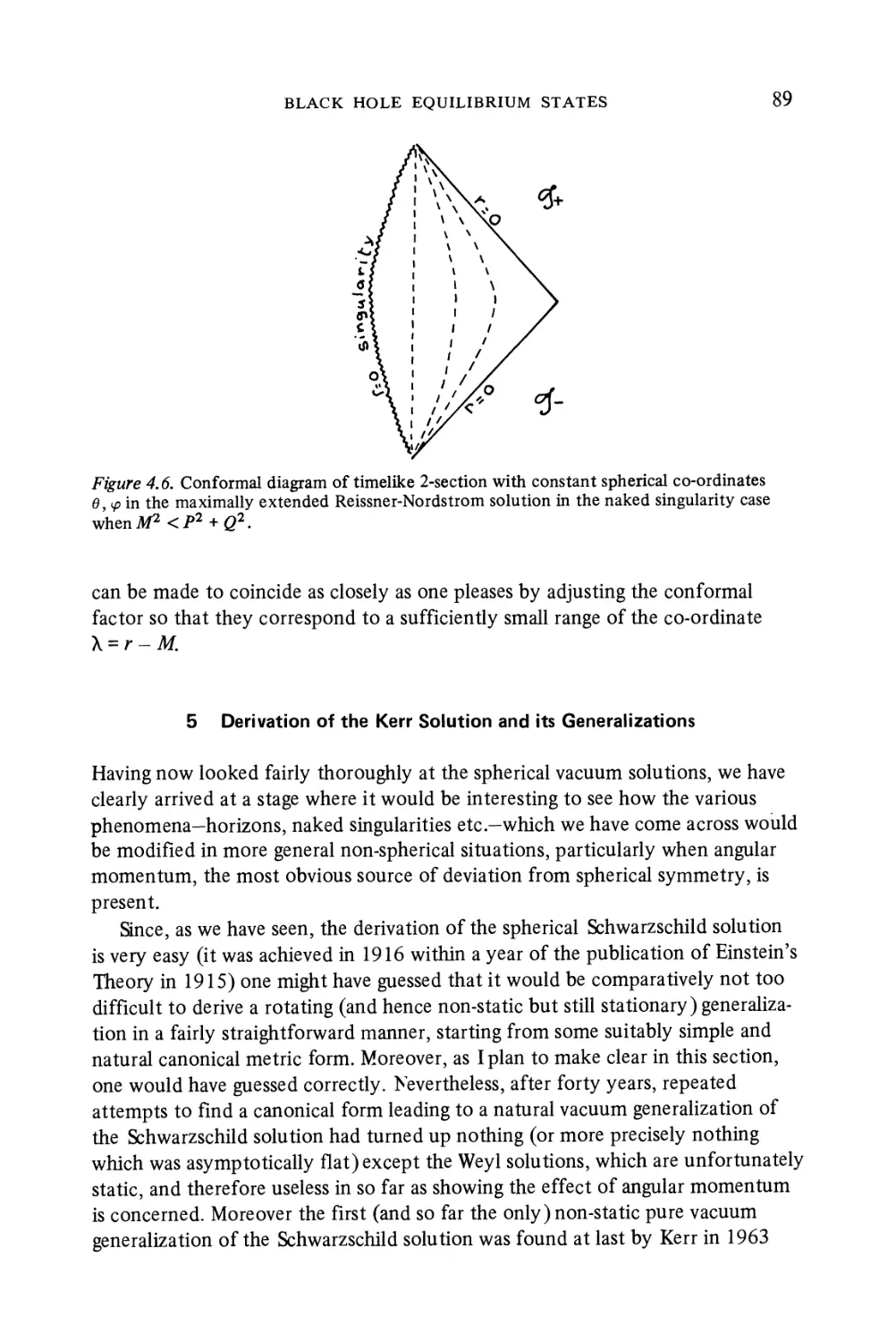
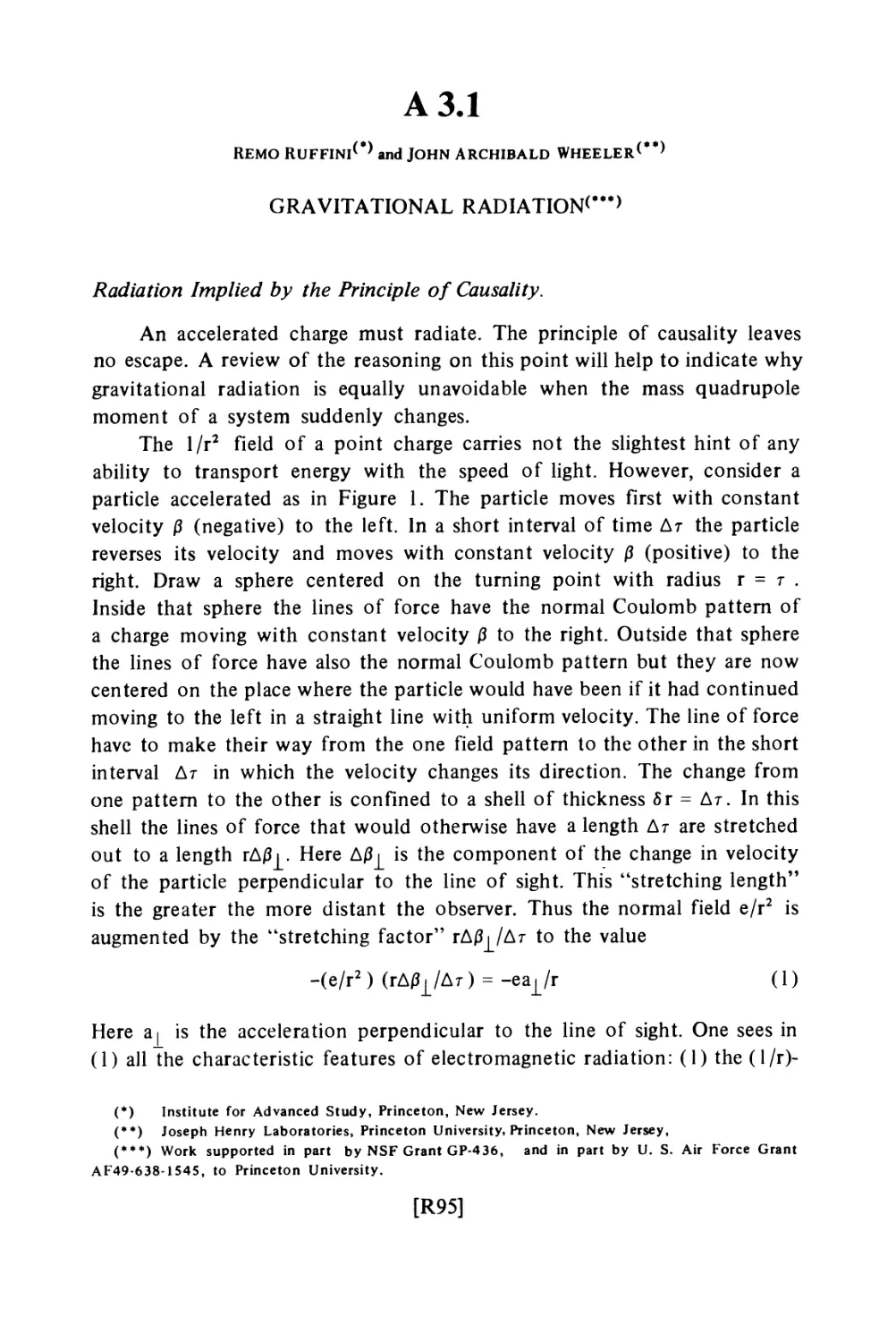
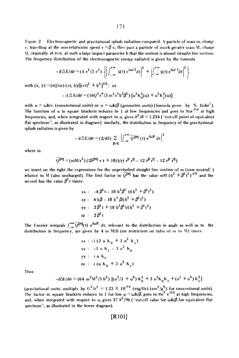
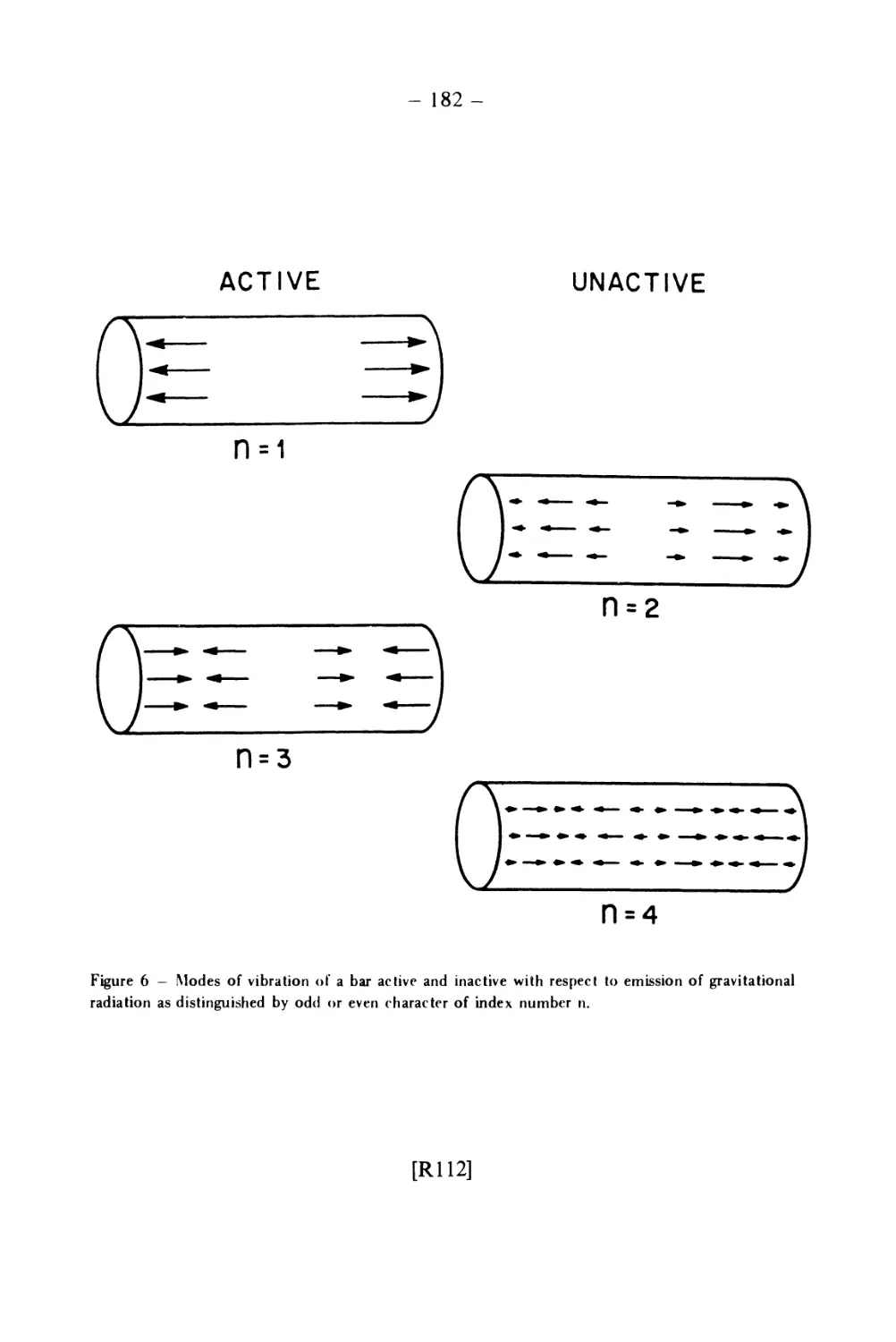
/


Text
Black Holes
Les Astres Occlus
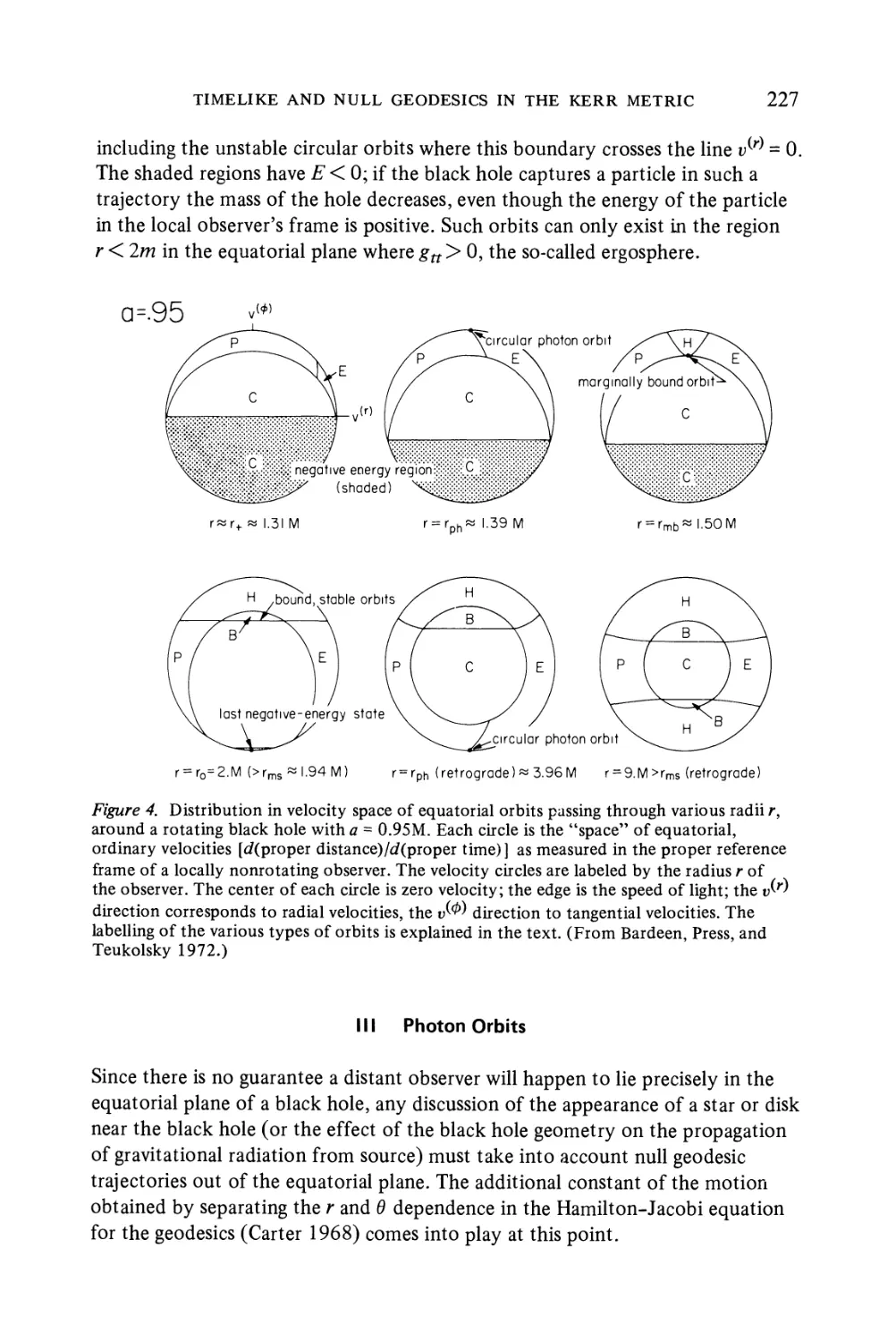
Universite Scientifique et Medicale et
Institut National Polytechnique de Grenoble
Ecole d'ete de Physique theorique Les H ouches
1951 Mecanique quantique. Theorie quantique des champs. (Polycopie) Epuise
1952 Quantum mechanics. Mecanique statistique. Chapitres de physique
nucleaire. (Polycopie) Epuise
1953 Quantum mechanics. Etat solide. Mecanique Statistique. Elementary
particles. (Polycopie) Epuise
1954 Mecanique quantique. Theorie des collisions; two-nucleon interaction.
Electrodynamique quantique. (Polycopie) Epuise
1955 Quantum mechanics. Non-equilibrium phenomena. Reactions nucleaires.
Interaction of a nucleus with atomic and molecular fields. (Polycopie)
Epuise
1956 Quantum perturbation theory. Low temperature physics. Quantum theory
of solids; dislocations and plastic properties. Magnetism; ferromagnetisme.
(Polycopie) Epuise
1957 Theorie de la diffusion; recent developments in field theory. Interaction
nucleaire; interactions fortes. Electrons de haute energie. Experiments in
high energy nuclear physics. (Polycopie) Epuise
1958 Le probleme a ? corps. Dunod, Wiley, Methuen
1959 La theorie des gaz neutres et ionises. Hermann, Wiley
1960 Relations de dispersion et particules elementaires. Hermann, Wiley
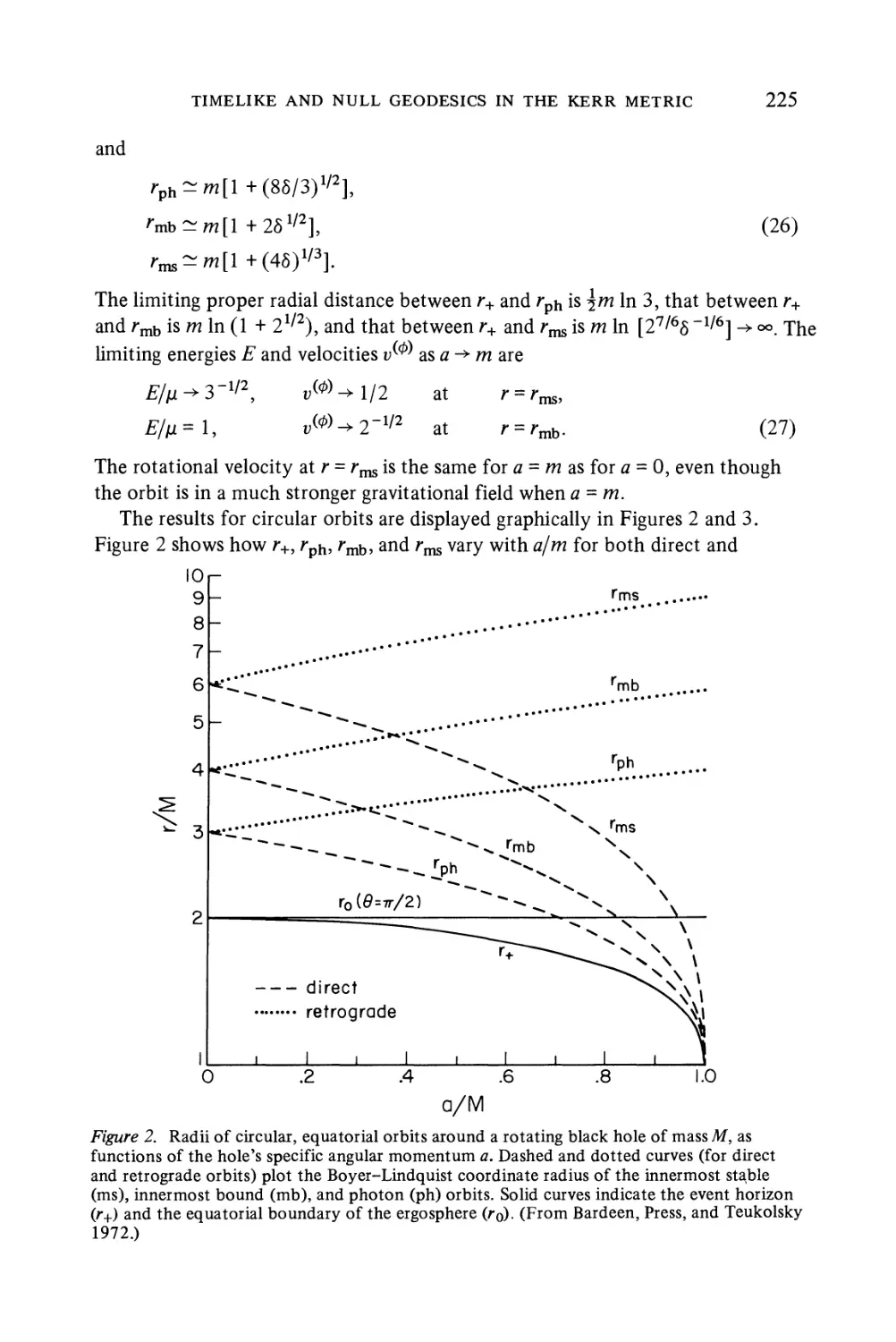
1961 La physique des basses temperatures. Low Temperature Physics. Gordon
and Breach, Presses Universitaires
1962 Geophysique exterieure. Geophysics: The Earth's Environment. Gordon
and Breach
1963 Relativite, groupes et topologie. Relativity, Groups and Topology. Gordon
and Breach
1964 Optique et electronique quantiques. Quantum Optics and Electronics.
Gordon and Breach
1965 Physique des hautes energies. High Energy Physics. Gordon and Breach
1966 Hautes energies en astrophysique. High Energy Astrophysics. Gordon and
Breach
1967 Probleme a N corps. Many-Body Physics. Gordon and Breach
1968 Physique Nucleaire. Nuclear Physics. Gordon and Breach
1969 Aspects physiques de quelques problemes biologiques. Physical Problems
in Biology. Gordon and Breach
1970 Mecanique statistique et theorie quantique des champs. Statistical
Mechanics and Quantum Field Theory. Gordon and Breach
1971 Physique des Particules. Particle Physics. Gordon and Breach
1972 Physique des Plasmas. Plasma Physics. Gordon and Breach
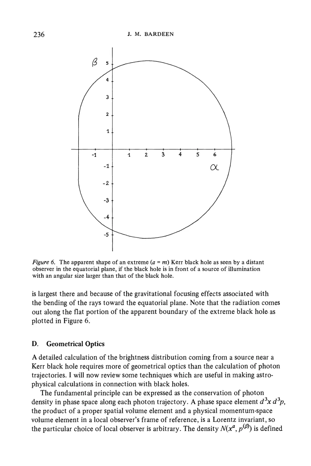
1972 Les Astres Occlus. Black Holes. Gordon and Breach
En preparation
1973 Hydrodynamique
1973 Liquides
1974 Physique Atomique et Moleculaire et Matiere Interstellaire
Les Houches, Aout 1972
Cours de l'Ecole d'ete de Physique theorique-
Organe d'interet commun de l'U.S.M.G.
et I.N.P.G. subventionne par l'OTAN et
le Commissariat a l'Energie Atomique
BLACK HOLES
LES ASTRES OCCLUS
edited by C. DeWitt
Faculte des Sciences, Grenoble
Dept. of Astronomy, University of Texas, Austin, et
B. S. DeWitt
Dept. of Physics, University of Texas, Austin
GORDON AND BREACH SCIENCE PUBLISHERS
New York London Paris
Copyright© 1973 by
Gordon and Breach Science Publishers, Inc.
One Park Avenue
New York, N.Y. 10016
Editorial office for the United Kingdom
Gordon and Breach Science Publishers Ltd.
42 William IV Street
London W.C.2
Editorial office for France
Gordon & Breach
7-9 rue Emile Dubois
Paris 14e
Library of Congress catalog card number Applied for. ISBN 0 677 15610 3. All
rights reserved. No part of this book may be reproduced or utilized in any form or by
any means, electronic or mechanical, including photocopying, recording, or by
any information storagj and retrieval system, without permission in writing from
the publishers. Printed in Greated Britain.
CONTENTS
Contributors .......... vi
Preface (English) .......... vii
Preface (Fran9ais) ......... ix
list of Participants ......... xi
S. W. HAWKING: The Event Horizon 1
B. CARTER: Black Hole Equilibrium States 57
J. M. BARDEEN: Timelike and Null Geodesies in the Kerr Metric. . 215
J. M. BARDEEN: Rapidly Rotating Stars, Disks, and Black Holes. . 241
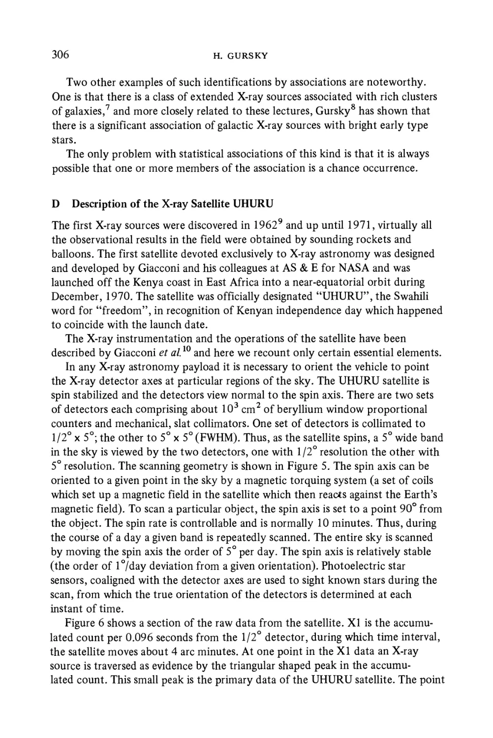
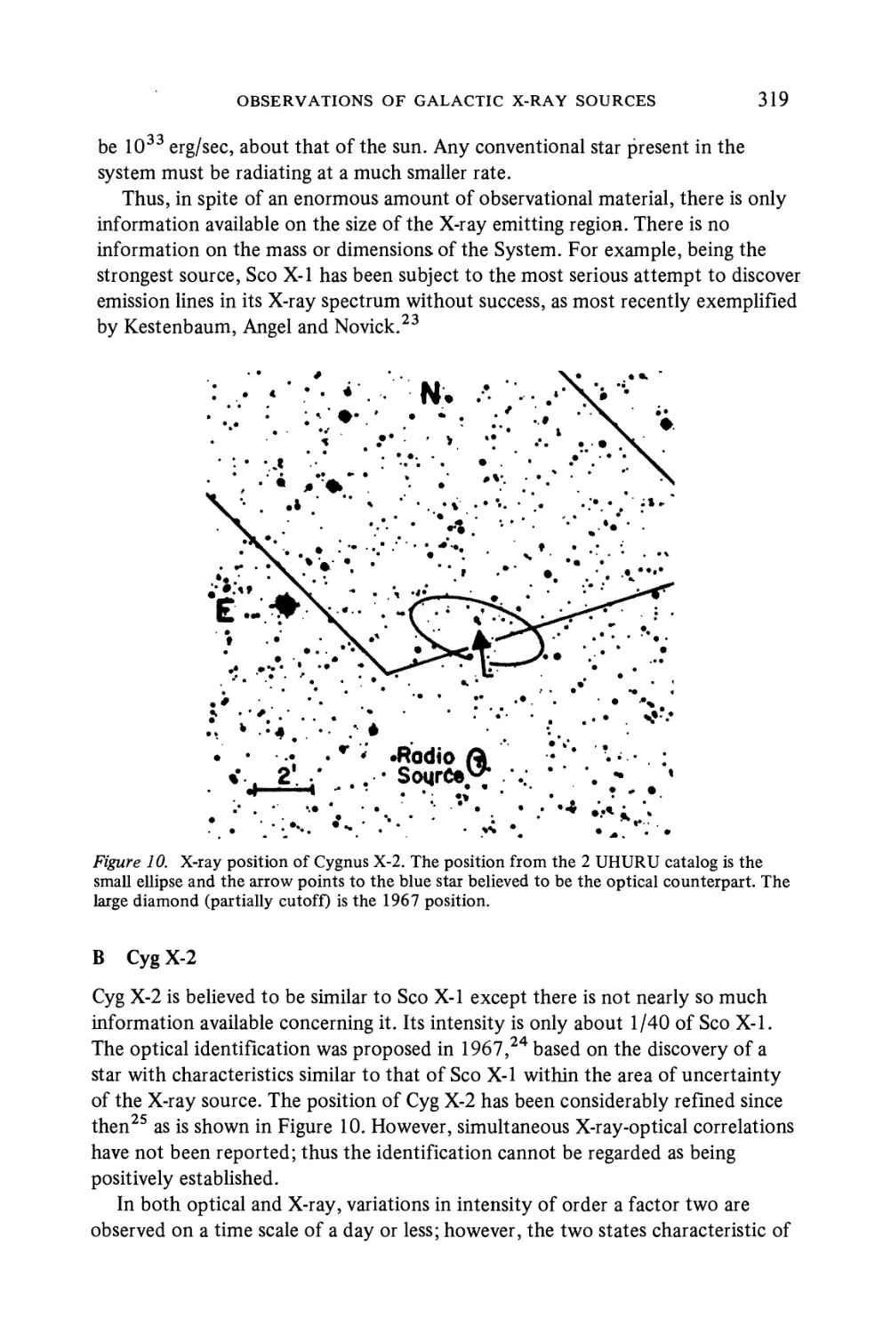
H.GUR SKY: Observations of Galactic X-ray Sources. ... 291
I. D. NOVIKOV and KL S. THORNE: Black Hole Astrophysics . . 343
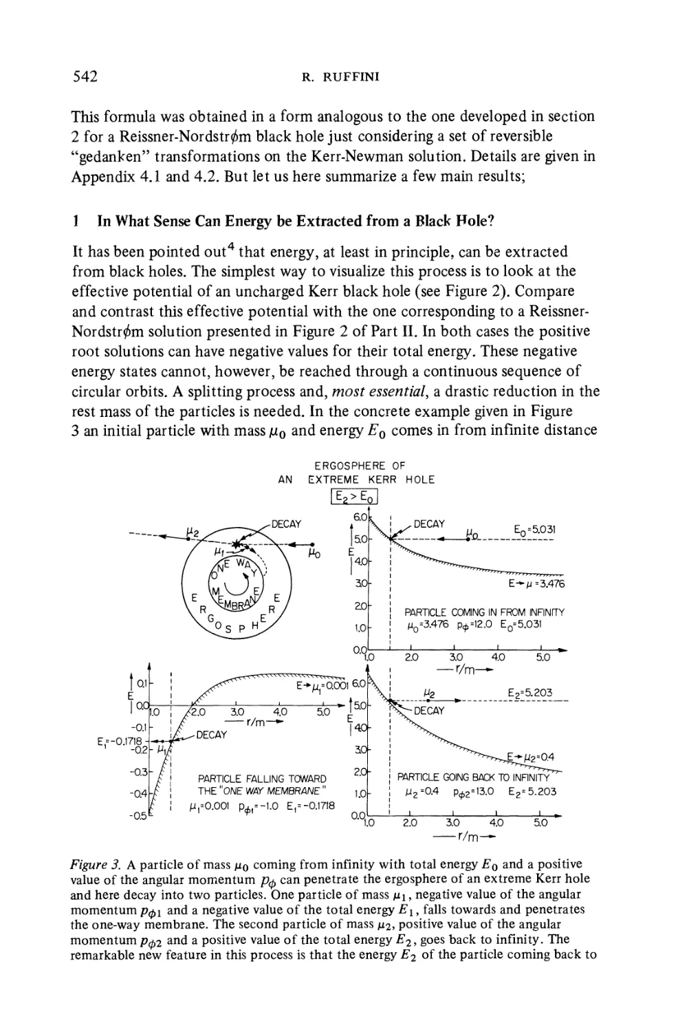
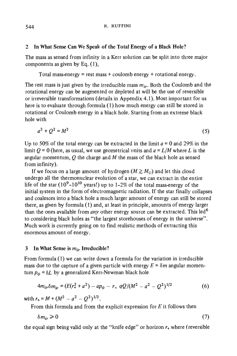
R. RUFFINI: On the Energetics of Black Holes. . . 451
Table of Contents 547
CONTRIBUTORS
J.M.BARDEEN
Yale University, New Haven, Conn.
B. CARTER
Institute of Astronomy, Cambridge
H. GURSKY
American Science and Engineering, Cambridge, Mass.
S.W. HAWKING
Institute of Astronomy, Cambridge
I.D.NOVIKOV
Institute of Applied Mathematics, Moscow
R. RUFFINI
Princeton University, Princeton, N.J.
K.S.THORNE
California Institute of Technology, Pasadena, Calif.
VI
PREFACE
The story of the phenomenal transformation of general relativity within little
more than a decade, from a quiet backwater of research, harboring a handful of
theorists, to a booming outpost attracting increasing numbers of highly talented
young people as well as heavy investment in experiments, is by now familiar.
The amazing thing about this revolution is that the physics is entirely classical.
But it is classical physics with a new twist. The student who embraces it must
learn to chart unfamiliar conceptual waters, where even the firmament of classical
fixed stars (energy conservation, causality, thermal equilibrium and entropy) has
become strangely distorted. That this revolution is yet far from having run its
course is clear from its classical nature. The quantum revolution is yet to come.
No single object or concept epitomizes more completely the present stage of
the revolution than the Black Hole. This volume, based on the lectures given at
the 23rd session of the Summer School of Les Houches, contains nearly every-
everything that is currently A972) known about black holes, and much that will remain
permanently useful to workers in the field. The contents, which are deliberately
pedagogical, begin with Hawking's masterful presentation of the fundamentals:
the definition of a black hole, event horizons, trapped surfaces, singularity
theorems, the area theorem, final state theorems. This is followed by Carter's
beautiful elaboration, with proofs, of the properties of Kerr-Newman and other
axisymmetric black holes: separability theorems, uniqueness theorems, variational
principles. Next comes a very detailed study by Bardeen of the properties of
timelike and null geodesies in the Kerr metric, of rapidly rotating stars, and of
extreme relativistic disks, illustrated by explicit computer results.
After this thorough theoretical introduction, the facts are brought on stage.
The data currently most likely to tell us whether black holes really do exist in
our universe are the X-ray data from the UHURU satellite. The article by Gursky
outlines the present status of X-ray astronomy, emphasizing the difficulties
of interpreting the data as well as the knowledge gained so far about the various
species of X-ray sources in the sky. Gursky presents the sober evidence placing
Cygnus X-l in the running as a prime candidate for black hole status. Then
comes a superb attempt at a grand synthesis. Starting with a pedagogical review
of the astrophysical processes relevant to black holes, Novikov and Thorne, in
one of the longest articles in the volume, deal successively with: accretion of inter-
interstellar gas onto an isolated black hole, with accompanying emission of optical and
ultraviolet radiation; accretion of gas onto a black hole from a companion star
in a close binary system, with accompanying emission of X-rays, ultraviolet and
optical radiation; and accretion of gas onto a supermassive black hole in the
nucleus of a galaxy, with accompanying emission of ultraviolet, optical, infrared
vii
and radio radiation. For the first time, explicit models are built that incorporate
the full general relativistic effects of the Kerr metric.
In the final chapter of this volume, Ruffini marshals most of the known results
on mass limits for neutron stars, radiation (both electromagnetic and gravitational)
emitted by single objects falling onto black holes, and general theory of the
energetics of black holes, including possible energy-extraction mechanisms.
Warmest thanks are due to the authors for the very many hours of preparation
and hard work that have made, first, the summer lectures and, finally, this
volume possible.
Cecile DeWitt
Bryce S. DeWitt
Vlll
PREFACE
L'histoire de la transformation prodigieuse de la Relativite Generale pendant
ces dix dernieres annees est chose connue; d'une baie tranquille ou quelques
theoriciens poursuivaient leurs recherches, elle est passee aux avant postes, en
pleine effervescence, qui attirent un nombre croissant de jeunes talents, ainsi
que de credits importants destines aux recherches experimentales. Et ce qui est
etonnant, c'est que cette explosion reste dans le cadre de la physique classique
— classique il est vrai quant a ses principes mais si nouvelle quant aux domaines
qu'elle explore que les principes classiques (conservation de l'energie,
causalite, equilibre thermique et entropie), ces etoiles fixes du physicien,
prennent un aspect etrangement nouveau avec lequel le navigateur doit se
familiariser pour determiner la route a suivre sur ces eaux inconnues. Et nous
n'en sommes qu'au debut du voyage, les phenomenes quantiques n'ont pas encore
ete abordes.
Plus que tout autre objet ou concept, les Astres occlusf sont l'epitome de
cette evolution. Ce volume a pour base les cours donnes a la 23eme session de
L'Ecole des Houches; ils contiennent presque tout ce qui est connu a l'heure
actuelle A972) sur les occlus; beaucoup en restera utile a ceux qui travaillent
dans ce domaine. Les exposes sont franchement pedagogiques; ils commencent
par la presentation, de main de maitre, par Hawking des notions et theoremes
fondamentaux: definition d'un occlus, de l'horizon des evenements, et, des
surfaces occlusives, theoremes de singularite, de surface, et, d'etats finaux. Cette
presentation est suivie de la belle elaboration de Carter sur les proprietes des
occlus Kerr-Newman et autres occlus a symmetrie axiale, ainsi que sur les
theoremes qui s'y rapportent: theoremes de separabilite, unicite, principes de
variation. Ensuite vient une etude tres detaillee faite par Bardeen sur les proprietes
des geodesiques temporelles et isotropes dans la metrique de Kerr, sur les
proprietes des etoiles a rotation rapide et des disques extremement relativistes;
cette etude est illustree par des resultats numeriques obtenus par ordinateurs.
Apres cette introduction theorique approfondie, les faits sont presentes sur la
scene. Les donnees actuelles les plus susceptibles de nous dire si les occlus
existent reellement dans notre univers sont celles des rayons X obtenues par le
satellite UHURU. L'article de Gursky schematise l'etat actuel de l'astronomie de
rayons X, et souligne les difficultes d'interpretation des donnees experimentales
tout en precisant les connaissances acquises sur les differentes sources de rayons X
t Apres de nombreuses discussions avec les specialistes de la question, l'expression "Astres
occlus" a semble la plus adequate compte tenu des proprietes de cet objet et de ses
denominations dans d'autres langues. "Trapped surface" devient ainsi surface occlusive
(quiproduit Pocclusion).
IX
dans le ciel. Gursky presente sobrement les indications suggerant la possibilite que
Cygnus X-l soit un occlus.
Vient ensuite, un essai de grande synthese: commencant par une revue pedagogique
des processus astrophysiques se rapportant aux occlus, Novikov et Thorne, dans
l'article le plus long de ce livre, traite successivement: la capture, par un occlus
isole, de gaz interstellaire, avec emission de rayonnement ultraviolet et optique;
la capture, par un occlus d'un systeme binaire, de gaz provenant de l'autre
composante du systeme, avec emission de rayonnement X, ultraviolet et optique;
la capture de gaz par un occlus supermassif dans le noyau d'une galaxie, avec
emission de rayonnement ultraviolet, optique et radio. Pour la premiere fois,
des modeles ont ete construits qui tiennent compte de tous les effets de
Relativite Generale presents dans la metrique de Kerr.
Pour terminer, Ruffini rassemble et classe presque tous les resultats connus
sur les masses limites des etoiles de neutrons, le rayonnement electromag-
electromagnetique et gravitationnel emis par un objet tombant dans un occlus, et la theorie
generale de l'energetique des occlus y compris les mecanismes possibles
d'extraction de l'energie.
Les remerciements les plus chaleureux sont dus aux auteurs pour les tres
longues heures de preparation et le lourd labeur, grace auxquels la session, puis
ce volume a pu etre realise.
Cecile DeWitt
Bryce S. DeWitt
LIST OF PARTICIPANTS
Abramowicz, Marek
Anile, Angelo
Bekenstein, Jacob D.
Bland, Roger W.
BREUER, Reinhard
CADEZ, Andrej
Cunningham
CHRISTENSEN, Steven M.
CHRZANOWSKI,Paul
Dem aret, Jacques
DEMIANSKI, Marek
DENARDO,Gallieno
Dyer, Charles C.
GlESSWEIN, Michael
GODDARD, Andrew J.
HAJICEK,Petr
Harrison, Bertrand K.
Hu,Bie-Lok
HUGHES, Henry G.
HUGHSTON,LaneP.
KALLM AN, Cerl-Gustav
MAGNON, AnneM.
MEINHARDT, Roberto
PERJES,Zoltan
PINEAULT, Serge
PRESS, William H.
QUINTANA,Hernan
Institut Astronomie, Varsovie
University Observatory, Oxford
Center for Relativity Theory, University of Texas,
Austin
Dept. of Natural Philosophy, University of
Glasgow
Int. fur Theoretische Physik II, Wurzburg
Fakult. Naravoslovje Technologijo, Ljubliana
Dept. Astronomy, University of Washington,
Seattle
Centre for Relativity Theory, University of Texas
Dept. Physics and Astronomy, University of
Maryland
Inst. Astrophysique, University of Liege
Inst. Physique theorique, Universitet Warszawskieg,
Warszawa
Inst. di Fisica Teorica, University of Trieste
Dept. of Astronomy, University of Toronto,
Toronto
Inst. Physique theorique, Vienne
University Observatory, Oxford
Inst. Physique Theorique, Berne
Dept. of Physics and Astronomy, Brigham Young
University, Provo, Utah
Jadwin Hall', Dept. Physics, Princeton University,
Princeton
1834 Marshall, Houston, Texas 77006, USA
1206 W. Louisiana, MacKinney, Texas 75069,
USA
Inst. for Pysik Abo Akademi, Porthansg 3-5
20500 ABO 50, Finlande
Dept. de Mathematiques, Universite de Clermont
Inst. Physique theorique, Hamburg
Central Research Inst. for Physics, Budapest
Dept. of Astronomy, University of Toronto,
Toronto
California Inst. of Technology, Pasadena
Inst. of Theor. Astronomy, Cambridge
xi
Rakavy, Gideon
Rasband, S. Neil
ROSS, Dennis K.
Schneider, Jean
SlLVESTRO, Giovanni
SMARR, Larry
SOBOUTI, Yousef
SOMMERS,PaulD.
STREUBEL, Michael
TEITELBOIM, Claudio
TEUKOLSKY,SaulA.
TOD, Kenneth P.
TREVES, AldoRenato
TSIANG, Elaine
VANDERMOLEN, Jean-Claude
Van Nieuwhenhuizen,P.
Walker, Martin A.
WILKINS, Daniel C.
WILL, Clifford M.
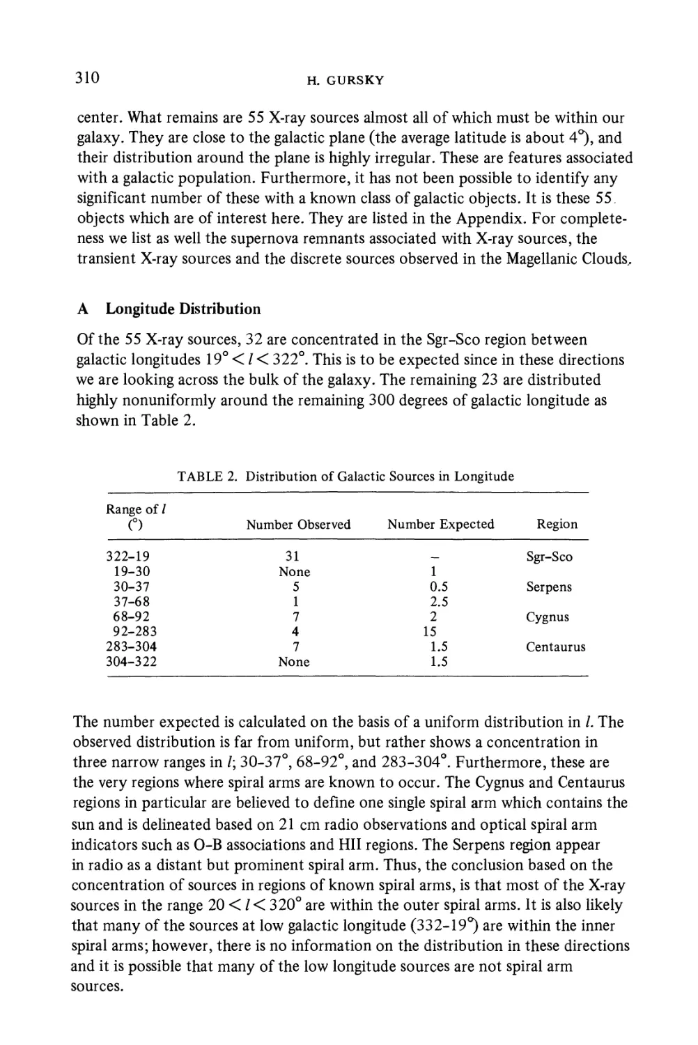
WOODHOUSE, Nicholas
Hebrew University, Jerusalem
Dept. of Physics, Brigham Young University,
Provo,Utah
Physics Dept., Iowa State University, Ames
Dept. d'Astronomie Fondamentale, Observatoire
de Meudon
1st. di Fisica Generale, Universita di Torino,
Turin
Center for Relativity Theory, University of
Texas, Austin
Physics Dept. University of Pahlavi, Shiraz
Center for Relativity Theory, University of
Texas, Austin
Inst. Physique theorique, Hamburg
Joseph Henry Laboratories, Princeton University,
Princeton
California Inst. of Technology, Pasadena
University Observatory, Oxford
1st. di Fisica dell'Universita di Milano, Milan
Center for Relativity Theory, University of
Texas, Austin
Inst. d'Astronomie et Geophysique, G. Lemaire
Kardinaal Mercierlaan, Louvain
Lab. Physique theorique et Hautes Energies,
Universite Paris, Orsay
Inst. Max Planck Physik und Astrophysik,
Munchen
Dept. of Physics, Stanford University, Stanford
Dept. of Physics, California Inst. of Technology,
Pasadena
University of London, King's College, London
Xll
The Event Horizon
Stephen W. Hawking
institute of Astronomy
Cambridge, Great Britain
This page intentionally left blank
Contents
Introduction . 5
1 Spherically Symmetric Collapse ....... 6
2 Nonspherical Collapse . . . . . . . . .11
3 Conformal Infinity . . . . . . . . .13
4 Causality Relations . . . . . . . . .16
5 The Focusing Effect 20
6 Predictability 24
7 Black Holes 29
8 The Final State of Black Holes 37
9 Applications .......... 44
A Energy Limits ......... 44
? Perturbations of Black Holes ....... 46
C Time Symmetric Black Holes . . . . . . .51
References ........... 54
This page intentionally left blank
Introduction
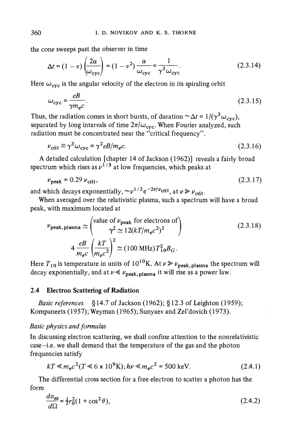
We know from observations during eclipses and radio measurements of quasars
passing behind the sun that light is deflected by gravitational fields. One would
therefore imagine that if there were a sufficient amount of matter in a certain
region of space, it would produce such a strong gravitational field that light
from the region would not be able to escape to infinity but would be "dragged
back". However one cannot really talk about things being dragged back in
general relativity since there are not in general any well defined frames of
reference against which to measure their progress. To overcome this difficulty
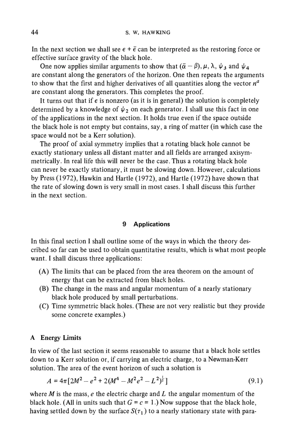
one can use the following idea of Roger Penrose. Imagine that the matter is
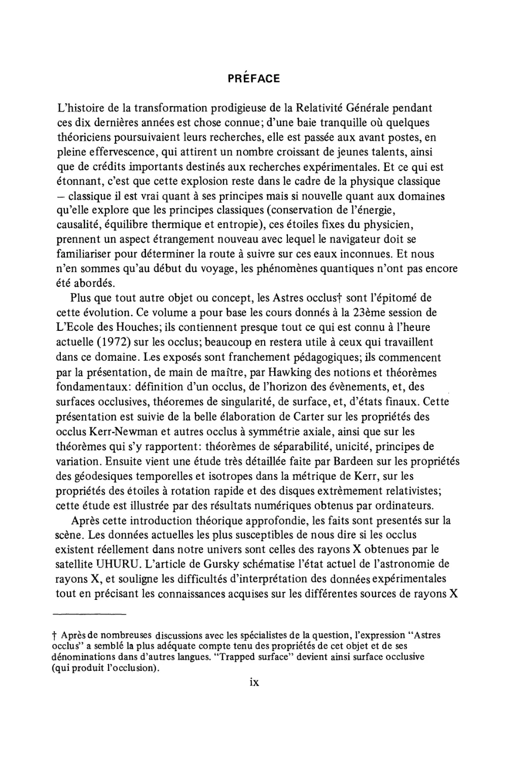
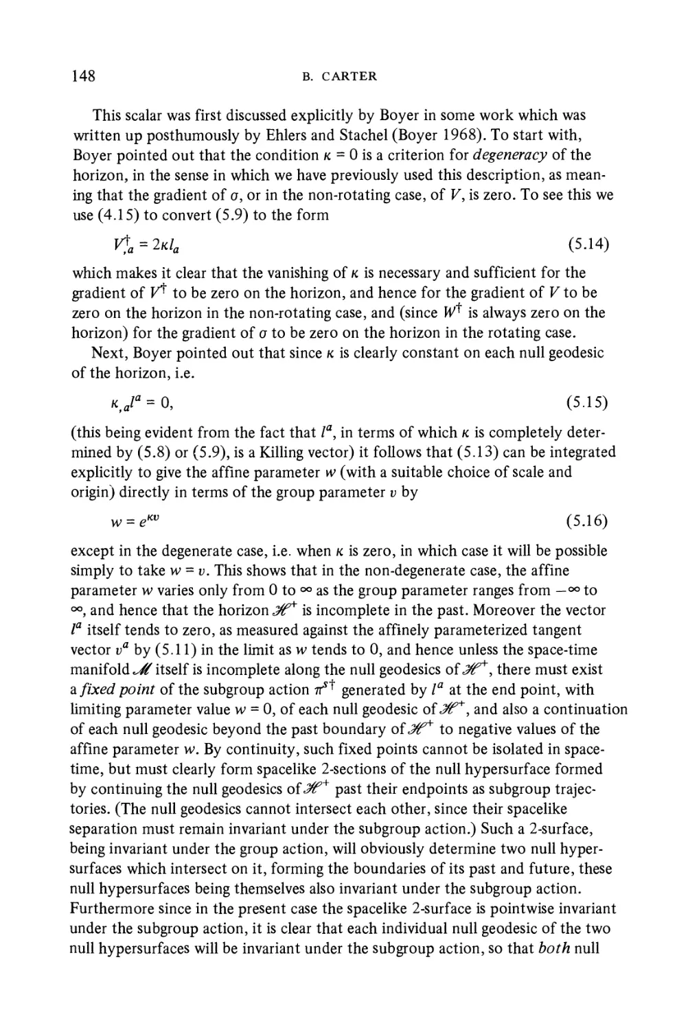
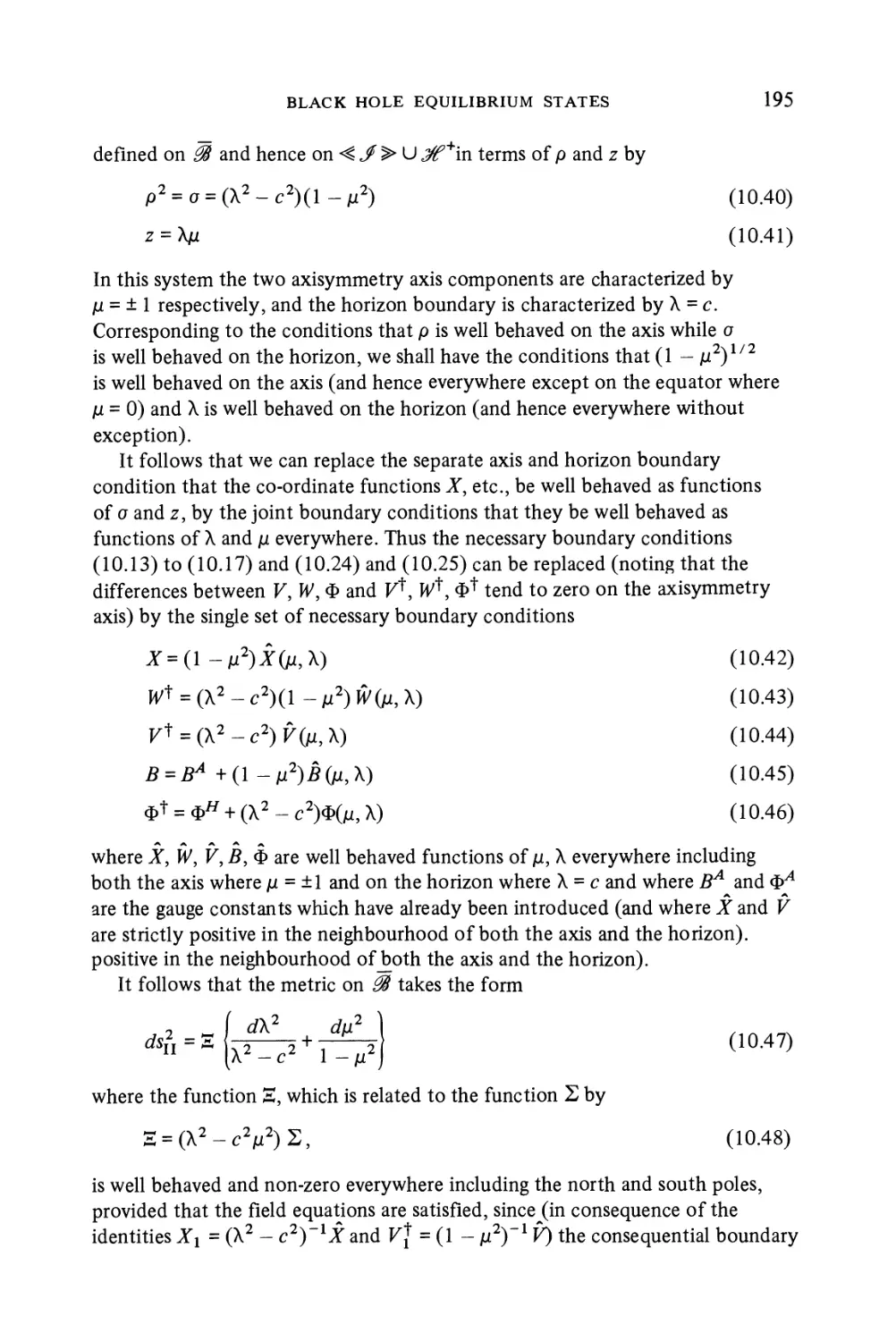
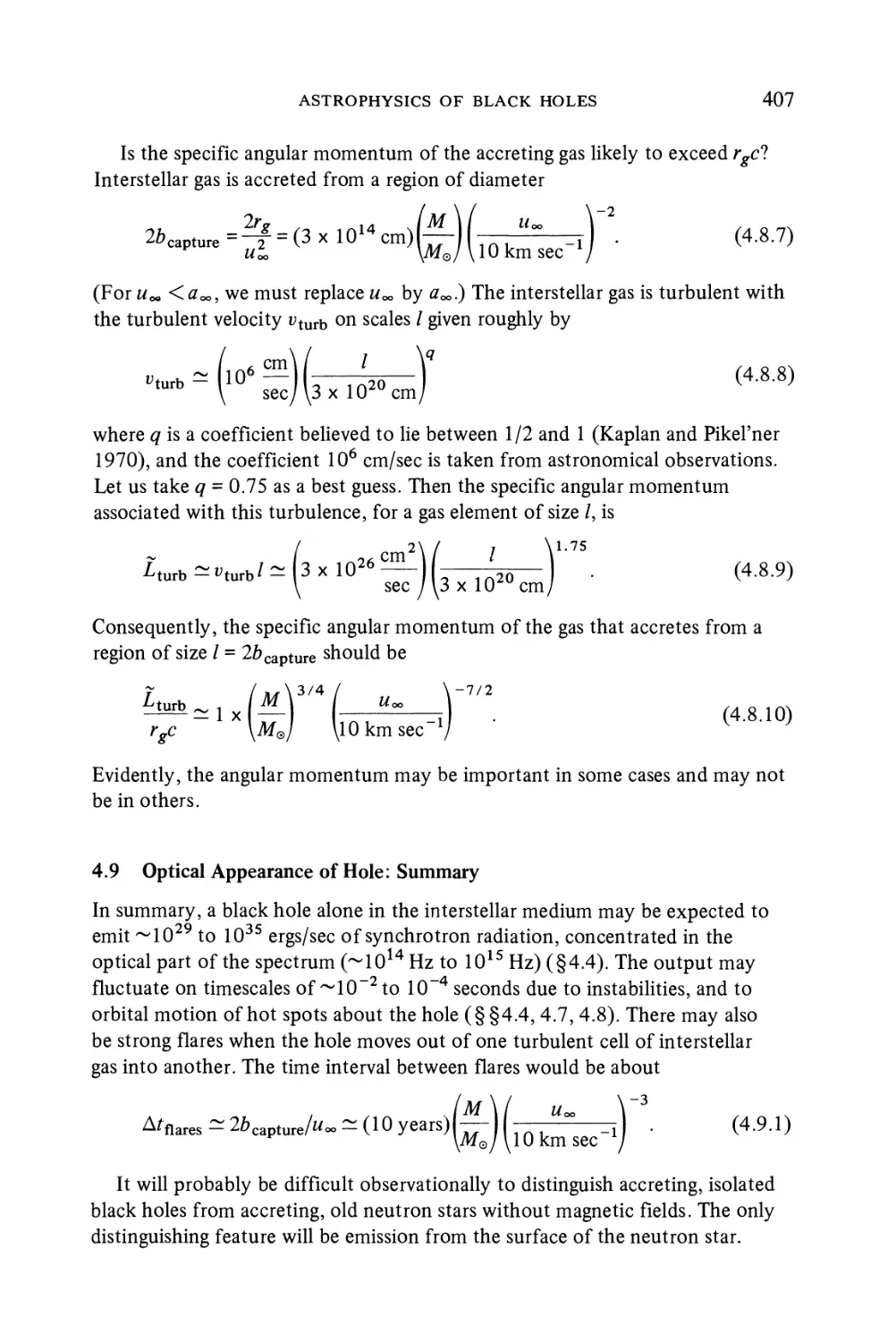
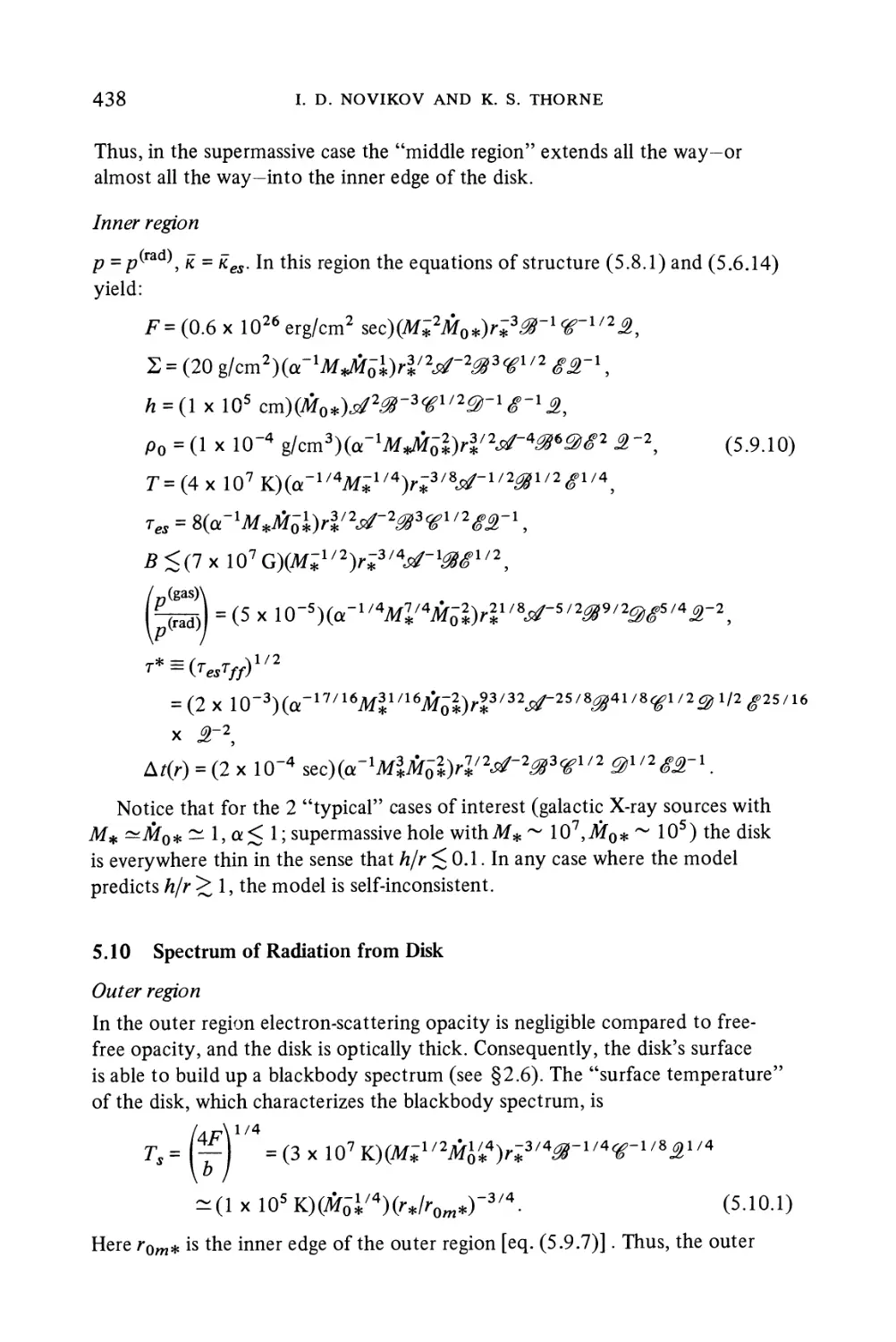
transparent and consider a flash of light emitted at some point near the centre
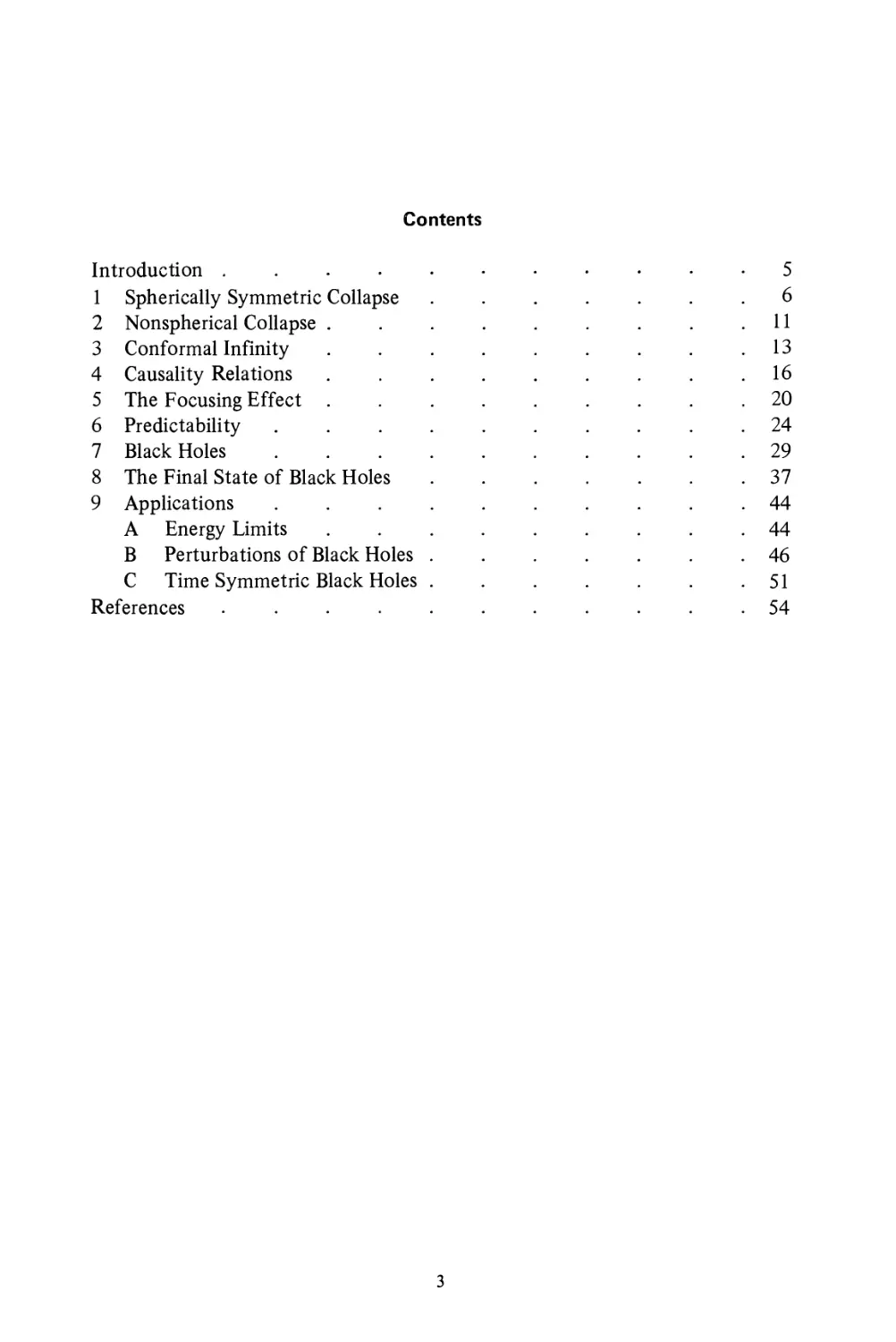
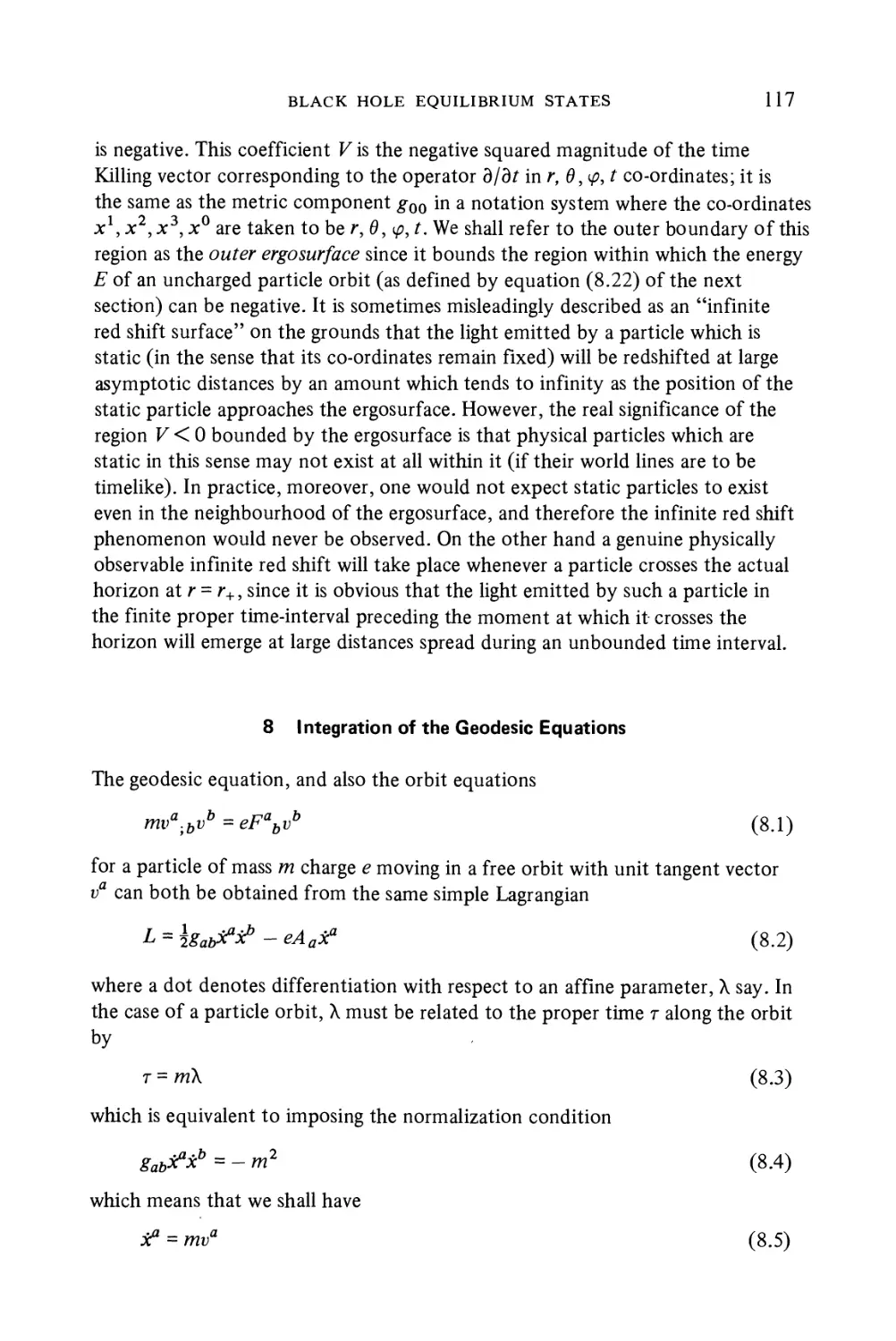
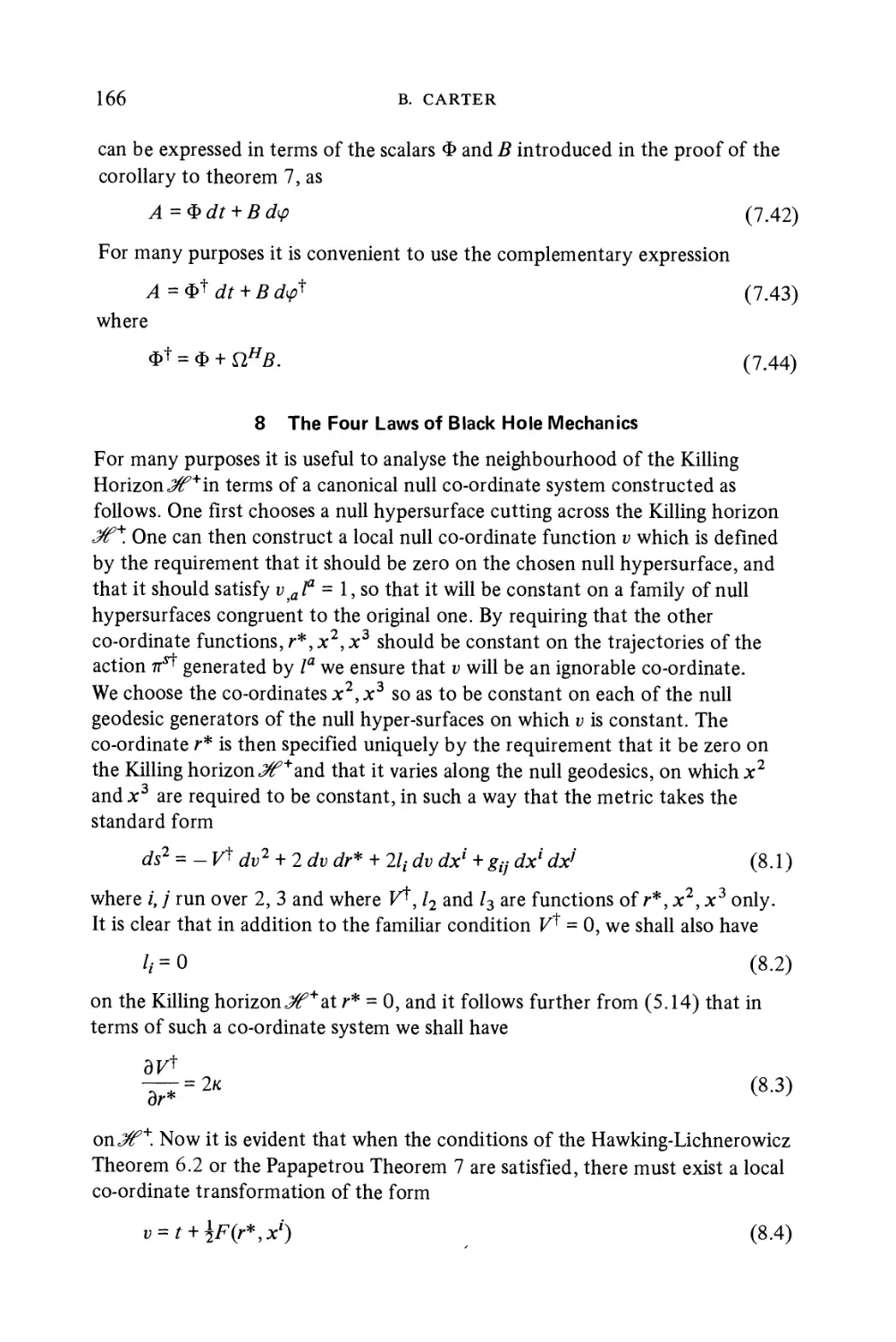
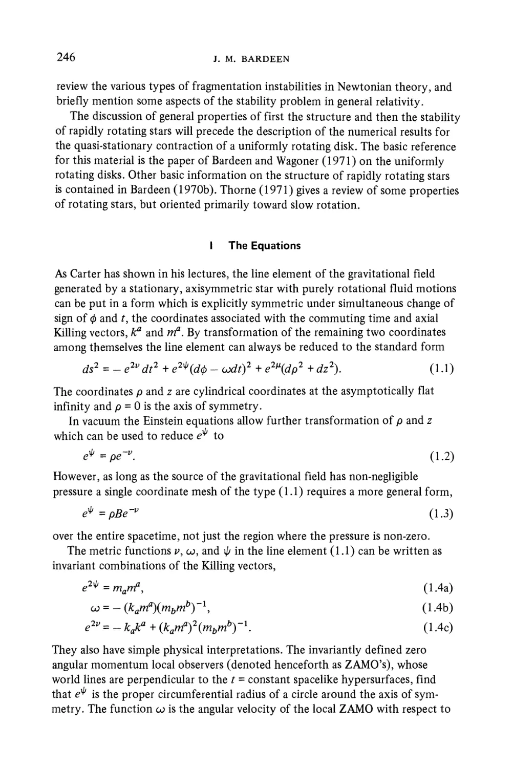
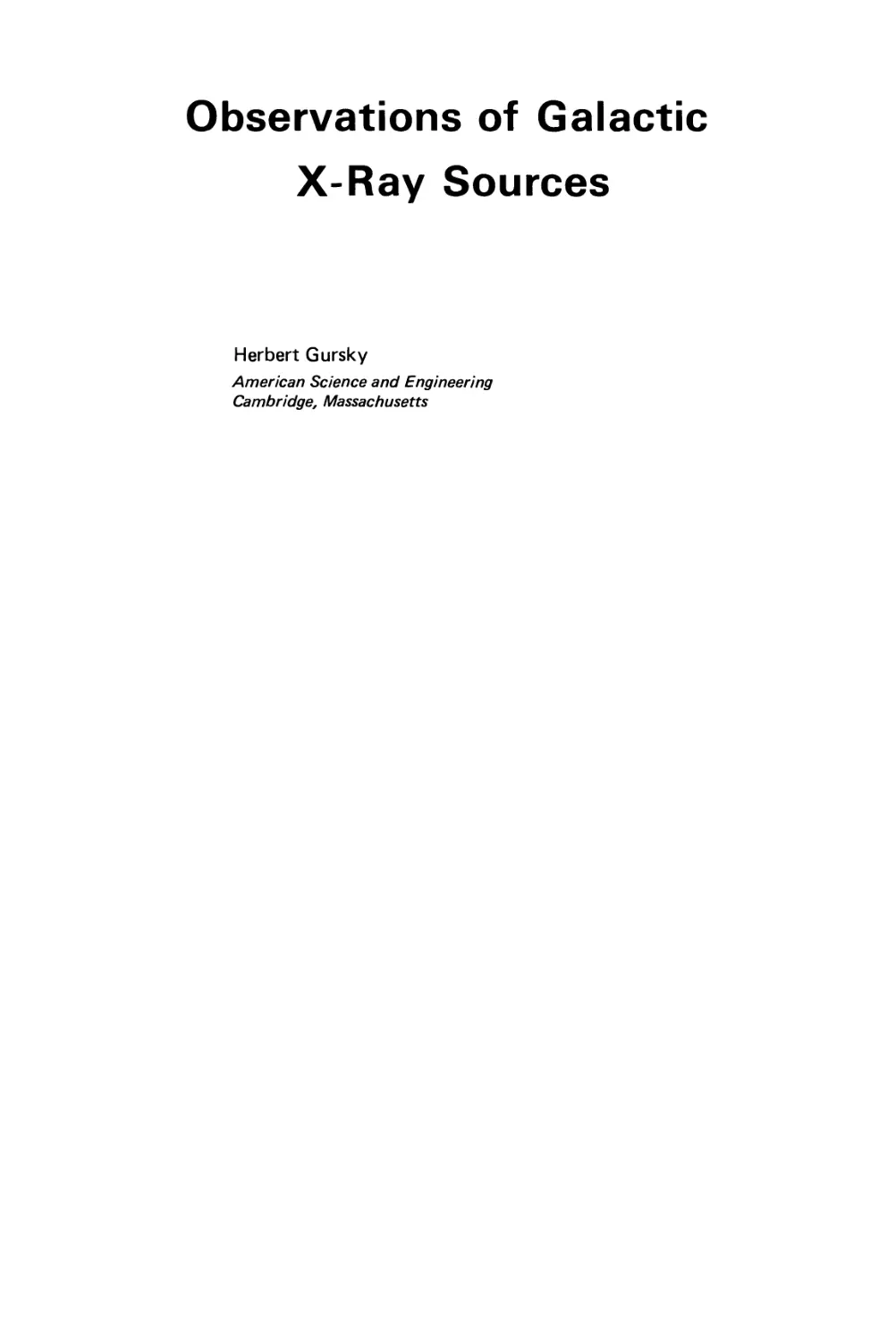
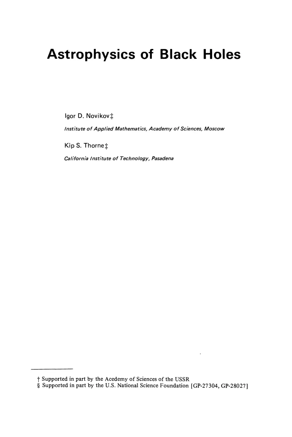
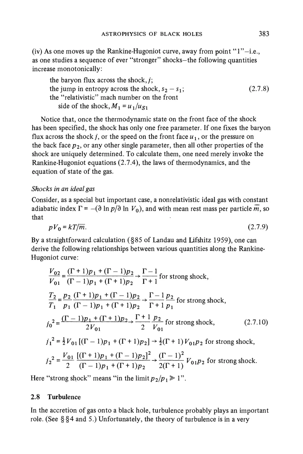
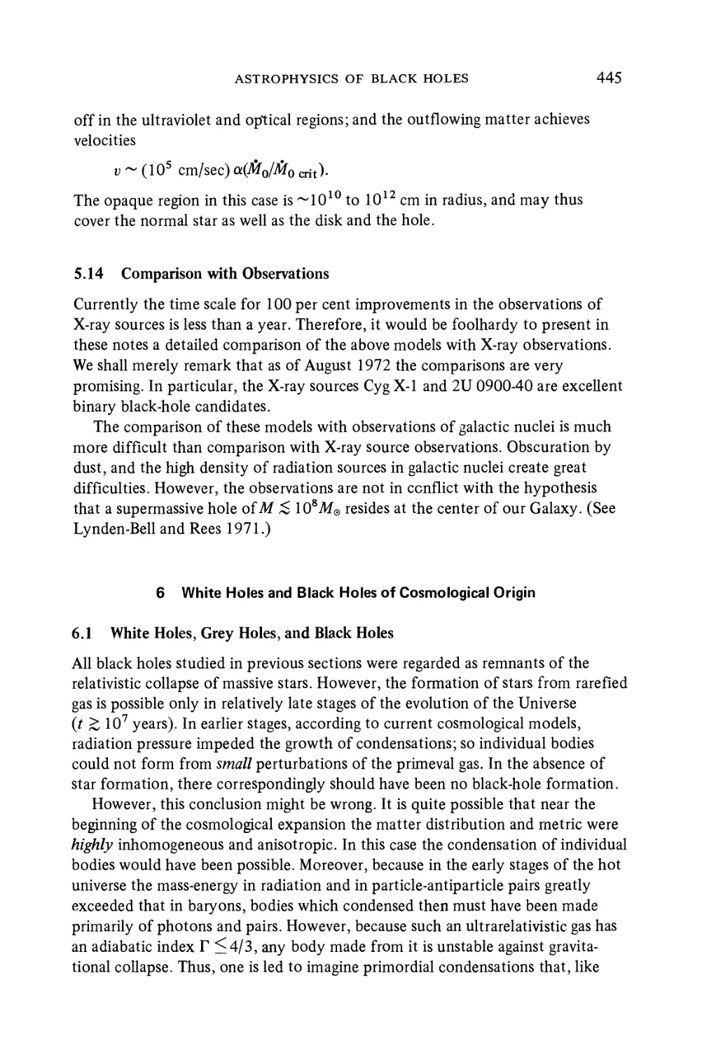
of the region. As time passes, a wave front will spread out from the point (Figure
1). At first this wave front will be nearly spherical and its area will be proportional
4—TRAPPED SURFACE AREA
OF WAVEFRONT DECREASING
<3— AREA OF WAVEFRONT
REACHES A MAXIMUM
TIME
SPACE
AREA OF WAVEFRONT
INCREASING
FLASH OF LIGHT EMITTED
Figure 1. The wavefront from a flash of light being focused and dragged back by a strong
gravitational field.
to the square of the time since the flash was emitted. However the gravitational
attraction of the matter through which the light is passing will deflect neighbouring
rays towards each other and so reduce the rate at which they are diverging from
each other. In other words, the light is being focused by the gravitational effect
of the matter. If there is a sufficient amount of matter, the divergence of neigh-
neighbouring rays will be reduced to zero and then turned into a convergence. The area
of the wave front will reach a maximum and start to decrease. The effect of
passing through any more matter is further to step up the rate of decrease of the
area of the wave front. The wave front therefore will not expand and reach
infinity since, if it were to do so, its area would have to become arbitrarily large.
Instead, it is "trapped" by the gravitational field of the matter in the region.
5
6 S. W. HAWKING
We shall take this existence of a wave front which is moving outward yet
decreasing in area as our criterion that light is being "dragged back". In fact
it does not matter whether or not the wave front originated at a single point.
All that is important is that it should be a closed (i.e. compact) surface, that
it should be outgoing and that at each point of the wavefront neighbouring
rays should be converging on each other. In more technical language, such a wave
front is a compact space like 2-surface [without edges] such that the family of
outgoing future-directed null geodesies orthogonal to it is converging at each
point of the surface. I shall call this an outer trapped surface (or simply, a trapped
surface). This differs from Penrose's definition (Penrose, 1965a) in that he
required the ingoing future-directed null geodesies orthogonal to the surface to
be converging as well. The behaviour of the ingoing null geodesies is of importance
in proving the occurrence of a spacetime singularity in the trapped region. However,
in this course we are primarily interested in what can be seen by observers at a
safe distance. Modulo certain reservations which will be discussed in section 2, the
existence of a closed outgoing wave front (or null hypersurface) which is
decreasing in area implies that information about what happens behind the
wavefront cannot reach such observers. In other words, there is a region of
spacetime from which it is not possible to escape to infinity. This is a black hole.
The boundary of this region is formed by a wavefront or null hypersurface which
just does not escape to infinity; its rays are asymptotically parallel and its area is
asymptotically constant. This is the event horizon.
To show how event horizon and black holes can occur I shall now discuss the
one situation that we can treat exactly, spherical symmetry.
1 Spherically Symmetric Collapse
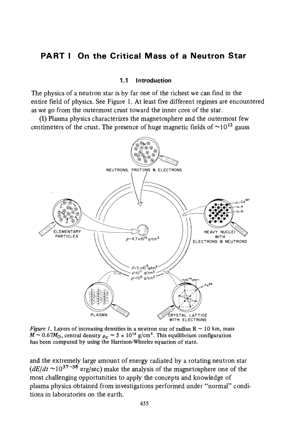
Consider a non-rotating star. After its formation from an interstellar gas cloud,
there will be a long period (\09-\011 years) in which it will be in an almost
stationary state burning hydrogen into helium. During this period the star will
be supported against its own gravity by thermal pressure and will be spherically
symmetric. The metric outside the star will be the Schwarzschild solution-the
only empty spherically symmetric solution
ds2 = (l - ^ J dt2 - (l - 7^) l dr2 - r2 {??2 + sin2 ???2) A.1)
This is the form of the metric for r greater than some value r0 corresponding to
the surface of the star. For r < r0 the metric has some different forms depending
on the distribution of density in the star. The details do not concern us here.
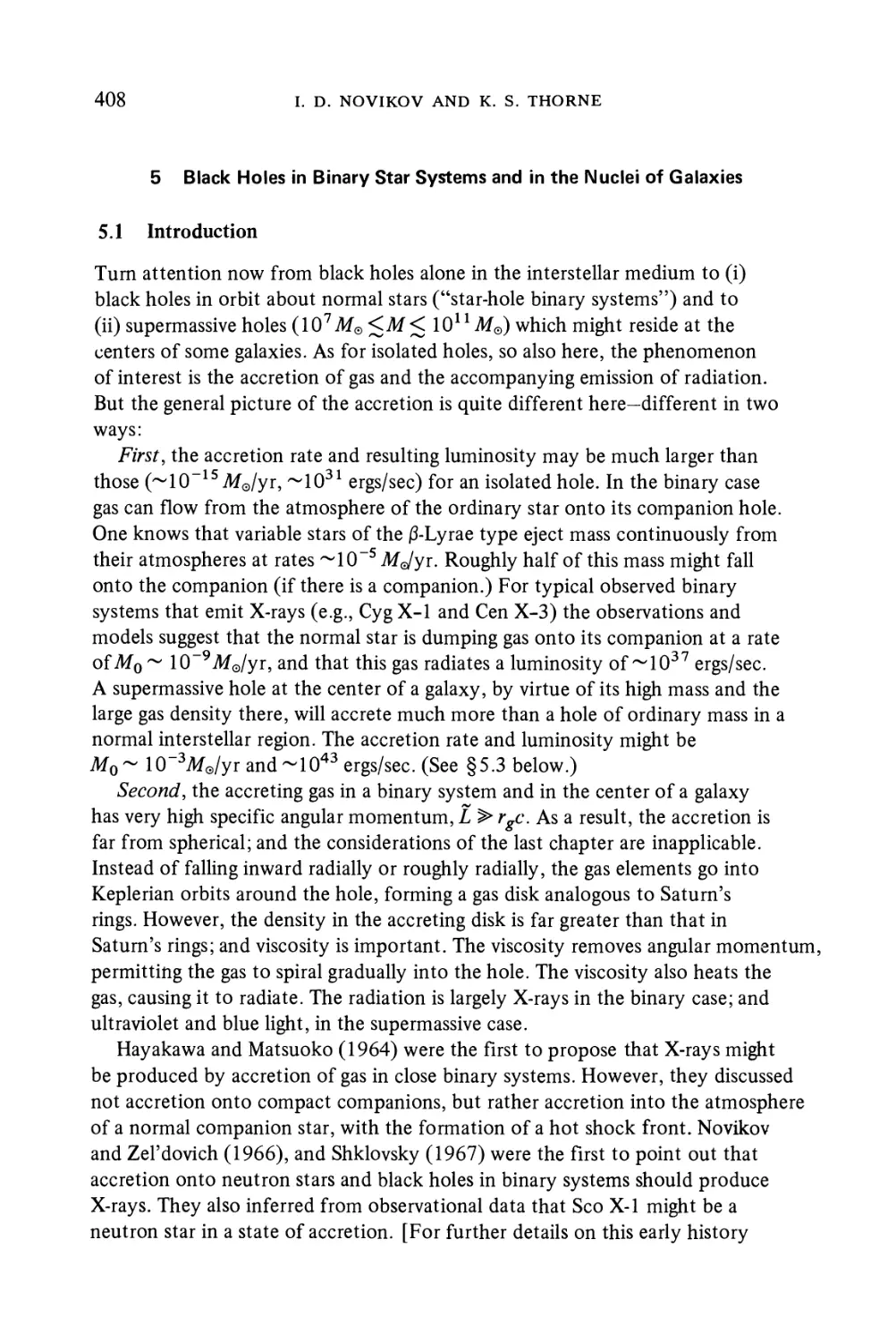
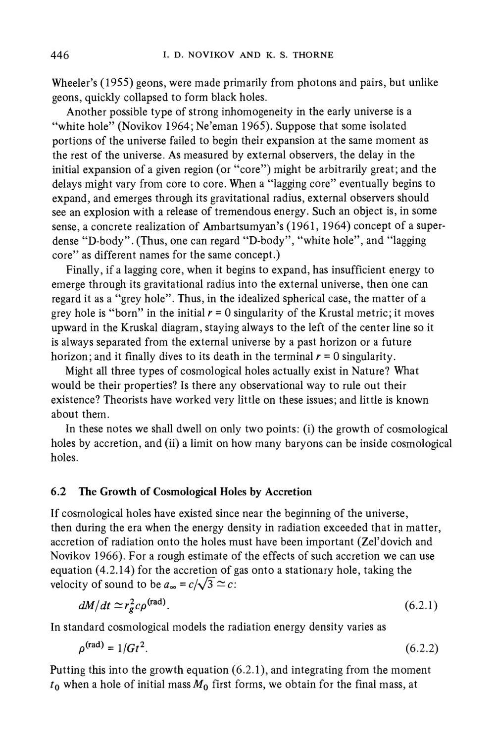
THE EVENT HORIZON 7
When the star has exhausted its nuclear field, it begins to lose its thermal
energy and to contract. If the mass ? is less than about 1.5-2??, this con-
contraction can be halted by degeneracy pressure of electrons or neutrons resulting
in a white dwarf or neutron star respectively. If, on the other hand, ? is greater
than this limit, contraction cannot be halted. During this spherical contraction
the metric outside the star remains of the form A.1) since this is the only
spherically symmetric empty solution. There is an apparent difficulty when the
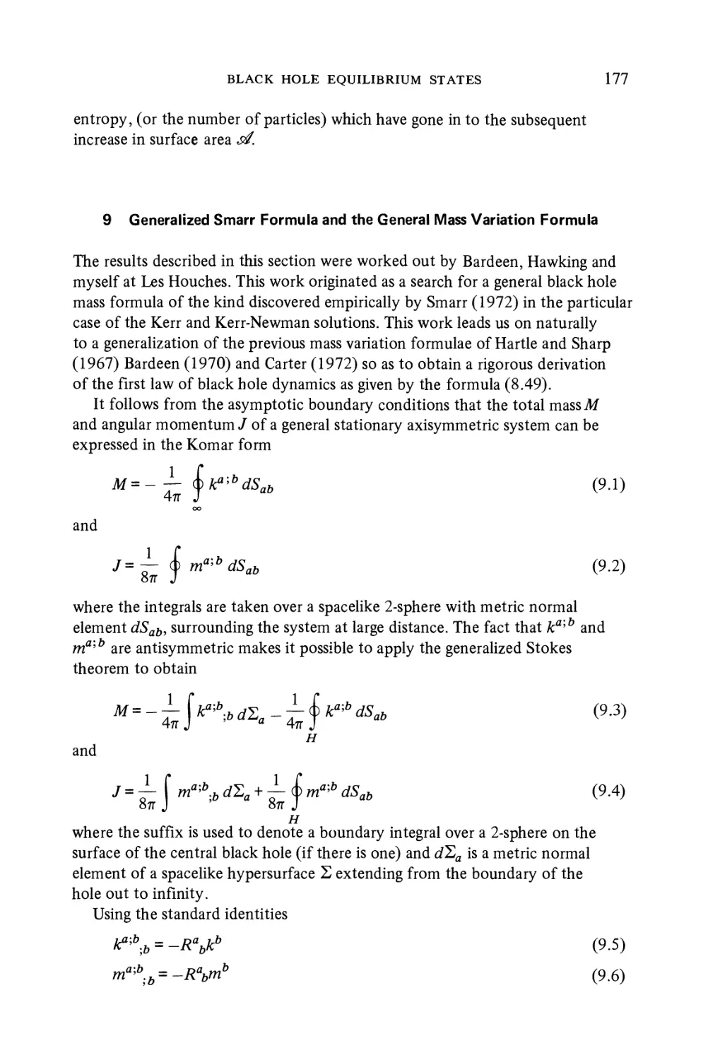
surface of the star gets down to the Schwarzschild radius r = 2M since the metric
A.1) is singular there. This however is simply because the coordinate system
goes wrong here. If one introduces an advanced time coordinate ? defined by
A.2)
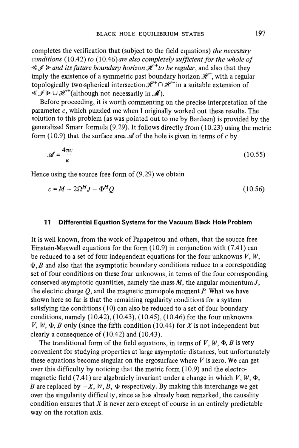
the metric takes the Eddington-Finkelstein form
= h _ — \dv2 _ 2dvdr - r2(dd2 + sin2fld02) A.3)
This metric is perfectly regular at r = 1M but still has a singularity of infinite
curvature at r = 0 which cannot be removed by coordinate transformation. The
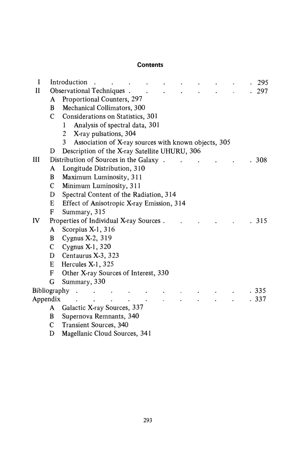
orientation of the light-cones in this metric is shown in Figure 2. At large values
of r they are like the light-cones in Minkowski space and they allow a particle or
photon following a nonspacelike (i.e., timelike or null) curve to move outwards
or inwards. As r decreases the light-cones tilt over until for r < ?? all nonspacelike
curves necessarily move inwards and hit the singularity at r = 0. At r = 2M all non-
nonspacelike curves except one move inwards. The exception is the null geodesic
r, ?, ? constant which neither moves inwards nor outwards. From this behaviour
it follows that light emitted from points with r > 7M can escape to infinity
whereas that from r<2M cannot. In particular the singularity at r = 0 cannot
be seen by observers who remain outside r = 1M. This is an important feature
about which I shall have more to say later.
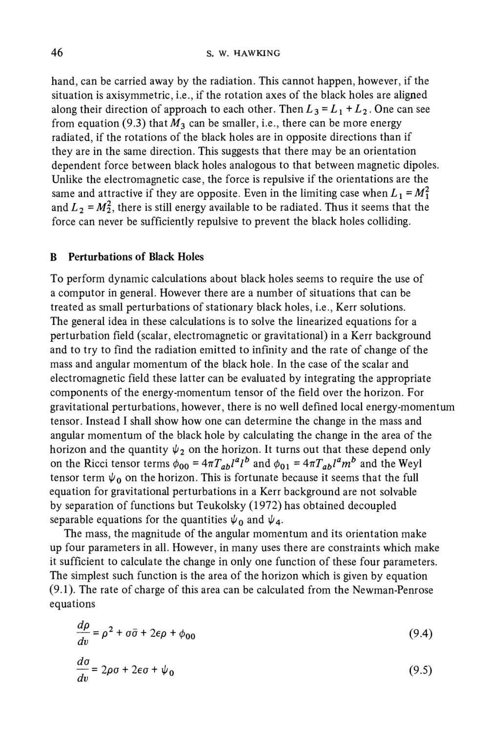
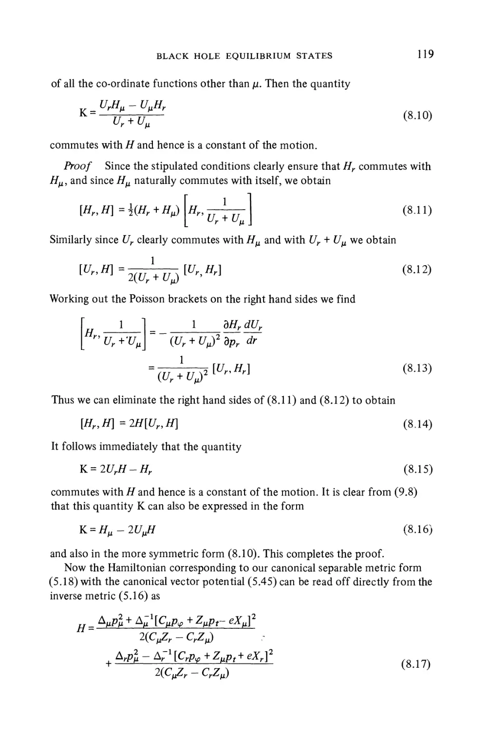
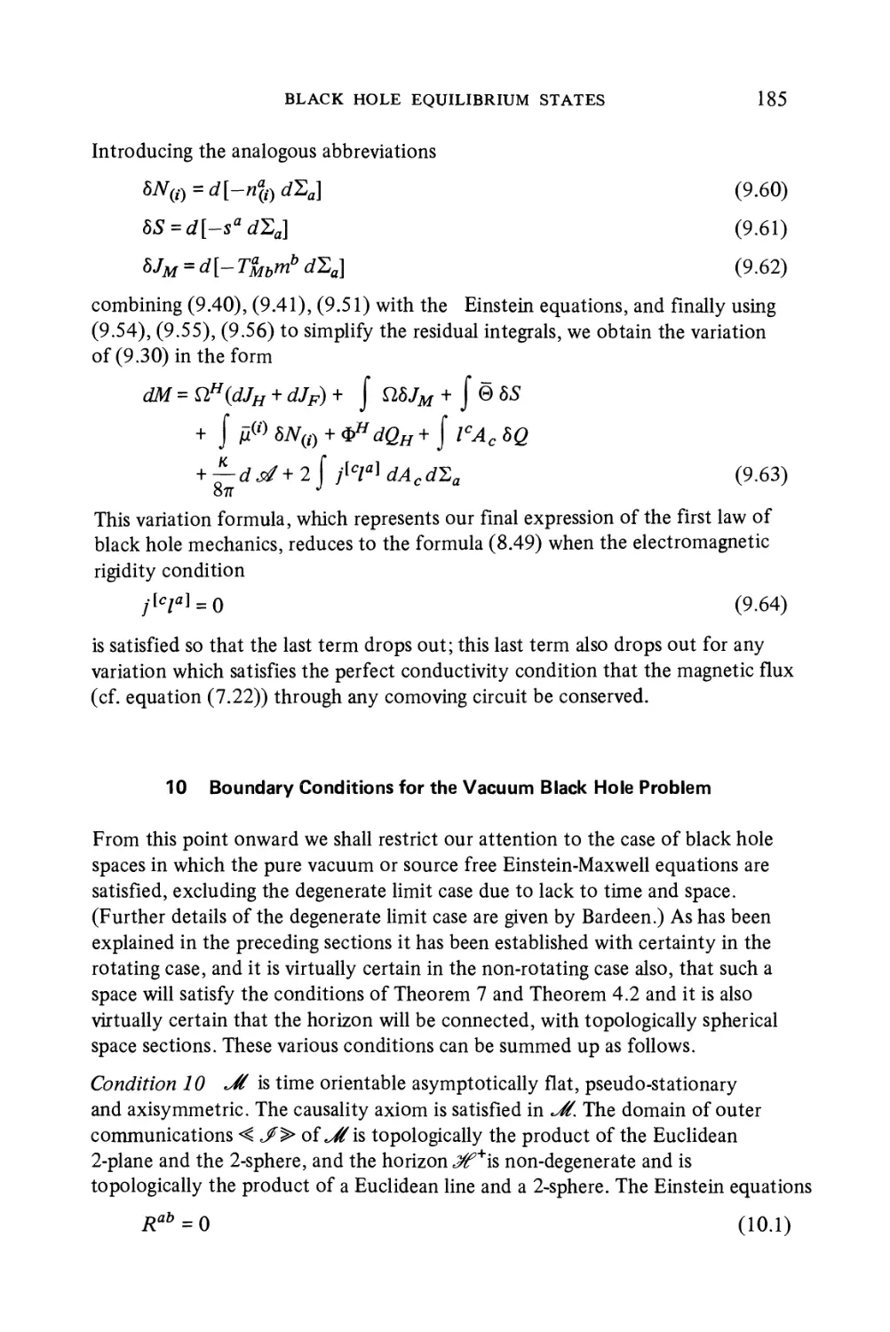
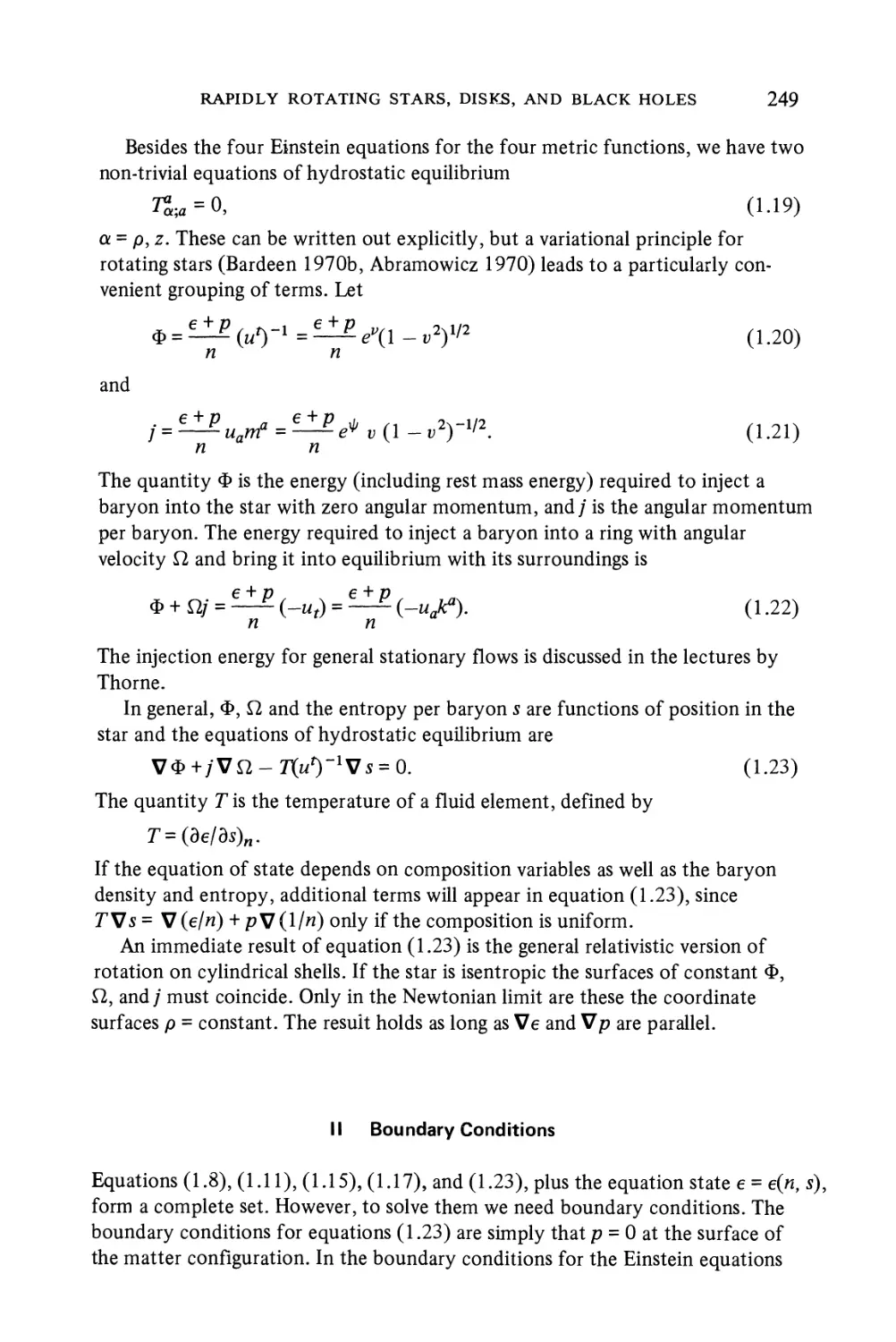
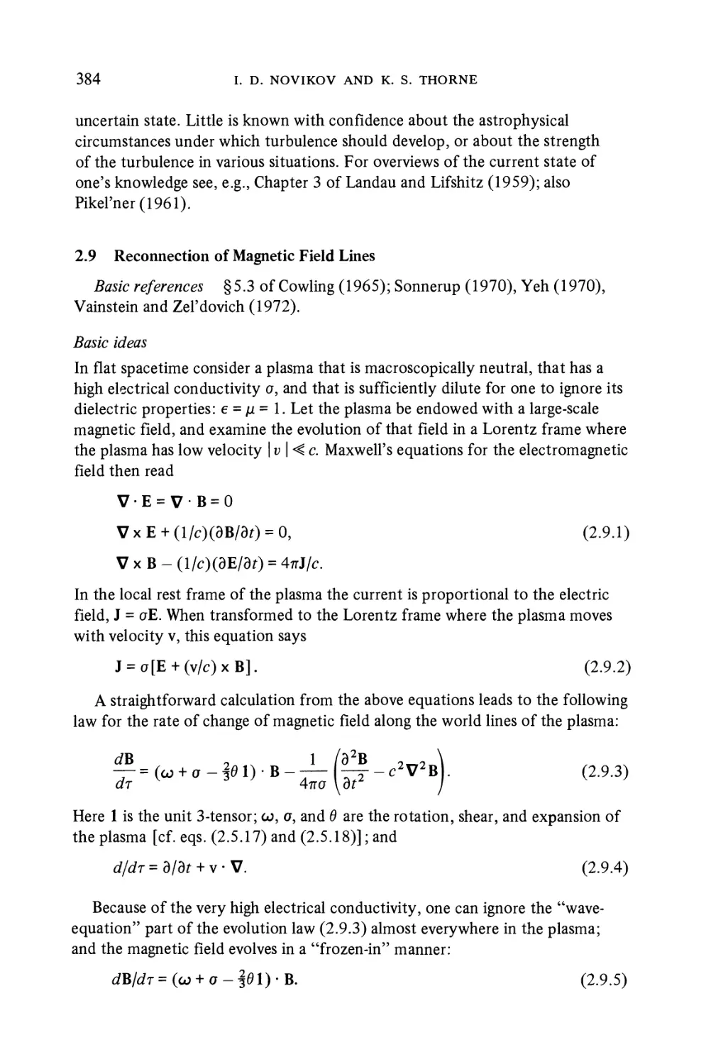
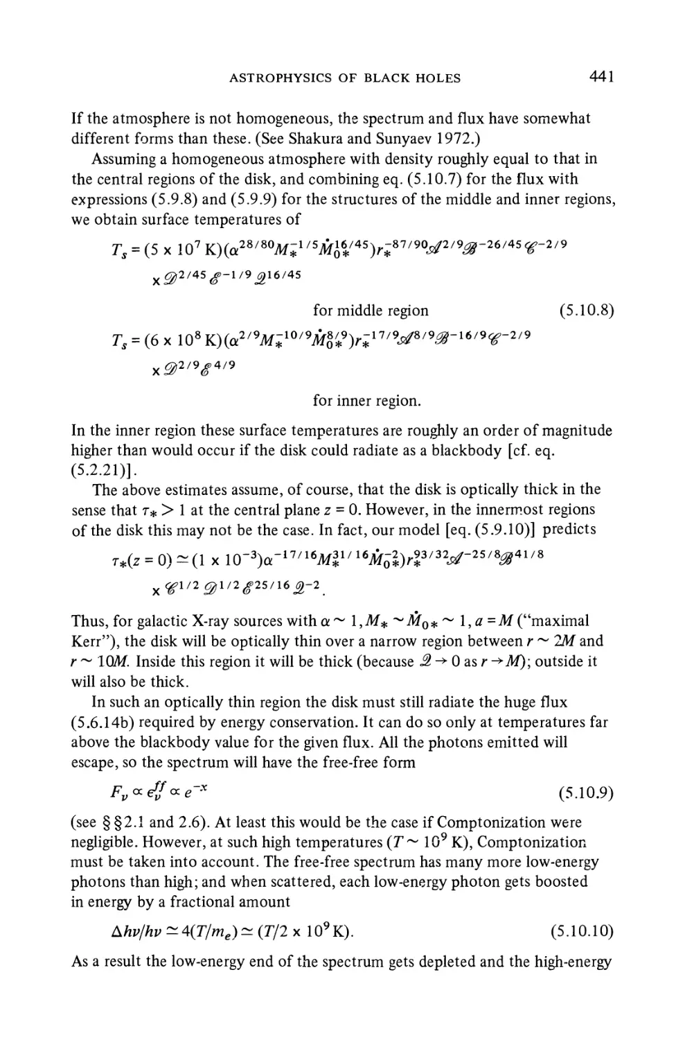
The metric A.3) holds only outside the surface of the star which will be
represented by a timelike surface which crosses r = 1M and hits the singularity
at r = 0. Inside the star the metric will be different but the details again do not
matter. One can analyse the important qualitative features by considering the
behaviour of a series of flashes of light emitted from the centre of the star which
again is taken to be transparent. In the early stage of the collapse when the density
is still low, the divergence of the outgoing light rays or null geodesies will not be
reduced much by the focusing effect of the matter. The wavefront will therefore
continue to increase in area and will reach infinity. As the collapse continues and
the density increases, the focusing effect will get bigger until there will be a
critical wavefront whose rays emerge from the surface of the star with zero
divergence. Outside the star the area of this wavefront will remain constant and
it will be the surface r=2Min the metric A.3). Wavefronts corresponding to
S. W. HAWKING
flashes of light emitted after this critical time will be focused so much by the
matter that their rays will begin to converge and their area to decrease. They will
then form trapped surfaces. Their area will continue to decrease, reaching zero
when they hit the singularity at r = 0.
SINGULARITY
TRAPPED
SURFACE
_ INTERIOR OF
STAR
Figure 2. The collapse of a spherical star leading to the formation of trapped surfaces, event
horizon and spacetime singularity.
The critical wavefront which just avoids being converged is the event horizon,
the boundary of the region of space-time from which it is not possible to escape
to infinity along a future directed nonspacelike curve. It is worth noting certain
properties of the event horizon for future reference.
A) The event horizon is a null hypersurface which is generated by null geodesic
segments which have no future end-points but which do have past end-
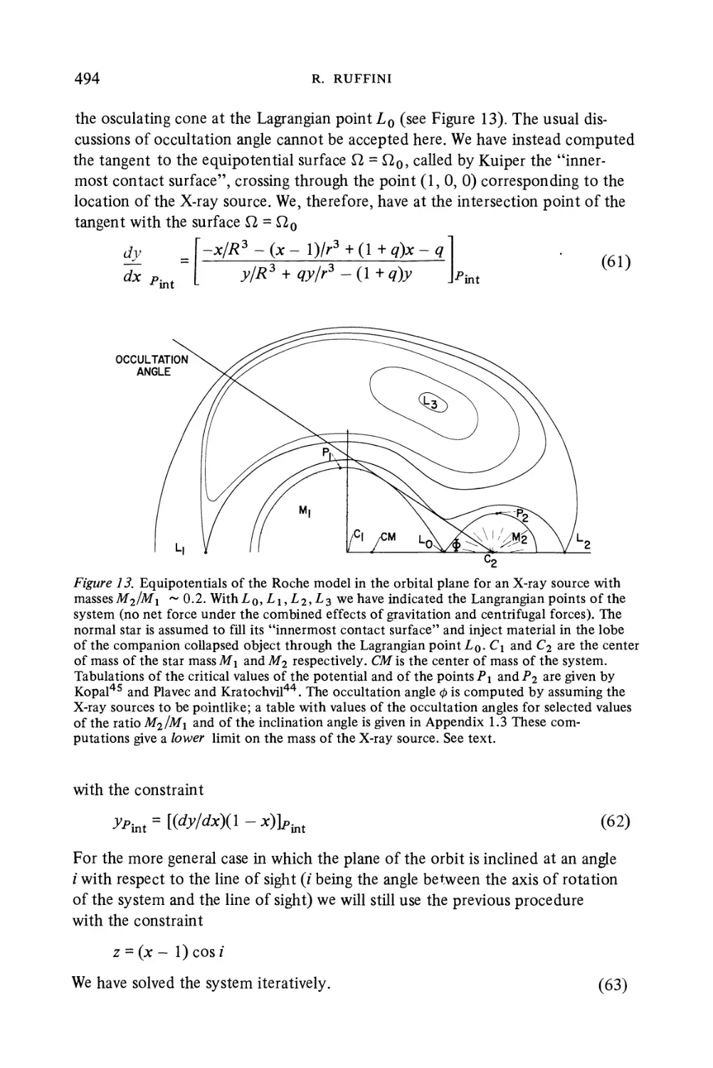
points (at the point of emission of the flash).
THE EVENT HORIZON 9
B) The divergence of these null geodesic generators is positive during the
collapse phase and is zero in the final time independent state. It is never
negative.
C) The area of a 2-dimensional cross-section of the horizon increases mono-
tonically from zero to a final value of ????2.
We shall see that the event horizon in the general case without spherical
symmetry will also have these properties with a couple of small modifications.
The first modification is that in general the null geodesic generators will not
all have their past end-points at the same point but will have them on some
caustic or crossing surface. The second modification is that if the collapsing star is
rotating, the final areas of the event horizon will be
Sn[M2+(M4-L2f] A.4)
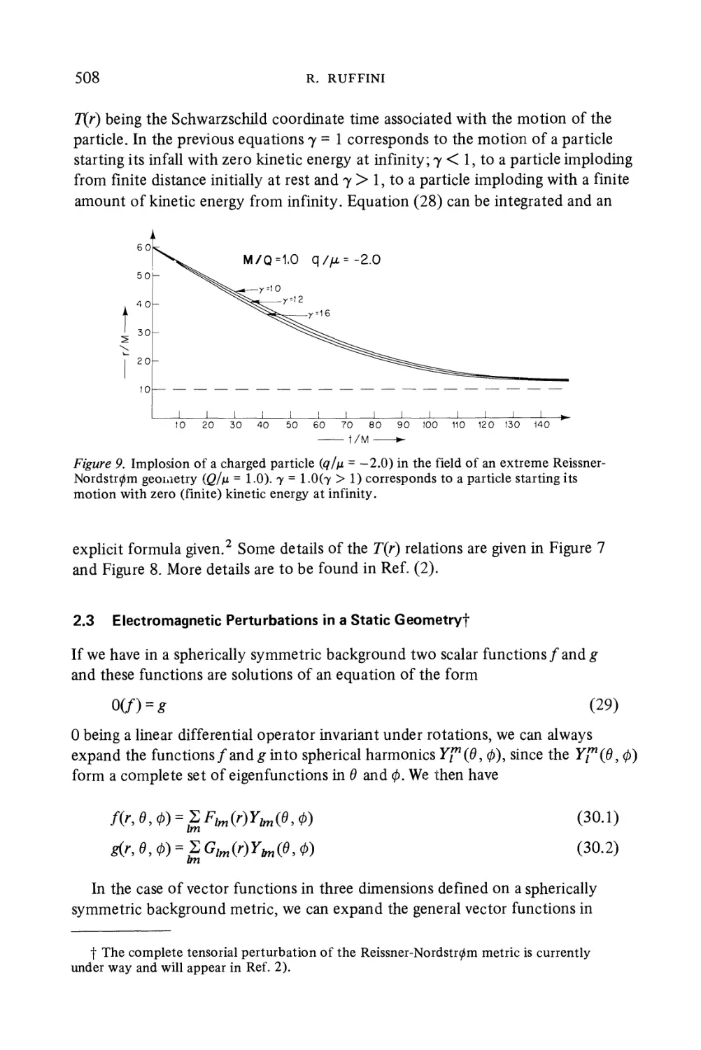
where L is the final angular momentum of the black hole, i.e., that part of the
original angular momentum of the star that is not carried away by gravitational
radiation during the collapse. This formula A.4) will play an important role later on.
In the example we have been considering the event horizon has another
property in the time-independent region outside the star. It is the boundary of
the part of spacetime containing trapped surfaces. This is not true however in the
time-dependent region inside the star. There has in the past been some confusion
between the event horizon and the boundary of the region containing trapped
surfaces, so it is worth spending a little time to clarify the distinction. Let us
introduce a family of spacelike surfaces S(j) labelled by a parameter ? which we
shall interpret as some sort of time coordinate. In the example we are considering
? could be chosen to be ? — r but the exact form is not important. Given a
particular surface S(t), one can find whether there are any trapped surfaces
which lie in S(r). The boundary of the region of S(t) containing trapped surfaces
lying in S(r) will be called the apparent horizon in S(r). This is not necessarily the
same as the intersection of the event horizon with S(t) which is the boundary of
the region of S(r) from which it is not possible to escape to infinity. To see the
differences consider a situation which is similar to the previous example of a
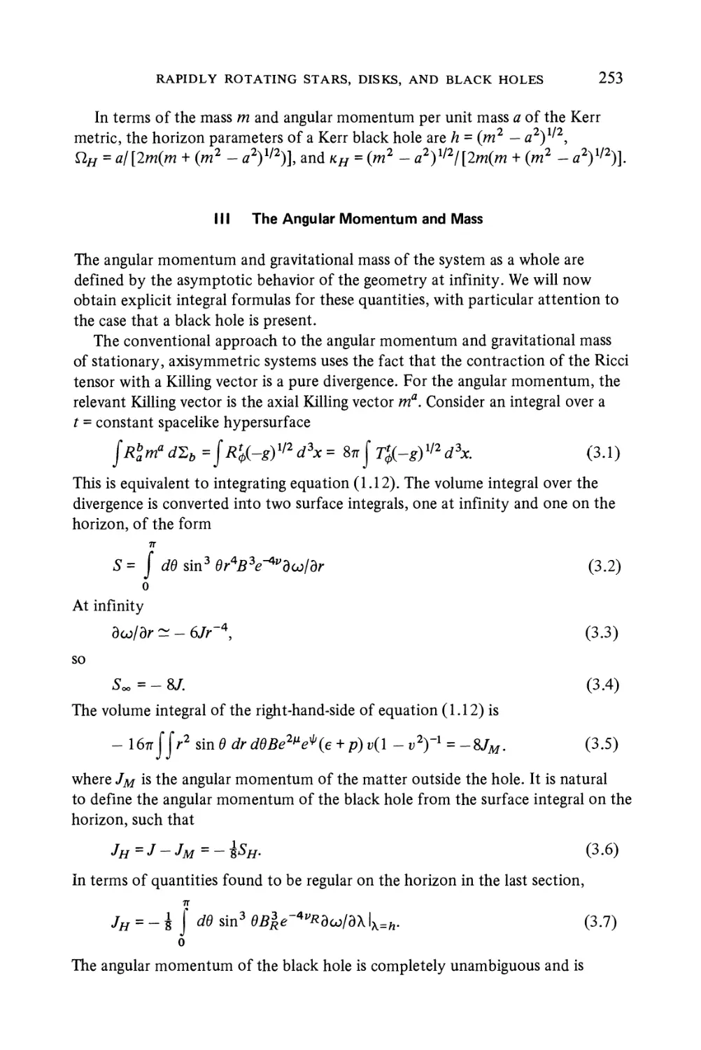
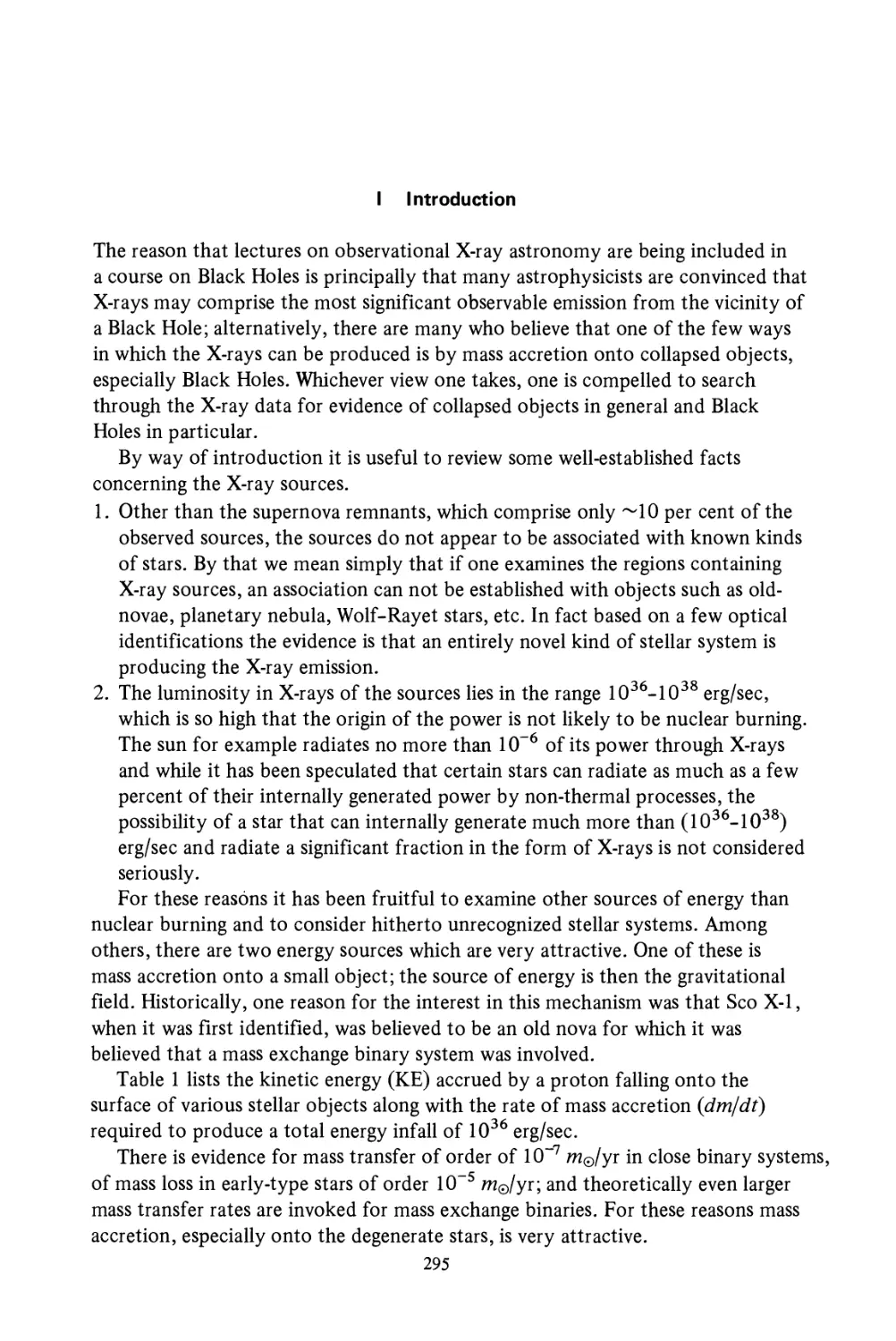
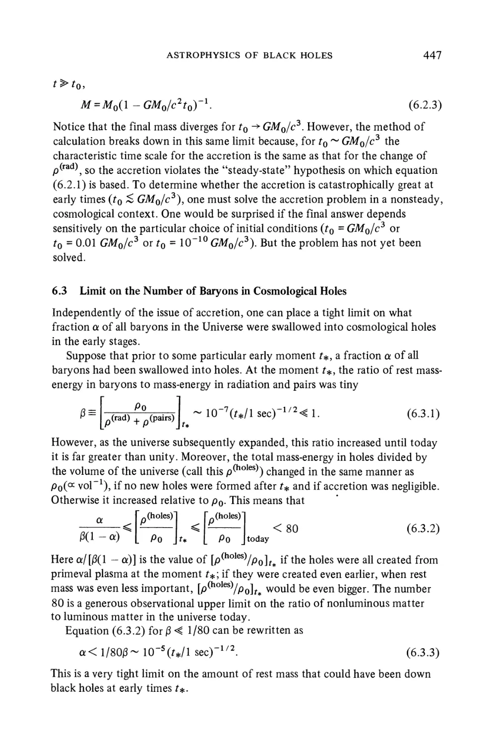
collapsing spherical star of mass ? but where there is also a thin spherical shell
of matter of mass 8M which collapses from infinity at some later time and hits the
singularity at r = 0. (Figure 3). Between the surface of the star and the shell the
metric is of the form A.3) while outside the shell it is of the form A.3) with ?
replaced by ? + 8M. The apparent horizon in S(t{), the boundary of the trapped
surfaces in 5(??), will be at r = 2M. It will remain at r = 2M until the surface S(t2)
when it will suddenly jump out to r = 2(M + ???). On the other hand, the event
horizon, the boundary of the points from which it is not possible to escape to
infinity, will intersect S(ji) just outside r = 1M. It will move out continuously
reach r = 2(M + ???) at the surface S(r2). Thereafter it will remain at this radius
provided no more shells of matter fall in from infinity.
10
S. W. HAWKING
The apparent horizon has the practical advantage that one can locate it on a
given surface S(t) knowing the solution only on that surface. On the other hand
one has to know the solution at all times to locate the event horizon. However,
the event horizon has the mathematical advantage of being a null hypersurface
_ r = 2 (M + $M)
Lhorizon
APPARENT
HORIZON
COLLAPSING
SHELL OF
MASS ??
APPAREN
HORIZON
event/-?
hori/onJ
EVENT
HORIZON
COLLAPSING
STAR OF
MASS ?
Figure 3. The collapse of a star followed by the collapse of a thin shell of matter. The
apparent horizon moves outwards discontinuously but the event horizon moves in a
continuous manner.
with nice properties like the area always increasing whereas the apparent horizon
is not in general null and can move discontinuously. In this course I shall therefore
concentrate on the event horizon. I shall show that it will always coincide with or
be outside the apparent horizon. During periods when the solution is nearly time
independent and nothing is just about to fall into the black hole, the two horizons
will nearly coincide and their areas will be almost equal. If the black hole now
undergoes some interaction and settles down to another almost stationary state,
THE EVENT HORIZON 11
the area of the event horizon will have increased. Thus the area of the apparent
horizon will also have increased. I shall show how the area increase can be used
to measure the amounts of energy and angular momentum which fell into the
black hole.
2 Nonspherical Collapse
No real star is exactly spherical; they all are rotating a bit and have magnetic fields.
One must therefore ask whether their collapse will show the same features as the
spherical case we discussed before. One would not expect this necessarily to be
the case if the departure from spherical symmetry were too large. For example a
rapidly rotating star would not collapse to within r = 2M but would form a thin
rotating disc, maintaining itself by centrifugal force against the gravitational
attraction. However one might hope that the picture would be qualitatively
similar to the spherical case for departures from spherical symmetry that are small
initially. One can divide this question of stability under small perturbations of the
initial conditions into three parts.
A) Is the occurrence of a singularity a stable feature?
B) Is the form of the singularity stable?
C) Is the fact that the singularity cannot be seen from infinity stable?
The Einstein equations being a well behaved system of differential equations
have the property of local stability. The solution at nonsingular points depends
continuously on the initial data (see Hawking and Ellis, 1973.1 shall refer to this
as HE). In other words, given a compact nonsingular region V in the Cauchy
development of an initial surface S, one can find a perturbation of the initial
data on S which is sufficiently small that the solution on V changes by less than
a given amount. One can apply this result to show that small initial departure
from spherical symmetry will not affect the fact that the wavefronts corresponding
to flashes of light emitted from the centre of the star will be focused and made to
start to reconverge. It follows from a theorem of Penrose and myself (Hawking
and Penrose, 1970) that the existence of such a reconverging wavefront implies
the occurrence of a space time singularity provided that certain other reasonable
conditions like positive energy density and causality are satisfied. Thus the answer
to question A) is "yes"; the occurrence of a singularity is a stable feature of
gravitational collapse.
As the local stability result holds only at non-singular points it cannot be used
to answer question B): is the form of the singularity stable? In fact the answer
is "no". For example adding a small amount of electric charge to the star changes
the singularity from that in the Schwarzschild solution to that in the Reissner-
Nordstrom solution which is completely different. It is reasonable to expect that
a small departure from spherical symmetry would also completely change the
singularity. This makes it very difficult to study singularities since one does not
know what a "generic" singularity would look like. The work of Liftshitz, Belinsky
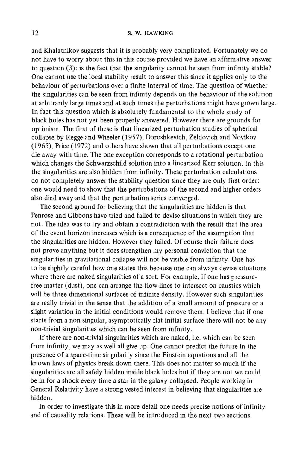
12 S. W. HAWKING
and Khalatnikov suggests that it is probably very complicated. Fortunately we do
not have to worry about this in this course provided we have an affirmative answer
to question C): is the fact that the singularity cannot be seen from infinity stable?
One cannot use the local stability result to answer this since it applies only to the
behaviour of perturbations over a finite interval of time. The question of whether
the singularities can be seen from infinity depends on the behaviour of the solution
at arbitrarily large times and at such times the perturbations might have grown large.
In fact this question which is absolutely fundamental to the whole study of
black holes has not yet been properly answered. However there are grounds for
optimism. The first of these is that linearized perturbation studies of spherical
collapse by Regge and Wheeler A957), Doroshkevich, Zeldovich and Novikov
A965), Price A972) and others have shown that all perturbations except one
die away with time. The one exception corresponds to a rotational perturbation
which changes the Schwarzschild solution into a linearized Kerr solution. In this
the singularities are also hidden from infinity. These perturbation calculations
do not completely answer the stability question since they are only first order:
one would need to show that the perturbations of the second and higher orders
also died away and that the perturbation series converged.
The second ground for believing that the singularities are hidden is that
Penrose and Gibbons have tried and failed to devise situations in which they are
not. The idea was to try and obtain a contradiction with the result that the area
of the event horizon increases which is a consequence of the assumption that
the singularities are hidden. However they failed. Of course their failure does
not prove anything but it does strengthen my personal conviction that the
singularities in gravitational collapse will not be visible from infinity. One has
to be slightly careful how one states this because one can always devise situations
where there are naked singularities of a sort. For example, if one has pressure-
free matter (dust), one can arrange the flow-lines to intersect on caustics which
will be three dimensional surfaces of infinite density. However such singularities
are really trivial in the sense that the addition of a small amount of pressure or a
slight variation in the initial conditions would remove them. I believe that if one
starts from a non-singular, asymptotically flat initial surface there will not be any
non-trivial singularities which can be seen from infinity.
If there are non-trivial singularities which are naked, i.e. which can be seen
from infinity, we may as well all give up. One cannot predict the future in the
presence of a space-time singularity since the Einstein equations and all the
known laws of physics break down there. This does not matter so much if the
singularities are all safely hidden inside black holes but if they are not we could
be in for a shock every time a star in the galaxy collapsed. People working in
General Relativity have a strong vested interest in believing that singularities are
hidden.
In order to investigate this in more detail one needs precise notions of infinity
and of causality relations. These will be introduced in the next two sections.
THE EVENT HORIZON 13
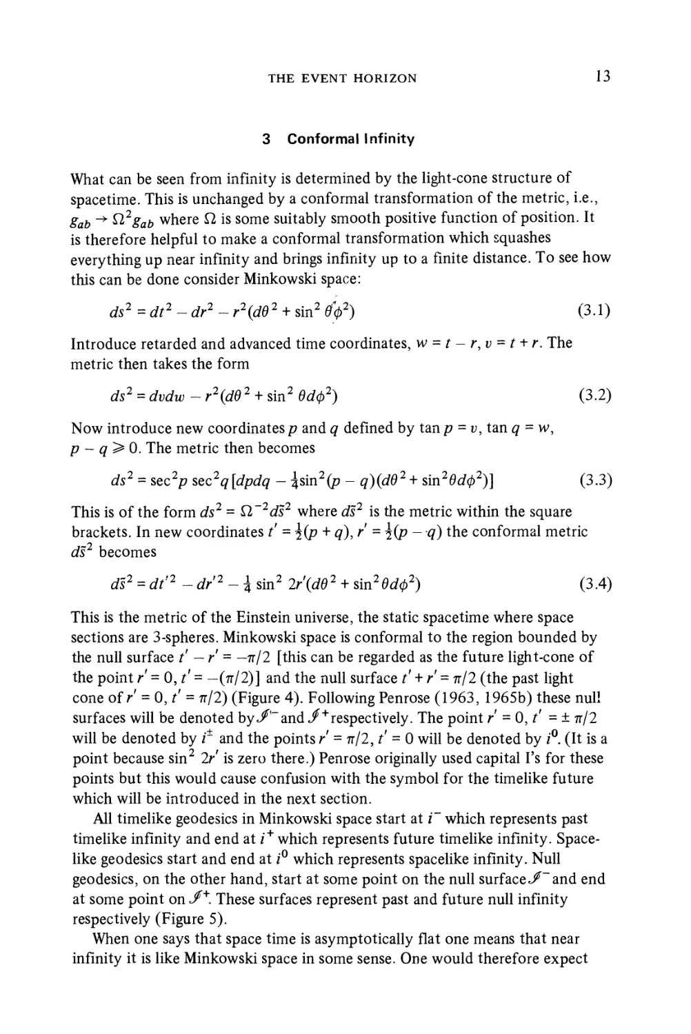
3 Conformal Infinity
What can be seen from infinity is determined by the light-cone structure of
spacetime. This is unchanged by a conformal transformation of the metric, i.e.,
gab -+ ?l2gab where ? is some suitably smooth positive function of position. It
is therefore helpful to make a conformal transformation which squashes
everything up near infinity and brings infinity up to a finite distance. To see how
this can be done consider Minkowski space:
ds2 = dt2 - dr2 - r2(dd2 + sin2 (?02) C.1)
Introduce retarded and advanced time coordinates, w = t - r, v = t + r. The
metric then takes the form
ds2 = dvdw - r2(dd2 + sin2 ???2) C.2)
Now introduce new coordinates ? and q defined by tan ? = ?, tan q = w,
? — q^ 0. The metric then becomes
ds2 = sec2p sec2q[dpdq - \sin2(p - q)(dd2 + sin2(9d02)] C.3)
This is of the form ds2 = ?l~2ds2 where ds2 is the metric within the square
brackets. In new coordinates t' = \{p + q), r - \{p — q) the conformal metric
ds2 becomes
ds2 = dt'2 - dr'2 - \ sin2 2r\dd2 + sin2(9rf02) C.4)
This is the metric of the Einstein universe, the static spacetime where space
sections are 3-spheres. Minkowski space is conformal to the region bounded by
the null surface t' ~r - -?/2 [this can be regarded as the future light-cone of
the point r = 0, f' = -(?/2)] and the null surface t' + r = ?/2 (the past light
cone of r = 0, t' = ?/2) (Figure 4). Following Penrose A963, 1965b) these null
surfaces will be denoted by</'~ and /"""respectively. The point r = 0, t' = ± ?/2
will be denoted by r and the points r - ?/2, t' = 0 will be denoted by i°. (It is a
point because sin2 2r is zero there.) Penrose originally used capital I's for these
points but this would cause confusion with the symbol for the timelike future
which will be introduced in the next section.
All timelike geodesies in Minkowski space start at i~ which represents past
timelike infinity and end at / + which represents future timelike infinity. Space-
like geodesies start and end at i° which represents spacelike infinity. Null
geodesies, on the other hand, start at some point on the null surface</~and end
at some point on </"*", These surfaces represent past and future null infinity
respectively (Figure 5).
When one says that space time is asymptotically flat one means that near
infinity it is like Minkowski space in some sense. One would therefore expect
14
S. W. HAWKING
the conformal structure of its infinity to be similar to that of Minkowski space.
In fact it turns out that the conformal metric is singular in general at the points
corresponding to /" /+ i°. However it is regular on the null surfaces«/" J>+. This
led Penrose A963, 1965b) to adopt this feature as a definition of asymptotic
f
[EINSTEIN
[[UNIVERSE
Figure 4. Minkowski space ? conform ally imbedded in the Instein Static Universe. The
Conformal boundary is formed by the two null surfaces <f , J~ and the points C ?-and c.
flatness. A manifold ? with a metric gab is said to be asymptotically simple if
there exists a manifold ? with a metric g^b such that
A) ? can be imbedded in ? as a manifold with boundary bM
B) OnM,gab = n2gab
C) On bM, ? = 0, ?1\??0
D) Every null geodesic in ? has past and future end points on bM.
E) The Einstein equations hold in ? which is empty or contains only an
electromagnetic field near bM (Penrose did not actually include this last
condition in the definition but it is useful really only if this condition holds)
THE EVENT HORIZON
15
Condition C) implies that the conformal boundary dM is at infinity from the
point of view of someone in the manifold ? Penrose showed that conditions D)
and E) implied that dM consisted of two disjoint null hypersurfaces, labelled
J>~ and J* which each had topology Rl xS2. An example of an asymptotically
simple space would be a solution containing a bounded object such as a star which
did not undergo gravitational collapse. However the definition is too strong to
apply to solutions containing black holes because condition D) requires that
every null geodesic should escape to infinity in both directions. To overcome this
CONSiDER
AS ONE POINT I
Figure 5. Another picture of Conformal Infinity as two light cones J~ and J+ joined by a
rim which represents the point t°.
difficulty Penrose A968) introduced the notion of a weakly asymptotically simple
space. A manifold ? with a metric gab is said to be weakly asymptotically simple
if there exists an asymptotically simple spacetime M',gab such that a neighbour-
neighbourhood of J* and J~ inM' is isometric with a similar neighbourhood in ? This
will be the definition of asymptotic flatness I shall use to discuss black holes.
Since condition D) no longer holds for the whole of ? there can be points from
which it is not possible to reach future null infinity J>* along a future directed
timelike or null curve. In other words these points are not in the past of J*. The
boundary of these points, the event horizon, is the boundary of the past of J>+.
I shall discuss properties of such boundaries in the next section.
16 S. W. HAWKING
Exercise
Show that the Schwarzschild solution is weakly asymptotically simple.
4 Causality Relations
I shall assume that one can define a consistent distinction between past and
future at each point of spacetime. This is a physically reasonable assumption. Even
if it did not hold in the actual spacetime manifold M, there would be a covering
manifold in which it did hold (Markus 1955).
Given a point ?, I shall denote by I+(p) the timelike or chronological future
of p, i.e. the set of all points which can be reached from ? by future directed
timelike curves. Similarly / ~(p) will denote the past of p. Many of the definitions
I shall give will have duals in which future is replaced by past and plus by minus.
I shall regard such duals as self-evident. Note that ? itself is not contained in
I+(p) unless there is a timelike curve from ? which returns to p. Let q be a point
in/+(p) and let X(v) be a future directed timelike curve from ? to q. The condition
that \(v) is timelike is an inequality:
dxa dxb
gab— — >0
dv dv
dxa
where — is the tangent vector to ?(?). One can deform the curve ?(?) slightly
without violating the inequality to obtain a future directed timelike curve from ?
to any point in a small neighbourhood of q. Thus/+(p) is an open set.
The causal future of p,J+(p), is defined as the union of ? with the set of
points that can be reached from ? by future directed nonspacelike, i.e., timelike
or null curves. If one considers only a small neighbourhood of p, then /+(p) is
the interior of the future light cone of ? and/+(p) is/+(p) with the addition of
the future light cone itself including the vertex. Note that the boundary of
/+(p), which I shall denote by/+(p), is the same as/+(p), the boundary of/+(p),
and is generated by null geodesic segments with past end points at p.
When one is dealing with regions larger than a small neighbourhood, there
is the possibility that some of the null geodesies through ? may reinterscct each
other and the forms of/+(p) and/+(p) may be more complicated. To see the
general relationship between them consider a future directed curve from a point
? to some point q EJ+(p). If this curve is not a null geodesic from p, one can
deform it slightly to obtain a timelike curve from ? to q. From this one can
deduce the following:
(a) If q is contained in J+(p) and r is contained in I+(q), then r is contained in
/+(p). The same is true if q is in /+(p) and r is in J\q).
THE EVENT HORIZON
17
(b) The set E+(p), defined as J+(p) — I+(p), is contained in (not necessarily
equal to) the set of points lying on future directed null geodesies from p.
(c) I+(p) equals J+(p). It is not necessarily the same as E+(p).
A simple example of a space in which E+(p) does not contain the whole of the
future directed null geodesies from ? is provided by a 2-dimensional cylinder
with the time direction along the axis of the cylinder and the space direction
round the circumference (Figure 6). The null geodesies from the point ? meet
FUTURE END
POINT OF
GENERATORS
OF J+ ( ? )
WHERE THEY
INTERSECT
EACH OTHER
J+(P)
Figure 6. A space in which the future directed null geodesies from a point ? have future
endpoints as generators of J+(P).
up again at the point q. After this they enter I+(p). An example in which E+(p)
does not form all of I+(p) is 2-dimensional Minkowski space with a point r
removed (Figure 7). The null geodesic in I+(p) beyond r does not pass through
? and is not in J+(p).
The definitions of timelike and causal futures can be extended from points
to sets: for a set S, I+(S) is defined to be the union of I+(p) for all ? ? S.
Similarly for J+(S). They will have the same properties (a), (b) and (c) as
the futures of points, Suppose there were two points q, r on the boundary
I+(S) of the future of a set S with a future directed timelike curve ? from q to r.
18 S. W. HAWKING
One could deform ? slightly to give a timelike curve from a point ? in I+(S)
near q to a point j> inAf - I+(S) near r. This would be a contradiction since
/+(jc) is contained in I+(S). Thus one has
(d) I+(S) does not contain any pair of points with timelike separation. In
other words, the boundary/+(S) is null or spacelike at each point.
Consider a point q G/+(S). One can introduce normal coordinates ? \ ?2, x3,
x4 (x4 timelike) in a small neighbourhood of q. Each timelike curve xl = constant
GENERATOR OF l· (P )
WHICH DOES NOT HAVE
PAST END POINT-
POINT REMOVED
FROM SPACE
?
Figure 7. The point r has been removed from two dimensional Minkowski spare.
(z = 1, 2, 3) will intersect/"^) once and once only. These curves will give a
continuous map of a small region of I+(S) to the 3-plane x4 = 0. Thus
(e) l\s) is a manifold (not necessarily a differentiable one).
Now consider a point q in I+(S) but not in S itself, or its topological closure
S. One can thus find a small convex neighbourhood U of q which docs not
intersect S. In U one can find a sequence {yn} of points in l\S) which converge
to the point q (Figure 8). From eachj>w there will be a past directed timelike
curve ?? to S. The intersections of the {??} with the boundary U of U must have
some limit point ? since iU is compact. Any neighbourhood of ? will intersect an
infinite number of the {??}. Thus ? will be in/+(S). The point ? cannot be
spacelike separated from q since, if it were, it would not be near timelike curves
from pointsyn near q. It cannot be timelike separated from q since if it were one
could deform one of the \n passing near ? to give a timelike curve from S to q
which would then have to be in the interior of I+(S) and not on boundary. Thus
? must lie on a past directed null geodesic segment ? from q. Each point of ?
between q and ? will be inl\S). One can now repeat the construction at ? and
THE EVENT HORIZON
19
obtain a past directed null geodesic segment ? from ? which lies in I+(S). If the
direction of ? were differed from that of 7 one could join points of ? to points
of 7 by timelike curves. This would contradict property (d) which says that no
two points of/+ (S) have timelike separation. Thus ? will be a continuation of 7.
One can continue extending 7 to the past in I+(S) unless and until it intersects S.
If there are two past directed null geodesic segments Ji and 72 lying in I+(S)
from a point q GI+(S), there can be no future directed such segment from q
since if there were, it would be in a different direction to and be timelike
separated from, either ji or ?2. One therefore has
(f) I+(S) (and also J\S)) is generated by null geodesic segments which have
U
Figure 8. The points yn converge to the point q in the boundary oiI+(S). From each yn
there is past directed timelike curve ?^ to S. These curves converge to the past directed
null geodesic segment 7 through q.
future end-points where they intersect each other but which can have past end-
points only if and when they intersect S.
The example of 2-dimensional Minkowski space with a point removed shows
that there can be null geodesic generators which do not intersect S and which do
not have past end-points in the space.
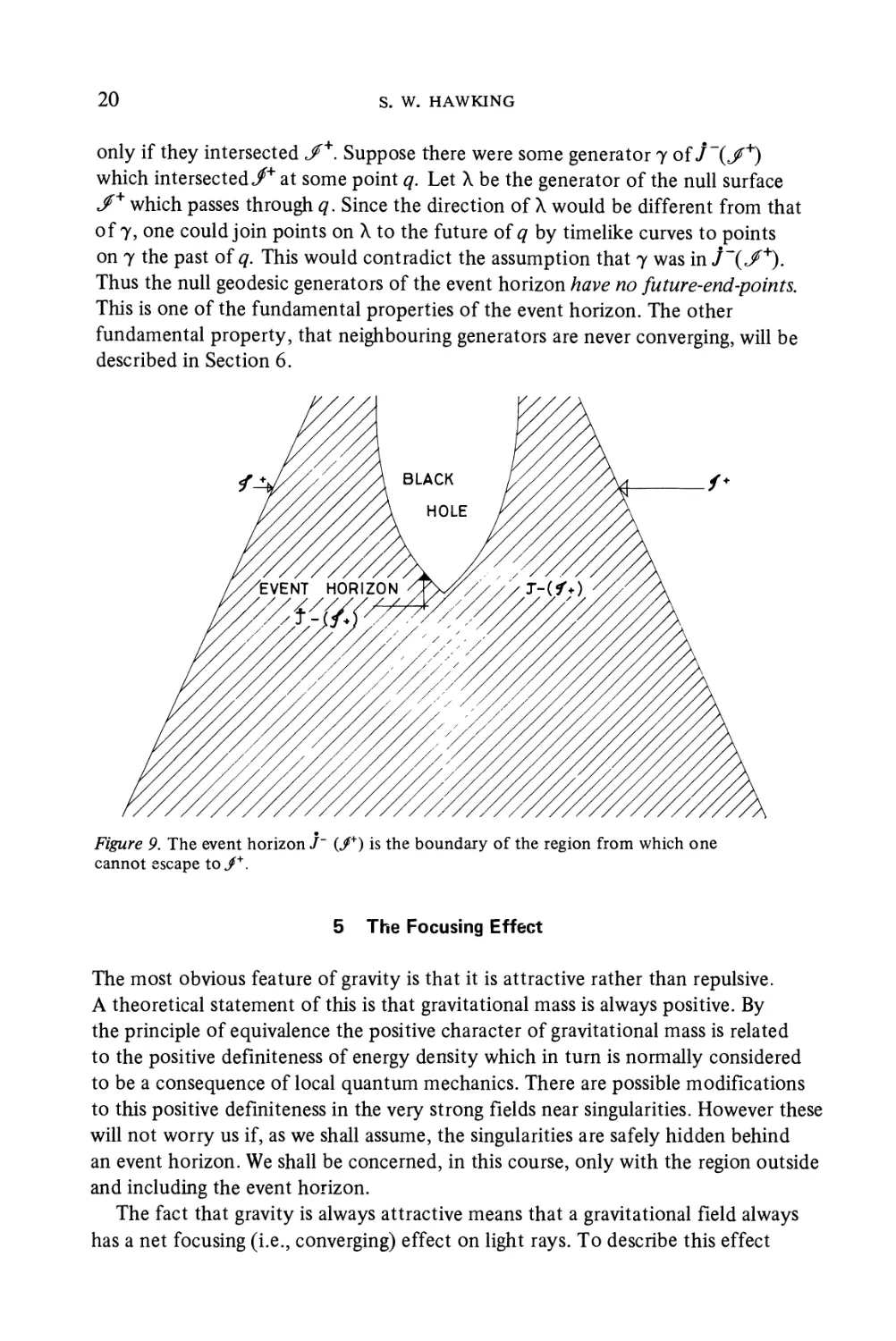
The region of spacetime from which one can escape to infinity along a future
directed nonspacelike curve is J~(J>*) the causal past of future null infinity. Thus
J~(</+) is the event horizon, the boundary of the region from which one cannot
escape to infinity (Figure 9). Interchanging future and past in the results above,
one sees that the event horizon is a manifold which is generated by null geodesic
segments which may have past end-points but which could have future end-points
20
S. W. HAWKING
only if they intersected J>*. Suppose there were some generator 7 of 7 (,/+)
which intersected/" at some point q. Let ? be the generator of the null surface
J>* which passes through q. Since the direction of ? would be different from that
of 7, one could join points on ? to the future of q by timelike curves to points
on 7 the past of q. This would contradict the assumption that 7 was in J~(J>+).
Thus the null geodesic generators of the event horizon have no future-end-points.
This is one of the fundamental properties of the event horizon. The other
fundamental property, that neighbouring generators are never converging, will be
described in Section 6.
Figure 9. The event horizon J~ (/+) is the boundary of the region from which one
cannot escape to/+.
5 The Focusing Effect
The most obvious feature of gravity is that it is attractive rather than repulsive.
A theoretical statement of this is that gravitational mass is always positive. By
the principle of equivalence the positive character of gravitational mass is related
to the positive defmiteness of energy density which in turn is normally considered
to be a consequence of local quantum mechanics. There are possible modifications
to this positive definiteness in the very strong fields near singularities. However these
will not worry us if, as we shall assume, the singularities are safely hidden behind
an event horizon. We shall be concerned, in this course, only with the region outside
and including the event horizon.
The fact that gravity is always attractive means that a gravitational field always
has a net focusing (i.e., converging) effect on light rays. To describe this effect
THE EVENT HORIZON 21
in more detail, consider a family of null geodesies. Let ? = dxa/dv denote the
null tangent vectors to these geodesies where ? is some parameter along the
geodesic. At each point one can introduce a pair of unit spacelike vectors aa
and ba which are orthogonal to each other and to la. It turns out to be more
convenient to work with the complex conjugate vectors
y/2ma =aa+ iba, y/2ma =aa - iba
These are actually null vectors in the sense that mama = rhafha = 0, they are
m
Figure 10. The null vector la lies along the null geodesic. The null vector na is such that
lana - 1. The null vector ma is complex combination of two spacelike vectors orthogonal to
la, na and to each other.
orthogonal to la, lama = lafha - 0 and they satisfy mafha = — 1. These conditions
determine ma up to a spatial rotation
ma ^ maei<t>
and up to the addition of a complex multiple of la
ma^ma+ cla
E.1)
E.2)
where c is a complex number. This is called a null rotation. Given ma there
is a unique real null vector rf such that lana - 1, nama = nama = 0. The vectors
(la, na, ma, fha) form what is called a null tetrad or vierbein (Figure 10).
Using this null tetrad one can express the fact that the curves of the family
are geodesies as
la;bmar = 0
E.3)
22
S. W. HAWKING
where semi-colon indicates covariant derivative. One can also define complex
quantities ? and ? as
= la,bmafh\
0 =
E.4)
The imaginary part of ? measures the twist or rate of rotation of neighbouring
null geodesies. It is zero if and only if the null geodesies lie in 3-dimensional null
hypersurfaces. This will always be the case in what follows so I shall henceforth
take ? to be real. The real part of ? measures the average rate of convergence of
NULL GEODESICS
MOVED
HERE
Figure 11. The area ? of two surface element ? ? increases by an amount -2pA8v when
? ? is moved a parameter distance ?? along the null geodesies.
nearby null geodesies. To see what this means consider a null hypersurface ?
generated by null geodesies with tangent vectors Ia. Let AT be a small element of
a spacelike 2-surface in ? (Figure 11). One can move each point of AT a parameter
distance ??; up the null geodesies. As one does so the area of AT changes by an
amount
= -2????
E.5)
The quantity ? measures the rate of distortion or shear of the null geodesies, that
is, the difference between the rates of convergence of neighbouring geodesies in
the two spacelike directions orthogonal to la. The effect of shear is to make a
small 2-surface which was spatially circular, become elliptical as it is moved up the
null geodesic.
THE EVENT HORIZON 23
The rate of change of the quantities ? and ? along the null geodesies is given
by two of the Newman-Penrose A962) equations
^ = p2 + aa + (e + e)p + 0oo E.6)
??
— = 2?? + Ce - e)o + ?0 E.7)
dv
where
(Note that my definitions of the Ricci and Weyl tensors have the opposite sign
to those of Newman and Penrose.)
The imaginary part of e is the rate of spatial rotation of the vectors ma
and fha relative to a parallelly transported frame as one moves along the null
geodesies. In what follows ma will always be chosen so that e - e = 0. The real
part of e measures the rate at which the tangent vector la changes in magnitude
compared to a parallelly transported vector as one moves along the null geodesies.
It is zero if la = dxa/dv where ? is an affine parameter. It is convenient however in
some situations to choose ? not to be an affine parameter.
The Ricci tensor term ?00 in equation E.6) represents the focusing effect of
the matter. By the Einstein equations
E.8)
it is equal to 4nTablalb. The local energy density of matter (i.e. non-gravitational)
fields measured by an observer with velocity vector va is Tabvavb. It seems
reasonable from local quantum mechanics to assume that this is always non-
negative. It then follows from continuity that Tabwawb > 0 for any null vector
wa. I shall call this the weak energy condition, (Penrose 1965a, Hawking and
Penrose 1970, HE) and shall assume it in what follows. With this assumption one
can see from equation E.6) that the effect of matter is always to increase the
average convergence p, i.e., to focus the null geodesic.
The Weyl tensor term i//0 can be throught of as representing, in a sense, the
gravitational radiation crossing the null hypersurface N. One can see from
equation E.7) that it has the effect of inducing shear in the null geodesic. This
shear then induces convergence by equation E.6). Thus both matter and pure
gravitational fields have a focusing effect on null geodesies.
To see the significance of this, consider the boundary 1+(S) of the future of
a set S. As I showed in the last section this will be generated by null geodesic
segments. Suppose that the convergence of neighbouring segments has some
24 S. W. HAWKING
positive value p0 at a point q G I*(S) on a generator 7. Then choosing i> to be an
affine parameter, one can see from equation E.6) that ? will increase and become
infinite at a point r on the null geodesic 7 within an affine distance of l/p0 to the
future of q. The point r will be a focal point where neighbouring null geodesies
intersect. We saw in the last section that the generators of I+(S) have future end
points where they intersect other generators. Strictly speaking, this was shown
only for generators which intersect each other at a finite angle but it is true also
for neighbouring generators which intersect at infinitesimal angles (see HE for
proof). Thus the generator 7 through q will have an end-point at or before the
point r. (It may be before r because 7 may intersect some other generator at a
finite angle.) In other words, once the generators of i\S) start converging, they
are destined to have future end-points within a finite affine distance. They may
not, however, attain this distance because they may run into a singularity first.
The importance of this result will be seen in the next section.
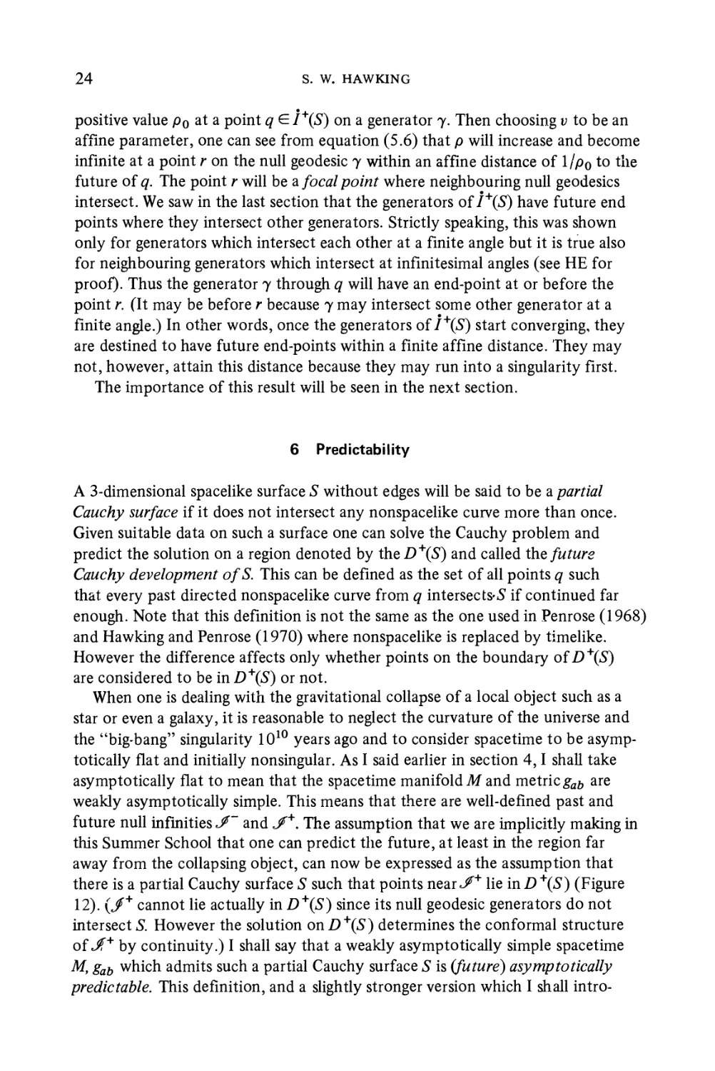
6 Predictability
A 3-dimensional spacelike surface S without edges will be said to be a partial
Cauchy surface if it does not intersect any nonspacelike curve more than once.
Given suitable data on such a surface one can solve the Cauchy problem and
predict the solution on a region denoted by the D+(S) and called the future
Cauchy development ofS. This can be defined as the set of all points q such
that every past directed nonspacelike curve from q intersects·S if continued far
enough. Note that this definition is not the same as the one used in Penrose A968)
and Hawking and Penrose A970) where nonspacelike is replaced by timelike.
However the difference affects only whether points on the boundary of D+(S)
are considered to be in D+(S) or not.
When one is dealing with the gravitational collapse of a local object such as a
star or even a galaxy, it is reasonable to neglect the curvature of the universe and
the "big-bang" singularity 1010 years ago and to consider spacetime to be asymp-
asymptotically flat and initially nonsingular. As I said earlier in section 4,1 shall take
asymptotically flat to mean that the spacetime manifold ? and metric gab are
weakly asymptotically simple. This means that there are well-defined past and
future null infinities J~ and</"*". The assumption that we are implicitly making in
this Summer School that one can predict the future, at least in the region far
away from the collapsing object, can now be expressed as the assumption that
there is a partial Cauchy surface S such that points near,/" lie in D +(S) (Figure
12). (J>+ cannot lie actually in D+(S) since its null geodesic generators do not
intersect S. However the solution on D+(S) determines the conformal structure
of,/" by continuity.) I shall say that a weakly asymptotically simple spacetime
M, gab which admits such a partial Cauchy surface S is (future) asymptotically
predictable. This definition, and a slightly stronger version which I shall intro-
THE EVENT HORIZON
25
duce shortly, will form the basis of my course. Asymptotic predictability implies
that every past directed nonspacelike curve from points near,/" continues back
to S and does not run into a singularity on the way. One can think of this as a
precise statement to the effect that there are no singularities to the future of S
which are naked, i.e., visible from/+.
SINGULARITY
Figure 12. A space with a partial Cauchy surface S such that the points near./4" are
contained in the future Cauchy development D+ (S).
Asymptotic predictability implies that the future Cauchy development D+(S)
contains J+(S) ? /~(,/+), i.e., it contains all points to the future of S which are
outside the event horizon. Suppose there were a point ? on the event horizon to
the future of S which was not contained in D+(S). Then there would be a past
directed nonspacelike curve ? (in fact a null geodesic) from ? which did not
intersect S but ran into some sort of singularity instead. This singularity would
be "nearly naked" in that the slightest variation of the metric could result in it
26 S. W. HAWKING
being visible from ^+. Since we are assuming that the non-existence of naked
singularities is a stable property, we would wish to rule out such an unstable
situation. One can also argue that the metric of spacetime is some classical limit
of an underlying quantum reality. This would mean that the metric could not be
defined so exactly as to distinguish between nearly naked singularities and those
which are actually naked. These considerations motivate a slightly stronger version
of asymptotic predictability. I shall say that a weakly asymptotically simple
spacetime M, gab is strongly (future) asymptotically predictable if there is a partial
Cauchy surface S such that
(a) J+ lies in the boundary of D\S),
(b) J\S) nj-(jf+) is contained inD+(S).
Suppose that at some time after the initial surface S, a star starts collapsing
and gives rise to a trapped surface ? in D+(S). Recall that a trapped surface is
defined to be a compact spacelike 2-surface such that the future directed outgoing
null geodesies orthogonal to it have positive convergence p. This definition assumes
that one can define which direction is outgoing. I shall assume that the 2-surface
is orientable and shall require that the initial surface S has the property:
(a) S is simply connected.
Physically, one is interested only in black holes which develop from non-singular
situations. In such cases the partial Cauchy surface S can be chosen to beR3 and
so will be simply connected. It is however convenient to frame the definitions so
that they can be applied also to spaces like the Schwarzschild and Kerr solutions
which are not initially non-singular but which may approximate the form of
initially non-singular solutions at late times. In these solutions also one can find
partial Cauchy surfaces S which are simply connected.
Given a compact orientable spacelike 2-surface ? in the future Cauchy develop-
development D+(S) one can define which direction is outwards. To do this one uses the
fact that on any manifold ? with a metric gab of Lorentz signature one can find
a vector fields which is everywhere nonzero and timelike. Using the integral curves
of this vector field, one can map the 2-surface ? onto a 2-surface f in S. Since S
is simply connected, this 2-surface ? separates S into two regions. One can label
the region which contains the part of S near infinity in the asymptotically flat
space as the outer region and the other as the inner region. The side of ? facing
the outer region is then the outer side and carrying this up the integral curves of
the vector field X* one can define which is the outgoing direction on T.
Now suppose that one could escape from a point on ? to infinity, i.e., suppose
that ? intersected /~(^+) (Figure 13). Then there would be some point q G/+
which was mj\T). Proceeding to the past along the null geodesic generator ?
of,/" through q one would eventually leave J\T). Thus ? must contain a point
r of J\T). The null geodesic generator 7 of J\T) through r would enter the
physical manifold M. If it did not have a past end point it would intersect the
THE EVENT HORIZON
27
partial Cauchy surface S. This is impossible since it lies in the boundary of the
future of ? and ? is to the future of S. Thus it would have to have a past end
point which, from section 4, would have to be on T. It would have to intersect
? orthogonally as otherwise one could join points of ? to points of 7 by
timelike curves. However the outgoing null geodesic orthogonal to ? are
Figure 13. If a trapped surface ? intersected / (/+), there would be a null geodesic
generator of J+(T) from ? XoJ+. This would be impossible as all null geodesies orthogonal
to ? contain a conjugate point within a finite affine distance of T.
converging because ? is a trapped surface. As we saw in the last section, this
implies that neighbouring null geodesies would intersect 7 within a finite affine
distance. This means that the generator 7 of J\T) would have a future end
point and would not remain in J\T) all the way out to J>+. This establishes
a contradiction which shows that the supposition that ? intersects J~(J>+) must
be false. In other words, every point on or inside a trapped surface really is
trapped: one cannot escape to J^+ along a future directed nonspacelike curve.
The same applies to a compact orientable 2-surface ? which is marginally
trapped, i.e., which is such that the outgoing future directed null geodesies
28
S. W. HAWKING
orthogonal to ? have zero convergence ? at T. For suppose ? intersected
/~G/+), then J\T) would intersect J+. The area of this intersection would be
infinite since it is at infinity. However the generators of J\T) start off with zero
convergence and therefore cannot ever be diverging. Thus the area of J\T) ? Jt*
could not be greater than that of T. This shows that marginally trapped surfaces
in D+(S) cannot intersect /~(,/+).
EVENT HORIZON
Figure 14. If the null geodesies orthogonal to a two surface F in the event horizon were
converging, one could deform F outwards slightly and obtain a contradiction similar to that
in Figure 13.
What has been shown in that a trapped surface implies either a breakdown of
asymptotic predictability (i.e., the occurrence of naked singularities) or the
existence of an event horizon. I shall assume that the first alternative does not
occur and shall concentrate on the second. As was shown is section 4, the event
horizon will be generated by null geodesic segments which have no future end-
points. If one assumed that these generators were geodesically complete in future
directions it would follow that the convergence of neighbouring generators could
not be positive anywhere on the horizon since, if it were, neighbouring generators
would intersect and have future end-points within a finite affine distance. In
examples such as the Kerr solution, the generators are geodesically complete in
THE EVENT HORIZON 29
the future direction but there does not seem to be any a priori reason why this
should always be the case. I shall now show, however, that asymptotic
predictability itself without any assumption of completeness of the horizon is
sufficient to prove that ? is non-positive.
Consider a spacelike 2-surface F lying in the event horizon to the future of S.
The null geodesic generators of the horizon will intersect F orthogonally.
Suppose their convergence ? was positive at some point p?F. In a small neigh-
neighbourhood of ? one could deform the 2-surface F slightly outwards into
J~(J>*) so that the convergence ? of the outgoing null geodesies orthogonal to
F was still positive (Figure 14). This would lead to a contradiction similar to the
one we have just considered. The null geodesies in/~(/+) which are orthogonal
to F would intersect each other within a finite affine distance and hence could
not be generators of J\F) all the way out to */+, which being at infinity is at an
infinite affine distance.
This shows that the convergence ? of neighbouring generators of the event
horizon cannot be positive anywhere to the future of S. Together with the result
that the generators of the event horizon do not have future endpoints, this implies
that the area of a two dimensional cross section of the horizon must increase with
time. This will be discussed further in the next section.
7 Black Holes
In order to describe the formation and evolution of black holes, one needs a
suitable time coordinate. The usual coordinate t in the Schwarzschild and Kerr
solutions is no good because all the surfaces of constant t intersect the horizon
at the same place (see Carter's lectures). What one wants is a coordinate ? such
that the surfaces of constant ? cover the future Cauchy development/)"^). By
the assumption of strong future asymptotic predictability the event horizon to
the future of S will be contained in D\S) and so will be covered by the surfaces
of constant r. I shall denote the surface ? = ?0 by S(r0) with S@) = S. Near
infinity the surfaces S(t) for r > 0 could be chosen to be asymptotically flat
spacelike surfaces like S which approached spacelike infinity i° and which were
such that J^+ lay in the boundary of D+(S(r)) for each ? > 0. However it is
somewhat more convenient to choose the surface S(r) for ? > 0 so that they inter-
intersect J>* (Figure 15). This means that asymptotically they tend to null surfaces of
constant retarded time. The advantage of such a choice of surfaces S(j) is that the
gravitational radiation emitted during the formation and interaction of black holes
will escape to J* and will not intersect the surfaces S(r) for ? sufficiently large.
When the solution settles down to a nearly stationary state, one can relate the
properties of the event horizon at the time r to the values of the mass and angular
momentum measured on the intersection of </"** and S(j). There is no unique
choice of the surface S(r) and of the correspondence between points on the
30
S. W. HAWKING
horizon and points on J* at the same values of r. This arbitrariness does not
matter provided one relates the properties of the event horizon to the mass and
angular momentum measured on */+ only during periods when the system is
nearly stationary. I shall be concerned with relations between initial and final
quasi-stationary states.
QiZ)
Figure 15. The surface S(t) of constant ? intersect·/" in the two-spheres Q{r).
It turns out that one can always find such a time coordinate r if the solution
is strongly asymptotically predictable, i.e., if there exists a partial Cauchy surface
S such that
(a) J+ lies in the boundary of D+(S),
(b) J\S) ? J'(,/*) lies inD+(S).
More precisely, one can find a function ? > 0 onD+(S) such that the surfaces
S(t) of constant ? are spacelike surfaces without edges in ? and satisfy
(i) S@)=S,
(ii) S(t2) lies to the future of S(tx) for r2 > rls
THE EVENT HORIZON 31
(iii) Each S(f) for ? > 0 intersects J* in a 2-sphere Q(r). The {Q(?)} for
r > 0 cover </+,
(iv) Every future directed nonspacelike curve from any point in the region of
D\S) between S and S(t) intersects either J+ or S{r) if continued far
enough.
(v) S(j) minus the boundary 2-sphere Q(r) is topologically equivalent to S.
The point that one can find such a time function ? is somewhat technical so I
shall just give an outline here. Full details are in HE. It is based on an idea of
Geroch A968). One first chooses a volume measure ?? on ? so that the total
volume of ? in this measure is finite. In the case of a weakly asymptotically simple
space such as I am considering, this volume measure could be that defined by the
conformal metric gab which is regular on J>~ and J*. For a point ? G D +(S) one
can then define a quantity/(p) which is the volume of J+(p) C)D+(S)
evaluated in the measure ??. Now choose a family {?(?)}, ? > 0 of 2-spheres
which cover J* + and which are such that Q(j2) lies to the future of Q(j\) for
t2>tx. Then, given ? G D \S) one can define a quantity h(p, r) as the volume
in the measure of ? of D+(S) ? [J~(p)-J~(Q(r))]. The functions/(p) and
h(p, ?) are continuous in ? and r. The surface S(t) can now be defined as the set
of points ? for which h(p, ?) = rf{p). Properties (i)-(v) can easily be verified.
With the time function ? one can describe the evolution of black holes. Suppose
that a star collapses and gives rise to a trapped surface T. As was shown in
the last section, the assumption of strong asymptotic predictability implies that
one cannot escape from ? to J^+. There must thus be an event horizon / ~(J^+) to
the future of S. Also by the assumption of strong asymptotic predictability,
J\S) nj~(J+) will be contained in D+(S). For sufficiently large r, the surface
S(t) will intersect the horizon and the set B(r) defined as S(j) —J~(J*) will be
nonempty. I shall define a black hole on the surface S(j) to be a connected
component of B(j). In other words, it is a connected region of the surface S{r)
from which one cannot escape to «/+. As ? increases, black holes may grow or
merge together and new black holes may be formed by further stars collapsing
but a black hole, once formed, cannot disappear, nor can it bifurcate. To see that
it cannot disappear is easy. Consider a black hole ??{?{) on a surface S(r{). Let
? be a point ????{?{). By property (iv), every future directed nonspacelike curve
? from ? will intersect either,/+ or Sij-i) for any r2 > ??. The former is impossible
since ? is not inJ~(J^+). This also implies that ? must intersect S(t2) at some point
q which is not in J~(J>*). Thus q must be contained in some black hole B2(r2) on
the surface S(t2) which will be said to be descended from the black hole ? ?(??).
Since black holes can merge together, B2(j2) may be descended from more than
one black hole on the surface ?(??). Alternatively, a black hole on S(r2) may not
be descended from any on S(jx) but have formed between rx and r2 (Figure 16).
The result that a black hole cannot bifurcate can be expressed by saying that
B\(j\) cannot have more than one descendant on a later surface S{r2). This follows
32
S. W. HAWKING
from the fact that any future directed nonspacelike curve from a point ? ???(??
can be continuously deformed through a sequence of such curves into any other
future directed nonspacelike curve from p. Since all these curves will intersect
S(t2), their intersection with S(t2) will form a continuous curve in S(t2). Thus
J+(p) ? S(r2) will be connected. Similarly /+(/??(??)) ? S(t2) will be connected.
It must be contained in ?(?2) and so will be contained in only one connected
component of B(j2). There will thus be only one black hole on S(j2) which is
descended from ?\{??).
EVENT HORIZON
NEW BLACK HOLE
FORMING
Figure 16. The two black holes??{??)and ??{?{) on the surface S{t\) merge to form the
black hole ?3G2) on the surface 5(r2). A new black hole ?^{?2) is formed between
S{ti) and 5(r2).
The boundary bBx(j{) in S(t?) of a black hole ??(??) is formed by part of
the intersection of the event horizon with the surface S(ti). Since we are assuming
that the initial surface S is simply connected, it follows from property (v) that each
of the surfaces S(t) is also simply connected. This implies that the boundary
bBxirx) is connected. For suppose that 32??(??) consisted to two components
biBi(ji) and d2^i(ri)· One could join a point qxe ??^????) to a point
q2e b2Bx(jx) by a curve ? lying in ??(??) and a curve ? lying in Sir^) - ?^??).
Joining ? and ?, one would obtain a closed curve in ?(??) which could not be
THE EVENT HORIZON 33
deformed to zero in ?(??) since it crossed the closed surface diBl(ri) only once.
This would contradict the fact that S(tx) is simply connected.
If the black holes are formed by collapses in a space which is nonsingular
initially, the surface S can be chosen to have a topology of Euclidean 3-spacei?3.
By property (v) each surface S(r) minus the bounding 2-sphere Q(j) on J^+ will
also have this topology. It then follows that the boundary 3i?i(r) of a black hole
Bx(j) will be compact and that the topology of S{r) ?/"(t/+), the space outside
and including the horizon, will have the topology of R3 minus a number of open
sets with compact closure. As I said earlier, it is sometimes convenient to consider
black hole solutions which are not initially nonsingular but which may outside
the event horizon approximate the behaviour of initially nonsingular solutions at
large times. If they are to do this it is not necessary that the surfaces S(r) - Q(j)
have the topology R 3 (indeed they do not in the Schwarzschild and Kerr solutions),
but they should have the same topology outside the event horizon. One can ensure
this by requiring that the initial surface S has the property.
(?) S ?/"(/"*) has the topology of R3 minus a finite number of open sets
with a compact closure.
It is easy to show that if S has the property (?) then each surface S(r) - Q(j)
has the property (?) also.
I showed earlier that the null geodesic generator of the event horizon did not
have any future endpoints and had negative or zero convergence p. It follows
from this that the area of the boundary bBx (r) of a black hole Bx(j) cannot
decrease with increasing r. If two black holes Bl(ri) and B2(r2) on a surface
S(tx) later collide and merge to form a black hole ?3G2) on the surface ?G2),
the area of 353(r2).must be at least as great as the sum of the areas of the
boundaries 31?!(??) and 3?2(Vi) of the original black holes. In fact it must be
strictly greater because ??3(?2) will contain two disjoint closed sets corresponding
to generators which intersected dB^r^ and 3?2(??) respectively. Since bB3(r2)
is connected, it must also contain an open set corresponding to generators which
had past endpoints between S(ti) and S(t2).
The area of the boundaries of black holes has strong analogies to the concept
of entropy in thermodynamics: it never decreases and it is additive. We shall see
later that the area will remain constant only if the black hole is in a stationary
state. When the black hole interacts with anything else the area will always
increase. Under favourable circumstances one can arrange that the increase is
arbitrarily small. This corresponds to using nearly reversible transformations in
thermodynamics. I shall show later how the area of a black hole in a stationary
state is related to its mass and angular momentum. The fact that the area cannot
decrease will impose certain inequalities on the change of the mass and angular
momentum of the black hole as a result of interaction.
I shall denote by T(j) the region of the surface S(j) that contains trapped or
marginally trapped surfaces lying in S(j). I shall call the boundary dT(r) of
?(?), the apparent horizon in the surface S(t). In the last section it was shown
that trapped or marginally trapped surfaces cannot intersect/"(j^1"). Thus T(r)
34 S. W. HAWKING
must be contained in B(j) and the apparent horizon must lie behind or coincide
with the event horizon. The apparent horizon 3?(?) will be a marginally trapped
surface. That is, it is a spacelike 2-surface such that the convergence ? of the
outgoing null geodesies orthogonal to it is zero. As ? increases, these null geodesies
may be focused by matter or gravitational radiation and the position of the
apparent horizon will move outwards on the surface S{r) at or faster than the
speed of light. As the example of the spherical collapsing shell shows, it can
move outwards discontinuously. When the solution is in a quasi-stationary state,
the apparent horizon will lie just inside the event horizon and the area of dT(r)
will be nearly equal to that of dB(r). In the transition from one quasi-stationary
state to another the area of bB(r) will increase and so the area of 3?(?) must be
greater in the final state than in the initial one. I have not been able to show,
however, that the area of 3?(?) increases monotonically though I believe it
probably does.
It is interesting to see the behaviour of the event and apparent horizon in
the case of two black holes which collide and merge together. Suppose two stars
a long way apart collapse to form black holes ??(?) and B2(j) which have settled
down to a quasi-stationary state by the surface S(ji) (Figure 17). Just inside the
two components dBi(ji) and dB2(?\) of the event horizon there will be two
components ???(??) and dT2(j\) of the apparent horizon. The 2-surfaces
dTx(ji) and ??2(??) will be smooth but the 2-surfaces ??????) and 3i?2(Vi)
will each have a slight cusp on the side facing the other. As the black holes
approach each other, these cusps will become more pronounced and will join
up to give a single component 3?3(r) of the event horizon. The apparent horizon
???(?) and 3?2(?) on the other hand, will not join up. As they approach each
other there will be some surfaces S(r2) on which there will be a third component
dT3(r2) which surrounds both 37^G2) and 3?2(?2).
I shall now show that each component of the apparent horizon 3?(?) must
have the topology of a 2-sphere. I originally developed this proof for the event
horizon in the stationary situations considered in the next section but I am
grateful to G. W. Gibbons for pointing out that it can be applied to the apparent
horizon at any time. The idea is to show that if a connected component 37\(?)
of the apparent horizon had any topology other than that of a 2-sphere, one
could deform it to give a trapped or marginally trapped surface just outside 3?(?).
This would be a contradiction of the fact that the apparent horizon is the outer
boundary of such surfaces.
Let ua be the unit timelike vector field orthogonal to the surface S(r). Let
la and na be respectively the future directed outgoing and ingoing null vector
fields, orthogonal to 37\(r) and normalized so that
The complex null vectors ma and fha will then lie in the 2-surface 37\(r). The
vector ?? = 2~T(la — na) will be the unit outward spacelike vector in S(t)
THE EVENT HORIZON
35
NEW APPARENT
HORTZON
VENT HORIZON
LACK HOLE
Figure 17. The collision of two Black Holes. The event horizons dB ? and bB2 merge to
form the event horizon dB3. The apparent horizons 97^2 do not merge but are enveloped
by a new apparent horizon 97^.
orthogonal to bT\{r). Suppose one now moves each point of 37\(?) a parameter
distance h outwards along the vector field ya = ???^ where /is some function on
3??(?). To maintain the orthogonality of la and na to the 2-surface requires
+ /3 = 0 G.1)
+ ?=0 G.2)
36 S. W. HAWKING
where
K=la;bmalb, r = la,bmanb
? = -na.,bmanb, ? = -na.bmalb
*f=nffw and a + $ = la,bnamb
Under this movement of the 2-surface 3??(?), the change in the convergence ?
at the outgoing orthogonal null geodesies can be evaluated from the Newman-
Penrose equations:
-j- = 2-*ef [?? + 0OO + (? - ?) (? - ?) + p(p + e + e - ? - ? - ?)
aw
?//2 + 2?] G.3)
where
? = ~na;bmamb, ? = -na.bmamb9 y = -h(na.blanb - ma.bmanb\
?2 = -lCabcd(lanblcnd~ laubmcmd\
? = — and ? = ? - (a - ?)
where a - ? = ma;bmamb. The first three terms on the right of equation G.3)
are non-negative. The term ??/is the Laplacian of/in the 2-surface. One can
choose /so that the sum of the last five terms on the right of equation G.3) is
constant over the 2-surface. The sign of this constant value will be determined
by that of the integral of (?? + ?2 + 2?) over the 2-surface C(? + ?) being a
divergence, has zero integral). This integral can be evaluated from another
Newman-Penrose equation which can be written as
5(ot + ?) - S(a + ?) + ?(? -?) + S(a - ?)
= -2?? - 2?2+ 2? + 20!? G.4)
where
When integrated over the 2-surface the terms in a + ? disappear but there is in
general a contribution from the ? - ? terms because the vector field ma will
have singularities on the 2-surface. The contribution from these singularities is
determined by the Euler number ? of the 2-surface. Thus
/(-?? - ?2 + 0h + A)dA = 2?? G.5)
(The real part of the equation is, in fact the Gauss-Bonnet theorem). Therefore
- /(?? + ?2 + 2?)<? = 2?? - /@? + 3A)cL4 G.6)
THE EVENT HORIZON 37
Any reasonable form of matter will obey the Dominant Energy condition
(Hawking 1971):- ?00 >\Tab\ in any orthonormal tetrad. This and the
Einstein equations imply that ??? + 3?> 0. The Euler number ? is + 2 for a
sphere, 0 for a torus and negative for any other compact orientiable 2-surface.
C7\(r) has to be orientable as it is a boundary.) Suppose ??^?) v/as not a
sphere. Then one could choose/so that the right hand side of equation G.3)
was everywhere positive or zero. This would mean that there would be a trapped
or marginally trapped surface just outside 3?(?), which is supposed to be the outer
boundary of such surfaces. Thus each component of the apparent horizon has the
topology of a 2-sphere.
In the next section I shall show that the event horizon will coincide with the
apparent horizon in the final stationary state of the solution. Thus each
connected component ???(?) of the event horizon will have spherical topology
at late times. It might, however, have some other topology during the earlier,
time dependent, phase of the solution.
8 The Final State of Black Holes
During the formation of a black hole in a stellar collapse, the solution will
change rapidly with time. Gravitational radiation will propagate out to J>* and
across the event horizon into the black hole. By the conservation law for
asymptotically flat space (Bondi et ah 1962, Penrose 1963), the energy of the
gravitational radiation reaching J>* will reduce the mass of the system as measured
from J*'. The radiation crossing the event horizon will cause the area of the
horizon to increase. The amount of energy that can be radiated to J>* or down
the black hole is presumably bounded by the original rest mass of the star. Thus
one might expect that the area of the horizon and the mass measured on J>* might
eventually tend to constant values and the solution outside the horizon settle
down to a stationary state. Although we cannot at the moment describe in detail
the time dependent formation phase it seems that we probably can find all these
final stationary states. In this section therefore I shall consider stationary black
hole solutions in the expectation that outside the horizon they will approximate
to time dependent solutions at late times.
More precisely, I shall consider spacetimes?,gab which satisfy
A) M,gab is strongly asymptotically predictable.
B) M,gab is stationary, i.e., there exists a one parameter isometry group
??: M^-M whose Killing vector/?a is timelike near J>~ and «/"*". (Note
that is may be spacelike near the black hole.)
Since these stationary spaces are not necessarily nonsingular initially, the partial
Cauchy surface S may not have the topology/?3. In fact, in most cases it will
be Rl ? S2. However, one wants these spaces to approximate physical initially
38 S. W. HAWKING
nonsingular solutions in the region outside and including the horizon at late times,
i.e., on S(t) ? J~(J*) for large r. Thus S(t) ? J~(J+) must have the same
topology as it would have in an initially nonsingular solution. One can ensure
this by requiring the property
(j3)S ? J~{J>*) has the topology of R3 minus a finite number of open sets with
compact closure.
It is also convenient (but not essential) to require
(ol)S is simply connected.
Finally, one is interested only in black holes that one could fall into from
infinity. Thus it is reasonable to require
G). There is some r0 such that for ? > r0, S(r) ? J~{J^) is contained in
I shall call a space satisfying A), (a), (|3), G) a regular predictable space. If,
in addition, B) is satisfied, I shall call it a stationary regular predictable space.
I shall show that in such a space the convergence ? and shear ? of the generators
of the horizon are zero. It then follows that the Ricci tensor term 0Oo = ^Tablalb
and Weyl tensor term ?? = Cabcdlamblcmd must be zero on the horizon. One can
interpret this as saying that no matter or gravitational radiation is crossing the
horizon.
The fact that ? is zero implies that each connected component 3i?/(r) of the
event horizon is a marginally trapped surface. Since, there are no trapped or
marginally trapped surfaces outside the event horizon dB^r) must coincide with
a component 3?/(?) of the apparent horizon. Thus all stationary black holes are
topologically spherical; there are no toroidal ones. There could be several compo-
components bBi(r) of the event horizon corresponding to black holes which maintain
themselves at constant distances from each other. This is possible in the limiting
case of non-rotating black holes carrying electric charge equal to their mass
(Hartle and Hawking 1972): the electric repulsion just cancels the gravitational
repulsion. It seems probable but has not yet been proved that these solutions
are the only stationary regular predictable spaces containing more than one
black hole.
Assuming there is only one black hole, the question of the final state has two
branches according as to whether or not the solution is static. A stationary
solution is said to be static if the Killing vector Ka is hypersurface orthogonal,
i.e., if the twist ?? = \rfbcdKbKa^d is zero. In a static regular predictable space which
is empty or contains only an electromagnetic field one can apply Israel's theorem
(Israel, 1968) to show that the space must be the Schwarzschild or Reissner-
Nordstrom solution.
If the solution is not static but only stationary, I shall show (modulo one
point) that the black hole must be rotating. I shall prove that a stationary regular
predictable space containing a rotating black hole must be axisymmetric. One can
then appeal to Carter's theorem (see his lectures) to show that such spaces, if
empty, can depend only on two parameters; the mass and angular momentum.
THE EVENT HORIZON 39
One two parameter family is known, the Kerr solutions for a2 < m2 (the Kerr
solutions for a2 > m2 contain naked singularities). It seems unlikely that there
are any others. Thus it appears that the final state of a black hole is a Kerr solution.
In the case where the collapsing star carries a net electric charge one would
expect it to be a Newman-Kerr solution.
I shall only give outlines of the results mentioned above. The full gory details
will be found in HE.
To show that the convergence and shear of the generators of the event horizon
are zero, consider a compact spacelike 2-surface Flying in the horizon. Under
the time translation 0f the surface F will be moved into another 2-surface 0f(F)
in the event horizon. Assuming that 0f(F) lies to the future of Fon the event
horizon for t > 0, one can compare their areas by moving each element of Fup
the generators of the horizon to 0f(F). I showed earlier that the generators had
no future end-points and did not have positive convergence p. If any of them had
past end-points or negative convergence between F and 0f(F)> the area of 0f(F)
would be greater than that of F. But the area of 0f(F) must be the same as that
of F since <f>t is an isometry. Thus the generators of the event horizon cannot have
any past end-points and must have zero convergence p. From the Newman-Penrose
equations
— = p2
??
dv
it follows that the shear ?, the Ricci tensor term 0Oo and the Weyl tensor term
?0 are zero on the horizon.
The only complication in this proof comes from the fact that the Killing
vector Ka which represents infinitesimal time translations, may be spacelike on
and near the horizon. (I shall have more to say about this later.) This means that
for an arbitrary 2-surface F in the horizon these may be some points of 0f(F)
for t > 0 which lie to the past of F. However one can construct a 2-surface F for
which <h(F) lies wholly to the future of Fin the following way. Choose a com-
compact spacelike 2-sphere C on/". The Killing vector Ka will be directed along the
null geodesic generators on/". Thus <j)t(C) will lie to the future of C for t > 0. The
intersection of/+(C), the boundary of the future of C, with the event horizon
will define a 2-surface F with the required properties.
If the solution is static, one can apply Israel's theorem. If the solution is
only stationary but not static one can apply a generalization of the Lichnerowicz
theorem (cf. Carter) to show that the Killing vector^ is spacelike in a non-
nonzero region (called the ergosphere) part of which lies outside the horizon. The
non-trivial part of this generalization consists of showing that a certain surface
integral over the horizon would be zero if Ka were not spacelike there. Details
are given in HE.
40 S. W. HAWKING
There are now two possibilities: either the ergosphere intersects the horizon
or it does not. The horizon is mapped into itself by the time translation. ??.
In the former case the Killing vector Ka will be spacelike on part of the horizon
and so some null geodesic generators will be mapped into other ones. The
generators form a 2-dimensional space Q which is topologically a 2-sphere, and
which has a metric corresponding to the constant separation of the generators.
The time translation <f>t which moves generators into generators can be regarded
as an isometry group on Q. Thus its action corresponds to rotating Q about
an axis. One can interpret this as follows. A point of Q represents a generator
of the horizon. As one moves along a generator one is moving relative to the
stationary frame defined by the integral curves of Ka, i.e., relative to infinity.
Thus the horizon would be rotating with respect to infinity. I shall show that
such a rotating black hole must be axisymmetric.
The other possibility is that the ergosphere might be disjoint from the horizon.
Hajicek A972) has shown that in general the ergosphere must intersect the
horizon if the region outside the horizon is null geodesically complete in both
the future and the past directions. However, these stationary spaces approximate
to physical solutions only at late times. There is thus no physically compelling
reason why they should not contain geodesies in the exterior region which are
incomplete in the past direction. I shall therefore give an alternative intuitive
argument to show that the ergosphere must intersect the horizon.
When there is an ergosphere one can extract energy from the solution by the
Penrose process (Penrose 1969). This consists of sending a particle with energy
?? =???? from infinity into the ergosphere. It then splits into two particles
with energies E2 and E3. By local conservation^ - E2 +^3- Since the Killing
vector^ is spacelike in the ergosphere, one can choose the momentumpa2 of
the second particle such that E2 is negative. Thus?3 is greater thani^. The par-
particle 3 can escape to infinity where its total energy (the rest mass + kinetic energy)
will be greater than that of the original particle 1. Thus one has extracted energy.
Particle 2, having negative energy, must remain in the region where Ka is space-
spacelike. Suppose that the ergosphere did not intersect the horizon. Then particle 2
would have to remain outside the horizon. One could repeat the process and
extract more energy. As one did so the solution would presumably change gradu-
gradually. However the ergosphere could not disappear because there has to be some-
somewhere for the negative energy particles to exist. If the ergosphere remained dis-
disjoint from the horizon one could extract an arbitrarily large amount of energy.
This does not seem reasonable physically. On the ? the* hand, if the ergosphere
moved so that it intersected the horizon, the solution would have to become axi-
axisymmetric. At the moment the ergosphere touched the horizon one would have
a stationary, non static, axisymmetric black hole solution. This could not be a
Kerr solution because in a non static Kerr solution the ergosphere actually inter-
intersects and does not merely touch the horizon. However it appears from the results
of Carter that the Kerr solutions are the only stationary axisymmetric black hole
solutions. Thus it seems that one ends up with a contradiction if one supposes
THE EVENT HORIZON
41
that the ergosphere is disjoint from the horizon. I shall therefore assume that
any stationary, non static, black hole is rotating.
My original proof (Hawking 1972) that a stationary rotating black hole must
be axisymmetric had the great advantage of simplicity. However it involved the
assumption that as well as the future event horizon / %/+) there was apasi
event horizon J +G/~) and that the two horizons intersected in a compact
spacelike 2-surface. Penrose pointed out that there is no necessity for this
assumption to hold. These stationary spaces represent physical solutions only at
NULL
GENERATORS
<| EVENT HORIZON
-ORBIT OF ??
Figure 18. The time translation ?? moves a point ? on the horizon along the orbit of
Ka to the point <j>t (P) on the same generator of the horizon.
large times. There would be a past horizon if the solution were time-symmetric.
By the Papapetrou theorem (see Carter) time-symmetry is a consequence of
stationary and axial-symmetry. It should not be assumed to prove axial symmetry.
I therefore developed another proof of axial symmetry which depends only on the
future horizon. Unfortunately, this proof is rather long and messy. I shall try to
give an intuitive picture of it here and shall give the full details in HE.
Consider a rotating black hole. Let tx be the period of rotation of the horizon.
This means that for a point ? on a generator ? of the horizon <pti(p) is also
on ? (Figure 18). One can choose a parameter ? on ? so that la = dxa/dv satisfies
42
S. W. HAWKING
where e is constant on ? and so that difference between the values of ? at ? and at
???(?) is tx. This fixes the scaling of la. One can now form the vector field
?
2? ?
on the horizon. The orbits of Ka will be closed spacelike curves in the horizon.
The aim will be to show that they correspond to rotations of the solution about
— EVENT HORIZON
Figure 19. The event horizon and the null surface ? intersected in the spacelike
surface F.
an axis of symmetry. Choose a spacelike 2-surface F in the horizon tangent to
Ka. Let ? be the null surface generated by the ingoing null geodesies orthogonal
to F (Figure 19). The idea of the proof is to consider the Cauchy problem for the
region to the past of both the horizon and N. The Cauchy data for the empty space
Einstein equations in this situation consists of ?0 on the horizon ?4 = Cabcd
on ? where na is the null vector tangent to ? and ?, ? = -na.brhamb
nafhbncmd
THE EVENT HORIZON 43
and ?2 = hCahcd(lanblcnd - lanbmcmd) on the 2-surface F. If there are other
fields present (e.g., an electromagnetic field) one has to give additional data for
them. I shall consider only the empty case but similar arguments hold in the
presence of any fields obeying well-behaved hyperbolic equations.
By the stationarity of the horizon, ? and ?0 are zero and one can show from
the Newman-Penrose equations that ? 2 is constant along the generators of the
horizon. Thus the only non-trivial Cauchy data are that on the null surface TV.
The idea now is to show that these Cauchy data are unchanged if one moves ?
by moving each point of the 2-surface F an equal parameter distance down the
generators of the horizon. If this is the case, it follows from the uniqueness of
the Cauchy problem that the solution admits a killing vector Ka which coincides
with la on the horizon. Then?a defined as tx\2n{Ka - Ka) will also be a Killing
vector. Since the oribits of Ka are closed curves on the horizon, they will be
closed everywhere and so will correspond to rotations about an axis of symmetry.
To show that the data on ? are unchanged on moving each point of F down
the generators of the horizon, I assume that the solution is analytic though this
is almost certainly not necessary. The data on ? can then be represented by
their partial derivatives at F in the direction along N. From the Newman-Penrose
equations one can evaluate the derivatives along a generator ? of the horizon
of these and certain other quantities. If one takes them in a certain order one
obtains equations of the form
dx
— = ax + b
dv
where ? is the quantity in question and a and b are constant along ?.
Now moving F a parameter distance tx (the period of rotation of the
black hole) to the past along the generators of the horizon is the same as moving
F by the time translation <f>_t. Since <j)_t is an isometry, the quantity ? will be
unchanged under it. Thus ? must be periodic along the generator ? with period
tx. This is possible only if ? is constant along ? and equal to —(b/a). One then
uses this to calculate the derivative along ? of another quantity and shows that it
is constant by a similar argument. Proceeding by induction one shows that all
the derivatives at the horizon of the Cauchy data on TV are constant along the
generators of the horizon.
The first quantity ? that one considers is a + ?. The Newman-Penrose
equation for this is
— (? + ?) = ?(€ + €)+?!.
By construction 6(e + e) is constant along the generators of the horizon and
by another Newman-Penrose equation, ? ? = 0 on the horizon. Therefore in order
for a + ? to be periodic it has to be constant along the generators and 5(e + e)
has to be zero. This means that e + e must be constant over the whole horizon.
44 S. W. HAWKING
In the next section we shall see e + e can be interpreted as the restoring force or
effective surface gravity of the black hole.
One now applies similar arguments to show that (a — ?), ?, ?, ?3 and ?4
are constant along the generators of the horizon. One then repeats the arguments
to show that the first and higher derivatives of all quantities along the vector na
are constant along the generators. This completes the proof.
It turns out that if e is nonzero (as it is in general) the solution is completely
determined by a knowledge of ?2 on each generator. I shall use this fact in one
of the applications in the next section. It holds true even if the space outside
the black hole is not empty but contains, say, a ring of matter (in which case the
space would not be a Kerr solution).
The proof of axial symmetry implies that a rotating black hole cannot be
exactly stationary unless all distant matter and all fields are arranged axisym-
metrically. In real life this will never be the case. Thus a rotating black hole
can never be exactly stationary, it must be slowing down. However, calculations
by Press A972), Hawkin and Hartle A972), and Hartle A972) have shown that
the rate of slowing down is very small in most cases. I shall discuss this further
in the next section.
9 Applications
In this final section I shall outline some of the ways in which the theory des-
described so far can be used to obtain quantitative results, which is what most people
want. I shall discuss three applications:
(A) The limits that can be placed from the area theorem on the amount of
energy that can be extracted from black holes.
(B) The change in the mass and angular momentum of a nearly stationary
black hole produced by small perturbations.
(C) Time symmetric black holes. (These are not very realistic but they provide
some concrete examples.)
A Energy Limits
In view of the last section it seems reasonable to assume that a black hole settles
down to a Kerr solution or, if carrying an electric charge, to a Newman-Kerr
solution. The area of the event horizon of such a solution is
A = 4?[2?2 -e2 + 2(Af4 -M2e2 - L2f] (9.1)
where ? is the mass, e the electric charge and L the angular momentum of the
black hole. (All in units such that G = c= 1.) Now suppose that the black hole,
having settled down by the surface ?(??) to a nearly stationary state with para-
THE EVENT HORIZON 45
meters Ml,elLl, now undergoes some interaction with external particles or
fields and then settles down again by the surface S(t2) to a nearly stationary
state with parameters M2i e2,L2. Since the area of the horizon cannot decrease
A2>AX (9.2)
where A x and A2 are given by equation (9.1) with the appropriate values of
M, e and L. In fact (9.2) is a strict inequality if there is any disturbance at the
horizon. It puts an upper limit on ? ? — M2i which represents the amount of
energy extracted from the black hole by the interaction. To see what this limit
is, it is convenient to express equation (9.1) in the form:
2 A 4nL2 ne* e2 / ?
?+++ (93)
The first term on the right can be regarded as the "irreducible" part of M2, the
part that is irretrievably lost down the black hole. The second term can be
regarded as the contribution of the rotational energy of the black hole and the
third and fourth terms as the contribution of the electrostatic energy. Christo-
doulou A970) has shown that one can extract an arbitrarily large fraction of the
rotational energy by the Penrose process of sending a particle from infinity into
the ergosphere where it splits into two particles one of which returns to infinity
with more than the original energy while the other falls through the horizon
and reduces the mass and angular momentum of the black hole. Similarly,
using charged particles, one can extract an arbitrarily large fraction of the
electrostatic energy.
Note that it isM2 and not ? which has an irreducible part. This distinction
does not matter when there is only one black hole but it means that one can
extract energy, other than rotational or electrostatic energy, by allowing black
holes to collide and merge. Consider two black holes ^(?) ????2(?) a long way
apart which have settled down to nearly stationary states. One can neglect the
interaction between them and regard the solution near each as a Kerr solution
with the parameters M1} ei,Lx andM2,e2 andZ,2 respectively. The areas A x
and^2 of dBiir) an(* ??2(?) will be given by equation (9.1). Suppose that at
some later time the two black holes come together and merge to form a single
black hole B3(r) which settles down to a nearly stationary state with parameters
M3, e3 andZ,3. During the collision process a certain amount of gravitational and
possibly electromagnetic radiation will be emitted to infinity. The energy of
this radiation will be ?? +?2 — M3. This is limited by the requirement that the
area ^3 of dB$(f) must be greater than the sum of A x and^2- The fraction
e =,(M1 + ?2)~1(?? +?2 —M3) of the total mass that can be radiated is always
less than 1 - 2~, i.e., about 65%. If the black holes are uncharged or carry the
same sign of charge, the fraction is less than a half, i.e., 50%. If the black holes are
also non-rotating the fraction is less than 1 - 2~?, i.e., about 29%.
By the conservation of charge e3 = ex + e2. Angular momentum, on the other
46 S. W. HAWKING
hand, can be carried away by the radiation. This cannot happen, however, if the
situation is axisymmetric, i.e., if the rotation axes of the black holes are aligned
along their direction of approach to each other. Then L3 =Lx+L2. One can see
from equation (9.3) thatAf3 can be smaller, i.e., there can be more energy
radiated, if the rotations of the black holes are in opposite directions than if
they are in the same direction. This suggests that there may be an orientation
dependent force between black holes analogous to that between magnetic dipoles.
Unlike the electromagnetic case, the force is repulsive if the orientations are the
same and attractive if they are opposite. Even in the limiting case when Z,! = M\
andZ,2 -M\, there is still energy available to be radiated. Thus it seems that the
force can never be sufficiently repulsive to prevent the black holes colliding.
? Perturbations of Black Holes
To perform dynamic calculations about black holes seems to require the use of
a computor in general. However there are a number of situations that can be
treated as small perturbations of stationary black holes, i.e., Kerr solutions.
The general idea in these calculations is to solve the linearized equations for a
perturbation field (scalar, electromagnetic or gravitational) in a Kerr background
and to try to find the radiation emitted to infinity and the rate of change of the
mass and angular momentum of the black hole. In the case of the scalar and
electromagnetic field these latter can be evaluated by integrating the appropriate
components of the energy-momentum tensor of the field over the horizon. For
gravitational perturbations, however, there is no well defined local energy-momentum
tensor. Instead I shall show how one can determine the change in the mass and
angular momentum of the black hole by calculating the change in the area of the
horizon and the quantity ?2 ?? the horizon. It turns out that these depend only
on the Ricci tensor terms 0OO = 4nTablalb and ?01 = 4nTablamb and the Weyl
tensor term ?0 on the horizon. This is fortunate because it seems that the full
equation for gravitational perturbations in a Kerr background are not solvable
by separation of functions but Teukolsky A972) has obtained decoupled
separable equations for the quantities ?0 and ?4.
The mass, the magnitude of the angular momentum and its orientation make
up four parameters in all. However, in many uses there are constraints which make
it sufficient to calculate the change in only one function of these four parameters.
The simplest such function is the area of the horizon which is given by equation
(9.1). The rate of charge of this area can be calculated from the Newman-Penrose
equations
-^ = p2 + aa + 2ep + 0oo (9.4)
??
do
2?? + 2??+?0 (9.5)
??
THE EVENT HORIZON 47
Choose a spacelike surface S which intersects the event horizon of the back-
background Kerr solutions in J+(Jr^) and is tangent to the rotation Killing vector Ka.
Then one can define a family S(t) of such surfaces by moving S under the
time translation 0f, i.e., by moving each point of S a parameter distance t along
orbits of the Killing vector Ka of the unperturbed metric. This defines a time
coordinate t on the horizon. It is convenient to choose the parameter ? along
the generators of the horizon to be equal to t. Then in the unperturbed Kerr
metric
?
e = 4M(M2+yy (9·6)
where
There are two kinds of perturbations one can consider, those in which there
is some matter fields like the scalar or electromagnetic field on the horizon with
energy momentum tensor Tab and those in which the perturbations at the
horizon are purely gravitational and are produced by matter at a distance from
the black hole. Consider first a matter field perturbation where the field is
proportional to a small parameter ?. The energy momentum tensor and so the
perturbation in the metric and in ?0 will be proportional to ?2. Thus ? and ?
will be proportional to ?2 and to order ?2 the equation (9.4) becomes
^-=2ep + 4nTablalb (9.7)
at
where e is given by (9.6). Suppose that the perturbation field is turned off after
some time t\. The black hole will then settle down to a stationary state with
p = 0.
Thus the solution of (9.7) for ? is
oo
? = -4? J exp {2e(r - t') }Tablalbdt'. (9.8)
t
The rate of increase of area of the horizon is
dt
where the integral is taken over the two surface dB(t) which is the intersection of
the event horizon with the surface S(r). Substituting from equation (9.8) and
performing a partial integration with respect to time one finds that the total
area increase of the horizon is
lbladLb (9.9)
48 S. W. HAWKING
where ??* = lbdAdt is the 3-surface element of the event horizon. The null
vector la tangent to the horizon can be expressed in terms of Ka and Ka the
Killing vectors of the background Kerr metric which correspond to time trans-
translations and spatial rotations respectively.
la=Ka + ??? + 0(?2), (9.10)
where
? 2M(M2+y) (9'U)
is the angular velocity of the black hole. The vectors TabKa and—TabKa represent
the flow of energy and angular momentum respectively in the matter fields.
They are conserved in the background Kerr metric and their fluxes across the
horizon give change of mass and angular momentum of the black hole.
Thus
?? =— [??-???]. (9.12)
This is just the change needed to preserve the formula (9.1) for the area of the
horizon of Kerr solution. It is therefore consistent with the idea that the
perturbation changes the black hole from one Kerr solution to one with slightly
different parameters.
The case of purely gravitational perturbations is rather more interesting because
one does not have an energy momentum tensor from which to compute the
fluxes of energy and angular momentum into the black hole. Instead one can
use the area increase as a measure of a certain combination of them. One takes
the gravitational perturbation field to be proportional to a small parameter ?.
Then from equations (9.4), (9.5) ? will be proportional to ? and ? to ?2
— =?? + 2??, (9.13)
dt
do
-=2??+?0. (9.14)
From (9.14)
oo
a = -J exp{2e(t-t')}\Podt' (9.15)
t
and
=- \
?? =- \oodAdt. (9.16)
THE EVENT HORIZON 49
One can apply this formula in at least two situations. First there are stationary
gravitational perturbations induced by distant matter which is stationary or nearly
stationary. In such perturbations there will be no radiation at infinity and the
energy of the sources of the perturbation will be nearly constant. Thus there
can be no energy flow into or out of the black hole and its mass must remain
constant. From equation (9.1) it then follows that the increase in the area,4 of
the horizon must be accompanied by a decrease in the angular momentum of the
black hole. In other words, the effect of stationary perturbation is to slow down
the rotation of the black hole. What is happening is that the rotational energy
part of M2 in equation (9.3) is being dissipated into the irreducible part of M2
represented by A.
There is a strong analogy between this process and ordinary tidal friction in
a shallow sea covering a rotating planet. A nearly stationary external body such
as a moon will raise tides in the sea. As the planet rotates, the shape of a fluid
element will change and so the fluid will be shearing. There will be dissipation
of energy at a rate proportional to the coefficient of viscosity times the square
of the shear. This energy must come from the rotational energy of the planet.
Thus the planet will slow down.
Similarly one can regard the perturbation field of a stationary external
object as tidally distorting the horizon of the black hole (Figure 20) with
consequent shearing as the black hole rotates and dissipation of rotational
energy at a rate proportional to the square of the shear. The dimensionless
analogue of the viscosity in this case is of order unity. Hartle A972) has
calculated the rate of slowing down of a slowly rotating black hole caused by
a stationary object of mass M' at coordinates r and ?. For rjM large he finds
dL , L (M'Y (MY
Because of the last factor, this seems too small ever to be of astrophysical
significance. The situation might be different, however, for a rapidly rotating
black hole with L nearly equal to ?2. In this case the quantity e which acts as a
restoring force in equations (9.13) and (9.14) is very small. In a sense the black
hole is rotating with nearly break up velocity so centrifugal force almost balances
gravity and a small object can raise a large tide on the horizon. For maximum
effect, the object should be orbiting the black hole near the horizon with nearly
the same angular velocity as that of the black hole. Under these circumstances
the black hole would lose energy and angular momentum at a significant rate to
the object. The object would also be losing energy and angular momentum in
radiation to infinity. It is possible that the rates would balance to give what is
called a floating orbit. To find out whether this could happen, it would be suf-
sufficient to calculate the rate of increase of the area of the horizon and the rate of
radiation of energy and angular momentum to infinity since an object in a circular
orbit can gain or lose energy and angular momentum only in a certain ratio.
50
S. W. HAWKING
For other problems it would be helpful to be able to calculate separately the
rate of change of the mass and the three components of angular momentum. In
the last section we saw that a stationary black hole solution is in general deter-
determined by a knowledge of the quantity ?2 on a 2-dimensional section of the
OBJECT
TIDALLY DISTORTED
EVENT HORIZON
Figure 20. The gravitational of an external object tidally distorts the event horizon.
horizon. In the case of a Kerr black hole, the angular momentum is represented
by the imaginary / = 1 part of ? p. From the Newman-Penrose equations one
can calculate the change in ?2 produced by the perturbation.
d
—
at
= Edo - Edp + i[(a + ?)? + ???] -
where § acting on a spin weight s quantity is ? + s(a - 0). Further details will
be given elsewhere.
THE EVENT HORIZON 51
C Time Symmetric Black Holes
The last application I shall describe is largely based on the work of G. W. Gibbons.
Some of it is about to be published (Gibbons 1972) and more will be in his
Ph.D. thesis.
To calculate the evolution of a section of the Einstein equation one requires
initial data on a partial Cauchy surface S. The Cauchy data on a spacelike surface
can be represented by two symmetric 3-dimensional tensor fields hy and x,y.
The negative definite tensor hy is the first fundamental form or induced metric
of the 3-surface S imbedded in the 4-dimensional space-time manifold M. It is
equal to gy - UjUj where ut is the unit timelike vector orthogonal to S. The
tensor ??;· is the second fundamental form or extrinsic curvature of S imbedded
inM. It is equal to uk;ihfhl The fields ?/;· and ?/;· have to obey the
constraint equations:
h [C)* + iXabhabJ - XabXcahachbd] = SnTabuaub
where II indicates covariant differentiation with respect to the 3-dimensional
metric hy in the surfaces. The constraint equations are non-linear and difficult
to solve in general. However the problem is much simpler if the solution is time
symmetric. The solution is said to be time-symmetric about the surface S if
there is an isometry which leaves the surface S pointwise fixed but reverses
the direction of time, i.e., it moves a point to the future of S on a timelike
geodesic orthogonal to S to the point on the some geodesic an equal distance
to the past of S. The time symmetry isometry maps ??;· to — x,y since it reverses
the direction of the normal u{ to S. Thus x,y = 0. The first constraint is trivially
satisfied and the second one becomes in the empty case
&R = ?
The convergence of the outgoing null geodesies orthogonal to a 2-surface F
mS is
? = 2~*mlmi(ui;j + ?>,·;7·)
where w,· is the unit spacelike vector in S orthogonal to F. The first term is zero
because ?/;· = 0. Thus if F is a marginally trapped surface, the convergence of its
normals in S must be zero. This means that it is an extremal surface, i.e., its area
is unchanged to first order under a small deformation. In fact F must be a
minimal surface if it is an apparent horizon, i.e., if it is the outer boundary of a
region containing closed trapped surfaces. Conversely any minimal 2-surface in S
is an apparent horizon.
One can write down an explicit family of solutions of the remaining constraint
52 S. W. HAWKING
equation by taking the metric h^ on S to be F4^· where 77^· is the three dimensional
flat metric and V satisfies the Laplace's equation in this metric
V2K=0.
I shall consider solutions of the form V= 1 + ???·/2??· representing the field
of a number of point masses Mt where the distance from the ith mass is r,·.
The solution with only one mass is the Schwarzschild solution expressed in
isotropic coordinance. The minimal surface, which in this case is both the
apparent and event horizon, is at r = \M and has area 16??2. Now consider
the case of two equal mass points Mx and7fci2· If they are far apart the minimal
surfaces around each will be almost at rl = \M and r2 = \M and their areas will
be nearly ????2. Each surface will however be slightly distorted by the field
of the other points and their areas will be slightly greater than ????2. As the
solution evolves the two black holes containing these two apparent horizons
will fall towards each other and will merge to form a single black hole which
will settle down to a Schwarzschild solution with massAf'. The energy of the
gravitational radiation emitted in this process will be the initial mass 1M of the
system minus the final massAf'. This is limited by the fact that the area ????'2
of the event horizon of the final black hole must be greater than the sum of the
areas of the event horizons around the two original black holes. The area of these
event horizons must be greater than those of the corresponding apparent
horizons since these are minimal surfaces. Thus the upper limit on the fraction
e of the initial mass that can be radiated is somewhat less than 1 — 2". If the
two mass points are moved nearer to each other in the initial surface S the
minimal surfaces around them become more distorted and their area increases.
Thus the upper limit on the fraction of energy that can be radiated becomes less.
This is what one would expect since the available energy of each black hole is
reduced by the negative gravitational potential of the other. In fact to first order,
the reduction in the upper limit on e just corresponds to the Newtonian
gravitational interaction energy of the two point masses. When the two mass
points are moved close to each other the area of the minimal surface around each
becomes greater than 32??2. This seems to indicate that the amount of energy
that could be radiated would be negative which would be a contradiction.
However before the two mass ponts are close enough for this to happen, it
seems that a third minimal surface will be formed which surrounds them both
and has area less than 64??2 (Figure 21).
Gibbons A972) has shown that any minimal surface in a conformally flat
initial surface must have an area greater than
-Lf
2? J
VudAa
where the integral is taken over the minimal surface. The expression in the
brackets represents the contribution to the total mass on the initial surface
THE EVENT HORIZON
53
arising from points within the minimal surface. The solution that evolves from
the initial surface will eventually settle down to a Schwarzschild solution with
an event horizon of area \6nM'2. Since this area must be greater than the area of
the event horizon on the initial surface which in turn must be greater than the
area of the minimal surface, the difference between the initial massAf and the
final massAf' must be less than A - 2~3/2)M. This means that a single distorted
black hole on a surface of time symmetry cannot radiate more than 65% of its
initial mass ? in relaxing to a spherical black hole.
The black holes that have been considered so far in this subsection are non-
rotating. This is because the condition that the solution be invariant under
t-> —t rules out any rotation. However, one can include rotation in a simple
way if the solution is invariant under the simultaneous transformation t^-t,
? -> —?. I shall call such a solution (t, ?) symmetric. To obtain such a solution
the initial data must be of the form
Xab it-
KCKC
where Ja is an axisymmetric vector field orthogonal to the Killing vector Kb
Figure 21. The two apparent horizons 97^ and 9?2 are surrounded by another apparent
horizon dT^.
which corresponds to rotations about the axis of symmetry. The first constraint
equation then becomes
One can integrate this equation to obtain the total angular momentum within
a given 2 - surface
8? J
JadAa
In the empty case, to which I shall now restrict myself, the angular momentum
will arise from singularities of the field Ja. The solution will be asymtotically
predictable and will represent black holes if those singularities are contained within
54 S. W. HAWKING
apparent horizons. From the form of ?^ it follows that the apparent horizons in
the initial surface of (t, ?) symmetry are minimal 2-surfaces. Note that this is
the case only in a surface of time symmetry or (t, ?) symmetry. It is not true
in later space-like surfaces.
In the empty case the second constraint equation becomes
This equation can be solved by a technique of Lichnerowicz. Choose a spatial
metric hab. Then choose a spatial vector field Ja which is axisymmetric, orthogonal
to Ka and which satisfies J\a = 0 in the metric hab. One then makes a conformal
transformation hab = V4hab. The first constraint equation will remain satisfied
if Ja transforms as Ja = V~2Ja. The second constraint equation will be satisfied if
V is chosen so that
? ??
VC)R -SVunhhab = 2
Wab* -¦ v
Kbj\
where the covariant derivatives are with respect to the metric hab. This equation
is non-linear so one cannot write down explicit solutions even in the case where
the metric hab is chosen to be flat. However one can note certain qualitative
features. One of these is that the addition of angular momentum tends to increase
the total mass of the solution. Thus it seems that the rotational energy of black
holes is positive as one would expect. Calculations by Gibbons in the case of two
black holes indicate that the ratio of the area of the apparent horizons to the
square of the total mass is bigger when the angular momenta of the black holes
are in opposite directions than when they are in the same direction. This
indicates that there is less energy available to the radiated in the former case than
in the latter which is consistent with the idea that there is a spin dependent force
between black holes which is attractive in the case of opposite angular momenta
and repulsive in the other case.
The calculations of Gibbons indicate that when the black holes are far apart
the force is proportional to the inverse fourth power of the separation which is
what one would expect from the analogy with magnetic dipoles.
References
H. Bondi, M. G. J. Van der Burg and A. W. K. Metzner, Proc. Roy. Soc. (London) A269, 21
A962).
D. Christodoulou, Phys. Rev. Letters 25, 1596 A970).
A. G. Doroshkevich, Ya, B. Zel'dovich and I. D. Novikov, Sov. Phys. JETP 22, 122 A966).
R. P. Geroch,/. Math. Phys. 9, 1739 A968).
G. W. Gibbons, Comm. in Math. Phys. 27, 87 A972).
J. B. Hartle, 1972 (preprint).
J. B. Hartle and S. W. Hawking, Comm. in Math. Phys. 26, 87 A972).
THE EVENT HORIZON 55
S. W. Hawking and R. Penrose, i>oc. Roy. Soc. A314, 529 A970).
S. W. Hawking, Comm. in Math. Phys. 18, 301 A970).
S. W. Hawking and J. Hartle, Comm. in Math. Phys. 27, 283 A972).
S. W. Hawking, Comm. in Math. Phys. 25,152 A972).
S. W. Hawking and G. F. R. Ellis, The Large Scale Structure of Space-Time (Cambridge
University Press, Cambridge, to be published).
W. Israel, Phys. Rev. 164,1776 A967).
L. Mmkus, Ann. Math. 62,411 A955).
?. ?. Newman and R. Penrose,/. Math. Phys. 3, 566 A962).
R. Penrose, Phys. Rev. Letters 10, 66 A963).
R. Penrose, Phys. Rev. Letters 14, 57 A965a).
R. Penrose, Proc. Roy. Soc. A284, 159 A965b).
R. Penrose, Battelle Rencontres, 1967 Lectures in Mathematics and Physics, edited by
C. DeWitt and J. A. Wheeler (W. A. Benjamin, Inc., New York 1968).
R. Penrose, Riv. Nuovo Cimento 1 (Num. spec.) 252 A969).
W. H. Press, APJ. 175, 243 A972).
R. Price, Phys. Rev. D5, 2419 A972).
T. Regge and J. A. Wheeler, Phys. Rev. 108, 1063 A957).
S. Teukolsky, 1972 (Caltech preprint).
This page intentionally left blank
Black Hole Equilibrium States
Brandon Carter
Institute of Theoretical Astronomy,
Cambridge, Great Britain
This page intentionally left blank
Contents
Part I Analytic and Geometric Properties of the Kerr Solutions
1 Introduction . . . . . . . . . .61
2 Spheres and Pseudo- Spheres ....... 62
3 Derivation of the Spherical Vacuum Solutions . . . .68
4 Maximal Extensions of the Spherical Solutions . . . .74
5 Derivation of the Kerr Solution and its Generalizations . . .89
6 Maximal Extensions of the Generalized Kerr Solutions . . .103
7 The Domains of Outer Communication . . . . .112
8 Integration of the Geodesic Equations . . . . . .117
Part II General Theory of Stationary Black Hole States
1 Introduction . . . . . . . . . .125
2 The Domain of Outer Communications and the Global Horizon . .133
3 Axisymmetry and the Canonical Killing Vectors .... 136
4 Ergosurfaces, Rotosurfaces and the Horizon . . . . .140
5 Properties of Killing Horizons . . . . . . .146
6 Stationarity, Staticity, and the Hawking-Lichnerowicz Theorem . 151
7 Stationary-Axisymmetry, Circularity, and the Papapetrou Theorem . 159
8 The Four Laws of Black Hole Mechanics . . . . .166
9 Generalized Smarr Formula and the General Mass Variation Formula . 177
10 Boundary Conditions for the Vacuum Black Hole Problem . .185
11 Differential Equation Systems for the Vacuum Black Hole Problem . 197
12 The Pure Vacuum No-Hair Theorem 205
13 Unsolved Problems 210
59
This page intentionally left blank
PART I Analytic and Geometric Properties of the
Kerr Solutions
1 Introduction
The Kerr solutions (Kerr 1963) and their electromagnetic generalizations
(Newman et al 1965) form a 4-parameter family of asymptotically flat solutions
of the source-free Einstein-Maxwell equations, the parameters being most con-
conveniently taken to be the asymptotically defined massAf, electric charge Q, and
magnetic monopole charge P, together with a rotation parameter a, which is such
that (in units of the form we shall use throughout, where the speed of light c and
Newton's constant G are set equal to unity ) the asymptotically defined angular
momentum J is given by
J = Ma
The parameters may range over all real values subject to the restriction
M2 >a2 + P2 +Q2
which must be satisfied if the solution is to represent the exterior to a hole rather
than naked singularity. It turns out (Carter 1968a) that the solutions all have the
same gyromagnetic ratios as those predicted by the simple Dirac theory of the
electron, as the asymptotic magnetic and electric dipole moments cannot be
specified independently of the angular momentum but are given, in terms of the
same rotation parameter, as Qa andPfl respectively.
The solutions are all geometrically unaltered by variations of ? and Q provided
that the sum P2 + Q2 remains constant, and since it is in any case widely believed
that magnetic monopoles do not exist in nature, attention in most studies is re-
restricted to the 3-parameter subfamily in which ? is zero. Ihis 3-parameter sub-
subfamily, and specially the 2-parameter pure vacuum subfamily in which Q is also
zero, has come recently to be regarded as being at least potentially of great
astrophysical interest, since the Kerr solutions do not merely represent the only
known stationary source-free black hole exterior solutions: they are also widely
believed (for reasons which will be presented in Part ? of this course) to be the
only possible such solutions.
We shall devote the whole of Part I of the present lecture course to the
derivation and geometric investigation of these Kerr solutions. In a strictly logical
approach, Part ? of this course (which will consist of a general examination of
stationary black hole states with or without external sources) should come first,
but it is probably advisable for a reader who is not already familiar with the sub-
subject to start with Part I, since the significance of the reasoning to be presented in
Part ? will be more easily appreciated if one has in mind the concrete examples
61
62 ?. CARTER
described in Part I. For the same reason many readers may find it easier to
appreciate the accompanying lecture course of Hawking if they have first become
familiar with the examples described here, although only the final stages of
Hawking's course actually depend on the results presented here, the bulk of it
being logically antecedent to both Part ? and Part I of the present course. This
present lecture course is intended to serve both logically and pedagogically as
an introduction to the immediately following course of Bardeen and hence also
(but less directly) to the subsequent courses in this volume.
2 Spheres and Pseudo-Spheres
A space time manifold J( is said to be spherically symmetric if it is invariant
under an action of the rotation group SOC) whose surfaces of transitivity are
2-dimensional. The metric on any one of these 2-surfaces must have the form
dsl =r2 (??2 + ??2???2) B.1)
in terms of a suitably chosen azimuthal co-ordinate ? running from 0 to ?, and a
periodic ignorable co-ordinate ? defined modulo 2?, where the scale factor r is
the radius of curvature of the 2-sphere. In what follows we shall frequently find
it convenient to use the equivalent alternative form
expressed in terms the customary alternative azimuthal co-ordinate
B.3)
running from —1 to +1. See Figure 2.1.
A space-time manifold^ is said to be pseudo-spherically symmetric if it is
invariant under an action of the 3-dimensional Lorentz group whose surfaces of
transitivity are timelike and 2-dimensional. The metric on one of these 2-surfaces
can be expressed in a form analogous to B) as
B-4)
where s is the radius of curvature and where the co-ordinate t is ignorable.
The two simple and familiar metric forms ds% and dsl illustrate a feature
which will crop up repeatedly in the present course, that is to say they both have
removable co-ordinate singularities. The spherical form B.2) is obviously singular
at ? = ± l; moreover we cannot remove this singularity simply by returning to the
form B.1) in which the infinity is eliminated only at the price of introducing an
equally undesirable vanishing determinant which will of course lead to an infinity
in the inverse metric tensor. We can cure the singularity and show explicitly that
the space is well behaved at the poles (as we know it must be by the homogeneity)
BLACK HOLE EQUILIBRIUM STATES
63
Figure 1. Figure la shows a plan of a timelike 2-section, in which the spherical co-ordinates
?, ? are held constant, of the space time manifold of a spherical collapsing star which
occupies the part of space time marked by horizontal shading. Locuses on which r is con-
constant are marked by dotted lines and null lines are marked by continuous lines. The horizon
^f+ is indicated by a heavy continuous line and the region outside the domain of outer
communications is marked by diagonal shading. Figure lb shows the extrapolation back
under the group action of the pseudo-stationary empty outer region of Figure la. The past
boundary marked by a heavy dotted line would become the horizon ^f" in an extended
manifold. (See Part II, Section 1)
only by giving up the use of the ignorable co-ordinate ?. Thus for example we can
cure the singularity at the north pole ? = 1 by introducing Cartesian type co-
coordinates x, y defined by
= 2r
? = 2r
1 +?
to obtain the conformally flat form
2 dx2 + fo2
1 +
x2 + y2
B.5)
B.6)
B.7)
64 ?. CARTER
which is well behaved everywhere except at the south pole. It is of course im-
impossible to obtain a form which is well behaved on the whole of the 2-sphere at
the same time (see Figure 2.1.).
Let us now consider the algebraically analogous singularities at ? = ± 1 in the
pseudo-spherical metric ds\. These singularities are of a geometrically different
nature since the metric is well behaved with the same signature, on both sides of
the singularities i.e. both in the static regions with \x \ > 1 and in the regions
where the ignorable co-ordinate is spacelike \x l< 1. (In contrast with the
spherical metric which has the right signature only for | ? \ < 1.) We can link the
Worth Pole
Figure 2.1. The 2-sphere. The light dotted lines represent trajectories of the Killing vector
well behaved domains ? > 1 and — 1 < ? < 1 by a co-ordinate patch extending
right across the divisions* = ±1, by introducing new co-ordinates
T=i^We~' B·8)
X=|l-x2|ref B.9)
which leads to the form
2) B.10)
in which the new co-ordinate ? is ignoreable. This form is well behaved over the
whole of the region ? > 0 including the loci ?? = ± 1 which correspond respec-
respectively to the divisions —x = ±1 in the original system B A). Moreover it can easily
be seen that these loci are in fact null lines. The situation can be visualized most
BLACK HOLE EQUILIBRIUM STATES 65
easily in terms of null-co-ordinates u, ? which we introduce by the defining
relations
u = t + - B.11)
?
»=?-? B.12)
which leads to the form
dsl ^/% B.13)
(u - vy
(whose u and ? are restricted by the condition u — ? > 0) in which the divisions
? = ±1 are represented by the lines u = 0 and ? = 0 respectively.
The relationship between the co-ordinate patches B.13) (which is equivalent
to B.10) with ? > 0) and the co-ordinate patches of the form B.7) is shown in
the con formal diagram of Figure 2.2a. This is the first example of a technique,
which we shall employ frequently, of representing the geometry of a timelike
2-surface on the plane of the paper, in a manner which takes advantage of the
fact that any such metric is conformly flat and thus can be expressed in the
canonical null form ds2 = Cdudv where C is a conformal factor. The method
consists simply of identifying the null co-ordinates u and ? with ordinary
Cartesian co-ordinates on the paper which conventionally are placed diagonally
so that timelike directions lie in a cone of angles within 45 degrees of the
vertical. There is nothing unique about such a representation since there is a
wide choice of canonical null form preserving transformations in which the co-
coordinates u,v are replaced respectively by new co-ordinates w*, v* of the form
u* = u*(u), ?* = v*(v) and in which the conformal factor C is replaced by
C* = C(du*/du)(dv*/dv). This freedom can be used to arrange for the co-
coordinate range w*, v* to be finite even if the original co-ordinate range is not
(e.g. by taking w* = tanh u,v*= tanh ?) thereby making it possible to represent
an infinite timelike 2-manifold in its entirety on a finite piece of paper.
The co-ordinate patch of Figure 2a with the spacially homogeneous form
B.10) is in fact still incomplete, as would have been expected from the fact that
starting from the time symmetric form B.4) one could have extended into
the past instead of the future by replacing t by —t in the transformation equations
B.8) and B.9). We can obtain a new form which covers both extensions by
setting
w = tan— B.14)
i; = -cot- B.15)
66
?. CARTER
which leads to the new null form
rjv2 - ?
tan2
dUdV
B.16)
In terms of these co-ordinates (which can both range from — °° to °° subject to
the restriction -? <U - V<n) the entire co-ordinate range of u and ? subject
to u + ? < 0, i.e. the entire range of ?, ? subject to ? > 0, is covered by the range
2.2a
2.2b
Figure 2.2 Conformal diagram of the 2-dimensional pseudo-sphere. In Figure 2a the light
dotted lines represent trajectories of the Killing vector 9/9i and the heavy lines represent
the corresponding non-degenerate Killing horizons. In the extended diagram of Figure 2b
the light dotted lines represent trajectories of the Killing vector a/a t, and the double lines
represent the corresponding degenerate Killing horizons.
0< V< 2?, and -n<U<n. The situation is illustrated in Figure 2b. The mani-
manifold in this figure is geodesically complete and hence maximal in the sense that
no further extension can be made. The null form B.16) covering this maximal
extension can be converted to an equivalent static form by introducing co-ordinates
?, ? defined by
X= tan
U- V
B.17)
BLACK HOLE EQUILIBRIUM STATES 67
i/+ V
T= B.18)
which gives the maximally extended static form
in which X and ? can range from ~°° to °° without restriction.
Looking back from the vantage point of this complete manifold we can see
clearly what has been happening. The timelike Killing vector whose trajectories
are the static curves ? = constant, \x | > 0 in the system B.4), becomes null on
the surfaces on which U or V are multiples of ?, these surfaces representing past
and future event horizons for observers who are fixed in that ? remains constant
relative to this system. [The past and future event horizon (cf. Rindler 1966) of
an observer being respectively the boundary of the past of his worldline, i.e. the
set of events he will ultimately be able to know of, and the boundary of the
future of his world line i.e. of the set of events which he could in principle have
influenced.] Thus for the Killing vector whose trajectories are the static lines
? = constant, | ? \ > 0 in the system B.4), the corresponding event horizons are
the lines on which U and V are multiples of ?. In the extension B.10) in which
the ignorable co-ordinate t has been sacrificed, there is a new manifest symmetry
generated by the Killing vector whose trajectories are the lines ? = constant, and
for the corresponding static observers the event horizons coincide with alternate
horizons of the previous set, specifically the lines on which U + ? and V are
multiples of 2?. In the maximal extension in which the ignorable co-ordinate ?
has in its turn been replaced by T, there is a third non-equivalent Killing vector
field, whose static trajectories are the lines X = constant, and in this case the
corresponding observers have no event horizons.
There is a fairly close analogy between the removable co-ordinate singularities
associated with rotation axes, as exemplified by the case of the ordinary 2-sphere
discussed earlier, and the removable co-ordinate singularities associated with
Killing horizons. Both arise from the inevitable bad behaviour of an ignorable
co-ordinate which is used to make manifest symmetry group action generated by
a Killing vector. The former case arises in the case of a spacelike Killing vector
generating a rotation group action when it becomes zero on a rotation axis, while the
latter arises in the case of a static Killing vector (and also under appropriate
conditions as we shall see later a stationary Killing vector) when it becomes null
on a Killing horizon. Killing horizons can be classified as degenerate or non-
degenerate according to whether the gradient of the square of the Killing vector
is zero or not. In the case of a non-degenerate Killing horizon (as exemplified by
the horizons on which the Killing vector whose trajectories are ? = constant) the
relevant Killing vector must change from being timelike on one side to being
spacelike on the other. In the case of a degenerate Killing horizon, the relevant
68 ?. CARTER
Killing vector may be (and in the sample of the Killing vector whose trajectories
are ? = constant, actually is) timelike on both sides of the horizon. We can see in
the example of the pseudo-sphere another phenomenon that will later be shown
to be true in general, namely that non-degenerate Killing horizons of a given
Killing vector field cross each other at what we shall call a Boyer-Kruskal axis, on
which the Killing vector is actually zero, this axis being very closely analogous to
a rotation axis. On the other hand degenerate Killing horizons (which have no
exact analogue in the case of axisymmetry) continue unimpeded over an un-
unbounded range.
Figure 2.3. Sketch of conformal diagram of 2-dimensional pseudo-sphere with the canonical
global topology obtained by identifying points with the same value of X but with values of
? differing by 2? in the maximally extended covering manifold of Figure 2.2b.
Since ? is ignorable, we could construct a new reduced manifold from the
manifold of Figure 2.2b by identifying points with the same values of X but for
which the values of ? differ by any arbitrarily chosen fixed ? period; the locus of
points at unit spacelike distance from the origin in 3-dimensional Minkowski
space is a manifold of the form obtained in this way where the period of ? has
the canonical value 2? (see Figure 2.3).
3 Derivation of the Spherical Vacuum Solutions
In this section we shall run rapidly through the steps by which the spherically
symmetric vacuum (both pure vacuum and source free Einstein Maxwell) solutions
are derived. Thus we start from the condition that the space time manifold under
consideration is invariant under an action of SO C) which is transitive over 2-
surfaces. Since the rotation group action is necessarily invertible in the sense
BLACK HOLE EQUILIBRIUM STATES 69
that associated with any point there is a discrete subgroup action-a rotation by
180°—which reverses the senses of the tangent vectors to the surfaces of transitivity,
it follows automatically (cf. e.g. Schmidt 1967, Caner 1969) that the group
action is orthogonally transitive in the sense that the surfaces of transitivity must
themselves be orthogonal to another family of 2-surfaces. Therefore by requiring
that they be constant on these 2-surfaces, we can extend the polar co-ordinate ?, ?
or equivalently ?, ? from the individual 2-surfaces to the 4-dimensional manifold
<Jt. It follows further that apart from an overall conformal factor r2 (where r is
the local radius of the 2-spheres) the space-time will locally have the form of a
direct product of the unit 2-sphere with a certain time-like 2-space, with metric
dl2 say, so that the overall metric will have the canonical form
^ (l
1 — ?
Since we are only considering stationary spaces in the present course, we can
introduce an ignorable co-ordinate t on the timelike 2-spaces (in fact by the well
known theorem of Birkhoff, the stationary assumption involves no loss of
generality at all in so far as spherically symmetric pure vacuum or electromagnetic
vacuum solutions are concerned). Moreover except in the special case
(which we shall consider later since it is not as irrelevant as is often assumed)
when r is constant, we may take the radius r itself as a co-ordinate on the time-
like 2-space. The t co-ordinate can then be fixed uniquely by the requirement
that it be orthogonal to the r co-ordinate. This leads to the canonical spherical
metric form
!-.! J*_*n_,,iw^·* ?«"'
*'¦'r'-wv
C.2)
where ?,. and Zr are two arbitrary functions of r only, and where the factors ?,.
have been distributed in such a manner as to cancel out of the expression for the
metric determinant #, so that the ubiquitous volume density weight factor y/^g
which appears in so many expressions takes the very simple form
r4
C-3)
The easiest way that I know of solving Einstein's equations in a case like this is
the method described by Misner A963), which is based on the application of
Cartan type calculus to the differential forms of the canonical tetrad. In this
method the metric is expressed in terms of 4 differential forms ?® = o$dxa,
i- 1, 2, 3, 0, which are orthonormal, so that the metric takes the form
C.4)
where the #(,·)(,·) are scalar constants which are the components of the standard
Minkowski metric tensor in a flat co-ordinate system. Instead of working with a
70
?. CARTER
large number of Christofel symbols one works with what will (specially if the
original metric form is fairly simple) be a comparatively small number of
connection forms, J^(j) = 7^(/) dxa defined (but not in practice computed) by
the equations
?(/)?;6 = ?(°?»?«? C.5)
These forms will automatically be symmetric in the sense that if the labelling
indices are lowered by contractions with the Minkowski scalors i.e. setting
(fc)(/), then we have they will satisfy
Moreover the antisymmetrized part of the equation C.5) can be expressed in
terms of Cartan form language as
duU) = ^r%A<jn C.7)
and it can easily be seen that the two expression C.6)and C.7) together (which
can easily be worked out without using covariant differentiation) can be used to
determine the forms y^(j) instead of the computationally more awkward defining
relation C.4). Furthermore the tetrad components R(i)(j)(k)(i) of the Riemann
tensor can also be read out without the use of covariant differentiation from
the expression
where the curvature two-forms 0 (/) = # (/>& dxa l\dxb are given (as can easily
be checked by differentiating A) and using the defining relation <jJ®a[b-c] =
\Rabc^« bv
9(?? = ^7(?? + 7(%?7(*>? C.9)
The tetrad components of the Ricci tensor are obtained simply by contracting
and if required the co-ordinate form is given by
In the present case the obvious tetrad of forms consists of
??
V&
?^ = ry/l - ?2 ??
?
zr
¦dt
C.12)
BLACK HOLE EQUILIBRIUM STATES 71
and a straightforward calculation on the lines described above shows that the
only solution of the pure Einstein vacuum equations
Rif=0 C.13)
are given (after use of co-ordinate scale change freedom to achieve a standard
normalization) by
Zr = r2 C.14)
Ar = r2-2Mr C.15)
where ? is a constant. The corresponding values of the curvature forms may be
tabulated as
= _M. ?A) ? ?B) 0C)(?) = _ ^ ?C) ? ?@)
= 2yz ?<2>?
= ^?<2> ??<0>
C.16)
The comparative conciseness of this array, from which, if desired, all 20 of the
ordinary Riemann tensor components can be read out, shows clearly the advantage
of the Cartan formulation. If one is interested in the Petrof classification, it can
be seen directly from the above array that the tetrad ?^ is in fact a canonical
tetrad and that the Riemann tensor, which in the vacuum case is the same as the
Weyl conformal tensor, is of type A (See Pirani 1964, 1962; Ehlers and Kundt 1962.
The familiar Schwarzschild metric itself is given explicitly by
To obtain the electromagnetic vacuum solutions we must first find the most
general forms of the electromagnetic field consistent with spherical symmetry.
We start from the well known fact that there are no spherically symmetric vector
fields on the 2-sphere, and only one unique (apart from a scale factor) spherically
symmetric 2-form on the 2-sphere, which takes a very simple form in terms of
the co-ordinate system B.2), namely ?? ? ??. Since any cross components of
the Maxwell field between directions orthogonal to and in the 2-spheres of
transitivity would define vector fields in the surfaces of transitivity it follows
that the most general spherical Maxwell field is a linear combination with co-
coefficients depending only on r, of dr ? dt and ?? ? ??, and hence can be expressed
in terms of the canonical tetrad in the form
F= 2?,?(?) ? ?@) + 2???{2) ? ?C) C.18)
72 ?. CARTER
where Er and Br are functions of r only. The dual field form *Fis then given
simply by
*F= 2?,?(?) ? ?@) + 2?,?B) ? ?C) C.19)
and in terms of these expressions the source free Maxwell equations simply take
the form dF = Q,d*F = 0 and thus they too can be worked out by the Cartan
method without recourse to covariant differentiation. The electromagnetic
energy tensor will be given by
&nTab = (?? +#){<4°U0> + ?&?? + ??)??) _ ????)} C.20)
and hence the Einstein-Maxwell equations
Rab = %*Tab C.21)
can easily be worked out with the Ricci tensor evaluated in the way described
above.
The solutions are given by
Er = 2 Br = l C.22)
(where Q and ? are constants which correspond respectively to electric and
magnetic monopole charges) with
Zr = r2 C.23)
Ar = r2 - 2Mr + Q2 + P2 C.24)
In presenting the information giving the curvature, it is worthwhile to make a
distinction now between the Riemann tensor, and the Weyl conformal tensor
since the Ricci tensor which may be read out by substituting C.20)in C.21) and
using C.22), is no longer zero. The Weyl forms ?^·)^·) = ^l(i)(j)ab ?? ??
defined in terms of the tetrad components Olj)(j){k)(i) by
??? C.25)
are related to the curvature forms 0^(/) by
?(?« = 9(OW + ?[@(?)??? ? ?^ + i«w« ? ?<? C.26)
where R is the Ricci scalar (which is of course zero in the present case). The Weyl
form may be tabulated as
?(?)(?) = 2 Mr-?-?* ?@) ? ?A) ?@)B) = Mr-?-* ^ ?
[ C.27)
BLACK HOLE EQUILIBRIUM STATES 73
Again the form of this array makes it immediately clear to a connoisseur that
the solution is of Petrov type/? The explicit form of the electromagnetic field is
r. · . C-28)
which may be derived via the relation
F=2dA C.29)
from a vector potential A given by
?=-??-???? C.30)
The explicit form of the metric itself is
? ?? dr2 ?2 9 ? r2-2Mr +Q2 + ?2
ds = r { ~2 2 2 + 2 + 0 ~~ ? ) ^ [ 2 dt
C-31)
this being the solution of Riessner and Nordstrom, which of course includes the
Schwarzschild solution in the limit when Q and ? are set equal to zero.
Our search for spherical solutions is not quite complete at this point because by
working with the spherical radius r as a co-ordinate, we have excluded the special
case where r is a constant. Of course a solution with this property cannot be
asymptotically flat, unlike the solutions which we have obtained so far, and there-
therefore it might be thought not to have much physical interest. However as we shall
see in the next section, it is impossible to have a full understanding of the global
structures of the solutions we have obtained so far, without considering this
special case, which arises naturally in a certain physically interesting limit.
To deal with this special case we must alter the canonical metric form C.2)
by replacing the co-ordinate r by a new co-ordinate, ? say, except in the con-
formal factor r2 outside the large brackets which remains formally as before, and
is now to be held constant.
Using the same methods as before, we find that there are no pure vacuum
solutions of this form, but that there do exist source free electromagnetic
solutions, which can be expressed as follows: The electromagnetic field takes
the form
C.32)
which can be derived from a vector potential
A^Qkdt-???? C.33)
and the metric is given by
ds2 = (Q2 +P2)\j^+ ~^ + 0 -f)d* ~ ?2 dt2 J C.34)
74 ?. CARTER
This is the solution of Robinson and Bertotti. This metric is in fact almost as
symmetric as possible, since it can easily be seen that it is the direct product of
a 2-sphere whose radius is the square root of Q2 + P2 with a pseudo sphere (cf
the form B.10)) of the same radius. Its maximal symmetry group therefore has
not four parameters as in the previous solutions (three for sphericity and one for
stationarity)but six.
4 Maximal Extensions of the Spherical Solutions
It is relatively easy to analyse the global structures of the solutions which we
have just derived, since, as indicated by C.1), all of them are equivalent, modulo
a conformal factor r2, to the direct product of a 2-sphere with a timelike 2-surface.
Thus the problem boils down to an analysis of the timelike 2-surfaces with metric
ds2 = r2dl2, whose structures can be represented by the simple conformal
diagrams whose use was described in section A).
The simplest case is of course simply flat space to which the Schwarzschild
form C.17) reduces when the mass parameter is set equal to zero. The
corresponding timelike 2-dimensional metric is simply dr2 — dt2 with the
restriction ?? > 0, which, via the transformation u = r — t,v = r + t,is equivalent
to the flat null form 2dudv, with the restriction u + ? > 0. The corresponding
conformal diagram is given in Figure 4.1, in which the null boundaries,/" and
J~ which play a key role in the Penrose definition of asymptotic flatness are
marked. To qualify as asymptotically flat in the Penrose sense—which he refers
to as the condition of weak asymptotic simplicity—a spacetime manifold must
be conformally equivalent to an extended manifold-with-boundary with well
behaved null boundary horizons/+ and /~ isomorphic to those of flat space.
(Asymptotic flatness is discussed in more detail in the accompanying course of
Hawking.)
The Schwarzschild solution is of course asymptotically flat in this sense, and
indeed when ? is negative the conformal diagram of the metric
j 2 r2 dr2 r2 - IMr 2 / N
^** D1}
is topologically identical to the flat space diagram of Figure 4.1, although there
is the important geometric difference that whereas in the former case the
boundary r = 0 represented only a trivial co-ordinate degeneracy at the spherical
centre, in the latter case, as can be seen from a glance at the array C.16) it rep-
represents geometric singularity of the Riemann tensor. In the physically more
interesting case where ? is positive the Schwarzschild conformal diagram still
agrees with the flat space diagram for large values of r, in accordance with the
Penrose criterion, but it has an entirely different behaviour going in the other
direction due to the fact that the metric form C.17)becomes singular not only
at r = 0 but also at r = 2M. The fact that the Riemann components, as exhibited
in the array C.16), are perfectly well behaved there suggests that this may not
BLACK HOLE EQUILIBRIUM STATES
75
be a true geometric singularity but merely a removable co-ordinate singularity of
the Killing horizon type which we have already come across in section 2.
It is not difficult to verify that this is indeed the case. By introducing just one
null co-ordinate v, defined by
{r+2M\og\r-2M\}
we obtain the form
r2 -
dsf =2dvdr- 5 dv
D.2)
D.3)
Figure 4.1. Conformal diagram of timelike 2-section with constant spherical co-ordinates
?, ? of Minkowski space.
This metric form is well behaved over the whole co-ordinate range 0 < r < °°
—°° < ? < °°. The removability of the co-ordinate singularity at r - 2M was first
pointed out by Lemaitre A933). The type of transformation we have used here
in which the manifest stationary symmetry is preserved is due to Finkelstein
A958). The conformal diagram of this Rnkelstein extension is shown in
Figure 4.2.
The Finkelstein extension is not of course maximal since we could equally
well have extended in the past direction, by introducing the alternative null
co-ordinate
u = t- {r+2Mlog|r-2M|}
and thereby obtaining a symmetric but distinct metric extension:
r2 -IMr
ds± - -Idudr -
du2
D.4)
D.5)
76
?. CARTER
/ //? ^#
Figure 4.2. Conformal diagram of timelike 2-section with constant spherical co-ordinates
?, ? of Finkelstein extension of Schwarzschild manifold. In this figure and in all the
conformal diagrams of section 2 and section 4 the convention is employed that the Killing
vector trajectories (which in this case are the curves on which r is constant) are marked
by light dotted lines, while Killing horizons are marked by heavy lines, except in that
degenerate Killing horizons are marked by double lines. Curvature singularities are
indicated by zig-zag lines.
In fact we can make a sequence of such extensions alternating between outgoing
and ingoing null lines. After four such Finkelstein extensions, we can arrange to
get back to our original starting point, in the manner shown in Figure 4.3. None
of the four patches covers the central crossover point in the diagram, but our
Figure 4.3. Conformal diagram of timelike 2-section with constant spherical co-ordinates
?, ? of Krushal's maximally extended Schwarzschild's solution.
experience with the analogous Killing horizon crossover points in the pseudo-
sphere, suggests that just as the extension from B.4) to B.10) could be augmented
to the maximal extension B.19), so also here there should be a further extension
to cover the crossover point. This is indeed the case, but unfortunately this
time in dropping the manifest symmetry represented by the ignorability of the
BLACK HOLE EQUILIBRIUM STATES 77
co-ordinate t we cannot expect to obtain any new compensating manifest sym-
symmetry as we did in the previous case, and so the new extended system will not
be very elegant.
To construct the required extension we first introduce the null co-ordinates
u, ? simultaneously to obtain the null form
r2 -2Mr
dsf = - 2 du dv D·6)
where now r is given implicitly as the solution of
r + 2M log \r-7M \ = \{? + ?) D.7)
At this point we are even worse off than with the original Finkelstein extension,
since we have restored the co-ordinate degeneracy at r = 2M. However we can now
easily make an extension both ways at once by setting
u = -4M\n\U\ D.8)
v = 4M\n\V\ D.9)
which gives
ds\ = D.10)
where r is given implicitly as a function oiU and V by
(r- 2M)er/2M = -UV D.11)
and where if required, the original time co-ordinate t can be recovered using the
equation
V
et/2=-jj D.12)
This form is well behaved in the whole of the UV plane. The original static
patch is determined by U< 0, V > 0 and the original Finkelstein extension is
determined by V > 0. It is fairly obvious that this extension is maximal since
most geodesies either can be extended into the asymptotically flat region or to the
geometrically singular limit. However to prove strictly that it is maximal we
should check that there are no incomplete geodesies lying on or tending to the
Killing horizons U= 0 and V - 0. We shall cover this point later on when we
discuss geodesies. [Checking that all geodesies are either complete or tend to a
curvature singularity is a standard way of proving that an extension is maximal,
but it is not the only way; for example a compact manifold must clearly be
inextensible even though it may—as was pointed out by Misner A963)—contain
incomplete geodesies.] This maximal extension was first published—in a somewhat
different co-ordinate system—by Kruskal A960), surprisingly recently when
one considers that the Schwarzschild solution, was discovered in 1916.
78
?. CARTER
For studying the stationary exterior field of a collapsed star, that is to say
the classical (if it is not premature to use such a word) black hole situation, the
Finkelstein extension is sufficient, as is indicated by the conformal diagram given
in Figure 4.4. The full Kruskal extension has the feature, which seems unlikely
to be relevant except in a rather exotic situation, of possessing two distinct
asymptotically flat parts, which are connected by wha4 has come to be known
as a bridge. The nature of the bridge can be under' >od by considering
the geometry of the three dimensional space sections, e.g. the locus U= V (which
coincides with t - 0 in the original co-ordinate system) whose geometry is
suggested by Figure 4.5 which is meant to illustrate an imbedding in 3-dimensional
s-
Figure 4A. Conformal diagram of timelike 2-section with constant spherical co-ordinates
?, ? of maximally extended space-time of a collapsing spherically symmetric star.
flat space of the 2-dimensional circumferential section ? = ? of the locus U = V.
These three sections have spherical cross sections whose radius diminishes to a
minimum value r = 2M (at the throat of the bridge) and then increases again
without bound. It can be seen from the conformal diagram of Figure 4.3 that an
observer on a timelike trajectory cannot in fact cross this throat, since after
crossing the horizon U= 0, the co-ordinate r must inevitably continue to
decrease, until after a finite proper time the observer hits the geometric singularity
at r - 0; this means in fact not only that such an observer is unable to reach
the region of expanding r on the other side of the throat, but also that he is
unable to return or even send a signal to the regions r > 1M on the side from
which he came. It is this latter phenomenon which is apparent even on the
restricted Finkelstein extension (Figure 4.2), and in the dynamically realistic
collapse diagram (Figure 4.4) which justifies the description of the null hyper-
surface at r = 1M as a horizon. Thus technically, the hypersurface U = 0 is the
past event horizon of J^+, and together with the hypersurface V - 0 bounding
the future of J~, it forms the boundary of the domain of outer communications
BLACK HOLE EQUILIBRIUM STATES 79
which we shall denote by <J> meaning the region which can both receive signals
from, and send them back to, asymptotically large distances which in the present
case is the connected region with r>2M specified by U< 0, V > 0. The horizon
U= 0 has the infinite red shift property (which is quite generally characteristic
of a past event horizon of J>+) that the light emitted by any physical object which
crosses it is spread out over an infinite time as seen by a stationary observer in
the asymptotically flat region, and thus not only gets infinitely red shifted as the
body approaches the horizon (which of course it can reach in a finite proper
time from its own point of view) but also progressively fades out. Thus the body,
which might for example be the collapsing star represented on Figure 4.4, will
Figure 4.5. Sketch of part of a space-like equatorial 2-section (cos ? = 0) of one of the t =
constant hypersurfaces through the throat of KruskaFs maximally extended Schwarzschild
manifold. Trajectories of the Killing vector 8/8y? are indicated by light dotted lines.
appear to become not only redder but also blacker until with a characteristic
time of the order of that required for light to cross the Schwarzschild radius
(~1CT4 seconds in the case of a collapsing star of typical mass) it effectively
fades out of view altogether. It is for this reason that the region inside the
horizon is referred to as a black hole.
Of course in the more exotic situation when the full Kruskal extension is
present, the region of the past of V = 0 is by no means invisible from outside,
and it would in fact be possible to see right back to the singularity (unless of
course, like the big bang of cosmology theory, it were hidden in some opaque
cloud of particles). The region to the past of V- 0 is often referred to as a white
hole, although with less justification than the application of the description
black to the future of U = 0. Without worrying about the question of colour,
it is obviously reasonable in all cases to describe the regions outside the domain
of outer communications ^«/> as holes.
80
?. CARTER
Let us now move on to see how the situation is modified in the electromagnetic
case. In the Reissner-Nordstrom solutions the timelike 2-sections have the metric
form
ds2 =
rl -2Mr+Qz
dr2 -
r2 - 2Mr + Q2 + P2
r
12 . p2
dt2
D.13)
When the charge is large, more precisely when Q2 + ?2 >?2, this metric is well
behaved over the whole range from the singularity at r - 0 (which from the array
C.26) can be seen to be a genuine geometric curvature singularity) to the asymp-
asymptotic limit r -> °°, and the conformal diagram is the same as in the negative ?
Point Qt internal
? ? f\ ? \ ty
Figure 4.7. Conformal diagram of timelike 2-section with constant spherical co-ordinates
?, ? of Finkelstein type extension of Riessner-Nordstrom solution with M2 =P2 + Q2.
Schwarzschild case and is given by Figure 4.6 (This also applies to the Reissner-
Nordstrom case with negative M.) However when M2 > Q2 + P2 there is a
singularity of the metric form D.13) at two different values of r, which we shall
label r+ and r_, and which are given by
^Q2 -P2 D.14)
We can use this notation to write the metric in the more convenient form
ds} =
-dr2-
-dt2
D.15)
As is suggested by the regularity of the Weyl curvature array C.26), these singulari-
singularities are removable in the manner with which we are beginning to become familiar,
as can easily be seen by making the obvious Finkelstein type transformation
BLACK HOLE EQUILIBRIUM STATES
81
rl
In I r - r+ I - —— In | r - r_ |
2M
which leads to the form
dsf = 2 dv dr - ¦
-dv2
D.16)
D.17)
which is clearly well behaved in the whole range 0 < r < °°. In this system there
is an inner static domain 0 < r < r_ in addition to the outer static domain as is
shown in the conformal diagrams of Figure 4.7. In the limit as the charges Q and
? tend to zero the inner horizon r-r- collapses down on to the curvature singu-
singularity r = 0 and the inner domain is squeezed out of existence, so that the manifold
goes over continuously to the Schwarzschild Finkelstein extension. The way in
which this limiting process takes place is illustrated in the conformal diagram of
Figure 4.8 in which the freedom to adjust the conformal factor is used to rep-
represent the Schwarzschild Finkelstein extension in a manner which approaches
the zero charge limit of the Reissner-Nordstrom Finkelstein extension.
°s+
4.8a
4.8b
Figure 4.8. Figure 4.8a is a modified version of Figure 4.2 and Figure 4.8b is a modified
version of Figure 4.7 showing how the Reissner-Nordstrom solution approaches the
Schwarzschild solution asP2 + Q2 -+ 0.
As in the Schwarzschild case, we can make a Finkelstein type extension not
only in the forward direction but also in the backward, by introducing the out-
outgoing null co-ordinate
D.18)
82
?. CARTER
which leads to the form
ds\ = -2 du dr -
(r-r+)(r-r.)du2
D.19)
By patching together forward and backward going extensions of this kind we
can build up what is in fact a maximal extension in the manner illustrated in the
Figure 4.9. Conformal diagram of timelike 2-section with constant spherical co-ordinates
?, ? of maximally extended Riessner-Nordstrom solution with M2 >P2 + Q2.
conformal diagram of Figure 4.9 to obtain an infinite double chain of asymp-
asymptotically flat universes linked together in pairs by wormholes. This manifold was
first described by Graves and Brill (I960). As in the Schwarzschild case it is
possible to construct Kruskal type co-ordinate extensions to cover the crossover
BLACK HOLE EQUILIBRIUM STATES 83
points of the horizons. It is possible to construct a co-ordinate system covering
the whole manifold at once, but it is simpler to construct local patches adapted
to the kinds of horizon r-r+ and r = r_ separately. The notation we are using
enables us to describe both kinds of patch at once as follows. Starting as in the
previous case from the double null form.
D.20)
where r is given implicitly as a function of u and ? by
2 r2
we introduce new co-ordinates if, V* or U~, V~ depending on whether we want
to remove the singularity at r = r+ or r = r_, defined by
D.22)
~??1?|+? '
which leads to the form
dsl = - fcV 6?? I _ ^\\r- r-+ |D^)/rl ^^- D.23)
where r is given implicitly as a function of t/1, K* by
D.24)
and the co-ordinate i, if required, is given by
BM\ V±
It can be seen that these forms are well behaved in the neighbourhood of r = r+
respectively, (although not in the neighbourhood of r = r+).
In the Graves and Brill manifold the time symmetric 3-dimensional space
sections (t = constant) fall into two classes, as illustrated in Figure 4.10 which
shows imbeddings in 3-dimensional flat space of 2-dimensional sections. The
first kind, exemplified by the locuses (? + V+ = 0, are topologically similar to
the Kruskal bridges connecting two asympototically flat regions except that
the throat is somewhat narrower, and can be (if the charges are larger) very
much longer. The second kind, as exemplified by the locus U~ + V~ = 0,
represents a sort of tube connecting two curvature singularities r = 0; only part
84
?. CARTER
of the tube is illustrated since the flat space imbedding breaks down before the
curvature singularities are reached.
Let us pause for a moment to consider the implications of what we have seen
so far for a gravitational collapse situation. We notice that a material sphere can
only undergo catastrophic gravitational collapse if the condition Q2 + P2 <M2
(or simply Q2 <M2 provided we take for granted the physical condition that
there are no material magnetic monopoles) is satisfied since otherwise electro-
electromagnetic repulsion would predominate over gravitational attraction, and that it
Figure 4.10. Sketches of spacelike equatorial 2-sections (cos ? - 0) of t = constant hyper-
surfaces in the maximally extended Reissner-Nordstrom when M2 >P2 + Q2. The sketches
are intended loosely to suggest imbeddings in 3-dimensional flat space; strictly, however,
the section passing through the Killing horizon crossover point r = r_ ceases to be sym-
symmetrically imbeddable when it gets too near to the curvature singularity r = 0.
is precisely the same in equality Q2 + P2 <M2 which determines whether a
horizon will be formed. This suggests what Penrose A969) has termed the cosmic
censorship hypothesis according to which, in any situation arising from the
gravitational collapse of an astrophysical object (such as the central part of a
star after a supernova explosion) starting from a well behaved initial situation,
the singularities which result are hidden from outside by an event horizon i.e.
that naked singularities which can both be approached from and seen from
outside (as in the case of the singularity at r = 0 in the Reissner-Nordstrom
solutions with Q2 + P2 >M2) cannot arise naturally from a well behaved initial
BLACK HOLE EQUILIBRIUM STATES 85
situation. This hypothesis does not exclude the visibility of preexisting singu-
singularities (such as that of the big bang in cosmology theory not to mention the so
called white holes) which cannot be reached in the future by a timelike trajectory
and in this sense are not completely naked.
Let us now move on to consider the special case of the Reissner-Nordstrom
solutions for which the critical condition Q2 + ?2 -?2 is satisfied, i.e. which
are poised between the normal hole situation Q2 + P2 <M2 and the naked
singularity situation Q2 + P2 >M2. According to the cosmic censorship hypo-
hypothesis a critical case such as this should represent a physically unattainable limit,
but one which is approachable and therefore of considerable interest in the same
way as for example the extreme relativistic limit is of great interest in particle
scattering theory.
The metric in this limiting case simply takes the form
D.26)
x r2 (r-MJ
This metric form is static both for r>M and for r < ? but it is none the less
singular at r - m. Its extension was first discussed by myself A966). The co-
coordinate singularity is in fact the first example in the present section of a Killing
horizon which is degenerate in the sense described in section 2, as would be
expected when it is thought of as the limiting case in which the two non-
degenerate Killing horizons r = r+ and r = r_ have coalesced.
As usual the Rnkelstein type extension can be carried out without difficulty
by introducing the null co-ordinate
v = t+(r-M)+2Af]n\r-M\- -^— D.27 )
r — ?
which leads to the metric form
(r-MJ
ds\ =2drdv- v 2 J dv2 D.28)
The corresponding co-ordinate patch which is well behaved over the whole range
0<r <oo, -oo <v<°°,is illustrated in Figure 4.10, in which we have also shown
the way in which this limit is approached by the Finkelstein extensions of the
ordinary Riessner-Nordstrom metrics as Q2 + P2 approaches M2 from below.
As usual we can also make the symmetric past extension, by introducing a
co-ordinate
M2
u = t- (r-M)-2M\n\r-M\ + — D.29)
r — ?
thus obtaining the form
ds2L = -2 du dr - 2 dr2 D.30)
86
?. CARTER
This time however there is no way of carrying out a further Kruskal type exten-
extension, because the transformation D.27) contains not only the by now familiar
logarithmic singularity but also a first order pole singularity. However it turns
out that a Kruskal type extension is quite unnecessary, since the Finkelstein
extensions can be fitted together in the manner illustrated in Figure 4.1.2 to form
an extended manifold which is in fact maximal since (as we shall verify later) all
geodesies either intersect the curvature singularity or can be completed. The
situation is rather different from those which we have come across so far, because
Figure 4.11. Conformal diagram of timelike 2-section with constant spherical co-ordinates
?, ? of Finkelstein-type extension of Reissner-Nordstrom solution in degenerate case when
222
the completed geodesies can not only approach the outer parts of the diagram
labelled J>* and «/"", but can also approach the inner boundary points labelled x,
each of which therefore represents (in a manner which is disguised by the
conformal factor) infinitely distant limit in the inward direction.
The nature of the limits represented by the points x, (which take the place
of the missing Kruskal crossover axes) can best be understood by considering the
time symmetric space sections, t - constant. In this case the analogue of Figure
4.10 is given by Figure 4.13 which shows that instead of having a minimum (the
throat) or a maximum of r in the respective cases r>M,r<M, the space sections
extend indefinitely, both approaching asymptotically the same infinite spherical
cylinder.
BLACK HOLE EQUILIBRIUM STATES
87
Points at internal
infinity
Figure 4.12. Conformal diagram of timelike 2-section with constant spherical co-ordinates
?, ? of maximal extension of Reissner-Nordstrom solution in degenerate case when
M2 = P2+Q2.
Figure 4.13. Sketches of spacelike equatorial 2-sections (cos ? = 0) of t = constant hyper
surfaces in the maximally extended Reissner-Nordstrom solution in the case M2 -P2 + Q2
and also in a Robertson-Bertotti universe, indicating how the latter represents an asymp-
asymptotic limit of the former.
?. CARTER
It is at this stage that the Robinson-Bertotti solution C.34) enters into the
discussion. We do not need to do any further work to find its global structure,
since its time sections have the metric
D.31)
which, as we have already remarked is the metric of a pseudo-sphere, so that the
4.14a
4.14b
Figure 4.14. Figure 4.14a represents a modified version of Figure 4.12 and Figure 4.14b
represents a modified version of Figure 2.2b. The shaded regions of the two diagrams can
be made to approximate each other arbitrarily closely in the neighbourhood of the horizons,
showing that the maximally extended Reissner-Nordstrom solution effectively contains a
Robertson-Bertotti universe within it in the bottomless hole case when M2 -P2 + Q2.
required extension past the singularity ? = 0 is given by B.19) and the corre-
corresponding conformal diagram is that of Figure 2.2b. Now it can easily be seen by
setting r = \+M,t = M2T, that the Reissner-Nordstrom solution with Q2 + P2 = M2
approaches the Robertson-Bertotti solution in the asymptotic limit as r -+ <».
The limiting spherical cylinder illustrated in Figure 4.13 is in fact the same as a
r = constant cross section of a Robinson-Bertotti universe. The conformal diagrams
of the Q2 + P2 = M2 Reissner-Nordstrom solution, and of the Robinson- Bertotti
solution are shown side by side for comparison in Figure 4.14. The shaded regions
BLACK HOLE EQUILIBRIUM STATES
89
Figure 4.6. Conformal diagram of timelike 2-section with constant spherical co-ordinates
?, ? in the maximally extended Reissner-Nordstrom solution in the naked singularity case
whenM2 2 2
can be made to coincide as closely as one pleases by adjusting the conformal
factor so that they correspond to a sufficiently small range of the co-ordinate
? = r - M.
5 Derivation of the Kerr Solution and its Generalizations
Having now looked fairly thoroughly at the spherical vacuum solutions, we have
clearly arrived at a stage where it would be interesting to see how the various
phenomena—horizons, naked singularities etc.—which we have come across would
be modified in more general non-spherical situations, particularly when angular
momentum, the most obvious source of deviation from spherical symmetry, is
present.
Since, as we have seen, the derivation of the spherical Schwarzschild solution
is very easy (it was achieved in 1916 within a year of the publication of Einstein's
Theory in 1915) one might have guessed that it would be comparatively not too
difficult to derive a rotating (and hence non-static but still stationary) generaliza-
generalization in a fairly straightforward manner, starting from some suitably simple and
natural canonical metric form. Moreover, as I plan to make clear in this section,
one would have guessed correctly. Nevertheless, after forty years, repeated
attempts to find a canonical form leading to a natural vacuum generalization of
the Schwarzschild solution had turned up nothing (or more precisely nothing
which was asymptotically flat) except the Weyl solutions, which are unfortunately
static, and therefore useless in so far as showing the effect of angular momentum
is concerned. Moreover the first (and so far the only) non-static pure vacuum
generalization of the Schwarzschild solution was found at last by Kerr in 1963
90 ?. CARTER
using a method which is by no means straightforward, and which arose as a bi-
product of the sophisticated Petrov-Pirani approach to gravitational radiation
theory which was developed during the nineteen fifties. In consequence of this
history it is still widely believed that the Kerr solution can only be derived using
advanced modern techniques. There is however an elementary approach of the
old fashioned kind which was rather surprisingly overlooked by the searchers in
the nineteen twenties and thirties, and which I actually found myself, with the
aid of hindsight, in 1967. This approach now seems so obvious that lam sure it
will be clear to anyone who follows it that despite the apparent messiness of the
form in which it is customarily presented, no non-static generalization of the
Schwarzschild solution which may be discovered in the future can possibly be
simpler in its algebraic structure than that of Kerr.
This approach starts from the observation that for practical computational
purposes one of the most useful, indeed almost certainly the most useful, algebraic
property which the Schwarzschild solution possesses as a consequence of
spherical symmetry, and which one might hope to return in a simple non-spherical
generalization, is that of separability of its Dalembertian wave equation and the
associated integrability of its geodesic equations.
Now it is physically evident from the correspondence principle of quantum
mechanics, (and it follows mathematically from standard Hamilton Jacobi
theory) that integrability of the geodesies as well, obviously, as separability of
the Dalembertian wave equation ?;?;? = 0, will follow if the slightly more general
Klein-Gordon wave equation ?'?;? — ??2?-0 (where m2 is a freely chosen
constant which may be interpreted as a squared test particle mass) is separable.
Separability is of course something which depends not only on the geometry
but on a particular choice of co-ordinates x2 (a = 0, 1,2,3), and in terms of these
co-ordinates it depends less directly on the form of the ordinary covariant tensor
gab defined by
ds2 = gab dxa dxb E.1)
than on the form of the contravariant metric tensor g*b defined in terms of the
inverse co-form
($¦
•"ah? <">
In terms of the contravariant metric components and of the determinant
g=det(gab)={det(sfb)T1 E.3)
the Klein Gordon equation can be expressed in terms of simple partial derivatives
in the form
??^0 E.4)
oxu
BLACK HOLE EQUILIBRIUM STATES 91
The standard kind of separability takes place if substitution of the product
expression
?=??/ E.5)
where each function ??(? = 0, 1, 2, 3 ) is a function of just the single variable x\
causes the left hand side of E.4) to split up into four independent single variable
ordinary differential equations, expressed in terms of four independent freely
chosen constants of which m2 is one.
To see how this works out in the spherical case, we note that the inverse metric
corresponding to our general spherical canonical formC.2) is
'
[dsj r<l '\??/ 1-^W "^ar/ A,\dt
and hence using C.3), the Klein Gordon equation takes the form
_i 3 2?^? -? ^ ^2 , .
— A — ? )?~+? ?—?? ~ m r
'"'^VV-^T^r^ E·7)
which has solutions of the form
t E.8)
where /, ?, ? are separation constants (of which / and ? must be integers if the
solution is to be regular) and Pln (?) is a solution of the (/, ?) associated Legendre
equation (and is thus an associated Legendre-polynomial in the regular case) and
where Rr is a solution of the equation
What we want to do now is find the simplest possible non-static generalization
of the canonical coform E.6), including in our criteria for simplicity not only the
most obvious requirement of all, namely that the manifest symmetry property of
stationarity and axisymmetry represented by the ignorability of the co-ordinates
t and ? be retained but also the requirement that the separability property of the
corresponding Klein Gordon equation be retained. There is a third obvious
92 ?. CARTER
simplicity property of the coform E.6) which can be retained without prejudice
to the other two, (and which greatly simplifies the computation of the Riemann
tensor etc.) namely the fact that it determines a natural canonical orthonormal
tetrad, such that two of the tetrad vectors contribute in the separation only to
the terms independent of r, while the other two contribute only to the terms
independent of ?.
This leads us to try the canonical coform
3 ?
where ??, ??, ?? are functions of ? only, and where Ar, Zr, Qr are functions of
r only, and the form of the conformal factor ? remains to be determined.
It is to be observed that the factors ?? are redundant, since the one in the
first term could be eliminated by renormalizing ? as a function of itself while the
one in the second term could be eliminated by a proportional readjustment of
?? and ??. The same applies to the factor ?,.. These factors have been included
explicitly however firstly because they are suggested by the canonical spherical
coform E.6) (to which E.10) reduces when one sets ?? = 1 — ?2 with ? = 1,
?? = Qr = 0 and ? = r2) but also for the more compelling reason that the
freedom of adjustment of ?? and ?,. can be used to achieve considerable simplifica-
simplification of the form of ? required to achieve separability. In any case they are
arranged so as to cancel out of the determinant which is simply given by
E·?)
Let us now investigate the conditions which must be imposed on ? to achieve
separability. Using E.10) and E.11) we obtain the Klein Gordon equation in the
form
It is clear that if these terms are to separate, the factor Z~ly/^g which occurs in
each one must depend on r and ? only as a product of single variable functions
which can be absorbed into ?,. and ?? (using our freedom to rescale these
BLACK HOLE EQUILIBRIUM STATES 93
functions) so as to reduce the factor Z~ly/^g to unity. Thus we are led to
choose the definition
? = ?&?-???}? E.13)
for the conformal factor. This is still not quite sufficient for separability except
in the case of the pure Dalembertian wave equation, since there remains the mass
term which now takes the form m2Z. In this expression we have not only made no
provision for cross terms between the non-ignorable co-ordinates, i.e. terms
proportional to C/??)C/3?), which would obviously destroy the separability,
but we have also, in accordance with our principle of maximum simplicity, ex-
excluded all other cross terms except those directly between the ignorable co-
coordinates, i.e. those proportional to C/3?)C/3?) whose presence is essential if
we are to have non-zero angular momentum. To achieve complete separability
this term also must split up into the sum of two parts each depending on only
one variable, i.e. ? must have the algebraic form
?=?? + ?? E.14)
where ?? depends only on ? and U\ only on ?. From the expression E.13) we
see that this requirement will be satisfied if and only if
dZJLdQI_
dr ? " ? dr~° C515)
There are basically two ways in which this can be satisfied: a more general
case in which either both Zr and ?? or both Qr arid ()? are constants, and a
more special case in which at least one of the four functions is zero, or can
be reduced to zero by a form preserving co-ordinate transformation in which ?
and t are replaced by linear combinations of themselves. In the more general
case we can take it without loss of algebraic generality that it is the Q's which
are constants. Thus replacing Qr, Qll by constant Cr, ?? respectively we obtain
the basic separable canonical form
ds
Ei6)
The original expression E.10) from which we started had algebraic symmetry
not only between r and ? (apart from a sign change) but also between t and ?.
In the coform E.16), in which the symmetry between t and ? has been lost, we
have chosen to set Qr and ?? rather than Zr and ?? constant in order that it
should include the spherical coform E.6), in which t and ? have their usual
94 ?. CARTER
quite distinct interpretations in the appropriate limit (that is to say when CM = 1,
Cr = 0, ?? = 0, Zr = r2, ?? = 1 - ?2 ).
In the alternative way of satisfying E.15) it can be arranged either thatZM is
zero, and Qr a constant or that ?? is zero and Zr a constant. I have studied the
resulting canonical forms (Carter 1968) and found that there are no vacuum
solutions except those which are in fact special cases of E.16) and therefore we
shall not consider these alternative possibilities any further here.
The steps by which we have arrived at the canonical separable coform 5.16
are so simple that it is really quite surprising that it was not found by any
researcher of the nineteen thirties, such as for example Eisenhart or Robertson
who both worked on separability of wave equations in curved spacetime (cf.
Robertson 1927, Eisenhart 1933). The corresponding metric determinant is
given by
VMM E.17)
and the covariant metric form is given by
dS2 =
[Crdt-
Zrd<p\2-&r[L
[???,-?,??
:???
]
-??
<?2
E.18)
It is very easy to derive the vacuum solutions corresponding to this canonical
form, using the same method as in the spherical case, working in terms of the
natural canonical orthogonal tetrad of forms,
11/2
dr E.19)
\ E.20)
? I/2
E.21)
@) = ?" [CM dt - ??'??] E.22)
[ ^^ ^^ )
?(
The complete set of solutions for the four unknown variable functions Zr,
??, Ar, ?? in terms of the constants CM, Cr turns out to be remarkably simple :
the variables functions are all required to be quadratic polynomials, whose co-
coefficients are subject to a few linear restraints. These quadratic functions can be
stated in a very compact form if we temporarily exclude the special cases which
arrive when either CM or Cr is zero (in the same way that it was convenient to give
BLACK HOLE EQUILIBRIUM STATES 95
the general spherical solutions in a form in which r was assumed to be a variable,
dealing separately with the special Robinson Bertotti case). When Cr and CM are
non-zero they may both be normalized to unity by a change of scale of ? and t.
We shall impose this normalization only for CM which is unity in the spherical
canonical form, but in order to be able to go over smoothly to the spherical
limit we shall retain Cr as a freely renormalizable parameter which—with a certain
prescience—we shall relable a. Thus setting
CM = 1 E.23)
Cr=a * E.24)
we can express the general solution (excluding special limiting cases where CM
or Cr is zero) in the concise form
Zr=r\ ??=-??2 E.25)
Ar = hr2 -2Mr + pa2 E.26)
2 ? E.27)
where h, M, q and ? are arbitrary parameters. (This would look more symmetric
between r and ? if we chose to use the available co-ordinate freedom to adjust a
to unity.) The complete set of solutions, including the special limiting cases, can
be obtained from these by first making linear co-ordinate transformations in
which r and ?? are replaced respectively by cr + d and ?? + /, and then allowing
the parameters c, d, a, /to vary freely over all values in the resulting somewhat
more complicated expressions including the values c = 0 and a = 0 for which the
original transformation would have been singular. The solutions, E.25), E.26),
E.27) represent a vast class of vacuum metrics most of which are unacceptable
for our present purposes for global geometric reasons, examples being the
Taub-N.U.T. space (cf. Misner, 1963) which is included in the family as one of
the special limiting cases and the more general family discovered by Newman
and Demianski A966).
In order to understand the global geometry of these solutions, we note that
the canonical metric form E.18) has singularities whenever ?,. and ?? are zero
which are very similar respectively to the Killing horizon type and symmetry axis
type co-ordinate singularities with which we are already familiar in the spherical
case. Moreover while we can conceive that r should be able to vary across a
region where ?,. vanishes in an extended metric, it is clear that if the metric is to
retain the correct signature ? must be absolutely restricted to the range in which
?? is non-negative. Now since we wish the co-ordinate to represent an azimuthal
variation between extending from a south polar to a north polar symmetry axis,
it is clear that we must require that the quadratic function ?? be positive in a
restricted range, whose limits will we hope—if things work out—turn out to be
the symmetry south and north polar symmetry axes. To achieve these conditions
96 ?. CARTER
it is clear that we need h > 0 and also hp + q2 > 0. Now we know that if the
symmetry axis is to be well behaved the overall coefficient of ??2 in the metric
form E.18) must be zero that is to say ?? must vanish for the same values of ?
as ??. Now the values of ?? and Zr may be adjusted to the extent of the
addition of the same arbitrary constant to both of them (by replacing t by a con-
constant coefficient linear combination of t and ?) but it is clear that even with
these adjustments the zeros of ?? will always occur for equal and opposite
values of ?, and can therefore match the zeros of ?? only if q is zero. Thus we
see that the restrictions
4 = 0 E.28)
h > 0 E.29)
? > 0 E.30)
are necessary for regular angular behaviour of the solutions. When the two latter
conditions are satisfied we can make scale changes of ? and r so as to obtain
h = ? = 1 thereby ensuring that ? varies over the conventional co-ordinate
range — 1 <? < 1. In doing so we use up our co-ordinate freedom to adjust a
which thereafter becomes a geometrically well determined parameter). The
adjustment of t and ? necessary to ensure that the zeros of ?? coincide with
those of ?? leads us to replace the forms E.25) of the solution (which were
previously adjusted for maximum algebraic simplicity) by
Zr = r2+a2 E.31)
?? = <?A-?2) E.32)
while the other conditions we have imposed cause the expressions E.26), E.27)
to reduce to the standard expressions
Ar = r2 -2Mr + a2 E.33)
?? = 1-?2 E.34)
On substituting these expressions together with E.23) and E.24) back into the
canonical form E.18) and making the substitution
? = cos (9 E.35)
we obtain the solution of Kerr A963) in the standard co-ordinate system intro-
introduced by Boyer and Lindquist A966), which takes the explicit form
?^ W cos2 0) L-^-3 + ^
sin2fl [a dt - (r2 + ?2) ??]2 - (r2 - 2Mr + a2)[dt - a{ 1 - ?2) ??]2
r2 + a2cos26
E.36)
BLACK HOLE EQUILIBRIUM STATES 97
where we have retained the grouping of the terms to make manifest the canonical
tetrad with respect to which the separability (which of course is not affected by
the replacement of ? by a function of itself) takes place. In terms of this tetrad
as given explicitly by E.19), E.20), E.21), E.22) and of the curvature forms
defined in section C), the Weyl tensor, which in this case is equal to the Riemann
tensor, may be presented in the form
? ?B) - Wo) ? ?™
? ?<0) - 2/2?<2) ? ?<3>
?%> = 2W2) ? ?<3) + 2/2?/1) ? ?@) E.37)
?<°>B) = ?? ?<2> ? ?<°> - ?2?™ ? ?™
where
<V2
E-38)
(?2+?2?2?
'? ~??? E·39)
It is obvious (to an expert) from this array that the canonical separation tetrad
is also a canonical Petrov tetrad, and that the Weyl tensor is of Petrov type D. It
was by searching for vacuum solutions with type D Weyl tensors that Kerr originally
found this metric.
Let us now move on to consider the electromagnetic generalization of the
method we have just applied. The obvious thing to do is to seek a generalization
of the spherical canonical form C.32) to canonical form of the electromagnetic
potential^ in a separable background metric of the canonical form E.18) which
will be such that not only the ordinary Klein Gordon equation but also its
electromagnetic generalization is separable, thus ensuring (as a consequence of
HamiltonJacobi theory, or from a physical point of view by the correspondence
principle) that not only geodesies but also charged particle orbits will be
integrable. In terms of an electromagnetic field potential
A=Aadxa E.40)
the electromagnetic Klein-Gordon equation takes the form
^ - ieAa) yj^fb i^r " ieAaj ?-??2? = 0 E.41)
98 ?. CARTER
In order not to introduce unnecessary cross terms we shall start off by requiring
that ,4 contain only the same two components as were necessary in the spherical
case, i.e. that it has the form
A=A3d<p + Aodt E.42)
where A 3 andy40 are scalars, independent of ? and t, whose functional dependence
on ? and r remains to be determined. On substituting this expression into C.41),
using the canonical co-form E.18) we obtain
????
where we have set
A0Zr+A3Cr=Xr
In order for the equation to separate we clearly need to choose Ao and^3 in
such a way that ?? and Xr are respectively functions of ? and r only. This can
be done simply by taking arbitrary functions Xr, ?? of r and ? respectively and
solving E.44) for Ao and^3. Thus we obtain the expression
A =:
,??-?? ??) + ??(?? dt - Zr ??)
????-
E.45)
for the canonical separable vector potential associated with the form E.18). We
can now go on to solve the source free Einstein-Maxwell equations for the forms
E.45) and E.18) in conjunction, using the method described in section 3. As in
the pure vacuum case the functions ??, Ar, Zr, ?? turn out to just quadratic
polynomials, and the new functions Xr, ?? are even simpler—they are linear.
Again there is a large class of solutions most of which have undesirable global
behaviour, and from which a small subclass can be selected by requiring ?????
should be a well behaved azimuthal angle co-ordinate. We shall not repeat this
selection procedure but merely present the final form of the well behaved sub-
subclass, using the same normalization conditions as in our presentation of the
vacuum Kerr solutions. Thus the solutions for which Cr or CM are non-zero are
given directly, setting
CM = 1 E.46)
Cr=a E.47)
BLACK HOLE EQUILIBRIUM STATES 99
by
Xr = Or E.48)
??=?? E.49)
Zr =r2+a2 E.50)
??=?A-?2) E.51)
?,. = r2 - IMr + a2 + Q2 + P2 E.52)
?? = 1-?2 E.53)
where in addition to the parameters ? and 0 which by comparison with the Lenz-
Thirring solution can be seen to represent mass and angular momentum per unit
respectively, we now have two more parameters Q and ? which represent electric
and magnetic monopole moments. This solution was first obtained by Newman
and his co-workers A965) using a guessing method based on an algebraic trick.
Written out explicitly, and again setting ? = cos ?, this Kerr-Newman solution
takes the standard form
ds2 = (r2 + a2 cos2
v
{r2-2Mr + a2+Q2+P2
sin2e[a dt - (r2 + ?2)??]2 -(r2 -2Mr + a2 + Q2+ P2)[dt - a sin2fl ??
r2 + a2 cos2 ?
E.54)
with
_ Qr[dt - a sin2fl ??] + ? cos 0 [a dt - (r2 + ?2) ??\
[These solutions can be obtained from the general solution [A] (Carter 1968) by
making the restrictions q = 0,h>0,p>0 and setting r = ?, a cos ? = ?,? = ??,
? = ? + ?2 ? where a2 = p.] The metric (but not of course the field) is invariant
under a duality rotation in which a and b are altered in such a way as to preserve
the value of the sum of their squares. The Ricci tensor for this metric can be
expressed in terms of the canonical tetrad as
Rab =f^2 [??»>4°> + ?&?? + ?<2>??° - ^W E.56)
and the Weyl tensor has the same basic form E.37) as in the vacuum case, but
this time with the more general expressions
Mr[r2 - 3«V] - (Q2 +P2)(r2 - ?2?2)
/l= (/*+*VK ( }
100 ?. CARTER
- a V] -:
(r2+*VK K '
for the coefficients.
We now come to the special case—the generalization of the Robinson-Bertotti
solution—which has been left out so far. These special cases can be obtained
from the general form by making the linear co-ordinate transformation r^ cr+k
and then taking the singular limit when c tends to zero. Again we select a subset
from a much wider class by the requirement that ? should behave as a regular azi-
muthal co-ordinate. The solutions could be expressed algebraically in terms of
the general canonical form E.18) but it would be geometrically misleading to do
so since t and ? would come the wrong way round. Instead we express the
solution directly in an alternative and in this case geometrically more enlightening
canonical form as follows. [These solutions can be obtained from the form [B{-)]
(Carter 1968) in the subcase q = 0, h > 0, k2 > Q2 + P2 by adjusting m to zero,
? to unity, setting a2 = k2 - Q2 - P2 and replacing ? by ??, ? by t and ?? by
(a2 + k2)^p]
+ 2 2M k2 [(#2 + k2) dV - 2ak^ dTY E-59)
with
. [(a2 + k2) ?? — 2ak\ ???
A=Q\dr + Pu ?-;—-= E.60)
??? ?" ?
where
?? = ?2 + ?
where Q, ?, ?, ? are independent parameters, of which the last, n, can
be adjusted to zero by suitable but non-trivial form preserving co-ordinate trans-
transformations using the fact that the solution has a 4-parameter isometry group (of
which only 2 degrees of freedom—those corresponding to the ignorability of t
and ?—are manifest) under which the hypersurfaces on which ? is constant are
homogeneous and partially isotropic. The parameter k is not independent of the
others, but must satisfy
k2=a2+Q2+P2 E.62)
[These solutions are not fundamentally new since they could have been obtained
from Taub-N.U.T. space (in the case where the "mass" term is zero) by analytic
BLACK HOLE EQUILIBRIUM STATES 101
continuation in complex co-ordinate planes—the parameter k turning up as the
analogue of the standard N.U.T. parameter /.]
In a more explicit form, having chosen ? = 0, and having set ? = 0, these
solutions can be expressed as
2 = ?^2/? , ,^o2/)\ . n2 . p2i )r__ j.w/12 ? 2 j^2
tfs2 = [*2A + cos2^) + ?2 +^2] Fy + ^2 - ?2 ??
? ?
sin2^ [B?2 + Q2 + ?2) ?? - 2a(a2 + Q2 + ?2I'2 ? dr]2 / x
+ 2 2 2 2I E.63)
with
. [{2a2 +Q2 + ?2) ?? - 2a(a2 + Q2 + P2)l/2 ? ??]
A =QXdT +? cosd1
[a2(l +cos2d) + Q2 +P2]
E.64)
which clearly reduces to the Robinson-Bertotti metric when ? is set equal to
zero.
The derivation of the source-free solutions of the separable form E.18) with
E.45) worked out so well, and the separability property is so valuable for sub-
subsequent applications, that I was tempted to go on and search for more general
solutions, in which for example, a perfect fluid is present. Unfortunately the
separability conditions are in fact very restrictive—so much so that it is rather
remarkable that there are any vacuum solutions at all—and nothing that was of
any obvious physical interest turned up (not that I would by any means claim to
have exhausted the subject). However, there was one generalization which came
out at once, namely to solutions with no material sources but in which a cosmo-
logical ? term is present. Although I don't think there is much physical justifica-
justification for believing a non-zero ? term, it is perhaps worth quoting the result as a
geometrical curiosity. When a ? term is present the solutions are still polynomials,
Xr and ?? being linear and Zr and ?? being quadratic, as before, but now ?,. and
?? are no longer quadratic but quartic. As before, the solutions which I quote
below are selected out of a much wider class by the requirement that ? should
behave as a regular and azimuthal angle co-ordinate, which ensures that the
solutions tend asymptotically this time not to Minkowski space as before but
to de-Sitter space. The pure vacuum solutions are given by
2
Ar 1 - iaL A cos
-^2Acos20\Fur^-(r2 + a2
r2 +a2 cos2<
r2 +a2 cos2<9
Ar \??-??[?2???\ ^ fi5)
102 ?. CARTER
where
2r2
?, = ^A(r4 + a2r2) +r2-2Mr + a2 E.66)
A straightforward electromagnetic generalization exists, but I shall not bother to
write it out here. [This solution can be obtained from the general solution [A]
(Carter 1968) by setting q = 0,p = a2,h=l + \a2A with the restriction
1 — \a2K> 0, and settingr = ?,a cos ? = ?, ? = ?{\ — ^?2?)? and
This solution has the property that it can be expressed in the form
dt - a sin20 dip dr
ds = ds
E.67)
where
dsl =(r2 + a2 cos20)
(a2 + r2)(l + \Kr2) 1 - \a2A cos2^
in (l - WA cos2d\\a dt - (r2 + ?2) ??\2
sin ? 2 2 27? r"S 2V~^ E·68)
1 -2-~2cos2<9/ A ??-2? ' v J
where the new time and angle co-ordinates ?and ? are defined by
The form whose square appears in the second term of E.67) is in fact a null form,
either with respect to the full metric ds2 or with respect to the metric ds\ to
which ds2 reduces when m is set equal to zero. The existence of the expression
E.67) establishes the claim that the solution is asymptotically de-Sitter (or
asymptotically flat when ? = 0) since the metric ds\ to which ds2 tends in the
limit is in fact exactly de-Sitter space (or exactly Minkowski space when ? = 0)
albeit in a somewhat twisted co-ordinate system. The co-ordinate system may be
untwisted, and E.68) reduced to a familiar expression for de-Sitter space (or
flat space when ? = 0) by introducing new co-ordinates ?,?,?,? defined by
A -\a2K)f2 =r2 +a2 sin2<9 -\a2hr2 cos2<9 E.71)
/'cos § =rcos0 E.72)
E·73)
BLACK HOLE EQUILIBRIUM STATES 103
which leads to
dr2
dso + —?~^+^(^2+sin20 ??2)-{\ + ^Ar2) dt2 E.75)
The fact that the original Kerr metric (with ? = 0) can be expressed as flat-space-
plus-squared-null-form was discovered by Kerr and Schild A965). This property,
with its cosmological term generalization to de-Sitter-space-plus-squared-null-form
(which also applies to the electromagnetic generalizations) distinguishes the
asymptotically well behaved solutions selected above from the much wider class
of separable solutions (including Taub-N.U.T. space) which have been rejected.
6 Maximal Extensions of the Generalized Kerr Solutions
It turns out that despite their much greater complexity, the generalized Kerr
solutions have maximally extended manifolds which are closely analogous to
those of the spherical special cases as described in section 4. The construction
of the appropriate maximally extended manifolds has been discussed in detail by
Boyer and LindquistA967) and Carter A968). The present section will consist
primarily of a somewhat abbreviated description of these extension constructions.
The metric forms E.36) and E.54) are of course singular on the locus r = 0,
? ? cos ? = 0 where the factor ? is zero, and where the curvature array E.37) is
clearly singular itself. However, whenM2 > Q2 + P2 + #2, these forms are also
singular on the loci where r = r+ or r = r_ with the definitions
r±=M±y/M2-a2-Q2 -P2 F.1)
i.e. where ?,. is zero. Since the curvature array E.36) is well behaved where ?,. is
zero, one might have guessed that the metric form singularities at r = r+ and r = r-
should be removable by co-ordinate transformations, as is in fact shown to be the
case by the existence of the transformation E.69), E.70) to the form E.67) which
is perfectly well behaved where r = r+. It will be convenient to make a slightly
different transformation, exactly analogous to the Finkelstein transformation
described in section 4, introducing an ingoing null co-ordinate v, and a corre-
corresponding angle co-ordinate ? by
dv = dt + dr
?? = ?? + — dr
F.2)
104 ?. CARTER
so as to obtain from E.54) the form
ds2 = 2drdv-2a sin2<9 drdtp + Zdd2
+ Z [(r2 + a2J - Ar a2 sin2<9] sin2<9 dtp2
- 2aZ~lBMr - Q2 - P2) sin2<9 ^ ?
- [1 -Z~lBMr- Q2 -P2)]dv2 F.3)
with
Z = r2+a2 cos2 0 F.4)
the corresponding electromagnetic potential form being
A= Z~l [Qr + Pa cos ?) dv - Z~l [Qra sin2<9 + P(r2 + a2) cos 0] ^ F.5)
where the new potential ,4 differs from ,4 by a gauge transformation. It was in this
form that both the pure vacuum solution (Kerr 1963) and its electromagnetic
generalization (Newman et al. 1965) were originally discovered (the curves on
which the co-ordinates ?, ? and ? are all held constant being the integral trajectories
of one of the two degenerate Debever A958) eigenvector fields, namely ?/°) — ?^?\ of
the Weyl tensor). The transformation F.2), from this original Kerr-Newman
form F.3) to the standard symmetric form E.36) was first discovered by Boyer
and Lindquist A967). The Kerr-Newman form F.3) is well behaved over the whole
of a co-ordinate patch whose topology is that of the product of a 2-plane and a 2-
sphere, with co-ordinates v, r running from —°° to °° and with spherical type co-
coordinates ? running from 0 to ? and ? periodic with period 2?, except for the
usual rotation axis co-ordinate singularity at ? = 0 and ?= ? where ? ceases to be
well defined, and except also for a ring singularity on the locus r = 0, ? = ?/2
where the function ? is zero. The rotation axis singularity is easily removable, for
for example by introducing Cartesian-type co-ordinates jc, y, ? defined by
? + iy = (r + id) ??? sin ? z = r cos ? F.6)
in terms of which the form E.67) is transformed (in the case ? = 0 under con-
consideration here) to the Cartesian Kerr-Schildt form
ds2 = dx2 + dy2 + dz2 - dt2
2Mr-Q2-P2(r{xdx+ydy)-a(xdy-ydx) ? dz
+ +
The ring singularity is irremovable, since as we have already remarked the
curvature array E.37) is singular when ? is zero.
Two dimensional cross sections at constant values of ? and ? are illustrated
in Figures 6.1 to 6.5. The ring singularity (which is irremovable since as we have
already remarked, the curvature components in the array E.37) are unbounded
in the limit as ? tends to zero) can be thought of as representing the frame of an
BLACK HOLE EQUILIBRIUM STATES
105
Alice-type looking glass separating the positive r part of the patch (which is
asymptotically flat in the limit r ^ °°) from the negative r part of the patch
(which can easily be seen to be asymptotically flat also in the limit r-> —°°).
It can be seen directly from the form F.3) that when they exist (i.e. when
the inequality M2 > Q2 + P2 + a2 is satisfied) the locuses r~ r+ and r = r_are null
Figure 6.1. Conformal diagram of symmetry axis ? = 0 of maximally extended Kerr or
Kerr-Newman solution whenAf2 > a1 +P2 + Q2. In all the diagrams of this section the
locus ? = 0, where the axis passes through (without intersecting) the ring singularity, is
marked by a broken zig-zag line.
hypersurfaces which can be crossed in the ingoing (decreasing r) direction only
by future directed timelike lines. The surfaces on which r has a constant value
between these limits (i.e. r_ < r < r+) are space like and can also be crossed only
in the sense of decreasing r by a future directed timelike line. Of course starting
from the t, ? reversal symmetric standard form 5.54, we could also have made
106
?. CARTER
an analogous extension by introducing outgoing null co-ordinates u, ? defined
by
du = dt —
r2+a2
dr
?? = ?? —— dr
F.8)
The metric form in the resulting co-ordinate system is identical to F.4) except
that u is replaced by —v and ? by -?. This metric form is well behaved on a co-
Points at
internal infinity
Figure 6.2. Conformal diagram of symmetry axis ? = 0 of maximally extended Kerr or
Kerr-Newman solution when M2 = a1 +P2 + Q2 (a2 > 0).
ordinate patch with the topology of the product of a 2-plane and a 2-sphere,
with co-ordinates u, r running from —°° to °° and with spherical type co-ordinates
? running from 0 to ? and ? periodic with periodic 2?, except as before for the
standard rotation axis co-ordinate singularity at ? - 0, ? - ?, and the ring
singularity at r = 0, ? = ?/2. Just as was done in the special case of the Reissner-
Nordstrom solutions in section 4, so also in this more general case, it is possible
to build a maximally extended manifold by combining ingoing null co-ordinate
patches (r, ?,?,?) and outgoing null co-ordinate patches (r, ?, ?, ?) in the criss-
crisscross pattern illustrated in Figures 6.1, 6.2 and 6.4 (which are analogous to 4.9,
BLACK HOLE EQUILIBRIUM STATES
107
\?
? ?
6.3a 6.3b
Figure 6.3. Figure 6.3a is a modified version of Figure 6.2 and Figure 6.3b is a conformal
diagram of the maximally extended homogeneous universe whose metric is given by
equation E.63). The shaded regions of the two diagrams can approximate each other
arbitrarily closely in the neighbourhood of the horizons, showing that the maximally
extended Kerr or Kerr-Newman solution effectively contains a homogeneous universe
within it in the bottomless hole case when M2 -P2 + Q2 + a2.
Figure 6.4. Conformal diagram of symmetry axis ? = 0 of maximally extended Kerr or
Kerr-Newman solution in the naked singularity case when M2 <a2 + P2 + Q2.
108 ?. CARTER
4.12 and 4.6 respectively). These figures can be thought of as showing the
basic pattern which the 4-dimensional ingoing and outgoing Finkelstein-type
extensions fit together to form a maximally extended manifold, and they can
also be given a more specific interpretation (as described in more detail by
Carter 1966) as exact conformal diagrams of the symmetry axis ? = 0 of the
maximally extended manifold. As in the Reissner-Nordstrom case, when there
are no horizons, i.e. whenAf2 < Q2 + P2 + a2, a single patch suffices as illustrated in
Figure 6.4; in this case the singularity where ? tends to zero is naked in the
sense that it can both receive light signals from and send light signals to the same
original asymptotically flat limit ./where r-> °°. In the general non-degenerate
case when M2 > Q2 + P2 + a2, i.e. when the horizons r = r+ and r - r- both
exist and are distinct, it is necessary to construct Kruskal type co-ordinate
patches analogous to those of 4.9 to cover the crossover points in Figure 6.1,
which represent 2-dimensional spacelike surfaces in the 4-dimensional extended
manifold, where the horizons r-r_ and r = r+ intersect themselves. As in the
spherical cases this construction can be carried out by first introducing the co-
coordinates u and ? simultaneously in place of r and t. We also take advantage of
the fact noticed by Boyer and Lindquist A968) who first carried out this con-
construction, that there are two particular Killing vector fields corresponding to
the two operators (r+ + a2) b/bt + a b|b? in the standard co-ordinates of the form
E.64), which coincide everywhere with the null generator of the horizons r = r±
respectively. This makes it possible to define new ignorable angle co-ordinates ?±
given by
2 ??± = ?? - dtp + a{rl + a2)'1 (du - dv) F.9)
which are constant on the null generators of the horizons at r - r± respectively.
We thus obtain two symmetric double null co-ordinate systems, analogous to
D.20) (and adapted respectively to the horizons r = r±) given by
2 Ar[ ? Z+ \(r2 -rl)a2 sin2? (du2 + dv2)
dS ? [ + )
? [r2 +a2 + r2+ a2){r2 + a2\rl + a2)
Z2 Z2 \dudv
42(
n+az J
with the obvious abbreviation Z± =rl + a2 cos2 ? and where r is defined implicitly
as a function of u and ? by
F(r) = u + v F.11)
BLACK HOLE EQUILIBRIUM STATES 109
where
F(r) = 2r + /<;1ln Ir-r+l + Kl1 m \r-r_\ F.12)
with the constants ?+ and ?_ defined by
K± =\{rl +a2)~\r± -r+) F.13)
As in section 4, we now introduce new co-ordinates if and F1" or U~ and V~
(depending on whether we wish to remove the co-ordinate singularity at r = r+ or
r = r_) defined by
u = -K:l\n\U±\ )
r F 14)
? = + /<±1 In | }r\ J
which leads directly to the forms
2 7-1
s =Z
rz +aL n+aL) (rL + ??)(? + ??) "
-J ?2 | zl
9 uu uv 9 a2 sin2
? (r - rT)K±-2G±(/·) -?— + ? <?>2 - ——
? Z?
? A^sin2 ???± -^r-^i(r-r%)G+(r)Kil(V±clUt-U±dV±)\d<p-
I i·2 + a2 ' I
¦a2)ifp±+aV^KilG:±('')
F.15)
[which is the generalization of D.23)] where r is now determined implicitly as a
function of ?/* and F* by
(r-r±)G±1(r) F.16)
where G±(r) is defined by
G±(r) = e-2K*\r-rT\lK±lK^ F.17)
The corresponding electromagnetic field potential forms are
± _ [Q(rr+ - a2 cos2 ?) - Pa cos
ZB2)
110 ?. CARTER
where the new potentials A± differ from A by gauge transformations. Since the
relations F.16) and F.17) ensure that r is an analytic function of ?? and F1" in
the neighbourhood of the horizons r = r+ and an analytic function of U~, V~ in
the neighbourhood of the horizons r = r_, it can easily be checked that the forms
F.15) and F.18) are well behaved in the neighbourhood of the horizons r = r+
respectively except for the usual co-ordinate singularities on the rotation axes
? = 0, ? = ? which could easily be removed by changing to a Cartesian type
system. Since it is rather complicated the form F.15) is of very little practical
use, but its existence is important in order to establish that the extended mani-
manifold includes the intersections of the two null hypersurfaces if = 0 and V* = 0
which make up the locuses r = r±. The fitting together of the co-ordinate patches
covering the maximally extended manifold of Figure 6.1 is described in more
explicit detail by Boyer and LindquistA967) and Carter A968).
In the naked-singularity case, i.e. whenAf2 < Q2 + P2 + a2, the patches covered
by the original standard metric form E.54) and by the Kerr-Newman form F.3)
are equivalent, and so a single patch gives the maximally extended manifold as
illustrated in Figure 6.4. In the limiting intermediate case M2 = Q2 + P2 + a2
where the horizonsr = r+ andr = r_ have coalesced to form a single degenerate
horizon at r = M, the Kerr-Newman patches of the form F.3) are sufficient to
build the whole maximally extended manifold illustrated in Figure 6.2, as is
described in more explicit detail by Carter A968). As in the degenerate spherical
case of Figure 4.12, so also in Figure 6.2 there are internal boundary points which
represent limits which can only be reached by curves of infinite affine length (in
addition to the boundary points representing the ordinary external asymptotically
flat limit, i.e. the boundary hypersurfaces congruent to«/). As in the spherical
case, so also in this more general case, it can easily be seen that the degenerate
limit manifold illustrated by Figure 6.2 approximates a homogeneous universe
whose metric is given by the special solution E.63), in the limit as the degenerate
horizon r = ? is approached, in the manner shown by Figure 6.3 (which is
analogous to Figure 4.14). This limiting case will be given special attention in
the following course of Bardeen.
The rigorous proof that these manifolds (as illustrated by Figures 6.1 to 6.4)
really are maximal (in the sense that they are not submanifolds of more extended
solution manifolds) depends (as in the spherical case) on the demonstration that
all geodesies can either be extended to arbitrary affine length or else approach the
curvature singularities, i.e. they are such that ? tends to zero along them. The
method of integrating the geodesies is described in the following section. The
explicit demonstration that the only incomplete geodesies are those which
approach the curvature singularity is decribed by Carter A968) and will not be
repeated in this course.
We conclude this section by remarking that the procedures described here can
also be applied in a straightforward manner to the asymptotically de Sitter ?-term
generalization E.65) of the Kerr solutions. In this case when the rotation para-
BLACK HOLE EQUILIBRIUM STATES
111
meter a is small compared with M, and when ? is small compared with the radius
parameter ?^2 of the asymptotic de Sitter universe, there will be four zeros of
Ar, of which two, which may be denoted by r = r+, r = r_, will be analogues of
the zeros r = r± in the ordinary Kerr solutions, while the other two, which may be
denoted by r = r++ > r+ and r = r__<r_ would exist even in the ordinary
de Sitter universe. The conformal diagram for the symmetry axis of the ordinary
de Sitter universe has already been given by Figure 2.3. It is easy to guess that the
To be identiFied
Figure 6.5. Conformal diagram of the symmetry axis ? - 0 of the Kerr-de Sitter solution
when ? > M2 > a2. The opposite sides of the diagram are to be identified [compare
Figure 2.3 which is also the conformal diagram of the symmetry axis ? = 0 for the pure
de Sitter universe].
corresponding conformal diagram of the symmetry axis of the simplest maximally
extended Kerr-de Sitter space will be as shown by Figure 6.5 which shows a
sequence of de Sitter universes in which antipodal points are connected by
Kruskal type throats. It is a straightforward (albeit lengthy) exercise, using the
techniques described in this section, to construct appropriate Finkelstein type
and Kruskal type co-ordinate patches to cover the manifold whose structure is
shown by Figure 6.5 and then to integrate the geodesic equations and use them
to prove that this manifold is indeed maximal. Since the Kerr-de Sitter solution
112 ?. CARTER
is of more geometrical than physical interest, we shall not discuss it further in
this course.
7 The Domains of Outer Communication
The only parts of the manifolds described in the previous sections which are
strictly relevant to studies of black holes are the domains of outer communications
(i.e. the parts which can be connected to one of the asymptotically flat regions by
both future and past directed timelike lines), more particularly the domains of
communications which are non-singular in the sense of having geodesically
complete closures in the extended manifolds, since (as is discussed in the introduc-
introduction to Part II of this course) it is these domains which are believed to represent
the possible asymptotic equilibrium states of a source-free exterior field of a
black hole. It is fairly obvious (and follows directly from the lemma 2.1 to be
given in Part II of this course) that in the cases when M2 < Q2 + P2 + a2 the
domains of outer communications consist of the entire manifold, whereas when
M2 >Q2 + P2 + a2 the domains of outer communications consist only of the
regions r>r+ bounded by the outer Killing horizons at r = r+. In the former case
—the case of naked singularities—the domain of outer communications is itself
singular, since there are always some geodesies which approach the curvature
singularities. (Nevertheless there are fewer incomplete geodesies than one might
have expected since one can show (Carter 1968) that only geodesies confined to
the equatorial symmetry plane ? = 0 can actually approach the curvature
singularities.) In the latter case, when the horizons at r = r+ exist, the singularities
will always be hidden outside the observable region r>r+ (since we always have
r+ > r_ > 0); therefore, since the only incomplete geodesies in the maximally
extended manifolds are those which approach the curvature singularities, it follows
that closures of the domains r>r+ are indeed complete in the sense that any
geodesic in one of these domains must either have infinite affine length or else
have an end point within the domain r>r+ or on the boundary r = r+ in the
extended manifold.
The remainder of our discussion will therefore be limited to these black hole
exterior domains r > r+in the cases when the inequality M2 > a2 + P2 + Q2 is
satisfied. An important property of these domains (without which they could not
be taken seriously as the basis of a physical theory) is that they satisfy the
causality condition that there are no compact (topologically circular) causal (i.e.
timelike or null) curves within them. This follows from the fact that the hyper-
surfaces on which t is constant form a well-behaved congruence of spacelike hyper-
surfaces within the domains r> r+ [which implies that t must increase monotonic-
ally along any timelike or null curve which remains in one of these domains]. The
fact that these hypersurfaces are spacelike when r > r+ follows from the fact that
the two-dimensional metric on the surfaces on which t and ? are both constant is
BLACK HOLE EQUILIBRIUM STATES
113
positive definite whenever ?,. is positive, (i.e. both when r>r+ and when r<r_)
and from the fact that the coefficient given by
(r2+a2J-Ara2
X =
a2sm2
r2 + a2 cos2
sin
(which represents the squared magnitude of the Killing vector corresponding to
the operator 3/3<p in r, ?, t, ? co-ordinates) turns out to be strictly positive also
throughout the domains r-r_ except of course on the rotation axis where it is
zero. The coefficient X does become negative in a subregion [indicated by double
shading in Figures 7.1 to 7.7] in the neighbourhood of the curvature singularity,
thereby giving rise to causality violation in the inner regions of the extended
manifold. In the naked singularity case, when M2 < a2 + P2 + Q2, it can easily be
shown (Carter 1968, Carter 1972) that the entire extended manifold is a single
vicious set in the sense that any event can be connected to any other by both a
Figure 7.1. Plan of a polar 2-section on which t; and ? are constant through maximally
extended Kerr solution with M2 > a1. The ring singularity is treated as a branch point
and only half of the 2-section (corresponding roughly to cos ? > 0) bounded by cuts is
shown—the other half should be regarded as being superimposed on the first half in the
plane of the paper. The same comments apply to Figures 7.2 and 7.3. In all the diagrams
of this section dotted lines are used to represent locuses on which r or ? is constant, and
the positions of the Killing horizons are marked by a heavy line except for degenerate
horizons which are marked by a double line. The regions in which V is negative are indicated
by single shading and the regions where X is negative are marked by double shading. Some
projected null cones are marked.
114
?. CARTER
Figure 7.2. Plan of polar 2-section in which t; and ? are constant through a maximally ex-
extended Kerr solution in the degenerate case whenM2 = a2.
Figure 7.3. Plan of a polar 2-section in which t; and 5 are constant through a maximally
extended Kerr solution when M2 < a1
BLACK HOLE EQUILIBRIUM STATES
115
Figure 7.4. Rough sketch in perspective of a polar 2-section in which t; and ? are constant
through a maximally extended Kerr solution whenAf2 > a2 (this is an alternative representa-
representation of the same section as is shown in Figure 7.1).
Figure 7.5. Rough sketch in perspective of a polar 2-section in which ? and ? are constant
through a maximally extended Kerr-Newman solution when M2 > a2 + P2 + Q2.
116
?. CARTER
Figure 7.6. Rough sketch in perspective of an equatorial 2-section in which t; is constant
and cos 0 = 0 through a maximally extended Kerr or Kerr-Newman solution when
M2 > a2 + P2 + Q2. The continuous lines represent envelopes of projected null cones.
Figure 7.7. Rough sketch in perspective of equatorial 2-section in which t; is constant and
cos ? = 0 through maximally extended Schwarzschild solution. This represents the static
limit of Figure 7.6.
future and a past directed timelike curve. However, in the black hole cases, i.e.
when M2 < a2 + P2 + Q2, the causality violation is restricted to the domains
r<r_, and so does not affect the domains of outer communications.
Another noteworthy feature of the domains of outer communications
(although its significance is often exaggerated) is that except in the spherical cases
they overlap with the regions [indicated by single shading in Figures 7.1 to 7.6]
in which the coefficient V given by
V= 1 -
r2 + a2 cos2
BLACK HOLE EQUILIBRIUM STATES 117
is negative. This coefficient ? is the negative squared magnitude of the time
Killing vector corresponding to the operator d/dt in r, ?, ?, t co-ordinates; it is
the same as the metric component g00 in a notation system where the co-ordinates
xl,x2,x3,x0 are taken to be r, ?, ?,?. We shall refer to the outer boundary of this
region as the outer ergosurface since it bounds the region within which the energy
? of an uncharged particle orbit (as defined by equation (8.22) of the next
section) can be negative. It is sometimes misleadingly described as an "infinite
red shift surface" on the grounds that the light emitted by a particle which is
static (in the sense that its co-ordinates remain fixed) will be redshifted at large
asymptotic distances by an amount which tends to infinity as the position of the
static particle approaches the ergosurface. However, the real significance of the
region V < 0 bounded by the ergosurface is that physical particles which are
static in this sense may not exist at all within it (if their world lines are to be
timelike). In practice, moreover, one would not expect static particles to exist
even in the neighbourhood of the ergosurface, and therefore the infinite red shift
phenomenon would never be observed. On the other hand a genuine physically
observable infinite red shift will take place whenever a particle crosses the actual
horizon at r = r+, since it is obvious that the light emitted by such a particle in
the finite proper time-interval preceding the moment at which it crosses the
horizon will emerge at large distances spread during an unbounded time interval.
8 Integration of the Geodesic Equations
The geodesic equation, and also the orbit equations
mvaibvb=eFabvb (8.1)
for a particle of mass m charge e moving in a free orbit with unit tangent vector
va can both be obtained from the same simple Lagrangian
L^hgab*"** -eAaxa (8.2)
where a dot denotes differentiation with respect to an affine parameter, ? say. In
the case of a particle orbit, ? must be related to the proper time ? along the orbit
by
T = m\ (8.3)
which is equivalent to imposing the normalization condition
gab*"** =-™2 (8.4)
which means that we shall have
x° = mva (8.5)
118 ?. CARTER
The geodesic equations are obtained from the Lagrangian (8.2) when e is set
equal to zero.
Introducing the momentum co-vector
Pa=gabXb-eAa (8.6)
we see that the Hamiltonian corresponding to the Lagrangian (8.2) has the very
simple form
? = y*(pa + eAa)(pb + eAb) (8.7)
Since the affine parameter ? does not appear explicitly in the Hamiltonian, the
Hamiltonian itself will automatically be a constant of the motion, and by the
normalization condition (8.4) it is clear that this constant is given simply by
H=-\m2 (8.8)
When one of the co-ordinates, x° say, is ignorable (i.e. does not appear explicitly
in the Hamiltonian) the corresponding momentum p0 will commute with the
Hamiltonian (in the sense that its Poisson bracket with the Hamiltonian will be
zero) and hence it will also be a constant of the motion. In the case of the metric
form E.18) with the electromagnetic field potential E.45) there are two
independent ignorable co-ordinates, namely t and ? and hence the corresponding
momenta pt and ?? will both be conserved, giving two constants of the motion in
addition to the constant given by (8.7) which would always exist.
To obtain a complete set of explicit first integrals of the motion we need to
have a fourth constant of the motion. In a general stationary-axisymmetric space-
time an independent fourth integral would not exist, but the condition that the
charged Klein Gordon equation be separable (which we imposed in our derivation
of the Kerr solutions) automatically guarantees the weaker condition that the
Hamilton-Jaeobi equation corresponding to the Hamiltonian (8.6) will be
separable in the present case (Carter 1968a, Carter 1968b), thus ensuring the
existence of the required fourth integral. We shall not use the Hamilton-Jaeobi
formalism in the present section, but instead shall show how the fourth constant
may be obtained directly by inspection of the Hamiltonian using the following
lemma:
lemma Let the Hamiltonian have the form
where Ur and ??? are single variable functions of the co-ordinates r and ? respec-
respectively and where Hr is independent of the momentum ?? and of all the co-
coordinate functions other than r, and ?? is independent of the momentum pr and
BLACK HOLE EQUILIBRIUM STATES 119
of all the co-ordinate functions other than ?. Then the quantity
?,??-???,
K= ur + u, (8·10)
commutes with ? and hence is a constant of the motion.
Proof Since the stipulated conditions clearly ensure that Hr commutes with
??, and since ?? naturally commutes with itself, we obtain
[Hr, H] = &Hr + ??) L·, -~jj- I (8.11)
Similarly since Ur clearly commutes with ?? and with Ur + ?? we obtain
Working out the Poisson brackets on the right hand sides we find
1 ]_ 1 bHr dUr
~~ (Uv + U,,J hvv dr
Thus we can eliminate the right hand sides of (8.11) and (8.12) to obtain
[Hr,H]=2H[Ur,H] (8.14)
It follows immediately that the quantity
Hr (8.15)
commutes with ? and hence is a constant of the motion. It is clear from (9.8)
that this quantity ? can also be expressed in the form
(8.16)
and also in the more symmetric form (8.10). This completes the proof.
Now the Hamiltonian corresponding to our canonical separable metric form
E.18) with the canonical vector potential E.45) can be read off directly from the
inverse metric E.16) as
???2? + ???[€??? + ????- ???]2
120 ?. CARTER
which clearly has the form (8.9) with
Hr = Arp2r - ?^?? +Z*t+ eXA2 (8-18)
?? = ???2 + ???[???? + ????- ???]2 (8.19)
[/, = ?,?, (8.20)
??=-?,.?? (8.21)
It follows at once from the lemma that there will indeed be a fourth constant of
the motion ? given equivalently by (8.10) or (8.16) in terms of the expressions
(8.18), (8.19), (8.20), (8.21), in addition to the constant ? given by (8.17) and
the energy and polar angular momentum constants ? and Lz given by
E=-pt (8.22)
Iz = p.- (8.23)
In terms of the actual source free solutions E.46) to E.53) we shall have
Arp2 - ?;\??? + (r2 + a2)pt + eQr]2
+ —5 9—9- (o.z4)
2(/-2+«V)
and the corresponding expression for ? will be
? = a\\ - ?2){?^2 - ?;?[??? + (r2 + a2)pt + egr]2}
(r2 + 02){A - ?2)?2 + A - ?2)^ + a{\ - ?2)?, - ^??]2}
? 2 9~~2
? + d ?
(8.25)
where ?,, is given by E.52).
Transforming from momentum to velocity co-ordinates and setting ? = cos ?
we obtain the four constants of the motion explicitly as two linear combinations
_ (r2 - IMr + a2 cos2 ? +?2 + Q2)i
r2 + a2 cos2 ?
~P2 - Q2)a sin2 0? + e(Qr + <*??) , ^
^ 7 9-i: (8.26)
..? ? _Z ?? vy
_
+ g2J - Ara2 sin2 0] sin2 O^p
sin2 0/ + e[urQr sin2 ? +P(r2 + a2) cos ?]
r2+*2cos20 (8'27)
BLACK HOLE EQUILIBRIUM STATES 121
and two quadratic combinations
•2
_ ,A2
(8.28)
2 · 2??^ +^2COS20 .2 ?,. 2 . 2
? = <z2 sin2 0 r2 --5 2 2 [? sin2 ?? - t]2
{ A r2 + ?2 cos2 0 L ? J
r 52 2
Ar r2 + ?2 cos2
f(r2 + a2 cos2 ?)?2 + ^ 9 [(r2
? ?"·A COS G
(8.29)
Introducing the functions
R(r) = [E(r2 + a2) - aLz - eQr]2 - Ar(m2r2 + K) (8.30)
0@) = ? - m2a2 cos2 0 - sin 0 [Ea sin2 0 -Lz + eP cos 0]2 (8.31)
= C+2aePEcos ? + [tf2(?2-ra2)-(Z,2 + e2P2)sin0]cos20 (8.32)
where C is a constant given in terms of ? by
C=K-(Lz-aEJ (8.33)
we can express the non-ignorable co-ordinate velocities by the equations
Z2r2 = R(r) (8.34)
Z202 = 0@) (8.35)
It is clear from the form of (8.35) and (8.31) that ? must always be positive if 0
is to be real. The ignorable co-ordinate velocities can be expressed directly as
-P2-n2)
[sin2 0 ?,.] ?,.
Zt = ? \ — a sin 0 — aLz (8.37)
L J
Hence we can obtain the final fully integrated form of the orbit equations as
(8.38)
(8.39)
122 ?. CARTER
r ?
J Ary/R J sin2 0^0 v ' J
r ?
_ | ? [E(r2 + a2J - aLJJMr - ?2 - ?2)] ^ f**?sir
Applications of these equations are discussed in the following course by Bardeen.
We conclude by remarking that the linear constants of the motion ? and Lz
can be expressed in the form
? = ^?? (8.42)
and
Lz = mapa (8.43)
in terms of the Killing vector components k° and ma defined by
h-^h (8·44)
= ma— (8.45)
It can easily be seen that the Killing equations
*(**) = 0 (8.46)
m(a;b)=0 (8.4?)
are both necessary and sufficient for ? and Lz as defined by (8.42) and (8.43) to
be constant along all geodesies. In order for them to be constant along charged
particle orbits as well it is further necessary and sufficient that the invariance
conditions
A'Kt+A^^O (8.48)
Aama;b+Ab;ama = 0 (8.49)
be satisfied, as they are in the present case.
Now the quadratic constant of the motion (8.29) can analogously be expressed
in the form
K = aabxaxb (8.50)
BLACK HOLE EQUILIBRIUM STATES 123
where aab is a symmetric tensor given by
aab dxa dxb = (r2 + a2 cos2 ?) ^-^ — + (r2 +
(r2 + a2) sin2 0 [(r2 + ?2) ?? - a dt]2
r2 + <z2 cos2 ?
Ara2 sin2 0 [a sin2 ???-dt]2
? 9 ?
r2 + <z2 cos2 ?
(o.51)
[This expression (8.50) for ? having a similar form to the expression (8.4) for the
constant m2.] It is a standard result (see Eisenhart 1926) that the equations
<W) = 0 (8.52)
are both necessary and sufficient for an expression of the form (8.50) to be
constant along all geodesies. Since the equation (8.52) is analogous to the Killing
equations (8.46) which are necessary and sufficient for the analogous linear
expression to be constant along geodesies, Penrose and Walker A969) in a recent
discussion have introduced the term Killing tensor to describe a symmetric tensor
satisfying the equations (8.52). Personally I would prefer to call it a Stackel tensor
since Stackel (a contemporary of Killing) actually made the first studies of the
kind of Hamilton-Jacobi separability which gives rise to the existence of such a
tensor (Stackel 1893).
It is to be noted that the existence of the Stackel-Killing tensor is not in itself
sufficient to ensure that the quadratic expression (8.50) is constant along charged
particle orbits as well as geodesies. It is easy to see that in general a necessary and
sufficient condition for the quadratic expression aabkaxb to be constant along
charged particle orbits is that in addition to (8.52) the electromagnetic field
should be such that
aa{bFc)a = 0 (8.53)
It is clear that in any space the metric tensor gab will satisfy the Stackel-Killing
equations (8.52) and also that it will satisfy the condition (8.53) for arbitrary
Fab, thus giving rise to the constant of motion (8.4). Also when there are Killing
vectors present their symmetrized products also form Stackel-Killing tensors, so
that in the Kerr metrics there is actually a five parameter family of Stackel-Killing
tensors of which five linearly independent members may be taken to be gab, the
tensor aab defined by (8.51), together with k(akb^, k(amb) and rn^amby These give
rise to five linearly independent constants of which of course only four are
algebraically independent.
The approach to the Kerr metrics which we have adopted here is to start with
the separability properties as a fundamental postulate, and then to derive other
basic algebraic properties such that the fact that the Weyl tensor is of Petrov
124 ?. CARTER
type D. The more traditional approach has been to start from the Petrov type D
property and then to derive the separability properties. The investigations initiated
by Penrose and Walker A969) are aimed at deriving the separability properties
directly from the Petrov type D property without actually going through the
explicit solution of the field equations. [It is to be emphasized however that the
direct derivation of the existence of the Stackel-Killing tensor can only be an
intermediate stage in this programme, and is by no means sufficient to establish
the full separability properties of the Kerr metrics: there is at present no known
way of deducing the separability of the wave equation—as opposed merely to the
separability of the Hamilton-Jacobi equation—from the Stackel-Killing tensor.]
Some important recent work by Teukolsky A972) has shown that the Kerr metrics
possess even stronger separability properties than those we have used in the
present course, by which higher spin wave equations (as well as the ordinary
scalar wave equation) can be at least partially separated by combining the
separation methods described at the beginning of section 5 with Petrov-type
analysis. This discovery is likely to prove to be of very great value in future
perturbation analyses of the Kerr solutions.
Bibliography
Bertotti,B.A959)i%s. Rev. 116, 1331.
Boyer, R. H. and Price, T. G. A965) Proc. Camb. Phil Soc. 61, 531.
Boyer, R. H. and Lindquist, R. W. A967) /. Math. Phys. 8, 265.
Carter, B. A966a) Phys. Rev. 141, 1242.
Carter, B. A966b) Physics Letters 21, 423.
Carter, B. A968a) Phys. Rev. 174, 1559.
Carter, B. A968b) Commun. Math. Phys. 10, 280.
Carter, B. A969) /. Math. Phys. 10, 70.
Debever, R. A969) Bull. Akad. Roy. de Belgique 55, 8,
Eisenhart, L. P. A926) Riemmannian Geometry (Princeton)
Finhelstein,D. A958) Phys. Rev. 110,965.
Graves, J. C. and Brill, D. R. A960) Phys. Rev. 120, 1507.
Goldberg, J. N. and Sachs, R. K. A962) Ada Phys. Polon. 13.
Hughston, L. P., Penrose, R., Sommers, P. and Walker, M. A972) Commun Math. Phys.27,
303.
Kerr, R. P. A963) Phys. Rev. Letters 11, 238.
Kerr, R. P. and Schild, A. A964) Am. Math. Soc. Symposium.
Kundt, W. and Trumper, M. A962) Akad. Wiss. Lit. Mainz 12.
Lemaitre, G. E. A933) Am. Soc. Scient. Bruxelles, A53, 51.
Misner, C. A963) /. Math. Phys. 4, 924.
Robinson, I. A959) Bull. Akad. Pol. 7, 351.
Schwarzschild, K. A916) Berl. Ber. 189.
Stachel A893) Compt. RendusAcad. Sci. 116, 1284.
Teukolski, S. A. A972) preprint Caltech.
Walker, M. and Penrose, R. A970) Commun. Math. Phys. 18, 265.
PART II General Theory of
Stationary Black Hole States
1 Introduction
The necessity of facing up to the problem of catastrophic gravitational collapse in
astrophysics was first appreciated by Chandrasekhar in 1931 when he discovered
the upper mass limit for a spherical equilibrium configuration of a cold sphere of
ordinary degenerate matter in Newtonian gravitational theory. Subsequent work
by Chandrasekhar, Landau, Oppenheimer and others established fairly clearly by
the end of the nineteen thirties that the upper mass limit would not be greatly
affected by taking into account the existence of exotic forms of high density
matter, such as a degenerate neutron fluid, nor by the corrections resulting from
the use of Einstein's theory of gravity, according to which an object above this
limit must ultimately disappear from sight within its Schwarzschild horizon—which
occurs when the circumferential radius r is diminished to twice the conserved
mass ? (where here, as throughout this work, we use units in which Newton's
constant G and the speed of light c are set equal to unity)—with the subsequent
formation of a singularity.
It is true of course that an arbitrarily large mass can exist in quasi-equilibrium
in a sufficiently extended differentially rotating disc-like configuration. However,
it would be rather surprising if nature contrived to avoid the formation of at least
some large stars with sufficiently small angular momentum for its effects to be
negligible even after contraction to the Schwarzschild radius. Moreover there are
many diverse effects (including viscosity, magnetic fields, and gravitational radia-
radiation) which would all tend to transfer angular momentum outwards, except in the
special case of uniformly rotating axially symmetric configurations, for which
there is in any case an upper mass limit, somewhat larger than the spherical upper
mass limit, but of the same order of magnitude. (See for example the work of
Ostriker et al.) Hence although its onset may in some cases be postponed or
prevented, the basic issue of catastrophic collapse cannot be avoided merely by
taking into account natural deviations from spherical symmetry.
Despite these considerations there was very little work in the field until the
mid nineteen-sixties. The first signs of renewed interest were a pioneering attempt
by Regge and Wheeler A957) to determine the stability of the Schwarzschild
horizon, and an equally important pioneering work by Lifshitz and Khalatnikov
A961) in which it was suggested that the ultimate singularity which occurs in the
spherical collapse case might be avoided in more general situations. These two
works forshadowed the subsequent subdivision of the field of gravitational collapse
125
126 ?. CARTER
investigations into two main branches, the first—with which we shall be concerned
here—being concerned primarily with horizons and astronomically observable
effects, and the second being primarily concerned with the fundamental physical
question of the nature of the singularities and the breakdown of the classical
Einstein theory. Another event which was of key importance in stimulating
interest in the field was the accidental discovery by Kerr A963) of a rotating
generalization of the spherical Schwarzschild solution of Einstein's vacuum
equations—accidental in the sense that Kerr's investigations were not directly
motivated by the astrophysical collapse problem.
However, the event which laid the foundations of the modern mathematical
theory of gravitational collapse was the publication by Penrose A965) of the
now famous singularity theorem which conclusively refuted the suggestion that
singularities are merely a consequence of the spherical idealization used in the
early work. The actual conclusion of the Penrose theorem was rather restricted,
being essentially negative in nature, and although its range of application has been
very greatly extended by the subsequent work of Stephen Hawking, there is so far
very little positive information about the nature of the singularities whose
existence is predicted. The real importance of the Penrose theorem lay rather in
the wealth of new techniques and concepts which were introduced in its proof,
particularly the notion of a trapped surface and the idea of treating boundary
horizons as dynamic entities in their own right. These developments lead directly
to the realization that the outcome of a gravitational collapse—in so far as it can
be followed up in terms of the classical Einstein theory—would have to be either
(a) the formation of a well behaved event horizon separating a well behaved
domain of outer communication (within which light signals can not only be
received from but also sent to arbitrarily large distances) from hidden regions (for
which the term black holes was subsequently introduced by Wheeler) within
which the singularities would be located, and from which no light could escape to
large distances, or (b) the formation of what have come to be known as naked
singularities, i.e. singularities which can be approached arbitrarily closely by time-
like curves or light rays which subsequently escape to infinity. If the latter situation
were indeed to occur it would mean that the classical Einstein theory would be
essentially useless for predicting the subsequent astronomically observable
phenomena, so that the development of a more sophisticated gravitational theory
would be an urgent practical necessity. However there are a number of features
of the situation as we understand it at present which encourage belief in the
conjecture which Penrose has termed the cosmic censorship hypothesis, which
postulates that naked singularities do not in fact occur, i.e. that the only possible
outcome of a gravitational collapse is the formation of black holes. It is probably
fair to say that the verification or refutation of this conjecture is the most
important unresolved mathematical problem in General Relativity theory today.
If the cosmic censorship conjecture is correct then there will be no theoretical
reason why Einstein's theory of gravity should not be adequate for all foreseeable
astronomical purposes, except for dealing with primordial singularities (sometimes
BLACK HOLE EQUILIBRIUM STATES 127
referred to as white holes) such as the cosmological big bang. (It will still of
course be possible that the theory may fail empirically by conflict with
observation.)
Having arrived at the idea of a black hole as a possible outcome, if not an in-
inevitable outcome, of a gravitational collapse, it is natural to conjecture that it
should settle down asymptotically in time towards a stationary final equilibrium
state—any oscillations being damped out by gravitational radiation—as indicated
in Figure 1. It was after all the non-existence of such a stationary final equilibrium
state for an ordinary massive star which led to the introduction of the alternative
black hole concept in the first place. With these considerations in mind, and the
recently discovered Kerr solution as an example, several workers including myself,
and notably Bob Boyer, began a systematic study of the properties of stationary
black hole states during the years 1965-1966. Too much concentration on the
stationary equilibrium states could not of course have been justified if the settling
down process took place over astronomically long timescales, but it has sub-
subsequently become fairly clear from the dynamical perturbation investigations of
the Schwarzschild solution by Doroshkeviteh, Zel'dovich and Novikov A966),
Vishveshwara A970), Price A972) and others that (as was suspected, by dimen-
dimensional considerations, from the outset) any dynamic variations of a black hole can
be expected to die away over timescales of the order of the time for light to cross
a distance equal to the Schwarzschild radius. These timescales are in fact extremely
short by astronomical timescales—of the order of milliseconds for the collapse of
an ordinary massive star, and at most hours or days for the collapse of an entire
galactic nucleus.
This early work served to clarify many of the elementary properties of the
black hole event horizons in the stationary case, and also their relationship with
other geometrically defined features such as what has subsequently come to be
known as the ergosurface, which are described in detail in sections 2 to 5. This
phase of elementary investigation was almost complete by the time of Boyer's
tragic death in the summer of 1966, although the results were not actually
published until somewhat later, (Boyer A969), Carter A969), Vishveshwara
A968)). The results described in section 8 were overlooked in this earlier period
and were obtained quite recently (by Hartle, Hawking and myself) while the
rigorous proofs in section 9 were actually worked out at Les Houches by Bardeen,
Hawking and myself.
An analogous first phase of investigation of the elementary properties of black
hole even horizons in the more general dynamic case has been carried out more
recently almost exclusively by Stephen Hawking, using some of the techniques
developed by Penrose, Geroch and himself for proving singularity theorems; the
most important of these elementary properties is that the area of the intersection
of a constant time hypersurface with the event horizon (which is of course
constant in the stationary case) can only increase but never decrease with time in
the dynamic case (Hawking 1971). An off-shoot of this work has been a much
more sophisticated second phase of investigations of stationary black hole event
128
?. CARTER
? Pole
po\e
Figure 2. Equatorial and polar sections of a conceivable axially and equatorially symmetric
galactic nucleus are illustrated. The nucleus is supposed to consist of a stellar system (whose
intersections with the equatorial and polar planes are represented by the shaded regions)
with a massive central black hole. (The hole will be non-Kerr-like due to the distorting
influence of the stellar mass distribution.) Projections onto the equatorial and polar planes
of two stellar orbits (related by a 90 degree axisymmetry rotation) are marked, using dotted
lines where the orbits lie behind the relevant planes. These would be typical orbits in a
system which is approximately stationary (in that mass redistribution as the stars fall into
the hole takes place over timescales long compared with the orbital periods) but in which
the circularity condition is violated due to a net inflow of matter at high latitudes com-
compensated by a net outflow near the equator. (In order to obtain this circularity violation
it is necessary not only that the orbits be eccentric but also that they should have a
consistent average tilt.) The Papapetrou theorem is sufficiently powerful to ensure that the
spacetime will be stationary-circular in the empty region in the neighbourhood of the hole
despite the non-circularity resulting from the quasi-convective matter flow in the region
occupied by the stars. (See section 7.)
BLACK HOLE EQUILIBRIUM STATES 129
horizons, in which (using the techniques originally developed by Newman and
Penrose for dealing with gravitational radiation problems) Hawking has shown
that many of the simplifying assumptions which were taken for granted in the
earlier work on stationary event horizons, particularly that of axisymmetry, can
in fact be rigorously justified. I shall use what I shall refer to as Hawking's strong
rigidity theorem as the starting point of section 3 of this course. The actual deriva-
derivation is discussed by Stephen Hawking himself in the accompanying lecture course,
but the full technical details of the proof are beyond the scope of the present
proceedings (see Hawking A972), Hawking and Ellis A973)). The main content
of sections 6 and 7 will be the demonstration that this theorem can be combined
with suitable generalizations (which I shall present in full detail) of earlier
theorems, originally derived outside the context of the black hole problem, by
Lichnerowicz A945) and Papapetrou A966), to justify the principle simplifying
conditions namely staticity and circularity, which are involved at various stages in
section 2 and in the subsequent sections.
The existence of the kinds of the results described in sections 2 to 7 were in
most cases at least conjectured before 1967, even though many of the detailed
formulae and rigorous proofs which are now available, particularly those due to
Hawking, are of more recent origin. However in that year a new result was
announced by Israel which took me, and as far as I know everyone else in the
field, by surprise, despite the fact that there were already many hints which
might have suggested it to us. This was the theorem which could be taken, subject
to some fairly obvious assumptions which have since been fully justified, as
implying that the Schwarzschild solution is the only possible pure vacuum
exterior solution for a stationary black hole which is non-rotating (in the sense
made precise in section 4). Until then I think that we had all thought of a black
hole even in the stationary limit, as potentially a fairly complicated object. I
know that I had always imagined it should have many internal degrees of freedom
representing the vestigial multipole structure of the star or other object from
whose collapse it had arisen. Yet here was a theorem which implies that if rotational
effects were excluded, there could be no internal degrees of freedom at all, apart
from the mass itself. My immediate reaction—and as far as I can remember this
was how Israel himself saw the situation—was to suppose that this meant that
only stars starting off with artificially restricted multipole structures, and in the
non-rotating case only exactly spherical stars, could form black holes with well
behaved event horizons, so that the natural outcome of a gravitational collapse
under physically realistic conditions would always be the formation of a naked
singularity. In short it seemed that the cosmic censorship conjecture was utterly
erroneous, and that our work on black hole theory had been, from a physical
point of view, rather a waste of time. This state of alarm did not last very long,
however, since in the discussions that followed, in which Roger Penrose took the
leading part, it soon became clear that there was an almost diametrically opposite
and far more plausible alternative interpretation which could be made. This was
130 ?. CARTER
that far from being an essentially unstable phenomenon, the formation of a black
hole is actually a stabilizing effect, which enables an object collapsing from one
of a very wide range of initial configurations, not only to form a well behaved
event horizon, but also to settle down (as far as the part of space-time outside the
event horizon is concerned) towards one of a very restricted range of possible
stationary equilibrium states, the excess multipoles being lost in the form of
gravitational radiation. Thus on this interpretation, an uncharged non-rotating
body (if it collapses in a part of space sufficiently far from external perturbing
influence) should give rise ultimately to a Schwarzschild black hole. The sub-
subsequent investigation of the decay of perturbations in a Schwarzschild background
space by Vishveshwara, Price, and others, provides strong support for this way of
viewing the situation, which is now almost universally accepted as correct, at least
for cases where the initial deviations from spherical symmetry are not too large.
Having reached this point of view, it was natural to conjecture that the only
possible pure vacuum exterior solutions for a rotating black hole were those
which were already known, that is to say the Kerr solutions, which until then we
had thought of as merely simple examples from a potentially much wider class.
The idea that the multipole moments could settle down to preordained values by
gravitational radiation made it seem particularly natural to conjecture that in the
pure vacuum case the only multipole moments which would remain as independent
degrees of freedom would be those for which there were no corresponding degrees
of freedom in the asymptotic gravitational radiation field, that is to say the mono-
pole and dipole moments, i.e. the moments corresponding to mass and angular
momentum (which cannot be radiated away directly, although they can of course
be varied indirectly in consequence of the non-linearity of the field equations).
These are in fact just the two degrees of freedom which actually are possessed by
the Kerr solutions. It is not yet known for certain whether the Kerr solutions
are absolutely the only possible stationary black hole exterior solutions, but it
can be established conclusively (using appropriate global conditions, and with the
aid of Israel's theorem and the strong rigidity theorem of Stephen Hawking, which
in conjunction make it possible to take axisymmetry for granted) that all solu-
solutions must indeed fall into discrete classes within which there are at most two
degrees of freedom, as the intuitive physical reasoning described above would
suggest. (It is this property of having no degrees of freedom except those
corresponding to multipoles which can not be directly radiated away which
Wheeler has described by the statement that "a black hole has no hair".) It can
also be shown that in the unlikely event that there does exist any other family
than the Kerr family, it must be somewhat anomalous, in so much as the range of
variation of the angular momentum within the family cannot include zero.
In addition to the strong rigidity theorem, Stephen Hawking has also derived a
very valuable theorem which he will describe in the accompanying lecture course,
stating that the constant time sections of stationary black hole boundaries must
be topologically spherical. Using these two theorems as the starting point and
BLACK HOLE EQUILIBRIUM STATES 131
making the further highly plausible but not yet rigorously justified assumption
that there cannot be more than one topologically spherical black hole component
in an asymptotically flat pure vacuum stationary exterior space, I shall give a
fairly complete derivation of the basic no-hair theorem whose content I have just
described. I shall also demonstrate, subject to the further assumption of axisymmetry
that the Schwarzschild black holes are the only ones with stationary pure
vacuum exteriors and with zero angular momentum; I hope that the treatment
given here will also be useful as an introduction to the study of the full scale
Israel theorem, in which axisymmetry is not assumed. Israel's original version of
the theorem A967) contained an alternative simplifying assumption which has
since been removed, at considerable cost in technical complexity, by Muller Zum
Hagen, Robinson, and Siefert A972). Both these versions of the theorem are
incomplete in that they assume various boundary conditions on what is presumed
to be the surface of the black hole without reference to a proper global definition
of the black hole event horizon; it should however be clear from the present
treatment that these boundary conditions can in fact be justified without too
much difficulty by means of the lemma described in section 4.
The net effect of the mathematical results which I have just outlined is to make
it virtually certain that for practical applications a stationary pure vacuum black
hole can be taken to be a Kerr black hole. However it is by no means certain that
the whole range of Kerr black hole states is physically attainable. The recent work
by Chandrasekhar A969), A970), and Bardeen A971) on equilibrium configura-
configurations for a self gravitating liquid in General relativity, suggests by analogy the likeli-
likelihood that although the Kerr solutions are almost certainly stable for sufficiently
small values of the dimensionless parameter J2/M4, (where ? is the mass and / the
angular momentum in natural units) there may be an eigenvalue of this parameter
(below the cosmic censorship limit J2/M4 =1) above which they would become
unstable. The existence of such an eigenvalue might be revealed in a purely
stationary analysis by the presence of a first order perturbation solution bifurcating
from the Kerr solutions at the corresponding value of J2/M4.1 have shown in the
proof of the no-hair theorem that there is no axisymmetric first order bifurcating
solution, but the theorem of Hawking, which excludes the existence of exact non-
axisymmetric perturbations, does not rule out the possibility of first order non-
axisymmetric perturbations. This suggests that if there is an instability in the
higher angular momentum Kerr black holes it is likely that it will lead to the
formation of «ow-axisymmetric deformations. If the cosmic censorship hypothesis
is correct the deformed black hole would presumably get rid of its excess angular
momentum by gravitational radiation, and ultimately settle down towards one of
the stable Kerr black holes below the critical eigenvalue. The recent developments
in dynamic perturbation theory, in which very diverse techniques have been
introduced by groups such as Chandrasekhar and Friedman, Hawking and Hartle,
and Press and Teukolsky, encourage the hope that the question of the stability
of the upper part of the Kerr black hole sequence will be solved conclusively, one
132 ?. CARTER
way or the other, in the not too distant future. Although it appears that the most
exciting future development in black hole theory will be concerned with dynamic
aspects, there remains a great deal to be done in stationary black hole theory,
particularly in relation with non-vacuum black holes. To start with there is the
question of how the results would be affected by the presence of an electro-
electromagnetic field. I have been able to allow for the presence of such a field in all
the results described in sections 2 to 11, but although Israel was able by an
impressive tour de force (Israel 1968) to generalize his theorem to cover the
electromagnetic case, I have not yet been able to do the same for the no-hair-
theorem (given in section 12). One would expect (as it is discussed in section 13)
that a stationary black hole solution of the source-free Einstein-Maxwell equations
would have just two extra degrees of freedom, (in addition to the mass and
angular momentum) which would correspond to the conserved electric and
magnetic monopole charges. In particular this means that an uncharged black hole
should have no magnetic dipole moment.) While no one has yet been able to
exclude the existence of a solution family branching off from the Kerr-Newman
solution family (which has just the four degrees of freedom one would expect),
it is not so difficult (as has been shown by Wald, and also independently by Ipser)
to prove that no such bifurcating solution family can start off from the pure
vacuum Kerr subfamily.
For practical astrophysical applications the question of electromagnetic
generalizations is probably not of very great importance, since magnetic monopoles
appear not to exist, and due to the fact that charges can be carried by electrons and
positrons (which are very light compared with the baryons which normally give the
principal contribution to the mass), it is very easy for electric charges to be neutral-
neutralized by ionization or pair creation processes, so that in an actual collapse situation
it is hard to see how any excess charge carried down into the black hole could
ever be more than a small fraction of a per cent (in natural units) of the mass. A
potentially more important generalization is to the case where the black hole is dis-
distorted from the simple Kerr form by the presence of some sort of fluid. In the case
of a black hole formed from the collapse of an ordinary star such effects would prob-
probably be negligible, since in order to produce significant deviation effects it is neces-
necessary that the perturbing mass be not too small compared with the mass of the hole,
and also that it be within a distance not too large compared with the Schwarzschild
radius of the hole. In other words the perturbing material must be condensed to
a density not too far below that determined by the dimensions of the hole. In the
case of an ordinary star sized black hole this could only arise if the perturbing
material itself consisted of a neutron star or another black hole in a close binary
configuration, and due to its lack of overall axisymmetry such a system would
lost energy rapidly by emission of gravitational radiation, and could survive for at
most a matter of seconds. However it seems much more likely that a supermassive
black hole of the kind whose existence in galactic nuclei was originally suggested
by Lynden-Bell A969) could deviate significantly from the Kerr form, at least
BLACK HOLE EQUILIBRIUM STATES 133
during an initial active period, lasting perhaps for a million years or so after its
formation. The sort of object I have in mind would be an axisymmetric system
consisting of a central black hole of something like 109 solar masses, surrounded
at a distance of a few Schwarzschild radii, by an equally massive cloud consisting
of 109 ordinary individual stellar mass Kerr black holes. To minimize the rate of
collisions (which would in any case be extremely small in terms of timescales
comparable with the several hour long orbital periods) one could make the further
not implausible supposition that the small Kerr black holes move in fairly
coherent orbits in a Saturn-like disc configuration. Being out of phase, the gravita-
gravitational radiation contributions of the individual Kerr black holes would almost
completely cancel out, and as far as calculations of the large scale properties of
the central non-Kerr black hole were concerned, the cloud of small black holes
could be treated approximately as a (suitably non-isotropic) fluid. Except in the
final sections 10 to 13 which are specialized to the vacuum cases, all the results
which follow will be valid for general stationary but non-Kerr black hole con-
configurations of the kind which I have just described. A more detailed treatment of
many aspects of non-vacuum black hole theory is contained in the following
course given by Jim Bardeen.
2 The Domain of Outer Communications and the Global Horizon
Throughout this course we shall be dealing with a space-time manifold Ji which
is asymptotically flat and pseudo-stationary. By asymptotically flat we mean that
^is weakly asymptotically simple, in the sense of Penrose A967), and by pseudo-
stationary we mean that *J( is invariant under a one-parameter isometry group
action 7^:11A) ? ^#-^# of the one-parameter translation group R(l), and that
the trajectories of this action 7^A.e. the sets of points {jc?^:? = i?{t, x0), i?R(l)}
for fixed xo€Ji() are timelike curves at least at sufficiently large asymptotic
distances. If the trajectories of ??* were timelike curves everywhere, Jt would be
said to be stationary in the strict sense. The maximal connected asymptotically
flat subdomain ?foi ~#that is stationary in this strict sense will be referred to as
the outer stationary domain oiJ(.
Our attention in this course will be almost exclusively restricted to the domain
of outer communications <J> of J( which is defined as the set of points from
which there exist both future and past directed timelike curves extending to
arbitrarily large asymptotic distances. In the terminology of Penrose A967), <J>
is the intersection of the chronological past of J+ with the chronological future
of J>~. It is evident that <J> (like,?7) is an open subset of J(, and can therefore
be regarded as an asymptotically flat space-time manifold in its own right. Clearly
the boundary < J>% of <J> in u? which we shall denote more briefly by ^
can be thought of as a union of the form Jf = ^ U Jf ~ where the subset of
134 ?. CARTER
points Jf+ forms part of the boundary of the chronological past of J*', (i.e. the
boundary of the subdomain of Ji from which there are future directed timelike
curves extending to arbitrarily large asymptotic distances) and where similarly the
subset ?? ~ forms part of the boundary of the chronological future of J>~. Using
the lemmas of Penrose and Hawking (Penrose A965), Hawking A966)) it is easy
to see that c^f+ must be a global past horizon in the sense (Carter 1971) that it is
an achronal hypersurface (i.e. a not necessarily differentiable hypersurface with
the property that no two points on it can be connected by a timelike curve) such
that from any point on it there is a null geodesic which can be extended without
bound towards the future (but not necessarily towards the past) lying entirely in
Jf+. Similarly J^~ is a future global horizon.
These definitions and properties of <J>, Jf+ and Jf~do not depend in any
way on the pseudo-stationary property. In a dynamic collapse starting from well
behaved intial conditions 2tf~ would not exist, andc#7+ could be regarded as being
either the past boundary of the black hole (i.e. the region of space-time outside
<J> or equivalently as the future boundary of the domain of outer communica-
communications (see Figure 1). The example of spherical collapse shows however that one
cannot expect that the corresponding pseudo-stationary limit space will, when
extrapolated back in time by the group action, have well behaved initial conditions,
although one can at least demand that the closure of the domain of outer
communications should be geodesically complete (in the sense that any inextensible
geodesic of finite length will have an end point on the boundary) if a horizon ffl~
is allowed for in Jl. The region lying to the future of Jf+ can still be quite appropri-
appropriately described as a black hole since, by its definition, no light from within it can
escape to an external observer. The analogous region to the past of $P~ (if it exists),
which has the property that it can never be reached by any signal or probe from
outside, has been referred to as a white hole—a rather misleading term, since light
of any colour might in principle emerge from it. Personally I should prefer to
refer to any such region (i.e. a region lying outside the future of </") as a primordial
hole. As far as the present course is concerned it will not be necessary to worry
about these distinctions, and I shall simply refer to the whole of the region
outside the domain of outer communications as a hole^ without further qualifica-
qualification. Since this work is motivated by the problem of gravitational collapse, our
attention will be entirely devoted to the domain of outer communications <J>
and its future boundary, the horizon^". It will at no stage be of any particular
importance whether the horizon J^~ exists, nor what its properties may be if it
does.
Since the domain of outer communications and its bounding horizon &f* are
globally defined subsets, it is not always easy to ascertain their position in relation
t A consensus at this school has agreed that the most appropriate French translation of
the term black hole is "piege noir". For more general purposes it has been suggested that the
term hole should be translated as "poche"; thus primordial hole would be translated as
"poche primordiale".
BLACK HOLE EQUILIBRIUM STATES 135
to locally defined structures on *Ji. Under favourable conditions however it is
possible to determine the position of <^+ locally, in relation to the symmetry
group structure, as will be shown in the next section. In establishing such relation-
relationships, I have found the following lemma, which gives an alternative global
characterization of the domain of outer communications, extremely useful.
lemma 2 <J> is the maximal connected asymptotically flat domain of «^ with
the property that the trajectory if (jc0) of the pseudo-stationary action if through
any point jc0 in the domain will, if extended sufficiently far in the forward direc-
direction, enter and remain in the chronological future of jc0 (i.e. in the set of points
which can be reached by a future directed time-like curve from jc0).
Proof The proof consists of two parts: Part I in which it is shown that any
connected asymptotically flat domain 3) oiJi, with the property that the
trajectory if{x^) of if through any point x0 G 3) will enter the chronological
future of x0 if extended sufficiently far in the forward direction, must lie within
<J>\ and Part II in which it is shown that the trajectory of if through any
point jc0 of ^«/> will enter and remain in the chronological future of jc0 if
extended sufficiently far in the forward direction.
Part I: The required result follows at once from the fact that any point x0 G 3)
can be connected to some point y on the trajectory if(y) of the action if through
any point y G 3) by a future directed timelike curve ? in 3. The existence of ?
is established as follows. Since 3) is connected there certainly exists some curve
? from x0 to y. By the defining property of 3, there must exist some point x0
on the trajectory ^(xq) such that x0 lies in the chronological future of x'o.
Therefore any point xx on ? sufficiently close to x0 will lie on some future
directed timelike curve ? ? from x'o. Since ? is compact, it is possible by repeating
this process to obtain a finite sequence of points jc,· on ? starting with jc0 and
ending with^, such that each point xt lies on a future directed timelike curve ?/
which starts from some point x\_ ? on the trajectory if(xi-\) of ??* through the
preceding point jc/_x of the sequence. By transporting the timelike segments \t
suitably under the group action 71s one can clearly construct a sequence of image
segments which connect up end to end to form a future directed timelike curve ?
from x0 to some point on ^(y).
Part II: It is evident that a possible subdomain 3, with the properties specified
above, is the outer stationary domain ?f. It is clear from the definition of <J>
that any point x0 in <J> can be connected to some point ? x in ?f by a future
directed timelike curve ?1? and that x0 can be reached from some other point x2
in ?f by a future directed timelike curve ?3. Moreover by the properties of 3)
discussed above, there must exist a future directed timelike curve ?2 from xl to
some point x2 in the trajectory ?%?2) of if through x2. Therefore by transporting
?3 suitably under the group action if, it is possible to construct an image segment
?'3 which links up with \x and ?2 to form a timelike curve ? from x0 to some
point x'o on ?^??) via xx and x2. This establishes that ^(xq) enters the chrono-
136 ?. CARTER
logical future of x0. ?^(?0) may of course leave the future of x0 after remaining
within it only for a limited group parameter distance, but in this case (by repetition
of the preceding argument) it will re-enter after a finite distance, and at the
second entry must remain in the chronological future of x0 for at least twice as
long (as measured by the group parameter) as on the first occasion. It is easy to
see that after at most a finite number of departures and re-entries, a point will be
reached beyond which v/ill never leave the chronological future of x0. This
completes the proof of the lemma.
In most of the work of this course, we shall need to employ the following
postulate:
causality axiom There are no compact (i.e. to be more explicit, topologically
circular) causal (i.e. everywhere timelike or null) curves in *J%.
This is almost the weakest possible global causality condition. Its necessity for
any reasonably well behaved physical situation can hardly be question. The lemma
which has just been established does not itself depend on the causality condition,
but most of its applications do. An example is the following immediate corollary:
corollary If the causality axiom holds in ^, then any degenerate trajectory
of if (i.e. any fixed point of the action) and also any topologically circular
trajectory of 71s, must lie outside the domain of outer communications ^</>.
Fixed points and circular trajectories can however lie on the boundary ?P of
<J>—indeed this is where one would normally expect them to turn up, as is
shown by the example of the Kerr black holes. The causality axiom is satisfied in
a Kerr black hole solution if, in defining Jt\ we exclude the region within the
inner horizon at r = r_. In this case there are in fact circular trajectories of the
pseudo-stationary action on the Boyer-Kruskal axis^f+? Jf", and also fixed
points of the pseudo-stationary action where c?f+n Jf~ intersects the rotation
axis. In the more special case of a Schwarzschild black hole, Jf+ ? Jf" consists
entirely of fixed points of the pseudo-stationary action.
The lemma which we have just proved can also be used, again in conjunction
with the causality axiom, to show that the domain of outer communications of a
pseudo-stationary space-time manifold is a fibre bundle over a well behaved three-
dimensional base manifold, the fibres being the trajectories of the group action
(Carter 1972b).
3 Axisymmetry and the Canonical Killing Vectors
Whenever it is convenient to do so, I shall suppose that the space-time manifold
Sunder consideration is axisymmetric, i.e. that it is invariant under an action
?4 :SOB) ? *Jt^> <Ji of the one-parameter rotation group S0B), in addition to
being invariant under the pseudo-stationary action if of R(l). In fact apart from
the discussion of static ergosurfaces in the present section, the only stage at which
BLACK HOLE EQUILIBRIUM STATES 137
I shall not assume axisymmetry will be in the derivation of the Hawking-
lichnerowicz theorem (which would not in any way be simplified by assuming
axisymmetry).
The original justification, (when the work described here was first undertaken)
for postulating axisymmetry was simply that it is difficult to imagine any realistic
astrophysical system to which the theory might be applied which could, as a good
approximation be treated as pseudo-stationary without being able, as an equally
good approximation, to be treated as axisymmetric (the idea being that
any non-axisymmetric bulge would probably need to rotate to support itself,
thereby radiating gravitationally). It is now possible to justify the axisymmetry
condition as a mathematical necessity, at least in the case of rotating black holes,
by appeal to Hawking's strong-rigidity theorem according to which, subject to
very weak and general assumptions, which are described by Hawking in the
accompanying notes, there exists an isometry group action n^ of R(l) on Ji
with the property that the null geodesic generators of Jf+ are trajectories of ?^.
The black hole is said to be non-rotating if ?^ is the same (up to a scale factor) as
7T5, and otherwise it is described as rotating. On account of the restrictions imposed
by asymptotic flatness, it may be taken for granted that the axisymmetry action
?'4 whose existence I have postulated commutes with the pseudo-stationary
action if (see Carter 1970; I should point out that in this reference I ought to
have stated that the vector fields referred to in the statement of Proposition 5 and
in the proof of Proposition 6 must be complete). Hawking has shown directly
that the action n^ predicted by his theorem commutes with it5 and that in the
rotating case the two together generate a two parameter Abelian isometry group
action ??^4 with a subgroup action ? of SOB). In the non-rotating case it is
possible to establish axisymmetry—and indeed spherical symmetry-by a rather
different method provided that <J> is a pure or electromagnetic vacuum, by
using first the generalized Hawking-Lichnerowicz theorem to be described in
section 6, and then the theorems of Israel A967), A968). In the case of a non-
rotating hole with external matter present, axisymmetry is not a mathematical
necessity, but even in this case it seems unlikely that there would be any natural
astrophysical applications which would not be axisymmetric in practice.
Even when Ji has a many parameter isometry group, resulting from axial or
even spherical symmetry, there will still be only one unique pseudo-stationary
subgroup action if (up to a scale factor), since any other subgroup action will
have spacelike trajectories at large distances. We shall denote the Killing vector
generator of if by
where the xa (a = 0, 1,2,3) are general local co-ordinates, and where t is a group
parameter along the trajectories. (At a later stage we shall impose further restric-
restrictions in order that t shall be well defined as a canonical co-ordinate function.) We
138 ?. CARTER
shall fix the scale factor by imposing the standard normalization condition, which
consists of the requirement that the squared magnitude scalar
V=-*?ka C.2)
should satisfy
V^ 1 C.3)
in the asymptotic limit at large distances. Subject to this requirement, the vector
kf1 is uniquely determined. It will of course satisfy the Killing equations
K;b = k[a;b] C·4)
Except in the spherically symmetric case, in which a choice must be exercised,
the axisymmetry action ??4 will also be uniquely determined, (up to a scale factor)
since other one-parameter subgroup actions will in general have non-compact
trajectories. We shall denote its generator by
where ? is a group parameter along the trajectories. The vector field rrf will be
zero on a necessarily timelike two dimensional rotation axis. We shall fix the
scale factor by imposing the standard normalization condition, which consists of
the requirement that the squared magnitude scalar
X=mama C.6)
should satisfy
C.7)
in the limit on the rotation axis. This ensures that the group parameter ? has the
standard periodicity 2?. Subject to this requirement rrf is uniquely determined
in the spherical case. It will of course satisfy the Killing equations
™a;b = ™[a-,b] C.8)
We have already remarked that the actions ??* and ??4 must commute, meaning
that together they generate a 2-parameter action ifA = if © ?'4 of the group
R(l)xS0B), defined by
?, ?, x) = ??*(
for any t G R(l), ? G SOB), x^JlAt follows that the generators V1 and rrf
satisfy the local commutation condition
ma.bkb = ka;bmb C.9)
BLACK HOLE EQUILIBRIUM STATES 139
The surfaces of transitivity of the action ??^4 i.e. the sets of points
will clearly be timelike in Sf. We shall define the outer stationary axisymmetric
domain i^of J( 2& the maximal asymptotically flat sub-domain of Ji in which
these surfaces of transitivity are timelike, or equivalently in which the Killing
bivector
pab = 2k[amb] C.10)
is timelike. Thus Sf is the maximal connected asymptotically flat region in which
V> 0 and ^is the maximal connected asymptotically flat region in which ? > 0,
where we introduce the notation
C.H)
where
W=kama C.12)
We note that
W = X=o = 0 C.13)
on the rotation axis, where ma is zero. By a trivial application of the lemma of
the previous section it is clear that^must lie within <J>>. By considering the
locally intrinsically flat geometry of one of the cylindrical timelike 2-surfaces of
transitivity of the action i?A in #", it is clear that any trajectory of the action
through a point x0 in the 2-cylinder must ultimately enter the chronological future
of x0 defined in relation to the intrinsic geometry on the 2-cylinder, and must
hence, a fortiori, enter the chronological future of x0 in the 4-dimensional space-
time geometry of *J(. Therefore by application of the lemma of the previous
section we deduce that #^must also lie in <J>>. Since we have already remarked
that Sf must lie within W we see therefore that we must have
cf^itr^<J> C.14)
whenever the relevant domains are defined.
We conclude this section by noting that while if is characterized by V> 0,
and i^is characterized by ? > 0, the whole of ^except for the rotation axis on
which X = W = ? = 0 must be characterized by
. C.15)
if the causality axiom holds.
140 ?. CARTER
4 Ergosurfaces, Rotosurfaces and the Horizon
In any space-time manifold with a pseudo-stationary isometry group action
generated by a Killing vector ka, the energy ? of a particle moving on a timelike
geodesic orbit is a constant given by ? = —??^?? where m is the rest mass of the
particle and va is the future oriented unit tangent vector of the orbit. It is evident
that this energy must always be positive within the outer stationary domain if.
More generally ? must always have a definite sign (depending on the time-
orientation of k1) in any region in which V= —k?ka is positive, while on the other
hand it may have either sign at any point where ka is spacelike. We shall refer to
any locus on which ? is zero, i.e. any boundary separating regions where k? is
timelike from regions where it is spacelike, as an ergosurface, and more particu-
particularly, we shall refer to the boundary^* of Sf as the outer ergosurface.
When <Jl is axisymmetric as well as pseudo-stationary we shall in an analogous
manner refer to a locus on which ? is zero as a rotosurface, and more particularly
we shall refer to the boundary^* of the outer stationary-axisymmetric domain
#"as the outer rotosurface.
Another way of thinking of these surfaces is to regard if* as a staticity limit, i.e.
the boundary of the outer connected region within which it is kinematically
possible for a timelike particle orbit to satisfy the condition of staticity i.e. for
its tangent vector va to be parallel to A^; similarly iV* can be thought of as a
circularity limit i.e. the boundary of the outer connected region within which it is
kinematically possible for a timelike orbit to satisfy the condition of circularity,
i.e. for its tangent vector to be a linear combination of k? and ma so that the orbit
represents a uniform circular motion. [The ergosurface Sf has sometimes been
referred to in the literature as an "infinite red-shift surface", but this is misleading
since the only physical particles whose observed light will suffer a genuine infinite
red shift are those which cross the black hole horizon 3%* itself.]
In consequence of C.14) we see that the rotosurface #^#—when it is defined—
must always lie outside or on the hole boundary 3? and similarly that the ergo-
ergosurface ?f* must always lie outside or on both ^#and^f. The main objective of
this section is to show that there are natural conditions under which either if* or
iV* (or both) must actually coincide with 3tf. This will be of great value when we
come on to the study of black hole uniqueness problems, since (being globally
defined) the hole boundary may in general be difficult to locate without integrating
the null geodesic equations. When ?F can be identified with ^# or 7F# whose
positions are locally determined in terms of the symmetry group structure, what
would be an extremely intractable integro-partial differential problem reduces to
a relatively straightforward (albeit non-linear) partial differential equation
boundary problem.
The situations under which this simplification occurs, arise when either the
pseudo stationary action if or the pseudo-stationary axisymmetry action it5 © ?^4
BLACK HOLE EQUILIBRIUM STATES 141
is orthogonally transitive meaning that the surface of transitivity (which will have
dimensionality ? equal respectively to 1 or 2 everywhere except on loci of
degeneracy) are orthogonal to a family of surfaces of the conjugate dimension
(i.e. of dimension ? — ? which will be respectively 3 or 2). In the former case, i.e.
when ns is orthogonally transitive, the geometry is said to be static. In the latter
case, i.e. when ?^ is orthogonally transitive, I shall describe the geometry as
circular for reasons which will be made clear in section 7. By Frobenius theorem
the necessary and sufficient condition for the geometry to be static in Sf (i.e. for
the Killing vector kf1 to be orthogonal to a family of hypersurfaces) is
k[a.bkc] = 0 D.1)
and similarly the necessary and sufficient condition for the geometry to be
circular in #~, (i.e. for the Killing bivector pab to be orthogonal to a family of
2-surfaces) is
k[a;bf>cd] = 0
™[a;bPcd] = 0 D·2)
It will be made clear in sections 6 and 7 that these conditions of staticity and
circularity are not imposed gratuitously but that as a consequence of the Hawking
strong rigidity theorem one or other can be expected to hold in the exterior of a
stationary black hole under practically any naturally occurring conditions.
The purpose of the present section is to show that subject to suitable global
conditions, the ergosurface (or staticity limit) 9** coincides with $? in the static
case, while the rotosurface (or circularity limit) if^* coincides with ?F in the
circular case. The demonstration depends on the two following lemmas, of which
the first was originally given (independently) by Vishveshwara A968) and Carter
A969) and the second was originally given by Carter A969).
lemma 4.i If the staticity condition D.1) is satisfied in if, then the boundary $f%
consists of null hypersurface segments except at points of degeneracy of the
action ^(i.e. where kf1 is zero).
lemma 4.2 If the circularity conditions D.2) is satisfied in iVy then the boundary
?** consists of null hypersurface segments except at points of degeneracy of the
action if ®-?? (i.e. where pab is zero).
Proof of Lemma 4.1 We start by using the Killing antisymmetry condition
3.3 to convert the Frobenius orthogonality condition 4.1 to the form
2ka;[bkc]=kak[b;c] D.3)
from which, on contracting with A^ and using the definition C.2) of V, we obtain
V,[bkc] = Vk[b;c] D.4)
142 ?. CARTER
This tells us immediately that on the locus Sf* on which V is zero, the gradient
Vfb is parallel to ka and hence null there, (except at points of degeneracy where
ft? is actually zero). In the non-degenerate case, i.e. when the gradient Vb is non-
nonzero, so that Vb determines the direction of the normal to the hypersurface on
which V = 0, it follows immediately that this hypersurface is a null hypersurface
as required. In the degenerate case where Vfb is zero on the locus V- 0 more care
is required since V might be zero not just on a hypersurface but over a domain of
finite measure. However by more detailed consideration of the situation (cf. Carter
A969)) it can easily be verified that it will still be true that the actual boundary
S/?m must be a null hypersurface.
Proof of Lemma 4.2 By analogy with the previous case, we use the Killing
antisymmetry conditions C.4) and C.8) to convert the Frobenius orthogonality
conditions D.2) to the form
K;[bPcd] = -^
™a;[bPcd] = ™a™[b-9<™d\ - kam[b;cmd] j D·5)
from which we can directly obtain
2Pae;[bPcd] = PaeP[cd;b] D·6)
Contracting this with the Killing bivector pab we obtain
O,[bPcd] =OP[cd;b] D·7)
This equation is analogous to D.4), and tells us immediately that in the non
degenerate case, i.e. when the gradient ? b is non-zero on the boundary #^ where
? is zero, the normal to#"# which is parallel to ob lies in the plane of the Killing
bivector pab. This is only possible (since the normal must also be orthogonal to
this bivector) if the normal is null, i.e. if i^m is a null hypersurface. As before it is
still possible with rather more care (see Carter 1969) to deduce that the boundary
#"#is a null hypersurface even in the degenerate case where ? b is zero, (except
on the lower dimensional surfaces of degeneracy of the group action, where the
Killing bivector pab is itself zero). This completes the proof.
The two preceding lemmas may be used respectively in conjunction with the
lemma of section 2, to prove the two following theorems, which are of central
importance in stationary black hole theory: (these results have been given in a
somewhat more general mathematical context by Carter 1972b).
theorem 4.1 (Static Ergosurface Theorem) Let ^ be a pseudo-stationary
asymptotically flat space-time manifold with a simply-connected domain of outer
communications <J>>. Then if the (chronological) causality axiom and the
staticity condition D.1) are satisfied in <J> it follows that <J> = if, where
c$^is the outer stationary domain and hence that the outer ergosurface if*
coincides with the hole boundary tf.
BLACK HOLE EQUILIBRIUM STATES 143
theorem 4.2 (Rotosurface Theorem) Let Jt be a pseudo-stationary axisymmetric
asymptotically flat space-time manifold with a simply connected domain of outer
communications <J>. Then if the causality axiom and the circularity condition
D.2) are satisfied in <J> it follows that <J> = HTwhere T^is the outer
stationary-axisymmetry domain, and hence that the outer rotosurface if*
coincides with the hole boundary &C
Proof of Theorem 4.1 We have already noted that if must always be entirely
contained within <J>. Let 3 be a connected component of the complement of
if in <J>>. Since ^ is connected (by definition) so also is the complement of 3
in <J>. Hence by the condition that <J>> is simply connected, it follows (from
elementary homotopy theory) that the boundary 3* of 3, as restricted to <J>,
is connected.
Now (as we remarked at the end of section 2) it follows from the causality
axiom by the corollary to Lemma 2 that the action if can never be degenerate
(i.e. k? can never be zero) in ^^>, and hence it follows from Lemma 4.1 that the
boundary 3m of 39 as restricted to <J>>, must consist entirely of one connected
null hypersurface. It follows that the outgoing normal (from 3) of this hyper-
surface must therefore be everywhere future directed or everywhere past directed;
in the former case no future directed timelike line in <J> could ever enter 3
from if, and in the latter case no future directed timelike line in ^J*^ could ever
enter if from 3. Neither alternative is compatible with the condition that 3 lies
in ^^>, unless 3 is empty. This establishes the required result.
Proof of Theorem 4.2 By analogy with the previous case we note that Hf
must lie entirely within <J>>, and we choose 3 to be a connected component
of the complement of i^'m <J>. As before we see that the boundary 3* of 3>
as restricted to ^^>, is connected.
We now use the causality axiom to establish that the action if © ?'4 is nowhere
degenerate (i.e. the Killing bivector pab is nowhere zero) in <C/"> except on the
rotation axis where ma is zero. This follows from the fact that V1 must be parallel
to ma at any point of degeneracy, so that the trajectories of the action if would
be circles. Any such circular trajectory of if must lie outside ^^> if the
causality axiom holds, by the corollary to Lemma 2.
We can now use Lemma 4.2 to deduce that the boundary 3)* of 3 as restricted
to <J> must consist of a null hypersurface everywhere, except perhaps at points
on the rotation axis where ma is zero. We can go on to deduce that the outgoing
normal to this boundary must be everywhere future directed or everywhere past
directed as before, despite the possibility of degeneracy on the rotation axis, since
the rotation axis must be a timelike 2-surface everywhere (by local geometrical
considerations) and as such could never form the boundary of a null hypersurface.
Hence as in the previous case we deduce that 3 must be empty as required. This
completes the proof.
144 ?. CARTER
The mathematically important qualification that the domain of outer communica-
communications should be simply connected does not restrict the practical application of
these theorems, since Stephen Hawking has given arguments (see his discussion in
the accompanying lecture course) which indicate that in any reasonably well
behaved gravitational collapse situation the domain of outer communications of
the resulting final equilibrium state should have the topology of the product of
the Euclidean line R(l) with a 3-space which has the form of a Euclidean RC)
from which a number of three dimensional balls (solid spheres) have been removed,
and which is therefore necessarily simply connected. Except in artificially con-
contrived situations one would expect further that the 3-space would have the form
of a Euclidean 3-space from which only one 3-dimensional ball has been removed,
i.e. that it would have the topology SB) xR(l) where SB) is the 2-sphere, so that
the domain of outer communications as a whole would have the topology
SB) ? RB). This latter stronger condition will be imposed in the theorems of
sections 10 to 13.
We shall conclude this section by proving an important corollary to Theorem
4.2, which is as follows:
corollary ?? theorem 4.2 (Rigidity Theorem) Under the conditions of
Theorem 4.2, it is possible to choose the normalization of the null tangent vector
la of c^'in such a way that it has the form
la = ka + nHma D.8)
where the scalar ?? is a constant over any connected component of +.
Proof It is evident from D.2) that la is a linear combination of V1 and ma
on the horizon, and hence can be expressed in the form D.8) where ?lH is some
scalar which represents the local angular velocity of the horizon. The non trivial
part of the proof is the demonstration that ?? is constant, i.e. that the rotation
which it determines is rigid, which is a consequence of the commutation condition
C.8), which was not required for the proof of the basic Theorem 4.2. Since any
vector in the horizon including ma in particular, is orthogonal to la we find on
contracting D.8) with ma that ?? must be given by
XnH=-W D.9)
where W and X are defined by C.12) and C.6). (On the rotation axis, where W
and X are both zero, ?? must be defined by a limiting process). Using the
relations
(of which the latter is a consequence of the commutation condition C.8)) we find
by differentiation of D.9) that the gradient of ?? is given by
X2?lHa = 2[Wmb - Xkb]mb;a D.11)
BLACK HOLE EQUILIBRIUM STATES 145
It follows, from the second of the Frobenius equations D.2), that we must have
X2nH[af)bc] = -4om[a;bmc] D.12)
where ? is defined by C.11). Since we have already established that ? is zero on
the horizon, this gives simply
This implies that the gradient of the coefficient ?? determined by D.9) lies in the
surface of transitivity of the group action ??^4 at the horizon, which is impossible
(since ?? is clearly a group invariant quantity) unless the gradient is actually zero
on the horizon, i.e.
?^=0 D.14)
which is the required result. This completes the proof.
Having established that ?? as defined by D.8) is constant on the horizon, we
can use this constant in D.8) to define a vector field la which will satisfy the
Killing equations
everywhere in Jt. Our demonstration of the existence of this Killing vector field
la that is null on the horizon has been based on the assumption that either the
staticity condition or the axisymmetric circularity condition is satisfied. The
strong rigidity theorem of Hawking, to which we have already referred, establishes
the existence of this Killing vector field without assuming either staticity or axi-
symmetry, subject only to very weak and general assumptions. If the hole is
rotating, i.e. if la does not coincide with k? then Hawking has shown, as an
immediate corollary to his basic theorem, that there must exist an axisymmetry
action ?'4 generated by a Killing vector field ma such that la has the form D.8). It
then follows from the generalized Papapetrou theorem which will be described in
section 7 that the circularity condition which was postulated in Theorem 4.2 must
necessarily hold. On the other hand if the hole is non-rotating, i.e. if the Killing
vector field la that is null on the horizon coincides with the pseudo-stationary
Killing vector field k?, it follows from the generalized Hawking-Lichnerowicz
theorem which will be described in section 6 that the staticity condition which
was postulated in Theorem 4.1 must necessarily hold (at least provided one is
prepared to accept the as yet not rigorously proved supposition that the ergo-
surface which coincides with the horizon in the non-rotating case is the same as
the outer ergosurface).
The net effect of the results of this section is to establish that tf* must be a
Killing horizon (in the sense defined by Carter 1969) that is to say it is a null hyper-
surface whose null tangent vector coincides {when suitably normalized) with the
representative of some {fixed) Killing vector field, this field being the la which has
just been constructed. This makes it possible to carry out a precise analysis of the
146 ?. CARTER
boundary conditions on «#* in the manner which will be described in the next
section.
5 Properties of Killing Horizons
The horizon Killing vector la, which generates the action ir^ referred to in section
3, can be thought of as being in a certain sense complementary to the pseudo
stationary Killing vector kf*. We shall consistently use a dagger to denote the
complementary analogue, defined in terms of la, of a quantity originally defined
in terms of kf*. Thus in particular we define
**=-/% E.1)
W* = lama E.2)
The quantity X is self complementary, as also is ? which can be expressed in the
form
a=FtJT+H>t2 E.3)
Since la is orthogonal to any vector in the horizon, including ma and la itself, it is
immediately evident that V^ and W^ and hence also (as was established directly
in Theorem 4.2) ?, are zero on the horizon, i.e. we have
pt = w/t=G==o E.4)
on Jf, which is closely analogous to the condition C.13) satisfied on the rotation
axis. Whereas kf1 is timelike at large asymptotic distances, (i.e. near J) becoming
spacelike between the ergosurface where V - 0 and the horizon (except in the non-
rotating case where it is timelike right up to the horizon), on the other hand la is
timelike just outside the horizon, becoming spacelike outside the co-ergosurface,
where V^ = 0 (except in the non-rotating case where la is timelike out to arbitrarily
large distances). [We remark that an analogous co-ergosurface can be defined for
any rigidly rotating body as the cylindrical surface at which a co-rotating frame
is moving at the speed of light; the surface so defined is of importance in the Gold
theory of pulsars.]
Being orthogonal to the horizon, la must satisfy the Frobenius orthogonality
condition
Wc]=0 E-5)
on 3tf. It is a well known consequence of this condition that the null tangent
vector of any null hypersurface must satisfy the geodesic equation. To see this
one uses the fact that the squared magnitude — V* of la is a constant (namely
zero) on the horizon, so that its gradient must be orthogonal to the horizon, and
BLACK HOLE EQUILIBRIUM STATES 147
hence satisfies
V\alb]=0 E.6)
on the horizon. Contracting E.5) with lc and using E.6) together with the condi-
condition V^ = 0, one immediately obtains the geodesic equation
= 0 E.7)
This is equivalent to the condition that there exists a scalar ? which is in fact the
positive root of the equation
K2 = k;*/;a E.8)
such that
la;blb = Kla E.9)
on J^+. (On yf~, la will satisfy an equation of the same form, except that ? is
replaced by — ?). The scalar ? measures the deviation from affine parametrization
of the null geodesic. If ? is a group parameter on one of the null geodesic
generators of J^+, i.e. a parameter such that
r-'-f E..0)
dv
where xa - xa{v) is the equation of the geodesic, and if va is a renormalized tangent
vector given by
vaj_^^dv_ia E.11)
dw dw
where w is an affine parameter, i.e. a function of ? chosen so that va will satisfy
the simple affine geodesic equation
va;bvb=0, E.12)
then it follows that they will be related by
d I dw\
4l
El3)
[The expression E.8) for ? is obtained by contracting E.5) with lb;a and using
the Killing equation D.15) with the defining relation E.9).]
The scalar ? defined at each point on the horizon in this way, will turn up
repeatedly in different contexts throughout the remainder of this course. (It also
plays an important role in the accompanying course of Stephen Hawking; in terms
of the Newman-Penrose notation used by Hawking, it is given by ? = e + e where
e is one of the standard spin coefficients for la, defined with respect to a null-tetrad
which is Lie propagated by the field la.)
148 ?. CARTER
This scalar was first discussed explicitly by Boyer in some work which was
written up posthumously by Ehlers and Stachel (Boyer 1968). To start with,
Boyer pointed out that the condition ? = 0 is a criterion for degeneracy of the
horizon, in the sense in which we have previously used this description, as mean-
meaning that the gradient of ?, or in the non-rotating case, of V, is zero. To see this we
use D.15) to convert E.9) to the form
V}a = 2nla E.14)
which makes it clear that the vanishing of ? is necessary and sufficient for the
gradient of V^ to be zero on the horizon, and hence for the gradient of V to be
zero on the horizon in the non-rotating case, and (since W^ is always zero on the
horizon) for the gradient of ? to be zero on the horizon in the rotating case.
Next, Boyer pointed out that since ? is clearly constant on each null geodesic
of the horizon, i.e.
Kja = 0, E.15)
(this being evident from the fact that la, in terms of which ? is completely deter-
determined by E.8) or E.9), is a Killing vector) it follows that E.13) can be integrated
explicitly to give the affine parameter w (with a suitable choice of scale and
origin) directly in terms of the group parameter ? by
w = eKV E.16)
except in the degenerate case, i.e. when ? is zero, in which case it will be possible
simply to take w = v. This shows that in the non-degenerate case, the affine
parameter w varies only from 0 to °° as the group parameter ranges from — °° to
°°, and hence that the horizon $* is incomplete in the past. Moreover the vector
la itself tends to zero, as measured against the affinely parameterized tangent
vector va by E.11) in the limit as w tends to 0, and hence unless the space-time
manifold <J( itself is incomplete along the null geodesies of 3tf*, there must exist
a fixed point of the subgroup action rf^ generated by la at the end point, with
limiting parameter value w = 0, of each null geodesic of Ji?+, and also a continuation
of each null geodesic beyond the past boundary of 2tf* to negative values of the
affine parameter w. By continuity, such fixed points cannot be isolated in space-
time, but must clearly form spacelike 2-sections of the null hypersurface formed
by continuing the null geodesies of Jif+ past their endpoints as subgroup trajec-
trajectories. (The null geodesies cannot intersect each other, since their spacelike
separation must remain invariant under the subgroup action.) Such a 2-surface,
being invariant under the group action, will obviously determine two null hyper-
surfaces which intersect on it, forming the boundaries of its past and future, these
null hypersurfaces being themselves also invariant under the subgroup action.
Furthermore since in the present case the spacelike 2-surface is pointwise invariant
under the subgroup action, it is clear that each individual null geodesic of the two
null hypersurfaces will be invariant under the subgroup action, so that both null
BLACK HOLE EQUILIBRIUM STATES 149
hypersurfaces are Killing horizons on which V* is zero. [Both Boyer himself in his
original unpublished work, and also Ehlers and Stachel in their rather different
edited version (Boyer 1968) made rather heavier work than necessary of the
proof of this last point.] Since J4?+, from which we started this construction
process, forms the part of one of these null hypersurfaces lying to the future of
the fixed point 2-surface, it can be seen that the part of the other null hyper-
surface lying to the past of the fixed point 2-surface must also lie on the boundary
of <J>>, and hence must form part of Jf~. We could have made a similar
construction starting from ffl~. We thus arrive at the following conclusion:
theorem 5.1 (Boyer's Theorem) Let the conditions of Theorem 4.1 or Theorem
4.2 be satisfied. Then if the horizon Jf'is non-degenerate, and if the closure <J>
of <J>> is geodesically complete, then both J^~ and $* exist and they intersect
on a spacelike 2-surface (on which the Killing vector la is zero) which contains
a future endpoint for every null geodesic of J^~, and a past endpoint for every
null geodesic of $*. On the other hand if Jfis degenerate, thenJ'f* contains null
geodesies which can be extended to arbitrary affine distance not only towards the
future (as always) but also towards the past.
Since a null geodesic on J^+ cannot approach J when it is extended towards
the past (since it lies on the boundary of the past of J>) it follows that in the
degenerate case <J> possesses an internal infinity, or in other words the hole is
bottomless, in the manner we became familiar with in Part I of this course, in the
limiting cases with a2 + Q2 + P2 = M2 of the generalized Kerr solution black
holes. This fact lends support to the conjecture, which is associated with the
cosmic censorship hypothesis, that degenerate black holes represent physically
unattainable limits, in much the same way that the speed of light represents an
unattainable limit for the speed of a massive particle, or (to introduce an analogy
which we shall see later can be pushed considerably further) in the same way that
the absolute zero of temperature represents an unattainable limit in thermo-
thermodynamics.
We shall continue this section with the description of some further important
boundary condition properties of Killing horizons. Substituting la into the
Raychaudhuri identity
(ua,a),bub = (ua.bub).a - ua.bub.a - Rabuaub E.17)
which is satisfied by any vector field ua whatsoever, where Rab is the Ricci tensor,
and using D.15), we obtain the identity
Vlja=2la;blb;a + 2Rablalb E.18)
which is satisfied by any Killing vector field. Using the further identity
**/V;a = \V\aV^a ~ 1v\<Ja E.19)
which also follows directly from the Killing equation, where we have introduced
150 ?. CARTER
the rotation vector ?^? of the field given by
E.20)
(where eabcd is the alternating tensor) E.19) can be expressed as
Evaluating the various terms on the horizon, we deduce directly from D.15) and
E.9) that the Laplacian of V^ takes the value
Kt;a;a=4/c2 E.22)
on Jf7, and hence from E.8) and E.18) that
Rabla!b=0 E.23)
on 34?. Since, by E.5) the rotation vector ?? is zero on ?? it is clear in the non-
degenerate case, and can be verified to be true even in the degenerate limit case,
that the ratio ?\?^?\?^ tends to zero on ^\ it therefore follows that
E-24)
in the limit on J#*. This last equation gives rise to another interpretation of ?. The
acceleration aa of an observer rigidly co-rotating with the hole, i.e. following one
of the trajectories of the field la, is given by
KV = la.blb E.25)
Introducing the convention (which will be employed frequently in the following
sections) of using a bar to denote quantities associated with orbits which have
been renormalized by multiplication by the time dilatation factor of the orbit
(which in this case is K**1/2), we define
~? = ()
In terms of this renormalized acceleration vector, we see that E.24) has the form
??^?2 E.27)
on J^, i.e. ? represents the limiting magnitude of the renormalized acceleration of
a co-rotating observer.
Since ordinary matter will always give positive contributions to Rablalb', the
equation E.23) implies that the immediate neighbourhood of the hole boundary
must always be empty, except possibly for the presence of an electromagnetic
field, which can be contrived so as to give zero contribution to the term Rablalb.
The restrictions required to satisfy this requirement are rather stringent however,
and place well defined boundary conditions on the field. Introducing the Maxwell
BLACK HOLE EQUILIBRIUM STATES 151
energy tensor Tp', which will be proportional to the Ricci tensor under these
conditions, by
Tf = 7- [F*°Fi - iF^Frtg"*] E.28)
where Fab is the electromagnetic field tensor, we obtain
TFablalb = -^ [E*E*a + B^a] E.29)
on
where we have introduced the co-rotating electric and magnetic field vectors E%
and Bl defined by
El = Fablb E.30)
&a = heabcaF°*lb E.31)
Since they are both orthogonal to la, neither can be timelike within the closure of
</>, so that E.29) is a sum of non-negative terms. Thus Rablalb and Tp<ablalb
can only be zero onJififEl and B% are both null onJ^ and hence (by the ortho-
orthogonality) parallel to la on M7. In other words the electromagnetic field must
satisfy the boundary conditions
E{alb] = 0 E.32)
Bfjb]=0 E.33)
6 Stationarity, Staticity, and the Hawking-Lichnerowicz Theorem
The terms stationary and static are used widely in different physical contexts.
Generally speaking a system is said to be stationary if it is invariant under a
continuous transformation group which maps earlier events into later ones. In
General Relativity this condition can be more precisely defined in terms of the
requirement that space-time be invariant under the action of a continuous one-
parameter isometry group generated by a Killing vector field which is either time-
like everywhere (in which case the space-time is said to be stationary in the strict
sense) or else timelike at least somewhere, e.g. in sufficiently distant asymptotic-
asymptotically flat region, (in which case I shall refer to the space-time as pseudo-stationary).
It is not quite so easy to give a definition of what is meant by the statement that
a general physical system is static, without referring to the specific context, but
broadly speaking a system is said to be static if it is not only stationary in the
strict sense, but also such that there is no motion (i.e. no material flow or current)
relative to the stationary reference system. How this is to be interpreted will of
course depend on which kinds of flow or current are relevant. For example a river
152 ?. CARTER
through which water is flowing at a steady rate could be said to be stationary, but
not static; on the other hand a stagnant pond might be describable as static in so
far as only liquid flow was being taken into account, while being non-static from
the point of view of a more detailed analysis in which perhaps the presence of a
steady downward heat flux might need to be considered. In general relativity the
requirement that a flow represented by a current vector field be static means that
the vector field must be parallel to a timelike Killing vector.
The most fundamental generally defined flow vector in General Relativity is
the timelike eigenvector of the energy-momentum tensor, which by Einstein's
equations is the same as the timelike eigenvector of the Ricci Tensor. Thus we are
led to the idea of a static Ricci tensor as one which satisfies the equation.
****[<&,] =0 F.1)
where the timelike eigenvector k? is a Killing vector. When electromagnetism is
present another fundamental flow vector is the electric current vector f. The
electric current vector is said to be static if it satisfies
j[akb] = 0 F.2)
i.e. if it only has a component (representing a fixed electric charge density) parallel
to the Killing vector.
Now although the basic physical idea of what is meant by a system being static
depends essentially on the behaviour of current flows, the concept can be often
extended by means of the field equations, to apply to the fields of which the
relevant currents are the sources. In particular the definition of the term static
can be extended to apply both to the space-time metric tensor gab and to the
electromagnetic field tensor Fab. The space-time metric tensor (or simply the
space-time itself) is said to be static if the Killing vector trajectories are every-
everywhere orthogonal to a family of spacelike hypersurfaces, i.e. (by Frobenius
theorem) if
k[a;bkc] = 0 F.3)
and the electromagnetic field is said to be static if it satisfies
F[abkc] = 0 F.4)
The justification for these definitions is that, by the field equations, they are not
only sufficient for the stacity condition F.1) and F.2) to be satisfied by the
corresponding source vectors, but also, at least under suitable global conditions,
necessary.
To prove that F.3) and F.4) are respectively sufficient conditions for F.1)
and F.2) to hold it is merely necessary to differentiate and use the appropriate
field equations locally. Using the Killing equations
?? = k[a;b] F·5)
BLACK HOLE EQUILIBRIUM STATES 153
together with the definition of the Riemann tensor, by which
i F-6)
and using the Riemann tensor symmetries, we obtain the equation
d F-7)
for the second derivatives of the Killing vector, and hence, on contracting, the
condition
ka;c =
for the Dalembertian of the Killing vector. Thus again using F.5), we obtain the
identity
{k[a;bkc]Yc = ikcRc[akb] F.9)
from which it is evident that the metric staticity condition F.3) is sufficient for
the Ricci staticity condition F.1) to hold.
To obtain B) from D) we must use the antisymmetry condition
Fab = F[ab) F-10)
together with the condition that Fab is invariant under the action generated by
ka, i.e.
&k[Fab] =Fab,ckc ~ 2Fclakc.b] = 0 F.11)
This, in conjunction with the Killing equation F.5), leads to the identity
{F[abkc]r = lk[aFb]* F.12)
from which, using second of the Maxwell equations
F[ab;c] =0 F.13)
Fab;b = 4nja F.14)
it is evident that the electromagnetic field staticity condition F.4) is a sufficient
condition for the current staticity condition F.2) to hold.
If the field staticity condition F.4) is satisfied, then it follows automatically
that the Maxwell energy tensor Tp defined by 4.12 will satisfy the staticity
condition
kaifbkc]=0 F.15)
If the Einstein equations
Rab-\Rgab=^Tab F.16)
hold, with the total energy tensor Tab given by
Jab = if + r$ F.17)
154 ?. CARTER
where 7$ is the matter contribution, then the Ricci staticity condition F.1) will
be satisfied at the same time as the field staticity condition 6.4 if and only if the
analogous matter staticity condition
0 F.18)
is satisfied. If the matter tensor is expressed in the canonical form
T$ = puaub+pab F.19)
where the velocity ua and the pressure tensor pab are required to satisfy the
normalization and orthogonality conditions
uaua=-\ pabub = 0 F.20)
and where the eigenvalue ? represents the mass density, the staticity condition
F.18) can be seen to be equivalent to
u[akb]=0 F.21)
The basic idea of theorems of the Lichnerowicz type is to establish converses
to these results, i.e. to find global conditions under which the basic flow staticity
conditions F.2) and F.21) are sufficient as well as necessary for the metric and
field staticity conditions to hold. It is a well known result of classical electro-
electromagnetic theory that F.2) is a sufficient condition for F.4) to hold in asymptotic-
asymptotically source free flat space. The first examination of this question in General
Relativity theory was made by Lichnerowicz A939). It was shown by Lichnerowic2
and Choquet-Bruhat (see Lichnerowicz A955)) that in a space-time which is
asymptotically Minkowskian and topologically Euclidean, F.2) is a consequence
of F.1) and hence, in the non-electromagnetic case, of B.1). When F.31) has
been established it is easy to show under the same conditions, that F.4) is a
consequence of F.2), but the demonstration that F.3) itself is a consequence of
F.21) and F.2) involves certain technical difficulties which I did not succeed in
resolving until a few days before the beginning of this school. I have not had time
to undertake a thorough search of the literature, but as far as I know this section
contains the first published account of the full electromagnetic generalization of
the Lichnerowicz theorem.
The global topology conditions originally assumed by Lichnerowicz and
Choquet-Bruhat were such as to explicitly exclude the presence of a central black
hole. However Hawking has recently shown that the original theorem can be
extended to cover the case of a non-rotating black hole, (i.e. one whose horizon
is an ergosurface) provided it is assumed that the horizon is in fact the outer-
ergosurface. In the present section I shall show that Hawking's result can also be
extended to the case where an electromagnetic field is present, at least in the
non-degenerate case. (At the time of writing I have not had time to verify that this
result still holds in the degenerate limit.)
BLACK HOLE EQUILIBRIUM STATES 155
Formally the results which will be established in this section may be stated as
follows:
theorem 6.1 (Generalized Lichnerowicz Theorem If Ji is topologically
Minkowskian and both asymptotically flat, and asymptotically source free, if it is
stationary in the strict sense and if the electromagnetic and material current
staticity conditions F.2) and F.21) are satisfied everywhere, then the electro-
electromagnetic field staticity condition F.4) and the metric staticity condition F.3)
will be satisfied everywhere.
theorem 6.2 (Generalized Hawking-Lichnerowicz Theorem) If <J( is asymptotic
ally flat and asymptotically source free, and the asymptotic magnetic monopole
moment is zero, if the domain of outer communications ^«/> is stationary in
the strict sense (which implies by Lemma 2 that 3tf is the outer ergosurface) and
simply connected, and if the electromagnetic and material current staticity
conditions F.2) and F.21) are satisfied everywhere, then the electromagnetic
field staticity condition F.4) and the metric staticity condition F.3) will be
satisfied in <J>>, subject (provisionally) to the requirement that the horizon be
non-degenerate.
Proof of Theorem 6.1 We start by introducing the rotation vector ?? of the
stationary Killing vector V1 by the definition
Va^heabcA&K1* F.22)
It is clear that the metric staticity condition F.3) that we wish to establish, has
the form ?? = 0. By differentiation of F.22), is easy to verify using the identity
F.7) that ?? must satisfy
=habcdkcRdeke F.23)
We introduce electric and magnetic field vectors E" and B" defined by
Ea = -Fabfsf F.24)
F.25)
in terms of which the electromagnetic field tensor can be given by
VFab = -2k[aEb] + eahcdkcW. F.26)
It is clear that the field staticity condition F.4) that we wish to establish has the
form Ba = 0.
Evaluating F.23) using the Einstein equations, we obtain
?[?;6, = -2E{aBb, - 4TreabcdkcTHke F.27)
156 ?. CARTER
From Maxwell's equations F.13) and the field invariance condition F.11) it is
clear that we shall always have
E[a;b]=0 F.28)
When the electric current staticity condition F.4) is satisfied, we shall also have
B[a;b]=0 F.29)
Since we are postulating that <J>> (which is the same as Sunder the conditions
of Theorem 6.1) is simply connected, these two equations imply the existence of
globally well behaved scalars ? and ? such that
Ea = *a F-30)
Ba = *,a F-31)
When the matter staticity condition (F.18) which follows from F.21)) is also
true, F.37) reduces to
Ula;b]=0 F.32)
where we have used the abbreviation
Ua = \?? + ??? - *Ea F.33)
As in the case of F.21) and F.29), this equation implies the existence of a
globally well behaved scalar U such that
Ua = Ua F.34)
Now by their definition the scalars ?, ? and U must satisfy the divergence identit)
_????? &Ba
? ?2 ? \.A ?2 ?
2??) j|f ? + ™??) + 2^??) F.35)
Moreover it follows directly from the definition F.22) that ?? must satisfy the
identity
^1=0 F.36)
and it follows from the Maxwell equations F.13) that B? must satisfy
0 F.37)
Hence the right hand side of F.35) reduces to a sum of two terms which are non-
negative in <J>>, since under the postulated conditions V is positive and V1 (to
which ?? and Ba are orthogonal by their definitions) is timelike in
BLACK HOLE EQUILIBRIUM STATES 157
We can convert the identity to which F.35) reduces, from a scalar divergence
equation to a vector divergence equation by multiplication by kf1, using the group
invariance conditions. In this way we obtain
| + \k F39)
\.A { V V I
We now construct an asymptotically flat spacelike hypersurface ? properly
imbedded in < J>> so that its only edge consists of a 2-surface where it intersects
Jf+(under the conditions of Theorem 4.1, ? will have no edge at all). According
to Stoke's theorem, the integral of the divergence of any antisymmetric quantity
V^ over a hypersurface with metric normal element dla must satisfy
F.40)
? 3?
where dSab is the 2-dimensional antisymmetric normal element to the edge 3 ? of
?. Applying this to 6.39 we obtain
f(t/t
where #«> <iSa& indicates the limit of large distance of the integral over a topologic-
ally spherical 2-surface in ?, and fndSab indicates the integral over the edge of
? where it meets 3%*.
The product —1<^??? is always positive since V1 and ??? are both timelike in
<J>, and as we have already remarked, the terms ????/?2 and B^BJV are non-
negative in <J>. Hence we shall obtain the required result, i.e. that the spacelike
vectors ?? and Ba must be zero everywhere in <J> if we can establish that the
surface integral terms on the right hand side of F.41) must be zero.
Now by the asymptotic boundary conditions, ?? must diminish like the
inverse cube, and Ea and Ba like the inverse square of the radial distance, which
makes it possible to choose U, ? and ? in such a way that their asymptotic limits
are all zero. With this choice, U will diminish like the inverse square, and ? and ?
like the inverse first power of the radial distance, which will lead at once to the
condition
(e^^MO F.42,
(since by C.3) the asymptotic limit of ? is 1). This is sufficient to establish
Theorem 6.1.
When a black hole is present, the situation is rather more complicated. The
integration on J4?+ is rather more delicate than the integration in the asymptotic
158 ?. CARTER
limit, since the quantity V in the denominators is zero. However the analysis is
not too difficult if the degenerate case, when the gradient of V is zero, is
excluded.
Since, under the conditions of Theorem 6.2, the horizon Killing vector la
discussed in the previous section is the same as A^, it follows from the boundary
conditions E.32) and E.33) that Ea and Ba will be orthogonal to Jf+, and hence
that the scalars ? and ? must be constant onJ^+, which makes it possible to
choose ? and ? to satisfy
? = ? = 0 F.43)
??^+. With this choice, it is clear at least in the non-degenerate case that ?/V
and ?/V will have finite limits ??^+. Since under the conditions assumed for
Theorem 6.2 k? is null onJf* and hence orthogonal to^+, it follows that the
Frobenius orthogonality condition ?? = 0 will hold at least ??<^+, which implies
that subject to the choice F.43) we shall have Ua = 0 on the horizon, which will
make it possible to choose
U=0 F.44)
onJ'f7". With this choice it is clear (at least in the non-degenerate case) that not
only U/Vbut even U/V2 will have a finite limit ??^+, so that we shall obtain
? { >
This is still not sufficient to establish Theorem 6.2 since the choice ? = ? = U= 0
on^f+ is not compatible with the choice of ?, ? and U in such a way that their
asymptotic large distance limits are zero, which was necessary in our previous
derivation of F.42). In order to obtain 6.42 at the same time as F.45) we must
use the additional assumption that the asymptotic magnetic monopole moment
is zero, which means that Ba must diminish as the cube (not just the square) of
the asymptotic radial distance. In this case it is clear that 6.42 will be true
independently of the choice of U, ? or ?. This enables us to deduce that
Ba = 0 F.46)
?? = 0 F.47)
everywhere in <^J>> as required, thus completing the proof.
corollary ?? theorems 6.1 and 6.2 Under the conditions of Theorem 6.1
and 6.2 the field tensor can be derived by the standard equation
Fab = 2A[a,b] F.48)
BLACK HOLE EQUILIBRIUM STATES 159
from a well behaved vector potential Aa in <J> which satisfies both the
invariance condition
& [Aa] = Aa;bkb + Abm% = 0 F.49)
k
and also the vector potential staticity condition
A[akb]=0 F.50)
Proof It can easily be checked that the vector Aa given in terms of the scalar
potential ?, (whose existence has already been established) by
??? = ???? F.51)
satisfies all the conditions F.48), F.49), F.50). (It is to be noted that it is possible
to choose ? either so that Aa has a finite limit on J4f, or so that Aa tends asymp-
asymptotically to zero at large radial distance, but not both at once.)
The Frobenius staticity condition implies (taking into account that < J> is
required to be simply connected) that there exist a globally well behaved time
co-ordinate function t on <J> defined up to an additive constant, in terms of
which the metric ds2 = gab dxa dxb can be expressed in the form
ds2 = g^ ??? dxv - Vdt2 F.52)
where ? and ? run only from 1 to 3. The electromagnetic potential form A = Aa dxa
will take the form
A = ? dt F.53)
7 Stationary-Axisymmetry, Circularity, and the Papapetrou Theorem
Just as a flow vector is said to be static if it is everywhere parallel to the stationary
Killing vector A^, so more generally it will be said to be circular or equivalently
non-convective if it is everywhere parallel to a general linear combination of the
two independent Killing vectors V1 and ma, i.e. if each integral curve of the flow
field lies in one of the surfaces of transitivity of the 2-parameter group generated
by V1 and ma, and therefore coincides with an integral curve of one of Killing
vector fields generating the group. (If furthermore the flow vector coincides with
a linear combination of kf1 and ma with everywhere constant coefficients, i.e. if it
coincides with a fixed Killing vector field generator of the group, then the flow is
said to be rigid.) Thus the circularity condition requires that each flow trajectory
be invariant under some one-parameter transformation sub-group, which is con-
consistent with steady circular motion relative to a non-rotating frame at infinity,
whereas the stronger staticity condition is incompatible with any motion at all
relative to such a frame. (A reasonably realistic example of a stationary-axisymmetric
but non-circular flow would be the case of a stationary-axisymmetric star containing
160 ?. CARTER
two convective zones, one in the northern hemisphere and one in the southern,
with fluid rising towards the surface at the equator, and descending towards the
centre at the poles.)
As in the previous section the basic flow vectors we shall wish to consider are
the timelike eigenvector of the energy momentum tensor, or equivalently, of the
Ricci tensor, and the electric current vector. When the Ricci tensor eigenvector is
circular the Ricci tensor will be referred to as invertible (meaning that it is
invariant under the tangent space isometry transformation in which directions in
the plane of the Killing vectors are reversed while orthogonal directions are left
unchanged). The condition for this, i.e. the necessary and sufficient condition for
the timelike eigenvector of the Ricci tensor to be invertible, is that the equations
d[aKC] = 0
™dRd[akbmc] =o
be satisfied. This circularity condition will play a role in the present section
analogous to that of the Ricci staticity condition F.1) in the previous section.
The corresponding circularity condition for the electric current vector, i.e. the
analogue of F.2), is simply
JlakbMc] = ° 07·2)
We can pursue the analogy with staticity by defining corresponding circularity
conditions for the space-time metric tensor and the electromagnetic field tensor.
The circularity condition for the metric is the condition that there should exist a
family of 2-surfaces everywhere orthogonal to the surfaces of transitivity of the
two-parameter group action, i.e. everywhere orthogonal to the plane of the Killing
vectors k? and ma. This orthogonal transitivity condition is the precise analogue of
the (one-parameter) orthogonal transitivity condition for metric staticity. By
Frobenius theorem the necessary and sufficient condition for orthogonal
transivity is
= 0 G 3)
m[a;bkcmd] = 0
these equations jointly being the analogue of F.3). The circularity condition for
the electromagnetic field tensor is that it should satisfy the equations
G.4)
these being jointly the analogue of F.4).
As for the staticity conditions of previous section, so also here we justify the
description of the conditions G.3) and G.4) as circularity conditions by showing
not only that they are sufficient for the respective source flow circularity condi-
conditions G.1) and G.2) to hold, but also, under global conditions much weaker than
BLACK HOLE EQUILIBRIUM STATES 161
those which were necessary in the previous case, that they are necessary. To prove
that G.3) is a sufficient condition for G.1) to hold we simply use Killing equations
™a;b = ™[a;b] G-5)
and the consequent identity
\ G-6)
together with the analogous equations F.5) and F.6) for kf1, and the commutation
condition
ma;bkb-ka;bmb = 0 G.7)
to derive the identities
{k[a;bkcmd]yd = -h^Rd[akbmc]
{m[a;bkcmd]yd = -\mdRd[akbmc]
It is immediately clear from these identities that the Ricci invertibility condition,
G.1), is a consequence of the orthogonal transitivity condition G.3).
To prove that G.4) is sufficient for G.2) to hold we use the group invariance
condition
& [Fab\ =Fab.cmc - 2Fc[am<:b] = 0 G.9)
m
together with the analogous equation F.11) and the commutation condition G.7)
to derive the identities
{ab,c^mb
from which, using the Maxwell equations F.13) and F.14), it is clear that the
current circularity condition G.2) will hold whenever the field circularity
conditions G.4) are satisfied.
Continuing the analogy with the previous section, we check that it follows
automatically from the electromagnetic field, circularity conditions that the
Maxwell energy tensor Tp satisfies the staticity condition
kajfbkcmd^ = 0 1
G?)
from which it follows, if the Einstein equations hold, that the Ricci circularity
condition G.1) will hold at the same time as the field staticity condition G.4) if
and only if the analogous matter circularity condition
kaitbkcmd^ = 0
162 ?. CARTER
are satisfied, i.e. if and only if
u[ak*rrf] = 0 G.13)
The basic converse theorem is due to Papapetrou (see Papapetrou 1966, Kundt
and Trumper 1966, Carter 1969). The electromagnetic generalization (Carter
1969) is quite straightforward, and does not require any special trick such as was
needed for the electromagnetic generalization of the Lichnerowicz theorem.
Moreover the topological and boundary conditions required for the Papapetrou
theorem are very much weaker than for the Lichnerowicz theorem, so that the
original theorem can be applied directly to the case where a hole is present.
The general result is as follows:
theorem 7 (Generalized Papapetrou Theorem) If ^is pseudo-stationary,
asymptotically flat and asymptotically source free, and if the electromagnetic and
material current circularity conditions G.2) and G.13) are satisfied in a connected
subdomain 3 of J( which intersects the rotation axes (or is otherwise known to
contain points at which G.4) and G.3) are satisfied) then the electromagnetic field
circularity condition G.4) and the metric circularity condition G.3) will be
satisfied everywhere in 3.
Proof We prove the basic Papapetrou theorem by introducing a second
twist vector ??, analogous to the vector ?? introduced (by equation 6.22) in the
previous section, defined by
^a = habcdmbmc-4 G.14)
It is evident that the required metric circularity condition 7.3 will be satisfied if
and only if the twist scalars ??°?0 and kctyc are both zero. Now the identities G.7)
can be converted to the equivalent dual forms
respectively. Hence it is clear that the Ricci circularity condition G.1) will be
satisfied in the domain Si if and only if the twist scalars are constant i.e.
G.16)
in 3). Since mc, and hence also ?€, are zero on the rotation axis, the twist scalars
are also zero on the rotation axis, and hence by conditions of the theorem, at
some points of 3). Thus G.16) implies that we shall have
??€?€ = 0 )
G.17)
BLACK HOLE EQUILIBRIUM STATES 163
at all points of 3. This completes the proof of the basic theorem establishing
that G.3) is a consequence of G.1), and hence in the non-electromagnetic case of
G.13).
To cover the electromagnetic case, we proceed from the fact that using the
Maxwell equations F.13) and F.14), the identities G.10) can be reduced to the
form
{Ebmb\a = 0
where Eb and Bb are as defined by F.24) and F.25). It is clear therefore that the
correct statisticity condition G.4) is sufficient to ensure that the scalar Bbmb is
constant in 3, while Ebmb will be constant in any case, i.e. we shall have
G-19)
in 3. Now the required electromagnetic field circularity condition G.4) is clearly
equivalent to the requirement that the scalars Ebmb and Bbmb should be zero.
These scalars will obviously be zero on the rotation axis where mb is zero and
hence at some points of 3, and therefore it follows from G.19) that we shall
have
Ebmb = 0
Bbmb = 0
which is equivalent to G.4), at all points of 3. We have already remarked that this
is sufficient for G.11) and hence, subject to G.13), for G.1) to hold. Therefore
by the first part of the proof G.3) will still hold in the electromagnetic case. This
completes the proof of the theorem.
corollary ?? theorem 7 If the conditions of Theorem 7.1 are satisfied, and
in addition the domain 3 is simply connected, then (except on the rotation axis)
the electromagnetic field tensor Fab is derivable, via F.48) from a vector potential
Aa which satisfies the group invariance condition
& [Aa] = Aa;bmb + Abmba = 0 G.20)
m
and its analogue F.49), and also the electromagnetic potential circularity condition
A[akbmc]=0 ' G.21)
(The vector potential will be well behaved on the rotation axis only if the magnetic
flux
G.22)
over any compact 2-surface S is zero, i.e. only if there are no magnetic monopoles.)
164 ?. CARTER
Proof It is clear that the electromagnetic field circularity condition G.4)
implies that (except on the rotation axis) the field can be expressed in the form
G.23)
where ea and fa are vectors which satisfy the orthogonality conditions
eaka = eama = 0 )
Moreover by the group invariance G.8) and F.11) ea and/a can be chosen to
satisfy the corresponding group invariance conditions
¦ eam*a = 0 ,
a 'a l G.25)
Now it can be verified by a little algebra that the Maxwell equation F.13) implies
that the vectors ?? and Ba defined by
G.26)
= Xfa+Wea J
will satisfy
G.27)
It follows from the simple connectivity condition that there will exist scalars ?
and ? everywhere on S) (including the rotation axis) such that
G.28)
It can now be checked that the vector Aa given by
?? + WB W<$> +VB ,
Aa = - ka + ma G.29)
? ?
will satisfy the conditions F.49), G.20), G.21). (However it follows from the
conditions C.13) that this vector potential will be singular on the rotation axis
unless ? can be chosen to be zero on the rotation axis, and it can be verified by
Stokes' theorem that this will be possible only if the no magnetic monopole
condition is satisfied.) This completes the proof of the corollary.
Except where the Killing bivector pab = 2k[amb] is null or degenerate (and
hence, by Theorem 4.2, everywhere in <J> except on the rotation axis) the
Frobenius orthogonality condition 4.3 implies that it is possible to choose locally
well behaved functions t and ? that are constant on the 2-surfaces orthogonal to
the surfaces of transitivity of the action ??^4, where t is also constant on the
BLACK HOLE EQUILIBRIUM STATES 165
trajectories of the action it4 generated by ma, and ? is also constant on the
trajectories of the action ns generated by ka. In other words t and ? can be chosen
so as to satisfy
tf[akbmc]=0 G.30)
o G.31)
0 G.32)
0 G.33)
They will be determined uniquely up to an arbitrary additive constant if we also
impose the standard normalization conditions
^=1 G.34)
?,?*?=1 G.35)
Under these conditions the metric form ds2 = gab dxa dxb on <J> can be
expressed (except on the rotation axis) in the form
ds2=go# dxa dx$ + ???2 + IVJdydt - Vdt2 G.36)
with X, W, V as defined in section 3, where ?, ? run from 1 to 2, and where the
co-ordinates xa are constant on the surfaces of transitivity of the action nsA. For
many purposes it will be convenient to work not with ? but with a complementary
angle co-ordinate function ?^ defined analogously to ? except for the requirement
that it be constant on the trajectories of the action if^ instead of if, i.e. ?^ is
defined by the requirements
= 0 G.37)
= 0 G.38)
= 1 G.39)
which determines it uniquely up to an additive constant, which may be chosen in
such a way that ?^ is related to ? by
?? = ?-??? G.40)
In terms of ?^ the metric form G.36) may be rewritten in the complementary
form
ds2 = g^ dxa dx$ + ???*2 + 2W* ??^ dt - V* dt2 G.41)
It can easily be seen that if <J> is simply connected t can be taken to be a
globally well behaved function on <J>, and ? and ?^ can be taken to be well
behaved angle co-ordinates, defined modulo 2?, on <J>>.
In terms of such a co-ordinate system, the electromagnetic field form A = Aa dxa
166 ?. CARTER
can be expressed in terms of the scalars ? and ? introduced in the proof of the
corollary to theorem 7, as
?=??? + ??? G.42)
For many purposes it is convenient to use the complementary expression
A = ?1" dt + ? ??? G.43)
where
?! = ? + ??^? ?44^
8 The Four Laws of Black Hole Mechanics
For many purposes it is useful to analyse the neighbourhood of the Killing
Horizon J>f+ in terms of a canonical null co-ordinate system constructed as
follows. One first chooses a null hypersurface cutting across the Killing horizon
Jf+ One can then construct a local null co-ordinate function ? which is defined
by the requirement that it should be zero on the chosen null hypersurface, and
that it should satisfy ? >a f = 1, so that it will be constant on a family of null
hypersurfaces congruent to the original one. By requiring that the other
co-ordinate functions, r*,x2,x3 should be constant on the trajectories of the
action n^ generated by la we ensure that ? will be an ignorable co-ordinate.
We choose the co-ordinates x2, x3 so as to be constant on each of the null
geodesic generators of the null hyper-surfaces on which ? is constant. The
co-ordinate r* is then specified uniquely by the requirement that it be zero on
the Killing horizon^* and that it varies along the null geodesies, on which x2
and x3 are required to be constant, in such a way that the metric takes the
standard form
ds2 = - }? dv2 + 2 dv dr* + 2/,· dv dxl + gij dxl dx> (8.1)
where /, / run over 2, 3 and where V*, l2 and /3 are functions of r*9 x2, x3 only.
It is clear that in addition to the familiar condition V^ = 0, we shall also have
/,= 0 (8.2)
on the Killing horizonM?+ at r* = 0, and it follows further from E.14) that in
terms of such a co-ordinate system we shall have
=2* (8.3)
on Jif+. Now it is evident that when the conditions of the Hawking-Lichnerowicz
Theorem 6.2 or the Papapetrou Theorem 7 are satisfied, there must exist a local
co-ordinate transformation of the form
,xi) (8.4)
BLACK HOLE EQUILIBRIUM STATES 167
relating the form (8.1) either to the form F.52) with xl = r* (in the non-rotating
case) or to the form G.41) with xl = r *, ?^ = ?3 (in the rotating case), where F
is a function of r*,x2,x3 only. It is clear that this requires
Vf^-2 (8.5)
^fl'h (8.6)
dx
vfz?=h~wf (8·7)
(provided we adopt the convection that W* is zero in the non-rotating case).
Since V^ is a well behaved function which lends to zero ??^+, it follows from
(8.3) that in the non-degenerate case (i.e. when ? is non-zero) we must have
In r*
F(r*9 xl) = + G(r*, xl) (8.8)
?
if (8.5) is to be satisfied, where G(r*, xl) is a function of r* and xl which is well
behaved in the limit as r* -> 0 on J^+. Now since li and /3 are all well behaved
functions which tend to zero ??^+, (8.6) and (8.7) imply that the quantities
V^(dF/dxl) must also be well behaved functions which tend to zero onjf+. This
will clearly be compatible with (8.4) only if the scalar ? satisfies
Thus we arrive at the following conclusion
theorem 8 Under the conditions of Theorem 6.2 or Theorem 7, the quantity
? defined on the horizon Jf+by E.9) is constant overjf+. It is an immediate
consequence of this theorem that a connected component of jf+is either
degenerate everywhere or not at all.
The result contained in Theorem 8 was first noticed, in the particular context
of the Kerr solutions, by Boyer and Lindquist A967) when they discovered that
transformation from the original co-ordinate system (which had the form (8.1))
in which the solution was discovered by Kerr A963) to the now standard Boyer-
Lindquist co-ordinate system (which has the form 7.41). I cam across the more
general result given by Theorem 8 in the course of an examination of the necessary
and sufficient boundary conditions required for the black hole uniqueness
problem (Carter 1971, Carter 1972). This result was discovered independently
under even more general conditions by Hawking A972) as a lemma in the proof
of the strong rigidity theorem. However this result has recently acquired a much
greater significance (which is the reason why I am giving it special attention at
168 ?. CARTER
the present stage) from the work of Hartle and Hawking A972), to be described
in the accompanying course by Hawking. As a result it is now clear that Theorem
8 (which Hawking and I had previously regarded as a minor lemma) deserves
to be dignified as the zeroth law of black hole mechanics for reasons which will
be explained in this section.
Before proceeding it is worth remarking that the fact that the limit E.24)
must be constant on the horizon is closely analogous to the fact that the limit
C.7) used in normalizing the axisymmetry Killing vector is constant on the
rotation axis. The analogy can be seen more clearly by considering the fixed
point axis Jf^n^"predicted by Boyer's Theorem 5—such an axis bearing the
same relation to a Lorentz rotation as the rotation axis does to an ordinary
space rotation.
The main content of this section will be to describe the extension to black
holes of very general heuristic argument originally due to Thorne A969) and
Zeldovich (Zledovich and Novikov A971)) relating variations in the equilibrium
mass of an isolated self gravitating system to corresponding variations in angular
momentum, chemical composition and entropy. Before doing so I shall rapidly
run through the basic argument, including its generalization (Carter 1972) to
include the effect of variation of electric charge.
The generalized Thorne-Zeldovich formula is derived as follows. We consider
a reversible change in the equilibrium state of the system, which to start with we
shall think of as a rotating star, assumed to be both stationary and axisymmetric,
which interacts with a freely falling particle of rest mass m, charge e, and unit
velocity vector va which is sent in from infinity. The energy
E=-kapa (8.6)
and angular momentum
Lz = mapa (8.7)
of the particle are conserved during the free motion, where the momentum
vector pa is defined by
Pa = mva - eAa (8.8)
where Aa is the electromagnetic vector potential. Following Thorne and Zeldovich,
we suppose that the particle interacts with the matter of the star at some point,
transferring some of its matter and momentum in the process, and that it is then
ejected back to infinity. We suppose that the material motion of the star is purely
circular, in the sense of section 7, so that at any point the unit velocity vector
ua of the material is a linear combination of the Killing vectors, i.e.
ua = -(ucucyl/2uc (8.9)
where the renormalized flow vector ua has the form
(8.10)
BLACK HOLE EQUILIBRIUM STATES 169
and where the quantity ? defined by this equation is the local angular velocity
at the point under consideration. (In the case of a star with rigid motion ? will
be independent of position and the renormalized flow vector ua will itself be a
Killing vector.) [We shall consistently use a bar to denote any quantity which has
been renormalized by multiplication by the time dilatation factor (—????)?/2.]
In the local rest frame, the energy ? U transferred to the material of the star will
be
W=uad(mva)
= ua(dpa+Aade) (8.11)
= {-????)~?? {-dE + ??2 + UaAa de}
Provided Aa is chosen so as to tend to zero in the limit of large distances, the
contributions to the charge in total massAf, angular momentum / and charge Q
of the star will be given by
3M=-dE (8.12)
3J=-dLz (8.13)
3Q = -de (8.14)
and hence we obtain
3M - ??/ - (uaAa)8Q = {-UaUa)l/2 W (8.15)
It the star is initially in local thermal and chemical equilibrium with a well
defined temperature ? and well defined chemical potentials ?@ associated with
various kinds of exchanged particles which are conserved in the interaction process,
and in the particular case of a thermodynamically reversible process (which will
only be possible, even in principle, if hysteresis effects can be neglected) the
local energy transfer will be given by
(8.16)
where bNt are the numbers of the various kinds of conserved particles which are
transferred, and 8S is the entropy transferred. Thus introducing the renormalized
effective temperature ? and effective chemical potentials ju^defined by
? = (-????)?/2? (8.17)
?@ = (_^^)?/2?@ (818)
we are led to the basic formula
3M = ??/ + UaAabQ + ???7?? + ? bS (8.19)
for the change in mass of the star. Of course after this process the star will no
longer be exactly in mechanical equilibrium. However the formula (8.19) should
still be valid for the change in mass after the star has settled down to a new
170 ?. CARTER
equilibrium (by radiation and other damping mechanisms) in the small perturba-
perturbation limit provided that it can be argued that the energy corrections due to the
initial departure from mechanical equilibrium are of second order. If this is the
case, we may evaluate the total first order change dM in the mass between the
mechanical equilibrium states due to a sequence of such transfer operations by
integrating (8.19) in the form
dM = \v>SJ+ \ uaAabQ + j ?(?)8?? + J ? 8S (8.20)
In order for it to be practically useful it is necessary that this formula should
be able to be interpreted as a space integral of locally well defined quantities.
With any metric normal element ??? associated with an element ?? of a space-
like hypersurface ?, there will be associated flux elements of, charge, particle
numbers, and entropy given by
dQ = fdXa (8.21)
dNi0 = rfadXa (8.22)
dS = sa ??? (8.23)
where/fl, «(,·) and sa are the current vectors of charge particle numbers and
entropy, which satisfy the conservation laws
J'fa = 0 (8.24)
4)* = 0 (8·25)
and in the case of entropy, the semi-conservation law
??>0 (8.26)
the latter being a strict equality for the reversible processes under consideration
here. There is also a well defined angular momentum flux element given by
dXa (8.27)
associated with an angular momentum current Tabmb which satisfies the
conservation law
[Tabmb];a = 0 (8.28)
in consequence of the conservation law
7*% = 0 (8.29)
of the total energy momentum tensor Tab and of the Killing equations G.5)
satisfied by ma. [It is not possible to give an equally meaningful local definition
of conserved mass since the time symmetry generated by ka is necessarily violated
during any alteration process.] With these definitions, and the interpretation
? = d(d) where the (first d refers to the alteration and the second d refers to the
differential element in the integration) the terms in the formula (8.20) become
well defined space integrals. In the non-electromagnetic case such an inter-
BLACK HOLE EQUILIBRIUM STATES 171
pretation will be perfectly valid, but in the electromagnetic case it must be born
in mind that the angular momentum transferred in an interaction is not well
localized at the point of exchange where ? is measured, since only part of it
goes into the matter, the rest being located elsewhere in the electromagnetic field.
Thus the value of ? to be associated with a contribution 8J = d(Tabmb ???) in
the angular momentum integral in (8.20) is not the locally measured value but
some weighted space average of ? over nearby and to a lesser extent more distant
regions. Thus the straightforward interpretation will only be correct either when
there is no electromagnetic field (the case originally treated by Thorne and
Zeldovich) or when there is no differential rotation, at least of the electro-
magnetically interacting parts of the system. These are also conditions under
which one could expect that the deviations from mechanical equilibrium
caused by the variation process will be of second order in the perturbation, as
required for the above formula to be applicable. In particular one can be
confident that these deviations will be of second order in the particular case
when the star is not only in crude mechanical equilibrium but also in equilibrium
with respect to all relevant perturbation processes in the sense that there can be
no energy release by internal transfer processes; clearly from (8.20) this requires
A) that the star be in thermal equilibrium in the sense that the effective tempera-
temperature ? is constant, B) that it be in chemical equilibrium in the sense that the
effective Gibbs potentials jjy* are constant, C) that it be in rotational equilibrium
(i.e. rigid) in the sense that ? is constant, and D) that it be in electrical equilibrium
in the sense that the comoving electrical potential
$s = uaAa (8.30)
be constant within the star. It is to be noted that this last condition is equivalent,
subject to rigidity, to the requirement that the locally measured electric field Ea
in the star be zero, since Ea is given by
Ea={-UcUcYU2Ea (8.31)
where
Ea=$Sa (8.32)
in the rigid case. When all these equilibrium conditions are satisfied, (8.20) can
be integrated explicitly to give the change in mass in a reversible variation
directly in terms of the total changes in angular momentum, charge, particle
numbers and entropy in the form
dM = ? dJ + ?5 dQ + ?(/) dN(i) + ? dS (8.33)
Under conditions when there are effective thermodynamic restraints which allow
the star to exist in equilibrium with variable ?, ?5, ffi\ ? more care is needed to
verify that the energy deviations from the mechanical equilibrium value after the
alteration process is really of second order. In fact non-uniform temperature ?
and chemical potentials ?^ cause no difficulties. In the non-electromagnetic case
172 ?. CARTER
non-uniform angular velocity ? (which requires zero viscosity) causes no
difficulty either since it is always possible consistently with the corresponding
restraint (that of local conservation of angular momentum in the individual
matter rings) to minimize the energy by appropriate expansions and displacements
of the matter rings. However in the electromagnetic case, when the zero viscosity
condition is extended to apply to the electric current, there will be additional
restraints (corresponding to conservation of magnetic flux through the matter
rings) which may be incompatible with the adjustments of the current rings
which would be required for energy minimization. Thus we are again led back
to the requirement that the electromagnetically interacting parts of the system
should be rigid if the formula (8.20) is to be applicable. Thus the most general
practically applicable formula which we can obtain by this line of reasoning has
the form
/ / ? UM + / ?'?? + / if° ???(/) + / ? 3S (8.34)
where we have separated the angular momentum contributions of the electro-
electromagnetic field, given by the flux element
dJF = Jfmb ??? (8.35)
from those of the matter field, given by
dJM = TffmbdXa (8.36)
in terms of the separate electromagnetic and matter energy tensors defined by
E.28) and F.19), and where we have been obliged to assume that there is a well
defined uniform angular velocity ?^ associated with the electromagnetic
contributions.
Let us now consider the extension of this formula to cover variations, in the
case where instead of or in addition to the material system, there is a central
black hole. It is obvious (Carter 1972) that in the neighbourhood of the hole
we should set
Qa = la (8.37)
where la is the horizon Killing vector field determined by the rigid angular
velocity ?? of the hole as described in section 4. There is no alternative to
this choice of ua in the black hole limit, since any vector of the form (8.7)
must approach the null tangent vector la of the horizon in the limit if it is to
remain timelike up to the horizon. The potential corresponding to ?? as defined
by (8.30) in the case of a star will be
?*=???? (8.38)
which is clearly the same as the quantity introduced by G.43). The electric field
vector i^ introduced by E.30) is clearly given by
?]=?? (8.39)
BLACK HOLE EQUILIBRIUM STATES 173
and it therefore follows from the boundary conditions E.32) that is constant on
the horizon. We shall denote the value of this constant by ?^ i.e. we set
?1" = ?" (8.40)
onJ^+, where ?^ is uniquely defined by the gauge condition, which we have
been using throughout this section, that Aa (and hence also ?^) tends to zero
in the large distance asymptotic limit. Thus we see that a black hole is analogous
to an ordinary body (with finite viscosity and electrical conductivity) in rigid
electrical equilibrium.
In extrapolating the formula (8.34) to a black hole, it is clear that the entropy
and particle number contributions associated with the hole will be zero, since
the time-dilation factor (-????)?/2 in the definitions (8.17) and (8.18) of the
effective temperature and chemical potentials, tends to zero on the horizon. In
other words it is clear that the effective temperature ?^ and the effective
chemical potentials ?)? of the hole must all be taken to be zero i.e.
fi®H = 0 (8.42)
This is an expression of the so called "transcendence" of ordinary particle
conservation laws and the second law of thermodynamics by the black hole.
It is to be noted that though particles which go down a black hole are
neither extractable nor even externally detectable, such a process is not
necessarily irreversible from a thermodynamic point of view since it is always
possible to send in a corresponding number of antiparticles. Thus by considering
the black hole limit of Thorne-Zledovich type interaction processes, we are
lead to the heuristic deduction that a reversible variation of the equilibrium
state of a system consisting of an axisymmetric black hole with surrounding
matter rings should satisfy
dM = ?lH(dJH + j 3JF) + j ? ddM + ?? dQH + J ?? bQ (8.43)
? 5S
J
where JH and QH are the angular momentum and charge of the hole itself, and
where we have supposed that the angular velocity of the electromagneticly
interacting parts of the system is the same as that of the hole.
In the particular case of the Kerr-Newman vacuum solutions ?? and ?? as
defined here are known functions of M, J and of Q (which in this case is the same
as Qh) given by
?lH=JM~lBMr+ - ?2) (8.44)
?" = Qr+ BMr+ - ?2) (8.45)
174 ?. CARTER
where
r+ = ? + (?2 - J2M~2 - Q2I/2. (8.46)
With these values, (8.43) reduces in this case to the exact differential of the mass
formula of Christodoulou and Ruffini A970, 1971) which takes the form
M= {(Mo + \Q2M01J + \J2M-2M02}1/2 (8.47)
where Mo is an integration constant, given by the expression
M2 = — j*= - {2M2 -Q2 + 2(M4-M2Q2-J2I/2} (8.48)
??? 4
where si is the surface area of the black hole (i.e. the integral of surface area over
a spacelike 2-dimensional section of J^+).
Although the basic variation formula for a (8.34) for a star was derived by
considering reversible processes, we can immediately deduce that it will hold for
any process if we assume that the equilibrium configuration is a well defined
function of the distribution of/, Q, S andTV^ over the rotating matter rings,
which will be the case under a wide range of natural conditions. Now in the case
when a central black hole is present our experience with the Kerr solutions leads
to the generalized no-hair conjecture according to which the system as a whole
should have just two additional degrees of freedom in the non-electromagnetic
case, and three in the electromagnetic case (leaving a mathematically conceivable
magnetic monopole moment out of account) in addition to the degrees of
freedom (determining the distribution of/, ?, S, N^l)) associated directly with
the external matter rings.
Now the formula (8.43) derived by considering reversible variations, involves
just one additional degree of freedom, namely JH, associated with the hole in
the non-electromagnetic case, and just two, namely JH and QH in the electro-
electromagnetic case. However it has been shown by Hawking A971) (in the manner
which he describes in the accompanying course) that the result discovered by
Christodoulou and Ruffini in the special case of the Kerr-Newman black holes
must be true in general, i.e. the surface area j/of the hole must always remain
constant in any transformation which is reverisble. Taking^ itself as the additional
degree of freedom, it therefore follows from the generalized no hair conjecture
that the mass variation in a completely general (not necessarily reversible) change
between neighbouring black hole equilibrium states should be given by
dM = 3~d$i+ SlH{dJH + J hJp) + J ? dJM
+ SPdQn + |?5?B+|??5+ J ?(/> 57V(O (8.49)
where the form of the coefficient 3? (which has the dimensions of surface
tension) remains to be determined. Since the ZFdsd contribution (unlike all the
BLACK HOLE EQUILIBRIUM STATES 175
other terms) can only be produced by a non-reversible transformation there is
no hope of evaluating it by considering a Thorne-Zeldovich type process. In the
particular case of the Kerr-Newman solutions, where ? is a known function of
/, Q and si only, it is of course possible to write down a differential formula of
the form (8.49) and read off the value of the co-efficient ^empirically, as has
been done by Beckenstein A972), but this does not give any insight into the
general form of the coefficient 3?. However a simple and elegant solution to the
problem of evaluating ST has come out of the recent work of Hartle and
Hawking A972). By applying the Newman-Penrose equations to the perturba-
perturbation effect on the horizon of a test field which represents uncharged matter
falling from infinity through the horizon tfP\ without interacting with any
external matter which may be present (so that there should be no contribution
either to dQH or to the variations ?/, 8Q, ???^·), 8S in the matter) and using a
limit in which there should be no gravitational or electromagnetic radiation to
infinity, Hawking and Hartle obtained the formula
dM=—dd+SlHdJ (8.50)
8tt
(where ? is the constant whose existence was established by Theorem 8) in the
manner described by Hawking in his accompanying course. If the generalized
no hair conjecture is correct, the coefficient of dsishould be the same for a
general variation as in the special kind of variation considered by Hawking
and Hartle, and therefore we are led from (8.50) to the conclusion that the
coefficient ST in the general mass variation formula (8.49) must be given by
iT=^ (8.51)
oTT
Since both the generalized Thorne-Zeldovich argument and the Hartle-Hawking
discussion (not to mention the generalized no-hair conjecture itself), on which
the present derivation of the general black hole mass variation formula (8.49)
is based, are essentially heuristic, it is obviously desirable to have a mathematical
proof of the validity of the formula (8.49). Such a proof has in fact been
constructed, during the course of the present summer school, by Bardeen,
Hawking and myself in collaboration. The existence of this proof, which is
described in the next section, provides strong evidence in favour of the generalized
no-hair conjecture.
Hawking A971) showed not only that the surface area si of a black hole must
remain constant in any reversible variation, but also that it must increase in any
irreversible transformation. This result immediately suggested to many people
an analogy between the role played by the surface area si in black hole mechanics
and the role played by entropy in what is traditionally known as thermodynamics
(although the term thermal equilibrium mechanics would be more appropriate).
The results of this section show that this analogy can be carried very much
176 ?. CARTER
further, with the locally defined scalar ? playing the role analogous to that of
temperature. Thus we are led to formulate the following four laws of black hole
equilibrium mechanics, which are closely analogous to the four standard laws of
thermodynamics.
The zeroth law of black hole mechanics will obviously be the result proved
in Theorem 8, that the scalar ? is constant over the horizon J^+.
The first law of black hole mechanics will be the mass variation formula
(8.49) whose heuristic derivation has just been described, and which will be
proved rigorously in the next section.
The second law of black hole mechanics will of course be the rule
0 (8.52)
whose derivation and applications are described by Hawking in the accompany-
accompanying course.
Continuing the analogy, I suggest that the third law of black hole mechanics
should be the statement that it is impossible by any procedure, no matter how
idealized, to reduce the constant ? of a black hole to zero by a finite sequence
of operations. In short, degenerate black hole states represent physically
unattainable limits.
Unlike the other three laws which are based on rigorous proofs, this third
law is still essentially conjectural. However the evidence provided by our
knowledge of the extreme (bottomless) Kerr and Reissner-Nordstrom black
hole spaces (as described in Part I of the present source and in the accompanying
course of Bardeen) provides strong evidence in favour of this conjecture, which
would appear to be a fairly direct consequence of the cosmic censorship hypo-
hypothesis. Conversely by showing that all degenerated black hole equilibrium states
are essentially bottomless, Boyer's Theorem 5 suggests directly that degenerate
black hole states are unattainable and this in turn provides support for the cosmic
censorship hypothesis. Thus it seems that the third law as stated above is
virtually equivalent to the cosmic censorship hypothesis in the sense that they
will stand or fall together.
The four laws collected together above are clearly of fundamental importance
in their own right. Although they correspond closely to the classical laws of
thermodynamics, it is to be emphasized that this is only an analogy whose
significance should not be exaggerated. Although they are analogous, ^~and
si play a quite distinct role from the temperature and entropy with which they
should not be confused (and which enter separately into the first law equation
(8.43)). The real effective temperature ?^ of a black hole is well defined and
unambiguously zero, as also are its chemical potentials ?^?. The ordinary
particle conservation laws, and the ordinary second law of thermodynamics are
unquestionably transcended by a black hole, in the sense that particles and
entropy can be lost without trace from an external point of view. It is not
possible to mitigate this trandescension by somehow relating the amount of
BLACK HOLE EQUILIBRIUM STATES 177
entropy, (or the number of particles) which have gone in to the subsequent
increase in surface area si.
9 Generalized Smarr Formula and the General Mass Variation Formula
The results described in this section were worked out by Bardeen, Hawking and
myself at Les Houches. This work originated as a search for a general black hole
mass formula of the kind discovered empirically by Smarr A972) in the particular
case of the Kerr and Kerr-Newman solutions. This work leads us on naturally
to a generalization of the previous mass variation formulae of Hartle and Sharp
A967) Bardeen A970) and Carter A972) so as to obtain a rigorous derivation
of the first law of black hole dynamics as given by the formula (8.49).
It follows from the asymptotic boundary conditions that the total mass ?
and angular momentum / of a general stationary axisymmetric system can be
expressed in the Komar form
and
/= — <j> ma;b dSab (9.2)
where the integrals are taken over a spacelike 2-sphere with metric normal
element dSab, surrounding the system at large distance. The fact that ka;b and
ma;b are antisymmetric makes it possible to apply the generalized Stokes
theorem to obtain
?
and
h\Ama*dS*» (9·4)
?
where the suffix is used to denote a boundary integral over a 2-sphere on the
surface of the central black hole (if there is one) and dCLa is a metric normal
element of a spacelike hypersurface ? extending from the boundary of the
hole out to infinity.
Using the standard identities
k?*.b = -Rabkb (9.5)
ma;b;b=-R%mb (9.6)
178 ?. CARTER
(derived in sections 6 and 7) which hold for any Killing vectors, and making the
obvious definitions
Mh^-^ §k?'>bdSab (9.7)
?
and
JH=± §ma>bdSab (9.8)
?
we can relate the boundary integrals to the Ricci tensor Rab in the intervening
space by
^ ^ (9.9)
and
J=-^^RabmbdZa+JH (9.10)
These formulae differ from the standard formulae for an ordinary star only
through the presence of the black hole boundary terms. For the Kerr solutions
on the other hand, these boundary terms will be the only ones that remain. The
neat mass formula recently discovered by Larry Smarr for the Kerr solution
prompts us to examine these terms more closely. Introducing the angular
velocity ?? of the hole, and the rigidly co-rotating Killing vector
la = ka + ?lHma (9.11)
we obtain the formula
\MH = tf*JH - ^ jla;bdSab (9.12)
?
Introducing a second null vector na orthogonal to the 2-sphere on the horizon,
with the normalization condition lana = 1, we can express the normal element
in the form dSab = l[anb] dS where dS is the element of surface area, and noting
that the gravitation constant ? discussed in the previous section can be expressed
in the form
K=/y6«a (9-13)
we thus obtain
hMH = nHJH+^-si (9.14)
BLACK HOLE EQUILIBRIUM STATES 179
We can use this expression to eliminate MH from the mass formula (9), which
leads to the basic generalized Smarr formula
(9.15)
where ^is given by the expression (8.45), which reduces to the original Smarr
formula, as obtained for the Kerr solutions, in the pure vacuum case when the
Ricci terms on the right hand side are zero.
The expression is not merely elegant. It is also extremely convenient as a
starting point for the rigorous derivation of the general mass variation formula.
Before starting on the variational calculation, we shall carry out a further
decomposition of the unperturbed mass formula, in order to separate the
electromagnetic field contributions in the manner suggested by the original
Smarr formula for the charged Kerr-Newman solutions. Thus we split up the
total energy momentum tensor Tab appearing in the Einstein equations
= 8nTab (9.16)
in the form
Tab = Tab + Tab q ^
where T$ is given by F.19) and Tf is given by E.28).
The field is assumed to have the form Fab = 2A[a;b] where the electro-
electromagnetic potential satisfies the group invariance conditions
Aa;bkb+Abhb;a = 0
Aa;bmb+Abmb;a = 0 (9.18)
The electric current vector ja is defined as usual by
Fab;b=4nja (9.19)
We can decompose the angular momentum into matter, field, and hole con-
contributions, the two former being defined by
??? (9.20)
and
= jmcAcfadXa + ^ (j) mcAcFabdSab (9.21)
?
where in deriving the last formula we have used the asymptotic boundary
conditions to eliminate a surface integral contribution. (We have also used the
180 ?. CARTER
fact—which will enable us to drop out many angular momentum contributions—
that ? can be chosen in such a way that rrf ??? = 0.) In terms of these the total
angular momentum takes the form
J = JM+JF+JH (9.22)
Before giving the corresponding subdivision of the mass term, we introduce
the total charge Q of the system, defined analogously to the mass and angular
momentum by a boundary integral at infinity as
? = -^- j>FabdSab (9.23)
oo
Using (9.19) we can write this as
Qh (9.24)
with the obvious definition
iab riv (9 2S~)
(9.26)
?
It was shown in the previous section that
is constant on the boundary of the hole. Using this to evaluate the boundary
integrals
lcAcFab dSab = -4??"?// (9.27)
?
and (with a little more work)
AcFcalb dSab = 2^QH (9.28)
?
we obtain the basic generalization of the electromagnetic Smarr formula in the
form
W= \[TaMbkb--
JM
(9.29)
In the source free case, when the electric current and the matter contributions
are zero, so that only the last three terms are left, this reduces to the original
Smarr formula as given for the Kerr-Newman solutions.
BLACK HOLE EQUILIBRIUM STATES 181
Although the expression (9.29) shows the connection with the original Smarr
formula most clearly, it is rather more convenient for starting the variational
calculation to recast it in a form in which the Lagrangian densities R and
FcdFcd for the gravitational and electromagnetic fields are brought into evidence.
Thus (again using (9.28)) we choose to set it out as
+ ^W (9.30)
where the term \M on the right hand side is to be interpreted as being given
directly by (9.7).
Up to this point we have been able to work with a fully general matter tensor
(subject only to group invariance) but in order to carry out the variational
calculation we shall now specialize to the case when the circularity conditions
discussed in section 7 are satisfied, so that the vector ua introduced in the
previous section is well defined.
We now begin the actual variational calculation. In any variational calculation
there is a certain freedom of choice in the way in which one identify parts of the
manifold before and after the variation. When matter is present a naturally
convenient choice is to identify particular particle world lines, i.e. trajectories
of ua or equivalently la before and after the variation. In the present cases
however an even more important consideration, to which we shall give priority,
is the preservation of the invariance group properties. Thus we shall require that
the Killing vectors (in their natural contravariant form) be left invariant by the
variation, i.e.
dk? = 0 dma = 0 (9.31)
Unfortunately (except in the restrictive case when the angular velocities are left
invariant by the variation, i.e. when dQ, = 0) this will not be compatible with
preservation of the particle world lines taken as a whole. This is not a very
serious problem however, since we are only interested in quantities evaluated on
a particular spacelike hypersurface ? or on its boundary, and we can, and
therefore shall, require that the points at which particle world lines cross ? be
left invariant. In particular we require that the boundary points on which
particular null generators of the horizon meet the boundary of ? remain the
same, even though the canonical null tangent vector itself will have a variation
given by
(9.32)
Introducing the metric variation tensor hab given by
dgab=hab; dfb=-hab (9.33)
182 ?. CARTER
we can express the variation of the covariant form of la as
dla=hablb+macmH (9.34)
Since la remains normal to the horizon, which itself remains invariant, this vector
must also satisfy the restriction
l[adlb]=0 (9.35)
Using this, together with the group invariance condition
lb(dla);b + lb;adlb = 0 (9.36)
it is easy to verify that the differential of the black hole surface gravity constant
? is given by
dK = -Wlaya - ma;blanb
(9.37)
The corresponding formula for the differential of the black hole surface potential
0^ is simply
??? = ladAa+ maAa dnH (9.38)
We can now proceed with the evaluation of the variations of the integrals in
(9.30), noting that for any integrand
d[ dXa]=(-gy1/2d[(-gY/2 ]??? (9.39)
and that
<*(-tfI/2=i(-S1/2)A2 (9-40)
It is evident that
(9.41)
It is well known (see any good standard textbook, such as Landau and Lifshits,
whose sign conventions I am following here) that
(9.41)
It is also true (see Carter 1972) that in a perfectly elastic variation of a solid
or perfect fluid
-I"d{p(-g)l>2}\n ??? (9.42)
where dp |? denotes the variation in ? calculated as it would be if <2? were held
equal to zero. (It is not true that ??/?? is itself zero, as would be the case in the
BLACK HOLE EQUILIBRIUM STATES 183
Newtonian limit, but the contribution to which it gives rise cancels out.) In a
purely elastic variation, in which entropy and particle numbers are conserved,
the variation will be given by dp |? = (dpldgab)hab where
) (9.43)
(see Carter 1972). In a perfectly elastic case the entropy and particle number
flux vectors can have no components transverse to the flow since it is necessary
to be able to regard the system as being in local thermal and chemical equilibrium,
i.e. we must have
Sa=Sua (9.44)
4) = «(iy (9.55)
Under these conditions it is easy to allow for more general variations in which
the local thermal and chemical equilibrium is altered, i.e. variations which do not
preserve entropy and particle numbers, provided that ? is a well defined function
not only of the geometry but also of the entropy and particle number density
scalars s and n^ defined by (9.44) and (9.45) so that the local temperature ? and
Gibbs chemical potentials ?^ are well defined by
dp
y=® (9.46)
(9.47)
It is to be noted that these quantities are not all independent, being related by
the identity
?+?=?? + ?('")«@ (9.48)
where we define
P = lPa (9.49)
When these more general variations are allowed, (9.43) will still be valid provided
we substitute
dp ?? = -hipab + puaub + pfb) + ? ds + ?« ??@ (9.50)
where ds and dn^ are not the total variations in s and the ? ? but only the
contributions due to non-conservation of entropy and particle numbers in the
local matter rings, i.e. they are given by
(9.51)
= dn(i)ua ??? (9.52)
184 ?. CARTER
Under these conditions (9.42) becomes
-g)ll2??? -{?? + ju«dnm} u\-gI'2 ??? (9.53)
where we have introduced the effective temperature and chemical potentials ?
and ?? defined by (8.17) and (8.18).
Having thus worked out the contributions to the variational integrands, we
are now ready to perform the actual integration. Using the group invariance
condition
Kb,ckc + hack% + htctfa = 0 (9.54)
to cast the integrand kah}c;b\b as a divergence in the form
t*h}c>% = {kah}c^ - *Vc; ]};b (9.55)
we obtain
^ Jk*hl%v ??? = ^ L
ab - ^ f
(9.56)
where the standard contribution ^(iM from the surface integral at infinity is
easily obtained from the a symptotic boundary conditions, and where the hole
terms sid 2F+Jh d^H are obtained with the aid of the formula (9.36). In a
similar manner we can cast the integrand kaFcd(dAd);c as a divergence in the
form
c = 2{Fc[akb] dAc};b+ 4ntfjc dAc
and hence we obtain
-{Jp- j fmcAc ???)???+ j IY dAc ??? (9.57)
with the aid of (9.37). Finally the variation of the second term in (9.30) gives
simply
d{ j lcAcf dXa] = | lcf dAc ???
+ dQ,H J fm°Ac ??? -\l°Ac 8Q (9.58)
where we have introduced the abbreviation
?? = <?-/?</??] (9.59)
BLACK HOLE EQUILIBRIUM STATES 185
Introducing the analogous abbreviations
??^=?[-??????] (9.60)
8S = d[-sadZa] (9.61)
f>JM = d[-TaMbmbdZa] (9.62)
combining (9.40), (9.41), (9.51) with the Einstein equations, and finally using
(9.54), (9.55), (9.56) to simplify the residual integrals, we obtain the variation
of (9.30) in the form
dM = nH(dJH + dJF) + J ??/? + J ?
+ J ?» 6Nm
^rfj/+2 f ?^??€??? (9.63)
This variation formula, which represents our final expression of the first law of
black hole mechanics, reduces to the formula (8.49) when the electromagnetic
rigidity condition
jlcla] = 0 (9.64)
is satisfied so that the last term drops out; this last term also drops out for any
variation which satisfies the perfect conductivity condition that the magnetic flux
(cf. equation G.22)) through any comoving circuit be conserved.
10 Boundary Conditions for the Vacuum Black Hole Problem
From this point onward we shall restrict our attention to the case of black hole
spaces in which the pure vacuum or source free Einstein-Maxwell equations are
satisfied, excluding the degenerate limit case due to lack to time and space.
(Further details of the degenerate limit case are given by Bardeen.) As has been
explained in the preceding sections it has been established with certainty in the
rotating case, and it is virtually certain in the non-rotating case also, that such a
space will satisfy the conditions of Theorem 7 and Theorem 4.2 and it is also
virtually certain that the horizon will be connected, with topologically spherical
space sections. These various conditions can be summed up as follows.
Condition 10 <JK is time orientable asymptotically flat, pseudo-stationary
and axisymmetric. The causality axiom is satisfied in ^#. The domain of outer
communications < J> oijtxs topologically the product of the Euclidean
2-plane and the 2-sphere, and the horizon c^+is non-degenerate and is
topologically the product of a Euclidean line and a 2-sphere. The Einstein equations
Rab = 0 A0.1)
186 ?. CARTER
or the Einstein-Maxwell equations
Rab = SnTg
ja = 0 A0.2)
are satisfied in *J(.
It follows from Condition 10, by Theorem 4.2 and Theorem 7, as we have
seen in section 7, that the metric on the union < J>> U^f +can be expressed in
the form
ds2 = ds^* ? ??2 + 2W ?? dt - V dt2 A0.3)
where ds2i = ga& dxa dx^ (?, ? =1, 2) is the metric projected orthonally onto a
2-dimensional surface,^ say, which intersects each surface of transitivity within
< J > U^+ of the action ?** once. The form A0.3) will be well behaved
except on ,^+and on the rotation axis, which form an edge to^?. Since the
topological conditions are such that the rotation axis will have two branches
(extending respectively from the north and south poles of the hole to infinity)
3$ will have the topology of a square in Euclidean 2-space possessing three
edges, but from which the remaining edge has been excluded, the included edges
corresponding in order, to the intersection of 88 with the southern rotation axis,
the horizon^*, and the northern rotation axis.
The purpose of this section is to show that the system of Einstein equations
and global conditions required by Condition 10 can be reduced to a comparatively
simple set of partial differential equations with boundary conditions for V, W, X
and the scalars ?, ? defined by G.28) as functions on if.
We start by considering the metric form dsji on & . In deriving the general
form A0.3) or G.36) for the metric and the form G.42) for the field potential
we have in effect made use of and satisfied only the Einstein-Maxwell equations
involving the cross components in the Ricci-tensor between directions lying in
and orthogonal to the surfaces of transitivity, but we have made no use of the
equations for the components of the Ricci tensor lying wholly in or wholly
orthogonal to the surfaces of transitivity. Now it is true generally that the source-
free Einstein-Maxwell equations require that the Ricci tensor as a whole be
trace-free; and in the case of a field satisfying the circularity conditions G.4),
it is easy to see further that the energy momentum tensor is such that the
projections of the Ricci tensor into the orthogonal to the surfaces of transitivity
must be trace free separately. Now it is well known from the work of Papapetrou
and others that the condition that the projection of the Ricci tensor into the
surfaces of transitivity be trace free, i.e. (in terms of the co-ordinate system of
the form A0.3))
XRtt - 2WRtsp + KRW= 0 A0.4)
is equivalent to the condition that the scalar ? defined, (whenever it is real) as
BLACK HOLE EQUILIBRIUM STATES
the non-negative root of the equation
187
A0.5)
must be harmonic i.e. its Laplacian, defined in terms of the two dimensional
metric dsjj, is zero. We can use this fact to show that ? has no critical points in
the interior of & (i.e. no points where its gradient vanishes) and hence that can
? be used as a globally well behaved co-ordinate in < J> except on the axi-
symmetry axis (Figure 10.1).
x
?
X
?
Figure 10.1. Plan of the 2-surface M. The continuous lines indicate locuses on which ? is
constant and the dotted lines indicate locuses on which ? is constant.
To prove this we remark that since by Theorem 4.2, ? is strictly positivejn
<J> except on the rotation axis (which corresponds to the boundary of «^),
? is strictly positive in the interior of 3$. On the other hand ? is zero on the
whole of the boundary of M, since it is immediately clear that ? is zero both on
the rotation axis where X and W are both zero (because ma is zero) and on
the horizon ^\ since, by Theorem A2,ffi*X\z% on the rotosurface where ? is
zero. Furthermore the asymptotic flatness boundary conditions at infinity
ensure that ? behaves in the limit at large distances like an ordinary cylindrical
radial co-ordinate, and hence that it has no critical points at large distances.
Under such well defined boundary conditions as these, ordinary Morse theory
tells us that provided there are no degenerate critical points, (i.e. points where
higher than first deviations of ? are zero) the number of maxima plus the
188
?. CARTER
number of minima minus the number of saddle points of ? in the interior of
«^is an invariant of the differential topology. By considering the special case
of a cylindrical co-ordinate in ordinary flat space it is obvious that in the present
case this invariant is zero. Since a harmonic function can have no maxima or
minima, it follows that in the present case there can be no saddle points either,
provided there are no degenerate critical points.
Now the more specialized harmonic Morse theory and Heinz A949) enables
us to exclude degenerate critical points as well. The critical points of a harmonic
function can be classified with a positive integral index number which is the
order of the highest partial derivative which vanishes at the point under considera-
consideration, this index number being unity for a non-degenerate critical point. According
Figure 10.2. Plan of hypothetical alternative form of the 2-surface 3$ corresponding to the
mathematically conceivable (but physically impossible) case of a topologically toroidal as
opposed to a spherical hole. The continuous lines indicate locuses on which ? is constant.
In this case there is necessarily just one non-degenerate critical point-
to this theory, if degenerate critical parts are present, the sum of the indices of
the critical points will be equal to the Morse invariant. In the present case this
tells us unambiguously that there are no critical points of ? at all degenerate or
otherwise in 3$. (In the case where the topology of ^corresponded to that of a
toroidal black hole, this theory would tell us equally unambiguously that there
would be one non-degenerate critical point (Figure 10.2); in the case of two
distinct toroidal black holes there would be an ambiguity, since there might be
either two non-degenerate critical points or one degenerate critical point of
index two.)
Having established that ? has no critical points in the interior of SS it follows
that the curves on which it is constant have no intersections, and that they have
BLACK HOLE EQUILIBRIUM STATES 189
everywhere the same topology, namely that at the Euclidean line. Hence not
only can we take ? itself to be a globally well defined co-ordinate on ^, but we
can also choose a globally well behaved scalar ? without critical points, and
constant on curves orthogonal to those on which ? is constant, as a second
globally well behaved co-ordinate. In terms of such a co-ordinate system, the
metric ds\Y on ? will have the form
f 22 A0.6)
where ? and ? are strictly positive functions in the interior of ^. Now it follows
at once by further application of the harmonicity condition that ? is a function of
of ? only, and hence that by a variable rescaling of the function ? we can arrange
to set ? equal to unity thus reducing the metric to
2 + dz2) A0.7)
In this form the co-ordinate ? is uniquely defined to an additive constant, and
this constant may itself be specified uniquely by the requirement that ? take
equal and opposite values,
z = ±c A0.8)
say, where c is a positive constant, in the limit as the junction of the symmetry
axis and the horizon is approached.
Thus we deduce finally that <J> may be covered globally apart from the
degeneracy on the symmetry axis, by a Weyl-Papapetrou co-ordinate system
?,?,?,? in which the metric takes the canonical form
ds2 = ? (dp2 + dz2) + ???2 + ?????? - Vdt2 A0.9)
while the electromagnetic field will have the form
F = 2(BfPdp+BfZdz)Ad<p + 2($>tPdp + <i>tZdz)Adt A0.10)
where the co-ordinate ? is defined modulo 2?, the co-ordinate ? ranges over the
positive half of the real line, and where t and ? range over the entire real line, and
where these co-ordinates are defined uniquely apart from the possibility of
adding a (clearly ignorable) constant to t or ?. The same applies to the comple-
complementary forms
ds2 = ?(??2 + dz2) + Xd^2 + 2W* ??* dt - F1" dt2 A0.11)
F=2(B>p dp +??z) ???* + 2(???? + ?]???) Adt A0.12)
It is well known (see e.g. Ernst A969) that for a metric of the simple form
A0.9) with an electromagnetic field of the form A0.10), the source free
Einstein-Maxwell field equations for the metric and potential components in
the surfaces of transitivity, i.e. for the variables V, W, X and ?, ? decouple from
the remaining field equations which are either redundant or serve to determine
190 ?. CARTER
? on 88 uniquely, (up to a constant multiplicative factor fixed by the boundary
conditions), by an explicit quadrature, as a function of V, W,X,B, ?.
In this section we shall give boundary conditions on these five variables V,
W, ?, ?, ? and SS which we shall show to be both necessary and (subject to the
field equations) sufficient for the axisymmetry axis and the horizon jf* in
^to be well behaved.
We start by considering the more familiar case of the axisymmetry axis, on
which ma and hence also X and W, are zero, leaving out of consideration for the
time being the intersection (on which V will be zero also) of the axis with the
horizon. Since the Killing vector squared magnitude X must increase in proportion
to the square of the orthogonal spacelike distance from the axis, the same must be
true also of ?, and it follows that its square root ? can be used as well behaved co-
coordinate, with finite non-vanishing gradient not only in the interior of 88 but also
in the part of the boundary corresponding to the axisymmetry axis. It follows
that the coefficient ? in the metric form, must be finite on the rotation axis (in
fact it must satisfy ? = V~l there) and that the orthogonal co-ordinate ? on 3$ is
also well behaved there.
Now (by considering the affect of a rotation by an angle ? about the axis)
it is evident that in order to be well behaved on the axis the scalars V, W, ?, ?,
? must all be even functions of p, and hence can be expressed as well behaved
functions not only of ? and ? but also of ? and z. Thus we see at once that
necessary boundary conditions on X, W, V are
V=V(o,z) A0.13)
W=oWx(o,z) A0.14)
?=???(?,?) A0.15)
where the functions Wi9 Xx and V are well behaved functions of ? and z, the
two last being strictly positive on the axis where ? is zero. We can deduce
corresponding conditions for ? and ? by considering the requirements for the
regularity of A0.10). The form dt in <J> is well behaved, but the form ??
is singular on the axis, and therefore ? must be correspondingly restricted in
order to ensure that (Bif) dp + ?jZ dz) ? ?? is well behaved. Now since we have
B>p ??=?>? ?? and since the form ?? tends to zero on the axis in such a way
that ?? ? ?? is well behaved, it follows that the restriction applies only to the
partial derivative ? z,which must itself tend to zero on the axis. Thus we obtain
the conditions
? = ?(?,?) A0.16)
B = BA +oBx(o,z) A0.17)
where ? and ? ? are well behaved functions of ? and z, and BA is a constant, which
will be the same on both the north and south branches of the axis only if the
magnetic flux defined by G.22) is zero.
The conditions A0.13), A0.14), A0.15), A0.16), A0.17) are not only
BLACK HOLE EQUILIBRIUM STATES 191
necessary for the symmetry axis to be well behaved, but they are also sufficient,
provided that the Einstein-Maxwell field equations are satisfied, since it follows
from the conditions A0.16) and A0.17) that the ?, ? component of the energy-
momentum tensor, and hence also at the Ricci tensor, in terms of the co-ordinate
system of the metric form A0.9), must tend to zero on the symmetry axis. Now
by analysing the explicit form of the Ricci tensor, using A0.13), A0.14), A0.15)
it can be checked that satisfying the equation Rpz = 0 on the axis automatically
ensures that the scalar function ? in the metric satisfied the boundary condition
?=?-2[?1(?,?) + ??1(?,?)] A0.18)
on the axis where e is a non-zero multiplicative constant of integration, ??5 is a
well behaved function of ? and z, and Xx is the same function as was introduced
in equation A0.15). It is now easy to see that the condition A0.13), A0.14),
A0.15) together with A0.18) are sufficient for the cylindrical co-ordinate
degeneracy of the form A0.7) on the symmetry axis ? = 0 to be removable in
the usual way be replacing ? and ? by Cartesian type co-ordinates jc, y defined
by
? = ? cos ? \
?=?$\?? J A0.19)
provided that the constant e has the value unity, which will in fact be the case
under the assumed global topological conditions, since both disconnected com-
components of the axisymmetry axis extend to asymptotically large distances, where
the asymptotic flatness conditions ensure that e is indeed unity. Under these
conditions the use of A0.13), A0.14), A0.15), A0.18) in conjunction with the
transformation A0.19) reduces the cylindrical co-ordinate form A0.9) of the
metric to the Cartesian form
ds2 = Xx [dx2 + dy2 + dz2] + ?? [(? dx +y dyJ + (x2 + y2) dz2]
+ 2Wx(x dy -ydx)dt - Vdt2 A0.20)
which can easily be seen to be well behaved on the axisymmetry axis where
? -y = 0. Similarly the use of A0.16) and A0.17) in conjuction with the
transformation A0.19) reduces the cylindrical co-ordinate form G.41) of the
vector potential to the form
? = ???+??(???-???)+???? ' A0.21)
Since BA is a constant on each branch of the axis, the final singular term can be
removed by a canonical form preserving gauge transformation whenever the
magnetic monopole G.22) is zero, and in any case, the electromagnetic field F
will have the well behaved Cartesian form
F=2d<bAdt + 2dBl A(ydx-xdy) + 4BX dy /\dx A0.22)
We now move on to consider the analogous boundary conditions required by
the regularity of the horizon jf+, again excluding for the time being the junction
192 ?. CARTER
of the horizon with the axis. For analysing the horizon, on which as we have
seen, ? and V^, and thereft re also W^ are zero, it is convenient to work with the
complementary form A0.J ') of the metric instead of A0.9). In consequence the
non-degeneracy condition the gradient of V^, and therefore also (since we are
excluding the rotation axis where X is zero) the gradient of ? in Jt are non-zero
on $*, and it follows this time that ? can be used as a well behaved co-ordinate
with finite non-vanishing_gradient not only in the interior of 88 but also on the
part of the boundary of 88 corresponding to the horizon. Thus the square root,
p, of ? will have a singular gradient on the horizon boundary of S8 (in contrast with
the situation on the axis boundary where p, but not ?, is well behaved as a co-
coordinate). Now using E.24) we can easily see that we must have
?=?,??'? = ^ O°·23)
on/'+ Since ? thus tends to a finite limit on the horizon boundary of 88, it
follows that ? is a well behaved co-ordinate on the horizon boundary. Hence
we deduce that V*, W^, ?, ?^, ? will be well behaved functions of ? and ? on
the horizon boundary, and therefore that in the neighbourhood of the horizon
boundary they will have the form
V* = oVt(o,z) A0.24)
W1" = oW\(o,z) A0.25)
? = ?(?,?) A0.26)
where the functions W\, v\ and X are well behaved functions of ? and z, the
two last being strictly positive, and
?? = ?" + ??]" (?, z) A0.27)
? = ?(?,?) A0.28)
where ?{ and ? are well behaved functions, and ?7* is the constant previously
introduced by (8.40).
As before it can be seen these conditions are also sufficient for the regularity
of the horizon when the Einstein-Maxwell field equations are satisfied since as in
the previous section the conditions A0.27), A0.28) imply that the Ricci com-
component Rpz in the form A0.11) must tend to zero on the horizon, and hence by
A0.24), A0.25), A0.26) that the scalar functions ? must have the form
)] A0.29)
where ?? is a well behaved function of ? and z, and ? is a strictly positive
multiplicative constant or integration, which is clearly, by A0.23) the same as
the constant ? with which we are already familiar. Thus the boundary conditions
A0.24) to A0.28) are sufficient to ensure that the condition (whose necessity
was shown in Theorem 8) that ? be constant will be satisfied. We can therefore
remove the co-ordinate degeneracy on the horizon by a Finkelstein A958) type
BLACK HOLE EQUILIBRIUM STATES 193
co-ordinate transformation in which t and ? are replaced in the form A0.11)
by ? and a new ignoreable co-ordinate ? defined by
v = t + K~l\n\p\ A0.30)
which leads to the form
ds2 = Vl [k~2 dz2 -(odv- \?~? do)dv]+? ??*2
+ ?~2?? [?dz2 + \ do2] + 2Wl(? dv - \?~l do) ??* A0.31)
which, can easily be seen to be well behaved on the horizon where ? is zero,
since Vx and X are strictly positive there. The corresponding forms for the
vector potential A and the electromagnetic field F are
?=???* + ?|[? dv _ ^K-i do] + ?^?-??-? dp A0.32)
which is non-singular except for the final term, which could be removed by a
gauge change, and
?=2?????* + 2^?"[ A[odv- \?~? do] + 2?{ do ? dv A0.33)
which is well behaved in any case.
The condition A0.24) to A0.28) are not only sufficient for the future
bounding horizon jf^of <</> to be well behaved, as we have just shown (still
leaving aside the junction of the horizon with the axisymmetry axis) but they
are also sufficient for there to exist a Kruskal type co-ordinate extension of
< J > to cover both a corresponding past boundary horizon $T oi<J>>
and a crossover axis e#?+ne#?~ on which la is zero, where the past and future horizons
bounding <J> meet (whether or not the past boundary horizon and the
crossover axis were included in c^as it was originally specified). To see this
we introduce co-ordinates w+ and w~ in plane of t and p, by the equation
w±=pe±Kt A0.34)
and thus obtain transform A0.11) to
ds2 =k~2V1 [dw+ dw~ + dz2] + ? ???
+ ? ?? [i(w~ dw+ + w+ dw~J + w+w~ dz2]
+ ?~? Wx [w~dw+ - w+ dw~] ??* A0.35)
which is well behaved both in the neighbourhood of the future bounding horizon,
^ which is represented by w+ = 0, and on the past bounding horizon Jf~
represented by w~ = 0, including the crossover where they both meet. The
corresponding values for the vector potential and field are
? [w~dw+ - w+ dw^] + ?" dt A0.37)
194
?. CARTER
which is well behaved in the neighbourhood of the horizons, except for the final
singular term which is removable by a gauge transformation, and
F=^A^t + /(-1 ??? ? [w~dw+ - w+ dw~]
+ 2?~1?1 dw~Adw+ A0.39)
which is well behaved near the horizons in any case.
We now come finally to the question of regularity on the north and south
poles of the black holes i.e. on the junctions of the two rotation axis components
Figure 10.3. Plan of the 2-surface 38. The continuous lines indicate locuses on which ? is
constant and the dotted lines indicate locuses on which ? is constant.
with the horizon. It is clear from symmetry considerations that the axis must
intersect the horizons orthogonally, and therefore it will obviously be convenient
to discuss the junction in terms of a new orthogonal co-ordinate system chosen
transverse to the ?, ? system, in such a way that one co-ordinate is constant on
ffl*while the other is constant on the rotation axis. The simplest way to construct
such a system is by introducing ellipsoidal polar type co-ordinates (Figure 10.3),
? running from -1 to +1 and ? running from cto°° (where ±c are the values of
? on the junctions and where c is strictly greater than zero since as we have seen,
? is a well behaved co-ordinate function of the horizon), these co-ordinates being
BLACK HOLE EQUILIBRIUM STATES 195
defined on 38 and hence on < J > U jf+in terms of ? and ? by
?2 = ? = (?2-?2)A-?2) A0.40)
? = ?? A0.41)
In this system the two axisymmetry axis components are characterized by
? = ± 1 respectively, and the horizon boundary is characterized by ? = c.
Corresponding to the conditions that ? is well behaved on the axis while ?
is well behaved on the horizon, we shall have the conditions that A - ?2I/2
is well behaved on the axis (and hence everywhere except on the equator where
? = 0) and ? is well behaved on the horizon (and hence everywhere without
exception).
It follows that we can replace the separate axis and horizon boundary
condition that the co-ordinate functions X, etc., be well behaved as functions
of ? and z, by the joint boundary conditions that they be well behaved as
functions of ? and ? everywhere. Thus the necessary boundary conditions
A0.13) to A0.17) and A0.24) and A0.25) can be replaced (noting that the
differences between V, W, ? and K1", PV1", ?1" tend to zero on the axisymmetry
axis) by the single set of necessary boundary conditions
?=A-?2)?(?,?) A0.42)
W* = (?2 - c2){\ - ?2) WQi, ?) A0.43)
V* = (X2-c2)Vfa9X) A0.44)
B = BA +A -?2)?(?,?) A0.45)
?-t = ?? + (?2 _ 02)?(?, ?) A0.46)
where ?, W, V, ?, ? are well behaved functions of ?, ? everywhere including
both the axis where ? = ±1 and on the horizon where ? = c and where BA and ??
are the gauge constants which have already been introduced (and where X and V
are strictly positive in the neighbourhood of both the axis and the horizon),
positive in the neighbourhood of both the axis and the horizon).
It follows that the metric on 0H takes the form
where the function S, which is related to the function ? by
? = (?2-^2?2)?, A0.48)
is well behaved and non-zero everywhere including the north and south poles,
provided that the field equations are satisfied, since^(in consequence of the
identities Xx = (?2 - c2)~lX and V\ = A - ?2) V) the consequential boundary
196
?. CARTER
conditions A0.18) and A0.24) for ? imply that we can write
and
A0.49)
Z = \2K-2[V + (k2-c2)Z\] A0.50)
for suitably chosen functions ?x, and a\ which will be well behaved functions
of ? and ? on the axis ? = ± 1 and the horizon ? = c respectively, and hence both
well behaved also on the poles where the axis and horizon meet.
We can now introduce co-ordinates x,y (analogous to the previous cartesian
co-ordinates x,y) and w+, w~ (analogous to the previous Kruskal type null
co-ordinates w+, w~) simultaneously by the definitions
A0.51)
which transforms A0.11) to the form
w+dw~ dx2+dy2
+ ?'1 W[w~dw+ - w+dw~] [x dy -$dx]
+ \?2 a{(w" dw+ - w+dw~J -Zi[xdy-y dx]2
A0.52)
which is well behaved everywhere in both the northern hemisphere (i.e. where
? > 0) and in the southern hemisphere (i.e. where ? < 0) including the horizon
on which w+ = 0, (and it can also be extended over a past bounding horizon of
</>on which w~ = 0, and over a Kruskal crossover axis w+ = w~ = 0) although
it is singular on the equator ? = 0 since we have x2 = y2 = 1 there.
The field in these co-ordinates, is derived from the vector potential
A =B[xdy-ydx] + ?~
+ ?* ??* + ?" dt
- w~dw+]
A0.53)
and therefore has the form
F=2dBA [xdy-ydx] + ?~? d<$> l\ [w+dw~ - w~ dw+]
2n-l& dw+ ? dw~
A0.54)
which is also well behaved in each hemisphere, although not on the equator.
Since we have already covered the equator by the Kruskal type co-ordinate
patch A0.35) (which is well behaved everywhere except at the poles), this
BLACK HOLE EQUILIBRIUM STATES 197
completes the verification that (subject to the field equations) the necessary
conditions A0.42) to (\0A6)are also completely sufficient for the whole of
<J> and its future boundary horizon ffi*to be regular, and also that they
imply the existence of a symmetric past boundary horizon ffl~~, with a regular
topologically two-spherical intersection $*? $?~ in a suitable extension of
<J> U^"""(although not necessarily in Jt).
Before proceeding, it is worth commenting on the precise interpretation of the
parameter c, which puzzled me when I originally worked out these results. The
solution to this problem (as was pointed out to me by Bardeen) is provided by the
generalized Smarr formula (9.29). It follows directly from A0.23) using the metric
form A0.9) that the surface area sd of the hole is given in terms of c by
j*= — A0.55)
?
Hence using the source free form of (9.29) we obtain
c=M-2?lHJ-<?HQ A0.56)
11 Differential Equation Systems for the Vacuum Black Hole Problem
It is well known, from the work of Papapetrou and others, that the source free
Einstein-Maxwell equations for the form A0.9) in conjunction with G.41) can
be reduced to a set of four independent equations for the four unknowns V, W,
?,? and also that the asymptotic boundary conditions reduce to a corresponding
set of four conditions on these four unknowns, in terms of the four corresponding
conserved asymptotic quantities, namely the massAf, the angular momentum/,
the electric charge Q, and the magnetic monopole moment P. What we have
shown here so far is that the remaining regularity conditions for a system
satisfying the conditions A0) can also be reduced to a set of four boundary
conditions, namely A0.42), A0.43), A0.45), A0.46) for the four unknowns
V, W, ?, ? only (since the fifth condition A0.44) for X is not independent but
clearly a consequence of A0.42) and A0.43).
The tranditional form of the field equations, in terms of V, W, ?, ? is very
convenient for studying properties at large asymptotic distances, but unfortunately
these equations become singular on the ergosurface where V is zero. We can get
over this difficulty by noticing that the metric form A0.9) and the electro-
electromagnetic field G.41) are algebraicly invariant under a change in which V, W, ?,
? are replaced by —X, W, ?, ? respectively. By making this interchange we get
over the singularity difficulty, since as has already been remarked, the causality
condition ensures that X is never zero except of course in an entirely predictable
way on the rotation axis.
198 ?. CARTER
The equations we obtain may be expressed conveniently in terms of the
background metric
2 d\2 | ??2
on 88 as two Maxwell equations
???? - wvb)
V =0 A1.2)
j = o (H3)
and two Einstein equations
? pi
[ X ) px2 + pX
+ 2pL^L = 0 A1.5)
Noting that the co-ordinates ?, ? can be related to co-ordinates r and ? which
behave asymptotically like the traditional Schwarzschild spherical co-ordinates
by the transformation ? = r — ? and ? = cos ?, we can easily express the standard
Papapetrou A948) type boundary conditions in the terms of the requirement
that W, ?, ? and \~2X are well behaved functions of ? and ? in the limit as
? -> 0, and that they satisfy.
A1.6)
?=-??+ ???) A1.7)
1 2 A1.8)
]+0(?) A1.9)
as ? -> 0 (In imposing these conditions we have fixed the gauge of ? and B.)
The boundary conditions derived in the previous section can be expressed as
3? 8?
— =0A) rr=0(l) A1.10)
3? 3?
f f=0(l-M2) A1.11)
TV= 0A -?2) A1-12)
BLACK HOLE EQUILIBRIUM STATES 199
*=0A-?2)-|7^=1+0A-?2) A1.13)
? ??
as ? -> ± 1, and
g-O(l) f + ^f=0(X2-C2) A1.14)
?? ?? ??
«'> !o(i) (??·?5)
7 ?1·17)
as X^c.
Thus our results so far amount to a demonstration of the following key
lemma:
To each domain of outer communications <J>ina spacetime in which the
condition 10 of the previous section satisfied, there corresponds a cannonically
defined solution of the system of equations A1.2) to A1.5) on the ?, ? plane
in the co-ordinate range — 1<?<1,?<?<°° subject to the boundary
condition A1.6) to A1.17), and conversely to each solution of this system
there corresponds a canonically defined manifold <J>> which can be extended
to form a manifold Jtwithin which <J>is the domain of communications,
and in which the conditions 10 are satisfied.
In short there is a one-one correspondence between source-free stationary
axisymmetric black hole exterior solutions and solutions of the above system.
The only known solutions of this system are the pure vacuum family of Kerr
A963), and its electromagnetic generalization given by Newman et al. A965).
These solutions are given by
r +a ?
/¦2+?2?2 ? '
X = A - ?2) |r2 + a2 + ^\ ~?} [Mr - Q2 - P2]} A1.21)
200 ?. CARTER
where we have used the standard notation
r = X+M A1.22)
a = J- A1.23)
These solutions are uniquely specified by the values of Q, P, J, ? (the gravita-
gravitational part being invariant under a duality rotation in which Q and ? are altered
in such a way that the sum of their squares remains constant) which are
restricted only by the condition that the boundary valve parameter c, which
is given by
c2=M2 -a2 -P2 -Q2 A1-24)
should remain real and positive. The other parameter involved in the specification
of the boundary-conditions, namely the black hole rotation velocity, ??, is given
by
The fundamental conjecture which one would like to verify is that there
exists a uniqueness theorem for the system according to which these should be
the only solutions. However due to the essential non-linearity of the system it
has not yet been possible to attain this objective, except in the static case. It is
therefore worthwhile to start by investigating the truth of the weaker conjecture
that there exists what has come to be known loosely as a no-hair theorem
according to which a continuous variation (in a suitably defined sense) of a
solution of this system should be uniquely determined by the corresponding
continuous variation of the four conserved quantities Q, P, J,M, i.e. any
solutions other than those above should also form discrete non-bifurcating
families depending on at most these four parameters.
It is evident that if the no-hair conjecture is correct the parameters c, ??
and ?? which appear in the boundary conditions must be essentially redundant
[part of this redundancy being made explicit by the relation A0.56)] merely
duplicating the information on the rotation and scale of the black hole already
given by M, J and Q. The scale parameter c is necessary to define the manifold
on which we are working and therefore cannot easily be eliminated from the
problem, so that it is more convenient instead to eliminate the mass parameter
? which also controls the overall scale, and which governs only the higher
order asymptotic corrections to X. However it turns out that ?^ and ?? can
be made to drop out of the problem altogether by recasting the problem in the
manner described by Ernst A967, 1969).
The Ernst method, whose basic purpose is to simplify the field equations,
consists of taking advantage of the fact that the equation A1.2) can be inter-
BLACK HOLE EQUILIBRIUM STATES 201
preted as an integrability condition which is necessary and (under the present
global conditions) sufficient for the existence of an electric pseudo-potential
? satisfying
?1·26)
and hence that A1.4) can be interpreted as an integrability condition which is
necessary and sufficient for the existence of a twist potential ? satisfying
A - ?2) y ? = XW,K - WXtK + 2A -
- (?2 - c2) 7 ? = JW ? - WXtll + 2(?2 - c2)(BEtX - ?? ?) A1.27)
The final stage in the Ernst procedure is to eliminate the variables ? and W in
favour of the new variable ? and Y. It was pointed out by Ernst A967) that in
the pure vacuum case (when ? and ? are zero) the resulting field equations can
be derived from a very simple positive definite Lagrangian. It turns out that in
the electromagnetic case the equations can still be derived from a positive definite
(but not quite so simple) Lagrangian. The Lagrangian integral to be varied has
the form
? A1.28)
where the Lagrangian density is
(the gradient contractions still being expressed in terms of the metric form
given by A1.1)) which reduces to the Lagrangian given by Ernst when ? and ?
are set equal to zero. It is to be remarked that this Lagrangian is invariant under
a duality rotation in which ? and ? are replaced by ? cos a + ? sin a and
? cos a - ? sin a respectively, where ? is a constant duality angle, as also is
the resulting system of field equations. These equations consist of two Maxwell
equations
= 0 A1.30)
= 0 A1.31)
A1.32)
Ed — V
EE= V
pVB
X
X2
\pVE) ?
{ X ] X2 *¦
and two Einstein equations
EY= V
7Y+2(EVB-B*
i\Tj VIS
'?)] =0
202 ?. CARTER
IVI I2 + IV ? + 2(EVB - BVE) \2
«*= V^T +p
=0 A1.33)
the two latter being obtained directly by variation with respect to ? and X
respectively and the two former being obtained with the aid of (9.9), by
variation with respect to ? and ? respectively.
The asymptotic boundary conditions, necessary and sufficient for asymptotic
flatness, (but dropping the higher order restriction the explicity specifying the
mass ? in the condition on X) are that ?, ?, ? and ?~2?, be well behaved
function of ? and ? in the limit as ? -> 0, and that they satisfy
) A1.34)
A1.35)
? = 2/?C - ?2) + 0(X-1) A1.36)
?~2? = A - ?2) + 0(X-1) " A1.37)
as ? -> 0, (with suitable choice of gauge for ? and Y). The symmetry axis
boundary conditions which are necessary and sufficient for A1.10), A1.11),
A1.12), A1.13) to hold are that ?,?,?,? should be well behaved functions
of ? and ? and that they satisfy the conditions
|5,0A) f-00-? A139)
?(,-? |?.0A_? A1.40)
?=0A-?2) 1^=1+0A-?2) A1.41)
as ? -> ± 1. The horizon boundary conditions are extremely simple in the present
formulation, and are merely that ?, ?, ?, ? be well behaved functions of ? and
? as ? -> c, with X non-vanishing, (the parameter ?? disappearing from the
specification completely) i.e.
^ A1.42)
^ = 0A) A1.43)
3?
BLACK HOLE EQUILIBRIUM STATES 203
— = 0A) —=0A) A1.44)
?? ??
?=0A) ? =0A) A1.45)
as ? -* c.
This Ernst formulation of the problem is completely equivalent to the
previous formulation, i.e. there is a one-one correspondence between solutions
of A1.30) to A1.33) subject to A1.34) to A1.45), and solution of A1.2) to
A1.5) subject to A1.6) to A1.17) [and hence also a one one correspondence
with domains of communications in manifolds satisfying the basic stationary
axisymmetric source free black hole conditions A0)].
The values of the Ernst potentials ? and ? in the Kerr-Newman solutions are
f) AL46)
r +a ?
?=2???C-?2) - ^^ W +P2)r-Ma2 A -?2)] A1.47)
It is evident that the Ernst formulation of the problem is as effective in
simplifying the boundary conditions as it is in simplifying the field equations.
This simplification would not have occurred if we had worked with the
complementary form of the equations using ? instead of X. (On the other
hand the actual solution is more complicated this way round.) The condition
that the Lagrangian density is positive definite and well behaved also depends
on using X, which is non-vanishing. The complementary form of the Lagrangian
density, obtained by using - V in place of X contains terms of opposite signs
outside the ergosurface, and is singular on the ergosurface. Unfortunately even
in the present case the positive definiteness of the Lagrangian cannot easily be
used for drawing global conclusions, since the boundary conditions on X as
? -> ± 1 ensure that the integral / is divergent when taken over the whole
domain.
The only case in which proper black hole uniqueness theorems (as opposed
to no-hair theorems) are available at present are those in which the angular
momentum is zero. In conjunction with theorem 4.1, the theorems of Israel
A969), A968) and their refinements (cf. Muller zum Hagen, Robinson, Siefert
A972) give an almost complete demonstration that a black hole solution of given
mass and charge is unique, (Schwarzschild or Riesmer-Nordstrom), provided that
staticity is assumed. We shall complete this section by proving the following
result.
Theorem 11 If the condition A0) is satisfied and if the angular momentum is
zero, then the metric is necessarily static (in the sense that ? and hence also W
204 ?. CARTER
are zero) and if furthermore the magnetic monopole moment is zero, then
the electromagnetic field is also static (in the sense that the magnetic potential
? is zero).
Proof: We shall start by considering the special case when the magnetic monopole
moment ? is taken to be zero. The proof depends on the identity
2(EVB-BVE)\
_ Jp(Y+2EB)[VY+2(EVB-BVE)] BVB
= V( ? + 4p -
- (Y + 2EB)EY - 4BEB A1.48)
When the field equations EY = 0, EB = 0 are satisfied, the right hand side
reduces to a divergence, and hence the integral of the left hand side over the
entire domain & can be expressed in terms of a boundary integral. Since the
quantities ?, ?, ?, X~l are all well behaved on the horizon, the presence of the
factor ? in the divergence ensures that the horizon gives no contribution to the
boundary integral. The situation on the axis ? = ± 1 is more critical, since X~l is
singular there; however the boundary conditions ensure that ? and ? are always
constant on the axis, and hence in the particular case when / and ? are zero
? and ? are respectively zero also on the axis. Hence we see using (9.22) that
the axis gives no contribution to the boundary integral when / and ? are both
zero, and it is also clear that under these conditions the same applies to the
asymptotic boundary integral. It follows that each of the two non-negative
terms on the left hand side must be zero everywhere. In conjunction with the
boundary conditions, the vanishing of the second term implies that ? is zero,
and hence the vanishing of the first term, in conjunctions with the boundary
conditions, implies that ? is zero also.
To see that ? must be zero whenever the angular momentum is zero, even
when a magnetic monopole ? (and hence also a non-zero magnetic contribution
? to the field) is present, we have only to notice that it is always possible to reduce
the magnetic monopole moment to zero by a duality rotation which of course
leaves ? invariant. This completes the proof.
In conjunction with this result, Israel's theorems provide an almost complete
proof of uniqueness for black holes with zero angular momentum, subject to
the axisymmetry assumption.
[Approaching the same conclusions from a slightly different angle, the closely
related generalised Hawking-Lichnerowicz Theorem 6.2, in conjunction with
Israels' theorems, provides an almost complete proof of uniqueness for black
holes with zero angular velocity, subject to the assumption that the hole
boundary ergosurface is the outer ergosurface.]
BLACK HOLE EQUILIBRIUM STATES 205
12 The Pure Vacuum No-Hair Theorem
In order to make progress when non-zero angular momentum is present, we shall
restrict our attention in this section to the purely gravitational case where there
is no electromagnetic field present, i.e. when ? and ? are zero.
In this case the field equations reduce to
GX{X,Y)= ?\??2 + P ' 3 =0 A2-1)
? vr)
Gy(Z,r)= Vp ?^- =0 A2.2)
and the boundary conditions are simply that as ? -»· 0, ? and \~2X must be
well behaved functions of ? and ? with
?-2? = A-?2)[1+0(?-1)] A2.3)
7=3/?A-?2) + 0(?~1) A2.4)
that as ? -> ± 1, X and ? must be well behaved functions of ? and ? with
X =0A -?2) ?-1 |^=1+0A -?2) A2.5)
??
|?=0A -?2) ^=0A -?2) A2.6)
?? ??
and that as ? -> c, ? and ? must be well behaved function of ?, ? with no other
restrictions than
X = 0A) JiT = 0A) A2.7)
|^=0(l) 1^=0A) A2.8)
3? ??
Simple as it is, this system remains essentially non-linear, and it is therefore
not easy to obtain a solution of the full uniqueness problem. However it turns
out that we can, without too much difficulty, prove the truth of the fundamental
no-hair conjecture by showing that continuous variations of these solutions are
uniquely determined by the corresponding continuous variations of the scale
parameter c and the angular momentum parameter J. We use the term continuous
in this statement to denote a restriction on solution families under discussion
sufficient to ensure that \?{?\, Y\}(J> c) and t^2> YtKJ* c) are two distinct
continuous families of solutions, which are functions over a set of values of the
parameter pairs (/, c), and which tend (in some appropriate topology on the
space of functions) to a common limit {Xo, Yo} as (/, c) tends to (/0, c0) then
206 ?. CARTER
there exists at least one subset of values of (/, c) such that over this subset the
difference {Xx — X29Y\ — Y2KJ, c) has a well defined limit direction,
represented by a non-zero function-space tangent vector {?, ?}, as (/, c)
tends to (/0> c0), (in the sense that there exists some parameter ? say which is
a function of (/, c) on the subset, tending to zero as (/, c) tends to (/0> c0), and
such that ?'1 {Xx - X2, Yl - Y2 } tends to {?, ?} as {Xl - X2, Yx-Y2} tends
to zero).
In view of a comment made by Wald we emphasize that this continuity
requirement has nothing to do with analyticity or even piece-wise analyticity; in
fact in a finite dimensional vector space the continuity property postulated
above would be an automatic consequence of the ordinary continuity condition
that any neighbourhood of the point {Xo, Yo} contains members of the families
{??, Yx} and {X2i Y2} other than {Xo, Yo} (in consequence of the fact that
in a finite dimensional vector space, as opposed to an infinite dimensional
Banach space, the unit sphere is compact). We shall not attempt to investigate
here the precise restrictivity of this continuity requirement in terms of explicitly
defined Banach space structure of function space. For anyone who may be
interested in following up such fine mathematical points, we refer to a discussion
of such questions in the context of a rather simple kind of non-linear partial
differential equation system by Berger A969).
The continuity property we have postulated implies that if there are two
distinct families {Xx, Yx}, {X2, Y2} of solutions bifurcating from some given
solution {Xo, Yo} then there will exist some subset of values, parametrized as
functions over some corresponding subset of values of a parameter ? such that
X2(J, c) = XX(J, c) + ?? + 0@) A2.9)
Y2(J, c) = YX(J, c) + ?? + 0@) A2.10)
as ? -> 0 over this subset for some (not everywhere vanishing) functions X, Y.
[We emphasize again that this condition does not imply any assumption that
{X\, Y\) and {X2, Y2} or the associated parameter values (/, c) are analytic
or even differentiate functions of ?, so that the present treatment automatically
covers "higher order bifurcation" in which the derivatives of {X2 - Xl9 Y2 - Yx }
with respect to (/, c)—if indeed such derivatives exist—are zero at (/0, c0).]
On substitution of the above expression into the operators defining the field
equations we obtain
GX{X2, Y-d = GX{XU Y1) + ???(??, ?1;?,?) + 0@) A2.11)
Gy(X2, Y2) = GY(XU Y{) + ?????, ??;?,?) + 0(?) A2.12)
as ? -*¦ 0 where the linearized perturbation operators GX(X, ?; ?, ?) and
BLACK HOLE EQUILIBRIUM STATES 207
GY(X, Y\ ?, ?) are given by
VXVX+VYVY
?? f?^ A2·
Using the fact that {X2, Y2} and {?1; Yx} are solutions of the exact field
equations, GX(X2, Y2) = GY(Y2, Y2) = 0 and GX(XU ??) = Gy(Z1; yt) = 0,
and dividing by ?, we obtain
0 A2.15)
O A2.16)
Hence we finally deduce that we must have
Gx(X,Y,X,Y) = 0 A2.17)
GY(X, Y;X, 7) = 0 A2.18)
when Z, y take the values Xo> ^o oftne solutions at which the hypothetical
bifurcation takes place.
Similarly by substituting A2.9), A2.10) into the boundary conditions
A2.3), A2.4), A2.5), A2.6), A2.7), A2.8), dividing by ?, and taking the#
limit, we obtain the corresponding linearized boundary conditions on ?, ?
in the form of conditions that as ? -> °° = ? and X~2X be well behaved
functions of ? and ? with
) A2.19)
7=0(?) A2.20)
that as ? -> ± 1, X and ? must be well behaved functions of ?, ? with
?=0A-?2) A2.21)
? ·
|f =0A -?2) —=0A -?2) A2.22)
?? ??
and that asX^c,X,Y must be well behaved functions of ?, ? with no other
restrictions than
i=0(l) A2.23)
?) ? ?)?
-=0A) -=0A) A2.24)
208
?. CARTER
We prove that the families {??9 Yx} and {X2, ? 2) must be identical, i.e.
that there can be no bifurcations by showing that if ?, ? satisfy the equations
A2.17), A2.18) and the boundary conditions A2.19), A2.20), A2.21), A2.22),
A2.23), A2.24) they must always be zero everywhere and so cannot determine
a well defined direction in function space. We point out that the converse
deduction could not be made i.e. although the non-existence of a non-zero
linearized bifurcation solution is sufficient to rule out the existence of a
bifurcating family of exact solutions, the existence of a non-zero linearized
bifurcation solution would not necessarily imply the existence of a bifurcating
family of solutions of the full non-linear system; it would only be in this latter
case that higher order analysis might be relevant.
The proof depends on the identity
YVY
XVY- YVX
A2.23)
which is analogous to that of the previous section in that the right hand reduces
to a divergence when the field equations Gx = GY = 0 and the linearized field
equations Gx = ?? = 0 are satisfied, so that the integral of the left hand side
over the entire domain 38 can be expressed in terms of a boundary integral,
which can be seen to vanish in consequence of the boundary conditions A2.19),
A2.20), A2.21), A2.22), A2.23), A2.24). Since each term on the left hand side
is non-negative, it follows that they must all three be zero everywhere. Thus we
obtain three linear first order differential equations for X and ?, from which,
by taking linear combinations we can obtain V ? = ??~? VX which implies (by
the boundary condition that ? is zero on the axis, together with the standard
uniqueness theorem for the solution of a homogeneous gradient equation of
this type) that ? is zero everywhere. The remaining first order differential
equations then imply directly that X is zero also, which completes the proof
of the following result:
theorem 12 (No-Hair Theorem) The mathematically possible domains of
communications < J > of space-time manifolds J( satisfying the conditions
10, fall in to discrete continuous families depending on at most the two para-
parameters / and c.
corollary There is at most one such family for which the angular momentum
parameter / can take the value zero.
This family consists of course of the Kerr vacuum solution with a2 <M2 for
BLACK HOLE EQUILIBRIUM STATES 209
which/ can take any value without restriction for arbitrary positive valves of C,
the mass parameter ? being given as a function of CbyM2 -\ {C2 + (C2 + 4/2I/2 }.
The corollary follows immediately from the staticity Theorem 11 and the
appropriate form of the Israel theorem establishing uniqueness in the static
case.
We can give a simple explicit proof of the relevant restriction of Israel's theorem
(i.e. the restriction to the axisymmetric pure vacuum case) by noticing that in the
static case when ? is zero the system Gx = GY = 0 reduces simply to
V{pV(lnX)} = 0 A2.24)
which is linear in In X, and hence will also be satisfied if X is replaced by the
quotient XJX2 of any two different solutions Xx and X2. Hence using the
further identity
p|V(lnZ)l2= ?{?1???A??)}-0??)?{??A??)} A2.25)
we can deduce that the quotient of any two solutions of A2.24) satisfies
v[ln(^)| 2= vfpln&Wflni^M I A2.26)
By integrating over the whole domain^, we can again use the relevant
boundary conditions A2.3), A2.5), A2.7) to deduce that the non-negative term
on the left hand side is zero everywhere, which proves that Xx = X2 i.e. that
the solution is unique, and must therefore be the relevant Schwarzschild solution
for which ? = (? + CJ(l -?2).
We remark that although this proof is much more restricted than Israel's
original A967) demonstration in that it assumes axisymmetry at the outset, it
has the advantage of being independent of Israel's assumption that the gradient
of V is nowhere vanishing, instead making use of the condition that X is
nowhere vanishing (except on the axis).
(In a static as opposed to merely stationary domain, it is clear that X must be
non-zero except on the axis, whether or not the global causality requirement is
satisfied in <Jif.)
It has in fact recently been shown by Muller-zum-Hager, Robinson and Siefert
that Israel's postulate that the gradient of V be non-zero can in fact be dispensed
with in the general (non-axisymmetric) vacuum Israel theorem, albeit at the
expense of considerable technical complexity in the demonstration. It would
be desirable to extend both the general demonstration of Muller-zum-Hagen,
Robinson and Siefert, and the very much simpler restricted demonstration
given here, to cover the electromagnetic case. Unfortunately, the demonstration
given in this section depends essentially on the linearization of the system which
can be achieved when both the angular momentum and the electromagnetic field
are zero, but which fails when even a static electric field is present.
210 ?. CARTER
13 Unsolved Problems
Having succeeded in proving the truth of the no-hair conjecture in the pure
vacuum case, we now consider the question of the electromagnetic generalization,
according to which any two continuous families
{XuYuEuBMcJ&P) and {X2, Y2,E2,B2}(c,J, Q,P)
of solutions {?, ?,?,?} of the system A1.30) to A1.45), parametrized by the
four quantities c, /, Q, ? should coincide if they have any solution, {Xo, Yo, EQ,
Bo} say, in common. As before we may assume that if they do not coincide there
exist non-zero perturbation functions ?, ?, ?, ? such that for a subset of values
of some parameter there exists a corresponding subset of values of c, J, Q, ? for
which the equations A2.9) and A2.10) and the further equations
A3.1)
A3.2)
as ?^? are satisfied, where {Xu Yl9EuBi} and {X2, Y2,E2,B2} both tend
to {Xo, Yo, Eo, Bo} as ? -> 0. By the same reasoning as used before the perturba-
perturbation functions ?, ?, ?, ? must satisfy the linearized equations
EX{X,Y,E,B;X,?,?,?) A3.3)
EY(X,Y,E,B;X,Y,E,B) A3.4)
EE(X, ?,?,?;?, ?,?,?) A3.5)
??(?,?,?,?;?,?,?,?) A3.6)
when {?, ?,?,?} takes the value {Xo, Yo,Eo,Bo}, where
„( VX XVX X A
??= V P^2-2p-p--3— [\VX\2+\VY+2(EVB-BVE)\2]\
— [VY+2(EVB-
x [VY + 2{EVB - BVE + EVB - BVE)]
]+—[VEVE + VBVB] A3.7)
EY= Vi-=2-[VY+2(EVB-BVE + EVB-
- 2p— [ VY + 2(?V? - 5V?)]I A3.8)
BLACK HOLE EQUILIBRIUM STATES
211
-^ V? [ VY
A3.9)
+ EVB -
A3.10)
The corresponding homogeneous boundary conditions, derived from A1.34) to
A1.45) are that ?~2?, ?, ?, ? be well behaved functions of ?, ? satisfying
??=0(?)
7=0(?)
?=0(?~?)
? · ·
as ? ->· 0, that ?, ?, ?, ? be well behaved function of ?, ? satisfying
|. oo-
A3.11)
A3.12)
A3.13)
A3.14)
A3.15)
A3.16)
A3.17)
A3.18)
as ? -> ± 1, and that ?, ?, ?, ? be well behaved functions of ?, ? subject only to
A3.19)
A3.20)
A3.21)
A3.22)
3? 3?
212 ?. CARTER
I have not found any way of determining whether or not this system can have
non-zero solutions ?, ?, ?, ? for general values of ?, ?, ?, ? subject to A1.30)
to A1.45). If non-zero solutions do exist for some eigenvalues of c, J, Q, ? it
would suggestf, but would not prove that the solution family bifurcates at the
corresponding solutions. There is however a special case which is much more
tractable, namely the case where the electromagnetic field in the unperturbed
solution is zero, i.e. when ? = ? = 0, since in this case the general form of the
Einstein-Maxwell equations ensures (independently of the special symmetry
conditions assumed in the present problem) that the linearized equations for the
gravitational perturbation decouple from those for the electromagnetic per-
perturbation, the latter reducing simply to a set of pure Maxwell equations in the
curved space background. Advantage has been taken of this by Wald A971), and
also independently by Ipser A971), who have shown that in the particular case
of a pure (non-electromagnetic) Kerr solution background the perturbation
solution of the Maxwell equations are indeed zero when the corresponding
perturbed values of the charge Q and monopole moment ? are zero, from which
it follows that even if bifurcations from the Kerr-Newman family do exist, they
cannot start from the pure vacuum members.
We shall conclude this course by presenting a generalization of this Wald-
Ipser theorem showing that the conclusion holds for electromagnetic
perturbations about any pure vacuum black hole solution family satisfying
conditions A0) even if it is not the Kerr family. That is to say it is true not only
for the Kerr-Newman family but for any other family of electromagnetic black
hole solutions of the system A1.30) to A1.45) (if there are any others) that no
bifurcation can take place starting from the pure vacuum members.
To prove this we use the fact that when ? and ? are zero, the full linearized
equations EE = 0, EB = 0 reduce simply to the pure Maxwell equations
¦ = 0 A3.24)
a.
^=0 A3.25)
(the other two equations ? ? = 0, ? ? - 0 reducing to the equations ?? = 0,
?? = 0 which we have already studied).
To establish that the only solution of A3.24), A3.25) subject to A3.17) to
A3.22) and A2.1) to A2.8) is ? = ? = 0, we use the identity
2
+
+ ?2 + B2)GX-2(EME + BMB) A3.26)
f The existence of a perturbation eigenvalue might be a symptom of the setting in of a
dynamic instability even where no exactly stationary bifurcation exists.
BLACK HOLE EQUILIBRIUM STATES 213
When the Maxwell equations ME = 0,MB = 0 are satisfied, and when the
unperturbed pure vacuum field equation Gx = 0 is satisfied, the right hand side
reduces to a divergence whose integral over the whole domain is a boundary
integral which can easily be seen to vanish by the boundary conditions. It follows
that each of the non-negative terms on the left hand side is zero. Hence, with
further use of the boundary conditions, it is clear that ? and ? themselves must
be zero everywhere, as required.
By an examination (based on the work of Vishveshwara A968)) of stationary
perturbations of the Schwarzschild and Reissner Nordstrom solutions it has also
been shown by Wald A972) that there can be no bifurcation from the spherical
members of the Kerr-Newman family of electromagnetic black hole solutions.
(This work is a generalization of an earlier perturbation analysis, now superseded
by the Vaccuum No Hair Theorem 12, which was carried out by Hartle and
Thome A968).)
Although it represents an amusing mathematical challenge, the problem of
generalizing these partial results to a complete electromagnetic no-hair theorem—
or finding a counter-example—is less important (and probably less difficult) than
the problem of generalizing the vacuum no-hair theorem to an absolute unique-
uniqueness theorem for vacuum black holes—or finding a counter example, i.e. a
family of non-Kerr pure vacuum black holes with the pathological property that
the angular momentum cannot be varied to zero. Neither of these problems is as
pressing as that of determining the stability of the black hole equilibrium states
which we have been discussing. (In the unlikely event that non-Kerr stationary
pure vacuum black holes are discovered, the physical implications would be less
startling if it were to turn out that they were all unstable.)
Bibliography
Bardeen, J. A970) ??. /. 162, 71.
Bardeen, J. A971) Ap. J. 167,425.
Bardeen, J., Carter, B. and Hawking, S. W. A972) Black Hole Mass Formulae. Preprint Inst.
of Astronomy, Cambridge.
Beckenstein, J. A972) Phd. Thesis, Princeton.
Berger, M. A969) Bifurcation Theory and Nonlinear Eigenvalue Problems, 113. Ed.
B. Keller and S. Autman, (Benjamin).
Boyer, R. H. and Price, T. G. A965) Proc. Camb. Phil. Soc. 62, 531.
Boyer, R. H. and Lindquist, R. W. A967) /. Math. Phys. 8, 265.
Boyer, R. H. A968) Proc. Roy. Soc. A.
Carter, B. A968) Phys. Rev. 174,1559.
Carter, B. A969) /. Math. Phys. 10, 70.
Carter, B. A970) Commun. Math. Phys. 17, 233.
Carter, B. A971a) General Relativity and Gravitation 1, 349.
Carter, B. A971b) Phys. Rev. Lett. 26, 331.
Carter, ?. A9? 2z) Domains of Stationary Communication in Spacetime. Preprint Inst. of
Astronomy, Cambridge.
Carter, B. A972b)Nature.
Carter, B. A972c) The Electrical Equilibrium of a Black Hole. Preprint Inst. of Astronomy,
Cambridge.
214 ?. CARTER
Carter, B. A972d) Variation Principle for a Rotating Solid Star. Preprint Inst. of Astronomy,
Cambridge.
Chandrasekhar, S. (\92>l) Ap. /. 74, 81.
Chandrasekhar, S. A935) Mon. Not. R.A.S. 95, 207.
Chandrasekhar, S. A969) Ellipsoidal Figures of Equilibrium, Yale.
Chandrasekhar, S. A970) Ap. J. 161, 561.
Chandrasekhar, S. and Friedman, J. A972) Ap. J. 175, 379.
Christodoulou D. A970) Phys. Rev. Lett. 25, 1596.
Christodoulou, D. and Ruffini, R. A911) Phys. Rev. 4, 2552.
Doroskevitch, A. G., Zel'dovich, Ya. B. and Novikov, L. D. A966), Sov. Phys. J.E.T.P. 22, 122.
Ernst, F. J. A968a) Phys. Rev. 167, 175.
Ernst, F. J. A968b) Phys. Rev. 167, 1175.
Geroch, R. P. A970)/. Math. Phys. 11,437, 2580.
Hajicek, P. A971) General Theory of Ergo spheres. Preprint, Bern.
Hartle, J. B. and Sharp, D. H. A967) Ap. J. 147, 317.
Hartle, J. B. and Hawking, S. W. A972) Commun. Math. Phys. 27, 283.
Hartle, J. B. and Thorne, K. S. A968), Ap. J. 153, 807.
Hawking, S. W. A967) Proc. Roy. Soc. A. 300, 187. Commun. Math. Phys. 27, 283.
Hawking, S. W. and Penrose, R. A970) Proc. Roy. Soc. A. 314, 529.
Hawking, S. W. {1911) Phys. Rev. Lett. 26, 1344.
Hawking, S. W. A972) Commun. Math. Phys. 25, 152.
Ipser, J. R. A971) Electromagnetic Perturbations of a Kerr Metric Black Hole. Phys. Rev.
Letters, 27,529.
Israel, W. A961) Phys. Rev. 164, 1776.
Israel, W. A968) Commun. Math. Phys. 8, 245.
Kerr, R. A963) Phys. Rev. Lett. 11, 237.
Kundt, W. and Trumper, M. A966) Z. Physik 192, 419.
Landau, L. D. A932) Phys. Zs. Swjetunion 1, 285.
Landau, L. D. and Lidshitz A962) Classical Theory of Fields, Addison Wesley.
Lewis, T. A937) Proc. Roy. Soc. A 136, 176.
Lichnerowicz, A. A955) TheoriesRelativistes de Gravitation et de ??leetromagnetism
(Paris: Mason).
Lynden-Bell, D. A969) Nature 223, 690.
Muller-Zum-Hagen, H., Robinson, P. and Seifert, H. J. A972) Black Holes in Static Vacuum
Spacetimes. Preprint, Kings College, London.
Oppenheimer, J. R., Serber, R. A938)Phys. Rev. 54, 530.
Oppenheimer, J. R., Volkoff, G. A939) Phys. Rev. 55, 370.
Ostriker, J. P., Bodenheimer, P. and Lynden Bell, D. A966) Phys. Rev. Letters 17, 816.
Ostriker, J. P. and Tassoul, J. L. A969) Ap. / 155, 987.
Papapetrou, A. A966) Ann. Inst. H. Poincare A4, 83.
Penrose, R. A965) Phys. Rev. Lett. 14, 57.
Penrose, R. A967) Battelle Rencontres Ed. C. M. De Witt and J. A. Wheeler (Benjamin).
Penrose, R. A969) Riv. Nuovo Cimento I, 1, 252.
Vishveshwara A968)/. Math. Phys. 9, 1319.
Vishveshwara A970), Phys. Rev. Dl, 2870.
Wald, R. A971), Static Axially Symmetric Electromagnetic Fields in Ken Spacetime.
Preprint, Princeton University.
Wald, R. A972), /. Math. Phys. 13, 490.
Timelike and Null Geodesies
in the Kerr Metric
James M. Bardeen
Department of Physics
Yale University
Figures 2, 3 and 4 in this chapter are reproduced from the AstrophysicalJournal by
permission of the University of Chicago Press. Copyright © 1972 by the American Astronomical
Society.
This page intentionally left blank
Contents
I Introduction . . . . . . . . . .219
II Orbits in the Equatorial Plane . . . . . . .221
III Photon Orbits 227
A The Equations, 228
? The Apparent Shape of the Black Hole, 229
C The Throat of the Extreme Kerr Metric, 233
D Geometrical Optics, 236
Bibliography 239
217
This page intentionally left blank
I Introduction
One of the best ways to get a feeling for the geometry of a spacetime is to study
the timelike and null geodesies. Furthermore, the nature of the geodesic trajec-
trajectories is of direct astrophysical interest. Models of accretion into black holes, such
as the models discussed here by Novikov and Thorne, often assume approximate
geodesic motion of the accreting matter. Radiation emitted near the black hole
propagates to a distant observer along null geodesies as long as the wavelength of
the radiation is sufficiently small compared with the radius of the black hole. In
calculating the geodesies I will assume that the Kerr metrics are in fact the generic
uncharged black hole metrics.
An important property of the Kerr metrics, as discussed in the lectures of
Carter, is the fact that the Hamilton-Jacobi equation for the geodesies separates,
so that one has explicitly a complete set of constants of the motion.
I will use this approach to discuss the nature of the photon orbits out of the
equatorial plane in the latter part of the chapter, but the constants of the motion
generated directly by the two Killing vectors of the Kerr metric are sufficient for
trajectories in the equatorial plane.
The first section will deal with trajectories in the equatorial plane, which have
been analyzed in some detail by de Felice A968). It is the circular test particle
orbits which are most important in astrophysical calculations, and I will present
the simplified formulas for the energy, angular momentum, etc. which have derived
recently by Teukolsky (Bardeen, Press, and Teukolsky 1972).
While in the second section I give the equations for general geodesic trajectories
out of the plane in a convenient form, only a few specific applications will be
discussed. One is the question of which null geodesies are trapped by the black hole
and which escape to infinity. Another is the nature of the null geodesies near the
horizon in the extreme Kerr metric with a = m. I will conclude with a discussion
of some of the techniques of geometrical optics which enable one to calculate the
appearance of a source of radiation near the horizon as seen by a distant observer.
The behavior of geodesies inside the Kerr horizon is of great importance for
obtaining the maximal analytic extension of the Kerr metric (see Carter 1968),
but is not relevant for the astrophysical aspects of black holes.
It will be convenient at times to use a standard form for the line element of a
stationary, axisymmetric metric:
d? = -e2vdt2 + e2*(d<j) - ???J + e2Xdr2 + ?2???2 A)
In the usual Boyer-Lindquist coordinates the Kerr Metrics have
e2v = AA/B,
e2xp=Bsm2e/A, B)
? = 2amr/B,
e2» = A,
219
220 J. M. BARDEEN
where
A =r2 + a2cos2e,
B = (r2+a2J-Aa2sin2e, C)
? = r2 - 2mr + a2,
and m and ma are the mass and angular momentum of the black hole, respectively.
The standard description of the direction of a geodesic at a point in spacetime
is through the tangent four-vector
D)
where ? is an affine parameter. I follow Carter in normalizing ? so
paPa = -V2 E)
where ? is the rest mass of the test particle. The proper time along a timelike
geodesic is ?? and a null geodesic has ? = 0.
The symmetries of the Kerr metric give immediately two constants of the
motion along the trajectory, the energy relative to infinity
E = -Pt, F)
and the angular momentum about the symmetry axis
?=?? G)
These are sufficient to determine trajectories in the equatorial plane, ? = ?/2.
It is often useful to refer to the physical components of the momentum of
the test particle as measured by local observers. These depend on the motion of
the observer; the natural choice at each point is the observer whose r and ?
coordinates are fixed and who has zero angular momentum (Bardeen 1970;
Bardeen, Press and Teukolsky 1972). The world lines of these observers are
perpendicular to the t = constant spacelike hypersurfaces, but because of the off-
diagonal term in the line element the observers rotate with coordinate angular
velocities ??/dt = ?(?, ?) relative to infinity.
Each observer sets up a frame of reference represented by an orthonormal
tetrad tied to the r, ? coordinate directions,
3 3
— +? —
«»¦«*·
-a
TIMELIKE AND NULL GEODESICS IN THE KERR METRIC 221
The locally measured energy of the test particle is then
?-\?-??). (9)
The physical momentum in the 0-direction is
and
p(r)=e-*pn pW=e-»pe. A1)
Note that a test particle with zero angular momentum moves perpendicular to the
0-direction in this frame. For a timelike test particle (?2 > 0) we may also define
a local velocity three-vector with magnitude ? and components v^\ v^r\ v^6' in
the usual way.
II Orbits in the Equatorial Plane
The motivation for considering only test particle trajectories lying in the equatorial
plane, and in particular circular orbits in the plane, is to a large extent just
mathematical simplicity. However, it seems plausible that of all particle orbits
with a fixed rest mass ? and a fixed angular momentum ? and which are not
trapped by the black hole, the orbit which minimizes the energy is the stable
circular orbit with the given value of ?/?, as long as ?/? is greater than the
minimum value for direct circular particle orbits or less than the minimum value
for retrograde circular orbits. If ?/? is within the range for which there are no
circular orbits in the equatorial plane the minimum energy for untrapped orbits
is presumably associated with an orbit out of the plane. Also, it seems plausible
that a dissipative process, such as gravitational radiation, will cause a test particle
to relax to such a minimum energy orbit unless the particle is first trapped by the
black hole. Of course, a strong preference for the equatorial plane would require
that ajm not be small compared with one. For information on certain types of
particle orbits out of the plane, the reader is referred to a paper by Wilkins
A972).
The equation governing radial motion in the equatorial plane is simply equation
E), with the constants of the motion ? and ? inserted. The explicit form for the
Kerr metric is
dr~j = r~2R(r) = r3{[r(r2 + a2) + 2a2m]E2
- ?????? - (r - 2??)?2 - ???2}. A2)
At a given radius r and for a given angular momentum ? the physically access-
accessible values of E, for which R(r) > 0, lie above a minimum value Emin. While
222
J. M. BARDEEN
R(r) > 0 also for ? less than a certain value, these values of ? are excluded because
they correspond to negative energies in the local observer's frame (see equation (9)).
Thus
_
Emin~
?1/2{?2?2 + [r(r2 + a2)
A3)
Considerable insight into the nature of the orbits comes from plotting E^^ as
a function of r for various values of ?. The typical behavior is shown in Figure 1.
As r -> °°, ????/? -* 1. There is a stable, bound circular orbit where ^minW has a
minimum and an unstable, unbound circular orbit where En^n(r) has a maximum.
The range in r for a trajectory with some particular value of ? is such that
? > Emjnif) and the turning points are where ? = En)ix)(r). If ?/? lies in a certain
? -
-I -
Unstable
? / ?, ?
/^- ^r—
Mar
circular
"·~
ginally
orbit
Stabli
stable
\
; circular
circular
__———
orbit/
orbit
Figure 1. Schematic examples of "effective potential" plots for time-like geodesies in the
equatorial plane of the Kerr metric. There is a separate effective potential for each value of
the angular momentum per unit mass ?/? (see Ruffini and Wheeler 1970).
range about zero the curve En^n(r) decreases monotonically as r decreases and
there are no circular orbits.
When ? ? 0 and r is sufficiently close to the horizon, E^^ is less than zero for
retrograde orbits, with ?? < 0. In this region particles with positive energy in the
local observer's frame can have negative energy with respect to infinity; in a sense,
their gravitational binding energy exceeds their rest mass energy. These negative
energy orbits are only possible in the ergosphere, wheregn> 0. Combining
equations (9) and A0) gives
^ = ^p(i) + o;^V0)· A4)
TIMELIKE AND NULL GEODESICS IN THE KERR METRIC 223
Any physical particle must have lp@) l<p(i), so necessary conditions for E< 0 .
are
A5)
andp@)<O.
Equation A3) simplifies considerably for photon trajectories (null geodesies),
and can be written
The upper sign holds if ? > 0, the lower sign if ? < 0. It is fairly easy to see
from equation A6) that for either direct or retrograde orbits Eu^{r) only nas a
maximum between the horizon at r+ = m + (m2 — a2I!2 and r = °°. Null geodesies
in the equatorial plane can have at most one turning point, and the circular photon
orbits, one for each sign of ?, are unstable.
Now I will discuss in some detail circular orbits in the equatorial plane using
the simplified formulas derived by S. Teukolsky (see Bardeen, Press, and Teukolsky
1972). Circular orbits are obtained from equation A2) by solving the two
simultaneous equations R = 0 and dR/dr = 0 for ? and ? as functions of r. After
considerable algebraic manipulation, one finds
^r3/4(r3/2_3mrl/2±2^l/2)l/25 I >
and
= ±
Again, the upper sign is for the direct orbit (? > 0) and the lower sign is for
the retrograde orbit (? < 0). Other physically interesting quantities are the angular
velocity of the particle as seen from infinity,
? = ????? = ± ml'2l{r3l2 ± aml/2), A9)
and the physical velocity of rotation
ml/2(r2T2 l/2rl/2+ 2)
V
At large r(r>m) both direct and retrograde orbits are bound, with nearly equal
binding energies. However, a "spin-orbit coupling" effect whfe&increases the
binding energy of the direct orbit and decreases the binding energy of the retro-
retrograde orbit relative to the Schwarzschild value becomes important at smaller r.
224 J. M. BARDEEN
The maximum binding energy A — ?/?) (and the minimum value of ?/?) in each
case is reached at the radius where the orbit becomes unstable. This radius of
marginal stability, rnis, is
rm = m{3 + Z2 + [C - ? 0C + Zx + 2
Zx= 1 +A -a2/m2I/3[(l + a/mI/3 + (l -a/m)l/3], B1)
and can be determined directly from equation A2).
When a = 0, rms = 6m for both direct and retrograde orbits, while in the limit
a^m, rms = m for direct orbits and rms = 9m for retrograde orbits.
At still smaller radii the value of ?/? becomes greater than one and the orbits
become unbound, as well as being unstable. The radius of the marginally bound
orbits is the minimum perihelion for parabolic orbits,
rmb = 2m + a + 2m 1/2(m + aI/2. B2)
All test particles which are non-relativistic at infinity are trapped if they get
inside rmb. When a = 0, rmb = Am and when a-m, rmb = m for direct orbits and
C + 23/2)m = 5.83m for retrograde orbits.
In the limit
r3/2 - 3mrl/2 ± 2am1/2 -+ 0, B3)
or
m
1+cosUcos +- B4)
both ?/? and ?/? become infinitely large; there is an unstable circular photon
orbit at r = rph. Again, the values are rph = 3m for a = 0, rph = m for direct a = m,
rPh = 4m for retrograde a = m. Given rph, the corresponding impact parameter as
calculated from equations B1) and B2) is ?/? = ± ^r^ml/2(rph/m + 3).
This impact parameter represents where the visual "rim" of the black hole
intersects the equatorial plane. Photon trajectories which circle the black hole a
large number of times before escaping have only slightly larger impact parameters.
The direct marginally stable orbit, the direct marginally bound orbit, the
direct circular photon orbit, and the horizon all seem to coincide at r = m when
a-m. The apparent conflict with the null character of the horizon is because the
coordinate r misrepresents the geometry of the spacetime near r = m when a-m.
An infinitesimal range of r near r = m can correspond to an infinite range of
proper radial distance. From equations (l)-C) the proper radius Rp is given by
Rp = f ??/2 dr -+ r + m In (r/m - 1) B5)
when a = m. Leta = m(l — ?); then in the limit ? < 1 the horizon is at
TIMELIKE AND NULL GEODESICS IN THE KERR METRIC
225
and
rmb~/n[l +2?1/2], B6)
rms^m[l +D?I/3].
The limiting proper radial distance between r+ and rph is \m In 3, that between r+
and rmb is w In A + 21/2), and that between r+ and r^ is m In [27/6? /6] -> °°. The
limiting energies ? and velocities i/^ as ? -> m are
at
at
r =
B7)
The rotational velocity at r = rms is the same for a = m as for a = 0, even though
the orbit is in a much stronger gravitational field when a = m.
The results for circular orbits are displayed graphically in Figures 2 and 3.
Figure 2 shows how r+, rph, rmb, and r^ vary with ?/ra for both direct and
10
9
8
7
6
5 -
^.-
^
direct
retrograde
? ? ?
>>.
? ?
rmb e
rph
^^^^
? 1
.2
.4
.6
.8
1.0
a/M
Figure 2. Radii of circular, equatorial orbits around a rotating black hole of mass M, as
functions of the hole's specific angular momentum a. Dashed and dotted curves (for direct
and retrograde orbits) plot the Boyer-Lindquist coordinate radius of the innermost stable
(ms), innermost bound (mb), and photon (ph) orbits. Solid curves indicate the event horizon
(>·+) and the equatorial boundary of the ergosphere (r0). (From Bardeen, Press, and Teukolsky
1972.)
226
J. M. BARDEEN
retrograde orbits. Figure 3 illustrates the development of the long cylindrical
throat at the horizon as a -+ m. The equatorial plane is embedded in a Euclidean
three-space such that the circumference is the proper circumference of a circle in
the equatorial plane, and the length along the tube is the proper radial distance in
the equatorial plane. Note how close a must be to m for the throat to have an
appreciable length.
Figure 3. Embedding diagrams of the "plane" ? = ??/2, f = constant, for rotating black holes
with near-maximum angular momentum. Here a denotes the hole's angular momentum in
units of m. The Boyer-Lindquist radial coordinate r determines only the circumference of the
"tube". When a-+m, the orbits at rms, rm^, and r^ all have the same circumference and t
coordinate radius, although-as the embedding diagram shows clearly-they are in fact
distinct. (From Bardeen, Press, and Teukolsky 1972)
Some information about the types of non-circular particle trajectories in the
equatorial plane is provided in Figure 4, for the case a = 0.95m. At each radius r
the various orbits passing through that point are represented by points in the ?; ,
v^ plane inside the speed-of-light circle i/^ + i/^ = 1. The orbits are classified
into bound, stable orbits, denoted (B); orbits which originate at infinity and are
captured by the hole, denoted (P); the time-reverse of (P) orbits which escape
from the past event horizon to infinity, denoted (E)\ hyperbolic orbits which are
scattered by the hole, denoted (//); bound orbits which plunged into the hole,
denoted (C). The orbits on the boundary between regions (//) and (P) are unstable,
TIMELIKE AND NULL GEODESICS IN THE KERR METRIC
227
including the unstable circular orbits where this boundary crosses the line uw = 0.
The shaded regions have ? < 0; if the black hole captures a particle in such a
trajectory the mass of the hole decreases, even though the energy of the particle
in the local observer's frame is positive. Such orbits can only exist in the region
r < 2m in the equatorial plane where gn > 0, the so-called ergosphere.
a=.95
rcular photon orbit
::··:·:· r . ¦ / X r
^;v:::v·^· ·······:·:;:;: negative energy region . y..
(shaded)
marginally bound orbit—
C
r+ « 1.31 ?
1.50 ?
? /bound, stable orbits
last negative-energy state
. . ? j
circular photon orbit
r = ro=2.M (>rms ~ 1.94 M) r = rph (retrograde) ~ 3.96 ? r = 9.M>rms (retrograde)
Figure 4. Distribution in velocity space of equatorial orbits passing through various radii r,
around a rotating black hole with a = 0.95M. Each circle is the "space" of equatorial,
ordinary velocities [improper distance)/d(proper time)] as measured in the proper reference
frame of a locally nonrotating observer. The velocity circles are labeled by the radius r of
the observer. The center of each circle is zero velocity; the edge is the speed of light; the v^
direction corresponds to radial velocities, the v^ direction to tangential velocities. The
labelling of the various types of orbits is explained in the text. (From Bardeen, Press, and
Teukolsky 1972.)
Ill Photon Orbits
Since there is no guarantee a distant observer will happen to lie precisely in the
equatorial plane of a black hole, any discussion of the appearance of a star or disk
near the black hole (or the effect of the black hole geometry on the propagation
of gravitational radiation from source) must take into account null geodesic
trajectories out of the equatorial plane. The additional constant of the motion
obtained by separating the r and ? dependence in the Hamilton-Jacobi equation
for the geodesies (Carter 1968) comes into play at this point.
228 J. M. BARDEEN
A The Equations
I will not set ? = 0 until after the equations are derived, so the equations will be
valid for all types of geodesies. The Hamilton-Jacobi equation has the form
where
?¦» <29)
and
f=W. C0)
??
From the overt symmetries
S = \?2? - ?? + ?0 + 5@, r). C1)
As Carter has shown, substitution of equation C1) into equation B8) gives the
solution
r 112 ?
SF,r)= ? J dr+ [ [0@)]1/2d0, C2)
J ? ·*
with
R{r) = r\r(r2 + a2) + 2a2m]E2 - 4amrE<$>
- (r2 - 2mr)$>2 - ?[rV + Q] C3)
and
0@) = Q + a\E2 - ?2) cos2 0 - ?2 cot2 0. C4)
The separation constant Q is zero for trajectories lying in the equatorial plane
and is greater than or equal to zero for all trajectories touching or crossing the
equatorial plane. Some trajectories confined near the axis of symmetry have
B<0,but
C5)
must always be greater than zero, or zero for trajectories along the axis of
symmetry, if [0@)]^2 is to be real.
The momentum components pr andp^ are given at each point along the
trajectory by
Y'2 ?? = [0@)]1/2. C6)
TIMELIKE AND NULL GEODESICS IN THE KERR METRIC 229
The signs of [R(r)]l/2 and [0@)]1/2 change at turning points in the r and ?
motions.
The tangent vector dxa/dr is now completely determined along the trajectory,
and the trajectory could be found by a direct integration. However, to avoid
integrals which mix ? and r it is better to take advantage of the fact that deriva-
derivatives of the Hamilton-Jacobi action S with respect to the constants of the motion
are themselves constants. The values of dS/dE, etc., represent initial values of the
coordinates and will be absorbed as constants of integration. Then dS/dE gives
t [r2(r2 + a2)E+2umr(aE-<i>)] [ ?'?2 cos2 ? (
t=J m^r dr J iwF'4"· ( }
35/3? gives
f [?2? + 2amr(aE - ?I ? ? cot2 ? ^??
and dS/dQ gives
f dr ¦ f M C9)
These equations suffice for most purposes, but to complete the set we present
the equation for the affine parameter, obtained from 35/3? = 0,
? ?)
f 2 ? 2
f *2
=J W)
?
It is now straightforward to evaluate these integrals numerically. They can be
reduced to standard elliptic integrals.
? The Apparent Shape of the Black Hole
One important question in the propagation of radiation outside the horizon is the
range of the parameters E, L, and Q for which null geodesies emitted at some
radius re are trapped by the hole. For null geodesies only the two ratios
?=?/? D1a)
and
2 D1b)
are really independent. Furthermore, ? and ? are directly related to the impact
parameters which describe the direction of the photon as seen by an observer at a
large distance ro from the black hole along the polar angle ??.
Assume that the observer measures directions of photons relative to the center
of symmetry of the asymptotic gravitational field. The component of the angular
230
J. M. BARDEEN
displacement perpendicular to the axis of symmetry, as projected on the plane of
the sky of the observer, is —p^/p^\ where the sign is appropriate to a situation
where the near edge of the black hole rotates from left to right as seen by the
observer. The component of the apparent angular displacement parallel to the
axis of symmetry is p^/p^\ These angles, for a given trajectory are inversely
proportional to r0, so it is convenient to work in terms of the impact parameters
a = -rop{(t>)lp{t) = -?/sin <9O D2a)
and
? = roP{e)lp(t) = ?? = [?? + cos2 ?? - ?2 cot2 ??],
D2b)
Symmetry axis
Figure 5. The impact-parameter coordinates ?, ? in the plane of the sky of an observer
slightly above the equatorial plane of the black hole are illustrated here, in relation to the
direction of rotation of the black hole. The ?-axis is the projection of the axis of symmetry,
and the ?-axis passes through the projection of the center of symmetry defined by the
gravitational field far from the black hole.
which are independent of ro. Each photon trajectory which reaches the observer
is a point in the ?-? plane, which represents a small portion of the celestial sphere
of the observer. Figure 5 shows the relationship between ?, ? and the rotation of
the black hole.
Now imagine a source of illumination behind the black hole whose angular size
is large compared with the angular size of the black hole. As seen by the distant
observer the black hole will appear as a "black hole" in the middle of the larger
bright source. No photons with impact parameters in a certain range about ?,? = 0
reach the observer. The rim of the "black hole" corresponds to photon
trajectories which are marginally trapped by the black hole; they spiral around
TIMELIKE AND NULL GEODESICS IN THE KERR METRIC 231
many times before they reach the observer. It is conceptually interesting, if not
astrophysically very important, to calculate the precise apparent shape of the
black hole.
In astrophysics one may have a source of radiation near the black hole and
want to calculate what portion of the emitted radiation is trapped by the black
hole and what portion escapes to infinity. For each direction of emission at the
source there is a corresponding pair of values of ? and 77 which can be calculated
by relating the direction cosines of the photon trajectory in the local observer's
frame at the position of the source to the covariant momentum components E,
? and ??.
For either of the above questions we want to know the range of the parameters
? and 77 for which the photon trajectory has a turning point in its radial motion
between the horizon at r = r+ and r = °°. Photons which originate behind the black
hole relative to a distant observer must have a turning point in radius to get to the
observer. Photons emitted by a local source must have a turning point to escape
if they are emitted inward, with p^ < 0. On the other hand, if they initially have
p^ > 0 a turning point means that they will be trapped by the black hole. No null
geodesies have more than one turning point outside the horizon.
The photon trajectories which are on the verge of having a true turning point
circle indefinitely at some constant value of r. The constant-r photon trajectories
are unstable, since a small perturbation causes the photon either to escape to
infinity or to fall into the black hole. To find these trajectories we solve simulta-
simultaneously/?(r) = 0 and
I [r^r)] = 0. D3)
The explicit equations are
[r{r2 + a2) + 2a2m] - 4am\ - (r - 2m)\2 - r~l(r2 - 2mr + ?2)? = 0 D4a)
and
3r2 + a2 - ?2 - r~\r2 - ?2)? = 0. D4b)
For general a/m it is only feasible to solve for ? and ? in terms of the radius r
of the orbit, which provides an implicit relation between ? and 17. The equations
are quadratic in ?. Of the two roots, one,
X = (r2 + a2)/a, D5)
gives
V = - r4la2 D6)
and
?/?2 = ? + (a - ?J = 0. D7)
232 J. M. BARDEEN
The only place ? = 0 is acceptable is on the axis of symmetry, where ? must
be equal to zero. Therefore, this solution must be rejected.
The physical solution is
_ -
? -
a(r — m)
and
V = a\r - mJ ^ " ^ " 3^J]' D9)
The constant-r orbits only exist as long as ? > 0, since they all cross the equa-
equatorial plane. Therefore, they are confined to a limited range of r, between (see
equation B3)) the radius of the direct circular photon orbit in the equatorial
plane, r*h, and the radius of the retrograde circular photon orbit in the equatorial
plane, r^. Let the corresponding extreme values of ? be ?+ and ?~, respectively.
Equations D8) and D9) determine implicitly a curve in the ?7,X-plane,
? = vc(X). In the region ?" < ? < ?+, 0 < ? < ?€(?), the photon trajectories do
not have turning points and independent of the radius of emission ingoing photons
are trapped by the black hole, outgoing photons escape.
Outside this region a turning point does exist. Let rc(X) be the inversion of
equation D8) for ?" < ? < ?+. For direct orbits with ? > X+ let rc(k) = r~h. For
all retrograde orbits with ? < ?" or with ? < 0 and ? > 0 let rc(X) = r~h. If the
photon is emitted at a radius rem < rc(k) the turning point is outside the radius of
emission and both ingoing and outgoing trajectories with the given values of ? and
? are trapped by the black hole. Conversely, if the photon is emitted at rem > rc(X)
both ingoing and outgoing trajectories escape to infinity.
The parameters ? and ? are directly related to the direction of emission in the
local observer's frame through equations (9)-(l 1) and equations C4), C6). For
instance,
? ^-??/A_?;?). E0)
It is a straightforward matter to find the range of solid angle over which
photons escape at any point outside the horizon. Once rem < r^h the only photons
which escape have ? and ? in the no-turning-point region, ? < 17C(X). In the limit
rem is infinitesimally close to the horizon (in proper radius) the no-turning-point
region in the X,i7-plane corresponds to an infinitesimal range of solid angle in the
local observer's frame, just as is familiar from the Schwarzschild metric. However,
we shall see that in the extreme a = m Kerr metric a substantial range of solid angle
can escape to infinity when rem is infinitesimally close to the horizon in coordinate
radius.
The apparent shape of the black hole is just the boundary of the no-turning-
point region, ? = 1?C(X), translated into a closed curve in the (a, |3) impact para-
parameter plane through equations D2). The apparent shape depends on the polar
TIMELIKE AND NULL GEODESICS IN THE KERR METRIC 233
angle ?0 of the distant observer and is particularly easy to calculate when the
observer is in the equatorial plane of the black hole. Then a = — ? and ? = ?//2.
Furthermore, for the extreme a = m Kerr metric equations D8) and D9) simplify
to
m2), E1)
v = m-2r\4m-r). E2)
The non-uniform nature of the limit a^-rn allows ? to range between 0 and
3m2 at r = m. Recall that when a = m the single coordinate radius r-m corre-
corresponds to an infinite range of proper radius. Equation E1) can be inverted to give
rc(X) = m + Bm2 - m\)l/2, E3)
and
Vc(\) = m-2[m + Bm2 - m\)l/2]3[3m - Bm2 - m\)l/2]. E4)
The apparent shape of the a = m Kerr black hole obtained from equation E4)
is plotted in Figure 6. The maximum diameter parallel to the axis of symmetry is
almost the same as the diameter of the apparent Schwarzschild black hole, which
is 2 · 3^2m = 10.39m. However, the effect of the frame dragging induced by the
angular momentum of the Kerr black hole is quite apparent.
Similar curves have been calculated by Godfrey A970). Unfortunately, a
mathematical error invalidates most of his results for photon orbits.
C. The Throat of the Extreme Kerr Metric
An interesting, if somewhat unphysical, special case is the behavior of photon
orbits emitted at (r/m — 1) ^ 1 in the extreme Kerr metric. Far down the
cylindrical throat of the black hole the geometry is essentially homogeneous in
the radial direction, and the metric reduces to a simple limiting form. We replace
r as a radial coordinate by
? = (r/m-I). E5)
Consider photons emitted at ? = ?6 < 1. All except the photons emitted precisely
perpendicular to the 0-direction in the local observer's frame have almost the same
impact parameter ? (see equation E0)),
X~oj-l~2m. E6)
Almost all trajectories with negative angular momentum have ? < 0 and are
captured by the black hole.
The direction of a photon trajectory in the local observer's frame at the point
of emission will be represented by two parameters,
7 = p@)/p(i) E7)
234 J· ?· BARDEEN
and
? = ?(?)/?(?) = e* -???/?? ~ 2??1/2/? E8)
in the limit %e <€ 1. To find the turning points in the photon orbits as a function
of ? and ? it is necessary to expand the expression for ? (equation E0)) to order
[^^ j E9)
as long as ?e/y < 1.
The frequency shift factor between the local observer's frame and infinity for
those photons that do escape is
g = E/p® = e+\y^y. F0)
The redshifts are not extreme over most of the forward hemisphere. On the
other hand, the time dilation factor between infinity and the local observer is
large,
^ = e-"^2/k. F1)
as
The energy of a typical photon is not greatly attenuated, but the average rate
photons are received at infinity is reduced by a factor %e/2 from the rate at which
the photons are emitted as measured in the local observer's frame. The photons
emitted continuously by a point source at ?6 < 1 are received at infinity in sharp
bursts, much like the synchrotron phenomenon for relativistic particles in circular
orbits in flat space. However, the gravitational radiation associated with the orbital
motion of a particle at ?€ < 1 is not affected in this way unless the particle is
relativistic in the local observer's frame (Misner 1972; Bardeen, Press, and
Teukolsky 1972).
The discriminant R(r) is calculated by taking the limit of equation C3) when
r/m — 1^1, with ? and Q expressed in terms of 7 and ?. In the limit both ? and
?€ are small compared with one,
?(?) ~ >2?2[C - 62)|2 + 47-1(l - 2i)%%e + ?-\\ - 2??%1\. F2)
The zeroth order approximation for ? is sufficient in 0@),
?(<9) ^ ^?2[?2 + cos2 ? -4 cot2 0]. F3)
The roots of R(?) are at
m,-2-^1-^^. F4)
A necessary condition for escape of the photon trajectory is that the coefficient
of ?2 in equation F2) be positive, or ?2 < 3. All photons emitted inward Qr-r' < 0)
TIMELIKE AND NULL GEODESICS IN THE KERR METRIC 235
with 7 > 1/2 must have ?2 <^3 from the condition
(p^ +?<·??)??& =72A+ ?2) <1. F5)
They reach a turning point at ?/?€ > 0 and escape. However, inward photons with
7 < 1/2 are trapped. All initially outgoing photons (p(r) > 0) with ?2 < 3 and7 > 0
escape, since the turning points are at ?/?€ < 1. When p^ = 0, 7 = 1/2 implies
?2=3.
If the photons are actually emitted by a particle in a direct circular orbit at
? = ?6, it is physically more relevant to describe the directions of emission and
the frequency shift factor in the frame comoving with the particle, rather than
the canonical local observer's frame. A Lorentz transformation with a velocity
^@) _ i/2, appropriate to a stable circular orbit at ?6 < 1, gives for the new
frequency shift factor
2-7
and for the new direction cosine relative to the +0-direction
7). F7)
The solid angle of escaping photons is greater than 2? in the comoving frame,
and photons with negative energy parameters are restricted to —1 < 7' < —1/2.
The variation of ? with radius along a photon trajectory is given by equation
C9). As long as ?6 < ? < 1 for escaping photons, equation C9) can be written
? S
? <*! ~C *2ri/2 ? ,-? dy F8)
J [o2 + cos20-4cot2^/2-('~6) J ? dl }
?/2
The ? coordinate oscillates between
cos ? = ± ? [(?2 + 1)(?2 + 9)]1'2 - ?(?2 + 3)}1/2, F9)
and in order of magnitude the number of periods of the oscillation is B?)-1 In ?^1
The maximum value of I cos ? I obtainable by photons for which %Jy < 1 is the
limit F9) for ?2 = 3,
lcos0l=[A2I/2-3]1/2 = O.684,
or an angle of 33° from the equatorial plane. This is valid at all r.
For an observer in the equatorial plane, almost all the photons he sees coming
from a source at ?6 < 1 in the extreme Kerr metric have an impact parameter
a = —2m and an impact parameter ? in the range —3^2m < ? < 3^2m. Any such
source will thus appear as a thin line of length A2I/2 parallel to the axis of
symmetry. The brightness distribution along the line will generally be very sharply
peaked at the equatorial plane, both because the average frequency shift factory
236
J. M. BARDEEN
Figure 6. The apparent shape of an extreme {a = m) Kerr black hole as seen by a distant
observer in the equatorial plane, if the black hole is in front of a source of illumination
with an angular size larger than that of the black hole.
is largest there and because of the gravitational focusing effects associated with
the bending of the rays toward the equatorial plane. Note that the radiation comes
out along the flat portion of the apparent boundary of the extreme black hole as
plotted in Figure 6.
D. Geometrical Optics
A detailed calculation of the brightness distribution coming from a source near a
Kerr black hole requires more of geometrical optics than the calculation of photon
trajectories. I will now review some techniques which are useful in making astro-
physical calculations in connection with black holes.
The fundamental principle can be expressed as the conservation of photon
density in phase space along each photon trajectory. A phase space element d3x d3p,
the product of a proper spatial volume element and a physical momentum-space
volume element in a local observer's frame of reference, is a Lorentz invariant, so
the particular choice of local observer is arbitrary. The density N(xa, p^) is defined
TIMELIKE AND NULL GEODESICS IN THE KERR METRIC 237
as a function of position xa in spacetime and the momentum three-vector of the
photon in the local frame, such that N(xa, p^) d3x d3p is the number of photons
in d3x d3p. It is a general relativistic, as well as a Lorentz, scalar.
A more conventional description of the radiation field in astrophysics is by
means of the specific intensity Iv(xa, v, iv®), the energy flux per unit frequency
range per sterradian in the beam of radiation with frequency ? and direction along
the unit three-vector n^ in some local observer's frame of reference. The specific
intensity is the surface brightness per unit frequency range the local observer sees
looking backward along the beam of radiation. Within a universal constant of
proportionality,
Iv = Nu3 G0)
for a given beam of radiation. Therefore, IJv3 is the same for any local observer
along the beam. Since ? can vary along the beam and with the choice of local
observers, Iv itself is not necessarily constant.
If detailed information about the frequency distribution of the radiation is not
required, it may be convenient to work with the intensity / of the radiation defined
by
oo
I=]lvdv. G1)
?
Then //V4 is constant along each beam of radiation as long as there is no scattering,
absorption, or emission of radiation out of or into the beam. Such processes require
that matter be present.
If the source of the radiation is a concentration of matter which radiates like a
blackbody at a temperature T, then Iv in the rest frame of the matter is just the
Planck function BV(T) for every ray leaving the surface.
Now consider a localized source of radiation which is in a circular orbit at a
radius rs in the equatorial plane of a Kerr metric. The source emits radiation iso-
tropically and with luminosity Ls in its own rest frame. The source might be a
spot on a disk of accreting matter or it might be a star orbiting the black hole. Let
an observer be in a direction represented by the polar angles ??, ?? of the Kerr
metric, at a radiusro>m. The apparent luminosity per unit solid angle at ? = ??,
(dL/dQ)o, is the energy flux times r2o.
The total energy flux is the sum over all the images of the product of the
intensity / and the apparent angular size for each individual image seen by the
observer. There are an infinite number of such images, since photon trajec-
trajectories can circle the black hole any number of times before reaching the observer.
If only the time-average of (dL/dQ)o is required, a simple graphical method
can be used. For each direction of emission in the local rest frame of the source,
let ? be the angle of the beam with the +0-direction and let ? be the angle with
the outward radial direction as projected into the plane perpendicular to the
0-direction. The conserved parameters of the photon trajectory are then
238 J· M. BARDEEN
^-frosQ + i;,)
?+^-^?,????+??^' W ^
771/2 = r^~\\ - ?5?) sin ? sin ?, G3)
where ?5 and vs are the angular velocity of the source with respect to infinity
and the velocity of rotation in the local observer's frame, respectively. Use
equation C9) to calculate the asymptotic value of ? at infinity, ??, as a function
of direction of emission.
The average rate at which photons reach infinity between ?? and ?? + ??? is
the rate of emission per unit solid angle in the rest frame of the source, times the
solid angle in the rest frame for which the asymptotic polar angle ?? is in the
required range, and corrected for the difference in average time scales between
the rest frame and infinity. The time dilation correction factor is just
(w*) = e\\ — v2)^2, where u* = dt/ds is the time component of the four-velocity
of the matter.
The ratio of (dL/dPu)o to the luminosity per unit solid angle in the rest frame is
just the ratio of the photon fluxes times the ratio of photon energy at infinity to
photon energy in the rest frame. This frequency shift factor is
g = g(p) = A - v2y1/2(ev + ??, + ?^ cos ?). G4)
Now, plot curves of constant cos ?? on a projection of the sphere of initial
photon directions in which ? becomes the plane polar angle coordinate and the
radius coordinate R is related to ? by
?
R2=2 J
G5)
In the projection planar area is equal to solid angle in the rest frame of the
source, weighted by the frequency shift factory. The planar area between two
values of cos ??, times ?,^/^??/), is the number of ergs per second reaching infinity
within that range of directions, which has a solid angle 2? d(cos ??).
Actually, for each value of cos ?? there are an infinite number of disjoint
closed curves in such a diagram, corresponding to photon trajectories which cross
the equatorial plane 0, 1, 2, 3,. . ., etc. times between the source and the
observer. Normally most of the area is taken up by the zero and perhaps the one-
orbit trajectories, but in the limit that the source radius rs is close to m in the
extreme Kerr metric the energy flux at infinity is dominated by photons which
have circled the black hole a large number of times before escaping, as we have
seen in the last section.
Of course, if the source is part of an optically thick disk, photons whose
trajectories intersect the disk will be reabsorbed and will not reach infinity.
TIMELIKE AND NULL GEODESICS IN THE KERR METRIC 239
Cunningham and Bardeen A972) have made numerical calculations of this sort
for isolated sources orbiting in the extreme Kerr metric. They find that when the
source is moderately close to the horizon, say at rs = 1.5m, something like 50 per
cent of the energy reaching infinity comes out within 5 degrees of the equatorial
plane.
Somewhat different techniques have been used by Campbell and Matzner
A972) to analyze the focusing of radiation from a localized source orbiting in the
Schwarzschild metric. The time dependence of (dL/dQ)o and the motion of the
images in the plane of the sky is discussed by Cunningham and Bardeen A972).
Some rather bizarre effects occur in the Kerr metric. Images are created and
destroyed in pairs, and most of the radiation comes out in one sharp pulse every
period when the source is moderately close to the black hole and the observer is
close to the equatorial plane.
Bibliography
Bardeen, J. ?. A910) Astrophys. J. 162, 71.
Bardeen, J. M., Press, W. H., and Teukolsky, S. A972) Astrophys. J. 178, 347.
Campbell, G. A. and Matzner, R. A. A972) preprint.
Carter, B. A968) Phys. Rev. 174,1559.
Cunningham, C. T. and Bardeen, J. M. A972) Astrophys. J. 173, L 137.
de Felice, F. A968) Nuovo Cimento 57B, 351.
Godfrey, B. A970) Phys. Rev. Dl, 2721.
Misner, C. W. A972) Phys. Rev. Letters 28, 994.
Ruffini, R. and Wheeler, J. A. A970) in The Significance of Space Research for Fundamental
Physics, ed. by A. F. Moore and V. Hardy (European Space Research Organization,
Paris).
Wilkins, D. C. A972) Phys. Rev. D5, 814.
This page intentionally left blank
Rapidly Rotating Stars, Disks,
and Black Holes
James M. Bardeen
Department of Physics
Yale University
The figures in this chapter are reproduced from the A strop hysicalJournaI by permission
of the University of Chicago Press. Copyright © 1971 by the American Astronomical Society.
This page intentionally left blank
Contents
Introduction .......... 245
I The Equations 246
II Boundary Conditions 249
III The Angular Momentum and Mass . . . . . .253
IV The Structure of the Matter Configuration 261
V Stability 266
VI Uniformly Rotating Disks 271
Bibliography 289
243
This page intentionally left blank
Introduction
The remainder of my lectures will be devoted to a discussion of rapidly rotating
stars and disks in general relativity. By rapidly rotating I mean configurations in
which the main support against gravitation is centrifugal force, as opposed to
pressure gradient forces. What I hope to impress upon you is that rapidly rotating
configurations offer an avenue of approach to black holes which is qualitatively
different from the much more intensively studied and much better understood
approach of spherically symmetric gravitational collapse, pioneered by
Oppenheimer and Snyder A939).
In the case of spherical or slowly rotating stars the gravitational field can never
become extremely strong at the surface as long as the star is in equilibrium. In the
extreme relativistic limit the gravitational potential becomes infinite at the center
of the star while it is still finite at the surface. Furthermore, for any realistic
equation of state the star becomes unstable to gravitational collapse before the
gravitational potential is large compared with unity anywhere in the star. The
exterior metric is unaffected by spherical collapse, and the process of formation
of a Schwarzschild black hole has been followed in great detail (see Harrison et al
1965).
In contrast, equilibrium models of rapidly rotating configurations can exist in
which the gravitational potential is arbitrarily large everywhere in the configura-
configuration. A true dynamic collapse is almost impossible to calculate in the presence of
rotation, but the quasi-stationary contraction of a rotating disk is represented by
a sequence of equilibrium models. We will see how the extreme Kerr geometry
forms around the disk in the limit that the disk becomes infinitely relativistic.
Rapidly rotating relativistic configurations are also of astrophysical interest.
The only way a supermassive star can have a large enough binding energy relative
to its rest mass energy to be a possible energy source for a QSO is if it is in rapid
rotation (Fowler 1966). When a rapidly rotating supermassive star collapses to
form a black hole, a significant fraction of its mass is likely to be left behind in a
disk around the black hole, where it can continue to release energy as it loses
angular momentum and gradually spirals into the black hole. We will discuss the
structure of both completely self-gravitating stars and the structure of disks
around black holes. We pay particular attention to the gravitational interaction of
the disk and the black hole and its effect on the energy of the black hole.
Disks around black holes are also important in models of accretion into black
holes in binary systems. Here the mass in the disk is necessarily very small com-
compared with the diameter of the black hole. The fluid elements in the disk follow
approximately geodesic trajectories in the background metric of the black hole.
While for spherical and slowly rotating stars the dominant instability is to
overall gravitational collapse, for rapidly rotating stars fragmentation instabilities
are perhaps more important, even when the stars are highly relativistic. We will
245
246 J. M. BARDEEN
review the various types of fragmentation instabilities in Newtonian theory, and
briefly mention some aspects of the stability problem in general relativity.
The discussion of general properties of first the structure and then the stability
of rapidly rotating stars will precede the description of the numerical results for
the quasi-stationary contraction of a uniformly rotating disk. The basic reference
for this material is the paper of Bardeen and Wagoner A971) on the uniformly
rotating disks. Other basic information on the structure of rapidly rotating stars
is contained in Bardeen A970b). Thorne A971) gives a review of some properties
of rotating stars, but oriented primarily toward slow rotation.
I The Equations
As Carter has shown in his lectures, the line element of the gravitational field
generated by a stationary, axisymmetric star with purely rotational fluid motions
can be put in a form which is explicitly symmetric under simultaneous change of
sign of ? and t, the coordinates associated with the commuting time and axial
Killing vectors, kf1 and nf. By transformation of the remaining two coordinates
among themselves the line element can always be reduced to the standard form
ds2 = -e2vdt2 +?2*{??-???J +e2%dp2 +dz2). A.1)
The coordinates ? and ? are cylindrical coordinates at the asymptotically flat
infinity and ? = 0 is the axis of symmetry.
In vacuum the Einstein equations allow further transformation of ? and ?
which can be used to reduce e^ to
e* =pe~v. A.2)
However, as long as the source of the gravitational field has non-negligible
pressure a single coordinate mesh of the type A.1) requires a more general form,
e* =pBe~v A.3)
over the entire spacetime, not just the region where the pressure is non-zero.
The metric functions ?, ?, and ? in the line element A.1) can be written as
invariant combinations of the Killing vectors,
e2*=manf, A.4a)
oj = -(kama)(mbmby\ A.4b)
e2v=-kjf +(kamaJ(mbmbyl. A.4c)
They also have simple physical interpretations. The invariantly defined zero
angular momentum local observers (denoted henceforth as ZAMO's), whose
world lines are perpendicular to the t = constant spacelike hypersurfaces, find
that e^ is the proper circumferential radius of a circle around the axis of sym-
symmetry. The function ? is the angular velocity of the local ZAMO with respect to
RAPIDLY ROTATING STARS, DISKS, AND BLACK HOLES 247
infinity, and e~v is the time dilation factor between the proper time of the ZAMO
and coordinate time (proper time at infinity). The ratio of frequency at infinity
to frequency measured by the ZAMO for a zero angular momentum photon is ev.
The energy-momentum tensor of the star or disk is assumed to be that of a
perfect fluid,
rb = (e + p)uaub+ptfb. A.5)
The energy density e and pressure ? are considered functions of two independent
thermodynamic variables: the baryon density ? and the entropy per baryon s. In
terms of the angular velocity of the matter relative to infinity, ? = ??/dt, the
velocity of rotation measured by the ZAMO is
? = (?-?)?*-? A.6)
and
u^e'^l-v2)-112, */ = ?*? A.7)
The Einstein equations for a line element of the type A.1) have been written
down many times; they take a particularly simple form if they are projected onto
the orthonormal tetrad of the ZAMO. Let V and V · be the gradient and
divergence operators in the Euclidean 3-space in which p,z, and ? are cylindrical
coordinates. The R(t)(t) Einstein equation becomes
B~l V -(BVv) = $p2B2e~4v Vo; ¦ Vo;
~ + 2?. A.8)
Equation A.8) is the Raychaudhuri equation for the world lines of the ZAMO's.
The acceleration four-vector Aa of a ZAMO has components
??=?? = 0, ?? = ????, A.9)
a = ?,?. The square of the shear of the world lines of the ZAMO's is
o2=^oaboab = ie2^-2ve-2^ Vco- Vco. A.10)
Therefore, equation A.8) can also be written
2 A.11)
In highly relativistic rapidly rotating stars the shear of the ZAMO world lines can
predominate over the matter terms as a source for the relativistic gravitational
potential v.
The source for the function ?(?, ?) is the angular momentum of the matter,
since an axisymmetric gravitational field carries no angular momentum of its own.
This can be seen from the R{t^) Einstein equation
23* 2-2pe2^(e + p)v (l-v2y\. A.12)
248 J. M. BARDEEN
The angular momentum per unit coordinate volume is
= p2B2e~2ve2\e + ?) ? A - ?;2). A.13)
Hawking, in his discussion of the initial value equations on (t, 0)-symmetric hyper-
surfaces, writes equation A.12) in terms of a vector field Ja,
Ja = Wxpe-^0L. A.14)
The metric function B(p, z) is obtained from the R$ + R{$ Einstein equation,
2^p. A.15)
Since this equation is linear in B, it is relatively easy to solve. In particular, if the
pressure is effectively zero over an entire space with Euclidean topology, the
solution for ? is uniquely ? = constant.
The remaining metric function ? only appears multiplying the matter source
terms in equations A.8), A.12), and A.15), so it decouples from ?, ?, and ? in
vacuum. Once ?, ?, and ? are known ? can be found by quadratures from some
combination of the R(p)(p) — R(z)(z) anc* the R(p)(z) Einstein equations. Define a
metric function f(p, z) by
f = M + ^. A.16)
Then the R(p)(p) — R(z)(z) Einstein equation becomes
p-lS,p+B-l[BJ,p-BJ>z]
= h~2B-\p2B,p),p - hB~lB)ZZ + (v,pJ - (y,zJ
-??2?2?-^[(?,?J-(?>?J1 A.17a)
and the ^(p)(z) Einstein equation becomes
,? + 2v>pv>z - \?2?2?-*????,?. A.17b)
Each of these equations is a first-order partial differential equation for ? (and
therefore ?); they are guaranteed to be consistent by the Bianchi identities. Matter
source terms are excluded from these equations by our assumption of a perfect
fluid stress tensor.
Equations A.8), A.12), and A.15) keep the same form under any explicit
coordinate transformation, as long as the operators V · and V are reinterpreted
appropriately. For instance, it is often convenient to use spherical polar coordinates
r, ?, 0 defined by
p = rsin0, z = r cosO. A-18)
Equations A.17) change form under such a coordinate transformation, but in a
straightforward way. The advantage of cylindrical coordinates at this point is that
they simplify equations A.17), but the spherical coordinates are more convenient
in discussing boundary conditions.
RAPIDLY ROTATING STARS, DISKS, AND BLACK HOLES 249
Besides the four Einstein equations for the four metric functions, we have two
non-trivial equations of hydrostatic equilibrium
K;a = 0, 0.19)
ol = p,z. These can be written out explicitly, but a variational principle for
rotating stars (Bardeen 1970b, Abramowicz 1970) leads to a particularly con-
convenient grouping of terms. Let
?2)?/2 A20)
and
/ = ^«X=^e*»(l-»2)-'/2. A.21)
The quantity ? is the energy (including rest mass energy) required to inject a
baryon into the star with zero angular momentum, and/ is the angular momentum
per baryon. The energy required to inject a baryon into a ring with angular
velocity ? and bring it into equilibrium with its surroundings is
A.22)
The injection energy for general stationary flows is discussed in the lectures by
Thorne.
In general, ?, ? and the entropy per baryon s are functions of position in the
star and the equations of hydrostatic equilibrium are
??+/??-7???)?5 = 0. A.23)
The quantity ? is the temperature of a fluid element, defined by
T=(belbs)n.
If the equation of state depends on composition variables as well as the baryon
density and entropy, additional terms will appear in equation A.23), since
?Vs = V (e/?) + ? V (l/«) only if the composition is uniform.
An immediate result of equation A.23) is the general relativistic version of
rotation on cylindrical shells. If the star is isentropic the surfaces of constant ?,
?, and/ must coincide. Only in the Newtonian limit are these the coordinate
surfaces ? = constant. The result holds as long as Ve and Vp are parallel.
II Boundary Conditions
Equations A.8), A.11), A.15), A.17), and A.23), plus the equation state e = e(«, s),
form a complete set. However, to solve them we need boundary conditions. The
boundary conditions for equations A.23) are simply that ? = 0 at the surface of
the matter configuration. In the boundary conditions for the Einstein equations
250 J. M. BARDEEN
we will allow for the possibility that a black hole is present, in which case there
must be boundary conditions on the event horizon as well as at the asymptotically
flat infinity and on the axis of symmetry. We will work with the spherical co-
coordinates defined by equation A.18).
In the limit r -» °° asymptotic flatness implies that
?, ?,?->0 B.1a)
and
5-M. B.1b)
The vacuum equations for ?, ?, and ? in the weak field limit give
v = -M/r + d(r2), B.2)
which defines the gravitational massAf,
? = 2//?3+?(?4), B.3)
which defines the angular momentum /, and
B=l+ ?(?2). B.4)
We then conclude from equations A.17) that
? = ?(?2). B.5)
On the axis of symmetry, ?, ?, and ? must be regular with zero gradients
normal to the axis. Equation A.17a) then guarantees that the same is true for the
function ? (or ?). The constant of integration in ? is fixed by the requirement of
local flatness on the axis, that the linear radius of a circle around the axis of
symmetry, ????, must equal the circumferential radius, Be~pdp. On the axis, then,
e*=B. B.6)
As long as every ? = constant line intersects the axis of symmetry the boundary
condition B.6) applied in equation A.17a) clearly fixes ? everywhere. If a black
hole is present, rewriting equations A.17) in spherical coordinates and integrating
B·7)
determines ? uniquely at all points outside the event horizon (see below). The
functions ?, ?, ?, and ? will be even in cos ? for a perfect fluid matter distribution.
The remaining boundary conditions are on the functions ?, ?, and ? at the inner
edge of the range in r. If no black hole is present the usual regularity conditions at
the origin of a spherical coordinate system apply at r = 0.
When a black hole is present, we rely on the general properties of stationary,
axisymmetric event horizons as discussed in the lectures of Hawking and Carter.
RAPIDLY ROTATING STARS, DISKS, AND BLACK HOLES 251
Without loss of generality, the coordinate locus of the horizon can be made a
sphere of constant radius. The value of the coordinate radius of the horizon,
r = h/2 B.8)
is a free parameter of the black hole. In this way we remove the ambiguity in
coordinates associated with transformations which leave the form of the line
element A.1) unchanged. Mere regularity of ? suffices when a black hole is not
present because r = 0 is a singular point of the equation for B.
The metric coefficient e2v is zero on the horizon. The metric coefficients
e2^/sin2 0 and r2e2M must be regular positive functions of cos 0 on the horizon,
in order that the intersection of the horizon with a spacelike hypersurface have a
regular two-geometry. We conclude that
r2B2 =e2v+2*/sin2 ? = 0 B.9)
on the horizon.
Immediately outside the horizon the space must be vacuum, since any
stationary matter configuration would have to resist an infinite gravitational
acceleration on the horizon. The general vacuum solution for ? consistent with
equation B.9) is
B(r, 0) = ? b/[l - (/z2/4r2)/+1]7I/2(cos 0). B.10)
The 7}1/2(cos 0) are Gegenbauer polynomials, with T<j2(cos 0) = 1. If there is no
matter with significant pressure between the horizon and infinity, the boundary
condition at infinity gives b0 = 1 and bx = 0, / > 0. However, if a source for ? is
present outside the horizon the bx should be adjusted to compensate for it.
Now define a new radius variable ? by
?_?2/4? = (?2-?2I/2 B.11)
or
X = r + /z2/4r. B.11b)
One can easily verify that
yB = (?2 - h2y!2BR(k, cos 0) B.12)
where BR(\, cos 0) is a regular function of ? and cos 0 at ? = h. In particular,
BR(h, cos 0) = ? (/ + lN,(/z/2/7}1/2(cos 0). B.13)
Carter A972) shows that necessary and sufficient conditions for regularity of
the event horizon are that e^/sin 0 and ? must be regular functions of ? and
cos 0 in the neighborhood of the horizon, with
^L·0· <2j4)
252 J. M. BARDEEN
Therefore,
Vr =?,-^1?(?2 -/?2) B.15)
is a regular function of ? and cos ? near the horizon. In terms of vR and BR,
e* =BRe-*Rsme. B.16)
Carter restricts himself to non-degenerate horizons, for which h > 0, but the
regularity conditions in the above form also apply when h = 0 and ? = r. Equations
A.17) guarantee that (???) is a regular function of ? and cos ? near the horizon if
?, ?, and ? satisfy the above conditions.
Hawking (Hawking and Ellis A972)) and Carter (see his lectures) have shown
that certain quantities are necessarily constant over the horizon. One of these is
the angular velocity of the black hole,
?? = ?\?=?. B.17)
Another is a quantity ?, which is denoted by e in Hawking's lectures. It is the
rescaled gravitational acceleration of a ZAMO on the horizon. The actual accelera-
acceleration felt by a ZAMO is
lf2 = e^[(u>rJ +'-2?2]1/2· B.18)
The physical acceleration is per unit proper time of the ZAMO; when it is re-
scaled to per unit coordinate time (proper time at infinity) by a factor ev, the
limit on the horizon is
KH = (e%e^. B.19)
From equation B.15),
?? = hevR/(re») = 2evRe~^. B.20)
This is a constant, independent of cos ?.
The black hole has two free parameters of its own, which may be specified in
addition to the matter distribution around the black hole. The values of these two
parameters may be considered part of the boundary conditions on the horizon.
We have already said that it is mathematically convenient to take h as one of these
parameters. The other parameter could be either ?// or ??. In the next section
we shall see that the physically most appropriate parameters are the surface area
of the black hole and its angular momentum.
To sum up, a complete set of boundary conditions on the horizon, one each
for equations A.8), A.11), and A.15), is that at r = h/2
A) e2v = 0
B) ? = ??
C) rB = 0.
The regularity conditions follow naturally out of solving the equations with these
boundary conditions.
RAPIDLY ROTATING STARS, DISKS, AND BLACK HOLES 253
In terms of the mass m and angular momentum per unit mass a of the Kerr
metric, the horizon parameters of a Kerr black hole are h = (m2 — a2I^2,
?? = al[2m(m + (m2 - a2)l/2)], and ?? = (m2 - a2I/2/[2m(m + (m2 - a2)l/2)].
Ill The Angular Momentum and Mass
The angular momentum and gravitational mass of the system as a whole are
defined by the asymptotic behavior of the geometry at infinity. We will now
obtain explicit integral formulas for these quantities, with particular attention to
the case that a black hole is present.
The conventional approach to the angular momentum and gravitational mass
of stationary, axisymmetric systems uses the fact that the contraction of the Ricci
tensor with a Killing vector is a pure divergence. For the angular momentum, the
relevant Killing vector is the axial Killing vector ma. Consider an integral over a
t = constant spacelike hypersurface
JRbanf dVb ^JR^-gI'2 d3x = 8? J T^-gI'2d3x. C.1)
This is equivalent to integrating equation A.12). The volume integral over the
divergence is converted into two surface integrals, one at infinity and one on the
horizon, of the form
?
S= j ?? sin3 er*B3e*»tolbr C.2)
?
At infinity
3co/3r ~ - 6jr4, C.3)
so
5oo=-8/. C.4)
The volume integral of the right-hand-side of equation A.12) is
- 16? JjV2 sin ? dr ????2??*{? + ?) ?{\ - ?2)'1 = -SJM. C.5)
where JM is the angular momentum of the matter outside the hole. It is natural
to define the angular momentum of the black hole from the surface integral on the
horizon, such that
Jn=J-JM=-iSH. C.6)
In terms of quantities found to be regular on the horizon in the last section,
JH = -l $ ?? sin3 0????4?*3?/3???=?. C.7)
?
The angular momentum of the black hole is completely unambiguous and is
254 J. M. BARDEEN
conserved in any axisymmetfic dynamic process in which no matter crosses the
horizon.
For the gravitational mass we have the relation
JRbX dHb = JR%-g)l/2 d3x = 8? j G? - ?T?)(-g)l/2 d3x. C.8)
This involves a combination of equations A.8) and A.12),
( (r2 sin ? drdO V-[BVv-%r2 sin2 0?V4"cjV cj]
= 4? \\r2 ??? drddBe2» \(e +p)^—^* 2p
J J [ 1 — ?
C.9)
Now the surface integrals have the form
S= j sin ? ?? \r2B ^- \ sin2 ?^?3^??^???? C.10)
At infinity the 3co/3r term is negligible compared with the dv/dr term, and from
dv/dr-??2, C.11)
&o = 2M. C.12)
In the surface integral on the horizon
r2Bdvlbr = rB(k2 - h2)l/2bu/d\ = hBR C.13)
and ? = ?//. From equation B.20),
?
f sin ? ddr2B ? = — ? 2? ???*(??) = — ??$?? C.14)
^ or 2? J 2?
0 ?
where j/// is the surface area of the black hole. Thus
M = — KHjtfH+ 2ilHJH +2?( \r2 sin ? dr ????2?[€ + 3p + intfSj]
4tt ' ^ ^
C.15)
In the vacuum case the mass of the black hole is unambiguously
MH = ^h^h + 2?1HJH. C.16)
Smarr A972) first showed that the mass of a Kerr black hole could be put in this
form. Equation C.15) was derived by Bardeen, Carter, and Hawking A972) and
generalized to include electromagnetic fields by Carter.
RAPIDLY ROTATING STARS, DISKS, AND BLACK HOLES 255
Even when a ring of matter is present around the black hole, the hole's gravita-
gravitational mass may be defined to be the surface integral on the horizon in the form
C.16). Just as an axisymmetric gravitational field can carry no angular momentum,
one may say that a stationary gravitational field has no energy of its own, as
opposed to the gravitational potential energy of the matter.
There is an important difference between the angular momentum and gravita-
gravitational mass. Consider a black hole with massA/// and angular momentum JH. If
an axisymmetric ring of matter is placed around the hole, the angular momentum
of the hole is the same as before, but the mass MH of the hole given by equation
C.16) changes by an amount first order in the mass of the ring. The net amount
of energy required to add the ring is not given by the volume integral in equation
C.15). The net amount of energy required to add the ring is astrophysically very
important, because subtracted from the rest mass energy of the ring it gives the
energy released in an accretion process.
By rearranging terms in the volume integral, equation C.15) can be rewritten
= — KHsiH + 2nHJH + JJ? dN + 2 jJQ, dJ
?
+ 2|J(p/«)(wO^7V C.17)
(see Bardeen and Wagoner 1971). The quantities dN and dJ are the number of
baryons and the angular momentum in a ring of matter,
dN = 2?«?/???2??2 sin ? dr ??, C.18)
C.19)
and ? and/ are given by equations A.20) and A.21). If an infinitesimal ring with
negligible pressure is added around a pre-existing configuration (either star or
black hole), equation C.17) would suggest (by neglecting the change in the mass
of the black hole or star already present) that the net energy increase would be
?? = ??^???^ + 2??^?/??^. C.20)
In fact, at least if the original configuration is a star, the actual net energy increase
is (Bardeen 1970b)
?? = ?,^??^ + firfngo/ring = (e/n)(-u^NTing C.21)
Note that (e/n)(—ut)8Nrilig is just the energy parameter for a test particle in a
circular geodesic orbit.
The physical meaning of this apparent paradox is transparent in Newtonian
theory. Consider a central mass which initially has a total mass-energy M. Add an
infinitesimal ring with mass m at radius r. The gravitational potential energy of the
ring in the field of the large mass is —mM/r, its kinetic energy is jmv2, and the
new total energy is
^tot = ? + m - mM/r + \mv2.
256 J. M. BARDEEN
However, this assigns all of the gravitational potential energy of interaction to the
small mass. In calculating the gravitational potential energy of a single self-
gravitating system one usually splits the potential energy of interaction between
pairs of mass elements evenly. Furthermore, the relative contribution to the total
energy from potential energy terms, rotational energy terms, and internal energy
terms can be redistributed through the Newtonian virial theorem,
The conventional Newtonian energy formula assigns a mass energy to the central
mass of ? — \Mmjr and a mass-energy to the ring of m — \Mmjr + \mv2. The
Newtonian limit of equation C.20) assigns a mass energy to the ring of
m — Mmjr + %mv2, or ? — \Mmjr + \mv2 plus E&SLY + 2ETOt. (The pressure is
assumed to be negligible in the ring.)
The decrease in the energy assigned to the black hole which compensates for
the excess energy assigned to the ring in equation C.20) over the amount actually
required to add the ring is accomplished by changes in Kh and ?//. As long as the
ring is added slowly (reversibly) and axisymmetrically, the area s$H and the
angular momentum JH of the hole are constant.
To verify that equation C.21) continues to hold when a black hole is present,
and more importantly to find a general expression for the difference in mass
between any two neighboring stationary, axisymmetric configurations, including
changes in the black hole parameters due to matter or radiation falling in, we
generalize the variational principle of Bardeen A970b) to allow for the presence
of a black hole. The action for the variational principle is constructed as an
integral over a (?, 0)-symmetric spacelike hypersurface,
. C.22)
The Lagrangian density for the matter is
&M = -n-*)m, C-23)
and the Lagrangian density for the gravitational field is
where R* is the curvature scalar on the (f, 0)-symmetric hypersurface with all
time derivatives of the metric functions omitted. The quantities W* are chosen so
that A)«5?g contains at most first derivatives of the metric functions; B) the
integral in Ix converges automatically if the metric functions have the appropriate
asymptotic behavior at infinity, and C) if the initial value aquations are satisfied
on the momentarily stationary hypersurface, ? ? can be written as the difference
of a surface integral at infinity and a surface integral on the horizon, with the
surface integral at infinity equal to the total gravitational mass. The gravitational
mass is defined from the asymptotic behavior of the spatial metric, since the
RAPIDLY ROTATING STARS, DISKS, AND BLACK HOLES 257
metric function ? is not well defined unless the spacetime is globally stationary.
The metric functions in the variational principle are defined by equation A.1),
which is a general form on a momentarily stationary hypersurface, except that
the spherical coordinates r, ? are used in place of the cylindrical coordinates ?, ?
and the metric coefficient e^ is represented as
e* =runde°. C.25)
The explicit expression one obtains for j??G is
&G = - ^ r2 sin d{(e°\r[(e% - r~V]
eVO.e + *V).e + cot ?<?+°]
+ \r2 sin2 0<?3?~?'[?,,?#. + /·~2????]}. C.26)
A less restricted form of the line element than A.1) gives a more complicated
expression for ?PG (see Bardeen 1970b). The W which lead to the expression
C.26) are
W= - ^-r2 sin ??-11^0*^, C.27a)
oTT
and
—
8?
·¦= - — sin ee-\ev+a+^ e. C.27b)
8? '
The statement of the variational principle is as follows. The action Ix is stationary
under arbitrary, independent variations of the metric functions ?, ?, ?, ? in any
bounded region of the spacelike hypersurface (outside the horizon) and of the
positions of rings of matter containing specified amounts of baryons, angular
momentum, and entropy if and only if ?, ?, ?, ? satisfy four independent Einstein
equations in that region and the matter distribution satisfies the equation of
hydrostatic equilibrium.
We want to use the variational principle to compare neighboring equilibrium
configurations in which corresponding rings of matter contain different amounts
of baryons, angular momentum, and entropy. Therefore, we relax the explicit
constraints on these quantities in the variational principle by introducing Lagrange
multipliers ?, for the baryon number dN in the ring, ?, for the angular momentum
dj in the ring, and&"for the entropy dS in the ring (see equations C.18) and
C.19)). Note that
dS = sdN. C.28)
258 J. M. BARDEEN
The Lagrange multipliers will in general be different for different rings in the
matter configuration. The new form of the action is
h =h -\\^dN-
The action I2 is stationary under the same variations of the metric functions and
the location of the rings as the action Il9 but it is also stationary under arbitrary
variations of the baryon density n, the angular velocity ?, and the temperature T.
When evaluated for a stationary equilibrium configuration the Lagrange multipliers
are(Bardeen 1970b)
* = [(e + p)/n-Ts](uty\ C.30)
? = ?, C.31)
and
<T=T(ut)-1. C.32)
Now consider two neighboring equilibrium configurations. Denote the difference
in baryon number between rings at the same coordinate location in the two con-
configurations and occupying the same coordinate range dr dd by bdN. Similarly
denote the difference in angular momentum by ddJ and the difference in entropy
by ddS. The differences in the integrals Ix and I2 between the two configurations
are ??? and ?/2, respectively. The values of the Lagrange multipliers do in fact
change between the two equilibrium configurations, so
?/2 = ?? - ff^tdN - fJAddJ - jj FhdS - jjW dN
C.33)
First let us calculate ?/?. For each of the equilibrium configurations equations
C.22)-C.24), plus the initial value equation
R*t - \R =Rf -i** = 8?7* C.34)
give
h =\\ \- i;Rf(-
Since RfX—gI^2 is a pure divergence, 11 can be written as the difference of two
surface integrals,
?
J
?
? = i J r2 sin ? ?? [-ev+a(o,r + ?,,) - \??,,?2 sin2 ??3?-"] \ rrl%/2
0 C.36)
At infinity a ~M/r, ?-M/r, and the ?,. term is negligible. On the horizon e" is
zero, ? = ??, and rea and re*1 are regular. From equation C.7), then,
I^M-SImJh C.37)
RAPIDLY ROTATING STARS, DISKS, AND BLACK HOLES 259
and
AIl = AM-JHA?lH - ?1HAJH. C.38)
Now consider ?/2. The variations in ?, ?, and ? do not contribute to ?/2 in
first order, by virtue of the modified variational principle. When the terms in the
variation of I2 containing derivatives of the variations in the metric functions be-
between the two equilibrium configurations are integrated by parts to factor out ? ?, ? ?,
??, and ?(^), the surface integrals on the horizon contribute to ?/2. Contrary to
the assumption of the variational principle the variations in the metric functions
are non-zero there. Over the entire range of coordinates outside the horizons of
both spacetimes the remaining volume integral vanishes, because the Einstein
equations for a stationary, axisymmetric spacetime are satisfied. There is a residual
volume integral contribution to ?/2 from the range of coordinate radius which is
outside one horizon, but not the other. Finally, there is a contribution to ?/2
from the variations in the Lagrange multipliers, which are held constant in the
variational principle.
Integrating by parts the radial derivatives of the quantities bev, ??, ? ?, and ??,
all of which are finite on the horizon as long as h > 0, gives a surface integral on
the horizon
71
{ j r2 sin ? ?? [e\o,r + ?,,
C.39)
Terms containing a factor of ep, which is zero on the horizon, are not included in
the expression C.39). The surface integral at infinity vanishes, due to the
asymptotic flatness.
Let ? (/z/2) be the change in the coordinate radius of the horizon. The
"Lagrangian" change in ep following the horizon is zero, so the "Eulerian" change
at the fixed coordinate radius r = /z/2 is
d(ev) = - (?,,·?(/?/2). C.40)
The condition that the change in proper radius of horizon be small is that ? (/z/2)
be small compared with /z/2, since ? (proper radius) = (re^br/r.
The terms inJSf^ which are non-zero on the horizon give a residual volume
integral
h/2
dr \ ?? [- \r2 sin Q(ev\re0(ofr + ?,,)]
= i J r2 sin ? dde°(o>r + ^r)(ev\rd(h/2). C.41)
260 J. M. BARDEEN
This contribution to ?/2 cancels the first term in the surface integral contribution
C.39).
The change in area of the horizon is
? ?? 1
?^// = 2? J r2 ???????+? \-dr + ?? + ?? + (?, + M,rNr . C.42)
? 1/ J
Since re° and ??? are regular functions of the radial coordinate ?, and either
dX/dr = 0 or 5r = 0 on the horizon,
^ C.43)
on the horizon. The quantity ?? = (e^^e^ is independent of ? on the horizon,
so the second term in the expression C.39) is (??) ??? s/H.
In the third term of the expression C.39) ?? is equal to
??? = ?? + ^ ? ??(/?/2), C.44)
dr '
again because either d\/dr = 0 or ?(/?/2) = 0 on the horizon. The third term is just
??// (which is independent of ?) times —JH.
The final expression for ?/2 is
^^J^^ -//??dN-//?? dJ-jjd^dS. C.45)
Now combine equations C.33), C.38), and C.45) to get
AM = ?- KHAs/H + ?1HAJH +||??^?? + ||??^/ +||^? c?5. C.46)
A more convenient form for some purposes (such as comparing two isentropic
stars with the same entropy per baryon) is
AM = — KHAs/H + nHAJH +fj <&3dN + jj SlbdJ
+ f J 7\?*)-??? dN, C.47)
where we have used equations C.30)-C.32) to evaluate the Lagrange multipliers.
Equations C.46) and C.47) depend only on the initial and final equilibrium
configurations and are independent of any details of a physical process of transition
between them. Hartle and Hawking A972) have previously calculated the contribu-
contribution to AM from As$H and AJH for some specific physical processes.
As it applies to the special case of a Kerr black hole, equation C.47) has been
discussed by Bekenstein A972). The quantity ?///8? can be interpreted as the
"surface tension" of the black hole, or alternatively the area is analogous to
entropy and ??/8? is analogous to temperature. Carter shows in his lectures that
RAPIDLY ROTATING STARS, DISKS, AND BLACK HOLES 261
the thermodynamic analogy can be carried quite far; all four laws of classical
thermodynamics correspond to laws of black hole physics.
An alternative derivation of equation C.46) in more abstract and covariant
language, due to Carter and Hawking, can be found in Carter's lectures. Carter
has generalized equation C.46) to include electromagnetic fields and matter with
variable composition.
If a number of baryons bdN are reversibly injected into a ring of matter and given
the same entropy per baryon and angular momentum per baryon as the matter
already present, ?^4/ = &JH = 0 and the increment in the total energy is
AM = (? + Qj)SdN = ^—?- {-ut)bdN. C.48)
Equation C.47) gives directly the net energy required to add a ring of infinitesi-
infinitesimal mass around a black hole (or central star) only if the internal energy of the
ring is small compared with its gravitational potential energy and rotational
energy. When the internal pressure is large enough to play a role in the equilibrium
of the ring, the net energy required to add the ring is calculated in the normal way
for a body in the fixed background metric of the unperturbed black hole (or
central star),
C.49)
J(^("O
Equation C.49) is the correct formula to use in astrophysical accretion calculations
as long as the mass in the disk or ring is small compared with the mass of the
central object, so the self-gravitation of the ring can be neglected. Use of equation
C.17) would require an elaborate calculation of metric perturbations to find the
changes in ?? and ?// (for a central black hole) produced by the presence of the
ring.
IV The Structure of the Matter Configuration
Given a matter configuration, we have seen how to put boundary conditions on
the metric functions to obtain a more or less unique solution of the Einstein
equations. If a black hole is present, the boundary conditions contain two free
parameters characterizing the black hole. The mathematically convenient para-
parameters are the coordinate radius of the horizon /z/2 and the angular velocity of
the hole ?//. However, in the last section we have seen that the physically appro-
appropriate parameters are the area stfH and the angular momentum JH, since these are
the parameters that remain constant under the influence of a ring of matter
surrounding the hole.
262 J. M. BARDEEN
Now we consider what might be appropriate parameters to characterize the
matter configuration. At least in a numerical calculation these parameters must
be chosen in such a way as to specify a model more or less uniquely. For a
uniformly rotating star with a given isentropic equation of state e = e(n) there are
only two free parameters. The physically appropriate choice, as suggested by the
Hartle-Sharp variational principle (Hartle and Sharp 1967), is the total baryon
number ? and the total angular momentum /. These are good parameters for
non-equilibrium axisymmetric configurations as well as equilibrium configurations.
However, it is mathematically more straightforward to specify the angular velocity
? and the zero-angular-momentum injection energy ?. The integral of the
equation of hydrostatic equilibrium is just ? = constant. Given the metric
functions and the values of ? and ?, one obtains immediately (e + p)/n and
through the equation of state ? as functions of position.
In general differentially rotating stars there are two free functions instead of
two free parameters, so things are considerably more complex. Furthermore,
certain minimal convective stability criteria should be satisfied. Bardeen A970b)
has argued that the angular momentum per baryon / should not decrease outward
from the axis of symmetry on surfaces of constant entropy per baryon s, and
that s should not decrease in the same direction that T/ut decreases (the direction
of heat flow) on surfaces of constant /. If either condition is violated mass exchange
permitted by conservation of angular momentum and entropy can lower the
energy of the star. Of course, some non-axisymmetric convective motions are
allowed which do not conserve angular momentum of each fluid element, and on
sufficiently long time scales entropy may not be conserved. For either reason the
above criteria are only necessary for stability. The Newtonian local convective
stability analysis of Goldreich and Schubert A967) could be adapted to handle
some of these questions.
When the star is isentropic, so surfaces of constant/, ?, and ? coincide, a
physically appropriate specification of the model, as Ostriker has emphasized in a
Newtonian context, is to fix the angular momentum per baryon/ of each
"cylindrical shell" of constant/, ?, and ? as a function of the number of baryons
N(j) inside the shell. Unfortunately, a rather complicated iterative procedure is
necessary to apply this in general relativity, since one doesn't know the surfaces of
constant/ beforehand.
Mathematically, one wants to simplify as much as possible finding the angular
velocity and density at every point of the star given a background gravitational
field. The quantity
<?=//?? D.1)
is independent of the baryon density ? and except in highly relativistic models is
rather insensitive to ?. In the Newtonian limit it is just the square of the
cylindrical radius p. Therefore, if we specify the functional relation
D.2)
RAPIDLY ROTATING STARS, DISKS, AND BLACK HOLES 263
and know the metric functions as a function of position in the star, it is a simple
matter to solve equation D.2) for ? as a function of position in the star. The
integral of the equation of hydrostatic equilibrium, equation A.23), can be put
in the form
if dF ?
? = ????? - J yF — dy . D.3)
Given ??, the value of ? on the axis, as an additional parameter of the star, one
has ? as a function of position in the star and from equation A.20) and the
equation of state (e + p)/n and ? as functions of position in the star. The relation
D.2) gives the rotation law and ?? is a measure of how relativistic the star is.
For a given choice of the relation D.2) and a given ?? an equilibrium model
may not exist. Since ?? = mbev where the axis of symmetry intersects the surface
of the star, the range of acceptable values of ?? is 0 < ?? < mb. The quantity
mb is the average rest mass per baryon,
mb=\im[(e + p)/n]. D.4)
The range of acceptable values of ? may be quite small for highly relativistic,
rapidly rotating stars. The rotational velo ity ? is sensitive to small differences in
? — ? when e~v is large.
Another possible problem is that q may not increase monotonically away from
the axis of symmetry. If it does not, then F(q) in equation D.2) should be a
double-valued function. However, our choice for q minimizes this possibility.
The angular momentum / must increase monotonically in a realistic model and
from the equation of hydrostatic equilibrium ? and ? change in opposite
directions. Since
V (??) = (? - ?/) ??, D.5)
?? will decrease outward if ? decreases outward for all except models which are
both highly relativistic and rapidly rotating. The choice q =j would avoid the
problem completely at the cost of complicating the iteration procedure necessary
to find ? and ? as functions of position.
Non-isentropic models introduce the second functional degree of freedom.
We will only discuss a limited class of such models, those in which the surfaces of
constant s and constant/ coincide, so the surfaces of constant/ are in neutral
convective equilibrium. This class is physically not unreasonable—one expects
Coriolis forces to inhibit convection perpendicular to the surfaces of constant /
in a rapidly rotating star. Furthermore, it allows an integral of the equation of
hydrostatic equilibrium like equation D.3). Specify the functional relation
s = s(j). D.6)
264 J. M. BARDEEN
Then equation A.23) becomes
?(? + ?/) - (? + T\u*)-1 j)vj = 0. D.7)
Surfaces of constant/, (? + ?/), and (? + T^)'1 ds/dj) are now forced to
coincide. The rotation law can be given by a relation of the form
?+7??1 ds/dj = F(j), D.8)
so that
? + ?/ = ?? + I F(y) dy. D.9)
?
A straightforward interaction process gives ?, /, ?, s, ?, and ? at each point in the
star, though it is considerably more complicated than in the isentropic case. Note
that F(j) is the angular velocity at the surface of the star, where ? — 0. In the
Newtonian limit, the behavior ds/dj < 0, which may be possible in a disk-like con-
configuration, implies that at constant ?, ? is larger at the equatorial plane than it is
at surface of the disk.
If the matter configuration is a disk or ring around a black hole with mass
small compared with the mass of the hole, the background metric is the Kerr
metric and the structure of the disk is found by the procedures of this section.
However, for a self-gravitating matter configuration the gravitational field is not
known in advance. In numerical calculations one may use the self-consistent field
method, which has been applied extensively in Newtonian theory by Ostriker
and his collaborators (Ostriker and Mark 1968). The technique is to make a guess
at the structure of the matter configuration, solve the four Einstein equations in
Part I for the metric functions, find the new matter configuration consistent
with hydrostatic equilibrium in this gravitational field, and iterate until the
process converges. In calculating the new field configuration one can use the old
metric functions in the non-linear terms in the Einstein equations, so at each
stage one is solving four independent linear partial differential equations.
Actual calculations of this sort for relativistic rotating stars have been carried
out by Bonnazola and associates (Bonnazola and Maschio 1970) and by Wilson
A972). Bonnazola has computed uniformly rotating models of neutron stars, and
Wilson has computed some rather highly flattened differentially rotating, non-
isentropic models. Much more remains to be done.
Some simple analytic results are possible in the limit that the centrifugal forces
dominate the pressure forces and the matter configuration takes on a disk shape.
When the thickness of the disk is small compared with its diameter the equilibrium
perpendicular to the plane decouples from equilibrium in the plane. The energy
density e becomes large compared with the pressure p, so e — mbn as it is in the
Newtonian limit. The difference in the gravitational potentials between a point in
RAPIDLY ROTATING STARS, DISKS, AND BLACK HOLES 265
the equatorial plane and the adjacent surface of the disk is small. For a self-
gravitating disk of mass ? and proper equatorial radius Re the pressure is the
order of M2/R^, just as it is for a spherical star. The energy density e is the order
of (M/Re)(W/Re)~l, so the pressure gradient force per unit inertial mass in the
plane of the disk,
(\
9], D.10)
is small compared with the gravitational and centrifugal forces. On the other
hand, perpendicular to the plane of the disk the centrifugal force is zero and the
pressure gradient force balances the gravitational force,
D.11)
Salpeter and Wagoner A971) have given a more quantitative treatment of the
equilibrium perpendicular to the plane of relativistic disks. Let ? be the proper
distance perpendicular to the equatorial plane,
z=je»dz. D.12)
The proper surface density measured by an observer comoving with the rotating
matter is
" edz. D.13)
In the comoving frame of the matter the locally Newtonian character of the disk
gives
| [.-?]. -4». D.14)
Integrate to find
?
bp/bz = -4ne j edz D.15)
?
and
?(?)-?@) = -2?\\ edz\ . D.16)
Since ? = 0 at the surface of the disk
W. D.17)
266 J. M. BARDEEN
Equation D.14) assumes that the self-gravitation of the local part of the disk
is a more important source of the potential gradients perpendicular to the plane
within the disk than the non-local part of the gravitational field. This condition
will usually fail close to the rim of a disk of non-zero thickness.
Equation D.17) will now be used to estimate how the thickness of the disk
depends on the surface density. We start from the rough estimate
W-iVe(O). D.18)
If the equation of state is isentropic, with a constant adiabatic index ?, there is a
unique relation between p@) and e@),
> = *[e(O)P. D.19)
Equations D.17) and D.18) give
?^-2^. D.20)
Unless y > 2, W increases as op decreases toward the rim of the disk. For any
gaseous disk one expects 4/3 < y <5/3, so the structure of the disk will tend to
become singular at the rim. The half-thickness W increases until the assumption
of local self-gravitation breaks down.
The flaring of the disk toward the rim can be avoided in a non-isentropic model
in which the entropy decreases outward from the axis of symmetry. Models with
s = s(j) and ds/dj < 0, as discussed above, have this property without being unstable
to convection on the surfaces of constant /.
A basic Newtonian result which remains valid for relativistic disks is that there
is a definite boundary perpendicular to the equatorial plane for any equation of
state stiffer than an isothermal equation of state.
V Stability
We now consider those instabilities which, in contrast to simple convective
instabilities, are potentially capable of radically changing the structure of the
equilibrium configuration. The instabilities may be either secular or dynamic
instabilities.
In a secular instability equilibrium is never lost. Under the influence of some
dissipative mechanism, a small violation of a constraint satisfied by the original
equilibrium model grows along a branching sequence of equilibrium models. For
instance, the constraint of axisymmetry satisfied by the Maclaurin spheroids is
violated when they become secularly unstable under the influence of a non-zero
viscosity at the point that the Jacobi sequence of ellipsoids branches off from the
Maclaurin sequence. Another possible type of secular instability in rapidly rotating
stars is a violation of the constraint of uniform rotation—viscosity may tend to
RAPIDLY ROTATING STARS, DISKS, AND BLACK HOLES 267
make the rotation non-uniform. The time scale for the growth of a secular
instability is set by the dissipative mechanism, and is typically much longer than
the hydrodynamic timescale.
Dynamic instabilities involve a genuine loss of equilibrium and generally have
much more dramatic and immediate consequences for the star than secular
instabilities. The time scale for growth is usually the order of the hydrodynamic
timescale. An example is the instability to gravitational collapse of spherical
stars when the average adiabatic index falls below a critical value D/3 in the
Newtonian limit, larger for relativistic stars). Other dynamic instabilities which
are particularly important for rapidly rotating stars are the fragmentation
instabilities. These are of two characteristic types. One is a non-axisymmetric
quadrupole mode in which the star becomes elongated into a bar perpendicular
to the rotation axis and may fission into a binary system. The other is a more
local type of fragmentation in which the star first breaks up into one or more
axisymmetric rings.
The effect of rotation is to decrease the instability to overall gravitational
collapse (Ledoux and Walraven 1958, Fowler 1966). There are indications that
sufficiently rapid rotation can remove this instability entirely for relativistic stars
(see Part VI). We will focus our attention on the fragmentation instabilities, since
it is these that put a limit on how rapidly rotating and disk-like the star can be.
About the only rapidly rotating stars for which exact results are known are
the Newtonian Maclaurin spheroids and the related ellipsoids. The Maclaurin
spheroids are axisymmetric, uniform density, uniformly rotating, incompressible
fluid configurations. By definition stable against overall collapse, they are the
source of most of the lore on fragmentation instabilities. The Newtonian
spheroids form a one-parameter sequence. The structure of the model depends
on the mass M9 the angular momentum /, and the density (mbn) through the
dimensionless parameter
y=j\mbn)^j(GMwl\ E.1)
where mb is the mass per baryon and G is the Newtonian gravitational constant
(see Bardeen 1971). A more conventional parameter along the sequence is the
eccentricity e, and another useful parameter is the ratio of polar radius to equa-
equatorial radius, a3/al. For a given density mbn and a given mass ? the spheroids go
from spheres when / = 0 to thin disks in the limit J->°°.
The first critical point along the Maclaurin sequence is at y - yx = 0.0572, or
?<$\?? = 0.5827. Two sequences of ellipsoids branch off from the Maclaurin
sequence here. The Jacobi ellipsoids rotate uniformly, without any internal
motions in the rotating frame. The Dedekind ellipsoids have a shape which is
fixed in the inertial frame; they do have internal motions with uniform vorticity.
The Jacobi ellipsoid and the Dedekind ellipsoid with the same density and with
the same values of the semi-principle-axes alfa2,a3 have the same mass and
energy, but the angular momentum of the Dedekind ellipsoid is less than the
268 J. M. BARDEEN
angular momentum of the Jacobi ellipsoid by a factor 2axa2\{a\ + ?\). Their
common energy is less than the energy of the Maclaurin spheroid with the same
density and mass and the angular momentum of the Jacobi ellipsoid.
Under the influence of viscosity a Maclaurin spheroid with y slightly greater
than yx is secularly unstable, in that the viscosity tends to increase an initial
deviation from axisymmetry until the configuration becomes the Jacobi
ellipsoid with the same density, mass, and angular momentum (see Chandrasekhar
1969, Press and Teukolsky 1973). The same Maclaurin spheroid is secularly un-
unstable under the influence of gravitational radiation reaction (Chandrasekhar
1970), only now the unstable mode converts the Maclaurin spheroid into the
(corresponding) Dedekind ellipsoid. The gravitational radiation emitted carries
off angular momentum, consistent with the lower angular momentum of the
Dedekind ellipsoid.
In both cases, the final configuration is one in which the dissipative mechanism
is neutralized. The Jacobi ellipsoid, but not the Dedekind ellipsoid, has zero shear,
and the Dedekind ellipsoid, unlike the Jacobi ellipsoid, does not radiate gravita-
gravitational waves, since its mass distribution is stationary in the inertial frame.
The mode that becomes secularly unstable to viscosity aty =yl becomes
dynamically unstable aty -y2 = 0.1608, a3\ax = 0.3033. The spheroid elongates
into a bar perpendicular to the axis of rotation and may eventually fission into a
binary system. The time scale for the growth of the dynamical instability is the
order of the period of rotation of the spheroid, independent of any dissipative
mechanisms that may or may not be present, once y >y2-
The rest of the Maclaurin sequence is only of academic interest. Several addi-
additional non-axisymmetric modes become unstable before the first axisymmetric
instability. At y = y3 = 0.2732, a<$\ax = 0.1713 the spheroids become secularly
unstable to differential rotation. It is no longer true that a positive viscosity acts
to restore uniform rotation. At this same point the post-Newtonian corrections to
the structure of the spheroids are singular, signifying a change from sphere-like to
disk-like behavior, and a sequence of uniformly rotating rings branches off the
Maclaurin sequence (see Bardeen 1971). If the initial perturbation of a spheroid
with y slightly greater than y3 is in the direction of the ring (decreased central
condensation) viscosity gradually changes the structure to that of the uniformly
rotating ring with the same density, mass, and angular momentum as the spheroid
and a lower energy. In the direction of increased central condensation viscosity
steadily transfers angular momentum outward and increases the amount of
differential rotation.
The first axisymmetric dynamic instability is at y = j>4 = 0.5779, or a-$jax = 0.0465,
for the same mode that became secularly unstable at y = y3. Once the mode
becomes dynamically unstable, it is again secularly stable in that a deformation
purely in this mode leads to a higher energy neighboring equilibrium configura-
configuration. The dynamic instability means that the neighboring non-equilibrium con-
configurations in which each ring of matter has the same angular momentum as in the
unperturbed configuration have lower energy.
RAPIDLY ROTATING STARS, DISKS, AND BLACK HOLES 269
The consequence of this first axisymmetric dynamic instability (ignoring the
several unstable non-axisymmetric modes present) is a collapse of the center of
the disk coupled with an expansion near the rim, or vice versa. In itself it may not
lead to true fragmentation, though in the direction of producing a ring the non-
axisymmetric instabilities to fragmentation will be enhanced.
How typical is the behavior of the Maclaurin sequence? Ostriker and Tassoul
A969) and Ostriker and Bodenheimer A972) have calculated sequences of
rapidly rotating polytropes in which the angular momentum of each cylindrical
shell of matter is conserved as the "entropy" coefficient in the equation of state
decreases and the star contracts. Both secular and dynamic stability to the
quadrupole mode associated with points yx and y2 on the Maclaurin sequence is
tested using the tensor virial theorem. A Jacobi-type neutral point indicating
onset of secular instability always seems to occur when the ratio of kinetic energy
of rotation to gravitational potential energy is about the same as at y ? on the
Maclaurin sequence, where K.E./P.E. = 0.1375. The ratio of the same quantities
at the onset of dynamic instability at the point corresponding to y2 is also always
close to the Maclaurin value. K.E./P.E. = 0.2738. These results suggest that no
configuration in which centrifugal force is the primary support against gravity
can be stable.
On the other hand, spiral galaxies seem to have a ratio of K.E./P.E. which is
fairly close to the virial theorem limit of 0.5, and an effective a3/al of perhaps
1/10 or less. An invisible massive halo must be present if they are to satisfy the
Ostriker criteria. Perhaps highly centrally condensed disk-like configurations can
be stable against fragmentation. The models calculated by Ostriker and collabor-
collaborators do not have sufficiently extreme central condensations and angular
momentum distributions to answer this question conclusively.
Since the stability of rapidly rotating stars is still not well understood in
Newtonian theory, it will probably be some time before much progress is made
in understanding the stability of highly relativistic rapidly rotating stars.
Chandrasekhar and Friedman A972) have begun to develop a mathematical
formalism for dealing with perturbations of rotating stars in general relativity,
largely restricted to axisymmetric perturbations. Another approach, based on the
use of velocity potentials, is described by Schutz A972).
Local, small scale fragmentation instabilities in a thin relativistic disk can be
studied using a straightforward generalization of the Newtonian analysis of
Goldreich and Lynden-Bell A965). They consider plane wave modes in a rotating
medium of finite thickness, but infinite horizontal extent relative to the wave-
wavelength of the perturbation. The effective half-thickness W is defined by
2W = [j(mpn) dz]2l f(mpnJ dz. E.2)
The wavelength of maximum instability is ? — 4nW and a half-thickness
W>-xGoK~2 E.3)
270 J. M. BARDEEN
is necessary to stabilize all wavelengths. The quantity ? is the surface density, ? is
the epicyclic frequency, and ? is a numerical coefficient which ranges from 0.57
to 1.35 as the polytropic index of the equation of state goes from 0 to °°. The
epicyclic frequency in a rotating disk is the frequency of oscillation of a test
particle in a slightly non-circular orbit about an unperturbed circular orbit. The
general formula for Newtonian disks rotating with angular velocity ? at radius ?
/(??). E.4)
dp
The analogue of equation E.3) in stellar dynamics (Toomre 1964) seems to
give a minimum thickness for stability which is roughly the observed thickness of
the Galactic disk in the neighborhood of the sun. To compare with the exact
results for Maclaurin spheroids, consider a uniformly rotating disk of perfect
fluid. The epicyclic frequency is ?2 = 4?2. The surface density is
? = 2???2?A - p2/fl2I/2. E.5)
The half-thickness required for marginal stability according to the local criterion
E.3) is
W = ±- a(l-pVI/2, E.6)
which is equal to the actual thickness as a function of ? for the Maclaurin
spheroid with a3/al = 1/7? = 0.0455. This is remarkably close to the value
a3/al = 0.0465 at the point j>4 where the Maclaurin spheroids first become
dynamically unstable to axisymmetric modes, even though the critical wave-
wavelength ? — ?? is the order of the radius of the disk.
Since a relativistic disk is locally Newtonian, equation E.3) still applies if the
proper distance perpendicular to the equatorial plane ? replaces ? in equation
E.2) for W, if ? becomes the proper surface density op in the frame comoving
with the matter, and if the proper relativistic formula is used for the epicyclic
frequency measured in the comoving frame.
Let
?= (? - ?)(^ ~?\??-? - ico pe"V ~\\ + ?2). E.7)
The local angular velocity of a fluid element about its own center of mass is
?(?) = ? + in,p<rV ""(? - v2yl. E.8)
The relativistic epicyclic frequency is given by
?2 = 4??B). E.9)
(seeBardeen 1970a).
RAPIDLY ROTATING STARS, DISKS, AND BLACK HOLES 271
The quantity cj^ is related to the angular momentum per unit rest mass in
the disk j/mb by
?(*> = i<r*(i _ v2yt2(j/mb\pe-» . E.10)
Therefore, a disk in which the angular momentum increases at a slow rate with
increasing proper radius is particularly susceptible to fragmentation.
The criterion E.3) is not likely to be very accurate for relativistic disks or
differentially rotating Newtonian disks, but it has the advantage of being easy to
apply.
VI Uniformly Rotating Disks
An infinitesimally thin disk is highly unstable to fragmentation, but the math-
mathematical simplifications of these configurations make them attractive for
exploratory relativistic calculations. Some of the qualitative features of the
highly relativistic disks may hold for more realistic models. Bardeen and
Wagoner A971) have obtained a rather complete picture of the behavior of
uniformly rotating disks in the relativistic limit, and we now review some of their
results.
Since the pressure is finite over an infinitesimal volume in an infinitesimaliy
thin disk, the solution of equation A.15) for ? is simply ? = I. The vacuum
equations outside the disk become
V2v = ip2e~*v Vcj· Vcj F.1)
and
p V-(p2 Vcj) = 4 Vv Vcj. F.2)
There is no interior solution to contend with; the structure of the disk only
enters the field equations through the boundary conditions at ? = 0, 0 < ? < ?,
where a is the coordinate radius of the disk. The metric functions ? and cj are
continuous across the disk, but the normal derivatives are discontinuous by an
amount proportional to a surface density ? defined by
\ee2[L dz. F.3)
Integrate equations A.8) and A.12) across the disk to find
'¦/¦
+=±2??A+?;2??-?;2?1 F.4)
and
3cj
+ = + 8??(? - cj)A - v2)'1. F.5)
272 J. M. BARDEEN
A third boundary condition on the disk comes from the equation of hydrostatic
equilibrium, which for uniform rotation has the form
? = m^Y1 = mbev(\ - v2I/2 = constant. F.6)
The boundary conditions F.4)-F.6), plus the usual asymptotic flatness conditions
at infinity, form a complete set. Given values of the angular velocity ? and the
coordinate radius a, they determine a more or less unique solution to equations
F.1) and F.2). The constant in equation F.6) is not an independent parameter;
the parameter ? defined by
? = ^^ = ^A -?)
is fixed by a requirement that the surface density ? be finite at the rim of the disk.
No knowledge of the metric function ? is required in the solution for ? and ?.
Once ? and ? are known, equations A.17a, b) in some combination can be
integrated to find ? and ?.
The rest mass, angular momentum, and binding energy of the disk can be
calculated as integrals over the disk.
The rest mass is
a
Mo = J euX-gI'2 d3x = 2ne~vc J op dp, F.7)
?
and
a
J = | eu^X-g)^ d3x = 2ne~2v« J (? - ?)??2?;??3 dp. F.8)
?
Eb/M0 = 1 - M/Mo = 7 - 2OT/M0. F.9)
Of the two parameters necessary to specify a model (? and a or Mo and /, for
instance), one is just a scale parameter. All dimensionless quantities depend on a
single dimensionless parameter, which we choose to be 7. The parameter 7 is
related to the redshift of a photon emitted from the center of the disk, Zc, by
ZC). F.10)
It varies from 0 in the Newtonian limit to 1 in the extreme relativistic limit.
We expand all dimensionless quantities in power series in 7. For instance,
*>= Ivn(p,z)yn F.11)
and
?=?/?= ??«(?,?)?". F.12)
n=l
In each order the partial differential equations for vn and \n are linear; the
RAPIDLY ROTATING STARS, DISKS, AND BLACK HOLES 273
coefficients of yn on the right-hand sides of equations F.1) and F.2) involve
only vm and \m of lower order.
To solve for the vn and \n we use oblate spheroidal coordinates ?, ? defined
by
?2?1\ F.13)
?=???. F.14)
The disk is then the coordinate surface ? = 0. Separation of variables in vn and
»&,*)= 2 v^WiM) F.15)
7=0
and
oo
Xn($,v)=IoXnfl($)W2i(v), F.16)
reduces the partial differential equations to ordinary differential equations. The
P2/(i?) are Legendre polynomials and the W2i(v) are defined by
W2fa) = B/ + I) dP2l+l(V)/dV. F.17)
The vnj and \n>i are zero for / > n in the case of a uniformly rotating disk.
Beyond post-Newtonian order (n = 2 in v, n = 1 in ?) the ordinary differential
equations for the vnl(?) and the \n,i(S) were solved numerically on a computer,
though an analytic solution is possible through n = 3 in ? and n = 2 in ? using the
Ernst formulation of the field equations. The calculations were carried out to
order n = 11 in ? and n = 10 in ?.
For many quantities the relativistic expansion converges rapidly enough that
the truncation at n = 10 or 11 is accurate to better than 1 per cent even in the
extreme relativistic limit, 7=1. The use of Pade approximants seems to increase
the accuracy to better than one part in 104 in some cases.
Our method of calculation gives us the whole sequence of disks from ? — 0 to
7=1. One physical interpretation of the sequence is that it represents a disk of
fixed rest massAf0 which gradually loses angular momentum, contracts, and
becomes more relativistic. The collapse of the disk is slow enough that to a good
approximation it proceeds through a sequence of equilibrium models. The relation
between J/Mq , the dimensionless combination of / andAf0, and the relativistic
parameter ? is shown in Fig. 1. The angular momentum decreases monotonically
as ? increases and approaches a non-zero limit as 7 ^ 1. There is a minimum value
of the angular momentum for which equilibrium exists, J/Mq = 0.393, barring
the existence of a separate sequence of uniformly rotating disks which does not
have a Newtonian limit and would not be found by our method of solution.
In the same Figure we see that the ratio of binding energy Eb to Mo increases
monotonically with 7 to a value of 0.373 in the limit ? -> 1. Typical spherical,
slowly rotating stars reach a maximum in the binding energy when they are only
274
J. M. BARDEEN
moderately relativistic. Near this point they become unstable to overall gravita-
gravitational collapse. It seems likely that the disks are stable against overall gravitational
collapse for all 7 < 1.
The results shown in Figure 2 support this conjecture. The ratio M2jJ is less
than one for all 7 < 1. In any axisymmetric collapse / is constant and ? can only
decrease. If one believes that gravitational collapse leads to a black hole, rather
than a naked singularity, and that all uncharged vacuum black holes are described
by the Kerr metrics, the fact that all Kerr black holes have M2/J > 1 means that
the entire disk cannot collapse into a black hole. Within the numerical accuracy,
0.9
1.0
Figure 1. Angular momentum / and binding energy E^ as functions of the relativistic
expansion parameter 7 for a sequence of disk models with constant rest mass7kf0· Note the
different scales. (From Bardeen and Wagoner 1971.)
M2/J for the disks is asymptotically precisely one in the limit ? -> 1. The [3, 7]
Pade approximant givesAf2//l7=1 = 1.00014. In the Figure, we see that ??-> 1/2
as 7 -> 1. The Pade approximant gives ?2/17=1 = 0.24999. These limiting values
for the disks correspond to the extreme (a = ??) Kerr metric, for which Af2// = 1
and the angular velocity of the horizon relative to infinity is ?? - 1/2?.
The scale of proper distances in the disk is represented by ae^c = ae~v°. The
ratio of the "gravitational radius" ? to ae~v° is plotted in Figure 3. Since bothAf
and M/ae~Pc have finite, non-zero limits as 7 -> 1, proper distances within the disk
are non-zero in the limit even though the coordinate radius a goes to zero. One
can also see the advantage of 7 over (??J as a relativistic expansion parameter, in
that an expansion in powers of (?0J would diverge at the point (?0J reaches
its maximum value.
RAPIDLY ROTATING STARS, DISKS, AND BLACK HOLES
275
01 02 03 04 05 06 07 08 09 1.0
?
Figure 2. Dimensionless combinations of the parameters measurable at infinity: gravitational
massM, angular momentum /, and angular velocity ?: versus 7. (From Bardeen and Wagoner
1971.)
0 32
0 28
0 24
0.20
0.16
012
0 08
0 04
I 1
-
-
yf
/ /
-1 /
V
1 1 1 1 1 1
/m/q€Vc
\(??J
\
? ? ? ? ? ? ^^^
O.I
02
03
04
05
?
0.6
07
08
09
Figure 3. Plot of two dimensionless ratios involving the coordinate radius a of the rim of the
disk, illustrating how a vanishes while the scale of proper radius a exp {-vc) remains finite as
7-> 1. (From Bardeen and Wagoner 1971.)
276
J. M. BARDEEN
Even though every point on the disk corresponds to r = 0 in the extreme rela-
tivistic limit, there is no singularity in the spatial geometry. In the oblate spheroidal
coordinates ?, ? the spatial line element in the vicinity of the disk is
ds2 = ?
A +
- v2)e
1+?
.2^21^-21;
??2
F.18)
Both e2vc~2v and e2vc+2li are regular at all finite values of ? in the limit ? -> 1,
except for the usual discontinuities in the normal derivatives across the disk.
0.7-
0 I -
Figure 4. Physical velocity of rotation t; as a function of fractional coordinate radius pi a for
four values of 7. (From Bardeen and Wagoner 1971.)
From the equation of hydrostatic equilibrium, e2vc~2v = 1 — ?2 on the disk.
The velocity of rotation ? is plotted as a function of p/a for several values of 7 in
Figure 4. At fixed p/a in the central part of the disk ? is largest at 7 — 1/2 and at
all p/a ? is decreasing with increasing 7 as 7 -> 1. The velocity of rotation never
exceeds 0.7, and the potential differences along the disk remain finite as ? -> — °°.
In spherical stars the potential difference between the center and surface
becomes infinite in the extreme relativistic limit, and the pressure and usually the
energy density become infinite at the center. In our disks the mass distribution
RAPIDLY ROTATING STARS, DISKS, AND BLACK HOLES
277
becomes less centrally concentrated as 7 ^ 1, as can be seen from the plots of the
proper surface density op in Figure 5. The basic reason for this striking qualitative
difference between rotating disks and spherical or slowly rotating stars is that in
the case of highly relativistic disks the shear of the ZAMO's, rather than the matter
terms, is the dominant source of the potential v. A counter-rotating disk, which is
the same as our disk in the Newtonian limit, produces no dragging of inertial
frames and has a relativistic limit qualitatively similar to spherical stars (Morgan
and Morgan 1969).
Figure 5. Proper surface density ?? in the comoving frame, in units of ??/?[? exp (-vc)] ,
versus p/a for the same values of 7 as Fig. 4. The slope becomes infinite at ? = a for all values
of 7. (From Bardeen and Wagoner 1971.)
At all finite values of ? the angular velocity of the ZAMO's relative to infinity
and the angular velocity of the disk relative to infinity become precisely equal as
? -> 1. Figure 6 shows how this goes at p/a = 0, 2~^2, and 1 on the disk. However,
the angular velocity of the disk measured by a ZAM0 on the disk,
? = (? - ?)?'
F-19)
is non-zero in the limit. It is the infinite time dilation, dt/ds = e v, between the
local ???0 and infinity that produces the infinite frame dragging. The angular
velocity ?^ of a fluid element about its own center of mass is equal to ? at the
278
J. M. BARDEEN
center of the disk, but increases more rapidly toward the rim (see Figure 7). The
local fragmentation instability of a uniformly rotating disk is governed by ?^
and ??.
A brief look at the spatial geometry outside the disk at finite r/a (finite ?) in
the equatorial plane is given in Figure 8. The quantity re~v is the proper circum-
circumferential radius of a circle about the axis of symmetry. In the limit ? = 1 rc~v
reaches a maximum just inside the rim of the disk and seems to approach a
constant value as r/a -* °°, re~v = 2M, identical to the proper circumferential
radius at the horizon of the extreme Kerr metric. The accuracy of the numerical
Figure 6. Ratio of the angular velocity ? of the "local inertial frame" to the angular velocity
? of the matter, both measured at infinity, as a function of y for three fixed values of p/a
corresponding to ?2 = 1, T, 0. This ratio approaches unity at all points on the disk as y -> 1.
(From Bardeen and Wagoner 1971.)
results becomes poor at large values of ? when ? — 1, because of slow convergence
of the relativistic expansion.
Now we consider how the metric behaves in the limit ? -> 1 if the coordinate
radius r, rather than r/a, is fixed at a non-zero value. In plotting metric quantities
the abscissa is rescaled from r/a to
r/ae~vc = (r/a)(l - ?). F.20)
We cannot calculate directly the limiting metric, since any finite r corresponds to
? = °° in the limit. Our conjecture is that the limiting metric is the a = m Kerr
RAPIDLY ROTATING STARS, DISKS, AND BLACK HOLES
279
metric, with a mass parameter m equal to the gravitational mass ? of the disk in
the limit 7=1. Our coordinate radius r is related to the Boyer-Lindquist
coordinate R by
R=r + m, F.21)
and when 7 = 1 at r > 0 the polar angle ? is related to the spheroidal coordinate
77 by
cos ? = ?.
F.22)
CD
<
ci
2.4
2.0
1.6
1.2
0.8
0.4
-
-
-
-1 1 ' r~
A@), B@)
—^—
1 1 1 1
~~i 1 r-
B(!^X
em/
? ? ?
1 1 1
1
/ -
y
1 1
0.2
0.4 0.6
?/a
0.8
1.0
Figure 7. Two local measures of the rotation of the disk. The quantity ? is the angular
velocity about the axis of symmetry measured by locally non-rotating observers, and the
quantity o/z) is the angular velocity about its center of mass of a fluid element. Plotted are
curves of ?/? =A{y) and ?/?)/? =B(y) for 7 = 0, ?·, 1. (From Bardeen and Wagoner 1971.)
The extreme Kerr metric functions are
eiv = ri[(r + mf + m2 Cos2 ?] [((r + mJ + m2J - m2r2 sin2 ?]~\ F.23)
? = 2m\r + m)[((r + ??J + m2J - m2r2 sin2 ?]'\ F.24)
B=l, F.25)
?2? = [(r + mJ + m2 cos2 <9]r. F.26)
280
J. M. BARDEEN
As a first example, consider the proper circumferential radius in the equatorial
plane. The curves for 7 < 5/6 in Figure 9 are identical to those in Figure 8, except
for the rescaling of the abscissa. They seem to approach the Kerr metric curve
smoothly as 7 -> 1 except at r = 0, where the entire 7 = 1 curve in Figure 8 is
compressed into a single point. Figure 10 is similar to Figure 9, except that re~v
is given as a function of r along the axis of symmetry. The relativistic expansion
of ev°~v converges more rapidly at ? = 0 than at ? = ?/2, so reasonably accurate
results were obtained for 7 = 0.95. The approach to the Kerr metric goes even more
smoothly here.
22
Figure 8. Behavior of re v, the proper circumferential radius of a circle around the axis of
symmetry in the equatorial plane. In units of ? exp {-vc), this is plotted against r/a for several
values of 7. All points on the 7 = 1 curve are at r/M = 0.(From Bardeen and Wagoner 1971.)
In the limit ? -> 1 the proper radial distance / ?? dr between any finite value of
r/a and any non-zero value of r/ae~Vc seems to become infinite along all radial
directions. It is certainly infinite from r = 0 to a finite r/m in the extreme Kerr
metric, since
je»dr~m(l + cos2 ?)?/2 lnr
F.27)
when r/m < 1. An infinitely long "cylindrical" region of the t = constant spacelike
hypersurfaces, in which the r = constant two-surfaces have constant area, connects
the disk region at finite r/a to the Kerr metric region at non-zero r/m. Figure 11
shows re^/m as a function of proper linear radius along both ? = 0 and ? = ?/2,
starting at r/a = 0 in the inner, disk region and picking up again in the vicinity of
r/m - 1 in the Kerr metric region. Also indicated are the transitional values in the
cylindrical region.
RAPIDLY ROTATING STARS, DISKS, AND BLACK HOLES
281
A particularly interesting aspect of the approach to the Kerr metric is the
development of the "ergosphere," the region where gn= 0 and negative energy
orbits can exist. The locus of the boundary, where gtt= 0, in the ? — ? plane was
calculated for two values of j, y = 2/3 and ? = 5/6rand plotted in Figure 12 along
Figure 9. Identical to Fig. 8, except that the abcissa is r/ae Vc - A - y)r/a instead of r/a and
the 7=1 curve is taken from the Kerr metric with / = M2. (Bardeen and Wagoner 1971.)
with the boundary in the Kerr metric. At any value of ? < 1 the "ergosphere" has a
toroidal shape, since ???~2? cannot be greater than one in a neighborhood of the
axis of symmetry as long as e~2v is finite. The "ergotoroid" first appears at
? — 0.6 in the vicinity of the rim of the disk. At ? = 2/3 the ergotoroid just
encloses the rim of the disk at p/ae~Vc = 1/3, but as ? increases the disk shrinks in
coordinate radius and the ergotoroid expands to match that of the Kerr metric.
282
J. M. BARDEEN
? .5
Figure 10. The quantity re v as a function of r along the axis of symmetry, both in units of
ae~Vc. Like Fig. 9, the 7=1 curve is the Kerr metric with the same / and ? as the 7=1 disk.
(From Bardeen and Wagoner 1971.)
Perhaps the most precise evidence that the metric at non-zero r approaches the
Kerr metric comes from the quadrupole moments Qv and Q\ associated with the
potentials ? and ?, respectively. Hartle and Thorne A968) give an invariant
geometrical definition of the quadrupole moments. At large radii the equipotential
surfaces have the intrinsic geometry of spheroids of eccentricity e. The quadrupole
moments are defined by
= 3\QV\/Mr2
(for v)
F.28)
and
e2 = 5\Qx\?l/2I (for ?). F.29)
The asymptotic behavior of corresponding flat-space potentials would then be
? ~-??? - Qvr~3P2(cos ?) + <9(r), F.30)
? ~ 2/?-? + Qxr5W2(cos ?) + <9(r). F.31)
The ellipsoids are prolate if Q > 0, oblate if Q < 0.
RAPIDLY ROTATING STARS, DISKS, AND BLACK HOLES
283
35
30
2 5
20
I 5
10
05
1 1 r
Inner Region
0 =
' 1 1 1
1 '
7?/2 /?
0 = 0
? y > ' · ? f ¦¦ ? ¦¦¦ ?
/ \ Kerr Metric
V
A
05
15 20 25
30
/•r
oo-2
oo
t
(r=m)
Figure 11. Variation of re v with the proper linear radius from the center of the disk, both
along the axis of symmetry and in the equatorial plane, when y is infinitesimally less than
unity. The "inner region" comprises points at finite r/a and finite proper distances from the
disk. Points in the "Kerr metric region" are at infinite proper distances from the disk, and
non-zero r/m. The point labelled «> on the abscissa corresponds to a coordinate radius r = m.
Also indicated are the transition values ofre~p/m. (From Bardeen and Wagoner 1971.)
-04
-16-
36
p/ae~
Figure 12. Curves of #oo = 0 in the (p, z)-plane for the indicated values of y and for the Kerr
metric (see text). Within each such curve goo > 0 and the r-coordinate axis is a spacelike
direction. (From Bardeen and Wagoner 1971.)
284 J. M. BARDEEN
The interesting quantities are the ratios of quadrupole moment to monopole
moment,
Kv = QJM F.32)
and
KX = SIQXI2I. F.33)
The Kerr values are
^(Kerr) = _ j2/M2 = ^Kerr) F 34)
Figure 13 shows how Kv and ?? for the disk approach the Kerr values as ? ^ 1.
The disk values for ? < 1 are always larger in absolute value than the Kerr values
corresponding to the same angular momentum and mass, consistent with the
arguments of Hernandez A967) that the quadrupole moments of the Kerr
metrics are too small for a perfect fluid distribution to be the source.
The results presented here and in more detail in the Bardeen-Wagoner paper are
important evidence that the Kerr metric really is formed in the gravitational
collapse of a rapidly rotating star. They are analogous, in a less complete way, to
the calculations of Price A972) which showed that the radiatable multipole
moments in nearly spherical gravitational collapse are radiated away to leave a
black hole characterized only by its gravitational mass, angular momentum, and
charge. In our case the multipole moments are not radiated away; they are
swallowed up by the infinitely long cylindrical region that develops as ? ^ 1. The
effect of the detailed structure of the disk on the gravitational field dies out as
powers of (a/r), which in the limit 7=1 means that the gravitational field at non-
nonzero r/m depends only on the value of the angular momentum of the disk (in the
absence of charge). The mass has disappeared as a free parameter because of the
requirement that the disk be in equilibrium as it contracts.
To get more insight into the relation of the disk and infinity in the extreme
relativistic limit we consider photon orbits in the equatorial plane, and in particular
photons emitted by the disk. Let ? be the energy of the photon relative to
(asymptotically flat) infinity and let ? be its angular momentum. The energy ?'
of the photon measured by an observer corotating with the disk is the same at all
points in the disk along the photon's trajectory, since
?' = ?/(? - ??) = ?'^? - ??). F.35)
Let a be the direction cosine of the photon trajectory relative to the forward
0-direction measured by a corotating observer. At a given point in the disk ? /?'
is a linear function of a ,
???' = epc + ?lpe-pc(af + v). F.36)
Equation F.36) holds for photons emitted in directions out of the equatorial
plane as well.
RAPIDLY ROTATING STARS, DISKS, AND BLACK HOLES
285
0.40
036
0 32
0.28
0.24
0.20
0.16
0.12
008
0.04-
? ?
1 ! I ?
06 0.7 0.8 0.9 1.0
Figure 13. Behavior of the invariantly defined ratios of quadrupole moment to monopole
moment for the potential v, Kv^s^\ and the potential ?, #\("isk). The corresponding ratios
for the Kerr metric with the same / and ? as the disk are both equal to - (j/MJ. All become
equal as y-+ 1. (From Bardeen and Wagoner 1971.)
In Figure 14 we plot ?/?' for photons emitted in the +0-direction as a function
of p/a at the point of emission, and similarly for photons emitted in the — ?-
direction. At any p/a < 1 the value of ? ? ?' for a particular a can be found by
linear interpolation between the ?/?' at a = 1 and the ? / ?' at a = — 1. The solid
angle in the corotating frame is proportional to a\ so one can estimate the average
? ? ?' of photons emitted isotropically in the corotating frame at any radius. In
particular, at the rim of the disk this average is precisely ? ? ?' = 1, independent of
7, and half of the photons emitted have blueshifts. The energy of the photons is
286
J. M. BARDEEN
not greatly degraded on the average even when the redshift for zero angular
momentum photons is infinite. However, the average rate the photons are
received at infinity is decreased by a factor (z/I = 1 — 7 relative to the rate they
are emitted in the comoving frame. The photons emitted by a given point on the
disk are received at infinity in sharp bursts when 7 — 1.
Once 7 > 1/2 not all of the photons emitted by the disk reach infinity. The
dashed lines in Figure 14 represent, for the respective values of 7, the minimum
values of ? ??' for photons that escape in the equatorial plane.
2-4
Figure 14. Plots which enable the redshift ? /?' - 1 of any photon emitted by a disk which
escapes to infinity to be calculated, for disks with the indicated values of 7. (See text for
details.) (From Bardeen and Wagoner 1971.)
The impact parameter which represents the apparent distance of closest
approach to the axis of symmetry for photons in the equatorial plane received by
a distant observer is ?/?. The value of ?^~^/? is plotted as a function of a at
the rim of the disk in Figure 15.
In the limit 7 -> 1 almost all the photons emitted by the disk have ?/? = 2M,
whether they are direct (? > 0) or retrograde (? < 0) orbits. This result is quali-
qualitatively the same as we found for photons emitted by a particle in a circular orbit
at rjm < 1 in the extreme Kerr metric in the first set of lectures. Therefore, a
highly relativistic disk emitting photons isotropically in the corotating frame
RAPIDLY ROTATING STARS, DISKS, AND BLACK HOLES
287
appears to a distant observer in the equatorial plane as a single spot at an impact
parameter of 2M on the approaching side of the axis of symmetry.
Figure 16 shows the value of ???'^/? for which the photon trajectory has a
turning point at the given value of p/a, both for direct and retrograde orbits. The
important point here is the existence of trapped retrograde photon orbits when
7 > 1/2. The presence of the disk means that these orbits are stable (there is no
black hole to capture them). A stable circular photon orbit is present near the
- 8
-I·
Figure 15. Combination ?? exp (-?€)/? of null geodesic parameters versus the direction
cosine a of the photon's trajectory relative to the +0-direction in the comoving frame of
emission, at the rim of the disk. This combination determines the trajectory of photon orbits
in the equatorial plane. The direction cosine of the zero-angular-momentum (? = 0) photon
trajectory is a = -v for each value of y. (See text for details.) (From Bardeen and Wagoner
1971.)
rim of the disk once j > 1/2. This is physically more significant than the existence
of negative energy photon orbits at larger values of 7. At all values of 7 the direct
photon trajectories escape to infinity.
Since some photons can always escape, there is no horizon, even in the limit
7 -> 1. However, in the limit the r = constant two-surfaces at r/a > 1 and rjm < 1
are marginally trapped surfaces, and the slightest dynamical perturbation will
create genuine trapped surfaces and a horizon. Once this happens the Hawking-
Penrose theorem guarantees that a singularity will develop. Also, typical photons
288
J. M. BARDEEN
that are captured by the exterior Kerr metric and have non-zero energy ? at
infinity reach the disk wiLi infinite energy ?' measured by a local corotating
observer, since they will not have rnpact parameters in the infinitesimal range
about ?/? = 1M for which ?/?' L· non-zero. Therefore, the limit 7 -> 1 is not
physically r°alizable, even if some stable models of rapidly rotating stars have the
same type of formal relativistic limit as the infinitesimally thin disks.
What may be relevant in astrophysical applications are some of the qualitative
features of the moderately relativistic models, with 7 in the range 0.5 to perhaps
0.9, Wilson A972) has calculated differentially rotating stars with various degrees
20 -
-10 -
50
Figure 16. Value of the combination ?? exp (-?€)/? characterizing an equatorial-plane photon
trajectory versus the value of p/a for which that photon orbit has a turning point. (See text for
details.) (From Bardeen and Wagoner 1971.)
of flattening. When the ratio of thickness to diameter is less than or equal to 1/8
the binding energy increases with increasing central redshift at least as far as
Zc/A + Zc) = 0.8. An ergotoroid appears when 7 exceeds about 0.7. A reasonable
hope is that models with trapped photon orbits and a binding energy as large as
10 or 15 per cent of the rest mass energy can be stable, at least if the apparent
shape of spiral galaxies is a valid indication.
RAPIDLY ROTATING STARS, DISKS, AND BLACK HOLES 289
Bibliography
Abramowicz, M. A. A970) Astrophys. Letters 1,13.
Bardeen, J. M. A970a) Astrophys. J. 161, 103.
Bardeen, J. M. A970b) Astrophys. J. 162, 71.
Bardeen, J. M. A971) Astrophys. J. 167, 425.
Bardeen, J. M., Carter, B. and Hawking, S. W. A973) to be published.
Bardeen, J. M. and Wagoner, R. V. A911) Astrophys. J. 167, 359.
Bekenstein, J. D. A972), Ph.D. Thesis, Princeton University (unpublished); available from
University Microfilms, Inc., Ann Arbor, Michigan.
Bonnazola, S. and Maschio, G. A971) The Crab Nebula, ed. by R. D. Davies and F. G. Smith
(D. Reidel Publishing Co., Dordrecht).
Carter, B. A972) to be published.
Chandrasekhar, S. A969) Ellipsoidal Figures of Equilibrium (Yale University Press, New
Haven).
Chandrasekhar, S. A970) Astrophys. J. 161, 561.
Chandrasekhar, S. and Friedman, J. L. A972) Astrophys. J. 175, 379; 176, 745.
Fowler, W. A. A966) in High Energy Astrophysics, edited by L. Gratton (Academic Press,
New York).
Goldreich, P. and Lynden-Bell, D. A965) M.N.R.A.S. 130, 97, 125.
Goldreich, P. and Schubert, G. A967) Astrophys. J. 150, 571.
Harrison, B. K., Thorne, K. S., Wakano, M., and Wheeler, J. A. A965) Gravitation Theory and
Gravitational Collapse (University of Chicago Press, Chicago).
Hartle, J. B. and Hawking, S. W. A972) Comm. Math. Phys. 27, 283.
Hartle, J. B. and Sharp, D. H. A961) Astrophys. J. 147, 317.
Hawking, S. W. and Ellis, G. F. R. A973) Spacetime in the Large, to be published.
Ledoux, P. and Walraven, Th. A958) Handbuch der Physik 51, 458, ed. by S. Fliigge (Springer-
Verlag, Berlin).
Morgan, T. and Morgan, L. A969) Phys. Rev. 183, 1097.
Oppenheimer, J. R. and Snyder, ? A939) Phys. Rev. 56, 455.
Ostriker, J. P. and Bodenheimer, P. A972) to be published.
Ostriker, J. P. and Mark. J. W.-K. A968) Astrophys. J. 151, 1075.
Ostriker, J. P. and Tassoul, J. L. A969) Astrophys. J. 155, 987.
Press, W. H. and Teukolsky, S. A973) to be published.
Price, R. H. A972) Phys. Rev. D 5, 2439.
Salpeter, E. E. and Wagoner, R. V. A971) Astrophys. J. 164, 557.
Schutz, B. F. A972) Astrophys. J. Suppl 24, 319.
Smarr, L. A973) Phys. Rev. Letters 30, 71.
Thorne, K. S. A971) in Gravitation and Cosmology, Proceedings of the International School
of Physics Enrico Fermi, Course 47, ed. by R. K. Sachs (Academic Press, New York).
Toomre, A. A964) Astrophys. J. 139, 1217.
This page intentionally left blank
Observations of Galactic
X-Ray Sources
Herbert Gursky
American Science and Engineering
Cambridge, Massachusetts
This page intentionally left blank
Contents
I Introduction . 295
II Observational Techniques ........ 297
A Proportional Counters, 297
? Mechanical Collimators, 300
C Considerations on Statistics, 301
1 Analysis of spectral data, 301
2 X-ray pulsations, 304
3 Association of X-ray sources with known objects, 305
D Description of the X-ray Satellite UHURU, 306
III Distribution of Sources in the Galaxy . . . . . .308
A Longitude Distribution, 310
? Maximum Luminosity, 311
C Minimum Luminosity, 311
D Spectral Content of the Radiation, 314
? Effect of Anisotropic X-ray Emission, 314
F Summary, 315
IV Properties of Individual X-ray Sources . . . . . .315
A ScorpiusX-1,316
? CygnusX-2, 319
C CygnusX-1,320
D CentaurusX-3, 323
? Hercules X-1,325
F Other X-ray Sources of Interest, 330
G Summary, 330
Bibliography 335
Appendix 337
A Galactic X-ray Sources, 337
? Supernova Remnants, 340
C Transient Sources, 340
D Magellanic Cloud Sources, 341
293
This page intentionally left blank
I Introduction
The reason that lectures on observational X-ray astronomy are being included in
a course on Black Holes is principally that many astrophysicists are convinced that
X-rays may comprise the most significant observable emission from the vicinity of
a Black Hole; alternatively, there are many who believe that one of the few ways
in which the X-rays can be produced is by mass accretion onto collapsed objects,
especially Black Holes. Whichever view one takes, one is compelled to search
through the X-ray data for evidence of collapsed objects in general and Black
Holes in particular.
By way of introduction it is useful to review some well-established facts
concerning the X-ray sources.
1. Other than the supernova remnants, which comprise only ~10 per cent of the
observed sources, the sources do not appear to be associated with known kinds
of stars. By that we mean simply that if one examines the regions containing
X-ray sources, an association can not be established with objects such as old-
novae, planetary nebula, Wolf-Rayet stars, etc. In fact based on a few optical
identifications the evidence is that an entirely novel kind of stellar system is
producing the X-ray emission.
2. The luminosity in X-rays of the sources lies in the range 1036-1038 erg/sec,
which is so high that the origin of the power is not likely to be nuclear burning.
The sun for example radiates no more than 10~6 of its power through X-rays
and while it has been speculated that certain stars can radiate as much as a few
percent of their internally generated power by non-thermal processes, the
possibility of a star that can internally generate much more than A036-1038)
erg/sec and radiate a significant fraction in the form of X-rays is not considered
seriously.
For these reasons it has been fruitful to examine other sources of energy than
nuclear burning and to consider hitherto unrecognized stellar systems. Among
others, there are two energy sources which are very attractive. One of these is
mass accretion onto a small object; the source of energy is then the gravitational
field. Historically, one reason for the interest in this mechanism was that Sco X-l,
when it was first identified, was believed to be an old nova for which it was
believed that a mass exchange binary system was involved.
Table 1 lists the kinetic energy (KE) accrued by a proton falling onto the
surface of various stellar objects along with the rate of mass accretion (dm/dt)
required to produce a total energy infall of 1036 erg/sec.
There is evidence for mass transfer of order of 10~7 ra©/yr in close binary systems,
of mass loss in early-type stars of order 10~5 ra©/yr; and theoretically even larger
mass transfer rates are invoked for mass exchange binaries. For these reasons mass
accretion, especially onto the degenerate stars, is very attractive.
295
296 ?. GURSKY
Another energy source which must be taken seriously is the rotational kinetic
energy in rapidly rotating stars; especially, since for one X-ray source, the Crab
Nebula pulsar NP0532, this is believed to be the energy source. In the case of this
object, accepted to be a neutron star of 1 m®, stored rotational energy is of
order 1049 erg. Based on the observed pulsar slowdown rate, the rate of loss of
rotational energy is of order 1038 erg/sec which just balances the total radiated
power of the pulsar and the extended region comprising the Crab Nebula. Of this
radiation about 1036 erg/sec is in the form of X-rays coming from the pulsar
itself.
Extending the introduction a bit farther it is useful to describe very briefly
two X-ray sources which appear to be collapsed objects accreting mass. One of
these is Cyg X-1. The X-ray emission is highly variable down to a time scale of
0.1 sec thus requiring a very small emitting volume. Optically a 9m BOI is
observed which is a double-line spectroscopic binary with a period of 5.6 days.
Based on the ratio of the velocities of the spectral lines, the mass ratio is 1.4. The
primary, the BOI, must be of mass of order 20 m®; the secondary, which is unseen
TABLE 1. Energetics of Mass Accretion
Stellar object KE dm/dt (for 1036 erg/sec)
10 mQ/yr
10-7mQ/yr
lO-lom0/yr
u
bun
White Dwarf
Neutron Star
Black Hole
1 keV
100 keV
100 MeV
-lGeV
optically, must then be about 15 m®. The most straightforward interpretation is
that the secondary is the source of the X-rays by mass accretion from the BOI.
Then since the X-ray source must be a collapsed object, the secondary must be a
Black Hole, since the only other known possibilities, neutron stars and white
dwarfs, cannot exist with such large masses.
The other X-ray source which is believed to involve a collapsed object is Her X-1.
In this object the bulk of the X-ray emission is pulsed with a very stable period of
1.24 sec. The system is an eclipsing binary with a period of 1.7 days. The limiting
mass of the X-ray source, based on the mass function (??/(?? + MsJ) and on the
possible dimensions of the Roche Lobes, is 0.2-3 m®. The most straightforward
interpretation of this system is that the X-ray source itself is a magnetic neutron
star rotating with a period of 1.24 sec, and the X-rays are produced by the same
process as is occurring in NP0532. The energy source now is taken to be mass
accretion from the second star.
There are problems with both these objects which will be discussed in detail
below, but they indicate the basis for the interest in the X-ray sources.
These lectures are organized into three sections; first, a section on observational
techniques in X-ray astronomy; second, a section on the distribution of the X-ray
OBSERVATIONS OF GALACTIC X-RAY SOURCES 297
sources in the Galaxy from which can be inferred certain average properties of
the sources; and finally, a detailed presentation of the observed characteristics of
the X-ray sources.
11 Observational Techniques
In this section are described elements of the hardware and data analysis that are
most directly related to the X-ray results. We also describe the X-ray satellite
"UHURU" which has provided much new data about the sources since its launch
in December 1970.
A Proportional Counters
The range of photon energy involved in X-ray astronomy extends from about 0.2
to 200 keV; however, most of what we know about the X-ray sources is based on
data gathered below about 20 keV. In this energy range the gas proportional
counter has proven to be an ideal detector, and it is employed almost exclusively.
The device consists of an enclosed volume of gas in which there is situated an
anode, almost always in the form of a thin (^25 microns) wire operated at
positive high voltage (^2500 volts). X-rays enter the gas through a thin window
and are absorbed in the gas by the photoelectric effect. The efficiency and band-
bandwidth of the device are determined by the transmission of the window and the
absorption in the gas; namely,
e(E) = exp (-owtw) [ 1 - exp (- ogtg)] A)
where
e(E) is the efficiency for photons of energy E,
ow, og are the photoelectric absorption coefficients of the window and the
gas respectively,
tw, tg are the thickness of window and the gas.
At low energies, the window absorption dominates the efficiency. For example,
using beryllium of 25? thickness, the efficiency falls rapidly below about 1.5 keV.
Measurements down to 0.2 keV require windows of organic films (e.g. formvar)
of about 1? thickness. At high energy the transmission of the gas dominates the
efficiency. Argon, which is a very commonly used gas, can provide high efficiency
to about 20 keV; above this energy it is necessary to use a heavy gas such as Xenon.
Because of these factors it is not possible to construct a proportional counter that
can function efficiently over more than a portion of the X-ray range; e.g., 2-10 keV.
Within this restricted range, however, the X-ray detection efficiency is very high,
essentially 100 per cent.
If the entire energy of the incident photon is absorbed by the gas, a number of
298 ?. GURSKY
ion pairs, electrons and positive ions, is formed, ?/30 (? in eV). The electrons
drift toward the anode wire under the influence of the high voltage. Within a few
wire diameters distance of the anode wire, the electric field is of such an intensity
that additional ion pairs are formed and an avalanche results, eventually yielding
a multiplication of 104 to 105 of the number of initial electrons. The electrons
are collected on the central wire and are detected externally in appropriate
electronics as a pulse of a certain amplitude.
The significance of these characteristics is that the device is automatically a
quantum detector; i.e., each absorbed photon yields a detectable signal that can
be recorded in external circuits. Also the amplitude of the signal is proportional to
the photon energy.
It is on this latter point however that the difficulties begin with proportional
counters. For a variety of reasons, one of which is simply that there are statistical
fluctuations in the number of ion pairs initially created in the gas, there is a large
spread in the amplitude of the detected signals from photons depositing a fixed
energy in the gas. This spread is about 25 per cent at 2 keV and varies approxi-
approximately as E~^2. Furthermore, the energy deposited in the gas, and thus the
average number of ion pairs created, is multivalued for photons of fixed energy.
The reason for this is that following absorption of a photon of energy ? by an
atom of gas, one of two things can happen. First, and fortunately, the more
probable occurrence is that two electrons are ejected, the sum of whose energy is
very close to E. One of these is a photoelectron of energy ? — Eb where Eb is
the binding energy of the atomic shell in which the photon is absorbed, and the
other is an Auger electron of energy Eb. Secondly, instead of the Auger electron,
a photon of energy Eb is reradiated by the atom. If this photon is absorbed by
the gas it is likely that its total energy, Eb, and hence the total energy, E, of the
incident photon appears in the gas. However, there is a significant probability that
this second photon will escape, in which case only an energy ? —Eb appears in the
gas. The net result in Xenon for 5.9 keV incident X-rays is shown in Figure 1. Two
peaks appear, one for which all the photon energy appears in the gas; the other at
about 4 keV less for which the reradiated photon—here the L-X-ray of Xenon
escapes the counter. In principle one must consider all possible atomic shells in
which the photon can convert; in practice only the highest energy shell need be
considered.
The net effect of the finite width and the multivalue of the amplitude distribu-
distribution of counter signals is that the determination of the spectrum of incident X-rays
from the observed distribution of the amplitudes of the signals is not trivial and
generally not unique. It is usual to analyze such data by the X2 method, whereby
a trial spectral function is used to calculate an amplitude distribution. The free
parameters in the trial function are varied until X2 is minimized. The values of the
parameters at this point are the most likely values corresponding to that particular
function. The uncertainty in the parameters is determined by varying them in the
vicinity of the minimum X2, and the goodness of the fit (i.e., the probability that
OBSERVATIONS OF GALACTIC X-RAY SOURCES
299
10
01 23456789 10
ENERGY EQUIVALENT SIGNAL AMPLITUDE (keV)
Figure 1. Proportional counter response to 5.9 keV X-rays. The counter gas was Xenon. The
peak at 2 keV is caused by the escape of L X-rays from the Xenon. The curve is a best fit to
the data points based on the known characteristics of the counter and of the gas.
a given spectral function actually fits the data) is determined from the value of
X2 min and the number of degrees of freedom in the data set. The amplitude
distribution is calculated from an equation of the form,
dN__ ?
dH~)
d<t>{E)
dE
e{E)[PiE, H)+P2(E,
B)
where ??/dE is the incident spectrum expressed a number of incident photons of
energy E, e(E) is the detector efficiency and [Pj + P2 + . . .] is the resolution
function as shown in Figure 1; that is, the sum of the probabilities that a given
photon will yield a given amplitude according to the several processes described.
This method of analysis has been described in detail by Gorenstein, Gursky and
Garmire.1
300
?. GURSKY
? Mechanical Collimators
It is necessary to restrict the arrival directions from which X-rays can reach the
detectors. For this purpose it has been customary to use a mechanical collimator
composed of slats, tubes, wire planes, etc. These are characterized by two
dimensions; w, the width of the opening, and /, the length of the slats as is
illustrated in Figure 2. Then the total acceptance angle for radiation is 2w/l radians.
The response function of such a collimator; i.e., the transmission as a function of
angular deviation from a central axis,-is in the shape of a triangle. The peak trans-
transmission defines the central axis of the collimator; outside ±w/l radians from the
central axis, the transmission is zero for a perfect collimator. It is customary to
FIELD OF VIEW
Figure 2. Schematic diagram of a cellular collimator used in X-ray astronomy.
characterize the transmission function by its full width at half the maximum
transmission (FWHM) which is just w/l. As shown in Figure 2, a collimator can
always be rotated around each of two axes; thus, for completeness the response
(FWHM) of the collimator must be specified for both these axes.
If a collimator is rotated past a point X-ray source, a variation in counting rate
is observed which is in the shape of the triangular response function. The peak of
the counting rate curve is the direction of closest approach to the X-ray source.
At this point the X-ray source must lie along a line normal to the direction of
collimator rotation; the length of the line is equal to the collimator response in
the direction of that line.
The quantity w/l is similar to the resolution of an optical telescope. Adjacent
point X-ray sources can be resolved if their separation is greater than w/l and the
OBSERVATIONS OF GALACTIC X-RAY SOURCES 301
structure of extended sources can be determined in units of w/l. Also a finite
angular size (smaller than w/l) X-ray source can be distinguished from a point
source based on the deviation of the observed response of the collimator from the
expected response to a point source.
C Considerations on Statistics
As noted, it is usual to detect and record individual X-ray photons; thus, the
primary data is a number of recorded events. Since the incident photons arrive at
random, the number of events, N, is subject to statistical fluctuations of order y/N.
If ? is sufficiently large (at least ~10), y/N is the standard deviation. Because of
the very low photon fluxes, it is more common than not, that the uncertainties in
any given result are dominated by y/N. In a given experiment there will generally
be a continuous background of events which can be expressed NB, the number of
counts recorded per angular resolution element w/l. If any X-ray source is present,
it will contribute an additional number of events A^. Then the uncertainty in the
determination of the intensity of the source, /, is just
dI/I = y/Ns + NB/Ns. C)
Also, the source can be located (i.e., the centroid of the collimator response) with
a precision,
50=E///)(w//) D)
It is fruitless to present all the kinds of analysis that are performed in X-ray
astronomy; it is useful however to present three examples of how statistical
consideration apply.
1 Analysis of spectral data
As noted above, the amplitude (pulse height) distribution of recorded X-ray
photons can be analyzed to uncover the incident photon spectrum using a X2
technique and a trial function. A typical trial function is
?(??/??) = K[exp (-E/kT)] [exp (-????)] E)
which is the expected distribution law for photons originating by the thermal
bremsstrahlung process. There are three free parameters in this function; namely,
K, the absolute intensity of the source, kT, the temperature of the source, and
NH, the column density of hydrogen along the line of sight to the source (?? is
the effective X-ray absorption coefficient per hydrogen atom). The latter term
results from the fact that the X-rays are strongly absorbed in the interstellar
medium and in material in or near the X-ray source itself. The value of NH at
which the absorption is l/e is plotted in Figure 3. Then oH = 1/NH.
As noted, in a given experiment, because of the poor energy resolution and
finite bandwidth, the amplitude distribution data only has a small number of
302
?. GURSKY
independent elements not much greater than three. Thus, it is always possible to
determine the best value of the three parameters in the above trial function but it
is not always possible to determine whether one particular trial function yields a
better fit to the data than another trial function.
??24
??23
"? 1 I 1—I I I 1
-? 1 1—?—? ? ?
10"
Ea (eV)
Figure 3. Photoelectric absorption in the interstellar medium. The vertical axis gives the
column density in units of hydrogen atoms/cm2 at which the absorption is 1/e at the
appropriate photon energy, Ea.
To complicate the problem further, it is known from observations that certain
spectra must be composite; i.e., they require a more complex trial function than
the one listed above; e.g., a mixture of an exponential plus a power law spectrum.
In this case the number of independent free parameters rises to five and it may be
impossible to fit the spectrum uniquely, even with data of high statistical precision.
Figure 4 shows an example of an attempt to fit X-ray spectral data from the
OBSERVATIONS OF GALACTIC X-RAY SOURCES
303
1.0
?
? ?'
?
?
Q.
?
3
.01
? ? ? ? ? I I I ]
7.14 71· 722
LOG ?
? ? ? ?
J ?
4 6
ENERGY ( keV
10
Model
Blackbody
Power law
Bremsstrahlung .. .
1
; 7
Spectral
? or n*
.55X1070
-2.25
O8XIO70
Analysis
?
?
??
1.
5.
3.
OF GX
i [cm-?
20X10"
01X10"
98X10"
340+0
Intensity t
1-10 keV
[keV cm"' s!
8.29 + 0.42
9.76 + 0.50
7.85 + 0.40
Confidence
[percent!
25.2
3.8
8.3
¦ As used in this paper, ? is the exponent describing the photon distribution. The power flux index is
n + 1.
t Errors quoted are statistical only.
Figure 4. X-ray spectrum of GX 340 + 0 BU 1641-45) as measured by Margon et al2 Table
shows result of fitting various spectral shapes.
X-ray source GX 340-02 BU1641-45). These data are of some interest because
they were believed to be evidence that the source was at least the size of a neutron
star. The argument was simply that a black-body spectrum was the best fit to the
data based on the probability of obtaining a certain X2 min. Thus, the total X-ray
luminosity is given by
Lx =
F)
304 ?. GURSKY
where R is the radius of the source, and ? the surface temperature is determined
from the spectral fit. The luminosity is given by
Lx = 4nD2I G)
where / is the measured X-ray intensity and D is the distance to the source. D can
be estimated from the value ofNH obtained again from the spectral fit. On this basis
a value of R is obtained of order 10 Km; i.e., appropriate to a neutron star. Thus,
the conclusion is that the object is most likely a neutron star with a surface
temperature of order 107°K.
There are two difficulties with this analysis. One is that there is no formal
criterion for deciding between one of several trial functions based on the
probability of obtaining a given X2. It is common to use a 95% criterion; i.e., as
long as the probability of achieving a given value of X2 exceeds 5 per cent, the fit
is considered acceptable. On this basis two trial functions, the black-body and the
exponential fit the data. Furthermore, many workers take a more conservative
view of such analyses and would say that all three trial functions fit the data
adequately.
The second problem is that the simplest spectral function was chosen whereas
it was noted for many sources more complex spectra must be applied. In fact this
source is one such object; it is known from other experiments to possess a high
energy "tail" of X-rays. Thus, a composite spectrum should be used as a trial
spectrum, which increased the number of independent parameters to five and
reduces the chance of distinguishing one spectral type from another. The purpose
of presenting this example is not to dispute the analysis made by Margon et al.2
which is perfectly correct, but only to point out the kinds of ambiguities that
often arise.
2 X-ray pulsations
When the X-ray source Cyg X-l was first observed from the satellite "UHURU",
it was found by Oda et al.3 to display large and very rapid bursts of X-rays which
appeared to be periodic. In fact these data were used to argue that Cyg X-l was a
black-hole. Subsequently, Terrell4 showed that purely random bursts of X-rays
could yield an apparent periodic component when subject to a fourier analysis.
The difficulty here is that if the X-ray intensity is organized into short bursts
occurring at random times, there is a significant probability that a number of the
individual bursts will be equally spaced. Upon fourier analysis, these can yield a
statistically significant period component. As additional data are analyzed, the
periodic component will fade away, and independent sets of data will not reveal
the same period. This is approximately what is observed in the case of Cyg X-l.
Thus, there are two alternate explanations of the X-ray pulsations from Cyg X-l;
one is that there is in fact a small quasi-periodic component to the X-ray emission,5
or the X-ray pulsations are entirely random.
OBSERVATIONS OF GALACTIC X-RAY SOURCES 305
3 Association of X-ray sources with known objects
Finally, we consider a problem which is central to X-ray astronomy at the present
time, just as it was to radio astronomy before it was possible to measure positions
of radio sources with high accuracy. In X-ray astronomy it is now possible to
determine the position of the sources with a precision in the range of arc minutes
to a degree. There are only a very few sources for which the position is known
with a precision of arc seconds. The result is that for most X-ray sources, the
solid angle of uncertainty in the sky in which the X-ray source is located is typically
a significant fraction of a square degree. Because of the high density of optical
and radio objects in the sky, it is difficult to establish the existence of an X-ray
source by positional coincidence alone, especially when there is no a priori basis
for a particular coincidence. For example, when the binary X-ray source Cen X-3
was first reported, a search through the catalogues of known binary stars revealed
an object LR Cen within 1/2° of Cen X-3 which was a spectroscopic binary with
a reported period that agreed with that of Cen X-3 within 1 part per 1000. Many
people were convinced that this could not be a chance coincidence, and the small
disagreement in period of the two was simply due to an error in the original data
on LR Cen (about 40 years old) or was a real change in the orbital period. The
latter was considered a real possibility since Cen X-3, based on the X-ray observa-
observation was known to be imbedded in a dense cloud of material. However, recent
measurements of the period of LR Cen6 have confirmed the historical data.
Improved positional data on Cen X-3 have excluded LR Cen as a possible candidate
as well.
There are numerous other examples of this kind of coincidence in the literature.
The problem of misidentifications is a serious one and has plagued X-ray astronomy
as it did radio astronomy 20 years ago. For this reason, in the discussion of individual
objects, positive identifications are claimed only for those objects where there is
correlated behavior observed. The problem is whether or not optical candidates
are present in a given field. The volume occupied by 1 min2 solid angle for a
distance of 1 Kpc is about 30 pc3; in the plane for this distance, about 30 stars
would be expected to be present. More than this number would be present if the
view angle is along a spiral arm.
However, it is possible to make a strong case for a group of identifications
based on the positional coincidence between X-ray sources and a unique class of
objects. For example eight supernova remnants are coincident with X-ray sources
within the positional errors. The likelihood that this is a chance coincidence is
negligibly small particularly since for two or three, the identification must be
regarded as positive, and the others are among the brightest of the known super-
supernova remnants. If the association were random, the spatial coincidences would
occur with the faintest remnants which are the most numerous. Conversely, it can
be established that the bulk of the galactic X-ray sources are not associated with
supernova remnants.
306 ?. GURSKY
Two other examples of such identifications by associations are noteworthy.
One is that there is a class of extended X-ray sources associated with rich clusters
of galaxies,7 and more closely related to these lectures, Gursky8 has shown that
there is a significant association of galactic X-ray sources with bright early type
stars.
The only problem with statistical associations of this kind is that it is always
possible that one or more members of the association is a chance occurrence.
D Description of the X-ray Satellite UHURU
The first X-ray sources were discovered in 19629 and up until 1971, virtually all
the observational results in the field were obtained by sounding rockets and
balloons. The first satellite devoted exclusively to X-ray astronomy was designed
and developed by Giacconi and his colleagues at AS & ? for NASA and was
launched off the Kenya coast in East Africa into a near-equatorial orbit during
December, 1970. The satellite was officially designated "UHURU", the Swahili
word for "freedom", in recognition of Kenyan independence day which happened
to coincide with the launch date.
The X-ray instrumentation and the operations of the satellite have been
described by Giacconi et ??10 and here we recount only certain essential elements.
In any X-ray astronomy payload it is necessary to orient the vehicle to point
the X-ray detector axes at particular regions of the sky. The UHURU satellite is
spin stabilized and the detectors view normal to the spin axis. There are two sets
of detectors each comprising about 103 cm2 of beryllium window proportional
counters and mechanical, slat collimators. One set of detectors is collimated to
1/2° ? 5°; the other to 5° ? 5° (FWHM). Thus, as the satellite spins, a 5° wide band
in the sky is viewed by the two detectors, one with 1 /2° resolution the other with
5° resolution. The scanning geometry is shown in Figure 5. The spin axis can be
oriented to a given point in the sky by a magnetic torquing system (a set of coils
which set up a magnetic field in the satellite which then reacts against the Earth's
magnetic field). To scan a particular object, the spin axis is set to a point 90° from
the object. The spin rate is controllable and is normally 10 minutes. Thus, during
the course of a day a given band is repeatedly scanned. The entire sky is scanned
by moving the spin axis the order of 5° per day. The spin axis is relatively stable
(the order of l°/day deviation from a given orientation). Photoelectric star
sensors, coaligned with the detector axes are used to sight known stars during the
scan, from which the true orientation of the detectors is determined at each
instant of time.
Figure 6 shows a section of the raw data from the satellite. XI is the accumu-
accumulated count per 0.096 seconds from the 1/2° detector, during which time interval,
the satellite moves about 4 arc minutes. At one point in the XI data an X-ray
source is traversed as evidence by the triangular shaped peak in the accumu-
accumulated count. This small peak is the primary data of the UHURU satellite. The point
OBSERVATIONS OF GALACTIC X-RAY SOURCES
307
Figure 5. Scan geometry of the UHURU X-ray detectors shown as the projection on a
sphere. As the satellite rotates the X-ray detectors view in a 5° band, 90° from the spin axis.
S2_
70.00 80.00 90.00 100.00
TIME IN SECONDS
110.00
12000
Figure 6. Portion of the raw data from UHURU satellite. SI and S2 are the outputs of the
star sensors; XI and X2 are from the X-ray detectors from the two sides of the experiment,
respectively. Star pulses appear in groups of three with the outer two always at a fixed
separation (shown with connecting lines). The X-ray data is in the form of accumulated
counts per 0.096 sec in XI and per 0.384 sec in X2. X-ray sources are traversed from
75-90 sec in X2 and 112-114 sec in XI.
308 ?. GURSKY
of maximum count rate defines the location of the source to a line of about 5°
length in the scan band. The integrated count in the peak yields the intensity.
The same X-ray counts are sorted in seven other channels according to amplitude
and these yield spectral data. Variations in intensity can be found by looking for
variations from sighting to sighting. On a shorter time scale, variations can be
found by looking between successive count accumulation elements, taking proper
account of the collimator response function. The UHURU satellite can only
detect X-rays in the range 2-20 keV and with limited angular resolution. Important
experiments continue to be performed in the rest of the X-ray range; particularly,
in the range 0.2-2 keV, in which the X-ray sky seems very different. Also X-ray
experiments are being performed from sounding rocket with very different
instruments—focusing optics, high resolution Bragg crystal spectrometers and
polarimeters. While the results to date are limited, these are the instruments of the
future. They will at some time dominate the field, just as UHURU results are now.
111 Distribution of Sources in the Galaxy
It is useful to look at the X-ray sources as a whole before considering the properties
of individual sources. The reason for this is simply that certain characteristics
emerge that are not apparent for single sources.
First, it is necessary to establish which X-ray sources we are in fact discussing.
The UHURU catalog11 lists 125 X-ray sources; these are plotted on a sky map in
Figure 7. The sources divide themselves naturally into two groups, those that are
clustered along the galactic plane (b < 20°) and those at high galactic latitude
(b > 20°). There is a real difference in the intensity distribution of the sources;
those on the galactic plane are on the average much more intense than those at
high latitude. This is just opposite from what is to be expected if both groups
were a single population in the galaxy. The latitude of the sources could be taken
as an indication of distance; those at high latitude would be nearby and much
brighter than those in the plane, as is the case for common stars. However, just
the reverse is seen. In fact, it can be shown that almost all the high latitude sources
are extragalactic. The evidence for this is that they are uniformly distributed in b
and /, and the log number-intensity distribution shows a slope of 1.5; all of these
are appropriate to an extragalactic population. Most importantly about 12 of the
weak high latitude sources can be convincingly identified with known external
galaxies. The importance of this discussion is that the extragalactic X-ray sources
which happen to lie near the galactic plane must be eliminated from discussion.
The criterion we adopt here for a galactic X-ray source are as follows.
1. The intensity must be greater than 8 ct/second,
2. The source is not identified with a known external galaxy.
We also eliminate from consideration sources identifiable with supernova remnants
of which there are six in the UHURU catalog, transient sources, and the galactic
OBSERVATIONS OF GALACTIC X-RAY SOURCES 309
<8ct/sec
8-32ct/sec
32-l28ct/sec
128-512 ct/sec
>5l2ct/sec
Transient
Extended
-20° Declination
Data Not
Analyzed
Figure 7. Distribution of X-ray sources from the 2 UHURU catalog, plotted in galactic coordinates.
310 ?. GURSKY
center. What remains are 55 X-ray sources almost all of which must be within our
galaxy. They are close to the galactic plane (the average latitude is about 4°), and
their distribution around the plane is highly irregular. These are features associated
with a galactic population. Furthermore, it has not been possible to identify any
significant number of these with a known class of galactic objects. It is these 55.
objects which are of interest here. They are listed in the Appendix. For complete-
completeness we list as well the supernova remnants associated with X-ray sources, the
transient X-ray sources and the discrete sources observed in the Magellanic Clouds,
A Longitude Distribution
Of the 55 X-ray sources, 32 are concentrated in the Sgr-Sco region between
galactic longitudes 19° < / < 322°. This is to be expected since in these directions
we are looking across the bulk of the galaxy. The remaining 23 are distributed
highly nonuniformly around the remaining 300 degrees of galactic longitude as
shown in Table 2.
TABLE 2. Distribution of Galactic Sources in Longitude
Range of /
(°)
322-19
19-30
30-37
37-68
68-92
92-283
283-304
304-322
Number Observed
31
None
5
1
7
4
7
None
Number Expected
1
0.5
2.5
2
15
1.5
1.5
Region
Sgr-Sco
Serpens
Cygnus
Centaurus
The number expected is calculated on the basis of a uniform distribution in /. The
observed distribution is far from uniform, but rather shows a concentration in
three narrow ranges in /; 30-37°, 68-92°, and 283-304°. Furthermore, these are
the very regions where spiral arms are known to occur. The Cygnus and Centaurus
regions in particular are believed to define one single spiral arm which contains the
sun and is delineated based on 21 cm radio observations and optical spiral arm
indicators such as O-B associations and HII regions. The Serpens region appear
in radio as a distant but prominent spiral arm. Thus, the conclusion based on the
concentration of sources in regions of known spiral arms, is that most of the X-ray
sources in the range 20 < /< 320° are within the outer spiral arms. It is also likely
that many of the sources at low galactic longitude C32-19°) are within the inner
spiral arms; however, there is no information on the distribution in these directions
and it is possible that many of the low longitude sources are not spiral arm
sources.
OBSERVATIONS OF GALACTIC X-RAY SOURCES 311
? Maximum Luminosity
Five discrete sources have been found in the Magellanic Clouds with an intensity
of 10-20 ct/sec. (The intensity is listed here as the peak counting rate observed
from the X-ray source from UHURU. The conversion to absolute units is approxi-
approximately 2 ? 10~u erg/cm2per count.) Since the Magellanic Clouds are at a distance
of about 60 Kpc, the luminosity of these sources must be on the order 1038 erg/sec.
We assume that the X-ray sources in the Magellanic Clouds are of the same kind
as exist in our own galaxy; thus, 1038 erg/sec must be the highest luminosity
among the galactic sources.
From consideration of the galactic sources alone, there is independent evidence
that 1038 erg/sec is the maximum luminosity. The argument is simply as follows.
We consider the sources in the Sgr-Sco region between 320 < /< 20°; we assume
that these must be symmetrically placed with respect to galactic center which is
at a distance of about 9 Kpc from the Sun. Thus, the average distance of the
sources must be 9 Kpc. The spread in distance from the center of the galaxy
is then just the maximum / at which the sources are seen; namely 20° on one side
and 40° on the other. If these longitudes are taken to define the boundary of a
disc centered on the galactic center, the radius of the disc is about 5 Kpc. The
sources in this region then range from 5 to 15 Kpc distance. Within a factor 2 then
we can find the maximum possible luminosity of these sources by assuming their
distance to be 10 Kpc. The brightest sources in this region are seen with an
intensity ^-700 ct/sec, which at a distance of 10 Kpc, represents a luminosity of
1.4 ? 1038 erg/sec. About ten of the other Sgr-Sco sources are seen with such a
counting rate that their luminosity would be 1038 erg/sec if placed in this inner
volume of the galaxy. There is another piece of information regarding these
sources that helps place them in the galaxy; namely, the deficiency of low energy
photons which is taken to be the result of photoelectric absorption in the inter-
interstellar medium. At least seven of the Sgr-Sco sources show significant absorption
effects which can be attributed to the interstellar medium.12 These can be placed
at distances of order 10 Kpc and their luminosity is of order 1038 erg/sec. They
are designated as "Distant" in the source list in the Appendix. There is no way to
avoid the L = 1038 erg/sec limit. Any significant number of L = 1039 erg/sec
sources would all be on the far side of the galaxy of order 30 Kpc from us, which
is implausible.
It must be kept in mind that it is not possible to tell with certainty the
luminosity of a particular one of the seven X-ray sources labelled as distant, since
the observed photon deficiency could be intrinsic to the source. Also, there may
be other X-ray sources of such high luminosity; for example, Sco X-l, the brightest
X-ray source, would be radiating at 1038 erg/sec if its distance is 2000 pc.
C Minimum Luminosity
It is apparent that most of the galactic sources can not be radiating at L = 1038
erg/sec. They must be substantially less luminous; otherwise, they would be
312 ?. gursky
outside the confines of the galaxy. It is not so direct to obtain the minimum
luminosity of the X-ray sources, but there are several arguments which indicate
that there are few if any sources that radiate at levels below about 1036 erg/sec.
These arguments all relate to the relative absence of weak, resolved sources or of a
diffuse component of radiation along the galactic plane that could be attributed
to distant, unresolved sources. Consider for example the Cygnus region between
70 and 90° / in which 7 discrete sources are observed ranging in intensity between
8 to 1000 ct/sec. The UHURU catalog lists no other sources below 8 ci/sec in this
region. Thus, on the average there is one per 3° of /; since the fine UHURU
collimator is 1/2° FWHM, there is no reason to expect a significant number to be
lost by source confusion. These sources are listed in Table 3 with their distance
calculated on the assumption that their luminosity is 1036 erg/sec.
The only embarrassment is the source 2UA926 + 43) which would be a height,
Z, above the plane of 1600 pc if assigned a luminosity of 1036 erg/sec, also a source
not listed here 2UA735 + 43). This source-is at b = 31° and a strength of 17 ct/sec.
TABLE 3. Distance of Cygnus Sources
Source
A954 + 31)
A956 + 35)
A926 + 43)
B030 + 40)
B142+38)
B130 + 47)
/, b
68, 1.7
71,3·
76, 12
80, 1
87, 11
92-3
/
(ct/sec)
75
1175
8
133
420
12
Distance (pc)
R
2800
700
8000
1700
1000
6300
?
90
35
1600
30
200
300
Location
Cygnus Arm
Cygnus Arm
?
Cygnus Arm
Cygnus Arm
Outer Arm
It is listed in the UHURU catalog with a positional uncertainty of 17 deg2 which
is unusually large. Thus, its existence is questionable; also it may be extragalactic.
Ignoring these two objects, four sources which are in the Cygnus Arm are
spread along the spiral arm with an average spacing of about 500 pc. If we assume
that another spiral arm at about 6 Kpc runs through this region of / (it would be
about 11 Kpc from the galactic center which is about the limit of the galaxy), we
would be seeing about 2000 pc of length of this arm between 70 and 90° of /, in
which four sources might be expected at a count rate of ~12 ct/sec where one or
two is observed. Since we do not know about the existence of such a spiral arm
or whether to expect the density of sources to be so high in the very outermost
spiral arms, this is not a discrepancy. If on the other hand the luminosity of the
X-ray sources is dropped to 1035 erg/sec the distances drop by a factor of 3, the
average separation drops correspondingly and discrepancy between the expected
and observed number of weak sources becomes more severe. Furthermore, as will
be discussed in the next section, from their observed properties, the distance to
2UA956 + 35) (Cyg X-l) is estimated to be between 1-2 Kpc and the distance to
2UB142 + 38) (Cyg X-2) is estimated to be between 500-900 pc which supports
the distance estimates above. This argument can be extended to other regions
OBSERVATIONS OF GALACTIC X-RAY SOURCES 313
outside the Sgr-Sco region with a similar result. The essential result is that the
sources are consistent with an average luminosity of 1036 erg/sec and there can not
be even an equal number radiating at L = 1035 erg/sec.
This argument can also be used to find the total number of sources in the
Galaxy. Assuming the radius of the Galaxy to be about 12 Kpc, the region between
20 to 320° / contains more than 1/2 the volume of the Galaxy. In this region are
seen 24 sources, thus 24 more are expected in the remaining region of / where 31
are actually reported. Here, however, one must allow for obscuration and confusion
effects and for some increase in the source volume density. However, the above
picture is consistent with no more than about 100 sources in the galaxy with
L = 1036 erg/sec and with a smaller number at lower luminosities.
An alternative method of arriving at the minimum luminosity is to look for a
diffuse component of radiation along the galactic plane which could be attributed
to distant, unresolved sources. The strength of this component is related directly
to the average luminosity of the sources and the distance of the farthest resolved
source. Arguments of this kind were presented already before the UHURU data
by Ryter13 and by Setti and Woltjer14 and have been more recently summarized
by Salpeter15.
Assuming a unique class of objects of constant luminosity, L, the basic relation
that one obtains is,
dj/dd = 2?(??,/4?) In (R^Rd flux/radian of /
where 2Z is the thickness of the galactic disc, ? is the volume density of X-ray
sources, R2 is the distance to the edge of the galaxy in a particular direction, and
Rx is the distance .to the last resolved source.
If/x is the intensity of the last resolved source at distance Rh and ? is the
number of discrete sources seen within an angular interval ? of longitude, then
L=4nR2j\ (8)
p=N/R2ldZ (9)
and the equation for dj/?? reduces to
dj/?? = B/VV/0) In (RjRd 00)
We can now use this relation to try to estimate the diffuse component in the
Sgr-Sco vicinity. Such a component is observed by UHURU in the form of a
gradual rise in the background of about 2 ct/sec per 1/2° of / in this vicinity. We
ignore the L = 1038 erg/sec sources of which we estimated there were 7, since
these must all be observed as discrete sources. The total number of sources seen
in the Sgr-Sco region is 31 in 60° of / (see Table 2) of which 7 are discounted,
leaving a source density, ?/?, of 0.4 per degree. The faintest source in this region
is about 12 ct/sec; thus
dj'/de = 9.6 In (R^Ri) ct/sec-deg.
= 4.8 In (?2/?1) ct/sec-1/2 deg.
314 ?. GURSKY
If we make L = 1036 erg/sec, Rx appropriate to 12 ct/sec is about 6 Kpc, R2l^i ^ 3
and dj/dd becomes about 5 ct/sec. Since interstellar absorption will affect this
number to some extent, and considering that the statistics are poor, it is possible
that this figure is consistent with the 2 ct/sec that is observed. However, if we
make L = 1035 erg/sec, R2/R1 becomes 9, dj/dd becomes about 10 ct/sec and the
discrepancy with the observed counting rate becomes more serious.
The conclusion is that the Sgr-Sco sources, after removing the L = 1038 erg/sec
sources are consistent with a class of objects with L = 1036 erg/sec. However, the
numbers actually favor a slightly higher luminosity, and it is possible that we are
seeing a continuous distribution of L between 1036-1038 erg/sec. This argument
also supports the view that there is a small number of sources in the galaxy.
D Spectral Content of the Radiation
In general, except for absorption effects, the flux density of X-rays is observed to
be a monotonically decreasing function of energy. There is no source of X-rays
observed above 20 keV that is not also seen with at least equal flux density in the
UHURU energy range of 2-10 keV. The converse is not true; most of the
galactic X-ray sources observed in the 2-10 keV energy range are seen with much
smaller flux densities at the higher energies. If one defines a characteristic energy
of the X-ray sources as the energy at which most of the power appears one would
state that number of source with characteristic energy between 2-10 keV is much
larger than the number that have a characteristic energy greater than 10 keV.
However, this does not continue into the regime less than 2 keV. A survey of
the galactic plane in this low photon energy range by the Livermore Radiation
Group16'17 has revealed at most one or two sources in the <1 keV energy range
not seen by UHURU between 2-10 keV. Interstellar absorption is not a dominant
factor since it is possible to see to between 1-2 Kpc at photon energies between
0.5-1 keV.
Thus, it appears that nature prefers making X-ray sources that radiate most of
their energy between 2-10 keV, compared to above or below this energy range.
It is possible that this is at least partly a result of intrinsic absorption in the
sources. There is evidence, as will be discussed in the next section, that a significant
number of the sources display intrinsic absorption. Thus, it could be that many of
the X-ray sources are accompanied by obscuring gaseous envelopes that prevent
the observation of X-rays below 1 keV.
? Effect of Anisotropic X-ray Emission
At least two of the most plausible models of X-ray sources, namely, rotating
neutron stars and rotating black holes (discussed in this book by Ruffini and
Thorne, respectively) predict that X-ray emission from the source is highly aniso-
anisotropic. Also, there is observational evidence that in the case of the pulsing X-ray
OBSERVATIONS OF GALACTIC X-RAY SOURCES 315
sources, Cen X-3 and Her X-l, the emission is beamed as with the pulsars. If this
is the case for many of the X-ray sources, it could affect certain conclusions
reached here.
If the X-ray emission from a source is emitted only within a solid angle ? the
probability of seeing the source is ?/4?, and the actual number of sources present
must be 4?/? greater than the number observed. Correspondingly, if this is a
property of all the sources, the estimate of the number in the galaxy must be
increased accordingly.
The absolute luminosity of the source must be decreased by the same factor
?/4?.
F Summary
Ignoring the effects of anisotropic X-ray emission, the following is the most
plausible set of statements that can be made about the galactic X-ray sources;
1. Their luminosity is within the range 10368 erg/sec.
2. The number in the galaxy is exceedingly small, perhaps no more than 100,
of which about 50 are seen.
3. The excitation process by which the X-rays are made favors the production
of 2-10 keV photons. Alternately most of the X-ray sources are surrounded
by an absorbing envelope of thickness of order 1022 atms/cm2 of hydrogen.
4. The sources in the outer regions of the galaxy are found in the spiral arms.
IV Properties of Individual X-ray Sources
In this section we present the information on the X-ray sources obtained from
observations with emphasis on those characteristics that relate most directly to
the nature of the object or the stellar system in which it resides. Necessarily the
most complete information is available on those sources that are optically identified.
We take the view that an optical or radio identification is positive only if there is
observed a definite correlation between the X-ray and the optical or radio
emission. There are only three such objects, Sco X-l, Cyg X-l and Her X-l. There
are a number of other sources for which optical identifications are suggested based
on statistical or similarity arguments. Much of the information here on the X-ray
sources have been taken from invited talks by Dr. Harvey Tananbaum at the IAU
Meeting on X- and ?-ray Astronomy at Madrid in May, 1972 and at the American
Astronomical Society Meeting in East Lansing, Michigan in August, 1972. Also at
the Madrid IAU Meeting were presented invited talks by Van den Heuvel and by
Kraft on the evolution of binary systems and by Salpeter on compact X-ray
sources that form a kind of general picture of the stellar systems that contain the
X-ray sources.
316 ?. GURSKY
A Sco X-l
Sco X-l was the first X-ray source observed.9 It was correctly identified in 196618
based only on positional data.19 The identification must be considered positive
since correlated optical and X-ray intensity variations have been observed since
then. The optical Sco X-l has been subject to intensive study since its discovery,
as has been reviewed by Hiltner.20 As part of the UHURU observing program,
more than 1 week was devoted to correlated X-ray-optical studies of this source.
The X-ray emission in the 1-10 keV energy range can best be fit by an
exponential spectrum with kT^ 5 ? 107 °K. However, it is seen at energies
>20 keV to possess a non-thermal tail. The X-ray spectral data themselves can
not be taken as positive evidence that the X-ray emission process is thermal
bremsstrahlung.
A more plausible case for the thermal mechanism can be made by looking at
the entire electromagnetic spectrum. The optical continuum is consistent with an
extrapolation of a simple thermal spectrum from X-ray into the visible light range.
An important characteristic has been revealed in the infrared region as observed
by Neugebauer et al}\ namely, that the flux density falls off as expected from
free-free absorption in the emitting region, from which the size of the emitting
region can be inferred of between 104-105 Km, depending on the distance to the
object. The observed absence of X-ray line emission is consistent with an object
of the size; the lines become broadened and weakened by electron scattering.
Optically, Sco X-l varies between 12-13 m. The intensity varies by a few per-
percent on a time scale of minutes (flickering) and flares by a factor of two on a time
scale of hours. The spectrum shows a strong continuum plus a number of high
excitation emission lines. There is no evidence for a periodic component in the
optical intensity or in the Doppler shift of the spectral lines, although the spectral
lines do vary in both intensity and position. Also, there is no evidence for the
presence of an ordinary star.
In radio, Sco X-l is the seat of a faint, highly variable radio source radiating
from about 0.2 flux units to below present limits of detectability of 0.005 flux
units. There are present two weak steady radio sources several arc minutes on
either side of Sco X-l. To a precision of arc seconds the line joining these two
sources passes through Sco X-l.22
Optical photometry and simultaneous X-ray-optical observations performed in
1971 between the UHURU satellite and the Observatory in Cerro Tololo, Chile,
a portion of which are shown in Figure 8, have revealed the intensity in Sco X-l
has two well defined states; one in which both the X-ray and optical intensity is
relatively steady, and variations occur of the order 20 per cent over times of a
day. The second state begins abruptly, both X-ray and optical intensity show
continuous variability (flaring?) of a factor of two or more on a time scale of the
order of less than 1 hour. The average intensity in both optical and X-ray in this
OBSERVATIONS OF GALACTIC X-RAY SOURCES
317
3
! ! ! !
00
I
X
?
?
?
.1
?
?
><
o «2
IS
II
«?- ?
318
?. GURSKY
second, active state are about a factor of two higher than in the first quiescent
state.
There is a correlated spectral change as well. When active, the X-ray spectrum is
harder (higher temperature?) and the optical colours become more blue. These
are average statements, the point to point values of intensity and spectrum do not
show a good correlation. The data in Figure 9 in which the X-ray intensity is
plotted against the simultaneously recorded optical intensity (^-magnitude), ,
illustrates the two states very well in that the data points fall only in two sharply
1900
1800
> 1700
1600
1500
?
>Z 1300
G5
?
? 12.00
?
or 11 00
?
1000
9 00
SCO X-l
23-28 MARCH 1971
1340 1320 13.00 12 80 12.60 12 40 12 20
BLUE MAGNITUDE
Figure 9. Simultaneous X-ray-optical variability of Sco X-l. Each point represents a single,
simultaneous measurement of the X-ray and optical intensity of Sco X-l.
delineated regions; however, within those regions, the points show considerable
scatter.
The time of persistence of each state is of the order of days; however, there is
no evidence that the occurrence of the states is periodic.
The conventional view of Sco X-l has been that the X-ray emission is thermal
bremsstrahlung and occurs in a volume the size of order 103-104 Km. The optical
emission is produced in an outer region and the radio even further out. If Sco X-l
is radiating in X-rays at 1036 erg/sec its distance would be 200 pc. Based on optical
distance indicators such as reddening, polarization on CaK absorption, it is at least
this distance, but could be much further. Its optical luminosity at 200 pc would
OBSERVATIONS OF GALACTIC X-RAY SOURCES
319
be 1033 erg/sec, about that of the sun. Any conventional star present in the
system must be radiating at a much smaller rate.
Thus, in spite of an enormous amount of observational material, there is only
information available on the size of the X-ray emitting region. There is no
information on the mass or dimensions of the System. For example, being the
strongest source, Sco X-l has been subject to the most serious attempt to discover
emission lines in its X-ray spectrum without success, as most recently exemplified
by Kestenbaum, Angel and Novick.23
• · * '.- \* ¦ * ¦
* · * ¦ «¦.·· N. / .· ? '
¦ ·· -.? ¦¦" : ··*·· ·. ' · . ·. /. · V
/v · ·· -v- .;· . ^
?
Figure 10. X-ray position of Cygnus X-2. The position from the 2 UHURU catalog is the
small ellipse and the arrow points to the blue star believed to be the optical counterpart. The
large diamond (partially cutoff) is the 1967 position.
? Cyg X-2
Cyg X-2 is believed to be similar to Sco X-l except there is not nearly so much
information available concerning it. Its intensity is only about 1/40 of Sco X-l.
The optical identification was proposed in 1967,24 based on the discovery of a
star with characteristics similar to that of Sco X-l within the area of uncertainty
of the X-ray source. The position of Cyg X-2 has been considerably refined since
then25 as is shown in Figure 10. However, simultaneous X-ray-optical correlations
have not been reported; thus the identification cannot be regarded as being
positively established.
In both optical and X-ray, variations in intensity of order a factor two are
observed on a time scale of a day or less; however, the two states characteristic of
320 ?. GURSKY
Sco X-l are not yet reported from Cyg X-2. The X-ray spectrum is best fit by an
exponential with ?«4? 107 °K, somewhat lower than that of Sco X-l.
The optical Cyg X-2 is actually very dissimilar from Sco X-l although they
share certain common features. The spectral lines show large changes in radial
velocity which were thought to be evidence of binary motion; however, Kraft and
Demoulin26 showed that these variations, which are of the order of several
hundred Km/sec were not periodic. Furthermore, they found that the bulk of
the optical emission could be accounted for by the presence of a G-type subdwarf
star based on the absorption-line spectrum. With this information the distance is
estimated to be 500-700 pc.
Based on this distance, the X-ray luminosity is of order 1036 erg/sec, the
optical luminosity is lower by a factor of 100 and is dominated by the G-type star.
The optical emission from the X-ray region could be, as in Sco X-l about 10~3 of
X-ray emission.
Several other X-ray sources have properties, in terms of the spectrum and
variabilities of the X-ray intensity, similar to Sco X-l and Cyg X-2; however, there
has been no other identification of a similar optical object. If, however, the ratio
Lx/Lopt = 103 then this is not so surprising. Sco X-l and Cyg X-2 are not only
bright in X-rays but located at high galactic latitude out of regions of high optical
obscuration. The visible emission from a source 10~2 of Sco X-l located in the
galactic plane would appear of 17 m if its optical emission were 10~3 of its X-ray
emission. Allowing for several magnitudes of obscuration, such a star would be
hopelessly difficult to find.
C Cyg X-l
Cygnus X-l was probably observed during the first X-ray astronomy experiment
in 1962 in which Sco X-l was observed. It was the first X-ray source observed to
be variable.27 Because it possessed an intensity and spectrum similar to the X-rays
from the Crab Nebula, it had been speculated for some time that the object was a
supernova remnant that had gone undetected. However, because of the reported
variability and the failure to find a radio remnant, this idea was eventually
dropped. In 1967, the same experiment which yielded the positional data on
Cyg X-2 leading to its identification, yielded equally good positional data for
Cyg X-l. However no optical candidate was found at the time that fit the then
current idea that the optical emission should be an extension of the observed
X-ray continuum. With the launch of UHURU attention focused again on Cyg X-l,
and two significant pieces of information were discovered.
1. The X-ray intensity was discovered to vary on a time scale of less than 1 second.
The emission seemed to be organized into short pulsations which were
thought to be periodic with a period less than 1 second. In fact it was
proposed that this object was a Black Hole, on the argument that only a
collapsed object could possess such a short periodic component; a neutron
OBSERVATIONS OF GALACTIC X-RAY SOURCES 321
star was excluded on the basis that there was no evidence for a supernova.
This latter argument is now known to be naive; in any event, subsequent
observations of Cyg X-l with higher time resolution than was available on
UHURU failed to disclose a true periodic component to the radiation.28'29'30
2. Based on improved positional data,31 a variable radio source was discovered
by Hjellming and Wade32 within the Cyg X-l location which, on the basis
of the Sco X-l radio source, was believed to be a reliable signature of an
X-ray source. Only two stars were located within the very small region of
uncertainty containing the radio source; one the 9m BOI star HDE 226868,
the other a faint, highly reddened star. This latter object was the subject of
much study as the candidate for Cyg X-l until refinements in the position
of the radio source showed that the BOI star was the radio source.
These two developments have generated even more interest in Cyg X-l and its
optical candidate. We can now consider the optical identification positive based
on a remarkable X-ray-radio correlation. When the radio source was first discovered,
it was thought to be variable because an earlier search failed to reveal significant
radio emission from the region. Since its discovery in Spring, 1971 the source has
been constant in intensity at about 0.015 flux units. Recently, Tananbaum,33 after
putting together more than a year's worth of UHURU X-ray observations of
Cygnus X-l discovered that the X-ray source underwent a change in its average
intensity by a factor of 3 at the same time the radio source came on. As shown in
Figure 11, when UHURU was first launched, Cyg X-l was observed with an
intensity of M000 ct/sec until March, 1971 when, within 10 days, its intensity
dropped to about 300 ct/sec where it has remained for more than a year. The
two transitions are coincident within a week, and since no such transition has
been seen in radio or X-ray otherwise, these must represent the same phenomena
with a high degree of certainty. This then is the basis for the optical identification
since the radio source is coincident with the star to a fraction of an arc second.
The general character of the time variations of the X-ray intensity have already
been presented. In spite of intensive work by a number of groups, the time
variability has failed to reveal a unique characteristic that is indicative of the
system in which this radiation originates. Thus, the only statement that can be
made is that, since significant variations are seen on a time scale 0.1 sec, the size
of the emitting region must be 0.1 light-sec C0,000 Km) or less depending on the
propagation velocity. However, it is possible that a number of independent
regions comprise the source.
Optically, for some time, the star was not seen to display any characteristics
unusual to a BOI. Based on periodic variations in the radial velocity of its spectral
lines, the star was determined to be a binary system with a 5.6 day period.34 The
only other peculiarity was the discovery of ?? emission lines with non-periodic,
radial velocities of order 100 Km/sec, indicative of mass loss or transfer. However,
neither the binary nature of this system, nor the presence of mass streaming is
322
?. GURSKY
unusual in such a star. Also, a search through 35 days of continuous observation
of Cyg X-l in X-rays33 has failed to reveal a 5.6 day variable component in the
X-ray emission.
Very recently, however, another spectral line in the star, Hell 4686 in emission
has been found to possess a periodic radial velocity change which is out of phase
with the radial velocity variations found for the primary star.35 Since the variations
are out of phase the region of emission of the Hell must be moving on the other
side of the center of mass from the BOI. If the emission region is assumed to be
tied gravitationally to the second object then it is possible to work out completely
?
?
?
UJ
CO
NTS PER
COU
X-RAY
¦6 keV
00
1600
1400
1200
1000
800
600
400
200
0
? ?
20 -
10 -
0
350
- i
-
- , , , u, ,
000 \\ \
1 1 1 1 1
? 1415 MHz
? 2695 MHz -
1 1 1 1 1 1
450
550 650
DAY OF 1970
750
DAYS (RELATIVE TO 1 JAN. 1970)
Figure 11. Simultaneous X-ray-radio variability of Cyg X-l. The vertical lines through the
X-ray data points show the variation of intensity within a given day. The simultaneous
transition occurs at around day 460.
the masses and dynamics of the binary system if we further assume that the BOI
has the usual properties associated with this class of object.
The mass normally associated to a BOI is 20 m®, although it can be as low as
12 m®. Since the velocity of the BOI, based on its radial velocities is 74 Km/sec
and the velocity of the unseen component (that of the Hell line) is 100 Km/sec,
the ratio of the two masses is about 1.4. Then the mass of the unseen object
must be greater than about 8 m® and its most likely value is 14 m®. There is no
evidence that this is a three body system; in fact, the eccentricity of the orbits,
based on the fit of the radial velocity variations to a sine wave, is close to zero.
Now if we accept the view that the X-ray emission is created at the secondary
OBSERVATIONS OF GALACTIC X-RAY SOURCES 323
by mass accretion onto a small object (the X-ray variability indicates a size no
bigger than a white dwarf), this secondary must be a black hole since its mass is
much greater than the limit of stability for either a neutron star or a white dwarf.
There are a few problems with this interpretation. Aside from the string of
assumptions one must make, the observational material on the BOI is still limited,
particularly with respect to the crucial Hell line on which basis the mass of the
secondary is determined. It is possible that the Hell is emitted in a region that is
moving at an odd velocity with respect to the primary and thus not correctly
indicating the velocity of the secondary. However even if we ignore the Hell
emission we are left with an uncomfortably high mass secondary. The mass
function (MI/CM! +?%)) based on the velocity of the primary alone is @.16/sin3 /)
where / is the inclination of the orbital plane of the binary system with respect to
the observer (/ = 90°, the observer's line of sight is in the plane of the orbit). If the
mass of primary, Mp, is taken to be only 15 mQ the mass of the secondary must
be greater than 3.4 mQ depending on the inclination of the orbit. This mass is also
above the conventional limits for a neutron star or a white dwarf. Thus, there is
no way to avoid a massive secondary, provided the identification of the BOI is
assumed.
Based on the optical magnitude, Cyg X-l is placed at a distance of 2000 pc.
Also, the inclination of the orbit (accepting the Hell radial velocities) is 26°. The
radius of the primary is taken to 16.5 R® typical of a BOI and the separation of
the centers of the primary and secondary is 30R®. Thus, it is not surprising that
no X-ray eclipse is observed; based on these dimensions an inclination angle of
about 60° would be required before the primary would eclipse the secondary.
It is also not surprising that no optical signature is present that could be
evidence for the presence of an X-ray source. If the X-ray emission region of Cyg
X-l were radiating as much in visible light as does Sco X-l relative to its X-ray
intensity, such an amount of light would only be about 10~3 of the brightness of
the BOI.
At least one other X-ray source, Cir X-l, is observed to exhibit the very short,
irregular pulsations characteristic of Cyg X-l; however, it has not been subject to
intensive study as yet.
D Centaurus X-3
This was the first X-ray source observed to be pulsing periodically,36 and the first
found to be a binary.37 Based on the X-ray data alone, it is known that the bulk
of the observed X-ray power is in the form of a periodic signal with a period of
4.84239 sec. Furthermore, we know that the source is in a binary system; the
X-ray emission is eclipsed every 2.08707 days; but more important, the period of
the emission is observed to vary sinusoidally with the same 2-day period. This
variation in period has a direct interpretation as a Doppler shift of 415 Km/sec
corresponding to the motion of the X-ray source around a central star. Furthermon
324
?. GURSKY
the center of the eclipse occurs when the Doppler velocity change is zero,
consistent with a binary system. The X-ray variations are illustrated in Figure 12.
There are many details of the X-ray emission which clearly relate to the nature
of the source of the system in which it is imbedded, but which do not lend
HO IK 160 ?00 2*0 ?B0 3?0 360 400 440 480 5?0 S60 ??? 640 MO >?0 TO) BOO ?*0 ??? 920 960
250
I
? -
INIt
... - -
MAY 6
HIGH
^~ PULSING
WEAK OR
^ NOT SEEN
-h-
JAN.1,1971 FEB.l
MAR.l
APR.l
MAY.l
JUNE,1
JULY,1 AUG.1,1971
Figure 12. X-ray variability of Cen X-3. The upper curve shows the 4.8 seconds pulsations
as they appear in the raw data (each bin is 0.096 sec). The fitted curve is the result of a fourier
analysis. The middle curve is the average intensity folded modulo the eclipse period of 2 days.
The period and phase of the eclipse were obtained from the Doppler velocity variations of
the pulsing. The lower curve is the time variability on a scale of months and shows extended
periods (e.g., February-April) when the source is weak or absent when it was predicted to
be seen.
themselves to such a clean interpretation. The pulsed portion of the X-ray
emission disappears for periods of many days in an apparently erratic fashion.
During this time and during the eclipse, continuous X-ray emission is observed
whose intensity is about 10 per cent of the peak intensity of the pulsed portion.
It can not be determined whether this portion of the radiation is present during
OBSERVATIONS OF GALACTIC X-RAY SOURCES 325
the time of the pulsing; however, its presence during the eclipse implies that it is
produced independently of the pulsed portion.
The transition into and out of the eclipse require about 0.8 hours; spectral
variations (deficiency of low energy photons) during this period indicate that the
X-ray flux is being absorbed rather than being cut off by a sharp edge; i.e., the
source appears to be "setting" into an atmosphere before going behind the central
star. Also, the time of the transition varies by an hour or more, indicating that
the "atmosphere" is not steady.
There is no optical candidate available for this object; however, it is located
right on the galactic plane in the direction of a spiral arm. Thus, it may be badly
obscured optically.
Assuming this to be a binary system, the picture that emerges is of a close
binary system of radius 6 ? 1011 cm («8 /?©). The separation between the edge of
the occulting disk and the X-ray source is only about 1011 cm. Based on the
Doppler velocity, the mass function is 15 ra©. The minimum mass of the
secondary is 15 m&. However, if one accepts the view that this is a mass-exchange
binary system in which the unseen object (ms) fills its Roche Lobe, an independent
relation arises between the ratio of the radio and the masses; which in turn allows
placing limits on the masses. However, there is some controversy here. Wilson38
argued that the eclipse duration required a central star that was tidally distorted
and derived an upper limit for the mass of the X-ray source of about 0.2 mQ.
Van den Heuvel and Heise,39 on the other hand, derive an upper limit of 0.7 mQ
for the object based on the central star filling its Roche Lobe. Ruffini and Leach40
have derived somewhat higher masses; the main point, insofar as the present
discussion is concerned, is that the mass is within the acceptable limits for neutron
stars; i.e., one is not compelled to make the X-ray source a black hole. Based on
the value of the mass function the other star is of the order of 15 ra©.
It is generally believed that the X-ray emission from Cen X-3 originates from a
rotating, magnetic, neutron star based on the similarity to NP0532. The period of
4.8 seconds of the pulsations is within the range of permissible rotation for a white
dwarf; however, the only other X-ray source of this kind we know of, Hercules
X-l, has a period of 1.24 seconds which is below the limit of stability for the
rotation of normal White Dwarfs.
The shape of the pulse is not consistent with rotation of a source of radiation
on the surface which emits isotropically; the pulse is too sharp. The most natural
explanation is that it is produced by the same process as is making the X-rays in
NP0532. If this is the case, the radiation is beamed, which has important
consequences regarding the average luminosity and number of sources of this
type.
? Hercules X-l
Hercules X-l is the only other pulsating X-ray observed as yet.41 Its essential
properties are similar to Cen X-3. The pulse period is 1.24 seconds; the eclipse
326
?. GURSKY
period is 1.70 days; the actual duration of the eclipse is about 5 hours. The binary
nature of the system is confirmed by the observation of the Doppler shift of the
1.24-second pulse rate and the phase of the eclipse.
The X-ray variability is displayed in Figure 13. Like Cen X-3, the source dis-
disappears; however, in this case, it is in a low intensity state for a much longer
duration than it is on and pulsing. Furthermore, this on/off alternation appears
to repeat every 35 days but not with a precise period. During this time the source
is on and pulsing for only about 12 days. Contrary to Cen X-3 there has yet to be
found any continuous emission at times when the source is not pulsing.
During the 12 or so days that it is "on", the average intensity shows a definite
100
200
300
BINS
Figure 13. Short time variability of Her X-l showing the periodic, 1.24 seconds pulsing. The
double pulse is characteristic of this source but the relative amplitude of the two varies from
time to time.
variation of intensity, not directly connected with the eclipse. As shown in Figure
14, the "on" state comes on abruptly within several hours, it increases slowly for
another 3 days, and then declines steadily. It is not likely that this is an absorption
effect, since during the entire "on" state, the X-ray spectrum is not observed to
vary. If the rise and decline were caused by absorption, a noticeable deficiency of
low energy photons would be seen in the spectrum as the intensity declines. Also,
prior to entering the eclipse, the intensity is seen to undergo a "dip" in value, a
kind of pre-eclipse. This is likely to be an absorption effect, since a spectral change
characteristic of absorption is observed. The dips only occur within a restricted
range of phase, just prior to eclipse. By contrast, the source makes a sharp transi-
transition when it comes out of eclipse with no sign of such an effect.
This source is positively identified with the 13.5 m optical object HZ Hercules,
OBSERVATIONS OF GALACTIC X-RAY SOURCES
327
Figure 14. The X-ray variability of Her X-l during its "on" state. The envelope shows a
sudden onset (9 January, 20.5 March) a gradual rise to a peak A4 January, 24 March) and a
more gradual decline. The envelope is modulated by the 1.7 day eclipse and by "dips" in
intensity just prior to entry into eclipse.
328 ?. GURSKY
an object catalogued as an irregular variable. Liller first called attention to the
presence of this star within the X-ray positional error.42 The identification must
be regarded as positive since it has been observed to eclipse at precisely the same
rate as does Her X-l #43»44 Periodic optical pulsing has been reported as well at
very low level (~0.1 per cent of the net power);45'46 however, many observers
have failed to detect such pulses. According to Liller's observations which extend
back to 1945 by use of historical material, there is no evidence for dimunition of
the optical emission corresponding to the 35-day X-ray cycle.
The optical eclipse, shown in Figure 15 shows a large excess of light in phase
with the X-ray emission; i.e., the peak of the optical emission occurs when the
X-ray source is in front of the central star. The peak X-ray power exceeds the
peak optical power by about a factor of 10; however, considering the short duty
cycle of the X-rays (beaming, 35-day cycle) and the probable extension of the
optical emission into the UV, it is likely that the average optical emission is much
in excess of the average X-ray power.
Based on the Doppler velocity measurements and the eclipse duration it is
possible to derive a limited picture of the system comprising Her X-l. The peak
velocity is 169 Km/sec, from which/(M) is derived to be 1 mQ. The diameter of
the orbit of the X-ray source is about 8 ? 1011 cm and the diameter of the central
occulting star is 3 ? 1011 cm. As with Cen X-3, the masses of the stars comprising
this system can be limited on the assumption that this is a mass transfer binary
system and that the diameters are given by considerations of the Roche Lobes.
Leach and Ruffini40 find that the mass of the X-ray object must lie between 0.2-
3 m©. Here again, one is not compelled to invoke a black hole for the X-ray source.
As discussed already, the most straightforward interpretation for Her X-l is a
rotating, magnetic neutron star—the key point being the very short pulse period.
Also, the pulse shape shows some similarity to what is seen in NP053; there being
a definite double pulse and both being relatively sharp. Cen X-3 may have a similar
double pulse structure; there the pulse shows a shoulder, which could be the
superposition of a second pulse. It is useful to summarize the observed character-
characteristics of Her X-l.
1. The pulse shape is double with both pulses being sharp.
2. The average intensity shows an on/off cycle of 35 days which may be
periodic. The on state persists for only about 12 days.
3. The average intensity during the 12 day on state (exclusive of the eclipse)
shows regular and complex variations.
As discussed in the case of Cen X-3, it is likely that the pulsed portion of the X-ray
emission is beamed, which has important implications for any model of this
system.
4. The optical object shows a large amount of non-stellar emission which must
be originating in or near the X-ray emitting region.
?
?
00?
? 08
?
00
? X X
° X
X X
?
-? ?-
X
Schematic of XRay Light Curve
?
? ?
-?-
-?? ? ?
? U Magnitude A972)
? ? Magnitude A9441950)
?
r
?
?
d
1
10
15 20 25
TIME IN DAYS
-a
15. Optical variability of Her X-1 (??? Her) as measured by Liller and Forman. The solid curve is the X-ray variability.
330 ?. GURSKY
F Other X-ray Sources of Interest
No other single X-ray source has provided the kind of detailed information as is
known for the above five objects; however, if we look at the set of sources as a
whole (at least the stronger ones) some interesting points emerge.
First, there appears to be a class of X-ray sources associated with bright stars
(<10 m). The analysis supporting this statement used 25 galactic X-ray sources
with the smallest positional errors. Of these, 10 are associated with stars from the
SAO catalogue, whereas fewer than 3 are expected by chance. Furthermore, a
preponderant number of these are of an early spectral type. If Cygnus X-l is not
a unique system, such an association must exist.
At least two of these are impressive in their own rights. One is the X-ray source
2U@900 - 40) for which the optical object may be HD 77581 a 6.9 m BOI. This
system has been found by Hiltner and Werner47 to be a spectroscopic binary with
a period of 7 days. The value of the mass function is 0.013 ra0; assuming a mass
of 15 m0 for the BOI, the mass of the secondary (X-ray source?) must be greater
than 1.4 ???, depending on the inclination of the system. A search for an X-ray
eclipse is so far partially successful; there is evidence for a seven day eclipse. The
X-ray emission is highly variable, but it does not appear to show the kind of
pulsations as does Cyg X-l.
There are two observed examples of what appear to be eclipsing X-ray sources.
Neither of these objects shows regular pulsing as do Cen X-3 and Her X-l. One of
these is 2UA700 - 37) which has a period of 3.4 days and an eclipse time of 1.3
days. This X-ray source may be associated with the star HD 153919, a 6™.607f.
The other is the X-ray source in the Small Magellanic Cloud 2U@115 - 73)
which shows a period in X-rays of 4 days and an eclipse time of 0.63 days.
As noted, none of these X-ray sources shows evidence of periodic pulsing; all
three however show a spectral shape deficient in low energy X-rays indicative of
absorption. In the case of the Small Magellanic Cloud source, this must be
intrinsic to the source since the interstellar material between us and the clouds is
not sufficient to account for it.
G Summary
In summarizing the observed characteristics of the X-ray sources, one would
almost have to say that their outstanding feature is their dissimilarity. Only two
X-ray sources, Cen X-3 and Her X-l, reveal themselves as obviously belonging to
a distinct class of objects. The others concerning which we have detailed informa-
information, Cyg X-l, Sco X-l and Cyg X-2, really seem to be quite different. This is
somewhat at variance with the conclusions reached in section III that the X-ray
sources appear to belong to a distinct class of objects with the following overall
characteristics.
OBSERVATIONS OF GALACTIC X-RAY SOURCES 331
1. Restricted luminosity range 1036-1038 erg/sec.
2. Restricted excitation range. In terms of effective temperature, few if any
sources exhibit kT less than about 1 keV.
3. Consistent with a distinct population type; in particular, a strong concentra-
concentration in the spiral arms.
Also their very small numbers argue for a distinct class of objects. The X-ray
sources are very rare. This means that it is a peculiar set of circumstances that
bring about an observable X-ray source. To invoke more than one class of objects
means invoking more than one set of peculiar circumstances.
Thus, it is useful to study the characteristics of the X-ray sources with a view
to seeing if there are present an underlying set of unique characteristics.
Table 4 summarizes certain known properties of the X-ray sources. It should
be kept in mind that the identifications are positive for only Sco X-l, Cyg X-l
and Her X-l. The identifications of the other are based on the statistical argument
discussed above of the positional association between X-ray sources and bright
stars. In addition to 0900-40 and 1700-37, there are eight other galactic X-ray
sources associated with stars brighter than 10 m. These must be binary systems.
The stars in these objects radiate 10378 erg/sec from their photospheres in
optical power; they cannot also be radiating 1036 erg/sec in X-rays. Thus, the
X-rays are mostly likely to be produced on a second, unseen object. In fact,
Cyg X-l, 2U1700 - 37, and 0900 - 40 are seen to be binary systems.
The conclusion is that there appears to be a class of X-ray sources in binary
systems in which there is present a bright, early spectral type @, B, A) star. The
absence of visible light that can be tied directly to the X-ray source may simply be
due to the overwhelming power of the normal star. If the visible emission from
the X-ray region is no more than about 0.01 of the X-ray power (it is 0.001 in
Sco X-l) this would be the case. Based on the analysis by Gursky,8 as many as
half of the galactic X-ray sources that radiate in the range 1036 erg/sec may be of
this kind.
On the other hand, four X-ray sources are associated with faint stars—Sco X-l,
Cyg X-2, Cen X-3, Her X-l. The X-ray characteristics of these objects is very
different, Cen X-3 and Her X-l being periodic and pulsating, Sco X-l and Cyg X-2
showing no regularity in their X-ray emission. However, here again the binary
character of the system is evident; both Her X-l and Cen X-3 are binaries and in
Cyg X-2 a strong case can be made for a binary system because of the presence of
a G-type star which cannot be the X-ray source.
Finally, we observe at least one other X-ray source not mentioned above,
2U0115 - 73 to possess X-ray variability which is best interpreted as an eclipse.
Aside from adding evidence to the general binary nature of the X-ray sources,
this source, being in the Small Magellanic Clouds, radiates at L = 1038 erg/sec; it is
the only high luminosity source that we can positively identify as being part of a ·
binary system.
?)
TABLE 4. Summary of Characteristics of X-Ray Sources
Object
Sco X-1
Cyg X-2
Cyg X-1
Cen X-3
Her X-1
090CM0
1700-37
1813-14
0115-73
l,b
0,24
87,-11
71,3
292,0
58,35
263, +4
347,2
16,1
300, -43
/
17,000
420
1,175
160
100
77
102
560
28
X-ray
variability
Slow
Slow
Fast
4.8 sec
1.24 sec
Slow flares
Slow
Slow
Slow
X-ray
eclipse
No
No
No
2.1 days
1.7 days
7 days (?)
3.4 days
No
4 days
Stellar
object
Blue 13m
sdG 14m
?0? 9.m
No candidate
HZ-Her
13.5m
B0I7m
07f6m
No candidate
No candidate
in SMC
Optical
binary
No evidence
No evidence
5.6 days
1.7 days
(eclipse)
7 days
9
Radio
Yes
Yes
Yes
X-ray cutoff
>2keV
No
No
No
Yes
Yes
Yes
Yes
Yes
Yes
?
OBSERVATIONS OF GALACTIC X-RAY SOURCES 333
Thus, the evidence is that a binary system is an important element in the
existence of the X-ray sources and the present information is consistent with all
the X-ray sources being in binary systems with periods of the order of days. It is
difficult to make this argument quantitative; of the 55 X-ray sources more
than a dozen have been studied in great detail, and of these particular attention
has been directed to some that were thought to be eclipsing.
Finally we review the evidence for collapsed objects among these X-ray
sources. In the case of Her X-l, the best explanation is that this is a rotating,
magnetic, neutron star; however, rotational energy can not be the energy source.
The mass function does not require a massive object. Thus, the picture here is
of a mass-transfer binary system, with mass accretion on to a neutron star being
the causative agent for the X-ray emission and for the bulk of the optical power.
In the case of Cyg X-l, the mass function requires a secondary of mass greater
than 3.4 m©; if the Doppler velocity of the Hell emission lines is believed, then
the mass of the secondary is about 13 m®, far in excess of what can be a neutron
star. Thus, the most straightforward explanation here is of mass-accretion onto a
black hole as being the causative agent for the X-ray emission.
Finally, there is one additional observational point that may be of great
significance. We discussed low energy cutoffs in connection with the distinction
between the distant, high luminosity X-ray sources and nearer, low luminosity
sources. The evidence for a cutoff is a deficiency of photons at low energies,
compared to a simple extrapolation from the observed spectrum at higher energy.
There is evidence for cutoffs far in excess of what can be accounted for absorption
in the interstellar medium; these must be caused by material in or near the source.
The UHURU instrumentation is sensitive only to cutoffs greater than about 2 keV,
corresponding to a column density of Hydrogen of about 3 xlO22 atms/cm2. Even
at a density of 1 cm, this corresponds to a distance of 104 pc. Thus, it is only
possible to account for cutoffs seen by UHURU as interstellar for those sources
which can be placed in the vicinity, or beyond the central regions of our galaxy.
Otherwise, the cutoffs must be intrinsic to the source.
The remarkable feature of the data is that, as shown in Table 4, every source
that displays an X-ray eclipse also shows a cutoff greater than 2 keV. Many of
these are at an /, b along which it can be stated firmly that such absorption can
not be interstellar. Furthermore, those sources for which no eclipse is observed,
Sco X-l, Cyg X-2, and Cyg X-l, are not cutoff as seen by UHURU. Based on data
from observations of these sources at lower energies, we know that their cutoffs
are below 1 keV, requiring at least a factor of 10 smaller column density of
hydrogen compared to the others. Also in these cases, and in the case of
2UA813 - 14) the observed cutoff can be accounted for by the interstellar
medium.
It is possible that we are seeing a view-angle effect here; i.e., if the X-ray
emission is coming off a disc, as is expected in the mass accretion model, the
spectrum may be expected to show absorption effects if the view direction to
334 ?. GURSKY
the source makes a large angle with respect to spin axis of the disc. The connection
to the observation of an eclipse then follows from the fact that the plane of the
disc coincides with the orbital plane of the binary system.
Another possibility is that the difference between eclipsing—non-eclipsing and
cutoff—non-cutoff sources is simply a matter of separation between the two
members of the binary system. As the separation becomes greater the probability
of seeing an eclipse decreases as the square of the separation. Furthermore, it is
possible that in the larger, widely separated systems the low energy X-ray
absorption does not occur, for one of several reasons. First, the absorption may
be caused by the atmosphere of the central star and increasing the separation
simply removes the X-ray source from the atmosphere. Secondly, the size of the
Roche Lobe around the X-ray source increases as the separation gets larger. If the
absorbing material is contained in that lobe, its absorbing power (i.e., column
density) becomes smaller if the same amount of gas fills the larger lobe; in fact, the
column density decreases as the square of the radius of the Roche Lobe for a
fixed mass of gas.
In any event there is good reason to expect a very strong dependence of the
observed characteristics of the X-ray emission as the geometry of the binary
system.
It is apparent that we are just beginning a new field of observational astronomy.
It is very encouraging that the X-ray observations are yielding information that
appears to be strongly model dependent. Of perhaps more importance is the fact
that we seem to be making optical identifications with complex, stellar systems
which themselves will yield important information on the distance to the
sources, the nature of the stars, the basic geometry of the system and the masses
of the components.
Much of the information presented here is as yet unpublished, and I wish to
thank the X-ray Astronomy group at American Science and Engineering; in
particular, Dr. Riccardo Giacconi, Dr. Harvey Tananbaum, Dr. Steven Murray, and
Dr. Ethan Schreier, for permission to use this material. Likewise, I have made use
of unpublished, as yet, material of Professor William Liller, Mr. William Forman,
and Miss Christine Jones of the Harvard College Observatory, for which I am
grateful.
Note Added in Proof
The above article was prepared during August 1972 while the Author was a
guest at the Summer School at Les Houches. The Editors have graciously consented
to allocate an additional page as a Note to bring the material more up to date.
Further study of the X-ray data of Hercules X-l has revealed new information
on the pulse period, the pulse shape and the 35 day on/off cycle. By analyzing
the X-ray emission over four 12-day intervals between January and July 1972,
it was found that a significant decrease in the pulse period of 1.24 seconds had
occurred between each successive interval. The net decrease was 4? sec over the
OBSERVATIONS OF GALACTIC X-RAY SOURCES 335
six month interval. The pulse shape itself is observed to display a complex structure.
The MIT group observed Her X-1 in a recent sounding rocket flight and found the
main pulse to have a double peaked structure with a pronounced dip in the
center. Similar behaviour is seen in the UHURU data which also show that the
dip comes and goes on a time scale of minutes. There are also large changes in the
interpulse.
The 35 on-off cycle (illustrated in Figure 14) has revealed surprising kinds
of regularity. It is found, following the analysis of 11 cycles, that the time
between successive onsets, is not fixed, but is either 35.7 or 34.9 days. However,
the time between successive peaks in the envelope (which occur 4-5 days
following the onset) seem to define a unique and steady period of 34.9 ± 0.01
days. It may be significant that the difference between the two times observed
between successive onsets C5.7-34.9) of ~0.8 days is consistent with half the
orbital period of 1.7 days.
Also, the "dips" (see Figure 14) seem to have a timing of their own. These
features are only seen within a restricted range of orbital phase, just prior to
eclipse. The exact phase of the dip may change systematically during the
12-day on interval, moving away from the eclipse by about 10° per 1.7 day
orbital period. However, the data is not entirely conclusive.
Additional optical observations of Hz-Hercules has extended and confirmed
the results quoted about regarding the light curve; namely, that the visible light
varies systematically (almost sinusoidally) between about 13m and 14.5m with
the peak occurring on the side of the star facing the X-ray source. Spectroscopic
observations by Crampton and Hutchings (Ap. J. Letters, 178, L65, 1972) reveal
an object that appears to be late ?-type at minimum light changing to B-type
during the increase to maximum light. Continued study of historical material
by Liller has revealed that there are extended time intervals (~ years) when the
light variations disappear, leaving behind only the image that we now observe at
minimum light.
Finally, I wish to correct an error in attribution. The radio counterpart of
Cygnus X-1 was discovered by Braes and Miley {Nature 232, 246, 1971). I
apologize to these gentlemen for my error.
Bibliography
1. P. Gorenstein, H. Gursky and G. Garmire, ??. /. 153, 885, 1968.
2. ?. Margon, S. Bowyer, M. Lampton and R. Cruddace, Ap. J. (Letters) 169, L45, 1971.
3. M. Oda, P. Gorenstein, H. Gursky, E. Kellogg, E. Schreier, H. Tananbaum and R. Giacconi,
Ap. J. (Letters) 166, LI, 1971.
4. N. James Terrell, h.,Ap. J. (Letters) 174, L35, 1972.
5. M. Oda, M. Wada, M. Matsuoka, S. Miyamoto, N. Muranaka and Y. Ogawara, Ap. J.
(Letters) 172, LI3, 1972.
6. J. Kristian, R. J. Burcato and J. S. Westphal, IAU Circ. No. 2395, 1972.
7.. H. Gursky, A. Sollinger, E. Kellogg, S. Murray, H. Tananbaum, R. Giacconi and
A. Cavaliere, Ap. J. (Letters) 173, L99, 1972.
336 ?. GURSKY
8. ?. Gursky, ??. J. (Letters) 175, L141, 1972.
9. R. Giacconi, F. R. Paolini, H. Gursky and ?. ?. Rossi, Phys. Rev. Lett. 9, 439, 1962.
10. R. Giacconi, E. Kellogg, P. Gorenstein, H. Gursky and H. Tananbaum, Ap. J. (Letters)
165, L27, 1971.
11. R. Giacconi, S. Murray, H. Gursky, E. Kellogg, E. Schreier and H. Tanabaum, Ap. J.
178,281, 1972
12. F. D. Seward, G. A. Burginyon, R. J. Grader, R. W. Hill and ?. ?. Palmieri, Ap. J.
178, 131,1972.
13. C. Ryter, Astron. and Astrophys. 9, 288, 1970.
14. G. Setti and L. Woltjer, Astrophys. and Space Set 9, 185, 1970.
15. ?. ?. Salpeter, "Models for Compact X-ray Sources", IAU Symposium on X- and 7-Ray
Astronomy, Madrid, 1972.
16. R. W. Hill, G. Burginyon, R. J. Grader, T. M. Palmieri, F. D. Seward and J. P. Stoering,
Ap.J. 171,519, 1972.
17. G. Burginyon, R. Hill, T. Palmieri, J. Scudder, F. Seward, J. Stoering and A. Toor,
submitted XoAp. J., June, 1972.
18. A. R. Sandage, P. Osmer, R. Giacconi, P. Gorenstein, H. Gursky, J. Waters, H. Bradt,
G. Garmire, B. Sreekantan, M. Oda, K. Osawa and J. Jugaku, Ap. J. 146, 316, 1966.
19. H. Gursky, R. Giacconi, P. Gorenstein, J. R. Waters, M. Oda, H. Bradt, G. Garmire and
B. V. Sreekantan, Ap. J. 146, 310, 1966.
20. W. A. Hiltner and D. E. Mook, Ann. Rev. Astron. and Astrophys. 8, 139,1970.
21. G. Neugebauer, J. Oke, E. Becklin and G. Garmire, Ap. J. 155, 1, 1969.
22. R. M. Hjellming and C. M. Wade,/lp. /. (Letters) 164, Ll, 1971.
23. H. Kestenbaum, J. R. P. Angel and R. Novick,/lp. /. (Letters) 164, L87, 1971.
24. R. Giaccon;, P. Gorenstein, H. Gursky, P. D. Usher, J. R. Waters, A. Sandage, P. Osmer
and J. V. Peach, Ap. J. (Letters) 148, L119, 1967.
25. S. Murray, Private Communication.
26. R. Kraft and M. Demoulin, Ap. J. (Letters) 150, L183, 1967.
27. E. T. Byram, T. A. Chubb and H. Friedman, Science 152, 66, 1966.
28. S. Rappaport, R. Doxsey and W. Zaumen,/lp. /. (Letters) 168, L43, 1971.
29. S. Holt, E. Boldt, D. Schwartz, P. Serlemitsos and R. Bleach, A p. J. (Letters) 166, L65,
1971.
30. S. Shulman, G. Fritz, J. Meekins and H. Friedman, Ap. J. (Letters) 168, L49, 1971.
31. S. Rappaport, R. Doxsey and W. Zaumen,/lp. /. (Letters) 168, L43, 1971.
32. R. M. Hjellming and C. M. Wade,/lp. /. (Letters) 168, L21, 197L
33. H. Tananbaum, H. Gursky, E. Kellogg, R. Giacconi and C. Jones, Ap. J (Letters)
177, L5,1972.
34. C. T. KoWon, Nature 235, 271, 1972.
35. R. J. Brucato and J. Kristian, IAU Circulai No. 2421, 1972.
36. R. Giacconi, H. Gursky, E. Kellogg, S. Murray, E. Schreier and H. Tananbaum, A p. J.
(Letters) 167, L67, 1971.
37. E. Schreier, R. Levinson, H. Gursky, E. Kellogg, H. Tananbaum and R. Giacconi, Ap. J.
(Letters) 172, L79, 1972.
38. R. Wilson, Ap. J. (Letters) 174, L27, 1972.
39. E. Van den Heuvel and J. Heise, Nature, 1972.
40. R. W. Leach and R. Ruffini, "X-ray Sources-? Transient State from Neutron Stars to
Black Holes", Preprint, August, 1972.
41. H. Tananbaum, H. Gursky, E. Kellogg, R. Levinson, E. Schreier and R. Giacconi, Ap. J.
(Letters) 174, L143, 1972.
42. W. Liller, IAU Circular 2415, 1972.
43. J. N. Bahcall and A. N. Bahcall, Ap. J. (Letters) 178, Ll, 1972.
44. W. Forman, C. A. Jones, and W. liller, Ap, J. (Letters) 177, L103, 1972.
45. D. O. Lamb and J. M. Sorvari, IAU Circular 2422, 1972.
46. A. Davidson, J. P. Henry, J. Middleditch and ?. ?. Smith, Ap. J. (Letters) 177, L97, 1972.
47. W. A. Hiltner, J. Werner and P. Osmer, Ap. J. (Letters) 175, L19, 1972.
OBSERVATIONS OF GALACTIC X-RAY SOURCES 337
Appendix
A Galactic X-ray Sources
Sources / > 8 ct/sec, b < 20° (but including known galactic sources, b > 20°)
2U Designation /, b /(ct/sec)
0114 + 63 126,1 70
0352 + 30 163-17 20
X-Persei Fm.O, B0) irregular variable
0613 + 09 200-3.5 63
0900-40 263,3.9 77 Vela XR-1
HD 77581 Fm.9, B0.5 Ib) spectroscopic binary
P=7days, f(M) = 0.013
ifMp^ 15Me,Ms>1.5Me
1022-55 283,1.4 10
1119,-60 292,0.4 160 Cutoff spectrum, Cen X3
Pulsing, 4.8 sec; binary, 2.087 days, irregular disappearance
1134-61 294,-0.3 8.5
1146-61 296,0 72
1223-62 300,0 32
SAO 251905 (9m.9, ??)
Highly variable in balloon energy range
1254-69 303,-6 25
1258-61 304,+1 47
Highly variable in balloon energy range
1516-56 322,0 720 NH~ 3 ? 1022 atm(cm2),
distance, Cir X-l
Irregular X-ray pulsations
1536-52 327,2 11
1542-62 321,-6 35
SAO 253287 (8™.7, B8)
1556,-60 324,-6 18
SAO 253382 (8™.6, B9)
1617,-15 359,24 17,000 Sco X-l
Radio K0.005 - 0.2) F.U.
13m, irregular variable, IR cutoff, correlated X-ray-opt, variable
338
?. GURSKY
A Galactic X-ray Sources—continued
2U Designation
/(ct/sec)
44
1624-49 335,0
SAO 226781 (9™.O, B8)
1626-67
1630-47
1637,-53
SAO 244064 (9m.7, F8)
1639,-62
1641,-45
1658,-46
1700-37
HD 153919 Fm.6, 07f)
X-ray Binary(?) ? ~ 3.4 days
1701 -31
1702-36
1704-42
1705-44
1705 - 22
1705 + 34
Pulsing 1.24 sec; binary, 1.7 days, disappears regularly ~ 35 days.
322,13
337,0
333,5
)
326,-11
340,0
340, -3
347,2
days
353,5
349, +3
344,-1.5
343,-2.3
0.5, 10.4
58,35
13
150
256
9.4
400
42
102
12
715
108
280
42
100
NH cutoff, near
NH>4x 10²², distant
NH « 1022 atm/cm2, distant
No cutoff, near
Cutoff spectrum, Her X-l
HZ Her A3 m) irregular variable, pulses and eclipses in phase
1718-39
1726-33
SAO 208881 FW.7,B5)
1728 - 24
1728- 16
1735 + 43
1744 _ 26
1757-25
1757-33
1758-20
1811 - 17
1813- 14
349,-1
354,0
)
2,5
8.5,9
69,31
2,1
5- 1
357-5
9 + 1
13,0
16,1
16
73
60
280
17
460 Cutoff?
1000 NF
GXE-
19
600 NH
300 NH
560 NH
GXA7-
j«3 ? 1022, distant.
1)
« 1.3 xlO22, distant
^3 xlO22, distant
^3 xlO22, distant,
f2)
Radio (<0.005-0.022) FU
OBSERVATIONS OF GALACTIC X-RAY SOURCES 339
A Galactic X-ray Sources—continued
2U Designation
1813- 12
1820-30
1822,0
1822,-37
1836,+05
1907, +02
1908,00
1912,-05
1926,+43
1954,+31
1956,+35
Radio(<0.005-0.015)
BD + 34° 3815,(9^.0,
l,b
18,2
2-8
30,6
357,-11
36,5
37,-3
36,4
31,-7
76,+12
68, 1.7
71,3
FU, strong and ^
/(ct/sec)
10
200
40
15
179
42
200
19
8
75
1175 Irregular pulsations,
CygX-1
variable at balloon energies,
BOI), double line spectroscopic binary, Ms/Mp ~ 1.4
? =5.6 days, Vp = 74 Km/s
2030,+40 80,1 133 Cyg X-3
Highly cutoff spectrum (~3 keV)
SAO 049756 (9m.l)
2130,+47 92,-3 12
2142,+38 87,-11 420 Cyg X-2
+ 14m, Irregular variable, absorption line spectrum of G type star,
Av « 300 Km/sec
340 ?. GURSKY
? Supernova Remnants
Name Distance Size Age X-ray Power
Crab Nebula 2.0 Kpc 2.1 pc 900 yr 1037 erg/sec 0.5-200 keV
Extended, power law spectrum
NP0532 2.0 Kpc - 900 yr 1036 erg/sec 0.5 keV-10ueV
Cas A 3.4 Kpc 4 pc 300 yr 5 ? 1036 erg/sec 0.5-5 keV
Thermal spectrum (kT ~ 2 keV)
Tycho 3.5 Kpc 7.1 pc 400 yr 5 ? 1036 erg/sec 0.5-5 keV
IC443 2.0 Kpc 23 pc 5 ? 1034 erg/sec 2-10 keV
Seen only by UHURU
MSH 15-52A 5 Kpc 12 pc 5 ? 1035 erg/sec 2-10 keV
Seen only by UHURU
PuppisA 1.2 Kpc 26 pc 104yr 1036 erg/sec 0.2-3 keV
VelaX,Y,Z 0.5 Kpc 35 Pc 104yr 1036 erg/sec 0.2-3 keV
Extended, resolves into point (?) sources plus extended region
Cygnus Loop 40 pc 104 yr 2 ? 1036 erg/sec 0.2-1 keV
Seen only below 1 keV-not seen by UHURU
Extended, thermal spectrum {kT ~ 0.2 keV)
C Transient Sources
Name Position /(peak) A-10 keV)
Cen X-2 13? Sm 5 ? 10 ergs/cm2-sec
-32° 15'
Seen for ~80 days (not scanned for 17 months prior to observation)
Cen X-4 14* 56m 5 ? 10 ergs/cm2-sec
-32° 15'
Seen for ~80 days
2U 1543 - 47 15* 43™ 50s 3 ? 10~8 ergs/cm2-sec
-47°33'36"
Seen for 9 months (as of June 1972).
Optical emission >18 mag
2U 1735 - 28 17* 35™ 50s 10~8 erg/cm2-sec
43°13'12"
Seen only on several occasions during a one week period,
May not be a transient source
OBSERVATIONS OF GALACTIC X-RAY SOURCES 341
D Magellanic Cloud Sources
2U Designation
/(ct/sec)
0115-73
Binary 4 days
0521-72
0532-66
0539 - 64
0540 - 69
28 C
15
9.4
21
19
28 Cutoff spectrum
Small cloud
Large cloud
Large cloud
Large cloud
Large cloud
This page intentionally left blank
Astrophysics of Black Holes
Igor D. NovikovJ
Institute of Applied Mathematics, Academy of Sciences, Moscow
KipS. ThorneJ
California Institute of Technology, Pasadena
I Supported in part by the Acedemy of Sciences of the USSR
§ Supported in part by the U.S. National Science Foundation [GP-27304, GP-28027]
This page intentionally left blank
Contents
1 Introductory Remarks ........ 347
2.1 Thermal Bremsstrahlung("Free-Free Radiation" From a Plasma) . 347
2.2 Free-Bound Radiation 355
2.3 Thermal Cyclotron and Synchrotron Radiation . . .357
2.4 Electron Scattering of Radiation ...... 360
2.5 Hydrodynamics and Thermodynamics ..... 362
2.6 Radiative Transfer 370
2.7 ShockWaves 379
2.8 Turbulence 383
2.9 Reconnection of Magnetic Field Lines ..... 384
3 The Origin of Stellar Black Holes 386
4 Black Holes in The Interstellar Medium 389
4.1 Accretion of Noninteracting Particles onto a Nonmoving Black
Hole 389
4.2 Adiabatic, Hydrodynamic Accretion onto a Nonmoving Black Hole390
4.3 Thermal Bremsstrahlung from the Accreting Gas . . . 396
4.4 Influence of Magnetic Fields and Synchrotron Radiation . . 397
4.5 Interaction of Outflowing Radiation with the Gas . . . 399
4.6 Validity of the Hydrodynamical Approximation . . . 401
4.7 Gas Flow Near the Horizon ....... 402
4.8 Accretion onto a Moving Hole ...... 404
4.9 Optical Appearance of Hole: Summary ..... 407
5 Black Holes in Binary Star Systems and in the Nuclei of Galaxies. . 408
5.1 Introduction 408
5.2 Accretion in Binary Systems: The General Picture . . . 409
5.3 Accretion in Galactic Nuclei: The General Picture . . .420
5.4 Properties of the Kerr Metric Relevant to Accreting Disks . . 422
5.5 Relativistic Model for Disk: Underlying Assumptions . . . 424
5.6 Equations of Radial Structure ..... .427
5.7 Equations of Vertical Structure . . . . . .431
5.8 Approximate Version of Vertical Structure .... 434
5.9 Explicit Models for Disk 435
5.10 Spectrum of Radiation from Disk 438
5.11 Heating of the Outer Region by X-Rays from the Inner Region . 443
5.12 Fluctuations on the Steady State Model 443
5.13 Supercritical Accretion. ....... 444
5.14 Comparison with Observations ...... 445
345
346 CONTENTS
6 White Holes and Black Holes of Cosmological Origin .... 445
6.1 White Holes, Grey Holes, and Black Holes . . . .445
6.2 The Growth of Cosmological Holes by Accretion . . . 446
6.3 Limit on the Number of Baryons in Cosmological Holes . . 447
6.4 Caution 448
References 448
1 I ntroductory R emarks
To analyze astrophysical aspects of black holes one must bring input from two
directions: from the elegant realm of general relativity (lectures of Hawking,
Carter, Bardeen, and Ruffini), and from the more mundane realm of astro-
astrophysics and plasma physics (§2 of these lectures). We shall here combine these
inputs to discuss the origin of stellar black holes (§3); and to analyze observable
aspects of black holes in the interstellar medium (§4), in binary star systems and
the nuclei of galaxies (§5), and in cosmological contexts (§6).
Readers with strong astrophysical backgrounds will wish to skip over our
brief treatment of the fundamentals of astrophysics and plasma physics (§2),
and dig immediately into our discussion of black-hole astrophysics (§ §3-8).
However, for the reader whose previous training has focussed primarily on
gravitation theory, the material of §2 is an important prerequisite for under-
understanding the rest of the notes.
The authors are deeply indebted to Mr. Alan Lightman for removing a large
number of errors from the manuscript.
2.1 Thermal Bremsstrahlung ("Free-Free Radiation" From a Plasma)
Basic references chapter 6 of Shkarofsky, Johnston, and Bachynski A966);
chapter 15 of Jackson A962); §4 of GinzburgA967).
Notation for fundamental constants
h
me
mp
e
c
a
?o
Ry
?
A
k
?
Planck's constant
rest mass of electron
rest mass of proton
charge of electron
speed of light
fine-structure constant
classical electron radius
Rydberg energy
charge of ions in plasma
atomic weight of ions
Boltzmann's constant
Euler constant (= 1.78 ....)
Radiation from a single classical collision
Consider a single ion of charge Z, at rest in the laboratory frame. Let a single
electron of speed ? < c (nonrelativistic) scatter off the nucleus (Coulomb
scattering), with impact parameter b. Let ?(?) be the total energy per unit
circular frequency, ?, radiated by the electron as it scatters. A simple classical
347
348 I. D. NOVIKOV AND K. S. THORNE
calculation [e.g. Jackson A962), p. 507] gives
/(?)-~|???|2, B.1.1)
where ??? is the change in electron velocity during a time ? = ?/? centered
about the electron's point of closest approach to the nucleus.
It is useful to examine two limiting cases: small-angle scattering @^1)
corresponding to large impact parameter (b > bs_i)', and large-angle scattering
(? ~ 2?), corresponding to small impact parameter (b ^ bs_i). The impact
parameter, bs_h which separates small-angle from large-angle scattering, is given
by
Ze2/bs_i = 1tmev2. B.1.2)
For small-angle scattering the total scattering angle ? is
eJ^l-_Z?»L-_h=±, B,3)
? \mevz b
and the time during which the scattering occurs is At« b/v. Hence, for
? = 1/?> At, the change in velocity during time r, | ??? I, is the full change
| ?? | of B.1.3); while forr= l/? <^ At the change is essentially zero. Inserting
these changes into equation B.1.1), we obtain
?(?) = 0 for ?>?/6,
/(?) = |-— ?^? for ?<?/6. B.1.4)
3? c \vb]
For large-angle scattering the electron orbit is very nearly a parabola, with
"perihelion" at radius
rp=b2/bs_l B.1.5a)
and with speed at perihelion
vp=cBZr0/rp)l/2. B.1.5b)
During time intervals ? = l/oj<rp/vp a negligible amount of velocity change
occurs; hence
?(?) = 0 for ? > vp/rp = cBZro^3_/I/2/^3· B.1.6a)
During time intervals ? = 1/?> rp/vp,but ?< bs_l/v, the electron is initially
(t = — ?/2) headed directly toward the nucleus with "parabolic" speed
ASTROPHYSICS OF BLACK HOLES 349
it swings into a sharp turn around the nucleus; and it emerges at t = +r/2 with
its initial velocity precisely reversed. Consequently, | ??? I is equal to 2vh and
Radiation from a nonchromatic beam of electrons
Consider a single ion of charge Z, at rest in the laboratory frame. Bombard the
ion with a monochromatic beam of electrons with speed ? ^ 1 and flux (number
per unit time per unit area) S. Examine the radiation of frequency ? (circular
frequency ? = 2??) emitted by the electrons as they scatter off the nucleus.
Let &v be the total power emitted per unit frequency (ergs sec Hz); and
define the emission cross section per unit frequency, do/dv, by
&v = (da/dv)Shv. B.1.7)
The dependence of the emission cross section on photon frequency ? and on
electron speed ? is most conveniently expressed in terms of the two dimension-
less parameters
On a sheet of paper (Figure 2.1.1) plot (hv)/(^mev2) vertically, and plot
(\mev2/Z2Ry) horizontally. This 2-dimensional plot can be split into several
different regions, in each of which the details of the emission process are
different.
Forbidden region The individual photons emitted in each scattering cannot
have energies greater than the electron kinetic energy—unless the electron gets
captured into a bound state around the ion. But capture produces "free-bound
radiation" (§2.2) rather than bremsstrahlung. Consequently, the region
(hv)l(\mev2)> \ B.1.9a)
of Figure 2.1.1 is a "forbidden region"; no bremsstrahlung is emitted in this
region; do/dv vanishes in this region.
Photon-discreteness region In the region
\<(hv)l(\mev2)<\ B.1.9b)
no more than 3 photons can be emitted by each scattering. This "photon
discreteness" has a significant effect on the emission cross-section, cutting it
down toward zero as one approaches the edge of the boundary of the forbidden
region, (hv)/(jmev2) = 1. No classical calculation can reveal such an effect; the
350 I. D. NOVIKOV AND K. S. THORNE
photon-discreteness region must be analyzed in a quantum mechanical manner;
see, e.g., Heitler A954), and see below.
Large-angle region All small-angle scatterings last too long (At ~ b/v >
bs_i/v) to produce any radiation of ? = ?/? < bs__l/v; cf. eq. B.1.4).*
Consequently, in the region
hv fico hv/bs_
s_t
\mev2 ~$mev2> \mev2 = \Z2Ry
only large-angle scatterings produce radiation. This region is shown in Figure
2.1.1. The power per unit frequency emitted at a fixed frequency ? in this region
is
j I(oj)S2nbdb, B.1.11a)
?
where/(?) is given by the large-angle formula B.1.6), and Z>max is the "cutoff
in that formula
bmax =Bc2Zr0b3s_l/oj2)m. B.1.11b)
Performing the integration, dividing by Shv to obtain do/dv, and rexpressing
the result in terms of fundamental atomic constants, one obtains
dv 35/3 ?2 ? '
A more exact classical calculation gives a slightly different numerical
coefficient:
do] __^???^ B112)
(Here "LA" stands for "large-angle region".)
In other regions of Figure 2.1.1, one gets other formulas for do/dv (see below).
It is conventional in all regions to lump the deviations from this large-angle cross
section into a correction term G(y, v) which is called the "Gaunt factor":
Thus, in the large-angle region G = 1; and in the forbidden region G = 0. It turns
out that throughout the photon-discreteness portion of the large-angle region,
G remains approximately 1; see Figure 2.1.1.
Small-angle, classical region In the region ? = ?/? > bs_i/v—i.e.
hv /|m/
ASTROPHYSICS OF BLACK HOLES 351
—radiation is produced by small-angle scatterings as well as by large-angle
- scatterings. As a function of impact parameter b, the energy radiated by a single
electron is constant in the large-angle region, b < bs_t (eq. 2.1.6b), and decreases
as lib2 in the small-angle region, b > bs_t (eq. 2.1.4). Hence, when one integrates
over 2nbdb to get the power radiated, 0>v, one obtains
(contribution from small angles)
.? ? "max ? @ ] 1 S^
(contribution from large angles) \bs_ij
where bmax is the cutoff in the small-angle region (eq. 2.1.4)
*m.x=»/co. B.1.16)
Since the small-angle contribution is logarithmically dominant, one can ignore
the contribution from large-angle scatterings and calculate
do _ 0>v _ 1 r
dv " Shv " Shv ? . J
bs-l
A more exact classical calculation gives a slightly different argument in the
logarithm:
do 16 cue ? r0 12 bmax\
— 2 ln 77 l· B.1.18)
dv 3 ?1 ? \? bs_i)
where f = 1.781 ... is the "Euler constant". Consequently, the Gaunt factor for
the small-angle, classical region is
Actually, this small-angle classical result is not valid throughout the region
B.1.14). The uncertainty principle requires a modification at electron energies
\mev2 larger thanZ2/?j>.
Small-angle, uncertainty-principle region Consider an electron with impact
parameter b and speed v. The electron is actually not a classical object; rather,
it is a quantum-mechanical wave packet. To scatter with impact parameter b,
the wave packet (i) must have transverse dimensions, Ax, less than b
Ax<b,
and (ii) must not spread transversely by more than b during the classical
scattering time At = b/v
> (Spreadin8) = N\ At > (-U ?, > /-*-) ± = -*-.
Thus, the uncertainty principle (">" in above equation) prevents the existence
of scatterings with b less than the electron de Broglie wavelength
bdB^n/meV. B.1.20)
If bdB < hs_h this limitation has no effect on small-angle scatterings; and the
small-angle, classical Gaunt factor B.1.19) is valid. If bdB > bs_l the uncertainty
principle comes into play, and one must use bdB rather than bs_t as the lower
limit on the small-angle integral B.1.17) for do/dv. The result is
^max
dv 3 v2
352 I. D. NOVIKOV AND K. S. THORNE
Figure 2.1.1. Regions and Gaunt factors for bremsstrahlung of frequency ? emitted by an
electron of kinetic energy 2mev2 when it impinges on an ion of charge Ze.
A more exact, quantum mechanical calculation gives a slightly different argument
in the logarithm,
dv 3 ?1 ? \ b )
corresponding to the Gaunt factor
^???? B.,22)
The "small-angle, uncertainty-principle region", in which this expression holds,
is separated from the "small-angle, classical region", where B.1.19) is valid, by
the line
bdBlbs-? = (i mev2)/(Z2Ry) = 1 B.1.23)
See Figure 2.1.1.
From Figure 2.1.1 it is clear that the uncertainty principle cannot have any
effect on the large-angle region.
"FORBIDDEN REGION"
^ "SMALL-ANGLE,
CLASSICAL REGION"
"LARGE-ANGLE
REGION" ^
"SMALL-ANGLE,
U.R REGION"
ASTROPHYSICS OF BLACK HOLES 353
In the "photon-discreteness" portion of the small-angle, uncertainty-principle
region, discreteness effects modify the Gaunt factor B.1.22) into the form
BL24a)
m[
? [ hv
Here ?;,· and ?? are the electron speeds before and after the collision:
\ \\ -hv. B.1.24b)
[Expression B.1.24) is the result of a quantum-mechanical Born-approximation
calculation, valid throughout the small-angle, uncertainty-principle region.]
Radiation from a plasma
Consider a plasma which may contain a variety of ionic species. Focus attention
on radiation from all ions of a particular type, with charge Ze and atomic weight
A. Let CA be the concentration by mass of the species of atom that gives rise to
this ion, and let/} be the fraction of all such atoms ionized to the state of interest.
Let/e be the number of unbound electrons per baryon in the gas. Then
?? = (number of ions per unit volume) =fiCAp0/Amp
ne = (number of electrons per unit volume) =fePo/mp.
Here p0 is the density of rest mass. (Of course, /,· < 1 \fe < 1; CA < 1.) The ions
and electrons both have Maxwell velocity distributions; but because me <^Ampi
the velocities of the electrons and their accelerations during Coulomb scattering
are far greater than those of the ions. Therefore, in calculating bremsstrahlung
one can regard the ions as at rest. The number of ions per unit mass of plasma is
fi/mp, so the total power per unit frequency emitted from one gram of plasma
by electron-ion scatterings is
/number of \ ? /fractions of all \ /number \ ,
= J ions per III electrons that have J j density If — i
\unitmass / J \speeds ? in range dvj \of electrons/
Amp J [ BnkT/me)
3/2
4nv2dv
fePo
mT
v — hv. B.1.26)
dv
lp * L V^""-1 l"le) J \ "lp ,
Here ? is the temperature in the plasma. By inserting into the integrand
expressions B.1.12) and B.1.13) for do/dv and performing the integration, one
obtains
mer\ l2wnec2\lnQ~hvlkTG(v T)
3 \ A J m2p"v\3kT ) B.1.27)
= |2.5xlO10 6rg \{€?""* II ^ 1 T^/2e-hv'kTG(u,T).
)i)|U
gsecHzM A Mg/cm3
354
I. D. NOVIKOV AND K. S. THORNE
Here TK is temperature measured in °K, and G(v, T) is the "Maxwell-
Boltzmann-averaged Gaunt factor", also called the "mean Gaunt factor":
\2(ykT+hv)\l/2
[ me J
G(v,T)= J G\(v,v =
? \
~ydy.
B.1.28)
Corresponding to the 2-dimensional plot of Gaunt factors (Figure 2.1.1) one
can make a 2-dimensional plot of mean Gaunt factors (Figure 2.1.2). It is
straightforward to calculate the mean Gaunt factors shown there (up to
quantities of order unity) from the Gaunt factors of Figure 2.1.1. Notice that,
10
hi/
kT
10"
10'
10
r 3
"SMALL-ANGLE,U.P.,
VTAIL REGION-H"
;VI/2
hi/ ,
"LARGE-ANGLE
TAIL REGION"
G - 1
"LARGE-ANGLE
REGION"
G = 1
"SMALL-ANGLE,
U. P.,TAIL
REG"ION-I"
kT
??7
1/2
"SMALL-ANGLE,
U.P. REGION"
4 kT
10
10
10"'
(kT)/(z2Ry)
10
100
Figure 2.1.2. Mean Gaunt factors for bremsstrahlung of frequency ? emitted by electron-
ion collisions in a plasma of temperature T.
aside from quantities of order unity, the mean Gaunt factors in the large-angle
and small-angle regions, hvjkT< 1, are obtained by simply taking the Gaunt
factors and making the replacement \mev2^ kT
G(yAmev2 = kT)
Notice also that the "forbidden region" of the Gaunt-factor plot is replaced, in
the mean-Gaunt-factor plot, by "tail regions". The radiation in these tail regions
is produced by the high-energy tail, \mev2 ^hv> kT, of the Maxwell-Boltzmann
distribution.
Tables of mean Gaunt factors, calculated with much higher accuracy than
Figure 2.1.2, are given by Green A959) and by Karzas and Latter A961).
ASTROPHYSICS OF BLACK HOLES 355
The total energy emitted by electron-ion collisions is obtained by integrating
expression B.1.27) over frequency:
e=\evdv = —^AJeJ'~ """'""PoI^tI G(T) B.1.29)
] ? 3 A mJ col.2 1 u ? )
\mec2)
.. aro\(Ctf f-72\ I
= 5.2 x
) [
gsec/\ A /\g/cmj
Here G(T) is the frequency-averaged mean Gaunt factor
00
G(T) = j G(v = xkT/h, T) e~x dx. B.1.30)
0
From a value of G ^ 1.2 at kT/Z2Ry ~ 0.01, it increases gradually to a maximum
of 1.42 at kT/Z2Ry ~ 1, and then decreases gradually toward an asymptotic,
high-temperature value of 1.103 at kT/Z2Ry > 100; see Figure 2 of Green
A959).
In a plasma at nonrelativistic temperatures, the radiation from electron-electron
collisions and from ion-ion collisions is negligible compared to electron-ion .
radiation. This is because (i) when identical particles scatter, the first time
derivative of the electric dipole moment is conserved, so only radiation of
quadrupole order and higher [with intensity ~(v/cJ less than dipole radiation]
can be emitted; (ii) the speeds and accelerations of colliding ions are far less than
those of electrons because of their much larger masses.
Equations B.1.27) and B.1.29), together with Figures 2.1.2 and 2.1.3, are
the chief results of astrophysical interest from this section. When dealing with
atoms that are only partially ionized, one must sometimes correct these results
for screening of the nuclear charge by the bound electron cloud; see, e.g.,
Ginzburg A967). For temperatures approaching and exceeding kT = mec2,
relativistic effects and electron-electron collisions modify the emissivity
B.1.29) to the form
020 ?&) (CAfefiZ2\ (_??_\ ??/2(
6 = E.2 ? 1020 ?&) (CAfefiZ\ (_??_\ ??/2A + 44 ? 1Q-10r )g(r)
\ gsec/\ A /\g/cm7
(Ginzburg 1967).
2.2 Free-Bound Radiation
Basic references §4-17 of Aller A963); Brussard and van de Hulst A962).
Basic physics and formulas
When an electron of kinetic energy
\mev2<Z2Ry
356 I. D. NOVIKOV AND K. S. THORNE
impinges on an ion, there is a significant probability that, instead of scattering
with the emission of bremsstrahlung, it will get captured into a bound state with
an accompanying emission of "free-bound" radiation.
We shall not compute here the details of the radiation. Instead we cite the
results of such a computation from the above references.
Consider a plasma at temperature ? and density of rest mass p0. Let CA be
the concentration by mass of a particular atom in the plasma; let/,· be the fraction
of all such atoms ionized into a given state, with charge Ze\ and let fe be the
number of free electrons per baryon [cf. eq. B.1.25)]. Consider the radiation
emitted by the capture of free electrons into a particular bound state about the
ion; and let nq be the principal quantum number of that state, and Ex its
ionization energy. Then the emissivity due to such transitions is
en = %c2
Anq
B.2.1)
Here Gbf is a "bound-free Gaunt factor", analogous to the "free-free" Gaunt
factors of §2.1. It depends on the kinetic energy
$mev2 = hv-Ei B.2.2)
of the electron that is captured, and on the structure of the bound state (which
one characterizes by its quantum numbers nq,lq, . . .):
Gbf = Gbf(hv - Et\ nq, lq,. . .). B.2.3)
Gaunt factors for various bound-free transitions of astrophysical interest are
tabulated and graphed by Karzos and Latter A961). Energy conservation
requires that all photons emitted have energies greater than E{\ consequently,
Gbf=0 for hv-Ei<0. B.2.4)
In general, Gbf "turns on" discontinuously at hv^E^ with an initial value
between ~0.5 and ~1.5:
Gbf~\ for 0<hu-Ei<Ei. B.2.5)
For hv — E,<Z2Ry, Gbf typically remains within an order of magnitude of
unity; as hv - Et increases in the region hv - Et > 10 Z2Ry, Gbf falls rapidly.
See Karzas and Latter A961).
ASTROPHYSICS OF BLACK HOLES 357
The total emissivity, e = f ev dv, due to a given free-bound transition is
2
Gbf
Gbf, B.2.6)
gsec/\ An\ /\gcm
where Gbf, the mean Gaunt factor, depends only on temperature and on the
bound state, and is approximately equal to one
Gbf= j Gbf(hv - E^xkTwi^l^ . . .) e~x dx ~1. B.2.7)
?
The total emissivity B.2.6) due to a given free-bound transition, compared
to the total emissivity B.1.29) of free-free radiation from the same type of ion,
is
'"%
Ginzburg A967) states that for astrophysical plasmas the ratio of total free-
bound radiation to total free-free radiation (summed over all states and all ions)
generally is less than
€ff total
2.3 Thermal Cyclotron and Synchrotron Radiation
Basic references Jackson A962); Ginzberg A967).
Power radiated by a single electron
Consider an electron of speed ? and total mass-energy ymec2,
??A_?2?1/2; B.3.1)
spiralling in a magnetic field of strength B. The Lorentz 4-acceleration of the
electron is
a0 = 0, a = (e/mec)y\ ? ?. B.3.2)
Consequently, the total power radiated—as obtained from the standard Lorentz-
invariant equation
358 I. D. NOVIKOV AND K. S. THORNE
—is
Here vL is the component of the electron velocity perpendicular to the magnetic
field. If the electron is nonrelativistic, ? < c, this radiation is called "cyclotron
radiation". If the electron is ultrarelativistic, y> 1, it is called "synchrotron
radiation".
Cyclotron radiation from a nonrelativistic plasma.
Consider a plasma with temperature
kT<mec2,i.e.T<6x 10⁹K, B.3.5)
and with a magnetic field of strength B. The radiation from protons spiralling
in the magnetic field is smaller by a factor (me/mpK~ 10~10 than that from
electrons,
dE
~dt{
since
ex"' ?
m2
1
c —
m
B.3.6)
(Recall: in thermal equilibrium the mean kinetic energies of protons and electrons
are the same.) Hence, we can ignore protons and other ions when calculating
cyclotron radiation. Let/e be the number of unbound electrons per baryon in
the plasma. Then the total emissivity (ergs per second per gram of plasma) is
H
mp
where < > denotes an average over the Maxwell-Boltzmann velocity distribution
of the electrons. Since 7=1, since 2 of the 3 spatial directions are orthogonal
to B, and since the mean kinetic energy per electron is \kT, we have
< G"iJ> = ? v2 > = 2kT/me. B.3.8)
Combining this with equations B.3.4) and B.3.7), we obtain
, B.3.9)
3\ mp
= @.32 ergs/g sec)/,
where TK is temperature in °K andi^ is magnetic field in Gauss.
Each electron emits its radiation monochromatically, with the cyclotron
frequency (orbital frequency of electron's spiral motion)
eB = B.79 MHz)rK?G· B.3.10)
2nmec
ASTROPHYSICS OF BLACK HOLES 359
Thus, if the magnetic field is uniform, the radiation will be monochromatic
with this frequency. But in Nature the magnetic field will always be inhomo-
geneous, and the spectrum will show a spread proportional to the spread ini?2.
(Of course, there are always other sources of spread in the spectrum—e.g., doppler
shifts and relativistic generation of harmonics.)
Synchrotron radiation from a relativistic plasma
Consider a plasma with temperature
kT>mec2,i.e.T>6x 10⁹K, B.3.11)
and with a magnetic field of strength B. As in the nonrelativistic case, radiation
from protons and ions is totally negligible. The total emissivity due to electrons
and positrons (recall: at kT>mec2 there will be many electron-positron pairsf)
is given, as before, by equation B.3.7); but now the factor fe must be the number
of electrons and positrons per baryon, and the relevant, ultrarelativistic Maxwell-
Boltzmann average is
B.3.12)
[One evaluates <?> using the distribution function in phase space
JT = dN ? e-E/kT=e-ymec2/kT^
d3x d3p
with
d3p = 4nc~3E2dE in ultrarelativistic limit;
in particular
? \\ 1 \E2e-E'kTE2dE ,JkT
K\mec2 / (mec2J e-E'kTE2dE \mec2
Combining equations B.3.12), B.3.7), and B.3.4), we obtain for the total
emissivity of the plasma
3\mp)\mec2
= B.2 ? 100 ergs/g Kc)feT2KB2G.
In the ultrarelativistic case the electrons do not emit monochromatically.
An electron of energy ymec2 beams most of its radiation into a forward cone of
half-angle a = 1/? (special-relativistic "headlight effect"). Since the electron is
headed toward the observer with speed ? when its cone is directed toward him,
f The case of an optically thin plasma is of particular interest in astrophysics. The kinetic
theory of the creation and annihilation of positrons in this case is somewhat complex; see,
e.g., Bisnovaty-Kogan, Zel'dovich, and Sunyaev A971).
360 I. D. NOVIKOV AND K. S. THORNE
the cone sweeps past the observer in time
?? = A -?)
Ba\
1
B.3.14)
B.3.15)
^cyc / wcyc
Here cocyc is the angular velocity of the electron in its spiraling orbit
eB
cyc ymec'
Thus, the radiation comes in short bursts, of duration ~At = l/G3<^Cyc)>
separated by long intervals of time 2?/????. When Fourier analyzed, such
radiation must be concentrated near the "critical frequency".
"ait ? T3^cyc = y2eB/mec. B.3.16)
A detailed calculation [chapter 14 of Jackson A962)] reveals a fairly broad
spectrum which rises as vl/3 at low frequencies, which peaks at
"peak = 0.29 Vcnu B.3.17)
and which decays exponentially, ~vl/2e~2pfvcnt9 at ? > vcnt.
When averaged over the relativistic plasma, such a spectrum will have a broad
peak, with maximum located at
/value of ypeak for electrons of\
"peak, plasma —
eB
mecz
Here ?10 is temperature in units of 1010K. At ? > ^peak, plasma tne spectrum will
decay exponentially, and at v< ^peak,plasma it wiU rise as a power law.
2.4 Electron Scattering of Radiation
Basic references § 14.7 of Jackson A962); § 12.3 of Leighton A959);
Kompaneets A957); Weyman A965); Sunyaev and Zel'dovich A973).
Basic physics and formulas
In discussing electron scattering, we shall confine attention to the nonrelativistic
case—i.e. we shall demand that the temperature of the gas and the photon
frequencies satisfy
kT < mec2(T< 6 ? 109K); hv < mec2 = 500 keV. B.4.1)
The differential cross section for a free electron to scatter a photon has the
form
^ irS(lcos2*), B.4.2)
ail
ASTROPHYSICS OF BLACK HOLES 361
where ? is the angle between incoming photon and outgoing photon. The total
cross section ("Thompson cross section"), obtained by integrating over all
directions, is
oes = (8??/3)?§ = 0.665 ? 104 cm2 B.4.3)
It is important for astrophysical applications that the scattering cross section
is "color blind" (no dependence on frequency). See, e.g., §4. .
It is also important that the differential cross section is symmetric between
forward and backward directions. This guarantees, for example, that on the
average a scattered photon transmits all of its momentum to the electron
(Ape) = py=(hv/c)ny. B.4.4a)
(Here ny is a unit vector in the direction of the initial photon motion). By
contrast, only a tiny fraction of the photon energy is transmitted to the electron.
In a frame where the electron is initially at rest, it receives a kinetic energy
AEe = (hv/mec2)hv(l - cos ?). B.4.4b)
(Recall: we have assumed hv/mec2 < 1).
Consider a monochromatic beam of photons, with frequency v, moving
through a thermalized plasma of temperature ? Scattering by protons and ions
will be negligible compared to scattering by electrons, since
l ie2lmec2J <* l/(mass of scattererJ. B.4.5)
On the average, how much energy (M^Fis transmitted to the electron in a
single scattering? The answer for electrons nearly at rest (kT< hv) is obtained
by averaging expression B.4.4b) over all angles. Because of the forward-backward
symmetry of the differential cross section, cos ? averages to zero and one obtains
(AEe) = (hv/mec2)hv if kT<hv. B.4.6)
One can calculate (AEe) for higher temperatures by invoking conservation
of 4-momentum, and averaging over all angles and electron speeds. However,
such a calculation is rather long and messy. To obtain the answer more easily,
one can use the following trick: An examination of the law of 4-momentum
conservation convinces one that < AEe > must have the temperature dependence
where ? is a constant to be calculated. (Thus, if hv > akT, the electrons get
heated by the photons; if hv < akT, they get cooled."* This law will reduce to
expression B.4.6) for kT^hv if and only if the proportionality constant is
hv/mec2:
(AEe) = (hv/mec2)(hv - akT). B.4.7)
To calculate the constant a, imagine the following experiment. Place a large
number of photons and electrons into a box with perfectly reflective walls.
362 I. D. NOVIKOV AND K. S. THORNE
Require that the photons and electrons interact only by electron scattering. Then
photons cannot be created or destroyed; only scattered. Hence, when thermal
equilibrium is reached, the photons acquire a Boltzmann energy distribution,
rather than a Planck distribution. (Recall that stimulated emissions are responsible
for Planckian deviations from the Boltzmann law; §2.5). Since photons have
zero rest mass, their Boltzmann distribution
JT = -fi^- ex e-E'kT = e-hv'kT, d3p = 4nc~3E2dE
d0x d*p
corresponds to a number of photons per unit frequency given by
dN „
^^ B48)
dv
and corresponds to
(hv) = 3kT, ((hvJ)=12(kif.
Thus, for our thought experiment the energy transfer in each collision, expression
B.4.7) averaged over the equilibrium photon distribution, is
((AEe)) = CkT/mec2)D - a)kT.
But in equilibrium there must be no average energy transfer between photons
and electrons; «?/?» must be zero. This condition tells us that a = 4.
Thus, turning back to the general situation, we conclude that monochromatic
photons passing through a plasma of temperature ? transfer an average energy
per collision
(AEe) = (hv/mec2)(hv - AkT) B.4.9)
to the electrons. When 4kT>hv, the photon energies get boosted by the
collisions, and one says that the radiation is being "Comptonized"; see §5.10;
see, e.g., Illarionov and Sunyaev A972).
This concludes, for the moment, our discussion of the interaction between
radiation and plasmas. We must point out that we have ignored a number of
plasma effects and instabilities which can be important in astrophysical
situations. See, e.g., Bekefi A966), and Kaplan and Setovich A972).
2.5 Hydrodynamics and Thermodynamics
Basic references § §22.2 and 22.3 of Misner, Thome, and Wheeler A973);
Ellis A971); Lichnerowicz A967) and references cited therein. We adopt the
notational conventions of Misner, Thorne, and Wheeler (cited henceforth as
MTW), including signature "—+++"; geometrized units (c = G = 1); Greek
indices ranging from 0 to 3 and Latin from 1 to 3; "hats" on indices that refer
ASTROPHYSICS OF BLACK HOLES 363
to local orthornormal frames, e.g. ua and TO}\ extra-bold, sans-serif type for
4-vectors and 4-tensors, e.g. u and T; normal bold-face type for 3-vectors and
3-tensors (local Euclidean geometry).
Parameters describing the "fluid"
"LRF" local rest frame of the baryons; i.e. local orthonormal frame in which
there is no net baryon flux in any direction.
u 4-velocity of LRF; i.e. 4-velocity of the "fluid".
? number density of baryons (number of baryons per unit volume) as
measured in LRF.
mB mean rest mass of a baryon in the fluid; i.e.
( of \ /fraction of all baryons that are\
hydrogen a torn j yin the form of hydrogen nucleij
rest mass
hydrogen a torn j yin the form of hydrogen
1 /rest mass of \ /fraction of all baryons that
4 yhelium atomy y are in helium nuclei
Note: in this section we restrict ourselves to fluids that are chemically
homogeneous and in which no nuclear reactions occur ("standard
fluid"). Thus, mB is constant.
Po rest-mass density, defined by
po = mBn. B.5.2)
V specific volume, i.e. volume per baryon, defined by
V= l//i. B.5.3)
Vo specific volume, i.e. volume per unit rest mass, defined by
K0 = l/p0. B.5.4)
? total density of mass-energy, as measured in LRF.
? specific internal energy, defined by
?=??A+?) B.5.5)
Note: here and throughout this section we set the speed of light equal to
one.
? isotropic pressure, as measured in LRF.
? temperature, as measured in LRF.
s entropy per baryon, as measured in LRF.
s0 entropy per unit mass, as measured in LRF; of course,
so=^b15· B.5.6)
364 I. D. NOVIKOV AND K. S. THORNE
? chemical potential, as measured in LRF; defined by
(The second equality follows from the first law of thermodynamics,
below.)
q flux of energy (due to heat conduction, radiation, convection, etc.) as
measured in LRF. This flux (ergs cm sec) is a purely spatial vector as
measured in LRF; i.e.
q · u = 0 B.5.8)
S entropy density-flux vector. In LRF this vector has time component equal
to the entropy density, s° = ns, and space components equal to the entropy
flux, s} = qJ/T. Hence, in frame-independent notation
B.5.9)
Note that
_ /rate at which entropy is being generated\ .
I per unit volume as measured in LRF J
First law of thermodynamics
Follow a fluid element, containing.4 baryons, along its world tube. The total
mass-energy in the fluid element, pA/n, changes as a result of compresssion
(change in volume, A/ri) and as a result of influx of heat:
d(pA/n) = -pd(A/n) + Td(As). B.5.11)
[Here and throughout this section we assume for simplicity no internal genera-
generation of entropy in the fluid element-e.g., no irreversible chemical reactions; this
enables us to write the influx of heat in terms of the change in entropy,
Td(As).]
One often uses A = const, and ? = (p + p)\n to rewrite this first law of thermo-
thermodynamics in the equivalent forms
dp =^—^dn + nTds, B.5.12)
??= Vdp + Tds. B.5.12')
From the first law one can read off partial derivatives, e.g.
ASTROPHYSICS OF BLACK HOLES 365
Fundamental relation and equations of state
The peculiar thermodynamic properties of the particular fluid being studied are
determined by a "fundamental thermodynamic relation"
p=p(n,s) or ? = ?(?,5). B.5.13)
Once this relation has been specified—and once the constant mB has been
specified—one can use the first law of thermodynamics B.5.12) or B.5.12')
and definitions B.5.2)-B.5.7) to derive explicit expressions for all other
thermodynamic variables as functions of n, s orp, s. For example, by combining
with the first law one can derive the "equations of state"
= n(f) -p
\bnj
Adiabatic index and speed of sound
One defines the adiabatic index Fb by
?>'[???).-&???.,[?); <2514)
where the third equality follows from the first law of thermodynamics. It turns
out that weak adiabatic perturbations (weak "sound waves") propagate, in the
LRF, with ordinary velocity
Second law of thermodynamics
Equation B.5.10) allows one to write the second law of thermodynamics in
the form
V-S>0 B.5.16)
Decomposition of 4-velocity
One decomposes the gradient of the 4-velocity, Vu, into its "irreducible
tensorial parts"
"?;? = ??? + °?? + ??? ~ #?^· B.5.17)
Here a is the 4-acceleration of the fluid
a= Vuu,i.e.tfa^Wa;^0 B.5.18a)
and —aaup is that portion of ua^ which is not orthogonal to u. The remainder
°f ??;? (i-e- ??? + °?? + ?^^??) is orthogonal to u; i.e. in the LRF it has only
spatial components. This orthogonal part is decomposed into an isotropic
366 I. D. NOVIKOV AND K. S. THORNE
expansion, ^??^, where ? is the "expansion"
6=V-u = u% B.5.18b)
and hap is the "projection tensor"
??=??? + uolu$\ B.5.18c)
plus a symmetric, trace-free "shear"
??? = \(??,???? +^.?)-^^; B.5.18d)
plus an antisymmetric "rotation" or "vorticity"
^?? = \(??,???? -^.?). B.5.18e)
An observer in the LRF sees all fluid elements in his neighborhood to move with
low (nonrelativistic) velocities. Let him use standard Newtonian methods to
calculate or measure the expansion ?; shear oj% and rotation u)j? of the fluid;
and let a relativist calculate ?, off, and coffe in the LRF from the above equations.
The two calculations will give the same answers. [See, e.g., of Ellis A971).]
Frozen-in magnetic field
Consider an ionized plasma which contains a "frozen-in" magnetic field. The
field is pure magnetic (no electric field) in the LRF. Therefore it can be described
by a magnetic-field 4-vector ? orthogonal to u.
Bu = 0. B.5.19)
[For simplicity we assume that the magnetic permeability of the plasma is the
same as that of vacuum; so we do not distinguish between "B" and "M". For a
more general treatment, see Lichnerowicz A967).] As the fluid moves, carrying
with it the frozen-in B-field, ? must change as
DR
? Bfi ?? ( ??)??. B.5.20)
The term ??????? is required to keep ? orthogonal to u; by the term ??*?? the
rotation of the fluid rotates the field lines; by the term (??? - ^Oh^B^, the
compression of the fluid orthogonal to B, conserving flux, magnifies B.
Stress-energy tensor
Consider a fluid with isotropic pressure, with shear and bulk viscosity, with
energy flowing between fluid elements, and with a frozen-in magnetic field. The
stress-energy tensor for such a fluid is
T# = ?????? + (?- ??)??? - 2vo"P + qau^ + ^V
+ -^ (B2/^ + B2^ - 2????). B.5.21)
8?
ASTROPHYSICS OF BLACK HOLES 367
The term puau^ is the total density of mass-energy (excluding only that of the
frozen-in B-field) as measured in the LRF. The term pha^ is the isotropic pressure
that would be measured in the LRF if the gas were not changing volume (if ?
were zero). The quantities ? and 77 are the coefficients of bulk viscosity and of
dynamic viscosity, respectively. The term —????? is the isotropic viscous stress
which resists isotropic expansion (? > 0) or compression @ < 0) of the fluid.
The term — 2???^ is the viscous shear stress which resists shearing motions. The
term qau^ + uaq^ is the energy flux and momentum flux relative to the LRF.
(Note: the energy density and stresses associated with the flowing energy q, as
measured in the LRF, are here neglected by comparison with puau^ and pha@.
This neglect is valid with enormous accuracy in most contexts of interest in these
lectures. An exception is the radiation pressure which produces "self-regulation"
of accretion onto black holes when the inflowing mass is sufficiently large; see
§§4.5 and 5.13.) The term
7^G = — (b2k V + B2haC - 2????) B.5.22)
oTT
is the Maxwell stress-energy associated with the frozen-in B-field (in LRF:
energy density ?2/8?, pressure ?2/8? orthogonal to field lines; tension
-?2/8? along field lines).
Equations of hydrodynamics
The fundamental equations governing the motion of a fluid in a given gravita-
gravitational field (spacetime geometry) are (i) the law ofbaryon conservation
V· (nu) = 0, i.e. dn/dr = -??, B.5.23)
or equivalently rest-mass conservation
V· (pou) = 0, i.e. dpo/dr = -??0; B.5.23')
(ii) the law of local energy conservation
u · ( V · T) = 0; B.5.24)
(iii) the Euler equations (i.e. law of local momentum conservation)
h-( V-T) = 0; B.5.25)
(iv) the laws of thermodynamics, B.5.11)-B.5.16); (v) the law of evolution
for the frozen-in B-field, B.5.20); (vi) the laws of energy transport, which govern
q(see §2.6 eq. 2.6.43).
Law of local energy conservation
When one evaluates the law of local energy conservation, u · ( V · T) = 0,
for the stress-energy tensor B.5.21), one finds that the Maxwell stress-energy
368 I. D. NOVIKOV AND K. S. THORNE
gives zero contribution
u-(V-TMAG) = 0 B.5.26)
(work done to compress magnetic field is precisely equal to increase in magnetic-
field energy); and that the remainder of the stress-energy tensor gives
??/?? = -(?+?)? + ??2 + 2?????????- V ¦ q - a · q. B.5.27)
Here djdi is derivative with respect to proper time along the world lines of the
fluid; i.e., in the language of the differential geometer, d/dT= u. The term
—(? +PH is the increase in mass-energy density due to compression. The terms
??2 and ??????^ are the increases in mass-energy density due to viscous heating
(conversion of relative kinetic energy of adjacent fluid elements into heat). The
term — V · q is the influx of mass-energy from neighboring fluid elements. The
term — a · q is a special relativistic correction to V ¦ q associated with the inertia
of the energy flux q—or, equivalently, with the "redshift" of q. To understand
this term, consider a flux of energy (e.g. photons) that is uniform as viewed in an
inertial frame. Examine these photons from the viewpoint of an accelerated fluid
(a ? 0) which does not interact with them. The acceleration gives rise to a redshift
(photons become more and more red as time passes; "gravitational redshift") and
hence to a nonzero V · q. To compensate for this and keep dp/dr = 0 (no
interaction between fluid and photons), one must include the correction factor
—a · q. For a similar reason, a similar relativistic correction appears in the law of
heat conduction
q = -Xthh · ( VT + aT). B.5.28a)
Here Xth is the coefficient of thermal conductivity. This law of heat conduction
is merely the "law of energy transport" B.6.43) rewritten in new notation. By
comparing the two laws, one can read off the relation between the coefficient of
thermal conductivity and the mean opacity:
4 bT3
X B.5.28b)
The law of thermal conductivity is valid only in the diffusion approximation—
i.e. when the mean-free path of the energy-carrying particles (or turbulent cells)
is small compared to other relevant scales of the problem. When one combines
the local law of energy conservation B.5.27) with this law of thermal conductivity
B.5.28), with the first law of thermodynamics B.5.12), with the law of baryon
conservation B.5.23), and with the definition B.5.9) of the entropy density-
flux vector, one obtains an explicit equation for the rate of generation of entropy
due to viscous heating and due to resistance to heat conduction:
? V · S = ??2 + ???^?^ + ^???^^(?,? + ???)(?,? + ???) > 0. B.5.29)
[Compare this with equations B.5.10) and B.5.16).]
ASTROPHYSICS OF BLACK HOLES 369
Euler equation for a perfect fluid
Consider a perfect fluid, flowing adiabatically through spacetime (? = ? = ? = q = 0).
In this case the Euler equations h · ( V · T) = 0 reduce to
(p+p)a = -h-Vp. B.5.30)
In words:
(inertial mass per\ , / pressure gradient \
, ? D-acceleration) = - F S
unit volume J \projected orthogonal to u/
Bernoulli equation
Consider a perfect fluid undergoing stationary, adiabatic flow in a stationary
spacetime. More particularly, setf = ?7 = B = q = 0; assume that spacetime is
endowed with a Killing vector field ?,
k;0 + *0;a = O, B.5.31)
which need not be timelike; and assume that the flow is adiabatic, ds/?? = 0,
and stationary in the sense that
^?? = 0, V?p = V?p = · · · = 0. B.5.32)
Here J5f? is the Lie derivative along ?. In this case the Euler equations B.5.30),
together with the first law of thermodynamics B.5.12), imply the relativistic
Bernoulli equation
?(??·?)/??=0- B.5.33)
i.e., ??? · ? is constant along flow lines.
Newtonian limit
The Newtonian limit of relativistic hydrodynamics is obtained when, in a nearly
global Lorentz frame, the following approximations hold:
???=-A+2?), ???1;
?/??<1, ?<19 ?2??0<1, ?2<1. B.5.34)
Here ? is the Newtonian gravitational potential with sign ? < 0, and ? is the
ordinary velocity of the fluid
y = vUj = (ui/u°)ef. B.5.35)
In the Newtonian limit the chemical potential ? reduces to
? = ???{\ +w), B.5.36)
370 I. D. NOVIKOV AND K. S. THORNE
where w is the enthalpy
B.5.37)
The Bernoulli equation B.5.33) reduces to the familiar form
? + \y2 + w = constant along flow lines. B.5.38)
The Euler equation for a perfect fluid in adiabatic flow, B.5.30), reduces to
dv
—
dr
1
- — Vp,
p0
B.5.39)
where d/dr, the derivative with respect to proper time along the flow lines, has
the Newtonian form
vV. B.5.40)
The first law of thermodynamics, B.5.12) and B.5.12'), reduces to
dU = -pdV0 + Tds0, B.5.41)
dw = Vodp + Tds0 B.5.42)
(In Newtonian theory one usually adopts a per-unit-mass viewpoint rather than a
per-baryon viewpoint; and thus one uses p0, Vo, s0 rather than n, V, s.)
2.6 Radiative Transfer
Basic references Appendix 1 of Pacholczyk A970); Mihalas A970);
Chandrasekhar A960); Lindquist A966).
Notation and terminology At an arbitrary event in space time pick an arbitrary
local Lorentz frame. In that frame pick an arbitrary spatial direction ? (? is a
unit vector; see Figure 2.6.1). Examine the amount of energy dE that is (i) carried
by photons across a unit surface area dA orthogonal to ? (the surface 5? of
Figure 2.6.1) during unit time dt, with (ii) the photons having frequencies ? in
Figure 2.6.1. The surfaces, directions, and solid angle used in the definition of intensity
and of flux.
ASTROPHYSICS OF BLACK HOLES 371
the range dv, and (iii) the photons being directed into a solid angle d?l about
n. The ratio
- dE B.6,)
dt dA
is called the specific intensity or simply the intensity. It depends on (a) the
event in spacetime; (b) the choice of Lorentz frame; (c) the direction n; (d)
the frequency v. One also defines the total intensity I by
the average specific intensity or average intensity Jv (averaged over all directions)
by
dn; B.6.3)
and the average total intensity J by
J=— \ ?<??, = — \lvdvdO,. B.6.4)
4? J 4? J
It is easy to see that the energy density per unit frequency in the radiation is
d°x dv c
and that the total energy density in the radiation is
pJ B.6.6)
d ? c
Pick a 2-surface Sfm in the chosen Lorentz frame, with unit normal m (Fig.
2.5.1). Examine the total energy dE per unit area dA that is carried across the
chosen surface during unit time dt, by photons having frequency ? in the range
dv. Make no restrictions on the photon direction or solid angle; but count
negatively those photons that cross dA from the front side toward the back.
The ratio
B·67)
is called the specific flux, or simply the flux. It is easy to see from Figure 2.5.1
that
Fv = flv cos ? d&. B.6.8)
The specific flux depends on (a) the chosen event in spacetime; (b) the chosen
Lorentz frame at that event; (c) the chosen 2-surface ?fm in that Lorentz frame.
372 I. D. NOVIKOV AND K. S. THORNE
The integral· of the flux over all frequencies is called the total flux
F=JFvdv = jl cos ? </?. B.6.9)
Notice that the total flux is the "first moment" of the total intensity (the
"moment" being taken with respect to the unit normal m). One can readily
verify that the "second moment" is equal to the radiation pressure that acts
across the surface ifm :
Tjffi = m -T(rad) · m =jl cos2 (9 <*?. B.6.10)
Invariance ofljv3
Choose a particular photon that passes through a given event in spacetime.
Observe that photon, and all others in the vicinity, from several different
Lorentz frames at the given event. The frequency ? of the photon will depend
on the choice of Lorentz frame (doppler shift from one frame to another).
The specific intensity Iv in the neighborhood of the photon will also depend
on the choice of Lorentz frame. However, the ratio Iv\v3 will be Lorentz-
invariant. (Aside from a factor h~*,Iv/v3 is the invariant number density in
phase space
dN
d3xd
jr= dN =-J-\- B.6.11)
d3xd3p h*v3 K }
see, e.g., §22.6 of MTW.)
When photons propagate freely through curved spacetime (no interaction with
matter), the ratio IJv3 is conserved along the world line of each photon
(Liouville's theorem).
Equation of Radiative Transfer
Consider the propagation of photons through a medium (e.g., through gas that
is falling into a black hole). Analyze the photon propagation from the viewpoint
of observers at rest in the medium (local rest frame; "LRF"). At each event SP
denote by u the 4-velocity of the medium—and hence also of the LRF. Focus
attention on all photons in the (phase-space) neighborhood of a given null
geodesic ray. Denote by ? the 4-momentum of that ray. Then at each event
along the given ray ? is given by
? = ??<??+?). B.6.12)
Here ? is a unit vector that (i) is purely spatial as seen in the LRF
n-u = 0, B.6.13)
and (ii) is interpreted in the LRF as the direction of propagation of the ray
(same as 3-vector ? of Figure 2.6.1). Also, in eq. B.6.12), ? is the frequency of
any photon which propagates along the ray, and hv is its energy, as measured in
ASTROPHYSICS OF BLACK HOLES 373
the LRF. Because of the acceleration and shear of the medium, the frequency.
? of the chosen ray changes from point to point along the ray. The change dv,
when the ray propagates a proper spatial distance dl as seen in the LRF, is
?>= Vu+n(-p-u/ft)d/.
(This frame-independent equation is derived easily by geometrical arguments
in the LRF.) A straightforward calculation, using the geodesic equation for the
ray
and using expansion B.5.17) for Vu, reveals
dvjdl = -v(n · a + \? + ???????). B.6.14)
The first term, — vn · a, is the "gravitational redshift" produced by the accelera-
acceleration of the LRF; the second and third terms, — ?(\? + n^rfio^), are the
"cosmological redshift" due to the expansion of the medium along the direction
of the ray.
If there were no interaction with the medium, then Iv/v3 would be conserved
along the ray. Hence, the equation of radiative transfer along the given ray must
have the form
—- — I 4 = (effects of interaction with medium);
dl \y dl]
i.e.,
dljdl + Cn · a + ? + 3???????)?? = (interaction effects). B.6.15)
Four types of interaction can occur: spontaneous emission of radiation by the
matter; stimulated emission; absorption; and scattering.
We shall assume that on all length scales of interest the medium is isotropic;
and we shall denote its emissivity by
,r /energy emitted spontaneously per unit frequency\
ev = = I during unit time by a unit rest mass, integrated 1
dv dt dm0 yoyer aU angles? and measured in LRF I
B.6.16)
(The emissivities for free-free and free-bound transitions were discussed in § §2.1
and 2.2.) Then spontaneous emission contributes
"i / spontaneous emission ?-??
to the specific intensity along the given ray. Here p0 is the density of rest mass
in the medium.
374 I. D. NOVIKOV AND K. S. THORNE
The rate of absorption and the rate of stimulated emission are both proportional
to the intensity of the passing beam. Hence, the effects of absorption and of
stimulated emission can be lumped together into a single absorption coefficient
??, defined by
?? B-6.18)
absorption plus
stimulated emission
The dimensions of the absorption coefficient are cm2/g ("absorption cross section
per unit mass" at the given frequency). When absorption dominates over
stimulated emission, ?? is positive; when stimulated emission dominates, ??
is negative ("negative absorption").
Scattering is more complicated to treat than emission and absorption. Let
be the differential cross section (as measured in the LRF) for a unit rest mass to
convert a photon of momentum ? into a photon of momentum p'; and let
/da
^ *>'*'¦ B.6.19)
be the total scattering cross-section ("scattering opacity") per unit rest mass.
For example, in the case of electron scattering by a nonrelativistic plasma
(hv < mec2, kT < mec2; see §4.4), when one neglects the tiny change in photon
frequency the cross sections per unit mass are
dil dv mp 2
*s = (fe/mp)(Sn/3)rl = @.40 cm2/g)/e B.6.20)
(Recall: ? = p/hv, ? = ?'/hv\fe is the number of free electrons per baryon in
the plasma.) Scattering, as described by the appropriate differential cross section,
can increase Iv (scattering into the beam from other directions), or can decrease
Iv (scattering out of the beam to other directions):
= + Po f ^7 <p'· v)Jt»???'dp1' w*1»· B·6·21)
scattering J dil dv
By combining equations B.6.15)-B.6.21), we obtain our final form of the
equation of radiative transfer
dljdl + Cn · a + ? + 3«Vg^) = D?)?0^ - Po*A B.6.22)
/dK
~^f-^ (P'> P)K dti dv - p0KsIv.
ASTROPHYSICS OF BLACK HOLES 375
Relationship between emissivity and absorption
Into an insulated box place a material medium and a radiation field; and then wait
until complete thermodynamic equilibrium is achieved. If ? is the equilibrium
temperature, then the radiation field as seen in the LRF will be isotropic with the
standard black-body intensity, Iv = Bv, where
Bh/c2)v3
Bv = ehv,kT_l- B-6.23)
In equilibrium there must be no net change of Iv along any ray: scattering into
the beam must be completely balanced by scattering out of the beam; and
emission must be completely balanced by absorption. The requirement of
"detailed balance" for emission and absorption can be met only if the emissivity
and the absorption coefficient are related by
i.e.,
ev/4nnv=Bv. B.6.24)
Since ev and ?? depend only on the thermodynamic state of the matter, and
have nothing to do with the state of the radiation, relation B.6.24) must be
satisfied not only inside our insulated box, but also in all other cases where
the matter by itself is in thermodynamic equilibrium but the radiation might
not be.
For matter not in thermodynamic equilibrium one can use a more sophisticated
version of the principle of detailed balance ("Einstein A and ? coefficients") to
derive a more complicated relationship between the emissivity and the absorption
coefficient. See, e.g., Chandrasekhar A960).
As an application of the equilibrium relationship ev/4nnv = Bv, consider free-
free transitions in an ionized gas. Whenever the free electrons (which do the
emitting and absorbing) are in thermodynamic equilibrium with each other
(Maxwell-Boltzmann velocity distribution), the absorption coefficient—as
derived from the emissivity B.1.27)—must be
, B.6.25)
x = hv/kT.
See §2.1 for notation.
376 I. D. NOVIKOV AND K. S. THORNE
Notice that for matter in thermodynamic equilibrium the relationship
€?/4??? = Bv permits one to rewrite the equation of radiative transfer B.6.22)
in the form
dl
?
ill I 7/ ? ' V ' ' y
Ul \?? /scattering
or, equivalently,
dl
scattering
Optical depth
Consider radiation propagating out of a medium into surrounding empty space.
Follow a given ray "backward", from "infinity" into the medium. Let the ray
have frequency ?? at infinity; then its frequency at location / (/ = proper distance
measured in LRF of medium) is
[oo
- I (n · a + \? + ???????) dl . B.6.28)
J
[cf. eq. B.6.14)]. In calculating the change of intensity along the ray, it is often
useful to replace the proper-length parameter / by the "optical-depth" parameter
oo
Tv=fp0KvdL B.6.29)
In the integration ?? must be evaluated at the frequency v(l). The optical depth
?? depends on (i) the world line of the ray in spacetime; (ii) location along that
world line; and (iii) the frequency of the ray at "infinity", v^.
One can also introduce an optical depth for scattering radiation out of the
beam, ts:
oo
rs= j p0Ksdl B.6.30)
In terms of optical depths, the law of radiative transfer B.6.27) reads
d(IJv3) Bv Iv \d(IJv3)]
~~??—=^>-^- J \ > B·6-31)
"Tv V V L dTv J scattering
where
scattering
One says that a medium is optically thick to emission and absorption (or to
scattering) along a given ray if optical depths ?? > 1 (or ts > 1) are achieved
ASTROPHYSICS OF BLACK HOLES 377
along the ray. One says that the medium is optically thin if everywhere along
the ray ?? < 1 (or ts < 1).
Consider a medium that (i) has its matter in thermodynamic equilibrium with
a spatially uniform temperature, (ii) is optically thick along a chosen ray, and
(iii) has emission and absorption dominant over scattering, i.e.,
kv>ks B.6.33)
along that ray. Then the radiation emerging to infinity along the chosen ray must
have the blackbody form
L· B634)
v3 ~ v3 ehv'kT- 1' U-0.J4)
[One can prove this easily from the equation of transfer B.6.31).] Moreover, at
a point in the medium where all rays are optically thick, the radiation will have a
blackbody intensity at all frequencies and in all directions; so the energy density
and pressure in the radiation will be
p(rad) = 3p(rad) = 6J4 B.6.35)
where b is the universal constant
I5c h cm ?
Consider, alternatively, a medium that is optically thin along a chosen ray,
and has negligible scattering (ts < 1) along that ray. Then the equation of transfer
B.6.31) predicts for the radiation emerging to infinity
,,3=:
entire ray
/>3= / (Bv/v3)dTv = (U4n)j(ev/v3)p0dl B.6.37)
— ( |??^?A/4??) (€p/v )in region of strongest emission· B.6.38)
In summary, the radiation from an optically thin source with negligible
scattering has the same spectrum as the spontaneous emissivity of the source,
/? ? €?, and has an intensity proportional to the amount of matter along the
line of sight. But radiation from an optically thick source in thermodynamic
equilibrium with negligible scattering has the blackbody form independent of
the nature of its emissivity. Media with non-negligible scattering will be studied
in §5.10.
Radiative transfer in the diffusion approximation
Consider the interior of an optically thick medium ?? > 1 which is in local
thermodynamic equilibrium. Suppose that the medium has a temperature
378 I. D. NOVIKOV AND K. S. THORNE
gradient and/or an acceleration, but that the characteristic length scale
l^WF^F\ B·639)
over which the temperature changes are long compared to the mean-free path of a
photon,
lfp~U*vPo<lT- B-6.40)
Then the radiation distribution will consist of a large, isotropic, blackbody
component, plus a tiny "correction" due to the temperature gradient
B.6.41)
There is no net flux F across any surface associated with the blackbody compo-
component Bv\ but the "correction" term/^ will lead to a flux in the direction of
h-(VT+aT). B.6.42)
(Here h is the projection operator of §2.5.) One can calculate the magnitude of
that flux by inserting expression B.6.41) ???1? into the equation of transfer
B.6.22), and by then integrating over cos ? d?l dv. (Here ? is the angle between
h · (V77 + aT) and the direction of </?.) The result is
q = A/???)(! M*)h · (Vr+ aT). B.6A3)
Here q is the energy flux vector of §2.5, and its magnitude is the flux of energy in
the h · (VT + aT) direction
|q|=F. B.6.44)
Also, in eq. B.6.43) ic is the "Rosseland mean opacity", defined by
±=fi = . B.6.45)
K j(dBJdT)dv
For free-free transitions by themselves (eq. 2.6.25) the Rosseland mean
opacity is
Hff= @.645 ? 1023 cm2/g) i^~) 3 ?^? ??'\ B.6.46)
See §2.1 for notation. For electron scattering by itself in the nonrelativistic case,
the Rosseland mean opacity is
iies = Kes = 0.40 cm2fe B.6.47)
ASTROPHYSICS OF BLACK HOLES 379
2.7 Shock Waves
Basic references Zel'dovich and Raizer A966); Landau and Lifshitz A959);
Taub A948); Lichnerowicz A967, 1970, 1971); Thorne A973a).
Types of shock waves
When gas in supersonic flow encounters an obstacle (e.g., the surface of a star,
or the geometric structure of the ergosphere of a black hole), a shock front
develops. In the shock front the flow decelerates sharply from supersonic to
subsonic, and some of the kinetic energy of the flow gets converted into heat
(increase in entropy!).
The structure of the shock depends on the nature of the forces which decelerate
the gas particles (atoms, ions, electrons). If those forces are collisions between
the particles themselves (the usual case), one has an ordinary shock. But if the
particles are decelerated without colliding-e.g., by impact onto the dipole
magnetic field of a neutron star, which swings the particles into Larmour
orbits—one has a collisionless shock. These notes will be confined to ordinary
shocks. For the theory of collisionless shocks see, e.g., the end of § 12 of Kaplan
A966).
Shock waves in a partially ionized gas (e.g., the interstellar medium) can have
a somewhat different form than ordinary shocks. As gas passes through the shock
front, much of its kinetic energy of supersonic flow can be converted into
excitation energy of atoms and ions, and can be quickly radiated away as "line"
radiation. The result is a bright glow from the shock front itself. See, e.g.,
Pikel'ner A961) and § 10 of Kaplan A966). In this section we shall ignore such
energy losses to radiation-i.e., we shall demand that the gas behind the shock
have the same total energy per unit rest mass as the gas in front of the shock.
The relativistic Rankine-Hugoniot equations
Pick a particular event 3P on a shock front. In the neighborhood of ^introduce
a local Lorentz frame ("rest frame of the shock") in which (i) the shock is
momentarily at rest; (ii) the shock is the surface^ = ? = 0; and (iii) on both
sides of the shock the fluid is moving in the ? direction, i.e., perpendicular to
the shock front ("normal shock"; see Figure 2.7.1) That such a local Lorentz
frame exists in general one can prove quite easily [see, e.g., Taub A948)].
Denote the "front" side of the shock (side from which the fluid moves) by a
", and denote the "back'" side (side toward which the fluid moves) by a ";
see Figure 2.7.1. Denote the velocity of the fluid, as measured in the rest frame of
the shock, by
vx = (dx/dt)i = ordinary velocity on front side, B.7.1a)
v2 = (dx/dtJ = ordinary velocity on back side, B.7.1b)
380
I. D. NOVIKOV AND K. S. THORNE
^? = ??7? = ??/A - ?2I/2= -velocity" on front side, B.7.1c)
u2 = V2l2 = ?2/(? _ ^2I/2 = .velocity" on back side. B.7.1A)
(Note that these -velocities" are scalars, not vectors.)
In the rest frame of the shock the law of baryon conservation is equilvalent
to continuity of the baryon flux:
= nlul=n2u2.
B.7.2a)
FRONT
(" side)
BACK
("side)
Figure 2.7.1. A shock wave viewed in the local-Lorentz rest frame of the shock front at an
event &.
Similarly, energy and momentum conservation are equivalent to continuity of
energy flux and momentum flux:
B.7.2b)
Hp}2. B.7.2c)
These junction conditions are more easily understood by writing them in a
form analogous to the Rankine-Hugoniot equations of Newtonian theory: First
take the law of baryon conservation B.7.2a) and turn it into equations for the
fluid 4-velocities
u1=jVl, u2=jV2.
B.7.3a)
(See §2.5 for notation.) Then take the law of momentum conservation B.7.2c);
rewrite it in terms of ?, V,j, and ? using the law of baryon conservation B.7.2a)
ASTROPHYSICS OF BLACK HOLES 381
and the relations ? = l/V, ? = (? + ?) V; and solve for the baryon flux to obtain
Finally, use the law of baryon conservation B.7.2a) to rewrite the energy equa-
equation B.7.2b) in the form
divide equation B.7.3b) by (?? Vx + ?2 V2), and combine withy =ul/Vi = u2/V2
[eq. B.7.2a)] to obtain
(M2J - Oi"iJ = (Pi -P2)(Mi^i + M2^2);
then subtract this from the square of the energy equation (?2?2J — (MiTiJ= 0>
to obtain
?? ~ ?? = (P2 -??)(?? V, + ?2?2). B.7.3c)
Equations B.7.3) are Taub's A948) junction conditions for shock waves. Their
Newtonian limits are the standard Rankine-Hugoniot equations:
«i =/o^oi> ?2 =/o^o2 B.7.4a)
(/? = "mass flux" of Newtonian theory);
w2-w,= \(p2 -Pl)(V0l + K02). B.7.4c)
The form of the Newtonian junction conditions B.7.4) motivates one to use ?
and Vo as one's independent thermodynamic variables when analyzing Newtonian
shocks; similarly, the form of the relativistic junction conditions B.7.3) motivates
one to use ? and ? ? as one's independent variables for relativistic shocks.
The Rankine-Hugoniot curve
Consider a family of shocks, each with the same thermodynamic state on the
front face (same ?? ??5??5 etc.), but with different states on the back face
(different ?2?2, ?2, etc.). This family of shocks is a one-parameter family. Thus,
if one plots all back-face states (?2?2, p2), in the ?? - ? plane, they lie on a
single curve-the "Rankine-Hugoniot curve "-passing through the point
iU\Vi,pi). (In the relativistic case this curve is also called the "Taub adiabat".)
One can also plot, in the ?? — ? plane, the Poisson adiabat (curve of constant
entropy) passing through {???,??). These two curves typically have the relative
shapes and locations shown in Figure 4.7.2. In particular, from the Rankine-Hugoniot
equations one can derive the following general properties of the Rankine-Hugoniot
382
I. D. NOVIKOV AND K. S. THORNE
curve.f [See Thorne A973a) for derivation.] (i) The Rankine-Hugoniot curve is
tangent to the Poisson adiabat, and has the same second derivative at point ";
i.e., for weak shocks the increase in entropy is third-order in the pressure jump:
B.7.5)
\2?? [ dp
(ii) As the gas passes from the front of the shock to the back, its entropy,
pressure, and chemical potential increase
s2>su p2>Pu M2>Mi; B.7.6a)
Figure 2.7.2. The Poisson adiabat 0>-0>' and the Rankine-Hugoniot curved-2tf' plotted
in the ??-? plane.
while its specific volume and the product [xV decrease
V2<Vl9
\. B.7.6b)
(Hence, only the "upper branch" of the Rankine-Hugoniot curve, Figure 2.7.2,
is physically relevant.) (iii) The flow on the front side is always supersonic; that
on the back side is always subsonic
ul/usi
| The derivation requires the assumption
B.7.7)
a condition which is satisfied by all materials of astrophysical or laboratory interest; see
Landau and Lifshitz A959). Some, but not all, of the listed properties remain true without
this assumption; see, e.g., Zel'dovich and Rayzer A966) for nonrelativistic details, and
Thorne A973a) for relativistic details.
ASTROPHYSICS OF BLACK HOLES 383
(iv) As one moves up the Rankine-Hugoniot curve, away from point "—i.e.,
as one studies a sequence of ever "stronger" shocks—the following quantities
increase monotonically:
the baryon flux across the shock,/;
the jump in entropy across the shock, s2- sx; B.7.8)
the "relativistic" mach number on the front
side of the shock, Mx = ul/uSi
Notice that, once the thermodynamic state on the front face of the shock
has been specified, the shock has only one free parameter. If one fixes the baryon
flux across the shock /, or the speed on the front face u x, or the pressure on
the back facep2> or any other single parameter, then all other properties of the
shock are uniquely determined. To calculate them, one need merely invoke the
Rankine-Hugoniot equations B.7.4), the laws of thermodynamics, and the
equation of state of the gas.
Shocks in an ideal gas
Consider, as a special but important case, a nonrelativistic ideal gas with constant
adiabatic index ? = -C In p/d In Vo), and with mean rest mass per particle m, so
that
= kT/m. B.7.9)
By a straightforward calculation (§85 of Landau and Iifshitz 1959), one can
derive the following relationships between various quantities along the Rankine-
Hugoniot curve:
V02 (?+1)??+(?-1)?2 ?-1
= — r ; > for strong shock,
VOi (?-1)??+(?+1)?2 ?+1 6
T2 ?2(?+1)??+(?-1)?2 ?-??2
— = — r r > for strong shock,
?? Pi (?-1)?!+(?+1)?2 ?+1?? ?
for strong shock, B.7.10)
i\ = \ ^01 [(? - l)Pi + (? + l)p2] -* ^(? + 1) F01p2 for strong shock,
. 2 Foi [(?+1)??+(?-1)?2]2 (?-?J ?, .
/22 = ^T ^-TT-—7?????—L- br7T7 ^oiP2 for strong shock.
Here "strong shock" means "in the limit p2/Pi ^ 1"·
2.8 Turbulence
In the accretion of gas onto a black hole, turbulence probably plays an important
role. (See § §4 and 5.) Unfortunately, the theory of turbulence is in a very
384 I. D. NOVIKOV AND K. S. THORNE
uncertain state. Little is known with confidence about the astrophysical
circumstances under which turbulence should develop, or about the strength
of the turbulence in various situations. For overviews of the current state of
one's knowledge see, e.g., Chapter 3 of Landau and Lifshitz A959); also
Pikel'nerA961).
2.9 Reconnection of Magnetic Field Lines
Basic references §5.3 of Cowling A965); Sonnerup A970), Yeh A970),
Vainstein and Zel'dovich A972).
Basic ideas
In flat spacetime consider a plasma that is macroscopically neutral, that has a
high electrical conductivity ?, and that is sufficiently dilute for one to ignore its
dielectric properties: e = ? = 1. Let the plasma be endowed with a large-scale
magnetic field, and examine the evolution of that field in a Lorentz frame where
the plasma has low velocity | ? | ^ c. Maxwell's equations for the electromagnetic
field then read
V E=V B=0
0, B.9.1)
In the local rest frame of the plasma the current is proportional to the electric
field, J = ??. When transformed to the Lorentz frame where the plasma moves
with velocity v, this equation says
J = a[E + (v/c)xB]. B.9.2)
A straightforward calculation from the above equations leads to the following
law for the rate of change of magnetic field along the world lines of the plasma:
Here 1 is the unit 3-tensor; ?, ?, and ? are the rotation, shear, and expansion of
the plasma [cf. eqs. B.5.17) and B.5.18)]; and
vV. B.9.4)
Because of the very high electrical conductivity, one can ignore the "wave-
equation" part of the evolution law B.9.3) almost everywhere in the plasma;
and the magnetic field evolves in a "frozen-in" manner:
dB/dr = (? + ? - |<91) · ?. B.9.5)
ASTROPHYSICS OF BLACK HOLES
385
[Cf. Eq. B.5.20) and associated discussion.] However, in regions of plasma where
the field has strong gradients, the "wave-equation" part must come into play.
Consider, as the case of greatest importance, a magnetic field that is chaotic
with an ordered structure on some scale lc (subscript c for "cell size"). At the
Figure 2.9.1. The region in a plasma where magnetic field lines are reconnecting (schematic
picture). In the top view, (a), the reconnection region is stippled; the magnetic field lines
are drawn solidly; and the flow lines of the plasma are dotted. The innermost field line is
in the process of reconnecting into the dashed form. The perspective view, (b), shows the
closed curve € around which one integrates to derive eq. B.9.6) for the EMF in the
connecting region.
interface between adjacent cells, the magnetic field must reverse sign ("neutral
point" or "neutral sheet"), and its gradients will be very large. Hence, at the
interface, "wave-equation" behavior can come into play destroying the frozen-in
behavior of the field. The result is a reconnection of magnetic field lines, as
386 I. D. NOVIKOV AND K. S. THORNE
depicted in Figure 2.9.1. This reconnection gradually converts the two adjacent
cells into a single cell, reducing the overall strength of the magnetic field.
In situations of interest (§§4.4 and 5.2), the decrease of field strength due
to reconnection will be counterbalanced by an increase in strength due to
compression or shear of the plasma.
The reconnection process creates very strong electric fields. In particular,
a simple application of Faraday's law
d ?
dt J
BdA,
with the curve ? as shown in Figure 2.9.1b, shows that the EMF built up in the
reconnecting region is
??? = (rate of reconnection of magnetic flux) = d^jdt. B.9.6)
In situations of interest to us [§5.12; Lynden-Bell A969)], these EMF's can be
far greater than 1010 volts. If the density of the plasma is sufficiently low to
permit long mean-free paths for charged particles, and if the reconnecting
region is sufficiently straight, then these EMF's can accelerate particles to ultra-
relativistic energies; and the particles can then radiate intense synchrotron
radiation. In this manner regions of reconnecting field lines may be sources of
flares.
3 The Origin of Stellar Black Holes
Basic references: §13.13 of ZN; Peebles A972).
Basic ideas and issues
How much of the mass of the Galaxy is in the form of black holes? What is the
spectrum of black-hole masses? How many black holes are created per year by
stellar collapse in our Galaxy? To these questions one has only the vaguest of
answers in 1972.
//the spectrum of stellar masses at birth is the same elsewhere as in the solar
neighborhood, and always has been the same, then roughly half of the mass of the
Galaxy has been cycled through stars of ? > 2Me , and such stars are being
born at a rate of about 0.2 per year, //the maximum mass of a neutron star is
2MQ, and if stars ofM>2MQ lose a negligible amount of mass during their
evolutions and deaths, then all of the matter which goes into such stars eventually
winds up in black holes. Thus, 5 per cent of the mass of the Galaxy might be in
black holes, and new black holes might be forming at a rate of ~0.2 per year.—
Might. But very probably not, because the if s which go into this result are
probably not satisfied.
TABLE 3.1. Summary of Numerical Computations of Supernova Explosions
Initial conditions
^core
MQ
2
4
8
32
10
1.4
1.5
2
10
>40
9 Mstar 9
* ?? '
6
12
24
96
30
4
3.5
6
30
>100
Results
^remnant
MQ
0.56
2.46
24f
96f
9.75
ot
0.87
0.98
1.8
0
^kinetic of
Envelope
1052ergs
2.3
0.66
0
0
0.025
0.07
0.1
0.1
1.6
3
Main Factor Regulating
The Explosion
Absorption of neutrinos\
in the envelope Strong
The core is opaque to \ emission of
e-neutrinos; there is ?-neutrinos
no mass loss )
Oxygen detonation in
the envelope during
collapse
Carbon detonation
during collapse
Carbon detonation in the
degenerate core at the end
of quasistatic evolution
Absorption of
neutrinos in the
envelope
Oxygen detonation in the
core at the end of quasi-
static evolution
Authors
Arnett A967)
Ivanova,
Imshennik and
Nadezhin A969)
Hansen and
Wheeler A969)
Arnett A969)
Colgate and
White A966)
Fraley A968)
¦(· In these calculations the initial core and final remnant have the same masses: 8?/© in one case, and 32M©in
the other. But since we have assumed that Afstar = 3AfCOre, and since the models give no mass loss, we must
take 3x8 = 24A/©and 3 ? 32 = 96??© as the masses of the "true" remnants.
$ In recent calculations by Bruenn A972) the thermal explosion of a star of 2M© produced a remnant.
(This does not change the conclusions given in the text about the formation of black holes.)
C/)
?
I
C/)
?
C/)
s
w
C/)
388 I. D. NOVIKOV AND K. S. THORNE
In particular, both observation and theory suggest that mass loss is very
significant during the late stages of stellar evolution and during the death throes
of massive stars. Mass loss might be so important that black holes are rare
beasts, indeed!
Let us focus attention on mass loss during the death throes, as predicted by
the best numerical calculations to date. But in doing so, let us keep in mind the
very primitive state of the modern computations—for example, their typical
neglect of the effects of rotation.
Modern computations conclude that stars whose masses exceed the
Chandrasekhar limit, M> 1.2MQ, at the endpoint of their evolution should
explode as supernovae. A supernova explosion can leave behind two remnants: an
expanding gas cloud (the outer part of the original star), and a remnant "star".
The remnant "star" will be a neutron star if its mass,Afremnant, is less than ~2M0,f
but will be a black hole if its mass is greater than ~2MQ.
We summarize in Table 3.1 the results of various calculations of the supernova
process.
In Table 3.1 MCOTe is formally the mass of the entire star used in the numerical
calculations. However, all the calculations assumed a homogeneous initial model
(typically polytropic or isothermal), whereas the theory of stellar evolution
predicts a highly inhomogeneous structure for presupernova stars. In particular,
stellar evolution predicts a central core of iron which is more or less homogeneous,
surrounded by a huge diffuse envelope of oxygen, helium, hydrogen, and other
elements. Thus, we must imagine the initial stars of the supernova calculations to
be the central, homogeneous core; and we must regard those calculations as
neglecting the envelope. Such neglect is reasonable when one studies supernova
dynamics, because the envelope is so large that it has not enough time to do
anything while the core is collapsing and reexploding. The envelope will generally
be thrown off, with little expenditure of work, by the reexploding parts of the
core. The mass of the envelope might be twice that of the core-or perhaps only
the same as the core, or perhaps even less. The theory of stellar evolution is far
from definitive on this point. Hence the question marks in column 2 of Table 3.1.
It is clear, from the diverse results shown in Table 3.1, that the theory of
supernova explosions is far from perfect in 1972. Nevertheless, one can form the
following very tentative conclusions, (i) For stars which approach the ends of their
quasistatic evolution with masses less than ~ 12 to 30MQ, the supernova explosion
may produce a neutron star, (ii) For stars with masses greater than ~ 12 to 3QM©,
the explosion may produce a black hole. If this tentative conclusion is correct, then
no more than ~ 1 per cent of the mass of the Galaxy should be in the form of
black holes today; and new black holes should be created at a rate no greater
than ~ 0.01 per year.
| Here one should not ignore the large mass defect for massive neutron stars; see Zel'dovich
and Novikov A971).
ASTROPHYSICS OF BLACK HOLES 389
4 Black Holes in the Interstellar Mediumt
4.1 Accretion of Noninteracting Particles onto a Nonmoving Black Hole
Consider a black hole at rest in the interstellar medium; and temporarily treat
the interstellar gas as though it were made up of noninteracting particles
[collisions neglected; mean free paths large compared to the region over which
the hole's gravity makes itself felt, Ifp > IGM/vL; see below]. In the case of a
Schwarzschild hole, all particles with angular momentum per unit mass
L < 2rgc eventually get captured by the hole (see Box 25.6 of MTW or Figure 12
of ZN). Here rg = 2GM/c2 is the gravitational radius of hole and ? is the hole's
mass. If the particle speeds far from the hole are ?«>, then this condition for
capture corresponds to an impact parameter
b = Z/tfoo < b capture = ^(c/uoo). D.1.1)
Consequently, the "capture cross section" of the hole is
O = ^capture)' = ^(c/vj2. D.1.2)
For a Kerr hole the capture cross section is of this same order of magnitude. The
rest mass per unit time crossing inward through a sphere of r > ?capture*
particles directed into the capture region (solid angle ?? = ?/r2), is
Mo = ?^? 4vr2A?l=poovoo0 = 4nr*pooc2/voo. D.1.3)
This is the rate at which the hole accretes rest mass. Rewritten in typical astro-
astronomical units, this accretion rate is
d(M0/Ms) (p\ (MV(vV1
1U
1O km sec
' ' }
[The typical densities and speeds of interstellar gas particles in ionized, "? ?"
regions are 10~24 g cm and 10 km sec; see e.g. Kaplan and Pikel'ner A970)].
Even if 100 per cent of the inflowing rest mass were somehow converted into
outgoing radiation, the total luminosity would be only
¦ r ~; [^t^iwj [i^^j <4L4)
—a value much too small to be astronomically interesting. Therefore it is fortunate
that the electrons, ions, and magnetic fields of the interstellar gas interact strongly
enough to make the accretion process obey fluid-dynamic laws rather than the
laws of noninteracting particles (see §4.6, below).
I Material for this section is drawn largely from Chapter 13 of ZN, and from Schwartzman
A971).
390 I. D. NOVIKOV AND K. S. THORNE
4.2 Adiabatic, Hydrodynamic Accretion onto a Nonmoving Black Hole
Switch, then, from a noninteracting description of accretion to a hydrodynamic
description. Assume, as above, that the black hole is at rest with respect to the gas
and is a Schwarzschild hole, so that the accretion is spherically symmetric. In the
hydrodynamic case the accretion rate Mo and all other basic characteristics of the
flow are governed by the gravitational field at distances much greater than the
gravitational radius. (This is because the flow at small radii is supersonic and
therefore cannot influence conditions at large radii.) Thus, one can calculate
the mass flow and other quantities at large radii accurately using the Newtonian
theory of gravitation. Phenomena close to the gravitational radius will be treated
later. The motion of the gas will be assumed adiabatic. Deviations from adiabatic
flow due to radiative losses and radiative transport between gas elements can be
taken into account later by suitably modifying the adiabatic index ?.
The form of the flow is governed by two fundamental equations: conservation
of rest mass ("continuity equation"), which we write in the formf
4nr2pu =Mq = constant, independent of r; D.2.1)
and the Euler equation
du 1 dp GM
u— = -—j--—. ' D.2.2)
dr ? dr r2 v J
[Cf.eqs. B.5.23') and B.5.39).]
Hereto *s tne total rate of accretion of rest mass, u is the radial velocity, and
? is the mass of the hole. We assume that the gas has constant adiabatic index
?, so that during the accretion the pressure and density are related by the
adiabatic law ? =???, and the speed of sound is given by a = (??/?I/2. Let
the constants ? and ? be given. Our task is to determine the accretion rateM0
and to compute as well the distributions of density p(r) and velocity u(r) in the
flow.
In place of the Euler equation D.2.2) we shall use the Bernoulli equation
B.5.38) rewritten in the form
9 GM 1 9 ,A _ _
-a2 - — = constant = aL. D.2.3)
a constant
| Notice that our notation differs from that in § 2. Throughout §4 we denote (for ease of
eyesight)
(speed of sound) = a, not cs
(density of rest mass) = p, not po
No confusion is likely, since nowhere in § 4 shall we deal with 4-accelerations a or with
total mass-energies p = po(l +7r); and because ? < 1 in all regions of the accreting gas.
We shall also retain factors of G, c, and k (i.e. use cgs units) throughout §4.
ASTROPHYSICS OF BLACK HOLES 391
[Here the enthalpy has been written in the form w = /p dp = ?2/(? — 1);
cf. eq. B.5.42).] The constant has been determined by conditions at infinity,
where the gas is at rest.
Rewrite the law of mass conservation D.2. i) with density expressed in terms
of sound speed
" = T—? ? · D-2.4.)
4?????2 \ a ]
The only unknown parameter in the coupled equations D.2.3) and D.2.4) is
the accretion rateM0. OnceM0 is known, one can readily solve for the radial
distributions of velocity, sound speed, and density.
The mass flux is determined in the following way. Consider the system of
equations D.2.3) and D.2.4). In the u - a plane, the Bernoulli equation D.2.3)
for fixed radius r defines an ellipse: value of r corresponds to a different ellipse.
See Figure 4.2.1. Similarly, the equation of mass conservation D.2.4) for each
value of r defines a hyperbola of fractional power, ua2/^r~ ^ = const. Now, let
the accretion rate Mo be chosen arbitrarily. For every value of r D.2.3) and
D.2.4) are 2 equations with 2 unknowns, u and a. Solving these equations—i.e.
finding the intersection point of the ellipse with the hyperbola—gives u and a
for that particular radius. In other words, in the u, a plane the curve u(a) is
determined parametrically by the intersections of corresponding ellipses and
hyperbolae. It is clear (see Figure 4.2.1) that for every ellipse-hyperbola pair,
there are either two intersection points, or one point of tangency, or no
intersection at all. If, for a particular chosen Mo, there exists any r at which the
curves do not intersect, then the two equations are incompatible for theM0, and
such flow cannot occur. Rejecting this case, we have 2 remaining possibilities, for
a given Mo (see Figure 4.2.2):
1. The ellipse and hyperbola intersect twice for every value of r (Figure 4.2.2a).
In this case we have 2 separate curves, u(a), corresponding to 2 families of inter-
intersection points.
2. The ellipse and hyperbola intersect twice for every value of r, except one
(call it rs), at which they meet tangentially (Figure 4.2.2b). In this case the two
families of intersection points u(a) cross each other at r = rs. We shall show
below that this crossing point necessarily lies on the "bisectrix" of the graph,
u = a. In both the cases, 1 and 2, the curves u{a) describe possible flows of gas
in the gravitational field. The curves begin on the innermost ellipse, r = °°. On
the upper curve u(a), at this ellipse we have a = 0, but u ? 0. These boundary
conditions are not of interest for the accretion problemf because accretion
requires u^ =0,???? 0, #«> ? 0.
The lower curve u{a) begins at the point u^ = 0,???? 0, which corresponds
| This curve describes the "stellar wind" by which some stars eject matter into interstellar
space; see Chapter 13 of ZN.
392
I. D. NOVIKOV AND K. S. THORNE
to our desired boundary condition. Hence we shall restrict attention to the
lower curve.
We must still decide which type of lower curve is reasonable—one that remains
always below the bisectrix (case 1), or one that crosses the bisectrix (case 2).
In case 1 the flow is subsonic at all radii, u<a. But this requires a large back-
backpressure at all radii to retard the inflow—back pressure that can never be provided
near the gravitational radius of a black hole. The gas must cross the gravitational
U A
supersonic
Figure 4.2.1. The u, a "solution plane" for solving the coupled Bernoulli equation D.2.3)
and law of mass conservation D.2.4).
radius with the speed of light, as measured in the proper reference frame of an
observer there; hence, the flow is surely supersonic near the gravitational radius.
Thus, the only acceptable solution u(a) is the lower curve of case 2 (Figure
4.2.2b). This curve begins at u =uoo = ?,? = ?^? 0; and it crosses from the
subsonic region into the supersonic region at r = rs. This transition to supersonic
flow is crucial to the accretion process. It governs the accretion rateM0, in the
same manner as the transition to supersonic flow in the throat of a rocket nozzle
governs the rate of mass flow through the nozzle. In both cases one and only
one mass flow rate is compatible with the required transition to supersonic flow.
Let us calculate the required accretion rateAf0. We begin by calculating the
ASTROPHYSICS OF BLACK HOLES
393
/ supersonic
\ /
y'
/\ /r = co /
-' V
A'
subsonic
/
/
(a)
uco>
supersonic
subsonic
(b)
Figure 4.2.2. Possible forms of adiabatic gas flow in a spherical, Newtonian gravitational
field. Curves (a) [case 1 in text] correspond to flow that remains subsonic or supersonic
everywhere. Curves (b) [case 2 in text] correspond to flow for which there is a sonic point,
394 I. D. NOVIKOV AND K. S. THORNE
flow velocity at the transition radius ("sonic radius") rs. To do this, we rewrite
the Euler equation D.2.2) in the form
du _ a^dp GM
dr ? dr r2
We differentiate the law of mass conservation D.2.1) with respect to r and put
dujdr from it into D.2.5). As a result we obtain
dp_la2-u2\_ GM^lu2
dr\ ? ) r' r ' .
which shows that at the sonic point, where a = u,
2u2s GM 2 2 XGM {?^??
— =~~?> or us=as = h—· D·2·7)
rs rs rs
By combining this result with the Bernoulli equation D.2.3) we obtain the
speed of sound at the sonic point in terms of the speed of sound at infinity
k 1/2
; D.2.8)
and using equation D.2.7) we obtain the radius at the sonic point
xGM
( }
(Notice that the gravitational potential GM/rs at the sonic point is of order aL)
Now it is straightforward to calculate the accretion rate from equation D.2.4):
= 4r3/2aG2M2Poo/ai = ar2gcpJrnpC2lkT^12. D.2.10)
Here ? is a constant of order unity which depends on ?:
2 \?5-3?)/(?-?)
,-rd -1.5 for ?=1, D.2.11)
s-*1/ 1.2 for ? =1.4,
0.3 for ? = 5/3;
and we have used the equation of state ?«> = (p°o/mp) kToo corresponding to a
mean mass per particle ofmp.
This expression for the accretion rate is the main result of our calculation.
Notice thatM0 depends on ? only very weakly. At a typical temperature of
??? ~ 104K the interstellar gas will be partially ionized, so when it is compressed
some energy will go into ionization. This means that the value of ? outside and
near the sonic point will be somewhat below 5/3. A value of ? = 1.4 might be
reasonable for use in equations D.2.10) and D.2.11).
ASTROPHYSICS OF BLACK HOLES 395
It is now straightforward to derive from equations D.2.3) and D.2.4) the
radial distributions of all quantities. The general picture is as follows. Outside
the "radius of influence"
ri=2GM/al=rg(c/aooJ
= \0rs for ?= 1.4. D.2.12)
the pull of the hole hardly makes itself felt, so ? and a are nearly equal to their
values at "infinity", ? = p^, a = #«>. At r ~ rt the gas begins to fall with significant
velocity, u ~ #«>; and the density and sound velocity begin to rise. After the gas
passes through the sonic point rs, it is in near free-fall
u~BGM/rI/2=aoo(ri/r)l/2 at r<rs; D.2.13a)
so the law of mass conservation requires the density to increase as
P 4nr2u 4? ?
^ O^poo^/rK72 if ? = 1.4 near sonic point. D.2.13b)
For adiabatic compression, temperature rises as ? & pr~l; consequently, at
r<rs
The above solution, D.2.10)-D.2.13), for adiabatic hydrodynamic accretion
is due originally to Bondi A952).
Rewrite the accretion rate D.2.10) for hydrodynamic flow in a form similar
to that (eq. 4.1.3) for noninteracting particles
?0-?2^???(???K D.2.14)
Direct comparison, and use of the approximate equality between speed of sound
tfoo and proton speeds !;«>, shows that the hydrodynamic accretion rate is larger
by a factor (c/vooJ — 109 than the accretion rate for independent particles. The
physical reason for this is clear: gas is distinguished from independent particles
by the frequent collisions of its atoms; these collisions limit the growth of
tangential velocities during infall, but permit radial velocities to grow.
Other, useful forms for the hydrodynamic accretion rate are
M9) \l(T24gcnr3/\10 km
D,,5a)
396 I. D. NOVIKOV AND K. S. THORNE
4.3 Thermal Bremsstrahlung from the Accreting Gas
The above idealized case of spherical, adiabatic, hydrodynamic accretion can be
complicated by various physical processes. Consider, first, the effects of energy
loss due to thermal bremsstrahlung. To calculate the bremsstrahlung most easily,
we shall assume that the energy loss has a negligible effect on the thermal energy
density of the gas, and then we shall check that this assumption is valid.
When the effects of bremsstrahlung losses are neglected, then the temperature,
density, and velocity distributions retain their adiabatic forms D.2.13). One can
readily check that for ?«> ~ 104K and ? ~ 1.4 the gas remains nonrelativistic,
kT<mec2 (but just barely so) down to r ~ rg. Consequently, the rate at which
one gram of gas at radius r radiates thermal bremsstrahlung is [cf. eq. B.1.29)]
eff= E ? 1020 ergs/g sec)(p/g cmO^/2
For comparison, the rate at which adiabatic compression increases the energy of
one gram of gas is [eq. B.6.41)]
? dp ? dp 3pu _?=?<???/?
Using expression D.2.12) for ru and the thermodynamic relations for a hydro-
hydrogen gas
al = (????/???) ~ ?(«??//??), D.3.3)
we can bring this heating rate into the form
This heating rate greatly exceeds the free-free loss rate D.3.1) at all radii. Hence,
we are justified in our use of the adiabatic forms of T(r), p(r), and a(r). The total
power radiated as thermal bremsstrahlung is
~ f
sec )\MQJ yiCT^gcnT
D.3.5)
Perhaps a more realistic value for ? would be a little less than 5/3 down to
r ~ 103r^ at which point kT ~ mec2, and then ? ~ 4/3 below that radius. In
this case Lff would be increased by several orders of magnitude [cf. the rela-
ASTROPHYSICS OF BLACK HOLES 397
tivistic corrections in eq. B.1.31)]. Even with such an increase, and even for
? = ????/?, Lff is so small that it is of little or no observational interest. For
this reason, we shall not attempt a more rigorous calculation of it.
4.4 Influence of Magnetic Fields and Synchrotron Radiation
Up to now we have ignored the fact that the interstellar gas possesses a magnetic
field. For interstellar temperatures of interest, Too ~ 104K, the magnetic field
will be frozen into the gas (cf. §2.5). The strength of the typical intergalactic
field, Boo ~ 10~6 G, is such that its energy density and pressure are not far below
those of the gas
8? cm mp cm
At large radii the field may be small enough that one can ignore its influence on
the accretion. In this case the standard hydrodynamical inflow will stretch each
fluid element out radially (cross-sectional area of fluid element °c r2, hence
diameter ? r\ volume ex p ex r3/25 hence radial diameter ex volume/r2 ex r/2).
This radial stretch and tangential compression must quickly convert the initial
field in the fluid element into a nearly radial field with strength
? ? (cross sectional area) °c r~2
(conservation of flux). Hence, the magnetic energy in a given fluid element will
rise as
.21
"8?
Emag =77· (volume of element) <xr V/2cxr 5/2
Not long after the gas crosses the sonic point, this magnetic energy will become
so large as to exceed the thermal energy in the fluid element
^therm = 2 — (mass of element) oc r-O/2)(r-1)
2 ????
At this point magnetic pressures must come into play, and the flow will cease
to obey the standard adiabatic hydrodynamic laws of §4.2.
The form of the modified magnetohydrodynamic flow is not understood at
all well today. The best guesses and calculations to date are those of Schwartzman
A971). They suggest a turbulent flow, with reconnection of field lines between
adjacent "cells" (cf. §2.9), and with a rough equipartition of the gravitational
potential energy between magnetic fields, kinetic infall of gas, turbulent energy,
and thermal kinetic energy of gas particles:
) 4^~4iM^4^urb~4^. D.4.2)
per unit mass ) r 8?? 2 2 turb mp V J
398 I. D. NOVIKOV AND K. S. THORNE
The mass density corresponding to this equipartition will be determined by the
law of mass conservation, 4nr2pu =Mq. Because Mo is determined by conditions
outside and at the sonic point, where the magnetic field is not yet large enough
to strongly influence the flow, we can use equation D.2.15b) forM0 and write
-3/2/ \ -3/2
Accepting this educated guess as to the nature of the flow, we can ask what
types of radiation might be emitted. As before (§4.3) bremsstrahlung is too weak
to be interesting. However, synchrotron radiation can be rather strong. Most of
the synchrotron radiation will come from the high-temperature, strong-field
region near the Schwarzschild radius. There kT^mec2, so the relativistic
formula B.3.13) for synchrontron radiation is applicable:
r^; D.4.4)
and, because the gas turns out to be optically thin, the total luminosity is
oo
- j esynchp47rr2 dr
For comparison, the rest mass-energy being accreted is
/ \ / \ ? / \
Since most of the radiation comes from r ~ 2rg where the thermal energy is
~3 to 10 per cent of the rest mass-energy, the synchrotron losses for
M> 10MQ are a significant fraction of the thermal energy available. However,
for ? < 100 MQ the effects of the energy losses on the temperature and thence
on the luminosity will not exceed a factor ~ 10. [See Schwartzman A971) for
detailed calculation of those effects.]
Equations D.4.5) and D.4.6) predict that a hole of ? ~ IOMQ will convert
~ 1 per cent of the rest mass of the infalling gas into synchrotron radiation,
producing a luminosity of ~1032 ergs/sec, which is about 3 per cent of the
luminosity of the sun. The radiation emitted from r ~ 2rg will have a spectrum
with a broad maximum located at [cf. eq. B.3.18)]
1/2/ ? \/4
() D.4.7)
Since the radiation from r — 2rg strongly dominates the synchrotron output, the
composite spectrum of all the radiation will also have a broad maximum at
ASTROPHYSICS OF BLACK HOLES 399
?;~7?1014??(?~ 4000 A); and it will die out exponentially for
v>lx 1014Hz;cf. §2.3. As Schwartzman A971) remarks, such a spectrum
and luminosity resemble those of "DC white-dwarf stars" (white dwarfs with
continuous, line-free spectra). This has led Schwartzman to speculate that
"perhaps some of the objects heretofore regarded as type DC white dwarfs are
actually black holes".
Instabilities and inhomogeneities in the flow (due, e.g., to reconnection of
field lines) might lead to marked fluctuations in the luminosity of the hole. The
timescales for such fluctuations might be of the order of the gas travel time from
OO to 10 sec)(M/MQ). D.4.8)
Such rapid fluctuations in an object so faint should be very difficult to detect,
even with the 200-inch telescope. For further details on the fluctuations, see
the end of §4.7.
4.5 Interaction of Outflowing Radiation with the Gas
As the luminosity L pours out from the region r ~ 2rg, it interacts with the
inflowing gas. For the luminosities L ~ 1032 ergs/sec and frequencies ? ~ 1014 Hz
derived in the last section, one can readily verify that the infalling gas is optically
thin to free-free absorption and to synchrotron reabsorption. (See §2.6 for
basic concepts and equations used in such a calculation.)
What of electron scattering? Electron scattering can exert 3 types of influence:
(i) If the electron concentration is sufficiently high, it can act as a "blanket" to
impede the outflow of the radiation. To test for such blanketing one can examine
the optical depth of the gas for electron scattering.
oo oo
res(r = 2rg)= J nespdr= j @.4 cm2/g)pdr
2 ?? 2?\?
* S D.5.1)
(A more careful calculation would replace the nonrelativistic absorption
coefficient nes = 0.4 cm2/g by the coefficient appropriate to relativistic
electrons, since ?~ 1012? at r ~ rg\ such a calculation would also reveal
extreme optical thinness), (ii) Since the outgoing photons have energies
hv~ 10 eV far less than the electron kinetic energies, Compton scattering can
modify the spectrum, producing high-energy photons [see eq. B.4.9)]. However,
the extreme optical thinness guarantees that only about one photon in a million
scatters; so this effect can be ignored, (iii) The outpouring photons exert a
pressure on the infalling gas when they scatter, and this effect can retard the
inflow. Notice that the magnitude of the first two effects is governed by the
400 I. D. NOVIKOV AND K. S. THORNE
density of the inflowing gas. By contrast, the magnitude of the pressure effect
is governed by the luminosity of the outpouring radiation. Let us calculate this
effect explicitly, at radii sufficiently large that the electrons are nonrelativistic.
Because the electron scattering cross-section dojdSl - \r\(\ + cos2 ?) is
symmetric between forward and backward angles, on the average a scattered
photon gives all of its momentum, hv/c, to the electron. Hence, the time-averaged
photon force acting on an electron at radius r is
? /"(momentumX ? ^(number of photons),
< Force >=< >= —71- hvoesdv D.5.2)
\ dt / J d(are2i)dtdv
= oesF=oes(L/4w2l
where oes = (8?/3)?*? = 0.657 ? 10~24 cm2 is the total scattering cross section,
F is the radiation flux (ergs cm sec) and L is the total luminosity of the hole.
Notice that this time-averaged force is completely independent of the spectrum
of the radiation (so long as most of the photons have hv < mec2 as seen in the
electron rest frame, so that nonrelativistic cross sections are applicable). It is
also independent of the optical thickness—being equally valid for ? > 1, in
which case
F<J = Dn)~lc (energy density of radiation),
and for ? < 1, in which case F — J (see §2.6 for notation).
The pull of gravity must work against this photon force. The photon force
acts almost entirely on the electrons (oes °c I/mass2, so each proton feels a photon
force 3 ? 106 times weaker than that felt by an electron). By contrast, the
acceleration of gravity acts equally on electrons and photons. Hence, the electrons
move outward slightly relative to the photons, creating an electric field that
transmits the photon force oesL/4w2 from electrons to protons. The net force
that then acts on each proton (assuming a completely ionized hydrogen gas) is
D.5.3)
Thus, there is a critical luminosity ["Eddington" A926) limit]
LCTit = 4nGMmp = (l3 ? 1038 ergs/sec) (M/M@) D.5.4)
such that for L <^LCTyX gravity dominates at all radii, but forZ, > LCTit photon
pressure dominates at all radii. Eddington derived this limit for the case of
stellar equilibrium. Zel'dovich and Novikov A964) developed the analogous
theory for the cases of quasars and accretion.
For the case of current interest—a black hole of ? ~ 1 to 100?/© swallowing
interstellar gas—the luminosity is far below the critical value, so the photon
pressure can be ignored.
ASTROPHYSICS OF BLACK HOLES 401
However in other contexts the accretion rateM0 may be so great, and the
efficiency ? for converting the inflowing mass-energy into outgrowing luminosity
L may be sufficiently high that
Mo )
^crit ^crit 0-1 \1018g/sec;
may temporarily exceed unity. When this happens, the photon pressure will
impede further mass inflow, thereby reducing the luminosity to L <?crit,
and thereafter maintaining roughly the correct Mo to make L ~ Lcnt. Such
accretion is said to be "self-regulated". Self-regulated accretion, with modifica-
modifications due to lack of spherical symmetry, may be important for black holes in
close binary systems; see §5.13. However, it is unimportant for the case at
hand.
The outflowing radiation from a black hole in interstellar space (L ~ 1032
ergs/sec, ? ~ 1014 — 1015 Hz) can also interact with the surrounding interstellar
gas. One can verify that the radiation is sufficiently intense to keep the gas at a
temperature Too ~ 104 ? in the neighborhood of r = r,·, and to keep it partially
ionized.
4.6 Validity of the Hydrodynamical Approximation
The above model for accretion onto an interstellar black hole relies crucially on
the validity of the hydrodynamical approximation at and outside the sonic point,
and on equipartition assumptions inside the sonic point. If the gas were to behave
like independent particles rather than like a fluid, then the accretion rate would
be greatly reduced (see §4.1). Thus, it is crucial to check the validity of the
hydrodynamic approximation.
In an ionized hydrogen plasma without magnetic fields, the deflection of
protons away from straight-line paths is caused primarily by the cumulative
effects of many small-angle Coulomb scatterings. The total distance a proton
must travel before the "random-walk" deflections add up to an angle of ~90°
is [see, e.g. Shkarofsky, Johnston, and Bachynski A966) or Pikel'ner A961)]
Here Lc is a "Coulomb-logarithm" (analogue of Gaunt factor in theory of
Bremsstrahlung) given by
Lc ~ 23 + \ In G71O4K) - \ In («e/cm); D.6.2)
ne and np are the number densities of electrons and (ionized) protons; and we
have evaluated \p for the case of a fully ionized hydrogen plasma. The plasma
will behave like a fluid on scales / > ??, but like independent particles on scales
402 I. D. NOVIKOV AND K. S. THORNE
/ <? \ . The scale of interest for determining the accretion rate is the sonic radius
at which point ?~ ???, ? ~ ?«>, so
Thus, if one ignores the magnetic field, then the gas will not quite behave like a
fluid near the sonic point—and it may fail even more to be fluid-like at small
radii; cf. §13.4 of ZN.
The interstellar magnetic field, of strength Boo ~ 10~6G, can "save" the
hydrodynamic approximation, It deflects protons away from straight-line
motion in a distance of the order of the Larmour radius
" eB v '\1(T6G/ \1O4K
and this is true even when the thermal pressure of the plasma exceeds the
magnetic pressure so that the field gets dragged about by the gas. The Larmour
radius is small compared to all macroscopic scales of interest (e.g. small compared
to rs when one uses the values ? ~ Boo and T~ Too appropriate to rs). Hence,
the hydrodynamical approximation is fairly well justified.
4.7 Gas Flow Near the Horizon
Near the horizon, r ~ rg, relativistic effects will modify the Newtonian picture
of accretion. It is not difficult to solve for the relativistic flow using the
relativistic Bernoulli equation B.5.33) and the law of mass conservation B.5.23').
Such a solution is analogous to the Newtonian hydrodynamical solution studied
in §4.2. However, such a solution is partially irrelevant because it ignores the
role of the magnetic field; and such a solution is not needed because the intensity
of the gravitational pull, as viewed in stationary frames near the horizon, is so
great as to guarantee supersonic flow with qualitatively the same form as free-
particle fall. Thus from a knowledge of geodesic orbits one can infer the main
features of the flow.
Consider, first, spherical accretion onto a nonrotating hole (Schwarzschild
gravitational field). A fluid element in the accreting gas, like a freely falling
particle, reaches the horizon in finite proper time. The moment of crossing the
horizon is in no way peculiar, as seen by the fluid element. The density does
not reach infinity there; and the temperature does not reach infinity. In fact,
because the equation for radial geodesies in the Schwarzschild geometry
ds2 = -(l -rjr)c2dt2 + (l -rglr)~ldr2 + r2d^.2. D.7.1)
ASTROPHYSICS OF BLACK HOLES 403
has the first integral
(dr/drJ = 2GM/r (for fall from near rest at r > rg), D.7.2)
and because the law of rest-mass conservation V · (pu) = 0 has the first integral
4*y/=ip(dr/dT)=M0, D-7.3)
the density of rest mass must vary as
This must be as true near and inside the horizon, r <rg9 as it is in the Newtonian
realm r > rg. Similarly, the temperature will retain its Newtonian form D.4.2):
r^A012K)(r,/r); D.7.5)
and the synchrotron emissivity will retain its Newtonian value D.4.4). However,
the radiation which reaches infinity will be sharply cut off as the gas element
passes through the horizon
/fraction of emitted radiation that \ ^ 27 / rg\
preaches r = °° from infalling gas at radius r] 64 \ r]
In previous sections we have taken rough account of this cutoff and of the
accompanying redshift by retaining the Newtonian luminosity down to r = 2rg,
and then arbitrarily ignoring all radiation from r < 2rg.
In the case of a rotating (Kerr) hole, near and inside the ergosphere the
dragging of inertial frames will swing the infalling gas into orbital rotation
about the hole. As the gas approaches the horizon, its angular velocity as seen
from infinity must approach the angular velocity of the horizon,
a
? ~* horizon = ~2 2 (geometrized units, c = G=l)
r++a D.7.7)
c3 /lO5\ IM \ ~l for "maximally rotating
2GM \secJ\M@) hole", ? = ?
Here a is the hole's angular momentum per unit mass. Any extra-luminous hot
spot in the gas (e.g. a region where magnetic field lines are reconnecting; cf.
§2.9) must orbit the hole with this angular velocity as it falls inward. The
brightness of the hole as seen at Earth will be modulated with a period
? ~ 4?/? > A0 sec) (?/??) as a result of the Doppler shift of the spot's
light and the bending of its rays. (One factor of 2?/? is the orbital period; the
other factor of 2?/? is the light travel time between the radius at which the
spot is located at the beginning of one period and the radius to which it has
fallen at the end of the period.) Thus, one might expect quasiperiodic
fluctuations in the light from a black hole living alone in the interstellar medium.
404 I. D. NOVIKOV AND K. S. THORNE
4.8 Accretion onto a Moving Hole
Turn attention now from a hole at rest in the interstellar medium, to a hole that
moves with a speed much larger than the sound speed, ?«> > #«>. Examine the
resulting accretion in the rest frame of the hole. At radii r > IGM/uL the kinetic
energy per unit mass, \uL, is far larger than the potential energy, GM/r; so the
pull of the hole has no effect on the gas flow. At r ~ 2GM/uL, the pull of the
hole becomes significant. Because the flow is supersonic the gas will respond to
that pull in the same manner as would noninteracting particles; its pressure
cannot have an influence. (One can see this, for example, in the Euler equation
! 2 GM a2 x 2 GM
const. = h - — + p-77- h ~ —, D.8.1)
where the speed-of-sound (enthalpy) term—which accounts for pressure effects
—is negligible compared to the kinetic-energy term.) Thus, the flow lines will be
identical to the trajectories of test particles: they will be hyperbolae
(Fig. 4.8.1a).
After passing around the hole, the trajectories of test particles intersect
(particle collisions; dotted line of Figure 4.8.1a). In the gas-dynamic case such
intersection of flow lines is prevented by rapidly mounting pressure. Con-
Consequently, a shock front must develop around the black hole (Fig. 4.8.1b).
Outside the shock front the flow lines will be hyperbolic test-particle trajectories.
Behind the shock front, they will not. The shock will be located roughly where
potential energy equals kinetic energy, so its characteristic size Is as shown in
Figure 4.8.1b will be
ls~GM/ul D.8.2)
In the shock, the gas will lose most of its velocity perpendicular to the shock
front ["strong shock" in terminology of §2.7; "strong" because Woo/tfoo =
(speed of gas)/(speed of sound) > 1 on front side]; but it will retain all of its
velocity parallel to the front (denote this by i^). For a given gas element, if the
remaining kinetic energy behind the front greatly exceeds the potential energy,
\v2 > GM/r, then the gas element will escape the pull of the hole. If \v2 < GM/r,
then it cannot escape. The dividing line between escape and capture is a dotted
line in Figure 4.8.1b; and the corresponding impact parameter is labelled
D capture ·
We can calculate ?capture in order of magnitude by idealizing the shock as
confined to the thin dotted region of Figure 4.8.1a, (Hoyle and Littleton 1939).
The value of ?capture will correspond to an orbit for which
\v2x=GM/x at y = 0.
ASTROPHYSICS OF BLACK HOLES
405
Straightforward examination of Kepler orbits reveals that
2>capture = 2GM/ul. D.8.3)
Since the mass flux in the gas at large radii is PooWoo, the accretion rate is
2oo"oo = 4nG2M2Poo/ui. D.8.4)
Dcaptui
L=f.
Figure 4.8.1. The trajectories of test particles (a), and the flow lines of supersonic gas (b)
relative to a black hole, as viewed in the rest frame of the hole. The trajectories and flow
lines are virtually the same, until the gas encounters the shock front.
More careful calculations give accretion rates which differ from this by multi-
multiplicative factors of ~0.5 to 1.0 (Bondi and Hoyle 1944).
Notice that the accretion rate D.8.4) for the supersonic case, and the rate
D.2.10) for a hole at rest are identical except for the replacement of sound
speed #«> by speed of flow Uoo, and except for a numerical coefficient of order
unity. In the intermediate case of Uoo ~ #«> one can use the hybrid formula
406 I. D. NOVIKOV AND K. S. THORNE
(Bondi 1952, Hunt 1971)
4nG2M2poo
~ il ? 1011 ^-\ WM0J(Poo/lQ-24gcm-3)
\ X /
sec/ [(oo/^^oo/)]
D.8.5)
[Salpeter A964) gave the first application of these formulas to black holes; all
previous work dealt with normal stars.]
It is worth noting that a significant fraction of the kinetic energy released in
the shock
f
may go into excitation of unionized atoms and thence into light as the atoms
decay, thus producing a shock front that glows (albeit weakly). See, e.g.,
Pikel'ner A961), and § 10 of Kaplan A966).
The motion of the gas behind the shock is practically unknown, particularly
when one takes account of magnetic fields. Many different types of instabilities
may occur, both here and in the case of a stationary black hole. For example at
radii r < ls, where the inflow has become supersonic again, turbulence may
create shock waves which convert kinetic energy into heat (Bisnovaty-Kogan and
Sunyaev 1971). A variety of plasma instabilities may also arise. And the recon-
nection of magnetic field lines will surely be important. One can only guess that
the overall, time-averaged picture will resemble the equipartition model of
Schwartzman (§4.4).
One factor that may be important near the gravitational radius, where most
of the luminosity is produced, is angular momentum. Suppose that the accreting
gas has nonzero angular momentum about the direction of motion of the hole
(—? direction in Fig. 4.8.1). If the angular momentum per unit mass, Z, exceeds
rgc, then centrifugal forces will become important before the infalling gas reaches
the horizon; the gas will be thrown into circulating orbits; and only after viscous
stresses have transported away the excess angular momentum will the gas fall
down the hole. (See §5 for a situation similar to this.) The resulting viscous
heating and lengthened time spent outside the hole, as well as the changed flow
pattern, may affect the outpouring luminosity significantly. Moreover, when the
hole moves from a region with angular momentum of gas in one direction to a
region with angular momentum in another, the gas flow may become particularly
violent for a while near the horizon; and a strong flare of luminosity may be
produced (Salpeter 1964, Schwartzman 1971). Almost nothing is known today
about these issues.
ASTROPHYSICS OF BLACK HOLES 407
Is the specific angular momentum of the accreting gas likely to exceed rgc?
Interstellar gas is accreted from a region of diameter
(For lit» <tfoo, we must replace u^ by a^) The interstellar gas is turbulent with
the turbulent velocity i;turb on scales / given roughly by
sec/\3x 102ucm
where q is a coefficient believed to lie between 1/2 and 1 (Kaplan and Pikel'ner
1970), and the coefficient 106 cm/sec is taken from astronomical observations.
Let us take q = 0.75 as a best guess. Then the specific angular momentum
associated with this turbulence, for a gas element of size /, is
D.8.9)
Consequently, the specific angular momentum of the gas that accretes from a
region of size / = 2Z>capture should be
^-lx- hrT^ ? · D.8.10)
rgc \MQ) \10kmsec ?
Evidently, the angular momentum may be important in some cases and may not
be in others.
4.9 Optical Appearance of Hole: Summary
In summary, a black hole alone in the interstellar medium may be expected to
emit ~1029 to 1035 ergs/sec of synchrotron radiation, concentrated in the
optical part of the spectrum (~1014 Hz to 1015 Hz) (§4.4). The output may
fluctuate on timescales of ~10~2to 10~4 seconds due to instabilities, and to
orbital motion of hot spots about the hole (§ §4.4, 4.7, 4.8). There may also
be strong flares when the hole moves out of one turbulent cell of interstellar
gas into another. The time interval between flares would be about
^flares - 26capture/"- - A0 years) — "°° ? . D.9.1)
\AZo/\lUkmsec /
It will probably be difficult observationally to distinguish accreting, isolated
black holes from accreting, old neutron stars without magnetic fields. The only
distinguishing feature will be emission from the surface of the neutron star.
408 I. D. NOVIKOV AND K. S. THORNE
5 Black Holes in Binary Star Systems and in the Nuclei of Galaxies
5.1 Introduction
Turn attention now from black holes alone in the interstellar medium to (i)
black holes in orbit about normal stars ("star-hole binary systems") and to
(ii) supermassive holes A07??© <M < 1011??) which might reside at the
centers of some galaxies. As for isolated holes, so also here, the phenomenon
of interest is the accretion of gas and the accompanying emission of radiation.
But the general picture of the accretion is quite different here—different in two
ways:
First, the accretion rate and resulting luminosity may be much larger than
those (~10~15A/o/yr, ~1031 ergs/sec) for an isolated hole. In the binary case
gas can flow from the atmosphere of the ordinary star onto its companion hole.
One knows that variable stars of the 0-Lyrae type eject mass continuously from
their atmospheres at rates ~10~5 MJyr. Roughly half of this mass might fall
onto the companion (if there is a companion.) For typical observed binary
systems that emit X-rays (e.g., Cyg X-l and Cen X-3) the observations and
models suggest that the normal star is dumping gas onto its companion at a rate
of Mo ~ 10~9??/??, and that this gas radiates a luminosity of ~1037 ergs/sec.
A supermassive hole at the center of a galaxy, by virtue of its high mass and the
large gas density there, will accrete much more than a hole of ordinary mass in a
normal interstellar region. The accretion rate and luminosity might be
Mo~ l(T3Af0/yr and~1043 ergs/sec. (See §5.3 below.)
Second, the accreting gas in a binary system and in the center of a galaxy
has very high specific angular momentum, L > rgc. As a result, the accretion is
far from spherical; and the considerations of the last chapter are inapplicable.
Instead of falling inward radially or roughly radially, the gas elements go into
Keplerian orbits around the hole, forming a gas disk analogous to Saturn's
rings. However, the density in the accreting disk is far greater than that in
Saturn's rings; and viscosity is important. The viscosity removes angular momentum,
permitting the gas to spiral gradually into the hole. The viscosity also heats the
gas, causing it to radiate. The radiation is largely X-rays in the binary case; and
ultraviolet and blue light, in the supermassive case.
Hayakawa and Matsuoko A964) were the first to propose that X-rays might
be produced by accretion of gas in close binary systems. However, they discussed
not accretion onto compact companions, but rather accretion into the atmosphere
of a normal companion star, with the formation of a hot shock front. Novikov
and Zel'dovich A966), and Shklovsky A967) were the first to point out that
accretion onto neutron stars and black holes in binary systems should produce
X-rays. They also inferred from observational data that Sco X-l might be a
neutron star in a state of accretion. [For further details on this early history
ASTROPHYSICS OF BLACK HOLES 409
see Burbidge A972).] The essential role of the angular momentum of the gas in
binary accretion was first emphasized by Prendergast [see Prendergast and
Burbidge A968)]. He built models for disk-type accretion onto white dwarfs
in binary systems. Later Shakura A972), Pringle and Rees A972), and Shakura
and Sunyaev A972) built models for disk-type accretion onto neutron stars and
black holes. All of these binary accretion models were Newtonian; Thorne
A973), and Novikov, Polnarev, and Sunyaev A973) have calculated the effects
of general relativity on the inner regions of the accreting disk.
Lynden-Bell A969) was the first to argue that galaxies might have super-
massive holes at their centers, and to analyze disk-type accretion onto such holes.
Subsequently Lynden-Bell and Rees A971) extended this work.
The analysis of disk-type accretion given in these lectures is based primarily
on the calculations of Shakura and Sunyaev A972) and of Thorne A973b); but
it has been strongly influenced also by the earlier work of Prendergast, of
Lynden-Bell A969), and of Pringle and Rees A971). Our analysis will make
extensive use of the mathematical tools of general relativity. Therefore,
throughout it we shall use geometrized units (gravitation constant G, speed
of light c, and Boltzmann constant k all equal to unity).
5.2 Accretion in Binary Systems: The General Picture
Consider a close binary system with one component a "normal" star and the
other a "compact star" (black hole or neutron star or white dwarf). "Close"
means that the separation a between the centers of mass is within a factor 2 or
so of the radius RN of the normal star
a<2RN. E.2.1)
For such a system, the interaction between the stars, acting over astronomical
time scales, may have produced a circular orbit and may have brought the normal
star into co-rotation with its companion ("same face" always turned toward
companion). For this reason, and to simplify the discussion, we assume a circular
orbit and and co-rotation of the normal star. By Kepler's laws, the angular
velocity of the stars about each other is
Sl=[(MN+Mc)/a3]l/2ez, E.2.2)
where ez is a unit vector perpendicular to the orbital plane, and where ?? and
Mc are the mass of the normal star and the compact star respectively. For cases
of interest (e.g., the binary systems associated with Cyg X-l and Cen X-3),
MN~MC~ 1 to2(W0,
a~2RN~ 10nto 1012cm E.2.3)
orbital period = 2?/? ~ 1 to 5 days.
410 I. D. NOVIKOV AND K. S. THORNE
Analyze the flow of gas from the normal star to its compact companion using
a coordinate system that co-rotates with the binary system (noninertial frame!).
In the Newtonian realm (i.e., everywhere except near the surface of the compact
star), the Euler equation B.5.30) for the flowing gas reduces to
dw T7 r, l T7 2 T7 , ? re ?
— = — ??? — ? ? ? — — ?? + — ?· (???). E.2.4)
dr s po Po
Here d/dr is the time derivative moving with a fluid element
v-V; E.2.5)
? is the gas velocity relative to the rotating frame;? and p0 are pressure and
rest-mass density; Qgc is the "gravitational-plus-centrifugal" potential
. ?. ? 2V-" - r) ; E.2.6)
| r - r^ | | r - rc |
and we have included a viscous shear stress, with 17 the coefficient of dynamic
viscosity and ? the shear. In the Euler equation the term - ??^ gives rise to
gravitational and centrifugal accelerations; and the term -? ? ? gives rise to
Coriolis accelerations.
Notice that when pressure and viscous accelerations are unimportant (test-
particle motion), the equation of motion E.2.4) is identical to that for a particle
with electric charge q moving in an electric field with potential &gc/q, and a
uniform magnetic field with strength ? = ?/q = (Q/q)ez. Conservation of energy
in this case requires ?^ + \\2 = const. When pressure forces are taken into
account, energy conservation [Bernoulli equation B.5.38)] is modified to read
&gc + hy1 + w = constant along flow lines. E.2.7)
When viscous stresses are taken into account, one cannot write such a simple
conservation law.
To deduce the qualitative nature of the gas flow from the "normal" star to
its companion, one must have a clear picture of the potential Qgc. Figure 5.2.1
gives such a picture for the orbital plane. Of particular interest is the equipotential
curve marked "Roche lobe". If the surface of the normal star is inside its Roche
lobe, then the only way it can dump gas onto its compact companion is by means
of a "stellar wind", which blows gas off the star supersonically in all directions
with only that gas blown toward the companion being captured. But if the
surface of the normal star fills its Roche lobe, then it can dump gas continuously
through the "Lagrange point" Lx (Fig. 5.2.1) onto its companion. In this case
the steady-state flow, as governed by the Euler equation E.2.5) and by the law
of mass conservation
0, E.2.8)
will have the qualitative form shown in Fig. 5.2.2.
ASTROPHYSICS OF BLACK HOLES
411
The gas falls from the surface of the normal star, over the "lip" of the potential
(Lagrange point Li), toward the compact companion. As the gas picks up speed,
Coriolis forces swing it to the right in Figure 5.2.2, and then gravitational forces
swing it back leftward into roughly circular motion about the compact companion.
Gas previously dumped onto the companion is now in an orbiting disk. The
incoming gas interacts viscously with the gas of the disk. Some of the incoming gas
-1.781
-1.781
Figure 5.2.1. The equipotentials ?^ = const, for the Newtonian-plus-centrifugal potential
in the orbital plane of a binary star system with a circular orbit. For the case shown here the
stars have a mass ratio Mn'.Mc = 10:1. The equipotentials are labelled by their values of <&gC
measured in units of (Mn + Mc)/a, where a is the separation of the centers of mass of the
two stars. The innermost equipotential shown is the "Roche lobe" of each star. Inside each
Roche lobe, but outside the stellar surface, the potential ? is dominated by the "Coulomb"
A/r) field of the star, so the equipotentials are nearly spheres. The potential <t>gC has local
stationary points (??^ = 0), called Lagrange points", at the locations marked Lj.
It is instructive to figure out why, even though L4 and L5 are maxima of the potential,
they are stable points for test-particle orbits. [Particles placed at Z,4 or Ls, when perturbed
slightly, go into stable orbits about L4 or Ls. The key to this stability is the role of Coriolis
forces; see eq. E.2.4).] The "trojan asteroids" orbit the Lagrange points L4 andLs of the
Sun-Jupiter system.
412
I. D. NOVIKOV AND K. S. THORNE
gets deposited into the disk. Other incoming gas is fed angular momentum from
the disk by means of viscous stresses, and thereby gets ejected out of the disk
region and back onto the normal star or through the Lagrange point L2 into
interstellar space.
This qualitative picture of the deposition of gas into the disk and removal
of angular momentum from the disk is based on qualitative examination of the
Figure 5.2.2. Schematic representation of the flow of gas off a "normal" star that fills its
Roche lobe, onto a compact star. The equipotentials ?^ = const, are drawn as solid curves;
the flow lines of the gas are drawn as dotted curves.
Euler equation E.2.4), and not on any explicit solutions to it. The few explicit
solutions known are for cases where the disk is absent [see p. 205 of Paczynski
A971) for references]; they give one no more insight into our situation than one
gets from qualitative considerations.
One can analyze quantitively the steady-state structure of the disk, even
though one has no quantitative understanding of the deposition process. The
key point is that most of the gravitational energy is released and most of the
luminosity is emitted from the inner parts of the disk | r - rc \ < a; whereas the
deposition of gas and removal of angular momentum occur in the outer parts.
Sections 5.4-5.11 will be devoted to a detailed analysis of the inner disk structure.
But before launching into that analysis, we shall examine the structure
qualitatively.
ASTROPHYSICS OF BLACK HOLES 413
Viscous stresses in the orbiting disk gradually remove angular momentum
from each gas element, permitting it to gradually spiral inward toward the
compact star. The angular momentum removed is transported by the viscous
stresses from the inner parts of the disk to the outer parts, and is then picked
up and carried away by passing gas (see above). At the same time, the shearing
orbital motion of the gas in the inner parts of the disk, acting against the
viscous stresses, produces heat ("frictional heating"). Much more heat is
generated than the gas can store, so most of the heat gets radiated away from
the top and bottom faces of the disk.
The total energy radiated by a unit mass of gas during its passage inward
through the disk must equal, approximately,t the gravitational binding energy
of the unit mass when it reaches the inner edge of the disk, i?bind· For a white
dwarf or neutron star the inner edge of the disk is near the star's surface, so
~ 10 for white dwarf E.2.9a)
— 0.05 for neutron star.
For a black hole the inner edge of the disk is at the last stable circular orbit,
which has
^ — 0.057 for nonrotating hole
E.2.9b)
— 0.42 for maximally rotating hole.
Thus, in order of magnitude the total luminosity of the disk must be
L ~ 10-4M0~ A034 ergs/sec)!-—^—-) for white dwarf, E.2.10)
\10 yMQ/yrJ
(\
—Tq-^ for neutron star or hole.
10 yMJyr]
HereM0 is tne accretion rate. In the case of a neutron star or white dwarf, the
gas hits the star (or its magnetic field) with a kinetic energy roughly equal to the
binding energy Ebind. In a steady state the energy liberated by this collision
must all get radiated away, so the star itself will emit a luminosity of the same
order as that emitted by the disk. In the case of a black hole, by contrast, the
disk is the only source of radiation.
If the total luminosity approaches the "Eddington limit"
LCTit ~ A ? 1038 ergs/sec)(M/M@) E.2.1 la)
f "Approximately" because the compact star itself can feed energy into the disk by means
of viscous stresses, and that energy can subsequently be converted to heat and radiated
away; see below.
414 I. D. NOVIKOV AND K. S. THORNE
(eq. 4.5.4), then radiation pressure will destroy the disk, and the general nature
of the accretion will be quite different from that depicted above. For details
see §5.13, below. We shall concentrate, until §5.13, on the "subcritical case"
L < Z/cnt, with a well-defined, thin disk. Note that this subcritical case
corresponds to an accretion rate of
Mo <MOcnt ~ 10Afo/yr for white dwarf
E.2.11b)
~ A0 8??/??)(?/??) for neutron star or black hole.
For a semiquantitative, Newtonian analysis of the subcritical disk structure,
introduce an inertial frame centered on the compact star and ignore the tidal
gravitational forces of the normal star. Let the rate at which gas is deposited
into the disk,M0 ("accretion rate"), be given.
The specific angular momentum of the gas at radius r is
L = (M/r3)U2r2 = (MrI/2, E.2.12)
where M—previously denoted Mc—is the mass of the compact star. Since the
radius of the compact star is far less than that of the outer edge of the disk, a gas
element must lose nearly all of its initial angular momentum by the time it reaches
the star. Thus, the rate at which angular momentum is removed from the disk by
passing gas must be
/ = Mo ? (Z evaluated at outer edge of disk, r0)
= M0(Mr0)
E.2.13)
In a steady state the accretion rate and the outer edge of the disk will adjust
themselves until this relation is satisfied, with angular momentum continually
being removed from the outer edge by passing gas.
Return to the inner regions of the disk. Let p0 be the mass density, let 2h
be the disk thickness, and let ?= 2hp0 be the surface density (g/cm2) at radius^
r. Let vr be the radial velocity of the gas. (Note: vr < 0.) The orbital velocity ??
and angular velocity ? are
v$ = ?lr = (M/r)l/2. E.2.14)
The viscosity will never get strong enough to allow large radial velocities; i.e.,
11/| will always be far smaller than ??. Let t$? be the viscous stress (components
relative to an orthonormal frame at radius r). This stress is related to the shear
of the circular Keplerian orbits by
E.2.15)
$ I/2, E.2.16)
where ? is the coefficient of dynamic viscosity (see §2.5). The sources of
viscosity will be discussed below. Let F be the flux of radiation (ergs/cm2 sec)
ASTROPHYSICS OF BLACK HOLES 415
off the upper face of the disk. An equal flux F will come off the lower face.
The steady-state structure of the disk is governed by four conservation laws
(conservation of mass, angular momentum, energy, and vertical momentum);
by the nature of the viscosity-i.e., value of 77-and by the law of radiative transfer
from the inside of the disk to its surface.
Rest-mass conservation
Mass must flow across a cylinder of radius r at a rate equal to the accretion rate
-2wZvp=M0. E.2.17)
Angular-momentum conservation
The rate at which angular momentum is carried inward across radius r by
inflowing gas must equal the rate at which viscous stresses carry angular
momentum out of radius r, plus the rate Jc at which angular momentum is
deposited in the compact star
M0(MfI/2=2nr'2h-t$;-r + Jc
The specific angular momentum Lc deposited into the compact star cannot
exceed the Keplerian angular momentum at the inner edge of the disk rj\
hence
Jc = ??0(?^)?/2 for some \? \ < 1.
Solving for the product of stress and disk thickness, we obtain
M0(Mr)l/2
- 2^2— for r>ri. E.2.18)
Notice that in a steady state the product 2ht$p is determined uniquely by the
accretion rate and the mass of the hole. If, at some radius, 2ht$p is (temporarily)
smaller than E.2.18), then the viscous stresses there will not be sufficient to
handle the mass flowM0· As a result, mass will accumulate in the deviant region,
increasing thereby the disk thickness h and/or the stresses t$p there, and returning
the deviant region to a steady-state structure. For a quantitative analysis of this
"approach to steady state" see Thorne A973b).
Energy conservation
Heat is generated in the disk by viscosity at a rate, per unit volume, given by
e = 2??2 = 4r](o$pJ = -2t$-o$p
416 I. D. NOVIKOV AND K. S. THORNE
(see §2.5). Thus, the heat generated per unit area is
and the heat generated between radii r\ and r2 is
3 . IM M\
-~M0 — - — for r2>rl>rI.
2 yi r2)
It is instructive to examine the origin of this heat energy by asking at what
net rate energy is being deposited in the region rx <r<r2. Gravitational
potential energy is released at a rate M0(M/rl - M/r2)\ but only half of this
energy can go into heat. The other half must go into orbital kinetic energy
(virial theorem). Thus, the rate at which gravitational energy gets converted
into heat is
-M/r2).
The viscous stresses transport outward not only angular momentum, but also
energy. The rate at which energy is transported across radius r is
E= ?/= ?B???. 2ft · t$p-r) =M0(M/r)[l - /3(r7/rI/2].
Thus, energy is deposited by viscosity between radii rx and r2 at a rate
This energy deposition rate plus the deposition rate for gravitational energy is
equal to the total heating rate. Notice that at radii r > rl9 gravity accounts
directly for only one-third of the heat. The remaining two-thirds is transported
into the heating region by viscous stresses. Much of the early literature on disk
accretion, e.g., Lyndon-Bell A969), failed to take account of energy transport
by viscous stresses, and therefore underestimated by a factor 3 the heating at
If none of the heat were radiated away, the thermal energy of the disk
would be 3/2 times its gravitational potential energy; and its temperature
would thus be
T~ (M/r)mp - A013 K)(r/105 cm)~l(M/MQ).
Such temperatures are absurdly high. Thermal bremsstrahlung and other
radiative processes will never permit such temperatures to arise. Instead, they
will quickly remove almost all of the heat that is generated. This means that
ASTROPHYSICS OF BLACK HOLES 417
the total flux 2F from the top and bottom faces of the disk must equal the
heating rate per unit area, as calculated above (the heat flows out of the disk
vertically rather than radially because the disk is so thin):
The total power radiated is thus
= j 2F- 2nr dr = Q - ?)?0 —. E.2.20)
rj
L
Of this total power radiated, ^M^M/rj comes from gravity, while A -
comes from the rotational energy of the star.
Spectrum
A detailed treatment of the spectrum radiated will be given in §5.10. Here we
only note that, if the radiation is blackbody, then the surface temperature of
the disk at radius r must be
3/4
\
/ \l/4 / ?? \ 1/4 / ?/? \ -1/2 /?/?
4F\ n i Mn \ M\ ?
?,= (— ~CxlO7K)l ° . — -
Kb J \10 Mo/yr/ \???/ \
vi/2
x II -01-
Because most of the radiation is emitted from r/M~ 10 for a black hole or
neutron star, and from r/M ~ 104 for a dwarf, and because the black-body
spectrum peaks at a photon energy of
^max - B.44 x 10-4eV)GV°K), E.2.22)
the spectrum of the total radiation from the disk should peak at
Mo \1/4/??~1/2 for neutron star
lO"9Af0/yr/ \MQ) or hole
^max ^ @.01 keV) ^_9;i0 . for white dwarf. E.2.23)
\10 ??/??]
Thus, for reasonable accretion rates the disk can emit strongly in the X-ray
region (~1 to 10 keV); but the X-ray spectrum should fall fairly rapidly with
increasing energy. It actually turns out that electron-scattering opacity impedes
the emission of blackbody radiation, and causes the spectrum to peak at energies
higher than that E.2.23). (See §5.10.) However, the above estimates are still
accurate to within a factor ~10.
418 I. D. NOVIKOV AND K. S. THORNE
Vertical pressure balance
The thickness of the disk is governed by a balance between vertical pressure force
and the tidal gravitational force of the compact star ("vertical momentum
conservation"):
dp Mz
— = p0 ? ("acceleration of gravity") = p0 —
— = p0 ? ("acceleration of gravity") = p0 —. E.2.24)
The approximate solution to this equation is
h~(p/po)l/2(r3/M)l/2~cs/?l. E.2.25)
Here h is the half-thickness of the disk, cs is the speed of sound in the gas, and
? = (M/r3)l/2 is the angular velocity of the gas.
Sources of viscosity
All of the above conclusions are based on conservation laws alone. To proceed
further, one must make some assumption about the magnitude of the viscosity.
The dominant sources of viscosity are probably chaotic magnetic fields, and
turbulence in the gas flow.
For cases of interest the normal star (typically a BO supergiant) could
have a surface magnetic field ofBs ~ 100 gauss. Field lines will be dragged,
by the flowing gas, off of the normal star and into the disk. The deposited field
should be rather chaotic because there is no preferred direction for the field
in the gas that flows off of the normal star. Turbulence, if present in the disk,
will also make the field chaotic. Once the chaotic field has been deposited in
the disk, the shear of the gas flow will magnify it at a rate (eq. B.5.20))
dB9/dr = ????? ~ ??9, dB9/dr = 0 E.2.26)
corresponding to an increase of B^ by the amount ? ? with every circuit around
the compact star. This growth of field will be counterbalanced, at least in part,
by reconnection of field lines at the interfaces between chaotic cells (see §2.9),
and perhaps also by a bulging of field lines out of the disk, pinch-off of field
lines, and escape of "magnetic bubbles." From a macroscopic viewpoint (scale
large compared to chaotic cells) the effects of the field can be described by
pressure and viscosity. The magnetic pressure will be of order ?2/8?, where ?
is the mean field strength. Because shearing of the chaotic field will tend to
string it out along the 0-direction, its shear stress t$? will be somewhat (perhaps
a factor 10?) smaller than its pressure
$>a8) <P(mag) =?2/8?. E.2.27)
The magnetic pressure cannot exceed the thermal pressure
p(mag) ?p(therm) ~ ?^2 . E.2.28)
ASTROPHYSICS OF BLACK HOLES 419
otherwise the field lines would bulge out of the disk, reconnect, and escape
("bubbles"). Thus, the magnetic viscous stresses will satisfy
t^<p~pocl E.2.29)
(Here cs is the speed of sound, and ? is the total pressure.)
The gas flow in the disk may well be turbulent. The coefficient of dynamic
viscosity associated with turbulence is
^-Po^turb'turb, E.2.30)
where i;turb is the speed of the turbulent motions relative to the mean rest
frame of the gas, and /turb is the characteristic size of the largest turbulent cells
[see, e.g., §31 of Landau and Lifshitz A959)]. If the turbulent speed ever exceeds
the sound speed, then shocks develop and quickly convert the turbulent energy
into heat. Thus, i;turb <?$. The turbulent scale is limited by the disk thickness,
/turb < h. Consequently, the shear stress due to turbulence is bounded by
p p. E.2.31)
Inequalities E.2.29) and E.2.31) on the magnetic and turbulent stresses are
identical. They suggest that one dump one's lack of knowledge about the true
magnitude of the viscosity into a single parameter a defined by
fy? = op. E.2.32)
Someday, perhaps ten years hence, when one understands the magnetic and
turbulent viscosities better, one can insert into the formalism a reliable value of
a. In the meantime one only knows that
?<1. E.2.33)
If a ~ 1. the disk will have a rather mottled structure on scales of order h; if
a < 1 it will be rather smooth on such scales.
Radiative transport
The heat generated by viscosity must be transported vertically to the surface of
the disk before it can be radiated. The disk turns out to be optically thick
(jff + res > 1 at ? = 0). Hence, one calculates the energy transport using the
diffusion approximation [eq. B.6.43) reduced to Newtonian form]:
The approximate solution to this equation of transport is
bT4^HXF. E.2.34)
420 I. D. NOVIKOV AND K. S. THORNE
Opacity and equation of state
The dominant source of opacity in the outer parts of the disk will be free-free
transitions, and also (of comparable but not much larger magnitude) bound-
free transitions and lines. Thus, in the outer regions one must take
?~??~0.(?? 1023(-^3|(^) cm2/g E.2.35a)
[eq. B.6.46)]. In the inner regions, where the temperature is higher, electron
scattering is the dominant source of opacity, so
ii ~ i<es ~ 0.40 cm2/g E.2.35b)
[eq. B.6.47)]. Throughout most of the disk gas pressure dominates over radiation
pressure, so
c2s~p/po~p^/po~T/mp ~771O13K. E.2.36a)
But in the innermost regions of the disk, where the temperature is particularly
high, radiation pressure dominates
4 -p/po-p&Q/po-ibTVpo. E.2.36b)
Summary
The steady-state structure of the disk is governed by the law of mass conserva-
conservation E.2.17), the law of angular momentum conservation E.2.18), the law of
energy conservation E.2.19), the law of vertical pressure balance E.2.25), the
magnitude of the viscosity E.2.32), the law of radiative transport E.2.34), the
magnitude of the opacity E.2.35), the equation of state E.2.36), and the
relation ? = 2poh. It is straightforward but tedious to combine these equations
algebraically and obtain explicit expressions for the structure of the disk. The
resulting explicit expressions are given, along with relativistic corrections, in
§5.9 below. The reader can examine them now, or he can ignore them until
after studying the relativistic theory of the disk structure (§ §5.4-5.8).
If a~ 1, one expects rather large deviations from the steady-state structure
on length scales of the order of the disk thickness. We shall discuss such
' mottling" and flares in §5.12.
5.3 Accretion in Galactic Nuclei: The General Picture
When one builds models for quasars and for the violent activity observed in the
nuclei of some galaxies, one typically is forced to invoke a strong energy source
confined to a small region. Whether one invokes as the energy source a dense
cluster of stars, a single supermassive star, a large black hole, or some combination
of these, one is led to speculate that it will evolve toward a black-hole—or will
explode completely-in a time less than the age of the universe. [See, e.g.,
ASTROPHYSICS OF BLACK HOLES 421
Lynden-Bell A969) and Gold, Axford, and Ray A965) for details.] Thus, it
becomes attractive to suppose that when a quasar dies, or when the violence
in a galactic nucleus terminates, one remnant left behind is a supermassive black
hole. In the case of a quasar the hole might have a mass of ~1010 to 10??/©. In
the case of a "normal" galaxy such as as our own, it might have a mass of
~107 to 108?/©. (These numbers are based on the total energies involved in the
quasar phenomenon and in galactic outbursts.) Moreover because (i) violent
activity and quasars are fairly abundant in our universe [see Lynden-Bell A969)
for details], and (ii) because quasars may well reside in the nuclei of galaxies, it
is quite possible that a large fraction of all galaxies once supported violent
nuclear activity and now possess black holes of masses ~107 to ~10???.
Such a large black hole, residing at the center of a galaxy, will accrete gas
from its surroundings. The accreted gas, like the galaxy itself, will typically have
specific angular momentum L far larger than that for a circular orbit near the
horizon of the hole, L > rgc. Consequently, the gas will form an orbiting disk
about the hole with a structure similar to that for disk accretion in binary
systems.
It is difficult to estimate the accretion rate for a supermassive hole in the
center of a galaxy, because one knows so little about the ambient conditions
there. The accretion rate would presumably not exceed the rate at which all
stars in the galaxy shed mass into the interstellar medium (~lM©/yr for our
Galaxy). But it might be much less than this. One can use observational data to
place a limit on the accretion rate. If the total power output from the center of a
galaxy is L, and if all of that power is supplied by accretion onto a hole with
~10 per cent efficiency for converting mass into energy, thenAf0 < 10L. For
the most violent of quasars, L ~ 1047 ergs/sec, soM0< lQM0/yr. For the
nucleus of our own Galaxy, L ~ 1042 ergs/sec, soM0 < 10~4A/©/yr.
The equations of structure for an accreting disk around a supermassive hole
in the nucleus of a galaxy are the same as for the binary accretion problem of
the last section. In particular, if the disk is optically thick and radiates as a
blackbody, then it will emit most of its radiation near the frequency E.2.23)—
which we rewrite as
Thus, the radiation will be concentrated largely in the ultraviolet and optical
region of the spectrum. If the disk cannot build up a blackbody spectrum, either
because of optical thinness or because of high electron-scattering opacity (see
§5.10 for details), then the radiation will be concentrated at somewhat higher
frequencies than E.3.1).
The strong optical and UV radiation (~1042 ergs/sec to ~1047 ergs/sec,
depending on the accretion rate) probably cannot escape from the neighborhood
of the disk. The accreting gas presumably contains dust, and radiation pressure
is likely to expell the dust from the disk. As a result, a thick cloud of dust may
422 I. D. NOVIKOV AND K. S. THORNE
build up around the disk. Such a cloud would absorb the optical and ultraviolet
radiation and would reemit it in the far infrared. [See Lynden-Bell and Rees
A971) for details.] Hence, as seen from Earth the hole would be a strong source
of infrared radiation (L ~ 1042 to 1047 ergs/sec depending on accretion rate).
Just such infrared sources are observed in the nucleus of our Galaxy
(L~3x 1041 ergs/sec), in the nuclei of many other galaxies, and in quasars.
Unfortunately, however, an accreting hole is not the only type of object that
can generate such radiation. Any strong source of optical or ultraviolet radiation,
surrounded by dust, will emit strongly in the infrared.
We shall see in §5.12 that the disk around a supermassive hole may also emit
a significant flux of radio waves, which propagate to Earth relatively freely.
5.4 Properties of the Kerr Metric Relevant to Accreting Disks
Before examining the details of the structure of an accreting disk (§5.9), we
shall extend our equations of structure from Newtonian theory to general
relativity. In this extension, we shall assume that the spacetime geometry
outside the hole is that of Kerr, and we shall assume that the disk lies in the
equatorial plane of the Kerr metric.
To treat the structure of such a disk, we shall need a number of properties
of "direct" circular orbits in the equatorial plane of the Kerr metric (orbits that
rotate in the same direction as the black hole). Most of our formulas are taken
from Bardeen, Press and Teukolsky A972), or Bardeen A973)—or are readily
derivable from results quoted there.
For simplicity in splitting formulas into Newtonian limits plus relativistic
corrections, we shall introduce the following functions with value unity far
from the hole:
s/ = 1 +al/rl + 2al/rl, E.4.1a)
31 =l+tf*/r|/2, E.4.1b)
«* =1 -3/r* + 2a*/rl/2, E.4.1c)
2 si -2/r*+4/rJ, EAid)
^ = 1+ Aallrl - ??\\?\ + 34/4, EAle)
^ = \ -2aJrl/2 + al/rl, E A If)
9 = l-2lr++ajrl'2, EAlg)
/=exp[-| f&-lV-l&ri2dr*]9 E.4.1h)
r*
ASTROPHYSICS OF BLACK HOLES 423
"*-?>*' /Jot· <5-41»
Here ? and a are the mass and specific angular momentum of the black hole; r is
radius; r* and a* are dimensionless measures of r and a
Lms is a constant defined below, and ? is a function of r defined below.
The properties of direct circular orbits that we shall need are the following,
(i) Form of Kerr metric in and near equatorial plane (| ? - ? 12 \<\)\
ds2 = -?-???2 + \(d<S> - ? dtJ + r—dr2 + dz2 E.4.2a)
? = r2 - 2Mr + a2 = r29,A ?/·4 + r2a2 + IMra2 = r*jtf
? = IMar!A = BMa/r3) $i~x. E.4.2b)
[We have replaced the usual angular coordinate ? by ? = r cos ? ~ r@ — ?/2).]
Note that the square root of the determinant of gap is {-g)l/2 = r. (ii) Angular
velocity of orbit:
_d<t> _ Ml/2 _Ml/2l
? 2 " r3/2^' EA3)
(iii) Linear velocity of orbit relative to 'locally nonrotating observer":
A Ml/2 !f
??) = ^T72(? - ?) = -???^??^ E.4.4a)
(iv) "?-factor" corresponding to this linear velocity:
Uft Q) 1/2
7 = 0 -n>)/2 ^(
(v) Orthonormal frame attached to an orbiting particle with 4-velocity u
("orbiting frame"):
lAil2 a
1/2 ? a J^ /mV/2/3
EA5a)
r dr dr' z dz
424 I. D. NOVIKOV AND K. S. THORNE
(vi) Corresponding othonormal basis of one-forms
? 9 A &
? =77*??
1/2
E.4.5b)
(vii) Shear of the congruence of circular, equatorial geodesies (congruence with
4-velocity u = e§)
all other ??]|?) vanish,
(viii) Angular momentum per unit mass for circular orbit:
L=u0=Ml/2rl/2&r/Vl/2. E.4.7a)
(ix) Energy per unit mass for circular orbit:
E=\uo\=&/Vl/2. E.4.7b)
(x) Minimum radius for stable circular orbits ("marginally stable" orbits) rms:
Z2-[C-Z1)C+Z1 + 2Z2)]1/2}, E.4.8a)
Z1 ? 1 + A - a2/M2)l/3 [A +a/M)l/3 + A - a/MI'3],
Z2 ? {3?21 ?2 +?12I/2. E.4.8b)
(xi) Angular momentum per unit mass for last stable circular orbit:
2M
Lms = ??72- C* - 2a), ? =M1/2rlJ2. E.4.9)
5.5 Relativistic Model for Disk: Underlying Assumptions
In order to avoid confusion, we shall lay more careful foundations for our
relativistic analysis of disk structure than we did for the Newtonian analysis
of §5.2.
We shall split the calculation of disk structure into three parts: the radial
structure (§5.6), the vertical structure (§§5.7, 5.8) and the propagation of
radiation from the disk's surface to the observer.
ASTROPHYSICS OF BLACK HOLES 425
In calculating the disk structure, we shall make the following assumptions
and idealizations:
(i) The central plane of the disk coincides with the equatorial plane of the
black hole,
(ii) The companion star in the binary system has negligible gravitational
influence on the disk structure (assumption valid in inner part of disk;
not at outer edges),
(iii) The disk is thin; i.e., its proper thickness 2h, as measured in the orbiting
frame of the disk's matter (same as proper thickness measured by any
other observer who moves in the equatorial plane), satisfies
h(r)<r. E.5.1)
(iv) The disk is in a quasisteady state. This assumption can be made precise
in terms of an averaging process. Pick a particular height z(\ ? | < h ^ r)
above the central plane of the disk, and pick a particular quantity ?
(e.g., ? = density or temperature of 4-velocity of gas) to be measured at
height z. Average ? over all ? (lie dragging it along 3/30 while averaging,
if it is a vector or tensor); average over a proper radial distance of order
2h; and average over the time interval required for gas to move inward
a distance 2h:
+ A
J
t + At/2 2?
J I I
r - &r/2 t - ??/2 ?
\grr\1/2Ar = 2h, (V1/2/mf&t = 2h;
(vr will be defined below). The assumption of a quasisteady state means
that <?> is time-independent-i.e.,
if <?> is a scalar,
0 if <?> is a vector or tensor, E.5.3)
where ^^t is tne Lie derivative along the Killing vector 3/3^. The
disk structure may be very far from steady state on scales < h; for
example, it may have turbulence, flux reconnection, and flares on such
scales. Such local violence will not invalidate the analysis that follows,
(v) When viewed "macroscopically" (turbulence removed by the above
averaging process), the gas of the disk moves (very nearly) in direct,
circular, geodesic orbits-i.e., with 4-velocity <u> ^ eg. Superimposed
on this orbital motion is a very small radial flow, produced by viscous
stresses, and an even smaller flow in the vertical direction, as required
by the variation of disk thickness with radius:
426 I. D. NOVIKOV AND K. S. THORNE
\v*(r,z)\<\v\r,z)\<r^~(M/rI/2. E.5.5)
By assuming that the orbital motion of the gas is very nearly geodesic,
we are automatically requiring that the gravitational pull of the hole
dominates over radial pressure gradients and over shear stresses. In
order of magnitude the gravitational pull of the hole ("gravitational
acceleration") is the gradient of the gravitational binding energy,
A —jt)tr\ and the acceleration due to pressure gradients and shears is
~(Pfipo) ~ (P7Po),r· Thus, we are automatically demanding that the
stress tensor in the fluid's rest frame (~ orbiting orthonormal frame)
satisfy
?^^?(?\ E.,6)
Po(r,z) 2 r
?
(Here = means "equals in the Newtonian limit".)
^Because the specific internal energy ? is approximately equal to
T}k/Po, the assumption of nearly geodesic orbits implies the condition
of "negligible specific heat":
~ /? 1 ?
Tl(r9z)<l-E(r)=-j. E.5.7)
In words-the density of internal energy, ?0? (including thermal
energy of gas, energy of turbulent motions, and magnetic-field energy)
is much smaller than the density of gravitational binding energy
O-?).
Notice that conditions E.5.6) and E.5.7) imply
<\. E.58)
at all r and z— even near the black hole. This means that, although
general relativistic effects (spacetime curature; deviations from
Newtonian gravity) are very important near the hole, one can everywhere
ignore special relativistic corrections to the local thermodynamic,
hydrodynamic, and radiative properties of the gas. Contrast this
situation with the interior of a neutron star and the early stages of the
Universe, where not only is gravity relativistic but so is the matter
Turn now from the underlying assumptions of the model to the reference
frames to be used in the calculations. Three reference frames will be needed:
(i) The Boyer-Lindquist coordinate frame [(t,r, ?, ?) inside and near disk;
(t, r, ?, ?) when | ? - ?/2 | is not < 1; see eqs. E.4.2a)]. (ii) The orbiting
ASTROPHYSICS OF BLACK HOLES 427
orthonormal frame [eg, ep, e^, e$); eqs. E.4.5)]. (iii) The mean local rest-
frame of the gas
e$^<u> as given by eq. E.5.4),
?? = ??, E.5.9)
e? = (e2 + v*eo - uVe~)/| ef + ??? - /VVl·
The mean local rest frame is nearly identical to the orbiting orthonormal frame.
5.6 Equations of Radial Structure
The relativistic equations of radial structure for our disk will be expressed in
terms of the following parameters: (i) The steady-state accretion rateMoj
(ii) The surface density of the disk
+ h
?= j (po)dz, E.6.1a)
-h
where p0 is the density of rest mass as measured in the rest frame of the gas.
(iii) The integrated shear stress
W= j (T$9)dz, E.6.1b)
where T$? is the component of the stress-energy tensor on the orbiting ortho-
normal basis vectors e$ and e?. (iv) The mass-averaged radial velocity of the gas
+ h
?? = A/?) j Upo)dz. E.6.1c)
-h
(v) The flux of radiant energy off the upper face of the disk (equal also to flux
off lower face)
F=(Td\z = h)) = (-T°\z = -h)). E.6.Id)
(vi) The mass ? and specific angular momentum a of the hole, (vii) The radial
coordinate r.
The laws governing the radial structure are conservation of rest mass,
conservation of angular momentum, and conservation of energy.
Conservation of rest mass
The amount of rest mass that flows inward across of cylinder a radius r during
coordinate time At, when averaged by the method of equation E.5.2), must
equal M0At (conservation of rest mass). The mass transferred can be written
428 I. D. NOVIKOV AND K. S. THORNE
as the flux integral
h
M0At = j (pou)-63X = (-2nr@1/2At) j (pov9)dz,
se -h
where if is the 3-surface {0<?<?, -h<z <h,O<t< At}. Rewritten in
terms of the mass-averaged radial velocity [eq. E.6.1c)], this equation becomes
Mo = -2nr ? v9@ l /2 = (constant, independent of r and t) E.6.2)
Conservation of angular momentum
The law of conservation of angular momentum can be written in the form
V-J = 0, ???-C/3?), E.6.3)
where ???? is the Killing vector associated with rotation about the symmetry
axis. Without any loss of generality, we can write the stress-energy tensor ? in
the form
T^po(l +n)u®u + t+u®q + q®u, E.6.4a)
where ? is specific internal energy, t is the stress tensor as measured in the local
rest frame of the baryons, q is the energy flux relative to the local rest frame
(see §2.5), and
ut=uq = 0. E.6.4b)
The corresponding density of angular momentum is
where we have dropped the angular momentum ponUyUa associated with the
internal energy because ? < 1. The law of angular-momentum conservation thus
reads
V· J = 0 = ?????/?? + rl(rt$)n + i^ V-q + q ^Vu? + V-(^u).
[Here we have used the law of rest-mass conservation, V · (Po") = 0·] Average
this equation over t, ?, r\ and integrate over z. The result is
h ? ? \
f (poXdu^d^dz + r1 \r f (fydz) +2<^>F=0.
-h \ -h I'
[Here we have invoked the thinness of the disk to infer that <q > is in the vertical,
e$, direction; we have used stationarity, axial symmetry, and reflection symmetry
about ? = 0 to discard several terms; and we have used the relation (qz(r, h)) =
(-qz(r, -h) ) = F.] Express the coordinate-frame component of the stress, <???>,
in terms of the orbiting orthonormal components (???)—which are the same to
high accuracy as components in the mean frame of the gas,
ASTROPHYSICS OF BLACK HOLES 429
[nserting this and the relation
into the conservation law, obtain
i 0. E.6.5)
The first term is the rate of increase of angular momentum in the gas; the second
is the rate at which shear stresses carry off angular momentum; the third is the
rate at which photons carry off angular momentum. When combined with the
law of mass conservation E.6.2), this law of angular momentum conservation
takes on the simpler form
(-M0L/2n + r2^^'1 /2@W)tr + 2rLF = 0. E.6.6)
Conservation of energy
Turn now to the law of energy conservation
u-(V-T) = 0. E.6.7)
Rewrite this law in the form
V-(u-T)-ua;PTaC=0. E.6.8)
Use the general stress-energy tensor E.6.4) to write
u-T=-po(l + n)u-q;
and combine this with the law of rest-mass conservation V · (pou) = 0 to obtain
V · (u · T) = -podU/dr - V · q. E.6.9)
Decompose ua;p into its irreducible tensorial parts
Ua-,? = ??? + °?? + \??? ~ ????
[eq. B.5.17)] ,and contract it into the stress-energy tensor E.6.4a) to obtain
^,????= ?????? + ifl/S + a · q. E.6.10)
Then use relations E.6.9) and E.6.10) to rewrite the law of energy conservation
E.6.8) in the form
p0 dU/dr + Vq = -?????? - \?% - aq. E.6.11)
The various terms in this equation have simple interpretations. The left-hand side
represents the fate of the energy being generated locally in the gas: p0 dU/dr is
the energy going into internal forms; V · q is the energy being transported out
of the region of generation. The right-hand side represents the rate at which
energy is generated: ?????? is the energy being generated by "factional"
(viscous) heating; —\?^ is the energy being fed in by compression. The remain-
430 I. D. NOVIKOV AND K. S. THORNE
ing term, a · q, is a special relativistic correction associated with the inertia of
the flowing energy q (see §2.5).
To put the law of energy conservation E.6.11) into a form relevant to the
radial structure of the disk, (i) we drop the internal energy and compressional
work terms, p0 dll/dr and -361^, because our condition of "negligible specific
heat" E.5.8) guarantees that they are negligible:
j (podn/dr)dT~ j (%dt%)dr~ p0U~?
< (gravitational energy released)
~ (energy generated by frictional heating);
(ii) we drop the special relativistic correction a · q because the gas is in nearly
geodesic (unaccelerated) orbits; (iii) we average and integrate vertically, and use
the relation (qz(r, h) > = < —qz(r, —h) > = F\ (iv) we replace the averaged shear of
the gas (???) by the shear of the equatorial geodesic orbits. The result is
/¦
2F = - ?<§°> J < t«h dz = -2?$°> W.
-h
Using expression E.4.6) for the shear, we obtain finally
E.6.12)
Manipulation of conservation laws
The conservation laws E.6.6) and E.6.12) for angular momentum and energy,
when combined, give a differential equation for the integrated stress
All quantities in this differential equation are explicit functions of r that
describe properties of the Kerr-metric (§5.4), except the constant accretion
rateM0 and the unknown integrated stress W(r). It is straight-forward to integrate
this differential equation. The constant of integration is fixed by the physical
fact that once the gas reaches the stable circular orbit of minimum radius,
r = rms, the gas will "fall out" of the disk and spiral rapidly down the hole.
Consequently, the gas density at r < rms is virtually zero compared to that at
r > rms—which means that no viscous stresses can act across the surface r = rms;
i.e., W must vanish at r = rms. The solution that satisfies this boundary
condition is
??*3
ASTROPHYSICS OF BLACK HOLES 431
The corresponding value of the flux, as obtained from the law of energy conserva-
conservation E.6.12), is
The final equations of radial structure are these two equations for W and F,
plus the law of rest-mass conservation E.6.2):
Mo = -27?? ? f®x /2. E.6.14c)
These are the relativistic, black-hole versions of the Newtonian equations of
radial structure E.2.17), E.2.18), and E.2.19).
The equations of radial structure can be viewed as three equations linking
the four radial functions ? (surface density), W (integrated stress), vr (mass-
averaged radial velocity), and F (radiant flux). Note that these equations
determine W and F explicitly; but they determine only the product ? vr, not
the individual functions ? and vr. To calculate ? and vr individually—and to
calculate other features of the disk such as thickness 2h, internal temperature
T, etc.-one must build a model for the vertical structure.
5.7 Equations of Vertical Structure
The equations of radial structure E.6.14) are based on conservation laws,
without any reference to the detailed properties of the gas in the disk (no
reference to equation of state, or to nature of viscous stresses, or to nature
of opacity, or to nature of turbulence and magnetic fields). By contrast, the
equations of vertical structure, discussed below, require explicit assumptions
about the properties of the gas. Hence, almost all of the uncertainties and
complications of the model are lumped into the vertical structure. Ten years
hence one will have a much improved theory of the vertical structure, whereas
the equations of (averaged, steady-state) radial structure will presumably be
unchanged.
Inside the disk the characteristic scale on which the vertical structure changes
is h, while the characteristic scale for changes in the radial structure is r>h.
Consequently, with good accuracy an observer inside the disk can regard the
local variables (temperature, density, etc.) as functions of height, z, only. To
analyze the local vertical structure most conveniently, one performs calculations
in the local orbiting orthonormal frame eg, e?, e^, e^, which is located in the
central plane of the disk (z = 0). Aside from rotation about the e^ axis-which
produces Coriolis and centrifugal forces-this frame is (locally) inertial.The
Coriolis and centrifugal forces have no influence on the vertical structure;
hence we can ignore them and throughout this section can regard the orbiting
frame as inertial.
The laws of physics in the orbiting inertial frame at any given t, r, ? are those
432 I. D. NOVIKOV AND K. S. THORNE
of special relativity (equivalence principle). And because ? ~ 7)&/p0 < 1 those
special relativistic laws take on their standard Newtonian forms. At least they
do so if one uses the correct Kerr-metric value for the tidal gravitational
acceleration which compresses the disk into its "pancake" shape:
("acceleration of gravity") ?g = Rzmz E.7.1)
(cf. eq. 5.2.24). An explicit expression for R%z§ can be obtained by a trans-
transformation of the "LNRF" components, R^(y)F), of the Riemann tensor as
given in Bardeen, Press and Teukolsky A972):
? hS+ay + 2Aa] M0P9±
[ J E-7.2)
Thus, a Newtonian astrophysicist can build a relativistically correct vertical
structure without knowing any relativity at all. He need merely follow standard
Newtonian procedures and theory; but he must use expression E.7.1) for the
vertical acceleration of gravity, rather than the Newtonian formula # = (M/r3)z.
We shall describe the vertical structure in terms of the following functions of
height-which we tacitly assume have all been averaged over t, r, ? by the
methods of equation E.5.2):
po(r, z) = density of rest mass;
p(r, z) = vertical pressure, T^
tar(r, ?) = shear stress;
? E.7.3)
T(r,z) = temperature;
qz(r, z) = flux of energy;
/c(r, z) = Rosseland mean opacity.
These 6 vertical structure functions are governed by the following 6 "equations
of vertical structure":
Vertical pressure balance
dp
= p0 ? ("acceleration of gravity") =
dz
E-7-4a)
Sources of viscosity
isome explicit expression which depends on|
(the explicit assumptions of the model I
ASTROPHYSICS OF BLACK HOLES 433
Energy generation [cf. eq. E.6.11)]
dz
Energy transport
5 _ isome explicit expression which depends on the)
[nature of the transport assumed by the model J'
The energy transport may be by radiative diffusion in some models, but by
turbulent gas motions in others. All models to date have assumed radiative
transfer with large optical depth, res + ? > 1 (see §2.6). In this case
^(i). E.7.4d')
Equation of state for vertical pressure
isome explicit expression which depends on)
[the explicit assumptions of the model J
Possible contributors to vertical pressure are thermal gas pressure, radiation
pressure, magnetic pressure, and turbulent pressure. Most models to date have
ignored magnetic pressure and turbulent pressure, and have therefore taken
? = po(Tfrmmmp) ? + &T4, E.7.4e')
where [x.mm is the mean molecular weight @.5 for an ionized hydrogen gas).
Equation for opacity
isome explicit expression which depends on)
[the explicit assumptions of the model J '
Of these 6 equations of vertical structure, 3 are differential equations. They
must be subjected to 3 boundary conditions. As in the theory of stellar structure,
the boundary conditions at the surface, ? = h, must be a join to an atmosphere in
which the diffusion approximation for radiative transfer (eq. 5.7.4d') is abandoned
Alternatively, one can use "zero-order boundary conditions" which ignore the
atmosphere—and then "tack" an atmosphere onto the model afterwards. The
zero-order version of the boundary conditions is as follows: (i) define the surface
of the disk, ? = h, to be that point at which the density goes to zero
Po = 0 at z=h; E.7.5a)
then (ii) temperature must also go to zero at the surface
T=0 at z=h] E.7.5b)
434 I. D. NOVIKOV AND K. S. THORNE
(iii) the flux must vanish on the central plane of the disk
q* = 0 at z = 0; E.7.5c)
(iv) the integrated stress must equal the expression E.6.14a) calculated from the
theory of radial structure
h
2 j trr dz = W. E.7.5d)
?
The equations of vertical structure E.7.4) and these boundary conditions
automatically guarantee that 3 of the equations of radial structure-E.6.14a, b)-
are satisfied. The vertical structure also provides one with a value for
h
?=2 J podz,
?
which one can insert into the third radial equation E.6.14c) to obtain the mean
radial velocity vr'. Then the entire structure, both radial and vertical, is known.
5.8 Approximate Version of Vertical Structure
Because of the great current uncertainties about the roles and forms of tur-
turbulence and magnetic fields, there is no justification in 1972 for building
sophisticated models of vertical structure. Therefore, let us solve for the
vertical structure in the same very approximate manner as we used in the
Newtonian treatment of §5.2. In particular, let us replace the vertical functions
??,?, ???, ?, and ? by their mean values in the disk interior, and let us rewrite
the equations of vertical structure E.7.4) in the following vertically-averaged
form, (i) Vertical pressure balance:
Vl/2@-l/2g-l/2. E.8.1a)
(ii) Source of viscosity:
??? = ?? E.8.1b)
[see eq. E.2.32) and preceding discussion]. (iii) Energy generation: we merely
replace qz by a mean value of \F, where F is the surface flux as calculated from
the theory of radial structure, (iv) Energy transport: we assume that radiative
transport dominates over turbulent energy transport, so that
bT* = KZF. E.8.1c)
(v) Equation of state: Turbulent pressure cannot exceed thermal pressure; if it
did, the turbulence would be supersonic and would quickly dissipate into heat.
ASTROPHYSICS OF BLACK HOLES 435
Magnetic pressure cannot exceed thermal pressure; if it did, the magnetic field
would break free of the disk. Therefore, we are not far wrong in ignoring
turbulent and magnetic contributions to the pressure, and setting
p=p(rad)+p(gas).
p(rad) = ±bT*9 p(gas) = ??(?//??). E.8.ld)
(vi) Opacity: Ignoring line opacity and bound-free opacity, which are less than
or of the order of free-free opacity at the high temperatures of our disk, we set,
E.8.le)
5.9 Explicit Models for Disk
We shall here combine our approximate equations of vertical structure E.8.1)
with our "exact" equations of radial structure E.6.14) to obtain explicit disk
models. These models are due originally to Shakura and Sunyaev A972)-except
for relativistic corrections, which are due to Thorne A973b).
In these models we shall express ? in units of 3??© (a typical black-hole mass);
we shall expressMo in units of 1017 g/sec ~ 10~9Mjyr (a value that will produce
a total X-ray luminosity typical of the strength of galactic X-ray sources,
L~ 1037 ergs/sec); and we shall express r in units of the radius of the extreme-
Kerr horizon:
M* =M/3MQ, Mo* -Mo/1017 g sec,
r*=r/M = (r/4Ax 105 cm)Mil. E.9.1)
Thus, for galactic X-ray sources, reasonable values are
M*~MO*~1; E.9.2a)
for a possible supermassive hole at the center of our Galaxy (M ~ 3 ? 107 M@,
Mq~ 10~4Af©/yr., see §5.3), reasonable values are
Af*~107, ???*~105. E.9.2b)
In addition to the quantities that appear explicitly in the equations of structure,
we shall calculate the optical depth at the center of the disk,
? = ?? ; E.9.3)
a rough limit on the strength of the chaotic magnetic field,
?<(????)?/2; E.9.4)
436 I. D. NOVIKOV AND K. S. THORNE
and the characteristic timescale for the gas to move inward from radius r to the
inner edge of the disk
At(r) = -r/v*. E.9.5)
The disk can be divided into 3 regions: an "outer region" (large radii) in
which gas pressure dominates over radiation pressure, and in which the opacity
is predominantly free-free; a "middle region" (smaller radii) in which gas
pressure dominates over radiation pressure, but opacity is predominantly due
to electron scattering; and an "inner region" (smallest radii) in which radiation
pressure dominates over gas pressure, and opacity is predominantly due to
electron scattering. Depending on the size of the mass flux, the inner and middle
regions may or may not exist. For this reason, we shall use the fully relativistic
equations for the radial structure in all regions, rather than take Newtonian
limits from the beginning for the outer and middle regions.
Outer region
? =p(gas)? n = ?^ in this region straightforward algebraic manipulations of
equations E.8.1) and E.6.14) yield the following radial profiles:
F= @.6 ? 1026 erg/cm2 sec)^2^*)^
Z = Bxl05g/cm2)(a-4/5Mi1/2M2i1V
X ^-17/20 ^-1/20^7/10
? ^-23/40^-19/40^3/20
p0 =(8 ? \0lglcrn3){a-inoMl
X^-ll/40^17/40J 11/20
? = (8? ??7 ?)(?-1/5??1/23??
X,f 1/20J3/10
^5^2/51/51/2^3/5#1/5 1/5; E.9.6)
? ( )
17/40
= 3 ?
ASTROPHYSICS OF BLACK HOLES 437
At(r) = B sec)(a-4/5Ml/2
It is worth noting that the relativistic correction 2. goes to zero smoothly at the
inner edge of the disk
?-»> 0,3,-»·0 as/->/·,„,.
The transition to the middle region occurs where T///rei ~ 1—i.e., at
r*=rom* = 2x l03(Mi2/3MU3)^'3a-ins&-l^-^?i/3. E.9.7)
— 100 for "supermassive case."
Middle region
? =p(gas\ ? = iies. In this region the equations of structure E.8.1) and E.6.14)
yield:
F= @.6 ? 1026 erg/cm2 sec)(M;2M0*)r;3 J^1
? =E ? 104g/cm24
h = Cx 103 cm)(a
? = C ? 108 YL){a-U5M?/5M20'*s)rl9n0@-2/s2)-us2t2'\ E.9.8)
Tes = Bxl04)(oF4/5Mi2/5Mli5yi3/5.^-3/5^l/2^-4/523/5,
B<A ? 109 G)(a1/20Mi17/20Mgis>;51/4V-1/2^1/10^-1/5
p(gas)'
^ =@.6x
At(r) = @.7 sec)(a-
The transition from the middle region to the inner region occurs where
()(»)
— 4 for supermassive case. E.9.9)
438 I. D. NOVIKOV AND K. S. THORNE
Thus, in the supermassive case the "middle region" extends all the way-or
almost all the way-into the inner edge of the disk.
Inner region
? = p(rad), ? = Kes. In this region the equations of structure E.8.1) and E.6.14)
yield:
F=@.6x 1026 erg/cm2 2^
? = B0 g/cm
A = (l x 105
Po = A x 10 glcm3){a-lMji^l)ri/2^-^^S2 J, E.9.10)
res =
?^(?) = B? 10 sec)
Notice that for the 2 "typical" cases of interest (galactic X-ray sources with
M* ^Af0* ~ 1, a< 1; supermassive hole withA/* ~ 107,71?0* ~ 105) the disk
is everywhere thin in the sense that h/r < 0.1. In any case where the model
predicts h/r > 1, the model is self-inconsistent.
5.10 Spectrum of Radiation from Disk
Outer region
In the outer region electron-scattering opacity is negligible compared to free-
free opacity, and the disk is optically thick. Consequently, the disk's surface
is able to build up a blackbody spectrum (see §2.6). The "surface temperature"
of the disk, which characterizes the blackbody spectrum, is
j\ =C ? io
^A ? 10s
Here rOm* is the inner edge of the outer region [eq. E.9.7)]. Thus, the outer
ASTROPHYSICS OF BLACK HOLES 439
region of the disk's surface emits a blackbody spectrum with temperature
~104K to ~105 K. For typical galactic X-ray sources (M* ~M0* ~ 1) the
inner edge of the outer region is located at rOm — 109 cm—compared to a size
r ~ 3 ? ? ?11 cm for the Roche lobe of the disk region, and compared to a size
r ~ 106 cm for the inner edge of the disk if the central object is a black
hole or neutron star, and r ~ 109 cm if it is a white dwarf.
Middle region and inner region
In the middle region and inner region electron-scattering opacity modifies the
emitted spectrum so it is no longer blackbody. An unsophisticated way to calculate
the modification is this: (i) At some fixed radius consider all photons that
emerge from the disk with some fixed frequency v. After being formed by free-
free emission or some other process, these photons must "random-walk" their
way through scattering electrons before they can emerge from the disk's
surface. Let yv be the depth in the disk at which these photons are formed, as
measured in g/cm2;
oo
yv = J Po in-
information point
The mean-free path of the photons between scatterings, as measured in these
same units, is ? = l/nes = 2.5 g/cm2 (independent of photon frequency). The
total depth travelled, yv, is the product of this mean-free path with the square-
root of the number of scatterings Nvs
-\\[l/2 -????/2
yv ~ i^vs ~ Kes iyvs
("standard square-root factor for random walks"). Hence, the total number of
scatterings between emission and emergence from disk is
Nvs = OWi;J = [^(emission point)]2
The depth of the emission point yv is determined by the demand that the total
free-free optical depth traversed along a photon's tortured trajectory be unity:
(emission point)res(emission point)]1/2.
Here rj, like res, is measured not along the tortured random-walk photon path,
but rather along the straight-line path of standard radiative transfer theory (§2.6).
Let us summarize: In an atmosphere dominated by electron scattering, those
photons of frequency ? that escape from the surface are generated at a depth
[Zel'dovich and Shakura A969), Shakura A972)]
TyRemission pt.) ? [^(emission pt.)^(emission pt.)]1/2
E.10.2)
440 I. D. NOVIKOV AND K. S. THORNE
[Note: throughout this discussion we have ignored the tiny changes in photon
frequency at each scattering; see §2.6 and see below.]
Because /q, decreases with increasing photon frequency
k{/qc ?—— x~3 for x>l
x3
~jc~2 for x<\, E.10.3)
? = hv/T
[eq. B.6.25)], the high frequency part of the spectrum gets formed at greater
depths than the low-frequency spectrum.
At the formation point, the specific intensity will be blackbody,/^ -Bv. The
specific flux that crosses outward through the surface at depth yv (ignoring for
the moment the flux that crosses back inward) thus has the blackbody form
?/2
j
But of all the photons in this specific flux, only a fraction l/(NvsI/2 ever
reaches the surface of the disk ("standardy/N random-walk factor"). All the
rest eventually get scattered back to depths greater than j>y, and eventually get
absorbed there. Hence, the specific flux emerging from the surface of the disk
will be
Fv = 2nBv(Nvsyl/2 = 2nBv[res(at pt. where ??+ = I)]. E.10.4)
This is the "modified spectrum" which emerges from the middle and inner parts
of the disk.
In the above derivation we tacitly assumed a homogeneous atmosphere.
However, a more sophisticated derivation, with an atmosphere in which tempera-
temperature and density (and hence ?{ ) vary with height, yields essentially the same
spectrum as E.10.4). (See Shakura and Sunyaev 1972). In the case of a homo-
homogeneous atmosphere, eqs. E.10.2) and E.10.3) show that the "spectrum
modification factor" has the form
['«(',.·= 1)?1/2«(???/2«*~3/2A -?1'2 E.10.5)
so the spectrum has the form
E10·6)
3/2 -x12
The total flux in this case works out to be
(' / \ l/2/T \9/4
^] ?? E.10.7)
ASTROPHYSICS OF BLACK HOLES 441
If the atmosphere is not homogeneous, the spectrum and flux have somewhat
different forms than these. (See Shakura and Sunyaev 1972.)
Assuming a homogeneous atmosphere with density roughly equal to that in
the central regions of the disk, and combining eq. E.10.7) for the flux with
expressions E.9.8) and E.9.9) for the structures of the middle and inner regions,
we obtain surface temperatures of
1/9 J16/45
for middle region E.10.8)
for inner region.
In the inner region these surface temperatures are roughly an order of magnitude
higher than would occur if the disk could radiate as a blackbody [cf. eq.
E.2.21)].
The above estimates assume, of course, that the disk is optically thick in the
sense that r* > 1 at the central plane ? = 0. However, in the innermost regions
of the disk this may not be the case. In fact, our model [eq. E.9.10)] predicts
r*(z = 0)^A ? lO-3)
Thus, for galactic X-ray sources with a ~ 1,M* ^Mo* ~ 1 >a =M ("maximal
Kerr"), the disk will be optically thin over a narrow region between r ~ 2M and
r ~ 1QM. Inside this region it will be thick (because ? -> 0 as r -+M); outside it
will also be thick.
In such an optically thin region the disk must still radiate the huge flux
E.6.14b) required by energy conservation. It can do so only at temperatures far
above the blackbody value for the given flux. All the photons emitted will
escape, so the spectrum will have the free-free form
Fv^/Vf^e~x E.10.9)
(see § §2.1 and 2.6). At least this would be the case if Comptonization were
negligible. However, at such high temperatures (T~ ??9 ?), Comptonization
must be taken into account. The free-free spectrum has many more low-energy
photons than high; and when scattered, each low-energy photon gets boosted
in energy by a fractional amount
Ahv/hv^4(T/me)~(T/2x 109K). E.10.10)
As a result the low-energy end of the spectrum gets depleted and the high-energy
442
I. D. NOVIKOV AND K. S. THORNE
end gets augmented. [See Shakura and Sunyaev A972) for quantitative estimates
of this effect].
The total spectrum as observed from Earth is the integral of Fv over the
entire disk—with corrections in the innermost regions for the capture of some
I -
O.I -
O.OI -
0.001
I I 1
Modified
Modified
1 1 1
1
(b)
\~e-W
I
??)
\
?
I
,-h,/T
\
-
I
0.01
O.I
I
hi/, keV
10
100
Figure 5.10.1. The total power per unit frequency Lv emitted by two model disks around
black holes, as calculated by Shakura and Sunyaev A972) without taking account of
relativistic corrections or capture of radiation by the hole. In both models the hole was
assumed to be nonrotating, so the inner edge of the disk was at r* = r/M = 6. Model (a)
corresponds to
?-??, M = MQ, Mo = lO~8MQ/yi,
L-LCTit= 1038 erg/sec;
model (b) corresponds to
a. ~ 10~2 to 1 (spectrum insensitive to a),
? = MQ, Mo = 10~6MQ/yi, L - 1036 erg/sec.
The portion of the spectrum marked "blackbody" is generated primarily by the outer,
cool region of the disk where electron scattering is unimportant. The portion marked
"modified" is generated by the middle and inner regions where electron scattering is the
dominant source of opacity. The temperature of the exponential tail is the surface
temperature of the innermost region.
of the radiation by the black hole. The foundations for calculating the capture
corrections are given in Bardeen's lectures in this volume.
Figure 5.10.1 shows the total spectrum as calculated by Shakura and Sunyaev
A972) for two typical cases, without taking account of relativistic effects or
capture by the black hole. In both cases the disk is optically thick everywhere.
In the X-ray region A to 100 keV) these spectra are similar to those observed
for typical galactic X-ray sources; see lectures of Gursky in this volume.
ASTROPHYSICS OF BLACK HOLES 443
5.11 Heating of the Outer Region by X-Rays from the Inner Region
Thus far we have ignored any radiative energy transfer from one portion of the
disk to another. As long as the disk is optically thick, no significant transfer can
occur through its interior. However, radiation can skim along the surface of the
disk from the hot, inner region toward the cooler outer region: Because the disk
is thick with increasing radius
h = constant in inner region
h oc r*1 /20 in middle region
h oc r*/8 in outer region,
such radiation will get captured in the middle and outer regions and will heat
their surface layers. As a result, the outer regions will thicken even more than is
predicted by the above model. Rough estimates by Shakura and Sunyaev A972)
suggest that for typical binary accretion models ~1 per cent of the total X-ray
luminosity can be captured and reradiated. About 10 per cent of the reradiated
flux comes off in spectral lines in the optical region, and about 90 per cent comes
off in ultraviolet free-bound and free-free emission.
5.12 Fluctuations on the Steady-State Model
Superimposed on the steady-state disk structure will be local fluctuations due to
turbulence, magnetic flux reconnection, and various plasma instabilities. Such
fluctuations will probably be large if a ~ 1, and unimportant if a < 1.
Local fluctuations will presumably create local, extra-luminous hot spots.
Sunyaev A972) estimates that such hot spots can last for many orbital periods.
Doppler shifts and focusing by the black hole will cause the frequency and
intensity of the radiation from a hot spot as seen at Earth to fluctuate with the
orbital period. The minimum possible fluctuation period is the orbital period at
the last stable circular orbit:
???? = 12?\/6??= @.5 msec)(M/MQ) for nonrotating hole,
???? = 4??? = @.06 msec)(M/M©) for maximally rotating hole.
In a binary system one can measure with some confidence the mass of the
compact, accreting object by examining the Doppler shifts of spectral lines
(lines from the normal star and from the outer regions of the disk, not from
the inner disk!) If one could also find quasiperiodic fluctuations in the X-ray
output and place a lower limit on their periods, one might be able to distinguish
whether the black hole is nonrotating [Pmjn ~ @.5 msec) (?/??)] or rotating
[@.06 msQc)(M/M@)<Pmin < @.5 msec)(Af/Af0)]. This "test for rotation" was
devised by the Moscow group of Zel'dovich, Novikov, Polnarev, and Sunyaev
(see Sunyaev 1972).
444 I. D. NOVIKOV AND K. S. THORNE
An alternative test for rotation devised by Thorne A973b) involves the shape
of Doppler-broadened spectral features. The "dragging of inertial frames" by the
rotation of the hole will produce a strong asymmetry in the Doppler broadening
of any spectral features emitted from in or near the ergosphere. Three factors
make such asymmetries a less attractive test for rotation then the Moscow test:
(i) the spectrum from in and near the ergosphere should be rather featureless
because of the high temperatures; (ii) the Doppler broadening is so great that
it would smear into the background all features except abnormally strong ones;
(iii) Comptonization can also produce asymmetries in spectral features.
Local fluctuations ("hot spots") may well produce nonthermal radiation. A
case of particular interest is the synchrotron radiation emitted by charged particles
that are accelerated in regions of reconnecting magnetic flux (see §2.9). For
superrnassive holes at the centers of galaxies, Lynden-Bell A969) has estimated
the spectrum of such synchrotron radiation. He argues that the mean free paths
of electrons against Coulomb scattering will be too small to permit acceleration
in the reconnection regions; but that protons, having larger inertia, can get
accelerated significantly. The result is a large amount of proton synchrotron
radiation in the radio band. Efforts are being made to compare the predictions
of this model with radio-frequency observations of the galactic center (Ekers
and Lynden-Bell 1970).
5.13 Supercritical Accretion
If the accretion rate onto a black hole were larger than
^ocrit ~A0-sMQ/yr)(M/MQ), E.13.1)
the luminosity produced by our model would exceed the "Eddington limit",
^crit -0 x 1038 erg/sec)(Af/Af0). E.13.2)
[See eq. D.5.4) and §5.1.] Shakura and Sunyaev A972) suggest the following
general picture for disk accretion in this "supercritical" case: In the outer regions
of the disk the gas is shielded from radiation pressure by high opacity, so it
accretes in the usual manner. However, as the gas nears the black hole, radiation
pressure builds up, and ultimately becomes strong enough to eject the gas out of
the disk, in the z-direction. Only a small fraction of the accreting matter ever
reaches the hole; and the total luminosity is self-regulated at the Eddington
critical value E.13.2).
Rough computations by Shakura and Sunyaev suggest that, if the accretion
is strongly supercritical
Mo>MOcntxA03aMJMJ/3,
the outflowing gas becomes opaque and reprocesses the radiation emitted near
the hole from high frequencies to lower frequencies. Most of the energy comes
ASTROPHYSICS OF BLACK HOLES 445
off in the ultraviolet and optical regions; and the outflowing matter achieves
velocities
? ~ A05 cm/sec) a(](io/](lo ^i).
The opaque region in this case is ~1010 to 1012 cm in radius, and may thus
cover the normal star as well as the disk and the hole.
5.14 Comparison with Observations
Currently the time scale for 100 per cent improvements in the observations of
X-ray sources is less than a year. Therefore, it would be foolhardy to present in
these notes a detailed comparison of the above models with X-ray observations.
We shall merely remark that as of August 1972 the comparisons are very
promising. In particular, the X-ray sources Cyg X-l and 2U 0900-40 are excellent
binary black-hole candidates.
The comparison of these models with observations of galactic nuclei is much
more difficult than comparison with X-ray source observations. Obscuration by
dust, and the high density of radiation sources in galactic nuclei create great
difficulties. However, the observations are not in conflict with the hypothesis
that a supermassive hole of ? ;$ 108?/© resides at the center of our Galaxy. (See
Lynden-Bell and Rees 1971.)
6 White Holes and Black Holes of Cosmological Origin
6.1 White Holes, Grey Holes, and Black Holes
All black holes studied in previous sections were regarded as remnants of the
relativistic collapse of massive stars. However, the formation of stars from rarefied
gas is possible only in relatively late stages of the evolution of the Universe
(t > 107 years). In earlier stages, according to current cosmological models,
radiation pressure impeded the growth of condensations; so individual bodies
could not form from small perturbations of the primeval gas. In the absence of
star formation, there correspondingly should have been no black-hole formation.
However, this conclusion might be wrong. It is quite possible that near the
beginning of the cosmological expansion the matter distribution and metric were
highly inhomogeneous and anisotropic. In this case the condensation of individual
bodies would have been possible. Moreover, because in the early stages of the hot
universe the mass-energy in radiation and in particle-antiparticle pairs greatly
exceeded that in baryons, bodies which condensed then must have been made
primarily of photons and pairs. However, because such an ultrarelativistic gas has
an adiabatic index ? <4/3, any body made from it is unstable against gravita-
gravitational collapse. Thus, one is led to imagine primordial condensations that, like
446 I. D. NOVIKOV AND K. S. THORNE
Wheeler's A955) geons, were made primarily from photons and pairs, but unlike
geons, quickly collapsed to form black holes.
Another possible type of strong inhomogeneity in the early universe is a
"white hole" (Novikov 1964; Ne'eman 1965). Suppose that some isolated
portions of the universe failed to begin their expansion at the same moment as
the rest of the universe. As measured by external observers, the delay in the
initial expansion of a given region (or "core") might be arbitrarily great; and the
delays might vary from core to core. When a "lagging core" eventually begins to
expand, and emerges through its gravitational radius, external observers should
see an explosion with a release of tremendous energy. Such an object is, in some
sense, a concrete realization of Ambartsumyan's A961, 1964) concept of a super-
dense "D-body". (Thus, one can regard "D-body", "white hole", and "lagging
core" as different names for the same concept.)
Finally, if a lagging core, when it begins to expand, has insufficient energy to
emerge through its gravitational radius into the external universe, then one can
regard it as a "grey hole". Thus, in the idealized spherical case, the matter of a
grey hole is "born" in the initial r = 0 singularity of the Krustal metric; it moves
upward in the Kruskal diagram, staying always to the left of the center line so it
is always separated from the external universe by a past horizon or a future
horizon; and it finally dives to its death in the terminal r = 0 singularity.
Might all three types of cosmological holes actually exist in Nature? What
would be their properties? Is there any observational way to rule out their
existence? Theorists have worked very little on these issues; and little is known
about them.
In these notes we shall dwell on only two points: (i) the growth of cosmological
holes by accretion, and (ii) a limit on how many baryons can be inside cosmological
holes.
6.2 The Growth of Cosmological Holes by Accretion
If cosmological holes have existed since near the beginning of the universe,
then during the era when the energy density in radiation exceeded that in matter,
accretion of radiation onto the holes must have been important (Zel'dovich and
Novikov 1966). For a rough estimate of the effects of such accretion we can use
equation D.2.14) for the accretion of gas onto a stationary hole, taking the
velocity of sound to be #«> = c/y/3 —c:
F.2.1)
In standard cosmological models the radiation energy density varies as
p(rad) = l/Gf2 F 2 2)
Putting this into the growth equation F.2.1), and integrating from the moment
t0 when a hole of initial massAf0 first forms, we obtain for the final mass, at
ASTROPHYSICS OF BLACK HOLES 447
M = M0(l-GM0/c2t0y1. F.2.3)
Notice that the final mass diverges for t0 -> GM0/c3. However, the method of
calculation breaks down in this same limit because, for t0 ~ GM0/c3 the
characteristic time scale for the accretion is the same as that for the change of
p^rad\ so the accretion violates the "steady-state" hypothesis on which equation
F.2.1) is based. To determine whether the accretion is catastrophically great at
early times (t0 ;$ GM0/c3), one must solve the accretion problem in a nonsteady,
cosmological context. One would be surprised if the final answer depends
sensitively on the particular choice of initial conditions (t0 = GM0/c3 or
t0 = 0.01 GMq/c3 or t0 = 100 GM0/c3). But the problem has not yet been
solved.
6.3 Limit on the Number of Baryons in Cosmological Holes
Independently of the issue of accretion, one can place a tight limit on what
fraction a of all baryons in the Universe were swallowed into cosmological holes
in the early stages.
Suppose that prior to some particular early moment t*, a fraction a of all
baryons had been swallowed into holes. At the moment t*, the ratio of rest mass-
energy in baryons to mass-energy in radiation and pairs was tiny
F.3.1)
However, as the universe subsequently expanded, this ratio increased until today
it is far greater than unity. Moreover, the total mass-energy in holes divided by
the volume of the universe (call this p(holes)) changed in the same manner as
??(? ???1), if no new holes were formed after t* and if accretion was negligible.
Otherwise it increased relative to p0. This means that
? (holes)] ? (holes)l
— -< <- <80 F.3.2)
0A -«) L PO \U [ Po Jtoday
Here a/[0A - a)] is the value of [p(holes)/Po]r* if the holes were all created from
primeval plasma at the moment t*\ if they were created even earlier, when rest
mass was even less important, [p^holesVPo]r* would be even bigger. The number
80 is a generous observational upper limit on the ratio of nonluminous matter
to luminous matter in the universe today.
Equation F.3.2) for 0 < 1/80 can be rewritten as
a< 1/80/3— \0~5(tJl sec)/2. F.3.3)
This is a very tight limit on the amount of rest mass that could have been down
black holes at early times t*.
448 I. D. NOVIKOV AND K. S. THRONE
One can also place a tight limit on the amount of mass-energy that white holes
have spewed forth as radiation in recent times (at cosmologica) redshifts ? < 10).
That mass-energy cannot exceed the total mass-energy in radiation today,
? from white holes <p(rad) = 5 ? 103 erg/cm3
= 6x 10⁴g/cm3 F.3.4)
6.4 Caution
We conclude with a word of caution. This cosmological section has dealt with
objects about which both theory and observation are equivocal. There is no firm
theoretical reason for believing that cosmological holes exist, though theory
surely permits them.
By contrast, theory virtually demands the existence of black holes formed
by stellar collapse. It would be astonishing indeed if every star in the Galaxy
somehow managed to avoid the black-hole fate! [See Hoyle, Fowler, Burbidge,
and Burbidge A964).]
The clear discovery of black holes, we expect, is only a few months or years
away. (The X-ray source Cyg X-l is an excellent candidate.) But cosmological
holes might never be found and might, in fact, not exist at all. On the other
hand, we might eventually discover that they are the energizers of quasars and
of explosions in galactic nuclei.
References
Aller, L. H. 1963, Astrophysics-The Atmospheres of the Sun and Stars (New York:
The Ronals Press Company).
Ambartsumyan, V. A. 1960, Collected Works, 2 (Yerevan).
Ambartsumyan, V. A. 1964, Rapport 13 Conseilde Physique Solvay (Brussels: Stoops.
Arnett, W. D. 1967, Canadian J. Phys. 45, 1621.
Arnett, W. D. 1969, A p. Space. Set 5, 180.
Bardeen, J. M. 1973. This volume.
Bardeen, J. M., Press, W. H., and Teukolsky, S. A. 1972, Ap. J., in press.
Bekefl, G. 1966, Radiation Processes in Plasma.
Bisnovaty-Kogan, G. S., and Sunyaev, R. A. 1912, Soviet Astron.-A. J. 49, 243.
Bisnovaty-Kogan, G. S., Zel'dovich, Ya. B., and Sunyaev, R. A. 1971, Soviet Astron.-A. J.
48,24.
Bondi, H. 1952,Mon. Not. Roy. Astron. Soc. 112, 195.
Bondi, H. and Hoyle, F. 1944, Mon. Not. Roy. Astron. Soc. 104, 273.
Bruenn, S 1972, Ap. J. Supp. 24, 283.
Brussaard, P. J. and van de Halst, H. C. 1962, Rev. Mod. Phys. 34, 507.
Burbidge, G. R. 1972, Comments Ap. Space Phys.,in press.
Chandrasekhar, S. 1960, Radiative Transfer (New York: Dover Publications, Inc.).
Colgate, S. A. and White, R. H. 1966, Ap. J. 143, 626.
Cowling, T. G. 1965, Chapter 8 of Stellar Structure, L. H. Aller and D. B. McLaughlin eds.
(Chicago: University of Chicago Press).
ASTROPHYSICS OF BLACK HOLES 449
Eddington, A. S. 1926, The Internal Constitution of the Stars (Cambridge: Cambridge
University Press).
Ekers, R. and Lynden-Bell, D. 19?1, Astrophys. Lett. 9, 189.
Ellis G. F. R. 197?, in Relativity and Cosmology, R. Sachs ed. (New York: Academic
Press).
Felton, J. E. and Rees, M. J. 1972, Astron. Ap. 17, 226.
Fraley, G. C. 1968, Ap. Space Sci. 2, 96.
Ginzburg, V. L. 1967, inHigh Energy Astrophysics, Vol. 1, C. DeWitt, E. Schatzman, P.
Veron eds. (New York: Gordon and Breach), p. 19.
Gold, T., Axford, W. I. and Ray, E. C. 1965, Chapter 8 of Quasistellar Sourcesand
Gravitational Collapse, I. Robinson, A. Schild and E. L. Schucking eds. (Chicago:
University of Chicago Press).
Green, J. 1959, Ap. J. 130,693.
Hansen, C. J. and Wheeler, J. C. 1969, Ap. Space Sci. 3, 464.
Hayakawa, S. and Matsuoko, M. 1964, Prog. Theor. Phys. Suppl. 30, 204.
Heitler, W. 1954, The Quantum Theory of Radiation (Oxford: Clarendon Press).
Hoyle, F. and Lyttleton, R. A. 1939, Proc. Camb. Phil. Soc. 35, 405.
Hoyle, F., Fowler, W. ?., Burbidge, G. R. and Burbidge, ?. ?. 1964, Ap. J. 139, 909.
Hunt, R. 1971, Mon. Not. Roy. Astron. Soc. 154, 141.
Illarionov, ?., and Sunyaev, R. A. 1972, Soviet Astron.-A. J. 49, 58.
Ivanova, L. N., Imshennik, V. S. and Nadezhin, O. K.,Sci. Inf. Astr. Council USSR Acad.
Sci. 13.
Jackson, J. D. 1962, Classical Electrodynamics (New York: John Wiley and Sons, Inc.).
Kaplan, S. A. and Pikel'ner, S. B. 1970, The Interstellar Medium (Cambridge: Harvard
University Press).
Kaplan, S. A. 1966, Interstellar Gas Dynamics (Oxford: Pergamon Press).
Kaplan, S. A. and Setovich, 1912, Plasmenaya Astrofizika (Moscow: Izdatel'stvo Nauka).
Karzas, W. J. and Latter, R. 1961, Ap. J. Suppl. 67 167.
Kompaneets, A. S. 1957, Soviet Phys.-JETP 4, 730.
Landau, L. D. and Lifshitz, ?. ?. 1959, Fluid Mechanics (London: Pergamon Press).
Leighton, R. B. 1959, Principles of Modern Physics (New York: McGraw-Hill).
Lichnerowicz, A. 1967, Relativistic Hydrodynamics and Magnetohydrodynamics (New
York: W. A. Benjamin, Inc.).
Lichnerowicz, A. 1970, Physica Scripta 2, 221.
Lichnerowicz, A. 1971, lectures in Relativistic Fluid Dynamics, proceedings of July 1970
summer school at Bressanone, C. Cattaneo ed. (Rome: Edizioni Cremonese).
Lindquist, R. W. 1966, Ann. Phys. (USA) 37, 487.
Lynden-Bell, D. 1969, Nature 223, 690.
Lynden-Bell, D. and Rees, M. J. 1971, Mon. Not. Roy. Astron. Soc, 152, 461.
Mihalas, D. 1970, Stellar Atmospheres (San Francisco: W. H. Freeman and Co.).
Misner, C. W., Thome, K. S. and Wheeler, J. A. 1973, Gravitation (San Francisco: W. H.
Freeman and Co.); cited as MTW.
Ne'eman, Y. 1965, Ap. J. 141, 1303.
Novikov, I. D. 1964, Astron. Zhur. 41, 1075.
Novikov, I. D., Polnarev and Sunyaev, R. ?., 1973, in preparation.
Novikov, I. D. and Zel'dovich, Ya. B. 1966, Nuovo Cim. Suppl. 4, 810, addendum 2.
Pacholczyk, A. G. 1970, Radio Astrophysics (San Francisco: W. H. Freeman and Co.).
Paczynski, ?. 19?1, Ann. Rev. Astron. Ap. 9, 183.
Peebles, P. J. E. 1972, Gen. Rel. Grav. 3, 63.
Pikel'ner, S. B. 1961, Foundations of Cosmical Electrodynamics (Moscow: Fizmatgiz) (in
Russian).
Prendergast, K. H. and Burbidge, G. R. 1968, Ap. J. Letters 151, L83.
Pringle, J. E. and Rees, M. J. 1912, Astron. Astrophys., in press.
Salpeter, E. 1964, Ap. J. 140, 796.
Schwartzman, V. F. 1911. Soviet Astronomy-A. J. 15, 377.
Shakura, N. I. 1972a, Soviet Astron.-A. J. 49, 642.
Shakura, N. I. 1972b, Soviet Astron.-A. J. 49, 495.
450 I. D. NOVIKOV AND K. S. THORNE
Shakura, N. I. and Sunyaev, R. A. 1972, Astron. Astrophys., in press.
Shkarofsky, I. P., Johnston, T. W. and Bachynski, M. P. 1966, The Particle Kinetics of
Plasmas (Reading Massachusetts: Addision Wesley).
Shklovsky, I. S. 1967, Ap. J. Letters 148, LI.
Sonnerup, B. U. O. 1970,/. Plasma Phys. 4, part 1, 161.
Sunyaev, R. A. 1972, Astron. Zhur. in press.
Sunyaev, R.A. and Zel'dovich, Ya. B. 1973, Ann. Rev. Astron ??., in press.
Taub, A. 1948, Phys. Rev. 74, 328.
Thome, K. S. 1973a, Ap. /., in press.
Thome, K. S. 1973b, Ap. /., in preparation.
Vainstein, S. I. and Zel'dovich, Ya. B. 1972, Uspekhi Fiz. Nauk 106, 431.
Weyman, R. 1965, Phys. Fluids 8, 212.
Wheeler, J. A. 1955, Phys. Rev. 97, 511.
Yeh, T. 1970,/. Plasma Phys. 4, part 2, 207.
Zel'dovich, Ya. B. and Novikov, I. D. 1966, Astron. Zhur. 43, 758.
Zel'dovich, Ya. B. and Novikov, I. D. 1971, Relativistic Astrophysics, Vol. 1 (Chicago:
University of Chicago Press); cited as ZN.
Zel'dovich, Ya. B. and Novikov, I. D. 1964, Doklady Akad. Nauk. SSSR 158, 811.
Zel'dovich, Ya. B. and Raizer, Yu. P. 1966, Physics of Shock Waves and High Temperature
Hydrodynamic Phenomena, Vols. I and II (New York: Academic Press).
Zel'dovich, Ya. B. and Shakura, N. I. 1969, Soviet Astron.-A. J. 46, 225.
On the Energetics of Black Holes*
Remo Ruffini
Joseph Henry Laboratories, Princeton, N.J. 08540
t Work partially supported by N.S.F. Grant GP30799X to Princeton University.
This page intentionally left blank
Contents
PART I On the Critical Mass of a Neutron Star
.1 Introduction .......... 455
.2 Special Relativity and the Concept of Critical Mass.... 457
.3 Nuclear Interaction and the Value of the Critical Mass . . . 466
.4 Critical Mass Without any Detailed Knowledge of the Equation of
State at Supranuclear Densities ....... 482
.5 The Critical Mass and the Late Stage of Evolution of Stars . . 483
.6 X-ray Sources and the Determination of the Critical Mass. . . 488
References . 495
Appendix 1.1 Hagedorn Equation of State in Neutron Stars
C. Rhoades and R. Ruffini Rl
Appendix 1.2 On the Masses of X-ray Sources
R. Leach and R. Ruffini R7
Appendix 1.3 On the Maximum Mass of a Neutron Star
C. Rhoades and R. Ruffini R19
PART II Electromagnetic Radiation in Static Geometries
2.1 Introduction .......... 497
2.2 Timelike Geodesies in Schwarzschild and Reissner-Nordstr0m
Geometries .......... 499
2.3 Electromagnetic Perturbations in a Static Geometry . . . 508
2.4 Electromagnetic Radiation from a Particle Falling Radially into a
Schwarzschild or Reissner-Nordstrom Black Hole . . . .511
2.5 Electromagnetic Radiation from a Particle in Circular Orbits in a
Schwarzschild or a Reissner-Nordstrom Geometry . . . .516
2.6 In what Sense can we Speak of an Object Endowed with a Net Chaige
in Astrophysical Problems?. ....... 525
References ........... 527
Appendix 2.1 On the Energetics of Reissner-Nordstrtfm Geometries
G. Denardo and R. Ruffini R33
Appendix 2.2 Electromagnetic Field of a Particle Moving in a Spherically
Symmetric Black-Hole Background
R. Ruffini, J. Tiomno and C. Vishveshwara . . . R45
Appendix 2.3 Fully Relativistic Treatment of the Brehmstrahlung Radiation
from a Charge Falling in a Strong Gravitational Field.
R. Ruffini R51
453
454
Contents
Appendix 2.4 Lines of Force of a Point Charge near a Schwarzschild
Black Hole
R. Hanni and R. Ruffini .....
Appendix 2.5 Ultrarelativistic Electromagnetic Radiation in Static
Geometries
R. Ruffini and F. Zerilli
Appendix 2.6 On a Magnetized Rotating Sphere
R. Ruffini and A. Treves
PART III Gravitational Radiation in Schwarzschild Geometries
Introduction .
References
Appendix 3.1
Appendix 3.2
Appendix 3.3
Appendix 3.4
Appendix 3.5
Appendix 3.6
Appendix 3.7
. R57
. R75
. R89
. 528
. 538
Gravitational Radiation
R. Ruffini and J. A. Wheeler R95
Gravitational Radiation in the Presence of a Schwarzschild
Black Hole. A Boundary Value Search
M. Davis and R. Ruffini Rl 17
Gravitational Radiation from a Particle Falling Radially into
a Schwarzschild Black Hole
M. Davis, R. Ruffini, W. Press and R. H. Price . . R121
Pulses of Gravitational Radiation of a Particle Falling Radially
into a Schwarzschild Black Hole
M. Davis, R. Ruffini and J. Tiomno . . . R125
Gravitation Radiation from a Mass Projected into a
Schwarzschild Black Hole
R. Ruffini R129
Can Synchrotron Gravitational Radiation Exist?
M. Davis, R. Ruffini, J. Tiomno and F. Zerilli . . R133
Polarization of Gravitational and Electromagnetic Radiation
from Circular Orbits in Schwarzschild Geometry
R. Ruffini and F. Zerilli R137
PART IV Energetics of Black Holes
Introduction .....
References
Appendix 4.1
Appendix 4.2
Appendix 4.3
Reversible Transformations of a Charged Black Hole
D. Christodoulou and R. Ruffini ....
On the Electrodynamics of Collapsed Objects
D. Christodoulou and R. Ruffini ....
Metric of Two Spinning Charged Sources in Equilibrium
L. Parker, R. Ruffini and D. Wilkins
539
546
R147
R151
R161
PART I On the Critical Mass of a Neutron Star
1.1 Introduction
The physics of a neutron star is by far one of the richest we can find in the
entire field of physics. See Figure 1. At least five different regimes are encountered
as we go from the outermost crust toward the inner core of the star.
(I) Plasma physics characterizes the magnetosphere and the outermost few
centimeters of the crust. The presence of huge magnetic fields of ~1012 gauss
HEAVY
WITH
ELECTRONS 8 NEUTRONS
CRYSTAL LATTICE
WITH ELECTRONS
Figure 1. Layers of increasing densities in a neutron star of radius R ~ 10 km, mass
? ~ O.67M0, central density pc~5x 10¹⁵ g/cm3. This equilibrium configuration
has been computed by using the Harrison-Wheeler equation of state.
and the extremely large amount of energy radiated by a rotating neutron star
(dEjdt ~1037 ~38 erg/sec) make the analysis of the magnetosphere one of the
most challenging opportunities to apply the concepts and knowledge of
plasma physics obtained from investigations performed under "normal" condi-
conditions in laboratories on the earth.
455
456 R. RUFFINI
(II) Solid state physics describes the next layer of material. This region can
be as large as tens of kilometers in the less massive neutron stars and as thin as a
few hundred meters in the more massive one. Lattices of iron nuclei or possibly
the existence of compounds in the presence of a degenerate background of
electrons make this region a natural place to apply concepts and techniques
acquired in the analysis of solid state properties of matter under normal condi-
conditions of pressure and density.
(III) Low energy nuclear physics is the domain of the third layer. Neutron
rich nuclei are here in equilibrium with a relativistic electron gas. The nuclei are
so heavy that neutron and proton drip occur from them.
(IV) Nuclear physics is needed to describe the main core of the neutron star
where ~1057 neutrons are collected together in an enormous nucleus due to the
effects of the gravitational field and the presence of a degenerate gas of protons
and electrons allowing the core to be stable. As we will see, this is by far the most
important region for the determination of the macroscopic features of the
neutron star.
(V) High energy nuclear physics dominates the innermost core. All kinds of
resonances and hadrons are generated due to the enormous compression
and the ultrarelativistic Fermi energies. The usual knowledge of the spectrum of
elementary particles must be used here under much more difficult conditions
caused by the presence of collective effects and ultrarelativistic degenerate
matter.
All these five regimes are not yet sufficient to describe completely the
equilibrium configuration of a neution star.
(VI) General relativity must also be used,
All the leading fields of physics varticipate in the description of this unique
object in our universe.
Black Holes are markedly different in the regimes of theoretical physics
needed for their descriptions: No equation of state, or strong interactions, or
degenerate gas of elementary particles here! Purely carved in the empty geometry
of spacetime, they are solely described by Einstein's theory Gf General
Relativity.
Yet so similar in their dimensions: a neutron star with a mass near its critical
value is expected to have a mass ~\Mq and a radius of ~10 km, a black hole of
? ~ 2MQ a radius of -5.88 km.
The key quantity which separates these two possible outcomes of gravitational
collapse is the critical mass of a neutron star. First introduced by the pioneering
works of Landau1 and Chandrasekhar,2 the existence of a critical mass has become
more and more the central issue in the entire analysis of the final state of a star at
the endpoint of thermonuclear evolution. The need, therefore, of establishing as
clearly as possible the major physical parameters which, quite apart from minor
details, determine its numerical value is the reason for this introductory chapter.
ON THE ENERGETICS OF BLACK HOLES 457
More precisely:
(I) how can we infer the existence of a critical mass just from special
relativistic effects?
(IT) how is the value of the critical mass affected by the detailed knowledge
of the interactions between nucleons, and which are the most promising
directions to attack this problem?
(III) can we establish, out of first principles and basic physical requirements,
an absolute upper limit for the value of the critical mass?
(IV) can we measure experimentally the effective value of the critical mass?
Only after these basic questions are answered will we proceed to a detailed
analysis of the "energetics of black holes" and all the associated processes of
emission of radiation (both electromagnetic and gravitational) in the three
subsequent chapters. Here is the place to mention how much the recent dis-
discovery of X-ray sources in binary systems has contributed to a new under-
understanding in this field.3 We finally have an extremely powerful experimental tool
to verify many of the most advanced theoretical predictions in this field.
1.2 Special Relativity and the Concept of Critical Mass
As far as 1927 E. Fermi4 and L. Thomas5 presented a simple model for the
description of an atom. Their approximation was particularly good for atoms
with a large number of electrons. The main assumptions in this model can be
easily summarized:
(a) The electrons are described by a degenerate gas of Fermi particles. The
total number of particles Ar in a given volume of phase space is simply
given by
3n2fi3
where Pp is the Fermi momentum of the electron gas and ? the number
of particles per unit of volume,
(b) All the interaction between electron are neglected apart from their
coulomb interaction with the nucleus of charge Z. The electric potential
? fulfills the equation
?0 = 4nne C)
with
?2?\1?-?? = const D)
458 R. RUFFINI
For a neutral atom we have
Ea)
¦?3'2 Eb)
which is the well known Fermi-Thomas equation. In dimensionless
units equation E) becomes
12 F)
with
(? \ 2/3 ? -fc2
4 I Z113 me2
and
Ze r ?
0 = — ?(?) Gb)
and boundary conditions
X(O) = 1 (8a)
and
X(oo) = 0 (8b)
Once the universal equation F) is tabulated (see e.g. Landau and Lifshitz6) then
the electron distribution for any atom with ? > 1 can be found from Eq. Ea) just
by a scaling law obtained from Eqs (8a) and (8b). In particular we can see that
the majority of the electrons are confined, in an atom of atomic number Z, to a
distance from the nucleus «?/3: the larger the ? the more compact the electron
distribution is. The success of this simple model is based mainly on its good
agreement with the experimental results: ionization potentials, charge dis-
distributions can be predicted and directly compared with experimental data. The
agreement is striking. To a more sophisticated many-bodies treatment, an Hartre-
Fock approximation, is left the theoretical justification for the validity of the
Fermi-Thomas model and the analysis of the detailed interactions taking also
into account the effects of the spin of the electrons. The important point for us
here is to remark how much can be done with so simple a model and also to
stress the clear existence of scaling laws.
Can we develop a similar simple model for neutron stars? Again we can make
some drastic simplifying assumptions
A) describe the neutron gas by a degenerate system of neutrons neglecting
all possible interactions between them apart from their mutual gravita-
ON THE ENERGETICS OF BLACK HOLES 459
tional attraction. The density of particles is therefore still related to the
Fermi momentum by Eq. B)
(T) the gravitational interaction can be simply described by the newtonian
and non-relativistic equation
Ag = A-nGmn (9a)
and
and therefore
Pi Bm2gKl2
(9b)
A0a)
A0b)
in dimensionless units Eq. (9a) reduces to
d2x x3/2
(? 1\
y/X
with
and
M-*?X A12)
The integration of Eq. A1) has been done numerically, assuming the
normalization condition
X1/V/2dx=l A3)
?
and the regularity of the potential g at the origin of the coordinate
system. The results of the integration are given in Figure 2; like in the
case of an atom an equilibrium configuration exists here for an arbitrary
number TV of particles. No collapse, no critical mass are present! From a
solution with a number of particles Nx it is possible to obtain a new
solution with a larger number of particles 7V2 just shrinking the dimen-
dimensions of the equilibrium configuration by a factor (Nl/N2I^3, following
Eq. A2.1), and deepening the gravitational potential by a factor N2/Nl
as from Eq. A2.2).
460 R. RUFFINI
Is this treatment really valid? What agreement have we with experimental
data? For a neutron star from the observation of pulsar timing we expect to
have an object of radius ~1012 kilometers and mass of the order of 1 solar mass
at nuclear or supernuclear density. Assuming for m the mass of the neutron and
W~ 1057, the equilibrium configuration obtained on the basis of the Fermi-
Thomas model will have a radius R ~ 6.53 km, a massAf ~ 1.7 ? 1033 gr and a
central density pc~8x 10¹⁵ g/cm3, in quite good agreement with the dimensions
to be expected for a neutron star. What happens, however, for a still larger number
of particles? From the scaling laws given by Eqs A2.1) and A2.2) we see that the
system should shrink and become nearly pointlike! A clear breakdown of our
approximation has, therefore, to occur. Special relativistic effects cannot be any
longer neglected once the Fermi energy of the neutrons becomes comparable
with the rest mass energy of the neutron and general relativistic effects cannot be
neglected once the system approaches its own Schwarzschild radius.
The first condition, namely a significant contribution of special relativistic
effects, is reached once we have a critical number TV of particles such that
mg = N*!3m5G2ti-2 IA ~ ?*'* ms GH~2 ~ me2 A4)
or
^crit~(^K~1057 A5)
Here as usual we assume raPlanck = (fic/GI^2, m being the mass of a neutron. At
the same time, for a configuration of equilibrium corresponding to a number of
particles TV ~ N^t, we have
?? A6)
We have indicated by R the radius of the system of self-gravitating neutrons. We,
therefore, conclude that for W~Wcrit the system is expected to be very near its
own Schwarzschild radius and general relativistic effects should be far from
negligible.
To properly evaluate the contributions due to special and general relativity
we still describe the neutron star material as an ideal, degenerate, self-gravitating,
perfect gas of Fermions, neglecting all the nuclear interactions. Instead of using
the Fermi-Thomas model of the atom, however, we will now use the more
familiar equations of hydrostatic equilibrium and describe the fluid by an
equation of state ? = p(p).
For a degenerate relativistic system of Fermions we have (see e.g. Landau
and Lifshitz6)
) + *) 07·1)
ON THE ENERGETICS OF BLACK HOLES 461
? m4C5
and
n=^=(mc/hK(l/3n2)sirui2 (?/4) A7.3)
Here ? = 4 sinh~l(pF/mc). We have indicated with ? the density of particles
while with ? we indicate the total energy per unit of volume, including the rest
mass and the relativistic contribution due to the kinetic energy. The profound
difference introduced by special relativity in this equation of state can be most
easily focused by going to the extreme relativistic and non-relativistic limits.
In the non-relativistic limit the dependence of the pressure from the number
density of particles is
P = Cn2J/3(h2/5m)(N/VM/3 A8)
while in the extreme relativistic regime
? = Cn2)l/3(nc/4)(N/VL!3 A9)
To have pointed out, as far as 1931, the deep significance of this "softening"
of the equation of state due to special relativistic effects for the final configuration
of a star at the endpoint of thermonuclear evolution, has been the great merit of
L. D. Landau.
As the density increases, Landau1 pointed out, the dependence of the pressure
from density smoothly varies from the expression given by Eq. A8) to the one
given by Eq. A9). The system, if endowed with a mass larger than a critical
value, reaches a density so high that special relativistic contributions are not
negligible anymore. As a direct consequence, the pressure is not strong enough
to support the system in an equilibrium configuration and gravitational collapse
occurs. The phenomenon of gravitational collapse was, therefore, discovered
and tied to a pure special relativistic effect. To a deeper analysis due to
Oppenheimer and Volkoff7 and Oppenheimer and Snyder8 in 1939 was left the
task of systematically analyzing the contributions of a general relativistic treat-
treatment to the equilibrium configuration of a neutron star and to explore for the
first time the physical implications of a continued gravitational contraction of a
collapsing star up to its own Schwarzschild radius.
Let us focus here first on the effects due to special relativity. The Newtonian
equilibrium configuration for any selected value of the central density is immedi-
immediately obtained by integrating the equations
dr =^p(r) B0.1)
462 R. RUFFINI
dp m(f)
dr r
.2
p{r) B0.2)
Here and in the following we use geometrical units G = c = 1. Different from a
classical Newtonian treatment, our special relativistic treatment has to take into
account the contribution to the gravitational field due to the kinetic energy of
the particles. Therefore, instead of using as usual p(r) = n(f) ? me2, we use the
density of energy of the degenerate neutron gas as given by Eq. A7.2). The mass
that comes out from the Newtonian treatment
R
M= J4npr2 dr
?
is neither the strict Newtonian mass (including as it does mass energy of com-
compression) nor the strict special relativistic value. It fails to correct for the mass
energy equivalent of gravitational binding:
/f B1)
0
It is simple to make the necessary corrections and have
B2)
Results of the integration are given in Figure 2.
The general relativistic equilibrium configuration, for any value of the central
density p0 and for the same relativistic equation of state, can be obtained by
direct integration of Eq. A7) and Eq. B0.1) and the general relativistic
generalization of Eq. B0.2).
nr2p)
l }
dr r(r-2m) '
Most important in this treatment is the effect of the "self regeneration" of
pressure present in Eq. B3) and the divergence in the strength of the gravita-
gravitational interaction for r = 2m. Both these effects, however, have only a limited
effect in our idealized model for the computation of the equilibrium configuration
of a cold catalyzed star due to the special relativistic instability discovered by
Landau.
Results and comparison between the three different treatments here considered
are given in Figure 2 and Table 1. The main conclusions can be summarized as
follows:
A) In a pure Newtonian non relativistic treatment a configuration of equili-
equilibrium exists for any number of particles. Simple scaling laws allow us to go
from one equilibrium configuration relative to a number No of particles to one
with a different number of particles (arbitrary!). No critical mass against
gravitational collapse can possibly exist.
ON THE ENERGETICS OF BLACK HOLES
463
B) The introduction of special relativity alone "softens" the equation of
state at high densities. The existence of simple scaling laws disappears and the
maximum critical mass against gravitational collapse is introduced.
"FERMI-THOMAS
MODEL
NON RELATIVISTIC
l.6r
1.4
1.2
1.0
.8
.6
.4
.2
M/
SPEC. RELAT
NEWTONIAN
10
13
10
14
10
15
I016 .0
9/cm3
17
10
18
10
19
Figure 2. Equilibrium configurations of a neutron star computed for selected values of the
central density, using the equation of state of a fully degenerate neutron gas interacting
only gravitationally. The upper curve represents the configurations of equilibrium com-
computed out of a non-relativistic "Fermi-Thomas" gravitational model. Next curve down,
Newtonian treatment including rest mass and mass energy of compression computed
from a special relativistic equation of state. Middle curve, same as previous one corrected
for mass-energy of gravitational binding. Lower curve computations from general relativistic
computations for the same fully degenerate and relativistic neutron gas.
C) General relativity gives very significant quantitative contributions but
does not substantially modify the general results of the special relativistic
treatment. The critical density at which the maximum mass is reached is moved
from a density of ~1016 g/cm3 down to a density of 6 ? 1015 g/cm3. It also
reduces the critical mass for gravitational collapse from 1.2M© down to O.IMq,
(see Figure 2).
464
R. RUFFINI
The entire treatment we have here presented for neutron stars is heavily
based on two major assumptions:
(a) The neutron star material can be described by a degenerate gas of self-
gravitating neutrons in which all possible strong interactions are neglected. Is
TABLE 1. General relativity versus Newtonian gravitation theory for configuration of
hydrostatic equilibrium, in both cases for the equation of state of a degenerate relativistic
neutron gas
(g/cm3)
7.781 ? 1013
2.729 ? 1014
6.127 xlO14
1.082 xlO15
1.660 ? 1015
2.361 ? 1015
3.214 ? 1015
4.400 ? 1015
5.852 ? 1015
7.653 xlO15
9.993 ? 1015
1.238 xlO16
1.543 ? 1016
1.927 ? 1016
2.362 ? 1016
2.895 ? 1016
3.558 ? 1016
4.379 ? 1016
5.358 ? 1016
6.463 ? 1016
7.834 ? 1016
9.518 ? 1016
1.148 xlO17
1.386 ? 1017
General
?/??
0.260
0.423
0.528
0.593
0 642
0.674
0.700
0.715
0.715
0.708
0.694
0.676
0.657
0.637
0.616
0.595
0.574
0.554
0.534
0.515
0.497
0.479
0.463
0.448
Relativity
R(km)
41.9
21.4
16.7
14.1
12.3
11.0
10.0
9.2
8.6
8.0
7.6
7.0
6.7
6.4
6.2
5.9
5.7
5.6
5.4
5.3
5.2
5.1
5.1
5.0
Newtonian
M/Mo
0.279
0.495
0.671
0.816
0.961
1.090
1.232
1.355
1.445
1.516
1.564
1.598
1.627
1.648
L660
1.666
1.666
1.658
1.644
1.624
1.601
1.574
1.514
1.512
Theory
R (km)
42.1
22.3
17.8
15.4
13.8
12.6
11.7
11.0
10.4
9.9
9.4
8.9
8.5
8.2
7.9
7.6
7.3
7.1
6.9
6.6
6.4
6.2
6.1
5.9
Column 1, central density in g/cm3; columns 2 and 4, mass-energy as sensed at infinity,
in units of the solar mass ?? = 1.987 ? 1033 g; columns 3 and 5, radius in km.
this a meaningful approximation? How significant are the modifications intro-
introduced by a more accurate description of the composition of the neutron star
crust (ions, heavy nuclei, lattice structure, etc.) and of the core of a neutron
star (protons, neutrons, electrons in equilibrium against beta decay and all kinds
of resonances in the innermost core)? How much is the "softness" of the equation
of state modified by the strong interactions between nuclei? To these issues we
will twin in the next two paragraphs.
ON THE ENERGETICS OF BLACK HOLES 465
(b) Both in the Fermi-Thomas model of the atom and in our treatment of the
neutron star we idealize the system of many Fermions by a perfect, degenerate
gas solely determined by its pressure and density. To prove the validity of this
model in the case of the atom is straightforward—we can describe the system of
many electrons in a self-consistent way by the Hartre-Fock approximation. The
results of the Fermi-Thomas model are reobtained to a very good approximation.
Can this treatment be extended to the case of a system of self-gravitating
neutrons? This has indeed been done. Ruffini and Bonazzola9 have developed a
method of self-consistent fields to study the equilibrium configurations of a
system of self-gravitating scalar bosons or spin \ fermions in the ground state.
The many-particle system is described by a second quantized free field, which in
the boson case satisfies the Klein-Gordon equation in general relativity,
m being the mass of the boson field and Vq^V") representing as usual covariant
(controvariant) differentiation. In the Fermion case the many-particle system is
described by a spin \ field fulfilling the general relativistic generalization of the
Dirac equation, t^V^i// = ??//. In turn the coefficients of the metric gap are deter-
determined by the Einstein equations with a source term given by the mean value
(?\ ??? \?) of the energy momentum tensor operator constructed from the scalar
or the spinor field. The state vector (?\ corresponds to the ground state of the
system of many particles. In the bosons case it is found that the concept of an
equation of state completely breaks down for any value of the density of the
system or for any number of particles. In the Fermion case, instead, it is shown
that the concept of an equation of state makes sense up to a density of 1042 g/cm3!
This treatment confirms beyond any possible doubt the Oppenheimer-Volkoff
treatment and the approximation of using an equation of state. The two approaches
are equivalent to an extremely high approximation. Similar to the Harte
Fock approximation in which an electromagnetic spin orbit coupling exist, in
the gravitational case a gravitational spin-orbit coupling is evidenced, but its
magnitude is generally negligible.
Much has been said recently about competing theories of gravity. It is, there-
therefore, of some interest to analyze here the influence on the equilibrium configura-
configuration of a neutron star of the scalar tensor theory of gravity as given by Jordan10
and Brans and Dicke11. The equations of hydrostatic equilibrium that this theory
leads to are more complicated than either the Newtonian one or the simple
standard Einstein theory. The necessary equations in Schwarzschild coordinates
are
dm(r) . 2??? ??'2 r-2m , 1 Cp(r) - p(r))] 2
= 4ttt — + ^ + ? B4)
dr \? ????2 r ? 3 + 2? \ V
466 R. RUFFINI
for the Jordan-Brans-Dicke version of Eq. B0.1).
_ dpjr) ^p + p(p)
dr r{r - 2m)
is the Jordan-Brans-Dicke version of Eq. B3), and finally we have the scalar wave
equation with source term
3 _ r-2m t 4? / ? ??'2 / o , 8? rCp - ?)]
r2
B6)
Here we indicate the scalar field with ? and with the prime its derivative with
respect to r. The quantity a; is a dimensionless constant for which Dicke favours
a value in the range 4 < ? < 6. To recover the general relativistic equations it is
sufficient to make ? -> °°.
The integration of this system of equations with ? = 4 gives results which are
qualitatively identical to the general relativistic ones. The only quantitative
difference is an increase of approximately two per cent (Mcnt = 0.73(Wo) in
the value of the critical mass for a neutron star and an increase of a similar order
of magnitude in the radius of the neutron star!
We can, therefore, conclude: The presence of a critical mass in the equilibrium
configuration of neutron stars is due to pure special relativistic effects. Different
gravitational theories introduce no qualitative changes in the description of the
family of stable equilibrium configurations of neutron stars. The numerical value
of the critical mass can change within a multiplicative factor of 2 depending upon
the particular gravitational theory used.
1.3 Nuclear Interaction and the Value of the Critical Mass
In the last paragraph we have emphasized the contribution of different gravita-
gravitational theories to the existence of a critical mass of gravitational collapse in the
computation of the equilibrium configuration of a neutron star. To focus on the
main difference introduced by alternative gravitational theories (newtonian,
general relativity, Jordan-Brans-Dicke theory) we described the neutron star
material by an idealized system of completely degenerate, self-gravitating
fermions neglecting all interactions between them. The aim in this paragraph is
quite different: assuming that the equilibrium configuration can, indeed, be com-
computed in the framework of general relativity by a perfect fluid approximation to
analyze how the introduction of strong interactions between nucleons can affect
the value of the critical mass. At the same time we will inquire into the effects of
introducing a more realistic composition of the material of a neutron star.
ON THE ENERGETICS OF BLACK HOLES 467
In particular: (a) the influence of a lattice structure of nuclei and possibly of com-
compounds in the crust and (b) the generation of all kinds of resonances and hadrons
in the innermost core of a neutron star.
We can divide the entire material of the neutron star into three main regions;
A) the crust with a density ? 5.7 g/cm3 < ? < 1013 g/cm3
B) the core with a density ? 1013 g/cm3 < ? < 5 ? 1015 g/cm3
C) the innermost core with a density ? 5 ? 1015 g/cm3 ;$ ?
The crust of a neutron star can, itself, be subdivided into a multiple set of con-
concentric layers of various composition.
The following regimes are encountered as one goes down in depth from the
"atmosphere": magnetic fields of the order of 1012 gauss are expected to exist on
the surface. In the outermost layers of matter, as suggested by Ruderman,12 matter
might exist in the form of very dense (average density of the order of 104 g/cm3)
one dimensional "hairs" parallel to the lines of force of the magnetic field. The
next shell of material in the density range between 104 g/cm3 ;$ ? ^ 107 g/cm3
is expected to behave as a lattice of nuclei embedded in a degenerate gas of
relativistic electrons (white dwarf material!), the reason being that the Fermi
energy of the electrons is very much higher than the ionization energy of the
atoms. Since the material is expected to be at the complete endpoint of nuclear
evolution, the nuclei are thought to be mainly iron nuclei. However, as pointed
out by F. Dyson,13 in this material some incompleteness of combustion could
occur (as, for example, ? burned to Helium, but not burned to iron) and the
formation of some compounds could still be possible (see Table 2). The Fe-He
compound listed in the last column is purely illustrative. The details of the thermo-
thermonuclear reactions taking place in the collapse of a core of a white dwarf material
are not known with the necessary details to state what nuclear material and in what
amount should be expected in the upper layers of a neutron star. The important
point is just to give a conceivable example of incompleteness of combustion,
implying the presence in any given layer of more than one nuclear species. The
simpler example considered by Dyson clearly shows that a particularly stable
configuration is given by a lattice with NaCl structure and with Fe-He composition.
At densities between 107 g/cm3 < ? < 1011 g/cm3 relativistic electrons
transform bound protons into neutrons. Under normal circumstances, in fact,
the total packing of a nucleus, under the two conflicting effects of nuclear and
electrostatic forces is minimized for a value of ? = 28 and ,4 = 56. A relativistic
electron transmutes a nucleus of charge ? and atomic number A by inverse beta
decay
The nuclei becomes neutron rich compared to nuclei unpressured by electrons.
For these neutron rich nuclei the mass number A = 56 no longer represents the
468
R. RUFFINI
point of maximum stability. Stability shifts to higher ,4 values. The details of
this shifting process are far from being well understood. For any electron
pressure there corresponds a nucleus with a fixed value of ? and ,4 which is in
beta equilibrium with the electrons and has the most favorable packing fraction.
At still higher densities in the range 1011 g/cm3 <p< 5x 10¹² g/cm3 nuclei
become so heavy (A ~ 122) and so neutron rich (?/? ~ 83/39) that neutrGn
"drip" occurs. An atmosphere of unbound free neutrons is formed. With a
further increase in density the Fermi energy of the electrons increases and
TABLE 2. Properties of a superdense star of central density 3.5 ? 1013 g/cm3. (Calculations
based on HW equation of state.14 The calculated mass is 0.18M®)
Schwarzschild
radial coordinate
(km) (approx.)
210 (top ~1 cm)
210 (next few cm)
170
50
30
20
2
Density
(g/cm3)
gaseous
7.85
8.00E 6
1.67E10
3.18E11
4.5E 12
3.49E13
Pressure
(g/cm sec2)
gaseous
"
8.96E23
1.56E28
5.83E29
6.62E30
1.85E32
Dominant
nucleus in
an idealized
neutron star
at the absolute
endpoint of
thermonuclear
evolution
26 Fe 56
26 Fe 56
26 Fe 56
31 Ga78
39 ? 122
( Fermi gas
1 neutrons
| protons
[ electrons
Sample of
conceivable
constitution for
an actual neutron star
(incomplete thermo-
thermonuclear combustion)
f gaseous Fe
^ 1 Fe-He compound
3/ Fe-He compound
" I Fe-He compound
y Fe-He compound
( Superfluid
neutrons plus
superconducting
protons plus
degenerate electrons
Reproduced from Cosmology from Space Platform-R. Ruffini and J. A. Wheeler-
ESRO Book SP52.
the nuclei become even more neutron rich. The number of free electrons in-
increases further. Three different components characterize this range of densities
(a) an ultrarelativistic degenerate gas of electrons, (b) a system of heavy nuclei,
(c) a degenerate neutron gas. The contribution of the nuclei to the pressure is
always negligible while the contribution of neutrons becomes more and more
relevant with the increase of density. At densities already of the order of
~5 ? 1012 g/cm3 the pressure of the degenerate gas of neutrons, extremely large
by comparison to the one of the nuclei, is comparable to the one of the ultra-
ultrarelativistic degenerate electron gas. To a further small increase in the density
corresponds the disappearance of nuclei as such. The material of the star is uniquely
formed of electrons, neutrons and protons in equilibrium against beta decay.
ON THE ENERGETICS OF BLACK HOLES 469
The properties of the material of the crust of a neutron star have been analyzed
in depth in recent years largely using notions of solid state physics. Major con-
contributions in this analysis have been made by D. Pines15 and collaborators M.
Ruderman16 as well as F. Dyson13 and R. Smoluchowsky17 and C. Rhoades.18
The major directions of research have been toward the determination of the
composition, strength and conductivity of the material contained in the crust.
The strength of this material is so small when compared with gravitational forces
existing at the surface of the neutron star, that only "mountains" of a few centi-
centimeters or less could be supported on the surface. This entire analysis could,
indeed, prove to be of extreme importance for the explanation of the tiny
observed "spin up" in the period of Pulsars (??/?~ 2 ? 10 in the Vela Pulsar
and AP/P ~ 10"9 in the case of the Crab Nebula Pulsar) as well as in the under-
understanding of the electrodynamic processes taking place near the surface of a
neutron star.
However, from the point of view of the main issue we are addressing ourselves
in this chapter, namely the determination of the critical mass of gravitational
collapse of the neutron star all these details can be completely neglected. The
reason is simply stated: The crust of a neutron star which extends a few tenths of
kilometers in the case of a configuration of equilibrium corresponding to a central
density pc ~ 1014 g/cm3, becomes extremely thin for configurations of equili-
equilibrium with larger values of the central density. For a neutron star with a central
density pc~5x 10¹⁵ g/cm3 the entire configuration of equilibrium has shrunk
to a radius of ~10 km, the crust is only a few hundred meters thick and only a
few per cent of the total mass of the star is contained at a density ? ~ 1013 g/cm3.
See Figure 3.
We can, therefore, neglect completely for our purpose the contribution due
to the crust and we will only focus on the physics of the core and innermost core.
The core of the neutron star can, indeed, be thought of as a big nucleus of ~1057
particles. From traditional nuclear physics a reliable equation of state can be
given up to densities of the order of ~2 ? 1014 g/cm3.
As a first approximation the system can be simply described by a mixture of
three non interacting degenerate gases of neutrons, protons and electrons in
equilibrium against beta decay. This approach followed by Harrison and
Wheeler can be summarized in a few formulas
(a) the condition of electrical neutrality implies
n{e) = [?^)?/3?2?3 = (??<?)?? smh3(t&/4)l3n2 = /i<W
^>323 ^? 3^>2 B7)
where the superscript indicates the kind of particle under consideration, (e)
electrons, (p) protons.
(b) to have stability against beta decay we need to have that the sum of the
Fermi energies of the electron and proton gas be equal to the Fermi energy of
470
10-
R. RUFFINI
HARRISON-WHEELER DENSITY DISTRIBUTIONS
r
? 1
?
?9?1
{\
?
3.9x1
?
2
?
?
? ? ?
?
10 \
?
1.0x1
? ? ?
?
? \
?
6.3?'
?.
?? ? ?
10
¦RADIUS (km)-
15
Figure 3. Density distribution of configurations of equilibrium of neutron stars for selected
values of the central density. The equation of state used is the one of Harrison and
Wheeler,14 given in Table 4. As the central density increases the configuration of equili-
equilibrium shrinks. The radius of the star becomes increasingly smaller and the thickness of the
crust (p < 2 ? 1013 g/cm3) drastically decreases. This last effect is even larger for smaller
values of the central density.
the neutron gas
m{e)c2
m{p)c2
= m{n)c2 cosh(r(">/4) B8)
(c) the pressure of the system of the three non interacting gases is simply given by
P=
$ sinh fi> - f sinh
tip)
tip)
+ (m^4c5/32n2fi3)^ sinh t^- | sinh — +
+ (m(nLc5l32n2h3)(% sinh tM - § sinh
(d) the density
? = (m(e) V/327r2fc3)(sinh t{e) - 6e)) +
+ (m(wL c5l32n2h3)(sinh t{n) - t{n))
B9)
c5/32n2fi3)(s\nh t{p) -
It is, therefore, straightforward to obtain the tabulation of the pressure versus
the density and at the same time the determination of the abundance of protons,
neutrons and electrons.
ON THE ENERGETICS OF BLACK HOLES 471
This treatment gives a value of the critical mass practically identical to the
one obtained in the primitive work of Oppenheimer and Snyder.8 The reasons
are clearly understood: the contribution of the electron and proton gases,
essential in guaranteeing the charge neutrality of the system as well as the
stability against beta decay, are completely negligible in the evaluation of the
total pressure and density. The major contributions, in fact, comes uniquely
from the neutron gas. Recently an alternative picture has been introduced by
Sawyer19 and Scalapino.20 They give evidence that a mixture of three gas of
neutron, protons, and ?" could be energetically more favorable than the one
traditionally adopted. However, this modification, while important as a matter
of principle, cannot sizably modify the value of the critical mass.
The previous treatment, extremely handy for any estimate of the size and
dimensions of a neutron star, in first approximation, neglects completely all the
strong interactions between nucleons and fails in four major respects from being
a realistic description of the material in the core of a neutron star:
(a) at densities below p~2x 10¹⁴ g/cm3 the attractive effects of nuclear inter-
interactions is not taken into proper account. The equation of state will give a value of
the pressure always larger than the one to be expected on the ground of a realistic
treatment of nuclear interactions. In different words this equation of state can
safely be considered the upper limit in hardness for all the realistic equations of
state in the range of density 1013 g/cm3 ? ? ? 2 ? 1014 g/cm3. Consequently
it will give upper limits to the masses of the equilibrium configurations com-
computed up to nuclear densities.
(b) at densities p>4x 10¹⁴ g/cm3 this equation of state neglects the hard
core repulsive forces. The value of the pressure computed will always be an
underestimate of the pressure to be expected in any realistic analysis. Con-
Consequently, the value of the mass for the equilibrium configurations is also
underestimated.
(c) No collective interaction between the many particle system is taken into
account.
(d) the entire approximation completely breaks down at densities ? > 5 ?
1015 g/cm3 (innermost core). In this range of densities, as predicted and com-
computed by Saakian and Vartanian,21 the entire spectrum of hadrons is. generated.
Moreover, the strong interactions between the particles cannot be neglected
without totally departing from a realistic analysis.
One of the first attempts to describe the interactions between nucleons in
matter at nuclear density was done by Cameron et al.22 as'far as 1966. Their
description was, indeed, extremely important in emphasizing the dependence
of the value of the critical mass on the particular kinds of interactions con-
considered between nuclei. At the same moment, however, it was failing from being
a realistic treatment in a very important respect: the speed of sound in the
nuclear material at supernuclear densities was found to be larger than the speed
of light (causality violation!). The most recent attempt at giving a description
472 R. RUFFINI
of matter in this regime has been done following totally different approaches
by V. R. Pandharipande23 and by R. Hagedorn24.
In the Pandharipande23 approach the system of ? nucleons (? ~ 1057!) is
described by a Schrodinger equation of the form
C1)
here and in the following the indices m, n, o, etc., denote the different kinds of
hadrons considered, while /, /, k, etc., label the single particles or states.
Two main assumptions have already been made at this point of the treatment:
A) the possibility of using the Schrodinger equation, (a non relativistic
equation) in the description of the highly relativistic system of hadrons at
nuclear and supernuclear densities.
B) the use of a two body potential vmn(rij).
Both of these assmptions could very well reveal to be inadequate for the
solution of our problem; the failure of any one of these two will clearly
invalidate the entire approach.
Equation C1) is unsolvable for ? > 3. To solve the problem a further
approximation is needed.
C) we can adopt a cluster expansion25 of Eq. C1). Neglecting for simplicity
the indices m,n,we can then expand
n—)
where
Eon C2)
? ?
1=1
l^iKi'Kn f}^
and more generally for an arbitrary ?
Eon = ? Cn({n }) = ? (??({? }), Hr({n })??({? }))?(??(?? })> ?«({^ }))
-5!(«,V"({ffl}) C4)
Here we have indicated by {w }cA^ the « particle subset of ? particles, and
Hn=~2M?iV**i<l<j<n Vii C5)
A further approximation is introduced at this stage.
ON THE ENERGETICS OF BLACK HOLES 473
D) the expansion C5) is truncated at the two body clusters. This truncation,
certainly valid in the low density regime (p<2x 10¹⁴ g/cm3), should be very
carefully and critically examined in the regime of nuclear and supernuclear
densities where also distant neighbors might be strongly correlated and, there-
therefore, have an effect far from negligible on the energy E.
The two body potential will usually depend on the angular momentum /
and will also differ for different nucleons. We are confronted with a further
approximation.
E) the determination of the potential vlmn(rj). In Figure 4 different possi-
possibilities are presented for the / = 0 state.
Clearly all the three possible choices are in perfect agreement for inter
nucleon distances larger than 1 Fermi where the potential is still attractive,
while they strongly differ in their short range behavior. This short range behavior
is, indeed, the only one which determines the main features of the equation of
state at nuclear and supernuclear density. The knowledge of the detailed form
of the potential is still poorer for larger / values! Clearly a potential of the
Hamada Johnston type will necessarily introduce a supraluminous speed of
sound at high densities as a consequence of the infinitely repulsive core.
Pandharipande chooses for the vlmn expressions of the Reid26 form
^L=^y^U~ 7=1,2,4,6,7 C6)
fj.r
TABLE 3. a1^ from Reid potential in MeV
/-0
/ = odd
/ = even ? 0
with the almnj given in Table 3.
What about the interactions between the many different hadrons in the core
or in the innermost core? A further approximation is needed.
F) universal repulsion and intermediate range attraction are chosen for all
pairs. We therefore, have
-10.463
+ 3.448
-10.463
0
0
-12
.332
-1650.6
- 933.48
-1112.6
0
+4152.
0
1
+6484
0
+6484
.2
.2
for all m and ? and for / = 6, 7 (repulsive terms) and / = 2, 4 (intermediate range
attraction). This last assumption has been relaxed in the recent work of V.
Canuto27 where more realistic interactions of hyperonic matter are made on
the basis of recent experimental data analysis.
Important for us here is to emphasize the large number of major approxima-
approximations adopted in this entire treatment. The breakdown of any one of them would
474
R. RUFFINI
make the entire model largely uninteresting and unreliable. Moreover, even
assuming the validity of the entire set of successive approximations the knowledge
of the two body interactions even in lower order is extremely poor, see Figure 4.
Before inferring the major consequences of the equation of state obtained follow-
following this approach, let us look at a totally different one: the Hagedorn thermo-
dynamical approach. The usual description based on the many body Schrodinger
equation explores the domain of densities ? > 1013 g/cm3. The Hagedorn work
applies to densities p>5x 10¹⁵ g/cm3. Emphasis on the interactions in the
previous approach, total emphasis on the spectrum of the particle and resonances
'So NUCLEAR POTENTIALS
BRESSEL- KERMAN-RUBEN
Figure 4. Nuclear potentials for two bodies interaction / = 0 state. For the determination
of the equation of state at supranuclear densities the knowledge of the potential at dis-
distances smaller than 1.0 Fermi is essential. The indeterminacy in the knowledge of the / = 0
two body potential is well summarized in the present figure.
here with a complete neglect of the interactions! A model which originates
not from nuclear physics but from elementary particle physics. This statistical
treatment was first introduced by Fermi28 in the analysis of high energy collisions.
No better explanation of the physical reasons at the basis of this approach than
the words of Fermi himself:
"When two nucleons collide with very great energy in their center of mass system this
energy will be suddenly released in a small volume surrounding the two nucleons. We may
think pictorially of the event as of a collision in which the nucleons with their surrounding
retinue of pions hit against each other so that all the portion of space occupied by the
nucleons and by their surrounding pion field will be suddenly loaded with a very great
amount of energy. Since the interactions of the pion field are strong we may expect that
rapidly this energy will be distributed among the various degrees of freedom present in this
ON THE ENERGETICS OF BLACK HOLES 475
volume according to statistical laws. One can then compute statistically the probability
that in this tiny volume a certain number of pions will be created with a given energy
distribution. It is then assumed that the concentration of energy will rapidly dissolve and
that the particles into which the energy has been converted will fly out in all directions.
It is realized that this description of the phenomenon is probably as extreme, although
in the opposite direction, as is the perturbation theory approach. On the other hand, it
might be helpful to explore a theory that deviates from the unknown truth in the opposite
direction from that of the conventional theory. It may then be possible to bracket the
correct state of fact in between the two theories. One might also make a case that a theory
of the kind here proposed may perhaps be a fairly good approximation to actual events
at very high energy, since then the number of possible states of the given energy is large
and the probability of establishing a state to its average statistical strength will be increased
by the very many ways to arrive at the state in question.
The statement that we expect some sort of statistical equilibrium should be qualified as
follows. First of all there are conservation laws of charge and of momentum that evidently
must be fulfilled. One might expect further that only those states that are easily reachable
from the initial state may actually attain statistical equilibrium. So, for example, radiative
phenomena in which photons could be created will certainly not have time to develop. The
only type of transitions that are believed to be fast enough are the transitions of the
Yukawa theory. A succession of such transitions starting with two colliding nucleons may
lead only ?? the formations of a number of charged or neutral pions and also presumably
of nucleon-anti-nucleon pairs. The discussion shall be limited, therefore, to these particles
only. Notice the additional conservation law for the difference of the numbers of the
nucleons and the anti-nucleons.
The proposed theory has some resemblance to a point of view that has been adopted by
Heisenbergj who describes a very high energy collision of two nucleons by assuming that
the pion "fluid" surrounding the nucleons is set in some sort of turbulent motion by the
impact energy. He uses qualitative ideas of turbulence in order to estimate the distribution
of energy of this turbulent motion among eddies of different sizes. Turbulence represents
the beginning of an approach to thermal equilibrium of a fluid. It describes the spreading
of the energy of motion to the many states of larger and larger wave number. One might
say, therefore, in a qualitative way that the present proposal consists in pushing the
Heisenberg point of view to its extreme consequences of actually reaching statistical
equilibrium".
The approach of Hagedorn is based on the assumption that, indeed, a thermo-
dynamic description of material compressed to supranuclear density is possible.
In statistical mechanics29 if we have an ensemble^ of systems ? with energy
{??, E2,. . ., Ek . . . } we can characterize an actual state of the ensemble by
saying how many systems (wx) have an energy Eu how many (n2) energy
E2, etc., or by a vector
n = (nl,n2,. . .,nk,.. .) C8)
Here rij and Ej are subject to the conservation law
?=??( and &?) = ????( C9)
i i
The average energy of a system is
erage energy of a system is
? =k ?^?/? e~BEi = - J^ In (?
? =k ?^?/? e~BEi = - J^ In (? e'BE^ D0)
| W. Heisenberg.Nature 164, 65, 1949;Zs. furPhys. 126, 569, 1949.
476 R. RUFFINI
and the average occupation number
I
If we now consider a thermodynamic treatment we can then ascribe to each
system ? a volume V, a temperature T, pressure P, energy E, entropy S etc. We
then have
P=T^ [In Z(V,T)] D2.1)
E=T2^_ [In Z(V,T)] D2.2)
^)] D2.3)
y | D2.4)
where Z(F, ?) = ?,· e~EiB, with 5 = 1/?, is the partition function of the system.
We can define the level density ?(?, V), ?(?, V) dE being the number of levels
lying between ? and ? + dE. We then have
oo
Z(V, T) = j o(E, V) e-E'T dE D2.5)
?
or Z(V, T) is the Laplace transform of ?(?, V). Therefore, from the knowledge
either ofZ(V, T) or ?(?, V) we can determine the thermodynamic properties of
the system.
To determine the function ?(?, V) in the specific case of matter at supra-
nuclear density much has to be known on the spectral distribution and on the
interactions of all elementary particles and resonances.
Here, however, following the work of Bethe and Uhlenbeck30 and of
Belenskij,31 Hagedorn introduces a drastic simplification: eliminate all the
interactions between the particles and express them by the change of level
density caused by additional terms due to the interaction phase shift.
This fundamental idea can be exemplified as follows: Let us have ? ???
interacting particles of mass ???, m2,. . ., m^ with a level density
aN(E,V,mu...9mN). D2.6)
Now let a force act between particle 1 and 2 such that the two particles are
bound together in a new state ml2— we can describe the system by using the
new level density
,.. .,mN) D2.7)
ON THE ENERGETICS OF BLACK HOLES 477
In other words, instead of considering the detailed features of the interaction we
can simply consider again a system of no ? interacting particles with a change in
the level density.
In a similar way, if we consider in a quantum mechanical system the transi-
transition probability of a system in an initial status |/) and energy ? to a final state
|/) with a N particles is given by
P(N, E) = j \(f\S\u\2 ? ? ? - ?? ??? 3/? ?\ ?? d3p(
=j\(f\S\u\2 drN(E, ml9 m2,..., mN). D3)
Suppose now that particles 1 and 2 have a resonant state A, 2)* with an invariant
mass m*9 then instead of expression D3) we can write
P(N,E) = J \(f\S'\ti\2 dRN(E, ml9 m2,..., mN)
\(f\S'\i)\2 dRN_x(E, m*, m3,..., mN) D4)
where in S' the interaction leading to the resonance has been eliminated.
The problem of taking into proper account strong interactions is, therefore,
solved if we could know the detailed spectrum of all particles and resonances, or
in other words the function p(m) dm = number of distinct particles and reson-
resonances in the mass interval (m, dm). In fact, the Beth-Uhlenbeck-Belenskij formalism
allows Hagedorn to eliminate all the interactions from \S\2 and to express them
as a change in the level density. Formally the gas is ideal (non interacting
particles), in reality strong interactions are fully contained in the hadronic
spectrum and in the freedom to create and annihilate the particles described by
the function p(m). The problem in this approach is, therefore, reduced to obtain
a detailed knowledge of the function p(m). The knowledge of this function
from experimental data is, however, far from complete.
To overcome this difficulty, Hagedorn imposes the "bootstrap" condition that
for very high energies
=l D5)
m being the mass of the very massive or energetic "particle" or "fireball". "Some-
"Somewhere where the mass becomes smaller and smaller, selection rules begin to make
a thermodynamic description less and less applicable, and fireballs gradually
obtain, according to their quantum numbers individual personalities. They be-
become what we call resonances. On the other hand, we know that with increasing
mass, resonances begin to decay statistically into more and more decay channels,
some of which contain resonances themselves. In other words: resonances with
478 R. RUFFINI
greater and greater masses gradually become what we call fireballs. Thus fireballs
aie resonances and vice versa—we call all of them fireballs".34
From this bootstrap condition a mass spectrum is obtained.
p(m) I} cm^em'T« D6)
Hagedorn first suggested a value for a = § and T0=mn= 160 Mev. In the mean-
meantime much more has been analyzed on the nature of the spectra of elementary
particles. An exponential mass spectrum has been confirmed by Fubini and
Veneziano,32 Fubini, Gordon and Veneziano33 on the basis of a different ap-
approach to a bootstrap theory. The most reliable value for the index a after the
analysis of Frautschi and Hamer34 and Frautschi35 appears to be a - 3.
If we take the initial value proposed by Hagedorn we can obtain two different
equations of state for matter at supranuclear densities:
in the limit ? ^ To
? - Po + Po + ln(p/p0)
po = 1.253 ? 1014 g/cm3 and p0 = 0.314 ? 1014 g/cm3 D7)
in the limit ? -> 0
? = p/ln(p/p0). D8)
Our main interest here is to analyze the effects of these equations of state on
the equilibrium configuration of a neutron star. A tabulation of the equations
of state of Harrison-Wheeler, Pandharipande, and Hagedorn is given in Table 4.
The interest in the equation D7) is clearly explained: it is the most extreme
dependence of pressure from density not violating Le Chatelier's principle en-
envisaged up to now for ultradense matter, a weaker dependence on ? than any
?-law could possibly predict. From this the analysis of Rhoades and Ruffini
presented in Appendix 1.1, to explore the effects of this most extreme depend-
dependence of pressure from density.
Can we understand in a simple way the physical reasons for the results
presented there? The Hagedorn equation of state, or for that matter any equa-
equation of state which takes into account production of hyperons and resonances
at high densities, is very much softer (lower value of ?) than the equation of
state obtained neglecting this effect. As a direct consequence all the configura-
configurations of equilibrium with a central density pc > 5 ? 1015 g/cm3 have a mass
nearly constant and insensitive to any change in the value of the central density.
The physical reasons for this is simply illustrated in Figure 5. The density in the
central innermost core increases but the equation of state is so soft that this
change of density and pressure is not transmitted to the main body of the star
(compare and contrast Figure 5 with Figure 3). Only a small part of the inner-
innermost core is affected by the change in density, the remaining part of the star is
left unchanged.
ON THE ENERGETICS OF BLACK HOLES
479
This drastic difference of behavior cannot, however, affect in any way the
stable equilibrium configuration of a neutron star. Only the unstable equilibrium
configurations are largely modified (see Appendix 1.1). The only detectable
difference in the stable equilibrium configuration is a small decrease (of the
order of a few per cent) in the value of the critical mass.
TABLE 4. Equations of State for Neutron Star Matter
Harrison-Wheeler
P/c2
2.54
4.11
6.18
8.90
1.29
2.03
2.10
3.42
6.06
1.23
2.54
8.21
3.55
1.11
3.50
1.47
4.39
1.31
5.30
1.31
3.27
9.91
2.23
4.85
1.36
2.81
5.78
g/cm3
xlO8
xlO9
xlO10
xlO12
xlO13
xlO14
? 1015
xlO16
xlO17
? g/cm3
1.00 xlO11
1.58
2.51
3.98
6.32
1.00 ? 1012
1.58
2.51
3.98
6.32
1.00 ? 1013
2.00
5.00
1.00 xlO14
2.00
5.00
1.00 ? 1015
2.00
5.00
1.00 ? 1016
2.00
5.00
1.00 ? 1017
2.00
5.00
1.00 xlO18
2.00
Pandharipande-Reid potential
Pic2
0.52
1.30
2.55
4.26
6.96
1.05
2.71
4.97
6.65
8.69
1.10
2.43
4.49
5.80
8.18
1.10
2.44
3.99
5.42
7.14
9.05
1.56
2.68
3.34
4.10
4.94
5.90
g/cm3
xlO12
xlO13
? 1014
? 1015
? 1016
? g/cm3
8.46 ? 1013
1.53 xlO14
2.22
2.91
3.61
4.30
6.27
7.95
8.90
9.85
1.08 xlO15
1.50
1.96
2.21
2.61
3.03
4.69
6.36
7.80
9.42
1.12 ? 1016
1.70
2.64
3.20
3.83
4.51
5.29
Hagedorn
T = 0
Pic2 g/cm3
_
_
_
_
_
_
_
_
—
_
9.46 ? 1014
1.36 xlO15
1.74
2.11
2.28
5.47
8.36
1.12 xlO16
1.37
1.50
3.86
6.02
8.10
1.01 ? 1017
1.11
? g/cm3
_
_
_
_
_
_
_
_
_
3.00xl015
5.00
7.00
9.00
1.00 xlO16
3.00
5.00
7.00
9.00
1.00 xlO17
3.00
5.00
7.00
9.00
1.00 xlO18
In Figure 6 compared and contrasted are the computations of the mass of the
stable equilibrium configurations for three different equation of state: Harrison-
Wheeler, Pandharipande, Hagedorn (T= 0). It is in particular clear that, as pre-
predicted in Appendix 1.1, the modifications in our results introduced by the
change from the Hagedorn equation of state with ? = To to the one ? = 0 are
not substantial (compare Figure 6 with Figure 2 in Appendix 1.1). What can we
conclude on the value of the critical mass? From the analysis of the different
equilibrium configurations for selected values of the central density, we have
480
R. RUFFINI
seen that in the determination of the critical mass we can always neglect
densities
? <1013g/cm3.
We have also seen that due to the "softening" of the equation of state in the
innermost core we can neglect the regions with
p>5x 10¹⁵ g/cm3.
4 6 8
RADIUS (km) *·
Figure 5. Density distribution of configurations of equilibrium of neutron stars for
sleeted values of the central density at supranuclear density. For density ? > 5 ? 1015 g/cm3
the Hagedorn equation of state has been used. To an increase of the central density only the
innermost core of the neutron star is affected; no sizable changes in the mass or the radius of
the equilibrium configuration occurs.
(This proof will be made even stronger in next paragraph by the introduction of
the "domain of dependence".)
The only important region, from the point of view of the determination of
the numerical value of the critical mass is the one with a density range
1013 g/cm3< ?<5? 1015 g/cm3.
From the different assumptions adopted in this range of densities the value
of the critical mass can have values (with equations of state not violating causality!)
0.69 <Mcnt/MQ< 1.5.
ON THE ENERGETICS OF BLACK HOLES
481
Again the range of variation is of the order of a multiplicative factor 2 (see
previous paragraph).
To describe this region two radically different approaches are available. One,
the perturbation treatment of Pandharipande, with emphasis on the interactions
PANDHARIPANDE
1.0
?,
0.5-
HAGEDORN
T=0
HARRISON
WHEELER
10'
10
15
iO
16
10
17
? g/cm-
Figure 6. Masses of the equilibrium configuration of neutron stars plotted as a function of
the central density for different equations of state (see also Table 4). The Pandharipande
equation of state takes into account the strong interactions between nucleons. The
Harrison-Wheeler equation of state neglects all the nuclear interactions and is substantially
a "free particle" approximation. The Hagedorn equation of state applies only asymptotic-
asymptotically for ? > 5 ? 1015 g/cm3. No matter what the different assumptions in the equation of
state are the values of the critical mass oscillate in a finite range 0.69 < merit ~ 1-45.
between the particles, presents us with serious difficulties in the proper treatment
of collective and relativistic effects as well as with the treatment of simple two
body interactions at supranuclear densities. The second, the treatment due to
Hagedorn in which, however, we have difficulty in extrapolating the results from
extreme relativistic supranuclear density regime to normal nuclear matter. It
might very well be that these two treatments "bracket" the true status of thinks.
482 R. RUFFINI
To extrapolate the Hagedorn approach to smaller and smaller densities and
carefully examine the region in which the thermodynamic approach fails to
apply or, vice versa, extrapolate with a proper relativistic treatment the
Pandharipande approach to higher densities, appears today, to be the most
important work yet to be done in this fundamental field of research.
In the next paragraph we are going to introduce a completely different
approach to the determination of an absolute upper limit to the value of the
critical mass without focusing on any detail of the equation of state at supra-
nuclear densities.
1.4 Critical Mass Without any Detailed Knowledge of the Equation of State
at Supranuclear Densities
The existing indeterminacy in the equation of state to be used at nuclear and
supranuclear densities in neutron star matter is well represented in Figure 7
where the pressure is plotted versus the density for some of the most frequently
examined possible equations of state. With this large unknown in the description
of matter, particularly at supranuclear densities, we can nevertheless conclude
that neutron stars can only exist in a limited range of densities,
1013< p< 5x 10¹⁵ g/cm3
and their maximum mass can vary
0.69 <Mcnt/MQ< 1.5.
If this uncertainty in mass can be found by trails of different equations of state,
how can we be sure that we could not arrive to a critical mass higher by a whole
order of magnitude by still further exploration of physically admissible equations
of state? Or, for that matter, why not an infinite critical mass and no instability
at all? Such a conclusion would throw doubt on the possible existence of
completely collapsed objects or black holes.
Instead of pursuing a more detailed analysis of the physics of matter at
supranuclear densities we answer to the previous question by following a radically
different approach:
We establish an absolute upper limit to the value of the critical mass of a
neutron star using only the following assumptions:
(a) general relativistic equations for hydrostatic equilibrium.
(b) an equation of state with a speed of sound always smaller there or equal
to the speed of light (conservation of causality) and such that dp/dp > 0
(Le Chatelier's principle).
We can then directly conclude that no matter the details of an equation of state
at nuclear or supranuclear densities a neutron star can never have a mass larger
than 3.2Mq. Moreover, if we know the equation of state up to a given density p0,
ON THE ENERGETICS OF BLACK HOLES
483
associated with that density then there exists a "domain of dependence" inside
which have to be contained all values of the critical mass and of the critical
central densities for all possible configurations of equilibrium of the neutron star.
12
10
10
10'
16
t „
*> 10
13
10
12
10
HAMADA JOHNSTON
BRESSEL
KERMAN
RUBEN
10
13
10
14
io15
p g /cm3-
10"
10
18
Figure 7. Pressure versus densities for selected equations of state describing neutron stars
material. Both the equations of state with a Reid and an Hamada-Johnston two bodies
nuclear potential violate causality at supra-nuclear densities. The free nucleons approxima-
approximation for densities smaller (larger) than 4.5 ? 1015 g/cm3 gives values of the pressure
systematically larger (smaller) than the one given by an equation of state taking into account
nuclear interactions. The masses of neutron stars with central densities ? < 4.5 ? 1015 g/cm3
(? > 4.5 ? ??15 g/cm3) computed with the free neutrons equation of state will always be
smaller (larger) than the one computed out of a realistic equation of state.
Details of both these results obtained by Rhoades and Ruffini are given in
Appendix 1.2.
1.5 The Critical Mass and the Late Stage of Evolution of Stars
After all the thermonuclear sources of energy are exhausted, a star undergoes
gravitational collapse. The main features of this phenomenon have been out-
484
R. RUFFINI
lined and investigated by the work of Colgate, May and White37 at Livermore.
The final outcome is clear: a supernova event occurs, a condensed collapsed core
is formed and a shell of material moving at relativistic velocities is expelled. That
a realistic supernova event could depart substantially from the general picture
^ 0.5
30 26 23 20 17 14 10.7 7.5
JIJ/J/
Figure 8. The two graphs in the upper part of the figure give the isodensity contours in
units of 106 g/cm3 at 0.72 sec. and 2.67 after the beginning of the gravitational collapse of
a rotating magnetic star of 7M0 in the Le Blanc-Wilson computations. With r is indicated
the distance in the equatorial plane from the rotational axis {z axis) in units of 108 cm. The
two graphs in the lower part indicate the magnetic flux contours parallel to the ? axis in
units of 1022 gauss cm2 again at 0.72 and at 2.67 sec. (We thank Dr. J. M. Le Blanc and
Dr. J. R. Wilson for allowing us to reproduce this figure from their paper.)
presented in Ref. C7) has been clearly evidenced by the recent results of LeBlanc
and Wilson38 and of Paczinsky.39
Le Blanc and Wilson38 have considered the evolution of a rotating magnetic
star of IMq after all the material has been burned to the endpoint of thermo-
ON THE ENERGETICS OF BLACK HOLES 485
Figure 9. Velocity vector in the jets developed in the collapse of a 1M& rotating magnetic star. R gives the distance in the equatorial plane
from the rotation axis (z direction) in units of 108 cm. The graph in the left part of the figure refers to a configuration 2.61 sec. after t = 0
(start of gravitational collapse). The maximum velocity magnitude is 2.43 ? 109 cm/sec. The graph in the right part of the figure refers to a
configuration 2.64 sec. after t - 0 with a maximum velocity of 4.38 ? 109 cm/sec. (We thank Dr. J. M. Le Blanc and Dr. J. R. Wilson for
allowing us to reproduce this figure from their paper.)
486
R. RUFFINI
nuclear evolution. The star is assumed to be initially in uniform rotation with a
value of the angular velocity ? ~ 0.7 rad/sec and an angular momentum of
~4.6 ? 1050 g cm2/sec. The magnetic field parallel to the ? axis is assumed to be
of the order of 0.025% the gravitational energy of the star. The computations
are started from an equilibrium configuration. After a few seconds enough
energy has been lost by neutrino emission that the star starts to collapse. As the
collapse proceeds, the temperature of the interior region rises above the iron
9.0
8.5
8.0
7.5
7.0
? ? ? ?
CORE
HELIUM
BURNING
— \
CORE
HYDROGEN
BURNING
\
\ yS
1.5
/
- 0.8
? 1
1
—]—
I
NON DEGENERATE
r>
/1
/ /,
///
///
///
_///
'i
?
/
A,
V
//
/]
A
7
//,
yj/
I
l)
/
1
i
I.I 1 1 |
/ DEGENERATE
/
? /
\ \y
—
\y ?
^ 1
^^ /
\ /
!c l
€4fl4m«y «|2,I2"C«'
-
I.I.I
5
Log pc
10
Figure 10. Evolutionary track for the clusters of stellar models proceeding toward the
endpoint of thermonuclear evolution. The temperature at the center of the star is given
as a function of the central density. At the beginning of each track the value of the mass of
the star is given in units of the solar mass. The large dots indicate the position of the
centers of the models on the main sequence and at the times helium and carbon ignition
occur.
The cores of the 3, 5 and 7?7© models are smaller and do not contract too rapidly after
the helium exhaustion. Neutrino emission cools them down and carbon ignition takes place
when the density at the center reaches 3 ? 109 g/cm3. Along the broken lines neutrino
energy losses balance either nitrogen + helium burning or carbon burning. The ignition of
carbon as suggested by Arnett 41 A968-69) could be explosive. However, in these com-
computations the effects of crystallization, electron capture, and general relativity were not
taken into account. Some of the nuclear reactions governing carbon burning rate are also
uncertain. The effects of these uncertainties could be so large as to make the system unable
to cause a thermonuclear explosion and the core would collapse directly to neutron star
density. Certainly the most striking feature in this model is the convergence of the
evolutionary tracks for 3?7© < ? < 1MQ into a common track after the exhaustion of
helium in the core has taken place. See also Table 5. (Figure 10 and caption based on the
paper in Ref. C9).)
ON THE ENERGETICS OF BLACK HOLES 487
decomposition temperature and the collapse rapidly accelerates. During the
collapse, no radial motions develop due to the increasing centrifugal forces and
the angular velocity approaches a vortex configuration. The shear in the magnetic
field generates large magnetic fields along the axis of rotation. The multiplication
of the strength of the magnetic field by this process is a hundred times larger
than that which we would expect from simple compression effects (flux con-
conservation). The collapse is stopped at a density of 1011 g/cm3; the combined
effects of rotation and magnetic field produce a jet in the axial direction with
a velocity of the order of a tenth of the speed of light. These jets carries a mass
of the order of 2.1 ? 1031 gr, a kinetic energy of 1.6 ? 1050 ergs, and a consider-
considerable amount of magnetic energy C.5 ? 1049 erg with fields ~10n gauss) see
Figure 8 and Figure 9.
TABLE 5. (from B. Paczinsky39) Mass of the core for selected values of the stellar mass at
these evolutionary phases A) helium ignition B) helium exhaustion and C) carbon ignition
(see also Fig. 10).
0.8
1.5
3.0
5.0
7.0
10.0
15.0
A)
0.39
0.40
0.45
0.56
0.83
1.35
2.54
Mcoie/Me
B)
_
0.51
0.95
1.45
2.32
3.89
C)
_
1.39
1.39
1.39
2.32
3.91
Paczinsky39 has recently analyzed the details of the evolution of population I
stars with masses 0.8, 1.5, 3, 4, 10 and 15MQ. In all these computations the
evolutionary tracks of the center of stellar models were computed and some of
the results are here reproduced in Figure 10. The most striking aspect of these
computations is the formation of a standard size degenerate core of material
(white dwarf material) after the exhaustion of helium in the center of the star.
The size of this core for initial configurations with 3 < M/MQ ;$ 7, is always the
same MCOTe ~ \39MQ. The remaining mass of the star, distributed in a large
envelope, should be expelled when the core becomes unstable and undergoes
gravitational collapse. If these computations are confirmed they could be used
as a natural initial condition with which to analyze the outcome of gravitational
collapse. In that case, the final outcome will strongly depend upon the value of
the critical mass. If
the system will necessarily collapse to a black hole unless a substantial part of
488 R. RUFFINI
the imploding material is expelled during the dynamical phases of the collapse.
In this last case the imploding core will settle down in a stable neutron star
configuration. If, instead
only neutron stars could be formed by direct collapse. The formation of black
holes would then be possible only if the implosion occurs with an amount of
kinetic energy large enough to overcome the barrier against gravitational collapse,
or by a multistep process by successive accretion of material on the already formed
neutron star (see e.g. Leach and Ruffini40). Needless to say, the Paczinsky
conclusions are applicable only up to a mass ? ~ 1SMQ and little is yet known
about the possibility of the same phenomenon occurring for larger mass stars.
1.6 X-ray Sources and the Determination of the Criticai Mass
The existence of an absolute upper limit to the possible mass of a neutron star
is the most powerful tool we have today to discriminate between different
families of collapsed objects. No hope exists of determining the masses of
neutron stars from pulsars. In the more than sixty pulsars known up to this
moment, none is known to be in a binary system. The presence of a pulsar in
a binary system can, in fact, be easily inferred by the modulation in the intrinsic
period due to the doppler effect of the orbital motion. Any other mass deter-
determination can only be indirectly done by the analysis of "glitches", sudden
changes in the period of slowing down; however, the interpretation of any one
of these phenomena is extremely model dependent and no definitive answer is
possible.
Quite on the contrary, no hope exists of finding out the presence of an isolated
black hole in space. Ruffini and Wheeler42 pointed out in 1971, "Of all objects
one can conceive to be travelling through empty space, few offer poorer prospects
of detection than a solitary black hole of a solar mass. No light comes directly
from it. Can it be seen by its lens action or other effect on a more distant star?
Not by any simple means! It is difficult enough to see Venus 12,000 km in diameter
swimming across the disk of the sun without looking for a 15 km object moving
across a stellar light source almost infinitely far away." Furthermore, "the
possibility to capitalize on such a double star system is more favorable when the .
black hole is so near to a normal star that it draws in matter from its companion.
Such a flow from one star to another is well known in close binary systems, but
no unusual radiation emerges. However, when one of the components is a
neutron star or a black hole a strong emission in the X-ray region is expected."
The recent discovery of X-ray sources has radically changed this state of
affairs. From the satellite UHURU, a completely new family of galactic X-ray
sources has been discovered. They all emit an amount of energy of ~1037-1038
erg/sec and they all appear to be members of binary systems3. The enormous
ON THE ENERGETICS OF BLACK HOLES 489
amount of energy emitted in the X-rays A03-104Z,o) and the fact that they are
members of close binary systems, implies that the energy emitted comes from
accretion onto a collapsed object. The rotational energy of the collapsed object
is far too small for explaining the energetics Gf these objects (see Appendix
1.3).
For the first time we will be able not only to measure the mass of a collapsed
object with unprecedented accuracy, but also to conclusively discriminate be-
between neutron stars and black holes.
What can we say about the formation of such a binary system with a collapsed
object as one of its members? Initially we have a binary system with two normal
stars as components, then one of the two stars undergoes gravitational collapse.
On this basis we can already advance some general considerations.
If we indicate by Mx and M2 the masses of the two stars and by a their
initial separation, the angular velocity of the system around the center of mass is
given by
?=? 3 D9)
G being the constant of gravity. Here and in the following we assume for sim-
simplicity that the orbital motion of the two masses is exactly circular. During the
process of gravitational collapse a large amount ot the mass of one of the stars is
expelled away and if the time of collapse is very much shorter than the orbital
period, the system will be endowed with a new value of the total energy
^ _ n E0)
here
represents the mass of the remnant and Af°ut the expelled mass during the collapse
ofMl. There exists a critical value for the mass of the remnant given by the
expression
?l - M2 = 2MrCTit E1)
If Mr <MfvX the system will become unbound and the collapsed object will
leave behind a runaway star; if instead Afr >M?lt, then the collapsed object
will still be a member of a binary system. We can also conclude that unless Ml
is larger than M2 the collapsed object will never become unbound. If Mr > Mc^x
the two stars Mr and M2 will still be a binary system with a separation b satisfying
the equation
M?ul =Ml-Mr = (Ml + M2)(l - 1/B - a/b)) E2)
490
R. RUFFINI
For values of Mr >Mcnx the value of the ratio b/a is usually fairly small: b/a < 10
(see Figure 11). Only for a value Af,. ~Afcrit can the star reach distances far away
from the companion without becoming unbound. We should, therefore, expect
16 .24 .32 .40 48 .56 .64 72 .80 88 .96 100
Mej
Mi
Figure 11. Ratio of the distance between the centers of the stars in a binary system of
initial masses ? ? and M2 with the mass M1 undergoing gravitational collapse. Mej- is the
amount of mass ejected by the star ??. By a (b) we have indicated the distance between
the centers of the two stars before (after) gravitational collapse has occurred. Values of
10 < b/a < °° are unlikely to occur. We should therefore expect that by mass ejection the
system becomes unbound or will form a new binary system with a period ? similar to the
initial period P0:P0<P <IOP0.
that binary systems with periods ? ? largely different from their original period
Pq{P\ ^ 10P0) are extremely unlikely.
In Figure 12 the mass of the remnant to be expected from a binary system
with masses Ml andAf2 has been plotted for selected values of the ratio b/a. It
ON THE ENERGETICS OF BLACK HOLES
491
is interesting to notice that to become unbound, a system must lose a very large
fraction of its mass and the ensuing collapsed object is an ideal candidate to form
a Pulsar associated with a runaway star. If, however, the massAfr is still larger
than the maximum critical mass of a neutron star, the collapsed object will
coalesce to a black hole isolated in space, with an exceedingly small chance of
detectability!
1.5
2.0
2.5
3.0
3.5
Figure 12. Mass of the remnant Mr plotted as a function of the ratio Mi/M2 in a binary
system with masses M1 and M2 . The mass ?/? is lowered to the value Mr by ejection of
material. We indicate by b/a the ratio of the distances of the centers of the two stars after
and before the occurrence of gravitational collapse. Only if the mass of the collapsing
star is larger than the mass of the companion (M\ >M2) can the system become unbound
by a large enough ejection of matter. In this case the collapsed object will either form a
pulsar or an isolated black hole in space. The two different outcomes depend upon the
value of the mass of the collapsed object. If an isolated black hole is indeed formed by this
mechanism no realistic detection possibilities exist. (Figure from R. Leach and R. Ruffini46.)
It is worthwhile to emphasize here that it is, indeed, possible in a binary
system that the star which appears to be less massive undergoes gravitational
collapse well before the one which appears to be the more massive component.
This does not contradict our usual notion that the more massive star evolves
faster than the less massive one. From the original work of Morton43 it has
become more and more clear that in binary systems the transfer of material
between the two member stars can go so far as to invert the original mass
492 R. RUFFINI
ratio. In other words, in a binary system with initial masses M°x >M% the mass
M^ undergoes thermonuclear evolution very much faster than the other mass.
During this evolution, see e.g. as Paczinsky39 a large amount of the star expands
and forms a diffuse envelope, the remaining mass condensing in an inner core.
This outer envelope flows over the Roche lobe of the binary system, matter is
accreted by the less evolved secondary and the system ends with a mass
??<?2
The massAfi then, already more evolved, can at the endpoint of thermonuclear
evolution undergo gravitational collapse before the less evolved starAf2.
Some of the recently discovered binary X-ray sources are pulsating with a
sharply defined period of ~ 1 second. From the Doppler variation of this intrinsic
period and from the Doppler shift in the emission and absorption lines of the
normal star, we can deduce the velocity of the components of the binary
system. By direct application of Kepler law some information on the parameters
of the system can then be immediately inferred. Knowing the period of the
binary ? we have
G(mx + ?) _ B?J
a3 =\T
3 "LI E3)
mx being the mass of the X-ray source, a the separation between the centers of
the two stars and ? the mass of the "normal" star. If we know the velocity of
the X-ray source
vx = rco sin / E4.1)
r = —^— a E4.2)
mx+M
i being the inclination of the orbit with respect to the plane of observation (at
/ = 90° we are looking in the equatorial plane of the system) we can determine
E5)
(m+MJ \2?) G
On the other hand, if we know the projected velocities of both stars and the
orbital period
(vsini)x E6.1)
and
(v sin iJ and ? E6.2)
we can derive:
mx sin3 / = [(t; sin i)x + (v sin iJ]2 77-^ E7)
ON THE ENERGETICS OF BLACK HOLES 493
? sin3 ? = [(? sin i)x + (? sin iJ ]2 ^^h E8)
Some of these formulae have been used in determining the numerical values
given in Appendix 1.3. To make a model for these X-ray sources we follow here
a very simple and straightforward approach: we assume that the binary system
can be described by the Roche potential, the X-ray source being a pointlike
source in the secondary lobe and the normal star completely filling up the
primary lobe.
In assuming the Roche model we adopt the following four main simplifying
assumptions44:
(I) The concentration of mass is so large that the gravitational attraction is
considered identical to the one generated by a point mass.
(II) The two components are assumed to revolve around the center of mass of
the system in circular orbits.
(III) Their axis of rotation is perpendicular to the orbital plane.
(IV) The period of axial rotation of the normal star is identical to the one
of orbital revolution. (This assumption can at least, in principle, be
experimentally verified.)
We choose (see Figure 13) a system of coordinate centered at the center of mass
of the normal star, with the ? axis directed toward the center of the X-ray source
and the y axis in the plane of the orbit. The ? axis is parallel to the axis of rota-
rotation of the system. The potential U, therefore, has the form
TT Gmx GM ? ~ 9 9. mxa-? 9 19/ amx \ , ·,
U = * + — + ?cj2(jc2 + y2) - * ?2 + \?2 ^- E9)
r R mx+M \mx+MJ
Here a is the separation of the centers of the two stars and cj the orbital angular
velocity. It is useful, instead of using Eq. E9) to use the dimensionless quantity
^^A+'7?19=1+7+^A+?7)(?2+^)~^ F0)
IR2 = x2 + y2 + z2,x = x/a,y = y/a,? = z/a and r2 ={x- IJ +
y2 + z2. Some of the critical equipotentials are shown in Figure 13. A complete
table of equipotentials and characteristic dimensions of the lobes has been given
by Plavec44 and Kopal45. Important for us here, is to compute the occultation
angle of the X-ray source by the eclipse of the "normal" star. We are assuming
that to give a sizable amount of accretion on the X-ray source the normal star
has at least to fill up its own Roche lobe. We are going, therefore, to assume
that the surface of the "normal" star follows the equipotential surface given by
? = ?? (see Table 1 in Appendix 1.3). Since the X-ray source is expected to be
either a neutron star or a black hole, we can safely assume it to be pointlike. The
occultation angle cannot, therefore, be computed as is usually done by means of
494
R. RUFFINI
the osculating cone at the Lagrangian point Lo (see Figure 13). The usual dis-
discussions of occultation angle cannot be accepted here. We have instead computed
the tangent to the equipotential surface ? = ??, called by Kuiper the "inner-
"innermost contact surface", crossing through the point A, 0, 0) corresponding to the
location of the X-ray source. We, therefore, have at the intersection point of the
tangent with the surface ? = ??
\-x/R3-(X-l)/r3+(l+q)x-q'
dy
dx
Pint
y/R3 + qy/r3 - A + q)y
F1)
int
OCCULTATION
ANGLE
Figure 13. Equipotentials of the Roche model in the orbital plane for an X-ray source with
masses M2JMX ~ 0.2. WithZ,0, ^i, L2,L3 we have indicated the Langrangian points of the
system (no net force under the combined effects of gravitation and centrifugal forces). The
normal star is assumed to fill its "innermost contact surface" and inject material in the lobe
of the companion collapsed object through the Lagrangian point Lo. C\ and C2 are the center
of mass of the star mass Mx and M2 respectively. CM is the center of mass of the system.
Tabulations of the critical values of the potential and of the points P\ and P2 are given by
Kopal45 and Plavec and Kratochvil44. The occultation angle ? is computed by assuming the
X-ray sources to be pointlike; a table with values of the occultation angles for selected values
of the ratio ?2/?? and of the inclination angle is given in Appendix 1.3 These com-
computations give a lower limit on the mass of the X-ray source. See text.
with the constraint
yP.=[(dy/dx)(l-.
"int
F2)
For the more general case in which the plane of the orbit is inclined at an angle
i with respect to the line of sight (/ being the angle between the axis of rotation
of the system and the line of sight) we will still use the previous procedure
with the constraint
z = (x - l)cosz
We have solved the system iteratively.
F3)
ON THE ENERGETICS OF BLACK HOLES 495
The occultation angles are reported in Table 1 of Appendix 1.2 for selected
values of the inclination. Here are the main conclusions:
On the basis of this very simple model we can advance the following general
conclusion: Pulsating X-ray sources appear to be systematically less massive than
non pulsating ones. The first should be identified with neutron stars, the second
with black holes. There will be, of course, the possibility of finding some neutron
stars withAf ~AfCnt and non pulsating due to the alignment of the magnetic
field with the rotation axis or to a particularly weak magnetic field. These
borderline cases are by far the most interesting to be investigated. See Appendix
1.2.
We are, therefore, finally able for the first time to infer the mass of a collapsed
object! Moreover, the result that the critical mass of a neutron star must
necessarily be less, then 3.2M© give us an extremely powerful tool to discriminate
between neutron stars and black holes.
This is only the starting point of an entire field of research. From now on let
us focus on a detailed treatment:
(a) on the orbital structure of particles in the field of a collapsed object
(Schwarzschild-Reifiner-Nordstr^m, Part II, Kerr, generalized Kerr,
Part IV).
(b) on the radiation emitted by particle falling into a collapsed object
through electromagnetic (Part II) and gravitational (Part III)
Brehmstrahlung.
(c) on the fully relativistic treatment of electromagnetic (Part II) and
gravitational (Part III) radiation emitted from particles in circular orbits
in static geometries.
(d) on the detectability and polarization features of gravitational radiation
from the previous sources (Part III).
(e) on the electromagnetic properties of magnetic black holes (Part IV).
(f) and finally on the "Energetics of Magnetic Black Holes" (Part IV).
References
1. Landau, L. A932) Phys. Zeit. of Soviet Union 1, 285.
2. Chandrasekhar, S. A931)M N. of Royal Astro. Society 91,456.
3. See e.g. Gursky, H., LesHouchesLectures, in this volume.
4. Fermi, E. A927) Rend. Lincei 6, 602.
5. Thomas, L. A927) Proc. Cambridge Phil. Soc. 23, 542.
6. Landau, L. and Lifshitz, L. A970) Mecanique Quantique— Editions de la paix, Moscow.
7. Oppenheimer, J. R. and Volkoff, G. M. A939) Phys. Rev. 55, 374.
8. Oppenheimer, J. R. and Synder, H. A939) Phys. Rev. 56,455.
9. Ruffini, R. and Bonazzola, S. A969) Phys. Rev. 187, 1767.
10. Jordan, P. A955) Schwerkraft und Weltall-Braunschweig.
11. Brans, C. and Dicke, R. H. (\96Q)Phys. Rev. 124, 925.
12. Ruderman, M. A971) Phys. Rev. Lett. 27, 1306, and ref. mentioned there.
13. Dyson, F. Annals ofPhysics-to be published.
496 R. RUFFINI
14. Harrison, B. K., Thorne, K. S. Wakano, M. and Wheeler, J. A. A965) Gravitation
Theory and Gravitational Collapse, The Univ. of Chicago Press.
15. Baym, G. and Pines, D. A971) Annals of Phys. 66, 816.
Baym, G. et al. A969)Nature 224, 872.
16. Ruderman, M. A970). Nature 225, 838.
17. Smoluchowsky, R. A970) Phys. Rev. Lett. 24, 923.
18. Rhoades, C. A971) Ph.D. Thesis-Princeton University-unpublished.
19. Sawyer, R. Preprint-Submitted to Ap. J.
20. Scalapino, D. J. preprint-Submitted to Phys. Rev. Lett.
21. Ambartsumian V. A. and Saakian, G. S. A961) Soviet A St. 6, 601.
22. Tsuruta S. and Cameron, A. G. W. A966) Can. J. Phys. 44,1895.
23. Pandharipande, V. R. A971) Nuclear Phys. A178, 123.
24. Hagedorn, R. A965) Nuovo Cimento Sup. 3,147.
Hagedorn, R. A968)Nuovo Cimento 56A, 1027.
Hagedorn, R. A910)Astron. and A strophys. 5, 184.
Hagedorn, R. CERN lecture notes-71-72.
25. vanKampen N. G. A961) Physica 27, 783.
Nosanov, L. H. A966) Phys. Rev. 146,120.
26. Reid, R. V. A968) Ann. of Physics 50,411.
27. Canuto,V.-to be published.
28. Fermi, E. A950) Prog. Theor. Phys. 5, 570.
29. Schrodinger, E. A946) Statistical Thermodynamics, Cambridge Univ. Press.
30. Beth, E., Uhlenbeck, G. E. A937)Physica 4, 915.
31. Belenskij, S. Z. A956) Nuclear Phys. 2, 259.
32. Fubini, S. and Veneriano, G. A969) Nuovo Cimento 64A, 811.
33. Fubini, S., Gordon, D. and Venenano, G. A969)Phys. Rev. Lett. 29B, 679.
34. Hamer, C. J. and S. C. Frautschi, Submitted to Phys. Rev.
35. Frautschi, S. C. A971) Phys. Rev. D3, 2831.
36. Personal communication of Hagedorn, see e.g. Note added in proof in Appendix 1.1.
37. Colgate, S. A. and White R. H. A966) Ap. J. 143,626.
May, M. M. and White, R. H. A966)Phys. Rev. 141, 1232.
38. Le Blanc, J. M. and Wilson, J. R. A971) Ap. J.
39. Paczinsky, A970) Acta Astronomica, 20,2.
40. Leach, R. and Ruffini, R. A972) "X-Ray Sources a Transient State from Neutron Stars
to Black Holes", preprint.
41. Arnett, W. D. A968)Nature 219, 1344.
Arnett, W. D. A969) A strephy. and Space Science 5, 180.
42. Ruffini, R. and Wheeler, J. A. A971) Cosmology from Space Platform, ESRO Book
SP52.
43. Morton, D. C. A960) Ap. J. 132,146.
Kippenham, R., Thomas, H. C. and Weigert, A. A966) Zeit. Ap. 64, 395.
Kippenham, R., Kohl, K. and Weigert, A. A967) Zeit. As. 66, 58.
Giannone, P., Giannuzzi, ?. ?. A9?2) Astron and Astrophys. 19, 289.
44. Plavec, M. and Kratochvil, P. BAC A963) 15, 165.
45. Kopal, Z. A969) Astrophys. Space Science 5, 360.
Kopal, Z. A959) Close Binary Systems, Chapman Hall and John Wiley, London,
New York.
46. Leach, R. and Ruffini, R.-to be published.
A 1.1
The Astrophysical Journal, 163:L83-L87, 1971 January i5
© 1971. The University of Chicago. All rights reserved.
HAGEDORN EQUATION OF STATE IN NEUTRON STARS*
Clifford E. Rhoades, Jr.
Joseph Henry Laboratories, Princeton University, Princeton, New Jersey 08540
AND
Remo Ruffini
Joseph Henry Laboratories, Princeton University, Princeton, New Jersey 08540,
and Institute for Advanced Study, Princeton, New Jersey 08540
Received 1970 November 27
ABSTRACT
At a density of ~5 X 10u g cm neutron-star matter can be described (Harrison and Wheeler) by a
system of three noninteracting degenerate gases—namely, electrons, protons, and neutrons. At a density of
~1014g cm, strong interactions between particles can give a significant contribution (Cameron, Cohen,
Langer, and Rosen). At densities of >10"g cm, production of new particles has to be taken
into account. Hagedorn has recently given an analytic equation of state for this regime. We have ex-
explored the effect of this new equation of state for supranuclaar densities on the equilibrium configura-
configurations of neutron stars.
That the configurations of equilibrium of a neutron star do not depend by a factor
larger than 2 on the particular gravitational theory used has been recently shown by
Ruffini and Wheeler A970).
More relevant to neutron-star models is the effect of the particular equation of state
used to describe neutron-star matter at nuclear and supranuclear densities. Unfortu-
Unfortunately, the physics of the region near nuclear densities and above is not well understood
because of the absence of experimental data on bulk nuclear matter and because of the
theoretical difficulties associated with the strong interactions between hadrons, and the
creation of new particles.
At densities greater than about 4.5 ? 1012 g cm, there are several different ap-
approaches which have been taken to describe the equation of state.
Harrison and Wheeler (Harrison et al. 1965; Hartle and Thorne 1968) consider high-
density matter to be composed of a mixture of three noninteracting Fermi gases—
namely electrons, protons, and neutrors—all in ?-equilibrium. At densities greater
than 1014 g cm, the Fermi momenta of even nucleons increase to relativistic values,
and the creation of new particles and the strong interactions have to be taken into ac-
account. For the sake of definiteness and simplicity, Harrision and Wheeler neglect al-
altogether both of these effects and consider matter to be a mixture of the three Fermi
gases even to the highest densities. Thus,
Cohen et al. A969) have treated the effect of particle-particle interactions on the
equation of state by considering a two-particle interaction between nucleons as given
by the velocity-dependent potential of Levinger and Simmons A961). Their equation
of state differs markedly from that of Harrison and Wheeler in the region of density
greater than 1014 g cm, and eventually reaches a region where
p = ? , ?-» oo .
* Work supported in part by NSF grant GP7669 and Air Force Office of Scientific Research grant
AF49F38)-1545 to Princeton University.
L83
[Ri]
L84
C. E. RHOADES, JR., AND R. RUFFINI
Vol. 163
Hagedorn A965, 1967, 1968<z, b, 1969) has recently suggested an analytic formula
for an equation of state which takes into account particle creation and which is valid
asymptotically for densities greater than about 10 times nuclear density. This equation
has the form
? = po + Po loge p/po ,
where
po = 1.253 ? 1014 g cm
po = 0.314 ? 1014 g cm .
This formula was obtained from the laws of statistical physics by taking the increase in
the number of species of particles with mass between m and m -f- dm to have the form
If dN increased any faster as m —> °° than the above formula, the partition function
would not converge. Also, the partition function converges only if the temperature is less
than To. Thus, To is the effective highest temperature for any system. Hagedorn obtains
To = 160 MeV and c = f from interpreting the transverse momentum distribution of
secondaries in very high-energy collisions in terms of the statistical model. The con-
constants a = 2.63 ? 104 MeV3/2 and m0 = 500 MeV are determined by fitting to the
1432 particles and resonances known in 1967 January.
Figure 1 is a logarithmic plot of pressure in units of grams per cm3 versus density in
grams per cm3 for the Harrison-Wheeler (HW), Cameron-Cohen-Langer-Rosen (CCLR),
and Hagedorn (HAG) equations of state. In addition, the line p = p, which represents,
as suggested by ZeFdovich A961), the hardest equations of state consistent with the
speed of sound less than or equal to the speed of light, is also plotted in this figure.
The effect of the strong interactions is easily seen from this graph in the differences
between the HW and CCLR equations of state. The extreme softness of the Hagedorn
equation of state is also evident from Figure 1.
With constants originally chosen by Hagedorn, the Hagedorn equation of state
crosses the HW and CCLR equations of state in the region of 10 times nuclear density.
1018r
??8 ??10 ??12 ??14 ??16 ~??18
? (g/cm3) —
Fig. 1.—Pressure versus energy density
[R2]
No. 2, 1971
HAGEDORN EQUATION OF STATE
L85
Since, as pointed out by Hagedorn, his equation of state is expected to be valid above
about 10 times nuclear density, we have matched the Hagedorn equation to that of
Harrison and Wheeler and to that of Cameron, Cohen, Langer, and Rosen at about 10
times nuclear density. A detailed treatment of this matching will be given elsewhere
(Rhoades 1971).
Computations of the mass, radius, and period or e-folding time of neutron-star
equilibrium configurations were performed for the following four different sets of equa-
equations of state in order to make appropriate comparisons: (a) HW; (b) HW for ? <
4.73 X 10¹⁵ g cm, Hagedorn for ? > 4.73 ? 1015 g cm; (c) CCLR; and (d) CCLR
for ? < 1.13 ? 1015 g cm, Hagedorn for ? > 1.13 X 10" g cm.
The results of our integrations of the Einstein equations of general relativity in the
Schwarzschild coordinate (Oppenheimer and Volkoff 1939) are shown in Figure 2. The
numerical integrations are calculated by using the standard Runge-Kutta method start-
starting at the origin for a given value of the central density and continuing outward until
O.7r
0.5
0.3-
0.1
101'
10*
? g/cm3 —-
1011
2.5r
1011
Fig. 2.—Mass in solar masses versus central density
[R3]
L86
C. E. RHOADES, JR., AND R. RUFFINI
Vol. 163
the pressure drops to zero. The total mass is then determined from the asymptotic form
of the goo component of the Schwarzschild metric. The top half of Figure 2 shows the
total mass in solar masses versus the logarithm of the central density in grams per cm3
for the HW equation of state and for the Hagedorn equation of state matched to the
HW equation of state near the region of 4.73 ? 1015 g cm. The bottom half of Figure
2 shows a similar plot for the CCLR equation of state and for the Hagedorn equation
of state matched to the CCLR equation of state near the region of 1.13 ? 1015 g cm.
It is evident from this figure that the change in the maximum equilibrium configura-
configuration caused by the introduction of the Hagedorn equation of state is very small. The
value of the critical mass changes by about 3 percent in the HW case and by about 11
percent in the CCLR case.
The major changes are introduced in the region beyond the maximum mass equilib-
equilibrium configurations in which a clear asymptotic behavior is introduced and neither a
large decrease in mass nor additional turning points in the (mass, central density)-
curve are present. This latter effect is in contradistinction to the Harrison-Wheeler case
as discussed in chapter 5, especially theorem 9, of Harrison et al. A965)! The physical
reasons behind this behavior will be discussed elsewhere (Rhoades 1971).
The question of the stability of the equilibrium configurations has also been analyzed
by calculations of the pulsation period for small radial oscillations. The pulsation period
TABLE 1
Periods or «-Folding Times of the Fundamental Normal Radial Modes
of Oscillation for Various Values of Central Density
Pc
(g cm"»)
1.00?15
1.26?15
1.58?15
2.00?15
2.51?15
3.16?15
3.98?15
5.01?15
6.31?15
7.94?15
1.00?15
3.98?14
5.01?14
6.3l?14
7.94?14
1.00?15
1.26?15
1.58?15
2.00?15
2.51?15
3.16?15
3.98?15
Mass
0
0
0
0
0
0
0
0
0
0
0
0
1
1
1
1
2
2
2
2
2
2
<ano>
Radius
(km)
Period or
«-folding
time (msec)
Harrison-Wheeler
.555
.582
.608
.631
.651
.666
.677
.685
.685
.680
.670
14.1
13.1
12.2
11.4
10.6
10.0
9.3
8.7
8.3
7.8
7.4
0.894
0.843
0.804
0.780
0.780
0.827
0.998
2.63
171.01
U0.633
i/0.469
Cameron-Cohen-Langer-Rosen
.788
.144
.437
.724
.995
.203
.333
.394
.398
.362
.330
12.4
12.9
13.0
13.0
12.7
12.3
11.8
11.3
10.8
10.3
10.0
0.419
0.389
0.416
0.443
0.468
0.526
0.650
1.07
i/1.22
i/0.658
i/0.559
Mas
0
0
0
0
0
0
0
0
0
0
0
0.
1.
1.
1.
1.
2.
2.
2.
2.
2.
2.
» BWO)
555
582
608
631
649
661
670
670
669
668
666
788
144
437
724
995
116
130
129
121
109
098
Radius
(km)
Hagedorn
14.1
13.1
12.2
11.4
10.7
10.1
9.5
8.9
8.9
8.8
8.8
Hagedorn
12.4
12.9
13.1
13.0
12.7
12.5
12.4
12.4
12.3
12.3
12.3
Period or
«-folding
time (msec)
0.894
0.845
0.813
0.806
0.867
1.53
i/0.746
i/0.401
i/0.367
i/0.311
i/0.267
0.419
0.389
0.416
0.443
0.471
0.606
?.818
i/1.94
U0.769
i/0.602
i/0.527
Note.—Values of the total mass and radius of the equilibrium configurations are also tabulated. Note that for central den-
density, computer notation is used; i.e., 1.00E15 stands for 1.00 X 10». Unstable modes are distinguished by a U beside the e-fold-
ing time. Stable modes have no distinguishing mark beside the period.
[R4]
No. 2, 1971 HAGEDORN EQUATION OF STATE L87
or e-folding time in the case of unstable stellar models can be obtained by perturbing
the star and solving an eigenvalue equation for the perturbations. The pulsation equa-
equation has previously been derived directly from Einstein's equations by Chandrasekhar
A964). The numerical method for obtaining the pulsation periods will be given else-
elsewhere (Rhoades 1971).
The fundamental pulsation period in milliseconds is given in Table 1 for the various
equations of state for several values of the central density. The radius and mass of the
equilibrium configurations are also given. Unstable modes are distinguished by a U
beside the e-folding time, whereas stable modes have no distinguishing mark beside
the period. The adiabatic indexes used in these calculations were those obtained directly
from the equations of state.
In conclusion, no substantial qualitative or quantitative changes are produced in
the stable neutron-star configurations by the introduction of the Hagedorn equation
of state—or, for that matter, by any soft equation of state where pressure depends on
density in a logarithmic way at densities greater than 10 times nuclear density.
The only changes are in the values of the critical mass, which are slightly lowered.
However, a completely new asymptotic behavior is introduced in the high-density region
greater than 1015 g cm: the (mass, central density)-curve does not decrease or oscillate
at higher densities as in previous models, but reaches a maximum and maintains a
nearly constant value. All the configurations beyond this maximum have been found
to be unstable against their lowest mode of radial pulsation. A similar behavior has been
found to apply not only to the Hagedorn equation of state but to any equation of state
with an adiabatic index decreasing as I/log ? or faster as ? —> °° .
Note added in proof.—The equation of state we have used at supranuclear densities
corresponds to the most extreme case of softness, and it will be valid for ? ~ To (Hage-
(Hagedorn limiting temperature). In the limit T—>0 the same equation of state will give
? ? p/log (p/po), as kindly communicated to us by Hagedorn. In the light of our
computations we can conclude that even this less extreme equation of state will not
introduce any significant qualitative or quantitative change in the value of the critical
mass, and the typical asymptotic behavior we have found will still be present.
For their continuous interest and suggestions, we are grateful to Professors Rolf
Hagedorn and John A. Wheeler. We are also indebted to Dr. Jeffrey Cohen for enlighten-
enlightening discussions of the CCLR equation of state.
REFERENCES
Chandrasekhar, S. 1964, Phys. Rev. Letters, 12, 114 and 437.
Cohen, J. M., Langer, W. D., Rosen, L. C, and Cameron, A. G. W. 1970, Ap. and Space Set., 6, 228.
Hagedorn, R. 1965, Nuovo Cimento Sup pi., 3, 147.
. 1967, Nuovo Cimento, 52A, 1336.
. 1968a, Nuovo Cimento Sup pi., 6, 311.
. 1968ft, Nuovo Cimento, 56A, 1027.
. 1969, CERN Rept. No. TH 1027.
Harrison, B. K., Thome, K. S., Wakano, M., and Wheeler, J. A. 1965, Gravitation Theory and Gravita-
Gravitational Collapse (Chicago: University of Chicago Press).
Hartle, J. B., and Thome, K. S. 1968, A p. J., 153, 807.
Levinger, J. S., and Simmons, L. H. 1961, Phys. Rev., 124, 916.
Oppenheimer, J. R., and Volkoff, G. M. 1939, Phys. Rev., 55, 374.
Rhoades, C. E., Jr. 1971, in preparation.
Ruffini, R., and Wheeler, J. A. 1970, in The Significance of Space Research for Fundamental Physics
(Paris: European Space Research Organization), chapter on "ReUtivistic Cosmology and Space
Platforms."
Zel'dovich, Ya. B. 1961, Zh. Eksper. i Teoret. Fiz. (USSR), 41, 1609 (English transl. in Soviet Phys —
JETP, 14, 1143).
[R5]
This page intentionally left blank
A 1.2
ON THE MASSES OF X-RAY SOURCES
Robert W. Leach
Remo Ruffini
Joseph Henry Laboratories, Princeton, N. J. 08540
ABSTRACT
An analysis of x-ray sources based on the Roche model is
here presented. On this basis we can conclude that pulsating sources
appear to have systematically smaller masses than nonpulsating sources.
We suggest identifying the first objects as neutron stars and the second
as totally collapsed objects or black holes. Detailed predictions are
presented. Discriminating features between neutron stars and black holes
are also given.
Work supported in part by National Science Foundation Grant OP3O799:<
to Princeton Univarsii.*/..
[R7]
The recent great interest in the physics of x-ray sources is
due to a fortunate coincidence of very significant results in the exper-
experimental and theoretical fields. From an experimental point of view it
has become clear that for the first time we will be able to determine the
mass of a collapsed object to within a few percent. This achievement is
made possible by the concurrence of two very important events: (a) many
of the most powerful x-ray sources (dE/dt ^ 10 erg/sec in the x-rays
region) are indeed collapsed objects. Evidence for this is clearly given
by arguments based on the energetics and on the short time scale which
modulates the x-ray emission; (b) nearly all these very energetic x-ray
sources show clear evidence of being members of binary systems. There-
Therefore from the orbital parameters and the inclination the mass of the
collapsed object can be inferred, or limits can be placed on it.
From the theoretical point of view it has become more evident
than ever (sec e.g. Ruffini 1972 ) that mass is indeed
the most powerful tool we have today for differentiating between different
families of collapsed objects. This for good reasons! We divide all
collapsed objects into three main families: A) neutron stars B) black
holes and C) others. To be more explicit, we call a black hole any
object collapsing asymptotically in tine toward a horizon which is assumed
to meet all the usual requirements of regularity. It appears more plaus-
plausible than before that this family is uniquely populated by the Kerr-New-
man solution and its subcases'. In "others" we will consider such examples
as naked singularities and non-stationary black holes. Our point here is
that, at least for the moment, no experimental evidence forces us to
accept the existence of this third class of objects, which will froui now
[R8]
-2-
on be discarded frcn our consideration.
How can we differentiate between neutron stars and black holes?
No differentiation is possible, based
(i) on detailed electrodynamic processes: Christodoulou and Ruffini A972)
and Treves and Ruffini A972) have explicitly shown striking similar-
similarities between the electrodynamic processes in all collapsed objects;
(ii) on spatial dimensions: a neutron star of 1MQ has a radius R'vlOkm;
a black hole of 2?? is expected to have a radius of R^5.88km!
y
Positively, however, neutron stars differ from black holes in two main
respects:
(i) The critical mass of a neutron star can only be as large as 0·7??
if all the strong interactions between nucleons are neglected
(Oppenheimer and Volkoff 19 39).
or 1.5?? if nuclear interactions are taken into account (V. Pand-
haripande 1971 and references mentioned there).
It has anyway to be always less than 3.2M- no matter what equation
y
of state is used which does not violate causality, the Chatelier's
principle or the general relativistic equations of equilibrium (C.
Rhoades and R. Ruffini 1972).
(ii) While regular pulsation processes have been conceived in black hole
1972
physics (D. Wilkins/)no way has yet been conceived to keep that regu-
regularity over a long time 'period. Regular pulsations on a long time
scale should therefore be expected to be associated with neutron stars
while black holes could have only bursts with a sharply defined period
(P ^ MG/c3) lasting ? ?- lQ2-103MG/c3 (see e.g. Ruffini 1972 )
Assuming a r.udel based on the Roche model we can explain some of
[R9]
-3-
the major features of x-ray sources. Moreover, the pulsating sources
appear to have masses consistent with neutron stars, while non-pulsating
sources seem to have systematically larger masses (m > m ) typical of
black holes.
In Table I we present the computations of the ratio of the mass
q «· m /M (m is the mass of the x-ray source, ? is the mass of the"normaln
occulting star) to be expected on the basis of the occultation angle ?
for selected values of the inclination (i = 90° line of sight lying in
the equatorial plane of the system). The ? is the critical value for
the Roche potential corresponding to a contact configuration, where
A) ?? - 7 + ^ + "^- [(x-q/(q+DJ+ y2]-q2/[2(l+q)]
The separation between ? and m is taken as unity; r'and r indicate the
distances of an arbitrary point from m and ? respectively. The occult-
occultation angle has been computed assuming the source of the x-rays to be
pointlike and the normal companion star just filling up its Roche lobe.
Using these data we are able to determine the minimum mass to be expected
for the x-ray source. In other words, a necessary condition to have an
x-ray source is that material flows from the primary through the inner
lagrangian point into the secondary. The energy in the x-rays has in fact
to be originated by accretion (Ruffini and Wheeler 1971 (a) and (b) * ref-
erencesmentioned there). The rotational energy is by far insufficient to
explain the x-ray power. In the case of Centaurus ? '? A.8sec I ^
2 x 10 grxcm — < 10 we have -?— ?» 10 erg/sec compared to
dE 37 U rOt
the — *v« 10 erg/sec actually detected! In this respect all these x-ray
sources strongly depart from the usual pulsating radio sources (p-ilsars!).
[R10]
TABLE I
Occultation angles for selected values of the inclination of the orbit and selected
value of the ratio q n m /M.
?^20°
?1=30°
?1=40°
?1=50°
?1=60°
?1=70°
?1=80°
?1=90°
??
m
q = M
10.46
13.25
19.81
21.29
22.00
23.30
3.7500
3.41697
1.0
0.8
no occultation
possible
16.40
20.41
23.22
26.00
25.03
27.56
3.06344
2.67810
0.6
0.4
12.59
29.83
48.54
27.01
36.97
51.83
26.70
35.92
42.98
55.07
10.77
24.50
35.58
42.10
47.63
57.87
9.58
17.15
21.16
26.04
33.15
41.13
46.37
51.04
60.06
23.09
26.69
29.16
32.52
37.97
44.60
49.17
53.35
61.63
28.00
30.85
32.88
35.73
40.52
46.54
50.77
54.69
62.55
29.42
32.09
34.00
36.72
41.32
47.16
51.29
55.13
62.87
2.46622
2.23273
2.10309
1.95910
1.78886
1.65702
1.59911
1.56256
1.52148
0.3
0.2
0.15
0.1
0.05
0.02
0.01
0.005
0.001
[Rll]
-4-
The expected values of mass based on the Roche model in the case of Cen-
taurus and Hercules are given in Table II and Table III. Given as well
are the radii and mass of the "visible" star and the separation of the
components and the value of their velocities. It is evident from these
tables that in both cases the x-ray sources should be expected to be
simply and clearly neutron stars! White dwarfs, although they have
masses in this range, do not have gravitational fields strong enough
to produce x-rays. We therefore disagree with recent suggestions (Wil-
(Wilson 1972 ) that the x-ray source could not be a col-
collapsed object or that the basic Roche model as a minimum criterion on the
mass should be relaxed (Hall et al., 1972 , in particular in
these computations the value of the occulting radius of the star was not
taken into proper account). In the case of Centaurus the "visible" star
should be expected to be a BO star with a luminosity lg L/L0 = 4.0 and
lg ? - -1.3(p in g/cc) . The fact that it has not yet been seen could be due to
absorption by galactic material.
So much for the most typical x-ray sources to be expected to be
neutron stars. Diametrically opposite is the case of Cygnus XI. Using
the analysis of Brucato and Kristian and Bolton gives values for the
velocities of the primary star and of a region emitting excited helium
lines associated with the secondary as well as the orbital period of the
system. The region emitting helium lines lies somewhere between the inner
Lagrangian point of the binary system and the collapsed secondary, so the
velocity of the secondary is known within an adjustable parameter (for
details see Brucato and Kristian 1972 ). A lower limit on the mass
comes from assuming the emitting region coinciding with the inner Isgranc-
ian point. We obtain ? > 8>L
v ? 0
0
[R12]
TABLE II
Characteristic parameters computed for selected values of the inclination for
Centaurus X3. We have assumed that the period of occultation is Tq =0.558 days,
the period of the binary system ? n 2,0871 days and v^sin i ?? 415.1 km/sec.
4
90°
80°
70°
60°
50°
40°
30*
m
0.0172
0.Q15
0.0115
0.008
0.0047
0.Q03
?..???2
m
??
0.275
0.250
0.220
0.194
0.163
0.176
0.186
16
16
19
24
35
59
120
.0
.6
.1
.2
a
R0
17.4
17.7
18.4
19.9
22.5
26.7
34.3
R
RQ
12.7
13.3
14.1
15.5
17.8
22.4
29.1
km
vm sec
415.1
421.5
441.7
479.3
541.9
645.8
830.2
km
? sec
7.14
6.32
5.08
3.81
2.55
1.94
1.25
TABLE III
Characteristic parameters computed for selected values of the inclination for
Hercules X1. We have assumed ? =0.2*4· days, the period of the binary ? — 1·70 days
oc c
and ? sin i n: 169 km/sec,
mx
4
90°
80°
70°
60°
50°
40°
30°
m
q " M~
0.57
0.43
?. 24
0.105
Q.048
0.022
o.ou
m
MQ
1.20
0.78
0.38
0.17
0.10
0.074
0.076
?
2.1
1.8
1.6
1.6
2.1
3.3
7.0
a
RQ
8.9
8.2
7.5
7.2
7.8
9.0
11.5
R
R0
3.8
3.7
3.7
4.1
4.8
6.1
8.2
km
?
m sec
169.0
171.6
179.8
195.2
220.6
262.9
338.0
km
VM sec
96.3
73.8
43.2
20.5
10.6
5.78
3.72
[R13]
-5-
Our further point here is that there are good reasons to believe
that some of the other non-pulsating binary x-ray sources are endowed
with a high mass collapsed object. In the case of 2U@115-73) the occul-
tation angle ? is small B8°); as a direct consequence from Table I we
m
see that the ratio q =^j~ is equal to 0.4 for an inclination of i = 90°
and 0.1 at 60°. This suggests that indeed this system is a very good
candidate for a substantial collapsed mass; this will be verified as
additional parameters become available. Also in the case of Cygnus X-3
we can make a similar inference if we consider the two sources to be
members of a binary system of period ? ^ 4.8 hours. Either the system
is formed by stars far apart and in that case they have to be fairly mass-
massive or the stars are near each other but then the lifetime of the system
should be fairly short.
One of the most interesting objects to explore the correlation
between non-pulsating sources and mass over the critical value for gravi-
gravitational collapse is 2U@900-40) observed by Hiltner et al. Assuming
for the mass of the primary 15 ?? j from the velocity of the primary and
the orbital period we can obtain a lower limit on the collapsed object of
1.4Me.
Only one object seems not to fit this model based on the Roche
model: 2UA700-37) whose value of the occultation angle (? = 69°) is much
too large to give reasonable results.
L ISCUSSION
The most important objects to be explored are clearly pulsating
objects with mass (a) m > 0.7Mn or (b) m > I.5M . The existence of such
tit)
[R14]
-6-
x-ray sources would strongly suggest in the case (a) that in the compu-
computations of neutron star equilibrium configuration the effects of strong
interactions between nucleons should be taken into serious account and
that the "free nucleons" model is completely inadequate. In case (b) we
should conclude that a perturbation expansion for the treatment of
nuclear interactions of the kind usually adopted in the analysis of neu-
neutron star physics is not satisfactory and a new approach is necessary.
In this light, particularly appealing is the treatment first supported
by Fermi and further developed by Hagedorn (see e.g., Ruffini 1972).
Vice versa, also of the greatest interest is the determination
of the minimum mass of non-pulsating sources. The absence of pulsation
could be due either to (a) a neutron star with a magnetic field endowed
with symmetry around the rotation axis or to a very weak magnetic field
12
(B<<10 Gauss) or (b) a black hole with mass m<m and formed by a star
imploding witn enough kinetic energy to overcome the barrier against grav-
gravitational collapse (see e.g., Ruffini and Wheeler 1971a and b) or a normal
black hole with mass near the critical value m .
crit
A theoretical analysis to predict more detailed features to dis-
discriminate between these four possibilities is currently under way and some
preliminary results have been presented elsewhere (R. Ruffini 1972). We
can already say, however, that the most interesting object from this point
of view to perform an experimental check is 2U@900-40); in this case the
mass of the collapsed object could indeed be very near the upper value
for the critical mass ^1.5MQ.
Some further predictions can be obtained from the present model.
If the "norral" star could emit part of its envelope as observed in CV
[R15]
-7-
Serpentis by Kuhi and Schweizer (we are indebted to S. Ames for point-
pointing out to us this interesting example) the star could have low periods
in which material will not be dumped on the collapsed object, the star
being contained inside its Roche lobe up to a value of ?<? . The x-ray-
emission as well as all the possible optical phenomena associated with
accretion will then simply stop and only the "normal" star will be ob-
observed with possibly a pulsar-like object around. On the contrary, a
too large rate of accretion from the normal star into the collapsed object
could create a piling up of material in the lobe and associated again will
be a disappearance of the x-ray source. This material could be absorbed
periodically by collapse into the x-ray source.
Let us finally emphasize the importance of these binary systems
both for the analysis of neutron stars and black holes. Knowing the mass
of the neutron star from a detailed analysis of the sudden changes in
period(glitches) of the x-ray sources, much can be inferred on the inter-
internal structure of a neutron star and the properties of its crust. In the
case of a non-pulsating source an analysis of bursts with a characteristic
3 2 3 3
period of the order ? ^ GM/c sec and lasting ^10 -10 GM/c sec could be of
the greatest importance in determining the angular velocity of the col-
collapsed object. An angular velocity can indeed be associated with a black
2 2
hole w = a/(r + a ) (a being the angular momentum or unit mass, r the
the radius of the horizon of a black hole, in geometrical units) as shown
by Christodoulou and Ruffini A972) and detectable effects should indeed
exist (Wilkins 1971).
[R16]
References
Bolton, C. T., 1972, preprint.
Brucato, R., Kristian, J., 1972, preprint.
Christodoulou, D., and R. Ruffini, 1972, "Electrodynamics of Collapsed
Objects", preprint.
Gursky, H., 1972, "X-Ray Sources", Les Houches, B. DeWitt, editor,
Gordon and Breach, in press.
Hall, D., Weedman, D. , 1972, Ap. J. Letter, ?76., L19.
Hiltner, W. , Osmer, P., Werner, J., 1972, Ap. J. Lett., ?75_, L19.
Huhi, L. V., Schweizer, F., 1970, Ap. J. Lett., 160, L185.
Oppenheimer, J. R. , Volkoff, G. ?. , 1939 Phys. Rev., 54^, 374.
Pandharipande, V. R., 1971, Nuclear Physics, A178, 123.
Rhoades, C., R. Ruffini, "On the Maximum Mass of Neutron Stars",
Submitted to Phys. Rev. Lett.
Ruffini, R., 1972, "On the Energetics of Black Holes", Les Houches
B. DeWitt, ed., Gordon and Breach , in press.
Ruffini, R., Treves, ?., 1973, "On a Magnetized Rotating Sphere",
Astrop. Lett., in press.
Ruffini, R., J. A. Wheeler, 1971 (a) Physics Today, January.
Ruffini, R., J. A. Wheeler, 1971 (b), Cosmology from Space Platform,
ESRO Book SP52, Paris.
Wilkins, D., 1972, Phys. Rev. 5^_ 814.
Wilson, R., 1972, Ap. J. Lett., ??, L27.
[R17]
This page intentionally left blank
A 1.3
On the Maximum Mass of a Neutron Star
Clifford E. Rhoades, Jr.++
Remo Ruffini
Joseph Henry Laboratories
Princeton University
Princeton, N. J. 08540
ABSTRACT
On the sole basis, of the Einstein theory of relativity, the
principle of causality and Le Chatelier's principle, it is here estab-
established that the maximum mass of the equilibrium configuration of a
neutron star cannot be larger than 3.2 ? . The extremal principle
given here applies as well when the equation of state of matter is
unknown in a limited range of densities. Trie concept of "domain of
dependence" associated with a given poinc of the equation of state is
introduced. The absolute maximum mass of a neutron star provides a
decisive method of observationally distinguishing neutron stars from
black holes.
'Work partially supported by NSF grant GP-3O799X to Princeton University.
++Present address: AFVfL(DYS), Kirtland AFB, NM 87117
[R19]
A neutron star with mass above a certain critical limit will in-
inevitably be unstable against complete gravitational collapse to a black
hole. Estimates of this critical mass range from .32 to 1.5 ? . This is
the best present understanding of the situation.
However, if one has found all that much uncertainty in the critical
mass by trails so far of different equations of state, how does one know
that one cannot arrive at a critical mass higher by a whole order of mag-
magnitude by still further exploration of physically conceivable equations
of state? And then why not an infinite critical mass and no instability
at all? Such a conclusion would throw doubt on the very existence of the
phenomenon of gravitational collapse and on the existence of completely
collapsed objects (Black Holes).
From a theoretical point of view, it has become more evident over
the last few years, that the greatest uncertainty in evaluating the cri-
critical mass of a neutron star for gravitational collapse comes from the
equation of state at nuclear densities and above. The understanding of the
physical properties of neutron star matter at a densities smaller than
10 Jg/cm is essential to describe the solid state properties of the
crust which extends in the less massive neutron stars to a size of a
hundred kilometers. While the knowledge of this outer region could in time
be of the greatest importance in understanding the sudden changes in the
period of the pulsars , it is of no relevance whatsoever in the determin-
determination of the maximum mass of a neutron star . The reason is clear. By
increasing the central density, the mass of the star increases and the
radius of the star decreases. The neutron star becomes more and more
[R20]
compact and approaches a radius of about 10 km, while its crust becomes
D)
only a few tens of meters thick or even less, depending on the models
Unfortunately, it is at nuclear densities and above that the most
difficulties in calculating a physical equation of state occur, because
'5)
of the lack of knowledge of the strong interactions between nucleonss
just above nuclear density, while at still higher densities the physics
is further complicated by the creation of resonances . The situation
is even more difficult that appears at first glance. It is, in fact,
possible that in the near future much more will be known both on the inter-
interaction between nucleons and on the creation of resonances. Very probably,
however this will not help to give a definite answer to the problem of an
equation of state for neutron star matter at nuclear and supranuclear
densities. It is conceivable in fact that the behavior of nucleons, caused
by the degeneracy of the system, in the case of a neutron star will
radically depart from that of nucleons in normal laboratory physics. Many
body interactions (in many respects, a neutron star can be considered
"compressed" nucleus of 10 particles) and threshold effects in the
creation of resonances because of the unavailability of phase space
could change in essential ways some features of an equation of state ob-
obtained by a direct extrapolation of the results deduced from laboratory
experiments.
From an experimental point of view, it has become evident recently
that one of the most powerful tools in determining the difference between
a neutron star and a black hole relies on the possible difference in mass
/ ? \
of the tvo objects . Other tests based on the electrodynamic properties
[R21]
of these objects seem, today, largely indecisive because of the large
variety of phenomena which take place in the ergosphere of a magnetic black
(9)
hole . Moreover, the recent discoveries of x-ray sources in binary
systems seems to give the first concrete possibility of determining the
mass of a collapsed object with unprecedented accuracy
From the above, there is a clear need for establishing on solid
ground the maximum mass of a neutron star.
Instead of trying to analyze nuclear forces and elementary particle
physics under conditions of high compression with greater accuracy, we
here approach the problem from a different point of view.
We disregard everything one knows about these effects and take
that most extreme of all conceivable equations of state that produces the
maximum critical mass compatible solely with these four conditions:
A) Standard relation between mass and density in a static general
relativity configuration of spherical symmetry.
B) Standard general relativity equation of hydrostatic equilibrium.
C) Le Chatelier's principle.
D) The principle of causality.
While no suggestion is made that the resultant equation of state accurately
represents the actual physical behavior of matter, it does illustrate a
point of principle by yielding a maximum value for the critical mass.
It is not altogether new to approach the equation of state from the
side of hydrostatic theory rather than from the side of the structure of
matter. Gerlach has shown that from a set of measurements on a seque
of star configurations (here as always for the "standard case" of cold
[R22]
matter catalyzed to the endpoint of thermonuclear evolution) of stellar
radius as a function of mass one can in principle work back to deduce
the equation of state, without any call on nuclear or elementary particle
theory.
We present here, first, an extremization technique for the case
in which we assume that the equation is known everywhere apart from a
finite range of pressure and densities
(la) pQ <_ ? <_ ? (lb) p(pq) 1 ? ? ?(??)
in order to avoid "supraluminous" equation of state (velocity of sound
greater than the speed of light; violation of causality, c = 1 in our
units) we demand
B) dp/dp <_ 1.
Also, we require that pressure be a monotonically non decreasing function
of the density (Le Chatelie^s principle; no spontaneous collapse of matter
locally; speed of sound real)
<» $ >-°
This last condition could, indeed, be relaxed, however the proof is more
straightforward assuming the validity of both conditions B) and C).
We wish to choose the equation of state between ? and ? , such as
to extremize the mass of the neutron star. We integrate the standard gsneral
relativistic equations
D.1) ?^- = 4w2 = H(o,r)
dr
[R23]
That is the total mass of the star is given by
E) ? = /R ^p(r)r2dr , R being the radius of the star.
This problem may be formulated in terms of the standard calculus
of variations with inequality constraints A2). We give here an alternate
formulation in terms of control theory A3) which yields both necessary
and sufficient conditions. We take ? as the independent variable.
Letting the primes denote derivative with respect to ? we have
F.1) u = p1 F.2) u/G = r1 F.3) Hu /G = m1
where u (p) is given by the known equation of state in the range
? >_ ? and ? >_ p.. and has to have
F.4) 0v_ u <_ 1 in the range ? <_ ? <_ ?.
Equations F) replace equations A), B), C), D), E). Here u becomes
the so-called control variable. Since we seek the maximum of m we in-
introduce the Hamiltonian
The variables y are Lagrange multipliers which satisfy the equations
^ (H/G)
(8.3) y' = - [y2 ? (H/G) + y3 ?¦ A/G)] u
[R24]
We see immediately without further effort that the desired extremum lies
on the boundary of the allowed functions ? = ?(?). That is
(9) u = 0 or u = 1 .
This is shown in fig. 1. To see which one of the two paths on the
boundary of the "allowed rhomboid11 maximize or minimize the mass we pro-
proceed to a direct integration of the equations. The upper path maximizes,
the lower path minimizes the mass . We can also show that the extremum
cannot lie on any intermediate path fulfilling conditions (9) and contained
in the allowed rhomboid (path c in fig. 1). This proof is straightfor-
straightforward: we subdivide our rhomboid in smaller ones and apply in turn our
extremizing technique to each one of them (path(d) in Fig. 1).
To apply this general treatment to a concrete example and to
obtain the desired maximum mass for a neutron star, we have to assume the
knowledge of an equation of state up to a fiducial density ? . In
Table I we give the results of the numerical integration performed by
assuming the Harrison-Wheeler equation of state at values of the density
smaller than the matching densities. In Fig. 2 an explicit example of
14 3
matching is given for ? = 2 ? 10 g/cm . How to use these results to
establish a firm upper limit to the value of the critical mass? Below
14 D)
? = 4.6 ? 10 the equation of state of Harrison and Wheeler is
already one which maximizes the mass of the equilibrium configuration.
For the reasons previously given, in fact, the equation of state at
13 3
densities ? < 10 g/cm does not directly affect the value of the
maximum mass. In the density range 10 <_p <_ the Harrison-Wheeler ne-
[R25]
? (?)
MAXIMUM MASS
(?)
MINIMUM MASS'
(b)
FIGURE 1 "Allowed rhomboid11 in the p. ? plane. The equation of state
is known for ? < ? and ? > ? . In the range ? <_ ? <_ ?
all equations of state compatible with the principle of causality
and Le Chatelie^s principle have to be contained inside the
rhomboid. Path a (b) maximizes (minimizes) the mass of the
neutron star.
[R26]
10*
FIGURE
10"
10
??1'
10"
???;
10"
??1
? g/cm3 -
Matching of the "allowed rhomboid" to the Harrison-Wheeler
14 3
equation of state for a value of the density ? = 2 ? 10 g/cm
(lower right side of the Figure). The different paths followed
correspond to an equation of state with
dp
1 or to a combination of a path with -?- = 0 and then -?-
dp dp
1 path a in Fig.
1
(path b in Fig. 1). The apparent difference between Fig. 1 and
Fig. 2 is due to the difference in scale: linear in Fig. 1
logarithmic here. In these computitions p. is supposed to be
very large (p > 10 g/cm ) and the integration are carried out
up to the value of critical central density at which the value of
the critical mass is reached (?"*? < 1017g/cm3).
[R27]
gleets the nuclear interactions, mainly attractive in this range of
densities, and gives a value of larger than the one to be expected
A4)
on the basis of any realistic treatment of nuclear matter . We can,
then, immediately conclude that no matter the details of an equation
of state at nuclear or supranuclear density a neutron star can never
have a mass as large as 3.2M .Let us introduce now the concept of "domain
of dependence associated with a given point ? , ? of the equation of
state".
Let us assume that we know the equation of state u?_ to a density
? , can we infer anything on the possible range of the value of the
critical mass? By integrating along paths with dp/dp = 1 and dp/dp = 0
see lower right side of Fig. II, we can define a domain of dependence in
the plane of the value of the critical mass ? . versus the value of
the central density ? . We can, therefore, establish that: if we
cent
know the equation of state up to a value of the density ? we can always
define a domain of dependence (M vs. ? ) such that all the possible
values of the critical mass and corresponding central densities are con-
contained in that domain. The domain of dependence corresponding to a den-
density pT > ? is always contained inside the one corresponding to the
? ?
lower density ? . From this also follows immediately that the knowledge
of an equation of state at supranuclear density (p ^> 10 g/cm ) cannot
influence substantially the value of the critical mass. The domain
of dependence for ? ^L 10 g/cm being extremely narrow en the ? axis!
If we want to increase the value of the critical mass the only way is to
act at nuclear densities, there the domain of dependence is still very ^
(see Fig.3) No matter what we do, however, the mass can never be larger
than ? % 3.2 ? !
— ?
[R28]
M,
DOMAIN OF DEPENDENCE
5.0
2.0
1.0
?0-2xl0wg/cm3
I I ? ? I
¦ ¦ 1
10
15
10
16
— Pz 9/crn3-
FIGURE 3 Domains of dependence for selected values of the density ? .
We have assumed for ? < ? ¦ the equation of state of Harrison
and Wheeler, for sake of example. The domain of dependence
corresponding to higher values of the density is always contained
inside the ones corresponding to lower value of the densities.
[R29]
TABLE I
? matching winaX
crit/
/MQ
pcent
5.62
8.91
1.12
1.41
1.78
2.00
2.24
g/cm
1014
1015
2 ? 1014g/cm3 4.80
3 ? 1014 3.93
4 ? 1014 3.41
5 ? 1014 3.06
6 ? 1014 2.80
7 ? 1014 2.59
8 ? 1014 2.43
Value of the critical mass and the corresponding critical central density
for selected values of the matching density. The Harrison-Wheeler equation
of state has been used for densities smaller than the matching density.
[R30]
References
1. G. Baym, C. J. Pethick, and D. Pines, Nature T2A_, 674, A969).
C. E. Rhoades, Jr., Ph.D. Thesis - Princeton University- 1971-
unpublished - Chapters VI, VII, VIII.
M. Ruderman, Nature 2^23, 547, A969) and Nature 21?, 1128, A968).
R. Smoluchowski, Phys. Rev. Lett. 2A_, 923, and Phys. Rev. Lett.
24_, 1191.
2. P. E. Boynton, E. J. Groth, R. B. Partridge, D. T. Wilkins, Ap.
J. Lett. 151^t L197, 1969.
3. R. Ruffini, Les Houches Lectures A972), B. DeWitt, Ed. Gordon and
Breach - in Press.
4. See. e.g. B. K. Harrison, K. S. Thome, M. Waakano, J. A. Wheeler,
Gravitation Theory and Gravitational Collapse, The Univ. of Chicago-
Press, 1965.
5. See e.g. V. R. Pandharipande, Nucl. Physics, A178, 123, 1971, see.
also Ref. 3.
6. V. A. Ambartsumian and G. S. Saakian, Astron. Zh. 37.» 193 A960)
Englishtrausla: Soviet Astron. A_, 187, A960).
R. Hagedorn, Astron. and Astrophysics, 5_, 184, A970). See also Ref. 3.
7. R. Sawyer, to be published in Ap. J. A972).
8. R. Leach and R. Ruffini, Submitted for publ. in Ap. J. Lett. A972).
9. D. Christodoulou and R. Ruffini, "On the Electrodynamics of Collapsed
Objects", A972) - Preprint - unpublished.
10. H. Gursky - Les Houches Lectures A972), B. DeWitt, ed. Gordon and
Ereach - in Press.
11. U. H. Gerlach, Phys. Rev. ?72_, 1325, A968),
[R31]
12. C. E. Rhoades, Jr., Ph.D. Thesis - Princeton University - May 1971
unpublished - Chapter V.
F. A. Valentine, "The Problem of Lagrange with Differential Inequa-
Inequalities as Added Conditions" in "Contributions to the Calculus of
Variations", 1933-37 - Chicago University Press
13. L. C. Young, "Calculus of Variations and Optimal Control Theory"
W. B. Saunders, Co. Philadelphia, 1969.
14. See e.g. Ref. 5 or for an explicit comparison of the different
equations of state for neutron star material, see Ref. 3.
[R32]
PART II Electromagnetic Radiation in
Static Geometries
2.1 Introduction
The aim of this part and of the following one is to examine concrete processes
of energy extraction from material accreting into black holes. We will mainly
focus on a perturbation analysis in a given fixed background metric to analyze
processes of emission of electromagnetic radiation; in the following part
the emphasis will be on gravitational radiation. For a long time speculations
have been advanced as to whether a particle falling in a gravitational field should
or should not radiate. Here the spectra, the intensity, the multipole expansion of
the radiation field are presented for particles (a) falling radially into static geo-
geometries, (b) projected with finite kinetic energy into static geometries, endowed
or not endowed with a net charge, (c) spiralling in stable or unstable circular
orbits. Possible beaming effects and polarization features are also analyzed.
Let us examine the major questions to which we are addressing ourselves in
this part.
In the case of radial infall:
(a) How much energy is radiated during the infall of a particle in the given
static geometry?
(b) How much can the amount of energy radiated be affected by the presence
of very strong electromagnetic fields (here simulated by the presence of a
net charge on the black hole)?
(c) At what frequency is the peak of the radiation emitted?
(d) Is there any hope of emitting radiation at frequencies ? > c3/GMl
(e) Can we predict the detailed features of a burst due to electromagnetic
or gravitational brehrnstrahlung in the gravitational field of a black hole,
and can we predict its detailed polarization features as well?
In the case of circular orbits in flat space one of the most important special
relativistic effects characterizing orbits of charged particles moving with speed
near the speed of light is the emission of synchroton radiation (see Figure 1).
From this arises the need of analyzing:
(a) the emission of electromagnetic radiation from highly relativistic orbits
under joint special and general relativistic effects
(b) how can the effect of a curved background modify the beaming due to
special relativistic effects
(c) the polarization features of the radiation from highly relativistic circular
orbits, both in the case of gravitational and electromagnetic radiation,
and giving detailed and observable experimental predictions
497
498
R. RUFFINI
(d) "transitions" of relativistic orbits with processes of emission taking place
either near or far away from collapsed objects and then recovering the
usual special relativistic treatments
the last stable circular orbits (maximum binding energy states) allowed
in a given background metric.
Y~\ ?»\
(e)
(a)
(b)
Figure 1. Schematic Representation of Synchroton Radiation.
We will finally address ourselves to a very important problem from an astro-
physical point of view. How many parameters should we expect to characterize
a collapsed object actually found in nature? In Part IV we will emphasize the
importance of the possible presence of a magnetic field and rotation for the
energetics of black holes. In the present chapter we are going to approach this
problem from a preliminary and totally classic point of view.
A particle moving in a circular orbit of radius R in an extreme relativistic
regime G = E/mc2 > 1) emits a sharply focused beam of radiation which sweeps
across a far away observer in a time At~R/cy3. This duration is determined by
the special relativistic transformation law for the time coordinate t' of an observer
moving with the particle and the time coordinate t of an observer at rest at
infinity (dt/dt' ~ I/72). A pulse of duration At contains frequency components
up to a critical frequency cjc ~ I/At ~ cy3/R. In the extreme relativistic regime
then cjc > cj0. Here cj0 is the angular velocity of the particle in a circular orbit.
ON THE ENERGETICS OF BLACK HOLES 499
In the orbital plane of the particle the intensity of the radiation is given in the
low frequency limit (? < cjc) by
dil
and in the high frequency limit is characterized by a cutoff at ? ~ coc
dil
In the low frequency limit (? < ?€) the radiation is confined in angles
? < 6C ~ (cjc/cjI/3/7 around the orbital plane; in the high frequency limit
(? > cjc) the intensity of the radiation is simply given as a function of ? by
??(?)
e
? \ d?l Jo
where we have indicated by (d7(co)/<i?2)o the intensity of the radiation in the
orbital plane. Therefore, there exists a cutoff angle 6C ~ (cjc/cjI/2/7. The
radiation for large values of 7 is strongly focused in the orbital plane and a
considerable amount of the radiation is emitted at frequencies ? > ?0. This
straightforward picture of synchroton radiation obtained from simple special
relativistic considerations is essentially modified by the presence of gravitational
fields. The radiation is deflected, stored and defocused by the presence of
strong gravitational fields (see Appendix 2.5 and Part III) and the beaming is
then much less effective.
2.2 Timelike Geodesies in Schwarzschild and Reissner-Nordstr0m Geometries
The metric for a Reissner-Nordstr0m geometry in Schwarzschild like coordinates
is given by
ds2 = -ev dt2 + r2(sin2 ? ??2 + dd2) +e^dr2 A)
with ev = 1 — IMjr + Q2/r2. Here and in the following we use geometrical units
with G = c = 1, Afconv = GM/c2 and Qconv = G1/2Q/c2, Greek indices ?? = 0.3,
latin indices / = 1,3. The motion of a test particle of charge q and mass ? moving
in the background metric A) is described by the Lagrangian
MM B)
where the dot denotes differentiation with respect to proper time ? and ??(?) is
the particle coordinate. The equation of motion of the particle is, then, derived
from the Lagrange equation
dxb
500 R. RUFFINI
with
and ?^? the Christoffel symbols obtained from the metric A). In the Reissner-
Nordstr0m metric we have
At = 0 and A0 = -Q/r. E)
Since the Lagrangian is independent of the time coordinate t and the angular
coordinate 0, we have the following conserved quantities
F)
0I 00 G)
and the Hamiltonian ?
H= -evt2 + e~vr2 + r2b2 + r2 sin2 ??2 = -1 (8)
for timelike geodesies. We can, as usual, define an effective potential for the
motion of the particle in the equatorial plane of the given black hole.
? (9)
Some of the details and implications of this effective potential in the Schwarzschild
geometry are given in Figure 2. The corresponding curves for the Reissner-Nordstr^m
geometry are given in Figure 3. The effective potential with the positive sign
(positive root states, E+) in Eq. (9), corresponds to solutions with
lim E+ = +?
the ones with the minus sign (negative root states, E-)
lim ?- = —?.
The most important difference between solutions with qQ > 0 and the ones
with qQ < 0, is that in this last case there can exist negative energy states of
positive root solutions and as a direct consequence, energy can be extracted from
a Reissner-Nordstr0m black hole. The region in which negative energy states of
positive root solutions can exist is given by
m
(m2 - Q2I'2 <r<m + (m2 - Q2 (I - q21 ?2)I'2 A0)
and, indeed, its extension depends upon the value of the charge of the test
particle (details in Appendix 2.1) ( generalized ergosphere). From Eq. (9) we
also notice the following important relation
ON THE ENERGETICS OF BLACK HOLES
501
3.864
3.764 3.664 3.564 3.464 4
0? /?\? »-
8
r/m -
10
Figure 2. "Effective potential" experienced by test particle moving under influence of
Schwarzschild geometry. Shown for values of angular momentum ?? and distance r close
to critical region of transition from stable circular orbits (minimum in effective potential)
to types of motion in which the capture of the test particle is immediate (no minimum in
effective potential). The transition ("last circular orbit") occurs at ??= (?2I/2 ???, r = 6m
where ? is the mass of the test particle, m is the mass of the center of attraction in geo-
geometrical units (m = 1.47 km for one solar mass; more generally, m = @.742 ? 10~2® cm/g)m0
and r is the "Schwarzschild distance" (proper circumference/27r). The energy at this point
is ? = (8/9I/2 ? = 0.943 ?, corresponding to a binding of 5.7 per cent of the rest mass. The
effective potential is defined here as that value of ? which annuls the expression
E2 =
- 2mA).
(Figure from Ruffini and Wheeler1.)
502
R. RUFFINI
?+(??, q, r) = -?-(??, -q, r)
(antiparticles are simply holes in a?_ state!)
and also
(?)
A2)
IN REISSNER NORDSTR0M GEOMETRIES
STABLE
NEGATIVE ENERGY
STATES
15
Figure 3. Effective potentials = Qq/r + ?(??(? - pfy/r2)I/2 in an extreme Reissner-
Nordstr^m geometry (Q/M = 1) for a particle of mass ? and angular momentum ??/??? =
4.0. The different curves refer to selected values of the charge of the particle q/?. The
effective potential in Reissner-Nordstr^m geometry differs markedly from the one in
Schwarzschild geometry for values of qQ < 0, due to the existence of negative energy
states. As in the Schwarzschild geometry, however, there still exist stable and unstable
circular orbits. Details of the energy and radii of the circular orbits, corresponding to the
diagram on the lower right side of Figure 2, in the case of a Reissner-Nordstr^m geometry
are presented in Figure 5.
The equal sign is valid only for particles at the horizon
A3)
This implies that in the Reissner-Nordstr0m geometry, there exist reversible and
irreversible transformations, the reversible ones existing if and only if the particles
cross the horizon with zero kinetic energy.
With a set of reversible transformations, a black hole can, in fact, undergo the
following two transitions
M,Q -+Ml,Ql by capture of a charged particle A4.1)
? , Ql -+M, Q by capture of a particle of opposite sign of the
previous one. A4.2)
ON THE ENERGETICS OF BLACK HOLES 503
To the capture of the two particles there is no change in the mass or the charge
of the black hole. We can then, using reversible transformations
A5)
define a succession of infinitesimal transformations
dm = Q dQ/im + (m2 - Q2)l/2) A6)
and integrating Eq. A6) we obtain the Christodoulou-Ruffini formula governing
the energetics of Reissner-Nordstr^m black holes
m = mir + Q2l4mir. A7)
Here, we have indicated, as usual, by m^ the irriducible mass of the black hole. The
fact that, indeed, the irriducible mass is irriducible follows immediately from the
following relations
* = (Er2 - wQ)l(m2 - Q2)l/2 A8)
This quantity is always positive (irreversible transformations) or null (reversible
transformations).
The existence of negative energy states for positive roots solutions implies
that processes of energy extraction from charged black holes are possible. A
particle Po can impinge from infinite distance into the generalized ergosphere,
here decay into two particles Pi andP2- The particle Px, with a charge opposite
to the one of the black hole, is suitably projected inside the horizon, the other
particle P2 comes out with more energy then the initial particle Po! The
most important feature in this process is that energy extraction can be done
approaching arbitrarily close to reversible transformations. If an extreme Reissner-
Nordstr0m solution, (Q/m = 1) is transformed into a Schwarzschild solution
(Q/m = 0) by reversible transformations up to 50% of the total energy of the
black hole can be extracted! More details on the energy extraction processes
and on the definition of ergosurface and generalized ergosphere in Reissner-
Nordstr0m geometries are given in Appendix 2.1.
Let us now proceed to give some explicit formulae governing a particle
moving in circular orbits or infalling radially into a metric given by Eq. A).
For circular orbits in the equatorial plane Eq. (8) gives
evt2 = \+rWQt2 A9)
here by ro we indicate the radius of the orbit and by ?0 = ??/dt, the angular
velocity measured by a far away observer. From the Lagrange equations for the
radial coordinate r we obtain
B0)
504
R. RUFFINI
From A9), B0) and G) we finally obtain (see App. 2.5)
+ A - 3M/ro + 2Q2/r2o + Q2q2l
- Q2/r*o - Qq[Qq/2ro + A - 3M/ro
?/? = -p0 = A - 2M/ro + Q2/r2)/(Qq/2ro
+ A - 3M/ro + 2Q2/r2 + (?^JI'2 + Qqjyo
B1.1)
B1.2)
B1.3)
H 0
100
90
80
70
6 0
50
40
30
20
I
0 95
—-.
095
/
?00
REISSNER
/090
ENERGY MIN'MA
I N
-NORDSTR0M GEOMETRY
070^
^=^^ "" 0^5
-^080
^0 = 05
/Q = 025
5 0 4 0 3 0 2 0 10 0 0 ? 0 -2 0 -3 0 -4 0 -5 0 -6 0 -7 0 -8 0 -9 0 HO
Figure 4. Energy of last stable circular orbits in Reissner-Nordstr^m geometries for
selected values of the ratio (Q/? = 1, 0.5, 0.25). The numerical values near the dots on the
curves indicate the total energy (binding + rest + kinetic energy) of the particle in circular
orbit. By increasing the charge of the test particle the last stable circular orbits moves
towards larger values of the radial coordinates and the binding energy of the orbits is also
augmented. Compare and contrast these values of the maximum binding energy and of the
radii of the circular orbits for selected values of Q/? and q/? with the ones given in Figure 2
for the Schwarzschild geometry. (Details in ref. 2.)
In the limit Q = 0 Eqs B1) give the usual Schwarzschild results: orbit with maxi-
maximum binding at r = 6m and ?/? = 2y/T/3, last unstable circular orbit at r = 3m
and ?/? = +°°, see Figure 2. In the Reissner-Nordstr0m case stable circular orbits
exist if and only if (see Figure 4)
Qq/??? I
The radius of the most bounded circular orbit increases with \Qq \ and the binding
energy also increases. In the limit \Qq\ -> +°° the binding energy goes to 100 per
ON THE ENERGETICS OF BLACK HOLES
505
cent. We have in fact (see ref. 2), in the limit \Qq\ -+ <*> from B1.3)
?/? - -2[{roM- Q2)/(r2o - 3Mro + 2Q2)]Qq/ro
- {rl - 7Mro + Q2)lQqro + 0(ro/QqK
B2)
REISSNER - NORDSTR0M
STABLE
ORBITS
\O
r/M
?/
?
Figure 5. Energy and radii of circular orbits in an extreme Reissner-Nordstr^m geometry
for selected values of the charge of the test particle q/?. The numbered line indicates the orbits
of maximum binding; for a fixed value of q/? orbits with r < +«> up to the orbit of maximum
binding r™3* are stable, orbits with [3M + (9M2 - 8?J)? ]/2<r< r™** are unstable.
The binding increases for I q/? I -> «> and the last stable circular orbit moves toward larger
values of the radial coordinate. Details in Appendix 2.6.
and for the orbit of maximum binding (r^
with an energy
3?B/!<2<7/??I/3/2 + Q(l/Qq))
B3)
B4)
506
R. RUFFINI
An electron orbiting a black hole of one solar mass and charge Q = 10 3M has
an r™ax - 0.39 light years and?min - 1.98 ? 10~7?! Some more details on the
orbits are given in Appendix 2.5. As in the Schwarzschild case, in the Reissner-
Nordstr^m case there exist stable and unstable circular orbits. The stable orbits
are the one with radius
the unstable ones
?3?? + (9??2 - 8?2
B5)
-mm/
Q/M = 0.95
V/V|ight=0 806<^
--0 7 54?
¦ mm/u
---5 0
: 0 675
Figure 6. Total energy and ratio vjvtyfax for particles in unstable ultra relativistic circular
orbits in Reissner-Nordstr^m geometries with Q/?. = 0.95. We have here defined
«Might =
- 2M/ro +
which is the ratio between the angular velocity of the particle and the velocity of a beam of
light at a given radius of the circular orbits, both velocities being measured by an observer at
rest at infinite distance.
The energy of the particle diverges for ro -+ [3m + (9m2 - 8?2I/2]/2. The
ratios of the velocity of the particle to the local value of the velocity of light as
measured by a far away observer are given in Figure 6 for unstable circular orbits
and selected values of q/? and Q/M =0.95.
Let us now examine the motion of a particle in radial infall in the equatorial
plane of the given Reissner-Nordstr0m black hole. Equation (8) then gives
and from the remaining equations
r= [G - QqlwJ - A - 2M/r + Q2/r2)]1'2
B6)
B7.1)
ON THE ENERGETICS OF BLACK HOLES
507
5-
4-
r/m
t, SCHWARZSCHILD TIME
T. PROPER TIME
L FREE FALL
10
15
-time/m-
20
25
30
Figure 7. Fall towards a Schwarzschild black hole as seen by comoving (proper time r)
and far away observer (Schwarzschild time t). The particle has been assumed to start its
implosion initially at rest at 6m. (Figure from Ruffini and Wheeler1).
70
60
50
40
30
20
Q/M=0.0
10 20 30 40 50 60 70 80 90 100 110 120 130 140 150
t/M >
Figure 8. Implosions time for a particle falling radially in the field of a Schwarzschild
black hole (Q/? = 0). The r/M coordinate is the Schwarzschild coordinate of the particle
and t/M the Schwarzschild time, both measured in units of the black hole mass. The
different curves refer to motion starting at rest G = 1.0) or with a finite value of the kinetic
energy at r = +«> G > 1.0). In each case the time coordinate has been chosen to have the
particle at r - 6M for t = 0.
i = G - Qqlnr)l{\ - 2M/r + Q2/r2)
and finally
-Jr = G - Qqlnr)l{{\ ~ 2M/r + Q2/r2) [(? - Qq/??
B7.2)
B8)
508
R. RUFFINI
T\r) being the Schwarzschild coordinate time associated with the motion of the
particle. In the previous equations 7 = 1 corresponds to the motion of a particle
starting its infall with zero kinetic energy at infinity; 7 < 1, to a particle imploding
from finite distance initially at rest and 7 > 1, to a particle imploding with a finite
amount of kinetic energy from infinity. Equation B8) can be integrated and an
M/Q=1,0 q//L=-2.0
-y --) ?
Figure 9. Implosion of a charged particle (q/? = -2.0) in the field of an extreme Reissner-
Nordstr^m geometry (Q/? = 1.0). 7 = 1.0G > 1) corresponds to a particle starting its
motion with zero (finite) kinetic energy at infinity.
explicit formula given.2 Some details of the T(r) relations are given in Figure 7
and Figure 8. More details are to be found in Ref. B).
2.3 Electromagnetic Perturbations in a Static Geometryf
If we have in a spherically symmetric background two scalar functions / and g
and these functions are solutions of an equation of the form
0(f) = g B9)
0 being a linear differential operator invariant under rotations, we can always
expand the functions/andg into spherical harmonics Y™(B, 0), since the ?™(?, ?)
form a complete set of eigenfunctions in ? and 0. We then have
lm
--?
on
C0.1)
C0.2)
In the case of vector functions in three dimensions defined on a spherically
symmetric background metric, we can expand the general vector functions in
I The complete tensorial perturbation of the Reissner-Nordstr^m metric is currently
under way and will appear in Ref. 2).
ON THE ENERGETICS OF BLACK HOLES 509
three dimensional vector spherical harmonics3
YjLM= ?^?,???,?, 1,4 U l,J',M)?q C1)
where (l,m,l,q\ /, lj',M) are the Clebsh-Gordan coefficients and Yjlm tne
eigenfunctions of the total angular momentum J-L +S,L being the orbital
angular momentum and S the spin angular momentum.
We then have
2J C2.1)
C2.2)
and the normalization condition
J / *$*(», ?)??·?'(?, ?) sin 0 rffl rf0 = ?- ??/' ???'
? ?
The vectors ^q, with ^ = ±1, 0, are the eigenfunctions of the spin angular
momentum S
S2eq = 2eq C3.1)
Szeq = qeq C3.2)
with
e+l=--^(ex + iey) C4.1)
eo = ez C4.2)
e-x=-^(ex-iey) C4.3)
where ?^, ey and ?2 are the usual unit vectors in cartesian coordinates.
There are only three different types of vector spherical harmonics with a given
/ andAf
Ym with parity (-iy
and
Yjj±lM with parity (-1)/+1
Instead of using the expressions C1) for the vector harmonics, it is very helpful
in our problem to introduce some linear combinations of the YjjtM and
Yj,j±\,M' We have, in fact
1/2 m C5.1)
510 R- RUFFINI
7
C5.2)
C5 3)
and
/ ? a a
= 0, #" ^ ^T~, - *r sin # 7T
\ sin (9 30 a<9
we then immediately obtain for the four dimensional vector spherical harmonics
the expression given in Appendix 2.2.
We can now write the equations for the perturbations produced by a test
particle moving in the background metric given by Eq. A) and analyze the
electromagnetic radiation emitted. We then obtain for the expression for the flux
of radiation through a given surface
\ = ???^2 ^????? C6)
In the limit of r -> °o we have grr ~ -goo ~ 1 (see Appendix 2.2), then
4???>2 sin ? = ? ? f [(-b g" bl'rm' + tf/j» ) C7)
bn i'm ' ' '
(r[em'r$/sin ? + Y<$ Y*y sin 9) + {J?h(rm' - b'tfa'^'WP Y^']
where the functions alm{r, f) and blm(r, t) fulfill the set of equations
ty,r* ~ a% ~ Kl + \Yalr = af C8.1)
Ity.r* ~ b%-l(l+ \Yrblmlr2 = fr[(r2?""),,- nl$r2](/(/+ 1))
C8.2)
We have adopted as usual the r* coordinate with
dp* *
in Eq. C8.1) and C8.2) a/m, ^/m and n/m are given by
^*|^+ 0C9.1)
ON THE ENERGETICS OF BLACK HOLES 511
?""(?, t) = qS{r - R(t))Ylm *(?, <i>)/r2g00 C9.2)
and
nlm(r, t) = q^8(r- /?(/))y""*@, <i>)AV C9.3)
at
at
We indicate by R(t), ?(?) and ?(?) the coordinates of a test particle. We are
now able to start a detailed analysis of the radiation emitted by particles moving
in the background metric A). We are going to consider particles in circular orbits
and in radial infall.
2.4 Electromagnetic Radiation from a Particle Falling Radially into a
Schwarzschild or Reissner-Nordstr^m Black Hole
Since we are dealing with particles moving in a purely radial motion, from Eq.
C9.1) it follows that alm = 0 and only the terms of parity (— l)m give a con-
contribution. We then have to solve only Eq. C8.2). To analyze the spectral distribu-
distribution of the radiation we use the Fourier transform equation C8.2), and we obtain
the following equation
dr*2
L J
1))· D0)
Since we are dealing with radial motion, only the m = 0 terms give contribu-
contributions. The explicit expressions of ??°(?, r) and ??°(?, r) are given in Appendix
2.3. Equation D0) has been solved numerically using the Green's function
technique imposing as boundary conditions purely ingoing waves at the black
hole surface (r* -» -°°) and purely outgoing waves at infinity (r* -» +°°). We
have, in fact,
+ OO
= f
f co, r*)G(co, r*,r*') dr' D1.1)
oo
with
, u, v) r*>r*'
7 , , , D1.2)
z(co, r*)wz(cj, r*)/Wz(cj, u,v) r*<r*'
where W\(ju) is the Wronskian of the two linearly independent solutions of
Eq. D0) without source term (?1??(?, r*) = 0); ul(co, r*) are the free waves
purely outgoing at infinity, and fz(oj,r*) the free waves purely ingoing at
r* -> -oo (black hole surface). Details of the numerical integration are presented
512 R. RUFFINI
SOURCE TERM
ON THE ENERGETICS OF BLACK HOLES 513
in Figures 10, 11 and 12. Results are given in Appendix 2.3. It is important for
us here to summarize the main results:
(I) If a particle falls in a Schwarzschild metric starting at rest from infinity,
the majority of the radiation is emitted in the dipole mode / = 1. The
peak of the spectrum occurs at a period ? ~ GM/c3.
(II) When the particle is either projected inside the black hole (finite kinetic
energy at infinite distance) or the particle falls in the field of an oppositely
charged Reissner-Nordstr0m black hole, then higher multipole modes
are excited and radiation can, indeed, be emitted with period ? < GM/c3.
The total amount of radiation also greatly increases.
What happens when a black hole captures a charged particle?
It would seem a priori that some difficulties in this capture process are con-
connected with the fact that as seen by a far away observer the capture of a test
particle by a black hole takes an infinite amount of time and really the particle
never reaches the horizon of the black hole. The problem is most easily treated
Figure 10. To evaluate the radiation emitted by a charged particle falling into a black hole
we have solved Eq. D0), imposing as boundary conditions purely outgoing waves at
infinity
lim (blo)out = ?1?(?) ????*
and pure ingoing waves at the black hole surface
lim
The total amount of radiation per unit frequency and averaged over all angles going inside
the black hole is then given by the expression
if) -?z
\??/{? 2? ?
while the radiation outgoing at infinity
idE \ ?2
\d(jj/out 2? /
Using the Green's function technique, we obtain from Eq. D0)
+ OO
(blo)out =?1?(?) ????* = ul(r*, ?) ? ??(?*\?) Slo(r*\ ?) dr*1 IW{tt>9 u9 v)
oo
+ oo
{bloyn =Il°(Gj)e-i0Jr*=vl(r*,Gj) J ul(r*\ ?) Slo(r*\ oj) dr*1 ???{?9 u, v).
Here we have indicated by u'(r*, ?) [ul(r*, ?)] the solutions of the homogeneous
(??(?, r*) = 0) Eq. D0) purely ingoing at r* -*- -«> [outgoing at r* -* +«>]. ?/(?, u, v) is the
Wronskian obtained from the two linearly independent solutions, ul(r*, ?) and ?>'(r*, ?).
The effective potential Vl(r*) = frl{l + l)/r2 in Eq. D0) is here plotted as a function of the
coordinate r* for a value of / = 2. Also plotted are the real and imaginary components of the
source term of Eq. D0) for / = 2.
514 R. RUFFINI
Figure 11. The numerical solution of the homogeneous Eq. D0) purely ingoing at the black hole surface ?1(?, r*) is here plotted as a function
of r* for a selected value of ? = 0.2/M. The function ??{?, r*) for r* -* +°° becomes a mixture of incoming and outgoing waves. The drastic
effect of the effective potential on the wave is clearly summarized by a direct comparison of the numerical values of the real v(y (?, r*) and
imaginary v((u>, r*) part of the function ??(?, r*) for values of r* < 10M and r* > 10M. Notice in particular that in the left side of the figure
(r* < 10?)? (?, r*) is given on a linear scale while on the right side (r* > 10M) on a logarithmic scale! The wave ??(?, r*) is scattered by the
effective potential (see Figure 10) and loses its purely ingoing character for r* > 0.
ON THE ENERGETICS OF BLACK HOLES 515
Figure 12. The numerical solution of the homogeneous equations D0) purely outgoing at r* -* +«>, ul{r*, ?) is here plotted as a function of
r* for a selected value of u> = Q.2/M. The function w'(>*, go) for a-* -* -°° becomes a mixture of incoming and outgoing waves, of intensity
much larger than the purely outgoing wave for r* -> +00. In the left part of the figure (r* < 0) the function ul(r*, ?) is given in logarithmic
scale; on the right side (r* > 0 purely outgoing wave) on a linear scale. Compare and contrast this figure with Figures 11 and 10.
516 R. RUFFINI
by considering a succession of equilibrium configurations (particle momentarily
at rest at selected values of the distance from the horizon). We can then
(a) neglect all the complications attached to the emission of radiation
(Appendix 2.3).
(b) focus only on the main features of the capture of the particle by the
black hole.
The fact that we consider the particle momentarily at rest is, indeed, a very
good approximation in the late stages when the particle is very near the horizon.
There the particle is practically "frozen" in time! See Figure 7. The details of
the treatment are given in Appendix 2.4. There were analyze the case of a
charged particle captured by a Schwarzschild black hole and we study the
consequent transition of a black hole from a Schwarzschild to a Peissner-
Nordstr^m geometry.
The most important feature for us to emphasize here is the fact that the
transition does not occur abruptly: charges are "induced" on the surface of the
black hole and the transition occurs gradually and with continuity. The lines of
force do, indeed, cross the horizon and at any given moment the far away ob-
observer will see the charge localized at the center of the black hole (monopole
contribution)! The contribution of higher multipoles (/> 1) always goes to
zero as the charge approaches the horizon. A detailed analysis is presented in
Appendix 2.4.
2.5 Electromagnetic Radiation from a Particle in Circular Orbits in a
Schwarzschild or a Reissner-Nordstrom Geometry
The non-vanishing terms in the source of Eq. C8.1) and Eq. C8.2) are in the
present case
i>lm(r, t) = 4nqd(r - ro)Ylm\e^)/r2g00 D2.1)
clm(ry i) = 4nqoH sin ? Yf* 50 - ro)/l(l + 1) D2.2)
where we have indicated the orbits radius by ro, and by ?? the angular velocity
(measured by a far away observer) of the particle
? / r\1
?? = M/rl - Q2/r% - Qq/?^ \Qq^ro+ 1 - 3M/ro + 2Q2 jr2o + —
D3)
Since we are interested in the spectral distribution of the radiation and the
particle has a periodic motion we expand Eqs C8.1), C8.1), D2.1) and D2.2) in
a Fourier series. We assume that the orbits are in the equatorial plane F = ?/2).
We then have
otm (??0, r) = -qcjoNI?+l(*l2) 3(m - n) b(r - ro)H0 + 1) D4)
ON THE ENERGETICS OF BLACK HOLES 517
with
m + I)!)]1/2
and Eq. C8.1) becomes
1*1 (?/2) ? (m - ?) ?(/* - rJ) D5)
with as usual
Analogously we have for the Fourier transform of Eq. C8.2)
+ (/?2?§ - /(/ + lYr/r2)bfm(na>0, r*) =
(r* - r*)>r· ?(/? - «)//(/ + 1) D7)
with
No = (-l)m \Bl + 1)(/-^ 1/2
We have solved Eqs D5) and D7) by the Gieen's Function technique G(co, r*, r*1
where
G(co, r*, r*1),,*,,* + [«2o;g - /(/ + l)^7r2]G(o;, r*, r*1) = 5(r* - r*1).
D8)
We then have
for ,*<,*! D9.1)
, ?, ?)
for ?·>?·». D9.2)
W(cj, u, v)
wz(co, r*) and vl(oj, r*) are the solutions of the homogeneous Eqs D5) and
D7). u1(gj, r*) is the solution purely outgoing at infinity (r* -^ +°°) and ??(?, r*)
the one purely ingoing at the surface of the black hole r* -> —°°. PV(o;, w, u) is
the Wronskian obtained from the two linearly independent functions wz(o;, r*)
and wz(o;,r*).
We obtain from Eqs D5) and D7)
+ OO
alm(nojQ,r*)= J Slm(ncjo,r*l)G(cj,r*,r*l)dr*1 E0)
— oo
where vriihSlm(ncu0, r*1) we have indicated the source term of Eq. D5); taking
518 R. RUFFINI
into account the explicit form of the source term we obtain from Eq. E0)
alm(nu>0, r*) = — -—^— NP^+l(n/2) 6(m - ?)???(?, r*)vl(oj, r*)/Woo, u, v)
/(/+ 1)
E1)
and analogously for blm(ncK>0, r*) we obtain from Eq. D7)
3, r*) = qPP(Ttl2)NQ d(m- ?)?41(?, r*)(dvl(u>, r*)ldr*)r*i=r*l
?,?,?) E2)
For the energy radiated integrated over all angles we simply have
?(??0) = (??0J ^ (afm + bfm) S(m - ?)/2?. E3)
Since we are interested in ultrarelativistic effects (very high beaming of the
radiation), we have examined orbits with ro^rc = CM + (9M2 - 8g2I/2)/2 or
Yo -> U.
For circular orbits very near r = rc we have developed an analytical treatment;
in the case of a general circular orbit we proceed instead by direct numerical
integration.
Since
nP BF+ 2m)\
(-1) ??? 7; if l-m = 2P
*?'·(? + »» E4)
0 if /-m = 2F+l
where ? is an arbitrary integer, we have that the only contribution to Eq. E3)
comes from terms with
E5.1)
for ?1??(??0, r*) (parity (— l)p), and terms with
/ = w + 2F E5.2)
for blm(noj0, r*) (parity (-1)/+1).
A Analytic Solutions (Orbits with rc - CM + (9M2 - SQ2) 1/2)/2 General Case
Both in the case of parity (— l)z and of parity (—1)/+1 the equation determining
the radial dependence of the electromagnetic perturbations in the given back-
background metric A) is of the form
^2 + [n2il>l-e»l(l+l)/r2]u=A(r>c
E6)
ON THE ENERGETICS OF BLACK HOLES 519
We can integrate equation D6) and choose the constant in such a way as to have
identically r* = 0 for r = rc for arbitrary values of Q and M. In Eq. E6) the
effective potential
7(?*) = ?(/+1)/?2 E7)
is a smooth function of r* and reaches a maximum value for r = rc or r* = 0. We
have in fact
dV
— = -21A + l)(r2 - 3mr + 2Q2)/r5 E8)
dr
and this quantity goes to zero at r = rc. In §2.2 we have seen that a series of
unstable circular orbits exists with energy approaching +°° as the radius ro^rc;
rc is also the radius at which a photon can be marginally trapped in a circular
orbit (unstable!). To obtain the explicit analytic form of the Green's functions
for Eq. E6) we use the method of Ford, Hill, Wakano and Wheeler4 already used
for scalar radiation by Misner et als We expand the potential V(r*) around
r* = 0 (see Figure 13 and Figure 14). Zerilli has given for Eq. E6) and orbits of
radius r0 ~ rc the following approximate form
W2+ ? (^ " l^)m +1)I/2 + e)u = source term· E9)
Here
F0.1)
? = rc/CMrc - 4Q2) F0.2)
F0.3)
o)oo is the angular velocity of the photon in a circular orbit at rc, ?? the angular
velocity of the particle given by Eq. D3). Introducing the quantity
e = -
4 - /(/+ l)ln2) /(/(/+ I)I'2 F1)
we can integrate analytically Eq. E9) in the homogeneous case (source term = 0)
The equation
^|+ (?2 -e)K = 0 F2)
is in fact the equation of the well known parabolic cylinder functions. Equation
F2) has two linearly independent solutions
*(?)=?_?_??[A-0?] F2)
=/?(-?). F3)
520
R. RUFFINI
is a purely outgoing wave for large positive values of ? while ?,(?) is a purely
ingoing wave for large negative values of ?.
The explicit expression of R(%) is given by the integral
F4)
EFFECTIVE POTENTIAL
— r/M—*-
Q = 1
1.23 I.27 I.32 I.39 I.48 I.6I I.78 2.00 2.28 2.63 3.05 3.53 4.02 4.67 5.3I 5.98
0.06 -
0.05 -
0.04 -
? C.03-
0.02 -
0.01 -
7 8
Figure 13. Effective potential of the electromagnetic perturbations in a Reissner-Nordstr^m
background (solid line, see Eq. E6) in the text). The dashed line corresponds to the
effective potential in the Ford, Hill, Wakano, Wheeler approximation. The solution R(%) is
matched to a free wave solution at a value of r* ~ 3M (see text.)
For large positive ? we have
F5)
For large negative ? the solution ?(?) consists of an incident plus a reflected wave.
ON THE ENERGETICS OF BLACK HOLES
521
Using Eqs F0.1) and F0.2) we can now give the explicit form of the Green's
functions. Let us first evaluate the Wronskian W(gj, u, v).
We can for simplicity assume r* = 0, since the value of the Wronskian is
independent of the coordinate value at which it is evaluated. We then have
F6)
EFFECTIVE POTENTIAL
r/M—>-
Q=0
4.88 549 6 15 6 84
? 03 -
0 02 -
0 01 -
Figure 14. Effective potential of the electromagnetic perturbations in a Schwarzschild
background (solid line). The dashed line wave corresponds to the Ford, Hill, Wakano,
Wheeler approximation (see text).
to explicitly evaluated Eq. D9.2). We need to know only the asymptotic
form of the function R(%) for ? > 0. We can clearly not extend the analytic
solution F4) to large ? values.
We then (see Figures 13 and 14) match the function R(?) to an outgoing wave
of the form ?(?) elCur* or ^(e) el(®. Zerilli has given2 the following explicit
form for the Green's functions
U
i e/4)
2?A -
I)I/8
F7)
522 R. RUFFINI
or in the coordinate r*
and
For values of the radial coordinate r
r~rc+Mb. F9)
Here ? is as usual the mass of the black hole. We can expand Eq. F1) by keeping
in ?0 only the lowest order term in ?. Thus the electric parity equations become
(K{l+4p + Q2q2\m\/fa2(Mrc-Q2))} for Qq > 0
e{e) = )K[i + 4p+Mrcb\m\/k2(Mrc - Q2)} for Qq = 0 G0)
Uf 1 + 4p + M2(l/fc2 + (9M2 - 8Q2^2/q2Q2)d2\m \/(Mrc - Q2)}
and for the magnetic parity (—l)z+1 equations
e( = e(e) + 2K G1)
Details of the spectrum in the general case of a charged particle moving in the
field of an extreme Reissner-Nordstr^m solution are given in Appendix 2.5.
The major results presented there are simply summarized.
(I) The electric terms with parity (— l)z give the major contribution to the
radiation field and magnetic terms with parity (—1)/+1 can always be neglected.
(II) For particles in ultrarelativistic orbits with r ~ rc a clear enhancement of
higher multipoles exists in the radiation field and a sizable part of the radiation
is emitted at frequencies ? > l/M.
(III) The spectrum of the radiation drastically differs from the one of
synchrotron radiation in flat space, since the enhancement of the highest multipoles
is here much less effective.
Let us now consider the treatment here developed in the particular case of a
charged particle moving in ultrarelativistic circular orbits in the Schwarzschild
geometry.
? Analytic Solutions (Orbits with r - 3M) Schwarzschild Case
In the case of the Schwarzschild metric the Eqs F8.1) and F8.2) can be
simplified and they acquire the form
\ r*) =L ???/2 ?1/4
4
G2.1)
ON THE ENERGETICS OF BLACK HOLES
VECTOR RADIATION
523
04
03
02
01
pel
L
/????2—
Exact computations^
8=005 Mcrlt~25
1 1
/ \n \
/ \ \
1 1 1 1 ^^ 1
02
01
05
-25
-20
-15
-10
-05
00
05
10
Figure 15. Electromagnetic radiation ?61) emitted by a particle of charge q in an ultra-
relativistic circular orbit, with angular velocity ?? = (M/r^I!2 in a Schwarzschild geometry.
The orbit of the particle is assumed to be at a radius r0 = C + ?)? with ? <^ 1. The
spectrum is clearly more flat than the one to be expected from a direct extrapolation of
classical synchroton radiation (compare and contrast with Figure 1). The frequency of
the radiation is here expressed in units of ejcrit, we have cj/o;crit = ?\ m\?/4. For direct
comparison we have also given the spectrum of the radiation emitted by a particle in
circular orbit at r = 3.05M as computed by a direct numerical analysis. On the right side of
the figure we have plotted the electromagnetic power in units 10~2(^/MJ/(ln 10 ?!????).
Since the diagram here presented is given as a function of the frequency in logarithmic
units the area subtended by this curve gives directly the total amount of energy radiated.
The asymptotic form of the spectrum for ? > ejcrit is obtained from Eq. G5) by an
asymptotic expansion of the gamma functions. This expansion yields
? ? qi e
- xiO"
-
2
?
VECTOR
podd
1 1 1
RADIATION
/? even
\
V
1 1 1
-2.5 -2 0 -15 -10 -05 -00
Figure 16. Ratio between electromagnetic energy radiated in odd terms (parity (-1)/+1)
and even terms (parity (-l)z) (see Eq. G5) in text). The contribution due to the terms of
parity (-l)z+1 is largely negligible.
524
R. RUFFINI
-?(??/8+€/4 In e/4) pP + JL € I e"^*
\4 4 /
with
eev = 1 +4P+
forvarity(-l)z
G2.2)
G3.1)
G3.2)
and
G4.1)
2P=l-\m\-l for varity (-1)/+1. G4.2)
Then for the total energy radiated at infinity as given by Eq. E3), the follow-
following analytic formula6
?{???0) = lim
?
l>\m\
exp \-
~1eod
G5)
In the above approximate expression only the leading terms in the sum are taken
into account (/ = \m | for parity (-l)z and / = \m \ + 1 for parity (-1)/+1) the con-
contribution of the "off diagonal term" being exponentially damped. In Figures 14
and 15 we give the main results of this treatment.
C Numerical Solution—General Case-Charge in Circular Orbit in a Reissner-
Nordstr^m Background
If we want to analyze the radiation emitted by a particle in an arbitrary circular
orbit in the Reissner-Nordstr^m metric (not necessarily at r ~ rc) the analytic
treatment presented in the previous two sections is no longer applicable. We
must then proceed to a direct numerical integration of Eqs E1) and E2) in the
limit of large r* values. Therefore it is necessary to evaluate the function vl(r*, ?)
at the radius r% of the circular orbit of the particle and the function ???(?, r*) for
large values of r*. We have carried out the numerical integration up to a distance
r* at which both the source term and the effective potential give negligible
contributions (see Figure 10):
Sl(u>,r*)~0 G6.1)
??(?*)<?2. G6.2)
ON THE ENERGETICS OF BLACK HOLES 525
The evaluation of the Wronskian and of the functions vl(r*, ?) and ul(r*, ?) is
totally analogous to the case already examined in §2.4. This numerical treatment
allows us to examine the radiation emitted by particles with circular orbits
arbitrarily far from the critical one at r ~ rc. These integrations are therefore of
the greatest relevance in the understanding of the physical nature of the beaming
process of radiation under highly relativistic regimes. In particular they are
essential in discriminating between the two competing and equally relevant pheno-
phenomena of focusing (special relativistic effect) and defocusing (general relativistic
effect) of the radiation field (see next section. Detailed results are given in
Appendix 2.5 where also a direct comparison is made between orbits with the
same ratio of orbital velocity with respect to the local value of the speed of
light but at different distances from the black hole surface.
D Summary and Conclusions
In the preceding sections we have reached the following important conclusions:
(I) Both in the Reissner-Nordstr^m and in the Schwarzschild metrics particles
in unstable ultrarelativistic circular orbits emit radiation at frequencies ? > l/M
Higher multipole radiation (/> 2) is always excited, and as a consequence the
radiation far from being emitted isotropically is beamed.
(II) Contrary to the classical synchro ton radiation, the spectrum of the
radiation emitted by charged particles in these ultrarelativistic orbits is much
more flattened. The reason for this defocusing effect has to be found in the fact
that the orbits of the particle are very near rc, which is also the radius of (unstable)
circular orbits for photons. The photons beamed by the usual special relativistic
effects are injected in an "effective storage ring" generated by the background
geometry and, largely defocused, they leak out from this resonant state. The
proof that this is indeed the reason for this defocusing effect is given in the
computations presented in Appendix 2.5.
2.6 In what Sense can we Speak of an Object Endowed with a Net Charge in
Astrophysical Problems?
It has been known for a long time that objects of astrophysical interest
(M~ IMq) can never be endowed with a net charge of large value. The reason
is simply stated: the presence of a net charge on a star will produce selective
accretion of opposite charged material. The system will discharge extremely fast,
under any reasonable assumption for the density of interstellar material.
These very straightforward considerations can be largely modified if the object
under examination is not only endowed with a net charge but also with rotation
and strong magnetic fields. The accreting material could then be trapped in the
magnetosphere of the rotating object (for simplicity we can assume a dipole
526 R. RUFFINI
magnetic field aligned with the rotation axis), completely screen the net charge
and consequently stop any process of selective accretion. Strictly speaking the
system as a whole is now neutral, though the "bare" object and the magneto-
sphere are indeed endowed with large and opposite charges. The possible existence
of such an object strongly depends upon two major assumptions:
(a) that the lifetime of charged particles in the magnetosphere is long enough,
(b) that the accretion through the "polar cup" has to be negligible. In this
region, in fact, particles will not be trapped any longer by the lines of
force of the magnetic field and they are free to impinge on the object
and discharge it.
Quite apart from these considerations, is there any physical reason why the
"bare" object itself should have a net charge? This is the motivation for the
analysis presented in Appendix 2.6. We have here analyzed a purely classical
model of a rotating magnetized sphere with a magnetic field aligned with the
rotation axis. The main conclusions are the following: The configuration which
minimizes the total electromagnetic energy of the system is endowed with a
non-zero net charge. How can we understand the physical reasons for this
result? (a) Consider a rotating sphere initially uncharged with a magnetic
field aligned with the axis of rotation and of strength Bo at the pole, (b) Add a
net charge to the system, (c) The Coulomb energy (electrostatic) of the system
then increases, (d) Concurrently for a proper combination of the sign of the
charge and the direction of the angular momentum, a new magnetic field is
generated, which decreases the total magnetic energy of the system. There
exists a minimum of the total electromagnetic energy of the system under
these two competing effects for a non-zero value of the net charge. This effect is
quite small in the case of the Earth. However, it is of the greatest importance in
the case of highly collapsed objects. The system which minimizes the total
electromagnetic energy is endowed with a fixed value of the gyromagnetic ratio.
The entire treatment presented in Appendix 2.6 is non-relativistic. However, the
relativistic generalization of this physical result appears to be of the greatest
interest. In particular, our result seems to suggest that the existence of a fixed
gyromagnetic ratio in the case of a magnetic black hole (generalized Kerr-Newmann
solution see Part 4) and the fact that a fixed net charge has always to be associated
in the presence of a given magnetic field and of a given spin in black hole physics,
can be a direct consequence of a minimum energy condition. This extremizing
condition should be automatically implied by the fulfillment of the complete
set of Einstein-Maxwell equations in vacuum.
In the case of a magnetic black hole, the lifetime of particles in the magneto-
sphere is indeed extremely large: as in the case of a Reissner-Nordstr^m black
hole, orbits with 100% binding energy exist (see Part 4). Moreover, particles
accreting into a magnetic black hole are mainly concentrated in the equatorial
plane: the effective potential in the ? direction becomes, for suitable values of
ON THE ENERGETICS OF BLACK HOLES 527
the parameter, infinitely repulsive in the limits ? = 0 and ? = ?. It is ex-
extremely difficult for a particle to accrete in the polar direction.
They are good reasons (energetics—see Part IV) to hope that indeed a magnetic
black hole can exist in nature, and computations now in progress suggest that
the screening effects are very efficient due to general relativistic effects.7
References
1. Ruffini, R. and Wheeler, J. A. Cosmology from Space ? at form-ESRO book SP52.
2. Ruffini, R. and Zerilli, F.-paper in preparation.
3. Edmonds, A. R. A960) Angular Momentum in Quantum Mechanics Princeton University
Press.
4. Ford, K. W., Hill, D. L., Wakano, M. and Wheeler, J. A. A959) Ann. Phys. 7, 239.
5. Misner, C. V., Breuer, R. ?., Brill, D. R., Chozanowski, P. L. Hughes, H. G. Ill and
Pereira, C. M. {1912) Phys. Rev. Lett. 28, 998.
6. This formula was obtained independently by Breuer, R. ?., Ruffini, R., Tionno, H. and
Vishveshvara, C. V.
7. Johnston M. and Ruffini, R.-To be published.
This page intentionally left blank
A 2.1
ON THE ENERGETICS OF REISSNER NORDSTROM GEOMETRIES*
Gallieno Denardo
Istituto di Fisica Teorica dell'Universita, Trieste
Institute for Advanced Study, Princeton, N. J. 08540
Remo Ruffini
Joseph Henry Physical Laboratories, Princeton, N. J. 085A0
ABSTRACT
We point out the existence of a generalized ergosphere in the
Reissner Nordstrom geometry and we give an explicit formula to determine
its range. These results are compared and contrasted with the ones
obtained in the case of the Kerr solution. An explicit process of
energy extraction frcm a Reissner Nordstrom black hole is given.
Work partially supported by N. S. F. Grant GP30799X to Princeton
University.
Part of this work was done while a visitor at the Institute for
Advarrced Studv.
[R33]
The recent discovery of binary x-ray sources and their identi-
B)
fication as collapsed objects has given raise to interest both in the pro-
problem of particles acceleration and energy extraction from black holes.
That, indeed, energy can be extracted from black holes has been explicitly
pointed out by Floyd and Penrose and Ruffini and Wheeler , in the
case of a rotating black hole. Christodoulou and Ruffini have
pointed out that not only rotational energy, but also electromagnetic energy
can be extracted and they established the general formula governing the
energetics of magnetic black holes:
A) M2 = E2 = (mir + Q2/4mirJ +
2 2 2 2 2
with a =L/M_<Q + ? , m. being the irreducible mass
L the angular momentum, Q the charge, ? the mass of the collapsed
object. Here and in the following we use geometrized units with G = c = 1.
This formula clearly shows that as much as 50% of the total mass energy of a
black hole can be stored in electromagnetic energy and at least in principle,
extracted by reversible transformations.
The region in which this extraction can occur is, here, analyzed in
the case of a Reissner-Nordstri$m geometry and by analogy with the Kerr-
Newman analysis we call this region the "generalized ergosphere". The
aim of this letter is mainly to focus on the major features of this process of
energy extraction in the case in which the collapsed object is endowed with a
net charge. No reference is, here, made to the possible direct application
of this analysis to realistic astrophysics-1 process. However, Ruffini and
[R34]
/g\
Treves have recently pointed out that the most likely solution for a
collapsed object endowed witn rotation and a magnetic field should be ex-
expected to possess a net charge.
The lagrangian for a particle ? and charge q moving in a given
background metric is
here A is the electromagnetic four potential and the dots represent
?
differentiation with respect to the proper time *t. Greek indices run from 0
to3 > latin indices from 1—3. In our specific case we have
C) ds2 = e~V dt2 + eVdr2 + r2(d62 + sin20d<i>2)
with
(A.I) ev - A - 2M/r + Q2/r2)
and
(A.2) k± = 0 i = 1,3 (A.3) AQ = - Q/r
Since we are dealing with a problem endowed with spherical symmetry we can
limit ourselves to analyze the orbits in the equatorial plane. We have for
the equation of motion of the test particle (not geodesic!)
[R35]
The Lagrangian being explicitly independent from the time coordinate t and
from the azimuthal coordinate ? , we have the following two conserved
quantities:
F.1) ? =-E = |^=-y(l-2^r + Q2/r2;t - q Q/r
> \ O at
and
F.2) ?? = |f = yr2sin26
? being the energy of the particle as measured by the observer at rest at
infinity. Since our background metric is static ve have a timelike Killing
vector field ? ^t) = A,0,0,0) and F.1) is clearly equivalent to
- ? = ? ? y(t). The fact that ? is, indeed, a conserved quantity is an
immediate consequence of the equation
G)
That the first term in the sum is identically zero follows from Eq.E) and the
second term from the equations defining the Killing vector field
? + ? = 0 . We have also for the Hamiltonian
(8) ? - f
then from Eq.F.1) and F.2) we have
[R36]
(9) e Vr2 + r282 + ?2?/( y2r2sin2e) - (p^ + Qq/? rJe"V = -1
By assuming ? = — and r = 0 we obtain the equation governing the "effective
potential" of the orbits in the equatorial plane of the Reissner-Nordstr^m
geometry, see Fig. 1. We have
A0) Eeff = - po = Qq/r ± ? (A + ?2?/ y r2
Here the positive sign corresponds to the positive roots state and the
negative sign to the negative roots state. The separation between the positive
2 2^
and negative roots goes to 2 ? for r -»· + °° . At the horizon r =M+(M -Q )
this separation goes to zero and we have
A1) lim E+ - E" = Qq/r+
r " r+
Most important for us here is the existence of the negative energy states
for the positive energy solutions which, indeed, allow us to introduce the
concept of "effective ergosphere". We also have the following important relation
A2) E+(r,Q,q) = - E~(r,Q, - q)
which interchanges the negative and positive roots state through the trans-
transformation
A3)
[R37]
Fig. 1
Positive and negative root states for a charge ? = q/?= - 1.0 in
the field of an extreme Reissner-Nordstr^m black hole (Q/M = 1). The
negative energy states of positive roots solution are, here, dashed. The
circular orbits for ? = + 1 obtained by the inversion of the ? and
? roots (see text) are further analyzed in Ref. 0*). As usual
minima1in the effective potential indicate stable circular orbits and
maxima unstable.
? = 1.0
6=6. (T
11 Ao/
w
0.0
^—
1
5.0
r/M—*¦
? ? ?
10.0
=====
? ? I
15.0
H.OH
NEGATIVE ENERGY STATES
??=0.0
-1.5H
[R38]
The negative energy states of positive roots are markedly, different in the
Kerr and in the Reissner-Nordstr^m geometries. In the Kerr case the energy
2 2 h
states for r -*¦ r = ? + (? -?.) are given by
AA) lim E+
Therefore, only counter6tating orbits (p < 0) can reach negative energy
?
states and their value is simply proportional to the angular momentum ?
?·
2 2 ^
In the case here under consideration for r -*¦ r = ? + (M -Q)
the negative states are totally independent from the value of the angular
momentum.- a big difference also exists in the extension of the ergosphere.
In the Kerr case,, the ergosphere does not depend upon any detail of the test
particle and extends from the horizon up to the infinite red-shift surface
A5) ? + (?2 - a2)** < r < ? + (?2 - a2cos26)^
moreover, negative energy states can be reached in the entire range of coordinate
given by Eq. 14 only in the limit ? -*¦ - °°. No extraction of energy is
possible in the Kerr case for px = 0 (see e.g. Fig. 18 in Ref. 6). In the
?
Reissner-Nordstrifa case the effective ergosphere extends in the range
A6) ? + (?2 - Q2)^ _< r <_ ? + (?2 - Q2(l - q2/ ?2))*5
The effective ergosphere does, indeed, depend upon the value of the test charge
Moreover, see Fig. 2, energy extraction is now possible in the entire range of
coordinates given by Eq.(l5) if and only if p, =0. No extraction is possible
in the unit ? ? | -»· + °° . The entire extraction process is
[R39]
Fig. 2
Effective potential for a charge ? = q/?= -2.0 in the field of an
extreme Reissner-Nordstr^m black hole (Q/m = 1). The effective potential
is unchanged by the transformation ?
The ergosurface, surface
2 2 ^ 2 ^
of ? ? ? in the r,p plane, extends up to r = ? + (M + Q A - q"/ y))
in the limiting case of ?
0.
ERGOSURFACE OF REISSNER NORDSTR0M GEOMETRY
[R40]
completely symmetric with respect to the interchange ? -*¦ - ? .
? ?
From the Eq. A ) we have for infinitesimal transformations
A6.1) dM = Q d Q/.(M + (M2 -
The integration of Eq. 16 gives immediately the Christodoulou-Ruffini formula
controlling the energetics of black holes in the limit a -»· 0.
A6.2) ? = mir + Q2/4mir
Finally, let us give an example of a process of energy extraction. We can
consider the process envisaged in Fig. 3. A particle ? comes in from
infinity and infringes the ergosphere of an extreme Reissner-Nordstr^m black
hole (Q = M). The parameters of the particle ? are
?
A7) ? = 2.197 ? = 4.5 pA =2.0 q = 6.586
? ? ?? ?
and the radius of the ergosphere
A8) r/M = 1 + q/ ? - 3.997
When the particle ? attains its turning point at r = 2M decays in two
particles:
one ? goes inside the black hole
A9) ^=1.0 ?? = - 0.5 ??]_ = 0 ^=2.0 ?? = - 2.0
the other Po
[R41]
Fig. 3.
A process of energy extraction from an extreme Reissner-Nordstr^m
black hole. A particle ? comes in and splits into two debris the
particle ? coming out has more energy of the initial particle ? . The
^ ?
process is most favorable for ?
??
0, see Fig. 2.
<Mi!-Q2(l-V!))/2
• 4.5 Aos2.197 ??'2.0 q =6.58
1.0
0.0
-1.0
-2.0
1
A
E,
/
1
«-0.5 /
-????? 1111111111111' ?
1 1 1 1 1 1
I 23456789 10 II
— r/M —
t-o 5- V-=-
8.58
[R42]
B0) ^ = 1.0 E2 = 5.0 ??2 = 2.0 ^= 2.0 q? = 8.586
goes back to infinity. The particle ? has more energy of the initial
particle ? . The energy gain is due to the loss of electromagnetic energy
(Coulomb energy) from the black hole.
It is important, here, to remark that, exactly like in the Kerr case,
since the separation between the positive and negative roots states goes to
zero at the horizon we can have processes of energy extraction that can
approach as much as we like reversibility. Let us finally remark that the
energy extraction process in the Reissner-Nordstr^m geometry appears to be
much more promising than the one in the Kerr case for two different and
equally important reasons: (a) the energy gain per event appear to be very-
much larger and (b) the reduction in rest mass necessary to make any energy
it ths
A0)
C9)
gain process possible is, here, much less stringent than in the Kerr case" ..
Details of this work are going to appear elsewhere
It is a pleasure to thank Professors D. Christodoulou and T. Regge
for discussions. One of us\is also thankful to Dr. C. Kaysen for the
hospitality at the Institute for Advanced Study, where part of this work
was done.
[R43]
References
A) For a review, see H. Gursky - Les Houches lecture - 1972, Gordon and
Breach, in press.
B) R. Leach and R. Ruffini - submitted for publication in Ap. J. Letters,
Oct. 1972.
C) R. Ruffini, Phys. Lett. 4??, 334, 19 72.
(A) M. Rees, R. Ruffini, J.A. Wheeler - Black Holes, Gravitational Waves
and Cosmology, Gordon and Breach 1972, in press.
E) R. Floyd, R. Penrose, Nature 229^, PS177, 1972.
F) R. Ruffini and J. A. Wheeler, "Cosmology from Space Platform", ESRO
Book SP52, 1971.
G) D. Chris todoulou, R. Ruffini, Phys. Rev. 4_, 3552, 1971.
(8) R. Ruffini, A. Treves, Astrophysical Letters, in press.
(9) B. Mashhoon - has analyzed the details of the reduction in rest mass in
the energy gain processes in Kerr geometries, to be submitted for
publication.
A0) G. Denardo, R. Ruffini, F. Zerilli - in preparation.
[R44]
A 2.2
Electromagnetic Field of a Particle Moving in a Spherically Symmetric
Black-Hole Background (*).
K. Ruffini and J. Tiomno
Joseph Henry Physical Laboratories - Princeton, N. J.
C. V. VlSHVESHWARA
New York University - New York, ?. ?.
(ricevuto il 22 ISovembre 1971)
Very much has been speculated recently on the possible existence of collapsed ob-
objects, usually called « black holes », and on their possible observation. Christodoulou
and Ruffini (*) have shown that « black holes », which had been considered for a long
time to be merely sinks for radiation and other forms of energy, could in fact yield up
to 50% of their total energy under favourable circumstances. For these reasons it
was justified to think of black holes as the strongest storehouses of energy in the Uni-
Universe B). The search for these objects should therefore be directed toward a careful
examination of strongly energetic events. From the theoretical point of view a detailed
analysis of accretion processes has to be undertaken. Some aspects of this analysis
(in the < one-particle approximation »!) have been examined for the emission of gravi-
gravitational radiation by Zerilli C), by Davis and Ruffini (-), by Davis, Ruffini, Press
and Price E), and by Davis, Ruffini and Tiomno F). Some related aspects con-
concerning the scattering of gravitational waves from black holes have been given by
Vishveshwara G). In this paper the theoretical basis for the analysis of the electro-
electromagnetic radiation emitted by a charge moving in the gravitational field of spheri-
spherically symmetric black holes is presented.
(*) Work partially supported by NSF GP-30799X and NSF GU-3186.
? D. Christodoulou and R. Ruffini: Phys. Rev., in press.
(*) D. Chkistodoulou and R. Ruffini: Back Holes, the largest-energy storehouse in the Universe,
in Gravity Foundation, 1971, in press.
(») F. Zerilli: Phys. Rev. D., 2, 2141 A970).
(*) M. Davis and R. Ruffini: Lett. Nuovo Cimento, in press.
F) M. Davis, R. Ruffini, W. Press and R. Price: Phys. Rev. Lett., 21, 1466 A971).
(e) M. Davis, R. Ruffini and J. Tiomno: submitted for publication.
G) C. V. Vishveshwara: Nature, 227, 936 A970).
[R45] 2ii
212
R. RUFFINI, J. TIOMNO and C. V. VISHVESHWARA
Israel (8) has shown that the most general spherically symmetric collapsed objects
with closed simply connected horizon is the one given by the Reissner Nordstrom metric,
which in Schwarzschild-like co-ordinate assumes the form
A)
= guvdx'ldxv= — A — — + — W+ ( 1— — + — | 'dr2+ r2(d02+ sin2
? \ r r2/ \ r r*/
here ?, ? = 0, 3 and G = c = 1, ? is the mass and Q the charge of the given back-
background metric.
We consider hero a black hole with ?)< ?. We analyze the electromagnetic
field generated by a particle of mass m and charge q moving in the above metric A)
under the assumptions that the charge g <C ? and the mass m <C 31. The electro-
electromagnetic vector potential associated with the moving particle can be expanded in
terms of four-dimensional vector spherical harmonics obtained from scalar spherical
harmonics by means of the following operations:
Ba)
Bb)
Bc)
1*??»(?, ?) ,
etYlm{d,<p) = {Ylm, 0, 0, 0) .
Here as usual L is the angular-momentum operator and V the gradient. The
parity of eq. B.a), B.6), B.d) is (— II (electric) and the parity of eq. B.c) is (— l)i+1
(magnetic). We obtain then
C)
??(?, ?, ?, t) =
?
?
alm(r,t) dYlm
sin ? ??
— alm(r, t) sin 0-
aiT
hlm(r, t) Ylm
dYim
The covariant Maxwell equations to be fulfilled in the given background are given by
D)
In the above equation; (,) indicates covariant (ordinary) derivative and g =
Further we have
E)
F — i —
(·) W. Israel: Phys. Rev., 164, 1776 A967).
[R46]
ELECTROMAGNETIC FIELD OF A PARTICLE MOVING ETC. 213
The four-current )? can itself be expanded in terms of vector harmonics
F)
0
0
aIm(r, t) dYlm
sin ? dq)
— aim(r, Osinfl —
Wlm(r, t) Ylm
r\lm (r, t) Ylm
dYlm
Xlm (r, t)
6(9
Xlm (r, t) ¦
69?
The nonvanishing components of the electromagnetic-field tensor ??? of parity
(— 1)I+1 are given by
= 9°°*lmo
(r2 «in ?); ?% = - gooalmo Ylmd/(r* sin ?) ,
(?)
Equation D) gives rise to a single differential equation for the radial function
' ' ^ a.r).r 9rr g^2 r2 ? ~~ ? "
The other equations obtained from eqs. D) are either identically satisfied or equivalent
to (8). Similarly, the nonvanishing components of ??? with parity (— II are
(9)
Z = (C- ? Ylm; Kl = 9°\^-1lm) Yle/r2,
sin ?),
and from eqs. D) we obtain now the following set of differential equations for the
radial parts:
A0a) 9roo[?(/Irl — ^(T
A06) 9rr(hl™ — fl?H
A0c) i(hlm — kl™)grr]r— (k1™ — flm)fig°°= xlm .
The remaining equations obtained from D) are either identically satisfied or equi-
equivalent to eqs. A0). The equation of conservation of current to be identically fulfilled is
This gives the subsidiary equation
(ID \ (rVWm
[R47]
214 R. RUFFINI, J. TIOMNO and C. V. VISHVESHWARA
We introduce a new function blm(r, t) defined by the following equation:
A2) **_?·_'IJIlji-,
and substituting in the expressions A0a) and A06) we get
r2 U/lm
A2?)
?(?+?)*
With the help of eqs. A2) we find that the eq. A0^) is identically satisfied in view of A1).
Further, integrability condition of these equations is summarized in the compact and
simple differential equation
A3) (9'rb'mr), + «A.'o" jjj^pj
Equations A3) and (8) take the same form in vacuum, in which case they were first
given by Wheeler (9). Equation A3) solves completely the problem of the determi-
determination of the electric multipole expansion as F^ given by (9) is expressed in terms of
blm, blm0, ?*™, ?1?? and r\lm. Both eqs. A3) and (8) have to be solved for any given J^ by
assuming as boundary conditions purely ingoing waves at the surface of the black hole.
The four-current 3? in the case of a point charge moving in the given background,
is given by
zu = (?, z) = (?, B(t), S{t)f <p{t)) describes the trajectory of the particle as given by the
equation
?/d^di\ d,«di d^d^/diV
as \ at as) * at d« ?? at at \ds) '
Both ??? and ??? are given by the background geometry. From D) and F) we obtain
A5?) ?*"(?, t) = -— ?(? — ?) ?*"*(?, ?) ,
r2g°°
A56) ?1?? (r, t) = -^- —<5(r — ?)?1??*(?, ?) ,
? y d-t
[ ?? ? ?? 1
sin©rim*, ? ? Ylm*, ?\ ?(? — ?) .
[ at sin© at J
a
A5c) <xlm (r, t) =
v ' ' 1A+ 1)
These are the relevant source terms to be used when solving eqs. (8) and A3).
(·) J. A. Wheeler: Geomctrodynamics (New York, 1962), p. 203. Similar results for the sourceless
case were also obtained by L. Favella - Test di Laurea, 1957, Torino University. We thank Prof.
T. Regge to have pointed out this interesting work.
[R48]
ELECTROMAGNETIC FIELD OF A PARTICLE MOVING ETC. 215
Finally we have to give the expression for the energy radiated. The tensor momentum
energy for the electromagnetic field is
???= Q Q
The flux of energy through a surface S is given by the expression
— | = \Tr0r
A6a) (— | = \Tr0r2 sin ????? .
\d</ J
8
Here
A66) Torr2sin6> = -/r?? [a'V^.'o + (kl? -hlm)(kl>m[0-fl'm')] (?1? ?1?1'sin 0 +
im I'm'
The spectral distribution of the radiation is immediately obtained by substituting
the Fourier transform of eqs. C) into A6) and taking the usual time average. Detailed
computations of the energy spectrum and amount of radiation emitted by a charged
particle falling into a black hole have been done by two of us (R.R. and J.T.) and will
be published elsewhere.
It is a pleasure to acknowledge discussions with F. Zerilli.
[R49]
This page intentionally left blank
A 2.3
Volume 41 ?, number 3 PHYSICS LETTERS 2 October 1972
FULLY RELATIVISTIC TREATMENT OF THE BREHMSTRAHLUNG RADIATION
FROM A CHARGE FALLING IN A STRONG GRAVITATIONAL FIELD *
R. RUFFINI
Joseph Henry Laboratories, Princeton University, Princeton, New Jersey 08540, USA .
Received 24 July 1972
The details of the spectral distribution of the radiation emitted by a particle freely falling in a gravitational field
are given in the case of the most general static asymptotically flat solution with regular horizon. No contradiction
exists with the principle of equivalence. A clear enhancement of high multipoles is shown to exist.
The radiation emitted by a charge in uniform acceleration has been treated with contrasting results. Born [1]
and Pauli [2] purported that such charge should not radiate at all, while Bondi and Gold [3] reached opposite
conclusions. Directly related by the principle of equivalence to the previous problem is the analysis of the brehm-
strahlung radiation emitted by a particle freely falling in a gravitational field. Also, this problem has been debated
with contrasting opinions focusing on different interpretations of the equivalence principle. A lucid analysis of
the recent situation in this field and a detailed bibliography has been given by Ginzburg [4]. It is surprising that
the only approach to the solution of this problem has been attempted in a weak-field, slow-motion approximation
of general relativity, see e.g. De Witt-De Witt [5], and De Witt and Brehme [6].
In this paper we present the main results of a complete relativistic treatment valid in strong gravitational fields.
This method of analysis suggested by Regge and Wheeler [7] has been already successfully applied by Zerilli [8],
Ruffini et al. [9] to .the problem of gravitational radiation. The amount of energy radiated, as well as the spectral
distribution are, here, given in the case of a charge falling from infinite distance (with zero or positive initial ve-
velocity) in the most general static gravitational field of a collapsed object [10]. We will also show that from a point
of principle the existence of the radiation does not invalidate any existing theoretical framework. The need for a
fully relativistic treatment in very strong gravitational fields has been dictated by the recent discovery of collapsed
objects, where this radiation might be observed.
We have to solve the coupled system of Maxwell-Einstein equations under the simplifying assumption that the
particle and the radiation emitted are a small perturbation on a given static asymptotically flat geometry. The
most general static metric with regular horizon [10] is the Reissner-Nordstrom geometry
??2???2). A)
Here and in the following we use geometrical units G = c= 1. Greek indices goes from 0 through 3. ? is the mass
and Q the charge of the background geometry. The covariant Maxwell equations to be fulfilled in the given metric
(l)are
F^w^Anf, B.1)
or
^ B.2)
where g=detgtiv,
* Work partially supported by National Science Foundation Grant GP-30799X.
334
[R51]
Volume 4IB, number 3
and
PHYSICS LETTERS
2 October 1972
C.2)
q is the charge of the particle and
describes the trajectory of the particle as given by the geodetic equation in the fixed background geometry:
ds \dt ds) « at as <*? ,di at \ds/ '
D)
To solve the problem of the radiation, we exploit the symmetry properties of the background space and of the
operators acting on our vector field [11]. Both the current/? and the vector potential ?? can then be expanded
in vector spherical harmonics which form in our problem a complete and orthonormal set of eigenfunctions. We
have ,_
0 /m(r, t)ylm
0 hlm(r, t)ylm
A (r, 0,0,f)= ?
? tm
and
4?/?= ?
bn
r, t)
r, r) sin ?
>,o-
Jm
E.1)
sin 0 90
, 0 sin 0
\m
(r, t)yl
r, t)ylm
*'*???
E.2)
The first column being of parity (-1)' and the second (-1)/+1. Eqs. B.1) and B.2) reduce then to the following
set of equations [12]
«lm F)
for the quantities of parity (— 1) and
G.1)
G.2)
[R52]
335
Volume 41 ?, number 3 PHYSICS LETTERS 2 October 1972
), G.3)
h _ tf^gtf +
for those of parity (-1)/+1.
In the case of a particle falling radially, eq. F) is identically zero and the only ones to be solved are eqs. G).
From eqs. C.2) and E.2), it immediately follows that
, 0 = 4?<7? (r- RWyy^'V, 0)/rV° , (8.1
? ? = 4nq???(? - RWyy*»*^ 0)/rV. (8.2)
The energy radiated through a surface 5" is computed from the 7^ component of the momentum energy tensor of
the electromagnetic field [12], in our case,
Since we are interested in computing the spectral distribution of the radiation, we obtain, by making the Fourier
transform of eqs. G.1), (8.1), (8.2) and (9), the final set of equations {m = 0, radial fall!)
w ¦ ? _(, ^.<ty«py=(? -^+|2
??(?, r) = B/ + i>7(d^/d0eiu;r(r)//-y0 , A0.2)
?/°(?, r) = B/ + i^e-^^/^. A0.3)
(dfiydi)s = (?2/?) ? ?*?(?, r)\2 1A + 1) . A0.4)
The coordinate r is related to the coordinate r by the equation
dr/ar*=\-BM/r) + Q2/rz A1)
and 1\r) is given by the solution of the geodetic equation D). In the case we are considering, we have simply
4^= y-qQ/??
fr" (\-2M/r+Q2/r2)[(y-qQlnrJ-(l-2M/r+Q2/r2)]1'2 l J
where ? is the mass of the particle.
Remembering now that
7- (!-?¦<*)?¦?-««..*/„ A3)
336
[R53]
Volume 41 ?, number 3 PHYSICS LETTERS 2 October 1972
is a constant of the motion, we can see immediately that y = 1 corresponds to the case of an infall starting at rest
from infinity, while y > 1 corresponds to an infall with initially a finite value of the kinetic energy.
The problem reduces now to the simultaneous solution of the system of eqs. A0), A1), A2), with the initial
value A3). The boundary conditions we have chosen are, clearly, purely outgoing waves at infinity
lim ?^{?, r) -*¦ ?(?) e1cjr , A4.1)
purely ingoing waves at the horizon (r = — °°, r = ? + y/M2 - Q )
lim ^(?, r)-+bl(oj)e~lij0r* . A5)
The solution of the problem has been found by the use of Green function techniques:
-H»
^(?, r) = f ^(?, r) G(co, r, r')dr', A6)
where G(co, r, r) are the Green functions obtained from the homogeneous equation A0.1). If we indicate by
?1 (?, r) the free waves purely ingoing at r* -*¦ — °° and by ??{?, r) the free waves purely outgoing at r* -> + °° \*
0 we
have
' , r) ?/(?, r)/Wl(oj) , r>r
G(co, r, r) =
?/(?, ?>'(?, r)/Wl(oo) ,
A7)
where H' (?) is the Wronskian of the two linearly independent solutions. This entire problem has been solved by
the use of numerical techniques, the details of which will be given elsewhere.
We turn now to the main results:
(a) Charge q falling into a collapsed object with Q = 0 (Schwarzschild solution) with initially y = 1. The major
amount of radiation (~ 90%) is radiated in the dipole term. The contribution due to the quadrupole and highest
multipoles is negligible. The total amount of radiation emitted is ?? ~ 2 X 10~2 q{q/M). The peak of the spectrum
is at a frequency ? ~ 0.2/M. Some of the results are plotted in fig. 1.
(b) Charge q falling into a collapsed object with Q = 0, with initially ? > 1. Two distinct effects are present: in-
increase in the amount of energy radiated and enhancement of highest multipoles. For a ? = 1.4, the total energy
emitted is ?? ~ 6 X 10~2 q(q/ftf), the energy emitted in the quadrupole term is now approximately \ of the di-
dipole radiation. As a direct consequence of the enhancement of the multipoles, the peak of the radiation shifts to-
toward larger values of the frequency. Some of the results are given in fig. 1.
(c) Charge q < 0 falling into a collapsed object with Q > 0 (Reissner-Nordstrom solution). In contrast to the
uncharged case, we notice a considerable increase in the amount of energy radiated and the contribution of the
higher multipoles (/ > 1) is now predominant. For Q = 0.95 (nearly extreme R.N.) and q/? = 50.0, we have
?? ~ Q(q/M)· The peak of the spectrum of the radiation is largely displaced toward higher frequencies (see fig. 2).
A detailed analysis of the results is going to appear elsewhere; however, from the results here presented, we
can reach as of now the following conclusions:
(I) A particle falling into a pure gravitational field radiates and its radiation is mainly of dipole type if the
particle is initially at rest at infinity.
(II) Higher multipole radiation (/ > 1) can be enhanced either if the falling particle has an initial non zero ener-
energy at infinity or if the collapsed object is charged, or clearly, if both these circumstances occur simultaneously.
(Ill) For realistic detection of the radiation this second case appears more promising. Let us recall here that
[R54]
337
Volume 41 ?, number 3
PHYSICS LETTERS
2 October 1972
Fig. 1. The spectrum of the electromagnetic energy radiated by Fig. 2. Energy spectrum for a charge (e = q/? = -50.0, ? mass
a particle falling into a Schwarzschild black hole is here given of the particle) falling into an almost extreme Reissner
for selected values of y (energy at infinity, y = 1 the particle Nordstrom geometry Q = 0.95 M, (Q is the charge of the col-
start the implosion from rest) and for the dipole and quadru- lapsed object measured in geometrical units) for selected valu-
pole term of the radiation. ? is here the mass of the collapsed es of the multipoles (/ = 1 dipole, / = 2 quadrupole, / = 3 octu-
object and q the charge of the particle. pole).
for an electron q/? ~ 2.0 ? 1021, therefore also a collapsed object with Q <M could give rise to the observation
of the phenomena we have here presented (enhancement of multipoles, increase in the amount of energy radiated);
moreover, extremely strong electromagnetic fields are expected to exist at the surface of a collapsed object [13,14]
(IV) Finally no disagreement can possibly exist between the existence of the radiation and the principle of
equivalence. The paradox is easily explained: An observer comooving with the particle in a region small "enough"
to allow the application of the principle of equivalence will not see any radiation, but only the coulomb part of
the field. To see the radiation the observer should look far away, but then the equivalence principle does not ap-
apply, its validity only in a local (small enough!) region.
It is a pleasure to acknowledge discussions on some aspects of this problem with T. Gold.
References
[1] M.Born, Ann. d. Phys. 30 A909) 1.
[ 2 ] W. Pauli, Enc. der math. Wissensch. V. A9 21) 2.
[3] H. Bondi, T. Gold, Proc. Roy. Soc. 229 A955) 416.
[4] V.L. Ginzburg, Soviet Physics - Uspekhi 12 A970) 571, and references quoted there.
[5] CM. De Witt and B.S. De Witt, Physics 1 A964) 3.
[6] B.S. De Witt and R.W. Brehme, Ann. Phys. 9 A960) 220.
[7] T. Regge and J.A. Wheeler, Phys. Rev. 108 A957) 1063.
[8] F. Zerilli, Phys. Rev. D2 A970) 2141.
[9] M. Davis and R. Ruffini, Nuovo Cimento Lett. 2 A971) 1165;
M. Davis, R. Ruffini, W. Press and R. Price, Phys. Rev. Lett. 27 A971) 1466;
M. Davis, R. Ruffini and J. Tiomno, Phys. Rev. D, May 15 issue A972);
M. Davis, R. Ruffini, J. Tiomno and F. Zerilli, Phys. Rev. Lett. 28 A972) 1352.
[10] W. Israel, Phys. Rev. 164 A967) 1776.
[11] See, e.g., C. Chevalley, Theory of Lie Groups, (Princeton Univ. Press), A946) 203.
[12] R. Ruffini, J. Tiomno and C.V. Vishveshwara, Nuovo Cimento Lett. 3 A972) 211.
[13] R. Ruffini and A. Treves, Astr. Letters, in press.
[14] D. Christodoulou and R. Ruffini (to be published).
338
[R55]
This page intentionally left blank
A 2.4
LINES OF FORCE OF A POINT CHARGE NEAR
A SCHWARZSCHILD BLACK HOLE*+
Richard Squier Hanni
and
Remo Ruffini
Joseph Henry Laboratories
Princeton University
Princeton, New Jersey 08540
Abstract
The electric field generated by a charge particle momentarily at
rest near a Schwarzschild black hole is analyzed using Maxwell's equations
for curved space. By examining the multipole expansion fo the field about
the center of the hole, we show that the transition to a Reigner-Nordstr^m
hole is continuous. After generalizing the definition of the lines of force
to our curved background, we compute them numerically and graph them with
the charge at r = 4M, 3M, and 2.2M.
Partially supported by National Science Foundation Grant #GP-30799X.
Work partially based on the junior paper of R. S. Hanni submitted at
Princeton University on December 11, 19 70.
[R57]
2.
Introduction
The formalism for gravitational perturbations away from a Schwarzschild
background has been developed by Regge and Wheeler . It was extended bv
Zerilli , who has shown that perturbations corresponding to a change in the
mass, the angular momentum, and the charge of a Schwarzschild black hole are
well behaved. The decay of the non-well behaved perturbations has been inves-
investigated by Price . He has shown that any multipole i >_ s, where s is the
spin of the field being examined, gets radiated away in the late stage of
-BZ + 2)
gravitational collapse and will die as t for large t.
Instead of analyzing how higher order multipoles are radiated away, we
focus on how the allowed transition from a Schwarzschild to a ReiSner-Nordstr^m
hole takes place through the capture of a charge particle in a given Schwarzs-
Schwarzschild background. In this paper we neglect the electromagnetic radiation
emitted during the fall of the particle and consider a succession of configu-
configurations in which the particle is momentarily at rest at decreasing distances
from the Schwarzschild horizon (r = 2m in geometrical units G = c = 1). The
problem of examining the radiation emitted is, indeed, of great interest and
has been presented elsewhere.
By considering the charge to be momentarily at rest, we vere able to
develop its electric field in a multipole expansion centered at the black hole.
For any finite separation of the charge from the black hole, the far away
observer will detect only the monopole term, the field corresponding to a
Reigner-Nordstr^m solution. In the region near the charge, however, the con-
contribution of higher multipoles is important and the lines of force are no
longer radial.
[R58]
3.
As the charge approaches the horizon, the strength of all multipoles,
except the monopole term, tends to zero. The lines of force assume more and
more their Reigner-Nordstr^m pattern, only a very small region around the
particle being significantly affected by the higher multipoles. The strengths
of the multipole terms are derived as a function of the distance of the
charge from the horizon. We generalize the concept of lines of force to
curved space, and show that they are equivalent to the lines of constant
flux. Finally, the concept of "induced charge" is introduced, and the
smooth transition from the Schwarzschild to a Reigner-Nordst^m field is
analyzed and a detailed graphical representation presented.
§1.2 Electrostatic Field in a Schwarzschild Background
The Schwarzschild metric can be expressed as:
A) ds2 = - A - ^-) dt2 + r2(d62 + sin2 ? drf2) + A - ?) ? dr2
In this background the only non-vanishing components of the electromagnetic
field
B.1) F = F dxVlldxV with B.2) F ?;=??,?~??,?
of a particle momentarily at rest are:
Frt " \,r " " Ftr and C) F9t = \,?
Using the relation,
D) *F = J^C—
yv 2
[R59]
4.
where ? , we indicate the Levi Civita symbol and g = det|g |, we
find that the only non-vanishing components of the dual electromagnetic tensor
are
E.1) *???= ???? Atfr and E.2) *??? = sine A- f-) "X A^.
The only non-vanishing component of the four current is
F) jC = q 9 6(r - a) <5(cos6 - 1)
2irr
where a is the value of the radial coordinate where the charge is located.
In covariant form Maxwell's equations are:
Ga) FaS;g=ja Gb) *???;?=0.
(Greek indices here and in the following go from 1 to 4). With E) and F)
they yield a second order differential equation:
8/2A ? ? 9 (sine A )
(8) 9(r At,r} /r2 + ^- /r2 sine A - ^) = 3
8r 8? r
Using the exial symmetry of the problem and its regularity on the axis of symmetry,
we can expand the solution in terms of Legendre polynomials
(9) A = I f (r;P (cose).
The functions fp(r) satisfy, then, the second order differential equation
A0) ^ [r2 ?? (f?(r))] - 1A + 1) f?(r)/(l - ?) P?(cos6) = q 6(r-a) 6(cose-l)/2r
Substituting u.(r) ¦ rfo^r^ and z = r/2M» Equation A0) takes the hyper-
[R60]
geometric form:
? t ? _?_ 1 ?
One of the two independent solutions of this equation is a polynomial of degree
I + 1 with coefficients given by the recursion relation:
A2) ? (? + 1) ?* , . = [?(?-- 1) - ?(? + 1) ] ?* .
? + 1 ?
The first few are:
A3.1) uQ = ? A3.2) U]_ = z(l - z) A3.3) u^ = z(z - 1) Bz - 1).
To obtain the other independent solution ? we use the following relation,
which follows form A1).
Integrating,
A6) v - c u / ^j .
From the explicit expressions for u we obtain for ? :
A7.1) vQ = 1 A7.2) v± = z(l - z)[2?n(z/(z - D) - z - (z - I)]
A7.3) v2 = z(z - 1) Bz - I) - (z -I) + 6?n(z/(z - 1)) - z]
[R61]
6.
and so on for larger I. The most general solution for the potential can be cast
in the form
A8) At = ? alul ^ ? VV17' P?(cos6).
All of the u 's except the one corresponding to ? = 0 vanish at the
horizon. In the region inside the charge all the B«'s must vanish, for the
potential to be regular at the event horizon and vanish far away from the hole.
Moreover, since PQ (cos6) = 1, we can conclude that the horizon is an equi-
potential surface (A = const.).
For the potential to be regular as r -* °° all the ? ?s must vanish in
the region outside the charge. As r -* °°, the term ? is constant while all
— ?
the other terms ? decreases as r . The monopole term dominates at infinity.
Gauss's law gives us the magnitude of the spherically symmetric electric field
and thus the weighting coefficient for the monopole term, ? = q. The field
far away approaches that of a point charge located at the center of the black
hole.
§1.3 Matching Conditions and Strength of the Multipoles
Tn order to calculate the electric field we must evaluate the weighting
coefficients: <*-,$., a_, B2··· Substituting the expansion A8) of A into
Poisson's equation A0) we relate the discontinuity in the slope of each
radial function to the amount of charge concentrated at r = a, ? = 0, we have,
A9) —— -Jfcrf— Pn(cos9)=^rI ?(«-^?) «(cos ?-1
[R62]
Integrating over a thin shell containing the point ? = yM we obtain
dup
B0) ?-??1-! - a - - BA + Dq/(a/2M)
The continuity of the radial functions and the boundary conditions at the
horizon and at infinity determine the weighting coefficients ? and ? uni-
uniquely. Because of the complexity of higher order terms we resort to numerical
integrations to evaluate ? , ? , u and ? .
Since the potential is continuous at the charge, we have
B1) aV (a) = eV(a) J*
The discontinuity in the field at the charge gives
? u'^(a) - ? v'? (a) =
or for I = 0 ? = q independent from the position of the charge and ? = q/a
B2) for 1=1 ?1 = 3q(a - 1) a1 = 3qvl(a)
2 2 5clv2(a)
B3) for ? =2 ? = 5qBa - 1) (a - 1) ? -
Figure 1 shows the behavior of the radial functions for selected values of
? and selected values of the distance of the particle a = 3M, a = 4M and
a = 6M. While the monopole coefficient remains constant, all the other mul-
tipoles vanish as the particle approaches the horizon. The decay of the higher
multipoles (i>0) and the constancy of the monopole term determine the
smooth transition from a Schwarzs child to a ????????-??^???^?? geometry.
[R63]
f| 0.2-
Fig. 1. Radial functions f
r/2M
u^, (r) + B^v (r))/r plotted as a function
of the radial Schwarzschild coordinate r for selected values of I and of the
distance of the particle from the Schwarzschild surface ( — = 2,1.5, 1.1).
I + 1
The strength of the multipoles 30
is constant for
0 and
increases with the distance of the particle from the black hole for I > 0 .
[R64]
8.
§1.4 Definition of the Lines of Force
The generalization of Gauss's theorem to curved space is D) given
by the», equation
B4) /6 *F = 4?? ,
where q is the total charge withing the surface c~ and
B5) *F = *F dx yA dx V.
Only the components E.1) and E.2) are non-zero, so
B6) *F = [r sin6 -^- ?? - A - ^) j±- dr]Ad<fr, .
If there exists a function ? satisfying
B7) /s *F = /s ?? ,
then
B7.2) Ji .-A-S)-1 ^
These conditions are met by the following expression for ? :
r2 A ff dp 5
l | 1
<28) ? - ? - l(l + d |? 7 jo
We define a line of force as the locus of points with a given value
of . At any given point, the slope of the line of force is:
ir - U / 21 = (i ?) r? !^ / !^
- _ U_ / = (i - ) r /
?? 3? ' 3r U r ; ? 3r ' 3?
[R65]
35
30-
25
20-
i-o
2 25
r/2M
3.5
Fig. 2. Strength of the multipoles in units of the charge of the test
particle q, as a function of the distance of the charge from the event hori-
horizon ( r = 2M0. As —¦ -* 1, the monopole is constant, while the higher
multipoles vanish.
[R66]
9.
This is equivalent to the operational definition of lines of force, intro-
introduced by Christodoulou and Ruffini . They define a line of force as the
line tangent to the direction of the electric force measured by an inertial
observer momentarily at rest; this definition is also valid for stationary
metrics. We then have
C0) e..,Fja ua dxk =0 or
C0.1) F^u^e - F6 tuUdr = 0,
which also gives expression B9) for the slope of the lines of force if we
assume an inertial observer with four velocity ua = @,0,0,1).
Figures 3,4, and 5 show the lines of force in Schwarzschild coordinates,
as the charged particle approaches the event horizon. When the charge is
at r - 2.2m (Fig. 5), the field far away (r > 10M) from the hole is nearly
radial about the center of the hole. The monopole term clearly dominates.
The contribution of the higher multipoles is dominant in the region near the
charge.
The lines of force intersect the event horizon. We interpret this
as a charge induced on the surface of the hole, which is proportional to the
electric field normal to the surface. The total flux through the Schwarzschild
surface, and thus the net induced charge is zero.
Let us assume that the point charge is positive. At angles less than
a critical angle ? , the induced charge is negative and the lines of
force go toward the even horizon. At the critical angle there is no induced
charge and the line of force is tangent to the Schwarzschild surface . At
angles greater than the critical angle, the induced charge is positive and the
lines of force are directed away from the horizon. Figure 6 shows the ratio
[R67]
Fig. 3. Lines of force with the test charge momentarily at rest at r = 4M.
[R68]
Fig. 4. Lines of force with the test charge momentarily at rest a r - 3M.
[R69]
Fig. 5. Lines of force with the test charge momentarily at rest at r = 2.2M.
[R70]
10.
of the positive charge induced to that of the point charge and the critical
angle, as functions of the radial coordinate of the charge.
The behavior of this induced charge shows clearly the smooth transi-
transition from a Schwarzschild to a ReiBner-Nordstr^m hole. As the charge
approaches the horizon, the magnitude of the induced charge approaches that
of the point charge and the negative induced charge is crowded into a decrea-
singly small area around the pole. In contrast, the positive charge dis-
disperses itself more and more evenly over the rest of the surface of the
sphere. The asymptotic limit of this evolution is a dipole with no strength
at the pole, and a positive charge, equal in magnitude to that of the point
charge, distributed evenly over the Schwarzschild surface. This charge dis-
distribution generates the monopole field of the Reigner-Nordstr^m solution.
It is essential to the interpretation of Figure 6, that the radial
coordinate of a freely falling non-radiating particle with no angular momentum
about the center of the hole decreases with time as:
r = 2m A + 4 e-8/Vt/2m)
If the particle radiates away some of its energy, then the approach will be
even slower. As seen by a far away observer, the charge approaches, but never
reaches, the horizon ( r = 2m). The ratio of the induced charge to the point
charge approaches, but never reaches, one. The critical angle approaches,
but never reaches zero. The coordinates velocity:
i| - . 4e-8/3e-t/2m (
decreases exponentially with time. Thus the system we have investigated is
a good approximation of a charged particle in radial fcee fall, when the
charge is sufficiently close to the hole.
[R71]
Qi/Q
— Q/m—>
Fig. 6. The critical angle, ? ^ 9 where the line of force is tangent to the
Schwarzschild surface and the induced surface charge vanishes, as a function
of the radial coordinate of the test particle. Also given is the ratio of the
charge induced on the black hole (see text) to the charge of the test particle.
[R72]
11.
Acknowledgment
It is a pleasure to acknowledge discussion on many aspects of this
problem with John A. Wheeler.
References
1. T. Regge and J. A. Wheeler, Phys. Rev. 108, 1063, 1957.
2. F. Zerilli, Phys. Rev., D2_, 2141, 1970.
F. Zerilli, Journ. Math. Phys. LI, 2203, 1970.
F. Zerilli, Phys. Rev. Lett. 2?, 737, 1970.
3. R. H. Price, Phys. Rev. D10, 2419, 1972 and 1?, 2439, 1972.
4. J. A. Wheeler, Geometrodynamics, Academic Press, 1962.
5. D. Christodoulou and R. Ruffini, "On the Electrodynamics of Collapsed
Objects", unpublished.
[R73]
This page intentionally left blank
A 2.5
Ultrarelativistic Electromagnetic Radiation in Static Geometries*
Remo Ruffini
Joseph Henry Physical Laboratories, Princeton*. New Jersey 08540
and
Frank Zerilli+
University of North Carolina, Chapel Hill, North Carolina 27514
Radiation from ultrarelativistic circular orbits are, here, exami-
examined in the Reissner-Nordstr^m background, both by analytic and numeri-
numerical techniques. Stable orbits with 100% binding and v/v-. ht ^ 1
exist. New insight and a physical explanation for the spectra recently
considered by Davis, Ruffini, Tiomno and Zerilli are presented.
*Work partially supported by National Science Foundation Grant GP-30799X.
tPresent address: Department of Astronomy, University of Washington,
Seattle, Washington 98105
[R75]
-2-
It has become more evident than ever that the proof for the exis-
existence of completely collapsed objects relies heavily on the observation
of a continuous flux of radiation emitted by a stream of charged par-
particles accreting toward the horizon . Gravitational radiation, though
extremely important, is expected to be emitted only in relatively rare
and very short bursts of energy » » » . Quite apart from considering
the problem of the energy emitted by a plasma in the ergosphere of a
magnetic black hole , which still presents superb difficulties both
from a mathematical and a physical point of view, we are here in-
interested in the radiation emitted by a particle in circular orbit in the
most general static geometry with regular horizon . This analysis is
also dictated by the need of a deeper understanding of the recent results
of Davis, Ruffini, Tiomno, and Zerilli, which clearly shows the
existence of different behavior in the radiation field generated by par-
particles of different spin in unbound ultrarelativistic circular orbits.
Their results have been confirmed to indeed apply also in the limit of
the highest multipoles and a very compact formula has been found to express
A2)
the main features of the radiation fields .We have, here, shown
that the Reissner-Nordstr^m field greatly differs from the Schwarzschild
or Kerr one, in the sense that orbit with 100% binding exist, they are
stable, and reachable from particles of the characteristic size of an
electron. For reasons we will explain we consider these orbits ultra-
ultrarelativistic. We have also given, using the Ford-Hill-Wakano-Wheeler^ ^ '
approach the explicit form of the Green's functions for the ultrarelativistic
unbound orbits in the Reissner-Nordstr^m geometry. Finally, we have used
these two results to give a new insight in the nature of the spectral dis-
distribution discovered in Ref. A1).
[R76]
-3-
(a) Orbit in Reissner-Nordstr^m geometry. The metric has the form
A) ds2=g vdxydxV=-(l-2M/r+Q2/r2) dt2+r2 (d62+sin26d<j>2)+dr2/ (l-2M/r+Q2/r2)
Greek indices goes from 0 to 3, G=c=l, ? and Q are the mass and the
charge characterizing the background geometry. For the energy and an-
angular velocity of a test particle in circular orbit in the given geometry
we obtain
B.1) co2=(d<j>/dtJ=M/R3-Q2/R4- ?Q/R3[?Q/2R+(l-3M/R+2Q2/R2+?2Q2/4R2)ii]
B.2) E/y=po=(l-2M/R+Q2/R2)/[?Q/2R+(l-3M/R+2Q2/R2+?2Q2/4R2)i5]+eQ/R
Here e=q/\i is the charge per unit mass of the test particle. The
main results are shown in Fig. 1 for the geometry with Q/M»l. Not shown is
an entire family of unstable circular orbits occuring for ? > 1 and at
radii r <_ [3M+(9M -8fk) ]/2. Details elsewhere. It is important to
remark here that for every given value of ? <_ 1 there exists an orbit
of maximum binding which corresponds to the last stable circular orbit;
orbits with larger value of the radius are stable, while the ones with
smaller radii, are unstable. The binding energy of a particle in the last
stable orbits increases very rapidly with decreasing values of ?, its
velocity tends toward the local, value of the velocity of light. (See Fig. 1).
In the entire family of unstable circular orbits, for fixed value of ?,
the ratio between the velocity of the particle and the local value of the
velocity of light increases monotonically for decreasing values of the radius
2 2 ^
and reaches the value of one at r = r = 3M+(9M -8Q J)/2. Finally for large
values of ? we can give asymptotic formulae for the radius and energy of
the last stable circular orbit:
[R77]
REISSNER - NORDSTR0M
STABLE
ORBITS
¦ r/M-
Fig. 1 Energy of circular orbits in an extreme Reissner-Nordstr^m field.
E/p is the energy, r/jf the radial coordinate and ? = q/y the charge of
the particle; v/v-. , is the velocity in the circular orbit measured with
respects to the local value of the speed of light. The total energy is
equal to the covariant ? component of the momentum. The orbits with radii
larger than the one corresponding to the last circular orbits are stable,
the remaining ones are unstable.
[R78]
-4-
These formulae apply in the limit R . >> ? and |eQ| >> M. Consider e.g.
.
an electron (?=?/? = 2.04 ? 10^ ), a black hole of 1 solar mass and a net
charge Q/M ^ 1? ^ 5 ? 1026 e.s.u., then ? . /? ^ 1.89 ? 1? and
— nun —
R . ^039 light years For the evaluati
should be expected on the surface of a collapsed object see Ref. (8).
(b) radiation from ultrarelativistic unbounded orbits.
Exploiting the symmetry properties of the equations and of the back-
background geometry we can expand the covariant Maxwell equations in vector
harmonics . The two equations mastering the solution are for parity
// in t*m ^2 2 ?(?+1) ., im , iNm 4 ? . , ,_m?, . AA ?, * *
D.1) b . . +(n ? -g —^ )b =(-1) . ,n ,., N— 6(m-n)P (o)A o(r -r
,r*,r* ? oo 2 ?(?+1) m ?
and for parity (-1)
(t ^^ ^m ?. * oo 0/0.i\ o™ „ 4?q? 1
v.4·/^ a ? ? . / / ?. ^j6"t_l^ ? Jem . 1 > m ? .. v-jirrTX^ ?
? ?? 2 ·?/E/4) ?
where [?(?+l)-m(m+l) ]\? ? (r*-r *)
m ?
The energy radiated is given by the formula
? 22
The solution of the problem is accomplished by finding the GreenTs functions
of Eq. D.1) and D.2). We have solved this problem exactly by numerical
A4)
techniques and we have given analytic expression for the Green's functions
for orbits near the top of the effective potential. To obtain the analytic
[R79]
-5-
form of the approximate GreenTs function we can expand the effective potential
for r ^ r into a power series of r . Introducing then a new coordinate
F) ? =
with
k = r CMr -
and, ?2=(?? - Q2)/r4
the homogeneous part of the equations D.1) and D.2) reduce to the well
known equations generating the parabolic cylinder functions. The three
cases q>0, q = O,q< 0'have to be treated separately. For the electric
parity equations (-1) we can introduce the following quantity:
[1 + 4p -»
G)
(e)
?2Q2/(Mr - Q2) ]
for qQ>0
and 6 << q
k[l + 4p + Mor |m|/k (Mr - Q )] for qQ
4p
9M2-8Q2
m| ( \ + 9M! f? )/(Mr - Q2)J for qQ < 0 and
kZ ? Q P
6 << qQ'
2/pV
with t - m = 2p.
?+1'
for magnetic parity terms (-1) we have
?(??) = ?(?) + 2k and ? - m = 2p + 1
We are now able to write down the two linearly independent solutions of
the homogeneous equations D.1) and D.2) for r ^ r :
?
(8) ??(?)=?,(-?)
exp[i
2-? ?/2)???]??
[R80]
-6-
where ?1(?) is purely outgoing wave for r ¦> + * , and ?,(?) a purely
ingoing wave for r ¦> - °°. Using Eqs. F) G) and (8) we can finally
give the explicit form of the Green's functions and their derivatives
(9.1) G(r*,r*) *
and
(9.2)
? (± + ±2
[4/5 ?(?+1K/8? J
(r
/8??
where the phase O)(r ) is determined by matching R(f) to a purely out-
going wave for large values of r . The final expression for the power
radiated is
2 2
A0.1)
*?m - ?— J/2
/k ?
for the magnetic terms of parity (-1)
A0.2) ?
n 2 2
r- ? 2 ? q
/k ? ? ?
?
9.+1
Bp+l)! - I n(m)
22P(P!J 6
We can then immediately reach from the form of Eq. A0.1) and A0.2)
the following general conclusions: the dominant term in the electric mul-
multipoles is the one with I = m in the magnetic multipoles the one with
I - 1 = m. In both cases the following term is down by a factor e
with k ?? 1. The ratio of magnetic to electric power is
(m), (e)_ k Bp+lWl-?2Q2/(Mr -
?2Q2/
-irk/2
im
?
? 7 + 7 in)
4 4
r<f + i in)
2 for qQ > 0
qQ ?
[R81]
-7-
which is of the order of 10 or smaller. (See Fig. 2). For a test charge
q = ?? > 0 we see that the m = 1 give the dominant contribution, each
succeeding term being damped by a factor ???(-?!?? Q | m| / 2 (Mr -Q )).
This behaviour in the spectrum is strictly connected with the fact that
the radiation is emitted at values of r < r . Details will be given
elsewhere.
Finally, let us here remark one of the main differences between this
case and the one treated in Ref. A1). If qQ < ? the critical value of
m at which the cutoff in the spectral distribution occurs is given by
A2) mcrit = 4(Mrp-Q2)/^kM2(l/k2 + (,9M2 - 8Q2)/?2Q2) ]62
which radically differs from the one in Schwarzschild geometries. Details
of the spectral distribution are given in (Fig. 2).
(c) Orbits with a constant value of v/v-. , . To have a better under-
light
standing of the results presented in Ref. A1) we consider a sequence of
configurations of equilibrium with a constant value of the ratio between
the orbital velocity and the local value of the speed of light.
here R is the radius of the circular orbit and ? is given by Eq. B.1).
These configurations correspond to different values of the test charge:
the largest is the magnitude of the charge, the further away from r = r
they occur and the nearer to the family of last stable circular orbits.
The main results of this analysis are summarized in Fig. 3, where two orbits
with v/v,. , ^ 0.915 and ? = 2.48 are considered. In one case the
light
test charge has been chosen to have q/y = -0.1 and the orbit has a radius
r = 2.93 ? (very near the top of the potential barrier where our asymptotic
[R82]
VECTOR RADIATION
0.2-
O.l-
-2.5
- 0.015
- 0.010
- 0.005
Fig. 2 Spectrum of electromagnetic energy radiated from a particle in
ultrarelativistic orbits with radius r ^ r . The ratio between the odd(-l)
?
?
and even (-1) parity contribution to the power radiated is also given
as a function of the frequency.
l+l
[R83]
treatment applies). In the other case, the test charge has been chosen
to have q/y = -10.0 the radius of the orbit occurs now at r = 6.795M
where a full treatment of Eqs. D.1) and D.2) is needed, the expansion
with the parabolic cylinder functions being inadequate in this range of
values of r. We have in both, cases used numerical techniques of inte-
integrations, details of which will be given elsewhere. The results are self-
explanatory just by looking at Fig. 3!
It is worthwhile, however, to summarize at least the main conclusions:
(I) With the increase of the absolute yalue of the test charge the orbits
move outward and the spectrum of the radiation emitted, rapidly recov-
recovers the main features of synchrotron radiation in flat space.
(II)/When the particle is near the top of the potential barrier r ^ r ,
the highest multipoles (shorter wavelengths!!) are maximally affected
and drastically damped . The dipole term is only slightly damped.
(Ill) The radiation going inside the black hole, is of the order of fifty
per cent, in the lowest multipoles limit in the first case considered
(q/y = -0.1) and drops to one part in 10 in the case of q/y = -10.
These results, clearly, point out that the reason of the anomalous
behaviour of the spectrum of the radiation for orbits near r , cannot be
explained in terms of the relativistic velocity of the particle (special
relativistic effect). It is, instead, mainly due to the fact that the
radiation originates in a region very near the photon circular orbit
(r = r ). Photons beamed by the special relativistic effects are chan-
channelled in a "storage ring" at r ^ r from which they leak out with varying
time scales. The higher the multipole, the sharper and more effective
the storage process is. This phenomenon, together with the large amounts
of energy which goes inside the black hole, are, in our opinion, the
[R84]
1 2 3 4 5 6 7 8 9 10 ? 12 13 14 15 16 17 18 19 20 21 22
Fig. 3 Compared and contrasted are the spectral distributions of the
radiation emitted by a charge in circular orbit near the top of the
potential barrier R ^ r (Q = -0.1) and one at r = 6.795M (Q = -10).
Both orbits have the s^e value of the velocity measured with respect to
the local value of the speed of light. The effects of the background geo-
geometry are in the case of Q = -10 is greatly reducded and the spectrum ap-
approaches the classical shape of synchrotron radiation.
[R85]
-9-
physical reasons for the defocusing effects pointed out in Ref. 11. These
effects clearly diminish when the radius of the orbit of the particle
increases. Similar arguments apply to the spin 2 case, as well, the de-
focusing effect being there very much more pronounced, due to the fact,
that the fundamental mode emission of the radiation is quadrupolar.
[R86]
REFERENCES
A) R. Ruffini and J. A. Wheeler, Physics Today - January 1971, p. 39.
B) M. Davis and R. Ruffini, Nuovo Cimento Lett. 2_, 1165, 1971.
C) M. Davis, R. Ruffini, W. Press, R. Price, Phys. Rev. Lett. 2_7, 1466, 1971.
D) M. Davis, R. Ruffini, J. Tiomno - Phys. Rev. D12_, 2932, 1972.
E) R. Ruffini, Submitted to Phys. Rev.
F) For the definition of ergosphere the e.g. R. Ruffini and J. A. Wheeler
in "Cosmology from Space Platform" H. Moore and V. Hardy ESRO SP-52-Paris-1971.
G) The ergosphere has been further generalized to the Kerr-Newman geometry
by D. Christodoulou and R. Ruffini, Phys. Rev. 4^,3552, 1971.
(8) R. Ruffini and A. Treves - Astrophysical Letters, in press.
(9) R. Leach and R. Ruffini - Ap. J. Lett., Submitted for publication
A0) W. Israel, Phys. Rev. 164 1776, 1967.
A1) M. Davis, R. Ruffini, J. Tiomno, F. Zerilli, Phys. Rev. Lett. 2i8, 1352, 1972.
A2) R. Breuer, R. Ruffini, J. Tiomno, C. V. Vishveshwara - Submitted to Phys.
Rev.
A3) K. W. Ford, D. L. Hill, M. Wakano, J. A. Wheeler, Am. Phys. 7_, 239 A959).
A4) Analogous treatment for the Scbwarzschild geometry has been given by
C. W. Misner, R. A. Breuer, D. R. Brill, P. L. Chrzanowski, H. G. Hughes,III
and C. M. Pereira, Phys. Rev. Lett. 2^, 998, 1972.
A5) R. Ruffini* J. Tiomno, C. V. Vishveshwara, Nuovo Cimento Lett. 3_, 211, 1972.
A6) This result manifestly contradict recent claim to have explained the
"Nature of Gravitational Synchrotron Radiation" and the spectrum first
'founded in Ref. 11 by the inapplicability of the law of geometrical
optics,-" in this regime. See e.g. D. M. Chitre and R. H. Price, Phys.
Rev. Lett, ^i» 185, 1972. If this was, indeed, the case the lowest
_ multipoles should have been maximally affected and not viceversa!
[R87]
This page intentionally left blank
Astrophysical Letters, 1973, Vol. 13, pp. 109-113
A 2.6
© Gordon and Breach, Science Publishers Ltd. Printed in Glasgow, Scotland
On a Magnetized Rotating Sphere
REMO RUFFINI Joseph Henry Physical Laboratories, Princeton, N.J. 08540, USA
ALDO TREVES Massachusetts Institute of Technology, Cambridge, Massachusetts 02138, USA
The issue of the most stable electromagnetic structure associated with a rotating sphere with a magnetic axis,
aligned to the rotation axis, is here discussed. With a classical model it is shown that the configuration that
minimizes the total electromagnetic energy of the system is endowed with a non-zero net charge. Some implications
for the physics of collapsed objects are stressed.
The physics of a rotating, magnetized charged
sphere has long attracted the attention of physicists;
see e.g. the lucid paper of Schiff A939) and the
paper by Blackett A952) and references mentioned
there. Today the interest in this problem has been
enhanced by at least two important results, (a)
From the experimental point of view, the discovery
of pulsars has given concrete evidence for the ex-
existence of rotating, magnetized, collapsed objects,
(b) From the theoretical point of view, the existing
exact solutions of Einstein's equations have shown
that the most general stationary solution, which is
asymptotically flat with a regular horizon for a
fully collapsed object, has to be rotating and
endowed with a net charge. The so-called Kerr-
Newman solution, with its properties of the
horizon, angular velocity, and structure of the
electro-magnetic field, has recently been examined
by Christodoulou and Ruffini A971).
With these two main results an entire set of
puzzling facts is associated. Not the least of the
unanswered questions is the fact that the gyro-
magnetic ratio associated with the Kerr-Newman
solution is equal to that of the Dirac electron (see
e.g. Carter A968)), while the mass of a black hole
could never be made comparable to a microscopic
system.
The aim in this work is to make a simple and
classical model to focus attention on the fact that
purely on energetic grounds a magnetized rotating
object should, indeed, be expected to possess a non-
nonzero net charge. Our treatment is made in the limit
of small rotation, ??/c < 1, where ? is the angular
velocity, ? is the radius of the sphere, and c is
the speed of light; interaction with the surround-
surrounding medium and non-radiative solutions are
neglected.
We add to the solution of Deutsch A955) a new
solution endowed with rotation and charge. The
Maxwell equations being linear we obtain a new
solution. We minimize the total electromagnetic
energy of the system with respect to the net charge
Q. The connection between the minimization of
electromagnetic energy, presented here, and the
generalization to the case of a generel relativistic
treatment are under investigation and the results
will be presented elsewhere. The electromagnetic
field of a magnetized sphere with axis of rotation
aligned to the magnetic axis is, inside the sphere,
Br = + 5ocos0
?? = -5osin0
?? = 0, (la)
Er = -(r(oB0lc)s\n2e
?? = — (rcoBo/c) sin 0 cos 0
?? = 0, (lb)
and outside the sphere,
Br = B0(a*Ir3) cos 0
. 5e=(Bo/2)(a3/r3)sin0
?? = 0, Ba)
Er = -Koa/c)B0(eVX3 cos 20 + 1)
?? = -i{coalc)BQ{aAlrA)sm2e
?? = 0, Bb)
Bo being the value of the magnetic field at the pole.
The internal electric field has been obtained under
conditions of large conductivity from the knowledge
of the magnetic field. The charge density inside
the sphere is
? = (?/4?) div ? = - ??0 co/2nc, C)
[R89]
110
REMO RUFFINI AND ALDO TREVES
while the surface charge and current density are
obtained immediately from the matching conditions
to be
?@) = (oaB0(sin20-$C cos20+l)) D)
and
J^&) = {2>??)?0 sin 0 5{r - ?)/?. E)
Let us consider, now, a charge uniformly distri-
distributed on the surface of the sphere rotating with
angular velocity ?. We assume that the charge is
in corrotation, and therefore generates a current in
the inertial system with origin at the center of the
sphere given by
jr = 0, Je = 0, J+ = Qm sin ?? ???. F)
Associated with this current we have outside the
sphere a dipole-like magnetic field
«¦
2?/??\
Qa cos 0/r3;
0.
G)
For the solution inside the sphere we require the
field to be independent of ?, stationary and sym-
symmetric with respect to the equatorial plane. The
most general solution is therefore of the form
Br = R^F^cosO); ?? = /?2(r)F2(cos0); ?? = 0
(8)
We can assume as a particular solution
Ft (cos 0) = cos0; the condition that the magnetic
field is divergence-free immediately implies that
Br = R^r) cos0, ??= - ——(r2/^) sin0,
where R^r) is a completely arbitrary function. We
can therefore choose for R^r) = constant = A,
obtaining the simple form
B?
A cosO; Bf* = -A sin 0; BJT = 0. (9)
The condition that the field ? is divergence-free
also implies the continuity of the radial component
of the field across the boundary of the sphere,
which together with equation (9) gives
3 ca
3 ca
B$s = 0. A0)
Assuming negligible ohmic dissipation inside the
sphere, we have
B/+1)'
4?
4ns = 0. A1)
The solution outside the sphere is simply given, in
our case of azimuthal symmetry {m - 0), by
Er-?
?? = 0. A2)
Imposing the matching conditions we have
From the discontinuities in some of the components
of the ? and ? fields, we can now complete the
currents and the charge distributions at the surface
of the sphere. We have
and for the current on the surface
J4 = — (??1-
Qo> sin 0/4??. A5)
[R90]
ON A MAGNETIZED ROTATING SPHERE
111
We notice that the density of charge on the surface
differs from the uniform charge distribution in
terms (??/cJ; the effects of these additional terms
are negligible in our approximation. This correc-
correction term could be made arbitrarily small—arbitrary
large power in (??/c)—by assuming an initial
charge distribution endowed with a sufficiently high
number of multipoles. The current components
J* do, indeed, agree with the one we had assumed
in the beginning of our treatment, providing once
again the self-consistency of our approach.
We can now proceed to write the total electro-
electromagnetic field of the charged sphere by adding the
Deutsch solution to our new solution, the equations
of Maxwell being linear. We conclude:
and for the magnetic field
? C cos20-1)-^ — B«AC cos20 + 1)
4 c r
a2 n . ? ???
?-cos 0 sin 0--—
•4 2 c
?4
???\??
- I — J-^
Btotsin0cos0,
A6)
-rsin20-Bto
= - r sin 0 cos 0 — Btot,
c
El™ - 0.
Here we have introduced the abbreviation
A7)
= BM? cosO,
0;
A8)
Btot cos0,
-[¦
= 0.
-Btot sin 0,
This gives inside the sphere
> A9)
We can now proceed to the minimization of the
total electromagnetic energy of the system. We
have
B0)
and outside
Wff = Q2/2a+a3B2ot//12+(o)a/cJa3B2rt/30 B1)
We can extremize the total energy with respect to
the charge ?; we obtain for a given configuration
a non-zero value of Q given by
? s - [?2?A + 2/?)????/@<?]/[1 + 2?2A + 2/?)
? (ao/cJ/27] B2)
and for the observable magnetic field 2?tot as a
function of the *bare' magnetic field,
Btot = B0/[l +2?2A +2/?)(??/<02/27]. B3)
From the two previous relations it also follows
immediately that
^ B4)
Introducing the angular momentum L = B/5)???2?
(? is the mass of the sphere) and the magnetic
moment of the total magnetic field
[R91]
112
REMO RUFFINI AND ALDO TREVES
we then obtain for equation B4) the form
L „
B5)
and clearly
? = ?—I1 + -J 1 ;
for the gyromagnetic ratio of the sphere we have
45
B6)
In Figure 1 the total electromagnetic energy is
plotted as a function of the net charge in properly
chosen units. It is of some interest to evaluate
here some numerical examples. To this end we
ENERGETICALLY
FAVORABLE
Q// 03(g Bo\
-0.5
FIG. 1. The total energy minus the 'bare' energy of
the magnetic field is given as a function of the net
charge. The minimum energy fVtot = ?2?02[±-±
? (acu/3cJ] is reached for a value Q = -a3coBol3c
of the net charge.
assume a neutron star of radius a = 106 cm
rotating at an angular velocity ? ~ 200 rad/sec.
In Table 1 the main results are summarized. It
becomes immediately clear that (a) the net charge
is not extremely large for an object with the size
and mass of a neutron star (even in the most
extreme circumstances we have 1 electron/1025
nucleons!), (b) the net charge is, however, sizable
enough to give very strong electric fields on the
surface of a neutron star (up to 1.5 ? 1016 Volts/m
in the example under consideration!), (c) the
total electromagnetic energy and initial magnetic
field are slightly modified by the introduction of the
electric charge.
In the case of the earth, ? ~ 7.3 ? 10 rad/sec,
a ~ 6.4 ? 108 cm, Bo ~ 1 Gauss; we then obtain
1.4 ? 1020 electron charges and
Our computation does not take into account any
interaction between the magnetized sphere and the
surrounding medium and applies to the case of a
*bare' magnetized sphere in vacuo. Also clear is
that processes of accretion should be taken into
account in any realistic astrophysical application.
This last problem, however, is much more compli-
complicated and quite outside the scope of the present work.
We would like, however, to point out that in the
realistic case the magnetized sphere could be
surrounded by a magnetosphere with an opposite
net charge, avoiding selective accretion of material
from the outside space and preventing the discharge
of the net charge of the surface. Moreover, the
fact that this net surface charge indeed minimizes
TABLE 1
Value of net charge to be expected on the surface of a magnetized rotating sphere for selected values
of the magnetic field.
Bo
(Gauss)
(Gauss)
Q
Electron
charges
?
(Volt/m)
(erg)
AfV
(erg)
107
109
1012
101*
102 -4.6 xlO25 1.5 xlO9
10* -4.6xlO27 1.5X10¹¹
107 -4.6 xlO30 1.5 xlO1*
109 -4.6 xlO32 1.5 xlO16
2.5 xlO31 2.5 xlO26
2.5 xlO35 2.5 xlO30
2.5 xlO41 2.5 xlO36
2.5 xlO45 2.5 xlO41
Bo is the 'bare' magnetic field of the neutron star, Btot is the observed magnetic field, Q the net
charge minimizing the energy, ? the surface electric field of the star at an angle ? = ?/4. Wtot is the
total electromagnetic energy, while AfV= B03a3f4— Wtot is the correction to the total electro-
electromagnetic energy due to the charge Q. These numbers refer to the case of a neutron star of radius
a = 106 cm, angular velocity, ? = 2 ? 102 rad/sec, and with ? — 1.
[R92]
ON A MAGNETIZED ROTATING SPHERE
113
the total electromagnetic energy also implies that
accretion of charged particles of opposite signs will
be avoided by the existence of self-consistent
electromagnetic fields.
The physical interpretation of our result can be
summarized very simply: The introduction of a net
charge has two different effects; (a) it increases the
Coulomb (electrostatic energy) of the system, and
(b) for a proper combination of the sign of the
charge and direction of spin, a magnetic field is
generated which decreases the total magnetic energy
of the system. There exists a minimum of the
energy under the two competing effects for a non-
nonzero net charge.
The application of this physical idea to a relativ-
istic system is under examination.
We thank Francis Everitt for helpful discussions. This
work was partially supported by National Science Foundation
Grant GP-30799X. A. T. is a ESRO NASA Postdoctoral
Fellow; his permanent address is the Instituto di Fisica,
Universita di Milano, Italy.
REFERENCES
Blackett, P. M. S., 1952, Phil Trans. Roy. Soc. London, 245,
309.
Carter, B., 1968, Phys. Rev., 174, 1559.
Christodoulou, D., and Ruffini, R,, 1971, Internat. Conf. on
General Relativity, Copenhagen, July 1971.
Deutsch, A. J., 1955, Ann. Astrophys., 1, 1.
Schiff, L. I., 1939, Proc. Nat. Acad. Sci., 25, 391.
Received in original form 6 July 1972
Received in final form 2 October 1972
[R93]
PART III Gravitational Radiation in Schwarzschild
Geometries
Introduction
The aim of this part is mainly to present some recent results of a completely
relativistic analysis of the gravitational radiation emitted by particles being
captured or spiralling around Schwarzschild black holes. A more general treat-
treatment of sources of gravitational radiation of astrophysical interest can be found
in Ref. A). There a detailed analysis of gravitational radiation detectors (cross
section, directional properties, etc.) as well as a critical analysis of the energetics
involved in gravitational radiation experiments is presented. Also in Ref. A) are
studied some preliminary spectral analyses of bursts of gravitational radiation
by a direct generalization of results and techniques usually adopted in electro-
electrodynamics. These results are generalized to a complete relativistic treatment in the
present part.
The theoretical background for developing a completely relativistic approach
to small perturbations in highly relativistic regimes near Schwarzschild black
hole was given as far as 1957 by Regge and Wheeler.2 This basic work was then
largely developed in a set of papers by Zerilli3 who has been able to reduce the
spectral analysis of any tensorial perturbation in a Schwarzschild background to
only two independent equations of the form:
(?2 - Vf(r*))f\o>, r*) = S'(a>, r*)
The details of this treatment for a particle falling radially into a Schwarzschild
black hole are given by Zerilli in Ref. C). The analysis for circular orbits is here
presented in Appendix 3.5. The perturbation analysis for a tensor field follows
a pattern very similar to the one we have presented in the previous chapter for
vectorial perturbations. First by using the symmetry properties of the back-
background geometry the angular part of the tensorial perturbations are developed in
a complete set of eigenfunctions obtainable, as in the electromagnetic case, from
the spherical harmonics ?1??(?,?) by repeated application of the 2, V, r/r opera-
operators. The two sets of perturbations are given by:
528
ON THE ENERGETICS OF BLACK HOLES
529
? 0 -ho(T, /-)(9/sin ? ty)Y% V7»(sin6>9/90)Ff
? ? -?^?,???/?????)!^ ?^?,^?? 0 9/90)rf
Sym Sym h2(T, r)(92/sin 0 86» 9? - cos 0 9/sin2 ? ?>?)?^ Sym
Sym Sym \h2(T, 7-)(82/sin 6> 8? 8? + cos ? 9/90 - sin ? d2/d6 30)Yf -?2(?, r)(sin ? 92/90 3? - cos ? 9/9<2>)rf
A)
for parity (l)z+1 and by
Sym Sym r2[K(T,r) Sym
Sym Sym r2G(T, r)(d2 /3<9 30 r2 [K(T, r) sin2 ?
- cos<9 3/sin ? 30)Tf + G(r, r)C2/30 30
+ sin<9cos<9 3/a<9)]rf
B)
for parity (— l)z
530 R. RUFFINI
The equations for the perturbations A) and B) are obtained by solving the
Einstein equations for the metric
8?? ~ (^y)schwarzschUd "*" ™?? W/
with a source term of the form
P» = m0 ^\x - ?(?)) — — dr. D)
Here m0 is the mass, ??(?) = (T(t), R(r), ?(?), ?(?)) the coordinates and ? the
proper time along the world line of a test particle in the given background metric.
The equation governing the radial dependence of the Fourier transformed
perturbations of parity (—l)z is of the form:
Jrl )V»(w, r*) = S[^(r*) E)
with
\) l)/r2 - 6M/r3) F)
?(w)(r*) is the source term which depends upon the detail of the motion of the
test particle and, as usual
Equation E) is the analogous of Eq. C8.1) in Part 2 for electromagnetic
perturbations.
For perturbations of parity (—1)/+1 we have
l' } + (?2 - VfXr*)) blm (?, r*) = S$(/*) (8)
drl2
with (see Figure 1)
)) = A - 2M/r)B\2(k + l)r3
+ 6\2Mr2 + 18M2V + 18M3)/r3(Xr +
and ? = (/ - 1)(/ + 2)/2 and S$ the source term determined by the test particle
motion. This equation is analogous to Eq. C8.2) in Part 2.
The gravitational radiation far away from the source is computed by a direct
evaluation of the energy-momentum pseudo-tensor and is simply given by
a—= ? \alm\2 + \blm\2 A0)
more details can be found in Ref. C) or in the Appendices 3.1-3.7.
ON THE ENERGETICS OF BLACK HOLES
531
In the problem of a particle falling radially into a Schwarzschild black hole
the entire set of perturbations is totally described only by perturbations of
(—1)/+1 parity and fulfilling Eq. (8), much like in the electromagnetic case
presented in part II. The detailed analysis of this problem is presented in ihe
Appendices 3.2, 3.3, 3.4 and 3.5. In Appendix 3.2 the detailed features and
tunnelling properties of the effective potential barrier are analyzed by direct
integration of the equations for selected values of the frequency. The essential
role of the source term in guaranteeing the possibility of both purely outgoing
Effective Potential
.15-
05
r-2.00002M
= 2.02M
-70 -60 -50 -40 -30 -20 -10
10 20 30 40 50 60 70
Figure 1. Effective potential for perturbations of parity (-1)'+1 as a function of the co-
coordinate r* for / = 2. For a direct comparison we also indicate the corresponding value of
the r coordinate.
waves at infinity and purely ingoing waves at the black hole surface is there
analyzed in terms of a double eigenvalue search, both in the amplitude and in
the phase of the waves.
In Appendix 3.3 the problem is approached from a totally different point of
view. As in the electromagnetic case the Green's functions technique is here
used. The effective potential (Figure 1) is extremely similar to the one shown
in Figure 10 of Part II. Here, also, for each selected value of ? we solve for the
two linearly independent solutions ?,?{?, r*) (purely outgoing at infinity) and
??(?, r*) (purely ingoing at the black hole surface). We then build up the Green's
functions and by usual techniques we find the solution of equation (8) by
integrating the Green function over the source term. The results of this treatment
are summarized in Appendix 3.3:
A) Approximately four times more energy is emitted in this complete relativ-
istic treatment as compared with the treatment presented in Appendix 3.1.
B) The qualitative features of the spectrum presented in Appendix 3.1 are
532 R, RUFFINI
indeed confirmed (spectrum goes to zero at low frequencies and peaks at
C) Also confirmed are the major features of the energetics: a particle falling
into a black hole emits an amount of energy AE ex m2/M. The larger the
black hole the smaller is the amount of energy radiated!
D) Only quadruple radiation is matter; contributions due to higher multiples
are totally negligible.
In Appendix 3.4, this work is taken one step forward. The major aim is to give
the shape of the burst of gravitational radiation by Fourier transforming the
results obtained in Appendix 3.3. The problem is solved and both the shape
of the burst of gravitational energy (see Figure 2) and the tide-producing
components of the Riemann tensor are obtained. This is perhaps the most
important result of this entire analysis. Since the Fourier transform is made
in retarded time we can also examine when the different parts of the burst have
been emitted. Indeed, we can then differentiate between three different regimes
in the pulse:
A) A precursor, emitted when the particle is still far away from the black
hole (r > SM)\ the energy emitted in this range is negligible.
B) A sharp burst lasting a few ? units emitted when the particle goes from
r ~ SM up to r ~ 2??, the majority of the radiation is being emitted in this
stage.
C) A "ringing tail" due to the capture of the particle by the black hole.
The angular distribution of the radiation is also reconstructed: the beaming
differs from the one of pure quadruple radiation. The radiation is focused
forward, but only of l\ degrees. Finally the detailed features of the polarization
of the radiation are analyzed.
How much radiation goes inside the black hole? This problem is analyzed in
Appendix 3.4. Markedly different from the case of radiation propagating out-
outward, in the case of the ingoing radiation, the higher multipoles contribution is
not negligible any longer: all the multipoles contribute approximately with the
same strength. Moreover, the total radiation going inside the black hole is now
not any longer dependent upon the ratio m/M and is enormously larger than
the radiation going outward. We have, in fact, AE < nm/8. The inequality is due
to a "natural" cutoff introduced in Appendix 3.4.
In at least two respects the results presented in the previous appendices
strongly limit the efficiency of emission of gravitational radiation:
(a) the frequency is always of the order i^ — 1/M
(b) The amount of energy is extremely low and always reduced by a factor
m/M.
If a very large black hole (~108??©) should exist then from the point of view
of these results its emission of gravitational energy would be largely uninteresting.
ON THE ENERGETICS OF BLACK HOLES 533
Figure 2. Shape of a burst of gravitational radiation plotted as a function of the retarded time (r* - t)/M. Here the tide producing
components R §20 (the significant components for gravitational radiation detectors, see Ref. A)) are plotted for selected values of
/. The three regions of the burst are clearly shown. The first for (r* - t)\M > 5 is the precursor, the second (sharp burst) for
-20 < (r* - t)/M < 5 and the third for (r* - t)/M < -20 is the "ringing tail".
534
R. RUFFINI
In Appendix 3.5 an alternative is presented. Though we do not believe the
example there presented is of direct astrophysical application, it is interesting
from a point of view of principle since it shows a way of overcoming both
difficulties (a) and (b).
?
?
\
?
Figure 3. Total energy radiated as a function of the y of the incoming particle. 7=1
corresponds to the case in which a particle implodes starting at rest at infinite distance,
7 > 1 to one in which the particle is initially endowed with a finite value of the kinetic
energy. At first glance it would seem that the energy radiated goes to zero at 7 = 1!
The message in Appendix 3.5 is very simply stated: do not let the particle drop
starting at rest at infinity, but project the particle with an initial finite value of the
kinetic energy. The radiation outward then increases tremendously (see Figure 3)
and the spectrum is shifted toward higher frequencies.
From particles falling radially into black holes let us focus our attention now
on particles moving in circular orbits. In the last chapter we have seen how the
ON THE ENERGETICS OF BLACK HOLES
535
presence of strong gravitational fields could have defocusing effects on the
electromagnetic radiation field beamed by pure special relativistic effects. The
situation is made even more extreme in the gravitational case. Better than any
further word, Figure 4 clearly exemplifies the situation in the case of three
different fields (scalar, vector, tensor). In the formal solution of the problem
presented in Appendix 3.6, exactly as in the electromagnetic case, both
electric (parity (— 1)') and magnetic (parity (—1)/+1) terms give a contribution.
Again the magnetic terms give a negligible contribution and they can be system-
systematically neglected. A numerical evaluation of the Green's functions has been done
for the analysis of circular orbits of arbitrary radius. The main formulae necessary
SCALAR - VECTOR-TENSOR RADIATION
?=3.05 ?
^.0002
?
I
.0001
-ft
Figure 4. Compared and contrasted are the spectral distribution of scalar, vector and
tensor radiation emitted by a particle in an ultrarelativistic circular orbit at r = 3.05?? The
contribution of the highest multipoles already weakened in the case of vector radiation
is further reduced in the case of tensor radiation. In this last case the quadrupole radiation
is always predominant with respect to any other multipole. Also compare and contrast
these results with Figure 1 of Part II.
for the solution of the problem are summarized in Table I of Appendix 3.6.
Once again the evaluation of the radiation emitted at infinity reduces to the
evaluation of the function wz(o;, r*) at large r* values and the function ?1 (?, r*)
at the radius rg corresponding to the coordinate of the circular orbit of the
particle. The problem is therefore solved in complete analogy to the treatment
presented in section c of § 2.5.
For orbits very near 3M we can again find explicit analytic formulae for the
Green's functions. Their form in the present case is identical to the one given by
Eqs G2.1) and G2.2) or Eqs F8.1) and F8.2) in part II. Once again
we can give analytic expressions for the power radiated from ultrarelativistic
536 R. RUFFINI
(unstable) orbits. We have4 for the terms of parity (— l)z
exp\--eeven
1 i
- + -ee
A1)
and
exp -
54n3/2m8
for the terms of parity (—1)/+1
with
Ceven = 1 + 4p + |tf2 |?, 2p = I - \m\
and
Some of the results of this numerical analysis are given in Figure 6 and Figure 5.
The main conclusion can be summarized as follows: the focusing and beaming
effects are in the gravitational case even less effective than in the electromagnetic
case. Moreover, once we turn from the ultrarelativistic unstable circular orbits
to the stable circular orbits (the only ones physically meaningful) the beaming
effects totally disappear. The reason is simply stated: the orbital velocity of the
particle in a circular orbit is always much smaller than the local value of the
speed of light; the necessary condition to have beaming i;orbMight ~ 1 is not
fulfilled.
In all these processes of emission of gravitational radiation we have noticed
that the spectral distribution of the radiation drastically differs for different
sources. The aim is now to capitalize on these differences as a tool with which to
identify with experiments possible sources of gravitational radiation. This brings
us automatically to the subject treated in Appendix 3.7. There the polarization
of electromagnetic and gravitational radiation from particles in circular orbits is
analyzed. In both cases the radiation is linearly polarized in the plane of the
orbit, circularly polarized at the pole and elliptically polarized in between. The
main issue, however, in Appendix 3.7 is not to study the polarization of the
radiation "in se" but to analyze how a detector can indeed be sensitive to
ON THE ENERGETICS OF BLACK HOLES
537
different polarizations and use this new data to discriminate between different
sources of gravitational radiation (one more data with which to characterize the
Figure 5. Spectrum of gravitational radiation emitted by a particle in an ultrarelativistic circular
orbit at r = C + ? )Af for selected values of the parameter ? = 0.1, 0.01, 0.001. Clearly the
contribution of the quadrupole term is always larger than the contribution of any other
multipole.
Figure 6. For the spectra given in Figure 6 we here present the ratio between electric
terms (parity (-Uneven) and magnetic terms (parity (-lI+1^odd)· Magnetic terms give
always negligible contributions quite independently of the value of ?.
"signature" of the radiation). The results are self explanatory by a direct look
at Figure 2 of Appendix 3.7. The response of a detector to randomly polarized
radiation and linearly polarized radiation not only differs markedly in intensity
but also drastically differs in its overall features!
538 R- RUFFiNi
We conclude this chapter with the consciousness that detectors already in
their operative stage could indeed determine very important features in the
gravitational radiation field and possibly discriminate between different sources.
References
Rees, M., Ruffini, R. and Wheeler, J. A. A97'3) Black Holes, Gravitational waves and
cosmology, Gordon and Breach. In press.
Regge, T. and Wheeler, J. ?. A95?) Phys. Rev. 108, 1063.
Zerilli, F. A970)/. Math. Phys. 11, 2213.
Zerilli, F. A910) Phys. Rev. Letters-24, 737.
Zerilli, F. A910) Phys. Rev. 2, 2141.
Formulae 11 and 12 were obtained independently by Breuer, R. ?., Ruffini, R.,
Tiomno, J. and Vishveshvara, C. V. The expressions obtained were identical apart from
numerical mistakes.
A 3.1
REMO RUFFINI*** and JOHN ARCHIBALD WHEELER****
GRAVITATIONAL RADIATION<***>
Radiation Implied by the Principle of Causality.
An accelerated charge must radiate. The principle of causality leaves
no escape. A review of the reasoning on this point will help to indicate why
gravitational radiation is equally unavoidable when the mass quadrupole
moment of a system suddenly changes.
The 1/r2 field of a point charge carries not the slightest hint of any
ability to transport energy with the speed of light. However, consider a
particle accelerated as in Figure 1. The particle moves first with constant
velocity ? (negative) to the left. In a short interval of time ?? the particle
reverses its velocity and moves with constant velocity ? (positive) to the
right. Draw a sphere centered on the turning point with radius r = ? .
Inside that sphere the lines of force have the normal Coulomb pattern of
a charge moving with constant velocity ? to the right. Outside that sphere
the lines of force have also the normal Coulomb pattern but they are now
centered on the place where the particle would have been if it had continued
moving to the left in a straight line with uniform velocity. The line of force
have to make their way from the one field pattern to the other in the short
interval ?? in which the velocity changes its direction. The change from
one pattern to the other is confined to a shell of thickness ?? = ??. In this
shell the lines of force that would otherwise have a length ?? are stretched
out to a length ??0^. Here ??^ is the component of the change in velocity
of the particle perpendicular to the line of sight. This "stretching length"
is the greater the more distant the observer. Thus the normal field e/r2 is
augmented by the "stretching factor" ??^/?? to the value
-(e/r2) (rA/Ji/Ar) = -eai/r A)
Here aj is the acceleration perpendicular to the line of sight. One sees in
A) all The characteristic features of electromagnetic radiation: A) the A/r)-
(*) Institute for Advanced Study, Princeton, New Jersey.
(**) Joseph Henry Laboratories, Princeton University, Princeton, New Jersey,
(***) Work supported in part by NSF Grant GP-436, and in part by U. S. Air Force Grant
AF49-638-1545, to Princeton University.
[R95]
- 166 -
Figure 1 — J.J. Thomson's way to understand why the strength of an electromagnetic wave falls
only as the inverse first power of distance r and why the amplitude of the wave varies (in the case of
low velocities) as sind (maximum in the plane perpendicular to the line of acceleration). The charge
was moving to the left at uniform velocity. Far away from it the lines of force continue to move as
if this uniform velocity were going to continue forever (Coulomb field of point charge in slow
motion). However, closer up the field is that of a point charge moving the right with uniform velocity
A/r dependence of strength upon distance). The change from the one field pattern to another is
confined to a shell of thickness ?? located at a distance r from the point of acceleration (amplification
of field by "stretching factor" r sin0 ?$\/?? ;(see text)). We thank C. Teitelboim for the construction
of this diagram.
[R96]
— 167 —
dependence of amplitude upon distance B) the dependence upon the charge
and acceleration of the source C) the dependence upon angle of observation
and D) the polarization of the radiation.
When we have several charges rather than one single charge the radiation
emitted is given by the charge of each particle multiplied by its own accel-
acceleration.
When we turn to gravitational radiation and consider the distant field
of two masses revolving around each other under the influence of their
mutual gravitational attraction alone the situation is very different. The prin-
principle of action and reaction tells us that mass dipole moment of the system
relative to the center of gravity is identically zero:
rtijaj + m2a2 - 0 B)
The radiative effects of the two masses compensate in this approximation.
Thus we have no dipole gravitational radiation. However, if we allow for the
fact that there is a time delay, that the detector receives a force with a
different time delay from one mass than from the other, then no longer
do the two effects compensate exactly There is a phase difference ?^
between the two which is governed by the angular velocity of revolution,
?, and the separation L, of the two objects:
??/? ~ ? L
The gravitational field of the pair of masses at a distance is of the order
Gma Gmej2L Gmej3L2
~ —— ?? ~ ??
G
third time rate of change of mass
quadrupole moment
The corresponding rate of radiation of energy is
dE G
?? c5
third time rate of change of mass
D)
quadrupole moment
A more detailed argument revises the conclusions about polarization and
angular distribution of the radiation given by this simple argument (actual
amplitude ~sin20, intensity ~sin40 as compared to amplitude ~sin0, inten-
intensity ~sin20 for electromagnetic radiation) but gives the same order of mag-
magnitude for the total emission.
The factor governing the emission is the third time rate of change
Qmn of the quadrupole moments
[R97]
168 -
Qmn = I p Cxmxn - 5mnr2) d (volume) E)
The total rate ?? emission is
-:r = -^Q'mnQ'mn F)
?? 45
Here we have converted from cgs units to geometrical units (mass, time,
energy in cm; mass of sun ?? - 1.47 ? 105 cm; frequency in cm ; power
in cm of mass-energy per cm of light travel time; conversion to conventional
units via the factor c5 /G = 3.6 ? 1059 erg/sec).
In the special case of two identical masses revolving about their com-
common center of gravity under the influence of their mutual attraction the
standard analysis gives for an "effective emission- time" the formula
1 -dr/dt 2 dco/dt (-dE/dt)
? r 3 ? -?
or
5 r"
-, G)
For m = 1 ?? = 1.47 km and a separation r = 1000 km we have an emitted
power of 3.2 X l(f6 ergs/sec and a time constant ? of 11.4 hr as contrasted
to a period of 0.39 sec. For m = 1 M0 and a separation of 10,000 km we
have an emitted power of 3.2 ? 1041 ergs/sec, ? = 13 year and a period
of 12.2 sec.
Spectrum of the Radiation.
In the case of electromagnetism the radiation is distributed in time
according to the second derivative of the dipole moment,
= ^ jp k(t)p k(t)dt
and to the third derivative of the quadrupole moment in the case of gravi-
gravitation
-?? = — Jq w(t)Q M(t)dt (8)
(geometric units! ). (?? from a description in time to a description in fre-
frequency via Fourier analysis:
[R98]
- 169 -
p"(w) = _L f eiwtp k(t) dt
'Qnico) = -L· ieiwt0w(t)dt (9)
\/2? J
When a particle of charge e and mass m flies past a heavy center of attraction
and experiences a sudden deflection, it gives off a spectrum of electromag-
electromagnetic radiation, the low frequency part of which has nothing to do with the
details of the deflection mechanism. Thus the loss of energy in the collision is
-?? = - ? ? k(co)p k*(co)dco , A0)
3 Jo
with a low frequency component governed by
co-*o v
or
dAE dAE 4
= -2? = - (? ?J (low frequencies) A1)
?? ?? 3
When the particle passes with a non-relativistic speed ? and impact parameter
b near a center of attraction of charge Q and mass ? it picks up a transverse
impulse 2eQ/b0. In this event one has
16 Q2e4
LlIT1 ~ ? ^2 SU2.2 )
?^0 d^ 3 m2c5b2^2
The distribution in frequency of the emitted radiation (Figure 2) is flat up
to a limiting cutoff value of the order
iimpact parameter b of)
J
Ithe incoming particle
(velocity ? of particle)
Ithe incoming particle J
"cutoff " 27ri;cutoff ~ (elocity ? of particl) A3)
These well known results for "splash" electromagnetic radiation1 allow
themselves to be extended to splash gravitational radiation (Figure 2, from
Ruffini and Wheeler2). Here the quantity that governs the intensity of the
low frequency part of the spectrum is the change in the second time deriv-
derivative of the quadrupole moment; thus.
??? 1 ·· - 64 m2M2
Urn - ¦— = — ??? ??? - — —?-
?->? ?? 45 5 b
[R99]
- 170 —
[R100]
ELECTROMAGNETIC
SPLASH RADIATION
GRAVITATIONAL
SPLASH RADIATION
? IN UNITS 0/b
? IN UNITS ?/b
171
Figure 2 Klectroinajaietic and gravitational splash radiation roinpand. ? particle of mass m, charge
e, travelling at the non-relativistic speed ? — ? c, flies pa.st a particle of much greater mass M, charge
i), originally at rest, at such a large impact parameter b that the motion is almost straight line motion.
The frequency distribution of the electromagnetic energy radiated is given by the formula
x(l)elU;tdt
2
y(t)
2 I
with(x, y)=(eQ/m)(vt, b)/[(vtJ + b2]3/2; or
with u = CJb/v (conventional units) or u = Oub/0 (geometric units) (formula given by IN. Bohr1).
The function of u in square brackets reduces to 1 at low frequencies and goes to 7Tue~ u at high
frequencies, and, when integrated with respect to u, gives 7?/8 = 1.234 ( "cut-off point of equivalent
flat spectrum", as illustrated in diagram) similaily, the distribution in frequency of the gravitational
splash radiation is given by
I +oo 2
-dAE/di/=B/45) ? 1/ Qpq(t)eiCOtdt
where in
(}'pq -(mM/r3)B6Pq r r + 18(r/r) r** rq - 12 rp r°l - 12 rP rq)
we insert on the right the expressions for the unperturbed straight line motion of m (now neutral! )
relative to ? (also uncharged). The first factor in (j·**1 has the value mM (b2 +02t2)~3/2 and the
second has the value ? t times:
xx : -4 02t- 18 b202 t/(b2 +j32t2)
xy : 6b0- 18 b30/(b2 +?212)
yy : 202t + 18 b2^2 t/( b2 +?2\.2)
zz : 2/Ft
The Fourier integrals /^QPq(t) e1 dt, relevant to the distribution in angle as well as to the
distribution in frequency, are given by 4 m M/b (no restriction on ratio of m to \1) times:
xx : -i B u Ko + 3 u2 K^
xy : -.) u Kj - 3 u KQ
yy i " ^o
zz : i (u KQ 4- 3 u2 K{)
Thus
-ilAt:/di; = F4 m2M2/5b2) [(u2/3 + u4) K2 +3 ?3?0?, +(u2 +u4)K2]
(gravitational units; multiply by G /c = 1.23 X 10" (erg/llz) (cm /g ) for conventional units).
The factor in square brackets reduces to I for low u ~ CJb/?, goes to 7Tu e~ u at high frequencies,
and, when integrated with respect to u, gives 37 ? /96 ("cut-off value for CJb/? for equivalent flat
spectrum", as illustrated in the lower diagram).
[R101]
- 172 —
where M is the mass of the center of attraction (still geometric units! ).
The quantity in A4) that governs the emission has qualitatively the
form of a "kinetic energy" - a directed kinetic energy, to be sure, but
still a kinetic energy. The same is true in the other principal impulsive
mechanisms for the production of gravitational radiation. Of such mecha-
mechanisms, in addition to A) the collisional impact just considered it is appro-
appropriate to look at C) the sudden collapse of a star with white dwarf core
(supernova and ensuing pursuit-and-plunge scenario) and B) the capture of
a star by a black hole (formed in the final stages of such a scenario).
The simplest case of B) capture is that in which a "particle" (star or
planet) of mass m falls straight into a standard Schwarzschild black hole
(zero angular momentum). No full treatment of this important problem is
yet available. However, F. Zerilli has given the foundation for such a treat-
treatment in his 1969 Ph.D. thesis3. He considered the incoming particle as
making a small perturbation upon the background of the Schwarzschild
geometry. He analyzed this perturbation of the geometry into tensorial
spherical harmonics. For the radial factor in each harmonic he wrote down
a second order differential equation, a wave equation in curved space. On the
right-hand side of each such equation appears a source term. The source
represents the driving effect of the incoming particle. It contains as key
factor the expression
m5(r-r(t))
The radial factor in the perturbation of the metric ("amplitude of specific
harmonic") is obtained by solving the radial equation. The character of the
solution is vitally affected by the choice of boundary conditions.
In the present problem, as in almost every problem of radiation physics,
the appropriate boundary condition at infinity is supplied by the require-
requirement that there should be no incoming wave at infinity, only an outgoing
wave (no "timing of sources at infinity in anticipation of the acceleration
of the source"! ) However the same kind of causality requirement imposes
still another demand on the radial wave: it may transport energy towards
the black hole, but it must not transport energy out of the black hole.
One A) determines the wave uniquely by solving the wave equation subject
to these boundary conditions B) evaluates the amplitude of this wave
asymptotically at great distances C) squares this amplitude D) inserts this
square into formulas given by Zerilli and thus E) finds the intensity of the
outgoing radiation in units of energy per unit of frequency and per unit
of solid angle.
James Bardeen has pointed out that the black holes formed in nature
will normally have the extreme or nearly the extreme possible angular mo
[R102]
- 173 -
mentiun, L(cm2 ) = [in(cm)]2. He has also noted that a particle spiralling
into a black hole of this so-called "extreme Kerr character" will give off 43
percent of its rest energy as gravitational radiation, whereas one spiralling
into a Schwarzschild black hole will give off only 5.72 percent of its rest
energy. Both circumstances give strong motivation to extend the analysis
of Zerilli to the gravitational radiation given off when the incoming mass
m, rather than spiralling in (extended opportunity to radiate) plunges in.
Such a plunge will create a powerful pulse of gravitational radiation with its
own characteristic pulse shape and its own characteristic polarization. The
"signature" of this pulse can be expected someday to be a key factor in
identifying and diagnosing this type of event.
In default of a detailed analysis, one can make a tentative rough
estimate of the "plunge spectrum" based upon the following two simple
but in principle contradictory idealizations:A) the particle starts from rest
at infinity and falls straight in according to the exact law for geodetic
motion in the Schwarzschild geometry and B) the particle radiates as if
it were moving in flat space.
Denote the mass of the black hole by M, and express the ? coordinate
of the plunging particle (x=0, y=0; mass m) in terms of a dimensionless
parameter 77; thus,
? - 2 ? ??2
4Mr?2 ??
t = 4M L3/3 + ? -l- In ZZ_JL_L A5)
I 2 * - ! J
The particle starts at t = -°°, ? = +°°, 77 = +°° and in infinite Schwarzschild
coordinate time (far away observer) arrives at t = -f°°, ? = 2M, ? = 1.
Its velocity and the derivatives of this velocity are
dz \
A6)
dt2 4???4 [ ??2
d3z _ 1 ? 1 j ? 6 6
dt3""M2r?7 f7 l·"^"^
Turn now from this motion as calculated in curved spacetime to the
formula for rate of gravitational radiation as idealized to a Hat background
tieometry. For the quadrupole moment of the system we have
[R103]
- 174-
Qab = mCxaxb -6ab Ixl2) + MCXaXb - 6ab IXI2); A7)
for its third time rate of change
Q'" (t) = 4m C zz + zz)
(idealization m < M); and for the Fourier transform
Q» (?) = -j= ? Q" e+iwt dt A8)
For the remaining components of the quadrupole moment different from
zero we have
qxx = Qyy = _1 qzz
The calculated intensity is
?? ?? 45
16m
Czz + z'z) eicotdt
2
B0)
15
Expressed in terms of the dimensionless parameter ? this formula becomes
dAE 16m2
B1)
exPi4Mo; ? + ? - \ In
13 2
+ ? \ In
3 2 ?? -
The intensity as given by this very rough and crude analysis (Figure 3)
goes to zero as well at low frequencies as at high frequencies. The calcu-
calculated intensity peaks at
? ~ 0.024/? (geometric units)
m ax
?
~ 4.9 ? ??3 _® Hz (cgs units) B2)
?
The calculated intensity at the peak is
- ¦ ~ 0.047 m2 (geometric units)
??
Jpeak
2
= 3.9 ? 1047 (erg/Hz)
m
(cgs units) B3)
[R104]
175
Figure 3 - Spectrum of plunge radiation as estimated from combination of two not quite consistent
simplifications: A) particle of mass m starts from rest at infinity and falls straight into standard
Schwarzschild black hole of mass M; but B) the gravitational radiation from m is calculated as if it
were executing this motion towards the mass ? (^ m) in flat space. Details and application in test.
? ? ~0.0025 m(m/M)
m = mass of infalling "particle"
? = mass of Schwarzschild Black Hole
- 176 —
The calculated total energy in the pulse is
-?? =
4m
2
15M
1 6 9
7-9 11-13 15-17 ?
= 0.00246 — B4)
For example let a neutron star with mass m = 0.604 km = 0.41 ?? and a
calculated radius4 of 21 km fall into a non-rotating black hole of mass
50 ?? (Schwarzschild radius 147 km). The foregoing rough estimates give
(energy of pulse) - 1.5 X 1049 erg = 8.4 ? 10 M0 c2
(frequency of peak in spectrum) ~ 98 Hz
(intensity at peak) - 6.2 ? 1046 erg/Hz B5)
Tullio Regge suggested the adjective "Nimmersatt" as good character-
izer of a black hole. That is the case here, where capture increases the mass
from 50 M0 to 50.4 M0, and with it increases the appetite and cross section
of the black hole. How big then can and will a black hole grow? ZeFdovich
and Novikov have given reasons to believe5 that a small black hole, if present
in the earliest days of the universe, would have soaked up the primordial
cosmic fireball radiation so rapidly as to acquire a mass far above the mass
of a galaxy, perhaps even as high as 1017 M0. A star of solar mass falling
into such a black hole will give a pulse with the peak in its frequency
spectrum at 1 cycle in 6 ? 105 yr, too low to be detected by a simple bar
of laboratory dimensions, and also too fantastically low in frequency even
to be detected by the lowest mode of quadrupole vibration of the earth itself.
No convincing reason has ever been given to believe that such an early
phase (and rapidly growing) black hole will ever have been formed in the
beginning of the universe. Therefore it is of interest to see that the physics
of a galactic nucleus offers a mechanism to produce a black hole of more
modest mass, ~107 M0 to ~1010 M0.
Standers and Spitzer6 analyze by computer the evolution of a cluster of
~ 108 stars. The stars exchange energy with one another by gravitational inter-
interaction. Some gain energy and move out into a halo. Others lose energy and
move together into a more compact configuration. Eventually the density
of stars rises to the point where collisions occur. Gas is driven out in these
collisions. It floats down near the bottom of the gravitational potential
well, at the center of the star cluster. Out of this gas new stars form.
The cycle repeats itself, but more quickly. Eventually the calculated com-
pactification reaches the point where Sanders and Spitzer cut off the ana-
analysis. Pursued a little further, it could hardly have failed to result in the
creation of a black hole with mass equal to some substantial fraction of
[R106]
- 177 —
the mass of the original star cluster. If such a process should have gone to
the stage in our own galaxy where for example there is by now present'
a black hole of mass 108 M®, then the fall of an additional solar mass
into such an object at a distance of 8.2 kpc = 2.5 ? 1019 cm from the
earth will be expected to give a pulse of gravitational radiation with roughly
these properties (with uncertainty arising as much as anything from question
about the angular momentum of this black hole (Schwarzschild vs. Kerr;
estimates made for Schwarzschild case)):
(energy of pulse) - 4.4 X 1043 erg = 2.5 ? 101 M0c2
(frequency at peak in spectrum) ~ 4.9 ? 10 Hz
(intensity at peak) ~ 3.9 ? 1047 erg/Hz
(intensity at this frequency at earth) ~ 6.2 ? 108 erg/cm2 Hz B6)
Collapse of a Star with White Dwarf Core; the "Pursuit - and - Plunge"
Scenario.
Mechanism C) for the production of powerful pulses of gravitational
radiation starts, not with a black hole, but with a star of several solar masses.
In the course of its normal astrophysical evolution7'8 it has come to the
point where it has developed, not only a dense core with roughly white
dwarf densities, but also an incipient instability against gravitational collapse.
Gravitational collapse gets under way, at first slowly, then with rapidly
increasing speed. The collapse proceeds as indicated in considerable detail
in the electronic computer analyses of Colgate and White9 and May and
White10 and others, with one exception. The system to begin with, like
most stars, has a non-trivial amount of angular velocity. As the collapse
proceeds, the angular velocity goes up. For an example of one among many
possibilities, consider what one might almost call a "maximal event": Col-
Collapse of a rotating star with core of mass ? ~ 6 ?? (Figure 4).
The initial angular velocity in this example is such that the configura-
configuration after collapse is rotating very rapidly. Far from being spherical, it is
forced by centrifugal effects to assume a pancake shape. In the example
the thickness of this pancake is of the order of 16 km and its diameter
roughly 100 km. Such a flattened configuration is unstable against fragmen-
fragmentation. The fragmentation will be expected to produce several neutron stars
with or without accompanying fragments of planetary mass, and conceivably
sometimes even already at the start one black hole.
The system of fragments whirls around, one mass in pursuit of another.
Gravitational radiation of slowly varying period comes off, taking away
[R107]
178 —
?
Figure 4 - A rotating star with white dwarf core (A) collapses to a pancake neutron star (B);it
fragments (C); the fragments lose energy in periodic and splash gravitational radiation and recombine.
The lower curve gives the schematic representation of the quadrupole moment as a function of time.
Between ? and C impulse radiation is created in thr act of fragmentation which is not adequately
described by the one indicated component of the quadrupole moment tensor. Between C and D
multiply periodic radiation is given out until at U, two fragments have lost enough angular momentum
so that they combine with a >plash of gravitational radiation; similary at E, etc.
[R108]
- 179-
not only energy, but also angular momentum. In consequence the system
becomes more compact. Inevitably one object plunges into coalescence with
another, and from time to time this kind of scene repeats itself (time of
minutes to days). Neutron stars or black holes or both grow in mass as
the amalgamation proceeds. Thus the phases of emission of gravitational
radiation with slowly varying frequency alternate with powerful pulses of
amalgamation gravitational radiation ("plunges"; Figure 4). Few sequences
of events can one easily imagine that give a stronger or more characteristic
signature of what is going on! Moreover, the gravitational radiation from
such an event penetrates out through the cloud of debris around the event
unaffected in polarization or intensity. Few channels of communication
from a far away event can be expected to send in such a characteristic
signal as this pursuit - and - plunge scenario.
How often such a collapse-and-fragment, pursuit-and-plunge event hap-
happens in this galaxy is uncertain. The figure of Zwicky11 for the occurrence
of a supernova in our galaxy is one every 300 years; Shklovsky12 estimates
one every thirty years. There is nothing evident to exclude the possibility
that events of "quiet collapse" and low optical luminosity-but of powerful
gravitational wave signature - may be even more frequent.
Apart from the multiply periodic gravitational radiation of slowly
changing frequency given out in the spin-down of the steeplechase of frag-
fragments, the truly characteristic parts of the signature are the pulses; (a) at the
time of collapse (b) at the time of fragmentation (c) at the time two frag-
fragments plunge into coalescence.
A star collapsing gravitationally with spherical symmetry will not pro-
produce any gravitational radiation because no quadrupole moment or change
of quadrupole moment is present in such event. In contrast, a star will
have a quadrupole moment when it is in steady rotation, but this quadrupole
moment will not change with time and no emission of gravitational radiation
will result. However, the combination of rotation and collapse implies both
quadrupole moment and time rate of change of this quadrupole moment,
and therefore gravitational radiation (see graph of sudden change of quadru-
quadrupole moment - negative to indicate flattening - in Figure 4). The estimated
amount of gravitational energy emitted in the low frequency part of the
spectrum during the collapse to the pancake configuration @.2 m sec) is
of the order -- ~ 1048 erg/Hz. Assuming the source to be at a distance
??
of 1000 pc away we have a flux at the earth's surface of ~ 104 ergs/cm2 Hz.
(b) The rotating neutron pancake may not be circular. An oval pancake
has a non-zero mass quadrupole moment turning periodically in time, and
serves as an emitter in its own right, before fragmentation. It has long been
[R109]
- 180-
known13 that a rotating self gravitating fluid with an equation of state of
the type ? = ?1 with 7 ^ 2.2 may have configurations of equilibrium with
3 unequal moments of inertia if it is rotating above a critical value of the
angular velocity. (Figure 5). An eccentricity as small as e = 5 X 10^* in
the equatorial plane of a rotating neutron star is enough to give a powerful
loss of energy by gravitational radiation.14
The fragmentation itself results in impulsive changes in quadrupole
moment and associated pulses of gravitational radiation.
(c) After fragmentation the separated objects will gradually spiral in.
One by one neutron stars will plunge into coalescence with each other or
with a black hole circulating in the same company, each time giving off a
pulse of gravitational radiation (cf. Eqs. 22-24).
No Obvious Nearby Sources of Strong Gravitational Radiation.
An earthquake might be imagined to be a significant source of gravita-
gravitational radiation. Of course the seismic waves themselves can be excluded
at the start. The detector of gravitational waves can be isolated from the
seismic waves, both by proper mounting, and by any reasonable means of
discrimination in time of arrival, so that a gravitational wave is clearly
differentiated from a seismic wave. However one can easily estimate that
the intensity of such a wave is absolutely negligible. Even a much more
spectacular event like the impact of a very large meteorite A km3) with
the surface of the earth will emit a far too small amount of radiation to
influence any conceivable detectors2.
Detectors.
The normal modes of vibration of an aluminum bar (Figure 6) are
not all active as detectors of gravitational waves. Changes in the quadrupole
modes are associated only with the odd numbered modes. Any given mode
can be described by its characteristic damping coefficient with respect to
rate of loss of energy by gravitational radiation. The damping coefficient
A r is obtained2 by dividing the rate of loss of gravitational energy by
the vibrational energy present in the bar
-(dE/dt) 64 G ?
A = — - -Slav = 4 B7)
*rav ? 15 c5 L2 U }
where ? is the mass of the bar, L the length of the bar and ? is the velocity
of sound in the bar. We can describe the absorption cross section of bar
for radiation of random polarization, averaged over all orientations of the
[R110]
181
Figure 5 — Slowing down by gravitational radiation of a mass of incompressible fluid turning at a
uniform angular velocity and with an angular momentum larger than the critical angular momentum
L = 0.303751 LQ, where LQ =(GM3I a (abcI * Horizontal scale: difference of semiaxes of ellipsoid
in equatorial plane divided by semiaxis along axis of rotation (zero when angular momentum is less
than critical amount). Correlation between angular momentum and shape (cf. Jeans*1 ') recomputed
fresh for this curve.
- 182 —
ACTIVE UNACTIVE
Figure 6 - Modes of vibration of a bar active and inactive with respect to emission of gravitational
radiation as distinguished by odd or even character of index number n.
[R112]
— 183 —
bar by the Breit-Wigner formula2
? = ~2 X2 A*^ AdiM B8)
(? -??J + - (A 4- A^. J
? ' ? grav diss'
where A y is the gravitational damping coefficient and the Adigs is the
sum of coefficients of damping due to all dissipative modes other than
gravitational radiation (mechanical friction, electrical resistance, signal read
out, etc). The quantity X is the "reduced wave length", ?/2?. In any detector
of gravitational radiation so far imagined the gravitational damping A
is many orders of magnitude smaller than the quantity Adiss. The relevant
figure for our purpose is not this cross section itself. To work at resonance
would require a too improbable degree of tuning. What counts for us is the
integrated cross section. In the approximation Adiss > A y the integrated
cross section has a value which is independent of the details of the damping
process, and primarily dependent upon the mass ? of the bar:
f ? (?)?? = (?/2) ?2 ? - C2/15?) (G/c) (V2 /c2) (?/?2 ) B9)
J resonance *
again for radiation incident with random polarization and from random
directions. The odd-integer index ? = 1, 3, 5, refers to the active modes of
Figure 6.
When we apply the same reasoning to evaluate of the cross section
of the earth for gravitational radiation of random polarization, we obtain
with some simplifying assumptions2 the integrated cross section
f ? (?;) ?? = B?/25) (G/c) Ma2/?2 = 4.7 cm2 Hz C0)
J resonance
random
polarization
where ? = 5.98 ? 1027 g is the mass and a the radius of the earth and
X = 1.55 ? 1013 cm is the reduced wave length of gravitational waves of
54 min period, the period of the lowest quadrupole mode of vibration of
the earth. The noise power spectrum of normal mode of excitation E4 min)
of the earth's surface during quiet periods as measured by a seismometer
according to Weber and Larson15 is given by 6.9 ? 104 (cm/sec2J/
/rad/sec). This mode of vibration is damped at a damping rate ?? = ?/Q ~
~ B?/3240 sec)/400 = 4.86 X 1CT6 rad/sec. Therefore the power dissipated
over resonance is
1.2 ? 109 erg/sec C\)
[R113]
- 184-
If we assume that all the energy that is dissipated is being fed into the mode
by gravitational radiation we get a flux of 2.6 ? 108 erg/cm2 sec Hz
required to keep the earth's vibration up to its present value. Assuming a
radiation with a flat spectrum extending from zero frequency up to the
frequency where we observe by way of the earth we obtain a total flux
of 2.4 X 1CT6 erg/cm3 implying a mass density of 2.6 ? 1027 g/cm3 of
effective gravitational radiation. This value is larger than the upper limit to
the energy density A0~27g/cm3) compatible with homogeneous relativistic
cosmology and maximum stretching of uncertainties in age and in the inverse
Hubble constant.
Let us now consider the corresponding problem for Weber's aluminum
bar. Eq. B9) with ? = 1.4 X 10⁶ g and v/c = 2.14 ? 10 gives for the
integrated cross section for the fundamental mode ? = 1 the result
f ? (i/)di/ = 1.0 X 10~21 cm2Hz C2)
J resonance
random polarization
random orientation
In the course of 81 days Weber's published work indicates that he found
one event in which the Argonne detector and the Maryland one gave pulses
in coincidence, each of the order of 5 kT = 2 X 10~13 erg. From this number
follows an upper limit for the pulsed intensity of gravitational radiation.
Dividing this amount of energy by the integrated cross section of the detector
we obtain an upper limit for the strength of pulses coming in over that 81
day interval, namely
~2 ? 108 erg/cm2 Hz in 81 days C3)
If one thinks of a spectrum flat from ? = 0 up to the frequency of observa-
observation vQ = 1660 cps he has an upper limit on the flux of ~3 X 10¹¹ erg/cm2.
With one such pulse every 81 days G ? 106 sec) this particular upper limit
on the flux would correspond to ~5 ? 104 erg/cm2 sec averaged over a long
period of time. The equivalent upper limit on the effective density of mass
energy in space, obtained by dividing the preceding figure by the cube of
the speed of light, is
? ~ 1.7 ? 107 g/cm3
'mass energy fe/
again more than appears reasonable on cosmological grounds. Weber has
reported evidence that the events observed did not originate in:
a) a surge of voltage in the interstate power grid
b) a coupling of the recorders by way of a telephone line
c) solar flares
[R114]
- 185 ~
d) low frequency signals sent by powerful transmitters to submarines
e) lightning strokes
0 cosmic rays.
Weber has also conducted an experiment in which he put a time delay in
one of the detectors. He found a ~ 10-fold smaller number of coincidences.
It would be helpful to put time delays in each of the detectors and tune
them so that the resulting time delay can be made the same or can be made
different. This would definitely make clear that the difference in counting
rates cannot be due to the fact that there was a different circuit in the two
cases. It appears too early to assume that any real effect of gravitational
waves has been demonstrated.
In summary, the amplitude of the quadrupole vibrations of the earth
and of Weber's bar give for the first time upper limits on the strength of
gravitational radiation coming in from space at 1 cycle/54 min. and at
1660 cycles/sec. Moreover, from what one knows about supernovae and
about proximity of stars near the center of the galaxy it seems inescapable
that from time to time an event must occur that gives off a powerful pulse
of gravitational radiation with spectrum peaking at a frequency of the rough
order of 103Hz. The expected output of energy in a single event is a little
different according as the event is the collapse of a dense star core to a
neutron star pancake in a supernova event, or the union of one neutron
star with another or with a black hole, but a figure of the order of ~ 10 51 erg,
with a factor of 10 either way, seems representative. For a source located at
the center of the galaxy (8 kpc or 24 ? 1021 cm) this implies an integrated
flux past the earth of ~1051 erg/7 ? 1045 cm2 ~105 erg/cm2, or
~102 erg/cm2 Hz near 103 Hz. The cross-section, integrated over resonance,
for a bar like Weber's being ~ 101 cm2 Hz, one expects an energy pickup
from such a pulse of the order of ~ 10~19 erg, compared to a value of k ?
at room temperature of 4 X 10 4 erg. Work is in progress at an increasing
number of centers aimed at improved circuitry and lower temperatures and
at the detection of such pulses.
REFERENCES
1. N. BOHR, Roy. Soc. London, Proc. A84, 395 A910).
2. R. RUFFINI and J.A. WHEELER, "Relativistic Cosmology and Space Platforms11, a chapter
in The Significance of Space Research for Fundamental Physics, European Space Re-
Research Organization book Sp-52, Paris, 1971.
3. F. ZERILLI, Ph. D. Thesis, Princeton University 1969 (unpublished) and Phys. Rev. D2,
2141, 1970.
[RH5]
- 186 -
4. B.K. HARRISON, K.S. THORNE, M. WAKANO, J.A. WHEELER, Gravitation Theory and
Gravitational Collapse, University of Chicago Press, Chicago 1965.
5. YA. B. ZEL'DOVICH and I.D. NOVIKOV, Stars and Rektivity. translated by Eli Erlock, ed.
by K.S. Thome and W.D. Arnett, University of Chicago Press, 1971.
6. R.H. SANDERS, Ph. D. thesis, Princeton University, 1970, (unpublished); L. Spitzer, Jr.,
report at Semaine d'Etude on the structure and activity of galactic nuclei, Vatican City,
April 1970, Pontificiae Academiae Scientiarum Scripta Varia 35, 1971.
7. B. PACZYNSKI, "Stellar Evolution from Main Sequence to White Dwarf or Carbon Ignition",
Acta Astronomica, 20, 47 A970).
8. D. SUGIMOTO, "Mixing between Stellar Envelope and Core in Advanced Phases of Evolution.
?, Prog. Theor. Phys., 44, 375 A970).
9. S. COLGATE and R.H. WHITE, Astrophys. /., 142, 626 A966).
10. M.M. MAY and R.H. WHITE, Phys. Rev. 141, 1232 A966).
11. F. ZWICKY, "Supernovae", a chapter in Handbuch der Physik, 51, Astrophysics II: Stellar
Structure, 766-785 S. Fiiigge, ed Springer, Berlin, 1958; also in Stellar Structure, p. 367,
ed. L.H. Aller and D.B. Me Laughlin, University of Chicago Press, Chicago, 1965.
12. J.S. SHKLOVSKY, Supernova, John Wiley-Interscience Publication, New York, 1968.
13. J.H.JEANS Astronomy and Cosmology, Cambridge University Press, Cambridge, 1919.
14. A. FERRARI and R. RUFFINI, Ap. J. Letters 158, L71 A969).
15. J. WEBER and J.W. LARSON, J. Geophys. Res. 41, 6005 A966).
[R116]
A 3.2
Gravitational Radiation in the Presence of a Schwarzschild Black Hole.
A Boundary Value Search (*).
M. Davis and R. Ruffini
Joseph Henry Laboratories, Princeton University - Princeton, N. J.
(ricevuto il 7 Ottobre 1971)
The analysis of the spectrum of the energy emitted in gravitational radiation by a
particle falling into a Schwarzschild black hole was first analysed by Ruffini and
AVheeler (x) in the framework of the linearized slow-motion approximation of general
relativity. Zerilli B) has shown that the tensorial-perturbation technique introduced
by Regge and Wheeler C) can be used in the analysis of this problem. Following this
approximation we do not impose any restriction on the velocity of the incoming par-
particle but we still assume that the perturbation introduced into the metric of the Schwarz-
Schwarzschild black hole by the incoming particle be small (m <c M). The radial functions of
the tensorial perturbations are solutions of differential equations of either « magnetic »
or « electric » parity. In the particular case where we analyse the motion of a particle
falling on a radial geodesic path starting from rest at infinity only the « electric » parity
need be considered (see Zerilli B)). The radial function Rt(r), which is a combination
of Fourier-transformed metric perturbations of the /-th multipole then satisfies the
following equation:
A)
with r* = r ~\- 2M\n(r/2M—1). Here and in the following we arc1 using geometrical
units G = c = 1. VL(r) is an «effective» potential defined by
B) Vl(r)= 1
r*(?.r + 371/)
(*) Work supported in part by the National Science Foundation Grant GP7669.
(l) R. Ruffini and J. A. Wheeler: Gravitational Radiation in the Curtona Symposium on ? cat. Inter-
Interactions, edited by L. Radicati A971).
(f) F. J. Zerilli: Phys. Rev. D, 2, 2141 A970).
(') T. Regge and J. A. Wheeler: Phys. Rev., 108, 1063 A957).
1165
[R117]
?. davis and r. ruffini
2) and St(r) is the /-pole component of the source of the wave
Si = (Si -f~ ioj)
} = — 2?? — 1 I—I BZ+1)J ,
1)* 2? 1
J
_ r-2M
3w)J
r V
1166
here ? ¦¦
C)
with
D.1)
D.2)
and
E)
The boundary conditions adopted in solving the problem have been such to obtain out-
outgoing waves at infinity and ingoing waves at the black-hole surface. We have integrated
eq. A) by a direct numerical technique. Initial values are chosen to satisfy one boundary
condition {e.g., ingoing waves for r* ->¦ — oo) and the equation integrated to the other
boundary (e.g., r* -> oo). The initial values are modified up to the point that both
boundary conditions are identically satisfied.
Since eq. A) has real and imaginary components, it is equivalent to two uncoupled
second-order equations. The four resulting initial-value variables are reduced to two
by the imposition of ingoing (r* ->¦ — oo) or outgoing (r* ->¦ + oo) waves at one of the
boundaries. The two remaining variables may be thought of as the amplitude and the
phase of the radiation function Et{r) at one point. In Fig. 1 we show some values of
0.20
0.15 -
010 -
0.05 -
0 530
2.42
2?3
2.45
2.46
2.44
amplitude
Fig. 1. - The energy emitted by a particle falling radially into a Schwarzschild black hole can be
expressed by the equation —dE/?? = (?/32?) ? 1A + 1)G - 1)(? + 2) |?,(?)|2. Asymptotically, when the
?
proper boundary conditions are fulfilled (outgoing waves at infinity) we have dJ3,/ar~ At(w) exp [icor*].
Here RL has to fulfill eq. A) in the text. For one and only one combination of the amplitude and
the phase (here plotted on the abscissa) of the ingoing radiation, we obtain a purely outgoing radiation
• at ininity (i.e. |^(?)|;^?= |?<(?)|^??). In this Figure the noncrossing of the two curves is due to the
contribution of the source which is still not negligible at the point where our asymptotic considera-
considerations apply (r*~380).
[R118]
GRAVITATIONAL RADIATION IN P^SENCE ETC.
1167
Fig. 2. - For selected values of I and ? A=2 ?? = 0.3) ?) the radiation function, b) the source and c) the effective potential are plotted as a fun-
function of rV The outgoing (r*-+ + oo) and ingoing (r* -> — oo) wave behavior of the radiation function as well as its behavior in the «near zone» region
are here shown with particular clarity: real component, —. —. — imaginary component.
[RI 19]
1168 ?. davis and ?. ?? ???
the parameters tried to fulfill the boundary conditions. All these computations refer
to a value of / = 2 and a value of the frequency ??= 0.3. In Fig. 2 the main
results of the computation are summarized. The radiation function, the source term
of eq. A) and the effective potential are plotted as a function of the radial co/ordinate r*.
For negative r* the real component of the radiation function leads the imaginary com-
component by 90° (R oc exp [— ???*] purely ingoing radiation) whereas for large r* the
real component trails the imaginary component by 90° (R oc exp [???*] purely out-
outgoing radiation). Because the source falls off only as ?*~- for large r* it is necessary to
integrate to large distances. The slow decay of the source limits the numerical accuracy
of our results to a few percent. Given the amplitude of the outgoing wave J? one can
compute the intensity of the outgoing radiation for that frequency and multipole. We
are therefore able to give the complete structure of the radiation function in the
three separate regions:
i) ?·*->¦ — oo radiation ingoing into the black hole,
ii) ?·*->- 4- oo radiation outgoing toward infinity,
iii) « near zone » where the contributions due to the source and to the potential
are maximal,
From these preliminary results we can conclude:
1) at the frequency examined the amount of gravitational radiation as computed
in tins new approximation is substantially larger than the one predicted by the linear-
linearized slow-motion approximation of the theory of gravitation (Ruffini and Wheeler A));
2) a large amount of gravitational radiation appears to fall into the black hole
and, at least at the frequency examined, the amount of this radiation appears to be
substantially larger than the radiation escaping at infinity.
We have also examined the entire spectrum of the radiation as a function of the
frequency by Green's function techniques D). The fact that we can compute both the
amount of radiation ingoing into the black hole and outgoing at infinity gives a good
hint in attacking the problem of the radiation reaction E). Details on this work will
be presented elsewhere.
Preliminary results of this work were presented by one of us (R.R.) at the Copen-
Copenhagen meeting GR6. A travel grant by the N.S.F. to one of us (R.R.) is gratefully
acknowledged.
(*) M. Davis, W. H. Press, R. H. Price and R. Ruffini: to be published.
E) M. Davis, R. Ruffixi and J. Tiomno: to be published.
[R120]
Volume 27, Number 21
A 3.3
PHYSICAL REVIEW LETTERS
22 November 1971
Gravitational Radiation from a Particle Falling Radially into a Schwarzschild Black Hole*
Marc Davis and Re mo Ruffini
Joseph Henry Laboratories, Princeton University, Princeton, New Jersey 08540
and
William H. Presst and Richard H. Price*
Kellogg Radiation Laboratory, California Institute of Technology, Pasadena, California 91109
(Received 24 September 1971)
We have computed the spectrum and energy of gravitational radiation from a "point test
particle" of mass m falling radially into a Schwarzschild black hole of mass M»m. The
total energy radiated is about 0.0104mc2(m/M), 4 to 6 times larger than previous esti-
estimates; the energy is distributed among multipoles according to the empirical law ?2j-pole
« @A4m2c2/M)e~21; and the total spectrum peaks at an angular frequency u=0.32c3/GM.
In view of the possibility that Weber may have
detected gravitational radiation,1 detailed calcula-
calculations of the gravitational radiation emitted by
fully relativistic sources are of considerable in-
interest. Three such calculations have been pub-
published in the past: waves from pulsating neutron
stars, by Thorne2; waves from rotating neutron
stars, by Ipser3; and waves from a physically
unrealistic collapse problem (important for the
points of principle treated), by de la Cruz, Chase,
and Israel.4 To these, this paper adds a fourth
calculation: the waves emitted by a body falling
radially into a nonrotating black hole. This cal-
calculation is particularly important for two rea-
reasons: (i) It is the first accurate calculation of
the spectrum and energy radiated by any realistic
black-hole process (though upper limits on the
energy output have been derived by Hawking5);
(ii) Weber's events involve such high fluxes that
black holes are more attractive as sources than
are neutron stars.
A first analysis of the radial-fall problem was
done by Ruffini and Wheeler6 with a simple ideal-
idealization: The particle's motion is derived from
the Schwarzschild metric, but its radiation is
calculated using the flat-space linearized theory
of gravity. This scheme yielded a total energy
radiated of 0.00246mc2(m/M) and a spectrum
peaked at an angular frequency 0.15cs/GAf. Ze-
rilli,7 using the formalism of Regge and Whee-
Wheeler,8 gave the mathematical foundations for a ful-
fully relativistic treatment of the problem. Unfortu-
Unfortunately, Zerilli's equations are sufficiently com-
complicated as to make a calculation of the energy
release inaccessible to analytic means.
We have used Zerilli's equations (corrected
for errors in the published form), and by nu-
numerical techniques we have (i) computed the
wave form of gravitational radiation, (ii) eval-
evaluated the amplitude of this wave asymptotically
at great distances, and (iii) used this amplitude
to compute the outgoing wave intensity in units
of energy per unit frequency per unit of solid
angle.
Zerilli describes the 2'-pole component of
gravitational waves by a radial function Rt(r)
which is a combination of the Fourier trans-
transform of metric perturbations in the Regge-Wheel-
Regge-Wheeler formalism. The function Rt(r) satisfies the
remarkably simple Zerilli wave equation (G = c
= 1)
with
r*=r + 2.Wln(r/2M- 1).
Vt(r) is an "effective potential" defined by
A)
B)
Vl(r) = (l - 2M/r)[2X2(X + l)r3 + 6?2?/>'2 + 18A72r + 18?73] /r3(Xr + 3M). C)
Here, ? =i(l- l)(Z + 2) and St(r) is the 2'-pole component of the source of the wave. We are interested in
the particular case of a particle initially at infinity (/ = +»,.r = + «») and falling radially into a Schwarz-
Schwarzschild black hole (t = + °°,r = 2M). For this simple case the source may be written as
Xr + 3M
D)
Here t = T(r) describes the particle's radial trajectory giving the time as a function of radius along the
1466
[R121]
Volume 27, Number 21 PHYSICAL REVIEW LETTERS
22 November 1971
FIG. 1. Spectrum of gravitational radiation emitted by a test particle of mass m falling radially into a black hole
)f mass ? (in geometrical units c =G = 1).
geodesic
The effect of gravitational radiation reaction
on the particle's motion is therefore ignored.
This is justified by the final result: The total
energy radiated, of order m2c2/M, is negligible
compared to the particle's final kinetic energy,
of order me2. Equation A) is solved with bound-
boundary conditions of purely outgoing waves at infin-
infinity and purely ingoing waves at the Schwarzschild
radius:
F)
E)
All these calculations gave results in agree-
agreement within a few percent. The results are sum-
summarized in Figs. 1-3. The total energy radiated
away in gravitational waves is
?total~0.0104mc2(m/M). (8)
\;*) as r*- + «,
\??'??(?)???(-???*) as r*--<».
The energy spectrum is determined by Zerilli's
formula,
2'-pole 3277 U-2)!
Two distinct methods were used to calculate
^,???(?): (i) direct integration of Eq. A) with a
numerical search technique to determine both
the phase and the amplitude of the outgoing wave
at infinity that would give a purely ingoing wave
at the black-hole surface [details of this analysis
done by two of us (M.D. and R.R.) will be pub-
published elsewhere]; (ii) integration by a Green's-
function technique (see Zerilli7). This method
allows the coefficient Atoux to be computed direct-
directly as an integral involving the source term Eq.
D) and certain homogeneous solutions to Eq. A).
FIG. 2. Details of the spectrum of gravitational ra-
radiation integrated over all angles for the lowest five
values of the multipoles.
[R122]
1467
Volume 27, Number 21
PHYSICAL REVIEW LETTERS
22 November 1971
This is about 6 times larger than Zerilli's esti-
estimate of the energy and 4 times larger than the
estimate of Ruffini and Wheeler based on a purely
linearized theory. The spectrum of the outgoing
radiation is the superposition of a series of over-
overlapping peaks, each peak corresponding to a cer-
certain multipole order /. Roughly 90% of the total
energy is in quadrupole (/ = 2) radiation and 9%
is in octupole (/ = 3). The total energy contributed
by each multipole falls off quickly with / obeying
the empirical relation (Fig. 3)
(9)
The spectrum shown in Fig. 1 is for the energy
integrated over all angles. An observer at a
particular angle ? from the path of the particle's
fall will see a slightly different spectrum because
of the different angular dependence of the various
2l-poles. For example, a pure 2'-pole has the
angular dependence _.
) + /(/ + 1)??'@, ?)]2. A0)
As shown in Fig. 2, the energy contribution of progressively higher multipoles peaks at progressive-
progressively higher angular frequencies, with the approximate relation
A1)
Each energy peak may be interpreted as due to a | ¦
train of gravitational waves produced by 2'-pole
normal-mode vibrations of the black hole which
the in-falling body excites (see Press9). Averag-
Averaging over angular factors and summing the various
Vs, one finds that the total spectrum is peaked
at u = 0.32c3/GM, and falls off at higher ? accord-
according to the empirical law
dE totai/^ ~exp(- 9.9GMoj/c3) A2)
Aside from the interesting details of our numer-
numerical results, the very fact that they are well be-
behaved is important. Extrapolation of the flat-
w(?2/.pole,peak)-{c2[7/(r)]maJ1/2«/c3B7)-1/VGM for large ?
¦ N> 92 xiO
\
¦
Sum of ?
(quadrupole)
\llxlO'2(oc
multipoles IO4x
upole)
4 ? ?0
\
?
?? m2
\J0
28 ?
-
\
io-\
space linearized theory indicates that only a
small fraction of a test body's rest mass [~(/w/
M)mc2\ should be converted to wave energy dur-
during "fast" parts of its orbit (parts with durations
- GM/cs). It has been an open question whether
this estimate holds in the region of strong fields
very near the black hole. If the estimates were
wrong, our results would have been divergent,
with either increasing / or increasing ?. In fact,
our results are strongly convergent.
The other side of the coin is equally important:
Although our computation verifies the linearized
theory's dimensional estimate, it shows that a
completely relativistic treatment can give quan-
quantitative amounts of gravitational radiation sub-
substantially larger than the linearized theory would
predict.10
This research was performed independently
and simultaneously at Caltech and Princeton,
using different integration techniques but arriv-
arriving at identical results. We thank Kip S. Thorne
and Jayme Tiomno for helpful suggestions.
3 4 5 "
Multipole of Radiation
FIG. 3. Total energy radiated by each multipole.
Quadrupole radiation contributes 90% of the total ener-
energy, and higher multipoles contribute progressively
smaller amounts. The solid line is a plot of const/2'
an empirical fit to the data.
*Work supported in part by the National Science Foun-
Foundation under Grants No. GP-19887, No. GP-28027, No.
GP-27304, and No. GP-30799X.
tFannie and John Hertz Foundation Fellow.
XPresent address: Department of Physics, University
of Utah, Salt Lake City, Utah 84112.
*J. Weber, Phys. Rev. Lett. 22, 1320 A969), and 24,
276 A970), and 25, 180 A970).
2K. S. Thorne, Atrophys. J. J?8, 1 A969).
3J. R. Ipser, Astrophys. J. JJ36, 175 A970).
4V. de la Cruz, J. E. Chase, and W. Israel, Phys.
Rev. Lett. 24, 423 A970).
5S. Hawking, to be published.
1468
[R123]
Volume 27, Number 21 PHYSICAL REVIEW LETTERS 22 November 1971
eR. Ruffini and J. A. Wheeler, in Proceedings of the A957).
Cortona Symposium on Weak Interactions, edited by *W. H. Press, to be published.
L. Radicati (Accademia Nazionale Dei Lincei, Rome, 10M. Davis, R. Ruffini, and J. Tiomno, to be published,
1971). will give further details on the intensity and pattern of
7F. J. Zerilli, Phys. Rev. D 2, 2141 A970). radiation for this problem and more general particle
8T. Regge and J. A. Wheeler, Phys. Rev. JJ38, 1063 orbits.
[R124]
Reprinted from:
PHYSICAL REVIEW D
A 3.4
VOLUME 5, NUMBER 12
15 JUNE 1972
Pulses of Gravitational Radiation of a Particle Falling
Radially into a Schwarzschild Black Hole*
Marc Davis, Remo Ruffini, and Jayme Tiomnot
Joseph Henry Laboratories, Princeton University, Princeton, New Jersey 08540
(Received 20 December 1971)
Using the Regge-Wheeler-Zerilli formalism of fully relativistic linear perturbations in
the Schwarzschild metric, we analyze the radiation of a particle of mass m falling into a
Schwarzschild black hole of mass ? »m. The detailed shape of the energy pulse and of the
tide-producing components of the Riemann tensor at large distances from the source are
given, as well as the angular distribution of the radiation. Finally, analysis of the energy
going down the hole indicates the existence of a divergence; implications of this divergence
as a testing ground of the approximation used are examined.
In a recent series of investigations Zerilli,1
Davis and Ruffini,2 and Davis, Ruffini, Press, and
Price3 have analyzed the problem of a particle
falling radially into a Schwarzschild black hole.
In this paper this process is analyzed further. We
are concerned with the features of the burst of the
components of the Riemann tensor significant in
the use of a detector and of the angular distribu-
distribution of gravitational radiation· General and appar-
apparently contradictory considerations on the struc-
structure of a burst of gravitational radiation in black-
hole physics were presented by Gibbons and Haw-
Hawking4 and by Press.5 Some of the major features
predicted in these two treatments are found indeed
to be present in the detailed analysis of the physi-
physical example under consideration. An analysis for
the radiation going into the hole is presented and
its implications are examined.
We can expand6 the perturbations hliV = gflv
-(<???)&?,»?? a Schwarzschild background in spheri-
spherical harmonics of multipole orders / and m. In
our case (a particle falling radially in along the ?
axis starting at rest from infinity) the "magnetic"
and the ???? "electric" terms identically vanish
(see Zerilli1). We have in this case for large val-
values of the radial distance, in Zerilli's radiation
gauge,
(?,?, 0, ?)
iir, t)
fl^) ???(?, ?)/2?
(?,?/=0,3). A)
Here ??? is the polarization tensor with the only
nonvanishing components P22 = r2 and p33= -r2sin20.
Thus the outgoing radiation will be totally polar-
polarized with the principal axes in the ? and ? direc-
directions. The function Rt(r, t) satisfies the Zerilli
equation which in Fourier-transformed form gives
+ [?2-
r, ?). B)
Here r*=r + 2Mln(r/2M - 1), V,(r) is the effective
curvature potential, and St(r, ?) is the Fourier-
transformed electric source term generated by the
incoming particle expressed in tensor harmonics.2·3
Equation B) has been numerically integrated with
the asymptotic boundary conditions
??(?
sr*-
C)
where >l°ut is given in the Green's function tech-
technique by
*', u>)dr*
Da)
Db)
Here u, (v,) is the solution of the homogeneous
equation obtained from B) specifying a purely in-
ingoing wave at r* = -°° (outgoing at r* = +°°). By a
further Fourier transformation we obtain the as-
asymptotic expression
RT(r*,t)=
E)
The explicit results of this integration are given
in Fig. l(b) as a function of the retarded time
t-r* for/ = 2.
2932
[R125]
PULSES OF GRAVITATIONAL RADIATION OF A PARTICLE...
2933
The asymptotic expression of the tide-producing
components of the Riemann tensor, which is what
is measured by gravitational-wave detectors,7 is
easily obtained in the radiation region from
and the factors l/(SnI/2r are plotted in Fig. l(c).
Finally, we have also computed the outgoing ener-
energy flux from the stress-energy pseudotensor which
becomes in the asymptotic region
where the comma (,) means ordinary derivative.
If we assume the ? axis is pointed along the line of
propagation of the wave and the principal axes of
polarization [see Eq. AI are pointed in the ? and y
directions, the only nonzero Newtonian tide-pro-
tide-producing components of the Riemann tensor are, in
our problem, R*no=-Rxaxo* with
R\0{r*,t)=T;Rl{r*t t)W,(et
G)
Here the dot indicates normal derivative with re-
respect to time. The components of the Riemann
tensor for selected I, without their angular depen-
dependence factor
(8)
0)
In Fig. l(d) we give the outgoing energy flux inte-
integrated over all directions for selected values of I.
The interference between terms of different I is
zero due to the orthogonality of the functions
W,Ft ?). As a check on our entire treatment we
have verified that the total energy Jl~(dE/dt)dt
for every I agrees with the value i'JdE/??) ?? as
given in Ref. 3 within 1%. From G) we can com-
compute the total flux per steradian; this quantity is
plotted in Fig. 2. For pure quadrupole radiation
the angular pattern of the radiation has a sin4? de-
dependence (z axis— 0 = 0). Inclusion of higher multi-
(a) EFFECTIVE
POTENTIAL
r = 2.2M
r = 2.O2M
¦ = 2.OOQO2M
r = 3M
-70 -50 -30 -10 10 30 50 70
— (r*-l)/M = (R*-T)/M—>
20 30
(d) ENERGY FLUX
-40 -30 -20 -10
?
IOxlOm2
fc-
-
(r -I)/M—
FIG. 1. Asymptotic behavior of the outgoing burst of gravitational radiation compared with the effective potential,
as a function of the retarded time (* - r+)/M. (a) Effective potential for I =2 in units of M2 as a function of the retarded
time (* - r*)/M = (T- R*)/M. For selected points the value of the Schwarzschild coordinate r is also given, (b) Radial
dependence of the outgoing field R, (r,t) as a function of the retarded time for I = 2. (c) R, (r*,/) factors of the Rie-
Riemann tensor components (soe text) given as a function of the retarded time for / = 2,3,4. (d) Energy flux integrated
over angles fo.* / - 2,3; the contributions of higher / are negligible.
[R126]
2934
DAVIS, RUFFINI, AND TIOMNO
poles introduces interference terms which tip the
peak of the pattern forward by 7|°. Figure 2 shows
that there is no beaming of the radiation.
From the comparison of the different diagrams
in Fig. 1 we can distinguish and characterize three
different regions in the total energy flux:
(i) 5s(r*-/)/Jlfs 30, a precursor,
(ii) -10^ {r*-t)/M^ 5, a sharp burst,
(iii) (r*-t)/M< -10, a ringing tail.
The precursor corresponds to the first part of
th<: pulse as produced in the Ruffini-Wheeler ap-
approximation.8 The sharp burst has a width ~10 ?
in agreement with the predictions on qualitative
ground by Gibbons and Hawking4 referring to any
emission process taking place during the forma-
formation of (or capture by) a collapsed object. How-
However, the present results do not support their sug-
suggestion that the "number of zeros" of the Riemann
tensor could discriminate between sources of dif-
different origin since the ringing tail produces many
zero crossings of the Riemann tensor. Finally,
the oscillating tail has characteristic frequencies
?~1//2? which correspond to the ringing modes of
the black hole found by Press.5 It is interesting,
however, that these ringing modes are energetical-
energetically significant in this physical example only for low
values of I, as is clear from Fig. l(d).
A deeper insight in the three regions (i), (ii),
and (iii) can be gained by the study of the effective
potential plotted in Fig. 1 as a function of the re-
retarded time (t-r*)/M referred to the observer at
large distances. This is equal to (T-R*)/M as
"seen" by the ingoing particle as the outgoing wave
sweeps past it. R* and ? are the particle's posi-
position and Schwarzschild coordinate time computed
from the geodesic trajectory (with T= -°° at
R* = + *>, and T = + °o at ?* = -<*). The implication
is that for radiation "directly" emitted outward
from the particle and not reflected, one can spec-
specify the radial position of the particle when it sup-
supposedly "emits" this radiation. Notice, for ex-
ample, that the peak of the radiation flux occurs
near retarded time (r* - t )/M = -2, when the par-
particle itself is at 2.3M (very near the horizon in-
indeed), and just inside the peak of the curvature
potential, which peaks at r = 3M.
We see that starting from large values of
(r* -t)/M the field R^r, t) builds up slowly and
thus the energy emission (proportional to R2) and
the Riemann tensor (proportional to R{) gives rise
to the very small "precursor" as the particle ap-
approaches the effective potential barrier. Concern-
Concerning the emission of the main burst we have noticed
in the evaluation of the integral Da) for A?ut(u>)
starting from r = 1M that the main contribution
came from the interval 2.1 <,r/Ms> 10. The con-
contributions beyond this point were oscillating, and
very slowly damped, since the source decreases
only as r ~1/2 for asymptotic distances. This aver-
averaging out of the contributions for large values of
r is expected from the linearized theory of grav-
gravitation. Note that the ringing comes out after the
particle is already inside the barrier. Here we
cannot be seeing direct radiation from the particle
because the driving source S, is exponentially de-
decaying, and the contributions toA°ut(u)) for 2<,r/M
^2.1 are very small. The wave emitted in this
region for a given mode has a characteristic fre-
frequency as expected from the frequency spectrum
calculated previously.3 These facts suggest that
part of the energy produced in the strong-burst
region (ii) was stored in the "resonant cavity" of
the geometry and then slowly released in the ring-
ringing modes.
We can now briefly summarize the main results
of the analysis of the radiation going into the black
hole. We have proceeded as follows: A) Evaluate
the amplitude A of the ingoing wave Ri(r*, ?) for
r* - -oo (purely ingoing waves), B) solve for the
scattering problem of Eq. B) without source, im-
imposing a purely ingoing wave of amplitude A at
r* = -°°. As a consequence at r* = +°° we have an
ingoing wave with amplitude ? and an outgoing
wave with amplitude C. The energy flux going into
the black hole is evaluated at r* = +<*, subtracting
from the energy going in (proportional to \B\2)
the energy coming out (proportional to | C\2).
From the structure of the homogeneous Eq. B) we
also have \A\2= \B\2- |C|2; therefore we can
evaluate the energy going into the black hole sim-
simply by the same expression as used to calculate
outgoing energy flux1:
H ^ 2 . A0)
FIG. 2. Angular pattern of the radiation. The particle
is supposed to fall down in the ? direction which corre-
corresponds to ?= 0.
The results of this analysis are given in Fig. 3.
The spectral distribution for every multipole is
[R127]
PULSES OF GRAVITATIONAL RADIATION OF A PARTICLE...
2935
FIG. 3. Energy spectrum of the radiation going into
the black hole for selected values of I. The total energy
radiated per multipole is roughly constant and ~O.25m2/
? for all considered I.
well behaved, and the total energy per multipole
is roughly constant ~0.25m2/M (at least up to
I = 100). This is in contrast to the case of outgo-
outgoing radiation, where the higher multipoles were
exponentially damped.3 It is plausible to assume
that this behavior is indeed valid even for larger
I. At first it would seem that the energy summed
over all I diverges. This divergence results from
the fact that we are treating the incoming object
as a point particle. Under this assumption the
Regge-Wheeler condition that the perturbation
introduced by the particle be small by comparison
with the background metric is no longer fulfilled.
However, this circumstance is automatically elim-
eliminated as soon as a minimum size is assumed for
the particle. We take as minimum size 2m. From
the preceding results we have seen that most of
the radiation is emitted in the region near the ho-
horizon. This and the assumption of the minimum
size 2m for the particle implies a cutoff in I given
by Zmax =* ^itM/m. The total energy going in is thus
of the order
m2 nM irm
Tm 2m ~ 8 *
It is remarkable that the ingoing radiation does
not depend, as does the outgoing radiation, on the
ratio m/M, and that the amount of this radiation
is a sizable fraction to the total rest mass of the
ingoing particle, for an incident particle of mini-
minimum size.
Study of the numerical integration of ?\?(?)
shows that for calculations of ingoing radiation,
one can neglect contributions beyond r = 5M. Most
of the ingoing radiation is generated inside the bar-
barrier, where ?2- Vl(r)<0, typically in the interval
2.01 <,r/M^ 3.5. This large inward burst of ener-
energy is therefore generated in a finite Schwarzschild
coordinate time interval; it occurs for -20
<{r*-t)/M<\% and vanishes as (r* - t)/M ~ -«.
It occurs early enough that its reaction on the geo-
geodesic path of the incoming particle could affect the
nature of the outgoing radiation, because the inte-
integral for ?°?1(?) has significant contributions be-
beginning as r-? 2.1M. Further analysis may give a
deeper understanding of this process, and details
on exactly how the reaction of ingoing radiation
affects the outgoing burst.
¦Work partially supported by the National Science
Foundation under Grant No. 30799X.
TAt the Institute for Advanced Study, Princeton, N. J.,
when this work was initiated.
*F. Zerilli, Phys. Rev. D 2, 2141 A970).
2M. Davis and R. Ruffini, Lett. Nuovo Cimento 2, 1165
A971).
3M. Davis, R. Ruffini, W. Press, and R. Price, Phys.
Rev. Letters 27, 1466 A971).
4G. Gibbons and S. Hawking, Phys. Rev. D 4, 2191
A971).
5W. Press, Astrophys. J. Letters 170, L105 A971).
6T. Regge and J. A. Wheeler, Phys. Rev. 108, 1063
A957).
7J. Weber, General Relativity and Gravitational
Waves (Interscience, New York, 1961).
8R. Ruffini and J. A. Wheeler, in Proceedings of the
Cortona Symposium on Weak Interactions, edited by
L. Radicati (Accademia Nazionale die Lincei, Rome,
1971).
[R128]
A 3.5
PHYSICAL REVIEW D
VOLUME 7, NUMBER 4
15 FEBRUARY 1973
Gravitational Radiation from a Mass Projected into a Schwarzschild Black Hole5*
Re mo Ruffini
Joseph Henry Physical Laboratories, Princeton, New Jersey 08540
(Received 14 July 1972)
Gravitational radiation emitted by a particle projected with nonzero kinetic energy from
infinite distance into a Schwarzschild black hole is examined. Direct comparison between a
semirelativistic approach and the fully relativistic approach in the Regge-Wheeler-Zerilli
formalism gives an insight into the nature of the results. Detailed spectral distributions are
given. Contrary to the case in which the particle falls in with zero kinetic energy, the spec-
spectrum does not vanish any more at low frequencies and a considerably larger amount of radia-
radiation is emitted.
I. INTRODUCTION
In recent works Ruffini and Wheeler,1 Davis and
Ruffini,2 Davis, Ruffini, Press, and Price,3 and
Davis, Ruffini, and Tiomno4 have examined the
details of a burst of gravitational radiation emitted
by a particle falling radially into a Schwarzschild
black hole. Different aspects of this problem
were separately analyzed. In Ref. 1 two apparent-
apparently contradictory assumptions are made: (a) The
particle follows a geodetic in the curved Schwarz-
Schwarzschild background, and (b) the system radiates as
if it were in flat space, the energy radiated being
simply proportional to the square of the third
time derivative of the quadrupole moment of the
system (see, e.g.. Landau and Lifshitz5). The
reason for adopting these approximations is sim-
simply explained: We can by an easy computational
and analytic analysis put in evidence some of the
main qualitative features of the spectrum of the
radiation.
We leave to more detailed analysis the search
for the exact numerical values, as well as the
details of the polarization of the radiation and the
study of the shape of the burst.
The subsequent analysis by Davis and Ruffini2
and Davis, Ruffini, Press, and Price3 was ap-
approached with the help of a different formalism
and was mainly directed to analyze these details.
Here the Regge-Wheeler formalism6 as developed
by Zerilli7 is adopted. The spectrum is found to
be qualitatively similar to the one given in Ref. 1,
but the amount of radiation is approximately four
times as large. Also, more details are given of
the multipole distribution of the radiation. Nearly
90% of the total energy emitted is contained in the
quadrupole mode G = 2), 9% in the octupole mode
A = 3), and the remaining part in higher multipoles.
In the subsequent paper by Davis, Ruffini, and
Tiomno4 the analysis is further generalized and
the shape of the burst of the radiation is obtained
for the first time.
In this paper it is our aim to examine the spec-
spectral distribution of the radiation emitted by a par-
particle falling radially inward, starting its motion
from infinite distance (r = +°°) with a finite value
of the kinetic energy. In the previous analysis we
always supposed that the particle was falling in-
inward starting at rest at infinity. That the spec-
spectrum of the radiation should indeed have complete-
completely new features can be deduced from the treat-
treatment given in Ref. 1. On the basis of these pre-
preliminary qualitative results we have developed
the full Regge-Wheeler treatment. The spectrum,
as expected using the approximation in Ref. 1,
does not go to zero at low frequencies. A consid-
considerably larger amount of energy is emitted by the
system consisting of the particle and the black
hole. Detailed results of the total energy emitted
as well as spectral and multipole distribution are
given here.
JI. LOW-FREQUENCY RADIATION IN
SEMI RELATIVISTIC APPROACH
Following the formalism developed in Refs. 1
and 5, we have that the gravitational radiation
emitted by a system with quadrupole moment Qr3
is given by
-f-*«'·«,..
A)
and the total amount of radiation emitted is given
by
-AE=J-5f* mQrsU)'Qr3U)dt
=-hf 'Q ?5(?)<???(?)<7? . B)
Here and in the following we assume geometrical
972
[R129]
GRAVITATIONAL RADIATION FROM A MASS...
973
units with G = c = l, and the dot represents differ-
differentiation with respect to time. In Eq. B) Qrs(u)) is
the Fourier transform of the quadrupole moment,
namely
1 dt.
C)
We are mainly concerned with the features of the
spectrum at low frequencies. We then have
D)
and for the emission of energy at low frequencie
—
dv
" (??
E)
Turning now from these general arguments to the
case of a particle of mass m falling into a larger
masSiV/, we have for the quadrupole moment of
the system
Qrs = mCxrxa - 6ra\x\2) + MCXrX* - 6ra\x\2) , F)
where with ? r(/) and Xr(l) we indicate respective-
respectively the coordinates of the masses m and M. We
then clearly have
Qra = mCxrx" + Qxrxs + 3xr xa -2braxpxp-2braxp'xp)
+ analogous term for the other mass. G)
In the asymptotic regime (r — +°°), we also have
x'=M(Xr-xr)/r3 , (8a)
s- xs)/r3 .
(8b)
In the other asymptotic direction (r-2m) the par-
particle, in the Ruffini-Wheeler1 approximation, is
"frozen" at r~2m in the final evolution of the im-
implosion. From G), (8a), and (8b) we can, there-
therefore, immediately conclude that:
(a) Quite apart from the details of the implosion,
uniquely from the asymptotic regimes, we can
predict that the intensity of the gravitational radia-
radiation emitted has to vanish in the limit of low fre-
frequencies if the particle starts its implosion from
rest. This effect was, indeed, clearly confirmed
in the detailed analysis in Ref. 3.
(b) If the implosion takes place with a nonzero
initial velocity (xr ??) then the spectrum will not
be mainly concentrated around frequencies -0.024/
? (see Ref. 1) but will have sizable low-frequency
components.
(c) The energy radiated at low frequencies should
be proportional to the fourth power of the velocity,
in the limit that the initial velocity of the particle
at infinity is small.
From these general conclusions let us proceed
to a detailed treatment.
III. RADIATION IN THE REGGE-WMEELER
FORMALISM
The radiation as well as the particle of mass m
are treated in the Regge-Wheeler formalism as a
small perturbation of the given Schwarzschild
background metric generated by the larger mass
M:
/>'? ? = (gl ^Schwamchlld + ?? ? ' (9)
Using the symmetry properties of the background
space the perturbations //„,. have been expanded in
tensorial spherical harmonics. The equations gov-
governing their radial dependence have been obtained
by requiring that the metric g^ v fulfill Einstein's
equations with a source term given by the tensor
energy-momentum of a pointlike particle of mass
m.
Details of the treatment with associated gauge
conditions are given by Zerilli in Ref. 7. For our
purpose it is enough to know that the magnetic par-
parity terms in the Zerilli formalism do not give any
contribution in the case of radial fall. The solu-
solution for the electric parity terms reduces to the
integration of equations governing the radial part
R^r) of the perturbation, the angular part being
automatically described by the orthonormal set of
spherical harmonics. We have
d2Rl
dr*2 » J ? ? » ·
Here
r+=r + 2Mln(r/2M-l); A1)
A0)
. _ A -2?/»[2?2(? + l)r3 + 6?2??r* + 18Af2r\ + 18?/3]
)= 3CAJ
A2)
?. being given by ? = |(Z- 1)(Z+ 2); and
A3)
[R130]
974
We have
REMO RUFFINI
A4b)
? being the proper time of the inward-fall ing par-
particle.
For a particle projected radially from infinity
with nonzero initial velocity we have for the Fou-
Fourier-transformed quantities A4a) and A4b)
2»W
r / dr '
A6)
We have to integrate Eq. A0) with the usual
boundary conditions of purely ingoing waves at the
surface of the black hole and purely outgoing waves
at infinity:
AMeiuJr*, r*-+°° A7a)
Bt(u})e-iujr*f r* «. A7b)
The integration of the equations has been carried
out by using numerical Green's function techniques.
More details will be given elsewhere (see Ref. 8).
the quantity ? being
A5a)
A5b)
FIG. 1. Compared and contrasted are the spectra of
the gravitational energy emitted by a particle radially
projected into a Schwarzschild black hole. The solution
for y = 1.0 refers to the case in which the particle starts
at rest at infinity. The solid lines give the quadrupole
radiation A=2) for selected values of y (y = 1.0, y = 1.2,
y = 1.4). The dashed lines show the octupole radiation
(/ = 3) for the corresponding selected values of y.
IV. RESULTS AND CONCLUSIONS
In Fig. 1 we compare and contrast the results of
the present analysis for y=1.2 and y=1.4 with the
ones presented in Ref. 3 for y=1.0.
?
c
w 3
FIG. 2. Total energy radiated outward by a particle
projected from infinite distance into a Schwarzschild
black hole as a function of y. The radiation for ? ~ 1
is here magnified to allow a direct comparison with the
treatment presented in Sec. III.
[R131]
GRAVITATIONAL RADIATION FROM A MASS...
975
O.I 0.2 0.3 0.4 0.5 0.6 0.7 0.8 0.9
FIG. 3. Gravitational radiation emitted outward by a
particle projected from infinity with ? = 4. The con-
contribution due to lowest multipoles as well as the total
energy emitted is clearly enhanced.
As we expected already on the basis of the semi-
relativistic approach presented in Sec. Ill, we can
reach the following conclusions:
A) The spectral distribution does not go to zero
at low frequencies.
B) The amount of energy increases substantially
with y, and at least for values of y near unity the
qualitative behavior suggested in Sec. Ill is, in-
indeed, found to be correct (see Fig. 2).
C) The contribution of higher-order multipoles
becomes more and more significant for larger
values of y.
?D) To the sizable change in the amount of energy
radiated there does not correspond a sizable
change in the maximum frequency of the spectrum.
The bulk of the radiation is still emitted at values
of ?-??.?/?.
These results are made even more transparent
and enhanced by going to larger values of ?. In
Figs. 3 and 4 we summarize the results, respec-
respectively, for y = 4 and y = 6. Finally, Fig. 2 sum-
summarizes the results for the total energy radiated
summed over all multipoles for values of ? >1.
The solution for y <1 corresponding to the motion
of a particle falling inward from rest at finite dis-
distance presents difficulties in handling the Fourier
transforms properly. We do not, however, expect
any new peculiar property in this regime apart
O.I 0.2 0.3 0.4 0.5 0.6 0.7 0.8 0.9 1.0
??
FIG. 4. Gravitational radiation emitted outward by a
particle projected from infinity with ? = 6. The / = 3
mode is approximately one half of the / = 2; the / = 4
one fourth. The contribution due to the / > 2 modes is
much larger than the one given in Ref. 3 for the case
? = 1.0.
from a reduction in the amount of radiated energy.
The violent dependence of the energy emitted on
the value of the initial kinetic energy (see Fig. 2),
while predictable on the ground of the work of
Ruffini and Wheeler,1 is of the greatest interest and
importance for the understanding of the nature of
gravitational radiation.
On the other hand, from a realistic astrophysi-
cal point of view we find it hard to conceive such
a relativistic source. Details of the polarization
and gravitational radiation going into the black
hole will be presented elsewhere.8
ACKNOWLEDGMENT
It is a pleasure to acknowledge discussions with
J. A. Wheeler on some aspects of this problem.
*Work partially supported by NSF Grant No. 30799X.
*R. Ruffini and J. A. Wheeler, in The Significance of
Space Research for Fundamental Physics, edited by
A. F. Moore and V. Hardy (European Space Research
Organization, Paris, 1971).
2M. Davis and R. Ruffini, Lett. Nuovo Cimento 2, 1165
A971).
3M. Davis, R. Ruffini, \V. Press, and R. Price, Phys.
Rev. Letters 2J_, 1466 A971).
4M. Davis, R. Ruffini, and J. Tiomno, Phys. Rev. D
5, 2932 A972)
5L. Landau and E. Lifshitz, Theorie des Champs (MIR,
Moscow, 1970).
6T. Regge and J. A. Wheeler, Phys. Rev. 108, 1063
[R132]
A 3.6
Volume 28, Number 20
PHYSICAL REVIEW LETTERS
15 May 1972
Can Synchrotron Gravitational Radiation Exist?*
Marc Davis and Remo Ruffini
Joseph Henry Physical Laboratories, Princeton, New Jersey 08540
and
Jayme Tiomno
Institute for Advanced Study, Princeton, New Jersey 08540
and
Frank Zerilli
University of North Caroline, Chapel Hill, North Carolina 27514
(Received 10 March 1972)
A complete relativistic analysis for gravitational radiation emitted by a particle in cir-
circular orbit around a Schwarzschild black hole is presented in the Regge-Wheeler formal-
formalism. For completeness and contrast we also analyze the electromagnetic and scalar ra-
radiation emitted by a suitably charged particle. The three radiation spectra are drastical-
drastically different. We stress some important consequences and astrophysical implications-
It has been recently suggested by Misner,1 Mis-
ner et al.,z and Campbell and Matzner3 that in the
emission process of gravitational radiation, high
beaming due to synchrotron effects could take
place in extremely relativistic regimes. Indeed
the existence of this phenomenon would be of
great importance for experimental detection of
gravitational radiation. The required total ener-
energy corresponding to an observed event may be
very much smaller than usually estimated if (in
order of importance !) (a) the beaming effect
exists; (b) a privileged plane of emission is
found for the beamed radiation; and (c) the de-
detector happens to be in that plane. The failure to
fulfill one of these three circumstances would
make the phenomenon largely uninteresting. In
this Letter we address ourselves to condition (a).
We analyze the gravitational radiation emitted by
a particle moving in the field of a Schwarzschild
black hole in stable (r > 6M) as well as unstable
CM$r<6Af) circular orbits (geometrical units,
G = c = 1). To compare and contrast the results
we also give the explicit analytic formulas and
the energy fluxes for the cases of a charged par-
particle emitting electromagnetic radiation (for de-
details see Ruffini, Tiomno, and Vishveshwara,4
Ruffini and Tiomno,5 and Denardo, Ruffini, and
Tiomno8) and a particle7 emitting scalar radia-
radiation in the same orbit. As a biproduct of our
results it will become evident that an extrapola-
extrapolation from the results obtained in the case of
scalar radiation to the case of gravitational syn-
synchrotron radiation does not properly account for
the complexity of the tensor field. The complete
treatment and details of these works will be pub-
published in later papers.5·8·8
Before giving the main results of our treatment
let us recall that the circular orbits between 3M
^r<6M are all unstable and therefore unphysi-
cal.9 The captured star will in fact spiral in
down to r = 6M (r = M in the case of a co-rotating
star in the extreme Kerr geometry) in the family
of stable circular orbits and then plunge in. How-
However, these stable configurations are uninterest-
uninteresting from the point of view of beaming of the radia-
radiation because the velocity of the particle is too
small to have any beaming effect.10·11 We here
consider the orbits 3M^r«6M only to explore
the more fundamental question of the physics of
the emission of gravitational radiation in a case
where the particle does indeed reach a velocity
comparable to the velocity of light. We have to
use a fully relativistic formalism in the sense
that (a) it be valid even for v/c~l; (b) it takes
into proper account the contribution from the
given background. Thus we use the Regge-Wheel-
Regge-Wheeler12 formalism with the Green's function tech-
techniques as previously developed by Zerilli,13 Davis
and Ruffini,14 Davis, Ruffini, Press, and Price,15
and Davis, Ruffini, and Tiomno.18
The power emitted from a particle in a circular
orbit around a Schwarzschild black hole is given
in all the three cases (scalar, vector, tensor) by
?(?)= ? ~(
A)
Here ? = m ?0 is the frequency of the radiation,
with ??= (M/ro3)l/2, r0 being the radial coordinate
of the circular orbit. The functions R{it)lm (non-
(nonexistent in the scalar case) have parity (- l)l + 1;
1352
[R133]
Volume 28, Number 20
PHYSICAL REVIEW LETTERS
15 May 1972
TABLE I. The magnetic and electric components of the power radiated from a particle in circular
orbit are here given in the case of scalar, vector, and tenBor radiation. Mis the mass of the black
hole, m0 the mass of the particle, Y = dt/ds = A -3M/rJ~i/2, r* =r +2M ln(r/2Af - 1), and r0 and r0*
are the orbit's coordinates. W is the Wronskian of the two independent solutions w(r) and vfr), and
/
8
\
<
It
0
?
n
3
¦
0
•is-,-·
In
n'E''"V'
4.
0
| i
D = ((I-1MI+2)J
ro
- Br
2M y
nz-m
(-1I electn
u(
i 2'
Kl+l)]5 W
? m m 2
0 V
(Kl+l))
+ ' + M
V 0
+ 1I AA+1)
c
r*)v(r
YroW
r rr
0 1
0
2?1
¦ )
n
d
ro
1
2 \
0
"*oro
in,
Im
R(M)(
Cm =
??
(/(/til -
m(r
„¦!.,'
1
magnetic
one
m + 1 rr ml u(r*)v'ro*
6m u(r"l
(??+???·2
the functions R{E)lm have parity (-1)'. They are
computed in the asymptotic region r-+ °°. Their
structure is different depending on whether they
refer to the scalar, electromagnetic, or gravita-
gravitational case as summarized in Table I. They are
expressed in terms of the two radial functions
u(r0) and ^(rj (purely outgoing wave at infinity
and ingoing wave at the black-hole surface, re-
respectively) which are solutions of Schrodinger-
type equations:
</Vrfr,2+(u2-Feff)« = 0. B)
Here ? = ??0, r, =r+ 2??ln(r/2A/ - 1), and Veff(r)
will depend on the particular field under examina-
examination. In the limit of high /, the potential approach-
approaches A- 2M/r)l (I - l)/r2 for all three fields. We
have integrated Eq. B) numerically for the three
cases.17 The powers radiated at the orbit r
= 3.05?/ are given in Fig. 1. The difference in
the three cases is manifest. Only for scalar
radiation can we find something similar to what
is usually called synchrotron radiation: most
of the radiation concentrated at high multipoles.
The contributions of lowest multipoles is signifi-
significant in the case of electromagnetic radiation and
very important in the case of gravitational radia-
radiation.
To complete the analysis of gravitational radia-
radiation from circular orbits, we have summarized
some of the main results in Fig. 2. The energy
emitted is here plotted again as a function of the
harmonic index / for different circular orbits
corresponding to different radii. In particular it
is clear from these results that for the gravita-
gravitational radiation A) the beaming (high-Z compo-
component) is insignificant for orbits up to the last
stable circular orbit; B) for orbits 3M^y6M
we have indeed an enhancement of high-/ com-
components. However, the lower multipoles continue
to give very substantial contributions.
The analysis of the physical reasons for the
drastic differences in the three cases is under
examination and will be presented elsewhere.
It is evident that the "water-sprinkler effect" of
the radiation arises because even zero-mass
quanta in extremely relativistic orbits (r~3M)
[R134]
1353
Volume 28, Number 20
PHYSICAL REVIEW LETTERS
15 May 1972
FIG. 1. Scalar, vector, and tensor radiation as functions of/ compared and contrasted. The particle is assumed
to be in a circular orbit atr=3.05/W with r/2 = A - 3?/?^~? = 61. Here, mis the mass, q the electric charge, and s
thp scalar charge of the particle. Sincp most of the radiation (~97%) comes from the / =m=n modes, this plot is
in fact a power spectrur"..
are strongly influenced by the background geom-
geometry.18 In this connection it has been proposed18
that a particle not in a geodesic orbit but suitably
propelled by nongravitational forces to acquire
relativistic velocities should emit "synchrotron" -
like gravitational radiation. We do not think how-
however that this effect has any realistic astrophvs -
ics application. We are currently considering
the corresponding efiect in the case of electro-
electromagnetic radiation by analyzing the motion of a
relativistic particle in a Reissner-Nordstrom
background.? We summarize our results as fol-
follows: (a) No gravitational synchrotron radiation
can be expected from stable circular orbits in
Schwarzschild geometry (this result has been
generalized to the stable Kerr orbits both co-
rotating and counter-rotating10); (b) for unstable
circular orbits a large amount of the radiation ie
still emitted at low multipoles, and thus at larger
angles. In computing the effect of the enhance-
enhancements of the highest multipoles we have to com-
compensate for this defocusing effect.
These results raise serious questions about
the effectiveness of the so-called gravitational
3? LAST ClPCULAR ¦
ORBIT (UNSTABLE),'
FIG. 2. The spectrum of gravitational radiation emitted by a particle in circular orbit around a black hole for
selected values of the orbital radius. Beaming effects are totally negligible up to the last stable circular orbit
FM). When r^3M, higher multipoles are enhanced; however, the amount of energy radiated at lower multipole·
is far from negligible.
1354
[R135]
Volume 28, Number 20
PHYSICAL REVIEW LETTERS
15 May 1972
synchrotron radiation mechanism in concentrat-
concentrating energy into a plane. We think, however, that
quite apart from any discussion of gravitational
synchrotron radiation a detailed analysis of the
polarization, intensity, and angular distribution
of the electromagnetic and gravitational radiation
emitted by material falling into a collapsed ob-
object can greatly help in the understanding of the
physical processes and in the design of the most
descriminating detectors.
We are thankful to John A. Wheeler for encour-
encouragement in this work.
•Work partially supported by the National Science
Foundation under Grant No. 30799X.
'c. W. Misner, Phys. Rev. Lett. 28, 994 A972).
2C. W. Misner, R. A. Breuer, D. R. Brill, P. L.
Chrzanovski, H. G. Hughes, ??, and C. M. Pereira,
Phys. Rev. Lett. 28, 998 A972).
3G. A. Campbell and R. A. Matzner, to be published.
4R. Ruffini, J. Tiomno, C. V. Vishveshwara, Nuovo
Cimento Lett. 3, 211 A972).
5R. Rifflni and J. Tiomno, to be published (derivation
of equation in Table I for the electromagnetic case,
with details of polarization and radiation features).
eG. Denardo, R. Ruffini, and J. Tiomno, to be pub-
published (radiation features for very highly bound orbits
in the Reisner-Nordstrom field).
7Details of this problem can be found in Ref. 2. In
Table I we have adapted the formulas of Misner et al.
for the scalar case to our Green's function approach.
8M. Davis, R. Ruffini, and J. Tiomno, to be published
(derivation of gravitational radiation equations given
in Table I, and a detailed analysis of the polarization
of the radiation).
9For analysis of geodesies in the Schwarzschild and
Kerr cases see R. Ruffini and J. A. Wheeler, in The
Significance of Space Research for Fundamental Phvs-
ics, edited by A. F. Moore and V. Hardy (European
Space Record Organization, Paris, 1971).
10R. Ruffini, Bull. Amer. Phys. Soc. ?7, 449 A972).
11 Moreover, tidal effects have to be taken into account
as shown and computed by Ruffini and Wheeler (see
Ref. 9) and B. Mashoon (to be published). The validity
of the "particle" approximation should be carefully
analyzed for any astrophysical application!
12T. Regge and J. A. Wheeler, Phys. Rev. H>?> 1063
A957).
13F. Zerilli, Phys. Rev. D 2, 2141 A970).
14M. Davis and R. Ruffini, Nuovo Cimento Lett. 2,
1165 A971).
15M. Davis, R. Ruffini, W. Press, and R. Price, Phys.
Rev. Lett. .27, 1466 A971).
16M. Davis, R. Ruffini, and J. Tiomno, Phys. Rev. D
5 (to be published).
17It has been shown that for very large values of I it
is possible to give analytic solutions of Eq. B) which
are the same in all three cases (see Ref. 2 and R. A.
Breuer, P. L. Chrzanowski, H. G. Hughes, and C. W.
Misner, to be published). This result is currently
being used to give asymptotic formulas V > 100) for the
electromagnetic and gravitational case by R. A. Breuer,
R. Ruffini, J. Tiomno, and C. V. Vishveshwara (to be
published).
18R. Ruffini, unpublished.
19The spectrum of bursts of gravitational radiation
emitted by a pair of particles in narrow elliptical or-
orbits about their mutual center of gravity has been ana-
analyzed in the linearized approximation by Ruffini and
Wheeler (Ref. 9). They point out a clear enhancement
of high multipoles. Quite independently from the pre-
present work on synchrotron radiation, we are currently
analyzing this interesting process in a completely rel-
ativistic approach.
[R136]
1355
A 3.7
Polarization of Gravitational and Electromagnetic Radiation
from Circular Orbits in Schwarzschild Geometry
Remo Ruffini
Joseph Henry Physical Laboratories, Princeton, New Jersey 08540
Frank Zerilli
University of North Carolina, Chapel Hill, North Carolina 27514
ABSTRACT
We give explicit analytic formulae for the polarization of gravi-
gravitational and electromagnetic radiation emitted by particles in circular
ultrarelativistic (unbounded) orbits in the Schwarzschild geometry.
Also the response of a gravitational wave detector to this radiation
field is analyzed.
*
Work partially supported by National Science Foundation Grant GP-30799X
Present Address: Department of Astronomy, University of Washington, Seattle,
Washington 98195
[R137]
In a recent letter, gravitational, electromagnetic and scalar radi-
radiation were examined in the limit of ultrarelativistic (unbounded) orbits
by Davis, Ruffini, Tiomno, Zerilli^ . In that paper the main features
of the power spectrum of the radiation were summarized; a further genera-
generalization of these results has been accomplished by Breuer, Ruffini, Tiomno,
B)
Vishveshwara . These authors, using asymptotic formulae for the Greens
function have been able to show that the main features of the spectrum,
discovered in Ref. A) are, indeed, valid even in the extreme relativis-
tic regimes where the particle has an orbit infinitely near to 3M (M being
the mass of the black hole). In this letter our main goal is to give de-
detailed results of the polarization pattern both for tensor and vector ra-
radiation from these orbits. Some indication of the possible polarization
limited to the gravitational case have been presented by Khalilov, Loskutov,
Sokolov, and Ternov in the framework of a semi-relativistic approach.
In the present paper we give the explicit analytic formulae for the
polarization which can be obtained from the relativistic Regge-Wheeler
formalism. Our results are not in agreement with the ones presented in
Ref. C).
It was already pointed out in Ref. A) that (a) no physical mechanism
has yet been conceived to enhance the highest multipole radiation charac-
characteristic of ultrarelativistic orbits and (b) the gravitational and electro-
electromagnetic case are less effective than the scalar one in beaming the radi-
radiation. The fact that both electromagnetic and gravitational radiation are
purely linearly polarized in the plane determined by the circular orbit
of the source is the main conclusion of this paper which puts a "signature"
to this radiation from ultrarelativistic orbits. The interest in the
[R138]
polarization of the radiation as a tool to infer the location of the
source of graviational radiation has been, recently, emphasized by
(A)
Douglas and Tyson .
In the Regge-Wheeler formalism the motion of the particle in the
given background metric is described by a perturbation
a6 = (ga6 ^schw + ha6 A)
8a
where the symmetric tensor h is expanded in a complete set of tensor
ap
harmcnic. The field equations for perturbations are immediately obtained
by writing the Einstein equations for the perturbed metric, with the energy-
momentum tensor of a test particle in a circular orbit . The polari-
polarization of the radiation is completely determined by the analysis in the
asymptotic region (far away from the source) of the first order corrections
to the Riemann tensor of the background geometry.
Ra3<5a = I (haa ,$? + hBO ,?? " ha6 ,?? " hBa,a<5 ) B)
We have in fact, asymptotically
?? _ I vTT , ,
Rjoko " " 2 hjk,oo C3)
TT
Here as usual, we indicate by h the transverse traceless part of the
radiation field. The only non-vanishing components are
R2020 " " R3030
? 1 9 ^ ·^
R2030 = R3020 " E,m >ta «e1** ( ik T^( V~ "COt 3y )
[R139]
here r = r + 2M lg(r/2M - 1) and ? = ??? ,? being the angular velocity
of the particle in circular orbit. It would be extremely difficult to give
any compact expression for the polarization if all the terms in the sums
(A.I) and (A.2) were equally important. It is possible, however, to
introduce a drastic simplification: in the case of circular orbits
?
only the electric [parity (-1) ] perturbations with I = m give a signifi-
significant contribution. Moreover, the contribution of the magnetic terms or
of the term with %? m are largely negligible. These results have been ex-
plicitely pointed out by Davis, Ruffini, Tiomno and Zerilli and con-
confirmed also in the asymptotic regimes by Breuer, Ruffini, Tiomno, and
B)
Vishveshwara .
We have, therefore, for the transverse traceless component of the
perturbation written in orthonormal frame the very simple expression
TT TT -i MT- 9 ? ?
h22 = " h33 ^e aMU?-l)(l+cosZe)p?(cos6)/Bu>(r-2m)sin ?) E.1)
TT iunr* l(i-l) i cos6 p/(cos6) / (u)(r-2m)sin26) E.2)
h32 = h23 * e *11 l
1/2
] .
expressions that the gravitational radiation is:
where a5j?= [B?+1)/(?? 2l\)] . We can now immediately conclude from these
(a) linearly polarized in the plane of the orbit (? = ?/2).
(b) circularly polarized on the axis of rotation (? = 0).
(c) elliptically polarized in between.
In the case of electromagnetic radiation, we expand the vector potential
associated with the particle moving in the circular orbit on the curved
[R140]
background in terms of four-dimensional vector spherical harmonic .
Once again only the electric parity (-1)A terms give a significant con-
contribution and the magnetic parity can be neglected. Also the term with
^
? ? m can be neglected^
We then have for the vector potential
A,, (r, ?, ? , t)
?
?
(r,t)
m(
sine
- a (r,t) sin
B)
im
1
8?
In an ortho-
where a m(r,t) satisfies a Schrodinger like equation
normal tetrad we obtain for the non vanishing components of the electro-
electromagnetic field
aU(r,t)
i-l)!!][ B1+1)/ Bi! 4
?? =
and
H_ =
cos6
cos6 eim<i>/r
?/2)
/?
F)
G.1)
G.2)
(8.1)
(8.2)
We, therefore, immediately conclude that the electromagnetic radiation emitted
by a particle in a circular orbit in a gravitational field is:
(a) linearly polarized in the plane of the orbit
(b) circularly polarized on the axis of rotation
(c) elliptically polarized in between.
It is of interest to notice here that the polarization formulae are not,
speaking, functions of the energy of the orbit and are valid as well in the
case of non-relativistic orbits. The condition to be fulfilled in our deriv-
derivation (main contribution coming only from electric perturbations with I = m)
[R141]
holds also outside the extreme relativistic regime . The average
polarization of the radiation is, however, strongly dependent on the
orbital energy of the particle. The beaming effects and the consequent
processing of the radiation in the equatorial plane are, in fact, a direct
result of the contribution due to the highest multipoles which in turn
are enhanced only under extreme relativistic circumstances. For different
energy of the orbits we have different angular distribution of the radi-
radiation and consequently different average polarization.
We can finally study some of the implications of the fact that the
polarization of the gravitational radiation is, indeed, on hundred per
cent polarized in the plane of the orbit. If we assume the source to be
located at the center of the galaxy we can examine the response of a de-
detector oriented east-west at the surface of the earth (see Fig. 1). Using
the formula given by Ruffini and Wheeler in the case of randon polari-
polarization, we have for the response function of the detector
W(H,<5) = (cos2H - sin2o sin2HJ + (sino sin 2 HJ ,g ±)
? being the hour angle and 6 the declination of the source. For a
completely polarized source we have
W(H,<5) = [cos2H-sin2Hsin2 <5)cos2a + sin2a sino sin2 H]2 (9.2)
a being, in our case, the angle between the plane of the orbit of the
?
source and the meridian for which the source is at the zenith (a = -31.7
for a cource at the galactic center and plane of polarization coinciding
with the plane of the galaxy). The response function of the detector is
given in Fig. B). ???? in Fig. B) is the direct comparison with a source
also located at the galactic center, but emitting unpolarized radiation.
These results agree with the analysis presented by Tyson and Douglas (apart
from a minus sign in their angle ? ) . Considerably different in intensity
[R142]
Fig. 1. (reproduced from R. Ruffini and J. A. Wheeler ref. 8, with their
permission). An idealized detector of gravitational waves, R, on the sur-
surface of the Earth, is driven by a far away source. The coupling between source
and detector is analyzed by transforming tensorial components in turn from
the laboratory frame (double barred coordinates) to a frame at the North
Pole (barred coordinates) and then to a frame at S. The angle a, in the
text, is simply the angle between the plane of the source and the plane identi-
identified by the axis ? and Z.
[R143]
RADIATION RANDOMLY POLARIZED
RADIATION FROM CIRCULAR ORBITS IN THE PLANE OF THE GALAXY
CENTER
OF
GALAXY
180°
-HOUR ANGLE
270°
360°
Fig. 2. Response of a detector of gravitational radiation, applied East-
West as indicated in Fig. A) to a source of gravitational radiation located
at hour angle ? and declination 6 = -28°.9 (center of the galaxy). Com-
Compared and contrasted are the two examples in which the radiation is randomly
polarized (upper part of the figure) and the radiation is fully polarized
and originates from circular orbits in the plane of the galaxy (see text).
The intensity as well as the peaks of the response function are clearly markedly
different.
[R144]
from the case of unpolarized radiation the peak of the response function
? ?
of the detector does not take place now at hour angle 0 or 180 .
This is of interest for a direct comparison with experimental results.
If we can compare these results with the one of a particle falling
(8)
radially into a black hole we can see what a large amount of information
can be gained in the understanding of the sources of gravitational
radiation just by the analysis of the shape and polarization of the
pulses. It is, therefore, clear that, if gravitational radiation is
indeed detected, a careful analysis of the polarization of the radiation
( 9)
by setting three detectors at different angles as suggested by Hamilton
and Fairbank^ * or just by changing the orientation of the detector as
(A)
suggested by Tyson and Douglas could greatly help in the indentification
of the source of gravitational waves.
REFERENCES
1. M. Davis, R. Ruffini, J. Tiomno, F. Zerilli, Phys. Rev. Lett. _2?, 1352 1972.
2. R. Breuer, R. Ruffini, J. Tiomno, C. V. Vishveshwara,
Phys. Rev. Scheduled February 15.
3. V. R. Khalilov, Ju. M. Loskutov, A. A. Sokolov, I. M. Ternor, Phys.
Lett. ^2A, 43, 1972.
4. J. A. Tyson, D. H. Douglas, Phys. Rev. Lett. ^8, 991, 1972.
5. F. Zerilli, Phys. Rev. _2, 2141, 1970.
6. R. Ruffini, J. Tiomno, C. V. Vishveshwara, Nuovo Cimento Lett. _3> 211> 19 72.
7. R. Ruffini, J. A. Wheeler, Cosmology from Space Platform-ESRO Report
SP. 52 - A. F. Moore and V. Hardy, ed.1971
8. M. Davis, R. Ruffini, J. Tiomno, Phys. Rev. - 5., 2932, 1972.
9. W. Hamilton - Invited talk at the A.P.S. Meeting Nov. 19 70, New Orleans
Bull. Am. Phys. Soc, Vol. 15, 1361, 1970.
10. W. Fairbank - Private communication.
[R145]
This page intentionally left blank
PART IV Energetics of Black Holes
Introduction
The emphasis in Part I was on the unavoidability of the formation of black
holes and on a critical approach to the key concept of critical mass against
gravitational collapse. The essential role of X-ray sources in discriminating between
neutron stars and black holes was also discussed. In Parts II and III the emphasis
has been on black holes as "particle accelerators" and consequently as strong
emitters of both gravitational and electromagnetic radiation. There the black
hole acts only as a "catalyst" for the emission of radiation which takes place in
its surrounding field. In this part the emphasis is on the black hole itself as a
source of energy (Appendix 4.1 and 4.2) and on a strong field analysis of
collapsed objects (Appendix 4.3).
In the previous two chapters our approach was based substantially on a per-
perturbation analysis of the background geometry of a given black hole. This
perturbation was usually driven by a test particle following a geodesic in the
Schwarzschild or Reissner-Nordstr0m geometry. In Appendix 4.2 a different
route is followed: we look for an exact two body solution. Using the approach
due to Israel and Wilson1 and to Perjes2 an explicit form is given for the metric
corresponding to two identical Kerr-Newman sources. They are not, of course,
two black holes since
L2/M2+Q2>M2 A)
for each one of them and they should therefore be considered as two naked
singularities in equilibrium under their mutual electromagnetic and gravitational
forces. The spin of the two solutions are oppositely directed along the sym-
symmetry axis. First we have examined the coalescence of these two naked singulari-
singularities. The problem of the coalescence of two black holes is one of the most com-
complicated problems to be attacked. There are two different aspects to be solved:
(a) changes in singularity structure and formation of a new horizon (b) emission
of gravitational radiation due to the change of quadrupole moment of the system.
In our case the system of two particles is in equilibrium (no matter what the
distance between the particles is) under the two different effects of gravitational
and electromagnetic interactions. The gravitational attraction is balanced by the
Coulomb repulsion (the particles are assumed to have charge equal to mass); the
repulsion due to the magnetic fields (the systems are indeed endowed with a
magnetic field due to the presence of the spin and since they are rotating in
opposite directions the interaction will be repulsive) is totally balanced by the
presence of a gravitational analogue to the magnetic field which is attractive for
oppositely directed spins and repulsive for aligned spins. We can therefore neglect
539
540 R. RUFFINI
in our case all the complications coming from the emission of gravitational
radiation emitted during the coalescence and focus entirely on the problem of
the analysis of the singularity's structure and the possible formation of a new
global horizon. Since the two particles are counterrotating and Eq. A) is
identically satisfied we should expect that upon reducing their distance the
system would approach an extreme Reissner-Nordstr0m solution with Q=M.
This is not the case (see Appendix 4.3). More work is needed in this field to
enlighten not least the main issue of the final stages of gravitational collapse from
this "strong field approximation" point of view.
Figure 1. The entire family of black holes is here presented with the formulae determining
their energy as a function of their characterizing parameters.
The perturbation approach analyzed in the last two chapters is of the maximum
importance not only to compute realistically the process of the emission of radiation
from test particles in extremely relativistic regimes but also as a theoretical tool
to probe the global features of collapsed objects. The main idea here is to analyze
the reaction of a black hole to the capture of infinitesimal and suitably directed
"gedanken" projectiles! How difficult these projectiles are to be concretized in
a realistic physical application is no matter here. Their "raison d'etre" is only one
of exploring and understanding, through a detailed mathematical analysis, the
structure of black holes and obtaining formulae and relations valid "in se" and
totally independent of the idealizations needed to obtain them. There is no
better or more powerful example than the one summarized by the general
formula governing the energetics of black holes (see Figure 1)
r>2 \2 ? 2
ON THE ENERGETICS OF BLACK HOLES
541
Figure 2. "Effective potential" experienced by a test particle moving in the equatorial
plane of an extreme Kerr black hole a/m = 1. Here m is the mass of the black hole expressed
in geometrical units m = (G/c2)mconv and a is the angular momentum per unit of mass. We
have considered values of angular momentum of the test particles (??/???) and distance r
close to the critical region of transition from stable circular orbit (minimum in effective
potential) to types of motion in which the capture of the test particle is immediate (no
minimum in effective potential). In contrast to the case of the Schwarzschild black hole the
behaviour of the effective potential is now considerably different depending on whether the
angular momentum ?? has positive or negative values. For negative angular momentum the
last circular orbit occurs at ??/??? = -22/C\/3? Here ? is the mass of the test particle and r
is the "Schwarzschild distance" (proper circumference/27r). The binding at this point is
3.78 per cent. For positive angular momentum we have circular orbits all the way down to
p = r/m = i. The last circular orbit occurs at ? ? = ?????? = 2\J3, r = 1 with a value of the
total energy ? = ?/?/J. The binding energy is at this point ~42%. The effective potential
is defined as the value of the energy which annuls the expression
E2{r3 + f+2) -
- rif - IJ + B - r)p% = 0
Of the two solutions of this equation we have here considered the one with the positive
sign in front of the radical. The other solution (not shown) is easily obtained by noticing
that the expression of the effective potential is unchanged with respect to a sinultaneous
change of ? in —E and ?? in -??. The potential energy surfaces for the two solutions
("positive" and "negative" energies) meet at the "knife edge" r — \,E = ?/? = ??/2.
From Ruffini and Wheeler Ref. E).
542
R. RUFFINI
This formula was obtained in a form analogous to the one developed in section
2 for a Reissner-Nordstr^m black hole just considering a set of reversible
"gedanken" transformations on the Kerr-Newman solution. Details are given in
Appendix 4.1 and 4.2. But let us here summarize a few main results;
1 In What Sense Can Energy be Extracted from a Black Hole?
It has been pointed out4 that energy, at least in principle, can be extracted
from black holes. The simplest way to visualize this process is to look at the
effective potential of an uncharged Kerr black hole (see Figure 2). Compare
and contrast this effective potential with the one corresponding to a Reissner-
Nordstr^m solution presented in Figure 2 of Part II. In both cases the positive
root solutions can have negative values for their total energy. These negative
energy states cannot, however, be reached through a continuous sequence of
circular orbits. A splitting process and, most essential, a drastic reduction in the
rest mass of the particles is needed. In the concrete example given in Figure
3 an initial particle with mass ?0 an(* energy Eo comes in from infinite distance
ERGOSPHERE OF
AN EXTREME KERR HOLE
|E?>En|
DECAY
6.0
w
14.0-
3.0
2?-
1.0-
E=-o.r
PARTICLE GOING BACK TO INFINITY
?2=0.4 ??2=13.0 E2= 5.203
PARTICLE FALLING TOWARD
THE "ONE WAY MEMBRANE"
„DECAY
? ¦* ? =3.476
PARTICLE COMING IN FROM INFINfTY
?0 =3.476 ??=12.0 EQ=5.031
5.0
Figure 3. A particle of mass ?0 coming from infinity with total energy Eo and a positive
value of the angular momentum ?? can penetrate the ergosphere of an extreme Kerr hole
and here decay into two particles. One particle of mass ??, negative value of the angular
momentum ??? and a negative value of the total energy ? ?, falls towards and penetrates
the one-way membrane. The second particle of mass ?2, positive value of the angular
momentum ??2 and a positive value of the total energy E2, goes back to infinity. The
remarkable new feature in this process is that the energy E2 of the particle coming back to
ON THE ENERGETICS OF BLACK HOLES 543
and splits in the ergosphere of a Kerr black hole, one debris (of mass ?? and
energy El < 0!) is projected into the black hole, the other of mass ?2 and energy
?2 comes out to infinite distance. We then have
C)
but with
D)
Limitations on the efficiency of this process of energy extraction as a consequence
of this drastic reduction in rest mass have been analyzed by B. Mashhoon. In the
case of generalized Kerr solution both extraction of Coulomb and rotational
energy are possible.
infinity is larger than the energy Eo of the particle coming in. For simplicity we consider a
decay process in the equatorial plane of a Kerr hole. The required conservation of the 4
momentum gives
E0=El+E2 (a)
??? =??? +??2 (b)
[(El - ?§>3 + 2»lmr2 + (a2E20 - p%0 - ?2?20? + 2m(Eoa - ??0J}^2
= - [(E\ - ??>3 + lAmr2 + {a2E\ - p%x - ?2?\)? + 2??(??? - ???J}1!2
+ [(??- ?!>3 + l&mr2 + {a2E\ - ?%2 - ?2?\)? + 2m(E2a - ??2J)??2
(c)
Here a is the angular momentum / per unit of mass of the Kerr hole a = J/m. We have further
simplified the problem by considering an extreme Kerr hole a/m = 1 and a decay process in
which the incoming particle is at a turning point of its trajectory. Equations (a) and (b) are
unaltered and Eq. (c) (conservation of radial momentum) simplifies to
[Ctf? - ??)? + 2??;2 + (E\ - pi, _ fif + 2(?? -
?\? + 2??;2 + {E\ - p%2 - ?&? + 2(E2 - p^J]1/2 (c1)
where r = r/m and ?? = ??/m. The system of Eqs (a) and (b), (c1) has been solved assuming
r = 1.5, ?? = 0.01, ??\ = -1.0, ?2 = 0.40, ??2 = 12.0. An additional condition is the
requirement that the total energies of the two particles ? ? and E2 be larger than or equal
to the respective turning point energies. One of the numerical solutions is given in this
figure. On the upper left side a qualitative diagram shows the main feature of the decay
process in the equatorial plane of the ergosphere of a Kerr hole. In the upper right side is
the effective potential (energy required to reach r as a turning point) for the incoming
particle. The effective potential is plotted at the lower left and at the lower right side for
the particle falling toward the one-way membrane and for the particle going back to
infinity. This "energy gain process" critically depends on the existence and on the size of
the ergosphere which in turn depends upon the value aim of the hole. In the equatorial
plane we have for the ergosphere 1 + A - a2lm2)ll2 < r < 2; when aim -> 0 (Schwarzschild
hole) the one-way membrane expands and coalesces with the infinite red shift surface, wiping
out the ergosphere. The particle falling towards the one-way membrane will in general alter
and reduce the ratio aim of the black hole.
From Ruffini and Wheeler Ref. (9).
544 R· RUFFiNi
2 In What Sense Can We Speak of the Total Energy of a Black Hole?
The mass as sensed from infinity in a Kerr solution can be split into three major
components as given by Eq. A),
Total mass-energy = rest mass + coulomb energy + rotational energy.
The rest mass is just given by the irreducible mass mir. Both the Coulomb and the
rotational energy can be augmented or depleted at will be the use of reversible
or irreversible transformations (details in Appendix 4.1). Most important for us
here is to evaluate through formula A) how much energy can still be stored in
rotational or Coulomb energy in a black hole. Starting from an extreme black
hole with
a2 + Q2=M2 E)
Up to 50% of the total energy can be extracted in the limit a = 0 and 29% in the
limit Q = 0 (here, as usual, we use geometrical units and a - L/M where L is the
angular momentum, Q the charge and ? the mass of the black hole as sensed
from infinity).
If we focus on a large amount of hydrogen (M > M0) and let this cloud
undergo all the thermonuclear evolution of a star, we can extract in the entire
life of the star A09-1010 years!) up to 1-2% of the total mass-energy of the
initial system in the form of electromagnetic radiation. If the star finally collapses
and coalesces into a black hole a much larger amount of energy can still be stored
there, as given by formula A) and, at least in principle, amounts of energy larger
than the ones available from any other energy source can be extracted. This led6
to considering black holes as "the largest storehouses of energy in the universe".
Much work is currently going on to find realistic methods of extracting this
enormous amount of energy.
3 In What Sense is m?> Irreducible?
From formula A) we can write down a formula for the variation in irreducible
mass due to the capture of a given particle with energy ? = 8m angular momen-
momentum ?? = ??, by a generalized Kerr-Newman black hole
ir = {E(rl + a2) - ??? - r+ qQ/(M2 - a2 - Q2I'2 F)
-a2 - Q2I/2.
From this formula and from the explicit expression for ? it follows then
dmir>0 G)
the equal sign being valid only at the "knife edge" or horizon r+ where (reversible
ON THE ENERGETICS OF BLACK HOLES
545
transformations!)
a2) (8)
See Appendix 4.1.
4 "In What Sense must the Area of the Horizon Increase?"
If we compute the area of the horizon of a generalized Kerr black hole we have
S = 4n(rl + a2)=l6nmfr (9)
The area uniquely depends on the value of the irreducible mass. Since ???^ > 0,
we have that the area of a black hole is left unchanged by reversible transforma-
transformations and must increase in irreversible transformations. The theorem of the in-
increase of the black hole surface area was independently found in a different con-
context by S. Hawking.7
5 "In What Sense Can We Speak of an Angular Velocity of a Black Hole?
In Appendix 4.3 we have given the explicit analytic expressions for the four
velocity of an inertial observer momentarily at rest at a given value of the r and
Figure 4. Final state of collapse of a black hole matched to a closed Universe.
? coordinates. On the horizon, r+ = m + (m2 — (a2 +
, the angular velocity
of the inertial observer as measured from infinity, is given by the equation
? = a/(rl + a2) A0)
Moreover, if we follow the geodesic motion of any particle falling into a general-
generalized Kerr black hole, it will approach asymptotically with time a circular motion
of constant latitude at the horizon. We then have dr/?? = ??/?? = 0, and the
546 R. RUFFINI
particle will have an angular velocity in the ? direction given by Eq. A0) or
??/dt = ?. This circumstance led us6 to define ? as the angular velocity of the
black hole. J. A. Wheeler pointed out that an alternative definition of angular
velocity could be obtained directly from Eq. B) by requiring as in classical
physics
angular _ dm
velocity dL
Indeed this definition of angular velocity coincides with the one given by Eq. A0)
and greatly contributes to a deeper understanding of the meaning of Eq. B).
6 What Happens to a Black Hole after It Has Been Formed?6
At its moment of formation, the black hole will most likely be a magnetic black
hole and will lose both rotational and electromagnetic energy by accretion of
matter and acceleration mechanisms, tending towards a Schwarzschild black
hole. However, as seen from infinity, it takes an infinite time to form a black hole.
In the Schwarzschild case as the collapsing star approaches the Schwarzschild
radius, the time of a far away observer, in approximately flat space increases
exponentially with respect to the time of an observer comoving with the surface
of the star. Therefore, since the lifetime of the Universe is finite, an observer on
the surface of the collapsing star will be able to calculate, tracing back the light
signal received, that the Universe is rapidly passing the moment of maximum
expansion and recontracting. However, when the radius of the Universe becomes
of dimensions comparable to the radius of the collapsing star, no far away
observer exists and the collapsing star as well as the rest of the Universe will form
a three sphere and the system as a whole will collapse to one and only one
singularity! The same reasoning applies, of course, if we have a system of collapsing
stars.
References
1. Israel, W. and Wilson, G. A972) Joum. Mat. Phys. 13, 865.
2. Perjes, Z. A971) Phys. Rev. Lett. 27, 1668.
3. The existence of this gravitational spin interaction was first pointed out by O'Connel,
R. F. see e.g. O'Connel, R. F. and Rasband, S. N. A9?1) Nature-VS232, 193. See also
Wilkins, D. Ph.D., Thesis, Stanford University, unpublished.
4. Floyd, R. and Penrose, R. {1911) Nature 229, 193.
5. Ruffini, R. and Wheeler, J. A. A970) Cosmology from space platform E.S.R.O. book
Sp 52, Moore, A. F. and Hardy, V. eds. Paris.
6. Christodoulou, D. and Ruffini R. A971) Gravity Research Foundation Essay, Third
prize.
7. Hawking, S. A971)Phys. Rev. Letters 26, 1344.
A 4.1
Reprinted from:
PHYSICAL REVIEW D
VOLUME 4, NUMBER 12
15 DECEMBER 1971
Reversible Transformations of a Charged Black Hole*
Demetrios Christodoulou
Joseph Henry Laboratories, Princeton University, Princeton, New Jersey 08540
and
Remo Ruffini
Joseph Henry Laboratories, Princeton University, Princeton, New Jersey 08540,
and Institute for Advanced Study, Princeton, Neu Jersey 08540
(Received 1 March 1971; revised manuscript received 26 July 1971)
A formula is derived for the mass of a black hole as a function of its "irreducible mass,"
its angular momentum, and its charge. It is shown that 50% of the mass of an extreme charged
black hole can be converted into energy as contrasted with 29% for an extreme rotating black
hole.
The mass m of a rotating black hole can be in-
increased and (Penrose1) decreased by the addition
of a particle and so can its angular momentum L;
but (Christodoulou2) there is no way whatsoever to
decrease the irreducible mass mir in the equation
A)
for the mass of a black hole. The concept of re-
reversible (mlr unchanged) and irreversible trans-
transformations (mlr increases), which was introduced
and exploited by one of us to obtain this result, is
extended here to the case where the object also
has charge, to yield the following four conclusions:
A) The rest mass of a black hole is given in
[R147]
REVERSIBLE TRANSFORMATIONS OF A CHARGED BLACK HOLE
3553
terms of its irreducible mass and its angular mo-
momentum L and charge e by the formula3
m2 = {mu +e2/Amu?+L2/Amu2 .
dratic equation of the form
??2-2??+?
C)
a requirement which is met and can only be met at
the horizon itself.
C) There exists a one-to-one connection between
(a) the irreducible mass (as defined here and pre-
previously exclusively through the theory of revers-
reversible and irreversible transformations), and (b) the
proper surface area S of the horizon (shown by
Hawking4 never to decrease),
S = 167rmir2. D)
D) The innermost stable circular orbit is the
simplest place for a black hole to hold a particle
bound and ready for capture. This orbit lies just
outside the horizon only when the black hole is an
extreme Kerr-Newman5 black hole in the sense
(L2/m2)+e2 (=a2+e2 in the notation of Kerr)=w2
E)
or parametrically
L = 2mir2cosx, ??=±2mir(sinxI/2,
m = 21/2mir(l+sinxI/2
(? has any value from 0 to in). The binding ener-
energies of a particle in this most-bound stable orbit
are given by the formula
F)
? Ba2 - m2)X+a(X2m2 +4a2 - m2I/2
?" 4?2-m2
G)
where ? = ??/?.?? (cf. Fig. 1). The transformation
on the black hole affected by capture of a particle
from such an orbit becomes reversible only when
the charge-to-mass ratios of the particle (e/?) and
the black hole (e/m) attain the limits | e/? | - °° and
parameter ?~0 (e/m~0, L~ m2) such that ee/???
°°. The binding of the particle in this orbit is
100% of its rest mass.
In black-hole physics one has reversibility with-
without reversibility. As compared to such frictional
processes as a brick sliding on a pavement, or an
accelerated charged particle radiating, or a freely
falling deformed droplet of molasses reverting to
sphericity, it is difficult to name an act more im-
impressively lacking in reversibility than capture of
a particle by a black hole. Lost beyond recall is
not a part of the mass-energy of the moving sys-
-0.6 -0.5 -0.4 -0.3 -0.2 -O.i
FIG. 1. Energy of a test particle of specified charge
e, corresponding to the circular orbit touching the one-
oneway membrane of a black hole of specified charge e of
the limiting configurations a2 + e2 = m2, versus e and e.
Such orbits will be stable and will be the orbits of lowest
energy if ? <?(?/?? for ee <0. The crossed curve is the
boundary between stable and unstable orbits. The num-
numbers on the energy minima correspond to the values of
the angular momentum for the most-bound orbit.
tern but all of it; and not only mass-energy but al-
also identity. The resulting black hole, like the
original black hole, is characterized by three "in-
"independent determinants," mass, charge, and an-
angular momentum, and by nothing else; all partic-
particularities (anomalies in higher multipole moments;
also baryon number, lepton number, and strange-
strangeness) are erased, according to all available indica-
indications .e~n To reverse the change in a black hole
brought about by the addition of a particle with a
given rest mass, charge, and angular momentum
(?> e> ? ?) one does not and cannot cause the black
hole to reexpel the particle. Nor is there any such
thing as a particle with a negative rest mass that
one can add to cancel the first addition. Add in-
instead (B in Fig. 1) a particle of the original rest
mass ? but of charge -? and angular momentum
-/><,. This addition restores the determinants m,
[R148]
3554
D. CHRISTODOULOU AND R. RUFFINI
e, L of the black hole to their original value when
and only when positive- and negative-root states
have zero separation, a condition that is fulfilled
only at the horizon itself, r =rhon2on =r+=m
+ (m2 -a2 -e2I12. At the horizon the positive- and
negative-root surfaces ? =? ±{??, e) meet at a
"knife edge" (cf. Fig. 18 in Ruffini and Wheeler12)
and the two "hyperbolas" of Fig. 2 degenerate to
the "straight line" (acquires one more dimension
and becomes a plane when the charge as well as
the angular momentum of the test particle is taken
into account),
(8)
The Hamilton-Jacobi equation
FIG. 2. Reversing the effect of having added to the
black hole one particle (A) by the Penrose process of
adding another particle (B) of the same rest mass but of
opposite angular momentum and charge in a "positive-
root negative-energy state." The diagram shows sche-
schematically the energy ? of the particle (measured in the
Lorentz frame tangent at r—*°°) as a function of the
charge e of the particle and its angular momentum/^
about the axis of the black hole (for simplicity one of
these two dimensions has been suppressed in the frame).
The particle under examination is in the equatorial plane
of the black hole (? =\?) at a specified value of r. The
energy lies on the indicated "positive-root" curve when
fir and?? are zero, otherwise in the dotted region above
the curve. Addition of ? is equivalent to subtraction of
B. Thus the combined effect of the capture of particles
A and ? is an increase in the mass of the black hole given
by the vector BA . This vector vanishes and reversibility
is achieved when and only when the separation between
positive-root states and negative-root states is zero [in
this case the hyperbolas coalesce to the straight line
given by Eq. (8I.
(9)
for the motion of the particle, separated and
solved by Carter,13 leads to the quadratic equation
C) for the energy with
y = _(r2_2mr+ e2)p2 + 2eearp(P + eVr 2 A0)
-(r2 -2mr +a2 +?2)(?2?2 +Q)
-[(r2-2mr+a2+e2)pr\2,
see Fig. 1. Here Q is a constant of the motion
(generalization of the usual expression for the
square of the angular momentum) related to the
polar momentum pe at any angle ? by the equation
Q = cos29[di(^2 -E2)+p(P2(sine)-2\+pe2 · A1)
The positive- and negative-root solutions of (a)
coincide only when the discriminant of this equa-
equation vanishes. This condition is satisfied only at
the horizon where the energy is given by Eq. (8).
The derivation of formula A) assumes and de-
demands that the in-falling particles make an effec-
effectively infinitesimal change in the properties of the
black hole. Applying the laws of conservation of
the three determinants and writing ? = dm, ?? = dL,
e = de, we obtain the partial differential equation
dm(L,e)
(L/m)dL+r+ede
'' r+2+L2/m2 ¦
A2)
Integration gives Eq. A), provided that the follow-
following condition is satisfied:
4mir2 16mir4^
A3)
For it to be possible to reverse the transformation,
both the original particle (positive energy) and the
added particle (negative energy) must arrive at
the horizon with zero radial momentum. Other-
Otherwise there is a nonzero kinetic energy that is irre-
irretrievably lost.
When one turns from reversibility as a criterion
for an interesting transformation to merely the
ability to extract energy, it becomes important to
specify under what conditions a positive-root state
has negative energy. From Eq. A0) it follows that
the region (outside the one-way membrane) where
positive-root states of negative energy are avail-
available to a particle of specified rest mass ?, charge
e, and angular momentum p^ extends to the sur-
surface
[R149]
REVERSIBLE TRANSFORMATIONS OF A CHARGED BLACK HOLE
3555
(r2-2mr +e2 +a2)[p(P2 + sin29(r2 +a2cos29)^2]
= sin2 ? (eer+???J.
A4)
When the transformation is reversible, the energy-
extraction process has its maximum possible ef-
efficiency. Repetition of an energy-extraction pro-
process with maximum possible efficiency results
in conversion into energy of 50% of the mass of an
extreme charged black hole and 29% of that of an
extreme rotating black hole. Thus, black holes
appear to be the "largest storehouse of energy in
the universe.4
ACKNOWLEDGMENT
We are indebted to John A. Wheeler for stimula-
stimulating discussions and also for advice on the wording
of this paper.
¦Work supported by tKe National Science Foundation
under Grant No. GP-30799X.
'R. Penrose, Nuovo Cimento, Rivista, Vol. 1, special
issue, 1969.
2D. Christodoulou, Phys. Rev. Letters 25, 1596 A970).
3D. Christodoulou and R. Ruffini, Bull. Am. Phys. Soc.
lj>, 34 A971).
4S. Hawking, Phys. Rev. Letters 26, 1344 A971).
5E. T. Newman, E. Couch, R. Chinnapared, A. Exton,
A. Prakash, and R. Torrence, J. Math. Phys. 6, 918
A965).
6J. Bekenstein, Bull. Am. Phys. Soc. Vo, 34 A971).
7B. Carter, Phys. Rev. Letters 26, 331 A971).
8J. B. Hartle, Phys. Rev. D 1, 394 A970).
*W. Israel, Phys. Rev. 164, 1776 A967).
10C. Teitelboim, Bull. Am. Phys. Soc. 16, 35 A971).
UJ. A. Wheeler, in a chapter in the Mendeleev anniver-
anniversary volume (Accademia delle Scienze di Torino, Torino,
1971).
12R. Ruffini and J. A. Wheeler, in The Significance of
Space Research for Fundamental Physics, edited by A. F.
Moore and V. Hardy (European Space Research Organiza-
Organization, Paris, 1970).
I3B. Carter, Phys. Rev. 174, 1559 A968).
14D. Christodoulou and R. Ruffini (unpublished).
[R150]
A 4.2
ON THE ELECTRODYNAMICS OF COLLAPSED OBJECTS*
Demetrios Christodoulou
Department of Physics
California Institute of Technology
Pasadena, California 91109
and
Remo Ruffini
Joseph Henry Laboratories
Princeton University
Princeton, New Jersey 08540
*
w'ork supoorrec in part uy ICazionai Science Foundation Gra.-«
No. 30799X ro Princeten University.
[R151]
ABSTRACT
The details of the magnetic and electric field to be expected
in a collapsed object nonradiative at °° ("Black Hole") are here given.
Also given are the formulae determining the maximum total energy ex-
tractable from a collapsed object and the definition of its angular
velocity as seen from infinity. Physical meaning is given to the
expression of the surface area. Typical order of magnitute of the pre-
preceding quantities for collapsed objects of different masses are here
estimated.
[R152]
(?
Newman et_. al. have shown that an exact solution to the Einstein
equation exists characterized only by mass m, charge e and angular
momentum L. Boyer and Lindquist have introduced a particularly
advantageous coordinate system in which the metric takes the form
?2 ? dr2+ ?2 d62 + ? sin26 [a dt -(r2+a2)dtf ]2 - ? ?
2 2
[dt - a sin ? df ] (Greek indices varying from ...
0, 3; Latin index from 1, 3) ^ }
2 2 2 2 2 2 2
with ? = r - 2mr + a + e and ? = r + a cos ?; a = L/m is the
angular momentum per unit mass. Here and in the following we use
2 1/2 2 3
geometrical units, m = Gm /c , e = G e /c , L = G L /c .
& * conv * conv conv
The electromagnetic field form associated with this solution is
Fyu = h f dxP ? dxV = e p~4(r2- a2 cos26)dr ? [dt - a sin26 d\f]
-2 e p a r cos6 sin6 d6 ? [a dt - (r2+ a2)dif ]. B)
It has been conjectured that this is the most general geometry lt.fi: behind
after a stellar object object has undergone complete gravitational collapse
and has finally reached stationary conditions. We are here mainly interested
in giving the explicit form of the electric and magnetic fields and the
formulae determining the dragging of the inertial frames in the space
surrounding the collapsed object. For this we limit our attention to
the singularity free range of the coordinate, namely r > r, =
? 2 ?
m + /m - e - a , and we define the surface r = r, to be the surface
of the black hole ? = 0).
Consider a local inertial frame in the neighborhood of each circle
r ? const, ? . Pick at each circle an inertial frame with r and 8"
* const
4-velocity components momentarily zero^ \0 components corresponding
[R153]
(?)
to that of a particle of zero azimuthal angular momentum. As seen
from the coordinate system (fixed) at infinity the angular velocity of
this local Lorentz frame is
a B m r - e )
= —2 ? 2
2 ? 2 2— *3'
(r + a) - a ? sinZ6
Christodoulou and Ruffini have shown that the total energy of a collapsed
object described by the metric A) can be written as
Here m is the irreducible mass (total energy of the collapsed object
after all the rotational and electromagnetic energy has been extracted).
We can associate therefore to the collapsed object the angular velocity
? - ? 2 LMmi2 2 2 E)
A surprising result is that
? « lir. + ? - a/(r^ + a2) F)
r -> r
which can be expressed in the following words: The angular velocity of
a collapsing object and the angular velocity of dragging of the inertial
frames on its surface tend to a common value (given by E), F)) in the
limit in which the collapsing object tends to its final stationary con-
configuration.
The Lorentz force experienced by a test charge q of mass ? at
g
rest in a reference frame with four velocity u is
[R154]
C;
^? 3 ???? ??)
in complete analogy we define the force experienced by a fictitous
test magnetic monopole ?
Here —^- gives the deviation of the particle trajectory from the
geodesic ???°7?? = dutt/dT + ?^ u ??? = 0, and the symbol * denotes
??
the duality operation:
* Fa0 " h(-*)H [a 3 ? ?] ^
Here, as usual, [a, 3, ?, ?] is the Levi-Civita indicator which changes
sign on interchange of any two indices, and [0, 1, 2, 3] has the value +1.
Assuming as reference frame the inertial system of reference previously
defined, we obtain for the components of the four velocity of an ob-
observer at rest with respect to that system of reference
r
u ¦ 0
r V a(-e2+ Imc) 1
u ¦ 0 uT - —*—?
sin29
?? ? ? ? ?
u- r + a } a ? sln 6
?
u »? u- r + a } ~a ? sln 6 (9)
The components of the electric and magnetic field measured by such an
observer are immediately derived from G) and (8) to be
or explicitly for the components of the electric field:
[R155]
MAGNETIC
ELECTRIC
FIGURE 1 Magnetic and electric lines of force for a magnetic "black hole
[R156]
D)
Dr - [e ? ?* (r2+ a2) (r2 - a2 cos26)] [ (r2+ a2J- a2
-[2 e a2 ? ?** r cos6 sin6] [ (r2+ a2J- a2 ?
D^ - 0 A1)
and for the components of the magnetic field:
Br - [2 e a p r (r2+ a2) cos6 &**] [(r2+ a2J- a2 ? alnh]"^
_? - [e a p ?** (r2- a2 cos26) sin6] [ (r2+ a2J- a2 ?
D
A2)
We obtain for the lines of force of the field the following close form
expressions
(r2-a2 cos26) (r2+a2) dB + 2 a2r cos6 sin6 dr = 0 electric A3.1)
2 r cos6 (rVa2) d6 - (r2- a2 cos26) sin6 dr = 0 magnetic A3.2)
In Fi?, 1 the electric and magnetic line.^ of force are plotted. In
Tab. 1 we give some typical value of the characteristic parameters of a
collapsed object as a function of the mass.
It is interesting to analyze the limit of expressions A1) and
A2) when terms of the order —, ( |a| + |e| + m) are considered
r
small and higher order terms neglected. To make the comparison with
analogous result in flat space, we will consider the physical com-
components: A. = /A A . " We have
A .1)
°
-a ? sin ? ] r ^ r r
2 h
Jt, ^q 2 e a r cos ? sine ? ua . /o
/DD6 = ? 2~^~2 ^ T~~ C " 4 Sin B ?
? P4[(r +a2J- a** sin26 ? r4
[R157] A .3)
and
r 2 2
Ja «r 2ear(r + a ) cos ? 2 e a a 2? ? ,, , ?
??* ?. —^- cose = -g cose A .1)
[(r + a ) -a ? sin ] r r
,/??? e a (r2 - a2 cos2 ? ) sin9 A** e a sin6 = -? sin6 A .2)
? A2222 3
A[(r2+a2J-a2Asin ] ,3
A .3)
We have assumed in Eq. 1 and corresponding Eqs. 1 ? = e a. Equation
17 gives us then the usual formula of a dipole field of magnetic moment ?
The first term in Eq. A .1) is clearly the Coulomb term due to the
charge. The last term in 1 .1 is an additional component of the electro-
electromagnetic field seen from the particular observer we have chosen. J.
Tiomno has shown that this last term disappears if we chose the parti-
particular set of observer introduced by Tamm (flat space background
observers.'). We can now give an important physical interpretation to
the terms in Eq. 16 containing the magnetic moment ?. Recalling Eq.
F) and the expression of the area of a black hole as given by Christo-
doulou and Ruffini
S - 16 ? m2lr A. )
and
r+2 + a2 = A m2ir A )
we can write A6.2) in the following form
D3 - - \* sin B?) = - -L ? -Ij. sir<20)
and the corresponding expression in A .1). This is exactly the electric
field generated by a classical aligned magnetic field at the surface S of
a star rotating with angular velocity ?.1 (see e.g. Deutsch). This new
relation greatly unifies and gives physical insight, both into the
expression of the angular velocity here introduced and the expression
of the surface area of a black hole.
[R158]
TABLE I
Typical values of the parameters associated with an extreme collapsed
object (m = ? + a and e = a) for selected values of the mass·
Maximum power
assuming a lifetime
of 10 years
iaximum energy
ixtractable from
the collapsed
object
Maximum net :
charge
in electron charge)
Maximum strength of
the magnetic field
see Eq. 12 in text (
Minimum rotation
period
u>=a/(r2 + a2)
?? See
.nitial radius of
-ollapsed object
¦=nrf/m2-(a2+e2)
Mass ]
2.19 ? 103»'
2.19 ? 10*6
2.19 ? 1050
).689 ? 1055
).689 ? 1062
3.689 ? 1066
7.59 ? 10
7.59 ? 10A6
7.59 ? 1050
1.05 ? 1018
1.05 ? 1011
1.05 ? 107
0.653 ? 10
0.653 ? 10A
0.653 ? 108
L.47 ? 106
L.47 ? 1013
L.47 ? 1017
10 M0 ]
108 M0 1
1O12M0 ]
[R159]
G)
References
R. ?. Boyer and R. W. Lindquist. Journ. Math. Phys. ?, 265, 1967.
D. Christodoulou and R. Ruffini. Phys. Rev. ^_ 3552, 1971.
A. J. Deutsch. Annales d1 Astrophysique. 1_, 1, 1955.
L. Landau and E. Lifschitz. Theorie des Champs-third Edition. Edit.
MIR. Moscow 1970.
E. T. Newman, E. Couch, R. Chinnapared, A. Exton, A. Prakash and R.
Torrence. Journ. Math. Phys. 6^, 918, 1965.
I. Tamm, J. Russ. Phys.-Chem. Soc. Phys. Div. 56., 2-3, 248, A924).
J. Tiomno. Private Communication
[R160]
A 4.3
Metric of Two Spinning Charged Sources in Equilibrium
Leonard Parker*
University of Wisconsin-Milwaukee, Milwaukee, Wisconsin 53201
and
Remo Ruffini
Princeton Univeristy, Princeton, New Jersey 08540
and
Daniel Wilkins§
University of California, Santa Barbara, California 93107
Using the approach of Israel, Wilson and Perjes we give
the explicit form of the metric corresponding to two identical Kerr-
Newman sources in equilibrium under their mutual electromagnetic and
gravitational forces, with their spins oppositely oriented along a given
axis. Symmetries, the complete analytic, extension, the limit of infinite
separation of the sources, and the two types of solution with vanishing
separation are discussed.
A class of static solutions of the Einstein-Maxwell equations corree-
ponding to an equilibrium distribution of charged sources was found in 1947
by Majumdar and Papapetrou . These solutions have recently been generalized
to the stationary case (sources with spin) by Israel and Wilson , and
A
Perjes (IWP). The first order set of partial differential equations char-
characterizing the IWP solutions must be solved to obtain the metric explicitly.
One member of the class of IWP solutions is the Kerr-Newman solution with
charge equal to mass (in units with G = c = 1) as has been proved in that
3 4
case by direct integration of the IWP differential equations ' . It is of
[R161]
-2-
interest to find the solution for several Kerr-Newman sources. The result
would provide a new explicit exact solution of the Einstein-Maxwell equations.
It could, for example, serve as the basis for an analysis of solutions
with slightly different parameters by means of perturbation or related
techniques.
The problem of forces and torques between spinning objects has been
extensively treated * ' . All these analyses, however, are based on the
assumption that one of the bodies is a test particle whose own effect can
be neglected. The solution we present in this paper allows for this
interaction in the realistic case of a two body problem and provides a
standard against which results obtained for test particles may be judged.
It is interesting that the solution here presented demonstrates the bal-
balance (correct to all multipole orders) of the forces between two
spinning sources.
In the present paper, we give the explicit stationary metric corre-
corresponding to two identical Kerr-Newmann sources in equilibrium under
their mutual gravitational and electromagnetic forces, with their spins
oppositely oriented along a given axis. We confirm that the result ob-
obtained has the expected properties. To our knowledge, this is the first
explicit non-static two-body solution of the Einstein-Maxwell equation. It
is of interest in connection with certain aspects of coalescence, such as
changes in singularity structure and possible horizon formation, and the
uniqueness of the final configuration, as well as in analyzing the force
balance and the electromagnetic field, which can only be given explicitly
in this highly relativistic regime now that the analytic expression for
[R162]
-3-
the metric is known.
The IWP class of metrics are written in the standard form
j 2 — 1 , m, ? . _/ , m S2 /1S
ds = -f ? dx dx + ?(? dx + dt) A)
mn m
where f, ? and ? are independent of t. The line element ? dx- dx
m 'mn 'mn
corresponds to a Euclidean 3-space (in arbitrary coordinates). Any function
U of the spatial coordinates which satisfies Laplace^ equation in the flat
3-space generates an IWP metric by means of the equations
f = U "? B)
and
enpq 3??? = i * f I™ 3/n ( U/ U*) C)
where U* is the complex conjugate of U.
The electromagnetic field follows from ? U and ? by means of the ex-
mn ?
pression given in Refs. 3 and 4.
The solution corresponding to two identical Kerr-Newman sources, with
change equal to mass, lying in equilibrium on the z-axis at ± b, each
with angular momentum per unit mass, a, pointing towards the origin, is
3 4
generated by '
U = l+? +f D)
Rl R2
with
and
x2 + y2 + (z - b - iaJ E)
R22 = x2 + y2 + (z + b + iaJ F)
In order to obtain the explicit form of the metric, one must solve Eq. C)
for ?.. We use spherical coordinates
[R163]
-4-
x + iy = r ???? e ? , ? = r cos6 G)
in terms of which
Rx2 ^ r2 - 2?r cos6 + I2, (8)
and
R22 = r2 + 2?r cos6 + I2, (9)
where
I = b + ia. A0)
The axial symmetry implies that the left side of Eq. C) vanishes when
the index ? = ? . Therefore, the coordinate t can be chosen such that
? and ?^ vanish, since the addition of a scalar function of ? to t changes
?. by a gradient. Then Eq. C) reduces to
1 2 (ID
and
8??
where Im denotes the imaginary part. One can check directly that A1) and
A2) satisfy the integrability condidtion ^— ( ~-| u> ) = -|- ( -^- ?.).
or ?? ? do ?? ?
After a very lengthy calculation one obtains the integral of A1) in the form.
?? . _ !» {|5_ u_r cos6 ] + ?-2(^2 - *2> -V-
1 2a(r2 -\l\2) Rl
2b (r2+|?|2) R2
+ [all previous terms with a-> -a, b -> - b, where ? = b + ia.
[R164]
No additive function of r appears for reasons discussed further on. Note
that the branches of the square root functions R- and R can be chosen in-
independently. Equations A), B), D), and A3) give the explicit expression
for the two-body metric in this case.
For the following discussion, it is convenient to introduce two redun-
redundant sets of oblate spheroidal coordinates, (r., , ?- ?-) and (r. Q. ?0)
centered at ? = +b and ? = -b, respectively. Each point (x,y,z) is relat-
related to the new coordinates as follows:
? + iy = [(r- - mJ + a2]h sine,
1 ?
A4)
? = b + (r1 - m) cos6
? + iy = [(r2 - mJ + a2]* sine,, e1 ?
? = -b + (r. - m) cos ? 2 .
Now R- and R assume the simple forms
R1 = r - m - ia cos6 , A5)
and
R2 = r - m + ia cos ? 2· A6)
Replacing (r. - m, ?.) by (m - r., ? - ?.) leaves (x,y,z) unchanged, but
does change the sign of R.(j = 1 or 2), thus changing the branch of the
square root function.
In the new coordinates, A3) becomes
2 2 2 2
(m - 2mr1) a sin ? 1 _ (m - 2mr2) a sin ?2
? , =
- mJ + a2cos26 ? (r? - mJ + a2
+ m2 a F [Bb) (r2 +\l\2) ? - (G + bH)] ,
A7)
[R165]
where
F = {[(?? - mJ + a2cos2 ??] X - [(r2 - mJ + a2cos262] X} (r2 + ?2) A8a)
G =· (r- - m) (? - m) + a cos6 .. cos6 . , A8b)
? = (r2 - m) cos6 1 - (^ - m) cos6 2 , A8c)
and
r2 + \a\2 = (r - mJ + a2(l + sin26 ) + 2b2 + 2b(r;L-m) ^^
= (r - mJ + a2 A + sin26 ) + 2b2 - 2b(r - m)cos6 . A8d)
Each of the first two terms in A7) is the ?, of a single Kerr-Newman
source with q = m ' .
Equation A2) requires that on the symmetry axis, where sin6 vanishes
?. is a constant, which must be set equal to zero so as to assure an asym-
asymptotically Minkowskian metric· The right side of Eq. A7) vanishes on the
symmetry axis, so that it is correct as it stands, without an added
function of r. To obtain that result, one notes that the first two terms
of Eq. A7) clearly vanish on the symmetry axis. Moreover, if one solves for
2
r in terms of r2 by means of Eq. A4), and notes that cos ? = 1 on the
symmetry axis, then one finds that the factor in square brackets in Eq. A7)
vanishes. Furthermore, one confirms by inspection that A7) vanishes as
expected when a = 0.
There are four regions: I, in which (r.. - m) and (r« - m) (equal, in
coordinate free form, to ReR- and ReR-, respectively) are positive, II, and
II-, in which they have opposite signs, and III, in which they are both
negative. One would expect by symmetry (since the spins are oppositely
directed) that, in region I and III, ? would vanish in the equatorial
[R166]
plane (z = 0) as well as when the two particles "coalesce" (b = 0). In
thi former case, Eq. A4) implies that r- = r2 and cos6 = -cos6 , from
which it follows that ? vanishes. In the latter case, it is necessary
Lo consider the limit as b approaches zero, since b appears in the
third term of Eq. A7). For small b, one finds from Eq. A4) that
rx = r2 + 0(b),
cos6 =cos6 + 0(b) ,
F = 0(b),
and
? = 0(b),
whence ? = 0(b)
?
As a final check on the metric, fix (r ,? ? ) and let b become large,
effectively carrying the second source off to infinity. One finds from
Eq. A4) that in the above limit
| (r2 - m) | = 0(b),
e0 = o(b),
and
r2 + |i,|2 = 2b2 + 0(b),
so that all terms but the first in Eq. A7) vanish as b , leaving
2 2
(m - 2mrJ a sin ?
? - ±5 2 V A9)
which is the ? for a simple Kerr-Newman source with q = m, and angular
?
mometum per unit mass, a, in the -z direction. We now turn to a discussion
of further properties of our metric.
Rings of infinite redshift occur where g = 0, or U = °°. At the
[R167]
-8-
first ring r - m = 0 and ? = ?/2, while at the second ring r. - m = 0
and ? = ?/2. In order to get, say, from gcegion I to II, one must change
the sign of r.. - m, which entails passing through the interior of the first
ring.
Naked ring singularities occur at U = 0, where one component of the
stree-energy tensor,
·"*« ¦ <™ fr -^ > |u|'6 B0)
?
diverges . Apart from exceptional cases such as b = 0 (see below) or
9
a = 0, which is treated by Hartle and Hawking , the real and imaginary
parts of U = 0 will give two independent equations for the two unknowns,
e.g. r-,? , thus determining a set of rings. We shall also see in the
following that ? may sometime diverge at a ring of infinite redshift,
where U = °°.
The circle r-, ? , t = constant is a closed timelike line if
*?? " ?\? " f (?? J < °-
This inequality is indeed usually satisfied near a ring singularity where,
f = |XJ | approaches + °° , ? does not vanish, and
? = [(r - mJ + a2] sinV
?? 1 1
is finite. In this paper we investigate the so-called electrovac solution
in which free electromagnetic fields provide the stress-energy. It is
customarily assumed that if corresponding exterior.solutions were found
in nature, closed time-like lines and singularities not surrounded by event
horizon would not accur thanks to an interior solution; that is to say the
electrovac condition would not hold everywhere.
The problem of dynamical coalescence is a very difficult one, which
[R168]
may conveniently be split into two parts, namely (a) change in singularity
stnucture and horizon formation, and (b) emission of gravitational
radiation. Consideration of the quasi-stationary approach of our two sources
through a sequence of equilibrium configurations, corresponding to
successively smaller values of b, may throw light on part (a) of the
more general problem of dynamical coalescence. The condition that the
charge equal the mass is necessary to allow part (a) to be focused by the
use of the electromagnetic field to produce equilibrium.
The Majumdar-Papapetrou geometry corresponding to many Reissner-
12 9
Nordstrom black holes, each with charge equal to mass has the metric ' '
ds2 = U dt2 - U2 ? dxm dx11, B2)
mn
where
U = 1 + ? (m /r.).
± ? ?
If the masses are equal for a system of ? such black holes, the area of
a spherical surface enclosing them satisfies S >_ 4?(???) . The equal sign
is only possible in the limit that the horizon (r. =0) touch one another.
If coalescence were to occur the horizon of the resulting black hole would
have area 4ir(Nm) . Examples given by Brill and Lindquist in the analysis
of time-symmetric solutions of the Einstein-Maxwell equations suggest that
the formation of a horizon may normally have to be accompanied by radiation
of energy with consequent binding of the set of black holes. It is inter-
interesting that quasistatic coalescence of our two sources does not yield a
Reissner-Nordstrffoi black hole. Rather, one obtains the following results.
When b = 0, the two rings of infinite redshift coincide. It is then
impossible to change the signs of r. - m and r« - m independently. There
are two types of solution, according to whether the interior of the redshift
[R169]
-10-
ring connects regions I and III or II.. and IL. In the former case,
r- - m = r. - m , cos ?-, = cose 9
U = 1 + m [(Rx) l + (B *)
B3)
Since U is real-valued ? vanishes. The solution is static. Expansion
?
of the axially symmetric U in powers of the spherical radius defined by
Eq. ( 7) shows that it differs from the Reissner-Nordstr^m form U = 1 + 2m/r
(for mass = ± charge = 2m) by higher multipoles which depend on even integral
powers of a.
In this static solution, solving U = 0 for the radius of the singu-
singularities yields in general two roots:
V2 2 2
m - a cos ?- , and
1 B4)
a cos ?^ if a cos6;L ? 0
When
a cos ?- = 0, the second root is spurious. Assuming a ? 0, -a gap
in the singularity's "surface" thus occurs at r - m = 0, ?, = ?/2
the location of the ring of infinte redshift. Although the singularity
has vanishing surface area according to (eqs.) A) and B), its structure
is much more complicated than that of the point singularity in the Reissner-
Nordstr^m solution.
For the other type of solution with b = 0,
r- - m - m - r , cos6 = -cost)o ,
1 2 12 B5)
2 2 2-1
U = 1 + 2iam cos6 [ (^ - m) + a cos ??]
[R170]
-11-
Expanding U in powers of r , and comparing with that for a single Kerr-
4
Newman particle allows the mass and angular momentum to be read off directly .
The coefficient of (r.. ) is the mass and the imaginary part of the coeffi-
coefficient of - cos61 (r-i) is tne angular momentum (taken positive along the
+ ? direction) In this case, the mass vanishes and the angular momentum is
-2am. U does not vanish anywhere. But eq.B0) enables one to show that
the redshift ring is a singularity: ? diverges as one approaches this
ring in the equatorial plane from outside (?.. = ?/2, r - m ? 0). In
eq. A7) the "interaction" term vanishes, leaving
m 4m(m-r1) a sin2 Q± B6)
? ^ 2 2
(r--m) + a cos ?..
The values of the electric and magnetic field at a point in space-
time become well-defined only when a local observer is specified. It is
natural to choose an observer with velocity u - dx ?/ds along
the symmetry directions 3/9? , d/dt of the field such that g
??
vanishes with respect to his local co-moving frame . This choice
is clearly suitable for any axially symmetric static geometry; in the
ergosphere of a Kerr-Newman black hole it yields, as desired, a timelike
world-line. The non-zero components of uv are
It follows that all components of u vanish except for u # The electric
and magnetic fields defined, respectively, by the Lorentz force on a unit
?
electric and magnetic monopole moving with velocity u are given by
EV=F* ,BV-***»,,
Ut - B8)
(-g)
[R171]
-12-
Here the completely anti-symmetric symbol [???? ] satisfies [0123]= +1,
it being understood that t corresponds to 0.
3
Those components of F not given in the following can be readily
derived from these:
Ftn = 3n At ' B9a)
Fmn m -h mnp ? }
? dp
Fnt = ? F™ + F ?**1 . B9c)
m tm
The two potentials A and ? are determined by
At + ?? = eia(l - U) , C0)
where the real parameter ? effects a duality transformation.
Let a caret ""',' over a quantity denote the value when ? = 0. From
eq. (i),
A = cos ? A - sin ? ?
/ ? C1)
? = cos ? ? + sina A
For the two source solution described here, it is straightforward to
prove that
? ?? ? ?
? = cosa ? + sin a * ?
C2)
?? = cosa ?? - sin ?· ??
To show this start by using oblate spherical coordinates (t, r-,? ,,? )
? mn is diagonal. Then from eqs. B8) and B
?? =0. Relations of the form C2) can be derived
s. The same linear relation holds trivially for
the vanishing ? and t components, and being tensorial C2) must then be
?
for which u>m = 3??? and ? ^ lg diagonal# ^ from eqs # B8) and B9)
for the r-, ?-. components. The same linear relation holds trivially for
[R172]
-13-
true in arbitrary coordinates.
The static b = 0 solution goes asymptotically to the Reissner-Nordstr^m
solution for large radii. It has no magnetic field unless a duality trans-
transformation is performed, in which case it will acquire a magnetic monopole
moment.
The stationary b = 0 solution is more unusual . Although the mass
and charge vanish, it possesses angular momentum and f for ? ^ 0y ^ a mag-
magnetic dipole moment. Expanding in powers of r- , one obtains by eq. B5)
and eq. C0) with a = 0,
C3)
At = Ba2m2 cos^) r^4 + 0 (r^5) ,
? = (am cos ? ) ??~2 + (Kr^3)
The resulting electromagnetic fields are
Erl = -4m2a2 A + cos2 ±) r^5 + 0(??),
? 1 = Dm2 a2 sine, cosej r~6 + 0(r~7) ,
111 X C4)
Bri = Bam cos ??) r^3 + 0(??) ,
??? = (am sine ) ?? + 0(??~5) .
To compare these with the results of classical electromagetism, one must
project at each point onto an orthonormal pair of vectors transported with the
preferred observer and directed along the r , ?- coordinate axes. At large
radii, this effectively multiples the e^components by r-. The magnetic
fi*ld is a dipole field with moment am directed along the +z direction.
If, however, the fields are expressed in terms of r«, ?- coordinates a
must be changed to -a, and the dipole moment changes sign. The electric
[R173]
-14-
field does not have the requisite angular dependence to be an octopole
3 -4
field, which may be derived by taking the gradient of U ^Ecos ? - 3cos6) r .
12
Mathematically, this arises both because A is not octopolar and because
thanks to ? ^0,F^n contributes to Fn in eq. B9c).
The table I summarizes the two types of solution with b = 0.
TABLE I
Two Types of Solution with b = 0
Type Coordinate Mass Angular Charge Magnetic Dipol
Relations Momentum Moment
( ? = 0)
1. Static r -m = r -m
« _ ? 2m 0 2m 0
2. Stationary r--m = m-r«
?1 = ?~?2 ° +2amz 0 +amz
Upper sign refers to r »? coordinates, lower to r ,?«. ? denotes unit
vector in +z-direction.
[R174]
Acknowledgments
We would like to thank R. A. Kobishe for checking many of the calculations.
References and Footnotes
*Reseach supported by NSF Grant GP-19432, and by the University of Wis-
Wisconsin-Milwaukee, Graduate School.
tOn leave to Department of Physics, Princeton University, Princeton, New
Jersey 08540 for the current year
^Partially supported by NSF Grant GP-30799X.
§Work supported in part by NASA Grant 05-020-019.
1S. D. Majumdar, Phys. Rev. 72 , 390 A947).
2A. Papapetrou, Proc. Roy. Irish Accad. A51, 191 A947).
W. Israel and G. A. Wilson, "A Class of Stationary Electromagnetic Vacuum
Fields" (preprint, 1971), Jrl. of Math. Phys. 1972.
4Z. Perjes, Phys. Rev. Letters 2_7, 1668 A971).
A. Papapetrou, Proc. Roy. Soc, 209= 248 A951).
6L. I. Schiff, Proc. Nat. Acad. Sci. _46^, 871 A960).
7D. C. Wilkins, Ann. Phys. 61, 277 A970).
The two electromagnetic invariants F FyV and *F FllV (where *F = %(-g)
[????] FPQ ) can also be used to test for singularities but they are not
invariant under duality transformations, which mix the electric and magnetic
fields in such a way as to preserve Maxwell^ equations in vacuum. The
stress-energy tensor and the metric are invariant under such transformations.
?
J. B. Hartle and S. W. Hawking, "Solutions of the Einstein-Maxwell Equations
with Many Black Holes" (preprint, 1971) have found no event horizons in the
non-static IWP solutions.
10D. R. Brill and R. W. Lindquist, Phys. Rev. 131, 471 A963).
[R175]
?. Christodoulou and R. Ruffini, "On the Electrodynamics of Collapsed
Objects" (unpublished preprint, 1972).
R. S. Hanni, "Slicing the Electromagnetic Field Around a Black Hole"
(unpublished junior paper, Princeton, 1972).
In general, from eq. C0), the complex electromagnetic potential
A + ?? does not satisfy Laplace^ equation with respect to the flat back-
background.
ACKNOWLEDGEMENTS
The author thanks the editors and publishers for permission
to reproduce the appendices, as follows:
Appendix
A 1.1
2.2
2.3
A 2.6
A 3.1
3.2
3.3
3.4
3.5
3.6
4.1
Source
The Astrophysical Journal, 163 A971) ,
The University of Chicago
Lettere al Nuovo Cimento, _3 A972)
Physics Letters, _41B A972), North-Holland
Publishing Company, Amsterdam
Astrophysical Letters, ?3 A973), Gordon and
Breach, London
Reprinted from Atti del Convegno Internazionale
sul Tema; The Astrophysical Aspects of the Weak
Interactions (Cortona "II Palazzone", 10-12
Quaderno N. 157. Roma, Accademia
1971
Giuno 19 70)
Nazionale dei Lincei,
Lettere al Nuovo Cimento, 2 A971)
Physical Review Letters, 2J7 A971)
Physical Review D, _5 A972)
Physical Review D, 1_ A973)
Physical Review Letters, _28 A972)
Physical Review D, _4 A971)
[R176]
Table of Contents
Contributors vi
Preface (English) vii
Preface (Francais) ix
List of Participants ......... xi
S. W. Hawking
The Event Horizon 1
Introduction 5
1 Spherically Symmetric Collapse 6
2 Nonspherical Collapse 11
3 Conformal Infinity ........ 13
4 Causality Relations 16
5 The Focusing Effect ........ 20
6 Predictability 24
7 Black Holes 29
8 The Final State of Black Holes 37
9 Applications 44
A Energy Limits, 44
? Perturbations of Black Holes, 46
C Time Symmetric Black Holes, 51
References 54
B. Carter
Black Hole Equilibrium States ....... 57
Part I Analytic and Geometric Properties of the Kerr Solutions
1 Introduction 61
2 Spheres and Pseudo-Spheres 62
3 Derivation of the Spherical Vacuum Solutions 68
4 Maximal Extensions of the Spherical Solutions ... 74
5 Derivation of the Kerr Solution and its Generalizations . . 89
6 Maximal Extensions of the Generalized Kerr Solutions . . 103
7 The Domains of Outer Communication 112
8 Integration of the Geodesic Equations 117
547
548 TABLE OF CONTENTS
Part II General Theory of Stationary Black Hole States
1 Introduction 125
2 The Domain of Outer Communications and the Global Horizon. 133
3 Axisymmetry and the Canonical Killing Vectors . . . 136
4 Ergosurfaces, Rotosurfaces and the Horizon . . . .140
5 Properties of Killing Horizons 146
6 Stationarity, Staticity, and the Hawking-Lichnerowicz Theorem 151
7 Stationary-Axisymmetry, Circularity, and the Papapetrou
Theorem 159
8 The Four Laws of ? lack Hole Mechanics . . . .166
9 Generalized Smarr Formula and the General Mass Variation
Formula 177
10 Boundary Conditions for the Vacuum Black Hole Problem . 185
11 Differential Equation Systems for the Vacuum Black Hole
Problem 197
12 The Pure Vacuum No-Hair Theorem ..... 205
13 Unsolved Problems 210
J. M. Bardeen
Timelike and Null Geodesies in the Kerr Metric 215
I Introduction . . . . . . . . .219
II Orbits in the Equatorial Plane 221
III Photon Orbits 227
A The Equations, 228
? The Apparent Shape of the Black Hole, 229
C The Throat of the Extreme Kerr Metric, 233
D Geometrical Optics, 236
Bibliography 239
J. M. Bardeen
Rapidly Rotating Stars, Disks, and Black Holes 241
Introduction 245
I The Equations 246
II Boundary Conditions 249
III The Angular Momentum and Mass ..... 253
IV The Structure of the Matter Configuration . . . .261
V Stability 266
VI Uniformly Rotating Disks 271
Bibliography .......... 289
TABLE OF CONTENTS 549
H. GURSKY
Observations of Galactic X-Ray Sources . . . . . .291
I Introduction 295
II Observational Techniques 297
A Proportional Counters, 297
? Mechanical Collimators, 300
C Considerations on Statistics, 301
1 Analysis of spectral data, 301
2 X-ray pulsations, 304
3 Association of X-ray sources with known objects, 305
D Description of the X-ray Satellite UHURU, 306
III Distribution of Sources in the Galaxy ..... 308
A Longitude Distribution, 310
? Maximum Luminosity, 311
C Minimum Luminosity, 311
D Spectral Content of the Radiation, 314
? Effect of Anisotropic X-ray Emission, 314
F Summary, 315
IV Properties of Individual X-ray Sources . . . . . 315
A ScorpiusX-1, 316
? CygnusX-2,319
C CygnusX-1,320
D Centaurus X-3, 323
? Hercules X-l, 325
F Other X-ray Sources of Interest, 330
G Summary, 330
Bibliography . . 335
Appendix .......... 337
A Galactic X-ray Sources, 337
? Supernova Remnants, 340
C Transient Sources, 340
D Magellanic Cloud Sources, 341
I. D. Novikov and K. S. Thorne
Astrophysics of Black Holes . 343
1 Introductory Remarks 347
2.1 Thermal Bremsstrahlung ("Free-Free Radiation" From a
Plasma) 347
2.2 Free-Bound Radiation 355
2.3 Thermal Cyclotron and Synchrotron Radiation . . 357
550 TABLE OF CONTENTS
2.4 Electron Scattering of Radiation ..... 360
2.5 Hydrodynamics and Thermodynamics .... 362
2.6 Radiative Transfer 370
2.7 Shockwaves 379
2.8 Turbulence 383
2.9 Reconnection of Magnetic Field Lines .... 384
3 The Origin of Stellar Black Holes 386
4 Black Holes in the Interstellar Medium ..... 389
4.1 Accretion of Noninteracting Particles onto a Nonmoving
Black Hole 389
4.2 Adiabatic, Hydrodynamic Accretion onto a Nonmoving
Black Hole 390
4.3 Thermal Bremsstrahlung from the Accreting Gas . . 396
4.4 Influence of Magnetic Fields and Synchrotron Radiation . 397
4.5 Interaction of Outflowing Radiation with the Gas . . 399
4.6 Validity of the Hydrodynamical Approximation . . 401
4.7 Gas Flow Near the Horizon 402
4.8 Accretion onto a Moving Hole ..... 404
4.9 Optical Appearance of Hole .'Summary .... 407
5 Black Holes in Binary Star Systems and in the Nuclei of Galaxies 408
5.1 Introduction 408
5.2 Accretion in Binary Systems: The General Picture . . 409
5.3 Accretion in Galactic Nuclei: The General Picture . . 420
5.4 Properties of the Kerr Metric Relevant to Accreting Disks . 422
5.5 Relativistic Model for Disk: Underlying Assumptions . 424
5.6 Equations of Radial Structure 427
5.7 Equations of Vertical Structure . . . . .431
5.8 Approximate Version of Vertical Structure . . . 434
5.9 Explicit Models for Disk 435
5.10 Spectrum of Radiation from Disk 438
5.11 Heating of the Outer Region by X-rays from the Inner
Region 443
5.12 Fluctuations on the Steady State Model ... 443
5.13 Supercritical Accretion 444
5.14 Comparison with Observations ..... 445
6 White Holes and Black Holes of Cosmological Origin . . 445
6.1 White Holes, Grey Holes, and Black Holes ... 445
6.2 The Growth of Cosmological Holes by Accretion . . 446
6.3 Limit on the Number of Baryons in Cosmological Holes . 447
6.4 Caution 448
References 448
TABLE OF CONTENTS 551
R. RUFFINI
On the Energetics of Black Holes 451
Part I On the Critical Mass of a Neutron Star
1.1 Introduction 455
1.2 Special Relativity and the Concept of Critical Mass. . . 457
1.3 Nuclear Interaction and the Value of the Critical Mass . . 466
1.4 Critical Mass Without any Detailed Knowledge of the Equation
of State at Supranuclear Densities ..... 482
1.5 The Critical Mass and the Late Stage of Evolution of Stars . 483
1.6 X-ray Sources and the Determination of the Critical Mass . 488
References 495
Appendix 1.1 Hagedorn Equation of State in Neutron Stars
C. Rhoades and R. Ruffini Rl
Appendix 1.2 On the Masses of X-ray Sources
R. Leach and R. Ruffini R7
Appendix 1.3 On the Maximum Mass of a Neutron Star
C. Rhoades and R. Ruffini R19
Part II Electromagnetic Radiation in Static Geometries
2.1 Introduction 497
2.2 Timelike Geodesies in Schwarzschild and Reissner-Nordstr^m
Geometries 499
2.3 Electromagnetic Perturbations in a Static Geometry . . 508
2.4 Electromagnetic Radiation from a Particle Falling Radially into
a Schwarzschild or Reissner-Nordstr^m Black Hole . . 511
2.5 Electromagnetic Radiation from a Particle in Circular Orbits in
a Schwarzschild or a Reissner-Nordstr^m Geometry . . 516
2.6 In what Sense can we Speak of an Object Endowed with a Net
Charge in Astrophysical Problems? 525
References 527
Appendix 2.1 On the Energetics of Reissner-Nordstr^m Geometries
G. Denardo and R. Ruffini R33
Appendix 2.2 Electromagnetic Field of a Particle Moving in a
Spherically Symmetric Black-Hole Background
R. Ruffini, J. Tiomno and C. Vishveshwara . . R45
Appendix 2.3 Fully Relativistic Treatment of the Brehmstrahlung
Radiation from a Charge Falling in a Strong
Gravitational Field
R. Ruffini R51
552
TABLE OF CONTENTS
Appendix 2.4 Lines of Force of a Point Charge near a
Schwarzschild Black Hole
R. Hanni and R. Ruffini R57
Appendix 2.5 Ultrarelativistic Electromagnetic Radiation in Static
Geometries
R. Ruffini and F. Zerilli R75
Appendix 2.6 On a Magnetized Rotating Sphere
R. Ruffini and A. Treves . R89
Part HI Gravitational Radiation in Schwarzschild Geometries
Introduction . 528
References 538
Appendix 3.1 Gravitational Radiation
R. Ruffini and J. A. Wheeler . R95
Appendix 3.2 Gravitational Radiation in the Presence of a Schwarz-
Schwarzschild Black Hole. A Boundary Value Search
M. Davis and R. Ruffini R117
Appendix 3.3 Gravitational Radiation from a Particle Falling
Radially into a Schwarzschild Black Hole
M. Davis, R. Ruffini, W. Press and R. H. Price . . R121
Appendix 3.4 Pulses of Gravitational Radiation of a Particle Falling
Radially into a Schwarzschild Black Hole
M. Davis, R. Ruffini and J. Tiomno . . . R125
Appendix 3.5 Gravitation Radiation from a Mass Projected into a
Schwarzschild Black Hole
R. Ruffini R129
Appendix 3.6 Can Synchrotron Gravitational Radiation Exist?
M. Davis, R. Ruffini, J. Tiomno and F. Zerilli . . R133
Appendix 3.7 Polarization of Gravitational and Electromagnetic
Radiation from Circular Orbits in Schwarzschild
Geometry
R. Ruffini and F. Zerilli R137
Part IV Energetics of Black Holes
Introduction 539
References 546
Appendix 4.1 Reversible Transformations of a Charged Black Hole
D. Christodoulou and R. Ruffini .... R147
Appendix 4.2 On the Electrodynamics of Collapsed Objects
D. Christodoulou and R. Ruffini . . . . R151
Appendix 4.3 Metric of Two Spinning Charged Sources in
Equilibrium
L. Parker, R. Ruffini and D. Wilkins . . . R161
Table of Contents 547
Printed in Great Britain by T. & A. Constable Ltd., Edinburgh