/


Text
The Early
Universe
Edward W.Kolb
Fermi National Accelerator Laboratory
and
The University of Chicago
Michaels. Turner
Fermi National Accelerator Laboratory
and
The University of Chicago
ADDISON-WESLEY PUBLISHING COMPANY
The Advanced Book Program
Redwood City, California • Menlo Park, Calif ornia • Reading,
Massachusetts • New York • Don Mills, Ontario • Wokingham,
United Kingdom • Amsterdam • Bonn • Sydney • Singapore •
Tokyo • Madrid • San Juan
FRONTIERS IN PHYSICS
David Pines/Editor
Volumes of the Series published from 1961 to 1973 axe not officially numbered. The parenthetical
numbers shown are designed to aid librarians and bibliographers to check the completeness of their
holdings.
Titles published in this series prior to 1987 appear under either the W. A. Benjamin or the
Benjamin/Cummings imprint; titles published since 1986 appear under the Addison-Wesky imprint.
Nuclear Magnetic Relaxation: A Reprint Volume, 1961
S-Matrix Theory of Strong Interactions: A Lecture Note and Reprint
Volume, 1961
Quantum Electrodynamics: A Lecture Note and Reprint Volume, 1961
The Theory of Fundamental Processes: A Lecture Note Volume, 1961
Problems in Quantum Theory of Many-Particle Systems: A Lecture
Note and Reprint Volume, 1961
The Many-Body Problem: A Lecture Note and Reprint Volume, 1961
The Mossbauet Effect: A Review—with a Collection of Reprints, 1962
Quantum Statistical Mechanics: Green's Function Methods in Equilib-
Equilibrium and Nonequilibrium Problems, 1962
Paramagnetic Resonance: An Introductory Monograph, 1962 [cr. D2)—
2nd edition]
Concepts in Solids: Lectures on the Theory of Solids, 1963
Regge Poles and S-Matrix Theory, 1963
Electron Scattering and Nuclear and Nucleon Structure: A Collection
of Reprints with an Introduction, 1963
Nuclear Theory: Pairing Force Correlations to Collective Motion, 1964
Mandelstam Theory and Regge Poles: An Introduction for Experimen-
Experimentalists, 1963
Complex Angular Momenta and Particle Physics: A Lecture Note and
Reprint Volume, 1963
The Equilibrium Theory of Classical Fluids: A Lecture Note and
Reprint Volume, 1964
The Eightfold Way: (A Review—with a Collection of Reprints), 1964
Strong-Interaction Physics: A Lecture Note Volume, 1964
Theory of Interacting Fermi Systems, 1964
Theory of Superconductivity, 1964 (revised 3rd printing, 1983)
Nonlinear Optics: A Lecture Note and Reprint Volume, 1965
A)
(«)
C)
D)
E)
F)
G)
F)
(9)
A0)
(H)
A2)
A3)
A4)
A5)
A6)
A7)
A6)
A9)
B0)
B1)
N. Bloembergen
G. F. Chew
R. P. Feynman
R. P. Feynman
L. Van Hove,
N. M. Hngsnholtz,
and L. P. Howland
D. Pines
H. Frauenfelder
L. P. Kadanoff
G. Baym
G. E. Pake
P. W. Anderson
S. C. Frautschi
R. Hofetadter
A. M. Lane
R. Omnes
M. Froissart
E. J. Squires
H. L. Frisch
J. L. Lebowitz
M. Gell-Mann
Y. Ne'eman
M. Jacob
G. F. Chew
P. Noziires
J. R. Schrieffer
N. Bloembergen
B2)
B3)
B4)
B5)
B6)
B7)
B6)
B9)
C0)
C1)
C2)
C3)
C4)
C5)
C6)
C7)
C6)
C9)
D0)
D1)
D2)
R. Brout
I. M. Khalatnikov
P. G. deGennes
W. A. Harrison
V. Barger
D. Cline
P. Choquard
T. Loucks
Y. Ne'eman
S. L. Adler
R. F. Dashen
A. B. Migdal
J. J. J. Kokkedee
A. B. Migdal
V. Kralnov
R. Z. Sagdeev and
A. A. Galeev
J. Schwinger
R. P. Feynman
R. P. Feynman
E. R. Caianiello
G. B. Field, H. Arp
and J. N. Bahcall
D. Horn
F. Zachariasen
S. Ichimaru
G. E. Pake
T. L. Estle
Volumes published from 1
43
44
45
46
47
46
49
50
R. C. Davidson
S. Doniach
E. H. Sondheimer
P. H. Frampton
S. K. Ma
D. Fotster
A. B. Migdal
S. W. Lovesey
L. D. Faddev
A. A. Slavnov
Phase Transitions, 1965
An Introduction to the Theory of Superfluidity, 1965
Superconductivity of Metals and Alloys, 1966
Pseudopotentials in the Theory of Metals, 1966
Phenomenological Theories of High Energy Scattering: An Exp
tal Evaluation, 1967
The Anharmonic Crystal, 1967
Augmented Plane Wave Method: A Guide to Performing Elect]
Structure Calculations—A Lecture Note and Reprint Volume, .
Algebraic Theory of Particle Physics: Hadron Dynamics in Ten
Unitary Spin Currents, 1967
Current Algebras and Applications to Particle Physics, 1966
Nuclear Theory: The Quasipartide Method, 1668
The Quark Model, 1969
Approximation Methods in Quantum Mechanics, 1969
Nonlinear Plasma Theory, 1969
Quantum Kinematics and Dynamics, 1970
Statistical Mechanics: A Set of Lectures, 1972
Photo-Hadron Interactions, 1972
Combinatorics and Renormalization in Quantum Field Theory,
The Redshift Controversy, 1973
Hadron Physics at Very High Energies, 1973
Basic Principles of Plasma Physics: A Statistical Approach, 19
printing, with revisions, 1980)
The Physical Principles of Electron Paramagnetic Resonance, !
tion, completely revised, enlarged, and reset, 1973 [cf. (9)—1st
Theory of Nonneutral Plasmas, 1974
Green's Functions for Solid State Physicists, 1974
Dual Resonance Models, 1974
Modern Theory of Critical Phenomena, 1976
Hydrodynamic Fluctuations, Broken Symmetry, and Correlate
lions, 1975
Qualitative Methods in Quantum Theory, 1977
Condensed Matter Physics: Dynamic Correlations, 1960
Gauge Fields: Introduction to Quantum Theory, 1960
51 P. Ramond
52 R A. Broglia
A. Winther
53 R- A. Btoglia
A. Winther
54 H. Georgi
55 P. W. Anderson
56 C. Quigg
57 S. I. Pekar
58 S. J. Gates,
M. T. Grisaru,
M. Rocek,
and W. Siege]
R. N. Cahn
G. G. Ross
S. W. Lovesey
P. H. Frampton
J. I. Katz
T-1. Ferbel
T. Appelquist,
A. Chodos,
and P. G. O. Freund
G. Parisi
R. C. Richardson
E. N. Smith
I. W. Negele
H. Oihmd
E.W.Kolb
M.S. Turner
E.W.Kolb
M. S. Turner
V. Barger
R. J. N. Phillips
T. Tajima
W. Ktuer
P. Ramond
B. F. Hatfield
P. Sokolsky
Held Theory: A Modem Primer, 1981 [cf. 74—2nd edition]
Heavy Ion Reactions: Lecture Notes Vol. I: Elastic and Inelastic Reac
dons, 1981
Heavy Ion Reactions: Lecture Notes Vol. II, in preparation
Lie Algehras in Particle Physics: From Isospm to Unified Theories,
1962
Basic Notions of Condensed Matter Physics, 1983
Gauge Theories of the Strong, Weak, and Electromagnetic
Interactions, 1983
Crystal Optics and Additional Light Waves, 1983
Superspace or One Thousand and One Lessons in Supersymmetry,
1983
Semi-Simple Lie Algebras and Their Representations, 1984
Grand Unified Theories, 1984
Condensed Matter Physics: Dynamic Correlations, 2nd Edition, 1986
Gauge Field Theories, 1986
High Energy Astrophysics, 1987
Experimental Techniques in High Energy Physics, 1987
Modern Kaluza-Klein Theories, 1987
Statistical Field Theory, 1988
Techniques in Low-Temperature Condensed Matter Physics, 1988
Quantum Many-Particle Systems, 1987
The Early Universe, 1990
The Early Universe: Reprints, 1988
Collider Physics, 1987
Computational Plasma Physics, 1989
The Physics of Laser Plasma Interactions, 1988
Field Theory: A Modern Primer 2nd edition, 1989
[cf. 51—1st edition]
Quantum Field Theory of Point Particles and Stringe, 1969
Introduction to Ultrahigh Energy Cosmic Ray Physics, 1989
EDITOR'S FOREWORD
The problem of communicating in a coherent fashion recent developments
in the most exciting and active fields of physics continues to be with us.
The enormous growth in the number of physicists has tended to make
the familiar channels of communication considerably less effective. It has
become increasingly difficult for experts in a given field to keep up with
the current literature; the novice can only be confused. What is needed
is both a consistent account of a field and the presentation of a definite
"point of view" concerning it. Formal monographs cannot meet such a
need in a rapidly developing field, while the review article seems to have
fallen into disfavor. Indeed, it would seem that the people most actively
engaged in developing a given field are the people least likely to write at
length about it.
FRONTIERS IN PHYSICS was conceived in 1961 in an effort to im-
improve the situation in several ways. Leading physicists frequently give a
series of lectures, a graduate seminar, or a graduate course in their special
fields of interest. Such lectures serve to summarize the present status of a
rapidly developing field and may well constitute the only coherent account
available at the time. Often, notes on lectures exist (prepared by the lec-
lecturer himself, by graduate students, or by postdoctoral fellows) and are
distributed on a limited basis. One of the principal purposes of the FRON-
FRONTIERS IN PHYSICS Series is to male such notes available to a wider
audience of physicists. A second principal purpose which has emerged is
the concept of an informal monograph, in which authors would feel free
to describe the present status of a rapidly developing field of research, in
full knowledge, shared with the reader, that further developments might
change aspects of that field in unexpected ways.
The Early Universe provides a fine example of what an informal mono-
monograph can accomplish in a frontier field of science. The authors, Edward
W. Kolb and Michael S. Turner, are theoretical astrophysicists of great
xii Editor's Foreword
distinction who have made seminal contributions to our understanding of
the early Universe. In the piesent volume they begin by treating those as-
aspects of cosmology for which the fundamental physics is well established,
that is events that occurred after the first 0.01 sec of the "big bang."
In the second part of their book, they examine events that occurred be-
before 0.01 sec for which the fundamental physics lies beyond the standard
model of particle physics, and is therefore tied to speculation about the
physics that lies beyond that model. In a joyously written finale, they
give their personal views on the future of the particle physics-cosmology
interface, while in a companion reprint volume, Early Universe: Reprints,
they provide the reader with a collection of reprints, accompanied by lu-
lucid and lively commentaries. The present volume has been long awaited
by the particle physics-astrophysics community, and I am confident that
their hope—that together the two volumes will provide both the beginning
graduate student and the interested outsider with a sound introduction to
modern cosmology—will be realized.
David Pines
Urbana, Illinois
September, 1989
CONTENTS
SERIES LISTING vii
EDITOR'S FOREWORD xi
PREFACE xiii
1. THE UNIVERSE OBSERVED
1.1 Introduction 1
1.2 The Expansion 2
1.3 Large-Scale Isotropy and Homogeneity 8
1.4 Age of the Universe 12
1.5 Cosmic Microwave Background Radiation 14
1.6 Light-Element Abundances 15
1.7 The Matter Density: Dark Matter in the Universe 16
1.8 The Large-Scale Structure of the Universe 21
1.9 References 26
xviii Contents
2. ROBERTSON-WALKER METRIC
2.1 Open, Closed, and Flat Spatial Models 20
2.2 Particle Kinematics 86
2.3 Kinematics of the RW Metric 39
2.4 References 45
3. STANDARD COSMOLOGY
3.1 The Friedmann Equation 47
3.2 The Expansion Age of the Universe 52
3.3 Equilibrium Thermodynamics 60
3.4 Entropy 65
3.5 Brief Thermal History of the Universe 70
3.6 Horizons 82
3.7 References 86
4. BIG-BANG NUCLEOSYNTHESIS
4.1 Nuclear Statistical Equilibrium 87
4.2 Initial Conditions (T » 1 MeV, t <1 sec) 80
4.3 Production of the Light Elements: 1-2-3 03
4.4 Primordial Abundances: Predictions 06
4.5 Primordial Abundances: Observations 100
4.6 Primordial Nucleosynthesis as a Probe 107
4.7 Concluding Remarks 100
4.8 References 111
Contents xix
B. THERMODYNAMICS IN THE EXPANDING UNIVERSE
5.1 The Boltzmann Equation US
5.2 Freeze Out: Origin of Species 110
5.3 Out-of-Equilibrium Decay 130
5.4 Recombination Revisited 136
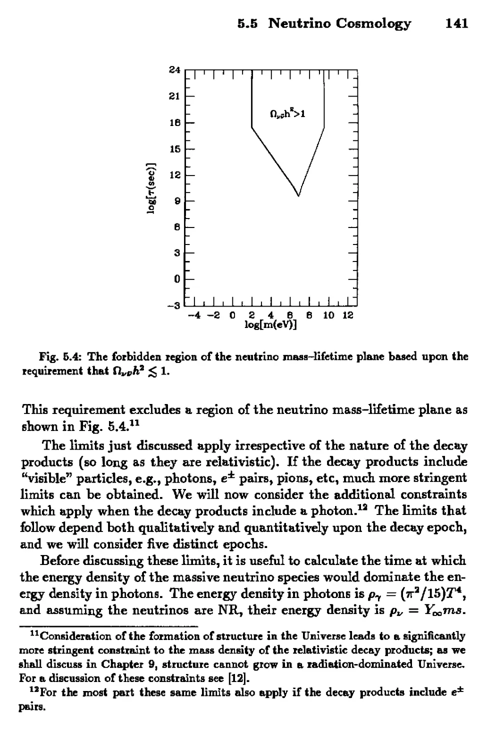
5.5 Neutrino Cosmology 130
5.6 Concluding Remarks 151
5.7 References 152
6. BARYOGENESIS
6.1 Overview 157
6.2 Evidence for a Baryon Asymmetry 158
6.3 The Basic Picture 160
6.4 Simple Boltzmann Equations 168
6.5 Damping of Pre-Existing Asymmetries 176
6.6 Lepton Numbers of the Universe 180
6.7 Way-Out-of-Equilibrium Decay 181
6.8 Sphalerons 184
6.0 Spontaneous Baryogenesis 100
6.10 Epilogue 101
6.11 References 103
Contents
PHASE TRANSITIONS
7.1 High-Temperature Symmetry Restoration 195
7.2 Domain Walls 218
7.3 Cosmic Strings 220
7.4 Magnetic Monopoles 233 <
7.5 The Kibble Mechanism 237
7.6 Monopoles, Cosmology, and Astrophysics 239 jj
7.7 References 255 f-
INFLATION %
8.1 Shortcomings of the Standard Cosmology 261
8.2 Inflation—The Basic Picture 270
8.3 Inflation as Scalar Field Dynamics 275
8.4 Density Perturbations and Relic Gravitons 283 |
i;
8.5 Specific Inflationary Models 291 S.
8.6 Cosmic No-Hair Theorems 303 \
8.7 Testing the Inflationary Paradigm 309 \
8.8 Summary: A Paradigm in Search of as Model 313 ;
8.9 References 317 *
Contents xxi
9. STRUCTURE FORMATION
9.1 Overview 321
9.2 Notation, Definitions, and Preliminaries 324
9.3 The Evolution of Density Inhomogeneities:
The Standard Lore 341
9.4 The Spectrum of Density Perturbations 364
9.5 Two Stories: Hot and Cold Dark Matter 369
9.6 Probing the Primeval Spectrum 378
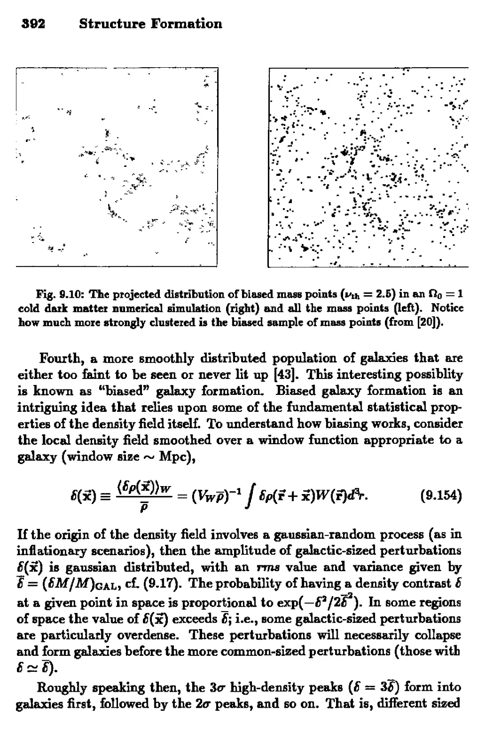
9.7 The n Problem 390
9.8 Epilogue 395
9.9 References 397
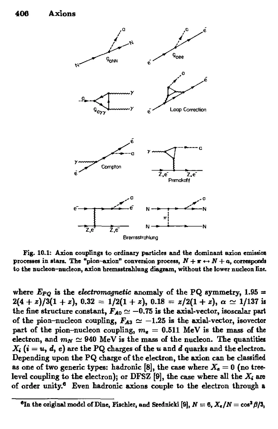
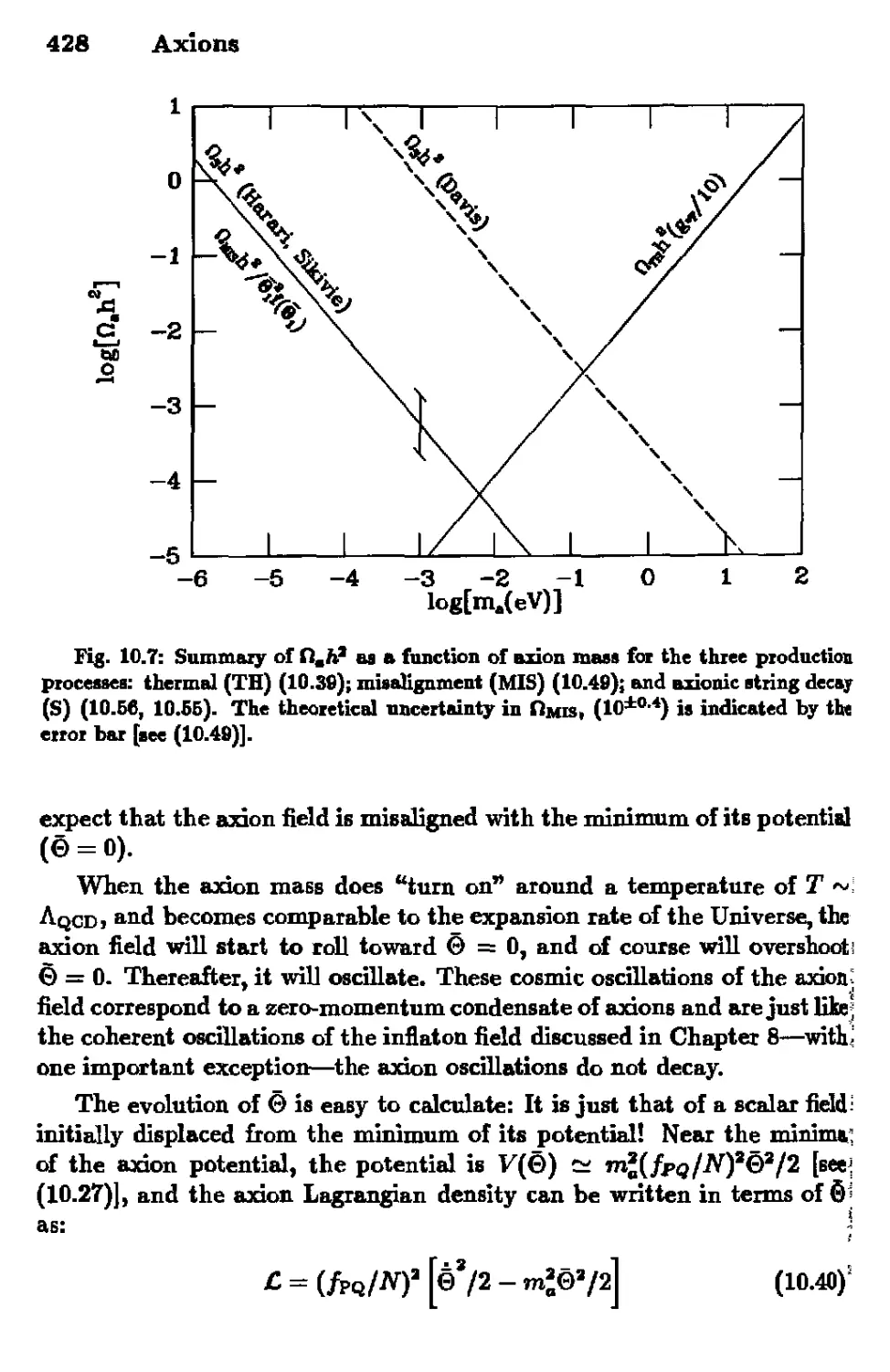
10. AXIONS
10.1 The Axion and the Strong-CP Problem 401
10.2 Axions and Stars 408
10.3 Axions and Cosmology 422
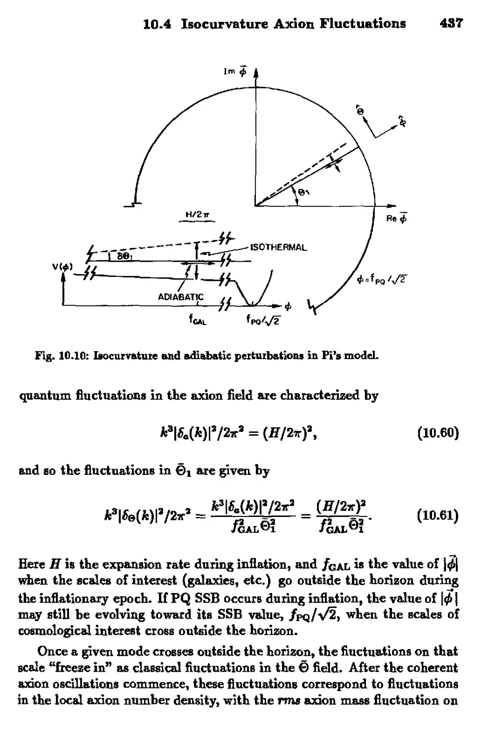
10.4 Isocurvature Axion Fluctuations 436
10.5 Detection of Relic Axions 439
10.6 References 443
xxii Contents
11. TOWARD THE PLANCK EPOCH
11.1 Overview 447
11.2 The Wheeler-De Witt Equation 451
11.3 The Wave Function of the Universe 458
11.4 Cosmology and Extra Dimensions 464
11.5 Limiting Temperature in Superstiing Models 485
11.6 References 487
FINALE 491
APPENDIX A
A.I Units 499
A.2 Physical Parameters 502
APPENDIX B
B.I Quarks, Leptons, and Gauge Bosons 507
B.2 The Standard Model 509
B.3 The ffiggs Sector 515
B.4 Beyond the Standard Model S21
B.5 References 532
INDEX 535
THE UNIVERSE OBSERVED
1.1 Introduction
Our current understanding of the evolution of the Universe is based upon
the Friedmann-Robertson-Walker (FRW) cosmological model, or the hot
big bang model as it is usually called. The model is so successful that
it has become known as the standard cosmology. In this first Chapter
we will review the observational basis for the standard cosmology. Di-
Direct evidence supporting its validity extends back to the beginning of the
epoch of primordial nucleosynthesis, about 10~2 sec after the bang. Cur-
Current speculations about the earliest history of the Universe, the subject of
this monograph, derive torn an extrapolation of the standard cosmology
to very early times. The FRW cosmology is so robust that it is possible to
make sensible speculations about the Universe at times as early as 10~43
sec after the bang! Of course, such speculations are necessarily based upon
some theory of the fundamental interactions at very high energies, ener-
energies approaching the Planck scale AO1S GeV). At present there exists a
standard model of particle physics, the SUC)C® SUB)l® U(l)r gauge
theory of the strong and electroweak interactions. It provides a funda-
fundamental theory of quarks and leptons and has been tested up to energies
approaching 1000 GeV. In addition, the past decade has produced very in-
interesting and important speculations about particle physics at very short
distances, e.g., grand unification, supersymmetry, BUperstring theory, etc.
It is these theories of fundamental physics at ultra-high energies which
allow us to speculate about the earliest history of the Universe.
Astronomy is a data-starved science. Cosmology is even more so. Ob-
Observers (and theii funding agencies) must pay dearly for each particle de-
detected from distant objects in the Universe. In spite of this handicap,
there is indeed a firm observational basis for the standard cosmology, with
2 The Universe Observed
fossils dating back to about 10~a sec after the bang. Moreover, there is
the reasonable expectation that the costnological data base will grow in
the next decades, both in the quantity and in the quality of the observa-
observations. At present the costnological observables include: the expansion of
the Universe; the Hubble constant Ho\ the deceleration parameter qo\ the
age of the Universe to; the present mass density po and composition of the
Universe (p;, i = baryons, radiation, etc.); the cosmic microwave back-
background radiation (CMBR), including its spectrum and spatial structure;
other cosmological background radiations (IK., UV, x ray, 7 ray, etc.); the
abundance of the light elements (particularly D, 3He, 4He, and rLi); the
baryon number of the Universe, quantified as the baryon-to-photon ratio;
and the distribution -of galaxies and larger structures (clusters of galaxies,
superclusters, and voids).
In the companion volume to this monograph, Early Universe: Reprints
[1], we have reprinted or referred to many of the key papers describing
the observed Universe. Here we will briefly summarize the observational
evidence that supports the standard cosmology, and in the process describe
the present state of the Universe.
Unless explicitly displayed, we will set the fundamental constants ft, c,
and kB equal to unity. Some handy conversion factors and a list of useful
physical parameters for astrophysics and cosmology are given in Appendix
A. We will assume that the reader is at least familiar with the basic ideas
of the standard model of particle physics and unified gauge theories; we
provide a brief primer on modern particle theory in Appendix B. We refer
those interested in the standard model and current speculations beyond the
standard model to the excellent monographs that exist on these subjects
[2]-
1.2 The Expansion
A most fundamental feature of the standard cosmology is the expansion
of the Universe. The expansion, discovered in the 1920's, plays a most
basic role in observational cosmology. Of the almost 28,000 galaxy spectra
measured by observers all over the world, all but a handful (those of nearby
galaxies) are red shifted, illustrating the universality of the expansion.
Many quasi-stellar objects (QSO's) with red shifts in excess of 3 have been
observed, and the current record holder has a red shift slightly greater
than 4.7 [3]. Many radio galaxies with red shifts in excess of 2 have been
1.2 The Expansion 3
12 16 20
CORRECTED APPARENT VISUAL MAGNITUDE
Fig. 1.1: The Hubble diagram. The collected apparent magnitude is proportional
to the logaiithm of the luminosity distance. The straight line indicates the theoretical
relationship for 50 = 1 (from [7]).
observed, with the current record holder having a red shift of 3.8 [4].1
The most distant cluster of galaxies observed has a red shift of 0.94 [6].
The light we see today from the most distant objects was emitted when
the Universe was only a few billion yeaxs old. Thus, galaxies and QSO's
provide a probe of the Universe back to times as eady as a few billion years
after the bang.
The relationship between the luminosity distance, d^ = (£/4ttJFI/2
(£ = object's luminosity, T = measured flux),2 and the red shift of a
galaxy z can be written in a power series:
ffofc =*+5A-
A.1)
1Few ordinary galaxies with led shifts greater than one have been seen—perhaps
because they are more difficult to detect. Very recently a candidate field galaxy has
been detected with a purported led shift of 3.38 [5].
2The precise definition of dx, and details of the di,—z relationship will be discussed
further in Chapter 2.
The Universe Observed
| + "- (I-2)
where the Hubble constant is the present expansion rate of the Universe,
Ho = iZ(to)/iZ(to), and the deceleration parameter measures the rate of
slowing of the expansion, g0 = -R{tB)/R{tB)H0' [E(t) is the FEW cosmo-
logical scale factor, denned in the next Chapter, and subscript 0 denotes
the present value of a quantity]. Red shifts are relatively simple (albeit
time consuming) to measure, while determining galaxy distances requires
well-established standard candles (i.e., objects with "known" £). Due to
the difficulty of calibrating the cosmic distance ladder, the distance scale
still has a factor of 2 uncertainty even at modest cosmological distances.
Moreover, for the most distant objects in the Universe (red shifts of or-
order unity or greater) one must worry about evolutionary effects: Do the
luminosities of the standard candles evolve with time?—after all, some
evolution must occur because 20 Gyr ago £ = 0.
At modest red shifts, say z < 1, the linear relationship between d.L and
z is quite clear and convincing (see Fig. 1.1). Using galaxies at relatively
modest red shifts (z <C 1) one may determine HB: On a log z vs. log dL
plot, loglTo is the intercept on the logz axis. At present, reported val-
values for Ho span the range 40 to 100 km sec Mpc, with many authors
quoting standard errors of 10 km sec Mpc~l or less! Clearly, systematic
uncertainties still dominate in the determination of Ho- [For a histori-
historical perspective, compare these values with Hubble's initial determination:
Ho = 550 km sec Mpc.] Without trying to address the complicated
issues in determining this most significant number (and risk making even
more enemies than we already have!), we summarize the current state of
affairs by writing
Ho = lOOfc km sec Mpc, A.3)
and, like all cosmologists, bury our lack of precise knowledge of Ha in
"little hi"
0.4 < h £ 1.0. A.4)
It then follows that the Hubble time or Hubble distance H^1 is
Ho1 = 9.78JT1 x 10° yr
= 3000JT1 Mpc
= 9.25 x lO27^-1 cm. A.5)
1.2 The Expansion
12 14 16 16
CORRECTED APPARENT VISUAL MAGNITUDE
Fig. 1.2: An optical Hubble diagram. The collected visual magnitude is proportional
to the logarithm of the optical luminosity distance. The curves xefei to models with
go = 0, lk 2, 5. No collection for galactic evolution has been included (from [9]).
With the continued refinement of statistically-based distance indicators,3
and the advent of the Hubble Space Telescope, there is hope that this frus-
frustrating uncertainty in Ho soon will be be eliminated. For further discussion
of the cosmic distance scale see [8] and Early Universe: Reprints.
In principle, the deceleration parameter q0 can be measured without
recourse to knowledge of HOt as it merely measures the deviation of the
red shift-distance relationship from the linear "Hubble law," z = Hod-L-
In practice, however, the distance scale is again a problem as one requires
reliable distances to objects at moderate to large red shifts. At such red
shifts the "look back" times are a significant fraction of the age of the
object, and one must worry about evolution. Uncertainties about the
effects of galactic evolution on the intrinsic luminosity of galaxies have
'Essentially all of the traditional techniques foz determining distances to distant
galaxies involve the use of only a single object as a standaid candle, e.g., the first-
xanked galaxy in a clustei or a supernova. Statistical methods like the IE Tully-Fisher,
Faber-Jackson, oi similar relationships allow one to determine the distance to a clustei
by using the properties of a large number of galaxies, e.g., by constructing an IE
luminosity vs. rotation speed (oi galaxy diameter) diagram.
6 The Universe Observed
prevented a definitive (or even near definitive) determination of g0. In
fact, there is not even agreement as to whether the "young" galaxies (i.e.,
galaxies at large red shift) should be intrinsically brighter or dimmer than
the "old" galaxies (i.e., galaxies at small red shift).
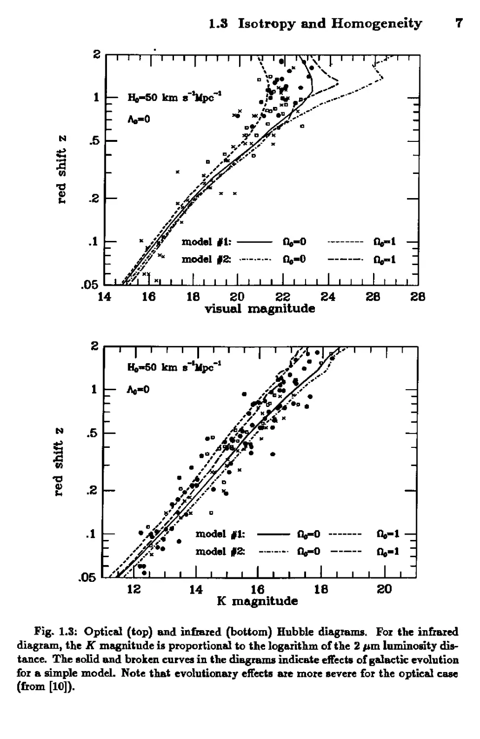
An optical Hubble diagram compiled in 1978 [9], and IR and optical
Hubble diagrams compiled in a recent review [10] are shown in Figs. 1.2
and 1.3.4 At present, the Hubble diagram probably only constrains q0 to
be between 0 and a few. As we will discuss in Chapter 3, q0 is related to
no6
9o = no(l + 3u,)/2, A.6)
where w is the present ratio of the pressure to energy density (for non-
relativistic matter, w ~ 0). Thus, current observations only restrict fl0 to
the interval [0, /eu>].
As we will discuss in Chapter 2, the functional dependence of the angu-
angular size of a standard ruler (e.g., the angular size of a galaxy or a cluster)
depends upon fi0, and can be used to determine fi0. The results of such
an attempt are shown in Fig. 1.4. Once again, this technique only restricts
g0 to the range 0 to a few.
Finally, we mention a very promising kinematic test of the standard
cosmology which can be used to determine q0 (or fi0): the galaxy number
count vs. red shift test. The number of galaxies in a volume element
comoving with the expansion, defined by the solid area dU and red shift
interval dzt depends upon the number density of galaxies (per comoving
volume), and the cosmological model. By counting galaxies as a function of
red shift it is in principle possible to deduce g0 (or Ho). Loh and Spillar [12]
have made a preliminary (and somewhat controversial) attempt to measure
fio based upon this technique and they infer a value of fi0 = O.Sto'l (see
Fig. 1.5). While this test is also subject to the effects of evolution, it is
more sensitive to the evolution of the number density of galaxies than to
the evolution of galactic luminosity. We will discuss the galaxy number
count test at greater length in Chapter 2.
*As emphasized in [10], evolutionary effects may be minimized by using the "IR"
luminosity distance. Because of the led shift effect, optical light from distant galaxies
comes predominately from hot, young, high-mass stars whose evolutionary time scale
is short, while IE light comes from older, low-mass stars whose evolutionary time scale
is longer.
fiThe quantity fie- = Po/pc, where po is the present mass density of the Universe,
and pa is the critical density, pa = 3ffJ/8irG = 1.88 x 10⁻²"h1g cm"'.
1.3 Isotropy and Homogeneity 7
.5 -
.8 -
.1 -
.05
- H.-50 km
- Ao-0
— „
. i i i >
»-Mpc-
n ,^>
model #1:
model §Z:
i 1 i i i
■*"„;•'
■
11
, ,| ivy jiii j..,-
- .* X v
- D.-0 Oi-
I 1 I I I 1 I I I 1 1
1 '
_
-
i I
1 1
14 16 18 80 88 24 SB SB
visual magnitude
.5 -
.3 -
.1 -
.05
1 1 1 1 1
H»-50 km i
- A.-0
model #1:
model #2:
1 , , , 1 , ,
0,^0
n<-o
, 1 , ,
1 '
-
0.-1-
0.-1 :
1
IS
14
16
K magnitude
18
SO
Fig. 1.3: Optical (top) and infoied (bottom) Hubble diagrams. Fox the in&&zed
diagram, the K magnitude is propottional to the logarithm of the 2 /im luminosity dis-
distance. The solid and broken curves in the diagrams indicate effects of galactic evolution
fbi a simple model. Note that evolutionary effects are more severe for the optical case
(torn [10]).
8 The Universe Observed
100
RED SHIFT Z
Fig. 1.4: The angle-led shift test. Shown are the angular diameters of galaxy clusters
at different led shifts, and the theoretical curves for go = 0, 0.5, and 1.0 (from [11]).
1.3 Large-Scale Isotropy and Homogeneity
A cornerstone of the FEW model is the high degree of symmetry of the
FRVV metric. As a practical matter the simplicity of the metric, which
depends upon only one dynamical variable, the cosmic scale factor R[t),
makes the theoretical analysis tractable (even for unsophisticated physi-
physicists like ourselves!).
The assumption of isotropy and homogeneity dates back to the earliest
work of Einstein, who made the assumption not based upon observations,
but as theorists often do, to simplify the mathematical analysis. Today
there is ample evidence for the jsotropy and homogeneity for the part of
the Universe we can observe, our present Hubble volume, whose size is
characterized by ff^1 ~ SOuOfc Mpc ~ lO28^-1 cm.
The best evidence for the isotropy of the observed Universe is the uni-
uniformity of the temperature of the CMBR: Aside from the observed dipole
anisotropy, the temperature difference between two antennas separated by
angles ranging from about 10 arc seconds to 180° is smaller than about
one part in 104 (see Fig. 1.6). The simplest interpretation of the dipole
anisotropy is that it is the result of our motion relative to the cosmic rest
1.3 Isotropy and Homogeneity 9
0.00
1.00
Fig. 1.5: Determination of fio from the galaxy number count test. The number of
galaxies counted in the counting volume (dz, dil) is proportional to zidzdQH^aA(zL>* ,
where $* is proportional to the galaxy number density per comoving volume and A(z)
depends upon the cosmological model (from [12]).
frame. If the expansion of the Universe were not isotropic, the expansion
anisotiopy would lead to a temperature anisotiopy in the CMBR of sim-
similar magnitude. Likewise, inhomogeneities in the density of the Universe
on the last scattering surface would lead to temperature anisotropies. In
this iegard, the CMBR is a very powerful probe: It is even sensitive to
density inhomogeneities on scales larger than our present Hubble volume.6
The remarkable uniformity of the CMBR indicates that at the epoch of
last scattering for the CMBR (about 200,000 yr after the bang) the Uni-
Universe was to a high degree of precision (order of 10~4 or so) isotropic and
homogeneous.
There is additional supporting evidence for the isotropy of the Uni-
Universe: the isotropy of the x-ray background radiation (to about 5%),7 of
eIts sensitivity decreases as (H^/XI; A = length scale of the inhomogeueity [14].
7ln addition, there is weak evidence for a dipole anisotropy of the cosmic x-ray
background, with magnitude and direction consistent with that of the CMBR dipole
anisotropy [15]. If the x-ray background arises from high-red shift sources, and the
x-ray anisotropy indeed coincides with the CMBR anisotropy, this would indicate that
10
The Universe Observed
finisotropy of 2.7K RodiQtion
(95% cl Upper Limits)
Dipole :
• I
1.0
5
10" 30" I' 3' 10' 30' 1° 3° 10° 30° 90° 180°
Angular Scale
O.I
.01
Fig. 1.6: RMS variation of the CMBR temperature as a function of the angular
separation of the two antennas (from [13]).
the distribution of faint radio sources, and of galaxies themselves. Some
substantial fraction of the x-ray background is believed to be from un-
unresolved sources (e.g., QSO's) at high red shift. Likewise, a substantial
fraction of the faint radio sources ace radio-bright galaxies at high red
shift. Both the Shane-Wirtanen (Lick) catalogue of about a million galax-
galaxies with effective depth of about 200 ft Mpc (see Fig. 1.7) and the IRAS
catalogue of infrared selected galaxies with an effective depth of about 60
k-1 Mpc provide evidence for the isotropy of the galaxy distribution.
Direct evidence for the homogeneity of the distribution of galaxies is
more tenuous. Galaxy counts in deep surveys provide supporting evi-
evidence, but their interpretation is not so straightforward. Moreover, since
light does not necessarily trace mass, such surveys only determine the dis-
distribution of light (i.e., bright galaxies) and not a priori that of mass. In
particular, if the mass-to-light ratio varies depending on the local environ-
environment (e.g., the local density), the light distribution will not reflect the true
distribution of the mass. Moreover, it is somewhat disturbing—although
perhaps not totally unexpected—that in the largest red shift surveys com-
the fiame defined by these distant sources is at rest with respect to the CMBR.
1.3 Isotropy and Homogeneity 11
Fig. 1.7: Equal-area projection of a southern sky portion D080 dig2) of the AFM
catalogue. The density of galaxies pel pixel A pixel = 14 (arc min)s) is indicated by a
gley scale. About 2 million galaxies are represented in this image (from [16]).
pleted, the biggest structures are as large as the limits set by the size of the
surveys themselves. As larger red shift surveys are completed (the largest
survey completed contains only about 9,000 galaxies), the distribution of
light, if not mass, should be better understood.
Finally, we mention the evidence for homogeneity from determina-
determination of the "peculiar velocity field of the Universe." Peculiar velocity
refers to the motion of an object (e.g., a galaxy) with respect to the cos-
cosmic rest frame (denned by the rest frame of the CMBR). In practical
terms, it corresponds to a galaxy's velocity after its "expansion velocity"
has been subtracted. The mhomogeneous distribution of matter leads to
gravitationally-induced peculiar velocities of the order of
Sv/c~n°°{X/H^)(Sp/p)x A.7)
on the scale A, where Fp/p)\ characterizes the amplitude of the mass
inhomogeneity on the scale A. Measured peculiar velocities extend to scales
as large as 60ft Mpc or so, where peculiar velocities of order 600 km sec
have been measured, indicating very roughly that (Sp/p)x ~ 10 on these
12 The Universe Observed
scales [17]. Note too, that in principle, peculiar velocity measurements
have the attractive feature that galaxies serve only as test particles tracing
out the gravitational potential and thus provide direct information about
the mass distribution rather than just that of the light. We will discuss
the peculiar velocity field in more detail in Chapter 9.
1.4 Age of the Universe
The age of the Universe can be measured in a variety of different ways:
by using the expansion rate of the Universe to compute the time back to
the bang; by dating the oldest stars in globular clusters; by dating the
radioactive elements; by considering the cooling of white dwarf stars; by
calculating the cooling time for hot gas in clusters, etc. At present, all
techniques yield results consistent with the range 10 to 20 Gyr.
However, the uncertainties, especially the unknown systematics, pre-
preclude a definitive determination by an; of the above techniques. In princi-
principle the present age of the Universe provides a very important test of cos-
mological models. We remind the reader of the discrepancy that existed
until the 1950's between the expansion age, 2 Gvr for the then Hubble
constant of 500kmsec~1Mpc~1, and the age of the solar system, about
4.5 Gyr. That discrepancy led to the birth of the "ageless" steady state
cosmology.
As we will discuss in Chapter 3, the expansion age is set by the Hubble
time Hq1 and fi0: for fio = 0, t0 = Hq1, with the age decreasing with
increasing fl0 (e.g., for a matter-dominated model, to = p/SjflJ for
fio = 1). For the range of plausible values of Ho (ft ~ 0.4 to 1.0), the
Hubble age H^% ~ 9.8 to 24.5 Gyr.
Much work has been carried out to determine the ages of the oldest
globular clusters, those which contain very metal-poor, pop II stars.8 By
detailed stellar modeling a theoretical Hertzsprung-Russell diagram can be
constructed, and then compared to that observed for the cluster. Roughly
speaking, the age of the globular cluster is determined by the position of
the turn-off point on the main sequence for the red giant phase. The point
where this occurs determines the mass of the stars that are just now en-
entering the red giant phase. With recourse to stellar models for such stars
one can calculate their ages. Most estimates of the ages of the oldest stars
6The oldest generation of Btara, those which have low metal abundances (elements
with A > 4), are referred to as pop II, while younger stars, like our sun, with metaj
abundances of oidei 2% (by mass) are referred to as pop L The hypothetical generation
of even oldei stars (possibly pie-galactic in origin) are referred to as pop III.
1.4 Age of the Universe 13
in the galaxy determined this way are in the range 10 to 20 Gyr. Sys-
tematics inherent to this ingenious and powerful technique (stellar mass
loss, convection, metallicity effects, uncertainties in the distance scale, in-
interstellar reddening, etc.) prevent determination of a more precise age or
even a definitive estimate of the uncertainty. Since the oldest globular
clusters likely formed much less than 1 Gyr after the Galaxy formed, and
the Galaxy itself formed less than a few Gyr after the bang, these age
determinations also serve to date the Universe.
Since Rutherford, cosmologists have used radioactive clocks to date the
Universe (and many other objects within it). For cosmological purposes the
most suitable radio isotopes are: S3aTh (mean lifetime t = 20.27 Gyr); 23BU
(r = 1.015 Gyr); M8U (r = 6.446 Gyr); 87Rb (r = 69.2 Gyr); and 187Re
(r = 62.8 Gyr). In order to use these clocks one must know the relative
abundances of these isotopes (or pairs of isotopes) today and at the epoch
of their production. All of these isotopes are so-called r-process elements,
elements thought to be produced by rapid neutron capture in an early
generation of stars. To illustrate this technique, consider the pair a3BU
and M8U. The production ratio is calculated to be [a3BU/M8U]j> = 1-71,
while the present abundance ratio is [s35U/338U]0 =; 0.00723. The time
elapsed since production is then
What does this time interval indicate? If we knew that all the r-process
elements were produced shortly after the Galaxy formed, At would provide
an accurate age for the Galaxy—but we don't! If r-process elements have
been formed continuously since the formation of the Galaxy then the age of
the Galaxy must be considerably greater. Our simple example illustrates
some of the inherent difficulties involved with this technique. Many, much
more sophisticated, analyses have been carried out, with derived ages for
the Galaxy spanning the range 10 to 20 Gyr.
Recently, Winget, et al. [18] have used the cooling of white dwarf stars
to determine the age of the Galaxy. The oldest white dwarf stars are
of course the coolest and least luminous. The observed number of white
dwarfs drops precipitously below a luminosity of 3 x 10~sLq—presumably
due to the finite age of the Galaxy. Based upon this observation and
models of white dwarf cooling, these authors conclude that the age of the
Universe is 10.3 ± 2.2 Gyr.9
6Since white dwarf atais are only obseived in the disk, the authors have actually
14 The Universe Observed
To summarize our brief and very pedestrian review of age determina-
determinations for the Universe, we can say that all techniques yield an age consis-
consistent with the range 10 to 20 Gyr. This in itself is very reassuring, cf. the
"age crisis" in cosmology which lasted until the L950's. Moreover, even
this somewhat inprecise dating of the Universe provides an important test
of cosmological models. In Chapter 3 we will show that for a matter-
dominated model a lower bound to the age of the Universe of 10 Gyr
provides an upper bound to fi0 of 6.8 (for h > 0.4) or 3.2 (for h > 0.5).
Further, if we consider a flat (fi0 = 1), matter-dominated model, then
t0 > 10 Gyr, necessarily impKes that h < 0.65. That is, a value of if0 > 65
km sec'1 Mpc-1 would rule out such a cosmological model. A determina-
determination of Ho to a precision of 10% is believed possible with the Hubble Space
Telescope; if and when this is done, there could be important cosmological
implications.
1.5 Cosmic Microwave Background Radiation
The CMBR provides the fundamental evidence that the Universe began
from a hot big bang. As we will discuss in Chapter 3, the surface of last
scattering for the CMBR was the Universe at a red shift z ~ 1100 and age
of 180,000(fi0fea)~l/2 yr- Flux measurements of the CMBR ranging from
wavelengths of about 70 cm down to wavelengths of less than 0.1 cm are
consistent with that of a black body at temperature 2.75 ± 0.015 K (see
Fig. 1.8). Such a temperature corresponds to a present photon number
density of 422 cm.10
As mentioned earlier, the temperature of the CMBR across the sky
is remarkably uniform: AT/T ;$ 10~4 on angular scales ranging from 10
arc seconds to 180° (after the dipole anisotropy has been removed); see
Fig. 1.6. The observed high degree of isotropy not only provides strong
evidence for the present level of large-scale isotropy and homogeneity of
our Hubble volume, but also provides an important probe of conditions in
the Universe at red shifts of order 1100.
As we will discuss in Chapter 9, the primeval density inhomogeneities
necessary to initiate structure formation result in predictable temperature
estimated the age of the disk. If, as some suspect, the disk formed several Gyr after the
galaxy, then several Gyr should be added to these estimates for the age of the galaxy.
10We mention that recently Lange and his collaborators [19] have reported evidence
for a distortion in the CMBR spectrum in the submUlimeter region (Wien part of the
spectrum). This submillimeter excess corresponds to about 10% of the total energy in
the CMBR. If their result stands it will have profound implications for cosmology.
1.6 Light Elements 15
5 3
WAVELENGTH (cm]
i L
-RAYLEIGH- JEANS-
X-Hc/3kT
—WIEN—
FREOUENCY (GHz)
Fig. 1.8: Temperature measurements of the CMBR (from [20]). PW indicates the
discovery measurement of Penzias and Wilson, and * indicates the recent measurements
ofLangeet al. [19].
fluctuations in the CMBR, and so anisotropies of the CMBR provide a
powerful test of theories of structure formation. In fact, the current lim-
limits to the anisotropy come within factors of 3 to 10 of the predictions of
the most attractive scenarios of structure formation: inflation-produced
adiabatic density perturbations with hot or cold dark matter, and cosmic
string-induced density perturbations with hot or cold dark matter. Spec-
Spectral distortions in the CMBR, if they exist, may provide fossil evidence for
the early history of galaxy, and possibly even star, formation.
1.6 Light-Element Abundances
Primordial nucleosynthesis is the earliest test of the standard model. Nu-
Nuclear reactions that took place from t ~ 0.01 to 100 sec (T ~ 10 MeV to
0.1 MeV) resulted in the production of substantial amounts of D (D/H
~ few x 10-B), 3He CHe/H ^ few x lO), 4He (mass fraction Y ~ 0.25),
and 7Li GIi/H ~ 1 to 2 xlO0). Deuterium and Helium-4 are of par-
particular importance as there are apparently no contemporary astrophysical
processes that can account for their observed abundances. While ordinary
16 The Universe Observed
stars produce 4He, even in regions where there has been significant stellar
processing, the stellar contribution is only about Al^teUar — 0.05. While
the observed Deuterium abundance is very small, even this small amount is
difficult, if not impossible, to account for, as almost all astrophysics! pro-
processes destroy the weakly-bound deuteron which burns at the relatively
low temperature of about 0.5 x 10s K.
The comparison of the predicted abundances with "inferred" primor-
primordial abundances provides a very powerful test of the standard cosmology.
At present there is concordance between the predicted and observed abun-
abundances for these four isotopes, provided that the baryon-to-photon ratio tj is
in the interval 17 = D to 7) x 100, corresponding to 0.015 < fiBftJ < 0.026,
or taking 0.4 < h < 1.0, 0.014 < fiB < 0.16. The standard cosmology
passes this very stringent test with flying colors, and further provides im-
important information about the density of baryons in the Universe. In fact,
primordial nucleosynthesis provides the most precise determination of the
baryon density. Most significantly, primordial nucleosynthesis implies the
fraction of critical density in baryons, fiB, must be less than one: For flB
~ 1, Deuterium would be severely underproduced, and both 4He and 'Li
would be overproduced. If flo is equal to 1, then primordial nucleosyn-
nucleosynthesis provides the strong indication that most of the mass density of the
Universe is in a form other than baryons.11
Finally, we add that primordial nucleosynthesis has also been used as
a probe of the early Universe and particle physics. We have already men-
mentioned that it provides an important constraint to the baryon density. It
has also been used to constrain the existence of additional hypothetical,
light (< MeV) particle species predicted by some particle theories (e.g.,
additional light neutrino species). Such species would contribute to the en-
energy density of the Universe, and thereby affect the predicted abundances.
Chapter 4 is devoted to a detailed discussion of primordial nucleosynthesis.
1.7 The Matter Density: Dark Matter
in the Universe
Previously, we discussed kinematical methods of determining fi0; here we
discuss dynamical means of measuring Ho. Measuring the mass density
of the Universe is a challenging task! Figuratively speaking, the average
11 In Chapter 4 we will discuss two unconventional scenarios of primordial nucleosyn-
nucleosynthesis which, if correct, would allow tip ~ 1.
1.7 Dark Matter 17
density of the Universe ((p)) can be measured by determining the number
density of galaxies (mGAI.) and the average mass per galaxy ((JWgal)):"
(p) = "gal(JWgal)- A-9)
Once (p) is found, fio = {p)fpc follows easily.
Measuring the mass of a galaxy by dynamical means involves detecting
the gravitational effect of the mass in the galaxy in one way 01 another.
The simplest means is the use of Kepler's 3rd Law:
GM(r) = v2r A.10)
where v is the orbital velocity at a distance r from the center of the galaxy,
M(r) is the mass interior to r, and spherical symmetry is assumed. Ap-
Applying this technique to spiral galaxies (taking the measured rotational
velocity to be u), and taking r to be the radius within which most of the
light emitted by the galaxy is emitted, one finds that the fraction of critical
density directly associated with light is
fiLUM ^ 0.01 or less. A.11)
Astonishingly, the mass associated with light provides less than 1% of the
critical density.
When astronomers extended this technique to distances beyond the
point where the light from a galaxy effectively ceases (by observing the
rare star, or 21 cm emission from neutral Hydrogen, or HI, gas clouds)
they found that M(r) continued to increase. If the mass associated with
the light were the whole story, v would decrease as r^3 beyond the point
where the light and mass cut off; rather they found v = constant, corre-
corresponding to M(r) oc r (see Fig. 1.9). By definition, the additional mass is
"dark," i.e., there is no "detectable" radiation associated with it. Further,
there is no convincing evidence for a rotation curve that "turns over" (i.e.,
v oc r/3), indicating the total mass associated with a spiral galaxy has
yet to be found! There is additional (weak) evidence that the dark matter
is roughly spherically distributed, implying that Pdark oc r~3. Rotation
curve measurements indicate that virtually all spiral galaxies have a dark,
"What astronomers actually do is measure mass-to-light ratios foe galaxies (oi parts
thereof), and then calculate (p) by: (p) = {M/L)C, where C is the luminosity density;
in the BT system, C ~ 2Ah x 108££OMpc~8. In these units, M/L for p = pc is
18
The Universe Observed
300
20 40 60
Rodius <kpc)
Fig. 1.9: Rotation curves determined from 21 cm obseivations. Vertical bars indicate
the point where the optical light is less than 25 (blue) mag (arc second)'3. For reference,
this corresponds to about 6% of the surface brightness of the night sky, and less than
about 1% of the brightness of the central legion of a typical spiral (from [21]).
diffuse "halo" associated with them which contributes at least 3 to 10 times
the mass of the "visible matter" (stars and the like). Based upon this we
can conclude:
"halo & 0.1 =* 10 fiLUM. A.12)
This is very strong evidence that dark matter is the dominant component of
the mass density of the Universe. Note that a comparison of the lower limit
to the barvon density based upon primordial nucleosynthesis, SIb > 0.015,
and Hlum already suggests that there is dark barvonic matter. This is not
a great surprise, as there are a variety of forms that baryons can take that
are not "luminous," e.g., jupiters, white dwarfs, neutron stars, black holes,
etc.
The average mass per galaxy in a cluster can also be determined by dy-
dynamical means. Assuming that the cluster in question is a gravitationally-
bound and well-relaxed system, the virial theorem applies and
A.13)
1.7 Dark Matter 10
where M is the cluster mass, (v2I?2 is the rma velocity of a galaxy, and
(r) is the mean inverse separation between galaxies. The estimates of
fio based upon this technique yield values of the order 0.1 to 0.3, also in-
indicating the presence of substantial amounts of dark matter.13 There are
uncertainties however: Are clusters well-relaxed (i.e., virialized), spheri-
spherically symmetric objects? Are projection effects important (only projected
velocities and positions are measured)? Are some of the galaxies misidenti-
fied interlopers—thereby raising (v2)—rather than cluster members? More
importantly, only about 10% of galaxies are in clusters, and one may ques-
question if the value of (Mgal) inferred for cluster galaxies is typical of all
galaxies.
The amount of matter in the Universe can be measured by a number
of other dynamical methods. For example, the Virgo cluster represents
a nearby (about 20 Mpc away) enhancement in the density of galaxies
(fnoAi/noAL ~ few) and hence of the mass density, whose presence dis-
distorts the local Hubble flow. By modeling the local distortion of the Hubble
flow around Virgo, one can determine (Mgal) for Virgo and thereby fio-
The "Virgo infall" method gives fi0 = 0.1 to 0.2. Virgo infall samples fi0
on a scale of about 20 Mpc. It is possible to use the infall method on a
larger scale, by relating the velocity of the Local Group with respect to
the CMBR to the velocity expected from the local cosmic gravitational
field that arises due to the inhomogeneous distribution of galaxies. The
local gravitational acceleration can be determined from the distribution
of matter out to some appropriate distance (see Chapter 9). Using the
matter distribution deduced from the IRAS survey, a value of flo greater
than 0.2 and perhaps as large as unity has been inferred [22]. Finally, on
even larger scales one can use the cosmic virial and energy theorems to
relate the kinetic energies of galaxies relative to the Hubble flow to the
gravitational potential energies determined by the mass density. Based
upon thiB technique, values for flo approaching unity have also been found
[23].
With these dynamical determinations of fl<>» there is a very important
caveat that should be kept in mind: All of the aforementioned determi-
determinations are only sensitive to material that clusters with bright galaxies.
Galaxies and clusters represent large local enhancements in the density of
the Universe, Bpfp ~ 10B (galaxies), ~ 10a to 103 (clusters), and there-
**We mention that many clusters show the presence of baryonic matter that is dark
at optical wavelengths, but luminous at x-ray wavelengths, and accounts for an amonnt
of matter comparable to the optically-bright matter, illustrating the fact that "dark"
is a relative term.
20 The Universe Observed
fore any locally-smooth distribution of matter (i.e., tpjp 5 1) makes only
a negligible contribution to the mass of these systems whose dynamics
is dominated by the large local overdensity (and not the average cosmic
density). On the other hand, the kinematical techniques discussed ear-
earlier (Hubble diagram, galaxy number count test, angle-red shift test, etc.)
measure the average cosmic density (averaged over 1000'e of Mpc). While
the kinematical techniques have thus far proven inconclusive, the dynami-
dynamical methods strongly indicate that the material which clusters with bright
galaxies on scales less than about 10 to 30 Mpc contributes
%„-»=! 0.2 ±0.1, A.14)
where the ± is not meant to be a formal error estimate, but rather indicates
the spread of values obtained using different techniques (somehow weighted
by their reliabilities). The implications for proponents of a flat Universe
(including both the authors) are both obvious and very significant. If
£la = 1, and the aforementioned dynamical measurements are correct, then
there must be a significant "less-clustered'' (or unclustered) component to
the energy density of the Universe, contributing
fisMOoTH=;0.8±0.1, A.15)
which is more smoothly distributed on scales less than 10 to 30 Mpc. We
will address this important issue, often referred to as "the fi problem," in
more detail in Chapter 9. For purposes of illustration we mention here only
three of the possibilities for a smooth component of the matter density:
(i) high-velocity particles, such as light (90ft2 eV), relic neutrinos, or a sea
of undiscovered relativistic particles, which by virtue of their great speeds
would not become bound to systems as small as 10 to 30 Mpc; (ii) a
relic cosmological term (or vacuum energy) which by definition is spatially
constant; (iii) a yet undiscovered (or unidentified) population of very dim
galaxies that are significantly less clustered than bright galaxies.
Summarizing our knowledge of fi0 based upon dynamical methods: (i)
luminous matter contributes only a small fraction of the critical density
(less than 0.01); (ii) dark matter dominates the contribution of luminous
matter by at least a factor of 10; (iii) the amount of matter that clusters
with galaxies on scales of 10 to 30 Mpc contributes 0.2 ± 0.1 of critical
density; (iv) dynamical measurements do not preclude a less clustered, or
even smooth, component that contributes as much as 0.8 ± 0.1. Taking
this information together with our knowledge of £Ib based upon primordial
1.8 Large-Scale Structure 21
0.01 0.1 1.0
llll| ■—I 1—I I I I H-| 1 1—I I I I
■«—*■ -• Halo Dork Matter " ? ■£? THEORY
-" Baryons (BBN) •■ ♦-Loh-Spillor-»
^?^ ^ ^
Disk Clusters, Virgo Infall
Dark Matter p
IRAS
Cosmic Viriol THM
Fig. 1.10: Summary of determinations of f?o-
nucleosynthesis @.015 < fie < 0.16), we can infer that some of the dark
matter must be baryonic, and if flo < 0.16, all of it could be baryonic
(e.g., in the form of black holes, neutron stars, jupiters, etc.). On the
other hand, if flo > 0.16, then there is strong evidence from primordial
nucleosynthesis that the dark component is non-baryonic, e.g., relic, stable
Weakly-Interacting Massive Particles (or WIMPs) left over from the ear-
earliest moments of the Universe. We will touch upon the subject of WIMPs
several times in later Chapters. Fig. 1.10 summarizes the dynamical de-
determinations of fto-
1.8 The Large-Scale Structure of the Universe
To this point we have described the Universe as a fluid of nearly constant
density. Such a description for the early Universe, comprised of a soup of
elementary particles with short mean free paths, or for the Universe today
when viewed on large scales (greater than 100 Mpc), is both well-motivated
and quite a good approximation. However, on smaller scales such a de-
description glosses over some of the most salient and conspicuous features of
the Universe today—the existence of structures including planets, stars,
galaxies, clusters of galaxies, superclusters, voids, etc. The existence of
such structures is an important feature of the Universe, and is likely to
provide a key to understanding the evolution of the Universe. While an
understanding of the origin and evolution of stars and planets is outside
the realm of cosmology, the origin and evolution of galaxies and larger
structures is definitely not.
Ideally, to develop an understanding of the structure of the Universe
one would like to know the distribution of both matter and light in a
22 The Universe Observed
representative volume of cosmological dimensions, say of order 1000A
Mpc on a Bide.14 However, all we can see are galaxies, and at that, only-
bright ones,15 like our own. As emphasized previously, it is not a priori
true that light faithfully traces the mass distribution.
An ambitious, but more realistic, goal would be to survey a suitably
large volume of the Universe, obtaining sky positions, velocities, and dis-
distances for a few million galaxies. The largest galaxy catalogue, the APM
Galaxy Survey, consists of some 5 million galaxies and has an effective
depth of 600A Mpc [I6j.16 The simplest means of obtaining the distance
to a galaxy is by determining its red shift: <£*, ~ Bq1^-, and of course this
necessitates obtaining spectral information. Only a total of 28,000 galaxy
red shifts are known, and the largest systematic survey, the CfA slices of
the Universe survey [25], contains about 9,000 red shifts. The hang-up is
obtaining red shifts: Using traditional techniques, a single red shift de-
determination requires about a half hour of telescope time, and a typical
telescope has only about 3,600 useful hours of observing time per year
(and more than 10,000 hours of requests for that time!). The present sit-
situation then is far from ideal; however it promises to improve dramatically
as larger red shift surveys employing automated and multiple object spec-
trograph techniques are completed in the next decade. In fact, a group of
astronomers at Chicago and Princeton have begun a decade-long project
to obtain red shifts for a million galaxies—a survey of the northern sky
out to a red shift of about 0.1.
We began with the above lengthy preface to place the present obser-
observational situation into proper perspective. Stated bluntly, we are just
beginning to develop a picture of the distribution of galaxies in the Uni-
Universe. What then do we know about the distribution of bright galaxies in
the Universe and the nature of the large-scale structure? Bright galaxies
14Foi reference, using the linear approximation, dz = Ho lz, it follows that the length
AX corresponds to the red shift interval Az ~ 0.03(A£/l00fc-lMpc).
15Biight galaxies have surface brightnesses which are about a factor of 10 above the
surface brightness of the night sky, i.e., the integrated light of all stars and galaxies. By
suitable integration techniques galaxies with surface brightnesses of only a few percent
of the night sky can be detected- If blight galaxies were a factor of 3 larger in linear size
they would fade into the night Bky. This fact suggests that there could be substantial
numbers of low surface brightness galaxies which have escaped dstection.
10The Lick (Shane-Wiitanen) Catalogue contains some 1.6 million galaxies and has
an effective depth of about 200ft- Mpc [24]. This survey is not really a catalogue
in that Bky positions aie not given for individual galaxies, rathe? just the number of
galaxies per 10 arc minute bin on the Bky. The Zwicky catalogue of galaxies and clusters
contains some 31,000 galaxies.
1.8 Large-Scale Structure 23
to a first approximation are distributed uniformly on the sky (see Fig. 1.7),
and presumably within our Hubble volume. However, they do show a ten-
tendency to cluster, quantified by the galaxy-galaxy correlation function, (ac
which measures the probability in excess of random of finding a galaxy at
a distance r from another galaxy:
ice ~ (r/SA^Mpc)-1"8, A.16)
valid for galaxy separations, O.lA-1Mpc < r < 20A~1Mpc.
Many galaxies are found in binary systems or small groups of galaxies.
About 10% of galaxies are found in galaxy clusters, bound and often well-
virialized groups containing anywhere from tens to thousands of galaxies.
The Virgo cluster and Coma clusters are familar nearby clusters. The best-
known catalogue of rich clusters is the Abell catalogue, where clusters are
categorized by their Abell richness class (classes that roughly correspond
to the number of galaxies within the cluster). Ab ell's combined northern
and southern catalogues contain some 4,076 clusters.17 Not to diminish
the importance of this catalogue, we mention that Abell himself warned
against the use of his catalogue for statistical purposes. With this in mind,
we mention that the clustering properties of Abell clusters have also been
determined, quantified by the cluster-cluster correlation function [28],
ice =2 (r^A^Mpc)*8 A.17)
The cluster-cluster correlation function has approximately the same power-
law slope as the galaxy-galaxy correlation function (to within the uncer-
uncertainties), but has a much larger correlation length, 25A Mpc compared
to 5A Mpc for galaxies. The fact that clusters seem to cluster more
strongly is a surprising result—if light faithfully traced mass this would
not be true. This suggests that light may be a "biased" tracer of mass; we
will return to this issue in Chapter 9. When considering the quantitative
difference between the two correlation functions, one should keep in mind
l7Abcll compiled his catalogue in the 1950's using the Palomar all-sky survey plates.
He identified dusters and cluster membership by subjective criteria: Clusters were
defined visually by an enhancement in the local density of galaxies. Since the exposure
time of the plates varied significantly across the iky, and the density of field stats also
varied, selection effects (depth of the survey, and the ability to pick out enhancements
in the galaxy density) axe significant. The Zwicky catalogue of dusters which contains
some 4000 clusters suffers from similar shortcomings. A recent analysis has attempted
to quantify and correct for selection effects inherent in the Abell catalogue [27].
24 The Universe Observed
Fig. 1.11: Distribution of TJGC (Uppsala General Catalogue) and ESO (European
Southezn Observatory) galaxies on the Bky. The white band is caused by obscuration
due to the disk of the Milky Way. The Antlin, Centaums, Hydra, and Virgo dusters
are indicated. The linear feature across the diagonal is referred to as the supergalactie
plane (from [26]).
the shortcomings of the Abell catalogue of clusters. Fig. 1.11 shows the
distribution of nearby galaxies on the sky, and several nearby clusters can
be easily identified.
Even larger structures seem to exist—superclusters, loosely-bound, non-
virialized objects with densities about twice the average density of the
Universe, containing several to many rich clusters. Nearby superclusters
include our own Local Supercluster (centered on the Virgo cluster), Hydra-
Centaurus, and Pisces-Cetus. Of order 20 or so such structures have been
identified, and attempts have even been made to quantify their clustering
properties.
Several surveys have found evidence for the existence of voids in the
distribution of bright galaxies. For example, the KOSS survey [29] showed
the existence of a void in Bootes of diameter about 50ft Mpc, and the CfA
slices of the Universe seem to indicate that voids of size about 20ft-1 Mpc
in diameter are quite common. The authors of the CfA survey have even
speculated that the overall distribution of galaxies may be "bubbly," with
1.8 Large-Scale Structure 25
Fig. 1.12: One of the CfA slices of the Universe [25].
galaxies concentrated on sheet-like structures surrounding nearly empty
voids (see Fig. 1.12).
Finally, we mention a very interesting probe of the Universe at high
red shifts: QSO Absorption Line Systems (QALS's). The spectra of many
high-red shift QSO's exhihit series of absorption lines with red shifts less
than that of the quasar itself. These absorption lines are thought to be due
to absorption of the light from QSO's by intervening objects, some of which
are likely to be galactic (or even pre-galactic) disks and/or halos. These
absorption line systems are classified by the nature of the absorption lines:
Lyman-a systems, damped Lyman-a systems, Lyman-limit systems, and
metal systems. The study of QALS*s (internal densities, number densities,
masses, clustering properties, etc.) will likely prove to be a very important
probe of the Universe at large red shift.
It is clear that an understanding of the present distribution of matter in
the Universe is crucial to understanding the origin of structure in the Uni-
Universe and to testing the detailed scenarios of structure formation that have
been developed in recent years. In turn, this will also test the theories of
the very early Universe that give rise to these scenarios of structure forma-
formation. At present, it is probably fair to say that we have an incomplete, but
26 The Universe Observed
rapidly-emerging, view of the large-scale structure of the Universe. Hope-
Hopefully, larger red shift surveys will answer pressing questions like: What is
the topology of the galaxy distribution and is it "bubbly?" Do clusters
cluster significantly more strongly than galaxies? What are the largest
coherent structures that exist in the Universe today? How is the nature
of the large-scale structure to be quantified? Are the mass and light dis-
distributions similar? When did galaxies and clusters of galaxies form? How
has the evolution of galaxy clustering proceeded?
1.9 References
1. E. W. Kolb and M. S. Turner, The Early Universe: Reprints (Addison-
Wesley, Redwood City, Calif. 1988).
2. C. Quigg, Gauge Theories of the Strong, Weak, and Electromagnetic
Interactions (Addison-Wesley, Redwood City, Calif. 1983); M. B.
Green, J. H. Schwarz, and E. Witten, Superstring Theory, Voh. land
II (Cambridge Univ. Press, Cambridge, 1987); G. G. Ross, Grand
Unified Theories (Addison-Wesley, Redwood City, Calif. 1984); J.
C. Taylor, Gauge Theories of Weak Interactions (Cambridge Univ.
Press, Cambridge, 1976); I. J. R. Aitctuson and A. J. G. Hey, Gauge
Theories in Particle Physics (Adam Hilger Ltd., Bristol, 1982).
3. D. P. Schneider, M. Schmidt, and J. E. Gunn, Astron. J., in press
A989). Second place goes to a QSO with a red shift of 4.43; see S.
J. Warren, P. C. Hewett, P. S. Osmer, and M. J. Irwin, JVirfiire 330,
453 A987).
4. K. Chambers, G. Miley, and W. van Breugel, Ap. J., in press A988).
5. L. L. Cowie and S. J. Lilly, Ap. J. 336, L41 A989).
6. J. Hoessel, B. Oke, and J. Gunn, Ap. J., in press A989).
7. A. Sandage, Physics Today, Feb. 1970, p. 34.
8. M. Rowan-Robinson, The Cosmological Distance Ladder (Freeman,
San Francisco, 1985).
9. J. Kristian, A. Sandage, and J. Westphal, Ap. J. 221, 383 A978).
1.0 References 27
10. H. Spiniad and S. Djoigovski, in Observational Cosmology (IAU
Symposium 124), eds. A. Hewitt, G. Buibidge, and Li-Zhi Fang (Rei-
del, Dordrecht, 1987), p. 129.
11. G. Bruzual and H. Spinrad, Ap. J. 220, 1 A978).
12. E. Loh and E. Spillar, Ap. J. 807, Ll A986); however see S. Bah-
call and S. Tremaine, Ap. J. 326, Ll A988) for a discussion of the
shortcomings of this determination.
13. D. T. Wilkinson, in Inner Space/Outer Space, eds. E. W. Kolb, M.
S. Turner, D. Lindley, K. Olive, and D. Seckel (Univ. Chicago Press,
Chicago, 1986), p. 126; D. T. Wilkinson, in ISth Texas Symposium
on Relativistic Astrophysics, ed. M. P. Ulmer (World Scientific, Sin-
Singapore, 1987), p. 209; R. B. Partridge, Rep. Prog. Phys. 51, 647
A988). Not included in Fig. 1.6 are the recent measurements of R.
D. Davis, et al., Nature 326, 462 A987) and A. C. S. Readhead, et
al., Ap. J., in press A989).
14. L. P. Grischuk and Ya. B. Zel'dovich, Sov. Astnm. 22,125 A978).
15. E. Boldt, Phys. Rep. 146, 215 A987).
16. S. J. Maddox, W. J. Sutherland, G. Efstathiou, and J. Loveday, Mon.
Not. Roy. Astnm. Soc, in press A989).
17. Galaxy Distances and Deviations from Universal Expansion, eds. B.
F. Madore and R. B. Tully (Reidel, Dordrecht, 1986); A. Dressier,
et al., Ap. J. 313, L37 A987); C. A. Collins, et al., Nature 320, 506
i); M. Aaronson, et al., Ap. J. 302, 536 A986).
18. D. E. Winget, et al., Ap. J. 315, L77 A987).
19. T. Matsumoto, et al., Ap. J. 820, 567 A988).
20. J. B. Peterson, et al., in Inner Space/Outer Space, eds. E. W. Kolb,
M. S. Turner, D. Lindley, K. Olive, and D. Seckel (Univ. Chicago
Press, Chicago, 1986), p. 119; D. T. Wilkinson, in ISA Texas Sympo-
Symposium on Relativistic Astrophysics, ed. M. P. Ulmer (World Scientific,
Singapore, 1987), p. 209. Not included in Fig. 1.8 are the recent
measurements of M. Bersanelli, et al., Ap. J. 330, 632 A989).
21. R. Sancisi and T. S. van Albada, in Dark Matter in the Universe,
eds. J. Kormendy and G. Knapp (Reidel, Dordrecht, 1987), p. 67.
28 The Universe Observed
22. M. A. Strauss and M. Davis, in Proceedings of the Vatican Study
Week on Large-Scale Motions in the Universe, eds. G. Coyne and V.
Rubin (Pontifical Scientific Academy, Vatican City, 1988); A. Yahil,
ibid.
23. M. Davis and P. J. E. Peebles, Ap. J. 267, 465 A983); M. Davis,
M. J. Gellei, and J. Huchra, Xp. J. 221,1 A978).
24. M. Seldner, B. Siebers, E. Groth, and P. J. E. Peebles, Astron. J.
82, 249 A977).
25. V. de Lapparent, M. J. Geller, and J. Huchra, Ap. J. 302, LI A986);
ibid, 332, 44 A988); M. J. Geller, J. Huchra, and V. de Lapparent,
in Observational Cosmology (IAU Symposium 124), eds. A. Hewitt,
G. Burbidge, and Li-Zhi Fang (Reidel, Dordrecht, 1987), p. 301.
26. D. Lynden-Bell, Q. Jl. R. astr. Soc. 28, 187 A987); ibid. 27, 319
A986).
27. A. Dekel, G. R. Blumenthal, J. R. Primack, and S. Oliver, Ap. J.
(Letter), in press, A989).
28. For a recent review of the clustering of rich clusters, see, N. A. Bali-
call, Ann. Rev. Astron. Astrophys. 26, 631 A988).
29. R. P. Kirshner, A. Oemler Jr., P. Schechter, and S. Shectman, Ap.
J. 248, L57 A981).
ROBERTSON-WALKER METRIC
2.1 Open, Closed, and Flat Spatial Models
As discussed in the last Chapter, the distribution of matter and radiation
in the observable Universe is homogeneous and isotropic. While this by no
means guarantees that the entire Universe is smooth, it does imply that a
region at least as large as our present Hubble volume is smooth. (We will
return to the smoothness of the Universe on scales larger than the Hubble
volume when we discuss the topic of inflation in Chapter 8.) So long as
the Universe is spatially homogeneous and isotropic on scales as large as
the Hubble volume, for purposes of description of our local Hubble volume
we may assume the entire Universe is homogeneous and isotropic. While a
homogeneous and isotropic region within an otherwise inhomogeneous and
anisotropic Universe will not remain so forever, causality implies that such
a region will remain smooth for a time comparable to its light-crossing
time. This time corresponds to the Hubble time, about 10 Gyr.
The metric for a space with homogeneous and isotropic spatial sections
is the maximally-symmetric Robertson-Walker (RW) metric, which can be
written in the form1
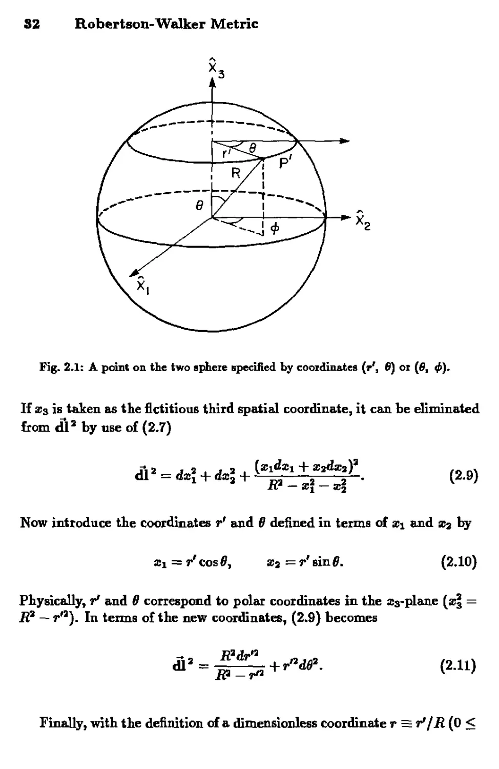
ds2 = dt2 - R2(t) I ** a + r2d82 + r2 sin' Bdtf 1
B.1)
'The sign conventions aie the same a* Landau and Lifshiti [4]: ds2 = dt3 — dl2;
G^ = +6iGT^; and R"uaf = BJ*^, - OpTr^ + T"^f^ - I*,,!",., and
r*,^ = (l/2)j'"'(8/)fc« + fioStrfl - 8<,g«f). Greek indices run fiom 0 to 3, while Latin
indices zun over the spatial indices 1 to 3. We assume that the reader is familiar with the
rudiments of general relativity; fox those interested in textbook treatments of general
relativity we suggest [1-4].
30 Robertson-Walker Metric
where (£, r, 8, $) are coordinates (referred to as comoving coordinates),
R(t) is the cosmic scale factor, and with an appropriate reseating of the
coordinates, k can be chosen to be +1, —1, or 0 for spaces of constant
positive, negative, or zero spatial curvature, respectively.3 The coordinate
r in B.1) is dimensionless, i.e., R(t) has dimensions of length, and r ranges
from 0 to 1 for k = +1. Notice that for k = +1 the circumference of a
one sphere of coordinate radius r in the j> = const plane is just 2ir R[t)r,
and that the area of a two sphere of coordinate radius r is just 4iri22(t)jl2;
however, the physical radius of such one and two spheres is i£(£) J^ drj{l —
Jfer8I'", and not R(t)r.
The time coordinate in B.1) is just the proper (or clock) time measured
by an observer at rest in the comoving frame, i.e., (r, 8, $)=const. As we
shall discover shortly, the term comoving is well chosen: Observers at rest
in the comoving frame remain at rest, i.e., (r, 8, $) remain unchanged, and
observers initially moving with respect to this frame will eventually come
to rest in it. Thus, if one introduces a homogeneous, isotropic fluid initially
at refit in this frame, the t =const hypersurfaces will always be orthogonal
to the fluid flow, and will always coincide with the hypersurfaces of both
spatial homogeneity and constant fluid density.
The spatial part of the metric will be denoted as
dla = hijdxidxi B.2)
where i, j = 1, 2, 3. Note that hy = — gij. The three-dimensional Bie-
mann tensor, Ricci tensor, and Ricci scalar will be denoted as 3Riju, 3Rij,
and S7£. Because the spatial metric is maximally symmetric, 3Riju and
3Rij can be expressed in terms of the spatial metric and R{t),
Bfe
6k
B3)
Because of the symmetry of the RW metric, calculation of the affine
'The scale factor R(t) should not he confused with the Bled scalar, ft.
2.1 Spatial Models 31
connection is particularly simple. The non-zero components are:
l.a (Shtj dhu, dhik\
2 \8xk 8x> 8x> )
rfoj = J*Y B.4)
For completeness, we also mention the non-zero components of the Ricci
tensor:
and the Ricci scalar:
In order to illustrate tlie construction of the metric, consider the sim-
simpler case of two spatial dimensions. Examples of two-dimensional spaces
that are homogeneous and isotropic are: (i) the flat "i — y" plane (Ra);
(ii) the positively-curved two sphere (S3); and (iii) the negatively-curved
hyperbolic plane (.ff2).
First consider the two sphere. To visualize the two sphere it is conve-
convenient to introduce an extra fictitious spatial dimension and to embed this
two-dimensional curved space in a three-dimensional Euclidean space with
cartesian coordinates Xi, x2, x3. The equation of the two sphere of radius
B.7)
The element of length in the three-dimensional Euclidean space is
B.8)
32 Robertson-Walker Metric
Fig. 2.1: A point on tlie two sphere specified by cooidinates (rr, 6) ot F, aS).
If £3 is taken as the fictitious third spatial coordinate, it can be eliminated
torn tfl2 by use of B.7)
dl
B.9)
Now introduce the coordinates rr and 6 defined in terms of x\ and scj by
a!i = / cos 9, x3 = r' Bin B. B.10)
Physically, r1 and 8 correspond to polar coordinates in the x3-plane (x| =
R2 — rn). In terms of the new coordinates, B.9) becomes
B-H)
R*-r"
Finally, with the definition of a dimensionless coordinate r = r'/R @ <
2.1 Spatial Models 33
r < 1), the spatial metric becomes
Note the similarity between this metric and the k = 1 RW metric. It
should also now be clear that R{t) is the radius of the space.
The two sphere is shown in Fig. 2.1. The poles are at r = 0, the equator
is at r = 1. The locus of points of constant r sweep out the latitudes of the
sphere, while the locus of points of constant 8 sweep out the longitudes of
the sphere.
Another convenient coordinate system for the two sphere is that speci-
specified by the usual polar and azimuthal angles (#, $) of spherical coordinates,
related to the a:; by
a;i = R sin 8 cos <f>, x3 = Rsin6sin<f>, x3 = RcosS. B.13)
In terms of these coordinates, B.8) becomes
«U * = B? \d8* + sin3 8d<p] . B.14)
This form makes manifest the fact that the space is the two sphere of
radius R. The volume of the two sphere is easily calculated:
V = Jd\y/h = p d<j> f* MR* sinfi = 4ir.fi? B.15)
as expected (h is the determinant of the spatial metric).
The two sphere is homogeneous and isotropic. Every point in the space
is equivalent to every other point, and there is no preferred direction.
In other words, the space embodies the Cosmological Principle, i.e., no
observer (especially us) occupies a preferred position in the Universe. Note
that this space is unbounded; there are no edges on the two sphere. It is
possible to circumnavigate the two sphere, but it is impossible to fall off.
Although the space is unbounded, the volume is finite.
The expansion (or contraction) of this 2-dimensional Universe is equiv-
equivalent to an increase (or decrease) in the radius of the two sphere, _R. Since
the Universe is apatiatly homogeneous and isotropic, the scale factor (ra-
(radius R) can only be a function of time. As the two sphere expands or
contracts, the coordinates (r and 8 in the case of the two sphere) remain
34 Robertson-Walker Metric
unchanged; they me "comoving." Also note that the physical distance
between any two comoving points in the space scales with R (hence the
name scale factor).
The equivalent formulas for a space of constant negative curvature can
be obtained with the replacement E —» iR in B.7). In this case the embed-
embedding is in a three-dimensional Minkowski space. The metric corresponding
to the form of B.12) for the negative curvature case is
B.16)
and the metric in the form corresponding to B.14) is
«U * = i? [dP + sinh* Sdtf] . B.17)
The hyperbolic plane is unbounded with infinite volume since 0 < 8 <
co. The embedding of H1 in a Euclidean space requires three fictitious
extra dimensions, and such an embedding is of little use in visualizing the
geometry.3
The spatially-flat model can be obtained from either of the above ex-
examples by taking the radius -R to infinity. The flat model is unbounded
with infinite volume. For the flat model the scale factor does not repre-
represent any physical radius as in the closed case, or an imaginary radius as
in the open case, but merely represents how the physical distance between
comoving points scales as the space expands or contracts.
The generalization of the two-dimensional models discussed above to
three spatial dimensions is trivial. For the three sphere a fictitious fourth
spatial dimension is introduced, and in cartesian coordinates the three
sphere is denned by: R? = x\ + x\ + x\ + x\. The spatial metric is
dl2 = dx\ + dxl + dxl + dx\. The fictitious coordinate can be removed to
give
"While the hypeibolic plane cannot be globally embedded in J23, it can be partially
represented by the psuedospheie, a 2-dimensional apace of constant negative curvature
which has a cusp. The pseudosphere is the surface of revolution of the tractiix, z =
4)]-sin4, x = cos tf (-sr/2 < <t> < sr/2), about the z-axis [6].
2.1 Spatial Models 36
In terms of coordinates x\ = r'sinff cos^, x^ = r'sin#sin^, a?s = r'cosff,
the metric is given by B.1) with k = +1 and r = r'/R, cf. B.12). In the
coordinate system that employs the 3 angular coordinates (x, 9, j>) of a
four-dimensional spherical coordinate system, zi = R sin x sin 9 cos (j>, aij =
R sin x sin 9 sin (j>, x3 = R sin x cos 9, xt = R cos x, the metric is given by
A2 = R2 [dx2 + sin2 X(d02 + sin2 9^)] . B.19)
The volume of the three sphere is V = Jd*xVh = 2v2R3.
As in the two-dimensional example, the three-dimensional open model
is obtained by the replacement R —» iR, which gives the metric in the form
B.1) with k = -1, cf. B.16), or in the form B.19) with sin* -» sinhx,
cf. B.17). Again the space is unbounded with infinite volume and R(t)
sets the curvature scale. Embedding H3 in a Euclidean space requires four
fictitious extra dimensions.
Finally, it is often convenient to express the metric in terms of "con-
formal time" i), defined by di) = dt/R{t):
da2 = R'(v) IV - j-^j - r2d6' - r2 sin2 9d<j,' 1.
B.20)
It then directly follows that the fiat RW model is conformal to Minkowski,
i.e., the line element is equal to the Minkowski line element times a confor-
conformal factor. In fact, all the RW models axe locally conformal to Minkowski
space, by which we mean that for a suitable local choice of coordinates,
the metric can be written as the Minkowski line element times a conformal
factor.4
It should be noted th&t the assumption of local homogeneity and isotropy
only implies that the spatial metric is locally 53, f3, or it3, and the space
can have dinerent global properties. For instance, for the spatially fiat case
the global properties of the space might be that of the three torus, T3,
rather than -R3; this is accomplished by identifying the opposite sides of a
fundamental spatial volume element. Such non-trivial topologies may be
relevant in light of recent work on theories with extra dimensions, such
4The RW line element Ilbs vanishing Weyl eurratuie, which is both a necessary
and sufficient condition fox conformal flatness. The Weyl curvature tensor, which cor-
corresponds to the traceless part of the Riemann cuxrature tensor, is given by C^f =
R"*,, - aS^K",) + A/3)«[°[7«''»]R. where [■ ■ "I uxlMatei that the indicies are to be
antisymmetrized.
36 Robertson-Walker Metric
as superstrings. In many such theories the internal space (of the extra
dimensions) is compact, but with non-trivial topology, e.g., containing
topological defects such as holes, handles, etc. If the internal space is not
simply connected, it suggests that the external space may also be non-
trivial, and the global properties of our 3 space might be much richer than
the simple S3, H3, or ij3 topologies.
2.2 Particle Kinematics
A fundamental question in cosmology that one might ask is: What frac-
fraction of the Universe is in causal contact? More precisely, for a comoving
observer with coordinates (r0, 80, </>o), for what values of {r, 8, F) would
a light signal emitted at t = 0 reach the observer at, or before, time t?
This can be calculated directly in terms of the metric B.1). A light signal
satisfies the geodesic equation da* = 0. Because of the homogeneity of
space, without loss of generality we may choose r0 = 0. Geodesies passing
through rB = 0 are lines of constant 8 and F, just as great circles eminating
from the poles of a two sphere are lines of constant 8 (i.e., constant lon-
longitude), so d8 = d<j> = 0. And, of course, the isotropy of space makes the
choice of direction @O, 4>a) irrelevant. Thus, a light signal emitted from
coordinate position (rjj, #o, ^o) at time t = 0 will reach ro = 0 in a time
t determined by
The proper distance to the horizon measured at time t,
dB(t) = £"y/g^dr, B.22)
is simply R(t) times B.21)
f B3)
If du(t) is finite, then our past light cone is limited by a particle horizon,
which ie the boundary between the visible Universe and the part of the
Universe from which light signals have not reached us. The behavior of
R(t) near the singularity will determine whether or not djj is finite. In
the next Chapter we will see that in the standard cosmology dtI(t) ~ t is
finite.
2.2 Particle Kinematics 37
Using the conformal form for the metric, B.20), the causal structure
of the space time is clear since light piopagates on 45° lines in the 17-space
plane, and the distance to the horizon is just
<taM = -R«[i«-i(t = °)]. B-24)
Next, consider the geodesic motion of a particle that is not necessarily
massless. The four-velocity u** of a particle with respect to the comoving
frame is referred to as its peculiar velocity. The equation of geodesic motion
where «** = dx^jds, and A i& some affine parameter. The four velocity
may be expressed in terms of the ordinary three velocity v' = efa'/eZt by
the familiar relation vf = («°, «') = G, 711*), where |v|a = hjjv'v', and
7 = A — |v|2)~*/a. If we choose the affine parameter to be the proper
length, da2 ~ gltvdxlldxt', the ft — 0 component of the geodesic equation is
T + rViV = 0. B.26)
da
For the Robertson-Walker metric, the only non-vanishing component of
T0^ is r°y = (RlH)hih and using the fact that /iy-uV = |uj3, the geodesic
equation becomes
^ + ||u|» = 0. B.27)
Since («°)J - |u|2 = 1, it follows that u°du° = |u|d|fi|, and the geodesic
equation can be written as
ifiS + !H=0. B.28)
Finally, since u° = dtjds, this equation reduces to jfl|/|u| = —RfR, which
implies that |u| oc R~1. Recalling that the four-momentum is jP = mvP,
we see that the magnitude of the three-momentum of a freely-propagating
particle "red shifts" as R~x.h Note that in B.28) the factors of da cancel.
"Since we &ie dealing with ju| or |p|, we don't have to woity about the fact that
the RW metric is not oithonormal. In a basis that is not oithonormal, neither jf not
p. corresponds to the "physical** momentum. What most physicists (as opposed to
38 Robertson-Walker Metric
That implies that the above discussion also applies to massless particles,
where da = 0 (formally by the choice of a different affine parameter).
In terms of the ordinary three-velocity |v|,
|u| = ^ <x R-1. B.29)
1 M2
We again see why the comoving frame is the natural frame. Consider an
observer initially (t = ti) moving non-relativistically with respect to the
comoving frame with physical three velocity of magnitude |vi|. At a later
time £oi the magnitude of the observer's physical three velocity, |vo|, will
gg B.30)
In an expanding Universe, the freely-falling observer is destined to come to
rest in the comoving frame even if he has some initial velocity with respect
to it.
A more formal derivation of the evolution of the momentum of a particle
propagating in a Robertson-Walker background may prove useful. Choose
the origin of the coordinate system at any point along the trajectory of
the particle. With the metric in the form
ds2 = R'ko) [dq2 -d^- sin3 X(M* + sin2 8d<?)] , B.31)
choose the trajectory of the particle along d8 = d<j> = 0. The Hamilton-
Jacobi equation of motion is
where S is the action of a free particle, 5 ex fds. With the metric in the
above form, the Hamilton-Jacobi equation is particularly simple:
The three-momentum |p| of a particle is given by |p| = dS/d\dl |, and
with d9 = d<f> = 0, |dl| = R{ij)dX. Therefore |p| = R^dS/dx- The
mathematicians) would lefei to as the physical three-momentum is that measured in
an orthonoimal frame, which is also equivalent to |p| = (^1'3
2.3 Kinematics of the RW Metric 39
energy of a particle is given by E = (EBE0)ll1 = dS/dr = R^dS/dij.
Thus we recognize that the Hamilton-Jacobi equation coriesponds to the
familial relation E3 — |p|3 = p"pM = mJ. Since {ill cyclic coordinate,
<JS/djt=const, from which it follows that SS/Sx = i?|p|=const, or |p| «
Brl.
2.3 Kinematics of the RW Metric
Without explicitly solving Einstein's equations for the dynamics of the
expansion, it is still possible to understand many of the kinematic effects
of the expansion upon light from distant galaxies. The light emitted by a
distant object can be viewed quantum mechanically as freely-propagating
photons, or classically as propagating plane waves.
In the quantum mechanical description, the wavelength of light is in-
inversely proportional to the photon momentum (A = h/p). If the momen-
momentum changes, the wavelength of the light must change. It was shown in
the previous section that the momentum of a photon changes in proportion
to Brl. Since the wavelength of a photon is inversely proportional to its
momentum, the wavelength at time t0, denoted as Ao, will differ from that
at time ti, denoted as Ai, by
As the Universe expands, the wavelength of a freely-propagating photon
increases—-just as all physical distances increase with the expansion. This
means that the red shift of the wavelength of a photon is due to the fact
that the Universe was smaller when the photon was emitted!
It is also possible to derive the same result by considering the prop-
propagation of light from a distant galaxy as a classical wave phenomenon.
Suppose a wave is emitted from a source at coordinate r = ti at time ti
and arrives at a detector at time to at coordinate r = 0. The massless
wave will travel on a geodesic (is3 = 0), and the coordinate distance and
time will be related by
The wavecrest emitted at a time t\ + &t\ will arrive at the detector at a
time t0 + ^o- The equation of motion will be the same as B.35) with
40 Robertson-Walker Metric
ti —* t\ + Sti and to —♦ to + Sto- Since /(**i) is constant (the source is fixed
in the comoving coordinate system)
k L
k m~L+H, m' ( '
By Eimple rearrangement of the limits of integration we have
rn+«. dt _ /•«.+«. dt
k m~k m'
If 6t is sufficiently email, corresponding to wavelengths A = 6t <£ t,
can be taken to be constant over the integration time of B.37), and
Since fti (fto) is the time between successive wave crests of the emitted
(detected) light, Stt Ft0) is the wavelength of the emitted (detected) light,
and
Ao it(t0)
just the result obtained above.
Astronomers define the red shift of an object, z, in terms of the ratio
of the detected wavelength to the emitted wavelength:
Any increase (decrease) in R[t) leads to a red sliift (blue shift) of the light
from distant sources. Since today astronomers observe distant galaxies to
have red shifted spectra, we can conclude tnat the Universe is expanding.
Hubble'a Law, the linear relationship between the "distance" to a galaxy
and its observed red shift, may be deduced directly from the RW metric
without specific knowledge of the dynamics of the expansion. Suppose a
source, e.g., a galaxy has an absolute luminosity £ (the energy per time
produced by the source in its rest frame), its luminosity distance is denned
in terms of the measured fiux T (the energy per time per area measured
by a detector) by
2.3 Kinematics of the RW Metric 41
The motivation for this definition of di, is clear: In the absence of expan-
expansion, the detected flux is simply equal to the fraction of the area of the two
sphere surrounding the source covered by the detector (A4./4jrdJ, where
AA is the area of the detector) times the luminosity L. In this case dL is
simply the distance to the source. The expansion of the Universe compli-
complicates matters: Is dL the distance to the source at the time of emission,
or at the time of detection, etc? Of course, it is neither. If a source at
comoving coordinate r = rj emits light at time ti, and a detector at co-
moving coordinate r = 0 detects the light at t = to, conservation of energy
CP%, = 0) implies
r' B'42)
B.43)
The rhs of B.42) may be understood as follows: At the detection time
to, the fraction of the area of a two sphere surrounding the source covered
by the detector is <2-i4./4iri23(to)rJ. In addition, the expansion decreases the
energy per unit time crossing the two sphere surrounding the source by a
factor of A + zI: one factor of A + z) arising from the decrease in total
energy due to the red shift of the energy of the individual photons, and the
other factor of A + z) arising from the increased time interval between the
detection of incoming photons due to the fact that two photons separated
by a time St at emission, will be separated by a time 6t(l + z) at the time
of detection [as in B.38)]. Therefore <§ = [fl(to)ri]*(l + *J as written in
B.43).
In order to express dL in terms of the red shift z, the explicit dependence
upon n must be removed. With explicit knowledge of lift) (which requires
solving the Einstein equations) this is straightforward; without explicitly
specifying R{t) this formally can be accomplished by expanding R(t) (and
other quantities) in a Taylor series about the present epoch (i.e., for small
B())
-^ = 1 + jffo(t - to) - \qoHHt - to)' + ■■■ B.44)
where
--flflj B-45)
42 Robertson-Walker Metric
are the present values of the expansion tate (or the Hubble constant) and
the so-called deceleration parameter. Now, remembering that i2(to)/i2(t) —
1 + z, B.44) can be inverted for small JHo(*o - t) to give
z = H0(to - t) + (l + |) Bi(t0 -1J + ■ ■ ■ B.46)
Eq. B.46) yields (t0 - t) in terms of z:
(to - t) = Ho1 [* - (l + f )*■ + -]. B-47)
It is also possible to expand /(rj), denned in B.35), in a power series
f sin'1*! =n+7-?/6 + -- (* = +l)
f(r1)=\r1 (fc = 0) B.48)
I sinh-ln =r,-ri/6 + --- (k = -1).
Using the expansion B.44) on the lhs of B.35) gives
n = R-ifo) [(to -1.) + |ffo(to -1,J + •••]. B.49)
Substituting expression B.47) for {to —1%) in terms of z gives
B.50)
Finally, using this expression in B.43) yields Hubble's law:
floife = * + i(l-«,)*» + •.■. B.51)
Note that the relationship between dL and z deviates from linear for mod-
moderate ziiqojt 1.
In the next Chapter we will solve the Einstein equations for R(t) to
obtain n as a function of z, cf. C.112). Using the exact result for tx(z) in
a matter-dominated Universe gives
( )] B-52)
2.3 Kinematics of the RW Metric 43
Of course, expansion of B.52) for small z yields B.51).
Note that the relationship between the observahie quantities d& and z
depends upon the cosmological model, and thus, in principle, we can use
the Hubble diagram (plot of z vs. dL) to infer go- As discussed in Chapter
1, the difficulty lies in finding appropriate standard candles.6
Another relationship whose form also depends upon the cosmological
model is the the galaxy count-red shift relationship. As mentioned in
Chapter 1, this relationship holds great promise as an observational tool
to determine our cosmological model. Consider a comoving volume element
dVc, containing dJV,j galaxies. In terms of the number density of galaxies
per comoving volume element j
B.53)
Of course, r is not an observable, and we must express r in terms of z.
Using B.50)
and we may express the galaxy count as a function of red shift:
B-54)
- %o + 1)* + • • ■]• B.55)
The exact solution for t(z) found in the next chapter gives
[zqo + (go - l){y/2qQz + 1 - I)]2
dzdil HZR*{1 + zfqt [1 - 2q0 + 2qo(l + z)]1/*
Expansion of the exact result for small z of course leads to B.55).
If one makes the reasonable assumption that ne(z) is constant (galaxies
are neither created oi destroyed—probably a good assumption at red shifts
8The luminosity distance, dL = D7r£/JrI/2, is an observable provided that the
absolute luminosity C is known. Determining absolute luminosities involves the use
of standard candles, i.e., classes of objects that axe easily identifiable and axe bright
enough to be seen at cosmological distances, whose absolute luminosities have been
determined and have very little variance.
44 Robertson-Walker Metric
less than a few), then the differential galaxy count can be used to determine
Finally, we mention one other relationship that depends upon the cos-
mological model, the angular diameter-red shift relation. Let us assume
that there is an object (say, a galaxy or a cluster) of proper diameter D at
coordinate r = n, which emitted light at t = ti, detected by the observer
at t = t0- As usual, we may choose the coodinate system such that the
observer is at the coordinate r = 0. From the metric B.1) it follows that
the observed angular diameter of the source, 6~, is related to D by
'-i&r B7)
The angular diameter distance, dA, is defined as
dA = % = fl(ti)r,. B.58)
a
In a static Euclidean geometry dA = dL is simply the "distance" to the
source.
It is easy to express dA in terms of dL and z using B.43): dA = dL(l +
z)~2. For small Ho{ti — ^o) the approximate relationship between dA and
z is, cf. B.51),
HBdA^z-\{Z + q<>)z* + --- B.59)
while the exact relationship is, cf. B.52)
BedA = <fo 2A + z)-' [zq0 + (g0 - 1) i^2qaz + 1 - 1^] . B.60)
Again, the form of the relationship depends upon the cosmological model
(go), and thus one may in principle use "standard rulers" to infer go-
We have discussed three relationships (dL vs z, dN^j vs z, and dA
vs z) which all depend upon the cosmological model through go. There
are also relationships between observables which do not depend upon the
cosmological model. The simplest example is the measured surface bright-
brightness of an object, say a galaxy or a cluster. The surface brightness, SB,
of an object is the energy fiux per projected solid angle (on the sky):
SB = dSjdU. The projected solid angle dfi is related to the projected
surface area on the object by dA = R2(t^)r\dil, from which it follows
that dFjdSl = SB^trimic/fl + z)*, where SBb,trii»ic is the intrinsic surface
2.4 References 45
brightness of the object (erg sec cm"!). Model-independent relationships
are useful because in principle they can be used to test whether spurious
astrophysical or observational problems affect the model-dependent rela-
relationships. For instance, a measured deviation of dF/dil from a A + z)~*
dependence would indicate that galactic evolution (and/or other effects)
must be taken into account when using standard candles. While earth-
based telescopes probably lack the resolving power to test this relationship,
the Hubble Space Telescope with its expected gain in resolution, may well
be able to exploit this relationship.
In the next Chapter we will derive the dynamical relationship between
the physical parameters of the cosmological model (curvature radius, en-
energy density, pressure, etc.) and q0 and Ho-
2.4 References
Further discussion of the Robertson-Walker metric can be found in:
1. S. Weinberg, Gravitation and Cosmology (Wiley, New York, 1972).
2. C. W. Misner, K. Thome, and J. A. Wheeler, Gravitation (Freeman,
San Francisco, 1973).
3. R. M. Wald, General .Relativity (Univ. Chicago Press, Chicago, 1984).
4. L. D. Landau and E. M. Lifshitz, Classical Theory of Fields (Pergamon
Press, Oxford, 1975).
5. Ya. B. Zel'dovich and I. D. Novikov, Rehtivistic Astrophysics, Vol. II
(Univ. Chicago Press, Chicago, 1983).
There are a multitude of theorems concerning the isometric (i.e., metric
preserving) embedding of Riemannian manifolds into Euclidean space; for
example, any n-dimensional manifold can be locally embedded into RN
for N = n(n +1)/2. Global embeddings are more difficult and the number
of dimensions required depends upon the smoothness of the embedding.
Any n-dimensional manifold can be C1 globally embedded in a Euclidean
space of at most 2n -f 1 dimensions; further, if the manifold is compact,
then at most 2n dimensions are required. (A Ck (fc > 3) global embedding
requires at most n(n + l)Cn + ll)/2 dimensions, nCn + ll)/2 for a com-
compact manifold.) In addition, it is known that the n-dimensional surface of
constant negative curvature cannot be globally embedded in iZ"+1. Since
the two sphere is compact, at most 4 dimensions are required for a global
46 Robertson-Walker Metric
Euclidean embedding, and our example shows that 3 suffice. On the other
hand, these theorems guarantee that the hyperbolic plane can be embed-
embedded in .R5, but not in R2. For further discussion, see the following reference
and references therein:
6. Encyclopedic Dictionary of Mathematics, eds. S. Iyanaga and Y. Kawada
(MIT Press, Cambridge, 1980), Sees. 96H, 114,177, 211, 283,360.
The proof of the conformal equivalence of Robertson-Walker and Minkowski
spaces can be found in:
7. A. P. Lightman, W. H. Press, R. H. Price, and S. L. Teukolsky, Problem
Book in Relativity and Gravitation (Princeton Univ. Press, Prince-
Princeton, 1975), problem 19.8.
References to some historical papers can be found in Early Universe:
Reprints. Also reprinted there is a paper of M. A. MacCallum that dis-
discusses anisotropic and inhomogeneous cosmologies:
8. M. A. MacCallum, in General Relativity: An Einstein Centenary Sur-
Survey, eds. S. W. Hawking and W. Israel (Cambridge Univ. Press,
Cambridge, 1979).
STANDARD COSMOLOGY
3.1 The Friedmann Equation
All of the discussions in the previous Chapter concerned the "kinematics"
of a Universe described by a Robertson-Walker metric. The dynamics of
the expanding Universe only appeared implicitly in the time dependence
of the scale factor R(t). To make this time dependence explicit, one must
solve for the evolution of the scale factor using the Einstein equations:
Rw, - -^9^ = G^ = 87rGT^, + Aft,,,, C.1)
where G,^, is the Einstein tensor, T^ is the stress-energy tensor for all the
fields present—matter, radiation, etc., and A is a cosmological constant.1
The Einstein equations follow directly from an action principle: The
action is stationary under small variations of the metric tensor. The action
that leads to the Einstein field equations is S = Se-h + SM, where Se-H is
the Einstein-Hilbert (gravitational) action and SM is the "matter" action:
Se1h = -
SM = 53 /dV^Awd., C-2)
Heidi1'
where the sum in SM runs over the Lagrangian densities for all the funda-
fundament C.1) it follows that R = -BirGT, where T s 2* ia the trace of T^, and the
Einstein equations can also be written in the form RpV = 8*G [T^ — A/2O*9,1,,].
48 Standard Cosmology
mental fields. The variation of the matter and gravitational actions are:
= -\ £ I AtyttT&Jg^, C.3)
and so the principle that SS/Sg^ = 0 yields the Einstein equations.
With very minimal assumptions about the dread right-hand side of the
Einstein equations, it is possible to proceed without detailed knowledge
of the properties of the fundamental fields that contribute to the stress
tensor T^. To be consistent with the symmetries of the metric, the total
stress-energy tensor T^ must be diagonal, and by isotropy the spatial
components must be equal. The simplest realization of such a stress-
energy tensor is that of a perfect fluid characterized by a time-dependent
energy density p(t) and pressure p(i):2
n = diag(/>,-p,-p1-p). C.4)
The it = 0 component of the conservation of stress energy (T^J, = 0)
gives the 1st law of thermodynamics in the familiar form
d{pR3) = -pd[R3), C.5)
or equivalently, in the unfamiliar form
C.6)
The physical significance of C.5) is clear: The change in energy in a co-
moving volume element, d(pIP), is equal to minus the pressure times the
change in volume, —pd(J23). For the simple equation of state p = wp, where
w is independent of time,3 the energy density evolves as p oc ii~3A+™'. Ex-
Examples of interest include
RADIATION (p = ip) => p oc IT*
3
aNote that an imperfect fluid with bulk viscosity would also satisfy the symmetry
requirements.
3Note that p can always be expressed as wp; the assumption hexe is that the constant
of proportionality is independent of time.
3.1 Friedmann Equation 49
MATTER (y> = 0) => pociT3
VACUUM ENERGY (p = -p) => p oc const. C.7)
The "early" Universe was radiation dominated, the "adolescent" Universe
was matter dominated, and in the absence of vacuum energy, the "late"
Universe will continue to be be matter dominated (or curvature dominated
if k ■£ 0). If the Universe underwent inflation, there was a "very early"
period when the stress-energy was dominated by vacuum energy. As we
shall see next, once we know the evolution of p and p in terms of the scale
factor R(t), it is straightforward to solve for R[t).
Before going on, we want to emphasize the utility of describing the
stress energy in the Universe by the simple equation of state p = wp. This
is the most general form for the stress energy in a RW space-time—and
the observational evidence indicates that on large scales the RW metric is
quite a good approximation to the space-time within our Hubble volume.
Throughout this monograph we use the equation of state p = wp (with w
constant) to describe a variety of contributions to the right-hand side of
the Einstein equations—matter, radiation, vacuum energy, coherent scalar
fields, cosmic strings, domain walls, and so on. This simple, but often
very accurate, approximation will allow us to explore many early-Universe
phenomena with a single parameter!
The dynamical equations that describe the evolution of the scale factor
R(t) follow from the Einstein field equations. The non-zero components of
the Ricci tensor for the Robertson-Walker metric are
R - 3*
and the Ricci scalar 7£ is
*—[{♦£♦£]■ '«»
The 0-0 component, of the Einstein equation, RliV — ^
gives the so-called Friedmann equation
<"•>
50 Standard Cosmology
while the i — i component gives
The three field equations, C.5), C.10), and C.11) are related by the
Bianchi identities and only two are independent. The two independent
equations are usually taken as C.5) and C.10). The difference of C.11)
and C.10) provides an equation for the acceleration R alone,
f = -^p(p + 3ri. C.12)
Today R > 0; if in the past p + 3p was always positive, then R was always
negative, and thus at some nnite time in the past R must have been equal
to zero. This event, referred to as the big bang, is usually identified as time
zero. At R = 0 there is a singularity; extrapolation past the singularity is
not possible in the framework of classical general relativity.
The expansion fate of the Universe is determined by the Hubble pa-
parameter H = R/R. The Hubble parameter is not constant, and in general
varies as f1. The Hubble time (or Hubble radius) H'1 sets the time
scale for the expansion: R roughly doubles in a Hubble time. The Hubble
constant, Ho, is the present value of the expansion rate. The Friedmann
equation can be recast as
l = n-l, C.13)
where ft is the ratio of the density to the critical density pc:
ft = A pc = ^l. C.14)
pc ottG
Since H2R2 > 0, there is a correspondence between the sign of k, and the
sign of fi — 1
Jfe = +1 => fi>l CLOSED
jfe = 0 => fi = l FLAT
k = -1 => n < 1 OPEN. C.15)
3.1 Friedmann Equation 51
In terms of fi, the Friedmann equation for the expansion rate is
* ^ = Jl - 1. C.16)
Equation C.16) is valid for all times; note however that fi — 1 and
pc are not constant, but change as the Universe expands. At early times
when the curvature term is negligible, H2 <x p which gives H2 oc R~3 for
a matter-dominated Universe, and H2 oc R~4 for a radiation-dominated
Universe. Since \il — 1| is at most of order unity today, then at early times
1 ' ~ I (Req/RoWReqJ = 10«(l + *)"' (RD),
where Req ch 10~iRo is the value of R at the transition between matter
domination and radiation domination. Apparently, at earlier epochs the
Universe was very nearly critical.
Recall from B.3) that the spatial curvature of the FRW model is 37£ =
6k/R2(t). Using C.13), we may also express the spatial curvature as 37i =
6H2(n - 1). From the form of the RW metric, it is clear that the effects
of spatial curvature become very significant for r ~ Ifcl/2, so we define
a physical "radius of curvature" of the Universe, JJmY = E(t)|fc|-*/a =
F/\sn\yl*, related to the Hubble radius, H~l, by
When \il — 1| is of order unity the two are comparable; when \il — 1| is
very small, R^^y ^> H~1. A Universe close to critical density is very flat.
Since |fi —1| must have been very small at early epochs, it is safe to ignore
spatial curvature in the early Universe.
Note that for the closed models (k > 0), Rcur, is just the physical radius
of the three sphere. Further, while we have scaled r such that k = +1, — 1,
or 0, there are an infinity of RW models, characterized by the curvature
radius, Rcsr, = iiftjlfcl'2, at some specified epoch.
Recall the definition of the deceleration parameter go from B.45): go =
-(R(to)/R(to))/H$. Here and below, sub-0 will denote the present value
of a quantity. By taking the ratio of Eqns. C.12) and C.10), and using
the definition of fio, it follows that
go = fio[l + 3p/p]/2 = fio(l + 3u>)/2. C.19)
52 Standard Cosmology
For a matter-dominated model 90 = fto/2; for a radiation-dominated model
q0 = Qo- and for a vacuum-dominated model q0 = —fi0 (in a vacuum-
dominated model the expansion is accelerating, R > 0).
3.2 The Expansion Age of the Universe
The Friedmann equation may be integrated to give the age of the Uni-
Universe in terms of present cosmological parameters. The energy density
scales as p/p0 ~ (jR/flo)"8 for » matter-dominated (MD) Universe, and
scales as p/po — (-R/^o)~4 for a radiation-dominated (RD) Universe. The
Friedmann equation becomes
Using the fact that k/R'a = f^(fi0 - 1), the age of the Universe as a
function of Ro/R — 1'+ z is given by
(RD). C.21)
As expected, the time scale for the age of the Universe is set by the Hubble
time Ho1.
As noted above, it is conventional to define the zero of time to be
that time when the scale factor R extrapolates to zero. Of course, this is
arbitrary as all the equations governing the Universe are invariant under
time translation. As we will see, in the calculation of physical quantities,
the timescale enters as H-1, which is independent of the zero of time. In
calculating the age of the Universe, a potential problem arises: Earlier
than some time, say t? (more accurately, for R less than some #?), our
knowledge of the Universe is uncertain, and so the time elapsed from R = 0
3.2 Expansion Age 53
to R = Rv cannot be reliably calculated. However, the contribution to
the age of the Uniyerse from R = 0 to R = R? is very small, providing
R ~ tn (n< 1) during this period: /0RT dRjR ~ Hf1. Put another way, so
long as R ~ tn {n < 1), most of the time elapsed since R = 0 accumulated
during the most recent few Hubble times. Unless there was some very long
early epoch where R ~ tn (n > I),4 the "error" in calculating the age of
the Universe at late times is negligible, and of course the precise age of
the Universe is irrelevant for any microphysical calculation since the only
timescale that enters such calculations is the Hubble time at the epoch of
interest.
The integrals in C.21) are easily evaluated. Consider the matter-
dominated case first. In terms of fto and z,
2(fi0 - If/'
for SJo > 1, and
» - rr-i
2A -tooK'2
l cosh { noz+fio ;+ fio(i+Z) JC-23)
for fi0 < 1. For il0 = 1, t = B/3)ffo-1(l + z)'3'1. The present age of
a matter dominated Universe, to, is given by the above expressions with
for fi0 > 1, and
4As an example, consider a Universe that "began" in a vacuum-dominated phase;
then early on R ~ exp(ift), and the time back to the singularity is infinite.
54 Standard Cosmology
1
.9
.8
.7
* .5
§ .4
.3
.2
.1
n
I i i—
i\
"i i i
11 i i i i i 11 i i
1 1 l
1 1 1
1 i i
-
-
\^ MATTER
RADIATION —" —__^
-
-
iii i i i 1 i i i
i i i
i i i
i i i
01234567
Fig. 3.1: The present age of the Universe in units of B^1 as a function of fjo-
for fi0 < 1. If fi0 = 1, to = {2/3)So1.
The age of the Universe is a decreasing function of fio: Larger Ho
implies faster deceleration, which in turn corresponds to a more rapidly
expanding Universe early on. In the limit fi0 —» 0, t —» ^"'A + z) =
9.78xlO8A-1(l+z)-1 years. Expressions C.24) and C.25) can be expanded
about fio = 1:
|[i ] C.26)
C.27)
At early times, A + z) » fij1, both C.22) and C.23) reduce to
For large 1+z the dependence of* upon fi0 simplifies greatly; this occurs
because for A + z) 3> fi^1 the fc/JJ* term becomes negligible compared to
the matter density term, and * -» B/3)ff ~ p~ll2 <x z'^,!^''2-
The present age of a matter-dominated, fi0 = 1 Universe is 6.52 X
lO'ft years. If h is not too much larger than 1/2, this age is consistent
3.2 Expansion Age 55
with the lower end of estimates for the age of the Universe based upon
stellar evolution and nucleocosmochronology.
Now consider the case of a radiation-dominated Universe. In terms of
{ ]
The present age of a radiation-dominated Universe is given by the above
expression with z = 0
For fio not too different from 1, C.28) can be expanded to give
l(fio _!) + ...]. C.30)
For A + z) » fio1, C.28) reduces to
t~i(l + *)-»ffo-1no1/2. C.31)
For both the matter-dominated and radiation-dominated cases, the
present age of the Universe is shown in Fig. 3.1 as a function of fio. In both
cases, Hoto = /(fto) is a decreasing function of fi0- As fio —» 0, /(fi0) —» 1-
If fio = 1, /(fi0) = 2/3 for the matter-dominated case and /(fi0) = 1/2 for
the radiation-dominated case. As fi0 -» (», /(fi0) -» Gr/2)fio"i/2 for the
matter-dominated case and /(fi0) —» ^o fot 'he radiation-dominated
case.
Finally, consider the age of a model Universe that is fiat, and contains
both matter and (positive) vacuum energy (equivalently, a cosmological
constant). The present age of such a model is also easily computed,
where fivAC = Pvac/pc and by assumption fivAC + ^matter = 1.- The
present age of such a model universe is shown in Fig. 3.2. It is interesting
to note that unlike previous models, a model Universe with fivAC *£ 0-74
56 Standard Cosmology
CO
2
1.5
1
.5
n
- ' 1
^- r
1 I
VAC+«ll
_
I '
1 1
' ' 1
Mil
1 1 '
^^
i 1 i
M 1 ' -
1
1 , M "
.2 .3 .4
.6 .7 B .9
Fig. 3.2: The age of a fc = 0 Universe with both matter and vacuum energy.
is older than Ho *; this occurs because the expansion rate is accelerating.
And of course in the limit ftvAC —» 1, *o —» °°.
As we will discuss in greater length in Chapters 7 and 8, there is no
understanding at present fot the absence of a cosmological constant; more-
moreover, the naive expectation for such is pVAC ~ "*pn a value which would
result in an expansion rate which is about a factor of 1061 larger than
that observed today. The problem of reconciling a "youthful" expansion
age with other independent age determinations has at several times in the
past led cosmologists to invoke a cosmological constant (and may again
in the future). Lacking a fundamental understanding of what its value
should be, we should probably keep an open mind to the possibility that
Pvac + 0-
As we discussed in Chapter 1, attempts to directly measure !2o probably
only restrict it to the range zero to a few. The age of the present Universe
provides a very powerful constraint to the value of fio» and to the present
energy density of the Universe. To see this, consider a matter-dominated
model. Its present age is *0 = H^ffio) = S^Sh^fiilo) Gyr. The
function /(fio) decreases monontonically with fi0 as discussed above (and
shown in Fig. 3.1). For fixed ft, a model with larger SJ0 is younger. Using
3.2 Expansion Age 57
this fact and an independent age determination one can then derive an
upper limit to fio- Independent measures of the age of the Universe suggest
that e0 = 10 to 20 Gyr (see Chapter 1). Since a smaller value for f(il0)
(larger fio) can be compensated for by a lower value of ft, we also need a
lower limit to h in order to constrain fto-
Taking t0 > 10 Gyr and h > 0.4 @.5), it follows from Fig. 3.1 that fi0
must be less than 6.4 C.1). And of course a larger lower bound to tot say
12 Gyr, results in a more stringent upper bound to il0: fio < 3.5 (A > 0.4),
or fi0 < 1.5 (h > 0.5).
In constraining the mass density contributed by a relic particle species,
Px = &XPC = ilxh'1.88 x 10⁸gcm-3, C.33)
it proves useful to have a constraint to ftoh2. By considering the age of
the Universe once again, one can derive a more stringent constraint than
the one that simply follows by using the individual constraints to fi0 and
h. Using again the fact that t0 = 9.78ft-1 /(fi0) Gyr, and defining «10 by
'o = *io x 1010 yr, we have
= fioA2(«o/9-78GyrK C.34)
0.956fio/2(no)/*?0 > "oA*- C-35)
The function fio/2(^o) increases monotonically, and is bounded from above
by its value at fi0 = oo: fio/2(fto) -» t2/4 ~ 2.47 as SJ0 -» o°- Irrespective
of the value of h, if t1B > 1, then iloh3 < 2.4. Using our limited knowledge
of h, we can do considerably better. Taking h to be greater than 0.4 @.5),
we find that fioftJ < 1 @.8); see Fig. 3.3.
One of the routine duties of an early-Universe cosmologist is to com-
compute the present mass density contributed by some massive stable particle
species hypothesized by a particle physicist down the hall, and to deter-
determine whether such a particle is at odds with the standard cosmology. In so
doing, it is very convenient to express the mass density contributed by the
particle species "X" in terms of pc: px = 1-88 x 10-m(ilxh') g cm.
The best limit to px follows from the age constraint discussed above:
Slxh* < iloh3 ;S 1. If the computed value of (Ixh* exceeds unity, it is
often—and incorrectly^—stated that the relic is forbidden because it would
"overclose" the Universe. The existence of a cosmological relic cannot, of
course, modify the geometry of the Universe, i.e., change an open, infinite
Universe with (I < 1 to a closed, finite Universe with (I > 1. Rather, the
58 Standard Cosmology
3
1.25
Fig. 3.3: The age of a mutter-dominated Universe as a function of tVi2.
existence of a relic with fiyft3 £ 1 would lead to a Universe that, at a
temperature of 2.75 K, would have a higher mass density, larger expansion
rate (Hubble constant), and smaller age than a Universe without relic X's,
because it would have become matter dominated at an earlier epoch. To
illustrate, consider a flat model where the relic density of X's at present
is such that ilxh2 = f>2 » 1. Since a flat model is characterized by fi = 1
whether X't, are present or not, such a Universe must have h2 = fJ 3> 1.
This would lead to a Hubble constant of 100/8 km sec-'Mpc > 100 km
sec~1Mpc"'1, in contradiction to the observed value.
The equations previously derived for t(z) can be inverted to give the
scale factor R as a function oft. To begin, ignore spatial curvature (Jfe = 0)
and consider the simple case in which the rhs of the Friedmann equation
is dominated by a fluid whose pressure is given by p = wp. Then it follows
that
p oc
R oc
C.36)
C.37)
which leads to the familiar results: R oc tl/2 for w = 1/3 (RD); R <x
3.2 Expansion Age 59
for w = 0 (MD); R oc exp(Hot) for w = — 1 (vacuum dominated); and
Roct for w = —1/3, which corresponds to a curvature-dominated model
(H1 oc R-»).
Now consider a matter-dominated model with arbitrary fto > 1* While
R{t) cannot be given in closed form, R and t can be represented paramet-
rically in terms of the "development" angle 6:
!^- C39)
The scale factor i?(i) increases from zero (at £ = 6 = 0) to its maximum
value
SMAX = * C.42)
and then back to zero (at 8 — 2tt, t = Umax)- The maximum value
of R obtains when 8rrGp/3 = fc/i?3 and the expansion rate // vanishes.
Fuithei expansion would lesult in a negative value for H2t so recollapse
muBt follow.
Now consider a matter-dominated model with f2o < 1. In this case the
development angle is imaginary, 6 = itli:
C-43)
^)/ C.44)
Here, of course, R(t) increases without limit.
The evolution of R(t) for both the open, closed, and flat FRW models
is shown in Fig. 3.4.
finally, consider a model with comparable contributions to the energy
density from both matter and radiation, but with negligible curvature: To
80 Standard Cosmology
TIME
Fig. 3.4: The evolution of «(*) foi closed (t = +1), open (t = -1), Mid flat (t = 0)
FEW models.
a very good approximation this corresponds to the Universe around the
time of matter-radiation equality (R = REQ =:4x lCr'^fiofc8).^). It is
simple to obtain the following expression for the time as a function of the
scale factor (inverting this expression is not so simple):
t/tE<3 = [(R/Req -
/J + 2]/B - -v/2) C.45)
where the epoch of equal matter and radiation densities is denoted by
subscript EQ, and 4ec = 4(\/2 — 1)HEq/3. As they must be, the limiting
forms of C.45) are: R oc i*/» (t «; t^), and R <x t1/3 (t » tE<i).
3.3 Equilibrium Thermodynamics
Today the radiation, or relativistic particles, in the Universe is comprised
of the 2.75 K microwave photons, and the 3 cosmic seas of 1.96 K relic
neutrinos. Because the early Universe was to a good approximation in
thermal equilibrium, there should have been other relativistic particles
present, with comparable abundances. Before going on to discuss the early
3.3 Thermodynamics 61
radiation-dominated phase, we will quickly review some basic thermody-
thermodynamics.
The number density n, energy density p, and pressure p of a dilute,
weakly-interacting gas of particles with g internal degrees of freedom is
given in terms of its phase space distribution (or occupancy) function /(p):
C-46)
C.47)
where E2 = |p|2 + m?. For a species in kinetic equilibrium the phase
space occupancy / is given by the familiar Fermi-Dirac or Bose-Einstein
distributions,
C.49)
where fi is the chemical potential of the species, and here and through-
throughout +1 pertains to Fermi-Dirac species and —1 to Bose-Einstein species.
Moreover, if the species is in chemical equilibrium, then its chemical po-
potential fi is related to the chemical potentials of other species with which it
interacts. For example, if the species (denoted by i) interacts with species
3, k, I,
i + j <—» k + I C.50)
then fii+lij = in +m, whenever chemical equilibrium holds. We will return
to the question of when local thermodynamic equilibrium (or, LTE) holds
later.
From the equilibrium distributions, it follows that the number density
n, energy density p, and pressure p of a species of mass m with chemical
potential /j at temperature T is
2jra7m exp[(£-
'
82 Standard Cosmology
p = *?L «pP- "'*>■>*■>-i™- C-51)
In the relativietk limit (T 3> m), for '.
_ f GrJ/30)pr4 (BOSE)
P ~ I G/8)(jr2/30)sr4 (FERMI)
f (CfS)/^2)^ (BOSE)
" " I C/4)(fC)/ir')9r» (FERMI),
p = p/3 C.52)
while for degenerate fermions (^i ^> T)
p =
n = (l/fcrV
p = (l/24^2)S/i4. C.53)
Here CC) = 1.20206... is the Riemann zeta function of 3. For a Bose-
Einstein species fl> 0 indicates the presence of a Bose condensate, which
must be treated separately from the other modes. For relativistic bosons
or fermions with fi < 0 and |/j| < T, it follows that
p =
p = exp^/T)^/^)!". C.54)
In the non-relativistic limit (m » T) the number density, energy den-
density and pressure are the same for Bose and Fermi species
n = &)
p = TTin
p = nT«:p. C.55)
For a nondegenerate, relativistic species, the average energy per particle
3.3 Thermodynamics 83
(B) = ?- = [7T4/30<C)]r ~ 2.70ir (BOSE)
n
(E) = ?■ = [7x4/180CC)]r ~ 3.151T (FERMI). C.56)
For a degenerate, lelativistic fermion species,
(E) = t. = »„. C.57)
For a non-ielativistic species, (E) = m + C/2)T.
The excess of a fermion species over its antiparticle is often of in-
interest, and is straightforward to compute in the relativistic and non-
relativistic limits. Assuming that /j+ = —/t_ (true if reactions like particle
+ antiparticle *-* -y + -y are occurring rapidly), the net fermion number
density is
X exp(-m/r) (T «: m). C.58)
The total energy density and pressure of all species in equilibrium can
be expressed in terms of the photon temperature T
C60)
where s; = mi/T, yt = /4;/T, and we have taken into account the possibil-
possibility that the species i may have a thermal distribution, but with a different
temperature than that of the photons.
64 Standard Cosmology
Since the energy density and pressure of a non-relativistic species (i.e.,
one with mass m 3> T) is exponentially smaller than that of a relativistic
species (i.e., one with mass m <C T), it is a very convenient and good
approximation to include only the relativistic species in the sums for pn
and pr, in which case the above expressions greatly simplify:
PR = Pr/3 = ~3.T1, C.61)
where g* counts the total number of effectively massless degrees of freedom
(those species with mass m. <& T), and
= E *§) + l E ^ (I)- C-62)
The relative factor of 7/8 accounts for the difference in Fermi and Bose
statistics. Of course, it is a straightforward matter to obtain an exact
expression for g.(T) from C.59).E Note also that g. is a function of T
since the sum runs over only those species with mass m; <c T. For T ^
MeV, the only relativistic species are the 3 neutrino species, (assuming that
they are very light) and the photon; since % = D/11I'3!', (see below),
p.(<£ MeV) = 3.36. For 100 MeV > T > 1 MeV, the electron and positron
are additional relativistic degrees of freedom and %, = T,; g, = 10.75. For
T > 300 GeV, all the species in the standard model—8 gluons, W±Z°, 3
generations of quarks and leptons, and 1 complex Higgs doublet—should
have been relativistic; g, = 106.75. The dependence of g,(T) upon T is
shown in Fig. 3.5.
During the early radiation-dominated epoch (i^4x 1O10 sec) p ~ prj
and further, when g. ~ const, pn = pr/3 (i.e., w = 1/3) and R(t) oc t1'2.
From this it follows
H = 166s1/2
t = OJOltf^-yiI.., C.63)
BIf the contribution to p and p of non-relativistic or Bemi-ielativistic species ate
significant the fl*(T) for p and p ate not equal; see Fig. 3.5.
3.4 Entropy 65
100 =
ttim i iiiiiiii i hum i him i Iwttn i Imiiii i \nmii i liniiii i
io3 ioz
io
T(GeV)
io io io"
Fig. 3.5: The evolution of tf»(T) as a function of temperature in the SU[Z)c ®
StrB)j, 8 V(l)r theory.
3.4 Entropy
Throughout most of the history of the Universe (in particular the early
Universe) the reaction rates of particles in the thermal bath, Tinl, were
much greater than the expansion rate, S, and local thermal equilibrium
(LTE) should have been maintained. In this case the entropy per comov-
Lng volume element remains constant. The entropy in a comoving volume
provides a very useful fiducial quantity during the expansion of the Uni-
Universe.
In the expanding Universe, the second law of thermodynamics, as ap-
applied to a comoving volume element of unit coordinate volume6 and phys-
physical volume V = R3, implies that
TdS = d(pV) + pdV = d[(p + p)V] - Vdp, C.64)
where p and p are the equilibrium energy density and pressure. Moreover,
"For simplicity, unless otherwise noted, we will take our comoving volume to be of
unit coordinate volume.
88 Standard Cosmology
the integrability condition,
8T8V = 8V8T ^'^
relates the energy density and pressure;
T— = p + p, C.66)
or equivalently7
* = Zjr^T- C-67)
If we substitute C.67) into C.64), it follows that
C.68)
dS = idl(p + p)V] - (p + p)V~ = d ^^- + const] .
That is, up to an additive constant, the entropy per comoving volume is
5 = R3(p -f p)/T. Recall that the first law (energy conservation) can be
written as
d\(p + p)V] = Vdp. C.69)
Substituting C.67) into C.69), it follows that
= 0. C.70)
This result implies that in thermal equilibrium, the entropy per comoving
volume, 5, is conserved.8
It is useful to define the entropy density a
C.71,
7Note, as it must, C.67) follows directly from the equilibrium expressions foi the
pressure and energy density.
®Here we have assumed that all chemical potentials are sero—a very good approx-
approximation, as all evidence indicates that \n\ <£ T. It is straightforward to include a
species with a chemical potential; in this case TdS = d(pV) + pdV - pd(nV), and
S fl8( )/T
3.4 Entropy 87
The entropy density is dominated by the contribution of relativistic parti-
particles, so that to a very good approximation,
^ C.72)
where
9.s= £ ftfjV + J £ *(§)". C.73)
For most of the history of the Universe all particle species had a common
temperature, and g.s can be replaced by jr.. Note also that s is propor-
proportional to the number density of relativistic particles, and that in particular
s is related to the photon number density, s = 1.80^57iT, where nT is the
number density of photons. Today s = 7.04nT. Since g,s is a function of
temperature, s and 7iT cannot always be used interchangeably.
Conservation of 5 implies that s oc R~3, and therefore that g.sT3!^
remains constant as the Universe expands. The first fact, that s oc R~3,
implies that the physical size of a comoving volume element oc R3 oc s~l.
Thus the number of some species in a comoving volume, N = R3n, is equal
to the number density of that species divided by s:
N = n/s. C.74)
For a species in thermal equilibrium
If the number of a given species in a comoving volume is not changing, i.e.,
particles of that species are not being created or destroyed, then N = njs
remains constant. The number of a species in thermal equilibrium in a
comoving volume is shown in Fig. 3.6 for ft = 0.
As an example of the utility of the ratio n/s, consider baryon number;
the baryon number in a comoving volume is
2* = ^=^. C.76)
88 Standard Cosmology
-.5
Fig. 3,6: The equilibrium abundance of a species in a comoving volume clement,
N = n/a. Since both i^ and s vary as T3, N is also proportional to n/nj.
So long as baryon number nonconserving interactions (if such exist in na-
nature) are occurring very slowly, the baryon number in a comoving volume,
Ti^/a, is conserved. Although tj = ns/^ ~ 1.80«s(n£/fi), the baryon
number-to-photon ratio does not remain constant with time because g,s
changes. During the era of e± annihilation, the number of photons per
comoving volume, JV^ = R3jnyt increases by a factor of 11/4, so that r\
decreases by the same factor. After the time of e* annihilations, however,
g, is constant, and i) ~ Iub/s and »b/« can be used interchangeably.
The second fact, that 5 = g,sT3R3 = const, implies that the temper-
temperature of the Universe evolves as
Whenever g,s is constant, the familiar result, T oc R *, obtains. The
factor of g~s enters because whenever a particle species becomes non-
relativistic and disappears (see Fig. 3.6), its entropy is transferred to the
other relativistic particle species still present in the thermal plasma, caus-
3.4 Entropy 66
ing T to decrease slightly less slowly.9
Massless particles that are decoupled from the heat bath will not share
in the entropy transfer as the temperature drops below the mass threshold
of a species; instead, the temperature of a massless decoupled species scales
as T ex R as we will now show. Consider a massless particle species
initially in LTE which decouples at time tD, temperature Tr>, when the
scale factor was ifo. The phase-space distribution at decoupling is given
by the equilibrium distribution
/(P. in) = [exp(i?/2y ± I] • C.78)
After decoupling, the energy of each massless particle is red shifted by
the expansion of the-Universe: E(t) = E{tD){R(tD)/R(t)). In addition,
the numbei density of particles decreases due to the expansion of the
Universe: n oc R~3. As a result, the phase space distribution function,
/ (p) = cfinftPp, at time t will be precisely that of a species in LTE with
temperature T(t) = TDRD/R(t):
= [exp(E/T)±l]-1. C.79)
Thus the distribution function for a massless particle species remains self-
similar as the Universe expands, with the temperature red shifting as R~*
T = TD—- oc BT1 DECOUPLED - MASSLESS, C.80)
it
and not as g~s' R which holds for the particle species remaining in
equilibrium.
Next, consider the evolution of the phase space distribution of a mas-
massive, non-relativistic (m ^> TD) particle species that was in LTE, and
then decouples (when t = tD, T = T&, and R = R&). The momentum
of each particle red shifts as the Universe expands: \p(t)\ — \pn\Rn/R't
from which it follows that the kinetic energy of each particle red shifts as
R~2: EK(t) = EK(tD)R2DlR2. Further, the numbei density of particles
eWe have been careful to distinguish hetween g, and g*s in this Section. While today
9* # B*s, eailier than 1 sec the difference should have been small, and henceforth, we
will not distinguish between the two.
TO Standard Cosmology
decreases as R~3. Owing to both of these effects, such a decoupled species
will have precisely an equilibrium phase space distribution characterized
by temperature T,
= TD(R§
\ txR-2 DECOUPLED - MASSIVE, C.81)
J
and chemical potential
M(t) = m + (Mc-m)T(t)/Tc. C.82)
The chemical potential must vary in this way to insure that the number
density of particles scales with the expansion as R~3.
So we see that a decoupled species that is either highly relativistic
(Tc 3> m) or highly non-relativistic [m. "%> TD) at decoupling maintains
an equilibrium distribution; the former characterized by a temperature oc
R~1, and the latter by a temperature oc Rr*. For a species that decouples
when it is semi-relativistic, Td ~ m, the phase space distribution does not
maintain an equilibrium distribution in the absence of interactions.
3.5 Brief Thermal History of the Universe
In the strictest mathematical sense it is not possible for the Universe to be
in thermal equilibrium, as the FEW cosmological model does not possess a
time-like Killing vector. For practical purposes, however, the Universe has
for much of its history been very nearly in thermal equilibrium. Needless
to say the departures from equilibrium have been very important—without
them, the past history of the Universe would be irrelevant, as the present
state would be merely that of a system at 2.75 K, very uninteresting in-
indeed! The key to understanding the thermal history of the Universe is the
comparison of the particle interaction rates and the expansion rate. Ignor-
Ignoring the temperature variation of ff, for this discussion, T oc Rr1 and the
rate of change of the temperature T/T is just set by the expansion rate:
TjT = —H. So long as the interactions necessary for particle distribution
functions to adjust to the changing temperature are rapid compared to the
expansion rate, the Universe will, to a good approximation, evolve through
a succession of nearly thermal states with temperature decreasing as R~x.
A useful rule of thumb is that a reaction is occurring rapidly enough to
maintain thermal distributions when T > If, where T is the interaction
3.5 Brief Thermal History 71
rate pei particle, V = ner|i7|. Here n is the number density of target par-
particles and <t\v\ is the cross section for interaction times relative velocity
(appropriately aveiaged).
This criterion is simple to understand. Suppose, as is very often the
case, F oc IT"; then the number of interactions a species has from time t
onward is given by
J~ C.83)
Taking the Universe to be radiation dominated, it follows that iVint =
(T/H)\t/(n — 2): For n > 2, a particle interacts less than one time subse-
subsequent to the time when T ~ H.
We remind the reader that T < H is not a sufficient condition for a
departure from thermal equilibrium to occur: A massless, non-interacting
species once in thermal equilibrium will forever maintain an equilibrium
distribution with T oc R-1. In order for a departure from equilibrium to
develop, the rate for some reaction crucial to maintaining equilibrium must
remain less than H.
The correct way to evolve particle distributions is to integrate the Boltz-
mann equation; this approach will be used in Chapter 5 to precisely cal-
calculate the relic density of a stable particle species which decouples, and
in Chapter 6 to compute the baryon asymmetry of the Universe. For the
moment we will use T > H (T < B) as the criterion for whether or not a
species is coupled to (decoupled from) the thermal plasma in the Universe.
To get a rough understanding of the decoupling of a particle species in
the expanding Universe, consider two types of interactions: (i) interactions
mediated by a massless gauge boson, e.g., the photon; (ii) interactions
mediated by a massive gauge boson, e.g., a W^ or Z° boson below the scale
of electroweak symmetry breaking (T g 300 GeV). In the first case the
cross section for a 2 «-> 2 scattering of relativistic particles with significant
momentum transfer is <r ~ ci'/T1 (g = i/iva = gauge coupling strength).
In the second case, for T ^ mx, the corresponding cross section is a ~
GjpT2 where rnx is the mass of the gauge boson, Gx ~ a/n^t an(^ the
mja factor results from the propagator of the massive gauge boson. For
T 3> rnx, the cross section is the same as that for massless gauge boson
exchange.
For interactions mediated by massless gauge bosons T ~ n<r\v\ ~ c?T;
during the radiation-dominated epoch H ~ T2/mpi, so that T/H ~
cPmpi/T.10 Therefore, for T g c?mPi ~ 10ls GeV or so, such reactions
10We will auume the tsiget particles ate relativijtic and in ME, so that n ~ T3.
72 Standard Cosmology
are occurring rapidly, while for T > c?mpi ~ 1016 GeV, such reactions
are effectively "frozen out." Now consider interactions mediated by mas-
massive gauge bosons: T ~ rur\v\ ~ CfyT* and T/H ~ G^mpiT3. Thus for
mjt>r> Gx'l3mp)/a ~ (m*/100GeVL/3 MeV, such reactions are oc-
occurring rapidly, while for T g (mx/100 GeVL/3 MeV such reactions have
effectively frozen out.
We should emphasize that for T £ d'm.p, ~ 1016 GeV all peiturbative
interactions should be frozen out and ineffective in maintaining or estab-
establishing thermal equilibrium. Thus the known interactions—plus any new
interactions arising from grand unification—are not capable of thermaliz-
itig the Universe at temperatures greater than 1016 GeV, corresponding
to times earlier than about 10~38 sec. Perhaps there exist other, as of
yet unknown, interactions that can thermalize the Universe at these ear-
earliest times (e.g., "strong" gravitational interactions). We should keep in
mind the fact that the Universe may not have been in thermal equilibrium
during its earliest epoch (T >, 1018GeV).
Fig. 3.7 provides a brief summary of the thermal history of the Uni-
Universe, based upon extrapolating our present knowledge of the Universe
and particle physics back to the Planck epoch (t ~ 10~43 sec and T ~ 1019
GeV), the point at which quantum corrections to general relativity should
render it invalid. At the earliest times the Universe was a plasma of rel-
ativistic particles, including the quarks, leptons, gauge bosons, and Eiggs
bosons. If current ideas are correct, a number of spontaneous symmetry
breaking (or SSB) phase transitions should take place during the course
of the early history of the Universe. They include the grand unification
(or GUT) phase transition at a temperature of 1014 to 1016 GeV, and
the electroweak SSB phase transition at a temperature of about 300 GeV.
During these SSB phase transitions some of the gauge bosons and other
particles acquire mass via the Higgs mechanism and the full symmetry
of the theory is broken to a lower symmetry. Subsequent to the phase
transition the interactions mediated by the X bosons which acquire mass
will be characterized by a coupling strength Gx, and particles which only
interact via such interactions will decouple from the thermal plasma at
T ~ G^J/3mpJ'3. SSB phase transitions will be discussed in Chapter 7.
At a temperature of about 100 to 300 MeV (t ~ 10~8 sec) the Uni-
Universe should undergo a transition associated with crural symmetry break-
breaking and color confinement, after which the strongly-interacting particles
are color-singlet-quark-triplet states (baryons) and color-singlet-quark-
antiquark states (mesons). ■ While we will not discuss the quark/hadron
I
K I IQSK
DOMINATION
• R>rmation«r • Fonnstfni
»,.
IO"ctY lO^GeV 10l2C<V I09OV lQStMf lTtV lOrt" lH»V ]k*V leV l«e\ En«
1>V [ TtVll Knrn»
io1",.!™'
io,.™ ib,.«.
NuclMr Watpr Air
io-«'«, io«,,r io-»,« lo-"., iff1"-, iff"',™ ioe
i io3 io9 io9t™ 3-
I, | ,l| | I | 11, , i Tim. 3,
CON 8TITUENTS
1SSK
If—NOW S1
SST
Ratio of Mirr»riR*di«Hfmi.^i< 10
IK N.ulrin. £.
O F>rBitafc.l9ai PhMMl
74 Standard Cosmology
transition, the details and the nature Ast order, 2nd order, etc.) of this
transition are of some cosmological interest, as local inhomogeneities in
the baryon number density may be produced and could possibly affect the
outcome of primordial nucleosynthesis (as discussed in the next Chapter).
The epoch of primordial nucleosynthesis follows when t ~ 10~a to 102
sec and T ~ 10 to 0.1 MeV; the next Chapter will be devoted to a de-
detailed discussion of this very important subject. At present, primordial
nucleosynthesis is the earliest test of the standard cosmology. At a time
of about 1011 sec the matter density becomes equal to that of the radia-
radiation. This marks the beginning of the current matter-dominated epoch and
the start of structure formation. Structure formation will be addressed in
Chapter 9. Finally, at time of about 10l3sec, the ions and electrons com-
combine to form atoms, and the matter and radiation decouple, ending the
long epoch of near thermal equilibrium that existed in the early Universe.
The surface of last scattering for the microwave background radiation is
the Universe itself at decoupling. We will now discuss some of these events
in more detail.
• Neutrino Decoupling: The phenomenon of decoupling of a massless
species is nicely illustrated by considering the decoupling of massless neu-
neutrinos. In the early Universe neutrinos are kept in equilibrium via reactions
of the sort vv *-* e+e~, ve *-* ve, etc. The cross section for these weak in-
interaction processes is given by a ~ G^T1, where Gp is the Fermi constant.
The number density of massless particles is n s; T3, and so the interaction
rate (per neutrino) is
Tim = nv\v\ ~ G^T*. C.84)
The ratio of the interaction rate to the expansion rate is
At temperatures above 1 MeV, the interaction rate is greater than the ex-
expansion rate and neutrinos are in good thermal contact with the plasma.
At temperatures below 1 MeV the interaction rate is less than the expan-
expansion rate and neutrino interactions are too weak to keep them in equi-
equilibrium: Thus at a temperature of order 1 MeV light neutrino species
decouple from the plasma. Below 1 MeV the neutrino temperature Tv
scales as fi. Shortly after neutrino decoupling the temperature drops
below the mass of the electron, and the entropy in e± pairs is transferred
to the hotons, but not to the decoupled neutrinos. For T > m,, the
3.5 Brief Thermal History 75
.5 1 1.5
log[R/R(T=m.)]
Fig. 3.8: The evolution of T and Tv through the epoch of e± annihilation.
particle species in thermal equilibrium with photons include the photon
(g = 2) and e± pairs (g = 4), for a value of g, = 11/2. For T < ro«,
only the photons are in equilibiium for a value of g* = 2. For the parti-
particles in thermal equilibrium with the photons g*{RTK remains constant;
therefore the value of RT after e1 annihilation must be larger than that
before e± annihilation by a factor of the third-root of the ratio of g, be-
before e* annihilation (=11/2) to gt after e* annihilation (=2). Thus the
e* entropy transfer increases (RTJ by a factor of A1/4I'3, while (RTJ)
remains constant. Therefore today the ratio of T and 2i, should be
C.86)
which gives Tv = 1.96 K. The increase of T relative to Tv is shown in
Fig. 3.8. Note that the decrease in g, does not lead to an actual increase
in T, but rather causes T to decrease less slowly than RT1.
Using this result we can now compute the values of g, and g.s today
76 Standard Cosmology
(assuming 3 massless neutrino species)
7 / 4 \4/3
g,(today) = 2+-x2x3x(—-I =3.36, C.87)
8 KHZ
g.s{today) = 2 + |x2x3xi- = 3.91. C.88)
Note that since Tv £ T, g* £ g+s- Also note that since the photon and
neutrino species are decoupled their entropies are separately conserved (a
fact which we implicitly used above). Using these results we can compute
the present energy density and entropy density
PR. = ^g.T* = 8.09 x KT^g cm
= 4.31 xUrs
a 2970 cm
= ^ cm-3 C 89)
assuming that To = 2.75K.
• Graviton Decoupling: Another example of decoupling is that of gravi-
tons. On purely dimensional grounds, the interaction tate {or particles with
only gravitational strength interactions should be Tint — woiv| ~± G*7* ^
TB/mj>i (which follows by taldng Gx = GN and aa ~ 1). This will be-
become less than the expansion rate, H ~ T*/mpi, at temperatures less than ,
about mpi. At the Planck time, the contribution to £* from the particles of!
the standard model is 106.75; of course, if current ideas about unification
are correct, there are likely many mote lelativistic degrees of freedom at
T *■- Tn.pi. IQ any case, if gravitons were in thermal equilibrium at the
Planck epoch (or before) and then decoupled, their present temperature
should be at most (S^l/IOB/Tsy/'T ~ 0.91 K, corresponding to a number
density of less than about 15 cm.
•Matter-Radiation Equality: If we define pu &s the total energy density
in "matter" (i.e., in non-relativistic particles: baryons and whatever else),
then today pM = 1.88 X 10-Mfloha g cm, where Slo is the fraction ol
the critical density contributed by matter. Using C.89), and the fact thai
dkIpm cc Ro/R — 1 + z, it then follows that the red shift, time, ant
3.5 Brief Thermal History 77
temperature of equal matter and radiation energy densities are given by
1 + ZEQ = Ro/Req = 2-32 x 104 ftoh*
Tbq = %A + zEQ) = 5.50 Jlofc2 eV
= 1.4 x lO^fiofc2)-2 years. C.90)
Note that the exact relationship for tEQ [cf. C.45)] results in a slightly
different value: tEQ = 0.39flo 1I1J1/2A + zeq)'2.
'Photon Decoupling and RecomUnation: In the eady Universe the mat-
matter and radiation were in good thermal contact, because of rapid interac-
interactions between the photons and electrons. However, eventually the density
of free electrons became too low to maintain thermal contact and mattei
and radiation decoupled. Roughly speaking this occurs when T7 ~ H, or
equivalently when the mean &ee path of the photons, AT ~ T, became
larger than the Hubble distance, H~x.
The interaction rate of the photons is given by
I1, = ne<rr, C.91)
where nK is the number density of free electrons, and o~t is the Thomson
cross section, cry = 6.65 x 10~aBcm2. The equilibrium abundance of free
electrons is determined by the Sana equation. The derivation of the Saha
equation will be a useful warm-up exercise for the calculation of elemen-
elemental abundances in nuclear statistical equilibrium, to be done in the next
Chapter.
Let njj, rip, and nt denote the number density of hydrogen, free pro-
protons, and free electrons, respectively. For simplicity we will ignore the one
4He nucleus per 10 protons and assume that all the baryons in the Universe
are in the form of protons. The charge neutrality of the Universe implies
»j> = ™«i "nd baryon number conservation implies that ns = "p + nH- In
thermal equilibrium, at temperatures less than m;
where i = e, p, Ht mi is the mass of species i, and fit is the chemical po-
potential of i. In chemical equilibrium, the process p + e —*■ .ff+7 guarantees
78 Standard Cosmology
that /ip + /ie = Ph- The factor of /ijj in njj can be expressed in terms of
/ie and iir, which, in turn, can be expressed in terms of np and nc:
C-93)
where B is the binding energy of hydrogen, B = m, + mc — mjj = 13.6
eV. In the pre-exponential factor we have set mjj = mp. In terms of the
total baryon number density the fractional ionization is
X. = ^-. C.94)
Using ft. = ffe = 2 and gB = 4, and jib = >;n7, the equation for nH gives
the equilibrium fractional ionization
This is the Saha equation for the equilibrium ionization fraction.
The baryon-to-photon ratio ij is related to ilBh3 by ij = (tlBfc2J.68 x
10~8, and the temperature T is related to the red shift z by T = A+z) 2.75
K. Using these relations we have solved C.95) for the equilibrium ionization
for three values of SlBh3, with the results shown in Fig. 3.9. If we define
recombination as the point when 90% of the electrons have combined with
protons, we see from Fig. 3.9 that recombination occurred at a red shift
between 1200 and 1400, depending on the value of ilBh'. Taking 1 + z =
1300 for the red shift of recombination, the temperature at recombination
is
Tr« = TBA + w) = 3S7S K = 0.308 eV. C.96)
Assuming that the Universe was matter dominated at recombination, the
age of the Universe at recombination is
= 4.39 x 10" {iloh1)-1" sec. C.97)
Note that recombination occurs at a temperature of about 0.3 eV, not
at T ~ B ~ 13.6 eV. This is due to the small value of the prefacton
3.5 Brief Thermal History 79
S1
X
1000
1300
1400 1600
A+z)
1B00
2000
Fig. 3.9: The equilibrium ionization fraction as a function of A + z).
to exp(B/T) in C.95): The large entropy (small rj) and (T/m.f" factor
result in Trtc being much less than the binding energy of hydrogen.
The equilibrium ionization is only appropriate to use when equilibrium
is maintained, i.e., when the reaction rate for e + p «-» H + 7 is greater
than the expansion rate. This question will be treated in detail in Chapter
5, where it will be shown that the equilibrium ionization is maintained for
A + z) > 1100, and that a residual ionization fraction of
, ~ 3 x io'
C.98)
remains for A + z) < 1100.
Using the equilibrium ionization, and the fact that the density of free
electrons is n. = XcnB = X.ryn^ ~ Xe(SlBh3)(l + zK1.13 x lO cm, the
photon mean free path can be found from C.91), and compared to the age
of the Universe, t = B/3)(l + z)-3/1^1^1'1. The mean free path of the
photons and the age of the Universe as a function of A + z) are shown in
Fig. 3.10. The age of the Universe depends upon O0, while the mean free
path depends on Ob. Decoupling occurs when A7 ~ F ~ t ~ H~l.
The red shift at decoupling depends upon Oo and SIb (remember they
80 Standard Cosmology
16
14.5
s
13.5
a :"
1S.S -
: nati
Djh =0.01-
1300
Fig. 3.10: Ihe mean ftee path of the microwave photons (solid line), and the age of
the Universe (dashed line) as a function of A + z).
might well be different), but is somewhere in the range 1 + z = 1100 to
1200. If decoupling occurred at a red shift of 1+z rz. 1100, the temperature
at decoupling was
= 2o(l + z™0 = 3030 K = 0.26 eV.
C.99)
If the Universe was matter dominated at decoupling, the age of the Uni-
Universe at decoupling was
5.64 x 10" (nofca)-l'» sec.
C.100)
In finishing our discussion of "decoupling," we want to emphasize that
there are at least three distinct events occurring at this epoch: the re-
recombination of matter, the decoupling of radiation, and the "freeze in" of
a residual ionization. Fitting the results shown in Figs. 3.9 and 3.10 to
simple analytic formulae, and stating the results obtained for the freeze in
3.5 Brief Thermal History 81
of the residual ionization derived in Section 5.3, we find that these events
occur at red shifts of
8 ~ 1100-1200
~ 1380(nBftsH023 ~ 1240-1380
where the red shift range corresponds to OBfc2 =0.01 to 1 and Oo/Ob =1
to 100, and we have assumed that the Universe is matter dominated at
this epoch. For simplicity, and somewhat arbitrarily, we shall define the
red shift of "decoupling/recombination/freeze in" to be 1 + zjcc = 1100,
corresponding to a temperature of 0.26 eV. We shall consistently use this
value throughout the monograph.
• The Baryon Number of the Universe: The baryon number density is
rts = ni, — Tig, where n& (ng) is the baryon (antibaryon) number density.
Today, all evidence suggests that there are very few antibaryons in the
Universe, and the only baryons present are nucleons, so
nB = nN = 1.13 x 10"B (fiBfca) cm. C.102)
As discussed earlier, the ratio of the net baryon number to the entropy,
nB/a, corresponds to the net baryon number in a comoving volume, a num-
number that is conserved in the absence of baryon number violating reactions.
Today that ratio is also the nucleon number in a comoving volume. Since
that ratio serves to quantify the baryon number, we define it to be the
baryon number of the UTiiverse:
B= — = 3.81 x lO"8 (nBft2). C.103)
Since the epoch of e* annihilation the entropy density s and the photon
number density n-, have been related by a constant factor, » ~ 7.04JL,, so
that
T)~7B~ 2.68 x 10⁻⁸(nBfts). C.104)
As we will discuss in the next Chapter, primordial nucleosynthesis con-
constrains ?7 to the interval D to 7)xlO~10, corresponding to B ~ F to 10)
82 Standard Cosmology
xlO-".11 The inverse of B, s/nB ca A to 2) xlO10, is the entropy per
baryon; we live in a Universe with very high entropy.
3.6 Horizons
In Section 2.2 it was shown that the proper distance to the horizon in a
Robertson-Walker space is given by
C105)
If R(t) a tn, then for n < 1, dB(t) is finite and equal to t/(l - n).
That is, in spite of the fact that all physical distances approach zero as
R —» 0, the expansion of the Universe precludes all but a tiny fraction
of the Universe from being in causal contact. This is a vejdng feature of
the standard cosmology to which we will return again. If curvature effects
can be neglected (which is a good approximation in the early Universe),
the Friedmann equation (R/R = (StGp/3I/1) implies R(t) a. *»/»{»+») for
f = wp. For a radiation-dominated Universe, R a. t1'*, and dB(t) = 2t,
wtile for a matter-dominated Universe R a t3'3, and djj(t) = 3t.
It is straightforward to find a more general expression for ds that
includes the effect of curvature. The integral for dg can be written as
Generalizing C.20) for p a. iJ-3^"),
the expression for ds[t) becomes
11 Here, and throughout, 1/ is defined as the value of the baiyon-to-photon ratio at
the present epoch.
3.6 Horizons 83
From this expression for ds we see that if w < —1/3, the integral will
diverge and the horizon distance will be infinite, i.e., no particle horizon
exists.
For a matter-dominated Universe (mi = 0)
dB(t) =
flbfl +
For 1 + z » fi^1, dE(t) -» 2/flov^(l + *K/a = 3t as expected.
It is interesting to calculate the fraction of a matter-dominated Universe
that is visible as a function of time. For k = 0 ot k = — 1, space is
infinite, so the question only makes sense for k = +1. Consider a matter-
dominated, k = +1 RW Universe. The value of the scale factor R(t)
can formally be related to its present value Ro by R[t) = -Ro/A + z) in
both the past (z > 0) and the future (z < 0), so that we can use the above
expressions to compute c?h(£)- At the moment of recollapse the scale factor
achieves its maximum value: Rm^/Ro = Oo/ffio — 1), corresponding to a
minimum (negative) value of z: z^^ = — Oo1- The circumference of the
3-sphere at time t is 2-xR(t) = 2-xRo/(l+z), and so the ratio of the horizon
distance to the circumference is
C.110)
As A + z) -> oo, dR(t)/2?rR(t) -► J(Po - l)/**nB(l + z) -» 0. As ex-
expected, the fraction of the Universe that is visible vanishes at early times.
At the epoch of maximum expansion, z = z^^, the ratio djr(t)/2irR{t) =
1/2. At the point of maximum expansion it is possible to see half way
around the Universe. Since the subsequent contracting phase is just the
time reverse of the expanding phase, we can infer that by the time of the
crunch dH[t)/2irR(t) —* 1, i.e., the entire Universe will become visible.
Returning again to the expressions C.105)-C.109) for dB(t), by chang-
changing the limits of integration we can obtain a relationship between the co-
coordinate ri of a source (e.g., a galaxy) whose radiation suffers a red shift
84 Standard Cosmology
z in propagating to us (at the present epoch):
_ = 1
For w = 0, k = — 1, 0, or +1, the solution is
and the very useful quantity dr/(l — kr3I!2 is related to z and iz by
A-kriyi*= iJofloCi + ^)[i - n0 + no(i + z)yi*- C>113)
It is useful to know the entropy and number of baryons contained within
the horizon. During the radiation-dominated era dn(t) = 2t and s =
2T?g,T3li5, so that
(JVb)hor = (^)
(^)\ C.114)
During the matter-dominated epoch, ds(t) ^ $t and a = ao(l + zK —
2970A + zf cm, so that
Shor - y*3» = 2.9 x
l + z)-s>\ C.115)
We see that today the horizon contains an entropy of order 1088, and a
baryon number of order 1079, while at very early times the horizon only
contained an entropy of order (mpi/TK and a baryon number of order
3.6 Horizons 85
10~10(mj>[/TK. The impact of particle horizons in the standard model is
very clear.
We will end this Chapter with an often asked question: How big is our
Universe? A simple question with a complicated answer! For the closed
model the answer is easy: The circumference of our three sphere is just
2irRmlr(t) = 27rff-1(«)/|n(t)-l|1/2. The negatively curved and flat models
are now, and were always, infinite in spatial extent. For these models, a
more sensible question to ask is: How large was the presently observable
Universe at some earlier epoch? For simplicity, let us consider the flat
model. As just shown, the distance to the horizon today is ds = 32g =
2H01—the Universe observable today has a diameter D0(t0) = 4fl^. At
some earlier time, this diameter corresponded to a distance12
Assuming no significant entropy production since time t, i?(t) and i2o
are related through the constancy of S: g.s(to)RlT$ = g,s(t)IP(t)T3(t).
Using g.s{to) = 3.91, it follows that
As an example, let us calculate the diameter of the presently observable
Universe at the Planck time. Assuming that the Universe is radiation
dominated at the Planck era, the temperature at the Planck time, Tpi,
and the Planck time, tp\ = mp^t are related by
tpi =
TP, = 0.559r1/4mP1. C.118)
(Note that the temperature at the Planck time is not equal to the Planck
energy.) Substituting into C.117), we find
„ ,± , 11.0 _ Jo.jy-1 = 1Ah-i x 10-3cm> C.119)
iaIt is important to note that D0(t) does not correspond to the diameter of the
observable Universe at time t, but rather the diameter at time t of the region that
eventually grows to become the presently observable Universe.
86 Standard Cosmology
o
Fig. 3.11: The ptesently obseivable Universe at the Planck time, assuming h = 0.4
A00 x magnification).
where the second expression follows from taking g,s = 106.75—the value
that follows by including just the degrees of freedom in the SU(S)C <8
SUB)i ® UA)Y model. The presently observable Universe at the Planck
time is shown in Fig. 3.11.
3.7 References
References to other developments of the standard cosmology were given in
the previous Chapter, cf. Sec. 2.4. For a discussion of the determination of
the cosmological parameters, Bo, go, Ho, Hb, <o> etc., we refer the reader to
the papers reprinted in Chapters 1 and 3 of The Early Universe: Reprints,
and references therein.
BIG-BANG NUCLEOSYNTHESIS
4.1 Nuclear Statistical Equilibrium
As a first step to understanding primordial nucleosynthesis we will con-
consider the consequences of nuclear statiGtical equilibrium (NSE) among the
light nuclear species. In kinetic equilibrium, the number density of a very
nonrelativistic nuclear species A[Z) with mass number A and charge Z is
given by
AT\3'*
where /^ is the chemical potential of the species. If the nuclear reactions
that produce nucleus A out of Z protons and A — Z neutrons occur rapidly
compared to the expansion rate, chemical equilibrium also obtains. In
chemical equilibrium, the chemical potential of the species A(Z) is related
to the neutron and proton chemical potentials by
liA = ZPr + lA-Zfr«- D-2)
Equation D.1) also applies to the neutron and proton. Using this fact,
when chemical equilibrium pertains we can express exp(fiA/T) in terms of
the neutron and proton number densities:1
exp (M/T) = exp [(Zft, + {A- Z)^)/T]
(•)- -.3A/2
^) 2-*eM(Zrnp + (A-Z)mn)/T). D.3)
1In all pre-exponential factors, the difference between %, nip, and mj^/A is not
important, and all will be taken to be equal to a common mass, the nucleon moss, ran.
87
88 Big-Bang Nucleosynthesis
2H
3H
3He
4He
»C
2.22 MeV
6.92 MeV
7.72 MeV
28.3 MeV
92.2 MeV
SA
3
2
2
1
1
Table 4.1: The binding energies of some light nuclei.
Recalling the definition of the binding energy of the nuclear species A(Z),
BA = Zmp + (A-Z)mn-mA, D.4)
and substituting D.3) into D.1), the abundance of species A(Z) is
D.5)
A list of binding energies of some light nuclei is given in Table 4.1.
Since particle number densities in the expanding Universe decrease as
R~3 (for constant number per comoving volume), it is useful to use the
total nucleon density, tijv = ?!« +7ip + ]C*(-^n-A)« *& a fiducial quantity and
to consider the mass fraction contributed by nuclear species A(Z),
XA =
nAA
nN
D.6)
Using this definition we find that in NSE the mass fraction of species A(Z)
is given by
where as usual,
r, = — = 2.68 x UP8 (tlBh*)
D.7)
D.8)
4.2 Initial Conditions 89
is the present baryon-to-photon ratio. The fact that the Universe is "hot"
(ij <€ 1, i.e., very high entropy per baryon) is of the utmost significance to
primordial nucleosynthesis.2 After considering the "initial conditions" for
primordial nucleosynthesis we will describe nucleosynthesis in three simple
steps.
4.2 Initial Conditions (T > 1 MeV, t < 1 sec)
The ratio of neutrons to protons is of particular importance to the outcome
of primordial nucleosynthesis, as essentially all the neutrons in the Universe
become incorporated into 4He. The balance between neutrons and protons
is maintained by the weak interactions (here v = i/c):
n «—* p + e" + £>,
v + n i—* p + c~
e+ + n «—» p + v. D.9)
When the rates for these interactions are rapid compared to the expansion
rate H, chemical equilibrium obtains,
D.10)
from which it follows that in chemical equilibrium
n/p = nn/np = Xn/Xp = exp[-Q/T + {p. - ^)/T] D.11)
where Q = mn — mp = 1.293 MeV. Based upon the charge neutrality of
the Universe we can infer that fie/T ~ (ne/7iy) — (npfny) ~ i], from which
it follows that fie/T ~ 1O0, cf. C.55). The electron neutrino number of
the Universe is similarly related to p>vjT\ however, since the relic neutrino
background has not been detected, none of the neutrino lepton numbers
(e, fit or r) is known. For the moment we will assume that the lepton
numbers, like the baryon number, are small («£ 1), so that |jfv|/T «£ 1. In
our discussion of non-standard scenarios of nucleosynthesis we will return
to the possibility that they might be of order unity (or larger). Having
3Foi purposes of comparison, in a stai like oui sun, jiy/njr ■—■ 10 3; even in the post-
collapse coie of a supernova njf/ny is only a few. Indeed, the entropy of the Universe
is enormous.
90 Big-Bang Nucleosynthesis
1
T(MeV)
Fig. 4.1: The equilibrium and actual values of the neutron to pioton ratio.
made this assumption, the equilibrium value of the neutron-to-proton ratio
is
(f{ =exp(-e/T) D.12)
which is shown in Fig. 4.1.
Now consider the rates for the weak interactions that interconvert neu-
neutrons and protons; the rates (per nucleon per time) for these reactions are
found by integrating the square of the matrix element for a given process,
weighted by the available phase-space densities of particles (other than
the initial nucleon), while enforcing four-momentum conservation. As an
example, the rate for pe -* vn is given by
All of these processes have in common a factor from the nuclear matrix
4.2 Initial Conditions 91
element for the /3-decay of the neutron,
|M|2«Gj.(l + 3ff»), D.14)
where gA ^ 1-26 is the axial-vector coupling of the nucleon. This factor
can be expressed in terms of the mean neutron lifetime Tn (or the neutron
half life r1/3(n) = lnB)rn) as
0 D.15)
where
Ao = j"de e(E - 9) V - If'2 ~ 1.636 D.16)
simply represents a numerical factor from the phase space integral for
neutron decay [9].
The neutron—proton mass difference and the electron mass determine
the limits of integration for these rates. In terms of the dimensionless
quantities q = Qlm,, e = Ee/mc, z = me/T, and z,, = mc/Tv,
In the high-temperature and low-temperature limits
r _f T-1(T/m,fexp{-Q/T) T<Q,m,
By comparing T to the expansion rate of the Universe, H ~ 1.66gll2T2/mpi
~ 5.5T2/mP1, we find that
T/H ~(T/0.8MeVK D.19)
for T J> me. Thus at temperatures greater than about 0.8 MeV one expects
the neutron-to-proton ratio to be equal to its equilibrium value, which at
temperatures much greater than an MeV implies Xn ~ Xf.
At temperatures greater than about an MeV, not only are the rates for
the weak interactions more rapid than the expansion rate, but so are the
rates for the nuclear reactions that build up the light elements, and so NSE
should obtain. For purposes of illustration, consider the following system
92 Big-Bang Nucleosynthesis
of light elements: neutrons, protons, deuterons, 3He nuclei, 4He nuclei, and
12C nuclei. We choose to represent mass 3 with the more tightly-bound
3He nucleus, and "metals" with laC. In NSE the mass fractions of the
various nuclear species are:
Xn/Xp = ert-Q/T) D.20)
X, = 16.3{T/mNf"vexp{B1/T)XnXp D.21)
X3 = 57A(T/mNfv'exp(B3/T)XnX$ D.22)
D.23)
D.24)
D.25)
In Fig. 4.2 the NSE abundances for this system are displayed. It is
significant to note that although the binding energies per nucleon are of
the order of 1 to 8 MeV, the equilibrium abundance of nuclear species
does not become of order unity until a temperature of order 0.3 MeV.
This is due to the high entropy of the Universe, that is, the very small
value of ij. Although for temperatures less than a few MeV nuclei are
favored on energetic grounds, entropy considerations favor free nucleons,
and the entropy of the Universe is very high. As a rough estimate of when
a nuclear species A becomes thermodynamically favored, let us solve for
the temperature T^uc when Xx ~ 1 (assuming Xn ~ XT ~ 1):
zy D-26)
For deuterium, TKuc c± 0.07 MeV, for sHe Tmrc ^ 0.11 MeV, for 4He
TNuc =: 0.28 MeV, and for "C TNuc ^ 0.25 MeV. The fact that the
abundances of the light elements did not begin to build up until tempera-
temperatures of much less than an MeV is often blamed on the very small binding
energy of the deuteron—the so called "deuterium bottleneck." In fact, the
NSE abundances of 4He and laC (nuclei with large binding energies) are
very small until temperatures that are less than about 0.3 MeV—a fact
that traces to the high entropy of the Universe and not the small binding
energy of the deuteron. At a somewhat lower temperature (T ~ 0.1 MeV),
the low abundances of D and 3He delay nucleosynthesis briefly; the myth
of the "deuterium bottleneck" is just that.
4.3 Light Elements 93
-25
-.5
log(Tu«v)
-1
-1.5
Fig. 4.2: The NSE mass fractions for the system of n, p, D, "He, 4He, and I2C as a
function of tempeiatuie. For simplicity we have taken Xn = Xp.
4.3 Production of the Light Elements: 1-2-3
• Step 1 (t = 10-2sec, T = 10 MeV): At this epoch, the energy density
of the Universe is dominated by radiation, and the relativistic degrees of
freedom are: e*, 7, and 3 neutrino species, so that g. = 10.75.3 All
the weak rates are much larger than the expansion rate H, so (n/p) =
("/p)e<J — 1 and Tu = T. The light elements are in NSE, but they have
very small abundances due to the fact that ij is so small. For example,
with v = lO"8
-Xn, -Xp — 0.5
X2 = 4.1(T/mjvK/VxpB.22/2W) ^ 6 X 10²
sThese are the light (< MeV) particle species known to exist. The upper limits to
the masses of the 3 neutrino species ate about: 13 eV (election neutrino); 0.25 MeV
(muon neutrino); and 35 MeV (tau neutrino). The electron and muon neutrinos are
clearly "light;" we will also take the tau neutrino to be light. We will use g, — 10.75
as the value for the standard scenario; later, we consider the possibility of additional,
hypothetical light species. If the tau neutrino is heavy (> MeV), then g. = 9.
94 Big-Bang Nucleosynthesis
X3 =
Xt =
Xn = 79(T/mArK3'V1exp(92.2/TMev)^2xl0-126 D.27)
where TMev = T/MeV.
• Step 8 {t ~ 1 sec, T = TF ~ 1 MeV): Shortly before this epoch, the
3 neutrino species decouple from the plasma, and as we have discussed in
the previous Chapter, a little later (T ^; me/3) the e* pairs annihilate,
transferring their entropy to the photons alone and thereby raising the pho-
photon temperature relative to that of the neutrinos by a factor of A1/4I'3.
At about this time the weak interactions that interconvert neutrons and
protons freeze out (F becomes smaller than H). When this occurs, the
neutron-to-proton ratio is given approximately by its equilibrium value,
(i)
= exP(-Q/7»~i. D.28)
freeze-out D
After freeze-out the neutron-to-proton ratio does not remain truly con-
constant, but actually slowly decreases due to occassional weak interactions
(eventually dominated by free neutron decays). The deviation of n/p from
its equiBbrium value becomes significant by the time nucleosynthesis be-
begins (see Fig. 4.1). At this time the light nuclear species are still in NSE,
with very small abundances:
Xn ~ 1/7
Xp ~ 6/7
X3 ~ 1(T23
X, ~ 10-2S
Xw ~ 10-108 D.29)
• Step S (t = 1 to 3 minutes, T = 0.3 to 0.1 MeV): At about this
time g, has decreased to its value today, 3.36, because the e* pairs have
disappeared and transferred their entropy to the photons. The neutron-
to-proton ratio has decreased from ~ 1/6 to "» 1/7 due to occassional
weak interactions; compare this to the equilibrium value for T = 0.3
4.3 Light Elements 95
MeV, (n/p)EQ = 1/74. At a temperature of 0.3 MeV the NSE value
of the mass fraction of 4He rapidly approaches unity. Shortly before this
(T ~ 0.5 MeV), the actual amount of 4He present first falls below its NSE
value. This occurs because the rates for the processes that synthesize 4He
[D(D,nKHe(D,pLHe, D(D,pKH(D,nLHe, and D(D,7LHe] are not fast
enough to keep up with the rapidly increasing "NSE demand" for 4He.
The reaction rates, T, which are proportional to nA{<r\v\), are not fast
enough for two reasons: A) While the abundances of D, 3He, and 3H are
actually beginning to exceed their NSE values, the NSE abundances are
still very small, Xt = 10"", 2 x 10"", 5 x lO'18, respectively. For this
reason the number densities of these fuels, tia = [XA/A)ijnyt are small.
B) Coulomb-barrier suppression is beginning to become significant: The
thermal average of the barrier-penetration factor is given by
H»|) <xe*p[-2A1>*(ZlZt)>>/>%£], D.30)
where A = AiAt/(Ai + Aj), and (<r\v\) indicates the thermally-averaged
cross section times relative velocity. Until the abundances of D, 3He, and
3H become of order unity at T ~ Tnvc ~ 0.1 MeV, these reactions cannot
produce sufficient 4He to establish its NSE abundance. Once these abun-
abundances build up, essentially all the available neutrons are quickly bound
into 4He, the most tightly bound light nuclear species. Assuming that all
the neutrons wind up in 4He, the resulting mass fraction of 4He is easy to
estimate:
x *0*= fK/2) = 2(n/p)KUC
niv nn + np 1 + (n/p)mrc
where (n/p)tfi/c — 1/7 is the ratio of neutrons to protons at the time 4He
synthesis finally takes place (T ~ 0.1 MeV).
While the binding energies per nucleon of 1!C, 180, etc. are larger than
that of 4He, by the time "the light-element bottleneck" is finally broken
and 4He is produced, Coulomb-barrier suppression is very significant. This
fact, together with the absence of tightly-bound isotopes with mass 5 and
8, prevents significant nucleosynthesis beyond 4He. Moreover, the low
nucleon density supresses the triple-alpha reaction by which stellar nuclear
burning bridges these mass gaps.
Some 7Li is synthesized, li/H ~ lO0 to lO"9, produced for v <; 3 x
10-10 by the process 4HeCH,7OLi, and for i) ^ 3 x lO0 by 4HeCHe,7)rBe
(followed by the eventual /3-decay of TJe to TLi by electron capture). As we
shall soon see, even this trace amount of rLi proves to be a very valuable
96 Big-Bang Nucleosynthesis
probe of primordial nucleosynthesis. In addition, substantial amounts of
both D and 3He are left unburnt, D, 3He/H ~ 10~B to 10, as the rates for
the reactions that burn them to 4He, T oc Xj,3(i;»7){<7-|7)|), become small
as X2, X3 become small and the reactions freeze out. Since these rates
are proportional to J), it is clear that the amounts of D, 3He left unburnt
should decrease with increasing ij.
4.4 Primordial Abundances: Predictions
The idea of primordial nucleosynthesis dates back to Gamow [2] in 1946.4
In the 1950's Alpher, Follin, and Herman [3] all but wrote a code to calcu-
calculate the synthesis of 4He. Shortly before the discovery of the CMBR, Hoyle
and Tayler estimated the amount of 4He that would be synthesized in the
early stages of a hot big bang [4]. Almost immediately after the discovery
of the CMBR Peebles [5] wrote a very simple code to follow 4He synthesis,
and in 1967 Wagoner, Fowler, and Hoyle [6] wrote a very detailed reaction
network to follow primordial nucleosynthesis all the way up the periodic
table. Other independent nucleosynthesis codes have been written since
[7]. Wagoner's 1973 version of the code [8] has become the "standard code"
for primordial nucleosynthesis. The nuclear reaction rates have been up-
updated periodically and the weak rates corrected for finite temperature and
radiative/Coulomb corrections [9]. The code has recently been "modern-
"modernized" (faster integration procedures, more user-friendly operation, better
documentation, etc.) by Kawano [10], and FORTRAN versions of the code
and documentation are available. All of the results presented here were
calculated using the most up to date version of the code.
How accurate are the predicted abundances? The numerical accuracy
of the code is better than 1%. In principle the abundances are sensitive
to the input nuclear physics data. In practice, the relevant cross sections
are known to sufficient accuracy that, with a few important exceptions,
the theoretical uncertainties are irrelevant. The predicted 4He abundance
essentially only depends upon the weak interaction rates (which determine
the neutron-to-proton ratio at freeze out). In turn, all of these rates depend
upon the same matrix element, which also sets the neutron half life, r1/3(n).
4Gamow originally proposed that all of the elements in the periodic table be built
up during big bang nucleosynthesis. Of course, it is now generally believed that the
heavy elements {A > 12) are produced by massive stars, and that the light elements B,
Be and 'Li are produced by cosmic ray spallation processes.
4.4 Abundances: Predictions 97
At present, the uncertainty in the neutron half life is surprisingly large:
7-1/3(n) = 10.5 ± 0.2 min. D.32)
In addition, some recent determinations suggest an even lower half life,
7i/»(B) = 10-1 to 10.3 min [11]- Shortly, we will discuss the sensitivity
of 4He production to the neutron half life. The only other significant
sensitivity of the predicted abundances to input parameters involves 7Li:
due to uncertainties in the cross sections for several reactions that both
destroy and produce 7Li, there is about a 50% uncertainty in the predicted
abundance of 7Li.
In Fig. 4.3 we display the time evolution of the light-element abun-
abundances for 3 neutrino species, i) = 3 x 10~10, and n/zC") = 10-6 min, and
in Fig. 4.4 their final abundances as a function of the present baryon-to-
photon ratio, i). We note that the predicted abundances are a function of rj
alone; this is simple to understand. During primordial nucleosynthesis the
Universe is radiation dominated, so that the expansion rate H = H(T).
The various reaction rates are proportional to thermally-averaged cross
sections, (tr\v\) = f{T), times the number densities of various nuclear
species, nA = (Xa/A)!/!^ = nA(i],T). Thus, all reaction rates are only a
function of the density parameter ij and the temperature T. Of course, ij
can be expressed in terms of Qb (at the expense of the unknown factor ft),
or in terms of ps (by specifying the present photon temperature, which is
now rather well determined).
Before comparing the predicted abundances with the observed abun-
abundances, it is useful to consider the sensitivity of the abundances to the one
free cosmological parameter, i), and the two physical parameters gt(T ~
MeV) and 7i/2(ra).
* 7i/2(n): As discussed previously, all the weak rates are proportional
to Gp(l + 3g\), or in terms of the neutron half life, T oc T*/T1/2(n). An
increase in the input value of ?i/3(n) decreases all of the weak rates that
interconvert neutrons and protons, and thereby leads to a freeze out of
the neutron-to-proton ratio at a higher temperature, 2> oc Ti/^nI/3, and
larger value of (n/p). Since the final 4He abundance depends upon the
value of (TO/j>)/ree*e-out> cf- D.28), this leads to an increase in the predicted
4He abundance. The abundances of the other light elements change also,
but since their present abundances are known far less precisely than that
of 4He, the changes are not yet of great interest.
• g,: Since H oc gl/aTa, an increase in the input value of g. leads to
a faster expansion rate (for the same temperature); this too leads to an
98 Big-Bang Nucleosynthesis
■r
0
-1
-B
-3
-4
-5
-6
-7
-B
-8
-10
-11
-IB
1 1
■"Vs-10.6
~ j;=3xlO
Pi '
1 1 1 1 1 \ -
| i i i i |
min A
1 '
1 1
1
'He
n —
1 7fie"
.1 .05
, , T(MeV)
1 mln 3 mln
.OB
t
1 hr
.01
Fig. 4.3: The development of primoidial nucleosynthesis. The dashed line is the
baiyon density, and the solid lines ate the mass fraction of 4He, and the numbet abun-
abundance (relative to H) foi the othet light elements.
earlier freeze out of the neutron-to-proton ratio: Tp a. gl*e, at a higher
value, and hence more 4He. Later we will use the dependence of Tp upon
g, to study the effects of the possible existence of additional light particle
species (e.g., additional light neutrino species).
• if. In NSE the abundances of species A(Z), XA <x tja~1. For a larger
value of i), the abundances of D, 3He, and 3H build up slightly earlier,
cf. D.26), and thus 4He synthesis commences earlier, when the neutron-to-
proton ratio is larger, resulting in more 4He. Around the time 4He synthesis
begins in earnest (T a 0.1 MeV), the neutron-to-proton ratio is only slowly
decreasing (due to neutron decays), and the sensitivity of 4He production
to ij is only slight. As mentioned earlier, the amount of D and 3He left
unbuint depends upon jj (decreasing with increasing ij). This sensitivity
to i) is much more significant, with the yields of D and 3He decreasing as
i)~" (to ~ 1 to 2). The 7Li "trough" at a value of -q ~ 3 x lO0 results
because of the two different production processes, one which dominates at
small ij and one which dominates at large ij.
An accurate analytic fit to the primordial mass fraction of 4He is Yp =
0.230 + 0.025log(»;/10-10) + 0.0075(ff, -10.75) + 0.014[r1/3(n) -10.6 nun].
4.5 Abundances: Observations 99
0.25
= I I I I I I I t I I I I I I I
Fig. 4.4: The piedicted primordial abundances of the light elements as a function
of 7j. The erioi bar indicates the change in Yp for At^ = ±0.2 min.
100 Big-Bang Nucleosynthesis
4.5 Primordial Abundances: Observations
Unlike the predicted primordial abundances, where within the context of
the standard cosmology the theoretical uncertainties are well denned—
and small, the uncertainties in the "observed" primordial abundances are
far less certain—and large. As the reader by now must appreciate, to a
first approximation, all observables in cosmology are impossible to mea-
measure! The problems with the primordial abundances of the light elements
are manifold. What we would like to measure are the primordial, cosmic
abundances, i.e., abundances at an epoch before other astrophysical pro-
processes, e.g., stellar production and destruction, became important. What
we can measure are present-day abundances in selected astrophysical sites.
Prom these we must try to infer primordial abundances.
We will not review the important work of numerous astrophysicists
which led to the modern view that the present abundances of the light
elements D, 3He, 4He, and 7Li are predominantly cosmological in origin
(for such a review see, e.g., [12] and [13]). However, it is interesting to
note that even in the mid-1960's it was not generally accepted that 4He
had a primordial component, and it wasn't until the early 1970's that it
was realized that no contemporary astrophysical process could account for
the observed D abundance. And, as we shall mention below, the primordial
component of 7Li was not determined until the early 1980's.
• Deuterium: The abundance of D has been measured in solar system
studies, in UV absorption studies of the local interstellar medium (ISM),
and in studies of deuterated molecules (DCO, DHO) in the ISM. The
solar system determinations are based upon measuring the abundances of
deuterated molecules in the atmosphere of Jupiter: D/H~(lto4) XICT6,
and inferring the pre-solar (i.e., at the time of the formation of the solar
system) D/H ratio from meteoritic and solar data on the abundance of
3He: D/H ~ A.5 to 2.9) xlO. These determinations are consistent with
a pre-solar value of (D/H) ~ B ± 1) x 10~B. An average ISM value for
(D/H) ~ 2 X lCT5 has been derived from UV absorption studies of the local
ISM (distances less than a few hundred pc), with individual measurements
spanning the range A to 4) xlO~6. Note that these measurements are
consistent with the solar system determinations of D/H. The studies of
deuterated molecules in the ISM that D/H ~ 1 X 10"B with about a factor
of 2 uncertainty. While isotopic chemical effects have been taken into
account, it should be noted that they can be significant, cf. the abundance
of deuterium in the ocean, D/H ~ 1.5 x 10~4, is about a factor of 10 above
4.5 Abundances: Observations 101
cosmic,5 and. the abundance of D in the atmosphere of Venus is 10~2, a
factor of 103 above cosmic. Very recently, studies of QSO absorption line
eystems, clouds of gas backlit by QSO's, have been used to try to determine
the extragalactic deuterium abundance. An absorption system with red
shift zah, = 0.03 associated with Mrk 509 yielded an upper limit to the
D abundance of: D/H ;£ 10~4, and a tentative detection in an absorption
system with red shift zahm = 3.09 associated with Q0420-388 gave D/H
~4xitr8 [14].
Since the deuteron is very weakly-bound, it is easily destroyed (burned
at temperatuies greater than about 0.5 x 10⁶ K) and hard to produce.
Thus, it has been difficult to find a contemporary astrophysical site to
produce even the small cosmic abundance of D.6 Therefore, it is seems
highly plausible that the presently-observed deuterium abundance provides
a lower bound to the primordial abundance. Using (D/H)p > 1 x 10~5
it follows that 17 must be less than about 10~9 in order for primordial
nucleosynthesis to account for the observed abundance of D.7 [Note: be-
because of the rapid variation of (D/H)p with 17, this upper bound to 17 is
rather insensitive to the precise lower bound to (D/H)p assumed.] Since
17 = 2.68 X 10~8 flBh2s an upper bound to SlB also follows: ilB ^ 0.037/r2 <
0.20, indicating that baryons alone cannot close the Universe. One is also
tempted to exploit the sensitive dependence of (D/H)p upon 17 to derive
a lower bound to 17; this is not possible because D is so easily destroyed,
and the present abundance could be significantly lower than the primordial
abundance. As we will see this end can be accomplished by instead using
the abundances of both D and 3He.
• Helivm-S: The abundance of 3He has been measured in solar sys-
system studies and by observations of the 3He+ hyperfine line in galactic HII
regions8 (the analog of the 21 cm line of H). The abundance of 3He in
the oldest meteorites, carbonaceous chondrites, has been determined to be
"The D abundance in some ocean-class lakes (e.g., Lake Michigan!) is about a factoi
of 2 higher than the "ocean" value.
6One might wonder why D can be produced in the hig bang if it is so easily destroyed
elsewhere. As is apparent from Fig. 4.2, the primordial NSE value of D/H should
never exceed about 10~13. However, because reaction rates cannot keep pace with the
changing temperature, large departures from NSE occur. In stars, densities and time
scales are much larger, and NSE is moie elosely tracked.
7Here and throughout the subscript P refers to the primordial abundance of an
element.
8An HII region is a cloud of ionized hydrogen gas; typical dimensions are 10's of
pc and typical temperatures are order 10,000 to 30,000 K. The energy input is usually
provided by several young O or B stars at the center.
102 Big-Bang Nucleosynthesis
3He/H= 1.4±0.4xl0-s. Since these objects are believed to have formed at
about the same time as the solar system, they provide a sample of pre-solar
material. The abundance of 3He in the solar wind has been determined
by analyzing gas-rich meteorites, lunar soil, and the foil placed upon the
surface of the moon by the Apollo astronauts. Since D is burned to 3He
during the sun's approach to the main sequence, these measurements rep-
represent the pre-solar sum of D and 3He. These determinations of D + 3He
are all consistent with a pre-solar [(D +3He)/H] ~ C.6 ± 0.6) X KTS. The
3.46 cm hyperfine transition of 3He+ is difficult to detect. Bania, Rood,
and Wilson [15] have searched 17 galactic HII regions for this line, and
have 9 detections with 3He+/H ~ A.2 to 15) X 10~e, and 8 upper limits
(i.e., no detection) with 3He+/H ^ @.4 to 6.2) X 10.
3He is much more difficult to destroy than D. It is very hard to efficiently
dispose of 3He without also producing heavy elements or large amounts of
*He (environments hot enough to burn 3He are usually hot enough to burn
protons to 4He). When the kind of stars we see today process material they
return more than 50% of their original 3He to the ISM. In the absence of
a generation of very exotic Pop III stars that process essentially all the
material in the Universe and in so doing destroy most of the 3He without
overproducing 4He or heavy elements, 3He can have been astrated (i.e.
reduced by stellar burning) by a factor of no more than fa s 2.e Using
this argument, the inequality
(D+3He)l g /D\ +fJaJ£)
/r\\ Cm _i_3 tt-Y
D.33)
H
pre-Q
and the presolar abundances of D and D+3He, we can derive an upper
bound to the primordial abundance of D+3He:
(D+:H*>1 £8X10-
D.34)
For a very conservative astration factor, fa c; 4, the upper limit becomes
13 x 10~B. Using 8 X 10~6 as an upper bound to the primordial D+3He
*The youngest stars, e.g., our sun, are called Pop I; the oldest obseived stars aie
called Pop II. Pop III refers to a yet to be discovered, hypothetical first generation of
stars.
4.5 Abundances: Observations 103
production implies that for concordance, 77 must be greater than 4 X 10~10
(for the very conservative upper bound of 13 x 10~B, 77 must be greater
than 3xlO~10). To summarize, consistency between the predicted big bang
abundances of D and 3He and their abundances observed today requires 77
to lie in the range ~ D to 10) XlO0.
• Lithivm-7: Until very recently, our knowledge of the TLi abundance
was limited to observations of meteorites, the local ISM, and Pop I stars,
with a derived present abundance of 7Li/H ~ 10~9 (to within a factor of
2), which is about a factor of 10 greater than that predicted by primordial
nucleosynthesis. Given that 7Li is produced by cosmic ray spallation and
some stellar processes (e.g., in novae outbursts), and is easily destroyed
in environments where T > 2 X 10⁶ K (e.g., 7Li/H ~ 10"" in the at-
atmosphere of our sun), there was not the slightest reason to suspect (or
even hope!) that this value accurately reflects the primordial abundance.
In 1982 Spite and Spite [16] attempted to observe 1i lines in the at-
atmospheres of 13 unevolved halo and old disk stars with very low metal
abundances (Z = Ze/12 to Zo/250), and masses in the range @.6 to
l.l)Af0. To the surprise of many they were successful. For these objects
they saw an interesting correlation in the 7Li abundance with stellar mass
(actually surface temperature): a plateau in the 7Li abundance for the
highest mass stars. While there was clear evidence that the lower mass
stars had astrated their 7Li (rapidly decreasing lithium abundance with
decreasing mass), the plateau provided very good evidence that the more
massive stars had not. Further observations of other very metal-poor, old
stars have confirmed their initial results. While a fundamental quantita-
quantitative understanding of the plateau and the mass where the 7Li abundance
starts to decrease is lacking, a qualitative explaination does exist: lower
mass stars have deeper surface convective zones and convect their 7Li deep
enough to burn it. The observational evidence for this qualitative expla-
explanation is very convincing. From the plateau a primordial 7Li abundance
follows: 7Li/H ~ A.1 ±0.4) x 100. This measured abundance represents
the pre-pop II Ti abundance, which, barring the existence of a generation
of Pop III stars that very efficiently destroyed (or produced) 7Li, is then
the primordial abundance.10
Remarkably, this is the predicted big bang production of 7Li for 37 in the
range B to 5) xl0~10. If we take this to be the primordial 7Li abundance,
"Recently, SN1987A provided the opportunity to determine the 7Li abundance in
the metal-poor ISM of the Large Magellanic Cloud. Absorption studies of the light
from SN1987A indicate GLi/H)tMc < 1 x 1O~10, consistent with the pop II abundance
in our own galaxy [17].
104 Big-Bang Nucleosynthesis
0.30
0.25
n Pi
—i—r
-
- X
■ *x*
X
1 L_
A
—1—
1
1 1 X '
X
X
• A A*
A X
A
1
~>—r
X
X
1 1
1 1 1
X
X
-1 1—1
1 1 '
X
, 1 1
—1—1—1—
-
-
x —
-
-
_
x —
—1 1 L__
0.005
0.01
( = 2.2X,6)
0.015
0.02
Fig. 4.5: Summary of 4He determinations for galactic and extragalactic HII regions.
The filled circles and triangles are two carefully studied Bets of metal-poor extragalactic
HII regions.
and allow for a possible 50% uncertainty in the predicted abundance of 7Li
(due to estimated uncertainties in some of the reaction rates that affect
7Li), then consistency for 7Li restricts 17 to the range A to 7) xlO0. It
is interesting to note that this range of values for 17 lies at the bottom of
the TLi trough, making 7Li a very powerful probe of the nucleon density.
Any value of 17 away from the trough results in the overproduction of 7Li.
To summarize thus far, concordance of the big bang nucleosynthesis
predictions with the derived abundances of D and sHe requires 17 ~ D
to 10) xlO0 (or being more conservative, C to 10) XlO~10); moreover,
concordance for D, 3He, and Tj together further restricts 17: 17 = D to 7)
XlO0, with the more conservative range being C to 10) XlO0.
• He&vm-4: In the past ten years the quality and quantity of 4He
observations has increased markedly. In Fig. 4.5 all the 4He abundance
determinations derived from observations of recombination lines in HII
regions (galactic and extragalactic) are shown as a function of metallicity
Z (more precisely, 2.2 times the mass fraction of 16O).
Since 4He is also synthesized in stars, some of the observed 4He is most
certainly not primordial. Since stars also produce metals, one would expect
4.5 Abundances: Observations 105
some correlation between Y and Z, or at least a trend: lower Y where Z
is lower. Such a trend is apparent in Fig. 4.5. From Fig. 4.5 it is also clear
that there is a large primordial component to 4He: Yp ~ 0.22 to 0.26. Is
it possible to pin down the value of Yp more precisely?
There are many steps in going from the line strengths (what the ob-
observer actually measures), to a mass fraction of 4He (e.g., corrections for
neutral 4He, 4He++, reddening, etc.). In galactic HII regions where abun-
abundances can be determined for various positions within a region, variations
are seen within a given region. Observations of extiagalactic HII regions
are actually observations of a superposition of several HH regions. Al-
Although observers have quoted statistical uncertainties of AY ~ ±0.01 (or
smaller), from the scatter in Fig. 4.5 it is clear that the systematic uncer-
uncertainties must be larger. For example, different observers have derived *He
abundances of between 0.22 and 0.25 for I Zwl8, an extremely metal-poor
dwarf emission line galaxy.11
Perhaps the safest way to estimate Yp is to concentrate on the 4He
determinations for metal-poor objects. From Fig. 4.5 Yp ~ 0.23 to 0.25
appears to be consistent with all the data (although Yp as low as 0.22
or high as 0.26 could not be ruled out). Kunth and Sargent have stud-
studied 13 metal-poor [Z ;£ Zq/5) Blue Compact galaxies (the solid circles
in Fig. 4.5). From a weighted average for their sample they derive a pri-
primordial abundance Yp ~ 0.245 ± 0.003; allowing for a 3<r variation this
suggests 0.236 <YP< 0.254.
For the range deduced from D, 3He, and 7Li: n > 4 X 10"*° (and
7i/j(n) > 10.3 min), the predicted 4He abundance is (see Fig. 4.6)
{0.227 for AT, = 2
0.242 for M, = 3 D.35)
0.254 for K = i.
[Using the more conservative lower bound, n > 3 X 10~10, the above num-
numbers become 0.224, 0.238, and 0.251, respectively.] Since YP ~ 0.23 to 0.25
there are values of n, Ai,, and 7i/2(n) for which there is agreement between
the abundances predicted by big bang nucleosynthesis and the primordial
abundances of D, 3He, 4He, and 7Li derived from observational data.
• Summary of the Confrontation Between Theory and Observation:
The only isotopes that are predicted to be produced in significant amounts
"An excellent discussion of the difficulties and uncertainties associated with 4He
determinations in HII regions (using I Zwl8 as a case study) is given in [18].
106 Big-Bang Nucleosynthesis
10°
Fig. 4.6: Predicted 4He abundance.
(A/H > 1CT13) during the epoch of primordial nucleosynthesis are: D, 3He,
4He, and 7Li, and their predicted abundances span some 9 orders of magni-
magnitude. At present there is good agreement between the predicted primordial
abundances of all 4 of these elements and their observed abundances for
values of Nu, Tyi(n), and r/ in the following intervals: 2 < Nv < 4; 10.3 min
< »i/j(n) < 10-7 min; and 4 X 100 <i,<7x 100 (or, with the more
conservative range, C to 10) xlO~10). This is a truly remarkable achieve-
achievement, and strong evidence that the standard model is valid at times as
early as 10~! sec after the bang.
The existence of a concordant range for r/ is a spectacular success for
the standard cosmology. The narrowness of the range is both reassuring—
in the end there can be but one set of concordant values—and a cause for
continued close scrutiny. For example, focussing on the 4He abundance;
should the primordial abundance be unambiguously determined to be 0.22
or less, then the present agreement would disappear. What recourses exist
if KP < 0.22? If a generation of Pop HI stars that efficiently destroyed
3He and 7Li existed, then the lower bound to rj based upon D, 3He (and
TLi) no longer exiBts. The only solid lower bound to r/ would then be that
based upon the amount of luminous matter in galaxies: rj > 0.3 X 1O~10.
4.6 Nucleosynthesis as a Probe 107
In this case the predicted ip could be as low as 0.15 or 0.16. Although
small amounts of anisotropy increase the primordial production of 4He,
recent work suggests that larger amounts could decrease the primordial
production of 4He [19]. Another possibility is neutrino degeneracy; as
mentioned earlier, a large electron lepton number, \pv\ > T, modifies the
equilibrium value of the neutron-to-proton ratio,
[\pJ
D.36)
and therefore the value of (n/p) at freeze out. Since the yield of 4He is de-
determined by this value, it is possible to dial in the desired 4He abundance.12
Finally, one might have to discard the standard cosmology altogether.
4.6 Primordial Nucleosynthesis as a Probe
If, based upon its apparent success, we accept the validity of the standard
model, we can use primordial nucleosynthesis as a probe of conditions in
the early Universe, and thereby of cosmology and particle physics. For
example, concordance requires: 4 x 1O~10 ;£ 17 ;£ 7 X 1O~10 (or being more
conservative, C to 10) X1O~10). This is the most precise determination we
have of the present baryon density
4C) X 1CT10 < v < 7A0) X 10-10
0.015@.011) < ilBh3 < 0.026@.037)
0.015@.011) < fiB < 0.16@.21)
6D) X 10"" < nB/s = 17/7 & 1A-4) X 10-10, D.37)
where the more conservative bounds are given in parentheses.
Recall that luminous matter contributes less than about 0.01 of critical
density, and that the dynamical determinations of the cosmic density sug-
suggest that, SIq = 0.2 iz 0.1. First, since primordial nucleosynthesis indicates
that ilB > 0.015fc~2 > 0.015, there must be baryonic matter that is not
luminous—not much of a surprise. Second, if, as some dynamical studies
suggest, Do > 0.15 to 0.20, then some other, non-baryonic, form of matter
"Large chemical potentials fox any, 01 several, of the S neutrino species also affects
the energy density in the neutrino species, and thereby the expansion rate.
108 Big-Bang Nucleosynthesis
must account for the difference between fi0 and fiB. Numerous candidates
have been proposed for the dark matter, including primordial black holes,
axions, quark nuggets, photinos, gravitinos, higgsinos, relativistic debris,
massive neutrinos, sneutrinos, monopoles, pyrgons, maximons, etc. We
will return to this intriguing possibility in the next Chapter.
Let us turn now to probing particle physics; the best known constraint
from primordial nucleosynthesis is the limit to the number of light neutrino
flavors: Nu < 4, which we will now discuss. In their 1964 paper, Hoyle and
Tayler realized from their estimates of primordial 4He production that an
additional neutrino species would lead to greater 4He production [4]. Wag-
Wagoner, Fowler, and Hoyle were more quantitative: They calculated primor-
primordial nucleosynthesis with an arbitrary "speed-up" factor, which is equiva-
equivalent to changing g, [6j. Schvartsman [21] and Peebles [22] also emphasized
the dependence of the yield of *He on the expansion rate of the Universe
during nucleosynthesis: 4He production increases with increasing expan-
expansion rate, or g,. Steigm&n, Schramm, and Gunn used this fact to place a
limit to the number of light neutrino species (originally Nv < 7) [20]. As
discussed earlier, the reason for increased 4He involves the freeze out of
the neutron-to-proton ratio, which occurs at a temperature of ~ 0.8 MeV.
At this epoch the known relativistic degrees of freedom are: 7, 3 species
of vv's, and e± pairs, and of course there may be additional, as of yet
unknown, light (mass less than about a MeV) particle species. The possi-
blities include, additional neutrino species, axions, majorons, right-handed
neutrinos, etc.
Now let us be more quantitative. Recall that Yp increases with in-
increasing values of 17, 7i/j(n), and g,{T), shown in Fig. 4.6. An upper limit
to g.{T ~ MeV) can be obtained from the following: (i) a lower limit to
7j—based upon the present D + 3He abundance r/ > C to 4) X1O~10; (ii) a
lower limit to 7i/j(n)—present results suggest Ty3(n) > 10.3 min (lcr); (iii)
an upper bound to Yp—present observations suggest that Yp < 0.25. The
resulting limit, stated in terms of g.t or the equivalent number of neutrino
species, is
Nv < 4 or g.(T ~ MeV) < 12.5. D.38)
Recall the definition of g*,
g. = 10.75 (std model; Nv = 3)
+ E mWilTf + l Y. SiiTilTf. D.39)
new boaoni new fermioni
4.7 Concluding Remarks 109
Then Nv <i,g.< 12.5, implies that
1.75 > 1.75(^-3)
+ £ x(Ti/Tf +1- Y, Si{TilTf. D.40)
new boBoni new ferraions
While at most 1 additional light (mjl MeV) neutrino species can be tol-
tolerated, many more additional species can be tolerated if their temperatures
T{ are less than the photon temperature T. For example, consider a par-
particle that decoupled at a temperature TD Z SO" GeV. when g. £ 106.75.
Mimicking the calculation we carried out for neutrino decoupling in Chap-
Chapter 3, we find that (Ji/TL < A0.75/106.75L'3 ~ 0.047, so that such a
species makes a very small contribution to ff«(T ~ MeV).
The number of neutrino species can also be determined by measuring
the width of the Z° boson: Each neutrino flavor less massive than mz/2
contributes about 190 MeV to the width of the Z". Present UAA) and
CDF collider data on the production of W± and Z° bosons and e+ e~
experiments that look for the process e+ + e~ —» nothing + 7 (which
includes c+ + e~ —* vv + 7) have placed limits to Nv which are of the
order of 4 to 7 [23]. When the width of the Z" boson is measured to
high precision at SLC and LEP, Nv should be determined very accurately,
ANV <, 0.2, and the big bang constraint put to the test.13
4.7 Concluding Remarks
Primordial nucleosynthesis is both the earliest and most stringent test of
the standard cosmology, and an important probe of cosmology and particle
physics. The present state of agreement between theory and observation
indicates that the standard cosmology is a valid description of the Universe
at least back to times as early as 10~J sec after the bang and temperatures
as high as 10 MeV. As a piobe it provides us with the best determina-
determination of fig, a very stringent limit to iV^,, and numerous other constraints
on particle physics and cosmology. Given the important role occupied by
18While big bang nucleosynthesis and the width of the Z° both provide information
about the number of neutrino flavora, they "measure" slightly different quantities. Big
bang nucleosynthesis is sensitive to the number of light (m < 1 MeV) neutrino species
and all other light degrees of freedom, whereas the width of the Z° is determined by the
number of particles less massive than nbout 46 GeV that couple to the Z° (neutrinos
among them). As we go to press, SLC reports Nv = 2.79 ± 0.63, and the four groups
at LEP report Nu = 3.27 ± 0.30, 3.42 ± 0.48, 3.1 ± 0.4, and 2.4 ± 0.4 ± 0.5 [24].
110 Big-Bang Nucleosynthesis
big bang nucleosynthesis, it is clear that continued scrutiny is in order.
The importance of new observational data cannot be overemphasized: ex-
tiagalactic D abundance determinations (Is the D abundance universal?
What is its value?); more measurements of the 3He abundance (What
is its primordial value?); continued improvement in the accuracy of *He
abundances in very metal poor HII regions (recall, a difference between
Yp = 0.22 and Yp = 0.23 is crucial); and further study of the 7Ii abun-
abundance in very old stellar populations (Has the primordial abundance of YLi
actually been measured?). Data from particle physics will prove useful too:
A high precision determination of ?ip(n) (i.e., Arx^n) < ±0.05 min) will
all but eliminate the uncertainty in the predicted 4He primordial abun-
abundance; an accurate measurement of the width of the Z" will determine the
total number of neutrino species (less massive than about 46 GeV) and
thereby bound the total number of light neutrino species. All these data
will not only make primordial nucleosynthesis a more stringent test of the
standard cosmology, but they will also make primordial nucleosynthesis a
more powerful probe of the early Universe.
On the theoretical side, one should not let the success of the standard
scenario keep us from at least exploring other possibilities. For example,
standard nucleosynthesis precludes the possibility of OB = 1. If our the-
theoretical prejudice is correct and fl0 = 1, primordial nucleosynthesis then
makes a very bold prediction: Most of the material in the cosmos today
is non-baryonic. Rather than blindly embracing this profound prediction,
one should keep an open mind to variants of the standard scenario of nu-
nucleosynthesis. Recently, two non-standard scenarios have been suggested
as a means to allow ilg — 1- A) A relic, decaying particle species with
mass ;> few GeV and lifetime r ~ 104 to 106 sec. The hadronic decays
of this relic, which occur well after the standard epoch of nucleosynthe-
nucleosynthesis, initiate a second epoch of nucleosynthesis, resetting the light-element
abundances—to acceptable values the authors hope [25]. B) Large, local
inhomogeneities in the baryon-to-photon ratio produced by a strongly, first
order quark/hadron phase transition. In this scenario, i) is highly inhomo-
geneous (varying by a factor of greater than 30 or so); in addition, due to
the ability of neutrons to diffuse through the cosmic plasma more easily
than protons, the high density regions become proton rich and the low den-
density regions neutron rich [26]. Because of the inhomogeneties, the cosmic
light-element abundances represent the average over the two very different
zones of nucleosynthesis, and the authors hope that the resulting abun-
abundances are compatible with the observations and fiD = tig = 1- At present
both scenarios have "serious lithium problems;" in the first scenario TLi
4.8 References 111
tends to be underproduced (by a factor of 2 to 3) and 6Li overproduced14
(by a factor of about 10). In the second scenario, the 7Li yield is A0 to
1000) xl0~10, compared to the observed abundance in old pop II stars
of about 10~10. (It also appears that in addition to the lithium problem,
4Ee may be overproduced). An interesting aside is that both scenarios
probably would have been viable 6 years ago prior to determination of the
primordial 7Li abundance. The lithium abundance is proving to be a very
powerful probe of the early Universe. The success of the very simple, stan-
standard scenario of nucleosynthesis is all that more impressive in the light of
the apparent inability of scenarios with adjustable parameters to achieve
the same success.
4.8 References
References to some historical papers on primordial nucleosynthesis are
given in Early Universe: Reprints.
1. A review of primordial nucleosynthesis stressing observational data
is given in A. M. Boesgaard and G. Steigman, Ann. Rev. Astron.
Astro. 23, 319 A985). This paper is reprinted in Early Universe:
Reprints.
2. G. Gamow, Phys. Rev. 70, 527 A946); R. A. Alpher, H. Bethe, and
G. Gamow, Phys. Rev. 73, 803 A948).
3. R. A. Alpher, J. W. Follin, R. C. Herman, Phys. Rev. 92,1347 A953).
4. F. Hoyle and R. J. Tayler, Nature 203, 1108 A964).
5. P. J. E. Peebles, Ap. J. 148, 542 A966).
6. R. V. Wagoner, W. A. Fowler, and F. Hoyle, Ap. J. 148, 3 A967).
7. A. Yahil and G. Beaudet, Ap. J. 208, 26 A976); B. V. Vainer, et
al., Sov. Astron. 22, 1 A976); Y. David and H. Reeves, in Physical
Cosmology, eds., R. Balian, J. Audouze, and D. N. Schramm (North-
Holland, Amsterdam, 1980); N. Terasawa and K. Sato, Ap. J. 294,
9 A985).
8. R. V. Wagoner, Ap. J. 179, 343 A973).
14At present there is no convincing evidence for a detection of 6Li; in the ISM the
lppei limit is "Li/H < lO0 and in old pop II stars "Li/H< Mr11.
112 Big-Bang Nucleosynthesis
9. D. A. Dicus, et al., Phys. Rev. D 26, 2694 A982).
10. L. Kawano, Let's Go: Early Universe, Fermilab preprint PUB-88/34-
A (unpublished).
11. P. Bopp, et al., Phys. Rev. Lett. 56, 919 A986); ibid. 57, 1192E
A986); J. Last, et al., ibid. 60, 995 A988); E. Klemt, et al., Z. Phys.
C37, 179 A988).
12. D. N. Schramm and R. V. Wagoner, Ann. Rev. NucL Part. Sci. 27,
37 A979).
13. S. M. Austin, Prog. Part. Nucl. Phys. 7, 1 A981).
14. D. York, et al., Ap. J. 276, 92 A984); R. Carswell, et al., Ap. J., in
press A988).
15. T. M. Bania, R. T. Rood, and T. L. Wilson, Ap. J. 323, 30 A987).
16. F. Spite and M. Spite, Astron. Astrophys. 115, 357 A982); for a re-
recent review of *Li determinations, see L. Hobbs, in 13th Texas Sym-
Symposium on Relativistic Astrophysics, ed. M. TJlmer, (World Scientific
Press, Singapore, 1987), p. 185.
17. D. Baade and P. Magain, Astron. Astrophys. 194, 237 A988); A.
Vidal-Madjar, et al., ibid 177, L17 A987); K. C. Sahu and M. Sahu,
ibid, in press A989); R. A. Malaney and C. R. Alcock, Ap. J., in
pre
18. K. Davidson and T. D. Kinman, Ap. J. Suppl. 50, 321 A985).
19. R. Matzner and T. Rothman, Phys. Rev. Lett. 48, 1565 A982), and
references therein.
20. G. Steigman, D. N. Schramm, and J. Gunn, Phys. Lett. 66B, 202
A977).
21. V. F. Shvartsman, JETP Lett. 9, 184 A969).
22. P. J. E. Peebles, Physical Cosmology (Princeton University Press,
Princeton, 1971), p. 267.
4.8 References 113
23. D. DeNegri, B. Saudolet, and M. Spito, CERN preprint CERN-EP-
88, LBL preprint 88-26014, Rev. Mod. Phys., in press A989); F. Abe,
et al., Phys. Rev. Lett. 63, 720 A989); G. Abrams, et al., ibid 83,
724 A989).
24. G. Abrams, et al. (SLC), Phys. Rev. Lett., in press A989); M. Z.
Akrawy, et al. (OPAL), Phys. Lett. B, in press A989); B. Adeva, et
al. (L3), Phys. Lett. B, in press A989); D. Decamp, et al. (ALEPH),
Phys. Lett. B, in press A989); P. Aarino, et al. (DELPHI), Phys.
Lett. B, in press |
25. S. Dimopoulos, R. Esmailzadeh, L. J. Hall, and G. D. Starkman,
Phys. Rev. Lett. 80, 7 A988); Ap. J. 330, 545 A988).
26. J. Applegate, C. Hogan, and R. J. Scherrer, Phys. Rev. D 35, 1151
A987); C. Alcock, G. Fuller, and G. J. Mathews, Ap. J. 320, 439
A987); H. Kurki-Suonio, R. A. Matzner, J. M. Centrella, T. Roth-
man, and J. R. Wilson, Phys. Rev. D 38,1091 A988); M. S. Turner,
Phys. Rev. D 37, 304 A988).
THERMODYNAMICS IN THE
EXPANDING UNIVERSE
5.1 The Boltzmann Equation
For much of its early history, most of the constituents of the Universe
were in thermal equilibrium, thereby making an equilibrium description a
good approximation. However, there have been a number of very notable
departures from thermal equilibrium—neutrino decoupling, decoupling of
the background radiation, primordial nucleosynthesis, and on the more
speculative side, inflation, baryogenesis, decoupling of relic WIMPs, etc.
As we have previously emphasized, if not for such departures from thermal
equilibrium, the present state of the Universe would be completely specified
by the present temperature. The departures from equilibrium have led
to important relics—the light elements, the neutrino backgrounds, a net
baryon number, relic WIMPs (weakly-interacting massive particles), relic
cosmologists, and so on.
As discussed in Chapters 2 and 3, once a species totally decouples from
the plasma its evolution is very simple: particle number density decreasing
as R~3 and particle momenta decreasing as If1. The evolution of the
phase space distribution of a species which is in LTE or is completely
decoupled is' simple. It is the evolution of particle distributions around the
epoch of decoupling that is challenging. Recall that the rough criterion for
a particle species to be either coupled or decoupled involves the comparison
of the interaction rate of the particle, T, with the expansion rate of the
Universe, H:
(coupled)
(decoupled) K '
where T is the interaction rate (per particle) for the reaction(s) that keep
115
116 Thermodynamics and Expansion
the species in thermal equilibrium. The units of T, of course, are time.
While this is a very useful rule of thumb which is usually surpris-
surprisingly accurate, in order to properly treat decoupling one must follow the
microscopic evolution of the particle's phase space distribution function
f^ff, x"). This of course is governed by the Boltzmann equation, which
can be written as
£[/] = C[/] E.2)
where C is the collision operator and L is the Liouville operator. The famil-
familiar non-relativistic Liouville operator for the phase space density /(v, x)
of a particle species of mass m subject to a force F = dp/dt is
The covariant, relativistic generalization of the Liouville operator is
Note, as expected, gravitational effects enter the equation only through the
affine connection. For the FEW model the phase space density is spatially
homogeneous and isotropic: / = /(|p|, t) [or equivalently f(E, t)]. For
the Robertson-Walker metric the Liouville operator is
Using the definition of the number density in terms of the phase space
density
^JE> 0. E-6)
and upon integration by parts, the Boltzmann equation can be written in
the form
4
The collision term for the process jj> + a + b + •■• <—> i + j + • • ■ is
given by
5.1 Boltzmann Equation 117
L«4(p^ +Pa+Pb Pi - Pj " " 0
(i±fi)-
• A ± /*)] E.8)
where /,-, /,-, , /„, fb, ■■■ are the phase space densities of species i, j, ■ ■ -,
a» &» •* S /it is the phase space density of ijj (the species whose evolution
we are focusing on); (+) applies to bosons; (—) applies to fermions; and
where g counts the internal degrees of freedom. The 4-dimensional delta
function enforces energy and momentum conservation, and the matrix ele-
element squared, \M\?+j+..._>$+a+b+...1 for the process i+j+ * $+a+b+- ■ -,
is averaged over initial and final spins, and includes the appropriate sym-
symmetry factors for identical particles in the initial or final states.1 The tope
of statistical mechanics in the expanding Universe is discussed by Wagoner
[2], and in the monograph of Bernstein [2].
In the most general case, the Boltzmann equations are a coupled set
of integral-partial differential equations for the phase space distributions
of all the species present! Fortunately, in problems of interest to us, all
but one (or two) species will have equilibrium phase space distribution
functions because of their rapid interactions with other species, reducing
the problem to a single integral-partial differential equation for the one
species of interest, denoted by ^.
There are two well motivated approximations that greatly simplify
E.8). The first is the assumption of T (or CP) invariance,3 which im-
implies
+_ = \M\'. E.10)
The second simplification is the use of Maxwell-Boltzmann statistics for all
species instead of Fermi-Dirac for fermions and Bose-Einstein for bosons.3
IFor n identical particles of a given species in the initial or final state, a factor of
1/n!. The rules for calculating |A4|Z are given in many standard texts, including Quigg,
and Bjorken and Drell [l],
aIn Chapter 6 we will lelax the assumption of CP invariance when we discuss baryo-
genesis. Since the only observation of CP violation is in the K°-K° system, this
assumption is well justified.
sIn the absence of a degenerate (i.e., m j> T) Fermi species or a Bose condensate,
118 Thermodynamics and Expansion
In the absence of Bose condensation or Fermi degeneracy, the blocking
and stimulated emission factors can be ignored, 1 ± / ^ 1, and ft(Ei) =
exp[—(£; — ni)IT] for all species in kinetic equilibrium. With these two
assumptions the Boltzmann equation may be cast in the familiar form
= - I
-/*-/i/r"] E-11)
where, as usual, H = Rj R.
The significance of the individual terms is manifest: The 3Hn^ term
accounts for the dilution effect of the expansion of the Universe, and the
right hand side of E.11) accounts for interactions that change the number
of V>'s present. In the absence of interactions the solution to E.11) is
n,i oc R-3.
Finally, it is usually useful to scale out the effect of the expansion of
the Universe by considering the evolution of the number of particles in
a comoving volume. This is done by using the entropy density, a, as a
fiducial quantity, and by defining as the dependent variable
Y = ^. E.12)
Using the conservation of entropy per comoving volume (sR3 = constant),
it follows that
Tty + 3Hnj, = sY. E.13)
Furthermore, since the interaction term will usually depend explicitly upon
temperature rather than time, it is useful to introduce as the independent
variable
x = m/T, E.14)
where m is any convenient mass scale (usually taken as the mass of the
particle of interest). During the radiation-dominated epoch x and t are
related by
the use of Maxwell-BoHzmann statistics introduces only a small quantitative change, bs
all three distribntion functions ate very similar (and much less than one) for momenta
near the peak of the distribution. Moreover, for any non-relativistic species, Maxwell-
Boltzmann statistics becomes exact in the limit (m^ — IH)/T ^ 1-
5.2 Freeze Out 119
so that the Boltzmann equation can be rewritten as
^ = —=j^t- f<mi,<madnb---dntdnj---B«i)\M\:'
ax H{m)s J
x«4(pi+P,----W-p.-P6---)[/«/b---/*-/i/i---] E-16)
where H(m) = 1.67jfc/sro!/mF|, and H{x) = H{m)x-2.
We will now consider some specific applications of the formalism we
have developed here to treat non-equilibrium thermodynamics.
5.2 Freeze Out: Origin of Species
If a massive particle species remained in thermal equilibrium until the
present, its abundance, n/s ~ (m/TK/2 exp(—m/T), would be absolutely
negligible because of the exponential factor. If the interactions of the
species freeze out (i.e., T < H) at a temperature such that m/T is not
much greater than 1, the species can have a significant relic abundance
today. We will now calculate that relic abundance.
First, suppose that the species is stable (or very long-lived compared
to the age of the Universe when its interactions freeze out). In the next
section we will consider the case where the species is unstable. Given that
it is stable, only annihilation and inverse annihilation processes, e.g.,
V>$ <—> XX, E.17)
can change the number of ij>'b and $'s in a comoving volume.4 Here X
generically denotes all the species into which $'s can annihilate. In addi-
addition, we assume that there is no asymmetry between iji'e and $'s.B
We will also assume that all the species X, X into which V1, $ annihilate
have thermal distributions with zero chemical potential. Because these
particles will usually have additional interactions which are "stronger"
than their interactions with ij>\ the assumption of equilibrium for the
X's is almost always a good one. For example, let jj>, ij> = v, v and
Xy X = e~, e+; while the neutrinos only have weak interactions, the e^s
have weak and electromagnetic interactions.
4Foi simplicity we will only consider 2 «-* 2 annihilation and creation processes,- it is
straightforward to generalize from here.
5Again, it is straightforward to generalise this to include the possibility of an excess
(or deficit) of ^'» over $'i.
120 Thermodynamics and Expansion
Now consider the factor [/^/^ — fxfx] in the collision term in the
Boltzmanxi equation. Since X^ JC are in thermal equilibrium (and for
simplicity we assume they have zero chemical potentialN
fx = exrf-Ex/T),
fx = expC-.Ejt/T)- E.18)
The energy part of the S-function enforces E$ + Ef = Ex + Ex, 60 that
fxfx = «p[-(£x + EX)/T] = exp[-(£, + Ef)/T] = %*%*, E.19)
since ff* = exp(-£^/T) and /|Q = exp(-£^/T). Therefore, it follows
that
[Mi ~ fxfx] = [Mi - /fVf "I- E-20)
Now the interaction term can be written in terms of n^, the actual number
density of ^/>*s, and n^ , the equilibrium number density of ^'b, as
^ 2], E.21)
dx H(m) ( eq)> ( 22)
where Y ~ n^/s = n$la ifi t^e ocfuaZ number of ^/>, ^'s per comoving
volume, and I^q = ^JQ/a = n^Q/s is tne cgu*fi6ritim number of ^>, ^f's
per comoving volume. The thermally-averaged annihilation cross section
times velocity is given by
. E.23)
Now if we consider other annihilation channels for ■$$, say $$ to some
final state F (not necessarily a two-body final state), there is an addi-
additional term in n^, which is simply E.21) with {<^_xJtM) replaced by
°WMle the Boltzmann equation is explicitly covariant, specifying the particle distri-
distribution functions singles out a frame—the comoving frame—and bieaics the covariance.
Once this is done, all quantities must be evaluated in this frame.
5.2 Freeze Out 121
{^JFM)- Summing over all annihilation channels yields the final result
in terms of tte total annihilation cross section {o-ji|»|)
In tte non-relativistic (a: 3> 3) and in tte extreme relativistic (a: <; 3)
regimes the equilibrium value of the number of ^'s per comoving volume
has tte following simple limiting forms,
(<) E.25)
27T* g*s g*s
where gKff = g (bosons) and jjeff = 3<j/4 (fermions).
This very convenient form of tte Boltzmann equation ttat we have
just derived tas all the "features" ttat we would have expected: Tte de-
destruction rate of ^/>, $'s per comoving volume is just proportional to tte
annihilation rate of V1, $*s, and the net rate of destruction is just balanced
by inverse (creation) processes when n$ = n^ . Moreover, creation pro-
processes are Boltzmann suppressed for T ^, m, because only a small fraction
of XX pairs have sufficient KE to create a ^$ pair. In fact, we could have
forgone the sleight-of-hand involved in rewriting /x, /jp in terms of /^ ,
/t » and just derived E.24) by invoking tte principle of detailed balance—
however, we would do so at the expense of pedagogy. Whenever all species
except the one of interest are in thermal equilibrium, the creation processes
can be obtained from the destruction processes by substituting n —> tiBq
for the species of interest.
Remembering that H oc aT2, so that H(T) = ar2Jff(m), we see that
E.24) can be cast in a very suggestive way,
, <k H [\Ym)
TA = v.m(*A\v\). E.26)
122 Thermodynamics and Expansion
In this form, we see that the change of $'s per comoving volume is con-
controlled by the effectiveness of annihilations, the usual T/H factoi, times a
measure of the deviation from equilibrium. It is then clear that when T/H
is less than order unity, the relative change in the number of $'s in a co-
comoving volume becomes small, -AY/Y (xdY/dz)/YEci ~ (IV if) < 1,
annihilations freeze out, and the number of t/>'s in a comoving volume
"freezes in."
The Boltzmann equation for the evolution of the abundance of a species
is a particular form of the Riccati equation, for which there are no gen-
general, closed-form solutions. Before we solve the equation by approximate
methods, let's consider the qualitative behavior of the solution. The anni-
annihilation rate Ta varies as nEQ times the thermally-averaged annihilation
cross section (trji|t;|). In the relativistic regime, Ueq ~ T3, and like other
rates, Ta will vary as some power of T. In the non-relativistic regime,
Ueq ~ (mTK'3exp(-m/T), cf. C.52), so that TA decreases exponen-
exponentially. In either regime, Ta decreases as T decreases, and so eventually
annihilations become impotent, roughly when Ta — H, which for def-
initeness, say occurs for x = x} ("freeze out"). Thus, we expect that
for x < Xf, Y ^ Ibq, while for x ^ Xf the abundance "freezes in:"
Y(x Z xf) = «*,(*/).
• Hot Relics: First consider the case of a particle species for which
xf ~ 3- In this case, freeze out occurs when the species is still relativistic
and YEq is not changing with time. Since Ibq is constant, the final value
of Y is very insensitive to the details of freeze out (i.e., the precise value
of Xf), and the asymptotic value of Y, Y(x -+ oo) = Y&,, is just the
equilibrium value at freeze out:
*■» = «5Q>/) = 0.278g,g/g.s(x,) (x,<3). E.27)
Thus the species freezes out with order unity abundance relative to s (or
the number density of photons). Assuming the expansion remains isen-
tropic thereafter (constant entropy per comoving volume), the abundance
of t/j's today is (s0 is the present entropy density)
n^ = soYn = 2970yM cm E.28)
= 825^/^(^I cm- E.29)
If, after freeze out, the entropy per comoving volume of the Universe should
increase, say by a factor of 7, the piesent abundance of ^>'s in a comoving
5.2 Freeze Out 123
volume would be diminished by 7: Y&, = Y{xf)/f. In the next Section we
will discuss an example of entropy production.
A species that decouples when it is relativistic is often called a hot
relic. The present relic mass density contributed by a hot relic of mass m
is simple to compute:
P*o = »oK»m = 2.97 X UpY^tm/eV) eV cm E.30)
il^h' = 7.83xW-2[gcg/g,s(x/)](m/eV). E.31)
Based upon the present age of the Universe we know that fio/i2 < 1;
applying this bound to the contribution of the species $ to £lah2 we obtain
a cosmological bound to the mass of the tj>:
m < 12.8 eVy.six,)/^]. E.32)
Light (mass < MeV) neutrinos decouple when T ~ few MeV, and
9'S = 9* = 10.75. For a single, 2-component neutrino species got =
2 x C/4) = 1.5, so that gdt/g.s = 0.140. This implies that
E-33)
m, <, 91.5 eV. E.34)
This cosmological bound to the mass of a stable, light neutrino species is
often referred to as the Cowsik-McClelland bound.7
Note that the present density of i>'s depends upon g.s(xf). If a species
decouples very early on, when g,s is large, its present number density is
proportionally smaller. As an example, consider a species with ffe(f = 1.5
which decouples at a temperature T £ 300 GeV, when g.s ~ g, ;> 106.75.
For such a species the present contribution to the energy density is
^ E-35)
about a factor of 10 less than that of a conventional neutrino species.
We see here that a species that decouples when g*s ^ 1 has a present
abundance much less than that of the microwave photons, and if the species
7In thai original paper, Coewik and McClelland [6] conuder a 4-component neutrino
species (g = 4), and took U < 3.8, h - 1/2 and % = T, which resulted in the bound
m<8eV.
124 Thermodynamics and Expansion
is massless, a temperature much less than the photon temperature, T$ ~
C.91/g,sy/3T. For the latter reason, such a relic is often referred to as a
warm relic. Examples of possible warm relics include a light gravitino, or
a light photino (here, "light" means mass less than about a keV).
• Cold Relics: Now consider the more difficult case where freeze out
occurs when the species is non-relativistic (xf ^> 3), and Yeq is decreasing
exponentially with x. In this case the precise details of freeze out are
important.
It is useful to parameterize the temperature dependence of the annihi-
annihilation cross section. On general theoretical grounds the annihilation cross
section should have the velocity dependence trA\v\ oc vp, where p = 0 cor-
corresponds to s-wave annihilation, p = 2 to p-wave annihilation, etc. Since
{v) ~ T1'2, (<rJi|i'|) oc T", n = 0 for s-wave annihilation, n = 1 for p-wave
annihilation, etc. Therefore we parameterize (o*^|vj) as
(aA\v\) = aB{T/my = aox~" [for x Z 3). E.36)
With this parameterization, the Boltzmann equation for the abundance of
$'s becomes,
dY/dx = -Xx-"-\Y2 - yBaQ), E.37)
where
X =
=1
Kbq = O.U5{g/g,s)xs''e-". E.38)
As we will now describe, this differential equation can be solved ap-
approximately to very good accuracy (better than 5%). To begin, consider
the differential equation for A = Y — Yem, the departure from equilibrium,
A' = -lgQ - Aa;-"-2ABKEQ + A), E.39)
where prime denotes d/dx. At early times (l < x <; xf), Y tracks Yeq
very closely, and both A and | A'[ are small, so that an approximate solution
is obtained by setting A' = 0:
A ~ -A-1i"+2KB'Q/ByB<j + A)
~ xn+*/2\. E.40)
S.2 Freeze Out 12S
At late times (x 2> Xf), Y tracks Yeq very poorly: i~V> Jeq, and
the terms involving YEti and Yeq can be safely neglected, so that
A' = -Xx-n-2A2. E.41)
Upon integration of E.41) from x = x/ to x = oo, we obtain
Y«, = A«, = ^y^^/+1- E-42)
Now we must determine Xf. Recall x = x} is the time when Y ceases to
track Yeq, or equivalently, when A becomes of order Yeq- Defining Xf by
the criterion: A(xf) = cYEa(xf), c = numerical constant of order unity,
the early time solution of E.41) becomes A(xf) ~ x^*2/XB + c), and the
freeze-out criterion gives
xf a In [B + c)Xac] - (n + i) In {In [B + c)Xac]} E.43)
where a = 0.145(g/g*s)- Note that Xf depends only logarithmically upon
the numerical criterion for freeze out, i.e., the value of c, as does the
final abundance. The results of a numerical integration of the Boltzmann
equation are shown in Fig. 5.1.
Choosing c{c •+■ 2) = n + 1 gives the best fit to the numerical results
for the final abundance ym (to better than 5% for any x, £ 3). With this
choice
x, =
- (n + i) In {in [o.O38(n + l){g/gl")mP, m <r0] } E.44)
3.79^ + 1)^ ,545)
(S.s/g.' )mpimtrB
We mention in passing that one could have obtained a very similar
result to E.45) by estimating x} by the freeze-out criterion T(xf) ~ H(xf),
and setting Yob = Y{xf). The formulae for Xf and Yoa obtained this way
differ very little; for x/t the coefficient of the lnln term is (—n -f 1/2) rather
than (—n — 1/2), and for Y*,, a factor of 5 instead of 3.79(n + 1).
126 Thermodynamics and Expansion
-5 -
r
-15 -
-20
-
~ ,1,1 ,,,,1
\
\
Yn
I I 11
Y
Y
W Y
1 1 1 1
Ti| "i " in n i
increasing {ffjjv|) -
1 1
-
1 :
,i i i r
10 30 100 300 1000
x=m/T
Fig. 6.1: The freeze out of a massive particle species. The dashed line is the actual
abundance, and the solid line is the equilibrium abundance.
In some ciicumstances the annihilation cross section may be bettei
approximated by (<7ji|v|) ~ trox~n(l -f- bx~m), e.g., if both s-wave and p-
wave annihilation processes are important. The modification to E.45) is
stiaightfoiward to compute: K» -» Yat/fl + fo + tybxyftm + n + l)], and
x, -> x, + ln[l + 6{ln@.038(ff/ff;/s)mp,m(ro)}-"].
As with a hot relic, the present numbei density and mass density of
relic ^/)'s is easy to compute,
= 2970^ cm"
E.46)
E.47)
It is veiy interesting to note that the ielic density of $'s is inversely
S.2 Freeze Out 127
proportional to the annihilation cross section and mass of the particle
■mm,P,(irA\v\) l '
The smaller the annihilation cross section, the greater the relic abundance—
the weak prevail. Moreover, the present mass density (p^0 « mYa,) only
depends upon the annihilation cross section at freeze out, which for n = 0
(s-wave annihilation) is independent of temperature (and energy).
• Two Examples of Cold Relics: Now let's apply this formalism to
two simple examples. First, consider a baryon symmetric Universe (not
ours!), that is equal numbers of nucleons and antinucleons. Using the above
machinery we can calculate the surviving relic abundance of nucleons and
antinucleons. Taking the nucleon-antinucleon annihilation cross section to
be (o-ji|»|) = Crtn'2, where m, = 135 MeV is the pion mass and cx is a
numerical constant of order unity, we find that
xf ~ 42 +In a,
1, ~ 22 MeV,
r«, ~ rxlO0^1. E.49)
Today, we know that the abundance of nucleons is Yx, = ub/s = vH ~
F to 10) xlO~n, some 9 orders of magnitude larger *>.-r. **ie relic abun-
abundance of nucleons in a baryon-symmetric Universe. As we will discuss
later, this calculation provides strong evidence for the necessity of a baryon
asymmetry—to prevent the so-called annihilation catastrophe in a baryon
symmetric Universe. The presence of an excess of nucleons over antin-
antinucleons, of course, precludes this catastrophe, as all the excess nucleons
necessarily survive annihilation. While the formalism developed here does
not allow for a $-$ asymmetry, it is straightforward to extend the for-
formalism. In the case of the nucleon-antinucleon asymmetric Universe (like
ours), the relic abundance of antinucleons can be computed (i.e., those
that survive annihilation); it is
Y^(N) = 1O1S exp(-9 X 10E). E.50)
This very, very small number illustrates an interesting feature of freeze
out. In the symmetric case, as time goes on the annihilation rate falls
128 Thermodynamics and Expansion
exponentially:
TA=nEQ{aA\v\) « (m/TK/2exv(-™/T){<TA\v\), E.51)
and annihilations necessarily quench as particles and antiparticles become
very rare.8 In the case of antinucleons in a baryon asymmetric Universe,
the annihilation rate of antinucleons is: Ta = njy((Tji|v|), which does not
decrease exponentially, as the nucleon abundance levels off at the value
set by the asymmetry, tiat ~ Ub- We will return to the origin of the all
important baryon asymmetry in the next Chapter.
Next, consider the relic abundance of a hypothetical heavy, stable neu-
neutrino species of mass m ^> MeV. Because of its large mass, such a neutrino
species will decouple when it is non-relativistic (though not necessarily at
the canonical T ~ few MeV), and the formulae for a cold relic pertain.
Annihilation for such a species proceeds through Z° exchange to final
states U\ where i — vLi e, /i, r, u, d, s, ■ ■ ■ [vL denotes any lighter neu-
neutrino species). The annihilation cross section depends upon whether the
heavy neutrino is of the Dirac or Majorana type; for T < 771 < Mz, the
annihilation cross section is
\\ E.52)
where zt = 7711/771, /3 is the relative velocity, and C\ and Ca are given in
terms of the weak ieospin j3, the electric charge q, and the Weinberg angle
6w by Ca = js» Cv = js — 2qsm26w9 The sum is over all quark and
lepton species lighter than 771.
8 While annihilations cease to significantly affect the abundance of i^'s after freeze
out, annihilations do occur at a rate per comoving volume per Hubble time proportional
to T* (r = 1 + n, RD; r = 1.5 + n, MD)—and may have interesting consequences [7].
•We have assumed that the neutrino is less massive than Mz. If the neutrino is
moie massive than the Z° the annihilation cross section will be cr* ~ a2fM2, and the
calculation of freeze out will be modified.
S.2 Freeze Out 120
In the Dirac case, annihilations proceed through the s-wave and {<ta |"|)
is velocity independent:
a0 =i Cj Gj.m2/27r E.53)
where £3 ~ 5. Taking g = 2 and g* ~ 60, from our formulae for Xf and 1^,
we find
a;, ~ 15 + 31n(m/GeV) + ln(c3/5)
from which we compute that
= 3(m/GeV)~2
where we have included the identical relic abundance of the antineutrino
epedes (Sltf, = 2fi,,). Note that freeze out takes place at TF ~ m/15 ~
70 MeV(m/GeV)—before the interactions of light neutrinos freeze out.
This is because as neutrinos annihilate and become rare, the annihila-
annihilation process quenches. Requiring fl^h? < 1 we obtain the so-called Lee-
Weinberg bound:
m^2 GeV. E.56)
Although it is often called the Lee-Weinberg bound [8], it was discovered
independently by a number of people.
For the Majorana case, annihilation proceeds through both the s-wave
and p-wave; however the formulae for x}, Ya, and n^pft2 are similar. In
Fig. 5.2 we show the contribution to floh* for a stable, massive neutrino
species. For m < MeV, flvph? tx m as the relic abundance is constant. For
m ;> MeV, fiviift* oc m~3 as the relic abundance decreases as m~s. The
relic mass density achieves its maximum for m ~ MeV; neutrino masses
less than about 92ft2 eV, or more than about 2 GeV (Dirac) or about 5
GeV (Majorana) are cosmologically acceptable.
The calculation of the relic abundance of some hypothetical, massive
stable particle species that was once in thermal equilibrium in the early
Universe {Origin of Species, if you will) is one of the routine chores of
an early-Universe cosmologist. Among the numerous potential relics ven-
venerated by cosmologists are hot or warm relics such as a light neutrino,
130 Thermodynamics and Expansion
10000
1000
100
10
1
1
-""""I
Mllll I I I
r
r /
^M I
IIIIIIIJ
/
/
11 mil
/
/
1 11 Illllt 1
/
II mill
/
Illlllll
»-
\
i
\\ MAJ0RANA:
\\ "!
DIRAc\\ -=
i iininl i 11nnif I iifini
10 10 10 10
10° 10°
m(eV)
10 10 10 10
Fig. 5.S: The contribution to t)oh2 foi a stable neutrino species of mass m.
gravitino, photino, right-handed neutrino, etc., or cold relics such as a
heavy neutrino, photino, sneutrino, higgsino, pyrgon, etc. In Chapters 7
and 10 we will discuss examples of non-thermal relics, monopoles and ax-
ions, respectively. The production of non-thermal relics diners from that
of their thermal counterparts in that they were never in thermal equilib-
equilibrium. In Chapter 9 we will stress the importance of early-Universe relics
as candidates for the dark matter.
5.3 Out-of-Equilibrium Decay
We will now consider another kind of non-equilibrium process, the decay
of a massive particle species which occurs out of equilibrium (i.e., after the
particle has decoupled and has an abundance Y 3> 1'eq)- As we shall see,
such a process can produce considerable entropy.
Consider a non-relativistic and relatively long-lived particle species $
that is decoupled and has a pre-decay abundance Yi = n^/s, (e.g., a
100 GeV gravitino whose lifetime is about 106 sec). Since the $ is non-
relativistic, its contribution to the energy density decreases as R~~3, but
grows relative to the radiation energy density as R. If it is sufficiently long
6.3 Decay 131
lived, it decays while dominating the energy density of the Universe, and
thereby releases considerable entropy. Let's make a simple estimate of the
entropy it releases. Suppose all the decays occur when t ~ r (r is the
mean lifetime of the V1)- To make things interesting let us assume that its
energy density dominates that of the radiation present before it decays.
The $ decays at a time t ~ ff~* ~ r, when the temperature of the
Universe is T = T©, and the energy density of the Universe is p ~ p$ =
sYim. Just before the iji's decay To and r are related by:
H2(TD) = Hl~Gp~ UTgm/mJ, ~ r"s. E.57)
Suppose that the ip's decay into relativistic particles that rapidly (com-
(compared to the expansion timescale) thermalize, yielding a post-decay radia-
radiation density pr. Then after the iji's decay,
PR-9.TL, E-58)
which, by energy conservation, must also equal the energy density in iJj'b
just before their demise, fi^mj,,. Comparing E.57) and E.58) we find that
the ratio of the entropy per comoving volume after decay to that before
decay is
In addition, it appears that the Universe has been heated up by the V1
decays:
T.nc/Tirfta. = Tfin/Ib = (Skita/SU..I'3- E.60)
As we will now see, the estimate for the entropy increase is quite accurate;
however, the temperature of the Universe never increases—rather, it just
decreases more slowly than it would in the absence of $ decays.
Now let's treat the problem more carefully. First consider the energy
density in ^fr particles: Due to ijj decays, the number of ^fr's in a comoving
volume (= .R3?^) decreases according to the usual exponential decay law,
d{R3n*)ldt = -r-^iPn*), which gives
y^ + 3.ff>v = -r!^. E.61)
Since the V"'s &re non-relativistic, their energy density is given by p$ =
mn^, and
-r"%. E.62)
132 Thermodynamics and Expansion
The solution is easily found:
(|) 3exp(-*/r). E.63)
Let us assume that the energy released from ■>!> decays is rapidly (i.e.,
on a timescale less than the expansion timescale) converted into relativistic
particles which are then thermalized. In this case the energy density of
the Universe resides in two components: non-relativistic $ particles and
radiation. The decay of $'s transfers energy from the former to the latter.
The second law of thermodynamics applied to a comoving volume element
implies that
^ S^/T). E.64)
Using the fact that S = Bv1/i5)g,T3R3, E.64) can be rewritten as
.1/3
E-65)
A formal solution to this equation is easily obtained:
Note that in the limit that g* is constant, the first law of thermodynam-
thermodynamics provides a simple means for obtaining the evolution equation for the
radiation energy density pr:
= T-ipj. E.67)
This equation is equivalent to E.65) if g* is constant. If g* is not constant,
then pr is not simply pr/3, E.67) is not valid, and E.65) must be used.
The physics of E.67) is manifest: The iHpR term represents the usual red
shift of the radiation energy density, and the p^/r term accounts for the
energy input from V1 decays. In the absence of the p^/r term, the solution
to E.67) is just pR oc R~*.
6.3 Decay 133
The expansion rate of the Universe is governed as usual by the Fried-
mann equation,
#3 = (R/Rf = ^-fo + pR). E.68)
The energy density in radiation is related to the entropy per comoving
volume by
Equations E.68), E.65) [or E.67)], and E.62) form a dosed set of differ-
differential equations governing the evolution of Rt S [or pjj], and p$.
We will consider their solution in the interesting limit of significant
entropy generation: Physically, this means that the ijt's come to dominate
the energy density of Universe at some time before t = t. Suppose that this
occurs at time t = t$. Roughly speaking then, until the time t = r when
the energy density in ^&'s begins to exponentially decrease, the Universe is
matter dominated, and R oc t2f3. During this time p+ ~ p$(Ri)(RjfR?) oc
£~s, and it is simple to solve E.67) for the energy density in radiation
PR = PR(Ri) (f )* + f<*(*0^. E-70)
where p(R;) is the energy density at some initial epoch t = U, and for
convenience we have taken £j to be some time shortly after the $'s begin
to dominate the energy density. The physical significance of this solution
is manifest: The first term represents the "primeval radiation" and the
second that produced by ijj decays. From this we see that the ^-produced
radiation starts to be the dominant component when t ~ t^(T/<^K/6. This
means that until this time pr oc R~l, and thereafter pr oc f oc Rr3*2. For
t > t, the "source term" pj,/t dies away exponentially and pr once again
decreases as R~*. Thus we see that pr always decreases, albeit at a much
slower rate when ip decays are producing significant energy density. This
fact is due to two things: (i) the exponential decay law—^i's don't suddenly
and simultaneously decay at t = r; (ii) the expansion of the Universe which
red shifts the decay-produced radiation energy density (oc R~*) after it is
produced. During the time interval from t ~ <^(r/t^K'B to t ~ r, when the
t!> produced radiation is the dominant radiation component, the entropy
per comoving volume is also growing: S oc R3p%* oc R1*/* oc t6/*.
Finally, let us compute the total entropy increase due to $ decays, in
the case that V's come to dominate the energy density of the Universe
134 Thermodynamics and Expansion
well before they decay. In general it follows from E.67) that the ratio of
the final [t ^> r) to initial [t <& r) entropy per comoving volume can be
written as
The integral / depends upon the functional form of the time dependence
of the scale factor R(t). In the case where ip's dominate the energy density
of the Universe before they decay, / can be evaluated numerically:
where the brackets indicate the appropriately-averaged value of g¥z over
the decay interval. Bringing together all the numerical factors we find
E.73)
which differs from our simple-minded estimate by only a numerical factor
of order unity. Note that the temperature at the end of the decay epoch
follows directly from the Friedmann equation:
Trh = T{r) ~ CSSg^imn/TI'2. E.75)
And as it should, this estimate for Trh agrees with that obtained from
E.60).
The numerical solution of the system of equations E.68), E.65) [or
E.67)], and E.62) through the epoch of out of equilibrium decay of ip
is shown in Fig. 5.3. The dashed lines indicate the evolution of the en-
energy densities in the absence of ip decay. Also indicated is the increase
in the entropy S due to iji decay. For this example, Y{ = 3.2 x 10~B,
5.3 Decay 135
log(R/R,)
Fig. 5.3: The evolution of the radiation and $ energy densities and entropy S
through the epoch of out-of-equilibrium ^ decay (solid lines). Broken lines indicate the
evolution of pjj and p+ in the absence of ^ decays.
p^Ri)/pR(Ri) = 10, Bfr = 100, and r/rop, = 10ls/roV/2- Equation
E.73) predicts Sj/Si = 59, in excellent agreement with the numerical re-
result shown in Fig. 5.3. Likewise, the analytic expression for the epoch when
^-produced radiation starts to dominate the primeval radiation, R/Ri ~ 3,
is also in agreement with the numerical results.
We will return to these equations when discussing the reheating of an
inflationary Universe, as they also describe that process; in that case $
is the scalar field that drives inflation. Before going on, let's consider an
example of a hypothetical, long-lived particle that decays out of equilib-
equilibrium, and produces significant entropy—the gravitino. The gravitino is
the supersymmetric partner of the graviton. Its mass and lifetime,
t ~ ro|,,/ro3 ~ 9.8 x 10¹³ro^v sec
E.76)
E.77)
are determined by the scale of supersymmetry breaking p.. Like the gravi-
graviton its interactions are so weak that it decouples very early on, while it is
136 Thermodynamics and Expansion
still relativistic. Thus we expect its initial abundance to be
Yi = 0.278(SrfF/9.s) ~ lO. E.78)
Using the formulae just derived, we find that
Trh ~ m3/2/mpf ~ 3 x l<rIomgv- GeV E.79)
^J E.80)
For the interesting value of the gravitino mass ro ~ 102 to 10s GeV, grav-
itino decays produce an enormous amount of entropy after nucleosynthesis,
seemingly excluding such a gravitino mass. This problem can be circum-
circumvented if the Universe inflated after gravitinos decoupled; then Yi <C 10~3,
as the only gravitinos present are those produced during the reheating pro-
process, a number which is much, much less than the equilibrium value. We
will return to gravitinos and inflation again.
5.4 Recombination Revisited
Armed with our Boltzmann technology we will now calculate more pre-
precisely the residual ionization of the Universe. Recall from our earlier dis-
discussion in Chapter 3, that X, = n,/(njr + n,) is the ionization fraction,
where nt, np and nn are the number densities of free electrons, free pro-
protons and hydrogen atoms, and that for simplicity we have ignored the
small abundances of the other light elements. The equilibrium ionization
fraction satisfies
E.81)
where 7} is the baryon-to-photon ratio and B = 13.6 eV is the binding
energy of hydrogen. In the "post-recombination" era, where XfQ <c 1,
the expression for XfQ reduces to
Jff ~ O-SliT1" (^K/4exp(-B/2T). E.82)
Following the evolution of the ionization fraction Xc is analogous to fol-
following the evolution of the abundance of a stable, massive particle species.
5.4 Recombination Revisited 137
The key reaction there is annihilation (ijnj) «—> XX), while here the key
process is recomhination (e + p t—t H + 7). By inspection we can write
the Boltzmann equation for ne:
n. + 3-ffn, = -(*m\v\) (n2 - (n^)J) , E.83)
where (crnc|v|) is the thermally-averaged recombination cross section. This
cross section is given hy
where (crn|?;|) is the thermally-averaged cross section for p + e —> H* (nth
excited level), and En = 13.6 eV/n2 is the binding energy of the nth level.
For simplicity, we will consider only the ground state (n = 1), so that
1 . " m2 Cm«T)»/J
= 4.7 x HP24 cm'T-y" E.85)
where TeV = T/eV.
Taking the Universe to be matter-dominated, and denning x = T^f,
E.83) can be rewritten as
A =
« ) ). E.8b)
= 1.4 x 10⁸(nBA/nJ/2), E.87)
L
E.88)
In the same way we did for the relic abundance of a massive particle species
we can obtain an approximate solution for X™, the residual ionization
traction. Again, consider A = X, — Xf1, the deviation from ionization
equilibrium. The equation governing the evolution of A is
A. E.89)
138 Thermodynamics and Expansion
For i^i/ui approximate solution is obtained by setting A' = 0,
On the other hand, for x > x,, A ~ X. » Af», JCf', so that *f,
X?Q' can be neglected, and
A' ~ -AaT'A2. E.91)
Integrating from x = Xf to x = oo we obtain
XT = ^. E.92)
As before, "freeze out" (x = xj) is found by using the approximate solu-
solution for A(x) to determine when the deviation from equilibrium ionization
becomes of order unity, A ~ Xf1:
^£x't^ 5.95 x lO^SlBh')-1'^3/* exp(-6.8:i;/). E.93)
The value of x at freeze out is
x, e ±l*[2.SxlO"(SlB/Sloy"]
~ 3.6 - 0.0741n(fJB/no). E.94)
Taking UB/UB ~ 0.1, the freeze in of the residual ionization occurs for
X] ~ 3.8, or
Tf = 3^ eV ~ °26 eV) E-95)
and the residual ionization fraction is
XT ^ ~ ^ 2.7 x 10-&{nl/3/nBh)9 E.96)
about comparable to the abundance of D oi 3He in the Universe. We note
that using the poor man's criterion for freeze out, {Trec/H)\Xf ~ 1, and
5.5 Neutrino Cosmology 130
setting X£° = X^(xf), we would obtain a numerical factor of 2.9 x 10~B
rather than 2.7 x 10"E.
5.5 Neutrino Cosmology
The fact that neutrinos decouple relatively early in the evolution of the
Universe (T > few MeV) guarantees that neutrinos should have a sub-
substantial relic abundance today. In turn, this means that they may have
important cosmological consequences. Moreover, their cosmological conse-
consequences can be used to place very significant constraints on their proper-
properties, constraints which go fat beyond the reach of conventional terrestrial
laboratories.
For a stable neutrino species, we have seen that requiring their relic
mass density to be not so great as to lead to a Universe that today is
younger than 10 Gyr (i.e., Slob? & 1) restricts any neutrino mass to be
either less than about 92ft* eV, or greater than a few GeV. The limit of
92fcJ eV is quite impressive when compared with the laboratory limits to
the mass of the n and r neutrinos, 250 keV and 35 MeV respectively.
Now consider the possibility of an unstable neutrino species whose de-
decay products are relativistic, even at the present epoch. It is clear that
the mass density bound for such a species must be less stringent: from the
epoch at which they decay (say, z = zc) until the present, the mass density
of the relativistic neutrino decay products decreases as R~*t as opposed to
the R~s had the neutrinos not decayed. Roughly speaking then, the masB
density today of the decay products is a factor of A + 2c) less than that
of a stable neutrino species.
The precise abundance of the neutrino decay products is very easy to
compute. Denote the energy density of the relativistic decay products by
PD, and for simplicity assume that they do not thermalize. The equations
governing the evolution of the daughter products are essentially the same
equations we discussed earlier for a decaying particle species:
pt> + lHpi> = pvlr,
ffSexp{-tM, E-97)
where Ri, tt is some convenient epoch prior to decay, U < r. The relic
140 Thermodynamics and Expansion
density of the decay products is obtained by integrating E.97):
MO = ft-* (f )* jf ^p exP(-*'/r)<tt'. (S.98)
Assuming that around the time the neutrinos decay (t ~ r) the scale factor
R oc t" (n = 1/2 radiation dominated; n = 2/3 matter dominated) we can
evaluate this integral directly, and find that the present density of relic,
relativistic particles from neutrino decays is
where pv(t0) is the present density that neutrinos and antineutrinos would
have had they not decayed, and -H(r) is the value of the scale factor at the
time t = r. As expected, the present energy density of the decay products
is less than that of a stable neutrino species, by a factor of nLR(r)/.Ro ~
A + zn)-1.10 During the matter-dominated epoch (t £ 4.4 x 10¹⁰(fi0h2)-2
sec), R{t)/Ra - 2.9 x Kr^fiofc2I'3^3, so that the reduction factor is
2.6 x 10⁻¹²(fi0fcaI/3T«/3. E.100)
During the radiation-dominated epoch, R(t)/Ro = 2Ag?1/12 x 10-10«J/2,
so that the reduction factor is
nlR(T)/Ra = 2.1 x l(Twg?ll2Tl£. E.101)
Using the results of our earlier calculations for fi^ph2, we obtain the
following constraint to the epoch of decay (for neutrino masses which fall
in the previously disallowed range)
m < 4 x lO^eV^V-y2 (light, r g «EQ)
m < 4 x lO^eVffioh3)-1^-2/3 (light, t £ «EQ)
m £ 3 x 10-BGeV<7.-I/MT.Vc4 (heavy Dirac, t g «EQ) .
m ^ 3 x lO-eGeV(noh2I/67i/3 (heavy Dirac, r £ «eq) K '
m > 7 x 10⁻⁵GeV<7.-1/MT,V« (heavy Majorana, t < tm)
m ^ 8 x 10⁻⁸GeV(fioh2I/6Ti/3 (heavy Majorana, t £ <EQ)
10Poi Mteience, A/2)! = y/i/2 ~ 0.886 and B/3)! = 0.903.
5.5 Neutrino Cosmology 141
Fig. 5.4: The forbidden region of the neutiino ma
requirement that fivph? <j 1.
-lifetime plane based upon the
This requirement excludes a region of the neutrino mass-lifetime plane as
shown in Fig. S.4.11
The limits just discussed apply irrespective of the nature of the decay
products (so long as they are relativistic). If the decay products include
"visible" particles, e.g., photons, e* pairs, pions, etc, much more stringent
limits can be obtained. We will now consider the additional constraints
which apply when the decay products include a photon.12 The limits that
follow depend both qualitatively and quantitatively upon the decay epoch,
and we will consider five distinct epochs.
Before discussing these limits, it is useful to calculate the time at which
the energy density of the massive neutrino species would dominate the en-
energy density in photons. The energy density in photons is py = Gra/l5)T4,
and assuming the neutrinos are NR, their energy density is pu = Yooins.
11 Consideration of the formation of structure in the Universe leads to a significantly
mote stringent conatiaint to the mass density of the relativistic decay products; as we
shall discuss in Chapter 9, structure cannot grow in a radiation-dominated Universe.
For a discussion of these constraints see [12].
12 For the most part these same limits also apply if the decay products include e*
pairs.
142 Thermodynamics and Expansion
Taking 17,5 — 4, the energy densities are equal when T ~ 3y«,m. For
heavy neutrinos 1^, is given by E.54), and for light neutrinos, y«, ~ 0.04.
Thus we find that the relic neutrino energy density will exceed the photon
energy density at T/m <: 0.1 for light neutrinos, and T/m < 2 x 10"8mo'v
for heavy neutrinos. Using t o± 1 sec/2^eV for the age of the Universe, the
epoch of matter domination (by massive neutrinos) is given by13
t(sec) = (
|3 8J heavy neutrinos.
• tcr ~ 3 x 101Tsec < t: If the neutrino lifetime is greater than the
age of the Universe, neutrinos will still be decaying at the present and
decay-produced photons will contribute to the diffuse photon background.
Assuming that the neutrinos are unclustered (the most conservative as-
assumption), the differential number flux of decay-produced photons (per
cm' sr sec erg) is
(s-io4)
where for simplicity we have assumed that each decay produces one photon
of energy m/2 and that fi0 = 1. Taking the number flux to be dj^/dfi ~
Ed^/dEdft and flo = 50 km sec^Mpc-1, we find
^i ~ 102V-J cm sr sec light neutrinos
(til
~ 3 x lO'V-'moJv cm sr sec heavy neutrinos(S.lOS)
A summary of the observations of the diffuse photon background is
shown in Fig. 5.5. The differential energy flux, dT'/dEtftl, is shown as a
function of energy and wavelength. From this data, a very rough limit of
can be placed to the contribution of neutrino decay-produced photons
to the photon background. Based upon this, the following lifetime limit
iaHeie, and thioughout the following discussion, "light" will refei to neutrinos of
mass less than an MeV, and "heavy" will xefer to neutrinos of mass gieatei than an
MeV (but less than Mg).
5.5 Neutrino Cosmology 143
lr
Fig. B.B: The diffuse photon background for 10' > A > 10~M cm. Vertical arrows
indicate upper limits, horizontal arrows indicate integrated 5ux (> E). Open circles
and triangles indicate the total cosmic ray 5ux (photons plus hadrons) which places an
upper limit to the photon 5ux (from [17]).
results:
' ~ | 10SBmGJv heavy neutrinos,
10Mm«v light neutrinos
E.107)
applicable for neutrino lifetimes r^3x 10¹⁷sec. The forbidden region of
the mass-lifetime plane is shown in Fig. 5.6.
• «,« ~ 6x 10"(noh2)/2sec < t < tv: If neutrinos decay after recom-
recombination, but before the present epoch, then the decay-produced photons
will not interact and should appear today in the diffuse photon background.
Again, for simplicity assume that each neutrino decay produces one photon
of energy m/2. Then the present flux of such photons is
dil
~ 3 x 10¹¹ cnT'sr^sec light neutrinos
~ 4 x 10⁴ m5'v cm'! sr~* sec heavy neutrinos E.108)
144 Thermodynamics and Expansion
where we have assumed that when the neutrino species decays it is non
relativistic, so that each decay-produced photon has energy E ~ m/2(l +
zD) today, where A + zD) = 3.5 x 10¹¹ {took')-1/3^/3. Comparing these
flux estimates to our rough estimate of the diffuse background flux we
obtain the constraints,
m < 2 xlO6(fioftar1/3T«?/3eV light neutrinos
m £ 8 xl(T3(fiofc2I/<i?i/(.3GeV heavy neutrinos, E.109)
applicable for neutrino lifetimes in the range 3.S x 101I(fio&a)~I'3sec <t <,
3 x 101Tsec. For very light neutrino species the assumption that the species
decays when it is non relativistic breaks down. If the species decays after
* — tthxrm — 106 sec and before the present epoch, and is relativisic when
it decays, the decay-prduced photons will be comparable in energy and
number to the CMBR photons, and will cause significant distortions to
the CMBR [17]. Thus a neutrino species that decays while relativistic in
the time interval 106 <: t < 3 x 10" sec is forbidden. The excluded region
is 200 £ (T.«/m«v) < 4 x 10²⁰(fioft2I/3, for
f 3.
\ 4.
3.s x lo
4.6 x IO
The forbidden regions of the mass-lifetime plane are shown in Fig. 5.6.
• ttherm — 106sec < t < trec; For neutrino decays that occur during this
epoch, the decay-produced photons can scatter with electrons, which can
in turn scatter with CMBR photons, thereby changing the spectral shape
of the CMBR. However, during this epoch processes that alter the number
of photons in the CMBR, e.g., the double Compton process, 7 + e —»
7 + 7 + e, are not effective (i.e., T < H). Therefore, the result of dumping
significant amounts of electromagnetic energy density from neutrino decays
is a Bose-Einstein spectrum (with 11-, / 0) for the CMBR. As discussed in
Chapter 1, the CMBR is to a very good precision a black body. Thus, any
electromagnetic energy density resulting from neutrino decays during this
epoch must be much less than that in the CMBR itself. Recalling that
Pi Pi
~ O.lm/T light neutrinos
5.5 Neutrino Cosmology 145
4-2 0 2 4 6 8 10 12
log[m(eV)]
Fig. 5.6: Cosmological limits to the mass and lifetime of an unstable neutrino species
that decays ladiatively.
146 Thermodynamics and Expansion
— ~ 2 x 10"8Tn^vm/T heavy neutrinos, E.111)
Pi
and requiring that pv/py & 1, we obtain the following limits for a neutrino
species that decays during this epoch:
m & IO't^* eV light neutrinos
m £ 4xlO-37£/''GeV heavy neutrinos, E.112)
where we have taken tsc<; ~ ^m«v * ^ese Hmits are applicable for neutrino
lifetimes in the range 106sec ;g T < 10x3sec. The forbidden region of the
mass-lifetime plane is shown in Fig. 5.6.14
• tend nudeo — 3 min < t < ttherm- For neutrino decays that occur
during this epoch, the decay-produced photons can be thermalized into
the CMBR because both Compton and double Compton scattering are
effective (F > H). However, in so doing the entropy per comoving volume
is increased (as we discussed in Section S.3). This has the effect of de-
decreasing further the present' value of rj relative its value during primordial
nucleosynthesis: In the standard scenario, 17 = 4)jbbjv/11. As discussed in
Chapter 1, luminous matter (necessarily baryons) provides Hlvm ~ 0.01,
and thus provides direct evidence that today 77 J> 4 x 101. On the other
hand, as discussed in Chapter 4, primordial nucleosynthesis indicates that
at the time of nucleosynthesis 77 corresponded to a present value of C to
10) xlO~10. Thus any entropy production after the epoch of nucleosyn-
nucleosynthesis must be less than a factor of ~ 10~8/4 x 101 ~ 30. Recalling our
formula for entropy production by a decaying species we obtain the bound
^^, E.113)
mpi
which leads to the limits
109 ;> mev tH* light neutrinos
10T Z "iclvT^ heavy neutrinos, E.114)
14 A neutrino species that decays after nucleosynthesis and produces photons of energy
greater than 30 MeV can lead to photofission of the light elements produced during
nucleosynthesis. Constraints that follow from this are discussed in the paper by Lindlcy
which is preprinted in Chapter 4 of Early Universe: Reprints.
5.5 Neutrino Cosmology 147
applicable for neutrino lifetimes in the range 200 sec < t < 10a sec. This
bound too is shown in Fig. 5.6.
• hegin nudeo — 1 sec < t < t^ni nUcteo' If the neutrino lifetime is
longer than about a sec, then massive neutrinos can contribute significantly
to the mass density of the Universe during nucleosynthesis, potentially
leading to an increase in *He production. Recall, only the equivalent of
1 additional neutrino species can be tolerated without overproducing *He.
One additional neutrino species is about equivalent to the energy density
contributed by photons. Since the crucial epoch is when the neutron-to-
proton ratio freezes out (t ~ 1 sec, T "- 1 MeV), the constraint that follows
*s (PiVp-y)r~MeV & 1- This results in the mass limit
m^Sx 10~3GeV heavy neutrinos. E.115)
Note there is no corresponding limit for a light species because a light
species is just one additional relativistic neutrino species. This limit, which
is applicable to a heavy neutrino species with lifetime greater than about
1 sec, is shown in Fig. 5.6.
• r < 1 sec: A neutrino species that decays earlier than about 1 sec
after the bang disappears without leaving much of a cosmological trace. Its
decay products thermalize before primordial nucleosynthesis, and its only
effect is to increase the entropy per comoving volume. If we understood
the origin of the baryon-to-entropy ratio in great detail, and could predict
its "pre-nucleosynthesis" value, then we could use entropy production by
the decaying neutrino species to obtain constraints for very short lifetimes.
■ Astrophysical Implications: Neutrino decay into visible modes can
have "astrophysical" effects too. As the detection of neutrinos from SN
1987A dramatically demonstrated, type II supernovae are a copious source
of neutrinos. The integrated flux of neutrino-decay-produced photons from
type II supernovae that have occurred throughout the history of the Uni-
Universe can be used to obtain a very stringent bound to acceptable neutrino
masses and lifetimes.
Each type II supernova releases about 3 x 1053 ergs of energy in thermal
neutrinos with average energy about 12 MeV—or about N^ ~ 5xlOBT neu-
neutrinos and antineutiinos of each species. The historical (last 1000 yr) type
II rate in our own galaxy is about 1 pei 30 yr (give or take a factor of 3),
and the observed extragalactic rate is roughly l.l/i3pei 100 yr per lQ10LBe
[15]. Using the measured mean blue luminosity density of the Universe,
LBq ~ 2.4A. x 108LBeMpc~3, this translates into a present type II rate
(per volume) of TSn — 2.5A.3 x 10"Mcm~3sec~1. Assuming that the type
148 Thermodynamics and Expansion
II rate has been constant over the history of the Universe, the differential
photon number flux from the decay of supernova-produced neutrinos is
1
dSldE
For simplicity we have assumed that the supernovae neutrinos are mono-
energetic: £„ = (£„) ~ 12 MeV, that each decay-produced photon carries
half the energy of the parent neutrino, and a flat Universe. Comparing the
expected photon number flux at energy (Ey) = (Ev)/6 cz 2 MeV,
with the measured diffuse 7-ray flux at a few MeV, 3 x 10cm"J sr s,
we obtain the following constraint:
t.,c Z S x 1012(rSJV/3 x 10-86cm-3sec-1)m«v. (S.118)
This bound applies to neutrino species light enough to be produced in
supernovae (m < 10 MeV) and which decay outside the envelope of the
exploding star G-,ec ;> 10-5mcV).1B This constraint is shown in Fig. S.7.16
For a neutrino species that decays within the envelope of the exploding
star, and thereby deposits energy in the envelope a different bound can be
derived. Any energy deposited by neutrino decays in the envelope will be
thermalized and radiated in the visible part of the spectrum. The energy
radiated by SN 1987A in the visible was only about 1047 ergs, while each
neutrino species carries off about 1063 ergs! The energy which is deposited
in the envelope by a hypothetical unstable neutrino species is
EDEp = N^{Ev)min[RBsG/TLAB,l] E.119)
~ min[1048mcV/''«cergs, 10B3ergs] (S.120)
where Rbsc ~ 3 x 10la cm is the radius of the envelope of the progenitor
blue super giant (Sanduleak —69 202, by name), and tlab = (Ev)TJm is
lfiln deriving E.116) we have assumed the lab lifetime, tlab ~ {Ev)T/m, is latgei
than the age of the Universe (t £ 10"rn,v sec). If not, d^/dtl ~ TsntuNw/S* a 1
cm~3sr-1s~1—which is ruled out, independent of m and t.
16Based upon 7-ray observations of SN 1987A made by the SMM spacecraft a similar,
more direct, and slightly more restrictive bound obtains [15].
5.5 Neutrino Cosmology 140
24
21 -
18 -
15
S 12-
I?
9 -
.1 ' IV 1 ' 1 '
— X\
—supernovae
~ white dwarfs /
_ /
•'5N
~ •Energetics
~\/'\ , 1 , \/
1 1
XI
/
/
1 ' 1 ' 1.
mImIm
—
—
1 , 1 I I"
-4-2 0 2 4 6 8 10 12
logtm(eV)]
Fig. 5.7: Astiophysical limits to the mass and lifetime of an unstable neutrino that
ecays radiatively.
ISO Thermodynamics and Expansion
the neutrino lifetime in the rest frame of the supernova. Comparing this
to the observed energy of 1047 ergs, we obtain the bounds
mcV/rnc <; 0.1 (r
This constraint too is shown in Fig. 5.7.
A neutrino species that can decay radiatively, Vj —* Vi +7, necessarily
has an electromagnetic coupling that can be quantified as a transition
magnetic moment, /iy = «;j(e/2mt). The transition magnetic moment
and neutrino mass and lifetime are related by
t'1 = aEMK2m3/8ml,
k = 0.44r-ysme"v/2. (S-122)
where we have assumed m, » mi. The transition moment leads to an
electromagnetic correction to v-e scattering. Laboratory limits to v-e
scattering through the transition moment leads to the bound Kc)i < 10"s,
r.« Z 2 x 10"™^ (vv ->v< + 7). E.123)
Further, such a transition moment leads to neutrino pair emission from
white dwarfs and red giants through the process plasmon —» vtVj. For
k ~ 1O~10 to 10~u plasmon vv emission can be a very significant cooling
mechanism for these objects, and can effect their evolution. Based upon
this, a limit of Kij ^ 10~10 or so has been derived for m ^ 10 keV (see,
e.g., the paper of Beg, Marciano, and Ruderman, in [15]). This translates
to the limit
Ice Z 2 x 10I8m^ (m £ 10 keV). E.124)
All of the astrophysical and cosmological constraints just discussed are
summarized in Figs. 5.6 and 5.7. These constraints serve to illustrate
how a large variety of cosmological and astrophysical observations can
be used to probe particle properties in regimes beyond the reach of the
terrestrial laboratory. We return in Chapter 10 to discuss another such
very interesting example: the anon.
5.6 Concluding Remarks 151
5.6 Concluding Remarks
In the first part of this Chapter we have focused on the treatment of non-
equilibrium processes in the expanding Universe. As we have stressed,
and will continue to stress, departures from equilibrium are responsible for
most of the cosmological relics—without such departures the past history
of the Universe would be irrelevant. The Boltzmann equation is the pri-
primary theoretical tool for dealing with non-equilibrium in the expanding
Universe, and we have used it to consider recombination, the freeze out of
the relic abundance of a massive particle species, and entropy production
by the out-of-equillbrium decay of a massive relic.
Of particular interest was the relic abundance of a massive particle
species. As we discussed in Chapters 1 and 4, most of the mass density in
the Universe is dark, and if f2o *S 0.15, the dark matter is unlikely to be
baryonic. The prime suspects in that case are relic particles from the early
history of the Universe—e.g., a light neutrino species of mass 92h2 eV, or
a heavy neutrino species of mass a few GeV would provide f2o — 1* As we
will discuss in Chapter 9, there are almost countless other candidates—
axioms, photinos, higgsinos, superheavy monopoles, etc., and most of the
candidates arise as thermal relics. In Chapters 7 and 10, we will discuss
the other class of relics, non-thermal relics; they include the axion, the
monopole, and cosmic string.
"Cold relics" have the interesting property that their present abun-
abundance is inversely proportional to their mass and annihilation cross section.
Consider a hypothetical species X, with mass m, 2 degrees of freedom,
and an annihilation cross section, {o^|«|) = ax lO7 cm2 (i.e., n = 0). It
follows from our discussion of freeze out that
xf = 18 + ln[o(m/GeV)]
2.7 x 1Q-"
_
o(m/GeV)
nxh2 = 0,043^0,77
a a
where we have taken 5* = 60. Note that up to logarithmic factors, i.e.,
Xf <■*" 18 + ln**-, fijc/i2 is determined by the annihilation cross section,
which is parameterized by a. It is also apparent that for Qxh? to be
of order unity, the annihilation cross section must be characteristic of a
weak process. It is now clear why a heavy neutrino, and many of the
152 Thermodynamics and Expansion
supersymmetric partners, are prime dark matter candidates—all interact
(with ordinary matter) with roughly weak strength.16
Because all interactions of relic dark matter particles with ordinary
matter—annihilation into ordinary matter, pair production, elastic scat-
scattering, etc.—are set by the annihilation cross section (and its scaling with
energy or temperature), the fact that Qxh3 ~ 1 fixes the annihilation
cross section to be order 10~36 to 10~37 cm2 has a multitude of implica-
implications. The production of dark matter particles at accelerators, or their
direct detection necessarily involves "weak processes.*5 There have been
a variety of interesting proposals for the detection of relic dark matter
particles—observing 7-rays from their annihilations in the galactic halo,
observing high energy neutrinos from the annihilations of relic dark matter
particles that are captured by and accumulate in the sun, and detecting
the tiny (order keV) energy they deposit when they scatter with ordinary
matter in a cryogenic, bolometric detector. All of the relevant cross sec-
sections are set by 12jc h?—and fortunately for us, a weak cross section appears
large enough to make the aforementioned detection schemes feasible.
5.7 References
Rules and conventions for calculating matrix elements, as well as matrix
elements for some of the processes considered in this Chapter can be found
in many references, e.g.,
l.C. Quigg, Gauge Theories of the Strong, Weak, and Electromagnetic
Interactions (Benjamin/Cununings, Menlo Park, Calif. 1983); J. D.
Bjorken and S. D. Drell, Relativistic Quantum Mechanics (McGraw-
Hill, New York, 1964).
Statistical mechanics in the expanding Universe is also discussed in
2. R. V. Wagoner, in Physical Cosmology, eds. J. Audouze, R. Balian,
and D. N. Schramm (North-Holland, Amsterdam, 1980); J. Bern-
Bernstein, Kinetic Theory in the Expanding Universe (Cambridge Univ.
Press, Cambridge, 1988).
The first discussions of the freeze out of massive particle annihilation were
laThis piesumes that the scale of the masses of the supersymmetric partners is, as is
currently popular, of older the weak scale.
5.7 References 153
3. Ya. B. ZeI'dovich, Zh. Ekap. Teor. Fiz. 48,986 A965); Ya. B. Zel'dovich
L. B. Okun, and S. B. Pikelner, Uap. Fiz. Nauk, 84,113 A965); H.-Y.
Chiu, Phys.Rev. Lett. 17, 712 A966).
An early numerical treatment of freeze-out was given by
4. S. Wolfram, Phys. Lett. 82B, 65 A979).
Convenient approximate analytic formulae for the decoupling of a massive
species and its relic abundance are given in
5. J. Bernstein, L. Brown, and G. Feinberg, Phys. Rev. D 32, 3261
A985); R. Scherrer and M. S. Turner, Phys. Rev. D33,1585 A986);
34, 3263 (E) A986).
The neutrino mass bound usually referred to as the Cowsik-McClelland
bound is given in
6. R. Cowsik and J. McClelland, Phys. Rev. Lett. 29, 669 A972). It
was first derived by G. Gerstein and Ya. B. Zel'dovich, Zh. Ekap.
Teor. Fiz. Pis'ma Red. 4,174 A966); and it was also discussed by G.
Marx and A. Szalay, in Neutrino '72, eds. A. Frenkel and G. Marx
(OMKDT-Technoinform, Budapest, 1972), p. 123.
Post freeze out annihilation is discussed in
7. M. H. Reno and D. Seckel, Phys. Rev. D38, 3441 A988); J. Hagelin,
R. Parker, and A. Honberg, Phys. Lett. 215B, 397 A988); J. Hagelin
and R. Parker, Nucl Phys. B, in press A989); J. A. Frieman, E. W.
Kolb, and M. S. Turner, Phys. Rev. D, in press A989).
The Lee-Weinberg bound is discussed in
8. B. W. Lee and S. Weinberg, Phys. Rev. Lett. 39,165 A977), although
it was discovered independently by many people: P. Hut, Phys. Lett.
69B, 85 A977); K. Sato and H. Kobayashi, Prog. Theor. Phys. 58,
1775 A977); M. I. Vysotskii, A. D. Dolgov, and Ya. B. Zel'dovich,
JETP Lett. 26, 188 A977).
The fact that the annihilation of massive Majorana particles into light
fermions is suppressed at low energies because Fermi statistics requires
p-wave annihilation was emphasized by
154 Thermodynamics and Expansion
9. H. Goldberg, Phys. Rev. Lett. 50,1419 A983). The effect on the Lee-
Weinberg bound was first noted by L. L. Krauss, Phys. Lett. 128B,
37 A983). Detailed numerical calculations of the Lee-Weinberg bound
for both Dirac and Majorana neutrinos are given in E. W. Kolb and
K. A. Olive, Phys. Rev. D 33, 1202 A986).
Evasion of the Lee-Weinberg bound by decay of the massive neutrino was
pointed out by
10. D. A. Dicus, E. W. Kolb, and V. L. Teplitz, Phys. Rev. Lett. 39,168
A977).
Cosmological and astrophysical limits to the lifetime of unstable massive
neutrino species have been discussed by many authors:
11. The total energy density of the Universe: M. I. Vysotsky, Ya. B.
Zel'dovich, M. Yu. Khlopov, and V. M. Chechetkin, Zh. Eksp. Tear.
Fiz. Pis'ma 28, 200 A977); ibid 27, 533 A978); K. Sato and E.
Kobayashi, Prog. Theor. Phys. 58, 1775 A977); D. A. Dicus, E. W.
Kolb, and V. L. Teplitz, Phys. Rev. Lett. 39,168 A977); Ap. J. 221,
327 A978); T. Goldman and G. J. Stephenson, Phys. Rev. D 16,
2256 A977).
12. Galaxy formation: K. Freese, E. W. Kolb, and M. S. Turner, Phys.
Rev. D 27,1689 A983); G. Steigman and M. S. Turner, Nucl Phys.
253B, 375 A985).
13. The spectrum of the CMBR: K. Sato and H. Kobayashi, Prog. Theor.
Phys. 58, 1775 A977); J. E. Gunn, B. W. Lee, I. Lerche, D. N.
Schramm, and G. Steigman, Ap. J. 223, 1015 A978); D. A. Dicus,
E. W. Kolb, and V. L. Teplitz, Ap. J. 221, 327 A978); R. Cowsilc,
Phys. Rev. Lett. 39, 784 A977).
14. Primordial nucleosynthesis: K. Sato and H. Kobayashi, Prog. Theor.
Phys. 58, 1775 A977); D. A. Dicus, E. W. Kolb, V. L. Teplitz, and
R. V. Wagoner, Phys. Rev. D 17, 1529 A978); S. Miyama and K.
Sato, Prog. Theor. Phys. 60, 1703 A977).
15. Stellar evolution and supernova: R. Cowsik, Phys. Rev. Lett. 39, 784
A977); S. W. Falk and D. N. Schramm, Phys. Lett. 79B, 511 A978);
M. A. B. Beg, W. J. Marciano, and M. Ruderman, Phys. Rev. D
5.7 References 155
17,1395 A978); M. Fukugita and S. Yazald, Phys. Rev. D 36, 3817
A987). The type II supernova rate is discussed in G. A. Tammann,
Ann. NY Acad. Set. 302, 61 A977) and S. van den Bergh, R. D.
McClure, and R. Evans, Ap. J. 323, 44 A987). The limit based
upon SN 1987A is discussed in E. W. Kolb and M. S. Turner, Phye.
Rev. Lett. 62, 509 A989).
16. The mass-lifetime limits appear in the reviews of A. Dolgov and Ya.
B. Zel'dovich, Rev. Mod. Phye. 53, 1 A981); M. S. Turner, in Neu-
Neutrino 81, eds. R. J. Cence, E. Ma, and A. Roberts (Univ. Hawaii
Press, Honolulu, 1981), p. 95; L. L. Krauss Phye. Rep., in press
A990).
A summary of the diffuse photon background can be found in
17. M. T. Ressell and M. S. Turner, Comments on Astrophysics, in press
A989).
Limits to the properties of supersymmetric particles can be found in
18. H. Pagels and J. Primack, Phys. Rev. Lett. 48, 223 A983); S. Wein-
berg, Phys. Rev. Lett. 48,1303 A983); J. Ellis, J. S. Hagelin, D. V.
Nanopoulos, K. A. Olive, and M. Srednicki, Nttcl. Phys. B238, 453
A984).
For magnetic monopoles see the discussion and references in Chapter 7.
For particles from higher-dimensional theories, see
19. E. W. Kolb and R. Slansky, Phys. Lett 135B, 378 A984).
For mirror fermions, see
20. G. Senjanovic, F.Wilczek, and A. Zee, Phys. Lett. 141B 389 A984);
J. Bagger and S. Dimopoulos, Nucl. Phys. B244, 242 A984).
It is likely that for any known, suspected, postulated, hoped-for, or dreaded
particle there exist cosmological limits to its properties.
The idea of detection of elementary particle dark matter by the energy
deposited in a cryogenic bolometric detector was proposed by
21. M. Goodman and E. Witten, Phys. Rev. D 31,3059 A985). Reprinted
in Early Universe: Reprints.
156 Thermodynamics and Expansion
For references to low-background cryogenic detectors, see
22. A. Drukier and L. Stodolsky, Phys. Rev. D 30, 2295 A984); A.
Drukier, K. Freese, and D. Spergel, Phys. Rev. D 33,3495 A986); B.
Cabrera, L. L. Krauss, and F. Wilczek, Phys. Rev. Lett. 65,25 A985);
S. P. Ahlen, et al., Phya. Lett. 195B, 603 A987); D. O. CaldweU, et
al., Phye. Rev. Lett. 61, 510 A988). For an up to date discussion of
dark matter detection techniques and the expected detection rates,
see J. Primack, D. Seckel, and B. Saudolet, Ann. Rev. Nucl. Part.
Sri. 38, 751 A988); K. Griest, Phys. Rev. D 38, 2357 A988); Phys.
Rev. Lett. 61, 666 A988).
For detection of elementary particle dark matter via its annihilation prod-
products, see
23. M. Srednicki, S. Theisen, and J. Silk, Phys. Rev. Lett 56, 263 A985);
S. Rudaz, Phys. Rev. Lett. 56, 2128 A986); S. Rudaz and F. W.
Stecker, Ap. J., in press A988); T. K. Gaisser, G. Steigman, and S.
Tilav, Phys. Rev. D 34, 2206 A986); M. Srednicki, K. A. Olive, and
J. Silk, Nucl. Phys. B279, 804 A987).
6
BARYO GENESIS
6.1 Overview
The goal of grand unification (or, grand unified theories—GUTs) is to
unify the strong, weak, and electromagnetic interactions and the quarks
and leptons within the framework of a gauge field theory based upon a
simple or semi-simple, non-Abelian symmetry group, e.g., SUE), 50A0),
Eg. Such theories make two startling predictions: new interactions that
violate baryon number (B) and lepton number (L) and thereby lead to the
instability of the proton, and the existence of stable, superheavy magnetic
monopoles (in the form of topologically-stable configurations of gauge and
Higgs fields). Both predictions have very significant cosmological conse-
consequences.
The B~violating interactions are today apparently very, very weak as
evidenced by the longevity of the proton.1 Roughly speaking, they can
be characterized by a coupling constant analogous to the Fermi coupling
constant, but at least 25 orders of magnitude smaller:
GAB ~ M~3 < 10-30 GeV F.1)
where M ~ the energy scale of unification, which is likely to be 1014 GeV
or greater. However, as discussed in Chapter 3, at temperatures compa-
comparable to, or greater than, M, B-violating forces (if they exist) should have
strength comparable to all the other interactions of Nature. As we shall
see, these interactions can allow a baryon-symmetric Universe to evolve
1 Current limits to the proton lifetime are in excess of 1OS1 to 1033 yr, depending upon
the particular mode of decay [2]. This tact rules out the simplest unified theory, 5GE),
as the SUE) prediction foi the ptoton lifetime is 1029±1 yr. Nevertheless, because of
its simplicity we will often use SU{Si) for purposes of illustration.
157
158 Baryogenesis
a baryon asymmetry of the magnitude required to explain the present
baryon-to-photon ratio. The baryogenesis scenario is one of the great tri-
triumphs of particle cosmology, and in the absence of direct evidence for
proton decay, baryogenesis may provide the strongest, albeit indirect, evi-
evidence for some kind of unification of the quarks and leptons.
As we shall discuss in Chapter 7, the other important prediction of
grand unification—superheavy magnetic monopoles—leads to a serious
cosmological problem. In the standard cosmology, superheavy magnetic
monopoles are grossly overproduced; so much so that it seems safe to say
that the standard cosmology and the (simplest) unified theories are in-
incompatible. This dark cloud is not without a silver lining; the search for a
solution to the monopole problem led to the inflationary Universe scenario.
6.2 Evidence for a Baryon Asymmetry
Antimatter is rare on earth. It exists in "large" quantities (lO'ip's ~ 10~13
g) only in the antiproton accumulators at Fermilab and CERN. Antimat-
Antimatter is also rare in the solar system. The fact that Neil Armstrong survived
his "one small step" is evidence that the moon is made of matter. Solar
cosmic rays indicate that the sun too is composed of matter. Planetary
probes have visited eight of the nine planets, and their survival dramati-
dramatically demonstrates that the solar system is made of matter.
Cosmic rays provide samples of material from throughout the entire
galaxy, and probably from distant galaxies as well. Antiprotons are seen
in cosmic rays at about the 10~* level compared to protons [3]. The mag-
magnitude of the antiproton flux is consistent with the hypothesis that the an-
antiprotons are secondaries produced by cosmic ray collisions with the ISM,
and does not seem to indicate the presence of antimatter in the galaxy,
even at the 1(T4 level. The flux of anti-'He is less than 10"B that of 4Ee,
and there has yet to be an indisputable detection of an antinudeus. Cos-
Cosmic rays are solid evidence that there is a galactic asymmetry between
baryons and antibaryons, and that this asymmetry is maximal, i.e., all
baryons and essentially no antibaryons.
The evidence on larger scales is somewhat more tenuous. Many dus-
dusters of galaxies contain intracluster gas, as evidenced by x-ray emission.
If both matter galaxies and antimatter galaxies existed in the same clus-
cluster there should also be strong 7-ray emission from nudeon-antinucleon
annihilations. The absence of such a 7-ray nux is evidence that nearby
dusters of galaxies (like Virgo) which typically contain 1013 to 1014Mo of
material are either all baryons or all antibaryons. There is little or no in-
6.3 Basic Picture 159
formation on scales larger than clusters of galaxies. The evidence against
the existence of large amounts of antimatter in the Universe is reviewed in
If there is a significant amount of antimatter in the Universe, it must
be segregated from matter on scales at least as large as 1012 Mq, and
probably larger than 10" Mq. On the face of it, this does not preclude
a baryon symmetric Universe. However, as we discussed in Chapter 5, in
a locally-baryon-symmetric Universe nudeons and antinudeons remain in
chemical equilibrium down to a temperature of ~ 22 MeV, when nj,/« =
nj/« ~7x 10~M, a number that is 9 orders of magnitude smaller than the
observed value of nj/s. In order to avoid the "annihilation catastrophe"
an unknown physical mechanism would have to operate at a temperature
greater than 38 MeV, the temperature when ns/s = nj/« ~8x 10~",
and separate nudeons and antinudeons. However, the horizon at that
time only contained ~ 10~7 M®, and so causality precludes separating out
chunks even approaching a solar mass, let alone 1014 AfG.
The most reasonable conclusion then is that the Universe at early times
(T > 38 MeV) possessed an asymmetry between the number of baryons
and the number of antibaryons which prevented the annihilation catastro-
catastrophe. As discussed in Chapter 3, this asymmetry is characterized by the
baryon-to-entropy ratio B = nB/« = 3.81 x WBilBh2, which in the ab-
absence of B-nonconserving interactions and/or entropy production remains
constant throughout the course of the expansion. From our knowledge of
primordial nucleosynthesis we know that B ~ !j/7 ~ D to 7) xl0~lo/7 ~
F to 10) xlO1. Although the baryon asymmetry is maximal today,
i.e., no antimatter, at high temperatures (T,J1 GeV) thermal quark-
antiquark pairs were present in great numbers (nQ ~ n§ ~ nT), so that the
baryon asymmetry observed today corresponds to a tiny quark-antiquark
asymmetry at early times (t & 10~6 sec):
Sl^^i ~ 3 x 10-". F.2)
n.
That is, for every 30 million antiquaries, there were 30 million and 1 quarks
present! A very tiny asymmetry indeed. The baryogenesis scenario pro-
provides a very attractive means by which this curious (but crucial) number
could arise dynamically in a Universe that is initially baryon symmetric,
or possibly even irrespective of any initial baryon asymmetry present.2
2While it now seems most fruitful to try to understand the origin of the small
160 Baryogenesis
6.3 The Basic Picture
There are three basic ingredients necessary to generate a non-zero baryon
number from an initially baryon symmetric state, (i) Baryon Number Vi-
Violation: There must obviously be a violation of baryon number. If baryon
number is conserved in all interactions, the present baryon asymmetry can
only reflect asymmetric initial conditions, (ii) C and CP Violation: Even
in the presence of B-nonconserving interactions a baryon asymmetry will
not develop unless both C (charge conjugation) and CP (charge conjuga-
conjugation combined with parity) are violated: In the absence of a preference for
matter or antimatter, B-nonconserving reactions will produce baryon and
antibaryon excesses at the same rate, thereby maintaining zero net baryon
number. Both C and CP violation are necessary to supply such an arrow.
Put concisely, baryon number is odd under both C and CP. (iii) Non-
Eqvilihrium Conditions: In chemical equilibrium the entropy is maximal
when the chemical potentials associated with all non-conserved quantum
numbers vanish. Further, particle and antiparticle masses are guaranteed
to be equal by CPT invariance. Thus, in thermal equilibrium the phase
space density of baryons and antibaryons, given by [l+exp((p3-|-m2)/T)]~1,
are necessarily identical, implying that nt = nj.
Within the context of unified gauge theories and the expanding Uni-
Universe all three ingredients are at hand. GUTs predict the existence of
B-nonconserving interactions; both C and CP are observed to be violated
microscopically in Nature—in the interactions of K" and ^° mesons; and
as we have emphasized the Universe has often undergone departures from
thermal equilibrium. .In a prescient paper in 1967, almost a decade be-
before the advent of GUTs, Sakharov [5] identified these ingredients that are
necessary for the Universe to dynamically evolve a baryon asymmetry.
To illustrate the mechanics of baryogenesis, consider a particle X that
decays to quark/lepton final states qq (B = 2/3) and ql (B = -1/3) (see
Table 6.1). Since the two final states have different baryon number, the
decays of X, X violate B. Note that CPT invariance requires the equality
of the decay rates of the X and X bosons; C and CP are violated if the
branching ratio of the X to the qq final state (= r) is unequal to the
branching ratio of the X to the qq final state (= f); that is, r / f.
initial baiyon-to-entiopy ratio, previously much effort was devoted to trying to explain
the reciprocal of this zatio: the very large entropy per baiyon. In the context of a
cold oi tepid bang, many researchers sought to invoke dissipative processes to create
the observed entropy pei baiyon, e.g., by the dissipation of initial anisotropy, and/or
inhomogeneity.
6.3 Basic Picture
161
particle
X -f
X -*
X -*
X -.
final state
99
ql
99
9l
branching ratio
r
1-r
r
1-f
B
2/3
-1/3
-2/3
1/3
Table 6.1: Final states and blanching ratios foi X, X decay.
Imagine a box containing equal numbers of X and X bosons, i.e., sym-
symmetric initial conditions. The mean net baryon number produced by the
decay of an X is equal to Bx = rB/3) + A - r)(-l/3), and that pro-
produced by the decay of an X is equal to Bx = r(-2/3) + A - r)(l/3). The
mean net baryon number produced by the decay of an X, X pair is just
c = Bx + Bjf =r — f. The baryon number produced vanishes, of course,
if C or CP is conserved [t = f). If there are no further baryon number
violating reactions, then a net baryon asymmetry will persist after all the
X, X bosons decay.
As we shall see in more detail, this very simple picture illustrates well
the so-called out-of-eq'uilibrium decay scenario. In the expanding Universe
the initial abundance of X, X bosons is thermal: nx = njp ~ Tty. Provided
that the X is massive enough, the interactions that decrease the number
of X, X's are ineffective for T < mjt, and X, X bosons become over-
overabundant as T falls below the X-boson mass. Eventnally, when T <C mx,
X, X bosons freely decay without "back" reactions—inverse decays and
other B-violating reactions are suppressed by the low temperature. The
resulting baryon number-to-entropy ratio is ns/s ~ £nx/g»ny ~ £/g*.
The remainder of this section is devoted to various refinements of the out-
of-equilibrium scenario.
First, let's consider the necessary ingredients—B, C, and CP violations
and non-equilibrium conditions—in more detail.
■ B Violation: The existence of baryon number violation seems to be
a generic feature of GUTs. When the strong and electroweak interactions
are unified, quarks and leptons typically appear as members of a common
irreducible representation of the gauge group. Thus gauge bosons mediate
interactions that transform quarks into leptons or antiquarks, and thereby
violate B. On dimensional grounds the lifetime of the proton should be
Tr ~ (GiB™?) ~ aaDTM*miB- The stability of the proton, t £ 1031
to 1033 yr, implies that such additional gauge bosons must be very mas-
162 Baryogenesis
sive: M ;> 10**GeV or so. In addition, there are also likely to be Biggs
bosons with B-nonconserving interactions. The typically weaker couplings
of Higgs bosons that mediate baryon-number violation allow them to have
somewhat smaller masses, perhaps as low as 1010 GeV. In both cases the
large mass of the intermediate boson is responsible for the feebleness of
baryon-number violation today. This suppression (relative to the fami-
lar interactions) is of course overcome at the extremely high temperatures
that should have existed shortly after the big bang, and interactions that
violate baryon number should have been just as potent as all other in-
interactions. The requirement of B violation arises naturally in GUTs. A
gauge or Higgs boson that violates baryon number in its decays will be
genetically denoted as X.
• CandCP Violation'. C is maximally violated in the weak interactions,
so C violation in the decay of the X boson should not be a fundamental
problem. CP violation is observed in the neutral kaon system, with dimen-
sionless strength of 10. Since its origin is not well understood, it is easy
to imagine that C and CP violation manifest themselves in all sectors of
the theory, including the superheavy boson sector—and of course at some
level C and CP violation must occur in the superheavy sector due to loop
corrections involving the light quarks. As we shall see, a C, CP violation
of only £ ~ 10~® or so is required to produce the observed value of ub/s.
To explicitly see how C, CP violation enters, consider a system with
two superheavy bosons, X and V, with baryon number violating decays.
The generalization of e denned above is
er = E^-i-qr-fl, F.3)
where the sum runs over all final states /, state / has baryon number
B/, and Tjt (IV) is the total X (V) decay width. For simplicity, assume
there are but two final states for X and Y decay, and that the interaction
Lagrangian is given by
£ = giXilit + g,Xili3 + giYi[i3 + gtYi\it + h.c. F.4)
where ii, ia, {3, i* are fermion states (quarks and leptons), and the gi are
coupling strengths (which can be complex). This Lagrangian leads to the
6.3 Basic Picture 163
Fig. 6.1: Lowest-order Feynman graphs for X and Y decay.
decay processes: X —» ti + i%, i3 + it, and Y —> i'i +i3, ia + i4. The
lowest order diagrams for X and Y decay are shown in Fig. 6.1. The
lowest order processes cannot contribute to e, as T(X —» iiij) = |fli|3Jjt =
T(.y —» iitj) = |fll|2/jf where the kinematic factors Ix = Ix MiBe from
the phase space integrals. The first non-zero contribution to c comes from
the interference of the lowest order graphs in Fig. 6.1 with the one-loop
corrections shown in Fig. 6.2. These interference terms are given by
+ {gl92glgtIxY)',
F-5)
where the phase-space factors Iu (I, J = X,Y) now also include the
kinematic factors arising from integrating over the internal momentum
loop due to J exchange in I decay. If the intermediate particles (ij, i2,
is, it) in the loop are kinematically allowed to propagate on shell, as will
be the case if X, Y are superheavy bosons and ii_4 are light quarks and
leptons, the quantity Irj will be complex. As we will see shortly, the
complexity of i/j is crucial to baryogenesis.
164 Baryogenesis
Fig. 6.2: One-loop corrections to X and Y decay.
The difference between X —> itij and X —
T(X -. i,ij) - T(X -» itij) = 2«7
is given by
After a similar calculation for the other decay mode, we find that
F.6)
F.7)
Repeating the same calculations for the Y decay modes, we find ey = —£x-
From this exercise we see that 3 things are required in order to have
e / 0. First, there must be two baryon number violating bosons, each
with mass greater than the sum of the (fermion) masses in the internal
loops; otherwise, Im/jty = 0. Second, C, CP violation arises from the
interference of loop diagrams with the tree graph, and manifests itself in
complex coupling constants. Thus, in general we expect c to be of the order
of a", where a characterizes the coupling constant of the loop particle(s)
6.3 Basic Picture 165
and JV is the number of loops in the lowest-order diagram that interferes
with the tree graph to give rise to e / 0. Note that for this reason,
e ~ a'' is expected to be small. Third, the X and Y particles in the above
example must not be degenerate in mass, or the baryon number produced
by X decays will precisely cancel that produced by Y decays.
• Departure from Thermal Equilibrium: The necessary non-equilibrium
condition is provided by the expansion of the Universe. Recall that if the
expansion rate is faster than key particle interaction rates, departures from
equilibrium can result. Here the departure from equilibrium will be the
overabundance of X, X bosons. Assume that at some very early time
when T ^ mj (e.g., the Planck time), Xt X bosons are present in equi-
equilibrium numbers, njt = mjf ~ n^. In LTE nx = nx = rt^ for T )> mx,
and nx = nx ~ (mxTK/2 exp(-mjt/T) <C ti, for T < mx (see Fig. 6.3).
Equilibrium numbers of X, X bosons will only be present provided that
the interactions which create and destroy X, X bosons (decay, annihila-
annihilation, and their inverse processes) are occurring rapidly on the expansion
time scale: F ^> H. The annihilation process is "self-quenching" since
Tank <x nx, and the decay process is most important for maintaining
equilibrium numbers of X, X bosons. For simplicity then, we will ignore
the annihilation process.
The conditions necessary for a departure from equilibrium can be quan-
quantified. The decay rate of the X, denoted by TD, the inverse decay rate
(i.e., X production), denoted as Tn>, 2 h2 B-nonconserving scatter-
scattering processes mediated by X, X boson exchange (e.g., ?i + ja *-* i3 + j4)
AB = (B, — B3) — (B2 -Bi)^ 0), denoted as Ts, and the expansion rate,
denoted as H, are given by
!/Jexp(-7nx/T) T&mx
T1
E = gl/'T2/mPl, F.8)
where a ~ 93/4ir measures the coupling strength of the X boson. Note
that decays are inhibited at high temperatures by the usual time dilation
factor, and that inverse decays are suppressed at low temperatures as the
log (z = mx/T)
Fig. 6.3: The equilibrium number of X, X bosons pet comoving volume, n^/n7
(solid), and the actual number per comoving volume, m/nT (dashed). The departure
from equilibrium is the overabundance of X, X bosons fot T < m* (arrow).
fraction of decay products with sufficient energy to produce an X or I
is suppressed by a Boltzmann factor. At high temperatures, the 2 h 2
scattering cross section is c ~ cP/T2, while at low temperatures a ~
aeifr7'V'njc — G^lbT2- A schematic comparison of the rates is shown in
Fig. 6.4. Note that all the reaction rates depend upon mjt, while H is
independent of mx- The scale of the rates for processes involving X, X
bosons relative to the expansion rate is set by *njp: For large values of mx
the rates become smaller relative to if, i.e., less effective (see Fig. 6.4).
For purposes of baryogenesis the most important rate is the decay rate,
as decays are the mechanism that regulates the number of X, X bosons.
It is therefore useful to define a quantity
K = (TD/2H)r=m
F.9)
which measures the effectiveness of decays at the crucial epoch (T ~ mx)
when X, X bosons must decrease in number if they are to stay in equilib-
equilibrium. Note also that for T ^ mi, K determines the effectiveness of inverse
6.3 Basic Picture
167
log[z=mjt/T]
Fig. 6.4: Rates for X, X boson interactions and the expansion rate H (schematic).
The upper line foi H conesponds to a lalge X-boson mass.
decays and 2 «-» 2 scatterings: TID/H ~ (mjc/TJs/'expf-mjr/T'J.K' and
Is/if ~ a(T/mxyK. If K < 1, then for T ~ mx the decay rate TD is
less than the expansion rate H (equivalently rx ^ t), and X, X bosons
do not decrease ixi number. Equilibrium will not be maintained and X, X
bosons will become overabundant (see Fig. 6.3). This overabundance is the
requisite departure from thermal equilibrium. In this limit X, X bosons
just drift along and then eventually decay. In the limit of pure drift and de-
decay (the British limit) it is simple to compute the baryon asymmetry that
l h fill d * ( K^)
they are very much overabundant: nx = njt ~ ny, i.e., no exponential
suppression. Since each decay produces a mean net baryon number £, the
resulting baryon number density is Kb ~ enjt ~ cn^. The entropy density
is, b ~ g*nyj and so the baryon asymmetry produced is
B = nB/s ~
~ c/g..
F.10)
Because A' <C 1, both inverse decays and 2«2 B-nonconserving scattering
processes are impotent when the decays finally occur and can be safely
ignored. Taking g, = 102 to 103, we see that only a tiny C, CP violation
168 Baryogenesis
is required: e ~ 10"' to 10~T can account for B ~ lO0. The condition
that K be much less than 1 translates into a condition on the boson mass:
n»x > ag^'mp, ~ (a/Kr*I0M GeV. F.11)
For a gauge boson a = Q^augel^ = aGUT — l/45» while for a Higgs boson
a can be much smaller.
In the other extreme, K ^ 1, one expects the abundance of X, X
bosons to track its equilibrium value as Tp 3> H for T ~ mjf. If the equi-
equilibrium abundance is tracked precisely enough, there will be no departure
from equilibrium, and no baryon asymmetry will evolve. The intermediate
regime, K not too different from 1, is more interesting and to address it
we will have to develop a more quantitative model.
6.4 Simple Boltzmann Equations
The tool for studying the precise evolution of the baryon asymmetry is
of course the Boltzmann equations. Given a definite GUT one can derive
Boltzmann equations to follow the development of the baryon asymme-
asymmetry of the Universe in the same detail that one does the light element
abundances during primordial nucleosynthesis. However, lacking strong
motivation for any particular GUT, we will write down Boltzmann equa-
equations for a highly simplified "toy model," one which serves to illustrate
most of the salient features of baryogenesis, and which can be used to
mimic realistic GUTs.
The simple model consists of a massive boson that is self conjugate
(X = X) and has interactions that violate B, C, and CP, "light" (i.e.,
highly relativistic) particles b and b that carry baryon numbers +1/2 and
—1/2, and light particles that carry no baryon number and represent the
thermal bath of radiation, and collectively have g. degrees of freedom. The
amplitudes for X decay are taken to be3
F.12)
Note that ejt = [(l/2)(l+£)|Mo|J-(l/2)(l-E)|Mo|a]/[(l/2)(l+e)|M,|J+
A/2)A - £)|M,|2] = e. We will assume that the interactions of the X
'CPT invaiiance relate ikf (t -. j) and ikf (j -• 5).
6.4 Simple Model 169
bosons and baryoris with the thermal bath are rapid enough to maintain
kinetic equilibrium,4 and thus their phase space densities are given by
ME) = «p[-(«-aO/:t]
ME) = exp[-(E + M)/T)
ME) = exp[-{E-px)/T], F.13)
where /i is the baryon chemical potential, /ix is the X chemical potential,
and for simplicity we use Maxwell-Boltzmann statistics. Kinetic equilib-
equilibrium also implies that p = fn = —/jj, and is maintained by B-canserving
interactions with the thermal plasma liie fc + i«7+7. Whether or not
chemical equilibrium- is maintained for baryon number depends upon the
rate for baryon number violating reactions: If they are sufficiently rapid,
then chemical equilibrium obtains for baryon number and X bosons, so
that n = nx = 0. The baryon number-to-entropy ratio is given by
f F.14)
where we have taken the entropy density s to be g.ny, and tl, ~ IT3jit1.
The Boltzmann equation for the number density of X's is easy to ob-
obtain. In the spirit of the simple model we will only include decays and
inverse decays as they are the most important process for regulating the
number density of X's. The equation governing nx is6
X [-fx(j>x)\M0\* + i(
4If instead one assumes that the X bosons are totally decoupled, the evolution of
the baryon asymmetry is affected very little. This is because all the action occurs
fox T £ mxt when the X bosons are very non-relativistic, so that the temperature
dependence of their decay and inverse decay rates is not significant.
"Note that nx = exp(/*x/r)/dVeip(-iP/r)/2jr* = exp(ftx/?>xQ, «° that either
fix or nx can be used to determine the X abundance. Henceforth we will use nx rather
than nx-
170 Baryogenesis
= J <HIJC<HI1<HI2B7rL«4(pjt - Pl - p2)
x [-fx(px) + f£Q{px)] IM,|J + O(e,
= -TD(nx-nx% F.15)
where nx is the equilibrium number density of X's and Fd is the thermally-
averaged decay width of the X. In expressing the rhs of F.15) in terms of
(nx — nx ) we have used the same "trick" that we did in Chapter 5 when
deriving the Boltzmann equation for the relic abundance of a massive par-
particle species. It is convenient to transform to the dimensionless evolution
variable z = Tnx/T and to follow the number of X's per comoving volume,
X = nx/t ~ sr*»ijt/»V After doing so we find
X' = -z-]DK(X - XEq)
A' = -X'EQ-z^Kb, F.16)
where
A = X-Xeq
K = Tj,(z = l)/2ff(mx) ~ amP,/3sy2mx F.17)
In a similar manner, one obtains the Boltzmann equation governing
the number density of t's:
nb + 3Hnb = J dRxdnidR^yS^x - Pi - p2)
X h(l - e)A(Pi)A(P») + A + c)fx{p
+2 j dlli ■ ■ ■ <ni4B7r)<f4(jI + P2-P3-P*)
6.4 Simple Model 171
+0(enB+n%). F.20)
Note that we have neglected terms that are O(enBt nB)'} because nB/s, e <S
1, they will be very small. The corresponding Boltzmann equation for nj
is obtained from F.20) by the interchange 6 *-> 1; e «-» —e.
The equation for the evolution of the baryon number density is obtained
by subtracting the equation for ng from that for nb and multiplying by a
factor of 1/2:
hB + 3HnB = eTD(nx - nxQ) - nB(n%Q/ny)rD - 7nBnb(a\v\). F.21)
Here and above \M\bb -• bb)\2 and \M'(bb -• 6i)|2 are the squares of the
matrix elements for 2 <-» 2 B-nonconserving scatterings, with the part due
to real intermediate-state X's removed (this part has already been taken
into account in the decay and inverse decay terms). The quantity
(«r|w|) = fdRr-.-dRiprfS^pt+pa-pa-p*)
A^ F3)
is the thermally-averaged 2 *-* 2 B-nonconservIng scattering cross section
(A is a numerical factor which accounts for the number of scattering chan-
channels, etc.). In deriving F.21) for the evolution of ng, one must take into
account the CP-violating part of the 2h 2 scattering amplitude. It is
obtained from the decay and inverse decay amplitudes by the use of CPT
and unitarity.6 The CP-violating part of \M\bh -» bb)\2 - |A4'F6 -» 66)|a
accounts for the crucial — eFi>n^ term.
Note that the source term for net baryon number reflects the three
necessary ingredients for baryogenesis: eT^nx — nx ) is only non-zero if
B, C, and CP are violated, and if non-equilibrium conditions pertain, i.e.,
"One might have thought that the CP-violating part of the 2 *-*■ 2 process would be
higher order and could be neglected; this is not the case. For a detailed discussion, see
[«].
172 Baryogenesis
nx 5^ mj^5. Note too that the last two terms on the rhs of F.21) account
for the damping of baryon asymmetry by inverse decays and 2 *-* 2 B-
nonconserving processes respectively.
Transforming the equation for jib to one for the baryon number per
comoving volume (= B) as a function of the evolution variable z we obtain:
B' = ezK-yDA - zK-]BB F.24)
where
IB = \j9.XEQ-YD + 2n7{<T\v\)]/TD(z=l) F.25)
„ I z/2 + Aa/z Z«l . .
- \ zs'*e-' + Aaz-* z » 1. I0"'
This equation together with F.16) forms a coupled system of equations
that can be solved for the evolution of B{z). The physics of these equations
is quite simple. The departure from equilibrium A drives the production
of a baryon asymmetry. Inverse decays and 2 <-> 2 scatterings, embodied
in 7b, tend to damp any baryon asymmetry. The changing value of Xeq
drives A; in the absence of the expansion of the Universe, T' = X'Eq = 0,
and any departure from equilibrium would decay away exponentially, A oc
exp(—Ks? J2). However, because of the expansion, 21', X'Eq ^ 0, and A
does not decrease exponentially quickly.
It is straightforward to formally integrate these equations to obtain
A(z) and B(z),
A(z) =
- £ X'EQ(z!) exp [jT* z"KiD(z")dz»] dz1 F.27)
B(z) = .ftexp[-jf z'#7B(Z')<fe']
j* [ £ j dz'
£
where Aj and Bi are the departure from equilibrium and baryon asym-
asymmetry at time zero respectively. For the moment we will take both to be
6.4 Simple Model 173
The solution for B(z) can easily be obtained in two limiting regimes:
if <£ 1 and if » 1. First consider K <£ 1, where we expect out-of-
equilibiium decay and a final baryon asymmetry of e/g*. In this case the
integrating factors are approximately equal to unity, since the arguments
of the exponentials are proportional to K. In this limit we have:
X(z) ~
B(z) ~
=S- B, = B(oo) = eX@) ~ — F.28)
That is, the X'b decay when z ~ K'1/' (t ~ T^1), producing a baryon
asymmetry B ~ e/ff., in agreement with the qualitative picture discussed
earlier.
In the other limiting regime, if 3> 1, the solution for A(z) is also easily
found:
A'(.) ~ 0
, F.29)
valid for z > 1. That is, because the rates for both decays and inverse
decays are rapid (F J> S), A(z) tracks the value that keeps A' nearly zero.
The departure from equilibrium is of order A". As noted earlier, A(z)
does not decrease exponentially because of the X'Eq source term. Any
initial departure from equilibrium (if one exists) does, however, decrease
exponentially.
Using the method of steepest descent, the integral for Bf = B(z = oo)
can be evaluated,
[ £^ F.30)
where zt is determined by:
z,K1B(z,) = 1 F.31)
and a = — (zK-ybYU,- The epoch z = Zf corresponds to the time when
the processes that damp the baryon asymmetry, inverse decays and 2 <-»
2 scatterings, freeze out, i.e., Tb(z/) a H(xj). Damping processes are
174 Baryogenesis
important until z ~ Zf and thereafter become ineffective, allowing the
baryon asymmetry present then to freeze in.
If K is greater than 1, but not too large (to be quantified shortly), then
during the epoch when B-nonconserving processes are effective A £ z £
Zf), inverse decays are more important in damping the baryon asymmetry
than are 2 *-* 2 scatterings, and Zf is determined by when inverse decays
freeze out: Az/5'2exp(—zt) ~ 1. Asymptotically the solution is z/ ~lnA;
however for K < 106, Zf ~ 4.2(ln ifH8 is a better fit. Bringing everything
together we have,
B,~-l—~ W*) F32)
' ~ g.Kz, ~ A(ln Kf* ( '
Note that the final baryon asymmetry produced only slowly decreases with
increasing A", a fact which is somewhat surprising. Recall that one ex-
expected that when A J> 1, corresponding to Tr> jt if(mx), an equilibrium
abundance of X bosons would be maintained and no baryon asymmetry
would evolve. Thus one would have expected Bf to fall precipitously for
A ^> 1. As we will now discuss, such a rapid decrease in Bf with A only
takes place when 2 4-» 2 scatterings are important.
When A 3> 1, 2 <-» 2 scatterings are the dominant B damping processes
at freeze out (z ~ z/). In this case z/ is determined by AKaZf~* ~ 1,
which implies that zt ~ (_AAaI/4, from which it follows that
B, ~ — (ASTcO^exp [-^AKaI'*/!] . F.33)
For very large K, when 2 «-» 2 scatterings are the most important B
damping process when z c^ zjt the final baryon asymmetry does decrease
exponentially (with A/4).
To determine approximately how large K must be before the exponen-
exponential fall off sets in, we can compare freeze out for inverse decay processes,
zt ~ 4.2(lnif)cle, with freeze out for 2 «-► 2 scatterings, zt ~ (AKaI/*.
The "crossover" value of K (= Kc) is determined by solving
#c(ln Kc)-14 =; 300/jla. F.34)
For 1 ;S A^ g Ac, Bf is given by the power law expression, F.32), and for
K J> Kc, Bf falls off exponentially and is given by F.33).
Figures 6.5 and 6.6 show the results of numerically integrating the equa-
equations for the evolution of the baryon asymmetry and the final asymmetry
which results respectively. For a GUT like SUE) or SOA0), g., the total
6.4 Simple Model 175
Fig. 6.6: The development of the baryon asymmetry B as a function of 2 = mx/T
for K « 1, Kc > K > 1, and K > Kc.
number degrees of freedom at temperatures of order 10" to 101B GeV is
of order 200, and the gauge coupling constant is about 1/45, so that for a
gauge boson «~7x 10" GeV/mx. For the XY gauge bosons of SUE),
mx ^ few X 10" GeV and A ~ few x 103, which implies that KXy ^ 30
and Kc c? 100. For such a boson
F.35)
The mass and couplings of the superheavy Eiggs bosons that mediate
B nonconservation are far less certain. For the triplet member of the 5-
dimensional Eiggs multiplet of 5f7E), the Eiggs coupling to fermions is
determined by the fermion masses and h ~ {mttTn&onl™'w)g (where aH —
A2/4tt and clout = g2f4ir). The heaviest quark mass determines h.7 For
a top quark mass of order 50 GeV, olh ~ few X 10~3. For olh — 10~3,
KH ^ 3 X 10" GeV/mjf and A ~ few x 103, so that Kc Z 103. Except
7To piopeily estimate the effective value of an one Bhould average an over all qnaik
species; in the limit of one veiy heavy quaik (like the top quark), that is equivalent to
dividing its coupling by the total number of quark species.
176 Baryogenesis
Fig. 6.6: Schematic summary of the final baryon asymmetry £/, as a function of
l
for light Higgs masses Kh & 1) so that the asymmetry produced is the
maximal value:
B, ~ e/g.. F.36)
This simple toy model serves very well to illustrate the pertinent fea-
features of baryogenesis. More sophisticated systems of Boltzmann equations,
based upon realistic GUTs, have been derived to evolve the baryon asym-
asymmetry [7]. The equations become quite complicated when proper account is
taken of all the particles and interactions, and the final baryon asymmetry
is sensitive to unknown Higgs masses and Yukawa couplings. Neverthe-
Nevertheless, in principle it is possible to calculate the evolution of the baryon
asymmetry in much the same way as one does the production of the light
nuclei.
6.5 Damping of Pre-Existing Asymmetries
Thus far we have set to zero any initial baryon asymmetry. We will now
consider the damping of initial or pre-existing baryon asymmetries. Since
there may be several superheavy bosons whose interactions violate baryon
6.5 Damping 177
number, with different masses, there may be several epochs during which
the baryon asymmetry evolves. Here we consider the damping effect of a
single superheavy boson species. Recall that essentially all the evolution of
ns/s takes place when T ~ mjt, cf. Fig. 6.5. Suppose that at temperatures
T 3> tnx the baryoxi asymmetry has the value (jib/*); = Bi. In this
case the solution to the equation governing the evolution of B is the one
previously obtained plus a solution to the homogeneous equation
B1 = -zK-ybB F.37)
that satisfies the initial condition: B(z <£ 1) = Bi. The solution to the
homogeneous equation is
B(z) = £,exp[- f'z'K-YB^dz1] F.38)
Aa)] F.39)
where the first term in the exponential accounts for the damping by inverse
decays and the second by 2 <-» 2 scatterings. Recall for the XY gauge
bosons of 51/E), Kxr — 30: They should strongly damp any pre-existing
baryon asymmetry.
Combining this solution with the particular soution found previously
we find that
B, = B, exp [- £° zK7Bdz] + ef(K) F.40)
where /(A") follows from F.27), with its limiting forms given by F.32) for
Kc k. K £ 1 and by F.33) for K £ Kc. In general the effect of a single
superheavy boson species is to damp any pre-existing asymmetry, to an
extent determined by K, and to produce an asymmetry proportional to
e. If the masses of the various superheavy bosons are sufficiently different,
so that the various epochs of baryon asymmetry evolution are dynami-
dynamically separate, then the equation above allows one to track the evolution
of (nfi/fi) through successive epochs of evolution. If the masses are not
sufficiently different, then the dynamics is more complicated and the above
equation is not applicable.
With this simple model we have neglected a potentially important fea-
feature of the evolution of the baryon asymmetry—the existence of so-called
non-thermalizing modes. This traces to the fact that we have treated B
(and X) as if they are carried by but one species. In fact, baryon num-
number is carried by a variety of species—doublet and singlet quarks (under
178 Baryogenesis
SUB)). Because of this, there exist different eigenmodes associated with
the damping of baiyon number, and this fact can play an important role in
the evolution of the baryon number of the Universe. We will now illustrate
nonthermalizing modes with a simple example.
Baryon minus lepton number (B~ X) is an accidental global symmetry
of the SU{5) gauge interactions. For the moment, suppose that it is also
effectively conserved by any Higgs interactions, i.e., either conserved by
these interactions, or these interactions are impotent (T ;S H). We can
deduce the structure of the equations governing the damping of both B
and £ by noting that in the absence of C, CP violation (i.e., e = 0) B and £
non-conserving interactions can only damp B and £ (or any combinations
of B and £), and thus the equations for B' and £' must be linear in B and
L and homogeneous:
B1 = -(l/2)zK-y{z){B + ct£)
£' = -(l/2)zK-y{z)(c2B + c2l), F.41)
where we have inserted the "kinematic factor" (l/2)zK-y(z) based upon
our experience above, cf. F.37). Subtracting the equation for L' from the
equation for B1 we must obtain zero, as B — £ is conserved. This implies
ca = 1 and cj = c3. Adding the two equations results in an equation for
£)':
IB + £)' = ~zK-y{z) [-^{B + £) + i^L(B - £)] - F.42)
Since B — £ is constant, the second term in the equation would generate
a B + L (and hence B and £) asymmetry with e = 0 unless ci = 1—in
contradiction to the rule that a C, CP violation is necessary. Thus ci must
be equal to 1. Setting Cj = 1, the equations become
(B-iy = 0
(B + iy = -zKi(z)(B + L). F.43)
That is, B — L and B + l are the two eigenmodes, where B — L does not
damp, and B + L damps at a rate given by
B + L = {B + L)i exp [- jT zK7(z)&] . F.44)
6.6 Lepton Numbers 179
Baryon and lepton number are related to B + Z and B — Z by
B = \(B + L) + l-(B-L), F.45)
I = \(B + L)-\(B-L). F.46)
Now consider the evolution of pre-existing B and L asymmetries Bi and
Li. Asymptotically we have
(B-L), = (B~L)it F.47)
(B + L)t = (B + Z);exp f- f° zK-ydz\ . F.48)
L Jo J
Transforming back to the Bt L basis, we find that
B, = i(£-Z)i + i(£ + Z)iexp[-jHz#7.fe], F.49)
I, = -i^-Zk + ifB + Zkexpf-jTzi^]. F.50)
The projection of B (or Z) onto the B — L mode undergoes no damping,
while the projection onto the B + Z mode does undergo damping. The
(B—Z) projection of B (or Z) is referred to as the non-thertnalizing mode.
This simple example illustrates a very important point: A pre-existing
asymmetry can survive an epoch of strong damping provided that it has
a projection onto a non-thermalizing mode. We will shortly make use of
this fact.
B — Z is a simple example of a non-thermalizing mode; many unified
theories have additional non-thermalizing modes, modes that may prove
useful in the protection of a baryon asymmetry against subsequent damp-
damping effects. With this fact in mind, we should modify our prescription for
the effect of a single superheavy species on the evolution of B:
B, = BNTi + Bn exp f- /" zK7B(z)dz] + ef(K), F.51)
L Jo 1
where Bn and BNTi represent the "thermalizing" and "non-thermalizing"
parts of the pre-existing asymmetry.
180 Baryogenesis
6.6 Lepton Numbers of the Universe
Given that the Universe possesses a batyon asymmetry, we have every rear
son to suspect that it is also endowed with a lepton asymmetry, and com-
common sense (as well as baryogenesie) suggests that the lepton asymmetry
should be comparable to the baryon asymmetry. The lepton asymmetry
L must reside in electrons and the undetected neutrino seas:
L = M = "'-"«-+ •£ ^L=J^. F.52)
Therein lies the difficulty: While the apparent charge neutrality of the
Universe8 implies that (ne — ne)/s ~ 0.95(tib/j) ~ 1(T10, we have no
direct knowledge of the lepton number that resides in the three undetected
neutrino seas. The successful predictions of primordial nucleosynthesis
provide sttong indirect evidence that for each neutrino flavor (nw — np)/a
is much less than unity. However, direct evidence is far less restrictive.
The strongest direct limit comes from the mass density contributed by the
relic neutrino seas. In the degenerate limit (|^| 3> 7), a massless neutrino
species contributes an amount
Puo = *iJ/87TJ, F.53)
to the present energy density of the Universe. Requiring that £lvh2 < 1
sets an upper limit to the individual neutrino chemical potentials of
ft, £ 8.9 X 10⁻³ eV, F.54)
or equivalently,
ft,/2l £ 53. F.55)
Since the net lepton number density is given by
this implies the rather weak limit of
V^^. < 3.7 x itf>. F.57)
8The best astiophysical limit to a possible charge asymmetry of the Universe is:
/ "]
6.7 Way-Out-of-Equilibrium Decay 181
Within the framework of baiyogenesis one would expect that the mag-
magnitude of the lepton asymmetry which evolves is comparable to that of the
baryon asymmetry. To be more specific, consider SU{5). The quantity
B — L is an accidental global symmetry of the gauge interactions of the
theory. Again supposing that B — L is at least effectively conserved by
the Higgs interactions we can make a definite statement about the lepton
asymmetry that evolves. Assuming an initially B and L symmetric Uni-
Universe (B — L = B — L = 0), any B and L asymmetries that evolve must
preserve B — L = 0 (as we discussed in the previous section B — L, is an
non-thermalizing mode in SU{5)). Thus the B and L asymmetries that
evolve must be identical:
^-^ = 0=s-i = B~ 10-10. F.58)
On the other hand, suppose that an initial B — L asymmetry did exist:
(B-L)i± 0. F.59)
That B — L asymmetry must Btill persist even after baryogenesis which
implies that
£.od.T = Biod., - (B - L)i F.60)
Thus the present lepton asymmetry depends upon the initial B — L asym-
asymmetry, and could, if that asymmetry were large, be very different from the
baryon asymmetry.
While this example was somewhat contrived, it illustrates a general
principle: Due to the possible existence of non-thermalizing modes asso-
associated with global symmetries involving both baryon and lepton number,
it is possible that with the help of an initial asymmetry in some baryon
and/or lepton species, the lepton asymmetry which exists today could be
quite different from the baryon asymmetry [9]. While in the standard cos-
cosmology one has the possibility of such initial asymmetries, in inflationary
models where any initial asymmetries are exponentially diluted away by
inflation, one does not have this freedom.
6.7 Way-Out-of-Equilibrium Decay
When computing the baryon asymmetry produced in the out-of-equilibrium
decay scenario we have neglected the entropy produced by X'e decays, tac-
tacitly assuming that it is small. In the standard scenario, where the entropy
182 Baryogenesis
of the 100'e of lelativistic degrees of freedom is very large this is probably a
reasonable assumption. Let us now consider the opposite extreme, namely
where only Xt X bosons are present, and all the entropy in the Universe
results from their out-of-equilibrium decays. This case will be of great in-
interest in inflationary models, wherein the X is the scalar field responsible
for inflation and its decays account for the reheating of the Universe.
Denote the number density of X 's and X's by nx, and that of the net
baryon number by nB. Further assume that each decay of an X, X pair
produces a mean net baryon number9 of e—and, for the moment neglect
any damping processes which destroy baryon number, i.e., inverse X, X
decays and 2 «-+ 2 B-nonconserving processes. Suppose also that the decay
products of the X, X decays are relativistic and quickly thermalize. The
equations governing the evolution of nx and nB are
nx + 3Hnx = —njr/r
=>nx = n
nB + 3HnB = enx/T
~(mxnx+ Pr), F.61)
3m'
where mx and t are the mass and lifetime of the X, subscript i refers to
some initial epoch t. ^ r, pr is the energy density of the relativistic decay
products of X, X's, and the entropy in a comoving volume is just
These equations are just those we derived in Chapter 5 for a decay-
decaying particle, supplemented by the equation for the evolution of Tig. The
9X, X decays might directly pioduce an excess of baryons over antibaryons, e.g.,
Xt X. —* Q*s + I's, or might produce the excess in several steps: Xt 3t —*■ ^'a—*■ g's + Ts,
i.e., X, X decay to <f> particles, which subsequently decay to quarks and leptons. In
either case it is the net excess batyon number per X, X decay that is relevant and is
denoted by e.
6.7 Way-Out-of-Equilibrium Decay 183
solution for ng is easily obtained:
nB = *;%% - exp(-«/r)]. F.63)
The physical content of this solution is clear: At late times, (>t, the net
baryon number per comoving volume (= R?nB) is just e times the initial
number of X's per comoving volume (= R-inxi). In Chapter 5 we wrote
down the solution for the asymptotic value of 5 (denoted by 5/):
1/3
^dfjt/r) F.64)
where here the initial entropy in the comoving volume is zero: Sf = 0. The
total energy density of the Universe is that of the X and its relativistic
decay products, and in this circumstance we have previously evaluated the
integral in the above equation:
F-65)
Taking the ratio of the final value of the net baryon number per comoving
volume to the entropy per comoving volume E/), we find
F.66)
Recalling that the reheat temperature is defined to be the radiation tem-
temperature at t ^ r, and that its value is given by
TRH ~ O.h5g:1'i(mpl/TI'1, F.67)
the baryon asymmetry produced can also be written as
^ ~ c^-. F.68)
i mi
We note that this same result, up to numerical factors, could have been
obtained using the simultaneous decay approximation, i.e., by assuming
184 Baryogenesis
that all the X, X'b decay at time t ~ t, reheat the Universe to a tem-
temperature TrH ~ T~2m%t1 and produce a net baryon number e per X, X
decay.
In the way-out-of-equilibrium decay scenario the baryon asymmetry
produced only depends upon the C, CP violation e and the ratio of the
reheat temperature to the mass of the decaying particle. (Since we have
ignored "damping processes," one must also verify that they are ineffective
during and after the decay epoch.) As we will see in Chapter 8, this mech-
mechanism provides an important means for producing the baryon asymmetry
in inflationary Universe models, because it bypasses the need for a high
reheat temperature—only the ratio of Trh to mx is relevant.
6.8 Sphalerons
As a result of non-trivial vacuum gauge configurations (i.e., AJ ^ 0), the
vacuum structure—so-called 0-vacuum—of non-Abelian gauge theories is
very rich.10 The 9-vacuum structure in the electroweak theory leads to the
anomalous non-conservation of baryon number. Transitions between the
different vacua are accompanied by a change in the baryon number. This
process is usually associated with the instanton solutions that describe the
tunnelling between different 0-vacua (see Fig. 6.7). Since the process is in-
inherently non-perturbative, the rate for baryon number non-conservation is
proportional to exp(—i7r/aw), where aw = ff3/4ir. Because 4ir/aw 3> 1,
such quantum tunnelling is unimportant today, and was certainly unim-
unimportant in the early Universe.
At finite temperature the transitions between different vacua can be
driven by thermal effects. Kuzmin, Rubakov, and Shaposhnikov (KRS)
have argued that the rate to surmount (rather than tunnel through) the
barrier may be appreciable at temperatures of order 100 GeV or so [10].
Since there is a change in baryon number associated with these transitions,
the rate for B violation should also be appreciable. In their analysis KRS
considered an SU{2) gauge theory, which is equivalent to the Weinberg-
Salam model in the limit sin2 Sw —* 0, aw fixed. The Lagrangian for their
S!7B) model with gauge coupling g is given by
10The 0-vacuum structure of the electroweak theory is analogous to that of QCD,
discussed in Chapter 10.
6.8 Sphalerons 185
-f— AB=3 > *» ' v
Fig. 6.7: Schematic illustration of the barriers separating different 0-vacua, the
instanton tunnelling path through the barrier, and the sphaleron path over the barrier.
The vertical axis is the free energy, and the horizontal*»»« represents gauge and Higgs
field configurations. Between adjacent $-vacua B + L differs by 2Na, and B differs by
Ng, where Ng is the number of generations (here taken to be 3).
where D^ = 8^ + i(g/2)TaAjiJ and the gauge field strength tensor is F£, =
dpA^ - dyA^ — gc^A^Al (r° are the Pauli spin matrices). The basic idea
is that thermal fluctuations in the SU{2) gauge field A£ and symmetry-
breaking Higgs field tjf* can cause transitions that proceed "over the poten-
potential barrier" between different 0-vacua, thereby resulting in baryon number
violation (see Fig. 6.7). The calculation of the transition rate is related to
the calculation of the decay of the false vacuum at finite temperature (to
be discussed in the next Chapter). However, in this case the calculation is
much more challenging and several crucial approximations must be made.
The first approximation is to ignore the effect of the fermion fields, and
to consider AJ and 0° as the only dynamical fields. The validity of this
approximation will be discussed later. The second approximation is to
replace the finite temperature "bounce" action (S3) by the free energy at
the maximum of the barrier between adjacent 0-vacua.
The maximum free energy for this transition is that of a static config-
186 Baryogenesis
illation called the sphaleron, given in the jig = 0 gauge by
where r2 = |x|* and.
/@) = ft@) = 0, /(oo) = A(oo) = 1 F.71)
are functions of the dimensionless parameter £ = r/rB = rgc-. The free
energy of this configuration is given by
F = y[^u^^ (^/)]
^ F-72)
where mw = gc/2. One can see that the sphaleron solution interpolates
between a vacuum state (|$|* = <rJ/2) it f > o- and the top of the
Higgs potential ($" = 0) at r <C <r~1. The sphaleron solution is a saddle
point in field configuration space: the lowest barrier between two 9-vacua.
Moreover, as its name implies {sphaleron, Greek for ready to fall) the
sphaleron configuration is classically unstable.
With the KRS assumption that the action for the tunnelling rate at
finite temperature is given by F, the rate of vacuum transitions should be
proportional to exp{—F/T). Heuristically, this corresponds to the prob-
probability of having a sufficiently large thermal fluctuation to take the fields
over a barrier of height F. The rate at which the baryon number per co-
moving volume is violated should be proportional to this rate times the
net baryon number per comoving volume, i.e.,
B = -cBTexp{-F/T), F.73)
where c is a dimensionless constant expected to be of order unity, and
the overall factor of T is assumed on dimensional grounds. Since CP is
conserved by the gauge and Higgs interactions in this model, a baryon
asymmetry cannot be generated by the vacuum transitions. In the early
6.8 Sphalerons 187
Universe 5, A, and a (and hence mw) are all functions of temperature.
The temperature dependence of g and A is only proportional to In T and
can be ignored. The temperature dependence of a around the critical
temperature is much more important. At T > Tc, c = 0, and as the
temperature passes below the critical temperature, o3 ~ c%(l — T*/T£)
(aB = 246 GeV).11
At lower temperatures, T <&Tc, F/T » 1 and the rate for sphaleron-
induced B violation is exponentially suppressed. However as T —» Tc,
F/T oc a[T)/T —* 0, and the rate for B violation is no longer exponen-
exponentially suppressed. For a range of temperatures just below Tc, T&b/H =
(B/B)/H ~ 1017c, corresponding to very rapid B violation.
The sphaleron solution has also been interpreted as a massive, unsta-
unstable particle whose interactions violate B. With this interpretation we can
immediately use the formalism developed earlier to write the Boltzmann
equation for the evolution of B,
B' = -zKv/k^am-rBB + €zKiD{X - XBQ), F.74)
where e = 0 (CP is conserved), and
z = mw@)/T
~ cmpi/mw ~ 10"c
fz/2 (z<mw@)/Tc)
t (K/2() (^@)/T)
Here, 7 = F/mwifi) = 4ir<r(T)fg7nw(9)t and mff@) is the zero tempera-
temperature W mass. Since Jf,pWeron ^» 1, damping should be very significant, cf.
F.40), although a precise estimate awaits a careful calculation of c.
The potential impact of the KR5 calculation certainly warrants moie
detailed calculations of the finite-temperature transition rate between 6-
vacua. In particular, one approximation made by KRS that might be
questioned is the neglect of the plasma effects on vacuum transitions. The
sphaleron configurations F.70) are spatially large. Their characteristic
size is several tr~1. Within such a volume there are 10* to 106 parti-
particles with weak charge. Since the gauge configuration is purely magnetic
X1F/T oc tr(T)/T is formally equal to acio for T > Tc- However the sphaleron
solution is not physically meaningful above the critical temperature since the size of
the sphaleron (proportional to c) diverges as tr —* 0 for T > Tc- Thus, for T >Tc,
the above formalism is no longer valid.
188 Baryogenesis
(>tg — 0) and the plasma is not a magnetic conductor, there are no plasma
screening effects for the static configuration. However, in the evolution to
and from the static configuration (which must occur during transitions be-
between different fl-vacua) there must be time-dependent gauge fields and A°
must have an electric component which will be affected by electric screen-
screening. The problem of electric screening can be addressed by considering
the analogous problem in electrodynamics; i.e., by calculating how long
it takes to establish an ordinary magnetic field configuration of size Cx
in a conducting plasma. By time-reversal invariance, the time it takes to
establish such a field configuration is the same as it takes the field con-
configuration to decay. In the limit that the conductivity of the Universe is
infinite, the time is infinite: In a perfect conductor currents in the plasma
do not decay. Of course, the Universe is not a perfect conductor, and the
time for the establishment of the coherent field will be proportional to the
conductivity. Plasma screening effects lead to a suppression of r&g by
powers of (mw/T).
If sphaleron-mediated B violation is indeed very effective, then there
are three possibilities for the origin of ng/s: (i) avoidance of sphaleron ef-
effects due to a first-order electroweak phase transition in which the Universe
becomes trapped in the 0" = 0 phase until a temperature T <£ Tc where
sphaleron effects are unimportant; (ii) production of the baryon asymmetry
by sphaleron processes; or (iii) the survival of a baryon asymmetry pro-
produced at an earlier epoch as a non-thermalizing mode. A first-order phase
transition is a viable possibility so long as the associated entropy produc-
production is not so great as to dilute the baryon asymmetry below B ~ 1O~10.
Because sphaleron processes proceed so rapidly, K,r^am 3> 1, possibil-
possibility (ii) seems unlikely as the factor f{K) will be very small. In addition,
sphaleron processes naively conserve CP. As we will now describe, possi-
possibility (iii) seems the most plausible.
While B + L'w anomalous under SU{7.)L ® U{l)y, B-LU not and is
conserved. Specifically, sphalerons mediate processes like
VACUUM [
where », j, k, I are SUB)z, indices and a, f), 7 are SUC)c indices. In
a sphaleron transition a color-singlet, Sf/B)j;-singlet neutral "hydrogen-
like" object from each generation forms out of the vacuum. Thus, B + L
is violated by 6 units and B is violated by 3 units, while K; — Li (« =
6.0 Spontaneous Baryogenesis 180
e, ft, r, or 1, 2, 3) is conserved. Here Bx is the baryon asymmetry in
u and d quarks, etc., Lc is the lepton asymmetry in i^'s and e~'s, etc.,
and B = B^ + B2 + B3, L = ie + £„ + IT. There are clearly three non-
thermalizing modes: Bt — Li. Denote the pre-existing baryon and lepton
asymmetries by (.Sjjhutiij and (-Lt)initiiii- Weak interaction processes ensure
that B-l = B2 = B3 = BjZ\ in the absence of neutrino masses, there
are no off-diagonal lepton interactions.12 Even with neutrino masses these
processes may be too slow to ensure that LK = L^ = XT, so we will not
assume that the lepton asymmetries are equal. In terms of the eigenmodes
B + L and B/3 — Z;, the baryon and lepton asymmetries are given by:
B = \(B + L) + i£(B/3-Z0 F.77)
U = i |
b
If there is strong B + L damping by sphalerons, any pre-existing B + L
asymmetry will be erased, while the (B/3 — Lt) asymmetries will survive.
Thus the post-sphaleron B and Li asymmetries will be:
i F.79)
- F-80)
In the simple case where L{ = L/3, this becomes
£u = \{B - i)i>dlM, (ij)w = - \{B - ijbuu. F.81)
Z D
It is clear that the potentially devastating effect of sphaleion-induced B-
violation can be circumvented provided that a B — L asymmetry is pro-
produced during an earlier epoch of baryogenesis. While B — L is conserved
in S?7E) and & B ~ L asymmetry cannot dynamically evolve, B — L is
violated in 50A0), Ee, and many other candidate GUTs, and so it is
very likely that any baryon asymmetry that evolves will have a non-zero
projection on to B — L which can survive sphaleron damping effects.
iaThat is, interactions that change lepton flavor; e.g., neutrino masses result in in-
interactions like fe «-* i/p, etc., and whose strength is proportional to the neutrino mass.
190 Baryogenesis
6.9 Spontaneous Baryogenesis
Numerous alternatives to the standard out-of-equilibrium decay scenario
have been suggested [11]; although many are interesting, all but one are
just variations on the theme of out-of-equilibrium decay, as they all in-
incorporate the basic ingredients, B, C, CP violation and non-equilibrium
conditions. The exception, spontaneous baryogenesis [12], is quite novel;
CP is not violated and the baryon asymmetry is produced in equililriuml
The key to this interesting scenario is a temporary, dynamical violation of
CPT invariance.13
The crucial feature of this model is the following term in the La-
grangian,
C= ... + lg^% F.82)
where jg is the baryon number current, 0 is a scalar field, and / is an energy
scale of the order of 1013 GeV or greater.14 This term, when non-zero,
violates CFT invariance. For simplicity, take <p to be spatially constant;
then we have
j3^j^ = j^nb-ns). F.83)
It is easy to see that this new term shifts the energy of a baryon relative
to that of an antibaryon by an amount 2^//; that is, it has the effect of
giving baryons a chemical potential fn, = —$// and antibaryons a chemical
potential pf = —in = 4>/f. Because of this fact, in thermal equilibrium
there will be a non-zero baryon number density:
18In all previous discussions CFT invariance has been assumed. While it is generally
believed that CFT invariance is a necessity to formulate a self-consistent quantum field
theory, the violation invoked in this scenario is only dynamical.
14This is actually the effective Lagrangian, valid at energies and temperatures T & f.
The $ field, called the ilion by the authors' [12], is mrion-Iike: the axion couples to the
axial vector current, and the ilion couples to the baryon number current. The axion is
discussed in Chapter 10.
6.10 Epilogue 191
In this scenario, <f> is initially displaced from its equilibrium point, i.e.,
where the first derivative of its potential vanishes; as it evolves toward that
equilibrium point $ ^ 0, which leads to a chemical potential for baryons.16
As it does, the equilibrium value of the net baryon number per comoving
volume, B = nB/s ~ —j>/g*fT, changes. Eventually, when 4> settles
into the minimum of its potential and <f> — 0, the equilibrium value of B
becomes zero. However, B can only track its equilibrium value so long as
B-violating interactions are occurring rapidly (rate V > H), If B-violating
interactions become ineffective before $ = 0, a non-zero value of B will
freeze in, leaving the Universe with a permanent baryon asymmetry. If we
denote the epoch when B-violating interactions freeze out by the subscript
/, V{Tf) ~ S{Tf), then the residual baryon asymmetry is
B(T<T/)~(j,/g.fT)\Tt F.85)
Through a temporary dynamical violation of CPT invariance, this novel
scenario actually produces the baryon asymmetry in thermal equilibrium
and without explicit CP violation.
6.10 Epilogue
The fact the Universe possesses a baryon asymmetry is one of its most
fundamental and important features. Its existence prevents the annihila-
annihilation catastrophe associated with locally-baryon-symmetric cosmologies; its
value determines 7} and hence the outcome of primordial nucleosynthesis,
and if baryons dominate the present mass density, it also determines the
epoct of matter-radiation equality. In short, nBjs ~ 1O~10 is a number of
tremendous cosmological significance.
Baryogenesis provides a very plausible and attractive scenario for the
origin of this number based upon unified gauge theories -and involving
non-equilibrium interactions that violate B, C, CP, and took place around
the GUT epoch (t ~ 10~34 sec). In the baryogenesis scenario the baryon
1BIn Chapter 8 we will discuss in gieat detail the evolution of a scalar field in the
expanding Universe; foi now it suffices to say that the equation of motion is just <}> +
3H4> + V'fa) =r 0, where VD>) is the scalar potential for $ and V = 8V/84>. If V £ 0,
4> will evolve.
102 Baryogenesis
asymmetry that evolves depends upon a statistical mechanics factor, /(-fiT),
which is of order unity, times the magnitude of the C, CP violation (e)
divided by g*. While baryon number violation appears to be a generic
prediction of unified gauge theories, our understanding of C, CP violation
is far less adequate (even in low-energy physics). Given the existence of
C, CP violation in the K°—K° system, C, CP violation must be incorpo-
incorporated into any viable unified gauge theory—and as we saw this is easily
accomplished with complex Higgs couplings. Attempts to relate the C,
CP violation necessary for the baryon asymmetry to that observed in the
neutral kaon system have been unsuccessful: Within the context of mod-
models where CP violation arises through a phase in the Kobayshi-Maskawa
matrix,16 not enough C, CP violation arises in X boson decays to explain
the observed value of no/d, missing by 8 or so orders of magnitude [13].
If the baryon asymmetry of the Universe did indeed evolve dynami-
dynamically, then there are a host of cosmological implications. For example,
since its value only depends upon K and e, ns/s cannot, in the standard
cosmology, be spatially-varying. This means that in the context of the
standard cosmology baryogenesis precludes isocurvature baryon number
fluctuations, and therefore favors curvature fluctuations.17 In Chapter 4
we mentioned that primordial nucleosynthesis could be used to constrain
the amount of entropy generation after nucleosynthesis since it provides a
probe of the baryon-to-entropy ratio at that epoch. Likewise, baryogene-
sis can be used to constrain entropy production after the epoch when the
baryon asymmetry is generated. Since the baryon asymmetry produced
is at most of the order c/ff*, and e is of order aN (N > 1), the baryon
asymmetry produced is very likely to be much less than about 10~4. Given
that the observed value today is about 10~10, we can conclude that the
entropy in the Universe cannot have increased by more than a factor of
order 10® since baryogenesis.
We have described the "standard scenario," out-of-equilibrium decay,
in detail and mentioned some alternative mechanisms. Other, even more
exotic possibilities have been suggested—production by primordial black
holes that evaporate by the Hawking process, by the out-of-equilibrium
decay of some species whose decays violate B, C, and CP, but at very low
16The Kobayshi-Maskawa., ot K-M, matrix parameterizes the mixing of the quark
mass eigenstates with the quark weak-interaction eigenstates.
17In Chapter 9 we will discuss density perturbations in gieat detail. If we allow
ourselves to deviate bom the standard cosmology, either by allowing large-amplitude,
large-scale shear [14], or with an inflationary epoch and spontaneous baiyogenesis [16],
it is possible to produce isocuivature baryon number fluctuations.
6.11 References 193
temperature (T <K 10M GeV), and by the temporary existence of a quark
or lepton condensate [16].
With the baryogenesis scenario we have traded one piece of "initial
data," (nfl/a)j, for a very attractive, dynamical framework, which at present
is incomplete. Moreover, if the Universe ever underwent inflation, or if
rapid B-violating interactions were present without C, CP violation, one
would not have the luxury of relying upon an initial baryon asymmetry to
explain ub/s: Baryogenesis would be mandatory! Once the theory that
unifies quarks and leptons is at hand, the baryon asymmetry of the Uni-
Universe can be calculated in the same way that the light element abundances
have been. Until that time, baryogenesis provides a compelling argument
that there is some kind of quark-lepton unification.
6.11 References
1. For a review of baryogenesis, see E. W. Kolb and M. S. Turner, Ann.
Rev. Ntic. Part. Sci. 33, 645 A983).
2. For a recent review of proton-decay experiments, see D. Perkins,
Ann. Rev. NticL Part. Sci. 34, 1 A984).
3. E. A. Bogomolov, et al., Proc. of the 16th Intl. Cosmic Ray Confer-
Conference (Kyoto, 1979), Vol. 2, p. 330; R. L. Golden, et al., Phys. Rev.
Lett. 43, 1196 A979); M. V. K. Apparao, Can. J. Phys. 46, S654
A968); A. Buffington, et al., Ap. J. 248,1179 A981); S. P. Ahlen, et
al., Phys. Rev. Lett. 61, 145 A988); R. Streitmatter, et al., (LEAP
collaboration), in preparation A989).
4. G. Steigman, Ann. Rev. Astrm. Astrophya. 14, 339 A976).
5. A. D. Sakharov, JETP Letters 6, 24 A967).
6. E. W. Kolb and S. Wolfram, Nvcl. Phys. B172, 224 A980); J. N.
Fry, K. A. Olive, and M. S. Turner, Phys. Rev. D 22, 2953 A980).
7. Boltzmann equations for SUE) have been derived by J. N. Fry, K.
A. Olive, and M. S. Turner, Phys. Rev. D 22, 2953 A980); 22, 2977
A980), and for both SUE) and SOA0) by J. A. Harvey, E. W. Kolb,
D. B. Reiss, and S. Wolfram, Nvcl Phys. B201,16 A982).
8. R. A. Lyttleton and H. Bondi, Proc. roy. Soc. (London) A252, 313
A959).
194 Baryogenesis
9. J. A. Harvey and E. W. Kolb. Phys. Rev. D, 24, 2090 A981).
10. V. A. Kuzmin, V. A. Rubakov, and M. E. Shaposhnikov, Phys. Lett.
155B, 36 A985).
11. Alternative baryogenesis scenarios involving primordial black holes
have been considered by M. S. Turner, Phys. Lett. B89,155 A979);
D. Lindley, Man. Mat. R. astron. Soc. 196, 317 A981); A. D. Dol-
gov, Zh. Eksp. Teor. Fiz. 79, 337 A980); A. F. Grillo, Phys. Lett.
94B, 364 A980); and L. L. Krauss, Phys. Rev. Lett. 49,1459 A982).
Baryogenesis in supersymmetric unified models has been studied by
E. W. Kolb and S. Raby, Phys. Rev. D 27,2990 A983); J. N. Fry and
M. S. Turner, Phys. Lett 125B, 379 A983); H. E. Haber, Phys. Rev.
D 26, 1317 A982). Models in which the baryon asymmetry evolves
at very low temperature (T <g; 1014 GeV) have been discussed by S.
Dimopoulos and L. Hall, Phya. Lett 196B, 135 A987); M. Claudson,
L. Hall, and I. Hinchliffe, Nucl. Phys. B241, 309 A984).
12. A. Cohen and D. Kaplan, Phys. Lett. 199B, 251 A987).
13. G. Segre and M. S. Turner, Phys. Lett. B99,339 A981); J. A. Harvey,
E. W. Kolb, D. B. Reiss, and S. Wolfram, Phys. Rev. Lett. 47, 391
A981).
14. J. D. Barrow and M. S. Turner, Nature 291, 469 A981); J. R. Bond,
E. W. Kolb, and J. Silk, Ap. J. 255, 341 A982).
15. M. S. Turner, A. Cohen, and D. Kaplan, Phys. Lett. 216B, 20 A989).
16. I. Affleck and M. Dine, Nucl. Phys. B249, 361 A985).
PHASE TRANSITIONS
7.1 High-Temperature Symmetry Restoration
One of the most important concepts in modern particle theory is that of
spontaneous symmetry breaking (SSB). The idea that there are underlying
symmetries of Nature that are not manifest in the structure of the vacuum
appears to play a crucial role in the unification of the forces. In all uni-
unified gauge theories—including the standard model of particle physics—the
underlying gauge symmetry is larger than that of our vacuum, whose sym-
symmetry is that of SUC)c ® UA)Em ■ Of particular interest for cosmology is
the theoretical expectation that at high temperatures, symmetries that are
spontaneously broken today were restored [1], and that during the evolu-
evolution of the Universe there were phase transitions, perhaps many, associated
with the spontaneous breakdown of gauge (and perhaps global) symme-
symmetries. In particular, we can be reasonably confident that there was such a
phase transistion at a temperature of order 300 GeV and a time of order
101 sec, associated with the breakdown of SUB)L ® UA)Y -> VA)Em ■
Moreover, the vacuum structure in many spontaneously broken gauge the-
theories is very rich: Topologically stable configurations of gauge and Higgs
fields exist as domain walls, cosmic strings, and monopoles. In addition,
classical configurations that are not topologically stable, so-called nontopo-
logical solitons, may exist and be stable for dynamical reasons. Interesting
examples include soliton stars, Q-balls, nontopological cosmic strings, and
so on [2].
The cosmological production, and subsequent implications, of such
topological defects will occupy much of this Chapter. The possibility that
the Universe undergoes inflation during a phase transition will be the sub-
subject of the next Chapter. Before discussing topological defects and their
production in cosmological phase transitions, we will review some general
195
196 Phase Transitions
Fig. 7.1: An example of a potential that implements SSB.
aspects of high-temperature symmetry restoration and phase transitions.
7.1.1 A simple model
To illustrate some of the features of finite temperature effects, consider a
real scalar field described by the Lagrangian density
£ = fo
G.1)
The potential V(<p) is shown in Fig. 7.1. Note that the Lagrangian is
invariant undei the discrete symmetry transformation $ «-* — $. The min-
minima of the potential (determined by the conditions V = dV/d4> = 0 and
V" = ff'V/B^1 > 0), denoted by <r±, and the value of the potential and its
second derivative at the minima, are given by
7.1 Symmetry Restoration 197
V(rj = -£.
4A
F"(cr±) = 2m2. G.2)
Since Vf+fm'/AI") = F(-(ma/AI/J), both cr± = ±{m1/XI'1 are
equivalent minima of the potential. On the other hand, although V@) =
0, D>) = 0 is an unstable extremum of the potential because V"@) < 0.
Since the quantum theory must be constructed about a stable extremum
of the classical potential, the ground state of the system is either (<j>) =
+(m2/AI/2 or D>) = -(ma/AI/2, and the reflection symmetry 0 <-♦ -(j>
present in the Lagrangian is broken by the choice of a vacuum state.1 A
symmetry of the Lagrangian not respected by the vacuum is said to be
spontaneously broken. The mass of the physical boson of the theory is
determined by the curvature of the potential about the true ground state:
M3 = F"(«r±) = 2ms = 2Xa%.
The stress tensor for a scalar field <p is given by
G.3)
Taking (j> to be constant, (j> = (<j>), we find that T>™ = V[ftf>))rf", so that
the energy density of the vacuum is
<:r°0> = Pv = -^. G.4)
The contribution of the vacuum energy to the energy density of the Uni-
Universe today can at most be comparable to the critical density pc = 1.88 X
10~i9h2 g cm ~ 106 GeV4. A larger vacuum energy would lead to
a present expansion rate greater than that observed. Since the vacuum
energy must be so incredibly small relative to any other fundamental en-
energy scale, it is tempting to require py — 0. This can be accomplished by
adding the constant +ro*/4A = A{<£L/4 to the Lagrangian. This constant
term will not affect the equations of motion or the quantum theory; its
sole effect is to make the present vacuum energy vanish. By adding this
constant, we can write the potential in the form
\ 4. G.5)
tHeie and throughout {- - •) denotes the vacuum expectation value of the quantity,
e.g., {$) = vacuum expectation value of the field $.
198 Phase Transitions
We should note that at present there is no physical principle that requires
pv to be so small. The apparent minuteness of the present value of the
vacuum energy remains an unexplained puzzle.
The phenomenon of high-temperature symmetry restoration can be
understood in several ways. A physical approach is to consider the ef-
effect of finite temperature (or density) upon the propagation of a particle.
If one naively attempts to construct a theory about (<j>) = 0 using the
potential of G.5), one finds that the mass squared of the scalar field is
negative: F"@) = —Ac2. The imaginary mass results in exponentially
growing solutions, with 4 growing until it finds the true ground state.
However, if the 4 field is in contact with a heat bath, the interaction of
<j> particles with particles in the thermal bath will, in general, damp this
exponential growth. A way to quantify this damping is to assign to the 4
a temperature-dependent "plasma mass," which on dimensional grounds
must be of the form mjj.^,, = aXT1, where a is a numerical constant of or-
order unity. At finite temperature the effective mass of the scalar field about
the classical solution {$) = 0 is m|. = —Ao~2 + m^i^^. At temperatures
where m\ < 0, (<p) = 0 will be an unstable point, signalling SSB; while at
temperatures where my > 0, the effective mass will be real, and {$) = 0
becomes a stable, classical minimum of the potential. Clearly, there is
some critical temperature, Tc — tr/a1^3, where m|- = 0; above this critical
temperature (<j>) = 0 is a stable minimum and the symmetry is restored.
The rigorous approach to symmetry restoration is to account for the
effect of the ambient background gas in the calculation of higher-order
quantum corrections to the classical potential [3].2 The finite-temperature,
effective potential is the free-energy density associated with the 4 field,
Vt($c) = P* — Ts$. From Vr(^c), one can compute the energy density:
p$ = VT($C) + Ts$, where s$ = —6VT(^)/dT and the pressure p# =
—Vr(<j>c). To one loop in these quantum corrections, the full potential is
given by [3]
^ Jo°°dx x1 In [l - exp[-(z3 + M'/T1I"]], G.6)
where V($c) is the zero-temperature, one-loop potential which is a function
of the classical field 4c and Af2@c) = -ms +3A03.. The zero-temperature
*To be completely accurate and technically correct, we use ^e to denote the classical
value of the field tji.
7.1 Symmetry Restoration 199
one-loop effective potential is3
\ ^ (£) G.7)
where /£ is an arbitrary mass scale which can be related to the renonnalized
coupling constants, and M($c) has been denned above.
At high temperatures (T > Tc), Vr(J>c) can be expanded in T:
J£r« + -, G.8)
P* = VWJ-|rV! + £j* + -. G.9)
We recognize the — jraT4/90 term in G.8) as the free-energy (or minus the
pressure) of a massless spin-0 boson, and the jr2T4/30 term in G.9) as
the energy density of a spin-0 boson; both terms arise due to the thermal
bath of 0 particles. Although not usually done, one might refer to the <j>c-
dependent terms in G.9) as the "temperature-corrected" potential [not to
be confused with the finite-temperature effective potential Vr($c)]. We see
that 52V/5$j, evaluated at $e = 0, changes sign at a temperature Tc —
2m/A1'2 = 2c. Below Tc the extremum at <4C = 0 is a local maximum, and
above Tc it is the global minimum, so that $c = 0 is the ground state. At
temperatures above Tc the reflection symmetry is restored since ^c = 0 is
the ground state.
The phase transition from the symmetric phase to the broken phase
in this model is second order. In general, a symmetry-breaking phase
transition can be first or second order. The temperature dependence of
VTD><:) for a first-order phase transition is shown in Fig. 7.2. For T > Tc
the potential is quadratic, with only one minimum at <j>c = 0. When
T = Tx, a local mimmum develops at & ^ 0. For T = Tc, the two
minima become degenerate, and below Tc, the ^c ^ 0 minimum becomes
the global minimum. If for T < Tc the extremum at <j>c = 0 remains a
local minimum, there must be a barrier between the minima at $c — 0
and <j>c jt 0. Therefore, the change in <f>c in going from one phase to
the other must be discontinuous, indicating a first-order phase transition.
3The only interactions in the theoiy we are considering are the self interactions of
the <)> particles that aiise bom the A^4 term. If the <S field interacts with other fields
there will be additional one-loop corrections to the potential.
200 Phase Transitions
Fig. 7.2: The temperature dependence of VT(ij>c) for a first-ordei phase transition.
Only the ^-dependent terms in H"(^e) aie shown.
Moreover, the transition cannot take place classically, but must proceed
either through quantum or thermal tunnelling.4 Finally, when T = T3
the barrier disappears and the transition may proceed classically. For a
second-order transition there is no barrier at the critical temperature, and
the transition occurs smoothly.
7.1.2 Tunnelling .
In a cosmological phase transition tf> evolves from the high-temperature,
symmetric minimum ^ = 0, to the low-temperature, symmetry-breaking
minimum <6 = cr. In the case of a first-order transition there is a potential
barrier separating the two minima. In this Subsection we will discuss how
the barrier is overcome through tunnelling.
Let us first review the dynamics of quantum tunnelling in the semiclas-
sical theory as developed by Coleman [4]. In so doing, we will illustrate
tunnelling with an example of relevance for cosmological phase transitions,
4 We use the tetm thermal tunnelling to refer to tnnnelling at finite temperature, and
the tetm quantum tunnelling to refer to tunnelling at gero temperature. Both involve
the nudeation of bubbles of the tiue vacnum which then expand at the speed of light.
7.1 Symmetry Restoration 201
namely a potential V(tj>) with a local "metastable" minimum at $ = 0 sep-
separated from the global "true" minimum at $ = a by a barrier. A simple
potential with the desired properties is5
shown in Fig. 7.3. Note that as e —♦ 0, the global minimum a approaches
^o, and the minima at $ = 0 and 4> = °" become degenerate. While the
methods we discuss here are of general applicability, for the purpose of
pedagogy, we will illustrate them with the specific example of potential
G.10).
Transition to the true vacuum state by quantum tunnelling occurs
through the nucleation of bubbles of the energetically favored asymmet-
asymmetric phase {<f> = a), which then expand outward at the speed of light [4].
The first step in the calculation of the probability for bubble nucleation is
solving the Euclidean equation of motion for $(tE, x)fi •
G.11)
where as usual, V'(tj>) = dV/d<f>. The boundary conditions to be im-
imposed upon the solution are: d<f>@, x)/dtE = 0; and ^(±oo,x) equal to
its metastable minimum (<6 = 0 for our example). This is referred to as
the "bounce" solution, because tj> starts from the metastable minimum at
ts = — oo, comes to rest at some value of ^ near the global minimum at
tE = 0, and bounces back to the starting point at tE = + oo.
The probability of bubble nucleation per unit volume per unit time is
'Note that for simplicity we have not adjusted the potential to give V = 0 at the
global minimum. In this Snbsection we only discuss tunnelling in Minkowski space
wheie the zero of the potential is irrelevant. When gravitational effects are taken
into account, the tunnelling rate depends upon the absolute value of the metastable
vacuum energy. The corrections to the Minkowski space zesnlts are of order V/m%t—
and therefore generally small; for details, see [5].
"That is, tE — it. One can think of the tunnelling rate as being associated with a
classical motion in imaginary time because the decay rate is related to the imaginary
part of the energy.
202 Phase Transitions
then given by
T = Aexp(-SE) G.12)
where Se is the Euclidean action for the solution of G.11):
. G.13)
The calculation of the pre-exponential factor A is in general quite compli-
complicated:
A (
where prime indicates that zero eigenvalues of the operator are to be omit-
omitted when computing the determinant.7 Luckily, for most applications an
estimate for A based on dimensional grounds will suffice—all the "action"
is in the exponential.
All possible solutions to G.11) contribute to the tunnelling rate; and the
one with least action makes the largest contribution to the tunnelling rate.
In flat space, at zero temperature, the least-action Euclidean solution has
OD) symmetry, in which case ^is only a function of r, where r3 — *2
and the OD)-Euclidean equation of motion for 4>(T) *s:
The boundary conditions for the OD) solution are: d<f>/dr = 0 at r = 0;
and (f> = 0 at r = +co. The value of tj> at r = 0, denoted as ^., is
implicitly determined by the other two boundary conditions, and is called
the "escape point." Starting with <f> = <f>, and d<f>/dr = 0 at *b = 0, <f> will
evolve to the value <f> = 0 at ts = oo. In general, tf>€ is somewhere between
tf> = 0 and tf> = u.
The operational method used to find the escape point can be illustrated
with the potential of G.10). If one imagines <f> to be the "position" of a
particle and r to be the "time" variable, G.15) describes the classical
motion of a particle under the influence of the inverted potential — V^(^)
with a velocity-dependent "friction" force. If $ starts at rest from the
7In general there ate 4 aeio modes associated with the translations! invariance of Eu-
Euclidean space. The factor (Sj;(<f>)/2x)J is the result of a product of four E£/
factors, one each from the four sero modes.
7.1 Symmetry Restoration 203
Fig. 7.3: Graph of potential G.10) used to illustrate quantum tunnelling. The OD)-
Euclidean equation of motion G.15) describes the evolution of a "particle" moving
under the inflnence of the "inverted" potential -V subject to a time-dependent friction
force. A particle released fiom the escape point ^ = ^s will overcome the friction and
roll to rest at ^ = 0 at infinite Euclidean time.
escape point, it will have just enough energy to overcome the friction force
and come to rest at <f> = 0 at infinite r. If 4> is released at test to the left
of the escape point, it will "undershoot" the desired final configuration—
after some finite r, <fr will come to rest and then reverse direction before
reaching tj> = 0. If ^ is released at rest to the right of the escape point,
it will "overshoot" the desired final configuration—after some finite r it
will pass tj> = 0 and continue toward <f> = -co. Once the escape point is
identified by trial, and mostly error, G.15) can be solved for ^(r). Once
the solution 4>(r) is known, the Euclidean action is obtained from G.13)
by a simple change of integration variables:
How is one to interpret the Euclidean solution ^
suppose that the transition of 4>[t) from ^(r = 0) =
)? For simplicity,
to ^(r = co) = 0
204 Phase Transitions
occurs suddenly at r = J2, so that very crudely: tft{r) — 4>e for r < R,
and ^(r) ~ 0 for r > R. (We will shortly give a specific example of just
such a solution.) When 4>(T) 's expressed in terms of Lorentzian time,
^(r) = ^[(|x|2 — t'I''], one can immediately glean the Minkowski-space
interpretation of the OD)-Euclidean solution: A spherical bubble of radius
R, within which <f> = fa, is nucleated at time tE = t = 0, and expands
outward at the speed of light.8 The equation of motion for the surface
of the bubble is (|x|2 - t') = R1; or |x™tol = (*S + R'Y"; as * -K»,
<J|x,lllf«c|/* -+ 1. Outside the bubble, i.e., |x| £ lx.nrf^.1, space is still in
the false vacuum: tfr — 0.8
In general, a closed-form analytic solution to equation G.15) cannot be
found. However in the "thin-wall" approximation, where the difference in
energy between the metastable and true vacua are small compared to the
height of the barriei, it is possible to find a simple, approximate analytic
expression for 5^. In the thin wall limit (e —v 0 in our example), the
minima are nearly degenerate. In order to overcome the friction term, <f>e
must be very close to a. The foim of the solution can be understood by
again using the particle analogy: For c <C 1, the inverted potential is very
flat near the escape point, and the particle sits near <f> = cr for a very long
time until it builds up "speed." Then, at some large value of r, say r ~ i2,
the particle rapidiy makes the transition across the "dip" in — V{^), and
finally slowly comes to rest at <f> = 0. Recall that <6(r) corresponds to the
bubble profile, and R to the bubble radius.
Because the transition from ^ ~ cr to <f> ~ 0 occurs over a small interval
of r, the thickness of the bubble is small—hence the name "thin wall." To
estimate the thickness of the wall we can solve G.15) for r > iL Since
it takes a long "time" (large r) before things start rolling, the friction
term, which is proportional to r, may be neglected in this limit, and the
equation of motion for r ~ R is quite simple:
G.17)
where Vo is the potential in the limit of exact degeneracy of the minima
6The evolution of 4> beyond the escape point 4> = & >s classical. The configuration
# = 4>* >s classically unstable, and 4> simply "rolls down" the potential V{4>) to ^> = <r in
a time of older o-. We will return to the classical evolution of a scalar field displaced
from its minimum in Chapter 8.
9Had we identified the nucleaiion event with some time t < 0, then the bubble would
first contract to size R, and then expand—an unphysical solution. Identification of the
nncleation event with some time t > 0, corresponds to the nnclestion of a bubble of
radius greater than R\ R, then, is the radius of the smallest possible bubble.
7.1 Symmetry Restoration 205
(e = 0 in our example). The solution to the equation of motion ignoring
the damping term is
For potential G.10), the solution to G.18) is
^] G.19)
where the thin-wall (TW) solution is only valid for r ~ R (where 0 <C
4> < ^o), and the bubble-wall thickness is A = ^f'^i/A. As we shall
see shortly, the bubble radius is R = (efoVz*)'1, so that A/R = 2e/A.
Hence the term "thin wall" is well justified provided that e< 1.
We now have a complete, albeit approximate, form for the thin-wall
bounce solution:
f 4*> r
I 0 r
r)=\ <P» r~tf G.20)
Examples of thin-wall and thick-wall solutions are shown in Fig. 7.4.
The Euclidean action is now straightforward to compute in terms of Ri
G.21)
where AV is the magnitude of the difference in energy density between
the two minima (AV > 0); in our example AV = cA^j/2. The first
line in G.21) is true in general; the second line is true in the thin-wall
approximation; and the third-line is specific to our example here. The
first term in the second or third lines is "vacuum energy" associated with
the period where r < H, $ ~ tr, and V{<f>) = —AV; while the second term
is the "gradient energy" associated with the bubble wall.
206
Phase Transitions
Fig. 7.4: The OD)-Eudidean solution F(r) for a thin-wall (dashed line) and thick-
wall (solid line) bubble; heie to = Q^/VX. The solution corresponds to the bubble
profile: $ ~ ^« (tine vacuum) inside the bubble, and ^ ~ 0 (false vacuum) outside the
bubble. Note that for the thin-wall bubble, the wall thickness (A) is much less than
the bubble radius.
The final step in the evaluation of the Euclidean action is the determi-
determination of R by the minimization of Se (dSe/dR — 0):
R = 3(AM-' f*° d<t>J2VD>).
Jo
G.22)
For our example, R = (y/iXefo) 1. The final expression for Se in the
thin-wall limit is
For our example, 5^ = ?r2/48Ac3. Note that for our example Se only
depends upon the dimensionless parameters A and c, and that in the thin-
wall limit, i.e., e< 1, the bubble action Se is much larger than one—as
one would expect since the energy difference between the two minima is
very small.
7.1 Symmetry Restoration 207
The tunnelling rate at finite temperature is computed by following the
same procedure above, remembering that field theory at finite temperature
is equivalent to Euclidean field theory, periodic in imaginary time with
period T-1 [6]. Thus, the finite-temperature tunnelling rate is found by
solving G.11) subject to the additional condition that 4>(tE,£) = $(tE +
T~*,x), and computing Se according to G.13). The periodicity in the
Euclidean time variable tE reduces the integral for SE to
SE = S3/T
53 = /^[^W + W)]. G-24)
where Vr(if) is the temperature-dependent potential discussed in the pre-
previous Subsection.
At sufficiently high temperatures, the least-action solution has OC)
symmetry [6], and G.11) becomes
3+!2-*»>=«. **>
where e2 = x2. The solution must satisfy the boundary conditions: 4>[» =
co) is the metastable minimum, and d$/ds evaluated at a = 0 vanishes.
After a simple change of integration variables, the Euclidean action for
the OC)-invaiiant solution is
As in the zero-temperature case, the "bounce" solution is straightforward
to obtain numerically. As before, the prefactor A is of less importance,
and more difficult to compute.
The connection between zero-temperature and finite-temperature tun-
tunnelling is manifest: At temperatures much less than the inverse radius of
the bubble—a scale that is set by the potential, Rr1 ~ ^o in our example—
the T periodicity of tE becomes irrelevant as T —» co, and the OD)
solution has the least action. In the opposite limit, at very high temper-
temperatures, the periodicity of tE becomes very relevant, the OC) solution has
the least action, and SE -» Ss/T.
208 Phase Transitions
7.1.3 E)lectroweak symmetry breaking
Let us illustrate the dynamics of a SSB phase transition with a worked
example—the phase transition associated with the breaking of the elec-
troweak symmetry. In this case the symmetry of the theory is an SUB)l®
U{l)r gauge symmetry. In the electroweak theory the full gauge symmetry
is broken down to 1/A)em by a complex SVB)L doublet of scalar fields
*, with potential V{$) = -ms*t* + A(***)a. The complex doublet can
be expressed in terms of four real scalar fields:
r7,71
Note that $*$ = {tj>\ + 4>\ -\- <f>2 4- tj%)j% Since the potential depends
only upon *'$, the "direction" of the mimimum in $-space is undeter-
undetermined, and its choice arbitrary. Following standard conventions, we pick
the diiection of {$} to lie along the real part of the neutral component
of <£, i.e., along the $ direction. The potential for ^ is now exactly the
same as the potential of G.1), and the vacuum expectation value for 4> is
D>y = m2/A = a2. Electroweak SSB gives masses to the W and Z gauge
bosons as well as to fermions:
Ml = tsV,
M] = hy, G.28)
where g and g' are the gauge coupling constants of SI7B)i, and U{l)r,
and hf is the Yukawa coupling of fermion / to the scalar doublet $, Cj =
—hf9f$9f. The weak-mixing, or Weinberg, angle is defined by g'/g =
tun 6W (sin3 8W = 0.229 ±0.004; e = gein9w). As before, the mass of the
physical scalar, or Higgs, particle is (at tree level) i/2m. The value of the
vacuum expectation value a is determined from the effective four-Fermi
interaction: Gr/y/2 = s*/8AfJ. = l/2o-!, which gives a = 246 GeV. Since
the top-quark mass and the Higgs mass are still undetermined, ht and A
are as yet unknown.
Because the Higgs couples to both gauge bosons and fermions, there
are additional contributions to the one-loop effective potential. At zero
7.1 Symmetry Restoration 209
temperature, the one-loop effective potential is
where, for simplicity, we have included the fermion loop corrections only
for the feimion with the largest Yukawa coupling (assumed to be the top
quark). The origin of the terms in G.29) is manifest: The first line is the
tree-level potential; the second line is the one-loop potential due to scalar
loops [cf. G.7)]; the penultimate line is from gauge boson loops; and the
last line is the one-loop contribution from the top quark. Note that the
sign of the fermion contribution to the one-loop potential is opposite to
that of the boson contributions.
The gauge-boson contribution to the ^4ln(^?) term is 1.75 x 10"*; the
top-quark contribution is -5.19xl0-4(Afe/100 GeVL; and the Higgs boson
contribution is 9.73 x 10"B(Af/100 GeVL. A priori, all three contributions
could be comparable. Let us first consider the case where the Higgs mass is
small (Af < 100 GeV) and the Eiggs contribution to the one-loop potential
can be ignored. We can then write the potential G.29) as
g). G.30)
Here we have used the fact that V'(o-) = 0 implies m% = (A
and B = 1.75 X 10 - 5.19 X 10-*(At/100 GeVL. The Higgs mass is
M1 = V'(cr) = 2(A + 6i?)c-s. The existence of a minimum at & = a
requires that V"(a) oc A + 6B > 0. The potential G.30) is shown in
Fig. 7.5 for several values of the Eiggs mass.
Let us now turn our attention to the case where B > 0, i.e., Mt ^ 76
210 Phase Transitions
.2
-.05
Fig. 7.5: The one-loop Higgs potential in the electiowealc model for different valnes
of the Higgs mass. Heie, one-loop scalai contributions have been ignored, and it is
assumed that B > 0. Mcw is the Coleman-Weinbeig mass, Mcw = >/%Btr. At one
loop, the Coleman-Weinbeig mass is about 9 GeV for Aft = 0, and it vanishes for
Mt £ 76 GeV. Note that if Af < Mcw there is a barrier between tfr = 0 and <t>c ~ a,
and that if Af < MCwf>/2, 4>* = cr is no longer the global minimum of the theory.
GeV.10 The extrema of the potential are at & = 0 and & = tr. Of partic-
particular interest for the development of the phase transition is the question of
whether, at zero temperature, $c = 0 is also a minimum of the potential.
The condition for tf>c = 0 to be a minimum is V"@) > 0, which is satisfied
for 2JB + A < 0, or equivalently, M2 < M%w where Mcw m the Coleman-
Weinberg mass, M%w = 8Bcr2 a (9 GeVJ.11 Therefore, if M < Mcw,
10The lower bound to the top quark mass is already in excess of 70 GeV; by the time
that this book appears in print the bound may well be in excess of 76 GeV—or the top
quark may have been discovered! Once Mt is known to exceed 76 GeV, the one-loop
correction to V($e) changes sign (B becomes negative). For all intents and purposes,
if Aft ^ 76 GeV, the electtoweait phase transition is second order irrespective of the
mass of the Higgs. Because the range of possibilities foi electroweale SSB is so rich if
Mt < 76 GeV, we have assumed such—risking that our assumption will be falsfied! In
any case, our discussion here serves as an exposition for a generic SSB phase transition.
11 For Af < Mew* the tree-level potential has no SSB minimum, and symmetry
breaking is driven by loop corrections. Af = Mcw is known as the Coleman-Weinbeig
7.1 Symmetry Restoration 211
0C = 0 is also a minimum, separated from $e = a by a barriei, and the
transition is first order. We will shortly see that this presents a problem
because the tunnelling rate from $c = 0 to fa = tr is very small.
In the event that M < Mew and 4>c = 0 is a local minimum, we
must require that the SSB minimum $c = <7 have a lower free eneTgy than
the minimum at ^ = 0; otherwise the Universe would have remained in
the symmetric minimum, and electroweak symmetry breaking would not
have occurred. V@) > V(u) is satisfied for A + AS > 0, or equivalently,
M1 > Mcwr/2. This bound is referred to as the Linde-Weinberg bound
[8].
Now consider the potential at finite temperature. As in the previous ex-
example, the finite-temperature potential will have a temperature-dependent
piece in addition to the zero-temperature part. The temperature-dependent
part receives a contribution from all particles that couple to the scalar field,
including the scalar field itself. The one-loop potential at finite tempera-
temperature can be written as a sum of integrals similar to the one in G.6), of the
form
= ± Jdx s'ln [l T exp[-(z2 + *(<fe)/T3)V»]] G.31)
{F+ applies to boson loops and F- to fermion loops). For the electroweak
model, VT(&) is given by [cf. G.6)]
, G.32)
where, as before, V(if>c) is the one-loop potential at zero temperature, and
for simplicity we have included only the ^.-dependent terms. For T ^ c,
the terms proportional to T* are just given by minus the pressure of a gas
of the massless fermions and bosons that couple to <f>.
It is convenient to study the phase transition in different regimes, de-
determined by the Higgs mass. First, consider the cruiserweight regime for
the Higgs mass," 1 TeV > Af > 100 GeV, where scalar loops domi-
dominate G.32). In this limit the transition is second order and proceeds like
limit p].
13If the Higgs mass is in the heavyweight division, M greater than a few TeV, A JJ 1,
and the Higgs is strongly coupled. The peiturbetive, high-tempemture analysis given
here is not strictly applicable (although it may be qualitatively collect).
212 Phase Transitions
the transition in the simple toy model discussed in Section 7.1.1, with
Tc =; 2m/\1/2 = 2<r~ 500 GeV.
Now consider the electroweak phase transition for Higgs masses in the
welterweight range: 100 GeV > M > Mew- Here the vector and fermion
loops dominate G.32) and the transition is (weakly) first order. Determi-
Determination of Tc is difficult; however, Tc is not the temperature of greatest
interest. Thermal and quantum tunnelling rates are slow, and the transi-
transition does not proceed until T = Tj < Tc, when the barrier vanishes and
the transition can proceed classically. The transition temperature T3 is
determined by the condition that V}'@) = 0 and is easily found:
1.32 + 2.65(Jlf,/100 GeV)"" K' >
The effective temperature for the phase transition is T2. From a tem-
temperature of Tc until a temperature of about Ta, the Universe is trapped
in the metastable, false-vacuum state $c = 0, during which time it is
said to "supercool" (just as supercooling hqoid water below 0°C). When
the barrier disappears (T ^ T2), the phase transition to the SSB vacuum
takes place, and the vacuum energy is released, heating the Universe to a
temperature of order Tc, and thereby increasing the entropy density by a
factor of about (Tc/T2K. Since for Higgs in this weight class, Tc is less
than twice T3, there is only a small amount of supercooling and associated
entropy production; hence the transition is weakly first order.
The transition will be strongly first order for Higgs masses in the ban-
bantamweight division, Mew > M > Mcw/V%- In this range there will
always be a barrier between the metastable and true vacuum (Ta —» 0
as M —» Mew), and the transition must proceed via tunnelling. From
Fig. 7.5 it is clear that, as is usually the case, the thin-wall approximation
is not valid and a numerical calculation of the bounce action is necessary.
Numerical calculations [9] give a quantum tunnelling action SE > 104 for
M g Mew, and of course, SE —» oo for M —» Mcwr/V% where the two
minima are exactly degenerate. The minimum value of the action rele-
relevant for thermal tunnelling, S3/T, is about 103 for M g Mew, and it too
diverges as M —» Mcw/y/2. Since the tunnelling rate is proportional to
the exponential of the action, the transition is never completed for Higgs
masses in the bantamweight division.
Witten [12], however, pointed out that there is an additional physi-
physical phenomenon that must be considered. The extreme supercooling will
eventually be terminated when QCD interactions become strong, at a tern-
7.2 Domain Walls 213
perature T ~ 200 MeV. Below this temperature, chiral symmetry is dy-
dynamically broken and a quark condensate forms, which is signalled by (qq)
developing a non-zero vacuum expectation value, (qq) ~ Aqce {Q '1s the
quark field). Since the Higgs Yukawa coupling makes a contribution to
the potential AV = —hq^iqq, the (qq) condensate will result in an effec-
effective linear term in the Higgs potential which destabilizes the symmetric
minimum, thereby driving the transition. However, the large amount of
supercooling will result in a big entropy release, Rafter/•S'beibre ~ (Tc/200
MeVK ~ 109, which dilutes the baryon number present before the phase
transition. Such a large reduction in the baryon-to-entropy ratio is proba-
probably unacceptable, and thus cosmological considerations constrain the Higgs
mass to be greater than about 1.1 or so times Mew [12].
Finally, for Higgs masses in the flyweight division, M < Mcw/y/2,
the true ground state at zero temperature is 4>c = 0. Since this is also
the ground state at high temperature, the Universe will remain in the
symmetric state, and the electroweak symmetry will never be broken—in
strong contradiction to reality! In sum, cosmological considerations of the
electroweak phase transition result in the limit M > l.lMcw-
While the preceeding discussion applies specifically to electroweak sym-
symmetry breaking, it provides an excellent paradigm for a generic SSB phase
transition, e.g., GUT symmetry breaking. Even if accelerator experiments
rule out the possibility that one-loop corrections play an important role in
electroweak symmetry breaking, the lessons learned by this worked exam-
example are still applicable to other phase transitions. Our discussion in this
Section will be of great utility when we turn to inflation in the next Chap-
Chapter. In this Section we only touched upon the interesting phenomena of
SSB and finite-temperature symmetry restoration; we refer the interested
reader to the more detailed reviews that exist, e.g. [10].
7.2 Domain Walls
We have seen that SSB is an intergal part of modern particle physics, and
provided that temperatures in the early Universe exceeded the energy scale
of a broken symmetry, that symmetry should have been restored. How
can we tell if the Universe underwent a series of SSB phase transitions?
One possibility is that symmetry-breaking transitions were not "perfect,"
and that false vacuum remnants were left behind, frozen in the form of
topological defects: domain walls, strings, and monopoles [11].
As the first example of a topological defect associated with spontaneous
symmetry breaking, consider the domain wall. The simple scalar model
214 Phase Transitions
of Section 7.1.1 can be used to illustrate domain walls. Recall that the
Lagrangian for a real scalar field that undergoes SSB can be written as
£=^WJ-JW2-^)S- G-34)
The Zi reflection symmetry of the Lagrangian, i.e., invariance under ^ —*
—<p, is spontaneously bioken when $ takes on the vacuum expectation
value ($) = +<j or (^) = —a. So far we have assumed that all of space
is in the same ground state, but this need not be the case! Imagine that
space is divided into two regions. In one region of space (#) = +<j, and
in the other region of space ($) = —<r. Since the scalar Meld must make
the transition from 4> = —c to $ = +a smoothly, there must be a region
where $ = 0, i.e., a region of false vacuum. This transition region between
the two vacua is called a domain wall. As we shall see, domain walls can
arise whenever a Zi (or any discrete) symmetry is broken.
Consider an infinite wall in the x-y plane at z = 0. At z = —oo, $ ~
—<7, and at z = +oo, $ = +c The equation of motion for $ is
-0 + A<W-<72) = O. G.35)
The solution to the equation of motion, subject to the boundary conditions
above, is
4w(z) = o- tanh(«/A), G.36)
where the "thickness" of the wall is characterized by A = (J
This solution is illustrated in Fig. 7.6. While we will not prove it here,
it should be clear that the domain wall is topologically stable; the "kink"
at z = 0 can move around or wiggle, but it can't disappear (except by
meeting up with an antikmk and annihilating).
The finite, but non-zero, thickness of the wall is easy to understand.
The terms contributing to the surface energy density include a gradient
term, proportional to A x (V$)a ~ cs/A, and a potential energy term,
proportional to A x Vty) ~ AAu4. The gradient term is minimized by
making the wall as thick as possible, while the potential term is minimized
by making the wall as thin as possible. The balance between these terms
results in a wall of thickness A ~ X'^'tr'1.
The stress tensor for the domain wall is obtained by substitution of the
wall solution G.35) into the expression for the stress-energy tensor for a
7.2 Domain Walls
215
-A/2
+A/8
Fig. 7.6: Hie solution 4>w{z) f°* an infinite wall in the x-y plane,
scalar field, cf. G.3):
T% = -tr4 cosh-(z/A)diag(l, 1,1,0).
G.37)
Note that the z-eomponent of the pressure vanishes, and that the x- and
^-components of the pressure are equal to minus the eneTgy density. The
energy density associated with the domain wall, i.e., T°o, as a function of z
is shown in Fig. 7.7. The surface energy density associated with the wall,
given by
, = /n^ = ^/V, G.38)
is identical to the integrated, transverse components of the stress, JT\dz.
That is, the surface tension in the wall is precisely equal to the surface en-
energy density. Because of this fact walls are inherently relativistic, and their
gravitational effects are inherently non-Newtonian (and very interesting).
For the stress tensor Tf, = diag(/>, —plt —p2, —p3), the Newtonian
limit of Poisson's equation is V2$ = ivG(p+pi +p2 +j>a) (here, of course,
4> is the Newtonian gravitational potential). For the planar domain wall
p3 = 0 and pj = pj = — p, so V2$ = — iizGp. The "wrong" sign on the
216
Phase Transitions
Fig. 7.7: Hie energy density in the wall as a function of z.
rhs of this equation implies that (gra'vitational) test paxtides are repelled
by an infinite domain wall, and that two infinite domain walls repel one
another [13]. This strange gravitational behavior pertains only for infinite,
planar walls. At large distances the gravitational field of a spherical wall
of radius R is that of a particle of mass m — 4irR27].
Whenever the Universe undergoes a phase transition associated with
the spontaneous symmetry breaking of a discrete symmetry, domain walls
will inevitably form. The production mechanism will be discussed in more
detail in Section 7.5; for the moment, simply assume that at the time of
the phase transition, the correlation length £ of the scalar field vacuum
expectation value (VEV) is finite. For any two points separated by a
distance D > £ the VEV is uncorrelated, and there is a 50% chance that
the two points will be in different vacua. If they are, they must be separated
by a domiun wall. Therefore, a phase transition associated with the SSB
of a Z% symmetry should lead to a network of domain walls, with walls
separated by a typical distance £ (see Fig. 7.8). In addition, a typical wall
in the network will be curved, with curvature radius characterized by £.
Within the network there will be both infinite walls and finite walls (i.e.,
a region of space surrounded by a domain wall, a vacuum bag if you will).
7.2 Domain Walls
217
Fig. 7.8: A domain wall netwoik formed in a numerical simulation of a cosmological
phase transition where a Z% symmetry is spontaneously broken. The contour lines
indicate the domain walls that separate the regions of difietent vacua (Ccom [14]).
Just as a membrane with a surface tension evolves to minimize its sur-
surface area, a curved wall will evolve so as to minimize its surface area. The
evolution of a wall can, in principle, be followed by solving the equations
of motion for the scalar field itself. Often it is easier to use the equa-
equations of motion for an idealized thin wall.13 The equations that describe
the minimization of the surface area of the wall can be derived from an
action principle. As the two-dimensional wall moves in space, it sweeps
out a three-dimensional (two space, one time) surface. The action whose
minimization yields the equation of motion for the wall is given by
G.39)
where dV is the invariant space-time volume of the "world tube" swept
out by the wall, and er* = (r, a1, a3) are coordinates on the wall (r is
timelike and a1'3 are spacelike). The space-time coordinates of the wall's
lsThere are two corrections to the idealized "thin" wall approximation: (i) finite
thickness effects due to the curvature of the wall, of order A/R [R = curvature radius
of the wall); and (ii) gravitational effects, of order A/d^K — (c/m-pi)8 where dgg —
(G^) is the distance to the wall's event horizon.
218 Phase Transitions
world tube are x"{t, it1, it2), and 7 = detG(n,)> where
7*, = ^x"{r, c-1, <r2)drX»(T, a\ a')ga0. G.40)
The physical content of the wall action is manifest: A wall evolves so
as to minimize its world-tube volume. Explicit equations of motion for
x"(t, it1, it2), of course, depend upon the choice of coordinates.
Solving for the cosmic evolution of a domain-wall network is quite in-
involved, but some gross features can be studied by considering the dynamics
of a perfect gas of walls* moving with velocity v, inside a box of volume
V>{. The perfect gas assumption neglects any dissipative effects due to
the motions or interactions of the walls.
For simplicity, let us first assume that there are N infinite, planar walls
in the x—y plane within the volume V. Because of the symmetry of this
configuration, the stress tensor will be a function only of z. The stress
tensor at the point z will receive contributions from all the walls. If walls
reside at points z% (i = 1, —, iV), the stress tensor will be Tfa/^z) =
Efei T^(z' — z), where T^(z' - z) is the energy-momentum tensor at
point z for a wall located at z = j, cf. G.37) with *-»*-«•'. T^z)
can also be expressed as an integral of a sum of ^-functions: T^(z) =
Jdz'T%{z - 2')£fci 6{z' - z{). In the limit of many walls, it is a good
approximation to replace the sum over f-functions by /(#'), the average
number of walls per unit length between z1 and 2' + dz\ normalized such
that / f(z')dz' = N. The average energy-momentum tensor of the wall
gas will be
If the average wall separation is (X), we may approximate f(z) by f(z) ~
(X)-1, and (TpJ) is given by
The tensor W^ is the stress-energy "surface density" (e.g., W% = tj).
Thus, the energy density of the above wall configuration is pw = (Vq) =
,/(£), cf. G.38).
If the walls are moving with average velocity v in the +z direction
with respect to an observer at rest in the box, it is straightforward to
7.2 Domain Walls 219
compute Wpt* by the appropriate Lorentz transformation. The tangential
components of W^ will not be affected, and W^ becomes
7*1
0
0
■fip
0
-v
0
0
0
0
-v
0
7V
0
0
■y'-qv'
37'
0
0
0
0
(«V-s)
0 (i
0
0
0
»V - 2)
0
0
0
0
where 7 = A — v1) 1/1. The form of W^, for walls moving in the — z
direction may be obtained from G.43) with the substitution v —t —». The
off-diagonal terms disappear upon averaging over walls moving in the ±z
directions. Repeating the procedure for walls moving in the :hx and zty
directions, the average stress tensor for a perfect gas of domain walls is
G.44)
With the usual definitions of the energy density and the pressure, pw =
(T°o) and pw = — (T\), the equation of state for the wall gas is
pnr = (v* - 2/3)pw. G.45)
Recall from Section 3.1 that if the pressure can be expressed in terms of
the energy density as p = vip, the energy density evolves as p oc B~3A+1"),
and the scale factor evolves as R(t) ex i2/3(i+»). Prom G.45) we see that
the dynamics of the expansion and evolution of the wall system depend
upon the average velocity of the wall gas. The evolution of pw and Il(t)
for several values of v are given in Table 7.1.
The result for non-relativistic walls is Pw « R-1. In this limit the wall
gas stretches conformally with the expansion, with the distance between
walls increasing as iZ, the surface area of the walls growing as iZ2, and the
number density of walls decreasing as R~3. Since the mass of a wall is
proportional to its area, and the wall energy density is proportional to the
product of the wall mass and the wall number density, the energy density
of the walls decreases as R~1. One expects the velocities associated with
any domain walls created in the early Universe to be rapidly red shifted
away, so cosmologies! walls should quickly come to dominate both the
220 Phase Transitions
V
0
1/V3
v^/V5
l
w
-2/3
-1/3
0
1/3
pw
Rrl
B-»
R-3
R-*
R{t)
t*
t1
I*'*
Table 7.1: The evolution of a well-dominated Universe foi several values of v.
radiation (pR « R~*) and the matter (pM « R~s) energy densities, and
thereby drastically alter the standard cosmology.
The existence of large-scale domain walls in the Universe today can
be precluded simply based upon their contribution to the total mass den-
density. A domain wall of size flj ~ lO^ft-'cm would have a mass of or-
order Af..n ~ i]Ho2 ~ 4 x lO^/V/lOOGeVK grams, or about a factor
of K^W^/lOO GeVK times that of the total mass within the present
Hubble volume. Walls would also lead to large fluctuations in temperature
of the CMBR unless a- is very small: ST/T ~ GtjH^ ~ 10wA1/1(«r/100
GeVK. Apparently, domain walls are cosmological bad news unless the
energy scale and/or coupling constant associated with them are very small
[15].
The existence of domain wall solutions for this simple model traces to
the existence of the disconnected vacuum states: (<j>) = ±a. The general
mathematical criterion for the existence of topologically stable domain
walls for the symmetry breaking pattern Q —t "H is that IIo(At) jt Z,
where At is the manifold of equivalent vacuum states At = G/fit and XIo
is the homotopy group that counts disconnected components. In the above
example, Q = 2,, K = I, At = 23, and IIo(At) = Z2^X.
7.3 Cosmic Strings
The next example of a topological defect is the cosmic string, a one-
dimensional structure. As we shall see, cosmic strings are much more
palatable to a cosmologist chan domain walls. A simple model that il-
illustrates the cosmic string is the Abelian Higgs model, a spontaneously
broken GA) gauge theory.1' The Lagrangian of the model contains a GA)
"Note, the &*A) gauge symmetry discussed here is not that of electromagnetism;
1)jbjv is of course unbroken.
7.3 Cosmic Strings 221
gauge field, A,,, and a complex Higgs field, <f, which carries 17A) charge e,
C = Dlt9D»& - -F^F"y - A(*»* - c3^J, G.46)
where
G.47)
We immediately recognize that the theory is spontaneously broken
is minimized for (|$|J = c^/2. The physical states after SSB are a scalar
boson of mass AfJ = 2Air2 and a massive vector boson of mass AfJ = e'c2.
The complex field <£ can be written in terms of two real fields: <£ =
($ + »Vi)/v5. If the VEV is chosen to lie in the real direction, then
the potential becomes V{^>) = (A/4)(<JS - a1I, where (|*|) = D)/V2.
However, energetics do not determine the phase of ($) since the vacuum
energy depends only upon |<f|; this fact follows from the GA) gauge
symmetry. Defining the phase of the VEV by (<£) = (it/y/2) exp(t#), we
see that 6 = #(x) can be position dependent. However, <£ must be single
valued; i.e., the total change in 8, AS, around any closed path must be an
integer multiple of 27r. Imagine a closed path with AS = 2t. As the path
is shrunk to a point (assuming no singularity is encountered), AS cannot
change continuously from A0 = 2ir to AS = 0. There must, therefore,
be one point contained within the path where the phase 8 is undefined,
i.e., (<£) = 0. The region of false vacuum within the path is part of a
tube of false vacuum. Such tubes of false vacuum must either be closed
or infinite in length, otherwise it would be possible to deform the path
around the tube and contract it to a point without encountering the tube
of false vacuum. In most instances, these tubes of false vacuum have a
characteristic transverse dimension far smaller than their length, so they
can be treated as one-dimensional objects and are called "strings.6
The string solution to the equations of motion for the Lagrangian in
G.46) was first found by Nielsen and Olesen [16]. At large distances from
an infinite string in the 2-direction, their solution is
"There should be no confusion between superstringa and the (cosmic) strings con-
considered here.
222 Phase Transitions
A,, —> -ie'^ [ln(v^*/o-)] , G.48)
where $ is the polar angle in the x-~y plane, and N is the "winding number"
of the string.16 Note this choice for Av and <£ results in a finite-energy
solution, since at large distances from the string, F^, —» 0, and £>„<£ —» 0
(the €>„<£ and A^ contributions to Dv$ exactly cancel). There is no general
solution to the coupled equations of motion for <f and Av. However, the
Higgs field <f and the ^-component of the gauge field for a string solution
can be well approximated by
« = -^[l-expl-r/J-iflexpf-iflj,
A, = [1~eXp(~r/r3I', G.49)
er
where rt and r3 are proportional to o- and depend upon the coupling
constants e and A [17], The results of a variational calculation for $ and
As are shown in Fig. 7.9.
The Hamiltonian (or energy) per unit length for an infinite string in
the ^-direction is given by
dH
dH t t
dz J J
Jo Jo
"rdrde ||=
where B = V x A is the "magnetic" field associated with the GA) gauge
field. The total magnetic flux within the string (or vortex, as it is often
referred to) is iVB7r/e).17 Because there are no closed-form solutions for Av
and <£, it cannot be calculated in closed form, except for the case Mv = Ms
wIn gentiol we will be interested only in N = 1; for My/Ms < 1, it ia energetically
favorable for a string with N > 1 to decay into N strings with N = 1. Even UN >1
strings are stable, the number of N > 1 strings formed in the phase transition is much
less than the number oIN = 1 strings [18].
irThe strings discussed here are called gauge strings. There are also strings associated
with the SSB of a global GA) symmetry (i.e., t = 0). Such strings are called global
(or axionic) strings. Other than the fact that their energy per length ia logarithimically
divergent (cut off by the distance to the next string), their cosmological properties are
very similar to gauge strings.
7.3 Cosmic Strings 223
p? .8 —
5 .6
«? .4
1
1 1
- /
-1
I
-.
\l
-I1
1 1 1 1
1 1 1 1
1 1 1 1
1 1 1 1 1
/
, 1 , , , , 1 , , , ,
1 1 1 1
11,1
1 1 1 1
-
-
_
-
1 1 1 1
Fig. 7.9: Solutions fol A,(t) and |*(j-)| for the case 2Af£/AfJ = e'/A = 1/2. Note
that for r > Z(e<r)-1 the solutions approach the Nidsen-Olesen solution G.48). Thus,
the "thickness11 of the string is approximately cr'1.
where the equations of motion for A^ and $ decouple. In this case fi = 7rcra.
In general, /j is a slowly varying function of MyjM\ = e2/2A. The results
of a variational calculation for (i as afunctionof e2/A are shown in Fig. 7.10.
It can be shown that the stress-energy tensor associated with a long,
thin, straight string is given by [19]
G.51)
where, as above, fi is the mass per unit length of the string. Note that
the pressure is negative—i.e., it is a string tension—and equal to — (i. Like
domain walls, strings are intrinsically relativistic.
Far from a string loop of radius 12, the gravitational field of the string is
that of a particle of mass Af»tring — 2irRfl. For a loop of size about that of
the present horizon, Af,tring — 101B(cr/GeV)s grams. As with domain walls,
there are non-Newtonian gravitational effects associated with strings. Re-
Recall that for a stress tensor of the form Z* = diag(p, —pi, — pa, —pa), the
Newtonian limit of Poisson's equation is V2^ = 4irG(p + pi+P2+P3). For
224 Phase Transitions
3
2 -
100
Fig. 7.10: The mass pa unit length, /*, of an infinite string in units of srir* as a
function of Af^/Af| = e3/2A. Note that p ia a very slowly varying function of e3/A.
an infinite string in the z direction p3 — — p and Pi = P3 = 0, and Poisson's
equation becomes Vs ^ = 0, which suggests that space is flat outside of an
infinite straight string.
Vilenkin has solved Einstein's equations for the metric outside an infi-
infinite, straight cosmic string in the limit that Gfi < 1 [20]. In terms of the
cylindrical coordinates (r, 8, z) the metric is
da3 = dp - dz' - dr2 - A - 4Gpi)*r'de3.
G.52)
By a transformation of the polar angle, 6 —* A—4GftHf the metric becomes
the flat-space Minkowski metric: As expected, space-time around a cosmic
string is that of empty space. However, the range of the flat-space polar
angle $ is only 0 < 0 < 2ttA - 4Gfi) rather than 0 < & < 2tt. This is
referred to as a conical singularity.18 The price paid in writing the metric
for a cosmic string in Minkowski form is a deficit angle of A0 = 87rGfi. Note
that the gravitational effects of the string depend upon the dimensionless
18The space ia called conical because two-dimensional hypersuif&ces in the plane
noimal to the string are cone shaped.
7.3 Cosmic Strings 225
quantity
Gil ~ 7r(c-/mP,J ~ l<rV/10leGeVJ. G.53)
As we shall see, all cosmological effects of cosmic strings are characterized
by this same parameter.
The conical nature of space around a string leads to several striking
effects: double images of objects located behind the string, fluctuations in
the microwave background, and the formation of wakes. To understand the
formation of double images, consider the simplified situation of an infinite
string normal to the plane containing the source and the observer. The
conical space is flat space with a wedge of angular size AS removed and
points along the cuts identified (see Fig. 7.11).18 Due to this, the observer
will see two images of the source, with the angular separation, 6a, between
the two images determined by
Here / (if) is the distance from the string to the source (observer), and the
second equation is a small-angle approximation.
The conical metric also leads to discontinuities in the temperature of
the microwave background. Imagine as the source, a point on the last
scattering surface for the microwave background radiation. An observer
at rest with respect to the string will see two images of the same point on
the last scattering surface, separated by an angle fa ~ At) (for d -C {).
Now if the string and observer are not at rest with respect to each other,
but instead have a relative velocity v which is perpendicular to the line
of sight, the momentum vector of one image will have a small component
(order A0) parallel to the direction of v, and the other, a small component
antiparallel to the direction of v. The net effect is a small Doppler shift of
the radiation temperature [21],
ST
— ~ SizGuv G.55)
across the string. Based upon this effect and the observed isotropy of
18The reader is encouraged to cut along the dotted lines of Fig. 7.11 and to tape the
identified edges together. If you ruin the book, you can always purchase another copy.
226 Phase Transitions
•=OBSERVER ffi=STRING -ft=SOURCE
6a
Fig. 7.11: The conical nature of space around an infinite straight string leads to
double images of distant sources.
the CMBR, we can conclude any strings that exist at present must be
characterized by G/j < 10~".
A third interesting, and potentially important, effect of cosmic strings
which arises from the conical structure of the space-time around a string are
string wakes. Consider a long, straight string moving through the Universe
with velocity v. As the string moves past particles in the Universe the
particles will be deflected and will acquire a "wake" velocity vw ~ AkGiiv,
transverse to the direction of motion of the string. If the particles have a
very small internal velocity dispersion, e.g., cold-dark matter particles, or
baryons after decoupling, then matter on both sides of the passing string
will move toward the plane defined by the motion of the string. In a
Hubble time, a wedge-shaped sheet of matter, with overdensity of order
unity, opening angle a BirGfi, and width vH'1, will form in the wake of
the string. The mass of the material within the wake-produced sheet can
be considerable, about 87tG/mj3 of that in the horizon; likewise, the scale of
the thin (thickness/width ~ BirGfi) sheets that are formed is comparable
to that of the horizon scale. It has been suggested that the sheets that
form in the wakes of long, straight cosmic strings play an important role
in structure formation [22].
Just as a wall network is formed when a discrete symmetry is broken,
a string network is formed when a t7(l) symmetry is broken. The initial
network consists of both infinite strings (about 80% by mass) and closed
string loops (about 20% by mass). Once formed, the string network will
7.3 Cosmic Strings 227
Fig. 7.12: A numerical simulation of a cosmic string network that forms when a
17A) symmetry is spontaneously broken. It consists of infinite (i.e., stretching across
the box) strings and finite string loops [23].
be conformally stretched by the expansion of the Universe. In addition,
due to the string tension, strings will evolve to straighten themselves out.
On scales larger than H~1 the conformal stretching dominates, while on
scales smaller than H1 the string tension dominates. The evolution of
cosmological string networks has been studied by numerical simulation
[23, 24], and the results of one such simulation are shown in Fig. 7.12.
In order to get a rough idea of the types of behavior possible for the
string network, we can treat cosmic strings as a perfect gas, just as we did
in the previous Section with walls. Performing the appropriate averages
for cosmic strings of average velocity v, the stress tensor becomes
G.56)
where (L) is the average separation between strings, cf. G.44). The equa-
228 Phase Transitions
V
0
l/\/2
1
w
-1/3
0
1/3
PS
S-"
fir3
R-*
W
t1
t2/3
Table 7.2: The evolution of a string-dominated Universe for several values of v.
tion of state far the string gas is
ps = B»f/3 - l/3)ps. G.57)
As in the domain wall case, the evolution of the Universe and of the
string density depends upon the average string velocity. The dependence
of w = ps/ps, PS « iJ-3A+t"), and R[t) oc ts/3(»+») upon the average string
velocity is shown in Table 7.2.
Just as with domain walls, low-velocity strings should rapidly come to
dominate the mass density of the Universe since ps oc R~2 (for vs = 0).
Thus one might expect that cosmic strings are also a cosmological disas-
disaster. However, the evolution of a string network is more complicated than
can be shown with the simple string-gas model. Two additional impor-
important effects must be included: (i) The intercosnmutation of intersecting
string segments, which leads to the continual chopping up of long strings
into smaller loops; (ii) the decay of small loops through the emission of
gravitational radiation. These two effects are discussed below.
In order to follow the evolution of a string network one needs the equa-
equation of motion for a string. In principle, one should use the classical field
equations for iji and A^. However, for a thin string (thickness much less
than radius of curvature), one can use the equation of motion for an in-
infinitely thin string. These equations are derived from the Nambu action,
S.Mn< = -lifdA = -pj V^dV, G.58)
where dA is the invariant area of the world "sheet" swept out by the
motion of the string, and a* = (r, c) are the coordinates on the string's
worldsheet (t = timelike, a = spacelike). The space-time coordinates of
the string's world sheet are x^tr, r), and 7 = detG|«,), where 7^ =
fl,,a!"(o-, 7-)fl1/a:''((r, t)^. The physical content of the Nambu action is
clear: A string evolves so as to minimize the area of its world sheet. Just
7.3 Cosmic Strings 22D
as a domain wall tries to minimize its surface area, a string evolves to
minimize its length—of course, in the process it will oscillate.
The actual equation of motion for the trajectory of the string depends
upon the choice of string coordinates. With an appropriate choice the
equations of motion are very simple:
£-x" = 0 G.59)
with x + xra = 1 and i ■ x' = 0. Here x(o-, t) is the spatial trajectory
of the string, t is clock time, o* is proportional to position along the string
(starting at some arbitrary point), with prime denoting djda and overdot,
8/dt. The oscillatory nature of the solutions is manifest from G.59).
The motion of a small, closed loop is particularly simple: Owing to
its string tension a loop of characteristic radius R oscillates relativistically,
with a period t ~ R. As it oscillates it will radiate gravitational waves due
to its time-varying quadrupole moment, Q ~ pR3. The power radiated in
gravitational waves is given by
Paw ^ G(Q)a =; lawGi? G.60)
where 7gw is a numerical constant of order 100 [25]. In a characteristic
time tgw the loop will radiate away its mass-energy, shrink to a point, and
vanish:
n. G.61)
That is, a loop will undergo about lCT2(G/i)~* oscillations before it disap-
disappears.
The other key bit of physics crucial to the evolution of a string network
is intercommutation. Two string segments that intersect and in the process
of intersection swap partners (rather than passing through one another),
are said to have intercommuted. Based upon numerical experiments it
appears that the probability for this to occur is nearly unity [26]. Through
the process of intercommutation, long string can be cut up into smaller
segments and /or loops, thereby regulating the energy of the string network.
As we saw earlier, the energy density associated with a long, slow string
only decreases as R~', whereas the energy density associated with a loop
decreases as R~3 (until it evaporates into gravitational waves).
Numerical experiments [23, 24] with string networks show that after
the string network is produced, it rapidly approaches a so-called "scaling
230 Phase Transitions
solution," where, in a radiation-dominated Universe,20
ps ~ 3<W<2, G.62)
so that ps oc R~4, and the ratio of string energy density to radiation
remains fixed:
ei^SO^G,,. G.63)
Pt 3
Most of this energy density resides in a few infinite strands per horizon
volume, with the rest in a "scale invariant" distribution of loops,
i. G.64)
Here nkap(E, t)dE is the number density of loops at time t with energy
E to E + dE (the rms radius of a loop of energy E is just R = £/2t/x).
These loops extend from nearly horizon size downward and are produced
by the chopping up of long strings (and even loops themselves) through
self-intersection and intercommutation.
Naively, the total energy density in loops is given by
"E^3. G.65)
Based upon this, one would conclude that pio<T ex t~3/a oc R~3, and that
Pioqp diverges as E^£ . Were either apparent feature of piOQp actually true,
cosmic strings would be a cosmic catastrophe, as they would quickly come
to dominate the mass density of the Universe. Fortunately, neither is true!
Recall that a loop undergoes of order [-jGwGfi)'1 oscillations before it
radiates itself away into gravitational waves. This means that at time t
the smallest loop has a characteristic size ij,,^ ~ iowG)it and energy
^mia ~ tGwGiiH. When this fact is taken into account, the actual energy
density in loops is
P^~(nawG,i)-^iil^, G.66)
which scales in the same way as the energy density in long strings.
We can easily estimate the energy density of the gravitational wave
background produced by the death throes of strings. In the time interval
0A similar scaling solution obtains in a matter-dominated Universe, with ps —
/7
7.3 Cosmic Strings 231
t-tt + dt, loops of size R ~ iGVfGiit -» R + dR~ icwGpit + dt) decay
and convert their energy density into gravity waves. Using G.65) and the
fact that once produced, the energy density of gravity waves is red shifted
as Rrl, it follows that
paw
=► R-td{RlpGW)ldt = (G^hGwfl'(Gt3)-\ G.67)
If we assume that the Universe is radiation dominated and p* is constant,
then pjj = 3/C27^*) ex R~*, and G.67) becomes
G.68)
PR I 3 \1GWJ
Integrating from some very early initial time i; when loops first begin
decaying ((,• ~ (^GwGli)~H{oim where t&xm ~ 'mpi/ii is the formation time
of the string network) until time t, we find
The ratio of string-produced gravity waves relative to radiation is propor-
proportional to (Gii/igwI^1 and grows logarithmically with time.
We see then, that the existence of the scaling solution depends in a
crucial way upon both string intercommutation and loop evaporation into
gravitational waves. In the absence of either effect, strings would have
disastrous cosmological consequences. As cosmic strings stand, they are
cosmologicajly safe and have several potentially interesting consequences:
• they leave behind a background of relic gravitational waves;
• relic string present today can lead to temperature fluctuations in the
CMBR;
• relic string present today can act as gravitational lenses; and
• string loops, or flattened structures formed in the wakes of strings,
can possibly serve as seeds to initiate structure formation in the
Universe.
232 Phase Transitions
The string-produced gravitational waves affect the yields of primordial
nucleosynthesis just as additional relativistic species. The limit "Nv < 4"
discussed in Chapter 4 implies that pGw/pR & 0.16 during nucleosynthesis.
Using G.69) for pGw/pR results in a limit of about Gfi < 10~B (for a
careful treatment and details, see [27]). In addition, if Gfi > 10~6, the
relic gravitational waves present today would have significantly affected
timing measurements of the millisecond pulsar—an effect not seen—and
therefore such values of Gfi are precluded [28]. As we have previously
mentioned the present isotropy limits of the CMBR are consistent with
Gfi < 10~6. As discussed, the characteristic separation between string-
produced double images is 8a. ~ AwGfi cz 3"(Gfi/10~e). The occurrence of
a line, or a "loop," of double images would be striking evidence for a relic
cosmic string.31 Finally, cosmic string characterized by Gfi ~ 10~e or so
(er ~ 1016 GeV) provides a potentially viable means of seeding structure
formation in the Universe. Whether loops, sheets formed by wakes, or a
combination of the two, are most important in this regard, depends upon
the relative amount of string in loops and infinite strands. The possibility
that cosmic string may play an important role in structure formation has
spurred a very active area of research in recent years [30].
If the cosmological consequences of cosmic string with Gfi ~ 10~6
weren't interesting enough, Witten [31] has shown that in relatively sim-
simple extensions of the non-Abelian Higgs model discussed here cosmic stiing
can be superconducting!23 The charge carriers on such strings can be ei-
either fermions or bosons, and the critical currents can be as large as 1020A.
The superconducting variety of cosmic string has a host of additional, in-
interesting astrophysical and cosmological consequences, including structure
formation initiated by the explosive electromagnetic decay of string loops
[32] and the production of ultra-high energy cosmic rays [33].
In our discussion of cosmic strings, we have used the simplest example
of a spontaneously broken gauge theory for which string solutions exist.
In general, there will be string solutions associated with the symmetry
breaking Q —* Ti, if the manifold of degenerate vacuum states, M. = GfH,
contains unshrinkable loops, i.e., if the mapping of M onto the circle is
21 Interestingly enough, Cowie and Hu recently reported evidence for four "twin galax-
galaxies" in a small region of the sky. With a little imagination one can trace out a string
loop! While twin galaxies are not an unusual occurrence, these twins have almost
identical red shifts [29].
"The simplest example is a U{l)'®U{l)EM gauge theory where U{l)EM is the 17A)
of electromagnetism, and the coupling between the two Z7(l)'s is such that UA)em is
spontaneously broken within the striug.
7.4 Magnetic Monopoles 233
non-trivial. This is formally expressed by the statement that topologically
stable string solutions exist if Ui(M) / 1. In the above example Q =
U(l), "H = X, and M = 17A). The group 17A) can be represented by the
points on a circle, and so IIi[J7(l)] is the mapping of the circle onto itself.
Such a mapping is characterized by the winding number of the mapping,
i.e., 8 -» N8 (N = 0, 1, • • •), so that TLi(M) = Z, the set of integers.
7.4 Magnetic Monopoles
Domain walls are two-dimensional topological defects, and strings are one-
dimensional defects. Point-like defects also arise in some theories which
undergo SSB, and remarkably, they appear as magnetic monopoles. A
simple model that illustrates the magnetic monopole solution is an 50C)
gauge theory,23 in which SOC) is spontaneously broken to 17A) by a Higgs
triplet $", where a is the group space index. The Lagrangian density for
this theory is
G.70)
Once again, we encounter a theory that undergoes SSB. In this model, two
of the three gauge bosons in the theory acquire a mass through the Higgs
mechanism. There is also a physical Higgs particle. The masses of the
vector and Higgs bosons are
Mi- = eV,
AfJ = A<rs. G.71)
The magnitude of ($°) is fixed by the minimization of the potential:
|$| = o-. However, the direction of ($°) in group space is not. This is
just a manifestation of the SOC) gauge symmetry. It should be clear that
the lowest energy solution is the one where $"(x) = const (x = spatial
coordinate) since this also minimizes the kinetic energy (spatial gradient
term). Even if $°(x) / const, the spatial dependence of the direction
19SOC) lefezi to the gioup of length-preserving rotations in a three-dimensional
"internal1' space.
234 Phase Transitions
of $° can often be gauged away, i.e., X)^$n made equal to zero by an
appropriate gauge configuration A^(x), with finite energy. However, there
are Higgs field configurationB that cannot be deformed into a configuration
of constant $° by a finite-energy gauge transformation.
An example of a configuration that cannot be gauged away is the so-
called "hedgehog" configuration, in which the direction of $° in group
space is proportional to r, where r is the unit vector in ordinary space.
This solution is spherically symmetric, and as r —» oo,
$°(r,0 -» or,
G.72)
Lilce the domain wall and the cosmic string solutions, continuity requires
that the Higgs field vanish as r —» 0. The vanishing of the Higgs field at
the origin accounts for the topological stability of the hedgehog: There
is no way to smoothly deform the hedgehog into a configuration where
(|$°|) = o- everywhere. The size of the monopole, i.e., the region over
which (|$°|) £ <r, is of order tr'1 (see Fig. 7.13). The energy of the hedge-
hedgehog configuration receives contributions from both the vacuum energy as-
associated with (|$°|) 7^ tr and spatial gradient energy associated with the
variation of ($")■
Next consider the long range (r —* oo) magnetic field associated with
the hedgehog solution:
B.° = ^i = U- ()
Remarkably, it corresponds to the magnetic field of a magnetic monopole
with charge of h = 1/e, or twice the Dirac charge." The hedgehog is a
magnetic monopole! Note that we started with a theory without funda-
fundamental magnetic monopoles, and due to the topology of the Higgs VEV, a
classical solution with the properties of a magnetic monopole arose. The
magnetic monopole solution was first found by't Hooft and Polyakov [34].
The energy of the magnetic monopole solution is obtained by comput-
computing the Hamiltonian for this configuration
E
= Jn tfx = -
34In CGS units (where e8 = oem) the charge of a Diiac monopole is hp = l/2e =
e/2a ^ 69c (e is the electric charge of the proton). In Heaviside-Lorenta units (where
«2/4t = Qjbm), the charge of the monopole is hp = 2ir/e at 69c.
7.4 Magnetic Monopoles 235
4 .6
r/(e<7)'
Fig. T.13: The Higgs field, *• = H(r)f/er, the gauge field, Af = «""«rj(l -
iT(r))/er, and the energy contained within a sphere of radius r, £(< r), fox the hedge-
hedgehog solution in the Piasad-Sommeiteld limit (\/e* -» 0). The "site" of the monopole
is roughly 0, and its mass is mja — 4x<r/c.
G.74)
where $° = ff(r)r°/er, A% = 0, Af = e°"f,-A - K(r))/er, and prime
denotes d/dr. The functions H(r) and K(r), as well as the monopole
mass mjtf, depend upon \Xje = MgjMy (the ratio of the Higgs to vector
boson mass), and in general there are no closed-form solutions. However,
in the special case Ms/My —» 0 (the so-called Prasad-Sommerfield limit
[35]), there is a closed-form solution,
vf-\ _ *■/*■"
H(t) = (r/r0) coth(r/ro) - 1;
G.75)
236 Phase Transitions
where rB = (e<r)~* (see Fig. 7.13). The monopole mass in the Prasad-
Sommerfield limit is given by
mM = 4^ = ^. G.76)
In general, the mass of the monopole is a monotonicaUy increasing func-
function of A/e2 = MJ/MJ-. The Piasad-Sommerfield solution bounds the
monopole mass from below; the upper bound to the monopole mass, the
mass in the M\rfM$ —* 0 limit, is a factor of 1.787 larger than this value
[36].
In general, gauge and Higgs Held configurations corresponding to a
magnetic monopole exist if the vacuum manifold (A4 = G/^i) associated
with the symmetry breaking pattern Q —»H contains non-shrinkable sur-
surfaces, i.e., if the mapping of A4 onto the two-sphere is non-trivial. Mathe-
Mathematically, this is expressed by the statement that monopoles solutions arise
in the theory if n2(M) ^ X. If Q is simply connected, then Il2(<7/«) =
IIi(W). If Q is not simply connected, the generalization of the above ex-
expression is U2{S/'H) = ni(W)/IIi(<7). In the example above, Q = SOC),
■H = UA),K and n2[SOC)/tf(l)] = IIi[tf(l)]/ni[SOC)] = Z/Z3, the
integers mod 2.
Since Hj.[E/(l)] = Z, it follows that when any semi-simple group is bro-
broken down to a subgroup 7i that contains an explicit 17A) factor IIiGi) /
7, and monopole solutions necessarily exist. Since the goal of grand unifica-
unification is to unify the strong, weak, and electromagnetic interactions within a
single gauge group that is ultimately broken down to SUC)®SU{2)®UA),
it is apparent that the existence of magnetic monopole solutions is a generic
prediction of grand unification. Moreover, since the scale of grand unifica-
unification is expected to be around lO14GeV, the magnetic monopoles associated
with GUTs are "superheavy," jum ~ 1016GeV.
Magnetic monopoles have been discussed by theorists and sought after
by experimentalists for decades. The existence of the *t Hooft-PolyaVov
monopole solution has spurred new interest, because unlike the Dirac
monopole, which could or could not be put into the theory at the theorist's
whim, these topological monopoles must necessarily exist if I^A-t) / X,
and they arise not as fundamental entities in the theory but as classical
solutions to the field equations. As we shall discuss shortly, if magnetic
3BSOC) is not simply connected. It is equivalent to the three-sphere with antipodal
points identified. (Warning: Identifying antipodal points can be hazardous and should
be attempted only by professionals,)
7.5 The Kibble Mechanism 237
monopoles are indeed present in the Universe, they have a myriad of in-
interesting astrophysical and cosmological consequences.
7.5 The Kibble Mechanism
We have discussed the three kinds of topological defects associated with
spontaneously broken symmetries: the point defect, or monopole; the line
defect, or cosmic string; and the sheet defect, or domain wall. The exis-
existence and stability of these objects is dictated by topological considera-
considerations.
Many spontaneously broken gauge theories predict the existence of one
or more of the above topological defects. These objects are inherently
non-perturbative and probably cannot be produced in high energy colli-
collisions at terrestrial accelerators. It is very likely that the only place they
can be produced is in phase transitions in the early Universe. Although
monopoles, strings, and domain walls are topologically stable, they are not
the minimum energy configurations. However, their production in cosmo-
cosmological phase transitions seems unavoidable. The "unavoidable" cosmo-
cosmological production mechanism is known as the Kibble mechanism [37] and
is very much akin to the mechanism for production of various defects in
ordinary, laboratory phase transitions.
The Kibble mechanism hinges upon the fact that during a cosmologi-
cosmological phase transition any correlation length is always limited by the particle
horizon. The particle horizon, first discussed in Section 2.2, is the maxi-
maximum distance over which a massless particle could have propagated since
the time of the bang. It is given by
If R oc tn (n > 1), then dH = t/(l - n).
The correlation length associated with the phase transition sets the
maximum distance over which the Higgs field can be correlated. The
correlation length depends upon the details of the phase transition and is
temperature-dependent. It is related to the temperature-dependent Higgs
mass: £ ~ Af^1(T) ~ T~x. In any case, the fact that the horizon distance
is finite in the standard cosmology implies that at the time of the phase
transition (t = tc, T = Tc), the Higgs field must be uncorrelated on scales
greater than dg, and thus the horizon distance sets an absolute maximum
for the correlation length.
238 Phase Transitions
During a SSB phase transition, some Higgs field acquires a VEV. Be-
Because of the existence of the particle horizon in the standard cosmology,
when this occurs {<£) cannot be correlated on scales larger than dg ~
H~x ~ mpi/T2. Therefore, it should be clear that the non-trivial vac-
vacuum configurations discussed in the previous Sections will necessarily be
produced, with an abundance of order one per horizon volume. While
these topological creatures are not the minimum-energy configurations of
the Higgs field, they arise as "topological defects" because of the finite
particle horizon. Since they are stable, they are "frozen in" as permanent
defects when they form.
Consider monopoles as an example of the "freezing in" of topological
defects. The direction of the VEV of the Higgs field $° must be random on
scales greater than dg. That means that in different Hubble-sized volumes,
($°) will point in different directions (in group space). The hedgehog cor-
corresponds to ($°) changing its direction as r (about some point). Thus
one expects that the probability that a monopole configuration will re-
result from a Higgs VEV whose direction is uncorrelated on scales greater
than H'1 should be of order unity. Therefore, about one monopole (or
antimonopole) per horizon volume should arise, nja ~ <2jj3 ~ ^>c/7n%im
The entropy density at temperature Tc is s ~ 3^, so that the resulting
monopole-to-entropy ratio is nnf/s ~ (Tc/mPiK.
Barring significant monopole-antimonopole annihilation, or entropy pro-
production, this ratio remains constant and determines the present monopole
abundance. For the canonical values associated with GUT SSB, Tc ~
1014GeV and ttim ~ 1016GeV, the relic monopole abundance, nM/s ~
10~13, results in a present monopole mass density of about 10upc» & value
that is clearly unacceptable. As we shall see in the next Chapter, the best
solution to this very serious problem is inflation, whereby the problem is
solved by the massive entropy production associated with a cosmological
phase transition. The infusion of entropy dilutes the initial value of nMJ3
exponentially.
The topological defects associated with SSB are very interesting beasts,
whose only plausible production site is a cosmological phase transition
wherein they are produced by the Kibble mechanism. We have not dis-
discussed the even more bizarre animals in the topological zoo, such as walls
bounded by strings, strings terminated by monopoles, or monopoles strung
on a string. These hybrid objects can arise in more complicated symmetry
breaking patterns [38J.
As we have seen, both domain walls and magnetic monopoles are in-
inherently cosmologically dangerous, while cosmic strings may provide the
7.6 Monopole Cosmology 239
seeds for structure formation if Gfi ~ 10~° or so. If anything can be said
with certainty about walls, strings, and monopoles, it is that, if discov-
discovered, they would both provide valuable information about particle physics
beyond the standard model and have profound cosmological consequences.
7.6 Monopoles, Cosmology, and Astrophysics
In this Section, we will discuss the intriguing astrophysics] and cosmo-
cosmological effects of magnetic monopoles in some detail. The effects are so
conspicuous—and thus far not seen—that they result in severe constraints
to the possible flux of relic monopoles. The astrophysical and cosmologi-
cosmological effects of monopoles involve the average monopole fiux in the Universe,
(^m) = nMvia/i'^j where vm is the monopole velocity, and the fraction of
critical density contributed by monopoles, fi«:
G.78)
(The use of 10~3c for the typical monopole velocity will be discussed in
detail later.)
7.6.1 Magnetic monopoles at birth
Let us begin with a more careful consideration of the monopole abun-
abundance produced via the Kibble mechanism. Consider first the case where
the transition is either second order or weakly first order. The age of
the Universe when t ~ tc is given in the standard cosmology by tc ~
0.3s./ampi/I?. For an SUE) GUT, Tc ~ 10MGeV, mM ~ 1016GeV,
and tc ^ 10~34s.' Using the SUE) example and taking the correlation
length to be tJJ1, we find
-) ~ 10-". G.79)
mpiJ
Preskill [39] has shown that unless nM/s is greater than about lO0,
annihilation of monopoles and antimonopoles does not significantly reduce
the initial monopole abundance. If %/j > lO0, he finds that nM ja is
240 Phase Transitions
reduced to about 10~10 by annihilations.28 Since the estimate for the initial
value of nM/s arising due to the Kibble mechanism is less than 10~10, we
can ignore annihilations. Assuming that the expansion has been adiabatic
since T ~ Tc, our estimate for nM/s in G.79) leads to
a flux that is easy to detect, and a mass density that is unacceptably large
(unless Tc < 1014GeV). As we discussed in Chapter 3, the age of the Uni-
Universe restricts fi0As to be less than one. It is very clear that the wedding of
the simplest GUTs (wherein Tc ~ 10"GeV) and the standard cosmology
results in a cosmic catastrophe, the so-called "Monopole Problem."
The limit to Hm based upon the age of the Universe translates into the
limit Tc ;$ 10nGeV for mM ~ Tc/a. Given the generous estimate taken
for the correlation length, even this is probably not safe; if one constructed
an attractive unified model wherein Tc c± 10" GeV, one would certainly
want to make a more careful estimate for the correlation length.
If the GUT transition is strongly first order (excluding inflationary Uni-
Universe scenarios), then the transition will proceed by bubble nudeation at
a temperature Tr ^C Tc, when the nucleation rate becomes comparable
to the expansion rate H. Within each bubble the Eiggs field is correlated;
however, the Higgs field in different bubbles should be uncorrelated. Thus,
one would expect about one monopole per bubble to be produced. To be
specific, when the Universe supercools to a temperature 7/y, bubbles nucle-
nucleate, expand, and rapidly fill all of space; if rt is the typical size of a bubble
when this occurs, one expects nja a r^s. After the bubbles coalesce, and
the Universe reheats, the entropy density is once again s ~ g*Tc, so that
the resulting monopole to entropy ratio is %/« ~ (fit'i^c)- Guth and
Weinberg [40] have calculated n and find that n ~ (g^^
which leads to a relic monopole abundance of
?-[&)-(*)]■■ <"■>
26This can be easily checked by using the method foi calculating the decoupling of a
massive particle species detailed in Chapter 5.
7.6 Monopole Cosmology 241
The logarithmic factor makes the monopole glut even worse than in the
case of a second-order phase transition.
There is no simple way around it; the standard cosmology extrapo-
extrapolated back to a temperature of order 1014GeV and the simplest GUTs are
incompatible. One (or both) must be modified. Although this result is
discouraging, especially when viewed in the light of the great success of
baryogenesis, it does provide a valuable piece of information about physics
at very high energies and/or the earliest moments of the Universe. In
that regard it is a valuable "window" to energies of 1014GeV and times of
10-34sec.
A number of possible solutions to the monopole problem have been sug-
suggested. To date, the most attractive is the inflationary Universe scenario,
which will be the subject of the next Chapter. The exponential expansion
associated with inflation allows a small, sub-horizon sized region of space,
within which the Higgs field is correlated, to encompass all of the presently
observed Universe. The end result is less than one monopole in the entire
observable Universe due to the Kibble mechanism.
Before proceeding to the astrophysical implications of monopoles, let
us mention two other solutions to the monopole problem. It has been
pointed out that if there is not a complete unification of the forces, e.g.,
if Q = H ® 17A), or if the full symmetry of the GUT is not restored in
the very early Universe (e.g., if the maximum temperature the Universe
reached was less than Tc9 or if a large lepton number, n/,/n7 > 1, pre-
prevented symmetry restoration at high temperature), then there would be
no monopole problem.
Langacker and Pi [41] have suggested a more interesting solution. It
is based upon an unusual (perhaps contrived) symmetry breaking pattern:
517E) -> 517C) ® 517B) ® 17A) -> 517C) -> 517C) ® 17A). The first
phase transition occurs at Tc a lO14GeV, the second transition at T\t
and the final transition at T2 (note Tx could be equal to Tc). The key to
their solution is the existence of an epoch Gi > T > T2) when the 17A)
of electromagnetism is spontaneously broken. During this period the Uni-
Universe is superconducting and magnetic flux must be confined to flux tubes,
leading to the efficient annihilation of the monopoles and antimonopoles
that were produced earlier at the GUT transition. The resulting monopole
abundance in this scheme is about one per horizon volume when the su-
superconducting phase ends, or
nM/s ~ 103(T2/mptK ~ HT46(:ra/103GeVK, G.82)
242 Phase Transitions
a number safely below the cosmological density limit if Ta is much less
than 10"GeV.s7
If the glut of monopoles produced as topological defects via the Kibble
mechanism can be avoided, then the only cosmic production mechanism
is pair production in very energetic particle collisions, e.g., particle(s) +
antiparticle(s) —» monopole + antimonopole. The numbers produced in
this way are intrinsically small, because monopole configurations do not
exist in the theory until SSB occurs (Tc ^ M = scale of SSB) and have a
mass mM ~ M/a ~ 100M ~ 1007c. Thermal pair production results in
a relic monopole abundance of
^)S(§^) G.83)
where TmMX is the highest temperature reached after SSB [43],
In general, one expects that mM/Tmax. is at least 100, so that QM &
10~40 and {Fm) & 10~32cm~2sr~1sec"'—a negligible number of monopoles.
However, the number produced is exponentially sensitive to m^/Tmax, so
that a factor of 3 to 5 change in rnM/Tma^ results in an enormous change in
the predicted production. It is not inconceivable that thermal production
of monopoles could lead to an interesting relic abundance.
Cosmology seems to make two firm predictions about the relic monopole
abundance: That there should be equal numbers of north and south mag-
magnetic poles, and that either far too few to detect, or far too many to be
consistent with the standard cosmology, should have been produced. The
detection of a single superheavy monopole would necessarily send theorists
back to their chalkboards!
7.6.2 Magnetic monopoles at adolescence
Leaving aside the question of the relic abundance, what is the fate of any
relic monopoles that were produced? As we have discussed, monopoles
and antimonopoles do not annihilate in significant numbers; however, they
do interact with the ambient charged particles (e.g., monopole + e~ «-»
monopole + e~) and thereby stay in kinetic equilibrium (KE ~ 3T/2)
a7E. Weinbeig has carried out an analysis of very efficient annihilation schemes like
this, and argues that initial fluctuations in the local monopole-antimonopole abun-
abundances result in a minimum relic monopole abundance of nMfs — 1037c7]i/"ipi [42],
If this is collect, it is not clear whether the superconducting scenario could sufficiently
reduce njjf/«.
7.6 Monopole Cosmology 243
until the epoch of e± annihilations (T ~ 0.3 MeV, t ~ 10 s). At the time
of e* annihilations, monopoles and antimonopoles should have internal
velocity dispersions of
«I/a ~ y/T/mM ~ 30 cm s-^lO^GeV/mj,I/2. G.84)
After this, monopoles are effectively collisionless, and theit velocity
dispersion decays as J2(£)~x. If one neglects gravitational and magnetic
effects, today monopoles should have a tiny internal velocity dispersion,
(O1'3 ~ 10-8cm s-^N^GeV/mMI/2. G.85)
Since they are collisionless, their velocity dispersion provides their only
support against gravitational collapse. With such a small velocity disper-
dispersion, monopoles are gravitationally unstable on all scales of astrophysical
interest.
After the Universe becomes matter dominated, matter can begin to
clump, and structure starts to form. Monopoles also should clump and
participate in the formation of structure [44]. However, because they can-
cannot dissipate their gravitational energy, they cannot collapse into the more
condensed objects found in the Universe, such as stars, planets, cheese-
cheesecake, the disk of the galaxy, etc., because the formation of these objects
certainly must have involved the dissipation of gravitational energy. Thus,
one would expect to find monopoles only in structures whose formation
did not require dissipation, such as clusters of galaxies and galactic halos.
As we shall see, galaxies with magnetic fields will not provide safe havens
for monopoles less massive than 1020GeV.
Although monopoles have a very small internal velocity dispersion ini-
initially, there are several astrophysical mechanisms that will inevitably in-
increase their velocities. Like any other form of matter, monopoles will
be accelerated by the gravitational fields that arise due to the inhomoge-
neous distribution of matter in the Universe. The gravitational field in the
neighborhood of our galaxy is such that our local group is moving at about
2 X 10c with respect to the CMBR (our peculiar velocity). Monopoles
that encounter a galaxy or a cluster of galaxies will be accelerated by their
gravitational fields to about 10~3c for a galaxy and to 0.3 to 1 X 10~2c for
a cluster. A typical monopole, however, will never encounter a galaxy or a
cluster of galaxies, as the mean free path of a monopole between encoun-
encounters is Aigj,,,. ~ 1028cm and AiduIlcI ~3x 10²S cm, while the distance
a monopole travels in a Hubble time is only about 102B h-1(vM/10~3c) cm.
244 Phase Transitions
Magnetic monopoles will also be accelerated by magnetic fields. Over
the age of the Universe, an intergalactic magnetic field of strength 10~uG
will accelerate a monopole to a velocity
The strength (and existence!) of any intergalactic magnetic field is still an
open question: Limits and measurements have been reported in the range
10-° to 10~uG [45]. The galactic magnetic field on the other hand, is well
measured. It has a strength of about 3 x 10~6G, and a coherence length of
about 300 pc. In traversing 300 pc of galactic magnetic field, a monopole
will acquire a velocity of
G.87)
While monopoles should emerge from the early Universe with very
small velocities, it is clear that contemporary astrophysical processes in-
insure that they will have a significant velocity today—at least of order
10~3c. As we shall see, the typical monopole velocity is important for
monopole detection schemes, and for determining the astrophysical effects
of monopoles, and the resulting fins limits.
7.6.3 Magnetic monopoles at middle age—flux limits
In discussing the astrophysical implications of GUT monopoles, the three
most important properties of a monopole are: (i) its macroscopic mass,
rnts ~ 1016GeV c^ 10~sg—comparable to an amoeba; (ii) its sizeable
magnetic charge, h = n69e (n = ±1, ±2, ■ • •); and (iii) its ability to
catalyze nucleon decay with a cross section of order 10~s8cms. We have
discussed the first two properties; shortly we will elaborate on the third
and most intriguing property. Based upon these three properties, a variety
of very stringent astrophysical bounds can be placed on the flux of relic
monopoles.
• Mass Density: Theoretical prejudice favors the flat cosmological
model (i.e., Qq = 1). As discussed in Chapter 4, big bang nucleosyn-
nucleosynthesis strongly indicates that baryons contribute much less than critical
density, fifi < 0.15. As we have discussed previously, flat rotation curves
of galaxies provide strong evidence that most of the mass associated with a
7.6 Monopole Cosmology 245
galaxy is dark and exists in an extended structure (most likely a spherical
halo). Monopoles are certainly a candidate for the dark matter in galaxies
and for providing closure density.
The age of the Universe implies that fioh2 ;$ 1; if monopoles are uni-
uniformly distributed in the cosmos and have typical velocity vm — 10~3c,
this constrains their average flux to be
y^)" • G.88)
If monopoles cluster in galaxies, ours in particular, the local galactic
flux can be significantly higher. The mass density in the neighborhood of
the sun is about 10~33g cm; of this, about half is accounted for (stars,
gas, dust, etc.). Monopoles can at most provide the other half, resulting
in the flux bound
(FM) & 5 x IIT'WVr-W (jjj^)"' • (T-89)
The actual situation is less favorable; the local unseen matter most cer-
certainly must be associated with the disk, whose scale height is a few hundred
pc. If it were associated with the halo, the halo mass interior to the solar
system would result in an orbital velocity for the solar system of about
1100 km s, or five times that observed. The best estimate for the local
halo density is /?hjo ~ 0.5 x 10~24g cm. Taking the local monopole mass
density to be less than 10~Mg cm, we obtain the more realistic bound
- G.90)
• Parker Limit: A monopole by virtue of its magnetic charge will be
accelerated by any magnetic field it encounters, and in the process it can
gain kinetic energy (KE). Of course, any KE gained must be compensated
for by a loss in field energy: AKE = —A[(Bs/2) x Volume]. Consider a
monopole with charge h = l/2e, which is initially at rest in a region of
uniform magnetic field. It will be accelerated by the field, and after moving
a distance I, the monopole will have kinetic energy and velocity
KE ~ hBi ~ 10"GeV(B/3 x 10G)(</300 pc),
BhBt\1/2
246 Phase Transitions
B I 1018GeV\1/3
~ 3 x 10c 1
3 x 10-"G 300 pc mM
,1/3
J ■ G-91)
If the monopole is not initially at rest, then the story is a bit differ-
different. There are two limiting situations, and they are delineated by the
relative sizes of the initial velocity of the monopole, u0, and the velocity
just calculated above, vmmF First, if the monopole is moving slowly com-
compared to xim«g, wo <C »m.g ^ fthBt/mtfI*1, then it will undergo a large
velocity change due to the magnetic field, and its change in KE will be well-
approximated by G.91). On the other hand, if vo ^ v^^g, the monopole
will be only slightly affected by the magnetic field, and its change in KE
will depend upon the direction of its motion relative to the orientation
of the magnetic field. In this situation the energy gained by a spatially
isotropic flux of monopoles, or a flux of equal numbers of north and south
poles, will vanish at first older in the magnetic field strength B, as some
poles will lose KE and others will gain KE. However, at second order in
B, the distribution of monopoles as a whole will increase its KE, by an
amount
(AKE) ~ -ihBt) (^5») (per monopole). G.92)
4 V Vo J
Our galactic magnetic field is characterized by B ~ 3 x 1CT8G, I ~ 300
pc, and vm.t ~ 3 x 10cA016GeV/mJtf )VJ. For any monopole within our
galaxy, v0 is set by the virial velocity: bo ~ 10~3c. Thus, monopoles less
massive than about 1017GeV will undergo large deflections when moving
through the galactic field, and their gain in KE is given by G.91). Because
of this energy gain, monopoles less massive than 10I7GeV will be ejected
from our galaxy in a very short time and will not cluster in our galactic
halo. In fact, even the second-order gain in KE will "evaporate" monopoles
as massive as 1020GeV in a time comparable to the age of the galaxy
[46]. Although gravitational considerations would suggest that monopoles
should cluster in galactic halos, galactic magnetic fields should prevent
monopoles less massive than 10JOGeV from residing there for the age of
the Universe.28
The "no free lunch" principle, AKE = -A(Magnetic Field Energy),
and the formulae for vm*t and (AKE) can be used to derive a limit to the
average flux of monopoles in the galaxy. If, as it is commonly believed,
MThese conclusions are not valid if the magnetic field of the galaxy is, in part,
produced by monopoles. This point will be discussed below.
7.6 Monopole Cosmology 247
the origin of the galactic magnetic field is due to dynamo action, then the
time required to generate/regenerate the field is of the order of a galactic
rotation time of r ~ 10s yr. Demanding that monopoles not drain the
field energy in a time shorter than this, i.e., [(B2/2) ■ Vo\]/[(FM) ■ (KE)-
Area -Gr-sr)] > r, results in the following constraints [46, 47]:
Here r is the regeneration time of the field, I is the coherence length
of the field, and r is the size of the magnetic field region in the galaxy.
Constraint G.93), valid for monopoles less massive than 10l7GeV, is known
as the "Parker bound," and has served as a "benchmark" for the sensitivity
of monopole search experiments, fbr more massive monopoles {ttim ^t
1017GeV) the "Parker bound" becomes less restrictive; however, the mass
density constraint becomes more restrictive. These two bounds together
restrict the flux to be less than about 10~l3cm~asrsec~* regardless of the
monopole mass (see Fig. 7.14).
Parker's argument can be applied to the survival of other astrophysical
magnetic fields. The most stringent bound obtained by this method follows
from consideration of intracluster (IC) magnetic fields. Many rich clusters
are observed to have IC magnetic fields with typical strength B ~ 10~7G,
and coherence length I ~ 100 kpc. The "Parker limit" from IC fields is
(Fm) %, 10~18cm~2sr~1sec [48]. Because our knowledge of the existence
and persistence time of IC fields is less secure, this bound is less reliable
than the bound from our own galactic field.
One might imagine the Parker bound being circumvented if monopoles
themselves participate in the maintenance of the galactic magnetic field.
This can occur if a coherent monopole magnetic plasma mode is excited,
and monopoles only "borrow" the KE they gain from the magnetic field, re-
returning it a half cycle later [46, 49]. In order for this to work the monopole
oscillations must maintain both spatial and temporal coherence; if they
-30
NS
NS w/ MS ACCRETION
10
12 14 16
lo£(Monopole Mass/GeV)
18
Fig. 7.14: Summary of the astiophysical/cosmological limits to the monopole flux
as a function of monopole mass. Whenever necessary, the monopole velocity was as-
assumed to be 10"~*c. The mass-density limits ace foi monopoles uniformly distributed
in the cosmos {UNIFORM) and clustered within the galaxy (CLUMPED). The limits
labeled WD, NS, and NS w/ MS ACCRETIONare based upon monopole catalysis with
(trv) = 10~S8cm2. The limit w/MS ACCRETIONincludes monopoles excreted during
the main-sequence phase of the NS progenitor. The WD and NS limits become less
restrictive foz mjtf ^ 1017GeV, as such monopoles should have velocities largei than
10~ac, which lowers the capture cross section. The line labeled Plasma Oscillations
indicates the lower limit to the flux predicted in the magnetic plasma oscillation sce-
scenario. The flux implied by Cabiera's Valentine's Day event [57] is so indicated. Cuirent
flux limits, as well as the expected sensitivity of the MACRO detector [58, 59] ace also
indicated.
7.6 Monopole Cosmology 240
do not, "phase-mixing" (Landau damping) will cause the oscillations to
damp rapidly, so that the previous bounds apply. A necessary condition
for temporal coherence to be maintained is that the phase velocity of the
oscillations vPh — wpi{£/2tc) be greater than the gravitational velocity dis-
dispersion of the monopoles (about 10~3c); £ is the wavelength of the relevant
mode. The monopole plasma frequency is given by
(,94)
where ti« is the monopole number density. The condition that vrh >
(w2I/3 ~ 10~3c implies a lower bound to the monopole flux of
and an upper bound to the oscillation period: r = 2ic/wpt <J i/fo3I?2 ~ 3x
l£Pyi(t/l kpc)—a very short time compared to other galactic timescales.
While it is intriguing that coherent monopole effects might allow a
monopole flux larger than the Parker bound, and that monopoles might
even play a role in the generation of the galactic magnetic field, there are
several hurdles that must be overcome if this possibility is to be realized.
How is spatial coherence maintained in the inhomogeneous environment of
our galaxy? What prevents small-scale instabilities from efficiently drain-
draining the oscillations through Landau damping? Last, and most important,
the lower bound to Fm predicted in such a scenario is at variance with
the experimental upper limit to Fm unless the monopole mass is less than
about 101BGeV.
• Monopole Catalysis: Perhaps the most intriguing property of the
monopole is its ability to catalyze nucleon decay with a strong interaction
cross section (<rv) ~ 10~a8cm2. Since the symmetry of the unified gauge
group is lestored at the monopole core, one would expect, on geometric
grounds, that monopoles should catalyze nucleon decay with a cross section
a ~ M~3 a l(PB6cm2 (Af-1 is the size of the monopole core). Such a small
cross section would be of little interest. However, Rubakov [50] and Callan
[51] have shown that due to the singular nature of the potential between the
a-wave of a fermion and a magnetic monopole, the fermion wave function
250 Phase Transitions
is literally sucked into the core. Due to s-wave sucking, the catalysis
cross section saturates the unitarity bound: (itv) ~ (fermion energy).
The actual catalysis reaction and value of the cross section depends upon
the unified theory.28 In 517E) for example, M + n —t M + ir~ + e+, or
Needless to say, monopole catalysis has great potential to produce as-
trophysical Jireworks. While the nuclear reaction that powers the sun,
Ap —»4He +2e+ + 2j/e, proceeds at a weak interaction rate (due to the first
step: p + p—> V + e+ + i/c) and releases only about 0.7% of the rest mass
involved, monopole catalysis proceeds at a strong interaction rate and re-
releases 100% of the rest mass of the nucleon. Monopole catalysis of nucleon
decay has the potential to liberate energy at a prodigious rate,
«c»i = nN(crv) ~ 3 x 10³(<rv)_j8 (pAr/g an) erg s~l (per monopole),
G.96)
where (<n>)_M = (o-v)/10*cm2 and pk is the density of nucleons. Only
about 1028 monopoles at the center of the sun are needed to produce the
entire solar luminosity of 4 x 1033erg s.
Because of their awesome power to release energy via catalysis, there
can't be too many monopoles in astrophysical objects like stars, planets,
etc.; otherwise the sky would be aglow in all wavebands from the energy re-
released by monopoles.30 The measured luminosities of neutron stars (some
as low as 3 x 1030erg s); white dwarfs (some as low as 1028erg s");
Jupiter A02Berg s); and the Earth C x lO^erg s) imply upper lim-
limits to the number of monopoles in these objects: some neutron stars,
Wm & 10"(trv)zl, monopoles; some white dwarfs, NM g 1018(<™)la8
monopoles; Jupiter, iVjw ;£ 10m(irv)zlt monopoles; and the Earth, Nu ;£
3 x 101E(<rv)ljS monopoles. In order to translate these limits into bounds to
the monopole flux and abundance we need to know how many monopoles
are predicted to reside m each of these objects.
Although planets, stars, etc., should be monopole free at the time of
their formation, they will accumulate monopoles during their lifetimes by
capturing monopoles that impinge upon them. The number captured by
"Monopoles are expected to catalyze nucleon decay through GUT effects in their
cores and through the weak anomaly. The latter effect is leas important, except foz
monopoles that do not have the full GUT symmetry zestozed in their cozes. Foz details,
see [52].
80The energy released by catalysis in these objects would, of course, be thermaliced
and radiated from the surface of the objects.
7.6 Monopole Cosmology 251
an object is
NM = DTrR2)(w - sr)(l + 2GM/Rvl,){FM)er, G.97)
where M, R and t are the mass, radius, and age of the object, vm is the
monopole velocity, and c is the efficiency with which the object captures
monopoles that strike its surface. The quantity A + 2GM/.Eujjj) is just
the ratio of the gravitational capture cross section to the geometric cross
section. The efficiency of capture depends upon the mass and velocity of
the monopole and its rate of energy loss in the object.31 Main sequence
stars of mass @.6 to 30)Afo will capture monopoles less massive than
about 1018GeV with velocities less than 10c with good efficiency (e ~
1), and in its main sequence lifetime a star will capture approximately
Wt0{F1ii) monopoles, relatively independent of the mass of the star [53].
Neutron stars will capture monopoles less massive than about lO^GeV
with velocities less than 10~3c with unit efficiency, capturing about 1037
monopoles in 1010yr. Planets like Jupiter can stop monopoles less massive
than about 1016GeV with velocities less than 10~3c, accumulating about
1038 monopoles in 1010yr. A planet like the Earth can stop only light,
or slowly moving, monopoles (for mm = 10MGeV, vm must be less than
about 3 X KT'c).
The most stringent limit to Fm follows from considering neutron stars
[54]. A variety of techniques have been used to obtain limits to the lu-
luminosities of neutron stars. We will discuss but one of the methods and
resulting monopole flux limit here; we refer the interested reader to a longer
review [55].
PSR 1929+10 is an old (age of about 3 x lO'yr) radio pulsar whose
distance from the Earth is about 60 pc. The Einstein x-ray observatory was
used to measure the luminosity of this pnlsar, and it was determined to be
C ~ 3 x 1030erg s, corresponding to a surface temperature of about 30 eV,
making it the coolest neutron star yet observed. In its tenure as a neutron
star it should have captured 1033 monopoles. The measured luminosity sets
a limit to the number of monopoles in PSR 1929+10, NM < 1013(<rv)rJg,
which by using [7.97] can be used to bound (Fm) [56]:
(*W) & 10-»(«rv)lJ,cni-1Br-1.ec-1. G.98)
S1 Monopoles lose energy due to electronic interactions, hadionic interac-
interactions, and atomic transitions induced between Zeeman-split levels. In a non-
degenerate gas, electronic losses (due to eddy currents) dominate, and dE/dz ~
A0 GeV/cm)[p/g cm-»)(™/c)(l0'- K/TI/'.
252 Phase Transitions
Progenitors of neutron stars are main sequence (MS) stars of mass A
to 30)Mo, which were either too massive to become white dwarfs (WDs)
or evolved to the WD state and were pushed over the Chandrasekhar limit
by accretion from a companion star. MS stars in the mass range A to
30)Mo during their MS lifetime capture A039 to 1041)(FAf) monopoles.
The progenitor of PSR 1929+10 should have captured at least 108 times
more monopoles during its MS phase than during its life as a neutron star,
and it is likely that a fair fraction of these monopoles should still be in the
neutron star. If these monopoles are included, the bound based upon PSR
1929+10 improves significantly, to
{Fm) £ lO^VvJl^cnrtrtec-1 G.99)
—corresponding to a flux of less than one monopole per Earth per year!
It is hoped that by this point the reader appreciates that monopoles
are extremely interesting objects, whose relic abundance is a priori com-
completely unknown, and whose relic flux is severely constrained by a host of
astrophysical/cosmological arguments. Now, what about their detectabil-
ity? It is clear that GUT monopoles cannot be created in the lab because
of their enormous mass, and so theix detection must necessarily involve
searching for relic cosmological monopoles [59]. Experimental searches for
relic monopoles can be divided into three categories; induction, ionization,
and "exotic." The induction experiments rely upon the fact that when a
monopole moves through a loop of wire, it induces a current, / = i-xh/L,
independent of all its other properties, i.e., velocity, mass, catalysis of nu-
cleon decay (£ = inductance of the loop). This current, of course, arises
due to the change in magnetic flux in the loop. Several induction-type
searches have been mounted, all utilizing well-shielded, superconducting
loops. While such detectors are conceptually very beautiful because their
response to a monopole is so clean, they are difHcult to build on a scale suf-
sufficiently large to make them competitive with the other detectors. Cabrera
pioneered this type of detector, and his first detector recorded a current
jump consistent with a monopole of Dirac charge on 14 February 1982,
corresponding at that time to a flux of 6 x 10~taaor1ti~1iec~x [57]. Since
then, he and others have improved the sensitivity of inductive monopole
searches by several orders of magnitude without seeing another event.
Ionization detectors rely on the fact that as a monopole moves through
matter it loses energy through its interactions with (bound) electronB. To
calculate this energy loss is not a simple matter—a typical monopole should
be moving with a velocity of about 10~3c, while the orbital velocity of a
7.6 Monopole Cosmology 253
bound election is about v = ac ~ 10~2c. Roughly speaking, an atomic
election feels a Lorentz force due to a monopole, which is comparable to
that of a charged particle with "charge" e~MXl~ e/2. Thus, one
would naively expect a monopole to lose energy at 1/4 the rate of a slowly
moving proton.38 In addition, for very-slowly-moving monopoles, there are
undoubtedly threshold effects: Simple kinematical considerations imply
that the maximum recoil energy a monopole can impart to an electron is
AE ~ 2mtVcVM ~ 7 eV(t>M/10~sc). Thus, at very low velocities (rM <
10~3c), a monopole's energy loss should drop precipitously.
Despite the drawbacks of an ionization detector, its great advantage
is the relative ease with which such a detector can be fabricated on large
scales. The best experimental limits to the monopole flux are provided by
ionization detectors. At present, a very large (football-field class) ioniza-
ionization detector is being built in the underground laboratory housed within
the Gran Sasso tunnel—MACRO, for Monopole, Astrophysics, and Cos-
Cosmic Kay Observatory [58]. It should reach a sensitivity level of about
10~16cra~2sr~1sec~1 and will be on the air soon.
Monopole searches based upon the catalysis process have also been
carried out. The signature of monopole catalysis is a string of catalyzed
nucleon decays. These searches too have been unsuccessful; however, the
flux limits are somewhat difficult to quote, as they depend upon both (ffv)
and ujf.
Exotic detectors is a grab bag, catch-all category, even including some
half-baked ideas! Buford Price and his collaborators [61] carried out a very
clever and interesting monopole search whose integration time was about
0.45 x 10° yr! Their search relies upon two facts: that monopoles are
highly penetrating—a monopole moving at v c^ 10~3c will pass through
the Earth—and that a monopole that picks up a nucleus of charge Z > 10
(e.g., Al) on its journey through the Earth will cause damage to the lattice
structure of any mica it passes through. By using track-etch techniques
they examined a relatively email sample of mica (area about 13.5 cm3)
which had been buried in Minas Gerais, Brazil, at a depth of about 5 km for
0.45 X 10Byr. Sadly, no candidate monopole track was found. Their clever
experiment was truly a "monopole search," and it is difficult to translate
their negative finding into a flux limit because of the intermediate steps
involved (probability of a monopole picking an Al nucleus, etc.). However,
making some reasonable assumptions, their flux sensitivity is estimated to
be 10~17cm~2srsec~1! Fig. 7.14 summarizes present and future monopole
32This estimate is boine out by moie sophisticated analyses [60].
254 Phase Transitions
search experiments.
Finally, the aforementioned half-baked ideas. The astrophysical con-
constraints discussed above suggest that any flux of relic monopoles must be
very small—if they catalyze nucleon decay, smaller than one per Earth per
year, making an Earth-based detector impractical. Perhaps it is possible to
turn these astrophysical arguments around to actually detect monopoles!
If monopoles catalyze nucleon decay they should keep old neutron stars
warm; with the next generation of x-ray observatories (e.g., AXAF) it
might be possible to exploit this fact to use old neutron stars as monopole
detectors. Along a slightly different vein, any monopoles that collect in
the sun will catalyze nucleon decays within the sun, and some fraction
of the time these catalyzed nucleon decays will produce high-energy neu-
neutrino. Such zieutrinos can be detected in large underground detectors such
as Kamiokande II (K1I), FVejus, Soudan, and Irvine-Brookhaven-Michigan
AMB), and they can be identified by the fact that they point back to the
sun. It is interesting to mention that these detectors were originally built
to search for nucleon decay.
After our fantasy excursion through the world of monopoles, astro-
astrophysics, and cosmology, there are a few thoughts we would like to leave
the reader with, (l) The superheavy magnetic monopoles predicted by
GUTs are exceedingly interesting objects, which, if they exist, must be
relics of the earliest moments of the Universe. B) Along with proton de-
decay and neutrino masses, they are one of the few predictions of GUTs
that can be studied in our present "low-energy" environment. C) Because
of the glut of monopoles that should have been produced as topologies!
defects in the very early Universe, the simplest GUTs and the standard
cosmology extrapolated back to times as early as 10~34sec are not compat-
compatible. This is a very important piece of information about physics at very
high energies and/or the earliest moments of the Universe. D) There is no
believable prediction for the flux of relic, superheavy magnetic monopoles.
E) Based upon astrophysical considerations, we can be reasonably certain
that the flux of relic monopoles is small. Since it is not obligatory that
monopoles catalyze nucleon decay at a prodigious rate, a firm upper limit
to the flux is provided by the Parker bound: (FM) & Kr^cirr'sr-'sec-1
("»Af 5 101?GeV). It is very likely that the flux must be even smaller, say
less than lO-^cm-'sr-'sec or even lO^cm-'sr-'sec-1. F) Lest we be
pessimistic, it is still possible that monopoles are the dark matter and/or
will be detected!
7.7 References 255
7.7 References
1. D. A. Kirzhnits, JETP Lett. 15, 745 A972); D. A. Kirzhnits and A.
D. Linde, Phys. Lett. 42B, 471 A972) [Reprinted in Early Universe:
Reprints]; A. D. Linde, JETP Lett. 19, 320 A974).
2. Nontopological solitons are discussed in R. Friedberg, T. D. Lee, and
A. Sirlin, Phys. Rev. V15,1964 A976). A scenario for theii formation
in cosmological phase transitions can be found in J. A. Frieman, G.
B. Gelmini, M. Gleiser, and E. W. Kolb, Phys. Rev. Lett. 60, 2001
A988). Variations on the theme of nontopological solitons include Q-
balls, S. Coleman, Nucl. Phys. B262, 263 A985); neutrino balls, B.
Holdom, Phys. Rev. D 36, 1000 A987); quark nuggets, E. Witten,
Phys. Rev. V SO, 272 A984); and soliton stars, R. Ruffini and S.
Bonazzola, Phys. Rev. 187, 1767 A969); T. D. Lee and Y. Pang
Phys. Rev. D 35, 3678 A987).
3. L. Dolan and R. Jackiw, Phys. Rev. D 9, 3320 A974) [Reprinted
in Early Universe: Reprints]; S. Weinberg, Phys. Rev. Lett. 9, 3357
A974).
4. S. Coleman, Phys. Rev. D 15, 2929 A977) [Reprinted in Early Uni-
Universe: Reprints],
5. S. Coleman and F. De Luccia, Phys. Rev. D 21, 3305 A980).
6. A. linde, Nucl Phys. B216, 421 A983).
7. S. Coleman and E. J. Weinberg, Phys. Rev. D 7, 1888 A973).
8. S. Weinberg, Phys. Rev. Lett. 36, 294 A976); A. D. Linde, Phys.
Lett. B70, 306 A977).
9. A. D. Linde, Phys. Lett. B70, 306 A977); B92, 119 A980); P. J.
Steinhardt, Nucl. Phys. B179, 492 A981); A. H. Guth and E. J.
Weinberg, Phys. Rev. Lett. 45, 1131 A980).
10. M. Sher, Phys. Rep. 179, 273 A989); E. Weinberg, Phys. Rep., in
press A989).
11. Some reviews of the cosmological production of topological defects
are: A. Vilenkin, Phys. Rep. 121, 263 A985) [Reprinted in Early
Universe: Reprints]; T. W. B. Kibble, J. Phys. A9, 1387 A976); J.
Preskill, Ann. Rev. Nucl. Part. Sci. 34, 461 A984).
256 Phase Transitions
12. E. Witten, Nucl. Phys. B177, 477 A981).
13. A. Vilenkin, Phya. Lett. 1S3B, 177 A983); P. Sikivie and J. Ipsei,
Phys. Rev. D SO, 712 A984).
14. L. Kawano, Ph. D. thesis, The University of Chicago A989).
15. Ya. B. ZePdovich, I. Yu. Kobzarev, and L. B. Okun, Sov. Phys. JETP
40, 1 A975).
16. H. B. Nielsen and P. Olesen, Nucl Phys. B61, 45 A973).
17. C. T. Hill, H. M. Hodges, and M. S. Turner, Phya. Rev. D 37, 263
A988).
18. H. M. Hodges, unpublished.
19. D. Forster, Nucl. Phys. B81, 84 A974).
20. A. Vilenkin, Phya. Rev. D2S, 852 A981). The conical structure per-
persists even when one considers the fully coupled gravity-string equa-
equations; see, R. Gregory. Phya. Rev. Lett. 59, 740 A987).
21. A. Stebbins, Ap. J. 327, 584 A988); F. Bouchet, D. Bennett, and A.
Stebbins, Nature, 355, 410 A988).
22. T. Vachaspati, Phys. Rev. Lett. 57,1655 A986); J. Charlton, Ap. J.
325, 521 A988); A. Stebbins, et al., Ap. J. 322, 1 A987).
23. A. Albrecht and N. Turok, Phya. Rev. Lett. 54,1868 A985); in press
>); Phys. Rev. D, in press A989).
24. D. B. Bennett and F. R. Bouchet, Phya. Rev. Lett. 60, 257
25. T. Vachaspati and A. Vilenkin, Phya. Rev. D 31, 3052 A985).
26. E. P. S. Shellard, JVuel Phya. B283, 624 A987); R. Matzner, Com-
putera in Physics 2, 51 A988); K. J. M. Moriaty, E. Myers, and C.
Rebbi, in Cosmic Stringa: The Current Status, eds. F. Accetta, et al.
(World Scientific, Singapore, 1988).
27. R. L. Davis, Phys. Lett. 161B, 285 A985); D. P. Bennett, Phya. Rev.
D 34, 3592 A986).
28. A. Albrecht and N. Turok, Phys. Rev. Lett., in press A989).
7.7 References 257
29. L. Cowie and Hu, Ap. J. 318, L33 A987).
30. N. Turok and R. Brandenberger, Phys. Rev. D S3, 2175 A986); R.
Brandenberger, et al., Phys. Rev. Lett. 59, 2371 A987); R. J. Scher-
ier, Ap. J. 320,1 A987); A. Melott and R. J. Scherrer, Nature, 328,
691 A987); R. J. Scherrer, A. Melott, and E. Bertschinger, Phys.
Rev. Lett. 62, 379 A989); E. Bertschinger, Ap. J. 316, 489 A987).
31. E. Witten, NucL Phys. B246, 557 A985).
32. J. P. Ostriker, C. Thompson, and E. Witten, Phys. Lett. 180B, 231
A986).
33. C. T. Hill, D. N. Schramm, and T. P. Walker, Phys. Rev. DS6,1007
A987).
34. G. 't Hooft, Nucl. Phys. B79, 276 A974); A. Polyakov, JETP Lett.
20,194 A974).
35. M. K. Piasad and C. M. Sommerfield, Phys. Rev. Lett. 35, 760
A975).
36. T. W. Kirkman, et al., Phys. Rev. D 24,999 A981); A. N. Schellekens,
et al., Phys. Rev. Lett. 50,1242 A983).
37. See T. W. B. Kibble, in reference [11].
38. T. W. B. Kibble, in Cosmology and Particle Physics (World Scien-
Scientific, Singapore, 1987), p. 171.
39. J. Preskill, Phys. Rev. Lett. 43, 1365 A979); Ya. A. Zel'dovich and
M. Y. Khlopov, Phys. Lett. 79B, 239 A978).
40. A. H. Guth and E. Weinberg, JVuel Phys. B212, 321 A983).
41. P. Langacker and S.-Y. Pi, Phys. Rev. Lett. 45, 1 A980).
42. E. Weinberg, Phys. Lett. 126B, 441 A983).
43. M. S. Turner, Phys. Lett 115B, 95 A982).
44. T. Goldman, E. W. Kolb, and D. Touseaint, Phys. Rev. D 23, 867
A981); D. A. Dicus, D. Page, and V. L. Teplitz, Phys. Rev. D, 26,
1306 A982); J. Fry, Ap. J. 246, L93 A981); J. Fry and G. M. Fuller,
Ap. J. 286, 397 A984).
258 Phase Transitions
45. C. Heiles, .Ann. Rev. Astron. Astro. 14, 1 A976); G. L. Verschuur,
Fund. Cosmic Pkys. 5,113 A979); J. P. Vallee, Astrophys. Lett. 23,
85 A983).
46. M. S. Turner, E. N. Parker, and T. Bogdati, Phys. Rev. D 26, 1296
A982).
47. E. N. Parker, Ap. J. 160, 383 A970).
48. Y. Raphael; and M. S. Turner, Phys. Lett. B121 115 A983).
49. E. Salpeter, S. Shapiro, and I. Wasserman, Phys. Rev. Lett 49 1114
A982); J. Arons and R. Blandford, Phys. Rev. Lett. 50, 544 A983).
50. V. A. Rubakov, JETP Lett S3, 644 A981); Nucl. Phys. B20S, 311
A982);
51. C. Callan, Phys. Rev. D 25, 2141 A982); 26, 2058 A982).
52. A. Sen, Nucl Phys. B251, 1 A985).
53. J. A. Frieman, K. Freese, and M. S. Turner, Ap. J. 335, 844 A988).
54. E. W- Kolb, S. Colgate, and J. A. Harvey, Phys. Rev. Lett 49,1373
A982); S. Dimopoulos, J. Preskill, and F. Wilczek, Phys Lett. 119B,
320 A982).
55. E. W. Kolb and M. S. Turner, Ap. J. 286, 702 A984).
56. K. Freese, M. S. Turner, and D. N. Schramm, Phys. Rev. Lett 51,
1625 A983).
57. B. Cabrera, Phys. Rev. Lett. 48, 1378 A982).
58. C. DeMarzo, et al., Nuovo dm., 9C, 281 A986).
59. For a review of experimental techniques and flux limits from induc-
induction and ionization monopole searches, see D. Groom, Phys. Rep.
140, 323 A985).
60. S. Ahlen and G. Tarle, Phys. Rev. D 27, 688 A983).
7.7 References 250
61. P. B. Price, S. Guo, S. Ahlen, and R. Fleisher, Pkys. Rev. Lett 52,
1265 A984). A discussion of some of the fundamental uncertainties
can be found in the paper of D. Seckel and E. W. Kolb, in Proceedings
of the Santa Fe Meeting, eds. T. Goldman and M. M. Nieto (World
Scientific, Singapore, 1984) .
8
INFLATION
As we have discussed at some length in Chapters 1-4, the standard, hot big
bang cosmology is remarkably successful: It provides a reliable and tested
account of the history of the Universe from at least as early as the time of
the synthesis of the light elements (t ~ 10'2 to 10* sec and T ~ 10 to 0.1
MeV) until today (t ~ 15 Gyr and T ~ 2.75 K). Moreover, it also provides
a sensible framework for discussing the earliest history of the Universe.
At present, there are no observational or experimental data that are at
variance with this simple, but very elegant, description of our Universe.
The standard cosmology is quite an achievement, comparable to that of the
standard model of low-energy particle physics, the SUC) g) 517B) g) V(l)
gauge theory of the strong, weak, and electromagnetic interactions.
Like its counterpart in particle physics, the standard cosmology is not
without its shortcomings—loose ends that point to some grander theory
that goes beyond it. These loose ends are not inconsistencies within the
hot big bang model itself; rather, they involve questions that the model
in the splendor of its success allows one to ask, but for which the model
has yet to provide answers. The cosmological puzzles that the standard
cosmology raises involve a handful of very fundamental cosmological facts
that the model can accommodate, but whose ultimate origin it has yet to
elucidate.
8.1 Shortcomings of the Standard Cosmology
■ Large-Scale Smoothness: The Robertson-Walker metric describes a space
that is homogeneous and isotropic. But the question remains—why is
space homogeneous and isotropic? There are other possibilities, including
homogeneous but anisotropic spaces, and inhomogeneous spaces. More-
Moreover, the most generic cosmological solutions to Einstein's equations are
not isotropic or even homogeneous: The Robertson-Walker space-time is
261
262 Inflation
a very special one. The most precise indication of the smoothness of the
Universe is provided by the CMBR, which is uniform to about a part in
104 on angular scales from 10" to 180° (see Fig. 1.6). Were the Universe
very inhomogeneous, oi were the expansion anisotx-opic, comparable tem-
temperature anisotropies in the CMBR would exist.
If the entire observable Universe were in causal contact when the radia-
radiation last scattered, it might be imagined that microphysical processes, such
as Compton scattering, could have smoothed out any temperature fluctu-
fluctuations, and a single temperature would have resulted. However, within
the standard cosmology this could not have happened because of the ex-
existence of particle horizons (discussed earlier in Chapter 3).1 The size of
the particle horizon at a given epoch is conveniently expressed in terms of
the entropy within a horizon volume:
Note that the entropy contained within the horizon at early times was
much less than that today, about 1088. The entropy within the horizon
at recombination, when typical photons in the CMBR last scattered, was
SHorB — 110°) — lo83- Th*16 means that the present Hubble volume
consisted of about 10B causally disconnected regions at recombination, so
that causal processes could not have effected the smoothness. We can
express this fact in another way: The Hubble distance at recombination,
i.e., H~1(t,ec), subtends an angle of only about 0.8° on the sky today, yet
the CMBR is uniform across the sky.
Furthermore, at the time of primordial nucleosynthesis, the entropy
within the horizon was Sir('iradeo) — 10e3, or only about 1(T35 of that in
the present Hubble volume. Remarkably, the synthesis of the light elements
seems to have been nearly identical in the 1035 causally independent regions
that comprise the present horizon volume.2
The first untidy fact about the standard cosmology is that there is no
1Of course, raising this point about the standard model is somewhat paradoxical, as
the FEW is exactly isotropic and homogeneous. However, one can imagine a perturbed
FEW model, with inhomogeneities and anisotropies that are greater than 10~4. Such a
model would still have particle horizons, and the discussion of the smoothness problem
would not be paradoxical.
aIf the baryon-to-enttopy ratio varied significant in the different causally distinct
regions—but had the same average value we observe today—then the light clement
abundances would differ greatly from those measured [1],
8.1 Shortcomings 263
physical explanation for why the Universe on very large scales is so very
smooth. This is frequently referred to as the horizon problem.
■ SmaU-Scale Inhomogeneity. Although the Universe is apparently very
smooth on large scales, there is a plethora of structure on smaller scales:
stars, galaxies, clusters, voids, and superclusters, ranging in size from much
less than 1 Mpc to 100 Mpc (and perhaps larger). As we shall see in
Chapter 9, the standard cosmology provides a very nice framework for
understanding the origin of such a rich abundance of small-scale structure.
Once the Universe becomes matter-dominated, small, primeval density
inhomogeneities grow via the Jeans (or gravitational) instability into the
rich array of structure present today. While the relic photons did not
take part in the gravitational collapse that gave rise to the structure, they
remain as a fossil record of the primeval inhomogeneity, and they indicate
that the initial density fluctuations must have been no larger than about
a part in 10*. The existence of abundant structure in the Universe today
then poses another puzzle for the standard cosmology—What is the origin
of the primeval inhomogeneity?
Density inhomogeneities are usually expressed in a Fourier expansion
(8.2)
where p is the mean density of the Universe, k is the comoving wavenum-
ber associated with a given mode, and 6k is its amplitude. So long as
a density perturbation is of small amplitude {Sp/p <?C 1), its physical
wavenumber and wavelength scale simply with R(t): kphj, = k/R(t),
Aphyi = i2(r-)B7r/ft). More often than not, R(t) is normalized so that
i?(today) = 1 and Api,,, = A. Once a perturbation becomes non-linear,
it separates from the general expansion and maintains an approximately
constant physical size. Often it is also convenient to describe a given mode
by the invariant mass contained within a sphere of radius A/2:
M(\) = |A^/.nr ~ 1.5 x 10" (fi0fc3)(A/MpcKJl/e. (8.3)
Thus a galactic-mass perturbation corresponds to Agal ~ Mpc.3
'Today, on the scale of a galaxy, Sp/p ~ 10*, and so galaxies separated fiom the
expansion long ago. When we say Aqal ~ Mpc, we mean that had galactic perturba-
perturbations not gone non-lineaz by the present, they would have a characteristic size of about
1 Mpc today.
264 Inflation
For gaussian fluctuations, all the information about the perturbations is
contained in the power spectrum, |£aK; a commonly used, intuitive measure
of the degree of inhomogeneity on a given scale is the rms mass fluctuation
on that scale, which is related to \6k\2 by,
where W^r) is a window function of characteristic scale A (i.e., W(r) —* 1
for r -C A, and W{r) < 1 for r » A), Vw = 4irfW(r)r2dr is the volume
defined by the window function, and V is the volume of the fundamental
cube (periodic boundary conditions must be imposed to Fourier expand
the density field; for more details, see the next Chapter).
In the absence of a definite model for the origin of density fluctuations,
it is usually assumed that the fluctuation spectrum is without a preferred
scale, i.e., is a power law, (£fc(a oc fen, for which, it follows that {$pfp)\ oc
As we shall see, a very convenient way to describe the spectrum of
density perturbations is by specifying the amplitude of each mode when
it crosses inside the horizon, i.e., when Apkyi ~ H~1.* It is convenient
because at horizon crossing and earlier, one can identify ($p/p)hoh &s the
fluctuation in the Newtonian potential. Of some interest is the so-called
Hatrison-ZeVdovich spectrum of constant-curvature fluctuations (n = —3),
for which (£p/p)hor — const. Such a spectrum is not only pleasingly
simple but also has the nice feature that it need not be cutoff at long or
short wavelengths to avoid {t>p/p)\ ^ 1, which for long wavelength modes
would lead to excessive CMBR temperature fluctuations, and for short
wavelength modes excessive black hole production.
Our understanding of structure formation is not good enough to be able
to determine the spectrum of primeval density perturbations from present
observations. However, based upon the fact that non-linear structures exist
today on scales from 1 Mpc to 10 Mpc or so, and the fact that fluctuations
in the linear regime grow as R{t) during the matter-dominated epoch, we
4Of course, by so doing, one is specifying the amplitudes of different modes at
different epochs.
8.1 Shortcomings 265
can infer that perturbations of amplitude 10~B or so must have existed
on these scales at the epoch of matter-radiation equality. At present,
it is fair to say that, depending upon the nature of the dark matter, a
range of spectra (including the Harrison- Zd'dovich spectrum) are plausibly
consistent with the structure we observe.
During the radiation-dominated epoch, the mass in particles that are
non-relativistic today (baryons and whatever else) contained within the
horizon is given by
A&orP) =* O.29g;1"(tloh'){T/MeV)-aMe. (8.5)
From this, it is clear that at very early times perturbations on the scales of
cosmological interest were well outside the horizon. (This is illustrated in
Fig. 8.4.) Herein lies the difficulty: If one imagines causal, microphysical
processes acting during the earliest moments of the Universe and giving
rise to primeval density perturbations, the existence of particle horizons in
the standard cosmology apparently precludes producing inhomogeneities
on the scales of interest.6 The finite horizon size strikes again!
■ Spatial Flatnesa-Oldness: For FRW models the quantity fi0, along
with Ho, specifies our present cosmological model,6 in that fi0 and Ho de-
determine the radius of curvature, i^, = Ho7/\fh — X|, and the density,
Pa = CHS/SnG)il0. As we have discussed in Chapter 1, the present ob-
observational data probably only restrict fl0 to lie in the interval [0.01, few].
The fact that flo is not significantly different from unity implies that
iZcurt ~ Ha1 and pa ~ pc.
This may not seem so remarkable, but when one takes account of the
fact that f) changes with time, cf. C.14),
fl(t) = l/[l-*(*)], (8.6)
(8.7)
the implications are quite astonishing! Because fl varies as 1/A — x),
BIt is possible for a phase transition, 01 similar event, to give rise to isocurvature
fluctuations at vezy eatly times, which later give rise to density perturbations. Cosmic
strings provide such an example. The differences between curvature and isocuivature
fluctuations are discussed in the next Chaptez.
eWe axe ignoring questions of global topology here.
266 Inflation
earlier fi was closer to unity. Specifically,
|nA0-43sec)-l| £
|n(l8ec)-l| £ OA0-16). (8.8)
Moreover, it also implies that the radius of curvature of tbe Universe was
enormous compared to the Hubble radius:
ftmA0-43sec) > 103°ff-\
i?cm(lsec) > lO'ff-1. (8.9)
While no law of physics precludes suet, viewed in the context of initial
data, this suggests that our FRW model was very special indeed, charac-
characterized by the following initial data at the Planck epoch
(8.10)
Were this not the case, we'd be in a very sorry state today! Were all
of the above quantities of order unity at the Planck time, the Universe
would have either recollapsed in a "jiffy" [few X103 sec) for k > 0, or the
Universe would have reached a temperature of 3 K at the ripe old age of
10~u sec for k < 0.7 Put another way, the natural time scale for cosmology
is the Planck time, 10~43 sec, and our FRW model has survived some 10™
Planck times without recollapsing or becoming curvature dominated.
• Unwanted Relics: Within the context of unified gauge theories there
are a variety of stable, superheavy particle species that should have been
produced in the early Universe, survive annihilation, and contribute too
generously to the present energy density, i.e., flje 3" 1* Monopoles provide
the most notable example. Further, any particle species with very a large
mass typically has a very small annihilation cross section. As we learned
in Chapter 5, for thermal relics fij- oc (o-jtlnj), so that any very massive,
7The crucial assumption in the discussion above is adiabaticity, i.e., T tx i2-1, which
we will see is grossly violated in inflationary models. And in fact, the flatna* puzzle
can also be described in terms of entropy: The invariant entropy within a curvature
volume, Scv ~ *^cur»i 'or our FKW model is enormous, Scv *£ 10M.
8.1 Shortcomings 267
stable particle species is likely to suffer from the "Hitler complex" (the
urge to dominate the Universe).
The standard cosmology has no mechanism of ridding the Universe of
relics that are overproduced early in the history of the Universe.
■ Cosmologicai Constant; The most general form of Einstein's equa-
equations (consistent with general covariance) includes Einstein's notorious cos-
cosmologicai constant:
RfM, — ~gni/R — SttGT^ + A^/pt,. (8-11)
It is simple to see that a cosmologicai term is equivalent to an addi-
additional form of stress-energy characterized by constant energy density and
isotropic pressure,
Pvac = A/&VG, pvac = -A/8B-G. (8.12)
The equation of state for vacuum energy is to = p/p = —1. As we discussed
in Chapter 7, modulo the factor of 8irG, a cosmologicai term is identical
to the stress-energy associated with the vacuum.' In modern cosmology,
the terms vacuum energy and cosmologicai term are used almost synony-
synonymously.
As we discussed in Chapter 3, the vacuum energy FRW solution (de
Sitter solution) is rather interesting,
PvAc = const,
B = (87rGpvAc/3I/3 = const,
R(t) oc exp(Bt). (8.X3)
Rather than slowing, the expansion accelerates with time, and the "total
energy within a comoving volume," Ejot « ^Vvac, grows exponentially.
These facts of course owe to the "elastic" nature of vacuum energy: The
pressure of the vacuum is more correctly described as a tension, and the
—pdV work the vacuum does increases, rather than decreases, the energy
content of a comoving volume. That the expansion accelerates rather than
slows can be understood in Newtonian terms, as the effective source of
gravity, p + 3p = — 2/9vac, is negative.
BBaaed upon the simple ciiteiion of covariance, "vacuum stress-energy*' must neces-
necessarily be of the form Tj^c = pvacb""-
268 Inflation
These unusual properties of vacuum energy are crucial to inflationary
cosmology and are seemingly in contradiction to the present state of the
expanding Universe. Based upon observations, we can probably be confi-
confident that pvAc (or A/8xG) is at most comparable to the critical density,
which in convenient units is 8.07 X lQ-*7h? GeV*. This fact leads to the
final conundrum on our list, the smallness of the present vacuum energy
relative to any fundamental scale in physics.
As mentioned above, no known symmetry forbids a cosmological term,
and on general grounds one might have expected A/SirG —* m%ti a possi-
possibility that is at variance with reality by a mere 122 orders of magnitude!
Moreover, as we discussed in Chapter 7, the energy densities associated
with the scalar potentials employed for SSB change by order <r* during
a phase transition @- = energy scale of SSB), and no known symmetry
principle in quantum field theory requires that the present vacuum energy
be zero (or even <C o*).9 The absolute value of the energy associated
with the scalar potential has no effect on SSB, nor on any routine calcu-
calculations in quantum field theory, e.g., cross sections, etc. The gravitational
effects of vacuum energy are stupendous: Even the relatively small change
in vacuum energy density that accompanies the quark/hadron transition.
AV ~ GeV4, is cosmologically intolerable today.
Since any present vacuum energy must be very small, perhaps even
zero, it is a routine practice to adjust all scalar potentials so that V{o) = C
(o- = the minimum of the potential). This simple act raises the possibility
that vacuum energy could play an important role in the early Universe.
Were a scalar field displaced from the minimum of its potential, an enor-
enormous vacuum energy would exist, of order 10B6 GeV* for the grand unifi-
unification scale. As we shall see, it is this energy that powers inflation. While
inflation offers solutions to all of the other cosmological puzzles, it sheds
no light on the problem of the cosmological constant.
The problems mentioned here do not invalidate the standard cosmology
in any way. All can be accommodated by the standard cosmology, even
if they are not explained by it. The goal of cosmology is to explain the
present state of the Universe on the basis of physical law, and one would
hope that physical law would some day more clearly elucidate the above
features of our Universe. Inflation is an attractive candidate for doing so.
9In Bupersymmetric theories the vacuum energy contributions of feimions exactlj
cancel those of bosons resulting in sero vacuum energy density. However, Bupersymme-
try is not a symmetry of the low-energy world; at beat, supersymmetry might requite
Pvac £ M& ~ 10* GeV4, where Mw is the effective scale of supersymmetry breaking
8.2 The Basic Picture 269
The first three of these shortcomings all involve the issue of initial
data—which to gome is a religious matter. In any case, the initial data
for our FRW model are apparently very special. This point was made
specific by Collins and Hawking [2] who showed that the set of initial data
that evolve to a Universe qualitatively similar to ours is of measure zero.
The other shortcomings in our list, in one way or another, involve the
wedding of the standard cosmology with modern quantum field theory, a
union that has also provided us with a very attractive explanation for the
cosmic asymmetry between matter and antimatter and gives rise to the
inflationary Universe.
The dilemma of initial data is by no means a new problem, nor is infla-
inflation the first solution that has been proposed. Before proceeding to discuss
inflation, we should briefly mention some of the previous attempts. Misner
and others [3] have advocated the "chaotic cosmology" approach, the hope
being that a more generic, anisotropic, and inhomogeneous initial space-
time would smooth itself out through dissipative processes, producing the
enormous entropy of our Universe. Penrose has advocated the possibil-
possibility that only certain kinds of initial singularities are permitted in Nature
[4]. Many have suggested that the resolution to these shortcomings lurks
within the Planck epoch, where (unknown) quantum gravitational effects
provide the answers. A recent offshoot of the last two approaches is that of
quantum cosmology and the wavefunction of the Universe, advocated by
Hartle and Hawking [5], Vilenkin [6], and others. The idea proposed here
is that the initial data for classical cosmology will arise as a consequence of
a proper quantum treatment of space-time at very early times (quantum
cosmology is discussed in Chapter 11). Perhaps the most unusual "expla-
"explanation" involves a retreat to the anihropic principle: Unless the Universe
and the laws of physics were as they are, intelligent life could not have
developed to discover and discuss them.10
As it will become clear, the inflationary solution is based upon classical
gravitational theory and well formulated, albeit highly speculative, ideas
in modern quantum field theory. As we shall see, in all viable inflationary
models, inflation occurs at an energy scale of order 1014 GeV or so (times of
order 10~34 sec). If the inflationary solution proves correct, pre-inflationary
history is rendered irrelevant, save for the possibility that it provides the
initial state for inflation.
10It is unclear to one of the authors how a concept as lame as the "anthropic idea*
was ever elevated to the status of a principle.
270 Inflation
8.2 Inflation—The Basic Picture
Tbe basic idea of inflation is that there was an epoch when vacuum energy
was the dominant component of the energy density of the Universe, so
that the scale factor grew exponentially. During such an epoch (known
as a de Sitter phase), a small, smooth, and causally coherent patch of
size less than H1 can grow to such a size that it easily encompasses
the comoving volume that becomes the entire observable Universe today.
While the concept of inflation is now understood to be much more general
than being associated with SSB, we will begin our discussion of the basics
of inflation in the context of a symmetry-breaking phase transition. We
do so, not only for reasons of deflniteness and history, but also because
such a connection is an attractive feature of inflation—should it prove to
be true.
Consider a symmetry-breaking phase transition characterized by an
energy scale tr, e.g., GUT symmetry breaking where tr ~ 1014 GeV. As we
discussed in Chapter 7, for temperatures greater than order tr, the finite
temperature potential l^(^) is minimized for (tf>) = 0, and the symmetry
is restored. In a first order transition, a second minimum develops for
(<£) = <r ^ 0 as the temperature approaches the critical temperature, Tc.
At the critical temperature the two minima are exactly degenerate, and
at temperatures below Tc the symmetry-breaking minimum is the global
minimum of the potential (see Fig. 7.2).
As with any phase transition, energetics are not the entire story. The
transition from (^) = 0 to (^) = tr does not take place instantly as soon as
it ie favored by energetics; the details and time required are determined by
the dynamics of the theory. Unlike the typical laboratory setting, in the
early Universe things are changing rapidly; for a GUT energy scale of 10"
GeV, the expansion time scale is only about 1CT34 sec, and the length of
time required for the phase transition can be significant compared to tbe
age of the Universe.11 This fact makes for interesting physics!
The first step in the transition to the symmetry-breaking ground state
involves the negotiation of any barrier between (^) = 0 and (^) = tr. This
can proceed either by quantum/thermal tunnelling with the nucleation of
bubbles, or by the disappearance of the barrier at some temperature below
Tc- For our purposes, the details are not of interest, only the fact that
in some region of the Universe the scalar fleld tf> is spatially uniform and
"Supposing that p ~ M*, it follow! that H~l ~ 1/y/Sp ~ M-l{mFilM). One
can see that the possibility for the expansion time scale to be greater than the physics
timescale (about M~l) is made eariex the closet M is to mj>|.
8.2 The Basic Picture 271
Fig. S.I: Schematic illustration of an inflationary potential. Notice the "flatness"
of the potential—a feature common to all inflationary models. The three qualitative
phases of inflation are depicted: (a) barrier penetration (if necessary); (b) slow roll; and
(c) coherent oscillations about the minimum of the potential.
is beyond the barrier but still far from the minimum of the potential (see
Fig. 8.1)."
Once <f> has made its way around the barrier (if there is one), its evo-
evolution to the true vacuum is classical (and downhill at that). As we will
discuss in the next Section the classical equation of motion for 4> is given
by
<S + 3HJ> + V'(<f>) = 0, (8.14)
just the equation for a ball rolling down a hill with friction (here provided
by the expansion of the Universe). We will consider the motion of <f> in
great detail in the next Section; for now, the crucial aspect of the evolution
of $ is the time required for $ to roll to its minimum. Provided that the
scalar potential is sufficiently fiat, this time At can be long compared to
the expansion time scale: that is, IIAt 3> 1. During the time it takes 4>
to evolve to tr the Universe is endowed with an enormous vacuum energy,
Pvac — V{*}> = 0) = M*, and once the temperature of the Universe falls
below a temperature T ~Tc m Mt this vacuum energy will dominate the
"In the language of Section 7.1.2, if tunnelling is involved the escape point (here
denoted by 4>i) should be very far from the symmetry breaking minimum ($ = <r); i.e.,
& < tr. This occurs for very flat potentials.
272 Inflation
energy density of the Universe. When that occurs the Universe begins a
de Sitter phase, expanding exponentially:
R{t) « exp(fft); & = —V(<t> = 0)^ M4/m3Pl. (8.15)
3
To be definite, let us assume that the time required for <j> to evolve
to ^ = <r is At = lOCff. During the de Sitter phase of exponential
expansion the scale factor grows by the enormous factor of exp(lOO) ~
3 x 1043! Using our canonical value of M ~ 1014 GeV, the expansion time
scale B'1 is 10~34 sec and the roll time is A* ~ 10~32 sec—a lot happens
in a short time. The period during which <j> slowly rolls to its minimum
is referred to as "slow rollover" and is a key feature of all viable models
of inflation. While a roll-down time of 10~32 sec may not seem that slow,
compared to the expansion time scale of the Universe (in this example
10-34 sec), it is.
As ^ nears the minimum of its potential, the potential "steepens" and
the evolution of <j> hastens; as <j> approaches and inevitiably overshoots
the minimum of its potential it begins to oscillate about ij> ~ tr on a
time scale short compared to the Hubble time and determined by the
curvature of the potential. The enormous vacuum energy of the scalar
field then exists in the form of spatially coherent oscillations of the $ field,
corresponding to a condensate of zero-momentum <f> particles. Particle
creation, or equivalently, the decay of ij> particles to the other, lighter fields
to which it couples, will damp these oscillations. And as the decay products
thermalize, the Universe is reheated; in the case that the conversion of
vacuum energy is prefectly efficient, T^g ~ V(<j> = 0) ~ M*, resulting in
a reheat temperature, 2rh — M. The evolution of <j> from ij> — 0 to the
symmetry-breaking minimum D> = tr) is illustrated in Fig. 8.1.
This is the broad-brush picture. To make the illustration more con-
concrete, and to show how the cosmological puzzles are addressed, let us
use the following parameters: M = 10" GeV; H~l = 10"M sec; At =
lOOZT-1 = 1(T3J sec; and Tc = Trh = 1014 GeV. Further, let the ini-
initial smooth patch have a size B = 10~s3 cm, although it will become
clear that its initial size is of little consequence. The crucial feature of
inflation is the massive entropy production that occurs during the "re-
"reheating" process. The initial entropy contained within the inflating patch
is Si ~ Jg(ff-'K ~ 10", far less than that in our present Hubble volume.
As the patch expands exponentially, it "supercools," i.e., T oc exp(—Bt),
with the entropy within the patch remaining fixed. The big event is re-
8.2 The Basic Picture 273
heating, during which the temperature rises again to 10" GeV, and the
entropy within the patch increases to 5/ ~ expCHAt)Tis[B-1 K ~ 10144.
The final size of the patch is exp[BA*)/? =* 3 x 10²° cm. The highly
nonadiabatic reheating process increases the entropy within the inflating
patch by a factor of 10130—inflation that is large even by Brazilian stan-
standards! The non-adiabaticity of reheating is illustrated in Fig. 8.2.
The enormous entropy increase solves three of the four cosmological
problems just like that. First, it Bolves the problem of large-scale smooth-
smoothness: The smooth patch, which contained only a small fraction of the
entropy of the presently observed Universe before infiation, after infiation
contains an entropy that is many times greater than that of the observ-
observable Universe. The comoving volume that encompasses all that we can see
today fits easily within the smooth patch after inflation—1056 times over.
Seen another way, using the fact that R <x T~l after inflation, we find
that our current Hubble volume had a size of only about 30 cm when the
temperature of the Universe was 1014 GeV, which is much, much smaller
than the post-inflation size of the patch (~3x 10²° cm).
Next, it solves the problem of spatial flatness-oldness: During inflation
the energy density of the Universe remained constant, while the curvature
radius grew exponentially, so that the ratio x = (k/R*)/(8irGp/3) de-
decreased by a factor of about expB00). Thus, the radius of curvature of the
Universe today should still be much, much greater than the present Hubble
radius, thereby "explaining" the flatness of the Universe and "predicting"
that fl0 should be exponentially close to 1.
Finally, the increase in entropy solves the problem of unwanted relics:
Consider an unwanted relic that was produced before inflation, with an
abundance given by (njr/s)f-. After inflation, its relic abundance is reduced
exponentially by the same factor that the entropy increased: (nx/s)/ =
exp(—300)(njr/s)i. Moreover, the initial entropy of the Universe is irrel-
irrelevant; the heat we see today was, to 130 decimal places, all produced
during reheating. Needless to say, the baryon asymmetry of the Universe
must be produced after inflation; provided that the reheat temperature is
sufficiently high this can occur in the usual way (see Chapter 6).
As described to this point, inflation does not solve the small-scale in-
homogeneity problem. The post-inflation patch is precisely smooth, be-
because at the classical level the homogeneous <j> field necessarily results in a
uniform radiation temperature after reheating. However, density pertur-
perturbations do arise due to quantum fluctuations in the scalar field </>■ And of
course, inflation sheds no light on the cosmological constant problem.
274 Inflation
STANDARD COSMOLOGY
R,T
10'9'
GeV
lO14
GeV
3K
- ,T
\
y
(ADIABATIC (RT = cons't)
\/ FA
/S^~ OF
i 1
,-— R
:tor
io3'
i— -t
10"?ec. lO'tel
TODAY
DX INFLATIONARY COSMOLOGY
R.T ^ R
GeV
GeV
3K
FACTOR .
OF
3x10'
REHEATING, RT INCREASES
BY FACTOR OF 3xlO43
IO""le£c.
TODAY
-STD. COSMOLOGY-
INFLATION
Fig. S.2: Comparison of the evolution of R and T in the standard and inflationary
cosmologies. Note the enormous jump in entropy [S oc fi*T3) at the end of inflation.
8.3 Dynamics of Inflation 275
The version of inflation described above is not the original model pro-
proposed by Guth in 1981 [7]; it is the variant proposed in 1982 by both Linde
[8], and Albrecht and Steinhardt [9], often referred to as "new inflation," or
more appropriately, "slow-rollover" inflation. As the latter name suggests,
the key feature is the slow evolution of the scalar field to the minimum of
the scalar potential. Virtually all models of inflation today are based upon
this simple principle.
Guth's original (and unsuccessful) model for inflation, now usually re-
referred to as "old inflation," differed from the present picture of inflation in
one crucial respect. In old inflation, the period of exponential expansion
occurred while the scalar field was trapped in the (<j>) = 0 false-vacuum
state, and not while ij> was slowly, but inevitiably, rolling down to ij> = tr.
Therefore, achieving successful inflation required that the tunnelling tran-
transition rate be small, implying that the nudeation of true-vacuum bubbles
was rare. On the other hand, the latent heat (false-vacuum energy) needed
for reheating was stored in the kinetic energy of bubble walls, so that re-
reheating had to proceed via bubble collisions. In the end, the small tun-
tunnelling rate—required for sufficient inflation—precluded bubble collisions
from reheating the Universe: The phase transition was never completed
and most of the Universe continued to inflate forever [10].
8.3 Inflation as Scalar Field Dynamics
As it is presently understood, and stated in the most general terms, infla-
inflation involves the dynamical evolution of a weakly coupled scalar field that
was at one time displaced from the minimum of its potential. As such, the
key to understanding the mechanics of inflation is scalar field dynamics in
the expanding Universe.
In order to make the analysis of the evolution of a scalar field manage-
manageable, it is necessary to make some simplifying assumptions. All of these
assumptions turn out to quite reasonable, and as we shall show later, are
quite well justified. They are as follows.
■ A background RW space-time with expansion rate given by
B' = 8jrGp#/3 - k/R1 (8.16)
where p$ is the energy density associated with the scalar field. While as-
assuming an RW space-time may seem like a tautology, not only does it make
the analysis tractable, but as we shall see in Section 8.6, it is well justified,
since shortly after inflation begins, space-time rapidly approaches a BW
276 Inflation
model. Ignoring the other forms of energy density is a good approximation
since they rapidly red shift away.
■ A homogeneous scalar field (at least on a scale comparable to H~l)
with initial value ^ ^ tr, where a is the global, zero-energy minimum of
the potential, i.e., V(or) = V'(a) = 0. Provided that any inhomogeneity
is sufficiently small (to be quantified later), it can be ignored as spatial
gradients in ij> are red shifted away rapidly. Only the zero-momentum
mode of the scalar field will be important.
■ Quantum fluctuations in the scalar field will be treated as small
corrections to the classical motion of the field, i.e.,
<tfl) = <Jd + A^QM; A(Jqm < (Jd- (8.17)
In the next Section we will discuss the important role of quantum fluctua-
fluctuations, and we will justify this assumption also. For brevity we will always
omit the subscript "cl."
Consider a minimally coupled scalar field <j> with Lagrangian density
given by13
C = a"^^/2 - V(<j>) = ^/2 - V(<j>). (8.18)
For the moment we will ignore the interactions that <f> must necessarily
have with other fields in the theory. As it turns out, they must be very
weak for inflation to be successful, so this is a self-consistent assumption.
The stress-energy for the <f> field is
7*" = fl*^* - £9*". (8.19)
With the assumption that <j> is spatially homogeneous, T"" takes the form
of a perfect fluid, with energy density and pressure given by
(8-20)
(8.21)
For comparison, we have also shown the spatial gradient terms in paren-
parentheses (V is with respect to comoving coordinates). From the form of the
18Minimally coupled refers to the coefficient of the +(l/2)£R(j>* teim in the La-
giangian density; £ = 0 corresponds to minimal coupling, while ( = 1/6 corresponds
to confonnal coupling. The equation of motion written in terms of the confoimal-time
variable n is ^" - (£ - X/6)fia7ty - V*^ + R*6V/61> = 0, wheie prime denotes d/ty,
1& = R$, and V is with respect to comoving coordinates. Note that for ( = 1/6, the
effects of space-time curvature disappear.
8.3 Dynamics of Inflation 277
spatial gradient contributions to the stress-energy, it is clear that their
importance is damped as exp(—2Ht), and so they quickly become irrele-
irrelevant. Moreover, it is also clear that were they the dominant form of stress
energy, the scalar field would behave like a fluid with p = —p/3, which
would result in i2(£) oc i, and not inflation.
The classical equation of motion for <j> can be obtained either by vary-
varying the action E^ = / d*x^/~g £), or using the conservation of energy-
momentum (T|1%/ = 0). Either way it follows that
4> + 3B(j> + Ttf + V'{<j>) = 0. (8.22)
The ZH4> term arises due to the expansion of the Universe and corresponds
to the red shifting of the momentum of the field ($) by the expansion of the
Universe. The Tjfa term requires further explanation as it does not follow
from the Lagrangian density as written. As we discussed in the previous
Section, the spatially coherent oscillations of the tf> field about $ = a
correspond to a condensate of zero-momentum <f> particles of mass roj =
V"(o*), which decay due to quantum particle creation of other fields that
couple to <j>. The damping of these oscillations leads to the all-important
reheating of the Universe. The damping of these oscillations by quantum
particle creation is precisely equivalent to the decay of ^ particles into
the other, lighter species to which they couple, and T$ is none other than
the decay width of the ij> particle [11]. For example, suppose that the ij>
particle decays into two very light iermions and couples to these fermions
with strength h; then the decay width T+ = h'm^/Sjr.
This equation of motion, which is the same as that for a ball rolling
down a hill with friction into a valley, has two qualitatively different
regimes, each of which has a simple analytical solution.14 The two regimes
are: A) the slow-roll regime, where friction dominates and <j> rolls at "ter-
"terminal velocity;" and B) the rapid oscillation regime, where the motion of
ij> is that of a damped, simple-harmonic oscillator. We will consider each
in turn.
■ Slow Roll: In this regime the <j> term is negligible, and the T^tj) particle
creation term is not operative." During the slow roll the equation of
14Of course, it is also very simple to solve foz the motion of ^ numerically; in most
instances this is not required as the analytical solutions are very accurate.
'^Significant particle creation takes place only when the scalai field is oscillating
about a^ = ff; moreover, this form foi the particle creation teem is coirect only when ^
u oscillating about i = a [11].
278 Inflation
motion reduces to
ZHJ> = -V(<1>). (8.23)
Tliat is, friction due to the expansion is balanced by the acceleration due
to the slope of the potential. The consistency condition for neglecting if>
requires
\V\<j>ymP,IV(<j>)\ < D8JTI/2. (8.24)
These two conditions determine the duration of slow roll, and they also
ensure that during the slow roll the kinetic energy of the scalar field (^2/2)
is much less than that of its potential energy, so that
H' ~ £-V[*)- (8-25)
Using equations (8.23) and (8.25) it is simple to calculate the number
of e-folds of growth in the scale factor that occur as <t> rolls hoia fa to <f>2:
, (8.26)
where we have used the fact that dt = d<j>/fa
For a polynomial potential, V"(<j>) ~ V'(fa)/fa and we see that N(fa -»
^2) ~ 3ff3/V", which by the first slow-roll condition must be > O(l).
That is, for any potential fiat enough to satisfy the slow-roll conditions,
many e-folds of growth in the scale factor occur as the field rolls down its
potential. The total amount of inflation is given by, JVtot = N(<j>{ —t fa),
where fa is the initial value of fa and fa is determined by when the slow-
rolling condition is no longer satisfied. Usually it suffices to take fa = tr.
• Coherent Oscillations: During this regime V" 3> IP, and tf> evolves
rapidly on the expansion time scale. Further, once ^ reaches the bottom
of its potential, it will begin to oscillate with frequency u3 = V"(tr). In
the rapid oscillation regime it is useful to rewrite (8.22) as
p* + 3Hfi + T+fi = 0, (8.27)
obtained by multiplying (8.22) by <j>. As <j> is rapidly oscillating about cr, ft
oscillates sinusoidally and can be replaced by its average over an oscillation
8.3 Dynamics of Inflation 279
cycle1"
W2>cydc = P*. (8.28)
With this substitution foi {F2>, the equation for the evolution of p$ be-
becomes
P4. + 3Hpt + T4,P4, = 0. (8.29)
We recognize this equation as an old friend: the equation governing the
decay of a massive particle species, which we discussed in Section 5.3. The
solution to this equation is given by E.63):
p* = M'lR/R^)-3 exp[-rV(i - *.,«)], (8.30)
where "osc" labels the epoch when the coherent oscillations commence,
and M* is the vacuum energy of the scalar field at that time.
We would like to keep our discussion of the reheating process as general
as possible. Let us assume only that the decay products of the 4> particle
are very light relative to the <j> itself, so that they will be highiy relativistic.
Then the additional equations required to describe reheating are:
H' = 87rG(p^ + pj,)/3, (8.31)
where pr is the energy density in the relativistic decay products. The equa-
equation of motion for p« follows from energy conservation, cf. E.67). Once
the decay products interact sufficiently to thermalize, pn = ff.7rs2^/30.
The set of equations describing the reheating process, (8.29) and (8.31),
is identical to that governing the out-of-equilibrium decay of a massive, NR
particle species, which was discussed in Section 5.3. We will briefly review
the salient features of the solutions here.
From t = tm ~ H~l ~ mpi/M3 until t ~ I^1, NR <j> particles (coherent
<j> oscillations) dominate the mass density, and so the Universe is matter-
dominated: R(t) oc i*l3. Because the Universe has undergone extreme
supercooling during the de Sitter phase, just as the oscillations commence
pR = 0. During the ^-dominated epoch, an approximate solution for pR is
given by
"Recalling that for a simple harmonic oscillator (V) = (<*J/2) = fy/2, we see that
j>f) = ((j'/2 - V(tf)) vanishes—the coherent rf> oscillations truly behave as NR matted
280 Inflation
LOG (p)
REHEAT
Fig. 8.3: Summary of the evolution of P4, Pr, and .5 during zeheating.
That is, pa rapidly increases from 0 to a value of about mpiTjJlf*, and
thereafter it decreases as R~3/3. Yes, just as we discussed in Chapter
5, after the initial transient, the temperature during reheating actually
decreases! Thus, the maximum temperature aclueved during reheating is
(8.33)
However, during this period, the all-important entropy per comoving vol-
volume, 5 oc IPp3r*, increases as .R16/*.
When t ~ F^1, the tf> particles begin to decay rapidly, the Universe
becomes radiation dominated, and the entropy per comoving volume levels
off. This is the beginning of the ordinary adiabatic, radiation-dominated
phase of the standard cosmology. The temperature at the beginning of the
radiation-dominated epoch is
= T(t
(8.34)
8.3 Dynamics of Inflation 281
Note that as a result of the ^-dominated epoch the reheat temperature is
determined by T$ and not the initial vacuum energy, and that in general
Trh is less than M. During the coherent-oscillation phase much of the
initial vacuum energy is red shifted away, by a factor of M*/T^Il."
While Tm« = T(t = t«,c) ~ (TrhATI'2 is the maximum tempera-
temperature attained during the reheating process, for all pratical purposes TRH is
the "reheat" temperature. This is because during the coherent-oscillation
epoch the entropy per comoving volume is increasing, and the abundance
of any relic that might be produced—e.g., monopoles, baryon number,
axions, etc.—is subsequently diluted by the entropy release. Fig. 8.3 sum-
summarizes the reheating process.
Shortly after, or possibly during, reheating one crucial event must take
place: baryogenesis, as any pre-inflationary baryon asymmetry has been
exponentially diluted away. There are at least two ways baryogenesis can
occur: A) via the usual out-of-equilibrium decay of X-bosons, or B) di-
directly through the decay of the <j> particles themselves. The first possibility
was discussed at length in Chapter 6; however, there is one important dif-
difference in this case: The X-bosons must first be created from the thermal
bath. For this to happen, Trh must be greater than, or at least comparable
to, the A'-boson mass. The second possibility was also discussed in Section
6.7, as way-out-of-equilibrium decay. In this case the baryon asymmetry
that results is nB/s ~ e TRH/m^.
Armed with our knowledge of the reheating process we can calculate the
amount of inflation, i.e., number of e-folds of exponential growth, required
to solve the smoothness and flatness problems. To solve the smoothness
problem our inflating patch must, at the end of reheating, contain an
entropy of greater than about 108s. Suppose the initial size of the patch
is given by the Hubble radius at the start of inflation, H'1 ~ mpi/Af2.
During inflation the patch grows by a factor of exp(iVxoT) and during
reheating by a factor of Rex/Ron ^ (Af4/2™I'3- Thus the final entropy
within the patch is
Sp.t* * exPCJ\rTOT)(Af4/TItH)ir9T,IH = expWioJ-j^^-. (8.35)
"If the decay width of the 4> particle is very large, P# J£ Jff ~ M7/mPU which ia
not usually the case, the coherent 4> oscillations decay in less than & Hubble time. In
this case there is no ^-dominated epoch, and 7rh "" ^—perfect conversion of vacuum
energy to radiation.
282 Inflation
Requiring that Sp.ich be greater than 1088, we find that
Wtot > N^n = 53 + §ln(itf/10M GeV) + ^(Tun/lO10 GeV). (8.36)
Taking both Af and Trh to vary between 1 GeV and 10ls GeV, JVmi,, varies
only from 24 to 68. Also notice that the amount of inflation requited de-
decreases, albeit logarthmically, with decreasing reheat temperature. While
a long ^-dominated phase degrades the reheat temperature, it increases
the entropy produced.
Now {or the flatness problem. The curvature radius before inflation is
related to H and the value of (I before inflation (= fij) by
During inflation the curvature radius grows by a factor of exp(iVrox) and
during the ^-dominated phase by a factor of (Af^/TJJuI/3. Using these
facts we can compute the entropy contained within a volume whose radius
is given by the curvature radius:
which is, up to the factor involving ilit precisely the same as the entropy
within the patch after inflation! Since the entropy within a curvature
volume remains constant (so long as the expansion is adiabatic), solving
the flatness problem requires sufficient inflation so that 5cut is greater
than that within our current Hubble volume, or iVroT > ^Lunt where
^id« = S3 + | ln(itf/10M GeV) + jln^/lO10 GeV) + ilnflfli - 1|),
Jo z
(8.39)
that is, up to the term involving ilit the same amount of inflation as
is required to solve the smoothness problem. Moreover, we see that the
present ratio of the curvature radius to the Hubble radius is given by
\tk-l
8.4 Density Perturbations and Gravitons 283
and that the present value of ft is given by
|ilo - 1| = exp[2(N^ - NToi)]\ik - 1|- (8.41)
In successful models of inflation, Ntot is typically much larger than N^n,
so that SpMdl » 1088, and |fi0 - 1| « 1.
8.4 Density Perturbations and Relic Gravitons
At the classical level, the fact that ^ is constant within the inflation-
inflationary patch ensures that the temperature within the patch is uniform after
inSation—reheating is entirely controlled by the value of ^ within the in-
inflating patch. However, inflation does have the means, both kinematically
and dynamically, to produce density perturbations on cosmologically in-
interesting scales. The dynamics of producing density perturbations involves
the quantum mechanical fluctuations that must arise in a scalar field in de
Sitter space.
Let's begin by discussing the kinematical aspect of inflation that makes
the generation of density perturbations possible. In the standard cosmol-
cosmology, all comoving scales A cross the horizon only once:18 They start larger
than the horizon, i.e., Aph,, ;» H~l, and then cross inside the horizon at
some later time. For comoving scales that come inside the horizon during
the radiation-dominated epoch, X < 13(n()A3)~1 Mpc, the temperature of
the Universe at horizon crossing is:
Thor(A) =s 63 eVa-^fl^A/Mpc)-1. (8.42)
For those scales that re-enter the horizon when the Universe is matter
dominated, A > 13(fioft*)~1 Mpc, the temperature is
2hor = 950 eV(fioft') (A/Mpc)"J. (8.43)
Since the Hubble parameter is constant during inflation, all cosmolog-
cosmologically interesting scales begin sub-horizon sized, cross outside the Hubble
radius during inflation, and later again cross back inside the horizon (at
the usual epoch). This cosmological "good bye" and "hello again" feature
"While the Hubble radius H'1 and the hoiiion distance are conceptually different,
in the standard cosmology they are essentially equal, and we will use the tezms inter-
interchangeably. To be precise, it is always the Hubble radius, the distance that provides
the "hoiigon for microphysics," that we mean to use.
284 Inflation
of inflation makes it kinematically feasible to imprint density perturbations
on interesting scales and is illustrated in Fig. 8.4. Roughly speaking, quan-
quantum fluctuations on a given scale arise when that scale is sub-horizon sized;
then as the scale crosses outside the horizon these fluctuations "freeze in"
as classical, metric perturbations and finally re-enter the horizon as density
perturbations.
In order to analyze the spectrum of fluctuations that results, we will
need to know when a given scale crosses outside the horizon during the
inflationary epoch. As can be clearly seen in Fig. 8.4, in inflationary cos-
cosmology it is "first out—last in." A convenient way of specifying when a
given scale crossed outside the horizon is by the number of e-folds between
horizon-crossing and the end of inflation. We know from the calculation
done at the end of the previous Section that the scale corresponding to the
present Hubble radius, A ~ 3000 Mpc, left the horizon
W»u» = S3 + | ln(Jtf/10" GeV) + | in^/lO10 GeV) (8.44)
e-folds before the end of inflation—which is why inflation has to last at
least this long to solve the smoothness problem. In general, the scale A
must have crossed outside the horizon lnC000 Mpc/A) e-folds later, so that
|ln(Af/10GeV) + ln(TRH/1010GeV); (8.45)
3 3
see Fig. 8.4.
Since the potentials of interest for inflation are very flat in the region
of the potential where inflation occurs, |V"| -C IP, it is a very good
approximation to treat the scalar field ^ as massless during the slow-roll
part of inflation. A massless, minimally coupled scalar field in de Sitter
space has a spectrum of quantum mechanical fluctuations characterized by
112]
(Afil = V-1*3|«^|a/27rJ = (H/2v)>, (8.46)
where the fluctuations in the scalar field have been decomposed into their
Fourier components,
Sfa = j & exp(»k ■ x)#x ). (8.47)
Note that the fluctuation power on each scale k, (A^>)*, is just given by the
Gibbons-Hawking temperature associated with the de Sitter space event
8.4 Density Perturbations and Gravitons 285
(NO INFLATION)
«- INFLATION | STANDARD COSMOLOGY
-+
Rhh
+^
R.
R.
log(R)
Rtoday
Fig- 8.4: The evolution of the physical size of the comoving scale, A, and of the
Hubble radius, H~xt in the standard and the inflationary cosmologies. In the stan-
standard cosmology (i.e., no inflation) a given scale crosses the horizon but once; while in
the inflationary cosmology all scales begin sub-horizon sized, cross outside the hori-
horizon ("good bye") during inflation, and re-enter again ("hello again*1) during the post-
inflationary epoch. Note that the largest scales cross outside the horizon first and
xe-entex last. The gtowth in the scale factor [N = 1ii(.Rrh/^)] between the time a
scale crosses outside the horizon during inflation and the end of inflation is also in-
indicated. Fox a galaxy, JVqal = ^(Rrb/Ri) ~ 45, and for the present horizon scale,
JVhor = 1h(-Rrh/^3) ~ 53. Causal microphysics operates only on scales less than £T-1
(indicated by arrows). During inflation S~l = Bf1 = const, and in the post-inflation
era, JET — i oc R1*" (n = 1/2—radiation dominated, n = 2/3—matter dominated).
286 Inflation
horizon, Tqh — HfTtK. The mean square fluctuation in ^ is given by:
^ / (8.48)
where N(t) ~ lit is the number of e-folds of inflation since inflation
began.19 As one would have expected, the size of the quantum fluctu-
fluctuations in 4> is set by H/2-k.
Causal microphysics operates only on distance scales less than order
the Hubble radius, as the Hubble radius represents the distance a light
signal can travel in an expansion time. As each mode k crosses outside
the horizon, it decouples from microphysics and "freezes in" as a classical
fluctuation.20 The classical evolution of a given mode k is governed by:
ffa + 3H$if>k + k28fa/R2, = 0 (8.49)
whose solution for super-horizon-sized modes (k ^ RH) is very simple:
b<j>k = const.
Of more importance is the energy density perturbation that arises due
to the fluctuations in 4>. Since the potential energy density depends upon
the scalar field ^>, fluctuations in <f> give rise to perturbations in the energy
density:
8pt « $4>(dV/d4>). (8.50)
In Chapter 9 we will discuss the evolution of classical, scalar metric (or den-
density) perturbations in some detail. The evolution of density perturbations
is particularily subtle for modes outside the horizon, as the gauge freedom
of general relativity makes it difficult to sort out the physical modes from
the gauge artifacts.31 Since microphysics is impotent on scales greater
than the Hubble radius one might expect that evolution of density pertur-
perturbations would be basically kinematical and quite simple. In fact that is
the case.
The evolution of the gauge invariant quantity £ is particularly simple
for super-Hubble-sized perturbations: £ = const [15]. At horizon crossing,
t9The factor of JV arises from integrating over all the modes that have ciossed outside
the horizon up to time t; fox further discussion see [13].
aoThe "freezing in" of quantum fluctuations in 4> m classical fluctuations is discussed
in some detail in [14].
31 The quantity 6p/p is not gauge invariant. For sub-horizon-sized modes this fact
causes little difficulty, as a Newtonian analysis suffices; however, for supei-hotizon-sized
modes it can be veiy problematic. We will discuss the subtleties in the next Chapter.
8.4 Density Perturbations and Gravitons 287
Aph,, ~ H'1, C has a particularity simple form: £ = Sp/{p + p)- In the
ordinary matter-dominated (MD) or radiation-dominated (RD) phase, (
at horizon crossing is, up to a factor of older unity, equal to Sp/p, Thus,
to calculate the amplitude of a density perturbation when it crosses back
inside the horizon, (£p/p)hor> one only needs to compute ( at the time the
fluctuation crossed outside the horizon during inflation. During inflation
Pi+Pi = <t? is very much smaller than pt ~ VD>)t so tna* C is much larger
than Sp/p. Equating the values of ( at the two horizon crossings we find:
(i*
where we have used the fact that 8<j> ~ Hf2ic and the slow-roll equation of
motion, V = -3H4>.
During inflation H and <f> vary rather slowly; moreover, the modes of
cosmological interest, say 1 Mpc to 3000 Mpc, crossed outside the horizon
during a period spanning only a small fraction of the total inflationary
epoch—about 8 e-folds out of the total of 60 or so.2a As a result, the
spectrum of perturbations predicted is very nearly scale invariant—the
Harrison-Zel'dovich spectrum [16].33 This is a very robust and generic
prediction of inflation, which traces to the time-translation invariance of
de Sitter space: As each mode crosses outside the horizon, it has the same
physical size (■"- H-1)t and the Universe has the same expansion rate; thus
each scale has impressed upon it a wrinkle of the same amplitude. Fur-
Further, because of the nature of quantum fluctuations, the induced density
fluctuations are gaussian (provided that the self-coupling of the scalar field
is small).24
On the other hand, the amplitude of the spectrum of constant curva-
curvature fluctuations is model-dependent, depending upon H2f4>. In order to
seed the observed structure in the Universe, perturbations of amplitude
10~* to 10 or so are probably required. On the basis of the measured
32As we shall come to appreciate, the natural "time variable" for inflation is the
number of e-folds, and since the horieon-crossing epoch ia specified by N\ ex In A, all
cosmologicaUy interesting scales cross outside the horizon during a narrow interval in
this variable.
S3In moat models the amplitude of the perturbations varies by less than a factor of 2
over the scales from 1 Mpc to 3000 Mpc [17].
S4If the inflaton field is strongly coupled, it is possible that different modes may
have non-linear couplings, resulting in nbn-gaiusian fluctuations (non-random phases
between different modes) [18].
288 Inflation
isotropy of the CMBR, the amplitude can be no larger than 10. As we
shall see in the next Section, finding a model that achieves this is no mean
feat. Arranging for acceptable density perturbations results in the most
restrictive constraint on inflationary potentials (and thereby the under-
underlying particle physics models) and necessitates the fact that inflationary
potentials must be extremely flat.
Before moving on, let's be very precise about the amplitude of the
density perturbations. The rms mass fluctuation is related to the rma
variance in <f> by
A or 3/4)[fc"»|«i|/-v/2*] = (ACK =* [*3/2|%l/V2*] (V/tf1). (8.52)
Modes k that re-enter the horizon while the Universe is still radiation
dominated, i.e., X < 13ft~J Mpc, do so as sound waves in the photon-
baryon plasma, with amplitude [15],
r ■ (8-53)
? / nx
Perturbations in non-interacting, relic particles—such as axions, photinos,
etc.— must, by the equivalence principle, have the same amplitude, but of
course do not oscillate. Rather they grow logarithmically, by a factor of 2
to 3, by the time of matter-radiation equality.
Modes k that re-enter the horizon when the Universe is dominated by
matter, i.e., X > I3h~* Mpc, do so as growing mode perturbations with
amplitude,
/ TT2 \
(8.54)
As we shall discuss in the next Chapter, it is the spectrum of density
perturbations at the epoch of matter-radiation equality that provides the
"initial data" for the structure formation problem. In the next Chap-
Chapter we shall "translate" these horizon-crossing amplitudes into amplitudes
specified at the epoch of matter-radiation equality.
All massless, or very light (m3 «; IP), fields are excited in de Sitter
space in a similar manner, with a spectrum given by (8.46). Once the
excited modes re-enter the horizon, they propagate as particles. That is,
de Sitter excitation ultimately results in particle production [19]. As a
very interesting example, consider the graviton field. Gravitons are the
8.4 Density Perturbations and Gravitons 289
propagating modes associated with transverse, traceless tensor metric per-
perturbations, and they behave as a minimally coupled scalar field with two
degrees of freedom. Thus, we can analyze graviton production by consid-
considering two minimally coupled scalar fields, </>+,><, which are related to the
dimenBionless tensor metric perturbation h*j by
(8.55)
where e+ = e* g) e* — ey g) e, and ex = e* g) e, + e, g) ex are the polarization
tensors for the two graviton modes.
The mean fluctuation in A+,x is obtained from our previous formula
for a minimally coupled, scalar field, cf. (8.46), by multiplying by v^M>irG,
and is given by
(*h+iX)k & &%\hk\i<Jhc = 4=—- (8-56)
Jufit as for a massless, minimally coupled scalar field the amplitude of a
given mode k remains constant while that mode is outside the horizon.
When a given graviton mode re-enters the horizon, the associated tensor
metric fluctuations thereafter propagate as gravitons. The energy density
in gravitons associated with a given mode as it crosses back into the horizon
is simple to estimate:26
16ttG
\.mp,
Phor
(8.57)
where the subscript "HOR" refers to the epoch of horizon crossing in the
post-inflationary Universe. By carrying out this calculation carefully, one
can compute the spectrum of relic gravitational radiation produced by
aEThe energy density in gravitational waves is given in terms of the transverse, trace-
less metric perturbations by Pgnvlton = [h^ + h^]/A6?rG), which in turn can be related
(+,x)t by p,milM = A JT| S]
290 Inflation
inflation that should be present today. The results of such a calculation
are shown in Fig. 8.5 [20].
From (8.57) we see that the energy density per octave (kd.ppwtojdk)
in gravitonB at horizon crossing is roughly (H/mpiJ times that of the total
energy of the Universe (H is the expansion rate during inflation). Once
a graviton mode crosses inside the horizon, its energy density evolves as
R~*, just as a relativistic species. If, for simplicity, we assume that g,
is constant, pn also evolves as R~~*t so that (fc<£pgraviton/<£&)/pfi remains
constant. For modes that cross inside the horizon while the Universe is
radiation dominated, 10~7 Mpc(GeV/TnH) £ X & 13/T2 Mpc, phor =s Pr,
so it follows that
^ 4 / H \2 = 32 / M
~~ 37r \rnpi) 9 \mpi
pR dk
=* 10-4 {—) , (8.58)
where fip.,Mon(*) = (kdpP^toJdk)/pc- That Og^taf*) is independent
of k for these modes accounts for the plateau in Fig. 8.5.
A graviton mode of particular interest is the one that is just crossing the
horizon at the present epoch, i.e., X ~ 3000 Mpc. That mode corresponds
to a quadrupole metric perturbation on the scale of the present horizon,
and as such it gives rise to quadrupole anisotropies in the CMBR of am-
amplitude (A/i)* ~ H/mpi. Based upon this fact and the present isotropy
level of the CMBR, we can conclude that the value of the Hubble param-
parameter during inflation must have been less than about 10~4mpi, or that the
vacuum energy associated with inflation must have been less than about
10~8T7ip,. That is, the energy scale of inflation must be very far removed
from that of the Planck scale.*6
The de Sitter phase excitations of other very light fields may also lead
to interesting levels of particle creation, e.g., the axion field or possibly
even the photon field; see [19, 21]. In the case of the photon field, it is pos-
possible that the de Sitter-space-produced fluctuations ultimately lead to the
generation of large-scale primeval magnetic fields. This is a particularly
interesting possibility, as the origin of the primeval magnetic fields needed
3eOf course, that does not exclude the possibility that inflation lasted a very long
time, i.e., JVtot ^ 60, starting with a vacuum energy comparable to m^, which had
fallen to less than lO^m^ by the time the present Hubble scale crossed outside the
horizon (about 60 e-folds before the end of inflation).
6.G Specific Models 281
-10
-12
-14
|-,6
o
" -20
-22
-84
-
-
-
_
- /
-I
7
1 I | 1 1 I 1 | 1 1 1 1 | 1 1 1 1 | 1 1 N l_
/ -
/
/ M=10l7GeV -
Tra=10"GeV -
-
i i 1 \ i i i 1 i i i \ 1 i i i i 1 \ i i i
10
15 20
logO(cm)]
30
Fig. 6.5: The present spectrum of relic gravitons produced during inflation.
ftgriiTitonffc) i* ^e fraction of critical density contributed per octave; from [20].
to "seed" the ubiquitous astrophysical magnetic fields observed today is
still an unsolved mystery [21].
8.5 Specific Inflationary Models
We have just discussed the mechanics of inflation in general. Now we will
turn to specific models, i.e., specific examples of scalar potentials and the
particle theories that motivate them. We should warn the reader at the
outset that there is no "standard model" of inflation; in fact, there are no
truly satisfactory models. There are, however, several very simple models
that serve as a framework for discussing inflation, just as the now-defunct
SUE) model serves as a simple example when discussing unified gauge
theories.
As will become apparent very quickly, all models of inflation involve
very fiat scalar potentials, usually characterized by the coefficient of the </>*
term in the potential having a value of order 10~14 or so. The first model
of slow-rollover (or new) inflation was based upon an SU(S) GUT that was
spontaneously broken down to SUC) ®SUB) ® U(l) by a 24-dimensional
Higgs field [8, 9). The scalar potential for this Higgs field was of the
282 Inflation
Coleman-Weinberg form (see Chapter 7). As we have done in previous ex-
examples of SSB, we can write the scalar potential for this multi-dimensional
Higgs field solely in terms of its magnitude in the SVC) ® SUB) ® 1/A)
direction. The one-loop, zero-temperature Coleman-Weinberg potential
written this way is given by G.21) with A + 2B = 0:
V{</>) = Bcr'/2 + B</>* [Htf/03) - 1/2] , (8.59)
where B = 2Sa^UT/16 ~ 10~3, «gut — 1/45, and the minimum of the
potential occurs at 0 = a ~ 2 x 10" GeV. As discussed in Chapter 7,
the <j>* lnffl/o3) term responsible for SSB arises due to one-loop quantum
corrections from the SU{5) gauge bosons. Because of the absence of a
mass term, i.e., no m2^2 term, the potential is very flat near the origin.
For <j> <C a, the potential is well approximated by,
A ~ |4Bln@3/o-2)| ~80B ~0.1. (8.60)
Very close to <j> = 0,
~ B^/2,
If ~ ^-i^_~A0loGeV)s, (8.61)
3 OT2p{
where we have neglected the energy density associated with the thermal
bath of particles, as it rapidly red shifts away.
We discussed Coleman-Weinberg SSB for the electroweak theory in
Chapter 7, and much of that discussion is directly applicable here. The
SSB phase transition is first order, and at a temperature above the critical
temperature (about 101* GeV) a symmetry-breaking minimum develops.
For temperatures below the critical temperature, a temperature-dependent
barrier separates the true vacuum, </>=&, from the metastable false vac-
vacuum, <j> = 0. The height of the barrier (~ T*) and the position of the
barrier (<j> ~ T) both vary with temperature. Above the critical temper-
temperature D>) = °; &t temperatures below the critical temperature the Higgs
field <f> remains trapped in the metastable minimum {$ ~ 0). Finally,
when the temperature of the Universe drops to 10° GeV or so, the action
6.G Specific Models 283
for thermal tunnelling becomes order unity, and the metastable 0 — 0
false vacuum state becomes unstable. In analogy with similar condensed
matter phenomenon, it is expected that at around this temperature the
Universe will undergo spinodal decomposition [9]. That is, it breaks up
into irregularly shaped regions within which $ is beyond the barrier and is
approximately constant, with a value of order T ~ 109 GeV. At this point
the evolution of <j> within a "fluctuation region" is downhill.
In the slow-roll, friction-dominated regime we can easily solve for the
evolution of $ using the approximate form of the potential, (8.60), and the
slow-roll equation of motion, 3HJ> = — V'(<j>),
3H* 11
where 4>i ~ 109 GeV is the initial value of the scalar field in the fluctuation
region. The slow-roll approximation is valid until |V"@e)| ~ BIP, or for
^S^^^-^SOfl1. (8.63)
The total number of e-folds during slow roll, JVtot = JV(<6( —» <j>t),
depends upon fa. Taking ^ ~ 10" GeV ~ ff/10, we see that JVTOt is
almost 1000—easily enough to solve the smoothness problem. However,
such a small value for fa belies our assumption that quantum fluctuations
are a small perturbation to the classical trajectory, as H/2-K ~ 10s GeV
is of the same order as ^. If we used the mean variance in <f> to make
this comparison, A^ = JV1'J(ff/27r), the situation would be even more
troubling. Moreover, it is clear that in order to obtain sufficient inflation
^ must be comparable to H/2-x, so that quantum fluctuations invalidate
our semi-classical analysis. Even if <j> initially had such a small value, we
would expect quantum fluctuations to "push" <j> sufficently far out on the
potential to terminate inflation, i.e., beyond <j> = 4>*- Apparently, the very
flat Coleman-Weinberg potential is not fiat enough. The excessive size of
the quantum fluctuations relative to the classical value of <j> will become
even more apparent when we calculate the resulting density perturbations.
284 Inflation
Recall that the amplitude of the inflation-produced density perturba-
perturbations is set by the value of H2/4>, 50 or so, e-folds before the end of inflation,
cf. (8.45). Using our slow-roll solutions it is a simple matter to evaluate
(*p/p)hor,
3H*
(*p/p)h
which for Nx =; 50 leads to density perturbations of older 10a—hardly
small enough to be called perturbations, and clearly at variance with the
isotropy of the CMBR.2T The fact that the resulting density fluctuations
are so large is directly traceable to the fact the value of $ during inflation
is comparable to H/2ir.
From the expression for Fp/p)noR, the smallness of the deviation from
a scale-invariant spectrum is easy to see: Since N(\) ~ 50 + ln(A/Mpc),
the deviation is proportional to [1 + ln(A/Mpc)/50]3/J. The smallness of
the deviation from scale-invariant spectrum is generic to all inflationary
models and owes to the fact that (Sp/p)uoR depends upon Nx, which only
varies logarithmically with the comoving wavelength.
Reheating in the Coleman-We'mberg model for inflation is not a prob-
problem. The 24-dimensional Higgs of 51/E) couples to all the 51/E) gauge
and Higgs fields that acquire superheavy masses with strength gy ~ fn/tr,
where m is the mass the field acquires from SSB. Since the masses that
these particles acquire are comparable to the GUT scale, their Yukawa
couplings are not too much smaller than unity. The decay width of the <j>
field is order F$ ~ Sym*, where m^ is the mass of the <j>. For any reason-
reasonable value of gy, I* is greater than H, so that reheating is 100% efficient,
i.e., TRH -^ it. Reheating proceeds without a hitch!
The Coleman-Weinberg SU(S) model, the first model of slow-rollover
inflation, is clearly a failure. In its demise, however, it points to a simple
cure for its difflciencies: Reduce the value of B (and thereby A). It should
be clear from (8.62) and (8.64) for iVT0T and (£p/p)hor that both problems
are solved by reducing the value of B. The first problem, the validity of
the semi-classical approach, requires a modest reduction, a factor of 100 or
*7Note, the A in Nx, refers to the comoving wavelength of a fluctuation, and should
not be confused with the A in the scalar potential.
8.G Specific Models 2BG
so. The density perturbation problem is more serious; in order to achieve
perturbations of order 10~B or so, B must be reduced to a value of about
10~16! In the context of a unified model where <j> is the (adjoint) Higgs
field which implements GUT symmetry breaking this is all but impossible.
The reason is simple: The size of the one-loop quantum corrections due
to the gauge bosons is fixed by the gauge coupling constant; in order to
have B ~ 10~16, the gauge coupling would have to be very, very small,
a ~ 3 x 10~8, far too small to fit into any framework of unification.28
With such a small value for B, the potential is very, very fiat and
squat; i.e., the height of the potential (~ Bit*) is much, much less than a*.
Because B is so small, the number of e-folds of inflation is enormous: taking
0; = lOOOff, the number of e-folds is about 107! All of these features-
tiny quartic coupling, short, squat potential, and an enormous amount of
inflation—are generic to models that successfully implement inflation.
It seems that in order to have a sufficiently flat scalar potential, the field
responsible for inflation, referred to by some as the infiaion field, must be
very weakly coupled to all fields (including gauge fields), so that one-loop
corrections to the scalar potential do not interfere with the extreme flatness
required. This strongly suggests that the inflaton field must be a very
weakly coupled, gauge singlet field. This fact has important implications
for reheating. Because the inflaton is so weakly coupled, its decay width is
necessarily small, and this makes reheating difficult, as Tun ^ (r#mpi)''!.
To be specific, suppose the inflation couples to a fermion species with
strength gy. The one-loop corrections to the scalar potential due to this
fermion species will be of order, g*, lnf^/o-2)^4. In order that they not
lead to a <f>* term larger than about 10~16^4, gy must be less than about
3 x 10~4. On the other hand, the decay width of the inflaton into these
fermions is F$ ~ gYm$—suppressing gr also reduces the decay width and
reheat temperature. A lower reheat temperature makes it more difficult
to generate the baryon asymmetry.
Although the original Coleman-Weinberg SUE) model for slow-rollover
inflation was ultimately a failure, it pointed the way for the construction of
a number of somewhat more successful models and to a set of rules for suc-
successfully implementing slow-rollover inflation [17]. The first model we will
discuss, a rather modest extension of the original new inflation model, was
suggested by Pi [22] and Shaft and Vilenkin [23]. In this model, the inflaton
is a weakly coupled, gauge-singlet field, whose potential is of the Coleman-
3sOne could of course try to cancel off the one-loop corrections of the gauge bosons
against a fermion species; this effectively happens in some supersymmetric models.
286 Inflation
Weinberg form. The radiative corrections arise from the inflaton's cou-
couplings to other scalar fields in the theory. In addition to implementing
inflation, the inflaton also breaks Peccei-Quinn symmetry39 and indirectly
leads to GUT symmetry breaking. While in this model the inflaton is
no longer the 24-dimensional Higgs field, it couples to the 24-dimensional
Higgs field by a term in the Lagrangian of the form +Xf^\9n\*- As the
inflaton moves away from <j> = 0, it induces a negative mass-squared for
the 24-dimensional Higgs and thereby triggers GUT symmetry breaking
by the 24-dimensional Higgs. Apart from the couplings of the inflaton to
other fields in the theory, its scalar potential is identical to that of the
original model, cf. (8.59), except B ~ 10~18—which is why we wrote the
Coleman-Weinberg inflationary potential (8.59) in the form that we did!
Supersymmetry is an idea that has received a great deal of attention
in particle physics in recent years. Not only does it provide a means of
stabilizing greatly discrepant mass scales, e.g., the weak and Planck scales,
and small couplings, but when it is promoted to a local symmetry (known
as supergravity) it provides the means of unifying gravity with the other
interactions. Supersymmetric and low-energy supergravity models have
been proposed as a means to stabilize the small couplings required in
inflationary potentials against radiative corrections. A particularly simple
supergravity model of inflation was proposed by Holman, Ramond, and
Ross [24]. Their model starts with a superpotential of the form, W =
I + S + G, where I, S, and G are the inflation, SUSY, and GUT sectors
of the theory, respectively. For / they choose the very simple form
I=(A2/M)D,-M)', (8.65)
where M = mpi/Vfbr is the reduced Planck mass, and A is some undeter-
undetermined, intermediate mass scale (between the weak scale and the Planck
scale). As we shall see, the value of A is determined by inflation! The
scalar potential is related to the superpotential /, by
|!/M*) {\81/8<t> + PI/HI1? - 3\I\2/M'} ; (8.66)
"The axion and Peccei-Quinn (PQ) symmetry are the subject of Chaptet 10. In
this model the inflaton is a complex scalar field, and it carries a PQ charge. When
it acquires its vacuum expectation value it thereby breaks PQ symmetry. The aiion
corresponds to the phase degree of freedom of the inflaton field.
6.G Specific Models 287
from which it follows that
^ tf/M* + 7<t>i/M*
- tf/M3 + l} . (8.67)
Note that V(<j> = M) = V'D> = Af) = 0. This potential can be expanded
in a power series in <f>/My
V,(<&) = A4 {l - itf/M3 + 6.5^/M1 - tof/M* + ...}. (8.68)
Once this is done, it is very easy to analyze the inflationary scenario
that results from this potential:
JVtot = ND>i->M),
(f), - 3**
Note that the amplitude of the density perturbations produced is propor-
proportional to Aa; taking A~3x 10~*M results in density perturbations of
an acceptable size and corresponds to an intermediate scale of about 10M
GeV, which is a very interesting energy scale!
For this model one can readily compute the reheat temperature. The
decay width of the inflaton is T+ ~ mJ/Jlf3 ~ A'/Af5, where the <j> mass is
mj = 8eAl/M* (here e = 2.71828 • • •)• The resulting reheat temperature is
about 10* GeV, too low to produce the baryon asymmetry in the standard
way, i.e., by out-of-equilibrium decay. However, in this model the baryon
asymmetry is directed produced by the decays of the inflaton particles
themselves, so that ns/s ~ eTRn/m^ a 10~4e.
On the face of it this model seems to have achieved successful inflation
without resort to a tiny coupling constant. However, the dimensionless
coefficient of the </>* term is 6.5(A/ilfL ~ 10~17. Depending upon how
you look at it, the small coupling has either been eliminated, or at least
finessed, by expressing it in terms of (A/M)*.
In general, supersymmetric models introduce several additional prob-
problems. For such models the high-temperature minimum of the potential is
288 Inflation
Fig. 8.6: Thermal evolution of a supersymmetxic potential, (a) If the nnite-
temperatme minimum of the potential occurs for ($)t > 0, it may smoothly evolve
into the sexo-temperature minimum of the potential; (b) insuring that {$)t < 0 solves
the problem.
generally not at <j> = 0, and often occurs for (<j>)t > 0, in which case the
high-temperature minimum can smoothly evolve to the zero-temperature
minimum, thereby precluding the possibility of inflation [25] (Bee Fig. 8.6).
There are at least two possible remedies. If the high-temperature min-
minimum occurs for ($)t < 0, there will always be a barrier between the
high-temperature and the low-temperature minimum, for which (<j>) > 0.
The other solution is to ignore the problem! Since the inflaton must be
weakly coupled, it is likely that it was never in contact with the bath of
thermal particles in the Universe, so that the initial value of ^ is not de-
determined by thermal considerations. The initial value of <j> will take on
different values in different regions of the Universe, and in some regions it
will be near {6 = 0. Those regions will undergo inflation. (This, in fact,
was the point of view taken by Holman, Ramond, and Ross above [24].)
A second problem that arises in supersymmetric models has to do with
the gravitmo, the supersymmetric partner of the graviton. Gravitinos are
weakly interacting, long-lived particles (see Chapter 5). They are pro-
produced during reheating, with an abundance proportional to the reheat
temperature (they never achieve their thermal abundance [26]). Unless
the reheat temperature is less than about 10e GeV, decays of the graviti-
gravitinos that are produced will adversely alter the light element abundances
produced in primordial nucleosynthesis by dissociating 4He and the other
light elements produced [27].
6.5 Specific Models 288
Finally, in supersymmetric models where supersymmetry breaking is
done with a Polonyi field,30 the Polonyi field can be set into oscillations,
just as the inflaton field, except that the Polonyi field oscillations do not
decay because the Polonyi field is so weakly coupled [28]. Since the energy
density in a coherently oscillating field behaves like non-relativistic matter,
it will eventually come to dominate the Universe (long before the Universe
should become matter-dominated).
As a final example of a model that successfully implements inflation,
let us consider the very simple and elegant model suggested by Linde [29],
which he calls "chaotic inflation." The scalar field is not part of any unified
theory, and in fact its only purpose is to implement inflation. The potential
for chaotic inflation is delightfully simple:31
VD.) = U*. (8.70)
The minimum of this potential is at {6 = 0, and so the potential clearly has
nothing to do with SSB. In Linde's model the scalar field must initially be
displaced from <j> = 0; we will denote the initial value of <j> by <j>{. Linde
envisions that the initial distribution of fc is "chaotic" (hence the name
"chaotic inflation"), with <j>{ taking on different values in different regions
of the Universe.
Inflation with this potential is very easy to analyze. It is simple to show
that the slow-roll approximation is valid for <j? £ <JJ = m|,,/2ir. During
the slow roll,
,J - 1/2,
JVtot = JV(&-mH/V^) = irlh/me,J - 1/2,
= 4v/2/3A1/»JVv'/». (8.71)
In order to obtain sufficient inflation, say 60 e-folds, <j>{ must be greater
than about 4.4 mpi; to obtain acceptable density perturbations, A must
be about 10~1B—as per usual. The model in its simplicity is not definite
80The Polonyi field is a veiy-weakly-interacting field (gravitational-strength interac-
interactions with ordinary matter-) whose sole purpose in life is to break snpeisyiametry.
"In fact, the equally simple potential, V{$) = m2ip2/2, works just as well. Such a
potential corresponds to a massive scalar field. We leave it as an exercise for the reader
to analyse such a potential. Answer: mJ = 2x 10~18mJ,r
300 Inflation
enough to discuss reheating. However, one can imagine coupling <frto other
fields, in which case Trh =* (T^mpiI/2.31
This model illustrates one of the prerequisites for inflation to occur:
the required smoothness of the inflationary patch. Remember for inflation
to occur the energy density in the spatial-gradient terms must be sub-
dominant:
(8.72)
If we take the dimension of the region over which <j> varies by order unity
to be I,
(V<6)a ~ (&/Z)a <K A<£ =* 1^2-^-H-1. (8.73)
That is, <j> must be smooth on a scale much greater than the Hubble
radius—such a requirement doesn't sound very chaotic.33
From these examples of specific models that implement inflation we
have learned a number of important lessons, lessons which generalize to
become a "prescription" for successful inflation [17]. That prescription
includes the following requirements:
■ Start Inflation'. The scalar field must be smooth in a large enough
region so that the energy density and pressure associated with spatial
gradients in <f> are smaller than the potential energy. If the average value
of <j> within the would-be inflationary patch is <j>{, and if the region has
spatial dimension Lt this requirement implies
(V<*)* = OKhlLf] <K V(<fc). (8.74)
If this requirement is not met and the (V0)a terms dominate, inflation will
not occur.
■ Slow Roll/Sufficient Inflation: In order to have a slow roll, the poten-
potential must have a flat region, where \V"D>)\ £ 9H2 and \V'{4>)mPl/VD>)\ £
D87TI/3. In addition, the interval of slow roll, [fa #„], must be long enough
so that quantum fluctuations do not quickly "scoot" the field across the
"The coherent oscillation phate foz this potential is somewhat different; for V = A04
it follows that (p^) = D>*/2 + V) = p^/3 (like relativiatic matter). Thus during the
coherent oscillation phase p$ oc R~*.
8SLinde [30] hat a different view on this matter. He imagines that chaotic inflation
begins at the Planck epoch with & ^ r'^Vl, bo that V(<6,-) - m*Pl (note that
iVroT ~ xA-1/* ~ 10s). Moreover, he assumes that V (<£,-) and (V^)= are at best
comparable, bo that L ~ A'4^ ~ lO4^. Therefore he argues that there will be
regions ofsiie greater than £Twl where ) C
6.5 Specific Models 301
flat part of the potential. That is, the quantum fluctuations should be a
Email perturbation to the classical trajectory of the field. Stated quan-
quantitatively, the classical change in <j> in a Hubble time, A^d ~ —V/3H1,
should be much greater than the change in the quantum variance in tf> in
a Hubble time, A<£>qm = H/2tt. This requires that
2* 3> ^_. (8.75)
We recognize 3H3/V as IP/j>, which sets the size of density perturba-
perturbations; thus, this condition is automatically satisfied provided that density
perturbations of an acceptable size are achieved.
In addition, the number of e-folds of expansion must be larger than
about 60 to solve the smoothness and flatness problems, cf. (8.26) and
(8.36). This condition is generally very easy to satisfy.
• Acceptable Density Perturbations: The magnitude of the inflation-
produced, adiabatic density perturbations must be less than about 10~4
on large scales in order to avoid excessively large fluctuations in the temper-
temperature of the CMBR. In addition, if the fluctuations produced by inflation
are to lead to structure formation, they should have amplitude greater
than about 10"B or so. This leads to the condition that IP/j> ^ 10~s to
10~4 at about 50 e-folds before the end of inflation. This is by far the most
difficult constraint to satisfy, and the fact that inflationary potentials must
be exceeding flat is a result of meeting this requirement.
• Sufficient Reheating: The reheat temperature must be high enough
so the Universe is radiation dominated in time for primordial nucleosyn-
nucleosynthesis, i.e., 2rh it 1 MeV—if not, the beautiful concordance between the
predicted and observed light-element abundances will be upset. Using the
fact that 2hh = (r^mPiI/3, this implies that T# must be greater than
about 10~SB GeV—a rather modest requirement. Baryogenesis provides a
more challenging requirement. If the baryon asymmetry is produced by
the out-of-equilibrium decays of superheavy bosons, the Universe must re-
reheat to a temperature comparable to the mass of the superheavy boson, in
order that these bosons be produced from the thermal bath after reheat-
reheating. While it is difficult to be precise about the minimum mass of such a
boson, the longevity of the proton would strongly suggest that any such
boson which couples to light quarks must be more massive than about 1010
GeV. That would imply the reheat temperature must be more than 10s
GeV.
302 Inflation
It is possible that the baryon asymmetry is produced directly by the
decay of the infiaton field itself, in which case, tib/« — e2im/m^, and a
significantly lower reheat temperature can be tolerated. In fact, models
have been suggested wherein baryogenesis occurs at temperatures as low
as a few GeV [31].
The reader has probably noticed that the density perturbation require-
requirement works at cross purposes with reheating. To obtain sufficiently small
adiabatic density perturbations, the infiaton must be very weakly coupled,
which tends to make the reheat temperature small, since 2rh oc Tj .
• Unwanted Relics One of the prime motivations for inflation was
to rid the Universe of an unwanted relic: superheavy monopoles. One
must be careful that inflation does not lead to the production of any nasty
relics itself. Certainly, GUT SSB should occur before or during inflation
to avoid excessive monopole production. Moreover, one must worry about
the production of other dangerous relics during reheating.
Of particular concern is any weakly interacting, stable (or long-lived)
NR species. This is because the energy density of matter grows relative to
radiation while the Universe is radiation-dominated, />nr/ph « ^(')- Even
a small contamination of stable, NR particles can be dangerous because of
the long post-inflationary, radiation-dominated epoch: From reheating un-
until the time the Universe should become matter dominated, Pnr/pr grows
by a factor of about 1018(Thh/1010 GeV). Thus, the production of any sta-
stable, NR species must suppressed by at least this factor, lest the Universe
become matter-dominated too early.34 Achieving such a large suppression
factor is not always an easy matter! Potentially dangerous NR relics in-
include gravitinos, whose decays can also adversely modify the abundances
of the light elements, and any field that might be set into oscillation, as the
infiaton field is (e.g., the Poloyni field in some supersymmetric models).
• Part of a Sensible Particle Physics Model: Perhaps the most impor-
important, and most difficult, task in building a successful inflationary model is
to ensure that the infiaton field is an integral part of a sensible model of
particle physics. It is this aesthetic requirement that causes us to say that
there is at present no truly compelling38 model of inflation. Put another
way, the infiaton field should spring forth from some grander theory, and
"If the Universe become! MD at a temperature Tmd, it teaches its present temper-
temperature of 3 K at an age of about 10 Gyr Gmd/10 eV)'1. A Universe that becomes
matter-dominated much before a temperature of about 10 eV would be unacceptably
young today.
88 Compelling model means a model that is "compelling* and "beautiful*1 to people
other than those who proposed it!
8.6 Cosmic No Hair 303
not vice versa.
That is not to say that there is a dearth of inflationary models. Noth-
Nothing could be further from the truth. There are workable models based
upon grand unification [22, 23], supersymmetry and supergravity [24], non-
minimally coupled scalar fields [32], induced gravity [33], higher-derivative
gravity theories (e.g., TV* gravity) [34], theories with extra spatial dimen-
dimensions (where the inflaton is related to the size of the extra, compactifled
dimensions) [35], and of course Linde's chaotic model. It is now apparent
that inflation, which was originally so closely tied to spontaneous symme-
symmetry breaking, is a much more general early-Universe phenomenon, one that
may, or may not, have anything to do with a cosmological phase transition.
Stated in its full generality, inflation involves the dynamical evolution of
a very weakly coupled scalar field that is initially displaced from the min-
minimum of its potential. Unfortunately, at present, inflation remains a very
attractive paradigm in search of a compelling model.
8.6 Cosmic No-Hair Theorems
Inflation is cosmologically attractive because it offers the possibility of
rendering the present state of the Universe, in regions much larger than
our present Hubble volume, insensitive to the initial state of the Universe.
Given this fact, our treatment of inflation thus far must seem very para-
paradoxical, as we have analyzed inflation in the context of a flat, FRW cos-
cosmological model. We will now address this central issue of inflation: Does
it proceed from very general initial conditions and resolve the dilemma
of initial data? Or put another way, is there a cosmic no-hair theorem?
While a complete proof of such a theorem does not exist—in fact, a very
simple class of counter examples exists (closed FRW models that recollapse
before they can inflate)—we will show that the idea is very well motivated,
and in the process we will justify our FRW treatment of the dynamics of
inflation.
Lacking the most general cosmological solution to Einstein's theory,
let us begin by considering the homogeneous but anisotropic cosmological
models—the so-called Bianclii models, classified according to the Lie al-
algebras of their isometries.36 For these models the expansion rate of the
36The complete class of homogeneous models also includes the special case of the
Kantowaki-Sachs model, whose spatial hypersuifaces have the topology of S3 x Rl.
Out discussion here also applies to these models.
304 Inflation
Universe can be written as [36]
(8.76)
where Xt are the scale factors of the three principal axes of the Universe;
V = XxXtXz is the "volume scale factor," the mean scale factor R a. V1'3;
and p is the total energy density including both the scalar field (/ty) and
any "ordinary stress energy" present, e.g., matter (pM oc R~3) and/or
radiation (jjr oc i2~4). In such cosmological models, the different axes
of the Universe expand at different rates. The function F accounts for
the effect of the anisotropic expansion on the mean expansion rate. For
a Bianchi I model, the functional form for F is very simple: F oc R~6;
however, in general F is very complicated. The crucial feature of F is that
for all the Bianchi models F decreases at least as fast as fir2. The quantity
F can be thought of as "the anisotropy energy density:" 8ttGpan/3 3 F.
The FRW models are included in the Bianchi classes as special cases:
h > 0, type IX; it = 0, types I and VII0; it < 0, types V and VIIj,. For
the FRW models Xi = X3 = X3 and F = —k/R1 simply corresponds to
the ordinary 3-curvature. Because of this, our discussion of anisotropic
space-times also applies to highly negatively curved FRW models, with
F = \h\/R'.
The equation of motion for the inflaton field $ in a Bianchi cosmological
model is the same as in a RW model,
4> + 3HJ, + V'((t>) = 0. (8.77)
(We have not included the T$$ term, as reheating will not play an essential
role in our discussions.) As usual, we will assume that (j> is constant and
initially displaced from the minimum of its potential, $ = fa =fi <r; and we
will also define V{4>() = Vq. So long as ^ ^ $;, the Universe is endowed
with a non-zero, constant vacuum energy, or equivalently an effective cos-
cosmological term. Further, lacking a definite, standard model of inflation,
we will assume that in the absence of anisotropy, <j> would slowly roll down
its potential, and while doing so the scale factor would grow by a factor of
exp(JVroT), where JVtot is given by (8.26), and only depends upon micro-
physical quantities, e.g., V($), mpi, etc. That the field <j>, in the absence
of anisotropy, undergoes slow rollover, means the following conditions are
8.6 Cosmic No Hair 305
satisfied:
\V{4>i)lmpL\ < (f^'V, (8.79)
where JTf = 8TrVof3m%L. We will study the inflating properties of the
same model, i.e., same initial value of ^ = 4>i and same potential VD>), in
the presence of anisotropy.
The proof of the no-hair theorem foi the Bianchi models involves three
basic elements [36]: (i) showing that a cosmological model with non-zero
vacuum energy (i«e., a cosmological constant) asymptotically evolves to
a de Sitter state; (ii) verifying that, in the time it takes the space-time
to become nearly de Sitter, 4> does not roll down to the minimum of its
potential, i.e., making sure that the vacuum energy does not "disappear"
before the model begins to inflate; and (iii) making sure that any growing
modes of anisotropy present before inflation do not "grow back" by the
present epoch.
With regard to (i), Wald has proven, with the exception of some highly
positively curved Bianchi IX models, that all Bianchi models with a pos-
positive cosmological constant become asymptotically de Sitter, in a time of
order (STrG^/3)-1/2 [37]. His result is very easy to understand. As the
Universe expands, the anisotropy energy density F decreases (at least as
fast as i2~2); likewise, the energy density in ordinary stress energy de-
decreases as some power of R. The vacuum energy, however, remains con-
constant. So eventually it must come to dominate the ihs of (8.76). When
it does, E2 ~ 87rGVb/3, so that t = tv ~ Ey1 ^ (SttGVo/S)/2. Once
the vacuum energy density begins to dominate, R oc exp(Hvt), and the
anisotropy and ordinary stress energy density terms decrease exponentially
relative to the vacuum energy, and the space-time rapidly approaches de
Sitter. The exceptional cases are also easy to understand: For highly posi-
positively curved Bianchi IX, where F = —fc/J?3, recollapse commences before
vacuum-domination can begin.37 We should also note that Wald's theorem
"Consider a closed Universe model comprised of vacuum energy (Vo) and radiation
(px = aT*). Assuming that the expansion is adlabatic, the entropy contained within
a curvature volume, 5curT = Dx/S)(iE*-1/8)8DaTB/S), remains constant and serves
to quantify the degree of curvature—smaller £feBrT corresponds to a higher degree of
curvature. If we ignore vacuum energy for the moment, the temperature at the epoch
of recollapse is determined hy JETB^da) = 0: 2^ = Cjra)~1/fl5^,USn»p/. In order for
306 Inflation
ensures that shortly after the onset of vacuum energy domination, the Uni-
Universe is well approximated by a flat Robertson-Walker model, justifying
this assumption in out analysis of inflationary scalar field dynamics (see
Section 8.3).
Wald's theorem is not directly applicable to inflation, as in an infla-
inflationary Universe, the Universe has an effective cosmological constant only
so long as <f> ^ o-, where a is the zero-energy minimum of the potential.
That brings us to the second element of the theorem, verifying that <f> does
not roll to the minimum of its potential before vacuum domination begins.
Provided that the conditions for slow roll are satisfied, the <j> term can be
neglected, and the equation of motion for (f> is given by
* = -£- (8-80)
The conditions that must be satisfied to justify the neglect of the ij> then
are: |V"'| < 9ff2 and \V'/mpi,\ < (pi/inI1*!!1. During the pre-de Sitter
phase H > Hv, because anisotropy, curvature, and ordinary energy density
serve only to speed up the expansion rate. Thus, the conditions for slow
rollover are necessarily satisfied with anisotropy or curvature present. The
physical explanation is simple; the more rapid expansion rate leads to
additional friction (larger 3H$ term) and hence slower evolution for <f>.
Just how far does 4> roll during the time it takes the Universe to become
vacuum dominated? The answer is obtained by integrating (8.80):
where t = tv is the time when the Universe becomes vacuum dominated,
i.e., when Vo becomes greater than or equal to all the other terms on the
rhs of (8.76). To compute how far <f> rolls before the Universe becomes
vacuum dominated, let us assume: (i) that R oc <", so that 3ff = 37J*;3*
and (ii) that A<f>/<j>i is small, so that - f d<f>/V'(<f>) ~ -A#/V'(&) (we will
verify the consistency of this assumption). We then find that the change
in $ during the period t = 0 —» t = tv is:
=%*)***• (8"82)
the Univeise to lecollapse before it becomes vacuum dominated, a7^|n must be greater
than Vo, or Smr, < (a/S65r1I/4(mJ,/V0t/4).
"It is simple to show that fiact" pertains when the ihs of (8.T6) varies as St'I".
8.6 Cosmic No Hair 307
By matching R and R at the time of change over from power law growth
of R to exponential growth we find that tv = n Hy1. Using this fact we
can rewrite A$ in a very suggestive form:
By comparing this expression to (8.80) (with H = BV), we see that the
change in <f> during the pre-inflationary epoch is simply (n/2) times the
change in 4> during the first Hubble time of the de Sitter epoch. Put an-
another way, during the pre-inflationary epoch $ rolls down its potential only
about the amount that it would during the first e-fold of inflation. The
physical reason behind this fact is straightforward: The anisotropy energy
density leads to an increased expansion rate and thereby increased "fric-
"friction," and so the scalar field <j> moves very Kttle during the time required
for the vacuum energy to become dominant. Part (ii) of the theorem is
now complete.
Since the period of exponential expansion is finite, the space-time never
reaches the asymptotic de Sitter state. After inflation ceases, growing
modes of curvature, or anisotropy, which decrease more slowly than R~4
(during radiation domination), or R~3 (during matter domination), will
grow relative to the energy density in the Universe. We must then ask if
these growing modes grow enough by the present epoch for the Universe to
again become anisotropic or curvature dominated. As we shall now show,
if the number of e-folds of inflation is large enough to solve the smoothness
and flatness problems, then the answer is no, completing the proof of the
no-hair theorem for anisotropic cosmologies.
At the beginning of the de Sitter epoch the anisotropy energy density
is, by definition, at most comparable to Vq. The fastest growing mode
of anisotropy evolves as Pan <x R~', just like the curvature term in a
FRW model. Calculating the value of pan today is essentially identical to
calculating the size of an ordinary curvature term today, and we find that
Pan/po S exp(-2JVTOT)(M/TiuO^tWlO eVJA0 eV/3 K), (8.84)
where the inequality follows because pan is at most comparable to % at
the onset of the de Sitter phase. To ensure that the level of anisotropy
is small today, i.e., pan/po & 1, the number of e-folds of inflation must
308 Inflation
satisfy
JVtot 2, JVo»n = 53 + \ ln( jtf/1014 GeV) + \ ln(TRH/1010 GeV) (8.85)
A o
—the very same requirement that pertains to solving the smoothness and
flatness problems. Note too that this lower bound to JVtot is independent
of the level of initial anisotropy, or ordinary curvature. For the modes
where F decreases even faster than R~3, the requirement on N^a is even
less stringent. Since the number of e-folds of de Sitter expansion is virtually
unaffected by the pre-de Sitter epoch, if the model, specified by V{$>) and
4>i, inflated sufficiently to solve the smoothness and flatness problems in
the absence of anisotropy (or curvature), growing modes of anisotropy will
be sufficiently reduced so that pan/Po is still small today. Of course, just
as with the 3-curvature, inflation only postpones the inevitable: If there
were growing modes of anisotropy present before inflation, then they will
eventually—in the exponentially distant future—come to be important
again, at time t — <an> where
«AN Z expCiVToT - 3^,,) 10'V (8.86)
To summarize the anisotropic models, all but a small class, those highly
positively curved Bianchi IX models, will inflate, become isotropic, and
remain isotropic until the present epoch. That's the no-hair theorem for
homogeneous models; what about the more general case of inhomogeneous
models? First consider small perturbations from homogeneity [38], Specif-
Specifically, consider a perturbation that is well outside the horizon at the onset
of inflation (i?A ~%> Hy1). Suppose that in the absence of inflation it has
comoving wavelength A and horizon-crossing amplitude eh. During infla-
inflation this mode remains super-horizon sized (see Fig. 8.4). Because the
mode is super-horizon sized during inflation the gauge-invariant quantity
C that describes its amplitude is completely unaffected by inflation: It has
the same value before and after inflation. Thus, when the mode eventually
re-enters the horizon, long after inflation, it does so with the same ampli-
amplitude that it would have had, had inflation not occurred: (£p/p)hor — £tf,
where horizon crossing occurs when RX ~ H~l.
Because of the inflationary phase, the physical wavelength of this per-
perturbation will have grown by an additional factor of exp(JVtot) compared
to the non-inflationary case. Therefore, inflation postpones the re-entry
into the horizon by an exponential amount. Consider a specific example,
8.7 Testing Inflation 309
a mode that in the absence of inflation, would at the present epoch (spec-
(specified by T = 2.75 K) have size 1 Mpc. That same mode, in an inflationary
model, would have a physical size today Apiy, = exp(JVroT) Mpc! Thus,
inflation does not reduce the level of inliomogeneity; rather it postpones
the epoch when a given mode re-enters the horizon. And of course, we need
not worry about the scales that are sub-horizon sized today (i.e., A ;$ 3000
Mpc), because they were sub-horizon sized during inflation and had their
amplitudes set by the de Sitter-produced scalar field fluctuations.
Finally, some brief comments on the most general case—initially inho-
mogeneous space-times, with arbitrary inhomogeneity. Jensen and Stein-
Schabes [39] have proven the analogue of Wald's theorem for negatively
curved models and have conjectured that inhomogeneous models that con-
contain a sufficiently large, negatively curved patch will undergo inflation (in
that region). Starobinskii [40] has shown that inhomogeneous space-times
that do indeed inflate are of the most general type (a metric that allows
four completely arbitrary functions of space and time to be specified).
In sum, a finite period of inflation does not make the Universe forever
isotropic, homogeneous, and flat. Nor do all initial space-times inflate—a
very positively curved FRW model will recollapse before it becomes vac-
vacuum dominated and can inflate. However, a large class of initial space-
times will inflate—the precise size of which depends upon the measure one
chooses to use on the set of initial space-time geometries—and the pro-
process of inflation creates very large smooth and flat regions, which easily
encompass our present Hubble volume. Not bad for 60 or so e-folds of
work! While inflation does not forever render the space-time smooth and
isotropic; it does postpone (exponentially) the inevitable: If our initial
space-time was anisotropic and/or inhomogeneous, that anisotropy and/or
inhomogeneity will eventually re-appear.
8.7 Testing the Inflationary Paradigm
Experiment and observation are the final arbiter of all theoretical spec-
speculation. The crowning glory of any theory is its ultimate verification by
experiment and observation. No different for inflation. To date one of
the few blemishes on early Universe cosmology is the lack of experimental
and/or observational tests for many, if not most, of the very interesting
theoretical speculations. Inflation, however, is an early Universe theory
that is rapidly becoming amenable to test.
How does one go about testing a theory that lacks a specific model and
involves physics at energy scales well beyond those that can be probed
310 Inflation
in the terrestrial laboratory? The key is to sieze upon the "inescapable"
predictions of inflation. For any inflationary model, those seem to be:
• flo = 1.0: To be more precise, a flat Universe today, with flc,, =
RMIkF1" = flo-Vlflo-ll1/2 » flo.39 Here, fl0 = ptot/pc, where pmr
includes all forms of energy density. As we have discussed, all viable infla-
inflationary models result in many more e-fblds than are necessary to ensure
that flo = 1-0 today; moreover, since the smoothness and flatness problems
require the same amount of inflation, if the amount of inflation were insuf-
insufficient to guarantee that flo = 1.0 today, the smoothness problem would
not be solved.
• Harrison-Zel'dovich spectrum of const ant-curvature fluctuations. The
amplitude of the spectrum is model-dependent, but the form of the spec-
spectrum is a generic prediction.
• Spectrum of relic gravitational waves. De Sitter space-produced fluc-
fluctuations in the metric tensor itself result in a stochastic background of
relic gravitational waves with wavelengths from 1 km to 3000 Mpc (see
Fig. 8.5).
These are the inescapable predictions; how can one test them?
A) Qo = 1.0. In Chapter 1 we discussed the kinematical methods
for determining flo, including the Hubble diagram, the galaxy-number-
count-red shift-test, etc. While no method has yet provided a definitive
determination, several of these methods seem very promising, and results
may be forthcoming in the not too distant future. In addition, provided
that the Universe is matter dominated today, the prediction that flo = 1.0
also implies that flo'o = 2/3. Here too, the data are less than defini-
definitive; taking the following reasonable ranges for HB and t0: Bo = 40 to
100 km s Mpc~* and t0 = 12 to 20 Gyr, HotB is constrained to lie only in
the interval [0.5, 2.0]. However, the situation could change dramatically,
if, for example, flo were determined to be greater than 65 km s Mpc,
in which case one could conclude that H^to > 0.66, in contradiction with
the inflationary prediction.
Recalling that primordial nucleosynthesis restricts the baryonic contri-
contribution to be £Ib & 0.15, we see that inflation requires non-baryonic matter
to be the dominant form of matter in the Universe. The simplest and
most plausible form of such is relic WIMPe.40 Prime candidates for the
"Since density perturbations correspond to fluctuations in the curvature, the density
perturbations on the present Hubble scale imply that a very accurate measurement of
fl0 would actually yield a value, flo = 1.0 ± («/>//>)hok = 1.0 ± OA0"J).
"WIMP© is a copyrighted trademark of the Chicago group, standing for Weakly
Interacting Massive Particle.
8.7 Testing Inflation 311
non-baryonic dark matter include axions, massive neutrinos, neutralinos,
and superheavy monopoles. Moreovei, a number of experimental efforts
are underway, or are being planned, to detect the relic WIMPs that should
reside in our halo; for further discussion of such efforts, see, e.g. [41].
As we discussed in Chapter 1, dynamical observations strongly suggest
that the amount of matter that is associated with bright galaxies con-
contributes: fi<io-3o — 0.2 ± 0.1. This appears to contradict the inflationary
prediction. If this determination is accurate—and there is no reason to
believe that it isn't—and inflation is not to be falsified, then there must
be a sizeable component of mass density that is not associated with bright
galaxies and is more smoothly distributed: fisM — 0.8 ± 0.1. A simple
resolution to this dilemma is illustrated by a Universe dominated by 90h2
eV neutrinos. Owing to their large velocities, perturbations in the neutri-
neutrinos on scales \v ;g 13h2 Mpc would have been smoothed out by neutrino
"free streaming" (see Chapter 9), so that one would expect neutrinos to be
smooth today on scales smaller than A,,. Because of this, their contribution
to flo would not be revealed by measurements of the amount of material
that clusters on scales less than 10 to 30 Mpc. Another possibility is the
existence of a substantial amount of material in faint galaxies that do not
cluster with bright galaxies—this is referred to as biased galaxy formation;
we will discuss this idea in the next Chapter. A number of even more ex-
exotic suggestions have been put forth: a relic cosmological term, or a sea of
relativistic particles produced by the recent decay of an unstable WIMP.41
B) Scale-invariant density perturbations. As we shall discuss in more
detail in the next Chapter, density perturbations necessarily lead to tem-
temperature fluctuations in the CMBK, of roughly the same amplitude. On
angular scales less than about 1° the temperature fluctuations may have
been diminished by mierophysical processes. However, since the size of
the Hubble radius at decoupling corresponds to an angular size of only
about 1° on the sky today, the temperature fluctuations on large-angular
scales should accurately mirror the virgin, primeval density fluctuations.
While the amplitude of the density fluctuations required to initiate struc-
structure formation in the Universe is not precisely determined, it seems certain
that perturbations of amplitude greater than about 10~5 are required and
that the CMBR fluctuations on large-angular scales are necessarily larger
41 If the mass density of the Universe is dominated by a relic cosmological teim, then
Hoto > 2/3, and if it is dominated by relativistic particles, Hoto < 2/3. Moreover,
if it is dominated by relativistic particles they mnst be of recent origin, otherwise the
Universe would never have been matter dominated, so that density pertuihations would
never have been able to grow into the structures that exist today.
312 Inflation
than a few x 10~e. Fluctuations of this amplitude on large, as well as
small, angular scales are definitely within the reach of the next generation
of experiments designed to probe the anisotropy of the CMBR.
As we shall discuss at length in the next Chapter, within the gravi-
gravitational instability picture, structure formation is truly an "initial data"
problem; the initial data being the quantity and composition of the mat-
matter in the Universe and the nature of the primeval density perturbations.
Inflation provides the initial data: gaussian density perturbations with
the Harrison-Zel'dovich spectrum and fio = 1-0, with baryons providing
about 10% of the mass density, and relic WIMPs providing the other 90%.
Of course, the amplitude of the primeval fluctuations is not specified but
must be determined by other considerations. With such initial data, struc-
structure formation reduces to two, or possibly three, very specific scenarios:
hot dark matter, where the relic WIMPs are light neutrinos or a similar
species; cold dark matter, where the relic WIMPs are just about anything
else; and warm dark matter, where the relic WIMPs are keV mass parti-
particles. The initial data provided by inflation are definite enough that the
resulting scenarios are specific enough to be falsified. At present the hot
dark matter scenario does not fare well when compared with the observa-
observations and has been all but falsified. Cold dark matter seems to do a very
good job, although the scenario is at variance with a couple of pieces of
observational data. The possibility of warm dark matter has received little
study. Structure formation will be the subject of the next Chapter.
C) Relic background of gravitons. Inflation really makes two predic-
predictions here. First, that the thermal background of about 1 K gravitons
should not be present, having been exponentially supercooled by infla-
inflation. The second prediction is the spectrum of gravitational radiation
illustrated in Fig. 8.5, extending from wavelengths of about 1 km to 3000
Mpc! As previously mentioned, the limit to the quadrupole anisotropy of
the CMBR constrains H/mpi to be less than about 10~4. Since ftgraviton
increases monotonically with A (see Fig. 8.5) and fig,1YUoii(A ~ 3000 Mpc)
~ (H/mpiI, the isotropy of the CMBR restricts figrnit™ to be less than
about 10~* on any scale. An additional constraint to fig,,Tiion is provided
by accurate timing measurements of the millisecond pulsar: at present,
figr..;ion(A ~ pc) <; 3 x 10~7 [42]." Moreover, the LIGO project (laser in-
interferometer gravity wave observatory) and similar projects in Europe and
41A background of relic gravitational waves would introduce a stochastic teim in
the pulse arrival time of this very accurate "clod.* The sensitivity of this unique
gravity-wave detector continues to improve with time [42].
8.8 The Paradigm 313
Australia when fully implemented should reach a sensitivity g
101, and a beam in space could achieve a sensitivity of ftgwiton ~ 10~le
[43]- The spectrum of relic gravitational waves has the potential to provide
a unique test of inflation and if detected could provide valuable informa-
information about the details of inflation: expansion rate during inflation and
reheat temperature. It is fair to say that the detection of these relic grav-
gravitational waves provides a very great challenge, even to the most clever
experimenters.
In discussing the testing of the inflationary Universe, we zeroed in on
the three most fundamental predictions and were bold enough to refer to
these predictions as "inescapable." Of course, theorists are a clever lot, and
even these three predictions are not entirely inescapable. For example, with
the right potential, it is possible for the density perturbations to deviate
significantly from constant amplitude [17], or perhaps to be non-gaussian
[18]. Several theorists have explored the idea of multiple inflation (even
double-bubble inflation), with the spectrum of density perturbations being
determined by two or more periods of inflation [44].43 Some [45] have
even raised this to an art form, "dialing in" the terms in the potential
(or potentials) to create the desired spectrum ("designer spectra" so to
speak!), with scalar fields rolling and rebounding on their potentials like
pinballs in a pinball machine! While the density perturbations that arise
due to de Sitter space-produced fluctuations in the infiaton field are always
present at some level, other perturbations may also be produced, e.g.,
isocurvature perturbations in a single species (axions or even baryons),
and it is possible that these could be the dominant perturbations [46].
When testing the inflationary paradigm it seems most fruitful to focus on
the most fundamental and simplest predictions and only when and if they
are falsified, to turn to the theorists for more exotic ideas!
8.8 Summary: A Paradigm in Search of a Model
Over the past decades many cosmologists, including Hoyle, Gold, Bondi,
K. Sato, Gliner, Starobinskii, and Kazanas, to name a few, have appreci-
appreciated and emphasized some of the very interesting cosmological aspects of
a period of exponential expansion (for a historical perspective, see [47]). It
was Guth's 1981 paper [7] that was the "shot heard round the world," and
48The trick here is to arrange for the final period of inflation to last less than 60 ol so
e-foldfl, so that some of the eosmologicany interesting scales cross outside the horiion
during pieviona periods of inflation.
314
Inflation
Fig. 8.7: Examples of inflationary potentials. All such potentials me necessarily vety
flat but do not necessarily have their minima at ^ = 0. It is ciuclal to inflation that,
for one reason or another, ^ be initially displaced from the minimum of its potential
(indicated by 8).
that clearly spelled out how a period of exponential expansion, or infla-
inflation, might resolve the shortcomings of the standard cosmology. The idea,
of slow-rollover (or new) inflation made Guth's idea into a workable early
Universe scenario. Today, inflation is a cosmological paradigm based upon
the dynamical evolution of a very weakly coupled scalar field, which at
some early but post-Planck epoch was displaced from the minimum of its
potential (see Fig. 8.7). That paradigm, however, is still without a stan-
standard model for its implementation. Of course, that shortcoming should
be viewed in light of the fact that our understanding of physics at energy
scales well beyond that of the standard model of particle physics is still
quite incomplete.
While in its original form inflation was associated with a cosmological,
symmetry-breaking phase transition, it is now well appreciated that that
need not be the case. Such an association is still perhaps the most attrac-
attractive realization of inflation. While inflation has the potential to solve all
of the purely cosmological conundrums of the standard cosmology, it does
not address the puzzle of the cosmological constant. Moreover, that puzzle
is a potential Achilles heel for the scenario: If some grand principle should
be discovered that renders vacuum energy at all times impotent, inflation
would lose the ultimate source of its power.
The implications of inflation for cosmology are manifold. For exam-
example, inflation implies that the Universe is many, many orders of magnitude
8.8 The Paradigm 315
larger than a simple adiabatic extrapolation would indicate (see Fig. 8.2).
Moreover, all that we see today arose from "nothing," in the form of
false vacuum energy. While our immediate neighborhood and well be-
beyond should be smooth and flat if the Universe inflated, it could well be
that the Universe on the very largest scales is very irregular, with regions
of space-time inflating at different times, and some regions never inflat-
inflating at all. Moreover, the "Universes" that evolve in different inflationary
regions could be quite different. For example, if the C, CP violation re-
required for baryogenesis arises due to SSB, then the sign of the baryon
asymmetry in different regions would presumably be different, resulting in
a globally baryon-symmetric Universe. In addition, some unified theories
(particularity supersymmetric and superstring theories) are plagued with
the existence of numerous degenerate vacuum states. Inflation could solve
the riddle of why our vacuum is SUC)C ®5f/B)£® U(l)y—different infla-
inflationary regions have different vacuum states.44 If inflation is indeed a part
of the early history of the Universe, the global structure of the Universe is
likely to be quite rich indeed.
Several people have addressed the space-time evolution of an isolated,
spherical region of false vacuum within an otherwise empty Universe [48].
This problem poses a paradox: An observer inside the bubble would expect
the bubble to grow exponentially due to the false-vacuum energy density,
while an observer outside the bubble would expect the bubble to shrink
as the pressure within it is negative and the pressure outside is zero. The
resolution is quite interesting. If the false-vacuum region is larger than a
certain critical size, a bubble-like region of space expands exponentially;
as viewed by an observer in the empty space-time, it collapses into a black
hole and becomes causally disconnected (see Fig. 8.8). Moreover, Guth
and his collaborators [49] have addressed the issue of producing additional
inflationary bubbles in the laboratory today, an event that they have shown
is classically forbidden but that can occur via quantum mechanical tun-
tunnelling.
Linde and Starobinskii [50] have further explored the effects of quan-
quantum mechanical fluctuations during inflation and have shown that infla-
inflationary bubbles within bubbles can result; and due to the role of quantum
fluctuations, most of the physical volume of the Universe should always
be inflating away! The physical mechanism behind this is simple: If the
44Since it is possible that the realization of physical law is different in different infla-
inflationary regions, inflation may, God forbid, provide some rational basis foi the anthropic
principle, as inflation provides a multitude of "Universes" from which to choose.
316 Inflation
CZZJ L
V
Q
V
Fig. 8.8: The space-time evolution of & bubble of ialse vacuum in lui otherwise
empty space-time. If the initial legion is sufficiently laige, it expands exponentially
and becomes causally disconnected from the suxrounding space-time. As viewed from
outside, the legion shrinks and becomes & black hole (from Guth, et al. [48]).
quantum change in ^ in a Hubble time, A^qm ~ H/2tt, is larger than
the classical change in t/>, A&i ~ V/3H*, tj> is just as likely to roll up
the potential as to roll down the potential, and so in some regions tj> will
climb the potential, prolonging inflation. The condition A^qm > A^i is
satisfied in Linde's chaotic model provided that & £ X~l>emp, ~ 300 mPl.
Many issues in inflationary cosmology remain unsettled, not the least of
which is the conirontation between inflation and cosmological observations.
Other pressing issues include the following.
• Who is ^? How does the inflaton field fit into the grander scheme?
Models have been put forth wherein the inflaton is reponsible for GUT
SSB, or for the SSB of supersymmetry, where ^ is associated with the
compactiflcation of extra spatial dimensions, where </> is a composite field
made out of preonic fermion fields, where 4> is related to the scalar curva-
curvature in a higher-derivative theory of gravity, or as in Linde's model, where
<j> is just some random scalar field. Of course, a not-unrelated issue is why
is 4> so weakly coupled? Surely the answers to these two questions must
be related.
8.9 References 317
• What determines ((>;? In the original models of inflation the initial
value of <j> was determined by thermal considerations. In many, if not
most, inflationary models ^ is so weakly coupled that it is oblivious to the
thermal bath of particles in the Universe. Moreover, it should be clear that
so long as ^ is displaced from the minimum of its potential, the existence
of an initial thermal sea of particles, or anything else for that matter,
is irrelevant! That is, the pre-inflationary phase need not be radiation
dominated.
• The quantum mechanics of inflation. While we have shown that
the semi-classical treatment of the evolution of <j> is very well justified
during inflation, could it be that the quantum mechanics of the inflaton
field at early times determines its initial value? Is some aspect of quantum
cosmology, or quantum gravity, key to understanding the initial conditions
for inflation? We will discuss quantum cosmology in Chapter 11.
8.9 References
1. J. Yang, et al., Ap. J. 281, 493 A984).
2. C. B. Collins and S. W. Hawking, Ap. J. 180, 317 A973).
3. C. W. Misner, Ap. J. 151, 431 A968); in Magic Without Magic, ed.
J. Klauder (Freeman, San Francisco, 1972).
4. R. Penrose, in Genera/ Relativity: An Einstein Centenary Survey,
eds. S. W. Hawking and W. Israel (Cambridge Univ. Press, Cam-
Cambridge, 1979).
5. J. B. Haitle and S. W. Hawking, Phys. Rev. D 28, 2960 A983).
6. A. Vilenkin, in Particles and the Universe, eds. G. Lazarides and Q.
Shan (North-Holland, Amsterdam, 1986).
7. A. H. Guth, Phys. Rev. D 28, 347 A981).
8. A. D. Linde, Phys. Lett. 108B, 389 A982).
9. A. Albrecht and P. J. Steinhardt, Phys. Rev. Lett. 48, 1220 A982).
10. A. H. Guth and E. J. Weinberg, Nucl. Phys. B212, 321 A983); S.
W. Hawking, I. Moss, and J. Stewart, Phys. Rev. D 26, 2681 A982).
318 Inflation
11. A. Albrecht, P. J. Steinhardt, M. S. Turner, and F. Wilczek, Pkys.
Rev. Lett. 48,1437 A982); L. Abbott, E. Farhi, and M. Wise, Phys.
Lett. 117B, 29 A982); A. Dolgov and A. D. Linde, Phys. Lett 116B,
329 A982).
12. T. Bunch and P. C. W. Davies, Proc. Roy. Soc. London A360, 117
A978).
13. A. Vilenkin and 1. Ford, Phys. Rev. D 26,1231 A982); A. D. Linde,
Phys. Lett. 116B, 335 A982).
14. W. Fiscoler, B. Ratra, and L. Susskind, Nvcl. Phys. B2S9, 730
A985).
15. The results discussed here are from J. M. Bardeen, P. J. Steinhardt,
and M. S. Turner, Phys. Rev. D 28, 679 A983). The spectrum of
density perturbations produced during inflation has also been calcu-
calculated independently by A. H. Guth and S.-Y. Pi, Phys. Rev. Lett.
49, 1110 A982); A. A. Starobinskii, Phys. Lett. 117B, 175 A982);
and S. W. Hawking, Phys. Lett. USB, 295 A982).
16. E. R. Harrison, Phys. Rev. D1,2726 A970); Ya. B. Zel'dovich, Mm.
Not. Roy. Astron. Soc. 160, lp A972).
17. P. J. Steinhardt and M. S. Turner, Phys. Rev. D 29, 2162 A984).
18. T. J. Allen, B. Grinstein, and M. Wise, Phys. Lett. 197B, 66 A987).
19. M. S. Turner and L. M. Widrow, Phys. Rev. D 37, 3428 A988).
20. The results shown here are from M. T. Ressell and M. S. Turner,
Phys. Rev. D, in press A989). Graviton production (and superadi-
abatic amplification) in the early Universe was first analyzed by L.
P. Grishchuk, Sot. Phys. JETP 40, 409 A975). In the context of in-
inflation, graviton production was first studied by V. A. Rubakov, M.
Sazhin, and A. Veryaskin, Phys. Lett. 115B, 189 A982); R. Fabbri
and M. Pollock, Phys. Lett. 12SB, 445 A983); B. Allen, Phys. Rev.
DS7, 2078 A988); and I. Abbott and M. Wise, NucJ. Phys. B244,
541 A984).
21. M. S. Turner and L. M. Widrow, Phys. Rev. D 37, 2743 A988).
22. S.-Y. Pi, Phys. Rev. Lett 52, 1725 A984).
8.9 References 319
23. Q. Shan and A. Vilenkin, Phys. Rev. Lett. 52, 691 A984).
24. R. Holman, P. Ramond, and G. G. Roes, Phys. Lett. 1S7B, 343
A984).
25. B. Ovrut and P. J. Steinhardt, Phys. Lett. 1S8B, 161 A983); L.
Jensen and K. A. Olive, Nucl. Phys. B263, 731 A986).
26. L. L. Krauss, Nucl. Phys. B227, 556 A983).
27. J. Ellis, J. E. Kim, and D. Nanopoulos, Phys. Lett. 145B, 181 A984);
M. Yu. Khlopov and A. D. Linde, Phys. Lett. 188B, 265 A984).
28. G. D. Coughlan, W. Fischler, E. W. Kolb, S. Raby, and G. G. Ross,
Phys. Lett. 131B, 59 A983).
29. A. D. Linde, Phys. Lett. 129B, 177 A983).
30. A. D. linde, Rep. Prog. Phys. 47, 925 A984); Comments on Astro-
phys. 10, 229 A985); Prog. Theo. Phys. 85, 279 A985).
31. S. Dimopoulos and I. Hall, Phys. Lett. 196B, 135 A987).
32. K. Maeda, Phys. Rev. D, in press A989).
33. B. L. Spokoiny, Phys. Lett. 147B, 39 A984); F. S. Accetta, D. Zoller,
and M. S. Turner, Phys. Rev. D 81, 3046 A985).
34. A. A. Starobinskii, Phys. Lett. 91B, 99 A980); M. B. Mijic, M. S.
Morris, and W.-M. Suen, Phys. Rev. DS4, 2934 A986).
35. Q. Shsfi and C. Wetterich, Phys. Lett 129B, 387 A983); ibid 152B,
51 A985).
36. M. S. Turner and L. M. Widrow, Phys. Rev. Lett. 57, 2237 A986);
L. Jensen and J. Stein-Schabes, Phys. Rev. D 34, 931 A986).
37. R. M. Wald, Phys. Rev. D 28, 2118 A983).
38. J. Frieman and M. S. Turner, Phys. Rev. Z?80, 265 A984).
39. L. Jensen and J. A. Stein-Schabes, Phys. Rev. D 35, 1146 A987).
40. A. A. Starobinskii, JETP Lett. 37, 66 A983).
320 Inflation
41. J. Primack, D. Seckel, and B. Sadoulet, Ann. Rev. Nucl. Part. Sci.
38, 751 A988).
42. L. A. Rawley, et al., Science 238, 761 A987); J. Taylor, et al., in
preparation I
43. See, e.g., K. S. Thorne, in S00 Years of Gravitation, eds. S. W. Hawk-
Hawking and W. Israel (Cambridge Univ. Press, Cambridge, 1989), p. 330.
44. J. Silk and M. S. Turner, Phys. Rev. D 35,419 A986); L. A. Kofman,
A. D. Linde, and J. Einasto, Nature 326, 48 A987).
45. D. Salopek, J. R. Bond, and J. M. Bardeen, Phys. Rev. D 40, 1753
A989).
46. Isocurvature axion fluctuations have been discussed by D. Seckel and
M. S. Turner, Phys. Rev. D 32, 3178 A985); A. D. Linde, JETP
Lett. 40, 1333 A984); A. D. Linde, Phys. Lett. 158B, 375 A985).
Isocurvature baryon number fluctuations have been discussed by M.
S. Turner, A. Cohen, and D. Kaplan, Phys. Lett. 216B, 20 A989).
47. D. Lindley, Fermilab preprint, unpublished A985).
48. V. A. Berezin, V. A. Kuzmin, and 1.1. Tkachev, Phys. Lett. 120B, 91
A983); S. K. Blau, E. I. Guendelman, and A. H. Guth, Phys. Rev.
D 35, 1747 A987); K. Sato, et al., Phys. Lett. 108B, 103 A982);
Prog. Theor. Phys. 65, 1443 A981); ibid 66, 2287 A981); ibid 68,
1979 A982).
49. E. Farhi and A. H. Guth, Phys. Rev. D, in press A989).
50. The question of what fraction of the Universe remains in a de Sitter
state goes all the way back to "old inflation," where most of the
physical volume of the Universe remained in the de Sitter state (Guth
and Weinberg [10]). Vilenkin [Phys. Rev. D 27, 2848 A983)] showed
that due to quantum fluctuations the same is true for new inflation—
although the consequences are not deleterious. Linde [Mod. Phys.
Lett. 1A, 81 A986); Phys. Lett. 175B, 395 A986)] and Starobinskii
[in Fundamental Interactions (MGPI Press, Moscow, 1984), p. 55]
have shown that the same is true for chaotic inflation, and Linde [Intl.
J. Mod. Phys. 2A, 561 A987)] has explored some of the consequences
of the "eternally reproducing" Universe.
9
STRUCTURE FORMATION
9.1 Overview
On small scales the Universe today is very lumpy. For example, the density
within a galaxy is about 10s the average density of the Universe, and that
within a cluster of galaxies is about 103 to 10s times the average density
in the Universe. Of course on very large scales, say much larger than 100
Mpc, the Universe is smooth, as evidenced by the isotropy of the CMBR,
the isotiopy of the x-ray background, and number counts of radio sources.
The surface of last scattering for the 2.75 K background radiation is
the Universe at ISO.OOOffioA2)/* yr after the bang, when the tempera-
temperature T ~ 0.26 eV, and the scale factor R = flo/1100 ~ 9.1 x 10.1 Thus
the CMBR is a fossil record of the Universe at that early epoch. The 2.75
K background radiation is very isotropic, ST/T ^ C?A0~4) on angular
scales ranging from 1' to 180° (see Fig. 1.6). There is a calculable relation-
relationship between ST/T and Sp/p, which depends upon the nature of density
perturbations present, but typically
= const X (f) £ OA0- - 10-3), (9.1)
where "const" is OA0 to 100). Thus the isotropy of the CMBR implies
that the Universe at decoupling was very smooth. (We will discuss the rela-
1In discussing structure formation it is very convenient to set Rq H 1; we will
do ao throughout this Chapter. Although decoupling, recombination, and freeze in
of a residual ionixation are three distinct events whose zed shifts depend upon Ct0
and &b (see Section S.4), fox simplicity, we will assume that all occux at a led shift
321
322 Structure Formation
tionship between anisotropies in the CMBR and density inhomongeneities
in Section 9.6.)
So the Universe was very smooth, and is very lumpy—how did it get
to "here" from "there?" For the past decade or so cosmologists have
had a general picture that describes how this took place: Small, primeval
density inhoznogeneities grew via the Jeans, or gravitational, instability
into the large inhoznogeneities we observe today, i.e., galaxies, clusters of
galaxies, superclusters, voids, etc. The growth of density inhomogeneities
can begin as soon as the Universe is matter-dominated; and this is the
case in a Universe dominated by non-interacting relic WIMPs. Baryonic
inhomogeneities cannot begin to grow until after decoupling because until
then, baryons are tightly coupled to the photons. After decoupling, when
the Universe is matter-dominated and baryons are free of the pressure
support provided by photons, density inhomogeneities in the baryons and
any other matter components grow as
(9.2)
Bp \ R $pfp & 1 (linear regime)
* (n ^ 3) tfp/p ^ 1 (non-linear regime).
The cosmic scale factor R(t) has grown by slightly more than a factor of
10s since decoupling, and the isotropy of the CMBR is consistent with
perturbations as large as 10~3 to 10~3 at decoupling. Thus, it is possible
for the large perturbations we see today to have grown from small pertur-
perturbations present at decoupling. The basic gravitational instability picture
is at least self-consistent and is a generally accepted part of the standard
cosmology.
One would like to understand the foimation of structure in detail. In
order to do so one needs to know the initial conditions at the time struc-
structure formation began. The formation of structure3 began when the Uni-
Universe became matter-dominated, *eq — 4.4 X 10lo(ftoA3)~2 sec, iEEq -
4.3 x lO-^floA2)-1, and TgQ ^ 5.5(ft0A3) eV, as this is the time density
perturbations present in the matter component of the Universe can begin
to grow. Thus the time of matter-radiation equality is the initial epoch
for structure formation. In order to fill in the details of structure forma-
formation one needs the "initial data" for that epoch. The initial data required
include: A) the total amount of non-relativistic matter in the Universe,
quantified by fioj B) the composition of the Universe, as quantified by the
sThe foimation of structure is often simply referred to as galaxy formation; strictly
speaking, that term should be reserved for details of how galaxies themselves form.
9.1 Overview
323
Suspect
Relic
Invisible Axion
Light Neutrino
Photino—Gravitino
Photino—Sneutrino—
Neutralino—Axino—
Heavy Neutrino
Magnetic Monopoles
Pyrgons—Maximons—
Newtorites
Quark Nuggets
Primordial
Black Holes
Mass
10-BeV
30 eV
keV
GeV
10l6GeV
10lsGeV
~ 1015g
> io"g
Origin
t,T
10-30sec, 10"GeV
1 sec, 1 MeV
lO-'sec, 100 MeV
10sec, 10 MeV
lO-^sec, 10"GeV
10-43Bec, 10wGeV
10-6sec, 300 MeV
> 10-"sec, £ 103GeV
Abundance
cm
10"
100
10
io-«
io-JI
10""
io-«
Table 8.1: WIMP candidates (or the dark matter. The cosmic abundance icquiied
for closure density is nwiMP — 1.05ft* x 10-Bcm-8/mwiMp(GeV).
fraction of critical density, fi;, contributed by the various components (i =
baryons, relic WIMPs, cosmological constant, relativistic particles, etc.);
and C) the spectrum and type (i.e., "adiabatic" or "isocurvatuie") of
primeval density perturbations. Given these initial data one can imagine
constructing a detailed scenario of structure formation, e.g., by numeri-
numerical simulation—one that can be tested by comparing to the Universe we
observe today.
The importance of specifying the initial data for the structure forma-
formation problem cannot be overemphasized. Without knowledge of the ini-
initial data, a detailed picture cannot be formulated. Moreover, "inverting"
present observations of the Universe to infer the initial data does not seem
feasible because of all the astrophysical filtering that has taken place. Re-
324 Structure Formation
cent speculations about the earliest history of the Universe have provided
crucial and well motivated "hints" as to the appropriate initial data, hints
that have led to a renaissance in the study of structure formation. These
important hints include: fio = 1—from inflation; 0.014 < Ob < 0.15
and fiwiMP ~ 0.9—from inflation, primordial nucleosynthesis, and particle
relics; adiabatic, or possibly isocurvature, density inhomogeneities with
the Harrison-Zel'dovich spectrum—from inflation; and cosmic strings as
the seed for structure formation—from phase transitions.
The list of suspect relics that could provide closure density and thus be
the dark matter is long: axions, light neutrinos, neutralinos, superheavy
monopoles, primordial black holes, etc. (see Table 9.1). As we shall see,
so far as structure formation goes, there are two limiting cases: relics with
large internal velocity dispersion, "hot dark matter," which only includeB
light neutrinos; and relics with very small internal velocity dispersion, "cold
dark matter," which includes essentially ever other candidate. Taken with
the hints for the seed perturbations that initiate structure formation, the
result is four well motivated scenarios: hot and cold dark matter witl
adiabatic (or possibly isocurvature) perturbations, and hot and cold dark
matter with cosmic-string-induced perturbations. In addition to being well
motivated, these early-Universe inspired scenarios are sufficiently specific
to be falsified!
At this point the reader may wish to re-read Chapter 1, an overview of
the observed Universe, to remind one what it is that structure formation
is supposed to produce. While our treatment of structure formation in
this Chapter is rather lengthy, it is by no means exhaustive. We refer
the interested reader to the other excellent treatments of the subject that
exist; see [1].
9.2 Notation, Definitions, and Preliminaries
It is convenient to discuss the density field of the Universe in terms of the
density contrast,
(), (9.3)
P P
and to express the density contrast £(x) in a Fourier expansion:
9.2 Foreplay 325
& = V-1 j S(x)exp(ik-x)<fi:. (9.4)
Here ~p is the average density of the Universe, periodic boundary conditions
have been imposed, and V = L3 is the volume of the fundamental cube.
The discrete spectrum of modes is labeled by integers 2, m, and n, and
the wavenumber k is related to I, m, and n by: kx = 2izl/L, ky = 2irm.IL,
and K = 2irn/£. In the limit that L is large compared to any length scale
in the problem, the passage to the continuum description is well justified.
Moreover, in the continuum limit it is convenient to eliminate the volume
factors in (9.4) by a re-definition of Si,: Sk —* VSk. In this Chapter we will
use the continuum description and eliminate the volume factors by such a
re-definition.3 Further, since £(x) is a scalar quantity, one can use either
comoving or physical coordinates in the Fourier expansion; we will always
use comoving coordinates.
A particular Fourier component is characterized by its amplitude |£fc|
and its comoving wavenumber k. Since x and k are (comoving) coordinate
quantities, the physical distance and physical wavenumber are related to
the comoving distance and wavenumber by
kphj. = k/R[t).
The wavelength of a perturbation is related to the wavenumber by
A = 27r/fc, Vy = ^)X. (9.5)
Because we have choosen to normalize the scale factor by Rq = 1, kpilJ, = k
and Aphyi = A today.
Before we go on, we should mention some of the assumptions implicit
in our description of density fluctuations. Strictly speaking, our expansion
is valid only in spatially flat models (curvature radius i^ipy = -fi^fc'3 =
oo); however, at early times the effect of spatial curvature is small and can
usually be neglected. In any case, it can always be neglected for modes
with Apiu. <£ R^ajy. (In spatially curved space-times, plane waves are re-
replaced by generalized solutions to the Helmholtz equation.) Second, the
quantity 6{x) is not a gauge invariant quantity. In fact, it is always possi-
possible to make 6{x) = 0 by a suitable gauge transformation: x** -+ xM + e**,
"Periodic boundary conditions and a Fourier series expansion of the density field are
routinely used in numerical simulations of structure formation.
326 Structure Formation
log(R)
Fig. 9.1: The physical size of a given petturbation mode, Aph;s, and the Hub>
radius, H~1, as a function of the cosmic scale factoi. Foi JR(t) oc tn, the Hubble radi>
K~l c< R1*". Note that Aph7a begins super-horizon sized &nd then crosses inside t
horizon. So long as Si, < 1, Aph^ increases as JR(t); when a pettuibation becom-
non-linear, Sj, ^ 1, it zepaiates from the geneial expansion and thereafter maint'
approximately constant physical size. It is conventional and very convenient to la>
perturbations that have become non-linear by the present, by the sice (~ X) they wo
have today, had they not become non-linear.
g —» g + O(e), where e1" ~ OFkt/R). For sub-horizon-sized perturb:
tions, i.e., \hy, <C B'1 ~ t, this fact is of little consequence, as a Newt'
nian analysis sufHces. However, for super-horizon-sized perturbations, i^.
Aphy, 3> ff, this fact can be troublesome, as the gauge transformatic
necessary can be very small, e ~ [t/X^j,)S <C 6, and care must be taken'
discussing the evolution of super-horizon-sized perturbations. This ieeu
will be addressed in some detail in the next Section.
In the linear regime (£* < 1), the physical size of a given density pertut
bation grows with the expansion: Ap^ = iZ(£)A. The use of a comovin
label (k or A) for a given mode is very convenient because it does no
change with time—i.e., the same physical perturbation is characterized b
the same comoving label. It is also useful (and conventional) to character
ize a density perturbation by the (invariant) rest mass M within a spher
9.2 Foreplay 327
of radius A/2:
=! 1.5 x U^Me^h")^, (9.6)
where as usual fi0 is the fraction of critical density in NR particles. For
reference, a galactic mass perturbation A012A/G including the dark matter)
corresponds to
1'3. (9.7)
Of course, the physical size of a galaxy is much less than 1.9 Mpc, more
like 30 kpc; this is because galactic-sized perturbations have already gone
non-linear (^ > 1). Once a perturbation enters the non-linear regime,
it "separates" from the the general expansion, i.e., ceases expanding, and
becomes a self-bound gravitational system. The scale 1.9 Mpc, then, is
the size a perturbation containing 101JMG would have today had it not
already gone non-linear and separated from the general expansion of the
Universe. The evolution of the physical size of a density perturbation is
shown in Fig. 9.1.
9.2.1 Spherical collapse model
To develop a feel for how a perturbation "breaks away" from the expansion,
consider the evolution of a spherical overdense region in an otherwise flat,
homogeneous, matter-dominated FBW model.4 Specifically, let p(r) = p >
p for r <rii p(r) = const < p for n < r < r3; and p[r) = p for r > r3
(where const is chosen so that the average density interior to r = rj is just
p). The overdense region behaves like a portion of a closed universe model,
so that within the overdense region
On the other hand, well outside the overdense region the model behaves
like a flat universe, with
*We could equally well consider an overdense region in an otherwise open, 01 closed,
FEW model. We leave these interesting cases as an exercise for the zeadet.
328 Structure Formation
The scale factor in the oveidense region will expand to a maximum size
and will then subsequently recollapse. In terms of the Hubble constant,
scale factor, and value of fi at some early epoch (labeled by subscript i),
the epoch of maximum expansion is specified by, cf. C.40-3.42),
PMAX = (^/iZMAX^'p^gJ^. (9.10)
Taking the initial epoch to be sufficiently early so that ft > k/R?, il£ ~ 1,
and pi ~ p(ti), it follows that the density contrast at the time of maximum
expansion is
g = £ * 5.55 or «(tMAX) = 4.55. (9.11)
Pl*MAx) 16
If we compare the density in the overdense region with that in the rest of
the Universe at early times, t < *max, we find that 6 = 1 - il~x oc ~R(t);
i.e., the density contrast grows as the scale factor. At the time of maxi-
maximum expansion, the Universe has expanded by a factor of (*MAx/*iJ'3 =
C7r/4J/3fii/(fii -1) c^l.77^; i.e., had the density contrast continued to
increase linearly with R, the value of S at maximum expansion would be
1.77.
After reaching its maximum size, the overdense region will recollapse
and virialize.6 Once the overdense region virializes, KE = —PVgrav/2,
where KE is the kinetic energy and Wqrav = —const x G/r is the grav-
gravitational potential energy. (For a constant density configuration, const
= —3Af3/10; M is the mass of the lump.) Assuming that dissipative
forces are not important, the total energy of the overdense region re-
remains constant during virialization. Before it virializes KE — 0, so that
Etot = Worav = —const x G/j-max. After virialization, the total en-
energy is, .Exot = Wgrav/2 = —const x G/2rvm. Equating the pre- and
BAs we shall discuss later, the physical mechanism of dissipationless virialization is
the time-varying gravitational field of the collapsing lump, and virialization occurs in
a few dynamical times, i.e., tvir ~ (Gpmax)**1'3* This process is known as "violent
relaxation" [2].
9.2 Foreplay 329
post-virialization energies we find that rvra = »"max/2. That is, after viri-
alization, the lump that separates from the expansion has shrunk by a
factor of 2, increasing its density by a factor of S.
9.2.2 The power spectrum and related quantities
Returning to the Fourier expansion of the density field, any statistical
quantity one might wish to compute can be specified in terms of the power
spectrum |fi*|a.6 In the absence of a specific model for the spectrum of
primeval fluctuations, it is often assumed that
\h\' = AVV, (9.12)
that is, a featureless power law (here V is the volume of the fundamental
cube).
First consider the rms density fluctuation defined by,
^ = («(x)«(x)I", (9.13)
where (• * *) indicates the average over all space. A bit of Fourier algebra
and the use of Paiseval's theorem yields:
"' Jo 2*> k-
where we have also made use of the fact that the power spectrum is
isotropic, i.e., depends only upon k = |k|.T Evidently, the contribution
to (Sp/pJ from a given logarithmic interval in k, dk/k = din k ~ 1, is
given by
eThis statement is only rigorously true for gaustian random fluctuations, i.e., for a
density field whose origin involves a gaussian random piocess. Foi gaussian fluctuations
the phases of the different Fourier modes are uncorrelated, referred to as "random
phases." Inflation-produced fluctuations are gaussian.
7For the sake of accuracy we have included the volume factor in this and subsequent
expressions which involve averaging over all space. The reader may wish to follow the
advice of one of the authors to ignore the various factors of V; they play no crucial
role. Moreover, the less ambitious reader may also wish to ignore all factors of x, the
so-called small-circle approximation.
330 Structure Formation
The fluctuation power per logarithmic interval, or variance, will occur
often in our discussions, and so we have denoted it by A2(fc).
Now consider FM/M), the mi mass fluctuation on a given mass scale.
This is what most people mean when they refer to the density contrast on
a given mass scale. Mechanically, one would measure FM)rm, as follows:
Take a volume Vw, which on average contains mass M, place it at all points
throughout space, measure the mass within it, and then compute the 77719
mass fluctuation. Although it is simplest to choose a spherical volume V\y
with a sharp surface, to avoid surface effects one often wishes to smear the
surface. This is done by using a window function W[r), which smoothly
defines a volume Vw and mass M = ^Vw% where
Vw - 4ir P r'W{r)dr. (9.16)
The rms mass fluctuation on the mass scale M = pVw is given in terms
of the density contrast and window function by
After some simple Fourier algebra, it follows that
Notice that the rms mass fluctuation is given in terms of an integral over
the variance A'(fc).
First consider the top hat window function, which has a sharply defined
edge:
K ' \ 0 r > to,
Vw =
Vw
afsinfop costr-p]
[l-(*ro)VlO]/3
0.2 Foreplay 331
The Fourier transform of the top hat window function is shown in Fig. 9.2.
For this window function,
'J *" ( 0)
Taking \Sk\3 = Akn, we find numerically that
ro1), (9.21)
for 0.8 > n > —2.9. Moreover, since |WJt|J <x ifc~* for k » r^1, we see that
the contribution of short wavelength modes (large k) is negligible only if
n < 1. This is the aforementioned unpleasant effect of the sharp edge
of this simplest window function. Provided that 1 > n > —3, (SM/M)
is given by an integral over all wavelengths longer than about ro and is
roughly equal to the rms variance A(fc = r^1). Using a top hat window
function, Davis and Peebles [3] find for the CfA red shift survey that
[SM/M) = 1 for a sphere of radius of ro = Sh~l Mpc.
Next consider the gaussian window function, which is both simple and
smooth:
W(r) = exp(-rs/2rj),
VW = BTrf"r30,
Wk = Vw exp(-fcV2/2) (9.22)
(see Fig. 9.2). For the gaussian window function,
We immediately see that for a gaussian window function the contribution
of short wavelength fluctuations is exponentially cut off, and so it is never
El problem. Taking the usual power law form for the power spectrum, we
find
332
Structure Formation
Fig. 9.2: The Fourier transform squared of the top hat window function (solid curve),
cf. (9.19), and the gaussian window function (broken curve), cf. (9.22).
where r(m) = (m — 1)!. Once again we see that (SM/MI is related to an
integral over modes with wavelengths longer than order r0, and provided
that n > —3, the rnu mass fluctuation on the scale r0 is given in terms of
the variance A evaluated on that scale. That the short wavelength model
do not contribute makes physical sense: Fluctuations with wavelengths
less than ro average to zero in a volume of size r0.
We have just discovered that the rnu mass fluctuation is related to
the variance by (SM/M)\ ~ A(A~X), where the precise numerical fac-
factors depend upon the form of the window function and of the power
spectrum. Further, we have discovered that the contribution of fluctu
ations on the scale A to the rms density fluctuation is also determined b,
A(A). As asserted, the power spectrum, or equivalently the varianc-
A2(fc) = V-Wtfrffiir1, is all important in describing the density fid'
and its properties. Finally, taking the usual power law form for \Skf, an
remembering that k ~ jr1 <x Af'3, we see that
(Sp/p)M = (SM/M) ~ fc3/2|&| tx M-1'*-"". (9.2.
Since (Sp/p) « |£t|, it is quite common to see |£*| and (Sp/p) used intel
9.2 Foreplay 333
changeably.
Next, consider the mass autocorrelation function £(r), denned by
(9.26)
Again, after some simple Fourier algebra, we obtain
f(r) = Bx)-3V-'y|«k|2exp(-ik-f)A (9.27)
\Sk\3 = V J t(t)exp(ik-r)&r. (9.28)
The power spectrum is the Fourier transform of the mass autocorrelation
function (and vice versa). Moreover, it follows that f(f = 0) = (Sp/pK.
Based upon the isotropy of the Universe, we expect that f (f) = ((r) where
r = |r|. If we suppose that |&|a = AVfc", then for -3 < n< -1,
^ (9.29)
While we do not have the means to measure the mass autocorrelation
function directly, the galaxy autocorrelation function (or galaxy-galaxy
correlation function) has been measured, cf. A.16),
(gg(t) ~ (r/Sfc-1 Mpc)-1J>. (9.30)
The galaxy autocorrelation function is denned as
( ggM = {6M.Z + ?)«n(x)). (9.31)
If we adopt the seemingly reasonable proposition that the number density
of galaxies n(x) is proportional to the mass density p(x), n(x) = const x
p(x), it then follows directly that the mass autocorrelation function and
the galaxy-galaxy correlation function should be identical.
Furthermore, the galaxy autocorrelation function also has a very phys-
physical interpretation: It measures the joint probability, over random and
averaged over all space, of finding two galaxies separated by a distance r
(in volume elements SVi and SV2):
(9.32)
334 Structure Formation
Or stated another way, n£V[l + f (r)] is the probability of finding a galaxy
at a distance r from a given galaxy.
Since galaxies are identified by the light they emit, another way of
stating the assumption that p(x) = const x n(x) is "light traces mass,"
i.e., the amount of light is proportional to the amount of mass (with a
"constant" constant of proportionality). This is a very strong and not
well tested assumption. Moreover, there is some indication that it is not
strictly true.
If it were strictly true, then the unit amount of light selected to quantify
the mass density should be irrelevant. For example, one could use as the
"unit of light" a cluster rather than a galaxy, and if light faithfully traced
mass, the duster-cluster correlation function would also provide us with
the mass autocorrelation function. That is, under the assumption of light
traces mass, the duster-duster and galaxy-galaxy correlation functions
should be identical since they both are determined by the same underly-
underlying mass density. However, as we discussed in Chapter 1, there is some
evidence that the galaxy-galaxy and duster-cluster correlation functions
are very different, apparently belying the assumption that light faithfully
traces mass:
fccM ~ G-/25A-1 Mpc)8 ~ 20f cofr). (9.33)
Moreover, the cluster-duster correlation, function depends upon the "rich-
"richness class" of the clusters being considered.8
As we emphasized in Chapter 1, the issue of whether or not the cluster-
duster correlation function has been reliably measured is still unsettled;
the discrepancy between £Cc and £gg is intriguing as it seems to undermine
the simple assumption of light traces mass. For the moment we will take
£(r) to be determined by the galaxy autocorrelation function, and we will
return to the important issue of whether or not mass traces light when
discussing cold dark matter.
Next, consider the following integral over f (r):
J3(R) = -L /flf(r)<fr = lRrH(r)dT. (9.34)
t17T JO JO
"Abell classified clusters by their "richness" @, 1,2,- -, 5), which is a measure of
the number of galaxies in a cluster.
0.2 Foreplay 335
In terms of the variance A(fc), MR) is given by
MR) = R Jo A (ft) ^ ^ - ^j-j y (9.35)
—just the integral of A'(fc) times the window function (more precisely,
Wk/3V\v) for a top hat of radius R. Using the form for IMjM appropriate
to a top hat window function and approximating Wk by a step function,
we see that
(SM\3 3J(fl)
(9-36)
That is, Ja(i!) is directly related to the rms mass fluctuation on the scale
R. Although Js[R) involves an integral over all scales, it is weighted such
that it is proportional to (£M/M)r.
Based upon measurements of the galaxy-galaxy correlation function
[3], J3(R) is determined to be 270ft-3 Mpc3 on the scale of 10A Mpc,
and 600A~3 Mpc3 on the scale of 30ft-1 Mpc. Using this data we can infer
that
* 0.9,
=s 0.25. (9.37)
Therefore, a scale just smaller than about 10A-1 Mpc separates the scales
that have already gone non-linear from those that are yet to go non-linear.
This is consistent with the determination of {SM/M) = 1 for a spherical
top hat window of radius 8A-1 Mpc.
By taking R —> co we obtain an interesting integral constraint to the
correlation function:
(9.38)
Taking as usual |fit|s af we see that provided n > 0 (i.e., Sp/p decreases
faster than Af'2),
J3= rr*t(r)dr = 0. (9.39)
JO
836 Structure Formation
This constraint to £(r) is really just a statement of mass conservation: If
mass (galaxies) are clustered on small scales, then on large scales they
must be "anti-clustered" to conserve the total amount of mass (number
of galaxies). On scales r ;S 5k'1 Mpc, £(r) is positive and greater than
unity; therefore, on some larger scale f (r) must become negative. Whether
or not, and on what scale, the galaxy-galaxy correlation function becomes
negative is an important probe of the power spectrum. The observational
side of this issue is quite unsettled at the moment.
We have just discussed how Js[R) can be used to infer 6M/M. In
principle, one can also directly use £(r) to infer the power spectrum. In
practice, it is somewhat more difficult. The power spectrum and f(r) are
related by
M* = vJ f M exp(ik • f)<ft = Vj j r( (t) sin kr dr. (9.40)
The galaxy correlation function is well determined only on scales 100 kpc <
t < Wh'1 Mpc; to invert f(r) to obtain the power spectrum we need to
know £(r) on all scales. However, we can make a stab at determining |#t|J,
from (9.40) by approximating ((r) as f (r) — (r/r0)"*'8 on all scales, where,
r0 ^ 5A Mpc. Doing so, we find
A'(fc) = V-1^- = -(kr0I-a
Z7T 7T JO
= -(fcroIJ!r@.2)sin@.l7r) ~ 0.9 (feroIJ>. (9.41)
Taking k ~ r^1 = EA Mpc), the scale on which f (r) ~ 1, our approx-'
imate inversion implies that :
=*<* = „->) = 1. (9.42)
Sli-lMpc
This result should not come as much of a surprise: One would have ex-
expected that SM/M ~ 1 on the scale where the clustering is just becoming
non-linear, and this result is consistent with the previous estimates based
upon Ja(R) and the direct determination that (SM/M)sh-t Mpg = 1. The
difficulty of inverting £(r) to obtain the power spectrum illustrates the
utility of J3(R): The factor of r3 in the integral weights J3(R) in such a
way that it is directly related to [6p/p)it, whereas l(r) is related to the
power on all scales.
9.2 Foreplay 337
9.2.3 Curvature and isocurvature perturbations
We have set up the machinery for describing density perturbations, and in
the next Section we will discuss the evolution thereof in some detail. Before
we do, we will discuss the two different kinds of primeval fluctuations:
curvature (or adiabatic) and isocurvature (or isothermal).
As we will emphasize in the next Section, when discussing the evolution
of density perturbations, there are two qualitatively different regimes: A)
The early regime, when the perturbation is outside the horizon, Aphy, J>
H~l, during which causal, microphysical processes are impotent and unim-
unimportant; B) the late regime, when the perturbation is inside the horizon,
during which causal, microphysical processes can be important, and the
evolution of the perturbation can be well described with a Newtonian anal-
analysis (see Fig. 9.1).
For modes that cross inside the horizon before matter-radiation equal-
>tv! A S ^EQ = 13 (ftoA8) Mpc, the horizon-crossing epoch (Api,,, = t) is
given by
= 6.1 x lOV^ffV^sec. (9.43)
While for those that cross inside the horizon after matter-radiation equal-
equality, the horizon-crossing epoch is given by
= 950(nok')-IAjJ«eV,
= 2.6xl07(fiofts)Aj,pcsec. (9.44)
At late times, t > tgQ, practically all the interesting fluctuation modes
are well within the horizon and correspond to "Newtonian" density per-
perturbations that can be so analyzed. However, at very early times, t -C %q,
when the cosmologically interesting scales were well outside the horizon,
there are two distinct and orthogonal types of primeval fluctuations: cur-
curvature (or adiabatic) fluctuations and isocurvature (or isothermal) fluctu-
fluctuations.
Curvature fluctuations are "honest-to-God" fluctuations in the energy
density Fp ^ 0) that, as we shall see in the next Section, can be char-
characterized in a gauge-invariant manner as fluctuations in the local value of
the spatial curvature. By the equivalence priciple, all components of the
338 Structure Formation
energy density participate in such perturbations:
where s is the entropy density, subscript B refers to baryons, and subscript
X to any other species X. Because both the radiation and matter species
participate in the fluctuation, £(njt/s) = Snx/s — nxgs/s2 = 0. That is,
the fluctuation in the local number density of any species relative to the
entropy density, i.e., the fluctuation in the number per comoving volume,
vanishes; hence the name adiabatic. Note too that the magnitude of the
temperature fluctuation is one third that in any species.
On the other hand, isocurvature fluctuations are not "honest-to-God"
fluctuations in the energy density (£p = 0) and are not characterized by a
fluctuation in the local curvature. Rather, they correspond to fluctuations
in the form of the local equation of state. The simplest example is provided
by spatial fluctuations in the number of some species X per comoving
volume, e.g., baryons or axions:
*(nJc/*) = /(x)?s0. (9.46)
This corresponds to a spatial variation in the equation of state since the
local pressure depends not only upon the density p but also upon the
composition, e.g., the number of X'b in a comoving volume.
So long as an isocurvature mode is super-horizon sized it must be char-
characterized by Sp = 0, because causality precludes the re-distribution of
energy density on scales larger than the horizon. As we shall see, once
an isocurvature mode becomes sub-horizon sized, fluctuations in the local
pressure can "push" energy density around and convert an isocurvature
fluctuation into an energy density perturbation. Thereafter, the distinc-
distinction between isocurvature and curvature perturbations is not important.
Using the fact that Sp must remain equal to zero for super-horizon
modes, we can show that isocurvature fluctuations are not truly isother-
isothermal (although the terms are routinely used interchangeably). Consider
an isocurvature fluctuation in a species X that is non-relativistic; fluctua-
fluctuations in the local number density of X\ nx, correspond to energy density
fluctuations in px- For simplicity write the total energy density as a com-
component due to X and a component due to radiation: p = px + pa, where
pn = const x T*. The requirement that Sp vanishes implies that there
0.2 Foreplay 330
must be compensating fluctuations in pr:
Sp = 6(mxnx + const x T*) = 0
The size of the compensating temperature fluctuations is determined by
pxfpR and Bnxfnx- Recall that nxfa measures the number of X's in a
comoving volume element. Let the fluctuation in the number of X's in a
comoving volume be characterized by (t>x)i,
While the mode in question is well outside the horizon the fluctuation in
the local number of X'b in a comoving volume cannot change—causality
precludes X's from being transported across super-horizon-sized distances.
Since a « Ta, we can relate (Sx)i, Snx/nx, and ST/T:
Combining this relation with (9.47) we find that
ST _ (fcr)i I pxIpr \
T ~~ ~ 4 \1 + 0.7Spx/pr)'
(9.50)
At early times when pa ?$> pxt the compensating temperature fluctua-
fluctuation is small:
hence the name isothermal. This is easy to understand: At early times
it does not take much of a temperature fluctuation to compensate for
an energy density fluctuation in the X's since pr ^ px- In addition,
we see that the fluctuation in the local number density of X's is just
340 Structure Formation
On the other hand, at late times, as the Universe becomes matter-
dominated, px becomes comparable to, and then greater than, pr, and
the temperature fluctuation becomes comparable to {f>x)i-
f —^ for PxZpR. (9-52)
In addition, the fluctuation in the local number density of A''b becomes
smaller than (Sx)i-
^-|(«*).-^ for pxZpr. (9.53)
"jc 3 px
That this must occur is also clear: As px becomes greater than pR, the
only way £p = 0 can be maintained is for £nx /nx to decrease.
Once an isocurvature mode enters the horizon, Ap^ £ -ff, energy
density (and X's) can be transported on the scale of the size of the fluc-
fluctuation, and the energy constraint £p = 0 no longer applies. Physically,
the transport of energy density occurs because of the local variations in
pressure that arise due to the local variation in the equation of state: Al-
Although isocurvature modes enter the horizon with Sp = 6pR + Spx = 0,
the compositional variations, here Snx/nx, give rise to pressure variations
since p = pR + px (ph = Pfl/3 and px Si 0) and Sp ~ £pr/3. Because;
microphysical processes become important once a mode crosses inside the
horizon, the analysis becomes more complex; however, the end result is
easy to state.
First, consider isocurvature modes that cross inside the horizon before
matter-radiation equality. As the fluctuation crosses inside the horizon,
6nx/nx ^ (fa)i and £T/T = -(px/p/Ofe)./4- The photon fluctuation;
becomes a sound wave in the baryon-photon plasma. The perturbation!
in the A''e, Snx/nx, maintains a constant amplitude (about (f>x)i) until
matter domination commences. As the radiation energy density becomes
sub-dominant, the fluctuation in the number density of X'e becomes a
density perturbation of amplitude £p/p ~ (Sx)i> which, after matter dom-
domination begins, behaves just like its adiabatic counterpart.
The situation for isocurvature modes that enter the horizon after mat-
matter domination begins is slightly different. Just before horizon crossing,
£T/T ~ (Sx)i/3 and £nxlnx = D/3)(«x)i(pfl/px). The temperature fluc-
fluctuation remains imprinted upon the photons, giving rise to an anisotropy
in the CMBR temperature (to be discussed in Section 9.6). As the mode
9.3 The Standard Lore 341
crosses inside the horizon, the fluctuation in the number density of A"s
grows to a size 8nx/nx ~ (£x)>> because of the pressure gradients that
have developed due to the compositional variations. After horizon cross-
crossing, the X fluctuation behaves just as an X density perturbation of am-
amplitude (Sx)i, and it continues to grow thereafter, just like its adiabatic
counterpart. As one can see, after horizon crossing, the difference between
adiabatic and isocurvature becomes irrelevant.
Adiabatic (curvature) fluctuations either are present initially as fluctu-
fluctuations in the curvature (and energy density) or can be produced at early
times provided that some mechanism (like inflation) allows sub-horizon-
sized scales to become super-horizon-sized (see Figs. 8.4 and 9.1). In infla-
inflationary models, de Sitter space produced fluctuations in the inflaton field
give rise to adiabatic fluctuations (see Section 8.4). Isocurvature fluctua-
fluctuations can also be produced during inflation, e.g., as fluctuations in the local
number density of baryons or axions (see Section 10.4). More generally,
isocurvature fluctuations are produced by causal, microphysical processes
that cannot transport energy across super-horizon scales but that can per-
perturb the local equation of state. These fluctuations in the local equation
of state ultimately lead to density perturbations after the mode enters the
horizon and the Universe becomes matter-dominated (as described above).
Cosmic strings provide another such example. During the phase transition
that leads to the production of these linelike defects, some of the energy
density in radiation is converted into cosmic string. Later on, cosmic string
becomes the seed for structure formation.
9.3 The Evolution of Density Inhomogeneities:
The Standard Lore
As we have stated several times now, it is widely believed that the struc-
structure we observe in the Universe today is the end result of the gravitational
amplification of small primeval perturbations in an otherwise smooth Uni-
Universe. In this Section we will discuss the theory of gravitational instability,
beginning with the Newtonian theory and working our way to the full gen-
general relativistic theory. We will start by considering the simplest possible
form of gravitational instability, the Jeans instability in a non-expanding,
perfect fluid. We will then include the effects of the expansion. The three
important scales that arise in the Newtonian analysis—the baryon Jeans
mass, the collisional-damping scale, and the collisionless-damping scale—
will then be discussed. We then proceed to the full general-relativistic
342 Structure Formation
analysis that is necessary to treat perturbations that are larger than the
horizon. Finally, as a reward for the readers who survive this long Section,
we provide an executive summary of important results.
9.3.1 Jeans analysis in a non-expanding fluid
The Eulerian equations of Newtonian motion describing a perfect fluid are
V*<j> = ivGp. (9.54)
Here p is the matter density, p the matter pressure, v the local fluid ve-
velocity, and 4> the gravitational potential.
The simplest solution is the static one where the matter is at rest
(vo = 0) and uniformly distributed in space (po = const, po = const).9
Throughout this Section, we will denote unperturbed quantities with the
subscript 0. The reader should take note of this, since previously we re-
reserved the subscript 0 for the values of various quantities at the present
epoch. Consider perturbations about this static solution, expanded as
follows
P = Po+Pi,
P = Po+Pi,
V = Vo + V,,
<t> = <k + 4>i- (9.55)
The pressure is related to the energy density by the equation of state.
We will consider adiabatic perturbations, that is, perturbations for which
there are no spatial variations in the equation of state. The (adiabatic)
flWe follow Jeans in assuming that for such a configuration the gravitational force
vanishes, i.e., V^o = 0. Of course, this contradicts the Poisson equation (the Jeans
swindle).
9.3 The Standard Lore 343
sound speed} v?, is denned as
and since by assumption there are no spatial variations in the equation of
state,
.? = &. (9.57)
Pi
To first order, the small perturbations, pi, Vi, and 4>u satisfy the per-
perturbed versions of (9.54):
(9.58)
Equations (9.58) can be combined to form a single, second-order differential
equation foi p\\
^ = ixGPoPl. (9.59)
Solutions to (9.59) are of the form
Pl(r,t) = S(t,t)p0 = Aexp [-ik■ r + iut] p0, (9.60)
and w and k satisfy the dispersion relation
w2 = vlk* - AirGpo, (9.61)
where k = |k|.
If lj is imaginary, there will be exponentially growing modes; if u is real,
the perturbations will simply oscillate as sound (compressional) waves.
From (9.61), it is clear that for k less than some critical value, w will be
imaginary. This critical value is called the Jeans wavenumber, kjt and is
given by
r
344 Structure Formation
For k3 <C kjj pt grows (or decays) exponentially on the dynamical timescale
It is useful to define the Jeans mass, the total mass contained within a
sphere of radius Aj/2 = jr/fcj:
Pertuibations of mass less than Mj are stable against gravitational col-
collapse, while those of mass greater than Mj are unstable.
There is a simple physical explanation for the fact that the scale Aj
separates gravitationally stable from gravitationally unstable modes. The
time scale for gravitational collapse is given by Tvvr ~ {Gpo)~1^1i which is
just the dynamical time scale. On the other hand, the "pressure response"
time scale is given by the size of the perturbation divided by the sound
speed: TpralIItc ~ A/».. If Tvmmc exceeds Tgr.,, the gravitational collapse
of a perturbation can occur before pressure forces can respond to restore
hydrostatic equilibrium; 7-pre,Irat. j> Tp,, occurs for A ^ va/(Gpoy/3 ~ Aj.
The classical Jeans analysis is not directly applicable to cosmology be-
because the expansion of the Universe is not taken into account and, further,
because the analysis is Newtonian. For modes of wavelength less than that
of the horizon, i.e., Api,7> -C H1, a Newtonian analysis suffices so long as
the expansion is taken into account.
9.3.2 Jeans analysis in an expanding fluid
When the expansion of the Universe is taken into account, the unperturbed
solution to (9.58) is
vo=|r, V^ = ^^r, (9.65)
where R(t) satisfies the usual Friedmann. equation.1
10Heie it is not necesswy to invoke the Jeans swindle foz the unperturbed solution;
but for scales |r| > if, the "velocity" jvj exceeds that of light. However, we remind
the leader that the Newtonian Jeans analysis given here is valid only foi perturbation
scales that ace sub-horizon sized.
9.3 The Standard Lore 345
The first order perturbations in p, v, and 4> satisfy the following set of
equations:
TST
(9.66)
If we define £(F, t) = pifpo, and if we expand £, vi, and fa in Fourier
integrals
~1
= 6, vi, (^>i), equations (9.66) simplify considerably:
(9.67)
d(Rvk)/dt - i£v*Sk - dcfa = 0,
(9.68)
Here we recognize k as the comoving wavenumber, and x = ijR as the
comoving coordinate. Moreover, it is useful to decompose the perturbed
velocity field into its rotational (vj_) and irrotational (vj) pieces:
(9.69)
where
V • vj. = 0, V X V|| = 0,
k • vj.(k) = 0, £ • v,|(k) = |k||v||(k)|. (9.70)
Note that vjj can be .written as the giadient of some scalar field, while Vj^
can be written as the curl of some vector field. The first-order equations
346 Structure Formation
governing the perturbations become
= 0 =!■
R -r const
fi. + 2|«* + (^ - 4^-Gpoj fc = 0. (9.71)
We immediately see that the rotational modes are not coupled to density
perturbations and that they decay as R~1.11
Henceforth, we will be interested in only the irrotational modes, which
do couple to the density perturbations. For brevity we will drop the sub-
subscripts || and k. From the equation for 8 we see that in a non-expanding
Universe (i.e., R = 0) Jeans1 result is recovered when we recognize |k|/i2
as the physical wavenumber. It is also clear that the qualitative behav-
behavior of the solution depends upon whether v*k2/R3 is larger, or smaller,
than 47rGpD. In an expanding Universe as well, the Jeans wavenum-
wavenumber, kj = iirGpoR3/v^t separates the gravitationally stable and unstable
modes."
For short-wavelength modes, k 3> kj, the perturbations oscillate as a
sound wave
«(t)~exp(±ia,t), (9.72)
where
and it has been assumed that R(t) oc tn. In general, the exact solution is
given by a Bessel function of some type, and the amplitude of the sound
wave slowly decreases. The exact solution depends upon whether the Uni-
Universe is matter or radiation dominated, and how v, evolves.
For k <Sikj there are unstable (growing mode) solutions. In this limit
the pressure gradient term can be neglected, and if we further assume
the spatially flat (k = 0), matter-dominated FEW model where R/R =
uThe lot&tional mode's evolve so as to conserve angular momentum: L ~ (po*8)«»i =
const, from which it follows that they must decay as vi oc v-1 oc R~l.
laIt is sometimes useful to write the differential equation for S in terms of the con-
formal time variable n (di) = <W/B(t), ij = A - n)-H/R(t) + const if R oc tn):
S" + (B'/B)«' + (iij*1 - irGfx,R*N = 0, where prime denotes d/di).
9.3 The Standard Lore 347
B/3)t-' and p0 = F7rGta)-*, (9.71) becomes
(9.74)
This equation has two independent solutions, a growing mode, 6+i and a
decaying mode, £_, with time dependence given by
(9.75)
The time ti is some convenient but arbitrary time chosen to normalize the
solution. Here we see the key difference between the Jeans instability in the
static regime (e.g., within a galaxy) and in the expanding Universe: The
expansion of the Universe slows the exponential growth of the instability
and results in power-law growth for unstable modes.
As expected, since the equation governing £ is second order, there are
two solutions. A given perturbation is expressed as a linear combination
of 6+{t) and £_(£); at late times, only the projection onto the growing
mode will be important. Physically, the decaying mode corresponds to
a perturbation with initial overdensity and velocity arranged so that the
initial velocity perturbation eventually "undoes" the density perturbation.
Thus far we have assumed that there is only one component to the
mass density. If there are several components, p = YliP* (* — baryons,
photons, neutrinos, exotic particle relics, etc.), the equation describing the
evolution of the perturbation in the NR component i is
where Cj = pj/po is the fraction of the total mass density contributed by
species j.13
Consider a two-component model with NR species i (e.g., * = baryons,
or a weakly interacting, relic species) and photons during the radiation-
dominated era. In this case R/R = l/2f, €j <C 1. First, consider the
"Since the derivation of @.76) relied upon a Newtonian analysis, one might question
whether @.76) is valid in a radiation-dominated era. Equation @.76) is valid for all
sub-horizon-sised perturbations in any non-relativistic species, bo long as the usual
Friedmann equation for the expansion rate is used.
348 Structure Formation
evolution of perturbations that are Jeans unstable, k -C kj. Supposing
that the photons are smooth (£, = 0), (9.76) becomes
k + \k = 0. (9.77)
In this case the solution is £;(t) = £*(ti)[l + flln(t/i»)], so only a pertur-
perturbation with an "initial velocity," 6(tj) / 0, can actually grow, and only
logarithmically at that.
Next, consider the evolution of small perturbations during a curvature-
dominated epoch. When the Universe is curvature dominated, Rtx t and
ivGp0 = \n(t)H* <K t~', so that (9.76) becomes
~t+6 + J«(O« * + \f = "• (9-78)
The solution in this regime is £{t) = ai+aai. That is, small perturbations
cease growing and become frozen in.14
The growth of linear perturbations in both a radiation-dominated and
curvature-dominated Universe is inhibited. The physical reason behind
this fact is simple. The classical Jeans instability, which is characterized
by exponential growth, is moderated by the expansion of the Universe.
In a matter-dominated epoch, perturbations grow as a power law. In a
radiation- or curvature-dominated epoch, the expansion rate is faster than
what it would be if there were only matter present, and so the growth of
perturbations is further moderated—in fact, quenched.
9.3.3 The baryon Jeans mass
Now let us consider the Jeans mass for baryonic perturbations. For sim-
simplicity, we will assume that the Universe consists only of photons (g, —
2) and baryons. For such a model the unperturbed energy density is
Po = PB + P-, = mnB + jrJT*/15. It is useful to express ps in terms
of the baryon number B = ns/s = 3.8 X W~*((lsh') and the entropy
density s = 4x»T3/45: pB = meB = 4ir17nBT3/45. The epoch of matter-
radiation equality for this model occurs for Beq !^ 4.3 x 10"B(fJBfc2)~I,
14We leave as an exezciae for the leader a mattez-dominated, flat Univeise with two
matter components, one of which is smooth (ei = pi/proT = ri &2 — 0). In this case
Si <x i"*, where a± = -A/6)[1 ± A + 24rI/*j; and the unstable mode grows more
slowly than «'/».
9.3 The Standard Lore
349
22
20
18
16
14
12
10
8
6
4
2
n
u
I
1 1 1
- nshB=0.047
-
-
~// i i
5 4 3
1 1 1
//
/
1 1 ^<
-
-
-
/Ms DEC0UPLING^~\^^
/l 1 1 1 1 1^-
2 10
log(T/eV)
-1 -2 -3 t-4
TODAY
Fig. fi.3: The Jeans mass in baiyons (solid line) and the mass in baryons within
the hoiison (dashed Une) as a fnnction of tempeTatuie for & baiyon-dominated model
wheie decoupling and mattex-iadiation equality occur simultaneously (i.e., Oo
and nBh2 ~ 0.047). Also shown ia the evolution of the Silk mass, Ms = \W
where As(() is given by (9.95).
while the epoch of recombination occurs for B,.« ~ 9.1 x 10~*. For simplic-
simplicity let us assume that recombination and the advent of matter domination
occur simultaneously, which corresponds to fJBfc2 ~ 0.047.u
First, consider the Jeans mass in the radiation-dominated era (i.e., be-
before recombination). Before recombination the baryons are tightly coupled
to the photons. The (act that the Universe is radiation-dominated implies
that the pressure in the baryon-photon plasma is supplied by the photons,
and so v' = 1/3. The physical Jeans wavenumber is given by
"Unlike most of oui readers, one of the authors can still remember when it was
fashionable to talk about a batyon-dominated Universe.
350 Structure Formation
The Jeans mass in baryons during the pre-recombination era is
MB-j = vf« frJ!—) ^SAxWw{ilBh2)T-v3Mo, (9.80)
3 VKjk/
where TK\ is the temperature in eV.16
Let us compare the baryon Jeans mass to the baryon mass within the
horizon. The mass inside the horizon depends upon the baryon density
and the distance to the horizon, dm ~ t:
MB-BOr = ^pBt* = . f Mj.B. (9.81)
3 (T/fcjiJ3
Expressing fcj_pi,y, in terms of t'1 = C2jrGpo/3I/s,
(9.82)
the baryon Jeans mass can be written in terms of the baryon mass within
the horizon,
^(?KV.K = 26. (9.83)
During the radiation-dominated era, the baryonic Jeans mass is larger
than the mass of baryons within the horizon, and so the only potentially
unstable modes cannot be treated with a Newtonian analysis.
After recombination, matter is decoupled from the radiation. The
pressure support is provided only by non-relativistic hydrogen atoms, and
the sound speed is: »| = E/3)(TB/7n) = E/3)T*/mTTcc." In the post-
recombination era, pB~ ps = Dir3/45)m£T3, and the Jeans mass is given
by (9.64) with p0 = pB:
25 ir3'2 m3pl I T \3'2
12J3B1" ro» \TTCC)
"Because we are ignoring the contribution of neutlinos to the mass density, the
formulae in this Section differ from theil counterparts in the Appendix by lactors and
powers of J./2 ~ 1.68.
17Once the baryons lose thermal contact with the photons, the temperature of the
baryons decreases as i2~', rather than R'1. Therefore, the temperature of the baryons,
TB, is related to the photon temperature by TB = {R,.c/Rfr = VI
9.3 The Standard Lore 351
~ 1.3 x 10B(nBftT1/a (I^)/Vo- (9.84)
The precipitous decrease in Mb-j owes to the enormous decrease in pres-
pressure when the baryons decouple bom the photons. This dramatic drop is
crucial for structure formation: Only after recombination can fluctuations
in the baryons on sub-horizon-sized scales begin to grow. Before recom-
recombination, the baryons cannot freely move through the photon plasma to
collapse. The fact that the value of the baryon Jeans mass just after de-
decoupling is about that of a globular duster has intrigued cosmologists for
decades. The evolution of the Jeans mass in baryons is shown in Fig. 9.3.
We have thus far assumed that the stress energy in the Universe is
accurately described as a perfect fluid. This is not always a good approx-
approximation, and when it breaks down there can be dissipational effects. We
will now consider two important such effects: collisionless damping (or free
streaming) and collisional (or Silk) damping.
9.3.4 Collisionless damping
Perturbations in a nearly collisionless component (e.g., neutrinos, axions,
etc.) are subject to Landau damping, also known as collisionless phase
mixing or free streaming. Until perturbations become Jeans unstable and
begin to grow when t = Ieq, collisionless particles can stream out of over-
dense regions and into underdense regions, in the process smoothing out
inhomogeneities. This effect has not been taken into account thus far, as
we have assumed a* perfect fluid. In order to take this effect into account
properly, one must integrate the Boltzmann equation that describes the
collisionless component. Here we shall just estimate the scale of collision-
collisionless damping.
Once a species decouples from the plasma, it simply travels in free fall
in the expanding Universe. As we have before, we may choose the particle's
motion to be along d<j> = dS = 0, so that the motion of a freely propagating
particle is simply R[t)dr = v{t)dt. The coordinate distance traversed by a
free-streaming particle from some initial time i; to time t is just
(9.85)
Of course the physical distance traveled is simply E[t) times the comoving
distance. Note the similarity of this expression to that for the horizon
distance, cf. B.21) to B.23).
352 Structure Formation
We are interested in the free streaming that takes place before the
Jeans instability becomes operative, at t = tEQ- Thus, the comoving free-
streaming scale is given by
where we have split the integral into two pieces: the relativistic regime,
when v ~ 1; and the non-relativistic regime, when v < 1. Since the species
is freely propagating, its momentum simply red shifts with the expansion,
p oc If1', once it becomes non-relativistic, p = mv and sot' a If1.
Therefore, we can write Xfs a-8
^rV^, (9.87)
where we have assumed that the Universe is radiation-dominated while the
particle is relativistic, i.e., Inr < teq; this is almost always the case. In
the radiation-dominated era, t = tnR(E/ENR)', so that
)]• (9-88)
A species X becomes NR when Tx — wijr/3, where we must remember
that for a species that is weakly interacting, Tx is likely to be less than the
photon temperature T. Using these facts we can calculate £nr and RtiK-
tNR ~ 1.2xl0Tf^-j (-£■) sec,
iJNH ~ 7.1 x UP7 |— | (?£
where Tx/T is the ratio of the temperature of species X to that of the
photons; e.g., for a neutrino species Tx/T = D/11I'3. It then follows
9.3 The Standard Lore 353
that
A^0.2Mpc(^H£)[ln(g)+2]. (9.90)
Using the fact Uxh2 = 30(mj/keV)(Tj/TK for a two-component fermion
species, the free-streaming length can be written in a very suggestive way:
\FS ~ 3Q[Uxh2)'\Tx/TLUVc, (9.91)
where ln(tEQ/*NR) has been set equal to 3. For a fixed value of ftj/i2,
earlier decoupling results in a smaller value for Tx/T and thereby a smaller
free-streaming length.
Consider a light neutrino species; TvfT ~ 0.71, and so the characteris-
characteristic scale for free streaming is
(^)"VO) (9.92)
where we have used M[X) ^ 1-5 x 10¹¹Afo(fi0'i3)AjfPc and 0**a ^ mv/9l
eV. A more accurate determination of Xfs-v using the Boltzmann equa-
equation gives a number more like 40 Mpc for a neutrino mass of 30 eV [8].
The neutrino free-streaming mass can be written in terms of fundamental
quantities as Mfs~v — m%>ifmtt which is precisely the same form as for
the Chandrasekhar mass {ran —> mj).
9.3.5 Collisional damping
Since baryons are not collisionless, they do not suffer collisionless damping.
However, perturbations in the photon-baryon plasma do suffer damping
around the time of recombination, because the assumption of a perfect
fluid breaks down. As decoupling is approached, the photon mean free
path becomes larger, and photons can diffuse out of overdense regions
into underdense regions, thereby damping inhomogeneities in the photon-
baryon plasma.18 In this case the operative word is not free streaming,
but rather photon diffusion, and the effect is known as Silk damping. A
careful treatment of Silk damping requires using the Boltzmann equations
I8The mean ftee path of the photons, X7 = (n^or), is always much larger than
that of an election, X, = (nTor)~1j since n,, ~ 10lonA. Therefore, photon diffusion is
much mote important than matte* diffusion, and the diffusing radiation "drags" the
matte* with it. bocnrvatuze baiyon fluctuations axe damped only by matter diffusion,
since the associated radiation perturbations axe small.
354 Structure Formation
to follow the photons and matter through decoupling. Here, we will simply
estimate the scale for Silk damping.
For T <£ m, the photon mean free path is
A, = (JT.ti.oi.)-1 =* 1.3 x 10mX^H'{Ush')-1cm, (9.93)
where oi- is the Thomson cross section and Xe is the election ionization
fraction. Well before decoupling Xe ~ 1; around the time of decoupling
Jf. ~ 0.1; thereafter, the residual ionization freezes in at a value, Xc ~
3 x 10-l[ill/3/SlBh). The perfect fluid approximation clearly breaks down
for any perturbation of wavelength A ^ A7, and photon streaming should
completely damp any such perturbation. At decoupling, E = 9.1 x 1CT4
and A7 corresponds to a comoving scale of about 0.03(n£h3)-1 Mpc.
Moreover, in a time At, a photon suffers At/A7(t) collisions and thereby
undergoes a random walk characterized by a mean coordinate distance
squared of
Summing up the mean coordinate distances squared until the time of de-
decoupling, we obtain an estimate for the photon diffusion length squared,
(9.95)
We shall define this coordinate distance squared to be the square of the
Silk damping scale. (The evolution of A$(t) as a function of time is shown
in Fig. 9.3.)
Assuming that the Universe is matter-dominated around the epoch of
decoupling (although not necessarily by baryons), the evolution of the scale
factor is given by R{t) = [t/2.1 x lO^pjofc')'' sec]3/3. Using this fact we
can evaluate \%:
(9.96)
that is, up to a factor of y/S/5, the total diffusion length is just the char-
characteristic photon diffusion length at the epoch of decoupling—essentially
all of the Silk damping occurs at decoupling. As we discussed in Chapter
3, the precise epoch of decoupling and recombination depends upon Qo
and Us. As we have throughout, we will take R£c = 1100, at which time
9.3 The Standard Lore 355
Xc ~ 0.1. Using these values we find
As = 3.5{UB/UB)l'\ihh')-3'tMpc,
Ms = 6.2 x W^Uo/nafiUoh3)-6'* Me. (9.97)
More accurate estimates of the Silk mass are a factor of about 3 smaller [9].
It is intriguing that the Silk scale is close to that of a cluster of galaxies.
We should emphasize that the scales we have calculated here are some-
somewhat arbitrary. For instance, does one define the Jeans mass as the mass
contained within a sphere of radius 2ir/kj, 1/Jfej, or x/fcj, etc? Since the
Jeans mass is proportional to the cube of the length chosen, conventions
concerning 2's, 2x's, etc. can be very important. The free-streaming scale
and the Silk scale are merely estimates for the scales below which there is
appreciable (exponential) damping. A definitive analysis of the damping
and the growth of perturbations is best addressed by numerical simulation,
and the results of some of these simulations will be reviewed in the next
two Sections.
9.3.6 Small fluctuations in general relativity
The analysis of the evolution of density perturbations to this point has been
Newtonian. For modes that are well within the horizon, Aphy, <£ H'1, the
Newtonian analysis suffices (and, as one would expect, is exact in the limit
A^hyi/i?" —+ 0). The Newtonian analysis clearly has its limitations; on
distance scales r ^ H'1, the Newtonian expansion velocity exceeds c and
(to exceeds c3; and retardation effects have not been taken into account
m computing $. In short, the analysis goes to hell for Aphyi 2> 17~M
Further, as we discussed in the previous Section, for modes well within
the horizon a density perturbation is a "density perturbation," and the
gauge ambiguities associated with the gauge non-invariance of Sp/p do
not cloud the issue. However, for super-horizon-sized modes, the gauge
non-invariance of Sp/p must be reckoned with, and the difference between
isocurvature and curvature type perturbations is very important.
As we emphasized in the previous Section, it is very natural to divide
the discussion of the evolution of a density perturbation into two regimes.
A) The early regime, when the perturbation is super-horizon sized, Aphy> £
J? or k/SR & 1, and microphysics (e.g., pressure forces) are impo-
impotent. While subtleties arise due to the gauge non-invariance of Sp/p, the
evolution of the perturbation in this regime is basically kinematic—the
evolution of a ripple in the fabric of space-time. We shall see that the
356 Structure Formation
evolution in this regime can be summarized very simply: the constancy of
a gauge-invariant quantity f = £p/(po+j>o). B) The late regime, when the
perturbation is sub-horizon sized, Aphy, < H'1 01 k/BE ;> 1, and micro-
physics is important. During the sub-horizon sized regime, the Newtonian
analysis discussed above is applicable. Fig. 9.1 illustrates the evolution of
the physical size of a perturbation, showing its size relative to the Hubble
radius decreasing with time.
In ordei to treat the evolution of a density perturbation during the
early phase one needs a full, general-relativistic analysis. To begin, let us
illustrate in a simple, geometric way the behavior of perturbations outside
the horizon by considering perturbations of the spatially flat (k — 0) FEW
model. Recall that the Friedmann equation for the unperturbed k = 0
model is
■ H* = StGpb/2 [k = 0).
Now consider a similar FRW model, one with the same expansion rate
17, but one that has higher density, p = pit and is therefore positively
curved:19
H* = 8-^-± (*>„). (9.99)
We shall always compare these two models when their expansion rates
are equal—this choice is called the uniform Hubble flow condition. We
immediately see that the density contrast between the two models is given
in terms of the curvature of the closed model by
The evolution of S has been reduced to that of the curvature k/R?
relative to the energy density pa. So long as £ is small, equivalently k/R2 <
8irGp0i the scale factors for the two models are essentially equal (fractional
difference of order 6). In a matter-dominated Universe, p oc i2", while in
a radiation-dominated Universe p oc R~*t so
{R radiation uuuumucu ._ lft1-.
R matter ?'''>**"•'>=+**'' '
R 2 f R1 radiation dominated
p \ R matter dominated.
ieOf course, the same analysis can also be applied to an undeidense model, in which
case the spatial curvature is negative.
9.3 The Standard Lore 357
Recall that in a matter-dominated Universe R oc t2'3, while in a radiation-
dominated Universe i2 oc t1/2, so
S - s I */** radiation dominated .
I (*/tiJ/3 matter dominated. V^'
This simple model illustrates several important points about the evolu-
evolution of super-horizon-sized perturbations. A) The geometric character of
a density perturbation, and why honest-to-God density perturbations are
referred to as curvature fluctuations. B) That what is actually relevant is
the difference in the evolution of the perturbed model as compared to an
unperturbed, reference model. C) That the freedom in the choice of the
reference model is equivalent to a gauge choice, so that in general, S will
be gauge dependent. As usual, when confronted with gauge ambiguity,
the correct thing to do is to ask a physical question, one whose answer
cannot depend upon the gauge. Here, the perturbed and reference models
are compared by matching their expansion rates.
To formulate a more quantitative picture of the evolution of perturba-
perturbations outside the horizon it is necessary to solve the perturbed Einstein
equations. This program was started (and essentially finished) in 1946 by
E. M. Lifshitz [4]. Here we will simply outline the steps involved, state the
key results, and refer the reader to several excellent sources for details [1,
5]. The Lifshitz analysis relies upon selecting a gauge, rinding the solutions
in that gauge, and then identifying the gauge modes. Another approach is
to formulate the problem in terms of gauge-invariant quantities; Bardeen
[6] has developed such a formalism, and we refer the interested reader to
his important work.
In the Lifshitz analysis the metric gm is taken to be the spatially flat
FEW metric, sJJ,,, as a background, plus small metric perturbations h^,:20
S^=g% + h^,. (9.103)
In addition, the gauge freedom can be exploited to choose a synchronous
gauge; hoo = A»o — 0.31 H we are interested only in scales larger than
the horizon, xnicrqphysical processes such as shear, heat conduction, and
bulk viscosity can be ignored, and the perturbed stress tensor is described
simply in terms of the perturbed energy density, p = p0 + pi, pressure,
2CIn Chapter 2 we defined hy = —gy to be the spatial put of the FRW metric. Here,
HV is the metric perturbation. The two different definitions should not be confused.
"This, unfortunately, does not exhaust all of the gauge freedom.
358 Structure Formation
p = p0 + pi, and matter velocity V = Df + ff.22 We will again assume
that the equation of state is everywhere the same; i.e., we will not consider
isocurvature fluctuations, only curvature fluctuations. The perturbation
equation that must be solved is tR^, - A/2)S \g,^R\ = 8-rGtT^,, or equiv-
alently
] , (9.104)
where T is the trace of the stress tensor, T = p—3p = (po—3po)+(pi— 3pi).
Now we will outline the steps involved in solving the perturbed Einstein
equations.
A) Calculate 6T£a to first order in h,^. For example, recalling that for
the unperturbed FEW metric 1$ = -(l/2KSy/3t, it follows that
B) Calculate SR^ to first order in h^,. For example,
tR«, = lh + ^h, (9.106)
£ it
where h = h^ = h\ = - X;|=i hkk/R* is the trace of the metric per-
perturbation. As expected, SR^ involves second derivatives and products
of first derivatives. Recall that for the unperturbed PRW metric Roo =
-3[R/R)gm.
) l
^ ^ov - PoV )(^
(9.107)■
D) Calculate %^T]:
* ts^^T] = iC(Pi - 3pi) + MPo - 3p0). (9-108)
E) Substitute the results from (l)-D) into (9.104). The result is three
equations: the 00, the ij, and the Oi components.33 For example, the 00
MThe flrst-ordei perturbation of the identity g^WU" = 1 gives gtmVgD? = 0 when
we recall that DJ" = (I, 0, 0, 0), and «o B? = 0. Therefore, Of has only non-vanishing
spatial components, denoted fay Ui.
3sRecall that foi the unpertuibed FRW metzie, only two independent equations follow
from the field eqnations; the Ot component gives 0 = 0.
9.3 The Standard Lore 35G
component of (9.104) gives
h + 2Hh = S*G{pi+3pi). (9.109)
As in the analysis of the FRW models, it is useful to use energy-
momentum conservation, T"".,, = 0, in place of one of the field equations.
To first order, the perturbed equation of energy-momentum conservation
gives
Pl + 3H[Pl + Pl) + [p0 + p0) [-A/2 + V - U,] = 0. (9.110)
Equations (9.104) to (9.110) govern the first-order perturbations of the
metric.
The metric tensor can always be decomposed into its trace, a trans-
transverse, traceless tensor, and a vectorial piece. Thus, the complete set of
coupled equations above describes three types of perturbations. For ex-
example, the perturbations in the transverse, traceless part of h^, describe
the propagation of gravitational waves, and these modes do not couple
to Uj, pi, or pi.34 The vectorial part of h^ couples only to the rota-
rotational part of the matter velocity U,, where just as in the Newtonian case,
Uj = Uj. + U||. The evolution of Uj. is given by |Uj.| « [A + c^iJVo],
which for p0 oc R~3, reduces to the previous Newtonian result. The vecto-
vectorial part of h^, is given by an integral over Uj.(x, t).
Of interest to us are the scalar (density) perturbations, which corre-
correspond to perturbations in the trace of the metric perturbation (denned as
h). These perturbations couple to pi, pi, and U|. For brevity, we will
hereafter omit the subscript ||, and use Ut to denote U||. As before, we
will express the perturbed quantities in a Fourier expansion
K pi. Pi, Ui « exp(-ik • £). (9.111)
For the density perturbation (scalar) modes the perturbed Einstein equa-
equations are
h + 2Hh - 3^A + 3vl)S = 0,
a4It is Btieigbtfotwaid to show that the tzaniveise, tiacdeu (TT) components of fc^v
satisfy the same equation of motion as a minimally coupled scalar field: ^ + 3H^ +
V/J = 0, where j = (hTT?,.
360 Structure Formation
« + A + Po/po)(« " ft/2) + 3J?KJ - po/po)« = 0,
'' (9"U2)
where 9 = V • Ui = — tk • Ui, and S = Pi/po. These equations may be
greatly simplified by assuming that po/po = »J = pi//>i, defining $ = 8/H,
and using y = In i2 as the time variable:
ft" + |A - 3».»)k' - 3A + 3v'.)S = 0,
where prime denotes <i/<^/ = H'^ijit, and the last term in (9.112) has
been neglected, as it is sub-dominant for supei-horizon-sized modes.
This set of equations is equivalent to a single, fourth-order equation.
Therefore, we expect four independent solutions. This is somewhat sur-
surprising since our Newtonian analysis indicated that there are only two
physical modes: one growing and one decaying. However, not all of the
four modes are physical—two correspond to pure gauge modes (the resid-
residual gauge freedom in synchronous gauge).
To illustrate a gauge mode, consider solutions where S = $ = 0 and
hij is defined in terras of F?(t) and spatial derivatives of f (x), with f (x) a
function of position only:
We will now show that such a perturbation does not describe a physical
perturbation, and that such a perturbation can be removed by a simple
coordinate transformation of the unperturbed metric, g^, without loss of
synchronicity. To wit, consider a coordinate transformation x11 —» xt>x =
Xf - ef (a;). For small e^,
dx1"
+ -. (9.1.)
9.3 The Standard Lore 361
The coordinate transformation will result in a new metric 5^B*'). For
small c* we can expand g^fo) about g^fe'):
The new metric (/^(a;') is related to g^ix) by the usual transformation
rules for a tensor,
= fl^W + £w- + «w (9.117)
Since A^ = gfu,{x) — 1^B:), we can see that the "perturbation" (9.114) is
not a true physical perturbation but rather simply represents a coordinate
transformation of the unperturbed metric given by e° = 0 and e"(x,t) =
^2@f*(^)* This is an example of a gauge mode.
The set of equations (9.113) for [£, $ , h, h'\ has four power-law solu-
solutions,
[S, #, h, h1] oc *t\ (9.118)
where K = 0, A, = -1, As = B + 6»,a)/C + 3v'.), and A4 = (9»J - l)/C +
3»J), and the Xi ■« given by
Xl = [0, 0, 1, 0],
)/2, 0, 1,-3A +».a)/2],
)/2, 0, 1,
2A + 3».s)(l + ».'), A + 3t.J)(l + v'.)[9v', - 1)]. (9.119)
For the matter-dominated case (uj = 0),
Ai = 0, Xi = [0, 0, 1, 0],
A3 = -l, » = [1/2,0, 1,-3/2],
As = 2/3, x» = [l/2, 0, 1, 1], la""UJ
A4 = -1/3, x* = [0, -1/2, 2, -1];
362 Structure Formation
while for the radiation-dominated case (»J = 1/3),
Ai = 0, Xi = [0, 0, 1, 0],
A» = -l, Xi = [2/3,0, 1, -2],
A3 = l, ^ = [2/3, 0,1,2],
Xt = 1/2, *4 = [8/9, 2, 16/3, 16/3].
The first two modes are pure gauge modes. Therefore, in the syn-
synchronous gauge, the physical growing and decaying modes for super-horizon
sized perturbations are
Note that these are the same growing-mode solutions that we obtained in
our uniform Hubble flow analysis.
So far we have neglected perturbations in the the equation of state,
i.e., isocurvature (or isothermal) perturbations. Such perturbations do not
grow while they are outside the horizon—after all, they are not honest-to-
God wrinkles in space-time. Of course, we should remember that this is a
gauge-dependent statement, true in synchronous gauge. What is true and
gauge-invariant is that an isocurvature perturbation eventually becomes a
density perturbation of the same amplitude after horizon crossing (see the
previous Section).
Finally, we should mention again the very useful gauge-invariant quan-
quantity introduced in Chapter 8, £ = 6p/(po + Po)-2B The evolution of £ is
particularity simple and independent of the background space-time. For
super-horizon-sized modes the evolution is: f = const for Apt,, ;> H.
In discussing the amplitude of the inflation-produced, adiabatic density
perturbations, we used the constancy of C to compute the amplitude of a
given mode when it re-enters the horizon: When a mode re-enters the hori-
horizon, the value of f, which is equal to A + ^"'(^p/pJhor, is given by the
value of C when the mode crossed outside the horizon during inflation. The
evolution of ( embodies the simplicity that we expected to be associated
with the "kinematic'' evolution of super-horizon-sized perturbations.
"Since bp is not gauge-invariant, £ ia not manifestly gauge-invariant; £ takes on this
simple foim at horizon crossing in the uniform Hubble constant gauge, see [7].
9.3 The Standard Lore 363
9.3.7 Executive summary
To finish, let us sumarize the highlights of this rather lengthy review of
the standard lore.
a For sub-horizon-sized perturbations a Newtonian treatment of the
evolution of perturbations suffices. There are two physical modes, a
growing and a decaying mode. During a radiation- or curvature-
dominated epoch, perturbations do not grow. During a matter-
dominated epoch perturbations on scales larger than the Jeans scale
grow as S oc R « tfl3. Perturbations on scales smaller than the Jeans
scale oscillate as acoustic waves, and depending upon the evolution
of the sound speed, the amplitude of the acoustic wave may decrease.
Before recombination, the baryon Jeans mass is larger than the hori-
horizon mass, by a factor of about 30; after recombination the baryon
Jeans mass drops precipitously to about 10EJlfG.
■ As we discussed in Section 9.2, there are two types of perturbations:
curvature (or adiabatic) perturbations and isocurvature (or isother-
isothermal) perturbations. For super-horizon-sized modes the distinction is
very important: Curvature perturbations correspond to honest-to-
God energy density fluctuations (fluctuations in the spatial curva-
curvature), while isocurvature perturbations do not and are characterized
by tip = 0. Isocurvature fluctuations correspond to local variations
in the equation of state, i.e., pressure variations, that eventually
lead to density perturbations of the same amplitude once they enter
the horizon. Unlike their adiabatic counterparts, super-horizon-sized
isothermal perturbations do not grow whilst they are outside the
horizon.
■ Collisionless phase mixing damps perturbations on scales smaller
than the free-streaming scale, Xrs — few X (*j™/^j™)i where the
subscript NR denotes the value of the quantity at the epoch when
the species became non relativistic. Taking the particle's mass to
be mx and the ratio of its temperature to the photon tempera-
temperature to be Tx/T, the free-streaming scale is roughly Xrs — 1 Mpc
Due to photon diffusion, adiabatic fluctuations in the baryons are
strongly damped on scales smaller than the Silk scale. This damping
occurs primarily just as the photons and baryons decouple. The Silk
scale is given by As = 3.5(fio/fiBI/3(fiofts)-3/4 MPC-
364 Structure Formation
■ For modes that are super-horizon sized the subtleties of the gauge
non-invariance of Sp are important, and a full general relativistic
treatment is required. There are two physical modes, a decaying
mode and a growing mode, and two pure gauge modes. In syn-
synchronous gauge, the growing mode evolves as S oc R* oc t (radiation
dominated) and S oc R oc t2/3 (matter dominated). Alternatively,
the evolution of super-horizon-sized modes can be described by the
constancy of the quantity ( = £p/(po + po).
9.4 The Spectrum of Density Perturbations
We know how to describe the spectrum of density perturbations and how a
given mode evolves. Now the question arises as to when we should specify
the spectrum. From our discussion of the evolution of density perturba-
perturbations, it seems very sensible to specify the amplitude of a given mode just
as it crosses inside the horizon, before any microphysical processing can
occur. Specifying the amplitude of a mode at horizon crossing not only
evades the subtleties associated with the gauge non-invariance of £{x,t),
but also has a simple Newtonian interpretation: The amplitude at hori-
horizon crossing directly corresponds to the amplitude of the perturbation in
the gravitational potential, cf. (9.68). Moreover, for Aph,, ;> J?, in the
synchronous gauge, £/, evolves in such a way that Sfa remains constant.
Of course, when one specifies the fluctuation spectrum by the amplitude
of each mode at horizon crossing, the amplitudes for different modes are
specified at different times. However, it is easy to relate the spectrum at
a fixed time to that at horizon crossing.
In the absence of a definite model for the primeval fluctuations, one
often supposes that the spectrum is a featureless power law,
= AM~a, (9.123)
whereaandn(|£*|3 oc fe") are related by a = l/2+m/6. As we discussed in
the previous Chapter, the inflationary prediction is the Harrison-Zel'dovich \
spectrum of constant-curvature perturbations; a = 0 (n = ~3).
Aside from the inflationary prediction, what can we say about o?
Roughly speaking, the formation of galaxies requires that {Sp/p)hor -
10~4±1 on the scale of a galaxy, i.e., 1013Mo. The measured isotropy of
the CMBR constrains (Sp/p)hor on the scale of the present horizon (about
1033 Mq) to be less than about 10~4. If the primeval spectrum has no long
9.4 Perturbation Spectrum 366
wavelength cutoff, then these two facts imply that the slope a must be
greater than about —0.1.
Now consider the perturbations on scales much less than 1013MG. If a
perturbation crosses the horizon with amplitude greater than order unity,
black hole formation is inevitable. Overdense regions will behave like small
closed-Universe models and will recollapse before pressure forces can re-
respond to prevent black hole formation. Black holes less massive than or-
order 101Eg will have evaporated via the Hawking process before the present
epoch. However, primordial black holes more massive than 101Bg will still
be with us today, and those of mass 101Eg will be evaporating now and
radiating 7 rays. If Fp/p)hor ti 0A) on a scale larger than 1016g, there
would be far too many black holes with us today to be consistent with
the observed 7 background and the mass density of the Universe. These
facts constrain a to be less than about 0.2, provided that the spectrum
is not cut off at short wavelengths. Since the long and short wavelength
constraints restrict a to be in the small interval [—0.1, 0.2], the a = 0,
constant-curvature spectrum is clearly singled out (if the primeval spec-
spectrum is featureless).
While it is most natural to specify the perturbation amplitude at hori-
horizon crossing, it is sometimes most convenient to specify the spectrum
of perturbations at a single, fixed time, e.g., at t = <EQ when structure
formation commences. To discuss the relationship between (Sp/p), and
(fp/p)HoR f°r modes that are still outside the horizon at time t, one must,
of course, specify a gauge. The most commonly used gauge is the syn-
synchronous gauge (used in the previous Section). Super-horizon-sized modes
at time t have yet to achieve their horizon-crossing amplitude. Using the
fact that tip/p grows as BJ1 (n = 1-matter dominated and n = 2-radiation
dominated) and the fact that the mass in non-relativistic particles within
the horizon Mhor grows as Rm (m = 3/2-matter dominated, and m = 3-
radiation dominated), it is simple to show that
(*p/p)HOR- (9-124)
Thus, for scales that are still outside the horizon at time t,
Fp/p)t = AM-°-*/3. (9.125)
Note for the constant-curvature spectrum (a = 0), (Sp/p)t oc M~*/3.
366 Structure Formation
0
-1 -
-2 -
£
1
-_
~ Cold
1
1
-__ Cold (Adiabatic)
(Isocurvature) "^^N
r
/Hot
1 / ,
1
\
1
I
-
1
-3 -
-5
-6
Fig. 9.4: The fully processed spectrum, *'/J|Si|, specified at some time aR«i
the epoch of matter-radiation equality, for hot and cold dark matter with constant-
curvature, adiabatic fluctuations; and for cold dark matter with isocurvature, Harrison-
Zel'dovich fluctuations, cf. (9.127, 9.126). For all three cases, *"/'|«»| oc k1 oc AM/'
for A 2& Af Q. The overall normalisation is arbitrary.
The relationship between (£p/p)i and (£p/p)hor for scales that are sub-
horizon sized at time t depends upon any microphysical processing that
may have taken place once they enter the horizon. Given the primeval
spectrum, i.e., (Sp/p)bor, we can use the results of the previous Section
to infer the processed spectrum.
A particularly convenient time to specify the processed spectrum is at
t ~ £eq, when structure formation begins. For sake of a concrete example,
let us assume that the primeval spectrum is the Earrison-Zel'dovich spec-
spectrum. (If not, the slopes of the various regions of the processed spectrum
can be obtained by changing those given here by a.) Scales that cross
inside the horizon before tEQ, i.e., those with
, ~ —— ~ Uffloh3)'1 Mpc, (9.126)
at best grow logarithmically from horizon-crossing until t ~ t^Q. On
9.4 Perturbation Spectrum 367
scales greater than AEq, (£p/p)eq = Af~3'3(£p/p)HOR> as discussed above.
Finally, we need to take into account the damping of sub-horizon-sized
peiturbations by the stieaming of matter particles out of the perturbations
before gravity acts to hold them together. For relic WIMPs, the damping
scale is given by the free-streaming scale, Ac ~ AFs; while for baryons,
the damping scale is given by the Silk scale, An ~ As- Roughly speaking
then, the processed spectrum is characterized by (Sp/p)eq ~ 0 for A <
^Ei (Wp)ecj — const x (*p/p)hor for An < A < Aeq; and (£p/p)eq =
(Wp)hor(A/Aeq)~j fOT ^ ~ ^eq- The processed spectrum is shown in
Fig. 9.4.
From the epoch of matter domination until decoupling, perturbations
in relic WIMPs can grow {fip/p oc R oc i2'3); however, perturbations in
the baryons cannot, since they are still tightly coupled to the photons.
After decoupling, the baryons are free of the pressure support provided
by the photons, and they quickly fall into the potential wells formed by
the WIMP perturbations. By a few expansion times after decoupling, the
baryon perturbations catch up with the WIMP perturbations (provided
that fiwiMP "> Re), and then perturbations in both components grow
together (see Fig. 9.5).
After matter-radiation equality, perturbations on all scales grow to-
together, Ip/p oc t'/3; and thereafter, the shape of the spectrum remains the
same, with its overall amplitude increasing as i£(t). If Ho < 1, the growth
of density perturbations ceases when R ~ Ho. When {Sp/p) becomes of
order unity on a scale, perturbations of that mass form bound systems that
separate from the general expansion. As we discussed in Section 9.2, in the
context of the spherical-collapse model, perturbations "break away" from
the general expansion when S ^ 4.6,26 and they collapse further during
virialization, by about a factor of 2, increasing their density by a factor
of about 8. For the Harrison-Zel'dovich spectrum (or any spectrum that
decreases with increasing mass scale), the first scale on which structures
form is set by AD (see Fig. 9.4).
There are two limiting cases; the first is when Ac ~ Aeq ^ 13(ilofi'3)~1
Mpc, which occurs for relic WIMPs that become NR at t ~ *eq—of the
candidates in Table 9.1, this applies only to light neutrinos. In this case
the damping scale is much greater than a galactic mass; it is closer to the
"This can be stated in a somewhat moie useful way; in discussing the spherical-
collapse model we found that the epoch of maximum expansion is characterized by
&l(RMAx/Ri) — 1*77; that is, estimating perturbation growth as being linear, break
away occurs when *F is about 1.77.
368 Structure Formation
log {ip/p)
1 -
Fig. 6.5: The evolution of {Sp/p) in the baiyon and WIMP components. The per-
perturbations in the WIMPs begin to grow at the epoch of matter-radiation equality;
however, the perturbations in the baryons cannot begin to grow until just after decou-
decoupling. After decoupling baryons fall into the WIMP potential wells, and within a few
expansion times the baryon perturbations "catch up" with the WIMP perturbations.
mass of a supercluster. This limiting case is known as hot dark matter.
The processed spectrum for hot dark matter is given precisely by [8]
(9.127)
where the neutrino damping scale k» = 0.16(m,,/30eV)Mpc * [\u =
40(m^/30eV)~1 Mpc), A provides the overall normalization of the power
spectrum, and [£p/p)hoti is assumed to be proportional to M~".
The second limiting case is when \D <, 1 Mpc (i.e., An <K Aecj), which
occurs for relic WIMPs that become non-relativistic long before the epoch
of matter-domination. In this case the first bound structures to form are
of galactic mass (or smaller). This limiting case is known as cold dark
matter. Assuming that Xd is negligibly small, the processed spectrum for
9.5 Hot and Cold Matter 369
cold dark matter is given precisely by [10]:2r
(9-128)
^)-1 Mpc, w = ^OiSloh'T^Mpc^, 7 = 1.0(fioft2)-2 Mpc2.
There is, of course, an intermediate case, An ~ 1 Mpc, corresponding
to Tx/T ~ 0.4 and mx ~ lteV, known as warm dark matter, however, we
will not discuss this possibility here (for details, see [12]). In this case the
first objects to form are necessarily of galactic mass. In the next Section
we will briefly review the course of structure formation in the hot and cold
dark matter scenarios.
We should note that while the shape of the processed spectrum is
precisely predicted in all four cases, the overall normalization is not. It
must ultimately be determined by observational data, e.g., £ggM, CMBR
anisotropies, or the peculiar velocity field. Of course, there is always the
possibility that a very specific inflation scenario could precisely predict A.
9.5 Two Stories: Hot and Cold Dark Matter
■ The Hints: As we have tried to emphasize throughout this Chapter,
structure formation is basically an initial-data problem; and in the past
decade or so there has been great progress in the study of structure forma-
formation due to "hints" about the correct initial data that derive from theories
of the earliest history of the Universe. The necessary initial data are the
quantity and composition of matter in the Universe and the nature of the
primeval inhomogeneities. Inflation (and good taste) argue for fi0 = 1;
moreover, primordial nucleosynthesis restricts Qb to be less than 0.15—
barring a highly non-standard epoch of nucleosynthesis (see Chapter 4).
Together, these facts suggest that the bulk of the material in the Universe
today should be non-baryonic, and we have a very long list of candidate
relics whose present energy density can provide closure density (see Table
9.1). As we have discussed in the two previous Chapters, both inflation
and cosmic strings provide attractive possibilities for the origin of the
primeval inhomogeneity. Inflation predicts the Harrison-Zel'dovich spec-
spectrum of adiabatic density perturbations—and in some models, isocurva-
"For isociuvature fluctuations, the processed spectrum is, |Sn|* = Ak1+*a/[l+(/3k+
ukl° + T*»)'»]••«, where 0 = lBfOofc')-1 Mpc, u = asplofc1)-" Mpc1', and T =
31.4@^')-'Mpc'[11].
370 Structure Formation
ture axion or baryon fluctuations. Cosmic string loops (or possibly string-
produced wakes) can act as seeds for galaxy formation. Thus, there are at
least four well motivated scenarios inspired by early Universe microphysics:
inflation-produced, constant-curvature adiabatic (or isocurvature) fluctu-
fluctuations with hot or cold dark matter; and cosmic strings with hot or cold
dark matter. Because the first two possibilities have become very well de-
developed scenarios, we will focus our attention on them. But before we do,
we should address a very important question.
• Why Nat Baryons?—Why, one might ask, isn't a baryon-dominated
Universe one of the well motivated possibilities? Well, there are several
reasons.28 In a baryon-dominated Universe density perturbations cannot
begin to grow until decoupling, Rj^c ~ 9.1 x 10~4, and they cease grow-
growing when the Universe becomes curvature dominated, R ~ SIb- There-
Therefore, the total growth factor for perturbations is only about 103fiB; for
comparison, in an Ho — 1, WIMP-dominated Universe, perturbations
can begin to grow as soon as the Universe becomes matter dominated,
R = Req ~ 4.3 x W-'h,-7. Therefore, the growth factor in a WIMP-
dominated Universe is larger by a factor of about 20h'/SlB ~ 200ft3. Be-
Because of this, in a baryon-dominated Universe one needs fluctuations whose
amplitude at horizon crossing is that much larger. The CMBR anisotropies
predicted by the hot and cold dark matter scenarios are already close to
the observational upper limits, so an ilB = 0.15 model is certainly in dire
straits, and even an(is = l model is in difficulty (see Section 9.6). If one
wishes to entertain the possibility of an SIb = 1 model, one has to sidestep
the bound from primordial nucleosynthesis and explain why only about
1% of the baryons are luminous, and where all the dark baryons reside.
While there are strong theoretical arguments against a baryon-dominated
Universe, if push came to shove, theorists could likely live with a baryon-
dominated Universe. For example, in Chapter 4 we mentioned two un-
unconventional scenarios for getting around the nucleosynthesis constraint,
and anisotropies in the CMBR can be significantly reduced provided that
the primeval inhomogeneities are isocurvature and that the Universe is
re-ionized after decoupling.
9.5.1 Hot dark matter
The processed spectrum for hot dark matter, cf. (9.127), is shown in
Fig. 9.4. The crucial feature of the spectrum is the short wavelength cut-
a8The pezceptive leader will realize that the case against a baryon-dominated Uni-
Universe must not be airtight, otherwise a single good xeason would suffice.
9.5 Hot and Cold Matter 371
off, Ad ~ 4XHmvf3XkiV)~1 Mpc, due to neutrino free streaming. Because
of this cutoff, the first structures to form axe of this size, roughly that
of a supercluster A015AfQ or so).2fl Moreover, since this is such a large
scale, collapse on this scale must have occurred rather recently (z & 3).
ZelMovich [13] has argued that when perturbations on the scale Ad go
non-linear, they do so in a highly non-spherical way, and that the result-
resulting structures should be one-dimensional objectst resembling pancakes or
bHni.30 Once a pancake forms and goes non-linear in one of its dimensions,
the baryons within it can collide with one another and dissipate their grav-
gravitational energy.31 Thereby, the baryons in the pancake can fragment and
condense into smaller (e.g., galaxy-sized) objects. The neutrinos, being
so weakly interacting, do not collide with one another or the baryons,
cannot dissipate their gravitational energy, and therefore cannot collapse
into more tightly bound objects. Thus they should remain less condensed,
with the resulting structure resembling a baryon-neutrino sandwich (the
baryons are the "meat"). Of course, some slowly moving neutrinos may
subsequently be captured by the baryon-dominated galaxies. In a phrase,
in a hot dark matter Universe the structure is said to form "from the top
down."
Several groups [14, 15] have numerically simulated structure formation
in a neutrino-dominated Universe.33 In all of the simulations one can see a
cell-like structure at late times (see Fig. 9.6). The cell-like structure traces
to the existence of a feature in the processed spectrum: the damping scale.
The large-scale structure in these simulations (scales J> 10 Mpc) seems to
some to be qualitatively similar to the voids and filamentary structure
seen in some of the red shift surveys, e.g., the CfA slices of the Universe,
ct Fig. 1.12. That's the good news. Now the bad news; in order to
reproduce the observed galaxy-galaxy correlation function, the epoch of
"pancaking" must be made to happen yesterday—that is, at a very low red
shift (z < 1). This fact is difficult to reconcile with the many galaxies with
"Because of the short-wavelength cutoff, the slope of the spectrum is relatively unim-
unimportant, except in determining very-large-scale structure.
30 A baryon-dominated Universe with adiabatic perturbations will behave in a similar
way, with a slightly smaller cutoff scale (\s); in tact, the pancake scenario was first
discussed in this context fay Zel'dovich [13].
slWe should emphasise that the crucial aspect of pancaking is the formation of a
caustic surface in one dimension; this can, and generally does, occur before the pancake
as a whole has gone non-linear.
83We remind the reader of the Oxford English Dictionary definition of simulation:
L The act, or practice, of simulating with intent to deceive; false pretense. 2. A false
assumption ox display; an imitation of something.
372
Structure Formation
Fig. 9.6: Equal area projections (onto the celestial sphere) of the galaxy distribution
on the northern sky made from the CfA catalogue of galaxies (upper left) and from red
shift catalogues produced fiom numerical simulations of a neutrino-dominated Universe
with fto =: 1 and h — 0.54, in which galaxy formation began at a red shift of z = 2.5
(from [16]). Note how the structure in the simulations is overdeveloped as compared to
the CfA galaxies.
red shifts greater than 1, and QSO's with red shifts greater than 3, that are
observed. Furthermore, the fact that the baryons are shock heated when
they fall into the pancakes is problematic. The baryons may be heated
to such a temperature that they are too hot to collapse, or remain so hot
that they radiate prodigious amounts of x rays.
That the epoch of pancaking needs to be so recent in order to match
the observed galaxy-galaxy correlation function should not come as a great
surprise. The pancake scale is order 40 (mv/SOeV) Mpc, while the galaxy
correlation function indicates that the scale on which non-linearity is oc-
occurring today is r0 ^' 5ft Mpc. Thus it is necessary that pancaking
should have been very recent if structure is not to "over develop" by the
present. The fundamental problem in the hot dark matter scenario is a
mismatch in scales: XD ~ ^(m^/SOeV) » ro =; 5ft Mpc. Recall
that flrh3 ~ mv/91 eV, so that AD can also be expressed as 13(il,,h3)-1
Mpc. The simulations can be made to agree relatively well with the ob-
9.5 Hot and Cold Matter 373
served galaxy correlation function if Ap i6 close to r0, which requires that
fivh ~ 2—not a very attractive proposition. Another idea proposed to re-
resuscitate the neutrino-dominated Universe is to suppose that the density
field of the Universe is better traced by clusters, and that the cluster-
cluster correlation function is reliably described by {cc = ('"/'"o)8 where
ro = 25ft Mpc; here too, the mismatch between r0 and A© is alleviated.
A general comment about numerical simulations of hot dark matter
is in order; the most detailed simulations of structure formation include
only neutrinos interacting through gravity, and thus cannot address the
crucial question: Where are the baryons and how do galaxies form? In
a hot dark matter model the formation of galaxies is necessarily a rather
complicated process, involving the hydrodynamics and thermodynamics
of shocked material. In order to compare their results to the Universe we
see, the simulators have to make plausible assumptions as to how matter
and light are correlated. In discussing the apparent failure of a neutrino-
dominated Universe one should keep this fact in mind.
Hot dark matter has another interesting feature. Since neutrinos are
fermions, their total number in any object is limited by the phase space
available: Nu < pV (p is the typical neutrino momentum and r is the
characteristic size of the object). From this, an upper bound to the mass
of an object composed solely of neutrinos follows: AfmD g mJffV, where
r and a are the characteristic size and velocity dispersion of the object
(GM,Mi/r ~ o-*). Turning this around, if neutrinos are to be the dominant
mass component in a gravitationally bound object, one can place a lower
limit to the neutrino mass [17],
For a galaxy like ours, r ~ 10 kpc and a ~ 220kmsec~l; this translates
to the limit, m* J> 30 eV, which is in the ball park of the neutrino mass
required to provide closure density.
For dwarf spheroidal galaxies (whose masses are as small as 106Afo
and include the satellite galaxies of the Milky Way, Draco, Carina, and
Ursa Minor) the constraint is much more stringent, more like mv ^ 300
to 500 eV, which is not consistent with the cosmological bound to the
mass of a neutrino species. If such objects have appreciable amounts of
dark matter—which is still an open question because of the difficulty of
measuring the tiny velocity dispersions of such objects, OA0 km sec)—
it can't be neutrinos. Of course, it could just be dark baryons, as such
374 Structure Formation
objects contribute only a tiny fraction of the total baryon density.
The so-called Tremaine-Gunn bound [17] is a kinematic constraint;
dynamics also play a role. Around the epoch of galaxy formation, 6ay z ~
2 to 3, neutrinos are smooth on scales smaller than Aj ~ 40(m,,/30eV)~1
Mpc, and so are not likely to find their way into structures as small as
galaxies, or perhaps even clusters. This aspect of hot dark mattei could
be a blessing in disguise: That neutrinos are likely to be smooth on scales
less than 30 Mpc or so could reconcile the theoretical prejudice for tlo = 1
with the observational reality that the amount of material clustered on
scales less than 10 to 30 Mpc is only 0.2 ± 0.1 of critical. If this is the case,
the dark matter in galaxies and clusters of galaxies must be either dark
baryons or the small fraction of neutrinos that did get captured.
In sum, hot dark matter has several attractive features. The large-scale
structure seen in the simulations is qualitatively similar to the voids and
filamentary structures that seem to be found in some galaxy surveys. If
neutrinos stay smooth on scales of less than 10 to 30 Mpc, that would
reconcile tl0 = 1 with ft<io-3o — 0.2 ± 0.1. However, in the hot dark
matter picture it is difficult to achieve galaxy formation at a sufficiently
early epoch, say z ~ 2 to 3, without having large-scale structure become
over developed by the present time, a problem that traces to the mismatdi
of the damping scale and the present scale of non-linearity. As we will
discuss in the next Section, the predicted level of CMBR anisotropy on
the angular scale of 4.5' is very close to the present upper limit. Hot
dark matter (with adiabatic) perturbations seems to be down for the eight
count, but not out yet. In fact, it is a certainty that if the mass of one
of the known neutrino species were determined to be of order 30 eV, hot
dark matter would become viable in short order!
9.5.2 Cold dark matter
The processed spectrum for cold dark matter and constant-curvature, adi-
adiabatic fluctuations is shown in Fig. 9.4. In this case the damping scale
is irrelevant (much less than 1 Mpc), while the initial shape of the spec-
spectrum is crucial. As a result of the small growth of perturbations that does
take place between horizon crossing and the epoch of matter-radiation
equality for scales less than XEq c± 13(£lo'>2)~1 Mpc, tip/p increases as one
goes to smaller scales. Thus, the first objects to form are of sub-galactic
size. As objects break away from the expansion, they virialize into gravi-
tationally bound objects through the process of violent relaxation [2]. The
underlying mechanism of violent relaxation is the chaotic gravitational
9.5 Hot and Cold Matter 375
field of a collapsing, non-spherical self-gravitating system. The time- and
space-varying gravitational field provides the means for individual, non-
interacting particles to change their energies and to become well mixed
in phase space. After only a few dynamical times (r ~ (Gp)'2) the re-
result is a virialized distribution of matter whose phase space distribution
is roughly Maxwellian and whose density varies as t~2—just like galactic
halos. Such a configuration is often referred to as an isothermal sphere,
because it corresponds to the spherically symmetric, isothermal solution
for a self-gravitating system of particles. If the WIMPs and baryons have
different masses, then isothermal is somewhat of a misnomer since the two
species will necessarily have different "temperatures." In addition, bary-
onic matter can, through dissipative processes, lose energy and condense
even further into the cores of the isothermal spheres that form. If the
galactic halos have angular momentum, then after dissipation baryons will
wind up in disk-like structures.
As larger and larger scales go non-linear, bigger structures form through
tidal interaction and mergers of smaller objects. In contrast to hot dark
matter, structure formation in a cold dark matter model proceeds hierar-
hierarchically, "from the bottom up." Were it not for dissipative processes that
allow baryons to sink to the cores of the WIMP halos that they are emersed
in, one might expect the formation of ever larger objects at the expense
of the previous generation of smaller objects. The ability of baryonic mat-
matter to undergo dissipation allows objects of astrophysical size to condense
out as individual and distinct entities. Moreover, since the dissipative
processes are well known and understood—e.g., collisional excitation of
atoms and molecules, and Compton scattering off the CMBR—the sizes
of the objects that can cool rapidly enough to form at a given epoch can
be calculated, and the properties of these objects, e.g, internal density and
gravitational potential, can be predicted.33 In the cold dark matter sce-
scenario, the predicted properties of the different kinds of galaxies that form
agree quite well with observation [19].
The formation of structure in a cold dark matter Universe has been
addressed in a beautiful series of numerical simulations carried out by
Davis, Efstathiou, Frenk, and White [20]. As before, the simulations con-
consist only of cold dark matter particles interacting via gravity in an expand-
MIt is important to mention that the mass of a galaxy is generally thought to be
unrelated to any feature in the spectium of density perturbations; instead, it is believed
that it is determined by the amount of gas that can cool and condense at a given epoch;
see [18].
376 Structure Formation
Fig. 0.7; Equal area projections (onto the celestial sphere) of the galaxy distribution
on the northern sky made from the CtK red shift catalogue (shown in c), and from red
shift catalogues produced from numerical simulations of a cold dark matter model with
tlfjh ~ 0.2 (a and b). In (b), the observer was chosen to be located near a prominent
duster (from [20]).
ing Universe. Thus the resulting structures cannot be directly identified
with galaxies; however, they should be able to be identified with objects
that have not undergone significant dissipation, such as galactic halos and
clusters of galaxies. (Of conrse, even this comparison with the observed
Universe depends in a critical way upon how one assigns light to mass.)
Some of their results, and for reference, a projection of the CfA red shift
survey, are shown in Fig. 9.7.
Making the simplest assumption, that light faithfully traces mass, Davis
and his colleagues find a good match between the correlation function
for their simulations and that of the observed Universe, provided that
Uok <-> O.2.34 In bo doing they find that the epoch of collapse of galactic
34The evolution of perturbations in an Einstein-de Sitter model are "scale free;" the
only scale in a cold dark matter (or hot dark matter) model is set by Xeq ~ 13(t1oA*)-1
Mpc, cf. (9,127) or (9.128). In the simulations, the present epoch is determined by when
the slope of the correlation function (which changes with time) is —1.8. Comparing the
correlation scale, r0 a 5h-1 Mpc, with the only scale in the simulation, \mq, then fixes
9.5 Hot and Cold Matter 377
sized objects is relatively recent, z ~ /ew, which is at least consistent
with present observations but could prove troublesome if numerous galax-
galaxies and/or QSO's are discovered with red shifts in excess of 3. Of course,
the fact that the simulations require tooh ~ 0.2 is not particularly pleasing
since our prejudice is for tog = 1 and present determinations of k are in the
range 0.4 to 1. The situation for flat models is actually somewhat worse;
when the pairwise velocities of galaxies in the simulations are examined, it
is found that they are excessive in flat models. That is, open models with
fl^k ~ 0.2 are preferred.
It is also interesting to note that cold dark matter models "predict" that
the galaxy-galaxy correlation function should become negative on scales
larger than about lSfflofc') Mpc; we discussed the necessity of such in
Section 9.2, as well as the fact that there is no definitive determination of
whether or not the correlation function does become negative.
Because the formation of structures like halos, clusters of galaxies, etc.
in cold dark matter models primarily involves gravitational forces alone,
it is relatively straightforward to compare the simulations directly to the
observed Universe. In such a comparison, cold dark matter does quite well,
nicely accounting for the internal densities and gravitational potentials of
galaxy halos, the number density of galaxies and clusters, and the like.
The shortcomings of cold dark matter are twofold. The first is its pref-
preference for nofc ~ 0.2. Not only does galaxy clustering seem to require such,
but with cold dark matter there is no reason that the ratio of baryons to
WIMFs should vary in structures whose formation does not involve dissi-
dissipation. That means the dynamical estimates for too based upon galactic
rotation curves and cluster dynamics should reflect the global value of fto—
supporting the view that fi0 ~ 0.2 ± 0.1. We will return to discuss this
dilemma, dubbed the to problem, in a later Section. For now, it suffices
to say that a key assumption underlying the comparison of the numerical
simulations and the actual observations is that of light faithfully tracing
mass.
The second shortcoming of cold dark matter involves large-scale struc-
structure. The amplitude of the cluster-cluster correlation function in cold
dark matter simulations falls at least a factor of 3 short of reproducing
the measured value. In addition, giant voids like that in Bootes are not
found, nor is it clear that the froth-like structure apparently seen in the
slices of the Universe survey, cf. Fig. 1.12, is present. The present discrep-
discrepancy between cold dark matter and the observed large-scale structure is
the value of flofc.
378 Structure Formation
difficult to quantify since out knowledge of such is less ceitain and more
qualitative. In the next Section we will discuss the peculiar velocity field
and CMBR anisotiopies predicted by cold dark mattei.
In closing, cold dark matter is a very successful scenario for structure
formation: It is well motivated, has great predictive power, and is able to
reproduce most of the features of the observed Universe. Whether or not
it will be falsified remains to be seen; at least for the moment it serves its
a useful paradigm for structure formation.
9.6 Probing the Primeval Spectrum
//light faithfully traces mass, then the distribution of bright galaxies pro-
provides us with a probe of the distribution of the mass density of the Uni-
Universe. However, that is a very bold assumption, and as we have discussed,
there is some evidence that it is not correct. In this Section we will dis-
discuss two other probes of the underlying mass distribution of the Universe:
the peculiar velocity field and anisotropies of the CMBR. Both rely on
the fact that matter is not uniformly distributed. Inhomogeneities in the
mass density result in a (Newtonian) gravitational potential that is spa-
spatially varying. Therefore test particles will be accelerated relative to the
cosmic rest frame, developing peculiar velocities; and photons traveling
from the last-scattering surface from different directions will suffer differ-
different gravitational red shifts, giving rise to temperature anisotropies in the
CMBR.
9.6.1 The peculiar velocity field
First let us discuss the peculiar velocity field. In our Newtonian analysis
of the evolution of density perturbations we decomposed the peculiar ve-
velocity of a particle Vi into its irrotational (v||) and rotational (vj.) pieces,
and we discovered that the rotational piece did not couple to density inho-
inhomogeneities and decays as Br1. On the other hand, the irrotational piece
does couple to the density field of the Universe,
(9.130)
9.6 Probing the Spectrum 379
where the constant piece, like its rotational counterpart, decays away. Us-
Using equations (9.68) we can solve for the peculiar velocity,
where the peculiar acceleration field g is given by
iSO-c/^ff^, (9-132)
and the first term represents the decaying piece of both the rotational
and irrotational components of vV In writing (9.132) we have used the
fact that fa = H(d\nSk/d\nR)Sk. For a flat model and modes k < kj,
Ck oc R, so that d\nSh/d\nR = 1. For open models, dinSk/dlnR is well
approximated by ft^*60. The expression for Vi can also be written in terms
of the density contrast alone,
The physical content of (9.132) is manifest: The peculiar velocity is
related to the gradient of the perturbed part of the gravitational potential
times a time of order the Hubble time. From these two expressions for Vi
we can learn several important facts. First, that the contribution to vi
from perturbations on the scale A is roughly
(v1)A~-^rfiS'6(«p/p)A- (8.135)
Provided that (Sp/p)\ decreases sufficiently rapidly, faster than A'1 (or
M'1!3), the contribution of very large scales (A J> Hq1) will be negligible,
thereby justifying our Newtonian treatment of Vi. Second, since the non-
decaying part of the peculiar velocity is supported by inhomogeneities in
the mass density, v\ is directly related to the density field and can be used
to probe it. Finally, the decaying part of v\ arises due to non-gravitational
effects (e.g., explosive hydrodynamics early on) and thereafter decays. Pre-
Presumably this piece of vi is small today, and hereafter we will ignore it.
380 Structure Formation
Expression (9.133) provides a very useful relationship between the pe-
peculiar velocity, fi0, and the density contrast. If one were confident that
one knew the value of fto» then (9.133) relates the underlying density con-
contrast to Vi(rtt). That is, by measuring v1( e.g., by using galaxies as test
particles, one could, in principle, infer the density field.
Conversely, as we mentioned in Chapter 1, one can use (9.133) to mea-
measure fl0. The velocity of the Local Group relative to the cosmic rest
frame has been determined from the dipole anisotropy of the CMBR:
600 ± 50 km sec toward Hydra-Centaurus [21]. A red shift survey ol
our nearby volume (e.g., that provided by the IRAS sample of infrared
selected galaxies) together with the assumption that Sp/p = foicju./»ej»Li
allows one to compute h, independent of p0. From the CMBR determi-
determination of Vi, by evaluating h, and by exploiting the Ho dependence of
din 6/din Rt one can infer the value of Ho. The dipole of the distribution
of IRAS galaxies points in approximately the same direction (within 10°
to 20°) as the dipole of the CMBR—which is what one expects if the inho-
mogeneous mass distribution (on scales where 6p/p is linear) is responsible
for the motion of the Local Group [22]. As we mentioned in Chapter 1,
the recent determinations of fi0 using this technique and the IRAS sample
of galaxies give a value of fi0 close to unity and seem to indicate that the
integral for h converges at a distance of about i0h~l Mpc [23].
Returning to expression (9.130), which relates the Fourier components
of vj to those of the density contrast, we can express the statistical proper-
properties of the peculiar velocity field in terms of £*. For example, using (9.130)
we can compute the rms peculiar velocity,
and the rms value of the peculiar velocity averaged over a volume of size
rt defined by a window function W(r),
Jo
9.6 Probing the Spectrum 381
Aside from the prefactors, these expressions are very similar to the anal-
analogous expressions for Spfp, with one important exception: The integrand
here is proportional to V-^&IV&r* = A2(fc)/fc3 rather than A2(fc)/fe.
The averaged properties of the peculiar velocity involve a different mo-
moment of the power spectrum, one that weights larger scales more heav-
heavily. If we suppose that the power spectrum \6k\2 oc kn, it follows that
■u(r) oc r~(n+1^a; for the Harrison- Zel'dovich spectrum, on scales much
greater than XBq ~ 13 Mpc, n = 1, so that it is expected that v(r) oc r
on large scales.
Determining the peculiar velocity field affords a great opportunity for
probing the underlying mass distribution directly. When probing the mass
distribution with the correlation properties of bright galaxies, one has to
make some assumption about the relationship of mass and light. In con-
contrast, when using the peculiar velocity field, galaxies are merely being
used as test particles to measure the local gradient of the gravitational
field.35 Of course, it is not easy to determine the peculiar velocity of a
galaxy other than our own. In order to determine the peculiar velocity
of a distant galaxy, one must independently measure the velocity of the
galaxy—using its red shift z—and the distance to the galaxy d—e.g., using
the Tully-Fisher or Faber-Jackson relations. The line-of-sight component
of the peculiar velocity is then given by, vpt.c = (zc — Had). The difficulties
associated with this method are clear: (i) Very reliable distance indicators
are required; (ii) the typical peculiar velocity of a galaxy is independent of
it6 location, which implies that the size of the peculiar velocity relative to
the galaxy's Hubble velocity decreases with distance—and because the rel-
relative errors in determining distances remain constant at best, the relative
errors in determining the peculiar velocity increase with distance; and (iii)
only the line-of-sight component of the peculiar velocity is determined.
In spite of the difficulties involved, several groups have measured the
volume-averaged, peculiar velocity in our local neighborhood on scales
r ~ 10ft~l to GOh*1 Mpc [24]. Because of the way in which real obser-
observations are made, it is not a simple matter to compare the observational
results with the theoretical predictions. For example, the observers do not
Bample the volume with a window function, or even uniformly, and the
errors in the peculiar velocity depend upon r (typically increasing with r
as discussed above). The values obtained for vfr) on scales from 10A-1
3BThis statement is not entirely accurate, as galaxies do not uniformly sample space.
If one had the luxury of being able to select galaxies at random throughout a given
volume, this statement would be precisely tiue.
382 Structure Formation
to 60ft Mpc range from a few 100 km sec to 600 kmsec, with one of
the largest measurements, eOOkmsec, that of [25], associated with the
largest volume, about F0ft MpcK. The hest—hut not the simplest—way
to compare these important observations to theory is to take a numerical
realization of a model, e.g., hot or cold dark matter, and use the same
protocol as the observers do to compute the same quantities. This is only
beginning to he done.
To crudely summarize the present situation, we mention that the pre-
predicted rms average peculiar velocity for hot dark matter with n0 = 1,
constant-curvature perturbations, and a gaussian window function is [26]
v{r) ~ 200 (r/25h~l MpcJ-'fc/3 km sec, (9.138)
and for cold dark matter it is [27]
v{r) ~ 160 (r/25fc-1 MpcJ-'/T3/4 km sec. (9.139)
The predicted peculiar velocities for hot or cold dark matter «eem to be
significantly lower than the observations,38 but one should keep in mind
that these predictions are for the raj average over the entire Universe, that
the predicted values depend upon the precise details of how the models are
normalized, that these predictions cannot be compared in a simple way to
the observations, and that the observational situation is far from being
settled.
The model that seems to best reproduce the observations of [25] is
the so-called Great Attractor model, in which there is a 1016Afe mass
concentration about 40ft Mpc from the Milky Way, in the direction of
Hydra-Centaurus [29]. The monopole field of the Great Attractor accounts
for the relatively large and roughly uniform peculiar velocity of the sur-
surrounding volume of radius about 60ft Mpc. In the context of cold dark
matter the probability of such a mass concentration developing nearby is
very small. While the implications of the present measurements of the pe-
peculiar velocity field are not completely clear, the importance of the peculiar
velocity field as probe of the density field is!
3aThe same is true for the predicted peculiar velocities for cosmic strings with hot oi
cold dart matter [26].
9.6 Probing the Spectrum 383
9.6.2 Anisotropies in the CMBR
Temperature fluctuations in the CMBR arise due to five distinct physical
effects: (i) our peculiar velocity with respect to the cosmic rest frame;
(ii) fluctuations in the gravitational potential on the last scattering sur-
surface; (iii) fluctuations intrinsic to the radiation field itself on the last-
scattering surface; (iv) the peculiar velocity of the last-scattering surface;
and (v) damping of anisotropies if the Universe should be re-ionized af-
after decoupling.37 The first effect gives rise to a dipole anisotropy, as we
have just discussed above. The second effect, known as the Sachs-Wolfe
effect [32], is the dominant contribution to the anisotropy on large-angular
scales, 0 » 1°. The last three effects provide the dominant contributions
to the anisotropy on small-angular scales, 0 <& 1°. That the angular scale
1° divides the large-scale and small-scale anisotropy traces to the fact that
the Hubble scale at decoupling subtends an angle of
0&c = 0.87° nS/B(*he/1100)-1/a. (9-140)
Thus, small-angular scales correspond to comoving lengths that are sub-
horizon sized at decoupling, while large-angular scales correspond to co-
moving lengths that are super-horizon sized at decoupling.
First consider the temperature fluctuations on large-angular scales that
arise due to the Sachs-Wolfe effect. These anisotropies are simple to com-
compute because they probe length scales that were super-horizon sized at
decoupling, and therefore insensitive to microphysical processes. Further-
Furthermore, because of their insensitiviy to microphysical processing, they pro-
provide a probe of the "virgin" spectrum of primeval fluctuations. In the
synchronous gauge and for a flat cosmology, the large-angle fluctuations
37Additional fluctuations can arise if the line of sight to the last-scattering surface
inteisects a cloud of very hot elections, e.g., the hot gas associated with many rich
clusters. CMBR photons are "up scattered" by inverse Compton scattering, with the
number of photons being conserved. The resulting distortion can be described by a
change in the equivalent black body tempeiatme as a function of wavelength: AT/T =
y[x/t&uh(x/2) - 4] (valid foe Jyt y < 1), where x = E7/Tt y = (T«/ro,)r, and the
optical depth r = nitric (»« and T€ are the electron temperature and number density).
On the Rayleigh-Jeans side, 6T/T ~ -2y, i.e., a "dip" in the temperature. This is
known as the Sunyaev-Zel'dovich effect [30] and has been detected in the direction of
several rich clusters [31].
384 Structure Formation
in the CMBR temperature are given by
(9.141)
where the vector x points to the last-scattering surface and has length
|x| = 2UJJ (the distance to the horizon). The second expression for ST/T
follows from the first by using the relationship between 4>k and 61, cf. (9.68).
During the post-recombination epoch 6,k oc R and Bj oc R~3, so that the
quantity H2R2Sk remains constant. Therefore, ^i(x,t<>) corresponds to
the perturbation in the Newtonian potential on the last-scattering surface.
Based upon Newtonian intuition one would have "guessed" that 6T/T
should be given by ^i(x, i); when all the general relativistic effects are
taken into account, the result is one third of that.
It is often convenient to expand ST/T in spherical harmonics,
■*■ 1=2 m=-l
where the angles 0 and 4> are spherical angles on the sky. The dipole
component has been left out; as we have discussed, it arises due to our
peculiar velocity.38 Using this expansion it follows that
g £ ^ (9.143)
where ji is the spherical Bessel function of order I, and the average is over
all observation positions in the Universe.39 Taking the power spectrum to
be \St\' = AVk", the integral over [ji(fcc)]a can be performed, with the
result that
16 r[D - n)/2]2 T[BJ + 5 - n)/2]'
"Moreover, it is not possible to separate an intrinsic dipole anisotropy from om
peculiar velocity.
S0Of course, the spatial average of any of the aim vanishes identically.
9.6 Probing the Spectrum 385
Remembering that FM/M)% ~ (*3|4Hk~n-' ~ ABr^3), we see that
up to a numerical factor (|oim|aI'2 » equal to the value of (Sp/p) on the
present horizon scale.
We expect the spectrum of density perturbations on scales greater than
\eq c^ 13(fioft3)~1 Mpc to preserve its initial form (for Harrison-Zel'dovich,
n = 1). Therefore, we can relate the quadrupole anisotropy, for example,
to the mu mass fluctuation on some scale r greater than Afg. Taking
n = 1 and a top hat window function to define (SMjM)n, we find that
%■
. (9.145)
IB.
Furthermore, using R = 30ft Mpc and (SM/M)r a 1/4, as determined
by Js(R) (see Section 9.2), we find
(|a*m|JI/2 = 2x 10"'. (9.146)
The present 90% confidence level upper limit to (|a2m|2I'a is slightly
smaller than 10~* [33]. Since the very same density inhomogeneities lead
to both structure formation and anisotropies in the CMBR, either can be
used to normalize the spectrum—and to predict the other.
CMBR anisotropy experiments often measure the rms temperature dif-
difference between two antennas separated by an angle a, averaged over some
substantial fraction of the sky: AT/T = ((T,-TsJ)x/s/T. The theoretical
expectation for AT/T is conveniently expressed in terms of the autocor-
autocorrelation function of ST{k)/T:
~) = 2[C.@)-C,(a)], (9.147)
where the averaging is done over the entire sky and all observation positions
in the Universe.40 The predicted autocorrelation function for two antennas
40In oidei to reduce systematic effects not associated with anisotropy intrinsic to
the CMBR, experimenters often use a triple beam arrangement, measuring AT/T —
{[To - (Ti + T3)/2]2I'2/T, where subscript 0 denotes the central beam, and subscripts
1 and 2 denote beams displaced by an angle a to either side of the central beam. In
this case, it is simple to show that (AT/TJ = 1.50,@) - 2Ca(a) + 0.5C»Ba).
386 Structure Formation
whose angular response is well modeled by a gaussian of angular width a
is given by41
(9.148)
where ii • Xj = cos a, and Pi is the Legendre function of order I. Note
that the finite beam width, which smears out any information on angular
scales less than about it, effectively cuts off the sum at I ~ it.
The CMBR anisotropy on small-angular scales is more difficult to com-
compute as these angular scales correspond to comoving length scales that were
sub-horizon sized at decoupling, so that microphysical processing is very
important. In order to calculate the small-scale anisotropy one must solve
the coupled Boltzmann equations for the evolution of matter and radiation
perturbations through the epoch of decoupling. t
In general, the dominant effect of the five previously mentioned is the j
intrinsic anisotropy of the radiation field itself, with the Sachs-Wolfe and i
peculiar velocity of the last-scattering surface being sub-dominant, and re-;
ionization being applicable only if the Universe is subsequently re-ionized..
Roughly speaking, for adiabatic perturbations ST/T ~ Sps/ZpB at de->
coupling. Moreover, if there is a substantial WIMP component present,
'pwmp/pwiMP will he larger than Sps/PB as sub-horizon-sized perturba-
perturbations in the WIMPs begin growing when the Universe becomes matter
dominated. Since Rdec/Rsti — 21(nofc2), one would expect that
(9.149)
at decoupling. As a crude estimate then, one would predict
(ST/T), ~ ±(Sp/p)x (baryons only),
(ST/T), ~ (nfto3)"Vp/p)A (WIMP-dominated), (9.150)
where the comoving wavelength A corresponds to the angular scale on the
sky, » = 34.4"(n0fe)(A/Mpc).
To make precise predictions, one has to integrate the Boltzmann equa-
equations, taking into account all the sources of anisotropy and the washing out
"Specifically, the ieupon»e function is dR{^,0) = exp(-0V2o-2)9<W<W2ir<'-1, where
6 and ^ are spherical polar angles and a is assumed to be much less than 1.
9.6 Probing the Spectrum 387
.5 -
1 1 1 1
1
1
i
i
j
/
/
' /
/ /
j /
1
/
/
/
/
T
1
,/•
\
\
J L_
1 1
\
\
a\
1 1
I I i i
1-
\ \
\.\
1 i . i .
-
1 ) I" 1 ^ -
1.6
Fig. 8.8: The effective "window function" W{k/2-1l'Ho<r~l,a/tr) foi a two-beam
experiment to measure AT/T, where the separation of the two antennas a = 1, 3, and
5 it. The function W = tipf-J^'H^o-')!! - Ja(\/2ltH^1a)], cf. (S.152).
of anisotropy on small-angular scales [0 <C 8') due to the finite thickness
of the last-scattering surface.42 Once the Fourier transform of the temper-
temperature fluctuation on the last scattering surface, 8T{^yk), is obtained, it is
relatively straightforward to calculate the autocorrelation function of the
CMBR temperature on the sky today in terms of
where Xx - x2 = cos a, a is the angular separation of the two antennas, a is
the gaussian beam width of the antennas, /i = cos fi = x * k, fi is the angle
43Because decoupling is not instantaneous, the last-scattering surface has a finite
width. Estimating that Azilc/z4te "- 0.1, cf. Section 3.4, this corresponds to a comoving
scale and angle on the sky of about 15 Mpe and 8', respectively. Owing to this fact,
any measurement of the CMBR temperature effectively averages over an angular scale
of about 8', smearing out any information on smaller scales.
388 Structure Formation
between the direction to the last-scattering surface and the wavenumber
k, and Jo is the zeroth-order Bessel function. (The Fourier transform of
the temperature fluctuation £r(/x,fc) can depend upon the angle p.)
The prediction for the rms temperature fluctuation measured in an
experiment with two antennas, each of beam width <r, separated by angle
(iri = ^■/fc>«ft
x {l - JB[2kH^l - We]}. (9.152)
Note that in the integral expression for (A7/TJ the power spectrum
\St(ii, k)\2 is weighted by two factors that act like a window function:
The exponential factor, which arises because of smearing due to the fi-
finite beam width and cuts off the contribution of wavelengths shorter than
(rHJ; and the [1 — Ja] factor, which arises due to the separation of the
two antennas and cuts off the contribution of all wavelengths longer than
(xHq1. Thus, roughly speaking, AT/T receives contributions from scales
(rflj to aflj (angular scales on the sky from it to a). Furthermore,
one should remember that due to the finite thickness of the last-scattering
surface, £r(/i, k) itself should decrease sharply on scales shorter than 15
Mpc (angles smaller than about 8'). The "window function" for AT/T is
shown in Fig. 9.8.
While the large-angle anisotropy probes the fluctuation spectrum only
on scales comparable to Hq1, the small-angle anisotropy has the potential
to probe it on scales closer to those relevant to structure formation. How-
However, the relationship between the small-angle anisotropy and the power
spectrum of the density field is much more complicated, as it involves de-
detailed microphysics. Moreover, small-angle anisotropy can be reduced by
re-ionization effects: If the ionization fraction should be increased to a
value close to unity after decoupling (e.g., due to the ionizing effects of
a very early population of QSO's), the photon mean free path does not
become of order ct until
i + **« = 7JiX;a"(a0/nBY"(nah*)--lf*. (9.153)
That is, with sufficient re-ionization, the Universe can become opaque at
a red shift of order 10. Due to this, anisotropy on scales up to the horizon
scale at the epoch of final decoupling, or 6 ~ 10.5gXJ'3(no/nB)-1/3(n2feI/3,
can be significantly reduced.
9.6 Probing the Spectrum 389
0 10 20 30 40
a(orc-min)
0 10 20 30 40
a(orc-min)
Fig. 9.9: The predicted small-scale anlsotropy for hot and cold dark matter models
and for a baryon-dominated model as a function of angle in a triple-beam experiment
with antenna beam widths of 1.5'. Also indicated is the upper limit to the anisotropy
on 4.5'. For the solid curves the Hairison-Zel'dovich spectrum (n = 1) is assumed;
for the broken curves, a primeval spectrum with n — 4; and for the dotted curves,
n = 0. On the left are shown a baryon-dominated model with ftjj = 0.1, and cold dark
matter models with ilQ = 0.4 and fl0 — 1. On the right are shown hot and cold models
with Ho = 1- Foz all models, h ~ 1/2, with the exception of the broken dotted curve
(fc=3/4)(fcom[34]).
With these facts in mind, we show in Kg. 9.9 the predicted anisotropy
as a function of angular scale for hot and cold dark xnattet models and for
a baryon- dominated model, as well as the upper limit to the anisotiopy on
the angular scale of 4.5', ST/T < 3 X 10"", based upon the measurements
of Uson and Wilkinson [35] and Readhead, et al. [36]. The hot dark matter
predictions are near the upper limit, while the cold dark matter predictions
can be as much as an order of magnitude below. These fine-scale anisotropy
measurements rule out any baryon-dominated model without substantial
re-ionization, independent of the value of Ub [37].
The CMBR is a powerful probe of the Universe at decoupling and per-
perhaps even later, e.g., through the Sunyaev-Zel'dovich effect or if the Uni-
Universe was re-ionized. The large-angle anisotropy probes the density field of
the Universe on scales comparable to H^1 ~ 3000ft Mpc, where micro-
390 Structure Formation
physical processing is unimportant. Large-angle anisotiopy measurements
provide the means of determining the "virgin" spectrum of fluctuations.
Sinall-angle anisotropy measurements probe the Universe on scales closer
to those relevant for structure formation, A ~ 10's Mpc, where microphys-
ical processing can be a very significant effect. Together, the large- and
small-angle anisotropy of the CMBR offers a unique probe of the spectrum
of density fluctuations and a stringent test of any scenario of structure for-
formation.
9.7 The Q Problem
This brings us to a pressing and very significant problem: the fact that
dynamical observations indicate that n;jiO_3o ~ 0.2 ± 0.1, while our the-
theoretical prejudices strongly favor f!0 = 1.0. As we discussed in Chapter
1, the dynamical determinations involve measuring the amount of mass
associated with blight galaxies on scales less than 10 to 30 Mpc. However,
a component of mass density that is smoothly distributed on these scales
would not be reflected in f!<jo-3o- In the cold dark matter scenario the fi
problem is particularly acute as on the scales of galactic halos and larger,
baryons (and the associated light) should be a good tracer of the mass,
since on scales this large there is no mechanism to separate baryons and
WIMPs.
Because of the strong theoretical preference for Ho = 1, based not only
on inflation, but also on the fact that the growth of density perturbations
in an open Universe is smaller by a factor of fij, the fi problem has received
a great deal of attention. A number of solutions have been proposed. All
basically involve the same idea: The existence of a "smooth" component
of mass density that is less clustered on scales of 10 to 30 Mpc than bright
galaxies and provides the additional mass density required to bring fto
to 1: £2sm = 1 — fijio-so — "•" ^ "■*■ ^e PIesence of this component
would not have been detected in dynamical measurements of the mass
density previously discussed, as they have probed only smaller scales. Of
course, its presence would be revealed by the global, kinematic techniques
discussed in Chapters 1 and 2, e.g., the magnitude red shift, angle red
shift, and galaxy-count red shift tests, and these measurements are still
inconclusive. Suggestions for the smooth component include, first, a relic
cosmological term (i.e., A = 3{IsmHo), which is absolutely smooth, and
corresponds to a uniform energy density pvAC = A/8irG throughout space
[39]. As we have previously emphasized, theory provides no prediction
for the present vacuum energy density other than the preposterous one,
9.7 The H Problem 301
Cvac = "ip,. A relic cosmological term has very little effect on the growth
of density inhomogeneities, and in fact, a cold dark matter model with
fiwiMP — 0.2 and Ha = 0.8 provides a very good match to the observed
Universe [20]. As we discussed in Chapter 2, a model with A ^ 0 is older
than its matter-dominated counterpart: Hoto > 2/3.
Second, relativistic (or very fast-moving) particles, produced by the
recent (red shift z ~ 2 to 5) decay of an unstable WIMP species, e.g.,
a 100 eV neutrino species that decays to a light neutrino and a massless
scalar [40]. Very fast moving particles cannot, because of their high speeds,
duster. It is necessary that the relativistic particles be of recent origin and
not "primordial." Were they present at early times when the Universe was
radiation-dominated, the fact that they dominate the mass density today
would imply that the Universe never became matter dominated, and so
small density perturbations would never have been amplified by the Jeans
instability. In a model with unstable dark matter the Universe becomes
matter dominated at an earlier epoch, R'%q ~ {^Inr/^r)Req and then
becomes radiation dominated again when R = £Inr/£Ir, resulting in the
same growth factor for density perturbations as in a matter-dominated,
flat model (here ilB is the fraction of critical density contributed today
by relativistic particles, and XInr is that of non-relativistic particles). Of
course, a model with fin — 0.8 is younger than its matter-dominated
counterpart: 1/2 < Hoto < 2/3, which could be problematic.
Third, a string network comprised of tangled strings, or of very fast-
moving, non-intercommuting strings, neither of which can cluster [41]. Un-
Unlike the "ordinary" strings discussed in Chapter 7, the string networks
envisioned here would never achieve a scaling solution, and the energy
density in string would evolve as: /taring c< R~3 (tangled network) or
P.tnni « (ift) (fast moving strings). In order that such strings not come
to dominate the mass density of the Universe before the present epoch, the
string tension fi ~ t/a and corresponding symmetry breaking scale >/ must
be very much smaller than the preferred values for ordinary cosmic strings
[Gii ~ 10-" and t/ ~ 10" GeV): G/i < 100 and r, < 10* GeV (tangled
network); and Gy. < 10"ao and t/ < 10° GeV (fast moving strings). If such
strings exist, they must have been created in a "relatively" recent phase
transistion. For either string scenario, once the strings dominate the mass
density the scale factor -fi(t) evolves as t—just like a curvature-dominated
Universe, and for this reason the growth of density perturbations in such
models is very similar to an fi0 < 1 model (suppressed by a factor of Hj
or more) [42].
3Q2
Structure Formation
< . ■ *-• %w-
•'■»-i''- •.'.■: ' v
Fig. 9.10: The projected distribution of biased mass points (fth = 2.5) in an Oo = 1
cold daik mattei numerical simulation (right) and all the mass points (left). Notice
how much moxe strongly clustered is the biased sample of mass points (from [20]).
Fourth, a more smoothly distributed population of galaxies that are
either too faint to be seen or never lit up [43]. This interesting possiblity
is known as "biased" galaxy formation. Biased galaxy formation is an
intriguing idea that relies upon some of the fundamental statistical prop-
properties of the density field itself. To understand how biasing works, consider
the local density field smoothed over a window function appropriate to a
galaxy (window size ~ Mpc),
(9.154)
If the origin of the density field involves a gaussian-random process (as in
inflationary scenarios), then the amplitude of galactic-sized perturbations
£(x) is gaussian distributed, with an rms value and variance given by
g = (SM/M)cal, cf. (9.17). The probability of having a density contrast 6
at a given point in space is proportional to exp(—S'/2f?). In some regions
of space the value of S(x) exceeds £; i.e., some galactic-sized perturbations
are particularly overdense. These perturbations will necessarily collapse
and form galaxies before the more common-sized perturbations (those with
6~6).
Roughly speaking then, the 3cr high-density peaks (£ = 30) form into
galaxies first, followed by the 2cr peaks, and so on. That is, different sized
0.7 The n Problem 393
perturbations, for definiteness labeled by v = £/£, form into galaxies at
different epochs. Now consider the clustering properties of the different
"classes" of galaxies that form. Because of non-linear interactions between
different Fourier components, the clustering properties depend upon v.
Roughly speaking, the correlation function of galaxies that are formed
from density perturbations of size v is given by
* (9-155)
where f (r) is the autocorrelation function of the underlying mass distri-
distribution, and Zeoiupu is the red shift of collapse of the v peaks. That is, the
galaxies that form from the high density peaks are more strongly corre-
correlated than the mass density itself (see Fig. 9.10). Why this should occur
can be illustrated by a simple example.
Imagine a sinusoidal wave with wavelength A ~ Mpc, whose ampli-
amplitude I varies in space and is gaussian distributed about the mean value 6.
Regions where the amplitude exceeds £ by a significant factor are exponen-
exponentially rare. Now imagine superimposing that wave on a longer wavelength
sinusoid. The overall amplitude of the two waves has different statisti-
statistical properties: It is easier to exceed a given threshold in amplitude, say
"a 3> 1, by riding on one of the crests of the longer wavelength pertur-
perturbation, and so peaks that exceed the threshold i^ will be preferentially
found on the crests of the underlying longer wavelength wave. This is the
origin of the stronger correlations among the high peaks.
A more "Earthly" analogy is sometimes used: Mountains of height
greater than 25,000 ft are strongly clustered in the Himalayas. This traces
to the fact that the Himalayas lie in the midst of the long-wavelength
crest of the long-wavelength "perturbation" created by the collision of the
continents of India and Eurasia.
The above discussion involves only elementary statistics. Now for the
astrophysics. Suppose for some reason that the formation of a bright
galaxy is a threshold phenomenon, i.e., that bright galaxies correspond to
peaks v > m, with faint galaxies corresponding to the more common v <
I4h peaks. Our knowledge of the Universe is based upon the biased sample
of bright galaxies {y > !/&) whose clustering properties are very different
from the underlying mass distribution. Several interesting facts follow
upon adopting the biasing hypothesis. A) Since £gg('*) >s determined by
the clustering properties of bright galaxies, the autocorrelation function
of the underlying mass density is a factor of order i^j, smaller, and the
304 Structure Formation
true value of \Ek\ is a factor of ordei i^j, smaller than that inferred from
f ggM- That is, the mass distribution is less lumpy than the distribution of
bright galaxies leads us to believe! B) There is a large population of more
smoothly distributed faint (or failed?) galaxies that is yet to detected.
The ratio of the bright to faint galaxies depends upon i-thi for "a, ~ 2 to 3,
the ratio is 3 to 5. C) Because the "faint" galaxies are more numerous and
more smoothly distributed, biasing reconciles the flo = 1 model with the
values of fio determined from measurements of the mass associated with
bright galaxies.
The biasing hypothesis resolves the H problem in a very clever way. The
population of failed galaxies provides the "smoother" component of mass
density that accounts for tlstf = 1 —n^ght =; 0.8. While the population of
more common galaxies that formed from the <r" peaks are fainter, they
should have the same mix of WIMPs and baryons. The only difference
between these galaxies and the bright galaxies is that for some reason
(astrophysical or otherwise) they are not bright today. If we write ~p =
naALMaALi as we did in Chapter 1, biasing solves the H problem not
by changing the mass associated with a galaxy, Mbal> tut rather, by
increasing the number density of galaxies nGALi by a factor of 3 to 5
because the faint galaxies have thus far gone undetected.
Biasing also affects other dynamical determinations of fi0. Recall in
the last Section we discussed how our own peculiar velocity can be used to
infer flo» by exploiting the relationship between the peculiar velocity, (?o,
and the density contrast, cf. (9.133). The density contrast is determined
by counting bright galaxies—which are "overclustered" as compared to the
mass density—and so leads to an inferred value of flo that is smaller than
the true value.
The idea of biasing is very plausible and suggests a most interesting
resolution to the fl problem. Biasing has also been suggested as the expla-
explanation for the discrepancy between the cluster-cluster and galaxy-galaxy
correlation functions; presumably rich clusters also correspond to very rare
density peaks [44].
Many important questions about biasing remain to be answered. What
is the physical mechanism associated with biasing? For example, could it
be gravitational, or is it that the early population of galaxies somehow
"poisons" the environment and stunts the development of the later form-
forming, more common galaxies? If there are indeed large numbers of faint
galaxies (three or four for every bright galaxy), they must have some ob-
observational effects: Do they fill the voids? Do they act as gravitational
lenses? Have they already been detected as the QSO absorption line sys-
0.8 Epilogue SOS
terns? Furthermore, if biasing is correct, then smaller scale dynamical
measurements should continue to yield values for flo that are less than
1, while global determinations should yield unity. We refer the reader
interested in more details about the statistical basis of biasing to [45].
9.8 Epilogue
The hints that follow from theories of the very early Universe have helped
to focus the efforts of those studying structure formation. We have at
present two rather detailed stories—hot and cold dark matter with in-
inflation produced adiabatic density perturbations—and two stories under
development—cosmic string with hot and cold dark matter [46]. Neither
of the two detailed stories provides a completely satisfactory picture. At
present, cold dark matter does a better job, and provides an attractive (if
only temporaryL3 paradigm for structure formation.
One thing seems certain: The origin of structure in the Universe most
likely traces back to events that took place during the earliest moments
of the Universe, and involved fundamental physics that today is still very
speculative. If cold dark matter should fall by the wayside, we should
not be too worried, as early Universe theorists are far from running out
of interesting and attractive ideas. There is another side to this lesson.
Since the origins of structure formation seem to be so intimately related to
eaxly Universe microphysics, sorting out the details of structure formation
provides a potentially powerful and unique probe of that interesting and
very distant epoch.
Lest we become overly impressed with our recent progress, we should
remind ourselves that our eventual understanding of the details of struc-
structure formation may involve a bold departure from the two stories and ideas
discussed here. The discussion of structure formation usually focuses solely
on the role of gravity, with astrophysics! fireworks (energy produced by the
galaxies themselves by nuclear and other processes) being ignored. Dur-
During the very early stages of structure formation (before any astrophysical
objects form) this is probably a very good approximation; but once a few
galaxies light up, the energy released by astrophysical processes within
them may play an important, or even primary, role. This point has been
particularly emphasized by Ostriker and others [47]. Moreover, many of the
4sOne of the authors is willing to w&ger a large amount of hard currency that cold
dark matter proves to be collect. The other author is willing to keep the money until
the winner is determined.
306 Structure Formation
mechanisms suggested for biasing galaxy formation involve astropbysical
processes. One of the most interesting and most speculative early-Universe
inspired scenarios for structure formation involves the explosive release of
prodigious amounts of electromagnetic energy when superconducting cos-
cosmic strings exceed their critical currents and quench [48].
While we have focused on the role of primeval perturbations, i.e., those
produced very early on, it could be that the necessary perturbations arise
due to physical processes that occur rather late, e.g., processes that result
in black hole formation (masses 10~° to 10° Me), with these black holes
then acting as the seeds for structure formation [49]. It has also been
suggested that a post-recombination phase transition could have triggered
structure formation by the production of cosmological-scale domain walls
[50]. As Hamlet is reported to have said,
There are more things in heaven and earth, Horatio,
Than are dreamt of in your philosophy.
Although much progress has been made toward understanding struc-
structure formation in the last decade, a "standard model" of structure forma-
formation still does not exist. Vital to developing such is more observational
and/or experimental data. And that much-needed experimental and/oi
observational aid may be coining soon! Consider the relic WIMP hy-
hypothesis; experiments are underway, or are being planned, to detect the
relic photinos, neutralinos, axjons, or even magnetic monopoles that may
comprise the halo of our galaxy [51]. Moreover, experiments to search
for supersymmetric particles—including the one that could be the dark
matter—are ongoing at CERN's pp collider (SppS) and e* collider (LEP),
at Fermilab's pp collider (the Tevatron), and at SLAC's e* linear collider
(SLC). The Superconducting Super Collider (SSC), a 20 TeV on 20 TeV
pp collider, will be built in Waxahachie, Texas, in the next decade. On the
astronomical side, the Hubble Space Telescope and the Gamma-Ray Ob-
Observatory should be launched soon, and a host of new, large ground-based
telescopes are planned or under construction. In addition, space-based x-
ray (AXAF) and infrared (SIRTF) observatories are planned. All of these
new observatories should help to reveal the Universe at large red shift
(large here means z ~ 2 to 10). A ten-year effort to produce a red shift
survey of 106 galaxies (a map of the Universe out to a red shift of about
0.1) using a dedicated 2.5 m telescope is in the early planning stages [52].
Several new CMBR anisotropy experiments (including the COBE satel-
satellite) are underway and should ultimately achieve sensitivities of ST/T ~
9.0 References 307
few xlO~6. Efforts to understand the peculiar velocity field and to clarify
the cluster-cluster correlation function continue. The next decade should
provide exciting developments in the area of structure formation, and in
the process we will gain valuable information about fundamental physics
and the earliest history of the Universe.
9.9 References
1. P. J. E. Peebles, The Large-Scalr. Structure of the Universe (Prince-
(Princeton Univ. Press, Princeton, 1980); S. Weinberg, Gravitation and Cos-
Cosmology (Wiley, New York, 1972), Chapter 15; L. D. Landau and E.
M. Lifshitz, The Classical Theory of Fields (Pergamon Press, Oxford,
1975); G. Efstatkiou and J. Silk, Fund. Cosmic Pkys. 0,1 A983); Ya.
B. Zel'dovich and I. Novikov, Relativistic Astrophysics, Val //(The
Univ. of Chicago Press, Chicago, 1983); J. R. Primack,in Proc. of the
Inti School of Physics "Enrico Fermi," Course 92, ed. N. Cabibbo
(North-Holland, Amsterdam, 1984), p. 137; G. Blumenthal, in The
Sante Fe TASI-87, eds. R. Slansky and G. West (WSPC, Singapore,
1988).
2. D. Lynden-Bell, Mon. Not. Roy. Astron. Soc. 136,101 A967); F. H.
Shu, Ap. J. 225, 83 A978).
3. M. Davis and P. J. E. Peebles, Ap. J. 267, 465 A983).
4. E. M. Lifshitz, J. Phys. (Moscow) 10, 116 A946); E. M. Lifshitz and
I. M. Khalatnikov, Adv. Phys. 12, 185 A963).
5. W. H. Press and E. T. Vishniac, Ap. J. 230, 1 A980).
6. J. M. Bardeen, Phys. Rev. D 22, 1882 A980).
7. J. M. Bardeen, P. J. Steinhardt, and M. S. Turner, Phys. Rev. D 28,
679 A983).
8. J. R. Bond and A. S. Szalay, Ap. J. 276, 443 A983).
9. G. Efstathiou and J. Silk, Fund. Cosmic Phys. 0, 1 A983).
10. P. J. E. Peebles, Ap. J. 263, LI A983); M. Davis, et al., Ap. J. 202,
371 A985).
308 Structure Formation
11. G. Efstathiou and J. R. Bond, Mm. Not. Roy. Astron. Soc. 218,103
12. J. R. Bond, A. S. Szalay, and M. S. Turner, Phys. Rev. Lett. 48,1636
A882).
13. Ya. B. Zel'dovich, Astrofizika B, 319 A970); Astron. Astrophys. 5,84
A970).
14. J. Centrella and A. Melott, Nature 305, 196 A882).
15. S. D. M. White, C. Frenk, and M. Davis, Ap. J. 274, LI A983); ibid
287, 1 A983).
16. S. D. M. White, in Inner Space/Outer Space, eds. E. W. Kolb, et al.
(The Univ. of Chicago Press, Chicago, 1986), p. 228.
17. S. Tremaine and J. Gunn, Phys. Rev. Lett. 42, 407 A979).
18. J. Silk, Ap. J. 211, 638 A977); M. J. Rees and J. P. Ostriker, Afon.
Not. Roy. Aatron. Soc. 179, 541 A977).
19. G. R. Blumenthal, S. M. Faber, J. R. Primack, and M. Rees, Nature
311, 517 A984).
20. M. Davis, G. Efstathiou, C. Frenk, and S. D. M. White, Ap. J. 292,
371 A985); »Krf 827 507 A988); Ap. J. Suppl. 57, 241 A985); Nature
317, 595 A985); ibid 330, 451 A987).
21. P. M. Lubin, G. L. Epstein, and G. F. Smoot, Phys. Rev. Lett. 50,
616 A983); P. M. Lubin, et al., Ap. J. 298, LI A985); D. J. Fixsen,
E. S. Chang, and D. T. Wilkinson, Phyt. Rev. Lett. 50, 620 A983);
I. A. Strukov, et al., Sov. Antron. Lett. 13, 65 A887).
22. A. Meiksen and M. Davis, Astron. J. 91,191 A986); A. Yahil, et al.,
Ap. J. 301, LI A986).
23. M. A. Strauss and M. Davis, in Large-Scale Motions in the Universe,
eds. V. Rubin and G. V. Coyne (Pontifical Scientific Academy, Vat-
Vatican City, 1988), p. 256; A. Yahil, ibid, p. 219.
24. A. Dressier, et al., Ap. J. 313, L37 A887); D. Lynden-Bell, et al.,
Ap. J. 326, 19 A988); C. A. Collins, et al., Nature 320, 506 A986);
M. Aaronson, et al., Ap. J. 302, 536 A986).
9.9 References 399
25. A. Dressier, et al., Ap. J. 313, L37 A987); D. Lynden-Bell, et al.,
Ap. J. 326, 19 A988).
26. N. Kaiser, Ap. J. 273, L17 A983); N. Vittorio and J. Silk, Ap. J.
293, LI A985); N. Vittorio and M. S. Turner, Ap. J. 316,475 A987).
27. N. Vittorio and J. Silk, Ap. J. 293, LI A98S); N. Vittorio and M.
S. Turner, Ap. J. 316, 475 A987).
28. See, e.g., E. Beitschinger, Ap. J. 324, 5 A988).
29. D. Lynden-BeU, et al., Ap. J. 326, 19 A988).
30. R. Sunyaev and Ya. B. Zel'dovich, Comm. Astrophys. Sp. Fhys. 4,
173 A972); Afon. Not Roy. Astron. Soc. 180, 413 A980). For a very
nice pedagogical treatment, see J. Bernstein and S. Dodelson, Phys.
Rev. D, in press A990).
31. M. Birkinshaw, G. F. Gull, and H. Hardebeck, Natm-e 309,34 A984).
32. R. K. Sachs and A. M. Wolfe, Ap. J. 147, 73 A967).
33. P. M. Lubin, G. L. Epstein, and G. F. Smoot, Phys. Rev. Lett. SO,
616 A983); D. J. Fixsen, E. S. Chang, and D. T. Wilkinson, Phys.
Rev. Lett. 50, 620 A983); A. A. Klypin, et al., Sov. Astron. Lett. 13,
104 A987); P. M. Lubin, et al., Ap. J. 298, LI A98S).
34. J. Silk, in Inner Space/Outer Space, eds. E. W. Kolb, et al. (The
Univ. of Chicago Press, Chicago, 1986), p. 143.
35. J. Uson and D. Wilkinson, Natwe 312, 427 A984).
36. A. C. S. Readhead, et al., Ap. J., in press A989).
37. M. Wilson and J. Silk, Ap. J. 243,14 A981); P. J. E. Peebles, Ap. J.
31S, L73 A987); A. C. S. Readhead, et al., Ap. J., in press A989).
38. N. Vittorio and J. Silk, Ap. J. 28S, L39 A984); J.R. Bond and G.
Efstathiou, ibid 285, L44 A984).
39. M. S. Turner, G. Steigman, and L. L. Krauss, Phys. Rev. Lett 52,
2090 A984); P. J. E. Peebles, Ap. J. 284, 439 A984).
400 Structure Formation
40. D. A. Dicus, E. W. Kolb, and V. L. Teplitz, Phys. Rev. Lett. 39,168
A977); M. S. Turner, G. Steigman, and L. L. Kiauss, Phys. Rev. Lett.
52, 2090 A984); M. Fukugita and T. Yanagida, Phys. Lett. 144B,
386 A984); G. Gelmini, D. N. Schramm, and J. Valle, Phys. Lett.
146B, 311 A984).
41. A. Vilenkin, Phys. Rev. Lett. 53, 1016 A984).
42. M. S. Turner, Phys. Rev. Lett. 54, 252 A985).
43. N. Kaiser, Ap. J. 284, L9 A985); in Inner Space/Outer Space, eds.
E. W. Kolb, et al. (The Univ. of Chicago Press, Chicago, 1986), p.
258; J. M. Bardeen, ibid, p. 212.
44. N. Kaiser, Ap. J. 284, L9 A985).
45. J. M. Baideen, J. R. Bond, N. Kaiser, and A. S. Szalay, Ap. J. 304,
15 A986).
46. N. Turok and R. Brandenberger, Phys. Rev. D 33, 2175 A986); R.
Brandenberger, et al., Phys. Rev. Lett. 69, 2371 A987); R. J. Scher-
rer, Ap. J. 320, 1 A987); A. Melott and R. J. Scherrer, Nature, 328,
691 A987); R. J. Scherrer, A. Melott, and E. Bertschinger, Phys.
Rev. Lett. 62, 379 A989); E. Bertschinger, Ap. J. 316, 489 A987).
47. J. P. Ostriker and L. Cowie, Ap. J. 243, L127 A981); S. Ikeuchi,
Publ. Astr. Soc. Jpn. 33, 211 A981); C. J. Hogan, Man. Not. Roy.
Astnm. Soc. 202, 1101 A983).
48. J. P. Ostriker, C. Thompson, and E. Witten, Phys. Lett 180B, 231
A986).
49. B. J. Carr, Nucl. Phyt. B252, 81 A985).
50. C. Hill, J. N. Fry, and D. N. Schramm, Comm. Nucl Part. Phys. 19,
25 A989).
51. J. Primack, D. Seckel, and B. Sadoulet, Ann. Rev. NucL Part. Sci.
38, 751 A988).
52. The Million Red Shift Project, a consortium of astronomers at The
University of Chicago and Princeton University A989).
10
AXIONS
Many of the most interesting theoretical speculations about physics beyond
the standard model involve energy scales that cannot be probed in terres-
terrestrial laboratory experiments. Fortunately, the Heavenly Laboratory—in
the guise of the early Universe and various contemporary astrophysical
sites—has proven to be invaluable in studying physics in regimes beyond
the reach of terrestrial laboratories. In Chapter 4 we discussed some of the
interesting constraints on particle properties that follow from primordial
nucleosynthesis, in Chapter 5 the dazzling array of astrophysical and cos-
mological constraints to the properties of neutrinos, and in Chapter 7 the
stringent astrophysical constraints to the flux of relic monopoles. There
is probably no better example of the use of the Heavenly Laboratory to
probe fundamental physics than the axion, and we will devote this Chapter
to the multitude of astrophysical and cosmological implications of axions.
The axion is a prediction of the most elegant solution to the strong-CP
problem of quantum chromodynamics (QCD), Peccei-Quinn symmetry. In
the Peccei-Quinn scheme, the mass of the axion is essentially a free pa-
parameter that could plausibly be anywhere the range of 10~12eV to 1 MeV.
Laboratory experiments have probed only two or three of these eighteen
orders of magnitude; the Heavenly Laboratory has probed some fourteen
orders of magnitude, and leaves open only two windows on the axion.
Moreover, if the axion does indeed exist, it has important astrophysical
and cosmological implications, e.g., providing closure density.
10.1 The Axion and the Strong-CP Problem
QCD is a remarkable theory and is almost universally believed to be the
theory of the strong interactions. Aside from technical difficulties associ-
associated with actually calculating the spectrum of states in the theory, QCD
has but one serious blemish: the strong-CF problem [1]. The problem
402 Axions
arises from the fact that non-perturbative effects violate CP, T, and P,
and unless suppressed would lead to an electric dipole moment for the
neutron which is in excess of experimental limits by some ten orders of
magnitude.
Owing to the existence of non-trivial, vacuum gauge configurations,
non-Abelian gauge theories have a rich vacuum structure. These degener-
degenerate vacuum configurations are characterized by distinct homotopy classes
that cannot be continuously rotated into one another and are classified fay
the topological winding number n associated with them,
A>-(x)A*(x), A0.1)
where g is the gauge coupling, A1 is the gauge field, and the temporal
gauge (A0 = 0) has been used. The correct vacuum state of the theory is
a superposition of all the degenerate states |n),
where a priori © is an arbitrary parameter in the theory which must be
measured. The state |©) is referred to as "the ©-vacuum." By appropriate
means the effects of the ©-vacuum can be recast into a single, additional
non-perturbative term in the QCD Lagrangian,
£qcd = ^
0 = e + ArgdetA-f, A0.3)
where G°»" is the gluon field strength tensor, G™" is the dual of the field
strength tensor,1 and M is the quark mass matrix. Note that the effective
6 term in the theoiy involves both the bare © term and the phase of the
quark mass matrix. Since the GG term is a total derivative, it affects
neither the equations of motion not the perturbative aspects of the theory.
However, the existence of such a term in the QCD Lagrangian violates
CF, T, and F, and leads to a neutron electric dipole moment of ordei
dn a 5 x 1O~160 e cm. The present experimental bound to the electric
dipole moment of the neutron, 4, < 10~9' e cm, constrains 6 to be less
■The dual of the field strength tensor G"" = f'^G"', and GG ot
10.1 The Axion 403
than (or of order of) 1O0. Why is the © parameter in QCD so small?
This is the strong-CP problem.
Before going on to discuss the axion, some general comments about the
strong-CP problem are in order. The unwanted, non-perturbative term in
the Lagrangian arises due to two separate and independent effects: the ©
structure of the pure QCD vacuum and electroweak effects involving quark
masses. In the limit that one or more of the quark species are massless the
GG term has no physically measurable effects: The 6 term can be rotated
away by a chiral rotation of the quark fields, and there is no strong-CP
problem. In the absence of a massless quark species (which seems to be
the case in our world, but see [2]), the effective GG term is made of two
unrelated contributions that have no reason to cancel.
One might be tempted to ignore this mysterious topological contribu-
contribution to the QCD Lagrangian on grounds that one has no need for it or in
the hope that its absence will be understood at some future date. This is
not a particularly good thing to do since the 6 structure of the QCD vac-
vacuum has at least one beneficial feature: the resolution of the UA)a puzzle.
In the absence of the GG term one would expect four Nambu-Goldstone
bosons when the UB)L ® UB)K global symmetry (of a massless, two fla-
flavor QCD theory) is spontaneously broken by nonperturbative QCD effects.
These Nambu-Goldstone bosons are the x and r\ mesons, the r\ meson being
the Goldstone mode of the spontaneously broken C(l)j( global symmetry.
When non-zero u and d quark masses are taken into account one can show
that the mass of the V must satisfy m, < V3m,, which is badly contra-
contradicted by reality [3]. The existence of the 6 vacuum structure of QCD
corrects this erroneous prediction and solves the UA)a problem.
So it seems likely that the 0 structure of the QCD vacuum and the
strong-CP problem are to be taken seriously. The most compelling solu-
solution is the one proposed by Peccei and Quinn in 1977 [4]. The crux of their
idea is to make Q a dynamical variable, which is driven to zero by the ac-
action of its classical potential. This feat is accomplished by introducing an
additional global, chiral symmetry, now known as PQ (or Peccei-Quinn)
symmetry, which is spontaneously broken at a scale fpQ. Weinberg and
Wilczek pointed out that because Ef A)fq is a spontaneously broken global
symmetry, there must be a Nambu-Goldstone boson, "the axion," associ-
associated with it [5]. Because t/(l)pg suffers from a chiral anomaly,2 the axion
is not massless but acquires a small mass of order A^CD//pg. Moreover,
sWhile PQ symmetry is a classical symmetry of the Lagrangian, quantum-
mechanical effects, in the form of triangle diagrams, break the symmetry.
404 Axions
due to the anomaly a term in the QCD Lagrangian of the form
arises, where a is the axion field and Ca is a model-dependent constant.
Note the similarity of this term to the previously discussed 0 term. These
two terms amount to a potential for the axion field, which is minimized by
Moreover, for this value of (a) the coefficient of the offending GG term
vanishes! Expanding the axion field about its vacuum expectation value
(a), the axion part of the QCD Lagrangian is
a + ft^^jGTGt, A0.6)
(where the axion's other interactions have yet to be included). Note that
the © parameter has been effectively replaced by the dy namicalaxion field,
and the axion acquires a mass due to the non-perturbative GG term.
In an axion model then, the price for resolving the strong-CP problem
is the existence of an additional, spontaneously broken global symmetry3
and its associated pseudo-Goldstone boson—the axion. A priori the ma6s
of the axion (or equivalently the PQ symmetry breaking scale) is arbi-
arbitrary: All values solve the strong-CP problem equally well. Taking fpq
to be somewhere between 100 GeV and 1019 GeV, the axion mass lies be-
between about 1 MeV and 10~"eV—a span of some eighteen or so orders of
magnitude to search.
10.1.1 Properties of the axion
So much for the high-brow theory and philosophy! If we are to search for
the axion, we must know how it couples to ordinary matter. As alluded
to above, an axion model has one basic free parameter: the axion mass, oi
sSuch a global symmetry often arises in supelsymmetrie and superstring-inspiied
models in any ease.
10.1 The Axion 405
equivalently the PQ symmetry-breaking scale. They are related by
A0.7)
where z = m^/md ~ 0.56, mu ~ 5 MeV is the mass of the up quark,
mj ~ 9 MeV is the mass of the down quark, m* = 135 MeV and /„ = 93
MeV are the pion mass and decay constant, and N is the color anomaly
of the FQ symmetry.4 The axion field a is related to the © angle by
a = (/PQ/JVH. A0.8)
The effective Lagrangian for the interaction of the axion with ordinary
matter (micleons, electrons, and photons) is
A0.9)
the corresponding Feynman diagrams are shown in Fig. 10.1.E
The axion couplings g^a are given by
-0.32)
9.pp = [(-Fao - FM)(XJ2N - 0.32)
+{-FM + Fjl3)(^d/2JV - 0.18)]7^- A0.10)
JPQl"
Normalization conventions and notation differ; see [6].
BIf there is only one Nambu-Goldstone boson in the problem, the pseudo-vector
coupling may be written as a pseudo-scalar coupling, e.g., >VaNHa(^7B^), by means of
a suitable phase rotation of the fermion fields. For further discussion, see [7].
406
A-Xions
Loop Correction
Z,e Z.e
Primakoff
Z.e"
Bremsslrahlung
Fig. 10.1: Axion couplings to ordinary particles and the dominant axion emission
processes in stars. The "pion-axion" conversion process, N + x «-* N + a, corresponds
to the nucleon-nudeon, axion bremsstrahlung diagram, without the lower nudeon line.
where Epq is the electromagnetic anomaly of the FQ symmetry, 1.95 =
2D + z)/3(l + z), 0.32 = 1/2A + z), 0.18 = z/2(l + z), a ~ 1/137 is
the fine structure constant, J^o ^ —0.75 is the axial-vector, isoscalar part
of the pion-nudeon coupling, Fa3 ^ —1.25 is the axial-vector, isovector
part of the pion—nudeon coupling, me = 0.511 MeV is the mass of the
electron, and mjv ^ 940 MeV is the mass of the nucleon. The quantities
Xi (t = u, d, e) are the PQ charges of the u and d quarks and the electron.
Depending upon the FQ charge of the electron, the axion can be classified
as one of two generic types: hadronic [8], the case where Xe = 0 (no tree-
level coupling to the electron); or DFSZ [9], the case where all the A'; are
of order unity.* Even hadronic axions couple to the electron through a
•In the original modd of Dine, Fischler, and Srednicki [9], N = 6, X./N = cosJ 0/S,
10.1 The Axion 407
small loop correction, proportional to c?, arising from the anomalous two-
photon coupling of the axion (see Fig. 10.1). The axion-electron coupling
is of great importance in determining the astrophysical effects of the axion,
and for this reason the the astrophysical constraints to DFSZ and hadronic
axions must be discussed separately.
Note that all the axion couplings are proportional to 1/(/fq/JV), or
equivalently, ma: the smaller the axion mass, or the larger the PQ-SSB
scale, the more weakly the axion couples. The coupling of the axion to the
photon arises through the electromagnetic anomaly of the PQ symmetry
and allows the axion to decay to two photons, with a lifetime,
The coupling of the axion to two photons depends upon the ratio of the
electromagnetic to the color anomaly; when the axion is incorporated into
the simplest GUTb, Epq/N = 8/3 and (EPQ/N - 1.95) ~ 0.72.7
The axion-nucleon coupling arises from two roughly equal contribu-
contributions: the tree-level coupling of the axion to up and down quarks and
a contribution that arises due to axion-pion mixing (both the axion and
pion are Nambu-Goldstone bosons with the same quantum numbers, and
the physically propagating states mix). This means that even a hadronic
axion that does not couple to light quarks at tree level8 still has a coupling
to nucleons comparable to that of a DFSZ axion.
While we have taken the view here that a priori the axion mass (or
symmetry-breaking scale) is an arbitrary parameter to be determined by
experiment, that viewpoint belies the history of the axion. The original
axion proposed by Peccei and Quinn was based upon a PQ symmetry-
breaking scale equal to that of the weak scale [fpQ ~ 250 GeV), leading to
an axion mass of about 200 keV. Such an axion was quickly ruled out by a
combination of direct experimental searches and astrophysical arguments.
The most sensitive laboratory searches involve looking for rare Kaon and
Xu = l~ cos 2/?, and JCi = 1 + cos 2/?. Here /? parameterizes the ratio of the "up" and
"down" PQ vacuum expectation values.
7However, it is possible that Epq/N could have a different value, even 2, in which
caBe its two-photon coupling (Epq/N —1.95 ~ 0.05) would be strongly suppressed [10].
We should keep this fact in mind, as it will be of some importance when discussing the
astrophysical effects of a hadronic anon.
"This was the case with the original "invisible" axion (see Kim [8]), which only
coupled to one very heavy, exotic quark.
408 Axions
quarkonium decays: K+ —» x+ + o; J/$ —» a + 7; and T —» o + 7. The
absence of such decays implies that if the axion exists, its mass must be
less than about 10 keV (or fPQ > 103 GeV) [11]. The most restrictive
astrophysical limit to the mass of the original axion followed from consid-
considering the effect of axion emission on stellar evolution, particularly red-giant
stars. These astrophysical arguments also ruled out the original axion [12].
After the original axion was ruled out, the "invisible axion" was in-
invented [8, 9]. The invisible axion is characterized by a symmetry-breaking
scale much larger than 250 GeV, mass much less than 200 keV, and inter-
interactions that are necessarily extremely weak (recall <ha oc ma oc /pj). And
of course, it goes without saying that once the weak scale had been ruled
out, all educated bets as to the PQ-SSB scale were off!9
10.2 Axions and Stars
The rather uncomplicated life of a star involves only the simple struggle to
regain the state of nuclear statistical equilibrium (NSE) lost during primor-
primordial nucleosynthesis (see Chapter 4). The far-from-equilibrium condition
is reflected in the enormous nuclear free energy associated with the primor-
primordial composition of the Universe (for every 10 atoms, roughly 9 H atoms,
1 He atom, and a trace of D, 3He, and 'Li). Given the short timescale
intrinsic to nuclear interactions, it might be a great surprise that stars live
as long as they do: A star like our sun burns hydrogen for 10*° yr. However
NSE is liie innocence: Once lost, it is not easily regained.
The reason for stellar longevity is simple; the rate at which a star
can liberate its nuclear free energy is not controlled by nuclear reaction
rates, but rather by the rate at which the nuclear energy liberated can be
transported through the star and radiated into the vacuum of space. Under
the conditions that exist in a typical star, say our sun, the mean free path
of a photon is only about one cm (!), and the time required for a photon
liberated at the center of the sun to make its way to the surface is of order
107 yr. The enormous opacity of ordinary matter to photons of course
traces to the strength of the electromagnetic interactions: The Thomson
cross section is very large, ut ~ 0.67 x 10~M cm*. Stellar longevity then is
eVery recently it has been argued that wormhole effects might cause the wave func-
function of the Universe to be very highly peaked at © = x (a CP-conserving value). If
collect, this would solve the stiong-CP problem and obviate the need far the axion [13],
In any case, Nature may still provide us with an axion, as PQ symmetry seems to be
generic to supersymmetiic and snperstring inspired models.
10.2 Axions and Stars 406
explained by the large interaction cross section of the photon with ordinary
matter.10
The existence of a light (i.e., compared to typical stellar temperatures,
T ~ keV to MeV), weakly interacting particle has the potential to ac-
accelerate the evolutionary process of stars of all types by more efficiently
transporting energy out of the star, thereby shortening stellar lifetimes.
To carry away the free energy liberated by the nuclear reactions in a star
effectively, the hypothetical "super coolant" must interact weakly enough
so that it streams out without being hindered by numerous interactions,
but strongly enough so that such particles are produced in sufficient num-
numbers to carry away large amounts of energy. As a rough rule of thumb, the
most efficient coolant will have an interaction length comparable to the
size of the object.11 Nature has provided us with at least three potential
Buper coolants—the three neutrino species—and contemporary theorists
have postulated another, the ajdon.
Before turning to the axion, let us orient ourselves by considering neu-
neutrino cooling in stars. Because of the nature of the weak interaction, neu-
neutrino cross sections are highly temperature sensitive, proportional to G\T2.
In ordinary main-sequence stars the neutrino luminosity Cv is proportional
to Tc", whereas as we shall see shortly, the photon luminosity £T oc T1/3 (Tc
is the central temperature of the star). Only in stars hotter than about
10s K does neutrino cooling begin to compete with photon cooling; for
these stars (oxygen- and silicon-burning stars and beyond) neutrino emis-
emission is the dominant cooling mechanism, and as a result the timescale for
these burning phases is greatly reduced as neutrinos can just stream out
(O burning timescale is of order 10s yr; Si burning timescale is of order
seconds). In fact, long ago it was argued that the existence of carbon-
burning stars places a limit to GF; had GF been a factor of three or so
larger, the evolution timescale for C stars would have been greatly reduced
due to neutrino emission, so much so that C burning stars would evolve so
quickly that they would not exist long enough to be observed [15]. The ap-
approximate timescales for the various stellar burning phases are summarized
in Fig. 10.2.
The most dramatic example of the importance of neutrino cooling is
SN 1987A. Thermal neutrinos carried away the bulk of the 3 x 10M erg
loFoi a textbook discussion of atais and stellar evolution, see [14].
11An interaction length much smaller than the object means that cooling will be
regulated by the slow process of diffusion, while an interaction length much larger
tnan the object means that the coolant interacts so weakly that its production tats is
necessarily very small.
410 Axions
iot-io'°YRS io'yrs io'Vrs secs <i sec
H He C 0 Si COLLAPSE
I 1 1 1 1 1
io'k io'k io'k io'k io'°k io"k
< r COOLING— vv COOLING >
Fig. 10.2: Timescales and temperatures foi the main stages of stellar nucleosynthesis.
of binding energy of the newly formed neutron star in about 10 sec—as
indicated by the detection of nineteen neutrino events [16, 17], and as
predicted for years by theorists. This observation can be used to limit
the number of neutrino species. If the number were nine, say, rather than
three, cooling would have proceeded three times as rapidly (in about 3
sec), in contradiction to observation.
The effect of axion emission on stars is clearly the acceleration of their
evolution and shortening of their lifetimes.12 In main-sequence stars and
red giants, the primary axion emission processes are the Compton-like
process, 7 +e~ —* a + e~; and axion bremsstrahlung, e~+Z —* a + e~+Z,
both of which are proportional to g^K oc m*. Of lesser importance (unless
jr«e vanishes at tree level, as it does for a hadronic axion) is the Primakoff
process 7 + Z( or e~) —t a + Z( or e"). In stars of low mass (Af ;g 0.2Me)
emission through the axio-electric effect (the analogue of the photo-electric
effect) is also important [18]. Feynman diagrams for the stellar axion
emission processes are shown in Fig. 10.1.
It is convenient to express the rate at which axions carry away energy
from stars, £„, in erg per gram per second. For the Compton-like processs
eo is given in terms of the production cross section <r, electron number
density ne, photon number density nT, mass density p, and axion energy
Ea, by:
where brackets indicate thermal averaging. The total axion luminosity of
"The importance of Hub fact for constraining the properties of the axion was first
pointed oat in [12],
10.2 Axions and Stars 411
a star is related to £„ by
£„= / eadM, A0.13)
where dM is the stellar mass element.
In the regime where electrons are non-degenerate and non-relativistic
(relevant conditions for most stellar interiors), and where the axion is
relativistic, the axion emission rates for the Compton-like process, the
bremsstrahlung process, and the PrimakofF process are given by [19]
VJ ergg sec; A0.14)
p 15Biry>/> mF9""
Hp/g cm-3)(T/107 KN'2
Jergg-1sec-1; A0.15)
- 1.95)/0.72]2(T/107 KI
x[l - 0.721n(w/T)] (mo/eVJ ergg sec; A0.16)
where nz is the number density of nuclear species ZA, (D) = 5r4/90,
CF) = ?re/945, and u is the plasma mass of the photon under the ambient
conditions. Here /je = [£; XiZi/Ai]-1 is the mean molecular weight per
electron, n' = [Sj XiZf/Ai]-1 is the mean molecular weight, weighted by
Zi, and Xi is the mass fraction of nuclear species ZA.*S
10.2.1 Axions and the sun
To begin, consider the sun. At the center of the sun the temperature is
about 1.6 xlO7 K, and nuclear reactions Dp —►*He+2e++2i',+7) liberate
"Fim pure hydrogen, Xh = 1, /•• = /•" = 1; wkile for pure 4He, Xhm = 1, /».
'
412 Axions
free energy at the rate of a few erg g sec. On the other hand, DFSZ
axion emission via the Compton process carries away energy at the rate of
kjfi) ~ 10(m./eV)a ergg sec. A0.17)
Roughly speaking then, if a DFSZ axion of mass greater than about 1
eV existed, axions would carry energy away from the center of the sun
faster than nuclear reactions could generate it. That statement bears closer
scrutiny!
The thermal time constant of a star like the sun is only about 107yr; this
is the time required for the star to radiate away its thermal energy reserves
and is known as the Kelvin-Helmholts time. Thus, an axion luminosity
greater than the rate at which nuclear energy is released can be tolerated
only on a short timescale (< 107yr or so). Put another way, if an axion
of mass greater than about 1 eV suddenly came into being, the sun would
have to "adjust itself" on a timescale shorter than 10r yr (relative to an
"axionless." model) to re-establish energy balance. As we shall see, in a'
hypothetical star in which one "turns on" axion emission, the star contracts
to raise its temperature and nuclear energy liberation rate to balance axion
losses. In the process it would also raise its photon luminosity, and as a
result of both axion emission and enhanced photon emission its lifetime
would be shortened. On the basis of this we see that the observable that,
allows one to constrain axion emission from the sun is its age at a given!
epoch in its evolution. A convenient means of specifying the epoch is the;
4He content. For mo > 1 eV, a sun with our sun's 4He abundance would,
be younger than our sun is known to be. j
Let us consider the sun in slightly more detail [20]. As we have dis-i
cussed, the photon luminosity of the sun is determined by the opacity
of solar material. Just by analyzing hydrostatic equilibrium and energy
transport in stars like the sun (i.e., stars less massive than about 2 Af@),|
Chandrasekhar [14] has derived a remarkable formula (the so-called lumi-1
nosity formula) that relates the photon luminosity of a star to its central
temperature,14
7B1/ A0.18)r
"The derivation of this formula is straightforward: Hydrostatic equilibrium implies
that T ~ GMp/R (R is the radius of the star). Radiative transfer implies that £T ~
R'T*/Tia, where rd» ~ H'/* is the photon diffusion time, and A = («/>)"* is the
mean fr«e path (fc is the opacity). For stars like the sun, fc oc pT-l*B and the radiative
enrtopy per nudeon is T*/{p/mtf) ~ G'mfy/*■££*. Taken together, the equations of
hydrostatic equilibrium and radiative transfer lead to A0.18).
10.2 Axions and Stars 413
where M is the mass of the star, Te is the central temperature, and n
is the mean molecular weight per particle, fj. = (p/mjv)/(ne + £z nz) =
[ 1
Energy balance requires that the energy liberated by nuclear reactions,
Q™* = / i^dM, A0.19)
/■tax
be equal to the photon (plus axion) luminosity. In general the nuclear
energy liberation rate is very temperature dependent and can be parame-
parameterized as £„« oc pT" oc 7™+3, where for the sun n ~ 4." In the absence of
axion emission, energy equilibrium in a star requires the photon luminosity
to be balanced by the rate of nuclear energy generation: £° = QJM @ will
denote values for a star without axion emission).
Now consider how axion emission would modify the structure of this
star. The additional luminiosity in axions, £„, must be compensated for
by an increased energy generation rate, and energy balance now reads
£7 + £« = <?.«, where Qam = (£„ + £>(?,«, £7 = £° + &£,. Using
Chandrasekhar's luminosity formula, we see that *£•,/£? = 0.5(ffTc/Tc0).
Since e,« oc 7*3, we have c5Qn«/QSM = 1{STCIT%). Using the perturbed
energy balance equation in the form 6C7+Ca = 4<Jnuc, and expressing Ca as
a fraction of the unperturbed nuclear energy generation rate (£„ = £<?°u),
we find that &£,/£" + £ = ffQWQiL. or ffT./T? = e/6.5. Using this
expression for STc/T^, we can compute the change in photon luminosity,
nuclear energy generation rate, and radius
Jlf = e/6.5 («
? = e/13,
= 14e/13,
= -e/6.5, A0.20)
where we have assumed that R oc T'1—which follows from hydrostatic
equilibrium.
As advertised, a star perturbed by axion emission restores equilibrium
by contracting, increasing its temperature and nuclear energy generation
rate, and in the process, increasing its photon luminosity. Suppose that
1BFoi stvB like our sun the radiative entropy pet buyon, which is proportional to
T3/p, is constant throughout the sun, so that p oc 7*.
414 Axions
fiXIDN MfiSS CONSTRAINTS
icf'Sw !O'5eV l*w loseV
I—] 1 1 1 1 1 I 1 1 1 ) 1 1 I 1 1 h»-
(—LABEXP'T-
I RGIDFSZI 1
I hHADROMCf'
|-5NB7A-|
no>l -I M RELIC DECAYS
— aa (Davis) >!-( ^
AXION WINDOWS
105eV I gj
I I 1 I I I I ] I l» rn0
I I I [] (HADflONIC ONLY)
D
Fig. 10.3: Summary of laboratory, astrophysical, and cosmological constraints to
the udon mass, and the two remaining windows on the ajdon.
e = 1/2; then the central temperature increases by about 8%, the total
luminosity increases by about 54%, and the evolutionary timescale, propor-
proportional to Q'l. oc A + SQvuc/QLc)'1, decreases by a factor of 20/13. This
strongly suggests that e > 1/2, or so, is inconsistent with our knowledge
of the sun."
An even more sensitive barometer for stellar axion emission is the rate
of 8B neutrino emission (the high energy neutrinos that have been detected
by Davis' 37C1 experiment and by the KII detector; for a discussion of solar
neutrinos, see [21]). The rate of emission of these high-energy neutrinos is
proportional to IT* (p ~ 13, depending upon which quantities in the stellar
model are held fixed). Using our previous formula for STC we see that
the *B neutrino flux would increase by almost a factor of 3 (for e — 1/2),
exacerbating an already large discrepancy. In the end, the simple limit
provided by ia < £„„ is more than justified!
We should mention that the germanium double beta decay experiment
of Avignone, et al. [22] provides a similar limit to the mass of a DFSZ
10To make such an argument rigorous one must also considex the vexy stxong compo-
compositional dependence of stellar models, reflected in CT cc /t?; see [20].
10.2 Axions and Stars 415
axion. Axions emitted by the sun would be detected by their interactions
with electrons in their Ge detector: e~ + a —► e~ + 7. Their data are
inconsistent with the predicted flux of DFSZ axions if mo > 1 eV.
To summarize then, the age of the sun and the observed solar neutrino
flux precludes a DFSZ axion more massive than about 1 eV (equivalently,
/pq/-^ ?S 107 GeV). For a hadronic axion the reasoning is identical, but it
is the Primakoff process that is most important, and the mass constraint
for a hadronic axion is mo < 2BeV/[(EPQ/N - 1.95)/0.72]. Moreover,
these limits do not apply to an axion of mass greater than 10 keV or so,
since the production of such axions would be severely suppressed because
the temperature at the center of the sun is only a few keV [12].
10.2.2 Axions and red giants
The discussion above should provide the reader with the flavor of stellar
limits to the axion mass. They all rely upon the fact that axion emis-
emission modiiies stellar evolution in such a way as to significantly affect an
observable, usually the lifetime of the star. Now let us turn to the most
stringent stellar evolution limits that exist at present. These limits are
provided by the evolution of red giant stars—helium-burning stars whose
central temperatures reach 10s K and whose central densities are 102 to
10*g cm. Because hadronic and DFSZ axions couple very differently to
electrons, the constraints that follows for each are very different.
The constraint to the mass of the hadronic axion is based upon the
helium-burning lifetimes of red giant stars. As we discussed above, when
axion emission is taken into account the central temperature of the star
is necessarily increased to satisfy the extra energy being carried away by
axions, and this accelerates the evolution and shortens the lifetime. The
helium-burning phase of a red giant lasts of order 10s yr—too long for
most astronomers to observe. However, when one observes a cluster of
stars (say M67, for example), the number of helium-burning red giants
one sees is determined by the length of time red giants spend burning
helium—the shorter the time, the fewer that will be seen, Raffelt and
Dearborn [23] argue that a hadronic axion of mass greater than about
2eV/[(EPQ/N-1.95)/0.72] would reduce the helium-burning timescale by
more than an order of magnitude. In turn, this would reduce the number
of red giants one would expect to observe by the same factor—in severe
contradiction with the number of helium-burning red giants seen in the
duster M67.
416 Axions
The red giant limit for the DFSZ axion is based upon a slightly more
subtle, dynamical argument. Before helium ignition occurs in the core of
a red giant, the 4He core is supported by electron degeneracy pressure.
This is a very dangerous condition because any increase in temperature is
not accompanied by a similar increase in pressure.17 Once 4He starts to
burn (via the triple-a process), the temperature increases, which causes
the rate of 4He burning to increase, and so on. Runaway nuclear burning
continues until thermal pressure support becomes dominant. The brief
period of thermal runaway is referred to as the helium flash.16 Before the
helium flash, hydrogen continues to burn just outside the helium core. As
the helium core grows in mass, its radius decreases (for degenerate matter
R oc M~^3), and the accompanying release of gravitational binding energy
heats the core. Eventually the helium core becomes hot enough for the
triple-a process to burn helium to carbon. The effect of axion cooling is
to decrease the temperature rise in the helium core associated with the
contraction, and according to Dearborn, et al. [24], for a DFSZ axion of
mass greater than about 10~2eV helium ignition never takes place.
Let us consider their argument in slightly more detail. As the helium
core increases in mass, the size of the core contracts {MR3 ~ const),
thereby releasing gravitational energy:
In the absence of axion cooling, the dominant cooling mechanism for the
approximately isothermal core is neutrino emission (because of the long
mean free paths of electrons in degenerate matter, degenerate matter is
almost always isothermal). For our purposes, let us assume that axion
emission dominates, which is the case for an axion of sufficiently large masi
to "screw up" the helium flash. The Compton-like process is the dominant
axion emission process in the helium core, and the energy radiated in
axions is, cf. A0.14), £„ ~ raJAfT6. Energy equilibrium, i.e., £gm = Qc,
determines the temperature of the core:
Tc ~ m-WM^'M1*. A0.22)
17We remind the reader thet in an ordinary star, the simple physical fact that the
pressure is proportional to the temperature stabilizes nuclear bnrning, as any increase
in temperature is accompanied by an increase in pressure, which causes the star to
expand and thereby cool—Nature's stellar thermostat!
18 A helium flash should not be confused with a hot flash.
10.2 Axions and Stars 417
Note, the larger the axion mass, the lower the temperature of the core;
this differs from the usual case where the existence of axions actually causes
the star to raise its temperature to compensate for axion emission. Of
course, in the present situation that is not possible since nuclear reactions
are not yet occurring in the 4He core. One can easily appreciate how a suf-
sufficiently massive axion can prevent the core from reaching the temperature
required to ignite helium.
Because the temperatures in the cores of red giant stars are of order 10
keV or so, emission of axions more massive than about 100 keV is severely
suppressed, and so these arguments do not apply to axions more massive
than about 200 keV (which of course are precluded by laboratory searches).
The red giant limits to the axion mass are shown in Fig. 10.3. We now
turn to the most stringent astrophysical test of the axion: SN 1987A.
10.2.3 Axionz and SN 1987A
SN 1987A not only confirmed astrophysicists' more cherished beliefs about
type II (core collapse) supernovae, but also provided a unique laboratory
for the study of the properties of ordinary neutrinos and hypothetical par-
particles such as right-handed neutrinos and axions. This supernova in the
LMC was triggered by the gravitational collapse of the blue super giant
Sanduleak -69 202 (thought to be a 15 Af0 star). Shortly after the grav-
gravitational collapse and hydrodynamic bounce of the 1.4 Afo Fe core, the
central temperature of the newly formed neutron star was about 30 MeV
and the central density was about 8 x 10" g cm. During the catastrophic
collapse of the Fe core about 3 x 10E3 erg of binding energy were liberated,
and according to the standard picture, this energy was radiated in ther-
thermal neutrinos of all three types. The neutrino mean free path within the
core is much smaller than the size of the core (about 10 km). Thus, even
neutrinos are "trapped" in the core and must diffuse out. In analogy to
the photosphere of a star, neutrinos are radiated from a neutrino sphere
(R ~ IS km, p ~ 10"g cm, T ~ 4 MeV), denned as the surface beyond
which a neutrino, on average, suffers about one scattering in escaping the
star.
Neutrino emission is characterized by two phases. The first is pow-
powered by residual accretion and hydrodynamic contraction of the outer
core and lasts 1 to 2 sec. The second phase is powered by the diffu-
diffusion of heat trapped in the inner-core region and lasts about 5 to 10 sec,
the timescale for neutrino diffusion from the inner core to the neutrino
sphere. The energies associated with the two phases are comparable, and
418 Axions
» e
S
■
1MB
Model A
Model B-
„ ; Model C
"""""■ V "
Model A
Model B
Model C
m,,(eV)
ro'2
KT 10
mn(eV)
Fig. 10.4: The characteristic length of the predicted nentrino burst in the KII and
1MB detectors, Af F0%), and the predicted number of neutrino events, as a function
of axion mass, fox thiee numerical models of axion cooled, nascent neution stars. The
1MB burst consisted of eight events over about 6 sec, and the KII consisted of eleven
events over about 12 sec (from [26]).
accordingly, one expects a neutrino burst of order 5 to 10 sec. This stan-
standard picture was dramatically confirmed [25] by the detection of nineteen
anti-electron neutrinos by the Kamiokande II (KII) [16] and the Irivine-
Brookhaven-Michigan AMB) [17] water Cherenkov detectors, which inter-
interestingly enough were originally built to search for nucleon decay!
If the axion exists, it should play an important role in the cooling of this
nascent neutron star. The observable effect of axion cooling would be the
shortening of the neutrino burst. Fortunately there are nineteen beautiful
neutrino events spread out over about 12 sec that detail the cooling of the
neutron star.
Under the conditions that existed in the post-collapse core, nudeon-
nudeon axion bremsstrahlung (NNAB) is the dominant axion emission
process (see Fig. 10.1). The relevant axion coupling for this process is
that to nudeons, which we should recall is insensitive to the axion type.
In terms of the matrix element squared, \M\2, the axion emission rate it
10.2 Axions and Stars 419
given by
+ pj - p3 - pt - p.)
/4), A0.23)
where (HI; = d3p,/B*K2.Ei, the labels i = 1 to 4 refer to the incoming
A,2) and outgoing C,4) nucleons, i = a denotes the axion, 5 is the sym-
symmetry factor for identical particles in the initial and final states, |M|S is
summed over initial and final nudeon spins, and the nuckon phase space
distribution functions are fi = [exp(£?f/T - /Jj/T) + I]. The emission
rate is relatively easy to evaluate in the fully degenerate or non-degenerate
regimes; however, the nucleons in the core are send-degenerate, that is
CFERMI ~ T. In addition, since the post-collapse core has roughly equal
numbers of neutrons and protons, three bremsstrahlung processes are im-
important: ?m—»nn + o, pp —tpp + a, and np —»np+o. The axion emission
rate, for all three processes and arbitrary nudeon degeneracy, has been
evaluated numerically, and it is found that the analytical rate for non-
degenerate conditions provides a good approximation to the actual rate
for the semi-degenerate conditions that exist in the hot neutron star [27]:
e.(NNAB) = 2.4 x 10* (p/8 x 1014gcm-3)
x (T/30 MeVK'6(mo/eV)s ergg sec,
£_ = 1.4Afoe.=;10"(fn./eV)*ergKc-1. A0.24)
For simplicity, it has been assumed that there are equal numbers of neu-
neutrons and protons, and that j^, = gKrr = 0.5mw/(/pQ/JV) ~ 7.8 x
10~8 (mo/eV). Note that for an axion mass of about 10-3eV, the ax-
axion luminosity is about that in thermal neutrinos: £, ~ (J ~ 3 x
10B3erg)/(At ~ few sec) ~ Wergsec. Thus one would expect axion
emission to significantly affect the cooling of the neutron star associated
with SN 1987A for m,, £ 10eV—provided that axions just stream out of
the neutron star.
Axions less massive than about 0.02 eV, once radiated, do freely stream
out of the nascent neutron star without interacting and thereby accelerate
its cooling. Qualitatively, one would expect axion emission to shorten
420 Axions
56
55 -
54 -
53 —
52 -
51
1
V
/ «- FREE
/ 1
1
/
STREAM
1
1
\
| TRAPPED
1
1
k
V "
\
1
-3
log[m. (eV)]
Fig. 10.5: The axion luminosity from SN 1687A as a function of axion mass based
upon a simple, analytical model. In the free-streaming regime jC» oc m*, while in the
tiapped regime Ca oc m^18'11. Fox an axion mass between about 10~s and 2 eV, the
axion luminosity is unacceptably large.
the duration of the neutrino pulse.19 Axion cooling has been incorporated
into numerical models of the initial cooling of the nascent neutron star, and
from these axion-cooled, numerical models the resulting neutrino flux and
the predicted response of the KII and 1MB detectors has been calculated
[26]: expected number of events; and expected burst duration, A£(90%),
the time required for the number of events to achieve 90% of its final value.
The quantity A£(90%) proves to be the most sensitive indicator of axion
emission. Axion emission tends to cool the inner core rapidly, depleting
the energy reserve that powers the second part of the burst. This effect
is clearly seen in Fig. 10.4, where Ai(90%) is plotted as a function of
mo. Axion emission has virtually no effect on A£(90%) until a mass of
~ 3 x 10eV, and by an axion mass of 10~3eV the duration of the neutrino
burst has dropped to less than 1 sec (the timescale for the first phase of
19Of course axion emission, which proceeds predominantly from the high temperature,
high density inner core, does not directly affect neutrino emission, which proceeds from
the neutrino sphere (in the outer core). Axion emission does, however, "drain" the
same energy reserves that power neutrino emission.
10.3 Axion Cosmology 421
the burst). For comparison, for an axion mass of 10~2eV, the expected
number of neutrino events has only dropped from ten to eight for KII and
from six to four for 1MB (see Fig. 10.4). Based upon the burst duration,
one can safely say that the cooling of the neutron star associated SN 1987A
precludes an axion of mass 10~3 to 0.02 eV.20
For axion masses greater than about 0.02 eV, axions interact sufficiently
strongly that they do not simply stream out. In this case the mean free
path for axion absorption (e.g., n + y + a —* n + p) is smaller than the
radius of the neutron star; a typical axion produced in the core will be
absorbed before it can escape, and axions are said to be "trapped." Just as
neutrinos are radiated from a neutrino sphere, axions of mass greater than
0.02 eV should be radiated from an axion sphere, with temperature To.
In the trapping regime, the axion luminosity is proportional to T*. With
increasing axion mass (and hence interaction strength), the axion sphere
moves outward and therefore has a lower temperature: Ta oc m'11. Thus,
for ma > 0.02 eV the axion luminosity decreases with increasing axion mass
(see Fig. 10.5); for comparison, recall that in the free-streaming regime the
axion luminosity increases as m*, cf. A0.24). For sufficiently large axion
mass the effect of axion cooling becomes acceptable. Simple analytical
models indicate that for an axion mass of about 2 eV or greater the axions
are so strongly trapped that their presence is equivalent to less than a
couple of additional neutrino species and is therefore consistent with the
observations of KII and 1MB [28].
In sum, the observed neutrino cooling of SN 1987A precludes an axion
of either type in the mass range, 10~3 to 2 eV, providing the most stringent
astrophysical constraint. To be sure there are residual uncertainties—the
equation of state at supernuclear densities and the possible existence of an
unusual state of matter at the core of the neutron star, e.g., pion conden-
condensate, quark matter, or even strange matter [29]. However, the physics of
the cooling of the nascent neutron star is so simple, and the anti-electron
neutrinos detected provide such a clear and complete record of the cooling
of the neutron star, that this test of the existence of the axion is both a very
stringent and a very reliable one. Moreover, it beautifully illustrates the
power of unique, contemporary astrophysical laboratories to probe funda-
fundamental physics at scales well beyond the reach of the terrestrial laboratory.
30One might wonder if a finite mass foi the electron neutrino could lengthen an axion-
shortened neutrino burst. A mass of 20 eV oi so might work just fine foi the KII events;
however, because the energies of the 1MB events are much laigei on average, a mass of
30 to 50 eV would be required to lengthen the 1MB burst, a valne precluded by the KII
data and laboratory experiments.
422 Axions
10.3 Axions and Cosmology
The cosmological history of axions begins with PQ symmetry breaking,
which occurs at a temperature T ~ /pq. In most axion models PQ sym-
symmetry breaking occurs when a complex scalar field <f>, which carries PQ
charge, develops a vacuum expectation value. This occurs in the usual
way discussed in Chapter 7: At temperatures below T ~ /Pq the potential
for $ is of the "wine bottle" form
V{t) = \{\$\*-fiQ/2)\ A0.25)
which is minimized for (|£|) = fc.Q/y/2 (see Fig. 10.6).21 When the U{1)
global PQ symmetry is broken, the argument of {$) is left undetermined;
that is, V{$) is independent of 0 = arg(^). The massless 0 degree of
freedom is the axion: a = (/pq/JV)©.
At high temperatures, T y%> Aqcd> the axion is massless; however, at
low temperatures, the axion develops a mass due to QCD instanton effects.
Because instantons are inherently large objects, size set by Aqcd> their
effects are strongly suppressed at high temperatures. The temperature
dependence of the axion mass is approximately given by [30]:
mo(T) ~ 0.1 mJT = 0) {Aqcd/TK-7, A0.26)
valid for 7rT/A(jcD >• 1. Roughly speaking then, the axion is massless
from T ~ /pq until T ~ Aqcd-
The axion mass is easy to visualize in models where N = 1. In terms
of y(^ ) one can think of the instanton effects as tipping the potential by a
small angle, O(mJ//p(j), so that the tipped potential develops a minimum
at the CP-conserving value 0 = 0 and the axion develops a mass ma. The
axion degree of freedom then, is periodic in © = a/fpQ, with a potential
() 4?( ]) K'
In axion models where N > 1, the situation is more interesting and
cannot be illustrated by the tipping of a wine bottle [31]. In such mod-
models, there is a residual discrete Zjq symmetry, and there are actually N
degenerate and distinct CP-conserving minima of the axion potential at
0 = 2nn (n = 0,1,2, • • -, JV - 1). As we learned in Section 7.2, the ex-
existence of these disconnected and degenerate vacuum states implies that
31The value of the coupling constant A will be of no importance in our discussions
here.
10.3 Axion Cosmology 423
Fig. 10.6: The potential V[f): left panel—just after FQ SSB; and right panel—
V{&) for T < Aqcd and N = 3.
axionic domain walls, separating legions of space in adjacent minima, can
develop when T ~ Aqcd- m the case that N > 1, the axion potential is of
the form
V(a) = ml(fa/N)' A - cos[fl/(/pQ/JV)]), A0.27)
where the overall factor of m^{fp(^/NJ follows from the fact that the
curvature of the potential at any of its minima is m£. Following our analysis
of domain walls in Chapter 7, we can estimate the properties of an axionic
domain walL The surface energy density, 17, of an axionic wall of thickness
A receives contributions from a potential term and a spatial gradient term:
V
A0.28)
The surface energy density tj is minimized when the two contributions are
comparable, which occurs for
V ~ m<l(/pQ/JVJ~lO8(m./eV)-Igcm-J. A0.29)
424 Axions
Since the 0 degree of freedom is massless at very high temperatures,
no value of © is singled out by energetics, and © will necessarily take
on different randomly chosen values in different causally distinct regions
of the Universe. When T ~ AqcDj the axion develops a mass due to
QCD instanton effects, and the axlon's potential is minimized for 0 = 0
modB7r). If N > 1, there are N distinct minima of the axion's potential,
and a network of axionic walls will necessarily form. Such domain walls
are just as disastrous as other cosmological domain walls, and must be
avoided! The problem of axionic domain walls is clearly side-stepped if
N = 1, or if the Universe inflated before or during PQ SSB, so that 0 is
constant within the observable Universe.23
The observant reader is probably wondering what happens to 0, which
was last seen initially displaced from © = 0 by some random value, and
has probably also noticed that the spontaneous breaking of the ^A)pq
symmetry should lead to axionic (global) strings. We will return to these
issues shortly—both, lead to the production of relic axions.
The topic of relic particles from the early Universe is a most interesting
one—especially when the relic is the axion! In Chapter 5 we discussed the
making of a thermal relic, and in Chapter 7 the making of non-thermal
topological relics. Relic axions arise due to both thermal and non-thermal
processes. In fact, relic axions arise due to three different and distinct pro-
processes: as thermal relics, through the usual "freeze-out" process [33]; as
non-thermal relics, through coherent production due to the initial misalign-
misalignment of the axion field [34]; and as non-thermal relics, through the decay
of axionic strings [35]. Each of these three processes can be the dominant
production mechanism, depending upon the axion mass and whether or
not the Universe ever underwent inflation (see Fig. 10.7). Let us consider
the three processes in turn.
10.3.1 Thermal production
As the result of near thermal equilibrium that existed in the early Universe,
all lands of interesting particles—possibly including axions—were present
in great abundance. For axions the important creation and destruction
processes are photo-production 7 + Q-»<3+o {Q is a quark) and "pion-
axion conversion" N + ir —* N 4- a (N is a nucleon) (see Fig. 10.1).
33 Axion domain wells can also be avoided if the different minima are gauge-equivalent.
This occurs in models where the ZN symmetry coincides with, ot lies within, the center
of the gauge group. In this case the Zpr is effectively a "discrete gauge symmetry** [32].
10.3 Axion Cosmology 425
In Chapter 5 we derived the Boltzmann equation governing the abun-
abundance of a particle species created and destroyed in pairs. However, to
lowest order in their small coupling, axions are produced singly. Assuming
that the processes relevant to regulating the abundance of axions are of
the form a 4- 1 *-* 2 + 3, where 1, 2, and 3 are other particle species that
are in thermal equilibrium, it is easy to derive the Boltzmann equation
governing the abundance of axions, i.e., the analogue of E.24):
s B g.
where x = mjy/77 (mjy = nudeon mass, or any other convenient en-
energy scale), and brackets indicate thermal averaging. Further, we have
assumed that the axion is relativistic during the epochs of interest, so that
n.9 = (ffiT3/**- Note the similarity of this equation to E.24), where the
controlling reaction rate is the annihilation rate.
The solution to A0.30) is simple to write down:
—bf§»4 <->
Since we are interested in the question of whether a thermal population of
axions is ever created, let us assume that K@) = 0, in which case
A0.32)
From the form of A0.32) it is clear that axions will reach their equi-
equilibrium abundance provided that Tabs/H was greater than unity for at
least an expansion time (in an expansion time Ax/x ~ \AT/T\ ~ 1). As
we shall see, for all the processes that create and destroy axions Tabs/H
increases with x for small x (high temperature), achieves its maximum
value, and then decreases with x for large x (low temperatures). Long
before thermal axions become non-relativistic (if ever), theii interactions
freeze out (Vabs/H S 1), and their relic abundance freezes in. Therefore,
the relic abundance of thermal axions is given by
A0.33)
426 Axions
where g+p is the value of gm at the freeze-out temperature.
The most important process for creating a thermal population of ax-
axions is pion—axion conversion: N 4- tt «-* N + a. Since nucleons come
into existence only after the quaxk/hadron transition, which occurs at a
temperature of about 200 MeV, they are non-relativistic, with an equilib-
equilibrium abundance of33 njv ~ (mTpe"'. The cross section for pion-axion
conversion is
^©'3' A0-34)
where we have used the fact that s«nn ~ ™jnt/(/?q/JV). The axion absorp-
absorption rate is rABS = »w<o-|«|)abs ~ (r»/mi)[mw/(/j>c./JV)]'*-1/>«p(-»).
The all-important ratio of the absorption rate to expansion is then
p ). A0.35)
At low temperatures Tabs/-^ is exponentially cut off by the small number
of nucleons present.
At high temperatures, T > 200 MeV, there are no nucleons or pions,
just a quark/gluon plasma, and the dominant axion production process is
photo-production (or gluon-production): a+Q «-» Q+7 (or +G). Provided
that the quark species is relativistic, the cross section for this process is
M*I>ABS ~ "[mg/tWJV)]"/?*, and Tabs ~ «T[m«/(/pQ/iV)]J (where
mq/(/pQ/JV) is the quark-axion coupling). The ratio of the absorption
rate to the expansion rate is given by
5^. ^ x(mg/GeV)!1(ro<l/0.1 eV)a, A0.36)
a
valid for T £ mq.
At high temperatures TABS/H varies as x, and at low temperatures
as x~3/ae~BJ achieving its maximum value just after the quark/hadron
transition. To estimate the relic abundance of thermal axions we can
simply integrate forward from the time of the quart/hadron transition:
y» = — [l - exp [-(m./lO-MO' exp{-xo)/x$]] A0.37)
"We are ignoring the non-seio chemical potential associated with nndeons, whici
ensures that today ij s; D to 7) x 1O~10. At the temperatures of interest the abundance
of mideon-antinucleon pairs is greatei than this. Only foi T ^ 35 MeV is the baiyon '
chemical potential important in determining the number of nucleons present.
10.3 Axion Cosmology 427
where we have approximated J^ exp(-x)x-'la dx by exp(—as^J/asj^1, and
1,1, is the value of x = rnN/T at the quark/hadion transition. From
this expression we see that a nearly equilibrium abundance of axions is
produced by thermal processes provided that the axion mass is greater
than 10 to 10"a eV. For an axion mass of much less than 10~3 eV,
axions interact so weakly that a thermal population never results. The
actual abundance of relic, thermal axions depends slightly upon the freeze-
out temperature, through g.F- As in Chapter 5, given Ym we can compute
the relic number density of thermal axions,
! A0.38)
Not surprisingly, their relic abundance is comparable to that of light
neutrinos or the CMBR photons. Their present contribution to the mass
density ifi
If thermal axions are to provide closure density the axion mass must be
about 130fc3eV. However, an axion of such mass would decay in less than
the age of the Universe and is excluded by the astrophysical constraints
discussed in the previous Section.34 While thermal axions cannot close the
Universe, their decays may be detectable as we shall discuss in Section
10.5.
10.3.2 Misalignment production
Axions are also produced by a very interesting and highly non-thermal
process involving the relaxation of the © angle. Today © is anchored at the
CP-conserving value 6 = 0. However, as we have just discussed, the axion
mass, which arises due to instanton effects, is very temperature dependent,
cf. A0.26), and at very high temperatures the axion is essentially massless.
That means that no special value of © is specified by dynamics and all
values of © are equally palatable! Therefore, the initial value of ©, denoted
by ©!, must be chosen by some stochastic process, and so there is no reason
to expect §i to be zero. Thus, at early times, there is every reason to
"It h ~ 1/2, a hadionic axion of mass 30 eV oi so, with E^q/N ~ 2, could possibly
avoid the astrophysical constEaint and live long enough to piovide closure density.
428
Axions
0
-1
-2
-3
-4
g
-
-
-
-6
1
1
-5
\
-4
1 1 1
\
\
\
\
\ /
1/
/
\ 1
-3 -2 -1
log[m.(eV)]
1
X
\N
\
N
1
0
1 y
-
1 2
Fig. 10.7: Summaiy of naM as a function of axion mass for the three production
processes: thermal (TH) A0.36); misalignment (MIS) A0.49); and axionic string decay
(S) A0.66, 10.55). The theoretical uncertainty in filers, A0*") is indicated by the
error bar [see A0.49)].
expect that the axion field is misaligned with the minimum of its potential
(© = 0).
When the aodon mass does "turn on" around a temperature of T ~.
Aqcdi an<3 becomes comparable to the expansion rate of the Universe, the
axion field will start to roll toward © = 0, and of course will overshoot!
© = 0. Thereafter, it will oscillate. These cosmic oscillations of the axior^
field correspond to a zero-momentum condensate of axions and are just like)
the coherent oscillations of the inflaton field discussed in Chapter 8—witk<
one important exception—the axion oscillations do not decay.
The evolution of © is easy to calculate: It is just that of a scalar field
initially displaced from the minimum of its potential! Near the minimi*
of the axion potential, the potential is F(©) ~ mJ(/pQ/JV)s©J/2 [s«J
A0.27)], and the axion Lagrangian density can be written in terms of S
A0.40)!
10.3 Axion Cosmology 429
Fig. 10.8: The evolution of m.(T) and © for m» = lO-^eV, where tqcD = <(T =
200 MeV) ~ 1.4 x lC-'sec. A functional foim that smoothly interpolates between
ro«(T > AqcD), cf. A0.26), and m*(T = 0) has been used.
where we have assumed that 0 is homogeneous.26
The equation of motion for 0 can be obtained in the usual way by
varying the action, S = J d*x i23£,
0 + 3ff 0 + ml(T)Q = 0.
A0.41)
Note, because the decay width of the axion is so small, the Fa0 term
need not be included. The new wrinkle with this familiar equation is the
temperature dependence of the axion mass.
_At high temperatures, T >• Aqcdi »"« — 0, and the solution to A0.41)
is 0 = 0! = const.28 Once the axion mass becomes greater than the
expansion rate, ma(T) £ 3H ~ 5pJ/2T2/mp,, © begins to oscillate with
angular frequency ma(T) (see Fig. 10.8). When the coherent © oscillations
commence, we can replace 0 by its average over an oscillation: @ ) = pa,
26We will be inteiested only in the zeio-momentum mode of G; the higher momentum
modes correspond to relativistic axions whose energy density rapidly red shifts away.
"We aie assuming that 6, < H initially.
430 Axions
where
| /2- A0-42)
Multiplying A0.41) by 0, and replacing @ > by pa, A0.41) becomes
A0.43)
The solution to this equation is simple to write down:
pa = const—5J"~^ A0.44)
Once the axion mass settles down to its zero temperature value (at
T <£ Aqod), the axion energy density varies as R~3: The coherent ax-
axion oscillations behave just like NR matter. Further, when this occurs,
0 decreases as iZ~3'2. While the axion mass is still varying, pa does not
decrease as i2~3; however, the axion number density, na = pa/ma(T), does.
This simply means that the number of axions per comoving volume is con-
conserved, even when the axion mass is varying. Using this fact it is simple
to estimate the present axion number density. The initial energy den-
density trapped in the misaligned axion field is />„ = mo(TiJ0j(/p(j/JV)a/2.
Taking the axion oscillations to begin at T = 7\, where Ti is denned by
"ioGi) — 3ifGi), the initial axion number density is
The temperature T% is found by solving 7no(Ti) = 3if(Ti). For an axion
of mass 10~BeV, 2i is about 1 GeV, and in general 2i scales as mj18.
Assuming that there has been no entropy production since the axion
field began to oscillate, the ratio of axion number density to entropy density
is conserved and is given by
The energy density in axions today is then given by this constant ratio
times the present entropy density, So, times the axion mass ma. Since
Ti oc mj-18, we see that OMiSfc2 ex mj118, where the unusual power of the
mass traces to the way in which the axion mass turns on.
10.3 Axion Cosmology 431
When this calculation is done very carefully (anhaimonic effects taken
into account, the motion of the axion field integrated precisely, and so on)
the following expression results for the action's contribution to the present
energy density [36]:
Hmsh' = 0.85 x 10±0-4Aj°,;7(ma/10-5eV)-118, A0.47)
where AMo = Aqcd/200 MeV, and the 10±04 factor reflects the theoretical
uncertainties. In deriving this formula, it has been assumed that there has
been no significant entropy production since the epoch of axion production
(T ~ Ti). If there has been significant entropy production, say the entropy
in a comoving volume E = R3s) increased by a factor 7, then tli/ash* is
reduced by the same factor of 7.
Moreover, we have assumed that the initial misalignment angle of the
anon field is just the rmt average of a uniform distribution of initial values
from —7T to tt:
(Si)™. = (jT «!©, e^*)"' = r/y/3. A0.48)
If the Universe never underwent inflation this is the reasonable thing to
do: At the time the axion field began to oscillate the presently observable
Universe was comprised of about 1030 or so causally distinct volumes, each
of which should have an independently chosen value for 6j.
On the other hand, if the Universe underwent inflation, either after
or during PQ symmetry breaking, then the entire observable Universe
should be within a single inflationary patch, within which 61 takes on the
same value. That value is equally likely to be in any interval between —tt
and ir; i.e., 61 is just as likely to be between 0.1 and 0.2, as it is to be
between 1.5 and 1.6.27 If one averages over all inflationary patches in the
entire Universe, then the rma value of 0, should be tt/>/5 (see Fig. 10.9).
However, that tells us nothing about the initial value of 6 in our "neck
of the woods." In order to determine Q\, we would have to measure the
mass density of axions and the axion mass! Restoring the ©i dependence
in the energy density of relic, coherent axions we find
' = 0.13 x 10±MAiS;7(ei)eJ(m»/l(rBeV)-1J«, A0.49)
>7Of course, it is fur to say that the a priori probability of §1 being in the interval
[1,1.5] is 100 times gieatel than that of it being in the interal [0.01,0.015].
432
Axions
0.6 1.2 1.6 2.4 3jO
Fig. 10.S: Distribution of |©i| in an inflationary Universe.
where the function /(©t) accounts for Enharmonic effects: /(©i) is mono-
tonically increasing and /(©i = 0) = 1.0.
Note that the theoretical uncertainties inherent in ftuis are large: from
particle physics a factor of lO*0'4 and from cosmology a factor of h3—all
told, easily a factor of 10. For canonical values and ©1 = ?r/-\/3, an axion
mass of about 10~5eV or so corresponds to closure density in axions.
Axion production from the initial misalignment of © is clearly highly
non-thermal: I^mis oc m-18, and ilhas ~ 1 obtains for ma ~ 10~EeV (see
Fig. 10.7).38 Moreover, the axions produced this way are a condensate of
zero-momentum axions. To see this, let us suppose that the axion field
varied significantly on the scale of Hj1 when the oscillations began.39 The
characteristic axion momentum at birth is H\ ^ ma(Ti); that is, axions
are born semi-relativistic (but at a temperature ^> than their mass). From
their initial momentum {pi ~ H*1) and number density, cf. A0.45), we
*80ne might wonder if the axion interactions discusssed previously could possibly,
thennalise thii coherent, non-thermal population. The answer is no, unless m* ^
eV. Although axions are absorbed out of the condensate, their re-emission is strongly,
stimulated by the existence of the condensate itself [37]. ;
MOf course, if the Universe inflated, then ©1 is smooth on all scales out to the present;
Hubble length and beyond. :
10.3 Axion Cosmology 433
can estimate their phase space occupancy:
= Q) „ ^(MM/lty „ loBo (WeV)-» A0.50)
Pi
—truly a Bose condensate! Likewise, we can estimate the typical axion
velocity today:
(m./eV)-0JB. A0.51)
10.3.3 Axionic string decay
The final mechanism for axion production is even more intriguing: produc-
production through the decay of axionic strings [35]. In the case that the Universe
sever inflated, the initial value of 6 within our present Hubble volume not
only uniformly samples the interval [—ir,ir], but can also have non-trivial
topology. That is, the mapping of @t to three-dimensional space cannot,
in general, be smoothly deformed to a uniform value of 6i throughout
space. The topological entities that arise are axionic strings. The reader
who stayed awake while reading Chapter 7 must have anticipated this fact,
since PQ SSB involves the spontaneous breakdown of a U(l) symmetry.
In Chapter 7 we discussed in some detail the formation of the one-
dimensional defects—strings—that arise when a 17A) gauge symmetry is
spontaneously broken. Strings also arise when a global GA) symmetry
is broken—here GA)pq. The main difference between global and gauge
strings is that the energy per length of a long straight string diverges
logarthmically. This is because there is no gauge field contribution to
cancel the 8$$ piece of DpQ in the spatial gradient term; for a global
symmetry D,, = 8^@ = angle around the string axis). The energy per
length of two anti-parallel strings is finite and proportional to the logarithm
of their separation. This is because at large distances 0 is constant and
does not wind, so that 8^(p = 0. The energy per length of an axionic
string is given by ft ~ /|,j ln(yj><j«l), where d is the characteristic distance
between strings.
Provided that the Universe did not inflate before, or during, PQ SSB, a
network of axionic strings will fill the Universe after PQ symmetry break-
breaking. Based upon our experience with a gauge string network, we expect
that the axionic string network will rapidly approach a scaling solution
434 Axions
where
ps-%- and ^-Gp. A0.52)
t3 PR
Recall that a string network is comprised of both long pieces of string
and small loops, and even more importantly, that a string energy crisis is
avoided by strings constantly cutting themselves into loops, with the loops
politely dissipating their energy into gravitational waves. If the scaling
solution for axionic strings is to be achieved, similar things must happen.
However, there is one important difference: Axionic string dissipates its
energy primarily by the radiation of axions, and not gravitational waves!
The decay of the axionic string network leads to a third population of relic
axions.
To maintain the scaling solution, in each Hubble time (If ~ t), es-
essentially the full energy density of axionic string must be dissipated by the
radiation of axions, so that the change in the number density of axions per
entropy density is given by
A(«./«) ~ ^A(fft). A0-53)
where u is average energy per axion radiated. The total number of ax-
axions produced in a cdmoving volume is obtained by integrating the above
equation:30
5/*'-^-, A0.54)
where Ti is the temperature at which the axion mass becomes comparable
to the expansion rate. For T < Ti, the axion mass becomes dynamically
important, and the string network becomes a network of domain walls
bounded by strings which then quickly decays.
In order to calculate axion production through string decay we must
know w(£), the average energy of an axion produced by string dissipation
at time t. This is where the discussion becomes less than clear: Davis [35]
argues that the axions produced have the longest wavelengths that they
could be expected to have, of order the horizon, w(t) ~ t~x\ whereas Harari
and Sikivie [38] argue that the radiated axions have a 1/k spectrum, which
leads to w ~ lnjypcjt)*—a difference of a factor of ln(/pQt) or about 100!
80 As before, it ia the relic number density of axions that ia important; any momenta
that axions radiated by strings may have will have long since been red shifted away bjr
the expansion.
10.3 Axion Cosmology 435
Integrating A0.54), we find that the number of axions produced by string
decay (pel comoving volume) is
^-. A0.55)
mpi
The form of this expression should be familiar: Up to a factor of
[l or ln(/pQti)J/@J, it is identical to the expression for the number of
axiom produced by the initial misalignment of the 0 angle! Depending
upon the spectrum of axions produced by the decay of axionic strings, these
axions contribute either a comparable number of axions, or 100 times as
many axions, as the misalignment mechanism does.
More precisely, if Davis is correct, the string-produced population of
axions contributes a mass density
fish3 ~ (m./lO-'eV)18, A0.56)
bo that axions provide closure density for a mass of about 10~3eV, rather
than about 10"BeV. If Harari and Sikivie [38] are correct, then string-
produced axions only slightly increase the axion density over that due to
the misalignment mechanism. Clearly the issue of the axion energy spec-
spectrum is a very important one. While much is known about the evolution
of gauge string networks, owing to their non-localized energy density, very
little is known about global string networks.
In any case, we see that the present energy density of axions produced
by coherent processes increases with decreasing axion mass. Based upon
our knowledge of the present age of the Universe, Slah' must be less than
about 1. In the non-inflationary case, this restricts the axion mass to be
greater than about lCT6eV if Harari and Sikivie are correct, or greater
than about 10~3eV if Davis is correct. Because of the peculiar scaling of
fia with the axion mass, cosmological axion production leads to a lower
limit to the axion mass.
In the inflationary case there are no string-produced axions (as the
value of 0i is uniform throughout the observable Universe). Moreover,
trie bound to ma based upon the present mass density of axions depends
ma £ 10-" [©a/fr/VSr'eV. A0.57)
These bounds are shown in Fig. 10.3.
To summarize our discussion of relic axions, thermal axions can prob-
probably never contribute closure density. However, the mass density of relic
436 Axions
axions produced by misalignment, or by the decay of axionic strings, cap
be very significant. There are still substantial uncertainties in the calcu-
calculation of the relic axion abundance: if the Universe inflated, the value of.
@i; and if the Universe did not innate, the spectrum of string-produced
axions. In either case, there are additional uncertainties in the values of
Aqcd and the Hubble constant. A precise determination of the value >
the axion mass that leads to 0n ~ 1 is impossible at present. One thint
is certain, if axions do indeed contribute fio = 1, they behave as cold dark
matter because of their intrinsically small velocities.31
10.4 Isocurvature Axion Fluctuations :
In an axion-dominated Universe (Ha ^ 1) that undergoes inflation aftet
or during, PQ symmetry breaking, isocurvature axion perturbations '*
arise in addition to the usual adiabatic perturbations associated with inj-
nation [39]. These isocurvature fluctuations correspond to fluctuations i
the local axion-to-entropy ratio («„/«)• In contrast, the adiabatic (c
vature) perturbations occur in all species (by the equivalence principl :
and are characterized by 6(na/s) = 0 (see Section 9.2). These isocurv. *
ture fluctuations arise due to de Sitter space induced quantum fluctuatio >
in the axion field, which in turn correspond to fluctuations in the initi
misalignment angle, ©i.
To understand the origin of the isocurvature fluctuations, express th'
fluctuations in 0, in a Fourier expansion:
H^ = Btt)-3 f^kS6(k) exp(-ik • x). A0.5:
After the coherent axion oscillations begin (T < Aqcd), fluctuations in 6
will result in fluctuations in na, since na oc ©J(as). In particular, j
& = 2«e(*), A0.591
where 6na/na = B7r)~3/d%foe"'**, and na is the mean axion numb-
density. '
As with any massless, minimally coupled scalar field, the axion field
have de Sitter space zero-point fluctuations. The de Sitter space produc
"Using the results of Section 9.3.4 to compute the free-streaming length, it {olio
that Xrs ~ 10-' Mpc for m. ~ 10"' eV.
10.4 Isocurvature Axion Fluctuations 437
Fig. 10.10: Isocuivatuze and adiabatic pextuzbations in Pi's model,
quantum fluctuations in the axion field are characterized by
A0.60)
and so the fluctuations in 0i are given by
do.61)
Here H is the expansion rate during inflation, and /gal is the value of \4>\
when the scales of interest (galaxies, etc.) go outside the horizon during
the inflationary epoch. If PQ SSB occurs during inflation, the value of \<ji\
may still be evolving toward its SSB value, /pq/\/2, when the scales of
cosmological interest cross outside the horizon.
Once a given mode crosses outside the horizon, the fluctuations on that
scale "freeze in" as classical fluctuations in the 6 field. After the coherent
axion oscillations commence, these fluctuations correspond to fluctuations
in the local axion number density, with the rms axion mass fluctuation on
438 Axions
a given scale being
c_ \ IT 1
A0.62)
Note that /pq and 0j are not independent: In an axion-dominated Uni-
Uni1 1) they are related by,
0, ~ 1.3
10uGeV
A0.63)
cf. A0.49).
Note that these fluctuations, like their adiabatic counterpart, are scale-
invariant. In order to be relevant for galaxy formation, 6na/na must be
of the order of 10~4 to 10~E. These isocurvature perturbations also lead
to anisotropies in the CMBR, and the observed isotropy of the CMBR
constraints foio/na to be less than a few x 10~4. If reheating after inflation
is "good," T^h ~ Hmpi. In order that the PQ symmetry not be restored
after inflation, Trh must be less than /pq. These two facts imply that
W/pcj) £ [fpa/mpi). If reheating is good and /pq ~ 10u to 1013GeV
(©i order unity), then fna/na ~ 10~T—far too small to be of relevance
for galaxy formation. However, if reheating is poor, 17//pq can be greater
than (/pcj/mpi), or if /pq » 1013GeV (corresponding to ©t ■« 1), /pq/fl
can be greater than 10~r, and 6na/na ~ 10~4 can easily be achieved.
An example of a model in which PQ symmetry breaking occurs during
inflation is the model of Pi discussed in Chapter 8. In Pi's model PQ
symmetry breaking is effected by the field responsible for inflation, i.e.,'
the inflation field $ = \$\. During inflation \$\ rolls in the 0i direction;
galactic-sized perturbations leave the horizon when |^>| = /gal — /re/300.
The de Sitter-space-produced quantum fluctuations in <fi can be decom-,
posed onto the <f> and 0 directions; each have magnitude of O(H/2-x). The
fluctuations in the $ direction lead to the usual adiabatic density pertur- -
bations, while the fluctuations in the 3 direction lead to the isocurvature
axion perturbations. The orthogonality of the two modes (curvature and
isocurvature) is manifest; see Fig. 10.10. In Pi's model fPQ ~ I018GeV
and 0i ~ 10~s, and 6na/na ~ 10~4—about the size required to initiate,
structure formation.
The processed spectrum for isocurvature axion perturbations is flatter ■
than the adiabatic one (see Fig. 9.4), and so with isocurvature axion per- -
58OOA
6000A 6200A
Wovelenglh X
6400A
Fig. 10.11: A high-resolution spectrum of the night sky (from [42]) and the narrow
line predicted from axion decays within our halo (for ts, = 3.S eV and 4.0 eV).
= 2x l(raoergcm~asec~1arcsec~JA~I
X {mJeVO [{EPQ/N - 1.95)/0.72]a. A0.65)
Here the line width is expected to be of order the virial velocity in a
cluster, or AA ~ KH'A^. Moreover, by observing a cluster one has two
other advantages: First, one can remove many of the airglow lines by
subtracting "off cluster" measurements from "on cluster" measurements'
second, the wavelength of the cluster axion line depends upon the red shi
of the cluster, ^(cluster) = A + Zeln.tct)Ao, and by looking at two or mor
dusters with different red shifts one can further discriminate against nigh
sky lines. Currently an observational effort is being mounted to search £o
line radiation from decaying cluster axions [43], and it is hoped that tli
effort will be sensitive to an axion as light as 2 eV. The rapidly decreas' i .*
strength of the axion line with decreasing axion mass, together with th
increasing glow of the night sky at longer wavelengths, precludes searchiii.*
for axion line radiation for axion masses smaller than about 2 eV.
10.5 Axion Detection 441
10.5.1 Sikivie-type axion detectors
While the discovery of any relic from the early Universe would be an ex-
tiemely important one, if that relic contributed the bulk of the present
mass density, the discovery would have to rank with the discovery of the
expansion of the Universe and of the CMBR. As discussed in Section 10.3,
relic axions of mass 10~BeV or so would likely provide the closure density.
Since such axions are so very cold, they behave as cold dank matter and
therefore should be present in the halo of out galaxy today. Based upon
the measured rotation curve of our galaxy and the amount of luminous
material inside of the orbit of the sun, the local halo density has been
estimated to be
PHALO 2 0.5X 10-M g cm ~ 0.3 GeV cm. A0.66)
If the halo material is composed of 10~BeV axions, this corresponds to a
local axion density of na(local) ~ 3 x 1013 cm. Moreover, such axions
should have gravitationally produced velocities of order 10~3c, so that the
local flux of axions should be T* = na(local)vo ~ 10J1 cm sec. These
axions have energies £„ = ma(l + v»/2) ~ 10~8eV [1 + 0A0-")].
The lifetime of these axions for free decay is excruciatingly long: ra ~
10*a yr. However, because of the axion's coupling to E - B, they can be
"coaxed" by a strong magnetic field to interconvert to photons of energy
£„, corresponding to frequencies of /„ = 2 GHz (mJVO-'eV). Sikivie [44]
has proposed a cosmic axion detector based upon this fact: a resonant
microwave cavity immersed in a very strong magnetic field. Because of
their enormous local number density and long de Broglie wavelengths,
Xa = h/mava ~ 10* cm A0~!eV/m,,), locally, axions can be described by
a coherent, classical field—at least on length scales much less than 104cm.
Provided that the cavity is smaller than this, the coupling of a given cavity
mode to the galactic axion field is
A0.67)
where E,j is the electric field amplitude for the mode labeled by nl, and
B is the constant, applied magnetic field. From this expression, it is clear
that axions couple only to TM cavity modes. The power delivered to the
442 Axions
cavity from axion-photon conversions is
where Cri is a mode-dependent form factor of order unity, Q^ is the Q
of the IWnio mode, and Qa = Ea/AEa ~ 10e characterizes the intrinsic
sharpness of the axion line. Needless to say, axion-photon conversion is
not going to solve the world's energy crisis!33
This signal must be detected above the intrinsic noise associated with
the detector system, i.e, cavity, amplifier, coaxial feeds, graduate students,
etc. The signal-to-noise ratio S/N is determined by the integration time
t, the bandwidth Bt and the system noise temperature
Prototype resonant cavity detectors based upon Sikivie's idea have been
built by three groups—at Brookhaven, Florida, and Japan [45]. Roughly
speaking, all three detectors are characterized by the following parameters;
volume of order 10 liters, magnetic field strength of order 6 Tesla, and cav-
cavity Q of order 10B. Operating at bandwidth of B ~ fo/Q* a 1000 Hz, sucl
detectors can achieve a signal-to-noise ratio of about 3 in a mere 106 sec.
That would be sufficient sensitivity to carry out a definitive search, pro-
provided that one knew the axion mass to an accuracy of a part in 10°. As we
have discussed in Section 10.3, that is far from being the case. Operating
with such a bandwidth, it would take about 2 x 10" sec F0,000 yr) to scan
an octave in axion mass. Therein lies the difficulty—not knowing where to
look. In the one experiment that has already reported results, a collabora-
collaborative effort of Rochester-Brookhaven-Fermilab [46], the actual integration
times were of order seconds, corresponding to an expected signal-to-noise
ratio of 3 X 10~3—not sensitive enough to detect halo axions if they have
the properties expected (but, theorists don't always get everything right
the first time). However, the first cosmic axion search did scan several
octaves in axion mass. Second generation detectors that are larger, have
stronger magnetic fields, and have lower system noise temperatures are
being planned. The search for cosmic axions goes on!
"However, it may come as close as cold fusionl
83Of course, in a leal experiment it is not possible to deliver 100% of the power
deposited in the cavity to the detector; typical efficiencies axe of older 2/3.
10.6 References 443
Another experiment based on Sikivie's idea of magnetically induced
axion-photon conversion has been proposed by van Bibber and his collab-
collaborators [47]. They would like to build a large, underground container filled
with gas (H3 or 4He) and immersed in a strong magnetic field, to search
for hadronic axions of mass 0.1 to 5 eV that are emitted by the sun. Solar
axions that interconvert in their detector would produce keV photons.
The axion is a very compelling theoretical idea, perhaps the most mini-
minimal extension of the standard model. The search for the axion provides an
immense challenge, with eighteen orders of magnitude in mass to be exam-
examined. While laboratory experiments have been able to explore only a few
decades in mass, the quest for the axion has spurred astrophysicists and
cosmologists to new heights of creativity: The Heavenly Laboratory has
left but two windows for the axion: 10eV to HTseV, and for hadronic
axions only, 2 to 5 eV, and provides the means of exploring both of these
windows. Moreover, relic axions of mass 10~fl to 10~5eV or 10~seV may
well be the dark matter in the Universe!
10.6 References
1. G. 't Hooft, Phys. Rev. Lett. 37, 8 A976); Phys. Rev. D 14, 3432
A976); R. Jackiw and C. Rebbi, Phys. Rev. Lett. 37, 172 A976); C.
G. Callan, R. Dashen, and D. Gross, Phys. Lett. 63B, 334 A976);
A. Belavin, A. Polyakov, A. Schwarts, and Yu. Tyupkin, Phys. Lett.
59B, 85 A975). Recent reviews of the axion and the strong-CP prob-
problem include, R. D. Peccei, in CP Violation, ed. C. Jarlskog (WSPC,
Singapore, 1888), p. 503; H.-Y. Cheng, Phys. Rep. 158, 1
and J.-E. Kim, Phys. Rep. 150, 1 A987).
2. K. Choi, C. W. Kim, and W. K. Sze, Phys. Rev. Lett. 61, 794 A988);
D. B. Kaplan and A. V. Manohar, Phys. Rev. Lett. 56, 2004 I
3. S. Weinberg, Phys. Rev. D11, 3583 A975), and references therein.
4. R. D. Peccei and H. R. Quran, Phys. Rev. Lett. 38, 1440 A977);
Phys. Rev. D16,1791 A977).
5. S. Weinberg, Phys. Rev. Lett. 40, 223 A978); F. Wilczek, Phys. Rev.
Lett. 40, 278 A978).
6. For a discussion of the properties of axions and their couplings to
matter, see: D. Kaplan, Nucl. Phys. B260, 215 A985); M. Srednicki,
444 Axions
Nucl. Phya. B260, 689 A985); P. Sikivie, in Coamology and Particle
Physics, eds. E. Alvarez, et al. (WSPC, Singapore, 1886). Here we
have followed the normalization conventions of Kaplan and Sikivie.
7. K. Choi, K. Kang, and J.-E. Kim, Phya. Rev. Lett. 62, 849 A989);
M. Carena and R. D. Peccei, Phya. Rev. V 40, 652 A988).
8. J.-E. Kim, Phya. Rev. Lett 43, 103 A979); M. A. Shifman, A. I.
Vainshtein, and V. I. Zakharov, Nucl. Phya. B166, 493 A980).
9. A. R. Zhitnitsky, Sov. J. Nucl. Phya. 31, 260 A980); M. Dine, W.
Fischler, and M. Srednicki, Phya. Lett. 104B, 199 A981).
10. D. Kaplan, Nucl. Phya. B260, 215 A985).
11. See, e.g., J.-E. Kim, Phya. Rep. 160, 1 A987).
12. D. A. Wens, E. W. Kolb, V. I. Tephtz, and R. V. Wagoner, Phya.
Rev. D18,1829 A978); K. Sato, Prog. Theor. Phya. 60,1942 A978).
13. H. B. Nielsen and M. Ninomiya, Phya. Rev. Lett 62,1429 A989); K.
Choi and R. Holman, Phya. Bev. Lett. 62, 2575 A989); J. Preskffl,
M. Wise, and S. P. Trivedi, Phya. Lett. B, in press A989).
14. S. Chandrasekhar, An Introduction to the Study of Stellar Structure
(Dover, New York, 1967); D. D. Clayton, Principlea of Stellar Evolu-
Evolution and Nucleosynthesis (The University of Chicago Press, Chicago,
1983); M. Schwarzschild, Structure and Evolution of the Stars (Dover,
New York, 1965).
15. R. Stothers, Ap. J. 165, 935 A969); Phya. Rev. Lett. 24, 538 A970).
16. K. Hirata, et al., Phya. Rev. Lett. 68,1490 A987).
17. R. M. Bionta, et al., Phya. Rev. Lett 68, 1494 A987).
18. S. Dimopoulos, J. Frieman, B. Lynn, and G. D. Starkman, Phya.
Lett. 179B, 223 A886).
19. These rates are from: D. A. Dicns, E. W. Kolb, V. L. Teplitz, and
R. V. Wagoner, Phya. Rev. D 22, 839 A980); M. Fukugita, S. Watt
mura, and M. Yoshimura, Phya. Rev. D 26, 1840 A982); and L. L
Kraues, J. Moody, and F. Wilczek, Phya. Lett. 144B, 391 A984). For
screening corrections to these rates, see G. G. Raffelt, Phya. Rev. D
33, 897 A986).
10.6 References 445
20. J. Frieman, S. Dimopoulos, and M. S. Turner, PhyB. Rev. Z>36, 2201
A987).
21. J. N. Bahcall and R. K. Ulrich, Rev. Mod. Phys. 60, 297 A988); also
see, J. Bahcall in [25].
22. F. Avignone, III, et al., Phys. Rev. Z>35, 2752 A987).
23. G. G. Raffelt and D. S. P. Dearborn, Phys. Rev. D 36, 2211 A987).
24. D. S. P. Dearborn, D. N. Schramm, and G. Steigman, Phys. Rev.
Lett. 56, 26 A886).
25. For a review of the standard picture of the cooling of a nascent
neutron star and analysis of the KII and 1MB data, see, e.g., J. N.
Bahcall, Neutrino Astrophysics (Cambridge University Press, Cam-
Cambridge, 1989); D. N. Schramm, Comments on Nucl. and Part. Set.
17, 238 A987); D. Q. Lamb and T. Loredo, Phys. Rev. D, in press
A889).
26. A. Burrows, M. S. Turner, and R. P. Brinkmaun, Phys. Rev. D 39,
1020 A988).
27. R. P. Brinkmann and M. S. Turner, Phys. Rev. D 38, 2338 |
28. M. S. Turner, Phys. Rev. Lett. 60,1797 A988).
29. C. Alcock and A. Olinto, Ann. Rev. Nucl. Part. Set. 38,161 A988).
30. D. Gross, R. Pisarski, and L. Yaffe, Rev. Mod. Phys. 53, 43 A881).
31. P. Sikivie, Phys. Rev. Lett. 48, 1156 A982).
32. See P. Sikivie, in [6].
33. M. S. Turner, Phys. Rev. Lett. 59, 2488 A987); also see G. G. Raffelt
and M. S. Turner, Phys. Rev. D, in press A889).
34. J. Preskill, M. Wise, and F. Wilczek, Phys. Lett. 120B, 127 A983);
L. Abbott and P. Sikivie, ibid, 133 A883); M. Dine and W. Fischler,
ibid, 137 A983).
35. R. Davis, Phys. Lett. 180B, 225 A886); R. Davis and E. P. S. Shel-
latd, Nucl. Phys. B, in press A988). Also see A. Dabholkar and J.
M. QuaBhnock, Nucl. Phys. B, in press A989).
446 Axions
36. M. S. Turner, Phys. Rev. D 33, 889 A986).
37. J. M. Flynn and L. Randall, Phys. Rev. D, in press A989).
38. D. Harari and P. Sikrvie, Phys. Lett. 195B, 361 A987).
39. D. Seckel and.M. S. Turner, Phya. Rev. D 3,2, 3178 A985).
40. T. Kephart and T. Weiler, Phys. Rev. Lett. 58,171 A987).
41. M. S. Turner, Phys. Rev. Lett. 59, 2488 A887).
42. A. L. Broadfoot and K. R. Kendall, J. Geophys. Res. Sp. Phys. 73,
426 A968).
43. M. Bershady, M. T. Ressell, and M. S. Turner, work in progress
A888).
44. P. Sikivie, Phys. Rev. Lett. 51, 1415 A883).
45. Proceedings of the 1989 BNL Workshop on Cosmic Axions, ed. A.
Melissinos (WSPC, Singapore, 1989).
46. S. De Panfilis, et al., Phys. Rev. Lett 69, 839 A987); W. U. Wuensch,
et al., Phya. Rev. D, in press A988).
47. K. van Bibber, P. M. Me Intyre, D. E. Morris, and G. G. Rafielt,
Phys. Rev. £>39, 2089 A989).
11
TOWARD THE PLANCK EPOCH
11.1 Overview
In this Chapter we will discuss some of the most interesting, profound, and
topical speculations about the earliest moments of the Universe: those con-
concerning the Planck epoch, t ;$ 103 sec. Up to this point our discussion
of the very early Universe (t <C 10~a sec) has been based upon highly
speculative, but nevertheless well formulated, ideas about the nature of
the fundamental interactions at energies well beyond 1 TeV. For instance,
the existence of a grand unified theory of the strong and electroweak in-
interactions is speculation, but the construction of a spontaneously broken,
Yang-Mills gauge theory based upon a specific gauge group is well under-
understood. In contrast to our discussions of the post-Planck epoch, even the
most promising ideas about the Planck epoch are based upon ideas that
have yet to reach the stage of being well formulated theories. Because the
underlying physics is still cloudy, it is not clear how (or even whether) one
should approach the Planck time. In spite of the fact that the physics is
not well formulated, we will attempt to give the reader a taste for some
of the most exciting and potentially important research being pursued at
present. The reader should understand that we are fishing in murky wa-
waters, and that the ideas we shall discuss here are both highly speculative
and not yet unambiguously formulated. The faint-hearted reader may wish
to skip to the Finale.
In order to understand the Planck epoch and answer one of the simplest
cosmological questions one can ask—How did the Universe begin?—one
must treat the gravitational degrees of freedom and interactions quantum
mechanically. This is a tall order and a goal that is 6till far from being
fulfilled. That is not to say that there is a lack of promising theoretical
avenues. In fact, at this moment there may be more promising ideas than
448 Toward the Planck Epoch
in the past several decades. Among the promising approaches to this most
difficult pioblem are superstring theory, quantum cosmology, and quantum
topology change.
Quantizing the gravitational degrees of freedom and interactions is a
very formidable task. One mature and well formulated first step in this
direction is the semi-classical approach. Here, the gravitational degrees
of freedom are treated classically, and the quantum evolution of the other
fields—in the simplest case a single scalar field—is studied in the classi-
classical, curved space-time background. We have discussed such an example in
Chapter 8, when treating the origin of density perturbations in inflationary
Universe models: The quantum fluctuations of the inflaton (scalar) field.
are computed in the classical de Sitter background. It is these fluctuations
that eventually give rise to density perturbations, which in turn, may initi-
initiate structure formation in the Universe. A second, related, example is the
quantum evolution of the inflaton field itself; while not discussed in Chap-
Chapter 8, the quantum evolution of the inflaton field is the subject of the paper
by Guth and Fi that is reprinted in Early Universe: Reprints. Another,
even more well known, result of the eemi- classical approach is the Hawki*.
radiation associated with black holes [1]. Hawking showed that becauseo
the event horizon associated with a black hole, a black hole should emit a
thermal spectrum of particles, with a temperature Tb = l/8wGM (M a
the mass of the hole). Owing to this radiation, black holes should evap-
evaporate in a time t a B5607r/p*)G2Af3—for holes less massive than 10lsg,
in less than the age of the Universe, If small (Af ;$ 1O1B g), primordial
black holes exist, they have a myriad of extremely interesting and impor-
important astrophysical and cosmological consequences [2], consequences that
could indeed provide the first experimental evidence for quantum gravita-
gravitational effects. The general area of quantum fields in curved space-time is a
mature subject in its own right, and we refer the interested reader to tie
monograph of Birrell and Davies [3].
One interesting, but more pedagogical, aspect of the semi-classical ap-
approach is that of the interpretation of quantum mechanics in the Universe—
a setting in which one cannot resort to the usual crutch of differentiating
between the observer and the system under study. This important issue
has been thoroughly addressed in several reviews [4].
Several promising and not-unrelated approaches to quantizing the grav-
gravitational degrees of freedom fall under the general category of quanta"
cosmology. One direction that has been pursued is to derive, using th-
canonical quantization procedure, the analogy of a Schrb'dinger equatio
(more accurately, a Klein-Gordon equation) for the wave function of t
11.1 Overview 449
Universe, a wave function governing both the matter fields and the space-
time geometry. The equation governing the wave function of the Universe
is known as the Wheeler-DeWitt equation [5]. This approach, especially
its path integral formulation, has been a lively avenue of investigation and
appears to be one of the most promising approaches to quantum gravity. In
the next Section we will go through the derivation of the Wheeler-DeWitt
equation, and in Section 11.3 we will discuss some mini-superspace wave
functions.
Another aspect of quantum cosmology is that of third quantization.
Third-quantized operators create and destroy Universes complete with
second-quantized fields. While today the single-Universe approximation
seems to be quite adequate—When was the last time you saw a Universe
created or destroyed?—the quantum effects of emitting or absorbing small
Universes ("baby Universes") could play an important role in determin-
determining the fundamental parameters that we measure in our Universe, e.g., the
value of the cosmological constant, particle masses, and coupling constants
[6]. One can think of this process as being analogous to the running cou-
coupling constant in QCD—the coupling constant of a quark is renonnalized
by the sea of virtual particles that exist within Nature's vacuum. Baby
Universes, wormholes, and space-time topology change is presently a very
intriguing and potentially fruitful avenue of research. We will not discuss
this subject here and refer the interested reader to p].
An apparently very different approach to quantum gravity is through
the unification of the interactions of Nature—strong, weak, electromag-
electromagnetic, and gravitational. There are at least two paths that are being pur-
pursued; that there are two paths traces to the fact that our understanding of
gravity is geometrical, while that of the other interactions involves gauge
symmetries. Historically, the first path involves trying to formulate the
non-gravitational interactions in a geometrical way, by introducing addi-
additional, compactified space-like dimensions. The isometries, or space-time
symmetries, of these extra spatial dimensions are supposed to give rise to
the gauge symmetries that are observed in Nature, e.g., seven additional
compact dimensions are required to account for the 5{/C) ® SUB) ® £/(l)
gauge symmetry of the standard model. The dynamics of these higher-
dimensional theories is usually derived from a straightforward generaliza-
generalization of the Einstein-HUbert action, and such theories are known as Kaluza-
Klein theories. While any additional space-like dimensions must be very
small today—much less than 10~16 cm—it could be that at early times
they were on equal footing with the more familiar three space-like dimen-
dimensions, and the fact that the Universe in its infancy was more than four
450 Toward the Planck Epoch
dimensional might have had important consequences for the subsequent
history of the Universe. While we will discuss extra-dimensional cosmol-
cosmology in this Chapter, this approach to unification does not look as promising
as other approaches at the moment. The difficulties lie in constructing a
consistent quantum field theory: Four-dimensional gravity theory is non-
renomalizable, and higher-dimensional theories are even worse; further,
such theories seem incapable of accomodating chiral fermions—and that
of course is the way fermions occur in Nature.
The other path to the unification of the interactions of Nature is almost
opposite in philosophy: The geometric character of gravity is ignored,
and the gravitational interaction is treated in the same way as the other
interactions. This approach has encompassed the ideas of supersymmetr;,
supergravity, and superstrings. The most promising idea by fax is that
of the superstring. The superstring theory is a quantum theory of one-
dimensional entities—open and closed strings—that unifies all the forces
of Nature in a self-consistent, finite quantum field theory. Gravity arises
because superstring theories must incorporate a massless spin-2 field if
they are to be consistent. The superstring theory is the first self-consistent
theory constructed that unifies all of the interactions of Nature. However,
much work remains. At present, the theory is formulated only as an 5-
matrix; and it is still a mystery as to how the geometric character of
gravity arises. Interestingly enough, the most elementary formulation of
the superstring requires (for consistency) at least six (and perhaps twenty-
two) extra-spatial dimensions.1 Of course, it may be that the additional
dimensions are a temporary construct that can be eventually discarded—
or it may be that the dimensionality of space is greater than four, and that
the extra dimensions are presently compactified. In this Chapter we will
discuss a unique implication of superstring theory—the possibility that
the Planck-epoch Universe was composed of string, which in turn implies
a limiting temperature for the Universe. Furthermore, our discussion of
cosmology with extra dimensions may be of some relevance for superstring
theory, as some of the same issues arise—Why are three of the space-like
dimensions large? and How do the compact dimensions get and stay that
way? Our discussion of quantum cosmology may be relevant to this issue
1Whlle both Kaluza-Klein and BUpeistring theories involve the existence of extta
spatial dimensions that today aie compactified, the philosophies of the two approaches
are very different. In the Kalusa-Klein approach it is the isometries of the compact
dimensions that give rise to the gauge symmetries of Nature, while in BUpeistring theoiy
the gauge symmetries are fundamental and the additional dimensions are required only
to formulate the theory.
11.2 Wheeler-DeWitt Equation 451
too; it could be that the wave function of the Universe involves a path
integral over spaces of different dimensionality and topology, and happens
to be "sharply peaked" around four! Since we will only barely touch upon
superstring theory, we refer the reader interested in superstrings to the
monograph by Green, Schwartz, and Witten [8].
As we stated at the beginning of this lengthy overview, the Planck
era, uulike the epochs that follow, involves theoretical ideas that are both
very speculative and not yet well formulated. The window on the Planck
era is a difficult one to open, as it necessarily involves treating gravity
on a quantum-mechanical basis. There are a number of very promising
and exciting developments at present—quantum cosmology, including the
wave function of the Universe and topology change, and superstrings, and
an understanding of this era may allow one to answer one of the simplest
questions of cosmology: How did the Universe begin?
11.2 The Wheeler-DeWitt Equation
In the wave function of the Universe program the quantum nature of geom-
geometry enters through canonical quantization of the Hamiltonian formulation
of general relativity. In this Section we will derive the Wheeler-DeWitt
equation, and in the next Section we will discuss some simple solutions.
We begin with a brief review of the Hamiltonian formulation. For a more
thorough exposition of the Hamiltonian formulation, the reader is referred
to Wald [9], or Misner, Thome, and Wheeler [10].
In the usual Lagrangian formulation of general relativity the funda-
fundamental field is the metric tensor, g^, and the formulation is manifestly
space-time covariant. The Einstein-Hilbert action is usually expressed as
5e-h = " itc jdSc^=9 Ws) + 2A], (n.i)
where TZ-(p) is the Ricci scalar, which is a function of g^, and its first and
second derivatives (see Chapters 2 and 3), and A is a possible cosmological
constant (or vacuum energy). The Einstein equations follow from requir-
requiring the action to be stationary under variations of the metric. Because
Tt involves second derivatives, if one considers a compact manifold with
boundary SM, and allows variations of the metric that vanish on 8M but
whose normal derivatives do not, one must add a surface term. Including
462 Toward the Planck Epoch
the necessary surface term, the action becomes
^ AL2)
where K is the trace of the extrinsic curvature Ky of the boundary three
surface, and h is the determinant of the metric induced on the three surface.
These will be made explicit below.
In contrast, the Eamiltonian formulation is not space-time covariant.
The Eamiltonian formulation of general relativity requires a 3 + 1 split of
the metric, and the dynamical degrees of freedom are the spatial compo-
components of the metric. The usual 3 + 1 split is accomplished through the
Arnowitt, Deser, Misner (ADM) decomposition of the space-time metric
jp in terms of a lapse function N, a shift vector Nit and an induced
spatial metric fcy.a To this end, one begins by constructing hypersui-
faces, Ef, parameterized by some global time-like variable t. Since even-
eventually we will restrict our study to closed FRW models, we will take the
three sphere (S3) as a concrete example for Ef to illustrate the Hamil-
tonian formalism. Recall that the line element for S3 can be written
as dl = R'(t) [dx? + sinJ X (<#3 + ™? *<^)] ■ Successive hypersurfaces
b h )
[ ( )]
will be described by the same spatial metric with R{t)
R(t + St). The choice of S3 for S, is an example of a synchronous system.
The spatial components otg^ on the hypersurfaces E, induce a spatial
metric (i.e., a three-dimensional Riemannian metric), given by hij = —gij+
n;nit where n^ is the vector field normal to E,. For our three-sphere
example, the normal vector to 53 is in the time direction, i.e., n; = 0, n0 =
1, and the induced metric on E( = S3 is simply the metric for a three sphere
of radius R(t).
The construction of the lapse function and the shift vector is illustrated
in Fig. 11.1. Pick a point Pi on St and construct the normal at that point.
The normal intersects E1+,u at the point P2. The proper distance between
points Pi and P2 defines the lapse function N: dr = Ndt. In general,
the normal vector will take the spatial coordinates x' on S, to some other
spatial coordinates on Et+rfi- Let Pa denote the point on S1+dt with the
same spatial coordinates as the point Pi on Ec. The vector from Pj to P3
defines the shift vector N\a The shift vector describes the distortion of
'One can question, and many have, whethei the ADM split is the collect path to
canonical quantization. The appropriate gravitational degrees of freedom to quantiie
is by no means a closed issue; see, e.g., [11].
sThe traditional convention may be confusing to the neophyte; the lapse N is not
11.2 Wheeler-DeWitt Equation 453
Fig. 11.1: The lapse function N and the shift vector N'.
the Burface Et as it evolves in time. Later we will show that the shift and
the lapse are not dynamical but are essentially Lagrange multipliers. For
our S3 example, n*1 has vanishing spatial components: The normal vector
takes us from a point on one three sphere with radius R(t) at time t to a
point on another three sphere with radius R{t + dt) at time t + dt with the
same spatial coordinates. Moreover, the lapse (unction is independent of
t, with value JV = 1.
Fig. 11.1 also demonstrates how the space-time metric can be con-
constructed from JV, JV* and fty. Take some other point, i\, on S1+J1 with
spatial coordinate x' + dx'. The pioper length from Pi to Pt is denned in
terms of the space-time metric g^ as
ds2 = g^dx^dx". A1.3)
The distance from Pi to Pt can also be expressed in terms of the lapse and
the shift as4
ds3 = (NdtJ ~ hij{N'dt + dx'ftN'dt + dx'). A1.4)
the mBgnitn<fe of the shift vector Nf, i.e. N' + j
4The metric on Ef is of course hijt which need not be equal to Qij.
454 Toward the Planck Epoch
By equating A1.3) and A1.4) it is a simple exercise to expiess the space-
time metiic and its inverse in terms of JV, JVj, and h^:
ft- - {
™ _ ( 1/JV -N'/IP \ . ,
Here h'' is the inverse of &„, and JVj = hijN'; moreover, it should be clear
that v/=p = Ny/K.
It is very useful to define the extrinsic curvature of £,:
where "|" denotes covariant differentiation with respect to the spatial met-
metric hij. The extrinsic curvature measures the curvature of St relative to
the enveloping 4-geometry. Continuing with our closed FRW example,
*«™*-s^--£!*"=-i* (u-7)
since JV = 1 and JV; = 0. The trace of Ky is denoted by K = K\ = fc«%
For the closed FRW model, ^ = -3fl/fl = -3H.
Using the metric in the form A1.5), it is straightforward to express the
Ricci scalar K in terms of the lapse, the shift, and the induced metric:
K = K1-KiJKii -3R. A1.8)
Up to a possible 4-divergence, the Ricci scalar calculated using A1-8) is
identical to the Ricci scalar found by the "old-fashioned" method (from
g,n. calculate F"TO, construct R? va0, and contract to find 71; see Chapters
2 and 3).' Equation A1.8) is the preferred form for construction of the
Eamiltordan, since it contains products of first derivatives but no second
derivative terms. To illustrate this, consider our closed-FRW example.
The Ricci scalar from A1.8) is K = 6(R/R)' -3K = 6(A/R)> - 6/i?(«).
"The nddition of a 4-divergence to the Lagrangian does not change the equations of
motion, as it contributes only a surface teim to the action.
11.2 Wheeler-DeWitt Equation 455
The Ricci scalar found in Chapters 2 and 3 by the "old-fashioned" method
(denoted here by TV) is R' = -6/fl2(f) - 6(fl/flJ - 6R/R, and it follows
that IV = K - (-g)~1'2dFRR')/dt. When we construct the Hamiltonian
for the closed-FRW model in the next Section, we will want an action that
involves R and R, but not R, so we will opt for A1.8).
Now express the gravitational Lagrangian density in terms of 3R, Kij,
and K using A1.8):
rG. A1.8)
Prom the definition of the extrinsic curvature, et A1.6), we see that Ky
(and its trace) involves time derivatives of fty and spatial derivatives of
Ni. The three-curvature 37c involves only spatial derivatives of hij. Since
A1.9) does not contain time derivatives of N or JVi, the momenta conjugate
to N and JVi vanish:
SC
* s Tn = °>
k< = j^ = 0, A1.10)
where overdot denotes time derivative. These are referred to as "primary"
constraints; moreover, it is clear that the lapse and the shift are not dy-
dynamical variables. The momenta conjugate to hij are
£ Vh(KKK)/llmG. A1.11)
The Hamiltonian is formed in the canonical way from the "coordinates"
j" and their conjugate momenta tt': H = J<ft: Ya {*■*«* - £[«*]}• Therefore,
the gravitational Hamiltonian is6
H =
A1.12)
eFor open cosmological models there aie additional surface teims th&t give rise to
the total energy.
456 Toward the Planck Epoch
here
Wo
id
= Vh(KiJKt'-K2-sK)/l6TrG
W* = -27r"../167rG.
h 3R/16jtG
A1.13)
A1.14)
Since the primary constraints 7r = jr* = 0 hold at all times, we have
i = i" = 0. Writing the Poisson brackets for 4> and 4>', we find
i* = -{«.«'} = ^=0. A1-15)
The vanishing of SH/SN and SB/SNi results in the "secondary" con-
constraints
Wo = W* = 0. A1.16)
The secondary constraint Wo = 0 can be expressed as
Wo = 165rG GijuT^r" - Vh 3R/16ttG = 0, A1.17)
where Gyu is defined implicitly in A1.13).
Note that H is independent of N and Nt; as promised the lapse and the
shift are not dynamical variables. The true dynamical variable is fc;j, and
its evolution is given by A1.17). It can also be shown that the secondary
constraint equations may be used in place of the Hamilton equations.
So far the development has been purely classical. The first step toward
quantization is to identify the Hamiltonian constraint equation Wo = 0 as
the zero-energy Schrodinger equation Wofoj, fcij)*[fcy] = 0, where the
state vector $ is the wave function of the Universe. The second step is
the canonical quantization procedure in which the momenta are replaced
by derivatives of their corresponding coordinates: it" —» —id/dq;, and
11.2 Wheeler-DeWitt Equation 4B7
The canonical quantization procedure leads to the Wheeler-DeWitt equa-
equation [5]
The generalization of the Wheeler-DeWitt equation with cosmological
constant and matter fields (denoted generically by <£) is straightforward:
where 1 = T°o(#, -id/df), and T^ is the stress-energy tensor of the
matter fields. We have ignored the subtleties in the factor ordering of
quantum operators associated with the 7r;g' terms. For many choices of
the factor ordering, the effect of factor ordering can be parameterized
by a constant a, and the corresponding Hamiltonian is obtained by the
substitution
The choice in A1.20) corresponds to a = 0. The factor ordering will not
affect any of the semi-classical calculations done in the next Section, and
we will let the choice of a be dictated by convenience.
A remarkable, and surprising, feature of the wave function of the Uni-
Universe is the fact that it is independent of time: 9 depends upon only the
three-geometry hy and the matter field content (j>. Because of this, the
interpretation of $ is a matter of intense debate [12]. One well motivated
interpretation of ¥[fcy, <f>] is that it measures probabilistic correlations be-
between hij and $. In this way one can imagine using some function of $,
e.g.t the energy density 14, as a surrogate time variable. The role of time,
or even whether time has a role to play in quantum cosmology, is an issue
that is far from settled. Likewise, the interpretation of 9 Las yet to be
resolved. The only statement that most practitioners would agree with is
that when * — exp[i5E-H/ft], classical behavior ought to pertain.
It should also be emphasized that having an equation for the wave func-
function of the Universe no more resolves the issue of the quantum evolution
of the Universe, than the Schrodinger equation for an electron resolves the
issue of the quantum evolution of said electron. The Schrodinger equation
merely evolves the wave function, and there are many solutions. To be
specific about the quantum evolution of an electron or of the Universe one
458 Toward the Planck Epoch
needs information about the initial quantum state. As we shall see there
are several well motivated proposals for the initial quantum state of the
Universe, which lead to different predictions. Provided that the predic-
predictions are sufficiently sharp, present-day observations can, in principle, be
used to test the various proposals for the initial state.
It may be that inflation provides a cosmological obstruction to such
a program. As we have emphasized in Chapter 8, if inflation occurs, it
occurs well after the Planck epoch, and presumably well into the epoch of
classical cosmology. Furthermore, in dealing with regions comparable in
size to our Hubble volume, the effect of inflation is to lessen severely the
sensitivity of the present state of the Universe to the conditions that existed
before inflation. In any case, the quantum cosmology era determines the
pre-inflationary state of the Universe; whether or not, or by how much,
inflation blurs the memory of that state remains to be seen.
11.3 The Wave Function of the Universe
The wave function ^[Ay, <j>\ of the previous section is defined on an infinite-
dimensional space of all possible 3-geometries and matter field configura-
configurations, known as superspace.7 In practice, the infinite number of degrees
of freedom of superspace make the problem intractable, and all but a fi-
finite number of degrees of freedom must be "frozen out." The resulting
finite-dimensional superspace is known as mini-superspace. In this Section
we consider a simple mini-superspace model in which the only degree of
freedom is that of the scale factor R of a closed homogeneous and isotropic
Universe, and a homogeneous, massive scalar field 4>.
Moreover, to begin we will freeze out the degrees of freedom of the
scalar field and assume that its only effect is to provide a vacuum energy
density. For simplicity, we shall write the vacuum energy density associated
with the scalar field as a cosmological term, A = SirGpvAC- The classical
evolution of the scale factor for this closed FRW model is governed by the
Friedmann equation
which has the familiar de Sitter solution
R{t) ~ .Rocoshfj^t), A1.23)
7Sup«apace as used here bean no relation to the supezspace of Bupcrsymmetiy.
11.3 Wave Function of the Universe 459
where Ro = (A/3)~1/3. The de Sitter solution describes a Universe that
in the infinite past was infinitely large, contracts to a minimum size Rq at
t = 0, and then expands to infinite size as t —» +co. Note too that the
classical solution has a forbidden range for Ri 0 < R < Ro-
Although it classically is impossible to start from "nothing" (here de-
defined as R = 0) and end up in de Sitter space, it may be possible when
one considers the quantum-mechanical nature of the problem. To address
this, we use the Wheeler-DeWitt equation. We could obtain the Wheeler-
DeWitt equation from A1.19), but it is easier (and more instructive) to
re-derive it for a mini-superspace model where the scale factor R is the
only degree of freedom.
Since the shift vector JVi vanishes for the FEW metric, the Wheeler-
DeWitt equation follows from the canonical quantization of H = 0, where
H is the Hamiltonian. Writing the metric in the form ds' = dt1 - R?{t)dn%
where the line element for the unit 3-sphere is dSt\ = d^ + sin3 x[d82 +
sin2 Od<p2], the action for our mini-superspace model becomes
5 = -^/v^[ + ]
^/[] A1.24)
where the angular degrees of fredom have been integrated out. We see
that the Lagrangian L = SS/St is equal to -Ctt/4G) [flJ?J - R + AiP/3].
The dynamical degree of freedom is R, with conjugate momentum itr =
SL/SR = -3irRR/2G. Thus the resulting Hamiltonian is
H = *RR - L = -^i + %R (l - AiF/3) . A1.25)
Following the canonical quantization prescription, ttr —» id/8R, the Wheeler-
DeWitt equation, H9(R) = 0, becomes
By choosing the factor ordering corresponding to a = 0, the equation has
the familiar form of a one-dimensional Schrodinger equation for a particle
460 Toward the Planck Epoch
Fig. 11.2: The potential U(R) (solid curve) and the mini-superspace wave functions
for Haitle-Hawking (dot-dashed cuive) and for Vilenkin boundary conditions (dashed
cuive). The real and imaginary parts of Vilenkin's wave function aie so indicated. The
Haitle-Hawxing wave function is real.
with zero total energy moving in the potential
<->
The potential U(R) is shown in Fig. 11.2. As expected, there is a classically
forbidden region 0 < R < Rq, a classically allowed region R > Rq, and of
course, Ro is the "turning point."
In the particle analogy there is a forbidden region 0 < R < Ro\ more-
moreover, a zero-energy particle at R = 0 will be stuck there if one considers
only its classical plight. However, there is a quantum-mechanical proba-
probability that the particle can tunnel through the barrier and emerge at the
classical turning point (fl = Ro), beyond which it can evolve classically.
Recall from Chapter 7 that the WKB approximation for the tunnelling
probability is proportional to exp(—Se), where Se is the Euclidean ac*
tion. The Euclidean version of de Sitter space is a 4-sphere of radius
Ro = (A/3)/' and volume V, = 87r»JJJ/3 = SV3A2. From the Euclidean
11.3 Wave Function of the Universe 461
field equations it follows that 7c = -4A, so (R + 2A) = -2A = const, and
the Euclidean action is simply
2A 3*
V
Note that the Euclidean action calculated by the usual analytic continu-
continuation technique is negative. Eartle and Hawking [13] use A1.28) to cal-
calculate the tunnelling probability for the Universe to make the transition
from R = 0 to R = Sj,:
PT ex exp(-5B) = expCjr/GA). A1.29)
Others [14] argue that the usual WKB result that leads to a tunnel-
tunneling probability proportional to exp(—5b) does not apply since the grav-
gravitational energy is negative, and that the correct analytic continuation
to imaginary time should yield a tunnelling probability proportional to
expf+Se), or more generally exp(—|SB|). With this prescription, the tun-
tunnelling probability is proportional to
PT ex exp(-37r/GA). A1.30)
We should emphasize that this disagreement is not a matter of some-
someone making a mistake; rather, it is a matter of the initial state (or bound-
boundary conditions) as our discussions below will make clear. Put another
way, within the context of the WKB approximation in quantum mechan-
mechanics, in a classically forbidden region the wave function is proportional to
exp[± /*(ilv)'V]> Wlth the prop" sign being determined by the boundary
conditions.
The solutions of A1.26) may also be found by familiar WKB methods.
With a different choice of factor ordering (which will have no effect on
semi-classical calculations), the Wheeler-De Witt equation for our mini-
superspace model can be cast in a form that can be solved exactly in terms
of special functions. With the choice of factor ordering corresponding to
a = 1, A1.26) becomes
Se!)]* <->
The solution to this equation is a linear combination of Aiiy functions
Ai[z(R)] and Bi[z(R)]t where z(R) = C7rJZj/4GJ/3(l - R2/I%). Everyone
462 Toward the Planck Epoch
agrees upon the solutions; the disagreement comes when one has to enforce
boundary conditions to obtain the correct linear combination of the two
solutionB. Vilenkin [15] argues that the correct boundary condition is that
of a purely expanding solution (i.e., iV^dV/dR > 0), corresponding to a
purely outgoing wave. Vilenkin refers to this solution as "creation of the
Universe from nothing," where "nothing" corresponds to the initial state
R = 0. Hartle and Hawking [13] advocate the "no-boundary" boundary
condition,8 which in this context corresponds to a real wave function (equal
mixtures of expanding and contracting solutions in the classically allowed
region). The wave functions corresponding to the Vilenkin and Hartle-
Hawking boundary conditions are
9V(R) oc
oc Ai[z(fl)]. A1.32)
These solutions are shown in Fig. 11.2.
Now let's extend the model by relaxing the assumption that the scalar
field ij> is frozen at a value corresponding to a vacuum energy Pvac =
A/8irG. With the assumption that 0 is spatially homogeneous, the action
is
s =
The new dynamical degree of freedom associated with the scalar field has
conjugate momentum ir« = 6L/6<j> = 2ir*R3<j>. The Hamiltonian now be-
H = -hrR + tt^-
8More specifically, the Haitle-Hawking proposal fox the initial state is 9opty] oc
JVgexj>[—SE(g)], where the path integral over geometries extends over all compact
manifolds (whose induced metric is h{j), and Ss(g) is the Euclidean action associated
with the manifold. Because a compact manifold has no boundaries, this proposal is
referred to as the "no-boundary" boundary condition.
11.3 Wave Function of the Universe 463
After canonical quantization, tth —» id/dR and jty —> id/dfa the Wheeler-
Dewitt equation, H9(R, $) = 0, becomes
=0>
A1.35)
where here we have left the factor ordering (parameterized by a) undeter-
undetermined.
If we make the loose-shoe approximation, $ = fo = const, the V(<j>0)
term is equivalent to a cosmological constant A = 87rGV(</>0), and A1.26)
is recovered. If the potential has several extrema,9 say at ^ = $*, then
using the prescription Pt « «xp(—\Se\)> cf. A1-30), quantum tunnelling
will exponentially favor the maximum with the largest value of V($j).10
This result is welcome news for inflationary scenarios, as it is compatible
with one of the most important requirements for inflation, namely that
there be a scalar field that is displaced from the minimum of its potential.
This raises the intriguing possibility that the necessary initial conditions
for inflation may in fact be predicted by quantum cosmology. If instead one
uses the prescription Pt oc exp(—SeO cf. A1.29), then quantum tunnelling
to the minimum with the smallest value of V{fc) is most favored.11
The quantum cosmology program is an ambitious and promising one,
and our brief discussion in this Chapter does not do it full justice. Several
very fundamental issues need to be resolved before the program stands on
firm enough ground to be tested. Among them is the question of the choice
of the gravitational degrees of freedom to be quantized. The ADM split
is but one of several possibilities; and one can question whether it isolates
the correct degrees of freedom to be quantized. As we have emphasized
earlier, just having the Schiodinger equation for the wave function of the
Universe does not solve the problem. Finding the solutions is one thing—
that's mathematics—selecting the appropriate solution is another thing—
that's physics! Or put another way, what are the boundary conditions
for the wave function of the Universe? Moreover, there is the question of
interpretation—what does the wave function of the Universe mean? And
BThe tunnelling calculation goes through even if fa is not an extiemum, and only
requires that \dVji4\ < max {\V\/mpi, mn/r1}.
10It is not deal how to interpret this result if the potential is unbounded from above.
uThe interpretation of this result is difficult for an extiemum where V(fa) = 0.
464 Toward the Planck Epoch
of course, there is the issue of time. Does it have a fundamental role to
play in quantum cosmology? Or can it simply be replaced by another
variable—e.g., the energy density of some field, or the entropy?
11.4 Cosmology and Extra Dimensions
In the past few years the search for a consistent quantum theory of gravity
and the quest for a unification of gravity with other forces have both led
to a renewed interest in theories with extra spatial dimensions.13 These
extra spatial dimensions must be "hidden," and are assumed to be unseen
because they are compact and small, presumably with typical dimensions
of order the Planck length, OA0~33cm). If the "internal" dimensions are
static and small compared to the large "external" dimensions, the only role
they might play in the dynamics of the Universe today is in determining
the structure of the physical laws. However, at the Planck time, the char-
characteristic size of both internal and external dimensions are likely to have
been the same, and the internal dimensions may have had a more direct
role in the dynamics of the evolution of the Universe. This Section presents
some speculations about the role of extra dimensions in cosmology.
Theories that have been formulated with extra dimensions include
Kaluza-Klein theories [IS], supergravity theories [IS], and superstring the-
theories [19]. The motivation and goals of these different approaches are quite
disparate (see Section 11.1); but for their cosmological applications, they
all have several common features. With this observation as a motivation,
we will keep our discussion of higher-dimensional cosmology as generic as
possible. Among the common features of theories with extra dimensions
are:
• There are large and small spatial dimensions. If some of the di-
dimensions are compact and smaller than the three large dimensions, it is
possible to dimensionally reduce the theory by integrating over the extra
dimensions and obtain an "effective" 3+ 1-dimensional theory. Accelerator
experiments have probed matter at distances as small as 10~16cm without
finding evidence of extra dimensions. This is not surprising, as the extra
dimensions in most theories are expected to have a size characteristic of
the Planck length. The large dimensions may also be compact. If so, their
characteristic size is certainly comparable to, or greater than, the present
"Theories with extia spatial dimensions date back to the seminal work of Kaluza
[16] and Klein [17]. Theories with additional time-like dimensions appeal to be plagued
with ghosts, see, e.g., [18].
11.4 Extra Dimensions 465
Hubble distance, 1038cm. This disparity of about 61 orders of magnitude is
somewhat striking, and seems to beg for an answer to the question: "What
makes the extra dimensions so small?" However, if gravity has anything
to do with the size of spatial dimensions, the only reasonable size is the
Planck length, and perhaps a more appropriate question to ask is: "What
makes the observed dimensions so large?" As discussed in Chapter S, one
possible answer to the last question is inflation.
• The effective low-energy theory depends upon the internal space. In
Kaluza-Klein theories the low-energy gauge group is determined by the
continuous isometries of the internal manifold. In superstring theories, the
structure of the internal space determines the number of generations of
chiral fermions, whether there a is low-energy supersymmetry, etc. Any
change in the character of the internal space could lead to drastically dif-
different low-energy physics.
• The fundamental constants we observe are not truly fundamental.
In theories with extra dimensions the truly fundamental constants are
those of the higher-dimensional theory. The constants that appear in the
dimensionally reduced theory are the result of integration over the extra
dimensions. If the volume of the extra dimensions should change, the
value of the constants we observe in the dimensionally reduced theory
would change. Exactly how "our" constants of Nature vary with the size
of the compactified dimensions depends upon the theory.
In Kaluza-Klein theories, the gauge symmetries arise from continuous
isometries of the internal manifold; while in superstring theories the gauge
symmetries are part of the fundamental theory. In all theories, the grav-
gravitational constant is inversely proportional to the volume of the internal
manifold. In the most general case, the size of the internal manifold is not
specified by a single length. However, for the sake of simplicity we will
assume that there is a single radius, 6, that characterizes the size of the
internal manifold.
• The internal dimensions are static If the internal dimensions change
with time, the fundamental constants also do so. Limits to the time vari-
variability of the fundamental constants can be translated to limits to the time
variability of the extra dimensions.
Primordial nucleosynthesis is a sensitive probe of changes in a, because
the neutron-proton mass difference Q = m* — rOp = 1.293 MeV has an
electromagnetic component, and the primordial yield of 4He is sensitive to
the value of Q. Although there is no detailed understanding of the neutron-
proton mass difference, it is reasonable to assume that the electromagnetic
contribution is comparable to the mass difference (but probably of the
466 Toward the Planck Epoch
opposite sign). With this assumption a/a0 = Q/Qo, where subscript 0
denotes the values today.
The neutron-proton ratio at freeze out is given in terms of the freeze-
out temperature 2/ by (n/p)/ ^ exp(—Q/Ty), so n/p is very sensitive to
small changes in Q. Therefore, if the internal dimensions had a different
size at the time of primordial nucleosynthesis, Q would be different, and the
primordial mass fraction of 4He produced would be different. As discussed
in Chapter 4, there are limits to the primordial abundance of 4He. These
limits can be used to restrict the range over which fundamental constants
could have varied between nucleosynthesis and now, which in turn limits
the amount by which 6 could differ from its present value (denoted as bo).
For the superstring theory, the primordial helium abundance lies within an
acceptable range only if 1.005 > bit/bo > 0.995, where bit is the value of
the internal radius at the time of primordial nucleosynthesis. For Kaluza-
Klein models, the constraint is slightly less stringent: 1.01 > fcjv/io >
0.99. In either case, by the time of primordial nucleosynthesis the internal
dimensions were already very close to the size that they are today [20].
All theories with extra dimensions must have some mechanism to keep
the internal dimensions static. In the absence of such a mechanism, the ex-
extra dimensions would either contract or expand. The origin of the vacuum
stress responsible for this is unknown.
• The ground state geometry does not have all the symmetries of the
theory. It is generally assumed that the ground state geometry of the space-
time is of the form M* X BD, where M* is four-dimensional Minkowski
space,13 and BD is some compact D-dimensional space. In general we
might expect that the symmetries of the ground state are not as large as
the symmetries of the full theory due to spontaneous symmetry breaking.
One of the implications of SSB is the existence of a massless (at least at
the classical level) Nambu-Goldstone boson, which is sometimes called the
dilaton.
• The particle spectrum contains an infinite number of massive states.
If the radius of the internal space is 6, then fc sets the scale for excitations
of the internal dimensions. In our C + l)-dimensional world, these exci-
excitations behave as massive particles. The spectrum of the massive states
depends upon the type of theory and the structure of the internal man-
manifold. Since b is expected to be close to the Planck length, the massive
states should have masses close to mpi-
laThe assumption of M* is not quite collect in a cosmological context, and should
be replaced by Rl X S' for the closed model, Rl x H* for the open model.
11.4 Extra Dimensions 467
11.4.1 A ten-dimensional example
In theories with extra dimensions new types of interactions may arise. As
a concrete example, consider the Chapline-Manton action [8, 21], which
is an N = 1 supergravity and an N = 1 super-Yang-Mills theory in ten
space-time dimensions. This theory is thought to be the point-like field-
theory limit of a ten-dimensional superstring theory. Whether the ten-
dimensional field theory limit of the superstring ever makes sense is an
open question. This is because the ten-dimensional field theory descrip-
description makes sense only in a realm between two similar length scales. The
lower limit to the range of validity is determined by the string tension. For
distances smaller than this scale, it is necessary to include the massive ex-
excitations of the string. Fundamental physics in this regime is "stringy" and
any point-like field theory description is inadequate. The largest distance
for which the ten-dimensional field theory is valid is set by the compact-
compactification scale, which is determined by the radius of the internal space.
At distances much larger than the compactification scale—energies much
smaller than the inverse of the radius of the internal space—the theory
should be well described by a C + l)-dimensional field theory. Thus, the
ten-dimensional field theory should be valid for distances larger than that
set by the string tension but smaller than that set by the compactification
scale. Since these two scales are expected to be of the same order of mag-
magnitude, it is not clear if the ten-dimensional field theory description ever
applies. Nevertheless, it offers a convenient and interesting starting point
for an exploration of cosmology in extra dimensions.
The Chapline-Manton Lagrangian contains an JV = 1 supergravity
multiplet {ejjfj ^M; Bun; A; <t>}> where eM is the vielbein, $u is the
Rarita-Schwinger field, Bmn is the Kalb-Ramond field, A is known as
the sub-gravitino, and $ is the dilaton; and a super Yang-Mills multiplet
{Gun; x}> where GMN is the Yang-Mills field strength tensor and x is
the gaugino field. With the definition <r = C/4)ln(8jrG^), and for the
moment setting 8ttG = 1 where G is the ten-dimensional gravitational
constant, the Lagrangian is"
14The following notation will be used: D is the number of extia dimensions;
M, N, P, Q, ■■■ run from 0 to D + 8; /*, is, p, ■■■ are indices in the extra dimensions;
and m, n, p, q, ■•■ are indices in the ordinary three spatial dimensions.
468 Toward the Planck Epoch
4 -^2 2
-iexp(-o-/2)TrGJlfArGJlfAr+---, A1.36)
where TMNF = rlTI*], JZ> = 7PDP, ^ = ipS1", and Hmnp VJ
(square brackets indicate that the indicies are to be antisymmetrized).
Four-fermion terms have been omitted for brevity.
The generalized Einstein equations follow from Rmn =
9AfJv3"/8) and are straightforward to obtain:
-exp(-<r/2)
Id
The task at hand is to solve A1.37) to find the evolution of the scale
factor(s) of the Universe as they evolve toward the expected ground state:
D static dimensions and three dimensions expanding as in the standard
FRW cosmology. This is a tall order—even for the C+lJ-dimensions]
Einstein theory we are far from knowing the most general cosmological
solution.
Before we can proceed to find solutions, it is necessary to choose back-
background field configurations for the gauge and matter fields. But, what are
the symmetries of the metric? What are the vacuum (background) values
11.4 Extra Dimensions 469
of Hitatp? of Gun? of xTx? of AI\A? of ai In general, many (possibly
infinitely many) solutions of the field equations are expected, even if there
is but one ground state that describes the microphysics of our Universe.
How is the ground state to be found? Is it unique? How does the Uni-
Universe evolve to the ground state? Perhaps when the tiue string nature of
the equations is taken into account there will be but one solution to the
string equations even if there are many solutions to the field theory. Per-
Perhaps something in the evolution of the Universe prefers a unique or small
number of possibilities.
Such questions are reminiscent of the questions we considered when
discussing inflation. If the conditions in some region of the Universe are
favorable for inflation, that region of the Universe will grow (in physical
size) relative to a region where the conditions do not favor inflation. One
might imagine that the Universe starts in a state with no particular back-
background field configuration, but in a quantum state described by a wave
function $ that describes the probability of a given configuration, $(field
configurations). If in some region of the Universe the wave function is
peaked about a particular configuration that leads to inflation of some of
the spatial dimensions, that region will grow relative to the non-inflating
regions. All that is required to produce the Universe we observe is some
region where the initial conditions are such that three spatial dimensions
inflate to a very large size and the other D spatial dimensions remain
static.
It could very well be then that the theory (Chapline-Manton or other-
otherwise) does not have a unique ground state, and that on scales much larger
that the present horizon, different regions of the Universe are today very
different—different numbers of "large" and "small" dimensions, and dif-
different topologies for the internal space, thereby leading to very different
microphysics in different parts of the Universe. All of this is a result of
the fact that initial conditions may not have been uniform throughout the
Universe and that some mechanism, like inflation, allowed some regions to
grow exponentially.
Before we become completely unglued and conclude that physics and
cosmology are environmental sciences, or even worse, become anthropocen-
tric, we should turn back to physics and discuss some possible mechanisms
fox the stabilization of the internal space. To wit, we will consider several
toy models where the rhs of A1.37) is simplified by considering only one
or two contributions out of the many possible.
To conclude, the purpose of this Subsection was to illustrate a possible,
well motivated starting point and to convince the reader (by brute force!)
470 Toward the Planck Epoch
of the utility of considering simple toy models. The toy models discussed
in the next Subsection will allow us to isolate the effects of individual
contributions of the terms on the rhs of A1.37).
11.4.2 Toy models with extra dimensions
For simplicity, the metric will he taken to have the symmetry R1 x S3 X SD,
),
A1-38)
where gmn is the metric for an S3 of unit radius so that the scale factoi
a(£) is the actual radius of our ordinary three space, and g^ is the metric
for an SD of unit radius so that the scale factor fe(i) is the actual radius
of the internal space. The components of the (D + 4)-dimensional Ricri
tensor are
= —3- — X»|,
[a a1 ab a?\
Writing the generalized Einstein equations, we have
= 8.G
where G is the gravitational constant in D + 4 dimensions,15 and A is a
cosmological constant in D + 4 dimensions. The form of the rhs of A1.40)
allows us to consider all of the different contributions to the rhs of A1.37).
As with the usual RW metric, the symmetries of the metric dictate the
form of the stress-energy tensor:
T\
= P,
1BG is related to Newton's constant G by 6 = GV%, where Vg is the volume of the
internal space today. The dimensions of G are (length)"*3.
11.4 Extra Dimensions 471
A1-41)
and it follows that T% = p — 3p3 — Dpn. In terms of p, ps, pE, and
PA — A/8ttG, the Einstein equations become
a o
Let us now consider different possibilities for the ths of A1.40).
*Rmn = Nothing. The simplest possible form for the right hand side
is zero. Provided that the curvature terms, i.e., the lhs of A1.37), are
more singular than the matter terms, i.e., the rhs of A1.37), the vacuum
solution may be a good approximation at very early times. To explore the
consequences of this possibility, let us abandon the choice of R1 x S3 xSD,
and consider a D + 3 torus for the ground-state geometry. The D + 3
spatial coordinates can be chosen to take the values 0 < x' < L, where
L is a parameter with dimensions of length. The general cosmological
solutions of the vacuum Einstein equations are the Kasner solutions, with
metric
D+3 , f , 2r,
The Kasner metric is a solution to the vacuum Einstein equations provided
the Kasnei conditions are satisfied:
The physical volume of a comoving volume element varies as [t/to)n, where
n = £j n = 1. Thus the mean scale factor, which is proportional to the
(D + 3)-root of the physical volume, grows as tl/(E+3>.
In order to satisfy the Kasner conditions at least one of the t\ must
be negative. It is possible to have three spatial dimensions expanding
472 Toward the Planck Epoch
isotropically and D dimensions contracting isotropically, with the choice
[22]
3 + CD1 + 6DI'2
D - CD1 + 6DI'1
'
Provided that D > 0, t > 0, and q < 0 as desired. With this choice the
metric may be written as in A1.38),
da1 = it1 - os(t)dx' - b\t)Ay2, A1.46)
where x' are the spatial coordinates of the three expanding dimensions,
and y' are the spatial coordinates of the D contracting dimensions. The
two scale factors evolve as o(t) = {t/to)T, 6(t) = (t/t0)'-
In three dimensions the Kasner models are well known and well stud-
studied. Both the Kasner model and the flat FRW model are specific examples
of Bianchi I cosmologies. The closed FRW model is a special case of the
Bianchi IX solutions. In general, the Bianchi IX vacuum solutions have
the interesting feature that the approach to the singularity16 is "chaotic"
[23]. As the initial singularity is approached, the scale factors in different
spatial directions undergo a series of oscillations, i.e., alternating phases
of contraction and expansion. The oscillation of the scale factors is well
described by a sequence of Kasner models in which expanding and con-
contracting dimensions are interchanged during "bounces." The question of
whether such a chaotic approach to the initial singularity is present in more
than three spatial dimensions has been considered. It has been shown that
chaotic behavior occurs only for models with between three and nine spa-
spatial dimensions [24]. If the vacuum Einstein equations provide a good
description of the dynamics at very early times, then this fact might be of
some importance.
The Kasner solutions do not have a static internal space; and if they
are ever relevant, it must be at early times—recall nucleosynthesis provide!
a stringent limit to the change in the size of the internal space since that
epoch. Thus at the very least, at late times the right-hand side must be
more complicated than nothing. Next to nothing, the simplest thing to
leWhen we refer to the "approach to the singularity" we mean the time reversal of
the usual expansion from the singularity.
11.4 Extra Dimensions 473
consider on the right-hand side is a free scalar field.17 Befoie discussing the
effect of a free scalar field on the evolution of the Universe it is necessary
to discuss the regularization of a scalar field in a non-trivial background
geometry.
The free energy of a non-interacting, spinless boson of mass ft is given
by [25]
F = TilnDet (-□<+£. + /»*)■ A1.47)
Since we are interested in finite-temperature effects, we take the time coor-
coordinate to be periodic in imaginary time, with period of 1/T. The relevant
geometry is S^xS3^ SD, where the radii of the spheres are l/2irT, o, and
h. The eigenvalues of "O" on a compact space are discrete and are given
by the triple sum (hereafter ft will be set to zero)
2f = T f) f) A^ln
r=—oo m,n=O
+ n(m + D - l)i~2], A1.48)
where Dmn is the factor that counts the degeneracy of states: Dmn =
(m + lJBn + D - l)(n + D - 2)\/{D - l)!n!.
The free energy given by A1.48) is, of course, infinite due to the usual
infinite zero-point energy. To deal with the infinities and extract the finite
physical energy density, a regularization scheme must be implemented. For
the purpose of regularization, each term in the sum can be expressed as
an integral using the formula [25]u
(u-49)
Using this prescription, we find that the finite part of the free energy is
17TMs doei not imply that a bee scalar field is next to nothing.
1*The basic idea of legularization is to extract the finite piece by taking the difference
of the result fox a compact space at finite tempezatnze and that for flat space at ieio
temperature. The leguloruation used here is valid only foi D odd. The D even case
may heve an additional logarithmic correction.
474 Toward the Planck Epoch
given by
flLSO)
where the functions cr, are given by
(n 51)
The full expression for the free eneigy is quite difficult to evaluate,
but it has several interesting limits. In the "flat-space" limit, that is,
where the radius of 5s is much larger than the radius of 5" (a 3> b),
a3 —» (■v/jr/4)o3t~3/a. In this limit the free energy can be approximated by
^t], A1.52)
where SU = 2Gr)fi+1>/»/r[(i +1)/2] is the volume of the unit i-sphere. (As
discussed in Chapter 2, fi3 = 2tt2.) The temperature-independent term
proportional to «i is the Casimir term.19
For temperatures much less than the energy scale set by the radius of
the internal space, T <K b~l, the leading-order, temperature-dependent
term is that proportional to cj. Farther, c3 = tt2/90 and F/Q3a3 =
—ir'T*/S0—just the free energy density of a massless, spin-zero boson
in 3 -|- 1 dimensions. In this regime, the excitations of the scalar field
in the internal space are "frozen out."*0 For temperatures much larger
than the energy scale set by the radius of the internal space, T 3> b~l,
the leading-order, temperature-dependent term is that proportional to
C3. In this case cj = (%{D + 4)/x3/a)r[(C + 4)/2]/r[(Z> + l)/2], and
F/Cl3a3ilDbD - -caTD+i/nD—just the free energy density of a massless,
spin-zero boson in D + 4 dimensions. In this regime the excitations of the
scalar field in the internal space are relevant.
'"'■■ ii ct, of Canddas and Weinberg [26].
~*ionents of the momentum in the compact dimensions aie quantised in
temperatures T <t t, these components must be in the lowest
= 0), and so the degrees of freedom in the internal space are said to
11.4 Extra Dimensions
475
P
Pi
PD
Casimir
Low Temperature
0 < T < b-1
{K2/90)T*/SlDbi+D
0
High Temperature
Table 11.1: Contributions to thermodynamic quantities.
The internal energy is given in terms of the tree energy, the tempera-
temperature, and the entropy,
fail
A1.53)
by V = F + TS. The thermodynamic quantities p, p3, and pD are denned
in terms of the internal energy:
P =
au
PD = —;
av
A1.54)
The important thermodynamic quantities are given in Table 11.1 in the
zero-temperature, low-temperature, and high-temperature limits. Much
can be learned from Table 11.1. In the zero-temperature and in the low-
temperature limits, dimensional reduction is possible. Upon integration
over the internal dimensions the effective energy density and pressure in
C+l)-dimensions is obtained by multiplying by VD = nc4D. After dimen-
dimensional reduction the Casimir terms are proportional to cjtr* (temperature
independent). Thus, at low temperatures, 0 <K T <K i, after dimensional
reduction, p = 3p3 -t (tt'/SOJT4 and pD = 0, which is precisely what one
expects for a spinless boson in 3 + 1 dimensions. In the high-temperature
limit dimensional reduction does not make sense.
It is straightforward to perform a similar analysis for particles of higher
spin. The technical details are more difficult, but the physics is quite
476 Toward the Planck Epoch
similar.
*Rmk = Radiation [27]. This case corresponds to the "fiat-space"
(a S> b), "high-temperature" (T ~3> b~*) limit with vanishing cogmological
constant. In this limit Tmn is isotropic, with j>3 = pD = p (see Table 11.1).
The Einstein equations are
Z- + D- = SirGp,
a b
In keeping with the fiat-space assumption we have neglected the curvature
term B/a2) in A1.42). The equation of state is that for a generalized
relativistic fluid: p = fi/N, where N = D + 3. Conservation of stress
energy, TMP,P = 0, implies that po***1 = const, where a « (aVI'* is
the mean scale factor. Moreover, since p <x TK+1, there is a conserved
quantity SK = [9T)N = O34DTW. We recognize SK as the entropy per
comoving volume in N = D + 3 spatial dimensions.
Equations A1.55) supplemented by the evolution of p and p can be
integrated to give a(t) and b(t). A typical solution is shown in Fig. 11.3.
Both scale factors emerge from an initial singularity. The scale factor for
the internal space reaches a maximum value and recollapses to a second
singularity. As b approaches the second singularity, a is driven to infinity.
The evolution of the temperature is also shown in Fig. 11.3. There is a
rather striking feature in Fig. 11.3: As the second singularity for the in-
internal space is approached, boih a(£) and T{t) increase. Such an occurence
seems paradoxical; recall that in the standard cosmology T <x R[t)~l. The
explanation is simple: T must increase so that SN = aKTN remains con-
constant. In the time interval where both a{t) and T(t) increase, the mean
scale factor is actually decreasing—IP decreases more rapidly than os in-
increases, and so T must increase to keep SK constant.
During the period of increasing scale factor a and temperature T,
the entropy per comoving volume in the three expanding dimensions,
5a = a^*, increases. Of course the total entropy in a comoving vol-
volume is conserved, but in the approach to the second singularity entropy
is "squeezed out" of the contracting dimensions and into the expanding I
dimensions. i
11.4 Extra Dimensions 477
GO
0 -
I
1
\
-\
-
_/
:/
i
i i
1 1
1 1
D=4
d=3
1
1
I
1
a
b
1
1
1
/
\
\
1
1 -
-
~
t
-
-
0 .1 .2 .3 .4 .5 .6 .7 .8 .9
Fig. 11.3: Evolution of the scale factors a and b and the temperature foi the Rmn =
radiation extxa-dimensional cosmological solution. The parameter as/a:, is a measure of
the time in units of the time necessary to teach the second singularity.
Increasing entropy per comoving volume in the three expanding di-
dimensions sounds interesting—recall, entropy production is the mechanism
by which inflation "solves" the shortcomings of the standard cosmology.
Consider the entropy contained within the horizon in the three expanding
dimensions, Shor = D7r/3)d^3r3, where rfna is the physical distance to
the horizon in the expanding 3-space:
A1.56)
In the approach to the second, singularity, das, T, and Shor ^ approach
infinity.21 That is, as b(t) ~+ 0, the entropy within a horizon volume di-
diverges. This is certainly a good start toward resolving the horizon problem.
To solve the horizon problem, the entropy within the horizon must
be greater than 1088; i.e., Shor must exceed 1088. However Shor an^y
diverges as b(t) —* 0. Before the second singularity is reached, two un-
unfortunate things necessarily happen. First, there must be a mechanism
aiRecall in the standard cosmology, at early times 5hoh ~ [jnpifTf -* 0 as T -+ oo.
478 Toward the Planck Epoch
that stabilizes the internal dimensions preventing b from becoming arbi-
arbitrarily small. Second, the high-temperature assumption, T S> b~1l breaks
down. This is because the decrease of 6 outpaces the increase in T, and so
eventually T falls below fc-1. When this occurs, it is necessary to use the
"low-temperature" limit of the free energy where the only dynamical effect
of the extra dimensions is to control the values of fundamental constants.
Both effects—the ultimate stability of &(£) and the temperature falling be-
below fc~*—serve to quench the increase in Shor- The conditions required to
allow Shor *° grow to a value in excess of 1088 have been carefully studied
[27]: Without resort to very special initial conditions, or extrapolation be-
beyond the point where the high-temperature assumption breaks down, it is
not possible to squeeze sufficient entropy into our three spatial dimensions
to solve the horizon problem.
The case of radiation domination had three features in common with
the vacuum Kasner solutions: (i) some expanding and some contracting
dimensions; (ii) no mechanism to stabilize the internal dimensions; and
(iii) a limited realm of applicability. The case of radiation domination also
had a new, very interesting feature—the possibility of squeezing entropy
out of the internal dimensions and into our three spatial dimensions.
'Rath = Casimir + A [26]. The combination of Casimir forces plus &
cosmological constant has one important new feature, the possibility of a
classically stable ground state. With p, p$t and pp from column 1 of Table
11.1, the Einstein equations, cf. A1.42), become
Again we have neglected the curvature of S3 (I/a3 —* 0), and the curvature
term for SD, (L> — l)/t2, has been moved to the right hand side of the /jv
equation.
To find a static solution we set b = b0 = const (i.e., 6 = 6 = 0) and
11.4 Extra Dimensions 470
a=- a = 0." The first two equations determine b0 in terms of pA:
Remembering that G = GVd, we can then use the third equation to de-
determine b0 in terms of the Planck length Jj>i = mj}:
In general, there may be other interesting solutions to this system of
equations. For instance in the limit where both a and b go to infinity, the
right-hand sides of all three equations approach a constant, given by
In this limit, the cosmological solution is a(t) = b(t) = exp(±Htfy/3).
This solution describes exponentially growing scale factors for both S3
and SD—driven of course by the cosmological constant.
The static minimum b = b0 is stable against small perturbations, since
a linear perturbation analysis reveals that 6b(t) = b(t)—b0 has no exponen-
exponentially growing modes. However, the existence of the exponentially growing
solutions for a and 6 suggests that the static minimum is not stable against
arbitrarily large excursions from b = bo.
*Rmn = Monopole + A [28]. In the previous model quantum Casimir
effects "working" against the cosmological constant stabilized the extra
diinensions. It is also possible to balance the cosmological constant by the
effects of a classical field. To illustrate this, consider the Einstein-Maxwell
theory in six space-time dimensions. The action for the model is given by
S = -^^/^v^^7i+7f^FMW + 2A , A1.61)
where Fmn is the field strength tensor in six dimensions. The effect of the
Maxwell field in the Einstein equations is through its contribution to the
MThe "luge dimensions" aie taken to be static also, because in the absence of any
matter or radiation, oi a curvature term for the large dimensions, one expects 0 = 0 = 0.
A realistic model would also include ordinary matter and ladiation, which would drive
the expansion of the ordinary three spatial diinensions.
480 Toward the Planck Epoch
stress tensor:
TMN = FMQFN9 - ^gMKFPQFp<i. A1.62)
We will take the ground-state geometry to be IPxS'x S1, where as usual,
we will assume that «»1. Further, we will take a magnetic monopole
form for FMtl. The magnetic monopole ansatz has vanishing components
of Fun except for indices in the internal space, Fm — y/—gi c^,f{t), where
f{t) is a function of time and g^ is the determinant of the S2 metric.
This ansatz, of course, satisfies the field equations for Fmn- The Bianchi
identities can be used to express f[t) in terms of the radius of the S2,
/(t) = /o/6(t), where /o is a numerical constant.
With the monopole ansatz for FMn the non-vanishing components of
the electromagnetic stress tensor ate
mO * JO rpm ^ JO -m mu * JO -u /-, -i en\
T „ = j Fi T „ = -~g „; T", = -^g"„, A1.63)
which can be expressed in terms of p, p^y and p2, where p = p3 = —p3 =
f£/2b4. The Einstein equations for cosmological constant plus monopole
As in the previous example, by setting b = b = 0 and a = a = 0 we can
solve for the radius bo of the static solution,
bo = i\li; bo = Vtefolpi. A1.65)
Pa
In addition to the static solution with b = 6o, there is a quasi-static
solution with b = y/3bo and a increasing exponentially: a = aoexp(lft),
where H = y/2/3bo- Finally, there is the solution where both a and 6 —* oo,
with both scale factors increasing exponentially with rate H = l/2\/5 to-
11.4 Extra Dimensions 481
mRj^if = 72? + A [29]. The Casimir, monopole, and cosmological con-
constant terms can arise in the Chapline-Manton action. Although terms
such as TO, RMKRMN, and RmhpqRmnpq do not explicitly appear in
the Chapline-Manton action, they are expected to be present in the low-
energy expansion of the superstring theory,23 and probably in all other
higher-dimensional theories as well. Consider the theory whose gravita-
gravitational action is given by24
(H.66)
There is a static M* x SD solution to the generalized Einstein equations
derived from this action, provided that the following conditions are met:
0 < D(D - l)Ol + (D - l)na + 2o3,
0 < (D - l)oa + 2na,
0 < o3,
A - X Dj.D-1)
For this solution, the value of 6 is given by
bl = 2D{D - l)oi + 2A? - l)oa + 4o3. A1.68)
This theory is more difficult to analyze because of the higher-derivative
terms in the equations of motion. Nevertheless, it has been shown that
in addition to the static solution, there is a solution with b constant and
a increasing exponentially [29]. Unlike the corresponding solutions for
Casimir or monopole plus cosmological term where 6 = constant and a
grows exponentially, this solution is not stable. This suggests that the
M* x SD static solution is stable against large dilations of the internal
space and is the true ground state.
"The Rice! tensor has dimensions of (energyJ, and so "ft2" terms have dimensions
of (energyL. Thus the coefficient of any "R7 term relative to the usual ft term must
have dimensions of (energy). One natuially expects this energy scale to be of order
mpi, so after the Planck epoch the effect of H2 terms is suppressed by m^f.
MFor D = 6j the action is ghost free provided that a* = —aa/4.
482 Toward the Planck Epoch
By simplifying the rhs of the Einstein equations and isolating the effects
of one or two individual contributions, we have been able to explore the
behavior of cosmological solutions to higher-dimensional theories. With
the help of our simple toy models we have seen an interesting parade
of solutions—from chaotic behavior to static solutions to de Sitter-like
solutions. None of our toy models has really resolved the fundamental
issues—Why do three dimensions get large while the others remain small?
and What physical mechanism stabilizes the size of the internal space?
These two very important questions remain unanswered in all theories
with extra dimensions.
11.4.3 Remnants from extra dimensions
Another aspect of cosmology with extra dimensions is the possibility that
some remnant associated with the extra dimensions, for instance a massive
monopole or a stable massive particle species, survives until the present.
Before discussing specific particles it is useful to review our discussion of
Chapter 5 about the survival of thermal relics. Once a particle species
with thermal abundance becomes non-relativistic, its abundance in a co-
moving volume must decrease if it is to remain in equilibrium. For a
stable (or long-lived) species, only annihilations can serve to keep the
species in equilibrium. However, the expansion of the Universe quenches
the annihilation of a species of mass m at a temperature Tj given by
Xf = m/Tf ~ ln(mpim<7o), where <r0 is related to the annihilation cross
section <ta by (|v|<Tji) = t7o(m/T)~n. As the reader no doubt appreciates
by now, it is useful to compare the density of any particle species under
consideration to the entropy density. Provided the expansion is adiabatic,
after annihilations cease, the ratio of the number density of the particle
species ijj to the entropy density remains constant and is given by
A1.69)
In general <7o oc m~°. Since the effective annihilation cross section
decreases with mass, the more massive the particle is, the more likely it is
to survive annihilation. For masses close to the Planck mass and <r0 ~ m~2,
annihilations are never effective and a particle survives with Y$ ~ 1, i.e.,
about as abundant as photons. This would be a great embarrassment,
since it would result in a contribution to fio from that species of about
10" or so. Creation of entropy, as in inflation, could circumvent this
11.4 Extra Dimensions 483
difficulty. If inflation occurs and the Universe is reheated to a temperature
of Trh -C m, the relic abundance of ^'s would not be determined by freeze
out, but instead by their production during and just after reheating. It
is likely that this number is too small to be interesting today, but it is
possible, if m is small enough, that interesting numbers of $'s would be
produced.
Here "interesting" means a value large enough to one day be detectable,
but small enough not to be already ruled out. The most general limit to the
abundance of massive stable particles follows from the overall mass density
of the Universe. For a particle of mass m, the limit fiofc2 < 1 implies Y$ <
3 X 10-J8(mpi/m), or n^ < 9 X Krm(mP|/m) cm. A more useful way
to express these limits is as a limit to the average particle flux: F+ < 2 X
10~18(m_pi/m) cm~2sr~asec~1. One would expect a massive relic to behave
as cold dark matter, in which case such particles would be concentrated in
the halo of our galaxy, and could have a larger local flux. Using the local
halo density, about 0.5 x 10~Mg cm, and the virial velocity, we obtain a
limit to the local flux of -pa: F* < 6 X Kr'^mji/mjcm-'sr-'sec-1.
Now for the candidates:
• Pyrgons [31]. In Kaluza-Klein theories there is an infinite tower of
four-dimensional particle states. These states, known as pyrgons, corre-
correspond to excitations of the particle species with non-zero momenta in the
internal space.
In the five-dimensional theory the mass spectrum of pyrgons is a tower
of spin-2 particles with mass m* = kb'1, where k is an integer and b is the
radius of the internal space25 (in the five-dimensional theory the internal
space is a circle). In this theory the fc = 1 pyrgons are stable. This is
because the charge operator is proportional to the mass operator. The
zero modes are neutral, and the feth mode has charge e4 = fcei. The feth
pyrgon can decay to k charge-1 pyrgons, but the h = 1 pyrgons cannot
decay to zero modes because the k = 0 states are neutral.
In more realistic Kaluza-Klein theories the mass spectrum is more com-
complicated, but the general features remain, namely that in four dimensions
there are zero modes and massive modes with masses proportional to the
inverse of the radii of the internal space. The question of stability of the
"This fact is easy to see. The energy of & five-dimensional massless pattide is
E2 = ps+p', where pis the component of the momentum in the thiee large dimensions
and pB is the component of the momentum in the internal space. The momentum in
the compact internal space must be quantised in units of b~1: pB = k/b [k integer), and
so E1 = p3 + (fc/oK. Viewed from four dimensions, the pyigon behaves as a pattide of
mass k/b.
484 Toward the Planck Epoch
pyrgons is, however, more subtle. In general, there will be selection rules
that prevent some of the massive modes from decaying. Such a selection
rule is present in N = 8 supergravity models with 5T as an internal space.26
The only reason for massive pyrgons to be stable is their being endowed
with a quantum number that cannot be represented by combinations of
zero-mode states (which here are assumed to include only the observed
particles). As an example, suppose a massive pyrgon state breaks the
usual 51/C) relationship of electric charge and triality. This could occur if
the pyrgon is color neutral with a fractional electric charge, or fractionally
charged but a color singlet. In either case, it could not decay to the known
particles (so long as SU{S) of color is unbroken). Another possibility is that
the pyrgon carries a quantum number that none of the observed particles
in Nature carries.
In sup erst ring theories, gauge symmetries are fundamental, but there
still could be excitations of the extra dimensions that are stable. There
could also be excited-string states that are stable. In the heterotic su-
perst ring [32] for instance, there are 8,064 zero modes, 18,883,584 k = 1
modes, 6,209,272,160 k = 2 modes, • • • (remember, the increase is expo-
exponential!). Some of these massive modes might be stable. For instance, in
the 50C2) heterotic superstiing there is a stable, massive fermion.
■ Monopoles. Just as GUT monopoles correspond to topological de-
defects in the orientation of the vacuum expectation value of a Higgs field,
there are magnetic monopoles in Kaluza-Klein theories that correspond to
topological defects in compactification [33]. The Kaluza-Klein monopoles
satisfy the Diiac quantization condition ge = 1/2 and have masses mjf ~
mpi/e ~ 1030GeV. The cosmological production of Kaluza-Klein monopoles
is uncertain because there is direct analogue to the Kibble mechanism [34].
Because the physical mechanism for compactification is unknown, it re-
remains to be seen whether the compactification transition is analogous to
a SSB transition; that is, all spatial dimensions on equal footing above
some critical temperature, and D compactined dimensions below the crit-
critical temperature.37 Since the symmetry breaking that gives rise to the
Kaluza-Klein monopoles is topological in nature, it does not seem likely
that its restoration can be studied by classical methods.
2aN = 8 supergravity in 3+1 dimensions is equivalent to N = 1 supergravity in eleven
dimensions. The case of D = 7 is interesting as at least seven additional dimensions
are required to account for an 517C) ® £17B) ® 17A) gauge symmetry.
a7In this case, SSB corresponds to the process of compactification; i.e., the symmetry
breaking DiffI)+4 —*■ Diff4 xl where DifF" is the diffeomorplusm group in n dimensions
and X is the isometry group of the internal space.
11.5 Ultimate Temperature 485
In theories where a gauge symmetry is broken by a topological mecha-
mechanism (rather than by the usual Higgs mechanism) [35], there are additional
topologically stable excitations, including magnetic monopoles and parti-
particles with fractional electric charge [36].
Relics provide an important, if not singular, probe of the earliest history
of the Universe. Some of the relics predicted by higher dimensional theories
are so unusual that, if detected, they could be uniquely identified as such.
This fact alone argues convincingly for searching for very massive particles
in the cosmic rays.
Whether or not extra dimensions are relevant to the Planck epoch
remains to be determined. We hope that at the very least we have given
the reader a glimpse of the very rich cosmological consequences of theories
with extra dimensions.
11.5 Limiting Temperature in Superstring Models
String theory was originally introduced as a theory of the strong inter-
interactions [37]. As a result, the thermodvnamic properties of string theories
have been studied for many years; see, e.g., [38]. A characteristic feature of
string theories is a density of states, p(m)dm is the number of states with
mass between m and m + dm, that increases exponentially with mass for
large mass.3* In the large-mass limit the density of states can be written
as
p(m) = CmTA exp(Bm). A1.70)
The constant C will not be of interest here. The constants A and B depend
upon the theory. Some examples are
Open String: A = 9/2, B = WS(a'I/J;
Closed String: A = 10, B = WSfa'I'*; A1-71)
The Heterotic String : A = 10, B = jtB + v/2)(a'I/!1;
where a' is the "Regge slope," the inverse of the string tension. For the
Euperstring theory a' is expected to be of order nip'. For the original
hadronic string, a' ~ 1/GeV2.
If one imagines that the Universe began in a "stringy" state, then the
exponential spectrum of string states has profound implications, which
"These st&tes simply correspond to classical excitations of a lelativistic string (en-
(endowed with the appropriate internal symmetries).
486 Toward the Planck Epoch
follow simply from the thermodynamics of such a theory. Some of the im-
implications are reminescent of the pre-quark model days, where based upon
the rapidly increasing number of hadron resonances, Hagedoin postulated
a density of states of the form A1.70) with A = 5/2, and showed that the
Universe should have a limiting temperature of about 200 MeV [39]. The
present situation is similar; however, the scale has been increased by about
nineteen orders of magnitude.
The usual way to discuss the thermodynamics of strings is to start with
the canonical ensemble. The partition function for the canonical ensemble
_/*»p(m)/Al. L-fJt
A1.72)
where V is the (nine-dimensional) spatial volume, 37 is the mass below
which the exponential approximation for p breaks down, and Kn is a
modified Bessel function of the second kind. Using the limiting form
Kn[x) —* a:'' exp(—x), we can express the partition function in terms
of the incomplete gamma function
where To = B'1.
From this expression it is clear that the partition function diverges
for T > To, independent of A. The pressure p, average energy {E)t and
specific heat Cy are given in terms of In Z by
For A < 13/2, they too diverge as T > To, hence the notion of a limiting
temperature. For A > 13/2, p and (E) approach a constant as T -» To,
and for A > 15/2, Cv also approaches a constant. If all thermodynamic
quantities remain finite as T —> To, To is not a limiting temperature [40],
11.6 References 487
Therefore, the open string has a limiting temperature To ~ mPi, but the
closed or heterotic string does not.
What actually occurs in the case A > 15/2 is that the partition function
diverges as T —> To, and the canonical-ensemble description breaks down.
Physically, fluctuations become so large that a thermodynamic descrip-
description based upon the canonical ensemble becomes nonsensical. One can get
around this difficulty by using the microcanonical ensemble. When the
microcanonical ensemble is used, it is found that the most likely config-
configuration is one string carrying most of the energy of the system, with the
remaining strings accounting for very little energy. Moreover, the specific
heat for such a configuration is negative.
The fact that the specific heat is negative has interesting consequences.
For example, it implies that a string system cannot come into thermal equi-
equilibrium with an ordinary heat bath. One might recall that black holes—
and self-gravitating systems in general—are also characterized by negative
specific heat.
It is somewhat ironic that in 1989, we end our treatment of cosmology
in almost the same way as Weinberg [41] ended his treatment of cosmology
in 1972—with a discussion of a limiting temperature for the Universe. In
Weinberg's case it was a limiting temperature of only 0.2 GeV, in our case
it is a limiting temperature of 1019 GeV. Perhaps it is some indication of
progress in the fields of particle physics and cosmology that in the inter-
intervening seventeen years we have been able to add seven chapters, covering
nearly twenty orders of magnitude in temperature.
11.6 References
1. S. W. Hawking, Nature 248, 30 A974); Ctrmrmm. Math. Phys. 43,
199 A975).
2. B. J. Carr, in Observational and Theoretical Aspects of Relativistic
Astrophysics and Cosmology, eds., J. L. Sanz and L. J. Giocoechea
(World Scientific, Singapore, 1985); Ap. J. 201, 1 A975); ibid 206,
8 A976).
3. N. D. Birrell and P. C. W. Davies, Quantum Fields in Curved Space
(Cambridge Univ. Press, Cambridge, 1982).
4. H. Everett, Rev. Mod. Phys., 29, 454 A957); B. DeWitt and N.
Graham, The Many Worlds Interpretation of Quantum Mechanics,
(Princeton Univ. Press, Princeton, 1973); M. Gell-Mann and J. B.
488 Toward the Planck Epoch
Hartle, in Complexity, Entropy, and Information (Vol. VIII in the
SFI Studies in the Science of Complexity), ed., W. Zurek (Addison-
Wesley, Redwood City, Calif., 1990).
5. B. S. DeWitt, Phys. Rev. 180,1113 A967); J. A. Wheeler, in Batelk
Rencontres, eds., C. DeWitt and J. A. Wheeler (Benjamin, New York,
1968).
6. S. Coleman, Nucl. Phys. 310, 643 A988).
7. See e.g., A. Strominger, in Proceedings of the 1988 Theoretical Ad-
Advanced Studies Institute (Brown Univ.), (World Scientific, Singapore,
) in press.
8. M. B. Green, J. H. Schwarz, and E. Witten, Superstring Theory
(Cambridge Univ. Press, Cambridge, 1987).
9. R. M. Wald, General Relativity (Univ. of Chicago Press, Chicago,
1984), Chs. 9 and 10 and Appendix E.2.
10. C. W. Misner, K. Thome, and J. A. Wheeler, Gravitation (Freeman,
San Francisco, 1973), Ch. 21.
11. A. Ashtekar, Phys. Rev. Lett. 57, 2244 A986).
12. For a listing of over 200 papers (containing well over 200 opinions) on
the subject, see J. J. Halliwell, A Bibliography of Papers on Quantum
Cosmology, ITP-UCSB preprint NSF-ITP-88-132. For an excellent
discussion of the intricacies of quantum cosmology, see J. B. Hartle,
in Highlights in Gravitation and Cosmology, eds, B. Iyer, A. Kanba-
jvi, J. V. Narlikar, and C. B. Vishveshuara (Cambridge Univ. Press,
Cambridge, 1988).
13. J. B. Hartle and S. W. Hawking, Phys. Rev. D 28, 2960 A983).
14. A. D. Linde, JBTP 80, 211 A984); A. Vilenkin, Phys. Rev. D 30,
549 A984); 37, 888 A988); V. A. Rubakov, Phys. Lett. 148B, 280
A984); Ya. B. Zel'dovich and A. A. Starobinskii, Sov. Astron. Lett.
10, 135 A984).
15. A. Vilenkin, Phys Rev. D 37, 888 A988).
16. T. Kaluza, Preus. Acad. Wiss. Kl, 966 A921).
11.6 References 489
17. O. Klein, Zeit. Phys. 37, 895 A926); Nature 118, 516 A926).
18. M. J. Duff, B. E. W. Nilsson, and C. N. Pope, Phys. Rep. 130, 1
A986).
19. J. H. Schwarz, Superstrmgs (World Scientific, Singapore, 1985).
20. E. W. Kolb, M. J. Perry, and T. P. Walker, Phys. Rev. D 38, 869
A986).
21. G. Chapline and N. Manton, Phys. Lett. 120B, 105 A983).
22. A. Chodos and S. Detweiler, Phys. Rev. D 21, 2176 A980).
23. J. Barrow, Phys. Rep. 85, 1 A982).
24. A. Hosoya, L. G. Jensen, and J. A. Stein-Schabes, Nucl. Phys. B283,
657 A987).
25. S. Randjbar-Daemi, A. Salam, and J. Strathdee, Phys. Lett. 1S5B,
388 A984).
26. P. Candelas and S. Weinberg, Nucl. Phys. B237, 397 A984).
27. E. Alvarez and M. Beleu-Gavela, Phys. Rev. Lett. 51, 931 A983); D.
Sahdev, Phys. Lett. 137B, 155 A984); E. W. Kolb, D. Lindley, and
D. Seckel, Phys. Rev. DSO, 1205 A984); R. B. Abbott, S. Ban, and
S. Ellis Phys. Rev. D 30, 720 A984).
28. Y. Okada, Phys. Lett. 150B, 103 A985).
29. Q. Shafi and C. Wetterich, Phys. Lett. 129B, 387 A983).
30. F. S. Accetta, M. Gleiser, R. Holman, and E. W. Kolb, Nucl. Phys.
B276, 501 A986).
31. E. W. Kolb and R. Slansky, Phys. Lett. 135B, 378 A984).
32. D. A. Gross, J. A. Harvey, E. Martinec, and R. Rohm, Phys. Rev.
Lett. 54, 502 A985).
33. R. Soikin, Phys. Rev. Lett. 51, 87 A983); D. Gross and M. J. Perry,
Nucl. Phys. B226, 29 A983).
490 Toward the Planck Epoch
34. J. A. Harvey, E. W. Kolb, and M. J. Perry, Phys. Lett. 149B, 465
A984).
35. Y. Hosotani, Phys. Lett. 129B, 193 A983).
36. X.-G. Wen and E. Witten, Nucl. Phys. B281, 651 A985).
37. See, for example, P. M. Frampton, Dual Resonance ModeU (Benjamin-
Cummings, Reading, Mass. 1974).
38. K. Huang and S. Weinberg, Phys. Rev. Lett. 25, 895 A970); S.
Frautschi, Phys. Rev. D 3, 2821 A971).
39. R. Hagedorn, Astron. Astrophys. 5, 184 A970).
40. M. Bowick and S. Wijewardhana, Phys. Rev. Lett 54, 2485 A985).
41. S. Weinberg, Gravitation and Cosmology (Wiley, New York, 1972),
Ch. 15.
FINALE
We conclude this monograph with our personal views on the future of
the particle physics-cosmology interface. Speculation about the future is
often preceded by a review of the path to the present; by taking a few
steps back it is possible to get a running start for the leap into the future.
In contrasting the past with the present, the most striking difference is
one of attitude. Prior to the mid-1960's, twentieth-century cosmologists
were hampered time and time again by a lack of confidence in their own
sound theoretical predictions, which led to numerous missed opportuni-
opportunities. In contrast, since the mid-1960's, cosmologists have shown a growing
confidence in theoretical predictions.
Shortly after Einstein introduced the field equations in 1915, he con-
constructed the first modern cosmological models. Although Einstein had
revolutionized the concepts of space, time, and geometry, he could not
extricate himself from his 19th-century view of a static Universe. While
his elegant cosmological models demanded an expanding (or contracting)
Universe, he chose to introduce the cosmological term to ensure static (but
unstable) solutions. In so doing, Einstein (and others) missed one of the
greatest opportunities ever in theoretical physics: the prediction of the
expansion of the Universe.1 Some ten years later the expansion of the
Universe was discovered by Hubble, and it was left to Lemaitre to relate
the Hubble expansion explicitly to the cosmological solutions found by
Friedmann.
This lack of confidence in sound cosmological predictions continued
after Gamow's prediction of a relic background radiation in the 1940's.
As Weinberg recounts in The First Three Minutes (Basic Books, New
1One could aigue that this apparent lack of confidence was not limited to cosmology
alone: Dirac first tried to identify his negative energy solution with the proton, rather
than predicting the existence of the unseen position.
402 Finale
York, 1977), this radiation covld have been discovered—and was all but
discovered—much earlier had Gamow's prediction been taken seriously.
Instead, it was not until 1964 that Penzias and Wilson accidentally discov-
discovered the background radiation. It is somewhat ironic that their discovery
came shortly before a Princeton experiment designed to actually look for
the CMBR came on line—and would have found it. A very sensible cos-
cosmological prediction, the existence of a relic background of photons, was
ignored because cosmologists did not have faith in their own predictions.
Soon after the discovery of the microwave background, several groups
finally took heed of Gamow and collaborators' suggestion that conditions in
the Universe seconds after the bang were just right for the synthesis of the
light elements D, He, and Li. Even so, it wasn't until the mid-1970's—and
early 1980's for Li—that the cosmological origin for these elements became
generally accepted. The successful predictions of primordial nucleosynthe-
nucleosynthesis remain the most solid evidence that the standard cosmology provides
an accurate description of the Universe at times as early as 10~3sec after
the bang, as well as a sensible framework for discussing the evolution of
the Universe at times as early as 10~43sec.
Fortunately for present-day cosmologists, the standard hot big bang
model does not explain everything—yet! As we emphasized in Chap-
Chapter 8, there are a small number of cosmological facts that the standard
model accommodates but does not explain. These facts include the ob-
observed predominance of matter over antimatter, the origin of the seed
inhomogeneities required to initiate structure formation, the nature of the
ubiquitous dark matter, the smallness of any cosmological term, and the
large-scale isotropy, homogeneity, and flatness of the Universe. In addi-
addition, there are several very big questions—What caused the bang? and
Did the Universe begin from a singularity?
In the twenty-five years since the discovery of the microwave back-
background a new confidence has emerged. Most—though not all—cosmologists
now subscribe to the view that the standard cosmology is basically cor-
correct, and that the above-mentioned shortcomings will eventually be solved
within the context of some extended version of the model, e.g., inflation.
Moreover, it is almost universally believed that the modification of the
standard cosmology will involve the input of fundamental physics in a cru-
crucial way. The appreciation that fundamental physics plays an important
role in cosmology is another important theme in the most recent history of
cosmology—which is also evidenced by the increasing numbers of physicists
who are turning their research efforts to cosmology.
The importance of physics input to cosmology is well illustrated by a
Finale 403
simple, although somewhat dated, example. In the late 1960's and early
1970's the success of primordial nucleosynthesis was somewhat dashed by
the specter of a Universe with a limiting temperature of only a few hundred
MeV, owing to the apparently exponentially rising number of hadronic
states. The introduction of the quark/paxton model in the 1970's, and
the emergence of QCD with its asymptotic freedom and small number of
fundamental constituents—quarks and gluons—as the theory of the strong
interactions shattered that barrier and opened the door to the study of the
very early history of the Universe (f <; 10~3sec).
The focus has now turned to the application of the most current—and
often still very speculative—ideas in modern particle theory to the ear-
earliest moments of the Universe. These ideas include the well established
SU(Z)c 8> SUB)i, g U(l)y gauge theory of the strong, weak, and electro-
electromagnetic interactions, and numerous well motivated ideas about funda-
fundamental physics at energies exceeding 1 TeV, e.g., supersynunetry, grand
unification, supergravity, quantum cosmology, and superstrings. More-
Moreover, the application of modern particle theory to cosmology has already
begun to shed light on many of the aforementioned loose ends of the stan-
standard cosmology. It appears likely that the baryon number of the Universe
evolved dynamically through interactions that are predicted to exist in al-
almost all schemes of the unification of the forces—interactions that do not
conserve B, C, and CP and operated with strength equal to that of the
other known forces at very early times (f ~ 10~34sec). Once we understand
the physics behind the unification of quarks and leptons—so-called grand
unification—we should be able to calculate the baryon number of the Uni-
Universe with the same ease that we now calculate the primordial abundances
of the light elements.
Inflation holds the promise of resolving the isotropy, homogeneity, flat-
flatness, and inhomogeneity puzzles. If inflation does not explain the origin of
the primeval inhomogeneity required to trigger structure formation, then
perhaps an early Universe phase transition will—for example, through the
production of cosmic string. The most attractive hypothesis for the na-
nature of the dark matter is that it consists of relic, elementary particles left
over from the earliest moments—and particle physicists have been very
generous in providing candidate relics.
The confidence of present-day cosmologists in their predictions and
their fervant application of modern particle theory to the early Universe
has revitalized the study of structure formation. Structure formation
throngh the gravitational amplification of primeval inhomogeneities is cer-
certainly a part of the standard cosmology. However, until recently progress
494 Finale
had heen hindered by ignorance of the "initial data" for this problem:
the quantity and composition of matter in the Universe and the nature of
the primeval inhomogeneity. Early-Universe scenarios have provided well
founded ideas as to the appropriate initial data for the structure formation
problem. One such scenario—cold dark matter with inflation-produced
density perturbations—is the most detailed picture of structure formation
ever formulated. While it remains to be seen whether or not this current
paradigm proves correct, one would be hard pressed to find any cosmol-
ogist who disagreed with the proposition that the key to understanding
structure formation ultimately traces to the earliest moments of the Uni-
Universe and fundamental physics. If cold dark matter should falter, there are
other attractive, but less well developed, ideas based upon cosmic strings
and other early-Universe scenarios waiting in the wings.
An optimist (e.g., either one of the authors) has no other choice than
to conclude that we are well on our way to answering many (if not all)
of the most pressing questions in cosmology. Even a less than optimistic
person would have to conclude that the answers to many of the pressing
questions must lie in understanding the earliest history of the Universe,
which in turn necessarily involves the application of physical theory at the
most fundamental level to the cosmological setting.
Now to the future. Inflation has literally revolutionized the way cos-
mologists think about the earliest history of the Universe, and it seems all
but certain that inflation, or at least one of its offshoots, will continue to be
a very promising avenue to pursue. The past decade has seen a renaissance
in the study of structure formation—with among other things the develop-
development of the first paradigm for structure formation: cold dark matter. Not
only will there be increased opportunities for testing this paradigm, but
other competing scenarios as well as they become more fully developed.
While the past two decades have seen the frontiers of cosmology pushed
back almost ten orders of magnitude in temperature, the Planck scale
continues to stand as a barrier. It is not clear how to surmount the Planck
barrier, but we know that it won't be done without an understanding of
the quantum nature of gravity. As we discussed in Chapter 11, until very
recently, there has been a lack of promising ideas about the quantization
of gravity. While there are now a number of promising ideas to pursue,
none has yet reached the state of being "well formulated." That situation
is likely to change in the decade ahead. Superstring theory is probably
the most promising approach to unification of gravity with all the forces.
Superstring cosmology—which is still in its infancy—opens a Pandora's
box of new challenges—Whence came geometry? Was there an initial
Finale 495
singularity? Are ttere extra spatial dimensions, and if so, why did some
remain small and others grow? If superstrings are correct, cosmologists
may again face the specter of a limiting temperature—albeit 1019GeV.
Unlike in the first fifty years of modern cosmology, where theory played
a more passive role, during last twenty-five years theory has led the way.
However, this pattern cannot continue indefinitely. If the first fifty years
of modern cosmology suffered from a lack of confidence in well motivated
theoretical predictions, it can be stated with equal fervor that cosmology
in the last decade has begun to suffer from a l&ck of experimental and
observational tests of exciting theoretical predictions. Even in cosmology,
the ultimate test of theory is grounded in experimental and/or observa-
observational verification. The problem confronting contemporary cosmologists is
a simple mismatch in red shift. Much of the most promising cosmological
speculation involves very high red shifts: The red shift of the Planck era
is zpi = 1032, while observations are most easily done at relatively low
red shifts 2 < 4 ~ ln[In(zpi)]. Optimists that we are, we are certain that
we see the light at the end of the tunnel. We firmly believe that exper-
experiments and observations that will be done in the next decade will begin
to restore the balance between theoretical speculation and experimental
reality. We see numerous "low-2" observations and = 0" (laboratory)
experiments on the immediate horizon that will provide windows to the
Universe at "high-z"—and in the process windows to fundamental physics
at very high energies and short distances.
By the end of this century NASA should have four space-based obser-
observatories in place that will view the Universe with unprecedented sensitivity
and resolution in the optical and ultraviolet (Hubble Space Telescope),*
in the infrared (SIRTF), in the x ray (AXAF), and in the gamma ray
(GRO). These observatories in space, together with the new generation
of large-aperture, ground-based telescopes (from 8 m to 16 m in diame-
diameter) and special-purpose cosmology telescopes, should provide cosmologists
with the data necessary to resolve important issues such as the value of
the Hubble constant (and perhaps even the deceleration parameter), the
epoch of galaxy formation, the clustering properties of both galaxies and
rich clusters, the topology of the galaxy distribution, etc. With some good
fortune and hard work, the LIGO project (or similar efforts in Europe or
Australia) may open a new window to the Universe—gravitational wave
2For those handful of readers who wageted that this monograph would be finished
before the Hubble Space Telescope was launched, write NASA Headquarters, Code EZ
to collect your winnings.
496 Finale
astronomy. As we have discussed, there aie many cosmologies! sources of
gravitational radiation—inflation and cosmic strings to mention two.
At present, our "highest-z" windows on the early Universe are the
CMBR—the Universe at red shift zda ~ 1100 and age few hundred-
thousand years—and the abundances of the light elements—the Universe
at a red shift of 2 ~ 1012 and age 1 sec. Here too, there should be dramatic
improvements. The Cosmic Background Explorer (COBE) is scheduled to
be launched soon, and a host of new experiments to probe the spectrum
and isotropy of the CMBR with significantly greater precision are either
underway or in the works. If the cold dark matter (or hot dark matter)
scenario is correct, a detectable anisotropy is just around the corner.
With regard to primordial nucleosynthesis, the deuterium abundance
is known only to within a factor of 2, and only in our immediate neighbor-
neighborhood. There is still debate as to whether the primordial abundance of Li
has been determined. And even the abundance of 4He is known only to a
precision of about 5%. The last parameter of the standard model that af-
affects primordial nucleosynthesis—the number of neutrino families—should
be determined in precise measurements of the width of the Z". All of these
issues should be settled in the coming decade, further strengthing the sta-
status of the standard cosmology and sharpening its precision as a unique
laboratory for studying particle physics—or perhaps finding a crack in the
cosmic egg.
Because of the linkage between the frontiers of cosmology and of high-
energy physics—the inner space/outer space connection—experiments in
particle physics will also undoubtedly play an important role in cosmology.
At present, there are two powerful proton-antiproton colliders operating
at center-of-mass energies of 2 and 0.5 TeV (the Tevatron at Fermilalj
and the SppS collider at CERN), and two new e* colliders operating at
a center-of-mass energy of about 100 GeV (SLC at SLAC and LEP at
CERN). The electron-proton collider B6 GeV on 820 GeV) at DESY
(HERA) should begin operations soon, and within the next decade both '
the Super Conducting SuperCollider (SSC), a 20 TeV on 20 TeV proton-
proton collider, and the UNK (at Serpukhov), a 3 TeV on 3 TeV proton- ,
proton collider, should come on line. In addition, there are other smaller
projects in the works—tte heavy-ion collider at Brookhaven (RHIC) and
proposals for B and r factories.
Experiments done at these facilities have the potential to discover the
top quark, evidence for supersymmetry or neutrino masses, the Higgs par-
particle, or even a dark matter candidate (or at the least, to narrow the list).
Discovery of the top quark and the electroweak Higgs particle would pro-
Finale 497
vide tte last parameters necessary to specify tte scalar potential for elec-
electroweak symmetiy breaking, and in turn, this would allow one to under-
understand the details of the electroweak phase transition in the early Universe.
The electroweak interaction provides the only Higgs system accessible to
laboratory experiment in the near future, and although the electroweak
Higgs cannot be the scalar field that drives inflation, the discovery of the
Higgs would reassure us that the Higgs mechanism has something to do
with Nature—or if the Higgs is not found, rudely awaken a generation of
particle theorists.
QCD is universally accepted as the theory of the strong interactions,
and it is generally believed that there should be a cosmologies! phase tran-
transition associated with deconSnement and/ or chiral symmetry restoration,
at a temperature of a few hundred MeV. However, our knowledge of the
details of the phase transition are far from complete—present-day com-
computational power has thus far proved no match for the non-perturbative
aspects of QCD. With a little optimism one can hope that the details of
the QCD deconfinement and chiral symmetry breaking transitions will be
sorted out by numerical experiments soon—among other things, settling
the issue of whether baryon number inhomogeneity can circumvent the
important nucleosynthesis bound to ilB-
These are some of the important experiments and observations that
should be done in the separate disciplines of cosmology and particle physics.
In the past decade, the blossoming of the field of particle cosmology has
brought with it an experimental component that is neither purely astron-
astronomy nor particle physics. Talented experimentalists have built and are
building experiments to detect relic dark matter particles—axions, photi-
nos, cosmions, and heavy neutrinos. The discovery of particle dark matter
would easily rank in importance with that of the CMBR and the expan-
expansion of the Universe. Others have built detectors to search for magnetic
monopoles and other exotic relics in the cosmic rays. Included in the cate-
category of experiments, often referred to as non-accelerator experiments, are
neutrino mass experiments and large, well instrumented underground de-
detectors such as the Kamiokande II and the Irvine-Brookhaven-Michigan
water Cherenkov detectors, which have been used to detect neutrinos from
SN 19S7A and the sun, to search for magnetic monopoles and neutrinos
from dark matter annihilations in the sun, and, oh yes, to search for proton
decay.
Most certainly we have not included in our list the most important or
exciting experimental and observational discoveries that will be made in
the coming years. As always, those discoveries will be the surprises that
498 Finale
await us! Even so, we can tiy to mention some startling examples of tte
kind of surprises that might lie ahead. For example, a definitive determina-
determination that Ho is not unity—undermining the theoretical prejudice of a gen-
generation of cosmologists; or that Hoto is greater than unity—necessitating a
cosmological constant. Lack of a detectable cosmological anisotropy in the
CMBR at level of 10~fl would shoot down essentially every existing theory
of structure formation.
Whatever future cosmologists write about cosmology in the decades
following the discovery of the CMBR, we can be certain that they will
not criticize contemporary cosmologists for failure to take their theoret-
theoretical ideas—and sometimes wild speculations—seriously enough. Perhaps
future cosmologists will laugh at our naivete. But, if they do, we can hope
they will admire our courage and boldness in attacking problems once
thought to be beyond the reach of human comprehension. The extent to
which we shall be rewarded for our courage and boldness remains to be
seen. These authors remain ever optimistic!
APPENDIX A
A.1 Units
The system of units one selects for a problem often reveals much about the
underlying physics of the problem and one's approach to it. Cosmology
today involves scales from the most microscopic, distances <£ 1 fermi =
10~13 cm, to the most macroscopic, distances 3> Mpc ~ 3 x 10M cm. The
focus of this monograph is. the early Universe, and that focus is reflected
in our choice of units, so-called natural, or high energy physics units. In
this system the fundamental constants fi = c = kB = 1, and there is one
fundamental dimension, energy, so that
[Energy] = [Mass] = [Temperature] = [Length] = [Time].
We will usually take the unit of energy to be a GeV = 103 MeV = 106 keV
= 10e eV. Of course, at times we will find it more convenient to use other
units—e.g., Mpc, Me, erg s, etc.
A.I.I Conversion factors
Energy: 1 GeV = 1.6022 X 10erg
Temperature: 1 GeV = 1.1605 x 10¹³K
Mass: 1 GeV = 1.7827 x 10"Mg
Length: 1 GeV = 1.9733 x 10"Mcm
Time: 1 GeV = 6.5822 x 10"Msec
Power: 1 GeV3 = 2.4341 X 10Merg sec
500 THE EARLY UNIVERSE
Number density: 1 GeV3 = 1.3014 x 1041cm-3
Mass density: 1 GeV4 = 2.3201 x 10irg cm
Volume emissivity: 1 GeV6 = 3.1678 x 1063erg cm^sec
Cross section: 1 barn = WPmb = 10-Mcm*
1 mb = 2.5681 GeV"*
1 acre = 4.0469 x 1031barns
Wavelengtt/energy: X = 12398.4 A/£(eV)
Aistronomical unit: 1 AU = 1.4960 x 1013cm = 7.5812 x 10MGeV"
Parsec: 1 pc = 3.2615 light - yr = 3.0856 x 1018cm
Megaparsec: 1 Mpc = 10V = 3.0856 x lO^cm
Sidereal day: 1 da (sidereal) = 86,164.091 sec
= 1.3090 x lC'GeV-1
Sidereal year: 1 yr (sidereal) = 3.1558 x 10⁷sec
= 4.7944 x lO^GeV = 7.0000 dog yrs
Magnetic field: 1 Tesla = 104 Gauss
Field energy: 1 (Gau8s)J/87r = 1.9084 x 10°GeV4
1 (TeslaO2 = 1.9084 x 10⁻³³GeV4
Lorentz force: 1 e' Gauss = 5.9157 x 10-"GeVJ
1 e Tesla = 5.9157 x 10-"GeV3
Current: 1 Amp = 4.1083 x 10e GeV
A.1.2 Fundamental constantz
Planck's constant: h = 6.6261 x 10-"cm2 g sec
fi = 1.0546 x 10-J7cm2g sec
Speed of light: c = 2.9979 x 1010cm sec
Boltzmann's constant: kB = 1.3807 x 10~16erg K
Electron charge (CGS): e = 4.8032 x 10-I0esu = 0.30282
Electron charge (MKS): e' = 1.6022 x 10⁻¹⁸Coulomb = 0.085425
Weak mixing angle: sin* t>w = 0.23 ± 0.005
APPENDIX A
501
Fermi constant:
Newton's constant:
Planck energy:
Planck masE:
Planck time:
Planck length:
Planck density:
Fine-structure const:
Rydberg:
Bohr radius:
Bohr magnetron:
Nuclear magnetron:
Thomson cross section:
Wien law const:
Electron mass:
Neutron mass:
Proton mass:
MasB 12C/12:
Avogadio's number:
Radiation density const:
Stefan-Boltzmann const:
Degree:
Radian:
Arc sec:
Steradian:
GF = 1.1664 x 10⁻⁵GeV"a
= B92.80 GeV)-2
G = 6.6720 x lO-'cm'g-'sec = mjj
mpi = (hct/GI'2 = 1.2211 x 101BGeV
mP, = (fic/GI'2 = 2.1768 x 10g
tpi = (ftG/e5I'2 = 5.3904 x 10⁴sec
hi = (fiG/c3I'2 = 1.6160 x 103cm
Ppi = cs/fiG2 = 5.1584 x 1083g cm
«EM = 1/137.036 = e2/47r = e'2
1 Ry = a2SMm«c2/2 = 13.606 eV
ao = (h/m^c)/aBM = 5.2918 x 10⁻⁹cm
= 2.6817 x lCGeV
flB = efi/2m«
= 5.7884 x 10-"GeV Tesla
/Jjv = eh/2m.p
= 3.1525 x 10->7GeV Tesla
trT = 8*alM/3m* = 6.6524 x 105cm2
>>max T = 0.28978 cm K = 1.2655
m« = 0.5110 MeV
mn = 939.566 MeV
mp = 938.272 MeV
1 amu = 931.494 MeV
NA = 6.0220 x 10²³
a = ir»*J/lSftV = 0.65797
= 7.5646 x 10⁻¹⁵erg cmK-4
a = ac/i = ^ki/GOtfc? = 0.16449
= 5.6705 x 10-Berg cm-2sec-1K-4
1 deg = 60 arc min = 3600 arc sec
1 rad = 57.296 deg
1 arc sec = 4.8481 x 10⁻⁶rad
1 sr = 3.2828 x 10³deg2
= 4.2545 x 10IO(arc BeeJ
502 THE EARLY UNIVERSE
Furthermore, we use Heaviside-Lorentz electromagnetic units, so that
oem = e'/4?r, the magnitude of the charge of the electron is Dir«»EMI'1 =
0.30282, and £ = -A/4)/''"'F^, is the Lagrangian density for the free
Maxwell field, where F"" is the electromagnetic field strength tensor. In
this system, magnetic field strength is measured in Tesla, the EM energy
density is (T"b)em = (E2+B!)/2, and the potential due to a point charge ;
is 4> = q/i-ar. For reference, in CGS EM units, aEM = e", the magnitude
of the charge of the electron is e' = a^J, = 0.085425, and the Lagrangian
density for the free Maxwell field is £ = -(l/165r)F»"'F^. In this system,
magnetic field strength is measured in Gauss, the EM energy density is
(T%)em = (E2 + Bs)/8?r, and the potential due to a point charge q is
4> = 9/r* Note that while a magnetic field of strength 1 Tesla is equivalent
to one of strength 104 Gauss, 1 Tesla — 104 Gauss is not a conversion
factor in the usual sense, e.g., A TeslaK/2 = A04 GaussJ/8?r.
A.2 Physical Parameters
The following is a list of useful physical parameters for astrophysics and
cosmology.
A.2.1 Astrophysical parameters
Solar mass: Me = 1.989 x 1033g = 1.116 x 10"GeV
= 1.189 x 10⁶Tpr°tonsi
Solar radius: Re = 6.9598 x 1010cm = 3.5270 x lO'^eV
Solar luminosity: £q = 3.90 x 1033erg sec = 1.60 x 10"GeV
Earth radius: Re = 6.3782 x 108cm = 3.2223 x lO^GeV
(Rg, = earth equatorial radius)
Earth mass: Ma = 5.977 x 1027g = 3.357 x 10"GeV
Luminosity: £ = 3.02 x 10³Beig sec-'lO"'/6
(Alt = absolute bolometric magnitude)
Energy flux: T = 2.52 x lO^-o^'erg cm^sec
(m& = apparent bolometric magnitude)
<£F/dA(A~4400A)
= 6.76 x 10-»-0-4mBeig cm-2Asec-1
(mB = apparent blue magnitude)
APPENDIX A 503
Solar magnitudes: 7n4e = -26.85 Mbe = 4.72
Distance modulus: m — M = 5log(I>/10 pc)
Specific intensity: Ix = eLF/dXdil
IE = dF/dEdSl = (X/E)h
Brightness: m4 mag (arc see) = m4/j
= 2.52 x lO-6-0-41"^^ cm~2(arc aecJ-Vc-1
me mag (arc sec)~"s = ms Pb
= 6.76 x 10-B-°-4mBerg cm-3(arc secJ-'A^sec
Night sky: 22/iB ~ 1.1 x l<r"erg cm-2(arc BecJ^'A^Bec
Jansky: 1 Jy = lO3 erg cm-'sec-'Hz
= 2.4730 x 10"" GeV3
A.2.2 Cosmological parameters
In the following, the subscript " mil denote the present value of a quan-
quantity, and T2.n = T.,,,/2.75 K.
Hubble const: Bo = 100ft km sec^Mpc
= 2.1332ft x 10"«GeV @.4 < ft < 1)
Hubble time: H^1 = 3.0856 X lO^ft-^ec = 9.7776 x lO^ft-^r
Hubble distance: cHJ = 2997.9ft-*Mpc = 9.2503 x lO^ft-'cro
Critical density: pc = 3BJ/&2rG = 1.8791ft2 x 10-38g cm
= 8.0992ft2 x 10-"GeV4 = 1.0540fts X 10*eV cm~3
Photons: T,o = 2.75Ts.TsK = 2.3697 X 10⁻¹³Ts.7b GeV
n7o = 421.84 T3.recm-3
Pto = 2.0747 x 10-MT4reGeV4
= 4.8135 x 10⁻³⁴T,475g cm
Neutrinos: TM = D/llI/3T,0 = 1.9629Tj.t5K
= 1.6914 x 10⁻¹³Tj.TSGeV
Jipo = ^-71,0 = 115.05T|_75cm (per species)
pM = JiD/llL'3p7o = 0.68132^0 C species)
Entropy: sB = [43*711 • 45 ■ CC)]n,0 = 7.0394 n,0
= 2969.51?.™ cm-3
504
THE EARLY UNIVERSE
Decoupled species: TXB = [3.9091/ff.s(Tri)]1/3TTo
Scale factor: R/Ro = 3.7329 x 10⁻¹³Ta.75ff7s1/3(GeV/T)
Radiation-matter Req = 4.3069 x lO-
equality: TE(j = 5.5021 (Sl
tEQ = 4.3608 x 1O10 (n0ft2)-3Tj6.T58ec
Decoupling: R^ = B0/1100
T*e = 0.26Tj.75K eV
fc™ = 5.6384 x 10"(noft2)/a sec
Age of Universe:
Rel. degrees of
freedom (pj,):
Rel. degrees of
freedom (s):
fi(relativistic):
fi(baryons):
Entropy in
the horizon:
Baryons in
the horizon:
t = 0.30118ff^1/2mpi/TJ (T > Teq)
= 2.4207 x 10-V1/2(GeV/TJsec
= 1.7372 x 10¹⁸ff2£V1/3(l + «)-asec
= O.4O157ff.-1/2mP,/T3/>Ti0 (T < Teq)
= 2.0571 x 10" (fioft2)-1/2(l + z)-3/2sec
= 7.5039 x 10¹¹(noft2)-1/2Ta%2(T/eV)-3/Jsec
g. = Efc^W/TjV; + | Ei=/CTmfo»(Ti/TLS;
ff.o = 2 + ^D/llL/3 = 3.3626 C v species)
g.s = E,=h,.™(U/TKfli + | Y^^miUTilTfg;
g.so = 2 + "D/11) = 3.9091 C v species)
fiBfts = 3.7278 x
= 2.6241 X W'T§_nnB/n
5Hor = (iv/3)t3s
= 5.01 x 10⁻²ff71/2(mpi/TK (t < tEQ)
= 2.94 x 1087(tloft2)-3/2(l + z)-3/2 (t > Ieq)
JVb-hor = (ib/«)Shc«
= 1.91 X 10-lo(nBft2)ffr1/aGnp,/rK (t < tE<1)
= 1.12 x 10n(ilB/i^''h)(l + z)-3/2 (t > tEq)
APPENDIX A 505
Baryon mass
in the horizon:
Mass within
scale A:
Physical size
of scale A:
Horizon crossing:
fB-HOR = miWVB-HOR
= 2.93 x 10-lo(fiBft2)jhr1/a(GeV/TKMe
(t < tEQ)
= 9.42 x 10»(nB/nJ/3ft)(l + z)-3"MG
(t > tEQ)
= 1.45 x 10u(noft2)AJ,pcMe
R A/Bo = 1.15 x 10"AMpc(GeV/T)ff;s/3 cm
= 5.83 x ^1
(A £
<hor(A) = 6.1 x IOV'Vs'^MpCKX
Thor(A) = 948(noftJ)-1A^ceV (A > Xeq)
<hor(A) = 2.6 x lO'f
Angle subtended by
Hubble radius:
Angle subtended by
scale A:
= 0.91° fi
fl(A,z » 1)
= 34.4" (Hoft)AMpc
and *hor(A) refer to the temperature and age of the Universe
when the comoving scale A had a physical size equal to that of the age of the
Universe (iZA = ct). The scale that crosses the horizon at matter-radiation
equality is A^g = ISffloft*) Mpc, as computed by using the matter-
dominated expression for tEQ. (Using the radiation-dominated expression
for tEQ leads to the change 13 -t 9.8.) Finally, the quantities At^H-1, z >
1) and A0(A,z 3> 1) are the angles subtended on the sky today by the
Hubble distance H~1 and the comoving scale A at a red shift z 3> 1,
respectively.
APPENDIX B
At early times the Universe was very hot and very dense, and thus fun-
fundamental physics must play a key role in understanding its earliest his-
history. Particle physicists have their own standard model, the SUC)c ®
SUB)i ® UA)y gauge theory of the strong, weak, and electromagnetic
interactions. It is every bit as successful as the standard cosmology, and
accounts for all known particle physics at energies below about 1 TeV in
a fundamental way. Moreover, their standard model, in the splendor of
its success, allows one to ask a new set of questions and to make specu-
speculations about physics at energies much greater than 1 TeV, corresponding
to distances much less than 10~17 cm. In this short "primer" on mod-
modern particle theory we will describe the standard model and some of the
interesting speculations—grand unification, supersymmetry, supergravity,
superstrings, and composite models—that attempt to go beyond it. In the
process we will emphasize three of the most important concepts in modern
particle theory: symmetry, both as an organizing principle and as a prin-
principle for describing dynamics; gauge theory, the mathematical framework
that incorporates symmetry into particle theory; and spontaneous sym-
symmetry breaking, the mechanism that allows Nature to have a much richer
underlying symmetry than we are able to perceive. Our primer is by no
means complete and is intended to introduce the neophyte to current ideas
in particle theory. It is not meant to be a review of modern particle theory;
for the reader interested in such we suggest the more complete expositions
given in [1-15].
B.I Quarks, .Leptons, and Gauge Bosons
At the most fundamental level yet probed, the constituents of matter are
quarks and leptons. Leptons are spin-1/2 particles that interact through
the electromagnetic and weak interactions (electroweak interaction), but
508 THE EARLY UNIVERSE
not the strong (color) interaction. Leptons come in pairs: the electron
and its neutrino [e~, v^), the muon and its neutrino (/j~, !/„), and the
tau lepton and its neutrino (t~, i/t). Quarks are spin-1/2 particles that
interact through the strong and electroweak interactions, and they too
come in pairs: up and down (u, d), charm and strange (c, s), and top
and bottom (t, b). The "up" version of each pair has charge +2/3, and
the "down" version of each pair has charge —1/3. Each quark type (or
"flavor") comes in three colors. Color is a "three-dimensional" analogue of
charge, and the force between colored particles h so strong that the only
states that exist in Nature are color singlet combinations: quark triplets
(one quark of each color) known as baryons, which include the proton
(uv<2), the neutron (ttdd), the A (utZj), and their myriad of friends; and
quark-antiquark states known as mesons, the pi mesons (ir+ = ud, etc.),
the K mesons (K+ = ust etc.), and their myriad of friends.
The energy of an isolated, colored particle is believed to be infinite;
put another way, at large separations, r 3> 10~13 cm, the potential energy
of a quark-antiquark pair increases with r, roughly as V(r) ~ GeW.
The fact that free colored states of finite energy do not exist is known
as confinement. At high temperature (or high baryon-number density) a
phase transition from the confined phase to a deconiined phase (where the
energy of an isolated colored particle is finite) is expected to take place.1
The phase transition temperature is thought to be about 200 MeV. The
confinement/deconfinement transition is currently being studied in lattice
simulations of quantum chromodynamics (the theory of the color force).
Each quark-lepton pair is referred to as a generation or family. At
present there is evidence for three complete families, with the important
exception of the top quark. To date searches for the top quark have been
unsuccessful and have set a lower limit to its mass of about 70 GeV. There
is no fundamental understanding as to the number of families; and it could
be that there are more than three. Since the Z° boson can decay into
quark-antiquark and lepton-antilepton final states, its decay width depends
upon the number of quark-lepton generations. Recent preliminary mea-
measurements of the Z" width at SLC and LEP are coming very close to ruling
out the possibility of a fourth generation. Moreover, primordial nucleosyn-
nucleosynthesis constrains the number of light (mass ;£ MeV) neutrino species to be
less than or equal to 4 (see Section 4.6). Thus it seems increasingly likely
1Actual]yt two phase transitions are expected (which are perhaps related): confine-
ment/deconnnement and chiial symmetry brealring. It is still possible that one or both
transitions ate not really phase transitions at all, but rather a smooth transition like
recombination.
APPENDIX B 509
that there are but three families of quarks and leptons.
The interactions of quarks and of leptons are mediated (or transmitted)
by the exchange of spin-1 particles called gauge bosons. The photon G)
mediates the electromagnetic interaction, the W± and Z° bosons mediate
the weak interactions, and eight gluons (G) mediate the color interaction.
Within the context of the standard model, all of these forces operate at the
quark-lepton level. The so-called strong nuclear force that binds nucleons
together is now interpreted as being the residual force between color neutral
objects that are made of quarks, in the same way that the van der Waals
force is the residual force between charge neutral objects that are made of
charged particles.
All of the elementary particles yet discovered are either leptons, quark
triplet states, quark-antiquark states, or gauge bosons.3 The fact that the
fundamental particles occur in multiplets—8 gluons, 3 pairs of quark color
triplets, and 3 lepton pairs reflects the underlying symmetries of Nature
that serve to organize the particle states. Moreover, these same symmetries
also describe the dynamics of the fundamental interactions.
B.2 The Standard Model
By the early 1960'e it was realized that symmetry plays an important
role in elementary particle physics as an organizing principle. The flavor
SUC) quark model,3 in which the u, d, and s quarks are the triplet of
fundamental constituents, organized all the then known hadrons (strongly
interacting particles) into family multiplets—an octet of spin-0 mesons
(which includes the ?r and K mesons), an octet of spin-1/2 baryons (which
includes the neutron and proton), a decuplet of spin-3/2 baryons (which
includes the AC,3) resonance), and so on.
By the 1970's it was realized that the role of symmetry was much
richer, describing both the dynamics as well as organizing the fundamental
fields into family multiplets. Theories that implement this grand role for
symmetry are known as Yang-Mills gauge theories. The gauge theory that
describes the strong, weak, and electromagnetic interactions of the quarks
3It is also expected that coloi neutral objects comprised of gluons, called glueballs,
should exist, and theie is some evidence for such bound states.
'Flavor SIfC) is now appreciated to be an approximate, global symmetry which
arises accidentally because the three lightest quark species, u, dt and 0, are nearly
masflless, and therefore approximately interchangeable entities for purposes of the strong
interaction. The symmetries of most relevance today are exact, albeit, spontaneously
broken.
510 THE EARLY UNIVERSE
and leptons at energies below about 1 TeV is the SUC)c®SUB)L®U{l)r
gauge theory. The SUC)c part describes the strong (color) inteiaction and
is known as quantum chromodynamics (QCD); the 5f7B)t ® VA)Y part
describes the electroweak inteiaction. Here C refers to color, L to left,
and Y to (weak) hypercharge, and SU(N) is the group of special unitary
transformations on N objects.
To illustrate the basics of gauge symmetry and gauge theory, consider
the familiar U(X)em gauge theory of electromagnetism (quantum electro-
electrodynamics, or QED). The Lagrangian density for QED is
where the gauge-covariant derivative is DM = dp + igA^, the electromag-
electromagnetic field-strength tensor is FMI1 = 9MA* — «?„A^, AM is the electromagnetic
potential (or gauge field), ip is the spinor that represents the electron, q and
me are the charge and mass of the electron, and 7M are the Dirac gamma
matrices. This theory is called a gauge theory because the Lagrangian is
invariant under the position-dependent gauge transformations
AM - Ap-djiix), (B.2)
where x{x) is a scalar function of the space and time coordinates. Because
x{x) is permitted to depend upon on the space-time coordinate, this iB
referred to as a local GA) @1 phase loatation) symmetry. Local gauge
invatiance necessitates the existence of the gauge field A**. Had x teen re-
restricted to be position independent) the gauge field AM would not have been
required; that is, the Lagrangian C — «^7^5'*i^ — mt^ is invariant un-
under position-independent phase rotations. Position-independent symmetry
transformations are called global symmetries. The "promotion" of a global
symmetry to a local symmetry requires the introduction of the gauge field;
moreover, the existence of the gauge field leads to a force mediated by it.
The invariance of the Lagrangian under local transformations of an
arbitrary gauge group is a straightforward generalization:
?; (B.3)
where G° are the generators of the group, [Go, Gt,] = icabcGc, and Cote are
called the structure constants of the group. The field-strength tensor is I
APPENDIX B 511
Fj^ = d^A* — 6tAJ - gCeicA^Al and g is the gauge coupling constant. To
summarize, the key features of local gauge invariance are: (i) The necessity
of gauge fields to implement local gauge transformation invariance; (ii)
the existence of gauge fields results in gauge interactions, i.e., interactions
between particles that carry the charge of the gauge group; and (iii) the
grouping of particles into multiplet representations of the gauge group.
The concept of multiplets, or families, of particles can be illustrated
with a familiar example: the scalars, vectors, and tensors in ordinary
three-dimensional space. Under the group of ordinary spatial rotations,
known as OC), different quantities transform in different ways. Scalar
quantities are unaffected by rotations, and are said to be singlets under
OC); the three components of a vector transform amongst themselves, and
are said to be the fundamental representation of OC); the components of
a two-index tensor also transform amongst themselves and form a tensor
representation (or realization) of the OC) group; and so on. In the same
way the particles of Nature are grouped into multiplets or representations
of the gauge group. Under gauge transformations different members of
the multiplet transform into one another; stated in the language of "in-
"interactions," the gauge bosons (the quanta of the gauge fields) mediate
interactions that transform multiplet members amongst themselves.
All the gauge bosons lie in the adjoint representations of the gauge
group: The adjoint representation of SU{3)c has eight components, cor-
corresponding to the eight gluons; the adjoint representation of SUB)i has
three members, corresponding to the W^ WQ bosons; and that of UA)y has
one component, corresponding to the B° boson. (As we shall see soon the
photon and Z° bosou are linear combinations of the W° and B" bosons.)
Under SUC)C, the quarks occur in triplets—the fundamental represen-
representation of 5C/"C)—and the leptons occur in color singlets—the scalars of
SUC). So far as SUC)C is concerned, there are six color triplet quarks
(plus antiquarks), and six color singlet leptons. The gluons carry color,
but not in the same way as the quarks do: Gluons carry a kind of color-
anticolor, so that a gluon interacting with a quark results in the quark
changing its color (red quark + blue-anti-red gluon —t blue quark).
Before discussing the multiplet structure of the electroweak part of the
theory we have to mention a very interesting feature of Nature: handedness
or chirality. The fields that participate in the electroweak interaction are
the left- and right-handed components of the quark and lepton fields:
, i> = i>L + i>R. (B.4)
512 THE EARLY UNIVERSE
In the ultrarelativistic limit the fields ^j, have a simple physical inter-
interpretation: A left-handed fermion is one whose spin is anti-parallel to its
momentum vector (negative helicity), and a right-handed fermion is one
whose spin is parallel to its momentum vector (positive helicity).
Remarkably, under the electroweak gauge group the left- and right-
handed projections of a fermion transform differently! Under 5?7B)^, the
right-handed projections are singlets, while the left-handed projections
form doublets; hence the notation S£/B)j> For example, (fe)j,, e£ form
a doublet; uLi dt form a doublet; and so on. That the left- and right-
handed components sit in different representations is responsible for parity
violation (the parity operator transforms i}jR <-> i}jl). Moreover, the fact
that right-handed fields do not participate in 5E7B)j, interactions means
that parity is violated maximally. The charge associated with U{1)y is
referred to as (weak) hypercharge and is just an analogue of ordinary
charge. The left- and right-handed components of quarks and leptons
have different hypercharge assignments so that parity is violated here too
(though not maximally). Hypercharge is related to the third component
of weak isospin £3 and ordinary charge Q by
Q = t3 + Y/2 (B.5)
where <3 = 1/2 for m, cj,, ti, (».)t, ("n)ti (*v)t—the upper components of
the doublets, <3 = —1/2 for dt,, at,-, f>Lt e£, /j£, t£—the lower components
of the doublets, and t3 = 0 for the right-handed singlet fields. Note that the
right-handed neutrino is a singlet under all the interactions of SUC)c ®
SUB)L ® UA)Y as it is a color singlet, t3 = 0, q = 0, and Y = 0. So far
as the standard model goes, i/jj does not exist!
The gauge bosons of SCB)t, W±W, also carry weak isospin, and
transform as a triplet (/ = 1), with t3(W+) = 1, t3(H'0) = 0, and
t3(W~) = —1. The gauge boson of UA)Y, B°, does not carry hypercharge
or weak isospin. (This is a generic feature of Abelian4 gauge symmetries:
the gauge boson is uncharged.) The W± bosons transform members of
weak doublets into one another: m + W~ —► dL, e£ + W+ —* vi (note
how weak isospin is conserved in each interaction). The full structure of
the standard model is shown in Table B.I.
An interesting and important feature of the standard model that we will
not discuss in any detail is that of Cabibbo-Kobayashi-Maskawa (CKM)
mixing. Namely, the fact that the quark flavor eigenstates and quark mass
4An Abelian group is one whose group elements commute. 1^A) transformation!
commute; SU[N) transformations do not. :
APPENDIX B
513
Particle
uL, cL, tL
dL, 'L, I>L
K)i, Ml, Ml
eL, Pi, tL
»fli «*i tB
ds., &r, bn
("«)«, Mb, Mr
8 gluons
w±
W
B"
*
2/3
-1/3
0
-1
2/3
-1/3
0
-1
0
±1
0
0
1,0
h
1/2
-1/2
1/2
-1/2
0
0
0
0
0
±1
0
0
±1/2
Y
1/3
1/3
-1
-1
4/3
-2/3
0
-2
0
0
0
0
1
Color
triplet
triplet
singlet
singlet
triplet
triplet
singlet
singlet
octet
singlet
singlet
singlet
singlet
SVC)c
SVC)c
SUC)C =>
l t'L
(Pi) (<\)
\ Ml J \ Ml J
Table B.I: The family structure and charge assignments of the standard model. The
superscripts r, g, and b refer to the three different colors. Each quark and lepton has &
corresponding antiparticle, related to it by the charge conjugation operator C. Since C
is violated in the electroweak theory, it is most useful to discuss the CP conjugates of
the quaiks and leptons: Under CP, tt£ —• fiji, e£ —• ej, and so on. The CP conjugates
sit in precisely the same multiplets: i.e., e£, Vr form an SUB)l doublet, and so on.
514 THE EARLY UNIVERSE
eigenstates do not coincide. Because of this the weak interaction leads
to transistions between quarks of the different generations: e.g., c —» d;
t —» a; and t —> d.
As the mathematician Emmy (Amalie) Noether pointed out more than
fifty years ago, there is an intimate relationship between symmetries and
conservation laws: For every symmetry of the Lagrangian there is a corre-
corresponding conservation law. For example, the time- and space-translation
invariance of the Lagrangian lead to energy-momentum conservation; and
rotational invariance leads to angular momentum conservation. The stan-
standard model possesses enormous "internal" symmetry,5 that of SU{S)c ®
SUB)L ® tf(l)y. Correspondingly, the charges associated with the gener-
generators of the gauge group—color, weak isospin, and hypercharge—are con-
conserved. (As we shall discuss in the next Section, SU(Z)c® SU{2)L® U{l)Y
is spontaneously btoken to SU(Z)c ® C^A)bmj so that only color and or-
ordinary charge are exactly conserved.)
In addition to the quantities that are conserved because of gauge sym-
symmetry, the theory has several global symmetries that lead to additional
conserved quantities. Baryon number (B) and the three lepton numbers
(Ze, ZM, LT) are exactly conserved, as the theory is invariant under global
phase rotations associated with these quantities.6 (Were it not for the
fact the quark flavor and mass eigenstates are not identical the baryon
number associated with each generation would be separately conserved.)
Further, because the color interaction cares not about quark flavor, the
strong interaction conserves flavor—that is, u-ness, d-ness, strangeness,
charm, bottomness, and topness—and flavor change must occur through
the weak interaction. For example, n —» p + c~ + Fe, A —» 7r~ + p, and
Aj -» K° +p are all weak processes (tt~ = ud, Aj = udc, and K° = ds).
One notices several interesting features of the quark and lepton family
structure. A) "Repetitiveness:" The pattern of quark pair, lepton pair is
repeated three times. That is, there are three identical families of quarks
and leptons. B) There are two types of fundamental constituents—colored
quarks and colorless leptons—which both participate in the electroweak
interactions in the same way. C) The "non-existence" of right-handed
E Gauge symmetries me often referred to as internal symmetries because gauge trans-
foimations correspond to rotations in an internal space, xather than in ordinary space.
'Within the standard model B conservation is violated by quantum mechanical
effects associated with instantons (which arise from "triangle diagrams"). Because B
is conserved classically but not quantum mechanically, baryon number is said to be an
anomalous symmetry. Except possibly at temperatures of order 100 GeV, these effects
are unimportant; see Section 6.8.
APPENDIX B 515
neutrinos: In the standard model right-handed neutrinos are without in-
interactions; i.e., they are singlets under the complete gauge group. As far
as the standard model goes, they are dispensible! D) The interactions are
"sewn together;" i.e., the gauge group is a product of three groups rather
than a single, simple group. As we shall discuss in Section B.4, all of these
facts are shortcomings associated with the SUC)c ® SUB)L ® VA)Y the-
theory, which like their counterparts in cosmology, point to something beyond
the standard model.
B.3 The Higgs Sector
The standard model as just described is mathematically beautiful, but
bears no resemblance to reality in several key respects: It predicts that the
W^ and Z° bosons are massless and that the weak force is long range—
whereas Mw ~ 80 GeV and M% ~ 91 GeV and the weak force is very
short range (less than 10~16cm); it cannot accommodate the masses of the
known fermions: mu c± 5 MeV, mj ~ 9 MeV, mc ~ 1.5 GeV, m, c^ 200
MeV, m, > 70 GeV, mb ~ 5 GeV, m« = 0.5 MeV, mM = 106 MeV,
mT = 1.8 GeV, m». < 13 eV, m^ < 0.25 MeV, and mVr < 35 MeV. These
difficulties delayed the emergence of the eletroweak model by more than a
decade.7
The crucial feature of the standard model that allows the rich un-
underlying symmetry of the model to be reconciled with the apparent lower
degree of symmetry of the world we live in is spontaneous symmetry break-
breaking (SSB). Not only does spontaneous symmetry breaking play a crucial
role in the standard model, but it also plays a central role in virtually all
theories that go beyond the standard model. Before we discuss the Eiggs
mechanism—the standard means of implementing SSB—we should warn
the reader that this aspect of the standard model is the one for which
there is essentially no direct experimental confirmation. All particle theo-
theorists would agree that there must be some means to degrade the underlying
gauge symmetry. Whether it is precisely the Higgs mechanism described
below is still an open question.
In discussing the Higgs mechanism and spontaneous symmetry break-
breaking, we will focus on the SUB)L ® F(l)y part of the standard model,
as that is where SSB occurs; the SUC)c part of the gauge symmetry is
unbroken.8 In our world, only the E7A)ejm- symmetry of electromagnetism
7The earliest version of the standard model, proposed by Glashow in 1961, resembled
the model described in the previous Section.
8 While the color force seems qualitatively different than the electromagnetic force, it
516 THE EABXY UNIVERSE
remains manifest: SVB)L ® V(\)y is said to be broken to UA)EM, in the
conventional notation, SUB)l ® U(l)r —» V{1)em• This feat is accom-
accomplished by a scalar field known as the Higgs field, for which there is as of
yet no experimental evidence.6
The Eiggs field required to break the electroweak symmetry to just
that of electromagnetism is a complex SUB)L doublet with hypercharge
Y = ±1. From the relationship between hypercharge, charge, and isospin,
we see that two of the four Eiggs fields must have electric charge ±1, and
that the other two must be neutral (see Table B.I). The Eiggs part of the
Lagrangian is given by
£m,B. = (£>"$)(/>„$) - V(|*|), (B.6)
where the non-derivative terms are collectively put in V(|$|) and. referred
to as the Eiggs (or scalar) potential. Such non-derivative terms are not
permitted for the fermion fields (they are forbidden by gauge and Lorentz
symmetry), but are permissible for a scalar field. Moreover, the gauge
symmetry of the electroweak theory does not specify the exact form of
V(|$|). Supposing that it contains no terms higher than |$|4, as is required
for renormalizability, the Eiggs potential must be of the general form
V(|*|) = -m»|*|I + A|*|« (B.7)
where
4=M jM, (B.8)
^li ^2> ^3i an*l 4> are four real scalar fields, and the mass scale m3 and
the coupling A are a priori arbitrary (also see Section 7.1.3). In fact, with
foresight, we have chosen the sign of the quadratic term in V to be negative;
that sign is essential to SSB.
In constructing a quantum theory one starts by finding the classical
ground state (vacuum), and then expands all the fields about it. Here
that entails minimizing the potential V(|$|). Provided that — m3 < 0, the
potential is minimized for a value
is not because of SSB; SUC)c is unbroken and the 8 gluons are massless. The difference
arise* due to the non-Abelian nature of SZ7C)c, and in particular, the fact that the
color force increases in strength at large distances.
•Nor has it been ruled out. The search foi the Higgs boson is at the top of tte
priority list foi the present and the next generation of accelerators.
APPENDIX B 517
That is, in the classical vacuum state |$| takes on a non-zeio value. Ab we
shall see the consequences of this are manifold. (We should emphasize that
had we chosen a positive coefficient for the |$|2 term, the classical vacuum
state would be |$| = 0.) Since $ is a field that is a second-quantized
operator, the fact that |<j| ^ 0 implies that the vacuum is filled with an
indeterminate number of Higgs particles. That the vacuum is filled with a
condensate of Eiggs particles leads to spontaneous symmetry breaking.
Because (|$|) ^ 0, some of the gauge bosons of Sl/B)i®l7(l)y acquire
a mass. That this should occur is simple to understand, although we will
not go through all the details. The key is the structure of the gauge-
covariant derivative,
where g is the SUB)L coupling constant, g' is the V(V)y coupling constant,
HJ are the three gauge fields associated with SVB)L, Bv is the gauge field
associated with E7(l)y, and ra are the Pauli matrices. In squaring /)p$,
terms of the general form WWfJV and |$|3BMBM arise; when |$| is
replaced with its vacuum-expectation value, these terms correspond to a
mass term for some of the gauge fields. This is a rather miraculous feat:
We started with a doublet scalar field coupled in a gauge-invariant manner
to massless gauge bosons, and because (|$|) ^ 0, some of the gauge bosons
acquire masses.10
When all the dust settles the W± bosons acquire a mass of
the Z" boson a mass of
«8
where o* = m2/A = B46 GeVJ and g'/g = tan^. The photon (A")
remains znassless. In terms of the original neutral gauge fields W* and £M,
the photon (A") and Z° boson {Z**) are given by
loOne might nsk why mass terms like maWJ, W and ma£^B" were not just included
in the fast place. They weren't because such terms spoil the renormalizability of the
theory and thereby make it inconsistent. The miracle of the Higgs mechanism is that
one can have the cake and eat it too: The "vacuum-induced" mass terms that arise do
not spoil renoimalizability.
518 THE EABXY UNIVERSE
Z" = cos 0WW3" - sin OwB", (B.14)
The electric charge of the position is e = gsin 9W, and the Fermi constant
(over V2) GF/-J2 = 9V8Afiv = ™2V2- Moreover, there is one neutrsl
Eiggs boson of (tree-level) mass Mr — \/2 m. Remember that m is a priori
arbitrary; as we discuss in Section 7.1.3 the Higgs mass could plausibly
be anywhere between about 10 GeV and a few TeV. Through the Eiggs
mechanism, the four original Eiggs fields have become the longitudinal
components of the W* and Z" bosons and the neutral Eiggs particle.
The Higgs mechanism allows the underlying gauge symmetry to be
"hidden," and the SUB)L ® F(l)y theory is said to be broken to tf(l)BM.
The symmetry is broken because the vacuum—i.e., the lowest energy
state—does not respect the full gauge symmetry: The state character-
characterized by |$|J = m3/A is not invariant under SVB)l or VA)Y, only U{l)EM.
Analogous phenomena occur in condensed matter physics; in fact the Eiggs
mechanism is borrowed from that discipline. Consider a ferromagnet; its
free energy11 can be written in terms of the bulk magnetization (|.M|). At
low temperatures, the free energy is minimized by {\M\) ^ 0, that is, by
having the individual spins aligned. Thefactthat (|Ai|) ^ 0 spontaneously
breaks the OC) invariance of Maxwell's equations. At high temperatures
(above the Curie temperature) entropy wins out over energetics, and the
free energy of a ferromagnet is minimized by (|A4|) = 0, that is, spins
unaligned and OC) symmetry restored.
An even closer analogue to SSB in modern particle theory is that of
superconductivity. Here the effective theory (Ginzburg-Landau theory)
is given by a potential of the same form as (B.7), where $ is a single
complex scalar Held and corresponds to the Cooper pair wave function. At
very low temperatures y(|<J>|) is minimized by (|$|) ^ 0 and V{\)em is
spontaneously broken. The implication of (|$|) =£ 0 is that the vacuum
is filled with a condensate (indefinite number) of Cooper pairs. At high
temperatures V{|3>|) is minimized by (|$|) = 0, and the gauge symmetry
of electiomagnetism is restored.
SSB in particle physics is analogous to that in condensed matter physics
in essentially all respects. Just as the OC) invariance in a ferromag-
ferromagnet or the UA)em invariance in a superconductor is restored by finite-
temperature effects, the full 517B)! ® V{1)Y invariance of the electroweai
11 At zero temperature, the free energy of a gauge theory is given by V($); at high
temperatures, by the thermally-corrected, effective potential %■($); see Chapter 7.
APPENDIX B 519
theory should be restored at high temperatures. For the electroweak the-
theory the symmetry restoration temperature is of the order of a ~ 246 GeV.
(Symmetry restoration and its implications for cosmology are addressed in
some detail in Chapter 7.)
Through SSB then, the electroweak theory is broken to UA)em, and
the underlying symmetry of the electroweak force is hidden: Only the
gauge boson of electromagnetism remains massless, with the weak force
mediated by the very massive W± and Z° bosons, which accounts for
its short range. At distances much larger than about 10~16 cm (energies
much less than 100 GeV), the weak interaction is effectively point-like and
the theory can be written as an effective current-current or four-point
interaction:
where
■ ■ • - 2 sin* 6
The charged-current interaction piece of the weak Lagrangian is the so-
called Fermi theory, or V — A theory; it is responsible for the charge-
changing weak processes like *>. + n —» e~ + p. The neutral current piece
is a prediction of the electroweak theory, one that was experimentally ver-
verified by experiments at CERN and Fermilab in 1973. It is responsible for
charge-preserving interactions like »/. +e~ —» vc + e~ or V{ + D —» n+p+vit
and neutral current processes can interfere with ordinary electromagnetic
processes. The interference between the weak neutral current and the ordi-
ordinary electromagnetic current has been seen in e~ D scattering experiments
at SLAC, in e* scattering experiments at SLAC, DESV, and KEK, and in
parity-violating atomic transitions (in cesium).
From the form of Aveak, it is clear that all weak cross sections should
be proportional to G\ (at energies well below Mw, Mz). Since G\ has di-
dimensions of (energy) and a cross section has dimensions of (energy), on
the basis of dimensional considerations it follows that a oc G\E2, where E
is gome characteristic energy in the problem. For example, the thermally-
averaged cross section for e+e~ —» W varies as GpT1 (for T 3> me).
520 THE EARLY UNIVERSE
Finally, let us consider the problem of fermion masses. A fermion mass
term is of the form mipij) and can also be written as m^ = mvl>iJ4'R +
m iI>r1J>l- That is, at the operator level the effect of a mass term is to create
a left-handed particle and destroy a right-handed particle (or vice versa).12
Because the electroweak theory is chiral—right-handed and left-handed
components sit in different representations—such a term is forbidden by
gauge symmetry: Under SUB)l $l is a doublet, while ^>jt is a singlet.
The Higgs comes to the rescue! A gauge singlet term can be formed
from qfo, ij>r, and $,
Such a term is an SVB)L singlet because both $ and ^i are SV{2)L
doublets. The coupling constant ft is called the fermion's Eiggs or Yukawa
coupling and is a priori arbitrary. When the Eiggs doublet takes on its
vacuum expectation value, ^femuon corresponds to a fermion mass term,
and the fermion acquires a mass
m, = ^ = ±
We see that the Eiggs mechanism can also give fermions mass, albeit of
size depending upon the arbitrary Yukawa couplings ft.
One can also see why, in the context of the electroweak theory, neutrinos
are massless: There is no vR. It is possible in an extended version of the
electroweak model—the so-called Majoron model—to give neutrinos mass,
through a term
S M") + &,(") £' ?i(")], (B-20)
where £ is a Eiggs triplet. Such a term turns a neutrino (vL) into an
antineutrino (Fji), or equivalently creates two neutrinos or antineutrinos,
and thus violates lepton number. This type of mass is referred to as a
Majorana mass; in the "economical" Majorana representation for the neu-
neutrino v = V, and neutrino and antineutrino are distinguished only by their
handedness. Charged fermions cannot have a Majorana mass, as charge
conservation forbids the possibility of a mass term like mV>(e~)i,V>(e~)i.
"That a mass term should do this is straightforward to understand: For a massive
particle the spin projection along the momentum can be changed by a Lorentz boost
antiparallel to the particle's momentum. For a massless particle this is not true as no
Loientg boost can "turn" the direction of the paiticle around.
APPENDIX B 521
Spontaneous symmetry breaking is a key element of the standard model.
However, the ultimate experimental test of the Higgs mechanism, the dis-
discovery of the Eiggs particle, still remains. Further, SSB is also a key ele-
element of essentially every model proposed that goes beyond the standard
model—grand unification, supersymmetry, superstrings, family symmetry,
etc. Much rides on this clever but untested idea.
In concluding our discussion of the standard model we should warn the
reader that there are a number of important features of the standard model
that we have not discussed; they include CP violation, CKM mixing, flavor-
changing neutral currents (FCNC), the GIM mechanism for suppressing
FCNC, nucleon structure functions, the computation of the mass spectrum
of the bound states of QCD, and the experimental tests of the model. We
refer the interested reader to the other more complete expositions in [1—15].
B.4 Beyond the Standard Model
The standard model of particle physics is a remarkable achievement. It pro-
provides a fundamental theory of the non-gravitational interactions of quarks
and leptons valid up to energies of order 1 TeV. Moreover, it is consis-
consistent with the great wealth of experimental data that exists at present.
In the glory of its success it allows one to ask a host of new and even
more profound questions and, upon closer examination it has a number of
shortcomings. This is very reminescent of the standard cosmology.
Included in its shortcomings and in the list of questions that it allows
one to ask are the following.
• The model is not really unified as there are three coupling constants,
9,9', and gs. This is because the gauge group is a product of three factors.
• Quarks and leptons are not unified as they appear as separate entities,
in different multiplets. Because of this fact, there is no a priori reason to
expect the magnitude of the electron and proton charges to be equal, yet
they are to many significant figures.
• The model contains at least 21 parameters—quark masses, the 0
angle of QCD, CKM mixing angles, 6wt etc.—which are not predicted by
the theory itself and must be put in by hand.
• There is no explanation for the family structure of three (or more)
generations; as 1.1. Rabi put it, uwho ordered the muon?" Moreover, so far
as everyday life goes, the first generation is all that we require. Related, is
the question of fermion masses; in the standard model masses are "dialed
in" as Yukawa couplingB.
• Why is the theory left-handed?
522 THE EARLY UNIVERSE
• Where does the weak scale, a ~ 246, come from, why is it bo small
compared to the other energy scale in physics, the Planck scale, and how
is it to be stabilized against radiative corrections?
• Where does gravity fit in?
• Why is the vacuum energy bo small today: Pvac & 10~46 GeV4?
Just like the standard cosmology these shortcomings/questions point
to a grander theory that goes beyond the standard model. Moreover,
the mathematical tools at hand—gauge theories, spontaneous symmetry
breaking, and more recently supersymmetry and superstrings—are so pow-
powerful that particle physicists have proposed a host of very attractive the-
theories that go beyond the standard model and address most, if not all, of
these issues.
B.4.1 Minimal extensions
To begin, there are a handful of simple extensions of the standard model
that have been put forth to address very specific issues. They include the
following.
Peccei-Quinn (PQ) symmetry. As we discuss in Chapter 10 in great de-
detail, PQ symmetry was proposed to solve the strong-CP problem of QCD,
namely the fact that 0 g 10~10. In order to implement PQ symmetry one
additional Eiggs doublet is required; in many unification schemes a second
Eiggs doublet arises automatically.
Majoron models. As we discussed in the previous Section, adding an
additional Eiggs triplet to the electroweak theory allows one to give the
neutrinos mass. This Eiggs too acquires a vacuum expectation value, but
typically it must be very small, less than about 10 keV! Another scale to
explain.
Right-handed interactions. It seems unfair that the lefties have all the
fun. Often as an attempt to restore left-right symmetry, an analogous
right-handed structure is added to the theory, with additional W and Z
bosons for the right-handed interactions. In some schemes of grand unifica-
unification these additional right-handed interactions arise automatically. In any
case, the masses of the "right-handed" W and Z bosons must be in excess
of about 1 TeV to be consistent with both laboratory and cosmological
data.13
18ln such theories the effective number of neutrino types doubles as there are bothleft-
and light-handed neutrinos. Only the (Tx/T)A factor can keep such models consistent
with the nucleosynthesis bound N, < 4, cf. D.40).
APPENDIX B 528
B.4.2 Grand unification
This is the modest goal for the Yang-Mill gauge theories that unify the
strong, weak, and electromagnetic interactions as well as the quarks and
leptons. Collectively, such theories, which are based upon some simple
group G that is broken to SUB)C ® SVB)L ® V(l)r by the Higgs mech-
mechanism, are referred to as GUTs, for grand unified theories.
At first sight such a unification might seem very implausible as the
intrinsic strengths of the three interactions are very different; in terms of
their coupling strengths, at laboratory energies: ots ^ otj ^ otEMi where
as = s|/4tt is the SUC)c color "fine structure constant," a3 = g'/ifr,
and clem — ca/47r ~ 1/137. However, owing to vacuum polarization effects
coupling constants are not constant, but "run" (vary) with energy. The
variation of a coupling constant with energy (or distance) is given by a
renormalization group equation
where y3 < 0 is the momentum transfer (which sets the energy /distance
scale) and \i is some convenient energy scale. Using this, it follows that
sv™.°); (b-22)
from which we see that clem increases logarithmically with energy. That
is, at short distances the electromagnetic interaction strengthens.
The situation for non-Abelian gauge theories can be very different; for
QCD the evolution of the coupling strength is given by
SW ' ~ 1 + [C3 -
where JVy is the number of quark flavors. The sense of the evolution is
opposite that of aEM (provided that N/ < 17): as(?J) tends to zero as
—ya —* oo—known as asymptotic freedom—and diverges for some small
value of —if—known as infrared slavery. (The scale at which the QCD
coupling constant becomes very large is denoted by Kqcd\ the value of
Agcc is between 100 and 400 MeV.) This qualitatively different behav-
behavior owes to the fact that in non-Abelian gauge theories the gauge bosons
524 THE EARLY UNIVERSE
themselves carry the charge of the theory and thus contribute to vacuum
polarization (with the opposite sign).
Because the coupling constants in gauge theories "run" with energy,
and at different tates, it is possible for the three coupling constants—as,
a2, and aEM—to evolve to a common value; and they do, at an energy of
about 3 x 10" GeV and value aGUT ~ 1/45.14 Moreover, since the weak
mixing angle f>w »s given by tan2 Sw = cti/a3, it too evolves with energy,
increasing to a value of sin^w = 3/8 at the "unification scale."
The hint that unification of the strong, weak, and electromagnetic with
a Yang-Mills gauge theory is on the right track is the convergence of the
three coupling constants at an energy scale of about 3 x 10" GeV. The
convergence is independent of the unification group: The only assumption
made is that only the known quarks, leptons, gauge and Higgs bosons con-
contribute to vacuum polarization (and thereby the running of the couplings).
The convergence of the couplings is a necessary condition for unification;
in addition, one needs a model that can accommodate the known particles.
As it turns out there are many simple groups G that will do the trick,
e.g., 51/E), SOA0), £6, ES, ■ ■ ■. Here we will focus on the simplest and
most economical unification scheme: 51/E). In spite of the fact that its
prediction for the proton lifetime has been falsified, we use 51/E) as an
example because of Ub simplicity and the lack of a better candidate.
In 51/E) each generation of quarks and leptons is assigned to the re-
reducible 15-dimensional representation 5 + 10 where 5 is the fundamental
representation. The quarks and leptons of the first family are accommo-
accommodated as follows
5 D d\, 3L 3L el, {uK)Li
10 D u\, i£, u\, 4, <£, dj, *4, B», «i, eLi (B.24)
where i — 1, 2, 3 is the color index and c = e+. The fifteen right-handed
CP conjugate fermion fields are accommodated in a 5 + 10 representation.
Note that each generation fits snugly into a 5 +10 representation with no
room for any new particles.16
14It is not actually the coupling constants as, a*, and agM that converge; rather,
it is as, at, and a = E/3)<*i where a% = tf'a/4x. Eoti/3 is used instead of a\ for
technical reasons.) At the unification scale, where the coupling constants converge,
sin2 6w must be precisely 3/8. A convenient means of testing the convergence is to
predict sin3 6w at low energies. Tne prediction, sin10^0.216 ± 0.003, is very close to
the present experimental value, sin3 Bw = 0.226 ± 0.005.
1EIn some GUTs new fermions ate predicted, e.g., in 5OA0) the right-handed neu-
neutrino Nr.
APPENDIX B 525
The gauge bosons are assigned to the 24-dimensional adjoint repre-
representation. Since the standard model has but twelve gauge bosons (eight
gluons, W±Ztt1 and 7) there are twelve new gauge bosons in Sf/E), dubbed
the X, Y gauge bosons. The X, Y gauge bosons are rather odd creatures,
sometimes referred to as diquarks or leptoquarks. Classified according to
their SVC)c ® 5f/B)£ ® f/(l)y quantum numbers they are
/ y-1/3 \
I y-4/3 )
isodoublet, color triplet, Y = -5/3,
isodoublet, color anti-triplet, Y = +5/3, (B.25)
These new gauge bosons have fractional electric charge and carry color.
They are sometimes called leptoquarks or diquarks because they mediate
transitions between quarks and leptons or quarks and antiquaries within a
given multiplet; e.g.,
Ul -> ex + y-1/3. (B.26)
It is impossible to assign the X, Y gauge bosons lepton and baryon
numbers so that these new interactions conserve B and X; thus, the new
interactions in SU{§) violate B and L. In fact this prediction is generic to
grand unification: Because quarks and leptons sit in the same representa-
representations, there must be new gauge bosons that mediate processes that violate
B and L conservation.
In our SUE) example, processes mediated by Xt Y exchange like
-- AL = 1), (B.27)
violate B and L by one unit.16 (Due to an accidental, global symme-
symmetry SU[5) gauge interactions do conserve B — L.) Because of these new
interactions the proton is unstable! It can decay through X exchange by
ieIn some GUTs, processes that violate B — L and B by two units are predicted
and give rise to neutron-antineution oscillations. Such an interaction is equivalent to
526 THE EARLY UNIVERSE
p->*° + e+, (B.28)
which at the quark level is uu(d) —> e+d(d) where the quark in parentheses
goes along as a "spectator."
Of course the full symmetry of the GUT cannot be manifest; if it
were the proton would decay in 10~M sec. The gauge group G must be
spontaneously broken to SUB)C ® SU{2)L x V(l)y.17 For SUE), this
is accomplished by a 24-dimensional Higgs representation, which leads to
masses of order the unification scale for the twelve X, Y gauge bosons.
Thus, like the weak interaction, at energies below 1014 GeV or so the
processes mediated by X, Y boson exchange can be treated as a four-
fermion interaction with strength GAB ~ a/Afs ~ 10~31 GeV~2, where
M cz 3 x 10¹⁴ GeV is the unification scale. Since G&b is extremely small
compared to GF ~ 1.17X 10~6GeV~a, these new B, L violating interactions
are extremely weak at energies below 1014 GeV. The decay rate of the
proton must be proportional to G'AB, so that on dimensional grounds the
proton lifetimes must be
r, = iy1 ~ (G^Bm|r)-' = cT%Mlmjf ~ 1031 yr. (B.29)
When the various theoretical uncertainties are taken into account, the
SU{5) prediction for the ptoton lifetime is lO30*1-5 yr. The current limits
to proton longevity are in excess of 1032 yr, which, seems to rule out the
SUE) GUT.
Additional Higgs bosons are required in order to give masses to the
quarks and leptons, at the very least one complex 5-dimensional Higgs.
The 5-dimensional Higgs contains the usual doublet Higgs required fox
electroweak SSB and a color triplet Higgs H*1?3, which can also mediate
B, L violation. The triplet component must acquire a mass comparable to
M to guarantee the proton's longevity, while the doublet component must
acquire a mass of order a few 100 GeV to trigger electroweak SSB at the
appropriate scale. We shall return to this dilemma.
In GUTs the quarks and leptons are assigned to common multiplets and
so relations among the fermion masses are predicted; as before the overall
Yukawa couplings are still arbitrary. In SU{6) there is an apparently
giving the neutron a Majoxana mass Fm); the n — n oscillation time rn = Sm.
On dimensional grounds the nuclear annihilation late due to n — n oscillations is T ~
Sm3/mzf. The current limit to the nucleon lifetime implies that -rn % 10s aec or
6m < 10-M eV.
L7In general, there can be various intermediate stages of symmetry breaking, e.g.,
50A0) - StfD) S SUB)L S StfB)* - SU{3)C ® SU{2)L )
APPENDIX B 527
successful prediction for the ft-quark mass: At the unification scale m& =
rrw; however, Yukawa couplings too run with energy and the low energy
prediction for m^ is 5 to 5.5 GeV.
In the simplest version of 51/E) neutrinos remain massless. However,
in more complicated versions of 51/E) and in GUTs in general the neutrino
can develop a small mass. The scheme for such, known as the "see-saw
mechanism," is very clever. In 51/E) there is no place for the right-
handed neutrino, here denoted by Nr\ however, it can be added as an
51/E) singlet. In other GUTs NR fits into the theory as an 5l/C)c ®
5f/B)t ® UA)y singlet. Once the theory has a right-handed neutrino a
Dirac mass term (mF^iVji) for the neutrino is possible. Moreover, because
NR is an 5l/C)c ® SVB)l ® VA)Y singlet it can have a large Majorana
mass term: M NrNr.w The neutrino mass terms can be written in matrix
form as
<•**«>(
When diagonalized, the result is two mass eigenstates: mj = m3fM and
m3 ~ M, where j/i is vL with a small, O(m3/Af2), admixture of NR, and
v2 is NR with the same small admixture of vL.
One would expect the Dirac mass m to be of the same size as the
other fermion masses—anywhere from m* to m*—and the Majorana mass
M can be as large as the unification scale—or in some schemes equal to
some "intermediate" scale between the weak and GUT scales. Thus, one
expects left-handed neutrinos to have masses that are very small compared
to other fermion masses, smaller by a factor of m/Af,
The see-saw mechanism explains why, if neutrinos do have mass, their
masses are so small (relative to other fermion masses) and suggests that
they are tantalizingly close to being of cosmological interest!
In sum, the successes of grand unification are:
• The unification of the strong and electroweak interactions.
• The unification of the quarks and leptons, thereby explaining why
(
18In the absence of an SUB)t, isottiplet of Higgs, vg, cannot have a Majoiana mass
teim.
528 THE EARLY UNIVERSE
■ The successful "prediction" of sin3 0W.19
• The successful prediction of the 6-quark mass.
■ Explanation of why neutrino masses are so small (if they are not
zero).
Moreover, GUTs have important cosmological implications. As we dis-
discuss in Chapter 6, the prediction of ^-violating interactions leads to a
framework for understanding the origin of the baryon asymmetry. In
addition, in GUTs cosmologically interesting topological beasts such as
monopoles, strings, and domain walls can arise.
On the other hand, GUTs provide no particular insight as to the reso-
resolution of the generation problem, the origin of CP violation, the unification
of gravity, nor are the number of required "input parameters" substantially
reduced. In addition, there is no particular prediction for the unification
gauge group, and 517E), the simplest GUT, seems to be ruled out.
B.4.S Super-symmetry/Sup ergravity
Supersymmetry is the symmetry that relates fermions and bosons. More-
Moreover, when supersymmetry is "promoted" from a global to a local sym-
symmetry, known as supergravity, it leads to a theory with general coordinate
invariance. General coordinate invarlance is of course the hallmark of gen-
general relativity. Thus, supersymmetry in its form as a local symmetry offers
the promise of unifying gravity with the other forces!
The particle multiplet structure of a supersymmetry theory consists
of boson-fermion pairs: @, 1/2), A/2, 1), C/2, 2). Unfortunately, the
known particles cannot be paired in such a way. Thus, if supersymmetry
has anything to do with our world it must be spontaneously broken and
supersymmetric partners—or superpartners—must exist for all the known
particles. Since "spartners" have not yet been discovered, they must be
sufficiently massive so that they would not have been found (typically more
massive than 50 to 100 GeV).
The simplest supersymmetric theory is a supersymmetrized version of
the standard model. Supersymmetric GUTs can also be constructed. To
supersymmetrize the standard model one must add: six spin-0 partners
for the known quarks—called squarks for scalar quarks; six spin-0 partners
for the known leptons—called sleptons for scalar leptons; twelve spin-1/2
partners for the gauge bosons—called gauginos; spin-1/2 partners for the
Higgs bosons—called higgsinos; and a spin-3/2 partner for the graviton—
"Although the prediction and the measured value differ by about 2tr.
APPENDIX B 520
called the gravitino. The masses of these new particles are expected to be
of order the weak scale for reasons described below. Moreover, because
of a global symmetry often imposed upon supersymmetric theories (R
parity),20 the lightest neutral sparticle—called the neutralino—must be
stable.31 Because the scale of supersymmetiy breaking is of order the
weak scale, the sparticles interact with ordinary matter with roughly weak
strength. This makes the neutralino an ideal dark matter candidate (see
Sections 5.2, 5.6).
Supersymmetric theories have a technical feature that makes them at-
attractive for another reason: stabilizing the hierarchy problem. The hierar-
hierarchy problem involves the existence of at least three apparently fundamen-
fundamental energy scales in particle physics: the weak scale, 300 GeV; the GUT
scale, 1014 GeV; and the Planck scale, 1019 GeV. Radiative corrections to
the masses of scalar particles are quadratically divergent, and one would
naively expect the masses of all scalar particles to be driven to the highest
possible energy scale—the Planck scale. This of course would be disas-
disastrous. (It is possible, by very "delicate" adjustment of the parameters of
the theory, to ensure that even in the face of radiative corrections the elec-
troweak Higgs doublet remains light. Such a "fine tuning" of parameters
is seen as abhorrent by many particle theorists.32)
In supersymmetric theories, the radiative corrections due to fermions
and bosons cancel miraculously, thereby stabilizing any mass hierarchies
that exist. Unfortunately, supersymmetry does little—or nothing—to ac-
account for the apparent hierarchy of energy scales in the first place. In a
supersymmetric theory you can set the mass hierarchy and forget it; ra-
radiative corrections will not upset it. In order to stabilize the weak scale,
supersymmetry must remain unbroken down to an energy scale of order
the weak scale, which, is why the scale of supersymmetry breaking is ex-
expected to be of order the weak scale. The wish that supersymmetry be
broken at the weak scale explains why the sparticle masses are expected
to be comparable to the weak scale. Moreover, the fact that the known
world of elementary particles does not exhibit supersymmetry, at least at
30R parity is imposed to forbid the existence of a class of dimension-4 operators that
would lead to veiy rapid proton decay.
31 In general the neutralino is a linear combination of the photino, lino, and higgsino
fields; in some of the simplest Bupersymmetric theories the neutralino is almost purely
a photino.
"Fine tuning refers to the fact that to achieve the necessary cancellations parameters
have to be chosen with extreme precision. Put another way, the final result for the Higga
mass is unstable to very small changes in any of the parameters.
580 THE EARLY UNIVERSE
mass scales up to 100 GeV or so, implies that the scale of supersymmetry
breaking must be comparable to the weak scale or larger.
In addition, in supersymmetric theories the fermionic and bosonic con-
contribution to the vacuum energy also cancel. So long as supersymmetry is
"in force" one has a reason why />vac — 0- Since supersymmetry must be
broken at a scale greater than about 100 GeV, supersymmetry can at best
guarantee that />VAC £ A00 GeVL, which misses solving the cosmologi-
cal constant problem by some 54 orders of magnitude—although it could
alleviate the problem by 68 orders of magnitude.
B-4.4 Sup erst ring theory
As in we discuss in Section 11.1, the superstring is a quantum field theory
of one-dimensional entities (strings) that unifies all the forces of Nature (in-
(including gravity) in a self-consistent and finite33 quantum theory. Quite an
achievement. Superstring theories incorporate both supersymmetry and
unified gauge theories and must be formulated in 10 or 26 dimensions F
or 22 additional spatial dimensions). The most attractive versions of the
superstring are based upon the gauge groups ES ® E8 and SOC2). At
"large" distances (much larger than 10~33 cm) and "low" energies (much
less than 10ls GeV) it is expected that the theory reduces to a unified
quantum field theory of point-like quarks and leptons; it is hoped that su-
superstring theory will predict the GUT. The mathematics underlying string
theory is very rich and beautiful (translation: complicated and not fully
understood), and so thus far this hope has yet to be realized, although
some strides have been made. For example, in some versions of the super-
string the number of families and the values of fermion Yukawa couplings
are determined by topological considerations. Whether or not superstring
theory has anything to do with reality remains to be seen. In any case
the superstring is a landmark achievement as it is the first example of a
self-consistent theory that unifies all the interactions of Nature.
B.4.5 Kaluza-KIein theories
As we discuss in Section 11.1, Kaluza-KIein theories realize Einstein's
dream of unifying the interactions of Nature geometrically. These theo-
theories are based upon a higher-dimensional version of general relativity. The
extra-spatial dimensions form a compact manifold whose characteristic size
must be less than OA0~ie cm) to have escaped detection, and they are
"Gauge theories are not finite; infinities arise and must be lenoxmaliied away.
APPENDIX B 531
typically expected to be OA0~33 cm). The isometrics (space-time symme-
symmetries) of the compactified dimensions give rise to the gauge symmetries of
four dimensions. In order to explain the standard model, seven additional
spatial dimensions are required. These theories have fallen out of favor
for several reasons. First, a quantum formulation of the four-dimensional
Einstein theory is plagued by infinities that cannot be renormalized away,
and the problem is worse in higher dimensions. Second, such theories do
not seem to be able to accomodate chiral fermions, and the known quarks
and leptons exhibit handedness.
B.4.6 Composite models
The hundreds of hadronic resonances that exist motivated the idea that
hadrons were made of something more fundamental—quarks. Three gen-
generations (perhaps more) and the existence of two kinds of fundamental
entities—quarks and leptons—suggests to some that quarks and leptons
may be made of more fundamental building blocks, called by some, preona.
Numerous such models have been proposed that are able to explain the
"spectroscopy" of the known quark and lepton states; however, dynamics
has posed serious problems for preon models. A fundamental hurdle is the
fact that an object that has structure on the scale df should naturally have
a mass of order d~x. Current experiments indicate that any substructure
of quarks and leptons must be on scales smaller than about 10~~1T cm, cor-
corresponding to a mass scale of more than a TeV. While there are ways of
protecting composite quarks and leptons from acquiring such large masses
(supersymmetry, chiral symmetry, or as Nambu-Goldstone states), com-
composite models have not met with any great success. (These models also
face the same problems that family symmetry does with regard to FCNC;
see below.)
Another variation on this theme is the idea that only the Higgs particles
are composite entities, bound states of techni-quarks held together by a
stronger version of the color force called technicolor. The idea is attractive
in that it eliminates the Higgs sector in favor of another gauge sector (recall
that the gauge sector of a theory has little or no arbitrariness once the
gauge group is specified). Technicolor models can account for essentially
all the features of the standard model ezcept fermion masses. In order to
account for fermion masses the models have to become very complicated.
For this reason, technicolor models have not met with any great success.
Technicolor models do have the great virtue that they can be tested with
the current and next generation of particle accelerators: A technicolor
532 THE EARLY UNIVERSE
version of the Higgs should have very different properties than the standard
B.4.7 Family symmetry
One of the fundamental questions in particle theory is that of the family
structure of quarks and leptons. Composite models address this problem
through quark and lepton substructure. The approach of family symmetry
is very different. Quarks and leptons are supposed to be fundamental with
family or horizontal symmetries relating the different generations. Both
global and gauge symmetries have been proposed, e.g., 51/B), OC), 51/C)
and 51/C) ® 5{/C).34 In either case, new interactions arise that mediate
transitions between the families, e.g., e~ «-> \i~ «-> r~ or d *-» s *-+ 6, so-
called flavor-changing neutral currents (FCNC).26 Such processes, if they
exist, are very rare. For example, consider the limits to the branching ratios
for the following FCNC processes: n~ -t e~f (< 5 X 10""); p- -» e~e+e~
(< 10-"); KL -> ii+n- (< 10-8); K+ -> ir+vv (< 1.4 x 10). Because
FCNC processes are very rare and because the masses of the different
generations are very different, any family symmetry that might exist must
be spontaneously broken at a very large energy scale (typically greater than
10* GeV). In the case that the family symmetry is a global symmetry, new
massless scalar (or pseudo-scalar) particles are predicted to exist. (That
such bosons should arise traces to Goldstone's theorem: For each broken
generator of a global symmetry there must be a massless boson, called
a Nambu-Goldstone boson.) These particles, sometimes referred to as
familonSj are very weakly coupled (coupling proportional to the inverse of
the family symmetry breaking scale) and can lead to interesting processes,
e.g., v —» v' + f. Like composite models, family symmetry has yet to meet
with any great success.
B.5 References
1. I. J. R. Aitchison and A. J. G. Hey, Gauge Theories in Particle
Physics (Adam Higler Ltd, Bristol, 1982).
24The original flavoi 5[^C) symmetry is a primitive example of a family symmetry.
"The weak interactions also change flavoi, e.g., u *-» d or i>« *-» e~\ however, these
processes involve charged currents, i.e., both the flavor and charge state of the quark
or lepton change.
APPENDIX B 533
2. D . H. Perkins, Introduction to High Energy Physics (Addison-Wesley,
Reading, MA, 1982).
3. C Quigg, Gauge Theories of the Strong, Weak, and Electromagnetic
Interactions (Benjamin/Cummings, Reading, MA, 1983).
4. G. G. Ross, Grand Unified Theories (Benjamin/Cummings, Reading,
MA, 1984).
5. P. Ramond, Field Theory: A Modern Primer (Benjamin/Cummings,
Reading, MA, 1981).
6. 3. C. Taylor, Gauge Theories of Weak Interactions (Cambridge Univ.
Press, Cambridge, 1976).
7. H. Georgi, Weak Interactions and Modern Particle Theory (Ben-
(Benjamin/Cummings, Menlo Park, CA, 1984).
8. H. Georgi, Lie Algebras in Particle Physics (Benjamin/Cummings,
Reading, MA, 1982).
9. E. D. Commins and P. H. Bucksbaum, Weak Interactions of Leptons
and Quarks (Cambridge Univ. Press, Cambridge, 1983).
10. L. B. Okun, Leptons and Quarks (North-Holland, Amsterdam, 1982).
11. J. Wess and J. Bagger, Supersymmetry and Supergravity (Princeton
Univ. Press, Princeton, 1983).
12. P. G. O. Freund, introduction to Supersymmetry (Cambridge Univ.
Press, Cambridge, 1986).
13. P. langacker, Phys. Rep. 72, 185-385 A981).
14. H. E. Haber and G. L. Kane, Phys. Rep. 117, 75-263 A985).
15. M. B. Green, J. H. Scnwarz, and E. Witten, Superstring Theory
(Cambridge Univ. Press, Cambridge, 1987).
INDEX
Abell catalogue, 23-24
Abundances of light elements,
15-16, 92-95
observations, 100-107
predictions, 96-99, 466.
See also Deuterium; Helium;
Lithium
Abundance of relic particle species,
119-130,151-152
of decaying particles, 130-136
Action, 38-39, 47-48, 217-218, 277,
459, 479
Chapline-Manton, 467, 481
Einstein-Hnbert, 47-48, 449,
451-452
Euclidean, 202-207, 460-461
Nambu, 228
Adiabatic density perturbations,
See Curvature
perturbations
Affine connection r|,, 29-31, 37,
116, 358
Age of the Universe t, 52-60, 64
at decoupling, 80, 353
at matter-radiation equality,
51, 77, 322, 366
at recombination, 78
by globular-cluster dating,
12-13
by radioactive dating, 12-13
from the expansion, 52
from white dwarfs, 12-13
matter dominated, 53-55
present <0, 12-14, 53-58, 310
radiation dominated, 55, 64,
118
vacuum dominated, 55-56
Angular diameter distance dA, 44
Angular diameter vs redshift
relation, 8, 44
Anisotropic cosmologies, 303-309,
471-472
Annihilation catatrophe, 127, 159
Anthropic principle, 269, 315
Average energy per particle, 62-63
Axions, 401-443
axionic strings, 222, 424,
433-436
bremsstranhing, 406, 418-419
couplings to matter, 404-408,
410-411, 418-419, 441
decay to two photons, 407,
439-440
detection, 439-443
Sikivie-type detectors,
441-443
domain walls, 422-424
DSFZ, 406-407, 411-417
hadronic, 406-407, 415
inflation, 296, 424, 431-432
mass, 403, 405, 422, 432
mass limits, 407-408, 408-421,
435
potential, 422-423
production, 424-136
misalignment, 427-433
string decay, 433-436
thermal, 424-127
relic density, 424-436
stars, 408-421
axion emission rates,
410-412, 418-420
red giants, 415-417
Sun, 411-415
536
Index
SN 1987A, 417-421
symmetry breaking scale fpQ,
403, 405, 422
B°, 512, 513, 518
B + L, 178-179, 188-189
B-L 178-179, 181, 188-189, 526
Baryogenesis, 157-193
inflation, 273, 281
simple model, 168-176
sphalerons, 184-189
spontaneous, 190-191
Baryon asymmetry, 127-128,
157-193, 168, 281
damping, 171-173, 176-179
evidence for, 158-159
non-thermalizing modes,
177-179, 181, 188-189
sphalerons, 184-189
Baryon number of the Universe B,
67-68, 81-82, 84, 159, 169,
172-176, 183, 191, 348
Baryon number violation, 157,
160-165, 525-527
monopole catalysis, 244,
249-264
sphalerons, 184-189
Baryon-to-photon ratio ij, 16, 68,
78, 81, 88-89, 96, 97-99,
101, 103-104, 105-107, 146
See also Baryon number of the
Universe.
0 decay, 90-91
Bianchi identity, 50, 480
Biancti models, 303-306, 472
Biasing, 23, 311, 392-395
Big bang nucleosynthesis (BBN),
See Primordial
nucleosynthesis
Big crunch, 83
Binding energy, 88, 92
Black holes, 365, 448
Boltzmann equation, 71, 115-119,
120-121, 124, 137,
168-176, 182, 187,
351-355, 386-387
axions, 425-427
baryogenesis, 168-176
origin of species, 119-130
Bose-Einstein statistics, 61-62,
117-118, 144
Bubble nucleation, 201-207, 205,
240
C & CP violation, 160-161,
162-165, 167-168, 171,
184, 190, 192, 314, 512, 514
strong CP problem, 401-404
Catalogues of galaxies, 10-11, 22,
24-25
APM.22
CfA, 22-25, 331, 371
IRAS, 10-11, 380
UGC, 24
Zwicky, 22-23
Chemical equilibrium, 61, 77-78,
87, 89, 159, 169
Chemical potential p, 61, 66, 70,
87, 89, 169, 180, 190-191
Clusters of galaxies, 18, 335-336,
376-377, 439-440
Virgo, 19,158
Coherent oscillations, 272, 278-281
axions, 427-433, 436
Cold dark matter, See Dark matter
Collisioxial damping, 353-355
Silk scale, 355, 363, 367-369
ColBsionless damping, 351-353
Collision operator, 116-118
Color, See Quantum
chromodynamics
Comoving coordinates, 30, 33-34,
38, 40, 43, 65, 83-84, 325
Composite models, 531-532
Confinement, 508
Index
537
Conformal time i), 35, 37, 38, 276,
346
Conformal flatness, 35, 46
Conservation of stress-energy, 41,
66, 277, 279, 359, 476
Correlation function (, 333-336,
376-377, 385-388, 393-394
duster-cluster, 23, 334, 373,
377
galaxy-galaxy, 23, 333-334,
335, 369, 371-372, 377,
393-394
J3, 334-336
Correlation length f, 237-238, 240
scalar field, 216
Cosmic microwave background
radiation (CMBR), 8-10,
14-15, 60
isotropy (anisotropy), 8,14-15,
262, 287-288, 294,
311-812, 321-322, 383-390
autocorrelation function,
385-388
cosmic strings, 231
density perturbations,
321-322, 374, 383-390
dipole, 380
domain walls, 220
gravitons, 290, 310, 312-313
Sachs-Wolfe effect, 383-384
spectral distortion, 14-15,
144-146
Cosmic no-hair theorem, 303-309
Cosmic rays, 158, 232, 485
Cosmic scale factor R(t), 4, 8, 30,
33-34, 47, 59-60, 267, 322,
325, 327-328, 353
cosmic strings, 227-228
domain vails, 219-220
extra dimensions, 470-482
inflation, 272
matter-radiation equality, 51,
322, 348, 370
Taylor expansion of, 41-42
Cosmic strings, 15, 220-233, 391
axionic strings, 222, 424,
433-436
evolution, 226-232
Intel-commutation, 228-230
scaling solution, 229-231,
433-434
gravitational effects, 223-226
lensing, 225, 231-232
radiation, 228-231
mass per unit length ji,
222-225, 433
metric, 224
deficit angle A0, 224-225
structure formation, 226,
231-231, 369-370, 391
superconducting, 232, 396
wakes, 226, 231
winding number, 221-222
Cosmic virial theorem, 19
Cosmological constant A, 20, 47,
56, 267-268, 305, 314,
390-391, 451, 458-461,
478-482
See also Vacuum energy
density
Cosmological principle, 33
Cowsik-McClelland bound, 123
Critical density fie 6, 50
See also fi
Critical temperature Tc, 187,
198-199, 212, 239-240,
270, 292
Cross section ff, 71, 74, 95,
120-121,124,126-127,
137,151-152,166, 171,
408-409, 426, 482
neutrino, 74,128-129,409
strong, 249-250
weak, 519-520
Curvature, 30
extrinsic, 454-455
538
Index
of the Universe, SO
three, 30, 51, 455
See also Riemann curvature
tensor; Ricci scalar; Ricci
tensor
Curvature perturbations, 337-341,
358, 363, 366
inflation produced, 283-288,
301, 438
Curvature radius, See Radius of
curvature
Dark matter, 16-21, 57, 110,
139-141,151, 310-311
baryonic, 18-19
candidates, 323
CMBR fluctuations, 389
cold, 15, 124-130, 312,
323-324, 374-378, 390, 529
perturbation spectrum, 366
detection, 152, 239-254, 396,
439-443, 483
hot, 15, 122-124, 311-312,
323-324, 370-374
perturbation spectrum, 366,
367-368, 370-371
See also Neutrinos; Relic
particle species
Decaying particles, 130-136,
139-150, 279-281, 407,
439-440
Decay rate, 91, 96-97, 165-168, 170
Deceleration parameter q0, 4-6, 41,
43-44, 51-52
Decoupling of particle species,
69-70, 76, 115, 119-130
neutrinos, 74-76
photons, 74, 77-81, 136-139,
321, 353-355, 383, 386
relativistic particle, 122-124
Degenerate particles, 62,107,180,
416,419 I
Degrees of freedom, 68
effectively massless g» & g,5,
64-65, 67, 75, 76, 93,
97-98, 108-109, 123, 426
internal g, 61, 117, 121
Density contrast S, 324, 329, 338,
343
biasing, 392-395
Fourier expansion, 324-325,
329-336, 345-348, 359-362,
378-380
growing mode, 347, 362, 364
horizon crossing, 364
Newtonian treatment, 341-348
particle horizon, 325-326
relativistic treatment, 355-362
See also Density perturbations;
Structure formation
Density perturbations, 8, 14, 263
amplitude, 288, 312
axions, 436-439
curvature-dominated Universe,
348
evolution, 341-364
Newtonian treatment, 341-348
relativistic treatment,
355-362
Fourier expansion, 263
gauge modes, 286, 360-362
gaussian fluctuations, 264, 329
inflation, 283-291, 293-295,
341, 362, 436-439
linear regime, 326, 335,
341-364
mass within a sphere, 326-327
non-linear regime, 327, 335
peculiar velocities, 378-380,
394
dark matter, 382
power spectrum, 264, 329-336,
380
correlation function, 333-336
dark matter, 368-369
rotational modes, 345-346
Index
539
spectrum, 288, 323, 364-369,
438-139
spherical collapse, 327-329, 367
temperature fluctuations,
338-340, 383-390
wavenumber k (& wavelength
A), 32S-326
window function, 264, 330-331,
335, 380-381
See also Curvature
perturbations; Density
contrast; Isocurvature
perturbations; Structure
formation
de Sitter phase, 267, 270-272, 283,
287, 30S-306, 458-459
See also Inflation
Detailed balance, 121
Deuterium (D), 15-16, 92, 98-99,
100-101,102-103
mythical bottleneck, 92
Development angle, 59
Diameter of the Universe Do, 85-86
Dilaton, 466, 467
Domain walls, 213-220, 422-424
gravitational effects, 215-216
thickness, 214, 422-424
Dwarf spheroidal galaxies, 373
Dynamical timescale, 344, 375
Effective potential,
finite-temperature, 198-200,
211-213, 270, 297-298
one-loop, 199, 208-210, 292,
295
Coleman-Weinberg, 292
Einstein equations, 47, 49, 267,
451, 479
D-dimensional, 468, 470-482
perturbed, 357-362
Energy density p, 48, 61-64, 76,
132-133, 198-199, 304-308
axions, 429-430
cosmic strings, 230
decaying particles, 131-132,
139-140
domain wall, 215, 218-220
gravitons, 289-291, 310,
312-313
See also Density perturbations;
Vacuum-energy density
Energy-momentum tensor, See
Stress-energy tensor
Entropy, 65-70, 81-82, 84, 85, 92,
262, 266, 272-273, 475
per comoving volume S, 65-70,
476-477
production, 130-136,146,
181-184,192, 477-478
inflation, 272-273, 281-282
Entropy density j, 66-67, 76,118,
122-123, 348
Equation of state, 48-49, 267,
338-341, 476
cosmic strings, 227-228
domain walls, 218-220
Euclidean equation of motion,
201-207
bounce solution, 201-207
escape point, 202-203
See also Bubble nucleation
Eulerian equation of motion, 342
perturbed, 342-343, 344-348
Expansion of the Universe, 2-7, 39,
65, 118, 133
anisotropic, 303-309
Expansion rate, See Hubble
parameter
Extra dimensions, 449-450,
464-485, 531
compactification, 316, 449-450,
464-465, 467, 484
fundamental constants,
465-466, 478
inflation, 316, 469
internal space, 465
540
Index
radius of, 471
magnetic monopoles, 484-485
metric, 470
Kasner, 471-472
Extragalactic background
radiations, 142-144
from neutrino decays, 142-144,
148
x ray, 9-10, 321
See also Cosmic microwave
background radiation
Faber-Jackson relation, 5, 381
False vacuum, 185-187, 204, 212,
214, 221, 315-316
decay of, 185-187, 200-207
Familon, 532-533
Fermi-Dirac statistics, 61-62,
117-118
Fine tuning, 529
Finite-temperature field theory,
185-187, 195-200, 207,
211-213, 237, 422-424,
473-475
See oho Effective potential
Flatness problem, 265-267, 273,
281-283
Flux, photon, 40-41
Free energy, 185-186,198-200,
473-475
See also Effective potential
Free-streaming length, 351-353,
363, 367-368, 371
See also Colljaionless damping
Freeze out, 72,119-130,173-174,
191
temperature, 125,129,138, 426
See also Decoupling of particle
species
Friedmann equation, 47-52, 82,
133, 458
Galactic evolution, 4-6
Galaxy formation, 21, 373
See also Structure formation
Galaxy number count vs. redshift
test, 6, 9, 43-44, 390
Gauge bosons, 71-72, 109, 161-162,
168, 175, 208, 233,
507-509, 513, 525-526
Gauge-invariant quantity (,
286-287, 355-357, 362
Gauge modes, 286, 360-362
Gauge theories, See Yang-Mills
gauge theories
Geodesic motion, 36, 37, 39
Gibbons-Hawking temperature,
284-286
Global symmetry, 510-511, 528, 532
Grand Unified Theories (GUTs),
157,160-161, 168,
174-176, 189, 213, 236,
268, 270, 316, 523-528
SJ7E), 178-179,181, 239-242,
291-296, 524-526
See also Phase transitions;
Spontaneous symmetry
breaking
Gravitational radiation, 288-291,
310, 312-313, 359
cosmic strings, 228-231
Gravitinos, 135-136, 298, 302, 529
Gravitons, 76,135, 288-291, 310,
312-313
Great attractor, 382
Ho, See Hubble constant
Halos, 17-18, 25, 245, 375-377,
439-443
Hamiltonian formulation of general
relativity, 451-458
lapse function, 452-456
shift vector, 452-456, 458
Hamilton-Jacobi equation, 38, 39
Hamlet, 396
Harrison- Zel'dovich spectrum,
Inde
541
264-265, 287, 310-312,
364-367, 381
See also Curvature
perturbations
Hawking radiation, 365, 448
Helium four DHe), 16-16, 92-93,
95, 97, 98-99, 104-107,
147, 466
stellar, 415-416
Helium three CHe), 15, 92-93,
98-99,101-103
Hidden symmetry, See SSB
Higgs boson, 162,168,175,
208-213, 221, 233, 518
Coleman-Weinberg mass,
210-213
Higgs mechanism, See Spontaneous
symmetry breaking
Homogeneity, 8-12, 29, 261-263,
276, 308-309
Horizon, See Particle horizons
Horizon problem, 261-263, 477-478
Hot dark matter, See Dark matter
Hubble constant Ho, 3-4,14,
41-42, 50, 266, 310
Hubble diagram, 6-7
Hubble distance, 4, 262
Hubble parameter H, 60, 64, 70,
91, 119, 133, 267
ladiation-dominated Universe,
64,91
inflation, 272, 275, 278-279,
304
Hubble radius, 50, 266, 282,
286-286
Hubble's law, 4-5, 40, 42-43
Hubble time, 4,12, 50, 62
Hypercharge (weak), 512-513
Inflation, 49, 241, 261-317
and baryogenesis, 181, 273,
281, 297, 301
chaotic, 299-300, 316-316
density perturbations, 283-291,
293-295, 301-302, 311,
341, 362, 369-370, 436-439
double, 313
flatness problem, 266-267, 273,
281-283
gravitinos, 136, 298, 302
gravitons, 288-291, 310,
312-313
horizon problem, 261-263
initial conditions, 303-309, 317,
468, 463, 469
magnetic monopoles, 238, 241
models, 291-303
new vs. old, 275
no-hair theorem, 303-309
number of e-folds, 278, 282,
284, 287, 293, 304, 307-308
observational tests, 309-313
reheating, 136,182,184,
272-274, 278-281, 294,
295, 297, 301-302, 438
SJ7E), 291-296
supersymmetry, 296-300
slow rollover 272-275, 277-278,
300-301
smoothness problem, 261-263,
281-282, 284, 293
successful, 300-303
See also Scalar field
Inhomogeneora cosmology, 308-309
Initial conditions, 447-487
Instanton, 184, 200-207, 422, 514
Interaction rate T, 65, 70, 74, 77,
95, 115-116, 121-122, 128,
166-167
axioms, 425-426
weak, 90-91, 96
Isocurvature perturbations, 266,
313, 337-341, 362, 363,
366, 369
axion, 436-439
baryon, 192
542
Index
Isothermal perturbations, See
Isocurvatuie perturbations
Isothermal sphere, 37S
Isotropy, 8-12, 29, 261-263,
303-309
Jeans instability, 263, 322, 342-351,
352, 363
in an expanding Universe,
344-348
wavenumber kj, 343-344, 346,
349-350
Jeans mass Afj, 344, 348-351, 355,
363
Kaluza-Klein theories, See Extra
dimensions
Kepler's third law, 17
Kibble mechanism, 237-239,
239-242
Kinematic tests, 6, 20, 310, 390
Kinematics, See Particle kinematics
Kinetic equilibrium, 61, 87,169,
242-243
Lagrangian density £, 162,
184-185, 196, 214, 221,
233, 276, 510, 516, 517,
519, 520
axion, 404, 405, 428
Chapline-Manton, 467-470
gravitational, 455, 459
QCD, 402-404
Large scale structure, 21-26
clusters of galaxies, 18,
335-336, 378-377, 439-440
superclusters, 24
voids, 24, 374, 377
See also Structure formation
Lee-Weinberg bound, 129
Lepton number of the Universe X,
178-179,180-181, 189
Leptons, 507-509, 512, 513
Light elements, abundances of, See
Abundances of light
elements
Line element, See
Robertson-Walker metric
LiouvUle operator, 116
Lithium (Li), 15-16, 95-96, 97,
98-99, 103-104, 110-111
Local symmetry, 510-511, 528, 532
Luminosity, 40-41, 412-413, 416
Luminosity distance dj, 3-4, 40-43
Magnetic fields, 243-244, 245-249,
290-291
Magnetic monopoles, 157-158,
233-237, 239-254, 266,
302, 479-480, 484-485
annihilations, 239-242
catalysis of nucleon decay, 244,
249-254
Dime charge, 234
flux limits, 239-240, 244-254
mass density, 239-240, 245
neutron stars, 250-252, 254
Parker limit, 245-245, 254
hedgehog configuration, 234
mass, 235-236
number density, 238, 239-240,
249
Prasad-Sommerneld limit,
235-236
thermal production, 242
velocity dispersion, 242-244,
246, 252-253
Majoron model, 520-521, 522
Mass density, 16-17, 57
of relic particles, 123,126,
151-152
Mass fluctuation, 330-336, 385
J3, 334-336
See also Density contrast;
Density perturbations;
Structure formation
Index
543
Mass fraction, 88-89, 92-93
Mass-to-light ratio, 10-11
Matrix elements, 90-91, 117,
418-419
foi baryogenesis, 168,171
Matter-dominated Universe, 49, 51,
53-55, 140, 346-347, 350
Matter-radiation equality, 51,
59-60, 74, 76-77, 141-142,
322
and structure formation, 337,
348, 386
See also Red shift; Age of the
Universe; Cosmic scale
factor
Maxwell-Boltzmann statistics,
117-118
Mean free path, 79, 353-354,
388-389, 408
Metric, See Robertson-Walker
metric
Million red shift project, 22,
396-397
Minkowski line element, 35
Nambu-Goldstone boson, 403, 466,
532-533
Neutrinos, 16, 20, 60, 74-76,
128-130, 139-150, 311,
409-410
and nucleosynthesis, 98-99,
106-106, 107, 108-109,
146-147, 180-181
chemical potential, 89, 180-181
cosmological limits, 123,129,
139-150
decoupling, 94,122-124
Dirac, 140, 520, 527
free streaming, 353, 371
Majorana, 140, 520-521, 527
masses, 520-521, 527
mass-lifetime limits, 140-150
relic density, 122-124,128-130,
151-152
stellar, 414-421
structure formation, 367-368,
371-374
unstable, 139-150
Neutron-antineutron oscillations,
526
Neutron half life Tl/2(n), 91, 96-97,
108
Neutron to proton ratio, 89-91, 94,
96, 107, 108, 147, 466
No-hair theorems, 303-309
Non-thermalizing modes, 177-179,
181, 188-189
Nontopological solitons, 195
Nuclear statistical equilibrium
(NSE), 87-89, 91-92,
408-409
Nudeon decay, 157, 244, 249-264,
526
Number density, 61-64, 67, 70,116,
120-121, 122-123, 169-171,
182-183, 190-191
or axiom, 425, 430, 434-435,
441
of magnetic monopoles, 238
of nuclei, 87-88
of photons, 14, 67, 76
cold dark matter, 126
0, 17, 60, 123, 126, 239-240,
265-266, 290, 312-313
tlB, 16, 18, 21, 101, 107, 310, 349,
369, 389
Do, 6, 14, 16-21, 107-108, 265, 367,
379-380
age of the Universe, 52-60
axions, 427, 431, 435
inflation, 273, 283, 310-311
luminous matter, 17-18
rotation curves, 17-18, 244-245
smooth component, 20,
544
Index
Virgo infall, 19
See also Kinematic tests
n problem, 20, 377, 390-395
Out-of-equilibrium decay, 130-136
Pancakes, 371-374
Farticle-antiparticle asymmetry,
63,127-128,180-181
baryon, 157-193
Particle horizons, 36, 82-86, 262,
283-285, 477
density contrast, 337
horizon problem, 261-263
Kibble mechanism, 237-238
mass within, 84, 265, 350
Particle kinematics, 36-39
Peccei-Quinn symmetry, 296,
401-408, 422-423, 522
Peculiar acceleration, 379-380
Peculiar velocity, 11-12, 37,
378-382, 394
dark matter, 382
Phase space distribution, 61, 69, 90,
115-119,169, 373, 375, 433
Bose-Einstein, 61,144
Fermi-Dirac, 61
Phase transitions, 72, 195-200, 268,
314, 518-519
electroweak, 72,187-188,
208-213, 519
first order, 199-200, 212, 240
GUT, 72, 239-242, 270-275,
292
quark/hadron, 72-74, 110, 508
second order, 199
See also Spontaneous
Symmetry Breaking
Planck epoch, 72, 85, 447-487
Pop I, 12,102
Pop H, 12,102
Pop HI, 12,102
Power spectrum, 264, 329-336, 380,
384, 388
correlation function, 333-336
dark matter, 368-369
Freons, 531
Pressure, 61-64,198-199, 223, 267,
276, 340, 344, 475-476, 486
Primordial abundances, See
Abundances of light
elements
Primordial nucleosynthesis, 15-16,
18, 74, 87-111, 232, 262,
298, 465-166
as a probe, 107-109
initial conditions, 89-93
neutrinos, 89, 94, 98-99,
105-106, 107, 108-109,
146-147
non-standard, 74,110-111
See also Abundances of light
elements
Proper distance, 36
Proton decay, See Nucleon decay
Fyrgons, 323, 483-484
{a, See Deceleration parameter
Quantum chromodynamics (QCD),
401-404, 508, 509, 510
Quantum cosmology, 269, 448-449
inflation, 317, 458, 463, 469
scalar field, 462-464, 473-475
Quantum gravity, 448-451
baby Universes, 449
semi-classical approximation,
448, 460-462
Quarks, 507-509, 512, 513
Quasi-Stellar Objects (QSOs), 2,
10, 372, 394-395
absorption line systems, 25,
101, 394-395
Radiation-dominated Universe,
48-49, 51, 55, 140,
347-348, 349-350
Radius of curvature £„,., 51,
265-266, 273, 282, 310-311 :
Index
545
Reaction rate, See Interaction rate
Recombination, 77-61,136-139,
262, 349
residual ionization, 78-79,
136-139, 354-355, 388-389
Red shift z, 3-4, 39-40, 41-43,
83-84
at decoupling, 81, 322, 353
at matter-radiation equality,
51, 77, 322, 348
at recombination, 81, 349
of particle momentum, 37-38,
69, 277, 352
surveys, 22, 371
CfA, 22-25, 331, 371
IRAS, 10-11, 380
Million red shift project, 22,
396-397
Reheating, 131, 134, 183-184,
272-273, 280-281, 297,
300, 301-302, 438, 483
Relic particle species, 57-68,
119-130, 239-254, 266-267,
273, 288, 482-485
abundances, 151-152, 239-254,
424-436, 482-485
gravitons, 76, 288-291, 310,
312-313
decaying particles, 130-136,
139-150, 391, 407, 439-440
inflation, 302
structure formation, 338-341
See also Asians; Dark matter;
Magnetic Monopoles;
Neutrinos
pc. See Critical density
Riemann curvature tensor J?*"^,
29-30
Riccati equation, 122
Ricci scalar 72, 30-31, 49, 451,
454-155
Ricci tensor fl"", 30-31, 49, 358
D dimensional, 468, 470-482
Robertson-Walker (RW) metric,
29-46, 49, 116, 261,
275-276, 459
for a two sphere, 31-34
for a three sphere, 34-36, 51,
452-453, 470
perturbed, 357-362
Rotation curves, 17-18, 244-245
r-process elements, 13
Saha equation, 77-78
Scalar field, 196-207, 208-213, 214,
458, 462, 473-475
coherent oscillations, 272,
278-281
decay width, 277
equation of motion, 271,
277-279, 304, 429
inflation, 275-283, 289
inflaton, 287, 295-296,
302-303
smoothness, 287, 295-296
lagrangian, 196, 214, 276
potential, 196-207, 291-292,
291, 422-423
See also Effective potential
quantum fiuctations, 276,
283-291, 293-294, 300-301,
309, 315-316, 436-438, 448
vacuum expectation value, 216
Scale factor, See Cosmic scale
factor
Silk damping, See Collisional
damping
Singularity, initial, 50
Smoothness problem, 261-263,
281-282, 284, 293
Sound speed V., 343, 346, 349-350
Spatial curvature 37J, 30, 51, 455
Sphalerons, 184-189
Spherical collapse, 327-329, 367
Spiral galaxies, 17-18
Spontaneous symmetry breaking
546
Index
(SSB), 72,195-254, 268,
292, 316, 515-521
condensed-matter phenomena,
518-519
axions, 403-404, 422-423,
436-439
domain walls, 213-220
electroweak, 72, 208-213
GUT, 72, 270-275
high temperature symmetry
restoration, 195-200
See also Inflation; Phase
transitions
Standard candle, 4, 43
Standard model of particle physics,
1, 71-72, 86, 89, 109, 128,
184-189,192,195, 315,
507-521
electroweak, 208-213, 515-521
degrees of freedom for, 64-65
QCD, 401-404, 508-509
Stellar evolution, 408-410, 412-413
and axions, 410-421
Stress-energy tensor T^, 47-48,
267, 358, 457, 470-471, 480
cosmic strings, 223, 227-228
domain wall, 214-215, 218-219
perfect fluid, 48, 276-277, 351
scalar field, 197
See also Conservation of T^
Structure formation, 21, 263-265,
321-397
biased, 392-395
cold dark matter, 374-378, 390
cosmic strings, 226, 231-232
gauge problems, 325-326,
355-357, 360-362, 364
hot dark matter, 370-374
initial data, 322-323, 364-369,
378-390
magnetic monopoles, 243
perturbation spectrum, 323
power law, 329-332, 364-369
spherical collapse, 327-329, 367
See also Density perturbations
Sunyaev-Zel'dovich effect, 383,
389-390
Supernovae, 147-150, 417-421
neutrinos, 147-150, 417-421
SN 1987A, 103, 148-150,
409-410, 417-421
Supergravity, 528-530
Superspace, 458
mini-, 458-464
Superstrings, 35-36, 450-451, 464,
467, 484, 530-531
limiting temperature, 485-487
Supersymmetry (SUSY), 295, 484,
528-530
inflation, 296-300, 316
Polyoni field, 299, 302
superpotential, 296-300
Surface brightness, 22, 44-45
Synchronous gauge, 357, 362,
364-365
Technicolor, 531-532
Thermal equilibrium, 60-65, 67, 70,
190, 424-427
departures from, 70,115,
130-136, 151, 160-161,
279-281
baryogenesis, 165-166,172,
181-184
local (LTE), 65-67
Thermal fluctuations, 185-187
Thermal history of the Universe,
70-81
Thermodynamics, 60-65
first law, 48, 66, 132
partition function, 486-487
second law, 65, 132
superstrings, 485-487
0-vacuum,
electroweak, 184-185
See also Sphalerons.
Index
547
QCD, 402-404, 422, 427-433
Thin-wall aproxknation, 204,
217-218
Topological defects, 195, 213-254
cosmic strings, 220-233,
433-436
domain walls, 213-220
formation of, 237-239
magnetic monopoles, 233-237,
484-185
Topology, 35-36, 45-46, 220, 233,
236, 402-403, 433
See also Topological defects.
Top quark, 208-210, 508
Tractrix, 34
Tully-Fisher relation, 5, 381
Tunnelling, 184, 200-207, 211,
270-271, 460-461
quantum, 184, 200-207, 463
thermal, 200, 207
Vacuum, 197, 205
QCD, 402-404
Vacuum-dominated Universe, 49,
55-56, 305-307
See also Inflation
Vacuum-energy density, 56,
197-198, 267-268, 270-272,
279, 305, 390-391,
458-161, 530
See also Cosmological constant
Vacuum-expectation value, 234, 238
Variance A, 330-332, 336
Vector bosons, See Gauge bosons
Violent relaxation, 328, 374-375
Virgo infall, 19
Virial theorem, 18-19, 328
cosmic, 19
Voids, 24, 374, 377
Volume of a sphere, 33, 35
W±W°, 509, 512, 513, 518
Wave function of the Universe 4,
269, 448-449, 451, 456-464
boundary conditions, 461-462,
463
creation from nothing, 462
no-boundary proposal, 462
Weak interactions, 89-91, 94, 96,
519-520
See also Cross section;
Interaction rates;
Neutrinos
Weakly Interacting Massive
Particles, See WIMPs
Weyl curvature tensor C°^, 35
Wheeler-DeWitt equation, 449,
451-464
White dwarfs, 12-13,150, 250
WIMPs, 21, 310-312, 322-324,
367-369, 386
and CMBR, 386
See also Axions; Neutrinos;
Dark Matter
Winding number, 221-222, 402
Window function, 264, 330-331,
335, 380-381, 387-388
Yang-Mills gauge theories, 509,
510-511
Abelian, 512
non-Abelian, 512
Z°, 109, 128, 508, 512, 513, 518
width, 109, 508