Other books by Adrian Bejan:
Entropy Generation through Heat and Fluid Flow, Wiley, 1982, 264 pages.
Convection Heat Transfer, Wiley, 1984, 477 pages.
Advanced Engineering Thermodynamics, Wiley, 1988, 759 pages.
Convection in Porous Media, with D. A. Nield, Springer-Verlag, 1992, 425 pages.
Heat Transfer, Wiley, 1993, 675 pages.
Convection Heat Transfer, Second Edition, Wiley, 1995, 652 pages.
Thermal Design and Optimization, with G. Tsatsaronis and M. Moran, Wiley, 1996, 542
pages.
Entropy Generation Minimization, CRC Press, 1996, 362 pages.
Advanced Engineering Thermodynamics, Second Edition, Wiley, 1997, 888 pages.
Convection in Porous Media, with D. A. Nield, Second Edition, Springer-Verlag, 1999, 546
pages.
Energy and the Environment, with P. Vadasz and D. G. Kroger, eds., Kluwer Academic,
1999, 276 pages.
Thermodynamic Optimization of Complex Energy Systems, with E. Mamut, eds., Kluwer
Academic, 1999, 480 pages.
Shape and Structure, from Engineering to Nature, Cambridge University Press, 2000, 343
pages.
Heat Transfer Handbook, with A. D. Kraus, eds., Wiley, 2003, 1477 pages.
Emerging Technologies and Techniques in Porous Media, with D. B. Ingham, E. Mamut and
1. Pop, eds., Kluwer Academic, 2004, 507 pages.
Porous and Complex Flow Structures in Modem Technologies, with 1. Dincer, S. Lorente,
A. F. Miguel and A. H. Reis, Springer-Verlag, 2004, 408 pages.

CONVECTION HEAT
TRANSFER
THIRD EDITION
Adrian Bejan
J. A. Jones Professor of Mechanical Engineering
Duke University
Durham, North Carolina
WILEY
JOHN WILEY & SONS, INC.

This book is printed on acid-free paper @.
Copyright © 2004 by John Wiley & Sons. All
Published by John Wiley & Sons, Inc., Hobokf
Published simultaneously in Canada
No part of this publication may be reproduced
transmitted in any form or by any means, elect
recording, scanning, or otherwise, except as pei
1976 United States Copyright Act, without eith
Publisher, or authorization through payment of
Copyright Clearance Center, Inc., 222 Rosewot
(978) 750-8400, fax (978) 750-4470, or on the
the Publisher for permission should be addressf
Wiley & Sons, Inc., 111 River Street, Hoboken
(201) 748-6008, e-mail: permcoordinator@wile
Limit of Liability/Disclaimer or Warranty: Whi
their best efforts in preparing this book, they m
respect to the accuracy or completeness of the (
disclaim any implied warranties of merchantabi
warranty may be created or extended by sales r
The advice and strategies contained herein may
should consult with a professional where appro]
shall be liable for any loss of profit or any othe
limited to special, incidental, consequential, or <
For general information on our other products a
please contact our Customer Care Department m
(800) 762-2974, outside the United States at (3
Wiley also publishes its books in a variety of el
print may not be available in electronic books.
library of Congress Cataloging-in-Publication
Bejan, Adrian, 1948-
Convection heat transfer / Adrian Bejan. -
p. cm.
Includes bibliographical references and ind(
ISBN 0-471-27150-0 (cloth : acid-free papf
1. Heat—Convection. I. Title.
QC327.B48 2004
621.402'25—dc22
Printed in the United States of America
10 987654321

CONTENTS
Preface xv
Preface to the Second Edition xix
Preface to the First Edition xxi
List of Symbols xxiii
1 Fundamental Principles
1.1 Mass Conservation / 2
1.2 Force Balances (Momentum Equations) / 4
1.3 First Law of Thermodynamics / 9
1.4 Second Law of Thermodynamics / 17
1.5 Rules of Scale Analysis / 19
1.6 Heatlines for Visualizing Convection / 23
References / 25
Problems / 27
2 Laminar Boundary Layer Flow 30
2.1 Fundamental Problem in Convective Heat Transfer / 31
2.2 Concept of Boundary Layer / 34
2.3 Velocity and Thermal Boundary Layers / 37
2.4 Integral Solutions / 42
2.5 Similiarity Solutions / 49
2.5.1 Method / 49
2.5.2 Flow Solution / 51
2.5.3 Heat Transfer Solution / 54
2.6 Other Wall Heating Conditions / 58
2.6.1 Unheated Starting Length / 58
2.6.2 Arbitrary Wall Temperature / 59

Viii CONTENTS
2.6.3 Uniform Heat Flux / 61
2.6.4 Film Temperature / 62
2.7 Effect of Longitudinal Pressure Gradient; Flow Past a Wedge
and Stagnation Flow / 63
2.8 Effect of Flow through the Wall: Blowing and Suction / 66
2.9 Effect of Conduction across a Solid Coating Deposited on
a Wall / 70
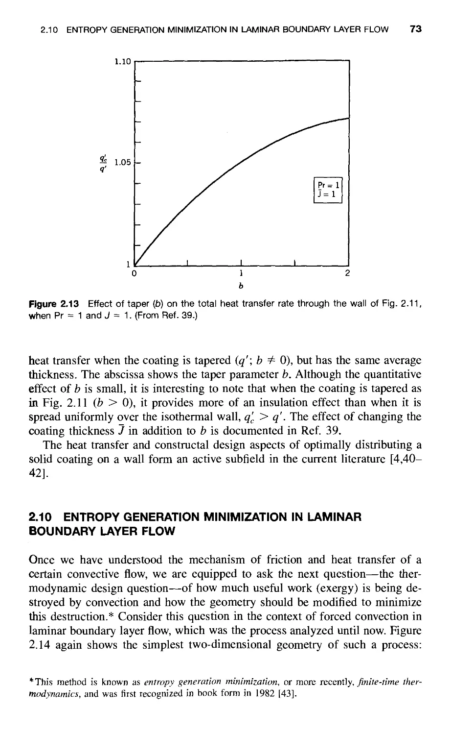
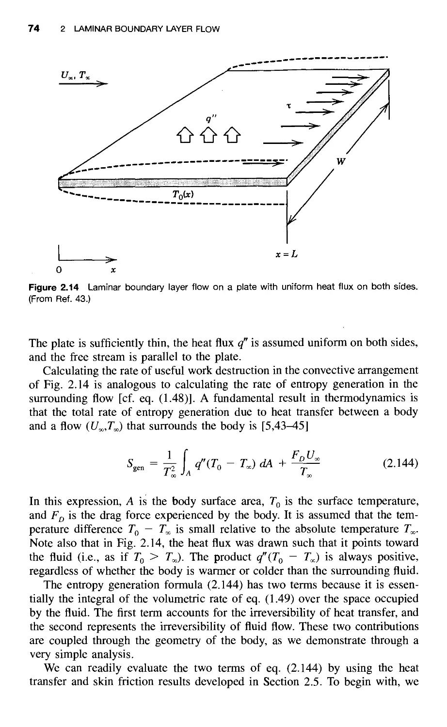
2.10 Entropy Generation Minimization in Laminar Boundary
Layer Flow / 73
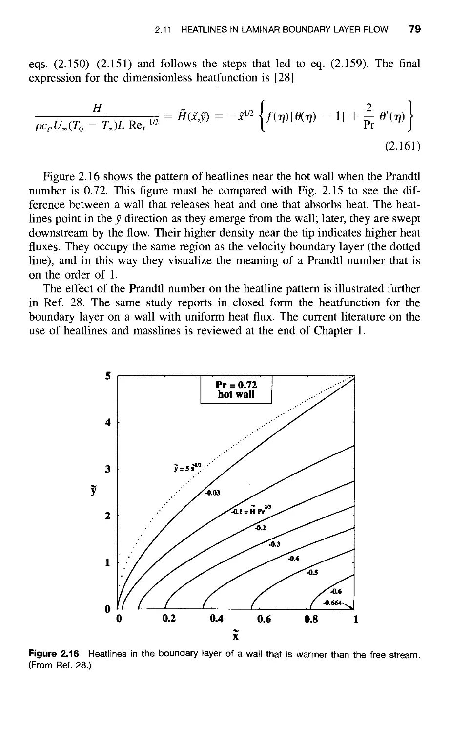
2.11 Heatlines in Laminar Boundary Layer Flow / 76
References / 80
Problems / 82
3 Laminar Duct Flow 96
3.1 Hydrodynamic Entrance Length / 97
3.2 Fully Developed Flow / 100
3.3 Hydraulic Diameter and Pressure Drop / 104
3.4 Heat Transfer to Fully Developed Duct Flow /111
3.4.1 Mean Temperature /111
3.4.2 Fully Developed Temperature Profile / 113
3.4.3 Uniform Wall Heat Flux / 116
3.4.4 Uniform Wall Temperature / 119
3.4.5 Tube Surrounded by Isothermal Fluid / 122
3.5 Heat Transfer to Developing Flow / 126
3.5.1 Scale Analysis / 126
3.5.2 Thermally Developed Uniform (Slug) Flow / 128
3.5.3 Thermally Developing Hagen-Poiseuille Flow / 131
3.5.4 Thermally and Hydraulically Developing Flow / 135
3.6 Optimal Cooling of a Stack of Parallel Heat-Generating
Plates / 136
3.7 Heathnes in Fully Developed Duct Flow / 141
3.8 Optimal Duct Shape for Minimum Flow Resistance / 144
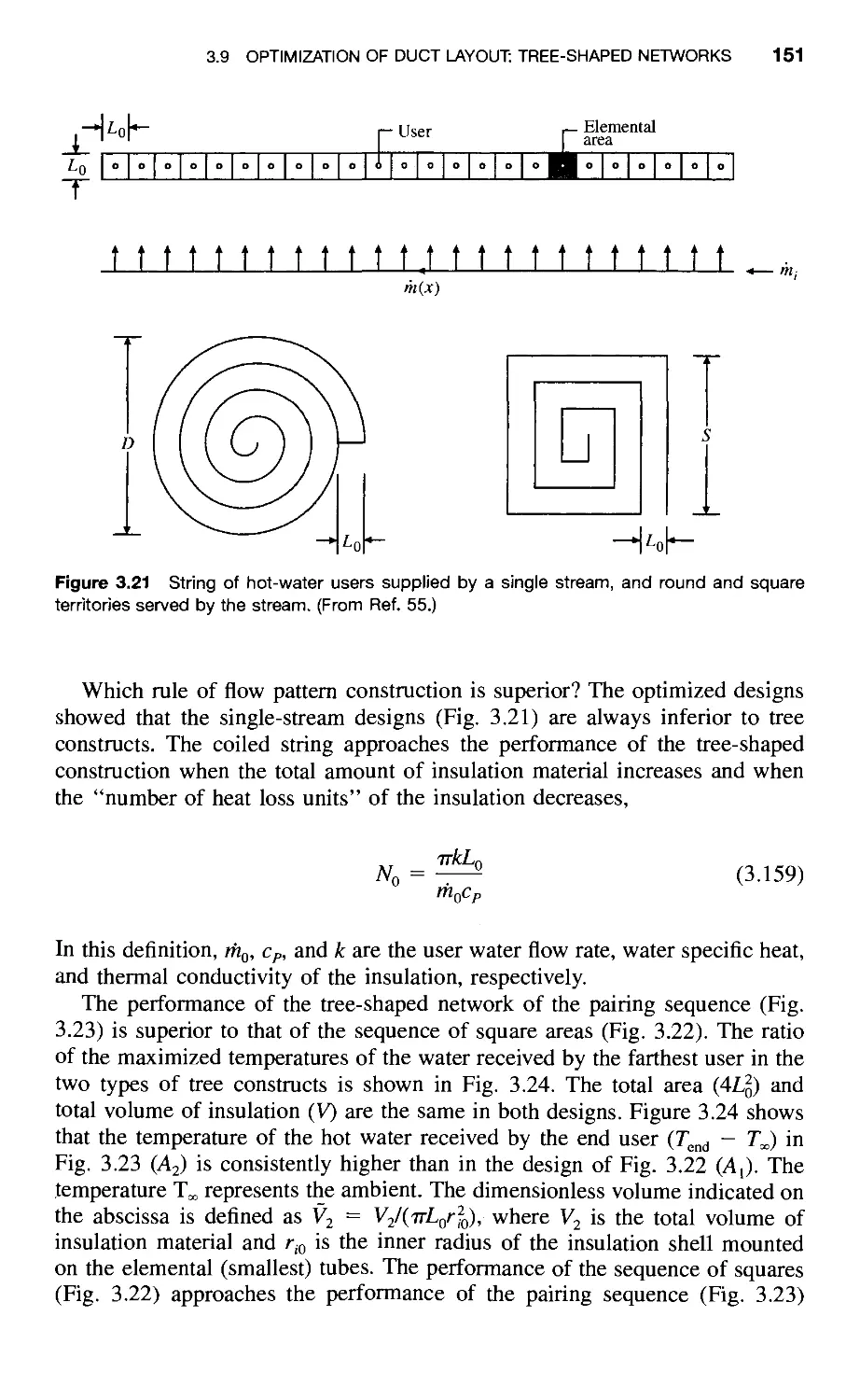
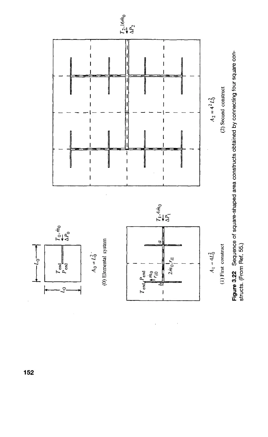
3.9 Optimization of Duct Layout: Tree-Shaped Networks / 147
References / 160
Problems / 165
4 External Natural Convection 178
4.1 Natural Convection as a Heat Engine in Motion / 179
4.2 Laminar Boundary Layer Equations / 181
4.3 Scale Analysis / 183
4.3.1 High-Pr Fluids / 185
4.3.2 Low-Pr Fluids / 187
4.3.3 Observations / 188

CONTENTS ix
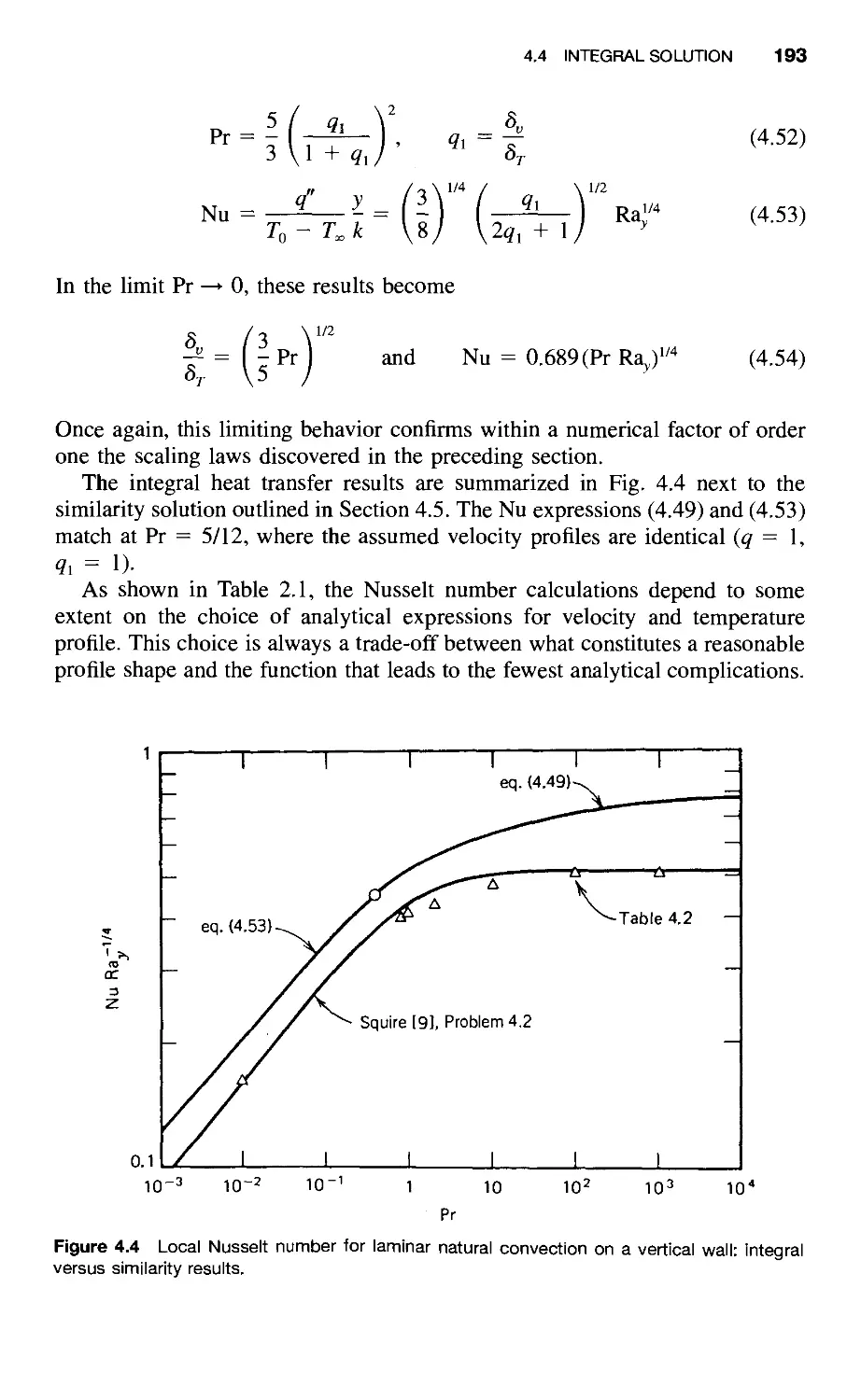
4.4 Integral Solution / 190
4.4.1 High-Pr Fluids / 191
4.4.2 Low-Pr Fluids / 192
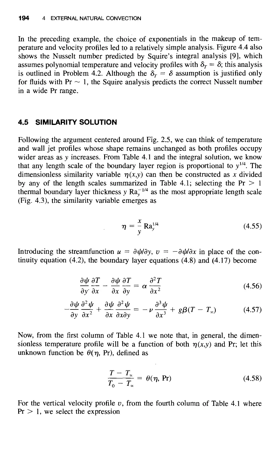
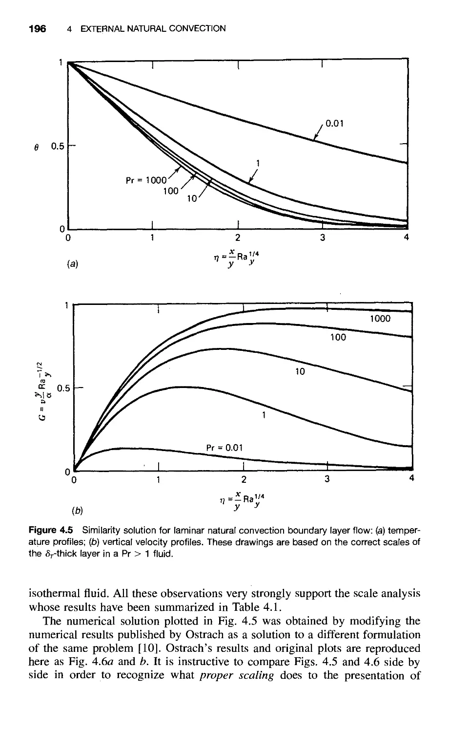
4.5 Similarity Solution / 194
4.6 Uniform Wall Heat Flux / 199
4.7 Effect of Thermal Stratification / 202
4.8 Conjugate Boundary Layers / 205
4.9 Vertical Channel Flow / 207
4.10 Combined Natural and Forced Convection (Mixed
Convection) / 211
4.11 Heat Transfer Results Including the Effect of Turbulence / 214
4.11.1 Vertical Walls / 214
4.11.2 Inclined Walls / 217
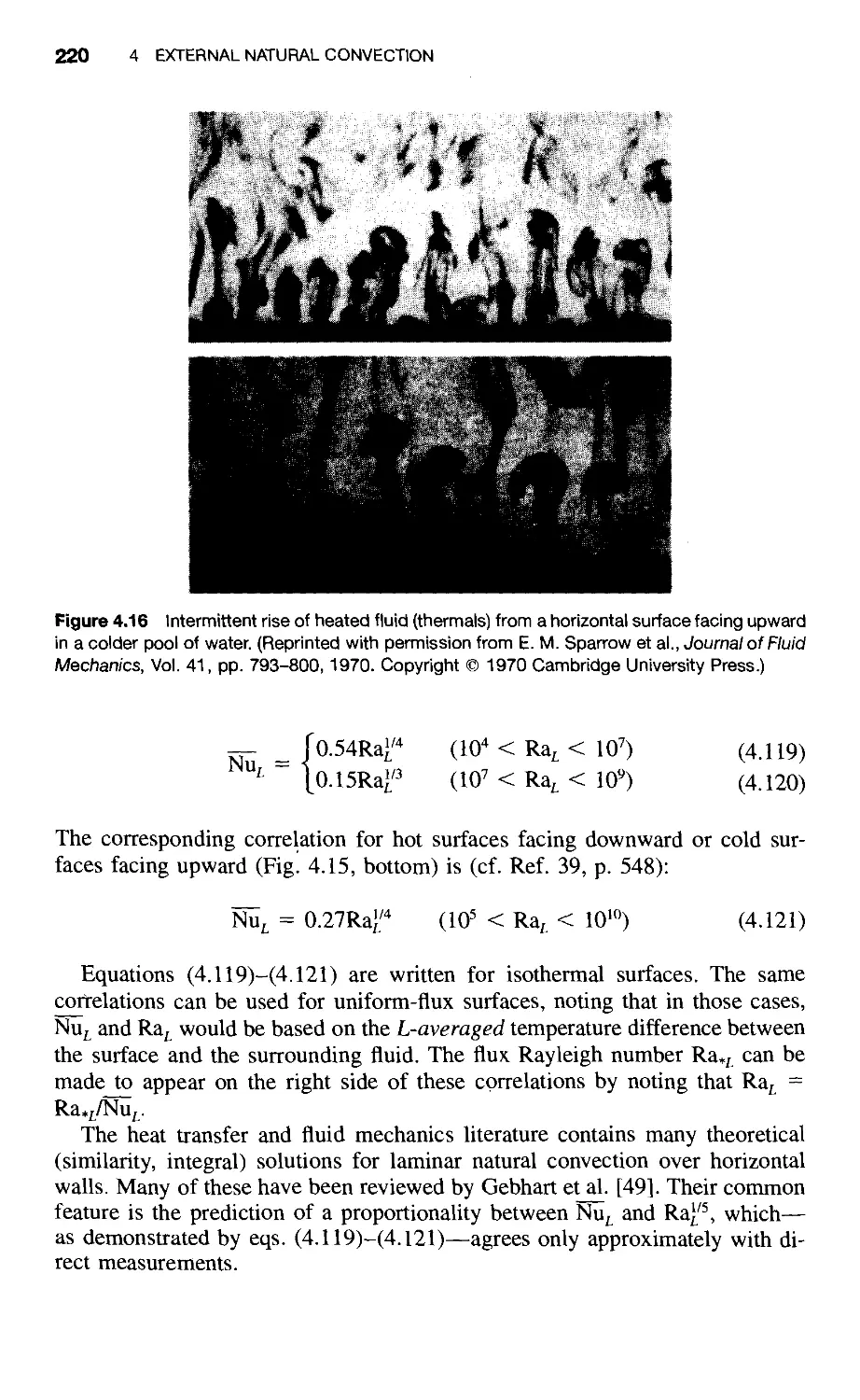
4.11.3 Horizontal Walls / 219
4.11.4 Horizontal Cylinder / 221
4.11.5 Sphere / 221
4.11.6 Vertical Cylinder / 222
4.11.7 Other Immersed Bodies / 223
4.12 Optimal Cooling of a Stack of Vertical Heat-Generating
Plates / 225
References / 228
Problems / 232
5 Internal Natural Convection 243
5.1 Transient Heating from the Side / 244
5.1.1 Scale Analysis / 244
5.1.2 Criterion for Distinct Vertical Layers / 248
5.1.3 Criterion for Distinct Horizontal Jets / 249
5.2 Boundary Layer Regime / 252
5.3 Shallow Enclosure Limit / 258
5.4 Summary of Results for Heating from the Side / 267
5.4.1 Isothermal Side Walls / 267
5.4.2 Sidewalls with Uniform Heat Flux / 270
5.4.3 Partially Divided Enclosures / 271
5.4.4 Triangular Enclosures / 274
5.5 Enclosures Heated from Below / 275
5.5.1 Heat Transfer Results / 275
5.5.2 Scaling Theory of the Turbulent Regime / 277
5.5.3 Constructal Theory of Benard Convection / 279
5.6 Inclined Enclosures / 286
5.7 Annular Space between Horizontal Cylinders / 288
5.8 Annular Space between Concentric Spheres / 290
5.9 Enclosures for Thermal Insulation and Mechanical
Strength / 290

CONTENTS
References / 297
Problems / 302
6 Transition to Turbulence 307
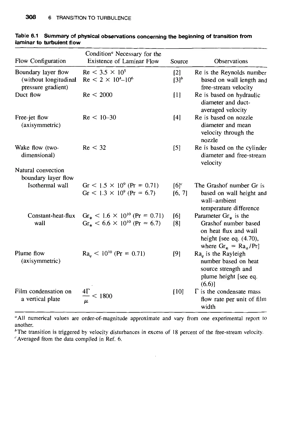
6.1 Empirical Transition Data / 307
6.2 Scaling Laws of Transition / 309
6.3 Buckling of Inviscid Streams / 313
6.4 Local Reynolds Number Criterion for Transition / 316
6.5 Instability of Inviscid Flow / 319
6.6 Transition in Natural Convection on a Vertical Wall / 326
References / 328
Problems / 331
7 Turbulent Boundary Layer Flow 334
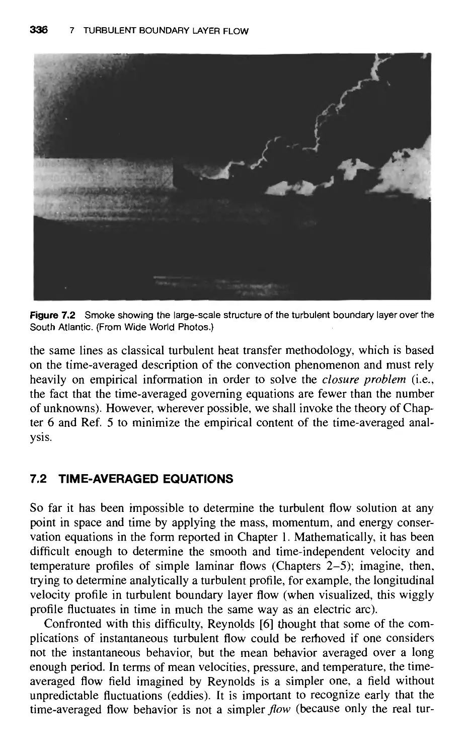
7.1 Large-Scale Structure / 334
7.2 Time-Averaged Equations / 336
7.3 Boundary Layer Equations / 339
7.4 Mixing-Length Model / 342
7.5 Velocity Distribution / 344
7.6 Wall Friction in Boundary Layer Flow / 351
7.7 Heat Transfer in Boundary Layer Flow / 353
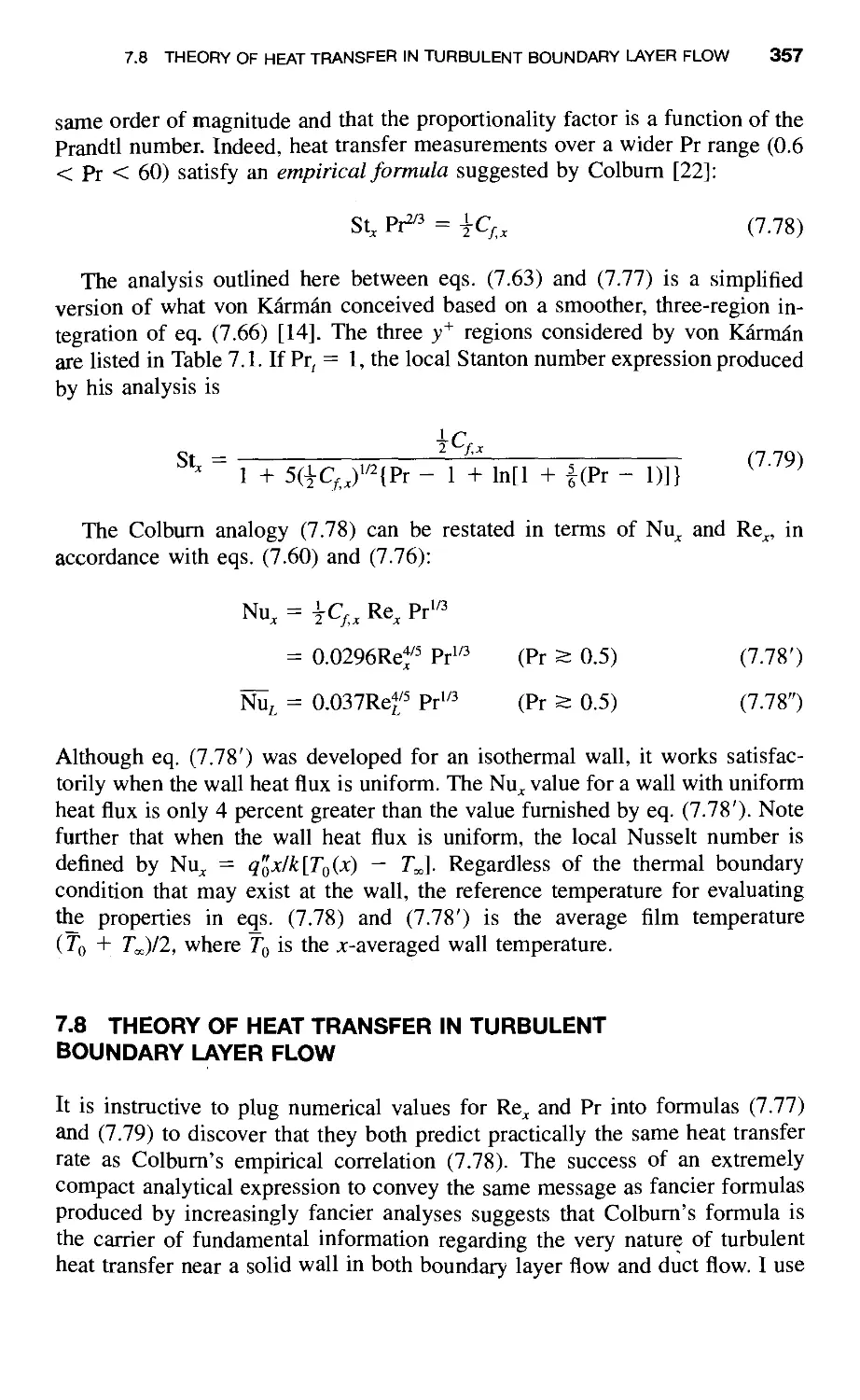
7.8 Theory of Heat Transfer in Turbulent Boundary Layer
Flow / 357
7.9 Other External Flows / 363
7.9.1 Single Cylinder in Cross Flow / 363
7.9.2 Sphere / 365
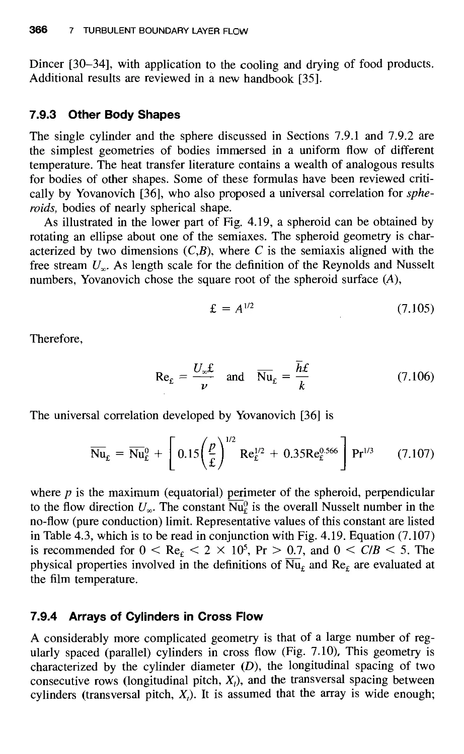
7.9.3 Other Body Shapes / 366
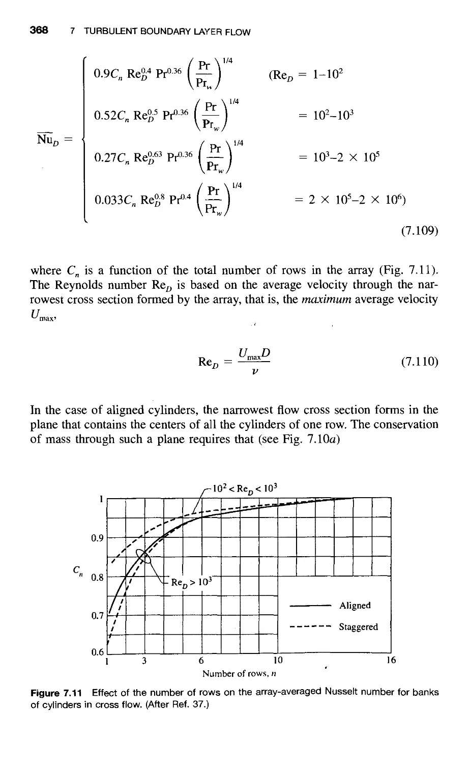
7.9.4 Arrays of Cylinders in Cross Flow / 366
7.10 Natural Convection Along Vertical Walls / 371
References / 374
Problems / 376
8 Turbulent Duct Flow 384
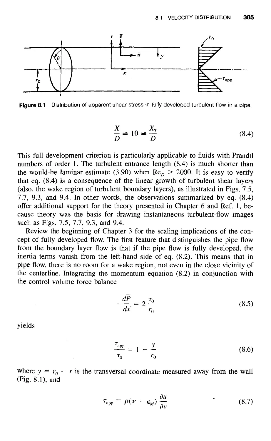
8.1 Velocity Distribution / 384
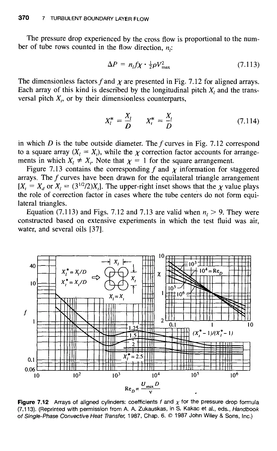
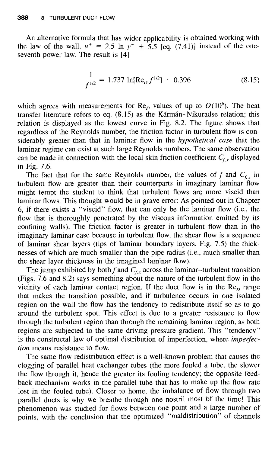
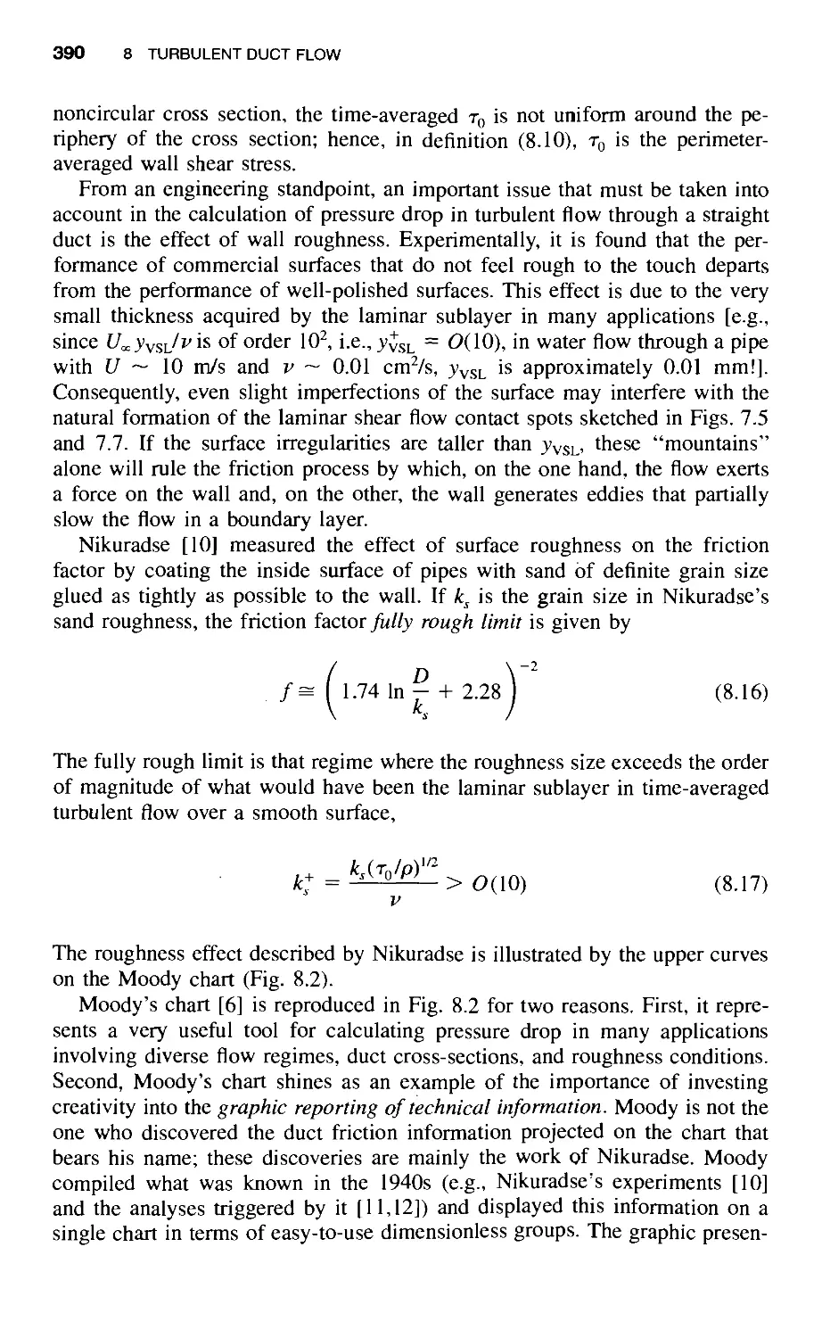
8.2 Friction Factor and Pressure Drop / 386
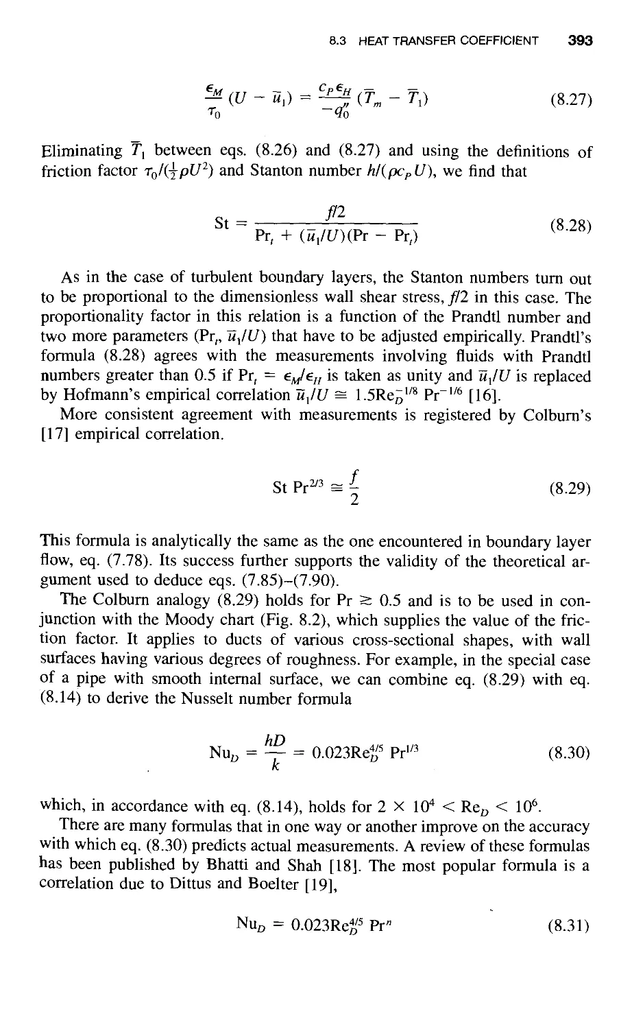
8.3 Heat Transfer Coefficient / 391
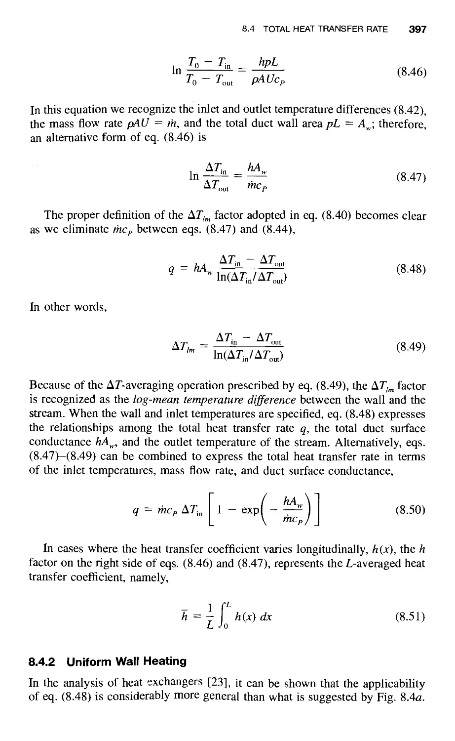
8.4 Total Heat Transfer Rate / 395
8.4.1 Isothermal Wall / 396
8.4.2 Uniform Wall Heating / 397
8.5 More Refined Turbulence Models / 398

CONTENTS Xi
8.6 Heatlines in Turbulent Flow near a Wall / 402
8.7 Optimal Channel Spacings for Turbulent Flow / 404
References / 406
Problems / 408
9 Free Turbulent Flows 414
9.1 Free Shear Layers / 415
9.1.1 Features of the Free Turbulent Flow Model / 415
9.1.2 Velocity Distribution / 418
9.1.3 Structure of Free Turbulent Flows / 419
9.1.4 Temperature Distribution / 421
9.2 Jets / 422
9.2.1 Two-Dimensional Jets / 422
9.2.2 Round Jets / 425
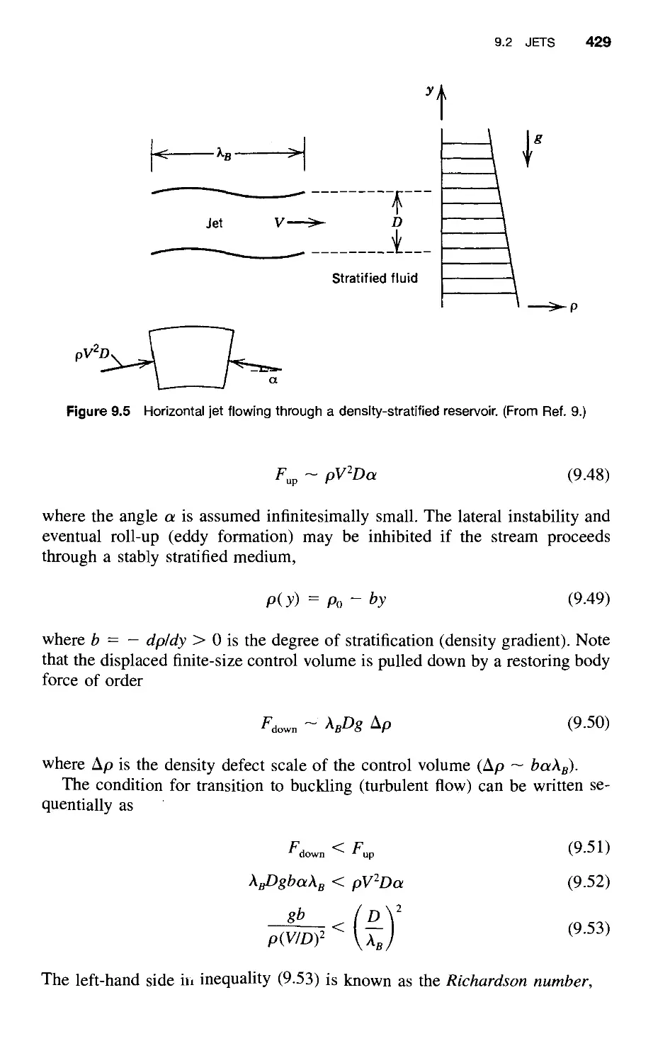
9.2.3 Jet in Density-Stratified Reservoir / 428
9.3 Plumes / 430
9.3.1 Round Plume and the Entrainment Hypothesis / 430
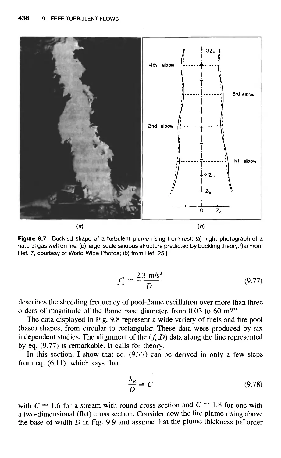
9.3.2 Pulsating Frequency of Pool Fires / 435
9.3.3 Geometric Similarity of Free Turbulent Flows / 439
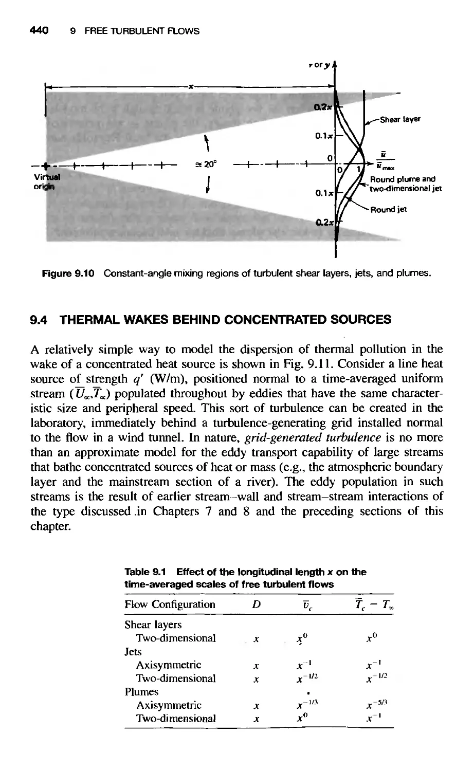
9.4 Thermal Wakes behind Concentrated Sources / 440
References / 442
Problems / 444
10 Convection with Change of Phase 446
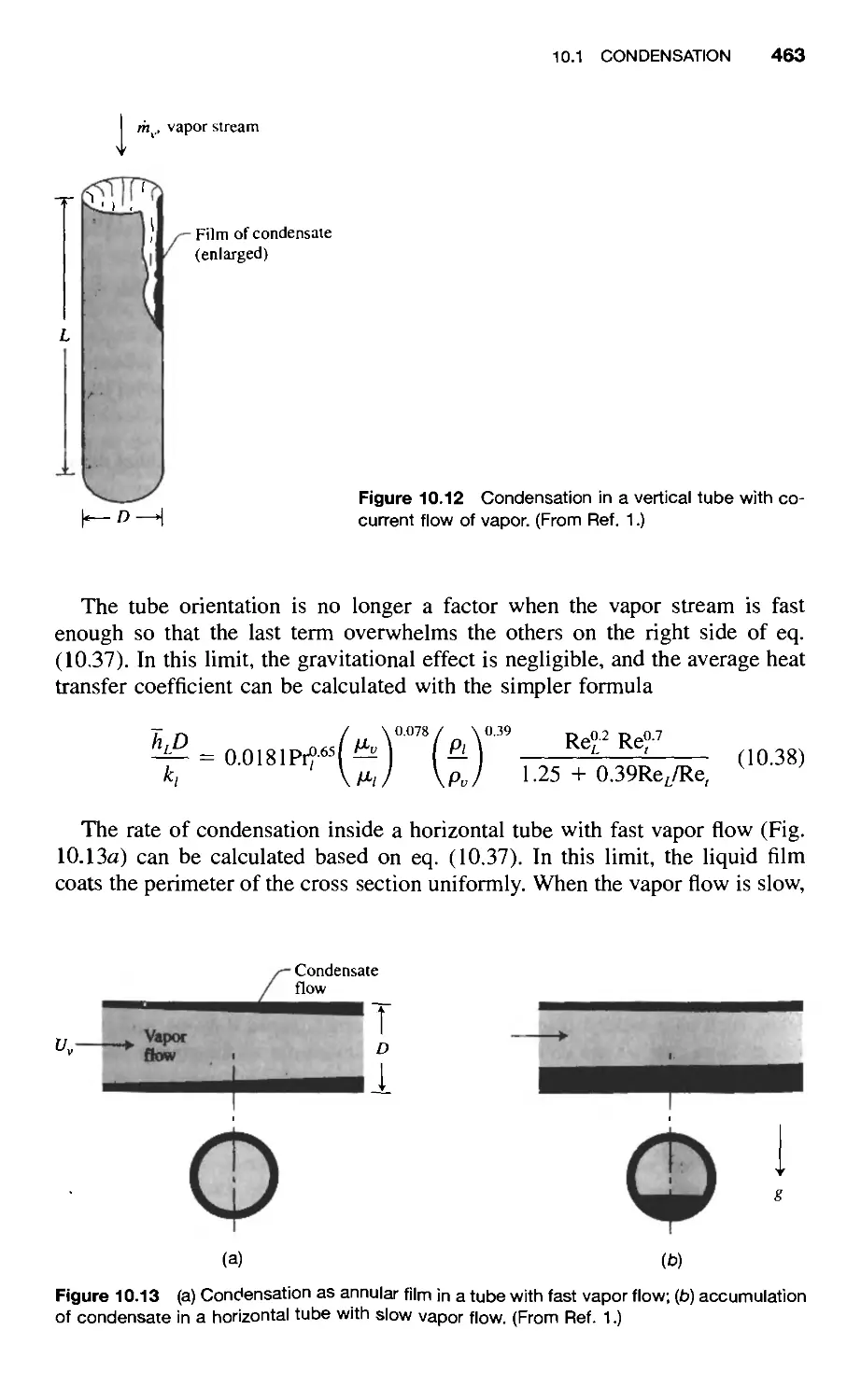
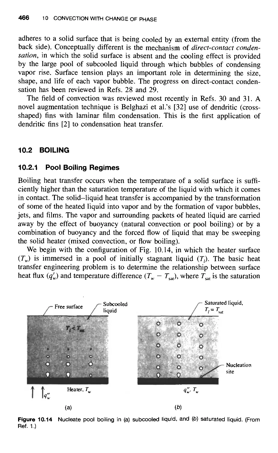
10.1 Condensation / 446
10.1.1 Laminar Film on a Vertical Surface / 446
10.1.2 Turbulent Film on a Vertical Surface / 453
10.1.3 Film Condensation in Other Configurations / 456
10.1.4 Drop Condensation / 464
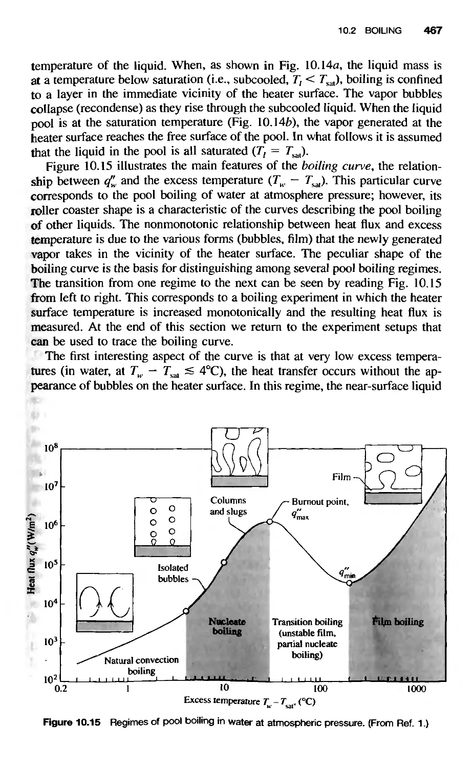
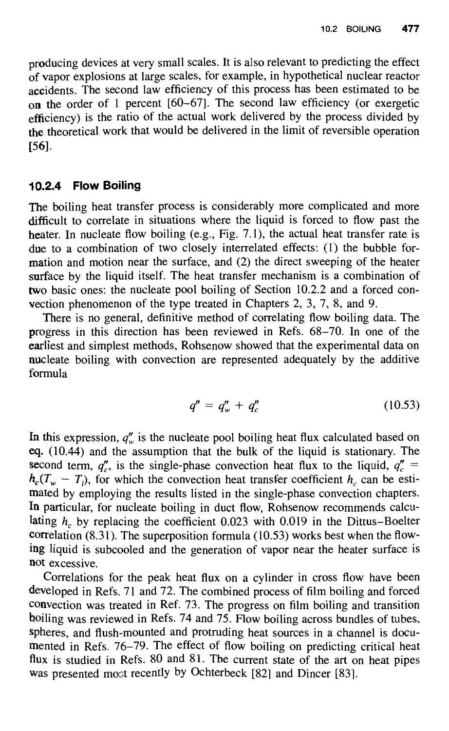
10.2 Boiling / 466
10.2.1 Pool Boiling Regimes / 466
10.2.2 Nucleate Boiling and Peak Heat Flux / 470
10.2.3 Film Boiling and Minimum Heat Flux / 473
10.2.4 Flow Boiling / 477
10.3 Contact Melting and Lubrication / 478
10.3.1 Plane Surfaces with Relative Motion / 478
10.3.2 Other Contact Melting Configurations / 482
10.3.3 Scale Analysis and Correlation / 485
10.3.4 Melting Due to Viscous Heating in the Liquid
Film / 487
10.4 Melting by Natural Convection / 490

Xli CONTENTS
10.4.1 Transition from the Conduction Regime to the
Convection Regime / 491
10.4.2 Quasisteady Convection Regime / 493
10.4.3 Horizontal Spreading of the Melt Layer / 497
References / 500
Problems / 507
11 Mass Transfer 515
11.1 Properties of Mixtures / 516
11.2 Mass Conservation / 519
11.3 Mass Diffusivities / 524
11.4 Boundary Conditions / 526
11.5 Laminar Forced Convection / 528
11.6 Impermeable Surface Model / 532
11.7 Other External Forced-Convection Configurations / 533
11.8 Internal Forced Convection / 536
11.9 Natural Convection / 538
11.9.1 Mass-Transfer-Driven Flow / 540
11.9.2 Heat-Transfer-Driven Flow / 540
11.10 Turbulent Flow / 544
11.10.1 Time-Averaged Concentration Equation / 544
11.10.2 Forced Convection Results / 545
11.10.3 Contaminant Removal from a Ventilated
Enclosure / 548
11.11 Massfunction and Masslines / 555
11.12 Effect of Chemical Reaction / 555
References / 559
Problems / 561
12 Convection in Porous Media 566
12.1 Mass Conservation / 567
12.2 Darcy Flow Model and the Forchheimer
Modification / 569
12.3 First Law of Thermodynamics / 572
12.4 Second Law of Thermodynamics / 577
12.5 Forced Convection / 577
12.5.1 Boundary Layers / 577
12.5.2 Concentrated Heat Sources / 583
12.5.3 Sphere and Cyhnder in Cross Flow / 584
12.5.4 Channel Filled with Porous Medium / 585
12.6 Natural Convection Boundary Layers / 586
12.6.1 Boundary Layer Equations: Vertical Wall / 586

CONTENTS xiJi
12.6.2 Uniform Wall Temperature / 587
12.6.3 Uniform Wall Heat Flux / 589
12.6.4 Optimal Spacings for Channels Filled with
Porous Structures / 591
12.6.5 Conjugate Boundary Layers / 593
12.6.6 Thermal Stratification / 595
12.6.7 Sphere and Horizontal Cylinder / 597
12.6.8 Horizontal Walls / 599
12.6.9 Concentrated Heat Sources / 599
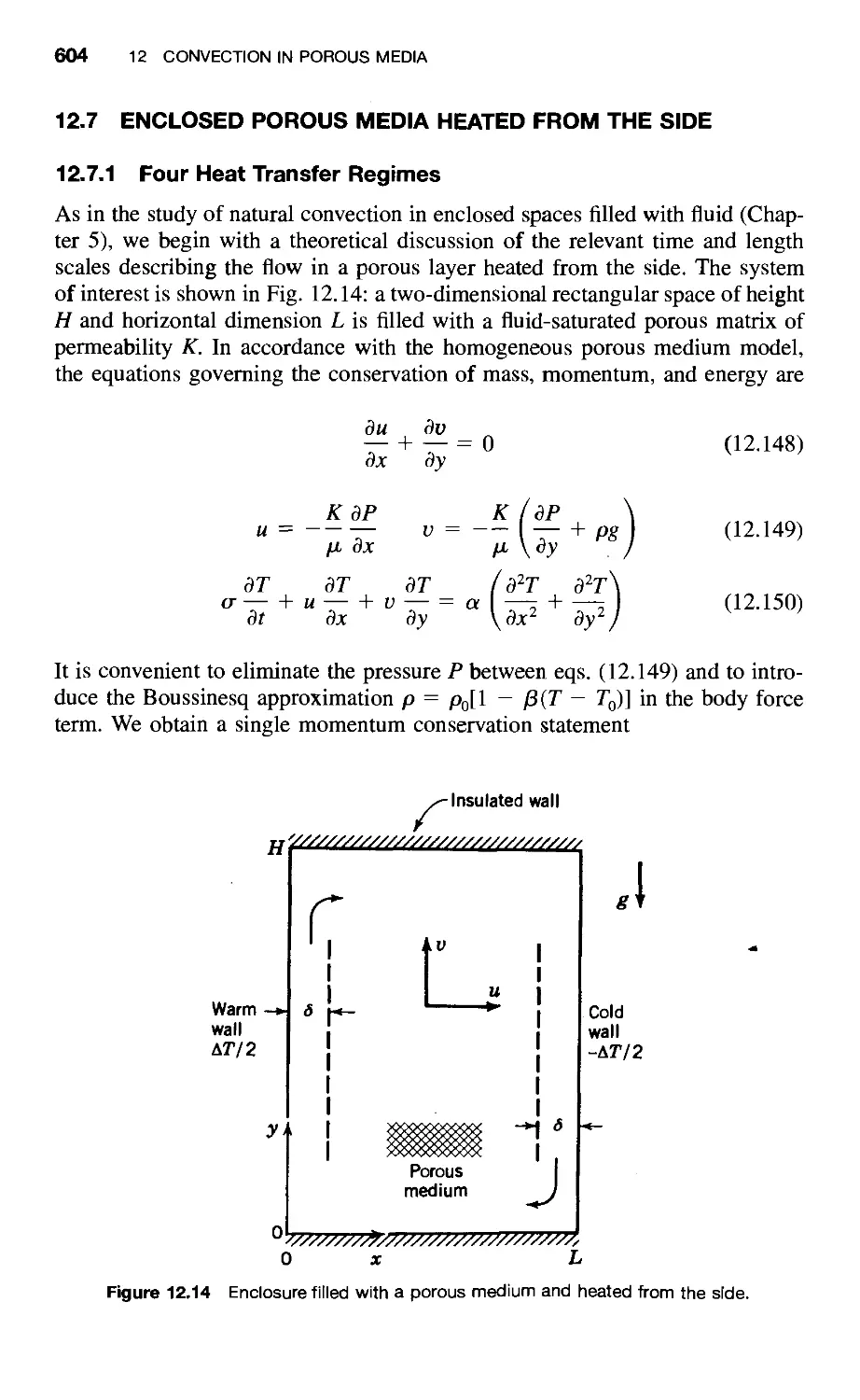
12.7 Enclosed Porous Media Heated from the Side / 604
12.7.1 Four Heat Transfer Regimes / 604
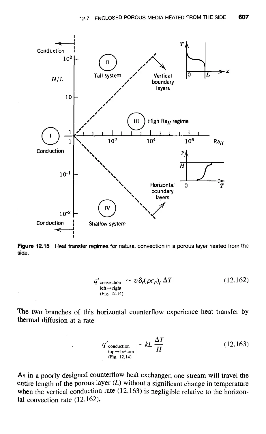
12.7.2 Convection Results / 608
12.8 Penetrative Convection / 610
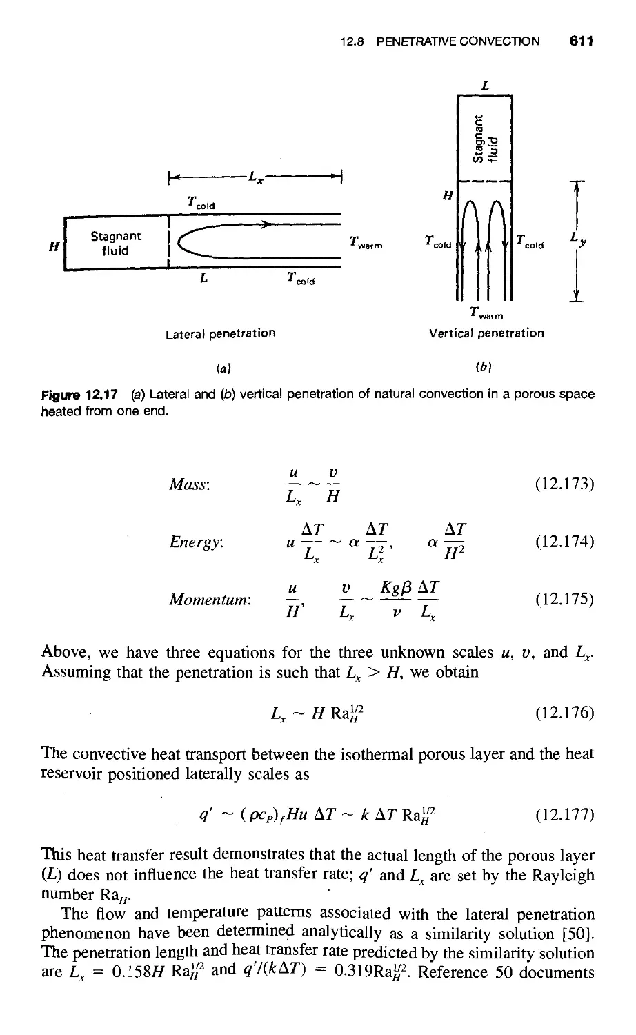
12.8.1 Lateral Penetration / 610
12.8.2 Vertical Penetration / 612
12.9 Enclosed Porous Media Heated from Below / 613
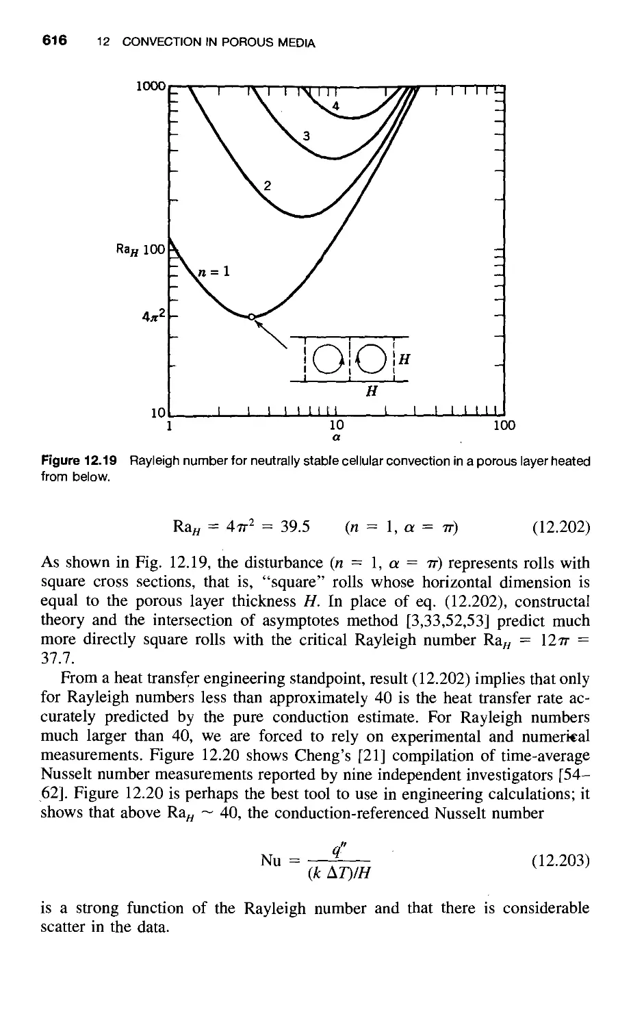
12.9.1 Onset of Convection / 613
12.9.2 Darcy Flow / 617
12.9.3 Forchheimer Flow / 619
12.10 Multiple Flow Scales Distributed Nonuniformly / 621
12.10.1 Heat Transfer / 624
12.10.2 Fluid Friction / 625
12.10.3 Heat Transfer Rate Density: The Smallest Scale
for Convection / 626
12.11 Constructal Design / 627
References / 628
Problems / 631
Appendixes 640
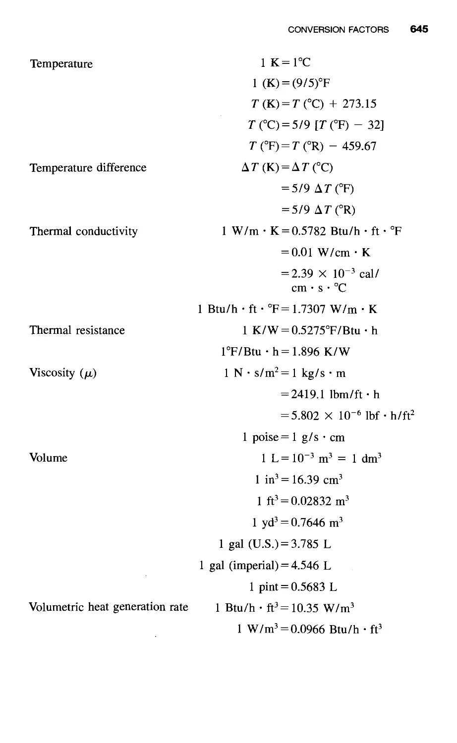
A Constants and Conversion Factors / 641
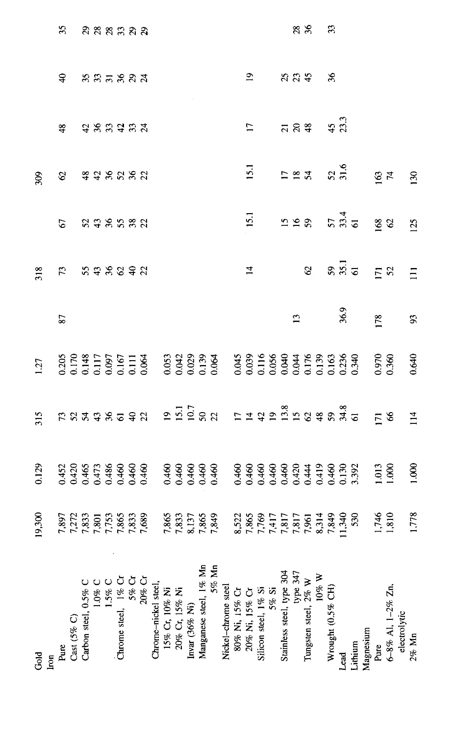
B Properties of Solids / 648
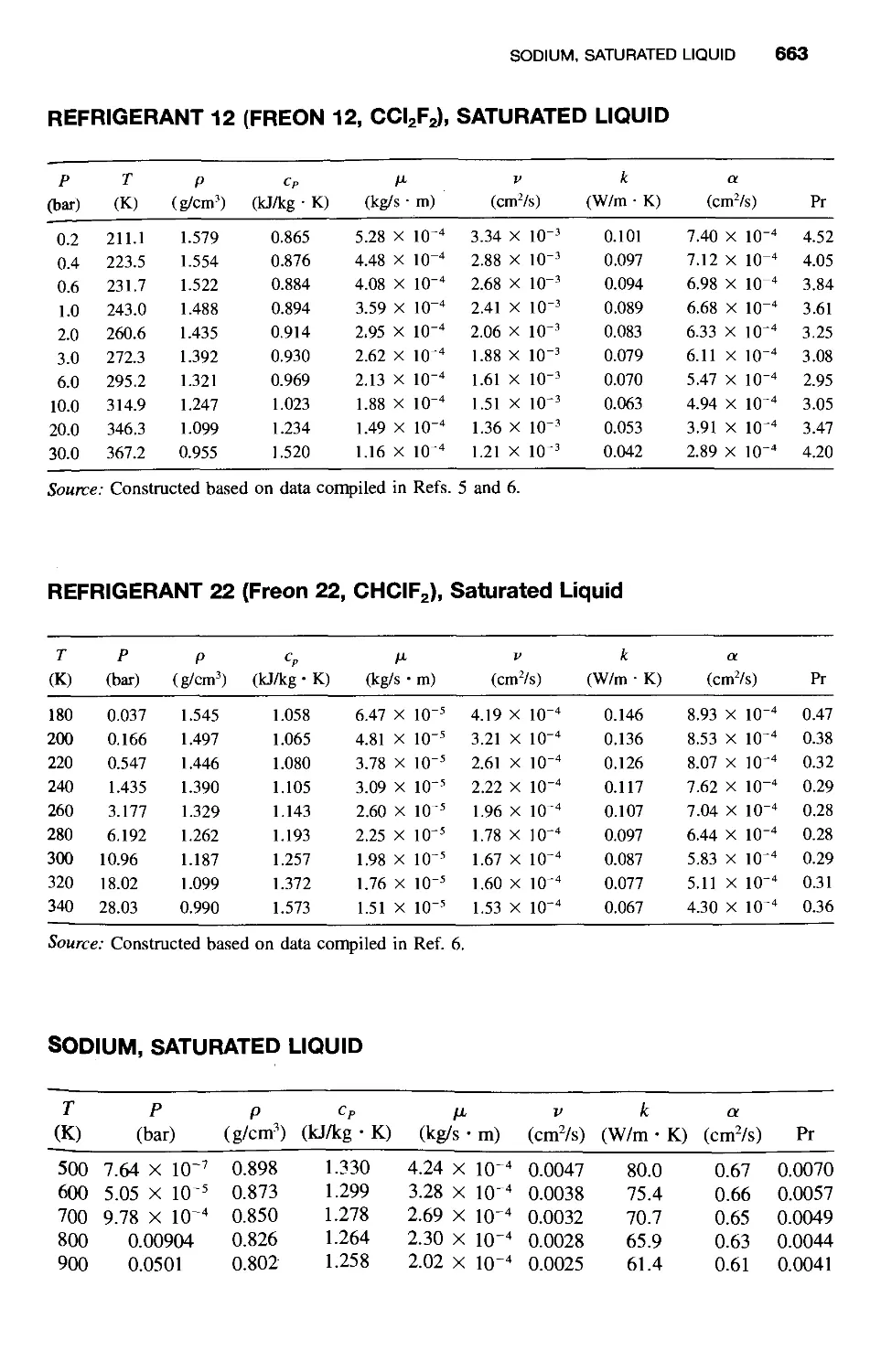
C Properties of Liquids / 658
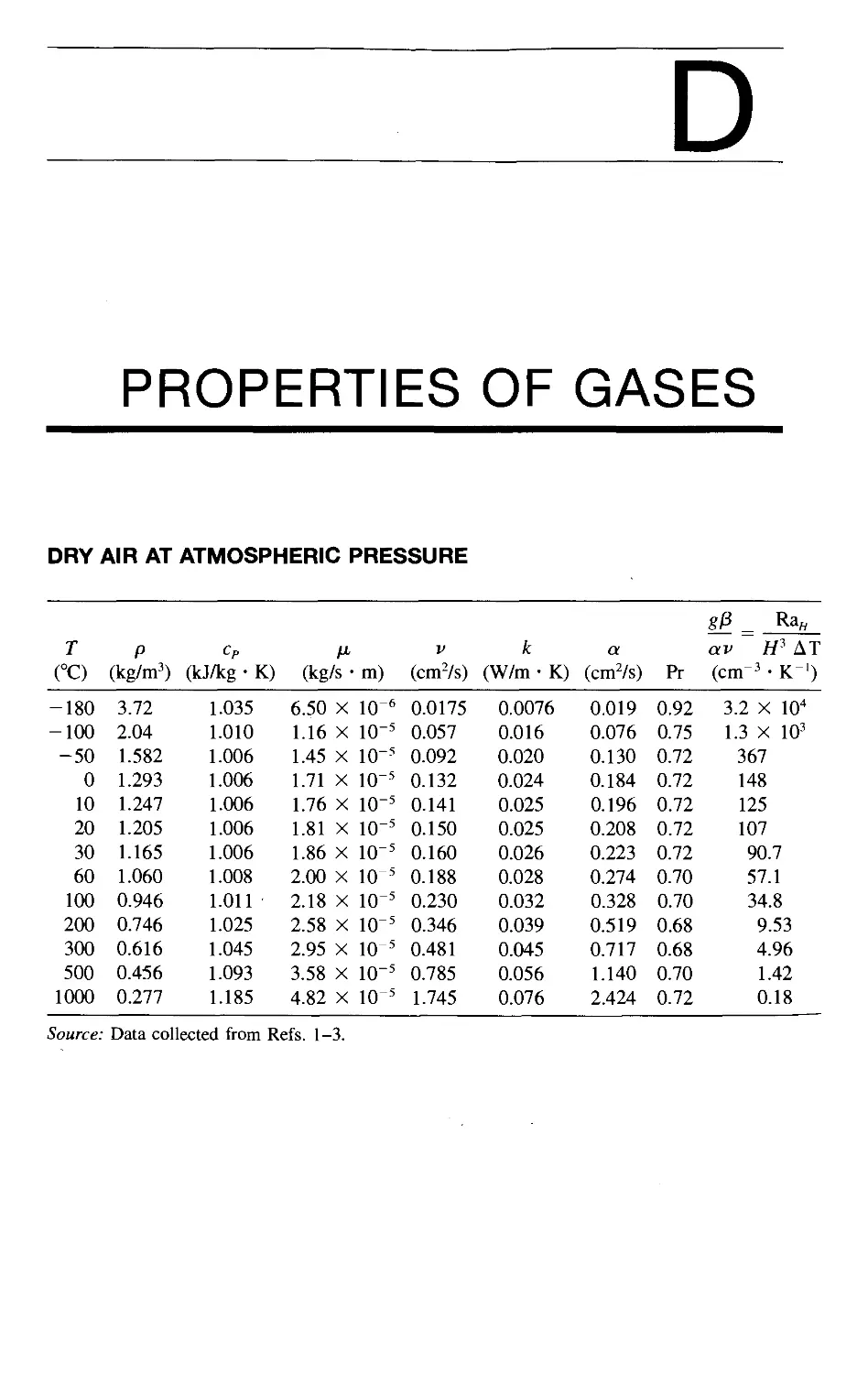
D Properties of Gases / 660
E Mathematical Formulas / 672
Author Index 675
Subject Index 685

LIST OF SYMBOLS
fl, b dimensions of rectangular duct cross section (Fig. 3.5)
j\ area
A cross-sectional area
j\^ B constants in the logarithmic law of the wall [eqs. (7.41) and
(7.42)]
Ar Archimedes number [eq. (10.80)]
b empirical constant, Forchheimer flow [eq. (12.15)]
b natural convection parameter [eq. (5.117)]
b radial length scale of round velocity jet [eq. (9.40)]
b stratification parameter [eq. (12.116)]
b taper parameter [eq. (2.140)]
b thermal stratification number [eq. (4.81)]
bj radial length scale of round thermal jet [eq. (9.43)]
bi2 empirical factors (Table 11.6)
B condensation driving parameter [eq. (10.26)]
B cross-sectional shape number (Fig. 3.7)
B dimensionless group [eq. (2.147)]
B dimensionless group [eq. (12.107)]
Be^ Bejan number, pressure drop number [eq. (3.133')]
Be^ Bejan number for a porous medium [eq. (12.113)]
Bi Biot number [eq. (3.80)]
Bo^ Boussinesq number [eq. (4.35)]
c specific heat of incompressible substance
c„ specific heat at constant volume
Cp specific heat at constant pressure
c,2 constants
C compressive impulse or reaction [eq. (6.7)]
C concentration [eq. (11.1)]
C constant
Cf^ local skin friction coefficient [eqs. (2.57) and (7.52)]
C„ factor (Fig. 7.11)
Q, Cj, C^ constants [eq. (8.61)]
Cfl drag coefficient [eq. (7.103)]
^sf constant (Table 10.1)
d, D diameter
D mass diffusivity [eq. (11.24), Tables 11.1 and 11.2]
D plate-to-plate spacing (Fig. 3.1)
^ stream transversal length scale
^h hydraulic diameter [eq. (3.26)]
^k~k knee-to-knee thickness of time-averaged turbulent shear layer
(Fig. 9.3)
XXIII

XXiV LIST OF SYMBOLS
Dj^ distance of maximum thermal penetration in the y direction, in
the vicinity of a direct contact spot [eq. (7.94)]
e specific energy (labeled u in Table 1.1)
/ Blasius streamfunction similarity profile [eq. (2.80)]
/ factor [eq. (7.113)]
/ friction factor [eq. (3.24)]
/ porous medium friction factor [eq. (12.12)]
/ roll thickness [eq. (5.92)]
/„ curve fit for the velocity profile [eq. (7.53)]
/j, frequency of vortex shedding [eq. (7.102)]
F force
F streamfunction similarity profile [eqs. (4.60) and (12.139)]
Fo Fourier number [eq. (10.104)]
Fj) drag force
F„ normal force
F, tangential force
g gravitational acceleration
Gr^ Grashof number [eq. (4.38)]
Gr^ Grashof number based on heat flux (Table 6.1)
Gz Graetz number [eq. (3.120)]
Gf constant (Table 4.3)
h heat transfer coefficient [eq. (2.4)]; local heat transfer
coefficient [eq. (2.100)]
h specific enthalpy
hfg latent heat of condensation or evaporation (Table 10.2)
h'fg augmented latent heat [eq. (10.10)]
h"g augmented latent heat [eq. (10.41)]
h^ mass transfer coefficient [eq. (11.46)]
h^f latent heat of melting
H enthalpy flow rate [eq. (10.5)]
H heatfunction [defined via eqs. (1.68) and (1.69)]
H height
H Henry's constant [eq. (11.35) and Table 11.3]
/ area moment of inertia
/ integral [eq. (3.148)]
j diffusion flux [eq. (11.20)]
y'app apparent mass flux [eq. (11.102)]
J dimensionless thickness parameter [eq. (2.139)]
Ja Jakob number [eq. (10.19)]
k thermal conductivity
k wave number
jf„', jf„" reaction rates, [eqs. (11.135) and (11.136)]
k^ sand grain size [eq. (8.16)]
K jet strength [eq. (9.33)]
K permeabihty [eq. (12.9)]

LIST OF SYMBOLS XXV
Ki2 constants
/ ' effective length [eq. (4.127)]
/ mixing length [eq. (7.27)]
L length
L length of direct viscous contact [eq. (7.92)]
L^ characteristic length
i equivalent length [eq. (10.86)]
L„ length of direct thermal contact [eq. (7.95)]
£ effective length [eq. (4.128)]
Le Lewis number [eq. (11.93)]
m exponent in flow over a wedge [eq. (2.124)]
m function [eq. (6.27)]
m profile shape function for integral analysis [eq. (2.54)]
m mass flow rate
rh' mass transfer rate per unit length [eq. (11.52)]
rii"' volumetric mass generation rate [eq. (11.15)]
M bending moment [eq. (6.8)]
M function [eq. (8.22)]
M impulse or reaction force due to fluid flow into or out of a
control volume (Fig. 2.3)
M mass
M massfunction [eqs. (11.133)-(11.134)]
M material constraint [eq. (3.145)]
M molar mass [eq. (11.4)]
n dimensionless coordinate across the velocity boundary layer
(y/8) [eq. (2.54)]
n number of cylinders
n number of heat-generating boards
n number of moles [eq. (11.4)]
n, number of rows
Ng buckling number [eq. (6.14)]
A'o number of heat loss units [eq. (3.158)]
Nu local Nusselt number [eq. (2.101)]
Nu Nusselt number in the fully developed region [eq. (3.52)]
Nu overall Nusselt number
Nu° constant (Table 4.3)
Nuq_^ overall Nusselt number [eq. (3.104)]
Nu^ local Nusselt number in the developing (entrance) region [eq.
(3.103)]
p dimensionless coordinate across the thermal boundary layer
(y/8r) [eq. (2.58)]
p even function (eq. (5.37)]
P wetted perimeter
P pressure
Poo pressure in the free stream

XAVI uar OF SYMBOLS
PCfl Peclet number (UD/a)
Pe^ Peclet number (f/^L/a)
Po Poiseuille number (/"Re^^)
Pr Prandtl number (v/a)
PTp porous medium Prandtl number [eq. (12.215)]
Pr, turbulent Prandtl number [eq. (7.66)]
q heat transfer rate (W)
q odd function [eq. (5.37)]
q' heat transfer rate per unit length (W/m)
^' heat flux (W/m^)
^'pp apparent heat flux [eq. (7.24)]
q'o^^^ maximum heat flux, under a direct thermal contact spot [eq
(7.86)]
q'" rate of internal heat generation (W/m^)
Q heat transfer rate (W)
Q flow rate (mVs) [eq. (10.69)]
r radial coordinate
Kq tube radius
Kf^ hydraulic radius [eq. (3.26)]
r, 0, z cylindrical coordinates (Fig. 1.1)
r, (f>, 0 spherical coordinates (Fig. 1.1)
R ideal gas constant
R universal gas constant
R radius
R thermal resistance
Ra^ Rayleigh number [eq. (4.25)]
Ra^ Darcy modified Rayleigh number [eq. (12.89)]
Ra„y mass transfer Rayleigh number [eq. (11.86)]
Ra^ Rayleigh number based on source strength [eq. (6.6)]
Ra^^ Rayleigh number based on heat flux [eq. (4.70)]
Ra^y Darcy modified Rayleigh number based on heat flux [eq
(12.99)]
Re^ Reynolds number (UD/v)
Re^^ Reynolds number based on hydraulic diameter {UDJv)
Re, local Reynolds number [eq. (6.15)]
Re^ Reynolds number (U^L/v)
Re, terminal Reynolds number [eq. (10.37)]
s constant (Table 10.1)
J specific entropy
s thickness of liquid zone (Fig. 10.24)
S entropy
^ggn entropy generation rate (W/K)
Sc Schmidt number [eq. (11.40)]
Sc, turbulent Schmidt number [eq. (11.116)]
Sh Sherwood number [eq. (11.42)]

LIST OF SYMBOLS XXVM
St^ local Stanton number [eq. (7.76)]
Ste Stefan number [eq. (10.80)]
Ste^ Stefan number for viscous heating [eq. (10.98)]
t thickness
t time
tg buckling time or time of eddy formation [eq. (6.13)]
u time of convective boundary layer development [eq. (5.13')]
t^ transversal viscous communication time [eq. (6.12)]
T absolute temperature
r^ Oseen-linearization function [eq. (5.25")]
Tq absolute temperature of the ambient
Tq reference temperature
Tq temperature of nozzle fluid
Tq wall temperature
r„ bulk temperature [eq. (3.42)]
T„ melting point
TjN inlet temperature
r„ free-stream temperature
r„ 0 bottom temperature of a thermally stratified fluid reservoir (Fig.
4.8)
r^„ core temperature in the high Ra^ regime
u^ Oseen-linearization function
u^ friction velocity [eq. (7.34)]
M^„ core velocity in the high Ra^ regime
Mq centerline velocity
M, V, w velocity components in the {x,y,z) system of coordinates (Fig.
1.1)
u',v' velocity disturbances [eq. (6.19)]
M, d disturbance amplitudes [eq. (6.21)]
U duct-averaged velocity
U longitudinal base flow [eq. (6.19)]
U slider velocity [eq. (10.55)]
U^ centerline velocity
f/n,„ maximum average velocity [eq. (7.111)]
Uq velocity of nozzle fluid
f/„ free-stream velocity
1^0 blowing or suction velocity
V stream velocity scale [eq. (6.7)]
V velocity
V volume [eq. (11.2)]
V volume constraint [eq. (3.144)]
W width
W work transfer rate, power
X, y, z Cartesian coordinates (Fig. 1.1)
Xi mole fraction [eq. (11.7)]

Xj dimensionless horizontal coordinate in the end-turn region [eq.
(5.58)]
x^ thermal entrance coordinate [eq. (3.97)]
x^ hydraulic entrance coordinate [eq. (3.118)]
Xq starting length [defined in eqs. (9.22) and (9.28)]
Xq unheated starting length (Fig. 2.8)
X hydrodynamic entrance length
X transversal coordinate of a point situated outside the boundary
layer
X(. concentration entrance length [eq. (11.73)]
X, longitudinal pitch
X, transversal pitch
Xj. thermal entrance length
X, Y, Z body force terms in eqs. (1.19)
Xf dimensionless longitudinal pitch [eq. (7.114)]
X* transversal longitudinal pitch [eq. (7.114)]
Y equilibrium shape of a nearly straight stream [eq. (6.8)]
Y y coordinate of a point situated in the free stream
Fj. thermal entrance length
z altitude (Fig. 10.24)
Greek Letters
a thermal diffusivity
a porous medium thermal diffusivity [eq. (12.35)]
a empirical constant [eq. (9.73)]
a^.j knee-to-knee angle of time-averaged turbulent shear layer (Fig. 9.3)
/3 coefficient of thermal expansion
/3^ concentration expansion coefficient [eq. (11.80)]
/3 wedge angle (Fig. 2.10)
r condensate mass flow rate [Table 6.1, eq. (10.4)]
7 empirical constant [eq. (9.19)]
7 function [eq. (6.27)]
7 vertical temperature gradient (K/m) [eqs. (4.77) and (12.110)]
7o empirical constant [eq. (9.37)]
A discriminant [eq. (6.28)]
A ratio [eq. (11.143)]
A.P pressure drop
Ar temperature difference
Ar^^g average temperature difference [eq. (3.110)]
^Ti„ log-mean temperature difference [eq. (3.105)]
S dimensionless thickness of the end region in a shallow enclosure
S film thickness
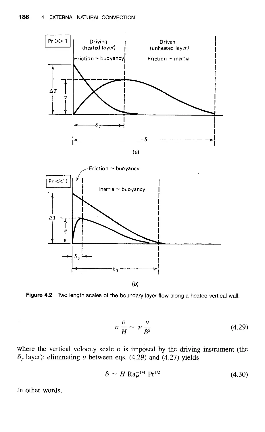
S outer thickness of a I*r > 1 natural convection boundary layer (Fig.
4.2)

LIST OF SYMBOLS XXiX
5 velocity boundary layer thickness
S^ concentration boundary layer thickness [eq. (11.87)]
gj. thermal boundary layer thickness
Sj-f thermal boundary layer thickness at the end of its development [eq.
(5.14)]
8^ inner viscous layer thickness of a Pr < 1 natural convection
boundary layer (Fig. 4.2)
S^ velocity boundary layer thickness [eq. (5.17)]
8* displacement thickness [eq. (2.86)]
e small parameter {HILf for shallow enclosures
e turbulence dissipation function [eq. (8.57)]
ejj thermal eddy diffusivity [eq. (7.23)]
e„ mass eddy diffusivity [eq. (11.103)]
e^ momentum eddy diffusivity [eq. (7.23)]
e„ emissivity [eq. (10.51)]
f similarity variable [eq. (12.58)]
f vorticity function [eq. (6.18)]
Tj density of contact spots [eq. (7.85)]
Tj similarity variable [eqs. (2.71), (4.55), (12.48), and (12.90)]
Tjj ventilation or displacement efficiency [eq. (11.121)]
e angle (Fig. 12.12a)
6 dimensionless temperature function [eq. (2.93)]
6 dimensionless time [eq. (10.103)]
6 momentum thickness [eq. (2.87)]
6 similarity temperature profile [eqs. (4.58) and (9.90)]
6 temperature difference
K von Karman's constant [eq. (7.31)]
A Lagrange multiplier [eq. (3.148)]
A wavelength
kg buckling wavelength
A] 2 functions of altitude [eq. (5.31)]
/u, viscosity
IJif friction coefficient [eq. (10.78)]
V kinematic viscosity
p density (labeled \lv in Table 1.1, where v is the specific volume)
o- capacity ratio [eq. (12.30)]
cr disturbance growth rate [eq. (6.21)]
o- empirical constant [eq. (9.8)]
cr normal stress
(T surface tension (Table 10.2)
o-j, o-j constants [eq. (8.61)]
T angle of tilt (Fig. 5.24)
T shear stress
T* dimensionless time [eq. (11.122)]
T3PP apparent shear stress [eq. (7.24)]

XXX LIST OF SYMBOLS
■'bmax maximum shear stress, under a direct viscous constant spot [e
(7.86)]
0 angle
0 fully developed temperature profile function [eq. (3.51)]
0 function [eq. (12.19)]
0 porosity [eq. (12.22)]
0 volume fraction [eq. (5.103)]
0, ratio [eq. (11.149)]
<I> mass fraction [eq. (11.6)]
<I> viscous dissipation function
X factor [eq. (7.113)]
ifj streamfunction
(X) wall parameter [eq. (4.85)]
(X) wall parameter [eq. (12.106)]
Subscripts
/app
/avg
)b
^b
air
apparent
average
average
base solution
bulk
cold
constant, uniform
convection
dimensionless variables for the shallow core solution [eq. (5.47)]
properties where the wall condition is imposed on the k-e model
[eqs. (8.64)-(8.65)]
property measured along the stream centerline
property of the control volume
icsL conduction sublayer
end
expressions for the integral analysis of the end region [eq. (5.61)]
final
fluid
saturated liquid
forced convection
saturated vapor
hot
heat transfer
component /
inner
inlet
liquid
>f
)fc

LIST OF SYMBOLS
mean
maximum
)min minimum
)^j mass transfer
)f,c natural convection
)„ outer
)op. optimal
)p pore
)rad radiation
)^f reference
)^gj components of a vector in cylindrical coordinates
)^ ^ g components of a vector in spherical coordinates
). solid
)sa. saturation
transition
X vapor
)vsL viscous sublayer
)>. wall
)^ water
)o wall
)o_^ quantity averaged from x =^ 0 to x = L
)^ dimensionless variables for the high-Ra^ solution [eq. (5.23)]
(•)oo property of reservoir fluid
Superscripts
(•) average
(•) time-averaged part
(•)' fluctuating part
(•y wall coordinates and wall variables [eq. (7.35)]

1
FUNDAMENTAL
PRINCIPLES
Convective heat transfer, or simply, convection, is the study of heat transport
processes effected by the flow of fluids. The very word convection has its roots
in the Latin verbs convecto-are and convSho-vehere [1],* which mean to bring
together or to carry into one place [2]. Convective heat transfer has grown to
the status of a contemporary science because of people's desire to understand
and predict how a fluid flow will act as a "carrier" or "conveyor belt" for
energy and matter.
Convective heat transfer is clearly, a field at the interface between two older
fields: heat transfer and fluid mechanics. For this reason, the study of any
convective heat transfer problem must rest on a solid understanding of basic
heat transfer and fluid mechanics principles. The objective in this chapter is to
review these principles in order to establish a common language to debate the
more specific issues addressed in later chapters.
Before reviewing the foundation of convective heat transfer methodology, it
is worth reexamining the historic relationship between fluid mechanics and heat
transfer at the interface we call convection. Especially during the past 100 years,
heat transfer and fluid mechanics have enjoyed a symbiotic relationship in their
development, a relationship where one field was stimulated by the curiosity in
the other field. Examples of this symbiosis abound in the history of boundary
layer theory and natural convection. The field of convection heat transfer grew
out of this symbiosis, and if we are to learn anything from history, important
advances in convection will continue to result from this symbiosis. Thus, the
student and the future researcher would be well advised to devote equal
attention to fluid mechanics and heat transfer literature.
* Numbers in brackets indicate references at the end of each chapter.

1 FUNDAMENTAL PRINCIPLES
1.1 MASS CONSERVATION
The first principle to review is undoubtedly the oldest: It is the conservation
of mass in a closed system or the "continuity" of mass through a flow (open)
system. From engineering thermodynamics, we recall the mass conservation
statement for a control volume [3]:
dt
= ^ rh
inlet
ports
2 ^
outlet
ports
(1.1)
where M^^ is the mass instantaneously trapped inside the control volume (cv),
while the m's are the mass flow rates associated with flow into and out of the
control volume. In convective heat transfer, we are usually interested in the
velocity and temperature distribution in a flow region near a solid wall; hence,
the control volume to consider is the infinitesimally small Ajc A_y box drawn
around a fixed location {x,y) in a flow field. In Fig. 1.1, as in most of the
problems analyzed in this book, the flow field is two-dimensional (i.e., the same
in any plane parallel to the plane of Fig. 1.1); in a three-dimensional flow field,
the control volume of interest would be the parallelepiped Ajc A_y Az. Taking
u and V as the local velocity components at point {x,y), the mass conservation
equation (1.1) requires that
dt
(p Ajf A_y) = pM A_y -I- pv Ajc —
pv H A_y
d{pu)
pu H :—Ajf
by
^.x
dx
Ay
(1.2)
or, dividing through by the constant size of the control volume (Ax Ay),
dp ^ d(pu) ^ d(pv) ^ ^
dt dx dy
(1.3)
In a three-dimensional flow, an analogous argument yields
dp ^ djpu) ^ d(pv) ^ d(pw) ^
dt dx dy dz
(1.4)
where w is the velocity component in the z direction. The local mass
conservation statement (1.4) can also be written as

1.1 MASS CONSERVATION 3
°y
puAy
I
-^-i pAxAy
I
J
pvAx
dx
{* Ax *\
(a) Cartesian coordinates
--z = 0
(b) Cylindrical coordinates
(c) Spherical coordinates
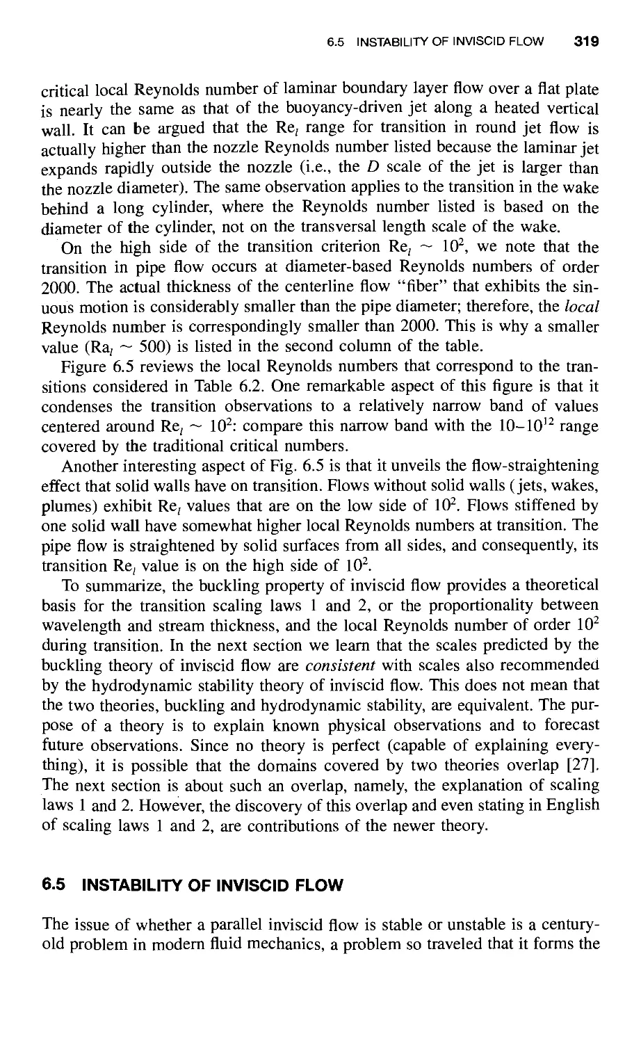
Figure 1.1 Mass conservation and systems of coordinates.
dp dp dp dp I du dv dw
V U \- V \- W hp 1 1
dt dx dy dz \ dx dy dz
0 (1.5)
or
Dp
Dt '^
(1.6)
In expression (1.6), v is the velocity vector {u,v,w), and DIDt represents the
"material derivative" operator, encountered frequently in convective heat and
mass transfer.

1 FUNDAMENTAL PRINCIPLES
D d d d d ,, „
— = — + u— + v— + w-~ (1.7)
Dt dt dx dy dz
Of particular interest to classroom treatment of the convection problem is
the wide class of flows in which temporal and spatial variations in density are
negligible relative to the local variations in velocity. For this class, the mass
conservation statement reads
du dv dw „ ,, „,
— + — + — = 0 (1.8)
dx dy dz
The equivalent forms of eq. (1.8) in cylindrical and spherical coordinates are
(Fig. 1.1)
dv, V, 1 dVa dv^ ^ ^, ^^
—^ + —+ ^ + -^ = 0 (1.9)
dr r r dd dz
and
- r e-'^^) + -^ ^ (^<^ ^i" ^) + -^ ^' = 0 (1.10)
r dr sm (p d(p ^ sm (p d6
It is tempting to regard eqs. (1.8)-(1.10) as valid only for incompressible fluids;
in fact, their derivation shows that they apply to flows (not fluids) where the
density and velocity gradients are such that the DpIDt terms are negligible
relative to the p V • v terms in eq. (1.6). Most of the gas flows encountered in
heat exchangers, heated enclosures, and porous media obey the simplified
version of the mass conservation principle [eqs. (1.8)-(1.10)].
1.2 FORCE BALANCES (MOMENTUM EQUATIONS)
From the dynamics of thrust or propulsion systems, we recall that the
instantaneous force balance on a control volume requires that [3]
I: iMvX. =
dt
Y.P'n+Y.'nVn-
inlet
ports
- X inv,
outlet
ports
(1.11)
where n is the direction chosen for analysis and v„ and F„ are the projections
of fluid velocity and forces in the n direction. Equation (1.11) is recognized in
the literature as the momentum principle or momentum theorem: In essence,
eq. (1.11) is the control volume formulation of Newton's second law of motion,
where in addition to terms accounting for forces and mass X acceleration, we
now have the impact due to the flow of momentum into the control volume.

1.2 FORCE BALANCES (MOMENTUM EQUATIONS) 5
plus the reaction associated with the flow of momentum out of the control
volume. In the two-dimensional flow situation of Fig. 1.2, we can write two
force balances of type (1.11), one for the x direction and the other for the y
direction.
Consider now the special form taken by eq. (1.11) when applied to the finite-
size control volume Ajc Ay drawn around point {x,y) in Fig. 1.2. Consider first
the balance of forces in the x direction. In Fig. 1.2a, showing the A jc Ay control
volume, we see the sense of the impact and reaction forces associated with the
flow of momentum through the control volume. In Fig. \.2b, we see the more
classical forces represented by the normal stress (o-^), tangential stress (t^),
and the jc-direction body force per unit volume (X).
Projecting all these forces on the x axis, we obtain
[puv + — (puv) Av) Ax
[p«2+^*AxlA^
3t
o^Ay.
j;
^y\ ' I > "
I I
^x
(
1
1
V
'V^-af ^^'^'^
^
~^
X^x^y 1
J
)
> <°x + ^ ^*) ^y
T^^Ax
(b)
Figure 1.2 Force balance in the x direction on a control volume in two-dimensional flow.

6 1 FUNDAMENTAL PRINCIPLES
— (dm Ax Ay) + pu^ Ay - dm^ H (dm^) Ax
dt dx
Ay
+ puv Ax —
puv H (puv) Ay
dy
da.
Ax
+ a,Ay-[a, + ~^Ax]Ay- t^ Ax
+ \ T^ + —^ Ay) Ax + X Ax Ay = 0
(1.12)
or, dividing by Ajc Ay in the limit (Ax, Ay) —► 0,
Du
p 1- u
^ Dt
Dp I du dv
-^ + p\ — + —
Dt '^V ^-^ ^3'
da ^Txy
'- + ^^ + X (1.13)
dx dy
According to the mass conservation equation (1.6), the quantity in brackets is
equal to zero; hence,
Du aOV ^^xy
p — = + —- + X
Dt dx dy
(1.14)
Next, we relate the stresses a^ and t,^ to the local flow field by recalling the
constitutive relations [4]
du 2 I du dv
a-, = P-2u— + -U— + —
^ dx 3 ^V^-^ ^y
du dv
"- = ^\Vy + Yx
(1.15)
(1.16)
These relations are of empirical origin: They summarize the experimental
observation that a fluid packet offers no resistance to a change of shape, but resists
the time rate of a change of shape. Equations (1.15) and (1.16) define the
measurable coefficient of viscosity /jl. Combining eqs. (1.14)-(1.16) yields the
Navier-Stokes equation,
Du
Dt
dp d
dx dx
d
dy
[K:
du
dx
)m dv\
iy dx)
2fJL 1 du dv\
T \al "^ a^/
+ X
(1.17)

1.2 FORCE BALANCES (MOMENTUM EQUATIONS) 7
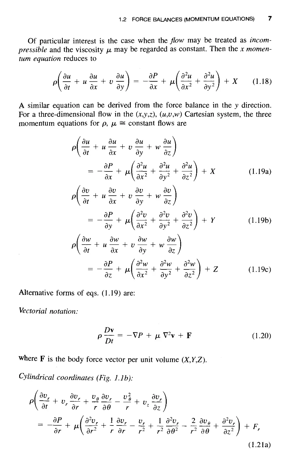
Of particular interest is the case when the flow may be treated as
incompressible and the viscosity /i may be regarded as constant. Then the x
momentum equation reduces to
du du du\ dP (d^u d^u
\- U \- V = 1- U r H
dt dx dyl dx \dx^ dy
p(- + "- + ^-) = -- + /^( 73 + 1:1)+^ (1-18)
A similar equation can be derived from the force balance in the y direction.
For a three-dimensional flow in the ix,y,z), iu,v,w) Cartesian system, the three
momentum equations for p, jjl = constant flows are
du du du du
p\ \- u \- V \- w —
dt dx dy dz
dP (d^u d^u d^u
= -—+ /.— + — + -
dx \dx^ dy dz
- + A~2 + —2 + 1^2]+^ (l-19a)
dv dv dv dv
p\ \- u hi; hw —
dt dx dy dz
dP (d^V d^V d^V
dy \dx^ dy^ dz
- + f^\^2 +1-2 + 1^2) + y (l-19b)
dw dw dw dw
p\ \- u hi; hw —
dt dx dy dz
dP (d^w d^w d^w\
Alternative forms of eqs. (1.19) are:
Vectorial notation:
D\
p — = -VP + /i, V^v + F (1.20)
where F is the body force vector per unit volume (X,Y,Z).
Cylindrical coordinates (Fig. Lib):
(dv^ dv, Vg dv, vl dv,
\dt ' dr r d9 r ' dz
dr ^\ dr^ r dr r^ ^ r^ dO^ r^ BO ^ dz^
(1.21a)

ji-.u<-viviniv rAL (-"HINCIPLES
^ dt ' dr r so r ' dz
r dO ^\ 37-2 ^ ^^ ^2 ^2 502 ^2 50 5^2
(1.21b)
/ dv, dv, Va dv^ dv,
\ dt ' dr r dO ' dz
dP / d^v, 1 dv, 1 d^v, d^v
dz \ dr^ r dr r^ dO^ dz
u—f + '- + -: —7 + —f + F. (1.21c)
^1 ^ -2 ,. Jif ,.2 a/32 ;j_2 I z V /
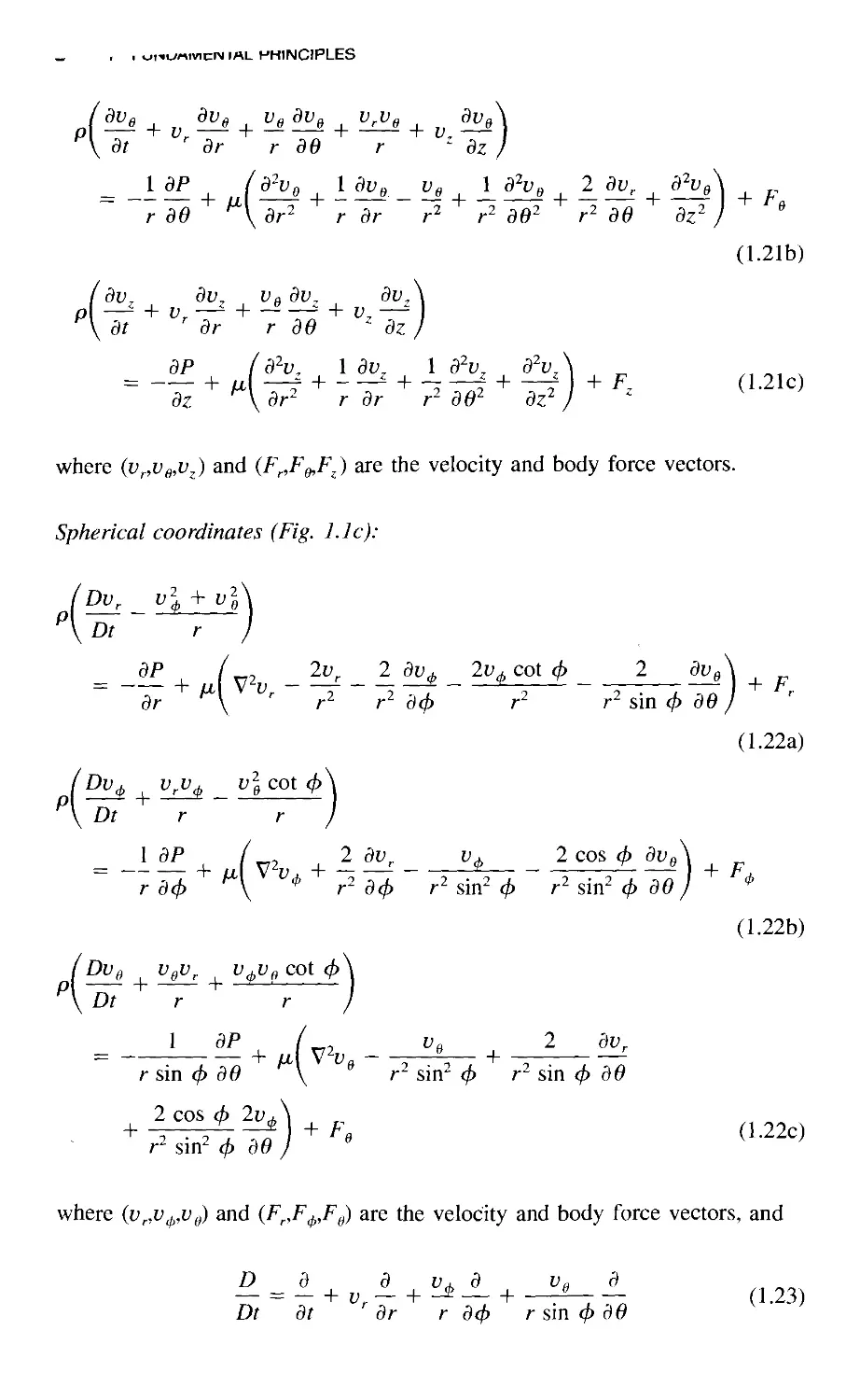
where (v^,Vg,v^) and (F^,Fg,F^) are the velocity and body force vectors.
Spherical coordinates (Fig. 1.1c):
JDv, vl + v\
\Dt r
dP
dr
1^2 2d^ 2 3d^ 2d^ cot (/> 2 ^^A I n^
V ^^ /-2 r^ a^/, r^ r^sincl^de) '
P
(1.22a)
^^A ^r^S ^l cot </)
Dt r r
(1.22b)
i^+ (V2 +^^^_ ^j. _ 2 cos (/> a^e
7-a</) ^V ^-^ r^ d(j) r^sin^cf) r^ sin^ (}> d9 > ' ' *
0, ^ + Mr + t;^D, cot (/>
^^ Dt r r
I dP (, Va 2 dv.
r sin (f) dO \ ^ r^ sin^ </> r^ sin </> 86
2 cos </) 2y^\
where (v„v^,Vg) and (F,,F^,Fg) are the velocity and body force vectors, and
D d a dj, a Vf, d
— = — + V,— + -^ — + (1.23)
Dt dt ' dr r dff} r sin (f> 86 ^

1.3 FIRST LAW OF THERMODYNAMICS 9
72 = 1A
+ ;^^^(^^"^^) + ;d^^ ^'-^^^
r^ dr \ dr
ate the material derivative and Laplacian operators in spherical coordinates.
1.3 FIRST LAW OF THERMODYNAMICS
The preceding two principles—mass conservation and force balance—are in
many cases sufficient for solving the flow part of the convective heat transfer
■Vl
Ipve + j-{pve) Ay] Ax
I
I
pueAy I
>
I
I
I
L.
'?x^j'C=;>|
^y
\Uf^U
I I
Ax
"n
3(pe)
dt
j lpue + — (pue) Ax] Ay
AxAy
-J
pveAx
0
3^
^y
{q'y + -ll Ay) Ax
1
1
q'" AxAy
n
|lZlC><'?x + ^^^)^J'
J
t.
<i'v^x
Figure 1.3 First law of thermodynamics applied to a control volume in two-dimensional flow
(for work transfer, see Fig. 1.2).

10
1 FUNDAMENTAL PRINCIPLES
problem; note at this juncture the availabihty of four equations (mass
conservation plus three force balances) for determining four unknowns (three velocity
components plus pressure). The exception to this statement is the subject of
Chapter 4, where the natural flow is driven by the heat administered to the
flowing fluid. In all cases, however, the heat transfer part of the convection
problem requires a solution for the temperature distribution through the flow,
especially in the close vicinity of the solid walls bathed by the heat-carrying
fluid stream (Chapter 2). The additional equation for accomplishing this
ultimate objective is the first law of thermodynamics or the energy equation.
For the control volume of finite size Ax Ay in Fig. 1.3, the first law of
thermodynamics requires that
rate of energy
accumulation in the
control volume
i
net transfer of
\ energy by fluid flow /
net heat transfer \
by conduction /
+
(rate of internal
heat generation (e.g.,
electrical power
dissipation)
net work transfer
from the control
volume to its
environment
(1.25)
According to the energy flow diagrams sketched in Fig. 1.3, the groups of
terms above are
{•}, = Ax A>'-(pe)
at
{•}, = -(Ax ^y)
d d
— (pue) + — (pve)
dx dy
(da" dq"
{•}, = (Ax Ay) q'"
{•}3 = (AxA,)(a.--T^- + a,-
+ (Ax Ay) u
da,
dx
dT^ da
u 1- i;
dy dy
dv_
^^" dx
dT
V
dx J*
(1.25')

1.3 FIRST LAW OF THERMODYNAMICS 11
where e, cl'x^ 4r ^'^ ^'" ^'"^ ^^ specific internal energy, heat flux in the x
direction, heat flux in the y direction, and dissipation rate or rate of internal
heat generation.
The origin of the dissipation rate term {•]^ lies in the work transfer effected
by the normal and tangential stresses sketched in Fig. Mb. For example, the
work done per unit time by the normal stresses cr^ on the left side of the Ax
A>' element is negative and equal to the force acting on the boundary (cr^ A>')
times the boundary displacement per unit time (m), which yields ~ucr^ l^y.
Similarly, the work transfer rate associated with normal stresses acting on the
right side of the element is positive and equal to [cr^ + {dajdx) Ax][m +
(du/dx) Ax] Ay. The net work transfer rate due to these two contributions is
[a^idu/dx) + uid(Tjdx)](Ax Ay), as shown in the {-jj term of eq. (1.25').
Three more work transfer rates can be calculated in the same manner by
examining the effect of the remaining three stresses, t^^ in the x direction and
ay and t^^ in the y direction. In the l-}^ expression above, the eight terms have
been separated into two groups. It can be shown that the group denoted as
(•)* reduces to —p{DIDt){u^ + v^)l2, which represents the change in kinetic
energy of the fluid packet; in the present treatment, this change is considered
negligible relative to the internal energy change d(pe)/dt appearing in {•}i.
Assembling expressions (1.25) into the energy conservation statement that
preceded them, and using constitutive relations (1.15) and (1.16), we obtain
p— + el— + p V-v) = -V-q" + q'" - P V-v + /u,4> (1.26)
where q" is the heat flux vector (q",q'y) and 4> is the viscous dissipation function,
shown later in eq. (1.45a). The quantity between parentheses on the left-hand
side of eq. (1.26) is equal to zero [cf. eq. (1.6)]. In the special case where the
flow can be modeled as incompressible and two-dimensional, the viscous
dissipation function reduces to
$ = 2
du\ I dv
dx) \dy
5" ^'^\
To express eq. (1.26) in terms of enthalpy, we use the thermodynamics
definition h = e + {\lp)P\ hence.
Dh De I DP P Dp
Dt ~ Dt p Dt p^ Dt
+ -^^-4^ (1.28)
In addition, we can express the directional heat fluxes q^' and q" in terms of
the local temperature gradients; that is, we invoke the Fourier law of heat
conduction.

12
1 FUNDAMENTAL PRINCIPLES
q" = -k VT
(1.29)
Then, combining eqs. (1.26), (1.28), and (1.29) in the manner desired, we
obtain
,|^-_v.,vr,.,».f..*-^^..v.v
(1.30)
Finally, we learn from the mass conservation equation (1.6) that the last terms
in parentheses in eq. (1.30) add up to zero; in conclusion, the first law of
thermodynamics reduces to
Dh DP
(1.31)
In order to express the energy equation (1.31) in terms of temperature, it is
tempting to replace the specific enthalpy on the left-hand side by the product
of specific heat X temperature. This move is correct only in cases where the
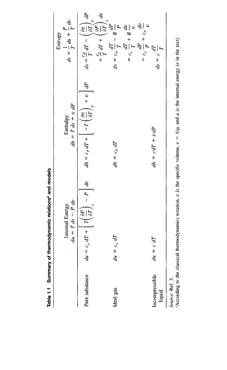
fluid behaves like an ideal gas (see the ideal gas model. Table 1.1). In general,
the change in specific enthalpy for a single-phase substance is expressed by
the canonical relation for enthalpy [3],
dh
Tds + -dP
P
(1.32)
where T is the absolute temperature and ds the specific entropy change.
ds = \ — \ dT +
\dT'
dP
dP
(1.33)
From the last of Maxwell's relations [3, p. 173], we have
ds_
dP
djl/p)
dT
1 I ^
dT
P
(1.34)
where fi is the coefficient of thermal expansion.
(1.35)
Table 1.1 also shows that

o ~
pq ^ih.
«
■o
o
E
■o
c
n
1.
c
.0
"ip
JO
£
u
1
n
1^
o
E
o
E
E
3
(A
I
£pa,
W
13 ^
3
s ■§!
OS
+
+
^|h, ^|h, %|a. f^i
%
+
=§
^
-i
=§
3
II
%
S
=§
-i
cn
CD
ac
^
tf
2
c§
•5
Q
OB
C
■3
1-
o
u
u
<

14 1 FUNDAMENTAL PRINCIPLES
ds \ _ Cp
(1.36)
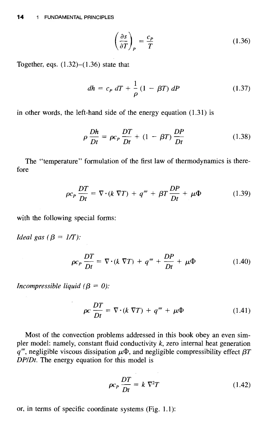
Together, eqs. (1.32)-(1.36) state that
dh = Cp dT + - (l ~ pT) dP (1.37)
P
in other words, the left-hand side of the energy equation (1.31) is
Dh DT DP
p — = pcp — + (1 - fiT) — (1.38)
^ Dt ^"^ Dt ^ ^ ^ Dt ^
The "temperature" formulation of the first law of thermodynamics is
therefore
pCp^=V-ik Vr) + q'" + )8r^ + At$ (1.39)
with the following special forms:
Ideal gas (^ = 1/T):
DT DP
pcp— = ^-ikVT) + q'" + — + ^cD (1.40)
Incompressible liquid ((3 = 0):
DT
pc — = V-(kVT) + q'" + fM^ (1.41)
Most of the convection problems addressed in this book obey an even
simpler model: namely, constant fluid conductivity k, zero internal heat generation
q'", negligible viscous dissipation fM'P, and negligible compressibility effect yST
DPIDt. The energy equation for this model is
pcp^ = kV'T (1.42)
or, in terms of specific coordinate systems (Fig. 1.1):

1 -3 FIRST LAW OF THERMODYNAMICS 15
Cartesian (x,y,z):
dT dT dT dT\ d^T d^T d^T
^"^ ^ dt dx dy dzj \dx^ dy^ dz^
(1.43a)
Cylindrical (kO,z):
dT dT v„ dT dT
pcp\ — + v^— + -— + V
dt
k
' dr r dd
dz
1 d I dT\ j_a^ d^T
rdr\ dr) r^ dd^ dz^
(1.43b)
Spherical (r </>, 6):
pcp
dT dT v^ dT v„ dT
dt dr r dtf) r sin </> dd
= k
L—{2^\ 1 a
r^ dr \ dr / r^ sin </> d(f)
sinc/.-l +
1 d'^T
r^ sin^(/> dO'^
(1.43c)
If the fluid can be modeled thermodynamically as an incompressible liquid,
then, as in eq. (1.41), the specific heat at constant pressure Cp is replaced by
the lone specific heat of the incompressible liquid, c (Table 1.1).
When dealing with extremely viscous flows of the type encountered in
lubrication problems or the piping of crude oil, the model above is improved by
taking into account the internal heating due to viscous dissipation.
DT
pCp— = k^^T+ ^(&
(1.44)
In three dimensions, the general viscous dissipation function can be expressed
as follows:
Cartesian (x,y,z):
$ = 2
du dv\
— + — +
dy dx j
du dv dw
- + — +
3 \ to dy dz
dw
aT
dv dw
dz dy
dw du
dx dz
(1.45a)

16
1 FUNDAMENTAL PRINCIPLES
Cylindrical (r,d,z):
$ = 2
[{
1
+ -
2
1
+ -
2
Spherical (r, </>, 6):
c& = 2|
1
+ -
2
1
+ -
2
M^
r^ ('^]
_ dr\rj
1 dv,
r sin (f) 86
'fhil'li^'iJ^i^J
fdVg _Ve j^}_ ^Y j^}_(}_^ ^ ^Y
\dr r r dd) 2\r 86 dz )
(dv, dv\ 1 „ ^
\r d^ r) \r sm (f) d6 r r
1 dv'
+ -
r d(f)
9 (
+ r —
dr\
' 1
+ -
2
7');
2
sint/. a / Ue \ 1
r d(f) \r sin </>/ r sin
}-|(V..
0^
(1.45b)
.y]
dVg
(/> 30
" 2
(1.45c)
If the density does not vary significantly through the flow field, V • v = 0 [eq.
(1.6)] and the last term in each of expressions (1.45) vanishes.
It is worth reviewing the constant-p approximation that led to eq. (1.8) and
recognizing that it differs conceptually from the "incompressible substance
model" of thermodynamics. The latter is considerably more restrictive than the
"nearly constant" density model, eq. (1.8). For example, a compressible
substance such as air can flow in such a way that eq. (1.8) is a very good
approximation of eq. (1.6).
For the restrictive class of fluids that are "incompressible" from the
thermodynamic point of view, the specific heat at constant pressure Cp can be
replaced by the lone specific heat of the fluid, c, on the left side of eq. (1.39).
Water, liquid mercury, and engine oil are examples of fluids for which this
substitution is justified. There are even convection problems in which the
moving materials are actually solid (e.g., a roller and its substrate, in the zone of
elastic contact). In such cases the Cp — c substitution is permissible also.
It is important to note that the specific heat at constant volume c^ does not
belong on the left side of eq. (1.39). This observation is important because
Fourier [5,6], and later Poisson [7], who were the first to derive the energy
equation for a convective flow, wrote c on the left side of eq. (1.39). They
made this choice because their analyses were aimed specifically at
incompressible fluids (liquids), for which c happens to have nearly the same value as Cp.
Because of this choice, they did not have to account for the P dV type of work
done by the fluid packet as it expands or contracts in the flow field. In the
modem era, however, the use of c^ instead of Cp is an error.

1.4 SECOND LAW OF THERMODYNAMICS 17
The prethermodynamics (caloric conservation) origins of the science of
convection heat transfer are also responsible for the "thermal energy equation"
label that some prefer to attach to eq. (1.39) without the jiT DPIDt term. This
terminology is sometimes used to stress (incorrectly) the conservation of
"thermal" energy as something distinct from "mechanical and thermal" energy. In
classical thermodynamics, however, this distinction disappeared as soon as the
first law of thermodynamics was enunciated, that is, as soon as the
thermodynamic property "energy" was defined, which happened in the years 1850-
1851 (see Ref. 3, pp. 30-32).
Equation (1.39) represents the first law of thermodynamics. This law
proclaims the conservation of the sum of energy change (the property) and energy
interactions (heat transfer and work transfer). The suggestion that mechanical
effects (e.g., work transfer) are absent from eq. (1.39) when the ^T DPIDt
term is absent is erroneous. The presence of Cp on the left side of the equation
is the sign that each fluid packet expands or contracts (i.e., it does P JV-type
work) as it rides on the flow. The terms q'" and ;u,4> are work transfer rate
terms also.
1.4 SECOND LAW OF THERMODYNAMICS
Any discussion of the basic principles of convective heat transfer must include
the second law of thermodynamics, not because the second law is necessary
for determining the flow and temperature field (it is not, because it is not an
equation), but because the second law is the basis for much of the engineering
motive (objective, purpose) for formulating and solving convection problems.
For example, in the development of knowhow for the heat exchanger industry,
we strive for improved thermal contact (enhanced heat transfer) and reduced
pump power loss in order to improve the thermodynamic efficiency of the heat
exchanger. Good heat exchanger design means, ultimately, efficient
thermodynamic performance, that is, minimum generation of entropy or minimum
destruction of exergy in the power/refrigeration system incorporating the heat
exchanger [8-10]. For this reason, it is useful to review the second law and in
this way to explain the commonsense origin of the engineering questions that
led to today's field of convective heat transfer.
The second law of thermodynamics states that all real-life processes are
irreversible: In the case of a control volume, as in Fig. 1.1, this statement is
^^- S I + S m. - 2 '^^ (1-46)
inlet outlet
ports ports
dt ^ Z
where S^^ is the instantaneous entropy inventory of the control volume, ms
represents the entropy flows (streams) into and out of the control volume, and
Tj is the absolute temperature of the boundary crossed by the heat transfer

18
1 FUNDAMENTAL PRINCIPLES
interaction q^.* The irreversibility of the process is measured by the strength
of the inequality sign in eq. (1.46), or by the entropy generation rate 5g^„,
defined as
gen
dt
i i inlet
ports
ms +
^ ms ^ 0
outlet
ports
(1.47)
It is easy to show that the rate of destruction of useful work in an
engineering system,
[8-10],
W|(,st, is directly proportional to the rate of entropy generation
*^lost ~ M)'-*B.
(1.48)
where Tq is the absolute temperature of the ambient temperature reservoir (Tq
= constant). Equation (1.48) stresses the engineering importance of estimating
the irreversibility or entropy generation rate of convective, heat transfer
processes: If not used wisely, these processes contribute to the waste of precious
fuel resources.
Based on an analysis similar to the analyses presented for mass conservation,
force balances, and the first law of thermodynamics, the second law (1.47) may
be applied to a finite-size control volume Ax Ay Az at an arbitrary point ix,y,z)
in a flow field. Thus, the rate of entropy generation per unit time and per unit
volume S'" is [8,9]
l(Vr)^ + ^4>>0
(1.49)
a 0
a 0
where k and fx are assumed constant. In a two-dimensional convection situation
such as in Figs. 1.1-1.3, the local entropy generation rate (1.49) yields
cm _ _2_
gen J.2
dT
dx
dT
'dy
+ f^<2
— + — ]
dy dx /
> 0 (1.50)
In the last two equations, T represents the absolute temperature of the point
where S'^^„ is being evaluated. The two-dimensional expression (1.50) illustrates
the competition between viscous dissipation and imperfect thermal contact
(finite-temperature gradients) in the generation of entropy via convective heat
cJtivp intn the control volume.

1.5 RULES OF SCALE ANALYSIS 19
transfer. The two-sided character of entropy generation in convective heat
transfer was illustrated most recently by Mahmud and Eraser [11].
Equations (1.48) and (1.50) constitute the bridge between two research
activities: fundamental convection heat transfer and applied thermodynamics
(entropy generation minimization). Beginning with Chapter 2, we focus on the
fundamental problems of determining the flow and temperature fields in a given
convection heat transfer configuration. However, through eq. (1.50), we are
invited to keep in mind that these fields contribute hand-in-hand to downgrading
the thermodynamic merit of the engineering device that ultimately employs the
convection process under consideration. The science of adjusting the convection
process so that it destroys the least exergy (subject to various system
constraints) is the focus of entropy generation minimization; this activity has been
reviewed in Refs. 8-10. The generation of flow configuration (geometry,
architecture) for maximal performance under constraints is constructal theory and
design [12-15].
1.5 RULES OF SCALE ANALYSIS
This section is designed to familiarize the student with the commonsense
problem-solving method of scale analysis or scaling. This section is necessary
because scale analysis is used extensively throughout the book; in fact, scale
analysis is recommended as the premier method for obtaining the most
information per unit of intellectual effort. Furthermore, this section is necessary
because scale analysis is not discussed in the heat transfer and fluid mechanics
textbooks of our time, despite the fact that it is a precondition for good analysis
in dimensionless form. Scale analysis is often confused with dimensional
analysis or the often arbitrary nondimensionalization of the governing equations
before performing a perturbation analysis or a numerical simulation on the
computer.
The object of scale analysis is to use the basic principles of convective heat
transfer to produce order-of-magnitude estimates for the quantities of interest.
This means that if one of the quantities of interest is the thickness of the
boundary layer in forced convection, the object of scale analysis is to determine
whether the boundary layer thickness is measured in millimeters or meters.
Note that scale analysis goes beyond dimensional analysis (whose objective is
to determine the dimension of boundary layer thickness, namely, length). When
done properly, scale analysis anticipates within a factor of order one (or within
percentage points) the expensive results produced by "exact" analyses. The
value of scale analysis is remarkable, particularly when we realize that the
notion of "exact analysis" is as false and ephemeral as the notion of
"experimental fact."
As the first example of scale analysis, consider a problem from the field of
conduction heat transfer [16]. In Fig. 1.4 we see a plate plunged at t = 0 into
a highly conducting fluid, such that the surfaces of the plate instantaneously

20 1 FUNDAMENTAL PRINCIPLES
Temperature
Figure 1.4 Transient heat conduction in a slab with sudden temperature change on the
boundaries.
assume the fluid temperature T„ = Tq + AT. Suppose that we are interested
in estimating the time needed by the thermal front to penetrate the plate, that
is, the time until the center plane of the plate "feels" the heating imposed on
the outer surfaces.
To answer the question above, we focus on a half-plate of thickness D/2
and the energy equation for pure conduction in one direction:
dT _ d^T
dt
dx'
(1.51)
Next, we estimate the order of magnitude of each of the terms appearing in
eq. (1.51). On the left-hand side we have
dT
pcp —
AT
pCp
(1.52)
In other words, the scale of the temperature change (in the chosen space and
in a time of order t) is AT. On the right-hand side we obtain
, d^T , d (dT
k —- = k — —
dx^ dx \ dx
k AT
DI2 Dll
kAT
{Dllf
(1.53)

1.5 RULES OF SCALE ANALYSIS 21
Equating the two orders of magnitude (1.52) and (1.53), as required by the
energy equation (1.51), we find the answer to the problem
{Dllf
t ~ -^ (1.54)
where a is the thermal diffusivity of the medium, kJpcp. The penetration time
(1.54) compares well with any order-of-magnitude interpretation of the exact
solution to this classical problem [16]. However, the time and effort associated
with deriving eq. (1.54) do not compare with the labor required by Fourier
analysis and the graphical presentation of Fourier series.
Based on this introductory example, the following rules of scale analysis are
worth stressing.
• Rule 1. Always define the spatial extent of the region in which you
perform the scale analysis. In the example of Fig. 1.4, the size of the region
of interest is D/2. In other problems, such as boundary layer flow, the size
of the region of interest is unknown; as shown in Chapter 2, the scale
analysis begins by selecting the region and by labeling the unknown
thickness of this region S. Any scale analysis of a flow or a flow region that is
not uniquely defined is pure nonsense.
• Rule 2. One equation constitutes an equivalence between the scales of two
dominant terms appearing in the equation. In the transient conduction
example of Fig. 1.4, the left-hand side of eq. (1.51) could only be of the
same order of magnitude as the right-hand side. The two terms appearing
in eq. (1.51) are the dominant terms (considering that the discussion
referred to pure conduction); in general, the energy equation can contain
many more terms [eq. (1.39)], not all of them important. The reasoning
for selecting the dominant scales from many scales is condensed in rules
3-5.
• Rule 3. If in the sum of two terms,
c = a + b (1.55)
the order of magnitude of one term is greater than the order of magnitude
of the other term,
Oia) > 0(b) (1.56)
then the order of magnitude of the sum is dictated by the dominant term:
(9(c) = Oia) (1.57)
The same conclusion holds if instead of eq. (1.55), we have the difference
c = a~boTc= —a + b.

22 1 FUNDAMENTAL PRINCIPLES
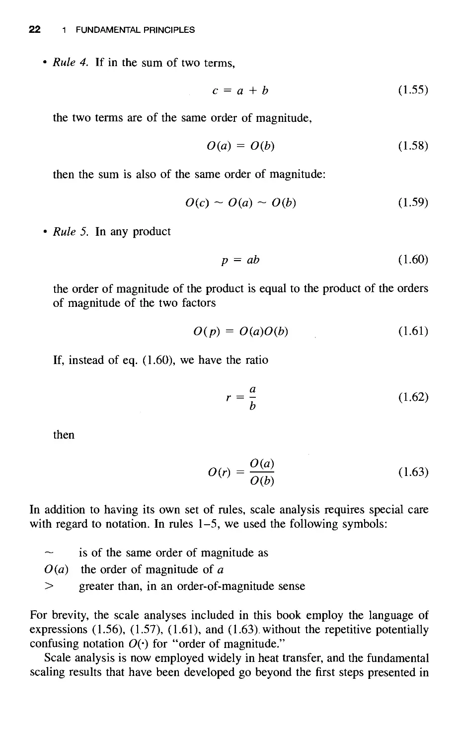
• Rule 4. If in the sum of two terms,
c = a + b (1.55)
the two terms are of the same order of magnitude,
0{a) = 0{b) (1.58)
then the sum is also of the same order of magnitude:
0{c) ~ 0{a) ~ 0{b) (1.59)
• Rule 5. In any product
p = ab (1.60)
the order of magnitude of the product is equal to the product of the orders
of magnitude of the two factors
0{p) = 0{a)0{b) (1.61)
If, instead of eq. (1.60), we have the ratio
r = I (1.62)
b
then
In addition to having its own set of rules, scale analysis requires special care
with regard to notation. In rules 1-5, we used the following symbols:
~ is of the same order of magnitude as
0(a) the order of magnitude of a
> greater than, in an order-of-magnitude sense
For brevity, the scale analyses included in this book employ the language of
expressions (1.56), (1.57), (1.61), and (1.63) without the repetitive potentially
confusing notation O(-) for "order of magnitude."
Scale analysis is now employed widely in heat transfer, and the fundamental
scaling results that have been developed go beyond the first steps presented in

dip
u = —,
dy
V =
dip
dx
1.6 HEATLINES FOR VISUALIZING CONVECTION 23
this book. For example, Bhattacharjee and Grosshandler [17] have reported the
scale analysis of a pressure-driven wall jet. Li and Djilali [18] have used scale
analysis to describe the behavior of separating flows behind backward-facing
steps (separation bubbles). Li [19] has reported the scaling results for jet
diffusion flames.
1.6 HEATLINES FOR VISUALIZING CONVECTION
The opportunity to actually "see" the solution to a problem is essential to a
problem solver's ability to learn from experience and in this way to improve
his or her technique. In convection problems it is important to visualize the
flow of fluid and, riding on this, the flow of energy. For example, in the two-
dimensional Cartesian configuration of Fig. 1.1, it has been common practice
to define a streamfunction ip{x,y) as
(1.64)
such that the mass continuity equation for incompressible flow,
du dv
- + — = 0 (1.65)
dx dy
is satisfied identically. It is easy to verify that the actual flow is locally parallel
to the ip = constant line passing through the point of interest. Therefore,
although there are no substitutes for u and v as bearers of precise information
regarding the local flow, the family of ip = constant streamlines provides a
much needed bird's-eye view of the entire flow field and its main
characteristics.
In convection, the transport of energy through the flow field is a combination
of both thermal diffusion and enthalpy flow [cf. eq. (1.42)]. For any such field,
Kimura and Bejan [20] defined a new function Hix,y) such that the net flow
of energy (thermal diffusion and enthalpy flow) is zero across each H =
constant line. The mathematical definition of the heatfunction H follows in the
steps of eqs. (1.64) if this time the aim is to satisfy the energy equation. For
steady-state two-dimensional convection through a constant-property
homogeneous fluid, eq. (1.42) becomes
dT dT (d^T d^T\
or

1 FUNDAMENTAL PRINCIPLES
-(pc,«r-.-j + -U.r-.-j=o (1.67)
The heatfunction is defined as follows:
Net energy flow in the x direction:
dH ST
— = pCpu{T~T,^,)~k— (1.68)
oy dx
Net energy flow in the y direction:
dH __
dx ~
pCpV{T -
■ T'.ef) -
dT
- k —
dy
(1.69)
so that the heatfunction H(x,y) satisfies eq. (1.66) identically. Note that the
definition above also applies to convection through a fluid-saturated porous
medium, where eq. (1.66) accounts for energy conservation.
The reference temperature r^^f is, in principle, an arbitrary constant that can
be selected based on convention. Patterns of H = constant heatlines are
instructive when Tj^f is the lowest temperature that occurs in the heat transfer
configuration. For example, if the wall shown in Fig. 2.1 is warmer than the
free stream, Tq > r„, the choice of reference temperature is T^^j = T^. For a
meaningful comparison of the heatlines of one flow with the heatlines of
another flow, I propose that T^^f always be set equal to the lowest temperature of
the flow field.
If the fluid flow subsides {u = v = 0), the heatlines become identical to the
heat flux lines employed frequently in the study of conduction phenomena.
Therefore, as a heat transfer visualization technique, the use of heatlines is the
convection counterpart or generalization of a standard technique (heat flux
lines) used in conduction. It is also interesting to point out that the
contemporary use of r = constant lines is not a proper way to visualize heat transfer
in the field of convection; isotherms are a proper heat transfer visualization
tool only in the field of conduction (where, in fact, they have been invented)
because only there are they locally orthogonal to the true direction of energy
flow. The use of T = constant lines to visualize convection heat transfer makes
as little sense as using P = constant lines to visualize fluid flow.
The heatline method for the visualization of .convective heat transfer was
proposed in the first edition of this book (1984), along with a first application
to natural convection in an enclosure heated from the side [20]. The method
has since been adopted and extended in several ways in the post-1984 heat
transfer literature [21-43].

REFERENCES 25
REFERENCES
1. D. B. Guralnik, ed., Webster's New World Dictionary, 2nd college ed., World
Publishing Company, New York, 1970, p. 310.
2. D. P. Simpson, Cassell's Latin Dictionary, Macmillan, New York, 1978, p. 150.
3. A. Bejan, Advanced Engineering Thermodynamics, 2nd ed., Wiley, New York,
1997, p. 193.
4. W M. Rohsenow and H. Y Choi, Heat, Mass and Momentum Transfer, Prentice-
Hall, Englewood Cliffs, NJ, 1961, p. 48.
5. J. B. J. Fourier, Memoire d'analyse sur le mouvement de la chaleur dans les fluides,
in Memoires de I'Academie Royale des Sciences de I'Institut de France, Didot,
Paris, 1833, pp. 507-530 (presented on Sept. 4, 1820).
6. J. B. J. Fourier, Oeuvres de Fourier, G. Darboux, ed.. Vol. 2, Gauthier-Villars, Paris,
1890, pp. 595-614.
7. S. D. Poisson, Theorie Mathematique de la Chaleur, Paris, 1835, Chapter 4, p. 86.
8. A. Bejan, Entropy Generation through Heat and Fluid Flow, Wiley, New York,
1982.
9. A. Bejan, Entropy Generation Minimization, CRC Press, Boca Raton, FL, 1996.
10. A. Bejan, G. Tsatsaronis, and M. Moran, Thermal Design and Optimization, Wiley,
New York, 1996.
11. S. Mahmud and R. A. Fraser, The second law analysis in fundamental convective
heat transfer problems. Int. J. Therm. ScL, Vol. 42, 2003, pp. 177-186.
12. A. Bejan, Shape and Structure, from Engineering to Nature, Cambridge University
Press, Cambridge, 2000.
13. R. N. Rosa, A. H. Reis, and A. F Miguel, eds., Bejan's Constructal Theory of
Shape and Structure, Evora Geophysics Center, University of Evora, Portugal,
2004.
14. H. Poirier, Une theorie explique 1'intelligence de la nature. Science & Vie, No.
1034, November 2003, pp. 44-63.
15. M. Torre, La Natura, vi svelo le formule della perfezione, La Macchina del Tempo,
Nos. 1-2, Year 5, January-February 2004, pp. 36^6.
16. A. Bejan, Heat Transfer, Wiley, New York, 1993, Chapter 4.
17. S. Bhattacharjee and W. L. Grosshandler, The formation of a wall jet near a high
temperature wall under microgravity environment, ASME HTD, Vol. 96, 1988, pp.
711-716.
18. X. Li and N. Djilali, On the scaling of separation bubbles, JSME Int. J., Ser B,
Vol. 38, No. 4, 1995, pp. 541-548.
19. X. Li, On the scaling of the visible lengths of jet diffusion flames, J. Energy Resour
TechnoL, Vol. 118, 1996, pp. 128-133.
20. S. Kimura and A. Bejan, The "heatline" visualization of convective heat transfer,
J. Heat Transfer, Vol. 105, 1983, pp. 916-919.
21. D. Littlefield and P. Desai, Buoyant laminar convection in a vertical cylindrical
annulus, J. Heat Transfer Vol. 108, 1986, pp. 814-821.
22. O. V. Trevisan and A. Bejan, Combined heat and mass transfer by natural
convection in a vertical enclosure, J. Heat Transfer Vol. 109, 1987, pp. 104-109.

26 1 FUNDAMENTAL PRINCIPLES
23. F. L. Bello-Ochende, Analysis of heat transfer by free convection in tilted
rectangular cavities using the energy analogue of the stream function, Int. J. Mech. Eng.
Ed, Vol. 15, 1987, pp. 91-98.
24. F. L. Bello-Ochende, A heat function formulation for thermal convection in a square
cavity. Int. Comm. Heat Mass Transfer, Vol. 15, 1988, pp. 193-202.
25. A. M. Morega, The heat function approach to the thermo-magnetic convection of
electroconductive melts. Rev. Roiim. Sci. Tech. Ser Electrotech. Energ., Vol. 33,
1988, pp. 33-39.
26. S. K. Aggarwal and A. Manhapra, Use of heatlines for unsteady buoyancy-driven
flow in a cylindrical enclosure, J. Heat Transfer Vol. HI, 1989, pp. 576-578.
27. S. K. Aggarwal and A. Manhapra, Transient natural convection in a cylindrical
enclosure nonuniformly heated at the top wall, Numer Heat Transfer Part A, Vol.
15, 1989, pp. 341-356.
28. C. J. Ho, Y. H. Lin, and T. C. Chen, A numerical study of natural convection in
concentric and eccentric horizontal cylindrical annuli with mixed boundary
conditions. Int. J. Heat Fluid Flow, Vol. 10, 1989, pp. 40^7.
29. C. J. Ho and Y. H. Lin, Thermal convection heat transfer of air/water layers
enclosed in horizontal annuli with mixed boundary conditions, Wdrme Stoffubertrag.,
Vol. 24, 1989, pp. in-llA.
30. C. J. Ho and Y H. Lin, Natural convection of cold water in a vertical annulus with
constant heat flux on the inner wall, J. Heat Transfer, Vol. 112, 1990, pp. 117-
123.
31. A. M. Morega and A. Bejan, Heatline visualization of forced convection boundary
layers. Int. J. Heat Mass Transfer, Vol. 36, 1993, pp. 3957-3966.
32. A. M. Morega and A. Bejan, Heatline visualization of forced convection in porous
media. Int. J. Heat Fluid Flow, Vol. 15, 1994, pp. 42^7.
33. V. A. F Costa, Double diffusive natural convection in a square enclosure with heat
and mass diffusive walls, Int. J. Heat Mass Transfer Vol. 40, 1997, pp. 4061-4071.
34. V A. F Costa, Double diffusive natural convection in enclosures with heat and
mass diffusive walls, in G. De Vahl Davis and E. Leonardi. eds., Proceedings of
the International Symposium on Advances in Computational Heat Transfer
(CHT'97), Begell House, New York, 1998, pp. 338-344.
35. H. Y Wang, F Penot, and J. B. Saulnier, Numerical study of a buoyancy-induced
flow along a vertical plate with discretely heated integrated circuit packages, Int.
J. Heat Mass Transfer, Vol. 40, 1997, pp. 1509-1520.
36. V. A. F Costa, Unification of the streamline, heatline and massline methods for
the visualization of two-dimensional transport phenomena. Int. J. Heat Mass
Transfer, Vol. 42, 1999, pp. 27-33.
37. S. J. Kim and S. P. Jang, Experimental and numerical analysis of heat transfer
phenomena in a sensor tube of a mass flow controller, Int J. Heat Mass Transfer,
Vol. 44, 2001, pp. 1711-1724.
38. Q.-H. Deng and G.-F Tang, Numerical visualization of mass and heat transport for
conjugate natural convection/heat conduction by streamline and heatline. Int. J.
Heat Mass Transfer, Vol. 45, 2002, pp. 2375-2385.
39. Q.-H. Deng and G.-F. Tang, Numerical visualization of mass and heat transport for
mixed convective heat transfer by streamline and heatline. Int. J. Heat Mass
Transfer, Vol. 45, 2002, pp. 2387-2396.

PROBLEMS 27
40. A. Mukhopadhyay, X. Qin, S. K. Aggarwal, and I. K. Puri, On extension of "heat-
line" and "massline" concepts to reacting flows through the use of conserved
scalars, J. Heat Transfer, Vol. 124, 2002, pp. 791-799.
41. V. A. F. Costa, Comment on the paper by Qi-Hong Deng and Guang-Fa Tang,
Numerical visualization of mass and heat transport for conjugate natural convection/
heat conduction by streamline and heatline, Int. J. Heat Mass Transfer, Vol. 46,
2003, pp. 185-187.
42. A. F Costa, Unified streamline, heatline and massline methods for the visualization
of two-dimensional heat and mass transfer in anisotropic media, Int. J. Heat Mass
Transfer, Vol. 46, 2003, pp. 1309-1320.
43. A. Mukhopadhyay, X. Qin, I. K. Puri, and S. K. Aggarwal, Visualization of scalar
transport in nonreacting and reacting jets through a unified "heatline" and "mass-
line" formulation. Numerical Heat Transfer, Part A, Vol. 44, 2003, pp. 683-704.
PROBLEMS
1.1. Consider the unsteady mass conservation equation (1.5) as it might
describe the flow accelerating through a duct with a variable cross section.
If the largest velocity gradient measured locally is du/dx and the largest
density gradient is dp/dx, what order-of-magnitude relationship must
exist between du/dx and dp/dx for the simplified equation (1.8) to be
applicable?
1.2. Derive the mass conservation equation in cylindrical coordinates [eq.
(1.9)] by applying the general principle (1.1) to an elementary control
volume of size Ar(r A0)Az in Fig. l.lb (assume that p = constant).
1.3. Derive the mass conservation statement for spherical coordinates [eq.
(1.10)] by writing eq. (1.1) for the elementary control volume (Ar) (r sin
cf> Aff)(r A(f>) around point (r,d,(f>) in Fig. 1.1c (assume that p =
constant).
1.4. Consider a flow in which p and /m may be regarded as constant. Show
that the x momentum equation (1.18) follows from eq. (1.17) through
proper use of the mass conservation principle.
1.5. Imagine a flow described by eqs. (1.9) and (1.21) in cylindrical
coordinates. If the flow is situated on one side of and infinitely far from the
r = 0 origin of the coordinate system, the local three-directional
increments Ar, r Ad, Az become analogous to three Cartesian increments
Ax, Ay, Az measured away from the local point {r,d,z) in the flow field.
Show that in the limit r —► oo, the transformation Ar —► Ax, r A6 —^ Ay,
Az —► Az leads to the collapse of eqs. (1.9) and (1.21) into their {x,y,z)
Cartesian equivalents [eqs. (1.8) and (1.19)].
1-6. Consider the conservation of mass and the three force balances in
spherical coordinates [eqs. (1.10) and (1.22)]. If the flow described by these

28 1 FUNDAMENTAL PRINCIPLES
equations is situated infinitely far from the r = 0 origin of the spherical
system, the following transformation is applicable (Fig. 1.1): Ar —► Ax,
r sivKf) Ad —^ Ay, r A<f) —>■ Az. Show that through this transformation, in
the limit r —► oo, eqs. (1.10) and (1.22) become the same as eqs. (1.8)
and (1.19).
1.7. Implicit in the derivation of the energy equation (1.39) is the assumption
that changes in kinetic energy V^/2 are negligible relative to changes in
internal energy e [see expressions (1.25), where e should, in general, be
replaced by e + V^/2]. Retrace the path leading to eq. (1.39) by taking
into account changes in kinetic energy; show that the result of this more
rigorous analysis is identical to eq. (1.39).
1.8. Demonstrate that lost work is always proportional to entropy generation
[eq. (1.48)], where 1V,„,, = IV^aximum " M^actuai' and where W^,^,^^^
corresponds to the reversible limit iSg^„ = 0). Write the first law of
thermodynamics for a control volume, first for the actual (real) process and
then for the reversible process. Then use the definition of W^^^i and S^^„
to prove eq. (1.48).
1.9. Derive the formula for the local rate of entropy generation [eq. (1.49)].
Begin with translating the general statement (1.47) into the language of
the two-dimensional control volume Ax Ay. Combine the resulting
expression with the first law of thermodynamics as given by eq. (1.26),
plus the canonical relation for internal energy (Table 1.1).
1.10. Consider the Couette flow between two parallel plates separated by a gap
of width D and moving relative to one another with a speed U. The
temperature difference Ar is imposed between the two plates. Estimate
the rate of entropy generation per unit volume in this flow. What
relationship must exist between D, U, AT, and the fluid properties /x and k
for Sg^„ to be dominated by the irreversibility due to fluid friction?
1.11. According to the one-dimensional (longitudinal) conduction model of a
fin, the temperature distribution along the fin, T{x), obeys the energy
equation [16]
hP{T - To) + q"'A = 0
Lateral Internal
convection heat
generation
where A, h, P, and q'" are the fin cross-sectional area, fin-fluid heat
transfer coefficient, perimeter of the fin cross section (called the wetted
perimeter), and volumetric rate of heat generation. Consider the semi-
infinite fin that as shown in Fig. PI. 11, is bathed by a fluid of temperature
Tq and is attached to a solid wall of temperature Tq. The heat generated
by the fin is absorbed by either the fluid or the solid wall.

PROBLEMS 29
1.12.
1
J^
l!H
■
.-"'
.A,q"',k, r(x)
y
/'
i
Fluid (Fo)
-/>
/
I
/J'
/"
Figure P1.11
(a) As a system for scale analysis, select the fin section of length x,
where x is measured away from the wall. Let r„ be the fin
temperature sufficiently far from the wall. Show that if x is large enough,
the longitudinal conduction term becomes negligible in the energy
equation.
(b) Invoking the balance between lateral convection and internal heat
generation, determine the fin temperature sufficiently far from the
wall, r^.
(c) Determine the fin section of length 5 near the wall where the heat
transfer is ruled by the balance between longitudinal conduction and
internal heat generation.
(d) Determine the heat transfer rate into the wall through the base of the
fin.
Consider the laminar flow near a flat, solid wall, as illustrated in Fig.
2.1. The momentum equation for this flow involves the competition
among three effects: inertia, pressure gradient, and friction [see eq.
(2.26)]. For the purpose of scale analysis, consider a flow region of length
L and thickness L. Show that in this region, the ratio of inertia to friction
is of order Re^, where Re^ is the Reynolds number based on wall length.
Note that the region selected for analysis is not the boundary layer region
discussed in Chapter 2. In a certain flow, the value of Re^^ is lOl What
force balance rules the L X L region: inertia ~ pressure, inertia ~
friction, or pressure ~ friction?

2
LAMINAR BOUNDARY
LAYER FLOW
To begin a course in convective heat transfer with a chapter on boundary layers
is to recognize the origins of the explosive growth of the field. In this chapter
we take a close look at the meaning of boundary layer theory and at the
revolution that this theory triggered, not only in convective heat transfer but
especially in fluid mechanics. What today is a universally accepted viewpoint
and language was, at the beginning of the twentieth century, simply one man's
revolutionary idea.
Boundary layer theory was proposed by Prandtl shortly after the completion
of his doctoral dissertation in 1904 [1]. To say that it was not immediately
accepted by its creator's contemporaries* is an understatement. To appreciate
Prandtl's enormous accomplishment in converting the establishment, the reader
has only to examine the 1932 edition of Lamb's Hydrodynamics [3]. This
treatise of 385 articles devotes only one article to boundary layer theory and
its pre-1932 results. It took three or four decades of persistent exposition by
Prandtl for his theory to become the common language we speak today.
However, it is unfortunate and pedagogically inaccurate for today's teachers
of convective heat transfer to present boundary layer theory as dogma to be
applied unreflectively to solve a very long list of engineering problems. A
theory is never perfect [4], and there is little that is "exact" about the similarity
solutions to Prandtl's approximate boundary layer equations. As students and
researchers, we can learn important lessons from the history of boundary layer
theory. For example:
1. No theory is perfect and forever, not even boundary layer theory.
2. It is legal and, indeed, desirable to question any accepted theory.
*As in Dryden's preface to Schlichting's Boundary Layer Theory [2].
30

2.1 FUNDAMENTAL PROBLEM IN CONVECTIVE HEAT TRANSFER
31
3. Any theory is better than no theory at all.
4. It is legal to propose a new theory or a new idea in place of any accepted
theory.
5. Lack of immediate acceptance of a new theory does not mean that the
new theory is not better.
6. It is crucial to persevere to prove the worth of a new theory.
The history of scientific progress is a string of episodes of the type exemplified
by Prandtl's boundary layer theory. Knowledge of history is good for the
happiness of the researcher. Theory is also good, and it should not be forgotten
under the current deluge of empiricism. On the rightful place of theory in
engineering science, I draw attention to the preface to my constructal theory
book [4].
2.1 FUNDAMENTAL PROBLEM IN CONVECTIVE HEAT TRANSFER
Consider the basic questions that engineers ask in connection with heat transfer
from a solid object to a fluid stream in external flow. Think, for example, of a
flat plate of temperature Tq suspended in a uniform stream of velocity U„ and
temperature T„, as shown in Fig. 2.1. If this flat plate is the plate fin protruding
from a heat exchanger surface into the stream that bathes it, we want to know:
1. The net force exerted by the stream on the plate
2. The resistance to the transfer of heat from the plate to the stream
We must answer question 1 in order to predict the total drag force exerted by
the stream on the heat exchanger surface. From a simple force balance around
i^», r„, i>„
^A
L.
OESESSfei^^
I
w.
Solid wall
1"
FTTf P~T
Figure 2.1 Velocity and temperature boundary layers near a plate parallel to a uniform flow.

ak: 2 LAMINAR BOUNDARY LAYER FLOW
the duct through which the stream flows (Chapter 3), we learn that the drag
force felt by the solid surface translates into the pressure drop—hence, the
pumping power or exergy payment [5] required to keep the stream flowing.
We must answer question 2 in order to predict the heat transfer rate between
solid and fluid. Question 2 is the fundamental question in the field of heat
transfer, while question 1 is the key question in fluid mechanics as it applies
to heat transfer engineering.
Referring to Fig. 2.1, we are interested in calculating the total force
Jo
tV^ dx (2.1)
and the total heat transfer rate
Jo
W dx (2.2)
Symbols t, q", and W stand for skin friction (shear stress experienced by the
wall)
wall heat flux
/ = /z(ro - rj (2.4)
and the width of the flat plate in the direction perpendicular to the plane of
Fig. 2.1, respectively. In eqs. (2.3) and (2.4), we recognize the definitions for
the concepts of viscosity ix and heat-transfer coefficient h.
Historically, eq. (2.4) was first written by Fourier [6], who in this way
introduced the concept of heat transfer coefficient {external conductivity in his
terminology), to which he gave the symbol h. Fourier also emphasized the
fundamental difference between h and the "proper" thermal conductivity k.
More than 100 years earlier, Newton [7] had published an essay in which he
reported temperature measurements showing that the rate of temperature
decrease (dT/dt) of a body immersed in a fluid is at all times proportional to the
body-fluid temperature difference {T — T^). This is why beginning with
Fourier's contemporaries (e.g., Peclet [8]), eq. (2.4) acquired the incorrect name
"Newton's law of cooling." Newton wrote no such thing. In today's
terminology, Newton's statement can be written [9] as dT/dt = b{T — T,J, in which
the b coefficient (assumed constant) accounts for the ratio h/c, that is, the heat
transfer coefficient divided by the specific heat of the immersed body. The
concepts of heat transfer coefficient and specific heat were unknown in New-

2.1 FUND
ton's time. Convection currents in liquids were first discovered experimentally
by Count Rumford [10,11], who also visualized the flow by suspending
neutrally buoyant particles in the liquid. The heat transfer effect of such currents
was named convection by Prout in 1834 [12]. In sum, convection was bom as
a field at the same time as conduction. The creator of both was Fourier, who
also wrote the first energy equation for a convective flow (see Section 1.3).
In this treatment, we accept empirically (i.e., as a matter of repeated physical
observation) that the fluid layer situated aty = 0^ is, in fact, stuck to the solid
wall. This is the no-slip hypothesis, on which the bulk of modem convective
heat transfer research is based; it acknowledges the observation that from heat
exchangers to the honey in a jar, a fluid wets the solid surface with which it
makes contact. The no-slip condition implies that since the 0 < y < 0^ fluid
layer is motionless, the transfer of heat from the wall to the fluid is first by
pure conduction. Therefore, in place of eq. (2.4), we can write the statement
for pure conduction through the fluid layer immediately adjacent to the wall.
Note the sign convention defined in Fig. 2.1: The heat flux q" is positive when
the wall releases energy into the stream. Combining eqs. (2.4) and (2.5), we
find a way to calculate the heat transfer coefficient when the temperature
distribution in the fluid near the wall is known:
-kidT/dy\^o
^ = T -T (2.6)
To summarize, the two key questions in the field of convective heat transfer,
the questions of friction and thermal resistance, boil down to carrying out the
calculations dictated by eqs. (2.1) and (2.2). However, eqs. (2.3) and (2.5)
demonstrate that to be able to calculate F and q, we must first determine the
flow and temperature fields in the vicinity of the solid wall. Thus, it is the
engineering demand for F and q that leads to the mathematical problem of
solving for the flow (m,;;) and temperature {T) in the fluid space oudined in
Fig. 2.1.
Modeling the flow as incompressible and of constant property (Chapter 1),
the complete mathematical statement of this problem consists of the following.
Solve four equations:
du dv
- + - = 0 (2.7)
ax By
du du 1 dP (d^u d^u
— + V — = + vl^ + —
dx dy p dx \dx dy
u — + V — = - Z— + H —2 + ^2 \ (2.8)

34
2 LAMINAR BOUNDARY LAYER FLOW
dv dv
U \- V
dx By
1 dP (d^V d^V
p dy \dx dy^
(2.9)
(2.10)
for four unknowns (u,v,P,T), subject to the following boundary conditions:
dT dT
u \- V —
dx By
(2.11)
(i) No slip
(ii) Impermeability
(iii) Wall temperature
(iv) Uniform flow
(v) Uniform flow
(vi) Uniform temperature
In eqs. (2.7)-(2.10), we recognize, in order, statements accounting for the
steady-state conservation of mass, momentum, and energy at every point in the
two-dimensional flow field. Conditions (i) and (ii) apply to the horizontal
surfaces in Fig. 2.1. Along the short leading and trailing surfaces of the flat plate
(x = 0, L), the no-slip condition reads u = 0 and the impermeable wall
condition reads m = 0.
u =
V =
T =
u =
V =
T =
0 ^
0
To.
0
T
► at the solid wall
infinitely far from
- the solid, in both
the y and x directions
2.2 CONCEPT OF BOUNDARY LAYER
The nonlinear partial differential problem stated as eqs. (2.7)-(2.11) has served
as one of the central stimuli in the development of the field of applied
mathematics during the past 200 years. The most remarkable feature of this problem
is that despite all this time and effort, it has not been solved. It is this feature
that makes the boundary layer idea so special: It is a clever way to think and
a way to solve many historically unsolvable engineering problems. As with any
great theory, it is a way to see simplicity in the complexity of unsolved
problems.
Referring once again to Fig. 2.1 and the complete problem statement (2.7)-
(2.11), we have the freedom to think that the velocity change from m = 0 to
u = U^ and the temperature change from T = TqIo T = T^ occurs in a space
situated relatively close to the solid wall. "How close is close" is the object
of the scale analysis presented later in this section. The important thing to
understand at this stage is the revolutionary step taken by Prandtl in thinking
of the region close to the wall (the boundary layer) as a region distinct from
the immense domain in which the difficult mathematical problem (2.7)-(2.11)
was formulated by his contemporaries. Prandtl's decision is equivalent to men-

2.2 CONCEPT OF BOUNDARY LAYER 35
tally carving out of the entire flow field only that region that is truly relevant
to answering the engineering questions formulated in the preceding section.
Outside the boundary layer, he imagines a free stream, that is, a flow region
not affected by the obstruction and heating effect introduced by the solid object.
The free stream is characterized by
« = [/„, u = 0, P = P„, T=T^ (2.12)
Let 6 be the order of magnitude of the distance in which u changes from 0
at the wall to roughly U^ in the free stream. Thus, in the space of height 6
and length L in Fig. 2.1, we identify the following scales for changes in x, y,
and m:
X ~ L, y ~ 8, u ~ U^ (2.13)
In the 6 X L region, then, the longitudinal momentum equation (2.8)
accounts for the competition between three types of forces:
Inertia Pressure Friction
f/„ f/» p u„ f/„
L 8 pL L^ 8^
U„—,v— — vi^, v-^ (2.14)
In (2.14) each term represents the scale of each of the five terms appearing in
eq. (2.8). Since the mass continuity equation (2.7) requires that
T ~ ^ (2.15)
L o
we learn that the inertia terms in eq. (2.14) are both of order Ul/L; hence,
neither can be neglected at the expense of the other However, if the boundary
layer region 6 X L is slender, such that
8« L (2.16)
then the last scale in eq. (2.14) is the scale most representative of the friction
force in that region. Thus, neglecting the d^u/dx^ term at the expense of the
3 u/dy^ term in the x momentum equation (2.8) yields
du du 1 dP d^u
— + V — = + I'—;
dx dy p dx dy
u— + V — = ^^+1^^^ (2.17)
Invoking the same scaling argument—the slenderness of the boundary layer
region—the y momentum equation reduces to

36 2 LAMINAR BOUNDARY LAYER FLOW
dV dV 1 dP d'^V
« —+ 1^ —=--—+^'-^ (2.18)
dx dy p dy dy^
Equation (2.18) is not usually discussed in connection with the boundary layer
analysis of specific laminar flow problems. However, it is the basis for another
important result: the replacement of dP/dx by a known quantity (dPJdx) in eq,
(2.17). To show how this is done, consider answering the following question:
In a slender region 6 X L, is the pressure variation in the y direction negligible
compared with the pressure variation in the x direction? Intuitively, we suspect
that the answer must be "yes" because the region of interest (6 X L) is by
definition slender.
In general, the pressure at any point in the fluid of Fig. 2.1 is a function of
both X and y; hence, the total derivative
dP dP
dP ^ —dx + — dy (2.19)
dx dy
Dividing by dx, the question formulated in the preceding paragraph amounts
to whether or not the last term is negligible in the expression
dP dP dP dy
— = — + (2.20)
dx dx dy dx
The orders of magnitude of the two pressure gradients can be deduced from
eqs. (2.17) and (2.18) by recognizing a balance between pressure forces and
either friction or inertia [eq. (2.14)]. For the present argument, it is not crucial
which balance we invoke as long as the same balance is invoked in both eqs.
(2.17) and (2.18). For instance, the pressure ~ friction balance in eq. (2.17)
suggests that
dP fxU^
whereas the same balance in eq. (2.18) yields
dP av
Ty ~ ^ ^'-''^
Now, turning our attention to the right-hand side of eq. (2.20), the ratio of the
second term divided by the first term is of order
{dPIdyWyldx) v8 (^V
dPfdx U^L \L ^^-^^^

2.3 VELOCITY AND THERMAL BOUNDARY LAYERS 37
Note that to complete this last statement, we had to use the mass continuity
scaling [eq. (2.15)] and the slendemess postulate [eq. (2.16)]. In conclusion,
the last term in eq. (2.20) is less significant as the 6 X L region becomes more
slender,
dx dx
This means that in the boundary layer, the pressure varies chiefly in the
longitudinal direction; in other words, at any x, the pressure inside the boundary
layer region is practically the same as the pressure immediately outside it,
dx ax
Making this last substitution in x momentum equation (2.17), we finally obtain
^M du 1 dP„ d U
\- V — = \- V —-
dx dy p dx dy
u— + V — = ;^ + v^^ (2.26)
This is the boundary layer equation for momentum, and keeping in mind how
it was derived, it is a statement of momentum conservation in both the x and
y directions.
The boundary layer equation for energy follows from eq. (2.10), where we
neglect the term accounting for thermal diffusion in the x direction,
dT dT d^T
u— + V— = a^ (2.27)
dx dy dy
With this statement, we finish rewriting the original flow and heat transfer
problem [eqs. (2.7)-(2.11)] in the language of boundary layer theory. We now
have only three equations to solve [eqs. (2.7), (2.26), and (2.27)] for three
unknowns {u,v,T). Compare this with the "four equations and four unknowns"
problem contemplated originally. In addition, the disappearance of the S^/Sx^
diffusion terms from the momentum and energy equations makes this new
problem solvable in a variety of ways. In the next section we begin with the
most cost-effective method of solution: scale analysis.
2.3 VELOCITY AND THERMAL BOUNDARY LAYERS
The boundary layer equations (2.26) and (2.27) are based on the thought that
the significant variations in velocity and temperature occur in a slender region
near the solid wall. This does not mean that u and T reach their free-stream

38 2 LAMINAR BOUNDARY LAYER FLOW
values within the same distance S. Indeed, we have the freedom to think not
of one but of an infinity of slender flow regions adjacent to the wall. Let S be
the thickness of the region in which w varies from 0 at the wall to U„ in the
free stream. Let 8-,- be the thickness of another slender region in which T varies
from Tq at the wall to T^ in the free stream. Keeping up with tradition, in the
present treatment we refer to 8 and 8-^ as the velocity boundary layer thickness
and the thermal boundary layer thickness, respectively. These scales are shown
schematically in Fig. 2.1; in general, 8 + 8j.
In scaling terms, the flow friction question (2.3) is
T ~ At % (2.28)
o
Thus, to estimate the wall frictional shear stress, we must evaluate the extent
8 of this imaginary slender wall region. Consider the simplest free stream
possible, a free stream with uniform pressure P„. (This is a very good
approximation for the flow around a plate fin in a heat exchanger passage because
the pressure drop in the direction of flow is not significant over the longitudinal
length L dictated by the plate fin.) With dPJdx = 0 in eq. (2.26), the boundary
layer momentum equation implies that
(2.29)
Referring once again to the mass continuity scaling (2.15), we conclude that
the two inertia terms are of the same order of magnitude. Therefore, eq. (2.29)
requires that
S ~ ( - j (230)
inertia -
ul
L '
8
- friction
In other words.
8
L
Re,-"^ (2.31)
where Re^ is the Reynolds number based on the longitudinal dimension of the
boundary layer region.
Equation (2.31) is an important result: It states that the slendemess postulate
on which the boundary layer theory is based (6 « L) is valid provided that
Re['^ ::?> 1. Thus, eq. (2.31) is a test of whether a given external flow situation
i^^Hc itself to boundary layer analysis, as Re^^ can easily be calculated before-

2.3 VELOCITY AND THERMAL BOUNDARY LAYERS 39
hand. Furthermore, even when Re['^ :^ 1, eq. (2.31) can be used to assess the
limitations of the boundary layer analysis: For example, the boundary layer
solution will fail in the tip region of length /, short enough so that Re/'^ is not
considerably greater than unity.
Returning to the engineering question at hand [eq. (2.28)], the wall shear
stress scales as
T ~ At ^ Re['2 ~ pUl ReZ"2 (2.32)
Therefore, the dimensionless skin friction coefficient Cf — T/(jpf/^) depends
on the Reynolds number,
C^~Re^"2 (2.33)
At this point, the question of wall friction has been answered in an order-of-
magnitude sense. The scaling analysis on which eq. (2.32) is based assures us
that the real (measured or calculated) value of t will differ from p[/^ Re^ "^
by only a factor of order unity. This prediction is amply verified by more exact
analyses, as is shown later in this chapter.
The heat transfer engineering question [eq. (2.6)] is answered by focusing
on the thermal boundary layer of thickness 6,-,
k(AT/8r) k
where liT = Tq - T„ is the temperature variation in the region 8^ X L. The
boundary layer energy equation (2.27) states that there is always a balance
between conduction from the wall into the stream and convection (enthalpy
flow) parallel to the wall:
convection ~ conduction
AT AT AT ^ ^,
w —, u — ~ a — (2.35)
L Of Of
The 8f scale needed for estimating h ~ kl8j can be determined analytically in
the following two limits:
1. Thick thermal boundary layer 8j » 8. In this limit, the 8j layer is
'thick" relative to the velocity boundary layer thickness measured at the same
L. The u scale outside the velocity boundary layer (and inside the 8j layer) is
According to eq. (2.15), the v scale in the same region is u ~ U„8IL. This
means that the second term on the left side of eq. (2.35) is of order

40 2 LAMINAR BOUNDARY LAYER FLOW
t; — ~ f/oo — — (2.36)
Oj L, Of
in which 5/5^ « 1. The second term, (v M)ISj, is therefore 5/5^^ times smaller
than the first, (m A7)/L, and the entire left side of eq. (2.35) is dominated by
the scale U^ LTIL.
In conclusion, the convection ~ conduction balance expressed by the energy
equation (2.35) is simply ([/,, A7)/L ~ (a A7)/5^, which yields
5
I _ pe-i/2 ~ Pr-'« Re-1/2 (2.37)
where Pe^ = U„Lla is the Peclet number. Comparing eq. (2.37) with eq. (2.31),
we find the interesting result that the relative size of 8j and 8 depends on the
Prandtl number Pr = via,
^ ~ Pr-"2 » 1 (2.38)
8
The first assumption, 8j 5i> 8, is therefore valid in the limit Pr"^ <SZ 1, which
represents the range occupied by liquid metals. The heat transfer coefficient
corresponding to the low-Prandtl number limit is
h Pr"2 Re['2 (Pr « 1) (2.39)
or, expressed as a Nusselt number Nu = hUk,
Nu ~ Pr"2 Re['2 (2.40)
2. Thin thermal boundary layer, 5^ <3C 8. Of considerable interest is the
class of fluids with Prandtl numbers of order unity (e.g., air) or greater than
unity (e.g., water or oils). As shown in Fig. 2.2b, the thermal thickness is
assumed smaller than the velocity thickness. Geometrically, it is clear that the
scale of u in the 5^ layer is not U„ but
u~ U^^ (2.41)
o
Substituting this scale into the convection ~ conduction balance (2.35) yields
^~Pr-'«Re-i« (2.42)

2.3 VELOCITY AND THERMAL BOUNDARY LAYERS
41
(a)
Pr«1
{b)
Pr» 1
Figure 2.2 Prandtl number effect on the relative thickness of the velocity and temperature
boundary layers.
which means that
^ ~ Pr-"3 « 1
8
(2.43)
Thus, the assumption 5^ <3< 5 is valid in the case of Pr"^ 5i> 1 fluids. The
heat transfer coefficient and Nusselt number vary as
k
h ~ - Pr"3 Re['2 (Pr » 1)
Nu ~ Pr"3 Re['2 (Pr » 1)
(2.44)
(2.45)
where Nu = hUk. These scaling results agree within a factor of order unity
with the classical results discussed next.
An important observation concerns eq. (2.31), which is the first place we
encounter the Reynolds number in external flow, Re^ = U^LIv. In most
introductory treatments of fluid mechanics, the Reynolds number is described as the
order of magnitude of the inertia/friction ratio in a particular flow (see Problem
1.12). This interpretation is not always correct because at least in the boundary
layer region examined above, there is always a balance between inertia and
friction, whereas Re^ can reach as high as 10^ before the transition to turbulent
flow (Table 6.1). The only physical interpretation of the Reynolds number in
boundary layer flow appears to be
Re'« =
wall length
boundary layer thickness
In other words, it is not Re^, but the square root of Re^, that means something:
Re['^ is a geometric parameter of the flow region—the slenderness ratio.

42 2 LAMINAR BOUNDARY LAYER FLOW
It is also worth noting that according to eq. (2.30), S must be proportional
to L"^. More refined analyses described later in this chapter confirm that along
the wall (0 < ;c < L), the boundary layer thickness increases as x "^. Now, one
particular property of the ;c"^ function is that its slope is infinite at ;c = 0, as
shown in Figs. 2.8 and 2.9. This geometric feature of the boundary layer is
inexplicably absent from the graphics employed by most texts that teach
boundary layer theory. Most texts show sketches of boundary layers with sharp tips
(finite slope at the tip), which are incorrect from the point of view of boundary
layer theory.
Scale analysis was formulated and recommended as a problem-solving
method in the first edition of this book [13] and elsewhere [14,15]. The method
has been used widely in the intervening years in both research and education.
One example is Bhattacharjee and Grosshandler's [16] original analysis of the
pressure-driven jet near a hot wall. Costa [17] formulated a unified treatment
of convection by identifying first the time scales of the respective growth
processes. Gersten and Herwig [18] developed a three-layer formulation of the scale
analysis of the laminar boundary layer. Herwig [19] presented the scaling basis
for all of heat transfer and discussed the dimensionless groups and their
physical significance.
2.4 INTEGRAL SOLUTIONS
The next step in the sequence of refining the answers to the friction and heat
transfer questions (2.3) and (2.6) amounts to determining the numerical
coefficients (factors) missing from the scaling laws (2.32), (2.39), and (2.44). So
far, the scaling laws tell us the manner in which various flow and geometric
parameters affect r and h. For example, we now know that both r and h are
proportional to L""^, meaning that the skin friction and heat flux are more
intense near the leading edge of the flat plate. In the realm of scale analysis,
we made no distinction between the local values of r and h (the values right
at ;c = L) and the average values Tq _ ^ and h^ _ ^, defined as*
1 r^ 1 r^
"^o-L = 7 T^^ K-L = 7 hdx (2.46)
L Jo L Jo
The reason for such treatment is that the average quantities (T,/j)o_i have
exactly the same scale as the r and h evaluated at ;c = L; this scaling conclusion
is easily drawn from eqs. (2.46) and the specific (more exact) results developed
in the remainder of this chapter.
The integral approach to solving the boundary layer equations is an
important piece of analysis developed by Prandtl's younger associates Pohlhausen
* These average values are also abbreviated as t and h.

2.4 INTEGRAL SOLUTIONS
43
and von Karman in the first decades of this century. The engineering philosophy
on which this approach is based is the same philosophy that allowed Prandtl
to separate from an immense and complicated flow field only the region most
relevant to answering the practical question at hand.
In the integral method, we look at the definitions of r and h [eqs. (2.3) and
(2.6)] and recognize that what we need is not a complete solution for the
velocity u{x,y) and temperature T{x,y) near the wall, but only the gradients
d(u,T)/dy evaluated at y = 0. Since the. y > 0 variation of u and T is not the
most relevant to evaluating t and h, we have the opportunity to simplify the
boundary layer equations (2.26) and (2.27) by eliminating y as a variable. As
shown in Fig. 2.3, this is accomplished by integrating each equation term by
term from y = Otoy = Y, where Y > max (5,5^) is situated in the free stream.
Before performing the integrals, it is useful to rewrite eqs. (2.26) and (2.27)
as
yi
T
Path of
integration
max (5, St)
(a)
My
dm
H -
Poo + rfPoo
AK^
dx
—> m + dm
Control
volume
^
x + dx
Tdx
ib)
Figure 2.3 Derivation of the integral boundary layer equations: force balance on a control
volume of height / and thickness dx.

44 2 LAMINAR BOUNDARY LAYER FLOW
(« ) H (uv) = 1- V —^ (2.47)
dx " ' dy ''"' p dx dy^
- (uT) + - (vT) = a —
5;c S}; dy
(uT) + — (uD = a TTY (2.48)
Form (2.47) is obtained by multiplying the left-hand side of the mass
conservation equation (2.7) by u and adding it to the left-hand side of eq. (2.26);
form (2.48) is obtained in a similar fashion, by multiplying eq. (2.7) by T.
Integrating eqs. (2.47) and (2.48) from y = 0 to y = Y, and using Leibnitz's
integral formula, yields
d r ,. ^ 1 ^dP^ du\ du
— u dy + UyVy - Un,Vr, = Y — 1- n — ~ H ^
dx Jo ^ "" "" ° ° p dx \dy/y \dy
0
(2.49)
dx Jo
Tdy + VyTy-vJ, = a['^j^-a{^j^ (2.50)
in which the indexes Y and 0 indicate the level y where the respective quantities
are to be evaluated. Since the free stream is uniform, we note that (d/dy)Y =
0, My = U^, and Ty = T„. Also, since the wall is impermeable, Vq = 0, and
we evaluate fy by performing the same integral on the continuity equation (2.7),
d r
— \ u dy + Vy - Vq = 0 (2.51)
dx Jo
Substituting Vy into eqs. (2.49) and (2.50), assuming that T^ is, in general, a
function of x and rearranging the resulting expression, we obtain, finally,
d r 1 dP„ dU^ r {du\
- uiU^-u)dy = -Y~ + ~\ udy+v(-] (2.52)
dx Jo p dx dx Jo \oy/Q
d r dT^ r /dT\
- u(T^-T)dy = ~ \ udy + a{ — ] (2.53)
dx Jo dx Jo \ dy /^
These are the integral boundary layer equations for momentum and energy;
they account for the conservation of momentum and energy not at every point
{x,y) as eqs. (2.26) and (2.27), but in every slice of thickness dx and height Y
(see Fig. 23b). It is worth noting that eqs. (2.52) and (2.53) can also be derived
by invoking the x momentum theorem and the first law of thermodynamics

2.4 INTEGRAL SOLUTIONS 45
(Chapter 1) for the control volume of size Y X dx shown in Fig. 23b. For
example, the momentum equation (2.52) represents the following force balance:
1. Forces acting from left to right on the control volume (Fig. 23b):
M^ = Jl pu^ dy Impulse due to the flow of a stream into the control
volume
My = C/oo dm Impulse due to the flow of fast fluid (UJ into the
control volume, at a rate dm, where m = Jl pu dy is
the mass flow rate through the slice of height Y
P„ Y Pressure force
2. Forces acting from right to left on the control volume (Fig. 23b):
M^+j^ = M^ + (dM^/dx) dx Reaction force due to flow of a stream out
of the control volume
T dx Tangential force due to friction
Y\P^ + (dPJdx) dx] Pressure force
Setting the resultant of all these forces equal to zero, we derive eq. (2.52).
The integral energy equation (2.53) can be obtained similarly by summing up
all the heat transfer and enthalpy flow rates around the control surface.
Consider now the simplest laminar boundary layer problem—the uniform
flow ([/„, P^ = constants) analyzed in the preceding section. To solve for the
wall shear stress now appearing explicitly in eq. (2.52), we must make an
assumption as a substitute for the information we gave up when we integrated
the original boundary layer equation (2.26): the y variation of the flow. Let us
assume that the shape of the longitudinal velocity profile is described by
u = {[;»'"(")' 0 J n ^ 1 (2.54)
where m is an unspecified shape function that varies from 0 to 1 and n = y/8
(see Fig. 2.4). Substituting this assumption into eq. (2.52) and noting that
dPJdx = 0 and dUJdx = 0 yields a first-order ordinary differential equation
for the velocity boundary layer thickness 8{x),
,"1
dx
\ m{\- m)dn = — — (2.55)
The resulting expressions for local boundary layer thickness and skin friction
coefficient are

46 2 LAMINAR BOUNDARY LAYER FLOW
y/i.
6
(a)
.V,
Sr
0
I
-1
^
,^,
[b)
1 m
"/ 1 0
Figure 2.4 Selection of (a) velocity profile and (b) temperature profile for integral boundary
layer analysis.
- = a, Re^
X
C,=
-/■^ X^772 "2 -^-x
TPC/
a. Re-1'2
(2.56)
(2.57)
with the following notation:
2idm/dn\^o
Jo
m(l — m) J«
2| ^- I L '"(1 ~ '") ^"
1/2
(2.56')
(2.57')

2.4 INTEGRAL SOLUTIONS 47
Results (2.56) and (2.57) agree in an order-of-magnitude sense with the
earlier conclusions [eqs. (2.31) and (2.33)]. The numerical coefficients a^ and
flj depend on the assumption made for the profile shape function m: Table 2.1
shows that as long as this shape is reasonable,* the choice of m(n) does not
influence the skin friction result appreciably.
Heat transfer coefficient information is extracted in a similar fashion from
eq. (2.53) with dTJdx = 0. Thus, we assume the temperature profile shapes
n~T=iTo- TJm(p), 0 < p < 1 ^2.58)
T = T^, I ^ p
with p = y/Sj^. Educated by the scale analysis discussed earlier [see eqs. (2.38)
and (2.43)], we assume that
-i = A (2.59)
where A is a function of Prandtl number only and 8 is given by eq. (2.56).
Based on these assumptions and 5^ < 5 (high-Pr fluids), the integral energy
equation (2.53) reduces to
Udmldp)^
Pr =
iaAf
f
Jo
m(pA)[l — m(/j)] dp
(2.60)
This result is an implicit expression for thickness ratio function A(Pr), thus
confirming the validity of the scaling arguments on which eq. (2.59) was based.
Table 2.1 Impact of the assumed profile shape on the Integral solution to the laminar
boundary layer friction and heat transfer problem
Profile Shape Uniform Uniform
m{n) or m{p) S q^ Temperature Heat Flux
(Fig- 2.4) X " Ref (Pr > 1) (Pr > 1)
*" = -I 3.46 0.577 0.289 0.364
fn = (n/2) (3 - n^) 4.64 0.646 0.331 0.417
« = sin (tto/2) 4.8 0.654 0.337 0.424
Similarity solution 4.92" 0.664 0.332 0.453
Source: After Ref. 20.
"TTuckness defined as the y value corresponding to ulU^ = 0.99.
A function that increases from n = 0 to n = 1 monotonically and smoothly and that has a finite
slope at n = 0.

48 2 LAMINAR BOUNDARY LAYER FLOW
Assuming the simplest temperature profile, m = p, expression (2.60)
becomes
A = Pr-"3 (2.61)
which is numerically identical to the scaling law for Pr 5S> 1 fluids [eq. (2.43)].
As shown by Table 2.1, other choices of profile shape m(p) will change the
proportionality factor in eq. (2.61) by only percentage points. The results
usually listed in the literature correspond to the cubic profile m = (p/2)(3 — p^):
A = -^ = 0.976Pr-"3 (2.62)
h = 0.331 - Pr"3 Re|'2 (2.63)
X
hx
Nu = — = 0.331Pr"3 Re|'2 (2.64)
k
The local heat transfer results listed above are anticipated correctly by the scale
analysis [eqs. (2.44) and (2.45)].
In the case of liquid metals (A 5i> 1), instead of eq. (2.60), we obtain
2(dm/dp)p^o
Pr =
ia,A)
2
m{pA)[\ - mip)] dp + I [1 - mip)] dp
Jo Jl/A
(2.65)
The sum of two integrals stems from the fact that when 5^ 5i> 8, immediately
next to the wall (0 < y < 8), the velocity is described by the assumed shape
U-_^m, whereas for 8 < y < 5^, the velocity is uniform, u = U^ [eq. (2.54)].
Since A is much greater than unity, the second integral dominates in eq. (2.65).
Taking again the simplest profile m = p, we obtain
A = ^ = (3Pr)-"2 (Pr « 1) (2.66)
8
In other words,
-J: = 2Pr-i'2 Re; "2 (Pr « 1) (2.67)
From eq. (2.6), we derive the local heat transfer coefficient

2.5 SIMILARITY SOLUTIONS 49
^ = T- = i - Pr'" Rey' (Pr « 1)
Or 2 X
(2.68)
or the local Nusselt number
hx 1
Nu = — = ^ Pr"2 Ref (Pr « 1)
(2.69)
These results compare favorably with the scaling laws [eqs. (2.37)-(2.40)]. As
shown in Section 2.5, they also compare favorably with more exact (and
expensive) solutions.
2.5 SIMILARITY SOLUTIONS
2.5.1 Method
In this section we review the exact solutions to the boundary layer problem of
Fig. 2.1, solutions due to two of Prandtl's students: Blasius [21] for the flow
problem and Pohlhausen [22] for the heat transfer problem. Relative to the
integral solutions presented in Section 2.4, the Blasius-Pohlhausen solutions
have the added benefit that they describe the y variation of the flow and
temperature fields in the boundary layer regions.
The basic idea in the construction of these solutions is the observation that
from one location x to another, the u and T profiles look similar (hence, the
name similarity solutions). Geometry, similarity, pattern and design (drawing)
are at the core of science [4]. Figure 2.5 shows that although more and more
fluid slows down near the wall as x increases, the longitudinal velocity is always
Stretchable in
they direction
<j) Kn
X = x■^ X = X2
Two similar profiles Master profile
Figure 2.5 Construction of similar profiles in the analysis of velocity boundary layers.

50 2 LAMINAR BOUNDARY LAYER FLOW
M = 0 at the wall and u = U„ sufficiently far from the wall. Imagine that the
two profiles Ui(y) and U2iy) were drawn by an artist who used the master
profile shown in Fig. 2.5; like the elastic metal band of a wristwatch, this master
profile can be stretched appropriately at ;C| and X2 so as to fit the actual velocity
profiles. Mathematically, the stretching of a master profile amounts to writing
— = function(T7) (2.70)
where the similarity variable tj is proportional to y and the proportionality
factor depends on x. Based on the scaling laws we already know, it is fairly
obvious that tj must be proportional to y/8{x), with 8 ~ x Rej"^. We assume,
therefore, that
u
t4
■f'iv) (2.70')
and
7j = -Ref (2.71)
X
Function /' = df/dr] is presently unknown and accounts for the shape of
the master profile; this function is the object of the following analysis. The
flow problem can be restated as the conservation of mass and momentum at
every point in a P„ = constant boundary layer:
du dv
— + — = 0 (2.72)
dx dy
du du d^U
\- V — = V —
dx dy dy
^— + v — = v—^ (2.73)
subject only to .three boundary conditions
u = V = 0 at>' = 0 (2.74)
u-^ U^ as >» — 00 (2.75)
A useful bit of shorthand is the introduction of a streamfunction ilf(x,y), defined
as
(2.76)
at//
u = —,
dy'
V =
dilf
—
dx

2.5 SIMILARITY SOLUTIONS 51
SO that the continuity equation (2.72) is satisfied identically (see Section 1.6).
In terms of the streamfunction, the problem consists of solving
dy dx dy dx dy^ " dy^
subject to
dilJ
— = 0, iIj = Oaty = 0 (2.78)
dy
dip
-^ - [/„ as >- - 00 (2.79)
dy
This problem is finally placed in the language of the similarity
transformation (2.70) and (2.71) by evaluating t// and its derivatives. For example, from
the first of eqs. (2.76), we obtain
4> = (U^vxy^fir,) (2.80)
and from the second of eqs. (2.76),
^ = \{^) (Vf'-f) (2.81)
Expressions for the partial derivatives of t// appearing in eq. (2.77) are obtained
by keeping in mind that according to eq. (2.80), t// depends on x directly and
via 'r](x,y). The similarity statement of the problem reduces to
2/'" + //" = 0 (2.82)
with the following boundary conditions:
f =f=0 at7, = 0 (2.83)
/' — 1 as 7j — 00 (2.84)
2.5.2 Flow Solution
Equation (2.82) is nonlinear; Blasius solved it approximately by the method of
matched asymptotic expansions (see Problem 2.2). Blasius's method as well as
a number of more recent solutions are reviewed in Schlichting and Gersten
[23]. The numerical shooting method, in which shooting is required only once,
is described in Problem 2.3.

52
2 LAMINAR BOUNDARY LAYER FLOW
The resulting velocity profile/' is shown in Fig. 2.6: u reaches f/„„
asymptotically as 7] tends to infinity. Unlike in the integral solution based on linear
profiles, there is no clear knee in the u/U„ curve to mark the boundary layer
thickness 8. For this reason, in the Blasius profile, 8 is defined based on
convention. Numerically, it is found that u = 0.99U^ at tj = 4.92; the boundary
layer thickness is taken as equal to the value of y corresponding to 99 percent
ofU-.
= 4.92Re:"2
(2.85)
To get around the need for convention in defining 8, two other thicknesses
have been in use in the field of boundary layer theory:
Displacement thickness:
8*
/:('-i)
dy
(2.86)
A
-Re
X
**r»
X
\/2
X
1/2
X
X
1/2
X
0 0.5 1
Figure 2.6 Similarity velocity profile for laminar boundary layer flow on a plate aligned with
a free stream.

2.5 SIMILARITY SOLUTIONS
53
ifomentum thickness:
wj^
(2.87)
As shown in Fig. 2.7, the displacement thickness is a measure of the fraction
of the original free stream slowed down viscously by the wall
8*U„
Too Too
= U^dy- \ u
Jo JO
dy
(2.88)
The dotted line on Fig. 2.7 shows that at any x, the free stream appears to be
^splaced away from the wall so that it can avoid and flow past the fluid
viscously stuck to the wall.
The momentum thickness d is based on a similar argument: It is a measure
of the longitudinal momentum missing at any x relative to the original (x = 0)
amount
dlA
Uldy- I u'dy ~ U^l (U^ - u) dy
Jo Jo Jo
(2.89)
X momentum
atx = 0
X momentum
at any x
X momentum of the
fluid displaced out of the
boundary layer region
In this regard, note that expression (2.87) is a restatement of the left-hand side
of the integral momentum equation (2.52). The displacement and momentum
thicknesses for the Blasius similarity solution (Fig. 2.6) are
Displaced fluid
._4—4—I
Control volume
(defined by the
dashed line)
x = 0
Figure 2.7 Displacement thickness S* and its physical interpretation.

54 2 LAMINAR BOUNDARY LAYER FLOW
8* f)
— = 1.73Re-"2, - = 0.664Re-"2 (2.90)
X X
Finally, the local skin friction coefficient predicted by the similarity solution
is
C,. = ^^?^ = 2(/'VoRe;- (2.91)
Numerically, it is found that (/")>,=o = 0-332 [24]; hence,
C^_, = 0.664Re;"2 (2.92)
This result is not far off from any of the considerably less laborious predictions
based on the integral method (Table 2.1). The average skin friction coefficient
that corresponds to the local result (2.92) is
C/,0-. = ^ = 1.328Re:"2 (2.92')
In other words, the value averaged from x = 0 to any x is twice as large as
the local value calculated at x. The laminar skin friction results (2.92) and
(2.92') are valid when Re^ < 5 X 10^ (see Table 6.1).
2.5.3 Heat Transfer Solution
The heat transfer part of the problem was solved along similar lines [22]:
Introducing the dimensionless similarity temperature profile
0(V) = 1^^ (2.93)
the boundary layer energy equation (2.27) assumes the form
0" + -jfd' = 0 (2.94)
This equation must be solved subject to the known wall and free-stream
temperature conditions:
6 = 0 at 7j = 0 (2.95)
e — 1 as 7j — 00 (2.96)

2.5 SIMILARITY SOLUTIONS
55
An interesting observation is that if Pr = 1 and 6 = f, the heat transfer
problem (2.94)-(2.96) becomes identical to the flow problem (2.82)-(2.84).
This means that for Pr = 1 fluids, the similarity temperature profile is already
laiown and plotted in Fig. 2.6. In general (for any Pr), eq. (2.94) can be
integrated, keeping in mind that/(i7) is a known function available in tabular form
[24]. Via separation of variables, we integrate eq. (2.94) and obtain
e'(T]) = 9'(0)exp
_Pr f"
2 Jo
f(P) dp
(2.97)
Integrating again from 0 to tj and using the wall condition (2.95) yields
eiv) = e'(0) exp -- f(l3)dl3
Jo 2 Jo
dy
(2.98)
where (3 and y are two dummy variables. The solution for 9(t]) above depends
on an unknown constant of integration, 6' (0), because the free-stream condition
(2.96) has not been used yet; using it, we find that
e'(0)
exp
_Pr p
2 Jo
fiP) dp
dy
(2.99)
The solution is now complete. The value of ^'(0) is all important in
calculating the heat transfer coefficient: From eq. (2.6), we learn that
h = - Rel'^ e'(0)
(2.100)
Hence,
hx
Nu = — = e'(0)Re;'
1/2
(2.101)
As shown by eq. (2.99), 0' (0) is a function of the Prandtl number that accounts
for the relationship between Nu and Pr predicted on scaling grounds early in
this chapter. Pohlhausen [22] calculated a number of ^'(0) values which, if Pr
> 0.5, are correlated accurately by
d'(0) = 0.332Pr''
(2.102)
The theoretical basis for this correlation is contained in the discussion leading
to eq. (2.45). The similarity solution for the local heat transfer coefficient (local
Nusselt number) is therefore

56 2 LAMINAR BOUNDARY LAYER FLOW
Nu = 0.332Pr'" Re^^ (Pr > 0.5) (2.103)
A different correlation must be used below Pr < 0.5, or if the Prandtl number
of a particular liquid metal is given, eq. (2.99) should be solved once for that
particular Pr. It is even better to develop an analytical replacement for the Nu
formula (2.103) in the Hmit Pr —► 0. According to Fig. 2.2a, in highly
conductive fluids, the velocity boundary layer is much thinner than the thermal
layer Therefore, in this limit, it is permissible to set /' = 1 in the region
occupied by the thermal boundary layer 6(7]). Differentiating eq. (2.94) once,
we obtain
e"\ Pr
This equation leads to an explicit solution for 6(7]) in the limit Pr —► 0. The
ensuing analysis is proposed as an exercise; its chief results are
6(7]) = erf( - Pr"2 ) (2.105)
1/2
^'(0) = (^ ) (2.106)
hx
Nu = — = 0.564Pr"2 Ref (Pr — 0) (2.107)
This limiting heat transfer result actually holds for Pr < 0.5 and compares
favorably with the scaling law (2.40).
The total heat transfer rate between the x-long wall and the adjacent flow,
per unit length in the direction normal to the plane of Fig. 2.1, is
f
Jo
cfdx = xcf^_^ (2.108)
Equation (2.108) is the definition of the x-averaged wall heat flux ^J-^; this
can be calculated by substituting eqs. (2.103) and (2.107) into Nu = hx/k, with
h = q"/(TQ — T-J. The average heat flux obtained in this manner can be non-
dimensionalized as the overall Nusselt number:
fljl _, X hr,__^x

2.5 SIMILARITY SOLUTIONS 57
where ho_]^ is the average heat transfer coefficient. The overall Nusselt number
formulas that correspond* to the local Nusselt number asymptotes (2.103) and
(2.107) are
^ 0.664Pr'" Rey2 (Pr > 0.5) (2.110)
Nuo-, 1 i.i28Pr"2 Re|'2 (Pr < 0.5) (2.111)
in which—it is worth noting—the numerical coefficients are twice as large as
the coefficients of eqs. (2.103) and (2.107). An overall Nusselt number
expression that covers the entire Prandtl number range was recommended by
Churchill and Ozoe [25]:
_ 0.928Pr'" Re]^^
^""-^ ~ [1 + (0.0207/Pr)2«]"4 ^^■^^^>
It is valid when the Peclet number Pe^ = U„x/a = Re^ Pr is greater than
approximately 100. The laminar heat transfer results developed in this section
are valid when Re^ < 5 X 10^ (see Table 6.1).
In concluding this section, it is worth commenting further on the imperfect
character of the boundary layer theory and the approximation built into the
exact similarity solution. Examination of the Blasius solution for the velocity
normal to the wall shows that v tends to a finite value, O.S6U„ Re~"^, as tj
tends to infinity [24]. This feature distinguishes the boundary layer problem
from the complete problem stated in eqs. (2.7)-(2.11), where u must clearly
vanish sufficiently far from the wall [condition (v), eq. (2.11)]. Since in
boundary layer theory, u/U„ ~ Rej"^ as tj —► <», this theory becomes "better" as
Re{'^ increases, that is, as the boundary layer region becomes more slender
Other limitations of the theory were discussed earlier in connection with the
breakdown of the slenderness feature in the region near the tip [see the
discussion following eq. (2.31)].
The average heat transfer coefficient that corresponds to a local heat transfer coefficient
expression can be estimated rapidly by invoking the following theorem. If the local quantity h has a
power law dependence on x,
h = Cx" (a)
where C is a constant, the quantity averaged from x = 0 to x is simply

58 2 LAMINAR BOUNDARY LAYER FLOW
2.6 OTHER WALL HEATING CONDITIONS
What we have seen so far is open competition among three methodologies
(scaling, integral, similarity) in the search for engineering answers to the basic
questions of convective heat transfer. The laminar boundary layer near an
isothermal flat plate was the simplest and, historically, oldest setting in which to
witness this competition. Despite what the pure scientists and pure engineers
among us may want us to believe, there can be no official winner in such a
competition. The individual researcher with personal mathematics background
and, most important, personal supply of curiosity and time can and should
judiciously evaluate the worthiness of any of these methodologies relative to
his ability and taste. And he is free to choose.
The engineering problems we encounter in the field are diverse and, quite
often, demand models that differ from the isothermal flat plate problem of Fig.
2.1. Although in each case the model and engineering answers (C^, Nu) are
different, the conceptual basis is the same, as defined by Prandtl's boundary
layer theory. Very many advances have been made along the lines of this theory,
and the most important of these are reviewed in the most recent handbook [26].
In this section we mention only a few examples.
2.6.1 Unhealed Starting Length
In cases such as the forced convection cooling of an electric circuit board, the
heating effect is distributed discretely along the flat plate. The simplest question
is sketched in Fig. 2.8: What is the heat transfer rate from the wall to the fluid
stream if the leading segment 0 < x < Xq is unheated {T = T^)l An answer
is possible based on the integral method [20]. Assuming the temperature
profile shape m = (p/2)(3 — p^) and the velocity cubic profile shape m =
(n/2)(3 — rp-), the integral energy equation (2.53) yields
A3 + 4A^.^ = 2:^ (2.113)
ax Pr
with the general solution
0 929
A3 = ^^^^^ + Cx-3'4 (2.114)
Pr
Constant C follows from the condition that heating, that is, a thermal boundary
layer, starts at x = Xq, hence.
A = 0.976Pr-"3
3/4
1 _ (fo
X
(2.115)
which is the same as eq. (2.62) if Xq = 0. The local Nusselt number is

2.6 OTHER WALL HEATING CONDITIONS 59
• Uoo, To.
.^'t
x = 0
T=T„
Unhealed length
X = Xo
(a)
r = rn
Heated length
Figure 2.8 Boundary layer with unhealed starting length.
T
Nu = — = 0.332Pr'" Ref
k
1 -(^
3/4
(2.116)
As is shown in Fig. 2.Sb, the effect of the unheated length Xq on the local
Nusselt number drops below 20 percent if x is beyond Sxq from the leading
edge of the flat plate.
2.6.2 Arbitrary Wall Temperature
The integral solution for heat transfer with an unheated starting length presented
above is the central ingredient in the construction of heat transfer results for

w« -1 LwiviiNAH BUUNDARY LAYER FLOW
more complicated situations. Consider, for example, heat transfer from the
heated spot Xi < x < Xj, shown in Fig. 2.9c: The wall temperature upstream
and downstream from the heated spot is equal to the constant free-stream value,
r„, while the spot temperature is Tq. Since the integral energy equation (2.53)
is linear in temperature, the thermal boundary layer generated by the Tq spot
can be reconstructed as the superposition of two thermal boundary layers of
type (2.116). The first thermal boundary layer, dj.^ (Fig. 2.9a), is the fingerprint
of wall heating (T„ + AT) downstream from x = Xj. The second thermal
boundary layer (Fig. 2.9b) is the result of wall cooling (T^ - AT) downstream
from X = Xj. The superposition of the two thermal layers (Fig. 2.9c) constitutes
the thermal boundary layer due to spot heating. Of interest is the heat flux ^'
from the wall to the fluid. To calculate q", we identify three distinct wall
regions:
1. 0 < x < Xp the unheated started length, where (/' = 0 because the wall
is in thermal equilibrium with the free stream
M f
/
+ + + + + + + + +
^T
'^ fcin-
X2 -^T
6 ^ ' T"'+''++ + r '■■'""""-■"
Figure 2.9 Principle of superposition in the construction of integral solutions for boundary
layers with finite heated length.

2.6 OTHER WALL HEATING CONDITIONS 61
2. Xi < X < X2, the heated spot, where eq. (2.116) applies unchanged
^ ^ 0.332 ^P,.» Re-{i5—|^j (2,117,
3. X > X2, the trailing section, where q" is the superposition of two effects
of type (2.117):
k ,„ ,„ r AT -AT
q" = 0.332 - Pr"3 Re^^ -—5^577^ +
x" '"' [[I - ix^/xf"]'" [I - ix2/xrY\
(2.118)
Note that since Xj > Xj, the heat flux q" in region 3 is negative. This means
that in the trailing section, the wall reabsorbs part of the heat released earlier
in region 2. Result (2.118) can be generalized (e.g., Ref. 27). The heat flux
from the wall to the fluid, downstream from A^ step changes AT, in wall
temperature, is given by
k '^ AT
where x^ is the longitudinal position of each temperature step change AT,. If
the wall temperature varies smoothly, Tg{x), formula (2.119) is replaced by its
integral limit (the limit of infinitesimally small steps):
q" = 0.332 - Pr"^ Ref T (^^o/^g) ^ 2.120)
^ X ' Jo [I - i&xf'Y^ ^
The heat flux cf' in eqs. (2.117)-(2.120) is the local value (i.e., the heat flux
at the position x along the wall). The numerical factor 0.332, which appears
on the right-hand side of eqs. (2.116)-(2.120), was borrowed from the
similarity solution (2.103). The actual factor generated by the integral solution with
cubic profile described in eqs. (2.113)-(2.115) is 0.331 (see Table 2.1).
2.6.3 Uniform Heat Flux
In many problems, particularly those involving the cooling of electrical and
nuclear systems, the wall heat flux ^" is known. In such problems, overheating,
burnout, and meltdown are very important issues; therefore, the object of heat
transfer analysis is the prediction of the wall temperature variation Tq(x). The
design objective is to control this temperature and to keep it under an allowable
limit (cf. constructal theory [4]). The heat transfer problem continues to be the
calculation of heat transfer coefficient h = (jf/lT^ix) — r„].

^ -r^.'.mir^r, OOONUAMY LAYtR FLOW
The integral method and profile shapes used to generate eqs. (2.62)-(2.64)
can be applied to the calculation of To(x) - T^ when cf' = constant is specified.
One such result is (see Table 2.1)
Nu = -—^ = 0.453Pr"3 Rei'^ (0.5 < Pr < 10) (2.121)
The similarity solution is reported in Problems 2.7 and 2.27 and in Ref. 28.
The more general result corresponding to the case of nonuniform wall heat flux
c(\x) is [29]
1 -
m
(F
-2/3
'r > 0.5) (2.122)
0.623 , „ „ , ,T r
T,{x) -r„ = -—Pr-'«Re;i«
Equations (2.116)-(2.122) are valid for fluids with Prandtl numbers of the order
of 1 or greater than 1. The flow regime must be laminar, Re^ < 5 X lOl
2.6.4 Film Temperature
The wall friction and heat transfer results developed so far are based
conceptually on the constant-property model adopted in Chapter 1. In real situations,
fluid properties such as k, v, fju, and a are not constant, as they depend primarily
on the local temperature in the flow field. It turns out that the constant-property
formulas describe sufficiently accurately the actual convective flows
encountered in engineering applications, provided that the maximum temperature
variation experienced by the fluid {Tq — T^) is small relative to the absolute
temperature level of the fluid {Tq or T„, expressed in kelvin). In such cases, the
properties needed for calculating the various dimensionless groups (Re, Pe, Pr,
Cy, Nu) can be evaluated at the average temperature of the fluid in the thermal
boundary layer.
T=HTo + T„) (2.123)
This average is commonly recognized as the film temperature of the fluid and
is generally recommended for use in formulas of the constant-property type.
Worth keeping in mind is that there are special correlations in which the effect
of temperature-dependent properties is taken into account by means of explicit
correction factors.

2.7 EFFECT OF LONGITUDINAL PRESSURE GRADIENT
63
2.7 EFFECT OF LONGITUDINAL PRESSURE GRADIENT: FLOW PAST
^ WEDGE AND STAGNATION FLOW
Xhe preceding analytical results are all based on the assumption that the
pressure gradient term is negligible relative to inertia and friction in the boundary
layer momentum equation (2.26). This assumption applies to the case of a flat
wall parallel to a uniform stream. If, as shown in the sketch at the bottom of
Fig. 2.10, the wall makes a positive angle fill with the free stream, the free
stream is accelerated in the x direction along the wall (x is measured away
from the tip of the wedge). Graphically, the acceleration of the flow is indicated
by the gradual increase in the density of streamlines.
Neglecting the laminar boundary layer in which viscosity balances inertia,
the flow engulfing the wedge of total angle )3 may be treated as inviscid and
may be determined analytically based on potential flow theory. The inviscid
flow residing outside the laminar boundary layer is governed by the balance
between inertia and pressure gradients. The potential flow solution for the
velocity variation along the wedge-shaped wall (i.e., along the boundary layer
that coats the wall) is
U^{x) = Cx"' (2.124)
where C is a constant and m is related to the )3 angle of Fig. 2.10,
7h 1
S. 0.5
—
"
—
-
-
—
-
-
/
/
/
1
1
1
1
/3=0
■'
.
'
0)
1 -
\
^
^
1
y
\ \
y
^
^
.0 ^^
y
y ,M3 Re , ^^_^
No Pf^,jU----;;^
-»——-'^k
X
^
^
y
^
^
^
^
/
Pr
1
-- 10
^
1^
n
1
~
—
.-,
^<^^
"^7 "
= IT
-
/3 (radians)
Figure 2.10 Local heat transfer and friction results for laminar, boundary layer flow over an
isothermal wedge-shaped body.

64 2 LAMINAR BOUNDARY LAYER FLOW
m = -^^ (2.125)
Invoking the Bernoulli equation along the streamline that coincides with the
wall,
--7^=-f/oo— (2.126)
p ax ax
and using formula (2.124), the boundary layer equation for momentum becomes
du du m ^ d^u
u — + v — = --Ul+v—-^ (2.127)
dx dy X dy
Falkner and Skan [30] showed that eq. (2.127) admits a similarity solution
with m as an additional parameter (note that the Blasius solution is the special
case m = 0). The development of the similarity equation is proposed in
Problem 2.8:
2/'" + (m + 1)//" + 2m[l - iff] = 0 (2.128)
In this equation, (•)' is shorthand for d{-)/drf, where tj = yiUJvxY'^ and U^
= Cx"'. The longitudinal velocity is m = U„f'. The function /(tj) can be
obtained numerically by solving eq. (2.128) subject to/(0) = 0,/'(O) = 0,
and/'(oo) = 1. The resulting expression for the local skin friction coefficient
is the same as in eq. (2.91),
C^,, = 2/"(0) Re;"2 (2.129)
except that now Re^ = U^x/v = Cx"""^ Vv. Representative values of the/"(0)
constant are shown in Table 2.2, while Fig. 2.10 provides a bird's-eye view of
the effect of the wedge angle. We learn that relative to the case of the plate
parallel to the flow ()3 = 0), the acceleration of the free stream brings about
a substantial increase in the numerical coefficient appearing in the Q^ ~
Re^"^ scaling law.
The heat transfer similarity solution can be developed in the same way as
Pohlhausen's solution, this time by substituting the Falkner-Skan similarity
flow into the boundary layer energy equation (2.27). The wedge surface is
isothermal at Tq, while the free-stream temperature is r„. The resulting equation
for the similarity temperature profile dirj) = (J — Tg)/iT^ — T^) is
d" + i Pr(m + \)fd' = 0 (2.130)

2.7 EFFECT OF LONGITUDINAL PRESSURE GRADIENT 65
Table 2.2 The local skin friction coefficient for laminar boundary layer flow over a
wedge
/^
277- =
77 =
77/2 =
77/5 =
0
-0.14
I
6.28
3.14
1.57
0.627
-0.199
Source:
Ref. 31.
m
00
1
1
3
1
9
0
-0.0654
-0.0904
/"(O) =
00
i q. Rel'^
1.233 (two-dimensional stagnation)
0.757
0.512
0.332
0.164
0 (separation)
which can be compared with eq. (2.94) to see that Pr is now replaced by Pr(w!
+ 1). Eckert [32] integrated eq. (2.130) subject to 6(0) = 0 and 0(oo) = 1;
some of his results for the local Nusselt number Nu = hx/k are shown in Table
2.3.
The solid curves in Fig. 2.10 show that when the proper heat transfer scaling
law (2.45) is used, the group Nu/Pr"^ Rej'^ depends mainly on the wedge angle
)3. The local heat transfer coefficient h varies as x ' Rej'^ as x increases away
from the tip. In view of eq. (2.124), this means that h varies as x*""""'^. The
relation between the local heat transfer coefficient at x and the heat-transfer
coefficient averaged from x = 0 to x is, therefore,
h 2
ho_^ = = h (2.131)
° " I + (m - l)/2 I + m ^ '
A special case of the general wedge geometry discussed until now is the
two-dimensional stagnation flow )3 = tt (or m = 1) sketched in Fig. 2.10. In
Table 2.3
wedge
P
-0.512
0
77/5
77/2
77
877/5
Source: Ref
Local Nusselt number Nu/Re^J''
. 32.
rn
-0.0753
0
1
9
1
3
1
4
0.7
0.242
0.292
0.331
0.384
0.496
0.813
for laminar boundary layer flow over a
0.8
0.253
0.307
0.348
0.403
0.523
0.858
Pr
1
0.272
0.332
0.378
0.440
0.570
0.938
5
0.457
0.585
0.669
0.792
1.043
1.736
10
0.570
0.730
0.851
1.013
1.344
2.236

66 2 LAMINAR BOUNDARY LAYER FLOW
this case, U„ increases as Cx away from the stagnation point, and since h varies
generally as x*'"" '"^, the local heat transfer coefficient delivered by Table 2.3
is a constant. The two-dimensional stagnation flow is a good approximation
for the flow near the stagnation line on a cylinder of diameter D suspended in
a cross flow whose far-field velocity is V. The free-stream velocity in the
immediate vicinity {x <iC D) of the stagnation line is f/„ = {AVID)x, where x is
measured along the circular perimeter away from the stagnation point. This
description also holds for a two-dimensional blunt body whose cross section
has a nose with the radius of curvature DI2.
The similarity solution for the three-dimensional stagnation flow against the
nose of an axisymmetric body can be derived through the Mangier coordinate
transformation [33] from a two-dimensional flow past a wedge. For fluids with
constant properties and Prandtl numbers in the range covered by Table 2.3, the
local heat transfer coefficient near the axisymmetric stagnation point is
correlated by [34]
Nu = 0.77Pr°'* Ref (2.132)
If the velocity of the far-field fluid is V and the radius of curvature of the
axisymmetric nose is DI2, the free-stream velocity in the vicinity of the
stagnation point {x «; D) is U^ = (3V7D)x. Substituting Re^ = U„xlv and Nu =
hxlk in eq. (2.132), we find that x drops out and /z is a constant. This result
also applies to the near-stagnation region on a sphere of diameter D. Additional
results for boundary layers with longitudinal pressure gradient are summarized
by Fletcher [35]. This class of results is pivotal in the fast-developing field of
electronics cooling by impinging jets (see, e.g., Ref. 36).
2.8 EFFECT OF FLOW THROUGH THE WALL.
BLOWING AND SUCTION
If the fluid can flow into or out of the wall surface, the skin friction and heat
transfer coefficients can differ substantially from the results presented so far.
Recall that until now the wall surface was assumed impermeable, as done in
the development of the Blasius similarity solution [see eq. (2.74); i; = 0 at y
= 0]. In this section we relax this assumption and consider the general case
where the boundary layer fluid crosses the wall surface with the normal velocity
Vq{x), which may vary with the distance x from the leading edge of the wall.
Fositive Vq values indicate blowing, the injection of fluid (the same fluid type
as in the free stream) from the wall into the boundary layer. Negative Uq values
are referred to as suction, the removal of some of the boundary layer fluid by
forcing it to flow through the porous surface of the wall.
To see this effect on Q^ and Nu^, consider again the free stream U^ =
Cx'" that flows outside the boundary layer that coats the wedge of angle )3 (see
Fig. 2.10). The surface is isothermal (Jg), and the fluid that crosses this surface

2.8 EFFECT OF FLOW THROUGH THE WALL BLOWING AND SUCTION 67
with normal velocity v^ has temperature T^. Let y be the direction perpendicular
to the wall. Similarity solutions for the boundary layer velocity and temperature
fields can be developed only if v^ varies as x<'"" '"^ along the wall. The reason
is that if we combine v = -d4>ld^ with ,p = (U^vxy^fivX V = yiUJvxY'^,
and f/o, = Cx'", we obtain
ip= {Cvx"'^'y'^f[y{Clvf'^x^"'~'^'^] (2.133)
and
dip m + 1
dx~ 2
^(m-|)/2//-,Al/2
(Cv)"^/(7,)
- {Cvx"'^')"^ -^ yiCIv)"^ ^ xC"-^)'^ (2.134)
dr] 2
At the wall, the normal velocity Vq = v{y = Q) reduces to
^^0= -^^4~^^*'""""(Cv)"V(0) (2.135)
This expression shows that if/(0) = constant is to be used [next to/'(0)
= 0 and/'(oo) = 1] as a boundary condition to solve eq. (2.128), Vq must vary
as x*'""'^'^ so that x drops from both sides of eq. (2.135). For example, if the
free stream is parallel to the flat wall (m = 0), v^ must decrease as x "^. In
two-dimensional stagnation flow (m = 1), the blowing velocity that leads to a
similarity solution is uniform (x-independent). The constant/(O) that accounts
for the i; = Uq boundary condition at y = 0 can be rewritten [cf. eq. (2.135)]
as
/(0)= -TTT^Rey^ (constant) (2.136)
in which Re^ = U„x/p. The dimensionless constant represented by the group
{Vq/U^) Re^^ is recognized as the blowing parameter and accounts for the effect
of a finite Vq in the flow similarity solution. The temperature profile 9{ri) is
obtained subsequently by substituting/(tj) in eq. (2.130) and using the
boundary conditions 0(0) = 0 and 0(oo) = l.
Table 2.4 shows the effect of the blowing parameter {vQ/U„)Rel'^ on the
local skin friction coefficient and the local Nusselt number when the wall is
parallel to the free stream (m = 0). The table is based on two compilations of
data made by Kays and Crawford [29]. The middle line of the table serves as
reference and corresponds to the impermeable wall, which is covered by the
Blasius and Pohlhausen solutions of Section 2.5. Worth noting is that in the

68
2 LAMINAR BOUNDARY LAYER FLOW
Table 2.4 Effect of flow through the wall: local skin friction coefficient and Nusselt
number for laminar boundary layer flow over a permeable isothermal wall parallel to
the stream
^0 n 1/2
— Re'"
-2.5
-0.75
-0.25
0
+0.25
+0.375
+0.5
+0.619
Source: Ref
/'(O)
.29.
2.59
0.945
0.523
0.332
0.165
0.094
0.036
0
Pr = 0.7
1.85
0.722
0.429
0.292
0.166
0.107
0.0517
0
Nu/Re^'^
Pr = 0.8
2.097
0.797
0.461
0.307
0.166
0.103
0.0458
0
Pr= 0.9
2.59 ]
0.945 I
0.523 J
0.332
0.165 ]
0.0937 [
0.0356J
0
Suction
Impermeable wall
Blowing
Separation
range covered by Table 2.4, the blowing parameter is on the order of 1. This
means that the blowing or suction velocity is of order U^ Re^"^ [i.e., of the
same order as the scale of the transversal velocity v inside the boundary layer,
eq. (2.81)]. Indeed, if the scale of v^ is small relative to the natural scale v of
the boundary layer fluid, the effect of Vq on Q^ and Nu is insignificant; in such
cases, the flow through the porous wall is too weak to influence the thickness
of the boundary layer.
The local skin friction coefficient Q^ is related to/"(0) through eq. (2.129).
The tabulated values show that one effect of suction {Vq < 0) is to increase
Cf,^ above the impermeable-wall limit of eq. (2.92). This effect is due to the
fact that as some of the fluid is drawn across the wall surface, the boundary
layer becomes thinner. The opposite effect—a lower Q^ caused by a thicker
boundary layer—occurs in a boundary layer with blowing {Vq > 0). Similarity
results of this type expire when/"(0), or the velocity gradient (du/dy)^^^,
becomes zero (i.e., when the boundary layer separates from the wall).
The local Nusselt number Nu = hx/k exhibits similar behavior: higher values
for thinner boundary layers on walls with suction, and lower values for thicker
boundary layers on walls with blowing. In the range covered by the blowing
parameter in Table 2.4, the Prandtl number effect cannot be correlated by using
the factor Pr"^, that is, by seeking a formula of the type Nu/Pr"-' Re^^ =
function [{Vq/U„) Re^^]. The reason is that for suction, Nu increases with Pr,
while in the case of blowing Nu decreases as Pr increases. Since the wall is
parallel to the free stream (m = 0), the heat transfer coefficient averaged from
j: = 0 to X is twice the local heat transfer coefficient at x; in other words,
ho-x = 2/z.
The effect of the wedge angle on the local Nusselt number is documented
in Table 2.5, which is a compilation based on data from the literature. The

2.8 EFFECT OF FLOW THROUGH THE WALL: BLOWING AND SUCTION 69
Table 2.5 Local Nusselt number H\i/Hel'^ for laminar boundary layer flow over an
isothermal wedge with blowing (Pr = 0.7)
iio.R 1/2 -0.0418 -0.0036 0 0.0257 0.0811 0.333 0.500 1
t/oo (/3/7r = -0.08) (-0.0072) (0) (0.05) (0.15) (1/2) (2/3) (1)
0 0.292 0.384 0.496
0.0239 0.103
0.25 0.166
0.333 0.242
0.375 0.107 0.259
0.5 0.0251 0.0517 0.293
0.518 0.087
0.558 0.109
0.667 0.131
1 0.146
Source: Ref. 29.
relation between m and the wedge angle )3 (Fig. 2.10) is given in eq. (2.125),
while U^ = Cx" and Re^ = U^xlv. The Nu data show once again the )3 effect
seen in Fig. 2.10 and Table 2.3 and the blowing parameter effect revealed by
Table 2.4. The average heat transfer coefficient h^^^ can be calculated with eq.
(2.131).
Similarity results for the stagnation flow against an axisymmetric body have
been obtained [37] by using the Mangier coordinate transformation [23,33].
Table 2.6 shows the effect of the blowing parameter when Vq is positive. Once
again, the local heat transfer coefficient decreases as the blowing velocity
increases. While using the data of Table 2.6, it is worth recalling that U^ = (3V7
D)x in the vicinity (x <$c D) of the stagnation point, where V is the approach
velocity of the far-field fluid and DI2 is the radius of curvature of the nose of
the axisymmetric body (e.g., sphere). The approaching fluid flows parallel to
the axis of symmetry of the blunt body. For the latest work and literature on
blowing models, the reader is directed to Ref. 38.
Table 2.6 Effect of blowing on the local Nusselt
number in laminar stagnation flow on an isothermal
axisymmetric body (Pr = 0.7)
— Rei'^ 0 0.567 1.154
U^
Nu/Re''^ 0.664 0.419 0.227
Source: Ref. 37.

70
2 LAMINAR BOUNDARY LAYER FLOW
2.9 EFFECT OF CONDUCTION ACROSS A SOLID COATING
DEPOSITED ON A WALL
The Pohlhausen solution (2.101)-(2.107) for heat transfer across the laminar
boundary layer on a flat impermeable wall is based on a model in which the
wall surface is assumed isothermal at Tg. Consider now the more general
situation [39] sketched in Fig. 2.11, in which an isothermal wall Tq is coated with
a layer of solid material of thermal conductivity k^. The layer thickness may
be nonuniform, ?(x); however, it is sufficiently smaller than the wall length L
so that the effect of longitudinal conduction through this layer can be neglected.
The thickness t{x) has been exaggerated in Fig. 2.11 for clarity. The heat
transfer between the wall Tq and the free stream J^ is impeded by two thermal
resistances in series, conduction across the t{x) layer and convection across the
laminar boundary layer. The heat transfer process is one of conjugate
conduction and convection, in which the surface touched by the flow acquires a
nonuniform temperature that floats to a steady position situated somewhere
between the extremes Tq and J^.
The relation between the temperature difference (J^ — Tq) and the total heat
transfer rate into the wall {q' = Lcfg^i) can be obtained by integrating the
energy equation (2.94) with the Blasius solution for f(T]), subject to the free-
stream condition (2.96) and the new surface condition
dT
iy = 0)
(2.137)
Free stream
Boundary layer
,h{x)
"A
■^-u
-^-
x^L
x = 0
Figure 2.11 Laminar boundary layer flow over an isothermal wall coated with a solid of
variable thickness. (From Ref. 39.)

2.9 EFFECT OF CONDUCTION ACROSS A SOLID COATING DEPOSITED ON A WALL
71
This equation states that the heat flux that enters the wall surface from the fluid
side continues as a pure conduction heat flux across the coating of thickness t.
The nondimensional version of eq. (2.137), which replaces eq. (2.95) of the
original Pohlhausen problem, is
5^ .
J— = d
(TJ = 0)
where 6 = (T - To)/{T^ - Tq), tj = y(UJwcy'\ and
J
(2.138)
k lU^t^''"
vx
(2.139)
The dimensionless number J is generally a function of x. The limiting value
y = 0 corresponds to the Pohlhausen problem: an isothermal wall without
coating or a wall coated with a sufficiently thin and thermally conductive solid
layer. A similarity solution 0(Tj,Pr,y) can be found for cases in which 7 is a
constant [i.e., when t{x) varies as x"^] (see Problem 2.6).
Lim et al. [39] solved the problem for the more realistic situation in which
the coating thickness is uniform or varies linearly along a wall,
t{x)
1 + b
(2.140)
In this expression, ~t is the coating thickness averaged from x = Q io x = L,
and i> is a dimensionless taper parameter. Note that the coating thickness varies
linearly from (1 + bll) at the leading edge to (1 - bl2) at the trailing edge.
The J parameter that corresponds to the thickness function (2.140) is
1 + b
1
(2.141)
in which J is the J value based on the L-averaged thickness t.
7 = A 1 Re[«
(2.142)
Since a single similarity solution for 6 does not exist in this case, Lim et al.
[39] integrated eq. (2.94) for a given xlL, and_obtained numerically the 6' (0)
coefficient of eq. (2.101) as a function of xlL, J, and Pr. The total heat transfer
rate that emerges from this calculation is

72
2 LAMINAR BOUNDARY LAYER FLOW
Jo \ dy
dx
j = 0
k(T^-T,)Kc^^\\'{oi~\ d""
(2.143)
Figure 2.12 shows the effect of the coating on the total heat transfer rate
when the coating has uniform thickness, q'^ = q'{b = 0). The 7 constant
differentiates between situations in which the overall thermal resistance is
dominated by the coating (7 ?5> 1) and by situations where the boundary layer poses
the greater resistance (7 <3< 1). Note that on the ordinate, q'^ was nondimen-
sionalized by using as the denominator the conduction heat transfer rate in the
7 ?5> 1 limit in which the coating is an effective insulator, k^L(T„ — Tq)/}. It
can be verified numerically that in the 7 <3< 1 limit, the group q'J[k^L{T^ -
Tq)/?] approaches the Pohlhausen solution, which for Pr s 1 is 0.664Pr"^ 7.
We should not be surprised that 7 ~ 1 marks the transition between an
overall resistance dominated by the boundary layer and one dominated by the
solid coating. If for the sake of the argument, in eq. (2.142) we assume that
the fluid and the coating have similar thermal conductivities, 7 emerges as the
ratio of two thicknesses: the coating thickness 't divided by the thickness of the
thermal boundary layer when Pr -- 1, namely, L Re^"^.
The effect of the taper parameter b is shown in Fig. 2.13, which was drawn
only for Pr = 1 and 7=1. Plotted on the ordinate is the ratio between the
total heat transfer when the coating has uniform thickness {q'^\ b = 0) and the
0.1
0.01
0.001
_
-
1
10^
3-y
1 1 Mini
•"1
^ Pr = 0.5
1 1 1 llllll
1 1 inn
0.01
0.1
10
100
Figure 2.12 Total heat transfer rate when the wall of Fig. 2.11 is coated with a layer of uniform
thickness (b = 0). (From Ref. 39.)

2.10 ENTROPY GENERATION MINIMIZATION IN LAMINAR BOUNDARY LAYER FLOW
73
1.10
2i
1.05 -
Figure 2.13 Effect of taper (b) on the total heat transfer rate through the wall of Fig. 2.11,
when Pr = 1 and J = 1. (From Ref. 39.)
heat transfer when the coating is tapered {q'; b ^ 0), but has the same average
thickness. The abscissa shows the taper parameter b. Although the quantitative
effect of b is small, it is interesting to note that when the coating is tapered as
in Fig. 2.11 {b > 0), it provides more of an insulation effect than when it is
spread uniformly over the isothermal wall, q'^ > q'. The effect of changing the
coating thickness J in addition to b is documented in Ref. 39.
The heat transfer and constructal design aspects of optimally distributing a
solid coating on a wall form an active subfield in the current literature [4,40-
42].
2.10 ENTROPY GENERATION MINIMIZATION IN LAMINAR
BOUNDARY LAYER FLOW
Once we have understood the mechanism of friction and heat transfer of a
certain convective flow, we are equipped to ask the next question—the
thermodynamic design question—of how much useful work (exergy) is being
destroyed by convection and how the geometry should be modified to minimize
this destruction.* Consider this question in the context of forced convection in
laminar boundary layer flow, which was the process analyzed until now. Figure
2.14 again shows the simplest two-dimensional geometry of such a process:
*This method is known as entropy generation minimization, or more Tscsntiy, finite-time
thermodynamics, and was first recognized in book form in 1982 [43].

74 2 LAMINAR BOUNDARY LAYER FLOW
U T
x = L
Figure 2.14 Laminar boundary layer flow on a plate with uniform heat flux on both sides.
(From Ref. 43.)
The plate is sufficiently thin, the heat flux ci' is assumed uniform on both sides,
and the free stream is parallel to the plate.
Calculating the rate of useful work destruction in the convective arrangement
of Fig. 2.14 is analogous to calculating the rate of entropy generation in the
surrounding flow [cf. eq. (1.48)]. A fundamental result in thermodynamics is
that the total rate of entropy generation due to heat transfer between a body
and a flow (U^JJ that surrounds the body is [5,43^5]
HI '^'"■«
TJdA +
FdU^
(2.144)
In this expression, A is the body surface area, T^ is the surface temperature,
and Ffl is the drag force experienced by the body. It is assumed that the
temperature difference T^ - T„ is small relative to the absolute temperature T^.
Note also that in Fig. 2.14, the heat flux was drawn such that it points toward
the fluid (i.e., as if Tq > TJ. The product ^'(7; - TJ is always positive,
regardless of whether the body is warmer or colder than the surrounding fluid.
The entropy generation formula (2.144) has two terms because it is
essentially the integral of the volumetric rate of eq. (1.49) over the space occupied
by the fluid. The first term accounts for the irreversibility of heat transfer, and
the second represents the irreversibility of fluid flow. These two contributions
are coupled through the geometry of the body, as we demonstrate through a
very simple analysis.
We can readily evaluate the two terms of eq. (2.144) by using the heat
transfer and skin friction results developed in Section 2.5. To begin with, we

2.10 ENTROPY GENERATION MINIMIZATION IN LAMINAR BOUNDARY LAYER FLOW 75
replace the integral with ^'(Tq - r„)(2LW), in which % - T^ is the wall-
fluid temperature difference averaged from x = 0 io x = L. This average can
be obtained by using the local temperature difference [Tq(x) - T^] furnished
by eq. (2.121), which holds for Pr > 0.5.
The second term on the right side of eq. (2.144) is evaluated by noting that
the drag force experienced by the thin plate is F^ = ILWtq^i. The average
wall shear stress is furnished by eq. (2.92'), which yields To_^ = 0.664pC/^
Re^''^. If we substitute these estimates in eq. (2.144), we obtain
w Tlk W^ RqY t; ^ ^ '
where q' is the total rate of heat transfer between the plate and the fluid, per
unit transversal length, q' = 2L^'.
The swept length L appears as Re^ = U^Uv in both terms on the right side
of eq. (2.145). The irreversibility due to heat transfer decreases as the plate is
made longer, while the fluid flow irreversibility increases. This behavior means
tbat Sgen is minimum when L has a certain value that is neither too small nor
too large. That optimal length is obtained by solving dS^^JdKci = 0, and the
result is
Re,,„p, = 0.554B2 (2.146)
where Re^ ^p, = UJ^^^Jv. The number B is the dimensionless version of the
ratio of the heat transfer rate divided by the flow speed.
The B number identified above governs the entropy generation
characteristics of forced convection by laminar boundary layer flow. If the flow and the
plate are such that Re^ <3< B^, the entropy generation rate is due mainly to
heat transfer, and is considerably greater than when the swept length is optimal
[eq. (2.146)]. At the other extreme, Re^ ?5> B^, the plate is so long that most
of its work destruction is due to fluid friction.
In conclusion, if a plate (e.g., fin) is to transfer heat at a given rate {q') to
a stream with specified velocity (C/„), its optimal swept length for minimum
irreversibility is
{q'f
kT^pUlW
V = 0-554 7;rf77f5375 (2-148)
The corresponding minimum rate of exergy destruction is T^S „,„, where

76 2 LAMINAR BOUNDARY LAYER FLOW
S = 1 OS '^ (1 149^
^ge„,™„ l-y« (^/^)./2 7^3/2 prl/6 ^ • ""
The minimization of entropy generation in other fundamental configurations of
external and internal convective heat transfer is presented in Refs. [43^5].
2.11 HEATLINES IN LAMINAR BOUNDARY LAYER FLOW
The heatfunction H(x,y) for two-dimensional flow in Cartesian coordinates was
defined in eqs. (1.68)-(1.69) for the more general case in which the longitudinal
thermal diffusion term k d^T/dx^ is not negligible in the energy equation. The
special feature of the boundary layer simplified equation (2.27) is that the k
d^T/dx^ term is missing. This feature demands a special definition for the heat-
function H(x,y) that is valid inside the boundary layer region:
'dy
pc,u{T - T^f) (2.150)
-— = pc,v(T - T,J -k~ (2.151)
dx ay
Assume that the wall is isothermal at Tq. We begin with the case where the
free stream is warm and the wall is cold, T^ > Tq, which means that T^^f =
Tq. Later, we consider the reverse situation in which the wall is warmer than
the stream.
It is easy to verify that the function H(x,y) defined by eqs. (2.150)-(2.151)
satisfies the energy equation (2.27) identically. The challenge is to find this
function by using eqs. (2.150)-(2.151). The boundary layer flow field is
described by the Blasius solution, eqs. (2.70') and (2.81). The boundary layer
temperature field is furnished by the Pohlhausen solution, eq. (2.98). It is
convenient to restate the heatfunction problem in terms of the appropriate (scale-
analysis based) dimensionless variables:
X
T -
'=T.-
-Tq
'Tq'
y -1/2
H
" " fXpU^iT^ - Tq)L ReZ"'
(2.152)
(2.153)
in which Re^ = U^LIv. By using these definitions, we can rewrite the
heatfunction gradients (2.150)-(2.151) as

2.11 HEATLINES IN LAMINAR BOUNDARY LAYER FLOW 77
— =/'« (2.154)
By
_^ = l^-./2( /'_/)e_l^ (2.155)
dx 2 ^ '-" -" ^ Pt dy
Like the temperature field of the Pohlhausen solution, the heatfunction field
depends on the Prandtl number. The derivation of the analytical form of the
dimensionless heatfunction H(x,y) begins by assuming that [28]
H(x,y) = x'''g[7l(x,y)] (2.156)
and rewriting eqs. (2.154)-(2.155) in terms of the unknown function ^(tj):
g'=f'0 (2.157)
V8' - 8 = (rif' -f)e-^^e' (2.158)
where g' = dg/dr). By eliminating g' between eqs. (2.157) and (2.158), we
obtain ^(tj) =fd + (2/Pr)0'. In conclusion, the analytical form of the boundary
layer-approximated heatfunction for a cold isothermal wall is
H{x,y) = x''
f(v)e(v) + ^^e'(v)
(2.159)
The expression found for the similarity heatfunction ^(tj) shows that the
heatfunction accounts simultaneously for the two heat transfer mechanisms that
are present in the boundary layer, convection (fd) and transversal conduction
(26'/Pt). The ^(tj) function is the similarity Hprofile of the boundary layer: g
is as basic a feature of the similarity boundary layer as are / and 9.
Equation (2.159) shows that H increases as x"^ along the wall because/(O)
= 0 and 6'(0) is only a function of Pr [eq. (2.99)]. The wall heatfunction is
zero at the tip. At the downstream end of the wall (x = 1), the heatfunction
reaches its highest value, which is 2d'{0)/PT. This value is proportional to the
total heat transfer rate absorbed by the wall. Note the factor of 2 in front of
d'(0) and the limiting values ^(1,0) = 0.664Pr-2'3 for Pr > 0.5, and ^(1,0)
= 1.128Pr-"2 for Pr «C 0.5. The factors 0.664 and 1.128 are the same as in
the expressions for the overall Nusselt number Nug.^ = q'Q_^L/k(T„ - T^),
which can be obtained based on eqs. (2.103) and (2.107). Over the entire Pr
range, the relationship between Nug.^ and the H value at the trailing edge is
NU(,_i = ^(l,0)Pr Re|'^, which is equivalent to

78
2 LAMINAR BOUNDARY LAYER FLOW
H{x = L,y
0) = c^o-lL
(2.160)
In conclusion, the physical (dimensional) value of the trailing-edge heatfunction
is equal to the total heat transfer rate through the wall.
Figure 2.15 shows the pattern of heatlines in the laminar boundary layer of
a Pr = 0.72 fluid such as air. The heatlines are plotted only in the boundary
layer region, which corresponds to y values where tj < 5. The tj = 5 curve
(or y = 5x"^) is shown by the dotted line. The heatlines show the actual path
of the energy absorbed by the wall. They are perpendicular to the wall because
at y = 0'^ the heat transfer is by pure conduction (remember: u = 0 at y =
0). The headines that ultimately cross the wall (0 < H Pr^'^ < 0.664) originate
from the flow region situated immediately upstream of the tip.
The heatlines that cross the wall are more crowded near the tip than farther
downstream. This feature of the heatline pattern makes visible the nonuniform
distribution of the heat flux over the isothermal wall, namely, a heat flux q"
that is proportional to x""^.
Consider now the reverse situation in which T^ is greater than T„, and the
wall heats the stream. The temperature field (the pattern of isotherms) is
insensitive to this change; however, the pattern of heatlines is markedly different.
The analytical construction of the H function begins with setting T^^f = T„ in
Pr = 0.72
cold wall
Figure 2.15 Heatlines in the boundary layer of a wall that is colder than the free stream.
(From Ref. 28.)

2.11 HEATLINES IN LAMINAR BOUNDARY LAYER FLOW
79
eqs. (2.150)-(2.151) and follows the steps that led to eq. (2.159). The final
expression for the dimensionless heatfunction is [28]
H
pCpU^iTo - TJLRe,
mm
x"M/(tj)[0(t,) - 1] +-e\in)
Pr
(2.161)
Figure 2.16 shows the pattern of heatlines near the hot wall when the Prandtl
number is 0.72. This figure must be compared with Fig. 2.15 to see the
difference between a wall that releases heat and one that absorbs heat. The heat-
lines point in the y direction as they emerge from the wall; later, they are swept
downstream by the flow. Their higher density near the tip indicates higher heat
fluxes. They occupy the same region as the velocity boundary layer (the dotted
line), and in this way they visualize the meaning of a Prandtl number that is
on the order of 1.
The effect of the Prandtl number on the heatline pattern is illustrated further
in Ref. 28. The same study reports in closed form the heatfunction for the
boundary layer on a wall with uniform heat flux. The current literature on the
use of heatlines and masslines is reviewed at the end of Chapter 1.
3 h
Figure 2.16 Heatlines in the boundary layer of a wall that is warmer than the free stream.
(From Ref. 28.)

80 2 LAMINAR BOUNDARY LAYER FLOW
REFERENCES
1. L. Prandtl, Uber Flussigkeitsbewegung bei sehr kleiner Reibung, Proceedings of
the 3rd International Mathematics Congress, Heidelberg, Germany, 1904; also
NACA TM 452, 1928.
2. H. L. Dryden, in H. Schlichting, Boundary Layer Theory, 4th ed., McGraw-Hill,
New York, 1960, p. v.
3. H. Lamb, Hydrodynamics, Dover, New York, 1945.
4. A. Bejan, Shape and Structure, from Engineering to Nature, Cambridge University
Press, Cambridge, 2000.
5. A. Bejan, Advanced Engineering Thermodynamics, 2nd ed., Wiley, New York,
1997.
6. J. Fourier, Analytical Theory of Heat, translated, with notes, by A. Freeman, G. E.
Stechert & Co., New York, 1878.
7. I. Newton, Scala Graduum Caloris, Calorum Descriptiones & Signa, Philos. Trans.
Roy Soc. London, Vol. 8, 1701, pp. 824-829; translated from Latin in Philos. Trans.
Roy Soc. London, Abridged, Vol. IV (1694-1702), 1809, pp. 572-575.
8. E. Peclet, Traite de la chaleur consideree dans ses applications. Vol. 1, 3rd ed.,
Victor Masson, Paris, 1860, p. 364.
9. A. E. Bergles, Enhancement of convective heat transfer: Newton's legacy pursued,
in E. T. Layton, Jr. and J. H. Lienhard, eds.. History of Heat Transfer, American
Society of Mechanical Engineers, New York, 1988, pp. 53-64.
10. Count of Rumford, Essays, Political, Economical and Philosophical, Vol. II, T.
Cadell and W. Davis, London, 1798, Essay VII.
11. S. C. Brown, The discovery of convection currents by Benjamin Thompson, Count
of Rumford, Am. J. Phys., Vol. 15, 1947, pp. 273-274.
12. W. Prout, Bridgewater Treatises, Vol. 8, Carey, Lea & Blanchard, Philadelphia,
1834, p. 65.
13. A. Bejan, Convection Heat Transfer, Wiley, New York, 1984.
14. A. Bejan, The method of scale analysis: natural convection in fluids, in S. Kakac,
W Aung, and R. Viskanta, eds., Natural Convection: Fundamentals and
Applications, Hemisphere, Washington, DC, 1985, pp. 75-94.
15. A. Bejan, The method of scale analysis: natural convection in porous media, in S.
Kakac, W Aung, and R. Viskanta, eds.. Natural Convection: Fundamentals and
Applications, Hemisphere, Washington, DC, 1985, pp. 548-572.
16. S. Bhattacharjee and W L. Grosshandler, The formation of a wall jet near a high
temperature wall under microgravity environment, ASME HTD-Vol. 96, 1988, pp.
711-716.
17. V. A. F Costa, A time scale-based analysis of the laminar convective phenomena.
Int. J. Therm. Sci., Vol. 41, 2002, pp. 1131-1140.
18. K. Gersten and H. Herwig, Stromungsmechanik, Vieweg, Braunschweig, Germany.
1992.
19. H. Herwig, Warmeubertragung A-Z, Springer-Veriag, Berlin, 2000.
20. W M. Rohsenow and H. Y Choi, Heat, Mass and Momentum Transfer, Prentice-
Hall, Englewood Cliffs, NJ, 1961, p. 149.

REFERENCES 81
21. H. Blasius, Grenzschichten in Hussigkeiten mit kleiner Reibung, Z. Math. Phys.,
Vol. 56, 1908, p. 1; also NACA TM 1256.
22. E. Pohlhausen, Der Warmeaustausch zwischen festen Korpem und Flussigkeiten
mit kleiner Reibung and kleiner Warmeleitung, Z. Angew. Math. Mech., Vol. 1,
1921, pp. 115-121.
23. H. Schlichting and K. Gersten, Boundary Layer Theory, 8th enlarged and revised
ed.. Springer-Verlag, New York, 2000.
24. L. Howarth, On the solution to the laminar boundary layer equations, Proc. R. Soc.
London. Ser A, Vol. 164, 1938, p. 547.
25. S. W. Churchill and H. Ozoe, Correlations for laminar forced convection with
uniform heating in flow over a plate and in developing and fully developed flow
in a tube, J. Heat Transfer, Vol. 95, 1973, pp. 78-84.
26. Y. Joshi and W. Nakayama, Forced convection: external flows, in A. Bejan and A.
D. Kraus, eds., Heat Transfer Handbook, Wiley, New York, 2003.
27. E. R. G. Eckert, Introduction to the Transfer of Heat and Mass, McGraw-Hill, New
York, 1959.
28. A. M. Morega and A. Bejan, Heatline visualization of forced convection boundary
layers. Int. J. Heat Mass Transfer, Vol. 36, 1993, pp. 3957-3966.
29. W. M. Kays and M. E. Crawford, Convective Heat and Mass Transfer, McGraw-
Hill, New York, 1980, pp. 51-54.
30. V. M. Falkner and S. W. Skan, Some approximate solutions of the boundary layer
equations, Philos. Mag., Vol. 12, 1931, pp. 865-896.
31. D. R. Hartree, On an equation occurring in Falkner and Skan's approximate
treatment of the equations of the boundary layer, Proc. Cambridge Philos. Soc, Vol.
33, Part II, 1937, pp. 223-239.
32. E. R. G. Eckert, Die Berechnung des Warmeiiberganges in der Laminaren
Grenzschicht um stromter Korper, VDI-Forschungsheft, Vol. 416, 1942, pp. 1-24.
33. W. Mangier, Zusammenhang zwischen eben und rotationssymmetrischen
Grenzschichten in kompressiblen Flussigkeiten, ZAMM, Vol. 28, 1948, pp. 97-103.
34. N. B. Cohen, Boundary-layer similar solutions and correlation equations for laminar
heat transfer distribution in equilibrium air at velocities up to 41,000 feet per
second, NASA Tech. Rep. R-118, 1961.
35. R. H. Fletcher, External flow forced convection, in S. Kakac, R. K. Shah, and W.
Aung, eds.. Handbook of Single-Phase Convective Heat Transfer, Wiley, New York,
1987, Chapter 2.
36. V. A. Chiriac and A. Ortega, A numerical study of the unsteady flow and heat
transfer in a transitional confined slot jet impinging on an isothermal surface. Int.
J. Heat Mass Transfer, Vol. 45, 2002, pp. 1237-1248.
37. J. T. Howe and W A. Mersman, Solutions of the laminar compressible boundary-
layer-equations with transpiration which are applicable to the stagnation regions of
axisymmetric blunt bodies, NASA TN D-12, Washington, DC, 1959.
38. L. Mathelin, F Bataille, and A. Lallemand, Blowing models for cooling surfaces.
Int. J. Therm. Sci., Vol. 40, 2001, pp. 969-980.
39. J. S. Lim, A. Bejan, and J. H. Kim, The optimal thickness of a wall with convection
on one side. Int. J. Heat Mass Transfer, Vol. 35, 1992, pp. 1673-1679.

82 2 LAMINAR BOUNDARY LAYER FLOW
40. A. Bejan, How to distribute a finite amount of insulation on a wall with nonuniform
temperature. Int. J. Heat Mass Transfer, Vol. 36, 1993, pp. 49-56.
41. M. Kalyon and A. Z. Sahin, Application of optimal control theory in pipe
insulation, Numer Heat Transfer, Part A, Vol. 41, 2002, pp. 391-402.
42. M. E. Ariel, Determination and use of the optimal variation of pipe wall thickness
for laminar forced convection heat transfer. Int. Comm. Heat Mass Transfer, Vol.
29, 2002, pp. 663-672.
43. A. Bejan, Entropy Generation through Heat and Fluid Flow, Wiley, New York,
1982.
44. A. Bejan, Entropy generation minimization: the new thermodynamics of finite-size
devices and finite-time processes, J. Appl. Phys., Vol. 79, Feb. 1, 1996, pp. 1191-
1218.
45. A. Bejan, Entropy Generation Minimization, CRC Press, Boca Raton, FL, 1996.
46. H. Weyl, On the differential equations of the simplest boundary layer problems,
Ann. Math., Vol. 43, 1942, pp. 381-407.
47. M. Van Dyke, Perturbation Methods in Fluid Mechanics, Parabolic Press, Stanford,
CA, 1975, p. 131.
48. S. Goldstein, ed.. Modern Developments in Fluid Dynamics, Oxford University
Press, London, 1938, p. 135.
49. E. M. Sparrow and S. H. Lin, Boundary layers with prescribed heat flux: application
to simultaneous convection and radiation. Int. J. Heat Mass Transfer, Vol. 8, 1965,
pp. 437-448.
50. A. Bejan, Theory of rolling contact heat transfer, J. Heat Transfer, Vol. Ill, 1989,
pp. 257-263.
PROBLEMS
2.1. Derive eq. (2.53) by invoking the first law of thermodynamics in the
open system defined by the control volume in Fig. 2.3fe.
2.2. Develop a power series expression for the Blasius profile (Fig. 2.6) as a
solution of eq. (2.82) subject to conditions (2.83) and (2.84). Assume
that/ = S'Lo^i''?'- Show that for small 17, the expression
_ aif aV HaV _ 375aV^
■^"2! (2)(5!)^ (4)(8!) (8)(11!) ^"'
satisfies the Blasius equation and the boundary conditions at 17 = 0. The
curvature at the wall, a = /"(O), is unknown and would have to be
determined from the condition (2.84) at 17 = 00, where, unfortunately, the
series expression above does not hold. To complete the solution, it is
necessary to develop an asymptotic expansion valid for large values of
/ = /, +/2 +

PROBLEMS 83
where the higher-order approximations must be small compared with the
lower-order approximations (e.g., /j <s; /,). Using Ref. 23 as a guide,
show that for large values of 17,
/= 7,-/3 + 7
r drj fexpL-J-Cr, - I3f] dr] +
J cc Joe
where /3 and y are two additional unknown constants. The three
unknowns (a,/3,7) can be determined matching the two expansions, that is,
by making/,/', and/" equal at some 17 = 17, = 0(1). Although this is
how Blasius found that a = 0.332 (which is extremely close to the
correct numerical result [24]), it has been pointed out that in this problem,
the matching of the two solutions is inappropriate because the
convergence radii of the two expressions are too small [46,47].
2.3. Determine the Blasius profile (Fig. 2.6) by solving eq. (2.82) numerically
using a shooting scheme. First, divide the 17 domain into small intervals
A17 of size 0.01 or smaller. Write finite-difference approximations for the
derivatives/" and/'" [e.g.,/;' = (/^, + /_, - 2/.)/(A7,)2, where i
indicates the position of the ith node, defined as 17, = / A17], and
substitute these expressions into eq. (2.82). The result of this operation is a
formula for calculating the value of/at any node, based on the/values
at the three preceding nodes. The numerical integration starts from the
wall, by first calculating/j based on/g =/ = 0 [eq. (2.83)] and a guess
for the value of/j. The calculation is repeated for/4, fs^ ■ ■ ■ ' until 17
becomes large, C>(10): in this range, the third boundary condition [eq.
(2.84)] must be used as the test for how good the initial/j guess was. If
eq. (2.84) is not satisfied, the integration sequence is repeated using an
updated guess for the value of/2 [synonymous with guessing/"(O)].
The need for performing the integration more than once is eliminated
based on the observation that the Blasius equation (2.82) and the initial
conditions (2.83) are invariant under the transformation [48]
f-^bf, V-^r
b
If eq. (2.82) is integrated to 17 ~ 10 using a certain initial curvature, say,
/"(O) = 1, the numerically calculated outer slope a = /'(lO) and eq.
(2.84) imply that the correct guess for initial curvature /"(O) must be
lA. Derive the expression for the local Nusselt number along a flat wall with
uniform heat flux using the integral method. Assume one of the
temperature profiles listed in Table 2.1 and you will take advantage of the fact
that the flow part of the problem has already been solved [i.e., 8{x) is
known]. Keep in mind that in this problem, Tq{x) is an additional un-

84 2 LAMINAR BOUNDARY LAYER FLOW
known; the necessary additional equation is the definition of 4' (known)
[eq. (2.5)].
2.5. Consider the laminar boundary layer flow of an isothermal fluid (f/„,r^)
over a flat isothermal wall (Tg). At a certain distance x from the leading
edge, the local skin friction coefficient is C^_^ = 0.0066. What is the
value of the local Nusselt number at the same location if the Prandtl
number is Pr = 7?
2.6. Assume that the solid layer that coats the isothermal wall shown in Fig.
2.11 has the thickness t = Cx^'^, in which C is a constant. Show that a
similarity solution exists for the temperature profile across the thermal
boundary layer. Let q' (J) be the total heat transfer rate through the coated
wall of length L, and q' (0) be the heat transfer when the coating is absent.
Show that when Pr > 0.5, the relative effect of the coating is described
by
q'(0)
(1 + 0.332Pr"3 J)-
2.7. It has been claimed that a similarity solution does not exist for the
laminar thermal boundary layer over a flat plate with uniform heat flux [29,
p. 151]. Develop this similarity solution for the geometry of Fig. 2.1, in
which q" = constant (see Ref. 28). As a similarity temperature variable,
choose 6 (i7,Pr), where
^ nx,y) - T„
i(/'/k)ivx/UJ''^
Show that the energy equation in the boundary layer reduces to [49]
0" + jife' -f'e) = o
Solve this equation numerically for several Pr values subject to
appropriate boundary conditions. Report your conclusions in the style of eqs.
(2.103) and (2.107), that is, as asymptotic formulas for the local Nusselt
number Nu = (/'x/klT^ix) - TJ.
2.8. Consider the laminar boundary layer formed by the flow of 10°C water
over a 10°C flat wall of length L. Show that the total shear force
experienced by the wall and the mechanical power P spent on dragging the
wall through the fluid is proportional to i^"^.
(a) The dissipated drag power described above refers to the case in
which the wall is as cold as the free-stream water. Show that if the
wall is heated isothermally so that its temperature rises to 90°C, the

PROBLEMS
85
dissipated power decreases by 35 percent. In other words, show that
P;/P, = 0.65, where h and c refer to the hot- and cold-wall
conditions,
(b) Compare the power savings due to heating the wall (P^ - PJ with
the electrical power needed to heat the wall to 90°C. How fast must
the water flow be so that the savings in fluid-friction power
dissipation become greater than the electrical power invested in heating
the wall? How short must the swept length L be so that the boundary
layer remains laminar while the power savings P^ - P^ exceed the
heat input to the wall?
2.9. The wind blows at 0.5 m/s parallel to the short side of a flat roof with
rectangular area 10 m X 20 m. The roof temperature is 40°C, and the
temperature of the air free stream is 20°C. Calculate the total force
experienced by the roof. Estimate also the total heat transfer rate by laminar
forced convection from the roof to the atmosphere.
2.10. Make a qualitative sketch of how the local heat flux q" varies along an
isothermal wall bathed by a laminar boundary layer of total length L.
Use ^' on the ordinate and x on the abscissa. On the same sketch, draw
a horizontal line at the level that would correspond to the heat flux
averaged over the entire length of the plate, ^". Determine analytically (a)
the position x where the local heat flux matches the value of the L-
averaged heat flux, and (b) the relationship between the midpoint local
flux and the L-averaged value, that is, the ratio (/'u2fq'i
2.11. Consider the sharp-edged entrance to a round duct of diameter D (Fig.
P2.ll). The laminar boundary layer that forms over the duct length L is
much thinner than the duct diameter. The temperature difference between
the duct wall (isothermal) and the inflowing stream is AT. The
longitudinal inlet velocity of the stream is U„. Derive expressions for the total
force F experienced by the duct section of length L, and the total heat
transfer rate from the duct wall to the stream, q. In the end, show that q
and F are proportional:
^ = Pr-
2/3
AT
f/.
(Pr s 0.5)
Figure P2.11

86
2 LAMINAR BOUNDARY LAYER FLOW
2.12. A Stream of 20°C water enters a duct, the wall temperature of which is
uniform and equal to 50°C. The water inlet velocity is 5 cm/s. The duct
cross section is a 20 cm X 20 cm square. Assume that the thickness of
the boundary layer that lines the inner surface of the duct is much smaller
than 20 cm, and calculate (a) the local heat transfer coefficient at ;c = 1
m downstream from the mouth, (b) the total heat transfer rate between
the duct section of length ;c = 1 m and the water stream, and (c) the
velocity boundary layer thickness (S) at ;c = 1 m. Verify in this way the
validity of the assumption that 8 is much smaller than the duct width.
20 cm
Figure P2.12
2.13. The plane wall shown in Fig. P2.13 is swept by the laminar boundary
layer flow of an isothermal fluid (T^,U^) with Prandtl number greater
than 0.5. Deposited on the surface of this wall is a narrow strip of metallic
film that runs parallel to the leading edge of the wall, that is, in the
direction normal to the plane of the figure. As part of an electrical circuit,
the strip generates Joule heating at the rate q^ (W/m), or as the heat flux
9w ~ qU^ ~ constant. The width of the strip is much smaller than the
distance to the leading edge, Ax <s; ;c,.
Determine analytically the wall temperature distribution over the un-
heated downstream'portion ;c > ;c,. In other words, determine the
"thermal wake" effect of the strip conductor. Assume that the entire Joule
heating effect q'^ can only escape through the fluid side of the metallic
strip. In other words, assume that the wall side of the strip of adiabatic.
Figure P2.13
./Hz
TJx)

PROBLEMS 87
2.14. (a) A plane wall of length L is cooled by the laminar boundary layer
flow of a fluid with Pr S: 0.5. The wall is heated electrically so that it
releases the uniform heat flux c(' over the front half of its swept length,
0 < ;c < L/2. The trailing half LI2 < x < L i^ without heat transfer.
Determine analytically the wall-fluid temperature difference at the
trailing edge, T^{L) — T„. (b) A simpler (approximate) approach would be
to assume that the total heat transfer rate described above (q"L/2) is
distributed uniformly over the entire length L. Determine the trailing-
edge temperature difference, compare it with the estimate of part (a), and
comment on the accuracy of this approximate approach.
2.15. An isothermal flat strip is swept by a parallel stream of water with a
temperature of 20°C and a free-stream velocity of 0.5 m/s. The width of
the strip, L = 1 cm, is parallel to the flow. The temperature difference
between the strip and the free stream is Ar = 1°C. Calculate the L-
averaged shear stress t and the L-averaged heat flux q" between the strip
and the water flow.
2.16. It is proposed to estimate the uniform velocity f/„ of a stream of air of
temperature 20°C by measuring the temperature of a thin metallic blade
that is heated and inserted parallel to f/„ in the airstream (Fig. P2.16).
The width of the blade (i.e., the dimension aligned with U„) is L = 2
cm. The blade is considerably longer in the direction normal to the figure;
therefore, the boundary layer flow that develops is two-dimensional. The
blade is heated volumetrically by an electric current so that 0.03 W
electrical power is dissipated in each square centimeter of metallic blade. It
is assumed that the blade is so thin that the effect of heat conduction
through the blade (in the x direction) is negligible. A temperature sensor
mounted on the trailing edge of the blade reads T^ = 30°C. Calculate
the free-stream velocity f/„ that corresponds to this reading.
-T =30°C
Figure P2.16
2.17. When two elastic cylinders are pressed against one another, they make
contact over a strip of width L (Fig. P2.17). This width is assumed

88 2 LAMINAR BOUNDARY LAYER FLOW
known. In general, it depends on the elastic properties and radii of the
two cylinders and on the force with which one cylinder is pressed against
the other. The radii of the cylinders are much larger than the contact
width L.
Two cylindrical bodies have different temperatures, T^ and Tj, and roll
past one another without slip. The peripheral velocity U with which both
bodies pass through the frame of reference attached to the contact region
is known. The objective of this exercise is to show how the "fluid"
boundary layer method of this chapter can be used to calculate the heat
transfer rate between two solids [50].
T.. p., c., k.
r
"v /-n
o---- \
\
V
Ty P2. Cy tj
Figure P2.17
(a) Assume that the interface temperature T^ (unknown) is uniform, that
is, independent of x. Write the expression for the local heat flux cl'x
by noting that the "flow" of each solid through its respective thermal
boundary layer region (with constant f/) is similar to that of a fluid
with extremely low Prandtl number.
(b) Show that the interface temperature depends on the physical
properties of the two solids in the following manner:
rr, r 1 . {pck)'l^
Tfi = r, ^ r, with r = r-
° 1 + r ' 1 + r ^ {pck)f
(c) Derive the following expression for the L-averaged heat flux between
the two bodies:
„ 1.128 , / I] \"^
(d) How fast must the cylinders roll for these analytical results to be
valid?
2.18. Design a plate fin for maximum heat transfer rate q^ subject to fixed
volume (V = hU = constant). If the heat transfer through the fin can be
described as one-dimensional, the total heat transfer rate pulled by the
fin from the wall Tg is

PROBLEMS
89
Qb = (Tb - TJihpkAy^ tanh
\kA
where h, p, k, and A are the average heat transfer coefficient at location
X along the fin (away from the wall; Fig. P2.18), the wetted perimeter at
X = constant, the thermal conductivity of the fin, and the fin cross-
sectional area at x = constant. It is assumed also that L 5i> fe 5i> f, where
L, b, and t are the dimensions of the plate fin. The fin is in contact with
a uniform stream {U^,T„) in laminar boundary layer flow parallel to the
b dimension of the fin; hence, the heat transfer coefficient at any location
X along the fin is
hb
0.664Pr
1/3
U^b
where k^ Pr, and v are the fluid conductivity, the Prandtl number, and
the kinematic viscosity, respectively.
Assuming that all other design variables are given (including the plate
thickness 0, determine the optimal dimension b for maximum qg and
fixed V. Express your result in dimensionless form as
opt
t
V kf Uj
function I -:,—, Pr, -^-
J^ k V
Wall
i/oo.r,
OOr i OO
\ \ \ \ \ \ \
\*-
Figure P2.18

90 2 LAMINAR BOUNDARY LAYER FLOW
2.19. Consider the plate fin discussed in Problem 2.18, and think of the limit
where the fin length L is large enough so that the base heat transfer rate
qg is no longer influenced by L. (a) If all design variables except b are
fixed, and if b increased by a factor of 2, by what factor will the total
base heat transfer rate qg increase? (b) When in contact with air, the fin
shown in Fig. P2.18 experiences the heat transfer rate qg ^. Immersed in
a water stream with the same velocity and temperature as those of the
original airstream {U^,T^), the same fin experiences a new heat transfer
rate, qg^. Calculate the ratio qs.wlQB.a^ keeping in mind the following
property ratios:
^'- 23, -^ = 0.07, ^'^ ^
K K Pr. 0.72
where subscripts w and a indicate water and air, respectively.
2.20. Develop the similarity forms of the boundary layer momentum and
energy equations for uniform flow past an inclined wall, as shown in the
bottom sketch of Fig. 2.10. For the momentum equation, begin with eq.
(2.127) and apply the similarity transformation contained in eqs. (2.71)
and (2.80). Show that Blasius's equation (2.82) is now replaced by
If" + (m + 1)//" + 2m[l - iff] = 0
Apply the same transformation to the energy equation and show that
Pohlhausen's equation (2.94) is replaced by the more general form
IQ" + Pr(m + Dfff = 0
Establish whether the angle of inclination has any effect on flie boundary
conditions to be used in conjunction with the equations above.
2.21. Consider the laminar boundary layer frictional heating of an adiabatic
wall parallel to a free stream ({/„, T^; Fig. 2.1). Modeling flie flow as
one with temperature-independent properties and assuming that the Blas-
ius velocity solution holds, use scaling arguments to show that the
relevant boundary layer energy equation for this problem is
dT dT\ d^T (du
— + y— =yt—r+it —
dx dy 5/ ^\dy
and fliat the wall temperature rise scales as Ullcp when Pr > 1.
Determine the wall temperature {Tq > TJ, assuming fliat flie wall is insulated
{dT/dy = 0 at y = 0) and fliat T -* T„ as y -* =o. The path suggested
is to develop the similarity solution for the dimensionless temperature
nrnfilp
profile

PROBLEMS
91
eAv)
Ul/ilcp)
where the similarity transformation is the same as in eqs. (2.71) and
(2.80). Show that the energy equation reduces to
O: + f/^: + 2Pr(/")' = 0
where/(tj) is the Blasius solution. Solving this equation subject to 0'(0)
= 0 and 61 (=o) = 0, prove that the temperature rise in the boundary layer
is [22]
O.iv) = 2Pr
X exp
'[/"(/S)]^ exp(^ f f{y)dy]d(i
^2 Jo
Pr ff \
Calculate the wall temperature rise 0^(0) as a function of Prandtl number
using the formula above. Evaluate the nested integrals numerically using
an appropriate analytical approximation for the streamfunction profile /
(tj). Based on scale analysis, show that 6^0) is of order 0(Pr) and 0(1)
in the two limits Pr —+ 0 and Pr —+ °o, respectively.
2.22. Consider the development of a two-dimensional laminar jet discharging
in the x direction into a fluid reservoir that contains the same fluid as the
jet (Fig. P2.22). The reservoir pressure P„ is uniform. The jet is generated
by a narrow slit of width D^, the average fluid velocity through the slit
is Uq.
y/,
Do -^
I—>-"
y/\
■^^ Dr
■U(x)
Figure P2.22

92
2 LAMINAR BOUNDARY LAYER FLOW
Let D(x) and U(x) be the jet thickness scale and the centerline velocity
scale at a sufficiently long distance x away from the nozzle (the slit).
Relying on the mass and momentum conservation equations, on boundary
layer theory (D <sC x), and on scale analysis in a flow region of length
X and thickness D, determine the order of magnitude of D and U in terms
of Dq, Uq, X, and v.
Djx)
Do
Ujx)
Uo
x/Dq
x/Dq
2/3
-1/3
2.23.
Hint: Integrate the momentum equation over an x = constant plane
(i.e., from y = -=oto>'= +=o) and show that the integral /:l:^ m^ dy is
independent of x. This result is the basis for an additional scaling law
necessary for determining the D and U scales uniquely.
Consider the development of a two-dimensional thermal jet if the velocity
jet {D,U) determined in Problem 2.22 has an original temperature Tq as
it comes out through the slit (Fig. P2.23). The reservoir temperature is
uniform, T^, and buoyancy effects are negligible.
^A
^k yT,
Do -^
"j^
-^-"
■^^ Dix) DtUx) 0
Figure P2.23
T
Ot{x)
i
T(x)
Let Dj{x) and T{x) be the thermal jet thickness scale and the centerline
temperature scale at a sufficiently long distance x away from the slit.
Again, based on boundary layer scale analysis, determine the order of
magnitude of Dj and T in terms of Dq, Uq, x, v, Tq, and a:

PROBLEMS 93
D{x)
T(x) - T^
^0 ~ ^=o
Pr
-1/2
x/D, J
'^° (Pr « 1)
x/D, J
Hint: Integrate the energy equation over an x = constant plane and
show that the integral JZ^ uT dy is independent of x. Consider the two
possibilities (Dj- < D and Dj > D) separately as you interpret the scaling
law implied by the x independent longitudinal enthalpy flow integral.
2.24. Consider the laminar flow of a two-dimensional liquid film on a flat wall
inclined at an angle a relative to the horizontal direction. The film flow
is driven by the gravitational acceleration component (^sina) acting
parallel to the wall. Attach the Cartesian system of coordinates {x,y) and
{u,v) to the wall, such that x and u point in the flow direction. In this
notation, derive the terminal velocity distribution in the liquid film u{y);
in other words, determine the flow in the limit where the film inertia is
negligible and the x momentum equation expresses a balance between
film weight and wall friction. Let U be the undetermined free surface
velocity at y = 5, where 8 is the film thickness. Note that U is
undetermined because the film flow rate can be varied at will by the person who
pours liquid on the incline.
Consider next the heat transfer from the wall to the liquid film in the
case where the film and wall temperature is Tq everywhere upstream of
X = 0, and where the wall temperature alone is raised to {T^ + AT)
downstream of x = 0. Let 8j be the thermal boundary layer thickness of
the thin liquid region in which the wall heating effect is felt. Based on
scale analysis, demonstrate that immediately downstream from x = Q
(where 8j is much smaller than 5), the thermal boundary layer thickness
6r scales as [{a8x)IUX'\
Determine the temperature distribution in the film based on an integral
analysis, assuming the following temperature profile:
nx,y) = To, 8r<y^ 8
Note that this integral analysis is valid as long as 8j{x) ^ 8. At what
distance x = x^ will the free surface feel the heating effect of the wall

94
2 LAMINAR BOUNDARY LAYER FLOW
(i.e., at what x will Sj equal S)? Devise an integral analysis to determine
the film temperature field T{x,y) downstream from the point x = x^.
2.25. An infinitely long, flat plate is initially at rest immersed in a liquid pool
with properties v, a, and T^. The plate is also in thermal equilibrium
with the pool. At a certain instant, t = 0, the plate starts moving at
constant velocity U along itself. Determine the time-dependent velocity
distribution in the fluid, for times ^ > 0 in the immediate vicinity of the
solid wall.
At another point in time, t = t^, the plate temperature is changed to
a new temperature T = Tq. Determine the time-dependent temperature
distribution in the fluid in the immediate vicinity of the wall and for
times t > t^. Based on the expressions obtained for the velocity and
temperature fields, decide whether the solid plate is lined by boundary
layer regions. Does the temperature field depend on the velocity
distribution [as in Pohlhausen's problem, eq. (2.98)]?
2.26. The flat plate shown in Fig. P2.26 is isothermal (TJ and parallel to the
flow of a fluid ik,U^,T„) with Prandtl number greater than 0.5. The
boundary layer flow is laminar. The plate is coated with a thin layer of
low-thermal-conductivity material (kj). The thickness of this coating, t
(x), varies in such a way that the heat flux (/' removed by the fluid is
independent of x. The L-averaged thickness of the coating, t, is known.
Determine the coating profile t{x) as a function of x, t, L, klk^, Pr, and
Re^^. Sketch t{x) qualitatively. Derive an expression for the overall
thermal resistance {T^ — T^)klq"L, and comment on why this expression has
two terms.
k.U^
T
ill
Trix)
fri \,:.^.'_:•■•
* III
x = 0
Coating
-^^x
x = L
Figure P2.26
2.27. Assume that the laminar boundary layer of Fig. 2.1 sweeps a wall with
uniform heat flux and that Pr = 0. Note that Pr = 0 means that u = U^
in the entire thermal boundary layer region. Show that in this case, the
temperature distribution in the fluid and the local Nusselt number can be

PROBLEMS 95
determined analytically in closed form [28]:
Nu = ^^Pr"^Re''2
2
where £, = yiU^/axy'^ and
r(^ = ^exp(-^)-^erfc(f
2.28. Use the same statement as in Problem 2.4. Assume the linear profile, but
instead of Pr 5i> 1, derive the local Nu solution for Pr <sC 1.
2.29. The nondimensionalization of wall shear stress as a skin friction
coefficient is not appropriate because the stagnation pressure rise jpf^^ is not
present in the boundary layer flow field. Use eq. (2.29') and arrive at a
new nondimensionalization of t,
— = 0.664
IJLV
i^fT
This shows that the wall shear stress increases monotonically with the
Reynolds number. Note also the similarity between the group tL^//xv
and the pressure drop number defined in eq. (3.133'), hence the notation
— = Be.Pr '
/JLV
where Be^ = rL^f/xa. Use the Pohlhausen solution for Pr > 1 to show
that the overall Nusselt number is essentially the same as Bey^:
Nu„_, = 0.6642'3Be
1/3

3
LAMINAR DUCT FLOW
In this chapter we consider the fluid friction and heat transfer between a stream
and a solid object in internal flow, that is, when the solid surface is the duct
that guides the stream. This is a vast field [1] in which the fundamental
questions are the same as in external flow (Chapter 2):
1. What is the friction force or the pressure drop in the longitudinal (flow)
direction?
2. What is the heat transfer coefficient or the thermal resistance to heat
transfer in the direction normal to the flow?
We will see shortly that the theoretical view, that is, the idea that makes the
answers to these questions most accessible to the analyst, is the concept of
fully developed flow and temperature fields. This is a powerful concept that
like Prandtl's boundary layer in external convective heat transfer is responsible
for much of the language and results presently known in connection with
laminar duct flow and heat transfer.
Traditionally, the concept of fully developed flow is taught as a self-standing
topic, as a useful approximation that one can make when confronted by the
tough (complete) forms of Navier-Stokes equations. This traditional approach
is not incorrect, provided that the theoretical basis for the approximation is well
understood. I find it more appropriate to introduce the concept of fully
developed flow as a direct consequence of the concept of boundary layer encountered
in external flow. That a close relationship between these two concepts must
exist should not surprise anyone; both concepts are expressions of the same
philosophical point of view, the view that certain finite-size regions of a flow
field possess special properties. The concept of boundary layer divides an ex-

3.1 HYDRODYNAMIC ENTRANCE LENGTH
97
temal flow into a free stream and a boundary layer. Similarly, the concept of
fully developed divides a duct flow into a developing length succeeded by a
fully developed length. The same point of view is exercised in Chapters 6-9,
where the longitudinal buckling wavelength A^ is a property of a flow region
oi finite thickness.
3.1 HYDRODYNAMIC ENTRANCE LENGTH
Consider the flow configuration sketched in Fig. 3.1: Two parallel plates form
a two-dimensional duct intaking the uniform stream U. We are interested in
the friction force exerted by the flow on the two walls and the dependence of
the velocity profile u{x,y) on the longitudinal position x along the duct. The
integral solution outlined below was constructed by Sparrow [2].
Based on what we learned in Chapter 2, we expect the formation of velocity
boundary layers along the two walls in the region x "close enough" to the
mouth of the channel. In this region, the tip of each plate is surrounded by the
U stream in the same manner as in Fig. 2.1. Since the thickness 5 of each layer
grows in the x direction, and since one layer can grow only to a thickness
DI2 before merging with the other layer, the channel flow can be thought of
as the succession of two distinct flow regions. In the first region (called the
entrance or developing section), distinct boundary layers coexist with core fluid
that has not yet felt viscously the presence of the walls. In the second region,
the core has disappeared and the boundary layers are no longer distinct. We
obtain a scaling (back-of-the-envelope) estimate of the entrance length X by
writing 8{X) = D/2 in Blasius's result for boundary layer thickness [eq. (2.85)],
X/D
0.01
(3.1)
Entrance
U
m'^
Entrance length-
Fully developed
flow
Figure 3.1 Developing flow in the entrance region of a parallel-plates duct.

98
3 U\MINAR DUCT FLOW
Relative to this simple result, the integral solution to the entrance length
problem accounts for the fact that the core fluid is squeezed, hence accelerated
in the x direction. This effect is illustrated graphically in Fig. 3.1: Since more
fluid stagnates near the walls as the boundary layers thicken, the core velocity
U^ must increase so that the mass flow rate in each cross section x is constant
and equal to pUD.
We start wifli the integral momentum equation (2.52), where C/„ = U^ and
Y = 8(x). The free-stream pressure gradient dPJdx appearing in eq. (2.52) is
now the core pressure gradient dPIdx. Since the core flow is by definition
inviscid, dPIdx is related to U^{x) through the Bernoulli equation pU]!! + P
= constant; hence.
dU, 1 dP
ax p dx
(3.2)
Eliminating dPIdx between eqs. (3.2) and (2.52) yields
d {" 1 dU, ('
(C/, - u)u dy + -p
ax Jo
dx
f
Jo
^i:tlJ"-^'>'''^-{Tyh '"'
du
In addition, mass conservation in the channel of half-width (from y = 0 to
y — DI2) requires that
rs rD/2
I pu dy + \
Jo Js
pudy + I pU, dy =^
puis 2
(3.4)
Equations (3.3) and (3.4) are solved for S{x) and U^(x) by first assuming a
boundary layer profile shape. Taking u/U^ = 2y/d - {ylSf, we obtain
''« = !(,a_2
Re.
5W
DI2
40
U
U_
16 1n^
U
U
U,{x)
(3.5)
(3.6)
At the location X where the two boundary layers merge, 8{X) - DI2, eqs.
(3.5) and (3.6) yield U^X) = |C/ and
XID
Ren
0.026
(3.7)
In conclusion, the laminar entrance length predicted by the integral solution
is of the same order of magnitude as the simplest estimate [eq. (3.1)]. The

3.1 HYDRODYNAMIC ENTRANCE LENGTH
99
important contribution of both analyses is that they show analytically the extent
of the laminar developing region: X scales with D Re^,, and the proportionality
factor is a number on the order of 10^^. Schlichting [3] solved the same
problem by obtaining a series solution for the accelerated boundary layer flow in
the beginning of the entrance length and by matching this series to a second-
series solution valid near the end of the laminar entrance length. Although in
his solution the velocity profile varies smoothly as it asymptotically reaches
the fully developed shape, the entrance region has a characteristic length
perceived approximately as [3]
XID
Re.
= 0.04
(3.8)
The fundamental difference between the entrance length and the fully
developed region is illustrated further by the variation of wall frictional shear
stress as x increases. Figure 3.2 shows the skin friction coefficient defined by
C,=
"^wall (-"■)
^'■' \pu'
(3.9)
with T^^,3i, = iJb{duldy)Q. In the case of the integral solution (3.5)-(3.7), the
Cfj^ formula becomes
8 C/, / U
(3.10)
Figure 3.2 also shows the C^^ calculation based on the Blasius result [eq.
(2.92)] with C/„ replaced by U in the definition of Q^ and Re^. In the entrance
102
eq. (3.10)
eq. (2,92)
10
10-«
■*12
10-3
xJD
10-2
Figure 3.2 Local skin friction coefficient in the entrance region of a parallel-plates duct.

100
3 LAMINAR DUCT FLOW
region, C^ _^ behaves in a manner that suggests the presence of distinct boundary
layers. In the fully developed region, on the other hand, t^^i, and Q^ are no
longer functions of x because the velocity profile uix,y) has become practically
independent of x. We focus more closely on this effect in the next section.
The hydrodynamic entrance length problem in a round tube can be
approached along similar lines. Figure 3.3 shows the variation of Q^ in the
entrance region. Note that in most textbooks and handbooks, the same drawing
appears with RtJ(xlD) plotted on the abscissa, which is a strange way of
plotting a quantity (QJ that varies along x. The dimensionless coordinate
plotted on the abscissas of Figs. 3.2 and 3.3 is {xlD)IRe,jj, which increases
proportionally with x as the flow travels deeper (to the right) into the duct of
Fig. 3.1. Figure 3.3 also shows the average skin friction coefficient, that is, the
value of C^_^ averaged from x = 0 to x. An analytical expression for (Cf)o_^ is
given later in eqs. (3.117)-(3.119).
3.2 FULLY DEVELOPED FLOW
The steady-state mass and momentum conservation statements at any point
ix,y) inside the two-dimensional channel of Fig. 3.1 are
du dv
dx dy
du du
u \- V —
dx dy
1 dP
-—+ v\
p dx
dhu d^u
(3.11)
(3.12)
100
10
10-3
r
_ ,,, ,_ 1
C/, X Reo-'^
1 1
1 I 1 1 1 1 1
^(C/)o_,Reo
1 1 1 1 1 1 1
r r r-r
1 111
-n I r
-
1 1 M
10-2
X
DReo
-16
10-
Figure 3.3 Local and average skin friction coefficients in the entrance region of a round tube.
(After Ref. 4.)

3.2 FULLY DEVELOPED FLOW 101
dV dV 1 dP fd^V d^v\ ,- ,-,
U— + V — = +z^ ? + 7-? (3-13)
dx dy p dy \dx^ dyy
These equations can be simplified greatly based on the following scaling
argument. At any location x ~ L in the fully developed region, we have y ~ D
and u ~ U. Therefore, using eq. (3.11), the transversal velocity in the fully
developed region scales as
DU
v~— (3.14)
We can then think of the fiilly developed region as being that section of the
duct flow that is situated far enough from the entrance such that the scale of
V is negligible. Based on this definition, the mass continuity equation (3.11)
requires in the fully developed flow limit
V = 0 and — = 0 (3.15)
dx
In most treatments, eqs. (3.15) are taken as definitions and a starting point
in the analysis of the fully developed regime. More important, I think, are the
scaling foundations of eqs. (3.15). We can think of a fully developed region
only because we can think of a flow region where the scale of y is D (fixed).
This corresponds to a velocity variation that spreads over the entire cross
section. In the entrance region, on the other hand, the scale of y is S (not fixed),
and as a consequence, neither v nor du/dx is negligible. Reexamine the integral
solution (3.5)-(3.7) to see this feature of the flow in tlie entrance region.
Based on eqs. (3.15), the y momentum equation (3.13) reduces to
dP
— = 0 (3.16)
dy
which indicates that P is a function of x only. This conclusion is similar to the
one reached previously in the study of the laminar boundary layer (Chapter 2):
The pressure is only a function of x in the two entrance boundary layers
merging to create the fully developed region.
Finally, the x momentum equation (3.12) becomes two equations
dP^ _ dhi
dx dy
IX -y-^ = constant (3.17)
Each term must be constant because P is a function of x only and m is a function
of y [cf. eq. (3.15)]. Solving eq. (3.17) subject to the no-slip conditions

102
3 LAMINAR DUCT FLOW
0
at y
■Dll
(3.18)
yields the well-known Hagen-Poiseuille solution for fully developed flow
between parallel plates,
U
3
2^
Mix
y
Dll
(3.19)
dx
where y is measured away from the centerline of the channel. The velocity
profile is parabolic and the velocity is proportional to the pressure drop per
unit duct length in the direction of flow.
In general, for a duct of arbitrary cross section, eq. (3.17) is replaced by
dx
/A
constant
(3.20)
where in the Laplacian operator V^, d^u/dx^ = 0. For example, the fully
developed laminar flow in a round tube of radius r^ is governed by
dip
dx
= /A
d-u
Idu
r dr
(3.21)
Solving this equation subject to m = 0 on the periphery of the cross section
(r = rg) yields
2U
U = -^
(3.22)
8/i,
dip
dx
These results were first reported by Hagen [5] in 1839 and, independendy, by
Poiseuille [6] in 1840.
In eqs. (3.19) and (3.22) we see the simplest solutions available for laminar
fully developed flow in the rectilinear duct. In general, as shown in the next
section, the solution to the Poisson-type equation (3.20) is considerably more
difficult.
It is common practice in the convection literature to assign to a Hagen-
Poiseuille flow a Reynolds number defined for a round tube as Re^ = UD/v.
Fluid mechanics textbooks repeat one after another the seemingly general ex-

3.2 FULLY DEVELOPED FLOW 103
planation that the Reynolds number is the ratio of two scales, the inertia divided
by the friction force. The proliferation of unexplained terms such as the
Reynolds number is perhaps the best example of the aging of fluid mechanics into
a field where the new generations obediently accept as dogma the language
coined by the pioneers who lived and created in a time when "anything goes"
was the rule.
Although there are certain flow regions in which one could envision a
Reynolds number as the inertia/friction ratio (e.g., Problem 1.12), it is not at all
clear that the Reynolds number means the same thing for all flows. In Chapter
2 we saw that in laminar boundary layer flow, the inertia effect always balances
the friction effect, and that the only physical meaning attached to the Reynolds
number is the geometric feature represented by the boundary layer slendemess
ratio squared [eq. (2.31)]. In the case of Hagen-Poiseuille flow through a
straight duct, it should be obvious that the inertia/friction interpretation of the
Reynolds number is nonsense. Hagen-Poiseuille flows are flows in which the
fluid inertia is zero everywhere; these flows are governed by a permanent and
perfect balance between the imposed (driving) longitudinal pressure gradient
(—dP/dx) and the opposing effect of friction exerted by the wall on the flow.
So if we must define a dimensionless group for fully developed laminar flow
through a straight duct, this group can only be the ratio
longitudinal pressure force
friction force
According to the momentum equation for Hagen-Poiseuille flow and all
subsequent solutions available for such flows, the order of magnitude of this ratio
is unity:
-dP/dx AP/L
= Oil)
IX d^u/dr^ ixUID^
revealing again the force balance that means Hagen-Poiseuille flow. The
dimensionless group that just appeared above is discussed later in this section
(see also the description of the group of/Re^^).
There are other signs that Re^ has no meaning in fully developed laminar
duct flow. First, it is well known that the Re^ calculated in such flows can
reach as high as 2300, which is a number considerably greater than unity. Such
a large number, coupled with the inertia/friction interpretation of the Reynolds
number, would suggest that inertia overwhelms friction in Hagen-Poiseuille
flow—an absurd conclusion.
Another sign is the friction factor / defined in eq. (3.24): In laminar flow,
both / and t„ are very sensitive to changes in Re^,, demonstrating that the
Reynolds number is an inappropriate ratio of scales and that the dynamic
pressure difference ^pV^ is an inappropriate pressure unit for Hagen-Poiseuille

104 3 LAMINAR DUCT FLOW
flow. The group jpU^ is inappropriate as a pressure unit here and in Chapter
2 because it is a Bernoulli equation concept, that is, a reversible flow concept
[7]. Note that laminar boundary layer regions and fully developed flows through
ducts are flows governed by friction (thermodynamic irreversibility); hence, the
use of a reversible flow concept to discuss such flows is a conceptual
inconsistency. Furthermore, the dynamic pressure does not occur anywhere in the
flow field; the flow is parallel to the walls, not perpendicular.
The fact that the Reynolds number is not conceptually justified in a
discussion of fully developed laminar flow does not mean that it is not a useful
dimensionless group for convective heat transfer engineering. The Reynolds
number is useful, particularly in the presentation of duct friction data on a
single plot for both the turbulent and laminar regimes (as in the Moody chart
of Fig. 8.2). For this reason, the classical Reynolds number nomenclature
is retained in the present treatment. But at the same time, the reader should be
constandy aware of the fact that the alleged meaning of the concept of Reynolds
number is questionable. A proposal in this direction is advanced in Chapter 6
and, more recently, in constructal theory [8], where the concept of Reynolds
number is linked to the equality of two characteristic time scales that compete
in the maximization of momentum transport (the constructal law).
3.3 HYDRAULIC DIAMETER AND PRESSURE DROP
The engineering objective of the preceding analysis is the calculation of the
pressure drop in a duct with prescribed flow rate or the calculation of the
flowrate in a duct with prescribed pressure drop. In fully developed laminar
flow, m and AP are proportional to one another. In general (especially in
turbulent flow), the m(AP) relationship is not as simple and is usually the object
of laboratory measurements. The historically empirical approach to determining
the m(AP) relationship* is responsible for the terminology in use today.
* This approach was the trademark of hydraulics, the precursor of modem fluid mechanics. About
the hydraulics of the nineteenth century, Tietjens [9] wrote in 1934: "The hydraulics, which tried
to answer the multitudinous problems of practice, disintegrated into a collection of unrelated
problems. Each individual question was solved by assuming a formula containing some
undetermined-coefficients and then determining these by experiments. Each problem was treated as a
separate case and there was lacking an underlying theory by which the various problems could
be correlated." In contemporary fluid mechanics research, we like to think that the classical
mechanics embodied in the Navier-Stokes equations offers a common theoretical basis for all
fluid flow phenomena. Despite this thought, the contemporary study of turbulence has retraced
the empirical course chosen by hydraulics; in fact, replace hydraulics with turbulence in the
quotation from Tietjens and you will obtain a fairly close description of what has been going on
in twentieth-century turbulence research. Granted, the empirical constants of hydraulics have been
replaced by shady (however, equally empirical) concepts such as eddy diffusivity, numerical
models, and many "universal" constants. It is on this background of unyielding empiricism that the
scaling laws of Chapter 6 and constructal theory [8] offer some hope that a single idea may be
used to account for turbulent flows.

3.3 HYDRAULIC DIAMETER AND PRESSURE DROP 105
Consider the duct of length L and arbitrary flow cross section A shown in
Fig. 3.4. Regarding the AL control volume as a black box, that is, without
looking inside to see the actual flow, the momentum theorem in the longitudinal
direction (Chapter 1) yields
A^P= T^pL (3.23)
where p is the perimeter of the cross section (the wetted perimeter). The
unknown wall shear stress t„ is replaced by a dimensionless unknown, the friction
factor, defined as
/=^ (3.24)
This definition is essentially the same as eq. (3.9) for the skin friction
coefficient in the entrance region. One important difference between/and C^^ is that
the friction factor f is x independent because it is a fiilly developed regime
concept. Definition (3.24) is not unique; the heat transfer literature also uses
4/ as the friction factor since the product 4/ appears explicidy in eq. (3.27).
The reader can tell which/definition is used in a particular treatment (if the/
definition is missing) by checking the/formula for a round tube. Thus, if/ =
16/Reo, the present definition [eq. (3.24)] was used.
After all these definitions, the pressure drop AP across the black-box duct
can be calculated from the formula
■PLfKrr2
AP=f'j\^-pU'] (3.25)
Finally, it is recognized that A/p represents a characteristic linear dimension of
the duct cross section:
Figure 3.4 Control volume showing the force balance expressed by eq. (3.23).

■ uo J LftMINAR DUCT FLOW
r^ = — hydraulic radius
(3.26)
or
D, = 4r, = —
hydraulic diameter
(3.26')
Table 3.1 shows a vertically aligned column of five different cross-sectional
shapes and sizes, all having the same hydraulic diameter D^. This arrangement
shows the meaning of hydraulic diameter; it is a conventional length that
accounts for "how close" the wall and its resistive effect are positioned relative
Table 3.1 Scale drawings of five ducts that have the same hydraulic diameter
Cross Section
Circular
Square
..
a
'■
^ ^
I Ok-a
\^ ^
' «... ^
Equilateral triangle
Rectangular (4:1)
r
1 1
_^^ -L 1
Infinite parallel plates
i I
■^;:rx

3.3 HYDRAULIC DIAMETER AND PRESSURE DROP 107
to the Stream. Thus, in the case of highly asymmetric cross sections such as
the gap between two infinite parallel plates, the hydraulic diameter scales with
the smallest of the two dimensions of the cross section. The D^ value of a
regular polygon is equal to the diameter of the inscribed circle.
The pressure drop formula (3.25) can be written as
AP=/^^(lpt/>) (3.27)
The calculation of AP is possible provided that we know the friction factor/.
The friction factors derived from the Hagen-Poiseuille solutions (3.19) and
(3.22) are, respectively:
24
/ = , Dfc = ID parallel plates (D = gap thickness) (3.28)
f = , Df, = D round tube (D = tube diameter) (3.29)
These formulas hold as long as the flow is in the laminar regime (Re^^ < 2000,
empirically).
The literature is rich in results that are equivalent to eqs. (3.28) and (3.29)
for other duct cross sections. Most of these numbers (the numerical values of
the product / Re^^) have been compiled in Ref. 10 and some are shown here
in Table 3.2. The product/Re^^ is a number that depends only on the shape
of the cross section. This number has been named the Poiseuille number [11],
Po = /Re^^. Furthermore, the reader may verify that/Re^^ is the same as the
dimensionless group identified in the force balance shown under eq. (3.22),
IxUID
2 f^^D.
h
The fact that/Re^^ is a constant (of order close to 1) expresses the balance
between the only two forces that are present, imposed pressure difference and
fluid friction.
The friction factor / is obtained by solving the Poisson equation (3.20) in
the duct cross section of interest. To illustrate this procedure beyond the two
simple examples given in Section 3.2, consider the fully developed laminar
flow through a duct of rectangular cross section (Fig. 3.5). We have to solve
dx \<iy^ dz
A^l T:2 + —2 I = constant (3.30)
in the y-z plane in which the cross-section dimensions are a and b, respectively.
Equation (3.30) can be solved for u(y,z) by Fourier series (see Problem 3.4).

108 3 LAMINAR DUCT FLOW
Table 3.2 Effect of cross-sectional shape on f and Nu in fully developed duct flow
Cross-section geometry / Re^^
B =
irDllA
Nu = hDJk
Uniform ^" Uniform Tq
13.3
0.605
2.35
14.2 0.785
3.63
2.89
16
4.364
3.66
18.3
1.26
5.35
4.65
24
1.57
8.235
7.54
One side insulated
24
1.57
5.385
4.86
Figure 3.5 Straight duct with rectangular cross section.

3.3 HYDRAULIC DIAMETER AND PRESSURE DROP
109
In this section we outline a more direct, albeit less accurate approach to the
answer needed. To calculate / or t^, we need the velocity distribution u (y,z):
from the parallel plate and round tube solutions discussed previously, we know
enough to expect u{y,z) to be adequately represented by the expression
u{y,z)
y_
all
\bl2
(3.31)
where Uq is the centerline (peak) velocity. The problem reduces to calculating
Mg from eq. (3.30): since u{y,z) of eq. (3.31) will not satisfy eq. (3.30) at every
point {y,z), we can select Uq such that expression (3.31) satisfies eq. (3.30)
integrated over the entire cross section:
ab
dx J-all J-bl2
a7 ^
dz dy
(3.32)
The result is
, dP 16 (b a
(3.33)
From the definition of average velocity U,
rail rbii
abU = u dz dy
J-a/2 J-i/2
(3.34)
we also obtain
"O = 4^
(3.35)
Substituting eqs. (3.33) and (3.35) into the pressure drop formula [eq. (3.27)]
yields
/ =
a^ + b^ 24
(a + bf Re^,
(3.36)
where
D,
Aab
2(a + b)
(3.37)
The friction factor/ [eq. (3.36)] is invariant to the transformation a —^ b,
b ^> a because the cross-section geometry is invariant (rectangular) to the

110
3 LAMINAR DUCT FLOW
transformation y —» z, z —» y (Fig. 3.5). Figure 3.6 shows this relatively simple
result next to the numerical calculation of/Re^^ [10]. The present/Re^^ result
coincides with the numerical result in the tall and flat cross-section shape limits
because in those limits, the profile shape assumption (3.31) is exactly the
Hagen-Poiseuille profile shape. Overall, the agreement between eq. (3.36) and
numerically derived results is better than 15 percent.
Table 3.2 shows a useful compilation of friction factors for laminar fully
developed flow in some of the most common duct geometries. Regardless of
cross-sectional shape, the value of / Re^,^ is consistently on the order of 20,
thus stressing the usefulness of the hydrodynamic diameter scaling discussed
immediately following eqs. (3.26). The fact that in Table 3.2 the numerical
value of/Re^^ varies from 13.3 to 24 is further evidence that the length scale
Dft accounts for the effective distance between the walls "squeezing" the flow.
In equilateral triangles, D^ underestimates this effective distance, whereas in
parallel-plate channels, the effective wall-to-wall distance is overestimated by
This mismatch between D^ and the effective wall-to-wall distance explains
the fact that / Re^^ increases in Table 3.2 from the equilateral triangle to the
parallel-plate channel. Indeed, as shown in Fig. 3.7, there is an approximate
30
20
Q
10
\s
V
'O
\
^
>
Ref.
^ ^^
«
10
1- (3.3
A
6)'
n-
—
—
Tall or flat
cross-section
0.5
a b
-or-
b a
t
Square
cross-section
Figure 3.6 Friction factor for fully developed flow in a duct with rectangular cross section.

3.4 HEAT TRANSFER TO FULLY DEVELOPED DUCT FLOW
111
0.3 I
0.3
1—r
II
I i
/
./
/
UJ
T
o
/
/
/
/O
/
[/
/
1/
/
/
J L
O /Reo,/16
3
e Nu
Nu^"/4.36
73.66
E-
h
Figure 3.7 Cross-sectional shape number B, and fully developed friction and heat transfer in
straight ducts.
proportionality between/Rcq^ and the degree to which D^ misjudges the wall-
to-wall distance. In the first edition of this book it was proposed to measure
the mismatch between D^ and the average wall-to-wall distance by using the
geometric ratio B = (77-D^4)Md^^, [in the case of extremely flat cross sections,
'^duct is equal to aD^^, where a is the actual plate-to-plate distance (see Table
3.1)]. The usefulness of the new dimensionless group B
illustrated further in Problem 3.6.
(77-D^4)M,„,, is
3.4 HEAT TRANSFER TO FULLY DEVELOPED DUCT FLOW
3.4.1 Mean Temperature
The key question about the heat transfer to any duct flow boils down to the
relationship between the wall-stream temperature difference and the wall-
stream heat transfer rate (or the longitudinal temperature variation of the

112
3 LAMINAR DUCT FLOW
Stream). Without loss of generality, consider a tube of radius r^ and average
axial velocity U. Thus, the mass flow rate through the duct is m = pirrlU
(Fig. 3.8). From the engineering thermodynamics of flow systems (Chapter 1),
we know that the net heat transfer from the wall to the stream (^"Itttq dx)
reflects in the enthalpy gain experienced by the stream; for the control volume
of length dx in Fig. 3.8, the first law of thermodynamics in the steady state
requires that
^' • Ittto dx = miK + j^ - h,)
(3.38)
Modeling the fluid as an ideal gas (dh = CpdT^) or an incompressible liquid
with negligible pressure changes (dh = cdT^)* eq. (3.38) yields
dT^
2 4'
dx Tq pCpV
where Cp is replaced by c for incompressible liquids.
(3.39)
pa dA
^-
^-
^-
^-
! I
* X -^ dx
Figure 3.8 Energy conservation in a duct segment of iengtli dx.
*This approximation is correct only if over the duct length of interest c Ar„ is considerably
greater than AP/p (see Table l.l).

3.4 HEAT TRANSFER TO FULLY DEVELOPED DUCT FLOW 113
The temperature T^ appearing in the first law analysis of the duct as a
"control volume" is the bulk temperature of the stream. In heat transfer
engineering—an activity that developed in parallel with and independent of
modem thermodynamics [7]—T^ is the mean temperature of the stream. Implicit
in this name is the fact that the fluid temperature cannot be uniform over the
duct cross section at a: = fixed; for example, if the stream is to be heated by
the wall, the fluid layer or lamina situated closer to the wall will be warmer
than a layer situated farther from the wall. Of course, a relationship
must exist between the temperature at every point in the cross section T{x,r)
and the mean temperature T^{x). However, T^ is not just any average; it is the
mean temperature the definition of which is the first law for bulk flow [eq.
(3.38)]. We can write the first law again, this time for the bundle of ministreams
pu dA piercing the tube cross section.
\l
if • IttTq dx = d \\ puCpT dA (3.40)
Combining eq. (3.40) with eq. (3.39), we obtain the formula for calculating
T^pCpUA = JJ^ pc^uTdA (3.41)
In constant-property tube flow, eq. (3.41) reduces to
1 flv fro
[/Jo Jo
TTTnC/ Jo Jo
uTr dr dd (3.42)
Returning now to the basic heat transfer question for duct flow, we want to
know the relationship between ^' and the wall-fluid temperature difference.
Since the fluid temperature varies over the duct cross section, Ar = Tq — T^
is conventionally selected as the representative wall-fluid temperature
difference. We are then interested in the heat transfer coefficient
,^_J^^Hsmr)^ (3.43)
To~T^ T,~T^
where, as in Chapter 2, ^ is defined as positive when proceeding from the wall
into the fluid [compare eq. (3.43) with eq. (2.6)].
3.4.2 Fully Developed Temperature Profile
Equation (3.43) outlines the path to follow: We must first determine the
temperature field in the fluid Tix,r) by solving the energy equation subject to

114 3 LAMINAR DUCT FLOW
appropriate wall-temperature boundary conditions. For steady, 0-symmetric
flow through a round tube, the energy equation (1.43b) reduces to
1 / dT dT\ d^T 1 ST d^T
~ [ u — + u — = —- + + —7 (3.44)
a\ dx dr j dr^ r dr dx^
In the hydrodynamic fully developed region, we have i; = 0 and u = u(r);
hence,
u(r) dT d^T 1 dT d^T
-^— = —r + + —r (3.45)
a dx dr^ r dr dx'^
The energy equation (3.45) expresses a balance among a maximum of three
possible effects: axial convection, radial conduction, and axial conduction. The
respective scales of these three effects are
Convection Conduction
radial longitudinal ^J 4g^
U / q" \ AT I / g"
a \DpCpUj' D^' X \Df)CpU
where we used eq. (3.39) to recognize that dTldx ~ (/'/(DpCpU). Of the three
scales in (3.46), the radial conduction effect will always be present because,
without it, the heat transfer problem of this chapter evaporates. Multiplying
scales (3.46) by D^IAT and using the definition of heat-transfer coefficient
h = ^'/AT, we obtain
Convection Conduction
radial longitudinal {1^ Al')
hD /hoV / g Y
^' ' [k ) [ud)
By comparing the first and third scales, we conclude that in the limit of large
Peclet numbers
UD
Peo = » 1 (3.48)
a
the longitudinal conduction effect is negligible. Next, from the convection-
radial conduction balance, we learn that the Nusselt number is a constant of
order 1;

3.4 HEAT TRANSFER TO FULLY DEVELOPED DUCT FLOW 115
hD
Nu = 1 (3.49)
k
This Nu scaling is confirmed by many (more accurate) solutions. In the same
domain (Pej, ?^ 1), the energy equation to solve for T(x,r) is therefore
u(r) dT d^T 1 dT ,^ ^^
^ = TT + - ^ (3.50)
a dx 6r^ r dr
It is instructive to summarize the assumptions on which the simplified energy
equation (3.50) is based. First, we assumed that the flow is hydrodynamically
fully developed; hence, the velocity profile uir) is the same at any x along the
duct. Second, we assumed that the scale of d^T/dr^ is AT/D^ [eq. (3.46)]; in
other words, the effect of thermal diffusion has had time to reach the centerline
of the stream. Certainly, this last assumption is not valid in a thermal entrance
region Xj near the duct entrance, where the proper scale of d^Tldr^ is AT/8j,
with S^. <5C D. The extent of Xf and the heat transfer coefficient in the thermal
entrance region are determined later in this chapter.
On theoretical scaling grounds, the two assumptions listed above should be
sufficient for regarding the temperature profile T(x,r) as fully developed: It is
simply the profile in the region situated sufficiently downstream from the two
entrance regions iX,Xj-) such that both u and T are developed. The scaling
feature of the thermally developed region is Nu = constant = 0(1) [eq. (3.49)].
Many authors define the fully developed temperature simply by writing
To~T .( r
= 0 - (3.51)
where, in general, T, Tq, and T^ can be functions of x. It is important to point
out that this special analytical expression for Tix,r) is purely the result of the
scaling law Nu ~ 1; to see the relationship between eqs. (3.51) and (3.49),
recall that
hD D d'
Nu = — = - —^—r (3.52)
Hence,
Nu = D^^^^~l (3.53)
T^~T„
Thus, the x variation of (ST/drX^^^ must be the same as that of Tq(x) — T^(x).
Since ST/dr is a function of both x and r, then, according to eq. (3.53),

116 3 LAMINAR DUCT FLOW
dTldirlr^)
Toix) - TJx) Vro/
Integrating this expression with respect to k/kq yields
rl X, - U (T, - TJf, i-\ +Mx) (3.55)
where fj and /j are arbitrary functions of r/r^ and x, respectively. Expression
(3.55) is essentially the same as eq. (3.51), which is used routinely as a quick
"definition" of full thermal development.
3.4.3 Uniform Wall Heat Flux
If {jf' is not a function of x, eq. (3.50) can be solved analytically because the
gradient ST/dx is a constant proportional to t/'. To see this property of the
longitudinal temperature gradient dT/dx, we rewrite the fully developed
temperature profile as
Hence,
dT _ dTo
Tix,r) = T„ix) ~ ^ cf, \y ] (3.56)
dx dx
(3.57)
Next, we rewrite eq. (3.49) as q"D/k[To(x) - T^ix)] ~ 1, differentiate it with
respect to x, and find that'
dTo^dT^
dx dx
(3.58)
In conclusion, combining eqs. (3.57) and (3.58) and using the first law
statement (3.39), we obtain
dT 2 cf
— = = constant (3.59)
dx Vq pCpU
This means that the temperature everywhere in the cross section varies linearly
in X, the slope of the line being proportional to cf'. The main features of this
temperature field are summarized schematically in Fig. 3.9.

3.4 HEAT TRANSFER TO FULLY DEVELOPED DUCT FLOW 117
+ t t t t 11
+
T T
Figure 3.9 Fully developed temperature profile in a round tube witli uniform heat flux.
The radial variation of T, namely, the dimensionless profile </)(r/r(,), is
obtained finally by solving the energy equation for thermally developed flow [eq.
(3.50)]. Substituting the temperature profile (3.56) and the Hagen-Poiseuille
velocity profile (3.22) into eq. (3.50) leads to the following dimensionless
equation for </)(r^), where r^ = r/rQ.
_2'f(l-..,).^ + l^
drl
r=c Jr*
(3.60)
The object of this analysis, hD/k = Nu, appears explicitly in eq. (3.60).
Integrating this equation twice and invoking one boundary condition (finite </>'
at r^ = 0) yields

118 3 LAMINAR DUCT FLOW
<t>= C,~ 2Nu( J - Y6 ' ^^'^^^
where Cj is the second, undetermined constant of integration. Combining eqs.
(3.61) and (3.56) and setting T = Tq at r^ = I to determine C,, we obtain
r = To - (To - rj Nu( ^ - ^ + ^ ) (3.62)
Finally, the mean temperature difference T^ — T„ follows from the definition
of bulk (mean) temperature [eq. (3.42)],
To~T„=^^\ (T^-T)urdrde
TTTnt/ •'O JO
= 4 I (To - r)(l - rl)r^ dr* (3.63)
JO
Using expression (3.62) for Tq - T under the integral sign, the mean
temperature difference drops out from both sides of the equal sign, leaving an equation
for Nu:
The Nusselt number for thermally fully developed Hagen-Poiseuille flow
with uniform heat flux is therefore
48
Nu = — = 4.36 (3.65)
which agrees in an order-of-magnitude sense with the scaling law (3.49). The
Nu values corresponding to other duct cross-sectional shapes are listed in Table
3.2. For noncircular cross sections, the Nusselt number is based on the
hydraulic diameter
Nu = V (3-66)
and for this reason, the Nu values of Table 3.2 appear to vary in the same
manner as the area ratio B = (7tDI/4)/A^^^^ (see the discussion in Section 3.3
and Problem 3.6),
For noncircular cross sections, the problem is solved numerically, starting
with the equation

3.4 HEAT TRANSFER TO FULLY DEVELOPED DUCT FLOW 119
a dx
and replacing dTldx by a first law balance of type (3.39), namely,
dT„ __ q'
dx pCpAU
= constant (3.68)
Here, q' is the heat transfer rate per unit duct length, regarded as independent
of X. The wall temperature Tq at a given x is usually assumed uniform around
the noncircular periphery of the duct; consequently, the local heat flux around
the periphery is nonuniform, varying from a maximum in wall regions close
to the stream to a minimum in wall regions close to other wall regions (cf'
drops to zero in the sharp comers of the cross section). Thus, q' is the perimeter
line integral of q". Also, since cf varies along the perimeter, the heat transfer
coefficient varies, too; the Nusselt numbers listed in Table 3.2 refer to the heat
transfer coefficient averaged over the duct perimeter. For further information
regarding the Nusselt numbers of various duct geometries and the numerical
method for calculating the Nu values, the reader is directed to Ref. 10.
3.4.4 Uniform Wall Temperature
In a round tube with wall temperature Tq independent of x, we expect a
temperature field of the type sketched in Fig. 3.10. Suppose that the stream bulk
temperature is T, at some place a: = x, in the fully developed region. Given
the temperature difference Tq — T,, heat will be transferred from the wall to
the stream and as a result, the stream temperature will rise monotonically in
the direction of flow. This also means that T^ — T^ (and ^0 will decrease
monotonically in the x direction.
This discussion can easily be translated into analysis by combining the first
law of thermodynamics [eq, (3.39)] with the only other thing we know at this
point (Tq = constant); thus,
cf{x) = h[To- TJx)] (3.69)
where, on scaling grounds, h is also a constant [see eq. (3.49)], Eliminating
tf(x) between eqs. (3.69) and (3.39) and integrating the result from T^ = T,
at X = Xi yields
To - TJx) = (To ~ r,) exp
a Nu
(x - x,)
rlU
(3,70)
The mean temperature difference decreases exponentially in the direction of
flow and so does the heat flux [eq. (3.69)]. These features are illustrated in Fig.
3.10.

120
3 LAMINAR DUCT FLOW
d
£_
Tq = constant
D
Figure 3.10 Exponential longitudinal variation of the mean temperature and wall heat flux in
thermally fully developed flow through a tube with isothermal wall.
The Nusselt number appearing in eq. (3.70) can be calculated by again
solving the energy equation (3.50). This time, dT/dx is replaced by
dT d , dT„
- = - [7-0 - ckiTo - TJ] = <t>-f
ax ax ax
(3.71)
Substituting this expression, the Hagen-Poiseuille profile, and T = T^^ -
4>iTg - r„) into the energy equation (3.50) yields the following dimensionless
equation for the unknown </>(r^):
. , d^(t> 1 deb
-2Nu(l - rl)ct> = -f + -~^
(3.72)
This equation is similar to eq. (3.60) for uniform heat flux, except that now
the unknown </)(r^) is present on the left-hand side of the equal sign.
Furthermore, we now have two boundary conditions to impose on </>:

3.4 HEAT TRANSFER TO FULLY DEVELOPED DUCT FLOW 121
d(j>ldr^ = 0 at r:H = 0 radial symmetry
</) = 0 at r:H = 1 isothermal wall
In principle, eq. (3.72) and conditions (3.73) are sufficient for determining
the unknown function </>. However, in view of the makeup of eq. (3.72), the
radial profile </> will be a function of both r^ and Nu, where Nu is the key
unknown in this problem. The necessary additional condition for determining
Nu uniquely is the definition of the heat transfer coefficient (i.e., Nu) [eq.
(3.43)]; this condition can be written as
The problem statement is now complete: The value of Nu must be such that
the 4>{r^, Nu) solution of eqs. (3.72) and (3.73) satisfies the Nu definition
(3.74). The actual solution may be pursued in a number of ways, for example,
by successively approximating (guessing) and improving the </> solution (see
Problem 3.7). Today, it is more convenient to solve the problem numerically:
the differential equation (3.72) is first approximated by finite differences and
integrated from r^ = 1 to r^ = 0. To perform the integration at all, we must
first guess the value of Nu, which also gives us a guess for the initial slope of
the ensuing </>(r^) curve [see eq. (3.74)]. The success of the Nu guess is judged
by means of the first of conditions (3.73); the refined result is ultimately
Nu = 3.66 (3.75)
which, again, agrees with the scaling law (3.49).
Table 3.2 lists other Nu values for noncircular cross sections. The slight
variation in these values mimics that of 6 = (7rD^/4)Mj„^.„ implying that it is
caused by hydraulic diameter nondimensionalization, that is, by the mismatch
between hydraulic diameter and effective wall-stream distance (Fig. 3.7). This
behavior again stresses the importance of the new dimensionless group B =
(7rD^4)M,„,,
Table 3.3 shows the fully developed values of the friction factor and the
Nusselt number in a duct with regular polygonal cross section. Some of the
cases covered by this table are also covered by Table 3.2. The less than 1
percent discrepancies that exist between the data covered by both tables (e.g.,
the square cross section) are representative of the discrepancies found between
results reported by different investigators. Note again that in noncircular cases
with uniform heat flux, the wall temperature changes along the perimeter. In
these cases, the heat transfer coefficient is based on the perimeter averaged wall
temperature. Additional data for noncircular ducts and channels are given in
Refs. 13 and 14.

122
3 LAMINAR DUCT FLOW
Table 3-3 Friction factors and Nusselt numbers for heat transfer to laminar flow
through ducts with regular polygonal cross sections
Cross Section
Square
Hexagon
Octagon
Circle
Fully
Developed
Flow
14.167
15.065
15.381
16
Nu =
Uniform Heat Flux
Fully Developed
Flow
3.614
4.021
4.207
4.364
Slug
Flow
7.083
7.533
7.690
7.962
hDJk
Isothermal Wall
Fully Developed
Flow
2.980
3.353
3.467
3.66
Slug
Flow
4.926
5.380
5.526
5.769
Source: Data from Ref 12.
Table 3.3 shows also that the thermally developed Nu value is considerably
smaller in fully developed flow than in slug flow. The latter refers to the flow
of a solid material (slug, rod), or a fluid with an extremely small Prandtl number
(Pr —► 0), where the viscosity is so much smaller than the thermal diffusivity
that the longitudinal velocity profile remains uniform over the cross section,
u = U, like the velocity distribution of a solid slug.
The presentation so far has been based on the assumption of large Peclet
numbers, eq. (3.48), which led to Nusselt numbers that are constant (x
independent) when the flow is thermally and hydrodynamically fully developed.
The existence of a fully developed temperature profile does not require the
assumption of a large Peclet number (i.e., negligible longitudinal conduction).
This has been demonstrated by Nield and Lage [15] for slug flow.
3.4.5 Tube Surrounded by Isothermal Fluid
Based on the ^' = constant and Tg = constant analyses and the Nusselt
numbers compiled in Tables 3.2 and 3.3, we conclude that in thermally developed
laminar flow, Nu is influenced by the cross-section geometry and the way in
which Tq, T„, or cf vary with x. For example, in a round tube, Nu drops from
4.36 to 3.66 as the mean temperature variation changes from linear in x (when
9" = constant) to exponential in x (when Tq = constant).
The effect of axial variation of imposed heating or cooling conditions is
illustrated further by a very instructive problem considered by Sparrow and
Patankar [16]. Figure 3.11 shows the expected temperature variation along a
tube heated by an isothermal external fluid. Assuming that the tube wall
thickness and its thermal resistance are negligible, the local heat flux may be taken
as proportional to the ambient-tube temperature difference
q" = h^[T^ - Tq{x)]
(3.76)

3.4 HEAT TRANSFER TO FULLY DEVELOPED DUCT FLOW 123
<I
Too, external fluid
J L
"] r
)
(Fig. 3.10)
h,»
h,«
Isothermal wall limit
Uniform heat flux limit
Figure 3.11 Fully developed flow in a tube surrounded by an isothermal fluid.
Here, h^ is the external heat transfer coefficient, assumed known and constant.
If the tube wall resistance is not negligible, h^ in eq. (3.76) must be replaced
by an effective external coefficient
'-^li'"^X
(3.77)
where k^ and r^ are the tube wall conductivity and outer radius.

124 3 LAMINAR DUCT FLOW
Comparing the external conductance h^ with the internal conductance
h{~klr^, we distinguish two limiting situations. When the external thermal
contact is superior, the wall temperature Tq approaches the isothermal condition
Tq = T^ = constant, which was the case considered in the preceding section
(Fig. 3.10). When the external thermal contact is relatively poor, h^r^/k <?: 1,
the mean temperature difference Tq — T„ is locally independent of x; both T^
and r„ vary linearly with x—but very slowly because the heat flux is controlled
(throttled) by the external resistance. Thus, the previous two analyses are the
limiting cases of the more general arrangement sketched in Fig. 3.11. When
h^r^/k is finite, Tq, T„, and q" vary exponentially in the flow direction.
Since the wall temperature floats between the known ambient temperature
T„ and the unknown bulk temperature T„, it is more useful to define the Nusselt
number as
Nu = — T (3-78)
The relationship between Nu and the duct-side Nusselt number [eq. (3.49)]
a" D
Nu = — (3.79')
To-T„k
is from a resistance series argument,
2 1 2
^r- -= — + — (3.79)
Nu Bi Nu ^ '
where
Bi = —^ Biot number (3.80)
k/rg
Writing the following expression for the thermally developed profile,
T = T^ - [T^ - T„(x)]eir^) (3.81)
the energy equation (3.50) becomes
-2Nu(l-d)e = ^ + ^^ (3.82)
with the two boundary conditions

3.4 HEAT TRANSFER TO FULLY DEVELOPED DUCT FLOW 125
^ ^ 10 at r* = 0
dr^ 1-Bie at r:H = 1
(3.83)
The second of these conditions is the statement of heat flux continuity through
the r = Kq surface:
c^' = k
dT
dr
h^{T„ - To) at r = To
(3.84)
FinaUy, the Nu definition (3.78) yields
de_
dr:t,
Nu
at r:|: = 1
(3.85)
The Nu eigenvalue problem represented by eqs. (3.82)-(3.85) was solved
numerically in Ref. 16. The same results are plotted as solid lines in Fig. 3.12.
The duct-side Nusselt number Nu varies smoothly from 4.36 to 3.66 as Bi
increases from 0 to 0°; this behavior was anticipated qualitatively in the
discussion of Fig. 3.11. The overall heat transfer coefficient (Nu) becomes
proportional to Bi in the limit of very poor external thermal contact [from eqs.
(3.76) and (3.78), Nu — 0]. In the isothermal waU limit (Bi — oo), Nu and
Nu are identical, in accordance with eq. (3.79).
0.1
0.1
1 1 I I I Ml|
-| 1 I I I I I i-l
I I I I I M I I I L
Velocity profile: Source:
-Hagen-Poiseullle Ref. 16
——Uniform (slug) eqs. (3.94),
(3.95)
I Mill
I I I I I I I I
-»-5.78
->-3.66
10
100
Figure 3.12 Nusselt number for thermally developed flow in a round tube surrounded by an
isothermal fluid.

126 3 LAMINAR DUCT FLOW
3.5 HEAT TRANSFER TO DEVELOPING FLOW
The heat transfer results listed in Table 3.2 and as solid lines in Fig. 3.12 apply
exclusively to laminar duct flow regions where both the velocity and
temperature profiles are fully developed. Measuring x from the actual entrance of the
duct (Fig. 3.13), these results are valid in the downstream section delineated
by
X > m&\{X,Xj) (3.86)
where X and Xj are the hydrodynamic and thermal entrance lengths,
respectively. We know already from the discussion of hydrodynamic entrance length
earlier in this chapter that the extent of Xj must be determined by the point
where the entrance thermal boundary layer thickness 8j becomes of the same
order as the hydraulic diameter of the duct.
3.5.1 Scale Analysis
Figure 3.13 shows the first qualitative result of the ^^(Xt.) ~ D^ scaling, namely,
the relative size of X and Xj as influenced by the Prandtl number. Since,
according to Chapter 2, the ratio 818j increases monotonically with Pr, the ratio
XIXj must decrease monotonically as Pr increases. To determine the Xj scale,
hence the ratio XIXj, first consider the limit of low-Prandtl number fluids.
Pr « 1. According to eq. (2.37), 8j develops faster than 8,
8j{x) ~ X Pr-"2 Re;"2 (3.87)
Because at the end of thermal development x ~ Xj and 8j ~ D^, we have
(a)
pr«i ^=:::^^ ^.
•PrX
^^^^^'^^=:^».
^^^^ T 1
0 X Xt- ~ Pr X
Figure 3.13 Prandtl number effect on the size of the hydrodynamic entrance length X, relative
to the size of the thermal entrance length X^.

3.5 HEAT TRANSFER TO DEVELOPING FLOW 127
Xj Pr-"^ Re^;'2 ~ D^ (3.88)
or
Re^,, Pr
(3.89)
This is a well-known Xj result listed in other reference books as
Xr/D,
Re^,, Pr
0.1 (3.90)
Note that eq. (3.90) is of the same type as eq. (3.1) where the constant is also
less than unity. In view of the apparent discrepancy between eqs. (3.89) and
(3.90), the reader should keep in mind that eq. (3.89) is the correct way of
writing Sj- ~ D^ [17]. Squaring any proportionality in which the coefficient is
0(1) but numerically less than 1 leads to a proportionality of type (3.90) where
the coefficient is no longer 0(1); this coefficient later assumes the role of
transition constant, adding to the long list of empirical constants the handbooks
ask us to memorize.
In conclusion, the correct scaling for the transition from the developing to
the thermally developed temperature profile is d^ ~ D^, which means that the
proper dimensionless group governing this transition is [(Xj./D^)/(Re£,^ Pr)]"^,
[cf. eq. (3.89)]. Similarly, the proper dimensionless group governing the
transition from the developing to the fully developed velocity profile is
The reason these groups govern transition phenomena is that they become of
order 1 during transition; they become of order 1 because they represent the
competition between the correct scales, which, after all, make the concept of
transition meaningful. This point is discussed further in Chapter 6.
Pr » 1. In the case of fluids such as water and oils (Fig. 3.13b), it is tempting
to compare D^ with the S^ given by eq. (2.42). Such a comparison would be
incorrect because the dj scale (2.42) is valid in boundary layers where the
velocity thickness is consistently much greater than S^ [so that the u scale is
i8j./S)U^ inside a layer of thickness 8^-]. In a duct, unlike in external flow
(Chapter 2), the velocity profile spreads over D^; hence, the u scale inside the
Sj- layer is U itself. Thus, it is easy to show that 8j(x) ~ x Pr""^ Re^"^, which
is identical to the scaling encountered in Pr «; 1 cases.
In conclusion, criterion (3.89) is general and also applies in the case of
Pr :» 1 fluids. Dividing eqs. (3.89) and (3.91'), we learn that

128
3 LAMINAR DUCT FLOW
Pr
(3.91)
This scaling is valid for all values of Pr (Fig. 3.13). The local Nusselt number
in the thermally developing section {x <s; Xj) scales as follows:
Nu =
hD,
^2h
AT k
D,
Reo, Pr
-1/2
(3.92)
Since the S^ scale is x Pr "^ Re~"^ over the entire Pr range, the Nusselt number
scale (3.92) should be valid for all values of Pr. As is shown later in this section
(Figs. 3.14-3.16), this conclusion is supported by numerical analysis.
3.5.2 Thermally Developed Uniform (Slug) Flow
Perhaps the simplest way to demonstrate the effect of incomplete development
on heat transfer is to consider Fig. 3.13a in the limit Pr —► 0, where the hy-
drodynamic length is infinitely greater than the thermal length. We can think
of a tube section sufficiently far downstream from x ~ Xj- and, at the same
100
10
V
x%:>.
Pr = oo /7C
i' / y
/ /
2' /
0.7'
^
Pr = 00
>,
s,
x^
^v
^
>
;
'^
^^
iv. ^-v.
^^^
, ^"^
^0.„ (Pr=oo)
:::^
-»-
•iW^
0.1
3.66
0.01
0.1
/ xlD \'^
Figure 3.14 Heat transfer in the entrance region of a round tube with isothermal wall. (Based
on data from Refs. 10 and 21.)

3.5 HEAT TRANSFER TO DEVELOPING FLOW
129
100
10
V
v^.
. \/'>
Pr = oo-'^
G
2'
0.7/
?sjj
^..
/ y
/
/
b
/
N
:J^s
/Nue
/
\ '^<
^N V
^^ "
-X (Pr =
00)
\
"--
— MUB
0.01
0.1
/ xlD \i/
\Reo Prj
Figure 3.15 Heat transfer in the entrance region of a round tube with uniform heat flux. (Based
on data from Refs. 10 and 21.)
time, sufficiently far upstream from x ~ X,'m which the temperature profile is
fully developed while the velocity profile is still uniform (sluglike, not
developed).
In real life, it is impossible to find such a flow section in fluids flowing
through tubes because the velocity profile is steadily departing from the
uniform flow description. Note further that the assumed Pr —► 0 limit is
incompatible with the PCfl » 1 assumption (3.48) associated with full thermal
development. However, the thermally developed uniform flow condition can
occur in the case of a solid (rod) moving with good thermal contact through a
heated sleeve.
The Nusselt number can be obtained analytically in the most general case
of a tube surrounded by an isothermal fluid (Fig. 3.11). The eigenvalue problem
(3.82)-(3.85) is first modified by replacing the Hagen-Poiseuille flow 2(1 -
r%) in eq. (3.82) with the factor 1, representing uniform flow. The solution
can be expressed in terms of Bessel functions.
2 /,(Nu'^2)
(3.93)
with the Nusselt number given implicitly by

130
3 LAMINAR DUCT FLOW
100
H
6
3
Z
H
3
Z
10
^s.
^-cr^
vSS
/
^
A
>
^>
./Nu,
1 Uniform
r wall heat flux
X
s
— Uniform 1 Nu,'^
wall J
temperature 1 Nuq.,
S;
/
/'
•->
/
>
'•-^^
-"^^^
8.23
7.54
0.01
0.1
\Re„Pr;
Figure 3.16 Heat transfer in the thermal entrance region of a parallel-plate duct with Hagen-
Poiseuille flow. (Based on data from Ref. 10.)
Nu''2 /i(Nu'^0 ^ Bi Jo(Nu"^)
(3.94)
This result is shown by the dashed curves on Fig. 3.12. The corresponding
inner-side Nusselt number Nu follows from eq. (3.79). The behavior of Nu in
the two Bi extremes is
Km Nu = 2Bi, lim Nu = 5.783
Bi-»0 Bi-**
(3.95)
Comparing the uniform flow with the fully developed flow Nusselt numbers
in Fig. 3.12, we conclude that even when the temperature profile is fully
developed, the underdevelopment of the velocity profile has the effect of
increasing the value of Nu, that is, the effect of enhancing heat transfer. Physically,
this conclusion makes sense because in uniform (slug) flow, the fluid does not
stick to the wall, and in this way, it does not insulate the wall as effectively as
in Hagen-Poiseuille flow.

3.5 HEAT TRANSFER TO DEVELOPING FLOW 131
3.5.3 Thermally Developing Hagen-Poiseuille Flow
The next step on the ladder of difficulty is to consider the high-Pr limit (Fig.
3.13^?) and focus on the tube section described by Z < a: < Zj^. Here the velocity
profile is fully developed while the temperature profile is just being developed.
Neglecting the effect of axial conduction (Pe^ 5*> 1), we must solve eq. (3.50)
subject to the conditions of
Uniform wall temperature, Tq = constant
Symmetry about the centerline, dT/dr = 0 at r = 0
Isothermal entering fluid, T = 7,^^ for x < 0, where x is measured (positive)
downstream from the location X in Fig. 3.13^?.
This problem was treated for the first time by Graetz [18] in 1883 and is
known as the Graetz problem. The problem statement is
1 , , 30* 3^0* 1 39^
- (1 - ri) = —T- H
2 dx^ dr% r* dr^
9^ = 0 at r* = 1
= 0 at r* = 0
5r*
0* = 1 at a:* = 0
(3.96)
with the following notation:
T - Tq r x/D
9* = —, r* = -, X* = — (3.97)
■'in - Tq a-q Reo Pr
The energy equation is linear and homogeneous. Separation of variables is
achieved by assuming a product solution for 9^(r^,x^),
9* = R(rr,) H (x:,) (3.98)
that yields two linear and homogeneous equations for R and H,
R" + —R' + XHl - rl)R = 0 (3.99)
'"*
H' + 2\^B = 0 (3.100)

132 3 UMINAR DUCT FLOW
The H equation admits solutions of the type 3 = C exp(-2A^A:^), where
both C and A^ are arbitrary constants. The R equation is of the Sturm-Liouville
type and its solution is obtainable as infinite series; the 0=,= solution satisfying
the r^ = 0, 1 boundary conditions in (3.96) becomes the Graetz series [19,20]
CO
0* = 2 C„/?„(A-*)exp(-2A2;c*) (3.101)
where /?„ and \„ are eigenfunctions and eigenvalues, and the C„ are constants
determined by the a:^ = 0 condition in the problem statement (3.96). The heat
transfer results of interest are
9^„ = ^f^ = 82% exp(-2A„2x*) (3.102)
■"IN ~ ■'0 " = 0 'V^
00
2 G, exp(-2A2jc*)
Nu^ = —^ (3.103)
22 (G„/A2) exp(-2A2x*)
n = 0
where 0*„, Nu^, and Nuo_^ are the bulk dimensionless temperature, the local
Nusselt number, and the overall Nusselt number for the entrance section of
length X. The eigenvalues A„ and the constants G„ = — (C„/2)/?^(l) for the first
five terms of the infinite series are tabulated in Table 3.4. The overall Nusselt
number for the thermal entrance region of a tube with isothermal wall is defined
as Nuo_^ = c(l_^DIk ATj^, where AT,^ is the log-mean temperature difference,
and r,N = r„(~0),
Table 3.4 Graetz series solution eigenvalues and
constants (round tube, isothermal wall, IHagen-
Poiseuille flow)
0
1
2
3
4
5
Source: Ref. 10.
2.704
6.679
10.673
14.671
18.67
22.67
0.7488
0.5438
0.4629
0.4154
0.3829
0.3587

3.5 HEAT TRANSFER TO DEVELOPING FLOW
133
^T„
^MVT^ - T^ixWiT^ - Tin)}
(3.105)
Figure 3.14 shows expressions (3.102)-(3.1O4) as the curves labeled "Pr =
00" for 0*„, Nu^, and Nuq.^. The group x%^ = [{xlD)l{R&a Pr)]''^ is used on the
abscissa to illustrate the scaling law (3.89) that rules the transition from
thermally developing to thermally fully developed duct flow. The Nusselt number
curves show a knee at xlp- = 0{\), in very good agreement with eq. (3.89):
the validity of this transition criterion is dramatized further by the sudden drop
of the bulk temperature from the inlet value (0*„ = 1) to the wall value
{e*,n = 0).
The following expressions are recommended by a simplified alternative to
the Graetz series solution, which is known as the Leveque solution [19,22].
Analytical alternatives [10,23] to the Pr = oo curves shown in Fig. 3.14 are
Nu,
l.OTTjc*"' - 0.7,
3.657 + 6.874(103;c*)-o"'^^ exp(-57.2x:*).
Nuo__^ = ■
\.6\5x*^'^ - 0.7,
1.615;c*'''3 - 0.2,
L 3.657 + 0.0499/;c*,
x^ < 0.005
0.005 <x^< 0.03
X* > 0.03
x^ < 0.01
x^ > 0.01
(3.106)
(3.107)
The thermally developing Hagen-Poiseuille flow in a round tube with
uniform heat flux i/' can be analyzed by applying the same method (Fig. 3.15, the
Pr = 00 curve). The results for the local and overall Nusselt numbers are
represented within 3 percent by the formulas [10,23]
Nu, = ^
NUo_, -
n.302;ci"3 - 1^
x^ < 0.00005
1.302x:i'''3 - 0.5,
0.00005 < ;c* < 0.0015
4.364 + 8.68(103;c*)-°-''°* exp(-41;c*),
x^ > 0.001
\.95?>x^^'^, x^ < 0.03
4.364 + Omil/xr,, xr, > 0.03
(3.108)
(3.109)
where Nu^ = q"D/k[Toix) - TJx)] and Nuo_, = ^'D/(k AT,,^) with

134
3 LAMINAR DUCT FLOW
Ar„„ =
IP
X JO Tq(.
dx
X) - T(x)^
(3.110)
Analogous results are available for the heat transfer to thermally developing
Hagen-Poiseuille flow in ducts with other cross-sectional shapes. The Nusselt
numbers for a parallel-plate channel are shown in Fig. 3.16. The curves for a
channel with isothermal surfaces are approximated by [10,23]
Nu. =
1.233;cii''3 + 0.4,
7.541 + 6.874(103;c*)-o-^**exp(-245;c*),
x^ < 0.001
x^ > 0.001
(3.111)
NUo_, =
\M9xl"\
1.849;c*'
7.541 + 0.0235/;c*,
1.849;c*'''3 + 0.6,
x^ < 0.0005
0.0005 <;c* < 0.006 (3.112)
x^ > 0.006
If the plate-to-plate spacing is D, the Nusselt numbers are defined as Nu^ =
q"ix)D,/k[To - T„ix)] and Nuo_, = q'LD^ ATJ, where D, = 2D and AT),,,
is given by eq. (3.105).
The thermal entrance region of the parallel-plate channel with uniform heat
flux and Hagen-Poiseuille flow is characterized by [10,23]
Nu, = <
Nuo_, = '
'lA90xi"\
lA90xi"' - 0.4,
.8.235 + 8.68(103;c*)"
'2.236;c;"3,
2.236;ci'''3 + 0.9,
.8.235 + 0.0364/;c*,
;c* < 0.0002
0.0002 < ;c* < 0.001
0.506 g^p(_ 164;^^)^ xr, > 0.001
(3.113)
x^ < 0.001
0.001 < ;c* < 0.01 (3.114)
X:t: > 0.01
The Nusselt number definitions are Nu^ = q"DJklTQix) — T^„(x)] and Nuq^^^ =
q"DJ(k ATg^g), where AT^^g is furnished by eq. (3.110). It is worth repeating
that a:^ represents the dimensionless longitudinal coordinate in the thermal
entrance region, eq. (3.97), which in the case of the parallel-plate channel
becomes x^ = (x/Di,)/Reiy^^ Pr All the results compiled in this section apply
in the limit Pr —► co.

3.5 HEAT TRANSFER TO DEVELOPING FLOW 135
3.5.4 Thermally and Hydraulically Developing Flow
The most realistic (and most difficult) version of the tube flow problem consists
of solving eqs. (3.96) with the Hagen-Poiseuille profile 2(1 — r%) replaced
by the actual A:-dependent velocity profile present in the hydrodynamic entry
region. This, the finite-Pr problem, has been solved numerically by a number
of investigators: the history of this numerical work is recounted in Ref. 10.
Figure 3.14 shows a sample of the finite-Pr data available for a round tube
with isothermal wall. The analytical expressions recommended for the local
[23] and overall [24] Nusselt numbers in the range 0.1 < Pr < 1000 in parallel-
plates channels are
0.024;c*"^0.0179PrO'^;ci°*^ - 0.14)
^"^ = '■'' + (1 + 0.0358PrO-.iO-)^ ^'-'"'^
0 024^:^''"
NU(,^ = 7.55 + '■ „,^ „^ (3.116)
'^' 1 + 0.0358Pr°'';ci°*^ ^
The pressure drop over the hydrodynamically developing length x, or AP =
P(0) — Pix), can be calculated with a formula developed by Shah and reported
in Ref. 10,
AP ,„ 1.25 + 6Ax. - 13.74(;c,)'''2
= 13.74(;c+)"2 + ^t,^^^., ,,, (3.117)
\pW ■ ^ +' Y + 0.00021(;c+)'
2
On the right-hand side, x+ is the dimensionless coordinate for the
hydrodynamic entrance region,
xlD
x^ = -- (3.118)
Reo
which also appears on the abscissa of Fig. 3.3. Equation (3.117) can be used
instead of the (C^)o^t R^d curve shown in Fig. 3.3 by noting the force balance
AP(7rZ)V4) = Tq^.ttDx, or
AP
= 4x^(C.)o_, Re^ (3.119)
Figure 3.15 shows several finite-Pr solutions for the local Nusselt number
in the entrance region of a tube with uniform heat flux. A closed-form
expression that covers both the entrance and fully developed regions was developed
by Churchill and Ozoe [25]:

136 3 LAMINAR DUCT FLOW
Nu,
4.364[1 + (Gz/29.6)2]i''«
Gz/19.04
1 +
[1 + (Pr/0.0207)2«]i''2[l + (Gz/29.6)2]i''3
3/2'
1/3
(3.120)
where Nu^ = q"Dlk[TQ{x) - T^{x)] and Gz = 7tI{Ax^) is the Graetz number.
Equation (3.120) agrees within 5 percent with numerical data for Pr = 0.7 and
Pr = 10, and has the correct asymptotic behavior for large and small Gz and
Pr.
The heat transfer and pressure drop results for thermally and hydrodynam-
ically developing flow in ducts with other cross-sectional shapes have been
cataloged in Refs. 10 and 23. In general, the results show that in the entrance
region {x]p- <5c; 1), the Nusselt number obeys a relationship of the type
/ xlD \"'"
Nu, = (constant)! ^ ''\ (3.121)
where (constant) = (9(1). This proves the validity of the scaling law (3.92) and
considering the century-long effort of obtaining and perfecting the curves of
Figs. 3.14-3.16, illustrates the power of proper scale analysis. The log-log
presentation of Figs. 3.14-3.16 is intentional, to illustrate the existence of the
scaling law (3.92) in the form of lines of slope —1.
Thermally developing flow is a fundamental topic with applications
throughout thermal engineering [1]. One important application is the maximization of
heat transfer rate density (heat transfer per unit volume) in the miniaturization
of heat exchanger structures [26], the theoretical basis of which is presented in
the next section. Another application is in bioengineering, in the detection of
vocal fold pathology [27]. Extensive applications exist in the cooling of
electronic packages where coupled with convection in the fluid is conduction
through the heat-generating components (e.g., Ref 28).
3.6 OPTIMAL COOLING OF A STACK OF PARALLEL
HEAT-GENERATING PLATES
In this section we determine the optimal spacing for maximum heat transfer
from a package (stack) of parallel plates that are cooled by forced convection
[29,30], An application of this arrangement is the forced-air cooling of a stack
of electronic circuit boards. Of principal interest is the maximum heat transfer
(i.e., the maximum density of heat-generating electronics that can be fitted in
a package of specified volume).
Consider the geometry of Fig. 3.17, in which the coolant inlet temperature
r„ and the pressure head established by the compressor (or pump) AP are fixed.

3.6 OPTIMAL COOLING OF A STACK OF PARALLEL HEAT-GENEFIATING PLATES 137
AP
H
Figure 3.17
29.)
Stack of parallel heat-generating plates cooled by forced convection. (From Ref.
The analysis is based on the intersection of asymptotes method, which was first
proposed for optimal natural convection spacings in the 1984 edition of this
book [31 J. It has since been generalized to other domains, including electrical
engineering [32J. The flow is assumed laminar, and the board temperature is
assumed uniform at the safe level T^. Each board has a thickness t that is
sufficiently smaller than D. To determine the optimal board-to-board spacing
D is the same as determining the optimal number of boards (« 5S> 1) that can
fill a space of thickness H,
n ~
H_
D
(3.122)
Small Spacings Limit Consider first the limit Z) —► 0 when each channel is
slender enough so that the flow is fully developed all along L. In the same
limit, the fluid outlet temperature approaches the board temperature T^. The
average fluid velocity in each channel is given by eq. (3.19),
D^ AP
" 12^ T
(3.123)
and the total mass flow rate m' through the stack of thickness H is
m
= pUH = pH
Z)2 AP
12;u, L
(3.124)
The mass flow rate m' is expressed per unit length in the direction perpendicular
to Fig. 3.17. The total heat transfer rate removed from the entire sandwich by
the m' stream is

138
3 LAMINAR DUCT FLOW
q: - Th'cpiT^ - TJ = pH -— — CpiT^ - TJ (3.125)
12/A L
In conclusion, in the limit Z) —► 0, the total cooling rate (or total rate of
allowable Joule heating in the package) decreases as D^. This trend is illustrated
qualitatively as curve (a) in Fig. 3.18.
Large Spacings Limit. In the opposite extreme, Z) —► oo, the boundary layer
that lines one surface becomes "distinct." In other words, each channel looks
like the entrance region to a parallel-plate duct. The overall pressure drop is
fixed at AP; therefore, the first question we must ask is: What is the free-stream
velocity U^ that sweeps these boundary layers? The overall force balance on
the control volume H X L requires that
AP H = n • IT-L
(3.126)
in which n is the number of channels and t^ is the L-averaged wall shear stress
[cf. eq. (2.92')],
7^ = 1.328Re,-"2 . ^pUl
Combined, eqs. (3.126) and (3.127) yield
1 AP H
U^ =
l/2„,,l/2
1.328 nU'^pv
2/3
(3.127)
(3.128)
q' ~ D , limit (a)
q' - D~'^^, limit (b)
Figure 3.18 Intersection of asymptotes method: the optimal spacing as the intersection of
the small-D asymptote with the large-D asymptote. (From Ref. 29.)

3.6 OPTIMAL COOLING OF A STACK OF PARALLEL HEAT-GENERATING PLATES 139
The total heat transfer rate from one of the L-long surfaces (q[) can be
calculated by recognizing the overall Nusselt number for Pr > 0.5 [cf. eq.
(2.110)],
k T^ - T„ k \ ^ /
which leads to
q[ = q"L = k{T^ - rj0.664Pr'« (^) (3.130)
The total heat transfer rate released by the entire stack is 2« times larger than
q\ (we are assuming that both surfaces of one board are Joule-heated to T^):
q[ = 2nq[ = lnk{T^ - rj0.664Pri'3 (^) (3.131)
In view of the n and U^ expressions Hsted in eqs. (3.122) and (3.128), the total
heat transfer rate becomes
Pj.1/3 rl/3 ^pl/3
ql = 1.208^(7^ - TJH ^u,^,,^2n (3.132)
Intersection of Asymptotes. The second conclusion we reach is that in the
large-Z) limit, the total heat transfer rate decreases as D^'^. This second trend
has been added as curve (b) to the same graph (Fig. 3.18), to suggest that the
maximum of the actual (unknown) curve q'(D) can occur only at an optimal
spacing D^^i that is of the same order as the D value obtained by intersecting
the asymptotes (3.125) and (3.132). The order-of-magnitude statement q^ ~
ql yields the following optimal spacing:
Z)„p, - 2.73L Bel'" (3.133)
where
AP L"
Be^ = (3.133')
/xa
is the dimensionless pressure drop that Bhattacharjee and Grosshandler [33]
termed the Bejan number. The role of this dimensionless group in forced
convection is discussed by Petrescu [34]. Equation (3.133) agrees very well with

140 3 LAMINAR DUCT FLOW
the more exact result obtained by locating the maximum of the actual q'{D)
sketched in Fig. 3.18. Bejan and Sciubba [29] showed numerically that in the
Pr range 0.7-10\ the optimal spacing is correlated by an expression like eq.
(3.133) in which the coefficient 2.73 is replaced by 3.05. The existence of the
optimal spacing (3.133) was just confirmed by experiments with microchannels
[35].
The numerical maximization [29] of the actual q' {D) relation demonstrated
that in the entire range 0.7 < Pr < 10^, the dimensionless length x* =
{LIDf)l{UDJa) was consistently equal to 0.04 when D = D^^^. In view of eq.
(3.90), this means that the optimal board-to-board spacing must be such that
the board length is of the same order of magnitude as the thermal entrance
length of the parallel-plate channel. This feature is the key to the design of
compact heat exchanger structures with maximal heat transfer rate density [26].
This idea has been taken to higher performance levels in two ways, by
optimally shaping the channel with optimized spacing (i.e., by fitting the duct to
the convective flow [36]) and by packing a series of smaller plates and channels
in the entrance regions of the stack of Fig. 3.17. The latter is a generally valid
strategy for achieving maximal heat transfer density by constructing a flow
structure with multiple length scales [37]. The smallest length scale in such a
structure (the "alveolus" of this "lung") is the cutoff below which convection
ceases to be effective (cf. constructal theory [8]). Along this conceptual route,
the multiscale flow structure with large-scale convection and small-scale
diffusion becomes a designed porous medium [38]. We return to this concept in
more detail in Section 12.10.
The order of magnitude of the maximum package heat transfer rate that
corresponds to D = D„^^ is obtained by combining eqs. (3.125) and (3.133):
0.62(^^1 HCf.(T^ - TJ (3.134)
The inequality sign is a reminder that the actual q' maximum is lower than the
q' value obtained by intersecting asymptotes (a) and (b) in Fig. 3.18. The group
of properties and dimensions that emerged on the right side of eq. (3.134)
represents the correct scale of q^^^. Indeed, the numerical maximization of the
actual q'(D) relation [29] for 0.7 < Pr < 10^ proved that q^^^ is correlated by
an expression of type (3.134) provided that the coefficient 0.62 is replaced by
0.52.
The intersection of asymptotes analysis presented in this section can be
repeated for the situation in which only one surface of the board is Joule-heated
to T^, and the other surface can be modeled as adiabatic. The only change is
that 2n is replaced by n in eq. (3.131), so that the results become

3.7 HEATLINES IN FULLY DEVELOPED DUCT FLOW
141
D.
Opt
2.10L Be^'
0.3,1 £^ I „.,<r., - rj
(3.135)
(3.136)
It is worth comparing eqs. (3.135)-(3.136) with eqs. (3.133)-(3.134) to see the
preservation of the correct scales derived for D^p, and q'^^^. In other words, the
change in the thermal boundary conditions of one board-to-board channel
affects (by a factor of order 1) only the value of the numerical coefficient in the
expressions for D^^^ and q'^^^.
The stack in which both surfaces of each board release uniform heat flux
was optimized in Ref. 29, in which the peak of the q' (D) curve was located
numerically. The results showed that in the Pr range 0.7-10, the optimal board-
to-board spacing is correlated by eq. (3.133) with 3.2 in place of the coefficient
2.73. In the same Pr range, the maximum thermal conductance of the stack
q'/(T^_i - T„) is once again correlated by eq. (3.134), with = 0.4 in place of
s 0.62 and (T^j^ - T^) in place of {T^ - T^). Note that when the boards
release uniform heat flux, the hot spot occurs at the trailing edge of the board,
where the temperature is T^^^.
The optimization of spacings for structures with maximal heat transfer
density has developed into a field of its own [39-47]. Optimal spacings have been
identified for packages filled with staggered parallel plates, round and elliptical
cylinders in cross flow, and pin-fin arrays with impinging flow. This work is
reviewed in two new books [8,38].
3.7 HEATLINES IN FULLY DEVELOPED DUCT FLOW
In this section we apply to duct flow the heatline visualization method
introduced in Section 1.6. Consider a parallel-plate channel of spacing D and flow
length L, and assume that the two walls release the heat flux c^' uniformly into
the stream (Fig. 3.19). The channel is long enough so that the flow is hydro-
dynamically and thermally fully developed over most of the length L. The
velocity distribution u{y) was derived in eq. (3.19). By repeating the steps that
led to eq. (3.62) for the round tube, it is possible to show that the temperature
distribution in the fluid is (see Problem 3.8 and Ref. 48)
T{x,y) = Ux) - (7-0 - TJ
105
68
\D/2
1
y
6 VD/2
(3.137)
in which q"D/k(Tf^ - TJ = 70/17. This Nusselt number can be rewritten based
on the hydraulic diameter Df, = 2D, namely, q"D^k{TQ - TJ =
140/17 = 8.235, to see that it agrees with the Nu value listed in Table 3.2.

142 3 LAMINAR DUCT FLOW
D/2
U
T„(0) 0
-D/2
T»(x)
1"
-X t'"
L X
Hot wall, -&Pe„=l
Ojt
\ H:0
1
o.iV.
■0.1/^
"•^'^■^--^
■OJ^^""'^
ojV
■OJ^—'^
o^^-~-.
■OAy—r
-—J^
-0S\
0.t M
Hot wall, -&Pe„=0
OJ
tA
H = 0
o.A
■"■H
ojV,__^
■"^'/^"'^
03^^ ^
-oj^-^
0^*^-.^
■*•*••
^~!!f^
A5\
O.t OJ
Cold wall, ^Pep=0
^^0J__
/*^"~^
^ 9A
~~~~^*-*
__,^0J
^-OJ
^_^0J
^"^■OJ
Jt.l
^\tt.l
H = 0
OJ
0^ 0.t
X
Figure 3.19 Heatlines in a parallel-plate duct with hydrodynamically and thermally fully de
veloped flow. (From Ref. 48.)

3.7 HEATLINES IN FULLY DEVELOPED DUCT FLOW 143
The heatfunction H(x,y) is obtained by integrating eqs. (1.68) and (1.69), in
which we note two important simplifications. First, the transversal velocity v
is zero in eq. (1.69) because the flow is hydrodynamically fully developed.
Second, the longitudinal conduction term k dT/dx must be left out of eq. (1.68)
because the same effect was neglected in the development of the energy
equation for thermally fully developed flow [cf. eq. (3.48)]. With these
simplifications, eqs. (1.68) and (1.69) reduce to
^ = pc,uiT - T,J (3.138)
dy
f = 'F (3.39,
dx dy
We note that if q" is assumed positive in the direction shown in Fig. 3.19,
the wall is warmer than the fluid. The lowest temperature in the entire duct
occurs at the inlet; therefore, we set r^^f ~ 7',„(x = 0) in eq. (3.138). In the
end, the heatfunction that is obtained by integrating eqs. (3.138) and (3.139)
can be written as
/3 1 •
Hix,y) =^(4^-4^
ID / 117 249 , 21 , 3 , ,
where Pe^, = UD/a, and
H X y
H = -, X =-, y=^- (3.141)
2Lq" L ^ DI2 ^ '
In the step prior to eq. (3.140), the constant of integration was determined by
setting H = 0 ai the start of each wall. Note also that the heatfunction scale
2L^', which was used in the nondimensionalization of H, is the total (known)
heat transfer rate released from both walls. Finally, eq. (3.90) shows that the
group (D/L)Peo that appears in eq. (3.140) must be on the order of 1 or smaller
because Xj^ <SC L and
D „ Xr
-Peo~10-^ (3.142)
The solution (3.140) shows that the heatfunction varies linearly along the
walls, increasing along the top and decreasing along the bottom, H(x, ± 1) =
± x/2. This linear variation accounts for the equidistant heatlines that are seen

144 3 LAMINAR DUCT FLOW
coming out of the walls in Fig. 3.19. The heatlines are perpendicular to the
wall because right next to the walls the longitudinal velocity is zero, and the
transfer of heat is by pure conduction. Close to the midplane of the channel,
the flow bends the heatlines and pushes them downstream.
The hot-wall frames of Fig. 3.19 show that the heatline pattern does not
change much as the group (D/L)Peg decreases from 1 to 0. In conclusion, when
(D/L)Peo < 1, the heatfunction H is approximated well by the first group
on the right-hand side of eq. (3.140); in other words, H is independent of
(D/DPe^.
The heatline pattern changes its complexion when the wall is colder than
the fluid (i.e., when (/' has a negative value in the sketch at the top of Fig.
3.19). In this case, the mean fluid temperature and the wall temperature
decrease linearly as we follow the flow. The lowest temperature in the entire
system occurs on the traihng edges of the walls; therefore, in eq. (3.138), we
set T^^f = Tq(x = L). The analysis consists of integrating eqs. (3.138) and
(3.139) by using eqs. (3.137) and (3.19), and the result is
/3 1 ,
^ D ^ ( ^ , 21 , 3 , ,
^ Jl^I "X ^ ^ Hy^ -yy5 + -f ) (3.143)
The last frame of Fig. 3.19 shows the heatline pattern when (D/L)Peo = 0.
The heatlines are equidistant and perpendicular as they enter the cold walls.
Note also that this pattern is the mirror image of the one drawn immediately
above it for the same (D/L)Peo value (imagine the mirror along x = 0). The
last two frames illustrate the significant reorientation of the paths of convection
when the role of the walls switches from that of heat source to heat sink.
Additional applications of heatline visualization are collected in the references
listed at the end of Chapter 1.
3.8 OPTIMAL DUCT SHAPE FOR MINIMUM FLOW RESISTANCE
In this section we consider the problem of determining the optimal geometry
(shape) of a duct [49] that must carry a stream (m) between two pressure levels
{Pq and Pl = Pq - AP) separated by a fixed distance (L). The objective is to
minimize the overall flow resistance AP/m. The duct is straight, with the flow
pointing in the x direction; however, the cross-sectional area A(x) and wetted
perimeter p{x) may vary with the longitudinal position.
There are at least two constraints that must be taken into account. One is
the total duct volume constraint.

3.8 OPTIMAL DUCT SHAPE FOR MINIMUM FLOW RESISTANCE 145
f
Jo
L
A{x) dx = V (constant) (3.144)
in which A{x) is the unknown duct shape. The volume constraint is important
in the design of compact heat exchangers. Another possible constraint refers
to the total amount of duct wall material used,
i
L
p(x) dx = M (constant) (3.145)
where p{x) is the unknown wetted perimeter of the duct cross section. The
material constraint is crucial in designs where the unit cost of the material is
high, or where the weight of the overall heat exchanger is constrained, as in
aerospace applications.
The overall flow resistance can be calculated by noting that regardless of
whether the flow is laminar, turbulent, or fully developed, the pressure gradient
is given by [cf. eq. (3.23)]
dP p(x)
In this expression we substitute/ = TjijplP), Re^^ = DfJJIv, and rh = pUA,
and integrate from the inlet to the outlet:
^p r pv
Consider as a first example the hydraulic entrance region to a duct of round
cross section [diameter D{x)] through which the flow is sufficiently isothermal
such that V may be regarded as constant. Note further that since the cross
section is circular, Df^ is equal to D, while p = ttD and A = ttD^/4. It follows
that the geometric group pM^D appearing in eq. (3.147) scales as D""*.
In the developing entrance region of a tube of constant diameter, the group
/Re^ decreases approximately as x~"^. This group is usually plotted in dimen-
sionless terms versus x/(D Re^) (see Fig. 3.3). In the present problem, D is not
a constant—in fact, to find the optimal function D(x) is the object of the
analysis. Consequently, instead of/Re^,, we write </)(x), where the function </> could
be determined after the duct shape D(x) is known. If the duct shape D(x) turns
out to be a weak function of x, that is, if the duct diameter is nearly constant
throughout the 0 < x < L domain, it is reasonable to expect (f) to decrease as
x~"^. We return to this observation at the end of this section.
In sum, the integrand of eq. (3.147) behaves as (f)/D'*. On the other hand,
the integrand of the volume constraint (3.144) varies as D^. The problem of

146 3 LAMINAR DUCT FLOW
finding the function D{x) that minimizes the flow resistance (3.147) subject to
the fixed volume (3.144) reduces to minimizing the integral
Jo \d
+ A,D2 dx (3.148)
where Ai is a Lagrange multiplier The variational calculus solution has the
form
DUx) =
2
-(Hx)
A,
1/6
(3.149)
where assuming that </)(x) is known, the constant A, is determined by
substituting (3.149) into the volume constraint (3.144). We develop a better feel for
the optimal duct shape prescribed by (3.149) by assuming that D„^^ is a
sufficiently weak function of x so that we may take x~"^ as the x dependence of
the function </>. Combining this assumption with (3.149), we conclude that the
Dgpt must vary approximately as x"'"^, which is indeed a weak function of
longitudinal position. It means that (3.149) reads approximately
^optW = (constant)x-'"2 (3.150)
In conclusion, for minimum flow resistance, the entrance region to a pipe
should be shaped like a very long trumpet. The constant listed in eq. (3.150)
is easily determined from the volume constraint, so that the closed-form result
of this first example is
i^V" (k
A similar conclusion is reached if the flow resistance of the same entrance
region is minimized subject to the wall surface (material) constraint (3.145)
[49]. The entrance regions of other duct geometries may be optimized in the
same way. If the duct cross section is a flat rectangle of height D{x) and constant
width W, such what W :» D{x), the group plA^D^ of eq. (3.147) varies as
IID^W. Assuming that the x dependence of D is sufficiently weak, the
/Re^^ product may be recognized again as a function proportional to x'^'^. The
optimal D{x) function that minimizes the flow resistance integral subject to
volume constraint is [49]
^-^^^" ^ U' ^'-'"'^

3.9 OPTIMIZATION OF DUCT LAYOUT: TREE-SHAPED NETWORKS 147
The optimal entrance shape is such that the plate-to-plate D tapers down very
slowly as the flow develops downstream. If instead of the volume we keep the
total duct wall surface fixed
f
Jo
2Wdx = M (3.153)
0
we find first that the M constraint does not depend on the narrow spacing of
the duct cross section, D. This means that an optimal wall-to-wall spacing
function D{x) does not exist. Instead, we may consider D as constant and the
cross-sectional width W variable, while D remains negligible with respect to
W{x). The optimal entrance width that minimizes the overall flow resistance
subject to the constraint (3.153) is
3M/l^"'
W'optW ^ ^ 1 - I (3-154)
This optimal entrance geometry is one in which the width of the flat cross
section decreases gradually in the flow direction, while D remains constant.
3.9 OPTIMIZATION OF DUCT LAYOUT: TREE-SHAPED NETWORKS
A new research direction in convection is the optimization of flow architectures
shaped as tree networks [8,38]. A tree-shaped flow is required in order to
connect one point (source, or sink) with a very large number of points (volume,
or area). When the flow proceeds from the point (root) to the volume (canopy),
the tree flow serves as a distribution network: The tree distributes the single
stream to every "inhabitant" of the volume. When the flow is oriented from
the canopy to the root, the tree is a collection network. In such cases the tree
structure generates (constitutes) a single stream out of a large number of mini-
streams that emanate from every point of the volume.
According to constructal theory [8], tree-shaped flow structures are
manifestations of the principle of maximization of global performance (e.g., minimal
global flow resistance, minimal global thermal resistance) subject to global
constraints (e.g., total volume, total duct volume) in a flow medium the
structure of which is free to morph. This principle is at work everywhere, in the
generation of flow structure in engineering as well as in nature. It is widely
applicable in engineering, from urban design [50] to the cooling of electronics
[8,32], and to heat exchanger design in general [38]. It is particularly evident
in the continuing march toward smaller scales, where increased "density" is
achieved not only through smaller working elements but also through better
constructs (geometry, structure, architecture, packing) [26,38].

148
3 LAMINAR DUCT FLOW
In this section we outline the method and main features and properties of
tree-shaped constructs of ducts. The treatment of assembhes of ducts as pipe
networks is well established [51-53]. Tree networks are special because they
do not have loops—tree networks are not "nets." The flow path between the
root and one point in the canopy is unique. We start with the simplest tree,
which is the T-shaped construct of round tubes shown in Fig. 3.20. The flow
connects one point (source of sink) with two points. There are two constraints:
(1) the total duct volume (D?Li -I- 2D^L2 = constant), and (2) the total space
allocated to the construct (iL^L^ = constant). If the flow is laminar and fully
developed, the minimization of the flow resistance subject to constraint 1 yields
the ratio of tube diameters.
1 ^ 2i«
(3.155)
This ratio is an old result, which in physiology is known as Murray's law [8,
p. 107]. This result is remarkable for its robustness: The optimal Dj/Dj ratio
is independent of the assumed tube lengths. It is also independent of the relative
positions of the three tubes. It is independent of layout. The result equivalent
to eq. (3.155) for channels that are formed between parallel plates of spacings
D, and D, is DJD2 = 2"^ (see Problem 12.22).
Figure 3.20 T-shaped construct of round tubes. (From Ref. 54.)

3.9 OPTIMIZATION OF DUCT LAYOUT TREE-SHAPED NETWORKS 149
New is the second level of optimization, which consists of selecting the ratio
L1/L2 subject to space constraint 2. The result
^ = 2"3 (3.156)
shows that at the junction the tube lengths must change in the same proportion
as the tube diameters. Equations (3.155) and (3.156) are a condensed summary
of the geometric proportions found more laboriously in the optimization of
three-dimensional flow constructs [8], where the tube lengths increase by
factors in the cyclical sequence 2, 1, 1, 2, 1, 1, ... . The average of this factor
for one step is 2"\ which means that the optimization of the plane construct
of Fig. 3.20 is an abbreviated substitute for the optimization of the three-
dimensional construct.
If the flow in the T-shaped construct is fully developed and turbulent (see
Section 8.2), eqs. (3.155) and (3.156) are replaced by [54]
^ = 23", ^ = 2'" (3.157)
Unlike in the laminar case, in which the ratio DIL was preserved in going from
each tube to its stem or branch, in turbulent flow the geometric ratio that is
preserved is DILr'. Note that eqs. (3.157) yield D^IL\ = Dj/Z^. The assembly
of three tubes can be optimized further by giving the morphing geometry more
degrees of freedom. One example is to allow the angle of confluence to vary
so that the T-shaped construct acquires an optimized Y shape.
Other simple flow constructs (e.g., open channels, gravity-driven flows) and
other global constraints (e.g., tube wall material) lead to similar, compact
conclusions. Another way to see the robustness of the results is to compare the
minimized flow resistances for laminar and turbulent flow in the T-shaped
arrangement (Fig. 3.20). It was found that the minimized resistance can be
expressed in terms of the two constraints, the total tube volume (V) and the total
area of the territory (A),
^3/2 ^7/4
^lam = 4—, /?,„, = 4^ (3.158)
These expressions are surprisingly close even though their respective flow
regimes are drastically different. Equations (3.158) indicate the role played by
global constraints. Flow resistances are smaller when the served territories are
smaller and when the tube volumes are larger
Consider now a more complex "heat and fluid flow" problem: the
distribution of hot water over a finite-size territory [55]. This is an interesting way
to illustrate the generation tree-shaped flows. It is a combination of two
problems, or two functions with their own constraints. One is the fluid mechanics

150 3 LAMINAR DUCT FLOW
problem of distributing the fluid with minimal resistance, or minimal pumping
power, subject to fixed total piping volume or total piping material. The other
problem is one of heat transfer, or thermal insulation: the minimization of heat
loss to the ambient, subject to fixed total thermal insulation material. The fluid
mechanics problem has been addressed in various forms, not only in
engineering but also in physics and biology—this work is reviewed in Ref. 8. Heat
current distribution networks have also been optimized, but the objective was
the maximization of flow access (i.e., the minimization of global thermal
resistance). In the conceptual development of hot water flow patterns, the
objective is just the opposite: It is to prevent the flow of heat from the links of the
network to the surrounding territory. This is accomplished by using a finite
amount of thermal insulation and distributing it optimally over all the pipes.
The same method applies to the optimization of systems for the distribution of
chilled water.
Several flow patterns and rules of network optimization and construction can
be selected [55]. In every case, the total area (A) and the total flow rate of the
hot water supply (m) are fixed. Assume that users are distributed uniformly
over the area. Each user receives the same water flow rate Mq = rhln, where
n is the number of users. In the following illustrations, each user occupies an
area element of size A In, which is shaped as a square with the side Lg. The
elemental length scale is fixed because it is dictated by the needs of the
individual user or by manufacturing constraints. The finite and fixed smallest
dimension of tree-shaped flow networks is a characteristic of the constructal
designs generated in engineering and in nature.
Three constructions are shown in Figs. 3.21-3.23. The simplest is the single
stream with no branches (Fig. 3.21), which can be coiled so that it covers the
given territory. Next is the sequence where each larger construct is shaped as
a square (Fig. 3.22) and where each new construct is made by grouping four
smaller area constructs. The alternative shown in Fig. 3.23 is based on the
pairing or constructal rule [8]: Each area construct contains two smaller
constructs. From the fluid mechanics part of the problem, one discovers that in
every tree-shaped network there is an optimal distribution of pipe sizes (ratios
of successive diameters) [e.g., eq. (3.155)] for fully developed laminar flow.
From the heat transfer problem one deduces the optimal distribution of thermal
insulation, or the optimal ratio r^lr^ (outer radius/inner radius) for each
insulated pipe. These geometric results are presented in detail in Ref. 55.
The thermal insulation part of the problem was pursued in three ways, with
similar geometric results: by maximizing the temperature of the hot water
received by the most distant user, by minimizing the rate of heat loss from the
entire system, and by maximizing the hot-water temperature averaged over all
the users. The optimal distribution of insulation is such that the optimal rjr,
ratios are larger for the smaller ducts, where r^ and r- are the outer and inner
insulation radii. The conclusion is that insulation shells must be relatively
thicker over the smaller pipes, that is, in the regions situated farther from the
root of the tree.

3.9 OPTIMIZATION OF DUCT LAYOUT: TREE-SHAPED NETWORKS 151
H^oh
Z.0 ° ° °
T
f,
User
. Elemental
area
o ^n o
111111111111111111111111
ih(x)
D
u
s
H^oh-
Figure 3.21 String of hot-water users supplied by a single stream, and round and square
territories served by the stream. (From Ref. 55.)
Which rule of flow pattern construction is superior? The optimized designs
showed that the single-stream designs (Fig. 3.21) are always inferior to tree
constructs. The coiled string approaches the performance of the tree-shaped
construction when the total amount of insulation material increases and when
the "number of heat loss units" of the insulation decreases,
A^o =
ttULq
rh^Cp
(3.159)
In this definition, mg, Cp, and k are the user water flow rate, water specific heat,
and thermal conductivity of the insulation, respectively.
The performance of the tree-shaped network of the pairing sequence (Fig.
3.23) is superior to that of the sequence of square areas (Fig. 3.22). The ratio
of the maximized temperatures of the water received by the farthest user in the
two types of tree constructs is shown in Fig. 3.24. The total area (4Lg) and
total volume of insulation (V) are the same in both designs. Figure 3.24 shows
that the temperature of the hot water received by the end user {T^„^ — T^) in
Fig. 3.23 (Aj) is consistently higher than in the design of Fig. 3.22 (A,). The
temperature T„ represents the ambient. The dimensionless volume indicated on
the abscissa is defined as Vj ~ ^iK'^'^f/l), where Vj is the total volume of
insulation material and r,o is the inner radius of the insulation shell mounted
on the elemental (smallest) tubes. The performance of the sequence of squares
(Fig. 3.22) approaches the performance of the pairing sequence (Fig. 3.23)

8
I
t
3
O)
,c
o
c
c
o
o
n
o
8
■D
01
a
CO
1
CO
0)
^?
E
M P
<>! it
« ^
152

■s
H -^
■s
_| a.
T
o
-J
1
,o| a.
-a
c
<no
-J
<N
II
-t:
r^o
-J
II
-?
'ij
II
o
r'
c
0
•o
c
0
u
en
CNi
5
w
«)
0-,
F=
u
>^
«)
"H
(5
E
53
o^
0
cr
E
S
u.
CO
o
3
V)
c
o
o
nl
^
nl
■D
0
N
E
'5.
o
'S
Q.
0
c
nl
B
O
CO
3
c
o
o
nl
J)
nl
0
o
c
0
3
CT
0
w
«
CM
«
2
3 ,^
.S>ir)
u. in
153

154
3 LAMINAR DUCT FLOW
(«)
ib)
0.5-
' end *
m
' end
"Mb)
Figure 3.24 Comparison between the maximized end-user temperatures in areas of size
ALl covered by the constructs shown in Figs. 3.22 and 3.23. (From Ref. 55.)
when the amount of insulating material increases and when the insulation
improves (i.e., when Nq decreases). Another useful property of the pairing
sequence is that each user receives hot water at the same temperature. The m„
stream received by each user passes through the same sequence of insulated
tubes.
The comparison illustrated in Fig. 3.24 was repeated for a larger system
(16L^) on the basis of the same amount of insulation material [55]. Although
the pairing design continues to perform better than the square design, the
difference between the two is smaller than in Fig. 3.24. This means that as the
flow system becomes larger and more complex, the global performance
becomes less sensitive to the actual layout of the tubes. More complex designs
are more robust. This tendency is general: It is found in other tree-shaped flows,
engineered or natural [8].

3.9 OPTIMIZATION OF DUCT LAYOUT: TREE-SHAPED NETWORKS 155
Another way to construct the distribution network is to "grow it" optimally,
by attaching one new user at a time [56]. The growing network is optimized
by placing each new user in the best spot that is available for it (i.e., in the
place where the temperature of the water received by the user after attachment
is the highest). Each such step can be executed only after considering all the
possible positions for the new user and by comparing the performance of each
configuration. The computational work becomes extensive as the network
becomes larger and more complex. A characteristic of the one-by-one growth is
the memory that is cemented into each design. What was built prior to the
attachment of the newest user is retained. This characteristic is found in natural
tree-shaped flows everywhere.
The construction of tree-shaped flow structures can be simplified. For
illustration, consider the problem of distributing a stream from one central point to
many points situated on a circle. This flow configuration has applications in
the cooling of electronics mounted on a disk [57,58]. A stream of coolant that
enters the disk through its center bathes the disk and exits through ports located
on the disk perimeter. There are two fundamental problems: the flow
architecture for best cooling (minimal overall thermal resistance) and the flow
architecture for minimal fluid flow resistance. In Figs. 3.25-3.27 we consider the
fluid-flow problem by employing two methods, the minimization of flow
resistance [59] and the much simpler and more direct method of minimizing flow
path lengths [60].
The flow structure covers the disk shown in Fig. 3.25a. The disk radius is
R. The mass flow rate and pressure drop from the center to the periphery are
m and AP. The fluid flows in Hagen-Poiseuille regime through round tubes of
diameter Z),, length L„ and flow rate m„ where / indicates the tube level (/ =
0 near the center and increasing / values toward the periphery). The flow
resistance posed by each tube is
^-'-^^, (3.160,
In the example of Fig. 3.25a, there are three levels of branching or pairing,
such that the numbers of tubes of the same level increase from the center to
the periphery: rig = 3, «, = 6, «2 = 12, n^ = 24. The number of outlets on
the disk perimeter is A^; in Fig. 3.25a, for example, A^ is equal to 24. The global
flow resistance AP/in can be minimized by selecting all the geometric features
of the flow structure [59]. These include not only the lengths and angles, but
also the ratios of tube diameters. When the total volume occupied by the tubes
is constrained, the optimal tube diameters are sized relative to each other in
accordance with eq. (3.155). When space is constrained, branchings with only
two tributaries pose less resistance than branchings with more tributaries [54].
The flow architecture of Fig. 3.25a was optimized numerically for minimal
global AP/in, by selecting the angles {a,l3,y) and tube lengths {Lf^,L^,L^ subject

> y
S E
o a)
>< 13
S o
-° 3
O i:
„ 0)
3 O
8
3
S E
0)
o
u>
-a
c
ni
If)
«
£
il
1^
li
II
If
it
il
11

3.9 OPTIMIZATION OF DUCT LAYOUT TREE-SHAPED NETWORKS
157
20
Figure 3.26 Effect of the number of levels of pairing on the global flow resistance {f} when
the number of points on the periphery (N) is fixed and the disk radius and total tube volume
are fixed. (From Ref. 59.)
to geometric constraints such as Lg + Xi + X2 = R. The flow architecture has
two degrees of freedom. Figure 3.25a shows one example of optimized layout
of tubes. The minimized flow resistance is reported as point 2 (N = 12) in Fig.
3.26, where/is a dimensionless flow resistance factor defined by
AP „ R^
— = Sirv—f
(3.161)
and V is the total volume occupied by the tubes. Point 2 is the start of the
"two pairings" or two levels of branching curve, which was obtained by
generating the optimized structures for cases with increasing numbers of outlets
(A/) on the perimeter. The number N (= 4no) varies discretely as the number
of central tubes Wg increases, despite the impression given by the continuous
curve shown in Fig. 3.26. Every flow structure on that curve has two levels of
pairing or bifurcation. Complexity increases when the number of pairing levels
increases. For example, point 3 represents the simplest design with three
pairings: This is drawn to scale in Fig. 3.25a.
All the tree-shaped flows developed so far represent design—optimal
geometric form with purpose. Which dendritic pattern is better? The answer
depends on what is fixed. We rely on the constructal theory statement that the
smallest length scale of the flow pattern—the elemental scale—is known and
fixed [8]. This length scale is the distance (d) between two adjacent points on

158
3 LAMfNAR DUCT FLOW
D Minimal-length [ree
o Optima] tree
P = 5
N= 192
p = 6
A'=18
^ = 48
p = 4
^=24
p = i
Nsn
p = 2
10
100
Figure 3.27 Minimal global flow resistance for (a) constructs obtained by optimizing every
geometric detail, and {b) constructs produced by minimizing every flow path length. (From Ref.
60.)
the circle. The radius of the circle (R) is also fixed. This means that the
number of points on the circle (AO is fixed. Under these circumstances, formulas
such as eq. (3.161) show that the global flow resistance of the tree construct
(AP/m) varies proportionally with /, while the other factors are constant. The
flow pattern with less global resistance is the one with the lower/value.
Figure 3.26 is instructive for several reasons. One conclusion is that pairing
is a useful feature if A^ is sufficiently large (greater than 6). The larger the A^
value, the more likely the need to design more levels of pairings into the flow
structure. If the number of points on the rim of the structure (AO increases, the
flow structure with minimal flow resistance becomes more complex.
Complexity increases because A^ increases and because the number of pairing levels
increases. Complexity is the mechanism by which the dendritic flow assures
its minimal resistance status (i.e., its minimal global imperfection). Optimized
complexity is the design principle. Optimal distribution of imperfection is the
principle that generates form [8].
If we take a fixed disk (R) with more and more points on the rim (AO, the
search for minimal flow resistance between the rim and the center requires
discrete changes in the structure that covers the disk. To start with, A' has to
be large enough for an optimized structure with one or more pairings to exist.
The starting A^ values (6, 12, 24, . . .) are indicated with circles in Fig. 3.26.
As the structures become more complex, the circles describe a nearly smooth
curve in the semilogarithmic plot of Fig. 3.26. When there are three or more

3.9 OPTIMIZATION OF DUCT LAYOUT TREE-SHAPED NETWORKS 159
levels of pairing, the circles indicate the transition from one type of structure
to the next type with one more level of branching. This transition, or
competition between competing flow structures, is analogous to the transition and
flow pattern selection in Benard convection (see Section 5.5). In the vicinity
of each circle in Fig. 3.26, the designer can choose between two structures, as
both have nearly the same resistance.
It was shown by Lorente et al. [60] that it is much simpler to optimize the
layout of the flow structure by minimizing the lengths of the tubes that inhabit
every area element. The method is detailed in Refs. 38 and 60. Figure 3.25/?
shows one minimal-length tree next to the design based on the resistance
minimization method. Visually, there is littie difference between the two
constructions. The same can be said about the / values of the competing designs. The
squares plotted on Fig. 3.27 show that although consistentiy inferior, the
performance of minimal-length structures resembles closely the performance of
fully optimized structures. In conclusion, the length-minimization method
proposed by Lorente et al. [60] provides a very effective shortcut to designs that
come close to the best designs. The minimal-length designs approach the
optimal designs in terms of global performance, and architecturally as well. The
closeness documented in Figs. 3.25 and 3.27 shows again that optimized tree
flow structures are robust.
The design features described in this section are important in general (i.e.,
regardless of what flows through the complex flow structure). For example,
structures similar to those of Fig. 3.25 can be used in the conduction cooling
of electronics. In such cases the disk generates heat at every point, and the
"ducts" are blades or fibers with very high thermal conductivity, which are
embedded in the heat-generating medium. The heat sink is the center of the
disk. In the optimized design the inserts are arranged as a tree, which becomes
larger, more complex, and more robust as the size of the disk increases [58].
In summary, the convection cooling of a heat-generating body is a design
challenge with at least two objectives: minimal thermal resistance and minimal
flow resistance (pumping power) [8,61]. In this section we outlined the
emergence of tree-shaped structures when only one objective is being pursued—
minimal flow resistance. Unlike in thermodynamic optimization [7], where the
search is for a unique balance (for minimal irreversibility) between heat transfer
performance and fluid mechanics performance, in constructal design the search
is for architectures in which both levels of performance are as high as possible.
On a graph of thermal resistance versus fluid flow resistance (Fig. 3.28), there
is one curve for each flow architecture (e.g., Ref. 63). In forced-convection
configurations, the thermal resistance decreases as the pumping power
increases. The objective is to morph the flow configuration—to optimize the flow
architecture so that it is represented by the curve that is situated as close as
possible to the origin [38,62].
Constructal theory recommends the use of hierarchical multiscale (e.g.,
dendritic) flow structures to maximize the access of a stream to an entire volume
and to maximize heat transfer density—the total heat transfer rate installed in

160 3 LAMINAR DUCT FLOW
0
One curve for one flow architecture
Increasing flow rate,
fixed architecture
0 Flow resistance
Figure 3.28 Search for flow architectures with low thermal resistance and low fluid-flow
resistance. (From Ref. 62.)
a fixed volume. Dendritic flow architectures were first reported in 1996 for
minimal-time transportation and for the cooling of electronics, where they were
used to optimize the insertion of high-conductivity blades and needles into the
heat-generating packages. Trees for heat convection, fin assemblies, fluid flow,
traffic, economics, and business have also been optimized based on constructal
theory, and are reviewed in Ref. 8. For example, it was shown that convection
trees are the basis for the correlation observed between body heat loss and
body size in animals of all sizes [8, pp. 260-266]. Trees for convection were
analyzed more recently by Pence [57,64] and by Chen and Cheng [65].
Constructs of trees for conduction (high-conductivity inserts) were optimized
recently based on numerical evolutionary algorithms [66]. The interest in
dendritic flow architectures is spreading to other sectors of the field of heat
and mass transfer, as illustrated by recent papers on the hierarchical geometric
structures of boiling [67,68], heat and mass exchangers [26,69,70], networks
for distributing non-Newtonian liquids [71], and the optimization of flow
topology in fluid mechanics in general [72-74].
REFERENCES
1. A. Bejan and A. D. Kraus, eds.. Heat Transfer Handbook, Wiley, Hoboken, 2003,
Chapter 5.

REFERENCES 161
2. E. M. Sparrow, Analysis of laminar forced convection heat transfer in the entrance
region of flat rectangular ducts, NACA TN 3331, 1955.
3. H. Schlichting, Boundary Layer Theory, 4th ed., McGraw-Hill, New York, 1960,
p. 169.
4. H. L. Langhaar, Steady flow in the transition length of a straight tube, J. Appl.
Mech., Vol. 9, 1942, pp. A55-A58.
5. G. Hagen, Uber die Bewegung des Wassers in engen zylindrischen Rbhren, Pogg.
Ann., Vol. 46, 1839, p. 423.
6. J. Poiseuille, Recherches experimentales sur le mouvement des liquides dans les
tubes de tres petits diametres, Comptes Rendus, Vol. 11, 1840, pp. 961, 1041.
7. A. Bejan, Advanced Engineering Thermodynamics, 2nd ed., Wiley, New York,
1997.
8. A. Bejan, Shape and Structure, from Engineering to Nature, Cambridge University
Press, Cambridge, 2000.
9. O. G. Tietjens, Preface, in L. Prandtl and O. G. Tietjens, Fundamentals of Hydro
and Aeromechanics, Dover, New York, 1957, p. vii.
10. R. K. Shah and A. L. London, Laminar Flow Forced Convection in Ducts,
Supplement 1 to Advances in Heat Transfer, Academic Press, New York, 1978.
11. S. W. Churchill, Viscous Flows: The Practical Uses of Theory, Butterworth, Boston,
1988, pp. 9, 40.
12. Y Asako, H. Nakamura, and M. Faghri, Developing laminar flow and heat transfer
in the entrance region of regular polygonal ducts, Int J. Heat Mass Transfer, Vol.
31, 1988, pp. 2590-2593.
13. Y S. Muzychka and M. M. Yovanovich, Laminar flow friction and heat transfer in
non-circular ducts and channels: Part L Hydrodynamic problem, in G. P. Celata,
B. Thonon, A. Bontemps, and S. Kandlikar, eds., Compact Heat Exchangers: A
Festschrift on the 60th Birthday of Ramesh K. Shah, Grenoble, France, Aug. 24,
2002, pp. 123-130.
14. Y S. Muzychka and M. M. Yovanovich, Laminar flow friction and heat transfer in
non-circular ducts and channels: Part 11. Thermal problem, in G. P. Celata, B.
Thonon, A. Bontemps, and S. Kandlikar, eds.. Compact Heat Exchangers: A
Festschrift on the 60th Birthday of Ramesh K. Shah, Grenoble, France, Aug. 24, 2002,
pp. 131-139.
15. D. A. Nield and J. L. Lage, The role of longitudinal diffusion in fully developed
forced convective slug flow in a channel. Int. J. Heat Mass Transfer, Vol. 41, 1998,
pp. 4375-4377.
16. E. M. Sparrow and S. V. Patankar, Relationship among boundary conditions and
Nusselt numbers for thermally developed duct flows, J. Heat Transfer, Vol. 99,
1977, pp. 483-485.
17. D. Poulikakos, private discussions.
18. L. Graetz, Uber die Warmeleitungsfahigkeit von Fliissigkeiten [On the thermal
conductivity of liquids], Part 1, Ann. Phys. Chem., Vol. 18, 1883, pp. 79-94; Part 2,
Ann. Phys. Chem., Vol. 25, 1885, pp. 337-357.
19. T. B. Drew, Mathematical attacks on forced convection problems: a review, Trans.
Am. Inst. Chem. Eng., Vol. 26, 1931, pp. 26-80.

162 3 LAMINAR DUCT FLOW
20. M. Jakob, Heat Transfer, Vol. 1, Wiley, New York, 1949.
21. R. W. Hombeck, An all-numerical method for heat transfer in the inlet of a tube,
Paper 65-WA/HT-36, ASME, New York, 1965.
22. A. Leveque, Les lois de la transmission de chaleur par convection, Ann. Mines
Mem. Ser., Vols. 12, 13, 1928, pp. 201-299, 305-362, 381-415.
23. R. K. Shah and M. S. Bhatti, Laminar convective heat transfer in ducts, in S. Kakac,
R. K. Shah, and W. Aung, eds.. Handbook of Single-Phase Convective Heat
Transfer, Wiley, New York, 1987, Chapter 3.
24. K. Stephan, Warmeiibergang und Druckabfall bei nicht ausgebildeter Laminarstro-
mung in Rohren und in ebenen Spalten, Chem. Int Tech., Vol. 31, 1959, pp. 773-
778.
25. S. W Churchill and H. Ozoe, Correlations for forced convection with uniform
heating in flow over a plate and in developing and fully developed flow in a tube,
J. Heat Transfer, Vol. 95, 1973, pp. 78-84.
26. A. Bejan, Dendritic constructal heat exchanger with small-scale crossflows and
larger-scales counterflows, Int J. Heat Mass Transfer, Vol. 45, 2002, pp. 4607-
4620.
27. J. V. C. Vargas and L. Gavidia-Ceballos, Temperature distribution in expiratory
speaking flow, and early detection of vocal fold pathology, J. Med. Techn., Vol. 21,
1997, pp. 190-198.
28. V. A. Chiriac and A. Ortega, Conjugate heat transfer from a rectangular source of
heat on a thin conducting board in uniform flow, in J. P. Bardon and J. B. Saulnier,
eds.. Thermal Management of Electronic Systems 111, Elsevier, Paris, 1997, pp. 80-
88.
29. A. Bejan and E. Sciubba, The optimal spacing of parallel plates cooled by forced
convection. Int. J. Heat Mass Transfer, Vol. 35, 1992, pp. 3259-3264.
30. A. Bejan, Heat Transfer, Wiley, New York, 1993, pp. 331-332.
31. A. Bejan, Convection Heat Transfer, 2nd ed., Wiley, New York, 1984, problem 11,
p. 157.
32. J. Lewins, Bejan's constructal theory of equal potential distribution. Int. J. Heat
Mass Transfer, Vol. 46, 2003, pp. 1541-1543.
33. S. Bhattacharjee and W L. Grosshandler, The formation of a wall jet near a high
temperature wall under microgravity environment, ASME HTD, Vol. 96, 1988, pp.
711-716.
34. S. Petrescu, Comments on the optimal spacing of parallel plates cooled by forced
convection. Int. J. Heat Mass Transfer, Vol. 37, 1994, p. 1283.
35. M. Favre-Marinet, S. Le Person, and A. Bejan, Maximum heat transfer rate density
in two-dimensional minichannels and microchannels, in S. G. Kandlilkar, ed..
Proceedings of the First ASME International Conference on Microchannels and
Minichannels, 2003, pp. 765-772; to appear in Microscale Thermophysical
Engineering, 2004.
36. T. Bello-Ochende and A. Bejan, Fitting the duct to the "body" of the convective
flow. Int. J. Heat Mass Transfer, Vol. 46, 2003, pp. 1693-1701.
37. A. Bejan and Y Fautrelle, Constructal multi-scale structure for maximal heat
transfer density. Acta Mech., Vol. 163, 2003, pp. 39-49.

REFERENCES 163
38. A. Bejan, I. Dincer, S. Lorente, A. F. Miguel, and A. H. Reis, Porous and Complex
Flow Structures in Modem Technologies, Springer-Verlag, New York, 2004.
39. G. Stanescu, A. J, Fowler, and A. Bejan, The optimal spacing of cylinders in free-
stream cross-flow forced convection. Int. J. Heat Mass Transfer, Vol. 39, 1996, pp.
311-317.
40. A. J. Fowler, G. A. Ledezma, and A. Bejan, Optimal geometric arrangement of
staggered plates in forced convection. Int. J. Heat Mass Transfer, Vol. 40, 1997,
pp. 1795-1805.
41. T. Furukawa and W.-J. Yang, Thermal optimization of channel flows with discrete
heating sections, J. Non-Equilib. Thermodyn., Vol. 28, 2003, pp. 299-310.
42. A. Campo, Bounds for the optimal conditions of forced convective flows inside
multiple channels whose plates are heated by a uniform flux. Int. Comm. Heat
Mass Transfer, Vol. 26, 1999, pp. 105-114.
43. R. S. Matos, J. V. C. Vargas, T. A. Laursen, and F. E. M. Saboya, Optimization
study and heat transfer comparison of staggered circular and elliptic tubes in forced
convection. Int. J. Heat Mass Transfer, Vol. 44, 2001, pp. 3953-3961.
44. L. A. O. Rocha, F. E. M. Saboya, and J. V. C. Vargas, A comparative study of
elliptical and circular sections in one- and two-row tubes and plate fin heat
exchangers, Int J. Heat Fluid Flow, Vol. 18, 1997, pp. 247-252.
45. G. Ledezma, A. M. Morega, and A. Bejan, Optimal spacings between pin fins with
impinging flow, J. Heat Transfer, Vol. 118, 1996, pp. 570-577.
46. G. W. Recktenwald, Numerical Methods with MATLAB: Implementations and
Applications, Prentice Hall, Upper Saddle River, NJ, 2000.
47. L. A. O. Rocha and A. Bejan, Geometric optimization of periodic flow and heat
transfer in a volume cooled by parallel tubes, J. Heat Transfer, Vol. 123, 2001, pp.
233-239.
48. A. M. Morega and A. Bejan, Heatline visualization of convective heat transfer in
porous media. Int. J. Heat Fluid Flow, Vol. 15, 1994, pp. 42-47.
49. R Jany and A. Bejan, Ernst Schmidt's approach to fin optimization: an extension
to fins with variable conductivity and the design of ducts for fluid flow, Int J. Heat
Mass Transfer, Vol. 31, 1988, pp. 1635-1644.
50. A. Bejan and S. Lorente, Thermodynamic optimization of flow geometry in
mechanical and civil engineering, J. Non-Equilibrium Thermodyn., Vol. 26, 2001, pp.
305-354.
51. J. Padet, Fluides en Ecoulement: Methodes et Modeles, Masson, Paris, 1991.
52. A. Lallemand, Ecoulement des fluides. Techniques de I'Ingenieur—Traite de Genie
Energetique, Vol. BE, Article 8161, 2001.
53. A. Bejan, G. Tsatsaronis, and M. Moran, Thermal Design and Optimization, Wiley,
New York, 1996.
54. A. Bejan, L. A. O. Rocha, and S. Lorente, Thermodynamic optimization of
geometry: T- and Y-shaped constructs of fluid streams. Int. J. Therm. Sci., Vol. 49,
2000, pp. 949-960.
55. W. Wechsatol, S. Lorente, and A. Bejan, Tree-shaped insulated designs for the
uniform distribution of hot water over an area. Int. J. Heat Mass Transfer, Vol. 44,
2001, pp. 3111-3123.

164 3 LAMINAR DUCT FLOW
56. W. Wechsatol, S. Lorente, and A. Bejan, Development of tree-shaped flows by
adding new users to existing networks of hot water pipes, Int. J. Heat Mass
Transfer, Vol. 45, 2002, pp. 723-733.
57. D. V. Pence, Improved thermal efficiency and temperature uniformity using
fractallike branching channel networks, in G. P. Celata, V. P. Carey, M. Groll, I. Tanasawa,
and G. Zummo, eds.. Heat Transfer and Transport Phenomena, Begell House, New
York, 2000, pp. 142-148.
58. L. A. O. Rocha, S. Lorente, and A. Bejan, Constructal design for cooling a
discshaped area by conduction. Int. J. Heat Mass Transfer, Vol. 45, 2002, pp. 1643-
1652.
59. W. Wechsatol, S. Lorente, and A. Bejan, Optimal tree-shaped networks for fluid
flow in a disc-shaped body, Int. J. Heat Mass Transfer, Vol. 45, 2002, pp. 4911-
4924.
60. S. Lorente, W. Wechsatol, and A. Bejan, Tree-shaped flow structures designed by
minimizing path lengths. Int. J. Heat Mass Transfer, Vol. 45, 2002, pp. 3299-3312.
6L A. Bejan and M. R. Errera, Convective trees of fluid channels for volumetric
cooling. Int. J. Heat Mass Transfer, Vol. 43, 2000, pp. 3105-3118.
62. W Wechsatol, S. Lorente, and A. Bejan, Dendritic convection on a disc. Int. J.
Heat Mass Transfer, Vol. 46, 2003, pp. 4381-4391.
63. K. Boomsma, D. Poulikakos, and F. Zwick, Metal foams as compact high
performance heat exchangers, Mech. Mater, Vol. 35, 2003, pp. 1161-1176.
64. D. V. Pence, Reduced pumping power and wall temperature in microchannel heat
sinks with fractal-like branching channel networks, Microscale Thermophys. Eng.,
Vol. 6, 2002, pp. 319-330.
65. Y. Chen and P. Cheng, Heat transfer and pressure drop in fractal tree-like micro-
channel nets. Int. J. Heat Mass Transfer, Vol. 45, 2002, pp. 2643-2648.
66. Z.-Z. Xia, Z.-X. Li, and Z.-Y Guo, Heat conduction optimization: high conductivity
constructs based on the principle of biological evolution, presented at the 12th
International Heat Transfer Conference, Grenoble, France, Aug. 18-23, 2002.
67. R. A. Nelson, Jn and A. Bejan, Constructal optimization of internal flow geometry
in convection, J. Heat Transfer, Vol. 120, 1998, pp. 351-3(A.
68. R. A. Nelson, h. and A. Bejan, Self-organization of the internal flow geometry in
convective heat transfer. Proceedings of the 7th AIAA/ASME Joint Thermophysics
and Heat Transfer Conference, ASME HTD-Vol. 357-3, 1998, pp. 149-161.
69. D. Tondeur, L. Luo, and U. D'Ortona, Optimisation des transferts et des materiaux
par I'approche constructale, Entropie, Vol. 30, 2000, pp. 32-37.
70. M.-O. Coppens, Y. Cheng, and C. M. van den Bleek, Controlling fluidized bed
operation using a novel hierarchical gas injection system. Paper 304d presented at
the AIChE Annual Meeting, Dallas, TX, Oct. 31-Nov. 5, 1999.
71. H. Brod, Residence time optimised choice of tube diameters and slit heights in
distribution systems for non-Newtonian liquids, J. Non-Newtonian Fluid Mech.,
Vol. Ill, 2003, pp. 107-125.
72. T. Borrvall, A. Klarbring, J. Petersson, and B. Torstenfelt, Topology optimization
in fluid mechanics, in H. A., Mang, F G. Rammerstorfer, and J. Eberhardsteiner,
eds.. Proceedings of the 5th World Congress on Computational Mechanics,
(WCCM V), Vienna, July 7-12, 2002.

PROBLEMS 165
73. T. Borrvall and J. Petersson, Topology optimization in fluid mechanics, in
Proceedings of the DCAMM Workshop, Denmark, 2002.
74. J. C. Ordonez, A. Bejan, and R. S. Cherry, Designed porous media: optimally
nonuniform flow architectures connecting one point with more points. Int. J. Therm.
ScL, Vol. 42, 2003, pp. 857-870.
75. A. Bejan, A. M. Morega, S. W. Lee, and S. J. Kim, The cooling of a heat generating
board inside a parallel plate channel. Int. J. Heat Fluid Flow, Vol. 14, 1993, pp.
170-176.
76. D. B. Tuckerman and R. F. W. Pease, High-performance heat sinking for VLSI,
IEEE Electron Device Lett., Vol. EDL-2, 1981, pp. 126-129.
77. R. W. Knight, J. S. Goodling, and D. J. Hall, Optimal thermal design of forced
convection heat sinks—analytical, / Electron. Packag., Vol. 113, 1991, pp. 313-
321.
78. A. Bar-Cohen and A. D. Kraus, eds.. Advances in Thermal Modeling of Electronic
Components and Systems, Vol. 2, ASME Press, New York, 1990.
PROBLEMS
3.1. Determine the skin friction coefficient Q^ for hydrodynamically
developing flow in a parallel-plate duct by using the integral solution for the
velocity distribution shown in eqs. (3.5) and (3.6).
3.2. Determine the velocity distribution corresponding to fully developed
(Hagen-Poiseuille) flow through the annular space formed between two
concentric tubes. Let r, and r^ be the inner and outer radii, respectively.
Show that the inner wall shear stress t^^ differs from the value along
the outer wall, t^,.^. Calculate the friction factor for this flow by using
instead of t^ in eq. (3.24) the average t^ value defined based on a force
balance of type (3.23): TT{rl - rj) AP = T^,,,g27T(r„ + r,)L =
27rL(r„T„_^^ + ^r^.r)-
3.3. Determine the velocity distribution and friction factor for Hagen-
Poiseuille flow through a duct whose cross section has the shape of an
extremely slender wedge (a triangle with tip angle e <3C 1 and long sides
equal to b). Neglect the friction effect introduced by the short wall
opposing the tip angle, whose length is eb. Start with eq. (3.30), where y
is along b and z along eb. Check the relative order of magnitude of the
two terms on the right-hand side of eq. (3.30), and neglect the
insignificant one. To calculate the friction factor, use the perimeter-averaged
wall shear stress r^^^^^g defined in Problem 3.2.
3.4. Determine the Hagen-Poiseuille flow through a duct of rectangular cross
section (Fig. 3.5) by solving eq. (3.30) for u(y,z) as a Fourier series. This
problem is analytically identical to determining the temperature
distribution inside a rectangular object with internal heat generation and iso-

166 3 LAMINAR DUCT FLOW
thermal walls. With reference to Fig. 3.5, the problem statement is
V72 1 dP
y u = —— = constant
^l dx (A)
^ fo 2L\.y = ±al2
" lo ate = ±bl2
To solve it, assume that
u{y,z) = Mi(>') + U2iy,z)
where Ui(y) is the Hagen-Poiseuille flow through the infinite parallel-
plate channel of width 2a,
cfui __ 1 dP
dy^ fi dx (B)
M, = 0 , aty ±a/2
and where Mj is the necessary correction,
V^«, = 0 (C^
0 aty = ±al2
-ufy) at z = ±bl2
Note that adding problems B and C equation by equation yields the
original problem A. The advantage of decomposing the problem as A =
B + C is that problem C can be solved by Fourier series expansion,
whereas problem A cannot. Problem C is solvable because the equation
V^Mj = 0 is homogeneous and one set of boundary conditions {y) is
homogeneous (see Ref. 30, pp. 91-98).
3.5. Consider the approximate solution to Hagen-Poiseuille flow through a
duct with rectangular cross section [eqs. (3.31)-(3.37)]. Retrace the
analytical steps of this solution by starting with an equally "reasonable"
velocity profile instead of eq. (3.31), for example.
Try TTZ
u(y,z) = Mq cos — cos —-
a b
3.6. Table 3.2 and Fig. 3.7 suggest that a very direct engineering
approximation for / and Nu in fully developed duct flow is

/ =
PROBLEMS 167
16 TrDl/4
Reo,
3.66
4.36
'^duct
TrDl/4
-^duct
TrDl/4
A
■^duct
7^0 =
q" =
constant
constant
Nu = i
Check the accuracy of these geometric correlations by completing Table
P3.6 for friction and heat transfer through a duct with regular hexagonal
cross section.
Table P3.6
Nu(rg = constant)
Nu(^" = constant)
Numerical
Results
(Table 3.3)
15.065
3.353
4.021
Approximate
Results
3.7. Determine the fully developed temperature profile in a tube with constant
wall temperature by solving eqs. (3.72)-(3.74) using the method of
successive approximations. The technique consists of guessing a particular
polynomial for </>(r^), substituting this guess into the left-hand side of
eq. (3.72), and finally, integrating eq. (3.72) to obtain a better guess
(approximation) for (/>(r^). The procedure can be repeated until the
change in the Nu value from one approximation to the next is below a
cost-determined percentage. To start the procedure, a reasonable initial
guess is </>o(r=^) = 1.
3.8. The heat flux through the walls of the channel of Fig. 3.1 is uniform, q".
The flow regime is laminar. The velocity and temperature profiles are
fully developed. Derive the analytical expression for the fully developed
temperature profile, and show that the Nusselt number based on hydraulic
diameter is Nu = 8.235.
3.9. Solid food is heated by flowing through a parallel-plates channel of
spacing D. The plates are isothermal at Tq, and the flow is thermally fully
developed. The flow can be modeled as slug, with the longitudinal
velocity U uniform across the channel. Attach a system of coordinates to
the channel as in Fig. 3.1, and determine analytically the fully developed
temperature profile and the longitudinal variation of the mean
temperature. Show that the Nusselt number based on hydrauUc diameter is Nu

168 3 LAMINAR DUCT FLOW
3.10. Verify that in cases where the wall thermal resistance is not negligible,
the effective external heat transfer coefficient for a tube immersed in an
isothermal fluid is given by eq. (3.77).
3.11. Use Fig. 3.11 and the limiting values of the Biot number hj-Jk to show
that Tq = constant and q^ ~ constant are two special cases of the heat
transfer problem involving fully developed flow through a tube
surrounded by isothermal fluid.
3.12. Consider the thermal development in the entrance region Xj of a tube
with uniform (slug) flow throughout the Xj length. This assumption
amounts to imagining a Pr = 0 fluid; in addition, the energy equation in
eqs. (3.96) is simplified as (1 - r%) is being replaced by the constant
\. Solve this simplified version of the problem using the separation of
variables indicated in eq. (3.98). As a guide, use a conduction heat
transfer textbook and the observation that the simplified problem is
analytically identical to the problem of transient heat conduction in an initially
isothermal {6^ = 1) cylindrical object with isothermal boundary (0^ =
0), where x^ assumes the role of dimensionless time.
3.13. Consider the Graetz series solution for Nu^ in a thermally developing
Hagen-Poiseuille flow in a tube [Table 3.4 and eqs. (3.102)-(3.104)].
Show that in the range x^^ > 0(1), the series expressions for Nu^ and
Nuo_^ tend to the fully developed value of 3.66 (Table 3.2).
3.14. Evaluate the hydraulic diameter of a tube of internal diameter D, which
has a slowly twisting tape insert (dividing wall) positioned right through
the middle (see Fig. P3.14).
Figure P3.14
3.15. A water stream is heated in fully developed flow through a pipe with
uniform heat flux at the wall. The flow rate is m = 10 g/s, the heat flux
q" = 0.1 W/cm^, and the pipe radius rg = 1 cm. The properties of water
are fi = 0.01 g/cm • s and /t = 0.006 W/cm • K. Calculate (a) the
Reynolds number based on pipe diameter and mean fluid velocity, (b)
the heat transfer coefficient, and (c) the difference between the wall
temperature and the mean (bulk) fluid temperature.
3.16. A water chiller passes a stream of 0.1 kg/s through a pipe immersed in
a bath containing a mixture of crushed ice and water. Thus, the pipe wall

PROBLEMS 169
temperature may be assumed to be T^ = 0°C. The original (inlet)
temperature of the stream is T, = 40°C, and the specific heat of water is c
= 4.182 J/g • K.
(a) If the effectiveness of this heat exchanger is e = 0.85, calculate the
final (outlet) temperature of the water stream.
(b) Under the same conditions, what is the overall heat transfer rate
between the stream and ice-water bath?
(c) Assume that the pipe length is L, the diameter D, and the flow regime
fully developed laminar. If a new pipe is to be used (D, = D/2) and
if the effectiveness is to remain unchanged, what should be the length
of the new pipe (relative to the old length L), Li/L = ?
3.17. Consider the Hagen-Poiseuille flow through a tube of radius rg. The flow
is extremely viscous, so that the energy equation reduces to
„ \ d ( dT\
where O is the viscous dissipation term O = {duldrf-. Determine the
temperature distribution inside the pipe, subject \.o T = Tq (constant) at
r = Tg. Let Q be the total heat transfer rate through the pipe wall, over
a pipe length L. Prove that Q = (th A.P)/p, where m and AP are the mass
flow rate and the pressure drop over the length L. Comment on the
thermodynamic (lost-work) significance of this result; show that it is the same
as eq. (1.48).
3.18. Water is heated as it flows through a stack of parallel metallic blades.
The blade-to-blade spacing is D = 1 cm and the mean velocity through
each channel is 6^ = 3.2 cm/s. Each blade is heated electrically so that
the two sides of the blade together release 1600 W/m^ into the water.
Assuming that the water properties can be evaluated at 50°C and that the
flow is thermally fully developed:
(a) Verify that the flow is laminar.
(b) Calculate the mean temperature difference between the blade and the
water stream.
(c) Calculate the rate of temperature increase along the channel.
(d) Show how long the channel must be so that the assumption that the
flow is thermally fully developed is valid.
3.19. The airflow through the gaps formed at the top and bottom of a closed
door is driven by the local air pressure difference between the two sides
of the door (Fig. P3.19). The door separates two isothermal rooms at
different temperatures, T^ and T,,. In each room, the pressure distribution
is purely hydrostatic, P^iy) and P^iy), and the height-averaged pressure
is the same on both sides of the door.

170
3 LAMINAR DUCT FLOW
(..It)
r.i.ini
/. p.
/;'>'
\ir liMk
/
\ii W.A
Door
cross section
Warm
room
1)
T
hM
Figure P3.19
r
(a) Assume that the airflow through each gap is laminar and fully
developed. In terms of the geometric parameters indicated in the
figure, show that the airflow rate through one gap is
m = (Pc ~ Ph)
gP^WH
lAvL
where W is the door width in the direction perpendicular to the plane
of the figure. Show further that the net convection heat transfer rate
from the warm room to the cold room, through the two gaps, is
q = mCp{T^ - r,)
(b) Given are T, = 10°C, 7^, = 30°C, D = 0.5 mm, L = 5 cm, H =
2.2 m, and W = 1.5 m. Calculate m and q, and comment on how
these quantities react to an increase in the gap thickness D.
3.20. The metallic blade shown in Fig. P3.20 is an electric conductor that must
be cooled by forced convection in a channel with insulated walls, with
spacing D and length L [75]. The blade and the channel are sufficiently
long in the direction perpendicular to the figure. The pressure difference
across the arrangement is fixed, AP, and the flow on either side of the
blade is laminar and fully developed. The inlet temperature of the coolant
is To-
Coolant,
Blade, T
Insulated
• Insulated
T
D
Figure P3.20

PROBLEMS 171
The objective is to lower tiie blade temperature as much as possible.
The total heat transfer rate from the blade to the fluid, through both sides
of the blade, is fixed by electrical design. What is the best position that
the blade should occupy in the channel—right in the middle, or closer
to one of the sidewalls?
For simplicity, assume that the blade is isothermal (TJ. Assume also
that on either side of the blade (area A J, the group hAJrhCp is sufficiently
greater than 1 so that the outlet temperature of the stream is
approximately equal to T^. The blade thickness is negligible relative to D.
3.21. Figure P3.21 shows a simplified model of an electronic circuit board
cooled by a laminar fully developed flow in a parallel-wall channel of
fixed length L. The walls of the channel are insulated. The board substrate
has a sufficiently high thermal conductivity so that the board temperature
T^ may be assumed uniform in the longitudinal direction. The pressure
difference that drives the flow is fixed, AP, and the fluid inlet temperature
is Tq.
Circuit board
T^, uniform ^ Insulated
Coolant,
A/' > / ^ Substrate O
f
^- Insulated
V L H
Figure P3.21
The channel spacing D must be selected such that the thermal
conductance ql{T^ — Tq) is maximum. In this ratio, q is the total heat transfer
rate removed by the stream from the board. Show that the optimal
spacing is given by
^ = 2.70 Ber''^
L ^
and that the corresponding maximum thermal conductance or average
heat transfer coefficient is
L
- = 0.693 Be^'-*
^^ ^O/max ^
where Be^ = (AP L^)/iJia.
3.22. The electronic circuit board shown in Fig. P3.22 is thin and long enough
to be modeled as a surface with uniform heat flux </'. The heat generated
by the circuitry is removed by the fully developed laminar flow channeled

172 3 LAMINAR DUCT FLOW
by the board and a parallel wall above it. That wall and the underside o
the board are insulated. The length L is specified, and the inlet temper
ature of the coolant is Tq.
Insulated
Circuit board
y". uniriMiii
Coolant,
^P ► D
J. Z i
^0 V
L
Insulated side
Figure P3.22
The circuit board reaches its highest temperature (7^) at the trailing
edge, that is, in the plane of the outlet. That temperature ceiling is fixed
by electrical design; otherwise, the performance of the electronic
components incorporated in the board will deteriorate. The designer would
like to build as much circuitry and as many components into the board
as possible. This objective is equivalent to seeking a board and channel
design that ensures the removal of the largest rate of heat generated by
the board {(fL). The lone degree of freedom is the selection of the
spacing D.
(a) Maximize the heat transfer rate removed by the stream, and show
that the optimal design is characterized by
^ = 3.14 Ber"^
L ''
7 = 0.644 Be[''*
where Be^ = AP LV/jia.
(b) Compare this optimal design with the results of Problem 3.21 (with
T^ = r^), in which the board was made isothermal by bonding it to
a high-conductivity substrate. Why is the maximum heat transfer rate
higher when the board is isothermal? Is the increase in heat transfer
significant enough to justify the use of a high-conductivity substrate?
3.23. Figure P3.23 shows the cross section through a bundle of microscopic
water channels that are intended to serve as a heat sink in the substrate
of an integrated circuit. Their job is to remove the heat generated by the
circuit. The channels are etched into the high-conductivity substrate
(silicon) and are capped with a cover plate that is a relatively poor thermal
conductor. Water is pumped through the channels, and the flow is laminar

PROBLEMS 173
T
L
i
Cover ^ F'ow
plate -N /^ direction
TirnfJ
Front side, facing
the circuit
Figure P3.23
and fully developed. Several ways of optimizing the geometry of this
compact heat sink are described in Refs. [76-78]. In this problem, we
consider only one question: What is the optimal fin thickness (t) that
maximizes the heat transfer rate from the substrate (T^) to the water flow
(local bulk temperature Ty)1 We conduct the optimization in the cross
section, that is, at each location along the stream.
Assume that the heat transfer from T^ to Ty occurs primarily through
the fins, in other words, that heat transfer through the unfinned portions
of the substrate is negligible. For the purpose of estimating the heat
transfer coefficient only, assume that L:^ D and that the wetted surfaces
are almost isothermal along L. Assume further that the thermal resistance
posed by the substrate of thickness S is negligible. Derive a formula for
the total heat transfer rate removed by all the channel streams, q'. This
quantity is expressed per unit length in the direction of flow. Arrange
your results in the dimensionless form
Q = function! b, — J
where Q is the dimensionless heat transfer rate group
e = ^-
kJT^ - Tf)BIL
and b is

174 3 LAMINAR DUCT FLOW
In this notation kp k^, and Nu are tiie fluid tiiermal conductivity, tiie fin
tiiermal conductivity, and tiie Nusselt number (constant) for fully
developed flow and heat transfer in the individual channel.
To find the optimal fin thickness for maximum q' when all the other
parameters are fixed, you can maximize Q numerically with respect to
t/D for every b. In this way, you can show that the optimal fin thickness
is approximately equal to the channel spacing when b ^ 2. On the other
hand, when b ^ I, the optimal fin thickness is proportional to (i.e., a
fraction of) the fin length L.
3.24. The electronic circuit board shown in Fig. P3.24 must be cooled by
forced convection in a parallel-plate channel of spacing D, length L, and
width W perpendicular to the plane of the figure [75]. The channel walls
are insulated. The coolant (air) is forced to flow through the channel by
the pressure difference AP, which is maintained by a fan. All the surfaces
may be modeled as smooth. The channel is sufficiently slender so that
the flow is laminar and fully developed in both subchannels, that is, on
both sides of the board.
' Insulated
Coolant
AP
^0 '
^ r ^Board ^r,W » "|p
J
■ Insulated
Figure P3.24
The board substrate has the thermal conductivity k^ and thickness t,
which is negligible relative to D. The two surfaces of the board are loaded
equally and uniformly with electronics; the constant heat generation rate
per unit board surface is q". It is important to note, however, that the
heat fluxes removed by the two streams generally are not equal because
of the conduction heat transfer across the board. The temperatures of the
two board surfaces {T^,T2) increase in the downstream direction and reach
their highest levels at the trailing edge, x = L.
How would you mount the board inside the channel to lower the

PROBLEMS 175
highest board temperature as much as possible? Would you place it in
the middle of the channel or closer to one of the sidewalls? You will
discover that the correct answer depends on the degree to which the board
substrate is a good thermal conductor in the transversal direction.
To simplify the analysis, assume that the local bulk temperature
of each stream is nearly the same as the temperature of the
neighboring spot on the board surface bathed by that stream. In other words,
assume that the local temperature difference between the stream and
the board surface is considerably smaller than the temperature rise from
X = Otox = L along the board surface. Derive expressions for the surface
temperature distributions Tiix) and T2ix), and try to minimize the larger
of the two trailing-edge temperatures, T^(L) or TjCL). It is
recommended to carry out this analysis in terms of the following dimensionless
parameters:
. X D D,
pcp AP D^ fxp LP D^
B = 12
I2fjd}q" ' ' ^ ' »' 12yLtLV'
k LP D^t
The dimensionless number B expresses the relative size of the thermal
conductance of the board substrate. The optimal board location iy) will
be a function of B.
3.25. In this problem you will determine the optimal spacing of cylinders in
cross flow [39]. The fixed volume H Y. L X W shown in Fig. P3.25
contains a bundle of parallel cylinders of diameter D and temperature T„
and is bathed by a cross flow of temperature T^ and velocity U^.
Maximize the heat transfer q between the bundle and the surrounding fluid
by selecting the cylinder-to-cylinder spacing S, or the number of
cylinders in the bundle.
That an optimal number of cylinders must exist can be expected based
on the following argument. If the volume // X L X W contains only one
cylinder, then perhaps two or more cylinders will transfer more heat to
the surrounding flow. This trend continues until the cylinders become so
numerous that they almost touch, and the bundle becomes impermeable
to the free stream. The optimal spacing S emerges as a trade-off between
the limit of dense cylinders (large heat transfer area) and that of sparse
cylinders (large flow cross-sectional area).

176
3 LAMINAR DUCT FLOW
H
A
U'O'O'O'UU
I ooooo i
DOOOOQ
i OOOOO i
DOOOOO
I OOOOOI
DOOOOO
i OOOOOI
.Q_Q_Q_Q.aO'-
-Vf-
U^,T^
Figure P3.25
This argument also suggests the analysis that you should construct.
Begin with the calculation of the heat transfer rate in the two asymptotic
regimes noted above. For the large S limit, assume that Nu^ =
c(UJ)/vy'^, where c is an empirical constant that can be deduced from
eq. (7.112). Finally, determine the optimal cyHnder-to-cyHnder spacing
by intersecting the two asymptotic estimates obtained for the total heat
transfer between the bundle and the free stream.
3.26. The optimal spacing derived in eq. (3.133) is valid for Pr > 0.5. Use the
intersection of asymptotes method (Section 3.6), assume that the group
of low-Pr fluids (Pr < 0.5), and show that eqs. (3.133) and (3.134) are
replaced by
A
-^ - 3.33Be-"4 Pfi'ie
0.92(p ^Py'^ Pr-3'« Hc^iT^ - TJ
3.27. The two-dimensional volume shown in Fig. P3.27 contains a solid of low
thermal conductivity kg [8]. This solid generates heat volumetrically at

PROBLEMS
177
the uniform rate q"'{W/m^). The overall size (A = HL) is fixed, but the
geometric aspect ratio H/L may vary. The perimeter of the H X L
rectangle is insulated. The heat current generated (q"'A) is removed by a
stream of ideal gas (Cp), which flows through a thin channel of spacing
D. The mass flow rate m'(kg/s • m) is proportional to the frontal
dimension (//), m' = m"H, where m"(kg/s • m^) is a constant. Assume that D
« H and H << L.ln this limit the conduction through the ko material
is oriented in the direction perpendicular to the channel.
The hot spots (T^^^) occur in the two comers that are situated farthest
from the inlet. Derive an expression for the overall thermal conductance
Af = (Tp^^ - T^I{q"'Alkf^, and minimize it with respect to the shape
parameter HIL. Report analytically {HIL)^^^ and Af^i„. For simplicity in
the derivation of Af, neglect the difference between the channel wall
temperature and the bulk temperature of the stream {T„ - T^^,). How
large must m" be so that your analytical results are valid?
H
peak
Figure P3.27
3.28. Assume that in Fig. 3.17 the flow is not driven by an imposed pressure
difference AF. Instead, the flow approaches the stack from the left with
a uniform velocity U, and when the stack is sufficiently dense, it
stagnates against the stack. The approach velocity U should not be confused
with the free-stream velocity in the channels, [/„. Approximate as AF ~
■J plfl the effective pressure rise that drives the flow through the stack,
and derive expressions that replace eqs. (3.133) and (3.136).
3.29. Consider the scale X of the hydrodynamic and thermal entrance regions
of a parallel-plate channel with spacing D and a fluid with Pr ~ 1. Show
that this scale can also be written as
X_
D
Bel,'^
where Be^ = (AF £)^)/a)Lt, and AF is the pressure drop along X.

4
EXTERNAL NATURAL
CONVECTION
The basic feature that unites the external i!ow problems of Chapter 2 with the
internal flow problems of Chapter 3 is the presence of an additional entity (a
mechanism) that in all cases is responsible for creating the flow. Fluid flow is
not merely a body of fluid such as the stagnant water pool in a glass: it is the
relative motion of one fluid layer past an adjacent fluid layer or solid surface.
Since it is an intrinsic property of fluid flow to destroy (dissipate) exergy [1,2],
any fluid flow requires a driving mechanism in order to exist. For example, in
order to witness the boundary layer forming along a smooth wall in parallel
uniform flow (Fig. 2.1), somebody must spend mechanical power to drag the
solid wall through the fluid; in the case of motorized sea transport, that
"somebody" is the ship's power plant. Similarly, in the duct flows of Chapter 3, the
fluid must be pumped (forced to flow) through the duct: The operation of a
pump always requires the expense of mechanical power
For the thermodynamic reason outlined above, the convective heat transfer
problems of Chapters 2 and 3 can be regarded as examples of forced
convection. The creation and maintenance of the flow require a consistent sacrifice of
mechanical power (exergy). Indeed, the destruction of exergy through fluid flow
is the thermodynamic reason for the existence of a fluid friction question in
heat transfer engineering [review eq. (2.1)].
From a mathematical standpoint, the flow problem in forced convection is
decoupled from the heat transfer problem. Historically, this has clearly been
the case, as the Blasius flow solution preceded the Pohlhausen heat transfer
solution and as the Hagen-Poiseuille flow emerged almost 100 years before
the fully developed heat transfer results summarized in Table 3.2. Of course,
the flow field must be known, or at least assumed, before proceeding with an
analysis of heat transfer in forced convection. Unless model-polishing second-
order effects such as temperature-dependent physical properties are taken into
account, the flow field can be analyzed independent of the temperature field.
178

4.1 NATURAL CONVECTION AS A HEAT ENGINE IN MOTION
179
In the present chapter we focus on a class of convective heat transfer
problems that differ fundamentally from the forced convection class considered so
far. The difference is thermodynamic and mathematical as well. Thermodynam-
ically, the flows of this chapter are not forced, but happen naturally; these flows
are driven by the buoyancy effect due to the presence of gravitational
acceleration and density variations from one fluid layer to another. Mathematically,
the flow field is intimately coupled to the temperature field, as temperature
variations within the fluid can induce density variations, hence a buoyancy-
driven flow.
4.1 NATURAL CONVECTION AS A HEAT ENGINE IN MOTION
The simplest configuration for the study of natural convection is shown in Fig.
4.1. Think of a body of temperature T^ and height H immersed in a fluid of
temperature T^. For a more meaningful discussion, we think of a heated body
immersed in a cold fluid reservoir, such as an old-fashioned stove in the middle
of a room. Since air at constant pressure expands upon being heated, the air
layer adjacent to the wall expands (becomes lighter, less dense) and rises. At
^je same time, the cold reservoir fluid is displaced en masse downward. Thus,
the wall-reservoir temperature difference drives the all-familiar "natural cir-
>.y I—►.!/
y = H
Heated
wall
y = 0
'Imaginary duct
/
/
I
/
y
N
It
I.?!
I ^ I
I X \
I ^
\
Brake
N
I
j Cooling
y and
I compression
I
I
N
Cold
fluid
reservoir
■ Heat engine cycle
.^V
Brake
Figure 4.1 Heat engine responsible for driving natural convection.

180 4 EXTERNAL NATURAL CONVECTION
culation" or free convection cell sketched in Fig. 4.1. In view of the
thermodynamics of forced convection discussed in the preceding segment, it is
appropriate to ask the question: Who or what power plant is responsible for
the steady cyclic flow encountered in natural convection?
To answer this question, we follow the evolution of a fluid packet through
the imaginary closed duct that guides the flow loop. Starting from the bottom
of the heated wall, the packet is heated by the wall and expands as it rises to
lower pressures in the hydrostatic pressure field maintained by the reservoir.
Later, along the downflowing branch of the cycle, the fluid packet is cooled by
the reservoir and compressed as it reaches the depths of the reservoir. From
the circuit executed by each fluid packet, we learn that the cellular flow is the
succession of four processes,
heating —► expansion —► cooling —+ compression
In conclusion, the convection loop of Fig. 4.1 is equivalent to the cycle executed
by the working fluid in a heat engine. This heat engine cycle should be capable
of delivering work if we insert a suitably designed propeller in the stream; this
is the origin of the "wind power" discussed in connection with the harnessing
of solar work indirectly from the atmospheric heat engine loop. In the absence
of work-collecting devices (e.g., windmill propellers), the heat engine cycle
drives its working fluid fast enough so that its entire work output potential is
dissipated by friction in the brakes at the interfaces between what moves and
what does not move. The real circulation pattern of Fig. 4.1 can be regarded
as an infinity of nested heat engine loops.
The thermodynamics of Fig. 4.1 illustrates the fundamental difference
between forced convection and natural convection. In forced convection, the
engine that drives the flow is external, whereas in natural convection the engine
is built into the flow itself. The convection of the entire atmosphere and
hydrosphere as a heat engine driven by the sun and rejecting heat to the cold
background is treated in Ref. 3, where it is shown that the optimization of the
convection loop in accordance with constructal theory [4,5] leads to the
prediction of the main features of global climate and circulation.
Natural convection will be analyzed in this chapter and the next by focusing
on two possible extremes. In this chapter we discuss mainly the interaction
between a vertical heated object and a much larger fluid reservoir, so large that
the downward motion sketched in Fig. 4.1 is negligible. Thus, the vertical
velocity of the reservoir fluid situated sufficiently far from the heated wall will
be taken as equal to zero. In Chapter 5 we study the circulation present in
finite-size fluid layers heated from the side (Fig. 5.1); in that case, the
downward portion of the natural convection loop of Fig. 4.1 is as strong as the
upward portion because both portions are driven by two vertical walls
maintained at different temperatures.

4.2 LAMINAR BOUNDARY LAYER EQUATIONS 181
4.2 LAMINAR BOUNDARY LAYER EQUATIONS
The chief heat transfer question in Fig. 4.1 is to predict the heat transfer rate
Q when the wall-reservoir temperature difference is known,
Q = {HW)h,_„{T, - TJ (4.1)
In other words, the objective is to calculate the wall-averaged heat transfer
coefficient /iq,^. Note that HW is the wall area and W the wall dimension in
the direction perpendicular to the x-y plane. In this section we focus on the
boundary layer regime, where the scale of /io_^ is k/8j. and the thermal boundary
layer thickness dj is negligibly small in comparison with H.
Proceeding as in Chapter 2, the complete Navier-Stokes equations for the
steady constant-property two-dimensional flow of Fig. 4.1 are
(4.2)
(4.3)
(4.4)
ay
dT dT
u— + v—=aV^T (4.5)
dx dy
Compare these with the equations of Chapter 2, and note the presence of the
body force term -pg in the vertical momentum equation (4.4). Equations (4.2)-
(4.5) reduce to simpler forms if the focus of the analysis is the boundary layer
region (x ~ 8j., y ~ H, and 5^. <sc: H). Thus, only the 3^3^:^ term survives in
the V^ operator and, as demonstrated in Chapter 2, the transversal momentum
equation (4.3) reduces to the statement that in the boundary layer, the pressure
is a function of longitudinal position only.
(4.6)
du dv
— + — = 0
dx dy
( du du\ dP
\ dx dy J dx
( dv , dv\ dP , ^,
p[u— + v — ] = -—+,jiV^v-
\ dx dy J dy
- pg
squatior
dv
u— +
dx
dT
u —
dx
dP _ dP dP„
dy dy dy
IS for momentum and enerj
^ ay \ _ dP„ d^v
^ dy) dy ^ dx^
dT d^T
+ y — = a -—r
dy dx^
pg (4.7)
(4.8)

182 4 EXTERNAL NATURAL CONVECTION
Noting further that dPJdy is the hydrostatic pressure gradient dictated by the
reservoir fluid of density p^, dPJdy = -p^g, the momentum equation (4.7)
becomes
dv dv\ d^v
1- y — = At —;
dx dyj dx^
Pi « — + ^ — ) = /^ ^i + (P« - P)^ (4-9)
Equations (4.2), (4.8), and (4.9) must be solved in order to determine u, v,
and T in the boundary layer. Through the body force term (p„ — p)g in the
momentum equation (4.9), the flow is driven by the density field p{x,y)
generated by the temperature field T(x,y). Equations (4.8) and (4.9) are coupled
via the equation of state of the fluid; for example,
P = pRT (4.10)
if the fluid behaves according to the ideal gas model [2]. At a level y, we have
PJR , PJR
P = ^fr- and p„ =-— (4.11)
J J CO
Hence,
p-p» = pfl-|^j (4.12)
Expression (4.12) can be rearranged as
P^Z_P(i_^^y'=ZLli^ (4.13)
Poo \ Poo / T^
which in the limit (T - TJ <<=: T^ yields
P'^' Poc
■* CO
(4.14)
This result states that the density decreases slighdy below p„ as the local
absolute temperature increases slightly above the reservoir absolute temperature
T^. In general, for fluids that are not necessarily ideal gases, expression (4.14)
is written as
p-pji -/3(r-rj+ •••] (4.15)
where /3 is the volume expansion coefficient at constant pressure [2],

4.3 SCALE ANALYSIS 183
Implicit in the first-order Taylor expansion (4.15) is the assumption that the
dimensionless product (3(7 - TJ is considerably smaller than unity.
The Boussinesq approximation of the boundary layer equations amounts to
substituting eq. (4.15) into eqs. (4.8) and (4.9) and, in each case, retaining the
dominant term. For example, in the momentum equation (4.9), p appears in
the inertia terms as well as in the body force term; using approximation (4.15),
the inertia terms will be multiplied by the dominant term p^ = constant,
whereas the leading body force term becomes p^fig(T - TJ. Therefore, the
momentum equation (4.9) can be written as
dv dv d V
\- V — = V ;
dx dy dx
«— + ^— ='^T^ + ^/3(r - TJ (4.17)
where g, (3, T„, and v = ijJp„ are constants. Similarly, the thermal diffusivity
appearing in the energy equation (4.8), a = klp^Cp is assumed constant.
The Boussinesq-approximated momentum equation (4.17) illustrates the
coupling between the temperature field and the flow field. If the fluid is
isothermal (T = r„), the driving force is zero everywhere and eqs. (4.17) and
(4.2) yield the "no-flow" solution u — v - Q. When the fluid is heated by the
wall, the body force term is finite {~g^(TQ — TJ)\ and so are the velocity
components u and v. In what follows we focus in more detail on the solution
to the Boussinesq boundary layer equations (4.2), (4.8), and (4.17) subject to
the following conditions:
Impermeable, no slip, isothermal wall:
u = V = 0 and T = Tq at a: = 0 (4.18a)
Stagnant, isothermal infinite reservoir:
V = 0 and T = T^ as a: — =o (4.18b)
4.3 SCALE ANALYSIS
Consider the conservation of mass, momentum, and energy in the thermal
boundary layer region (x ~ Sj-, y ~ H), where the heating effect of the vertical
wall is felt. In the steady state, the heat conducted from the wall horizontally
into the fluid is swept and carried upwards as an enthalpy stream. The energy
equation (4.8) expresses a balance between convection and conduction.

184 4 EXTERNAL NATURAL CONVECTION
"T' ^-77- «— (4-19)
Ot n
where AT = Tq — T^ is the scale of T — T^. From mass conservation in the
same layer, that is,
M V
we learn that the two convection terms in eq. (4.19) are of order (v AT)/H.
Thus, the energy balance involves two scales,
AT AT
v-J^-a- (4.21)
and it yields
oH
8
2 (4.22)
where the thermal thickness 8j is still unknown.
Turning out attention to the momentum equation (4.17) and still focusing
on the dj X H region, we recognize the interplay among three forces:
V V VV
Inertia Friction Buoyancy
The mass conservation scaling (4.20) indicates that the two inertia terms are
of order v^/H. It remains to establish under what conditions the 8j^ layer is
ruled by an inertia ~ buoyancy balance, as opposed to a friction ~ buoyancy
balance. The buoyancy force is not negligible since, without it, there would be
no flow. Dividing expression (4.23) through the buoyancy scale g/3 AT and
using eq. (4.22) to eliminate the vertical velocity scale v, we obtain
f] Ra^'Pr-' (fj Ra^' 1 (4.24)
Inertia Friction Buoyancy

4.3 SCALE ANALYSIS 185
where the Rayleigh number is defined as
qR M H^
Ra„ = ^ (4.25)
av
From expression (4.24) it is clear that the competition between inertia and
friction is decided by a fluid property, the Prandtl number: High-Pr fluids will
form a 8j layer ruled by the friction-buoyancy balance, while low-Pr fluids
will form a 8j layer with buoyancy balanced by inertia. Below, we examine
these two possibilities in detail.
4.3.1 High-Pr Fluids
When Pr 5>> 1, the friction-buoyancy balance of eq. (4.24) yields
8t~ H Ra^"^ (4.26)
and using eq. (4.22),
V ~ ^ Rai'^ (4.27)
Since the heat transfer coefficient scales as kl8j, the Nusselt number scale is
Nu = Ral^^ (4.28)
k
It will be shown later that the Nu ~ Ra]/" proportionality for Pr 5S> 1 fluids is
confirmed by more precise analyses and numerous laboratory measurements;
therefore, the 8j and v scales derived above are the correct scales for the
thermal boundary layer region.
Figure 4.2a shows qualitatively the conclusions reached so far: the 5j.-thick
layer effects the transition from Tq to T^, and at the same time, drives fluid
upward with a velocity given by eq. (4.27). The fluid motion is not restricted
to a layer of thickness 8j. It is possible for the heated 8j layer to entrain
viscously a layer of outer (unheated) fluid. Let 8 be the thickness of this outer
layer and let us also assume that 8 5>> 8j. Consider now the conservation of
momentum in the boundary layer of thickness 8 [eq. (4.17)]. Since the outer
fluid is isothermal, the buoyancy effect is absent. The 8 layer is driven viscously
by the much thinner 8j layer, and it is restrained by its own inertia. Thus, eq.
(4.17) dictates an inertia ~ friction balance in a layer of thickness 8,

186 4 EXTERNAL NATURAL CONVECTION
(b)
Figure 4.2 Two length scales of the boundary layer flow along a heated vertical wall.
V V
(4.29)
where the vertical velocity scale v is imposed by the driving instrument (the
8f layer); eliminating v between eqs. (4.29) and (4.27) yields
8~ H Ra^"4 pj.1/2
(4.30)
In other words.

4.3 SCALE ANALYSIS 187
— ~ Pr"2 > 1 (4.31)
Oj-
In conclusion, the higher the Prandtl number, the thicker the layer of un-
heated fluid driven upward by the heated layer. Influenced by the language of
forced convection (Chapter 2), the present natural convection literature refers
to 8 as the velocity boundary layer thickness. This terminology is conceptually
inappropriate because it obscures the fundamental difference between forced-
convection boundary layers and natural convection boundary layers. This
fundamental difference is illustrated in Fig. 4.2, where the velocity profile is
described by two length scales {8j and 8), not by a single length scale (5) as
in forced convection. The velocity scale [eq. (4.27)] is reached within a thin
layer 8j^, while the velocity decays to zero within a thick layer 8.
4.3.2 Low-Pr Fluids
Looking back at eq. (4.24), when Pr <sC 1, we see a balance between inertia
and buoyancy in a layer of thickness 8j^. Combining this balance with the v
scale of eq. (4.22) yields, in order,
8j. ~ H(Ra„ Pr)-"^ (4.32)
V ~ ^ (Ra^ Pr)"2 (4.33)
Nu = ^ ~ (Ra^ Pr)"^ (4.34)
Correct scale analysis shows us the correct (new) dimensionless group, Ra^ Pr,
which plays the same role for low-Pr fluids as Ra^ plays for high-Pr fluids.
The name Boussinesq number is used for this group:
gB ATH^
Bo„ = Ra„ Pr = ^^^ (4.35)
a
Figure 4.2b shows the meaning of scales (4.32) and (4.33): the 5^- layer is
driven upward by buoyancy and restrained by inertia. This means that outside
the 8j^ layer, where the fluid is isothermal and the buoyancy effect is absent,
the fluid is motionless. The velocity profile must then be as wide as the
temperature profile. However, since the no-slip condition still applies at the wall,
the location of the velocity peak is an important second-length scale in the
description of the velocity profile. Let 5„ be the thickness of a very thin layer
right near the wall, a layer in which the buoyancy-driven fluid is restrained

188 4 EXTERNAL NATURAL CONVECTION
viscously by the wall. The buoyancy ~ friction balance in the layer of thickness
5„ yields
v^^-gP^T (4.36)
where the v scale is dictated by the 8j layer scale [eq. (4.33)]. Combining, we
find that
8,~H Gv-„''' (4.37)
where the Grashof number is defined as
_g^Artf^_Ra„
Gr, -^ - — (4.38)
Dividing eqs. (4.37) and (4.32) side by side yields
8j
Pr"2 < 1 (4.39)
This relationship is shown qualitatively in Fig. 4.2; however, it should not be
confused with eq. (4.31), as 8^ should not be confused with 8.
4.3.3 Observations
Table 4.1 provides a bird's-eye view of the conclusions reached based on scale
analysis. The first three columns contain the length scales governing the thermal
layer and the buoyancy-driven wall jet. It is apparent that the length scale H
Ra^"" plays the role of primary length unit, and that the remaining length scales
follow from H Ra^"" through an appropriate stretching/compression factor de-
Table 4.1 Summary of flow and heat transfer scales in a natural convection boundary
layer along a vertical wall
Thermal Wall Jet Velocity Profile Nusselt
Prandtl Boundary Distance from Number
Number Layer Wall to Thickness of Velocity j,^ _ ^
Range Thickness Velocity Peak Wall Jet Scale k
Pr > 1 H Ra-'"* H Ra;;'"* W\H Ra;;'"*) - Raj;^ Ra^"*
H
Pr < 1 ^r-^'\H KHh^"^) Vt^'\H Ra;;'"*) Pr-"*(// KHh'"^) ^ (Pr Ra„)"^ (Pr Ka^f"'
H

4.3 SCALE ANALYSIS
189
pending solely on Pr. The relative order of magnitude of all length scales is
shown in Fig. 4.3 using H Ra^"" as the length unit on the ordinate; it is clear
that the boundary layer geometry of Pr < 1 fluids differs from the geometry
of Pr > 1 fluids.
I developed the double-layer structure and scale analysis based on Fig. 4.2
while writing the first (1984) edition of this book. Subsequently, I found that
Kuiken [6,7] had recognized the same double-layer structure earlier. The scale
analysis of natural convection is an active field, as shown by the recent paper
of Padet and de Lorenzo [8]. Although the scales of Table 4.1 are the result of
remarkably simple and brief analysis, they are still unknown or misused in
contemporary natural convection research. Most common is the erroneous view
that for Pr > 1 fluids, the wall jet thickness varies as Gr^"". This is responsible
for the widespread and incorrect use of the Grashof number in the nondimen-
sional presentation of natural convection results in external (boundary layer)
flow. The scales derived in this section demonstrate that Gr^ appears as a
relevant dimensionless group only in the 8^ scale for Pr < 1 fluids [eq. (4.37)]:
as such, Gr^ would be relevant to estimating the shear force along a vertical
wall immersed in a liquid metal—not a pressing engineering problem! From a
heat transfer standpoint, the important groups in external natural convection
are the Rayleigh number for Pr > 1 fluids and the Boussinesq number for Pr
< 1 fluids.
Another worthwhile observation concerns the very meaning of dimensionless
numbers such as Ra„, Bo„, and Gr^. For example, we often hear that the
Grashof number can be interpreted as the parameter describing the ratio of
buoyancy to viscous forces in the natural convection boundary layer. To see
100
Figure 4.3 Length scales (thicknesses) of natural convection boundary layers.

190 4 EXTERNAL NATURAL CONVECTION
the error in this interpretation, consider the natural convection of air along the
cold vertical wall in a room, where Gr^ ~ 10*-10'°: According to the
interpretation above, the viscous forces must be negligible in comparison with the
body force because the Grashof number is enormous vis-a-vis unity. This is
certainly not true, because for air (Pr ~ 1) there always exists a balance
between friction and buoyancy (or between inertia and buoyancy): without a
balance of forces, the wall jet cannot exist in the steady state. As shown in
Problem 4.18, the notion that the inertia/friction ratio scales as Gr^ comes from
incorrect scale analysis performed in a flow region distinct from the boundary
layer region.
By themselves, dimensionless numbers such as Ra^,, Bo^, and Gr^ have no
meaning. What has meaning is the one-fourth power of these numbers:
wall height
Ra-
Rr.!'-*
Bo„
GrL«
thermal boundary layer thickness
wall height
thermal boundary layer thickness
wall height
(Pr > 1)
(Pr < 1)
(Pr < 1)
The meaning of Ra^'", Bo^'", and Gr^'" is purely geometric; these numerical
values account for the slenderness of the boundary layer region occupied by
the buoyancy-induced flow. When in an actual problem the calculated value of
Ra^ or Gr^ is enormous compared with unity, Nature is telling us that the real-
life slenderness ratio RaJ^" (already a number much greater than 1, because
boundary layers are present) was unnecessarily raised to the fourth power!
4.4 INTEGRAL SOLUTION
As a step beyond scale analysis, an integral solution to the governing equations
may be used to determine the actual y variation of features such as local heat
flux iq"), thermal boundary layer thickness {8j), and wall jet velocity profiles.
So far, we know only the order of magnitude of the relevant flow and heat
transfer parameters (Table 4.1). Integrating the momentum equation (4.17) and
the energy equation (4.8) from the wall {x = 0) to a far enough plane x = X
in the motionless isothermal cold reservoir, we obtain the integral boundary
layer equations for momentum and energy,
^1 v^dx= -H ^ ) + g/3 I (r - rj dx (4.40)
d {^
dy Jo
jiT^'T)dx = al^] (4.41)
dyJo \5^/, = o

4.4 INTEGRAL SOLUTION 191
The length scales of Table 4.1 and Fig. 4.3 are very useful in selecting the
proper shapes of v and T profiles to be substituted into the integral equations
(4.40) and (4.41). To begin with, we must carry out the integral analysis in two
parts, for Pr > 1 and Pr < 1, as the boundary layer constitution changes
dramatically across Pr ~ 1. The other lesson learned from Fig. 4.3 is that the
velocity profile shape is governed by two length scales, one for the wall shear
layer and another for the overall thickness of the moving layer of fluid.
4.4.1 High-Pr Fluids
A suitable set of profiles for Pr > 1 fluids compatible with Fig. 4.2a is
T - T„ = ATe-'''^^ (4.42)
y = Ve-^«(l - e-^«r) (443)
where V, 8j., and 8 are unknown functions of altitude (y), and AT = Tq — T„
= constant. Substituting profiles (4.42) and (4.43) into the momentum and
energy integrals, and setting X —► co yields
vVq 8
-f + gpAT- (4.44)
8 q
d
dy
d
dy
V^8q^
_2(2 + q)(l + q)_
V8
(1 + q)il + 2q)_
where q is the Pr function (Fig. 4.3):
qiPT)
a
~ 5
8
8r
(4.45)
(4.46)
In eqs. (4.44) and (4.45), we have two equations for three unknowns: V( y),
8(y), and ^(Pr). The third equation, necessary for determining V, 8, and q
uniquely, is a challenging proposition. Historically, older integral analyses such
as Squire's [9] avoided this problem altogether by assuming that 8j^ = 8 from
the outset (i.e., q = 1). However, since a great deal of the information relating
to boundary layer geometry is buried in the 8/8j^ function (Table 4.1, Fig. 4.3),
it is instructive to meet the challenge of an integral analysis with 8 i^ 8j. It is
up to the individual researcher to come up with a third equation that, next to
eqs. (4.44) and (4.45), determines V, 8, and q uniquely. First, we must keep in
mind that eqs. (4.44) and (4.45) are approximate substitutes for the real
equations to be satisfied [eqs. (4.17) and (4.8)]. So we have the freedom to bring
into the analysis any other condition (equation) that accounts approximately
for conservation of momentum or conservation of energy. Since the energy

192 4 EXTERNAL NATURAL CONVECTION
equation is, in a scaling sense, less ambiguous than the momentum equation,*
it makes sense to select as a third equation a force balance: One that is both
clear and analytically brief is the statement that in the no-slip layer 0 < x <
0"^, the inertia terms of eq. (4.17) are identically zero:
0- v~, + gP(To-TJ (4.47)
This is to say that right next to the wall, there is no ambiguity associated with
whether inertia is negligible compared with both friction and buoyancy,
regardless of the Prandtl number.
Equations (4.44), (4.45), and (4.47) are solved for V, 8, and q by first noting
that 8 ~ y^''* and V ~ y^'^; the main results are the function ^(Pr)
^' = 2^'~i (4.48)
6 q + 2
and the local Nusselt number
?" y
Nu
^0 ^o= '^
q'
Ral'^ (4.49)
8(^+ \){q + \){q + 2)
In the limit Pr —► co, this solution reduces to
8 / 6 \ "^
— = ( - Pr j and Nu = 0.783Ra;'^ (4.50)
thus confirming the scaling laws summarized in Table 4.1.
4.4.2 Low-Pr Fluids
According to Fig. A.2b, for a Pr < 1 fluid, we combine the temperature profile
(4.42) with a new velocity profile:
V = V^e-^'^iX - e-'''^) (4.51)
where Vj, 8j, and 5„ are unknown functions of y. Again using eqs. (4.40),
(4.41), and (4.47), and noticing from Table 4.1 that 8j ~ y^'*, 5„ ~ y^'\ and
^1 ~ }'"^' the solution reduces to
♦Because in natural boundary layer flow, the energy equation spells conduction ~ convection,
whereas the momentum equation spells either friction ~ buoyancy or inertia ~ buoyancy.

4.4 INTEGRAL SOLUTION
193
Pr
Nu
5
3
(r
4'
Qi
+ q.
y
qi =
T^k
2q, + 1
Ra
(4.52)
(4.53)
In the limit Pr —► 0, these results become
5„ /3
Pr
and Nu = 0.689 (Pr Ra^)'
(4.54)
Once again, this limiting behavior confirms within a numerical factor of order
one the scaling laws discovered in the preceding section.
The integral heat transfer results are summarized in Fig. 4.4 next to the
similarity solution outlined in Section 4.5. The Nu expressions (4.49) and (4.53)
match at Pr = 5/12, where the assumed velocity profiles are identical (^ = 1,
q, = 1).
As shown in Table 2.1, the Nusselt number calculations depend to some
extent on the choice of analytical expressions for velocity and temperature
profile. This choice is always a trade-off between what constitutes a reasonable
profile shape and the function that leads to the fewest analytical complications.
Figure 4.4 Local Nusselt number for laminar natural convection on a vertical wall: Integral
versus similarity results.

194 4 EXTERNAL NATURAL CONVECTION
In the preceding example, the choice of exponentials in the makeup of
temperature and velocity profiles led to a relatively simple analysis. Figure 4.4 also
shows the Nusselt number predicted by Squire's integral analysis [9], which
assumes polynomial temperature and velocity profiles with 8j^ = 8; this analysis
is outlined in Problem 4.2. Although the 8j^ = S assumption is justified only
for fluids with Pr ~ 1, the Squire analysis predicts the correct Nusselt number
in a wide Pr range.
4.5 SIMILARITY SOLUTION
Following the argument centered around Fig. 2.5, we can think of temperature
and wall jet profiles whose shape remains unchanged as both profiles occupy
wider areas as y increases. From Table 4.1 and the integral solution, we know
that any length scale of the boundary layer region is proportional to y^'^. The
dimensionless similarity variable r](x,y) can then be constructed as x divided
by any of the length scales summarized in Table 4.1; selecting the Pr > 1
thermal boundary layer thickness y Ra^"" as the most appropriate length scale
(Fig. 4.3), the similarity variable emerges as
Tj = - Ray^ (4.55)
y
Introducing the streamfunction u = dif/Zdy, v = —difz/dx in place of the
continuity equation (4.2), the boundary layer equations (4.8) and (4.17) become
dij/dT _ diff dT _ (fT
dy' dx dx dy dx
diffdhff diff d^iff _ aV
dy dx^ dx dxdy dx
a -:-^ (4.56)
2 + 77I± = -^75 + 8P(T-TJ (4.57)
Now, from the first column of Table 4.1 we note that, in general, the
dimensionless temperature profile will be a function of both r](x,y) and Pr; let this
unknown function be 0(tj, Pr), defined as
e(v, Pr) (4.58)
To
For the vertical velocity profile v, from the fourth column of Table 4.1 where
Pr > 1, we select the expression

4.5 SIMILARITY SOLUTION 195
y = - Raf G(tj, Pr) (4.59)
y
where {aly) Ra^'^ represents the scale of v, and G(tj, Pr) is the 0(1) dimen-
sionless similarity profile of the wall jet. From the definition v = -dift/dx, we
conclude that the streamfunction expression must be
lA = a Ralf" F(r}, Pr) (4.60)
where G = -dF/dr). Substituting eqs. (4.58) and (4.60) into the boundary layer
equations for energy and momentum [eqs. (4.56) and (4.57)], we obtain a
system of dimensionless equations
}Fd' = e" (4.61)
— (-F'2 - -FF") = -F'" + 9 (4.62)
Pr \2 4 /
where (•)' is shorthand notation for d(-)/dr]. These equations show once again
the meaning of the Pr > 1 scaling adopted in the definition of tj and G (both
of order 1) [eqs. (4.55) and (4.59)]. The energy equation (4.61) is a balance
between convection and conduction, while the momentum equation (4.62)
reduces to a balance between friction and buoyancy as Pr —+ co, that is, as the
inertia effect vanishes.
Equations (4.61) and (4.62) must be solved subject to the similarity
formulation of the appropriate boundary conditions [see eqs. (4.18)]:
(i) At ;c = 0,
(T, = 0)
(ii) As j: —+ CO,
(TJ-* 00)
M = 0
V = 0
T=T,
V = 0
T = T
F = 0
F' = 0
d = 1
F' = 0
e= 0
(4.63)
Figure 4.5a and b present the solution as temperature profiles and velocity
profiles in the thermal boundary layer region tj = 0(1). As anticipated by Fig.
4.2, in the limit Pr —+ oo, the temperature profiles collapse onto a single curve.
Also, in the same limit, the tj ~ 1 portions of the velocity profiles approach a
single curve, while the dimensionless velocity peak is consistently a number
of order 1 (the velocity peak falls in the region occupied by the thermal
boundary layer). As Pr increases, the velocity profile extends farther and farther into

196
4 EXTERNAL NATURAL CONVECTION
e 0.5
-
1 1
^^^^\^ 1
Pr = 1000^ /^JSjT^^'^
100''^ /^^>J^
1 1
1
»^ ,0.01
-
0
(a)
V y
(b)
Figure 4.5 Similarity solution for laminar natural convection boundary layer flow: (a)
temperature profiles; (b) vertical velocity profiles. These drawings are based on the correct scales of
the Sy-thlck layer in a Pr > 1 fluid.
isothermal fluid. All these observations very strongly support the scale analysis
whose results have been summarized in Table 4.1.
The numerical solution plotted in Fig. 4.5 was obtained by modifying the
numerical results published by Ostrach as a solution to a different formulation
of the same problem [10]. Ostrach's results and original plots are reproduced
here as Fig. 4.6a and b. It is instructive to compare Figs. 4.5 and 4.6 side by
side in order to recognize what proper scaling does to the presentation of

■9 s
£
CO H t>^
CN
^
,_^
3.
o
CO
U)
^
*
" si^
«l?s
CN
^
o S
E
B
sS-
. .
5
^
5=
l_
o
>,
i5
^
CO
"O
c
3
XI
c
o
o
la
c
I- ^~^
ra o
.e ^
E ^
ra (D
— cc
c
■a>|
= u.
ra ==-
o ■
u
0 O
fe ^
^.^
— o
•s °
s s
g-s
ra in
X (D
LU =
.1
t <D
-. l-
Q D
^ +-<
3 ^

198 4 EXTERNAL NATURAL CONVECTION
numerical results. Note, first, that for the boundary layer length scale, Ostrach
chose y Gt^"'* which, as observed in Section 4.3.3, is an incorrect scale (this
scale had been used earlier by Schmidt and Beckmann [11], who were the first
to apply boundary layer theory to solve the laminar natural convection
problem). The best indication that y Gr^T'"* is not appropriate as boundary layer
thickness is that in both Pr limits (Pr —+ 0 and Pr —+ co), the temperature and
velocity profiles of Fig. 4.6 shift as Pr changes. Note also that the vertical
velocity scale chosen by Ostrach [(v/y)Gry^'^] is also incorrect because it does
not characterize either the Pr —+ 0 limit or the Pr —+ co limit (Table 4.1). The
best indicator that Ostrach's vertical velocity scale is incorrect is that the
velocity profiles of Fig. 4.6b move constantly as Pr changes, and the peak di-
mensionless velocity is not 0(1). Improperly scaled as they are, Ostrach's plots
have been reproduced in virtually every heat transfer textbook. This illustrates
the importance of teaching the method of scale analysis, and using this method
in heat transfer in general.
The local heat transfer coefficient predicted by the similarity solution is
Nu = ^ = -ieX^o R<' (4.64)
which is the expected scaling law in the Pr 5^ 1 range (Table 4.1). The
numerical coefficient —(0'),,=o iS' in general, a function of the Prandtl number,
as shown in Table 4.2 and Fig. 4.4. In the two Pr limits of interest, the Nusselt
number approaches the following asymptotes [12]:
Nu = 0.503Raj'^ as Pr -* oo (4.65)
Nu = 0.6(Ra,. Pr)"^ as Pr-* 0 (4.66)
Noting that since h ~ y'^'"* the average heat transfer coefficient for a wall of
height H is hg^fj = (4/3)h(y = H), the average Nusselt number Nug^^ =
hQ_fjH/k is equal to (4/3) Nu (y = H). Therefore, the wall-averaged heat
transfer results corresponding to the two Pr limits are
Nuo_/, = 0.671Raj/^ as Pr -* «= (4.65')
Nuo_^ = 0.8 (Ra/, Pr)"^ as Pr-* 0 (4.66')
Table 4.2 Similarity solution heat transfer results for natural convection boundary
layer along a vertical isothermal walP
Pr
Nu Ra;""
0.01 0.72 1 2 10 100 1000
0.162 0.387 0.401 0.426 0.465 0.490 0.499
"Numerical values calculated from Ostrach's solution [10],

4.6 UNIFORM WALL HEAT FLUX 199
These conclusions are anticipated within 30 percent by the scaling laws of
Table 4.1: such good agreement is not uncommon when the scale analysis is
correct.
Figure 4.4 shows that despite the factor of 10 increase in the Prandtl number
from air (Pr = 0.72) to water (Pr == 5-7), the Nusselt number varies by only
15 percent if the Rayleigh number is held constant. This observation is why
the natural convection of air in room-size systems is often simulated in small-
scale laboratory systems using water as working fluid (see Problem 4.4).
4.6 UNIFORM WALL HEAT FLUX
The analyses presented so far are based on the assumption that the vertical
wall is isothermal. This would be a good approximation in cases where the
vertical wall is massive and highly conducting in the vertical y direction:
indeed, the object of Problem 4.5 is to estimate the needed vertical conductance
through the wall so that the T^ — constant description is valid.
From a practical standpoint, however, an equally important wall model is
the uniform heat flux condition 4' — constant. In many applications, the wall
heating effect is the result of radiation heating from the other side or, as in the
case of electronic components, the result of resistive heating. The constant heat
flux condition applies to nuclear radiation heating, and only under special
conditions to thermal radiation heating (in general, in thermal radiation heat
transfer, the wall heat flux depends on the wall temperature). The heat transfer
problem in such cases consists of predicting the wall-ambient temperature
difference Ti^{y) — T^ when the uniform heat flux 4' is given. The solution
can be pursued step by step according to the methodology outlined in the
preceding three sections. To avoid repetition, however, we outline only the scale
analysis, leaving the integral and similarity solutions as journal-supervised
homework for the reader (Problems 4.6 and 4.7).
Regardless of how q", Ar, and 8j vary with altitude y, the definition of wall
heat flux requires that
Ar
4' ~k— (4.67)
Figure 4.7a illustrates this scaling law in the case of an isothermal wall, where
both Ar and the product c('8j are independent of y. Figure A lb shows what
to expect in the case of constant 4', namely, identical AT and 8j functions of
y. To determine these y functions, we make the observation that the scaling
analysis starting with eq. (4.19) is general; in other words, in that analysis, 8j
and Ar represent the correct order of magnitudes of thermal layer thickness
and wall-ambient temperature difference along a wall of height H.
For Pr » 1 fluids, eq. (4.26) recommends

200 4 EXTERNAL NATURAL CONVECTION
^y
i «r~
Flow
: t
yl/4 j
/
/
/
/
/
/
/
/
!_/
1^ I
6r ~y''^
I
I
/
Flow /
t /
AT
\
A
1 ~y
-1/4 \
>-V
((?) Isothermal wall
1
AT~y"5i:
\
\ 1
l"
(b) Uniform wall heat flux
Figure 4.7 Effect of the thermal boundary condition on the natural convection boundary layer
along a vertical wall.
8j~ H
g^ATH'
av
(4.68)
Recognizing that in the present problem Ar is not given {q" is), we use eq.
(4.67) to eliminate Ar and solve for 5^^,
8j~ H Ra;^'5
(4.69)
where Ra, is a Rayleigh number based on heat flux ^',

4.6 UNIFORM WALL HEAT FLUX 201
Ra.„ = «-^ (4.70)
avk
From eq. (4.67), the corresponding (Pr ::» 1) scale of the wall-ambient
temperature difference is
AT'-^HRa;''^ (4.71)
k
Note that both 5^^ and AT are proportional to H"^; because the //-averaged
quantities are proportional to //"^, the local values of 5^^ and AT are
proportional to j"^. This conclusion is illustrated in Fig. 4.7ft. The local Nusselt
number for a constant heat flux wall may be defined as
q" y
Nu = (4.72)
T,(y)-T„k
Therefore, in the range Pr S: 1, the Nusselt number must scale as
H
St
Nu ~ — ~ Ralg (4.73)
For the low-Prandtl number fluids, we start with eq. (4.32) and using the
same analysis as above, obtain
8^ ~ //(Ra,^ Pr)
-1/5
AT~ — //(Ra,„ Pr)^"5 (4.74)
k
Nu ~ (Ra,„ Pr)"5
The validity of these scaling results can be tested by referring to more exact
analyses published on the same topic. Sparrow [13] carried out an integral
analysis of the same type as Squire's [9] (i.e., assuming only one length scale
8j^ for the velocity profile) and arrived at the local Nusselt number
2 / P \"^
The similarity solution was reported by Sparrow and Gregg [14], who found
that eq. (4.75) is, in fact, an adequate curve fit for the similarity Nu results in

202 4 EXTERNAL NATURAL CONVECTION
the range 0.01 < Pr < 100. Thus, in the two Pr limits, eq. (4.75) yields the
following local Nusselt numbers;
r0.616Ral'5 (Pr — oo)
Nu = -^ ' (4.76)
L0.644Ral^5 Pr"^ (Pr — 0)
Note that these limiting expressions are anticipated correctly by the scale laws
[eqs. (4.73) and (4.74)].
Similarity solutions can be developed for an infinity of wall temperature
conditions, provided that they obey either the power law Tq — T„ = Ay"" [\5],
the exponential law T^ - T^ = Ae"'^ [15], or the line T^ - T^ = A + By [16],
where A, B, and m are all constants. Thus, the Tj, = constant and (f' - constant
problems discussed so far are only two special cases of the vast analytically
accessible class of problems. From an engineering standpoint, however, the T^
= constant and cf' = constant results are by far the most useful. A method for
calculating the heat transfer characteristics of a vertical wall with arbitrary
distribution of heat flux is described by Lee and Yovanovich [17].
4.7 EFFECT OF THERMAL STRATIFICATION
To unveil the basics of natural convection along a vertical wall, so far we have
considered the simplest model possible, that is, the heat transfer interaction
between a vertical wall and an isothermal semiinfinite fluid reservoir (Fig. 4.1).
Proceeding now on the road from the simple to the complex, we take a closer
look at the problem of modeling a real situation involving natural convection.
Vertical walls are rarely in communication with semi-infinite isothermal pools
of fluid: more often, their height is finite and the heated boundary layer
eventually hits the ceiling. At that point, the heated stream has no choice but to
discharge horizontally into the fluid reservoir (to the right in Fig. 4.1): The
direction of this discharge is horizontal because the discharge contains fluid
warmer than the rest of the reservoir. The long-time effect of this discharge
process is thermal stratification, or warm fluid layers floating on top of
gradually colder layers. Indeed, thermal stratification is a characteristic of all fluid
bodies surrounded by differentially heated sidewalk lined by boundary layers,
as demonstrated in Chapter 5. At this point it is sufficient to recognize that the
air in any room with the doors closed is thermally stratified in such a way that
the lowest layers assume the temperature of the coldest wall, and the layers
near the ceiling approach the temperature of the warmest wall.
In view of this discussion, the inset in Fig. 4.8 is a more general model for
the buoyancy-driven flow near a vertical wall. The fluid reservoir is now
linearly stratified.

4,7 EFFECT OF THERMAL STFIATIFICATION 203
0.3
1 \ \ ]r
y / ■ * H ^0 - ^"o, 0
0 ?"«, 0 Tq
Temperature
0.324
0.5
b
Figure 4.8 Effect of reservoir thermal stratification on the heat transfer from an isothermal
vertical wall.
TJy)
+ yy
(4.77)
T^ 0 being the lowest temperature in the arrangement and y the constant
temperature gradient (assumed known). The dashed line in Fig. 4.8 shows the
location of the isothermal reservoir model employed so far (y = 0 °C/m). From
the outset, if the bottom temperature difference Tq - T„q remains constant, we
expect the overall heat transfer rate to decrease as y increases: The reason for
this expectation is that the effective (mean) temperature difference between wall
and fluid decreases as y increases.
Current progress in the study of a vertical wall in contact with a stratified
reservoir has been reviewed by Angirasa and Srinivasan [18], who also reported

204 4 EXTERNAL NATURAL CONVECTION
numerical finite-difference results for flow and heat transfer. An integral
solution can be constructed in a relatively straightforward manner by combining
the integral equations (4.40) and (4.41) with polynomial temperature and
velocity profiles.
T-T„ = {To- rj ( 1 -f )
^ ^^^ (4.78)
where 8j = d and, according to eq. (4.77), Tq - T^(y) = Tq - T„q — yy. In
the dimensionless form required by numerical integration, the momentum and
energy equations reduce to
1 d T „ V* 5* ,
——- — {VI8^) = - — + -{1- by^) (4.79)
(105)Pr dy^ d* 3
-— [V*5*(l - by^)] = ^ (1 - by^) (4.80)
ay* o*
with the nondimensional notation suggested by Table 4.1, and the definition of
a new dimensionless stratification parameter (b):
y* = 77' ^
*
yH Ar
- 1 - ~f^, ^T=T^- T„{y)
^n ^00 n ^^mav
■O -"".O
Equations (4.79) and (4.80) can be integrated numerically from j^ = 0 to
j^ = 1 to determine 8^(y^, b) and V^{y^, b). The local heat flux is then
dT\ ^ k{T, - r„,o) 2
-n-J = Vo„-.r4"^- - (1 - by*) (4.82)
Integrating (/' over the wall height H yields ij' and the overall Nusselt number

4.8 CONJUGATE BOUNDARY LAYERS 205
Nuo_« = . ,^ ^ ^ . = Raj;* f |- (1 - ftj*) dy* (4.83)
k(TQ - T^o) Jo 5*
The result of this calculation for Pr —► oo is shown in Fig. 4.8 as Nuo_^
Ra^"* versus the new dimensionless group b, where it should be kept in mind
that both Nuo_,^ and Ra^ are based on the maximum temperature difference
Tq — T^ 0- Of special interest is the heat transfer rate in the fully stratified limit
(b = 1),'
Nuo^w = 0.324Ra';* (Pr -^ oo) (4.84)
that matches within 11 percent the conclusion of an Oseen-linearized analysis
of boundary layer convection in a stratified enclosure [19]. (The details of this
analysis are given in Chapter 5.)
Figure 4.8 also shows the Pr = 6 and Pr = 0.7 results predicted for the
same problem by Chen and Eichhom [20], based on the local nonsimilarity
technique [21-23]. The general trend is the same as in the integral solution,
namely, a gradual decrease in Nug.^ as the stratification degree b increases. In
the isothermal reservoir limit, the Chen and Eichhom results match the
similarity solution (Table 4.2); hence, they fall slightly below the corresponding
results based on the Squire type of integral analysis (Fig. 4.4).
4.8 CONJUGATE BOUNDARY LAYERS
There are many engineering situations in which the vertical wall that heats a
buoyant boundary layer is itself heated on the back side by a sinking boundary
layer. Such is the case in walls, partitions, and baffles encountered regularly in
the thermal design of living quarters and insulation systems. As shown in Fig.
4.9, this heat transfer arrangement describes the common single-pane window
where an insulating impermeable wall of finite thickness separates two fluid
reservoirs at different temperatures. Boundary layers form on both sides of the
wall; however, the wall temperature or heat flux are not known a priori as in
the simpler models considered earlier; the condition of the wall is the result of
the heat transfer interaction between the two boundary layers. It is said that
depending on the layer-to-layer interaction, the wall temperature "floats" to an
equilibrium distribution between the two extreme temperatures maintained by
the two reservoirs. Since one boundary drives the other, the boundary layers
are termed conjugate (as two oxen engaged in the same yoke; note the Latin
verb conjungere = to yoke).
Because of its common occurrence in real life, the conjugate boundary layer
configuration has become an active area of heat transfer research [24-27].
Figure 4.9 shows the Nusselt number predicted analytically in the Pr —► oo limit

206
4 EXTERNAL NATURAL CONVECTION
RaV^
■Constant flux, Pr» 1
•Constant flux, Pr = 0.72
"Oseen-linearized solution (Pr» 1)
\ I \ \
10
20
Figure 4.9 Heat transfer between two fluid reservoirs separated by a vertical wall with natural
convection boundary layers on both sides. Note that both A/Uo.„ and Ra„ are based on the
overall temperature difference AT = T„ - T^. (From Ref. 24.)
based on the Oseen-linearization method (Chapter 5) [24]. This approach
consists of writing integral conservation equations analogous to eqs. (4.40) and
(4.41) for both sides of the wall, with the additional complication that the wall
temperature T^iy) is unknown. The additional equation necessary for
determining Tq is the condition of heat flux continuity in the x direction, from one
face of the wall to the other. In Fig. 4.9, both the overall Nusselt number and
the Rayleigh number are based on the overall temperature difference imposed
by the two fluid reservoirs. The heat transfer rate (hence, the ratio Nug^///
Raj^'*) decreases as the wall thickness resistance parameter o) increases. The
dimensionless wall number proposed in Ref. 24 is
"//
(4.85)
where t, H, k, and k^ are the wall thickness, wall height, fluid conductivity, and
wall conductivity, respectively. Note that the dimensionless group o) is the ratio
of wall thermal resistance t/Hk„ divided by the thermal resistance scale of one
boundary layer (H Ra^^'yHL

4.9 VERTICAL CHANNEL FLOW
207
One of the contributions of the analysis described in Ref. 24 is to show that
the wall heat flux distribution negotiated between two conjugate natural
convection boundary layers is approximated satisfactorily by the c[' ~ constant
model discussed earlier. Therefore, as shown in Problem 4.9 and in Ref. 24,
an estimate of the NuQ_^(a), Ra^) relationship can be obtained by adding in
series the three resistances constituted by the two q" - constant boundary layers
sandwiching the wall. Figure 4.9 shows good agreement between this more
direct approach and the Oseen-linearized analysis.
The effect of thermal stratification on the conjugate boundary layer
configuration has been documented in Ref. 27. Figure 4.10 shows that the coefficient
in the Nuq^,^ ~ Raj^'* proportionality increases as the degree of thermal
stratification on either side increases (the dimensionless temperature gradients a and
b are defined graphically in Fig. 4.10. This behavior appears to contradict the
effect shown in Fig. 4.8 for a single isothermal wall. The contradiction is
explained by the fact that in Fig. 4.8, both Nug.,^ and Ra,^ are based on the
maximum temperature difference, whereas in Fig. 4.10 (and in Fig. 4.9), the
same numbers are based on the reservoir-to-reservoir temperature difference
evaluated at midheight. Thus, the Ar sketched in Fig. 4.10 is the arithmetically
averaged temperature difference between the two stratified reservoirs.
4.9 VERTICAL CHANNEL FLOW
Consider now the interaction between the boundary layers formed along two
parallel walls facing each other (Fig. 4.11). If the boundary layer thickness
scales are much smaller than the wall-to-wall spacing D, the flow along one
wall may be regarded (approximately) as a wall jet unaffected by the presence
AT-
'T
Temperature
Figure 4.10 Effect of thermal stratification on heat transfer between two fluid reservoirs
separated by a vertical wall (w = 0, Pr a 1). (From Ref. 27.)

208 4 EXTERNAL NATURAL CONVECTION
l-^-H
H
JL
L
L
T
Temperature
profiles
lip Fully developed
III region
ill K7-entrance
region
T
jU
To
Too
la)
lb)
Figure 4.11 Natural convection in the channel formed between two vertical hot plates.
of another wall. On the other hand, if the boundary layer grows to the point
that its thickness becomes comparable to D, the two wall jets merge into a
single buoyant stream rising through the chimney formed by the two walls.
The latter case is characteristic of vertical fin-to-fin cooling channels provided
in certain pieces of electronic equipment.
It is clear from Fig. 4.11 that the channel flow departs from the wall jet
description in the same way that the duct flows of Chapter 3 depart from the
pure boundary layer flows of Chapter 2. Because of this fundamental departure
and a sufficient number of engineering applications, the buoyant channel-flow
configuration constitutes an important segment in natural convection research
(see e.g., Refs. 28 and 29). As an exercise, we focus below on the simplest
analysis of the channel flow, with the final objective of predicting the capability
of this flow to cool or heat the walls of the channel. The flow part of the
problem may be solved by considering the momentum equation in the y
direction (for notation, see Fig. 4.11).
dv dv \ dP
p\ u \- V — 1 =
dx dy / dy
+ /A V^i; - pg
(4.86)
The mass continuity equation, in conjunction with the assumption that the
channel is long enough so that the u scale becomes sufficiently small, leads to
the concept of fully developed flow, for which we have
M = 0 and
ay
dy
(4.87)

4.9 VERTICAL CHANNEL FLOW 209
The momentum equation in the lateral direction x can be used to show that the
pressure in the fully developed region is a function of y only, and, because
both ends of the channel are open to the ambient of density p„,
— = — = -p=„g (4.88)
dy ay
Combining eqs. (4.86)-(4.88) and again using the Boussinesq approximation
yields the much simpler momentum equation
dx^ V
2 _{T~ TJ (4.89)
which is the natural convection equivalent of the Hagen-Poiseuille equation
encountered in Chapter 3.
To solve eq. (4.89), it is first necessary to derive the temperature profile T
— r„; the reader can verify that in order to derive the temperature profile from
the energy equation, one must know the velocity profile. The two profiles,
velocity and temperature, are coupled; hence, eq. (4.89) and the energy equation
must be solved simultaneously. A much simpler solution approach is possible
if we observe that in the fully developed region between two isothermal walls,
the temperature difference can be approximated by Tq — T^; in other words,
To~ T «T,~ T„ (4.90)
The range of validity of this approximation will be determined later in this
section. Based on this approximation, the right-hand side of eq. (4.89) becomes
a constant, and the heat transfer solution follows without difficulty in a few
algebraic steps. The main features of this solution are:
Velocity profile:
V
81^
TJ
1 -
\D/2
Mass flow rate per unit length normal to the plane of Fig. 4.11:
pgBD^iTo - TJ
^ = ^^^ ° ^ (4.91)
(12)1/
Total heat transfer rate between stream and channel walls:
q' = m(outlet enthalpy — inlet enthalpy)
= mCp{TQ - rj

210 4 EXTERNAL NATURAL CONVECTION
Average heat flux:
q'i„ = q'/{2H)
Overall Nusselt number:
q'i„H __ Rap
(To - rjA; 24
Note that the dimensionless group emerging from this analysis is the Ray-
leigh number based on wall-to-wall spacing,
Ra, = imkJlIA (4.92)
av
and that the Grashof number is once again absent from the discussion. This
conclusion again raises the question of whether the Grashof number is a
relevant dimensionless group in natural convection.
The fully developed flow and heat transfer solution (4.91) is valid for all
Prandtl numbers. The Rayleigh number range of its validity follows from the
requirement that the thermal entrance length Yj be much smaller than the
channel height H,
Yj.< H (4.93)
The order of magnitude of Yj. follows from the observation that the thermal
boundary layer thickness S^. becomes of order D/2 when y is of order Yj., that
is,
Yr Ray^'" ~ I (Pr > 1)
Yt Bo^;'^ ~ I (Pr < 1)
Evaluating Yj. from above, criterion (4.93) becomes
(4.94)
Rar
Bor
< 2
< 2 1
{h^
U,
1/4
1
1/4
1
(Pr
(Pr
>
<
1)
1)
(4.95)

4.10 COMBINED NATURAL AND FORCED CONVECTION (MIXED CONVECTION) 211
In conclusion, the fully developed flow and temperature profile assumptions
break down if the Rayleigh number exceeds an order of magnitude dictated by
the geometric aspect ratio of the channel, HID (see also Problem 4.13).
The maximization of heat transfer in chimney flow has received a lot of
interest in the literature. This is reviewed in Refs. 30 and 31, which show in
addition that this objective can be accomplished by optimally distributing
patches of heating and insulation along the vertical walls. The connection
between the generation of such heating architectures and constructal design is
also discussed.
4.10 COMBINED NATURAL AND FORCED CONVECTION
(MIXED CONVECTION)
If we think of the basic heat transfer configuration examined in this chapter
(Figs. 4.1 and 4.2) as a model of the flow near a wall in a room, a major
limitation of this model is the assumption that the fluid reservoir is motionless.
Lx)ok around any modem building and you will see that the air inventory of
each room is replenished continuously or intermittently by, in most cases, a
central air-conditioning system. This means that in the vicinity of every heated
wall or cooled window, the room air reservoir is actually in motion: The
reservoir is forced into and out of the room by an external agent (the fan in the
ventilation system). Depending on the strength of this forced circulation, the
heat transfer from the wall to the room air may be ruled by either natural
convection or forced convection or a combination of natural and forced
convection.
To understand the interaction between natural convection and reservoir-
driven forced convection is important because many engineering systems rely
on a combination of these two mechanisms. There are many ways in which
these two mechanisms can interact and fight one another for dominance, as
there are many ways in which the reservoir fluid may move relative to the
direction of buoyant flow near the wall. Think of the heated wall jet rising on
the outer surface of a flat solar collector in wintertime, and how this wall jet
will be affected by the changing wind direction and changing wind velocity.
Due to the diversity of the natural-forced convection interaction, it is
impossible to treat this subject fully; however, it is instructive to study one simple
configuration and to experience the power and cost-effectiveness of pure scaling
arguments.
As is shown in the inset of Fig. 4.12, let us consider the heat transfer from
a vertical heated wall (Jq) to an isothermal fluid reservoir moving upward (r„,
f/oo), that is, in the same direction as the natural wall jet present when V^ =
0. This basic problem has been solved by a number of authors using
approximate analytical methods, for example, in Refs. 32-34. From a heat transfer
standpoint, the key question is: Under what conditions is the combined natural-

212 4 EXTERNAL NATURAL CONVECTION
10
I
1.0
0.01
TTT
TTl
TTm
l/po, T-po
I
I ""-' similarity solution [34]
Gravity field —•—Pure forced convection
^••—Pure free convection
Pr = 072
il I 1 I M nil I I I I mil L
0.1
1.0
10
Gry/Re^
Figure 4.12 Heat transfer by natural and forced convection along a vertical wall. (After Ref.
34.)
forced phenomenon characterized (approximately) by the scales of pure natural
convection, and conversely, under what conditions is it characterized by the
scales of pure forced convection? In other words, what is the criterion for the
transition from one convection mechanism to another?
If the mechanism is natural convection, the thermal distance between the
heat-exchanging entities is of order
{St\
'NC
y Ra;"^
(Pr > 1)
(4.96)
as reservoir fluid supplies the buoyant wall jet of thermal boundary layer
thickness (S7.)nc- On the other hand, if the mechanism is forced convection, the wall
and the reservoir are separated by a thermal length of order (cf. Chapter 2)
(Sr)pc ~ y Re;"' Pr
-1/2 D.--I/3
(Pr > 1)
(4.97)
The type of convection mechanism is decided by the smaller of the two
distances, {8^)f^^ or (57.)p(,, because the wall will leak heat to the nearest heat sink
(or because currents seek and construct paths of least resistance, or fastest
mixing, in accordance with the constructal law [4,5]). Thus, the scale criterion
for transition from natural to forced convection is

4.10 COMBINED NATURAL AND FORCED CONVECTION (MIXED CONVECTION) 213
(St)nc *^ (^7-)fc natural convection .. g^s
(St)nc > (^7-)fc forced convection
In other words, for Pr > 1 fluids,
Raj''* J >0(1) natural convection
Rey2 Pri'3 I <0Q) forced convection
(4.99)
To verify the validity of this criterion, we examine the local similarity
solution to the combined heat transfer problem (Fig. 4.12). This solution shows
that forced convection dominates at small values of the group Gr^ej, while
natural convection takes over at large values of the same parameter. Note,
however, that the knee in each Nusselt number curve shifts to the right as Pr
increases: this effect is due to the fact that the abscissa parameter used, GtJ
Rej, is not the same as the dimensionless group that properly serves as
transition parameter in eq. (4.99):
Gi, ^ /_Ra^'^
Re? ~ \ Rey2 Pr
L = Z Prl/3
Pri'3 (4.100)
Figure 4.13 shows the replotting of the similarity solution [34] using the
proper transition parameter on the abscissa and the proper forced-convection
Nusselt number scaling on the ordinate. The sign of correct scaling analysis
[hence the validity of criterion (4.99)] is that the Pr > 1 curves fall on top of
each other, and the knee of all the curves is at 0(1) on the abscissa. Figure
4.13 shows that we can estimate the Nusselt number with sufficient accuracy
and efficiency by first using criterion (4.99) and by relying on the appropriate
asymptotic scaling (i.e., either pure natural convection or pure forced
convection).
In conclusion, mixed convection can be understood and predicted by
intersecting its asymptotes, natural convection and forced convection. This is one
of the earliest applications of the intersection of asymptotes method (cf. the
1984 edition of this book, pp. 142-146).
Repeating the geometric argument of eq. (4.98), this time for Pr < 1 fluids,
we find the following transition criterion:
Boj''* f >0(1) natural convection
rSy \^<0{1) forced convection
Note that the dimensionless group Boj''* Pe^"^ is equal to Lloyd and Sparrow's
[34] abscissa parameter GryTlej raised to the one-fourth power (Fig. 4.12).

214
4 EXTERNAL NATURAL CONVECTION
0.332
0.1
-
—
—
1 1
/
Pure forced
convection
1 1
1 1 T—1—r
Pr = 100 .
Forced
convection
1 1 1 1 1
/
>C Pure natural _
/ ^~^ convection
/ (Pr - ~) _
0.72 _
10 y
. Redrawn from the
^ data of Ref. 34 _
and Fig. 4.12
—
Natural
convection
1
0.3
Ra^
Re 1/2 prW3
Figure 4.13 Correct transition between natural and forced convection on a vertical wall when
Prs 1.
Criteria (4.99) and (4.101) suggest one more time that the Grashof number is
not an appropriate dimensionless group in natural convection.
The progress on mixed natural and forced convection was reviewed by Chen
and Armally [35] for external flows and by Aung [36] for internal flows.
Additional progress is reviewed in the newest heat transfer handbook [37].
Transient natural convection was studied by de Lorenzo and Padet [38].
4.11 HEAT TRANSFER RESULTS INCLUDING
THE EFFECT OF TURBULENCE
4.11.1 Vertical Walls
Consider again the vertical walls sketched in Figs. 4.1 and 4.7. The boundary
layer flow remains laminar if y is small enough so that the Rayleigh number

4.11 HEAT TRANSFER RESULTS INCLUDING THE EFFECT OF TURBULENCE 215
I
fRn does not exceed a certain critical value. Until recently, it was thought that
the transition to turbulent flow occurs at the y position where Ra^ ~ 10^,
■jegardless of the value of the Prandtl number (e.g., Ref. 39). The established
view was questioned by Bejan and Lage [40], who showed that it is the Grashof
number of order l(f (i.e., not the Rayleigh number of order 10^) that marks
the transition in all fluids:
Gr^ ~ 10" (10^3 < Pr < 10^) (4.102)
Xhis universal transition criterion is derived in Section 6.6. It can also be
expressed in terms of the Rayleigh number by recalling that Ra^ = Gr^ Pr,
Ra^ ~ lO^Pr (10'3 < Pr < 10^) (4.103)
The heat transfer rate from a vertical wall in the presence of turbulence in
the boundary layer has been measured experimentally and correlated as a
function Nu^(Ra^, Pr), where Nu^ is an alternative notation for the overall Nusselt
number Nug^^. It was found that in the turbulent regime, Nu^ is approximately
proportional to Ra^'^; this dependence differs from the Nu^ ~ Raj'"
proportionality that characterizes laminar flow in high-Pr fluids.
An empirical isothermal-wall correlation that reports the wall-averaged
:Nusselt number Nu^ for the entire Rayleigh number range—laminar, transition,
jturbulent—was constructed by Churchill and Chu [41]:
0.387Ra^"
[1 + {QA92l?vf"^f
Nu> = 0-825 + n^.n.oo/p^9.6..7 \ (4-104)
This correlation holds for 10~^ < Ra^ < 10'^ and for all Prandtl numbers. The
physical properties used in the definition of Nu^, Ra^, and Pr are evaluated at
the film temperature (7^ + T^)I2. In the case of air (Pr = 0.72), eq. (4.104)
.leduces to
Nll^ = (0.825 + 0.325Ra^"')2 (Pr = 0.72) (4.105)
In the laminar range, Gr^ < 10", a correlation that represents the experi-
fOiental data more accurately than eq. (4.104) is [41]
Nu, = 0.68 + ., , .^.^^L..n.... (4.106)
0.67Ra^'"
[1 + (0.492/Pr)''"«]'"''
Nll^ = 0.68 + 0.515Ra^"' (Pr = 0.72) (4.107)
These correlations are an alternative to eq. (4.65'), especially in the low-
Rayleigh number limit, where the boundary layer (slender flow) approximation
loses its validity.

216 4 EXTERNAL NATURAL CONVECTION
When the vertical wall is heated uniformly, q'^ = constant, the wall
temperature T^ increases monotonically in the y direction. In the laminar regime,
the temperature difference (T^ - TJ increases as y"^ (e.g.. Fig. 4.7b). In fluids
of the air-water Prandtl number range, the transition to turbulence occurs in
the vicinity of Ra.^ ~ 10'^. For calculating the local and wall-averaged Nusselt
numbers, Vliet and Liu [42] recommend the formulas
Nu^ = 0.6Ral^^ 1 laminar,
nU^ = 0.75Ral^5 J 10^ < Ra.^ < lO'^*
Nu^ = 0.568Ra^^221 turbulent,
nU„ = 0.645Ra°,22 | lO'^ < Ra,„ < 10'*
(4.108)
(4.109)
The average Nusselt number Nu^ is based on the wall-averaged temperature
difference (T^ ~ T^). In particular, for calculations of heat transfer to air, Vliet
and Ross [43] recommend
Nu^ = 0.55Ralf laminar (4.110)
Nu^ = O.lTRal^'* turbulent (4.111)
A correlation that is valid for all Rayleigh and Prandtl numbers has been
proposed by Churchill and Chu [41]:
r 0.387Rai* V
In this expression, Ra^ is based on the y-averaged temperature difference (r,^,
— T^). This correlation is almost identical to the one recommended for
isothermal walls, eq. (4.104). In the case of air at normal (room) conditions, the
correlation (4.112) reduces to the simpler formula
nII^ = (0.825 + 0.328Ra^*)2 (Pr = 0.72) (4.113)
The high-Rayleigh number asymptote of this last formula is
m^ s 0.107Ra^'3 (Pr = 0.72 and Ra^ > 10'°) (4.114)
Equations (4.112)-(4.114) can be restated in terms of the flux Rayleigh number
Ra,^ by noting the substitution Ra^ = Ra,yNu^. For example, the high-
Rayleigh number asymptote for air (4.114) becomes
nU^ s 0.187Ral(,'* (Pr = 0.72 and Ra., > 10'^) (4.115)

4.11 HEAT TRANSFER RESULTS INCLUDING THE EFFECT OF TURBULENCE
217
4.11.2 Inclined Walls
Figure 4.14 shows four possible configurations in which a plane wall is inclined
relative to the vertical direction. The angle between the plane and the vertical
direction </) is restricted to the range -60° < </) < 60° (horizontal walls are
discussed in Section 4.11.3). In the cases labeled a and d—heated wall tilted
upward and cooled wall tilted downward—the effect of the angle </) is to
thicken the tail end of the boundary layer and to give the wall jet a tendency
to separate from the wall. The opposite effect is illustrated in cases b and c,
where the wall jet is squeezed against the wall until it flows over the trailing
edge.
In the boundary layer analysis of the flows of Fig. 4.14, it is found that the
momentum equation is analogous to eq. (4.17), except that g cos0 replaces g
Heated
wall
(a)
(b)
Cooled
Willi
wall
(c) (d)
Figure 4.14 Plane walls inclined relative to the vertical direction.

218 4 EXTERNAL NATURAL CONVECTION
in the buoyancy term. The group g cos0 is the gravitational acceleration
component that is oriented parallel to the wall. For this reason, the heat transfer
rate in the laminar regime along an isothermal wall can be calculated with eq.
(4.106), provided that the Rayleigh number Ra^ is based on g cos0:
^ , COS0 (3iT^ - r.),3
av
Similarly, for laminar flow over a plate with uniform heat flux, the Nusselt
number can be calculated with eqs. (4.108) and (4.110), in which
g COS0 /SQ^
avk
Ra.^ = __7 (4.117)
In the turbulent regime, it was found that the heat transfer measurements are
correlated better using g instead of g coscf) in the Rayleigh number group [44].
Therefore, eq. (4.104) is recommended for isothermal plates. For inclined walls
with uniform heat flux, the Nusselt number is given by eqs. (4.109) and (4.111).
The tilt angle cf) has a noticeable effect on the location of the laminar-
turbulent transition, when the uniform-flux wall is oriented as in cases a and
d of Fig. 4.14 [44]. The flux Rayleigh numbers tabulated below mark the
beginning and the end of the transition region in water experiments (Pr = 6.5):
4>
0°
30°
60°
Ra,,
5 X IO'2-IO'^
3 X 10'°-10'2
6 X 10^-6 X 10'
The Ra.^ spread between the beginning and end of transition covers almost two
orders of magnitude. This observation reinforces the approximate character of
the threshold value Ra.^ ~ 10'^ used in eqs. (4.108)-(4.109). See also the
transition criterion derived in Section 6.4. The effect of wall inclination on
transition along an isothermal wall has been documented [45] for water (Pr ~
6):
<p
0°
20°
45°
60°
Ra„
8.7 X 10«
2.5 X 10"
1.7 X 10^
7.7 X 10'
Once again, the transition Rayleigh number [Ra^, = (g/iy^ \T)/av] decreases
as the tilt angle 0 increases.

4.11 HEAT TRANSFER RESULTS INCLUDING THE EFFECT OF TURBULENCE 219
.11.3 Horizontal Walls
'wbe flow changes its character as the tilt angle cf) increases beyond the moderate
Ijyalues considered in Fig. 4.14. Two flow types are encountered in the extreme
*"Where the plane wall becomes horizontal (Fig. 4.15). When the wall is heated
jgnd faces upward, or when it is cooled and faces downward, the flow leaves
■|lie boundary layer as a vertical plume rooted in the central region of the wall.
'when the temperature difference is sufficiendy large, the heated fluid rises from
lall over the surface. As illustrated in Fig. 4.16, this flow is intermittent and
consists of balls of heated fluid (called thermals) that rise in buckling fashion
through the colder fluid [46].
In cases where the surface is hot and faces downward, or when it is cold
*and faces upward, the boundary layer covers the entire surface, and the flow
spills over the edges. This situation is illustrated in the lower half of Fig. 4.15.
A two-sided plate, hot or cold, will have flow of one type on the top side, and
flow of the other type on the bottom side.
Average Nusselt number measurements for several horizontal-plate
configurations have been correlated by defining the characteristic length of the plane
surface [47]:
, A
; L = - (4.118)
P
In this definition, A is the area of the plane surface and p is the perimeter of
A. In the case of a disk of diameter D, for example, L = D/4. The Nu^ formulas
listed below are valid for Prandd numbers greater than 0.5. The average Nusselt
number Nu^ and the Rayleigh number Ra^ are both based on L.
In the case of hot surfaces facing upward, or cold surfaces facing downward
(Fig. 4.15, top), the Nusselt number varies as [48]
Boundary
k^oia, aownwara
I,
jgygf Cold, downward
Hot, upward
Hot, downward i' i' i'
t t t Cold, upward
Figure 4.15 Horizontal surfaces with plume (top row) and without plume (bottom row).

220 4 EXTERNAL NATURAL CONVECTION
Figure 4.16 Intermittent rise of heated fluid (thermals) from a horizontal surface facing upward
in a colder pool of water. (Reprinted with permission from E. M. Sparrow et al., Journal of Fluid
Mechanics, Vol. 41, pp. 793-800,1970. Copyright © 1970 Cambridge University Press.)
Nu,
0.54Rar
0.15Raf
(10"* < Ra^ < 10^)
(10^ < Ra^ < 10')
(4.119)
(4.120)
The corresponding correlation for hot surfaces facing downward or cold
surfaces facing upward (Fig. 4.15, bottom) is (cf. Ref. 39, p. 548):
Nu^ = 0.27Rai"* (10' < Ra^. < 10'°)
(4.121)
Equations (4.119)-(4.121) are written for isothermal surfaces. The same
correlations can be used for uniform-flux surfaces, noting that in those cases,
Nu^ and Ra^ would be based on the L-averaged temperature difference between
the surface and the surrounding fluid. The flux Rayleigh number Ra,^ can be
made to appear on the right side of these correlations by noting that Ra^ =
Ra.f./Nut.
The heat transfer and fluid mechanics literature contains many theoretical
(similarity, integral) solutions for laminar natural convection over horizontal
walls. Many of these have been reviewed by Gebhart et al. [49]. Their common
feature is the prediction of a proportionality between Nu^ and Ra[", which—
as demonstrated by eqs. (4.119)-(4.121)—agrees only approximately with
direct measurements.

4.11 HEAT TRANSFER RESULTS INCLUDING THE EFFECT OF TURBULENCE
221
4.11.4 Horizontal Cylinder
The natural convection flow around an isothermal cylinder positioned
horizontally in a fluid reservoir (Fig. 4.17) is similar to the flow along a vertical surface.
The difference is that now the wall is curved, and instead of the wall height y
(or H), the vertical dimension is the cylinder diameter D. These similarities
explain why the heat transfer correlation for horizontal cylinders [41],
Nuo = ^ 0.6 +
0.387Ral,*
[1 + (0.559/Prf'*]
,9/16i8/27
(4.122)
lias the same form as the vertical wall correlation (4.104). Equation (4.122) is
iralid for 10"' < Ra^, < 10'^ and the entire Prandtl number range. The average
iusselt number and the Rayleigh number are both based on diameter.
^"^ Ar k'
Rao =
g^MD^
av
(4.123)
r.11.5 Sphere
te flow around a sphere suspended in a pool at a different temperature has
lie general features outlined in Fig. 4.17. The vertical dimension of the spher-
sal body is its diameter D, on which both Nu^ and Ra^, are based [cf. eqs.
|4.123)]. Heat transfer data are correlated well by the formula [50]
NUr
2 +
O.SSQRaJ,'-*
[1 + (0.469/Pr)«"*]'*«
in which the appropriate ranges are Pr s 0.7 and Ra^, < 10".
(4.124)
Plume
^. \ — Boundary layer
Warm fluid
Horizontal
cylinder.
Cold fluid "" " or sphere
Figure 4.17 Horizontal cylinder, or sphere immersed in a fluid at a different temperature.

222
4 EXTERNAL NATURAL CONVECTION
4.11.6 Vertical Cylinder
There are three surfaces in the vertical-cylinder geometry: the top and bottom
disks, which can be handled according to Section 4.11.3, and the lateral surface.
The boundary layer flow that develops over the lateral surface is illustrated in
Fig. 4.18. When the boundary layer thickness 8j is much smaller than the
cylinder diameter D, the curvature of the lateral surface does not play a role,
and the Nusselt number can be calculated with the vertical-wall formulas
(4.104)-(4.107). Note that if H is the height of the cylinder, and if Pr > 1, the
8j criterion requires that
H "
(4.125)
The inequality above and the simplified heat transfer calculation
recommended by it represent the "thick cylinder" limit. The opposite limit is
illustrated on the right side of Fig. 4.18. An integral heat transfer solution that
accounts for the effect of wall curvature in the laminar regime is [51]
Nu,
7Ra„ Pr
5(20 + 21Pr)
4(272 + 315Pr)tf
35(64 + 63Pr)D
(4.126)
where Nu^ = hH/k, Ra^ = (g/3 AT H^)lav, h is the wall-averaged heat transfer
coefficient, and AT is the temperature difference between the surface and the
fluid reservoir
Thick cylinder
Thin cylinder
H
Boundary -
layer
Figure 4.18 Vertical cylinders with natural convection boundary layers on the lateral surfaces.

4.11 HEAT TRANSFER RESULTS INCLUDING THE EFFECT OF TURBULENCE 223
4.11.7 Other Immersed Bodies
So far, we have reviewed the simplest and most common body shapes that are
encountered in calculations of external natural convection. It turns out that the
heat transfer from bodies of other, less regular shapes follows Nu-Ra relations
that are similar to what we have seen so far This similarity and the general
need for fewer and simpler formulas continue to stimulate research on a
universal heat transfer correlation for immersed bodies of various shapes. The
simplest formula of this kind was proposed by Lienhard [52],
Nn, s 0.52Ra/''' (4.127)
in which Nu, = hllk, Ra, = (g/3 AT 1^)1 av, and Ti is the heat transfer coefficient
averaged over the entire surface of the body. Lienhard's length /, on which
both Nu; and Ra, are based, is the distance traveled by the boundary layer fluid
while in contact with the body. In the case of a horizontal cylinder, for example,
/ = ttDII. Equation (4.127) should be accurate within 10 percent provided that
Pr 2: 0.7 and the Rayleigh number is sufficiently large so that the boundary
layer is thin.
Sparrow and Ansari [53] tested eq. (4.127) in an experiment in which a
vertical cylinder of equal height and diameter {H = D, hence / = 2D) was
suspended in air They found that eq. (4.127) generally underpredicts the
measured Nu; (Ra,) data. The error was of order 30 percent at Ra, ~ W, and less
than 8 percent when Ra, exceeded 10^. Their experimental data for the vertical
cylinder with H = D in air was correlated very closely by Nu^ =
0.775Ra°,2°^ when Ra^, > 1.4 X 10\ in which D is the length scale used for
defining the Nusselt and Rayleigh numbers.
Yovanovich [54] developed a correlation that covers the entire laminar range,
0 < Ra^ < 10^, that includes the limit of pure conduction Ra^, —♦ 0. As a
length scale, he used the square root of the entire surface of the immersed
body,
£ = A"2 (4.128)
and defined Nug = h^k and Ra^ = (g/3 AT S^)/av. The correlation contains
two constants,
0.67G. Ral/''
^"^^ ^ ^"° ^ [1 + (0.492/PrrY- ^'-'''^
namely, the conduction-limit Nusselt number Nu° and the geometric parameter
Gg. The latter is a weak function of body shape, aspect ratio, and orientation
in the gravitational field. Table 4.3 lists the values of these two constants for
the bodies and orientations shown in Fig. 4.19. These values do not vary ap-

224
4 EXTERNAL NATURAL CONVECTION
Table 4.3 Constants for Yovanovich's correlation [54] for laminar natural convection
heat transfer from immersed bodies (Fig. 4.19)
Body Shape
Sphere
Bisphere
Cube 1
Cube 2
Cube 3
Vertical cylinder"
Horizontal cylinder"
Cylinder" at 45°
Prolate spheroid {C/B =
Oblate spheroid {C/B =
Oblate spheroid {C/B =
-- 1.93)
0.5)
0.1)
Nu°
3.545
3.475
3.388
3.388
3.388
3.444
3.444
3.444
3.566
3.529
3.342
G,
1.023
0.928
0.951
0.990
1.014
0.967
1.019
1.004
1.012
0.973
0.768
"Short cylinder, H = D.
Sphere
Cube 1
Cube 2
Cube 3
Bisphere
0 W
T
c
1
^
B H
Oblate spheroid
Prolate spheroid
Figure 4.19 Shapes and orientations of bodies immersed in a fluid (Table 4.3).

4.12 OPTIMAL COOLING OF A STACK OF VERTICAL HEAT-GENERATING PLATES
225
preciably; therefore, a general expression based on the average values of Nu°
and Gp and valid for Pr s 0.7 is [54]
Nu^= 3.47 + 0.5 IRa^'''
(4.130)
A more extensive correlation that covers the conduction, laminar, and
turbulent regimes was developed by Hassani and Hollands [55]. This correlation
employs two length scales, one of which is £, eq. (4.128). It covers the Rayleigh
number range O-IO'''. Further evidence that £ = A"^ is an effective length scale
was provided by Lee et al. [56], who also studied the effect of the orientation
of the immersed body. Experimental and numerical results for heat transfer
from horizontal disks and rings were published by Sahraoui et al. [57].
4.12 OPTIMAL COOLING OF A STACK OF
VERTICAL HEAT-GENERATING PLATES
In this section we consider the natural convection analog of the forced-
convection question posed in Section 3.6. The optimization of spacings for
natural convection was the first theoretical step toward optimal internal structure
(cf. the 1984 edition, p. 157, prob. 11) and constructal theory (Ref. 4, Chap.
3). This step also marked the beginning of the method of intersecting the
asymptotes. For a current generalization and use of the method, see Lewins [58].
With reference to Fig. 4.20, we seek to find the optimal spacing D so that
the heat transfer rate from the vertical stack to the ambient (T^) is maximized.
This problem is fundamental in the cooling of electronic packages, where the
objective is to maximize the density of heat-generating electronics that can be
H
I I 1 1! M I I
Figure 4.20 Vertical stack of heat-generating plates cooled by natural convection.

226
4 EXTERNAL NATURAL CONVECTION
fitted in a package of specified volume. In Fig. 4.20, the package volume is
LHW, where W is the width perpendicular to the plane of the figure.
The simplest way to solve this problem is by recognizing the limiting
regimes (D —♦ 0 versus D —♦ oo) of the stack cooling mechanism. For this analysis
it is sufficient to assume that the surface of each board is smooth and isothermal
at Tq and that the board thickness t is negligible with respect to D. The number
of boards is « = L/D, and the parameters H, W, Tq, T„, and L are assumed
given.
(a) Small Spacings Limit. Consider first the limit of vanishingly small plate-
to-plate spacing, D —► 0. In this hmit we can use with confidence eq. (4.91)
for the overall heat transfer rate extracted from the two surfaces of one channel,
li =
\2v
W
(4.131)
where AT = Tg - T^. The total number of channels is LID; therefore, the total
heat transfer rate removed from the assembly is
la
L
D
Uv D
(4.132)
This shows that in the D —♦ 0 limit, the total heat transfer rate decreases as D^.
This trend is shown in Fig. 4.21.
(to) Large Spacings Limit. Consider now the limit in which the spacing D is
sufficiently large, that is, larger than the thickness of the air boundary layer
formed on one of the vertical surfaces, D > H Ra^"'', where Ra„ = {gPH^
9/^
.q ~D^, limit (a)
-^y
/ ^^^^ .q~ D'\ limit (b)
Figure 4.21 Optimal plate-to-plate spacing as the intersection of the (a) small-D asymptote
with the (b) large-D asymptote.

4.12 OPTIMAL COOLING OF A STACK OF VERTICAL HEAT-GENERATING PLATES 227
AT)/av and AT = Tq - T„. The boundary layers are distinct (thin compared
with D), and the center of the plate-to-plate spacing is occupied by r„-air. The
number of air boundary layers is 2{LID) because there are two for each D
spacing. The corresponding formula for the total heat transfer rate is
?/, = 2 I qg, (4.133)
where q^^ is the heat transfer rate through only one boundary layer (one plate
surface W X H)\
<1bl = KWH AT (4.134)
We set Pr = 0.72 and calculate the average heat transfer coefficient based on
Table 4.2, where NU = (4/3)Nu = (4/3)0.387 = 0.516,
- k
/i„ =-O.SlGRaJ,"* (4.135)
H
In conclusion, in the large-D limit, the total heat transfer rate is proportional
to 1/D:
qi, = 2-WH AT-~ O.SlGRaJ,"* (4.136)
D H
Intersection of Asymptotes. What we have determined are the two
asymptotes of the real (unknown) curve of q versus D. Figure 4.21 shows that the
asymptotes intersect above what would be the q maximum of the actual curve.
The optimum spacing {Dg^J can be estimated (approximately) as the D value
where the two asymptotes intersect,
Qa = % (4.137)
By using eqs. (4.132) and (4.136) and setting D = D„^^, we obtain, in order,
Rao„^, ~ 12.4Raj;* (4.138)
D„p, ~ 2.3//Ra„"* (4.139)
The maximum heat transfer rate that corresponds to this optimal spacing is
obtained by placing D = D„pt in eq. (4.136) or (4.132):

228 4 EXTERNAL NATURAL CONVECTION
LW
QASk LT ^^ R&]? (4.140)
The inequality sign is a reminder that the peak of the actual curve q versus D
is located under the intersection of the two asymptotes, as shown in Fig. 4.21.
Despite this inequality, the right side of eq. (4.140) represents the correct order
of magnitude of q^^^. It shows, for example, that the maximum heat-generation
(or electronics) density q^^JHLW is proportional to H~^'^AT^'^ because Ra,^ is
proportional to H^AT.
I first proposed this problem and method of solution in the 1984 edition of
this book, specifically, as Problem 11 on p. 157. In the same year, the same
problem was solved by Bar-Cohen and Rohsenow [59], who located the peak
of the actual q (D) curve. Since then, Anand et al. [60] determined the optimal
spacing numerically by calculating the flow and temperature fields based on a
finite-difference formulation of the governing equations. The optimal spacing
Dopt revealed by these more extensive studies are anticipated within 20 percent
by the compact dimensionless correlations (4.139) and (4.140). The
identification of optimal spacings for the internal structure of volumes cooled by
natural convection—volumes with maximal heat transfer density—has become an
active and distinct research direction in constructal theory and design [4,61-
65].
REFERENCES
1. A. Bejan, Entropy Generation through Heat and Fluid Flow, Wiley, New York,
1982, Chapter 3.
2. A. Bejan, Advanced Engineering Thermodynamics, 2nd ed., Wiley, New York,
1997.
3. A. Bejan and A. H. Reis, Thermodynamic optimization of global circulation and
climate, lEEES Proceedings of the First International Exergy, Energy and
Environment Symposium, Elsevier, Paris, 2003; to appear in Int J. Energy Res., 2005.
4. A. Bejan, Shape and Structure, from Engineering to Mature, Cambridge University
Press, Cambridge, 2000.
5. R. A. Nelson, Jr. and A. Bejan, Constructal optimization of internal flow geometry
in convection, J. Heat Transfer, Vol. 120, 1998, pp. 357-364.
6. H. K. Kuiken, An asymptotic solution for large Prandtl number free convection, J.
Eng. Math., Vol. 2, 1968, pp. 355-371.
7. H. K. Kuiken, Free convection at low Prandtl numbers, J. Fluid Mech., Vol. 37,
1969, pp. 785-798.
8. J. Padet and T. de Lorenzo, Similitude criteria for free convective heat transfer, Int
J. Energy Res., Vol. 26, 2002, pp. 365-381.
9. H. B. Squire, in S. Goldstein, ed.. Modern Developments in Fluid Dynamics, Vol.
II, Dover, New York, 1965, pp. 641-643.

REFERENCES 229
10. S. Ostrach, An analysis of laminar-free-convection flow and heat transfer about a
flat plate parallel to the direction of the generating body force, NACA TN 2635,
1952.
11. E. Schmidt and W. Beckmann, Das Temperatur und Geschwindigkeitsfeld von einer
warme abgebenden senkrechten Platte bei naturlicher Konvektion, Forsch. Ingen-
ieurwes.. Vol. 1, 1930, p. 391.
12. E. J. LeFevre, Laminar free convection from a vertical plane surface, Paper 1-168
presented at the 9th International Congress on Applied Mechanics, Brussels, 1956.
13. E. M. Sparrow, Laminar free convection on a vertical plate with prescribed
nonuniform wall heat flux or prescribed nonuniform wall temperature, NACA TN 3508,
July 1955.
14. E. M. Sparrow and J. L. Gregg, Laminar free convection from a vertical plate with
uniform surface heat flux, Trans. ASME, Vol. 78, 1956, pp. 435-440.
15. E. M. Sparrow and J. L. Gregg, Similar solutions for free convection from a non-
isothermal vertical plate. Trans. ASME, Vol. 80, 1958, pp. 379-386.
16. K. T. Yang, Possible similarity solutions for laminar free convection on vertical
plates and cylinders, J. Appl. Mech., Vol. 27, 1960, pp. 230-236.
17. S. Lee and M. M. Yovanovich, Linearization of natural convection from a vertical
plate with arbitrary heat-flux distributions, J. Heat Transfer, Vol. 114, 1992, pp.
909-916.
18. D. Angirasa and J. Srinivasan, Natural convection heat transfer from an isothermal
vertical surface to a stable thermally stratified fluid, J. Heat Transfer, Vol. 114,
1992, pp. 917-923.
19. A. Bejan, Note on Gill's solution for free convection in a vertical enclosure, J.
Fluid Mech., Vol. 90, 1979, pp. 561-568.
20. C. C. Chen and R. Eichhom, Natural convection from a vertical surface to a
thermally stratified medium, J. Heat Transfer, Vol. 98, 1976, pp. 446-451.
21. E. M. Sparrow, H. Quack, and C. J. Boemer, Local nonsimilarity boundary layer
solutions, AIAA J., Vol. 8, 1970, pp. 1936-1942.
22. E. M. Sparrow and H. S. Yu, Local nonsimilarity thermal boundary layer solutions,
J. Heat Transfer, Vol. 93, 1971, pp. 328-334.
23. W. J. Minkowycz and E. M. Sparrow, Local nonsimilar solution for natural
convection on a vertical cylinder, J. Heat Transfer, Vol. 96, 1974, pp. 1778-1783.
24. R. Anderson and A. Bejan, Natural convection on both sides of a vertical wall
separating fluids at different temperatures, J. Heat Transfer, Vol. 102, 1980, pp.
630-635.
25. E. M. Sparrow and C. Prakash, Interaction between internal natural convection in
an enclosure and an external natural convection boundary layer flow, Int. J. Heat
Mass Transfer, Vol. 24, 1981, pp. 845-907.
26. R. Viskanta and D. W. Lankford, Coupling of heat transfer between two natural
convection systems separated by a wall. Int. J. Heat Mass Transfer, Vol. 24, 1981,
pp. 1171-1177.
27. R. Anderson and A. Bejan, Heat transfer through single and double vertical walls
in natural convection: theory and experiment, Int. J. Heat Mass Transfer, Vol. 24,
1981, pp. 1161-1620.

230 4 EXTERNAL NATURAL CONVECTION
28. W. Aung, Fully developed laminar free convection between vertical plates heated
asymmetrically, Int. J. Heat Mass Transfer, Vol. 15, 1972, pp. 1577-1580.
29. C. Gau, K. A. Yih, and W. Aung, Reversed flow structure and heat transfer
measurements for buoyancy-assisted convection in a heated vertical duct, J. Heat
Transfer, Vol. 114, 1992, pp. 928-935.
30. A. K. da Silva, A. Bejan, and S. Lorente, Maximal heat transfer density in vertical
morphing channels with natural convection, Numer Heat Transfer, Part A, Vol. 45,
2004, pp. 135-152.
31. A. K. da Silva, S. Lorente, and A. Bejan, Optimal distribution of discrete heat
sources on a wall with natural convection, Int. J. Heat Mass Transfer, Vol, 47,
2004, pp. 203-214.
32. E. M. Sparrow and J. L. Gregg, Buoyancy effects in forced-convection flow and
heat transfer, J. Appl. Mech., Vol. 26, 1959, pp. 133-134.
33. A. A. Szewczyk, Combined forced and free-convection laminar flow, J. Heat
Transfer, Vol. 86, 1964, pp. 501-507.
34. J. R. Lloyd and E. M. Sparrow, Combined forced and free convection flow on
vertical surfaces. Int. J. Heat Mass Transfer, Vol. 13, 1970, pp. 434-438.
35. T. S. Chen and B. F. Armaly, Mixed convection in external flow, in S. Kakac, R. K.
Shah, and W. Aung, eds.. Handbook of Single-Phase Convection Heat Transfer,
Wiley, New York, 1987, Chapter 14.
36. W. Aung, Mixed convection in internal flow, in S. Kakac, R. K. Shah, and W.
Aung, eds.. Handbook of Single-Phase Convection Heat Transfer, Wiley, New York,
1987, Chapter 15.
37. Y. Jaluria, Natural convection, in A. Bejan and A. D. Kraus, eds.. Heat Transfer
Handbook, Wiley, New York, 2003.
38. T. de Lorenzo and J. Padet, Parametric study of transient free convection heat
transfer. Int. J. Heat Mass Transfer, Vol. 45, 2002, pp. 2629-2632.
39. F. P. Incropera and D. P. DeWitt, Fundamentals of Heat and Mass Transfer, 3rd
ed., Wiley, New York, 1990, pp. 539-540.
40. A. Bejan and J. L. Lage, The Prandtl number effect on the transition in natural
convection along a vertical surface, J. Heat Transfer, Vol. 112, 1990, pp. 787-790.
41. S. W. Churchill and H. H. S. Chu, Correlating equations for laminar and turbulent
free convection from a vertical plate. Int. J. Heat Mass Transfer, Vol. 18, 1975, pp.
1323-1329.
42. G. C. Vliet and C. K. Liu, An experimental study of turbulent natural convection
boundary layers, J. Heat Transfer, Vol. 91, 1969, pp. 517-531.
43. G. C. Vliet and D. C. Ross, Turbulent natural convection on upward and downward
facing inclined heat flux surfaces, J. Heat Transfer, Vol. 97, 1975, pp. 549-555.
44. G. C. Vliet, Natural convection local heat transfer on constant-heat-flux inclined
surfaces, J. Heat Transfer, Vol. 91, 1969, pp. 511-516.
45. J. R. Lloyd and E. M. Sparrow, On the instability of natural convection flow on
inclined plates, J. Fluid Mech., Vol. 42, 1970, pp. 465-470.
46. E. M. Sparrow, R. B. Husar, and R. J. Goldstein, Observations and other
characteristics of thermals, J. Fluid Mech., Vol. 41, 1970, pp. 793-800.
47. R. J. Goldstein, E. M. Sparrow, and D. C. Jones, Natural convection mass transfer
adjacent to horizontal plates. Int. J. Heat Mass Transfer, Vol. 16, 1973, pp. 1025-
1035.

REFERENCES 231
48. J. R. Lloyd and W. R. Moran, Natural convection adjacent to horizontal surfaces
of various planforms, Paper 74-WA/HT-66, ASME, New York, 1974.
49. B. Gebhart, Y. Jaluria, R. L. Mahajan, and B. Sammakia, Buoyancy-Induced Flows
and Transport, Hemisphere, New York, 1988.
50. S. W. Churchill, Free convection around immersed bodies, in E. U. Schunder, ed.,
Heat Exchanger Design Handbook, Hemisphere, New York, 1983, Section 2.5.7.
51. E. J. LeFevre and A. J. Ede, Laminar free convection from the outer surface of a
vertical circular cylinder, in Proceedings of the 9th International Congress on
Applied Mechanics, Brussels, Vol. 4, 1956, pp. 175-183.
52. J. H. Lienhard, On the commonality of equations for natural convection from
immersed bodies. Int. J. Heat Mass Transfer, Vol. 16, 1973, pp. 2121-2123.
53. E. M. Sparrow and M. A. Ansari, A refutation of King's rule for multi-dimensional
external natural convection. Int. J. Heat Mass Transfer, Vol. 26, 1983, pp. 1357-
1364.
54. M. M. Yovanovich, On the effect of shape, aspect ratio and orientation upon natural
convection from isothermal bodies of complex shape, ASME HTD-Vol. 82, 1987,
pp. 121-129.
55. A. V. Hassani and K. G. T. Hollands, On natural convection heat transfer from
three-dimensional bodies of arbitrary shape, J. Heat Transfer, Vol. 111,1989, pp.
363-371.
56. S. Lee, M. M. Yovanovich, and K. Jafarpur, Effects of geometry and orientation
on laminar natural convection from isothermal bodies, J. Thermophys. Heat
Transfer, Vol. 5, 1991, pp. 208-216.
57. M. Sahraoui, M. Kaviany, and H. Marshall, Natural convection from horizontal
disks and rings, J. Heat Transfer, Vol. 112, 1990, pp. 110-116.
58. J. Lewins, Bejan's constmctal theory of equal potential distribution. Int. J. Heat
Mass Transfer, Vol. 46, 2003, pp. 1541-1543.
59. A. Bar-Chen and W. M. Rohsenow, Thermally optimum spacing of vertical, natural
convection cooled, parallel plates, J. Heat Transfer, Vol. 106, 1984, pp. 116-123.
60. N. K. Anand, S. H. Kim, and L. S. Fletcher, The effect of plate spacing on free
convection between heated parallel plates, J. Heat Transfer, Vol. 114, 1992, pp.
515-518.
61. A. Bejan, A. J. Fowler, and G. Stanescu, The optimal spacing between horizontal
cylinders in a fixed volume cooled by natural convection. Int. J. Heat Mass Transfer,
Vol. 38, 1995, pp. 2047-2055.
62. B. Morrone, A. Campo, and O. Manca, Optimum plate separation in vertical
parallel-plate channels for natural convective flows: incorporation of large spaces
at the channel extremes. Int. J. Heat Mass Transfer, Vol. 40, 1997, pp. 993-1000.
63. G. A. Ledezma and A. Bejan, Optimal geometric arrangement of staggered vertical
plates in natural convection, J. Heat Transfer, Vol. 119, 1997, pp. 700-708.
64. M. S. Sadeghipour and Y P. Razi, Natural convection from a confined horizontal
cylinder: the optimum distance between the confining walls. Int. J. Heat Mass
Transfer, Vol. 44, 2001, pp. 367-374.
65. A. Bejan, Designed porous media: optimal spacings for maximal heat transfer
density at decreasing length scales, Int. J. Heat Mass Transfer, Vol. 47, 2004, pp. 3073-
3083.
66. J. S. Lim, A. Bejan, and J. H. Kim, The optimal thickness of a wall with convection
on one side. Int. J. Heat Mass Transfer, Vol. 35, 1992, pp. 1673-1679.

232 4 EXTERNAL NATURAL CONVECTION
PROBLEMS
4.1. Derive the integral forms of the momentum and energy equations [eqs.
(4.40) and (4.41)] by integrating eqs. (4.17) and (4.8) from the wall {x
= 0) to a plane x = X outside the vertical boundary layer.
4.2. Perform an integral analysis of the natural convection boundary layer by
assuming the following temperature and velocity profiles [9]:
T - T^ = AT[l -^
O-r
2
2
X I X
For brevity, assume that S = Sj. Follow the steps between eqs. (4.42)
and (4.49) to show that the local Nusselt number is given by
Nu = ^' ^ = 0.5081 1 + ^^1 Raj'*
T,-T^k \ (21)Pr/ ^
Note that since Sj = S, eq. (4.47) cannot be satisfied by the solution.
Comment on the Pr range of validity of this dj = d integral solution,
and explain why the Nusselt number predicted agrees with more exact
calculations over a surprisingly wide range (Fig. 4.4).
4.3. Derive the equations for energy and momentum in the similarity solution
formulation [eqs. (4.61) and (4.62)]; start with eqs. (4.56) and (4.57) and
exploit the similarity variable transformation (4.55) and (4.58)-(4.60).
4.4. Consider the natural convection heat leak from a life-size room with one
3-m-tall wall exposed to the cold ambient. The room-air temperature is
25°C, while the room-side surface of the cold wall has an average
temperature of 10°C. If the room circulation is to be simulated in a small
laboratory apparatus filled with water, how tall should the water cavity
of the apparatus be? In the laboratory water experiment, the temperature
difference between the water body and the inner surface of the cooled
wall is 10°C.
4.5. In many analyses of natural convection heat transfer problems, the
vertical wall heating a fluid or dividing two differentially heated fluids is
usually modeled as isothermal. This, of course, is an approximation valid
in some cases and invalid in others. To be isothermal, while bathed by
natural convection in boundary layer flow, a vertical solid wall must be
thick enough. Comparing the thermal conductance to vertical conduction
through the wall (k^yW/H) with the thermal conductance to lateral heat
transfer through the same wall (and the fluid boundary layer, kH/8j),

PROBLEMS 233
determine below what range of wall widths W the "isothermal wall"
assumption becomes inadequate {k^^, H, k, and 8j are the wall thermal
conductivity, wall height, fluid thermal conductivity, and thermal
boundary layer thickness, respectively). For a wall of fixed geometry (W, H),
is the isothermal wall assumption getting better or worse as Ra^
increases?
4.6. Determine the local Nusselt number for the boundary layer natural
convection along a 4' ~ constant vertical wall by performing an integral
analysis using the profiles [13]
r - 7L = Ar I 1 - f
X X
2
and taking dj = d. Show that the wall temperature distribution is given
by
T^iy)- T„= 1.622 V S^ Rari'5
and that the local Nusselt number is given by eq. (4.75).
4.7. Construct the similarity formulation of the boundary layer flow problem
along a vertical wall with uniform heat flux. Start with eqs. (4.56) and
(4.57) and strive to obtain the equivalent of eqs. (4.61) and (4.62) by first
noting the similarity variable dictated by the scaling law (4.69), 17 =
(x/)')Raly^. Compare your final expressions for momentum and energy
conservation with the equations of Ref. 14; keep in mind that Ref. 14
uses (x/)')(Ra.j,/Pr)"^ as the similarity variable, not {x/y)Ra]J^.
4.8. Consider the integral analysis of laminar natural convection along a
vertical wall bathed by a linearly stratified fluid (Fig. 4.8). Starting with eqs.
(4.78), show that the integral momentum and energy equations can be
expressed as in eqs. (4.79)-(4.81). Solve these equations in the limit of
negligible inertia, Pr —► 00; show that in this limit, the differential equation
ofS.()'.)is
dA _ 240 + f fcA
dyn: 1 - fcy*
where A = S*. Approximate this equation via finite differences and
integrate it setting b = 1. Compare your estimate of the average Nusselt
number [eq. (4.83)] with Fig. 4.8 and eq. (4.84).

234
4 EXTERNAL NATURAL CONVECTION
4.9.
4.10.
4.11.
Estimate the Nuo_,/(<w, Ra,^) function displayed in Fig. 4.9 by matching
in series the thermal resistance of one 4' ~ constant boundary layer [eq.
(4.75)], the thermal resistance of the wall, and finally, the resistance of
another cf = constant boundary layer. For the sake of this matching
procedure, assume that the temperature along each face of the wall is y-
independent and equal to the actual temperature "averaged" over the wall
height. Keep in mind that eq. (4.75) describes the local heat transfer
(hence, the local temperature difference), and that the end result of this
analysis, Nuq,//, describes the overall heat transfer. For more details on
how to approach this solution, consult Ref. 24, pp. 634-635.
An electrical conductor in a piece of electronic equipment may be
modeled as an isothermal plate (Tq) oriented vertically. The heat transfer rate
generated in the plate and released via laminar natural convection to the
ambient (T^) is fixed and equal to Q. The height of the plate (//) may
vary.
(a) Neglecting numerical factors of order 1, what is the relationship
between the Nusselt number and the Rayleigh number for this
arrangement?
(b) How will the temperature difference (Tq - T^ vary with the height
of the system? In other words, if H increases by a factor of 2, what
happens to (r^ - T^)?
One way to visualize the y^'^ dependence of the thickness of the laminar
natural convection boundary layer is to execute the experiment shown in
Fig. P4.ll. The vertical isothermal wall, T^ = 20°C, is placed in contact
with an isothermal pool of paraffin, T„ = 35°C. Since the solidification
point of this paraffin is T^ = 27.5°C, the wall becomes covered with a
thin layer of solidified paraffin.
H
Solidified
layer of
1 paraffin
Liquid paraffin, 7"^
- Boundary
layer flow
Figure P4.11

PROBLEMS 235
Show that under steady-state conditions, the thickness of the soUdified
layer, L, is proportional to the laminar boundary layer thickness; that is,
it increases in the downward direction as y^'*. Calculate L numerically
and plot to scale the L{y) shape of the solidified layer. The relevant
properties of liquid paraffin are k^ = 0.15 W/m • K, /3 = 8.5 X lO^'* K^',
a = 9 X lO^'* cm^/s, and Pr = 55.9. The thermal conductivity of solid
paraffin is k^ = 0.36 W/m • K. The overall height of the isothermal wall
is // = 10 cm.
4.12. The fully developed natural convection channel flow analysis presented
in Section 4.9 refers to only one simple geometry (the parallel-plate
channel). Using this analysis as a guideline, develop the corresponding Nus-
selt number formula for other vertical channel cross sections, for
example, (a) circular, (b) square, and (c) equilateral triangle. Express
your result in the form
(T, - TJk ~ ^'^^'^"
where (?) is a numerical coefficient to be determined for each channel
cross-sectional shape and Ra^^ is the Rayleigh number based on
hydraulic diameter. [Hint: Note that, in general, eq. (4.89) is replaced by
V'v = -^ (To - TJ
V
which is of the same type as eq. (3.20). The mean velocity solution to
this equation may be deduced from the friction factor data assembled in
Table 3.2.]
4.13. Find the Rayleigh number range in which the fully developed regime
formulas (4.91) are valid by translating the inequality (4.90) in the
language of Ra^ and HID. Demonstrate that the R2l^{HID) criterion
determined in this manner is essentially the same as criterion (4.95).
4.14. Prove that for Pr < 1 fluids, the scale criterion for transition from natural
convection to forced convection in boundary layer flow along a vertical
wall (Fig. 4.12) is given by eq. (4.101).
4.15. One 0.5 m X 0.5 m vertical wall of parallelepiped water container is
heated uniformly by an array of electrical strip heaters mounted on its
back. The total heat transfer rate furnished by these heaters is 1000 W.
The water temperature is 25°C. Calculate the height-averaged
temperature of the heated surface. Later, verify that most of the boundary layer
that rises along this surface is turbulent.

236 4 EXTERNAL NATURAL CONVECTION
4.16. The air in a room is thermally stratified so that its temperature increases
by 5°C for each 1-m rise in altitude. Facing the room air is a 10°C vertical
window which is 1 m tall and 0.8 m wide. The room-air temperature at
the same level as the window midheight is 20°C. Assume that the natural
convection boundary layer that falls along the window is laminar, and
calculate the heat transfer rate through the window.
4.17. You have a bottle of beer at room temperature, and you would like to
drink it cold and as soon as possible. The beer bottle has a height/
diameter ratio of about 5. You place the bottle in the refrigerator;
however, you have the option of positioning the bottle (1) vertically or (2)
horizontally. The refrigerator cools by natural convection (i.e., it does not
employ forced circulation). Which way should you position the bottle?
Describe the goodness of your decision by calculating the ratio t^ltj,
where t represents the order of magnitude of the time needed for the
bottle to reach thermal equilibrium with the refrigeration chamber (base
this calculation on scale analysis).
4.18. Consider a vertical wall of height H in contact with an isothermal fluid
reservoir, as shown in Fig. 4.1. For the purpose of scale analysis, select
the square flow region of height H and artificial horizontal length H.
Show that if in the momentum equation (4.17) you invoke a balance
between friction and buoyancy, the inertia/friction ratio comes out to be
of order Gr„ = {gfi AT H^)/v^ (note that the H X H region is not the
boundary layer region; hence, the conclusion "inertia/friction ~ Gr,^"
does not apply to the boundary layer region). Is the vertical velocity scale
derived above compatible with the v scale recommended by the energy
equation (4.8) for the H X H region? In other words, is the invoked
balance friction ~ buoyancy in the H X H region realistic?
4.19. The downward treiid exhibited versus b by the Nu^/Ra^ curves of Fig.
4.8 can be anticipated by means of a very simple analysis. Let AT^^^ he
the average temperature difference between the isothermal wall and the
stratified reservoir. Assume a large Prandtl number (Pr —► oo), and
estimate the Nusselt number by using eq. (4.65'), in which both Nu^ and
Ra^ are based on AT^^^ (note also that y = H). Multiply and divide this
, relationship by AT^^x to reshape it in teims of the Nu,^ and Ra^ groups
defined in eqs. (4.83) and (4.81). Show that this relationship becomes
Nu„ = 0.671(^1 --j Rar
and that it approximates within 13 percent the values suggested by the
Pr —► 00 curve of Fig. 4.8.

PROBLEMS
237
4.20. A long, rectangular metallic blade has width // = 4 cm and temperature
T^ = 40°C. It is surrounded on both sides by atmospheric air at T^ =
20°C. The long side of the blade is always horizontal. Calculate the total
heat transfer rate per unit of blade length when the short side of its
rectangular shape (H) is (a) vertical, (b) inclined at 45° relative to the
vertical, and (c) horizontal. Comment on the effect that blade orientation
has on the total heat transfer rate.
4.21. The external surface of a spherical container with the diameter D = 3
m has a temperature of 10°C. The container is surrounded by 30°C air,
which is motionless except in the immediate vicinity of the container.
(a) Calculate the total heat transfer rate absorbed by the spherical
container.
(b) It is proposed to replace the spherical container with one shaped as
a horizontal cylinder with the diameter d = 1.5 m. This new
container would have the same volume as the old one. Calculate the
total heat transfer rate absorbed by the cylindrical container.
(c) Which container design would you choose if your objective is to
prevent the warming of the liquid stored inside the container?
4.22. A cubic block of metal is immersed in a pool of 20°C water and is
oriented as "Cube 1" in Fig. 4.19. The cube has a 2 cm side and an
instantaneous temperature of 80°C. Calculate the average heat transfer
coefficient between the cube and the water by using (a) Lienhard's
method, eq. (4.127); (b) Yovanovich's method, eq. (4.129); and (c) Yo-
vanovich's simplified formula (4.130). Comment on the agreement
among these three estimates.
4.23. A block of ice has the shape of a parallelepiped with the dimensions
indicated in Fig. P4.23. The block is oriented in such a way that two of
its long surfaces are horizontal. It is surrounded by 20°C air from all
sides.
Air, ICC
0. ^ "' a'"-"°^
f^L^— if II 'I ^-1 r M
0.3 m
I m
Figure P4.23

238
4 EXTERNAL NATURAL CONVECTION
Calculate the total heat transfer rate between the ambient air and the
ice block, q(W), by estimating the heat transfer through each face. Also
calculate the ice melting rate that corresponds to the total heat transfer
rate. The ice latent heat of melting is h^^ = 333.4 kJ/kg.
4.24. Consider again the natural convection heat transfer from air to the ice
block described in Problem 4.23. Obtain a "quick" estimate of the total
heat transfer rate q{W) by using Lienhard's formula (4.127). The length
/ on which Nu, and Ra, are based can be approximated as the half-
perimeter of the smaller (0.3 m X 0.3 m) cross section of the ice block
(see Fig. P4.23).
4.25. An electrical wire of diameter D = 1 mm is suspended horizontally in
air of temperature 20°C. The Joule heating of the wire is responsible for
the heat generation rate q' = 0.01 W/cm per unit length in the axial
direction. The wire can be modeled as a cylinder with isothermal surface.
Sufficiently far from the wire, the ambient air is motionless. Calculate
the temperature difference that is established between the wire and the
ambient air. [Note: This calculation requires a trial-and-error procedure;
expect a relatively small Rayleigh number.]
4.26. The single-pane window problem consists of estimating the heat transfer
rate through the vertical glass layer shown in Fig. P4.26. The window
separates two air reservoirs of temperatures T^ and T^. Assuming constant
properties, laminar boundary layers on both sides of the glass, and a
uniform glass temperature T^, show that the average heat flux q" from
T^ to T^ obeys the relationship
Warm
air
Cold
Figure P4.26

PROBLEMS
239
H
r. k
0.217
gfiiT, - T,)H'
av
Use Table 4.2 as a starting point in this analysis, and neglect the thermal
resistance due to pure conduction across the glass layer itself.
4.27. Consider again the single-pane window described in Problem 4.26, and
model the heat flux through the glass layer as uniform, q". Starting with
the height-averaged version of eq. (4.75) for air, show that the
relationship between cf' and the overall temperature difference T^, — T^ is
^'
_H
r. k
0.252
av
1/4
Compare this result with the formula recommended by the uniform-r^
model in Problem 4.26, and you will get a feel for the "certainty" with
which you can calculate the total heat transfer rate through the window.
4.28. Evaluate the proposal to install windows with glass panes of nonuniform
thickness as a means of minimizing the heat leak from a room to the
cold outside air. This proposal was stimulated by the thought that since
the room-side heat transfer coefficient is higher near the top of the
window (at the start of the descending boundary layer), it is there that a
thicker glass layer can have the greatest effect on reducing the local heat
flux [66]. This thought points toward the tapered glass design illustrated
on the left side of Fig. P4.28. The thickness of the glass layer has been
exaggerated to make the notation clearer.
Glass, k
Outside
cold, t;
Room-side, warm
h.T^ + AT
Room-side
boundary
layer
Variable-thickness design
Constant-thickness design
Figure P4.28

240 4 EXTERNAL NATURAL CONVECTION
One way to evaluate the merit of the proposed design is to compare
the total heat leak through the window, q' (W/m), with the corresponding
heat leak through a constant-thickness glass window. The amount of glass
used in the variable-thickness design is the same as in the constant-
thickness (or reference) design. For the tapered glass window, assume
that the glass thickness decreases linearly in the downward direction:
5 = 5 + /,(J. _ ^
In this expression, ^ = ylH, and the taper parameter b = —dd/d^ is a
design variable that must be determined optimally. The //-averaged
thickness 8 is fixed because the window height H and the glass volume are
fixed.
For the heat transfer coefficient on the room-air side, assume a >'
dependence consistent with that found in laminar natural convection
boundary layers,
h = h ^""■*
" "mm 6
where /j„i„ is the smallest h value that occurs at the bottom of the window,
where the room-side boundary layer is the thickest. The heat transfer
coefficient on the outside of the glass layer is sufficiently large so that
the temperature of that surface is equal to the atmospheric temperature.
To have access to a bird's-eye view of the merit of the proposed design
relative to the reference design, determine numerically the ratio q'/q^^f as
a function of two dimensionless groups, the taper parameter
- ^l -^
and the bottom-end Biot number Bi = h^^^ 8/k^. Determine the best taper
parameter S for the smallest q'/q^^f ratio for a fixed Bi. By means of a
numerical example, determine the Bi range in which a common window
is likely to operate. Comment on the practicality of the heat leak
reduction promised by the tapered glass design.
4,29. The optimal spacing between horizontal tubes in a fixed volume cooled
by natural convection can be determined based on the method of Section
4.12. Consider the bundle of horizontal cylinders shown in Fig. P4.29.
The overall dimensions of the bundle {H,L,W) and the cylinder diameter
(D) are fixed. Natural convection heat transfer (q) occurs between the
cylinder surfaces (T^) and the surrounding fluid reservoir {T„). The
objective is to select the number of cylinders in the bundle, or the cylinder-
to-cylinder spacing (S) such that the overall thermal conductance
between the bundle and the ambient q/{T^ - TJ is maximized.

PROBLEMS
241
g,T^
H
A
O'U'O'O'G'U
I ooooo i
Dooooa
j ooooo i
DOOOOO
i ooooo i
DOOOOO
i o o o o o i.
.Q.Q.Q.Q.Qa/
-w-
Figure P4.29
For the sake of concreteness, assume that the cylinders are staggered
and that their centers form equilateral triangles. Other arrays can be
treated similarly. The analysis consists of estimating the overall thermal
conductance in the two asymptotic regimes (large S, small S) and
intersecting the two asymptotes to locate the optimal spacing for maximum
conductance.
4,30. This problem is about the thermodynamics fundamentals of the natural
convection engine described at the start of Section 4.1. We explore the
fundamentals in two parts, in accordance with Fig. P4.30.
(a) Consider a stream of ideal gas with the flow rate m, which flows
isothermally and reversibly through the system shown in Fig. P4.30a.
The temperature T is constant throughout the system. The inlet and
outlet pressures are P^^ and P^^,. Invoke the first and second laws,
the ideal gas model, and the isothermal and reversible model, and
show that the heat input rate Q and work output rate W are equal
and given by
Q = W= ThRT In ^
P

Sun
Qh
Wh-^
(a)
m
Iw
■ System
Th
^ ^ *■ ^ ^
n
■w,
Equatorial
zone
Polar
zone
(b)
Figure P4.30
(b) Next, the circulation of the atmosphere can be modeled as a heat
engine that functions in a cycle of four processes (Fig. P4.30Z?): 1-
2, isothermal heating and expansion at T^, 2-3, isobaric cooling at
Pi, 3-4, isothermal cooling and compression at T^, and 4-1, isobaric
heating at f^. The cycle is executed reversibly: There are no pressure
drops from 2 to 3, and from 4 to 1, and locally, there is no
temperature difference between the 2-3 and 4-1 streams. The internal
(regenerative) heat transfer Q^ occurs across a zero temperature
difference. The heating and expansion process is a model for how
the air warms up and rises to higher altitudes (lower pressures) over
the equatorial zone (r^). The cooling and compression is a model
for the sinking of the same airstream over the polar zones {T^). The
counterflow formed by the 4-1 and 2-3 streams is a model for the
circulation of the atmosphere in the meridional direction.
Use the results of part (a) to calculate the net power output of the
atmospheric heat engine {W^^^ = Wfj - Wj) and the energy
conversion efficiency 77 = W^JQ^. Does your resulting expression for 77
look familiar? Why?

5
INTERNAL NATURAL
CONVECTION
Enclosures filled with fluid are central components in a long list of engineering
and geophysical systems. The flow induced in the inner airspace of a double-
pane window system differs fundamentally from the external natural convection
boundary layer considered earlier. In this chapter we focus on natural
convection as an internal flow; convection in an enclosure is the result of the complex
interaction between a finite-size fluid system in thermal communication with
all the walls that confine it.
Natural convection in enclosures is a challenging subject. This fact is amply
reflected by the volume of research during the past three decades [1-3].
However, instead of compiling and reviewing the multitude of individual heat
transfer results reported so far, we focus on the fundamentals of the mechanism
responsible for heat transfer through a fluid-filled enclosure. We will identify
the correct scales that characterize the internal flow. Armed with this
information, we will be able both to anticipate the flow and to devise simplified
analyses to describe the flow and heat transfer.
The phenomenon of natural convection in an enclosure is as varied as the
geometry and orientation of the enclosure. Judging from the number of
potential engineering applications, the enclosure phenomena can be loosely
organized into two large classes: (1) enclosures heated from the side, and (2)
enclosures heated from below. The first class is representative of applications
such as solar collectors, double-wall insulations, and air circulation through the
rooms in a building. In addition, we find enclosures heated from the side in
the cooling systems of industrial-scale rotating electric machinery. The second
class refers to the functioning of thermal insulations oriented horizontally, for
example, the heat transfer through a flat-roof attic space. The study of both
flow classes is also relevant to our understanding of natural circulation in the
atmosphere, the hydrosphere, and the molten core of the Earth.
243

244 5 INTERNAL NATURAL CONVECTION
We focus primarily on enclosures heated from the side. The reason for this
choice is twofold. First, current applications in thermal insulation engineering,
solar technology, rotating fluid machinery, and energy management in
architectural design demand an emphasis on this particular class of flows. The
second reason is historical. Natural convection in fluid layers heated from below
(the B^nard flow) is already a classical subject [4,5]. By comparison, enclosures
heated from the side represent a much younger subfield in convective heat
transfer research; the mission of this chapter is to bring this new subfield into
perspective and to provide future researchers and engineers with a solid
methodology for attacking new problems.
5.1 TRANSIENT HEATING FROM THE SIDE
5.1.1 Scale Analysis
Consider a two-dimensional enclosure of height H and horizontal length L, as
is shown in Fig. 5.1. The enclosure is filled with a Newtonian fluid such as air
or water. We are interested in flie transient behavior of the cavity fluid as the
sidewalls are instantaneously heated and, respectively, cooled to temperatures
Insulated
Heated, +
AT
Cooled, - —
■ Insulated
Figure 5.1 Two-dimensional rectangular enclosure with isothermal side walls.

5.1 TRANSIENT HEATING FROM THE SIDE 245
+Ar/2 and -Ar/2. The top and bottom walls (y = 0, H) remain insulated
throughout this experiment. Initially, that is, before the establishment of the
temperature difference Ar across the cavity, the fluid is isothermal (T = 0) and
motionless (u = v = 0) everywhere inside the cavity.
The equations governing the conservation of mass, momentum, and energy
at every point in the cavity are
du dv
— + — = 0 (5.1)
dx dy
du du du 1 dP I d^U d^U
— + U— + V — = +1^—r+—-
dt dx dy p dx \ dx dy
dv dv dv 1 dP d^v d^v
— + u — + V — = + i^ —; + —
dt dx dy p dy \dx^ dy
— + " — + ^ — = -- — + i^ I T3 + TT I - ^n - /3(r - To)]
(5.3)
+ " — + ^ — = «It:i + ^^1 (5-4)
dT dT dT d^T d^T
\- u \- V — = a —^ "I
dt dx dy \ dx'^ dy
The symbols appearing in eqs. (5.1)-(5.4) are defined in Fig. 5.1. Note that in
writing these equations, we modeled the fluid as Boussinesq-incompressible,
in other words, p = constant everywhere except in the body force term of the
y momentum equation, where it is replaced by p[l — /3(r — Tq)].
Instead of solving eqs. (5.1)-(5.4) numerically and displaying the
"experimental" results, we rely on pure scaling arguments to predict theoretically the
types of flow and heat transfer patterns that can develop in the enclosure. This
scaling analysis is due to Patterson and Imberger [6]. Immediately after / = 0,
the fluid bordering each sidewall is motionless: this means that near the side
wall, the energy equation (5.4) expresses a balance between thermal inertia and
conduction normal to the wall.
Ar AT
81
a — (5.5)
This equality of scales follows from recognizing Ar, t, and 8j as the scales of
changes in T, t, and x in eq. (5.4). In the same equation, we took u = v = Q\
we also recognized that d^T/dy^ <3c: d^T/dx^ because near t = 0^, the thermal
boundary layer thickness S^- is much smaller than the enclosure height (note
that y ~ H and x ~ dj). Equation (5.5) dictates that in the time immediately
following t = 0, each side wall is coated with a conduction layer the thickness
of which increases as

246 5 INTERNAL NATURAL CONVECTION
8r ~ (at)"^ (5.6)
The heated layer S^- rises along the heated wall. The velocity scale of this
upward motion v is easier to see if we first eliminate the pressure P between
the two momentum equations (5.2) and (5.3):
d I dv dv dv\ d I du du du
— — + M— + U— { — + U— + V ~
dx \dt dx dy / dy \dt dx dy
d (d^v d^v\ d fd^u d^u\~\ dT
+ gP~ (5.7)
dx
dx \dx^ dy^j dy \dx^ dy^
Inertia
d^v
dx dt'
Friction
d'v
dx^
Buoyancy
dx
This new equation contains three basic groups of terms: inertia terms on the
left-hand side and four viscous diffusion terms plus the buoyancy term on the
right-hand side. It is easy to show that the three terms that dominate each basic
group are (Problem 5.1)
(5.8)
In terms of representative scales, the momentum balance (5.8) reads
dj-t 8^ 8j-
The driving force in this balance is the buoyancy effect (g^ AT)/dj, which is
not zero. It is important to find out whether the buoyancy effect is balanced
by friction or inertia. Dividing eq. (5.9) through the friction scale and recalling
that 8j~at yields
Inertia Friction Buoyancy
]_ ^ gj3 AT 81 (^-^^^
Pr' V V
Therefore, for fluids with Prandtl number of order 1 or greater, the correct
momentum balance at f = 0^ is between buoyancy and friction,
sB M 81
1~^ 1 (5.11)
V V
We conclude that the initial vertical velocity scale is

5.1 TRANSIENT HEATING FROM THE SIDE 247
-^^-^^ (5.11')
This velocity scale is valid for fluids such as water and oils (Pr > 1) and is
marginally valid for gases (Pr ~ 1).
Having identified the velocity scale of the first fluid movement, we turn our
attention back to the energy equation. The heat conducted from the sidewall
into the fluid layer S^- is no longer spent solely on thickening the layer: part of
this heat input is carried away by the layer S^- rising with velocity v. Thus, in
the energy equation, we see a competition among three distinct effects:
Inertia Convection Conduction
AT AT AT ^^-^^^
T' 'If "- "M
As t increases, the convection effect increases [v ~ t, eq. (5.11')], while the
effect of inertia decreases in importance. There comes a final time tf when the
energy equation expresses a balance between the heat conducted from the wall
and the enthalpy carried away vertically by the buoyant layer,
AT AT
u —~a-y (5.13)
H 81
which yields
1/2
At such a time, the layer thickness is
8.,^ ~ (atfy^ ~ H Ra^"^ (5.14)
where Ra^^ is the Rayleigh number based on the enclosure height,*
gfiATW
Ra« = — (5.15)
av
*Note that the majority of the experimental studies on natural convection in enclosures,
particularly those on tall enclosures, report their results in terms of a Rayleigh number based on the
horizontal dimension L; from a theoretical scaling viewpoint, this choice is without foundation.

248 5 INTERNAL NATURAL CONVECTION
The time tf when the Sj layer becomes convective could have also been
determined by setting inertia ~ convection in eq. (5.12). Note further that beyond
the time tf, the convection ~ conduction balance in eq. (5.12) is preserved only
if both V and 8j no longer increase in time. Therefore, beyond t ~ tf, the
thermal layers along each sidewall reach a steady state characterized by an
energy balance between conduction and convection and a momentum balance
between buoyancy and viscous diffusion (see Chapter 4).
In addition to thermal layers of thickness 8ff, the sidewalls develop viscous
(velocity) wall jets. The thickness of these jets 5„ follows from the momentum
balance (5.7) for the region of thickness x ~ 8^ outside the thermal layer. In
this region, the buoyancy effect is minor, and we have a balance between inertia
and viscous diffusion.
V V
— ~ V —
8J 8
v-3 (5.16)
Hence,
(j^)i/2 ^ pri/2 g^ (5 17)
In the steady state, t > tf, the fluid near each sidewall is characterized by a
two-layer structure: a thermal boundary layer of thickness 8jf and a thicker
wall jet 8^f~ Pr"^ 8j-f. The development of this structure is shown in Fig.
5.2.
5.1.2 Criterion for Distinct Vertical Layers
If the final thermal boundary layer thickness 8jfh smaller than the transversal
extent of the enclosure (L), the thermal layers will be distinct; using eq. (5.14),
this criterion reads
I < Rali' (5.18)
We could have arrived at the same inequality by stating that the vertical layers
become convective in a time shorter than the thermal diffusion time between
the two vertical walls (tf < l}la). The HIL — Ra^ subdomain in which we
should expect distinct wall layers in the horizontal temperature profile is shown
in Fig. 5.3. This subdomain is bounded on the left by the conduction heat
transfer regime (the proof that Ra^^ < 1 is the criterion for conduction-
dominated heat transfer is proposed as Problem 5.3). Note further that the
corresponding criterion for distinct velocity boundary layers (wall jets) is 5„^
< L; hence,
- < Raj^^ Pr-"2 (5.19)

5.1 TRANSIENT HEATING FROM THE SIDE 249
Theroiol
boundory loyer
Won jet
Figure 5.2 Development of the two-layer structure near the warm wall.
5.1.3 Criterion for Distinct l-iorizontal Jets
The scaling analysis presented so far can be extended to cover events near the
two horizontal adiabatic walls in an attempt to predict the shape of the
temperature and velocity profiles vertically across the cavity [6]. A more direct
approach to predicting the presence of distinct wall layers in the steady state
is to regard the circulation loop as a counterflow heat exchanger in which the
horizontal branches can communicate thermally over a horizontal distance of
order L [6,7]. The enthalpy flow between the two vertical ends is
^convection
left—»right
(Fig. 5.1)
{pu8j)fCp AT
k AT Raj,'^
(5.20)
This estimate is the same as the heat transfer rate through each of the vertical
walls, {kldjf)H AT. Heat can diffuse vertically from the warm upper branch
of the counterflow to the lower branch at a rate

250 5 INTERNAL NATURAL CONVECTION
Conduction i
-I
I0»
H/L
10
Conduction
10"
lo-V.
Toll systems
/
/ Verticol
/ boundory
/ loyers
/
/
/
/
/
/
TTT \ High Ro« regime (Boundory loyer regime)
\
\0*
\0*
10" Ro«
\
\
\
\
y k.
\
Conduction
\
\
Shollow systems
\
\
\
Horizontal
boundory
loyers
Figure 5.3 Four heat transfer regimes for natural convection in an enclosure heated from the
side.
^conduction '^^ -wj
top—'bottom
(Fig. 5.1)
(5.21)
The enthalpy carried by the stream {pv8j-y reaches the opposite end intact
when the diffusion vertically to the counterflowing stream is negligible,
AT
kL—-<kAT Ra],'''
H

5.1 TRANSIENT HEATING FROM THE SIDE 251
in Other words, when
J- > Ra„"^ (5.22)
When condition (5.22) is met, the horizontal streams along the adiabatic walls
retain their temperature identity, as shown in the sketch accompanying the
H/L = Ra^"'' line in Fig. 5.3.
The two criteria for distinct thermal layers [eqs. (5.18) and (5.22)] and the
convective heat transfer requirement [Ra^ > 1] divide the HIL — Ra^^ field into
four sectors. Each sector corresponds to a distinct regime in the steady state:
• Regime I: conduction limit. The temperature varies linearly across the
cavity; hence, the heat transfer rate between the two sidewalk is of order
{kH ^T)/L. The horizontal temperature gradient Ar/L gives rise to a slow
clockwise circulation; however, the heat transfer contribution of this flow
is insignificant.
• Regime II: tall enclosure limit. For most of the enclosure height, the
temperature varies linearly between the two sidewalk. The heat transfer
rate is of order {kH £^T)IL, as in the preceding case. The clockwise
circulation pattern is characterized by distinct layers in the vicinity of the
top and bottom walls.
• Regime III: high-ROfj limit (boundary layer regime). Vertical thermal
boundary layers form distinctly along the differentially heated sidewalk.
The heat transfer rate across the cavity scales as {kl8jj)H Ar. The
adiabatic horizontal walls are lined by distinct thermal layers. Most of the
cavity fluid (the core) is relatively stagnant and thermally stratified.
• Regime IV: shallow enclosure limit. The heat transfer mechanism is
dominated by the presence of vertical thermal layers; hence, it scales again
as (k/dj-j)H AT. This scale represents an upper bound because an
additional insulation effect is provided by the long horizontal core of the cavity.
In this region, the two branches of the horizontal counterflow make good
thermal contact, rendering the counterflow an effective insulation in the
left-right direction [8].
The circulation patterns corresponding to regimes I-IV are sketched in Fig.
5.4. These patterns have been confirmed by numerous experimental studies
involving Pr > 1 fluids. The scales and regimes of natural convection in shallow
enclosures were investigated more recently by Boehrer [9]. The identification
of the time scale of the rotation of the fluid inside a cavity with periodic heating
from the side led to the discovery of a phenomenon of resonance for the global
heat transfer across the cavity [10]. This development generated a new direction
in heat transfer research [11-19]. The scales of natural convection in a two-
dimensional enclosure were used to develop a model for analyzing and
optimizing the process of pasteurization of beverages in bottles [20-24].

252 5 INTERNAL NATURAL CONVECTION
Regime H
Reginrte I
Regime in
Regime CT
Figure 5.4 Circulation patterns associated with regimes l-IV shown in Fig. 5.3.
5.2 BOUNDARY LAYER REGIME
In the next two sections we focus on two classes of analytical advances in the
direction of predicting the heat transfer rate under regimes III and IV. The first
major theoretical work on natural convection in enclosures [25] considered
regimes (I), (II), and (III). Although Ref. 25 served as a stimulus for the
theoretical work that followed, it is not as critical to heat transfer engineering
because under regimes I and II, the heat transfer rate is practically equal to the
pure conduction estimate.
When vertical thermal boundary layers are present, the heat transfer rate is
controlled by the thermal resistance of order 8jjlk, which coats each sidewall.
To calculate this thermal resistance we must determine the temperature field in
the vertical region of thickness 5^^^. This engineering task justifies the following
nondimensionahzation of the governing equations (5.1), (5.4), and (5.7):
x^ —
^T,f
y* =
y_
H
* AT
(5.23)
M* =
{8jflH)Vf
V

5.2 BOUNDARY LAYER REGIME 253
In these definitions, Sjf is the final thermal boundary layer thickness [eq.
(5.14)] and Vf is the velocity scale (5.11') evaluated at t = tf. Substituting the
new dimensionless variables (5.23) into the steady-state conservation equations
yields
V- + T^ = 0 (5.24)
dTjf dTnf d J* „ in 9 Tit:
M* -^ + i;* -^ = -^ + Ra^"2 -^ (5.25)
dxm oyjti ox%: oy%:
Pr
d I 3i;* ^f* \ ^ _,„ d ( dU9f dU9f
M* 1- f* - Ra„' ^ M* 1- f*
dXiif \ dx^ dy^ / dyn: \ to* dyn:
' + Ra„"2 —f - Ra;;"^ —^ + Ra"''^
dx^ \ dxl " dyl ) " dy^ \ dxl " dyl
+ ^ (5.26)
In the high-Ra^ hmit and for Pr > 1 fluids, eqs. (5.24)-(5.26) reduce to
3m* 3i;*
—^ + ^ = 0 (5.24')
to* dy:i:
ar* dT^ a^r* /c^c/x
M* 1- f* = :r- (5.25 )
to* dy=t, to*
0 = ^ + ^ (5.26')
to * to*
Gill [26] solved these equations approximately subject to the sidewall
conditions
M* = i;* = 0, r* = I at ;c* = 0 (5.27)
and the outer (far from the wall) conditions
M*—►«*,,(>'*), f*—► 0 as j:* —► CO (5.28)
n^n^iy*) as;c*^co (5.29)

254 5 INTERNAL NATURAL CONVECTION
where m^„ and r^„ are the unknown flow and temperature stratification of the
core. To circumvent the nonlinearity of the energy equation (5.25'), Gill [26]
relied on the Oseen-linearization technique and replaced the u^ and dT^/dy^
factors appearing on the convective side of eq. (5.25') with two unknown
functions of altitude only, u^(y^) and T^(y^),
(«.) ^ + iK)v, = -~ (5.25")
Eliminating T^ between this equation and the momentum equation (5.26')
yields
;, 4 - («a) TT^ + (n)v* = 0 (5.30)
ox * ox *
This equation can be integrated in x^f.. The general solution has the form
4
i;* = S a,{y^)e-^"y'''' (5.31)
;= 1
where the A,'s are the four roots of the characteristic equation
A" + M^A^ + r; = 0 (5.31')
Applying the boundary conditions (5.27)-(5.29), the solution takes the form
(_e-A2^. + g-A,^,) (5.32)
(A^g-^^^^. - A^e"^'-'-) + Jhc^ • • • (5.33)
where A, and Aj are the two roots with positive real parts of eq. (5.31').
The solution expressed by eqs. (5.32) and (5.33) depends on four unknown
functions of altitude. A,, Aj, m^„, and r^„. The fourth unknown, m,„, appears
in the expression for m„ which is obtained by combining eqs. (5.32) and (5.24).
Gill determined these functions uniquely by invoking the energy integral
condition
M* T— + i^* T— d^* = - T— (5.34)
•'o \ dx^ a.y*/ \dxr^j^^
n =
1
2
1
2
Aj-
n^
-A?
-A?

5.2 BOUNDARY LAYER REGIME 255
plus two centrosymmetry conditions, meaning tliat tlie cold-side boundary layer
solution must approach the same core solution (5.28) and (5.29). The integral
condition (5.34) must be an energy condition because the inexact character of
solution (5.32, 5.33) stems from the Oseen-Hnearization (approximation) of the
energy equation (5.25')- The final results for the auxiliary functions can be
expressed as
A,,2 = ipCl - ?)[1 ± '(1 + 2qy'^] (5.35)
n^ = —^ (5.36)
where p(y^) is an even function and q(y^) is an odd function resulting from
the system:
2(1 + 3q')
2\ll/9
^ C(l + q'r\l - q')
dq 2(1 + 3^2)"«
dy^ C\l - q^){\ - q^fH + q^f
(5.37)
(5.38)
For this formulation, the origin of >':^ was taken at the midheight of the
enclosure, so that y^ varies from —y to y. Gill integrated eqs. (5.37) and (5.38)
numerically and determined the constant C from the arbitrary condition that
the vertical velocity in the boundary layers (i;^) is zero at the two comers (>'^
= ±j). Representative boundary layer isotherms and streamlines based on this
solution are reproduced in Fig. 5.5 (note the different notation; in Fig. 5.5, z
is y^, T is T^, and ijj is the streamfunction defined as m^ = —dipldy^f, i;^ =
di(//dx^). The complete solution was compared with the temperature and
velocity profiles reported experimentally by Elder [27]. The agreement between
theory and experiment proved adequate, although questions have persisted in
connection with the arbitrary choice of impermeable top and bottom walls made
to determine the constant C. The basis for these equations is the fact that the
solution for d^ is valid in the boundary layer only; therefore, it is improper to
use it in the comers, where the boundary layer scaling (5.23) breaks down.
The important heat transfer engineering result of the preceding analysis, not
reported by Gill [26], is the overall heat transfer rate across the enclosure [28],
J-Ha \ dxj^^^
= 0364k AT Ra'^'' (5.39)

256 5 INTERNAL NATURAL CONVECTION
0-5
-0-5
f.
.
^/^ = 0-38 ' '
1 l^ = 0•76
l^=0•79
MO '
i\ ' 8
1 V 1^ = 0-57
V
Vi' = 0'19
(*)
Figure 5.5 Streamlines and isotherms near the vertical wall in the boundary layer regime.
(Reprinted with permission from A. E. Gill, Journal of Fluid Mechanics, Vol. 26, pp. 515-536,
1966. Copyright © 1966 Cambridge University Press.)
Noting that the majority of experimental and numerical studies have reported
their findings in the form of overall Nusselt number correlations where Nu is
defined as
NII= ^
" pure conduction
the present result can be rewritten as
Nu =
(kH M)/L
= 0.364 - Rai
H
(5.40)
The analytical heat transfer result developed above was improved and
extended in more recent studies. As a substitute for Gill's choice of impermeable
wall conditions at >'=^ = ±^, Bejan [28] proposed the condition of zero net
energy flow (by convection and conduction) through the top and bottom walls.

5.2 BOUNDARY LAYER REGIME
257
^ro
ft 7^
pcpvT - k—\ dx = Q aiy = ±HI2
dy
(5.41)
This statement takes into account, in an integral sense, the conditions of both
impermeable and adiabatic horizontal walls. The heat transfer result based on
this approach is shown in Fig. 5.6: The numerical coefficient in the Nu ~ (L/H)
Ra^'* relation (5.40) is a function of the new group Ra]^(H/L)'*'''. Equation
(5.40) emerges as a limiting result, valid for the boundary layer regime in the
high-Ra^ limit. The general result of Fig. 5.6 shows that the Nu (H/L, Ra^)
relationship is more complicated than the one suggested by eq. (5.40). As
shown by the solid curves of Figs. 5.7 and 5.8, this relationship cannot be
expressed as a power law of the type Nu = a (L///)* Ra^, with constant a, b,
and c (note that, in general, c > ^ and b < I).
We end this section with a survey of the overall Nu correlations often quoted
in the literature. Figures 5.7 and 5.8 show a selection of experimental [29-33]
and numerical [34-36] correlations vis-a-vis the theoretical result of Fig. 5.6.
As should be expected, the numerical correlations of Fig. 5.8 are in superior
mutual agreement compared with the experimental results in Fig. 5.7. The
analytical results for the overall Nusselt number (the solid lines) split the field
covered by these correlations right through the middle.
The agreement between theory and correlations based on numerical
correlations is excellent, particularly near (L/H)Ra"'^ ~ 10, which is the range where
the boundary layer model {LISjj > 1) is an acceptable approximation. Below
this range, the heat transfer mechanism is slowly replaced by direct conduction
in the horizontal direction (see Fig. 5.3). Above this range, the boundary layer
picture becomes considerably more complicated due to the transition to
turbulent flow. The theoretical Nusselt number of Fig. 5.6 and eq. (5.40) can be
used with the same, if not a higher degree of confidence than the heat transfer
correlations available today.
In this section we focused on the boundary layer regime in enclosures filled
with Pr > 1 fluids such as water, oils, and as a limiting case, gases (air). The
0.5
_ Nu
-»■
0.364
10
100
1000
(H/L)*''' Ra;^^
Figure 5.6 Overall Nusselt number for the boundary layer regime In an enclosure heated from
the side. (From Ref. 28.)

258 5 INTERNAL NATURAL CONVECTION
10
Nu
I I I I I I
Seki et a\. [32]
Eckert and Carlson [29] .
MocGregor ond Emery [31] / y"
_ Jacob [30] / /
10
(L/HjRa;,"
30
Figure 5.7 Comparison of the theoretical Nusselt number (Fig. 5.6) with experimental
correlations. (From Ref. 28.)
Oseen-linearized solution based on the zero energy flow condition (5.41) [28]
was extended to Pr < 1 fluids by Graebel [37]. This extension was not
compared with numerical or experimental results.
The problem considered originally by Gill [26] (i.e., Pr > 1 fluids, Ra^ >
1, and impermeable tops and bottom walls) was solved by Blythe and Simpkins
[38] using an integral method instead of the Oseen-linearization approach.
5.3 SHALLOW ENCLOSURE LIMIT
Another convection-dominated regime is regime IV: According to Figs. 5.3 and
5.4, if H/L decreases and Ra^ and Pr remain fixed, the cavity becomes
dominated by a horizontal counterflow in which the two branches are in very good
thermal contact. Of engineering interest is the end-to-end insulation effect
produced by the horizontal counterflow sandwiched by the two adiabatic walls of
the enclosure. For this reason, we focus on the core region—that is, the region

5.3 SHALLOW ENCLOSURE LIMIT 259
Nu
Figure 5.8 Comparison of the theoretical Nusselt number (Fig. 5.6) with numerical
correlations. (From Ref. 28.)
sufficiently far from both vertical walls—where the proper scales for x and y
are L and H, respectively (see Fig. 5.9).
. In the shallow enclosure limit H/L —► 0, the scales of the terms that dominate
the steady-state mass, energy, and momentum conservation statements [eqs.
(5.1), (5.4), and (5.7)] are
u
HL
Inertia
or
u
L
AT
"T
Convection
V
U
IP
Friction
V
H
Ar
"^
Vertical
conduction
(5.42)
(5.43)
(5.44)

260 5 INTERNAL NATURAL CONVECTION
cold V
H
Warm
/Cold
0
c
■*-K
3
0
End
region
Core region
Figure 5.9 Shallow enclosure heated In the horizontal direction.
This display is instructive because it unmasks the potential for erroneously
evaluating the scales of u and v. We have three apparent balances [eqs. (5.42)-
(5.44)] for determining only two unknowns, u and v. The correct way to
proceed is to recognize that, physically, the velocity scale is the result of a force
balance. This means that the u scale follows from eq. (5.44), not from eq.
(5.43). Now, in the momentum equation (5.44), we distinguish two possibilities:
1. Friction ~ buoyancy
2. Inertia ~ buoyancy
In both cases, the buoyancy effect is present because it is the driving effect
(without it, i.e., when g = 0, there is no flow). The second choice, inertia ~
buoyancy, is incompatible with the H/L —► 0 limit (see Problem 5.5). Assuming
the first possibility, friction ~ buoyancy, we find that
vL
(5.45)
and from eq. (5.42),
(5.46)
Using these scales, the relative order of magnitude of the terms appearing in
the energy and momentum equations is
H
Ra«
Convection
(- 0)
(5.43')
Vertical
conduction

5.3 SHALLOW ENCLOSURE LIMIT 261
l) Pr '
Inertia
(- 0)
1 ~ 1
Friction Buoyancy
(5.44')
Examining eq. (5.44'), we conclude that the assumed balance between
friction and buoyancy is the correct choice for the flow regime of interest (H/L —►
0). Second, expression (5.43') states that in this regime, the heat transfer by
thermal diffusion in the vertical direction is far greater than the enthalpy flow
in the horizontal (end-to-end) direction. Indeed, the sharp imbalance revealed
by expression (5.43') is the meaning of "good thermal contact in the vertical
direction," the distinguishing feature of regime IV (Fig. 5.3).
Scales (5.45) and (5.46) recommend the following dimensionless variables
for the core region:
«. =
{g^H^ M)lvL
X
yc
y_
ig^H" M)/vL^
T =
T - T
cold
AT
(5.47)
where T^^i^ denotes the cold-end temperature and AT = T^^^ — T^.^^ is the
overall, end-to-end temperature difference. Expressions (5.43') and (5.44')
indicate that in the H/L —► 0 limit, the governing equations reduce to the
following:
Mass:
Momentum:
Energy:
Ra„
e—-
Pr
^=0
dye
d ( dv dv\
€ [ U^ \- V. ^ -
dx, \ dx, dy.
dx, \ dxi dyl J dy.
eRa„
( ar, dT\ dX
\ ' dx, 'dyj dxl
' (
^r
^e^T
du^
— + ^,
dx^
dylj
duAl
dyd.
(5.48)
dx^
(5.49)
(5.5(
))
where e = {HILf is a number considerably smaller than unity. The smallness
of e justifies the pursuit of solutions of the type

262 5 INTERNAL NATURAL CONVECTION
The solution for u^., v^, and T^ is developed systematically by substituting the
series expansions (5.51) into the three governing equations (5.48)-(5.50). Next,
the terms multiplied by the same power of e are grouped together and, as a
group, set equal to zero. Corresponding to each power of e, say, e*, we must
solve a system of three equations, subject to solid adiabatic wall conditions,
yielding as a solution (m^,i;^,7'^,)*. For this procedure to work, we must start with
the A: = 0 solution and sequentially work our way down the right-hand side of
the series expansion (5.51). This asymptotic expansion procedure is described
in some detail in Ref. 39, which shows that except for iu^,v^,T^)Q, all the
functions (u^,v^,T^)j, have the same analytical form, regardless of order k. The core
solution emerges as
TA.M = '^.-v. + ^, + K^{f)' Ra„(|; - i^ + I) (5.53)
Parameters A", and A'j must be determined from end conditions in the x direction
to account for the flow and temperature patterns prevailing in the two end
regions (Fig. 5.9). The velocity and temperature profiles across the core region
are plotted in Fig. 5.10; the core flow consists of a thermally stratified coun-
terflow whose velocity profile and degree of thermal stratification are
independent of longitudinal position x.
The net heat transfer rate from T^^.^^ to T^^^^ (Fig. 5.9) follows from the
energy flux integral at any x across the core counterflow;
Jo \ dx
pCpuT dy (5.54)
Combining this statement with the core solution [eqs. (5.52) and (5.53)] and
using the conduction-referenced Nusselt number definition (5.40), we obtain
the general result [40J
^3 /^ \2
nu = K. + —-^— - Ra„ (5.55)
' 362,880 \L "j ^
The heat transfer rate depends on the core axial gradient K^. To determine K^,
we reason that as (H/Lf Ra„ decreases, the core temperature distribution (5.53)
becomes independent of y/, hence, the core temperature must decrease linearly
between the extreme ends of the cavity [40]. Writing

5.3 SHALLOW ENCLOSURE LIMIT
2S3
Temperature
Velocity
720
127.4
figure 5.10 Velocity and temperature profiles in the core region of a shallow enclosure. (From
;Bef. 40.)
r, = 0 at a;, = 0 and T, = 1 at a;, = 1
(5.56)
in the (H/Lf Ra„ — 0, we find that
a:, = 1 and a:, = 0
(5.57)
Therefore,
^" = ^^^(!^^«) ^^(f) ^'"-'
(5.55')
The asymptotic heat transfer result (5.55') is of Hmited applicability; the real
challenge lies in evaluating parameters K^ 2 for the general Nu expression (5.55)
when {HILf Ra„ is finite, that is, when the longitudinal temperature drop across
the core region is less then the overall end-to-end temperature difference r^^,„
— T^^^^. The general situation is shown schematically in Fig. 5.11 where, in
order to make the end regions visible, the horizontal coordinate is redefined as
X, =
H
(5.58)
Figure 5.11 shows that as {HIL)- Ra„ increases, the thermal stratification of the
core must be taken into account. One way of treating this general case analyt-

264 5 INTERNAL NATURAL CONVECTION
-H 8 I-
Core region -
8 h-
End region
Upper well, K»l -
Lower wal 1,^ = 0
Ra^(///i)^-^0 linnit
Figure 5.11 Temperatures along the top and bottom walls of a shallow enclosure. (From Ref.
40.)
ically is to match the core solution [eqs. (5.52) and (5.53)] to integral solutions
for flow and temperature in the end regions [40].
We define the end region as that portion of the horizontal enclosure in which
the core solution [eqs. (5.52) and (5.53)] breaks down. Inside the end region,
0 < j:, < S, the flow is turned around and cooled as it comes in contact with
the vertical wall at x, = 0. We seek two equations for the unknown parameters
K^ and K-^^. The first equation follows from integrating the steady-state energy
equation (5.4) twice, the first time from y^. = 0 to y^ = 1, and the second time
from X[ = 0 to j:, = S. To obtain the second equation, we also integrate the
momentum equation (5.7) twice. We obtain
Jo
ar„
\ T^dy,
JO
dy.
i-l=0
JO
dx^ —
dy.
l=S
n=o
(5.59)
(5.60)
The next step is the selection of reasonable profiles for the velocity and
temperature distributions inside the end region (these functions are denoted by
subscript e). The recommendation is to select profiles that satisfy the boundary
conditions along the solid walls {y^ = 0, 1 and x^ = 0) and match the value
and slope of the core profiles at j:, = S, as shown in Fig. 5.12. Thus, using

5.3 SHALLOW ENCLOSURE LIMIT 265
<'.-. = 0,f|-=0
Figure 5.12 Boundary conditions for the end region. (From Ref. 40.)
iMl
1 + 3/^1
yl -yl + y^
6 4 12
1 -^1
-^fi-i(.--i I-
JJ
T^ - 8K, -
2^
S
^' 2
H
(5.61)
the energy and momentum integrals (5.59) and (5.60) yield
l""^ 725,760 - ""^ + U ""' I^
5 L
2H /I
- K^S { — - I ] = K, +
4S^
H
K,
_Ra^
1440
(5.59')
(5.60')
The third equation necessary for uniquely determining X,, K2, and 8 must
come from the equivalent integral analysis of the warm-end region, (L/H - 8)
<Xi< L/H. This procedure is equivalent to noticing that the flow in the entire

266
5 INTERNAL NATURAL CONVECTION
cavity is symmetric about the geometric center of the cavity; the centrosym-
metry condition can be expressed as
r = X
^c 2
at x^ = y, = i
or, substituting into the core temperature expression (5.53),
, 2
^1
— + K. +
H
K,
_Ra^
1440
1
2
(5.62)
(5.62')
Equations (5.59'), (5.60'), and (5.62') constitute a parametric solution for
the result of interest, the function K^ (H/L, Ra„). Substituting this result into
the general Nu expression (5.55) leads to the relationship Nu(H/L, Ra^), which
is displayed in Fig. 5.13. The presentation of this relationship is made on a Nu
- (H/L) Ra„ field, so that the asymptotic result (5.55') can be plotted as a
single line. Figure 5.13 also shows that the Nusselt number predicted by the
integral analysis of the end regions [40] is in excellent agreement with
experimental and numerical results [41, 42] for a wide variety of shallow enclosures,
including the limiting square geometry (H/L =1).
Nu
Figure 5.13 Natural convection in a shallow enclosure heated from the side. (From Ref. 40.)

5.4 SUMMARY OF RESULTS FOR HEATING FROM THE SIDE
267
The usefulness of Fig. 5.13 is stressed further by the fact that the theoretical
curves agree with the empirical data not only in domain IV (Fig. 5.3), but also
well into domain (III): this would be easy to see if the III-IV frontier Ra^ ~
(H/ty* were plotted on Fig. 5.13 (the frontier is not shown because it would
interfere with the reading of the Nu information). The success of the theoretical
curves in domain III is explained by the fact that the theory takes into account
the thermal resistances associated with the vertical end walls: Earlier in this
chapter, we concluded that regime III is one where the vertical boundary layers
dominate the overall T„^^ —► T.^ij thermal resistance.
5,4 SUMMARY OF RESULTS FOR HEATING FROM THE SIDE
5.4.1 Isothermal Side Walls
In Sections 5.2 and 5.3, we stressed the method behind two theoretical results
that predict the heat transfer through a two-dimensional rectangular space
heated from the side. From an engineering standpoint, a good way to use these
results is to think of three classes of possible applications:
1. Tall enclosures (H/L > 1). The Nusselt number formula recommended
for this class is eq. (5.40) or Fig. 5.6. As shown by the experimental and
numerical data cited in Figs. 5.7 and 5.8, this calculation procedure is
applicable when {LIH) Raj/'' a 5, that is, when the convective heat
transfer effect is significant (Nu > 1).
2. Shallow enclosures {H/L < 1). For this class of applications, the
theoretical curves shown in Fig. 5.13 are adequate. For cases not plotted in
Fig. 5.13, the Nusselt number can be calculated using eqs. (5.55), (5.59'),
(5.60'), and (5.62').
100
Nu
—1 1 1—r-
(1) deVahl Davis [44], calculations
5 - (2) Emery [45], experimental
(3) Portier et al. [46], calculations, Pr = 0.7
(4) Bumay el al. [47], experimental, Pr = 0.7
eq. (5.40)
2
10
5
2
1
Ra„
Figure 5.14 Experimental and numerical natural convection in a square enclosure. (From Ref.
43.)

268
5 INTERNAL NATURAL CONVECTION
3. Square enclosures {H/L = 1). Figure 5.13 showed that the integral
matching analysis of Ref. 40 predicts the Nusselt number correctly,
provided that {HIL) Ra^ does not exceed 10^. A better way is to use the
formula recommended for tall cavities [eq. (5.40)]; Figure 5.14 shows
that eq. (5.40) agrees very well with numerical and experimental data
[43] gathered from eight independent sources [44].
Figure 5.15 presents an alternative summary of the heat transfer
methodology discussed in this chapter. Plotting the conduction-referenced Nusselt
number Nu versus the geometric ratio HIL, we learn that the convective heat transfer
effect reaches a maximum in the vicinity of HIL ~ 1, that is, when the
enclosure geometry does not suppress the fluid circulation. Conversely, the
convective heat transfer contribution vanishes (Nu —► 1) as the buoyancy-driven loop
is snuffed out (flattened) into a counterflow whose two branches are in excellent
thermal contact {HIL —> 0 or HIL —► oo).
One way to see why Nu can reach a maximum is to think of a double-wall
structure, as shown in the upper part of Fig. 5.15. The fluid layer is heated
from the side (Ar = 7), — T^), and its thickness—the horizontal dimension—is
fixed. The ensuing flow is segmented into rolls by the insertion of horizontal
partitions, which are impermeable and adiabatic. The partitions are equidistant,
100
(
(
(
-. L
^
)
)
^
Nu
H/L
Figure 5.15 Geometric maximization of heat transfer through an enclosure heated from the
side. (From Ref. 51.)

5.4 SUMMARY OF RESULTS FOR HEATING FROM THE SIDE
269
but their vertical spacing H may vary. Tiie ciianges occur at constant L, that
is, at the constant Rayleigh number based on L, Ra^ = (g/3 Ar L^)lav. The
thermal conductance reaches a maximum when each roll has a certain,
intermediate shape (not too tall, not too shallow). The evidence that supports the
maxima exhibited in Fig. 5.15 is strong and comes from seven independent
studies, which are indicated in the figure. The optimal roll shape becomes more
slender as the convection becomes more intense (i.e., as Ra^ increases).
The analogy between the geometric optimization of segmented vertical
layers (Fig. 5.15) and the geometric maximization of thermal conductance in
layers heated from below (Section 5.5.3) was not noted until recently [52,53]. An
analogous geometric principle governs the maximization of thermal
conductance across a segmented vertical layer filled with a fluid-saturated porous
medium [51]. The maximum of Fig. 5.15 was also found by Frederick [54].
Landon and Campo [55] and Costa et al. [56] showed that further improvements
are possible if the corners of the two-dimensional cavity are rounded.
Noteworthy is the direction started in Refs. 57-61, in which the cavity walls are
deformable and the effect of deformation on global heat transfer is documented.
The effect of cavity shape on natural convection during pasteurization was
investigated by Guerreri [23].
The enclosure flows discussed so far are all laminar. As shown in Chapter
6, the transition to turbulence occurs when the wall jet Reynolds number based
on the vertical velocity scale and the local thickness of the jet exceeds O(IO^).
The heatline visualization of natural convection in a square cavity with
isothermal sidewalls is presented in Fig. 5.16. The Rayleigh number is high
enough so that the side-to-side heat transfer rate is dominated by convection.
The heatlines show vividly that "heat rises" and that the true energy corridor
consists of two vertical boundary layers connected through an energy tube
positioned along the upper wall. The heatlines are parallel to the top and bottom
walls, which are adiabatic. Along the two isothermal vertical walls, the heat-
Figure 5.16 Heatlines in natural convection (square enclosure, Pr = 7, Ra„
streamlines; (b) isotherms; (c) heatlines. (From Ref. 62.)
1.4 X 10^)-. (a)

270 5 INTERNAL NATURAL CONVECTION
lines are normal to the wall because the near-wall regions are dominated by
conduction (both u and v vanish at the wall). One interesting contribution of
the heatline pattern is that it shows graphically the magnitude of the Nusselt
number: Note that the conduction-referenced Nusselt number appears in Fig.
5.16c as the value of maximum H on the top heatline of the heatfunction plot.
Note further that the heatline pattern shows graphically the flow of energy
downward through the core.
The recommended heat transfer correlation for laminar natural convection
in a rectangular enclosure heated and cooled from the side is due to Berkovsky
and Polevikov [63]:
_ / Pr \ 0.28/^X0.09
M
2 < - < 10, Pr < 10', Ra« < 10'^ (5.63)
r, \ 0.29 / . \ -0.13
Pr \ I L
NUf. = 0.18 —; — Ra„ ,
" ',0.2+ Pr "/ \H
1 < - < 2, 10"^ < Pr < 10^
L
103 < —^— Ra„ ( - ) (5.64)
0.2 + Pr " \hJ
where Nu^ = (j"H/(k AT). These correlations are valid in the domain indicated
(H/L, Pr, Ra„), and in the "wide" cavity limit, eq. (5.18). In Ref. 63, tiie
Berkovsky-Polevikov correlations show a deceptively strong L/H effect
because the Nusselt and Rayleigh numbers in that paper were based on L as
length scale, namely, Nu^ and Ra^.
5.4.2 Sidewalls with Uniform Heat Flux
A completely analytical solution for the flow and temperature field is possible
[64] when the sidewalls are heated and, respectively, cooled with uniform heat
flux, Cjf'. In the boundary layer regime, the temperature increases linearly in the
vertical direction along the heated wall, the cooled wall, and in the core region,
— = 0.0425 -^ - Ral'^ (constant) (5.65)
Because the temperature increases at the same rate in the vertical direction
along both walls, the wall-to-wall temperature difference is a constant at every
level, T^iy) - T^(y) = AT. The solution for the average Nusselt number Nu/,
= ^'H/(AT k) in the boundary layer regime in Pr s 1 fluids is

5.4 SUMMARY OF RESULTS FOR HEATING FROM THE SIDE
271
Nu„ = 0.34Ra|'?;
*H
H
lf9
(5.66)
where Ra^,, = g l3H*(f'/avk. If, instead of the fluxjlayleigh number Ra^,,, we
use the AT-based Rayleigh number Ra,, = Ra^/,/Nu// = (gl3 AT H^)/av, then
eq. (5.66) becomes
Nu„ = 0.25Ra^"
H
1/7
(5.67)
It is important to note that since Ra^" = Ra^^*^, this theoretical alternative
reproduces almost all the features of the empirical correlations (5.63) and (5.64)
recommended for enclosures with isothermal sidewalls. This reinforces the
observation that the heat transfer correlations developed for a system with
isothermal walls apply reasonably well to the uniform-flux configuration, provided
that the Ra,, number is then based on the wall-averaged temperature difference,
Ra// = Ra^^z/Nu//. The analytical solution for the rectangular enclosure with
uniform flux on the sidewalls was validated through numerical simulations of
the flow and temperature fields [64], Fig. 5.17. Natural convection in enclosures
with discrete heat sources arranged in an array was documented numerically
by Tou et al. [65,66].
5.4.3 Partially Divided Enclosures
Real-life systems such as buildings, lakes, and solar collectors rarely conform
to the single-enclosure model used in much of the natural convection literature.
V7777777777777777777Z
Soundory
conditions
Figure 5.17 Natural convection in an enclosure with uniform heat flux (Pr = 7, Ra.„ = 3 5 x
10^ W//. = 2). (From Ref. 64.)

272
5 INTERNAL NATURAL CONVECTION
A very basic model for the study of natural convection in such systems is the
association of two enclosures communicating laterally through a doorway,
window, corridor, or over an incomplete dividing wall. The partially divided
enclosure model was studied [67-72] in the form of basic experiments involving
the two-dimensional geometries sketched in Fig. 5.18.
The new flow feature caused by the presence of a vertical obstacle inside
the cavity is the trapping of the fluid on one side of the obstacle. For example,
if the partial wall is mounted on the floor of the cavity, the fluid on the cold
side of the obstacle becomes trapped and inactive with respect to convection
heat transport. Relative to convection in a box without internal flow
obstructions, where the flow fills the entire cavity, the presence of sizable pools of
inactive fluid in Fig. 5.18 has a significant effect on the overall heat transfer
rate between the far ends of the cavity.
The reduction in the end-to-end heat transfer rate can be predicted based on
scale analysis, as shown in Refs. 67 and 70. Assuming that no heat transfer
takes place through the incomplete partition, the end-to-end heat transfer is
impeded by the two thermal resistances associated with the two vertical
boundary layers driven by the differentially heated end walls. Let (5,, //,) and (§2,
H2) be the length scales of the two boundary layers, as shown in Fig. 5.18.
The two heights, H^ and Hj, are known from the geometry of the internal
partition. The thermal boundary layer thickness scales are known from
arguments presented earlier in this chapter and in Chapter 4 for Pr > 1,
5i
//, R^„\'\
H, Ra/,,"^
(5.68)
where the subscripts //, and H2 indicate that in each case, the Rayleigh number
is based on the actual height of the boundary layer, not on the height of the
enclosure, H. Noting that the thermal resistances of the two boundary layers
scale as
_ Trapped Insulating
fluid (hot) /^material
ir
Hot
side
Sn-*\
m
H.
H
Trapped Cold
fluid side
(cold)
Hot
side
(a) //, +H2 >H
(b) H,=H
1
T
Cold
side
Figure 5.18 Natural convection patterns in enclosures communicating through a side
opening.

5.4 SUMMARY OF RESULTS FOR HEATING FROM THE SIDE
273
kH,
and
"2
kH.
(5.69)
the end-to-end heat transfer rate q' may be calculated as
q' =
AT
C^d^IkH^ + C282/kH2
(5.70)
where C, and C2 are by definition numerical coefficients of order 0(1). This
heat transfer result may be cast in dimensionless form to show specifically the
effect of obstacle geometry.
Ra
1/4
k AT C^iHIH.f"' + C2{HIH2?"^
(5.71)
Looking at Fig. 5.18i» and at eq. (5.71), we see that as the opening left above
the partition decreases, the ratio HIH2 becomes very large and the heat transfer
rate drops sharply. Setting C, = 1.5 and C2 = 3, eq. (5.71) correlates the heat
transfer rates measured in a box with a single internal partition [70] (as in Fig.
5.18fc, where H = H,) in the Ra,, range 10*^-10'°.
The "fluid trap" phenomenon created by the partitions considered above is
capable of totally shutting off the natural circulation in the enclosure. Figure
5.19 shows the two ways in which one could install two incomplete internal
walls whose heights add to more than H. If the floor obstacle is on the hot
side of the enclosure, the fluid sandwiched between the two obstacles is stably
stratified and natural convection is prohibited. If the floor obstacle is on the
cold side. Fig. 5.19 shows that natural convection is possible as a single cell
strangled by the two obstacles. The effect of a Venetian blind inserted in a
double-walled enclosure and modeled as a vertical permeable screen was stud-
Stably
, Hot fluid / stratified region
Cold
fluid
(a) No flow
Insulating material
Cold
side
(t>) Hi +//2 <H
Figure 5.19 Incomplete partitions in an enclosure.

a INTERNAL NATURAL CONVECTION
ied by Zhang et al. [73]. Similar natural convection phenomena which lead to
thermal stratification in piping networks of nuclear reactors were studied by
Kim et al. [74].
5.4.4 Triangular Enclosures
Another basic enclosure geometry that has important applications is the
triangular enclosure with different temperatures maintained along the horizontal
wall and the sloped wall (Fig. 5.20). The interest in this geometry stems from
problems involving the natural circulation in shallow waters with sloping
bottoms heated by solar radiation, and energy conservation in solar collectors and
attics. Experiments in triangular enclosures were first reported by Flack et al.
[75,76], who, using an enclosure filled with air, achieved Rayleigh numbers
based on height in the range 7.5 X 10"*-10^. This Rayleigh number range
characterizes solar collectors of triangular shape; however, it is too low to be
relevant to building-size spaces (attics). Experiments in the Rayleigh number
range 10^-10' were carried out in a triangular enclosure filled with water [77];
numerical simulations for 1 < Ra,, < 10^ and an asymptotic analytical solution
valid for very shallow attic spaces are also available [78]. Attic spaces were
simulated more recently by Haese and Teubner [79].
The natural convection picture painted by the study of triangular enclosures
constitutes an interesting interaction between the two basic configurations
identified in the introduction to this chapter: enclosures heated from the side and
enclosures heated from below. If the sloped wall is situated above the horizontal
wall, and if the sloped wall is heated and the bottom wall is cooled, the
downward heat transfer through the enclosure is ruled by pure conduction. If, on the
other hand, the sloped wall is cooled and the bottom wall is heated, the enclo-
Fjgure 5.20 Natural convection In an attic space heated from below (Pr = 0.72, Gr^, = 10^).
Effect of geometry: (a) H/L = 0.4; (b) H/L = 1. (From Ref. 78.)

5.5 ENCLOSURES HEATED FROM BELOW 275
sure is ruled by a single-cell flow driven by the sloped wall. The single-cell
circulation persists (in a time-averaged sense) even at high Rayleigh numbers,
where the flow is turbulent [77]. The interesting aspect of this conclusion is
that whereas the enclosure is cooled from above and from the side (along the
sloped wall), the natural circulation observed is of the type associated with
enclosures heated from the side (i.e., single-cell). However, this conclusion is
based on a limited set of observations [76-78]. It may very well be that at
high enough Rayleigh numbers and in shallow enough triangular spaces cooled
from above, the flow will opt for the multicellular Benard pattern characteristic
of layers heated from below, which is discussed next.
5.5 ENCLOSURES HEATED FROM BELOW
The fundamental difference between enclosures heated from the side (Fig. 5.1)
and enclosures heated from below (Fig. 5.21) is that in enclosures heated from
the side, a buoyancy-driven flow is present as soon as a very small temperature
difference (T^ - T^) is imposed between the two sidewalls. By contrast, in
enclosures heated from below, the imposed temperature difference must exceed
ja finite critical value before the first signs of fluid motion and convective heat
ifransfer are detected. In this section we start with a review of the experimental
evidence on enclosures heated from below, and continue with a series of new
and purely theoretical attempts to predict the experimental results.
5.5.1 Heat Transfer Results
When the enclosure is sufficiently long and wide in the horizontal direction,
tiie condition for the onset of convection is expressed by the critical Rayleigh
number [80]
- Quiescent, ' r- Cellular
thermally stratified / flow
fluid r- Cooled / pattern
H
1
Heated -
Ra„ < 1708
Nu„ = 1 Nu„ > 1
(a) {b)
Figure 5.21 Horizontal fluid layer heated from below.

276
5 INTERNAL NATURAL CONVECTION
Ra„ s 1708
(5.72)
where Ra^ = gl3{Tf, - T^)Wlav. As suggested in Fig. 5.21, immediately above
R&u = 1708, the flow consists of counterrotating two-dimensional rolls, the
cross sections of which are almost square. This flow pattern is commonly
recognized as Benard cells, or Benard convection, in honor of H. Benard who
reported the first investigation of this phenomenon in 1900. The cellular flow
becomes considerably more complicated as Ra,, exceeds by one or more orders
of magnitude the critical (convection-onset) value. The two-dimensional rolls
break up into three-dimensional cells, which appear hexagonal in shape when
viewed from above (Fig. 5.22). At even higher Rayleigh numbers, the cells
multiply (become narrower), and eventually, the flow becomes oscillatory and
turbulent. The hierarchy of flow regimes and various transitions in Benard
convection has been reviewed by Busse [82].
The heat transfer effect of the cellular flow is to augment the net heat transfer
rate in the vertical direction (i.e., to increase it above the pure-condition rate
that would prevail in the absence of fluid motion). The dimensionless number
Rolls
Rigid surface
Figure 5.22 Rolls and hexagonal cells in a fluid layer heated from below. (Reprinted with
permission from J. Zierep and H. Oertel, Jr., eds., Convective Transport and Instability
Phenomena, 1982, p. 10. Copyright © 1982 G. Braun, Karlsruhe, Germany.)

5.5 ENCLOSURES HEATED FROM BELOW 277
that measures this augmentation effect is the average Nusselt number based on
the vertical dimension H, namely, Nu^^ = c['HI{k AT). Experimental heat
transfer measurements in the range 3 X 10' < Ra^^ < 7 X 10' support the
correlation [83]
N^„ = 0.069RaJ^3 pjO.074 ^5 73^
The physical properties needed for calculating Nu^, Ra^^, and Pr are evaluated
at the average fluid temperature {T^ + T^)I2. Equation (5.73) holds when the
horizontal layer is sufficiently wide so that the effect of the short vertical sides
is minimal.
The experimental data correlated by eq. (5.73) line up in such a way that
the exponent of Ra^ in that correlation increases slightly as Ra^^ increases. The
exponent is closer to 0.29 at the low Ra^^ end of the correlation (roughly, when
Ra^^ < 10*). Its value becomes practically equal to one-third at higher Rayleigh
numbers; in other words, Nu^^ ~ RaJ/'^ when Ra^^ exceeds approximately 10*.
The proportionality Nu^^ ~ RaJ^^ persists as Ra^ increases above the range
covered by eq. (5.73).
The proportionality Nu^^ ~ RaJ,'^ expressed by eq. (5.73) means that the
actual heat transfer rate {q") from Tf, to T^ is independent of the layer thickness
H. In the 1984 edition of this book, I showed that the Nu^ ~ Raj/'^
proportionality can be predicted theoretically by performing the scale analysis of a
single roll (cell) of the Benard convection pattern. Two alternative theories are
presented later in this section.
At subcritical Rayleigh numbers, Ra^^ S 1708, the fluid is quiescent, and
the temperature decreases linearly from Tf^ to T^. The heat transfer rate across
the fluid layer is by pure conduction; therefore, Nu^ = 1.
The convection onset criterion (5.72)—the value 1708 on the right side—
refers strictly to an infinite horizontal layer with rigid (no-slip) and isothermal
top and bottom boundaries. Similar criteria, with critical Rayleigh numbers on
the order of 10^, hold for other horizontal layer configurations (i.e.,
combinations of top and bottom boundary conditions).
5.5.2 Scaling Theory of the Turbulent Regime
When the Rayleigh number Ra^^ is orders of magnitude greater than the critical
value, convection in the bottom-heated fluid layer is turbulent. The core of the
fluid layer is practically at the average temperature (7^, -I- rj/2, while
temperature drops of size {T^ - T^ll occur across thin fluid layers that line the two
horizontal walls (Fig. 5.23). The turbulence over most of the horizontal layer
of thickness H is caused by the buckling thermals that rise from the heated
bottom and those that fall from the cooled top. In this way, the turbulent core
of the layer is sandwiched between two 5-thin conduction layers. Each 5 layer
becomes unstable when its Rayleigh number based on height (5) exceeds the
order of magnitude 10^:

278
5 INTERNAL NATURAL CONVECTION
• Conduction
Turbulent
core, or
meandering
counterflowing
thermals
Figure 5.23 Flow structure of a layer heated from below in the high-Ra„ regime.
Ra, ~ 10^
(5.74)
This is equivalent to writing
Ra„ ~ 10^1 ?
(5.75)
in which Ra^^ is the usual Rayleigh number, Ra„ = {gP M H^)/av, and Ar
= T^ - T^. The heat transfer from T,, to T^ is impeded by layers of thickness
8 (not H); therefore,
(5.76)
and
^ ^'
Nu„ =
{k M^IH
H
S
(5.77)
By eliminating H/S between eqs. (5.75) and (5.77), we obtain
Nu„ ~ lO-iRai'3
(5.78)
It is rewarding that this simple theoretical result reproduces almost all the
features of the empirical correlation recommended for turbulent (high Ra^^)
Benard convection calculations, eq. (5.73). This back-of-the-envelope
derivation is also a good reminder that the actual heat transfer rate does not depend
on H [see eq. (5.76)].

5.5 ENCLOSURES HEATED FROM BELOW 279
5.5.3 Constructal Theory of Benard Convection
Considerably more theoretical progress was made recently based on constructal
theory [52,53]. This progress is reviewed in this section.
First is the transition between the two heat transfer regimes shown in Fig.
5.21. Why should a disorganized motion and heat transfer mechanism (chaotic,
molecular thermal diffusion) change abruptly such that the disorganized entities
ride together in a macroscopic motion visible as streams? Why should shape-
lessness (diffusion) coexist with shape and structure (streams)? The single-
phase fluid layer is characterized by the thickness H and the bottom excess
temperature AT = T,^ — T^. In line with the access-optimization principle of
constructal theory, we search for the fastest (most direct) route for heat transfer
across the fluid layer In other words, we subject heat transfer to the same
principle of maximization of momentum transfer that in Chapter 6 is used to
predict turbulence. The classical solution for time-dependent thermal diffusion
near a wall with a sudden jump in temperature (AT) is
Ar
erfc
2(aty
(5.79)
where T^ is the far-field temperature in the fluid. The effect of the wall
temperature jump is felt to the distance
^ ' (5.80)
2iaty'^
which represents the knee in the temperature profile indicated by eq. (5.79).
The time needed by this heating effect to travel by thermal diffusion the
distance H is
'o ~ T- (5.81)
4a
The time Iq corresponds to the heating of the entire layer (y ~ H). The factor
4 in the denominator arises from the geometry (shape) of the time-dependent
temperature profile in eq. (5.79).
Pure conduction continues to be the preferred heat transfer mechanism, and
the fluid layer remains macroscopically motionless as long as H is small enough
that Iq is the shortest time of transporting heat across the layer. The alternative
to conduction is convection, or the channeling of energy transport on the back
of fluid streams, which act as conveyor belts (rolls. Fig. 5.216). The question
is whether the convection time (fj) around the convection cell is shorter than
tQ. this is the constructal principle of maximization of access [53]. The
convection time is f, ~ 4H/v, where v is the vertical velocity of the fluid (the
peripheral velocity of the roll).

280 5 INTERNAL NATURAL CONVECTION
To evaluate the v and ti scales, we rely on the method of scale analysis. The
effective diameter of each roll is on the order of H, but smaller, for example,
H/2. When the roll turns, an excess temperature on the order on AT/2 is created
between the moving stream and the average temperature of the fluid layer. This
excess temperature induces buoyancy (modified gravitational acceleration) on
the order of (^/3 AT)/2. The total buoyancy force that drives the roll is on the
order of [gfi AT/2]p(H/2f. When the Prandtl number is on the order of 1 or
greater, the driving force is balanced by the viscous shearing force tH/2, where
the shear stress scale is t ~ jjlvUHIA). The force balance buoyancy ~ friction
yields the velocity scale v ~ {gfi AT fP)/16vand the corresponding convection
time scale
641/
(5.82)
To see the emergence of an opportunity to optimize the geometric features
of the flow pattern, imagine that H increases. The thermal diffusion time tg
increases with H, whereas the convection time fj (a property of the H-tall
system, even if quiescent) decreases monotonically. Setting f, £ tg and using
eqs. (5.81) and (5.82), we find that the first streams occur when Ra^, = 256,
where Ra^, = (^/3 AT H^)/av is the Rayleigh number
The exact solution for this critical condition is Ra^, = 1708, in other words,
Ra^, = O(IO^). The error in the result of scale analysis is understandable (and
not that important) because it can be attributed to the imprecise geometric ratios
(factors on the order of 1) introduced along the argument made above eq.
(5.82). A more exact estimate can be achieved in an analysis that estimates
better the scales of the flow, as we demonstrate next. What is important is that
the critical Ra^, predicted is a constant considerably greater than 1. This
constant expresses the compounded effect of all the geometric ratios of the roll-
between-plates configuration. Had we neglected the geometric reality of how
the rolls must fit, e.g., the geometric fact that the factor 4 belongs in the
denominator of approximation (5.81), we would have obtained only Ra^, ~ 1
[i.e., the correct dimensionless group Ra^, but not the important result that the
critical Ra^, is a geometric (structural) constant]. All the transition (critical)
numbers of fluid mechanics are constants that reflect the geometry (shape) of
the "elemental system" of constructal theory—the first roll or the first eddy
(e.g., Table 6.1), where stream flow is balanced by diffusion.
When convection is present there are two heat transfer mechanisms, not one.
Each roll characterized by tg ~ t^ is an elemental system in the sense of
constructal theory. The equipartition of time t^ ~ t^ is the analog of the equipar-
tition of temperature difference and pressure drop in other optimized multiscale
flow structures [53]. Conduction, or thermal diffusion, is present and does its
job at every point inside the elemental volume H X 2L^, shown in Figs. 5.24
and 5.25. Superimposed on this volumetric heat flow is an optimal pattern of
convection streets that guide the imposed heat current/a^fer across H.

5.5 ENCLOSURES HEATED FROM BELOW 281
h-2L,-HH
AT,
2
rn
w^
at;
2
-L^
0 L, ^
(a)
Figure 5.24 Flow geometry in the many-cells limit. (From Refs. 52 and 53.)
The geometric minimization of the temperature difference across H
continues to manifest itself as H (or Ra^,) increases, and convection becomes more
intense. In this case geometric optimization means the selection of the number
of rolls that fill a layer of horizontal dimension L, or the selection of the roll
aspect ratio HIL^. The key is to regard the natural flow pattern as the result of
a process in which many flow patterns are evaluated until the flow with minimal
thermal resistance is identified. We can describe this process analytically by
intersecting the two asymptotes of the geometric configuration: many cells
versus few cells. This method of intersecting the asymptotes has been used with
consistently good results throughout this book.
51
T
0-*^ [-•— 2i,-
Figure 5.25 Flow geometry in the few-cells limit. (From Refs. 52 and 53.)

282 5 INTERNAL NATURAL CONVECTION
All of the physical parameters of the system of Fig. 5.21 are fixed except
for the half-thickness of the cell L^, or the number of cells. For simplicity, we
assume that the flow is two-dimensional; however, a strongly three-dimensional
flow can be optimized by use of the same intersection of asymptotes method
[84]. Because we are free to vary L^, we can imagine the many-cells limit
shown in Fig. 5.24. Each cell is a very slender counterflow, which has the
important property that it can sustain a longitudinal (i.e., vertical) temperature
gradient of the same order as the imposed gradient AT/H. The longitudinal
temperature gradient occurs because one branch of the counterflow loses heat
to (or gains heat from) the other branch.
We are interested in more than just the orders of magnitude of the flow
variables: This is why in addition to using scale analysis we assume a
reasonable shape for the laminar temperature profile. If the temperature profile is
parabolic across each branch (Fig. 5.24), and if the maximum temperature
difference across one branch is Ar,/2, the average temperature difference
between the two branches is f AT,. We can estimate the mass flow rate of one
branch, m', by writing the momentum equation for fully developed flow in the
upflowing branch:
i - - — (T'up - T'down) (5.83)
In this equation T^^ and T^^^^ are the average temperatures of the upflowing
and downflowing branches, respectively. Noting that (J^^ - T^^^^) = f Ar, and
integrating eq. (5.83) subject to the conditions of no-slip ai x = Q and zero
shear ai x = L^, we obtain v{x) and the mass flow rate as
rH' = ?^^^^' (5.84)
The enthalpy lost by the upflowing branch is m'cp{T^^ — T^^J, where T-^^ and
r^m are the start and the finish bulk temperatures of the branch. Figure 52Ab
shows that 7^^ ~ T^^^ = AT — Ar,. This enthalpy loss is being conducted
horizontally to the downflowing branch. The horizontal temperature gradient
across the interface between the two branches {x = 0; dashed line in Fig. 5.24a)
is 2{\A.T,IL^), where the leading factor of 2 is the mark of the assumed
parabolic temperature profile. Finally, the first law of thermodynamics written for
the upflowing branch as a flow system of size H X L^is
AT,
m'CpiAT - AT,) = kH —'- (5.85)
Combining eqs. (5.84) and (5.85), we find the relation between the transversal
temperature difference Ar, and the difference imposed vertically {AT):

5.5 ENCLOSURES HEATED FROM BELOW
283
Ar, ^ ^ 9 H
^T 2Ra/, V4
(5.86)
Another property of the counterflow is that it convects energy longitudinally
(upward) at the rate m'cp (T^^^ - T^„^^^). The present analysis is sufficiently
approximate so that we may replace the bulk temperature difference with the
mean temperature difference f AT,. The counterflow carries this energy current
upward through a space of thickness 2L^. Consequently, the average heat flux
removed by the counterflow from the bottom wall is
,--^
24
or, after eqs. (5.84)-(5.86) are used.
Tlav
9
1
2Ra/,
(f.
(5.87)
(5.88)
This result has been sketched in Fig. 5.26. The heat flux decreases
approximately as L^ in the limit L^ —► 0 (i.e., as the cells become more numerous).
Consider now the opposite limit, in which the flow is spread out and consists
of a small number of upflows and downflows (Fig. 5.25). Each vertical flow is
a plume formed over a long portion of horizontal wall of length L = 4L^. The
thermal resistance is due to the horizontal boundary layers that line each section
of length 2L^. Although it is possible to obtain a purely theoretical estimate for
the heat transfer rate across such a boundary layer by using boundary layer
theory, we may use an estimate derived from an experimental correlation. The
plume rises or sinks in a quiescent and thermally stratified fluid of average
temperature difference AT/2. This means that the effective temperature differ-
■r, opt
Figure 5.26 Intersection of the many-cells and few-cells asymptotes and the optimal cell
thlcl<ness for maximal global thermal conductance. (From Refs. 52 and 53.)

284 5 INTERNAL NATURAL CONVECTION
ence between the horizontal base of each plume and the fluid reservoir that
surrounds it is 0 = Ar/2. The average heat flux removed by the plume is
known from direct measurements [85]:
^ = 0.54Raf, (5.89)
where Ra^g is the Rayleigh number based on L and 6 and Ra^g < 10^. Note
that according to eq. (5.89), the heat flux is independent of the vertical
dimension of the system, H. Expressed in terms of L^ and Ar, eq. (5.89) reads as
^" = 0.161 ^(^y'^Raj,'^ (5.90)
In conclusion, when the horizontal surfaces are covered sparsely with
isolated plumes, the wall-averaged heat flux decreases monotonically as the
spacing L^ increases. This asymptotic trend has been added to Fig. 5.26 to show
that a flow geometry with maximal heat flux exists. We can locate the optimal
flow structure (L^) by intersecting asymptotes (5.88) and (5.90):
Rai" ( %^
2Ra/, V4,op,,
t/9
= 1.41 (5.91)
It is convenient to define the dimensionless factor/as
L
' = -hSf' •'"«
"//
such that eq. (5.91) provides imphcitly the function /(Ra^,):
Equations (5.92) and (5.93) pinpoint the optimal value of the flow slender-
ness ratio L^^^JH as a function of Ra^. The maximum heat flux that
corresponds to this geometry is obtained by substitution of L^ = L^^p, into eq.
(5.88) or (5.90):
Nu„3„ < 0.161/-i'^Ra),'3 (5 94)
The inequality sign is a reminder that the actual peak of the q^^J^L^) curve falls
under the intersection of the two asymptotes (Fig. 5.26). Electronics cooling
applications of the intersection-of-asymptotes method have shown repeatedly
that the inequality sign accounts for a factor of approximately \ between the
height of the point of intersection and the peak of the actual curve. Finally, at
the optimum, eq. (5.86) reads as

5.5 ENCLOSURES HEATED FROM BELOW
285
Ar,
Ar
; = 1-47/
-9/8
(5.95)
Figure 5.27 shows the main features of the optimal geometry derived based
on this simple analysis. The plotted Nu„„ curve is based on relation (5.94)
with the equal sign, which means that the actual Nu„^^ should be lower by a
factor of the order of j. Several features of this solution are worth noting:
1. The NUn,aj;(Ray) curve comes close to the experimental data [e.g., the Pr
~ 1 range of the widely accepted correlation (5.73)]. If the expected
factor on the order of j is applied, the Nu„„ curve falls right on top of
the correlation, which is shown by a dashed line in Fig. 5.27a. Further-
Nu
Figure 5.27 Heat transfer in the cellular flow structure optimized in Fig. 5.26. (From Refs. 52
and 53.)

286 5 INTERNAL NATURAL CONVECTION
more, L^^^JH = 0.35, which agrees with the linear stability solution L^„p,/
H ~ 0.5.
2. The NUn,a^(Ra/,) curve cuts the Nun,„^ = 1 line at an Ra^, = 526, which
is a value on the order of 10^. In other words, the predicted transition
between pure diffusion and stream flow is in agreement with the time-
minimization (or access-maximization) principle, eqs. (5.79)-(5.82). This
improved estimate of the critical Ra^ for the onset of convection validates
the comments made in the second paragraph under eq. (5.87).
3. The Nu^3^(Ra/,) curve is described approximately by NUn,^^ ~ Ra^, where
the exponent n decreases from 0.333 to 0.313 as Ra^, increases. Over
most of the Ra^, range of Fig. 5.27, the n value is close to 0.313 as the
/ factor approaches 1.033 Raj/'^. This behavior also agrees with
observations. The minor and gradual decrease of the Ra^, exponent is well
known and is one point of controversy in the field of Benard convection.
In this section we predicted this trend from theory.
4. The transversal temperature difference between the vertical branches of
the roll (Ar,) decreases as Ra^, increases (i.e., as convection intensifies).
Although this trend may seem counterintuitive, it is explained by the fact
that the rolls become more slender as Ra^, increases. In this limit the
vertical streams find themselves in a more intimate thermal contact.
5. The optimized slendemess ratio is given by L^^^^ = //f Ra]/^ and
approaches L^op( = 1.033//Ra^"" as Ra^, increases (i.e., when / =
1.033Ra],"2)'.
5.6 INCLINED ENCLOSURES
Consider now the tilted enclosure configuration of Fig. 5.28, in which L is the
distance measured in the direction of the imposed temperature difference (T/,
— T^). The angle made with the horizontal direction, t, is defined such that in
the range 0° < t < 90°, the heated surface is positioned below the cooled
surface. The enclosure heated from the side is the t = 90° case of the inclined
enclosure of Fig. 5.28. Note also that the t = 0° case represents the rectangular
enclosure heated from below (Fig. 5.21), except that now the distance between
the differentially heated walls is labeled L.
The inclination angle t has a dramatic effect on the heat and flow
characteristics of the enclosure. As t decreases from 180° to 0°, the heat transfer
mechanism switches from pure conduction at t = 180°, to single-cell
convection at T = 90°, and finally, to Benard convection at t = 0°. The conduction-
referenced Nusselt number Nu^ = q"L/(k AT) rises from the pure conduction
level NUi^ (180°) = 1 to a maximum Nu^^ value near t = 90°. As t decreases
below 90°, the Nusselt number decreases and passes through a local minimum

5.6 INCLINED ENCLOSURES 287
Hot
Stably stratified fluid
Cold
x= 180°
Nu,
180°
Cold
Cellular convection,
Fig. 5.21
Hot
x = 0°
Heating
from the side
Fig. 5.1
I
0°
90° X*
Angle of inclination x
Figure 5.28 Effect of inclination on natural convection in an enclosure.
at a special tilt angle t = t*, which is a function of the geometric aspect ratio
of the enclosure [86]:
HIL
T*
1
25°
3
53°
6
60°
12
67°
>12
70°
As T continues to decrease below t = t*, the heat transfer rate rises toward
another maximum associated with the Benard convection regime, Nu^(0°). The
Nu^(t) curve is illustrated qualitatively in the lower part of Fig. 5.28. According
to Refs. 87-89 and a review article [63], the various portions of the curve are
represented well by the following formulas:
180° > T> 90°:
90° > T > T*:
NUi,(T) = 1 + [NUi,(90°) - 1] sin T
Nu^(T) = NuJ90°)(sin t)
1/4
(5.96)
(5.97)

288 5 INTERNAL NATURAL CONVECTION
T* > T > 0° and HIL < 10: Nu^^Ct) = NUi.(0°)
T* > T > 0° and HIL > 10: Nu,(t) = 1 + 1.44 1
"t^ (sin ^y^
lNu,(0°)
(5.98)
1708
Ra^ cos T
X
+
1 -
(sin 1.8t)1-«1708
Ra, cos T
Ra^ cos T
5830
1/3
(5.99)
The quantities in parentheses with an asterisk, (•)*, must be set equal to zero
if they become negative. The Rayleigh number is based on the distance between
the differentially heated walls, Ra^^ = gfiiTf, - T^)L^/av.
5.7 ANNULAR SPACE BETWEEN HORIZONTAL CYLINDERS
The flow generated between concentric horizontal cylinders at different
temperatures iTj,TJ has features similar to the circulation in an enclosure heated
from the side. As illustrated in Fig. 5.29, in the laminar regime, two counter-
rotating kidney-shaped cells are positioned symmetrically about the vertical
plane drawn through the cylinder centerline. Because the two cells are essen-
Cold, T
D.
D„
Figure 5.29 Natural convection in the space between concentric cylinders or splieres.

5.7 ANNULAR SPACE BETWEEN HORIZONTAL CYLINDERS 289
tially being heated and cooled from the side, the overall heat transfer correlation
should have the features of eqs. (5.63)-(5.64). The role of vertical dimension
in this case can be played by either of the two diameters (Di,DJ: When D, is
sensibly smaller than D^, the overall heat transfer rate is determined
("throttled") by the smallness of D, rather than D^. These expectations are confirmed
by the present interpretation* of a correlation developed by Raithby and
Hollands [90],
, 2A25kiT,-TJ ( PrRa^, V^^
^ ~ [1 + {DJDf'f' V 0.861 + Pr/ ^ '
This q' (W/m) expression refers to the total heat transfer rate between the two
cylinders per unit length in the direction normal to the plane of Fig. 5.29. The
Rayleigh number is based on the cylinder-to-cylinder temperature difference
and on the inner diameter, Ra^, = gfiiT^ — TJDpav.
Equation (5.100) agrees within ± 10 percent with experimental data at
moderate (laminar regime) Rayleigh numbers as high as 10^. The low Rayleigh
number limit of the validity of eq. (5.100) occurs where the thickest free-
convection boundary layer would become larger than the transversal dimension
of the annular cavity
D, Ra^y^ > D, - D, (5.101)
The left side of this inequality shows the thermal boundary layer thickness
along the outer cylinder, which—it is easy to seef—is greater than the
corresponding thickness associated with the inner cylinder, D, RaQ."". When the
Rayleigh number is small enough that the inequality (5.101) is satisfied, the
heat transfer mechanism approaches the pure conduction regime. Another way
of making sure that the Rayleigh number is large enough for eq. (5.100) to
apply is to calculate q' twice, using eq. (5.100) and the pure conduction
formula, and to retain the larger of the two q' values. This alternative is based on
the constructal law of maximization of access [53]: the true heat transfer rate
q' cannot be smaller than the pure-conduction estimate.
Equation (5.100) has been tested extensively in the range Pr > 0.7. It should
hold also in the low-Prandtl number range because the function [Pr/(0.861 +
Pr)]"" is known to account properly for the Pr effect at both ends of the Pr
spectrum. Compare, for example, eq. (5.100) with eq. (4.106). All the physical
properties that appear on the right side of eq. (5.100) are evaluated at the
*The writing and use of the original correlation [90] is more complicated because its Rayleigh
number was based on the thickness of the annular space, (D„ - D,)/2.
t Recall that in laminar boundary layer natural convection along (or around) a surface (flat, or
curved) of a certain height, the boundary- layer thickness increases as the height raised to the
power J. The boundary layer thickness scale is equal to the height times the Rayleigh number
(based on height) raised to the power ^.

290 5 INTERNAL NATURAL CONVECTION
average temperature (J, + T„)I2. A lengthier correlation that covers a wider
Rayleigh number range, including the turbulent regime, was developed by
Kuehn and Goldstein [91].
5.8 ANNULAR SPACE BETWEEN CONCENTRIC SPHERES
The natural circulation in the annulus between two concentric spheres has the
approximate shape of a doughnut. At small enough Rayleigh numbers in the
laminar regime, a vertical cut through the center of the two spheres reveals two
kidney-shaped flow patterns similar to what we saw in Fig. 5.29. A compact
expression for the total heat transfer rate q (W) between the two spherical
surfaces can be reduced from a correlation due to Raithby and Hollands [90],
2325kD,{T,- Tj( Pr Ra^, V^^
^ [1 + (D,/D„)^«j5/4 \^0.861 + Pr/ ^ '
where, again, Ra^, = gl^iT- — TJD^/av. The argument for employing the
Rayleigh number based on D, is the same as in the opening paragraph of
Section 5.7. Equation (5.102) holds over the entire Prandtl number range, and
the physical properties are evaluated at the average temperature (T^ + TJ/2.
The similarities between eq. (5.102) and eq. (5.100) are worth contemplating.
Equation (5.102) is accurate within ±10 percent in the laminar range, at
Rayleigh numbers as high as 10^. When the Rayleigh number is so low that
the inequahty (5.101) apphes, eq. (5.102) is no longer vahd and the heat
transfer must be evaluated based on the pure conduction model. As a safety check,
it is always a good idea to calculate q based on both formulas, eq. (5.102) and
pure conduction and to retain the larger of the two values, in accordance with
the constructal law.
5.9 ENCLOSURES FOR THERMAL INSULATION AND
MECHANICAL STRENGTH
In this section we review a recent development showing that the internal
structure of a cavernous wall can be derived optimally from the competition between
the thermal insulation and mechanical strength functions of the wall [92]. This
combination of two functions, thermal and mechanical, is new in an
optimization at such a simple and fundamental level. The classical literature on walls
with air enclosures deals primarily with the thermal insulation characteristics
of various wall structures.
Here is why we expect to find an optimal cavity size when we design a
cavernous wall as an insulation system. The two-dimensional wall configuration
shown in Fig. 5.30 has the thickness L, height H, and width W, which is
perpendicular to the plane of the figure. There are n vertical air-filled cavities

5.9 ENCLOSURES FOR THERMAL INSULATION AND MECHANICAL STRENGTH
291
Brick, kf,
Section A-A
ib)
Figure 5.30 Vertical insulating wall with alternating layers of solid material (brick) and air.
(From Ref. 92.)
of thickness t^, which are distributed equidistantly over the wall thickness L.
This means that there are (n + 1) slabs of solid wall material (e.g., brick) of
individual thickness ?^, which are also distributed equidistantly. We characterize
the air and brick (terra-cotta) composite by using the air volume fraction 0,
which along with the wall volume HLW is a global design parameter,
4> = ntJL
I - 4> = (n + \)tJL
(5.103)
(5.104)
The overall thermal resistance of this composite is the sum of the resistances
of air and brick layers. If the heat transfer across each airspace is by pure
conduction, the thermal resistance posed by each airspace is tJkJlW, where
k^ is the thermal conductivity of air. Similarly, the resistance of each layer of
brick material is t^/kJiW. The overall resistance is

292 5 INTERNAL NATURAL CONVECTION
R = Jlls^ + (" + 1)^^ (5.105)
kJIW k^W
or, after using eqs. (5.103) and (5.104),
chL (1 - ch)L
R = -^^-— + ^^ ^^ (5.106)
kJiW kJHW
Equation (5.106) states that the thermal performance of the composite does not
depend on the varying geometry (i.e., on how many airspaces and slabs of
brick we use). This is correct only when the airspace is ruled by pure
conduction, that is, when the thickness t^ is smaller than the thickness of the laminar
natural convection boundary layers that would line the vertical walls of each
cavity,
?, S//Ra^,y^ (5.107)
The Rayleigh number ^a^e is based on the height {H) and temperature
difference {d) across one air cavity,
Ra/,e = gpWdlav (5.108)
The temperature difference 6 is smaller than the overall temperature difference
Ar that is maintained across the entire system. In the case of air and brick
material, the two thermal conductivities are markedly different {kjk^ ~ 20 ;:^
1), and this means that the overall Aris essentially the sum of the temperature
differences across all the air cavities,
AT=nd (5.109)
Putting eqs. (5.107)-(5.109) together, we see that the insensitivity of R to
varying the internal structure (n) [eq. (5.106)], can be expected only when the
number of airspaces is sufficiently large so that
n5/4>0|RaW4^ (5.110)
In this inequality, Ra^^j^ is based on the overall temperature difference,
R^HAT ^ (^/3//^ AT)/av, and is a known constant because H and AT are
specified global parameters.
If the number of airspaces is smaller than in eq. (5.110), the natural
convection effect decreases the resistance posed by each airspace, and the overall
R value is greater than in eq. (5.105). This is why a large enough n, or a small
enough t^, is desirable from a thermal insulation standpoint. On the other hand,

5.9 ENCLOSURES FOR THERMAL INSULATION AND MECHANICAL STRENGTH 293
the effect of a large n is detrimental to the mechanical stiffness of the wall
assembly. When 0 is prescribed, the stiffest wall is the one where all the solid
material is placed in the outermost planes (i.e., the wall where two 4-thin slabs
sandwich a single airspace). The stiffest wall is the worst thermal insulator,
because it contains the thickest airspace, which is penetrated by the largest
natural convection heat transfer current.
The optimal internal structure of the wall (n) results from the competition
between thermal performance and mechanical performance. If the mechanical
performance is specified, the wall stiffness serves as a constraint in the process
of maximizing thermal performance, from which the optimal geometric form
emerges. The mechanical strength of the wall, or its resistance to bending and
buckling in the plane of Fig. 5.29 is controlled by the area moment of inertia
of the horizontal wall cross section:
ru2
I„ = \ x^Wdx (5.111)
J-U2
The cross section over which this integral is performed is shown in Fig. 5.30i>.
The area element W dx counts only the solid parts of the cross section, namely,
the ?(,-thick slabs of brick material. For the sake of simplicity, in this calculation
we neglect the transversal ribs [detail (a). Fig. 5.30] that connect the ?^ slabs
so that the wall cross section rotates as a plane during pure bending. It is
assumed that the transversal ribs use considerably less material than do the 4
slabs. Their role is the same as the role of the central part (the web) of the
profile of an I-beam. In fact, the cross section of the cavernous wall structure
is a conglomerate of I-beam profiles that have been fused solidly over the top
and bottom surfaces of the I shape. In practice, the ribs {a) are more commonly
arranged in a staggered pattern, as shown in the upper-right comer of Fig. 5.30.
In the case of a wall with no cavities (</> = 0), the area moment of inertia is
maximum and equal to L?WI\2. We use this value as reference in the nondi-
mensionalization of /„,
where the subscript n indicates the number of air gaps. The integral (5.111)
can be evaluated case by case [92], assuming that the cross section is symmetric
about X = Q, for example, /, = 1 — </>^ and /„ = 1 - </>. These results are
displayed in Ref. 92. The stiffness is larger when n and 0 are smaller.
Alternatively, when the stiffness is constrained, 7„ is constant, and for each geometry
(n) that the designer might contemplate, there is one value of 0 that the wall
composite must have. In such cases the 0 value is larger when the number of
air gaps is smaller [92]. Less structural (solid) material is needed when there
are fewer air gaps.

294
5 INTERNAL NATURAL CONVECTION
When the effect of natural convection cannot be neglected, the overall
thermal resistance formula (5.105) has the form
R
nt„
KHW Nu
kJiW
(5.113)
In the denominator of the first term (the contribution of all the air gaps), Nu
is the overall Nusselt number that expresses the relative heat transfer
augmentation effect due to natural convection in a single airspace, Nu = i?actua/
•yconduction- Thc geomctrfc maximization of R was performed numerically by
using a Nu function that covers smoothly the entire range of possibilities, from
conduction (small t^ to convection (large t^). The convection asymptote (5.40),
Nu
0.364 ^ RaJ/j
(when Nu s 2)
(5.114)
was joined with the pure conduction asymptote (Nu
nique of Churchill and Usagi [93],
1) by using the tech-
Nu
+ I 0.364 ^Ra}/^
(5.115)
with m = 3. The overall resistance formula (5.113) can be nondimensionalized
by using as reference scale the resistance across a completely solid wall {LI
kfflW), and converting Ra^/g into Ra//^^ via eqs. (5.108) and (5.109):
R
R
L/kfflW
0
1 + ( O.364n-5'40 - Rai/4^
+ 1-0 (5.116)
The overall resistance R emerges as a function of the variable geometric
parameters n and 0, the fixed parameter ki,/k^ and the global natural convection
parameter
— Ra"4
(5.117)
The geometric parameters n and 4> are related through the global stiffness
constraint. When the stiffness constraint is invoked, the global resistance R
depends on only one geometric parameter, cf) or n. This effect is illustrated in
Fig. 5.31, which shows that R can be maximized with respect to the number
of air cavities. The R maximum shifts toward larger n values (more numerous

5.9 ENCLOSURES FOR THERMAL INSULATION AND MECHANICAL STRENGTH 295
0
15-
10-
5-
0-
b
= 0 .
2 V
2.98^!!^^
4 X'^^'*!^^
6 1 // /'"'^-^^ .
8 1 // /^
10 y// /
u // /
16 VX
20 -/
30
■ 1 ■ 1 ' 1
7 = 0.7
Figure 5.31 Overall thermal resistance as a function of the number of air gaps when the
global natural convection parameter b and global wall stiffness parameter /" are fixed. (From
Ref. 92.)
and narrower air gaps) as h increases. The R maximization illustrated in Fig.
5.31 was repeated for other 7 values in the range 0.7-0.95. Let R^^^ and n^^^
denote the coordinates of the peak of one of the h = constant curves. Larger
h values represent stronger natural convection, and this is reflected in smaller
^max values. Larger / values represent stiffer walls that use more solid material,
and consequently, ^^^^ decreases as / increases. The optimal number of air
gaps (n^pj) that corresponds to R^^^ is reported in Fig. 5.32. Fewer air gaps are
better when the natural convection effect is weak (small V), and when the
required stiffness approaches that of the solid wall (/ = 1).
In sum, simultaneous consideration of the thermal and mechanical functions
of the complex structure is the defining feature of the idea pursued in this
section. The chief conclusion is that the number of air gaps built into the wall
can be optimized when the overall stiffness is specified. The optimal number
of air gaps increases when the effect of natural convection increases and when
the specified wall stiffness decreases. The maximized wall thermal resistance
is larger when the effect of natural convection in the air gaps is weaker and
when the wall stiffness is smaller. The optimal volume fraction occupied by
air in the cavernous structure decreases when the natural convection effect
becomes stronger and when the wall stiffness increases.
Future work on the optimization of cavernous wall structures may include
additional features, which, for the sake of simplicity, were not used in Fig.

296 5 INTERNAL NATURAL CONVECTION
Figure 5.32 Optimal number of air gaps as a function of the global natural convection
parameter b and the global stiffness parameter /. (From Ref. 92.)
5.30. For example, the interplay between air conduction and natural convection
in bricks with cavities depends, among other things, on how the bricks are
assembled in the wall. A brick is usually 20-25 cm tall, while a wall has a
height of roughly 250 cm (the height of a floor). This means that the aspect
ratio of one continuous (vertical) airspace formed by stacking the bricks is 10
times greater than the aspect ratio of the airspace of a single brick.
Consequently, the global heat transfer across the airspace changes. Lorente [60]
reported calculations based on a combined model of conduction, radiation, and
natural convection [94]. The results show that the behavior of the global thermal
resistance changes when the height of the airspace changes. In the model, the
total thickness of the bricks remains constant but the number of enclosures (and
thus their thickness) could vary. The cavity width was always greater than the
airspace thickness, so that the natural convection pattern was essentially two-
dimensional.
Another effect is that of radiation in the airspaces, which can be modeled
through the use of surface radiosities [95]. The shapes of air cavities in
terracotta walls and the type of thermal boundary conditions on such cavities also
play important roles in the model [94,96]. Furthermore, terra-cotta is a porous
material in which thermal diffusion is accompanied by the diffusion of
moisture. The latter has an important effect on heat transfer, as documented by
Vasile et al. [97].

REFERENCES 297
The work outlined in this section is fundamental and exploratory. Its
principal objective is to show that the "combined heat flow and strength" method
of Ref. 92 can be used in a wide domain of great contemporary importance:
structures that combine mechanical strength with thermal resistance. An
important contemporary application is the optimization of the architecture of
mechanical structures that must serve two functions, mechanical strength and
resistance (survival) in the presence of sudden intense heating (terrorist attack,
explosion, fire) [98]. This is unlike traditional approaches, where structures are
optimized for mechanical strength alone, and for heat resistance alone. On the
background of the constructal architectures that have been developed so far
[53], this section and Ref. 98 outline the first steps toward the constructal design
of multiobjective (multidisciplinary) architectures.
REFERENCES
1. S. Kakac, W. Aung, and R. Viskanta, eds.. Natural Convection: Fundamentals and
Applications, Hemisphere, Washington, DC, 1985.
2. B. Gebhart, Y. Jaluria, R. L. Mahajan, and B. Sammakia, Buoyancy-Induced Flows
and Transport, Hemisphere, New York, 1988.
3. Y Jaluria, Natural convection, in A. Bejan and A. D. Kraus, eds., Heat Transfer
Handbook, Wiley, New York, 2003.
4. S. Chandrasekhar, Hydrodynamic and Hydromagnetic Stability, Clarendon Press,
Oxford, 1961.
5. J. S. Turner, Buoyancy Effects in Fluids, Cambridge University Press, Cambridge,
1973.
6. J. Patterson and J. Imberger, Unsteady natural convection in a rectangular cavity,
J. Fluid Mech., Vol. 100, 1980, pp. 65-86.
7. A. Bejan, A. A. Al-Homoud, and J. Imberger, Experimental study of high Rayleigh
number convection in a horizontal cavity with different end temperatures, J. Fluid
Mech., Vol. 109, 1981, pp. 283-299.
8. A. Bejan, A general variational principle for thermal insulation system design. Int.
J. Heat Mass Transfer, Vol. 22, 1979, pp. 219-228.
9. B. Boehrer, Convection in a long cavity with differentially heated end walls. Int.
J. Heat Mass Transfer, Vol. 40, 1997, pp. 4105-4114.
10. J. L. Lage and A. Bejan, The resonance of natural convection in an enclosure heated
periodically from the side. Int. J. Heat Mass Transfer, Vol. 36, 1993, pp. 2027-
2038.
11. B. V. Antohe and J. L. Lage, A dynamic thermal insulator: inducing resonance
within a fluid saturated porous medium enclosure heated periodically from the side.
Int. J. Heat Mass Transfer, Vol. 37, 1994, pp. 771-782.
12. B. V Antohe and J. L. Lage, Amplitude effect on convection induced by time-
periodic horizontal heating, Int. J. Heat Mass Transfer, Vol. 39, 1996, pp. 1121-
1133.

298 5 INTERNAL NATURAL CONVECTION
13. B. V. Antohe and J. L. Lage, Experimental investigation on pulsating horizontal
heating of a water-filled enclosure, J. Heat Transfer, Vol. 118, 1996, pp. 889-896.
14. B. V. Antohe and J. L. Lage, The Prandtl number effect on the optimum heating
frequency of an enclosure filled with fluid or with a saturated porous medium. Int.
J. Heat Mass Transfer, Vol. 40, 1997, pp. 1313-1323.
15. H. S. Kwak and J. M. Hyun, Natural convection in an enclosure having a vertical
sidewall with time-varying temperature, /. Fluid Mech., Vol. 329, 1996, pp. 65-
88.
16. H. S. Kwak, K. Kuwahara, and J. M. Hyun, Resonant enhancement of natural
convection heat transfer in a square enclosure, Int J. Heat Mass Transfer, Vol. 41,
1998, pp. 2837-2846.
17. H. S. Kwak, K. Kuwahara, and J. M. Hyun, Prediction of natural convection in an
enclosure heated periodically from the side. Int. J. Heat Mass Transfer, Vol. 41,
1998, pp. 3157-3160.
18. G. B. Kim, J. M. Hyun, and H. S. Kwak, Enclosed buoyant convection of a
variable-viscosity fluid under time-periodic thermal forcing, Numer. Heat Transfer,
Part A, Vol. 43, 2003, pp. 137-154.
19. S. K. Kim, S. Y. Kim, and Y. D. Choi, Resonance of natural convection in a side
heated enclosure with mechanically oscillating bottom wall. Int. J. Heat Mass
Transfer, Vol. 45, 2002, pp. 3155-3162.
20. G. Guerreri, Pasteurization of beverages: unsteady heat transfer model and process
analysis. Trans. Inst. Chem. Eng., Vol. 71, Part C, 1993, pp. 67-76.
21. G. Guerreri, Pastorizzazione delle bevande, Ind. Chim. Petrochim., Apr. 1994, pp.
44-55.
22. G. Guerreri, Unsteady heat transfer for beverages in cylindrical containers treated
in a pasteurizer, Ind. Chim. Petrochim., May 1995, pp. 157-165.
23. G. Guerreri, Pasteurization of beverages: analysis of effectiveness of process cycles,
Ind. Chim. Petrochim., Dec. 1996, pp. 228-233.
24. G. Guerreri, Pasteurization of beverages: simulation model and process analysis,
Ind. Chim. Petrochim., Jan. 1997, pp. 133-140.
25. G. K. Batchelor, Heat transfer by free convection across a closed cavity between
vertical boundaries at different temperature, Q. Appl. Math., Vol. 12, 1954, pp.
209-233.
26. A. E. Gill, The boundary layer regime for convection in a rectangular cavity, J.
Fluid Mech., Vol. 26, 1966, pp. 515-536.
27. J. W. Elder, Laminar convection in a vertical slot, J. Fluid Mech., Vol. 23, 1965,
pp. 77-98.
28. A. Bejan, Note on Gill's solution for free convection in a vertical enclosure, J.
Fluid Mech., Vol. 90, 1979, pp. 561-568.
29. E. R. G. Eckert and W. O. Carlson, Natural convection in an air layer enclosed
between two vertical plates with different temperatures. Int. J. Heat Mass Transfer,
Vol. 2, 1961, pp. 106-120.
30. M. Jakob, Heat Transfer, Wiley, New York, 1957.
31. R. K. MacGregor and A. F. Emery, Paper 68-WA HT-4, ASME, New York, 1968.
32. N. Seki, S. Fukusako, and H. Inaba, Visual observation of natural convective flow
in a narrow vertical cavity, J. Fluid Mech., Vol. 84, 1978, pp. 695-704.

REFERENCES 299
33. S. H. Yin, T. Y. Wung, and K. Chen, Natural convection in an air layer enclosed
within rectangular cavities. Int. J. Heat Mass Transfer, Vol. 21, 1978, pp. 307-315.
34. F. Landis and A. Rubel, discussion of Ref. 35, J. Heat Transfer, Vol. 92, 1970, pp.
167-168.
35. M. E. Newell and F. W. Schmidt, Heat transfer by natural convection within
rectangular enclosures, J. Heat Transfer, Vol. 92, 1970, pp. 159-167.
36. D. W. Pepper and S. D. Harris, Numerical simulation of natural convection in
closed containers by a fully implicit method, J. Fluids Eng., Vol. 99, 1977, pp.
649-656.
37. W. R Graebel, The influence of Prandtl number on free convection in a rectangular
cavity, Int J. Heat Mass Transfer, Vol. 24, 1981, pp. 125-131.
38. P. A. Blythe and P. G. Simpkins, Thermal convection in a rectangular cavity, Phys-
icochem. Hydrodyn., Vol. 2, 1977, pp. 511-524.
39. D. E. Cormack, L. G. Leal, and J. Imberger, Natural convection in a shallow cavity
with differentially heated end walls. Part 1: Asymptotic theory, J. Fluid Mech., Vol.
65, 1974, pp. 209-229.
40. A. Bejan and C. L. Tien, Laminar natural convection heat transfer in a horizontal
cavity with different end temperatures, J. Heat Transfer, Vol. 100, 1978, pp. 641-
647.
41. J. Imberger, Natural convection in a shallow cavity with differentially heated end
walls. Part 3. Experimental results, J. Fluid Mech., Vol. 65, 1973, pp. 247-260.
42. D. E. Cormack, L. G. Leal, and J. H. Seinfeld, Natural convection in a shallow
cavity with differentially heated end walls: Part 2. Numerical solutions, J. Fluid
Mech., Vol. 65, 1974, pp. 231-246.
43. A. Gadgil, F. Bauman, and R. Kammerud, Natural convection in passive solar
buildings: experiments, analysis, and results. Passive Solar J., Vol. 1, 1982, pp. 28-
40.
44. G. de Vahl Davis, Laminar natural convection in an enclosed rectangular cavity.
Int. J. Heat Mass Transfer, Vol. 11, 1968, pp. 1675-1693.
45. A. F Emery, The effect of a magnetic field upon the free convection in a conducting
fluid. Trans. ASME, J. Heat Transfer, Vol. 85, No. 2, 1963, pp. 119-124.
46. J. J. Portier and O. A. Amas, Heat Transfer and Turbulent Buoyant Convection,
Vol. II, Hemisphere, Washington, DC, 1977.
47. G. Bumay, J. Hannay, and J. Portier, Heat Transfer and Turbulent Buoyant
Convection, Vol. II, Hemisphere, Washington, DC, 1977.
48. A. Rubel and R. Landis, Numerical study of natural convection in a vertical
rectangular enclosure, Phys. Fluids, Suppl. II, Vol. 12-11, 1969, pp. 208-213.
49. C. Quon, High Rayleigh number convection in an enclosure: a numerical study,
Phys. Fluids, Vol. 15-1, 1972, pp. 12-19.
50. J. E. Fromm, A numerical method for computing the nonlinear, time dependent,
buoyant circulation of air in rooms. Building Science Series 39, National Bureau
of Standards, Washington, DC, 1971.
51. A. Bejan, A synthesis of analytical results for natural convection heat transfer across
rectangular enclosures. Int. J. Heat Mass Transfer, Vol. 23, 1980, pp. 723-726.
52. R. A. Nelson, Jr. and A. Bejan, Constructal optimization of internal flow geometry
in convection, J. Heat Transfer, Vol. 12,0, 1998, pp. 357-365.

300 5 INTERNAL NATURAL CONVECTION
53. A. Bejan, Shape and Structure, front Engineering to Nature, Cambridge University
Press, Cambridge, 2000.
54. R. L. Frederick, On the aspect ratio for which heat transfer in differentially heated
cavities is maximum, Int. Commun. Heat Mass Transfer, Vol. 26, 1999, pp. 549-
558.
55. M. Landon and A. Campo, Optimal shape for laminar natural convective cavities
containing air and heated from the side. Int. Commun. Heat Mass Transfer, Vol.
26, 1999, pp. 389-398.
56. V A. F. Costa, M. S. A. Oliviera and A. C. M. Sousa, Control of laminar natural
convection in differentially heated square enclosures using solid inserts at the
corners. Int. J. Heat Mass Transfer, Vol. 46, 2003, pp. 3529-3537.
57. B. Lartigue, S. Lorente, and B. Bourret, Multicellular natural convection in a high
aspect ratio cavity: experimental and numerical results, Int. J. Heat Mass Transfer,
Vol. 43, 2000, pp. 3159-3170.
58. B. Lartigue, S. Lorente, and B. Bourret, Multicellular convection in vertical bent
cavities. Int. J. Heat TechnoL, Vol. 19, 2001, pp. 51-60.
59. B. Lartigue, S. Lorente, B. Bourret, and R. Escudie, PIV investigation of
multicellular laminar natural flow in vetical bent cavities, Exp. Heat Transfer, Vol. 14,
2001, pp. 89-106.
60. S. Lorente, Heat losses through building walls with closed, open and deformable
cavities. Int. J. Energy Res., Vol. 26, 2002, pp. 611-632.
61. S. Lorente and B. Lartigue, Maximization of heat flow through a cavity with natural
convection and deformable boundaries. Int. Commun. Heat Mass Transfer, Vol. 29,
2002, pp. 633-642.
62. S. Kimura and A. Bejan, The "heatline" visualization of convective heat transfer,
J. Heat Transfer, Vol. 105, 1983, pp. 916-919.
63. I. Catton, Natural convection in enclosures, in Proceedings of the 6th International
Heat Transfer Conference, Toronto, 1978, Vol. 6, pp. 13-43.
64. S. Kimura and A. Bejan, The boundary layer natural convection regime in a
rectangular cavity with uniform heat flux from the side, J. Heat Transfer, Vol. 106,
1984, pp. 98-103.
65. S. K. W. Tou, C. P. Tso, and X. Zhang, 3-D numerical analysis of natural convective
liquid cooling of a 3 X 3 heater array in rectangular enclosures. Int. J. Heat Mass
Transfer, Vol. 42, 1999, pp. 3231-3244.
66. S. K. W. Tou and X. F. Zhang, Three-dimensional numerical simulation of natural
convection in an inclined liquid-filled enclosure with an array of discrete heaters.
Int. J. Heat Mass Transfer, Vol. 46, 2003, pp. 127-138.
67. A. Bejan and A. N. Rossie, Natural convection in horizontal duct connecting two
fluid reservoirs, J. Heat Transfer, Vol. 103, 1981, pp. 108-113.
68. M. W. Nansteel and R. Greif, Natural convection in undivided and partially divided
rectangular enclosures, J. Heat Transfer, Vol. 103, 1981, pp. 623-629.
69. S. M. Bajorek and J. R. Lloyd, Experimental investigation of natural convection in
partitioned enclosures, J. Heat Transfer, Vol. 104, 1982, pp. 527-532.
70. N. N. Lin and A. Bejan, Natural convection in a partially divided enclosure. Int.
J. Heat Mass Transfer Vol. 26, 1983, pp. 1867-1878.

REFERENCES 301
71. R. Jetli, S. Acharya, and E. Zimmerman, Influence of baffle location on natural
convection in a partially divided enclosure, Numer. Heat Transfer, Vol. 10, 1986,
pp. 521-536.
72. J. Neymark, C. R. Boardman III, A. T. Kirkpatrick, and R. Anderson, High Ray-
leigh number natural convection in partially divided air and water filled enclosures.
Int. J. Heat Mass Transfer, Vol. 32, 1989, pp. 1671-1679.
73. Z. Zhang, A. Bejan, and J. L. Lage, Natural convection in a vertical enclosure with
internal permeable screen, J. Heat Transfer, Vol. 113, 1991, pp. 377-383.
74. J. H. Kim, R. M. Roidt, and A. F. Deardorff, Thermal stratification and reactor
piping integrity, Nucl. Eng. Des., Vol. 139, 1993, pp. 83-95.
75. R. D. Flack, T. T. Konopnicki, and J. H. Rooke, The measurement of natural
convective heat transfer in triangular enclosures, J. Heat Transfer, Vol. 101, 1979,
pp. 648-654.
76. R. D. Flack, The experimental measurement of natural convection heat transfer in
triangular enclosures heated or cooled from below, J. Heat Transfer, Vol. 102, 1980,
pp. 770-772.
77. D. Poulikakos and A. Bejan, Natural convection experiments in a triangular
enclosure, J. Heat Transfer, Vol. 105, 1983, pp. 652-655.
78. D. Poulikakos and A. Bejan, The fluid dynamics of an attic space, J. Fluid Mech.,
Vol. 131, 1983, pp. 251-269.
79. P. M. Haese and M. D. Teubner, Heat exchange in an attic space. Int. J. Heat Mass
Transfer, Vol. 45, 2002, pp. 4925-4936.
80. A. Pellew and R. V. Southwell, On maintained convective motion in a fluid heated
from below, Proc. R. Soc, Vol. A176, 1940, pp. 312-343.
81. J. Zierep and H. Oertel, Jr., eds., Convective Transport and Instability Phenomena,
G. Braun, Karlsruhe, Germany, 1982, p. 10.
82. F. H. Busse, Non-linear properties of thermal convection. Rep. Prog. Phys., Vol.
41, 1978, pp. 1929-1967.
83. S. Globe and D. Dropkin, Natural convection heat transfer in liquids confined by
two horizontal plates and heated from below, J. Heat Transfer, Vol. 81, 1959, pp.
24-28.
84. G. Ledezma, A. M. Morega, and A. Bejan, Optimal spacing between fins with
impinging flow, J. Heat Transfer, Vol. 118, 1996, pp. 570-577.
85. J. R. Lloyd and W. R. Moran, Natural convection adjacent to horizontal surfaces
of various platforms. Paper 74-WA/HT-66, ASME, New York, 1974.
86. J. N. Arnold, I. Catton, and D. K. Edwards, Experimental investigation of natural
convection in inclined rectangular regions of differing aspect ratios, J. Heat
Transfer, Vol. 98, 1976, pp. 67-71.
87. J. N. Arnold, P. N. Bonaparte, I. Catton, and D. K. Edwards, in Proceedings of the
1974 Heat Transfer Fluid Mechanics Institute, Stanford University Press, Sanford,
CA, 1974.
88. P. S. Ayyaswamy and I. Catton, The boundary layer regime for natural convection
in a differentially heated tilted rectangular cavity, / Heat Transfer, Vol. 95, 1973,
pp. 543-545.
89. K. G^ T. Hollands, T. E. Unny, G. D. Raithby, and L. J. Konicek, Free convection
heat transfer across inclined air layers, J. Heat Transfer Vol. 98, 1976, pp. 189-
193.

302 5 INTERNAL NATURAL CONVECTION
90. G. D. Raithby and K. G. T. Hollands, A general method of obtaining approximate
solutions to laminar and turbulent free convection problems. Adv. Heat Transfer,
Vol. 11, 1975, pp. 265-315.
91. T. H. Kuehn and R. J. Goldstein, Correlating equations for natural convection heat
transfer between horizontal circular cylinders. Int. J. Heat Mass Transfer, Vol. 19,
1976, pp. 1127-1134.
92. S. Lorente and A. Bejan, Combined "flow and strength" geometric optimization:
internal structure in a vertical insulating wall with air cavities and prescribed
strength. Int. J. Heat Mass Transfer, Vol. 45, 2002, pp. 3313-3320.
93. S. W. Churchill, and R. Usagi, A standardized procedure for the production of
correlations in the form of a common empirical equation, Ind. Eng. Chem. Fundam.,
Vol. 13, 1974, pp. 39-46.
94. S. Lorente, M. Petit, and R. Javelas, Simplified analytical model for thermal transfer
in a vertical hollow brick. Energy Build., Vol. 24, 1996, pp. 95-103.
95. S. Lorente, R. Javelas, M. Petit, and K. N'Guessan, Modelisation simplifiee des
ecoulements dans une cavite verticale de petites dimensions. Rev. Gen. Therm., Vol.
388, 1994, pp. 273-279.
96. S. Lorente, M. Petit, and R. Javelas, The effects of temperature conditions on the
thermal resistance of walls made with different shapes vertical hollow bricks.
Energy Build., Vol. 28, 1998, pp. 237-240.
97. C. Vasile, S. Lorente, and B. Perrin, Study of convective phenomena inside cavities
coupled with heat and mass transfers through porous media—application to vertical
hollow bricks—a first approach. Energy Build., Vol. 28, 1998, pp. 229-235.
98. L. Gosselin, A. Bejan and S. Lorente, Combined 'heat flow and strength'
optimization of geometry: mechanical structures most resistant to thermal attack. Int. J.
Heat Mass Transfer, Vol. 47, 2004, pp. 3477-3489.
99. A. Bejan and S. Kimura, Penetration of free convection into a lateral cavity, J.
Fluid Mech., Vol. 103, 1981, pp. 465-478.
PROBLEMS
5.1. Employing the proper scales for the development of a thermal boundary
layer along the heated vertical walls of a rectangular enclosure, show that
the momentum equation (5.7) is dominated by the three terms the scales
of which are listed as expression (5.9).
5.2. Derive the criterion for distinct vertical thermal boundary layers
[expression (5.18)] by comparing the time of convective layer development
{tf) with the time of penetration by pure conduction over the entire length
of the enclosure L.
5.3. Rely on pure scaling arguments to prove that Ra^ < 1 denotes the
domain in which the overall heat transfer rate across a square enclosure is
dominated by pure conduction.

PROBLEMS 303
5.4. Derive an expression for the horizontal velocity u^ in the vertical
boundary layer in the high-Ra^ regime. Recognizing u^„ = lim^^_„w^ as the
horizontal velocity through the core region, show that u^„ is an odd
function of altitude. What is the scale of the horizontal velocity in the
core region?
5.5. Prove that inertia ~ buoyancy in eq. (5.44) is inadmissible as a
momentum balance in the shallow enclosure limit (H/L —► 0). In view of this
finding, is the stratified counterflow core solution (5.52) and (5.53) valid
for all values of Pr?
5.6. Machined into a solid wall of temperature T is a slender two-dimensional
cavity of height H and length L {H <i^ L). The cavity communicates
laterally with an infinitely large fluid reservoir of temperature T + hT.
The situation is shown schematically in Fig. 12.17a. Show that if the
cavity is slender enough, the buoyancy-driven flow will penetrate the
cavity only to a certain depth whose order of magnitude is
L,~//Raj;2
Determine also the order of magnitude of the total heat transfer rate
between the fluid reservoir and the walls of the cavity. Compare the
results of your scale analysis with the similarity solution to the same
problem [99].
5.7. Consider the penetration of natural convection into a vertical slender
cavity of height H and gap thickness L (H ^?> L). As is shown in Fig.
\2.nb, one end of the cavity is closed and the other communicates with
a very large fluid reservoir. Rely on scaling arguments to show that when
a temperature difference AT is established between the fluid reservoir
and the walls of the cavity, the flow penetrates vertically to a depth that
scales as
Ly~L Ra^
Also estimate the order of magnitude of the heat transfer rate between
the fluid reservoir and the walls of the cavity, assuming that Ly < H.
5.8. Predict the time interval between the formation of two successive balls
of heated fluid (thermals) that rise from the same spot on the hot surface
photographed in Fig. 4.16. The bottom surface and water pool
temperatures are 43.1 and 23.6°C. Use an order-of-magnitude calculation based
on the view that the surface heats by conduction a thin layer of water.
As shown in Fig. P5.8, the thickness of this layer increases in time until
iis thickness-based Rayleigh number reaches the critical level for the

304
5 INTERNAL NATURAL CONVECTION
5
1
T
onset of convection. Thermals are the aftermath of the onset of
convection in the conduction layer that grew over the surface.
g Thermal
>'A
Warm wall, T
Stable wall layer,
Ra5« 10^
(a)
Onset of convection
in the wall layer.
Rag- 10^
(b)
Figure P5.8
5.9. The large-diameter cylindrical reservoir shown in Fig. P5.9 is perfectly
insulated and filled with water. Two horizontal tubes with an outer
diameter of 4 cm are positioned at the same level in the vicinity of the
reservoir centerline. The temperatures of the tube walls are maintained
at T^ = 30°C and Tj = 20°C by internal water streams of appropriate
(controlled) temperature.
Adiabatic
I surface
T
D
Figure P5.9
Calculate the heat transfer rate from the hot tube to the cold tube via
the water reservoir by assuming that the tube-to-tube spacing is wide
enough so that the boundary layers that coat the tubes do not touch (this
case is illustrated in the figure). Assume further that the film-temperature
properties of the two boundary layers are equal to the properties evalu-

PROBLEMS
305
ated at the average temperature of the water reservoir, T^. Begin with the
calculation of 7"„, and recognize the centrosymmetry of the flow pattern,
that is, the symmetry about the centerline of the large reservoir.
5.10. The double-pane window problem consists of determining the H-
averaged heat flux through the system when the overall temperature
difference T^ - T^ is specified (see Fig. P5.10). If the glass-to-glass spacing
is wide enough to house distinct laminar boundary layers, it is possible
to approximate the double-pane system as a sandwich of two of the
single-pane windows. Use the formula listed in Problem 4.26 for the
single-pane window with uniform heat flux, and show that the average
heat flux through the double-pane window system is given approximately
by
H
—- = 0.106
gpiT, - T,W
av
Glass
Warm
air
Air cavity
Glass
H
lilt
Cold
air
Figure P5.10
5.11. The thermal insulation capability of a horizontal layer of fluid is impaired
if natural convection currents are present. As shown in Fig. 5.21, the heat
transfer coefficient is lower when convection is absent, and the transfer
of heat from the bottom wall to the top wall is by pure conduction.
Consider the design of a thermal insulation that consists of a horizontal
layer of fluid of thickness H and bottom-to-top temperature difference T,,
~ T^ = Ar. These two parameters, H and AT, happen to be large enough
so that convection currents would form in the fluid. To suppress the
formation of these currents, it is proposed to install a horizontal partition

306 5 INTERNAL NATURAL CONVECTION
at some level between the bottom wall and the top wall (Fig. P5.ll).
What is the optimal level at which the partition should be installed?
'I
T
H
i
T.
Conduction on both sides
Benard convection of the panition
Figure P5.11
To simplify your analysis, assume that the partition can be modeled
as an isothermal wall with a temperature between the bottom wall
temperature and the top wall temperature. Assume further that convection
currents are absent above and below the partition. Find the optimal
partition level by maximizing the overall temperature difference AT for
which this state of pure conduction can be preserved.

6
TRANSITION TO
TURBULENCE
Most of the flows treated in the preceding chapters are laminar and, as such,
are destined to exist only under special circumstances. It is common
knowledge—a fact reinforced daily by direct observations—that laminar flows can
come undone and break down to a seemingly more complicated flow called
turbulence. It is also observed that turbulent flows that slow down become
laminar. Yet there is nothing in the laminar flow solutions of Chapters 2-5 to
suggest that these laminar flows do not exist for all Reynolds and Rayleigh
numbers imaginable. The special circumstances necessary for the transition
from analytically predictable laminar flows to analytically unpredictable
turbulent flows (as shown in Chapter 7) form one of the most active subfields in
fluid mechanics research today. In convective heat transfer research, however,
the study of transition is important because the heat transfer potential of a
turbulent flow differs vastly from that of its laminar counterpart.
The traditional presentation of the phenomenon of transition in convective
heat transfer is empirical—a collection of observations recorded as "critical"
dimensionless groups (Reynolds numbers, Rayleigh numbers, etc.). In this
chapter we review this body of information, and in addition, we develop a
theory to predict transition in every flow configuration imaginable. The theory
is based on the constructal principle [1] (also Section 5.5.3), according to which
the flow opts for the configuration that offers maximal access to its currents.
We shall see that the natural choice between the laminar and turbulent regimes
is the one that maximizes the transfer of momentum (mixing) between the fast
and slow layers of fluid.
6.1 EMPIRICAL TRANSITION DATA
The available observations of transition are summarized in Table 6.1. There are
important reasons for doing this up front. First, there is little interesting in

308
6 TRANSITION TO TURBULENCE
Table 6.1 Summary of physical observations concerning the beginning of transition from
laminar to turbulent flow
Flow Configuration
Condition" Necessary for the
Existence of Laminar Flow
Source
Observations
Boundary layer flow Re < 3.5 X 10=
(without longitudinal Re < 2 X ICf-lO^
pressure gradient)
Duct flow Re < 2000
Free-jet flow
(axisymmetric)
Wake flow (two-
dimensional)
Natural convection
boundary layer flow
Isothermal wall
Re < 10-30
Re < 32
Gr < 1.5 X 10' (Pr = 0.71)
Gr < 1.3 X 10" (Pr = 6.7)
Constant-heat-flux Gr^ < 1.6 X 10'" (Pr = 0.71)
wall Gr* < 6.6 X 10'° (Pr = 6.7)
[2]
[3]"
[1]
[4]
[5]
f61'
[6,7]
[61
[8]
Re is the Reynolds number
based on wall length and
free-stream velocity
Re is based on hydraulic
diameter and duct-
averaged velocity
Re is based on nozzle
diameter and mean
velocity through the
nozzle
Re is based on the cylinder
diameter and free-stream
velocity
The Grashof number Gr is
based on wall height and
wall-ambient
temperature difference
Parameter Gr^ is the
Grashof number based
Plume flow
(axisymmetric)
Ra„ < 10"'(Pr = 0.71)
Film condensation on 4r
a vertical plate ~ "^ ^^^^
on heat flux and wall
height [see eq. (4.70),
where Gr^ = Ra^/Pr]
[9] Ra^ is the Rayleigh
number based on heat
source strength and
plume height [see eq.
(6.6)]
[10] r is the condensate mass
flow rate per unit of film
width
"All numerical values are order-of-magnitude approximate and vary from one experimental report lo
another.
''The transition is triggered by velocity disturbances in excess of 18 percent of the free-stream velocity.
'^ Averaged from the data compiled in Ref 6.

6.2 SCALING LAWS OF TRANSITION 309
repeating after so many others that particular laminar flows break down at
certain (critical) Reynolds and Grashof numbers when, as demonstrated in the
earlier chapters, the conceptual basis for even speaking about numbers such as
Re and Gr is not at all clear. That laminar flows break down according to Table
6.1 is of engineering interest, of course (this is why the table is shown). But
an important story lies beneath the type of physical observations we usually
associate with transition. The goal in this chapter is to stimulate the reader to
search for the meaning behind the numbers of Table 6.1: why they exist, why
each is a constant, and why each constant is much greater than 1.
6.2 SCALING LAWS OF TRANSITION
Nature offers us clear signs that the phenomenon of transition is associated
with a fundamental property of fluid flow. Table 6.1 shows that any special
class of laminar flows is characterized by a critical number that serves as a
landmark for the laminar-turbulent transition. One century of research on
transition has shown that these critical numbers are universal, despite the
sometimes sizable numerical variations from one experimental reporting of transition
observations to another. The concept of critical number of transition is
empirical in origin: indeed, the real challenge for the researcher is to predict these
numbers.
Another important clue emphasized in some textbooks (e.g., Ref. 11) is that
although the critical transition numbers differ in orders of magnitude from one
flow class to another, they all seem to suggest that an appropriate Reynolds
number based on the relevant velocity and transversal dimension of the flow
has in all cases the same order of magnitude, 0(10^). This observation is true
not only for forced boundary layer flow, as shown in Ref. 11, but for wall jet
flows and free-jet flows encountered in natural convection phenomena, as well
as for jet and wake flows (Table 6.1), It is important to keep in mind that this
seemingly universal transition Reynolds number is a number considerably
greater than 0(1).
We can identify the most important features of the laminar-turbulent
transition by taking a close look at one of the most common occurrences of the
phenomenon, namely, the cigarette-smoke plume shown in Fig. 6.1. The air
plume was generated by a concentrated heat source of known strength q (W)
and where the smoke was introduced separately only to visualize the flow [9].
An important feature is that the laminar plume prevails below a certain
characteristic plume height j,,. Another important feature is that the transition is
marked by the meandering or buckling of the plume into a sinusoidal shape of
characteristic wavelength Ag, One can take many photographs of the type
shown in Fig. 6.1; one can cough or not cough while taking each picture, but
the buckling or meandering wavelength kg always turns out to be proportional
to the transition height j,r [9]. By varying the heat source strength q, one has

310 6 TRANSITION TO TURBULENCE
Figure 6.1 Smoke visualization of transition in air plume flow above a concentrated heat
source: left side, side view; right side, direct view; (q = 5.1 W; one division on the vertical
scale equals 1 cm). (From Ref. 9.)
the opportunity to observe more than just one cigarette-smoke plume; as
summarized in Fig. 6.2a, although A^ and j^. decrease as q increases, the Ag ~ >\,
proportionality is preserved. According to Fig. 6.2a, the line
.>V~10Ag (6.1)
is an order-of-magnitude curve fit for the observations reported in Ref. 9. We
will return to this observation in Fig. 6.8.
Another interesting aspect of these observations is that the buckled shape of
the transition section of the plume is in one plane. By photographing the plume
simultaneously from the front and the side, one learns that the meander is most
visible from the special viewing direction that happens to be perpendicular to
the plane of the meander. This observation is important because it contradicts
the belief that the transitional shape of the buoyant jet is spiral (helical), hence
three-dimensional. This belief is a good example of how an existing theory
(hydrodynamic stability) influences the written record of experimental
observations: In the first analytical treatment of the instability of an inviscid axisym-
metric jet, Batchelor and Gill [12] postulated the existence of helical, not
plane-sinusoidal disturbances. This postulate was adopted by subsequent
theoretical studies (e.g., Refs. 13 and 14) and it soon became possible to talk

6.2 SCALING IJ^WS OF TRANSITION 311
0.01
XeCml
(a)
3<10«
Figure 6.2 Observations on transition in air plume flow: (a) transition height versus bucl<ling
wavelength; (b) constancy of the transition Rayleigh number and local proportionality between
bucl<ling wavelength and stream thicl<ness scale. (From Ref. 9.)
about observed helical and corkscrew deformations based on a purely two-
dimensional photographic record (e.g., Refs. 15 and 16).
In the case of the cigarette-smoke plume of Fig. 6.1, the disturbances were
unknown (random), yet the observed shape was plane-sinusoidal and the
wavelength was basically the same from one photographed instance to another It
seems that the flow has the natural property to, as Gebhart and Mahajan [17]
put it, "sharply filter disturbances for essentially a single frequency" out of an
entire spectrum of unspecified disturbances. Put another way, the flow appears
to have the natural property to meander with a characteristic wavelength during
transition, regardless of the nature of the disturbing agent. This observation is
important because it illustrates the conflict between hydrodynamic stability
thinking, to which the postulate of disturbances is a necessity, and the natural
meandering* tendency of real-life flows during transition.
The characteristic wavelength chosen by the flow during transition is
proportional to the local thickness of the flow (the stream). For the air plumes
documented in Fig. 6.2a, we know from the scale analysis presented in Chapter
4 that (see Table 4.1, and set Pr ~ 1)
D~y,
g^^Tyl
av
-1/4
(6.2)
where D is the transversal length scale of the plume and M is the plume-
ambient temperature difference scale. We also know the vertical velocity scale
* In the present context, meandering or buckling means a naturally sinusoidal flow with a universal
proportionality (scaling) between longitudinal wavelength and stream thickness.

312 6 TRANSITION TO TURBULENCE
^^^fsl^AY' (6.3)
Jtr \ av /
and from the argument that the plume carries all the energy released by the
heat source,
q ~ pCpD^v ^T (6.4)
Combining eqs. (6.2)-(6.4) to eliminate v and Ar, we find that
D ~ y,,Ra~"' (6.5)
where Ra^ is the Rayleigh number based on heat source strength,
Ra, = ^ (6.6)
^ avk
Figure 6.2b shows the replotting of the transition data qf Fig. 6.2a as Ag/D
versus Ra^. It is clear that regardless of the source strength q, the meander
wavelength Ag always scales with the local plume thickness scale D. In
addition, the value of Ra^ at transition oscillates about 10'° as q varies: It is easy
to show that the local Reynolds number (vD/v) based on the scales (6.3) and
(6.5) is of order 10^ at transition [see Problem 6.3 and eq. (6.15)].
To summarize, cigarette-smoke observations suggest that the transition from
laminar flow to turbulent flow is characterized by two scaling laws:
1. A universal proportionality between longitudinal wavelength and stream
thickness, that is, by a meander or buckling phenomenon
2. A local Reynolds number of order 10^, where the Reynolds number is
based on the local stream velocity scale and the local stream thickness
scale
These features can be detected by observing many other flows that undergo
transition in nature; an extensive compilation of such observations is provided
in Refs. 18 and 19. Perhaps, the most striking transition phenomenon that
confirms conclusions 1 and 2 is the highly regular (buckled) vortex street
formed in the wake of a solid obstacle. There, the universal proportionality
between wake wavelength and wake thickness is obvious, and the local
Reynolds number is certainly of order 10^ (see Table 6.1). Deep down, the rule for
being able to see these common characteristics in other naturally behaving
flows appears to be Leonardo da Vinci's forgotten advice, "O miseri mortali
aprite li occhiV [20].*
*0, wretched mortals, open your eyes!

6.3 BUCKLING OF INVISCID STREAMS
313
6.3 BUCKLING OF INVISCID STREAMS
If the transition phenomenon is characterized by scaling laws 1 and 2, then to
predict the transition is to account for these scaling laws theoretically. The
remainder of this chapter is devoted to the presentation of two alternative
theoretical arguments, both capable of predicting the transition laws 1 and 2. The
first argument is the most direct and is based on the buckling property of
inviscid flow [18]. The second approach is based on reviewing the scaling
implications of classical results known from the hydrodynamic stability analysis
of inviscid flows [9].
An interesting analogy between the buckling of elastic solid columns and
the meandering of inviscid streams results from considering the static
equilibrium of a finite-size control volume drawn around the stream. If, as shown in
Fig. 6.3, the stream and control volume thickness is of order D and if the
stream cross section is A, the control volume (or the thin-walled hose
surrounding the stream) satisfies the two conditions necessary for sinusoidal
infinitesimal buckling in elastic systems [18]:
1. The control volume is in a state of axial compression subject to the
impulse and reaction forces (see the force balance discussed also in
connection with Fig. 23b)
C = pV^A
(6.7)
Ambient
Jet
.z
Control surface
■Control volume
|K
M
Figure 6.3 Translational and rotational equilibrium of a finite-size stream. (From Ref. 18.)

314 6 TRANSITION TO TURBULENCE
2. If subjected to a separate bending test, the control volume develops in
its cross section a resistive bending moment that is directly proportional
to the induced curvature (see Problem 6.4)
M = -pVH—-: (6.8)
ax
In eq. (6.8), / is the area moment of inertia of the stream cross section, / =
//^ z^ dA, and {~Y") is the local curvature of the infinitesimally deformed
control volume. Note also that eq. (6.8) is analogous to the expression M —
—EIY" derived from applying the same bending test of prescribed curvature to
a slender elastic beam. This means that in inviscid streams, the product
pV^ plays the role of modulus of elasticity, a fact confirmed easily by trying
to manually bend a thin-walled hose containing a high-Reynolds-number
stream. The stream control volume possesses elasticity, that is, conservative
mechanical properties, because in the inviscid flow limit, the material and flow
that fill the control volume is incapable of generating entropy [18].
Conditions 1 and 2 are essential to the static equilibrium of the control
volume. The translational equilibrium is evident, as the two forces C balance
each other. However, as in Euler's buckling theory of solid columns, the
rotational equilibrium must be preserved even when the two forces C are not
perfectly collinear; hence,
-M(jc) + Cr + Mo = 0 (6.9)
or, substituting expressions (6.7) and (6.8),
{pV^I)Y" + {pV^A)Y + Mo = 0 (6.10)
This static rotational equilibrium condition indicates that the static equilibrium
shape of the nearly straight stream column is a sinusoid of vanishingly small
amplitude and characteristic (unique) wavelength,
A„ = 27r| -
•^fi
n'"
77 .
— D Circular cross section
(6.11)
y^ D rectangular cross section
L3
which means that in an order-of-magnitude sense,
Ag ~ 2D (6.11')

6.3 BUCKLING OF INVISCID STREAMS 315
The buckling wavelength Ag is a geometric property of the finite-size control
volume, a length about twice the transversal dimension D. The A^ ~ D scaling
predicted by the buckling theory of inviscid streams accounts for the empirical
scaling law 1 detected during transition (see Section 6.2). Before showing how
the buckling property also accounts for the transition scaling law 2, it is worth
making the following observations:
1. The buckling wavelength of an inviscid stream is unique (and of order
D) because the compressive load pV^A is always proportional to the
elasticity modulus pV^. This feature sharply distinguishes the buckling of
inviscid streams from that of elastic solid columns where C and E are
independent. This is why in solid columns we encounter an infinity of
Ag's (an additional degree of freedom) and out of these we must
determine a discrete sequence of special Ag's that satisfy end-clamping
conditions. In the case of inviscid streams, the buckling wavelength is unique,
and end-boundary conditions are not an issue (where along the jet the
first meander appears depends on the transition scaling law 2, as is shown
later in this section and in Fig. 6.7).
2. The buckling theory of inviscid streams invokes the static equilibrium of
a finite-size region of the flow field and, as such, represents a dramatic
departure from the methodology that prevails in contemporary fluid
mechanics. Routine fluid mechanics analysis has as its starting point the
Navier-Stokes equations, which account for mechanical equilibrium
among infinitesimally small fluid packets (see Chapter 1).
3. Although the proportionality Ag ~ D is universal, the control volume of
transversal dimension D has been selected arbitrarily. Any fluid fiber, that
is, any control volume of thickness D' ^ D, satisfies conditions 1 and 2
for infinitesimal buckling. Out of this infinity of fibers, however, only a
special class is in a state of unstable equilibrium. The instability of
inviscid flow, the discovery that certain fluid fibers are unstable, is an
entirely different flow property and the contribution of an entirely different
theory (hydrodynamic stability). As shown in Section 6.4, it is only the
fibers thicker than the stream that are unstable, that resonate when shaken
with a prescribed frequency (wavelength) by the mathematician, or the
loudspeaker in a laboratory flow experiment.
4. The buckling property or the scaling law Ag ~ D is widely observed in
natural flows and can also be visualized in the laboratory. An extensive
photographic record of such observations is presented in Refs. 18 and
19; among these, we note the river meandering phenomenon [21], the
waving of flags and the meandering fall of paper ribbons [22], the
buckling of fast liquid jets shot through the air [23], the wrinkling of two-
dimensional fluid layers being pushed from one end [24], and the sinuous
structure of all turbulent plumes [25].

316 6 TRANSITION TO TURBULENCE
Anyone can visualize tiie buclcling scaling (6.11') by placing an
obstacle under the capillary water column failing from a faucet. Figure 6.4
shows the front and side views of the buckled stream: The sinuous
deformation is mainly in one plane, like the cigarette-smoke plume of Fig.
6.1, and the locally measured Ag/D ratio is consistently on the order of
2, as in eq. (6.11')-
6.4 LOCAL REYNOLDS NUMBER CRITERION FOR TRANSITION
We now return to transition scaling law 2 armed with the idea that a stream
has the Xg ~ D property if it is inviscid. The inviscidity (or viscidity) of the
stream is a flow property, not a fluid property. It is inappropriate to refer to
fluids such as honey and lava as viscous when if the respective streams are
wide and fast enough, they buckle (meander) just as rivers do.
Consider the transition from the state of viscid stream to that of inviscid
stream, in the flow sketched in Fig. 6.3. In time, viscous diffusion penetrates
in the direction normal to the stream-ambient interface, so that in a time of
order
to~T7- (6.12)
loi^
the stream is fully viscous. The time scale above follows from the error-function
solution to the problem of viscous diffusion normal to an impulsively started
wall (see Problem 6.5); according to this solution, the knee of the error function
Figure 6.4 Plane buckled shape of a water column impinging on the flat end of a screwdriver:
left side, direct view; right side, view through the side mirror. (From Ref. 26.)

6.4 LOCAL REYNOLDS NUMBER CRITERION FOR TRANSITION 317
is such that the time of viscous penetration to the stream centerHne (to a depth
DI2) is given by
"'^ ■ (6,12',
2(>",)
1/2
Whether or not the stream has time to become viscous depends on how fast
it can buckle as an inviscid stream. The end result of the incipient buckling
analyzed early in this section is the birth of eddies, as the crests of the Ag
waves roll at the stream-ambient interface. From symmetry, the Ag wave moves
along the stream with a velocity of order V/2; hence, the buckling time or the
time of eddy formation is
r„~— (6.13)
" VI2
The stream can buckle only \f tg < t^, in other words, if the buckling frequency
number Ng = tjt^ is greater than 1. The same comparison of time scales and
the same transition criterion are recommended by the constructal principle of
maximizing the growth rate of the flow, D{i) [1, pp. 151-158].
In conclusion, the time-scale argument presented above recommends the
following criterion for transition:
^B
k
tB
' < 1 laminar flow
~ 1 transition (6.14)
^ > 1 buckling or turbulent flow
After replacing t^ and tg with D-/\6v and 2Ag/V, respectively, this criterion
becomes
Re,
VD
V
'< m-
~ 102
> 102
laminar flow
transition (6.15)
buckling or turbulent flow
The group VDIv is the local Reynolds number Re,, which is based on the local
longitudinal velocity scale (V) and the local transverse dimension of the stream
(£)). Therefore, the local Reynolds number criterion (6.15) correctly predicts
transition scaling law 2, discovered empirically in Section 6.3.
It is useful to reexamine the empirical critical numbers associated with the
transition (Table 6.1) by first recognizing the correct V and D scales and then
calculating the associated local Reynolds number. This bird's-eye view of the
transition phenomenon is provided by Table 6.2 and Fig. 6.5. For example, the

318
6 TRANSITION TO TURBULENCE
Table 6.2 Traditional critical numbers for transition in several l<ey flows and the
corresponding local reynolds number scale
Flow
Traditional
Critical Number
Local Reynolds
Number
Boundary layer flow over flat
plate
Natural convection boundary
layer along vertical wall with
uniform temperature (Pr ~ 1)
Natural convection boundary
layer along vertical wall with
constant heat flux (Pr ~ 1)
Round jet
Wake behind long cylinder
in cross-flow
Pipe flow
Film condensation on a
vertical wall
Re, ~ 2 X 10''-10'
Ra, ~ 10'
Ra^^ ~ 4 X 10'^
Re„ozz,e ~ 30
Re ~ 40
Re ~ 2000
Re ~ 450
Re, ~ 94-660
Re, ~ 178
Re, ~ 330
Re, a 30
Re, a 40
Re, ~ 500
Re, ~ 450
XI
E
III
fe a s
.!j
LAMINAR
FLOWS
Pipe flow
Film condensation on vertical wall
Natural convection along vertical wall
Forced convection boundary layer over flat plate
Wake of cylinder in cross flow
Round jet
L_
TURBULENT
FLOWS
10^
10 10^ |03
Local Reynolds number Re,
Figure 6.5 Universal transition criterion: the local Reynolds number of order 10^

6.5 INSTABILITY OF INVISCID FLOW 319
critical local Reynolds number of laminar boundary layer flow over a flat plate
is nearly the same as that of the buoyancy-driven jet along a heated vertical
wall. It can be argued that the Re, range for transition in round jet flow is
actually higher than the nozzle Reynolds number listed because the laminar jet
expands rapidly outside the nozzle (i.e., the D scale of the jet is larger than
the nozzle diameter). The same observation applies to the transition in the wake
behind a long cylinder, where the Reynolds number listed is based on the
diameter of the cylinder, not on the transversal length scale of the wake.
On the high side of the transition criterion Re, ~ 10^, we note that the
transition in pipe flow occurs at diameter-based Reynolds numbers of order
2000. The actual thickness of the centerline flow "fiber" that exhibits the
sinuous motion is considerably smaller than the pipe diameter; therefore, the local
Reynolds number is correspondingly smaller than 2000. This is why a smaller
value (Ra, ~ 500) is listed in the second column of the table.
Figure 6.5 reviews the local Reynolds numbers that correspond to the
transitions considered in Table 6.2. One remarkable aspect of this figure is that it
condenses the transition observations to a relatively narrow band of values
centered around Re, ~ 10^: compare this narrow band with the 10-10'^ range
covered by the traditional critical numbers.
Another interesting aspect of Fig. 6.5 is that it unveils the flow-straightening
effect that solid walls have on transition. Flows without solid walls (jets, wakes,
plumes) exhibit Re, values that are on the low side of 10^. Flows stiffened by
one solid wall have somewhat higher local Reynolds numbers at transition. The
pipe flow is straightened by solid surfaces from all sides, and consequently, its
transition Re, value is on the high side of 10^.
To summarize, the buckling property of inviscid flow provides a theoretical
basis for the transition scaling laws 1 and 2, or the proportionality between
wavelength and stream thickness, and the local Reynolds number of order 10^
during transition. In the next section we learn that the scales predicted by the
buckling theory of inviscid flow are consistent with scales also recommended
by the hydrodynamic stability theory of inviscid flow. This does not mean that
the two theories, buckling and hydrodynamic stability, are equivalent. The
purpose of a theory is to explain known physical observations and to forecast
future observations. Since no theory is perfect (capable of explaining
everything), it is possible that the domains covered by two theories overlap [27],
The next section is about such an overlap, namely, the explanation of scaling
laws 1 and 2. However, the discovery of this overlap and even stating in English
of scaling laws 1 and 2, are contributions of the newer theory.
6.5 INSTABILITY OF INVISCID FLOW
The issue of whether a parallel inviscid flow is stable or unstable is a century-
old problem in modern fluid mechanics, a problem so traveled that it forms the

320
6 TRANSITION TO TURBULENCE
core of one of the most voluminous chapters in the field. The analytical
treatment of this problem originated with seminal papers by Helmholtz [28], Kelvin
[29], and Rayleigh [30], who focused on the inertial instability of a
homogeneous incompressible fluid. In this section we take another look at Rayleigh's
analysis of an inviscid jet [30] in order to identify the proper length and time
scales that govern the transition phenomenon.
Consider the parallel flow of homogeneous incompressible fluid shown in
Fig. 6.6. Modeling the flow as inviscid and two-dimensional, the continuity
and momentum equations reduce to
du dv
dx dy
(6.16)
'?
5 ..
O V
6 2
100
Stable -<— 2 -5? ^ Unstable
3 >
Z 5
(b)
Figure 6.6 Stability characteristics of an inviscid jet of triangular profile.

dt
+ u
c
dx
_ dv
dx
du
"dy
6.5 INSTABILlPi' OF INVISCID FLOW 321
(6.17)
(6.18)
where ^ is the vorticity function. Equations (6.17) and (6.18) are obtained by
eliminating the pressure gradient terms between eqs. (1.19a) and (1.19b). Next,
we assume that the parallel flow Uiy) is disturbed slightly, such that
u = U(y) + u' (5 19)
i; = 0 + i;'
where the disturbance components {u',v') are regarded as small compared with
the base flow U{y). Finally, we seek to find out whether the disturbance
amplitude grows with time, that is, whether the flow is unstable relative to the
postulated disturbance.
Substituting the (base flow) + (disturbance) decomposition (6.19) into the
governing equations and linearizing the result (i.e., neglecting the terms of
second order in u',v') yields
du' dv'
— + — = 0
dx c)y
d 3 \ / di; du \ d^U
dt dx) \dx dy ) dy^
Seeing sinusoidal disturbances that grow or decay in time (i.e., using
empiricism), Rayleigh replaced u' and v' by the real parts of
where ^ is the wave number IttIK describing the disturbance periodicity in the
X direction. Substituting these expressions into eqs. (6.20) and solving for
i){y) yields what is recognized in the literature as the Rayleigh equation,
^ + u) iv" - k^v) - U"v = 0 (6.22)
Before proceeding further with the solution for v{y), it is worth commenting
on the step between eqs. (6.20) and (6.22). The postulate of sinusoidal
disturbances is now made routinely and without explanation in stability analyses of
all kinds. Rayleigh, however, had a very good reason to be curious about the
growth of sinusoidal disturbances. We have to remember that he lived and

322 6 TRANSITION TO TURBULENCE
created in a period when rooms were lit by gaslight and candlelight and when
the university club did not display a "No Smoking" sign; his mind was
stimulated by images very similar to Fig. 6.1, that is, by the flickering of cigarette
smoke and candle flames. Rayleigh referred to such flows as sensitive jets
because they all appeared to resonate and meander most visibly when exposed
to a particular sound frequency (musical tone).
From the preceding discussion and Fig. 6.2, it is already clear that this
natural sensitivity is the same as the buckling property of the jet manifested
for the first time during transition. For Rayleigh and his epigones, the postulate
of sinusoidal disturbances is pure empiricism, the result of unexplained physical
observations. In sharp contrast with stability analysis, the buckling theory
predicts the mathematically sinusoidal shape of the deformed stream in the earliest
stages of transition. Herein lies the aggregate contribution of the two theories:
in time, the hydrodynamic stability analysis begins where the buckling theory
leaves off.
To solve eq. (6.22), most insight per unit effort is achieved by modeling the
base flow as a dashed-line profile (Fig. 6.6). Thus, U" vanishes in any region
of the base flow; hence.
Ic'i) = 0 (6.23)
with the general solution
e = C-e'^- + Cje-'^ (6.24)
For the four-line jet profile of Fig. 6.6, we write
d = Cie*> + Cje"*^, y > Dll
(6.25)
V = Cjg*^ + C^e-''*', D/2> y> 0
V = Cje*^ + Qe"*^ 0> y > -Dll
e = Cje'^- + Cgg-*^, -D/2 > y
where from the condition that i; does not blow up as y —► ±3°, we have C^ =
Cg = 0. The remaining six unknowns, C2-C7, are determined from the six
conditions that account for the continuity of d and pressure across the three
interfaces, y = —Dll, 0, Dll. For example, the condition that d is continuous
across y = Q yields C3 + C4 = C5 + Q. The three pressure continuity
conditions are obtained by integrating the Rayleigh equation (6.22) across each
interface.

6.5 INSTABILITY OF INVISCID FLOW 323
~ + U ] (K - t)L) ~ t)iU'^ ~ U'_) = 0 (6.26)
k
where the ( + ) and (-) subscripts indicate values calculated at the interface,
while approaching the interface from above and below. It is easy to see that
these six continuity conditions form a system of homogeneous equations;
setting the determinant equal to zero yields the condition necessary for nontrivial
solutions
(m - y^)[m^ + {IcD - 3 + y^) m + y\l + kD)] = 0 (6.27)
where
_,„,- , <tD
y = e ''""■ and m = 1 H
Equation (6.27) contains the information sought by the stability analysis:
namely, the growth rate cr compatible with the postulated wave number k. From
the exponential forms chosen for u' and v' [eqs. (6.21)], it is clear that only if
cr is complex will the disturbance grow exponentially in time, indicating
instability. Complex cr's are possible if the discriminant is negative in the quadratic
formed by setting the brackets of eq. (6.27) equal to zero,
A = ()tD - 3 + y2)2 _ 4^2(1 + ytD) < 0 (6.28)
Solving this numerically for kD, we find that the instability condition means
that
kD < 3.666 or A > 1.714D (6.29)
In conclusion, the disturbance wavelength must exceed a certain multiple of
the jet diameter D for the flow to be unstable relative to the postulated
disturbance. Consulting eqs. (6.21), we discover that during instabihty, the time rate
of growth of the disturbance (the imaginary part of a) is proportional to
(-A)"2.
7^ = (-A)"2 (6.30)
The growth rate has been plotted in Fig. 6.6b, showing once again that the
neutral wavelength scales with the jet transversal scale D. Beginning with Ray-
leigh's paper [30], much has been made in the literature of the maximum
exhibited by the growth rate curve o-jD/Uq. More important, however, is the

324
6 TRANSITION TO TURBULENCE
"coincidence" that the neutral wavelength 1.714D is only 5 percent smaller
than the buckling wavelength scale of a two-dimensional stream [{tt/3^'^)D =
1.81 D, eq. (6.11)]. This coincidence seems to be insensitive to the actual shape
of the U{y) profile chosen for analysis. For example, in a stack of D-thick
counterflow jets of sinusoidal profile {u = Uq simry/D), the neutral wavelength
is 2D, which is only 10 percent greater than the buckling length scale {tt/3^'^)D.
The same scaling between flow thickness and neutral wavelength is revealed
by the stability analysis of many other finite-thickness flows [19].
What does this scaling tell us about the laminar-turbulent transition? It says
that during transition, the stream can fluctuate relative to its ambient with a
period on the order of \/{Uq/2), where A is the assumed disturbance
wavelength. Because A is greater than a length nearly identical to Ag, the fluctuation
time scale can only be greater than the buckling time scale tg [eq. (6.13)].
Therefore, the fluctuation period exceeds a minimum time scale that is
proportional to the transversal length scale D. The domain of inviscid instability
appears to the right of the tg-D line sketch in Fig. 6.7. However, as was argued
in the preceding section and in Ref. 18, any stream of finite thickness becomes
viscid at times greater than the viscous penetration scale t^ given by eq. (6.12);
the viscid flow domain belongs to the right of the /„ ~ D^ curve sketched in
Fig. 6.7.
Stream
thickness, D
Stable
(viscously penetrated)
Time, t
Figure 6.7 Transition as the competition between the viscous penetration time (fj and the
time of buckling and rollup (tg).

6.5 INSTABILITY OF INVISCID FLOW 325
To read Fig. 6.7, imagine the upward development of a plume like the
cigarette smoke shown in Fig. 6.1. The stream thickness increases monotonically
with altitude (this is why D is plotted on the ordinate in Fig. 6.7) and remains
laminar as long as t^ < tg. Transition becomes possible beyond a critical plume
diameter (or plume height) marked by r„ ~ tg or by criterion (6.15) established
earlier. The first wave during transition has a length about twice the local stream
thickness.
In conclusion, the scaling revealed by the stability analysis of an inviscid
jet (Fig. 6.6) leads back to the local Reynolds number criterion for transition
(6.15). In this way, the inviscid stabihty scahng accounts for transition laws 1
and 2 stated in Section 6.2.
The existence of a semi-infinity of wavelengths for which the D-thick jet is
unstable (Fig. 6.6) would seem to contradict the uniqueness of the wavelength
scale predicted by the buckling theory. In fact, there is no contradiction. The
scale analysis of the Rayleigh equation (6.22) or (6.23) indicates that the
disturbance amplitude is always felt to a y thickness of order ^"' ~ A. This means
that the thickness of the fluid layer that resonates to the imposed disturbance
wavelength A always scales with A, regardless of the actual thickness of the
base flow region [31].
It was shown [32,33] that the transition scaling laws 1 and 2 mean that the
laminar sections of all slender (i.e., boundary layer type) flows are
geometrically similar. For example, the proportionality between the laminar length and
the first buckling wavelength, which in eq. (6.1) was identified empirically, is
universal and can be derived from the local Reynolds number criterion of eq.
(6.15). Figure 6.8 reproduces Gore et al.'s [33] compilation of the transition
observations furnished by experiments with several flow types, which show that
the proportionality (6.1) is valid universally:
L^ ~ lOAg (6.31)
In this proportionality, L^^ represents the length to transition [i.e., the length of
the laminar section of the slender flow (boundary layer, jet, plume, shear
layer)].
The scahng law (6.31) is a direct consequence of the two scahng laws
recognized at the start of this chapter,
Afl ~ 2D (6.32)
10^ (6.33)
VD
V
where V and D are the local velocity scale and the local thickness of the flow.
For example, if the flow is a laminar boundary layer on a flat plate, the
thickness at transition is

326
6 TRANSITION TO TURBULENCE
1 -
0.1 -
s
0.01
0.001
D buoyant plume [9]
O sudden expansion [34]
■ O buoyant and nonbuoyant
water jets [35]
; < water jet issuing into air [16]
> cavity flow [36]
It flow over spinning projectile [37]
O plane mixing layer [38]
A confined coaxial jets [32]
0 flow over flat plate [39]
•
•
•
>I
> ,''
^ #
'<^
1 1 1 1 1 1111 1
4
-t
' 0
III
•
^
K
I 1
•
^-^o
J'
1 1 1
'iP
B
11 li
J"'
b
1
0.0001
0.001
0.01
0.1
XB(m)
Figure 6.8 Proportionality between the length of the laminar section and the buckling
wavelength. (From Ref. 33.)
V
'1/2
(6.34)
where L is the length of the laminar section and c is a factor of order 2 or 3,
depending on how the boundary layer thickness 8 is calculated (see Chapter
2). By ehminating V and D between eqs. (6.32)-(6.34), we obtain
50
L ~ ^ Ab ~ lOAe
(6.35)
which anticipates the empirical correlation (6.31).
6.6 TRANSITION IN NATURAL CONVECTION ON A VERTICAL WALL
A theory is powerful when it predicts observations and when it corrects and
simplifies older beliefs that are based on empirical evidence. The comparison
of time scales on which this chapter is based, or the equivalent (constructal)
maximization of access for momentum transfer [1, Chap. 6] and heat transfer

6.6 TRANSITION IN NATURAL CONVECTION ON A VERTICAL WALL
327
(Section 5.5.3), accounts for the transition phenomenon over a very wide
territory. We close with one more example—natural convection on a vertical wall
(Fig. 6.9)—and show how the theory unveils the effect that the Prandtl number
has on transition.
For a long time it was thought that the transition from laminar to turbulent
flow occurs at the y position where Ra^ ~ 10', regardless of the value of the
Prandtl number (e.g., Ref. 41). The established view was questioned by Bejan
and Lage [42], who showed that it is the Grashof number of order 10', not the
Rayleigh number, that marks the transition in all fluids:
Gr, ~ 10" (10-3 < Pr < 10^)
(6.36)
This universal transition criterion can be expressed also in terms of the Rayleigh
number, by recalling that Ra^ = Gr^ Pr:
Ra, ~ lO'Pr (10-3 < Pr < 10^)
(6.37)
Turbulent
region
Transition
region
Laminar
region
Reservoir fluid
entrained by
large eddy
The shaded fluid has
been penetrated by
viscous diffusion
T
Wavelength proportional to
thickness of the wall jet
i
The transition Gr^
corresponding to this
band of jy values is
shown in Fig. 6.10
i
Figure 6.9 Laminar, transition, and turbulent sections of a natural convection boundary layer
along a vertical wall. (From Ref. 40.)

328
6 TRANSITION TO TURBULENCE
10"
109
Gr„
10«
10'
- If
Sheriff an
1 ^
*1 -=j=
:fe
*Uotani[51]
^ Humphreys and
Weltv [461
- ■ Mahajan and
Gebhart [48]
ta
1
1 ♦ 1 {
Fujii [44]
I H
I
i
[p
T
50]
1
X
1
0.001
0.01
0.1
10
100
Pr
Figure 6.10 Universal criterion for transition to turbulence along a vertical wall with natural
convection boundary layer flow. (From Ref, 42.)
It is supported very well by the experimental observations [43-51] reviewed
in Fig. 6.10 and in great detail in Ref. 42. The Gr^ ~ 10' transition criterion
coincides with the traditional criterion Ra^. ~ 10^ in the case of fluids with
Prandtl numbers of order 1 (e.g., air). In the liquid-metal range of Prandtl
numbers (Pr ~ 10~'-10"^), for example, the Grashof number criterion (6.32)
means that the actual transition Rayleigh number is of order 10*-10^, which is
well below the often-mentioned threshold of 10'.
The Pr range of the transition observations assembled in Fig. 6.10 can be
extended by adding the observations reported by Lloyd et al. [52]. In the current
context, Lloyd et al.'s experiments indicated that the laminar boundary layer
regime expires somewhere above Ra^ ~ 3 X 10" when Pr = 2000. This agrees
very well with the transition criterion (6.32), as Gr^ = Ra^/Pr ~ (3 X 10")/
2000 = 1.5 X lOl
Correlations of transition for natural convection were reported most recently
by Yang [53]. Buckhng of plumes and salt fingers during solidification was
described by Wirtz et al. [54]. Universality and correlation of transition
observations were developed by Levi [55], Cervantes et al. [56], and Gharib et al.
[57] for vortex rings. Oscillating buckling jets were analyzed by Cervantes and
Solorio [58]. The Pr effect on transition in an enclosure with natural convection
was documented numerically by Lage and Bejan [59].
REFERENCES
1. A. Bejan, Shape and Structure, from Engineering to Nature, Cambridge University
Press, Cambridge, 2000.
2. H. Schlichting, Boundary Layer Theory, 4th ed., McGraw-Hill, New York, 1960,
pp. 376-379.
3. R. A. Granger, Fluid Mechanics, Holt, Rinehart and Winston, New York, 1984.
4. A. J. Reynolds, Observations of a liquid-into-liquid jet, J. Fluid Mech., Vol. 14,
1962, pp. 552-556.
5. F. Homann, Einfluss grosser Zahigkeit bei Stromung um Zylinder, Forsch. Ingen-
ieurwes.. Vol. 7, 1936, pp. 1-10.

REFERENCES 329
6. R. L. Mahajan and B. Gebhart, An experimental determination of transition limits
in a vertical natural convection flow adjacent to a surface, J. Fluid Mech., Vol. 91,
1979, pp. 131-154.
7. A. A. Szewczyk, Stability and transition of the free convection layer along a vertical
flat plate. Int. J. Heat Mass Transfer, Vol. 5, 1962, pp. 903-914.
8. R. Godaux and B. Gebhart, An experimental study of the transition of natural
convection flow adjacent to a vertical surface. Int. J. Heat Mass Transfer, Vol. 17,
1974, pp. 93-107.
9. S. Kimura and A. Bejan, Mechanism for transition to turbulence in buoyant plume
flow. Int. J. Heat Mass Transfer, Vol. 26, 1983, pp. 1515-1532.
10. W. M. Rohsenow and H. Y. Choi, Heat, Mass and Momentum Transfer, Prentice-
Hall, Englewood CUffs, NJ, 1961, p. 243.
11. W. M. Kays and M. E. Crawford, Convective Heat and Mass Transfer, 2nd ed.,
McGraw-Hill, New York, 1980, p. 163.
12. G. K. Batchelor and A. E. Gill, Analysis of the stability of axisymmetric jets, J.
Fluid Mech., Vol. 14, 1962, pp. 529-551.
13. P. G. Drazin and L. N. Howard, Hydrodynamic stability of parallel flow of inviscid
fluid. Adv. Appl. Mech., Vol. 9, 1966, pp. 1-89.
14. J. L. Lopez and U. H. Kurzweg, Amplification of helical disturbances in a round
jet, Phys. Fluids, Vol. 20, 1977, pp. 860-861.
15. S. C. Crow and F. H. Champagne, Orderly structure in jet turbulence, J. Fluid
Mech., Vol. 48, 1971, pp. 547-593.
16. J. W. Hoyt and J. J. Taylor, Waves on water jets, J. Fluid Mech., Vol. 83, 1977,
pp. 119-127.
17. B. Gebhart and R. Mahajan, Characteristic disturbance frequency in vertical natural
convection. Int. J. Heat Mass Transfer, Vol. 18, 1975, pp. 1143-1148.
18. A. Bejan, Entropy Generation through Heat and Fluid Flow, Wiley, New York,
Chapter 4.
19. A. Bejan, BuckUng flows: A new frontier in fluid mechanics, in T. C. Chawla, ed..
Annual Review of Numerical Fluid Mechanics and Heat Transfer, Vol. 1,
Hemisphere, Washington, DC, 1987, pp. 262-304.
20. J. P. Richter, The Notebooks of Leonardo da Vinci, Vol. II, Dover, New York, 1970,
p. 295.
21. A. Bejan, Theoretical explanation for the incipient formation of meanders in straight
rivers, Geophys. Res. Lett., Vol. 9, 1982, pp. 831-834.
22. A. Bejan, The meandering fall of paper ribbons, Phys. Fluids, Vol. 25, 1982, pp.
741-742.
23. M. G. Stockman and A. Bejan, The nonaxissymmetric (buckling) flow regime of
fast capillary jets, Phys. Fluids, Vol. 25, 1982, pp. 1506-1511.
24. K. R. Blake and A. Bejan, Experiments on the buckling of thin fluid layers
undergoing end-compression, J. Fluids Eng., Vol. 106, 1984, pp. 74-78.
25. A. Bejan, Theory of instantaneous sinuous structure in turbulent buoyant plumes,
Warme Stoffubertrag., Vol. 16, 1982, pp. 237-242.
26. S. Kimura and A. Bejan, The buckling of a vertical liquid column, J. Fluids Eng.,
Vol. 105, 1983, pp. 469-473.

330 6 TRANSITION TO TURBULENCE
27. P. Feyerabend, Against Method, Verso, London, 1978.
28. H. Helmholtz, Uber diskontinuierliche Fliissigkeitsbewegungen, Monatsber. Konigl.
Preuss. Akad. Wiss. Berlin, 1868, pp. 215-228; translation by F. Guthrie, On
discontinuous movements of fluids, Philos. Mag., Vol. 4, No. 36, 1868, pp. 337-346.
29. W. Kelvin, The influence of wind on waves in water supposed frictionless, Philos.
Mag., Vol. 4, No. 42, 1871, pp. 368-374.
30. J. W. S. Rayleigh, On the stability, or instability of certain fluid motions, Proc.
London Math. Soc, Vol. XI, 1880, pp. 57-70.
31. R. Anderson and A. Bejan, The instability of a round jet surrounded by an annular
shear layer, J. Fluids Eng., Vol. 107, 1985, pp. 258-263.
32. R. A. Gore, C. T. Crowe, and A. Bejan, Experimental observations on transition
to turbulence in confined coaxial jets and other boundary layer flows, ASME FED,
Vol. 94, 1990, pp. 79-83.
33. R. A. Gore, C. T. Crowe, and A. Bejan, The geometric similarity of the laminar
sections of boundary layer-type flows. Int. Commun. Heat Mass Transfer, Vol. 17,
1990, pp. 465-475.
34. K. J. McNaughton and C. G. Sinclair, Submerged jets in short cylindrical vessels,
J. Fluid Mech., Vol. 25, 1966, pp. 367-375.
35. C. D. Ungate, D. R. F Harleman, and G. H. Jirka, Mixing of submerged turbulent
jets at low Reynolds numbers. Report 197, Ralph M. Parsons Laboratory for Water
Resources and Hydrodynamics, Department of Civil Engineering, Massachusetts
Institute of Technology, Cambridge, MA, Feb. 1975.
36. C. Brennen, Cavity surface wave patterns and general appearance, J. Fluid Mech.,
Vol. 44, 1970, pp. 33^9.
37. T J. Mueller, R. C. Nelson, J. T. Kegelman, and M. V. Morkovin, Visualization of
boundary layer transition on a spinning axisymmetric body, AIAA J., Vol. 19, 1981,
pp. 1607-1608.
38. G. L. Brown and A. Roshko, On density effects and large structures in turbulent
mixing layers, J. Fluid Mech., Vol. 64, 1974, pp. 775-816.
39. H. Werle, Transition and separation: visualization in the ONERA water tunnel,
Rech. Aerosp., 1980-5, pp. 35^9.
40. A. Bejan, Heat Transfer, Wiley, New York, 1993.
41. F P. Incropera and D. P. DeWitt, Fundamentals of Heat and Mass Transfer, 3rd
ed., Wiley, New York, 1990, pp. 539-540.
42. A. Bejan and J. L. Lage, The Prandtl number effect on the transition in natural
convection along a vertical surface, J. Heat Transfer, Vol. 112, 1990, pp. 787-790.
43. W. P. Farmer and W. T McKie, Natural convection from a vertical isothermal
surface in oil. Paper 64-WA/HT-12, ASME, New York, 1964.
44. T. Fujii, Experimental studies of free convection heat transfer. Bull. JSME, Vol. 2,
No. 8, 1959, pp. 555-558.
45. R. Godaux and B. Gebhart, An experimental study of the transition of natural
convection flow adjacent to a vertical surface, Int J. Heat Mass Transfer, Vol. 17,
1974, pp. 93-107.
46. W. W. Humphreys and J. R. Welty, Natural convection with mercury in a uniformly
heated vertical channel during unstable laminar and transitional flow, AIChE J.,
Vol. 21, 1975, pp. 268-274.

PROBLEMS 331
47. p. S. Lykoudis, private communication, 1989.
48. R. L. Mahajan and B. Gebhart, An experimental determination of transition limits
in a vertical natural convection flow adjacent to a surface, J. Fluid Meek, Vol. 91,
1979, pp. 131-154.
49. N. Sheriff and N. W. Davies, Sodium natural convection from a vertical plate. Heat
Transfer 1978, Vol. 5, Hemisphere, Washington, DC, 1978, pp. 131-136.
50. Y. S. Touloukian, G. A. Hawkins, and M. Jakob, Heat transfer by free convection
from heated vertical surfaces to liquids, Trans. ASME, Vol. 70, 1948, pp. 13-23.
51. M. Uotani, Natural convection heat transfer in thermally stratified liquid metal, J.
Nucl. Sci. TechnoL, Vol. 24, No. 6, 1987, pp. 442^51.
52. J. R. Lloyd, E. M. Sparrow, and E. R. G. Eckert, Laminar, transition and turbulent
natural convection adjacent to inclined and vertical surfaces, Int. J. Heat Mass
Transfer, Vol. 15, 1972, pp. 457^73.
53. S.-M. Yang, Improvement of the basic correlating equations and transition criteria
of natural convection heat transfer. Heat Transfer—Asian Res., Vol. 30, 2001, pp.
293-300.
54. K. Wirtz, M. Koochesfahani, J. J. McGrath, and A. Benard, Molecular tagging
velocimetry applied to buoyancy-driven convective phenomena during
solidification, ASME HTD-Vol. 361-4, 1998, pp. 103-110.
55. E. Levi, A universal Strouhal law, ASCE J. Eng. Mech., Vol. 109, 1983, pp. 718-
727.
56. J. G. Cervantes, F. J. Solorio and F. Mendez, On the buckling and the Strouhal law
of fluid columns: the case of turbulent jets and wakes, J. Fluids Struct., Vol. 17,
No. 8, pp. 1203-1211, 2003.
57. M. Gharib, E. Rambod, and K. Shariff, A universal time scale for vortex ring
formation, J. Fluid Mech., Vol. 360, 1998, pp. 121-140.
58. J. G. Cervantes and F. J. Solorio, Entropy generation in a plane turbulent oscillating
jet. Int. J. Heat Mass Transfer, Vol. 45, 2002, pp. 3125-3129.
59. J. L. Lage and A. Bejan, The Ra-Pr domain of laminar natural convection in an
enclosure heated from the side, Numer Heat Transfer, Part A: AppL, Vol. 19, 1991,
pp. 21^1.
60. A. Bejan and G. R. Cunnington, Theoretical considerations of transition to
turbulence in natural convection near a vertical wall, Int. J. Heat Fluid Flow, Vol. 4,
1983, pp. 131-139.
PROBLEMS
6.1. Show that the transition condition listed for boundary layer flow in Table
6.1 corresponds to a critical Reynolds number of order 10^ if this critical
Reynolds number is based on either the displacement or momentum
thickness of the boundary layer.
6.2. Show that for the vertical natural convection boundary layer flow, the local
Reynolds number based on vertical velocity scale and velocity boundary
layer thickness (Table 4.1) is of order Pr-"^ Raj'"* if Pr > L Then, by

332 6 TRANSITION TO TURBULENCE
examining Table 6.1, prove that during transition, this local Reynolds
number is of order 10^.
6.3. Prove that in the case of the cigarette-smoke plume of Figs. 6.1 and 6.2,
the local Reynolds number based on the scales (6.3) and (6.5) is of the
same order as Ra^" during transition. Based on the physical observations
compiled in Fig. 6.2, show that this locally defined Reynolds number is
of order 10".
6.4. Consider the straight inviscid stream (p,V,Pq,D,A) shown in Fig. 6.3, and
subject this stream to a bending test of prescribed radius of curvature R^.
Show that in the limit of vanishingly small curvature, D/R^ —» 0, the
resistive bending moment integrated over the stream cross section is
M = J J [pvizf + P(z)]z dA = ^^ '
R^
where z is measured radially away from the stream centerline and toward
the center of curvature. [Hint: Invoke the Bernoulli equation along a
streamline and a force balance in the radial direction to derive analytical
expressions for the velocity and pressure profiles v{z) and P{z) in the
stream cross section.]
6.5. Consider the transient flow generated in the vicinity of a flat wall: At
times f < 0, both the fluid and the wall are motionless, whereas for t >
0, the wall moves along itself with a constant velocity U. Recognizing
that the wall is infinitely long (compared with the thickness of the viscous
boundary layer forming along the wall), show that the fluid is entrained
in laminar flow according to
u = U erfc
2{vty
where u is the fluid velocity in the direction parallel to the wall and y is
the distance measured away from the wall. Show that the knee in the above
velocity profile resides at yl2{vty- ~ 1.
6.6. Verify that the local Reynolds number of a streani VDIv is of order 10-
during transition, that is, when the buckling frequency number Ng is of
order 1. [Hint: Use eqs. (6.11)-(6.14).]
6.7. Determine the range of disturbance wavelengths for which the following
inviscid flows are unstable:

PROBLEMS 333
(a) Shear flow: U = Uq for j > h
U = Uoy/h forh>y> -h
U = -Uq for -h > y
(b) Wall jet [60]: f/ = 0 for y > D
f/ = f/o (2 - ^j for D > J > Dll
y D
^ = Uq-^ for - > j > 0
°D/2 2
In each case, verify that the neutral wavelength scales with the transversal
length scale of the flow. [Hint: Follow the analytical course traced between
eqs. (6.22) and (6.30).]
6-8. A two-dimensional jet discharges freely into a reservoir that contains the
same fluid as the jet. The jet nozzle is a two-dimensional slit of gap D„.
The Reynolds number based on nozzle size (Dg) and mean velocity
through the nozzle (f/g) is Reg = 1. Consulting Table 6.1 and the scaling
laws of transition discussed in this chapter, decide whether the jet is
laminar over its entire length, or turbulent, or something else (review the
scaling laws revealed by the solution to Problem 2.22).
6.9- One of the most fundamental problems of convection in lubrication by
sliding contact is the "lid-driven cavity" problem (see Fig. P6.9). A groove
with square cross section of side D is machined into one of the solid parts
and is filled with a fluid of kinematic viscosity v. The other solid part
slides over the top of the square cavity with the velocity U, and drives a
clockwise circulation of fluid inside the cavity. Predict the value of the
cavity Reynolds number (Re^, = UDI v) that marks the transition between
laminar flow and turbulent flow. Rely on the local Reynolds number
criterion (6.15) and the thickness of the laminar boundary layer that lines
the sliding wall.
Figure P6.9

7
TURBULENT BOUNDARY
LAYER FLOW
7.1 LARGE-SCALE STRUCTURE
Looking back at the ground covered so far, we see that we began this treatment
by formulating the fundamental principles that govern all convection
phenomena (Chapter 1) and then applied these principles to the task of predicting
friction and heat transfer in laminar flow (Chapters 2-5). The limitations of
the laminar flow description formed the subject of Chapter 6, in which we
developed a theory for predicting the transition to turbulent flow. It is natural
to continue with a discussion of momentum and heat transfer in turbulent flow;
this very important topic is the subject of the next five chapters.
The objective of the present treatment is to review some of the basic ideas
behind the contemporary treatment of turbulent heat transfer. This objective is
both interesting and feasible because most of the turbulent heat transfer
language in use today was coined almost a century ago by Reynolds, Boussinesq,
and Prandtl, and because during all this time, relatively little has been done to
question the ideas that produced this language.
It goes without saying that a turbulent flow and temperature field is
complicated,* as witnessed by the irregularity and randomness in the electrical
output from velocity and temperature probes inserted in the flow. It is not
difficult to relate this irregularity to the agitated eddy motion exhibited so
clearly and unpredictably by many flows that surround us (cumulus clouds,
muddy rivers, or the post-transition upper section of the cigarette-smoke plume
of Fig. 6.1). Thus, there is a great temptation to define turbulence as an irregular
and random fluid motion, but to do this would mean disregarding an important
* After all, this is why this type of flow was even named lurbulenl (note the original Latin meaning
of this terminology: words like turba, turbidus, lurbulenius, etc., were used to describe tumult,
uproar, commotion in a crowd of people, confusion, the mentally deranged, muddy waters).

7.1 LARGE-SCALE STRUCTURE 335
development in turbulence research, the recognition that turbulent flows possess
an orderly structure [1,2]. For this reason, we begin our discussion with Figs.
7.1 and 7.2, which show two strikingly similar turbulent flows photographed
under strikingly different circumstances by two strikingly different people.
Perhaps, the only touch of similarity between the two photographs is that the two
photographers were not looking to photograph the large-scale structure of the
turbulent flow.
Figure 7.1 shows the turbulent boundary layer downstream from the leading
edge of a flat plate; the flow is visualized by boiling, that is, by the entrainment
of vapor bubbles formed near the solid surface. Figure 7.2 offers a glimpse of
the turbulent boundary layer over the surface of the South Atlantic; the
visualization in this case is made possible by flames (fed by an oil slick) and thick
black smoke. Of course, one may argue that in both photographs, the flow
visualization agents are buoyant and interfere with the actual boundary layer
flow. This interpretation is correct only for regions situated sufficiently far
downstream, where buoyancy has had enough time to accelerate the marked
fluid to a vertical velocity comparable with the horizontal velocity of unmarked
fluid.
The visualization method works best, that is, is closest to revealing the truth
near the leading edge of each flow. It is near the leading edge that both flows
exhibit the same large-scale structure. Note that sharpness of the interface
between boundary layer and free stream, and note the waviness of this interface.
Large eddies protrude through the interface, and their diameters appear to scale
with both the local thickness of the boundary layer and the local distance
between two consecutive large eddies. This scaling is consistent with the
Ag/D = constant scaling law recommended by the buckling theory of inviscid
flow shown in Chapter 6. In fact, the theoretical A^/D can be used to predict
that the angle between the wavy interface and the solid surface is roughly 20°
[3], which is the angle visible in Figs. 7.1 and 7.2 as well as in photographs
of the same flow taken in the laboratory [4].
In this chapter we focus on the mechanism by which turbulent flows
transport energy between a stream and a solid wall, as might be the case in Fig.
7.1 in the absence of boiling. The following presentation is constructed along
Figure 7.1 Turbulent boundary layer in boiling water flowing from left to right over a flat
surface; U^ = 0.52 m/s, •:(o = 4.8 x 10* W/m^. (Reprinted with permission from J. H. Lienhard,
A Heat Transfer Textbook, 1981, p. 417. Copyright © 1981 Prentice-Hall, Inc.)

336 7 TURBULENT BOUNDARY LAYER FLOW
Figure 7.2 Smoke showing the large-scale stmcture of the turbulent boundary layer over the
South Atlantic. (From Wide World Photos.)
the same lines as classical turbulent heat transfer methodology, which is based
on the time-averaged description of the convection phenomenon and must rely
heavily on empirical information in order to solve the closure problem (i.e.,
the fact that the time-averaged governing equations are fewer than the number
of unknowns). However, wherever possible, we shall invoke the theory of
Chapter 6 and Ref. 5 to minimize the empirical content of the time-averaged
analysis.
7.2 TIME-AVERAGED EQUATIONS
So far it has been impossible to determine the turbulent flow solution at any
point in space and time by applying the mass, momentum, and energy
conservation equations in the form reported in Chapter 1. Mathematically, it has been
difficult enough to determine the smooth and time-independent velocity and
temperature profiles of simple laminar flows (Chapters 2-5); imagine, then,
trying to determine analytically a turbulent profile, for example, the longitudinal
velocity profile in turbulent boundary layer flow (when visualized, this wiggly
profile fluctuates in time in much the same way as an electric arc).
Confronted with this difficulty, Reynolds [6] thought that some of the
complications of instantaneous turbulent flow could be reitioved if one considers
not the instantaneous behavior, but the mean behavior averaged over a long
enough period. In terms of mean velocities, pressure, and temperature, the time-
averaged flow field imagined by Reynolds is a simpler one, a field without
unpredictable fluctuations (eddies). It is important to recognize early that the
time-averaged flow behavior is not a simpler/ow (because only the real tur-

7.2 TIME-AVERAGED EQUATIONS 337
bulent flow exists); rather, it is a simpler way to think about turbulent flows.
Unfortunately, this is also an effective method of simplifying the reader's mind,
inviting it to see smoothness in turbulence rather than coarseness and orderly
structure.
The derivation of the conservation laws for time-averaged flow begins with
the transformation
u = u + u', P = P + P'
V = V + v', T =f + T' (7.1)
w = w + w'
where, by definition, the quantities denoted with an overbar (•) represent the
mean values obtained by time-averaging over a long enough period, for
example,
I fperiod
period Jo
u ditime) (7.2)
Combining eqs. (7.1) and (7.2), we recognize that by definition, the fluctuating
components denoted with a prime (•)' average to zero over time, for example,
/:
period
u' ditime) = 0 (7.3)
Definitions (7.2) and (7.3) are the foundation of a special kind of algebra that
emerges in the process of substituting the (• ) + (•)' decomposition (7.1) into
the mass, momentum, and energy equations, and then time-averaging these
equations according to definition (7.2). Some of the rules (theorems) of this
algebra are [7]
(7.4)
(7.5)
(7.6)
(7.7)
(7.8)
(7.9)
(7.10)
U + V
uu'
uv
1
ir
du
—
dx
du
dt
du
dt
=
=
=
=
=;
=
^^
U + V
0
Tiv + u'v'
w + u -
du
—
dx
0
0

338 7 TURBULENT BOUNDARY LAYER FLOW
Consider first the transformation of the mass conservation equation (1.8),
du du' dv dv' dw dw' „ ,-,,,.
— + — + — + — + — + = 0 (7.11)
dx dx dy dy dz dz
Integrating this equation term by term over time and applying rules (7.3) and
(7.8) yields
du dv dw
— + — + — = 0 (7.12)
dx dy dz
which is analytically identical to the original equation [eq. (1.8)]. Equation
(7.12) represents the condition for conservation of mass in time-averaged flow.
Consider next the x momentum equation listed as eq. (1.19a); this equation
may be rewritten as
du d ^ d d I dP „^
— + - (u^) + — (uv) + - (uw) =--—+, V V^M (7.13)
dt dx dy dz p dx
Averaging each term over time and applying rules (7.8)-(7.10) yields
d — d _ d \ d'P
- (m2) + (j,y) + ^uw) = - - — + V V^M (7.14)
dx dy dz p dx
Now applying the product averaging rules (7.6) and (7.7), we obtain
d -: d _ d
-iu^) + -{uv) + -{uw)
dx dy dz
= __+^V2m-- (m'2) - - {u'v') - - iu'w') (7.15)
p dx dx dy dz
Making use of the mass continuity equation (7.12), the left-hand side of eq.
(7.15) can be simplified to read
_ du _ du du I dP _^ d —-:
u — + v — + w—= + vV^u (m^)
dx dy dz p dx dx
d —— d
(u'u')--iu'w') (7.16a)
dy dz
The corresponding time-averaged forms of the momentum equations in the y
and z directions are

7.3 BOUNDARY LAYER EQUATIONS 339
du _du _dv 1 dP _2_ d ^-^^
dx dy dz p dy dx
d -3T
(v'^) ~ - (v'w') (7.16b)
dy dz
_ dw __ dw _ dw I dP ^^__ d ——-
U V V l-W = h V V W (m W )
dx dy dz p dz dx
- -(i;'w')--(w'2) (7.16c)
dy dz
Finally, the energy equation expressed as eq. (1.42) yields, after a similar
time-averaging procedure,
df _ dT df
u— + v — + w — =aW^T (u'T') (v'T') (w'T')
dx dy dz dx dy dz
(7.17)
The derivation of eq. (7.17) follows in the steps contained between eqs. (7.13)
and (7.16a) in the derivation of the time-averaged x momentum equation.
To summarize, the time-averaged conservation laws for constant-property
flow are represented by eqs. (7.12), (7.16a-c), and (7.17). These laws represent
five equations for 17 unknowns [the unknowns are u, v, w, P, T, and the 12
terms of type d (u'v')/dy appearing in eqs. (7.16a-c) and (7.17)]; hence, the
closure problem. The difference between the number of equations and the
number of unknowns has its origin in the original transformation [eqs. (7.1)], which
doubled the number of unknowns; the final number of unknowns ballooned to
17 due to the various product combinations of fluctuating quantities that survive
the time-averaging process. Fortunately, the gap between equations and
unknowns is not nearly as menacing if we consider especially simple flow
configurations such as boundary layers and fully developed flows through straight
ducts.
7.3 BOUNDARY LAYER EQUATIONS
Consider turbulent flow near a wall parallel to a free stream [/<„, T„ oriented
in the positive x direction, as in Fig. 2.1 Although the actual turbulent flow is
three-dimensional regardless of how simple the flow boundaries, from
symmetry, the terms representing the d/dz derivative of time-averaged quantities in
eqs. (7.16a) and (7.17) must vanish. Furthermore, if we think of u' and v' as
the velocity fluctuations caused by an eddy (a rotating fluid blob; a wheel) as
it rides along with the mean flow, then u' and v' are of comparable orders of

340 7 TURBULENT BOUNDARY LAYER FLOW
magnitude. This means that in the boundary layer, we can neglect id/dx)(u'^)
relative to id/dy)iu'v') in eq. (7.16a), and {dldx){u'T') relative to {didy)
(uT') in eq. (7.17). Applying the other simplifications that result from
boundary layer theory (Chapter 2), the x momentum and energy equations reduce to
du Su 1 dP d^u a
— + V — = + V—r
dx dy p ax dy dy
u— + v— =---;:-+ v-—^-—(u'v') (7.18)
dT _ dT d^T a
\- V — = a —r
dx dy dy dy
'^— + v—=a^-^-—(v'T') (7.19)
Note that the use of dP/dx instead of dP/dx in eq. (7.18) is the result of
having taken into account the boundary layer momentum equation in the y
direction (which says that P in the boundary layer is a function of x only; see
Chapter 2). Equations (7.18) and (7.19), in conjunction with the two-
dimensional mass continuity equation
du dv
— + — = 0 (7.20)
dx dy
represent the time-averaged conservation laws of the boundary layer region.
These equations look very much like their counterparts in laminar flow [eqs.
(2.26), (2.27), and (2.7)] with one important difference: the id/dy)(u'v') and
id/dy){v'T') terms appearing in eqs. (7.18) and (7.19). These terms represent
two additional unknowns and account for the closure problem in the two-
dimensional boundary layer geometry.
It is instructive to rewrite eqs. (7.18) and (7.19) as
_ as du \ dp \ d ( du
u— + v — =--— + --\y.— -pu'v'] (7.21)
dx dy p dx p dy \ dy
_ aT df \ d ( df —-, .
dx dy pcp dy \ dy
and to ask the question: If the products u'v' and v'T' survive the time-
averaging process, that is, if they are nonzero, are they negative or positive?
The answer is visible in Fig. 7.3, which shows two possibilities in the evolution
of the instantaneous u velocity at some point A' in the boundary layer. Figure
7.3a presumes the existence of an eddy that causes a downward velocity
fluctuation through point N, v' < 0; if the instantaneous u profile is such that the
fluid moves faster if situated farther from the wall, the short-time effect of v'
< 0 is to increase the longitudinal velocity at point A', in other words, to induce
a positive fluctuation u' > 0.

7.3 BOUNDARY LAYER EQUATIONS
341
>,.
NO-
>,.
NO
Figure 7.3 Behavior of the instantaneous longitudinal velocity profile, showing how the
product u'v' survives the time averaging of the x momentum equation.
The reverse of this scenario is illustrated in Fig. 7.3i> and what is most
interesting, the product u'v' emerges as a negative quantity regardless of the
sign of u' and v'. Based on this argument (which applies unchanged to figuring
out the sign of v'T), we suspect that the time-averaged products u'v' and
v'T are both negative. Since the size of the u' and T' fluctuations with which
the flow responds to the postulated v' appears to depend on the steepness of
the average u and T profiles (Fig. 7.3), it makes sense to introduce the notation
[8]
—;— dU
—puv = pe^ — eddy shear stress
^y (7.23)
df
—pCpV'T' = pcp€[j — eddy heat flux
That —pu'v' and —pCpV'T' represent shear stress and heat flux can be seen
from the last terms of eqs. (7.21) and (7.22): for example, in the momentum
equation (7.21), the molecular diffusion shear stress pi{duldy) is augmented by
the time-averaged eddy shear stress {-pu'v'). Comparing the momentum and
energy equations for turbulent boundary layer flow [eqs. (7.21) and (7.22)] with
the laminar boundary layer equations (2.26) and (2,27), we see that the role
played by shear stress and heat flux in turbulent flow is played by augmented
expressions*
*Note that as in Chapter 2, q" is defined as positive when heat is transferred from the wall to
the fluid.

342 7 TURBULENT BOUNDARY LAYER FLOW
"^app" ^^~P"'^' ~ P(^ ~^ ^m) ~ apparent shear stress
--puv =pi.+ e,) -
pcpv T = pcp(a + e„) —
oy dy
"?app ~ ^ ^ pCpV'T' = pcpia + e„) — apparent heat flux
(7.24)
1 dP a
p dx dy
(t^
dT
(« + ^h) —
dy
du
dy_
(7.25)
(7.26)
Substituting the new notation (7.23) into the boundary layer equation (7.21)
and (7.22) yields
_ du _ du
u \- V — = —
dx dy
_dT _ aT a
u \- V — = —
dx dy dy
where e^ and e^ are two empirical functions known as momentum eddy dif-
fusivity and thermal eddy dijfusivity, respectively. Note that e^ and e^ are flow
parameters, not fluid properties. Although eqs. (7.25) and (7.26) look even
more like their correspondents in laminar flow, no real improvement has taken
place in our chances of solving the problem theoretically, that is, without
relying on experiment. The problem consists of three equations [eqs, (7.20),
(7.25), and (7.26)] outnumbered by five unknowns (m, v, T, e^, and e^).
The search for additional information to close the problem is the objective
of the activity known as turbulence modeling. This empirical activity consists
of closely scrutinizing the available body of experimental data in order to
identify possible trends and flow characteristics that might lead us to generally
applicable expressions (models) for e^ and e^. In the present treatment, we
discuss first the simplest and oldest models that lead to concise engineering
formulas for wall friction and heat transfer.
7.4 MIXING LENGTH MODEL
The order of magnitude of e^ can be discussed based on the following scaling
argument due to Prandtl [9]. In the boundary layer of Fig. 7.3, imagine a ball
of fluid that at some point in time is situated at a distance y where the mean
longitudinal velocity is u{y). Imagine, next, that this ball migrates toward the
wall to the new location y — I, where the mean velocity is u{y - I); the
distance / is the mixing length along which the ball of fluid maintains its
identity. Assuming that from (y) to (y - I) the ball does not lose its
longitudinal momentum, the u' fluctuation produced by it at the new level (y - I)
is on the order oiu(y) — u{y — I); in other words.

7.4 MIXING LENGTH MODEL
343
Oiu') = lf
dy
(7.27)
As argued earlier, in the motion of an eddy superimposed on the time-averaged
motion, v' is of the same order of magnitude as m'; hence.
Oiv') = lf
dy
(7.28)
Recalling the message of Fig. 7.3, namely, the negative sign of u'v', we write
,2
U'V' = /M -
dy
(7.29)
where / is the length scale associated with travel normal to the wall. Therefore,
from the definition of momentum eddy diffusivity [eqs. (7.23)],
du
'dy
(7.30)
There is no general rule for estimating the mixing length / since it clearly
must vary from one type of flow to another. In a turbulent boundary layer,
however, an upper bound for / must be the distance to the wall; therefore, we
set
/
xy
(7.31)
where k is an empirical constant of order 0(1). As is shown later, a suitable
value for von Karman's constant k turns out to be 0.4, thus reconfirming the
view that y is an upper bound for the mixing length of individual eddies.
Combining eqs. (7.30) and (7.31), we conclude that Prandtl's mixing-length
model for momentum eddy diffusivity is
kY
du
Vy
(7.32)
with the value of k and the goodness of this model to be decided based on
experiment.
Using eq. (7.32) or an equivalent model for e^, the mass and momentum
conservation equations (7.20) and (7.25) could be integrated numerically to
determine the flow field u, v. However, as shown below, some analytical
progress can be made based on additional scaling arguments.

344 7 TURBULENT BOUNDARY LAYER FLOW
7.5 VELOCITY DISTRIBUTION
If we are interested primarily in how the turbulent boundary layer rubs against
the wall and how it carries heat away from the wall, we can imagine an inner
region situated close enough to the wall that the left-hand side of eq. (7.25) is
sufficiently small. If the longitudinal pressure gradient dP/dx is zero, as in the
case of uniform flow parallel to a flat wall, the inner region is also characterized
by an apparent shear stress (i^ + e^)(du/dy) that does not vary with y [see eq.
(7.25)]. Therefore, we can write after Prandtl (see Ref. 10)
(. + e,) ^ = ^ (7.33)
dy p
in which Tq is the actual wall shear stress, that is, the value of r^^pp at y = 0
where the Reynolds stress —pu'v' vanishes. Keep in mind that Tq is the
engineering objective of the entire analysis; however, since the dimensions of
(tq/p)"^ are those of velocity, (rg/p)''^ is recognized in the turbulence literature
as the friction velocity*
u, = 1^-^" (7.34)
and is used in the following nondimensionalization of the flow problem.
u ^ _ V
V ' V
(7.35)
In the wall coordinates above, the constant r assumption (7.33) becomes
app
1+^^=1 (7.36)
V ) dy^
where it should be noted that u^ is a function of y^ only (hence, the dldy^
derivative sign) and that the x dependence is accounted for in the friction
velocity M^ used in definitions (7.35).
* The fact that «. has the dimensions of m/s does not mean that «, is' the appropriate scale of m
in the boundary layer (the appropriate scale of « is U^). That the friction velocity is not the
appropriate velocity scale is illustrated by the numerical values of u*, which are very much
different from 0(1) (see Fig. 7.4).

7.5 VELOCITY DISTRIBUTION 345
The velocity distribution near tlie wall m"^(>'"^) results from integrating eq.
(7.36) in conjunction with a suitable e^ model such as eq. (7.32). The
integration is considerably simpler and more instructive if we recognize that the
u'^iy'^) function produced by eq. (7.36) must have two distinct hmiting
behaviors, depending on the relative size of e^ and v. That the ratio ejv must
vary with the distance measured away from the wall is argued by the mixing
length model outlined in Section 7.4. In the inner layer defined by the constant
Ta assumption (7.33), we can visualize two sublayers:
1. The viscous sublayer, where v ^^ e^
2. The fully turbulent sublayer (or the turbulent core), where e^ ::» i^
These two sublayers mesh at some value of y"^, say, ^vsl' where v and e^ are
of the same order of magnitude. Neglecting the term e^/i^ in eq. (7.36) and
integrating from the wall condition m"^(0) = 0, we learn that in the viscous
sublayer, the velocity profile is linear,
u^ = y^ (7.37)
In the fully turbulent sublayer, the eddy diffusivity dominates, and eq. (7.36)
reduces to
6w du'^
— TT = 1 (7-38)
V ay
or, using Prandtl's mixing-length model (7.32),
K\y^)' (^1=1 (7-39)
Integrating this equation from the sublayer interface ^vsl [where, according to
eq. (7.37), m"^ = y^^^] to any y^ in the fully turbulent sublayer yields
u^ =-\ny^ + y^,^ - -^ In y^^L (7-40)
K K
In other words,
u^ = Alny^ + B (7.41)
where A and B are two empirical constants. Equation (7.41) is referred to as
the law of the wall [11] and is attributed to both Prandtl and Taylor [12]. Fitting

346 7 TURBULENT BOUNDARY LAYER FLOW
the logarithmic expression (7.41) to experimental measurements, it is found
that the constants are approximately*
A = 2.5 and B = 5.5 (7.42)
By examining eq. (7.40), note that A and B are equivalent to
K s 0.4 and y+j^ ^ 11.6 (7.43)
Equations (7.37) and (7.41) are one way (perhaps, the simplest) to
empirically fit the u'^(y^) measurements that pertain to the inner region. The success
of fitting the data with the law of the wall (7.41) (see Fig. 8 in Ref. 12)
demonstrates the goodness of Prandtl's constant r^^pp assumption (7.33) and
mixing-length model (7.32). In fact, experimental measurements indicate that
the law of the wall holds even in situations with finite pressure gradient [note
the dP/dx assumption that preceded eq. (7.33)].
As expected, eqs. (7.37) and (7.41) fail to agree with experiment in the
vicinity of y'^ = y^sL' where neither v nor e^ can be neglected (see Fig. 7.4),
A number of improved models have been proposed to smooth out the transition
between the two limiting behaviors; these have been reviewed in Ref. 12 and
are summarized in Table 7.1. It is not difficult to verify that the analytical
expressions for u'^iy'^) listed in Table 7.1 fall in the area covered by
experimental measurements in the Purtell et al. [13] data reproduced in Fig. 7.4.
The experimental observation that the transition from the viscous sublayer
to the fully turbulent sublayer takes place around y^sL = 0(10) is an interesting
example of the general applicability of the transition criterion discovered in
Chapter 6. The nature and very existence of a viscous sublayer free of eddy
motion have been the subject of debate because for a long time it was
impossible to probe the velocity field so close to the wall. The development of new
techniques during the past three decades (e.g., laser-Doppler anemometers) has
made it possible to observe the evolution of the instantaneous velocity near the
wall. The viscous sublayer picture that emerges is one of a laminar shear layer
that develops (grows) until it becomes unstable and breaks down. The
breakdown of the laminar layer is punctuated by a burst in which the slow fluid is
ejected into the faster-moving turbulent core. Kays and Crawford [7, p. 165]
associated the periodic breakdown of the viscous sublayer with the local
Reynolds number becoming supercritical; in a time-averaged sense, the viscous
sublayer maintains the same thickness ^v^l - 0(10), regardless of the overall
thickness of the boundary layer. As shown in Fig. 7.4, as the overall boundary
*The numerical values of these constants vary from one report to another. For example. Coles
[11] suggested that A = 2.5 and B = 5.1, while Kays and Crawford [7] and Purtell et al. [13]
(Fig. 7.4) use A = 2AA and 8 = 5. In view of all the assumptions that preceded the law of the
wall (7.41), these slight adjustments in A and B are not crucial. In the present treatment, we use
the constants listed as eq. (7.42), as they also happen to correlate the u*(y*) measurements in
fully developed pipe flow (see Chapter 8).

7.5 VELOCITY DISTRIBUTION 347
30
25 -
20
«+ 15 -
10
-I 1—n
1 \—n-
u+ = 5 + 2.44 ln^ +
J L_L
I I I
10
100
_y +
1000
10000
Figure 7.4 Example of u*ly*) velocity measurements in turbulent boundary layer flow without
longitudinal pressure gradient. Note the use of/A = 2.44 and S = 5 to fit the data. (Reprinted
with permission from L. P. Purtell et al., Physics of Fluids, Vol. 24, pp. 802-811, May 1981.
Copyright © 1981 American Institute of Physics.)
layer thickness increases, the viscous sublayer occupies a smaller fraction of
the boundary layer.
To predict the viscous sublayer scale based on the time-scale argument of
Chapter 6, consider one event that repeats itself many times near the solid wall.
Imagine the high-momentum fluid ball envisioned in the mixing length
argument that led to eq. (7.32). If this fluid packet runs into the wall, then due to
its high longitudinal momentum, it will give birth to a sheer layer adjacent to
the wall (Fig. 7.5). Initially, the shear layer will be laminar because it is very
thin and its transversal viscous communication time is very short. The laminar
shear layer grows until the local Reynolds number based on local thickness
becomes of order 10^; hence,
>'vSLf^oc
10^
(7.44)
It was assumed that the velocity scale outside the laminar shear layer is U„,
which is a reasonable upper bound for the longitudinal velocity of the fluid

348
7 TURBULENT BOUNDARY LAYER FLOW
Table 7.1 Summary of longitudinal velocity expressions for the inner region of a
turbulent boundary layer
«"(>'")
M+ = 2.5 In y* + 5.5
tt+ = y^
u^ = 5lny+ - 3.05
M+ = 2.5 In y+ + 5.5
M+ = 14.53 tanh(>'+/14.53)
M+ = 2.5 In y+ + 5.5
du^ 2
dy* 1 + (1 + 4k^>'+^[1 - exp(-
K = 0.4 A+ = 26
M+ = 2.5 ln(l + 0.4>'+)
+ 7.8[1 - expC-^Vll)
- (vVll)exp(-0.33>'+)]
-y^/A^)fYi^
Range
Q <y* < 11.6
y* > 11.6
0 < >'+ < 5
5 < >>+ < 30
.V+ > 30
0 <y^ < 27.5
y^ > 27.5
All>'+
All>'+
Reference
Prandtl and
Taylor [10]
von Karmto [14]
Rannie [15]
van Driest [16]
Reichardt [17]
du^ _ 1
dy^ ~ I + n^u^y+n - exp(-n^u^y^)]
n = 0.124
M+ = 2.78 In y^ + 3.8
0 < y+ <26 Deissler [18]
y+ = u+ + A[exp Sm+ - 1 - Sm+ - iiBuy
- i(Buy - -kiBuy]
(last term in m"^'' may be omitted)
All>'+
A = 0.1108
B = 0.4
Spalding [19]
Source: After Ref 12.
ball that ran into the wall. Under the same conditions, the wall shear stress
scales as iJiUJyy^i. The scale of ^v^l at transition can be calculated as
>'VSL
>'VSL
1/2
>'vSLf^=<
1/2
(7.45)
or using the transition criterion (7.44),
>'VSL
10
(7.46)
Since 0(10) is the measured scale of ^vsl^ th^ scaling argument that led to eq.
(7.46) implies that the time-averaged viscous sublayer is the superposition of
many laminar shear layers terminated by buckling when Ng = 0(1) [3].
In conclusion, the time-scale arguments (the constructal law) of Chapter 6
provide a purely theoretical basis for the existence of a viscous sublayer and
for predicting the thickness of such a sublayer. They also provide a means for

7.5 VELOCITY DISTRIBUTION 349
f
Laminar The smallest
shear layer eddy
Figure 7.5 Formation of the viscous sublayer as the time-averaged superposition of laminar
shear layers with /oca/ Reynolds numbers no greater than ~ 10^.
estimating the B constant in eq. (7.41) without relying on experiment [note the
definition of B in terms of >'vsl and k in eq. (7.40)].
An important implication of the y:^^^^ ~ 10 theory presented above is that
the first eddy that forms immediately after the laminar shear layer reaches a
local Reynolds number value of order ICF is also characterized by a local
Reynolds number of order ICP. According to the scenario sketched in Fig. 7.5,
the first eddy is also the smallest eddy in the eddy population resulting from
the repeated buckling and rolling-up of the shear layer. Thus, the smallest eddy
Reynolds number (based on peripheral velocity and eddy diameter) is of order
ICP [3]; this conclusion contradicts the often-quoted statement that the small-
scale eddy motion is characterized by a Reynolds number equal to 1 (e g , Ref.
20, p. 20).
Why does the mixing-length-generated velocity profile (7.41) depend on two
empirical constants (A and B, or k and >'+sl) when, in fact, the mixing-length
model (7.32) introduces only one such constant («)? It is always important, I
believe, to question the origin and proliferation of empirical constants in time-
averaged analysis of turbulent flow. To find the answer to this question, let us
derive the u^(y^) profile as if we were unaware of the derivation taught by
most textbooks [eqs. (7.37)-(7.41)]. Combining the mixing-length model (7.32)
with the near-wall momentum equation (7.36) yields

350 7 TURBULENT BOUNDARY LAYER FLOW
1 + k2( +)2^
^ = 1 (7.47)
Note that this equation was integrated earlier in two extremes, each time by
neglecting one of the terms appearing in brackets. But since this time we are
"unbiased," we proceed with eq. (7.47) alone and find that it can be integrated
in closed form. Integrating away from the wall, where the boundary condition
is u^(0) = 0, we obtain
cosa — 1
KU = h In
sma
tan|- + -
(7.48)
where
a = arctan(2/<>'+) (7.49)
The reader can easily verify that regardless of the value of k, the solution
above is not a good curve fit for the data presented in Fig. 7.4. For example,
in the two limits discussed earlier in this section, the K-dependent solution
(7.48) and (7.49) yields
■A- -A- . -i- r\
' 0 (7.50)
M^ -^y^
1 , _, 2 In 2 + In K - 1
- In >>+ +
K K
as
as
y
y
Furthermore, if k = 0.4, the law of the wall recommended by this solution is
M+ = 2.5 ln>'+ - 1.325 (7.51)
Comparing this result with the curve that agrees with the data [eqs. (7.41) and
(7.42)], we conclude that the single-constant profile (7.48) fails in the high->'^
limit. To ensure a reasonable curve fit in the high->'"^ limit is the function of
an additional constant, B [eq. (7.41)]. The additional constant is the result of
a sleight of hand, namely, the breaking up of the integration of eq. (7.47) into
cases 1 and 2. The additional constant B represents the newly created degree
of freedom associated with joining the two solutions at a certain intermediate
y^.
As shown in Fig. 7.4, the two-constant curve fitting of the velocity data
works for sufficiently low values of y^, say y^ < 100. This means that the
constant r^pp assumption that led to the law of the wall (7.41) breaks down as
we leave the wall region. The departure of u^(y^) measurement away from the
law of the wall is vividly demonstrated by the right side of Fig. 7.4. The
turbulent boundary layer region emerges as the sandwiching of two distinct

7.6 WALL FRICTION IN BOUNDARY L^YER FLOW 351
zones: an inner zone* where the t^^^ = constant assumption is fairly good, and
an outer zone where that assumption fails. Recognizing the logarithmic scale
employed on the abscissa of Fig. 7.4, we note that the outer zone is generally
much thicker than the constant t^^^ layer. Furthermore, the thickness of the
outer zone increases relative to that of the inner zone as the momentum
thickness Reynolds number U^dlv increases (in other words, the outer zone becomes
relatively thicker in the downstream x direction, as 6 is expected to increase
monotonically in x).
If the outer zone is a region where the t^^^ = constant assumption fails, then
according to the complete momentum boundary layer equation (7.25), the outer
zone is ruled by a balance between inertia and changes in r^^^. It is shown in
Chapter 9 that such a balance is characteristic of all turbulent shear flows in
regions situated sufficiently far from solid walls (jets, wakes, plumes). For this
reason and due to the similar appearance of turbulent wakes and the outer
regions of turbulent boundary layers, the literature refers to the outer region of
a boundary layer as the wake region. Note that the outer region is the one
visible in Figs. 7.1 and 7.2. Note also the similarity between the large-scale
buckling of this region and the meanders displayed by turbulent jets, wakes,
and plumes.
7.6 WALL FRICTION IN BOUNDARY LAYER FLOW
Of interest to engineers is the time-averaged friction force exerted by the
turbulent boundary layer on the wall. The wall shear stress Tq or, in dimensionless
form, the local skin friction coefficient
can be derived from the longitudinal velocity measurements plotted in Fig. 7.4.
Recall that Tq was already used to nondimensionalize both the abscissa and the
ordinate in Fig. 7.4. Let the function/„(>'"^) be an appropriate curve fit for the
velocity data of Fig. 7.4,
u^=L{y^) (7.53)
Examples of/„ expressions can be found in the left column of Table 7.1.
Now, assuming that/„ fits the measurements sufficiently well near the high->'"^
extremity of the profile (i.e., in the wake region), we can use the curve fit (7.53)
to define an outer boundary layer thickness 8 such that the time-averaged ve-
*The inner zone divided earlier into a viscous sublayer and a fully turbulent sublayer, in tlie
discussion immediately preceding eq. (7.37).

352 7 TURBULENT BOUNDARY LAYER FLOW
locity u calculated with eq. (7.53) equals C/„ when y equals d. Analytically,
this definition amounts to applying eq. (7.53) at the point of m = U„ and
y= d:
(To/P)
1/2 Ju
^ / To
V \p
(7.54)
Equation (7.54) is the source of a particular formula for Tq or Q^, a formula
that depends on the particular expression chosen for/„. However, to derive this
formula, we must determine the outer boundary layer thickness d. To do this,
we first recognize that the thickness S and its x variation are intimately tied to
the behavior of the wake region. In other words, the thickening of the boundary
layer must be due to the progressive slowing down of outer layers of the free
stream as the flow proceeds in the x direction. To account for this phenomenon,
we must consider the complete form of the momentum equation for the
boundary layer [eq. (7.25)]. Integrating this equation across the boundary layer and
keeping in mind that in the present case dP/dx = 0 yields
1 Too
- Ti(U„ -u)dy = ^ (7.55)
dx Jo p
The derivation of the more general momentum integral, for finite dPIdx, is the
object of Problem 7.6.
Equations (7.54) and (7.55) are sufficient for determining both 8{x) and Tq
(jc). For example, using Prandtl's one-seventh power law as the curve fit for
the u'^iy*) data,
we obtain the following results [9,10]:
'0
;{
U^S
-1/4
,^^ = 0.0225 ^^ (7.57)
^ = 0.37(^y" (7.58)
S = 8S* = ^ 0 , (7.59)
Combining eqs. (7.57) and (7.58) yields the local and average skin friction
coefficients

7.7 HEAT TRANSFER IN BOUNDARY LAYER FLOW
353
^<^ = 1 C, = 0.0296' ^=°''
^ = tQox = 0-037
-1/5
-1/5
(7.60)
(7.60')
Equation (7.60) is shown plotted in Fig. 7.6 next to Schultz-Granow's
empirical correlation [21]
q. = 0.37
logio
V
-2.584
(7.61)
The figure shows that the agreement between formula (7.60) and measurements
deteriorates above Reynolds numbers U„x/v of order 10^-10^; the imperfect
character of expression (7.60) can be traced back to the approximate character
of the velocity profile curve fit/„ chosen as the pedestal for the entire analysis
that produced eq. (7.60). Other curve fits/„ will certainly lead to friction
formulas that differ from eq. (7.60) and to boundary layer thickness formulas that
differ from eq. (7.58).
This last observation is particularly relevant to understanding the not-so-
fundamental character of the notion that the turbulent boundary layer thickness
5 always varies as x*'^, as might be memorized from eq. (7.58) or Ref. 10.
What varies as x"*'^ is the distance normal to the wall, calculated by intersecting
u = U„ with an arbitrarily chosen curve fit of the velocity profile [eq. (7.56)].
The distance defined in such an arbitrary manner is certainly not the distance
from the wall to the stepped interface so evident in the turbulent boundary layer
photographs shown as Figs. 7.1 and 7.2.
7.7 HEAT TRANSFER IN BOUNDARY LAYER FLOW
For the heat transfer part of the turbulent boundary layer problem, we use the
time-averaged energy equation (7.26) and make the assumption that sufficiently
10-2
—I—I 'I 111{ 1—1—I—I I 1111
See Table 6.1
for the range of the laminar-
Jurbulent transition
T-r-i-i-pi-n 1 g^
Schultz-Grunow [21],
Eq. (7.61)
in
O CO
Figure 7.6 Local skin friction coefficient for turbulent boundary layer flow over a plane wall.

354
7 TURBULENT BOUNDARY LAYER FLOW
close to the solid wall, the left-hand side of eq. (7.26) becomes negligible. This
move is analogous to the constant T,pp assumption made earlier in connection
with the velocity profile. The energy equation reduces to the statement that
sufficiently close to the wall, the apparent heat flux ^"pp does not depend on y.
dT
(a + %) — =
dy
(« + %)
In other words.
dT
dy
, = 0
(7.62)
dT -q"
(a + e^) - = -^
dy pcp
(7.63)
As we shall demonstrate shortly, the assumed constancy of ql^^ leads in
relatively few steps to an analytical expression for temperature distribution in
the close vicinity of the wall. Introducing the wall coordinates (7.35), the
constant q" statement (7.63) becomes
pCpUit^ d
(T - T,)
1
-q"o a>'+ " a/v + Efjv
This form is the basis for defining the temperature in wall coordinates:
(7.64)
^+(x^ y^) = (7^0 - T)
. pCpU^
?0
(7.65)
In this notation, the integral of eq. (7.64) reads
Jo
1/Pr + {irPr^ieJv)
(7.66)
We see that the temperature profile in the ^"pp = constant region is governed
by the Prandtl number, the turbulent Prandtl number (Pr, = Ca/c//), and, via
e^lv, the velocity distribution in the same region [see eq. (7.36)]. The integral
appearing on the right-hand side of eq. (7.66) can be evaluated in closed form
based on further assumptions regarding Pr, Pr,, and ejv. To begin with, we
note that in the fully turbulent region of the constant r^pp layer, eqs. (7.36) and
(7.41) yield
V
df
du'
= Ky
{1.61)
Therefore, according to the mixing-length model, the second term in the
denominator of the integrand in (7.66) increases steadily as y^ increases. Con-

7.7 HEAT TRANSFER IN BOUNDARY LAYER FLOW 355
sidering the range of values taken by y^ (Fig. 7.4) and assuming that both Pr
and Pr, do not depart too drastically from 0(1), chances are good that in the
integrand of eq. (7.66), the term {ejv)r?r, will outweigh the term 1/Pr if y* is
sufficiently large. This observation suggests the following two-part integration
of (7.66):
pcsL dy' p" dy_
L 4- ( negligible \ ■'>csl / negligible ^ , J_ £m
T^ = J„ -^ / \ + I . / \ T— (7-68)
Pr \ term J \ term J Pr, v
where >'Jsl is the dimensionless thickness of a conduction sublayer in which
the molecular mechanism outweighs the eddy transport of heat. Combining
eqs. (7.68) and (7.67) and regarding Pr, as y independent, we obtain a broken
line expression for the temperature profile
^^^Ip^v^' +PSn^' r->v'^" (^-69)
I ^r >'csL + — In ~^—' y > >'csL
^ K >'CSL
This result depends on three empirical constants, Pr„ k, and yc^^_. According
to Ref. 7, good agreement with temperature measurements is achieved if
Pr, = 0.9, K = 0.41, >'+sL = 13.2 (7.70)
provided that the Prandtl number of the fluid is in the range 0.5-5. Substituting
these values into the y^ > y^gi_ portion of the T^ profile (7.69) yields
r+ = 2.195 In y^ + 13.2Pr - 5.66 (7.71)
We conclude that in the fully turbulent region of the layer where ^"pp is
constant, the temperature profile T^ is analytically the same as the law of the wall
encountered earlier [eq. (7.41)].
A wall heat flux formula consistent with the temperature distribution
developed above can be derived by making the assumption that eq. (7.69) holds well
enough near the outer edge of the boundary layer (i.e., at the edge of the wake
region). Tliis assumption is, of course, made for analytical convenience because
the wake region is neither one of constant ^"pp nor one of constant T3pp.
However, this assumption turns out to be a fairly good one, and the heat transfer
coefficient formula facilitated by it turns out to be very instructive. Setting T
= T^ at y = d in eq. (7.69), we obtain
Tq - T„ „ , Pr, du*/v
pcpu* —-;;— = Pr >'^SL + — In —T' (^.72)
^0 K >'csL

356 7 TURBULENT BOUNDARY LAYER FLOW
Note that the heat transfer coefficient h = c/^(To - T„) appears explicitly
and that d is an unknown. To determine S, we might be tempted to rely on eq.
(7.58), but this would be inappropriate because Prandtl's formula for d(x) is
based on the one-seventh power law velocity profile, whereas the temperature
profile (7.69) is based on the law of the wall. Therefore, to be consistent, we
apply the law of the wall (7.41) at the outermost edge of the turbulent boundary
layer,
^='-ln^ + B (7.73)
U* K V
Eliminating dujv between eqs. (7.72) and (7.73) and keeping in mind that, by
definition.
1/2
(7.74)
we obtain the desired heat transfer result,
^ = ^ (7 75)
pc,U„ Pr, + (K/.J^^LPr ^csL - 5 Pr, - (Pr,//<) In j^^J
The left-hand side of this equation is a dimensionless way of reporting heat
transfer coefficient in turbulent flow, namely, the local Stanton number.
h Nu^ Nu,
St^ = = -^ = i- (7.76)
pCpU^ Pe, Re^Pr
The right-hand side of eq. (7.75) can be refined by using appropriate values
for the empirical constants; for example, using the constants listed as eq. (7.70)
and taking B = 5.1, the heat transfer rate formula becomes [7]
-C
St = —— (7 77)
' 0.9 + (^q.j"2(13.2Pr - 10.25)
This result is worth thinking about before proceeding. Looking at the already
weak relationship between C^^ and Re^ displayed by Fig. 7.6, we get the feeling
that the denominator in expression (7.77) is not very sensitive to changes in
the Reynolds number. Also, the Prandtl number Pr was already assumed to be
in the range 0.5-5, which means that the denominator is of order 0(1) and Pr-
dependent. We reach the interesting conclusion that at any x along the wall,
the Stanton number and the skin friction coefficient are proportional and of the

7.8 THEORY OF HEAT TRANSFER IN TURBULENT BOUNDARY LAYER FLOW 357
same order of magnitude and that the proportionaHty factor is a function of the
Prandtl number. Indeed, heat transfer measurements over a wider Pr range (0.6
< Pr < 60) satisfy an empirical formula suggested by Colbum [22]:
St, Pr2« = iq, (7.78)
The analysis outlined here between eqs. (7.63) and (7.77) is a simplified
version of what von Karman conceived based on a smoother, three-region
integration of eq. (7.66) [14]. The three y* regions considered by von Karman
are listed in Table 7.1. If Pr, = 1, the local Stanton number expression produced
by his analysis is
^^' " 1 +5(iC,r^{Pr- 1 +ln[l +i(Pr- 1)]} ^^'^^^
The Colbum analogy (7.78) can be restated in terms of Nu_j and Re_j, in
accordance with eqs. (7.60) and (7.76):
Nu, = iq. Re, Pr'«
= 0.0296Ref Pr"^
NU^ = 0.037Ref Pr''^
(Pr s 0.5)
(Pr s 0.5)
(7.78')
(7.78")
Although eq. (7.78') was developed for an isothermal wall, it works
satisfactorily when the wall heat flux is uniform. The Nu, value for a wall with uniform
heat flux is only 4 percent greater than the value furnished by eq. (7.78'). Note
further that when the wall heat flux is uniform, the local Nusselt number is
defined by Nu, = qlxlk[TQ{x) - T^\ Regardless of the thermal boundary
condition that may exist at the wall, the reference temperature for evaluating
the properties in eqs. (7.78) and (7.78') is the average film temperature
(^i) + T^)I2, where T^ is the x-averaged wall temperature.
7.8 THEORY OF HEAT TRANSFER IN TURBULENT
BOUNDARY LAYER FLOW
It is instructive to plug numerical values for Re, and Pr into formulas (7.77)
and (7.79) to discover that they both predict practically the same heat transfer
rate as Colbum's empirical correlation (7.78). The success of an extremely
compact analytical expression to convey the same message as fancier formulas
produced by increasingly fancier analyses suggests that Colbum's formula is
the carrier of fundamental information regarding the very nature of turbulent
heat transfer near a solid wall in both boundary layer flow and duct flow. I use

358 7 TURBULENT BOUNDARY LAYER FLOW
this opportunity to present a theory that predicts* Colbum's empirical formula
(7.78).
The Pr = 1 equivalent of Colbum's formula can be derived rather easily
based on an argument recognized as the Reynolds analogy between heat transfer
and wall friction in turbulent flow [23],
St, = \Cf^ (Pr = 1) (7.80)
The same result follows from setting Pr = 1 in von Karman's expression (7.79).
To derive the Reynolds analogy from the basic premises of this chapter, recall
that the near-wall region is characterized by both constant t^^^ and constant
To = (;Lt + pe^)-^ (7.81)
dy_
dT
-ql =(k+ pcpe„) — (7.82)
dy
Setting Pr = 1 and e^ = e^ and dividing eqs. (7.81) and (7.82) yields
Tn \ du
^ = - — (7.83)
-(fo Cp dT
Integrating this from the wall (u = 0, T = Tq) all the way to the free stream
(u = U„, T = r„; note the reality-bending character of this move) leads to
^°° (7.84)
-q'o Cp{T„ - Tq)
Recalling the definitions of the skin friction coefficient [eq. (7.52)] and the
Stanton number [eq. (7.76)], we conclude that eq. (7.84) is the same as eq.
(7.80). Considering the Pr, = 1 assumption that led to eqs. (7.80) and (7.84),
the Reynolds analogy is nothing but shorthand for the view that each eddy has
the same propensity to convect heat as it has to transfer momentum in the
direction normal to the wall. Although the Reynolds analogy works for Pr =
1 fluids such as the common gases, it must be distinguished from Colbum's
formula (7.78) because any time we try to relax the Pr = Pr, = 1 assumptions
in time-averaged analysis, we end up with St, expressions that never reproduce
*Colbum did not offer any theoretical basis for the Pr^" factor appearing in eq. (7.78). A number
of authors before him proposed similar empirical formulas, with the Pr exponent ranging from
0.6 to 0.7; Colbum chose the 0.66 = f exponent "because it is more or less an average value"
[22].

7.8 THEORY OF HEAT TRANSFER IN TURBULENT BOUNDARY LAYER FLOW 359
the Prandtl number dependence envisioned by Colbum [e.g., eqs. (7.77) and
(7.79)].
The observation above is, in fact, a very good clue for the path we might
follow toward deriving the Colbum scaling on a purely theoretical basis. If
time-averaged analysis never leads to Colbum's correlation of so many
experimental results, perhaps the opposite sort of analysis does. To try the opposite
analysis (in this case, an analysis based on the view that the turbulent boundary
layer is a coarse structure pulsating in time, not a smooth picture that does not
change in time) is to proceed against method, against the crowd. It is worth
recalling that by recognizing the fluctuating character of the boundary layer,
we have already been able to predict the existence of a viscous sublayer as
well as its time-averaged thickness [see Fig. 7.5 and eqs. (7.44)-(7.46)]. Now
we rely on the same point of view, and conclude that the instantaneous
distribution of shear stress r^it) and heat flux qlit) along the wall of Fig. 7.5 must
be as shown qualitatively in Fig. 7.7. Each spot on the wall that is
instantaneously in contact with [/<„-fast and r„-cold fluid is instantaneously
characterized by maximum shear stress and heat flux. The in-between regions, being
covered by slow and already hot fluid that is ejected from the wall, are regions
of substantially lower shear stress and heat flux.
Instantaneously, pictures of T^it) and q^(t) (of the type sketched in Fig. 7.7)
dance along the x —► x' wall section as time passes. The time-averaged
quantities Tq(x) and (/q(x) are both related to the local density of contact spots,
defined as
cumulative length of direct contact spots
Tj(x) = ;- (7.85)
total length of sample wall section (x —► x )
That relationship is
V —;;— ('-^6)
, max , max
Focusmg for the time being on only the extreme ends of this relation and
writing the time-averaged Tq and ql in terms of the local coefficients Q^ and
St„ we obtain
^tj ^ '?0,max ^« /T an\
Finally, since the direct contact spots are covered with laminar shear flow,
and since outside these laminar layers the flow temperature conditions are
described by U^ and r„, the scales of Tq^^,^ and ?'o „„ are (see Chapter 2)

360 7 TURBULENT BOUNDARY LAYER FLOW
Fig. 7.5
Figure 7.7 Analogy between skin friction and wall heat flux in turbulent boundary layer flow.
' 0, max
pUl
m'"
(7.88)
^',
To-Z_
max ^ ^ p^i/3 ( UJ-
L
(Pr > 1)
(7.89)
In eqs. (7.88) and (7.89), L is the longitudinal length scale of each laminar
shear layer. Combining eqs. (7.87)-(7.89), we obtain the following scahng law:

7.8 THEORY OF HEAT TRANSFER IN TURBULENT BOUNDARY LftYER FLOW 361
SL
Pj.-2/i (Pj > J) ^7^Q^
This is the same as Colbum's formula (7.78). Therefore, experimental
measurements of both wall friction and wall heat flux support the theory of Chapter
6, which, after all, is the basis for the intermittent-contact scenario illustrated
in Figs. 7.5 and 7.7.
There is more to the foregoing theory than the ability to predict Colbum's
formula. Regarding the new geometric concept of density of contact spots [eq.
(7.85)], we can easily estimate the order of magnitude of rj,
^ ^ ^0 C^^^
Recalling that the growth of each laminar layer is terminated when the
thickness-referenced Reynolds number is of order 10^, eq. (6.15), and that in
laminar shear flow the thickness varies as L"^, we conclude that the Reynolds
number based on spot length scale L has a characteristic order of magnitude
-^— ~ 10* (7.92)
Substituting this result into the density formula (7.91), we find that
r, ~ lO^q^ (7.93)
This conclusion is very interesting. Looking at Fig. 7.6, which shows that
Cf^ is consistently of order 10~^-10^^, we learn that the density of contact
spots is of order 0.1-1; in other words, the laminar contact regions cover a
significant percentage of the wall. This is why the laminar shear layer thickness
alone accounts successfully for the time-averaged viscous sublayer thickness
[eqs. (7.44)-(7.46). Most important, however, is the proportionality between t]
and Cf^: This proportionality gives us a geometric interpretation for the
meaning of the skin friction coefficient in turbulent boundary layer flow. In addition,
eq. (7.93) explains why the C^^ values are so much smaller than unity.
The turbulent boundary layer emerges as a sequence of laminar spots
terminated when their buckling number A^g exceeds 0(1) (Chapter 6), a population
the density of which decreases very gradually as the outer thickness of the
boundary layer increases in the downstream direction.
The theory that led to eq. (7.90) demonstrates that the Colbum analogy
(7.78) is valid in the Pr > 1 range. What, then, is the corresponding scaling
law for liquid-metal near-wall turbulence? To answer this question, we recall
that in Pr < 1 fluids the thermal diffusivity is such that given the same fluid
layer thickness, the thermal communication time across the layer is shorter than
the viscous communication time. Thus, although the laminar spot breaks down

362 7 TURBULENT BOUNDARY U\YER FLOW
when it reaches a length L, the direct thermal contact between wall (Tq) and
outer fluid (T^) persists over a longer length L^ (Fig. 7.5). In other words, if
the Prandtl number is sufficiently small, the wall will communicate via thermal
diffusion even across the first (smallest) eddies formed in the wake of laminar
spot breakdown.
As in the case of transition to turbulence (Chapter 6), the maximum eddy
diameter Dj across which the thermal diffusion effect will still have time to
travel can be estimated by equating the thermal diffusion time Dj/I6a with the
rolling period Djl{U^/l); hence.
a
W (7.94)
From the study of laminar thermal boundary layers in liquid metals (Chapter
2), we recall that
Combining eqs. (7.94) and (7.95), we find that
^^ ~ lO^Pr"' (7.96)
or, using eq. (7.92),
L Pr
> 1 (7.97)
We conclude that for liquid metals, which occupy the Pr range 10~'-10~^,
the ratio LJL evaluated above would be of order 10-10^. However, since L^
cannot be greater than LIt) [Fig. 7.7 and eq. (7.85)], and since t) is of order
10~' (Fig. 7.6), we learn that the ratio LJL cannot exceed 0(10). This means
that in liquid metals, the intermittent thermal contact between free stream and
wall is not terminated by criterion (7.94) but by the next inrush of free-stream
fluid (note that the longitudinal length scale between two consecutive inrush
events is of order Lliq). The thermal contact between wall and free stream is
therefore characterized by the front portion of a thermal boundary layer of
length Ll-q in the Pr —► 0 limit (Chapter 2):
Combining this estimate with eqs. (7.92) and (7.93), we anticipate the following
scaling law between St^ and Q^ for liquid metals:

7.9 OTHER EXTERNAL FLOWS 363
St
mj"
10-'Pr
(7.99)
The validity of eq, (7.99) is confirmed by experimental results available for
turbulent pipe flow; see the discussion of eq. (8.39).
7.9 OTHER EXTERNAL FLOWS
7.9.1 Single Cylinder in Cross Flow
In the preceding sections we uncovered the most basic aspects of turbulent
convection by focusing on the simplest wall geometry—the flat plate. These
fundamentals are also present in more complicated configurations and account
for the largest portion of the external-convection literature and handbooks. This
section is a problem solving-oriented review of some of the simplest external
convection results that have been obtained for nonplane walls.
Consider the heat transfer between a long cylinder oriented across a fluid
stream of uniform velocity ([/„) and temperature (r„) (Fig. 7.8). The
temperature of the cylindrical surface is uniform {TJ. There are many heat transfer
correlations for this configuration, but generally speaking, they are not in very
good agreement with the experimental data. For example, one correlation that
is based on data from many independent sources was developed by Churchill
and Bernstein [24],
Nuo = 0.3 +
0.62Re;,^' Pr'^3
[1 + (0.4/Pr)^3]i/4
1 +
RCr
282,000
5/8'
4/5
(7.100)
where Nu^, = hDlk. This formula holds for all values of Re^ and Pr, provided
that the Peclet number Pe^ = Re^Pr is greater than 0.2. In the intermediate
U , T
Large vortex
Buckling
(meandering)
wake
Separation
of boundary
layer
Figure 7.8 Single cylinder or sphere in turbulent cross flow.

364 7 TURBULENT BOUNDARY LAYER FLOW
Reynolds number range 7 X 10"* < Re^ < 4 X 10\ eq. (7.100) predicts Nu^
values that can be 20 percent smaller than those furnished by direct
measurement. The physical properties needed for calculating Nu^, Pr, and Re^ are
evaluated at the film temperature (T^ + T^)/2. Equation (7.100) also applies to
a cylinder with uniform heat flux, in which case the average heat transfer
coefficient h is based on the perimeter-averaged temperature difference between
the cylindrical surface and the free stream.
In flows slow enough so that Pe^ < 0.2, a formula due to Nakai and Okazaki
[25] is more accurate than eq. (7.100):
Nur, = (7.101)
"^ 0.8237 - 0.5 In(Peo)
This agrees well with experimental measurements conducted in air; however,
it has not been tested for a wide range of Prandtl numbers.
The single cylinder in cross flow also has been studied extensively from a
fluid mechanics standpoint. The first portion of the surrounding flow that
becomes turbulent as the Reynolds number Re^ = UJ)lv increases is the wake.
When the Reynolds number is of order 1 or smaller, the flow is nearly
symmetric about the transversal diameter of the cylinder. Eddies of size comparable
with the cylinder itself begin to shed periodically when Re^, ~ 40: this is
another manifestation of the local Reynolds number criterion of transition to
turbulence (Table 6.1). The wake becomes increasingly turbulent as Re^
increases; however, the shedding of vortices of diameter comparable with D
remains a feature of the wake over most of the 10^ < Re^ < 10^ range. The
frequency/, [s~'] with which the vortices shed is roughly proportional to the
flow velocity [26]:
L ~ 0.21 ^ (7.102)
The total, time-averaged drag force F^ exerted by the flow on the cylinder
can be calculated with the help of Fig. 7.9. Plotted on the ordinate is the drag
coefficient C^, which is a dimensionless way of expressing the drag force:
The area A is the frontal area of the cylinder (as seen by the approaching
stream), namely, A = LD, if L is the length of the cylinder. The drag coefficients
of several other body shapes have been summarized by Simiu and Scanlan
[27].

7.9 OTHER EXTERNAL FLOWS
365
100
10
0.1
C'yli
1
>phei
/
Sph
441
= Cylinder
iU
..
>ag coefficient;
F-/A
Co =
ipui
2
A = frontal area
Fq = drag force
t4o = free-stream
velocity
10-'
10
10^
10^
10"
105
Re„
U D
10*
0.1
0.08
Figure 7.9 Drag coefficients of a smooth sphere and a single smooth cylinder in cross flow.
(Drawn based on data from Ref. 10, p. 16).
7.9.2 Sphere
For the average heat transfer coefficient between an isothermal spherical surface
{TJ and an isothermal free stream {U^,TJ (Fig. 7.8), Whitaker [28] proposed
the correlation
Nuo = 2 + (0.4ReJ,'2 + 0.06Re2,«)Pi^ ^ t^
1/4
(7.104)
This relation has been tested for 0.71 < Pr < 380, 3.5 < Re^ < 7.6 X 10^
and 1 < /xJix^ < 3.2. All the physical properties in eq. (7.104) are evaluated
at the free-stream temperature T„, except fx^, which is the viscosity at the
surface temperature, ix^ = iMJJ. It is worth noting that the no-flow limit of
this formula, Nu^, = 2, represents the pure-conduction estimate for steady radial
conduction between the spherical surface and the motionless, infinite
conducting medium that surrounds it. Equation (7.104) also applies to spherical
surfaces with uniform heat flux, with the understanding that in such cases, Nu^, is
based on the surface-averaged temperature difference between the sphere and
the surrounding stream, Nu^ = hDlk = ^^/k{f^ - TJ.
Figure 7.9 shows the dimensionless drag coefficient for a sphere suspended
in a uniform stream. The total time-averaged drag force F^ experienced by the
holder of the sphere can be calculated with eq. (7.103), in which the frontal
area this time is A = {tt/4)D^. The regimes that are exhibited by the flow
around the sphere are similar to those encountered in the case of a cylinder in
cross flow.
Correlations for turbulent heat transfer from spherical and cylindrical objects
immersed in airflow have been developed by Dincer and Genceli [29] and

366 7 TURBULENT BOUNDARY LAYER FLOW
Dincer [30-34], with application to the cooling and drying of food products.
Additional results are reviewed in a new handbook [35].
7.9.3 Other Body Shapes
The single cylinder and the sphere discussed in Sections 7.9.1 and 7.9.2 are
the simplest geometries of bodies immersed in a uniform flow of different
temperature. The heat transfer literature contains a wealth of analogous results
for bodies of other shapes. Some of these formulas have been reviewed
critically by Yovanovich [36], who also proposed a universal correlation for
spheroids, bodies of nearly spherical shape.
As illustrated in the lower part of Fig. 4.19, a spheroid can be obtained by
rotating an ellipse about one of the semiaxes. The spheroid geometry is
characterized by two dimensions (C,B), where C is the semiaxis aligned with the
free stream U„. As length scale for the definition of the Reynolds and Nusselt
numbers, Yovanovich chose the square root of the spheroid surface (A),
11/2
(7.105)
Therefore,
Re£ = — and Nu^ = — (7.106)
V k
The universal correlation developed by Yovanovich [36] is
1/2
NUf = Nu? +
0.151 ^ ) Rey^ + 0.35Re0 566
Pr"3 (7.107)
where p is the maximum (equatorial) perimeter of the spheroid, perpendicular
to the flow direction U„. The constant Nu£ is the overall Nusselt number in the
no-flow (pure conduction) limit. Representative values of this constant are listed
in Table 4.3, which is to be read in conjunction with Fig. 4.19. Equation (7.107)
is recommended for 0 < Re^ < 2 X 10^ Pr > 0/7, and 0 < C/B < 5. The
physical properties involved in the definitions of Nu£ and Re£ are evaluated at
the film temperature.
7.9.4 Arrays of Cylinders in Cross Flow
A considerably more complicated geometry is that of a large number of
regularly spaced (parallel) cylinders in cross flow (Fig. 7.10), This geometry is
characterized by the cylinder diameter (D), the longitudinal spacing of two
consecutive rows (longitudinal pitch, Z,), and the transversal spacing between
cylinders (transversal pitch, X,). It is assumed that the array is wide enough;

7.9 OTHER EXTERNAL FLOWS 367
Aligned Staggered
U
Row I Row 2 Row 3
o o o
o o o|
O O Or
Direction
(a)
Figure 7.10 Cylinders in cross flow: (a) aligned array versus {b) staggered array.
that is, enough cylinders exist in each row, so that the top and bottom
boundaries (the shroud) do not affect the overall flow and heat transfer characteristics
of the array.
In the field of heat exchanger design, arrays such as those of Fig. 7.10 form
when tube banks or tube bundles are placed perpendicular to a stream of fluid.
Assume, for example, that this stream is warm. A second stream of cold fluid
flows inside the many tubes of the bundle, and because of the heat transfer
interaction between each tube and the external cross flow, it absorbs the energy
lost by the warm stream.
The two most common types of arrays have cylinders that are aligned one
behind the other in the direction of flow (Fig. 7.10a) and cylinders that are
staggered (Fig. 7.10^). Aligned cylinders form rectangles with the centers of
their cross sections, whereas staggered cylinders form isosceles triangles.
There has been an enormous amount of work published on the heat transfer
performance of banks of cylinders in cross flow; see the review presented by
Zukauskas [37]. The overall Nusselt number formulas presented below are
based on Zukauskas's recommendations, in which
K
and h is the heat transfer coefficient averaged over all the cylindrical surfaces
in the array. The total area of these surfaces is nrmrDL, where n is the number
of rows, m the number of cylinders in each row (across the flow direction), and
L the length of the array in the direction perpendicular to the plane of Fig.
7.10.
For aligned arrays of cylinders, the array-averaged Nusselt number is
anticipated within ±15 pe'^cent by

368 7 TURBULENT BOUNDARY LAYER FLOW
NUr
0.9C„ Re^i^ Pr°36
Pr.
0.52r Re?,5 Pi^
n i^'-D
0.27C„ Reo,'^^ p^.36
0.033C„ Re°i« Pi^^
P£
Pr
1/4
(Re^ = 1-10^
= 102-103
= 10^-2 X 10=
2 X 10^-2 X 10*^)
(7.109)
where C„ is a function of the total number of rows in the array (Fig. 7.11).
The Reynolds number Re^, is based on the average velocity through the
narrowest cross section formed by the array, that is, the maximum average velocity
Re„ = ^^
(7.110)
In the case of aligned cylinders, the narrowest flow cross section forms in the
plane that contains the centers of all the cylinders of one row. The conservation
of mass through such a plane requires that (see Fig. 7.10a)
0.9
" 0.8
0.7
0.6
y
/
/ /
/ /
/
/
'
•
•
//
/
f
*
•^ *
-Re
/
J.
D>1
^IC
0^
2<Rep<103
Aligned
6 10
Number of rows, n
16
Figure 7.11 Effect of the number of rows on the array-averaged Nusselt number for banks
of cylinders in cross flow. (After Ref. 37.)

7.9 OTHER E>CTERNAL FLOWS
369
UJC, = U^^JX, - D)
(7.111)
All the physical properties except Pr„ in eqs. (7.109) are evaluated at the
mean temperature of the fluid that flows through the spaces formed between
the cylinders. The mean (or "bulk") temperature is a concept defined in eq.
(3.42), in which the cross flow of Fig. 7.10 can be viewed as a stream that
flows through the "duct" constituted by all the spaces between cylinders. The
denominator Pr„ is the Prandtl number evaluated at the temperature of the
cylindrical surface, Pr„ = Pr(r„).
Figure 7.11 shows that the number of rows has an effect on the array-
averaged Nusselt number only when n is less than approximately 16. In the n
< 16 range, C„ and Nu^ increase as more rows are added to the array. This
effect is analogous to the observation that the individual h value of a cylinder
positioned in the front row is lower than that of the cylinder situated behind
it. The front-row cylinder is coated by a relatively smooth boundary layer
formed by the undisturbed incoming stream U^, whereas a downstream cylinder
benefits from the heat transfer augmentation effect provided by the eddies of
the turbulent wake created by the preceding cylinder.
For staggered arrays, the following relations approximate Nu^ within ±15
percent [37]:
Nuo =
1.04C„ Re°i^ Pi^-3^
0.71C„ Re^i^ Pi^^^
0.35C„ Re°j^ Pi^^^
0.031C„ Re°i' Pr°-'''
Pr„
Pr\"Vx^°'
Pr,.
(Rco = 1-500
= 500-10^
= 10^-2 X 10^
= 2 X 10^-2 X 10^)
(7.112)
The observations made in connection with eqs. (7.109) apply here as well. A
new effect is the role played by the aspect ratio of the isosceles triangle, XJ
X,, which is felt at relatively large Reynolds numbers. The Reynolds number
continues to be based on U^^^, eq. (7.110); however, which flow cross section
is the narrowest depends on the slendemess of the isosceles triangle. For
example, in the staggered array shown in Fig. 7.10i>, the narrowest flow area
occurs in the vertical plane drawn through the centers of one row of cylinders.
In the other extreme, where X, is considerably smaller than X,, the strangling
of the flow may occur through the area aligned with the sloped direction labeled
"a."

370
7 TURBULENT BOUNDARY LAYER FLOW
The pressure drop experienced by the cross flow is proportional to the
number of tube rows counted in the flow direction, «,:
^P = njx • ipVL
(7.113)
The dimensionless factors/and x are presented in Fig. 7.12 for aligned arrays.
Each array of this kind is described by the longitudinal pitch Z, and the
transversal pitch X„ or by their dimensionless counterparts,
' D
Xf = -^
D
(7.114)
in which D is the tube outside diameter. The/curves in Fig. 7.12 correspond
to a square array (Z, = Z,), while the x correction factor accounts for
arrangements in which Z, i= X,. Note that ;^' = 1 for the square arrangement.
Figure 7.13 contains the corresponding / and x information for staggered
arrays. The / curves have been drawn for the equilateral triangle arrangement
[Z, = Xj or Xi = (3"^/2)Z,]. The upper-right inset shows that the x value plays
the role of correction factor in cases where the tube centers do not form
equilateral triangles.
Equation (7.113) and Figs. 7.12 and 7.13 are valid when «, > 9. They were
constructed based on extensive experiments in which the test fluid was air,
water, and several oils [37].
' ^1
^1
10
1 1
-lo^-
• n
/" 10
^ = Re^
5s^'"
Figure 7.12 Arrays of aligned cylinders: coefficients 1 and x for the pressure drop formula
(7.113). (Reprinted with permission from A. A. Zukauskas, in S. Kakac et al., eds., Handbook
of Single-Phase Convective Heat Transfer, 1987, Chap. 6. © 1987 John Wiley & Sons, Inc.)

7.10 NATURAL CONVECTION ALONG VERTICAL WALLS 371
\>10=
10"
-OQ^
102
Rp - in-
D -y
/ 10
■^ 10
y
J
■>
3 4
Figure 7.13 Arrays of staggered cylinders: coefficients 1 and x for t*^e pressure drop formula
(7.113). (Reprinted with permission from A. A. Zukauskas, in S. Kakac et al., eds., Handbook
of Single-Phase Convective Heat Transfer, 1987, Chap. 6. Copyright © 1987 John Wiley &
Sons, Inc.)
7.10 NATURAL CONVECTION ALONG VERTICAL WALLS
We studied the behavior of laminar boundary layers in natural convection in
Chapters 4 and 5 and then featured this phenomenon in order to identify the
scaling laws of transition to turbulence (Chapter 6). Several key correlations
for laminar and turbulent natural convection heat transfer have been assembled
in Section 4.11, and are recommended for engineering calculations.
In this section we take an additional look at the vertical wall with turbulent
natural convection (Fig. 7.14) in light of what we learned from the time-
averaged treatment of the forced-convection boundary layer (Section 7.3).
Consider again the Churchill-Chu correlation (4.104), which for an isothermal wall
(Tq) of height H reads
K-hH
s \ 0.825 +
0.387RaJ^
1/6
[1 + (0.492/Pr)^"^]
,9/1618/27
(7.115)
In this expression, ^q-h i^ the heat transfer coefficient averaged over the entire
wall of height H and Ra„ is the Rayleigh number based on H and (Tq - TJ.
Of special interest are the asymptotes suggested by the Churchill-Chu
correlation in the turbulent flow limit (large Ra^),

372 7 TURBULENT BOUNDARY LAYER FLOW
Figure 7.14 Coordinates for turbulent natural convection along a vertical wall and the velocity
and temperature profiles used by Eckert and Jackson [38].
[O.lSRaj^^
[0.19(Ra^Pr)"3
(Pr » 1)
(Pr « 1)
(7.116)
In the lower expression, the 0.19 coefficient is replaced by 0.198 if the wall
condition is of uniform heat flux. Equations (7.116) should not be seen as exact
or definitive answers to the heat transfer question; nevertheless, they do offer
a bird's-eye view of the trends followed by heat transfer data.
On the analytical side, the continuing effort of explaining the foregoing
trends has been influenced by the first analysis reported by Eckert and Jackson
[38]. Below I outline an abbreviated version of the Eckert-Jackson analysis, a
version that is better suited for the classroom because it accomplishes as much
as Eckert and Jackson's analysis with less algebra. Relative to the
time-averaged turbulent flow analysis presented earlier in this chapter, the new element
in vertical boundary layer convection is the momentum equation with the body
force term. In the frame of Fig. 7.14, the time-averaged boundary layer
momentum equation is

7.10 NATURAL CONVECTION ALONG VERTICAL WALLS 373
_ dV _ dV d
u y- V — = —
dx dy dx
(v + %)
dU
dx
+ gpiT-TJ (7.117)
Note the use of the Boussinesq incompressible flow model already seen in
the treatment of laminar flow (Chapter 4). Integrating eq. (7.117) across the
boundary layer region yields
dy
/*oo roc
v^ dx = - ^ + gp \ (f-TJdx (7.118)
Jo p Jo
Eckert and Jackson used this momentum integral in conjunction with the
following velocity and temperature profiles:
-".i-iTir"
(7.119)
r - r„ = (To - rj
1/7'
which have been sketched in Fig. 7.14. Here we depart from Eckert and
Jackson's analysis and neglect the inertia term in eq. (7.118):
Tn O
P 8
The energy equation for the boundary layer flow of Fig. 7.14 is
df'
(7.120)
_dT _dT d
u hi; — = —
dx dy dx
(a + %)
dx
(7.121)
Integrating this equation across the boundary layer,
- f% (r - rj dx = ^
dy Jo pCp
and making use of the assumed profiles [eqs. (7.119)] yields
(7.122)
0.0366 (To - rj 4 (V,5) - ^
dy pcp
(7.12.3)
At uiis stage we have two equations for four unknowns (tq, g", 8, V,) [eqs.
(7.120) and (7.123^]. To close the problem, Eckert and Jackson made two
additional assumptions:

374 7 TURBULENT BOUNDARY LAYER FLOW
1. The wall shear stress Tq depends on the velocity scale V, and on the outer
boundary layer thickness 8 in the same manner as in forced convection,
To = 0.0225pV2/ __L J (7.124)
2. The local shear stress and heat flux are related through a scaling law of
the Colbum type,
^ Pr2'3 = JL (7.125)
(To - TJpcpV, pV\
By solving the problem represented in this book by eqs. (7.120) and (7.123)-
(7.125), we obtain the local Nusselt number (see Problem 7.25),
Nu„ = ^^Z = 0.039Pr-"5Ra?'5 (7.126)
' (To - TJk ^
If the inertia term of eq. (7.118) is not neglected (i.e., unlike in the analysis
sketched above), the local Nusselt number takes the seemingly more general
form derived by Eckert and Jackson [38].
Pj.l/15
Nu„ = (0.0295) ;7r-nr Ra?'^ (7.127)
Equation (7.127) becomes the same as eq. (7.126) as Pr —+ °o but leaves the
impression that by taking the inertia term into account, it is valid for low
Prandti numbers as well. In reality, the Eckert and Jackson formula (7.127) can
only refer to fluids with Pr of order 0(1) or greater* because the Pr —+ 1 range
is a constraint brought into the analysis through adoption of the scaling law
(7.125) (see the scaling analysis built around Fig. 7.7). Therefore, the retention
of the inertia term in eq. (7.118) only complicates the analysis because it is
inconsistent with a simplifying assumption inserted later. This inconsistency is
corrected in Problem 7.26, where the retention of the inertia term is combined
with a more appropriate assumption for Pr < 1, that is, with eq. (7.99) in place
of the Colbum form (7.125).
REFERENCES
1. A. Roshko, Structure of turbulent shear flows: a new look. Dryden Research
Lecture, AIAA J., Vol. 14, 1976, pp. 1349-1357.
*As eq. (7.126) does after considerably less algebra.

REFERENCES 375
2. B. J. Cantwell, Organized motion in turbulent flow, Annu. Rev. Fluid Mech., Vol.
13, 1981, pp. 457-515.
3. A. Bejan, Entropy Generation through Heat and Fluid Flow, Wiley, New York,
1982, pp. 88, 89.
4. P. Bandyopadhyay, Large structure with a characteristic upstream interface in
turbulent boundary layers, Phys. Fluids, Vol. 23, 1980, pp. 2326, 2327.
5. A. Bejan, Shape and Structure, from Engineering to Nature, Cambridge University
Press, Cambridge, 2000.
6. O. Reynolds, On the dynamical theory of incompressible viscous fluids and the
determination of the criterion, Philos. Trans. R. Soc. London, Ser A, Vol. 186,
1895, pp. 123-164.
7. W. M. Kays and M. E. Crawford, Convective Heat and Mass Transfer, McGraw-
Hill, New York, 1980, p. 40.
8. J. Boussinesq, Theorie de I'ecoulement tourbillonant, Memoire presente par divers
savants a I'Academie des Sciences, Vol. XXIII, pp. 46-51, Paris, 1897.
9. L. Prandtl, Essentials of Fluid Dynamics, Blackie & Son, London, 1969, p. 117;
in German, Fuhrer durch die Stromungslehre, Vieweg, Braunschweig, Germany,
1949.
10. H. Schlichting, Boundary Layer Theory, 4th ed., McGraw-Hill, New York, 1960,
p. 489.
11. D. Coles, The law of the wall in turbulent shear flow, in H. Gortler and W. Tollmien,
eds., 50 Jahre Grenzschichtforschung, Vieweg, Braunschweig, Germany, 1955, pp.
153-163.
12. J. Kestin and P. D. Richardson, Heat transfer across turbulent, incompressible
boundary layers. Int. J. Heat Mass Transfer, Vol. 6, 1963, pp. 147-189.
13. L. P. Purtell, P. S. Klebanoff, and F. T. Buckley, Turbulent boundary layer at low
Reynolds number, Phys. Fluids, Vol. 24, May 1981, pp. 802-811.
14. T. von Karman, The analogy between fluid friction and heat transfer. Trans. ASME,
Vol. 61, 1939, pp. 705-710.
15. W. D. Rannie, Heat transfer in turbulent shear flow, J. Aero Sci., Vol. 23, 1956, pp.
485-489.
16. E. R. van Driest, On turbulent flow near a wall, J. Aero Sci., Vol. 23, 1956, pp.
1007-1011.
17. H. Reichardt, Die Grundlagen des turbulenten Warmeiiberganges, Arch. Gesamte
Waermetech., Vol. 2, 1951, pp. 129-142.
18. R. G. Deissler, Analysis of turbulent heat transfer, mass transfer and friction in
smooth tubes at high Prandtl and Schmidt number, NACA TN 3145, 1954.
19. D. B. Spalding, A single formula for the "law of the wall," J. Appl. Mech., Vol.
28, 1961, pp. 455^57.
20. H. Tennekes and J. L. Lumley, A First Course in Turbulence, MIT Press,
Cambridge, MA, 1972.
21. F. Schultz-Grunow, Neues Widerstandsgesetz flir glatte Platten, Luftfahrtforschung,
Vol. 17, 1940, p. 239; also NACA TM-986, 1941.
22. A. r. Colbum, A method of correlating forced convection heat transfer data and a
comparison with fluid friction. Trans. Am. Inst. Chem. Eng., Vol. 29, 1933, pp.
174-210.

376 7 TURBULENT BOUNDARY LAYER FLOW
23. O. Reynolds, On the extent and action of the heating surface for steam boilers,
Proc. Manchester Lit. Philos. Soc, Vol. 14, 1874, pp. 7-12.
24. S. W. Churchill and M. Bernstein, A correlating equation for forced convection
from gases and liquids to a circular cylinder in crossflow, J. Heat Transfer, Vol.
99, 1977, pp. 300-306.
25. S. Nakai and T. Okazaki, Heat transfer from horizontal circular wire at small
Reynolds and Grashof numbers: I. Pure convection, Int. J. Heat Mass Transfer, Vol. 18,
1975, pp. 387-396.
26. J. H. Lienhard, A Heat Transfer Textbook, 2nd ed., Prentice-Hall, Englewood Cliffs,
NJ, 1987, p. 346.
27. E. Simiu and R. H. Scanlan, Wind Effects on Structures, 2nd ed., Wiley, New York,
1986, pp. 143-152.
28. S. Whitaker, Forced convection heat transfer correlations for flow in pipes, past flat
plates, single cylinders, single spheres, and flow in packed beds and tube bundles,
AIChEJ., Vol. 18, 1972, pp. 361-371.
29. I. Dincer and O. F. Genceli, Cooling process and heat transfer parameters of
cylindrical products cooled both in water and in air. Int. J. Heat Mass Transfer, Vol. 37,
1994, pp. 625-633.
30. I. Dincer, Development of new effective Nusselt-Reynolds correlations for air-
cooling of spherical and cylindrical products, Int. J. Heat Mass Transfer, Vol. 37,
1994, pp. 2781-2787.
31.1. Dincer, Surface heat transfer coefficients of cylindrical food products cooled with
water, J. Heat Transfer, Vol. 116, 1994, pp. 764-767.
32. I. Dincer, Development of new correlations for forced convection heat transfer
during cooling of products. Int. J. Energy Res., Vol. 19, 1995, pp. 791-801.
33. I. Dincer, Heat transfer during heat sterilization and cooling processes of canned
products. Heat Mass Transfer Res. J., Vol. 34, 1998, pp. 101-105.
34. I. Dincer, Heat transfer models for practical cooling applications. Int. J. Transport
Phenomena, Vol. 3, 2001, pp. 283-290.
35. A. Bejan and A. D. Kraus, Heat Transfer Handbook, Wiley, New York, 2003.
36. M. M. Yovanovich, General expression for forced convection heat and mass transfer
from isopotential spheroids. Paper AIAA 88-0743, presented at the AIAA 26th
Aerospace Sciences Meeting, Reno, NV, January 11-14, 1988.
37. A. A. Zukauskas, Convective heat transfer in cross flow, in S. Kakac, R. K. Shah,
and W Aung, eds.. Handbook of Single-Phase Convective Heat Transfer, Wiley,
New York, 1987, Chapter 6.
38. E. R. G. Eckert and T. W Jackson, Analysis of turbulent free convection boundary
layer on a flat plate, NACA Report 1015, 1951.
PROBLEMS
7.1. Prove the validity of the time-averaging rules expressed as eqs. (7.4)-
(7.10).

PROBLEMS 377
7.2. Derive the time-averaged form of the energy equation [eq. (7.17)] by
starting with eq. (1.42) and applying the rules of time-averaging [eqs.
(7.4)-(7.10)]. Use the derivation of eq. (7.16a) as a guide.
7.3. One way to improve the mixing-length model, that is, to achieve a
smoother overlap between measurements and the empirically adjusted
curves suggested by the mixing-length model (Fig. 7.4), is to do away
with the assumption that the eddy diffusivity e^ is zero in a layer of
finite thickness }'vsl- Instead, as proposed by van Driest [16], assume that
e^ decays rapidly as y decreases and becomes zero strictly at the wall.
Starting with the new mixing-length model,
/ = /cy(l - e-y*^''*)
and assuming that it is valid throughout the inner region defined by the
constant shear stress postulate (7.33), develop the analytical means for
calculating m"^ as a function oiy^, k, and A"^. Setting k = 0.4, show that
the new m"^ calculation fits the data of Fig. 7.4 smoothly if the new
empirical constant A"^ is approximately 25.
7.4. Integrate the constant r^pp equation (7.47), using the wall condition m"^(0)
= 0. A hint for performing the integration is hidden in eq. (7.49). Show
graphically that in the )>+ —+ oo limit, the m"^(k,}'"^) formula (7.48) does
not agree with the data plotted in Fig. 7.4. Show also that the
disagreement persists even if the value of k is lowered below 0.4.
7.5. Prove that in a time-averaged turbulent boundary layer, the total flow rate
through the viscous sublayer, /^vsl u dy, is independent of the
longitudinal position X.
7.6. Derive the integral momentum equation for a boundary layer with a finite
longitudinal pressure gradient. Start with eq. (7.25) and integrate it across
the boundary layer; show that the resulting momentum equation is
de e dU^ T.
— + (H + 2) — ^ = —^
dx U^ dx pUi
where 6 is the momentum thickness [see eq. (2.87)]. Parameter H is the
shape factor,
where d* is the displacement thickness [see eq. (2.86)]. Is themomentum
integral above valid only for time-averaged turbulent flow?

378 7 TURBULENT BOUNDARY LAYER FLOW
7.7. Derive the skin friction coefficient formula recommended by Prandtl's
one-seventh power law velocity profile [eq. (7.56)]. Note that in this case,
eq. (7.54) implies that ulU^ = {y/Sy^. Step by step, compare your
findings with those listed as eqs. (7.57)-(7.60).
7.8. The X variation of the boundary layer thickness 8 [eq. (7.58)] depends
on the choice of the analytical curve fit for the W^iy^) data. Prove this
statement by deriving general formulas for Tq(x) and 8{x) based on the
general curve fit
/„ = Ciy^r-'
where C and m are constants. Note that the expression above is a
generalization of eq. (7.56), and that the present problem is a generalization
of Problem 7.7.
7.9. Consider the classical view that there exists an inner (near-wall) region
in turbulent boundary layer flow where the apparent shear stress r^pp and
the apparent heat flux ^'pp are constant, that is, independent of the
distance to the wall y. What is then the constant (^"pp^'^app) according to the
Colbum correlation St^ Pr^^ = \CjJ}
7.10. Consider the heat transfer in boundary layer flow from an isothermal
wall Tq to a constant temperature stream {U^,T^). The leading laminar
section of the boundary layer has a length comparable with the length
of the trailing turbulent section; consequently, the heat flux averaged over
the entire wall length L is influenced by both sections. Derive a formula
for the L-averaged Nusselt number, assuming that the laminar-turbulent
transition is located at a point x (between x = 0 and x = L) where xUJ
j^ = 3.5 X 10^
7.11. (a) Show that the following general relationships exist among the
Stanton, Nusselt, Reynolds, Peclet, and Prandtl numbers in boundary
layer flow:
St = J:iH£_ = ^
' Re, Pr Pe,
(b) Show that the Colburn analogy (7.78) also applies to the laminar
section of the boundary layer near an isothermal wall if the fluid has
a Prandtl number in the range Pr s 0.5.
7.12. Water flows with the velocity [/„ = 0.2 m/s parallel to a plane wall. The
following calculations refer to the position x = 6 m measured
downstream from the leading edge. The water properties can be evaluated at
20°C.

PROBLEMS 379
(a) A probe is to be inserted in the viscous sublayer to the position
represented by y^ = 2.7. Calculate the actual spacing y (mm)
between the probe and the wall.
(b) Calculate the boundary layer thickness 8, and compare this value
with the estimate based on the assumption that the length x is covered
by turbulent boundary layer flow.
(c) Calculate the heat transfer coefficient averaged over the length x.
7.13. It is proposed here to reduce the drag experienced by the hull of a ship
by heating the hull to a high enough temperature so that the viscosity of
the water in the boundary layer decreases. Evaluate the merit of this
proposal in the following steps:
(a) Model the hull as a flat wall of length L that is swept by turbulent
boundary layer flow. Show that the power spent on dragging the wall
through the water is proportional to v^'^.
(b) Assume that the hull temperature is raised to 90°C, while the water
free-stream temperature is 10°C. Calculate the relative decrease in
the drag power, a decrease that is caused by the heating of the wall.
(c) Compare the decrease (savings) in drag power with the electrical
power that would be needed to maintain a wall temperature of 90°C.
Show that when the ship speed is of order 10 m/s, the savings in
drag power are much smaller than the power used for heating the
wall.
7.14. A flat sheet (tabular) iceberg drifts over the ocean as it is driven by the
wind that blows over the top. The temperature of the surrounding sea-
water is 10°C, and the relative velocity between it and the iceberg is 10
cm/s. The length of the iceberg in the direction of drift is L. Calculate
the corresponding wind velocity when the atmospheric air temperature
is 40°C.
7.15. Air flows with velocity 3.24 m/s over the top surface of the flat iceberg
discussed in Problem 7.14. The air temperature outside the boundary
layer is 40°C, and the ice surface temperature is 0°C. The length of the
iceberg in the direction of airflow is L = 100 m. The ice latent heat of
melting is h^f = 333.4 kJ/kg.
Calculate the L-averaged heat flux deposited by the airflow into the
upper surface of the iceberg (model this surface as flat). Calculate, in
millimeters per hour, the rate of melting caused by this heat flux, that is,
the erosion (thinning) of the ice slab.
7.16. The large faces of the tall building shown in Fig. P7.16 are swept by a
parallel wind with [/„ = 15 m/s and T„ = 0°C. Calculate the heat transfer
coefficient for the outer surface of a window situated on a large face at
X = 60 m downstream from the leading surface of the building. Evaluate

380 7 TURBULENT BOUNDARY LAYER FLOW
all the air properties at 0°C. Do you expect the calculated heat transfer
coefficient to be smaller or larger than the true value?
Wind
u , r
m
H
Figure P7.16
7.17. You are fishing wading in a 75-cm-deep river that flows at 1 m/s. The
immersed portion of each bare leg can be approximated as a vertical
cylinder with a diameter of 15 cm. The river velocity is approximately
uniform, and the water temperature is 10°C.
(a) Calculate the horizontal drag force experienced by one leg.
(b) Compare the drag force with the weight (in air) of the immersed
portion of one leg.
(c) Determine the average heat transfer coefficient between the wetted
skin and the river water.
(d) After a long-enough wait, the temperature of the wetted skin drops
to 11°C. Calculate the instantaneous heat transfer rate that escapes
into the river through one leg.
7.18. The baseballs used in the major leagues have an average diameter of 7.4
cm and an average weight of 145 g. The distance between the pitcher's
mound and home plate is 18.5 m. The pitcher throws an 80-mile/h
fastball. The rotation of the ball and its motion in the vertical direction are
negligible.
(a) Calculate the drag force experienced by the fastball.
(b) Show that the drag force calculated is comparable with the weight
of the ball.
(c) Estimate the final horizontal velocity of the baseball as it reaches the
catcher's mitt.
7.19. By holding and rubbing the ball in his hand, the pitcher warms the leather
cover of the baseball to 30°C. The outside air temperature is 20°C and
the ball diameter is 7 cm. The pitcher throws the ball at 50 miles/h to
the catcher, who is stationed 18.5 m away.

PROBLEMS 381
(a) Assume that the ball surface temperature remains constant, and
calculate the heat transferred from the ball to the surrounding air during
the throw.
(b) Calculate the temperature drop experienced by the leather cover to
account for the heat transfer calculated in part (a). Assume that the
thickness of the layer of leather that experiences the air cooling effect
is comparable to the conduction penetration depth 8 ~ (aty^, where
a is the thermal diffusivity of leather. Validate in this way the
correctness of the constant surface temperature assumption made in part
(a).
7.20. An electrical light bulb for the outdoors is approximated well by a sphere
with a diameter of 6 cm. It is being swept by a 2-m/s wind and its surface
temperature is 60°C. The air temperature is 10°C. Calculate the rate of
forced-convection heat transfer from the outer surface of the light bulb
to the atmosphere.
7.21. During the cooling and hardening phase of its manufacturing process, a
glass bead with a diameter of 0.5 mm is dropped from a height of 10 m.
The bead falls through still air of temperature 20°C. The properties of
the bead material are the same as those listed for window glass in
Appendix B.
(a) Calculate the "terminal" velocity of the free-falling bead, that is, the
velocity when its weight is balanced by the air drag force. Also,
calculate the approximate time that is needed by the bead to achieve
this velocity, and show that the bead travels most of the 10 m height
at terminal velocity.
(b) Calculate the average heat transfer coefficient between the bead
surface and the surrounding air when the bead travels at terminal
velocity and when its surface temperature is 500°C. Treat the bead as
a lumped capacitance and estimate its temperature at the end of the
10-m fall. Assume that its initial temperature was 500°C.
7.22. Hot air with an average velocity U„ = 2 m/s flows across a bank of 4-
cm-diameter cylinders in an array with X, = X, = 7 cm. Assume that
the air bulk temperature is 300°C and that the cylinder wall temperature
is 30°C. The array has 20 rows in the direction of flow. Calculate the
average heat transfer coefficient when the cylinders are (a) aligned, and
(b) staggered. Comment on the relative heat transfer augmentation effect
associated with staggering the cylinders.
7.23. The core of a cross-flow heat exchanger employs a bank of staggered
bare tubes with a longitudinal pitch of 20.3 mm and transverse pitch of
24.8 mm (Fig. P7.23). The outer diameter of each tube is 10.7 mm. Air
flows perpendicular to the bare tubes. The frontal area seen by the air-
stream is a 0.5 m X 0.5 m square. The length of the heat exchanger core

382
7 TURBULENT BOUNDARY LAYER FLOW
is 0.5 m. The air mass flow rate is 1500 kg/h, and the air properties may
be evaluated at 200°C and 1 atm. Calculate the air pressure drop across
the core of the heat exchanger
Tube
Bare tube
Airflow
24.8 mm -(--)— 10.7 mm
20.3
h-
Airflow
Figure P7.23
7.24. In a cross-flow heat exchanger, air flows across a bundle of tubes with
dimensions D = 5 cm and X, = Xj = 9 cm. The air velocity averaged
over the frontal area of the bundle is 3 m/s. There are 21 rows of tubes
counted in the direction of airflow. The average air temperature inside
the heat exchanger is 100°C. Calculate the air pressure drop caused by
the tubes by assuming that the tubes are (a) aligned, and (b) staggered.
Compare the two pressure drops, and comment on the effect of staggering
the tubes in the array.
7.25. Consider the turbulent natural convection boundary layer shown in Fig.
7.14. Derive the local Nusselt number formula (7.126) by combining the
momentum and energy integrals (7.120) and (7.123) with Eckert and
Jackson's assumptions (7.124) and (7.125). YHint: Assume power law
expressions for velocity and boundary layer thickness, V^ = Ay"', S =
By.] Derive the corresponding formula for the wall shear stress Tq, and
sketch qualitatively the variation of Tq with altitude y.
7.26. As noted in the text, Eckert and Jackson's formula (7.127) cannot be
applied to Pr < 1 fluids. Construct an abbreviated analysis of the type
shown in the text between eqs. (7.119)-(7.126), this time for the Pr <
1 Hmit. In the integral momentum equation (7.118), retain only the
buoyancy and inertia terms, and instead of the Colbum analogy (7.125), use
the scaling law for Pr < 1 fluids [eq. (7.99)]. Compare your result with
eqs. (7.116) and (7.127) for Pr « 1 fluids.
7.27. In the cases of air and water, numerically compare the abbreviated
analysis result (7.126) with the Pr > 1 asymptote followed by measurements
[eq. (7.116)]. Determine the Ra„ range in which the agreement between
these two formulas is better than 5 percent. [Note that eq. (7.126) refers
to the local Nusselt number.]

PROBLEMS 383
7.28. Consider the round turbulent jet analyzed in Section 9.2.2. The nozzle is
horizontal, and the nozzle conditions are diameter Dq, mean velocity C/,,,
and temperature Tq. The fluid reservoir is motionless and at a lower
temperature r„. Buoyancy acts, and bends the jet upward. Far enough
from the nozzle, the initially horizontal jet becomes a vertical plume.
(a) Let y{x) be the curve that describes the centerline of the time-
averaged jet plume. The virtual origin is located at x = y = 0.
Determine y{x) based on the following simplified approach. Assume
that in the vicinity of the bend the horizontal and vertical components
of the centerline velocity {u^.,v^) are represented adequately by the
pure-jet and pure-plume solutions listed in the text: namely, u^ =
CiX" and v^ = Cjj'". Identify the appropriate constants Cj, Cj, n, and
m.
(b) Let (xiJi) be the point on the centerline where the trajectory reaches
the 45° angle. This point may be regarded as the location where the
flow makes the transition from horizontal jet to vertical plume. Show
that yi/Xf is a constant independent of the initial momentum and
energy strengths of the nozzle flow.
(c) The round plume of Section 9.3.1 is driven by a concentrated heat
source of strength q. What quantity plays the role of q in the present
jet-plume problem?

8
TURBULENT DUCT FLOW
In this chapter we turn our attention to the effect of turbulence on the duct heat
transfer configurations considered in Chapter 3 when the flow was laminar. The
time-averaged analysis of friction and heat transfer in turbulent duct flow
involves many of the assumptions already made in the presentation of the
turbulent boundary layer problem (Chapter 7). To avoid repetition, we highlight
only the differences.
8.1 VELOCITY DISTRIBUTION
Consider turbulent flow through the round tube geometry sketched in Fig. 8.1.
The time-averaged equations for mass, momentum, and energy are
du 1 d
— + (ru) = 0
dx r dr
du du I dP I d
u \- V — = 1
dx dr p dx r dr
dT dT \ d
u \- V — =
dx dr r dr
r{a + Cft
du
r{v + e^)—
df
dr
(8.1)
(8.2)
(8.3)
Equations (8.1) and (8.2) have already been simplified based on boundary layer
arguments of the type employed in Chapter 7 [see eqs. (7.25) and (7.26)]. It is
observed that the turbulent flow becomes hydrodynamically and thermally/«//>'
developed after a relatively short distance from the entrance to the tube.

8.1 VELOCITY DISTRIBUTION 386
Figure 8.1 Distribution of apparent shear stress in fully developed turbulent flow in a pipe.
- = 10 = -^
D
D
(8.4)
This full development criterion is particularly applicable to fluids with Prandtl
numbers of order 1. The turbulent entrance length (8.4) is much shorter than
the would-be laminar estimate (3.90) when Re^ > 2000. It is easy to verify
that eq. (8.4) is a consequence of the linear growth of turbulent shear layers
(also, the wake region of turbulent boundary layers), as illustrated in Figs. 7.5,
7.7, 9.3, and 9.4. In other words, the observations summarized by eq. (8.4)
offer additional support for the theory presented in Chapter 6 and Ref. 1,
because theory was the basis for drawing instantaneous turbulent-flow images
such as Figs. 7.5, 7.7, 9.3, and 9.4.
Review the beginning of Chapter 3 for the scaling implications of the
concept of fully developed flow. The first feature that distinguishes the pipe flow
from the boundary layer flow is that if the pipe flow is fully developed, the
inertia terms vanish from the left-hand side of eq. (8.2). This means that in
pipe flow, there is no room for a wake region, not even in the close vicinity of
the centerline. Integrating the momentum equation (8.2) in conjunction with
the control volume force balance
dP Tn
ClX Kr,
(8.5)
yields
-f££ = 1 _ Z
(8.6)
where y = rg - r is the transversal coordinate measured away from the wall
(Fig. 8.1), and
^app - p{v + e^)
du
(8.7)

386 8 TURBULENT DUCT FLOW
According to the fully developed flow momentum equation (8.6), the
apparent shear stress t^^^ decreases linearly to the pipe centerline. Close enough
to the wall (i.e., such that y <3C Kq), the turbulent flow is one of constant r^^p.
For this reason, the mixing-length analysis that produced the law of the wall
(7.41) for boundary layer flow could be applied here as well, with the
understanding that it necessarily breaks down near the pipe centerline, where t^^^ is
no longer approximately equal to Tq. It is found that the broken-line velocity
distribution represented by eqs. (7.37) and (7.41) (with A = 2.5 and B = 5.5)
fits measurements sufficiently well. One drawback of the t^^^ = Tq
approximation of eq. (8.6) is that it produces a velocity profile with a finite slope at
the pipe centerline,
7^) =2.5—^ (8.8)
An empirical velocity profile with zero slope at the centerline is [2]
M+ = 2.5 In
3(1 + r/r,) ,
2[1 +2{r/r,f]^
+ 5.5 (8.9)
This profile becomes identical to the law of the wall (7.41) in the limit y^ —► 0.
Evidence that supports a power law profile, rather than the logarithmic law,
has been reviewed by Barenblatt et al. [3].
8.2 FRICTION FACTOR AND PRESSURE DROP
To each analytical expression that fits the measured velocity distribution
corresponds a certain formula for Tq, the friction factor
f-T±2 (8-10)
2
pU^
As in all duct flow problems, the role of velocity scale U is played by the
velocity averaged over the duct cross section; in the geometry of Fig. 8.1, the
average velocity is
irrft Jo Jo
(/ = —r urdrde (8.11)
ttTq Jo Jo
To illustrate the derivation of a friction factor formula^ consider Prandtl's
one-seventh power law (7.56) under the assumption that it holds all the way
to the pipe centerline (u = U^., y = Kq):

8.2 FRICTION FACTOR AND PRESSURE DROP
387
f/.
(To/P)'
8.7
roiTo/pY
(8.12)
Noting that the / definition (8.10) impHes that (To/p)"^ = Uifliy^, and that
eq. (8.11) provides the needed relationship between the centerline velocity U^
and the average velocity U (namely, U^IU = 120/98), the friction factor
formula derived from eq. (8.12) is
/^
0.078Reo"^
(8.13)
In this notation, Re^, is the Reynolds number based on average velocity and
pipe diameter, D = Ir^. Formula (8.13) agrees well with measurements for
Re^, values up to 80,000 [4]; this formula is nearly identical to the one proposed
by Blasius in 1913,/= 0.0791Reo"'' [5]. An empirical relation that holds at
higher Reynolds numbers in smooth tubes (Fig. 8.2) is
/ s 0.046Re^
2 X 10^ < Ren < 10*
(8.14)
Surface condition
Riveted steel
Concrete
Wood stave
Cast iron
Galvanized iron
*, (mm)
0.9-9
0.3-3
0.18-0.9
0.26
0.15
Asphalted cast iron
Commercial steel or
Wrought iron
Drawn tubing
0.12
0.05
0.0015
Oof
Figure 8.2 Friction factor for duct flow. (After Ref. 6.)

388 8 TURBULENT DUCT FLOW
An alternative formula that has wider applicability is obtained working with
the law of the wall, u^ = 2.5 In y^ + 5.5 [eq. (7.41)] instead of the one-
seventh power law. The result is [4]
-4 = 1.737 ln[Reo/''^] - 0.396 (8.15)
which agrees with measurements for Re^, values of up to 0(10*). The heat
transfer literature refers to eq. (8.15) as the Karman-Nikuradse relation; this
relation is displayed as the lowest curve in Fig. 8.2. The figure shows that
regardless of the Reynolds number, the friction factor in turbulent flow is
considerably greater than that in laminar flow in the hypothetical case that the
laminar regime can exist at such large Reynolds numbers. The same observation
can be made in connection with the local skin friction coefficient C^ ^ displayed
in Fig. 7.6.
The fact that for the same Reynolds number, the values of / and C,, in
turbulent flow are greater than their counterparts in imaginary laminar flow
might tempt the student to think that turbulent flows are more viscid than
laminar flows. This thought would be in grave error: As pointed out in Chapter
6, if there exists a "viscid" flow, that can only be the laminar flow (i.e., the
flow that is thoroughly penetrated by the viscous information emitted by its
confining walls). The friction factor is greater in turbulent flow than in the
imaginary laminar case because in turbulent flow, the shear flow is a sequence
of laminar shear layers (tips of laminar boundary layers. Fig. 7.5) the
thicknesses of which are much smaller than the pipe radius (i.e., much smaller than
the shear layer thickness in the imagined laminar flow).
The jump exhibited by both/and Q,. across the laminar-turbulent transition
(Figs. 7.6 and 8.2) says something about the nature of the turbulent flow in the
vicinity of each laminar contact region. If the duct flow is in the Re^ range
that makes the transition possible, and if turbulence occurs in one isolated
region on the wall the flow has the tendency to redistribute itself so as to go
around the turbulent spot. This effect is due to a greater resistance to flow
through the turbulent region than through the remaining laminar region, as both
regions are subjected to the same driving pressure gradient. This "tendency"
is the constructal law of optimal distribution of imperfection, where
imperfection means resistance to flow.
The same flow redistribution effect is a well-known problem that causes the
clogging of parallel heat exchanger tubes (the more fouled a tube, the slower
the flow through it, hence the greater its fouling tendency; the opposite
feedback mechanism works in the parallel tube that has to make up the flow rate
lost in the fouled tube). Closer to home, the imbalance of flow through two
parallel ducts is why we breathe through one nostril most bf the time! This
phenomenon was studied for flows between one point and a large number of
points, with the conclusion that the optimized "maldistribution" of channels

8.2 FRICTION FACTOR AND PRESSURE DROP 389
gives birth to dendritic flow stnictures [7]. The role of nonuniformly distributed
(dendritic) flow arrangements for heat exchanger design, as opposed to
uniformly distributed arrangements (e.g., parallel tubes), is discussed in Ref. 8.
Each spot of direct contact between wall and outer fluid (Fig. 7.5) is a region
f three-dimensional flow, as the surrounding fluid must go around what it
rceives as a region of relatively higher resistance. This is illustrated with
ater clarity by the photograph of the transition to turbulence in a water
let sandwiched between two glass plates [9] (Fig. 8.3). The laminar straight
ion is a strand of the Hagen-Poiseuille flow that would have filled the
re parallel-plate channel; this strand shows that whenever a turbulent region
elops, the flow seeks ways to go around this region (note that the Reynolds
ber based on gap thickness is about 2000, in agreement with Table 6.1).
or fully developed flow through ducts with cross sections other than round,
Karman-Nikuradse relation (8.15) still holds if Re^ is replaced by the
nolds number based on hydraulic diameter, Re^,. Note that for a duct of
(a) (b) (c)
Figure 8.3 Transition to turbulence in Hagen-Poiseuille water rivulet flow between two
transparent plates: (a) overall view; (b,c) closeups of the transition zone. Plate-to-plale spacing =
1.45 mm, volumetric flow rate = 1.35 ml/s, transition Reynolds number based on mean
velocity and spacing = 1950. (From Ref. 9.)

390 8 TURBULENT DUCT FLOW
noncircular cross section, the time-averaged Tq is not uniform around tiie pe-
ripiiery of tiie cross section; hence, in definition (8.10), Tq is the perimeter-
averaged wall shear stress.
From an engineering standpoint, an important issue that must be taken into
account in the calculation of pressure drop in turbulent flow through a straight
duct is the effect of wall roughness. Experimentally, it is found that the
performance of commercial surfaces that do not feel rough to the touch departs
from the performance of well-polished surfaces. This effect is due to the very
small thickness acquired by the laminar sublayer in many applications [e.g.,
since U^y^^Jv is of order 10^, i.e., Jvsl = 0{\Q), in water flow through a pipe
with [/ ~ 10 m/s and v ~ 0.01 cm^/s, Jv^l is approximately 0.01 mm!].
Consequently, even slight imperfections of the surface may interfere with the
natural formation of the laminar shear flow contact spots sketched in Figs. 7.5
and 7.7. If the surface irregularities are taller than jy^^^, these "mountains"
alone will rule the friction process by which, on the one hand, the flow exerts
a force on the wall and, on the other, the wall generates eddies that partially
slow the flow in a boundary layer.
Nikuradse [10] measured the effect of surface roughness on the friction
factor by coating the inside surface of pipes with sand of definite grain size
glued as tightly as possible to the wall. If k^ is the grain size in Nikuradse's
sand roughness, the friction factor/M/Zy rough limit is given by
f= ( 1.74 In- + 2.28 ) (8.16)
The fully rough limit is that regime where the roughness size exceeds the order
of magnitude of what would have been the laminar sublayer in time-averaged
turbulent flow over a smooth surface,
k: = ^-^"""^P^"' > 0(10) (8.17)
The roughness effect described by Nikuradse is illustrated by the upper curves
on the Moody chart (Fig. 8.2).
Moody's chart [6] is reproduced in Fig. 8.2 for two reasons. First, it
represents a very useful tool for calculating pressure drop in many applications
involving diverse flow regimes, duct cross-sections, and roughness conditions.
Second, Moody's chart shines as an example of the importance of investing
creativity into the graphic reporting of technical information. Moody is not the
one who discovered the duct friction information projected on the chart that
bears his name; these discoveries are mainly the work of Nikuradse. Moody
compiled what was known in the 1940s (e.g., Nikuradse's experiments [10]
and the analyses triggered by it [11,12]) and displayed this information on a
single chart in terms of easy-to-use dimensionless groups. The graphic presen-

8.3 HEAT TRANSFER COEFFICIENT 391
tation of this information eliminated much of the difficulty associated with
handling implicit friction factor formulas on the slide rule. In addition to being
very useful, Moody's original chart is also a high-quality drawing: this, I feel,
is partly responsible for the so-frequent reproduction of this drawing in its
original form (without mentioning Nikuradse, unfortunately).
Recent work on drag reduction techniques shows that roughness can be
useful: Skin friction can be reduced by using a random arrangement of
protuberances [13].
8.3 HEAT TRANSFER COEFFICIENT
The heat transfer potential of turbulent pipe flow may be deduced from the
friction factor information discussed above by adopting further simplifying
assumptions. As a start, it is instructive to rewrite the energy equation (8.3) for
fully developed flow:
_ aT 1 a
pc;.« —= --«pp) (8.18)
dx r dr ^^
and then to integrate it from 0 to r, and from 0 to r^,:
pcpu —
Jo dx
pcpu — rdr=rc{:^^ (8.19)
/.
pCpU — rdr = r^c('^ (8.20)
0 dx
Dividing eqs. (8.19) and (8.20) side by side and using the distribution of t.^^^
(8.6) as a guide, we obtain [14]
4'
= Ml 1 - ^ 1 (8.21)
where
2 f _ ar
— M — r dr
M = rA-^ (8.22)
2 ('■"^dT
rl Jo dx
dr
dx
In particular, if the pipe is Jieated with .;c-independent heat flux, the
longitudinal temperature gradient dT/dx is independent of r; hence.

392 8 TURBULENT DUCT FLOW
2
2 , ur dr
r
M = (8.23)
2 f" _
ur dr
Function M is the ratio of u averaged over a round cross section of radius r
divided by u averaged over the entire pipe cross section. Because the pipe
velocity profile u resembles the slug profile (the laminar sublayer is one or two
orders of magnitude thinner than the pipe radius), in many practical cases, M
is approximately equal to 1, while not a strong function of r. Therefore, an
acceptable approximation for the distribution of apparent heat flux over the
pipe cross section is
%^ - 1 - ^ (8.24)
In conclusion, the apparent heat flux follows a distribution that is practically
the same as the one followed by the apparent shear stress. This observation is
the starting point in an analysis that ties the Stanton number to the friction
factor information presented earlier in this section. The following analysis was
first reported by Prandtl in 1910 (more detailed accounts of this analysis may
be found in Ref. 4, pp. 403-407 and Ref. 15, pp. 494-496). Dividing eqs.
(8.6) and (8.24) and recognizing the definitions of g"pp and t^^^ yields
v+ ^M ,- _ Cpja + 6„) -
du = — dT (8.25)
To ~%
Now, imagine that the pipe cross section is composed of two distinct regions:
an annular region near the wall (.0 < y < y^) where v ^?> e/^, and a :» e^,
and a disk-shaped region in the center (ji < >' < Tq) where i' <3C e^ and a
<3C 6^. Integrating eq. (8.25) from y = 0 to y = y^, neglecting both e/^, and e^,
we obtain
-S, =^(7, -To) (8.26)
To ^Qo
where u^ and 7, are the time-averaged quantities at y = y,. Next, we integrate
eq. (8.25) from y = y\toy = yj, where jjjs chosen in such a way that Tiy^)
is equal to the mean temperature T^,, and uiyj) is approximately the same as
the mean velocity U\ the result of this second integration is

8.3 HEAT TRANSFER COEFFICIENT 393
^ ([/ - M,) = ^ (T; - T,) (8.27)
Eliminating T^ between eqs. (8.26) and (8.27) and using tiie definitions of
friction factor Tq/(-jpU^) and Stanton number hIipCpU), we find tiiat
' " Pr, + (M,/[/)(Pr - Pr,) ^^"^^^
As in the case of turbulent boundary layers, the Stanton numbers turn out
to be proportional to the dimensionless wall shear stress, fll in this case. The
proportionality factor in this relation is a function of the Prandtl number and
two more parameters (Pr,, ~u^lU) that have to be adjusted empirically. Prandtl's
formula (8.28) agrees with the measurements involving fluids with Prandtl
numbers greater than 0.5 if Pr, = ej€fj is taken as unity and «,/[/ is replaced
by Hofmann's empirical correlation «,/[/ = 1.5Re^"* Pr"'* [16].
More consistent agreement with measurements is registered by Colbum's
[17] empirical correlation.
f
St Pr^3 ^ L (8 29)
This formula is analytically the same as the one encountered in boundary layer
flow, eq. (7.78). Its success further supports the validity of the theoretical
argument used to deduce eqs. (7.85)-(7.90).
The Colbum analogy (8.29) holds for Pr ^ 0.5 and is to be used in
conjunction with the Moody chart (Fig. 8.2), which supplies the value of the
friction factor. It applies to ducts of various cross-sectional shapes, with wall
surfaces having various degrees of roughness. For example, in the special case
of a pipe with smooth internal surface, we can combine eq. (8.29) with eq.
(8.14) to derive the Nusselt number formula
hD
Nu„ = — = 0.023Re^'5 Pr"^ (8.30)
k
which, in accordance with eq. (8.14), holds for 2 X 10"* < Re^, < 10*.
There are many formulas that in one way or another improve on the accuracy
with which eq. (8.30) predicts actual measurements. A review of these formulas
has been pubHshed by Bhatti and Shah [18]. The most popular formula is a
correlation due to Dittus and Boelter [19],
Nuo = 0.023Re4« Pr" (8.31)

394 8 TURBULENT DUCT FLOW
which was developed for 0.7 < Pr < 120, 2500 ^ Re^ < 1.24 X 10^ and LI
D > 60. The Prandtl number exponent is n = 0.4 when the fluid is being
heated (?;, > TJ, and n = 0.3 when the fluid is being cooled {T^ < TJ. All
the physical properties needed for the calculation of Nu^,, Re^,, and Pr are to
be evaluated at the bulk temperature T„. The maximum deviation between
experimental data and values predicted using eq. (8.31) is on the order of 40
percent.
For applications in which temperature influence on properties is significant,
recommended is Sieder and Tate's [20] modification of eq. (8.30),
/ \0.14
Nuo = 0.027Re^'5 p^i/s/ t. \ (8.32)
which is valid for 0.7 < Pr < 16,700 and Re^ > lO''. The effect of temperature-
dependent properties is taken into account by evaluating all the properties
(except /ifl) at the mean temperature of the stream, T^. The viscosity /Xq is
evaluated at the wall temperature, jjlq = /i-(7'o)-
The most accurate of the correlations of type (8.30)-(8.32) is a formula due
to Gnielinski [21]:
(//2)(Reo - 103) Pr
1 + 12.7(//2)"2(Pr2« - 1)
Nuz, = . . ./:.A./2.p.2/3 .. (8-33)
in which the friction factor is supplied by Fig. 8.2. It is accurate within ± 10%
in the range 0.5 < Pr < 10*' and 2300 < Re^ < 5 X lO*'. Like eqs. (8.30)-
(8.32), the Gnielinski correlation (8.33) can be used in both constant-^o ^nd
constant-ro applications. Two simpler alternatives to eq. (8.33) are [21]
Nuo = ■
0.0214(Re- - 100)PrO^ W ^Z^'h 10^) ^'"^'^
0.012(Re-^ - 280)PrO^ f'^ %^'^^^^^ ,,.^ (8.35)
The preceding results refer to gases and liquids, that is, to the range Pr S
0.5. For liquid metals, the most accurate formulas are those of Notter and
Sleicher [22]:
^ [6.3 + 0.0167Re2i'*^ Pr'''^^ (^^' = constant) (8.36)
•^ [4.8 + 0.0156Re2,'*^ Pr«^3 (7^^ = constant) (8.37)
These are valid for 0.004 < Pr < 0.1 and 10^ < Re^, < Ifl* and are based on
both computational and experimental data. All the properties used in eqs.
(8.36)-(8.37) are evaluated at the mean temperature T„.
One peculiarity of the mean temperature of the stream is that it varies with
the position along the duct, T^{x). This variation is linear in the case of con-

8.4 TOTAL HEAT TRANSFER RATE
395
stant-^o ^nd exponential when the duct wall is isothermal (review Figs. 3.9 and
3.10). In order to simplify the recommended evaluation of the physical
properties at the T^ temperature, it is convenient to choose as representative mean
temperature the average value
= KT'in
+ T'out)
(8.38)
In this definition, T^ and Tg^^ are the bulk temperatures of the stream at the
duct inlet and outlet, respectively (Fig. 8.4).
In closing, it is worth noting that the high-Re^ limit of the liquid metals
correlation (8.36) can be combined with eq. (8.14) to yield
St
(//2)
1/2
(0.11Reo'"'^)Pr
-0.07
(8.39)
In the RCq range 10'*-10*, the right-hand side of this equation is equal to a
number of order 10 times a function that decreases with increasing Pr. This
result confirms most of the scaling law proposed on purely theoretical grounds
in eq. (7.99). The fact that the Pr exponent in eq. (8.39) is not as large as in
eq. (7.99) does not necessarily spell disagreement, considering the narrow Pr
range on which the experimental correlation (8.36) is based.
8.4 TOTAL HEAT TRANSFER RATE
A primary objective of Chapter 3 and Section 8.3 has been proper evaluation
of the heat transfer coefficient between the duct wall and the stream. We
learned, for example, that in fully developed laminar and turbulent duct flows,
h is independent of longitudinal position. The heat transfer coefficient is es-
(")
(b)
Figure 8.4 Temperature distributions along the duct: (a) isothermal wall; (b) wall with uniform
heat flux.

396 8 TURBULENT DUCT FLOW
sential in calculation of the total heat transfer rate ^(W) that is received by the
stream as it travels the entire length of the duct, L. The heat transfer rate q can
be expected to be proportional to the h constant, to the total duct surface swept
by the stream {A^ = pL), and to an effective temperature difference that is
labeled AT',^, and which is determined next:
q = hA^ M,„ (8.40)
8.4.1 Isothermal Wall
The magnitude of the effective temperature difference AT',^ depends on how
the actual wall-stream temperature difference varies along the duct, T(^ix) —
T^„(x). Consider first the case where the wall temperature T^ is constant, as
shown in Fig. 8.4a. In fully developed laminar or turbulent flow, the
temperature difference
Ar = To - T^n (8-41)
decreases exponentially in the downstream direction, from a value at the duct
inlet, to a value at the outlet,
AT^in = T,- T.„, Ar„„, = To - r„„, (8.42)
The effective temperature difference AT',^ falls somewhere between the
extremes AT^in and Ar^m. Its precise value can be determined by deriving the q
formula (8.40) in a rigorous manner, based on thermodynamic analysis. For
the stream viewed as an elongated control volume, the total heat transfer rate
through the duct wall is
q = rnc.iT^,, - TJ (8.43)
Figure 8.4^: shows that the bulk temperature excursion (r^m — 7]„) is the same
as the difference (AT^i^ - Ar^yt); therefore, an alternative to eq. (8.43) is
q = mc,(AT,^ ' AT^J (8.44)
It remains to determine the relationship between the heat capacity flowrate
mcp and the group hA^ that appears on the right side of eq. (8.40). For this,
we use eq. (3.39), in which/? = luTf^, A = ttt-q, and <f^ = hiT^- TJ; therefore,
^^^ - ^'^ dx ■ (8.45)
7^0 - Tn. ApcpU
Assuming constant A, p, and Cp, we integrate eq. (8.45) from the inlet (T^ =
Ti„ at ;c = 0) all the way to the outlet (T„ = ?;„( at x = L) and obtain

8.4 TOTAL HEAT TRANSFER RATE 397
, Tfy — T-„ hpL
In _," '" = -7— (8.46)
In this equation we recognize the inlet and outlet temperature differences (8.42),
the mass flow rate pAU = m, and the total duct wall area pL = A^; therefore,
an alternative form of eq. (8.46) is
ln^ = ^ (8.47)
Ar„„j mcp
The proper definition of the AT',^ factor adopted in eq. (8.40) becomes clear
as we eliminate mCp between eqs. (8.47) and (8.44),
Ar - M ,
ln(Ari„/A7;j
In other words,
Ar - AT ,
Because of the AT^-averaging operation prescribed by eq. (8.49), the AT',^ factor
is recognized as the log-mean temperature difference between the wall and the
stream. When the wall and inlet temperatures are specified, eq. (8.48) expresses
the relationships among the total heat transfer rate q, the total duct surface
conductance hA^, and the outlet temperature of the stream. Alternatively, eqs.
(8.47)-(8.49) can be combined to express the total heat transfer rate in terms
of the inlet temperatures, mass flow rate, and duct surface conductance.
q = mCp A7:„
1 I ^^H"
1 — exp
' mCp
(8.50)
In cases where the heat transfer coefficient varies longitudinally, h{x), the h
factor on the right side of eqs. (8.46) and (8.47), represents the L-averaged heat
transfer coefficient, namely,
L h
L
h{x) dx (8.51)
8.4.2 Uniform Wall Heating
In the analysis of heat exchangers [23], it can be shown that the applicability
of eq. (8.48) is considerably more general than what is suggested by Fig. 8.4a.

398 8 TURBULENT DUCT FLOW
For example, when the heat transfer rate q is distributed uniformly along the
duct, the temperature difference A? does not vary with the longitudinal
position. This case is illustrated in Fig. iAb, where it was again assumed that A,
p, h, and Cp are independent of x. Geometrically, it is evident that the effective
value AT',^ can only be the same as the constant AT recorded all along the
duct,
Ar,„ = Ar,„ = Ar„„, (8.52)
Equation (8.52) is a special case of eq. (8.49): the limit M-JM„„, ->■ 1.
8.5 MORE REFINED TURBULENCE MODELS
The fundamental feature that distinguishes the analysis of time-averaged
turbulent flow from other analyses (laminar flow, Chapters 2-5, 10, 11; porous
media. Chapter 12) is the closure problem. Even in relatively simple time-
averaged turbulent flows such as the boundary layer near a flat wall or the fully
developed flow through a round tube, the number of unknowns exceeded the
number of equations.
To proceed with the analysis, the difference between these numbers was
made up by introducing additional equations whose validity is supported by a
combination of intuitive reasoning and laboratory measurements. Thus, in the
case of the flow part of the turbulent convection problem, we relied on Prandtl's
mixing-length model [eq. (7.32)] to evaluate the unknown called momentum
eddy diffusivity e,^. Similarly, for the heat transfer part of the convection
problem, we assumed a constant value for the turbulent Prandtl number [eq. (7.70)]
in order to be able to evaluate the thermal eddy diffusivity e^. In both cases,
e^ and e„ resulted from the assumed algebraic expressions, that is, from
algebraic models. Alternatives to the mixing-length model as an algebraic model
for e^ are summarized in Table 7.1. Alternatives to writing Pr, = 0.9, constant,
as a means of evaluating % are reviewed by Reynolds [24].
The main shortcoming of these simple models is their proven lack of
universal applicability. For example, a model that works near the wall in turbulent
pipe flow breaks down near the pipe centerline [eq. (8.8)]. Also, as shown in
Chapter 9, turbulent flow regions situated sufficiently far from solid walls
demand eddy diffusivity models that differ from eq. (7.32). The need for a
universally applicable turbulence model is obvious; however, the idea that such a
model could be invented has been met with varying degrees of difficulty by
proponents and users of turbulence models. Due to technological advances in
high-speed computers during recent decades, the field of heat transfer has
witnessed the emergence of a new generation of more powerful turbulence models.
The progress in this area of research has been reviewed in monographs [25,26].

8.5 MORE REFINED TURBULENCE MODELS 399
Below, we illustrate this approach to turbulence modeling by means of the k-
e model [27].
The starting point in the k-e model and other nonalgebraic (one- and two-
equation) models is the analogy that can be drawn between the motion of a
fluid packet in turbulent flow and the random motion of a molecule in an ideal
gas. A classical result in the kinetic theory of gases (a result derived first by
Maxwell in 1860 [28]) is that the kinematic viscosity of a gaseous substance
may be calculated with the formula v = \ak, where a is the mean speed of
the molecule and A is the mean free-path length. In the case of a fluid packet
in turbulent flow, the mean speed scale is A:"^, where k is the turbulence energy.
k = \[{u'f + {v'f + {w'f] (8.53)
Therefore, the momentum eddy diffusivity e,^ may be modeled as
e^ = C^e'^L (8.54)
where C^ is a dimensionless empirical constant, and for the time being, L is
an unknown length scale that plays the same role for the fluid packet as the
mean free-path length plays for the molecule of a gas. The eddy diffusivity
model represented by eq. (8.54) was proposed independently by Kolmogorov
[29] and Prandtl [30]. This model says that in order to calculate e,^, that is, in
order to close the flow part of the problem, we must determine two more local
quantities, k and L. As shown below, these two quantities follow from two
more equations: the A:-equation and the e-equation.
The k-equation may be derived from the complete momentum equations.
The procedure consists of multiplying the x momentum equation (7.13) by m',
the y momentum equation by u', and the z momentum equation by w'\ then
time-averaging these three equations; then adding them term by term. From the
resulting equation, we subtract the equation obtained by first multiplying the x
momentum equation by u, the y momentum equation by v, and the z momentum
equation by w, and then time averaging and adding these equations term by
term.
A more direct approach is to imagine a control volume in a slender flow
region [e.g., boundary layer (Fig. 7.5)] and to argue that the convection of k
into the control volume (Dk/Dt) equals the eddy diffusion of k in the transversal
iy) direction plus the rate of k generation minus the rate of k destruction [31].
The rate of k diffusion in the transversal direction may be written as (assuming
that e^ » v)
dy\a;dy/

400 8 TURBULENT DUCT FLOW
where cr,. is a dimensionless empirical constant. The rate of k production can
be evaluated by multiplying the eddy shear stress (e^ duldy) by the time-
averaged velocity gradient {duldy),
- = CX'l^X T- (8-56)
Finally, the rate of k destruction or the dissipation rate e may be
evaluated by imagining a fluid packet of diameter L, oscillating with velocity
/t"^ in turbulent flow field. The drag force on this fluid packet is of order
C^pL^k^'^Y, where C^, is a drag coefficient approximately equal to 1 [31]; the
mechanical power dissipated per unit mass is k^'^C^pL^{k^'^)^lpO ~
Coik^'^flL; in other words,
e = Co — (8.57)
In conclusion, the ^-equation for a boundary layer type of flow region is
(8.58)
Dk
Dt
Convection
9y \o-k 9yJ
Diffusion
^ ^m -
Generation
€
Destruction
where the dissipation rate e should not be confused with the momentum eddy
diffusivity e^.
The e-equation for a boundary layer type of region may be constructed in
a similar manner:
£!.Af%l'),c,J*yf-C.l^ (8.59)
Dt dy \cr^ dyj ' \dyJ k ^ k
where cr^, Cj, and C2 are three more dimensionless empirical constants. Finally,
setting C[) = 1 and eliminating the unknown length scale L between eqs. (8.54)
and (8.57) yields
^M = C^ 7 (8-60)
The three equations (8.58)-(8.60) are sufficient for determining the three
unknowns {k, e, and e^). The recommended values for the five empirical constants
appearing in these equations are [32]

8.5 MORE REFINED TURBULENCE MODELS 401
r = 0.09, Ci = 1.44, C2 = 1-92
'^ (8.61)
a■^^ =1, o-j = 1-3
These values have been found to be appropriate for the plane jets and plane
shear layers discussed in Chapter 9. A nearly identical set of constants works
for turbulent boundary layers; hence, it is reasonable to expect the foregoing
constants to adequately serve the numerical simulation of boundary layers as
well.
To solve the heat transfer part of the problem, the most common approach
is to combine the e^ calculation above with the statement that the turbulent
Prandtl number eje^j is equal to 0.9.
It is instructive to look back at the mixing-length model used throughout
Chapters 7 and 8 and to see if there is any overlap between that model and
the k-e model of eqs. (8.58)-(8.59). According to the mixing-length model
[eq. (7.30)], we can write
f )^ ^ 1?
where / is the mixing length. This means that the ^-generation term in the k-
equation (8.58) assumes the form
^j =^=C^u^''^ = ^l7l ^ (8.63)
which shows that the ^-generation term equals the ^-destruction term e if the
length scale L is taken as
c
t3
Clk"^ -7 --
^ /4
C :
= ^
Co
L
-
V
l\ T^ ] (8-64)
We conclude that in the inner region of a turbulent boundary layer (i.e., in
the layer where the mixing-length model works), the generation of k is balanced
by the dissipation of k. For this reason, the inner layer is usually referred to as
the equilibrium layer. In general, a given turbulent flow region is the ballpark
for competition among four effects; convection, diffusion, generation, and
destruction, as indicated by eq. (8.58).
The k-e model outlined above is valid only in those flow regions that are
strongly turbulent, that is, in regions where the eddy diffusivity e^ overwhelms
the molecular diffusivity v. This limitation is illustrated by the construction of
the diffusion terms in eqs. (8.58) and (8.59). In the case of turbulent boundary
layer flow or fully developed turbulent flow through a duct, eqs. (8.58)-(8.59)
do not apply in the viscous sublayer.

402 8 TURBULENT DUCT FLOW
One way to bridge the viscous sublayer and to impose the soHd-wall
boundary condition on the k-e simulation of the strongly turbulent regions is the
wall-function method. Let y^. be the physical distance to the solid wall from a
point situated just outside the viscous sublayer, where the logarithmic law of
the wall holds (Fig. 7.4). The wall-function approach consists of the assumption
that aty = y^., the velocity component parallel to the wall obeys the logarithmic
law of the wall [eq. (7.40)],
^ = i Inf ^ ) + B (8.65)
and that at the same location, the generation of k is in equilibrium with the
destruction of k. If k^ and e^ are the turbulence energy and dissipation rate at
y = y^., it can be shown that the conditions imposed on eqs. (8.58) and (8.59)
in lieu of solid-wall boundary conditions are [33]
9 3
K = -^2^ ^c = — (8.66)
For further information on the numerical implementation of the k-e model, the
reader is directed to Refs. 25, 26, 32, and 33.
8.6 HEATLINES IN TURBULENT FLOW NEAR A WALL
In the second edition of this book it was reported that the time-averaged
solution for heat transfer from a plane wall with turbulent flow can also be
visualized by using heatlines. With reference to the coordinates shown in Fig.
2.1, the boundary layer-approximated energy equation is
_dT _dT d
u \- V — = —
dx dy dy
(« + ^h) —
dy
(8.67)
The heatfunction H(x, y) that satisfies eq. (8.67) identically is defined by
^ = pcpI7(r - r,,f) (8.68)
dy
dH ~ ,dT
- — = pCpViT - T„f) - ik + pcpCfj) — (8.69)
dx dy
with the observation that in eq. (8.69), the apparent heat flux ql^^ = -{k +
pcp€fj) dfldy can be replaced with the wall heat flux, c^'^^ = ql{x). The heat-
function is obtained by integrating eqs. (8.68) and (8.69), for which we need

8.6 HEATLINES IN TURBULENT FLOW NEAR A WALL 403
u, V, T, and cf^. Analytical expressions for il(x,y) and vix,y) are obtained by
assuming that Prandtl's one-seventh power curve fit, eq. (7.56), is a good
approximation:
— = 8.7 -^ (8.70)
w* \ V J
where u^ = (Tq/p)"^ and Tq{x) is the wall shear stress based on eq. (8.70),
namely, eq. (7.60). Combining m, with eq. (8.70), we obtain
The corresponding vix,y) expression follows from integrating the mass
conservation equation (7.20),
To obtain a simple analytical expression for T{x,y), we make the classical
assumption that e^ = Cfj or Pr, = 1. If, in addition, the fluid has a Prandtl
number of order 1, we may write Pr = 1 such that in wall coordinates, we
have T'^iy'^) - m'^(>''^), or after using eq. (8.70),
[W-r]^ = 8.7(^)" (8.73)
Combining eq. (7.60) and the Colbum analogy [eq. (7.78) for Pr = 1], we
obtain an estimate for the local heat transfer coefficient,
^^^^° - ^-> = 0.0296f ^)"'^ (8.74)
When the wall is isothermal (Tq = constant) and warmer than the free stream
(r,,f = TJ, the integration of eqs. (8.68)-(8.69) by using eqs. (8.71)-(8.74)
yields
jg =- im5x~^™f'' - 1.054f~«''™>?^'' - Omix'" (8.75)
kiTo - rjRe;
where ^ = a:/L and j; = {y/L)Re]^\ Equation (8.75) is obtained if eq. (8.68) is
integrated first and eq. (8.69) second. If the order of integration is reversed,
the coefficient 1.054 on the right side of eq. (8.75) is replaced by 0.591. This

404
8 TURBULENT DUCT FLOW
small discrepancy is due to the fact that the assumed u profile (8.70) is only
an approximation. Figure 8.5 shows the heatlines based on eq. (8.75). This
figure can be compared with Fig. 2.16 to see the differences between the heat-
lines of the turbulent flow and the laminar flow. That the heatlines are inclined
as they come out of the wall in Fig. 8.5 illustrates the high velocity (u ~ U^)
that occurs close to the wall when the flow is turbulent.
The corresponding heatline pattern for the cold isothermal wall with
turbulent boundary layer flow is shown in Fig. 8.6. This is based on setting T^^f =
To and integrating eq. (8.68) before eq. (8.69), which yields
H
KK - ro)Re;
4/5 = 1.054j-""^o>?5'^ + 0.031 x'"
(8.76)
If eq. (8.69) is integrated before eq. (8.68), the coefficient 1.054 is again
replaced by 0.591. The heatline pattern of Fig. 8.6 has some of the features seen
in laminar flow (Fig. 2.15), except that the heatlines are straighter and enter
the cold wall at an angle. The dotted lines in Figs. 8.5 and 8.6 show the
thickness of the boundary layer according to eq. (7.58).
8.7 OPTIMAL CHANNEL SPACINGS FOR TURBULENT FLOW
The optimization of packing of channels into a fixed volume, which in Section
3.6 was outlined for laminar duct flow, can be pursued based on the same
0 0.2 0.4 0.6 ' 0.8 1
Figure 8.5 Heatlines near a hot r'sothermal wall with turbulent flow. (Drawn by A. M. Morega.

8.7 OPTIMAL CHANNEL SPACINGS FOR TURBULENT FLOW 405
0.4
liep
0.2
Cold wall, Pr, = Pr = 1
Figure 8.6 Heatlines near a cold isothermal wall with turbulent flow. (Drawn by A. M.
Morega.)
method when the flow is turbulent [34]. With reference to the notation defined
in Fig. 3.17, where the dimension perpendicular to the figure is W, the analysis
consists of intersecting the two asymptotes of the design: a few wide spaces
with turbulent boundary layers and many narrow spaces with fully developed
turbulent flow. The plate thickness (?) is not negligible with respect to the
spacing D. When Pr > 0.5, the optimal spacing and maximal global
conductance of the HWL package are
DqJl
(1 +
?/£»opt)'
,4/11
= 0.07 IPr
-5/11
Be
-1/11
(8.77)
and
q'L
mT^
TJ
< 0.57Pr^'55 1 +
D.
Opt
Be
47/99
(8.78)
■o/,
where Be = (AP L^)li^a. These results are valid in the range lO'* < Re^
10* and 10* ^ Re^ ^ 10^ which can be shown to correspond to the pressure
drop number range 10" < Be < 10'*.
The literature on turbulent heat transfer in ducts and other enclosed spaces
is vast [35-37]. For example, in the electronics cooling field, turbulent flows
have been studied numerically and experimentally with application to the
cooling of walls with discrete heat sources [38-40]. Noteworthy also is the push

406 8 TURBULENT DUCT FLOW
toward small dimensions and low Reynolds numbers. Muzychka and Yovano-
vich [41,42] have developed models for predicting the thermohydraulic
characteristics of offset strip fin arrays at low Reynolds numbers. Chen and Cheng
[43] have constructed a fractal description of the effect of wall roughness on
pressure drop in microchannels.
REFERENCES
1. A. Bejan, Shape and Structure, from Engineering to Nature, Cambridge University
Press, Cambridge, 2000.
2. H. Reichardt, Die Grundlagen des turbulenten Warmeiiberganges, Arch. Gesamte
Waermetech., Vol. 2, 1951, pp. 129-142.
3. G. I. Barenblatt, A. J. Chorin, and V. M. Prostokishin, Scaling laws for fully
developed turbulent flow in pipes, Appl. Mech. Rev., Vol. 50, 1997, pp. 413-429.
4. L. Prandtl, Essentials of Fluid Dynamics, Blackie & Son, London, 1969, p. 117;
in German, Fiihrer durch die Stromungslehre, Vieweg, Braunschweig, Germany,
1949.
5. H. Blasius, Forschungsarb. Ver Deutsch. Ing., No. 131, 1913; see also Ref. 4, p.
163.
6. L. F. Moody, Friction factors for pipe flow. Trans. ASME, Vol. 66, 1944, pp. 671-
684.
7. J. C. Ordonez, A. Bejan, and R. S. Cherry, Designed porous media: optimally
nonuniform flow structures connecting one point with more points. Int. J. Therm.
Sci., Vol. 42, 2003, pp. 857-870.
8. A. Bejan, Dendritic constructal heat exchanger with small-scale crossflows and
larger-scales counterflows. Int. J. Heat Mass Transfer, Vol. 45, 2002, pp. 4607-
4620.
9. A. Anand and A. Bejan, Transition to meandering rivulet flow in vertical parallel-
plate channels, J. Fluids Eng., Vol. 108, 1986, pp. 269-272.
10. J. Nikuradse, Stromungsgesetze in rauhen Rohren, VDI-Forschungsh., Vol. 361,
1933, pp. 1-22.
11. T. von Karman, Mechanische Ahnlichkeit und Turbulenz, Nachr Ges. Wiss. Got-
tingen Math. Phys. Kl. Fachgruppe 1, 1930, no. 5, pp. 58-76; also. Mechanical
similitude and turbulence, NACA TM 611, 1931.
12. L. Prandtl, Neuere Ergebnisse der Turbulenzforschung, Z. Ver Dtsch. Ing., Vol. 77,
1933, pp. 105-114.
13. P. Carpenter, The right sort of roughness. Nature, Vol. 388, Aug. 21, 1997, pp.
713-714.
14. W. M. Rohsenow and H. Y. Choi, Heat, Mass and Momentum Transfer, Prentice-
Hall, Englewood Cliffs, NJ, 1961, p. 183.
15. H. Schhchting, Boundary Layer Theory, 4th ed., McGraw-Hill, New York, 1960,
p. 489.
16. E. Hofmann, Die Wameiibertragung bei der Stromung im Rohr, Z Gesamte Kdlte-
Ind., Vol. 44, 1937, pp. 99-107.

REFERENCES 407
17. A. P. Colbum, A method of correlating forced convection heat transfer data and a
comparison with fluid friction, Trans. Am. Inst. Chem. Eng., Vol. 29, 1933, pp.
174-210.
18. M. S. Bhatti and R. K. Shah, Turbulent and transition flow convective heat transfer
in ducts, in S. Kakac, R. K. Shah, and W. Aung, eds.. Handbook of Single-Phase
Convective Heat Transfer, Wiley, New York, 1987, Chapter 4.
19. P. W. Dittus and L. M. K. Boelter, Heat transfer in automobile radiators of the
tubular type, Vniv Calif Publ. Eng., Vol. 2, No. 13, Oct. 17, 1930, pp. 443-461;
reprinted in Int. Commun. Heat Mass Transfer, Vol. 12, 1985, pp. 3-22.
20. E. N. Sieder and G. E. Tate, Heat transfer and presure drop of liquids in tubes,
Ind. Eng. Chem., Vol. 28, 1936, pp. 1429-1436.
21. V. Gnielinski, New equations for heat and mass transfer in turbulent pipe and
channel flow. Int. Chem. Eng., Vol. 16, 1976, pp. 359-368.
22. R. H. Notter and C. A. Sleicher, A solution to the turbulent Graetz problem: III.
Fully developed and entry region heat transfer rates, Chem. Eng. ScL, Vol. 27,
1972, pp. 2073-2093.
23. A. Bejan, Heat Transfer, Wiley, New York, 1993, Chapter 9.
24. A. J. Reynolds, The prediction of turbulent Prandtl and Schmidt numbers. Int. J.
Heat Mass Transfer, Vol. 18, 1975, pp. 1055-1069.
25. B. E. Launder and D. B. Spalding, Mathematical Models of Turbulence, Academic
Press, New York, 1972.
26. D. Anderson, J. C. Tannehill, and R. H. Pletcher, Computational Fluid Mechanics
and Heat Transfer, Hemisphere, Washington, DC, 1984.
27. F. H. Harlow and P. Nakayama, Transport of turbulence energy decay rate. Report
LA-3854, Los Alamos Science Laboratory, University of California, 1968.
28. R. D. Present, Kinetic Theory of Gases, McGraw-Hill, New York, 1958, p. 41.
29. A. N. Kolmogorov, Equations of turbulent motion of an incompressible turbulent
fluid, Izv Akad Nauk SSSR, Sen Fiz., Vol. VI, No. 1-2, 1942, pp. 56-58.
30. L. Prandtl, Uber ein neues Formelsystem fiir die ausgebildete Turbulenz, Nachr
Akad. Wiss. Gottingen, 1945.
31. E. R. G. Eckert and R. M. Drake, h., Analysis of Heat and Mass Transfer, McGraw-
Hill, New York, 1972, pp. 364-368.
32. B. E. Launder and D. B. Spalding, The numerical computation of turbulent flows,
Comput. Methods Appl. Mech. Eng., Vol. 3, 1974, pp. 269-289.
33. W. Rodi, Examples of turbulence models of incompressible flows, AIAA J., Vol.
20, 1982, pp. 872-879.
34. A. Bejan and A. M. Morega, The optimal spacing of a stack of plates cooled by
turbulent forced convection. Int. J. Heat Mass Transfer, Vol. 37, 1994, pp. 1045-
1048.
35. A. E. Bergles, Techniques to augment heat transfer, in W. M. Rohsenow, J. P.
Hartnett, and E. N. Ganic, eds.. Handbook of Heat Transfer Applications, McGraw-
Hill, New York, 1985, Chapter 3.
36. R. L. Webb, Principles of Enhanced Heat Transfer, Wiley, New York, 1994.
37. A. Bejan and A. D. Kraus, Heat Transfer Handbook, Wiley, New York, 2003.
38. G. P. Xu, K. W. Tou, and C. P. Tso, Numerical modelling of turbulent heat transfer
from discrete heat sources in a liquid-cooled channel. Int. J. Heat Mass Transfer,
Vol. 41, 1998. pp. 1157-1166.

408 8 TURBULENT DUCT FLOW
39. K. W. Tou, G. p. Xu, and C. P. Tso, Direct liquid cooling of electronic chips by
single-phase forced convection of FC-72, Exp. Heat Transfer, Vol. 11, 1998, pp.
121-134.
40. C. P. Tso, G. P. Xu, and K. W. Tou, An experimental study on forced convection
heat transfer from flush-mounted discrete heat sources, J. Heat Transfer, Vol. 121,
1999, pp. 326-332.
41. Y. S. Muzychka and M. M. Yovanovich, Modeling / and j characteristics of the
offset strip fin array, J. Enhanced Heat Transfer, Vol. 8, 2001, pp. 243-259.
42. Y. S. Muzychka and M. M. Yovanovich, Modeling /and j characteristics for
transverse flow through an offset strip fin at low Reynolds number, J. Enhanced Heat
Transfer, Vol. 8, 2001, pp. 261-277.
43. Y Chen and P. Cheng, Fractal characterization of wall roughness on pressure drop
in microchannels. Int. Commun. Heat Mass Transfer, Vol. 30, 2003, pp. 1-11.
PROBLEMS
8.1. Derive the friction factor formula (8.13) recommended by Prandtl's
one-seventh power velocity distribution (7.56). In the course of this
derivation, show that the average velocity is only slightly smaller than the
centerline velocity, U = 0.817C/^.
8.2. Use the scaling laws of transition discussed in Chapter 6 to explain the
jump in the value of/as the laminar flow breaks down (Fig. 8.2).
8.3. Determine the function M [eq. (8.23)] for Hagen-Poiseuille flow through
a pipe, and compare it with the M function that corresponds to the time-
averaged turbulent profile fitted with the one-seventh power law, u/U^ =
(yl^o)^'^■ Comment on the validity of the linear apparent heat flux
distribution shown as eq. (8.24).
8.4. Consider the fully developed turbulent flow through a parallel-plate
channel with uniform heat flux. Following the procedure outlined in the text
for turbulent pipe flow, show that T,pp decreases linearly from Tq at the
wall to zero along the centerline. Also derive the equivalent of eq. (8.21)
and show that the apparent heat flux follows (approximately) the same
linear distribution.
8.5. Consider the case of uniform heat flux to fully developed turbulent flow
in a pipe, and derive a relationship among St,//2, and Pr [i.e., an
equivalent of eq. (8.28)] in the following manner. Start with the energy
equation (8.18) and assume that m is practically independent of r and equal
to U. Show that in wall coordinates, the integral of the energy equation
reads
Jo "
(i/Pr) + {e^v)

PROBLEMS 409
Integrate this result by breaking the 0 < >''^ < r^ interval into two
subintervals, a conduction sublayer 0 < y^ < y^^^ where Cf/v <?:
1/Pr, and a core region in which 1/Pr is negligible relative to Cf/v. Make
the additional assumptions that Pr, is a constant and that e^/v is
adequately represented by the mixing-length model [see eq. (7.38)]. Derive
the relationship St(//2, Pr, Pr„ k, y^^O by writing T^ir^) = 7+ and
noting the difference between centerline temperature T^ and mean
temperature T^ in the definition of heat transfer coefficient. Assume the one-
seventh power law for the distribution of both u{r) and {Tq — T)/{Tq —
T^.) in order to calculate the ratios U/u^ and (Tq - T^)/(Tq - T^).
8.6. Consider the flow of a fluid through a tube of fixed diameter D and length
L. The mass flow rate m is also fixed. The only change that may occur
is the switch from laminar to turbulent flow because the Reynolds number
Re^ happens to be in the vicinity of 2000. In either regime, the flow is
fully developed. Calculate the change in the pumping power required as
the laminar flow is replaced by turbulent flow.
8.7. A stream of air (Pr = 0.72) is heated in fully developed flow through a
pipe of diameter D (fixed) and uniform heat flux q'l (fixed). Since the
Reynolds number Re^ happens to be equal to 2500, there is some
uncertainty with regard to the flow regime that prevails in the airstream.
Calculate the relative change experienced by the local temperature
difference T^ — T^ as the flow regime switches from laminar to turbulent.
8.8. Water flows at the rate of 0.5 kg/s through a 10-m-long pipe with an
inside diameter of 2 cm. It is being heated with uniform wall heat flux
at the rate of 5 X lO'* W/m^. Evaluate the water properties at 20°C,
assume that the flow and temperature fields are fully developed, and
calculate (a) the pressure drop over the entire pipe length, (b) the heat
transfer coefficient based on the Colbum analogy (8.29), (c) the heat
transfer coefficient based on the Dittus-Boelter correlation (8.31), (d) the
difference between the wall temperature and the local mean water
temperature, and (e) the temperature increase experienced by the mean water
temperature in the longitudinal direction from the inlet to the outlet.
8.9. Atmospheric pressure steam condenses on the outside of a metallic tube
and maintains the tube wall temperature uniform at 100°C. The interior
of the tube is cooled by a stream of 1-atm air with a mean velocity of 5
m/s and an inlet temperature of 30°C. The tube inside diameter is 4 cm.
Assume that the flow and temperature distributions across the tube are
fully developed, and calculate (a) the heat transfer coefficient, (b) the
length of the tube if the outlet mean temperature of the airstream is 90°C,
and (c) the flow and thermal entrance lengths. Is the assumption of fully
developed flow and heat transfer justified?
8.10. Water is being heated in a straight pipe with an inside diameter of 2.5
cm. The heat flux is uniform, (/^ = lo'* W/m^, and the flow and temper-

410
8 TURBULENT DUCT FLOW
ature fields are fully developed. The local difference between the wall
temperature and the mean temperature of the stream is 4°C. Calculate
the mass flow rate of the water stream, and verify that the flow is
turbulent. Evaluate the properties of water at 20°C.
8.11. Tap water of temperature 20°C flows through a straight pipe 1 cm in
diameter, with a mean velocity of 1 mJs. Verify that the flow regime is
turbulent, and calculate the friction factor / for fully developed flow. If
the dimensionless thickness of the viscous sublayer of the constant-r^pp
region of the flow is equal to >''^ = 11.6, what is the actual thickness y
(mm) of the viscous sublayer?
8.12. One method of extracting the energy contained in a geothermal reservoir
consists of using the "downhole coaxial heat exchanger" shown in Fig.
P8.12. The underground temperature increases almost linearly with
depth. The stream m = 100 tons/h of cold water is pumped downward
through the annular space of outer diameter D„ = 22 cm and inner
diameter D, = 16 cm. In this portion of its circuit, the stream is heated by
contact with the increasingly warmer rock material, across the wall of
diameter D„.
/f Hot
water
Cold
water
Ground level
Well
tt
UMJ
Ko.H
—o —
Figure P8.12
After reaching the lower extremity of the well, the heated stream
returns to the surface by flowing through the inner pipe. A very effective

PROBLEMS 411
layer of insulation is built into the wall of diameter D„ which separates
the downflowing cold stream from the upflowing hot stream.
(a) Consider only the downflow through the annular space, and assume
that the depth (jc) to which your calculations apply is such that the
mean temperature of the stream is 80°C. The wetted surfaces of the
annular space are made of commercial steel. Calculate the frictional
pressure drop per unit length experienced by the stream at that depth.
(b) Calculate the temperature difference AT between the outer wall of
the annulus and the mean temperature of the stream. Again, the depth
JC is such that the mean temperature of the stream is 80°C. Known
also is the mean temperature gradient dTJdx = 200°C/km, that is,
the rate of temperature increase with depth.
8.13. The single-stream coaxial heat exchanger described in Problem 8.12
brings up a fundamental design question regarding the diameter of the
inner pipe, D,. The thickness of the wall of diameter D, is assumed
negligible. If D, is much smaller than D„, the stream is "strangled" as it
flows upward through the inner pipe. Conversely, when D, is nearly the
same as D^, the flow is impeded by the narrowness of the annular space.
In both extremes, the overall pressure drop that must be overcome by
the pump is excessive. Clearly, when D„ is fixed, there exists an optimal
inner diameter D^ (or an optimal ratio D^D^ such that the total pressure
drop experienced by the stream is minimum.
(a) Determine this optimal DJD^ ratio in the large Reynolds number
limit of the turbulent regime (Fig. 8.2) where the friction factors for
the annular space (/^) and for the upflow through the inner pipe
(/)) are both constant. For simplicity, assume that/^ = /.
(b) Consider next the regime in which the flow is laminar both through
the annular space and through the inner pipe. Assume that the friction
factor for the annular space is approximately equal to the friction
factor for flow between two parallel plates positioned {D„ — D,)/2
apart. Calculate the optimal DJD^ ratio for minimum total pressure
drop, and show that this result is almost the same as the result
obtained in part (a).
8.14. Air at 30()°C and 2 m/s approaches a bundle of 4-cm-diameter tubes
arranged in a staggered array (X, = X, = 7 cm), with 21 rows and six
or five tubes per row (i.e., across the flow) (see Fig. P8.14). Each tube
is 3 m long, and its wall temperature is maintained at 30°C by water
flowing in the tube. The bundle-averaged heat transfer coefficient
between tubes and airstream is 62 W/m^ • K. The parallel sidewalls of the
air duct are insulated. Calculate the outlet temperature of the airstream
and the total heat transfer rate absorbed by the tube bundle.

412
8 TURBULENT DUCT FLOW
Cold tubes
o o o o o
o o o o o o
o o o o o
o o o o o o
t
t
t
Hot air
Figure P8.14
f 21
Row 2
Row 1
8.15. Consider the turbulent flow near a solid wall, and let y^ be the distance
to the wall from a point situated in the layer where the logarithmic law
of the wall (8.65) holds. Prove that according to the k-e model, the
turbulence energy k^ and the dissipation rate e^. at y = y^ are related to
the friction velocity a^ by eqs. (8.66).
8.16. Consider again the stack of parallel boards cooled by forced convection
(Fig. 3.17), and this time, assume that the flow is turbulent [34]. The
total heat transfer rate removed from the H X L stack is q'. Assume that
the board surfaces are isothermal at T^^^, while the coolant supply
temperature is T^. The pressure difference across the stack is fixed, A. P. The
board thickness t is not necessarily negligible when compared with the
board-to-board spacing D. In other words, the number of boards in the
stack of thickness H is n = H/(D + t), where we assume that n 5i> 1.
Assume further that Pr S: 0.5 and that the board surfaces are smooth.
Determine the optimal spacing, or the optimal n such that the overall
thermal conductance q'/(T^^^ — T^) is maximized. Do this by applying
step by step the method used in Section 3.6 for laminar flow. Show that
in turbulent flow, the optimal spacing and maximum conductance are
generally given by
"-^ = (fC V'Z Pr-2«
(1 + tmr ^^ '^
opt/
q'L
kH(T^,^ - TJ
C.
/1 \ o,.
IJLa
Finally, substitute appropriate expressions foi' C^and/, and show that the
opdmal spacing and maximum conductance are given by eqs. (8.77) and
(8.78)

PROBLEMS 413
8.17. Consider the flow of a fluid through a tube of fixed diameter D and length
L. The mass flow rate m(kg/s) is also fixed. The only change that may
occur is the switch from laminar to turbulent flow, because the Reynolds
number Re^ happens to be in the vicinity of 2000. In both regimes, the
flow is fully developed. Calculate the relative change in the required
pumping power as the laminar flow is replaced by turbulent flow.

9
FREE TURBULENT FLOWS
It is a tradition in the field of convection to discuss turbulent transport only in
the context of the wall friction and wall heat transfer problems stated in Chapter
2. Wall problems are very important because they constitute the backbone of
many applied activities (e.g., heat exchanger development). In the present
chapter we depart from tradition and add a different class of turbulent transport
problems, "free" turbulent flow through regions that are situated sufficiently
far from solid walls that the effect of the walls is not important.
To include free-stream turbulent flows in a course on convection heat transfer
is to recognize an important development in contemporary engineering: the
emphasis placed by affluent industrial societies on coexisting with and
protecting the environment. Almost without exception, the processes selected to
effect interactions between our lifestyle and the environment are turbulent
transport processes. The smoke plume swept by the wind in the wake of an industrial
area and the water jets discharged by a city into the river are examples of how
our presence affects what surrounds us.
These free-stream flows rely on turbulent mixing to diffuse away our refuse
and in this way, to minimize the negative effect that high concentrations of
such refuse might have on the biosphere. Our almost total reliance on turbulent
jets and plumes to disperse fluid pollutants (thermal as well as chemical) is
easily explained by the fact that turbulent mixing is the most effective transport
mechanism known. In fact, turbulent mixing exists because at macroscopic and
environmental length and velocity scales it is considerably more effective than
laminar mixing [1]. Turbulent flow is the result of the maximization of access
for momentum transfer, or mixing. This is achieved through the generation of
macroscopic flow architecture (streams, eddies), as opposed to viscous
diffusion. This general principle of maximization of access by generating geometry
is the constructal law [1]. To introduce the reader to the most basic
characteristics of turbulent mixing is the objective of this chapter.

9.1 FREE SHEAR LAYERS
415
9.1 FREE SHEAR LAYERS
9.1.1 Features of the Free Turbulent Flow Model
One of the simplest turbulent mixing problems concerning regions far away
from solid surfaces is sketched in Fig. 9.1. Consider the time-averaged growth
(swelling) of the turbulent interface between a stream and a stagnant fluid
reservoir, and keep in mind that the instantaneous picture of the interface (the
shear layer) is, in fact, dominated by a chain of large eddies—so large that
their diameters define the visual thickness of the shear layer. The instantaneous
large-scale structure of a two-dimensional shear layer is shown in Fig. 9.2: Two
shear layers of this type form on both sides of a two-dimensional jet discharging
into a reservoir, as shown in Fig. 9.1.
How thick will the shear layer be a certain distance x downstream from the
edge of the nozzle? The answer to this question is relevant to predicting the
mixing of ((/qTo) ^^^'^ ^'^h stagnant reservoir fluid (.U„,T^). Considering the
flow part of the mixing problem first, we begin with the time-averaged
continuity and momentum equations for the (x,y) frame drawn in Fig. 9.1,
■Vo-To
P^
■ Virtual
origin of
turbulent
shear liayer
Ambient
-Tim -■ i : !ed
velocity profile
Figure 9.1 Development of the free shear layers on the two sides of a two-dimensional jet.

416
9 FREE TURBULENT FLOWS
Figure 9.2 Discrete, stepwise growth of a turbulent shear layer (upper side: helium, Uq =
9.15 m/s; lower side: nitrogen, U„ = 0.33 m/s; pressure = 7 atm). (Reprinted with permission
from G. L. Brown and A. Roshko, J. Fluid Mechanics, vol. 64, pp. 775-816, 1974. Copyright
© 1974 Cambridge University Press.)
dx
du
dx
- +
dv _
^ dy~
_ du
V =
dy
0
-
1 dP
p dx
+
d
dy
(t' + ^m)
(9.1)
(9.2)
Note that the momentum equation (9.2) is of the boundary layer type; hence,
it applies to the space occupied by the shear layer only if the shear layer is
slender. The two unknowns to be determined from eqs. (9.1) and (9.2) are «
and v; however, in order to proceed with an analytical solution, it is necessary
to invoke additional simplifying assumptions:
1. The longitudinal pressure gradient in the shear layer (dP/dx) is zero, as
the static pressure is uniform on both sides of the shear layer. This
assumption is fairly good for most turbulent free shear layer flows,
including the two-dimensional jet development sketched in Fig. 9.1. It is worth
noting that the pressure inside a developing jet is practically the same as
that of the ambient fluid at rest [2].
2. The momentum eddy diffusivity e/^ is much greater than the kinematic
viscosity v, so that v can be omitted on the right-hand side of eq. (9.2).
This assumption is made without much hesitation in classical treatments
of the free shear layer problem (e.g., Refs. 2-4), presumably because the
flow region is already assumed to be situated sufficiently far from solid
surfaces. However, if we look at the tip section of the shear layer of Fig.
9.2, we see that near its origin the shear layer must be laminar; in other
words, sufficiently close to -v = 0 the i' <K e^ assumption must break
down. The fact that the v <^ e^ assumption is valid only beyond a certain
value of X (hence, beyond a certain shear layer thickness) should be
expected based on the theory of transition presented in Chapter 6.

9.1 FREE SHEAR LAYERS 417
It is worth noting that the governing equations (9.1) and (9.2) could
be solved for laminar flow by setting e,^ = 0 and applying the boundary
layer methods of Chapter 2. Since there is nothing in the steady-state
laminar shear layer solution to suggest that it does not hold for all values
of X, and since the transition criterion (6.15) has universal applicability,
the laminar shear layer is destined to break down when it exceeds a
certain thickness: in other words, when jc exceeds a certain order of
magnitude (see Problem 9.1). The v <^ e^ assumption is valid only in the
turbulent section of the shear layer, sufficiently far downstream from the
laminar-turbulent transition region that the largest eddies are much bigger
than the critical thickness of the shear layer during transition (i.e., much
bigger than the smallest eddies discussed in Chapter 7).
The third assumption concerns the eddy diffusivity e^: This assumption
is necessary for closing the (a, v) problem described by eqs. (9.1) and
(9.2). It is important to understand from the beginning that what is usually
assumed as an expression for e^, [namely, eq. (9.4)] is purely empirical
in origin: This e^ model is the result of observing that the shear layer
thickness D appears to be proportional to x (cf. Fig. 9.2). Based on this
observation and subject to assumptions 1 and 2 above, the momentum
equation (9.2) represents the following balance of scales:
'0 - _0
D
%7^ (9.3)
Since the eye sees D ~ x, the scaling law (9.3) requires that
e^ ~ Vox (9.4)
The €^ scale derived above can also be derived by invoking the mixing-
length model (Chapter 7) coupled with the D ~ jc observation, as done
originally by Prandtl [2] (see also Ref. 3). Thus, writing
r-
ffU
dy
(9.5)
and by taking in an order-of-magnitude sense
^-^ and l~D (9.6)
dy D
the mixing-length model (9.5) becomes identical to the scaling law (9.4). In
conclusion, physical observations alone suggest that e^^ is proportional to jc and
that e^ is not a function of y. The conclusion that e^ is independent of y may
seem paradoxical considering that regardless of how large e^ is inside the shear

418 9 FREE TURBULENT FLOWS
layer, e^ must decrease to zero outside the shear layer, where, as Fig. 9.2 shows
clearly, there are no eddies. In fact, no paradox exists, simply because eq. (9.4)
is the result of scale analysis that is valid only inside the slender shear layer
region.
9.1.2 Velocity Distribution
According to assumptions I and 2, the boundary layer momentum equation
(9.2) reduces to
_d'u _ du d^H
u— + v — =e^~, (9.7)
dx dy dy-
The D ~ X observation that led to the e^ model (9.4) suggests the following
formulation for seeicing a similarity solution to the turbulent free shear layer
problem [2-4],
X 4cr (93)
2 UoF'iTi) ^= ^
u =^UoF'{rj) ik= ^UoF{Ti)
where a is an empirical constant, tj is the similarity variable, and i{/ is the
time-averaged streamfunction defined as a = dip/dy, v = —difz/dx. Function
F'iri) represents the shape of the dimensionless velocity profile in the shear
layer region. In the notation of eqs. (9.8), the mass and momentum equations
(9.1) and (9.7) collapse into
F'" + laFF" = 0 (9.9)
subject to the following boundary conditions:
, 2
u = Uq as y —► 00 or F = — as 77 —► —00
a
a = 0 as >'— -=c or F' = 0 as 77 — -00 (9.10)
V = 0 as y —► -=c or F = 0 as 77 —► -00
The similarity problem (9.9)-(9.10) can be solved numerically, and the
resulting velocity profile resembles the shape sketched in'Fig. 9.1. A closed-form
curve fit to the numerical solution is [6]

9.1 FREE SHEAR LAYERS 419
f/n
U =
1 + erf o-
(9.11)
Comparison with measurements indicates that
o-= 13.5
(9.12)
is the approximate value for the empirical constant that accounts for the linear
growth of the shear layer.
9.1.3 Structure of Free Turbulent Flows
The large-scale structure observed for the shear layer (Fig. 9.2) is responsible
for the closed-form solution, (9.11) and (9.12). Geometrically, this solution
implies that the shear layer thickness grows linearly in jc, the actual growth rate
depending on the definition of shear layer thickness: for example, if the
effective thickness is defined as the knee-to-knee distance D^._^. sketched in Fig. 9.3,
where the two knees are the intersections of the line u/y = {du/dy)^.^Q with the
two vertical lines Ti = Uq and a = 0. The knee-to-knee growth angle a^_^ is
a)._). = arctan
TT
= 7.5°
(9.13)
Half-angle of visual growth; arctan
Local thickness
-L
r:
Virtual
origin
T"
D'
Local wavelength
" Knee
Time-averaged
velocity profile
Figure 9.3 Constant-angle growth of a turbulent shear layer, as the repeated manifestation
of the Ap ~ D buckling law of Chapter 6.

420 9 FREE TURBULENT FLOWS
Although the 7.5° growth angle is an important constant to remember in
turbulence research, the numerical value of a^_^ is intimately connected to the
definition of knee-to-knee thickness. Figure 9.2, for example, shows very
clearly that the visual growth angle is considerably greater (on the order of 20°
[5]); a purely theoretical explanation for the growth rate illustrated was reported
in Ref. 7 based on the Ag ~ D scaling law discussed in Chapter 6, and is
presented below. The same scaling law provides a theoretical basis for the time-
averaged linear growth rate of the shear layer, a fact that until recently was
accepted empirically in the development of the e^ model given by eq. (9.4)
(see Ref. 7, pp. 84, 89).
The scaling argument that predicts the constant-angle shape of the shear
layer is the following: If the A^ ~ D proportionality is a property of the shear
layer as a finite-size region, the Ag wave will be rolled into a large eddy in
time of order tg ~ X^iUJl). Note that from symmetry, VJ2 is the scale of
the relative velocity between the shear layer fluid and the fluid situated on
either side of the shear layer. During the same period, the formation of the
eddy leads to the stepwise thickening of the shear layer into a new region of
thickness D„^„ > D^^^ (scale analysis of the lateral growth of each elbow of
the Ag wave indicates that D„^„ ~ ID^u [7, p. 75]). Also during a time of order
fg, the shear layer fluid travels downstream to a distance of order Ag because
the shear layer fluid velocity relative to one of the fluid reservoirs at rest is
f/o/2.
In summary, the shear layer region thickens stepwise in the downstream
direction and as shown schematically in Fig. 9.3, each building block is D thick
and Ag long. Furthermore, if the Ag ~ D proportionality is universal, that is, if
it applies anywhere along the shear layer, all the steps are geometrically similar.
Averaging in time the parade of large eddies through this sequence of steps,
we anticipate that the time-averaged shear layer region must grow linearly with
a constant half-angle of order arctan [(D/2)/(3Ag/2)] = arctan[ 1/(77-3''-)] ~ 10°.
The linear growth of turbulent free shear layers (and turbulent jets and
plumes) is amply documented, and through the eddy diffusivity model (9.4), it
forms the backbone of the classical time-averaged analytical description
exhibited in this chapter. Because of this ample documentation, the scaling argument
developed in the preceding two paragraphs could be reversed to conclude that
the universally observed constant-angle geometry of turbulent shear flow
validates the theory—the view that the Ag ~ D scaling is a fundamental property
of the flow. Additional evidence that supports this view has been compiled in
Chapter 6 and in Refs. 7-9.
An important consequence of the stepped (repeated buckling) structure of
the shear layer (Fig. 9.3) is that, in time, the birth of the small eddy precedes
the birth of the next (larger) eddy. At every position x, the flow is a
conglomerate of eddies, small ones rolled up inside larger ones. In this conglomerate,
the smallest eddy is the oldest and the largest, the youngest. This structure and
distribution of ages are shared by all the turbulent flows treated in this chapter,
not just the two-dimensional shear layer. They are shared by all flow
architectures, e.g., trees [1].

9.1 FREE SHEAR LAYERS 421
I Stressed these features in my 1982 review of the buckling theory of
turbulent flow [7, p. 83] as well as in the 1984 edition of this book and Refs. 8
and 9. The idea that the small eddy is older than the next size (larger) eddy
was restated a decade later by Gibson [10] in the annual forum entitled Some
Unanswered Questions in Fluid Mechanics. Gibson pointed out that present-
day turbulence theory is built on exactly the opposite (and incorrect) view that,
in time, large eddies break down into smaller eddies. He traced the classical
view to a Richardson's [11] poem, which influenced the early days of thinking
about turbulence:
Big whorls have little whorls,
Which feed on their velocity;
And little whorls have lesser whorls,
And so on to viscosity
(in the molecular sense).
9.1.4 Temperature Distribution
Turning our attention to the heat transfer part of the problem, that is, the
thermal mixing between T^ and Tq fluids in the shear layer region, we note that
assumptions 2 and 3 in Section 9.1.1 can also be applied to the eddy thermal
diffusivity. Hence, based on the assumptions that e^ is much greater than a
and that e^ is not a function ofy inside the shear layer region, the time-averaged
energy equation assumes the simpler form
_ df df d^f
Making the additional assumption that the turbulent Prandtl number is a
constant equal to 1,
Pr = ^ ^ 1 (9.15)
the eddy thermal diffusivity e^ is given by the same expression as that for e,v,
in eqs. (9.8). Finally, comparing the y —► ±<» boundary conditions for
temperature T with those for longitudinal velocity H and noting the identical form
of the simplified momentum and energy equations [eqs. (9.7) and (9.14)], the
temperature field problem T(x,y) becomes identical to the flow problem u(x,y)
already discussed (see also Problem 9.5):
To - r» Uo~ 2
1 + erf( 0--J (9.16)

422 9 FREE TURBULENT FLOWS
According to this solution, the temperature gradient dTldy is maximum at 3'
= 0; in other words, the heat transfer rate between the two semiinfinite fluid
reservoirs is maximum across the plane of original velocity discontinuity. If
we are asked to evaluate the time-averaged heat flux across the y = 0 plane,
we might be tempted to write ^^'^g — k{dT/dyX^Q, as in the early chapters of
this book; this would be wrong because the temperature field solution (9.16)
was developed based on the assumption that the eddy heat transport mechanism
is much more effective than the molecular mechanism (assumption 2).
Therefore, the proper way to evaluate the midplane heat flux is by writing
q%, = pc,€J~j (9.17)
which combined with the eddy diffusivity model [eq. (9.8)] and with the Pr,
assumption (9.15) yields [4]
^'= 1
—^ =-^^5 pc,f/o (9.18)
Tq - r„ 4C7-77-'"
We reach the interesting conclusion that the midplane heat transfer coefficient
is j:-independent or that the midplane Stanton number is a constant equal to
(4o-7r"')-' =0.01.
9.2 JETS
9.2.1 Two-DJmensJonal Jets
Another common example of turbulent mixing in free-stream flow is the jet
flow discussed in connection with Fig. 9.1. In the case of a two-dimensional
jet {Uq,Tq) injected through a slit of width Dq into a stagnant isothermal fluid
reservoir (T^), the initial mixing between the two fluids is ruled by the free
shear layer phenomenon. Since the two shear layers grow linearly in the
direction of the flow, they are destined to merge downstream from the nozzle at
a characteristic distance that scales with the nozzle dimension Dg. In the shear
layer section of the flow (Fig. 9.4), the centerline velocity is very close to Ug
and practically independent of x. Beyond the point where the two shear layers
merge, the stream proceeds as a jet and the centerline velocity u^ decreases
monotonically with x. The following analysis applies only to the jet region of
the flow, again, based on the boundary layer theory that this region is slender.
An analytical description of the time-averaged jet profile is possible [6] if
the mass and momentum equations (9.1) and (9.2)'are coupled with
assumptions 1-3 in Section 9.1.1. In particular, assumption 3 is justified by the em-

9.2 JETS 423
Nozzle l/oo = 0, Too
Uq.To
T ^
Do Zt
"Shear layer" region (the
interface wavelength scales
with the local shear layer
y I thickness)
J
Virtual
origin of
"jet" region
—•■«5
- "Jet" region (the interface
wavelength scales with the
local jet thickness)
tl.-
Time-averaged
presence
Figure 9.4 Large-scale buckled structure of a two-dimensional turbulent jet and constant
angle of the time-averaged flow region.
pirical observation that the jet region flares out Hnearly in the x direction. As
shown in the bottom half of Fig. 9.4, if the jet thickness D is proportional to
X, the point of x = 0 represents a fictitious, point-size origin of the jet flow.
After assumptions 1-3, the momentum equation assumes the simpler form
(9.7), with the eddy diffusivity obeying the model
^^ = ^ "'^
(9.19)
where y is the empirical constant accounting for the growth rate of the jet
region.
Before proceeding with the similarity solution to eqs. (9.1), (9.7), and (9.19),
is instructive first to deduce the relationship between Ti^ and x. As shown in
Problem 2.22, by integrating the x momentum equation from y = —°o all the
way to y = 00, we find that
/:
u^ dy = UIDq (constant)
(9.20)
In an order-of-magnitude sense, eq. (9.20) states

424 9 FREE TURBULENT FLOWS
M?D ~ mo^ (9.21)
or defining Xq such that D/Dq = x/Xq, we can now write
-1/2
(9.22)
In conclusion, in a two-dimensional turbulent jet, the centerline velocity
decays as x~"^. This scaling is the basis for the following construction of the
similarity solution:
vix,y) = y- M = C/o(-) F'iv) (9.23)
X
In terms of the time-averaged streamfunction,
iA = - UX'^x^'^Fiv) (9.24)
7
where m = difj/dy, v = -dipldx, the momentum equation (9.7) reduces to
{F'f + FF" + \F"' = 0 (9.25)
The appropriate boundary conditions on the dimensionless streamfunction
profile F are
F = 0 and F" = \ at tj = 0
(9.26)
F' = 0 at TJ = 00
The problem represented by eqs. (9.25) and (9.26) can be solved in closed form
(see Ref. 3),
/ \-l/2
M = f/ol - J (1 - tanh^Tj) (9.27)
To use the velocity solution (9.27), we have to determine the value of Xq in
terms of \hejet strength LJIDq, which is assumed known. Substituting eq. (9.27)
into the jet strength constraint (9.20) yields
•vD f" 4
^ 0 - ^ (1 - isinh^-qf d-n ='- (9.28)
':~-l
Finally, it is found that the linear growth parameter y that produces the best
agreement between experimental measurements and the similarity profile is [12]

9.2 JETS 425
y = 7.67 (9.29)
This empirical constant is comparable with the one determined for shear layers,
stressing once more the universality of constant-angle growth in free-stream
turbulent flow.
The temperature distribution in the jet region is closely related to the velocity
distribution. The close connection between the two fields is to be expected in
view of the large-scale eddy formation process that as in shear layers (Fig. 9.3),
is responsible for the lateral growth of the jet. Indeed, starting with the
assumption that €„ is equal to e^j^, it is not difficult to show that the temperature
excess function {T — T„) is given by an expression analogous to eq. (9.27) as
the boundary layer momentum and energy equations become identical and the
jet strength constraint (9.20) is replaced by an enthalpy flow constraint (see
Problem 2.23). However, experimentally, it is found that the temperature field
data are fitted better by [13]
T-T^ (u''"
(9.30)
where Pr, = 0.5 and (T^ — r„) is the time-averaged temperature difference
between jet centerline and stagnant ambient. The temperature difference {T^ -
r„) decreases in the downstream direction as x~"^, that is, in the same manner
as the centerline velocity u^. The curve fit (9.30) shows that at a fixed
longitudinal position X, the temperature profile is broader than the velocity profile
because the ratio u/u^ is always less than 1 and the exponent Pr, is also less
than 1.
The jet analysis reviewed in this section was based on the equations of
motion and the energy equation (the first law of thermodynamics). The
complete thermodynamic analysis of the two-dimensional turbulent jet must also
account for the second law of thermodynamics (i.e., for the irreversibility of
the heat and fluid flow in the jet region). This analysis has been performed
[14,15], and one of its results is that the natural shape of the velocity and
temperature profiles of the turbulent jet is the one that minimizes the total rate
of entropy generation. The analysis of entropy generation in a two-dimensional
turbulent jet with quasiperiodic lateral oscillations was reported by Cervantes
and Solorio [16].
9.2.2 Round Jets
Another common free turbulent flow is the round jet formed by discharge from
a nozzle into a fluid reservoir. The initial section of this type of jet is also
governed by the free shear layer flow sketched in Fig. 9.1; however, this time,
the shear layer fills an annular region that surrounds the fluid issuing from the
nozzle. The jet section of the flow begins at a distance of approximately SDq
downstream from the nozzle [17], D^ being the nozzle diameter.

426 9 FREE TURBULENT FLOWS
An analytical solution for the time-averaged flow in the jet section is again
possible based on assumptions 1-3 [18]. In a cylindrical coordinate system
(r^) drawn as in the lower half of Fig. 9.4 (where r replaces y), the mass
continuity and the simplified momentum equations are
(9.31)
(9.32)
where e^^^ is again modeled as proportional to the product {xu^. In addition,
the jet strength defined as
Su 1 d
— + (n;) = 0
dx r dr
du Su 1 3 1
dx dr r dr
Jo
K = 2tt \ u^rdr = - UlDl (9.33)
must have the same value at any distance x downstream from the fictitious
point-size origin of the jet (Fig. 9.4). The jet strength constraint (9.33) implies
that
ulD^ ~ K (not a function of x) (9.34)
In other words,
M, (9.35)
X
because, visually, the jet thickness D is proportional to x. Recognizing once
more the eddy diffusivity model, we conclude that
e^ ~ xu^ ~ A:"2 (constant) (9.36)
The conclusion that in turbulent round jets the eddy diffusivity can be
modeled as a constant independent oi x or y is important. Its immediate implication
is that analytically, the turbulent round jet problem is identical to the laminar
round jet problem [19] as the constant eddy diffusivity e^^^ replaces the
kinematic viscosity v in the boundary layer formulation of the momentum equation
[eq. (9.32)]. Therefore, the solution for the velocity profile can be written by
inspection as
where tj is the similarity variable.

9.2 JETS
427
%■
(9.38)
and Jo is the empirical constant related to the angle of the cone filled by the
time-averaged round jet. Reichardt's experiments indicate that tjie value
To = 15.2
(9.39)
is adequate for matching expression (9.37) to longitudinal velocity
measurements [3, p. 608]. An alternative, purely empirical way to curve-fit the time-
averaged velocity profile is to use the Gaussian form
u = u^ exp
(9.40)
where b is a characteristic radial dimension proportional to the transversal
length scale D. Fischer et al. [20] surveyed the m data produced by 15
independent experiments with water and concluded that
b = (0.107 ± 0.003)x
(9.41)
In other words, the Gaussian profile used more often as a substitute for
expression (9.37) is
u = u^ exp
- 9.35
(9.42)
The reader can easily verify that expressions (9.37) and (9.42) are essentially
equivalent if tj < 2. Furthermore, substituting eq. (9.42) into the jet strength
constraint (9.33) yields m^, = TASK^'Vx, which is only 0.4 percent higher than
the corresponding u^ valued deduced from the right-hand side of eq. (9.37).
The temperature distribution is again closely related to the velocity field.
Thus, it is found that the transversal scale of the flow region heated by the
turbulent jet is proportional to x. Using Gaussian forms to curve-fit the
temperature profile,
T - T„ = (T^ - rj exp
(9.43)
the 15 experiments compared by Fischer et al. [20] showed that the transversal
length scale b^ varies little from one report to another.

428 9 FREE TURBULENT FLOWS
bj = (0.127 ± 0.004)x (9.44)
The variation of the centerline temperature can be determined by invoking
the conservation of the flow of energy in a constant-x cut,
Too
I _ — 77"
277- pCpU(T — T^)r dr = constant = pcpUq{Tq — T^) — Dg (9.45)
Jo 4
The constant listed on the right side was determined by performing the integral
in the plane of the nozzle, where Ti = Uq and T = Tq. Using eqs. (9.40) and
(9.43) in the integral of eq. (9.45), we obtain the expression for the temperature
difference between the centerline and the reservoir.
T^ ^ 5.65 ^^ ^^ (9.46)
The excess centerline temperature decreases as x~' in the downstream direction.
Together, eqs. (9.43) and (9.46) describe the extent to which the hotness or
coldness of the jet has spread into the otherwise isothermal reservoir. Formulas
(9.41) and (9.44) indicate that at a given axial location x, the temperature profile
is slightly broader than the velocity profile,
— = 1.19 (9.47)
b
The consistency of this observation, not only here but also in two-dimensional
jets and free shear layers, is worthy of our curiosity (Problem 9.5).
9.2.3 Jet in Density-Stratified Reservoir
When a jet is injected horizontally into a stratified fluid reservoir, it becomes
turbulent only if the density stratification is sufficiently weak. I use this
opportunity to show that the Ag ~ D scaling law of Chapter 6 can be used to
predict the critical stratification for the transition to the turbulent jet flows
described so far in this section.
Consider the inviscid jet of transversal length scale D and longitudinal
velocity scale V sketched in Fig. 9.5. The inviscid stream has the property to
buckle with a longitudinal wavelength scale Ag that is fixed by the stream
thickness D, eq. (6.11). The subsequent instability of the infinitesimally buckled
stream can be viewed as the result of the net lateral force (F„p) that acts on a
control volume (elbow) of thickness D and length Xg/l,

9.2 JETS 429
Figure 9.5 Horizontal jet flowing through a density-stratified reservoir. (From Ref. 9.)
F„p ~ pV^Da
(9.48)
where the angle a is assumed infinitesimally small. The lateral instability and
eventual roll-up (eddy formation) may be inhibited if the stream proceeds
through a stably stratified medium,
Piy) = Po - h
(9.49)
where b = — dpidy > 0 is the degree of stratification (density gradient). Note
that the displaced finite-size control volume is pulled down by a restoring body
force of order
XgDg Ap
(9.50)
where Ap is the density defect scale of the control volume (Ap ~ baXg).
The condition for transition to buckling (turbulent flow) can be written
sequentially as
F. < F
down ' up
XeDgbaXg < pV^Da
(9.51)
(9.52)
(9.53)
The left-hand side in inequality (9.53) is known as the Richardson number.

430 9 FREE TURBULENT FLOWS
Ri = ^^ , (9.54)
p{VIDf
On the right-hand side of eq. (9.53), A^ is roughly equal to 2D [cf. eq. (6.11)],
so that the (9.53) criterion for transition to turbulent jet flow is simply [9]
Ri < ^ (9.55)
The same criterion describes the transition to turbulence in a two-dimensional
shear flow, where VID represents the scale of the velocity gradient of the shear
flow.
It is important to note that eq. (9.55) is the same as one of the classical
results of hydrodynamic stability theory [21]; however, the back-of-the-
envelope analysis presented above is much shorter and more direct (and
transparent) than the classical stability analysis. By reading eqs. (9.48)-(9.55) in
the reverse order, we conclude that if eq. (9.55) is classical and acceptable,
then also acceptable is the \g ~ D scaling law of the buckling theory, eq.
(6.11). The same kind of reverse-reading argument can be used in connection
with the success of the local Reynolds number criterion for the laminar-
turbulent transition (Table 6.2 and Fig. 6.5), the prediction of the viscous
sublayer thickness (Section 7.5) and the derivation of the Colbum formula, eq.
(7.90).
9.3 PLUMES
9.3.1 Round Plume and the Entrainment Hypothesis
In this section we analyze the mixing in turbulent jet flows driven not by the
strength given to them by the nozzle, but by the effect of buoyancy. Consider
the vertical flow of heated fluid above a point heat source or above a round
nozzle discharging upward, and attach to this flow a cylindrical coordinate
system (y,r) such that the axial point y = 0 coincides with the virtual origin
of the time-averaged plume. As suggested by Fig. 9.6, it is widely observed
that at sufficiently large values of y, the plume thickness D is proportional
to y.
In the case of free shear layers and jets, we saw that the observed constant-
angle growth of the flow region leads in relatively few steps to similarity
solutions that represent the time-averaged flow quite adequately. In this section
we conduct an integral analysis of the round plume: The chief conceptual focus
of this analysis will be to highlight the relationship between the universally
observed D ~ y proportionality and a practice described as the entrainment
hypothesis in the turbulent-jet literature [22].
The mass, momentum, and energy equations applicable to the plume as a
slender flow region are

Large-scale
eddies:
their diameter
and spacing
increase
withy
(see the \g ~D . ■»
scaling. Fig. 8.3) V.^
' Heat source, f (W)
(a)
9.3 PLUMES 431
Time-averaged
presence
Virtual origin
{b)
Figure 9.6 (a) Buckled shape of a turbulent plume above a concentrated heat source; (b)
funnel shape of the time-averaged flow region.
1 d dv
(ru) + — = 0
r dr dy
d ^ \ d Id
—(v^) + (mu) =
ay r dr r dr
d - 1 a - 13
— (uT) + (ruT) =
dy r dr r dr
r(v
r(a
+
+
^m)
%)
dv'
dr_
dT~
dr
(9.56)
+ g/3(T - rj (9.57)
(9.58)
The integral analysis begins with integrating eqs. (9.56)-(9.58) over the flow
cross section defined by the plane y =■ constant. Integrating the mass continuity
equation (9.56) yields
{ru)^ - {ru\ + ^
' Jo
d_
dy
vr dr = 0
(9.59)

432
9 FREE TURBULENT FLOWS
In this equation, the second term is zero because of symmetry. The first term
requires special attention because it is quite tempting to see a vanishing m as r
becomes large. We must keep in mind, however, that in this boundary layer
analysis, "large r" means "sufficiently larger than the transversal length scale
of the plume." Therefore, as we look at the instantaneous picture of the plume
edge (in Fig. 9.6 or in an actual industrial smoke discharge), we conclude that
(ru)„ must be finite because at the edge both r and u are finite. The actual scale
of (m)^ will become evident later in this section. In conclusion, eq. (9.59)
reduces to
dy Jo
r dr = -{ru)^
(9.60)
Turning our attention to the momentum equation (9.57), its corresponding
integral form is
J roc
— FV dr + (ruv)^ - {mvX
zv Jo
dy
r{v + €^) —
or
r{v + €^)
dr
f
Jo
+ gfi\ {T- TJrdr
(9.61)
Although {fu)„ is finite, the second term, (ruv)„, vanishes because u vanishes
as we approach the T„ reservoir The third term, (ruuX, is zero due to
symmetry. On the right-hand side of eq. (9.61), the first term vanishes because v
= 0 and the second term is zero, again due to symmetry. Thus, the momentum
equation (9.57) reduces to
d r , r -
- vhdr = g^ (T- TJrdr
iy Jo Jo
dy
(9.62)
Finally, the energy equation (9.58) can be integrated over the plume cross
section to yield
d_ r _
dy Jo
Tr dr + {ruT)„ - {ruT\
dT
r{a + €„)
dr
(9.63)
The last three terms in this equation drop out based on arguments similar to
those preceding eq. (9.62). The second term {ruT)^ is, in fact, {ru)„T^. where
(ru)r^ is given by the mass conservation equation (9.60). Therefore, combining

9.3 PLUMES 433
eqs. (9.60) and (9.63), we conclude that the enthalpy flow rate is conserved in
each cross section,
— viT -
ay Jo
TJr dr = 0
(9.64)
A more useful version of eq. (9.64) is to write that the integral alone is y-
independent and proportional to the strength of the heat source q: Setting q
equal to the enthalpy flow rate through each cross section yields
i
viT- T^)rdr = -^—
0 ZTTpCp
(9.65)
The second phase of any integral analysis is to assume known the actual
variation of the unknowns in the direction in which the governing equations
were integrated. Assuming the Gaussian profiles recommended by the survey
of round water jet data [20]
V = v^exp - [^
T - T„ = {T^ ~ TJ exp
(9.66)
(9.67)
and keeping in mind that the ratio bj/b is a constant of order 1 [eq. (9.47)],
the integral equations (9.60), (9.62), and (9.65) reduce to
d_
dy
d_
Jy
ivM) = -2(ra)„
^ ivlb^) = 2g/3(r, - TJb\
TTpCp b
(9.68)
(9.69)
(9.70)
These three equations are sufficient for determining v^(y), T^{y), and b(y)
provided that the entrainment term (ru)^ is known. The scale of (ru)^ is the
direct consequence of observing that the time-averaged thickness of the plume
is proportional to the plume height,
b ~ y (9.71)
From this observation and eq. (9.68), we deduce the following scaling law:

434
9 FREE TURBULENT FLOWS
u^b ~ {ru\
(9.72)
In other words, near the sharp interface between the plume stream and the
ambient the entrainment velocity must scale with the longitudinal (vertical)
velocity. This conclusion is consistent with the eddy formation mechanism
recommended by the Ag ~ D property of any inviscid stream: The growth of
the stream thickness is affected by D-wide eddies, which, rotating like bicycle
wheels on a track (on the ambient), bring ambient fluid into the stream with a
velocity proportional to the peripheral velocity of the eddy. Noting that in the
case of a plume v^> Q and {ru)^ < 0, we write
(m)„ = -abv^
(9.73)
where a is an empirical constant tied to the measured cone angle of the plume.
This linear growth feature—either accepted empirically or derived theoretically
based on the Ag ~ D property—is the source of eq. (9.73).
The entrainment model (9.73) becomes the necessary substitute for the
similarity variable tj = JotIx [eq. (9.38)] if the similarity formulation of the earlier
sections is replaced by the integral formulation presented in this section. The
same entrainment hypothesis was used by Morton et al. [23] in the analysis of
buoyant turbulent jets in stratified media. Thus, combining the entrainment
assumption (9.73) with the integral equations (9.68)-(9.70) and appropriate
starting conditions (at y = 0), we have the means to derive the y dependence
of v^ and T^.
The starting conditions for integrating eqs. (9.68)-(9.70) require special
attention. We can focus on the simplest case—the simple plume [20]—in which
we assume that the strength of the jet vlb^ is zero at j = 0. In addition, we
take the flow rate v^ti^ to be zero at j = (). These assumptions make the simple
plume one that originates from a fictitious point, as shown on the right-hand
side of Fig. 9.6. The integral solution subjected to these starting conditions is
[21,22]
b = jay
v^ =
24TTa^ f)Cpy \ b^
(9.74)
(9.75)
T-T^ = 0.685 1 + 7T 1 + 7^
fe?^-"^
b'
TTpCp
a-"'y-"\gpr
(9.76)
An approximate value for the empirical constant is a — 0.12 [22].

9.3 PLUMES 435
Historically, the turbulent simple-plume problem was first solved and
published in 1941 by Wilhelm Schmidt [24], who used a similarity formulation of
the type presented earlier in the chapter (in other words, he used the mixing-
length eddy diffusivity model instead of the entrainment hypothesis of integral
analysis). Fifteen years later, Morton et al. [23] published an integral solution
for the more general problem involving ambient stratification and pointed out
that the integral solution for zero stratification [eqs. (9.74)-(9.76)], "is of the
same form as that of Schmidt [24]." They also pointed out that the agreement
between Schmidt's solution and the integral solution for zero stratification
"illustrates the fact that the entrainment assumption is consistent with Schmidt's
mixture length assumptions."
The integral equations (9.68)-(9.70) can be solved for the more general case
where the initial section of the plume is, in fact, a forced jet, one defined by
a nozzle producing a jet of known flow rate iv^b^)^^^ and known strength
(v^b\ = Q. Given enough time, that is, above a certain height, the strength of
the buoyant jet becomes dominated by the effect of buoyancy [eq. (9.69)] and
the behavior of the buoyant jet becomes similar to that of the simple plume.
The height range above which the initial jet becomes a plume can be evaluated
by comparing the local strength of the simple plume \v^b^, eqs. (9.74) and
(9.75)] with the imposed jet strength (v^b^)y^Q.
9.3.2 Pulsating Frequency of Pool Fires
The time-averaged turbulent plume description provided by eqs. (9.74)-(9.76)
in conjunction with the assumed Gaussian profiles (9.66)-(9.67) is adequate
only for sufficiently large values of y, depending on the particular device that
acts as a heat source. For example, in the case of the smoke plume shown in
Fig. 6.1, the section immediately above the heat source is laminar; hence, the
y = 0 point of Fig. 9.6 does not coincide with the heat source. Another example
is the plume generated by a very large heat source (e.g., a barbecue or a
campfire). In its initial stages, this flow accelerates upward as an inviscid
stream, and over a height of a few diameters, its thickness decreases.
Eventually, the formation of large eddies takes over as a plume-thickening mechanism,
and the upper section of the plume falls in line with eqs. (9.74)-(9.76).
However, even near the base, the stream exhibits the \g ~ D scaling law; Fig. 9.7
compares the sinuous shape predicted by buckling theory [25] with the
photographed base section of a natural gas fire [7].
The known buckled structure of the turbulent plume is the key to predicting
the natural pulsating frequency of pool fires [26]. To predict this frequency was
the problem proposed by Pagni [27] to the 1989 forum on Some Unanswered
Questions in Fluid Mechanics. With reference to the empirical frequency data
of Fig. 9.8, he pointed out that "it has been known for twenty years that fires
pulsate with a regular frequency, releasing large annular vortices (coherent
structures) from their bases. What is not known is why the formula

436
9 FREE TURBULENT FLOWS
4th elbow
2nd elbow J-
Srd elbow
',\ 1st elbow
(a)
{b)
Figure 9.7 Buckled shape of a turbulent plume rising from rest: (a) night photograph of a
natural gas well on fire; (fc) large-scale sinuous structure predicted by buckling theory, [(a) From
Ref. 7, courtesy of World Wide Photos; (b) from Ref. 25.]
J V
23jn/£
D
(9.77)
describes the shedding frequency of pool-flame oscillation over more than three
orders of magnitude of the flame base diameter, from 0.03 to 60 m?"
The data displayed in Fig. 9.8 represent a wide variety of fuels and fire pool
(base) shapes, from circular to rectangular These data were produced by six
independent studies. The alignment of the (f^,D) data along the line represented
by eq. (9.77) is remarkable. It calls for theory.
In this section, I show that eq. (9.77) can be derived in only a few steps
from eq. (6.11), which says that
-5 = C
D
(9.78)
with C = 1.6 for a stream with round cross section and C = 1.8 for one with
a two-dimensional (flat) cross section. Consider now the fire plume rising above
the base of width D in Fig. 9.9 and assume that the plume thickness (of order

9.3 PLUMES 437
20
10
0.1
'°t«o 0
* *^
^m^.
. . . .
^^^^^4^
1
^\
,
eq. (9.77)
. , , ,
0.01
0.1
1
D(m)
10
100
Figure 9.8 Natural pulsating frequency of fires: measurements collected from six independent
studies. (From Ref. 27.)
D itself) is large enough so that the stream is not penetrated horizontally by
viscous diffusion (i.e., it is "inviscid"). We validate this assumption at the end
of this section. In an inviscid plume, the vertical flow is ruled by the balance
between buoyancy and inertia. At a height corresponding to the wavelength of
the buckled shape, the vertical velocity scale is the same as the Galilean
velocity
t^
k
Figure 9.9
Ref. 26.)
Basic scales of a pulsating fire plume. (From

438 9 FREE TURBULENT FLOWS
v = {lg-Xgy'^ (9.79)
where
, _ Poc - Pfin
(9.80)
and p„ is the density of the surrounding atmosphere. The effective gravitational
acceleration g' is nearly the same as g because p^, 5>> p^^^ (recall that p = PI
RT, P = constant, p„ ~ 300 K, and Pn,, ~ 1000-2000 K); therefore, g' = g.
The symmetry of the shear flow about the fire-ambient interface suggests
that if the plume velocity is v and the ambient velocity is zero, the interface
(meander) velocity is approximately v/2. This means that the meander of the
length \g rises along the plume with the velocity v/2. The period of the swaying
motion of the A^-tall section of the fire plume is
t ^ -^ (9.81)
v/2
From the point of view of the observer on the ground, t is also the period
of the fire vortex shedding process. The frequency of this pulsating motion is
/„-i-f (9.82)
or, after using eqs. (9.78) and (9.79) and g' = g,
fl^^ (9.83)
This theoretical trend already agrees with the trend of the empirical correlation
(9.77). It also agrees quantitatively, because if we substitute g = 9.81 m/s^, we
obtain
n
•3.1 m/s^
D
2.7 m/s^
D
(round plume) (9.84)
(two-dimensional plume) (9.85)
The better than 16 percent agreement between these theoreticalZ^, values and
the empirical f^ value provided by eq. (9.77) is remarkable in view of the
approximate character of the scale analysis on which eqs. (9.84)-(9.85) are
based. Furthermore, the 7 percent discrepancy between the/^, values calculated

9.3 PLUMES 439
with eqs. (9.84) and (9.85) explains some of tiie scatter tiiat is visible in the
data of Fig. 9.8. This scatter can be attributed in part to the different shapes of
the pool fires whose pulsating frequencies have been plotted in that figure.
It remains to clarify when the fire plume is thick enough to be modeled as
inviscid. According to the buckling theory, the plume is not penetrated by
viscous diffusion when the order of magnitude of the local Reynolds number
is greater than 10^, [cf. eq. (6.15)],
vD
— > 10^ (9.86)
V
When this inequality holds, the plume buckles and becomes turbulent. The
vertical velocity scale can be calculated by using eqs. (9.78) and (9.79). The
kinematic viscosity v can be approximated in terms of the viscosity of air at
atmospheric pressure and a temperature of order 10(X)°C. And if we use C =
1.7 as an average value of the geometric constant of the buckled plume, the
inequality (9.86) assumes the dimensional form
D > 0.02 m (9.87)
This order-of-magnitude threshold for the size of the flame base agrees very
well with Pagni's observation that vortex shedding occurs when D exceeds 0.03
m [see the quotation following eq. (9.77) and the leftmost data in Fig. 9.8]. It
also suggests that vortex shedding can be observed in pool fires with base
diameters even larger than 60 m (i.e., to the right of the data of Fig. 9.8).
9.3.3 Geometric Similarity of Free Turbulent Flows
Based on the foregoing treatment of turbulent free shear layers, jets, and
plumes, we draw the very important conclusion that in a time-averaging sense,
all these flows and their associated temperature fields are geometrically similar.
Figure 9.10 shows a drawn-to-scale summary of the mean velocity profiles
discussed earlier in this chapter. This drawing is a restatement of the
observation that the transversal length scale of shear layers, jets, and plumes is
proportional to the distance x measured from a fictitious origin. This physical
observation was the basis for the similarity treatment of shear layers and jets,
and for the entrainment hypothesis incorporated in the integral analysis of the
simple plume. The constant-angle growth is a consequence of the \g ~ D
scaling law of inviscid flow (Fig. 9.3).
Table 9.1 summarizes the results that we have obtained for the effect of the
longitudinal distance x on the flow Jiickness scale (D), centerline velocity (v^),
and centerline excess temperature (T^ - TJ. The two-dimensional plume forms
the subject of Problem 9.3. The table shows that the proportionality between
D and x is a feature that characterizes all these flows.

440 9 FREE TURBULENT FLOWS
TOty I
H 1-
Virtual
or'. I
„,^Shear layer
0/ ly """-
Round plume and
two-diinensional jet
Round jet
Figure 9.10 Constant-angle mixing regions of turbulent shear layers, jets, and plumes.
9.4 THERMAL WAKES BEHIND CONCENTRATED SOURCES
A relatively simple way to model the dispersion of thermal pollution in the
wake of a concentrated heat source is shown in Fig. 9.11. Consider a line heat
source of strength q' (W/m), positioned normal to a time-averaged uniform
stream (U„,T^) populated throughout by eddies that have the same
characteristic size and peripheral speed. This sort of turbulence can be created in the
laboratory, immediately behind a turbulence-generating grid installed normal
to the flow in a wind tunnel. In nature, grid-generated turbulence is no more
than an approximate model for the eddy transport capability of large streams
that bathe concentrated sources of heat or mass (e.g., the atmospheric boundary
layer and the mainstream section of a river). The eddy population in such
streams is the result of earlier stream—wall and stream—stream interactions of
the type discussed .in Chapters 7 and 8 and the preceding sections of this
chapter.
Table 9.1 Effect of the longitudinal length x on the
time-averaged scales of free turbulent flows
Flow Configuration
Shear layers
Two-dimensional
Jets
Axisymmetric
Two-dimensional
Plumes
Axisymmetric
Two-dimensional
D
X
X
X
X
X
Vc
JC»
X "-
.
x"
T,- n
.t"
X '
X '"
X ^'
X '

9.4 THERMAL WAKES BEHIND CONCENTRATED SOURCES 441
I >
/.
Time-averaged effect;
Dj- varies as v^
/
Tly q' (W)
Line heat source
Eddy size
Figure 9.11 Development of a thermal wake behind a line heat source perpendicular to a
uniform stream w\th grid-generated turbulence.
To determine the time-averaged temperature field in tlie wake of tlie line
source of Fig. 9.11, consider the energy equation applicable to that situation:
dT _ d^T
dx dy
■H —2 (9-88)
Equation (9.88) has already been simplified based on the following
assumptions:
1. The thermal eddy diffusivity is much greater than the molecular
diffusivity, e„ ;s> a.
2. The thermal wake region is slender; hence, eq. (9.88) is of the boundary
layer type.
3. The eddy diffusivity e„ is not a function of either y or x\ the value of
this constant, assumed known, is controlled by the mechanism that
generates turbulence in the {/„ stream.
With these assumptions in mind, the scale analysis of the energy equation
shows that the thermal wake thickness scales as ie^x/U^Y''^. Also, the scale
analysis of the enthalpy conservation constraint
i:
q' = pcp\ UUT - rj dy (9.89)
J —3C
shows that the centerline-to-ambient temperature difference (T^ - TJ scales
as {q'lpcp)(U^€Hxy^'-. The similarity solution recommended by these results
is

442 9 FREE TURBULENT FLOWS
_ q'IpCp
T, = y(^^\ (9.91)
where the similarity profile 9 is given by the solution to the following problem:
-\{e + riO') = 6", 0 — 0 as Tj — ±00, and 6 dr] = I (9.92)
J —00
The result is
xr2 ^M - ? I (9-93)
277'
In conclusion, the time-averaged temperature field behind the line source
has a Gaussian profile the span of which increases as j:"^. The centerline
temperature difference (T(x,0) — T^) decreases as 1/x"^ in the flow direction [eq.
(9.90)]. The temperature field is known if the eddy diffusivity e„ associated
with the uniform turbulence is known; in fact, the solution above can be
combined with actual measurements of T{x,y) in order to calculate the e„ value of
the population of eddies produced by a laboratory technique.
The thermal wake behind a point source immersed in grid-generated
turbulence can be analyzed according to the same model. The temperature field
is given by (see Problem 9.4)
nx,r) - T„ = ^ expf - ^ ) (9.94)
where (?(W) is the strength of the point source and r is the radial distance
measured away from the wake centerline.
Free turbulent flows and their effect on the dispersal of heat and mass in
environmental configurations are treated in a new book [28], which focuses on
the interface between energy engineering and environmental and civil
engineering.
REFERENCES
1. A. Bejan, Shape and Structure, from Engineering to Natiire, Cambridge University
Press, Cambridge, 2000.
2. L. Prandtl, Essentials of Fluid Dynamics. Blackie & Son, London, 1969, p. 122.

REFERENCES 443
3. H. Schlichting, Boundary Layer Theory, 4th ed., McGraw-Hill, New York, 1960,
p. 596.
4. E. R. G. Eckert and R. M. Drake, Jr., Analysis of Heat and Mass Transfer, McGraw-
Hill, New York, 1972, p. 386.
5. G. L. Brown and A. Roshko, On density effects and large scale structures in
turbulent mixing layers, / Fluid Mech., Vol. 64, 1974, pp. 775-816.
6. H. Gortler, Berechnung von Aufgaben der freien Turbulenz auf Grund eines neuen
Naherungsansatzes, Z. Angew. Math. Mech., Vol. 22, 1942, pp. 244-254.
7. A. Bejan, Entropy Generation through Heat and Fluid Flow, Wiley, New York,
1982.
8. A. Bejan, Buckling flows: a new frontier in fluid mechanics, in T. C. Chawla, ed.,
Annual Review of Numerical Fluid Mechanics and Heat Transfer, Vol. 1,
Hemisphere, Washington, DC, 1987, pp. 262-304.
9. A. Bejan, Buckling flows: a new frontier in convection heat transfer, Lat. Am. J.
Heat Mass Transfer, Vol. 10, 1986, pp. 83-103.
10. C. H. Gibson, The direction of the turbulence cascade, in L. M. Trefethen, R. L.
Panton, and J. A. C. Humphrey, eds.. Some Unanswered Questions in Fluid
Mechanics, 1991, Paper 91-WA-FE-l, ASME, New York.
11. L. F. Richardson, Atmospheric diffusion shown on a distance-neighbour graph,
Proc. R. Soc, Vol. A110, No. 756, 1926, pp. 709-737.
12. H. Reichardt, Gesetzmassigkeiten der freien Turbulenz, VDI-Foschungsch., 1942,
p. 414, 2nd ed., 1951; also, Ref. 3, p. 607.
13. H. Reichardt, Impuls und Warmeaustausch in freier Turbulenz, Z. Angew. Math.
Mech., Vol. 24, 1944, p. 268.
14. A. Bejan, Thermodynamics of an "isothermal" flow: the two-dimensional turbulent
jet. Int. J. Heat Mass Transfer, Vol. 34, 1991, pp. 407^13.
15. A. Bejan, Entropy Generation Minimization, CRC Press, Boca Raton, FL, 1996.
16. J. Cervantes and F. Solorio, Entropy generation in a plane turbulent oscillating jet,
Int. J. Heat Mass Transfer, Vol. 45, 2002, pp. 3125-3129.
17. S. C. Crow and F H. Champagne, Orderly structure in jet turbulence, J. Fluid
Mech., Vol. 48, 1971, pp. 547-592.
18. W. ToUinien, Berechnung turbulenter Ausbreitungsvorgange, Z. Angew. Math.
Mech., Vol. 6, 1926, pp. 468^79; also, NACA TM 1085, 1945.
19. H. Schlichting, Laminare Strahlausbreitung, Z. Angew. Math. Mech., Vol. 13, 1933,
p. 260; also, Ref. 3, p. 181.
20. H. B. Fischer, E. J. List, R. C. Y Koh, J. Imberger, and N. H. Brooks, Mixing in
Inland and Coastal Waters. Academic Press, New York, 1979, Chapter 9.
21. Y Jaluria, Natural Convection Heat and Mass Tramfer. Pergamon, Oxford, 1980,
p. 198.
22. J. S. Turner, Buosancy Effects in Fluids, Cambridge University Press, Cambridge,
1973.
23. B. Morton, G. 1. Taylor, and J. S. Turner, Turbulent gravitational convection from
maintained and instantaneous sources, Proc. R. Soc. London, Sen A, Vol. 234, 1956,
pp. 1-23.
24. W. Schmidt, Turbulente Ausbreitung eines Stromes erhitzter Luft, Z. Angew. Math.
Mech., Vol. 21, 1941, pp. 265-278. 351-363.

444 9 FREE TURBULENT FLOWS
25. A. Bejan, Theory of instantaneous sinuous structure in turbulent buoyant plumes,
Warme Stofflibertrag., Vol. 16, 1982, pp. 237-242.
26. A. Bejan, Predicting the pool fire vortex shedding frequency, J. Heat Transfer, Vol.
113, 1991, pp. 261-263.
27. P. J. Pagni, Pool vortex shedding frequencies, in L. M. Trefethen and R. L. Panton,
eds.. Some Unanswered Questions in Fluid Mechanics, 1989, Paper 89-WA/FE-5,
ASME, New York.
28. A. Bejan, I. Dincer, S. Lorente, A. F. Miguel, and A. H. Reis, Porous and Complex
Flow Structures in Modem Technologies, Springer-Verlag, New York, 2004.
29. A. Bejan, Heat Transfer, Wiley, New York, 1993, p. 179.
PROBLEMS
9.1. Study the slender shear layer region of Fig. 9.1 as a laminar flow problem.
Rely on scale analysis to show that the thickness of this laminar region
must increase as {vxIUqY'^. Note the difference between the nonlinear
growth of the laminar layer and the linear growth of the turbulent case
treated in the text. Apply the local Reynolds number criterion for the
laminar-turbulent transition [eq. (6.15)], and determine the laminar tip
length of the shear layer. Sketch to scale the structure of the shear layer,
showing both the laminar and turbulent sections for two cases (a) and (b)
such that (f/o)a ~ 2(f/o)6- Comment on the change in this structure as {/q
increases.
9.2. Repeat the scaling argument of Fig. 9.3 for the more general case where
both Uq and {/„ are finite (note that Fig. 9.2 corresponds to such a case).
Show that relative to the observer at rest, the constant angle of the mixing
region must scale as
^ D(f/o - f/J
arctan
3Ag(f/o + f/J
where Ag/D is a constant comparable with 2. The implication of this result
is that the angle photographed in Fig. 9.2 stands to decrease as {/„
approaches Uq. Test this conclusion against the comprehensive set of
photographs published in Ref. 5 and against Fig. 7 of Ref. 5.
9.3. Consider the time-averaged development of a two-dimensional turbulent
plume above a horizontal line heat source of strength (?'(W/m). In the
usual Cartesian system {x,y) and {u,v), with y and v pointing upward,
derive the integral equations for mass, momentum, and energy in each
horizontal cut through the plume. Combining the mass continuity equation
with the lateral entrainment hypothesis (discussed in the text in
conjunction with round plumes), and assuming that the velocity profile thickness

PROBLEMS 445
D is of the same order as the temperature profile thickness Dj, use scale
analysis to derive the scales of Dj, v, and T^ — T„. In this notation, T^ -
T^ is the temperature between a point on the centerplane and the ambient
fluid reservoir. Sketch qualitatively the variation of D^, v, and T]. - T^
with the altitude y. Assuming Gaussian profiles for both v and T — T^,
derive expressions for the centerline velocity and temperature difference,
f7^ and T^ — T^. Compare your results with the bottom line of Table 9.1.
9.4. Consider the development of a thermal wake behind a point source of
strength i?(W) situated in a uniform stream U„ that contains grid-generated
eddies. The eddy thermal diffusivity of this stream e,^ is constant and
assumed known. Develop a similarity solution for the time-averaged
temperature field behind the point source. Express your result as
T{r^) - 7"^ = function(^,e/,,{/^,r^)
where {r^) is the cylindrical coordinate system attached to the point
source, with the x axis pointing downstream (i.e., in the same direction as
f/oo). Note the analogy between the energy equation simplified for this
problem and the transient equation for pure radial conduction away from
a line source. Show that your solution for the thermal wake behind a point
source is analytically the same as that for transient conduction around a
line source instantly releasing a finite amount of energy per unit length
[29].
9.5. Consider the free shear layer formed between two streams at different
temperatures (Fig. 9.1). Show that in Pr > 1 fluids, the thickness of the
velocity profile, D, must be of the same order as the thickness of the
temperature profile, Dj. [Hint: Based on scale analysis, estimate the
thermal penetration distance by which the D-size eddy swells as a temperature
field during one rotation. What is the scale of DjID in Pr < 1 fluids?]

10
CONVECTION WITH
CHANGE OF PHASE
When the temperature difference between the fluid and the wetted solid surface
is sufficiently large, the fluid or the surface may experience a change of phase.
The circumstances where convection heat transfer is accompanied by phase
change are extremely diverse, and to cover them all is not the objective of this
book. The objective is to show how the basic principles and analytical tools of
single-phase convection can be extended to problems of convection with phase
change. We accomplish this in two steps. In the first part of the chapter we
review the main ideas and results of the classical phase-change topics of
condensation and boiling. In the second part we discuss for the first time in the
classroom two basic phenomena of melting with fluid flow: contact melting
and lubrication, and melting in the presence of natural convection. These
phenomena have generated considerable interest in contemporary research and
engineering.
10.1 CONDENSATION
10.1.1 Laminar Film on a Vertical Surface
One of the simplest convection phase-change processes is the condensation of
a vapor on a cold vertical surface (Fig. 10.1). The film of condensate that forms
on the vertical surface can have three distinct regions. The laminar section is
near the top, where the film is the thinnest. The film thickness increases in the
downward direction as more and more of the surrpunding vapor condenses on
the exposed surface of the film. There comes a point where the film becomes
thick enough to show the first signs of transition to a nonlaminar flow regime.
In this wavy flow region, the visible surface of the film shows a sequence of

10.1 CONDENSATION 447
Cold
wall,
T
Laminar
Wavy
Vapor
reservoir,
I Turbulent
Velocity
Temperature
Figure 10.1 Flow regimes of the film of condensate on a cooled vertical surface. (From
Ref. 1.)
regular ripples: the film buckles (cf. Chapter 6 and Ref. 2). Finally, if the wall
extends sufficiently far downward, the film enters and remains in the turbulent
region, where the ripples appear irregular in both space and time.
The right side of Fig. 10.1 shows that even in the laminar film region, which
is the simplest of the three regions, the flow of the liquid film interacts with
the descending boundary layer of cooled vapor. The temperature of the liquid-
vapor interface is the saturation temperature that corresponds to the local
pressure along the wall, T^^^. The saturation temperature is sandwiched between the
temperature of the isothermal vapor reservoir, r„, and the wall temperature, T„.
Through the shear stress at the liquid-vapor interface, the descending jet of
vapor aids the downward flow of the liquid film. The vapor in the descending
jet is colder than the vapor reservoir and warmer than the liquid in the film
attached to the wall.
This two-phase flow is considerably more complicated in the wavy and
turbulent sections of the wall. To make matters worse, in applications where the
film is sufficiently long to exhibit all three regimes, the overall heat transfer
rate from the vapor reservoir to the wall is dominated by the contributions
made by the wavy and turbulent sections. The same can be said about the total
rate of condensation, which, as we will learn in eq. (10.21), is proportional to
the overall heat transfer rate from the vapor to the vertical wall.

448
10 CONVECTION WITH CHANGE OF PHASE
Consider the two-dimensional laminar film sketched in Fig. 10.2, in which
the distance y measures downward the length of the film. This flow is
considerably simpler than the one shown in Fig. 10.1, because this time the entire
reservoir of vapor is isothermal at the saturation pressure T^^^. The merit of this
simplification is that it allows us to focus exclusively on the flow of the liquid
film, and to neglect (as much as is permissible) the movement of the nearest
layers of vapor.
The analysis of the flow of liquid begins with the steady-state version of the
momentum equations (1.19), which in the case of a slender film (i.e., in
boundary layer flow) reduce to the single equation
P;( "
dv dv
— + V —
dx dy
dP d^v
dy dx-
(10.1)
The last term on the right side represents the body force experienced by each
small packet of liquid. Because of the slenderness of the film, the vertical
pressure gradient in the liquid is the same as the hydrostatic pressure gradient
in the external vapor, dP/dy = p,,g. Review the second simplification of the
»
'--\
y
y +dy
■^ ^
"A
- m
[ i
Laminar film
of condensate
■x = i>(y)
Interface
h dr. from reservoir
of saturated vapor,
T =T
T + dT
H + dH
Zero shear, ^ = 0
dy
T =r.
(b)
(a)
Figure 10.2 Laminar liquid film supplied by a resen^oir of saturated vapor. (From Ref. 1.)

10.1 CONDENSATION 449
boundary layer momentum equations in Chapter 2, specifically eq. (2.25).
Equation (10.1) can now be rewritten to show that the net sinking force felt
by the liquid is, in general, resisted by a combination of the effects of friction
and inertia:
du du\ d^V
1- u — = /A/ —;
dx dyj ^'dx^
P/ I « ~ + " ~ ) = /^/ Tl + ^(P/ " P^) (10-2)
Inertia Friction Sinking effect
We continue the analysis by assuming that the inertia effect is small
compared with the effect of friction, and set the left side of eq. (10.2) equal to
zero. The domain of validity of this assumption is discussed at the end of this
section. Without the inertia terms, eq. (10.2) can be integrated twice in .v and
subjected to the no-slip conditions at the wall (u = 0 at x = 0) and zero shear
at the liquid-vapor interface {dv/dx = 0 at x = 5). The solution for the vertical
Hquid velocity profile is
v(x,y) = — {p,- pJS-
1^1
X _l X
8 2 U
(10.3)
in which the film thickness is an unknown function of longitudinal position,
S(y). The local mass flow rate through a cross section of the film is
Fiy) = f p,vdx = ^(p,- p„}S' (10.4)
Jo 3iJLi
The mass flow rate F (kg/s • m) is expressed per unit length in the direction
normal to the plane of Fig. 10.2. The downward velocity and the flow rate are
proportional to the sinking effect gip, ~ p„); they are also inversely
proportional to the liquid viscosity.
The film thickness 8(y) can be determined by invoking the first law of
thermodynamics for the control volume 8 X dy shown in the lower part of Fig.
10.2a. Entering this control volume from the right is the saturated vapor stream
dV, the enthalpy flow rate of which is h^dF. The vertical enthalpy inflow
associated with the mass flow rate F (W/m) is
// = J^ PiV[hf - c^/T'sa, - T)] dx (10.5)
The quantity in brackets is the local specific enthalpy (kJ/kg) of the liquid at
the point (x,y). Since the liquid is slighdy subcooled {T < T^J, its specific
enthalpy is smaller than the specific enthalpy of saturated liquid (h^). Next, we

450 10 CONVECTION WITH CHANGE OF PHASE
assume [3] that the local temperature T is distributed approximately linearly
across the film,
^°" ~ ^ 1 - ^ (10.6)
and after using eqs. (10.3) and (10.6) in the integral (10.5), we obtain
H=[hf- ic^,,(T,ac - TJ] r (10.7)
Finally, in accordance with the linear temperature profile assumption (10.6),
the heat flux absorbed by the wall is
€ ^ K ^"' g ^^ (10.8)
The first law of thermodynamics for the 8 X dy system requires that in the
steady state
0 = H - (H + dH) + h^dr - (/I dy (10.9)
or, after using eqs. (10.7) and (10.8),
-{ (T^, - TJ dy = [/v, + f c^./r,, - TJ] dr (10.10)
The group h^^ represents the augmented latent heat of condensation, which
includes the proper latent heat (hf^) and a contribution accounting for the
cooling of the fresh condensate to temperatures below T^^^. Combined with the F
expression (10.4), eq. (10.10) becomes
kl^liTs^t- ^w)^^^ g3 Jg (10.11)
ftfggipl - Pv)
and after integrating from y = Q where 5 = 0,
8{y)
h'fggiPi - Pv)
1/4
(10.12)
In conclusion, the thickness of the laminar film increases as the film length
raised to the power \ that is, in the same way as the thickness (thermal, or
velocity) of the vertical laminar boundary layer in a single-phase fluid, eq.

10.1 CONDENSATION
451
(4.26). Knowing S(y), we can calculate in order the local heat transfer
coefficient
k,
8
1/4
(10.13)
the average heat transfer coefficient for a film of height L,
P...
(10.14)
and the overall Nusselt number based on the L-averaged heat transfer
coefficient.
— h,L
Nu, =
k,
0.943
(10.15)
Regarding the physical meaning of the dimensionless group formed on the right
side of eq. (10.15), we note that it is nearly equal to the geometric slendemess
ratio of the liquid film [cf. eq. (10.12)]:
8(L)
= 0.707
L%8(p,
PJ
ki^iiT^^, ~ TJ
L '^1
(10.16)
In numerical applications, the liquid properties that appear in these formulas
are best evaluated at the average film temperature {T^ + T^^ll. The latent heat
of condensation h^^ is found in thermodynamic tables of saturated-state
properties, and takes the value that corresponds to the phase-change temperature
r^a,. Rohsenow [4] refined the preceding analysis by discarding the linear profile
assumption (10.6) and by performing an integral analysis of the temperature
distribution across the film. He found a temperature profile whose curvature
increases with the degree of liquid subcooling, Cp i(T^^^ — TJ. In place of the
modified latent heat h'^g defined under eq. (10.10), Rohsenow recommends
"/«
hf, + 0.68c^,,(7,,, - TJ
(10.17)
This expression is also recommended for calculations involving the wavy and
turbulent flow regimes. It can be rewritten as
h' = hfJl + 0.68Ja)
(10.18)
in which the Jakob number Ja is a relative measure of the degree of subcooling
experienced by the liquid film.

452 10 CONVECTION WITH CHANGE OF PHASE
Ja = ^pjHsm LA (10.19)
To summarize, the total heat transfer rate absorbed by the wall per unit
length in the direction normal to the plane of Fig. 10.2 is
q' = h,L(T^, - TJ = ki(T,,, - Tjm, (10.20)
The total (bottom-end) flow rate F (L) can be calculated by substituting y = L
in what results from combining eqs. (10.4) and (10.12). It is easy to show that
the total condensation rate r(L) is proportional to the total cooling rate
provided by the vertical wall,
r(^) ^T7 = T7 (^ac - Tjm, (10.21)
The global eqs. (10.20) and (10.21) hold for the entire film, not only for the
laminar section. Rewritten as q' = F(L)/iy^(l + 0.68 Ja), eq. (10.21) also shows
that the cooling rate q' increases with both the latent heat h^^ and the degree
of liquid subcooling Ja. This trend is expected because the cooling provided
by the wall causes both the condensation of vapor at the x = 8 interface and
the cooling of the newly formed liquid to temperatures below r^^,.
The laminar-film results discussed until now were derived by Nusselt [3]
based on the assumption that the effect of inertia is negligible in the momentum
balance (10.2). The complete momentum equation was used by Sparrow and
Gregg [5] in a similarity formulation of the same problem. Their solution for
Nu^ falls below Nusselt's eq. (10.15) when the Prandtl number is smaller than
0.03 and the Jakob number is greater than 0.01.
In a subsequent analysis, Chen [6] abandoned the assumption of zero shear
at the liquid-vapor interface (Fig. I0.2b), while retaining the effect of inertia
in the momentum equation. The vapor was assumed saturated and stagnant
sufficiently far from the interface. Next to the interface, the vapor is dragged
downward by the falling film of condensate and forms a velocity boundary
layer that bridges the gap between the downward velocity of the interface and
the zero velocity of the outer vapor (see the small detail above Fig. 10.3).
Chen's chart for calculating the overall Nusselt number Nu^ is reproduced in
Fig. 10.3. Especially at low Prandd numbers, the Nu^ values read off Fig. 10.3
are smaller than those furnished by Sparrow and Gregg's solution [5], and agree
better with experimental data. The lower Nu^ values are due to the additional
restraining effect that the vapor drag has on the downward acceleration of the
Hquid film.
The scale analysis of the laminar film condensation problem was reported
in the first edition of this book (see Ref. 7, pp. 146-151). It showed that the
fall of the liquid film is restrained by friction when Pr^ > Ja and by inertia

10.1 CONDENSATION 453
Nu,
0.943
and
^\,SfP/-p,J
WT.,rTJ
Nil,,
0.729
D\g(P,-Pv)
Wl.,-'rj
0.002 0.005 0.01 0.02 0.05 0.1 0.2 0.5 I 2
Ja =
Figure 10.3 Prandtl number and wall subcooling (Ja) effects on laminar film condensation on
a vertical wall and on a single horizontal cylinder. (From Refs. 1 and 6.)
when Pr, < Ja. The group that marks the transition from one type of flow to
the other is the ratio Pr/Ja. Indeed, if we use the group Pr,/Ja on the abscissa
of Fig. 10.4, the low-Pr, information of Fig. 10.3 is correlated well by the
single curve shown in Fig. 10.4.
10.1.2 Turbulent Film on a Vertical Surface
The liquid film becomes wavy and, farther downstream, turbulent when the
order of magnitude of its local Reynolds number is greater than 10^ (see
Chapter 6). The local Reynolds number of the liquid film [eq. (6.15)] is the group
PIuSZ/jli, in which 8 is the local thickness and u is the representative scale of
the local downward velocity. And since the product p^uS is of the same order
Nu,
0.943
and
^■X,sfp,-p,J
*/^'^sa
Nur
0.729
o-\,srp,-p,j
V/f^sal-^J
I
0.9
0.8
0.7
0.6
0.5
0.4
.^
X
^^
f
\
^^—■ T
Friclion > Inertia
^— The superposition of th
e
Pr = 0.001-0.3 curves
chnuin in Fio \(\ ?,
0.3
Figure 10.4 Transition from inertia-restrained film to friction-restrained film condensation on
a vertical wall and on a single horizontal cylinder. (After Ref. 7, p. 150.)

454
10 CONVECTION WITH CHANGE OF PHASE
of magnitude as the local liquid mass flow rate F, the local Reynolds number
can also be expressed as the ratio rZ/x,. This is why in the field of condensation
heat transfer, the local Reynolds number of the liquid film has historically been
defined as
4
/A/
Re=-r(y}
(10.22)
The flow rate T(y) and the Reynolds number Re^ increase in the downstream
direction. Experimental observations of the condensate indicate that the laminar
section of the film expires in the general vicinity of Re^, ~ 30. The film can
be described as wavy in the segment corresponding approximately to 30 :£ Re,,
^ 1800. Farther downstream, the film appears turbulent. The succession of
these flow regimes is illustrated on the abscissa of Fig. 10.5.
Experiments also revealed that the heat transfer rate in the wavy and
turbulent sections is considerably larger than the estimate based on the laminar
film analysis, eq. (10.15) and Fig. 10.3. The sizable record of experimental data
and correlations on condensation heat transfer in the wavy and turbulent
regimes was reviewed by Chen et al. [8] and Chun and Kim [9]. Chen et al. [8]
developed the following correlation for the average heat transfer coefficient for
an L-tall film that may have wavy and turbulent regions:
1
0.9
0.8
0.7
0.6
0.5
0.4
0.3
0.2
0.1
■N
Lami
secti
/
/
nar
on
-Eq. (10.24)]]
'
"T'^^
Wav)
IS»
^Eq.
jJJ
cUon
III
(10.23)
Tu
Pr,= 10y
rbulent s
III
. 6
ect
4
on
2
10
I02
I03
Re, = — T(L)
10"
10'
Figure 10.5 /.-averaged heat transfer coefficient for laminar, wavy, and turbulent film
condensation on a vertical surface. (From Ref. 1.)

10.1 CONDENSATION 455
'^(^\ = (Rer"*" + 5.82 X 10-«Re°-« Pr;-^)"^ (io.23)
Figure 10.5 shows that this correlation applies only above Re^ ~ 30. Equation
(10.23) agrees within ± 10 percent with measurements in experiments where
the vapor was stagnant (or slow enough) so that the effect of shear at the
interface was negligible. Below Re^ ~ 30, the average heat transfer formula
recommended is eq. (10.15), which when p, 5>> p^ can be projected on Fig.
10.5 as the line
h
1/3
, , - 1 = 1.468Re;:"3 (1Q24)
The usual engineering unknown in the vertical-film condensation problem
is the total condensation rate r(L), or alternatively, Re^. This unknown
influences both sides of eq. (10.23), or both the ordinate and abscissa parameters
of Fig. 10.5. Instead of the trial-and-error procedure that goes with using eq.
(10.23) or Fig. 10.5, it is more convenient to rewrite the ordinate parameter of
Fig. 10.5 as [1]
hjv^y Re^
in which fi is a new dimensionless group that is proportional to the physical
quantities that, when increasing, tend to augment the condensation rate, namely,
L and (7,,, - TJ:
B = LiT,^,-TJ^(^A (10.26)
The B group can be viewed as a driving parameter for film condensation [1].
Equation (5) is a consequence of the global statements (10.20)-(10.21), and
aflows us to rewrite eqs. (10.23) and (10.24) as
B = Re^(Re;:0'"' + 5.82 X lO-^Re^-* PrJ 3)-"2 (10.27)
= 0.681Ref (10.28)
Figure 10.6 displays this information by using the unknown Re^ on the
abscissa and the driving parameter B on the ordinate. We now see directly how
the condensation rate and the bottom-end Reynolds number increase monoton-
ically as the driving parameter increases. The condensation rate increases faster
when the film length is dominated by the turbulent regime.

456 10 CONVECTION WITH CHANGE OF PHASE
4X 10^
10=
-J^- '0'
■J
II
10-^
10=
20
t
/
/
'^F
1 1
q.(l(
INI
)?8)
—FT
/^ \.
\ ■
1 1 ^-t'
P
jTX
//^
. z^/
'< yy
yy^
Eq. (10.2-
y 'i'
%>!■
y^ v^^ ^'
-^ ' .■^ \{\-
y"
•^
')
^ —
10
10=
10-^
lO"*
10^
Re, = —~r(L)
Figure 10.6 Film condensation on a vertical surface: the total condensation rate (or ReJ as
a function of the condensation driving parameter S. (From Ref. 1.)
10.1.3 Film Condensation in Other Configurations
The vertical-wall results described until now hold not only for flat surfaces
(Fig. 10.7a) but also for curved vertical surfaces on which the film of
condensate is sufficiently thin. In the case of the vertical cylindrical surface (internal
or external) shown in Fig. 10 Jb, the film is "thin" when the order of magnitude
of its thickness is smaller than the cylinder diameter.
In the case of a plane wall inclined at an angle d with respect to the vertical
direction (Fig. 10.8a), the gravitational acceleration component along the
surface is g COS0. Condensation heat transfer results for the inclined wall can be
obtained by replacing g with g cos6 in the results reported until now for a
vertical plane wall.
More complicated surface shapes are those that are curved in such a way
that the tangential component of gravity varies along the flowing film of con-

10.1 CONDENSATION 457
\
- Film
H
•Thin
film
-8«D
Figure 10.7 Vertical surfaces whose films of condensate can be modeled as plane. (From
Ref. 1.)
densate. One example is the spherical surface shown in Fig. lO.Sb. If the film
is laminar all around, the diameter-averaged heat transfer coefficient is given
by [10,11]
NUr
0.815
D%gip,- pj
1/4
(10.29)
The laminar-film condensation on the surface of a single horizontal cylinder
of diameter D (Fig. 10.9a) was first analyzed by Nusselt [3], who relied on the
Sphaieal\^ Thin film of
boity \\ condensate
(a)
m
Figure 10.8 Film condensation on (a) an inclined plane surface, and (fa) a spherical surface.
(From Ref. 1.)

458 10 CONVECTION WITH CHANGE OF PHASE
Film of condensate
Sheet
(a)
Film
First cylinder
Second cylinder
^-^ f ^^———' ^ \f yj \f '' I /■*! il I ' I '<>! Hi' li'i J'-Hy
Drops
Jets
Sheet
Increasing condensation rate >
(c)
Figure 10.9 Film condensation on (a) a single horizontal cylinder, and (b) a vertical column
(e.g., n = 2) of horizontal cylinders of the same size, (c) Effect of the condensation rate on the
type of flow that impinges on the next cylinder. (From Ref. 1.)
same simplifying assumptions as in the vertical-wall analysis detailed in
Section 10.1.1. The formula for the average heat transfer coefficient under a
condensate film that is laminar all around the cylinder is [10]
Nuo = -7- = 0.729
k,
DXsip,
P.)
kiV,{T,^,i - TJ
1/4
(10.30)
This expression is similar to the laminar-film relations for the sphere, eq.
(10.29), and the vertical wall, eq. (10.15). For the horizontal cylinder and the
sphere, the diameter D plays the role of vertical dimension in the same sense
that L measures the height of the vertical plane wall in eq. (10.15). The physical
properties needed in eqs. (10.29), (10.30), and other formulas presented in this
subsection are to be evaluated at the film temperature (T^ + T^J/2.
The Prandtl number effect on laminar-film condensation on a single
horizontal cylinder was documented by Sparrow and Gregg [12] and Chen [13].
The latter also took into account the effect of interfacial shear and found that
the Pr, effect is described fairly well by the curves plotted in Fig. 10.3. Note
the alternative Nu^, meaning of the ordinates of Figs. 10.3 and 10.4.

10.1 CONDENSATION
459
Analogous to the analysis that yields the single-cylinder formula (10.30),
the laminar-film analysis of a vertical column of n horizontal cylinders (Fig.
I0.9b) leads to
NUd,„ =
hn.D
k,
= 0.729
(10.31)
The heat transfer coefficient /i^, „ has been averaged over all the cylindrical
surfaces, so that the total heat transfer rate per unit of cylinder length is q' =
hajnrD{T,^^ - TJ. By comparing the right sides of eqs. (10.30) and (10.31),
we note that the average heat transfer coefficient of the n-tall column is
generally smaller than that of the single cylinder,
K,n =
(10.32)
The /iq „ values that are found experimentally are usually greater than the
values calculated based on eq. (10.31). This augmentation effect can be
attributed to the splashing caused by the sheet or droplets of condensate, as they
impinge on the next cylinder. Figure 10.9c shows that the condensation rate
has an effect on the type of flow (i.e., drops, jets, or sheet) that falls on the
next cylinder, as the condensation rate increases. An additional factor is the
condensation that takes place on the sheet (or droplets) between two
consecutive cylinders [13] because the falling sheet is at an average temperature below
r^jjt. Finally, if each tube is tilted or bowed slightly (due to its weight, or a
defect in the assembly), the condensate runs longitudinally along the tube and
drips only from its lowest region. In such cases, most of the length of the next
cylinder is not affected by the condensate generated by the preceding cylinder.
When the cooled surface is perfectly horizontal and faces upward (Fig.
10.10a), the condensate flows away from the central region and spills over the
edges [14]. In the case of a long horizontal strip of width L, the average heat
transfer coefficient is given by a formula similar to eq. (10.15) except that the
exponent of the dimensionless group on the right side is 3-:
Nu, =
k,
1.079
^\8iPl - Py)
kiViiT^, - TJ
1/5
(10.33)
The average heat transfer coefficient for an upward-facing disk with free edges
is similar [14]:
Nuo = -p = 1-368
(10.34)

460 10 CONVECTION WITH CHANGE OF PHASE
-D-
-L-
0.9
0.8
0.7
0.6
0.5
0.4
0.3
0.1
(a)
Film on cold surface (strip, or disk)
facing upward
-Thickened film
on vertical surface
kV'
Hi *^tf
n:
10
(b)
1
1
5-«
I
—
y
V
;rtical
slab
^s/ '
-"^X
^o—H
1
Verti
:ylin
cal
der
H
100
Figure 10.10 Film of condensate on a horizontal strip of width L and on a horizontal disk of
diameter D. (From Refs. 1 and 14.)
Clifton and Chapman's [15] analytical solution for the film on the horizontal
two-dimensional strip replaces the 1.079 factor with 1.083 on the right side of
eq. (10.33).
The corresponding formula for any other surface whose shape is somewhere
between the very long shape of the strip and the round shape of the disk can
be deduced from eqs. (10.33)-(10.34) by using the concept of characteristic
length of eq. (4.118). Equations (10.33) and (10.34) are based on an analysis
and set of assumptions of the same type as those outlined in Section 10.1.1.

10.1 CONDENSATION 461
These results may be used to estimate the contribution made by the
horizontal "roof" surface to the total condensation rate on a three-dimensional
body. The horizontal surface contributes to the total condensation rate in two
ways: directly, through the flow rate estimated based on eqs. (10.33) and
(10.34), and indirectly, by thickening the film that coats the vertical lateral
surface [14]. When the condensate collected on the top surface spills over the
edge, the vertical-surface heat transfer coefficient is smaller than the value that
would be calculated based on eq. (10.15). This effect is documented in Fig.
lO.lOfo, in which [unlike in eq. (10.15)] the height of the vertical surfaces is
labeled H. The symbol Yiu is defined on the figure and represents the dimen-
sionless group that emerged on the right side of eq. (10.15). Figure 10.10 shows
that the roof condensate inhibits condensation on the vertical surfaces when
the abscissa parameters exceed the order of magnitude 1.
All the film condensation processes described until now are examples of
natural convection because in all cases, the flow is being driven by gravity.
Considerably more complicated are condensation processes where the vapor is
forced to flow over the cooled surface. In these processes the vapor and the
condensate film interact across their mutual interface. The forced flow of vapor
tends to drag the liquid in its direction, and the overall condensation heat
transfer process is one of natural convection mixed with forced convection.
One example of this type is the film condensation on the outside of a
horizontal cylinder in cross flow (Fig. 10.1 la). The surface heat transfer coefficient
depends on the free-stream velocity of the vapor, U^, as well as on gravity
[16]:
1 + 1 + 1.69
ghLt^P ^"^
L'a,^(('sat 'w)
(10.35)
(b)
(a)
Figure 10.11 Film condensation on (a) a horizontal cylinder in cross flow, and (b) a flat plate
parallel to the flow. (From Ref. 1.)

462 10 CONVECTION WITH CHANGE OF PHASE
The Reynolds number in this expression is based on the kinematic viscosity of
the liquid, Re^ = U^DIv,. Equation (10.35) holds for Reynolds numbers up to
10*. In the limit of negligible gravitational effect, the right side of (10.35)
approaches 0.64Reo^. In the opposite extreme, when the vapor stream slows to
a halt, eq. (10.35) becomes identical to eq. (10.30), which, after all, represents
the pure natural convection limit of the process of Fig. 10.11.
The results for laminar film condensation on a flat plate in a parallel stream
of saturated vapor (Fig. 10.1 Ifc) are well represented by [17]
'^ = 0.872Rel'2
1.508 , Pr,/p,;./'^^
(1 + JayT'r,)^'^ j^ y ^^^^
1/3
(10.36)
In this expression, the Reynolds number is again based on the liquid viscosity,
Re^ = U^LIvi, and the Jakob number is the same as the one defined in eq.
(10.19). Equation (10.36) has the proper asymptotic behavior and has been
tested in the range (pi/x,/p^/xy^ ~ 10-500 and Ja/Pr, ~ 0,01-1.
Inside a vertical cylinder with cocurrent vapor flow (Fig. 10.12), the
downward progress of the liquid is aided by the vapor that flows through the core
of the cross section. The liquid film is therefore thinner than in the absence of
downward vapor flow, and the L-averaged heat transfer coefficient (hi) and the
condensation rate are greater. Chen et al. [8] reviewed the experimental
information available on this configuration and proposed a correlation that can be
rearranged in the following way:
Re-°-^ + 5.82 X 10 *Re°» Prj"
+ 3.27X10-^^^^"^^^
X
D
p,\"' Re^Re;-^
/A/
pj (1.25 -H 0.39Rei^/Re,)2
1/2
(10.37)
This formula is similar to eq. (10.23) because the only difference between the
present configuration (Fig. 10.12) and those of Fig. 10.7 is the presence of the
core flow of vapor. Indeed, _the third group on the right side of eq. (10.37)
accounts for the increase in /z^ that is due to the interfacial shear between the
vapor and the liquid film. The Reynolds number Re^ is defined according to
eq. (10.22). The terminal Reynolds number Re, is based not on the actual flow
rate r(L), but on rhJirD, in which rh^ is the total flow rate of the vapor that
enters through the top of the tube. In other words, the terminal Reynolds
number Re, is the maximum value approached by Re^^ as a greater and greater
fraction of the original vapor stream is converted into liquid at the bottom of
the tube (note that Re^^ < Re,).

10.1 CONDENSATION 463
rh,, vapor stream
Film of condensate
(enlarged)
Figure 10.12 Condensation in a vertical tube with co-
current flow of vapor. (From Ref. 1.)
The tube orientation is no longer a factor when the vapor stream is fast
enough so that the last term overwhelms the others on the right side of eq.
(10,37). In this limit, the gravitational effect is negligible, and the average heat
transfer coefficient can be calculated with the simpler formula
h,D
-^ = 0.0181Pif-*M ^
fJ-v
0.39
Re°-2 Re°-^
1.25 + 0,39Re,/Re,
(10.38)
The rate of condensation inside a horizontal tube with fast vapor flow (Fig.
10.13a) can be calculated based on eq. (10,37). In this limit, the liquid film
coats the perimeter of the cross section uniformly. When the vapor flow is slow.
Condensate
flow
(a)
(b)
Figure 10.13 (a) Condensation as annular film in a tube witfi fast vapor flow, (b) accumulation
of condensate in a horizontal tube with slow vapor flow. (From Ref. 1.)

464 10 CONVECTION WITH CHANGE OF PHASE
the liquid flow favors the lower region of the tube cross section (Fig. \0.l3b).
Chato [18] found that when the vapor-flow Reynolds number is small,
^^^^ < 3.5 X lO-* (10.39)
the condensation process is dominated by natural convection and that /z^, is
given by an expression similar to eq, (10.30):
^ = 0.555
k,
D%8ip, - P.)
(10.40)
In eq. (10.40) the effect of the buildup of condensate in the longitudinal
direction has not been taken into account.
Procedures for calculating the heat transfer and condensation rates in several
other configurations are described in Refs. 19 and 20. For example, in cases
where the vapor is superheated, T^ > T^^,, Rohsenow [20] recommends
replacing hj^^ with a slightly larger quantity, hj^, which also accounts for the cooling
experienced by the vapor en route to its saturation temperature at the interface,
f'J, = f'k + ^P.^C^- - T^sa.) (10.41)
A common feature of all the configurations discussed until now is that the
vapor is pure (i.e., it contains nothing but the substance that eventually
condenses into the liquid film). When the gas is a mixture containing not only the
condensing species but also one or more noncondensable gases, the heat
transfer coefficient is significantly lower than when the noncondensable gases are
absent. The condensation rate is lower because the condensing species must
first diffuse through the concentration boundary layer that coats the gas side of
the interface. The condensing species must first overcome the mass transfer
resistance posed by the concentration boundary layer. This process and its effect
on the condensation rate are described in Refs. 21 and 22.
The film condensation process can be complicated further by transient
effects, such as a sudden change in wall temperature, vapor flow, or wall
orientation. Note that all the results reviewed until now refer to the steady state, in
which the heat transfer and condensation rates are time-independent. A good
view of the results developed for situations in which the condensation process
is time-dependent was presented by Flik and Tien [23], who also developed a
general analysis for this class of problems.
10.1.4 Drop Condensation
The condensate distributes itself as a continuous thin film on the cooled surface
only when the liquid wets the solid. This happens when the surface tension

10.1 CONDENSATION 465
between the liquid and the solid material is sufficiently small: for example,
when the solid surface is clean (grease-free), as in the condensation of steam
on a clean metallic surface.
When the surface tension is large, the condensate coalesces into a multitude
of droplets of many sizes. In time, each droplet grows as more vapor condenses
on its exposed surface. The formation of each droplet is initiated at a point of
surface imperfection (pit, scratch) called a nucleation site. There comes a time
when the tangential pull of gravity, or shear force exerted by the vapor stream,
dislodges the droplet and carries it downstream. The moving droplet devours
the smaller droplets found in its path, creating in this way a clean trail ready
for the initiation of a new generation of droplets of the smallest size. Since the
condensation rate is the highest in the absence of condensate on the surface
(film or droplets), the periodic cleaning performed by the large drops renews
finite-size regions of the surface for restart of the time-dependent condensation
process. This surface renewal process is the main reason why dropwise
condensation is a highly effective mechanism. The heat transfer coefficient for
dropwise condensation is approximately 10 times greater than the
corresponding coefficient estimated based on the assumption that the condensate forms a
continuous film. To be safe, it is recommended that the heat transfer coefficient
be estimated based on the continuous film model.
In the design of condensers, the function of which is to cool a vapor stream
and to convert it into liquid, there is a great incentive to promote the breakup
of the condensate film into drops. This can be accomplished by (1) coating the
solid surface with an organic substance (e.g., oil, wax, kerosene, oleic acid),
(2) injecting nonwetting chemicals into the vapor so that they would be
deposited on the condenser surface, and (3) coating the surface with a polymer
with low surface energy (e.g.. Teflon, silicone), or with a noble metal (e.g.,
gold, silver) [24]. In methods 1 and 2, unfortunately, the "promoter" material
wears off, as it is gradually removed by the scraping action of the droplet
movement. In method 3, fluorocarbon coatings such as Teflon have good
surface characteristics but a relatively low thermal conductivity. If the coating is
thicker than about 20 fxra, its conduction resistance tends to offset the heat
transfer augmentation effect due to dropwise condensation on the vapor side
of the coating.
As a fundamental mechanism of convection with change of phase, the
phenomenon of dropwise condensation is complicated by its intermittent time-
dependent character, the dominant effect of surface tension (drop size and
shape), and the uncertainty associated with the location of nucleation sites and
the time when the largest droplet would start its movement downstream. For
all these reasons, a unifying theory of dropwise condensation has not been
developed. Reviews of the experimental information on the performance of
surfaces with promoters of dropwise condensation can be found in Refs.
25-27.
The film and drop condensation mechanisms are two examples of what is
generally referred to as surface condensation. In both cases, the condensate

466 10 CONVECTION WITH CHANGE OF PHASE
adheres to a solid surface that is being cooled by an external entity (from the
back side). Conceptually different is the mechanism of direct-contact
condensation, in which the solid surface is absent and the cooling effect is provided
by the large pool of subcooled liquid through which bubbles of condensing
vapor rise. Surface tension plays an important role in determining the size,
shape, and life of each vapor bubble. The progress on direct-contact
condensation has been reviewed in Refs. 28 and 29.
The field of convection was reviewed most recently in Refs. 30 and 31, A
novel augmentation technique is Belghazi et al.'s [32] use of dendritic (cross-
shaped) fins with laminar film condensation. This is the first application of
dendritic fins [2] to condensation heat transfer.
10.2 BOILING
10.2.1 Pool Boiling Regimes
Boiling heat transfer occurs when the temperature of a solid surface is
sufficiently higher than the saturation temperature of the liquid with which it comes
in contact. The solid-liquid heat transfer is accompanied by the transformation
of some of the heated liquid into vapor and by the formation of vapor bubbles,
jets, and films. The vapor and surrounding packets of heated liquid are carried
away by the effect of buoyancy (natural convection or pool boiling) or by a
combination of buoyancy and the forced flow of liquid that may be sweeping
the solid heater (mixed convection, or flow boiling).
We begin with the configuration of Fig. 10.14, in which the heater surface
(rj is immersed in a pool of initially stagnant liquid (T,). The basic heat
transfer engineering problem is to determine the relationship between surface
heat flux (q!J and temperature difference (T^ - T^^,), where T^^, is the saturation
Free surface Subcooled Saturated liquid,
liquid '/- 'mi
Nucleation
site
ea er, T^ q'^. 7;.
(a) (b)
Figure 10.14 Nucleate pool boiling in (a) subcooled liquid, and (b) saturated liquid. (From
Ref. 1.)

10.2 BOILING
467
temperature of the liquid. When, as shown in Fig. 10.14a, the liquid mass is
at a temperature below saturation (i.e., subcooled, T, < T^^J, boiling is confined
to a layer in the immediate vicinity of the heater surface. The vapor bubbles
collapse (recondense) as they rise through the subcooled liquid. When the liquid
pool is at the saturation temperature (Fig. 10.146), the vapor generated at the
heater surface reaches the free surface of the pool. In what follows it is assumed
that the liquid in the pool is all saturated (7) = 7^^,).
Figure 10.15 illustrates the main features of the boiling curve, the
relationship between g'^ and the excess temperature (T,,, — T^^). This particular curve
corresponds to the pool boiling of water at atmosphere pressure; however, its
roller coaster shape is a characteristic of the curves describing the pool boiling
of other liquids. The nonmonotonic relationship between heat flux and excess
temperature is due to the various forms (bubbles, film) that the newly generated
vapor takes in the vicinity of the heater surface. The peculiar shape of the
boiling curve is the basis for distinguishing among several pool boiling regimes.
The transition from one regime to the next can be seen by reading Fig. 10.15
from left to right. This corresponds to a boiling experiment in which the heater
surface temperature is increased monotonically and the resulting heat flux is
measured. At the end of this section we return to the experiment setups that
can be used to trace the boiling curve.
The first interesting aspect of the curve is that at very low excess
temperatures (in water, at 7,., - T^^, £ 4°C), the heat transfer occurs without the
appearance of bubbles on the heater surface. In this regime, the near-surface liquid
10«
10^
I
10=
10""
10^-
10=
l.
V
u
o o
o o
o o
0 0
Natural convecuon
boiling
Transition boiling
(unstable film,
partial nucleate
boiling)
-J I I I M ] I
I I III.
0.2
10 100
Excess temperature T -T . (°C)
l^il^ boiling
_l—|- ri 111!
1000
Figure 10.15 Regimes of pool boiling In water at atmospheric pressure. (From Ref. 1.)

468 10 CONVECTION WITH CHANGE OF PHASE
becomes superheated and rises in the form of natural convection currents to
the free surface of the pool. If the heater surface is horizontal and large, and
if the liquid pool is shallow, the convection currents are similar to the cellular
(Benard) flow shown in Fig. 5.2lb. The relationship between q'^ and T^ — T^^^
depends on the shape and orientation of the immersed heater, and can be
determined by employing the formulas assembled in Chapters 4 and 5.
Proceeding toward larger excess temperatures, the next regime is that of
nucleate boiling. This is characterized by the generation of vapor at a number
of favored spots on the surface (nucleation sites). A probable nucleation site is
a tiny crack in the surface, in which the trapped liquid is surrounded by a
relatively large heater area per unit of liquid volume. At the low end of the
nucleate boiling curve, the boiling process consists of isolated bubbles. At
higher temperatures, the bubble frequency increases, the nucleation sites
multiply, and the isolated bubbles interact and are replaced by slugs and columns
of vapor.
The formation of more and more vapor in the vicinity of the surface has the
effect of gradually insulating the surface against the T^^^-cold liquid. This effect
is responsible for the gradual decrease in the slope of the nucleate boiling part
of the curve and for its expiration at the point of maximum (peak) heat flux,
(f^^. The latter is also called critical heat flux (CHF), and in water it is on the
order of 10* W/m^. The excess temperature at this point is approximately 30°C.
The next regime is the most peculiar because the heat flux actually decreases
as the excess temperature (T^ — T^^J continues to increase. This trend is a
reflection of the fact that increasingly greater portions of the heater surface
become coated with a continuous film of vapor. The vapor is unstable and is
replaced intermittently by nucleate boiling. This regime is called transition
boiling: It expires at the point of minimum heat flux (^^^n), where the excess
temperature (the Leidenfrost temperature [33]) has become just large enough
to sustain a stable vapor film on the heater surface. In water at 1 atm, the
minimum heat flux is in the range 10''-10' W/m^, and occurs at an excess
temperature in the range 100-200°C.
At even larger excess temperatures, the vapor film covers the entire surface
and the heat flux t/^ resumes its monotonic increase with T^ — T^^^. Radiation
heat transfer across the film plays a progressively greater role as the excess
temperature increases. This high-temperature mode is known as the film boiling
regime. It persists until T^ reaches the melting point of the surface material
[i.e., until the meltdown (burnout) of the heater surface]. If, as in the case of
a platinum surface, the melting point is very high (e.g., 2042 K), the film
boiling portion of the boiling curve can extend to heat fluxes above the critical
cj^^ of the nucleate boiling regime.
The tracing of the boiling curve from left to right in Fig. 10.15 was based
on the assumption that the excess temperature (T^ - T^^^) can be controlled
and increased monotonically. An experiment in which the heater temperature
control is possible is shown in Fig. 10.16a. The heater is a horizontal tube
immersed in a pool of liquid. The heater surface temperature is controlled by
a preheated stream that flows through the tube. In this temperature-controlled

10.2 BOILING 469
■^ Fluid
"Voltage"
iigi g
Electric
current
C'
^max
"min
V
//
V
\
r
>
*«■
T -T
(a)
T -T
(b)
Figure 10.16 Pool boiling curve in (a) a temperature-controlled experiment, and (b) a power
controlled experiment. (From Ref. 1.)
experiment, the boiling curve can be traced in either direction by increasing or
decreasing the excess temperature gradually.
An alternative setup is the power-controlled experiment shown in Fig.
10.16fo. The heater is a horizontal cylinder (wire) stretched in a pool of liquid.
The heat flux ^" is controlled by the experimentalist, who measures the power
dissipated in the electrical resistance posed by the wire. In this experiment, the
shape of the emerging boiling curve depends on whether the power is increased
or decreased.
When the power increases monotonically, the experimentalist observes the
transition from the natural convection regime to the several forms of the
nucleate boiling regime. As the imposed heat flux increases slightly above the
critical value (f^^^, the wire temperature increases abruptly to the value
associated with the film boiling portion of the boiling curve. In most cases, this
new temperature would be above the melting point of the surface material, and
the wire bums up. This is why the peak of the nucleate boiling portion of the
curve is often called the burnout point. The catastrophic event that can occur
at heat fluxes comparable with and greater than ^^^^ is why in power-controlled
applications of boiling heat transfer (e.g., nuclear reactors, electrical resistance
heaters), it is advisable to operate at heat fluxes safely smaller than ^^3^.
The power-controlled pool boiling experiment can be run in reverse by
decreasing the heat flux. In that case, the excess temperature decreases along the
film boiling portion of the curve all the way down to the Leidenfrost
temperature. As the heat flux is lowered slightly below the minimum heat flux of film

470 10 CONVECTION WITH CHANGE OF PHASE
boiling, ^i„, the vapor film collapses, isolated bubbles form, and the wire
temperature drops to the low level associated with the nucleate boiling regime.
To summarize, during heat flux-controlled boiling, the transition boiling
regime is inaccessible, and certain portions of the boiling curve can be reached
while varying q'l, in only one direction. For example, the nucleate boiling
regime in the vicinity of the point of maximum heat flux can be established only
by increasing the heat flux, starting from a sufficiently low level. Although
much less important in practice, the film boiling regime in the vicinity of
^IJ,i„ can be achieved only by decreasing the heat flux, by starting from a
sufficiently high level. It is said that ^^-controlled boiling is an example of
hysteresis,* a phenomenon that depends not only on the imposed condition (^"),
but also on its previous history: in this case, the previous value of q'l.
The boiling curve was first determined by S. Nukiyama [34] of Tohoku
University (Sendai, Japan), who employed the ^^-controlled method illustrated
in Fig. \Q.\6b. The existence of the missing transition-boiling portion of the
curve was demonstrated based on T^-controlled experiments by Drew and
Mueller [35].
10.2.2 Nucleate Boiling and Peak Heat Flux
The most important regime of the entire curve displayed in Fig. 10.15 is the
regime of nucleate boiling, because here the boiling heat transfer coefficient
T — T
■' M ■■ sat
(10.42)
reaches characteristically large values. These cover the range 10^-10^ W/m^ • K.
An enormous volume of research has been devoted to the measurement and
correlation of the nucleate-boiling heat transfer coefficient. One of the earliest
and most successful correlations, which has withstood the test of time, was
proposed by Rohsenow [36]:
T^ - T,. = 7^ Pr? Csf
1/2
_/A,/j,„ \gipi - p„)
(10.43)
This correlation applies to clean surfaces, and as an engineering approximation,
is insensitive to the shape and orientation of the surface. It depends on two
empirical constants, Q^and s, which are listed in Table 10.1. The dimensionless
factor Cj^ accounts for the particular combination of liquid and surface material,
while the Prandtl number exponent s differentiates only between water and
* This term has its origin in the Greek words hysteresis (a deficiency) and hysterein (to lag, to be
behind, to come short).

10.2 BOILING 471
Table 10.1 Empirical constants for Rohsenow's nucleate
pool boiling correlation (10.43)-(10.44)
Liquid-Surface Combination
Water-copper
Polished
Scored
Emery polished, paraffin treated
Water-stainless steel
Ground and polished
Chemically etched
Mechanically polished
Teflon pitted
Water-brass
Water-nickel
Water-platinum
CCl4-copper
Benzene-chromium
n-Pentane-chromium
n-Pentane-copper
Emery pohshed
Emery rubbed
Lapped
n-Pentane-nickel
Emery pohshed
Ethyl alcohol-chromium
Isopropyl alcohol-copper
35% KjCOj-copper
50% KjCOj-copper
n-Butyl alcohol-copper
Csf
0.013
0.068
0.015
0.008
0.013
0.013
0.0058
0.006
0.006
0.013
0.013
0.010
0.015
0.0154
0.0074
0.0049
0.013
0.0027
0.0025
0.0054
0.0027
0.0030
i
1.0
1.0
1.0
1.0
1.0
1.0
1.0
1.0
1.0
1.0
1.7
1.7
1.7
1.7
1.7
1.7
1.7
1.7
1.7
1.7
1.7
1.7
Source: Refs. 36 and 37.
Other liquids. The subscripts / and v denote saturated liquid and saturated vapor,
and indicate the temperature {T^^^ at which the properties are evaluated.
Representative values of the surface tension a (N/m) have been collected in
Table 10.2 along with other data needed for boiling heat transfer calculations.
The surface tension plays an important role in the growth of each vapor bubble,
and this role is being recognized in the theories aimed at predicting the nucleate
boiling curve [42]. For example, in Problem 10.8, it is shown that the radius
of a spherical vapor bubble in mechanical equilibrium is 2al{P^ - P^, where
P^ and P; are the pressures inside and outside the bubble.
^yritten as eq. (10.43), Rohsenow's nucleate boiling correlation can be used
to calculate the excess temperature {T^ - r,J when the heat flux ^^ is known.
The calculated excess temperature agrees with experimental data within ± 25
percent. In the reverse case, in which the excess temperature is specified, eq.
(10.43) can be rewritten as

472
10 CONVECTION WITH CHANGE OF PHASE
41 = /A;/J
'Si
giPl - Pv)
a
1/2 r
(10.44)
in order to calculate the unknown heat flux. In this case, the (/^ calculated
agrees with actual heat flux measurements within ±100 percent.
In conclusion, eqs. (10.43) and (10.44) provide only an approximate,
engineering type of estimate of the true position of the nucleate boiling curve. One
reason for this is the S shape taken by the nucleate boiling curve on the
logarithmic grid of Fig. 10.15: this shape departs from the straight line that would
correspond to eq. (10.44). Another reason is the potential effect of surface
roughness, which tends to increase the number of active nucleation sites. In
artificially roughened surfaces, for example, the heat flux can be one order of
magnitude greater than the q'^ value furnished by eq. (10.44).
Table 10.2 Surface tension and other physical properties needed for calculating
boiling and condensation heat transfer rates
Fluid
Ammonia
Ethanol
Helium
Hydrogen
Lithium
Mercury
Nitrogen
Oxygen
Potassium
Refrigerant 12
Refrigerant 22
Sodium
Water
T
^ sat
K
223
300
351
4.2
20.3
600
800
630
77.3
90.2
400
800
243
200
250
300
500
1000
323
373
423
473
523
573
°C
-50
27
78
-269
-253
327
527
357
-196
-183
127
527
-30
-73
-23
27
227
727
50
100
150
200
250
300
P
(10= N/m^y
0.409
10.66
1.013
1.013
1.013
4.2 X 10-"
9.6 X 10-«
1.013
1.013
1.013
1.84 X 10-'
0.0612
1.004
0.166
2.174
10.96
7.64 X 10"'
0.1955
0.1235
1.0133
4.758
15.54
39.73
85.81
Pi
(kg/m^)
702
600
757
125
70.8
503
483
12,740
809
1134
814
720
1488
1497
1360
1187
898
776
988
958
917
865
799
712
Pv
(kg/m^)
0.38
8.39
1.44
16.9
lO*
3.90
4.61
2.2 X 10-'
0.037
6.27
0.87
9.64
46.55
4.3 X 10"'
0.059
0.08
0.60
2.55
7.85
19.95
46.15
hf
(kJ/kg)
1417
1158
846
20.42
442
22,340
21,988
301
198.4
213.1
2196
2042
165.3
252.8
221.9
180.1
4438
4022
2383
2257
2114
1941
1716
1405
cr
(N/m)
0.038
0.020
0.018
10-*
0.002
0.375
0.348
0.417
0.0089
0.013
0.110
0.083
0.016
0.024
0.016
0.007
0.175
0.130
0.068
0.059
0.048
0.037
0.026
0.014
Source: Adapted from Refs. 38-41.
"Note that the standard atmospheric pressure is nearly the same as the pressure of 10^ N/m^ (i.e.,
1 bar); specifically, 1 atm = 1.0133 X 10= N/ml

10.2 BOILING 473
For calculations involving the critical or peak heat flux on a large horizontal
surface, the recommended relation is [43]
C = 0.149Vf [o-^(P/ - Pv)V" (10.45)
The analytical form of this expression has a theoretical foundation, having first
been proposed based on dimensional analysis by Kutateladze [44], and based
on the hydrodynamic stability of vapor columns by Zuber [45].
The peak heat flux formula (10.45) is independent of the surface material.
It applies to a sufficiently large surface whose linear length is considerably
greater than the characteristic size of the vapor bubble. Equation (10.45) can
also be used for a sufficiently large horizontal cylinder by replacing the factor
0.149 with 0.116 [46]. When the size of the heater is comparable with or
smaller than the bubble size, the peak heat flux also depends on the size and
geometry of the heater. The peak heat flux can be calculated with a formula
similar to eq. (10.45), which contains an additional geometric correction factor
[43]. Overall, the peak heat flux is relatively insensitive to the shape and
orientation of the heater surface; therefore, eq. (10.45) provides an adequate order-
of-magnitude estimate of q'^^^ when more specific correlations are not available.
The maximum heat flux of eq. (10.45) depends strongly on the pressure that
prevails in the liquid pool. The pressure effect is brought into this relation
through both h^^ and a. Near the critical pressure, for example, the peak heat
flux approaches zero because both hf^ and p; — p„ approach zero. The
relationship between ^^^^ and pressure is not monotonic; in the case of water,
(f^^ increases as the pressure rises to about 70 atm and then decreases to zero
as the pressure approaches the critical-point pressure of 218.2 atm.
Regarding the effect of the gravitational acceleration, the nucleate boiling
correlations presented in this and the next section are valid in the range 10-1
m/s^. Despite the proportionality between cf^ and g^'^ suggested by eq. (10.44),
it has been found that the gravitational effect has a considerably weaker effect
on the nucleate boiling heat flux.
10.2.3 Film Boiling and Minimum Heat Flux
The outstanding feature of the film boiling regime is the continuous layer of
vapor (typically, 0.2-0.5 mm thick) that separates the heater surface from the
rest of the liquid pool. The minimum heat flux q"^-^^ is registered at the lowest
heater temperature where the film is still continuous and stable (Fig. 10.15).
The recommended correlation for the minimum heat flux on a sufficiently large
horizontal plane surface is
^;,n = 0.09V.
o"g(P; - Pv)
(P, + Puf .
(10.46)

474 10 CONVECTION WITH CHANGE OF PHASE
An interesting feature of this correlation is that (/^i^ does not depend on the
excess temperature 7,^ - r^^,. The analytical form of eq. (10.46) was discovered
by Zuber [45], who analyzed the stability of the horizontal vapor-liquid
interface of the film. In the field of fluid mechanics, the unstable wavy shape that
can be assumed by the horizontal interface between a heavy fluid (above) and
lighter fluid (below) is called Taylor instability [47]. The 0.09 numerical
coefficient in eq. (10.46) was determined by Berenson [48] based on experimental
data. For minimum-flux film boiling on a horizontal cylinder, the right side of
eq. (10.46) is multiplied by an additional factor to account for the cylinder
radius [49].
The minimum heat flux calculated with eq. (10.46) agrees within 50 percent
with laboratory measurements at low and moderate pressures. The accuracy of
this correlation deteriorates as the pressure increases. The surface roughness
has only a negligible effect on the minimum heat flux (on the order of 10
percent) because the surface asperities are cushioned by the film against the
liquid.
For the rising portion of the film boiling curve, the correlations that have
been developed have the same analytical form as the formulas encountered in
our study of film condensation. For example, the formula for the average heat-
transfer coefficient on a horizontal cylinder [50],
^ = 0.62
(10.47)
is similar to the film-condensation formula (10.30). One important difference
is that in eq. (10.47), the transport properties are those of vapor (/:„, vj because
this time the film is occupied by vapor. The similarity between film boiling
and film condensation is also geometric, as can be seen by comparing Fig.
10.17 with Fig. 10.9a. The corresponding formula for film boiling on a sphere
is [43]
hoD
0.67
In eqs. (10.47) and (10.48), the augmented latent heat of vaporization h^^
also accounts for the superheating of the fresh vapor to temperatures above the
saturation temperature [50]
h;^ = h^^ + 0.4c^.,(r^ - TJ (10.49)
The vapor properties /:„, v^, p„, and Cp „ are best evaluated at the average film
temperature (7,, + T^J/2. Equations (10.47)-( 10.48) state further that the heat

10.2 BOILING 475
- 'O ^ ^ '
O /-TWo-phise
_. Q / buoyant
Oo
jdirnie
i <,
Figure 10.17 Film boiling regime on a sphere or horizontal cylinder. (From Ref. 1.)
transfer coefficient hj^ is proportional to (7"„ — T^^)~ "", which means that during
film boiling, the heat flux ^l^. is proportional to (7",^, — 7"sai)^'^-
As the heater temperature increases, the effect of direct thermal radiation
across the film contributes more and more to the overall heat transfer rate from
the heater to the liquid pool. Bromley [50] showed that the thermal radiation
effect can be incorporated into an effective heat transfer coefficient h.
h — h + ^ h
(when /lo > h,J
(10.50)
for which h^ is furnished by eqs. (10.47)-(10.48) and h^^^ is the radiation heat
transfer coefficient
h...
T - T
(10.51)
The tr factor is the Stefan-Boltzmann constant, a = 5.669 X 10"" W/m- • K^,
which should not be confused with the symbol used for surface tension. In the
same equation, e„. is the emissivity of the heater surface, and numerically, the

476 10 CONVECTION WITH CHANGE OF PHASE
temperatures (r„„ T^^) must be expressed in kelvin. Equation (10.51) can be
derived from the more general formula for the net radiation heat transfer across
a narrow gap [1] by assuming that the emissivity of the liquid surface is equal
to 1.
In water, the effect of thermal radiation begins to be felt as r„, - T^^,
increases above the range 550-660°C [51]. When h^ is comparable with or
greater than hp, the recommended rule for the effective heat transfer coefficient
h is [50]
/T \l/3
/^ = Ujl +h^ (when/^o S/^rad) (10.52)
Sparrow [52] showed that a rigorous analysis of combined convection and
radiation in the vapor film leads to results that match within a few percentage
points the values calculated based on eq. (10.52). It can be shown that the
simpler eq. (10.50) follows from eq. (10.52) as Ji^/hp —>■ 0.
All the pool boiling heat transfer correlations described until now apply
when the pool contains saturated liquid. In cases where the bulk of the liquid
is subcooled (e.g.. Fig. 10.14a), the degree of liquid subcooling {T^^ — 7,)
constitutes an additional parameter that further complicates the relationship
between the actual heat flux cfl and the excess temperature {T^ - T^^. On the
natural convection portion of the boiling curve, where the liquid flow is single
phase, the heat flux increases if the degree of liquid subcooling increases. For
example, when the heater is small enough so that the natural convection flow
is laminar, the heat flux increases as (7^ — T^^''^, or in terms of the degree of
subcooling as [{T„ - T^J + (7^, - 7,)]''''*. The subcooling parameter (7^, -
7;) has a relatively negligible effect on c^l in the nucleate boiling regime, while
both (/^3^ and ^„ increase linearly with T^^^ - 7;. The effect of liquid
subcooling is most pronounced in the film boiling regime.
New directions of inquiry are emerging in the current literature. One is the
use of constructal theory [2,53,54] to account for the emergence of hierarchical
multiscale flows in the presence of phase change. This theory was repeated
subsequently in Ref. 55, which used Ref. 56 (Chap. 13) for making several
observations on the general applicability of constructal theory. A fractal model
for nucleate pool boiling was reported by Yu and Cheng [57]. The effect of
the interaction between neighboring nucleation sites was documented by
Gobble and Gjerkes [58]. The constructal design of tree-shaped networks with
evaporating flow, which are used for cooling a surface (e.g., skating rink), was
developed by Zamfirescu and Bejan [59].
Another direction is study of metastable explosive evaporation, which may
occur when the formation of bubbles is delayed and the liquid that comes in
contact with a wall with high superheat is metastable. In such a liquid, the
formation of vapor may occur en masse, causing a sudden and explosive
expansion of the mixture. This process is important in the design of work-

10.2 BOILING 477
producing devices at very small scales. It is also relevant to predicting the effect
of vapor explosions at large scales, for example, in hypothetical nuclear reactor
accidents. The second law efficiency of this process has been estimated to be
on the order of 1 percent [60-67]. The second law efficiency (or exergetic
efficiency) is the ratio of the actual work delivered by the process divided by
the theoretical work that would be delivered in the limit of reversible operation
[56].
10.2.4 Flow Boiling
The boiling heat transfer process is considerably more complicated and more
difficult to correlate in situations where the liquid is forced to flow past the
heater. In nucleate flow boiling (e.g.. Fig. 7.1), the actual heat transfer rate is
due to a combination of two closely interrelated effects: (1) the bubble
formation and motion near the surface, and (2) the direct sweeping of the heater
surface by the liquid itself. The heat transfer mechanism is a combination of
two basic ones: the nucleate pool boiling of Section 10.2.2 and a forced
convection phenomenon of the type treated in Chapters 2, 3, 7, 8, and 9.
There is no general, definitive method of correlating flow boiling data. The
progress in this direction has been reviewed in Refs. 68-70. In one of the
earliest and simplest methods, Rohsenow showed that the experimental data on
nucleate boiling with convection are represented adequately by the additive
formula
^ = 41^ € (10.53)
In this expression, <?" is the nucleate pool boiling heat flux calculated based on
eq. (10.44) and the assumption that the bulk of the liquid is stationary. The
second term, (/^, is the single-phase convection heat flux to the liquid, c{[ =
K^T^ — 7;), for which the convection heat transfer coefficient h^ can be
estimated by employing the results listed in the single-phase convection chapters.
In particular, for nucleate boiling in duct flow, Rohsenow recommends
calculating h^ by replacing the coefficient 0.023 with 0.019 in the Dittus-Boelter
correlation (8.31). The superposition formula (10.53) works best when the
flowing liquid is subcooled and the generation of vapor near the heater surface is
not excessive.
Correlations for the peak heat flux on a cylinder in cross flow have been
developed in Refs. 71 and 72. The combined process of film boiling and forced
convection was treated in Ref. 73. The progress on film boiling and transition
boiling was reviewed in Refs. 74 and 75. Flow boiling across bundles of tubes,
spheres, and flush-mounted and protruding heat sources in a channel is
documented in Refs. 76-79. The effect of flow boiling on predicting critical heat
flux is studied in Refs. 80 and 81. The current state of the art on heat pipes
was presented most recently by Ochterbeck [82] and Dincer [83].

478 10 CONVECTION WITH CHANGE OF PHASE
10.3 CONTACT MELTING AND LUBRICATION
In this section we turn our attention to close-contact melting, which is a
relatively new subfield in phase-change heat transfer. Melting and lubrication can
occur between two mating solid parts, one of which is at the melting point. It
is a phenomenon complicated by the fact that the phase-change heat transfer
is tied intimately to the fluid mechanics of the thin film of melt and to the
mechanics of the two solid bodies. The research progress on contact melting
and lubrication is reviewed in Ref. 84.
The classical example of contact melting and lubrication is the friction on
ice and snow. Among the more modem applications is the coating of a metallic
part with another metal whose melting point is considerably lower. The function
of the latter is to melt and serve as a lubricant in the manufacturing process to
which the former may be subjected. Another application is in the field of
interior ballistics, where a projectile (e.g., brass bullet) melts superficially as it
travels along the gun barrel. Other applications include the storage of energy
as latent heat inside capsules and the burial of heat-generating objects.
10.3.1 Plane Surfaces with Relative Motion
The principles of contact melting and lubrication become evident if we analyze
the simplest geometric configuration possible, which is shown in Fig. 10.18. A
block of a substance at the melting point (T^) is pushed with the force f„ (N/
m) against another solid that moves to the right with the velocity U. The sliding
solid is relatively warmer (T^ + AT) and causes steady melting at the lower
surface of the T^ block. The liquid that is generated by this melting process
fills the gap 8 and lubricates the relative motion between the two solids. The
tangential (friction) force is F, (N/m).
1
I''-
+ +
+ +
/ 1
7"^ + AT" 8
Liquid,
k.\i.p
Figure 10.18 Block of melting material pressed against a plane slider (From Ref. 1.)

10.3 CONTACT MELTING AND LUBRICATION 479
The energy equation for the Hquid fihu § can be written with reference to
the (x,y) frame shown in Fig. 10.18, in which (u,v) are the corresponding liquid
velocity components,
— + V — = a—r + -^
dx dy dy p Cp
u— + v — = a-—^ + -^^ (10.54)
V \T AT J^(y_
Equation (10.54) is based on the assumption that the film is thin, S <s: L.
Listed underneath are the representative scales of the three effects that compete
in the energy balance, convection, conduction, and internal heat generation.
The transversal conduction effect is always important because, without it, there
would be no melting at the >> = S interface. Convection is negligible relative
to conduction if (U M)IL « {a M)I8^, which means that
SV UL
« 1 (10.55)
a
This holds true in most thermal film lubrication problems because the film is
very thin, S/L <3c: 1, and the P6clet number UL/a is finite. The viscous heating
effect is negligible with respect to transversal conduction when {ijJpcp){UISf
<3c: {a Ar)/S^, which means that
k AT
where the scale of the temperature difference is AT = T,^ — T^. It is interesting
that the viscous dissipation criterion (10.56) does not depend on the film
thickness S.
When conditions (10.55) and (10.56) are satisfied simultaneously, the heat
transfer in the liquid film is by pure conduction across the film. The energy
equation for the liquid in the relative-motion gap reduces to
dy
^3 = 0 (10.57)
with the general solution T = f^y + /2, where/, and/j are at most functions
of X. They are determined from the boundary conditions

480 10 CONVECTION WITH CHANGE OF PHASE
T^ + AT aty = 0 (10.58)
7"m aty = 8 (10.59)
so that the temperature distribution emerges as a function of v only:
T=T^+ [I --g] AT (10.60)
The energy balance for a control volume of infinitesimal thickness drawn
around the melting front requires that
AT (10.61)
LpV h^ + Lk— = LpV hf
Enthalpy Conduction Enthalpy
inflow from heat transfer outflow,
above from below downward
The second term on the left side comes from using eq. (10.60) in the definition
of the heat transfer rate oriented in the y direction,
Lk \ -|^j (10.62)
Equation (10.61) constitutes one relationship between the chief unknowns of
this problem, the melting speed V and the liquid gap thickness 8:
k AT
V8 = (10.63)
The second relationship between V and 8 is provided by the fluid mechanics
of the liquid flow. The momentum equation reduces to
dP d^u
ax dy-
and this yields
M =^(^jy-+/o-+/4 (10.65)
The functions/3(jc) and/4(jc) are determined by invoking the boundary
conditions

10.3 CONTACT MELTING AND LUBRICATION 481
^ at >> = 0 (10.66)
(10.67)
" 10 at >> = 8
and the resulting expression for u{x,y) is
This solution cannot be used yet because it involves the unknown excess
pressure gradient dPIdx. The excess pressure must be related to the normal
force with which the melting block is pushed downward and to the fact that P
= 0 at both ends of the liquid channel, jc = 0 and x = L. We determine the
excess pressure distribution by first calculating the liquid flow rate
Q= \ udy (10.69)
Jo
which, after using eq. (10.68), becomes
Next, we recognize the mass conservation statement
dx dy
which can be integrated across the liquid gap to yield
du dv
— + —= 0 (10.71)
£[udy + ivX..,~ivX., = 0
(10.72)
or dQ/dx = V, where V is the downward velocity of the solid block, (Fig.
10.18). By eliminating Q from eq. (10.70), we obtain an equation for P(x),
d^P\ ,
--T-j S^ = V (10.73)
U/jL \ dx'
which can be integrated subject to the end conditions (P = 0 at x = 0 and
X = L)

482 10 CONVECTION WITH CHANGE OF PHASE
Pix) = ^ (Lx ^ x') (10.74)
Integrated along the liquid gap, this yields a second relationship between V
and S,
F^ = jp dx = ^V l^j (10.75)
The answer for the melting speed is obtained by eliminating 8 between eqs.
(10.63) and (10.75):
F^yUiALV (10 76)
fJ-J \phsfLJ
An alternative form of this result, which will be compared later with the general
correlation (10.89), i.s
^ , (£^^)"" Be;- (10.76',
where Be^ is the dimensioniess number defined in eq. (3.133'), Be, = {F„IL)
• L-/fjba, and F„/L is the scale of the pressure difference. The tangential force
experienced by the melting block is equal to the negative of the shear force
felt by the hot slider:
F,= -| J^] dx = Lix^ (10.77)
The coefficient of friction is [85]
which shows that the coefficient of friction decreases as the normal force
increases.
10.3.2 Other Contact Melting Configurations
To review the diversity of the contact melting field [84), it is sufficient to list
the theoretical results that have been reported. The melting of a phase-change
material inside a horizontal cylinder (Fig. 10.19) was analyzed by Bareiss and
Beer |87). Initially, the solid is at the melting point (TJ and fills the cylinder.

10.3 CONTACT MELTING AND LUBRICATION 483
Liquid
Heated
wall
Figure 10.19 Contact melting inside a capsule shaped as a sphere or horizontal cylinder.
(From Ref. 86.)
The wall temperature is raised to r,^. at time t = 0. The time ?y needed to melt
all the solid is given by the dimensionless expression
or.
2.491 - Ste
(Pr Ar)^"^(l + Cy
(10.79)
where the Stefan number and Archimedes number are defined by
Ste
Ar
p\gl^'
PJ V-
(10.80)
The term C is an empirical correction that accounts for additional melting (a
minor effect) associated with natural convection over the upper surface of the
solid.
, p Ra
C - 0.25 - Ste
Ps
Pr Ar
(10.81)
in which Ra = g/3(r,^ - TJD^/av. Labeled .v in Fig. 10.19 is the distance
traveled by the geometric center of the original solid in the downward direction.
This distance is the same as the largest liquid gap sit) at the top of the solid
when melting over the upper surface of the solid is negligible. Bareiss and Beer
[87] found that the .solid falls with the nearly uniform speed. V = D/?^ because
.j(0 increases almost linearly from .v(0) = 0 to s(t^) = D.
Roy and Sengupta [88] and Bahrami and Wang [89] reported thin-film
analyses for contact melting in a spherical enclosure. Roy and Sengupta's results
are presented as a family of curves with Ste/Pr and Ar/(p/p,) as independent
parameters. The predicted melting rate agrees well with Moore and Bayazito-
glu's [90] experiments with «-octadecane. In addition, analysis shows that the

484 10 CONVECTION WITH CHANGE OF PHASE
contact melting film is thinner at the lowest point of the spherical surface, and
the melting rate decreases as Ar/(p/p,) decreases. Bahrami and Wang [89],
developed a closed-form expression for the time interval needed to melt all the
solid. Bahrami and Wang's expression can be rewritten as
rvt / \-3/''
, 2.03 -^ Ste (PrAr)^"" (10.82)
If we turn the geometry of Fig. 10.19 inside out, we arrive at Fig. 10.20,
which shows how a hot object sinks into a larger body of solid phase-change
material. Contact melting occurs over the leading portion of the hot object:
The pressure built in the liquid film supports the weight of the object during
its quasisteady sinking motion. If the solid phase-change material is subcooled,
the liquid wake generated behind the object refreezes at some distance
downstream.
Emerman and Turcotte [91] studied the motion of a heated sphere (r„.)
through a solid phase-change material whose temperature T^ is below its
melting point (r,„). They found that the liquid film thickness S((^) increases
dramatically in the direction away from the nose of the sphere ((^ = 0),
8{cf>) = " ^^\ (Ste«l) (10.83)
V cos <p
where the Stefan number Ste = Cp(T^, — T^)lh'^f is based on the augmented
latent heat of melting h[f = h^f + c\(T^, — T^). The vertical velocity of the
sphere, V. is proportional to the imposed temperature difference (T^. - r„,)
Liquid
Solid
Figure 10.20 Hot sphere or horizontal cylinder sinking in a solid phase-change material. (From
Ref. 86.)

10.3 CONTACT MELTING AND LUBRICATION 485
raised to the power }. If the Stefan number is much smaller than 1, the velocity
is given by
— = Ste-^'^ -\ ^ (Ste « 1) (10.84)
a \ 3^la /
in which Ap is the difference between the density of the object (sphere) and
the density of the surrounding melt, Ap = p^ — p.
The sinking of a horizontal cylinder embedded in a solid phase-change
medium was studied experimentally and analytically by Moallemi and Viskanta
[92]. Their analytical results are valid for any Stefan number. In the Ste <iC I
limit, the film thickness varies according to eq. (10.83) over the leading surface
of the cylinder, while the vertical velocity V is given by
— = Ste^'^ — ^-^— (Ste « 1) (10.85)
a \ 16 fxa /
10.3.3 Scale Analysis and Correlation
All the contact melting results reviewed in Sections 10.3.1 and 10.3.2 can be
anticipated based on a very simple analysis [86]. We write Cfor the longitudinal
length scale of liquid flow through the film, and further assume that the contact
surface is not necessarily plane (Fig. 10.21). The conservation of mass in the
liquid film requires that
u8 ~ VC (10.86)
The momentum balance is simply
Solid
Phase-Change
Material
id
Hea
Figure 10.21 General shape of mating surfaces with close-contact melting. (From Ref. 86.)

486 10 CONVECTION WITH CHANGE OF PHASE
p. ^ (10.87)
because, if present, the shearing caused by relative motion does not contribute
at all to the longitudinal pressure gradient LPIt Finally, the conservation of
energy at the melting front requires that
AT
T
^ — ~ pA/V (10.88)
If we eliminate u and S between eqs. (10.86)-(10.88), we obtain a melting
speed that can be nondimensionalized in the form of the Peclet number based
on ^
Vi
P
3/4
- Ste Be!"* (10.89)
« \Ps '
The Bejan number is also based on £, Be^ = (APP)/^ia.
The scaling law (10.89) reproduces exactly the plane contact melting result
(10.76) if we set K = L and AP = FJL. More important is that eq. (10.89)
also correlates the results for contact melting inside capsules and around
embedded hot objects. First, we must recognize that the excess pressure scale
AP is, in general,
_ net weight of the object surrounded by liquid
horizontal projected area of that object
In the case of melting inside capsules, the numerator in this definition represents
the net initial weight of the solid phase-change material. The definition (10.90)
yields AP = g ApiirDJA) for a horizontal cyHnder, and AP = g Ap(2D/3) for
a sphere. The excess density of the sinking object is Ap = p^ — p for melting
inside a capsule (Fig. 10.19) and Ap = pQ — p for objects embedded in a solid
phase-change material (Fig. 10.20). The contact melting results reviewed in
Section 10.3.2 can be rewritten as follows:
Cylindrical capsule, horizontal [Fig. 10.19, eq. (10.79) with (1 -I- C) = 1 and
V = DJtf]:
— = 1.015 - Ste^'^ BeL'^ (i = 0.971D) (10.91)
a Ps
Spherical capsule [Fig. 10.19, eq. (10.82) with V = D/t^]:

10.3 CONTACT MELTING AND LUBRICATION 487
— = 1.297 -^ Ste^/^ Be''^ (t = 0.595D) (10.92)
Oi P,
Embedded horizontal cylinder [Fig. 10.20, eq. (10.85)];
VD
a
1.257Ste3'^ Be],'^ {i = 0.633D) (10.93)
Embedded sphere [Fig. 10.20, eq. (10.84)]:
VD
a
= 1.682Ste3'^ Be],'^ (K = 0.353D) (10.94)
The Bejan number is based on D as length scale, Be^, = (APLr)//xa.
Equations (10.76) and (10.91)-( 10.94) show that the scaling law (10.89)
anticipates within percentage points the melting speed in all geometries if the
length scale (■ is interpreted as the actual dimension of the projected area of
contact, namely, t=D,in Figs. 10.19 and 10.20. There is some disagreement
with regard to the role played by the density ratio p/p^. Note that this ratio
enters as (p/psf^ in the scahng law (10.89), as p/p^ in the formulas (10.91)
and (10.92) for melting inside capsules, while being absent from the results
(10.93) and (10.94) for melting around embedded hot objects. Numerically,
however, the effect of p/p^ is very small because this ratio is a number close
to 1.
Listed in parentheses to the right of eqs. (10.91)-( 10.94) are the t values
that would make these equations agree exactly with eq. (10.89), again, if we
discount the small p/p^ effect. In this case, exact agreement means that the
leading numerical factor on the right-hand side of eqs. (10.91)-(10.94) becomes
equal to 1.
The analysis presented in this section and Ref. 86 was extended later in
Refs. 93 and 94, which included the effects of film inertia and, respectively,
longitudinal convection. Contact melting in various configurations was
analyzed more recently in Refs. 95-99.
10.3.4 Melting Due to Viscous Heating in the Liquid Film
In the configurations covered in Sections 10.3.1-10.3.3 melting is caused by a
temperature difference maintained between the solid surface and the melting
front. Consider now the case where the plane slider of Fig. 10.18 is not heated
externally, and where the viscous heating of the liquid film is responsible for
the steady melting of the phase-change material. This happens at sufficiendy
high slider velocities U. In this limit the conduction heat transfer absorbed by
the melting front is balanced by the viscous heating effect, as shown by that
last two scales of eq. (10.54),

488 10 CONVECTION WITH CHANGE OF PHASE
so that the temperature difference scale becomes
AT~~U^ (10.96)
k
Note that the AT scale is independent of the film thickness 8. The order-of-
magnitude conservation statements for mass, momentum, and energy continue
to be represented by eqs. (10.86)-(10.88), for which i~ L, and the AT scale
is now furnished by eq. (10.96). By solving these equations, we obtain the
melting speed V,
^ Ste^ Ber (10.97)
« \P. /
where Be^ = {APL^)Ifxa. Equation (10.97) looks like eq. (10.89) except that
Ste^ is a new dimensionless group: namely, the Stefan number based on the
viscous heating temperature rise (10.96),
Equation (10.97) shows that when the contact melting is due to viscous
heating, the melting speed V is proportional to W^. We saw earlier that when
viscous heating is negligible [eq. (10.76)], V in independent of U. The film
thickness scale is
5- / \ 1/4
8 / p
Ste I BeZ^'^ (10.99)
^ \Ps J
which shows that the film thickness increases as f/^'^ (i.e., as the viscous heating
effect intensifies). The 8 scale is also proportional to L}'^ and AP "". Finally,
the friction coefficient scale is obtained by dividing the total friction force F,
~ fjiUI8)L by the total normal force F„ = APL,
AV~-^f-Ste;j BeZ^'^ (10.100)
This can be compared with eq. (10.78) to see the difference that the viscous
heating effect makes in the behavior of the friction coefficient. In eq. (10.100),
the friction coefficient is proportional to f/"^ whereas in eq. (10.78), it is

10.3 CONTACT MELTING AND LUBRICATION
489
proportional to U. The dependence of /a^ on L and AP is the same in eqs.
(10.78) and (10.100); in other words, the impact of parameters L and AP is
insensitive to the degree to which viscous heating sustains the melting and
lubrication process.
The scaling trends outlined in this section agree with the more exact results
delivered by complete thin-film analyses of the viscous melting and lubrication
process [84]. In addition to the scale shown in eq. (10.99), the film thickness
has the peculiar feature illustrated in Fig. 10.22. The relative motion gap is a
converging-diverging channel with liquid squirting out through both ends. The
slider moves to the right, so that jc = 0 represents the upstream end and x =
L the downstream end. The curves are labeled according to the liquid flow rate
(2o forced to the left through the x = Q opening. This flow rate increases with
the normal force (or AP = FJL) in a manner that is reported parametrically
in Ref. 85.
The excess temperature between the slider {T^ and the melting from (r^)
varies longitudinally as shown in Fig. 10.23. The hot spot is always on the
slider and in the plane of its entrance to the contact region (jc = 0). The slider
temperature increases as (2o ^nd the normal force increase.
Contact melting and lubrication can occur in several other circumstances.
One example is when the phase-change material is subcooled (below the
melting point) and the slider is not isothermal [100]. Melting can occur when a
shaft rotates inside a bearing [101] and when a cylinder rolls on a plane surface
[102]. A topic that attracts considerable attention is the sliding friction on ice
[103], which is complicated further by the asperities of the melting surface and
the effect of pressure melting, or the decrease experienced by the ice melting
point as the applied pressure increases [104,105]. Finally, glass like substances
can provide a contact-heating lubrication effect similar to that of melting phase-
change materials [106].
xlL
Figure 10^2 Shape of the relative motion gap when melting is driven by viscous heating in
the liquid film. (From Ref. 85.)

490
10 CONVECTION WITH CHANGE OF PHASE
xlL
Figure 10.23 Temperature of the slider in Fig. 10.18 when melting is driven by viscous heating
in the liquid film. (From Ref. 85.)
10.4 MELTING BY NATURAL CONVECTION
The field of convection witfi cfiange of pliase is vast and very active, as
illustrated in Sections 10.1-10.3. To close this chapter, I chose the topic of melting
in the presence of natural convection because it is a beautiful example of how
the convection principles and tools of this course can be used to make sense
out of a seemingly complicated phenomenon. Other segments of the modem
work on convection melting and solidification can be surveyed in Refs. 107-
111.
Melting in the presence of a significant natural convection effect is an
important phenomenon in the field of materials processing, thermal energy storage
in phase-change materials, waste heat utilization as latent heat, the loss of heat
from building foundations to frozen ground, deicing, and the melting of the ice
that builds up on transmission lines. Considerable empirical and theoretical
work has been devoted already to this phenomenon, and one 1985 conclusion
was that this phenomenon is quite complicated, to the point that "no unified
theoretical treatment ... is within our grasp" [107]. The complications stem
from the strong coupling that exists between the flow of the liquid phase and
the melting rate of the solid. It is this coupUng that determines the instantaneous
shape of the two-phase interface, which constitutes one of the unknowns in
each problem.

10.4 MELTING BY NATURAL CONVECTION
491
10.4.1 Transition from the Conduction Regime to the
Convection Regime
The key to the correct correlation of comphcated trends such as those of natural
convection melting is the identification of the correct scales of the phenomenon.
Consider the two-dimensional configuration shown in Fig. 10.24, in which the
solid phase-change material is at the melting point (T, = T^. Beginning with
a certain point in time (f = 0), the left wall of the enclosure is heated and
maintained at the constant temperature level T^. This heating effect induces
melting at the liquid-solid interface, and natural convection in the region carved
out by the liquid phase.
The natural convection melting process can be analyzed as a sequence of
four regimes [112]: These are labeled (a)-(d) in Fig. 10.24. The first regime
is the conduction limit, when the heat flux across the incipient vertical liquid
film is balanced entirely by the enthalpy absorbed at the two-phase interface,
T - T
pK
dt
(10.101)
In dimensionless terms, this yields
KStop-H
'(?
1 1
«-S-*-
//^\op
7^ /
/
z
K^av-H
t—/-H
(a)
(b)
(0
(d)
Figure 10.24 Regimes for melting in the presence of significant natural convection when the
phase-change material is being heated from the side. (From Ref. 112.)

492 10 CONVECTION WITH CHANGE OF PHASE
H
where 6 is the dimensionless time group
^ 0"2 (10.102)
Q = ^-^ -^ t = Ste Fo (10.103)
and Ste and Fo are the Stefan and Fourier numbers,
Ste = ^^^^ ~ ^'\ Fo = 4 (10.104)
The Nusselt number that corresponds to this pure conduction limit is
Nu = J^ ~-~ e-"^ (10.105)
where Q is the total heat transfer rate through the left wall of the enclosure,
per unit length in the direction perpendicular to the plane of Fig. 10.24.
In the second regime, the conduction process is gradually replaced by
convection. It has been named the mixed regime (conduction + convection) and
is characterized by an upper liquid region that has become wide enough so that
its lateral surfaces are lined by distinct boundary layers (Fig. 10.24^?). Let the
unknown dimension z be the height of this upper region. Heat transfer across
the remainder of the liquid space (height H — z) continues to be ruled by
conduction.
Convection in the upper zone means that the thermal boundary layer
thickness in this zone, 8^, is smaller than the horizontal dimension of the carved-
out upper zone. The convective zone expires at its lower extremity, where S^,
is of the same order as the gap thickness of the lower (conduction) zone:
8^~ s at the convection-conduction transition level. (10.106)
Assuming that the liquid has a Prandtl number of order 1 or greater, we write
[cf. eq. (4.26)]
8^~ z Ra;"^ (10.107)
where Ra^. is the Rayleigh number based on z, namely, Ra^ = g(iz^{T^ - T^)l
av or Ra, = {zJHf Ra. Combining eqs. (10.106) and (10.107) with eq. (10.102)
for the conduction gap s yields

10.4 MELTING BY NATURAL CONVECTION 493
z~HRad^ (10.108)
In conclusion, the convection zone expands downward as the time increases.
The expansion is faster at higher Rayleigh numbers.
With regard to the total heat transfer rate through the heated wall, Q, we
note that the heat transfer mechanism is convection over the height z and
conduction over H — z. The total heat transfer rate is therefore the sum
Q~kz ^"7 ^' + k{H - z) ^"'~ ^' (10.109)
which in view of eqs. (10.102), (10.105), (10.107), and (10.108) translates into
Nu = K^e-^'^ + K2 Ra e^'^ (10.110)
where K^ and K2 are constants of order 1. The Nusselt number is made up of
two contributions, one due to conduction and the other to convection. One
rewarding feature of eq. (10.110) is that it meshes perfectly with the scaling
law that holds in the 0 —► 0 limit, eq. (10.105). This time, however, the
convection contribution (Ra 6^'^) is not necessarily negligible compared with the
conduction contribution (0""^).
In conclusion, the heat transfer scaling law (10.110) holds starting with
0 = 0 until the assumed convection zone (height z) extends all the way to the
bottom of the liquid space, that is, until z ~ //. If we label 0, the time scale
that corresponds to z ~ //, eq. (10.108) suggests that the mixed regime ends
at a time of order
01 ~ Ra-"2 (10.111)
in which the factor of order 1 on the right side is neglected. The Nusselt number
scaling law (10.110) distinguishes itself through the theoretical prediction of
an Nu minimum of order
Nu„,„~Ra"^ at 0„,„ ~ Ra-"^ (10.112)
(i.e., at the end of the mixed heat transfer regime, d^^ ~ 0,). These scales
follow from applying dNu/d0 = 0 to eq. (10.110). The Nu minimum is
confirmed by many experiments and is one of the reasons for the statement quoted
from Ref. 107 at the start of this section.
10.4.2 Quasisteady Convection Regime
In the convection regime (Fig. 10.24c), the convection-dominated zone fills the
entire liquid space of height H. According to eq. (4.28), the overall Nusselt
number scale is

494
10 CONVECTION WITH CHANGE OF PHASE
Nu ~ Ra'
(10.113)
This scaling law holds even though the phase-change interface is deformed and
continues to deviate from the vertical plane shape. It is known that the boundary
layer convection scaling law (10.113) also works very well for curved surfaces,
provided that Ra is based on a length scale of the same order as the vertical
dimension of the surface. The same is true in single-phase natural convection
(Chapter 4). The height-averaged melting front location that corresponds to eq.
(10.113) is
H Ra"^ e
(10.114)
In a system of finite horizontal extent L, this scenario holds until the liquid-
solid interface reaches the right wall, s^^ ~ L. Let 62 represent the time scale
associated with this event. Equation (10.114) yields immediately
6,
H
Ra"
(10.115)
The convection regime exists only if 62 > 0\, that is, if
Ra"^ > -
(10.116)
40
Nu
30
20
10
l_
-
1
1
jsl
~~
1
I
1
\ 10^
1
1
1
Ro
1
1 '
= 10^
1 °
1
-
-
0.00
0.04
0.08
0.12
0.16
e
Figure 10.25 Numerical solutions for the average Nusselt number as a function of time and
Rayleigh number (From Ref. 112.)

10.4 MELTING BY NATURAL CONVECTION
495
When this criterion is not satisfied (i.e., when 62 < 0^), the mixed conduction
plus convection regime of Fig. 10.24fe ends at a time of order 62, that is, before
the Nu(0) curve has had time to reveal its minimum. Criterion (10.116) and
the Nu minimum are threatened as Ra decreases: this is illustrated by the
numerical Nu(0) curves plotted in Fig. 10.25. What happens after the melting
front reaches the right wall, 6 > 62, constitutes a distinct heat transfer regime,
the main features of which are sketched in Fig. 10.24d. The scales of this
regime are described in Ref. 112.
The scaling trends reviewed above have been verified numerically, as shown
in Figs. 10.25 and 10.26. The numerical simulations are based on the quasi-
steady natural convection approximation [112] and are valid in the limit of
negligible liquid thermal inertia, Ste <SC 1. Figure 10.25 shows how the Ray-
leigh number affects the shape and position of the Nusselt number versus time
curve. Each Nu(0) curve has the features anticipated by the scale analysis: first,
the pure conduction decay of order 0""^, followed by the mixed regime with
its Nu minimum, and finally, the pure convection Nu plateau of order Ra"''.
The Nusselt number curve changes slope as it passes through the "knee" point
where the melting front first touches the right-hand-side adiabatic boundary.
The time associated with this event is 6^.^^^. At times greater than 0,
knee'
the
Nusselt number decreases relatively fast and almost linearly in time.
Figure 10.26 tests the correctness of some of the scaling laws reviewed
earlier in this section. The top row of points shows that the time of the Nusselt
number minimum, 0^i„, is indeed on the order of di. The second row of points
shows that the time 6 when the melting front reaches the right wall is of order
10.0
TTTTnW
1.0
0.1
10^
I I mil
f
rWTT
f
TTTTTl
emin'R°
-1/2
L-GKnee/Ro'^''*
▲ A
pNu^nee'R°
1/4
♦ ♦
^NUnnin /RO
♦
■
1/4
I I II
10-
10"^
10'
tt™
mil I I iiiiiil I I iiiiiil I I iiiiiil 1
10° 10-
Ro
Figure 10.26 Numerical verification of the theoretical scales predicted for e^^^, e^nee, Nu^
and NuKnee- (From Ref. 112.)

496
10 CONVECTION WITH CHANGE OF PHASE
Ra""^. The third row of points uses the knee-point Nusselt number to show
that in the pure convection limit, the Nusselt number scales as Ra"''.
Furthermore, the bottom row shows that NUj^jn scales as Ra"'', as anticipated in eq.
(10.113).
The tested Nusselt number and time scales provide the necessary backbone
on which to construct a heat transfer correlation that spans the conduction,
mixed, and convection regimes. In the conduction regime (6 <SC 0,), the Nusselt
number must approach the pure-conduction asymptote (20)""^. In the mixed
regime (6 ~ 0,), the Nu(0) passes through a minimum of order Ra"''. In the
pure convection regime (0, < d < 6^, the Nusselt number is time independent
and of order Ra"'*. These three types of Nu versus d behavior are explicitly
evident in the single correlation [112]
Nu = (20)-"2 + [c, Ra"'' - (2a)-"2][l + (Cj Ra^''' e^'^fr" (10.117)
for which the recommended empirical constants are c, = 0.35, Cj = 0.0175,
and n = —2.
The numerical results obtained for the average melting-front location versus
time can be correlated similarly.
Solid
Liquid
Heated
Figure 10.27 Development of a shallow intrusion layer of liquid on top of a block of
n-octadecane heated from the right. (From Ref. 109; drawn to scale after Ref. 114.)

10.4 MELTING BY NATURAL CONVECTION
497
^ = {[{ley^r + [c, Ra"^ erv""
H
(10.118)
by using the numerical constants c, = 0.35 and m = 5. It was shown that the
correlations (10.117) and (10.118) agree very well with numerical and
experimental data [112]. It has also been shown that it is possible to go significantly
beyond scale analysis and to produce an entirely analytical description of the
heat transfer and melting process [113-115].
10.4.3 Horizontal Spreading of the Melt Layer
In this final section we consider yet another effect, perhaps the most difficult
to incorporate in an analytical model of the natural convection melting process.
This is the effect of the severe deformation undergone by the upper end of the
melting front [109]. The preceding analysis was based on the assumption that
the melting front is relatively smooth and nearly vertical. In reality, even during
the earliest stages (conduction-dominated melting), the freshly formed liquid
erodes the upper end of the melting front much faster, creating a shallow pool
near the upper surface (Fig. 10.24a detail). This pool continues to grow
horizontally and after some time becomes a distinct layer of shallow liquid. Its
development is evident in Fig. 10.27, which is based on experimental
observations at high Rayleigh numbers (Ra^ ~ 10'° [114]). The horizontal liquid
layer is labeled A, on the left side of Fig. 10.28.
H
'avg
Figure 10.28 Liquid zone as a vertical slot l/\^) added to a horizontal intrusion layer {A^) (the
heating is from the left). (From Ref. 109.)

498 10 CONVECTION WITH CHANGE OF PHASE
The behavior of the horizontal intrusion layer can be anticipated based on
scale analysis, as shown in Ref. 109. Consider the two-dimensional layer
enlarged on the right side of Fig. 10.28. The coordinate system x-y is attached
to the tip of the liquid layer, which advances to the right with the velocity
U = dlJdt, where L{t) is the instantaneous length of the layer. In this coordinate
system, the solid moves to the left with the velocity [/. The solid is isothermal
and at the melting point r„.
The analysis is based on two key assumptions. First, it is assumed that the
natural convection velocities in the liquid layer are greater than the melting
speed, M 5>> [/. The domain of validity of this assumption will be established
later in eq. (10.128). When this assumption is valid, the natural convection in
the horizontal layer is quasisteady; that is, it proceeds as if the liquid blowing
velocity across the melting front (the melting effect) is negligible. The second
assumption is that the horizontal liquid intrusion layer is slender, S <i^ L. Later,
in eq. (10.129), we will see that this assumption is justified when the Rayleigh
number is large.
In accordance with these assumptions, the equations that govern the
conservation of mass, momentum, and energy in the horizontal liquid layer are
^ + ^ = 0 (10.119)
dx dy
d^u ST
dy dx
dT dT d^T
hi; — = a —
dx dy dy
v—,~S^— = ^ (10-120)
u— + V— = a^-^ (10.121)
The inertia terms have been neglected in the momentum equation (10.120)
because the Prandtl number is considerably greater than 1 (for n-octadecane,
Pr s 50). The liquid is being modeled as Newtonian with constant properties
{a,fi,v); the use of the Boussinesq approximation is evident in eq. (10.120).
An additional equation is provided by the melting-front energy continuity
condition. According to this, the conduction heat flux arriving from the liquid
side of the interface is balanced by the new solid that crosses the 3S/3x-sloped
interface with the horizontal velocity U,
It is assumed that the solid density p is equal to the liquid density. Properties
k and h^j- are the liquid thermal conductivity and the latent heat of melting.
The system selected for scale analysis is the liquid layer of length L and
depth of order S. The scale of the liquid excess temperature above the melting
point is AT = Tf, - T„, where T^ is the temperature of the left wall in Fig.

10.4 MELTING BY NATURAL CONVECTION 499
10.28. With this notation, and if we write u and v for the horizontal and vertical
velocity scales, we can replace eqs. (10.119)-(10.122) by the following order-
of-magnitude statements:
u V
u ^T
(10.123)
J^^-g/S— (10.124)
^T Ar AT
M^-, u-^-a-j (10.125)
Ar s
^^-pKfU-f (10.126)
The mass conservation eq. (10.123) implies that the two scales listed on the
left side of eq. (10.125) are both of order {uM)IL. The system (10.123)-
(10.126) can be combined with U ~ Lit in order to solve for L,
g^V( kt
(Ar)™ ( ^1 I ^ ) (10.127)
or in dimensionless form,
- ~ Ra)f(Ste Fo)^''' (10.127')
H
In this expression, Ra^ is the usual Rayleigh number based on H and Ar,
namely, Ra^^ = {g^W i^T)lav, while the group Ste Fo is the dimensionless
time 6 of eq. (10.103). By solving the same system, it can be shown that the
assumption that the melting front moves slowly, [/ <SC m, is equivalent to the
statement that the degree of liquid superheat is small,
Ste « 1 (10.128)
Similarly, the shallow-layer assumption S <SC L holds when
Ra/XSte Fo)3'2 » i (10.129)
Equation (10.127') agrees in an order-of-magnitude sense with the Lit)
measurements reported in five different experiments [116-118], which covered a
relatively wide domain in Rayleigh number (10^-10^) and in Ste Fo time
number (lO-^'-lO"'). The data are fitted within 30 percent by the correlation [109],

500 10 CONVECTION WITH CHANGE OF PHASE
L
- = O.llRaj;^ ste Fo (10.130)
H
Note that in eq. (10.130) the effect of H cancels out, leaving a penetration
distance L that increases as
L = 0.n{^Tf^{ — \ — (10.131)
This correlation is qualitatively similar to the form anticipated analytically in
eq. (10.127).
The current literature shows that there is great interest in applying melting
and solidification phenomena to processes at large and very small scales. For
example, Poulikakos and co-workers have documented the behavior of molten
microdroplets when they impact and solidify on a cold surface [119-131]. This
class of phenomena is important in spray deposition and manufacturing at very
small scales. The solidification counterpart to the melting process of Section
10.4 was analyzed in Ref. 132. Melting by electric arc heating was treated by
Gosselin and Lacroix [133]. El Qamia et al. [134] analyzed the use of phase-
change materials to prevent frosting in heat exchangers. Lacroix [135]
presented the state of the art in the field of latent heat storage.
REFERENCES
1. A. Bejan, Heat Transfer, Wiley, New York, 1993.
2. A. Bejan, Shape and Structure, from Engineering to Nature, Cambridge University
Press, Cambridge, 2000, Chapter 6.
3. W. Nusselt, Die Oberflachenkondensation der Wasserdampfes, Z. Ver Dtsch. Ing.,
Vol. 60, 1916, pp. 541-569.
4. W. M. Rohsenow, Heat transfer and temperature distribution in laminar-film
condensation. Trans. ASME, Vol. 78, 1956, pp. 1645-1648.
5. E. M. Sparrow and J. L. Gregg, A boundary-layer treatment of laminar-film
condensation, J. Heat Transfer, Vol. 81, 1959, pp. 13-18.
6. M. M. Chen, An analytical study of laminar film condensation: 1. Flat plates, J.
Heat Transfer, Vol. 83, 1961, pp. 48-54.
7. A. Bejan, Convection Heat Transfer, Wiley, New York, 1984.
8. S. L. Chen, F. M. Gemer, and C. L. Tien, General film condensation correlations,
Exp. Heat Transfer, Vol. 1, 1987, pp. 93-107.
9. M. H. Chun and K. T. Kim, Assessment of the new and existing correlations for
laminar and turbulent film condensations on a vertical surface. Int. Comm. Heat
Mass Transfer, Vol. 17, 1990, pp. 431-441.

REFERENCES 501
10. V. K. Dhir and J. H. Lienhard, Laminar film condensation on plane and axisym-
metric bodies in non-uniform gravity, J. Heat Transfer, Vol. 93, 1971, pp. 97-
100.
11. J. H. Lienhard, A Heat Transfer Textbook, 2nd ed., Prentice-Hall, Englewood
Cliffs, 1987, p. 400.
12. E. M. Sparrow and J. L. Gregg, Laminar condensation heat transfer on a horizontal
cylinder, J. Heat Transfer, Vol. 81, 1959, pp. 291-296.
13. M. M. Chen, An analytical study of laminar film condensation: Part 2. Single and
multiple horizontal tubes, J. Heat Transfer, Vol. 83, 1961, pp. 55-60.
14. A. Bejan, Film condensation on an upward facing plate with free edges. Int. J.
Heat Mass Transfer, Vol. 34, 1991, pp. 578-582.
15. J. V. Clifton and A. J. Chapman, Condensation of a pure vapor on a finite-size
horizontal plate. Paper 67-WA/HT-18, ASME, New York, 1967.
16. L G. Shekriladze and V. L Gomelauri, Theoretical study of laminar film
condensation of flowing vapour. Int. J. Heat Mass Transfer, Vol. 9, 1966, pp. 581-591.
17. J. W. Rose, A new interpolation formula for forced-convection condensation on a
horizontal surface, J. Heat Transfer, Vol. Ill, 1989, pp. 818-819.
18. J. C. Chato, Laminar condensation inside horizontal and inclined tubes, J. ASH-
RAE, Vol. 4, Feb. 1962, pp. 52-60.
19. J. G. Collier, Convective Boiling and Condensation, 2nd ed., McGraw-Hill, New
York, 1981.
20. W. M. Rohsenow, Film condensation, in W. M. Rohsenow and J. P. Hartnett, eds..
Handbook of Heat Transfer, McGraw-Hill, New York, 1973, Section 12A.
21. E. M. Sparrow and S. H. Lin, Condensation in the presence of a non-condensible
gas, J. Heat Transfer, Vol. 86, 1963, pp. 430-436.
22. W. J. Minkowycz and E. M. Sparrow, Condensation heat transfer in the presence
of noncondensibles, interfacial resistance, superheating, variable properties, and
diffusion, Int. J. Heat Mass Transfer, Vol. 9, 1966, pp. 1125-1144.
23. M. L Flik and C. L. Tien, An approximate analysis for general film condensation
transients,/ Heat Transfer, Vol. Ill, 1989, pp. 511-517.
24. K. M. Holden, A. S. Wanniarachchi, P J. Marto, D. H. Boone, and J. W. Rose,
The use of organic coatings to promote dropwise condensation of steam, J. Heat
Transfer, Vol. 109, 1987, pp. 768-774.
25. P. Griffith, Dropwise condensation, in W. M. Rohsenow and J. P. Hartnett, eds..
Handbook of Heat Transfer, McGraw-Hill, New York, 1973, Section 12B.
26. H. Merte, Jr., Condensation heat transfer. Adv. Heat Transfer, Vol. 9, 1973, pp.
181-272.
27. L Tanasawa, Advances in condensation heat transfer. Adv. Heat Transfer, Vol. 21,
1991, pp. 55-139.
28. S. Siderman and D. Moalem-Maron, Direct contact condensation. Adv. Heat
Transfer, Vol. 15, 1982, pp. 227-281.
29. F. Kreith and R. Boehm, eds.. Direct Contact Heat Transfer, Hemisphere,
Washington, DC, 1988.
30. J. W. Rose, Interphase matter transfer, the condensation coefficient and dropwise
condensation, Heat Transfer 1998, Proceedings of the 11th International Heat
Transfer Conference, Kyongju, Korea, Aug. 23-28, 1998, Vol. 1, pp. 89-104.

502 10 CONVECTION WITH CHANGE OF PHASE
31. M. A. Kedzierski, J. C. Chato, and T. J. Rabas, Condensation, in A. Bejan and
A. D. Kraus, eds., Heat Transfer Handbook, Wiley, New York, 2003, Chapter 10.
32. M. Belghazi, A. Bontemps, and C. Marvillet, Condensation heat transfer on
enhanced surface tubes: experimental results and predictive theory, J. Heat Transfer,
Vol. 124, 2002, pp. 754-761.
33. C. Wares, On the fixation of water in diverse fire. Int. J. Heat Mass Transfer, Vol.
9, 1966, pp. 1153-1166.
34. S. Nukiyama, The maximum and minimum values of the heat Q transmitted from
metal to boiling water under atmospheric pressure, J. Jpn. Soc. Mech. Eng., Vol.
37, 1934, pp. 367-374; English translation in Int. J. Heat Mass Transfer, Vol. 9,
1966, pp. 1419-1433.
35. T. B. Drew and C. Mueller, Boiling, Trans. AIChE, Vol. 33, 1937, pp. 449-473.
36. W. M. Rohsenow, A method for correlating heat transfer data for surface boiling
of liquids. Trans. ASME. Vol. 74, 1952, pp. 969-976.
37. R. I. Vachon, G. H. Nix, and G. E. Tanger, Evaluation of constants for the
Rohsenow pool-boiling correlation, J. Heat Transfer, Vol. 90, 1968, pp. 239-247.
38. P. E. Liley, Thermophysical properties, in S. Kakac, R. K. Shah, and W. Aung,
eds.. Handbook of Single-Phase Convective Heat Transfer, Wiley, New York,
1987, Chapter 22.
39. ASHRAE Handbook of Fundamentals, ASHRAE, New York, 1981.
40. R. H. Kropschot, B. W. Birmingham, and D. B. Mann, eds.. Technology of Liquid
Helium, Monograph 111, National Bureau of Standards, Washington, DC, October
1968.
41. D. K. Edwards, V E. Denny, and A. F. Mills, Transfer Processes, 2nd ed..
Hemisphere, Washington, DC, 1979.
42. W. M. Rohsenow, What we don't know and do know about nucleate pool boiling
heat transfer, ASME HTD—Vol. 104. Vol. 2, 1988, pp. 169-172.
43. J. H. Lienhard and V. K. Dhir, Extended hydrodynamic theory of the peak and
minimum pool boiling heat fluxes, NASA CR-2270, July 1973.
44. S. S. Kutateladze, On the transition to film boiling under natural convection, Ko-
tloturbostroenie. No. 3, 1948, p. 10.
45. N. Zuber, On the stability of boiling heat transfer. Trans. ASME, Vol. 80, 1958,
pp. 711-720.
46. K. H. Sun and J. H. Lienhard, The peak pool boiling heat flux on horizontal
cylinders. Int. J. Heat Mass Transfer, Vol. 13, 1970, pp. 1425-1439.
47. C. S. Yih, Fluid Mechanics, McGraw-Hill, New York, 1969, pp. 439-440.
48. P. J. Berenson, Film boiling heat transfer for a horizontal surface, J. Heat Transfer,
Vol. 83, 1961, pp. 351-358.
49. J. H. Lienhard and P. T. Y Wong, The dominant unstable wavelength and
minimum heat flux during film boiling on a horizontal cylinder, J. Heat Transfer, Vol.
86, 1964, pp. 220-226.
50. A. L. Bromley, Heat transfer in stable film boiling, Chem. Eng. Prog., Vol. 46,
1950, pp. 221-227.
51. M. R. Duignan, G. A. Greene, and T. F. Irvine, Jr., Film boiling heat transfer to
large superheats from a horizontal flat surface, J. Heat Transfer, Vol. 113, 1991,
pp. 266-268.

REFERENCES 503
52. E. M. Sparrow, The effect of radiation on film-boiling heat transfer, Int. J. Hear
Mass Transfer, Vol. 7, 1964, pp. 229-238.
53. R. A. Nelson, Jr. and A. Bejan, Constructal optimization of internal flow geometry
in convection, J. Heat Transfer, Vol. 120, 1998, pp. 357-364.
54. R. A. Nelson, Jr and A. Bejan, Self-organization of the internal flow geometry
in convective heat transfer, ASME HTD-Vol. 357-3, 1998, pp. 149-161.
55. L. H. Chai and M. Shoji, Self-organization and self-similarity in boiling systems,
J. Heat Transfer. Vol. 124, 2002, pp. 507-515.
56. A. Bejan, Advanced Engineering Thermodynamics, 2nd ed., Wiley, New York,
1997.
57. B. Yu and P. Cheng, A fractal model for nucleate pool boiling heat transfer, J.
Heat Transfer, Vol. 124, 2002, pp. 1117-1124.
58. I. Golobic and H. Gjerkes, Interactions between laser-activated nucleation sites in
pool boiling, Int. J. Heat Mass Transfer, Vol. 44, 2001, pp. 143-153.
59. C. Zamfirescu and A. Bejan, Constructal tree-shaped two-phase flow for cooling
a surface. Int. J. Heat Mass Transfer, Vol. 46, 2003, pp. 2785-2797.
60. S. Glod, D. Poulikakos, and Z. Zhao, Explosive vaporization and microbubble
oscillation on a thin-film microheater, J. Heat Transfer, Vol. 121, No. 3, 1999.
61. Z. Zhao, S. Glod, and D. Poulikakos, Pressure and power generation during
explosive vaporization on a thin-film microheater. Int. J. Heat Mass Transfer, Vol.
43, pp. 281-296, 2000.
62. S. Glod, D. Poulikakos, Z. Zhao, and G. Yadigaroglu, An investigation of micro-
scale explosive vaporization of water on an ultrathin Pt wire. Int. J. Heat Mass
Transfer, Vol. 45, pp. 367-379, 2002.
63. P. Yi, D. Poulikakos, J. Walther, and G. Yadigaroglou, Molecular dynamics
simulation of vaporization of an ultra-thin liquid argon layer on a surface. Int. J. Heat
Mass Transfer, Vol. 45, pp. 2087-2100, 2002.
64. O. Craciunescu, A. Bejan, D. G. Cacuci, and W. Schiitz, Time-dependent
interaction between water at supercritical pressures and a hot surface, Numer Heat
Transfer, Part A; AppL, Vol. 30, 1996, pp. 535-554.
65. A. Bejan, N. Dan, D. G. Cacuci, and W. Schiitz, On the thermodynamic efficiency
of energy conversion during the expansion of a mixture of hot particles, steam
and liquid water. Energy, Vol. 22, 1997, pp. 1119-1133.
66. N. Dan, A. Bejan, D. G. Cacuci, and W. Schiitz, Evolution of a mixture of hot
particles, steam, and water immersed in a water pool, Numer Heat Transfer, Part
A; AppL, Vol. 34, 1998, pp. 463-478.
67. A. Bejan, N. Dan, D. G. Cacuci, and W. Schiitz, Exergy analysis of energy
conversion during the thermal interaction between hot particles and water. Energy,
Vol. 23, 1998, pp. 913-928.
68. W. M. Rohsenow, Boiling, in W. M. Rohsenow and J. P. Hartnett, eds.. Handbook
of Heat Transfer, McGraw-Hill, New York, 1973, Section 13.
69. P. B. Whalley, Boiling, Condensation and Gas-Liquid Flow, Clarendon Press,
Oxford, 1987, Chapters 16, 17, and 20.
70. J. R. Thome, Boiling, in A. Bejan and A. D. Kraus, eds.. Heat Transfer Handbook,
Wiley, New York, 2003, Chapter 9.

504 10 CONVECTION WITH CHANGE OF PHASE
71. J. H. Lienhard and R. Eichhom, Peak boiling heat flux on cylinders in a cross
flow, Int. J. Heat Mass Transfer, Vol. 19, 1976, pp. 1135-1142.
72. K. Kheyrandish and J. H. Lienhard, Mechanisms of burnout in saturated and
subcooled flow boiling over a horizontal cylinder, presented at the ASME-AIChE
National Heat Transfer Conference, Denver, CO, Aug. 4-7, 1985.
73. A. L. Bromley, N. R. LeRoy, and J. A. Robbers, Heat transfer in forced convection
film boiling, Ind. Eng. Chem., Vol. 45, 1953, pp. 2639-2646.
74. A. Sakurai, Film boiling heat transfer, Proceedings of the 9th International Heat
Transfer Conference, Jerusalem, 1990, Vol. 1, pp. 157-186.
75. V. K. Dhir, Nucleate and transition boiling heat transfer under pool and external
flow conditions. Proceedings of the 9th International Heat Transfer Conference,
Jerusalem, 1990, Vol. 1, pp. 129-155.
76. G. R Xu, K. W. Tou, and C. P. Tso, Two-phase void fraction and pressure drop
in horizontal cross-flow across a tube bundle, J. Fluids Eng., Vol. 120, 1998, pp.
140-145.
77. G. P. Xu, C. P. Tso, and K. W. Tou, Hydrodynamics of two-phase flow in vertical
up- and down-flow across a horizontal tube bundle. Int. J. Multiphase Flow, Vol.
24, 1998, pp. 1317-1342.
78. C. P Tso, K. W. Tou, and G. P Xu, Flow boiling critical heat flux of FC-72 from
flush-mounted and protruded simulated chips in a vertical rectangular channel. Int.
J. Multiphase Flow, Vol. 26, 2000, pp. 351-365.
79. S. K. W. Tou and C. P. Tso, Improvement on the modelling of film boiling on
spheres. Int. Comm. Heat Mass Transfer. Vol. 24, 1997, pp. 879-888.
80. I. L. Pioro, S. C. Cheng, A. Z. Vasic, and R. Felisari, Some problems for bundle
CHF prediction based on CHF measurements in simple flow geometries, Nucl.
Eng. Des., Vol. 201, 2000, pp. 189-207.
81. I. L. Pioro, D. C. Groeneveld, S. S. Doerffer, Y. Guo, S. C. Cheng, and A. Vasic,
Effects of flow obstacles on the critical heat flux in a vertical tube cooled with
upward flow of R-134a, Int. J. Heat Mass Transfer, Vol. 45, 2002, pp. 4417-4433.
82. J. Ochterbeck, Heat pipes, in A. Bejan and A. D. Kraus, eds.. Heat Transfer
Handbook, Wiley, New York, 2003, Chapter 16.
83. I. Dincer, Refrigeration Systems and Applications, Wiley, Chichester, West Sussex,
England, 2003.
84. A. Bejan, Contact melting heat transfer and lubrication. Adv. Heat Transfer, Vol.
24, 1994, pp. 1-38.
85. A. Bejan, The fundamentals of sliding contact melting and friction, J. Heat
Transfer. Vol. Ill, 1989, pp. 13-20.
86. A. Bejan, Single correlation for theoretical contact melting results in various
geometries. Int. Commun. Heat Mass Transfer, Vol. 19, 1992, pp. 473-483.
87. M. Bareiss and H. Beer, An analytical solution of the heat transfer process during
melting of an unfixed solid phase change material inside a horizontal tube. Int. J.
Heat Mass Transfer, Vol. 27, 1984, pp. 739-746.
88. S. K. Roy and S. Sengupta, An analysis of the melting process within a spherical
enclosure, ASME SED—Vol. I, 1985, pp. 27-32.
89. P. A. Bahrami and T. G. Wang, Analysis of gravity and conduction-driven melting
in a sphere, J. Heat Transfer, Vol. 109, 1987, pp. 806-809.

REFERENCES 505
90. F. E. Moore and Y. Bayazitoglu, Melting within a spherical enclosure, J. Heat
Transfer, Vol. 104, 1982, pp. 19-23.
91. S. H. Emerman and D. L. Turcotte, Stokes' problem with melting. Int. J. Heat
Mass Transfer, Vol. 26, 1983, pp. 1625-1630.
92. M. K. Moallemi and R. Viskanta, Melting around a migrating heat source, J. Heat
Transfer, Vol. 107, 1985, pp. 451-458.
93. M. Oka and V. P. Carey, A unified treatment of the direct contact melting processes
in several geometric cases. Int. Commun. Heat Mass Transfer, Vol. 23, 1996, pp.
187-202.
94. D. Groulx and M. Lacroix, Fundamental study of convection dominated contact
melting. Proceedings of the 13th International Symposium on Transport
Phenomena, Victoria, British Columbia, Canada, July 14-18, 2002.
95. S. A. Fomin, P. S. Wei, and V. A. Chugunov, Contact melting by a non-isothermal
heating surface of arbitrary shape, Int. J. Heat Mass Transfer, Vol. 38, 1995, pp.
3275-3284.
96. S. A. Fomin, T. S. Saitoh, and V. A. Chugunov, Contact melting materials with
non-linear properties. Heat Mass Transfer, Vol. 33, 1997, pp. 185-192.
97. M. Lacroix, Contact melting of a phase change material inside a heated parallel-
epipedic capsule. Energy Comers. Manage., Vol. 42, 2001, pp. 35-47.
98. A. V. Wilchinsky, S. A. Fomin, and T. Hashida, Contact melting inside an elastic
capsule. Int. J. Heat Mass Transfer, Vol. 45, 2002, pp. 4097-4106.
99. S. A. Fomin and A. V. Wilchinsky, Shape-factor effect on melting in an elliptic
capsule. Int. J. Heat Mass Transfer, Vol. 45, 2002, pp. 3045-3054.
100. P. A. Litsek and A. Bejan, Sliding contact melting: the effect of heat transfer in
the solid parts, J. Heat Transfer, Vol. 112, 1990, pp. 808-812.
101. A. M. Morega, A. M. Filip, A. Bejan, and P. A. Tyvand, Melting around a shaft
rotating in a phase-change material. Int. J. Heat Mass Transfer, Vol. 36, 1993, pp.
2499-2509.
102. A. Bejan, The process of melting by rolling contact. Int. J. Heat Mass Transfer,
Vol. 31, 1988, pp. 2273-2283.
103. A. J. Fowler and A. Bejan, Contact melting during sliding on ice. Int. J. Heat
Mass Transfer, Vol. 36, 1993, pp. 1171-1179.
104. A. Bejan and P. A. Tyvand, The pressure melting of ice under a body with flat
base, J. Heat Transfer. Vol. 114, 1992, pp. 529-531.
105. P. A. Tyvand and A. Bejan, The pressure melting of ice due to an embedded
cylinder, J. Heat Transfer, Vol. 114, 1992, pp. 532-535.
106. A. Bejan and P. A. Litsek, The contact heating and lubricating flow of a body of
glass. Int. J. Heat Mass Transfer, Vol. 32, 1989, pp. 751-760.
107. R. Viskanta, Natural convection melting and solidification, in S. Kakac, W. Aung,
and R. Viskanta, eds.. Natural Convection: Fundamentals and Applications,
Hemisphere, Washington, DC, 1985.
108. L. S. Yao and J. Prusa, Melting and freezing. Adv. Heat Transfer, Vol. 19, 1989,
pp. 1-95.
109. A. Bejan, Z. Zhang, and J. H. Kim, Analytical advances on melting by natural
convection, keynote paper presented at the 22nd ICHMT International Symposium

506 10 CONVECTION WITH CHANGE OF PHASE
on Manufacturing and Materials Processing, Dubrovnik, Yugoslavia, Aug. 27-31,
1990.
110. V. J. Lunardini, Heat Transfer with Freezing and Melting, Elsevier, Amsterdam,
The Netherlands, 1991.
HI. K. C. Cheng and N. Seki, eds.. Freezing and Melting Heat Transfer in
Engineering, Hemisphere, New York, 1991.
112. P. Jany and A. Bejan, Scaling theory of melting with natural convection in an
enclosure. Int. J. Heat Mass Transfer, Vol. 31, 1988, pp. 1221-1235.
113. A. Bejan, Analysis of melting by natural convection in an enclosure. Int. J. Heat
Fluid Flow, Vol. 10, 1989, pp. 245-252.
114. Z. Zhang and A. Bejan, Melting in an enclosure heated at constant rate. Int. J.
Heat Mass Transfer, Vol. 32, 1989, pp. 1063-1076.
115. Z. Zhang and A. Bejan, The problem of time-dependent natural convection
melting with conduction in the solid. Int. J. Heat Mass Transfer, Vol. 32, 1989, pp.
2447-2457.
116. M. Bareiss and H. Beer, Experimental investigation of melting heat transfer with
regard to different geometric arrangement. Int. Commun. Heat Mass Transfer, Vol.
11, 1984, pp. 323-333.
117. C. Benard, D. Gobin, and A. Zanoli, Moving boundary problem: heat convection
in the solid phase of a phase-change material during melting driven by natural
convection in the liquid. Int. J. Heat Mass Transfer, Vol. 29, 1986, pp. 1669-
1681.
118. N. W. Hale and R. Viskanta, Photographic observation of the solid-liquid interface
motion during melting of a solid heated from an isothermal vertical wall, Lett.
Heat Mass Transfer, Vol. 5, 1978, pp. 329-337.
119. D. Poulikakos and J. Waldvogel, Heat transfer and fluid dynamics in the process
of spray deposition. Adv. Heat Transfer, Vol. 28, 1996, pp. 1-73.
120. Z. Zhao, D. Poulikakos, and J. Fukai, Heat transfer and fluid dynamics during the
collision of a liquid droplet on a substrate: I. Modeling, Int. J. Heat Mass Transfer,
Vol. 39, 1996, pp. 2771-2789.
121. Z. Zhao, D. Poulikakos, and J. Fukai, Heat transfer and fluid dynamics during the
collision of a liquid droplet on a substrate: II. Experiments, Int. J. Heat Mass
Transfer, Vol. 39, 1996, pp. 2791-2802.
122. J. M. Waldvogel and D. Poulikakos, Solidification phenomena in picoliter size
droplet deposition on a composite substrate. Int. J. Heat Mass Transfer, Vol. 40,
1997, pp. 295-309.
123. D. Attinger, Z. Zhao, and D. Poulikakos, An experimental study of molten mi-
crodroplet surface deposition and solidification: transient behavior and wetting
angle dynamics, J. Heat Transfer, Vol. 122, 2000, pp. 544-556.
124. S. Haferl, Z. Zhao, J. Giannakouros, D. Attinger, and D. Poulikakos, Transport
phenomena in the impact of a molten droplet on a surface: macroscopic
phenomenology and microscopic considerations: I. Fluid dynamics. Rev. Heat Transfer,
Vol. XI, 2000, pp. 65-143.
125. D. Attinger, S. Haferl, Z. Zhao, and D. Poulikakos, Transport phenomena in the
impact of a molten droplet on a surface: macroscopic phenomenology and micro-

PROBLEMS 507
scopic considerations: II. Heat transfer and solidification, Rev. Heat Transfer, Vol.
XI, 2000, pp. 145-205.
126. S. Haferl, D. Poulikakos, and Z. Zhao, Employing scanning force microscopy to
investigate the dynamic wetting behavior of liquid microdroplets on smooth
surfaces: gathered experiences, Exp. Heat Transfer, Vol. 14, 2001, pp. 1-25.
127. D. Attinger and D. Poulikakos, Melting and resolidification of a substrate caused
by molten microdroplet impact, J. Heat Transfer, Vol. 123, 2001, pp. 1110-1122.
128. V. Butty, D. Poulikakos, and J. Giannakouros, Three dimensional presolidifcation
heat transfer and fluid dynamics in molten microdroplet deposition. Int. J. Heat
Fluid Flow, Vol. 23, 2002, pp. 232-241.
129. S. Haferl and D. Poulikakos, Transport and solidification phenomena in molten
microdroplet pile-up, J. Appl. Phys., Vol. 93, 2002, pp. 1675-1689.
130. K. K. Haller, Y. Ventikos, D. Poulikakos, and P. Monkewitz, A computational
study of high speed liquid droplet impact, J. Appl. Phys., Vol. 92, 2002, pp. 2821-
2828.
131. S. Haferl and D. Poulikakos, Experimental investigation of the transient impact
fluid dynamics and solidification of a molten microdroplet pile-up. Int. J. Heat
Mass Transfer, Vol. 46, 2003, pp. 535-550.
132. Z. Zhang and A. Bejan, Solidification in the presence of high Rayleigh number
convection in an enclosure cooled from the side. Int. J. Heat Mass Transfer, Vol.
33, 1990, pp. 661-671.
133. L. Gosselin and M. Lacroix, Heat transfer and banks formation in a slag bath with
embedded heat sources. Int. J. Heat Mass Transfer, Vol. 46, 2003, pp. 2537-2545.
134. H. El Qamia, M. Lacroix, and Y. Mercadier, Use of a phase change material to
prevent frosting in a compact crossflow heat exchanger. Energy Convers. Manage.,
Vol. 42, 2001, pp. 1277-1296.
135. M. Lacroix, Modeling of latent heat storage systems, in I. Dincer and M. A. Rosen,
eds.. Thermal Energy Storage, Wiley, Chichester, West Sussex, England, 2002,
Chapter 7.
PROBLEMS
10.1. Consider the control volume drawn around the entire film of height L
shown in Fig. PlO.l, and make no assumption concerning the flow
regimes that may be present inside the control volume. The vertical wall
is isothermal, T^. To the right of the film of condensate, the vapor is
stagnant and saturated. Show that in this general configuration, the
total wall cooling rate is proportional to the condensate mass flow rate,
q' = h}^r(L).

508 10 CONVECTION WITH CHANGE OF PHASE
r
Vapor, 7"
Control volume
(condensate film)
ir(L)
Figure PI 0.1
10.2.
10.3.
10.4.
Show that regardless of the flow regime, the length of a vertical film of
condensate L is related to the average heat transfer coefficient hi^ and
the total condensation rate T(L) by the general formula
Use this formula to derive eq. (10.24), which holds only for a laminar
vertical film, when p, ;«> p„.
Saturated vapor condenses on a cold vertical slab of height L. Both
sides of the slab are covered by laminar films of condensate. A single
horizontal cylinder of diameter D and at the same temperature as the
slab is immersed in the same saturated vapor. For what special diameter
D will the total condensation rate on the cylinder equal the total
condensation rate produced by the slab?
The horizontal thin-walled tube shown in Fig. P10.4 is cooled by an
internal fluid of temperature T^.. The tube is immersed in a stagnant
atmosphere of saturated vapor, which condenses in laminar-film fashion
on the outer cylindrical surface. It is proposed to increase the total
condensation rate by flattening the tube cross section into the shape
shown on the right side of the figure. Calculate the percent increase in
condensation flow rate associated with this design change.

PROBLEMS
509
Coolant
D
Thin-walled
tube
Round-tube design
Saturated
vapor
Figure PI 0.4
-Coolant
Flat-tube design
A plane rectangular surface of width L = 1 m, length Z ^^ L, and
temperature T„ = 80°C is suspended in saturated stream of temperature
100°C. When this surface is oriented such that L is aligned with the
vertical, the steam condenses on it at the rate 0.063 kg/s • m. The
purpose of this exercise is to show how the condensation rate decreases
when the surface becomes tilted relative to the vertical direction (Fig.
P10.5).
(a) Calculate the condensation rate when the L width makes a 45° angle
with the vertical and the Z length is aligned with the horizontal.
Determine also the film Reynolds number and the flow regime.
(b) Assume that the surface is perfectly horizontal facing upward (as
the top surface in Fig. 10.10) and that the film of condensate is
laminar. Calculate the condensation rate and the Reynolds number
of the liquid film spilling over one edge, and verify the validity of
the laminar film assumption.
45
(a)
Figure PI 0.5
(b)
0.6. The bank of horizontal tubes shown in Fig. P10.6a is surrounded by
100°C saturated steam, which condenses on the outside of each tube.

510 10 CONVECTION WITH CHANGE OF PHASE
The tube surface is maintained at 60°C by a cold fluid that flows through
each tube in the direction perpendicular to the plane of the figure.
Assuming that the condensate film is laminar, calculate the total mass flow
rate of condensate per unit length of tube bank. In a competing design,
the same bundle of tubes appears rotated by 90°, as shown in Fig.
P10.6fo. Calculate the total condensate mass flow rate in this new design,
and comment on the effect of the 90° rotation.
oxoxo oooo
o><oxo ooooo
0><OnO OOOO
^O^ OOO
(a) (b)
Figure P10.6
10.7. The average heat transfer coefficients for film condensation on an
upward-facing strip and disk (Fig. 10.10) are listed in eqs. (10.33)-
(10.34). Rewrite each of these formulas by using as a length scale the
characteristic length of the surface, L^ = Alp, where A and p are the
area and perimeter of the surface. Show that the average heat transfer
coefficient of any other surface whose shape is somewhere between the
"very long" limit (the strip) and the "round" limit (the disk) is given
by the approximate formula
Nu^_^ = ^ = 0.8
10.8. Consider the spherical vapor bubble of radius r shown in Fig. PI0.8.
The pressure and temperature inside the bubble (P,„ TJ are slightly
above the pressure and temperature in the liquid (P,, T/). The liquid is
saturated, T, = 7^^,.
(a) Invoke the mechanical equilibrium of one hemispherical control
volume and show that the bubble radius varies inversely with the
pressure difference, r = 2a-/(P^ - P,).

PROBLEMS
511
(b) Rely on the Clausius-Clapeyron thermodynamics relation dPIdT =
hfJTVfg in order to show that the bubble radius also varies inversely
with the temperature difference, r = laT^Jh^gp^(T^ - T^^X
(c) Calculate the radius of a steam bubble with T^ - T^^, = 2 K in
water at r„
100°C.
Tnm
KM
Figure PI 0.8
The vacuum insulation around a spherical liquid helium vessel develops
an air leak and allows the heat transfer rate of </^ = 10^ W/m'^ to land
on the external surface of the vessel (Fig. P10.9). An amount of
saturated liquid helium at atmospheric pressure boils at the bottom of the
vessel. Calculate the excess temperature (T^. — T^^) by assuming
nucleate boiling with C^y = 0.02 and s = 1.7. Compare the heat leak q'^.
with the peak heat flux for nucleate boiling in the pool of liquid helium.
Vessel
Liquid helium, T
Figure PI 0.9
0.10. Water boils in the pressurized cylindrical vessel shown in Fig. PIO.IO.
The steam relief valve is set in such a way that the pressure inside the
vessel is 4.76 X 10^ N/rn^. The bottom surface is made out of copper
(polished), and its temperature is maintained at T^ = 160°C. Assume
nucleate boiling, and calculate the total heat transfer rate from the bot-

512 10 CONVECTION WITH CHANGE OF PHASE
torn surface to the boiling water. Later, verify the correctness of the
nucleate boiling assumption.
^Relief valve
Steam
Water
T
//=5cm
J_
T = !60°C
h D=20cm— ^
Figure P10.10
10.11. The cylindrical vessel described in Problem 10.10 has an inner diameter
of 20 cm. The depth of the original amount of liquid is 5 cm, and the
pressure is maintained at 4.76 X 10^ N/m^ (Fig. PIO.U). The nucleate
boiling heat transfer rate to the liquid (calculated in Problem 10.10) is
q^. = 12.44 kW.
(a) Estimate the time needed to evaporate all the liquid. Base your
estimate on the relation q^ = mhf^, which is used routinely.
(b) The q^ = rnhf^ relation is valid only approximately and is incorrect
from a thermodynamic standpoint. With reference to the control
volume defined by the pressurized vessel, show that the correct
proportionality between q^^ and m i^ q^ = m[hg — (UfV^ — u^Vf)l
{Vg — v^)] where u, v, (•)g, and (•)/are the usual thermodynamics
symbols for specific internal energy, specific volume, saturated
vapor, and saturated liquid. Note that the pressure (or temperature)
and the total volume (V) remain constant. Numerically, show that
the quantity arrived at in parentheses deviates from h^^ [assumed in
part (a)] as the saturated liquid-vapor mixture approaches the
critical point.

PROBLEMS 513
Vapor: m . u , v
P = constant
V= constant
Control
volume
r
Figure PI 0.11
12. In a power-controlled pool boiling experiment, a horizontal cylindrical
heater is immersed in saturated water at atmospheric pressure. The peak
heat flux is 10* W/m'^. The power is increased slightly above this level,
and the nucleate boiling regime is replaced abruptly by film boiling
(Fig. 10.16fo). Estimate the excess temperature in this new regime by
assuming that radiation is the only mode of heat transfer across the film.
Also assume that e„, = 1. Compare your estimate with the value read
off Fig. 10.15. Will the actual excess temperature be larger or smaller
than this pure-radiation estimate?
13. Film boiling occurs on the surface of a sphere of temperature r„, =
354°C and diameter D = 2 cm, which is plunged in a bath of saturated
water at atmospheric pressure. The sphere is made out of polished
copper.
(a) Calculate the heat transfer coefficient due to convection, h[), the
correction due to radiation, \^^, and the total heat transfer rate from
the copper ball to the water pool. For the emissivity of the copper
surface, assume that e„, = 0.05.
(b) Model the copper sphere as a lumped capacitance, and calculate its
new temperature 10 s after the start of film boiling.
0.14. Solar energy is stored by heating from above a large pool of molten
salt (Fig. PI0.14). The heated liquid is drawn slowly horizontally. Cold
salt at the temperature T^ is injected slowly and horizontally along the
bottom of the pool. As a very good approximation, the motion of the
salt is purely vertical with the uniform velocity V. The temperature field
is unidimensional, T(y). The temperature gradient at the free surface
(y = 0) is fixed by the solar heat flux q", which is a known constant.
The temperature of the molten salt sufficiently far from the surface
approaches Z,. Determine analytically the temperature distribution T(y)

514 10 CONVECTION WITH CHANGE OF PHASE
and the surface temperature T{0). What is the order of magnitude of the
thickness of the salt layer that is heated by the solar effect?
." i i i i
Figure PI 0.14

11
MASS TRANSFER
The convective heat transfer phenomena in nature are often accompanied by
mass transfer, that is, by the transport of substances that act as components
(constituents, species) in the fluid mixture. The circulation of atmospheric air
is in many cases driven by differential heating; however, in an industrial area,
atmospheric circulation also acts as a carrier for the many ih^^^s put on drawing
boards by engineers, and eventually, by factories into the atmosphere. Ocean
currents driven by differential heating also act as freight trains for salt (in the
form of saline water). Closer to home, the forced ventilation system in my
building lets me know whenever a cigar is lit in somebody else's office.
Beyond these environmental engineering applications, convection mass
transfer alone (in the absence of heat transfer) constitute the backbone of many
operations in the chemical industry. This seems like enough reason to include
mass transfer in this convection course. An additional argument in favor of this
decision is the analogy that exists between convective mass transfer and
convective heat transfer. This analogy is pedagogically very important because it
gives the student an opportunity to organize his own understanding of heat
transfer and to learn mass transfer with the least memorization. In the present
chapter we highlight this analogy; although the focus is on mass transfer, the
structure of the presentation constitutes a review of the principles outlined in
this book, including the application of constructal design to the maximization
of mass transfer density in mass exchangers [1] and fuel cells [2]. In the first
edition of this book I extended the analogy between mass transfer and heat
transfer to the topics of Chapters 4 and 12; the topics of natural convection
mass transfer and mass convection through porous media are usually not
included in a textbook treatment of mass transfer.

516 11 MASS TRANSFER
11.1 PROPERTIES OF MIXTURES
The study of convective heat transfer—the object of the first 10 chapters of
this book—began with a review of the thermodynamics of pure substances.
That review was demanded, first, by the role of mutual relative played by
thermodynamics to both heat transfer and fluid mechanics [3], and second, by
the fact that the student is likely to have been exposed first to thermodynamics.
For the same reasons, we begin a discussion of mass convection with a brief
review of the thermodynamics and, especially, the nomenclature of mixtures of
substances.
Consider a batch of fluid of overall volume V and total mass m. Like the
air surrounding a fin in natural convection or like the river water sweeping
away the discharge from a chemical plant, this fluid batch is a mixture of
identifiable components (e.g., in the case of air, the components are nitrogen,
oxygen, carbon dioxide, inert gases, and impurities). Let /w, be the individual
masses of the components that constitute the mixture. Then, by definition, the
concentration of component / in the mixture (m,V) is
C.'^ 01.1)
with units of kg/m^. Note that concentration is another word for the component
density p, demanded by the viewpoint that each component (/w,) fills the entire
volume V,
A-5 (11.2)
Because all the components contribute to the total mass of the batch, 2 /w, =
m, the aggregate density of the mixture p is the sum of all concentrations,
P = SC,. (11.3)
The aggregate density p is the density used in the preceding chapters to describe
the mixture's ability to act as conveyer belt for energy.
The size of the fluid batch can be described in terms of its extensive
properties mass (m) and volume (V). An alternative description, preferred with good
reason by chemical engineers, involves the concept of mole: A 2-mole batch
of a certain substance is bigger than a 1-mole batch of the same substance. By
definition, a mole is the amount of substance in a batch (in a thermodynamic
system) that contains as many elementary entities (e.g., molecules) as there are
in 0.012 kg of carbon-12 [3]. That special number of entities is Avogadro's
constant, 6.022 X 10^1
The mole is not a mass unit, simply because the mass of 1 mole is not the
same for all substances (five basketballs together weigh more than five tennis

11.1 PROPERTIES OF MIXTURES 517
balls taken together; note that in this example, the group of five entities plays
the role of 1 mole). The molar mass Af of a mixture or a component (molecular
species) in a mixture is the mass of 1 mole of that mixture or component. The
units of molar mass M are g/mol or kg/kmol, where kmol represents 1000
moles. The total number of moles n found in a batch is obtained by dividing
the total mass of the batch by the mass of 1 mole,
m
The number of moles of a component («,) found in a mixture is equal to the
mass of that component (/w,) divided by its molar mass (Af,),
m:
«, = - (11.5)
A dimensionless way to describe the composition of a mixture is by use of
the mass fraction of each constituent.
4), = ^ (11.6)
m
where 2 4>, = 1. Note that the concept of mass fraction is the same as that of
quality encountered in the study of liquid and vapor mixtures. (When the
quality of wet steam is 0.9, the mass fraction of saturated steam in the two-phase
mixture is 0.9.) Another dimensionless alternative to describing composition is
by comparing the number of moles of each component («,) with the total
number of moles found in the mixture («),
^ S^, = l (11.7)
The ratio x, is the mole fraction of component /. To summarize, we have seen
three alternative ways to discuss composition: a dimensional concept
(concentration) and two dimensionless ratios (mass fraction and mole fraction). The
conversion formulas relating these three properties are
M
^' = P^i = pt:^> (11.8)
M
Where the equivalent molar mass of the mixture (Af) is related to the molar
masses of all the constituents by

518 11 MASS TRANSFER
M = ^M,x, (11.9)
If the mixture can be modeled as an ideal gas, one of its equations of state
is
PV = mRT or PV = nRT (11.10)
where the mixture's ideal gas constant (R) and the universal gas constant (R
= 8.314 J/mol • K) are related via
R = ^ (11.11)
M
The partial pressure P, of constituent / is the pressure that one would measure
if constituent / alone were to fill the mixture volume (V) at the same
temperature as the mixture (T).
P,V=m.RT or P,V = n^RT (11.12)
Summing the foregoing equations over /, we obtain Dalton's law,
P = ^Pi (11.13)
which states that the pressure of a mixture of gases at a specified volume and
temperature is equal to the sum of the partial pressures of constituents. Of use
in the calculation of concentrations is the relationship between partial pressure
and mole fraction,
^ = x, (11.14)
which is obtained by dividing eqs. (11.12) and (11.10). The concentration of a
gaseous species (C,) can then be related to the partial pressure of that gas via
eq. (11.8).
The nomenclature reviewed in this section applies to a mixture in
equilibrium, that is, to a fluid batch whose composition, pressure, and temperature do
not vary from point to point. Beginning in the next section, we focus on a
fundamental departure from the equilibrium mixture description: We focus on
the flow of a mixture whose composition, pressure, and temperature may vary
from one point to another. We view this rionequilibrium mixture as a patchwork
of small equilibrium batches of the type described in the field of entropy
generation minimization [3]; the equilibrium state of each of these batches varies
slightly as one shifts from one batch to the next.

11.2 MASS CONSERVATION
519
11.2 MASS CONSERVATION
The centeqjiece in the analysis of convective mass transfer is the principle of
mass conservation in (or continuity through) the control volume sketched in
Fig. 11.1- In Chapter 1 we invoked the same principle in the case of a fluid of
density p whose composition was not questioned: that fluid might very well
have been a mixture of two or more fluids. In this section we apply the principle
of mass conservation to each component or constituent in the mixture. Relative
to Fig. 11.1, we argue that the net flow of constituent / into the control volume
is equal to the rate of accumulation of constituent / inside the same control
volume,
— Ax A}; = AM: Ay
dt
+ AU, Ax
PiUi + y^^Pi^i) ^^
Ay
PiVi + —iPiVi) Ay
dy
Ax + m"' Ax Ay (11.15)
In the balance above, p, is the number of kilograms of constituent / per cubic
meter found locally in the mixture at point (x,y). The velocity components
(m,,i;,.) account for the motion of constituent / relative to the control volume.
The use of the (m,,^,) notation at this stage should not be taken as a suggestion
y'~
Ay
[p,y, + g-(p,y,)A3,JAAc
p;„;Ay
[p,«; + g^(p,K,)AAcjAy
(HAxAy I ^^
I
I
I I
p,u,- A.V
-A.V-
H
Figure 11.1 Conservation of the mass of component / during the flow of a mixture.

520 11 MASS TRANSFER
that a motion with such velocity components can actually be seen or measured.
These velocity components do have a physical meaning: The group p,M,
represents the net mass flux of constituent i (measured in kg/s • m^) in the x
direction. Concluding eq. (11.15) is the term containing m'", which is the
volumetric rate of constituent / generation (the units of m'" are kg/s • m^). This
last term must be taken into account in reactive flows that generate constituent
/ locally, as a product of reaction. If constituent i is consumed by the reaction,
the species generation rate m'" is negative.
The mass conservation statement (11.15) reduces to
— + — (p,M,) + — (p,y,) = m'" (11.16)
dt dx ^' ' dy ^' •' '
which in the absence of constituent generation (m'" = 0) has the same form as
the mass conservation statement for mixture flow, eq. (1.3). Indeed, the mass
conservation equation for mixture flow can be derived as in Fig. 11.1 by
viewing the mixture flow as the superposition of all the flows involving one
constituent at a time. Superposing the constituent flows, that is, summing eq.
(11.16) over i and letting m"-' = 0, we obtain
t7 + -Spa + -Sp,^, = o (11.17)
dt dx dy
This mass conservation statement must be the same as the statement derived
in Chapter 1,
dp d d
-f + -ipu)+-ipv) = 0 (11.18)
dt dx dy
A term-by-term comparison of eqs. (11.17) and (11.18) brings us to a very
important concept in mass convection—the concept of mass-averaged velocity
components (u,v),
P P
What in the heat transfer part of this convection book was called the velocity
component emerges in mass transfer as a weighted average of all the constituent
velocities.
In general, the mass-averaged velocity differs from the velocity of each
constituent. To see this, take a glass with some water in it and inject a layer
of grenadine syrup in the lower portion of the glass. What happens is shown
in Fig. 11.2: in time, the syrup diffuses upward, its place being taken by clear
water diffusing downward. In any horizontal cross section, the vertical velocity
of each constituent is finite (one positive and the other negative), while the

11.2 MASS CONSERVATION 521
/^
Oh 7h 15 h 25 h 38 h
Figure 11.2 Vertical diffusion of grenadine syrup in water.
mass-averaged velocity—the velocity of the mixture as a whole—is zero (to
the fluid mechanicist of Chapter 1, the water in the glass is stagnant). Clearly,
each constituent moves relative to the mixture as a whole.
The velocity difference («, — u) is the diffusion velocity of constituent i in
the jc direction. The product p,(M, — u) is the flow rate of constituent i per unit
area in the x direction relative to the bulk motion of the mixture; a shorter
name for this quantity is diffusion flux, j^j. Combining the diffusion flux
definitions
A, = p, («,-«) (,j20)
with the mass continuity equation for constituent i [eq. (11.16)] yields
^ + - (p,«) + - (fti;) = -^ - 1^ + < (11-21)
dt dx ay dx dy
Reverting now to the concentration notation fC, = p-, eqs. (11.1) and (11.2)]
and assuming that the mixture flow may be treated as one with p = constant,
the conservation of constituent / requires that
dC: dC dC: di ■ dL:
-f + u—^ + v-^=-^-^ + ni':' (11.22)
dt dx dy dx dy
The three-dimensional counterpart of this conclusion is

522 11 MASS TRANSFER
DC
-^= -V-i + mr (11.23)
The diffusion flux vector j, is driven by the concentration gradient VC, in
the same manner that the conduction heat flux is driven by the local temperature
gradient. This idea was put forth by the German physiologist Adolph Fick in
1855 [4]: It has the merit of having triggered the modem analytical
development of the field of mass transfer in the same way that Fourier's ideas on
conduction made heat transfer a modem science. For a two-component mixture,
Pick's law of mass diffusion is
j, = -D,2VC, (11.24)
where D,2 = £>2i = D is the mass diffusivity of component 1 into component
2, and vice versa. The diffusivity D, whose units are m^/s, is a transport
property whose numerical value depends, in general, on the mixture pressure,
temperature, and composition. In view of the thermodynamics of irreversible
processes, it is worth keeping in mind that the diffusion flux is caused solely
by the concentration gradient [as in eq. (11.24)] strictly in a fluid with uniform
pressure and temperature [3]; nevertheless, eq. (11.24) is a useful
approximation even in combined mass and heat transfer problems. Substituting eq. (11.24)
in the mass conservation statement (11.23) and dropping the subscript / yields
DC
— = DV2c + m"' (11.25)
Dt
Throughout the remainder of this chapter, the concentration C refers to the
component whose migration by mixture flow is of interest.
The mass transfer problem consists of solving eq. (11.25) for the
concentration field C{x,y,z)-, and determining the mass fluxes associated with the
concentration field from Pick's law (11.24). Prom the outset, we note the
similarities between the mass convection problem and the energy convection
problem formulated in Chapter 1. The latter consists of determining the
temperature field T{x,y,z) from the energy equation
— = a V2r+ — (11.26)
Dt pCp
and the heat fluxes from Fourier's law of thermal diffusion, q" = —k VT [recall
that eq. (11.26) holds under special circumstances outlined in Chapter 1].
Equations (11.25) and (11.26) show that the concentration C occupies the place of
temperature, while the mass diffusivity D replaces the thermal diffusivity a. To
streamline the presentation and to avoid repetition, the correspondence between
mass transfer and heat transfer in convection will be exploited throughout this
chapter.

11.2 MASS CONSERVATION 523
The mass conservation or concentration equation (11.25) has the following
forms in three dimensions (Fig. 1.1):
Cartesian (x,y,z):
dC dC dC dC Jd^C d^C d^C\ ,„ ,,,^^,
dt dx dy dz \ dx^ dy^ dz
Cylindrical (r,9,z):
dC
dC v„dC dC
dt ' dr r 36 ' dz
= D
r dr\ dr I r^ 39^ dz^
+ m"
(11.27b)
Spherical (r,cf),6):
dC dC Vj, dC v„ dC
dt dr r d(t> r sm<p dO
= D
1 d
— r
dC
1
— smcb —
r^dr\' dr J ' r^ sivKf) d(t>\^ d(})
1 d^C^
r^ sin^c/) dO^
+ m"
(11.27c)
Given the proportionality that links concentration, mass fraction, and mole
fraction as a means of quantizing composition [eq. (11.8)], the concentration
equations formulated above can easily be replaced with equations written in
terms of mass fraction (O),
Dt p
j = ~pD VO
(11.28)
(11.29)
or in terms of mole fraction (x),
Dx _
Dt ~
DV^x + —
M m"
M, p
M,
J = -p~DVx
M
(11.30)
(11.31)

524 11 MASS TRANSFER
where M, is the molar mass of the constituent of interest (whose mole fraction
is x). To be consistent, the material that follows refers to only one formulation,
the concentration-type equations (11.24), (11.25), and (11.27).
11.3 MASS DIFFUSIVITIES
To solve the concentration equation (11.27), we need information on the mass
diffusivity of the species of interest, D, and the species conservation at the two
surfaces that define the mass transfer medium. The second item—the
specification of boundary conditions—forms the subject of the next section. Here, we
review the contents of Tables 11.1-11.3 and the ways in which these mass
Table 11.1 Mass diffusivities of binary gaseous mixtures at
atmospheric pressure
Gaseous Mixture
Air-acetone
Air-ammonia
Air-benzene
Air-carbon dioxide
Air-ethanol
Air-helium
Air-n-hexane
Air-methanol
Air-naphthalene
Air-water vapor
Ammonia-hydrogen
Argon-carbon dioxide
Argon-hydrogen
Benzene-hydrogen
Benzene-nitrogen
Carbon dioxide-nitrogen
Carbon dioxide-oxygen
Carbon dioxide-water vapor
Cyclohexane-nitrogen
Helium-methane
Hydrogen-nitrogen
Hydrogen-water vapor
Methane-water vapor
Nitrogen-water vapor
Oxygen-water vapor
D
(m^/s)
1.09 X
2.80 X
0.77 X
1.42 X
1.77 X
1.45 X
7.65 X
0.80 X
1.32 X
5.13 X
2.60 X
2.88 X
5.70 X
1.10 X
1.33 X
8.29 X
4.04 X
1.02 X
1.67 X
1.53 X
1.98 X
0.73 X
6.76 X
7.84 X
9.15 X
3.56 X
3.59 X
3.52 X
10-5
10-5
10-5
10-5
10-5
10-5
10-5
10-5
10-5
10-*
10-5
10-5
10-5
10-*
10-5
10-5
10-5
10-5
10-5
10-5
10-5
10-5
10-5
10-5
10-5
10-5
10-5
10-5
T
(K)
273
298
273
276
317
313
317
294
273
273
298
313
263
358
276
295
311
311
298
293
307
288
298
298
307
352
352
352
Source: Data from Refs. 5-7.

11.3 MASS DIFFUSIVITIES 525
Table 11.2 Mass diffusivities of gases and organic solutes at
low concentrations in water (dilute aqueous solutions)
Solute
Acetone
Air
Aniline
Benzene
Carbon dioxide
Chlorine
Ethanol
Ethylene glycol
Glycerol
Hydrogen
Nitrogen
Oxygen
Propane
Urea
Vinyl chloride
Solvent
Water
Water
Water
Water
Water
Water
Water
Water
Water
Water
Water
Water
Water
Water
Water
D
(m^/s)
1.16 X
2.5 X
0.92 X
1.02 X
1.92 X
1.25 X
0.84 X
1.04 X
0.72 X
4.5 X
2.6 X
2.1 X
0.97 X
1.2 X
1.34 X
10-'
10-'
10-'
10-'
10-'
10-'
10-'
10-'
10-'
10-'
10-'
10-'
10-'
10-'
10-'
T
(K)
293
293
293
293
298
298
298
293
288
298
293
298
293
293
298
Source: Data from Refs. 5 and 6.
diffusivity data can be extrapolated to temperatures and pressures that differ
from those specified in the tables.
Consider first the case of a binary gaseous mixture, such as hydrogen and
nitrogen at atmospheric pressure and room temperature. Let subscripts 1 and 2
represent the two components in the mixture. Table 11.1 shows the value of
the mass diffusivity D, which is shorthand for the mass diffusivity of species
1 into 2 [namely, Djj, eq. (11.24)], and for the mass diffusivity of species 2
into 1 (labeled Djj); in other words, D = D,2 = £>2i- Por this reason, the D
values listed in Table 11.1 are also known as mutual diffusion coefficients.
The theoretical work of predicting the mass diffusivity in binary gaseous
mixtures has been reviewed in Refs. 6 and 8. Recommended is a semiempirical
correlation developed by Fuller et al. [9], according to whom D is proportional
to the group r' ^'/P, where T and P are the mixture absolute temperature and
Table 11.3 Henry's constant H for several gases in water at moderate pressures
T
(K)
290
300
320
340
Air
6.2 X 10-*
7.4 X 10-*
9.2 X 10-*
1.04 X lO'
N,
7.6 X 10-*
8.9 X 10"*
1.1 X 10'
1.24 X 10'
HQaai)
O,
3.8 X 10"
■ 4.5 X 10"
5.7 X 10"
6.5 X 10"
H,
6.7 X 10"
7.2 X 10"
7.6 X 10"
7.6 X 10"
CO2
1.3 X 10'
1.7 X 10'
2.7 X 10'
3.7 X 10'
CO
5.1 X 10"
6 X 10"
7.4 X 10"
8.4 X 10"
Source: Data from Ref. 15.

526 11 MASS TRANSFER
pressure. This functional dependence can be used to extend the applicability
of the mass diffusivity data of Table 11.1. If T,, and P,, are the mixture
temperature and pressure specified in the table, the diffusivity at different values
of T and P can be evaluated by writing
~ ' ' — (11.32)
D(ro,P„) \T,
The real-life effect of temperature on mass diffusivity deviates somewhat from
this simple formula if the ratio T/r^ is significantly greater than 1. Worth
keeping in mind is that the mass diffusivity of a binary gaseous mixture does not
depend on the concentration.
The evaluation of mass diffusivities is considerably more complicated for a
multicomponent gaseous mixture because the mixture composition plays an
important role (see, e.g., Ref. 7). Nevertheless, Pick's law of diffusion and eq.
(11.27) continue to hold, provided that D is an appropriately chosen (calculated,
or measured) coefficient. The method for making this selection is outlined in
Refs. 6 and 9-12.
The mass diffusivities of liquid mixtures are generally lO^'-lO'' times smaller
than the diffusivities exhibited by gaseous mixtures. In binary liquid mixtures,
the mass diffusivity is a function of composition (i.e., unlike in binary gaseous
mixtures). The effect of mixture composition on D becomes negligible in the
limit of infinite dilution, where only small amounts of the diffusing species of
interest (the solute) are mixed with a second species (the solvent).
Table 11.2 shows a collection of mass diffusivity data for dilute binary liquid
mixtures, in which the solvent is always liquid water. More data for other dilute
binary liquid mixtures can be found in Refs. 5 and 6. In engineering terms,
dilute means that the solute mole fraction does not exceed approximately 5
percent.
The D values of Table 11.2 refer strictly to the mixture temperature listed
in the rightmost column. Let subscript 1 represent the solute and subscript 2
represent the solvent in the dilute binary liquid mixture. It has been shown [13]
that the diffusion coefficient of interest (D,,, or D in Table 11.2) increases with
the temperature as the group T/^ij, where the viscosity of the solvent (^ij) is,
in general, a function of temperature. If Tq is the absolute temperature that
corresponds to the D value listed in Table 11.2, the temperature domain covered
by that table can be extended by using the relation
D{T) T iJL,{Tr,)
__L^ = — ^-^ °' (11.33)
11.4 BOUNDARY CONDITIONS
An important feature of the boundary conditions to be specified in connection
with the concentration equation is that each condition applies to the inner side

11.4 BOUNDARY CONDITIONS 527
of the boundary. The inner side is the side of the interface that faces the medium
through which the species of interest diffuses. This feature has been stressed
in the drawing of Fig. 11.3, where the boundary conditions have been attached
to the inner sides of the boundary (i.e., in the shaded domain). It is an important
feature because—unlike the temperature—the species concentration does not
vary continuously across the interface. The exception is the case of the single-
component system (pure substance), in which the mole fraction is equal to 1
on both sides of the interface. Figure 11.3 shows three examples of interfaces
that may confine a certain diffusive domain. The diffusive domain of interest
is indicated by the shaded area: the shaded side of the interface forms the
subject of the mass transfer analysis.
The first example (Fig. 11.3a) shows the interface between an ideal-gas
mixture and the liquid phase of one of its components. For example, if 1 is a
pure substance in the liquid phase (e.g., water), 1 is also a component in the
gaseous mixture above the interface (i.e., water vapor in air). The proper
boundary condition on the gas side of the interface states that the vapor pressure of
the component of interest (P,) is equal to its own saturation pressure at the
temperature of interface liquid (T),
P^=P^..AT) (11-34)
The second example (Fig. 11.3^?) is the interface between a liquid medium
and a gaseous mixture. The species of interest—species 1—diffuses through
the liquid, and is also present as a component in the gaseous mixture. The
boundary condition of interest is the mole fraction of species 1 on the liquid
side of the interface: namely, .v^. The boundary mole fraction a^ will be greater
when larger quantities of species 1 are present in the mixture on the gaseous
Gaseous mixture
with species I
as a component, P^
Pure species I, liquid
(a) (b)
Species I, pure substance
ic)
Figure 11.3 Bound?ry types, and ways of specifying boundary conditions. (From Ref. 14.)

528 11 MASS TRANSFER
side of the interface, that is, when the partial pressure P, is higher In the case
of a dilute solution, where only small amounts of the solvent 1 are found in
the liquid, a^ and P, are linked through the proportionality known as Henry's
law,
A, = ^ (11.35)
Table 11.3 shows a collection of values of Henry's constant H, the units of
which are those of pressure. In addition to the dilute-solution requirement
mentioned already, it should be noted that Henry's law applies only at low and
moderate pressures, for example, when the partial pressure P, does not exceed
1 atm in the gaseous mixture [5]. At higher partial pressures, Henry's constant
is a function of the partial pressure itself, and the use of a certain H value in
eq. (11.35) is restricted to a limited range of partial pressures P,.
The third example (Fig. 11.3r) refers to a binary liquid mixture in which
species 1 is the solute. The other side of the interface is occupied by pure 1,
as a pure substance at the temperature and pressure of the liquid mixture. For
example, this type of boundary condition occurs between a block of salt (NaCI).
which would be situated on the upper side of the interface in Fig. 11.3r, and
a pool of saline water (NaCl and HjO). The concentration of NaCl on the liquid
side of the interface can be determined by claiming thermodynamic equilibrium
at the interface and consulting the solubility data available in the chemical
engineering literature [5,15-17]. For the example above, Ref. 5 indicates that
the solubility of NaCl in HjO is 35.7 at 0°C, which means that 35.7 g of NaCl
will coexist with 100 g of HjO in the solution. The mass fraction of NaCl on
the liquid side of the interface is therefore 35.7/(35.7 + 100) = 0.263 if the
interface temperature is 0°C.
11.5 LAMINAR FORCED CONVECTION
The analogy between mass transfer and heat transfer is clear in laminar
boundary layer flow, (Fig. 11.4). A uniform stream U,„ flows parallel to a solid surface
coated or made out of a substance that is soluble in the stream. An example is
the forced convection drying of a porous solid wall saturated with water The
airstream t/,. is humid, its water vapor content far away from the wall described
by the free-stream concentration C^. Following the boundary layer
methodology presented in Chapter 2, we can expect a concentration boundary layer in
the vicinity of the wall, that is, a concentration distribution that smoothes out
the discrepancy between the relatively dry free stream C^ and the relatively
wet flow lamina situated close to the wall C,,. The concentration gradient
between the wall and the free stream sucks the soluble substance away from the
wall: To predict the rate of such mass transfer is the engineering objective of
this chapter.

11.5 LAMINAR FORCED CONVECTION 529
Concentration
—»- Free stream ,,,,
/
Solid wall
Figure 11.4 Concentration boundary layer near a flat surface
The wall concentration Q is the concentration of a fluid batch adjacent to
the wall, not the concentration of soluble substance inside the wall. The
concentration C() is the concentration on the y = 0^ side of the wall (Fig. 11.4).
Returning to the wall-drying example of the preceding paragraph, the
concentration of HjO can differ vastly from v = 0" to y = 0^. The concentration
inside the wall (}• = 0~) depends on the porosity of the wall and the degree
to which the pores are filled with water The concentration on the fluid side of
the wall-stream interface is dictated by the equilibrium vapor pressure of water
at the free-stream pressure and temperature (assuming that dPJdx = 0 and
there is no wall-stream temperature difference) [18].
The mass flux from the wall into the stream is, by Pick's law.
The concentration field C(.v,v) is obtained by solving the boundary layer
concentration equation
(iC dC (PC
u — + V — = D —r (11.37)
dx dy a.v-
subject to the following boundary conditions:
C = C„ at }■ = 0, C -> C as y -> x (11.38)
where both C„ and C_ are constants. The mixture flow field {u,v) is known
from Blasius's solution for laminar boundary layer flow (Chapter 2). The mass
transfer problem |(11.37) and (11.38)] is identical to that solved by Pohlhausen

530 11 MASS TRANSFER
for heat transfer [see eqs. (2.93)-(2.96)]; hence, the wall concentration gradient
can be written by noting the 7 —► C, a —► D transformation:
(11.39)
In this solution we see the emergence of a new dimensionless group, the
Schmidt number,
Sc = - (11.40)
D
in place of the Prandtl number v/a of the original Pohlhausen solution.
Recalling the two asymptotes of the nested integral of eq. (11.39), we conclude that
(dOdyX^Q r0.332Sc"^ (Sc> 1)
(11.41)
(C - Co) (UJj^y^ [0.564Sc"^ (Sc < 1)
Mimicking the Nusselt number nondimen&ionalization of temperature gradient
(or wall heat flux) employed in convective heat transfer, the conclusion above
can be put in dimensionless form as a local Sherwood number,
(dC \ X in X
— = —^^ (11.42)
dy Jy^o C'- ~ Q Cq- C^D
namely,
r0.332Sc"3 Rei/^ (Sc > 0.5) (11.43)
Sh = -^
L0.564Sc"2 Rey^ (Sc < 0.5) (11.44)
Carrying the analogy between mass transfer and heat transfer one step further,
the ratio
Lq Leo
may be called the mass transfer coefficient h^, so that the Sherwood number
can also be defined as

11.5 LAMINAR FORCED CONVECTION 531
Sh = ^ (11.46)
D
The symmetry between the mass transfer scaling laws (11.43) and (11.44)
and their heat transfer correspondents [eqs. (2.102) and (2.107)] implies that if
the bulk (mixture) flow configuration is the same in both problems and if the
wall boundary condition is the same (e.g., Tq = constant versus Q = constant),
the mass transfer result is obtained directly from the heat transfer result through
the transformation
Nu — Sh, Pr — Sc, Re, — Re, (11.47)
The local mass transfer coefficient h^ can be calculated with eqs. (11.43)
and (11.44), in which h^ = (Sh D)/x. This coefficient can be averaged over
the total length L of the swept surface.
1 f^
L Jo
dx (11.48)
The overall Sherwood number based on this L-averaged mass transfer
coefficient is
Sh = -^ (11.49)
D ^
and after using eqs. (11.43) and (11.44), can be calculated with the formulas
r0.664Sc"3 Re['2 (Sc > 0.5) (11.50)
Sh = .
1.128Sc"^ Re['2 (Sc < 0.5) (11.51)
In summary, the mass transfer coefficient is needed to calculate the rate at
which the species leaves the surface swept by the flow:
m' = h^L{C^-CJ (11.52)
The mass transfer rate m' (kilograms of species per second per meter) is
expressed per unit length in the direction perpendicular to Fig. 11.4. More general
is the relation
m = KA(C^- C:) (11.53)
in which A is the area of the swept surface and m (kilograms of species per
second) is flie total mass transfer rate.

532 11 MASS TRANSFER
11.6 IMPERMEABLE SURFACE MODEL
The mass transfer-heat transfer analogy described in Section 11.5 rests on the
important assumption that the transversal velocity of the flow (v, in Fig. 11.4)
is zero at the wall. Only then is the flow distribution [u,v, assumed known in
eq. (11.37)] the same as in the velocity boundary layer studied in Section 2.5.
In a mass transfer problem, this assumption is, by definition, an approximation
because the transfer of mass through the surface amounts to a flow
perpendicular to the surface. The y = 0 approximation is justified when the concentration
of the species of interest is "low" (i.e., lower than a critical level).
To see this, consider the laminar boundary layer mass transfer configuration
studied in relation to Fig. 11.4. The mass transfer conclusions (11.50)-(11.51)
mean that the mass flux (kg/s • m^) through the y = 0 surface has the following
order of magnitude:
Jo ~ (Q - CJ ^ Ref Sc" (11.54)
The exponent n is an abbreviated notation for j when Sc S 0.5 and y when
Sc < 0.5.
The next challenge is to determine when the transversal mass flow (or
surface blowing effect) is negligible. The analysis presented in the second edition
was based as a comparison of two transversal velocity scales, which was first
reported in Ref. 14. One scale is the transversal velocity associated with the
addition of the mass flux jg from the wall side of the concentration boundary
layer,
1^0 ~- (11-55)
P
The other scale is the transversal velocity of the laminar boundary layer,
which according to eq. (2.81) is
y„ ~ f/„Re;i'^ (11.56)
Weber [19] pointed out that this comparison is valid only for Sc ^ 0.5, when
the velocity boundary layer is thinner than the concentration boundary layer.
The following is Weber's alternative, which is valid for all Schmidt numbers.
The comparison now is not between Vq and v„, but between Vq and the
transversal velocity at the outer edge of the concentration boundary layer, v^. The
wall mass transfer is negligible, and the wall may be regarded as impermeable,
when ^0 *^ ^c-
When Sc s 0.5, the concentration boundary layer thickness 8^ is greater
than the velocity boundary layer thickness S, and consequently, v^ ~ y„. The

11.7 OTHER EXTERNAL FORCED-CONVECTION CONFIGURATIONS 533
impermeable wall condition vjv^ becomes Vq < v„, which after using eqs.
(11.54)-(11.56) and n = i yields
^^-^^<Sc"2<i (11.57)
When Sc s 0.5, the concentration thickness S^ is smaller than the velocity
thickness S,
f~Sc-"3<i (1158)
o
This can be deduced by comparing eq. (11.43), in which Sh ~ xl8^, with eqs.
(2.31) and (2.33), where Cf ~ x/8. Next, at the edge of the concentration
boundary layer, the longitudinal velocity scale is
«, ~f/»-| (11.59)
Mass conservation in the 8^ layer requires that [cf. eq. (2.7)],
.,~^ (11.60)
Combining eqs. (11.59)-(11.60) with 8 ~ x Rej'" leads to
^ ~ (Ij ~ Sc-^'3 (11 61)
Finally, the impermeable wall condition Vq < v„ can be written by using eqs.
(11.54)-(11.56) with n = i and eq. (11.60). The result is
^^-^-^<l (11.62)
P
In summary, eqs. (11.57) and (11.62) show that the impermeable-surface
assumption is valid at sufficiently low concentrations. Table 11.4 lists the Sc
values of several common substances that diffuse through air or water.
11.7 OTHER EXTERNAL FORCED-CONVECTION CONFIGURATIONS
Analogous mass transfer rate formulas can be deduced for the other external
forced convection configurations treated in this book. For example, in the case

534
11 MASS TRANSFER
Table 11.4 Schmidt number, Lewis number, and composition buoyancy coefficient at
low concentration, 1 atm, and approximately 25°C
Main Ruid
Species at Low
Concentrations
Sc = vID Le = Sc/Pr p/3^ = -{dp/dp,)r
Air
(Pr = 0.7)
Water
(Pr = 7)
Ammonia
Carbon dioxide
Hydrogen
Oxygen
Water vapor
Benzene
Ether
Methanol
Ethyl alcohol
Ethylbenzene
Ammonia
Carbon dioxide
Hydrogen
Oxygen
Nitrogen
Chlorine
Sulfur dioxide
Calcium chloride
Sodium chloride
Methanol
Sucrose
0.78
0.94
0.22
0.75
0.60
1.76
1.66
0.97
1.30
2.01
445
453
152
356
468
617
523
750
580
556
1700
1.11
1.34
0.314
1.07
0.86
2.51
2.37
1.39
1.86
2.87
63.57
64.71
21.71
50.86
66.86
88.14
74.71
107.14
82.86
79.43
242.86
+ 1.07
-0.34
+ 13.4
-0.094
+0.61
-0.63
-0.61
-0.095
-0.37
-0.73
-0.5
+0.8
+0.7
-0.17
Source: After Ref 20.
of a turbulent boundary layer flow over a flat surface, we begin with the overall
Nusselt number relation (7.78"):
Nu,
0.037Pr"3 Ref5
(Pr > 0.5, 10*^ < Re^ < 10») (11.63)
and substitute Sh^ in place of Nu^ and Sc in place of Pr. In this way, we arrive
at the formula for the overall Sherwood number, or the L-averaged mass transfer
coefficient h^,
— li L
Shi = -^ = 0.037Sc"3 Ref (Sc > 0.5, 10'^ < Re^. < 10») (11.63')
An alternative expression for the high-Re^ range can be obtained by
recognizing the Colbum relation for the local heat transfer coefficient.
St,
= iq, Pr"2'3 (Pj. > Q 5)
(11.64)
and the corresponding local skin friction coefficient expression

11.7 OTHER EXTERNAL FORCED-CONVECTION CONFIGURATIONS 535
iq, = 0.0296( —j (11.64')
Combined, eqs. (11.64) and (11.64') yield
St^ = 0.0296Pr-2'3 Rg-1/5 (pj. > o.5) (11.65)
The next challenge is to find the mass transfer analog of the local Stanton
number that appears on the left side of eq. (11.65): namely,
fx:pU„ kU^ (Tq - TJkU„
The mass transfer analog of St^ is obtained by replacing q^ with jg, Tq ~ T„
with Co — Coo, oi with D, and k again with D:
go" , JqD (,,...
(To - TJkU^ (Co - Coo)D{/oo
What emerges on the right side of (11.66) is simply the ratio hJU„, which is
called the local mass transfer Stanton number,
St. = ^ (11.66')
In the end, the mass transfer analog of eq. (11.65) becomes
St„ = 0.0296Sc-2'3 Re;"' (Sc s 0.5) (11.67)
or in terms of the L-averaged mass transfer coefficient,
St„ = — = 0.037Sc-2'3 Re^"' (Sc > 0.5) (11.67')
For a single cylinder in cross flow, the expression for the surface-averaged
Sherwood number can be derived from the heat transfer correlation listed in
eq. (7.100), where Nu^ is replaced by
Sho„ = ^ (11.68)
in which the outer diameter of the cylinder (D„, Fig. 11.5) must not be confused
with the mass diff'isivity coefficient D. As usual, on the right side of eq.

536 11 MASS TRANSFER
Figure 11.5 Uniform flow past a perpendicular
cylinder or a sphere.
(7.100), the Reynolds number Re^ retains its position (it becomes labeled
Re^^), while Pr is replaced by Sc:
1/2 o„l/3
Sho„ = 0.3 +
0.62Rei,'2 Sc
[1 + (0.4/Sc)2«]i"'
Re^
1 + ( 5^
282,000
5/8-
4/5
(Re^^ Sc > 0.2)
(11.69)
Similarly, the surface-averaged Sherwood number for mass transfer from a
sphere of diameter D„ to a uniform flow (U^, C„, Fig. 11.5) can be deduced
from eq. (7.104). The operation consists of replacing Pr with Sc, and Nu^ with
the average Sherwood number defined in eq. (11.68):
Sho„ = 2 + (0.4Re],'^ -t- 0.06ReJPj Sc°^ (3.5 < Re^^ < 7.6 X 10")
(11.70)
11.8 INTERNAL FORCED CONVECTION
In configurations of internal forced convection, or duct flow, the local mass
transfer coefficient is based on the difference betv/een the species concentration
of the exposed side of the wall (C^) and the bulk concentration of the stream
(Q),
^- = 7^77^ (11-71)
In a way that parallels the definition of bulk temperature at the start of Chapter
3, the bulk concentration of the stream is defined by
C, = '^\uCdA (11.72)
UA J A
In this averaging process, u is the longitudinal velocity of the stream (Fig.
11.6), U is the cross section averaged velocity, and A is the cross-sectional area.
The flow begins with an entrance region, followed by a fully developed
region. In the entrance region, the concentration profile changes shape from

U (mean velocity)
11.8 INTERNAL FORCED CONVECTION 537
I
~^ T
D
C. (bulk concentration) /- C (constant)
/- C^ (constant) I
I* Xf. 4* Fully developed
Concentration entrance region
region
Figure 11.6 Flow through a round tube with constant species concentration at the wall.
one longitudinal location to the next. In accordance with eqs. (3.8) and (3.91)
and the mass transfer-heat transfer analogy discussed in the preceding sections,
the concentration entrance length X^, for laminar flow is
D
^s0.04Reo, Sc (11.73)
The Reynolds number is based on the mean velocity U and the hydraulic
diameter D;,; in other words, Re^^ = UDJv. The X^ estimate provided by eq.
(11.73) is valid for all Schmidt numbers.
In the case of laminar flow through a round tube with constant species
concentration at the wall (C^, Fig. 11.6), the local mass transfer coefficient h^
can be estimated with the help of Fig. 3.14. On the ordinate of that figure, Nu^
is replaced by the local Sherwood number based on the tube inner diameter
Sh^, = ^ (11.74)
In this definition, the tube inner diameter D, should not be confused with the
mass diffusivity D. The subscript / is a reminder that the diameter D, is internal.
In other words, in this instance, / does not refer to the species / mentioned in
many parts of this chapter.
The new dimensionless group for the abscissa of Fig. 3.14 is (x/D,)/(Re£,^
Sc), while the new parameter that distinguishes between the curves is Sc instead
of Pr. This modified version of Fig. 3.14 shows that in the fully developed
region, the mass transfer coefficient becomes independent of longitudinal
position, approaching the value
^ = 3.66 (11.75)
In the turbulent regime, the concentration entrance length is about 10 times
the tube diameter [i.e., approximately the same as the hydrodynamic entrance

538
11 MASS TRANSFER
length X of eq. (8.4)]. The heat transfer correlations of Chapter 8 can be
converted into their mass transfer equivalents through the substitutions Nu^ —»
Shfl., Pr —> Sc, and Re^ —> Re^.. For example, the heat transfer correlation
(8.30) leads to the following estimate for the Sherwood number in fully
developed turbulent flow:
Sh,
0.023Re^f Sc"3 (Sc > 0.5, 2 X 10" < Re^, < 10'^) (11.76)
Forced-convection mass transfer plays an important role in food
manufacturing and drying [21-27]. Additional formulas for calculating mass
transfer rates are reported in Refs. 27 and 28.
11.9 NATURAL CONVECTION
Consider the vertical wall with heat and mass transfer sketched in Fig. 11.7,
where Tq, T^, Cq, and C^ are known constants. The vertical boundary layer
flow is due to the buoyancy effect associated with the density difference be-
T
Figure 11.7 Combined mass and heat transfer effected by a buoyant boundary layer flow.

11.9 NATURAL CONVECTION 539
tween boundary layer fluid and unaffected (reservoir) fluid. As was shown in
Chapter 4, the boundary layer momentum equation for this flow is
dv dv a^y 1
u— + v--= v-^ + ~ip^- p)g (11.77)
In the case of heat transfer, we saw that the density difference (p„ - p) is
approximately proportional to the temperature difference {T — T^), in
accordance with the Boussinesq approximation. In the presence of mass transfer, the
driving density difference {p^ — p) may also be due to the concentration
difference (Fig. 11.7); a vertical buoyant layer forms if the wall releases a
substance less dense than the reservoir fluid mixture. The thermodynamic state of
the fluid mixture depends on pressure, temperature, and composition. In the
limit of small density variations at constant pressure, we can write
Recalling the definition of thermal expansion coefficient,
we introduce the concentration expansion coefficient,
I ( dp
p \dC/
to obtain the equivalent of the Boussinesq approximation for the combined heat
and mass transfer problem. Coefficients /3 and /3^ can be positive or negative;
hence, in the scale analysis of this section, ^{Tq — T^) means the absolute
value of /3(ro - T„). Based on the approximation (11.78), the boundary layer
momentum equation (11.77) becomes
dv dv d^V
"- + f^- =^^2+ 8PiT-T^) + g/3,(C-CJ (11.81)
OX ay ■ ax
Inertia Friction Body force Body force
due to due to
nonuniform nonuniform
temperature concentration
The flow field is coupled to the temperature and concentration fields obtained
by solving the boundary layer energy and concentration equations

540 11 MASS TRANSFER
„f+„!?.„« (,,.82)
dC dC d^C
— + V — = D—-
dx dy dx^
u— + V ^- = D—- (11.83)
11.9.1 Mass-Transfer-Driven Flow
To determine the mass transfer rate between wall and fluid reservoir, we focus
on two limiting situations. Consider first the limit of no heat transfer, that is,
the case of a boundary layer driven solely by the concentration gradient. The
problem reduces to solving eqs. (11.81) and (11.83), subject to the velocity and
concentration boundary conditions sketched in Fig. 11.7. This problem is
analytically identical to the heat transfer problem solved in Chapter 4; the local
Sherwood number is obtained by subjecting the heat transfer results to the
transformation Nu — Sh, a — D, Pr — Sc, ^3(^0 - TJ — )3^(Co - CJ. The
mass transfer results are
r0.503Ral"', (SO 1) (11.84)
Sh = -^
L0.6(Ra^,, Sc)"'* (Sc<l) (11.85)
where Ra^^ is the local Rayleigh number of a vertical boundary layer the
buoyancy of which is caused by mass transfer
gj3,(Co - CJy'
vD
Ra^,, = ' \ r. (11-86)
11.9.2 Heat-Transfer-Driven Flow/
The second limit of interest is the mass transfer to a vertical boundary layer
driven by the wall-reservoir temperature difference. The length and velocity
scales of such a layer have been summarized in Table 4.1. Below we rely on
pure scale analysis to derive the mass transfer rate, or the Sherwood number.
Let 8^ be the boundary layer thickness scale of the concentration profile. In
the flow region of thickness 8^ and height H, the concentration equation (11.83)
requires that
V D
Note that v is the vertical velocity scale in the region of thickness 8^: naturally,
V will depend on the relative size of 8^ and the other (two) length scales of the
Ar-driven boundary layer flow. Four possibilities exist, as is shown in Fig.
11.8. We examine in some detail the first possibility (Pr > 1, S^. < 8j), and
for the remaining three, we list only the conclusions (Table 11.5).

11.9 NATURAL CONVECTION 541
Pr>1
s.-H
\*-&T^
O7"
&,>Sr
Pr<1
5,<5v
6,>6„
Figure 11.8 Relative size of the boundary layer thicknesses in natural convection mass and
heat transfer.
Table 11.5 Mass transfer rate scales for a vertical boundary layer driven by heat
transfer
Fluid
Pr> 1, 6^ < 6,.(orLe > 1)
Pr> 1, 6, > 6j.(orLe < 1)
Pr < 1, 6, < 6„ (or Sc > 1)
Pr < 1, 6, > 6„ (or Sc < 1)
Overall Sherwood Number
or Concentration Layer
Slendemess Ratio H/S,.
Le'" Ra);"
Le"2 Raj,"
Le Pr"2 Ra);"
Lei/3 Pj1/i2 1^31/4
Lei/2 pri/4 R3I/4
Le Pr"^ Ra'»
(Sc > 1)
(Sc < 1)
(Le > 1)
(Le < 1)

542 11 MASS TRANSFER
Table 4.1 shows that in a heat-transfer-driven boundary layer, the vertical
velocity reaches the order of magnitude {alH) RaJ,'^ at a distance of order H
Ra^"'' away from the wall (if Pr > 1). Turning our attention to the first sketch
of Fig. 11.8, we conclude that the velocity scale in the S^-thin layer is
v~f^Ka]/,\ 8^.<8r (11.88)
where 8^ ~ H Ra^"'' is the thermal boundary layer thickness. Combining eqs.
(11.87) and (11.88), we obtain the S, scale,
8^~h\-j Raj^i'^ (11.89)
The order of magnitude of the overall Sherwood number is inversely
proportional to 8^,
— In H H
Sh = ^ -^° - ~ - (11.90)
Q- C^D 8^
Hence,
Sh~(^j Rar (11.91)
More exact analyses could be carried out to refine this mass transfer result [29-
31]. However, based on the extensive comparison of scaling results with
integral and similarity results (Chapters 2-5), it is reasonable to expect eq. (11.91)
to be correct within 25 percent.
It is known that dimensional analysis reveals all the dimensionless groups
that could be formed by combining the dimensional parameters of the problem
algebraically [32]. Scale analysis, on the other hand, leads (1) to quantitative
results, and (2) to only those dimensionless groups that have a physical
meaning. In this way, eqs. (11.90) and (11.91) teach us that the slendemess ratio of
the concentration boundary layer is governed by a new dimensionless group,
)l/3
Rai/4 ~ height of boundary layer (11 92)
" thickness of concentration layer
The dimensionless ratio a/D has been identified already by dimensional
analysis, and is called the Lewis number.
a
D
or
Sc
Le = —
Pr
Le = - or Le = — (11.93)

11.9 NATURAL CONVECTION 543
Finally, we note that the 8^ < Sj- assumption made in the beginning of this
analysis means that
H Le-"\ Ra^"" < H Ra^"" (11.94)
or
Le > 1 (11.95)
In conclusion, the first case of Fig. 11.8 corresponds to fluid mixtures with
both Prandtl number and Lewis number greater than unity. The remaining three
possibilities are sketched in Fig. 11.8, and their corresponding mass transfer
scaling laws are listed in Table 11.5. The student is invited to derive these
results based on scale analysis (see Problem 11.11). Note that in the case of
low-Prandtl number fluids, the concentration thickness 8^ is compared with the
viscous layer thickness S„ (Chapter 4).
To summarize, we analyzed the combined heat and mass transfer problem
in natural convection by first calculating mass transfer in a mass-transfer-driven
flow [eqs. (11.84) and (11.85)], and later by deriving the mass transfer scales
in boundary layers driven by heat transfer (Table 11.5). It remains to decide
whether a given layer is actually driven by mass transfer or heat transfer; in
other words, is the Sherwood number given by eqs. (11.84) and (11.85) or
Table 11.5? One way to decide is to think of the wall surface, whose
concentration is Cq, as being coated with two mass-insulating blankets, one (S^)mt
thick when the layer is driven by mass transfer, and the other with a thickness
(^c)ht when heat transfer is the driving mechanism [one blanket extends from
Jc = 0 to X = (S^)mt and the other from x = 0 to x = (S^)ht]- The mass flux
released by the wall will choose the shortest path to the mass sink (the
reservoir); hence, the scales of Table 11.5 hold when their corresponding S^'s are
smaller than the concentration profile thickness in a mass-transfer-driven layer,
(Sc)ht < (Sc)mt (11-96)
For example, for fluids with Pr > 1 and Le > 1 (the top line in Table 11.5),
criterion (11.96) implies that
)3,(Co - CJ
as a condition for heat-transfer-driven natural convection mass transfer. Note
that this criterion is not the same as the direct comparison of the scales of the
last two terms in the boundary layer momentum equation (11.81).
In the scale analysis above, the competition between the temperature and
concentration layers of Fig. 1 l.V was illustrated by calculating the mass transfer
rate from the wall to the fluid reservoir. The transition from concentration-

544 11 MASS TRANSFER
driven to temperature-driven natural convection also has an interesting effect
on the heat transfer rate calculation. This aspect of the combined heat and mass
transfer problem is examined in Problem 11.13.
Similarity and integral solutions for vertical boundary layer natural
convection driven by the combined effect of mass and heat transfer have been reported
by Gebhart and Pera [20], Somers [33], and Khair and Bejan [29]. The problem
formulated in Ref. 29 was extended to natural convection along a wavy wall
[34] and in a fluid-saturated porous medium [35]. Natural convection with
combined temperature and concentration buoyancy effects was documented
most recently by McBain [36] and Nishimura et al. [37,38].
It is important to note that the commonsense invocation of a principle of
"shortest path" for the mass current, eq. (11.96), is one example of how the
constructal law of maximization of flow access [39] accounts for flow structure
in nature (see also Chap. 13 in Ref. 3). Many more examples of constructal
law action in nature are reviewed in Ref. 39 under the title of constructal theory.
The use of the same principle in the configuring of engineering systems with
maximal global performance under finiteness constraints is known as
constructal design; the latest work is reviewed in Refs. 28 and 39.
11.10 TURBULENT FLOW
11.10.1 Time-Averaged Concentration Equation
The analogy between mass transfer and heat transfer also rules turbulent
convection again under conditions of low-wall-mass transfer rates. The time-
fluctuating concentration field can be smoothed out through the process of time
averaging of Chapter 7, which begins with the decomposition
C =C + C (11.98)
where C{x,y,z) is the itime-averaged concentration field. Substituting eq. (11.98)
into the concentration equation (11.27a) with w'" = 0 and observing the rules
of time-averaging algebra yields
M— + i; — + w— = D'^^C (m'C) {v'O {w'O
c)x (iy dz dx dy dz
(11.99)
The time-averaged products of type (v'C) are the additional unknowns that
are responsible for the closure problem in turbulent convective mass transfer.
In a two-dimensional slender flow region such as the forced boundary layer
sketched in Fig. 11.4, the time-averaged concentration equation (11.99)
assumes the simpler form

11.10 TURBULENT FLOW 545
dc _ ac ^ d^c d
u^ + v^ = D-^--(v'C') (11.100)
dx dy dy^ dy
To bring into view the eddy mass transfer across the boundary layer, we write
eq. (11.100) as
dC _ dC ^y'app
M— + u — = (11.101)
dx dy dy
where the apparent mass fluxy,,pp(x,>') is due to both molecular and eddy
transport,
App--0^ + ^^^ (11-102)
Based on an argument similar to the one presented in Fig. 7.3 for heat transfer,
the eddy mass flux term v' C is related to the mean concentration gradient
dC
-v'C ^ e„— eddy mass flux (11.103)
This notation is, in essence, a definition for the mass eddy diffusivity €^(x,y),
an empirical function that is not to be confused with the momentum eddy
diffusivity e^ of Chapter 7. In sum, we can write the boundary layer
concentration equation (11.100) as
_ ac _dc d
u 1- t; — = —
dx dy dy
11.10.2 Forced-Convection Results
dC
(D + ej —
dy
(11.104)
The similarity between eq. (11.104) and the boundary layer energy equation
(7.26) makes many of the turbulent heat transfer results convertible into mass
transfer results. Thus, in the case of mass transfer in turbulent boundary layer
flow from a wall surface of concentration Q to a free stream of concentration
C„, we can combine the t^^^ = Tq analysis of the momentum boundary layer
with a similar assumption for the concentration layer,
Japp = Jo independent of >> (11.105)
to obtain the equivalent of eq. (7.77)

546 11 MASS TRANSFER
— = , 1^ (11.106)
f/^ 0.9 + (iC^Ji'2(i3 2Sc - 10.25)
Here Cj-,^ is the local skin friction coefficient (Fig. 7.6). Experimental
measurements of the mass transfer coefficient h^ are correlated very well by
formulas like eq. (11.106), or the Colbum relation,
-^Sc^3 = -Q, (11.107)
In conclusion, experiment-aided formulas for the mass transfer coefficient in
turbulent boundary layer flow can be obtained by subjecting the heat transfer
correlations to the transformation
^ ^"^ (11.108)
pCpU^ U„
Pr —Sc (11.109)
For fully developed turbulent mass transfer inside a duct, we can derive in
a straightforward manner the mass transfer equivalent of eq. (8.28). Simpler
experimental correlations are the formulas obtained by changing the notation
in the Colbum and Dittus-Boelter relations, eqs. (8.29) and (8.31),
^Sc^B^f (11.110)
U 2
D
=^-^ = 0.024Sc°" Rcll (11.111)
In these formulas D;, is the hydraulic diameter of the duct, D the mass diffu-
sivity, and U the cross-section-averaged velocity.
The turbulent mixing of a flow region surrounded by a region of different
concentration is a phenomenon of great interest in environmental engineering.
The mass transfer by free-stream turbulence can be analyzed based on the
methodology constructed in Chapter 9. The first idea in this methodology is
that free-stream mixing regions such as shear layers, jets, and plumes are
slender, so that the boundary layer approximation applies. In addition, recognizing
the overwhelming contribution of large eddies to turbulent transport across the
stream, it is assumed that the eddy diffusivity is independent of the coordinate
normal to the stream. Finally, based on empirical observations or the X^D =
constant property of inviscid flow (Chapter 6), it is recognized that all these
mixing regions grow linearly in the flow direction (Fig. 9.10).
For a two-dimensional flow proceeding in the x direction, the boundary layer
concentration equation (11.104) reduces to

11.10 TURBULENT FLOW
547
_dC _ dC
u-—- + v^-
dx dy
(11.112)
because in the free-stream region, e^ can be regarded as much greater than D.
The identical form of eq. (11.112) for mass transfer and eq. (9.14) for heat
transfer suggest that the time-averaged temperature fields derived in Chapter 9
can be converted to concentration fields by effecting the transformation
C
(11.113)
(11.114)
For example, the time-averaged concentration in a two-dimensional shear layer
may be condensed in the expression
C - C^
1 + erf a
(11.115)
where Cq and C„ are the constant concentrations found on either side of the
shear layer and where a is an empirical constant accounting for the angle of
the mixing region (a = 13.5). Note that expression (11.115) also rests on the
assumption that the turbulent Schmidt number Sc, is approximately equal to 1,
Sc, = ^ s 1
(11.116)
As a second example, the turbulent mixing zone created by the discharge of
a round jet of concentration Q into a reservoir of concentration C„ has a
concentration field described by [eq. (9.43)]
c-c„
c - c
= exp
0.127x
(11.117)
The centerline concentration Q is related to the nozzle concentration Cq by
invoking the conservation of the constituent of concentration C,
Uo(Cq - CJ
(C- CJrdr
(11.118)
where Mq is the cross-section-averaged velocity through the nozzle and m is the
time-averaged velocity distribution in the conical mixing region, eq. (9.40).
As a third example, the concentration downstream from a point mass source
bathed by a turbulent stream with uniform time-averaged velocity V^ and
uniform eddy diffusivity e„ (grid-generated turbulence. Chapter 9) is distributed
according to

548 11 MASS TRANSFER
C-C = -^-exp( -^) (11.119)
In this expression, m is the strength of the point mass source measured in
kilograms (of the constituent whose concentration is C) per second. The
concentration field downstream from a line source of strength m (kg/m • s) is
analogous to the temperature field behind a line heat source in a uniform
turbulent stream, eqs. (9.90) and (9.93),
11.10.3 Contaminant Removal from a Ventilated Enclosure
We close this section with an example of numerical results of turbulent mass
transfer, with emphasis on correlating the results by relying on a simple theory.
The example is the time-dependent removal of contaminated air from a two-
dimensional enclosure with one inlet and one outlet [40] (Fig. 11.9 inserts). It
is a very important application, stimulated by concern over the quality of indoor
air and that office workers may be exposed to the sick building syndrome. A
healthy building must supply an adequate amount of outside air and control
indoor contaminants in addition to saving energy. The mass transfer
phenomenon addressed in this section is relevant to the problem of providing adequate
forced-convection cooling to enclosures containing electronic components.
In the two-dimensional model of Fig. 11.9, the chamber is initially filled
with contaminated air in which the contaminant concentration is Cq. Clean air
starts flowing through the inlet at f = 0, while an equal flow rate of
contaminated air exits through the outlet. In time, the amount of contaminant held in
the enclosure decreases. Its evolution is described by the ventilation or
displacement efficiency
V,= J_^ (11.121)
where C(t) is the instantaneous contaminant concentration averaged over the
enclosure volume and Q^ is the concentration in the inlet stream (Q^ = 0).
The dimensionless time is defined as
T*=^^ (11.122)
LH
where L and H are the length and height of the enclosure, ?/;„ is the mean
velocity through the inlet, and h is the inlet width (the dimension transversal
to the flow). The enclosure becomes clean (rjj —► 1) as f —► <».

11.10 TURBULENT FLOW 549
Id
-
-
-
~ /
- f^
v
1
30,,,-—-""'^
300______-
^nnn
Re = 5000
1
1
2
X*
(a)
Id
-
- \-
-
— ^^
_/
1'—1
-^ 1
n.::^:^
1
"*" ^-—!^—
H
-^
L
-^
0 1 2
X*
(b)
Figure 11.9 Effect of (a) Reynolds number; (b) flow configuration on the ventilation
displacement efficiency (Re = 1000). (From Ref. 40.)
The numerical results sampled in Fig. 11.9 were obtained for Sc = 1, Sc,
= 0.7, UH = 2, and h/H = 0.1 by solving eq. (11.99) in combination with
the turbulence model of Jones and Launder [41]. The details of the model,
numerical formulation, and execution can be found in Ref. 40. The evolution
of the flow and concentration patterns is illustrated in Fig. 11.10, where ^ is
defined by writing U = d'^/dY, V = -d^/dX, (X,Y) = (x,y)/h, and (U,V) =
iu,v)IU^^. The local instantaneous dimensionless concentration is C = (Q —
The important features revealed by the numerical results are that the
ventilation efficiency depends very strongly on the position and orientation of the
inlet and oudet and on the Reynolds number based on inlet quantities.
Re =
U,„h
(11.123)

550 11 MASS TRANSFER
"f
T =0.6
^
€r^
\ 0,6
06 V
T'=1.2
WZi
V
"0.4
02 J
c
-^Sr
3
-~^e
0.6 \
) \
t =2.8
\
\
(5^
06 _
08 1
^\oe
t'=4.0
(a)
(b)
Figure 11.10 Evolution of the flow and concentration patterns when the inlet and outlet ports
are located in diametrically opposite corners (Re = 5000). (From Ref. 40.)
Many charts like Fig. 11.9 can be produced numerically; however, the challenge
is to explain the emerging trends and to try to anticipate them. Let us not forget
that the engineering objective is to predict and, later, minimize by design the
characteristic time associated with the removal of the original contaminant. This
can be done only if the trends are understood and if the results can be predicted
without having to simulate numerically every single possible design
configuration.
For environmental design calculations, it is useful to condense the numerical
ventilation efficiency curves into simple analytical expressions of the type 77^

11.10 TURBULENT FLOW
551
(t*, Re, flow configuration). The analytical form of these expressions can be
anticipated theoretically. Three possible models are sketched in Fig. 11.11.
In the first model (Fig. 11.1 la), it is assumed that the new fluid (C = 0)
displaces the contaminated fluid in pistonlike fashion. This is equivalent to
assuming that (1) the new and old fluids do not mix, and (2) the new fluid
arrives at the outlet only after all the old fluid has vacated the enclosure. It is
easy to show that under these circumstances, the ventilation efficiency is given
by
Vd =
1,
0 < T* < 1
T* > 1
(11.124)
In the second model (Fig. 11.11ft), the instantaneous fluid inventory of the
enclosure is assumed perfectly mixed, so that the concentration at the outlet is
equal to the concentration at a point inside the enclosure. The analysis is the
same as in the classical problem of batch mixing (Ref. 14, p. 499). The result
(a)
C=^
Pl5
1
i
lon Flow
•••••••. c=o •••'•
Perfectly Mixed Flow
(c)
Jet
Roll
Jet - Roll Flow
C=1 «=
,,.,„..,,,,....,,„,,,,,^,„„,,,,.,.
: "-Shear layer :.;i.:.j v.
;.;;;;:C,.c,M,i._
C=0
Figure 11.11 Three models for predicting the ventilation efficiency function. (From Ref. 40.)

552
11 MASS TRANSFER
is that the concentration of the mixed fluid rises exponentially to the
concentration of the inlet stream
Tjj = 1 - exp(-T*)
(11.125)
One would think that these two simple models—no mixing and perfect
mixing—would recommend formulas that act as upper and lower bounds for
the actual tj^ value revealed by numerical simulations. Figure 11.12 shows that,
surprisingly, both models overpredict the displacement efficiency for all times
T* > hlH. The overprediction is dramatic at high Reynolds numbers, while the
simple models do relatively better in the low-Re range of 5-30. The piston-
flow model is successful only in the very beginning of the through-flow process,
when the new fluid travels directly from the inlet to the outlet.
A third model is outlined in Fig. 11.11c. The enclosure volume is viewed
as a sandwich of two regions. The upper region—the "jet"—connects the inlet
to the outlet and has a width on the order of h. Only in this region does the
new fluid displace the contaminated fluid in pistonlike fashion. The jet region
becomes filled completely with new fluid at a time t on the order of LIU^^,
which corresponds to the dimensionless time t* ~ hlH. At times t* shorter
than hlH, this new model is equivalent to the piston-flow model discussed first;
therefore, the displacement efficiency is
Vd
hlH
(11.126)
At times t* > hlH, the jet region is inhabited by new fluid (C = 1). It is
assumed that the remaining (lower) volume of the enclosure—the "roll" (Fig.
11.10, left)—contains fluid that is well mixed by the recirculating flow. The
: /
nd -
/
/\ Piston
model
Mixed model
Numerical result
Figure 11.12 Ventilation efficiency: comparison between numerical results and predictions
based on the models of Fig. 11.11 (Re = 5000; inlet and outlet oriented as in Fig. 11.9a). (From
Ref. 40.)

11.10 TURBULENT FLOW
553
instantaneous dimensionless concentration in this lower region is time-
dependent C,(t*). This concentration increases in time because of the mass
transfer that takes place across the turbulent shear layer that separates the jet
region from the roll region (Fig. 11.11c). The existence of this turbulent shear
layer was already noted while examining Fig. II.IOZ?, which shows a thin
concentration boundary layer between the jet and the roll.
It is assumed finally that the mass transfer rate across the jet-roll
concentration boundary layer is proportional to the instantaneous jet-roll concentration
difference (1 — C,). Taking into account the geometry of the enclosure, we
write that the conservation of contaminant in the roll region of height {H — h)
and length L requires that
L(H - h)^ = b,L(l - C,)
at
(11.127)
in which the factor b^ accounts for the effective mass eddy diffusivity in the
boundary layer region. This factor will be determined empirically.
In the search for the tj^ expression in the limit t* —► oo, we integrate eq.
(11.127) from the beginning (C, = 0 at t* = 0),
C,
1 — exp
LH
h{H - h)
b^T*
(11.128)
by writing b^ for the dimensionless empirical factor that corresponds to b. Next,
we note that the ventilation efficiency tj^ is equal to the concentration averaged
over the entire volume (jet + roll),
h H - h ~
(11.129)
and arrive in this way at the expression
h
V,= 1
1
H
exp
LH
h{H - h)
b^T*
(11.130)
Finally, we recognize that in the volume-averaging operation executed in eq.
(11.129), the geometric factors hlH and {H - h)IH are correct only in an order-
of-magnitude sense. This means that a more accurate alternative to eq. (11.130)
is
Vd
1
1
H
b-j exp
LIh
b^T"
(11.131)
1 - hlH
where ^j is a second empirical factor whose expected order of magnitude is 1.

554
11 MASS TRANSFER
The contribution of the jet-roll model is that it predicts the exponential form
(11.131), in which h^ and ^2 are independent of time. The constancy of 5, in
time stems from the observation that the flow pattern (in particular, the turbulent
shear layer) is in steady state during most of the long-time interval (t* & h/
H) in which eq. (11.131) applies. This prediction is equivalent to saying that
the numerical tj^ results must appear as a straight line when plotted as log (1
— rij) versus t*. It has been shown that this is indeed the case [40]. Such
figures were drawn for each flow configuration to determine the b^ and ^2
factors that lead to the best agreement between eq. (11.131) and the numerical
7]J data. The h^ and ^2 values were themselves curve fitted as functions of
Reynolds number in the range 5-5000. The resulting expressions for Bj and
^2 are reported in Table 11.6. Equation (11.131) reproduces the calculation 17^
values with an accuracy better than 4.3 percent. This correlation also includes
the effect of the geometry {UH, h/H), which was fixed during the numerical
simulations.
In conclusion, significant gains in ventilation efficiency can be achieved by
properly positioning and orienting the inlet and outlet ports. Figure 11.9
(bottom) showed that the highest efficiency belongs to geometric arrangements
where the path of the jet that transverses the enclosure is the longest. Important
in an educational sense is the demonstration that it is possible to invent a simple
theory to correlate numerical results into formulas that have wider applicability.
I believe that it is not sufficient to produce volumes of empirical results
(numerical or experimental) aimlessly, and to blindly accept these results as
"facts." Theory and empiricism must be given equal rights in heat transfer
research and in heat transfer journals.
Another key problem in the design of healthy buildings is the removal of
contaminated air from an enclosure in which the contaminant is produced by
Table 11.6 Empirical factors 5., and 82 needed for the
ventilation efficiency correlation (11.131)
fe, = O.OSRe^"'*' ^2 = 0-^
b, = 0.1 IRe-"^" b^ = ^SSRe-"^"
b, = aiORe-^^s b, = 9.12Re-
Source: Ref. 40.

11.12 EFFECT OF CHEMICAL REACTION 555
a discrete source. This problem was investigated similarly in Ref. 42, where it
was shown that superior ventilation is achieved when the inlet and outlet ports
are arranged in relation to the position of the source of contaminant. The time-
dependent migration of contaminant from one region of a room to the
remainder (initially clean region) of the same room is documented in Ref. 43.
11.11 MASSFUNCTION AND MASSLINES
The transport of mass by convection can be visualized by using the concepts
of massfunction and masslines [44]. These are the mass transfer analogs of the
heatfunction and heatlines discussed beginning in Section 1.6. With reference
to the concentration equation (11.27a) for steady two-dimensional convection
without chemical reaction,
dC dC (d^C d^c\
dx dy \ dxr dyr I
the massfunction M{x,y) is defined by
bM dC
— = u{C-C,,,)-D— (11.133)
dy dx
dM dC
-—= i;(C- Qf)-D— (11.134)
dx dy
such that M satisfies eq. (11.132) identically. The pattern of masslines (the M
= constant curves) is most instructive when the reference concentration Q^f is
set equal to the lowest concentration that occurs in the space of interest. Mass-
lines are exhibited in Ref. 44 for the phenomenon of mass transfer by natural
convection in an enclosure with sidewalls at different temperatures and
concentrations. Additional massline visualization studies are reviewed in Section
1.6.
11.12 EFFECT OF CHEMICAL REACTION
In the laminar and turbulent mass transfer examples discussed so far, the
mixture was not reacting chemically. Of interest in chemical engineering is the
case when a chemical reaction is present and the constituent generation term
m'" in eq. (11.25) is finite. In some reactions, the species of interest is a product
of reaction (m"' > 0); in others, the species is being consumed (m'" < 0). In
the case of homogeneous reactions, the volumetric mass rate of production of
a species can be expressed as [8]

556 11 MASS TRANSFER
tW" = kl^C (11.135)
where n is the order of the reaction and /f„" is the rate constant. In the case of
a first-order reaction n = \, and units of k" are s"'. In homogeneous reactions
the production or consumption of the species of interest takes place in the fluid,
that is, wherever the species exists. In heterogeneous reactions, on the other
hand, the reaction takes place on the surface of a catalyst; the rate of species
production in this case may be expressed as
m'" = /f^Cg (11.136)
where Q is the concentration at the surface, n is the order of the reaction, and
1^'„ is the reaction rate.
Because a reaction can either generate or consume a species, it influences
the distribution of that species in the flow of the mixture. Perhaps the best way
to illustrate the effect of chemical reaction on mass convection is to focus on
a very basic problem for which we already know the solution for the case when
the chemical reaction is absent. We will then solve the problem, allowing for
the presence of a chemical reaction, and comparing the two solutions, we will
develop a feeling for the effect of chemical reaction.
As a test problem, consider the laminar boundary layer flow sketched in Fig.
11.4: Mass is being swept away from a wall surface of concentration Q by a
uniform stream containing none of the species released by the wall, C„ = 0.
The concentration field for this flow configuration is known [see the Pohlhausen
solution leading to eq. (11.39)]. With homogeneous reaction present, the
problem assumes a slightly different statement,
dC dC d^C
u— + v — = D—^ - CC" (11.137)
dx dy dy
Cix,0) = Co, C(x,oo) = 0 (11.138)
where the flow {u,v) is known from Chapter 2. Note the minus sign of the last
term in eq. (11.137), which implies that in this example the chemical reaction
consumes the species of interest. This homogeneous reaction problem was
solved by Chambre and Young [45], and its counterpart with catalytic surface
reaction by Chambre and Acrivos [46]. Below, we outline and extend somewhat
the integral solution reported by Bird et al. [8].
The integral version of the concentration equation (11.137) is
^ f uCdy= -D ( ^ I - C [ C" dy (11.139)
Assuming the simplest shape for the velocity and concentration profiles

11.12 EFFECT OF CHEMICAL REACTION 557
U — U„
c = a
SixY
1
y
Mx)
eq. (11.139) reduces to
1 4 d{A^)
0 < y < 5
0 < y < 5,
Sc 3 dx
(n + l)U,
xA'
where
(11.140)
(11.141)
(11.142)
A = ^< 1
5
(11.143)
Note that 5^ is the unknown thickness of the concentration profile, while the
velocity boundary layer thickness 5 is listed in Table 2.1,
3A6x Re:"2
(11.144)
In the absence of chemical reaction (^^' = 0), the solution of eq. (11.142) is
A = Sc~"^, as is known already from eq. (2.61). With chemical reaction, the
thickness ratio A emerges as a function of two parameters.
A = A(Sc, X)
where X is a dimensionless longitudinal variable
^_ i2ccr'
in + Dt/,
(11.145)
(11.146)
such that X = 0 represents the case of no chemical reaction.
The local Sherwood number or the local wall mass flux can be expressed
as
Sh
C,D
0.289
Re'
(11.147)
5. A
In the absence of chemical reaction, the local Sherwood number reduces to
Sh = 0.289SC'" Ref (Sc > 1) (11.148)
which is only 13 percent below the similarity solution (11.43). Now the effect
of chemical reaction on mass transfer can be presented as the ratio

558
11 MASS TRANSFER
<}>r-
Sh (with chemical reaction)
Sh (without chemical reaction)
which, dividing eq. (11.147) by eq. (11.148), means that
0.
1
Sc'" A
or 0, =
A(Sc, 0)
A(Sc, X)
(11.149)
(11.150)
Function 0^ has been plotted in Fig. 11.13 after integrating eq. (11.142)
numerically from the initial condition A = Sc"^'^ at X = 0. It is evident that,
depending on the values of Sc and X, the effect of chemical reaction on the
mass transfer rate can be significant. For a given fluid (Sc = constant), the
mass transfer rate with chemical reaction is greater than the mass transfer rate
in the absence of chemical reaction, and the discrepancy between the two rates
increases in the downstream direction. This effect is due to the decrease in 8^.
caused by the chemical reaction (i.e., by the consumption of the species of
concentration C). The reverse effect would be observed if the homogeneous
reaction were generating the species in the boundary layer. ,
In conclusion, the local Sherwood number in Sc > 1 laminar boundary layer
flow with homogeneous reaction that consumes the species can be calculated
as
Sh = 0.2890, Sc"3 Re
J/2
(11.151)
10
1 1
—
—
1 1 1 1 1 11 1 II
<^ ^x"^ ^_^y/^ \y^
"TTii xTT 1 II
1 U^
y^ —
Mil
0.1
1
X
10
Figure 11.13 Effect of species-depleting chemical reaction on forced-convection mass
transfer to laminar boundary layer flow on a plane surface.

REFERENCES 559
where 4>^ is given by Fig. 11.13. It can be shown [8] that sufficiently far
downstream {X > 10), the correction factor 0^ asymptotically approaches
Sc'* X"^, so that the local Sherwood number becomes
Sh = 0.289Sc"2
12k':'C
nr'n- I „2
(« + \)V
1/2
(11.152)
This limit shows that sufficiently far downstream, the mass transfer rate Jq (or
8 ) becomes independent of longitudinal position.
REFERENCES
1. A. Rivera-Alvarez and A. Bejan, Constructal geometry and operation of adsorption
processes, Int. J. Therm. ScL, Vol. 42, 2003, pp. 983-994.
2. J. V. C. Vargas and A. Bejan, Thermodynamic optimization of internal structure in
a fuel cell. Int. J. Energy Research, Vol. 28, 2004, pp. 319-339.
3. A. Bejan, Advanced Engineering Thermodynamics, 2nd ed., Wiley, New York,
1997.
4. A. Pick, On liquid diffusion, Philos. Mag., Vol. 4, No. 10, 1855, pp. 30-39;
reprinted in J. Membrane Science, Vol. 100, 1995, pp. 33-38.
5. H. R. Perry and C. H. Chilton, Chemical Engineers' Handbook, 5th ed., McGraw-
Hill, New York, 1973.
6. R. C. Reid, J. M. Prausnitz, and T. K. Sherwood, The Properties of Gases and
Liquids, 3rd ed., McGraw-Hill, New York, 1977.
7. T R. Marrero and E. A. Mason, Gaseous diffusion coefficients, J. Phys. Chem. Ref.
Data, Vol. 1, 1972, pp. 3-118.
8. R. B. Bird, W. E. Stewart, and E. N. Lightfoot, Transport Phenomena, Wiley, New
York, 1960.
9. E. N. Fuller, P. D. Schettler, and J. C. Giddins, A new method for prediction of
binary gas-phase diffusion coefficients, Ind. Eng. Chem., Vol. 58, No. 5, 1966, pp.
19-27.
10. J. O. Hirschfelder, C. F. Curtiss, and R. B. Bird, Molecular Theory of Gases and
Liquids, Wiley, New York, 1954.
11. R. Krishna and G. L. Standart, Mass and energy transfer in multicomponent
systems, Chem. Eng. Commun., Vol. 3, 1979, pp. 201-275.
12. E. Obermeier and A. Schaber, A simple formula for multicomponent gaseous
diffusion coefficients derived from mean free path theory. Int. J. Heat Mass Transfer,
Vol. 20, 1977, pp. 1301-1306.
13. C. R. Wilke and P. Chang, Coirelation of diffusion coefficients in dilute solutions,
AIChE J., Vol. 1, 1955, pp. 264-270.
14. A. Bejan, Heat Transfer, Wiley, New York, 1993.
15. J. H. Perry, ed.. Chemical Engineers' Handbook, McGraw-Hill, New York, 1950.

11 MASS TRANSFER
16. A. E. Markham and K. A. Kobe, The solubility of gases in liquids, Chem. Rev.,
Vol. 28, 1941, pp. 519-588.
17. R. Battino and H. L. Clever, The solubility of gases in liquids, Chem. Rev., Vol.
66, 1966, pp. 395-463.
18. D. K. Edwards, V. E. Denny, and A. F. Mills, Transfer Processes, 2nd ed.,
Hemisphere, Washington, DC, 1979, Chapter 3.
19. M. E. Weber, private communication, McGill University, Montreal, July 23, 1998.
20. B. Gebhart and L. Pera, The nature of vertical natural convection flows resulting
from the combined buoyancy effects of thermal and mass diffusion. Int. J. Heat
Mass Transfer, Vol. 14, 1971, pp. 2025-2050.
21. G. Guerreri, Membrane alcohol separation process: integrated pervaporation and
fractional distillation, Trans. IChemE, Vol. 70, Pt. A, 1992, pp. 501-508.
22. G. Guerreri, Membrane separation process: pervaporation plants problems, Ind.
Chim. Petrochim., Mar 1995, pp. 165-168.
23. I. Dincer and S. Dost, An analytical model for moisture diffusion in solid objects
during drying. Dry. Technol.—Int J., Vol. 13, No. 1/2, 1995, pp. 425-435.
24. I. Dincer, M. M. Hussain, B. S. Yilbas, and A. Z. Sahin, Development of a new
drying correlation for practical applications. Int. J. Energy Res., Vol. 26, 2002, pp.
245-251.
25. I. Dincer, M. M. Hussain, A. Z. Sahin, and B. S. Yilbas, Development of a new
moisture transfer (Bi-Re) correlation for food drying applications. Int. J. Heat Mass
Transfer, Vol. 45, 2002, pp. 1749-1755.
26. I. Dincer, Thermal processing in food preservation technologies, in F. Kreith, ed..
Handbook of Thermal Engineering, CRC Press, Boca Raton, FL, 2000, pp. 4.440-
4.457.
27. I. Dincer, Heat Transfer in Food Cooling Applications, Taylor & Francis,
Washington, DC, 1997.
28. A. Bejan, I. Dincer, S. Lorente, A. F Miguel, and A. H. Reis, Porous and Complex
Structures in Modern Technologies, Springer-Verlag, New York, 2004.
29. K. R. Khair and A. Bejan, Mass transfer to natural convection boundary layer flow
driven by heat transfer, J. Heat Transfer, Vol. 107, 1985, pp. 979-981.
30. A. Bejan, Mass and heat transfer by natural convection in a vertical cavity. Int. J.
Heat Fluid Flow, Vol. 6, 1985, pp. 149-160.
31. A. Bejan, The basic scales of natural convection heat and mass transfer in fluids
and fluid-saturated porous media, Int. Commun. Heat Mass Transfer, Vol. 14, 1987,
pp. 107-123.
32. W. M. Rohsenow and H. Y Choi, Heat, Mass and Momentum Transfer, Prentice-
Hall, Englewood Cliffs, NJ, 1961, Chapter 17.
33. E. V. Somers, Theoretical considerations of combined thermal and mass transfer
from a vertical flat plate, J. Appl. Mech., Vol. 23, 1956, pp. 295-301.
34. J.-H. Jang, W.-M. Yan, and H.-C. Liu, Natural convection heat and mass transfer
along a vertical wavy surface. Int. J. Heat Mass Transfer, Vol. 46, 2003, pp. 1075-
1083.
35. A. Bejan and K. R. Khair, Heat and mass transfer by natural convection in a porous
medium. Int. J. Heat Mass Transfer, Vol. 28, 1985, pp. 909-918.

PROBLEMS 561
36. G. D. McBain, Vapour transport across gas-filled enclosures, Ph.D. dissertation,
James Cook University, Townsville, Queensland, Australia, 1999.
37. T. Nishimura, A. M. Morega, K. Kunitsugu, and S. Sakura, Direct simulation of
double-diffusive convection in a salt-stratified system, Paper AJTE99-6376,
presented at the 5th ASME/JSME Joint Thermal Engineering Conference, San Diego,
CA, Mar. 15-19, 1999.
38. T. Nishimura, Y. Ogata, S. Sakura, and A. M. Morega, Interfacial breakdown of
double-diffusive convective layers by a horizontal temperature gradient. Int. J. Heat
Mass Transfer, Vol. 42, 1999, pp. 1479-1489.
39. A. Bejan, Shape and Structure, from Engineering to Nature, Cambridge University
Press, Cambridge, 2000.
40. J. L. Lage, A. Bejan, and R. Anderson, Efficiency of transient contaminant removal
from a slot ventilated enclosure. Int. J. Heat Mass Transfer, Vol. 34, 1991, pp.
2603-2615.
41. W. P. Jones and B. E. Launder, The prediction of laminarization with a two-equation
model of turbulence. Int. J. Heat Mass Transfer, Vol. 15, 1972, pp. 301-314.
42. J. L. Lage, A. Bejan, and R. Anderson, Removal of contaminant generated by a
discrete source in a slot ventilated enclosure. Int. J. Heat Mass Transfer, Vol. 35,
1992, pp. 1169-1180.
43. P. A. Litsek and A. Bejan, Transient natural convection between two zones in an
insulated enclosure, J. Heat Transfer, Vol. 110, 1988, pp. 116-125.
44. O. V. Trevisan and A. Bejan, Combined heat and mass transfer by natural
convection in a vertical enclosure, J. Heat Transfer, Vol. 109, 1987, pp. 104-112.
45. P. L. Chambre and J. D. Young, On the diffusion of a chemically reacting species
in a laminar boundary layer flow, Phys. Fluids, Vol. 1, 1958, pp. 48-54.
46. P. L. Chambre and A. Acrivos, On chemical surface reactions in laminar boundary
layer flows, J. Appl. Phys., Vol. 2, 1956, pp. 1322-1328.
PROBLEMS
11.1. Show that concentration (C,), mass fraction ($;), and mole fraction (x,)
are proportional to one another, and that these proportionalities are
given by eqs. (11.8) and (11.9).
11.2. Consider the configuration of Fig. 11.4, in which air passes in laminar
boundary layer flow past a porous wall saturated with water. The wall
is so porous that it contains 25 percent water on a volume basis. The
airstream is at atmospheric pressure and temperature (r^ = 310 K).
Calculate the stream-side water concentration Q, and compare the result
with the water concentration immediately below the wall-stream
interface.
11.3. A shallow pool is filled with water at 25°C. The pool surface is a 3 m
X 3 m square. The wind blows at 30 km/h parallel to the water surface
and parallel to one side of the square. The atmospheric air has a tem-

562
11 MASS TRANSFER
perature of 25°C and a relative humidity of 30 percent. Assume that
relative to this airflow, the pool water surface behaves as a plane
stationary wall.
(a) Calculate the instantaneous flow rate of the water that is being
removed by the wind.
(b) How long does the wind have to blow for the pool level to drop
by 2 mm?
11.4. Consider the straight duct with fully developed mixture flow sketched
in Fig. PI 1.4. The mixture average velocity is U, the duct cross-
sectional area is A^, and the duct length is L. The cross-section perimeter
is p = AIL, where A is the total surface of the duct wall. The bulk
density of the species of interest is denoted by p (kg/m^) (the symbol
C was used in the text). The p value at the duct inlet is known, Pi„.
Specified also is the p value on the duct wall, p^ = constant. Show that
the rate of mass transfer from the entire duct to the mixture stream is
m = UA,{p„- pj
h„ A
a L.
= constant
•^ Po,
L —
Figure P11.4
11.5. The double-pane window system shown in Fig. PI 1.5 is plagued by the
deposition of liquid water (fogging) on the inner surfaces of the glass
panes. On each surface, the liquid is approximated well by a film with
the constant thickness 5 = 10"' m. It is proposed to defog the window
by blowing dry air through the parallel-plate channel. The mean velocity
of the channel airstream is 0.1 m/s. The temperature in the entire system
is uniform and equal to 25°C. The pressure is atmospheric. Neglecting
natural convection effects, determine (a) the flow regime over most of
the length L, (b) the mass transfer coefficient between the liquid films
and the channel flow, (c) the rate at which the airstream removes water
from the wetted surfaces (using the formula listed in the preceding
problem statement), and (d) the time needed to defog the double-pane
window system completely.

PROBLEMS
563
L-1.5m
0.1 m/s
d=lcm
r
r
6 = 0.0i mm
Water film
Glass
I Dry air
Figure P11.5
11.6. Determine the mass flux of a gas i that diffuses into a hquid film that
falls along a vertical solid wall. Assume that the liquid film flow is
laminar and that it has reached terminal velocity. Let v^^^ = constant
and 5 = constant be the film velocity at the liquid-gas interface and
the film thickness, respectively. Take a two-dimensional Cartesian
system of coordinates with the y axis pointing downward and x = 0 on
the liquid-gas interface. The concentration of / at the interface (on the
liquid side) is Q = constant, and the solid surface is impermeable to
i, dCldx = 0 at X = 5. State the complete mathematical problem that
would allow you to determine the mass fluxyg = ~D(dC/dx)^^Q as a
function of altitude. Solve this problem in the limit of "small contact
length y," that is, in the limit where the concentration boundary layer
thickness (or penetration distance) 5^ is much smaller than the film
thickness 5.
11.7. Use scale analysis or the order-of-magnitude conclusions of Problem
11.6 to estimate the rate of gas absorption from a gas bubble into the
liquid pool through which the gas bubble rises. The gas concentration
on the liquid side of the gas-liquid interface is Q and the mass diffu-
sivity is D. The bubble has a diameter D^ and rises through the liquid
pool with the terminal velocity v^^. State clearly all the assumptions
on which your scale analysis is based.

564 11 MASS TRANSFER
11.8. A film of liquid solvent flows downward along a vertical wall and in
the process dissolves the layer of paint with which the wall is coated.
The liquid film falls at terminal velocity in fully developed laminar flow;
hence, its velocity distribution and thickness 8 are independent of
vertical position. Attach a two-dimensional Cartesian system to the wall
such that the y axis points downward and the plane x = 0 coincides
with the wall surface. The liquid film extends from x = 0 to x = 8.
The concentration of paint in the film is Cq = constant at x = 0.
Determine the local mass flux -D(dC/dx)^^Q, assuming that the
concentration layer is much thinner than the layer of liquid solvent. Is the coat
of paint being eroded evenly?
11.9. Water wets as a thin film a vertical wall 1 m high and 1 m wide. The
temperature of the wall and the surrounding air is 25°C. The
surrounding air is still and has a relative humidity of 40 percent. Calculate the
mass transfer Rayleigh number based on height, and the water mass
transfer rate removed by the natural convection of humid air. Is the
humid air rising or descending along the wall?
11.10. Consider the laminar natural convection boundary layer driven by mass
transfer along a vertical wall of height H. The wall and the surrounding
fluid mixture (density p) are at the same temperature, while the species
mass concentration difference between the vertical surface and the
mixture reservoir is (p,. ^ - p, „).
(a) Invoke the analogy between natural convection mass transfer and
natural convection heat transfer, and obtain an order-of-magnitude
expression for the horizontal (or "entrainment") velocity
component of the mixture.
(b) Rely on the same analogy to estimate the order of magnitude of
the mass flux of species i through the wall.
(c) Compare the horizontal mass fluxes estimated in parts (a) and (b),
and show that the vertical surface may be modeled as an
impermeable surface when | p;^ - p,^| <?C p. In other words, show that
the analogy with the heat transfer phenomena of Chapter 4 holds
when the species of interest is present in small quantities in the
mixture.
11.11. Determine the overall Sherwood number scales for the last three
configurations sketched in Fig. 11.8. In each case, determine the condition
necessary for heat-transfer-driven natural convection mass transfer.
[Note that for Pr > 1 and Le > 1, this condition is expressed by eq.
(11.97).]
11.12. A vertical wall of height H heats a liquid pool in such a way that the
local heat flux through the wall surface (/' is independent of position
along the wall. This arrangement generates a natural convection bound-

PROBLEMS 565
ary layer flow along the wall. The liquid has the property to dissolve
the wall material; the concentration of wall material is Q at the wall
surface and C„ = 0 sufficiendy far from the surface. Assuming the mass
diffusivity of wall material known, D, determine the order of magnitude
of the mass transfer rate from the wall to the boundary layer flow. Base
this analysis on the assumption that the boundary layer is driven by heat
transfer.
11.13. Consider the concentration and temperature boundary layers sketched
in Fig. 11.7. If the flow is driven by mass transfer (i.e., not by heat
transfer), what is the wall-reservoir heat transfer rate?
11.14. Consider the mass transfer with chemical reaction in laminar boundary
layer flow in the limit Sc —* 0. Construct an integral analysis based on
eq. (11.137) and the assumption that the concentration layer is much
thicker than the velocity boundary layer; hence, m = [/„ and j; = 0.
Determine the local Sherwood number, and explain how this parameter
is influenced by the presence of chemical reaction.
11.15. Illustrate the effect of a first-order chemical reaction on the mass
transfer rate in forced convection to a uniform flow (U„ = constant, C„ =
0) adjacent to a surface of concentration Q. Show that the concentration
equation in this case reduces to
dC d^C
dx dy^ '

12
CONVECTION IN POROUS
MEDIA
In this final chapter we focus on a rapidly growing branch of fluid mechanics
and heat transfer: the flow of energy-carrying fluids through porous media.
Porous materials such as sand and crushed rock underground are saturated with
water which, under the influence of local pressure gradients, migrates and
transports energy and mass through the material. The transport properties of fluid-
saturated porous materials are very important in the petroleum and geothermal
industries. Further examples of convection through porous media may be found
in manufactured systems such as fiber and granular insulations, small-scale
channels for cooling electronic packages, winding structures for high-power
density electric machines, and the cores of nuclear reactors.
The fluid mechanics of flow through a porous medium is a relatively old
topic because of the proper management of the underground water table and
the engineering of irrigation systems. Indeed, the conceptual centerpiece in this
branch of fluid mechanics—the Darcy flow model—originated in the nineteenth
century in connection with the engineering of public fountains [1]. The con-
vective heat transfer potential of flows through porous media is a relatively
new topic, as the technologies of porous insulation, gas-cooled electric
machinery, and nuclear reactors grew out of the contemporary concern with the
cost of energy and the miniaturization of cooling schemes. This body of work
was reviewed in Refs. 2-5.
Convection in porous media was used for the first time as a heat transfer
classroom topic in the first edition of this book. In this chapter we outline the
basic principles of fluid mechanics and heat transfer through a fluid-saturated
porous structure, in the same manner in which we developed the foundations
of convective heat transfer in Chapter 1.

12.1 MASS CONSERVATION
567
12.1 MASS CONSERVATION
The analytical treatment of convection through a porous medium begins with
the observation that the actual heat and fluid flow picture is complicated: Figure
12.1 shows a porous structure with flow through the pores. The flow geometry
differs unpredictably from one region of the material to another. If we try to
imagine the flow of fluid and energy through such a complicated labyrinth, it
is tempting to disregard the local complication and unpredictability of the
phenomenon and instead, to concentrate on the overall capability of this system
to transport fluid and energy. This temptation is, of course, fueled by the
engineering interest in the overall performance of finite-size layers or spaces filled
with porous materials. But at the same time, the decision to assume away (to
smooth out) the complicated features of the actual phenomenon is, in fact, an
admission of defeat in the face of nature. This decision is analogous to the idea
of time-averaging a turbulent flow field (Chapter 7) in order to do away with
the flow complications called eddies. These decisions do not simplify the
respective flows—as smooth (laminarlike) porous media and turbulent flows do
not exist—instead, they simplify and often trivialize the discussion devoted to
"explaining" such phenomena.
For these reasons, the analysis of convection through porous media is largely
an empirical exercise. The method consists of applying the conservation
principles of Chapter 1 to a "gray" medium visualized by holding the porous
structure sufficiently far away so that the grain become indistinguishable [3].
A two-dimensional version of such a medium is sketched in Fig. 12.1, which
Averaged
velocity
distribution
y,.
TTTTTTTTT o+T^Ay
[Homogeneous
porous medium
model
IHHHH
Figure 12.1 Averaging of the pore velocity distribution, as a basis for the homogeneous
porous medium model.

568 12 CONVECTION IN POROUS MEDIA
shows that a small enough control volume Ax Ay retains the irregular features
of the grainy structure. Although the flow and heat transfer through the gray
medium may be regarded as two-dimensional, the picture in the small control
volume Ajc Ay differs from one z = constant plane to another. Locally, in
regions of size comparable with the channel size and solid grain size, the flow
is always three-dimensional. This is another similarity between porous medium
flow and turbulent flow: In the latter, the time-averaged flow may be two-
dimensional when, in fact, the real (eddy) flow is always three-dimensional.
From an overall two-dimensional flow, we can isolate a volume element (Ax
Ay W) with W so much larger than either Ax or Ay, so that for the purpose of
mass-flow accounting, the important flow rates are in the x and y directions
only (the flow cross sections in the x and y directions are W Ay and W Ax,
and both are much larger than the flow cross section in the z direction. Ax Ay).
Consider first the mass flow rate entering the Ax Ay W chunk of porous material
from the left through the x = constant plane,
ry + ^y rw
m^ = p j J Updzdy (12.1)
where u^ (y,z) is the uneven jc-velocity distribution over the void patches of the
X = constant plane. Imagining a control surface W Ay sufficiently larger than
the pore and solid grain cross sections, we define the area-averaged velocity in
the X direction,
1 ry + Ay rw
fy + Ay rw
J J^ u^{y,z)dzdy (12.2)
W Ay jy
In other words,
m^ = pu{WAy) (12.3)
The area-averaged velocity in the y direction is defined in the same way.
1 rx + Ax rw
— v^{x,z) dz dx (12.4)
Ax Jx JO '^
fx + Ax fW
V
W.
so that the mass flow rate in the y direction can be expressed as in Chapter 1,
thy = pv{W Ax) (12.5)
Note that in deriving eqs. (12.3) and (12.5), we treated the density p as constant
in the Ax Ay element of the two-dimensional flow: This does not mean that p
is constant throughout the x-y field.

12.2 DARCY FLOW MODEL AND THE FORCHHEIMER MODIFICATION 569
The reward for smoothing out the complications of the channel flow and
introducing the area-averaged velocities u and v is that, with expressions such
as (12.3) and (12.5), the averaged flow looks like any other homogeneous fluid
flow. Therefore, applying the mass conservation principle [eq. (1.1)] to the
Ax Ay W element yields
d dm ^>^y
- (pcAw ^x ^y) +—^ ^x +-^ ^y = 0 (12.6)
dt ax dy
where c/) is the porosity or void fraction of the medium, (/» = (void volume)/
(total volume) [see also eq. (12.22)]. Note that cf)W Ax Ay is the volume
occupied by fluid in the W Ax Ay element, and pcfiW Ax Ay is the instantaneous
fluid mass inventory of the element. Combining eqs. (12.3), (12.5), and (12.6),
we obtain
^9p^dipu)^dipv)^^ (12.7)
dt dx dy
In general, the mass conservation equation for three-dimensional averaged
flow reads
c/,^ + V(pv) = 0 (12.8)
where v is the volume-averaged velocity vector (u,v,w). Note that eq. (12.8)
with (/» = 1 (pure fluid) is the same as eq. (1.6): This coincidence is not
accidental because the concept of area-averaged velocity was introduced
precisely to be able to apply the pure-fluids mathematical apparatus (Chapter 1)
to flows through porous media.
12.2 DARCY FLOW MODEL AND THE
FORCHHEIMER MODIFICATION
In the fluid mechanics of porous media, the place of momentum equations or
force balances is occupied by the numerous experimental observations
summarized mathematically as the Darcy law. These observations were first
reported by Darcy [1], who, based on measurement alone, discovered that the
area-averaged fluid velocity through a column of porous material is
proportional to the pressure gradient established along the column. Subsequent
experiments proved that the area-averaged velocity is, in addition, inversely
proportional to the viscosity (/i) of the fluid seeping through the porous
material. For the history of these developments, the reader is directed to Lage [6].

570
12 CONVECTION IN POROUS MEDIA
With reference to the one-dimensional forced flow sketched in Fig. 12.2, the
Darcy observations amount to writing
u =
K
dx)
(12.9)
where K is an empirical constant called permeability. From eq. (12.9), which
is in essence the definition of permeability in much the same way as the Fourier
law of heat conduction is the definition of thermal conductivity, we learn that
the dimensions of K must be
[K\ =
[-dPIdx]
(length)^
(12.10)
There is an obvious similarity between eq. (12.9) and the formula for average
velocity in Hagen-Poiseuille flow [eq. (3.22)]; this similarity suggests that the
Darcy flow is the macroscopic manifestation of a highly viscous flow through
the pores of the permeable structure, and that X""^ is a length-scale represen-
P + AP
-] h-
Bundle of
capillary tubes
Porous
medium
"♦- X Direction
(a)
Stack of
capillary fissures
(b)
X + Ax
H^h
Packed spheres
Figure 12.2 Darcy experiment and three possible models for estimating the permeability.

12.2 DARCY FLOW MODEL AND THE FORCHHEIMER MODIFICATION 571
tative of the effective pore diameter. In fact, by assuming a small-scale network
of channels of known geometry (e.g.. Fig. 12.2), and assuming Hagen-
Poiseuille flow through each channel, it is possible to derive eq. (12.9), where
K will emerge as a function of the network geometry. Analyses of this kind
are proposed in Problems 12.2-12.4. Ergun [7] proposed that K = d^(f)y[l50{l
— (^)^] as a correlation for the measured permeabilities of columns of packed
spheres of diameter d and porosity (/».
Using K^'^ as a length scale to define the Reynolds number
Re = (12.11)
and the friction factor
/= -2 (12.12)
pu
the Darcy law (12.9) can be rewritten as
f=l (12.13)
Experiments [8] have shown that eqs. (12.9) and (12.13) are valid as long as
0(Re) < 1. There is a transition in the Re range 1-10, and if the Reynolds
number based on K^'^ exceeds 0(10), inertial effects flatten the/(Re) curve in
a manner reminiscent of the friction factor curve in turbulent flow over a rough
surface (Fig. 8.2):
/=^ + C (12.14)
where C is an empirical constant approximately equal to 0.55 and discussed in
Ref. 2. The more general friction factor expression (12.14) follows from Forch-
heimer's [9] modification of the Darcy law,
--- = -« + bp\u\u (12.15)
dx K
where b is another empirical constant. Ergun's [7] correlation for a column of
packed spheres is i» = 1.75(1 - (f))/ct)^d.
In the presence of a body force per unit volume pg^, the Darcy law (12.9)
becomes

572 12 CONVECTION IN POROUS MEDIA
K ( dP
"%i-^ + ^^^) ^'^-''^
acknowledging the fact that the flow through the porous column of Fig. 12.2
stops when the externally controlled pressure gradient dPIdx matches the
hydrostatic gradient pg^. In vectorial notation, the three-dimensional
generalization of eq. (12.16) is
v = -(-VP + pg) (12.17)
where v is the velocity vector {u,v,w) and g the body acceleration vector
In many problems involving only the seepage flow of water through soil, p
and IX may be regarded as constant. With the y axis oriented upward against
the gravitational acceleration g, the body acceleration vector is (0, —g, 0); in
other words, eq. (12.17) becomes
V = V(/» (12.18)
where the new function 4){x,y,z)
4> = P + pgy (12.19)
should not be confused with the porosity. Note that under the same conditions
(p = constant), the mass conservation statement (12.8) reduces to
V • V = 0 (12.20)
Combining eqs. (12.18) and (12.20), we find that seepage flows are governed
by the Laplace equation
V2(/» = 0 (12.21)
which in the absence of free surfaces can be solved in the {x,y,z) space
according to, for example, the classical methods of steady-state conduction heat
transfer [10].
12.3 FIRST LAW OF THERMODYNAMICS
A simple way to illustrate the derivation of the energy equation for a porous
medium is by considering the one-dimensional heat and fluid flow model of

12.3 FIRST LAW OF THERMODYNAMICS
573
Fig. 12.3. The figure shows the elementary building block suggested earlier by
models such as the capillary tube bundle and the capillary fissures of Fig. 12.3.
The void space contained in the volume element A Ax is A^ Ax; the volume
element is defined such that the ratio (A^ Ax)/{A A.x) matches the porosity ratio
of the porous medium from which the elementary volume has been isolated.
Therefore, in the system of Fig. 12.3, the porosity is defined as the ratio
ct>
A, Ax
A Ax
(12.22)
To derive the energy equation for a porous medium regarded as a
homogeneous medium, we start with the energy equations for the solid and fluid
parts and average these equations over the elementary volume A Ax. For the
solid part, we have
dT
dx'
+ q:
(12.23)
where {p,c,k)^ are the properties of the solid matrix and q'" is the rate of internal
heat generation per unit volume of solid material. Assuming that the
temperature rdoes not vary within the solid volume, the integral of eq. (12.23) over
the space occupied by the solid is
Ax(A - A^)p,c, ^ = Ax(A - A^)k, ^ + Ax(A - A^l' (12.24)
The energy conservation equation at any point in the space occupied by fluid
is [eq. (1.39)]
"" \
1
\
\
\
>•
\\
\
\
\
1
1
/
/
ik^'
Flow direction
(pore filled
with fluid)
Figure 12.3 Unidirectional flow element for formulating the first law of thermodynamics for a
homogeneous porous medium.

574 12 CONVECTION IN POROUS MEDIA
(n'T' J^T\ ^2t
where (p,Cp,A:)y are fluid properties. The subscript (O/is used to distinguish the
fluid properties only in the energy equation; thus, p^ is the same as the fluid
density p used in the mass conservation equation (12.8) and in the Darcy law
(12.17). It is assumed that the compressibility term jiT DPIDt is negligible in
eq. (1.39). It is also assumed that {c,k)^ and {Cp,k)fZxe. known constants.
Note further that T is the temperature of both parts, solid and fluid; in other
words, the fluid and the porous structure are assumed to be in local thermal
equilibrium. This assumption, although adequate for small-pore media such as
geothermal reservoirs and fibrous insulation, must be relaxed in the study of
nuclear reactor cores, electronic packages, and electrical windings where the
temperature difference between solid and fluid (coolant) is a very important
safety parameter. When the solid and fluid are not in thermal equilibrium
locally, every point of the volume-averaged medium has two temperatures, one
for the solid and the other for the fluid. The use of two-temperature models
for the forced convection cooling of electronic microstructures is illustrated by
Kim and Kim [11] and Kim and Jang [12].
Integrating eq. (12.25) over the pore volume A^ Ax yields
dT 37 . d^T f f ^
Ax ApPyCp^ Yt^ ApfCp^u -^ = ^x Apkf ^ -H Ax /i, J J ^ dAp
(12.26)
In the second term on the left-hand side we made use of the definition of
average velocity [eq. (12.2)]: In the present case, Au = fj^ u^ dA^. The last
term on the right-hand side represents the internal heating associated with
viscous dissipation or entropy generation. The dissipation term in eq. (12.26)
equals the mechanical power needed to extrude the viscous fluid through the
pore; this power requirement is equal to the mass flow rate times the externally
maintained pressure drop, divided by the fluid density,
^x fji j j <:> dA^ = Aul-~ + p^g) Ax (12.27)
Ar, ^ ^
It is easy to prove this identity in the case of known Hagen-Poiseuille flows
through pores with simple cross sections (Problem 12.6); however, eq. (12.27)
holds for any unspecified pore geometry.
Volumetric averaging of the energy conservation statement is achieved by
adding eqs. (12.24) and (12.26) side by side and dividing by the volume
element A Ax of the porous structure regarded as a homogeneous medium:

12.3 FIRST U\W OF THERMODYNAMICS 575
dT dT
[(i)PfCpf + (1 - c/>)p,cj — + PfCp^U —
= [#^ + (1 - (f>)k,] 0 + (1 - 4>)q7 + " ( -^ + Pf8. ] (12.28)
The thermal conductivity of the porous medium k emerges as a combination
of the conductivities of the two constituents,
k = (f)kf+ {I - (f))k, (12.29)
This simple expression, however, is the result of the one-dimensional model of
Fig. 12.3 which corresponds to a parallel conduction model. In general, k must
be measured experimentally, as the thermal conductivity of the porous matrix
filled with fluid.
Other models for approximating k when k^ and k^ are known are discussed
in Refs. 2 and 3. Metallic foams offer high k values and are very attractive
features in the design of high-heat-transfer-density heat exchangers [13-15].
The optimization of the configuration of the high conductivity material {k^ in
this case) is an opportunity to maximize the global thermal conductance of the
two-material medium [16] and to minimize the thermal contact resistance at
the boundary between this medium and another body [16,17]. The optimization
of the fluid space configuration is pursued in Ref. 18, where it is shown that
minimal global flow resistance is achieved when the flow is distributed non-
uniformly or optimally "maldistributed" as a multiscale flow structure of small
and large nonparallel channels (e.g., tree-shaped heat exchangers) [19,20].
When scales are small enough, the complex flow structures constructed in this
manner may be viewed as designed porous media. This new direction is charted
in Ref. 3.
The thermal inertia of the medium depends on the inertias of the solid and
the fluid. This complication is accounted for by introducing the capacity ratio
[21],
cf>PyCp^ + (1 - cf>)p,c,
cr = (12.30)
Pf^Pf
The internal heat generation rate per unit volume of porous medium q'"
decreases as the porosity increases,
?'" = (1 - cf>)q:' (12.31)
With the new notation defined in eqs. (12.29)-(12.31), the energy equation for
the homogeneous porous medium reads
P/-''/i-^ + "^j=^^ + ^"' + f"^ (12.32)

576 12 CONVECTION IN POROUS MEDIA
A similar derivation performed for a three-dimensional flow model yields
p^p(a^+yVTJ=k V^T + q'" + | (v)^ (12.33)
where v is the volume-averaged velocity vector {u,v,w). In situations without
internal heat generation q'" and negligible viscous dissipation effect (fjJK) (v)^,
the first law of thermodynamics reduces to
dT dT dT dT /d^T d^T d^T
dt dx dy dz \dx^ dy^ dz^
The thermal diffusivity of the homogeneous porous medium a is defined as
the ratio
a = ^ (12.35)
PfCp,
Note that k and a are aggregate properties of the fluid-saturated porous
medium, whereas p^p^ is a property of the fluid only.
In the present treatment, we rely on eqs. (12.8), (12.17), and (12.34) as
governing equations for convection through a homogeneous porous medium.
The assumptions made in deriving these equations are:
1. The medium is homogeneous; in other words, the solid material and the
fluid permeating through the pores are distributed evenly throughout the
porous medium.
2. The medium is isotropic, meaning that transport properties such as K and
k do not depend on the direction of the experiment from which they are
measured. When the medium is anisotropic, the permeability,
conductivity and thermal diffusivity depend on the direction of the measurement:
namely, {K^,Ky,K;), {k^,ky,k^, and (a^,ay,a^) = {k^,ky,k^)/pfCpf. When the
principal directions of the anisotropic medium [22, p. 691] coincide with
the axes x, y, and z, the Darcy law (12.17) assumes the form
u = —
IX \
w = —^
IL \
' dp
-— + P8,
^ dx
' dF
' dp
(12.36)
and the energy equation (12.34) is replaced by

12.5 FORCED CONVECTION 577
dT dT dT dT d^T d^T d^T
——f-u hu f-vv—-— a^ —- + a„ —r + a, —^
dt dx dy dz ■" dx^ ^ dy^ ^ dz^
3. At any point in the porous medium, the solid matrix is in thermal
equilibrium with the fluid filling the pores.
4. The local Reynolds number based on averaged velocity and K^'^ does not
exceed the range 1-10, meaning that the Darcy law applies in its original
form (12.17).
12.4 SECOND LAW OF THERMODYNAMICS
Convection processes through fluid-saturated porous media are inherently
irreversible, due partly to the transfer of heat in the direction of finite temperature
gradients and partly to the viscous flow through the pores. The second law of
thermodynamics [eq. (1.47)] may be applied to the one-dimensional flow model
discussed in the preceding section (Fig. 12.3) to yield the entropy generation
rate per unit volume of homogeneous porous medium,
T^\dx) KT
Sln = T2\~^ +^~^ (12.38)
assuming that q'" = 0. The analysis leading to eq. (12.38) is proposed as an
exercise using Ref. 23 as a guide (Problem 12.7). For a general three-
dimensional convection process, the local rate of entropy generation becomes
'gen ^2 *- ' p-y
S'L = ~, i^Tf + £- {yf > 0 (12.39)
S:0
where, it must be stressed, T represents absolute temperature. Note that the
viscous irreversibility term in eq. (12.39) may not be negligible, even in cases
when the viscous dissipation term can be neglected in the energy equation
(12.33) (see Ref. 23, p. 102).
12.5 FORCED CONVECTION
12.5.1 Boundary Layers
The basic problem in heat convection through porous media consists of
predicting the heat transfer rate between a differentially heated, solid impermeable
surface and a fluid-saturated porous medium. Although in nature many porous
media interact thermally with one another, porous media ultimately make con-

578 12 CONVECTION IN POROUS MEDIA
tact with the human realm across soHd surfaces. For this reason, we begin the
study of convection by focusing on the simplest possible wall heat transfer
problem, namely, the interaction between a solid-wall and the parallel flow
permeating through the porous material confined by the wall.
Constant Wall Temperature. Relative to the two-dimensional coordinate
system of Fig. 12.4, the steady-state governing equations are
du dv
— + — = 0
dx dy
KdP^ __ KdP^
fx dx t^ dy
dT dT d^T
u V V -— = a —-T
dx dy ay
(12.40)
(12.41)
{llAl)
where it has been assumed that p is constant, the boundary layer is slender,
and the gravity effect is negligible. Consider now the uniform parallel flow
Uniform flow t/o„, 7",
OO/ ' OO
y u
mim/m
x- = 0
f
.""t'
Porous
medium
Unhealed
wall section
Heated
wall section
k ;
^ ,
k >
, '
\ ,
I ,
^
Heat flux
varia
tlon.
1
^^-1/2
Figure 12.4 Thermal boundary layer near an isothermal wall with parallel flow.

12.5 FORCED CONVECTION 579
u = U„, V = 0, Pix) = -p U^x + constant (12.43)
K
which satisfies the fluid mechanics part of the problem [eqs. (12.40) and
(12.41)]. If the temperature of the fluid-saturated medium is T„ and if the wall
temperature downstream of some point x = 0 is Tq, what is the heat transfer
rate between the x > 0 wall and the porous medium? We answer this question
based on scale analysis.
Let Sj- be the thickness of the slender layer of length x that affects the
temperature transition from Tq to T„. We refer to 8^ as the thermal boundary
layer thickness, keeping in mind the analogy between the present problem and
the Blasius-Pohlhausen problem of Chapter 2. However, unlike in Chapter 2,
this time we do not encounter a velocity boundary layer thickness. Writing AT
= Tq — T^, the energy equation (12.42) reveals a balance between enthalpy
flow in the x direction and thermal diffusion in the y direction.
AT AT
X Oj
Uo.~~ a— (12.44)
where it has been assumed that the thermal boundary layer region is slender,
Sj <3C X. The relevant heat transfer implications of eq. (12.44) are
— ~ Pe;"2 (12.45)
Nu^ = /i 7 ~ -f ~ Pef (12.46)
k Oj
The Peclet number is based on the thermal diffusivity of the porous medium,
U^x
Pe^ = -^ (12.47)
a
In conclusion, the thermal boundary layer thickness 8j increases as x"^
downstream from the point where wall heating begins. The local heat transfer
coefficient (or the local heat flux ^') decreases as x~^'^. Since results (12.45)
and (12.46) are based on the slender thermal boundary layer assumptions, they
are valid only when Pe^'^ > 0(1), that is, sufficiently far downstream from
X = Q.
The similarity solution to the heat transfer problem defined by eqs. (12.40)-
(12.42) and the boundary conditions of Fig. 12.4 is developed by introducing
the similarity variable suggested by the scaling law (12.45),

580 12 CONVECTION IN POROUS MEDIA
T] = - Pel'^ (12.48)
The similarity temperature profile is
T - Tr
^=o -"O
0 _
= 6(7]) (12.49)
With this notation, the energy equation and its boundary conditions become
e" + ^vS' =0 (12.50)
6(0) = 0, 0(0^) = 1 (12.51)
Solving eqs. (12.50) and (12.51) by separation of variables, we find that
e = erf(|J (12.52)
— ) = 77-"2 = 0.564 (12.53)
/ 77 = 0
Cheng [24] found the same result by integrating (12.50) and (12.51)
numerically. According to this similarity solution, the local Nusselt number is
Nu, = -^ I = (^) Pel'' = 0.564Pef (12.54)
which agrees within a factor of order 1 with the scale law (12.46). Averaging
the heat-transfer, coefficient over the wall length L, we obtain
m = h~ = 1.128PeJ'^ (12.55)
k
Constant Wall Heat Flux. If the impermeable wall is subjected to the uniform
heat flux condition ^' = constant, the temperature difference Tq(x) — T„ varies
as x^'^ downstream from x = 0. This problem was first solved numerically in
the first edition of this book, where the method was based on finite differences
(Problem 12.10). Morega and Bejan [25] reported that the problem can be
solved analytically in closed form; this compact approach is shown next.
The energy equation to solve is (12.42) with m = f/„ and v = 0, subject to
the boundary conditions

12.5 FORCED CONVECTION 581
— = - ^ at y = 0 (12.56)
T^T„ asy — oo (12.57)
We select the similarity variables by keeping in mind the proportionality
between thermal boundary layer thickness and x^'^, eq. (12.45), and the
proportionality between [T^J^x) - T„] and x^'^:
^^,(^1 (12.58,
Tjx, y) - T„
{q"lk){axlUj
^(O = .2:;'...,rr :V2 (12.59)
The similarity version of eqs. (12.42), (12.56), and (12.57) is
t" + \{C^ - t) = 0 (12.60)
t'(0) = -1 (12.61)
t(oo) = 0 (12.62)
Separation of variables is achieved by differentiating eq. (12.60) once,
T
-^ = -H (12.63)
The equation is then integrated sequentially three times, and after using eqs.
(12.60)-(12.62), the analytical expression for the similarity temperature profile
becomes
^(^) = -^1 e^p(- f) - ^ ^^'^(^ ) (12.64)
This expression shows that the value at the wall is t(0) - IItt^''^ = 1/0.886.
The local Nusselt number is therefore
^"^ = w£r^^ = '-'''^^^'^ ^'^-''^
with the corresponding overall Nusselt number

582
12 CONVECTION IN POROUS MEDIA
Nu = -^
q"L
k{T^~ T^)
= 1.329PeJ'2
(12.66)
where 1.329 stands for Stt^^M. The similarity temperature profile has been
superimposed on Fig. 12.5 because ^ of eq. (12.58) is the same as rj of eq.
(12.48). This new curve was drawn as t/t(0) such that its ends coincide with
the ends of the 6(7]) profile. In this way, Fig. 12.5 shows that the t profile is
steeper than the 6 profile. The heatlines of these boundary layers are presented
in Ref. 26. The analytical solution (12.64) also represents the Pr —' 0 limit of
the thermal boundary layer on a flat plate with uniform heat flux (Section 2.6.3).
Other Conditions. In the preceding two examples, the flow was uniform and
parallel to the impermeable wall. A more general class of problems emerges if
we consider the uniform flow (U„,T„) incident to a wedge-shaped impermeable
obstacle of included angle rmr. As in the classical Falkner-Skan flows of
Section 2.7, potential flow theory reveals that the velocity along each side of the
wedge varies as m = Cx", where n = m/(2 - m). Cheng [24] showed that in
such cases, a similarity solution exists for the heat transfer problem if the wall
temperature varies as Tq(x) = T„ + Ax", with x measured downstream from
0.5
(1 -e)or j/r(0)
Figure 12.5 Similarity temperature profiles of the forced-convection boundary layers in a
porous medium with uniform flow.

12.5 FORCED CONVECTION
583
the tip. The isothermal wall problem considered earlier in this section is the
n = 0 special case of the class of wedge flows documented by Cheng [24].
The time-dependent heat transfer and thermal boundary layer near a wall heated
suddenly in a porous medium are described in Ref. 27.
12.5.2 Concentrated Heat Sources
With reference to Fig. 12.6a, the temperature field Tix.r) downstream form a
point heat source of strength q buried in a fluid saturated porous medium is
[cf. eq. (9.94)]
T - T^ =
Airkx
exp
ur
Aax
(12.67)
This result is vahd where convection overwhelms diffusion as a longitudinal
heat transfer mechanism in the wake (i.e., where uxia » 1).
• \ nx,r)
L I
a,r.
1 )
y
<!■ \
nx,y)
U.T.
(a)
(6)
".r.
b
-wy::^=
yOT r
6 *- X
JI
1
^— T
" D
^_1
(e)
W)
Figure 12.6 Forced convection configurations: (a) point heat source; (b) line heat source in
cross flow; (c) sphere or cylinder in cross flow; (d) long duct filled with a porous medium.

584 12 CONVECTION IN POROUS MEDIA
The thermal wake behind a line heat source perpendicular to a uniform
volume-averaged flow (u,TJ is sketched in Fig. 12.6b. If the source strength
is q', the two-dimensional temperature field T(x,y) is analogous to what we
derived in eqs. (9.90)-(9.93):
T~T^ = 7 TTJ zm ^m-T- I (^2.68)
(pCp)^(4'7TOax)'" \ 4ax/
Equation (12.68) holds in the convection-dominated regime, ux/a » 1. When
this criterion fails, the T field is governed by pure diffusion, and its analytical
form may be derived by classical heat conduction methods (e.g., Ref. 10, pp.
177_184).
12.5.3 Sphere and Cylinder in Cross Flow
The distributions of heat flux around the sphere and cylinder in cross flow were
determined by Cheng [28], who assumed that the flow is in the Darcy regime.
With reference to the angular coordinate 6 defined in Fig. 12.6c, Cheng
obtained the following expressions for the local peripheral Nusselt number:
Sphere:
„\ 1/2 /„ \ !/2 / ^ \ -1/2
Nu« = 0.564| ^^ I [:: Gj sin^^f - cos^^ - cos 0 + -
(12.69)
Cylinder:
1/2
Nue = 0.5641 ^^ 1 (26)"^ sin 6(1 - cos d)'"^ (12.70)
a
Worth noting in these expressions is the Peclet number based on the swept arc
r(f6: namely, Pe^ = ur^Ola. The local Nusselt number is defined as Nug =
q\e/[kiT^ - TJl Equations (12.69) and (12.70) are valid when the boundary
layers are distinct (thin) (i.e., when the boundary layer thickness rgPeg "^ is
smaller than the radius r^). This requirement can also be written as Pe^'^ »
1 or Nue » 1.
The heat flux averaged over the area of the cylinder and sphere, q", can be
calculated by averaging the local heat flux q" expressed by eqs. (12.69) and
(12.70). This operation was performed by Nield and Bejan [2], and the results
are

12.5 FORCED CONVECTION 585
Sphere: Nu^ = l.ll^?e]!,^ (12.71)
Cylinder: Nu^ = l.OlSPeJj'^ (12.72)
In these expressions, the Nusselt and Peclet numbers are based on the diameter
D = 2rQ. namely, Nu^ = '4'DlkiJ^ - TJ and Pe^, = uDla.
12.5.4 Channel Filled with Porous Medium
Consider a seepage flow of volume-averaged velocity u through a porous
medium that fills a long channel (Fig. 12.6^0- In the Darcy flow regime, the
velocity u is uniform over the channel cross section. For this reason, when the
temperature field is fully developed, the relationship between the wall heat flux
c(' and the local temperature difference (7^ — 7„) is analogous to the formula
for fully developed heat transfer to "slug flow" through a channel without a
porous matrix (Chapter 3). The temperature T^ is the mean or bulk temperature
of the stream that flows through the channel (Section 3.4.1), which for slug
flow reduces to
= - T dA (12.73)
A Ja
in which A is the area of the channel cross section.
In cases where the confining wall is a tube with the internal diameter D, the
relation for fully developed heat transfer can be expressed as a constant Nusselt
number [29],
Nuo = ^ ^y,, 7 = 5.78 (tube, T^ = constant) (12.74)
Nur, = = 8 (tube, q" = constant) (12.75)
T^x) - T^ix) k
When the porous matrix is sandwiched between two parallel plates with the
spacing D, the corresponding Nusselt numbers are [30]
Nuo = ^ f, T = 4.93 (parallel plates, T^ = constant) (12.76)
cf' D ^
N"d = ^ , X T- n 7 " ^ (parallel plates, (f = constant) (12.77)

586
12 CONVECTION IN POROUS MEDIA
The forced correction results (12.74)-( 12.77) are valid when the temperature
profile across the channel is fully developed [i.e., sufficiently far from the
channel entrance (x = 0 in Fig. I2.6d)]. The length needed for the temperature
profile to become fully developed can be estimated by recalling from eq.
(12.45) that the thermal boundary layer thickness scales as (ax/uY'^. By setting
X ~ X;r in (ax/u)"^ ~ D, we obtain the thermal entrance length Xj ~ D^u/a.
Inside the entrance region 0 < x < Xj^, the heat transfer is impeded by the
forced-convection thermal boundary layers that line the channel walls and can
be calculated approximately with the formulas derived in Section 12.5.1.
12.6 NATURAL CONVECTION BOUNDARY LAYERS
12.6.1 Boundary Layer Equations: Vertical Wall
In this section we consider the heat transfer between a vertical heated surface
and a fluid-saturated semiinfinite porous reservoir (Fig. 12.7). This, the simplest
boundary layer model for natural convection in porous media, was published
in a classical paper by Cheng and Minkowycz [31]. Because the gravitational
acceleration g is oriented in the negative y direction, the Darcy flow satisfies
Impermeable
wall
y Temperature
°° profile
Porous
medium
Figure 12.7 Natural convection boundary layer flow through a porous medium placed near
a hot vertical wall.

12.6 NATURAL CONVECTION BOUNDARY UKYERS 587
KdP ^ ^P ^ 1 no7e^
M = — V = \^^PS] (12.78)
or by eliminating P,
Defining
du
the streamfunction i//
dip
dy'
dv
dx
^Kgdp
IX dx
dip
dx
(12.79)
(12.80)
so that the mass continuity equation (12.40) is satisfied identically, the Darcy
law (12.79) becomes
ay ay _ Kg dp
dx^ dy^ IX dx
2+T^ = —T7. (12.81)
If the boundary layer of Fig. 12.7 is slender, the governing balances [force
(12.81) and energy (12.34)] reduce to
d^tp KgB dT
-~ = —~ (12.82)
dx V dx
dijj dT _ dijj dT _ d^
dy dx dx dy dx
= oi-n (12.83)
In writing eq. (12.82), we used the Boussinesq approximation of Chapter 4,
p = Pq[1 - P(T - 7g)], to effect the coupling between the flow field i}/(x,y)
and the temperature field T(x,y).
12.6.2 Uniform Wall Temperature
Consider first the configuration where the temperature of the vertical
impermeable wall is uniform, Tq-, in this case, the boundary conditions are
7 = 7o, ijj= 0 at X = 0 (12.84)
T — r„, dtp/dx —► 0 as X —► t»
The scale analysis of problem (12.82)-(12.84) reveals the order of
magnitude of the heat transfer rate between the wall and the semi-infinite porous
reservoir. From eqs. (12.82) and (12.83), we obtain

588 12 CONVECTION IN POROUS MEDIA
■A . KgPAT
8^ V Sj-
(12.85)
dj AT AT
^ ~ a — (12.86)
where Sy is the boundary layer thickness (the x scale) and AT = Tq - T^.
Combining expressions (12.85) and(12.86), we conclude that
-^ ~ Ra-"2, ij/- a Ral'^ (12.87)
y
Nu^ = /if ~^~R<2 (12.88)
where the heat transfer coefficient scales as /i ~ (/'/AT ~ k/Sj-, and Ra^ is the
Darcy-modified Rayleigh number
KeBy AT
Ra = -^^ (12.89)
' av
Natural boundary layers in Darcy-flow porous media have a single length scale
Sy [eq. (12.87)]. This feature distinguishes them from their counterparts in pure
fluids (Chapter 4), which are characterized by two length scales (see Fig. 4.3
and Table 4.1).
The similarity formulation of the isothermal wall problem starts with
recognizing from eq. (12.87) the similarity variable
7, = - Ra;'2 (12.90)
Introducing the similarity profiles
the problem statement (12.82)-(12.84) becomes
/" = -6' (12.92)
fff = 26" (12.93)
em = I, m = 0 ^^2.94)
0(00) — 0, /'(00)-»0
The numerical integration performed by Cheng and Minkowycz [31] yielded

12.6 NATURAL CONVECTION BOUNDARY UKYERS 589
Nu, = ^ ^ ^ I = 0.444Ray2 (12.95)
or, averaged over a wall of height H,
— M
W = h- = 0.888Ra];2 (12.96)
k
These exact heat transfer results confirm the validity of the scahng law (12.88).
Mixed convection is the heat transfer mechanism that occurs when,
superimposed on the buoyancy effect shown in Fig. 12.7, there is also a forced stream
such as the one shown in Fig. 12.4. The latter is pushed from the bottom in
Fig. 12.7 and flows with the uniform velocity V„ in the y direction. According
to eq. (12.45), the thermal boundary layer thickness in the limit of pure forced
convection is Sp^ ~ y Pe^"^, where Pe^ = V^/a and a is the thermal diffu-
sivity of the saturated porous medium. In the limit of pure natural convection,
eq. (12.87) indicates the thermal boundary layer thickness S^c ~ y Ra,r"^.
Note that both Sp^ and S^c increase as y^'^. This is important because it
means that the ratio Sp^/Snc is a constant of order (Ra^/Pep"^ [32]. Invoking
once again the constructal law [3,32] of selecting the configuration that
minimizes the thermal resistance between the wall and the fluid-saturated porous
medium, \ye expect the flow field to acquire the smaller of 8pQ and 3^,^.
Accordingly, when (Ra^/Pe^)"^ < 1, the forced-convection thickness is the smaller
thickness, and the mixed convection flow is dominated by forced convection.
When (Ra^/Pe^)"^ > 1, the natural convection thickness is the smaller of the
two thicknesses: It is selected by the flow, and the heat transfer rate resembles
the result known for the natural convection limit.
12.6.3 Uniform Wall Heat Flux
If the vertical impermeable wall is characterized by a uniform heat flux q", the
local temperature difference T^iy) ~ r„ and the boundary layer thickness S^
must vary such that
q" ^ k ^oCy) - T„ ^ ^jjjj^j^jjj ^2.97)
Combining this with the earlier scahng results (12.85)-(12.87), we conclude
that
— ~ Ra;^i'3 (12.98)
where Ra,^ is the Darcy-modified Rayleigh number based on heat flux,

590 12 CONVECTION IN POROUS MEDIA
Ra,^ = ^ii^ (12.99)
avk
The local heat transfer rate must therefore scale as
The numerical solution to the similarity for formulation of this problem was
reported by Cheng and Minkowycz [31], and confirms this scaling result (see
Problem 12.14),
1 ^ _ rv T)^n,l/3
Nu, = -—^ f = 0.772Ralt^ (12.101)
' T,(y)-T„k
Nu = - ^ J = 1.03Ralg (12.102)
The results presented above for a vertical wall apply, subject to a slight
modification, to the more general case where the wall is inclined relative to
the vertical direction. In such a case, the gravitational acceleration acts in both
X and y directions,
where g^ and g^ are the respective components of gravitational acceleration.
Introducing the Boussinesq approximation and eliminating P between eqs.
(12.103) yields
dx^ '^ dy^ ' V V' dx ^' dy
2+^2=~\Sy^-S.- (12.104)
which is a more general version of eq. (12.82). In the boundary layer regime,
we have x ~ 8-^ and y » Sj-; therefore, the boundary layer approximation of
eq. (12.104) is
dx V ax
This approximation is valid as long as g^ is not order-of-magnitude greater than
gy. Note that eq. (12.105) is the same as eq. (12.82) employed earlier. In
conclusion, if the impermeable wall makes an angle y with the vertical direction.

12.6 NATURAL CONVECTION BOUNDARY LAYERS 591
the results developed for vertical walls are applicable as long as g is replaced
by g cos y in the Rayleigh number calculations.
12.6.4 Optimal Spacings for Channels Filled with Porous Structures
The optimization of spacings in the limit of decreasing length scales (Sections
3.6 and 4.12) leads to flow structures that look more and more like porous
structures with "designed" pores. The development of such structures defines
a field that may be regarded as designed porous media [3]. In this section we
cover another fundamental configuration of designed porous media: namely,
the optimization of spacings between plates that sandwich a porous medium
[5]. For example, the channels may be occupied by a metallic foam such that
the saturated porous medium has a thermal conductivity (k) and a thermal
diffusivity (a) that are much higher than their pure fluid properties (^^, a^),
which were used in Chapters 2-4. We consider both natural convection and
forced convection with Boussinesq incompressible fluid and assume that the
structures are fine enough that Darcy flow prevails in all cases. The analysis is
another application of the intersection of asymptotes method [33].
The natural convection configuration is shown in Fig. 12.8. This time each
D-thin space is filled with the assumed fluid saturated porous structure. The
width in the direction perpendicular to Fig. 12.8 is W. The effective pressure
difference that drives the flow is due to buoyancy.
Small-O
asymptote
—
s
R
3
o
a.
D
k
a
#
f f f f f f f f f To
,^ Large-Z) asymptote
D„
D
Figure 12.8 Volume filled with vertical heat-generating plates separated by a fluid-saturated
porous medium, and the effect of the channel spacing on the global thermal conductance.

592 12 CONVECTION IN POROUS MEDIA
AP = pHgpiT^ - To) (12.106)
This A/* estimate is valid in the limit where the spacing D is sufficiently small
so that the temperature in the channel porous medium is essentially the same
as the plate temperature T^. In this limit, the heat current extracted by the flow
from the H X L volume is ^ = mcp(T^ - Tq), with m = pULW and Darcy's
law, U = K A.P/iJbH, where K is the permeability of the structure. In conclusion,
the total heat transfer rate in the small-D limit is independent of the spacing
D (see Fig. 12.8),
q = pcp (T^ - To)LW{K AP)/fLH (12.107)
In the opposite hmit, D is large enough so that the natural convection
boundary layers that line the_//-tall plates are distinct. The heat transfer rate from
one boundary layer is hHW{T^ — Tq), where the classical equation (12.96)
yields JiH/k = 0.888Ra;^"^, and Ra^ is the Rayleigh number for Darcy flow,
Ra^ = KgjiH{T^ - TQ)/av. The number of boundary layers in the H X L
volume is 2L/D. In conclusion, the total heat transfer rate decreases as D
increases (see Fig. 12.8),
q = l.7S(L/D)Wk{T^ - To)RaU^ (12.108)
The effect of the spacing requires discussion. For maximal thermal
conductance q/(T^ - Tq), the spacing D must be smaller than the estimate obtained
by intersecting asymptotes (12.107) and (12.108),
D„pj///S 1.78Ra^"^ (12.109)
The simplest design that has the highest possible conductance is the design
with the fewest plates (i.e., the one with the largest D^^^); hence D^^JH =
1.78Ra^"^ for the recommended design. Contrary to Fig. 12.8, however, q does
not remain constant if D decreases indefinitely. There exists a small enough D
below which the passages are so tight (tighter than the pores) that the flow is
snuffed out. An estimate for how large D should be so that eq. (12.109) is valid
is obtained by requiring that the D„p, value for natural convection when the
channels are filled only with fluid, D^^JH = 2.3 [gl3H\T^ - To)/afV]-"'* [cf.
eq. (4.139)], must be smaller than the D„p, value of eq. (12.109). We find that
this is true when
If a
> Ra„ (12.110)
K Uf
in which, normally, a/a^::^ 1 and H^/K ::» 1.

12.6 NATURAL CONVECTION BOUNDARY LAYERS 593
The forced convection configuration can be optimized similarly. The flow is
driven by the imposed AP through parallel-plates channels of length L and
width W. The thermal conductance in the small-D limit is the same as in eq.
(12.107). In the large-D hmit there are 2H/D distinct boundary layers, jind the
heat transfer rate across one boundary layer is hLW{T^ — Tq), where hL/k =
1.128(f/L/a)"2 [cf. eq. (12.55)]. Putting these formulas together, we find that
in the large-D limit the global thermal conductance is
q = 2.26(H/D)Wk{T^ - T^WLIaf'^ (12.111)
The forced-convection asymptotes (12.107) and (12.111) have the same
behavior as in Fig. 12.8. The highest conductance occurs to the left of the intersection
of the two asymptotes, when
D„p./L S 2.26Be;"^ (12.112)
and where Be^ is the porous medium Bejan number, Be^ = (AP K)l iJiu. This
forced-convection optimization is valid when the D^^ estimate for the channel
with pure fluid [eq. (3.133)] is smaller than the D^p, value provided by eq.
(12.112), that is, when
L^ a
-->Be^ (12.113)
K Uf '^
In summary, eqs. (12.109) and (12.112) provide estimates for the optimal
spacings when the channels between heat-generating plates are filled with a
fluid-saturated porous structure. The relevant dimensionless groups are Ra^,
Bep, KIH^, KII}, and a/o^ The symmetry between eqs. (12.109) and (12.112),
and between eqs. (12.110) and (12.113), reinforces Petrescu's [34] argument
that the role of the Bejan number in forced convection is analogous to that of
the Rayleigh number in natural convection.
These results are most fundamental and are based on a simple model and a
simple analysis: Darcy flow, and the intersection of asymptotes method. The
same idea of geometry optimization deserves to be pursued in future studies
of "designed porous media," based on more refined models and more accurate
methods of flow simulation.
12.6.5 Conjugate Boundary Layers
Natural boundary layers are rarely driven by surfaces with known temperature
or heat flux, as in Fig. 12.7; more often, they are the consequence of the thermal
interaction between two fluid systems separated by a vertical (or inclined)
impermeable wall. The wall may face fluid-saturated porous media on both sides
(Fig. 12.9a) or on only one side (Fig. 12.9fe). If a temperature difference exists

594 12 CONVECTION IN POROUS MEDIA
W
Hh-
Porous
medium
I
I Porous
medium
H
Porous
medium
Fluid
reservoir
(b)
Figure 12.9 Conjugate boundary layers on the two sides of a vertical impermeable partition
separating: (a) two porous media; (£>) a porous medium and a fluid reservoir
between the two fluid systems, conjugate boundary layers form on both sides
of the wall.
The problem of conjugate boundary layers on both sides of a solid wall
inserted in a fluid-saturated porous medium was treated in Ref. 35. The problem
was solved analytically based on the Oseen-linearization method described in
Chapter 5: it was found that the coefficient in the (Nusselt number) ~ (Rayleigh
number)"^ proportionality decreases steadily as the wall thickness parameter o)
increases,
Nu = 0.382(1 + 0.615a>)-°^^5 RaJ/^
(12.114)
In this expression, Nu = c^'HI[(J^u — T^i)V\ and where (f is the heat flux
averaged over the height H. In addition, Ra^ = Kg(3H{T^ff — T^j)lav, the
wall thickness parameter o) is defined as o) = (Wk/Hk^) Ra]/^, where k^ is the
thermal conductivity of wall material.
If one side of the wall faces a fluid reservoir (as the surface of a double
wall filled with fiberglass insulation, in a house), the conjugate boundary layer
problem consists of the interaction of a porous medium layer with a wall jet
(Fig. I2.9b). When both sides of the interface are lined by boundary layers,
the overall Nusselt number may be estimated as [36]
Nu = [(0.638)"
+ (0.888B)-']'' Rally
(12.115)

12.6 NATURAL CONVECTION BOUNDARY LAYERS 595
where NS = Y'H/[(T^jj - T^^Jk] and B = k Raf-lk^ Raj/;*^. The parameter k^
is the fluid-side thermal conductivity; the fluid-side Rayleigh number is Ra^^-
= g{filav)fH\T„jj - r„ J. Equation (12.115) is valid in the regime where
both boundary layers are distinct, RaJ^^ 5>> 1 and Raj/^ 5>> 1; it is also assumed
that the fluid on the right side of the partition in Fig. \2.9b has a Prandtl number
of order 1 or greater. Structures with solid walls separating cavities filled with
porous media and spaces filled with air are being contemplated in the advanced
design of bricks and buildings [37].
12.6.6 Thermal Stratification
Since the fluid-saturated porous medium of Fig. 12.7 is not truly infinite in the
X and y directions, the discharge of the boundary layer into the medium leads,
in time, to the thermal stratification of the x > 8-^ region. According to Fig.
12.10, if the bottom (or starting) temperature difference T^ — T^q remains
fixed, then as the positive temperature gradient y = dTJdy increases, the
average temperature difference between the wall and the porous medium
decreases. Therefore, we should expect a steady decrease in the total heat transfer
rate as y increases.
The effect of stable thermal stratification on natural convection in porous
media was studied in the context of two conjugate boundary layers on both
sides of an impermeable partition inserted vertically into a porous medium [35]
(Fig. 12.9a). We focus on this case later. The much simpler problem of a
vertical or slightly inclined impermeable wall facing a linearly stratified porous
medium was treated by integral analysis in the first edition of this book. This
analysis is shown next.
In accordance with the previous notation and the new temperature conditions
of Fig. 12.10, the Darcy law (12.82) integrated once requires
y.
H
0
\*-yH-*\
i/.
7"oo 0 ^
0
75:
n
CC
5:
6
3
0.5
^^sj 1 1 1
6 = 0 Similarity
solution
1 1 1 1
1 1 1 1
Integral analysis, ""
r^Eq. (12.123) _
1 1 1 1
Temperature
b =
0.5
■=,0
Figure 12.10 Heat transfer from a vertical isothermal wall to a linearly stratified porous
medium saturated with fluid.

596 12 CONVECTION IN POROUS MEDIA
T = -^ V + function(j) (12.116)
Kgfi
Therefore, unlike in the Karman-Pohlhausen integral procedure employed in
Chapter 2, in the present case we have the freedom to choose only one profile
shape (e.g., v), as the second profile follows immediately from eq. (12.116).
Let the vertical velocity profile be
y = ^0 exp( --^ I (12.117)
where both Vq ad 8^ are unknown functions of altitude. Then, using the Darcy
law (12.116) and the temperature boundary conditions T(Q,y) = Tq and T{x^y)
= T„Q + yy, the corresponding temperature profile is
T(x,y) = (T, - r„o - yy) expl -^1 + r„,o + yy (12.118)
with the maximum (wall) vertical velocity Vq = {Kgfilv) (Tq - T^q - yy).
The integral form of the boundary layer energy equation is obtained by
integrating eq. (12.83) across the boundary layer from x = 0 to x —♦ c». Thus,
we obtain
{uX^^iTX^^ + - vTdx= -a[ — ] (12.119)
where {T)^^^ = T„q + yy and from the mass conservation equation,
I Too
(m),^„= -- vdx (12.120)
ay Jo
Substituting the assumed v and T profiles into the energy integral equation
(12.119) yields
^ == ^ (12.121)
dy* 5*(1 - fej*)
with the following dimensionless notation:

12.6 NATURAL CONVECTION BOUNDARY LAYERS 597
yH
To - T^.o
stratification parameter
J* — 7: ^* ~ 77
H H av
gjmTo-T^j
1/2
(12.122)
Integrating eq. (12.121) from 5^(0) = 0, we obtain ^^(j*) = [-(4/b)
In (1 - by*)y^, which reduces to the expected result (5^ ~ j*^) as b
approaches zero.
The total heat transfer rate can then be calculated in the usual manner by
averaging the heat flux over the wall height H; the result can be arranged as
Nuo_„ ^ p (I - by:,) dy^ n9 19-:^^
a'« Jo r-(—'-- ---ni« uz.izj;
Rajf Jo [-(4/b) In (1 - by,)]
where both Nug,^ and Ra^ are based on the maximum (starting) temperature
difference
Nuo_„ = ~— —— Ra„ = (7^0 - r^o) (12.124)
k{To - T^,o) o^v
Equation (12.123) is plotted in Fig. 12.10: as expected, the coefficient in the
Nuo_^ ~ RaJ:/^ proportionality decreases monotonically as b increases. The
accuracy of the integral solution above can be assessed by comparing its ft = 0
limit, Nuo_^/Ra],'^ = 1, with the similarity average Nusselt number for an
isothermal wall adjacent to an isothermal porous medium [eq. (12.96)]. Therefore,
in the b = Q limit, the discrepancy between the two solutions is 12.6 percent.
The effect of stable stratification on both sides of an impermeable wall was
studied analytically in Ref. 35 based on the Oseen-linearization method. The
heat transfer result is reproduced in Fig. 12.11, along with the temperature
conditions sufficiently far from the vertical wall (Fig. 12.9a). The stratification
parameter b', defined in Fig. 12.11, is the same for both porous sides. The
average Nusselt number Nug.^ and the Rayleigh number are this time based
on the temperature difference Ar between the two fluid-saturated porous media
(note that AT is a constant independent of y).
12.6.7 Sphere and Horizontal Cylinder
With reference to the coordinate system shown in Fig. 12.12a, the local Nusselt
numbers for boundary layer convection around an impermeable sphere or a
horizontal cylinder embedded in an infinite porous medium are:

598 12 CONVECTION IN POROUS MEDIA
7*
Z 0.5 -
y,.
H
l.*''^^.! U
1 2 1 r
1 if 1
'// '
■5'/ 1
i-'AT- ,
2 1
•A"
>■
Temperature
Figure 12.11 Effect of stable stratification on natural convection heat transfer through a
vertical wall embedded in a porous medium. (From Ref. 35.)
Sphere:
Nu, = 0.444Raf (|6>)"2 sm'di^ cos36> - cos6> + \r"^ (12.125)
Horizontal cylinder:
Nu^ = 0.444Raf (26>)"2 sin6>(l - cos6>)-"2 (12.126)
where Nu^ = cf\dlk{T^ - TJ and Ra^ = Kg^Or^iT^ - TJ/av. These steady-
state results have been reported by Cheng [28]; they are valid provided that
(o)
7". (cold)
7". (hot)
--J~.^X- .,-^-^-.
^ T^ (hot)
T
p«>f*«r*ffn
".yfiiiiiii
T^ (cold)
—— L
(W
(c)
Figure 12.12 External natural convection in a porous medium: (a) impermeable sphere or
horizontal cylinder; (fa) hot surface facing upward; (c) cold surface facing upward.

12.6 NATURAL CONVECTION BOUNDARY LAYERS 599
the boundary layer region is slender (i.e., if Nu^ 5£> 1). The corresponding
overall Nusselt numbers are (see also Ref. 2):
Sphere:
Horizontal cylinder:
Nuo = 0.362Ra],'" (12.125')
Nuo = O.SeSRaJ,'^ (12.126')
where NH^ = V^'l^iK " TJ, D = Ir^ and Ra^ = KgfiD{T^ - TJIav.
12.6.8 Horizontal Walls
The boundary layer flow in the vicinity of a heated horizontal surface that faces
upward (Fig. ll.llb), was studied by Cheng and Chang [38]. Measuring x
horizontally away from the vertical plane of symmetry of the flow, the local
Nusselt number for an isothermal wall is
Nu^ = 0.42Raf (12.127)
where Nu^ = q"xlk{T„ - TJ and Ra^ = Kg^xiT^ - TJIav. The local Nusselt
number for a horizontal wall heated with uniform flux is
Nu, = 0.859Ral^ (12.128)
where Ra,^ = Kg^x^cf'lkav. Equations (12.127) and (12.128) are valid in the
boundary layer regime, Ra^^ » 1 and Ral^"* » 1, respectively. They also
apply to porous media bounded from above by a cold surface; this new
configuration is obtained by rotating Fig. \2.\2b by 180°.
The other horizontal wall configuration, the upward-facing cold plate of Fig.
12.12c was studied by Kimura et al. [39]. The overall Nusselt number in this
configuration is
Nu = 1.47Ra|'3 (12.129)
where Nu = q'lk{T^ - TJ and Ra^ = KgpL{T^ - TJIav, and where q' is
the overall heat transfer rate through the upward-facing cold plate of length L.
The result of eq. (12.129) holds if Ra^ 55> i and applies equally to hot
horizontal plates facing downward in an isothermal porous medium.
12.6.9 Concentrated Heat Sources
The heat transfer from small heat sources buried inside conducting media is
already a relatively large and important chapter in conduction heat transfer (e.g.,

600
12 CONVECTION IN POROUS MEDIA
Ref. 10, Chap. 4). If the conducting medium is saturated with fluid, as, for
example, the ground beneath us, the heat released by concentrated sources
migrates in accord with the principles of natural convection through porous
media. There are obvious applications of this class of convection problems,
from heat transfer calculations for the cooling of underground electric cables
to the environmental impact of underground explosions and buried nuclear
(heat-generating) waste.
There are many heat source configurations that occur in real life: a review
of the published work is available in Ref. 2. This work can be divided into two
categories: (1) the low-Rayleigh number regime, and (2) the high-Rayleigh
number regime. Regime 1 is ruled by pure conduction, with a small
contribution due to natural convection [40]. Regime 2 is dominated by convection: The
thermal plume rising above the buried heat source is slender (i.e., of the
boundary layer type), as shown in the following analysis.
The boundary layer approach to the point source problem was alluded to in
one paragraph by Wooding [41], who, in the same paper, explicitly derived the
corresponding form of the two-dimensional flow above a horizontal line source.
In what follows we carry out in some detail the boundary layer analysis for
the plume above a point heat source in a porous medium, as this analysis is
not available in the literature.
Imagine a slender plume above the point heat source of Fig. 12.13 and attach
a cylindrical system of coordinates (r,z) and iv^,v^) to the plume so that the z
axis passes through the heat source and points against gravity. The governing
equations for this ^-symmetric convection problem are
dr r dz
(12.130)
KdP^
^t dr
K (dP
(12.131)
dT dT
v^ \- V, — = a
" dr ' dz
1 d
dT\ d^
rdrX^dr) dz^
(12.132)
Inside the slender plume (i.e., boundary layer) regime, we can write r ~ 8j
and z ~ H » 8j, therefore, after eliminating the pressure terms, eqs. (12.131)
and (12.132) reduce to
dv^ _ KgpdT
dr V dr
dT dT a d ( dT
V. \- V, — = r —
dr ' dz r dr\ dr
The scale analysis of these two equations dictates that
(12.133)
(12.134)

12.6 NATURAL CONVECTION BOUNDARY LAYERS 601
I
i.-H
i
:i^a
A-^^v,
-*- r
Point heat
source
30 20 10 0 10 20 30
r.
Figure 12.13 Natural convection above a point heat source In a porous medium.
v^~^^AT and v, ~-^
(12.135)
where Ar is the plume-ambient temperature difference, T - T„ = function (z).
A third scaling law follows from the fact that energy released by the point
source q (W) is convected upward through the plume flow,
q~pv^SjcpAT (12.136)
Combining relations (12.135) and (12.136) yields the wanted plume scales
(12.137)
y, ~ ^ Ra, 8r~ H Ra "2, Ar ~ -^
Where Ra is the Rayleigh number based on source strength, Ra = Kgfiqlavk.
The scale analysis above suggests the following dimensionless formulation of
the problem:

602 12 CONVECTION IN POROUS MEDIA
Dimensionless variables:
ti ti
(12.138)
{a/H)Rsi '* {alH)R3}'^ qIkH
Equations:
dv v^^ dv
+ —^ + —^ = 0 (12.139a)
(12.139b)
Vr. —^ + J^.. —^ = —^ (12.139c)
'* dr^ '* dz* dzl
Boundary conditions:
v,^ = 0, r— = 0 at r* = 0
dr^:
v^^ — 0, r* — 0 as r* — CO (12.140)
Integrating eq. (12.139b) subject to the r^ —» «= boundary conditions, we
find that v^^ = T^. Replacing T^ by v^^ in eqs. (12.139c) and (12.140), we
obtain a problem identical to the boundary layer treatment of a laminar round
jet discharging into a constant-pressure reservoir. The round jet problem was
solved by Schlichting [42]: Applied to the present problem, his method consists
of introducing the similarity variable tj and streamfunction profile F{r]) such
that
T, = -, if,= z^Fi-n) (12.141)
z*
where tp is the streamfunction
(12.142)

12.6 NATURAL CONVECTION BOUNDARY LAYERS
603
Substituting eqs. (12.141) and (12.142) into the energy equation (12.139c)
yields,
d „ F' FF'
{f"~- + —
dT]\ V V
0
(12.143)
Integrating this result once and invoking the tj —» «= condition, we obtain the
second-order equation
FF' = F' - -qF"
(12.144)
Schlichting showed that the solution satisfying both eq. (12.144) and boundary
conditions (12.140) is
F =
{c-nf
1 + {CT]Hf
(12.145)
where constant C is determined (in our case) from the energy conservation
integral
q=\ pCpViT - T„)r dr de (12.146)
Jo Jo
We find that C = 1/(477"^) = 0.141; therefore, the solution is
r* = V,
1
2C^
Z* 1 + {C-q/lf
C Cy- iJCigf
1 +
Cv
(12.147)
Figure 12.13 shows the traces of the ij/, T^ = constant surfaces left in a
6 = constant cut through the point source. Note that the T^ = constant trace
has the same shape as the vertical velocity profile v^^, in accordance with the
first of eqs. (12.147). Note further that the flow and temperature field is
presented in dimensionless form (in the r^, z^ domain). Whether or not the actual
flow field is slender is determined by the slendemess condition 8j/H < 0(1),
which, from eq. (12.137), translates into Ra"^ > 0{l). Therefore, the low-Ra
steady-state solution of Ref. 40 coupled with the high-Ra solution presented as
eqs. (12.147) and Fig. 12.13 cover fairly wefl the entire Ra range for convection
around a point heat source in a saturated porous medium.

604
12 CONVECTION IN POROUS MEDIA
12.7 ENCLOSED POROUS MEDIA HEATED FROM THE SIDE
12.7.1 Four Heat Transfer Regimes
As in the study of natural convection in enclosed spaces filled with fluid
(Chapter 5), we begin with a theoretical discussion of the relevant time and length
scales describing the flow in a porous layer heated from the side. The system
of interest is shown in Fig. 12.14: a two-dimensional rectangular space of height
H and horizontal dimension L is filled with a fluid-saturated porous matrix of
permeability K. In accordance with the homogeneous porous medium model,
the equations governing the conservation of mass, momentum, and energy are
du
dx
K dP
^t dx
dT dT
a \- u \- V
dt dx
dv
+ —
dy
V =
dT
= 0
K /dP
— \^ + PS
fd^T d^T\
(12.148)
(12.149)
(12.150)
It is convenient to eliminate the pressure P between eqs. (12.149) and to
introduce the Boussinesq approximation p = po[l — j8(r — Tq)] in the body force
term. We obtain a single momentum conservation statement
/"
Insulated wall
H
Y////////////////y///yyy/yy///yyy^_
Warm
wall
Ar/2
y-
r
,,u
Porous
medium
g'
Cold
wall
-Ar/2
Ox L
Figure 12.14 Enclosure filled with a porous medium and heated from the side.

12.7 ENCLOSED POROUS MEDIA HEATED FROM THE SIDE 605
du dv _ KgP dT
dy dx V dx
(12.151)
Consider now the following transient heating process [43]. Initially, the
porous layer is isothermal {T = 0) and the fluid permeating through it is
motionless (m = u = 0). At the time t = 0, the vertical wall temperatures are instantly
changed to +A772 and -AT/2, respectively. The object of the following
discussion is the evolution of the flow through the porous layer, subject to the
boundary conditions
= 0,
= 0,
= 0,
T = AT/2
T = -AT/2
dT
— = 0
dy
at.x = 0
at X = L
aty = 0, H
(12.152)
These conditions account for the impermeability of the rectangular frame and
for the fact that the two horizontal walls are insulated.
Since the fluid is initially motionless, the vertical wall effect will first
propagate into the porous space through pure conduction. The energy equation
(12.150) dictates a balance between the thermal inertia and heat conduction
into a layer of thickness 8{t),
AT AT
o-y-"-^ (12.153)
Hence
8~iat/o-y'^ (12.154)
The growth of the 8 layer gives rise to a horizontal temperature gradient of
order dT/dx ~ AT/8. This development makes the buoyancy term in the
momentum equation finite: The scales of the three terms appearing in eq. (12.151)
are
u V KqR at
H 8 ^T ^''-'"'^
Noting that mass conservation requires u/8 ~ v/H, we conclude that (u/H)/
{v/8) ~ i8/Hf. Therefore, if the vertical layer is slender (6 < H), the
momentum equation dictates a balance between the second and third terms in
expression (12.155); the result of this balance is the vertical velocity scale in
the vicinity of each vertical wall.

606 12 CONVECTION IN POROUS MEDIA
AT (12.156)
An interesting aspect of this scale is that it is time independent. However, in
view of the earlier result for 8{t) [eq. (12.154)], we learn that the flow rate
driven by the heated wall (vS) increases in time as f"^.
Once fluid motion is initiated, the energy equation (12.150) is ruled by three
different scales.
AT AT AT
a — V — a
(12.157)
t H S"
Inertia Convection Conduction
r' t" r'
Below each scale we see the evolution of each effect in time. Because
conduction from the wall will always be present, the convection effect eventually
takes the place of inertia in the energy balance. The time f^ when the vertical
layer becomes convective is given by the balance a ATlt^ ~ v ATIH, hence
tf (12.158)
^ V
Beyond this point, the boundary layer thickness ceases to grow: its steady-state
scale is
Sf-HRsiJ,"^ (12.159)
where Ra^^ is the Darcy-modified Rayleigh number based on height,
R&„ = {KgpH AT)lav (12.160)
The necessary condition for the existence of distinct vertical boundary layers
in the steady state is 8^ < L; in other words,
^ Ra],'^ > 1 (12.161)
This condition is plotted on the H/L - Ra„ field of Fig. 12.15.
The flow scales reported as eqs. (12.156) and (12.159) can be used to predict
the existence of distinct horizontal layers along the horizontal adiabatic walls
(Fig. 12.14). The volumetric flow rate driven horizontally in counterflow is of
order uS^. This stream carries enthalpy between the two vertical walls at the
rate

12.7 ENCLOSED POROUS MEDIA HEATED FROM THE SIDE 607
Conduction
^A
102
HIL
10
O^
Conduction
10-
1-1
10
Conduction
■2 _
0 /\
Tall system /* Vertical
/ boundary
/ layers
( III j High Ra„
regime
I I I I I I I I
102
10"
H
0 V
Horizontal 0
boundary
layers
Shallow system
-^-JC
10^ Ra„
4
Figure 12.15 Heat transfer regimes for natural convection In a porous layer heated from the
side.
9'convection ~ v8f{f)Cp\M
left—'right
(Fig. 12.14)
(12.162)
The two branches of this horizontal counterflow experience heat transfer by
thermal diffusion at a rate
H conduction '^'-'
top—'bottom
(Fig. 12.14)
AT
H
(12.163)
As in a poorly designed counterflow heat exchanger, one stream will travel the
entire length of the porous layer (L) without a significant change in temperature
when the vertical conduction rate (12.163) is negligible relative to the
horizontal convection rate (12.162),

608 12 CONVECTION IN POROUS MEDIA
kL — < v8Apcp)f AT (12.164)
n
Therefore, the criterion for distinct horizontal layers is
H
(I) Pure conduction
(II) Tall layers
(III) High-Ra^ convection
(IV) Shallow layers
q' ~ {kH AT)/L
q' > (kH \T)/L
q' ~ {kH AT)/8j.
q' < {kH AT)/8j.
Rai'2 > 1 (12.165)
Figure 12.15 shows the four natural convection regimes possible in a porous
layer heated from the side. These regimes are analogous to regimes I-IV
present in fluid-filled cavities heated from the side. The main features of the four
circulation patterns presented in Fig. 5.4 apply unchanged to the four regimes
identified in a porous layer. Of interest in thermal insulation engineering is the
net heat transfer rate q' across the overall AT. The scaling results of this section
suggest the following heat transfer rate scales:
(12.166)
In the following section we focus on regimes III and IV, where the heat transfer
rate is dominated by convection.
12.7.2 Convection Results
Considerable analytical, numerical, and experimental work has been done to
estimate more accurately the overall heat transfer rate q', or the overall Nusselt
number ••
Nu = ~ (12.167)
kH{T, - T,)IL
where Tf, - T^ = AT is the side-to-side temperature difference. Note that unlike
the single-wall configurations of Section 12.6, in confined layers of thickness
L the Nusselt number is defined as the ratio (actual heat transfer rate)/(pure
conduction heat transfer rate). An analytical solution that covers smoothly the
four heat transfer regimes was reported in parametric form by Bejan and Tien
[44]:

12.7 ENCLOSED POROUS MEDIA HEATED FROM THE SIDE 609
Nu = ^, + Y^ ^?(Ra« ~] (12.168)
where the function K^{HIL, Ra^) is obtained by eliminating 8^ (i.e., the ratio
end region thickness///) from the system:
^6.Ra^/r3(fY=l-^,=i/r,f(i--6,) (12.169)
This result is displayed in Fig. 12.16, along with numerical results reported by
Hickox and Gartling [45]. The two asymptotes of this solution are
Nu ~ 0.508 - K&f as Ra„ -co (12.170)
H
1 / hV h
Nu ~ 1 + Ra„- as ►O (12.171)
120 \ '^ L / L '
The heat transfer in the convection-dominated regime III is represented well
by eq. (12.170) or by alternative results reported specifically for the high-
Rayleigh number regime: Weber [46] obtained Nu = Q.511{LIH) Ra^'^; this
formula overestimates by roughly 14 percent experimental and numerical data
from three sources (see the first edition of this book, p. 398). More refined
theories for regime III have been proposed in Refs. 47 and 48, where the
constant that appears in Nu ~ {L/H)Ra]^^ is replaced by a weak function of
both H/L and Ra^. For expedient engineering calculations involving heat
transfer dominated by convection, Fig. 12.16 is recommended for shallow layers
and eq. (12.170) for regime III, Ra^^^^ < H/L < Ra]f.
In the field of thermal insulation engineering, a more appropriate model for
heat transfer in the configuration of Fig. 12.14 is the case where the heat flux
<f is distributed uniformly along the two vertical sides of the porous layer. In
the high-Rayleigh number regime (regime III), the overall heat transfer rate is
given by [49]
1 /lY"
Nu = -(^-j Ra5« (12.172)
where Ra,^ = Kgl3H^c/'/avk.The overall Nusselt number is defined as in eq.
(12.167), where T/, - T^ is now the height-averaged temperature difference
between the two sides of the rectangular cross section. The result (12.172) holds
1/3
*H-
in the high-Rayleigh number regime Ra.-;]'^ <- ^^^ ^ ^^
Convection heat transfer results for many other configurations of enclosed
porous media heated from the side can be found in Refs. 2-5.

610
12 CONVECTION IN POROUS MEDIA
100
Figure 12.16 Rate of heat transfer through a porous layer heated from the side. (From
Ref. 44.)
12.8 PENETRATIVE CONVECTION
A separate class of buoyancy-driven flows through porous media is defined by
the interaction of finite-size porous layers with neighboring heat reservoirs. The
basic configuration can be modeled as a two-dimensional layer of size y X L,
with three sides at one temperature. The fourth side is permeable and in
communication with a reservoir (fluid, or porous medium) of different temperature.
In this section we focus on two possible orientations of this configuration, a
shallow layer with lateral heating (Fig. 12.17a) and a tall layer with heating
from below or cooling from above (Fig. \2.\lb). In both cases, natural
convection penetrates the porous medium over a length dictated by the Rayleigh
number alone and not by the geometric ratio HIL.
12.8.1 Lateral Penetration
To determine the scale of the lateral penetration length L^, consider the
governing equations (12.148), (12.150), and (12.151):

H
Stagnant
fluid
C
12.8 PENETRATIVE CONVECTION 611
Lateral penetration
(a}
H
*J
c
ID
&.-0
2 5
Ui ^
A
A
'■ ,j ■
' warm
Vertical penetration
^co(d ^y
Figure 12.17 (a) Lateral and (b) vertical penetration of natural convection in a porous space
heated from one end.
Mass:
Energy:
u
V
H
Ar
AT
a
Momentum: —, —
V Kgfi AT
(12.173)
(12.174)
(12.175)
Above, we have three equations for the three unknown scales u, v, and L^
Assuming that the penetration is such that L^ > H, we obtain
HRa
1/2
(12.176)
The convective heat transport between the isothermal porous layer and the heat
reservoir positioned laterally scales as
q' ~ {pcp)fHu AT- kAT Raj;
1/2
(12.177)
This heat transfer result demonstrates that the actual length of the porous layer
{L) does not influence the heat transfer rate; q' and L^ are set by the Rayleigh
number Ra„.
The flow and temperature patterns associated with the lateral penetration
phenomenon have been determined analytically as a similarity solution [50].
The penetration length and heat transfer rate predicted by the similarity solution
are L, = 0.158// Rajf and q'l{kAT) = 0.319Ra^'2 Reference 50 documents

612 12 CONVECTION IN POROUS MEDIA
the effect of anisotropy in the medium and the effect of temperature variation
along the horizontal walls of the porous layer.
12.8.2 Vertical Penetration
Consider the two-dimensional layer of Fig. 12.17b, where the bottom wall is
permeable and in communication with a different reservoir. We learn in the
next section that in porous layers heated from below (or cooled from above),
fluid motion is possible only above a critical Rayleigh number. In Fig. 12.17b,
however, fluid motion will set in as soon as a Ar is imposed between the
bottom surface and vertical walls. Fluid motion will be present because no
matter how small the Ar, the porous medium experiences a finite-temperature
gradient of order A77L in the horizontal direction near the heated wall [see eq.
(12.151)].
Let Ly be the distance of vertical penetration. From eqs. (12.148), (12.150),
and (12.151), we have the following balances:
Mass: " ~ ii (12.178)
AT AT AT
Energy: u— a —, a — (12.179)
u V Kg^ AT
Momentum: —, (12.180)
Ly L V L
Assuming vertical penetration over a distance L^ greater than L, we conclude
that
Ly~ L Ra^ (12.181)
where Ra^ is the Rayleigh number based on L, Ra^ = {Kg^LAT)lav. The net
heat transfer rate through the bottom wall of the system scales as
q'y ~ (f)Cp)fLu AT ~ k AT Ra^ (12.182)
We learn that both L^ and q'^ are proportional to Ra^, unlike the
corresponding quantities in the case of lateral penetration, which are proportional to
Ra)j^. Once again, the imposed temperature difference {AT) and the transversal
dimension of the layer (L) determine the longitudinal extent (L^) of the
penetrative flow. The physical height of the porous layer {H) does not influence the
phenomenon as long as it is greater than Ly
The phenomenon of partial vertical penetration was studied in the cylindrical
geometry in an attempt to model geothermal flows or the flow of air through

12.9 ENCLOSED POROUS MEDIA HEATED FROM BELOW 613
the grain stored in a silo [51]. The vertical penetration length and net heat
transfer rate are LJr^ = 0.0847Ra^ and qy(rQkAT) = 0.255Ra,„, where Ra,„
= (Kg^rQ AT)/av is the Rayleigh number based on the dimension
perpendicular to the penetrative flow (the cylindrical well radius, Kq).
12.9 ENCLOSED POROUS MEDIA HEATED FROM BELOW
12.9.1 Onset of Convection
We now consider the Benard-type flow, that is, the cellular convection that may
take place through a porous layer heated from below and cooled from above.
Figure 12.18 shows the simplest model in which to study the possibility of
thermal convection in a system with zero horizontal temperature gradient. We
look at an infinite horizontal layer of thickness H with a warm bottom (Tq) and
a cold top (Tq - AJ). The steady-state version of the transient equations
(12.148), (12.150), and (12.151) admits the solution (no-flow, pure conduction)
"6 = 1^6 = 0
T, = T^-^T^ (12.183)
The question is whether this no-flow solution will prevail forever, regardless
of how high a Ar we impose. We answer this question by running a stability
experiment of the type described in Chapter 6 in connection with the laminar-
turbulent flow transition. The stability experiment consists of dynamically
disturbing the base solution (12.183) and observing under what conditions the
imposed disturbance grows in amplitude. Thus, we substitute
nx,y,t) = T,{y) + T'{x,y,t)
u(x,y,t) = 0 + u'ix,y,t)
v(x,y,t) = 0 + v' ix,y,t) (12.184)
Transient Base Disturbance
flow
into the transient governing equations. We obtain
du' dv'
^ + ^ = 0 (12.185)

614 12 CONVECTION IN POROUS MEDIA
-
y,
H
0
I
ISK"
^«>,d = To - Ar
Porous medium
'——*^
Figure 12.18 Two-dimensional porous layer heated from below.
dT'
dt
dT'
dx
dTf, dT'
dy
du' dv'
dy dx
a
d^T' d^T
dy / \ dx^
Kgfi dT'
V dx
+
dy^
(12.186)
(12.187)
In the energy equation (12.186), we eliminate the nonlinear terms u' dT'ldx
and v' dT'ldy based on the assumption that in the very beginning, the flow and
temperature disturbances are negligibly small. Thus, we retain only the first-
order terms in primed (disturbance) quantities.
dT' bl ,
a V
dt H
d^r d^T'
a I —- +
(12.188)
dx' dy^
One way to nondimensionalize the problem is to introduce the variables
X = xlH, y = ylH
u
f = T'IbT
V =
alH
t = atlH^a
(12.189)
The mass, momentum, and energy equations become
du
— +
dx
du
—
dy
df
-
dt
dv
— = 0
dy
dv df
— = -Ra„ —
dx " dx
Qlf Qlf
- V = r ^ r
dx^ dS^
(12.190)
(12.191)
(12.192)
The horizontal velocity u is eliminated by cross-differentiating between eqs.
(12.190) and (12.191), leading to

12.9 ENCLOSED POROUS MEDIA HEATED FROM BELOW 615
^ + -:t = Ra„ —r (12.193)
Equations (12.192) and (12.193) must be solved subject to the following
isothermal impermeable wall conditions:
tj = f = 0 at}^ = 0, 1 (12.194)
The initial condition to this transient problem is arbitrary; however, inspired
by visual observations of Benard cells, i.e. based on empiricism, it makes sense
to assume sinusoidal variation in x and exponential variation in f,
f= 0(3?) 6"' + '"*, tJ = V(}?)e'" + "^ (12.195)
This assumption transforms the (T,v) problem into one of determining the
})-profiles 6 and V subject to
Momentum: -a^V + V" = -a^ Ra„0 (12.196)
Energy: pd ~ V = -a^d + 6" (12.197)
Boundary conditions: 0=V=O at3; = 0, 1 (12.198)
Finally, we zero in on the condition of neutral stability (p = 0), and eliminating
Viy) between eqs. (12.196) and (12.197), we obtain
e^" - la^e" + a'^e= a^ Ra„ 6 (12.199)
This equation admits solutions of the form
e= C sin(n7ry) (12.200)
where C is an arbitrary constant and n is an integer so that the boundary
conditions (12.198) are satisfied. Combining eqs. (12.200) and (12.199), we
learn that the assumed flow is neutrally stable when
Ra„ = ^ '- (12.201)
a
This result says that the assumed disturbance {n,a) is likely to exist, neither
growing nor decaying, if the Rayleigh number is as high as in eq. (12.201).
Figure 12.19 shows the dependence of Ra„ on both a and n. As Ra„ increases
above zero, the first chance of convective heat transfer materializes at n = 1
and aRa^aa = 0, that is, when

616 12 CONVECTION IN POROUS MEDIA
1000
Ra;, 100
10
I II I I
OiOi"
H
' ' I u
I I I I I I I I
10
a
100
Figure 12.19 Rayleigh number for neutrally stable cellular convection In a porous layer heated
from below.
Ra^ = 47r2 = 39.5 (n = 1, a = tt)
(12.202)
As shown in Fig. 12.19, the disturbance (n = 1, a = tt) represents rolls with
square cross sections, that is, "square" rolls whose horizontal dimension is
equal to the porous layer thickness H. In place of eq. (12.202), constructal
theory and the intersection of asymptotes method [3,33,52,53] predict much
more directly square rolls with the critical Rayleigh number Ra„ = 127r =
37.7.
From a heat transfer engineering standpoint, result (12.202) implies that only
for Rayleigh numbers less than approximately 40 is the heat transfer rate
accurately predicted by the pure conduction estimate. For Rayleigh numbers
much larger than 40, we are forced to rely on experimental and numerical
measurements. Figure 12.20 shows Cheng's [21] compilation of time-average
Nusselt number measurements reported by nine independent investigators [54-
62]. Figure 12.20 is perhaps the best tool to use in engineering calculations; it
shows that above Ra^, ~ 40, the conduction-referenced Nusselt number
Nu =
(k M)IH
(12.203)
is a strong function of the Rayleigh number and that there is considerable
scatter in the data.

12.9 ENCLOSED POROUS MEDIA HEATED FROM BELOW 617
4000
Figure 12.20 Heat transfer measurements in a porous layer heated from below. (Reprinted
with permission from R Cheng, Adv. Heat Transfer, Vol. 14, pp. 1-105, 1978. Copyright © 1978
Academic Press.)
12.9.2 Darcy Flow
The slope of the log Nu-log Reifj curve for Reifj > 40 can be predicted on the
basis of a pure scaling argument. Educated by the linear stability experiment
that showed the formation of a local cellular flow, we can think of a convection-
dominated regime made up of rising warm plumes coexisting with descending
cold plumes. Let L (unknown) be the thickness of each plume, that is, the
horizontal extent of an elementary cell (Fig. 12.21). Let 5„ be the thermal
boundary layer thickness across which the bottom-top Ar takes place. Note
that in the convection-dominated regime, the scale of dT/dy is not AT/H; it is
^T/Sfj, with 8fj unknown. The cellular flow model contains two building blocks:
1. Core region: a vertical counterflow of length H and thickness L
2. End regions: two identical boundary layers of length L and thickness 5„
Invoking the conservation principles in the core region, we write

618 12 CONVECTION IN POROUS MEDIA
I^
^
Cellular element
AT
Temperature
profiles
Figure 12.21 Cellular convection model for determining the scales of the convection regime
in a porous layer heated from below.
Momentum balance (Darcy):
Energy balance:
Results:
V _ KgpAT
L V L
V ~ (Kgp AT)/v
(12.204)
(12.205)
(12.206)
(12.207)
A relationship for 5^ is obtained by stating that the enthalpy flow vertically
through the core must match the heat conducted vertically through the end
region, pvLcp AT ~ (kL \T)/8fj, or
//Ra^i
(12.2t)8)
Therefore, in the convection-dominated regime with Darcy flow, the Nusselt
number scales as
actual heat transfer (kL AT)/df, H „
Nu = Ra^
pure conduction {kL AT)/H 8^
(12.209)
This means that in Fig. 12.20, the initial slope of the log Nu-log Ra„ curve
in the convective domain must be 1; this result is confirmed by the bulk of the
heat transfer measurements, and an adequate correlation is

12.9 ENCLOSED POROUS MEDIA HEATED FROM BELOW 619
( 1 if Ra„ < 40
Nu = < (12.210)
[^Ra« if Ra« > 40 (Darcy)
12.9.3 Forchheimer Flow
Wang and Bejan [63] showed that the deviation of experimental data from eq.
(12.210) in Fig. 12.20 is due to inertial effects (i.e., the transition from Darcy
flow to Forchheimer flow). They repeated the analysis based on the cellular
model of Fig. 12.21 by using a momentum balance between inertia and
buoyancy:
Kbv^ Kg 13 AT
Momentum balance (Forchheimer): —; (12.211)
The origin of the inertia scale on the left side of eq. (12.211) can be seen by
comparing it with the Darcy scale of eq. (12.204) and with the two terms on
the right side of eq. (12.15). Combining eqs. (12.211) and (12.205) yields
/ a^b \"
L- H\ -—— (12.212)
\gp AT)
/glBATY'
V ~ — (12.213)
The continuity of energy from the core counterflow to the horizontal boundary
layers, pvLcp AT ~ {kLAT)/8fj, requires, finally,
b '"'
Sh ~ a\ — (12.214)
The overall Nusselt number in Forchheimer flow must scale as (Fig. 12.22)
Nu ~ ^ ~ (Ra„ Pr^)"^ (12.215)
where Prp is the new dimensionless group called the porous medium Prandtl
number [63,64],
abK
^^P^Z.Z^ (12.216)
The transition from Darcy flow to Forchheimer flow occurs at the intersection
of eqs. (12.209) and (12.215),

620
12 CONVECTION IN POROUS MEDIA
Nu
ScliiKi<l«[33]
I 4300 CombanXHU tad Borica [S4]
T IMG Buietta uid Beimu (S&]
« 31000
♦ 1803
• 1404 ,
* 3103 ) Jonuon and Cauoa [64]
* 332 '
♦ 718
♦ 2109
Figure 12.22 (a) Asymptotes of the function Nu(Ra„, Pfp) suggested by scale analysis; (fa)
heat transfer nneasurements in a horizontal layer heated from below. (From Ref. 63.)

12.10 MULTIPLE FLOW SCALES DISTRIBUTED NONUNIFORMLY 621
Ra„~
from which we deduce the arrangement
Nu 1 Ra„
Pr, 40 Pr^ '
Nu /Ra,\-
Pr. \PrJ '
Pr,
40 < Ra„ < Prp
Ra« > Pt,
(12.217)
(12.218)
(12.219)
An important feature of eqs. (12.218) and (12.219) is that they are both of
the form Nu/PTj, = /(Ra^/Prp). This motivates the plotting of Nu/Prp against
Ra^/PTp to produce the graph shown in Fig. 12.22^?. The agreement is
surprisingly good with the notable exception of Schneider's [55] data for Pr^ = 12
in the top-right comer of the figure. A line through this subset of data has the
correct slope but is clearly too high, and possibly the deduced Pr^ value of 12
is not correct [2]. With this subset ignored, Wang and Bejan [63] obtained the
correlation
Nu = 1(5^ j + [c(Ra PT^y^r I (12.220)
where n and c are two empirical constants, n — —1.65 and c = 1896.
12.10 MULTIPLE FLOW SCALES DISTRIBUTED NONUNIFORMLY
In this final section we bring together several of the main threads followed in
this book: Convection in fluids vs. convection in porous media, constructal
design of flow architecture, and the design of multiple scales and optimized
complexity. We find that in the pursuit of maximal heat transfer density, the
design acquires multiple length scales that are distributed nonuniformly through
the working volume. The flow and its length scales are optimally maldistributed
[3,65]. Smaller and smaller flow passages are placed in all the "comers" that
can be forced to perform better, to contribute more to the global enterprise. As
in the alveolus of the lung, when flow passages are small enough, the heat
transfer mechanism of convection is replaced by conduction (thermal diffusion)
across the fluid. In the direction of decreasing scales, complexity increases and
the flow stmcture becomes a designed porous medium [3].
The emergence of flow stmctures with multiple length scales that are
distributed nonuniformly is well illustrated in the development of tree-shaped con-
vective flows (cf. Section 3.9). Dendritic stmctures are unlike the classical
stmctures of heat transfer and heat exchanger design. The classical stmctures
have very small numbers of length scales, which are distributed uniformly

622
12 CONVECTION IN POROUS MEDIA
through the flow system (e.g., parallel plates, bundles of cylinders in cross
flow).
In this section we illustrate in even simpler terms the development of multi
scale structures for maximal heat transfer density by focusing on a key design
development: the existence of optimal spacings in any convective heat transfer
structure (cf. Sections 3.6 and 4.12). In Fig. 3.17, for example, the optimal
parallel-plate spacing has a single value. This length scale is distributed
uniformly through the flow volume. Is the stack of Fig. 3.17 the best way to pack
heat transfer into a fixed volume?
Bejan and Fautrelle [66] showed that structures such as Fig. 3.17 can be
improved if more length scales (Dg, D,, Dj, . . .) are available. The technique
consists of placing more heat transfer in regions of the volume HLq where the
boundary layers are thinner (Fig. 12.23). Those regions are situated
immediately downstream of the entrance plane, x = 0. Regions that do not work in a
heat transfer sense must either be put to work, or eliminated. The key
observation is that the wedges of fluid contained between the tips of opposing
boundary layers are not involved in transferring heat. They can be involved if
heat-generating blades of shorter lengths (L,) are installed on their planes of
symmetry. This new design is shown in Fig. 12.24.
V, Tq, AP
u.
to
Figure 12.23 Optimal package of parallel plates with one spacing. (From Ref. 66.)

12.10 MULTIPLE FLOW SCALES DISTRIBUTED NONUNIFORMLY 623
I I
I I
I I
0
Figure 12.24 Optimal multiscale package of parallel plates. (From Ref. 66.)
Each new L, blade is coated by Blasius boundary layers with the thickness
S(x) = 5x{Ux/v)~^'^ [cf. eq. (2.85)]. Because 5 increases as x''^ the boundary
layers of the Lj blade merge with the boundary layers of the Lg blades at a
downstream position that is approximately equal to Lf^/4. The approximation
is due to the assumption that the presence of the Lj boundary layers does not
affect significantly the downstream development (x > LqIA) of the Lg boundary
layers. This assumption is made for the sake of simplicity. By choosing L^ such
that the boundary layers that coat the L^ blade merge with surrounding
boundary layers at the downstream end of the L, blade, we invoke one more time
the optimal packing principle of Sections 3.6 and 4.12. We are being consistent
as constructal designers, and because of this, every structure with merging
boundary layers will be optimal, no matter how complex.
The wedges of isothermal fluid (Tg) remaining between adjacent Lg and Lj
blades can be populated with a new generation of even shorter blades, Lj =
LJA. Two such blades are shown in the upper-left comer of Fig. 12.24. The
length scales become smaller {1^,1^,1^), but the shape of the boundary layer

624 12 CONVECTION IN POROUS MEDIA
region is the same for all the blades, because the blades are all swept by the
same flow ([/)• The merging and expiring boundary layers are arranged
according to the algorithm
L,. = i L,._„ D, = i D,._, a = 1, 2, ... , m) (12.221)
where we shall see that m is finite, not infinite. In other words, as in all the
constructal tree structures, the image generated by the algorithm (12.221) is
not a fractal. It is a Euclidean image (cf. Ref. 22, p. 765). The sequence of
decreasing length scales is finite, and the smallest size {D^,L^ is very important
and known, as we will see in Section 12.10.3.
To complete the description of the sequential construction of the multi-scale
flow structure, we note that the number of blades of a certain size increases as
the blade size decreases. Let n^ = HIDq be the number of Lg blades in the
uniform structure of Fig. 12.23, where Dg = 25(Lo) = \Q{vLqIU)^'^. The
number of L| blades is «, = Hq, because there are as many L, blades as there are
Dq spacings. At scales smaller than L,, the number of blades of one size doubles
with every step,
n, = 2n,._i (i = 2, 3, . . . , m) {\1.11T)
Two conflicting effects emerge as the structure grows in the sequence started
in Fig. 12.24. One is attractive: The total surface of temperature T^ installed
in the HLq volume increases. The other is detrimental: The flow resistance
increases, the flow rate driven by the fixed AP decreases, and so does the heat
transfer rate associated with a single boundary layer. The question is how the
volume is being used: What happens to the heat transfer rate density as
complexity increases?
MAO A Heat Transfer
The total heat transfer rate from the T^ surfaces to the Tq fluid can be estimated
by summing up the contributions made by the individual blades. The Jieat
transfer rate through one side of the Lg blade is equal in an order of magnitude
sense to the heat transfer rate associated with a laminar boundary layer [cf. eq.
(2.110)], q'^o/{k^T) = 0.664(f/Lo/i/)"l Here q'^ (W/m^) is the Lg-averaged
heat flux, AT = T^ — Tq, and k is the fluid thermal conductivity. There are 2«o
such boundary layers, and their combined contribution to the total heat transfer
rate of the package of Fig. 12.24 is qo = 2«o^^ = l32Sk ^TnoiULo/vY'^.
The same calculation can be performed for any group of blades of one size,
L,. Their total heat transfer rate q' (W/m) is given by a formula similar to the
9o formula above, in which n^ and Lg are replaced by n, and L,. The heat transfer
rate of all the blades is the sum

12.10 MULTIPLE FLOW SCALES DISTRIBUTED NONUNIFORMLY 625
q' =^ q[ = 1.328)t AT Hq —-] S {U.llZ)
where S is the dimensionless geometric parameter
s^. + iilhY^-^lk'"'
"o \^o/ "o \m
n„ L„\ . m
+ — -r = 1 + X (12.224)
This analysis confirms the anticipated trend: The total heat transfer rate
increases monotonically as the complexity of the structure (m) increases.
12.10.2 Fluid Friction
It is necessary to evaluate the flow resistance of the multiscale structure,
because the velocity U that appears in eq. (12.223) is not specified. The
pressure difference AP is specified, and it is related to all the friction forces felt
by the blades. We rely on the same approximation as in the case of heat transfer
and estimate the friction force along one face of one blade by using the solution
for the laminar boundary layer [cf. eq. (2.92')], namely, t, = Cffilfill and C^
= l.^l^liULJvy^. Here t,. and C^ are the averaged shear stress and skin
friction coefficient, respectively. The total force felt by the blades of size L,
is Fi = 2«,T;L,. = 1.328p(t'L,)'"«,.f/^'l The total force for the multiscale
package is
F = Y,Pi= 1-328 pivLoY'^noU^'^S (12.225)
(=0
This force is balanced by the longitudinal force imposed on the control volume,
^P H = F, which combined with eq. (12.225) and Dq = lOivLo/U)^'^ yields
the order of magnitude of the average velocity of the fluid that permeates
through the structure:
U = 2.7 1 — 1 (12.226)
This result confirms the second trend that we anticipated: The flow slows down
as the complexity of the structure (S or m) increases.

626 12 CONVECTION IN POROUS MEDIA
12.10.3 Heat Transfer Rate Density: The Smallest Scale
for Convection
Putting together the results of the heat transfer and fluid flow analyses, we find
how the structure performs globally, when its constraints are specified (AP, AT,
H, Lq). Eliminating U between eqs. (12.223) and (12.226) yields the dimen-
sionless global thermal conductance,
-^ = 0.36 - Be'"5"2 (12.227)
kAT Lq
where the pressure drop number is based on Af and Lq. namely. Be =
(APLl)/fjLa. In this expression, /x and a are the viscosity and thermal diffusivity
of the fluid. The alternative to using the global conductance is the heat transfer
rate density, q'" = q' IHLq. Both quantities increase with the applied pressure
difference (Be) and the complexity of the flow structure {S).
In conclusion, despite the conflicting effects of S in eqs. (12.223) and
(12.226), the effect of increasing S is beneficial from the point of view of
packing more heat transfer in a given volume. Optimized complexity is the
route to maximal global performance in a morphing flow architecture
[33,67,68]. The optimization of complexity should not be confused with the
maximization of complexity.
How large can the factor S be? The answer follows from the observation
that the geometry of Fig. 12.24 is valid when boundary layers exist (i.e., when
they are distinct). To be distinct, boundary layers must be slender. Figure 12.24
makes it clear that boundary layers are less slender when their longitudinal
scales (L,) are shorter. The shortest blade length L^ below which the boundary
layer heat transfer mechanism breaks down is L„ ~ D„. At this scale,
convection along the channel is as effective as diffusion across the channel. The
channel becomes a pore. In view of eqs. (12.221), L^ ~ D„ means that Lq ~
1"" Dq. The analysis concludes with the smallest scale, which occurs at the level
m given by [66]: 2'"(1 + m/2)"'' ~ 0.17 Be"*. This establishes m as a slowly
varying monotonic function of Be"*, such that the complete effect of Be on
the global heat transfer performance is ■•
_i_.0.36^Be'"(l+i„)'" ,12.228)
In conclusion, the required complexity (m) increases monotonically with the
imposed pressure difference (Be). More flow means more length scales and
smaller smallest scales. The structure becomes not only more complex but also
finer. The monotonic effect of m is accompanied by diminishing returns: Each
new length scale (m) contributes to global performance less than the preceding
length scale (m — 1).

12.11 CONSTRUCTAL DESIGN 627
Forced convection was used in Ref. 66 only for illustration (i.e., as a flow
mechanism on which to build the multiscale structure). A completely analogous
multiscale structure can be deduced for laminar natural convection. This is
recommended by the complete analogy that exists between optimal spacings in
forced convection and natural convection (see Petrescu [34]).
12.11 CONSTRUCTAL DESIGN
Making a better design has always been the goal in engineering. A valuable
first step is to understand what better means, that is, to see the objective
(purpose) of maximizing global performance, and to feel the finiteness embodied
in the global constraints. This step must be made early, before the system
configuration (the design, the 'drawing') has taken shape. This step frees the
designer to think of an infinity of eligible configurations or to imagine a
configuration that "morphs" freely. Better and better configurations are generated
(not assumed), as global performance is pursued under constraints.
This unbiased way of approaching the discovery of optimal configuration is
the constructal design flavor of this new edition. This orientation is particularly
timely and relevant as we look ahead, because our computational tools continue
to improve. It is becoming progressively easier and cheaper to simulate and
evaluate flow architectures with many degrees of freedom. Such freedom was
not available in the past, which is why until recently the "better" designer was
the one who had the intuition to assume only one or two clever configurations.
Brilliance in innovation pushed performance upward but kept design at the level
of art.
The future promises a design activity of a different kind—design as science,
based on principle, where freely morphing flow structures compete for
performance, under the same constraints. Anything goes—all possible designs are
eligible competitors, and the competition never ends. In engineering, the end
is brought about by economics and is known as the point of diminishing returns.
In nature, the competition is permanent (e.g., river basins and animals continue
to morph and improve); however, it is jolted by changes in the constraints,
which redefine the search for the best.
In heat transfer, there is a growing body of work that illustrates the
constructal method. Three recent books [3,33,69] review numerous examples of
optimized internal and external flow structures for natural convection or forced
convection. The global objective is the maximization of heat transfer density,
or the minimization of the hot-spot temperatures when the total heat generation
rate, volume, and other constraints are specified. Compactness, miniaturization,
complexity, and multiscale flow structures are generated with strategy along
this route [70]. The strategy is summarized in the constructal law, which
accounts for the generation of configuration in nonequilibrium systems and is a
new and integral component of thermodynamics [71,72].

628 12 CONVECTION IN POROUS MEDIA
REFERENCES
1. H. Darcy, Lesfontaines publiques de la ville de Dijon, Victor Dalmont, Paris, 1856.
2. D. A. Nield and A. Bejan, Convection in Porous Media, 2nd ed., Springer-Veriag,
New York, 1999.
3. A. Bejan, 1. Dincer, S. Lorente, A. F. Miguel, and A. H. Reis, Porous and Complex
Flow Structures in Modem Technologies, Springer-Veriag, New York, 2004.
4. A. Bejan, Porous media, in A. Bejan and A. D. Kraus, eds.. Heat Transfer
Handbook, Wiley, New York, 2003.
5. D. B. Ingham, A. Bejan, E. Mamut, and I. Pop, Emerging Technologies and
Techniques in Porous Media, Kluwer Academic Publishers, Dordrecht, The Netherlands,
2004.
6. J. L. Lage, The fundamental theory of flow through permeable media from Darcy
to turbulence, in D. B. Ingham and I. Pop, eds.. Transport Phenomena in Porous
Media, Pergamon, Oxford, 1998, pp. 1-30.
7. S. Ergun, Fluid flow through packed columns, Chem. Eng. Prog., Vol. 48, No. 2,
1952, pp. 89-94.
8. J. C. Ward, Turbulent flow in porous media, J. Hydraul. Div., ASCE, Vol. 90, No.
HY5, 1964, pp. 1-2.
9. P H. Forchheimer, Z. Ver Dtsch. Ing., Vol. 45, 1901, pp. 1782-1788.
10. A. Bejan, Heat Transfer, Wiley, New York, 1993, Chapter 3.
11. S. J. Kim and D. Kim, Forced convection in microstructures for electronic
equipment cooling, J. Heat Transfer, Vol. 121, 1999, pp. 639-645.
12. S. J. Kim and S. P. Jang, Effects of the Darcy number, the Prandtl number and the
Reynolds number on local thermal non-equilibrium. Int. J. Heat Mass Transfer, Vol.
45, 2002, pp. 3885-3896.
13. K. Boomsma and D. Poulikakos, The effects of compression and pore size
variations on the liquid flow characteristics in metal foams, J. Fluids Eng., Vol. 124,
2002, pp. 263-272.
14. K. Boomsma and D. Poulikakos, On the effective thermal conductivity of a three
dimensionally structured fluid-saturated metal foam. Int. J. Heat Mass Transfer,
Vol. 44, 2001, pp.' 827-836.
15. K. Boomsma, D. Poulikakos, and F. Zwick, Metal foams as high performance heat
exchangers, Mech. Mater, Vol. 35, 2003, pp. 1161-1176.
16. M. Neagu and A. Bejan, Constructal placement of high-conductivity inserts in a
slab: optimal design of "roughness," J. Heat Transfer, Vol. 123, 2001, pp. 1184-
1189.
17. J. V. C. Vargas and A. Bejan, The optimal shape of the interface between two
conductive bodies with minimal thermal resistance, J. Heat Transfer, Vol. 124,
2002, pp. 1218-1221.
18. J. C. Ordonez, A. Bejan, and R. S. Cherry, Designed porous media: optimally
nonuniform flow structures for connecting one point with more points. Int. J.
Therm. Sci., Vol. 42, 2003, pp. 857-870.
19. A. Bejan, Dendritic constructal heat exchanger with small-scale cross flows and
larger-scales counterflows. Int. J. Heat Mass Transfer, Vol. 45, 2002, pp. 4607-
4620.

REFERENCES 629
20. W. Wechsatol, S. Lorente, and A. Bejan, Dendritic convection on a disc, Int. J.
Heat Mass Transfer, Vol. 46, 2003, pp. 4381^391.
21. P. Cheng, Heat transfer in geothermal systems, Adv. Heat Transfer, Vol. 14, 1978,
pp. 1-105.
22. A. Bejan, Advanced Engineering Thermodynamics, 2nd ed., Wiley, New York,
1997.
23. A. Bejan, Entropy Generation through Heat and Fluid Flow, Wiley, New York,
1982, Chapter 5.
24. P. Cheng, Combined free and forced convection flow about inclined surfaces in
porous media, Int. J. Heat Mass Transfer, Vol. 20, 1977, pp. 807-814.
25. A. M. Morega and A. Bejan, Heatline visualization of forced convection laminar
boundary layers, Int. J. Heat Mass Transfer, Vol. 36, 1993, pp. 3957-3966.
26. A. M. Morega and A. Bejan, Heatline visualization of convective heat transfer in
porous media, Int J. Heat Fluid Flow, Vol. 15, 1994, pp. 42-47.
27. A. Bejan and D. A. Nield, Transient forced convection near a suddenly heated plate
in a porous medium. Int. Commun. Heat Mass Transfer, Vol. 18, 1991, pp. 83-91.
28. P. Cheng, Mixed convection about a horizontal cylinder and a sphere in a fluid-
saturated porous medium. Int. J. Heat Mass Transfer, Vol. 25, 1982, pp. 1245-
1246.
29. W. M. Rohsenow and H. Y Choi, Heat, Mass and Momentum Transfer, Prentice-
Hall, Englewood Cliffs, NJ, 1961.
30. W. M. Rohsenow and J. P. Hartnett, eds., Handbook of Heat Transfer, McGraw-
Hill, New York, 1973.
31. P. Cheng and W J. Minkowycz, Free convection about a vertical flat plate
embedded in a saturated porous medium with application to heat transfer from a dike, J.
Geophys. Res., Vol. 82, 1977, pp. 2040-2044.
32. I. Pop and D. B. Ingham, Discussions during the NATO Advanced Study Institute
on Emerging Technologies and Techniques in Porous Media, Neptun, Romania,
June 9-20, 2003.
33. A. Bejan, Shape and Structure, from Engineering to Nature, Cambridge University
Press, Cambridge, 2000.
34. S. Petrescu, Comments on the optimal spacing of parallel plates cooled by forced
convection. Int. J. Heat Mass Transfer, Vol. 37, 1994, 1283.
35. A. Bejan and R. Anderson, Heat transfer across a vertical impermeable partition
imbedded in a porous medium, Int. J. Heat Mass Transfer, Vol. 24, 1981, pp. 1237-
1245.
36. A. Bejan and R. Anderson, Natural convection at the interface between a vertical
porous layer and an open space, J. Heat Transfer, Vol. 105, 1983, pp. 124-129.
37. C. Vasile, S. Lorente, and B. Perrin, Study of convective phenomena inside cavities
coupled with heat and mass transfers through porous media—application to vertical
hollow bricks—a first approach. Energy Build., Vol. 28, 1998, pp. 229-235.
38. P. Cheng and I. D. Chang, Buoyancy induced flows in a saturated porous medium
adjacent to impermeable horizontal surfaces, Int. J. Heat Mass Transfer, Vol. 19,
1976, pp. 1267-1272.
39. S. Kimura, A. Bejan, and I. Pop, Natural convection near a cold plate facing upward
in a porous medium, J. Heat Transfer, Vol. 107, 1985, pp. 819-815.

630 12 CONVECTION IN POROUS MEDIA
40. A. Bejan, Natural convection in an infinite porous medium with a concentrated heat
source, J. Fluid Mech., Vol. 89, 1978, pp. 97-107.
41. R. A. Wooding, Convection in a saturated porous medium at large Rayleigh or
P6clet number, J. Fluid Mech., Vol. 15, 1963, pp. 527-544.
42. H. Schlichting, Boundary Layer Theory, 4th ed., McGraw-Hill, New York, 1960,
p. 181.
43. D. Poulilkakos and A. Bejan, Unsteady natural convection in a porous layer, Phys.
Fluids, Vol. 26, 1983, pp. 1183-1191.
44. A. Bejan and C. L. Tien, Natural convection in a horizontal porous medium
subjected to an end-to-end temperature difference, J. Heat Transfer, Vol. 100, 1978,
pp. 191-198; also. Vol. 105, 1983, pp. 683, 684.
45. C. E. Hickox and D. K. Gartling, A numerical study of natural convection in a
horizontal porous layer subjected to an end-to-end temperature difference, J. Heat
Transfer, Vol. 103, 1981, pp. 797-802.
46. J. E. Weber, The boundary layer regime for convection in a vertical porous layer,
Int. J. Heat Mass Transfer, Vol. 18, 1975, pp. 569-573.
47. A. Bejan, On the boundary layer regime in a vertical enclosure filled with a porous
medium, Lett. Heat Mass Transfer, Vol. 6, 1979, pp. 93-102.
48. R G. Simpkins and P. A. Blythe, Convection in a porous layer. Int. J. Heat Mass
Transfer, Vol. 23, 1980, pp. 881-887.
49. A. Bejan, The boundary layer regime in a porous layer with uniform heat flux from
the side. Int. J. Heat Mass Transfer, Vol. 26, 1983, pp. 1339-1346.
50. A. Bejan, Lateral intrusion of natural convection into a horizontal porous structure,
J. Heat Transfer, Vol. 103, 1981, pp. 237-241.
51. A. Bejan, Natural convection in a vertical cylindrical well filled with porous
medium. Int. J. Heat Mass Transfer, Vol. 23, 1980, pp. 726-729.
52. R. A. Nelson, Jr. and A. Bejan, Constructal optimization of internal flow geometry
in convection, J. Heat Transfer, Vol. 120, 1998, pp. 357-364.
53. R. A. Nelson, Jr. and A. Bejan, Self-organization and internal flow geometry in
convective heat transfer, in Proceedings of the 7th AIAA/ASME Joint Thermo-
physics and Heat Transfer Conference, ASME HTD-Vol. 357-3, 1998, pp. 149-
161.
54. M. A. Combamous and S. A. Bories, Hydrothermal convection in saturated porous
media. Adv. Hydrosci., Vol. 10, 1975, pp. 231-307.
55. K. J. Schneider, in Proceedings of the 11th International Congress on Refrigeration,
1963, Paper 11-4.
56. R. J. Buretta and A. S. Berman, Convective heat transfer in a liquid saturated porous
layer, J. Appl. Mech., Vol. 43, 1976, pp. 249-253.
57. Y. C. Yen, Effects of density inversion on free convective heat transfer in porous
layer heated from below. Int. J. Heat Mass Transfer, Vol. 17, 1974, pp. 1349-1356.
58. J. W. Elder, Steady free convection in a porous medium heated from below, J. Fluid
Mech., Vol. 27, 1967, pp. 29^8.
59. T. Kaneko, M. F. Mohtadi, and K. Aziz, An experimental study of natural
convection in inclined porous media. Int. J. Heat Mass Transfer, Vol. 17, 1974, pp. 485-
496.

PROBLEMS 631
60. V. P. Gupta and D. D. Joseph, Bounds for heat transport in a porous layer, J. Fluid
Mech., Vol. 57, 1973, pp. 491-514.
61. J. M. Straus, Large amplitude convection in porous media, J. Fluid Mech., Vol. 64,
1974, pp. 51-63.
62. M. A. Combamous and P. Bia, Combined free and forced convection in porous
media, Soc. Pet. Eng. J., Vol. 11, 1971, pp. 399-405.
63. M. Wang and A. Bejan, Heat transfer correlation for Benard convection in a fluid
saturated porous layer, Int. Commun. Heat Mass Transfer, Vol. 14, 1987, pp. 617-
626.
64. T. Jonsson and I. Catton, Prandtl number dependence of natural convection in
porous media, J. Heat Transfer, Vol. 109, 1987, pp. 371-377.
65. J. C. Ordonez, A. Bejan, and R. S. Cherry, Designed porous media: optimally
nonuniform flow structures connecting one point with more points, Int J. Therm.
Sci., Vol. 42, 2003, pp. 857-870.
66. A. Bejan and Y. Fautrelle, Constructal multi-scale structure for maximal heat
transfer density, Acta Mech., Vol. 163, 2003, pp. 39-49.
67. A. Bejan, Designed porous media: maximal heat transfer density at decreasing
length scales, Int. J. Heat Mass Transfer, Vol. 47, 2004, pp. 3073-3083.
68. C. Bisemi, L. A. O. Rocha and A. Bejan, Inverted fins: geometric optimization of
the intrusion into a conducting wall. Int. J. Heat Mass Transfer, Vol. 47, 2004, pp.
2577-2586.
69. R. N. Rosa, A. H. Reis and A. F. Miguel, eds., Bejan's Constructal Theory of
Shape and Structure, Evora Geophysics Center, University of Evora, Portugal,
2004.
70. H. Poirier, Une th6orie explique 1'intelligence de la nature. Science & Vie, No.
1034, Nov. 2003, pp. 44-63.
71. A. Bejan and S. Lorente, The constructal law and the thermodynamics of flow
systems with configuration, Int. J. Heat Mass Transfer, Vol. 47, 2004, pp. 3203-
3214.
72. A. Bejan and S. Lorente, Equilibrium and nonequilibrium flow system architectures.
Int. J. Heat TechnoL, Vol. 22, 2004, pp. 85-92.
PROBLEMS
12.1. Derive the two-dimensional mass conservation equation (12.7) by
invoking the instantaneous conservation of mass in the t^x t^y porous
element of Fig. 12.1. {Hint: Start with eq. (1.1).]
12.2. The unidirectional flow through a porous medium can be modeled as
the flow through a bundle of capillary tubes of diameter Ir^, as shown
in Fig. 12.2. Assume that the density of such tubes per unit frontal area
is NIA (tubes/m^). Assume further that the flow through each tube can
be modeled Hagen-Poiseuille (Chapter 3). Demonstrate that based on
these assumptions, the Darcy law (12.9) can be derived analytically and
that the effective permeability K of the capillary tube bundle porous
medium is

632 12 CONVECTION IN POROUS MEDIA
12.3. Another way of deriving the proportionaHty between mean velocity and
pressure gradient, the Darcy law (12.9), is to employ the capillary fissure
model of Fig. 12.2. Assume the existence of parallel cracks (fissures)
separated by a distance a; the thickness of each crack is fc = constant.
Assuming that in each crack the flow can be modeled as Hagen-
Poiseuille through a parallel-plates channel, derive eq. (12.9) and show
that the effective permeability of the medium is
K
(12)(fl + b)
12.4. Model the porous column of Fig. 12.2 as a swarm of spherical particles
all of diameter d; the packing is such that the number of spheres per
unit volume is A^^,;,, (particles/m^), and the number of spheres per unit
frontal area is A'^ (particles/m^). For simplicity, assume that the fluid
velocity u^ is uniform through the pores (void spaces) left between the
A'^ particles on the frontal area. If Upd/v is of order 0(1) or less, the
drag force F, exerted by the flow on each particle is given by Stokes'
equation,
Fi/(TrdV4) _ _ 24
I 2 ~ ^D ~ J,
2PUp Upd/V
where Q, is the drag coefficient. Summing up these forces over the A^^.^,
particles, derive the Darcy law (12.9) and the porosity function cf)
(d/L), and show that for this model, the permeability is [67]
18(1 - 4>)
12.5. Derive the friction factor equation (12.14) from Forchheimer's
modification of the Darcy law, eq. (12.15).
12.6. Model the elementary pore flow of Fig. 12.3 as Hagen-Poiseuille flow
through a cylinder of radius Tq and length ^x. Recalling that the
volumetric dissipation rate anywhere in the fluid is (Chapter 1)
, du

PROBLEMS 633
demonstrate that eq. (12.27) is correct. Repeat this proof by modeUng
the pore flow as Hagen-Poiseuille through a fissure (parallel-plates
channel) of thickness b.
12.7. Derive the local entropy generation rate formula (12.39) for a
homogeneous porous medium. Start by applying eq. (1.47) to the one-
dimensional convection model of Fig. 12.3; write eq. (1.47) for the solid
part and the fluid part separately. Integrate each S'g^„ expression over
their respective volumes, (A — A^) Ax and A^ Ax, and then average the
sum of the two entropy generation integrals over the total volume A Ax.
To obtain eqs. (12.38) and (12.39), make use of the appropriate mass
and energy conservation statements and the canonical relation among
entropy, enthalpy, and internal energy.
12.8. In the one-dimensional porous medium flow of Fig. 12.2fl, top, the
following scales are known: x ~ L, dT/dx ~ ATIL, and u ~ U. In
addition, the transport properties {k,K,^) are known. Based on this
information, it is found that the viscous dissipation term may be neglected
in the energy equation (12.33); in other words,
AT ixU^
k—r>
L^ K
Show that the scaling conclusion above does not imply that the viscous
contribution to irreversibility can be neglected in the S'^^„ formula
(12.39).
12.9. Develop the heat transfer results for uniform porous medium fluid flow
along an isothermal wall [eqs. (12.54) and (12.55)]. Derive first the
similarity form of the energy equation [eq. (12.50)] and integrate this
equation, keeping in mind the error function notation reviewed in
Appendix E.
12.10. Determine numerically the local heat transfer coefficient for uniform
seepage flow parallel to a wall with uniform heat flux. Define the new
similarity temperature profile ^^"(tj) by writing
g"/k (ax\'^
where 17 is given by eq. (12.48). Show that the similarity energy
equation is the same as eq. (12.60) with d^, in place of t. Solve this equation
numerically subject to ^^ = 1 at tj = 0 and 0^ = 0^. = 0 as tj -» 00.
Divide the 17 domain into equal intervals of size Atj. At each level 17,
= J A17, approximate the 9^ function and its derivatives by finite
differences. Substituting these finite-difference approximations into the en-

634 12 CONVECTION IN POROUS MEDIA
ergy equation will yield a recurrence formula for calculating 6^ at
location i based on the 6^ values at the preceding two locations (i —
1, i — 2). Determine the 9^(17) profile by marching from 17 = 0 to a
sufficiently large 17; this can be done by guessing the value of (dd/
drf)^^Q and "shooting" to satisfy the outer boundary conditions 0^- =
6'^ = 0 at as large a value of 17 as possible. Compare your result with
the results summarized Table P12.10. Note that the accuracy of the
numerical integration depends on the value chosen for A17.
Table PI 2.10
Step Size
Arj
0.1
0.05
0.01
0.005
0.001
{~de^/dTi\^o
or Nu^ Pej'"
0.898
0.892
0.887
0.886
0.8863
Value of rj where
0^ = 0;- - 0
5.5
5.25
4.94
4.68
5.722
12.11. Consider a fluid-saturated porous medium with u = Cx" near a solid
impermeable wall of temperature Tq = T„ + Ax''. The temperature T^
is the porous medium temperature sufficiently far away from the wall,
outside the thermal boundary layer. Referring to eqs. (12.40)-(12.42),
prove that a similarity temperature profile exists if « = A. Derive the
similarity form of the boundary layer energy equation (12.42), and show
that this form matches eq. (12..50) if « = 0 (i.e., if the wall is
isothermal).
12.12. Develop an integral solution for the natural boundary layer along the
vertical isothermal wall of Fig. 12.7. Assume the vertical velocity profile
V = Vq expl --
where both Vq and 8j are unknown functions of altitude (y). Determine
the temperature profile based on the assumption above and the boundary
layer approximation of the Darcy law [eq. (12.82)]. Finally, integrate
the energy equation (12.83) across the boundary layer and determine
VQ(y) and Sj-iy). Verify that these results agree with the results of the
scale analysis [eqs. (12.87)]. Calculate the local Nusselt number Nu^,
and estimate the percent departure of your result from the similarity
result of eq. (12.95).
12.13. Develop the dimensionless similarity formulation of the problem of
natural boundary layer convection along a vertical wall with uniform wall

PROBLEMS 635
heat flux 4'■ Begin your analysis with the boundary layer equations
(12.82) and (12.83) and use the scale analysis (12.97)-(12.100) in order
to define the appropriate similarity variables.
12.14. For the local heat transfer coefficient in natural convection along a g"
= constant wall, Cheng and Minkowycz [31] reported that
Nu^ = 0.6788Ra;''^
where Nu^, and Ra^, are defined as in eqs. (12.89) and (12.95). Keeping
in mind, however, that this time T^ — T^ is a function of y and that the
appropriate scales for uniform heat flux convection are given by eqs.
(12.97)-(12.100), translate the expression above into the language of
eq. (12.100); compare your result with the local Nusselt number given
in eq. (12.101).
12.15. Consider the heat transfer between two isothermal porous media
separated by an impermeable partition (Fig. 12.9fl). Develop an approximate
estimate for the overall heat transfer rate by modeling the partition as
isothermal. Report your result in the dimensionless notation employed
in eq. (12.114) with w = 0. Repeat this approximate calculation by
modeling the partition as a surface with uniform heat flux. Comparing
both results with eq. (12.114), which partition model is better—the
constant temperature or the constant heat flux?
12.16. Consider the natural convection heat transfer between a porous medium
and fluid reservoir separated by a vertical impermeable surface (Fig.
12.9fc). Calculate the overall Nusselt number based on H and overall
temperature difference (J^j^ — T^j) by first modeling the surface as
isothermal. Show that the B number [eq. (12.115)] emerges from this
calculation as the ratio of the thermal resistances for each side. Repeat
the analysis by modeling the interface as a surface with uniform heat
flux.
12.17. Repeat the integral analysis (12.116)-(12.124) for an isothermal wall
facing a linearly stratified porous medium (Fig. 12.10) by assuming the
parabolic velocity profile
in place of the exponential profile (12.117). Based on this exercise,
determine how susceptible the heat transfer results of Fig. 12.10 are to
the selection of profile shapes for the integral analysis. Comparing your
result with the similarity solution known for b = 0, decide which choice

636 12 CONVECTION IN POROUS MEDIA
of profile shape yields more accurate predictions, the exponential or the
parabolic.
12.18. A swarm of honeybees attached to a tree branch can be approximated
as a ball of diameter D ~ 10 cm containing packed spheres (the bees)
of diameter d ~ \ cm. The temperature inside the swarm is roughly
35°C, while the ambient temperature is 5°C. The swarm loses heat to
the ambient in two ways: (1) internally, to the air that rises through the
bees; and (2) externally, to the natural convection boundary layer that
rises over the surface of the swarm. Rely on scale analysis to show that
the ratio between the internal and external heat transfer rates is of order
{KID^) [{g^D^ li^TjIavf"^ and that the internal heat transfer rate is
comparable with the external heat transfer rate.
12.19. Determine the boundary layer-type flow and temperature field above a
horizontal line heat source of strength q' (W/m). Recognizing that this
flow is two-dimensional, attach the coordinate system {x,y), (u,v)
perpendicularly to the hne source so that the y axis points upward.
Proceeding in the same manner as in the analysis of high-Ra convection
above a point source [eqs. (12.130)-(12.147)], show that the vertical
velocity distribution is the same as in a plane incompressible momentum
jet [42, p. 164]. Consult Refs. 21 and 41 for the correct answer as well
as for two alternative ways of deriving the same result.
12.20. Consider the heat transfer through a shallow porous layer with different
end temperatures. Show that the heat transfer rate scale is ^' < (kH
t^T)l8f and explain the basis for the "<" sign in this inequality [see
eqs. (12.166), regime IV].
12.21. Show that in the Ra^ —► <^ limit, the Nusselt number of shallow layers
[eq. (12.168)] acquires a form similar to that for the high-Ra^ regime
[eq. (12.170)].
12.22. A fissured porous medium is dominated by features that can be modeled
as bifurcated two-dimensional parallel-plate channels organized into Y-
shaped constructs. As shown in Fig. P12.22, one channel of length L^
and spacing D^ branches into two identical channels of length L2 and
spacing D2. One mechanism that generates such structures through
natural porous media is the maximization of flow access, or the constructal
minimization of global resistance to fluid flow. Neglect local pressure
losses associated with entrance and junction effects. Show that if the
total fluid volume of the Y construct is fixed, the overall flow resistance
of the construct is minimized when the ratio of channel spacings is D^l

PROBLEMS
637
Figure PI 2.22
12.23. A fissured porous medium is used to enhance a chemical reaction
between a gas and graphite. The porous structure shown in Fig. PI2.23 is
a stack of graphite blades of high thermal conductivity k^ and thickness
Dj. The fissures are of size Df and are filled with flowing gas of low
thermal conductivity kf. The structure is two-dimensional with the
dimensions H, L, and W defined in the figure.
The gas is driven into the fissures by the pressure difference scale
AP, which is measured between the entrance to the fissures (the bottom
plane in the figure) and the pressure on each reacting adsorbing surface
LW. The flow is in the Darcy regime, and the gas viscosity is \i,. The
chemical reaction is accompanied by heat generation: If m" is the scale
of the mass flow rate of gas adsorption per unit area of adsorbing
surface, then q" = Cm" is the rate of heat generation per unit area and C
is a known constant factor. The heat current generated is conducted
along the blades toward the gas reservoir, which acts as heat sink. The
scale of the allowable excess temperature that drives the heat current is
AT. The top and lateral surfaces of the HLW volume shown in the figure
are adiabatic and impermeable.
The objective is to maximize the use of the volume filled by the
porous structure. The proposal is to select the flow structure that
maximizes the volumetric rate of gas used (m'" = ml HLW), where m is the
total gas flow rate. Of special interest is the optimal porosity of the
structure, or the aspect ratio DJDf.

638 12 CONVECTION IN POROUS MEDIA
H^/h- H £>. h-
L, AP, AT
Figure PI 2.23

APPENDIXES

A
CONSTANTS AND
CONVERSION FACTORS
CONSTANTS
Universal ideal gas constant
Boltzmann's constant
Planck's constant
Speed of light in vacuum
Avogadro's number
Stefan-Boltzmann constant
Atmospheric pressure
Ice point at 1 atm
Gravitational acceleration
^ = 8.314 kJ/kmol-K
= 1.9872 cal/mol- K
= 1.9872 Btu/lbmol • °R
= 1545.33 ft • Ibf/lbmol • °R
A:= 1.38054 X lO'^^ J/K
^ = 6.626 X 10-34 J- s
c = 2.998 X 10* m/s
A'=6.022 X 10^3 molecules/
mol
C7= 5.669 X 10"*
W/m^ • K^
= 0.1714 X 10"* Btu/
h • ft^ • °R4
P,j„ = 0.101325 MPa
= 1.01325 bar
= 1.01325 X 10^ N/m^
ri^e = 0°C = 273.15 K
g = 9.807 m/s^
= 32.17 ft/s^

642
A CONSTANTS AND CONVERSION FACTORS
Calorie
Mole
Natural logarithm
Important numbers
1 cal = 4.187 J
1 mol = sample containing 6.022
X 10^^ elementary entities
(e.g., molecules); also
abbreviated as
1 gmol, or
1 mol = 10-3 j^jjjol
= 10"^ kgmol
Ibmol
453.6
In x = 2.30258 logigX
logiox = 0.4343 \nx
e = 2.71828
-77=3.14159
1° = 0.01745 rad
CONVERSION FACTORS
Acceleration
Area
Density
Energy
1 m/s^
1 in^
Ift^
1 yd^
1 mi^
1 hectare
1 acre
1 kg/m^
1 Ibm/ft^
1 kJ
= 4.252 X lO^ft/h^
= 6.452 cm^
= 0.0929 m^
= 0.8361 m^
= 2.59 km^
= (100 mf
= 4047 m^
= 0.06243 Ibm/ft^
= 16.018 kg/m^
= 737.56 ft-Ibf
= 0.9478 Btu
= 3.725 X 10-'* hp • h
= 2.778 X lO-'^kW -h

CONVERSION FACTORS
643
Force
Heat flux
Heat transfer coefficient
Heat transfer rate
Kinematic viscosity (v),
thermal diffusivity (a),
mass diffusivity (D)
1 Btu=1055 J
= 778.16 ft-Ibf
= 3412.14 kW-h
= 2544.5 hp-h
1 cal = 4.187 J
1 erg = 10-M
1 lbf=4.448 N
= 0.4536 kgf
1 dyne =10-^ N
1 W/m2 = 0.317 Btu/h-ft^
1 Btu/h-ft2 = 3.154 W/m^
1 W/m^ • K = 0.1761 Btu/h • ft^ • °F
= 0.8598 kcal/h-m2-°C
1 Btu/h • ft^ • °F = 5.6786 W/m^ • K
1 Btu/s=1055 W
1 Btu/h = 0.2931 W
1 hp = 745.7 W
1 ft •lbf/s = 1.3558 W
1 mVs=10'*cmVs
Latent heat, specific energy,
specific enthalpy
Length
= 10^* stokes
= 3.875 X lO'^ftVh
= 10.764 ftVs
1 kJ/kg = 0.4299 Btu/lbm
= 0.2388 cal/g
1 Btu/lbm = 2.326 kJ/kg
1 in = 2.54 cm
1 ft = 0.3048 m
1 yd = 0.9144 m
1 mile =1.609 km

644
A CONSTANTS AND CONVERSION FACTORS
Mass
Mass transfer coefficient
Power
Pressure, stress
Specific heat, specific entropy
Speed
1 lbm =
Ikg^
1 oz =
1 m/s =
1 ft/h =
1 Btu/s =
1 Btu/h =
1 W =
1 HP =
1 Pa =
1 psi =
1 atm =
1 bar =
] torr =
1 psi
;H20
1 kJ/kg • K
1 ftHjO:
1 Btu/lbm-°F =
1 mi/h =
1 km/h =
1 m/s =
0.4536 kg
2.2046 Ibm
1.1023 X lO-^U.S. ton
10~^ tonne
28.35 g
1.181 X lO^'ft/h
8.467 X 10"' m/s
1055 W = 1.055 kW
0.293 W
3.412 Btu/h
9.48 X lO"'* Btu/s
0.746 kW
0.707 Btu/s
1 N/m^
6895 N/m^
14.69 psi
1.013 X 10' N/m^
lO' N/m^
1 mmHg
133.32 N/m2
27.68 in HjO
0.4335 psi
0.2388 Btu/lbm • °F
0.2389 cal/g • °C
4.187 kJ/kg-K
0.447 m/s
1.609 km/h
0,278 m/s
0.622 mi/h
3.6 km/h
2.237 mi/h

CONVERSION FACTORS
645
Temperature
Temperature difference
Thermal conductivity
Thermal resistance
Viscosity (/a)
Volume
Volumetric heat generation rate
1 K =
1 (K) =
r(K) =
T (°C) =
r(°F) =
Ar(K) =
1 W/m-K =
1 Btu/h -ft- °F =
1 K/W =
1°F/Btu -h^
1 N- s/m2 =
1 poise =
1 L =
1 in3 =
lft3 =
1 yd3 =
1 gal (U.S.) =
1 gal (imperial) =
1 pint =
1 Btu/h •ft3 =
1 W/m3 =
= 1°C
= (9/5)°F
= r(°C) + 273.15
= 5/9 [r(°F) -
32]
= T (°R) - 459.67
= Ar(°C)
= 5/9 Ar(°F)
= 5/9 Ar(°R)
= 0.5782 Btu/h
= 0.01 W/cm- ]
• ft • °F
fC
= 2.39 X 10-3 cal/
cm • s • °C
= 1.7307 W/m-
= 0.5275°F/Btu
= 1.896 K/W
= 1 kg/s • m
= 2419.1 Ibm/ft
= 5.802 X 10"*
= 1 g/s • cm
K
•h
•h
Ibf • h/ft^
= 10-3 j^3 = 1 Jj^3
= 16.39 cm'
= 0.02832 m'
= 0.7646 m'
= 3.785 L
= 4.546 L
= 0.5683 L
= 10.35 W/m'
= 0.0966 Btu/h
•ft'

646
A CONSTANTS AND CONVERSION FACTORS
DIMENSIONLESS GROUPS USED
Bejan number
Biot number
Boussinesq number
Eckert number
Fourier number
Graetz number
Grashof number
Lewis number*
Mass transfer Rayleigh number*
Mass transfer Stanton number
Nusselt number
Peclet number
Porous medium Bejan number''
Porous medium Peclet number "^
Porous medium Prandtl number''
Porous medium Rayleigh
number, Darcy flow"
Porous medium Rayleigh
number based on heat flux,
Darcy flow
Prandtl number
Rayleigh number
Rayleigh number based on heat
flux
Reynolds number
IN THIS BOOK"
Bi = hUk,
Bo = (gl3\TH^)/a^
Fo= at/V"
Gz = D^U/ax = Re^FriD/x)
Le = a/D = Sc/Pr
Si=hJU
m m
Nu = hL/k,
Pe=UL/a = Re Pr
Be=iAP K)/tJia
Pe=UL/a
PT = iv/a)iH/bK)
Ra = (KgPH AT)/av
Ra^ = Kg^ii'If I avk
Pr=Wa = Sc/Le
Ra = gfiATH^Iav
Ra^= gpcjf'HVavk
Re=UL/v
"Subscripts: (•), = solid, (-y = fluid.
''D is the mass diffusivity (m^/s).
'k and a are properties of the fluid-saturated porous medium.

DIMENSIONLESS GROUPS USED IN THIS BOOK 647
Schmidt number* Sc = vID = Le Pr
Sherwood number* Sh = hJ.ID
Stanton number St = h/pCpU = Nu/Re Pr
Stefan number Ste = (c^^T)/h^f
Turbulent Prandtl number Pr, = e^/ e^

B
PROPERTIES OF SOLIDS
NONMETALLIC SOLIDS
Material
Asbestos
Cement board
Felt (16 laminations/
cm)
Fiber
Sheet
Asphalt
Bakelite
Bark
Beef {see Meat)
Brick
Carborundum
Cement
Chrome
Common
Facing
Firebrick
Magnesite
(50% MgO)
Masonry
Silica (95% Si02)
Zircon (62% ZrOj)
r
(°C)
20
40
50
20
50
20
20
25
1400
10
100
20
20
300
20
20
20
20
P
(kgW)
470
2120
1270
340
720
1800
2000
2000
1700
1900
3600
Cp
(kJ/kg • K)
0.82
0.92
1.59
1.26
0.84
0.96
0.84
k
(W/m • K)
0.6
0.057
0.11
0.74
0.17
0.70
0.230
0.074
11.1
0.34
1.9
0.38-0.52
1.3
0.1
2.68
0.66
1.07
2.44
a
(cmVs)
0.0029
0.0036
0.0011
0.0017
0.0028-0.0034
0.00054
0.0046

NONMETALLIC SOLIDS
649
NONMETALLIC SOLIDS {Continued)
Material
Brickwork, dried in air
Carbon
Diamond (type lib)
Graphite
(firm, natural)
Carborundum (SiC)
Cardboard
Celluloid
Cement (Portland,
fresh, dry)
Chalk (CaCO,)
Clay
Fireclay
Sandy clay
Coal
Anthracite
Brown coal
Bituminous in situ
Dust
Concrete, made with
gravel, dry
cinder
Cork
Board
Expanded
Cotton
Earth
Coarse-grained
Clayey
(28% moisture)
Sandy (8% moisture)
Diatomaceous
Fat
Felt, hair
Fiber insulating board
Glass
Borosilicate
Fiber
Lead
Mirror
Pyrex
Quartz
T
(°C)
20
20
20
100
0-20
20
20
20
20
100
20
20
900
900
30
20
24
20
20
30
20
20
20
20
20
-7
94
20
30
20
20
20
60-100
20
P
(kg/m^)
1400-1800
3250
2000-2500
1500
-790
1380
3100
2000-3000
1450
1700-2000
1780
1200-1500
1500
1300
730
2200
150
120
81
2040
1500
1500
466
910
130-200
130-200
240
2230
220
2890
2700
2210
2210
Cp
(kJ/kg • K)
0.84
0.51
0.61
0.62
1.67
0.75
0.74
0.88
0.84
1.26
1.3
0.88
1.88
1.15
1.84
0.88
1.93
0.68
0.80
0.75
0.73
k
(W/m • K)
0.58-0.81
1350
155
58
-0.14
0.23
0.3
2.2
1.28
0.5-1.2
0.9
0.26
0.2
0.1
0.5-0.7
0.12
1.28
0.76
0.042
0.036
0.059
0.59
1.51
1.05
0.126
0.17
0.032-0.04
0.054-0.051
0.048
1.09
0.035
0.7-0.93
0.76
1.3
1.4
a
(cmVs)
0.0049-0.0054
8.1
1.02-1.27
0.62
0.001
0.0013
0.01-0.015
0.01
0.35-0.71
0.0014-0.0017
0.003-0.004
0.0013
0.0066
0.0015
0.0063
0.0016
0.0031
0.001
0.0036-0.0047
0.0035
0.0078
0.0087

650
B PROPERTIES OF SOLIDS
NONMETALLIC SOLIDS (Continued)
Material
Window
Wool
Granite
Gypsum
Ice
Ivory
Kapok
Leather, dry
Limestone (Indiana)
Linoleum
Lunar surface dust, in
high vacuum
Magnezia (85%)
Marble
Meat
Mica
Mortar
Paper
Paraffin
Plaster
Plexiglas
(acrylic glass)
Polyethylene
Polystyrene
Polyurethane
Polyvinyl chloride
(PVC)
Porcelain
Quartz
Rubber
Foam
Hard (ebonite)
Soft
Synthetic
Salt (rock salt)
Sand
Dry
Moist
Sandstone
Sawdust, dry
T
CO
20
0
20
20
0
80
30
20
100
20
250
38-204
20
25
20
20
20
30
20
20
20
20
20
20
95
20
20
20
20
20
0
20
20
20
20
P
(kg/m^)
2800
200
2750
1000
917
860
2300
535
1500 ± 300
2600
-1060
2900
1900
700
870-925
1690
1180
920
1050
1200
1380
2400
2100-2500
500
1150
1100
1150
2100-2500
1640
2150-2300
215
Cp
(kJ/kg • K)
0.80
0.66
0.89
1.09
2.04
1.5
0.9
-0.6
0.81
0.8
1.2
2.9
0.8
1.44
2.30
2.09
0.96
1.08
0.78
1.67
2.01
1.67
1.97
0.92
0.71
k
(W/m • K)
0.81
0.037
2.9
0.51
2.25
0.5
0.035
0.12-0.15
1.1
0.081
-0.0006
0.067-0.08
2.8
0.3-0.6
0.52
0.93
0.12
0.24-0.27
0.79
0.184
0.35
0.157
0.32
0.15
1.03
1.40
0.09
0.16
-0.2
0.23
7
0.58
1.13
1.6-2.1
0.07
a
(cmVs)
0.0034
0.0028
0.012
0.0047
0.012
-0.001
-0.005
0.013
-0.0014
0.0061
0.0014
-0.001
0.0058
0.0011
0.0017
0.0013
0.0011
0.004
-0.008
0.0011
0.0006
-0.001
0.001
0.03-0.036
0.01-0.013

NONMETALLIC SOLIDS
651
NONMETALLIC SOLIDS {Continued)
Material
Silica aerogel
Silica stone
(85% SiC)
Silicon
Silk (artificial)
Slag
Slate
Parallel to
lamination
Perpendicular to
lamination
Snow, firm
Soil (see also Earth)
Dry
Wet
Strawberries, dry
Sugar (fine)
Sulfur
Teflon (polytetrafluoro-
ethylene)
Wood, perpendicular
to grain
Ash
Balsa
Cedar
Mahogany
Oak
Pine, fir, spruce
Plywood
Wool
Sheep
Mineral
Slag
T
CC)
0
700
20
35
20
20
20
0
15
15
-18
0
20
20
15
15
15
20
20
20
20
20
50
25
P
(kg/m^)
140
2720
2330
100
2500-3000
2700
2700
560
1500
1930
1600
2070
2200
740
100
480
700
600-800
416^21
590
100
200
200
Cp
(kJ/kg • K)
1.05
0.703
1.33
0.84
0.75
0.75
2.1
1.84
1.25
0.72
1.04
2.4
2.72
1.72
0.92
0.8
k
(W/m • K)
0.024
1.56
153
0.049
0.57
2.9
1.83
0.46
1
2
0.59
0.58
0.27
0.23
0.15-0.3
0.05
0.11
0.16
0.17-0.25
0.15
0.11
0.036
0.046
0.05
a
(cmVs)
0.055
0.94
0.0037
0.0023-0.0027
0.014
0.009
0.0039
0.004
0.0029
0.0018
0.001
-0.0012
0.0012
0.0021
0.0025
0.0031
Source: Constructed based on data compiled in Refs. 1-9.

o
U
(O
a
li
O
(O
o
lU
U iii
u ^
U i<i
U i<i
U i<i
i^
o
8.
o
-I
"O -^
-H ON
rJ -H
"O
oo
—
^ lo r-- -H
-H -H 0\
rJ
^ rJ
O oo
rJ ^
"O
r--
—
^ — r-- rJ
-H 0\ ON
—■
rJ ON
O "O
r--
-^
06 r^
ON
10 ^D
— ts
ts —
o\
^
—
ON NO
— ts
—
ts
^ VD —
s
3
rj -H -H
10 ^ "O -^ ^ ^ rJ
ts -H ^ ^ r*^ r-. O
— "O O "^ 00 rJ rJ
o d o d d d d
ON 00
r-^ rj ^ O O
On r^ On r--
r^
^ r-- r^
-H 0 rJ
— 00
"^ 10
r^ r^
^ ^
00 00
0 —
.H
^
0
0000
i
00
d
00
00
d
00
d
00
d
0^ — 0
10 rJ c*^ c*^
r- —^ rJ rN
'^000
C*^ ON
d d
^ o\
d d
0
5^
d
00
d
NO c*^ r-
r- ^ r-
c*^ c*^ c*^
(5 '^ d>
0
5^
d
O O O O (^ O O
ON "o 00 10 r-- ON o
^ 00^ r--^ ^ 00 -H on^
^ -^ ON 00 —" f~~" 00
ON
00
8
00
00
00
0
0
00
00
8
00^
00
VD
ON
1
C
3
Q
u
0
3"
u
1
c*^
-3
<
ss
1
1
•;?
i
c
0
<
J
1
pa
Z3
ed
"o
3
e
m
s
■ t«
3
u
it
3' 3 U U
5U U
■g g
gi "o m
2i ?•
II
& 3 5 ^
N S
e =
= u
m m
o o
o
u
652

ON 00 00 C^ On ON
fN CN CN (^ CN CS
.— .— in
in ^O On
-^ .— in
r-- r^ .—
in r^ NO
00 CN
NO NO
r-- in >—
inooor--r--r--'— "^
r-- or--'^^ONNo^No
^ d d d d d d d d
r^ CN On On -^
in Tt cN r^ ^
O O O ^ O
d d d d d
in On NO NO O
NO On r^ ^ O
OOOOOOOOOOO
On r^
d d
o
NO
d
r^cN-^r^NO— OCN
r--ininTtr^NO"^cN
^ ^
On in d
O CN
in CN
cNOmroNOOOQ
incNNor--ooNONo^
didd'didididi'zi
s
o o o o
_ \o ^ ^ ^
^ ^ ^ ^ ^
d a a a a
o o o o o o
\0 ^ ^ ^ \C OA
^ ^ ^ ^ ^ ^
5 2
O O <N
^ C*^ ON
^ •— c*^
c*^
o
O
O
q
8
r--cNr^.— r^inr^ON
ONr--r^omNOr^oo
00 CN^ 00 00 r--_^ 00 00 NO^
rC r--" fC r^" r-T fC fC r-T
in r^ r-- in On
^ r^ r^ NO "^
00_^ 00 —^^ 00 00^
r--"^ r-^ 00 r--" r--"
cNinoNr--r--r--'— "^onOO
cNNo^-— >— — NO-— "^"^r^
in^ 00^ r--^ Tt oo oo on ro oo r^^ m
00 r--" r-^ r--" r--" r-^ r-^ 00 r--' >—"
U U U U U U _r
^ ^ ^ ^ ^ ^ S
in o i'^ ~^ ^'^ O <^
ai
u u
SS
o ^
z z - ■" 2 u u '=^ =^ S.
S ^ .•:? 1
O in >' *
I U U ^b S
cd -li
o in
II
g u-1 1/-1 "
I.:-.":-"'
•^ z z
•3 ^ ^
j< o o
.O 00 CS
« s;s:fs ^
° u
— in _- _r
a
S o
Ob
§ i
^ _ ^
^11
_2
c
00
cd
P
i-
<2
< e
^ M
00 "ij
c
s
^

u ^
u ^
u ^
On
O
VO
o 3
u
u ^
u ^
—. r^ r^
—. r^ r^
ts
ts
o
o
o
o
o
00
o
s
o
o
ts
o
o
o
^ O ^ O VO VO
^ t*^ m m ts NO 00
O ts ts ts NO —' ^
o o o o —
—- r^
On ts NO ^ m -^
o r^ NO —' ts ^
o
^
e
OO 0\
l>
(N —■
^O
0\ —.
in
r- r*^ in
-H in r-
^^t*^ooooor^^^t*^r^r~;
— — ^ ^ —
«
3
.C
■B
C
O
o
w
a
^
3
NO
00
o
NO
o
d
ts
d
4
in
o
88
r- r*^ —
^ r^ ^
(N (N —■ l> —.
OO OO ^O ^O ^ OO
■^ -^ r*^ r*^ O r*^ CN
(N r<^ (N (N (N —' (^
o
ts
ts
o'
o
NO
(X
NO
o
On_
o6
o
ts_
ot?
oooooooooo—-oo
^OI>(Nm^OOmr<^(N(NI>00
^omo-^oo-H-^mmmON^^f^^
oo'^ oo'^ rT --^ —'^ ri ^ c> c> '^ »
o
I
S
s
1
s
1
B ^
•s 2
00 ._r
§ Z
S
e s
is
o o
s s
—• £1^
II
2
(U
o
2
^ z
u ^
JJi
bo bo
< <
2III
3
^
0
J5
Bi
3
'■B
3
3
Bi
ON
=^
s?
S'
>
:3
c«
0
On
0^
On
"3
G 3 2
c« H H

(N (N r^ —
c-J oo c-J r*^
c-J r*^
(N (N
en c^ 0\ en v~t
gON C-J O C-J
\C -H —I OO
O O O O O
d d
C-J On OO — C-J
c-j r-- c-j r*^ —1
-H (VJ
(N (N
r^ ^ \C (N r--
(N r<^ -H o ^
in —1 —I lo —<
d> d> d> d> d>
in r<^ r-- — O
■^' aC oo' \d —-*"
OO C-J
oo r-
d d
^ o
"1 ^
rC \i3
B
o
o
n
<a <a
i'i
b b
>^ >^
S. S-
II
If
1
1
1
1
IN #
in U
^ >
3^ ^
T5 •.-
1*
N N
3
(«
b
O
>>
"o
G.
a
T3
<D
O
H
M
C
o
U
655

656 B PROPERTIES OF SOLIDS
ICE PROPERTIES
(0°C) (g/cm^) (kJ/kg) (K-')°
0 0.9164 333.4
-5 308.5
-10 0.9187 284.8 1.56 X 10"
-15 261.6
-20 0.9203 241.4
-40 0.9228
-100 0.9273
-200 0.9328
Source: Constructed based on data compiled in Ref. 10.
"At atmospheric pressure.
1.38 X
1.29 X
1.24 X
1.1 X
10-^
10-^
10-^
10-5
POROUS MATERIALS
Material
Agar-agar
Black slate powder
Brick
Catalyst (Fischer-Tropsch,
granules only)
Cigarette
Cigarette filters
Coal
Concrete (ordinary mixes)
Concrete (bituminous)
Copper powder (hot-
compacted)
Cork board
Fiberglass
Granular crushed rock
Hair (on mammals)
Hair felt
Leather
Limestone (dolomite)
Sand
Sandstone ("oil sand")
Silica grains
Silica powder
Soil
Spherical packings (well
shaken)
Wire crimps
Porosity
<P
0.57-0.66
0.12-0.34
0.45
0.17-0.49
0.02-0.12
-0.10
0.09-0.34
0.88-0.93
0.45
0.95-0.99
0.56-0.59
0.04-0.10
0.37-0.50
0.08-0.38
0.65
0.37-0.49
0.43-0.54
0.36-0.43
0.68-0.76
Permeability
K (cm^)
2 X 10-'M.4 X 10"'
4.9 X 10''°-1.2 X 10''
4.8 X 10'"-2.2 X 10''
1.1 X 10'-'
1 X 10-'-2.3 X 10"'
3.3 X 10'*-1.5 X 10-5
2.4 X 10-M.l X 10-'
8.3 X 10-^-1.2 X 10-5
9.5 X 10-'°-1.2 X 10-'
2 X 10-"-4.5 X 10-'°
2 X 10-^-1.8 X 10-*
5 X lO-'2-3 X 10-8
1.3 X 10-'°-5.1 x.lO-'°
2.9 X 10-'-1.4 X 10-'
3.8 X 10-5-1 X 10-^
Contact Surface per
Volume (cm-')
7 X
1.2 X
6.8 X
10^-8.9 X 10'
5.6 X 10'
560-770
; 10^-1.6 X 10^
150-220
10^-8.9 X 10'
29-40
Source: Bejan et al. [11], based on data compiled in Refs. 12-14.

REFERENCES 657
REFERENCES
1. E. R. G. Eckert and R. M. Drake, Analysis of Heat and Mass Transfer, McGraw-
Hill, New York, 1972.
2. Y. S. Touloukian and C. Y. Ho, eds., Thermophysical Properties of Matter, Plenum,
New York, 1972.
3. K. Raznjevic, Handbook of Thermodynamic Tables and Charts, Hemisphere,
Washington, DC, 1976.
4. U. GriguU and H. Sandner, Heat Conduction, translated by J. Kestin, Hemisphere,
Washington, DC, 1984, Appendix E.
5. F. Kreith and W Z. Black, Basic Heat Transfer, Harper & Row, New York, 1980,
Appendix E.
6. J. H. Lienhard, A Heat Transfer Textbook, 2nd ed., Prentice-Hall, Englewood Cliffs,
NJ, 1987, Appendix A.
7. L. C. Witte, P. S. Schmidt, and D. R. Brown, Industrial Energy Management and
Utilization, Hemisphere, New York, 1988.
8. M. S. Qashou, R. I. Vachon, and Y S. Touloukian, Thermal conductivity of foods,
ASHRAE Trans., Vol. 78, pt. 1, 1972, pp. 165-183.
9. R. Dickerson, Jr. and R. B. Reed, Jr., Thermal diffusivity of meats, ASHRAE Trans.,
Vol. 81, 1975, pp. 356-364.
10. P. V. Hobbs, Ice Physics, Oxford University Press, 1974, Chapter 5.
11. A. Bejan, I. Dincer, S. Lorente, A. F. Miguel and A. H. Reis, Porous and Complex
Flow Structures in Modern Technologies, Springer-Verlag, New York, 2004.
12. D. A. Nield and A. Bejan, Convection in Porous Media, 2nd ed.. Springer-Verlag,
New York, 1999.
13. A. E. Scheidegger, The Physics of Flow through Porous Media, University of
Toronto Press, Toronto, 1974.
14. A. Bejan and J. L. Lage, Heat transfer from a surface covered with hair, in S.
Kakac, B. Kilkis, and F. A. Kulacki, eds., Convective Heat and Mass Transfer in
Porous Media, Kluwer Academic, Dordrecht, The Netherlands, 1991.

c
PROPERTIES OF LIQUIDS
WATER AT ATMOSPHERIC PRESSURE
T
("C)
0
5
10
15
20
25
30
35
40
50
60
70
80
90
100"
T
(°C)
0
5
10
P
(g/cm^)
0.9999
1
0.9997
0.9991
0.9982
0.9971
0.9957
0.9941
0.9923
0.9881
0.9832
0.9778
0.9718
0.9653
0.9584
M
(g/cm • s)
0.01787
0.01514
0.01304
Cp
(kj/kg • k;
4.217
4.202
4.192
4.186
4.182
4.179
4.178
4.178
4.178
4.180
4.184
4.189
4.196
4.205
4.216
V
(cmVs)
0.01787
0.01514
0.01304
c„
) (kJ/kg • K)
k
(W/m-
0.56
0.57
0.58
4.215
4.202
4.187
4.173
4.158
4.138
4.118
4.108
4.088
4.050
4.004
3.959
3.906
3.865
3.816
a
K) (cmVs)
0.00133
0.00136
0.00138
\
(kJ/kg)
2501
2489
2477
2465
2454
2442
2430
2418
2406
2382
2357
2333
2308
2283
2257
Pr
13.44
11.13
9.45
P
(K-')
-0.6 X 10 ''
+0.1 X 10 ''
0.9 X lO''
1.5 X 10 ''
2.1 X 10 ''
2.6 X lO"'*
3.0 X lO"'*
3.4 X lO"'*
3.8 X 10 '^
4.5 X lO"''
5.1 X lO"''
5.7 X lO"''
6.2 X 10 ''
6.7 X lO''
7.1 X lO'''
gP Ra„
av H^ AT
(K' • cm-3)
-2.48 X 10^
+0.47 X 103
4.91 X 10^

WATER AT SATURATION PRESSURE
659
WATER AT ATMOSPHERIC PRESSURE {Continued)
SP Ra„
T
(°C)
15
20
25
30
35
40
50
60
70
80
90
100
M
(g/cm • s)
0.01137
0.01002
0.00891
0.00798
0.00720
0.00654
0.00548
0.00467
0.00405
0.00355
0.00316
0.00283
V
(cm'/s)
0.01138
0.01004
0.00894
0.00802
0.00725
0.00659
0.00554
0.00475
0.00414
0.00366
0.00327
0.00295
k
(W/m • K)
0.59
0.59
0.60
0.61
0.62
0.63
0.64
0.65
0.66
0.67
0.67
0.68
a
(cm^/s)
0.00140
0.00142
0.00144
0.00146
0.00149
0.00152
0.00155
0.00158
0.00161
0.00164
0.00165
0.00166
Pr
8.13
7.07
6.21
5.49
4.87
4.34
3.57
3.01
2.57
2.23
1.98
1.78
av H^ Ar
(K > • cm-3)
9.24 X 10^
14.45 X 10^
19.81 X 10^
25.13 X 103
30.88 X 10^
37.21 X 103
51.41 X 10'
66.66 X 10^
83.89 X 10'
101.3 X W
121.8 X W
142.2 X 10'
Source: Data collected from Refs. 1-3.
"Saturated.
WATER AT SATURATION PRESSURE
T
CC)
0
10
20
40
60
80
100
150
200
250
300
340
370
P
(g/cm')
0.9999
0.9997
0.9982
0.9922
0.9832
0.9718
0.9584
0.9169
0.8628
0.7992
0.7125
0.6094
0.4480
Cp
(kJ/kg • K)
4.226
4.195
4.182
4.175
4.181
4.194
4.211
4.270
4.501
4.857
5.694
8.160
11.690
^i■
(g/cm • s)
0.0179
0.0130
0.0099
0.0066
0.0047
0.0035
0.0028
0.00185
0.00139
0.00110
0.00092
0.00077
0.00057
V
(cmVs)
0.0179
0.0130
0.0101
0.0066
0.0048
0.0036
0.0029
0.0020
0.0016
0.00137
0.00128
0.00127
0.00127
k
(W/m • K)
0.56
0.58
0.60
0.63
0.66
0.67
0.68
0.68
0.66
0.62
0.56
0.44
0.29
a
(cmVs)
0.0013
0.0014
0.0014
0.0015
0.0016
0.0017
0.0017
0.0017
0.0017
0.0016
0.0013
0.0009
0.00058
Pr
13.7
9.5
7
4.3
3
2.25
1.75
1.17
0.95
0.86
0.98
1.45
2.18
Source: Data collected from Refs. 1 and 2.

660 C PROPERTIES OF LIQUIDS
AMMONIA, SATURATED LIQUID
T p Cp IX V k a
(°C) (g/cm') (kJ/kg • K) (kg/s • m) (cm^/s) (W/m • K) (cm^/s) Pr
-50 0.704 4.46 3.06 X lO"" 4.35 X 10"' 0.547 1.74 X 10~' 2.50
-25
0
25
50
0.673
0.640
0.604
0.564
4.49
4.64
4.84
5.12
2.58 X 10^"
2.39 X 10""
2.14 X 10""
1.86 X 10""
3.84 X 10^3
3.73 X 10"'
3.54 X 10"'
3.30 X 10"'
0.548
0.540
0.514
0.476
1.81 X 10"'
1.82 X 10^3
1.76 X 10"'
1.65 X 10~'
2.12
2.05
2.01
2.00
Source: Constructed based on data compiled in Ref. 4.
CARBON DIOXIDE, SATURATED LIQUID
T
(K)
216.6
220
240
260
280
300
304.2
P
(bar)
5.18
6.00
12.83
24.19
41.60
67.10
73.83
P
(g/cm')
1.179
1.167
1.089
1.000
0.885
0.680
0.466
Cp
(kJ/kg • K)
1.707
1.761
1.933
2.125
2.887
(kg/s • m)
2.10 X IQ-"
1.86 X IQ-"
1.45 X IQ-"
1.14 X 10^"
0.91 X 10"
0.71 X 10"
0.60 X 10"
V
(cm^/s)
1.78 X 10"'
1.59 X 10"'
1.33 X 10~'
1.14 X 10~'
1.03 X 10~'
1.04 X 10~'
1.29 X 10~'
k
(W/m • K)
0.182
0.178
0.156
0.128
0.102
0.081
0.074
a
(cm^/s)
9.09 X 10"
8.26 X 10"
7.40 X 10"
6.03 X 10"
4.00 X 10""
Pr
1.96
1.93
1.80
1.89
2.57
Source: Constructed based on data compiled in Refs. 5 and 6.
FUELS, LIQUIDS AT P = 1 atm
T p Cp . fi V k a
(°C) (g/cm') (kJ/kg • K) (kg/s • m) (cm^/s) (W/m • K) (cm^/s) Pr
Gasoline
20
50
100
150
200
0.751
0.721
0.681
0.628
0.570
2.06
2.20
2.46
2.74
3.04
5.29 X 10"
3.70 X 10""
2.25 X 10""
1.56 X 10"
1.11 X 10""
7.04 X 10-3
5.13 X 10~'
3.30 X 10"'
2.48 X 10~'
1.95 X 10""
0.1164
0.1105
0.1005
0.0919
0.0800
7.52 X 10^"
6.97 X 10^"
6.00 X 10""
5.34 X 10""
4.62 X 10"
9.4
7.4
5.5
4.6
4.2

LITHIUM, SATURATED LIQUID 661
FUELS, LIQUIDS AT P = 1 atm {Continued)
T
CO
20
50
100
150
200
250
P
(g/cm')
0.819
0.801
0.766
0.728
0.685
0.638
Cp
(kJ/kg • K)
2.00
2.14
2.38
2.63
2.89
3.16
M
(kg/s- m)
V
(cm^/s)
Kerosene
1.49 X 10-3
9.56 X 10""
5.45 X 10"^
3.64 X 10"^
2.62 X 10-^
2.01 X 10-^
1.82 X 10-2
1.19 X 10-2
7.11 X 10-'
5.00 X 10-'
3.82 X 10'
3.15 X 10 '
k
(W/m • K)
0.1161
0.1114
0.1042
0.0965
0.0891
0.0816
a
(cm^/s)
7.09 X 10"^
6.50 X 10^^
5.72 X 10^^
5.04 X 10-^
4.50 X 10^^
4.05 X 10^^
Pr
25.7
18.3
12.4
9.9
8.5
7.8
Source: Constructed based on data compiled in Ref. 7.
HELIUM, LIQUID AT P = 1 atm
T p Cp /i, V k a
(K) (g/cm') (kJ/kg • K) (kg/s • m) (cm^/s) (W/m • K) (cm^/s) Pr
2.5
3
3.5
4
4.22"
0.147
0.143
0.138
0.130
0.125
2.05
2.36
3.00
4.07
4.98
3.94 X 10-*
3.86 X 10-*
3.64 X 10 *
3.34 X 10-*
3.17 X 10-*
2.68 X 10-^
2.69 X 10-^
2.64 X 10-^
2.57 X 10-^
2.53 X 10-^
0.0167
0.0182
0.0191
0.0196
0.0196
5.58 X 10-^
5.38 X 10-^
4.62 X 10-^
3.71 X 10-^
3.15 X 10"^
0.48
0.50
0.57
0.69
0.80
Source: Data collected from Ref. 8.
"Saturated.
LITHIUM, SATURATED LIQUID
T
(K)
600
800
1000
1200
1400
P
(bar)
4.2 X 10-"
9.6 X 10^^
9.6 X 10-^
0.0204
0 1794
P
(g/cm')
0.503
0.483
0.463
0.442
0.422
Cp
(kJ/kg-
4.23
4.16
4.16
4.14
4.19
K)
M
(kg/s • m)
4.26 X 10-^
3.10 X 10-^
2.47 X 10^^
2.07 X 10"^
1.80 X 10-^
V
(cm^/s)
0.0085
0.0064
0.0053
0.0047
0.0043
k
(W/m • K)
47.6
54.1
60.0
64.7
68.0
a
(cm^/s)
0.223
0.270
0.312
0.355
0.384
Pr
0.038
0.024
0.017
0.013
0.011
Source: Constructed based on data compiled in Refs. 5 and 6.

662 C PROPEFITIES OF LIQUIDS
MERCURY, SATURATED LIQUID
T
(K)
260
300
340
400
500
600
800
1000
P
(bar)
6.9 X 10-*
3.1 X lO"**
5.5 X 10-'
1.4 X 10"'
0.053
0.578
11.18
65.74
P
Cp
(g/cm') (kJ/kg • K)
13.63
13.53
13.43
13.29
13.05
12.81
12.32
11.79
0.141
0.139
0.138
0.137
0.135
0.136
0.140
0.149
M
(kg/s • m)
1.79 X 10"'
1.52 X 10"'
1.34 X 10-'
1.17 X 10"'
1.01 X 10"'
9.10 X 10-"
8.08 X 10""
7.54 X 10-"
V
(cm^/s)
1.31 X 10'
1.12 X 10^'
1.00 X 10-'
8.83 X 10-"
7.72 X 10'"
7.10 X 10-"
6.56 X 10'"
6.40 X 10-"
*;
(W/m • K)
8.00
8.54
9.06
9.80
10.93
11.94
13.57
14.69
a
(cm^/s)
0.042
0.045
0.049
0.054
0.062
0.071
0.079
0.084
Pr
0.0316
0.0248
0.0205
0.0163
0.0125
0.0100
0.0083
0.0076
H
(K->)
1.8 X 10 "
1.8 X 10 "
1.8 X 10 "
1.8 X 10"
1.8 X 10~"
1.9 X 10 "
1.9 X 10 ^
1.9 X 10 "
Source: Constructed based on data compiled in Refs. 5 and 6.
NITROGEN, LIQUID AT P = 1 atm
T
(K)
65
70
75
77.3"
P
(g/cm')
0.861
0.840
0.819
0.809
Cp
(kJ/kg • K)
1.988
2.042
2.059
2.065
M
(kg/s • m)
2.77 X 10-^
2.12 X 10"^
1.77 X 10-^
1.64 X 10"^
V
(cmVs)
3.21 X 10-'
2.53 X \Q-^
2.17 X 10-'
2.03 X 10-3
k
(W/m • K)
0.161
0.151
0.141
0.136
a
(cmVs)
9.39 X lO-''
8.77 X 10-"
8.36 X lO"''
8.15 X lO-''
Pr
3.42
2.88
2.59
2.49
Source: Interpolated from data in Ref. 9.
"Saturated.
POTASSIUM, SATURATED LIQUID
T
(K)
400
600
800
1000
1200
1400
P
(bar)
1.84 X 10"^
9.26 X lO-''
0.0612
0.7322
3.963
12.44
P
(g/cm')
0.814
0.767
0.720
0.672
0.623
0.574
Cp
(kJ/kg • K)
0.805
0.771
0.761
0.792
0.846
0.899
M
(kg/s • m)
4.13 X lO-''
2.38 X lO-''
1.71 X 10""
1.35 X 10-"
1.14 X 10""
0.98 X 10""
V
(cmVs)
0.0051
0.0031
0.0024
0.0020
0.0018
0.0017
k
(W/m • K)
52.0
43.9
37.1
31.3
26.3
21.5
a
(cmVs)
0.794
0.742
Q.611
0.589
0.499
0.416
Pr
0.0064
0.0042
0.0035
0.0034
0.0037
0.0041
Source: Constructed based on data compiled in Refs. 5 and 6.

SODIUM, SATURATED LIQUID 663
REFRIGERANT 12 (FREON 12, CCI2F2), SATURATED LIQUID
P T p cp M V k a
(bar) (K) (g/cm') (kJ/kg • K) (kg/s • m) (cmVs) (W/m • K) (cmVs) Pr
0.2
0.4
0.6
1.0
2.0
3.0
6.0
10.0
20.0
30.0
211.1
223.5
231.7
243.0
260.6
272.3
295.2
314.9
346.3
367.2
1.579
1.554
1.522
1.488
1.435
1.392
1.321
1.247
1.099
0.955
0.865
0.876
0.884
0.894
0.914
0.930
0.969
1.023
1.234
1.520
5.28 X
4.48 X
4.08 X
3.59 X
2,95 X
2.62 X
2.13 X
1.88 X
1.49 X
1.16 X
10^"
10-"
10-"
10""
10-"
10-"
10-"
10-"
10-"
10-"
3.34 X
2.88 X
2.68 X
2.41 X
2.06 X
1.88 X
1.61 X
1.51 X
1.36 X
1.21 X
10-'
10-'
10-'
10-'
10-'
10-'
10-'
10-'
10-'
10-'
0.101
0.097
0.094
0.089
0.083
0.079
0.070
0.063
0.053
0.042
7.40 X 10-"
7.12 X 10-"
6.98 X 10-"
6.68 X 10-"
6.33 X 10-"
6.11 X 10-"
5.47 X 10-"
4.94 X 10-"
3.91 X 10-"
2.89 X 10-"
4.52
4.05
3.84
3.61
3.25
3.08
2.95
3.05
3.47
4.20
Source: Constructed based on data compiled in Refs. 5 and 6.
REFRIGERANT 22 (Freon 22, CHCIF^), Saturated Liquid
T
(K)
180
200
220
240
260
280
300
320
340
P
(bar)
0.037
0.166
0.547
1.435
3.177
6.192
10.96
18.02
28.03
P
(g/cm')
1.545
1.497
1.446
1.390
1.329
1.262
1.187
1.099
0.990
'^p
(kJ/kg • K)
1.058
1.065
1.080
1.105
1.143
1.193
1.257
1.372
1.573
M
(kg/s • m)
6.47 X 10-'
4.81 X 10-'
3.78 X 10-'
3.09 X 10-'
2.60 X 10-'
2.25 X 10-'
1.98 X 10-'
1.76 X 10-'
1.51 X 10-'
V
(cmVs)
4.19 X 10-"
3.21 X 10-"
2.61 X 10-"
2.22 X 10-"
1.96 X 10-"
1.78 X 10-"
1.67 X 10-"
1.60 X 10-"
1.53 X 10-"
*;
(W/m • K)
0.146
0.136
0.126
0.117
0.107
0.097
0.087
0.077
0.067
a
(cmVs)
8.93 X 10-"
8.53 X 10-"
8.07 X 10-"
7.62 X 10""
7.04 X 10-"
6.44 X 10-"
5.83 X 10-"
5.11 X 10-"
4.30 X 10-"
Pr
0.47
0.38
0.32
0.29
0.28
0.28
0.29
0.31
0.36
Source: Constructed based on data compiled in Ref. 6.
SODIUM, SATURATED LIQUID
T
(K)
500
600
700
800
900
P
(bar)
7.64 X 10~^
5.05 X 10~5
9.78 X 10"
0.00904
0.0501
P
(g/cm^)
0.898
0.873
0.850
0.826
0.802
Cp
(kJ/kg • K)
1.330
1.299
1.278
1.264
1.258
M
(kg/s • m)
4.24 X 10-"
3.28 X 10-"
2.69 X 10-"
2.30 X 10-"
2.02 X 10-"
V
(cmVs)
0.0047
0.0038
0.0032
0.0028
0.0025
k
(W/m • K)
80.0
75.4
70.7
65.9
61.4
a
(cmVs)
0.67
0.66
0.65
0.63
0.61
Pr
0.0070
0.0057
0.0049
0.0044
0.0041

664
C PROPERTIES OF LIQUIDS
SODIUM, SATURATED LIQUID (Continued)
T
(K)
1000
1200
1400
1600
P
(bar)
0.1955
1.482
6.203
17.98
P
(g/cm^)
0.776
0.729
0.681
0.633
Cp
(kJ/kg • K)
1.259
1.281
1.330
1.406
M
(kg/s • m)
1.81 X 10'"
1.51 X 10'"
1.32 X 10'"
1.18 X 10"
V
(cmVs)
0.0023
0.0021
0.0019
0.0019
k
(W/m • K)
56.7
54.5
52.2
49.9
a
(cmVs)
0.58
0.58
0.58
0.56
Pr
0.0040
0.0036
0.0034
0.0033
Source: Constructed based on data compiled in Refs. 5 and 6.
UNUSED ENGINE OIL
T
(K)
260
280
300
320
340
360
380
400
P
(g/cm')
0.908
0.896
0.884
0.872
0.860
0.848
0.836
0.824
Cp
(kJ/kg • K)
1.76
1.83
1.91
1.99
2.08
2.16
2.25
2.34
M
(kg/s • m)
12.23
2.17
0.486
0.141
0.053
0.025
0.014
0.009
V
(cmVs)
135
24.2
5.50
1.62
0.62
0.30
0.17
0.11
k
(W/m • K)
0.149
0.146
0.144
0.141
0.139
0.137
0.136
0.134
a
(cmVs)
9.32 X 10"
8.90 X 10'"
8.53 X 10'"
8.13 X 10'"
7.77 X 10'"
7.48 X 10'"
7.23 X 10'"
6.95 X 10"
Pr
144500
27200
6450
1990
795
395
230
155
fi
(K'')
7 X 10"
7 X 10^"
7 X 10'"
7 X 10"
7 X 10'"
7 X 10"
7 X 10'"
7 X 10"
Source: Constructed based on data compiled in Refs. 5 and 6.
CRITICAL POINT DATA
Liquid
Air
Alcohol (ethyl)
Alcohol (methyl)
Ammonia
Argon
Butane
Carbon dioxide
Carbon monoxide
Carbon tetrachloride
Chlorine
Critical
K
133.2
516.5
513.2
405.4
150.9
425.9
304.3
134.3
555.9
417
Temperature
°C
-140
243.3
240
132.2
-122.2
152.8
31.1
-138.9
282.8
143.9
Critical Pressure
MPa
3.77
6.39
7.98
11.3
4.86
3.65
7.4
3.54
4.56
7.72
atm
37.2
63.1
78.7
111.6
48
36
73
35
45
76.14
Critical
Specific
Volume
(cmVg)
2.9
3.6
3.7
4.25
1.88
4.4
2.2
3.2
1.81
1.75

REFERENCES
665
CRITICAL POINT DATA (Continued)
Liquid
Ethane
Ethylene
Helium
Hexane
Hydrogen
Methane
Methyl chloride
Neon
Nitric oxide
Nitrogen
Octane
Oxygen
Propane
Sulfur dioxide
Water
Critical Temperature
(K) (°C)
305.4
282.6
5.2
508.2
33.2
190.9
416.5
44.2
179.3
125.9
569.3
154.3
368.7
430.4
647
32.2
9.4
-268
235
-240
-82.2
143.3
-288.9
-93.9
-147.2
296.1
-118.9
95.6
157.2
373.9
Critical Pressure
(MPa) (atm)
4.94 48.8
5.85 57.7
0.228 2.25
2.99 29.5
1.30 12.79
4.64 45.8
6.67 65.8
2.7 26.6
6.58 65
3.39 33.5
2.5 24.63
5.03 49.7
4.36 43
7.87 77.7
22.1 218.2
Critical
Specific
Volume
(cmVg)
4.75
4.6
14.4
4.25
32.3
6.2
2.7
2.1
1.94
3.25
4.25
2.3
4.4
1.94
3.1
Source: Based on a compilation from Ref. 10.
REFERENCES
1. A. Bejan, Convection Heat Transfer, Wiley, New York, 1984, pp. 462-465.
2. K. Raznjevic, Handbook of Thermodynamic Tables and Charts, Hemisphere,
Washington, DC, 1976.
3. G. K. Batchelor, An Introduction to Fluid Dynamics, Cambridge University Press,
Cambridge, 1967.
4. E. R. G. Eckert and R. M. Drake, Analysis of Heat and Mass Transfer, McGraw-
Hill, New York, 1972.
5. D. W. Green and J. O. Maloney, eds., Perry's Chemical Engineers' Handbook, 6th
ed., McGraw-Hill, New York, 1984, pp. 3-1 to 3-263.
6. P. E. Liley, Thermophysical properties, in S. Kakac, R. K. Shah, and W. Aung,
eds., Handbook of Single-Phase Convective Heat Transfer, Wiley, New York, 1987,
Chapter 22.
7. N. B. Vargaftik, Tables on the Thermophysical Properties of Liquids and Gases,
2nd ed.. Hemisphere, Washington, DC, 1975.
8. R. D. McCarty, Thermophysical properties of Helium-4 from 2 to 1500K with
pressures to 1000 atmospheres, NBS TN 631, National Bureau of Standards,
Washington, DC, November 1972.
9. R. T. Jacobsen, R. B. Stewart, R. D. McCarty, and H. J. M. Hanley, Thermophysical
properties of nitrogen from the fusion line to 3500 R (1944 K) for pressures to
150,000 psia (10342 X 10^ N/m^), NBS TN 648, National Bureau of Standards,
Washington, DC, December 1973.
10. A. Bejan, Advanced Engineering Thermodynamics, 2nd ed., Wiley, New York,
1997.

D
PROPERTIES OF GASES
DRY AIR AT ATMOSPHERIC PRESSURE
T
(°C)
-180
-100
-50
0
10
20
30
60
100
200
300
500
1000
P
(kg/m3)
3.72
2.04
1.582
1.293
1.247
1.205
1.165
1.060
0.946
0.746
0.616
0.456
0.277
Cp
(kJ/kg • K)
1.035
1.010
1.006
1.006
1.006
1.006
1.006
1.008
1.011
1.025
1.045
1.093
1.185
M
(kg/s • m)
6.50 X 10 **
1.16 X 10-5
1.45 X 10"'
1.71 X 10-5
1.76 X 10-5
1.81 X 10-5
1.86 X 10 5
2.00 X 10 5
2.18 X 10 5
2.58 X 10^5
2.95 X 10 5
3.58 X 10-5
4.82 X 10-5
V
(cmVs)
0.0175
0.057
0.092
0.132
0.141
0.150
0.160
0.188
0.230
0.346
0.481
0.785
1.745
k
(W/m • K)
0.0076
0.016
0.020
0.024
0.025
0.025
0.026
0.028
0.032
0.039
0.045
0.056
0.076
a
(cmVs)
0.019
0.076
0.130
0.184
0.196
0.208
0.223
0.274
0.328
0.519
0.717
1.140
2.424
Pr
0.92
0.75
0.72
0.72
0.72
0.72
0.72
0.70
0.70
0.68
0.68
0.70
0.72
SP Ra„
av H^AT
(cm-3 . K')
3.2 X 10"
1.3 X 10'
367
148
125
107
90.7
57.1
34.8
9.53
4.96
1.42
0.18
Source: Data collected from Refs.

HELIUM, GAS AT P = 1 atm 667
AMMONIA, GAS AT P = 1 atm
T p Cp /i, V k a
(°C) (kg/m^) (kJ/kg • K) (kg/s • m) (cmVs) (W/m • K) (cmVs) Pr
0
50
100
150
200
0.793
0.649
0.559
0.493
0.441
2.18
2.18
2.24
2.32
2.40
9.35 X lO**
1.10 X 10'^
1.29 X 10"^
1.47 X 10-5
1.65 X 10-5
0.118
0.170
0.230
0.297
0.374
0.0220
0.0270
0.0327
0.0391
0.0467
0.131
0.192
0.262
0.343
0.442
0.90
0.88
0.87
0.87
0.84
Source: Constructed based on data compiled in Ref. 4.
CARBON DIOXIDE, GAS AT P = 1 bar
T p Cp IX V k a
(K) (kg/m^) (kJ/kg • K) (kg/s • m) (cmVs) (W/m • K) (cmVs) Pr
300
350
400
500
600
700
800
900
1000
1.773
1.516
1.326
1.059
0.883
0.751
0.661
0.588
0.529
0.852
0.898
0.941
1.014
1.075
1.126
1.168
1.205
1.234
1.51 X 10-5
1.75 X 10-5
1.98 X 10-5
2.42 X 10-5
2.81 X 10-5
3.17 X 10-5
3.50 X 10-5
3.81 X 10-5
4.10 X 10-5
0.085
0.115
0.149
0.229
0.318
0.422
0.530
0.648
0.775
0.0166
0.0204
0.0243
0.0325
0.0407
0.0481
0.0551
0.0618
0.0682
0.109
0.150
0.195
0.303
0.429
0.569
0.714
0.873
1.043
0.78
0.77
0.77
0.76
0.74
0.74
0.74
0.74
0.74
Source: Constructed based on data compiled in Refs. 5 and 6.
HELIUM, GAS AT P = 1 atm
T
(K)
4.22
7
10
20
30
60
100
200
300
600
1000
P
(kg/m^)
16.9
7.53
5.02
2.44
1.62
0.811
0.487
0.244
0.162
0.0818
0.0487
Cp
(kJ/kg • K)
9.78
5.71
5.41
5.25
5.22
5.20
5.20
5.19
5.19
5.19
5.19
M
(kg/s • m)
1.25 X 10-**
1.76 X 10-**
2.26 X 10-**
3.58 X 10-**
4.63 X 10-**
7.12 X 10-**
9.78 X 10-<*
1.51 X 10-5
1.99 X 10-5
3.22 X 10-5
4.63 X 10-5
V
(cm'/s)
7.39 X 10-"
2.34 X 10-3
4.49 X 10-3
0.0147
0.0286
0.088
0.201
0.622
1.22
3.96
9.46
k
(W/m • K)
0.011
0.014
0.018
0.027
0.034
0.053
0.074
0.118
0.155
0.251
0.360
a
(cmVs)
6.43 X 10-
3.21 X 10-
6.42 X 10-
0.0209
0.0403
0.125
0.291
0.932
1.83
5.94
14.2
Pr
" 1.15
3 0.73
3 0.70
0.70
0.71
0.70
0.69
0.67
0.67
0.67
0.67
Source: Data collected from Ref. 7.

668 D PROPERTIES OF GASES
n-HYDROGEN, GAS AT P = 1 atm
T
(K)
250
300
350
400
500
600
700
P
(kg/m^)
0.0982
0.0818
0.0702
0.0614
0.0491
0.0408
0.0351
Cp
(kJ/kg • K)
14.04
14.31
14.43
14.48
14.51
14.55
14.60
M
(kg/s • m)
7.9 X 10-**
8.9 X 10-**
9.9 X 10-**
1.09 X 10-5
1.27 X 10^5
1.43 X 10-5
1.59 X 10-5
V
(cmVs)
0.804
1.09
1.41
1.78
2.59
3.50
4.53
k
(W/m • K)
0.162
0.187
0.210
0.230
0.269
0.305
0.340
a
(cm^/s)
1.17
1.59
2.06
2.60
3.78
5.12
6.62
Pr
0.69
0.69
0.69
0.68
0.68
0.68
0.68
Source: Constructed based on the data compiled in Refs. 5 and 6.
NITROGEN, GAS AT P = 1 atm
T
(K)
77.33
100
200
300
400
500
600
700
P
(kg/m^)
AMI
3.483
1.711
1.138
0.854
0.683
0.569
0.488
Cp
(kJ/kg • K)
1.123
1.073
1.044
1.041
1.045
1.056
1.075
1.098
M
(kg/s • m)
5.39 X lO**
6.83 X lO"**
1.29 X 10-5
1.78 X 10-5
2.20 X 10-5
2.58 X 10-5
2.91 X 10-5
3.21 X 10-5
V
(cm^/s)
0.0117
0.0197
0.0754
0.156
0.258
0.378
0.511
0.658
k
(W/m • K)
0.0076
0.0097
0.0185
0.0259
0.0324
0.0386
0.0442
0.0496
a
(cmVs)
0.0147
0.0261
0.103
0.218
0.363
0.535
0.722
0.925
Pr
0.80
0.76
0.73
0.72
0.71
0.71
0.71
0.71
Source: Data collected from Ref. 8.
OXYGEN, GAS AT P = 1 atm
T
(K)
250
300
350
400
500
600
700
P
(kg/m^)
1.562
1.301
1.021
0.976
0.780
0.650
0.557
Cp
(kJ/kg • K)
0.915
0.920
0.929
0.942
0.972
1.003
1.031
M
(kg/s • m)
1.79 X 10-5
2.07 X 10-5
2.34 X 10-5
2.58 X 10-5
3.03 X 10-5
3.44 X 10-5
3.81 X 10-5
V
(cmVs)
0.115
0.159
0.229
0.264
0.388
0.529
0.684
k
(W/m • K)
0.0226
0.0266
0.0305
0.0343
0.0416
0.0487
0.0554
a
(cm%)
0.158
0.222
0.321
0.372
0.549
0.748
0.963
Pr
0.73
0.72
0.71
0.71
0.71
0.71
0.71

STEAM AT P = 1 bar 669
REFRIGERANT 12 (FREON 12, CCUFs), GAS AT P = 1 bar
T
(K)
300
350
400
450
500
P
(kg/m^)
4.941
4.203
3.663
3.248
2.918
'^P
(kJ/kg • K)
0.614
0.654
0.684
0.711
0.739
M
(kg/s • m)
1.26 X 10-5
1.46 X 10'^
1.62 X 10''
1.75 X 10"'
1.90 X 10-5
V
(cmVs)
0.026
0.035
0.044
0.054
0.065
k
(W/m • K)
0.0097
0.0124
0.0151
0.0179
0.0208
a
(cmVs)
0.032
0.045
0.061
0.077
0.097
Pr
0.80
0.77
0.73
0.70
0.67
Source: Constructed based on the data compiled in Ref. 5 and 6.
REFRIGERANT 22 (FREON 22, CHCIF2), GAS AT P = 1 atm
T p Cp fjL V k a
(K) (kg/m^) (kJ/kg • K) (kg/s • m) (cm^/s) (W/m • K) (cm'/s) Pr
250
300
350
400
450
500
4.320
3.569
3.040
2.650
2.352
2.117
0.587
0.647
0.704
0.757
0.806
0.848
1.09 X 10^5
1.30 X 10^5
1.51 X 10^^
1.71 X 10-^
1.90 X 10-^
2.09 X 10'^
0.025
0.036
0.050
0.065
0.081
0.099
0.008
0.011
0.014
0.017
0.020
0.023
0.032
0.048
0.065
0.085
0.105
0.128
0.80
0.77
0.76
0.76
0.77
0.77
Source: Constructed based on the data compiled in Ref. 5 and 6.
STEAM AT P = 1 bar
T p Cp fJL V k a
(K) (kg/m^) (kJ/kg • K) (kg/s • m) (cm^/s) (W/m • K) (cm^/s) Pr
373.15
400
450
500
600
700
800
900
1000
1200
1400
1600
1800
2000
0.596
0.547
0.485
0.435
0.362
0.310
0.271
0.241
0.217
0.181
0.155
0.135
0.120
0.108
2.029
1.996
1.981
1.983
2.024
2.085
2.151
2.219
2.286
2.43
2.58
2.73
3.02
3.79
1.20 X
1.32 X
1.52 X
1.73 X
2.15 X
2.57 X
2.98 X
3.39 X
3.78 X
4.48 X
5.06 X
5.65 X
6.19 X
6.70 X
10'^
10-5
10-5
10-5
10-5
10-5
iO-5
10-5
10-5
10-5
10-5
10-5
10-5
10-5
0.201
0.241
0.313
0.398
0.594
0.829
1.10
1.41
1.74
2.48
3.27
4.19
5.16
6.20
0.0248
0.0268
0.0311
0.0358
0.0464
0.0581
0.0710
0.0843
0.0981
0.130
0.160
0.210
0.330
0.570
0.205
0.246
0.324
0.415
0.633
0.899
1.22
1.58
1.98
2.96
4.00
5.69
9.10
13.94
0.98
0.98
0.97
0.96
0.94
0.92
0.90
0.89
0.88
0.84
0.82
0.74
0.57
0.45
Source: Constructed based on data compiled in Refs. 5 and 6.

670 D PROPERTIES OF GASES
IDEAL GAS CONSTANTS AND SPECIFIC HEATS^
Gas
Air, dry
Argon
Carbon dioxide
Carbon monoxide
Helium
Hydrogen
Methane
Nitrogen
Oxygen
Water vapor
—
Ar
CO2
CO
He
H,
CH4
N,
O3
HjO
M
(kg/kmol)
28.97
39.944
44.01
28.01
4.003
2.016
16.04
28.016
32.000
18.016
R
(kJ/kg • K)
0.287
0.208
0.189
0.297
2.077
4.124
0.518
0.297
0.260
0.461
Cp
(kJ/kg • K)
1.005
0.525
0.846
1.040
5.23
14.31
2.23
1.039
0.918
1.87
Cv
(kf/kg • K)
0.718
0.317
0.657
0.744
3.15
10.18
1.69
0.743
0.658
1.40
Source: After Ref. 9.
"The Cp and c„ values correspond to the temperature 300 K. This ideal gas model is valid at low
and moderate pressures (P S 1 atm).
HUMID AIR AS AN IDEAL GAS MIXTURE OF DRY AIR
AND WATER VAPOR
Mole fraction of water vapor:
jc,, -
p Pv ~ partial pressure of water vapor
P P = mixture pressure
Relative humidity
Py P^jj, = pressure of saturated water vapor at
P^aST)' ^^^ mixture temperature T
<P
x^ in the actual mixture, at T and P
x^ in the saturated mixture, at the same T and P
Specific humidity, or humidity ratio:
m (kg water vapor in the mixture)
(1) —
m^ (kg dry air in the mixture)
0.622
[P/<pP^,iT)] - 1

REFERENCES 671
Relations between relative humidity and specific humidity:
w P
4>
io + 0.662 P,3,(r)
0.662P,,,iTy ^
Source: After Ref. 9.
REFERENCES
1. A. Bejan, Convection Heat Transfer, Wiley, New York, 1984, p. 465.
2. K. Raznjevic, Handbook of Thermodynamic Tables and Charts, Hemisphere,
Washington, DC, 1976.
3. G. K. Batchelor, An Introduction to Fluid Dynamics, Cambridge University Press,
Cambridge, 1967.
4. E. R. G. Eckert and R. M. Drake, Analysis of Heat and Mass Transfer, McGraw-
Hill, New York, 1972.
5. D. W. Green and J. 0. Maloney, eds.. Perry's Chemical Engineers' Handbook, 6th
ed., McGraw-Hill, New York, 1984, pp. 3.1 to 3-263.
6. P. E. Liley, Thermophysical properties, in S. Kakac, R. K. Shah, and W. Aung, eds.,
Handbook of Single-Phase Convective Heat Transfer, Wiley, New York, 1987,
Chapter 22.
7. R. D. McCarty, Thermophysical properties of Helium-4 from 2 to 1500 K with
pressures to 1000 atmospheres, NBS TN 631, National Bureau of Standards,
Washington, DC, November 1972.
8. R. T. Jacobsen, R. B. Stewart, R. D. McCarty and H. J. M. Hanley Thermophysical
properties of nitrogen from the fusion line to 3500°R (1944 K) for pressures to
150,000 psia (10,342 X 10= N/m^), NBS TN 648, National Bureau of Standards,
Washington, DC, December 1973.
9. A. Bejan, Advanced Engineering Thermodynamics, 2nd ed., Wiley, New York, 1997.

E
MATHEMATICAL
FORMULAS
ERROR FUNCTION
Definition and properties:
erf(;c) =
7T
1/2
f
Jo
erf(—;c) = — erf(;c)
erfc(;c) = 1 — erf(;c)
2
dm
(complementary error function)
— [erf(;c)]^_o =
7T
1/2
1.12838
The usual error-function table: finding erf(;c) when x is specified.
X
0
0.01
0.1
0.2
0.3
0.4
0.5
0.6
0.7
0.8
erfU)
0
0.01128
0.11246
0.2227
0.32863
0.42839
0.5205
0.60386
0.6778
0.74210
X
0.9
1
1.2
1.4
1.6
1.8
2
2.5
3
00
erfW
0.79691
0.8427
0.91031
0.95229
0.97635
0.98909
0.99532
0.99959
0.99998
1
672

REFERENCE 673
The inverted table: finding x when erf(;c) is specified:
erfW
0
0.1
0.2
0.25
0.3
0.4
0.5
0.6
0.7
0.75
0.8
0.9
1
X
0
0.08886
0.17914
0.22531
0.27246
0.37081
0.47694
0.59512
0.73287
0.81342
0.90619
1.16309
00
Closed-form approximate expressions for erf(;c) and erfc(c), accurate within
0.42 percent [1]:
erfix) = 1 - A exp[- B{x + Cf]
erfc(;c) = A exp[- Bix + Cf]
where A, B, and C are three constants,
A = 1.5577, B = 0.7182, C = 0.7856
LEIBNIZ'S FORMULA FOR DIFFERENTIATING AN INTEGRAL
d_
dx
r''(^> 1 r''(^> dF{x,.
F{x,m) dm =
Ja{x) Ja(x) dx
,m) db da
dm + F{x,b) F{x,a) —
dx dx
REFERENCE
1. P. R. Greene, A useful approximation to the error function: applications to mass,
momentum and energy transport in shear layers, J. Fluids Eng., Vol. Ill, 1989, pp.
224-226.