/


Text
Seott Pious
•SYC ILI Y
J I I
I CISII
A 2 s *
i
-f
THE PSYCHOLOGY
OF JUDGMENT
AND DECISION MAKING
MCGRAW-HILL SERIES IN SOCIAL PSYCHOLOGY
CONSULTING EDITOR
Philip G. Zimbardo
Leonard Berkowitz: Aggression: Its Causes, Consequences, and Control
Sharon S. Brehm: Intimate Relationships
Susan T. Fiske and Shelley E. Taylor: Social Cognition
Stanley Milgram: The Individual in a Social World
Ayala Pines and Christina Maslach: Experiencing Social Psychology:
Readings and Projects
Scott Pious: The Psychology of Judgment and Decision Making
Lee Ross and Richard E. Nisbett: The Person and the Situation:
Perspectives in Social Psychology
Philip G. Zimbardo and Michael R. Leippe: The Psychology of Attitude
Change and Social Influence
THE PSYCHOLOGY
OF JUDGMENT
AND DECISION MAKING
SCOTT PLOUS
Wesleyan University
McGraw-Hill, Inc.
New York St. Louis San Francisco Auckland Bogota
Caracas Lisbon London Madrid Mexico City Milan
Montreal New Delhi San Juan Singapore
Sydney Tokyo Toronto
This book is printed on acid-free paper.
THE PSYCHOLOGY OF JUDGMENT
AND DECISION MAKING
Copyright © 1993 by McGraw-Hill, Inc. All rights reserved.
Printed in the United States of America. Except as permitted under the
United States Copyright Act of 1976, no part of this publication may be
reproduced or distributed in any form or by any means, or stored in a data
base or retrieval system, without the prior written permission of the publisher.
Credits appear on pages 293-294, and on this page by reference.
34567890 DOC DOC 90987654
ISBN 0-07-050477-6
This book was set in New Aster by The Clarinda Company.
The editors were Christopher Rogers and James R. Belser;
the designer was Rafael Hernandez;
the production supervisor was Annette Mayeski.
The cover painting was by Paul Rogers.
R. R. Donnelley & Sons Company was printer and binder.
Library of Congress Cataloging-in-Publication Data
Pious, Scott.
The psychology of judgment and decision making / Scott Pious.
p. cm.
Includes bibliographical references and index.
ISBN 0-07-050477-6
1. Decision-making. 2. Judgment. I. Title.
BF448.P56 1993
153.8'3—dc20 92-38542
ABOUT THE AUTHOR
Scott Pious is an assistant professor of
psychology at Wesleyan University.
He graduated Summa cum Laude
from the University of Minnesota and
received his Ph.D. in psychology at
Stanford University. Following
graduate school, he completed two years
of postdoctoral study in political
psychology at Stanford and held a
two-year visiting professorship at the
University of Illinois in Champaign/
Urbana.
Pious has been the recipient of
several honors and awards, including a
MacArthur Foundation Fellowship in
Photo by Paul Rome International Peace and Cooperation,
the Gordon Allport Intergroup
Relations Prize, the IAAP Young Psychologist Award, and the Slusser Peace
Essay Prize. He teaches courses in judgment and decision making,
social psychology, statistics, and research methods, and he has
published more than 20 articles in journals and magazines such as
Psychology Today, Psychological Science, the Journal of Consulting and Clinical
Psychology, the Journal of Conflict Resolution, and the Journal of Applied
Social Psychology.
Although Pious is best known for his research on the psychology of
the nuclear arms race, his recent work has focused on ethical issues
concerning animals and the environment. In 1991, he published the first
large-scale opinion survey of animal rights activists, and he is currently
editing an issue of the Journal of Social Issues on the role of animals in
human society. In addition to academic life, Pious has served as a
political or business consultant on numerous projects, and many of his
experiences consulting have laid the foundation for this book.
v
To P.G.Z. and K.M.,
Who Believed
When Others Did Not.
CONTENTS
Foreword xi
Preface xiii
READER SURVEY
SECTION I: PERCEPTION, MEMORY, AND CONTEXT 13
Chapter 1: Selective Perception 15
Chapter 2: Cognitive Dissonance 22
Chapter 3: Memory and Hindsight Biases 31
Chapter 4: Context Dependence 38
SECTION II: HOW QUESTIONS AFFECT ANSWERS 49
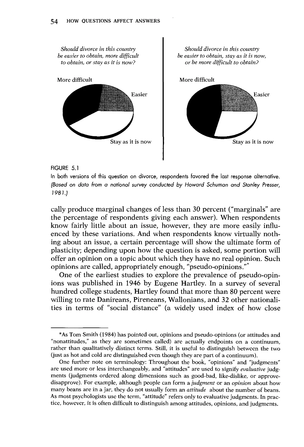
Chapter 5: Plasticity 51
Chapter 6: The Effects of Question Wording and Framing 64
SECTION III: MODELS OF DECISION MAKING 77
Chapter 7: Expected Utility Theory 79
Chapter 8: Paradoxes in Rationality 84
Chapter 9: Descriptive Models of Decision Making 94
SECTION IV: HEURISTICS AND BIASES 107
Chapter 10
Chapter 11
Chapter 12
Chapter 13
Chapter 14:
Chapter 15
Chapter 16:
The Representativeness Heuristic 109
The Availability Heuristic 121
Probability and Risk 131
Anchoring and Adjustment 145
The Perception of Randomness 153
Correlation, Causation, and Control 162
Attribution Theory 174
IX
CONTENTS
SECTION V: THE SOCIAL SIDE OF JUDGMENT
AND DECISION MAKING 189
Chapter 17: Social Influences 191
Chapter 18: Group Judgments and Decisions 205
SECTION VI: COMMON TRAPS 215
Chapter 19:
Chapter 20
Chapter 21
Overconfidence 217
Self-Fulfilling Prophecies 231
Behavioral Traps 241
Afterword: Taking a Step Back 253
Further Reading 262
References 264
Credits 293
Indexes
Author Index 295
Subject Index 299
FOREWORD
To discover where the action is in psychology, look to social psychology.
In recent years, the field of social psychology has emerged as central in
psychology's quest to understand human thought, feeling, and behavior.
Thus, we see the inclusion-by-hyphenation of social psychology across
diverse fields of psychology, such as social-cognitive,
social-developmental, social-learning, and social-personality, to name but a few recent
amalgamations.
Social psychologists have tackled many of society's most intractable
problems. In their role as the last generalists in psychology, nothing of
individual and societal concern is alien to social psychological
investigators—from psychophysiology to peace psychology, from students'
attributions for failure to preventive education for AIDS. The new political
and economic upheavals taking place throughout Europe and Asia, with
the collapse of Soviet-style communism, are spurring social
psychologists to develop new ways of introducing democracy and freedom of
choice into the social lives of peoples long dominated by authoritarian
rule. Indeed, since the days when George Miller, former president of the
American Psychological Association, called upon psychologists to "give
psychology back to the people," social psychologists have been at the
forefront.
The McGraw-Hill Series in Social Psychology is a celebration of
the contributions made by some of the most distinguished researchers,
theorists, and practitioners of our craft. Each author in our series
shares the vision of combining rigorous scholarship with the educator's
goal of communicating that information to the widest possible audience
of teachers, researchers, students, and interested laypersons. The series
is designed to cover the entire range of social psychology, with titles
reflecting both broad and more narrowly focused areas of
specialization. Instructors may use any of these books as supplements to a basic
text, or use a combination of them to delve into selected topics in
greater depth.
ABOUT THIS BOOK
Just as cognitive psychologists have advanced the frontiers of decision
research by exposing several limitations of traditional "rational-actor"
models of decision making, social psychologists have enriched this area
XI
FOREWORD
of knowledge by expanding its boundaries in many directions. In this
new and original integration of the entire field, Scott Pious shows us
how a social perspective on judgment and decision making can offer
practical suggestions on how to deal with many common problems in
daily life. Not only has Pious created an easily grasped overview of a
vast research literature; his book includes a number of novel insights,
valuable new terms, and intriguing conclusions.
What I believe readers will find most delightful here is the remarkable
blend of high-level scholarship and Plous's concern for effectively
communicating complex ideas to the broadest possible audience—from
undergraduates, to professionals in business and health, to national
public opinion leaders. This book is filled with pedagogical gems, new
formulas for enriching old ideas, unique exercises in critical thinking
that instruct while they capture the imagination, and provocative
juxtapositions of usually unrelated topics. Rarely has a first book by a young
scholar offered so much to so many on such a vital topic.
Philip Zimbardo
PREFACE
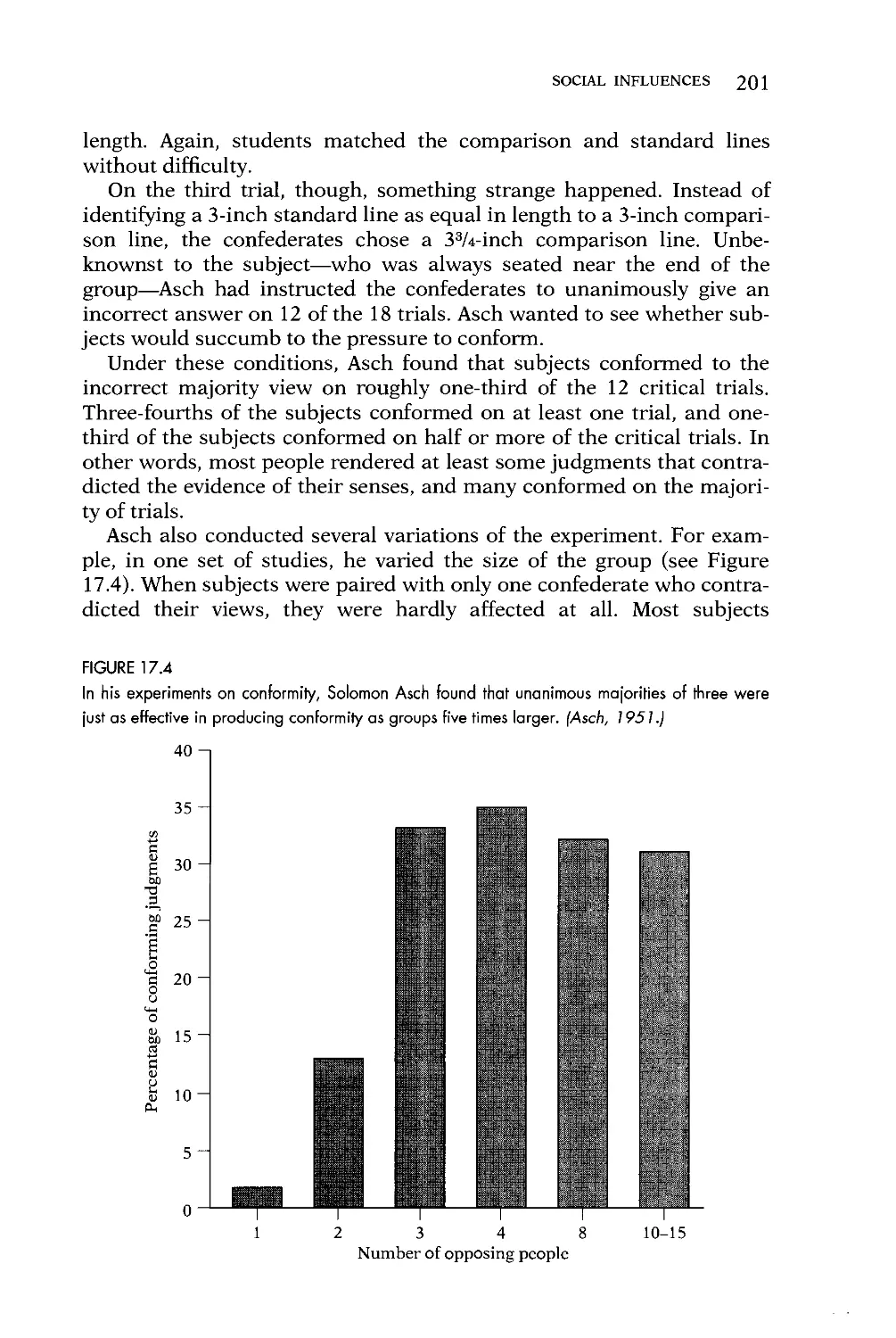
Today, Americans can choose from more than 25,000 products at the
supermarket. They can read any of 11,000 magazines or periodicals.
And they can flip channels between more than 50 television stations
(Williams, 1990, February 14). In short, they are faced with a
bewildering array of choices.
How do people make decisions? How do they sift through the
information without drowning in a sea of alternatives? And what are the
factors that lead them in a certain direction?
This book offers some tentative answers. It is a book intended for
nonspecialists who would like an introduction to psychological research
on judgment and decision making. The focus is on experimental
findings rather than psychological theory, surprising conclusions rather
than intuitions, and descriptive prose rather than mathematics. It is, in
brief, a book designed to entertain and challenge as much as to inform
and instruct.
The book is divided into six sections. The first two sections cover
several building blocks of judgment and decision making: perception,
memory, context, and question format. In the third and fourth sections,
historical models of decision making are contrasted with recent models
that take into account various biases in judgment. The fifth section
examines judgments made by and about groups, and the sixth section
discusses common traps in judgment and decision making. Each
chapter is intended as a relatively "free standing" review of the topic it
covers; thus, readers can skip or rearrange chapters with ease.
An unusual feature of this book is the Reader Survey preceding
Chapter 1. The Reader Survey is made up of questions that are reproduced or
adapted from many of the studies discussed in later chapters. Once you
complete the survey, you will be able to compare your answers with the
responses people gave in the original studies. Sometimes your answers
will match theirs, sometimes they will not. In either event, though,
you will have a written record of what your own style of judgment and
decision making was before reading this book. Because your answers
to the Reader Survey will be discussed throughout the book, it is
very important that you complete the survey before reading any of the
chapters.
Xlll
PREFACE
A NOTE ON PSYCHOLOGICAL EXPERIMENTATION
To readers unfamiliar with psychology, some of the terminology and
experimental procedures discussed in this book may seem callous or
insensitive. For example, experimental participants are referred to
impersonally as "subjects." Also, a number of experimental procedures
initially deceive participants about the true purpose of the study, and
the final results of some studies portray human decision makers as
seriously biased or flawed in some way.
These concerns are important and deserve some comment.
First, the reason for using an impersonal term such as subject is that
it often allows for greater clarity than generic terms such as person or
individual, and it is less awkward than terms such as participant or
volunteer. The word subject—which is standard in psychology and is used
throughout this book—does not mean that psychologists treat
experimental participants as though they are inanimate objects. In fact, the
actual subject of most psychological research is not the experimental
participant per se—it is the participant's behavior.
Second, there are several reasons why deception is sometimes used in
psychological research. In many cases, subjects are given vague or
misleading "cover stories" so that they are not influenced by the true
purpose of the experiment. For example, subjects in an experiment on
group dynamics might be told initially that the experiment is about
"learning and memory" to keep them from paying too much attention to
their division into groups. In other cases, deception is used to give the
appearance of a situation that would otherwise be impossible to create.
For instance, subjects in an experiment on creativity might be randomly
assigned to receive positive or negative feedback about their solutions to
a problem. If subjects were accurately informed in advance that they
would be receiving randomly assigned feedback, the feedback would not
be viewed as meaningful.
Although there are good reasons to oppose the use of deception in
research (Warwick, 1975, February), it is important to note that the
American Psychological Association (1989) has established a set of
ethical guidelines designed to protect subjects in the event that deception is
used. These guidelines mandate that subjects be told enough about the
experiment to give their informed consent, that deception be used only
as a last resort, that subjects be protected from harm or significant
discomfort, that subjects be allowed to discontinue participation at any
time, that information about individual subjects be treated as
confidential, and that any use of deception be explained after the experiment is
over. Most universities require investigators to adhere strictly to these
guidelines.
Finally, there are several reasons for concentrating on biases and
flaws more than successes. The most mundane reason for emphasizing
PREFACE
such research is that there is simply more of it (Kahneman, 1991).
Academic journals prefer to publish research findings that run counter to
ordinary intuitions, and, as a consequence, more research has been
published on failures in decision making than on successes. In this respect,
professional journals are similar to newspapers and magazines: They
place a premium on news that is surprising or intriguing. According to
one estimate (Christensen-Szalanski & Beach, 1984), journal articles
cite studies of flawed reasoning roughly six times more often than
studies of successful reasoning. Because this book is intended as an
introduction to research on judgment and decision making, it naturally
reflects the wider priorities of the research community.
There is a more important reason for focusing on shortcomings,
however. Failures in judgment and decision making are usually more
informative than successes—even (and especially) when successes are the
rule. The attention this book devotes to biases and errors is not meant
to imply that people are generally poor decision makers; rather, it
suggests that failures in judgment and decision making often reveal how
these processes work, just as failures in an automobile often reveal how
a car works. As Richard Nisbett and Lee Ross (1980, p. xii) explain, this
approach is based on "the same premise that leads many of our
colleagues to study perceptual illusions or thinking disorders—the belief
that the nature of cognitive structures and processes can be revealed by
the defects which they produce."
And of course, an emphasis on error has the additional advantage of
yielding results that are easy to apply. Once you recognize that a certain
situation typically leads to biases or errors, you can often sidestep it or
take remedial actions. To facilitate this process, I have included
everyday examples from medicine, law, business, education, nuclear arms
control (my own specialization), and other fields. Indeed, many of the
results in this book are general enough that I offer the following pledge
to readers not yet familiar with research on judgment and decision
making: by judiciously applying the results described in this book, you should
be better able to avoid decision biases, errors, and traps, and you will
better understand the decisions made by other people.
ACKNOWLEDGMENTS
I wish to thank the following people for their comments on earlier
drafts of this book: Joel Brockner, Baruch Fischhoff, Nancy Gallagher,
Beth Loftus, Duncan Luce, Dave Myers, Heather Nash, Jim Pious, Paul
Slovic, Janet Sniezek, Mark Snyder, Amos Tversky, Willem Wagenaar,
Elke Weber, and Phil Zimbardo.
I am also indebted to Tamra Williams and Heather Nash for their
library assistance, and to Steven Lebergott for running what is arguably
the best Interlibrary Loan Service in the United States.
PREFACE
It was a pleasure working with Chris Rogers, Laura Lynch, Nomi
Sofer, Jim Belser, and other members of the editorial staff at McGraw-
Hill.
And for all that coffee, for innumerable discussions late into the
night, for love and encouragement and cheerful help every step of the
way, I thank Diane Ersepke.
Scott Pious
THE PSYCHOLOGY
OF JUDGMENT
AND DECISION MAKING
READER SURVEY
It is very important that you complete this survey BEFORE
reading ahead. That way, you won't fall prey to hindsight biases,
or the "l-knew-it-all-along effect" (discussed in Chapter 3). If
you prefer not to write in the book, just jot down your answers
on a piece of paper and use the paper as a bookmark.
(1) Linda is 3 I years old, single, outspoken, and very blight. She majored in
philosophy. As a student, she was deeply concerned with issues of
discrimination and social justice, and also participated in antinuclear
demonstrations. Please check off the most likely alternative:
-I Linda is a bank teller.
J Linda is a bank teller and is active in the feminist movement.
(2) If you were faced with the following choice, which alternative would you
choose? '
J A 100 percent chance of losing $50
J A 25 percent chance of losing $200, and a 75 percent chance of
losing nothing
(3) John is envious, stubborn, critical, impulsive, industrious, and intelligent
In general, how emotional do you think John is? (Circle one number)
Not emotional at all 1 2 3 4 5 6 7 8 9 Extremely emotional
(4) Jim is intelligent skillful, industrious, warm, determined, practical and
cautious. Please circle the other traits you think Jim is most likely to have.
Circle one trait in each pair:
Generous — Ungenerous
Unhappy Happy
Irritable - Good-natured
Humorous Humorless
2 RLADMR Sl.RVHY
(5) Here's a question for college students only: Compared to other students
of your sex and age, what are the chances that the following events will
happen to you? (Check the one answer that comes closest to your view
for each event.)
(5a) VV/7/ develop a drinking problem:
-i 60+ percent more likely
J 40 percent more likely
J 20 percent more likely
J No more or less likely
J 20 percent less likely
J 40 percent less likely
J 60+ percent less likely
(5 b) VV/7/ own your own home:
J 60+ percent more likely
■J 40 percent more likely
J 20 percent more likely
J No more or less likely
J 20 percent less likely
J 40 percent less likely
J 60+ percent less likely
(5c) Will receive a postgraduate starting salary above $ 15,000:
-1 60+ percent more likely
J 40 percent more likely
J 20 percent more likely
^J No more or less likely
:j 20 percent less likely
J 40 percent less likely
J 60+ percent less likely
(5d) Will have a heart attack before the age of 40:
"J 60+ percent more likely
■J 40 percent more likely
J 20 percent more likely
J No more or less likely
J 20 percent less likely
J 40 percent less likely
J 60+ percent less likely
(6) As the president of an airline company, you have invested $ 10 million of the
company's money into a research project. The purpose was to build a plane
that would not be detected by conventional radar, in other words, a
RFADER SLRVT.Y 3
radar-blank plane. When the project is 90 percent completed, another firm
begins marketing a plane that cannot be detected by radar. Also, it is
apparent that their plane is much faster and far more economicol than the plane
your company is building. The question is: Should you invest the last 10
percent of the research funds to finish your radar-blank plane?
j NO—It makes no sense to continue spending money on the pro-
|ect
j YES—As long as $10 million is already invested, I might as well
Finish the project.
(7) Which is a more likely cause of death in the United States — being killed
by falling airplane parts or by a shark?
J Falling airplane parts
J Shark
(8) For each pair, circle the cause of death that is most common in the
United States. .
Diabetes/Homicide
Tornado/Lightning
Cat Accidents/Stomach Cancer
(9) Consider the following historical scenario: "The government of a country
not far from Superpower A, after discussing certain changes in its party
system, began broadening its trade with Superpower B. To reverse these
changes in government and trade, Superpower A sent its troops into the
country and militarily backed the original government."
(9a) Which country is Superpower A3
J Soviet Union
J United States
(9b) How confident are you of your answer? (Circle one number.)
Not confident at all 1 23456789 Very confident
(10) Here's another scenario: "In the 1960s Superpower A sponsored a
surprise invasion of a small country near its border, with the purpose of
overthrowing the regime in power at the time. The invasion failed, and
most of the original invading forces were killed or imprisoned."
(10a) Which counhy is Superpower A?
J Soviet Union
J United States
t
4 RllADi-R SURVHY
(10b) How confident are you of your answer? (Circle one number.)
Not confident at all 1 23456789 Very confident
(11) Place a check mark beside the alternative that seems most likely to
occur within the next ten years:
J An all-out nuclear war between the United States and Russia
:J An all-out nuclear war between the United States and Russia in
which neither country intends to use nuclear weapons, but both
sides are drawn into the conflict by the actions of a country such as
Iraq, Libya, Israel, or Pakistan
(12) A piece of paper is folded in half. It is folded in half again, and again.
. . . After 100 folds, how thick will it be?
(12a) My best guess is that the paper will be thick.
(12b) I am 90 percent sure that the correct answer lies between
and .
(13) Including February 29, there are 366 possible birthdays in a year.
Consequently, a group would need to contain 367 members in order to be
absolutely sure that at least two people shared the same birthday. How
many people are necessary in order to be 50 percent certain?
The group would need members.
(14) Suppose a study of 250 neurology patients finds the following
frequencies of dizziness and brain tumors:
BRAIN TUMOR
Present Absent
Present 160 40
Dizziness
Absent 40 10
(14a) Which cells of the table are needed in order to determine whether
dizziness is associated with brain tumors in this sample of people?
(Check all that apply.)
J Upper left
J Lower left
J Upper right
3 Lower right
Rf.AnF.K SI RVEY 5
(14b) According to the data in the table, is dizziness associated with brain
tumors?
J Yes J No J Not sure
(15) The mean IQ of the population of eighth graders in a city is known to
be 100. You have selected a random sample of 50 children for a study
of educational achievements. The first child tested has an IQ of 150.
What do you expect the mean IQ to be for the whole sample?
ANSWER-
(16) On the whole, do you see yourself as c^ sexist person? (Check one.)
J Yes J No J Not sure
(17) If all the human blood in the world were poured into a cube-shaped
tank, how wide would the tank be?
The tank would be wide.
(18) If you had to guess, which of the following interpretations of a
Rorschach inkblot are most predictive of male homosexuality? (If you
haven't heard of the Rorschach inkblot test, just skip this question.) Rank
the following interpretations from 1 (most predictive of homosexuality)
to 6 (least predictive of homosexuality).
Human figures of indeterminate sex
Human figures with both male and female features
Buttocks or anus
Genitals
A contorted, monstrous figure
Female clothing
(19) "Memory can be likened to a storage chest in the brain into which we
deposit material and from which we can withdraw it later if needed.
Occasionally, something gets lost from the 'chest,' and then we say we
have forgotten."
Would you say this is a reasonably accurate description of how memory
works?
J Yes J No J Not sure
6 RF.ADKR SI.RVI1Y
(20) A man bought a horse for $60 and sold it for $70. Then he bought it
back for $80 and again sold it for $90. How much money did he
make in the horse business?
The man ended up with a final profit of $ .
(21a) Absinthe is:
J A liqueur
J A precious stone
(21b) What is the probability that your answer is correct?
(Circle one number.)
.50 .55 .60 .65 .70 .75 .80 .85 .90 .95 1.00
(22) Without actually calculating, give a quick (five-second) estimate of the
following product:
8x7x6x5x4x3x2x1=
(23) Suppose you consider the possibility of insuring some property against
damage, e.g., fire or theft. After examining the risks and the premium
you find that you have no clear preference between the options of
purchasing insurance or leaving the property uninsured.
It is then called to your attention that the insurance company offers a
new program called probabilistic insurance. In this program you pay
half of the regular premium. In case of damage, there is a 50 percent
chance that you pay the other half of the premium and the insurance
company covers all the losses; and there is a 50 percent chance that
you get back your insurance payment and suffer all the losses.
For example, if an accident occurs on an odd day of the month, you
pay the other half of the regular premium and your losses are covered;
but if the accident occurs on an even day of the month, your insurance
payment is refunded and your losses are not covered.
Recall that the premium for full coverage is such that you find this
insurance barely worth its cost.
Under these circumstances, would you purchase probabilistic
insurance?
J Yes
J No
READER SURVEY J
(24) Suppose you performed well on a variety of tests over a range of
occasions, but other people taking the same tests did not do very well. What
would you conclude? (Check the one answer that comes closest to your
view.)
3 Explanation A: The tests were probably easy.
J Explanation B: The other people were probably low in ability.
:j Explanation C: I am either good at taking tests or must have known
the material well.
In a few pages, you will be asked some questions about the following
sentences. Please read them carefully now and continue with the Reader Survey:
• The ants ate the sweet jelly which was on the table.
• The ants were in the kitchen.
• The ants ate the sweet jelly.
• The ants in the kitchen ate the jelly which was on the table.
• The jelly was on the table.
• The ants in the kitchen ate the jelly.
(25) If you were faced with the following choice, which alternative would
you choose?
3 A sure gain of $240
J A 25 percent chance to gain $1000, and 75 percent chance to
gain nothing
(26) If you were faced with the following choice, which alternative would
you choose?
J A sure loss of $750
Zi A 75 percent chance to lose $ 1000, and 25 percent chance to
lose nothing
(27) What do you think is the most important problem facing this country
today?
The most important problem is: .
(28a) If you were given a choice, which of the following gambles would you
prefer?
O $1,000,000 for sure
a A 10 percent chance of getting $2,500,000,
an 89 percent chance of getting $1,000,000,
and a 1 percent chance of getting $0
$ READER SURVEY
(28b) If you were given a choice, which of the following gambles would you
prefer?
□ An 1 1 percent chance of getting $1,000,000,
and an 89 percent chance of getting $0
□ A 10 percent chance of getting $2,500,000,
and a 90 percent chance of getting $0
(29) Imagine two urns filled with millions of poker chips. In the first urn, 70
percent of the chips are red and 30 percent are blue. In the second
urn, 70 percent are blue and 30 percent are red. Suppose one of the
urns is chosen randomly and a dozen chips are drawn from it: eight
red chips and four blue chips. What are the chances that the chips
came from the urn with mostly red chips? (Give your answer as a
percentage.)
Answer: percent
(30) How much money would you pay to play a game in which an unbiased
coin is tossed until it lands on Tails, and at the end of the game you are
paid ($2.00)* where K equals the number of tosses until Tails appears?
In other words, you would be paid $2.00 if Tails comes up on the first
toss, $4.00 if Tails comes up on the second toss, $8.00 if Tails comes
up on the third toss, and in general:
Tosses until Tails: 12 3 4 5 ■■■ K
Payoff in Dollars: 2 4 8 16 32 - 2K
I would pay $ to play this game.
(31) Suppose an unbiased coin is flipped three times, and each time the
coin lands on Heads. If you had to bet $100 on the next toss, what side
would you choose?
□ Heads
□ Tails
□ No preference
U'ATO'K !»LHVL"\
9
(32) Compare Lines 1, 2, and 3 with Line A below. Which line is equal in
length to Line A? (Check one answer.)
|
A
1
J Line A is equal in length to Line 1
J Line A is equal in length to Line 2.
J Line A is equal in length to Line 3.
(33) How many times does the lettei f appear in the following sentence?
These; functional tusos \v.i\e hei-n developed after \rars ol
scientific investigation ut olei trie phenomena, combined wiili the fmii of
lnnu e.\perieiue mi ihc pan ut ihc \\\o investig.iKirs \\hn have
inmi- turward wiih them lur uur nieeiinjis t>>du\.
The letter f appears
times.
\Q READER SURVEY
(34) Without looking back at the list, please indicate whether the following
sentences were included in the set of sentences you read earlier. After
each answer, indicate your degree of confidence using a 1 to 5 scale
in which 1 = "very low" and 5 = "very high."
(34a) "The ants ate the jelly which was on the table."
□ This sentence appeared before.
□ This sentence did not appear before.
My confidence rating is:
(34b) "The ants in the kitchen ate the sweet jelly which was on the table."
□ This sentence appeared before.
□ This sentence did not appear before.
My confidence rating is:
(34c) "The ants ate the sweet jelly."
□ This sentence appeared before.
□ This sentence did not appear before.
My confidence rating is:
(35} Suppose that scores on a high school academic achievement test are
moderately related to college grade point averages (GPAs). Given the
percentiles below, what GPA would you predict for a student who
scored 725 on the achievement test?
Student Percentile
Top 10%
Top 20%
Top 30%
Top 40%
Top 50%
Achievement Test
>750
>700
>650
>600
>500
GPA
>3.7
>3.5
>3.2
>2.9
>2.5
I would predict a grade point average of
KI'MK'K SI KM \
11
(36) Does the act of voting for a candidate change your opinion about
whethet the candidate will win the election?
J Yes
J No
J Not sure
(37) Consider the two structures, A and B, which are displayed below.
Struuinv A:
\ X X X-JC XXX
X X X X XJi^X X
x x-x~ sfx x x x
Stiiu'iiuv B
X X
X K
\/c
tf'x
Ix
|x
Jx
X. \
x\
A path is a line that connects an X in the top row of a structure to an X
in the bottom row by passing through one (and only one) X in each
row. In other words, a path connects three X's in Structure A (one in
each of the three rows) and nine X's in Structure B (one in each of the
nine rows). One example of a path is drawn in each structure above.
(37a) In which of the two structures are there more paths?
J Structure A J Structure B
(37b) Approximately how many paths are in Structure A?
(37c) Approximately how many paths are in Structure B?
(38) Which of the following sequences of X's and O's seems more like it
was generated by a random process (e.g.. flipping a coin)?
J XOXXXOOOOXOXXOOOXXXOX
J XOXOXOOOXXOXOXOOXXXOX
|2 RK-\ni-R Sl'RVliY
(39) Suppose each of the cards below has a number on one side and a
letter on the other, and someone tells you: "If a card has a vowel on one
side, then it has an even number on the other side." Which of the cards
would you need to turn over in order to decide whether the person is
lying?
I would need to turn over the following cards
(check all that apply):
-» E
J 4
-I K
:j 7
SECTION
PERCEPTION,
MEMORY, AND
CONTEXT
There is no such thing as context-free
decision making. All judgments and
decisions rest on the way we see and
interpret the world. Accordingly, this first
section discusses the way that judgments and
decisions are influenced by selective
perception, pressures toward cognitive
consistency, biases in memory, and changes
in context.
CHAPTER ]
SELECTIVE PERCEPTION
"We do not first see, then define,
we define first and then see."
—Walter Lippmann (cited in Snyder & Uranowitz, 1978)
Look in front of you. Now look at your hands. Look at the cover of this
book. How much of what you see is determined by your expectations?
If you are like most people, your perceptions are heavily influenced
by what you expect to see. Even when something is right before your
eyes, it is hard to view it without preconceived notions. You may feel
that you are looking at things in a completely unbiased way, but as will
become clear, it is nearly impossible for people to avoid biases in
perception. Instead, people selectively perceive what they expect and hope
to see.
CALLING A SPADE A SPADE
One of the earliest and best known experiments on selective perception
was published by Jerome Bruner and Leo Postman (1949). Bruner and
Postman presented people with a series of five playing cards on a tachis-
toscope (a machine that can display pictures for very brief intervals),
varying the exposure time from ten milliseconds up to one second. The
cards they showed these people were similar to the cards on the cover of
this book. Take a moment now to note what these cards are.
Did you notice anything strange about the cards? Most people who
casually view the cover of this book never realize that one of the cards is
actually a black three of hearts! Bruner and Postman found that it took
people more than four times longer to recognize a trick card than a
normal card, and they found that most reactions to the incongruity could
be categorized as one of four types: dominance, compromise,
disruption, or recognition.
A dominance reaction consisted mainly in what Bruner and Postman
called "perceptual denial." For example, faced with a black three of
hearts, people were very sure that the card was a normal three of hearts
or a normal three of spades. In the first case, form is dominant and
color is assimilated to prior expectations, and in the second case, color
15
16 PERCEPTION, MEMORY, AND CONTEXT
is dominant and form is assimilated. In Bruner and Postman's
experiment, 27 of 28 subjects (or 96 percent of the people) showed dominance
reactions at some point.
Another reaction people had was to compromise. For instance, some
of Bruner and Postman's subjects reported a red six of spades as either a
purple six of spades or a purple six of hearts. Others thought that a
black four of hearts was a "greyish" four of spades, or that a red six of
clubs was "the six of clubs illuminated by red light" (remember,
experimental subjects were shown the cards on a tachistoscope). Half of
Bruner and Postman's subjects showed compromise responses to red
cards, and 11 percent showed compromise responses to black cards.
A third way that people reacted to the incongruity was with
disruption. When responses were disrupted, people had trouble forming a
perception of any sort. Disruption was rare, but when it happened, the
results were dramatic. For example, one experimental subject
exclaimed: "I don't know what the hell it is now, not even for sure
whether it's a playing card." Likewise, another subject said: "I can't
make the suit out, whatever it is. It didn't even look like a card that
time. I don't know what color it is now or whether it's a spade or heart.
I'm not even sure now what a spade looks like! My God!"
The final reaction was, of course, one of recognition. Yet even when
subjects recognized that something was wrong, they sometimes misper-
ceived the incongruity. Before realizing precisely what was wrong, six of
Bruner and Postman's subjects began to sense that something was
strange about how the symbols were positioned on the card. For
example, a subject who was shown a red six of spades thought the symbols
were reversed, and a subject who was shown a black four of hearts
declared that the spades were "turned the wrong way."
These results show that expectations can strongly influence
perceptions. In the words of Bruner and Postman (p. 222): "Perceptual
organization is powerfully determined by expectations built upon past
commerce with the environment." When people have enough experience
with a particular situation, they often see what they expect to see.
Item #33 of the Reader Survey contains another illustration of how
prior experience can interfere with accurate perceptions. In that
question, you were asked to count how many times the letter f appeared in
the following sentence:
These functional fuses have been developed after years of scientific
investigation of electric phenomena, combined with the fruit of long
experience on the part of the two investigators who have come forward
with them for our meetings today.
Most native English speakers underestimate the number of times the
letter f appears (Block & Yuker, 1989). The correct answer is 11
(including four times in which f appears in the word of). Because experienced
SELECTIVE PERCEPTION \J
speakers pronounce the word of with a "v" sound, they have more
difficulty detecting these occurrences of the letter f than do inexperienced
speakers, and as a result, past experience actually lowers performance.
POTENT EXPECTATIONS
Imagine you are a male college student participating in a study at the
Rutgers Alcohol Research Laboratory. Your job, you are told, is to drink
a vodka and tonic, wait twenty minutes for the alcohol to enter your
bloodstream, and speak with a female assistant of the experimenter in
an attempt to make as favorable an impression as possible. The
experimenter then mixes a vodka and tonic in proportion to your body weight,
hands you the glass, and leaves you in a private room to consume the
drink.
After you have finished the drink, a female assistant enters the room,
sits down, and looks you straight in the eye. You begin to talk to her.
How nervous are you? How fast is your heart beating?
When G. Terrence Wilson and David Abrams (1977) conducted this
experiment, they found that subjects who thought they had been given a
vodka and tonic showed much smaller increases in heart rate than
subjects who thought they had been given tonic water alone—regardless of
whether subjects had actually ingested alcohol. Heart rates were not
significantly affected by whether subjects had been given alcohol to drink;
they were affected by whether subjects believed they had been given
alcohol to drink. Expectations proved more important than changes in
blood chemistry.
David McMillen, Stephen Smith, and Elisabeth Wells-Parker (1989)
took these results one step further. Using an experimental technique
similar to the one used by Wilson and Abrams, these researchers
randomly assigned college students to drink either alcoholic beverages or
nonalcoholic beverages. Some of the students had been previously
identified as high "sensation seekers" who liked to take risks, and others had
been identified as low "sensation seekers." Then, half an hour after
drinking their beverages, the students played a video game in which
they drove along a roadway and had the opportunity to pass other cars
by using an accelerator pedal. Students were told to drive the simulated
car as they would drive a real car.
McMillen and his colleagues found that high sensation seekers who
believed they had consumed alcohol—whether or not they actually
had—changed lanes and passed cars significantly more often than high
sensation seekers who, rightly or wrongly, did not have this belief. In
contrast, low sensation seekers who thought they had consumed alcohol
were more cautious than low sensation seekers who thought they had
not. Equally strong expectancy effects have been found among frequent
users of marijuana (Jones, 1971).
18 PERCEPTION, MEMORY, AND CONTEXT
In these experiments and the experiment of Bruner and Postman,
people's perceptions were strongly influenced by their prior beliefs and
expectations. Psychologists refer to such influences as "cognitive"
factors. Yet perception is affected not only by what people expect to see; it
is also colored by what they want to see. Factors that deal with hopes,
desires, and emotional attachments are known as "motivational"
factors. The remaining sections of this chapter discuss instances of
selective perception in which motivational factors are intertwined with
cognitive factors.
WHEN THE GOING GETS ROUGH
On November 23, 1951, the Dartmouth and Princeton football teams
went head to head in Princeton University's Palmer Stadium. Shortly
after the kickoff, it became clear that the game was going to be a rough
one. Princeton's star player, who had just appeared on the cover of Time
magazine, left the game with a broken nose. Soon thereafter, a
Dartmouth player was taken off the field with a broken leg. By the end of the
game—which Princeton won—both sides had racked up a sizable
number of penalties.
Following the game, tempers flared and bitter accusations were
traded. Partisans on both sides wrote scathing editorials. For example, four
days after the game, a writer for the Daily Princetonian (Princeton's
student newspaper) declared: "This observer has never seen quite such a
disgusting exhibition of so-called 'sport.' Both teams were guilty but the
blame must be laid primarily on Dartmouth's doorstep. Princeton,
obviously the better team, had no reason to rough up Dartmouth." On the
same day, the Dartmouth (Dartmouth's undergraduate newspaper)
charged that Princeton's coach had instilled a "see-what-they-did-go-get-
them attitude" in his players. Throughout the ensuing week, Dartmouth
and Princeton students continued to fiercely debate what had happened
and who was responsible.
Into that turmoil stepped Albert Hastorf (a social psychologist then at
Dartmouth) and Hadley Cantril (a Princeton survey researcher).
Capitalizing on the controversy, Hastorf and Cantril (1954) conducted what is
now a classic study of selective perception.
They began by asking 163 Dartmouth students and 161 Princeton
students the following question, among others: "From what you saw in the
game or the movies, or from what you have read, which team do you
feel started the rough play?" Not surprisingly, Hastorf and Cantril found
a large discrepancy between common Dartmouth and Princeton
reactions. Of the Dartmouth students, 53 percent asserted that both sides
started it, and only 36 percent said that Dartmouth started it. In
contrast, 86 percent of the Princeton students felt that Dartmouth had
started it, and only 11 percent said that both sides were initiators.
SELECTIVE PERCEPTION 19
This difference of opinion led Hastorf and Cantril to wonder whether
Dartmouth and Princeton students were actually seeing different games,
or whether they were observing the same game but simply interpreting
the evidence differently. To explore this question, they asked a new
group of students at each school to watch a film of the game and to
record any infractions they noticed. Students from both schools
watched the very same film, and they used the same rating system to
record any observed infractions.
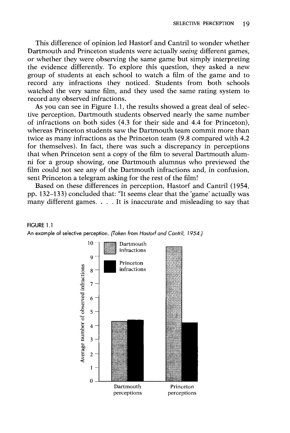
As you can see in Figure 1.1, the results showed a great deal of
selective perception. Dartmouth students observed nearly the same number
of infractions on both sides (4.3 for their side and 4.4 for Princeton),
whereas Princeton students saw the Dartmouth team commit more than
twice as many infractions as the Princeton team (9.8 compared with 4.2
for themselves). In fact, there was such a discrepancy in perceptions
that when Princeton sent a copy of the film to several Dartmouth
alumni for a group showing, one Dartmouth alumnus who previewed the
film could not see any of the Dartmouth infractions and, in confusion,
sent Princeton a telegram asking for the rest of the film!
Based on these differences in perception, Hastorf and Cantril (1954,
pp. 132-133) concluded that: "It seems clear that the 'game' actually was
many different games. . . . It is inaccurate and misleading to say that
FIGURE 1.1
An example of selective perception. (Taken from Hastorf and Cantril, 1954.]
10
■a
a
-a
-8
u
E
3
C
a
Dartmouth
infractions
Princeton
infractions
Dartmouth
perceptions
Princeton
perceptions
20 PERCEPTION, MEMORY, AND CONTEXT
different people have different 'attitudes' concerning the same 'thing.'
For the 'thing' simply is not the same for different people whether the
'thing' is a football game, a presidential candidate, Communism, or
spinach." In 1981, John Loy and Donald Andrews carefully replicated
Hastorf and Cantril's study, and they came to much the same
conclusion.
THE HOSTILE MEDIA EFFECT
Many years after the Dartmouth-Princeton study, Robert Vallone, Lee
Ross, and Mark Lepper (1985) speculated that this kind of selective
perception might lead political partisans on each side of an issue to view
mass media coverage as biased against their side. Vallone, Ross, and
Lepper called this phenomenon the "hostile media effect," and they first
studied it in the context of the 1980 presidential election between
Jimmy Carter and Ronald Reagan. Three days before the election, they
asked 160 registered voters to indicate whether media coverage of the
candidates had been biased, and if so, to indicate the direction of the
bias. What they found is that approximately one-third of the
respondents felt that media coverage had been biased, and in roughly 90
percent of these cases, respondents felt that the media had been biased
against the candidate they supported.
Intrigued by these initial findings, Vallone, Ross, and Lepper (1985)
conducted a second study in which 68 "pro-Israeli" college students, 27
"pro-Arab" students, and 49 "generally mixed" or "neutral" students
watched the same set of televised news segments covering the tragic
Beirut massacre (in 1982, a series of Arab-Israeli conflicts had resulted
in the massacre of Arab civilians in the refugee camps at Sabra and
Chatilla, Lebanon). The news segments were drawn from six different
evening and late-night news programs broadcast nationally in the
United States over a ten-day period.
In support of the hostile media effect, Vallone, Ross, and Lepper
found that each side saw the news coverage as biased in favor of the
other side. Pro-Arab students thought the news segments were generally
biased in favor of Israel, pro-Israeli students thought the segments were
biased against Israel, and neutral students gave opinions that fell
between the two groups. Moreover, pro-Arab students felt that the news
programs had excused Israel "when they would have blamed some other
country," whereas pro-Israeli students felt the programs blamed Israel
"when they would have excused some other country."
As in the case of the Dartmouth-Princeton game, Vallone, Ross, and
Lepper found that these disagreements were not simply differences of
opinion; they were differences in perception. For example, pro-Arab and
pro-Israeli students differed in their perceptions of the number of
favorable and unfavorable references that had been made to Israel during the
SELECTIVE PERCEPTION 21
news programs. On the average, pro-Arab students reported that 42
percent of the references to Israel had been favorable and only 26 percent
had been unfavorable. Pro-Israeli students, on the other hand, recalled
57 percent of the references to Israel as having been unfavorable and
only 16 percent as having been favorable. Furthermore, pro-Israeli
students thought that most neutral viewers would become more negative
toward Israel as a result of watching the news clips, whereas pro-Arab
students thought that most would not.
Vallone, Ross, and Lepper concluded that partisans tend to view
media coverage of controversial events as unfairly biased and hostile to
the position they advocate. They also speculated that similar biases in
perception might arise in the context of mediation, arbitration, or other
situations in which two sides are heavily committed to prior positions.
This speculation makes good sense. As we will see in Chapter 2, when
people become committed to a particular cause or a course of action,
their perceptions often change in order to remain consistent with this
commitment.
CONCLUSION
Perceptions are, by their very nature, selective. Even the simple
identification of a playing card—or the perception of one's own intoxication—
depends critically on cognitive and motivational factors. Consequently,
before making an important judgment or decision, it often pays to
pause and ask a few key questions: Am I motivated to see things a
certain way? What expectations did I bring into the situation? Would I see
things differently without these expectations and motives? Have I
consulted with others who don't share my expectations and motives? By
asking such questions, decision makers can expose many of the
cognitive and motivational factors that lead to biases in perception.
CHAPTER 2
COGNITIVE
DISSONANCE
Soon after the first studies of selective perception, Leon Festinger (1957)
proposed the theory of "cognitive dissonance." Since the 1950s,
dissonance theory has generated hundreds of experiments, many of them
among the most clever and entertaining in psychology. To understand
the theory of cognitive dissonance and see how dissonance can
influence judgment and decision making, consider a story told by Nathan
Ausubel (1948; see also Deci, 1975, pp. 157-158).
A PARABLE OF COGNITIVE DISSONANCE
There was once a Jewish tailor who had the temerity to open his shop
on the main street of an anti-semitic town. To drive him out of town, a
gang of youths visited the shop each day, standing in the entrance and
shouting, "Jew! Jew!"
After several sleepless nights, the tailor finally devised a plan. The
next time that the gang came to threaten him, the tailor announced that
anyone who called him a Jew would get a dime. He then handed dimes
to each member of the gang.
Delighted with their new incentive, members of the gang returned the
next day, shouting "Jew! Jew!", and the tailor, smiling, gave each one a
nickel (explaining that he could only afford a nickel that day). The gang
left satisfied because, after all, a nickel was a nickel.
Then, on the following day, the tailor gave out only pennies to each
gang member, again explaining that he could afford no more money
than that. Well, a penny was not much of an incentive, and members of
the gang began to protest.
When the tailor replied that they could take it or leave it, they decided
to leave it, shouting that the tailor was crazy if he thought that they
would call him a Jew for only a penny!
WHY THE CHANGE?
Why would members of the gang harass the tailor for free but not for a
penny? According to the theory of cognitive dissonance, people are usu-
22
COGNITIVE DISSONANCE 23
ally motivated to reduce or avoid psychological inconsistencies. When
the tailor announced that he was happy to be called a Jew, and when he
changed the gang's motivation from anti-semitism to monetary reward,
he made it inconsistent (or "dissonance-arousing") for gang members to
please him without financial compensation. In the absence of a
sufficiently large payment, members of the gang could no longer justify
behaving at variance with their objective (which was to upset the tailor,
not to make him happy).
BOREDOM CAN BE FUN
The same principle was demonstrated by Leon Festinger and Merrill
Carlsmith (1959) in one of the most famous studies in all of social
psychology. Sixty male undergraduates at Stanford University were
randomly assigned to one of three experimental conditions. In the $1.00
condition, participants were required to perform tedious laboratory
tasks for an hour, after which they were paid $1.00 to tell a waiting
student that the tasks were interesting and enjoyable. In the $20.00
condition, students were paid $20.00 to do the same thing. And in the control
condition, participants simply engaged in the tedious tasks.
What were the tasks? First, students spent half an hour using one
hand to put 12 spools onto a tray, unload the tray, refill the tray, unload
the tray again, and so on. Then, after thirty minutes were up, they spent
the remainder of the hour using one hand to turn each of 48 pegs on a
pegboard—one-quarter turn at a time! Each participant was seen
individually, and the experimenter simply sat by, stopwatch in hand, busily
making notes on a sheet of paper.
Once the student had finished his tasks, the experimenter leaned back
in his chair and said:
I'd like to explain what this has been all about so you'll have some idea
of why you were doing this. . . . There are actually two groups in the
experiment. In one, the group you were in, we bring the subject in and
give him essentially no introduction to the experiment. . . . But in the
other group, we have a student that we've hired that works for us
regularly, and what I do is take him into the next room where the
subject is waiting—the same room you were waiting in before—and I
introduce him as if he had just finished being a subject in the
experiment. . . . The fellow who works for us then, in conversation
with the next subject, makes these points: ... It was very enjoyable, I
had a lot of fan, I enjoyed myself, it was very interesting. . . .
Following this explanation, the experimenter asked subjects in the
control condition to rate how enjoyable the tasks had been. In the $1.00
and $20.00 conditions, however, the experimenter continued with his
explanation:
24 PERCEPTION, MEMORY, AND CONTEXT
The fellow who normally does this for us couldn't do it today—he just
phoned in, and something or other came up for him—so we've been
looking around for someone that we could hire to do it for us. You see,
we've got another subject waiting [looks at watch] who is supposed to
be in that other condition. ... If you would be willing to do this for
us, we'd like to hire you to do it now and then be on call in the future, if
something like this should ever happen again. We can pay you a dollar
[or twenty dollars, depending on condition] for doing this for us, that
is, for doing it now and then being on call. Do you think you could do
that for us?
All $1.00 and $20.00 subjects agreed to be hired, and after they told
the waiting person how enjoyable the tasks were, they were asked,
among other things, to evaluate the tasks. What Festinger and Carlsmith
(1959) found was that subjects in the $1.00 condition rated the tasks as
significantly more enjoyable than did subjects in the other two
conditions.
Festinger and Carlsmith argued that subjects who were paid only
$1.00 to lie to another person experienced "cognitive dissonance."
According to Festinger (1957), people experience cognitive dissonance
when they simultaneously hold two thoughts that are psychologically
inconsistent (i.e., thoughts that feel contradictory or incompatible in
some way). In this instance, the dissonant cognitions were:
1. The task was extremely boring.
2. For only $1.00, I (an honest person) just told someone that the task
was interesting and enjoyable.
When taken together, these statements imply that subjects in the $1.00
condition had lied for no good reason (subjects in the $20.00 condition,
on the other hand, had agreed to be "hired" for what they apparently
considered to be a very good reason: $20.00).
Festinger (1957) proposed that people try whenever possible to
reduce cognitive dissonance. He regarded dissonance as a "negative
drive state" (an aversive condition), and he presented cognitive
dissonance theory as a motivational theory (despite the word "cognitive").
According to the theory, subjects in the experiment should be motivated
to reduce the inconsistency between the two thoughts listed above.
Of course, there wasn't much subjects could do about the second
thought. The fact was that subjects did tell another person that the task
was enjoyable, and they did it for only $1.00 (and they certainly weren't
going to change their view of themselves as honest and decent people).
On the other hand, the tediousness of the task afforded subjects some
room to maneuver. Tediousness, you might say, is in the eye of the
beholder.
Thus, Festinger and Carlsmith (1959) concluded that subjects in the
COGNITIVE DISSONANCE 25
$1.00 condition later evaluated the task as relatively enjoyable so as to
reduce the dissonance caused by telling another person that the task
was interesting and enjoyable. In contrast, subjects in the $20.00
condition saw the experimental tasks for what they were: crushingly dull.
Subjects in that condition had no need to reduce dissonance, because
they already had a good explanation for their behavior—they were paid
$20.00.
SELF-PERCEPTION THEORY
The story does not end here, because there is another way to account
for what Festinger and Carlsmith found. In the mid-1960s, psychologist
Daryl Bern proposed that cognitive dissonance findings could be
explained by what he called "self-perception theory." According to self-
perception theory, dissonance findings have nothing to do with a
negative drive state called dissonance; instead, they have to do with how
people infer their beliefs from watching themselves behave.
Bern's self-perception theory is based on two main premises:
1. People discover their own attitudes, emotions, and other internal
states partly by watching themselves behave in various situations.
2. To the extent that internal cues are weak, ambiguous, or uninter-
pretable, people are in much the same position as an outside observer
when making these inferences.
A self-perception theorist would explain Festinger and Carlsmith's
results by arguing that subjects who saw themselves speak highly of the
task for only $1.00 inferred that they must have enjoyed the task (just as
an outside observer would infer). On the other hand, subjects in the
$20.00 condition inferred that their behavior was nothing more than a
response to being offered a large financial incentive—again, as an
outside observer would. The difference between self-perception theory and
dissonance theory is that self-perception theory explains classical
dissonance findings in terms of how people infer the causes of their behavior,
whereas cognitive dissonance theory explains these findings in terms of
a natural motivation to reduce inner conflict, or dissonance. According
to Bern, subjects in the Festinger and Carlsmith (1959) study could have
experienced no tension whatsoever and still given the same pattern of
results.
A great deal of research has been conducted comparing these theories
(cf. Bern, 1972), but it is still an open question as to which theory is
more accurate or more useful in explaining "dissonance phenomena."
For many years, researchers on each side of the issue attempted to
design a definitive experiment in support of their favored theory, but
each round of experimentation served only to provoke another set of
26 PERCEPTION, MEMORY, AND CONTEXT
experiments from the other side. In the final analysis, it probably makes
sense to assume that both theories are valid in a variety of situations
(but following psychological tradition, I will use dissonance terminology
as a shorthand for findings that can be explained equally well by self-
perception theory).
As the next sections demonstrate, cognitive dissonance influences a
wide range of judgments and decisions. Most dissonance-arousing
situations fall into one of two general categories: predecisional or postdeci-
sional. In the first type of situation, dissonance (or the prospect of
dissonance) influences the decisions people make. In the second kind of
situation, dissonance (or its prospect) follows a choice that has already
been made, and the avoidance or reduction of this dissonance has an
effect on later behavior.
AN EXAMPLE OF PREDECISIONAL
DISSONANCE
A father and his son are out driving. They are involved in an accident.
The father is killed, and the son is in critical condition. The son is
rushed to the hospital and prepared for the operation. The doctor comes
in, sees the patient, and exclaims, "I can't operate; it's my son!"
Is this scenario possible? Most people would say it is not. They would
reason that the patient cannot be the doctor's son if the patient's father
has been killed. At least, they would reason this way until it occurred to
them that the surgeon might be the patient's mother.
If this possibility had not dawned on you, and if you consider
yourself to be relatively nonsexist, there is a good chance you are
experiencing dissonance right now (see Item #16 of the Reader Survey for a self-
rating of sexism). Moreover, according to the theory of cognitive
dissonance, you should be motivated to reduce that dissonance by
behaving in a more nonsexist way than ever.
In 1980, Jim Sherman and Larry Gorkin used the female surgeon
story to test this hypothesis. Sherman and Gorkin randomly assigned
college students to one of three conditions in an experiment on "the
relationship between attitudes toward social issues and the ability to
solve logical problems." In the sex-role condition, students were given
five minutes to figure out how the story of the female surgeon made
sense. In the non-sex-role condition, students were given five minutes to
solve an equally difficult problem concerning dots and lines. And in the
control condition, students were not given a problem to solve. In the
sex-role and non-sex-role conditions, the experimenter provided the
correct solution after five minutes had passed (roughly 80 percent of the
subjects were not able to solve the assigned problem within five minutes).
Next, subjects were told that the experiment was over, and they were
presented with booklets for another experimenter's study about legal
COGNITIVE DISSONANCE 27
decisions (the students had been told previously that they would be
participating in "a couple of unrelated research projects"). Subjects were
informed that the principal investigator of the other study was in South
Bend, Indiana, and that they should put the completed booklets in
envelopes addressed to South Bend, seal the envelopes, and drop them
in a nearby mailbox. Then subjects were left alone to complete the
booklet on legal decisions.
In reality, the experiment on legal decisions was nothing more than a
way to collect information on sexism without subjects detecting a
connection to the first part of the experiment. Subjects read about an
affirmative action case in which a woman claimed that she had been turned
down for a university faculty position because of her gender. Then they
indicated what they thought the verdict should be, how justified they
thought the university was in hiring a man rather than the woman, and
how they felt about affirmative action in general.
Sherman and Gorkin (1980) found that, compared with subjects in
the control group and subjects who were presented with the problem
concerning dots and lines, subjects who had failed to solve the female
surgeon problem were more likely to find the university guilty of sexual
discrimination, less likely to see the university as justified in hiring a
male for the job, and more supportive of affirmative action policies in
general. In other words, after displaying traditional sex-role stereotypes,
students tried to reduce their dissonance by acting more "liberated" (or,
in terms of self-perception theory, trying to show themselves that they
were not sexist). This method of dissonance reduction, called
"bolstering," has also been used successfully to promote energy conservation.
S. J. Kantola, G. J. Syme, and N. A. Campbell (1984) found that heavy
users of electricity cut their consumption significantly when they were
informed of their heavy use and reminded of an earlier conservation
endorsement they had made.
OTHER EXAMPLES OF PREDECISIONAL
DISSONANCE
Predecisional dissonance can also influence consumer behavior, as
shown by Anthony Doob and his colleagues (1969). These researchers
matched 12 pairs of discount stores in terms of gross sales, and they
randomly assigned each member of a pair to introduce a house brand of
mouthwash at either $0.25 per bottle or $0.39 per bottle. Then, after
nine days, the store selling the mouthwash at $0.25 raised the price to
$0.39 (equal to the price at the other store). The same procedure was
followed with toothpaste, aluminum foil, light bulbs, and cookies (and,
in general, the results for these items paralleled the results using
mouthwash).
What Doob et al. (1969) found was that, consistent with cognitive dis-
28 PERCEPTION, MEMORY, AND CONTEXT
sonance theory, stores that introduced the mouthwash at a higher price
tended to sell more bottles. In 10 of 12 pairs, the store that introduced
the mouthwash at $0.39 later sold more mouthwash than did the store
that initially offered the mouthwash for $0.25.
Doob and his associates explained this finding in terms of customer
"adaptation levels" and the need to avoid dissonance. They wrote:
"When mouthwash is put on sale at $0.25, customers who buy it at
that price or notice what the price is may tend to think of the product
in terms of $0.25. They say to themselves that this is a $0.25 bottle
of mouthwash. When, in subsequent weeks, the price increases to
$0.39, these customers will tend to see it as overpriced, and are
not inclined to buy it at this much higher price" (p. 350). Furthermore,
according to dissonance theory, the more people pay for something, the
more they should see value in it and feel pressure to continue buying it.
This principle is true not only with purchases, but with any
commitment of resources or effort toward a goal (for another example, see
Aronson & Mills, 1959). The net result is similar to that found with
many of the behavioral traps discussed in Chapter 21.
EXAMPLES OF POSTDECISIONAL
DISSONANCE
Postdecisional dissonance is dissonance that follows a decision rather
than precedes it. In the mid-1960s, Robert Knox and James Inkster
studied postdecisional dissonance by approaching 141 horse bettors at
Exhibition Park Race Track in Vancouver, Canada: 72 people who had
just finished placing a $2.00 bet within the past thirty seconds, and 69
people who were about to place a $2.00 bet in the next thirty seconds.
Knox and Inkster reasoned that people who had just committed
themselves to a course of action (by betting $2.00) would reduce
postdecisional dissonance by believing more strongly than ever that they had
picked a winner.
To test this hypothesis, Knox and Inkster (1968) asked people to rate
their horse's chances of winning on a 7-point scale in which 1 indicated
that the chances were "slight" and 7 indicated that the chances were
"excellent." What they found was that people who were about to place a
bet rated the chance that their horse would win at an average of 3.48
(which corresponded to a "fair chance of winning"), whereas people
who had just finished betting gave an average rating of 4.81 (which
corresponded to a "good chance of winning"). Their hypothesis was
confirmed—after making a $2.00 commitment, people became more
confident that their bet would pay off.
This finding raises an interesting question: Does voting for a
candidate increase your confidence that the candidate will win the election?
COGNITIVE DISSONANCE 29
(See Item #36 of the Reader Survey for your answer.) In 1976, Oded
Frenkel and Anthony Doob published a study exploring this question.
Frenkel and Doob used the same basic procedure as Knox and
Inkster (1968); they approached people immediately before and
immediately after they voted. In one experiment they surveyed voters in a
Canadian provincial election, and in another they queried voters in a
Canadian federal election. In keeping with the results of Knox and
Inkster, Frenkel and Doob (1976, p. 347) found that: "In both elections,
voters were more likely to believe that their candidate was the best one
and had the best chance to win after they had voted than before they
voted."
CONCLUSION
As the opening story of the Jewish tailor shows, cognitive dissonance
theory can be a formidable weapon in the hands of a master. Research
on cognitive dissonance is not only bountiful and entertaining, it is
directly applicable to many situations. For example, retail stores often
explicitly label introductory offers so as to avoid the kind of adaptation
effects found by Doob et al. (1969). Similarly, many political campaigns
solicit small commitments in order to create postdecisional dissonance
(this strategy is sometimes known as the "foot-in-the-door technique").
In the remainder of this book, we will discuss several other applications
and findings from cognitive dissonance theory.
One of the leading authorities on dissonance research is Elliot Aron-
son, a student of Festinger and an investigator in many of the early
dissonance experiments (for readers interested in learning more about the
theory of cognitive dissonance, a good place to begin is with Aronson,
1969, 1972). It is therefore appropriate to conclude this chapter with a
statement by Aronson (1972, p. 108) on the implications of cognitive
dissonance theory:
If a modern Machiavelli were advising a contemporary ruler, he might
suggest the following strategies based upon the theory and data on the
consequences of decisions:
1. If you want someone to form more positive attitudes toward an
object, get him to commit himself to own that object
2. If you want someone to soften his moral attitude toward some
misdeed, tempt him so that he performs that deed; conversely, if you
want someone to harden his moral attitudes toward a misdeed,
tempt him—but not enough to induce him to commit the deed*
*The masculine pronouns in this statement refer to people of both genders. Before
1977 (when the American Psychological Association adopted guidelines for nonsexist
language), this literary practice was common in psychology.
30 PERCEPTION, MEMORY, AND CONTEXT
It is well known that changes in attitude can lead to changes in
behavior, but research on cognitive dissonance shows that changes in
attitude can also follow changes in behavior. According to the theory of
cognitive dissonance, the pressure to feel consistent will often lead
people to bring their beliefs in line with their behavior. In Chapter 3, we
will see that, in many cases, people also distort or forget what their
initial beliefs were.
CHAPTER 3
MEMORY AND
HINDSIGHT BIASES
"To-day isn't any other day, you know."
"I don't understand you," said Alice. "It's
dreadfully confusing!"
"That's the effect of living backwards," the Queen said kindly:
"it always makes one a little giddy at first—"
"Living backwards!" Alice repeated in great astonishment.
"I never heard of such a thing!"
"—but there's one great advantage in it, that one's memory
works both ways. . . . It's a poor sort of memory that only works backwards,"
the Queen remarked.
—Lewis Carroll, Through the Looking-Glass
Take a moment to reflect on whether the following statement is true or
false: "Memory can be likened to a storage chest in the brain, into which
we deposit material and from which we can withdraw it later if needed.
Occasionally, something gets lost from the 'chest,' and then we say we
have forgotten."
What do you think—true or false? (See Item #19 of the Reader Survey
for your answer.) Roughly 85 percent of the college students in a study
by P. A. Lamal (1979, October) agreed with this statement, yet
something is terribly wrong with the way it characterizes memory (aside
from the question of whether material is ever truly lost from memory).
Memories are not like copies of our past experiences on deposit in a
memory bank. Instead, they are constructed at the time of withdrawal
(Loftus, 1980; Myers, 1990). The "materials" used in this split-second
reconstruction are logical inferences that fill in missing detail,
associated memories that blend in with the original memory, and other relevant
information. To verify that memory is reconstructive, try an exercise
suggested by Myers (1990): Close your eyes and recall a scene in which
you experienced something pleasurable. Don't read any further until
you have finished replaying your experience.
Did you see yourself in the scene? Most people do. But if you saw
yourself, then you must have reconstructed the scene (unless, of course,
you were looking at yourself during the original experience).
31
34 PERCEPTION, MEMORY, AND CONTEXT
FIGURE 3.1
Reconstructive memory. (Doonesbury copyright 1992 G. B. Trudeau. Reprinted with permission
of Universal Press Syndicates. All rights reserved.)
More interesting is your response to Item #34b: "The ants in the
kitchen ate the sweet jelly which was on the table." Even though this
sentence did not appear in the first set, students in the study by Brans-
ford and Franks tended to be very confident that they had seen it before.
Were you?
What is significant about the sentence in Item #34b is that it contains
combinations of relations that are not contained in any individual
sentence from the first set. The original sentences never explicitly stated
that the jelly in the kitchen was sweet, or that the ants in the kitchen ate
the sweet jelly. The sentence in Item #34b can only be derived by
combining separate sentences from the first set.
Thus, people do not simply memorize sentences; they construct and
memorize a general scenario. Once one piece of information is
integrated with others, it is sometimes difficult to remember which information
was new and which was already known.
MEMORY AND HINDSIGHT BIASES 35
I KNEW IT ALL ALONG
People also have difficulty telling how they are affected by information
about an outcome. For example, if they learn about the results of a
psychological experiment, they tend to regard the findings as having been
fairly predictable all along—or at least more predictable than they
would have judged before learning of the results (one of the reasons
why this book has a Reader Survey!). Moreover, if people are asked to
behave as though they know nothing about the outcome of an
experiment, they still respond more like people who know about the results
than people who do not. That is, if they are asked to estimate in
retrospect how likely they once thought the results were to occur, they assign
higher probabilities than do people predicting the experimental
outcome in advance.
This tendency is known as "hindsight bias," or the "I-knew-it-all-
along" effect. Hindsight bias is the tendency to view what has already
happened as relatively inevitable and obvious—without realizing that
retrospective knowledge of the outcome is influencing one's judgments.
Hindsight biases have been documented in elections (Leary, 1982; Syn-
odinos, 1986), medical diagnoses (Arkes, Wortmann, Saville, & Hark-
ness, 1981), pregnancy tests (Pennington, Rutter, McKenna, & Morley,
1980), buying decisions (Walster, 1967), games (Leary, 1981), and a
number of other areas. They have also been shown using a variety of
experimental techniques, response instructions, and groups of people
(for reviews of hindsight bias and related effects, see Campbell & Tess-
er, 1983; Christensen-Szalanski & Willham, 1991; Hawkins & Hastie,
1990; Verplanken & Pieters, 1988).
One of the first studies on hindsight bias was published in 1975 by
Baruch Fischhoff and Ruth Beyth. The main events Fischhoff and Beyth
(1975) used in their study were President Nixon's trips to China and the
Soviet Union in 1972. In the first phase of the experiment, several
groups of Israeli students were asked to estimate the probability of 15
different outcomes for either the China trip or the Soviet trip—before
the trip took place. For example, students who were asked about the
China trip estimated the chances that the United States would establish
a diplomatic mission in Peking, that President Nixon would meet Mao
at least once, that President Nixon would announce the trip a success,
and so forth. Similarly, students who were asked about Nixon's trip to
the Soviet Union estimated outcomes such as the establishment of a
joint space program, or the arrest of Soviet Jews trying to speak with
Nixon.
In the second phase of the study—two weeks to six months after the
trip had taken place—students were asked to recall what their earlier
predictions had been. For instance, students who had answered
questions about the China trip were told the following:
36 PERCEPTION, MEMORY, AND CONTEXT
As you remember, about two weeks ago, on the eve of President Nixon's
trip to China, you completed a questionnaire by providing probabilities
for the occurrence of a number of possible outcomes of the trip. We are
presently interested in the relation between the quality of people's
predictions and their ability to remember their predictions. For this
reason, we would like to have you fill out once again the same
questionnaire which you completed two weeks ago, giving the same
probabilities which you gave then. If you cannot remember the
probability which you then assigned, give the probability which you
would have given to each of the various outcomes on the eve of
President Nixon's trip to China.
Students were also asked to indicate whether, as far as they knew,
each outcome had in fact occurred. Fischhoff and Beyth wanted to see if
students would remember their predictions as having been more
accurate than they actually were.
In general, this is just what Fischhoff and Beyth (1975) found. Three-
quarters of the students tended to remember having assigned higher
probabilities than they actually had to outcomes that they thought had
occurred, and the majority of students remembered having assigned
lower probabilities to outcomes they believed had not occurred.
Hindsight biases were particularly strong when the initial predictions
preceded the recall task by several months. When three to six months
separated the prediction and recall tasks, 84 percent of the students
showed hindsight biases—after learning the outcome of Nixon's trips,
they viewed the outcome as having been more predictable than it
actually was.
REDUCING HINDSIGHT BIAS
In 1977, Paul Slovic and Baruch Fischhoff published a study that
showed how to reduce hindsight biases when learning the results of
research (the feeling of having known the results all along). Slovic and
Fischhoff found that hindsight biases diminished when people stopped
to consider reasons why the results might have turned out differently.
Subjects in this research read four brief descriptions of studies drawn
from biology, psychology, and meteorology. Foresight subjects were told
that the four studies would be conducted soon, and hindsight subjects
were told that the studies had already been conducted. After reading
about each study, all subjects then estimated the probability of
replicating an outcome obtained on the first experimental trial (each trial
always had two possible outcomes). In other words, hindsight subjects
were told that a particular outcome had already been observed, and
foresight subjects were asked to suppose the outcome occurred.
Slovic and Fischhoff (1977) found that compared with foresight
subjects, hindsight subjects gave higher probability estimates that all future
CHAPTER 3
MEMORY AND
HINDSIGHT BIASES
"To-day isn't any other day, you know."
"I don't understand you," said Alice. "It's
dreadfully confusing!"
"That's the effect of living backwards," the Queen said kindly:
"it always makes one a little giddy at first—"
"Living backwards!" Alice repeated in great astonishment.
"I never heard of such a thing!"
"—but there's one great advantage in it, that one's memory
works both ways. . . . It's a poor sort of memory that only works backwards,"
the Queen remarked.
—Lewis Carroll, Through the Looking-Glass
Take a moment to reflect on whether the following statement is true or
false: "Memory can be likened to a storage chest in the brain, into which
we deposit material and from which we can withdraw it later if needed.
Occasionally, something gets lost from the 'chest,' and then we say we
have forgotten."
What do you think—true or false? (See Item #19 of the Reader Survey
for your answer.) Roughly 85 percent of the college students in a study
by P. A. Lamal (1979, October) agreed with this statement, yet
something is terribly wrong with the way it characterizes memory (aside
from the question of whether material is ever truly lost from memory).
Memories are not like copies of our past experiences on deposit in a
memory bank. Instead, they are constructed at the time of withdrawal
(Loftus, 1980; Myers, 1990). The "materials" used in this split-second
reconstruction are logical inferences that fill in missing detail,
associated memories that blend in with the original memory, and other relevant
information. To verify that memory is reconstructive, try an exercise
suggested by Myers (1990): Close your eyes and recall a scene in which
you experienced something pleasurable. Don't read any further until
you have finished replaying your experience.
Did you see yourself in the scene? Most people do. But if you saw
yourself, then you must have reconstructed the scene (unless, of course,
you were looking at yourself during the original experience).
31
32 PERCEPTION, MEMORY, AND CONTEXT
SHATTERED MEMORIES
One of the best demonstrations that memory is reconstructive was
provided in two experiments by Beth Loftus and John Palmer (1974). In the
first experiment, 45 students were asked to view seven different film
clips depicting a traffic accident. The clips ranged from five to thirty
seconds in length and were borrowed from longer driver's education films.
After each film clip, students answered a series of questions,
including one on how fast the cars had been traveling. One-fifth of the
students answered the question: "About how fast were the cars going when
they contacted each other?" Equal numbers of the remaining students
answered the same question, except that the word "contacted" was
replaced with "hit," "bumped," "collided," or "smashed."
As you can see in Table 3.1, students who were asked how fast the
cars were going when they "smashed" gave a mean estimate that was 9
miles faster than the average estimate given by students who were asked
how fast the cars were going when they "contacted" each other. Thus,
Loftus and Palmer concluded that the form of a question—even when
changed by only one word—can markedly affect how people reconstruct
their memory of an event.
If anything, results from the second experiment were even more
dramatic. This time, Loftus and Palmer had 150 students watch a one-
minute film that included a four-second, multiple-car crash. Fifty
students were asked: "About how fast were the cars going when they
smashed into each other?" Another 50 students were asked: "About how
fast were the cars going when they hit each other?" And the last 50
students were not asked to judge car speed. Then the students returned one
week later and, without viewing the film again, answered a series of
questions. The key question Loftus and Palmer were interested in was
whether students remembered having seen any shattered glass during
the car crash.
Loftus and Palmer found that asking students how fast the cars were
going when they "smashed" not only led to faster estimates, but that one
TABLE 3.1
HOW FAST WERE THE CARS GOING WHEN THEY . . .
Verb Mean Speed
Smashed 40.8
Collided 39.3
Bumped 38.1
Hit 34.0
Contacted 31.8
Note: These are average speed estimates from Experiment 1 of a study by Elizabeth Loftus and John
Palmer (1974).
MEMORY AND HINDSIGHT BIASES 33
TABLE 3.2
DID YOU SEE ANY BROKEN GLASS?
Response
Yes
No
"Smashed"
16
34
EXPERIMENTAL CONDITION
"Hit" Control Group
7 6
43 44
Note: This is the distribution of "yes" and "no" answers found in Experiment 2 of a study by Elizabeth Lof-
tus and John Palmer (1974). Fifty subjects were assigned to each of the three experimental conditions.
week later, a greater proportion of the students remembered the
accident as having involved broken glass. The results, which show
statistically reliable differences among the experimental conditions, are shown
in Table 3.2. What is interesting about these results is that the accident
never involved broken glass—subjects who estimated the speed of
smashing cars reconstructed the accident so that it involved broken
glass!
SWEET REMEMBRANCES
As the experiments by Loftus and Palmer show, memories are not fixed
in storage. In 1971, John Bransford and Jeffrey Franks further showed
that memories are not stored separately from one another. Bransford
and Franks (1971) initially presented college students with a list of
sentences about an event. For example, one of the lists—reprinted on page
7 of the Reader Survey—went like this:
• The ants ate the sweet jelly which was on the table.
• The ants were in the kitchen.
• The ants ate the sweet jelly.
• The ants in the kitchen ate the jelly which was on the table.
• The jelly was on the table.
• The ants in the kitchen ate the jelly.
Then, after five minutes or so, students were presented with another
list of sentences and asked to indicate which sentences were in the first
list. They were also asked to rate their confidence in each answer on a
scale from 1 to 5. Item #34 in the Reader Survey contains a second list
of sentences, along with blanks for confidence ratings as to whether
these sentences appeared in the original list.
As it happens, the only sentence that appeared in the first set was
Item #34c: "The ants ate the sweet jelly." If you are similar to most
people in the study by Bransford and Franks, you were moderately
confident (2 to 4 on the confidence scale) that this sentence had appeared
before.
34 PERCEPTION, MEMORY, AND CONTEXT
FIGURE 3.1
Reconstructive memory. (Doonesbury copyright 1992 G. B. Trudeau. Reprinted with permission
of Universal Press Syndicates. All rights reserved.)
More interesting is your response to Item #34b: "The ants in the
kitchen ate the sweet jelly which was on the table." Even though this
sentence did not appear in the first set, students in the study by Brans-
ford and Franks tended to be very confident that they had seen it before.
Were you?
What is significant about the sentence in Item #34b is that it contains
combinations of relations that are not contained in any individual
sentence from the first set. The original sentences never explicitly stated
that the jelly in the kitchen was sweet, or that the ants in the kitchen ate
the sweet jelly. The sentence in Item #34b can only be derived by
combining separate sentences from the first set.
Thus, people do not simply memorize sentences; they construct and
memorize a general scenario. Once one piece of information is
integrated with others, it is sometimes difficult to remember which information
was new and which was already known.
MEMORY AND HINDSIGHT BIASES 35
I KNEW IT ALL ALONG
People also have difficulty telling how they are affected by information
about an outcome. For example, if they learn about the results of a
psychological experiment, they tend to regard the findings as having been
fairly predictable all along—or at least more predictable than they
would have judged before learning of the results (one of the reasons
why this book has a Reader Survey!). Moreover, if people are asked to
behave as though they know nothing about the outcome of an
experiment, they still respond more like people who know about the results
than people who do not. That is, if they are asked to estimate in
retrospect how likely they once thought the results were to occur, they assign
higher probabilities than do people predicting the experimental
outcome in advance.
This tendency is known as "hindsight bias," or the "I-knew-it-all-
along" effect. Hindsight bias is the tendency to view what has already
happened as relatively inevitable and obvious—without realizing that
retrospective knowledge of the outcome is influencing one's judgments.
Hindsight biases have been documented in elections (Leary, 1982; Syn-
odinos, 1986), medical diagnoses (Arkes, Wortmann, Saville, & Hark-
ness, 1981), pregnancy tests (Pennington, Rutter, McKenna, & Morley,
1980), buying decisions (Walster, 1967), games (Leary, 1981), and a
number of other areas. They have also been shown using a variety of
experimental techniques, response instructions, and groups of people
(for reviews of hindsight bias and related effects, see Campbell & Tess-
er, 1983; Christensen-Szalanski & Willham, 1991; Hawkins & Hastie,
1990; Verplanken & Pieters, 1988).
One of the first studies on hindsight bias was published in 1975 by
Baruch Fischhoff and Ruth Beyth. The main events Fischhoff and Beyth
(1975) used in their study were President Nixon's trips to China and the
Soviet Union in 1972. In the first phase of the experiment, several
groups of Israeli students were asked to estimate the probability of 15
different outcomes for either the China trip or the Soviet trip—before
the trip took place. For example, students who were asked about the
China trip estimated the chances that the United States would establish
a diplomatic mission in Peking, that President Nixon would meet Mao
at least once, that President Nixon would announce the trip a success,
and so forth. Similarly, students who were asked about Nixon's trip to
the Soviet Union estimated outcomes such as the establishment of a
joint space program, or the arrest of Soviet Jews trying to speak with
Nixon.
In the second phase of the study—two weeks to six months after the
trip had taken place—students were asked to recall what their earlier
predictions had been. For instance, students who had answered
questions about the China trip were told the following:
36 PERCEPTION, MEMORY, AND CONTEXT
As you remember, about two weeks ago, on the eve of President Nixon's
trip to China, you completed a questionnaire by providing probabilities
for the occurrence of a number of possible outcomes of the trip. We are
presently interested in the relation between the quality of people's
predictions and their ability to remember their predictions. For this
reason, we would like to have you fill out once again the same
questionnaire which you completed two weeks ago, giving the same
probabilities which you gave then. If you cannot remember the
probability which you then assigned, give the probability which you
would have given to each of the various outcomes on the eve of
President Nixon's trip to China.
Students were also asked to indicate whether, as far as they knew,
each outcome had in fact occurred. Fischhoff and Beyth wanted to see if
students would remember their predictions as having been more
accurate than they actually were.
In general, this is just what Fischhoff and Beyth (1975) found. Three-
quarters of the students tended to remember having assigned higher
probabilities than they actually had to outcomes that they thought had
occurred, and the majority of students remembered having assigned
lower probabilities to outcomes they believed had not occurred.
Hindsight biases were particularly strong when the initial predictions
preceded the recall task by several months. When three to six months
separated the prediction and recall tasks, 84 percent of the students
showed hindsight biases—after learning the outcome of Nixon's trips,
they viewed the outcome as having been more predictable than it
actually was.
REDUCING HINDSIGHT BIAS
In 1977, Paul Slovic and Baruch Fischhoff published a study that
showed how to reduce hindsight biases when learning the results of
research (the feeling of having known the results all along). Slovic and
Fischhoff found that hindsight biases diminished when people stopped
to consider reasons why the results might have turned out differently.
Subjects in this research read four brief descriptions of studies drawn
from biology, psychology, and meteorology. Foresight subjects were told
that the four studies would be conducted soon, and hindsight subjects
were told that the studies had already been conducted. After reading
about each study, all subjects then estimated the probability of
replicating an outcome obtained on the first experimental trial (each trial
always had two possible outcomes). In other words, hindsight subjects
were told that a particular outcome had already been observed, and
foresight subjects were asked to suppose the outcome occurred.
Slovic and Fischhoff (1977) found that compared with foresight
subjects, hindsight subjects gave higher probability estimates that all future
MEMORY AND HINDSIGHT BIASES 37
trials would replicate the first one. This difference was substantially
reduced, however, when hindsight subjects were asked to consider
reasons why either experimental outcome might have occurred. Hindsight
bias was still present in this case, but to a much lesser degree.
Thus, the moral of the story is as follows: If you want to reduce
hindsight biases, you should explicitly consider how past events might have
turned out differently. If you only consider the reasons why something
turned out as it did, you run a good risk of overestimating how
inevitable that outcome was and how likely similar outcomes are in the
future. In fact, Fischhoff (1977) has found that informing people about
hindsight bias and encouraging them to avoid it is not enough to
remove the bias. To avoid the ravages of hindsight bias, it is important
to consider how an alternative outcome might have occurred.
CONCLUSION
In his book Memory, Ian Hunter (1964) tells the story of two British
psychologists who secretly recorded a discussion that took place after a
meeting of the Cambridge Psychological Society. Two weeks later, the
psychologists contacted all the participants and asked them to write
down everything they could remember about the discussion. When
these accounts were checked against the original recording, it turned
out that respondents typically omitted more than 90 percent of the
specific points that had been discussed. Moreover, of the points that were
recalled, nearly half were substantially incorrect. Respondents
remembered comments that were never made, they transformed casual
remarks into lengthy orations, and they converted implicit meanings
into explicit comments.
This story highlights the value of keeping accurate records. Even the
most sophisticated decision maker is susceptible to biases in memory,
and there is no better way to avoid these biases than maintaining
careful notes and records of past events (e.g., meetings, important
conversations, and agreements). As the research in this chapter shows, memory
is, by its very nature, reconstructive and highly dependent upon
contextual factors. Chapter 4 further explores the effects of context on
judgment and decision making.
CHAPTER 4
CONTEXT DEPENDENCE
As the previous three chapters imply, the effect of a stimulus is "context-
dependent." That is, decision makers do not perceive and remember
material in isolation; they interpret new information in light of past
experience and the context in which the material occurs. In one
situation, a stimulus (for example, a personality trait) may be perceived one
way, and in another situation, the "same" stimulus may be seen very
differently. Many perceptual illusions exploit the principle of context
dependence (see Figure 4.1). In the area of judgment and decision
making, four of the best illustrations of context dependence are the contrast
effect, the primacy effect, the recency effect, and the halo effect.
THE CONTRAST EFFECT
Here is a simple experiment you can perform on yourself (or on your
friends). All you need is three large bowls of water. Fill the first bowl
with hot water, the second bowl with tepid water, and the third bowl
with ice water. Next, submerge one hand in the hot bowl and one in the
cold bowl, and keep them there for thirty seconds. Once your hands
have adjusted to the water temperature, place the "hot" hand in the
bowl of tepid water and, after five seconds, join it with the "cold" hand.
If you are like most people, you will feel a very strange sensation. The
hand that was formerly in hot water will be telling you that the tepid
water is cold, and the hand that was in cold water will be telling you
that the tepid water is hot. In fact, if you try this experiment on a friend
and keep the temperature of the tepid water a secret, she or he will
probably not be able to tell what temperature the tepid water is. Each
hand will be exhibiting a "contrast effect," but the two effects will be in
opposite directions!
Many early studies in psychology concerned perceptual judgments
such as temperature discrimination, color discrimination, and weight
estimation. Consequently, contrast effects were among the first
psychological phenomena to be reliably demonstrated in the laboratory. For
example, Muzafer Sherif, Daniel Taub, and Carl Hovland (1958)
published an influential article on contrast effects in judgments of weight.
Sherif, Taub, and Hovland found that when subjects initially lifted a
heavy weight, they subsequently rated relatively light weights as lighter
than they actually were.
38
CONTEXT DEPENDENCE 39
FIGURE 4.1
To see some effects of context on visual perception, hold this page up to a bright light source.
Most people report that the edges of the square bend inward and that the parallel lines no
longer look parallel. (Adapted from Block and Yuker, 1989.)
40 PERCEPTION, MEMORY, AND CONTEXT
FIGURE 4.1 (continued)
CONTEXT DEPENDENCE 41
One of the most interesting studies of the contrast effect was
published by Stanley Coren and Joel Miller (1974). Coren and Miller noted
that a 5-foot 10-inch sports announcer looks very short when
interviewing a team of basketball players, but looks very tall when interviewing
race horse jockeys. At the same time, the apparent size of the announcer
does not shrink when the announcer is standing beside a large race
horse—or, for that matter, a stadium.
From this observation, Coren and Miller speculated that the contrast
effect only occurs when the contrasted stimuli are similar to one
another. To test this hypothesis, they presented a dozen volunteers with each
of the clusters shown in Figure 4.2. The cluster in the upper left
quadrant is an example of the famous Ebbinghaus illusion. In the Ebbing-
haus illusion, the center circle appears larger when it is surrounded by
smaller circles than when it is contrasted with larger circles.
Coren and Miller found, however, that the Ebbinghaus illusion
diminished as the surrounding shapes became less like circles (as
judged by the experimental volunteers). The illusion was weaker with
hexagons than circles, weaker still with triangles, and weakest of all using
irregular polygons. By comparing the quadrants in Figure 4.2, you can
see that even simple judgments of size depend critically upon context.
FIGURE 4.2
Stanley Coren and Joel Miller explored the contrast effect using four variants of the Ebbinghaus
illusion. The upper left quadrant contains a typical example of the standard Ebbinghaus illusion.
(Coren and Miller, 1974. Reprinted with perm;ss/on.j
O o
OoO °o°
o °
A
AOA «0«
A
0 0
OoO °g°
0
C3
&oo »6»
42 PERCEPTION, MEMORY, AND CONTEXT
46 PERCEPTION, MEMORY, AND CONTEXT
cold, determined, practical, and cautious. Thus, both groups of subjects
heard the same description, except that the person was described as
warm in the first instance and cold in the second.
Subjects were then presented with pairs of traits (mostly opposites)
and were asked to indicate which trait was most consistent with the
impression they had formed of the person. The pairs included traits
such as generous/ungenerous, unhappy/happy, irritable/good-natured,
and humorous/humorless. In keeping with the earlier findings of
Thorndike, Asch found that the inclusion of a central characteristic
such as warm or cold influenced subjects' overall impression of the
person—that is, subjects created a "halo." For example, 75 to 95 percent of
the subjects who formed an impression of the warm person thought
that such a person would also be generous, happy, good-natured, and
humorous (you can compare yourself to these subjects by checking your
answer to Item #4 of the Reader Survey). In contrast, only 5 to 35
percent of the subjects who formed an impression of the cold person
thought that such a person would have these traits.
These results are not simply a by-product of using simple paper-and-
pencil tasks. Harold Kelley (1950) published a study that explored the
halo effect using real people instead of lists of traits, and he found much
the same halo effect that Asch had observed several years earlier.
Students who were led to expect a warm instructor saw the instructor not
only as relatively considerate, good-natured, and sociable, but as more
popular, humorous, and humane. Moreover, there was a marginal
tendency for students to interact more with the instructor when they
believed he was warm. Fifty-six percent of the "warm" subjects entered
into the class discussion, compared with only 32 percent of the "cold"
subjects. These results suggest that the halo effect operates in social
interactions and may influence subsequent behavior.
As with the contrast, primacy, and recency effects, the halo effect
illustrates that the way people react to a stimulus is context-dependent.
Indeed, there is no such thing as a stimulus without a context.
Contextual factors strongly influence how people respond—whether the
stimulus is a geometric shape, a personality trait, a legal argument, or
spinach.
CONCLUSION
Context effects are so common they sometimes seem invisible. In fact, it
is hard to imagine a world in which perceptions are not
context-dependent. What would such a world look like? What would it mean to talk
about context-free judgment?
As a student in one of my seminars pointed out, context effects raise
CONTEXT DEPENDENCE 41
One of the most interesting studies of the contrast effect was
published by Stanley Coren and Joel Miller (1974). Coren and Miller noted
that a 5-foot 10-inch sports announcer looks very short when
interviewing a team of basketball players, but looks very tall when interviewing
race horse jockeys. At the same time, the apparent size of the announcer
does not shrink when the announcer is standing beside a large race
horse—or, for that matter, a stadium.
From this observation, Coren and Miller speculated that the contrast
effect only occurs when the contrasted stimuli are similar to one
another. To test this hypothesis, they presented a dozen volunteers with each
of the clusters shown in Figure 4.2. The cluster in the upper left
quadrant is an example of the famous Ebbinghaus illusion. In the Ebbing-
haus illusion, the center circle appears larger when it is surrounded by
smaller circles than when it is contrasted with larger circles.
Coren and Miller found, however, that the Ebbinghaus illusion
diminished as the surrounding shapes became less like circles (as
judged by the experimental volunteers). The illusion was weaker with
hexagons than circles, weaker still with triangles, and weakest of all using
irregular polygons. By comparing the quadrants in Figure 4.2, you can
see that even simple judgments of size depend critically upon context.
FIGURE 4.2
Stanley Coren and Joel Miller explored the contrast effect using four variants of the Ebbinghaus
illusion. The upper left quadrant contains a typical example of the standard Ebbinghaus illusion.
(Coren and Miller, 1974. Reprinted wiffi permission.)
O 0
OoO °o°
o °
A
AOA «0«
A
0 0
OoO °o°
0
C3
&OU »0»
42 PERCEPTION, MEMORY, AND CONTEXT
THE PRIMACY EFFECT
A classic study of context dependence was published by Solomon Asch
(1946). Although Asch is best known for his research on conformity
(discussed in Chapter 17), he also pioneered the study of "impression
formation." In most of his research on impression formation, Asch
asked subjects to give their impressions of a hypothetical person who
had certain traits. His 1946 article reviewed 10 different experiments
using this paradigm, but for now, we will consider just one.
In this experiment, Asch asked subjects for their impressions of
someone with the traits listed in Item #3 of the Reader Survey. Half of
the subjects were asked about someone who was envious, stubborn,
critical, impulsive, industrious, and intelligent. The other half were asked
about someone with the very same characteristics, except that the
characteristics were presented in the opposite order: intelligent, industrious,
impulsive, critical, stubborn, and envious.
What Asch found was that the characteristics appearing early in each
series influenced impressions more strongly than the characteristics
appearing later. This pattern is known as a "primacy effect." If you
responded to Item #3 by rating John's emotionality as very high, a
primacy effect may have occurred—the emotional traits envious and stub-
bom may have affected your impressions more than they would have if
they had appeared later in the list.
Would envious and stubborn still produce a primacy effect if
intelligent preceded them as the first word? According to a study by Norman
Anderson (1965), they probably would. Anderson found that the
primacy effect is not merely a product of the first entry in a series. Instead, it
is a general relationship between the position an entry occupies and the
effect it has on judgments. First impressions are the most important
impressions, but second and third impressions still show a significant
primacy effect.
THE RECENCY EFFECT
The primacy effect occurs not only when people form impressions of
each other, but in a great many situations involving the evaluation of
sequential information. For example, a primacy effect sometimes occurs
when people are exposed to opposite sides of a controversial issue. In
many cases, people are more influenced by the first presentation of an
issue than by subsequent presentations.
This is not always the case, however. In some instances, the final
presentation has more influence than the first presentation. Such a pattern
is known as the "recency effect." The recency effect often occurs when
people are able to remember the last presentation more clearly than the
first one.
CONTEXT DEPENDENCE 43
An interesting question arises as to which effect is the strongest. For
example, suppose you are participating in a public debate, and suppose
further that you are offered the choice of speaking first or last. What
should you choose? If you speak first, you might be able to take
advantage of a primacy effect, but if you speak last, you might capitalize on a
recency effect. Which choice is best?
This question was investigated by Norman Miller and Donald
Campbell (1959). Miller and Campbell edited the transcript of a court trial
concerning damages allegedly incurred as a result of a defective
vaporizer. The proceedings were rearranged so that all the material for the
plaintiff appeared in one block of text, and all the material for the
defendant appeared in another block. In other words, the "pro"
communication included testimony from witnesses called by the plaintiff, the cross-
examination of witnesses for the defense by the plaintiff's lawyer, and
the opening and closing speeches by the plaintiffs lawyer. The "con"
communication included testimony from witnesses for the defense, the
cross-examination by the defense, and the opening and closing speeches
by the counsel for the defense.
After Miller and Campbell edited the transcripts, they recorded the
proceedings with different people reading the parts of different
characters (lawyers, witnesses, and so forth). Each recording lasted about
forty-five minutes, and the communications were presented in one of
eight different ways (see Figure 4.3 for an overview). In some
conditions, subjects rendered judgments immediately after hearing back-to-
back communications (pro-con or con-pro), and in other conditions, a
one-week delay separated various phases of the experiment.
FIGURE 4.3
Norman Miller and Donald Campbell (1959) investigated primacy and recency effects by
comparing the impact of communications in the eight experimental conditions shown below.
Condition Order of Events
Pro Message
Con Message
Pro Message
Con Message I
Pro Message
Con Message I
Pro Message
]*
Con Message I
44 PERCEPTION, MEMORY, AND CONTEXT
What Miller and Campbell found was a primacy effect in some cases
and a recency effect in others—that is, they found that in some
conditions people were more persuaded by the first communication, and in
others, they were more persuaded by the second communication
(regardless of whether the communication was pro or con). When
subjects were asked about the court case one week after hearing back-to-
back presentations (Conditions 3 and 4), a primacy effect occurred. On
the other hand, when the communications were separated by a week
and subjects were asked about the case immediately after the second
communication (Conditions 5 and 6), a recency effect occurred. The
first two conditions and the last two conditions did not result in
significant primacy or recency effects.
Miller and Campbell (1959) also found evidence that recency effects
were a function of differences in recall. As measured by a multiple-
choice test, subjects in Condition 5 tended to recall more factual
material about the con communication than about the pro communication,
and subjects in Condition 6 tended to recall more factual material about
the pro communication than about the con communication.
So to answer the original question: If you are offered the choice of
speaking first or last in a public debate, you should speak first if the
other side will follow you immediately and there will be a delay between
the debate and people's responses to it. For example, if you are debating
an issue that will be voted on in a week, then you should choose to
speak first. On the other hand, if some time will separate the two
communications, and if people will be asked to act immediately after the
second presentation, you should capitalize on the recency effect and
choose to go last.
Stephen Hoch (1984) found essentially the same results in several
experiments on how people make predictions. Hoch asked people to
generate reasons why a future event might occur ("pro-reasons") and
reasons why the same event might not occur ("con-reasons"). For some
events people listed pro-reasons first, and for others they listed
con-reasons first. Hoch found a strong primacy effect when people generated
both sets of reasons back-to-back, but a recency effect when people
worked on a three-minute task between listing pro- and con-reasons.
These findings are consistent with age-old selling techniques in which
customers are encouraged to list the reasons for making a purchase
(pro-reasons) and list the reasons against making a purchase
(con-reasons). If the two sets of reasons are generated back-to-back, customers
may unwittingly fall prey to primacy effects (Gross, 1964).
HALO EFFECTS
Contrast, primacy, and recency effects show that the same stimulus can
have a different effect depending on its context and order of presenta-
CONTEXT DEPENDENCE 45
tion. Another example of context dependence is the "halo" effect, so
named by Edward Thorndike back in 1920. Thorndike found that when
army superiors were asked to evaluate their officers in terms of
intelligence, physique, leadership, and character, the ratings were often highly
correlated. According to Thorndike, a flight commander who had
supervised the work of aviation cadets showed a correlation of .51 between
his ratings of their intelligence and their physique, .58 between their
intelligence and their leadership ability, and .64 between their
intelligence and their character.* Thorndike also found positive correlations
among various teacher evaluations that were used to determine salaries
and promotions. In one case, for example, general merit as a teacher
correlated strongly with ratings of general appearance, health,
promptness, intellect, and integrity and sincerity. In another case, ratings of a
teacher's voice correlated strongly with ratings of intelligence and
"interest in community affairs."
In his original article on the halo effect, Thorndike (1920, pp. 28-29)
concluded that "even a very capable foreman, employer, teacher, or
department head is unable to treat an individual as a compound of
separate qualities and to assign a magnitude to each of these in
independence of the others." Nowadays, we know that Thorndike's findings
were partly due to technical aspects of how the rating scales were
constructed, but his general idea has stood the test of time. Even when
ratings are solicited using sophisticated measurement techniques, a halo
effect often results (Cooper, 1981; Feldman, 1986).
Since the time of Thorndike's observations, many different halo
effects have been documented. For example, research on "beauty halo
effects" has shown that, relative to average-looking or unattractive
people, physically attractive people are seen as happier, higher in
occupational status, more likely to get married, and more desirable in terms of
personality (Dion, Berscheid, & Walster, 1972). David Landy and Harold
Sigall (1974) also found that essays were rated as higher in quality when
they were attributed to a physically attractive author rather than an
average-looking or unattractive author.
As in the case of the contrast effect, many pioneering experiments on
the halo effect were performed by Asch (1946). For instance, in one
experiment, Asch asked roughly half the subjects to form an impression
of someone who was intelligent, skillful, industrious, warm, determined,
practical, and cautious. Similarly, he asked the other subjects to form
an impression of someone who was intelligent, skillful, industrious,
"Correlation coefficients usually vary between +1.00 and -1.00. Positive correlations
mean that one variable increases as the other increases, negative correlations mean that
one variable decreases as the other increases, and a correlation of 0.00 means that the
variables are not related in either direction. Thus, in Thorndike's case, high ratings of
intelligence were associated with high ratings of other desirable characteristics.
46 PERCEPTION, MEMORY, AND CONTEXT
cold, determined, practical, and cautious. Thus, both groups of subjects
heard the same description, except that the person was described as
warm in the first instance and cold in the second.
Subjects were then presented with pairs of traits (mostly opposites)
and were asked to indicate which trait was most consistent with the
impression they had formed of the person. The pairs included traits
such as generous/ungenerous, unhappy/happy, irritable/good-natured,
and humorous/humorless. In keeping with the earlier findings of
Thorndike, Asch found that the inclusion of a central characteristic
such as warm or cold influenced subjects' overall impression of the
person—that is, subjects created a "halo." For example, 75 to 95 percent of
the subjects who formed an impression of the warm person thought
that such a person would also be generous, happy, good-natured, and
humorous (you can compare yourself to these subjects by checking your
answer to Item #4 of the Reader Survey). In contrast, only 5 to 35
percent of the subjects who formed an impression of the cold person
thought that such a person would have these traits.
These results are not simply a by-product of using simple paper-and-
pencil tasks. Harold Kelley (1950) published a study that explored the
halo effect using real people instead of lists of traits, and he found much
the same halo effect that Asch had observed several years earlier.
Students who were led to expect a warm instructor saw the instructor not
only as relatively considerate, good-natured, and sociable, but as more
popular, humorous, and humane. Moreover, there was a marginal
tendency for students to interact more with the instructor when they
believed he was warm. Fifty-six percent of the "warm" subjects entered
into the class discussion, compared with only 32 percent of the "cold"
subjects. These results suggest that the halo effect operates in social
interactions and may influence subsequent behavior.
As with the contrast, primacy, and recency effects, the halo effect
illustrates that the way people react to a stimulus is context-dependent.
Indeed, there is no such thing as a stimulus without a context.
Contextual factors strongly influence how people respond—whether the
stimulus is a geometric shape, a personality trait, a legal argument, or
spinach.
CONCLUSION
Context effects are so common they sometimes seem invisible. In fact, it
is hard to imagine a world in which perceptions are not
context-dependent. What would such a world look like? What would it mean to talk
about context-free judgment?
As a student in one of my seminars pointed out, context effects raise
profound questions about the nature of social relationships. For
example, the contrast effect suggests that it is impossible to "know a person"
CONTEXT DEPENDENCE 47
in any absolute sense. When you judge the honesty of a friend, this
judgment is relative and depends to some extent on the honesty of other
people you know. According to the contrast effect, you will see your
friend as more honest if other people you know deceive you—even if the
behavior of your friend remains the same. The judgment you make of a
friend's honesty may seem unrelated to the honesty of other people, but
as the research in this chapter shows, social judgments often depend in
part on context.
Even happiness is context-dependent. Philip Brickman, Dan Coates,
and Ronnie Janoff-Bulman (1978) found this to be the case in a study of
Illinois State Lottery winners. Compared with a geographically matched
control group of nonwinners, lottery winners reported feeling less
pleasure from a variety of daily activities, including watching television,
talking with friends, eating breakfast, buying clothes, and so forth.
Brickman, Coates, and Janoff-Bulman argued that this difference was
partly the result of a contrast effect in which ordinary activities were
compared with the thrill of winning a lottery.
Persuasion professionals have long recognized the power of context
effects. For instance, real estate agents sometimes exploit the contrast
effect by showing buyers a run-down or overpriced property before the
home that is under serious consideration. Political candidates often
capitalize on the halo effect by painting a picture of wide-ranging ability
from one or two previous successes. And advertisers take painstaking
care to create appealing contexts for the products they promote.
Of course, the effects of context are not limitless. A pathological liar
will not seem honest regardless of how much other people lie, and an
incompetent politician can only exploit the halo effect so far. A
background of concentric circles can make the edges of a square seem
curved, but it cannot make a square into a circle. Nonetheless, any
comprehensive analysis of judgment and decision making must take context
effects into account. Indeed, some authors have suggested that
laboratory demonstrations of context effects underestimate the effects of context
in daily life (Hershey & Schoemaker, 1980).
SECTION ||
HOW
QUESTIONS
AFFECT
ANSWERS
Section I showed how the context of a
stimulus shapes the way it is perceived. The
present section extends this theme by
considering how the format of a problem can
influence the way people respond to it.
Chapters 5 and 6 focus on the following two
Questions: (1) How much do judgments and
ecisions depend on the way a problem is
worded? (2) What are some specific ways in
which the wording of a question or problem
influences the answer?
CHAPTER 5
PLASTICITY
Just as every stimulus has a context, so has every question. This chapter
takes a look at how the context and wording of questions can influence
judgment and decision making.
In some cases, offering the same choice in two different contexts can
lead to very different answers. For example, suppose you were faced
with the following choice:
Alternative A: A If Ml percent chance <>1 losing $50 '
Alternative B: A 25 percent chance of losing $200, and a 7S
peivcnt chance nf losing nothing
Which alternative would you choose? (see Item #2 of the Reader
Survey for your answer). If you are like 80 percent of the people asked by
Paul Slovic, Baruch Fischhoff, and Sarah Lichtenstein (1982b), you
prefer Alternative B. Most people are "risk seeking" when it comes to
losses; that is, they prefer to risk a relatively large loss (in this case, $200)
rather than suffer a sure loss with the same expected value (a 25 percent
chance of losing $200 has the same expected value as a sure loss of $50
because both alternatives yield the same expected return over the long
run).
A moment's reflection will reveal that something is wrong here,
though. If people were always risk seeking when it came to losses, then
insurance companies would be out of business. The insurance industry
is based on people's willingness to pay a sure loss (a "premium") in
order to avoid a larger but uncertain loss. Do people behave differently
when sure losses are dressed in the language of insurance? How would
people choose between Alternative A and Alternative B if a sure loss of
$50 were presented as an insurance premium that protected against the
potential of losing $200?
Slovic, Fischhoff, and Lichtenstein found that in this case, 65 percent
of their respondents preferred the sure loss of $50. Perhaps because
insurance premiums highlight the potential for large losses, or perhaps
because they invoke a social norm to act prudently, people prefer to pay
a premium rather than risk a larger loss. In any event, it is clear that the
very same choice leads to a different preference when it is cast in terms
51
52 HOW QUESTIONS AFFECT ANSWERS
TABLE 5.1
WHICH ALTERNATIVE DO YOU PREFER?
RISKY ALTERNATIVE
Probability
.001
.01
.01
.10
Loss, $
10,000
10,000
100,000
10,000
Sure Loss, $
10
100
1000
1000
Gamble Context,
% Preferring
Sure Loss
54
46
37
29
Insurance Context,
% Preferring
Sure Loss
81
66
76
59
Note: As the two far right columns in this table show, 20 to 40 percent more people prefer a sure loss in
the context of an insurance premium than in the context of a pure gamble. This data comes from a study by
John Hershey and Paul Schoemaker (1980).
of insurance. When a sure loss is presented as an insurance premium,
most people become "risk averse" rather than risk seeking; they prefer a
sure loss to the risk of losing a larger amount.
Slovic, Fischhoff, and Lichtenstein (1982b) found a similar reversal
of preferences when people were given a choice between paying $5 or
facing a 1 in 1000 chance of losing $5000. Although only two people out
of every five preferred to pay $5 in the context of a simple preference,
roughly two out of three preferred the sure loss when it was presented
as an insurance premium. The same effect has also been documented
across a range of situations by John Hershey and Paul Schoemaker
(1980) (see Table 5.1).
ORDER EFFECTS
How people answer questions can also be influenced by the ordering of
questions or response alternatives. Usually these effects are fairly small,
but in some cases they can be substantial. For instance, if two questions
concern the same topic and there is a need on the part of respondents to
appear consistent, then answers to the second question can be pulled in
the direction of answers to the first.
In their book Questions and Answers in Attitude Surveys, Howard
Schuman and Stanley Presser (1981) illustrated this effect with results
from a survey on freedom of the press. Schuman and Presser asked a
random sample of American adults the following two questions:
1. Do you think a Communist country like Russia should let American
newspaper reporters come in and send back to America the news as
they see it?
2. Do you think the United States should let Communist newspaper
reporters from other countries come in and send back to their papers
the news as they see it?
PLASTICITY 53
Roughly half the respondents were asked these questions in the order
above, and the remainder were asked the questions in reverse order.
Schuman and Presser found that when respondents were first asked
about American reporters, 82 percent said that American reporters
should be allowed to report freely from Communist countries.
Consistent with this answer, nearly 75 percent of the respondents also granted
that Communist reporters should be allowed to report freely within the
United States. On the other hand, when respondents were first asked
about Communist reporters, only 55 percent approved of giving
Communist reporters free license in the United States. In this case,
presumably to remain consistent and avoid showing a double standard, only 64
percent of the respondents said that American reporters should be
allowed into Communist countries (closer to 55 percent than 82
percent). Thus, a different ordering of the very same questions produced a
marked change in the answers.
Answers can also be influenced by the order in which response
alternatives are presented. Response-order effects are usually slight, and
they rarely occur when questions involve very brief dichotomous
choices (such as "agree" or "disagree") or fairly large sets of alternatives.
One of the most common response-order effects is a recency effect, in
which the same answer is chosen more frequently when it appears as
the last alternative in a series.
Schuman and Presser (1981) found a moderately strong recency
effect in two variations of a question on divorce. They asked
approximately half the respondents in a national opinion poll the following
question: "Should divorce in this country be easier to obtain, more
difficult to obtain, or stay as it is now?"
In response to this question, 23 percent of the respondents said that
divorce should be made easier, 36 percent said that it should be made
more difficult, and 41 percent said it should stay as is (see Figure 5.1).
The remaining respondents were asked the same question, except
that the order of the last two response alternatives was inverted:
"Should divorce in this country be easier to obtain, stay as it is now,
or be more difficult to obtain?"
In this case, 26 percent of the respondents said that divorce should be
made easier, 29 percent favored the status quo, and 46 percent said that
it should be made more difficult. In both variations of the question, the
most popular response was the last alternative mentioned.
PSEUDO-OPINIONS
Although context and order can significantly influence the way people
answer questions, responses are "plastic" only to a certain point (survey
researchers refer to the malleability of responses as plasticity). When
people are familiar with an issue, variations in context and order typi-
54 HOW QUESTIONS AFFECT ANSWERS
Should divorce in this country
be easier to obtain, more difficult
to obtain, or stay as it is now?
More difficult
Stay as it is now
Should divorce in this country
be easier to obtain, stay as it is now,
or be more difficult to obtain?
More difficult
I ,asier
Stay as it is now
FIGURE 5.1
In both versions of this question on divorce, respondents favored the last response alternative.
(Based on data from a national survey conducted by Howard Schuman and Stanley Presser,
1981.)
cally produce marginal changes of less than 30 percent ("marginals" are
the percentage of respondents giving each answer). When respondents
know fairly little about an issue, however, they are more easily
influenced by these variations. And when respondents know virtually
nothing about an issue, a certain percentage will show the ultimate form of
plasticity; depending upon how the question is asked, some portion will
offer an opinion on a topic about which they have no real opinion. Such
opinions are called, appropriately enough, "pseudo-opinions."*
One of the earliest studies to explore the prevalence of
pseudo-opinions was published in 1946 by Eugene Hartley. In a survey of several
hundred college students, Hartley found that more than 80 percent were
willing to rate Danireans, Pireneans, Wallonians, and 32 other
nationalities in terms of "social distance" (a widely used index of how close
*As Tom Smith (1984) has pointed out, opinions and pseudo-opinions (or attitudes and
"nonattitudes," as they are sometimes called) are actually endpoints on a continuum,
rather than qualitatively distinct terms. Still, it is useful to distinguish between the two
(just as hot and cold are distinguished even though they are part of a continuum).
One further note on terminology: Throughout the book, "opinions" and "judgments"
are used more or less interchangeably, and "attitudes" are used to signify evaluative
judgments (judgments ordered along dimensions such as good-bad, like-dislike, or approve-
disapprove). For example, although people can form a judgment or an opinion about how
many beans are in a jar, they do not usually form an attitude about the number of beans.
As most psychologists use the term, "attitude" refers only to evaluative judgments. In
practice, however, it is often difficult to distinguish among attitudes, opinions, and judgments.
PLASTICITY 55
people feel to each other). The catch was that there is no such thing as a
Danirean, Pirenean, or Wallonian—Hartley simply invented these
nationalities in order to see how many students would pretend to have
an opinion about them.
The next year, Tide magazine publicized a similar poll that asked
respondents about a piece of fictitious legislation called the Metallic
Metals Act:
Which of the following statements most closely coincides with your
opinion of the Metallic Metals Act?
(a) It would be a good move on the part of the U.S.
(b) It would be a good thing but should be left to individual states.
(c) It is all right for foreign countries but should not be required here.
(d) It is of no value at all.
Even though there was no such thing as a Metallic Metals Act, 70
percent of the respondents gave an opinion. Forty-one percent favored
leaving the Metallic Metals Act to individual states, 15 percent thought it
would be a good U.S. move, 11 percent felt it should not be required,
and 3 percent said the act had no value at all (Gill, 1947, March 14).
The same article also discussed the results of a survey in which
respondents were asked: "Are you in favor of or opposed to incest?" (in
the 1940s, the word "incest" was not as well known as it is today). Of the
respondents who expressed an opinion, two-thirds said they were
opposed to incest and one-third said they favored it!
PSEUDO-OPINIONS IN POLITICAL AFFAIRS
After reviewing research on pseudo-opinions—including several
experiments of their own—Schuman and Presser (1981) concluded that the
problem, while significant, was not as serious as earlier studies had
suggested. In their own survey work, only a third or a fourth of the
respondents offered pseudo-opinions in response to questions about obscure
legislation. Other researchers have found similar results (Bishop, Olden-
dick, Tuchfarber, & Bennett, 1980).
Although pseudo-opinions offered by 25 to 35 percent of all
respondents may not appear serious, it is important to remember that in many
democracies (including the United States), 30 percent of the public
can elect a president. Political controversies are often decided by
margins of only a few percent, and as a result, pseudo-opinions can
decisively influence political affairs. Moreover, if respondents who know
very little about an issue are added to those who have never heard of it,
the percentage of pseudo-opinions frequently constitutes an absolute
majority.
Pseudo-opinions are particularly common in judgments concerning
foreign and military policy, where strong social pressures to express an
56 HOW QUESTIONS AFFECT ANSWERS
opinion often collide with low levels of political involvement or
awareness. For instance, consider these examples of American "political
illiteracy," taken from Pious (1989, March):
• A 1988 Gallup poll of American adults found that almost half did
not know that the country with a government policy of apartheid
was South Africa, and three-fourths could not name four countries
that officially acknowledged having nuclear weapons.
• A 1985 survey of college students found that 45 percent could not
name the two cities on which nuclear weapons have been dropped.
• According to a 1979 government survey reported in the New York
Times, 40 percent of high school seniors mistakenly thought that
Israel was an Arab nation.
• A 1983 Washington Post article, entitled "El Salvador Is Not In
Louisiana," reported that three-fourths of the respondents in a
national poll did not know the location of El Salvador (the title of
the article was taken from an answer provided by one of the
respondents).
• Other polls have shown that 68 percent of those surveyed were
unaware that the United States has no means of defending itself
from incoming ballistic missiles, and 81 percent falsely believed
that U.S. policy was to use nuclear weapons against the Soviet
Union only if the U.S.S.R. attacked first with nuclear weapons.
This level of political illiteracy tremendously complicates the
interpretation of public opinion toward foreign and military policies. For
example, what does support for Israel mean if Israel is mistaken for an
Arab country? What does support for the Strategic Defense Initiative
mean when thousands of people believe that the United States can
already defend itself against ballistic missiles? For such political
judgments to be comprehensible, true opinions must first be separated from
pseudo-opinions.
FILTERING OUT PSEUDO-OPINIONS
Historically, most public opinion surveys have used "unfiltered"
questions. No effort has been made to exclude respondents who lack an
opinion, and response options have not explicitly included categories
such as "no opinion" or "don't know." Increasingly, though, survey
researchers have realized the usefulness of "filters." Filters are designed
to weed out respondents who have no opinion on a given topic.
There are several ways in which filtering is usually accomplished. In
some polls, respondents are first asked whether they have heard or read
anything about a particular issue. If they reply affirmatively, they are
asked for their opinion; if not, they are asked about different issues.
PLASTICITY 57
Other polls begin by asking respondents whether they have thought
much about an issue, or even more directly, whether they have formed
an opinion on the topic. Yet another filtering technique is to explicitly
mention "no opinion" or "don't know" as response alternatives.
Filters are generally effective in screening out pseudo-opinions. In
some cases, though, they run the risk of biasing survey results. For
example, "don't know" responses tend to be negatively correlated with
educational level or interest in certain issues. If relatively uneducated or
uninterested respondents are filtered out, survey results may not be
representative of the population as a whole.
To assess the effects of filtering, Schuman and Presser (1981)
conducted a number of experimental polls comparing filtered and unfiltered
questions. Based on their findings, they concluded that most filters (1)
shift at least one-fifth of the respondents from expressing an opinion to
answering "don't know"; (2) do not significantly affect the relative
proportion of respondents who give a particular answer (for example, the
proportion who say "yes" versus "no"); and (3) do not strongly affect the
correlation between answers to one question and answers to another.
For instance, the following pair of questions, which appeared in an
American national survey in 1974, yielded results typical of those found
by Schuman and Presser:
Unfiltered Version: "The Arab nations are trying to work for a real
peace with Israel. Do you agree or disagree?"
Agree [17 percent]
Disagree [60 percent]
Don't Know (volunteered) [23 percent]
Filtered Version: "The Arab nations are trying to work for a real
peace with Israel. Do you have an opinion on that? (If yes) Do you
agree or disagree?"
Agree [10 percent]
Disagree [45 percent]
No opinion [45 percent]
Even though the filtered version drew 22 percent more "no
opinion/don't know" responses than the unfiltered version, the ratio of
disagreement to agreement remained fairly similar in both versions
(about four respondents disagreeing for every one agreeing).
Of course, this similarity does not mean that the effect of filtering is
unimportant. Suppose, for example, that a devious pollster wants to
show that an absolute majority of the public disagrees with the
statement: "The Arab nations are trying to work for a real peace with Israel."
In that case, the pollster might ask the question without filtering it first.
58 HOW QUESTIONS AFFECT ANSWERS
On the other hand, if a pollster wants to show the lowest absolute level
of agreement, then the filtered version would be a better choice. This
kind of manipulation has been responsible for more than a few
sensational headlines.
INCONSISTENCY: THE HOBGOBLIN
OF ATTITUDES
Plasticity in choices and opinions is closely related to attitudinal
inconsistency. Whereas plasticity usually refers to a discrepancy in how
people answer two versions of the same question, inconsistency refers to a
discrepancy between two related attitudes (attitude-attitude
inconsistency) or between an attitude and a corresponding behavior (attitude-
behavior inconsistency). One of the most striking demonstrations of
attitude-attitude inconsistency was published in 1960 by James Prothro
and Charles Grigg.
Prothro and Grigg were interested in whether Americans would
support specific applications of popular democratic principles. At the time
of the study, these principles were accepted by the vast majority of
Americans. For example, the principles included:
1. Public officials should be chosen by majority vote.
2. Every citizen should have an equal chance to influence government
policy.
3. The minority should be free to criticize majority decisions.
After Prothro and Grigg outlined these general principles, they
derived 10 specific statements that either illustrated or contradicted the
principles, such as:
If an admitted Communist wanted to make a speech in this city
favoring Communism, he should be allowed to speak.
or:
In a city referendum, only people who are well informed about the
problem being voted on should be allowed to vote.
Then Prothro and Grigg asked a random sample of registered voters
in Ann Arbor, Michigan, and Tallahassee, Florida, whether they agreed
or disagreed with each of the 10 derived statements.
What they found was surprising. Respondents failed to reach a 90
percent consensus on any of the 10 statements, and more often than
not, their judgments about specific applications of democracy were
inconsistent with widely accepted democratic principles. For example,
51 percent of the respondents endorsed the antidemocratic idea that
only well-informed people should be permitted to vote, 79 percent said
PLASTICITY 59
that only taxpayers should vote, and only 44 percent felt that a bona fide
member of the Communist Party should be allowed to publicly advocate
Communism. Commenting on the irony of these results, Prothro and
Grigg (1960, p. 293) concluded: "Assuming that the United States is a
democracy, we cannot say without qualification that consensus on
fundamental principles is a necessary condition for the existence of
democracy."
Although this study provides an extreme example of attitude-attitude
inconsistency, subsequent research has confirmed the findings of
Prothro and Grigg. Attitudes about abstract propositions are often
unrelated to attitudes about specific applications of the same propositions.
When it comes to specific applications, there are invariably
complicating factors: situational constraints, other principles that present
conflicts, and so forth. As the next section shows, research on attitude-
behavior inconsistency suggests that abstract attitudes also bear little
relation to specific actions.
ON THE ROAD AGAIN
In 1930, Richard LaPiere, a Stanford University sociologist, began
traveling the United States with a young Chinese couple. For two years,
LaPiere and the couple swept across the country, visiting a total of 184
eating establishments and 67 hotels, auto camps, and tourist homes.
Despite the intense anti-Chinese prejudice that prevailed in those days,
LaPiere observed racial discrimination only once in 251 encounters. In
fact, LaPiere judged that his companions were received with "more than
ordinary consideration" on 72 occasions. Based on this experience,
LaPiere concluded that one would never suspect the American people of
being prejudiced against the Chinese.
Yet prejudice was very apparent at the level of abstract opinion. Six
months after visiting each establishment, LaPiere sent the proprietors a
survey that asked, among other things: "Will you accept members of the
Chinese race as guests in your establishment?" With persistence,
LaPiere was able to obtain responses from 81 restaurants and cafes, and
47 hotels, auto camps, and tourist homes. Of the 128 respondents, 118
indicated that they would not accept Chinese guests (nine said that it
would depend upon the circumstances, and one woman from an auto
camp replied affirmatively, stating that she had hosted a Chinese
gentleman and his wife during the previous summer—LaPiere's friends!).
LaPiere also obtained identical results from a sample of 128
establishments that were located in similar regions of the country but had not
been visited by the Chinese couple: 118 negative responses, 9
conditional responses, and 1 affirmative response (see LaPiere, 1934, for further
details). These findings suggest that people can hold abstract opinions
which have little or nothing to do with their actual behavior.
60 HOW QUESTIONS AFFECT ANSWERS
Three years after LaPiere published his study, Stephen Corey (1937)
published an experiment that arrived at similar conclusions. Corey was
interested in the relation between attitudes toward cheating and
behavioral measures of cheating. He measured attitudes toward cheating by
asking 67 college students to fill out several attitude scales concerning
their opinions about cheating. These scales appeared to be anonymous,
but in fact, Corey used a secret system of markings to identify individual
respondents. In this way, he was able to elicit candid opinions that
could later be related to actual measures of cheating.
The way Corey measured cheating was to administer five weekly true-
false examinations to the students, secretly score each exam, return the
unmarked exams to the students, and ask students to score their exams
and report the grades. The total discrepancy between the scores
students reported and their actual scores constituted the measure of
cheating (the average cheating amounted to roughly two questions per 40- to
45-item exam).
What Corey found is that the correlation between attitudes and
behavior was almost exactly zero. The attitudes students had about
cheating apparently bore no significant relation to their own tendency
to cheat. What did correlate significantly with cheating was test
performance; the number of exam points that students missed correlated .46
with cheating. According to Corey (1937, p. 278): "Whether or not a
student cheated depended in much greater part upon how well he had
prepared for the examination than upon any opinions he had stated about
honesty in examinations."
A PARABLE FOR OUR TIMES
In 1973, John Darley and Daniel Batson published a contender for the
all-time most vivid demonstration of attitude-behavior inconsistency.
Darley and Batson were interested in the factors that determine whether
people will help someone in trouble. Their subjects were seminary
students en route from one building to another to give either a speech
about jobs at which seminary students would be effective, or a speech
on the parable of the Good Samaritan (a biblical injunction to help
those in need). An experimental assistant told the students that these
speeches should be three to five minutes in length and would be
recorded by another assistant. Then, as students made their way to the
appropriate building, they were confronted with someone who appeared to
need help. Darley and Batson wanted to see if helping was related to (a)
whether the student was about to give a speech on the virtue of giving
help and (b) how much of a hurry the student was in to get where he
was going.
In the high-hurry condition of the experiment, the experimental
assistant looked at his watch and suddenly said to the student: "Oh, you're
late. They were expecting you a few minutes ago. We'd better get mov-
PLASTICITY 61
ing. The assistant should be waiting for you so you'd better hurry. It
shouldn't take but just a minute." In the intermediate-hurry condition,
the experimental assistant said: "The assistant is ready for you, so please
go right over." And in the low-hurry condition, the experimental
assistant announced: "It'll be a few minutes before they're ready for you, but
you might as well head on over. If you have to wait over there, it
shouldn't be long."
In order to get from one building to the other, each student had to
pass through an alley, and in that alley Darley and Batson had placed a
shabbily dressed man who sat slumped in a doorway, head down, eyes
closed, motionless. As the seminary student went by, the man coughed
twice and groaned without lifting his head. If the student stopped to ask
if something was wrong, or if the student offered to help, the man acted
startled and said somewhat groggily:
Oh, thank you [cough]. . . . No, it's all right. [Pause] I've got this
respiratory condition [cough]. . . . The doctor's given me these pills to
take, and I just took one. . . . If I just sit and rest for a few minutes I'll
be O.K. . . . Thanks very much for stopping though.
If the student insisted on taking the man into the building, the man
accepted whatever help was offered and thanked the student for taking
the trouble to be of assistance. Then, once the student left, the man
rated the student on the following five-point scale:
0 = Failed to notice the man as possibly in need at all
1 = Perceived the man as possibly in need but did not offer aid
2 = Did not stop but helped indirectly (e.g., by telling someone about
the man)
3 = Stopped and asked if the man needed help
4 = After stopping, insisted on taking the man inside the building
Darley and Batson (1973) found that students in a hurry were much
less likely to offer help than were students not in a hurry, but that giving
a speech on the parable of the Good Samaritan did not significantly
influence whether students offered help. In fact, in several cases a
seminary student en route to give a talk on the parable of the Good
Samaritan literally stepped over the man in the alley so as not to be late! These
results dramatically illustrate that abstract opinions—in this case, about
the importance of helping people in need—can be at extreme variance
with actual behavior.
INCONSISTENCY REVISITED
Are attitudes and behaviors usually this discrepant? In 1969, a
psychologist named Allan Wicker published a research review that suggested the
answer is yes, and in doing so, he dealt a major blow to attitude
62 HOW QUESTIONS AFFECT ANSWERS
research. As the basis for his review. Wicker located 46 studies in which
attitudes and corresponding behaviors were measured on separate
occasions. The participants in these studies ranged from college students to
insurance agents to industrial employees to maternity ward patients,
and they numbered in the thousands. Likewise, the attitude topics
ranged from public housing to football to civil rights activities and
beyond.
After reviewing all 46 studies. Wicker (1969, p. 65) concluded that "it
is considerably more likely that attitudes will be unrelated or only
slightly related to overt behaviors than that attitudes will be closely
related to actions." According to his findings, the correlation between
attitudes and behavior often approached zero, and only in rare cases did
it exceed .30. Indeed, two years after his initial review, Wicker (1971)
went even further and suggested that it might be desirable to abandon
the very idea of attitudes.
As you can imagine, these conclusions did not sit well with attitude
researchers, and before long, a "revisionist" school was born. Adherents
to the revisionist school argued that attitudes are consistent with
behavior, provided certain conditions are met. These conditions include the
following: (1) All measures of attitudes and behaviors must be carefully
chosen to be as valid and reliable as possible; (2) whenever feasible,
multiple items should be used to assess attitudes and behaviors;
(3) to avoid intervening variables, attitudes and behaviors should be
measured closely together in time; and (4) attitudes should match
behaviors in terms of the action performed, the target of the action, the
context in which the action occurs, and the time at which the action
takes place.
In a 1977 literature review, leek Ajzen and Martin Fishbein
demonstrated the importance of several of these conditions. Ajzen and
Fishbein classified attitude-behavior relations reported in more than 100
studies according to whether the attitudes and behaviors had high,
partial, or low correspondence in terms of the target and action specified.
In almost every instance in which the attitudes and behaviors were low
in correspondence, Ajzen and Fishbein found no significant correlation
between the two. On the other hand, attitudes and behaviors were
always correlated at least .40 when they were measured appropriately
and corresponded well in their targets and actions. In other words, if an
attitude concerned a particular action directed at a particular target,
then the attitude predicted that behavior fairly well. If the target of an
attitude did not match the target of a behavior, however, attitude-
behavior consistency was unlikely. Ajzen and Fishbein argued that
LaPiere (1934) had observed low attitude-behavior consistency because
the target of attitudes in his study (i.e., Chinese people in general) was
far more general than the target of behaviors (i.e., a particular Chinese
couple).
PLASTICITY 63
CONCLUSION
There is a wonderful Russian proverb that characterizes many of the
findings discussed in this chapter. The proverb, as paraphrased by
famous Russian emigre Alexander Rivilis, runs roughly like this: "Going
through life is not so simple as crossing a field." When applied to
judgment and decision research, the proverb might be rephrased:
"Measuring an attitude, opinion, or preference is not so simple as asking a
question."
Attitudes, opinions, and choices are often surprisingly plastic. In
many cases, the wording of a question significantly influences the
answers people give. Consequently, it is worth paying close attention to
the structure and context of questions. Chapter 6 illustrates this point
with a discussion of several ways in which subtle changes in wording
can affect judgment and decision making.
CHAPTER ^
THE EFFECTS OF
QUESTION WORDING
AND FRAMING
When asked whether their country's nuclear weapons made them feel
"safe," 40 percent of the respondents in a 1986 British Gallup poll said
yes, and 50 percent said no (the remaining 10 percent had no definite
opinion). But when another pollster used the word "safer" rather than
"safe," these percentages reversed: 50 percent of the respondents said
that nuclear weapons made them feel safer, and 36 percent said that
nuclear weapons made them feel less safe (Lelyveld, 1986, October 5).
These results illustrate the importance of subtle changes in wording.
Sometimes changes of only a word or two—either in the response
alternatives or the question itself—can profoundly affect how people answer
a question (Borrelli, Lockerbie, & Niemi, 1987). Consider, for example,
the mysterious case of the Missing Middle Category. . . .
A TRICKY ASSIGNMENT
The year is 1969. You, a Machiavellian pollster par excellence, have
infiltrated the Gallup polling organization. Secretly, your mission is to conduct
a survey showing that the American public wants a speedy troop
withdrawal from the Vietnam War. How will you attain your objective?
In June of that year, Gallup told respondents that President Richard
Nixon had "ordered the withdrawal of 25,000 troops from Vietnam in
the next three months." Respondents were then asked whether "troops
should be withdrawn at a faster or a slower rate" ("same as now" was
not explicitly included in the response alternatives, but if respondents
spontaneously declared that the present rate was about right,
interviewers accepted this answer). Nearly half of the respondents (42 percent)
said "faster," 16 percent said "slower," and 29 percent volunteered
"same as now" (Converse & Schuman, 1970, June).
You release these results to the press, and the next day newspapers
across the country run the headline: AMERICANS FAVOR SPEEDIER
TROOP WITHDRAWAL. Sitting back in your chair, you toast the
successful completion of your mission. Or so you think.
64
THE EFFECTS OF QUESTION WORDING AND FRAMING 65
Soon after the Gallup poll, Harris conducted a similar survey using
the following question: "In general, do you feel the pace at which the
President is withdrawing troops is too fast, too slow, or about right?" In
response to this question, approximately half of the respondents (49
percent) felt that the troop withdrawal was proceeding at about the
right rate. Only 29 percent said they preferred a speedier withdrawal,
and 6 percent said the withdrawal was too fast (Converse & Schuman,
1970, June).
Picking up a newspaper, you now read the following headline:
AMERICANS FAVOR STATUS QUO; EARLIER POLL IN ERROR.
"Earlier poll in ERROR?" you say to yourself. Surely the poll conducted
by Gallup is not in error. But if not, then which poll is correct?
Instead of asking which poll is correct—cases can be made for both—
a more useful question is to ask what the results from each one mean.
Gallup used a "forced choice" question that did not include an explicit
middle category. As a consequence, people with very slight leanings
came out for either faster or slower troop withdrawals. Questions
without middle categories are often useful for assessing general inclinations,
but to be entirely accurate, the Gallup headline should have read:
WHEN FORCED TO CHOOSE BETWEEN FASTER AND SLOWER
TROOP WITHDRAWALS, AMERICANS FAVOR A SPEEDIER
WITHDRAWAL. Results from the Gallup poll do not indicate the percentage
of Americans who were actually dissatisfied with the rate of troop
withdrawals.
In contrast, the Harris survey explicitly offered respondents a middle
category. The effect of adding a middle category is much the same as
adding a "no opinion/don't know" filter; usually, 10 to 40 percent of the
respondents shift their answers to this category, but the marginal
proportions stay roughly the same (in this case, the proportion saying "too
fast" or "too slow"). The disadvantage of including a middle category is
that it is a "safe" answer, and in some instances, may therefore act as a
magnet for pseudo-opinions.
OPEN PRIORITIES
Just as the inclusion of a middle category encourages people to choose
that category, the inclusion of other response alternatives often
increases the number of respondents who choose those alternatives.
This pattern was clearly documented in a study published by Howard
Schuman and Jacqueline Scott (1987).
Schuman and Scott asked respondents in a national survey to name
"the most important problem facing this country today." As the first
column of Table 6.1 shows, when respondents were asked this question in
an "open" format (in which they answered in their own words), only 2
percent spontaneously named the energy shortage, the quality of public
66 HOW QUESTIONS AFFECT ANSWERS
TABLE 6.1
A QUESTION OF PRIORITIES
PERCENTAGE CHOOSING EACH ANSWER
Problems Open Question Closed Question
Quality of public schools 1 32
Pollution 1 14
Legalized abortion 0 8
Energy shortage 0 6
All other responses 98 40
Note: These data come from a survey by Howard Schuman and Jacqueline Scott (1987] in which 178
respondents were asked the open question "What do you think is the most important problem facing this
country today?" and 171 respondents were asked the closed question "Which of the following do you think is the
most important problem facing this country today—the energy shortage, the quality of public schools,
legalized abortion, or pollution—or, if you prefer, you may name a different problem as most important."
schools, legalized abortion, or pollution (see Item #27 of the Reader
Survey for your own answer). When Schuman and Scott included these
infrequent answers in a "closed" version of the question, however, the
story was very different (in a closed format, respondents select an
answer from a list of offered alternatives). As you can see from the
second column in Table 6.1, the majority of respondents chose an
uncommon answer as the most important problem facing the country. Simply
by mentioning these uncommon response alternatives, Schuman and
Scott generated a thirtyfold increase in their popularity.
Although closed questions can distort the results of a survey when
uncommon response alternatives would not otherwise come to mind,
there are also cases in which open questions can yield misleading
answers. For example, when people are asked to name the most
important world event that has taken place in recent history, less than
2 percent spontaneously mention the invention of the computer.
When the invention of the computer is explicitly included as a response
alternative, however, approximately 30 percent of the respondents
select this answer (Schuman & Scott, 1987). In this case, the closed
question may come closer to measuring actual opinion than the open
question.
Even answers to the most mundane questions can be affected by the
number and type of response alternatives. For instance, one study found
that reported television usage varied as a function of the response
categories that were provided in the question (Schwarz, Hippler, Deutsch, &
Strack, 1985). In this experiment, respondents used one of two scales to
indicate how much television they watched per day. Both scales were
divided into six half-hour increments, but the first scale began with "up
to a half hour" and ended with "more than two and a half hours,"
whereas the second scale began with "up to two and a half hours" and
THE EFFECTS OF QUESTION WORDING AND FRAMING 67
TABLE 6.2
WHERE LIES THE TRUTH?
Question
Do you get headaches frequently, and if so, how often?
Do you get headaches occasionally, and if so, how often?
In terms of the total number of [headache] products,
many other products have you tried? 1 ? 5? 10?
In terms of the total number of [headache] products,
many other products have you tried? 1 ? 2? 3?
How long was the movie?
How short was the movie?
How tall was the basketball player?
How short was the basketball player?
how
how
Mean Answer
2.2/week
0.7/week
5.2 products
3.3 products
130 minutes
1 00 minutes
79 inches
69 inches
Note: The top pair of questions are taken from a study by Elizabeth Loftus (1975], and the bottom pair of
questions are taken from a study by Richard Harris (1973]. All differences are statistically significant.
ended with "more than four and a half hours." Of the respondents who
were given the first scale, 84 percent reported watching television two
and a half hours or less per day. In contrast, of the respondents who
used the second scale, only 63 percent gave this answer.
According to Norbert Schwarz and his colleagues (1985, pp.
388-389): "Response scales are not simply 'measurement devices' that
respondents use to report their behaviors. Rather . . . respondents may
use the range of behaviors described in the response alternatives as a
frame of reference in estimating and evaluating their own behavior."
Structured response alternatives—like questions—are never perfectly
neutral, and they often convey an implicit range of acceptable answers
(see Table 6.2 for some other questions that implicitly suggest
appropriate responses). As the next section shows, response biases may also
arise because certain answers are more socially desirable than others.
SOCIAL DESIRABILITY
In 1982, Richard Wirthlin, who used to be in charge of opinion polling
for President Reagan, found that 58 percent of the respondents in a
national survey agreed with this statement: "A freeze in nuclear
weapons should be opposed because it would do nothing to reduce the
danger of the thousands of nuclear warheads already in place and
would leave the Soviet Union in a position of nuclear superiority." But
then, several minutes later in the very same polling interview, 56
percent agreed with the statement: "A freeze in nuclear weapons should be
favored because it would begin a much-needed process to stop everyone
68 HOW QUESTIONS AFFECT ANSWERS
in the world from building nuclear weapons now and reduce the
possibility of nuclear war in the future." In fact, 27 percent of the
respondents actually endorsed both statements, in what Wirthlin called "the
most singular inconsistency on any question we've ever asked" (Clymer,
1982, May 6).
Why the inconsistency? In the absence of a firm opinion concerning a
nuclear freeze, respondents may have tried to give the most "socially
desirable" answer. The first question equated support for a nuclear
freeze with Russian nuclear superiority, and the second question
associated it with world peace. Very few Americans are in favor of Russian
nuclear superiority or opposed to world peace.
When people do not have deep convictions about an issue, they often
respond to "catch phrases" that point them in a socially desirable
direction. For example, U.S. News & World Report published the results of a
poll in which 58 percent of the respondents favored aid to Nicaraguan
rebels "to prevent Communist influence from spreading," but only 24
percent favored assistance to "the people trying to overthrow the
government of Nicaragua" (Budiansky, 1988, July 11). To most Americans,
"preventing Communism" is a commendable goal and "overthrowing
governments" is not.
Schuman and Presser (1981) found similar results from a pair of
opinion polls conducted in 1978. In the first poll, respondents were
asked: "If a situation like Vietnam were to develop in another part of the
world, do you think the United States should or should not send
troops?" In response to this question, only 17 percent of those surveyed
felt that the United States should send troops. When the threat of
Communism was explicitly mentioned, however, support for sending troops
doubled; 37 percent of the respondents supported sending troops when
asked: "If a situation like Vietnam were to develop in another part of the
world, do you think the United States should or should not send troops
to stop a Communist takeover?"
Back in 1940, Hadley Cantril found essentially the same pattern of
results in two polls on the U.S. involvement in World War II. Only 13
percent of Cantril's respondents agreed that "the U.S. should do more
than it is now doing to help England and France," but this figure
climbed to 22 percent when a second set of respondents were asked:
"Do you think the U.S. should do more than it is now doing to help
England and France in their fight against Hitler?" At the time, helping in the
"fight against Hitler" was seen as more socially desirable than simply
helping England and France.
TO ALLOW OR FORBID?
In another early pair of experimental polls, Rugg (1941) asked
respondents one of two questions:
THE EFFECTS OF QUESTION WORDING AND FRAMING 69
Do you think that the United States should allow public speeches
against democracy?
Do you think that the United States should forbid public speeches
against democracy?
Even though these questions seem as though they are asking the
same thing, Rugg found that they led to very different responses. When
people were asked whether the United States should allow public
speeches against democracy, 62 percent said no. On the other hand,
when people were asked whether the United States should forbid
speeches against democracy, only 46 percent of all respondents said yes
(the logical equivalent of not allowing such speeches). Of those
respondents who expressed an opinion, about 20 percent more said they would
"not allow" antidemocratic speeches than would "forbid" them!
Schuman and Presser (1981) repeated Rugg's experiment three times
in the 1970s, and on each occasion they found results similar to those
observed by Rugg (1941). Thus, in a total of four survey administrations
spanning more than 30 years, the "forbid" version of the question led to
substantially more support for free speech than did the "allow" version
(presumably because of the loss in freedom associated with "forbidding"
something). The only significant difference between Schuman and
Presser's results and Rugg's results was that Americans in the 1970s
were relatively more tolerant of free speech. In both forms of the
question, roughly 30 percent more people supported free speech in the 1970s
than in the 1940s.
The allow-forbid distinction has also been observed with respect to a
number of other topics. For example, Hans-J. Hippler and Norbert
Schwarz (1986) found differences between "not allowing" and
"forbidding" peep shows, X-rated films, and the use of salt to melt snow on the
highways. Other polls have found that only 29 percent of those surveyed
were in favor of a constitutional amendment "prohibiting abortions,"
but 50 percent were in favor of a constitutional amendment "protecting
the life of the unborn" (Budiansky, 1988, July 11).
FRAMING
As the foregoing results suggest, people respond differently to losses
(e.g., prohibitions) than to gains (e.g., allowances). The importance of
this difference was not widely appreciated, however, until psychologists
Amos Tversky and Daniel Kahneman popularized the notion of
"framing." According to Tversky and Kahneman (1981, p. 453), a decision
frame is "the decision maker's conception of the acts, outcomes, and
contingencies associated with a particular choice." Tversky and
Kahneman (1981) proposed that decision frames are partly controlled by the
formulation of the problem, and partly controlled by the norms, habits,
70 HOW QUESTIONS AFFECT ANSWERS
and characteristics of the decision maker. What Tversky and Kahneman
focused on in their research, though, was the effect of formulating
problems in different ways.
To see how powerful these effects can be, consider the following pair
of monetary bets (taken from an experiment by Tversky and
Kahneman). In Decision 1, you must choose between Alternative A and
Alternative B:
Alternative A: A sure gain of $240
Alternative B: A 25 perccnl chance to gain $1000, and a 75
percent chance to gain nothing
What would you choose? (See Item #25 of the Reader Survey for your
answer.) After noting your preference, consider Decision 2:
Alternative C: A sure loss of $750
Alternative D: A 75 percent chance to lose $1000, and a 25
percent chance to lose nothing
What would you choose this time? (See Item #26 of the Reader
Survey.)
Tversky and Kahneman (1981) found that Alternative A was preferred
in Decision 1. Eighty-four percent of their subjects chose Alternative A
over Alternative B. As mentioned in Chapter 5, people tend to be risk
averse when gains are at stake (they prefer "a bird in the hand" to "two
in the bush").
In Decision 2, however, people usually prefer to gamble. Eighty-seven
percent of Tversky and Kahneman's subjects chose Alternative D. When
losses are at stake, people tend to be risk seeking. Indeed, this pattern of
risk seeking and risk aversion was so common that 73 percent of
Tversky and Kahneman's respondents chose Alternatives A and D, and only 3
percent chose Alternatives B and C.
The interesting thing about this problem is that choosing B and C
turns out to be better than choosing A and D. You can see this by simply
adding the chosen alternatives together (see Figure 6.1). By choosing A
and D, a sure gain of $240 is added to a 75 percent chance of losing
$1000 and a 25 percent chance of losing nothing. This becomes a 75
percent chance of losing $760 and a 25 percent chance of gaining $240.
By choosing B and C, a sure loss of $750 is subtracted from a 25 percent
chance of gaining $1000 and a 75 percent chance of gaining nothing.
THE EFFECTS OF QUESTION WORDING AND FRAMING J\
A&D
B&C
$240
$240
-$1000
SO
-$760
75%
f
$0
$240
25%
SI 000
-$750
-$750
-$750
S2T>
FIGURE 6.1
Even though Alternatives B and C yield a better outcome than A and D, Amos Tversky and
Daniel Kahneman (1981) found that people choose A and D far more often than B and C.
This leaves a 25 percent chance of gaining $250 and a 75 percent chance
of losing $750.
In other words, the combined choices are:
A and I): A 7i pm-i-nr diuiiLi' <>l losing n?60 mid a 2t pmvnl
vhaiKc of amiiing $240
B and C: A 75 poivont cliuiuv „( lusinii S750 and a 2fi punvnl
cliaiKV ol nainina S2S0
If you choose A and D, you stand to lose more or gain less than if you
choose B and C. Regardless of whether you lose or gain, choosing B and
C is better than choosing A and D.
72 HOW QUESTIONS AFFECT ANSWERS
A BITTER PILL TO SWALLOW
The effects of framing are particularly important in medical decision
making. The earliest and most famous example of a framing problem
related to medicine is Tversky and Kahneman's (1981) "Asian disease"
question:
Imagine that the U.S. is preparing for the outbreak of an unusual Asian
disease, which is expected to kill 600 people. Two alternative programs
to combat the disease have been proposed. Assume that the exact
scientific estimate of the consequences of the programs are as follows:
• If Program A is adopted, 200 people will be saved.
• If Program B is adopted, there is 1/3 probability that 600 people will be
saved, and 2/3 probability that no people will be saved.
Which of the two programs would you favor?
Tversky and Kahneman found that 72 percent of the people given this
frame were risk averse; they preferred to save 200 lives for sure rather
than gamble on saving a larger number of lives.
By changing the frame, however, Tversky and Kahneman were able
to elicit a very different pattern of preferences. They gave a second set of
respondents the same problem, except that the consequences were now
described as follows:
• If Program C is adopted 400 people will die.
• If Program D is adopted there is 1/3 probability that nobody will die,
and 2/3 probability that 600 people will die.
Even though Programs C and D in this frame are numerically
equivalent to Programs A and B in the former frame, 78 percent of the
respondents now became risk seeking; they preferred to gamble rather than
accept a sure loss of 400 lives.
Similar results have been found in other studies of medical decision
making (cf. Wilson, Kaplan, & Schneiderman, 1987). For example, an
experiment published in the New England Journal of Medicine found
that framing influenced physicians' decisions about how to treat lung
cancer (McNeil, Pauker, Sox, & Tversky, 1982). The participants in this
study were 424 radiologists, 491 graduate students who had completed
coursework in statistics and decision theory, and 238 ambulatory
patients with different chronic problems. All 1153 participants were
presented with summary information on two forms of treatment for lung
cancer (surgery and radiation therapy). Once they finished reading this
summary information, they were asked which of the two treatments
they would prefer.
In approximately half the cases, the summary information was
framed in terms of the cumulative probability of survival after a
particular amount of time (e.g., a 68 percent chance of living for more than one
year). In the other cases, the summary information was cast in terms of
THE EFFECTS OF QUESTION WORDING AND FRAMING 73
mortality (e.g., a 32 percent chance of dying by the end of one year).
Because the danger of dying during or immediately after surgery is the
major disadvantage of treating lung cancer surgically, the experimenters
hypothesized that surgery would be selected more frequently when the
summary information was framed in terms of the probability of living
than when it was framed in terms of the probability of dying.
And in fact, this is exactly what they found. Surgery was preferred to
radiation therapy 75 percent of the time in the survival frame, but only
58 percent of the time in the mortality frame. This pattern was found
among physicians and graduate students as well as patients. Thus, even
in the case of life-and-death decisions made by highly trained
specialists, framing can significantly influence the choices that are made.
DEDUCTIVE LOGIC
In a thought-provoking essay on "economic reasoning," Harvard
economist Thomas Schelling (1981) presented an interesting case in
which "reframing" a choice can lead to surprising conclusions.
Schelling began his discussion by noting that the U.S. income tax laws
at that time allowed families to deduct $1000 for each child (i.e., to
subtract $ 1000 per child in the process of converting gross income to
taxable income). The amount of this deduction was fixed; it did not depend
on the total income a family earned.
Schelling raised the question, though, whether it might not be better
to allow wealthy families to take larger tax deductions for each child.
After all, wealthy families spend more on their children than do poor
families, and the amount of money it costs for wealthy families to have
children is much higher than the amount it costs poor families.
Most people would object to such a policy. "There is no reason," goes
the argument, "to extend further privileges to the rich—and certainly
not at public expense."
But consider (says Schelling) what would happen if the tax laws were
reformulated. Suppose that instead of deducting the cost of children
from a tax schedule based on childless families, a "childless premium"
were added to a tax schedule that assumed the typical family had two or
three children. In other words, suppose a childless family were charged
"extra" taxes (instead of giving families with children a tax break).
Should a poor family without children pay just as high a premium as a
wealthy family without children?
In this case, it is tempting to argue that rich families should pay more
than poor families. Because rich families spend more on their children
than do poor families, it stands to reason that a rich family without
children can afford to pay higher premiums than a poor family without
children. The problem is, however, that this argument directly
contradicts the earlier argument against allowing wealthy people to take larger
74 HOW QUESTIONS AFFECT ANSWERS
deductions for their children. In the words of Schelling (1981, p. 55):
"Since the same income tax can be formulated either as a base schedule
for the childless couple with an adjustment for children, or as a base
schedule for the family with children plus an adjustment for
childlessness, it should not make any difference which way we do it."
But of course it does make a difference, and as long as there are
deductions for children, people will argue—with good reason—that
these deductions should be fixed in size.
PSYCHOLOGICAL ACCOUNTING
Not only do decision makers frame choices—they frame the outcomes of
their choices. Tversky and Kahneman (1981) dubbed this process
"psychological accounting." Psychological accounting has to do with
whether an outcome is framed in terms of the direct consequences of an
act (what Tversky and Kahneman called a "minimal account"), or
whether an outcome is evaluated with respect to a previous balance (a
more "inclusive" account).
The following pair of problems (taken from an experiment by Tversky
& Kahneman, 1981) illustrates psychological accounting:
Problem 1. Imagine that you have decided to see a play where
admission is $10 per ticket. As you enter the theater you discover that
you have lost a $10 bill. Would you still pay $10 for a ticket for the play?
Of the 183 people who Tversky and Kahneman asked, 88 percent said
they would still buy a ticket to see the play. Most respondents did not
link the loss of $10 with the purchase of a ticket; instead, they charged
the loss to a separate account.
Now consider the second problem:
Problem 2. Imagine that you have decided to see a play and paid the
admission price of $10 per ticket. As you enter the theater you discover
that you have lost the ticket. The seat was not marked and the ticket
cannot be recovered. Would you pay $10 for another ticket?
Of the 200 people who Tversky and Kahneman asked, only 46 percent
said they would purchase another ticket. Even though the loss of a
ticket is financially equivalent to the loss of $10, most respondents
apparently added the cost of a second ticket to the cost of the original ticket—
and viewed $20 as excessive.
Here is another example of psychological accounting from Tversky
and Kahneman:
Imagine that you are about to purchase a jacket for $125, and a
calculator for $15. The calculator salesman informs you that the
calculator you wish to buy is on sale for $ 10 at the other branch of the
store, located 20 minutes drive away. Would you make the trip to the
other store?
THE EFFECTS OF QUESTION WORDING AND FRAMING 75
In response to this question, 68 percent of Tversky and Kahneman's
subjects said they would be willing to make the 20-minute drive to save
$5.
But what if the calculator cost $125 and the jacket cost $15? Tversky
and Kahneman presented this problem to 88 people:
Imagine that you are about to purchase a jacket for $15, and a
calculator for $125. The calculator salesman informs you that the
calculator you wish to buy is on sale for $120 at the other branch of the
store, located 20 minutes' drive away. Would you make the trip to the
other store?
Now only 29 percent of Tversky and Kahneman's subjects said they
would make the drive. When the calculator was valued at $125, more
than two-thirds of the respondents said they would not drive 20 minutes
to save $5, even though this price reduction is no different than the
savings mentioned in the earlier problem.
Why? According to Tversky and Kahneman (1981), respondents
frame the first problem in terms of a minimal account in which the 20-
minute drive is weighed directly against $5 in savings. In the second
problem, though, respondents include the entire purchase price in the
account, and as a consequence, $5 seems rather negligible. More
formally, George Quattrone and Amos Tversky (1988) have proposed that
people make choices according to a "ratio-difference principle" in which
the impact of any fixed positive difference between two amounts
increases with their ratio. Thus, the difference between a price of $20
and $15 yields a ratio of 1.33, which is larger and more influential than
the rather negligible ratio of 1.04 between $125 and $120. Richard
Thaler (1985) has found similar framing effects in his research on the
role of psychological accounting in consumer choices.
These findings, and the findings mentioned earlier in this chapter, do
not mean that a clever salesperson or pollster can elicit any response
from the public. Rather, they indicate only that question wording and
framing often make a substantial difference, and that it pays to be
aware of their effects. Although these observations may seem
self-evident, they have been—as the next three chapters show—a long time in
coming.
CONCLUSION
When people learn the results of a public opinion poll, they rarely think
about whether the questions were filtered, whether a middle category
was included among the response alternatives, whether the problem
was framed in terms of gains or losses, and so forth. The natural
tendency most people have is to assume that the survey respondents simply
answered in keeping with their beliefs. A great deal of research suggests,
76 HOW QUESTIONS AFFECT ANSWERS
however, that framing and question wording can significantly affect
how people respond.
Before relying on results from survey research and other studies of
judgment and decision making, it is important to consider how people's
answers would have changed as a function of factors such as:
i> The order in which the questions were presented
i> The context in which the questions appeared
i> Whether the question format was open or closed
i> Whether the questions were filtered
i> Whether the questions contained catch phrases
J> The range of suggested response alternatives
V The order in which response alternatives were presented
i> Whether middle categories were provided
i> Whether problems were framed in terms of gains or losses
If you suspect that changes in these factors would have led to changes
in how people answered, you should qualify your interpretation of the
results until variations in wording can be tested. As Paul Slovic, Dale
Griffin, and Amos Tversky (1990, p. 25) have argued: "If [the results
from multiple procedures] are consistent, we may have some basis for
trusting the judgment; if they are not, further analysis is required."
Because judgments are so easily influenced by question wording and
framing, the safest course of action is to elicit them in a variety of ways
and compare the results.
SECTION
MODELS OF
DECISION
MAKING
Despite the context-dependent nature of
judgment and decision making, early models
of decision making assumed that people had
a fixed set of attitudes and preferences that
did not change as a function of how they
were elicited. Decision makers were treated
as "rational actors" who sought to maximize
their utility, or self-benefit, and who obeyed
various principles of rational behavior. The
chapters in this section review these models,
their shortcomings, and alternative theories
of decision making.
CHAPTER 7
EXPECTED UTILITY
THEORY
In 1713, a Swiss professor named Nicolas Bernoulli posed an intriguing
question. In rough translation, Bernoulli was interested in how much
money people would pay to play a game with the following two rules:
(1) An unbiased coin is tossed until it lands on Tails, and (2) the player
is paid $2.00 if Tails comes up on the opening toss, $4.00 if Tails first
appears on the second toss, $8.00 if Tails appears on the third toss,
$16.00 if Tails appears on the fourth toss, and so forth. How much
would you pay to play this game? (The Reader Survey included a
version of this question as Item #30, so you might check to see how you
answered.) Most people are willing to pay no more than a few dollars to
play the game.
Since Bernoulli first posed this problem, it has been dubbed the "St.
Petersburg Paradox." It is a paradox because the expected value of the
game (the average payoff you would expect if the game were played an
endless number of times) is infinite, yet very few people are willing to
pay huge sums of money to play. To verify that the average payoff is
infinite, we can calculate the expected value of Bernoulli's game by
multiplying the payoff for each possible outcome against the chances of that
outcome occurring. The chances of Tails on the first toss (which would
result in a payoff of $2.00) are 1/2, the chances of one Heads followed
by Tails (a payoff of $4.00) are 1/4, the chances of two Heads followed
by Tails (a payoff of $8.00) are 1/8, and in general, the expected value
(EV) (where K = number of tosses) is:
EV(game) = (y2)($2.00) + (V4)($4.00) + (%)($8.00) + - + (1/2)x($2.00)/c
= $1.00 + $1.00 + $1.00 + - + $1.00
= an infinite amount of money
*This section of the book is more mathematical and more theoretical than other
sections. Consequently, some readers may find this material more challenging than the topics
covered in previous chapters. If you are unfamiliar with notions such as "expected value,"
don't give up the ship—most of the main points should be understandable without any
training in mathematics, and very little mathematics is used in later chapters.
79
80 MODELS OF DECISION MAKING
The question is, then, why people are unwilling to pay more than a few
dollars to play a game with an infinite expected return.
Twenty-five years after Nicolas Bernoulli posed the problem, his
younger cousin, mathematician Daniel Bernoulli, arrived at a solution
that contained the first seeds of contemporary decision theory. Daniel
Bernoulli (1738/1954) reasoned that the value, or "utility," of money
declines with the amount won (or already possessed). For example,
according to the younger Bernoulli (1738/1954, p. 24): "A gain of one
thousand ducats is more significant to a pauper than to a rich man
though both gain the same amount." Specifically, Bernoulli argued that
the value of money could be represented as follows:
Wealth
By assuming that the value of additional money declined with wealth,
Bernoulli was able to show that the expected utility of the St. Petersburg
game was not infinite after all.
EXPECTED UTILITY THEORY
Although scholars have debated whether Daniel Bernoulli actually
solved the St. Petersburg Paradox (e.g., Lopes, 1981; Weirich, 1984), his
observation of declining marginal utility set the stage for later theories
of choice behavior. The most famous example of such a theory, now
referred to as "expected utility theory," was published by John von
Neumann and Oskar Morgenstern (1947). Von Neumann and Morgenstern
proposed expected utility theory as a "normative" theory of behavior.
That is, classical utility theory was not intended to describe how people
actually behave, but how people would behave if they followed certain
requirements of rational decision making.
EXPECTED UTILITY THEORY 81
One of the main purposes of such a theory was to provide an explicit
set of assumptions, or axioms, that underlie rational decision making.
Once von Neumann and Morgenstem specified these axioms, decision
researchers were able to compare the mathematical predictions of
expected utility theory with the behavior of real decision makers. When
researchers documented violations of an axiom, they often revised the
theory and made new predictions. In this way, research on decision
making cycled back and forth between theory and observation.
What are the axioms of rational decision making? Most formulations
of expected utility theory are based at least in part on some subset of the
following six principles:
• Ordering of alternatives. First of all, rational decision makers
should be able to compare any two alternatives. They should either
prefer one alternative to the other, or they should be indifferent to
them.
• Dominance. Rational actors should never adopt strategies that
are "dominated" by other strategies (for our purposes, adopting a
strategy is equivalent to making a decision). A strategy is weakly
dominant if, when you compare it to another strategy, it yields a
better outcome in at least one respect and is as good or better than
the other strategy in all other respects (where "better" means that
it leads to an outcome with greater utility). A strategy is strongly
dominant if, when you compare it to another strategy, it yields an
outcome that is superior in every respect. For example, Car A
strongly dominates Car B if it is superior in mileage, cost, and
looks, and it is weakly dominant if it gets better mileage than Car B
but is equivalent in cost and looks. According to expected utility
theory, perfectly rational decision makers should never choose a
dominated strategy, even if the strategy is only weakly dominated.
• Cancellation. If two risky alternatives include identical and
equally probable outcomes among their possible consequences,
then the utility of these outcomes should be ignored in choosing
between the two options. In other words, a choice between two
alternatives should depend only on those outcomes that differ, not
on outcomes that are the same for both alternatives. Common
factors should cancel out.
• Transitivity. If a rational decision maker prefers Outcome A to
Outcome B, and Outcome B to Outcome C, then that person
should prefer Outcome A to Outcome C.
• Continuity. For any set of outcomes, a decision maker should
always prefer a gamble between the best and worst outcome to a
sure intermediate outcome if the odds of the best outcome are
good enough. This means, for example, that a rational decision
maker should prefer a gamble between $100 and complete finan-
82 MODELS OF DECISION MAKING
cial ruin to a sure gain of $ 10, provided the odds of financial ruin
are one in 1,000,000,000,000,000,000,000,000,000,000,000. . . .
• Invariance. The Invariance Principle stipulates that a decision
maker should not be affected by the way alternatives are
presented. For example, a rational decision maker should have no
preference between a compound gamble (e.g., a two-stage lottery with a
50 percent chance of success on each stage and a $100 payoff if
both stages yield successful outcomes) and the simple gamble to
which it can be reduced (i.e., a one-stage lottery with a 25 percent
chance of winning $100).
Von Neumann and Morgenstem (1947) proved mathematically that
when decision makers violate principles such as these, expected utility
is not maximized. To take an example, suppose that in violation of the
Transitivity Principle, you have intransitive preferences for Outcomes A,
B, and C. You prefer Outcome A to Outcome B, Outcome B to Outcome
C, and Outcome C to Outcome A. This means that I should be able to
give you Outcome C and offer—say, for a penny—to take back Outcome
C and give you Outcome B. Because you prefer Outcome B to Outcome
C, you would undoubtedly accept my offer and pay the penny.
Now you have Outcome B. In the same way, I should be able to
offer—for another penny—to take back Outcome B and give you
Outcome A (which you prefer to Outcome B). This would leave you with
Outcome A. But now, because your preferences are intransitive, I can
offer—say, for a third penny—to take back Outcome A and give you
Outcome C (which you prefer to Outcome A). The result is that you are
back where you started from, minus three pennies (or $3, or $3000, or
whatever). In other words, I can continue to use this intransitivity in
preferences as a "money pump" until your supply of money runs out. In
later chapters, we will discuss cases in which the Transitivity Principle
and other principles of rational behavior are violated.
EXTENSIONS
After von Neumann and Morgenstem (1947) proposed their theory of
expected utility, dozens of other theorists developed extensions and
variations. One of the most notable variations is "subjective expected utility
theory," initially developed by Leonard Savage (1954). The main
difference between Savage's theory and the theory of von Neumann and
Morgenstem is that Savage allowed for subjective, or personal, probabilities
of outcomes. Before 1954, the probabilities in expected utility theory
had been treated as objective probabilities in the classical sense (i.e.,
based on relative frequency). Savage generalized the theory to include
people's subjective probabilities that an outcome would occur.
This generalization is particularly important in cases when an objec-
EXPECTED UTILITY THEORY 83
tive probability cannot be determined in advance or when the outcome
will only occur once. For example, within the framework of subjective
expected utility theory, it makes sense to consider the probability of an
unrepeatable event such as worldwide nuclear war, even though there is
no way to determine the probability of nuclear war based on relative
frequency. In contrast, it is hard to know what "the likelihood of nuclear
war" actually means within the context of classical utility theory.
Other theorists have improved on classical utility theory in additional
ways. For example, Duncan Luce (1959) and others have developed
what they call "stochastic" models of choice—models that treat
preferences as though they have a random component. Until stochastic
models were developed, utility theorists had a difficult time explaining why
it is rational to prefer soup one day and salad the next. The way Luce
solved this problem is to treat preferences for soup and salad as
probabilistic, rather than fixed choices that occur 100 percent of the time.
Further extensions or alternatives to expected utility theory have been
offered by Peter Fishburn (1984), Udar Karmarkar (1978), John Payne
(1973), and Clyde Coombs (1975), among many others. Thus, even
though expected utility theory is often discussed as though it were one
unified theory, there is no one accepted utility theory. Expected utility
theory is actually a family of theories (although "expected utility theory"
is often used as a shorthand reference to the theory developed by von
Neumann and Morgenstern).
CONCLUSION
In a comprehensive review of expected utility theory and its variants,
Paul Schoemaker (1982, p. 529) wrote that: "It is no exaggeration to
consider expected utility theory the major paradigm in decision making
since the Second World War." Certainly it has generated more research
and discussion than any other theory of decision making. As Chapter 8
shows, however, there are several thorny problems and paradoxes that
undermine the assumptions of classical expected utility theory. These
problems have led many decision researchers to forsake expected utility
theory in search of more useful alternatives.
CHAPTER 8
PARADOXES IN
RATIONALITY
As sensible as the principles of expected utility theory sound, there are
many cases in which decision makers violate them. For example, the
framing effects discussed in Chapter 6 show that the Invariance
Principle is often violated (for further violations of invariance, as well as
violations of dominance, see Tversky & Kahneman, 1986). In this chapter,
we will focus mainly on violations of the Cancellation Principle and the
Transitivity Principle.
THE ALLAIS PARADOX
According to the Cancellation Principle, a choice between two
alternatives should depend only on how those two alternatives differ—not on
any factor that is the same for both alternatives. Any factor that is the
same for both alternatives should not affect the choice a rational person
makes. For instance, if you are choosing between two cars, and they
both get the same mileage, then the mileage factor should not influence
which car you choose.
On the face of it, this principle seems very plausible; if two cars
get the same mileage, why should your choice between them be
affected by whether the mileage is high or low? Rational decision makers
should only decide between alternatives on the basis of how the
alternatives differ. In 1953, however, a French economist named Maurice
Allais published a paper that seriously challenged the Cancellation
Principle. In this paper, Allais (1953) outlined what is now known
as the Allais Paradox—a paradox that shows how the Cancellation
Principle is sometimes violated. Let's take a look at how the paradox
works.
Suppose I offer you a choice between two alternatives, A and B.
If you choose A, you will receive $1,000,000 for sure. On the other
hand, if you choose B, you stand a 10 percent chance of getting
$2,500,000, an 89 percent chance of getting $1,000,000, and a 1 percent
chance of getting nothing at all. In other words, your choice is the
following:
84
PARADOXES IN RATIONALITY 85
Alternative A: $ 1,000,000 for sure
Alternative B: A 10 percent chance of getting $2,500,000, an 89
percent chance of getting $1,000,000, and a 1
percent chance of getting SO
What would you choose? (See Item #28a for your answer in the
Reader Survey.) Most people choose the sure outcome in Alternative A even
though Alternative B has an expected value greater than $1,000,000.
You can verify that the expected value (EV) of Alternative B is actually
$140,000 greater than the sure outcome in Alternative A by multiplying
the probability of each possible outcome in Alternative B against the
payoff if that outcome were to occur:
EV(B) = (.10)($2,500,000) + (.89)($ 1,000,000) + (.01)($0) = $1,140,000
Still, most people are content to receive a guaranteed payment of
$1,000,000.
Now suppose I offer you another choice. This time, Alternative A is
an 11 percent chance of receiving $ 1,000,000 and an 89 percent chance
of getting nothing, whereas Alternative B is a 10 percent chance of
receiving $2,500,000 and a 90 percent chance of getting nothing. In
other words, you have the following choice:
Alternative A: An 11 percent chance of getting $1,000,000, and
an 89 percent chance of getting $0
Alternative B: A 10 percent chance of getting $2,500,000, and a
90 percent chance of getting $0
What would you choose in this case? (See Item #28b of the Reader
Survey for your answer.) Most people choose Alternative B. They
usually reason that there is not much difference between a 10 percent chance
of winning and an 11 percent chance of winning, but there is a large
difference between $1,000,000 and $2,500,000. Also, Alternative B has the
greatest expected value. The expected value of Alternative B is 10
percent of $2,500,000, or $250,000, which is more than twice the expected
value of Alternative A (11 percent of $1,000,000, or $110,000). The
problem, or paradox, is that anyone choosing Alternative A in the first
situation should also choose Alternative A in the second—otherwise, the
Cancellation Principle is violated.
To see how the Cancellation Principle is violated, suppose the payoffs
86 MODELS OF DECISION MAKING
A
First
choice
B
A
Second
choice
B
10W
$1 M
10W
$2.5 M
10W
$1 M
10W
89R
IB
1
$1M
89R
$1 M
IB
1
$1 M
89R
$0
IB
1
$0
89R
$1 M
IB
1
$2.5 M $0 $0
FIGURE 8.1
Illustration of the Allais Paradox. (Based on Pool, 1988, and a freehand sketch by Elke Weber.}
for each alternative are determined by drawing a ball randomly from a
jar of 100 colored balls: 89 red, 10 white, and 1 blue. In the first choice,
Alternative A yields $1,000,000 for a red, white, or blue ball (in other
words, $1,000,000 no matter what), and Alternative B yields $1,000,000
for a red ball, $2,500,000 for a white ball, and nothing for a blue ball
(see Figure 8.1). By the same logic, Alternative A in the second choice
situation yields nothing for a red ball, $1,000,000 for a white ball, and
$ 1,000,000 for a blue ball, whereas Alternative B yields nothing for a red
ball, $2,500,000 for a white ball, and nothing for a blue ball.
Viewed in this way, you can see that the two choice situations offer
identical alternatives, with the sole exception being that in the first
problem, you get $ 1,000,000 for a red ball regardless of which
alternative you choose, and in the second problem, you get $0 for a red ball
regardless of which alternative you choose. In both problems, white and
blue balls in Alternative A are worth $1,000,000, and white and blue
balls in Alternative B are worth $2,500,000 and $0, respectively.
Alternative A in the first problem is identical to Alternative A in the second
problem except for the addition of an 89 percent chance of winning
$ 1,000,000, and Alternative B in the first problem is identical to
Alternative B in the second problem except for the addition of an 89 percent
chance of winning $1,000,000.
PARADOXES IN RATIONALITY 87
Thus, the addition of equivalent consequences—a red ball worth
$1,000,000 in the first problem or a red ball worth nothing in the
second—leads many people to make different choices in the two situations.
This difference violates the Cancellation Principle, which states that a
choice between two alternatives should depend only on how those two
alternatives differ, not on any factor that is common to both
alternatives.
ELLSBERG'S PARADOX
Another famous violation of the Cancellation Principle was documented
by Daniel Ellsberg (1961). Ellsberg's Paradox (as it is now called) goes
like this: Suppose an urn contains 90 balls. Thirty of these balls are red,
and the remaining 60 balls are either black or yellow, in unknown
proportions. One ball is to be drawn from the urn, and the color of
that ball will determine your payoff according to the scheme listed in
Figure 8.2a.
What color would you bet on—red or black? Most people choose red
in order to avoid the uncertain mix of black and yellow balls. But
suppose you are faced with the payoff scheme contained in Figure 8.2b.
What would you bet on then? In the second situation, most people
prefer to bet on a black or yellow ball rather than a red or yellow ball, again
in order to avoid the uncertainty associated with the ratio of black and
yellow balls. In other words, many people choose Alternative 1 in the
first problem and Alternative 2 in the second.
According to the Cancellation Principle, though, people should
FIGURE 8.2a
This is the payoff scheme for the first part of Ellsberg's Paradox.
30 BALLS 60 BALLS
Betting Alternatives Red Black Yellow
Alternative 1: A red ball $100 $0 $0
Alternative 2: A black ball $0 $100 $0
FIGURE 8.2b
This is the payoff scheme for the second part of Ellsberg's Paradox. The only change is that a
yellow ball is now worth $1 00 rather than $0.
30 BALLS 60 BALLS
Betting Alternatives Red Black Yellow
Alternative 1: A red or yellow ball $ 100 $0 $ 100
Alternative 2: A black or yellow ball $0 $ 100 $ 100
88 MODELS OF DECISION MAKING
choose the same alternative in both problems. As you can see from
Figure 8.2, the two payoff schemes are equivalent in every respect except
that a yellow ball is worth no money in the first scheme and $100 in the
second. Because a yellow ball is always worth the same amount in
Alternative 1 and Alternative 2 ($0 in the first scheme and $100 in the
second), the value of a yellow ball should not influence which choice is
made within each scheme (just as equal mileage should not influence a
choice between two cars). Contrary to expected utility theory, however,
people often choose differently in the two problems.
INTRANSITIVTTY
Another principle of rational decision making is the Transitivity
Principle, which states that a decision maker who prefers Outcome A to
Outcome B, and who prefers Outcome B to Outcome C, should prefer
Outcome A to Outcome C. Chapter 7 discussed how a decision maker with
intransitive preferences can be used as a "money pump." Another
example of intransitivity is given in Figure 8.3.
Suppose you have to choose between three job applicants (listed as
Applicants A, B, and C in Figure 8.3), and you have information about
each applicant's intelligence and work experience. Suppose further that
your decision rule is the following: If the difference in IQ between any
two applicants is greater than 10 points, choose the more intelligent
applicant. If the difference between applicants is equal to or less than 10
points, choose the applicant with more experience.
This sounds like a reasonable enough rule, but let's look at what
happens if you follow it. If we compare Applicant A with Applicant B, we
should choose B because A and B do not differ by more than 10 points
in IQ, and B is more experienced than A. Similarly, if we compare
Applicant B with Applicant C, we should choose C because B and C do not
differ by more than 10 points in IQ, and C is more experienced than B.
Yet if we compare Applicants C and A, we should choose A because the
FIGURE 8.3
The following decision rule leads to intransitive preferences for Applicants A, B, and C: If the
difference in intelligence between any two applicants is greater than 10 points, choose the more
intelligent applicant. If the difference between applicants is equal to or less than 10 points,
choose the applicant with more experience.
APPLICANTS
A
B
C
DIMENSIONS
Intelligence (IQ)
120
110
100
Experience, Years
1
2
3
PARADOXES IN RATIONALITY 89
IQ of A is more than 10 points higher than the IQ of C. Thus, Applicant
B is preferred to Applicant A, Applicant C is preferred to Applicant B,
and Applicant A is preferred to Applicant C. This intransitivity arises
because the decision rule is based on two different
dimensions—intelligence and experience—that increase in small steps and are inversely
related.
Do people actually violate the Transitivity Principle? In 1969, Amos
Tversky published a study in which one third of the experimental
participants behaved intransitively. Tversky began the study by presenting 18
Harvard undergraduates with the five gambles listed in Figure 8.4. As
you can see, the expected value of each gamble increased with the odds
of winning and decreased with the payoff amount. The students were
randomly presented with a pair of gambles and asked to choose which
one they preferred. After they chose three times between all 10 possible
pairings (A and B, A and C, and so on), Tversky selected eight subjects
who showed some tendency toward intransitivity, and he asked them to
return to his laboratory once a week for an intensive five-week study.
What he found was that six of the students showed highly reliable
intransitivities. When two alternatives had a very similar probability of
winning (e.g., Gambles A and B), subjects chose the one with the higher
payoff. In contrast, when the difference in probabilities was extreme
(e.g., Gambles A and E), subjects chose the alternative with the higher
probability of winning. Thus, Gamble A was preferred to Gamble B,
Gamble B to Gamble C, Gamble C to Gamble D, and Gamble D to
Gamble E, but Gamble E was preferred to Gamble A. Tversky (1969) also
found intransitivities using problems similar to the job applicant
example above.
Intransitivity is more than an experimental curiosity; it can have
important implications for decision makers. For example, consider the
"committee problem," as it is known among decision analysts. In a
typical version of the committee problem, there are five members of a
faculty search committee: Ann, Bob, Cindy, Dan, and Ellen. Their task
FIGURE 8.4
These gambles were used in an experiment on intransitivity by Amos Tversky (1969). The
expected value (EV) for each gamble is calculated by multiplying the payoff amount by the probability
of winning.
Gamble
A
B
C
D
E
Probability of a Win
7/24
8/24
9/24
10/24
11/24
Payoff, $
5.00
4.75
4.50
4.25
4.00
EV,$
1.46
1.58
1.69
1.77
1.83
90 MODELS OF DECISION MAKING
Candidates
Joe Schmoe
Jone Doe
Al Einstein
Ann
1
2
3
1
Bob
1
3
2
COMMITTEE MEMBERS
Cindy
2
3
1
Dan
3
1
2
Ellen
3
1
2
FIGURE 8.5
These are ranked preferences in a typical version of the committee problem. Lower numbers
indicate greater preferences (for example, Ann prefers Joe Schmoe to Jane Doe, and she prefers
Jane Doe over Al Einstein).
is to hire a new professor, and their top three preferences are given in
Figure 8.5.
Suppose you are chair of the faculty committee, you know everyone's
preferences, and you want to control the balloting so that Al Einstein is
chosen. What should you do?
The answer is that you should avoid any direct votes between
Einstein and Jane Doe, because three of the five committee members prefer
Doe to Einstein (Ann, Dan, and Ellen). Instead, you should ask
committee members to vote on whether to hire Schmoe or Doe, and after
Schmoe wins, you should ask for a second vote between Schmoe and
Einstein. On the other hand, if you prefer to hire Doe, you should first
call for a vote between Schmoe and Einstein, and after Einstein has
won, ask for a vote between Einstein and Doe. Because the committee's
preferences are intransitive with a majority rule based on pairwise
comparisons, the person setting the agenda has complete control over the
outcome.
PREFERENCE REVERSALS
As if intransitivity were not bad enough, in some cases preferences
actually "reverse" depending on how they are elicited. One of the first studies
documenting preference reversals was published by Sarah Lichtenstein
and Paul Slovic (1971). Lichtenstein and Slovic reasoned that choosing
between a pair of gambles might involve different psychological
processes than bidding for each one separately (i.e., setting a dollar value
on their worth). Specifically, they hypothesized that choices would be
determined primarily by a gamble's probabilities, whereas bids would
be affected predominantly by the amount to be won or lost.
They tested this hypothesis in three experiments. In each study, they
first presented experimental subjects with several pairs of bets. Each
pair of bets had very similar expected values, but one bet always had a
high probability of winning, and the other always had a high payoff for
PARADOXES IN RATIONALITY 91
Pair
1
2
3
4
5
6
High Probability
.99 Win $4.00
.01 Lose $1.00
.95 Win $2.50
.05 Lose $.75
.95 Win $3.00
.05 Lose $2.00
.90 Win $2.00
. 10 Lose $2.00
.80 Win $2.00
.20 Lose $1.00
.80 Win $4.00
.20 Lose $.50
EV
$3.95
$2.34
$2.75
$1.60
$1.40
$3.10
High Payoff
.33 Win $16.00
.67 Lose $2.00
.40 Win $8.50
.60 Lose $1.50
.50 Win $6.50
.50 Lose $1.00
.50 Win $5.25
.50 Lose $1.50
.20 Win $9.00
.80 Lose $.50
.10 Win $40.00
.90 Lose $1.00
EV
$3.94
$2.50
$2.75
$1.88
$1.40
$3.10
FIGURE 8.6
These gambles were used by Sarah Lichtenstein and Paul Slovic in an experiment on preference
reversals. EV = expected value. (Based on Lichtenstein and Slovic, 1971 .j
a win (see Figure 8.6). After subjects indicated which bet they preferred
within each pair, they made a bid for each gamble considered
separately. Bids were elicited by telling subjects that they owned a ticket to play
the gamble and asking them to name the minimum dollar amount for
which they would be willing to sell the ticket.
In the first experiment, college students indicated which bets they
preferred and how much they would be willing to sell their tickets for.
As a measure of preference reversal, Lichtenstein and Slovic calculated
the percentage of times that the selling price for the high-payoff gamble
exceeded the selling price for the high-probability gamble, given that the
high-probability gamble had been chosen when the two gambles were
paired. Lichtenstein and Slovic found that 73 percent of the subjects
always showed this reversal in preference. The second experiment
basically replicated the first one with a different bidding procedure, and the
third experiment found that even when lengthy and careful instructions
were administered to each subject individually, and the gambles were
actually played, people showed reliable preference reversals.
Of course, the preference reversals Lichtenstein and Slovic (1971)
found were carefully produced in a laboratory experiment, and there is
still the question of whether these reversals occur outside the
laboratory. To answer this question, Lichtenstein and Slovic (1973) replicated
their experiment in a casino in Las Vegas. Armed with a computer and a
roulette wheel, they were able to collect data on 44 gamblers (including
seven professional dealers).
92 MODELS OF DECISION MAKING
Their results were impressive. Of the cases in which people preferred
the high-probability gamble to the high-payoff gamble, 81 percent set a
larger dollar value on the high-payoff gamble. This proportion of
reversals is even higher than the proportion found in the first experiment. It
seems, then, that preference reversals are not limited to the laboratory;
they also exist for experienced decision makers who have financial
incentives to perform well.
Since the time of these early experiments, several studies have
replicated and extended the basic findings of Lichtenstein and Slovic
(Grether & Plott, 1979; Schkade & Johnson, 1989; Slovic, Griffin, &
Tversky, 1990; Slovic & Lichtenstein, 1983; Tversky, Slovic, & Kahne-
man, 1990). Preference reversals are robust, and they do not diminish
with financial incentives (Tversky, Slovic, & Kahneman, 1990). When
people are asked to choose between two bets, they pay particular
attention to the probability of winning, but when they are asked to set a
price for how valuable the bet is, they look at how large the potential
payoffs are.
ARE VIOLATIONS OF EXPECTED UTILITY
THEORY TRULY IRRATIONAL?
There is little doubt that people violate the principles of expected utility
theory, but we might ask whether these violations show that people are
truly irrational. Do such findings mean that the way people make
decisions is unreasonable?
The answer is almost certainly no because we have no information
about the cost of people's errors compared with the cost of following
normatively rational principles such as cancellation and transitivity
(this point will be discussed further in the Afterword). As Lichtenstein
and Slovic (1971, p. 55) have written: "The approximations subjects
follow in order to simplify the difficult task of bidding might prove to be
rather efficient, in the sense that they reduce cognitive effort and lead to
outcomes not too different from the results of optimal strategies. In
using such approximations, the decision maker assumes that the world,
unlike the present experiments, is not designed to take advantage of his
approximation methods." A decision strategy that cannot be defended
as logical may nonetheless be rational if, over the long run, it provides a
quick and easy approximation to normative strategies that maximize
utility.
CONCLUSION
The studies in this chapter have been presented as though they examine
specific principles of rationality in isolation, but as Duncan Luce (1990)
has observed, it is sometimes difficult to pinpoint which principle an
PARADOXES IN RATIONALITY 93
experiment is testing. For example, preference reversals are frequently
interpreted as evidence against the Transitivity Principle, but recent
research suggests that preference reversals may be better characterized
as violations of the Invariance Principle (Bostic, Herrnstein, & Luce,
1990; Tversky, Sattath, & Slovic, 1988; Tversky, Slovic, & Kahneman,
1990). Regardless of how this debate is settled, however, it is clear that
expected utility theory does not adequately describe how people make
decisions.
In the aftermath of von Neumann and Morgenstern's (1947) seminal
work, many decision theorists tried to use expected utility theory as a
descriptive model of decision making. Yet these efforts frequently met
with failure, and as the pillars of cancellation, transitivity, invariance,
and dominance fell, a number of formerly loyal utility theorists turned
to other models of decision making. Several of these alternative models
are discussed in Chapter 9.
CHAPTER 9
DESCRIPTIVE MODELS
OF DECISION
MAKING
In 1977, Jay Russo published a field study on the effect of unit pricing
schemes in supermarkets (unit prices are breakdowns of the cost per
ounce, per gram, or per whatever unit the product comes in). In this
study, Russo discovered several interesting things about the way people
shop. First, when shelf tags include unit price information, shoppers
save an average of 1 percent in their cost per unit. The way they save
this money is almost always by buying larger sizes of the product, rather
than buying cheaper brands (1 percent may not seem like much money,
but keep in mind that billions of dollars are spent in supermarkets).
Second, Russo found that when the supermarket displayed a list comparing
the unit prices of different brands, shoppers saved an average of 3
percent per unit. The main way shoppers saved money in this case was by
switching to store brands and other less expensive products.
The latter finding is somewhat surprising, because a comparison of
unit prices does not add any new information; it merely lists the unit
prices already displayed beside each brand. According to the Invariance
Principle of expected utility theory, decisions should not be influenced
by the way in which choices are presented. Nonetheless, Russo (1977)
found that the presentation of a unit price list had a significant effect
upon consumers. When unit prices for different brands appeared
together on a single sheet, shoppers tended to buy less expensive
brands. By listing unit price information on the same piece of paper, the
supermarket was able to influence consumer choices.
SATISFICING
Expected utility theory makes a number of simplifying assumptions in
order to yield mathematically tractable problems and analytically
elegant solutions. Typically, decision makers are assumed to have
complete information about the probabilities and consequences attached to
each alternative course of action. Expected utility theory also assumes
that decision makers understand this information, and that they are
94
DESCRIPTIVE MODELS OF DECISION MAKING 95
able to implicitly or explicitly calculate the advantages and
disadvantages of each alternative. Finally, the theory postulates that decision
makers compare these calculations and choose the course of action that
maximizes expected utility.
Clearly, decision makers do not operate this way. Information about
alternatives is often missing or inherently uncertain, and perception is
highly selective. Memory is fraught with biases. The consequences
attached to various alternatives are frequently misunderstood, and as
Russo showed, unaided decision makers do not necessarily compare all
available alternatives. Thus, although expected utility is useful as a
normative model of decision making (a model about how rational actors
would behave if certain assumptions were met), it is not very useful as a
descriptive model (a model of how people actually make decisions). To
describe how people actually arrive at their decisions, it is necessary to
turn to other theoretical models.
One of the earliest alternatives to expected utility theory was
proposed by Nobel Laureate Herbert Simon (1956). Simon proposed that
people "satisfice" rather than optimize when they make decisions. To
satisfice is to choose a path that satisfies your most important needs,
even though the choice may not be ideal or optimal. For example, in
renting an apartment, people tend to search for an alternative that
satisfies certain needs (price, location, space, safety, and so on). They do not
conduct an exhaustive search of all available apartments and choose the
apartment that has the highest overall utility. As Simon (1956, p. 129)
wrote: "However adaptive the behavior of organisms in learning and
choice situations, this adaptiveness falls far short of the ideal of
'maximizing' in economic theory. Evidently, organisms adapt well enough to
'satisfice'; they do not, in general, 'optimize.'"
PROSPECT THEORY
Many alternatives to expected utility theory have been proposed since
the time of Simon's paper, but the most widely accepted is "prospect
theory." Prospect theory was developed by Daniel Kahneman and Amos
Tversky (1979), and it differs from expected utility theory in a number
of important respects.
First, it replaces the notion of "utility" with "value." Whereas utility is
usually denned only in terms of net wealth, value is denned in terms of
gains and losses (deviations from a reference point). Moreover, the
value function for losses is different than the value function for gains.
As you can see in Figure 9.1, the value function for losses (the curve
lying below the horizontal axis) is convex and relatively steep. In
contrast, the value function for gains (above the horizontal axis) is concave
and not quite so steep. These differences lead to several noteworthy
results.
96 MODELS OF DECISION MAKING
Value
-$500
»
t
+ $500
FIGURE 9.1
A hypothetical value function in prospect theory. (Figure adapted from Kahneman and Tversky,
1979.)
Because the value function for losses is steeper than that for gains,
losses "loom larger" than gains. For instance, a loss of $500 is felt more
strongly than a gain of $500 (see Figure 9.1). As George Quattrone and
Amos Tversky (1988) have pointed out, this asymmetry, or "loss
aversion," is consistent with the advantage that incumbent politicians have
over challengers (i.e., voters weigh the potential loss from an
unfavorable change in leadership more heavily than the potential gain from a
favorable change in leadership). Quattrone and Tversky (1988, p. 726)
also note that loss aversion may complicate bargaining and negotiation,
because "each party may view its own concessions as losses that loom
larger than the gains achieved by the concessions of the adversary. . . .
In negotiating over missiles, for example, each superpower may sense a
greater loss in security from the dismantling of its own missiles than it
senses a gain in security from a comparable reduction made by the
other side."
Another result of loss aversion is the so-called "endowment effect," in
which the value of a good increases when it becomes part of a person's
endowment (Thaler, 1980). For example, when people are asked to
name a selling price for something they own (e.g., a chocolate bar, pen,
or coffee mug), they often require much more money than they would
pay to own the very same item (Kahneman, Knetsch, & Thaler, 1990;
Knetsch & Sinden, 1984). According to Richard Thaler and his
colleagues, the reason for this effect is that losses (of the item in question)
DESCRIPTIVE MODELS OF DECISION MAKING 97
are felt more strongly than equivalent gains. This asymmetry is
routinely exploited by companies that offer products on a trial basis. Trial
ownership often increases the value of a product and makes it more difficult
to return.
Unlike expected utility theory, prospect theory predicts that
preferences will depend on how a problem is framed. If the reference point is
denned such that an outcome is viewed as a gain, then the resulting
value function will be concave and decision makers will tend to be risk
averse. On the other hand, if the reference point is denned such that an
outcome is viewed as a loss, then the value function will be convex and
decision makers will be risk seeking. As an illustration, consider the
following pair of problems (adapted from an experiment by Kahneman
and Tversky, 1979):
Problem 1. In addition to whatever you own, you have been given
$1000. You are now asked to choose between Alternative A and
Alternative B.
jtitaEOtovtiye A; A 50 percent chance of gaining $1000
-Jftys&Mtlve 9: A sure gain of $500
l ..mil. ■--».. —.. - , ■-.,...-■, ., ■,■,■,. »»■■
Of the 70 respondents who were given a version of this problem by
Kahneman and Tversky, 84 percent chose the sure gain. As the upper
half of Figure 9.1 shows, this answer makes a good deal of sense,
because the value function rises more from $0 to $500 than from $500
to $1000. If you do not value the second $500 as much as the first $500,
then you should not accept an even wager for the second $500.
Now look at the second problem, a variant of which was given to 68
respondents:
Problem 2. In addition to whatever you own, you have been given
$2000. You are now asked to choose between Alternative C and
Alternative D.
gJllijgtfaJiveC: A 50 percent chancy of losing $1000 \ ■/J|
•Jj&eenatfcfcJ* A sure loss of $500 ,-'- ' il
In this case, nearly 70 percent of those surveyed chose the risky
alternative. As the bottom half of Figure 9.1 shows, risk seeking makes sense
when losses are at stake because more value is lost from $0 to $500 than
from $500 to $1000 (so losing $500 for sure is worse than a 50 percent
98 MODELS OF DECISION MAKING
chance of losing $1000). Thus, even though the two problems are
numerically equivalent, they lead to very different choices. As a
consequence of having an "S-shaped" value function, people are generally risk
averse when it comes to gains and risk seeking when it comes to losses.
And because value is always defined with respect to a reference point,
prospect theory—unlike expected utility theory—predicts that
preferences will be affected when the reference point shifts (as with the
framing problems in Chapter 6).
Prospect theory also differs from expected utility theory in the way it
handles the probabilities attached to particular outcomes. Classical
utility theory assumes that decision makers value a 50 percent chance of
winning as exactly that: a 50 percent chance of winning. In contrast,
prospect theory treats preferences as a function of "decision weights,"
and it assumes that these weights do not always correspond to
probabilities. Specifically, prospect theory postulates that decision weights tend
to overweight small probabilities and underweight moderate and high
probabilities. As you can see in Figure 9.2, a typical weighting function
lies above the diagonal for low probabilities and below it for moderate
and high probabilities.
Kahneman and Tversky (1979) illustrated people's tendency to
overweight small probabilities with a pair of problems similar to the
following:
Problem 1. Choose between Alternative A and Alternative B.
FIGURE 9.2
Hypothetical decision weights according to prospect theory. (Figure adapted from Kahneman
and Tversky, 1979.)
Probability
DESCRIPTIVE MODELS OF DECISION MAKING 99
Alternative A: A 1 in 1000 chance of winning $5000
Alternative B: A sure gain of $5
Of 72 respondents who were presented with a variant of this problem,
nearly three in four chose the risky alternative. Thousands of people
make much the same choice each day when they purchase lottery
tickets. But consider the second problem:
Problem 2. Choose between Alternative C and Alternative D.
Alternative C: A 1 in 1000 chance of losing $5000
Alternative D: A sure loss of $5
Of the 72 respondents who were given a version of this problem,
more than four out of five preferred the sure loss. Kahneman and Tver-
sky explained this preference in terms of a tendency to overweight the
chances of a large loss—a tendency that greatly benefits the insurance
industry.
THE CERTAINTY EFFECT
Still another difference between prospect theory and expected utility
theory is that prospect theory predicts a "certainty effect" in which "a
reduction of the probability of an outcome by a constant factor has
more impact when the outcome was initially certain than when it was
merely probable" (Tversky & Kahneman, 1981, p. 455). The certainty
effect was exploited by Maurice Allais (1953) in his famous
counterexample to expected utility theory, and a very concrete example of how it
works has been provided by economist Richard Zeckhauser. Zeckhauser
observed that most people would pay more to remove the only bullet
from a gun in Russian roulette than they would to remove one of four
bullets. Even though the probability of being shot is reduced by the
same amount with each bullet removed, people regard the difference
between 0 and 1 bullet as more important than the difference between 3
and 4 bullets. This effect is predicted by prospect theory, but not by
expected utility theory.
To see why prospect theory predicts a certainty effect, consider the
results from a survey Kahneman and Tversky (1979) conducted on
"probabilistic insurance." In this survey, Kahneman and Tversky asked
college students to suppose they were evaluating some insurance
100 MODELS OF DECISION MAKING
against theft or damage to property, and to suppose further that, after
weighing the insurance premiums against the benefits of insurance,
they had no clear preference whether to insure or not. Then the students
were asked whether they would be interested in purchasing a new type
of policy called "probabilistic insurance," in which the premium would
be cut in half but there would be only a 50 percent chance that their
losses would be covered in the event of an accident (with a full refund of
the premium if the loss was not covered). In other words, under
probabilistic insurance, they would pay only 50 percent of the premium and
would be covered against theft or damage only 50 percent of the time.
This problem may seem contrived, but as Kahneman and Tversky
pointed out, there are many forms of protective action in which the probability
of an undesirable event is reduced without being eliminated (installing
a burglar alarm, replacing old tires, quitting smoking, and so on).
When faced with this problem, 80 percent of the students indicated
that they would not buy probabilistic insurance (see Item #23 of the
Reader Survey for your own answer to the problem). Kahneman and
Tversky argued that reducing the probability of a loss from whatever it
is (say p) to half that amount (p/2) is less valuable than reducing the
probability from half (p/2) to zero. People would much rather eliminate
risk than reduce it, even if the probability of a catastrophe is diminished
by an equal amount in both cases. This finding is predicted by prospect
theory, because in prospect theory the decision weights "overweight"
small probabilities and thereby inflate the importance of improbable
events. In contrast, expected utility theory predicts that probabilistic
insurance should actually be more attractive than regular insurance (the
proof for this statement is somewhat complicated and can be found on
page 270 of Kahneman & Tversky, 1979).
PSEUDOCERTAINTY
In addition to the certainty effect, Tversky and Kahneman (1981) have
discussed a "pseudocertainty effect." The pseudocertainty effect is
similar to the certainty effect, except that in this case the certainty is
apparent rather than real. Paul Slovic, Baruch Fischhoff, and Sarah Lichten-
stein (1982a) published a clever demonstration of the pseudocertainty
effect.
Slovic and his colleagues presented 211 respondents with one of two
descriptions concerning a vaccination program. In the probabilistic
protection condition, respondents were asked whether they would volunteer
to receive a vaccine that protected half the recipients from a disease that
was expected to afflict 20 percent of the population. In other words, the
vaccine would reduce the risk of disease from 20 percent to 10 percent.
Only 40 percent of the respondents indicated that they would be
interested in receiving such a vaccine.
DESCRIPTIVE MODELS OF DECISION MAKING 1Q1
In the pseudocertainty condition, respondents were told that there
were two mutually exclusive and equally probable strains of the disease,
each of which was expected to afflict 10 percent of the population.
Respondents were told that the vaccine would give complete protection
against one of the strains and no protection against the other. Thus,
here again the overall risk of disease would be reduced from 20 percent
to 10 percent. Of the respondents in this condition, however, 57 percent
indicated that they would get vaccinated. According to Slovic, Fischhoff,
and Lichtenstein (1982), the vaccine was more popular in the pseudo-
certainty condition because it appeared to eliminate risk rather than
simply reduce it.
Marketing professionals often use analogous techniques to enhance
the perceived value of price reductions. For example, instead of
advertising a 25 percent price reduction, a dry cleaner may offer to clean one
shirt free with each order of three. The idea is that a free service will be
more appealing than a discounted service, even if the free service does
not represent a greater overall price reduction.
REGRET THEORY
As prospect theory makes clear, decision makers evaluate their
alternatives relative to a reference point. The status quo is probably the most
common reference point, but in some cases, people compare the quality
of their decisions to what might have happened if they had made a
different choice. The comparison of imaginary outcomes is sometimes
referred to as "counterfactual reasoning," because it relies on
hypothetical events (Dunning & Parpal, 1989).
Counterfactual reasoning forms the basis of regret theory, an
economic theory of choice independently proposed by David Bell (1982; see
also 1985) and Graham Loomes and Robert Sugden (1982, 1983,1987). In
the words of Loomes and Sugden (1982, p. 820): "Regret theory rests on
two fundamental assumptions: first, that many people experience the
sensations we call regret and rejoicing; and second, that in making
decisions under uncertainty, they try to anticipate and take account of those
sensations." For example, if people are faced with a choice between $1000
for sure and $2000 if an unbiased coin lands on Heads, they may choose
the sure bet to avoid any regret they would feel if the coin landed on Tails.
This is the same risk aversion predicted by prospect theory, but regret
theory predicts this choice by adding a new variable, regret, to the
normal utility function. With the addition of this variable, regret theory is
able to account for many of the same paradoxes as prospect theory,
including the Allais Paradox, Ellsberg's Paradox, preference reversals,
the avoidance of probabilistic insurance, and so on. Indeed, Loomes
and Sugden (1982) explicitly offered regret theory as an alternative to
prospect theory. The anticipation of regret need not be viewed as incon-
102 MODELS OF DECISION MAKING
sistent with prospect theory, however, and in decisions involving a risk
of death (e.g., open heart surgery), it makes no sense to speak of regret
following a negative outcome.
MULTI-ATTRIBUTE CHOICE
In many choice situations, the outcomes cannot be scaled along a single
metric such as money or risk of disease. When trade-offs must be made
(such as the trade-off between cost and quality), there is not an
objectively optimal solution in the same sense as when only one criterion is
involved. Instead of objective optimality, there is only consistency with
one's goals and values (Einhorn & Hogarth, 1981). As a result, much of
the research on "multi-attribute choice" concerns how, rather than how
well, people make decisions.
People use a number of different decision strategies to make multi-
attribute choices, and these strategies vary quite a bit depending on
problem type. When decision makers are faced with simple choices
between two alternatives, they often use what are known as
"compensatory" strategies (Payne, 1982). A compensatory strategy trades off low
values on one dimension against high values on another. For instance, a
car buyer might trade off poor gas mileage against stylish looks, or a
candidate for an untenured faculty position at Harvard might forsake
long-term job security in return for academic prestige.
There are several possible ways to make such trade-offs (cf. Hogarth,
1987). One strategy is to use a "linear model." In a linear model, each
dimension is weighted according to its importance, and the weighted
values are summed to form an overall index of value. For example, in
choosing among graduate school applicants, an admissions committee
might form a weighted index based on grade point average, test scores,
and letters of recommendation. Even though people do not normally
use linear equations to arrive at their decisions, linear decision rules
often yield choices that agree closely with the choices people make (and
can therefore be used to model human decision making, or at times,
even replace it).
Another compensatory strategy is known as the "additive difference
model." This model is similar to the linear model, except that in the
linear model, each alternative is evaluated on all the dimensions and then
compared with other alternatives, whereas in the additive difference
model, each dimension is first evaluated across alternatives, and only
the differences among alternatives are weighted and summed together.
Focusing on differences has at least two advantages—it greatly
simplifies the choice between two alternatives, and as a model of decision
making, it seems closer to how people actually make decisions. For
example, a car buyer would be much more likely to focus on the
difference between two cars than to examine every dimension of each car and
sum the weighted values (as in the case of a linear model).
DESCRIPTIVE MODELS OF DECISION MAKING 103
Still another compensatory strategy is the "ideal point model." The
ideal point model is algebraically similar to the linear model, but it is
very different in principle. According to this model, decision makers
have a representation of what an ideal alternative would be (for
example, an ideal job or an ideal car). Then the actual alternatives are
evaluated in terms of how far they are from the ideal on each dimension.
NONCOMPENSATORY STRATEGIES
When people are confronted with complex choices among a number of
alternatives, they typically use "noncompensatory" strategies. In
contrast to compensatory strategies, these strategies do not allow trade-offs.
Four well-known examples of noncompensatory strategies are the
conjunctive rule, the disjunctive rule, the lexicographic strategy, and
elimination-by-aspects (Hogarth, 1987).
Decision makers using the conjunctive rule eliminate any alternatives
that fall outside certain predefined boundaries. For example, applicants
to graduate school might be excluded from consideration if their
Graduate Record Examination (GRE) score falls below 1000, their college
grade point average is less than 3.0, or their letter of application
contains three or more spelling mistakes. The conjunctive rule is an
example of satisficing, rather than optimizing.
On the other hand, a decision maker using the disjunctive rule might
be willing to allow quite a few misspellings if the applicant's GRE score
or grade point average is high enough. According to the disjunctive rule,
each alternative is evaluated in terms of its best attribute, regardless of
how poor other aspects of the alternative may be. To take an extreme
example, a graduate admissions committee using the disjunctive rule
might admit an applicant whose cover letter was typed by a
chimpanzee, provided the applicant had attained high enough GRE scores.
The third noncompensatory choice strategy is lexicographic. A
decision maker using this strategy begins by identifying the most important
dimension for comparison and choosing the most desirable alternative
or alternatives on this dimension. If more than one alternative remains,
the alternatives are compared on the next most important dimension,
then the next, and so on until only one alternative is left.
The fourth noncompensatory choice strategy, proposed by Tversky in
1972, is known as elimination-by-aspects (EBA) and is essentially a
probabilistic variation of the lexicographic strategy. According to EBA,
each dimension—or aspect—of comparison is selected with a
probability proportional to its importance. The alternatives are first compared
with respect to a selected aspect, inferior alternatives are then
eliminated, another aspect of comparison is selected, additional alternatives are
eliminated, and so forth until only one alternative remains. Tversky
(1972, p. 285) illustrated EBA this way: "In contemplating the purchase
of a new car, for example, the first aspect selected may be automatic
104 MODELS OF DECISION MAKING
transmission: this will eliminate all cars that do not have this feature.
Given the remaining alternatives, another aspect, say a $3000 price
limit, is selected and all cars whose price exceeds this limit are
excluded. The process continues until all cars but one are eliminated."
THE MORE IMPORTANT DIMENSION
Although a number of theoretical and mathematical papers have been
written on multi-attribute choice strategies, relatively few experiments
have been conducted on this topic. One notable exception, however, is a
series of experiments published by Slovic (1975).
Slovic was interested in how people choose between two equally
valued alternatives. His hypothesis was that, given a choice between two
equally valued alternatives, people tend to choose the alternative that is
superior on the more important dimension. Slovic called this the "more
important dimension hypothesis."
To test this hypothesis, Slovic first had subjects equate two
alternatives in value (e.g., two baseball players in value to their teams). For
example, they were asked questions similar to the following:
Player 1 has hit 26 home runs and has a batting average of .273. Player
2 has hit 20 home runs. What would Player 2's batting average have to
be in order to make the two players of equal ability and value to their
teams?
After subjects equated the two alternatives (and some time had
elapsed), Slovic asked them to rate the relative importance of the
dimensions and to choose between the alternatives. The results strongly
supported the more important dimension hypothesis. By an
overwhelming margin, subjects tended to choose the alternatives that were
superior on the more important dimension.
These results show that when faced with equally valued alternatives,
people do not choose randomly. Nor are they paralyzed by indecision,
as in the case of Dante's tortured soul who starved to death when
confronted with two equally appealing foods. Instead, people usually select
the alternative that is superior on the most important dimension under
consideration.
CONCLUSION
Just as the St. Petersburg Paradox led to the development of expected
utility theory, problems such as the Allais Paradox and Ellsberg's
Paradox resulted in the development of alternatives to expected utility
theory. The most widely accepted of these alternatives is prospect theory.
Although many decision analysts still use expected utility theory as a
normative model, prospect theory provides a more accurate description
DESCRIPTIVE MODELS OF DECISION MAKING 1Q5
of how people actually make decisions. It can also be applied rather
easily to a range of common situations.
For example, the loss aversion predicted by prospect theory means
that credit card companies will profit by promoting cash discounts
rather than credit card surcharges (Thaler, 1980). Surcharges are
perceived as out-of-pocket losses, whereas cash discounts are viewed as
gains; thus, even though the fee structure is equivalent in both cases,
prospect theory predicts that surcharges will be felt more strongly than
the absence of a cash discount. Similar strategies are adopted by stores
that use "suggested retail prices" to shift the consumer's reference point
and make sale prices seem like "savings" (Thaler, 1985).
Loss aversion has also been used to encourage women to perform
self-examinations for breast cancer. Beth Meyerowitz and Shelly
Chaiken (1987) presented college-aged women with one of three
pamphlets: (1) a pamphlet that framed the benefits of breast
self-examination (BSE) in terms of gains in protection against cancer, (2) a pamphlet
that warned against a loss in protection, or (3) a pamphlet that
contained neither frame. For instance, the gain-frame pamphlet said: "By
doing BSE now, you can learn what your normal, healthy breasts feel
like so you will be better prepared to notice any small, abnormal
changes that might occur as you get older." In contrast, the loss-frame
pamphlet pointed out that: "By not doing BSE now, you will not learn
what your normal, healthy breasts feel like so you will be ill prepared to
notice any small, abnormal changes that might occur as you get older."
The no-frame pamphlet simply omitted these statements.
Meyerowitz and Chaiken found that, four months later, 57 percent of
the women who were given a loss-frame pamphlet reported an increase
in BSE, compared with only 38 percent of those given a gain-frame
pamphlet and 39 percent given a no-frame pamphlet. According to
Meyerowitz and Chaiken, women who received a loss-frame pamphlet
were more likely to perform BSE because the prospect of a loss in
health protection was perceived as more important than an equal gain
in protection—even though the two are logically equivalent. These
results show how loss aversion can be used to improve the health and
welfare of society.
Prospect theory represents a great improvement over classical
expected utility theory. Indeed, many violations of expected utility theory are
explicitly predicted by prospect theory. Section IV reviews a number of
additional ways in which decision makers deviate from normative
principles of rationality. As its chapters show, decision makers are prone to
a range of biases in judgment and choice behavior, but in many cases,
these biases are systematic and can be controlled or predicted in
advance.
SECTION |Y
HEURISTICS AND
BIASES
When people are faced with a complicated
judgment or decision, they often simplify the
task by relying on heuristics, or general rules
of thumb. In many cases, these snortcuts yield
very close approximations to the "optimal"
answers suggested by normative theories. In
certain situations, though, heuristics lead to
predictable biases and inconsistencies. This
section of the book focuses on several of the
best-known heuristics and biases.
CHAPTER 10
THE REPRESENTATIVENESS
HEURISTIC
How do people come to their decisions? How do they choose among
different options? And how do they form judgments of the value or
likelihood of particular events or outcomes? This section of the book focuses
on two related issues: the processes by which decision makers reach
their conclusions, and the biases that can result as a consequence of
these processes.
Amos Tversky and Daniel Kahneman (1974) have proposed that
decision makers use "heuristics," or general rules of thumb, to arrive at their
judgments. The advantage of heuristics is that they reduce the time and
effort required to make reasonably good judgments and decisions. For
example, it is easier to estimate how likely an outcome is by using a
heuristic than by tallying every past occurrence of the outcome and
dividing by the total number of times the outcome could have occurred.
In most cases, rough approximations are sufficient (just as people often
satisfice rather than optimize).
Normally, heuristics yield fairly good estimates. The disadvantage
of using heuristics, however, is that there are certain instances in
which they lead to systematic biases (i.e., deviations from normatively
derived answers). The heuristic discussed in this chapter is known as
"representativeness," and it leads to very predictable biases in certain
situations. As mentioned earlier, the reason for focusing on biases
rather than successes is that biases usually reveal more of the
underlying processes than do successes. In fact, virtually all current theories of
decision making are based on the results of research concerning biases
in judgment.
THE A, B, C's OF REPRESENTATIVENESS
According to Tversky and Kahneman (1974, p. 1124), people often judge
probabilities "by the degree to which A is representative of B, that is, by
the degree to which A resembles B." Tversky and Kahneman called this
rule of thumb the "representativeness heuristic."
What are "A" and "B"? It depends on the judgment you are making. If
109
HO HEURISTICS AND BIASES
you are estimating the probability that A came from B, then A might be
an instance or a sample, and B might be a category or a parent
population. For example, A might be a person, B might be a group, and the
judgment in question might be the probability that A is a member of B.
On the other hand, if you are trying to estimate the probability that A
was produced by B, then A might be an event or an effect, and B might
be a process or cause. For instance, B might be the process of flipping
an unbiased coin, A might be the event of getting six Heads in a row,
and the judgment might concern the chances of observing such an event
with an unbiased coin. Because this definition of representativeness is
abstract and a little hard to understand, let's consider some concrete
examples of how the representativeness heuristic works and how it can
lead to biases in certain situations.
Item #1 of the Reader Survey provides one example. This problem,
taken from a study by Tversky and Kahneman (1982), reads as follows:
Linda is 31 years old, single, outspoken, and very bright. She majored
in philosophy. As a student, she was deeply concerned with issues of
discrimination and social justice, and also participated in antinuclear
demonstrations. Please check off the most likely alternative:
□ Linda is a bank teller.
□ Linda is a bank teller and is active in the feminist movement.
Most people feel that Linda is more likely to be a feminist bank teller
than a bank teller. When Tversky and Kahneman (1982) put this
question to 86 people, nearly 9 of every 10 respondents answered this way. If
you think about it, though, this response violates a fundamental rule of
probability. The conjunction, or co-occurrence, of two events (e.g.,
"bank teller" and "feminist") cannot be more likely than the probability
of either event alone (e.g., "bank teller"). For this reason, Tversky and
Kahneman (1983) called this phenomenon the "conjunction fallacy" (see
also Leddo, Abelson, & Gross, 1984; Morier & Borgida, 1984).
You can verify the conjunction rule by looking at Figure 10.1. The
circle on the left represents the universe of all bank tellers, the circle on the
right represents the universe of all feminists, and the shaded area
represents all bank tellers who are feminists. Because some bank tellers are
not feminists, the chances of being a bank teller (whether feminist or
not) will always be greater than the chances of being a bank teller who
is feminist.
Just to make sure that people were not interpreting "bank teller" to
mean "bank teller who is not active in the feminist movement," Tversky
and Kahneman (1982) ran additional experiments in which different
groups of subjects were presented with a set of alternatives that
included one of the alternatives from Item #1 but not the other (so that the
two alternatives were never directly compared). Even in these experi-
THE REPRESENTATIVENESS HEURISTIC \\\
Feminist bank tellers
FIGURE 10.1
The overlapping worlds of bank tellers and feminists.
ments, subjects assigned a higher probability to Linda being a feminist
bank teller than to Linda being a bank teller.
Tversky and Kahneman (1982) also found similar results with
problems about "Bill" (who was thought more likely to be an accountant and
jazz player than simply a jazz player), a Wimbledon tennis player (who
was thought more likely to lose the first set but win the match than
simply to lose the first set), and a former president of the United States
(who was thought more likely to provide federal support for unwed
mothers and to cut federal support to local governments than simply to
provide federal support for unwed mothers).
From results such as these, Tversky and Kahneman (1982, p. 98)
concluded: "As the amount of detail in a scenario increases, its probability
can only decrease steadily, but its representativeness and hence its
apparent likelihood may increase. The reliance on representativeness,
we believe, is a primary reason for the unwarranted appeal of detailed
scenarios and the illusory sense of insight that such constructions often
provide. . . . For example, the hypothesis 'the defendant left the scene
of the crime' may appear less plausible than the hypothesis 'the
defendant left the scene of the crime for fear of being accused of murder,'
although the latter account is less probable than the former."
This conclusion is further supported by the way that most people
respond to Item #11 of the Reader Survey. This question asked which of
the following two scenarios was more likely:
112 HEURISTICS AND BIASES
Scenario 1: An all -out nuclear war between the United States
and Russia
Scenario 2: A situation in which neither country intends to
attack the other side with nuclear weapons, but an
all-out nuclear war between the United States and
Russia is triggered by the actions of a third country
such as Iraq, Libya, Israel, or Pakistan
As with the bank teller problem, most people feel that the more
specific event (an all-out war triggered by a third country) is more probable
than the more general event (an all-out war). Indeed, the Pentagon has
spent decades developing war plans and procuring weapons to handle
highly detailed but extremely improbable scenarios. According to Tver-
sky and Kahneman, specific scenarios appear more likely than general
ones because they are more representative of how we imagine particular
events.
THE LAW OF SMALL NUMBERS
Another consequence of the representativeness heuristic is that people
tend to believe in what Tversky and Kahneman (1971) call "the law of
small numbers." The law of small numbers is a tongue-in-cheek
reference to a law in statistics known as the law of large numbers (a law
stating that the larger a sample you draw from a population, the closer its
average will be to the population average). A belief in the law of small
numbers is a belief that random samples of a population will resemble
each other and the population more closely than statistical sampling
theory would predict.
For example, when people are asked to write down a random
sequence of coin tosses without actually flipping a coin, they often try to
make the string look random at every point (Kahneman and Tversky,
1972, call this "local representativeness"). As a consequence, they tend
to exclude long runs and include more alternations between Heads
and Tails than you would normally find in a chance sequence. In a
chance sequence, there are many points at which the series does not
look random at all. To verify this fact, you can approximate a chance
sequence by tossing a coin 100 times and recording the pattern of Heads
and Tails.
An illustration of the law of small numbers is given in Item #15 of the
Reader Survey. This problem comes from a study by Tversky and
Kahneman (1971), and it runs as follows:
THE REPRESENTATIVENESS HEURISTIC 113
The mean IQ of the population of eighth graders in a city is known to
be 100. You have selected a random sample of 50 children for a study
of educational achievements. The first child tested has an IQ of 150.
What do you expect the mean IQ to be for the whole sample?
Most people answer that the mean IQ should still be 100, but in fact,
the correct answer is that the average IQ should be 101. The correct
answer is 101 because the first child has an IQ of 150 and the 49
remaining children have an expected IQ of 100 each. This makes a total
of 5050 IQ points (150 + 4900) which, when divided by 50 children,
comes out to an average expected IQ of 101.
If you answered 100 rather than 101, you probably assumed that
there would be low IQ scores to "balance out" the high score of 150.
Such a view implicitly assumes, however, that chance is self-correcting.
Chance does not correct or cancel out high scores with correspondingly
low scores; it merely "dilutes" high scores with additional scores that
are closer to the average (in this case 100). Tversky and Kahneman
(1971) have argued that the tendency to view chance as self-correcting is
an example of a bias resulting from the representativeness heuristic,
because samples are expected to be highly representative of their parent
population.
In the same vein, Tversky and Kahneman (1971) proposed that the
representativeness heuristic leads people to commit the "gambler's
fallacy"—the belief that a successful outcome is due after a run of bad luck
(or, more generally, the belief that a series of independent trials with the
same outcome will soon be followed by an opposite outcome). Item #31
of the Reader Survey examined your tendency to commit the gambler's
fallacy. You were asked:
Suppose that an unbiased coin is flipped three times, and each time the
coin lands on Heads. If you had to bet $100 on the next toss, what side
would you choose?
Because the coin is unbiased, the normatively correct answer is that
you should have no preference between Heads and Tails. Some people
erroneously believe, however, that Tails is more probable after a run of
three Heads. Tversky and Kahneman explain this answer in terms of the
mistaken belief that chance sequences must be locally representative
(i.e., that every part of the sequence must appear random).
THE HOT HAND
One of the most entertaining demonstrations of the law of small
numbers was published by Thomas Gilovich, Robert Vallone, and Amos
Tversky (1985). Instead of looking at coin tosses, these researchers
examined people's perceptions of a "hot hand" in basketball. A player
114 HEURISTICS AND BIASES
with a hot hand (also known as a "streak shooter" or an athlete "on a
roll") is a player who has a better chance of making a basket after one or
more successful shots than after having missed a shot.
What Gilovich, Vallone, and Tversky discovered is that Philadelphia
76er basketball fans—and several players and coaches as
well—perceived streak shooting when statistical analyses showed that none
existed. That is, people thought that the chances of making a basket
increased after a player had made several successful shots, when in
truth the chances of making the next basket were not significantly
different from the player's overall probability of making a basket. Gilovich
and his associates found the same results with free-throw records from
the Boston Celtics and with laboratory experiments (or, more precisely,
gymnasium experiments) on men and women from Cornell's varsity
basketball teams.
For a short time, these findings created a national uproar in the
sports community. How could Gilovich, Vallone, and Tversky say that
streak shooting was simply an illusion? Anyone who has played or
watched basketball knows that players are sometimes hot or cold!
Basketball teams even alter their strategies in order to defend against streak
shooters. The idea that basketball shots made by the same player are
statistically unrelated seems very hard to swallow.
In order to find out why people strongly perceive streak shooting
when successes and failures are statistically independent of one
another, Gilovich, Vallone, and Tversky (1985) conducted an experiment in
which subjects viewed six different series of X's and O's (which you
might think of as "hits" or "misses" in a basketball game). Each series
contained 11 X's and 10 O's, and the probability of alternating between
the two letters was set at .40, .50, .60, .70, .80, or .90. For example, the
string "XOXOXOOOXXOXOXOOXXXOX" represented an alternation
probability of .70 (because it alternated between X and O on 14 of 20
possible alternations).
Gilovich, Vallone, and Tversky found that subjects selected the .70
and .80 sequences as the best examples of a chance series, rather than
correctly selecting the .50 sequence. The sequence with a .50 probability
of alternation was classified as a chance series by only 32 percent of the
subjects. Indeed, 62 percent of the subjects classified the .50 sequence as
"streak shooting."
To see how you would have performed on this task, take a look at
your answer to Item #38 of the Reader Survey. The first string
(XOXXXOOOOXOXXOOOXXXOX) alternates on half of all possible
occasions (similar to what might be expected from a chance series).
In contrast, the second sequence (XOXOXOOOXXOXOXOOXXXOX)
represents an alternation probability of .70—far higher than the .50
expected by chance alone. If you thought that the first sequence
contained runs that were too long to have been generated randomly, you
THE REPRESENTATIVENESS HEURISTIC 115
were expecting too many alternations between X and O in the
series (just as people do when they see "streak shooting" in chance
sequences). Chapter 14 discusses the perception of randomness in
greater detail.
NEGLECTING BASE RATES
In some instances, a reliance on representativeness leads people to
ignore "base rate" information (a base rate is the relative frequency with
which an event occurs). Kahneman and Tversky have demonstrated this
tendency in a series of experiments. In one study, for example,
Kahneman and Tversky (1973, p. 241) told subjects that:
A panel of psychologists have [sic] interviewed and administered
personality tests to 30 engineers and 70 lawyers, all successful in their
respective fields. On the basis of this information, thumbnail
descriptions of the 30 engineers and 70 lawyers have been written. You
will find on your forms five descriptions, chosen at random from
the 100 available descriptions. For each description, please indicate
your probability that the person described is an engineer, on a scale
from 0 to 100.
For example, here is a thumbnail description that Kahneman and
Tversky intended to be fairly representative of an engineer:
Jack is a 45-year-old man. He is married and has four children. He is
generally conservative, careful, and ambitious. He shows no interest in
political and social issues and spends most of his free time on his many
hobbies which include home carpentry, sailing, and mathematical
puzzles.
Using the same five thumbnail descriptions, Kahneman and Tversky
also gave a second group of subjects identical instructions with the
proportion of engineers and lawyers reversed (that is, 70 engineers and 30
lawyers), but because the results are comparable, we will focus
exclusively on the condition with 30 engineers.
Once subjects rated the probability that each of the five people might
be an engineer, they were asked to estimate the probability that
someone randomly selected from the pool of 100 descriptions (a person
about whom they were given no information) would be an engineer. Not
surprisingly, on average subjects rated the chances that a randomly
chosen person would be an engineer as roughly 30 percent. In other words,
they used the base rate given in the problem.
On the other hand, when subjects were provided with descriptive
information—even information that had nothing to do with being an
engineer or lawyer—they tended to ignore base rates. For example,
Kahneman and Tversky (1973) deliberately constructed the following
portrait to be equally descriptive of an engineer or a lawyer:
116 HEURISTICS AND BIASES
Dick is a 30-year-old man. He is married with no children. A man of
high ability and high motivation, he promises to be quite successful in
his field. He is well liked by his colleagues.
Such a description is entirely uninformative with respect to Dick's
profession; consequently, the probability of being an engineer in this
case should be equal to the base rate of 30 percent. Kahneman and
Tversky (1973) found, however, that subjects given this description gave
a median probability estimate of 50 percent. Apparently, subjects
ignored the base rate information and simply judged the description as
equally representative of an engineer or a lawyer.
A good deal of research has investigated the conditions under which
people tend to use or neglect base rate information (Bar-Hillel, 1980,
1990; Fischhoff & Bar-Hillel, 1984; Osberg & Shrauger, 1986). For
example, leek Ajzen (1977) found that people often use base rate
information when it is consistent with their intuitive theories of cause and
effect. In one experiment, Ajzen asked subjects to predict a student's
grade point average based on either causal factors (such as the number
of hours per week the student studied) or noncausal information (such
as the student's weekly income). Ajzen found that people used base rates
more often when the information was causal than when it was not—
even when they were told that the noncausal factors predicted grade
point average just as well as the causal factors.
NONREGRESSIVE PREDICTION
People also tend to neglect the diagnosticity of the information on
which they base their predictions, and as a result, they make "nonre-
gressive" predictions. For example, Item #35 of the Reader Survey
(based on a problem from Kahneman and Tversky, 1973) posed the
following question:
Suppose that scores on a high school academic achievement test are
moderately related to college grade point averages (GPAs). Given the
percentiles below [shown in Figure 10.2], what GPA would you predict
for a student who scored 725 on the test?
How did you respond? Most people predict a GPA between 3.5 and
3.7 (a GPA highly "representative" of a 725 test score). This answer
makes sense if the achievement test is perfectly diagnostic of a student's
GPA. If there is an exact correspondence between test scores and GPAs,
then a score of 725 would translate into a GPA of about 3.6. According
to the problem, though, scores on the achievement test are not perfect
predictors of GPA. The problem states that scores on the test are only
"moderately related to college grade point average." Because test scores
are only moderately predictive of GPA, the best GPA prediction lies
between 3.6 and the average GPA of 2.5—thereby allowing for
"regression to the mean."
THE REPRESENTATIVENESS HEURISTIC 1 \ ~]
FIGURE 10.2
The relationship between performance on an achievement test and grade point average. (Taken
from Item #35 of the Reader Survey.)
Student Percentile Achievement test GPA
Top 10% >750 >3.7
Top 20% >700 >3.5
Top 30% >650 >3.2
Top 40% > 600 > 2.9
Top 50% >500 >2.5
Regression to the mean is a statistical phenomenon in which high or
low scores tend to be followed by more average scores, just as very tall
parents tend to have children who are closer to average height. Because
a test score of 725 is quite high, a student who is tested a second time
would probably receive a score that is somewhat closer to the average of
500 (and, by the same logic, would have a correspondingly lower GPA).
You can think of it this way: A GPA of 2.5 is the best guess if you have
no information about the student, and a GPA of 3.6 is the best guess if
high school achievement test scores correlate perfectly with college
GPAs. Because test scores are only moderately predictive of GPAs, the
best choice is somewhere between 2.5 and 3.6 (i.e., somewhat higher
than the average, but not nearly as high as 3.6).
Most psychologists think of test scores as being made up of two
independent components: the "true score" and "error." The true score is the
score that a student would receive if the test were a perfect measure of
ability, and the error component is the result of all the factors that have
nothing to do with ability but nonetheless influence a particular test
score (amount of sleep the previous night, blood sugar level, mood,
lighting conditions, and so on). In most cases these factors tend to
cancel each other out, but occasionally they combine so as to dramatically
increase or decrease a test score. Because this fluctuation is
independent of the true score, however, future test scores are likely to "regress"
toward the true score.
The tendency to overlook regression can lead to critical errors in
judgment. For example, Kahneman and Tversky (1973) discuss a case in
which instructors in a flight school concluded that praising pilots for
well-executed flight maneuvers caused a decline in subsequent
performance. Does this decline mean that teachers should stop reinforcing
successes? Not at all! On the basis of regression alone, outstanding
performances will be followed by performances that are closer to the
average. Likewise, poor performances that are punished will improve
regardless of whether punishment is genuinely effective.
118 HEURISTICS AND BIASES
In their book on human inference, Richard Nisbett and Lee Ross
(1980, pp. 163, 165) describe some additional consequences of
misinterpreting regression:
Such mislabeling of simple regression phenomena (whereby extremely
good or bad performances will, on the average, be followed by less
extreme performances whenever there is an element of chance in such
performances) is common in everyday experience. One disconcerting
implication of such mislabeling is that measures designed to stem a
"crisis" (a sudden increase in crime, disease, or bankruptcies, or a
sudden decrease in sales, rainfall, or Olympic gold medal winners) will,
on the average, seem to have greater impact than there actually has
been. . . . Superstitions about what one must change to end a "bad
streak" of outcomes, or must not change for fear of ending a "good
streak," will arise from the observation of simple regression
phenomena.
George Gmelch (1978, August), a professional baseball player who
later became a social science researcher, chronicled several examples of
such superstition in an article entitled "Baseball Magic." According to
Gmelch, the New York Giants refused to clean their uniforms during a
16-game winning streak for fear of "washing away" their good fortune.
Similarly, Leo Durocher wore the same black shoes, grey slacks, blue
coat, and knotted tie for three and a half weeks while the Brooklyn
Dodgers clinched a pennant victory in 1941.
Regression toward the mean can also explain why highly successful
athletes and teams tend to experience a drop in performance
immediately after appearing on the cover of Sports Illustrated magazine.
Athletes typically appear on the cover following an unusually good
performance, and from regression alone, a decline in performance would be
expected. The "Sports Illustrated Jinx," as it is known, is not a jinx at
all—most likely, it is nothing more than regression to the mean.
CLINICAL VERSUS ACTUARIAL PREDICTION
The tendency people have to neglect information on base rates and diag-
nosticity contributes to a very surprising and embarrassing state of
affairs. As documented in nearly 100 studies in the social sciences
(Dawes, Faust, & Meehl, 1989), the accuracy of "actuarial" predictions
(predictions based solely on empirical relations between a given set of
variables and an outcome) is equal to or better than the accuracy of
"clinical" predictions (predictions based on the judgment of human
beings). In other words, contrary to common sense, predictions are
usually more accurate when they are not made by a human decision
maker—even when the decision maker has full access to actuarial
information.
THE REPRESENTATIVENESS HEURISTIC 119
For example, in one study on clinical prediction, the judgments of 21
psychiatric staff members were compared with the weight of patients'
compensation claim files in predicting readmission for psychiatric care
(Lasky, Hover, Smith, Bostian, Duffendack, & Nord, 1959). The weight
of claim files was used as a crude measure of past hospitalizations. As it
turned out, staff judgments were not significantly more accurate in
predicting readmission than were folder weights (the correlations were .62
and .61, respectively).
Apparently, the expertise of staff members and the advantage of
having additional information were more than offset by other factors.
Because clinical judges generally rely on heuristics such as
representativeness—and are therefore susceptible to a variety of biases—their
predictions are rarely more accurate than predictions based exclusively on
actuarial relations.
CONCLUSION
Research on the representativeness heuristic suggests several ways to
improve judgment and decision making skills, including the following
tips:
u* Don't Be Misled by Highly Detailed Scenarios. The very
specificity that makes detailed scenarios seem representative also
lessens their likelihood. In general, the more specific a scenario is,
the lower its chances are of occurring—even when the scenario
seems perfectly representative of the most probable outcome.
k* Whenever Possible, Pay Attention to Base Rates. Base rates are
particularly important when an event is very rare or very
common. For example, because the base rate is so low, many talented
applicants never get admitted to graduate school (and it would be
a mistake to interpret nonadmission as indicating that an
applicant lacks academic ability). Conversely, because the base rate is
so high, many unskilled drivers are awarded a driver's license.
When base rates are extreme, representativeness is often a fallible
indicator of probability.
u+ Remember That Chance Is Not Self-Correcting. A run of bad
luck is just that: a run of bad luck. It does not mean that an
equivalent run of good luck is bound to occur, and it does not mean
that things are doomed to stay the same. If a chance process (like
tossing an unbiased coin) has a certain probability of producing a
certain outcome, past events will have no effect on future
outcomes.
k* Don't Misinterpret Regression Toward the Mean. Even though
a run of bad luck is not necessarily balanced by a run of good luck
(or vice versa), extreme performances tend to be followed by more
120 HEURISTICS AND BIASES
average performances. Regression toward the mean is typical
whenever an outcome depends in part upon chance factors. Every once in
awhile these factors combine to produce an unusual performance,
but on subsequent occasions, performance usually returns to normal.
By keeping these suggestions in mind, it is possible to avoid many of
the biases that result from a reliance on the representativeness
heuristic. Chapter 11 focuses on another well-known heuristic, "availability,"
and the biases that often result from it.
CHAPTER ] 1
THE AVAILABILITY
HEURISTIC
According to Amos Tversky and Daniel Kahneman (1974, p. 1127), the
availability heuristic is a rule of thumb in which decision makers
"assess the frequency of a class or the probability of an event by the ease
with which instances or occurrences can be brought to mind." Usually
this heuristic works quite well; all things being equal, common events
are easier to remember or imagine than are uncommon events. By
relying on availability to estimate frequency and probability, decision
makers are able to simplify what might otherwise be very difficult
judgments.
As with any heuristic, however, there are cases in which the general
rule of thumb breaks down and leads to systematic biases. Some events
are more available than others not because they tend to occur frequently
or with high probability, but because they are inherently easier to think
about, because they have taken place recently, because they are highly
emotional, and so forth. This chapter examines three general questions:
(1) What are instances in which the availability heuristic leads to biased
judgments? (2) Do decision makers perceive an event as more likely
after they have imagined it happening? (3) How is vivid information
different from other information?
AVAILABILITY GOES AWRY
Which is a more likely cause of death in the United States—being killed
by falling airplane parts or by a shark? Most people rate shark attacks as
more probable than death from falling airplane parts (see Item #7 of the
Reader Survey for your answer). Shark attacks certainly receive more
publicity than do deaths from falling airplane parts, and they are far
easier to imagine (thanks in part to movies such as Jaws). Yet the
chances of dying from falling airplane parts are 30 times greater than
the chances of being killed by a shark (Death Odds, 1990, September
24). In this case, availability is a misleading indicator of frequency.
Item #8 of the Reader Survey contains additional comparisons that
many people find surprising (taken from Combs & Slovic, 1979). For
instance, contrary to the relatively scarce media coverage they receive,
121
122 HEURISTICS AND BIASES
diabetes and stomach cancer kill roughly twice as many Americans
annually as homicide or car accidents, and lightning claims more lives
than tornadoes do. According to Tversky and Kahneman, these kinds of
statistics are counterintuitive because most people estimate the
frequency of an event by how easy it is to bring instances of the event to mind.
Because car accidents, tornadoes, and murders are all headline
grabbers, they are more "available" than higher frequency causes of death
such as stomach cancer, lightning, and diabetes.
Availability can also lead to biased judgments when examples of one
event are inherently more difficult to generate than examples of
another. For instance, Tversky and Kahneman (1973) asked people the
following question: In a typical sample of text in the English language, is
it more likely that a word starts with the letter K or that K is its third
letter (not counting words with less than three letters)? Of the 152
people who were asked questions such as this, 105 generally thought
that words with the letter in the first position were more probable.
In truth, however, there are approximately twice as many words with
K in the third position as there are words that begin with it. Because
it is easier to generate words that start with K than have K as the
third letter, most people overestimate the relative frequency of these
words.
Still another way that availability can lead to biases is when one type
of outcome is easier to visualize than another. Item #37 of the Reader
Survey illustrates this kind of bias:
Consider the two structures, A and B, which are displayed below.
Structure A: Structure B:
XXX MX X X
XXX X X^X X
x x^jTxx xxx
X X
X X
XA
X
i x
X X
k
A path is a line that connects an X in the top row of a structure to an X
in the bottom row by passing through one (and only one) X in each
row. In other words, a path connects three X's in Structure A (one in
each of the three rows) and nine X's in Structure B (one in each of the
nine rows).
(a) In which of the two structures are there more paths?
(b) Approximately how many paths are in Structure A? Structure B?
THE AVAILABILITY HEURISTIC 123
Most people find it easier to visualize paths running through
Structure A than Structure B, and as a consequence, they guess that
Structure A contains more paths than Structure B. Of the respondents who
Tversky and Kahneman (1973) presented with a version of this problem,
85 percent thought there were more paths in Structure A than Structure
B. The median estimates they gave were 40 paths in Structure A and 18
paths in Structure B.
In reality, both structures contain the same number of paths. In
Structure A, there are eight elements to choose from in the top row,
eight in the middle row, and eight in the third row. This yields 8 X 8 X
8 (or 512) possible combinations. In Structure B, there are 2 X 2 X 2 X
2x2x2x2x2x2 potential combinations, which also comes out to
a total of 512 paths. Thus, both structures have an equal number of
paths, even though the paths in Structure A are easier to see than those
in Structure B (the paths in Structure A are more distinctive than the
paths in Structure B because, on the average, two paths in Structure A
share only about one-eighth of their elements, whereas two paths in
Structure B overlap in half of their elements).
AN IMAGINATIVE STUDY
In 1978, John Carroll published a study that linked the availability
heuristic with the act of imagining an event. Carroll reasoned that if
easily imagined events are judged to be probable, then perhaps the very
act of imagining an event will increase its availability and make it
appear more likely. He tested this hypothesis in two experiments.
In the first experiment, conducted one day before the American
presidential election in 1976, subjects were asked to imagine watching
televised coverage of the presidential election results either the night of the
election or the following morning. Roughly half the experimental
subjects were told to imagine that:
Ford wins the election as Carter fails to hold some key states and Ford
wins much of the Midwest and West. He wins 316 electoral votes to
Carter's 222, and a listing of states and electoral votes under columns
for Carter and Ford shows Ford with 32 states and Carter with 18 states
and the District of Columbia.
The remaining experimental subjects were instructed to imagine that:
Carter wins the election as his strength in the South and East builds an
insurmountable lead that Ford's near sweep of the West cannot
overtake. He wins 342 electoral votes to Ford's 196, with 28 states and
the District of Columbia to 22 states for Ford.
These scenarios were constructed using the most up-to-date polls at
the time of the study, and subjects were asked not only to imagine that
the scenario they were given was true, but to imagine the winner's
victory speech and the loser's concession of defeat. Thus, the overall image
124 HEURISTICS AND BIASES
was intended to be as plausible and as vivid as possible. Then, after
subjects had imagined a particular outcome, Carroll asked them to predict
how they thought the election would actually turn out.
The results showed that subjects who imagined Carter winning
believed that Carter would win, and subjects who imagined Ford
winning believed that Ford would win. According to Carroll, imagining a
given outcome made that outcome more available and increased
subsequent probability estimates that it would occur.
In the second experiment, Carroll (1978) asked University of
Pittsburgh students to imagine either that their football team did well during
the 1977 season or that it did poorly (Pittsburgh won the national
championship in 1976, but the coach and several top players did not stay on
in 1977). Although the results of the second experiment were not
uniformly positive, there was again some indication that imagining an
outcome made it seem more likely. For example, of the 35 subjects who
imagined Pittsburgh having a good season, 63 percent predicted a major
bowl bid in the 1977 season, but of the 38 subjects who imagined
Pittsburgh having a poor season, only 40 percent did so. On the whole, then,
Carroll was able to conclude that imagining an outcome made it appear
more likely, and, since the time of his study, several other researchers
have replicated and extended this finding (Anderson, 1983; Gregory,
Cialdini, & Carpenter, 1982).
THE LIMITS OF IMAGINATION
What if an outcome is difficult to imagine? If a decision maker tries
unsuccessfully to imagine an outcome, does the perceived likelihood of
that outcome increase or decrease? In 1985, Jim Sherman, Robert
Cialdini, Donna Schwartzman, and Kim Reynolds published a study that
examined this question.
Sherman and his associates asked subjects to read about one of two
diseases that were reported to be growing in prevalence on campus.
Both diseases were referred to as "Hyposcenia-B," but they were
described differently depending upon the experimental condition. In the
"easy-to-imagine" conditions, subjects read about a disease with
concrete symptoms such as muscle aches, low energy level, and frequent
severe headaches. In the "difficult-to-imagine" conditions, subjects read
about a disease with abstract symptoms such as a vague sense of
disorientation, a malfunctioning nervous system, and an inflamed liver.
Subjects in the control groups simply read the description they were
given of Hyposcenia-B—whether easy or difficult to imagine—and
judged how likely they were to contract the disease in the future.
Subjects in the experimental groups, on the other hand, were asked to read
about the disease "with an eye toward imagining a three-week period
during which they contracted and experienced the symptoms of the dis-
THE AVAILABILITY HEURISTIC 125
ease." Experimental subjects were also asked to write detailed
descriptions of how they thought they would feel during these three weeks.
Sherman and his colleagues found that control subjects were not
significantly influenced by how easy the symptoms were to imagine, but
experimental subjects were strongly affected. Experimental subjects in
the easy-to-imagine condition thought they were relatively more likely to
contract the disease, but those in the difficult-to-imagine condition
actually rated themselves as less likely to contract the disease than did
control subjects who never imagined the disease. Sherman et al. (1985)
concluded that imagining an outcome does not guarantee that it will appear
more likely; if an outcome is difficult to envision, the attempt to imagine
it may actually reduce the perceived likelihood that it will occur.
DENIAL
Another case in which imagining an event may not increase its apparent
likelihood is when the outcome is extremely negative. Some events are
so upsetting that the very act of contemplating them leads to denial that
they might occur (Rothbart, 1970).
For many people, the most extreme example of such an event is
nuclear war. In 1989,1 published a study in which approximately 2000
people were asked to estimate the chances of a nuclear war within the next
ten years. Although Chapter 13 will examine this study in detail, there
are two findings relevant to availability. First, asking people to vividly
imagine what a nuclear war would be like (i.e., increasing "outcome
availability") had no significant effect on how likely they judged nuclear
war to be. Second, asking them to consider the likelihood of various
paths to nuclear war (i.e., increasing "path availability") had an equally
insignificant effect on probability estimates. The latter finding is especially
surprising in light of several studies that have documented the
importance of path availability (Hoch, 1984; Levi & Pryor, 1987; Ross, Lepper,
Strack, & Steinmetz, 1977; Sherman, Zehner, Johnson, & Hirt, 1983).
What may have happened is that the event subjects were asked to
imagine—which included the incineration of close friends and family
members—was so aversive as to elicit a feeling of denial that nuclear
war could ever occur. If so, then this denial may have canceled out the
effect of increased availability, leaving probability estimates unchanged.
Thus, if the prospect of an event is so horrifying that it leads to denial,
then imagining its occurrence may not make it seem more likely.
VIVIDNESS
A close cousin of availability is vividness. Vividness usually refers to
how concrete or imaginable something is, although occasionally it can
have other meanings. Sometimes vividness refers to how emotionally
126 HEURISTICS AND BIASES
interesting or exciting something is, or how close something is in space
or time. A number of studies have shown that decision makers are
affected more strongly by vivid information than by pallid, abstract, or
statistical information (Nisbett & Ross, 1980).
For example, Eugene Borgida and Richard Nisbett (1977) published a
study that contrasted the effectiveness of a statistical summary of
college course evaluations and a more vivid form of presenting such
evaluations. The subjects in their experiment, mostly prospective psychology
majors at the University of Michigan, were assigned to one of three
experimental conditions: (1) a base rate condition, in which they read
through a statistical summary of 5-point course evaluations from
"practically all the students who had enrolled in the course during the
previous semester"; (2) a face-to-face condition, in which subjects heard
between one and four student panelists evaluate the 10 courses (these
panelists prefaced their remarks with 5-point ratings that were, on
average, equal to the ratings given in the base rate condition); and (3) a no
evaluation control condition, in which they neither heard nor read any
evaluations of the courses. Then, after either reading the statistical
summary or listening to the panel presentation (or, in the case of the control
group, receiving no evaluation at all), students were asked to indicate
which of 27 college courses they were likely to take in the future.
Because the base rate condition included a nearly exhaustive
summary of student evaluations, the most "logical" result would have been for
base rate subjects to follow course recommendations more often than
face-to-face subjects. As shown in Table 11.1, however, Borgida and
Nisbett found just the opposite. Subjects were more persuaded by a few
other students talking in a panel presentation than by a comprehensive
statistical summary of course evaluations. In fact, subjects in the base
rate condition did not plan to take significantly more of the
recommended courses or fewer of the nonrecommended courses than subjects in
the control group. Only subjects in the face-to-face condition differed
from subjects in the control group. Students in the face-to-face
condition indicated that they would take an average of 1.4 more
recommended courses and 0.9 fewer nonrecommended courses than students in the
control condition.
These results show that a handful of individual testimonials can
outweigh comprehensive statistical summaries. As many new car buyers
are aware, vivid stories about one person's lemon can quickly erode the
confidence that might otherwise come from reading an endorsement in
Consumer Reports (Nisbett, Borgida, Crandall, & Reed, 1976). Similarly,
particularly vivid crimes or terrorist actions can overshadow crime
statistics and other summary reports. Because vivid information is more
"available" and easier to recall than pallid information, it often has a
disproportionate influence on judgments.
THE AVAILABILITY HEURISTIC 127
TABLE 11.1
THE POWER OF VIVID TESTIMONIALS
Condition
Face-to-face
No evaluation (control)
Base rate
Recommended Courses
4.73
3.33
4.11
Nonrecommended Courses
.50
1.39
.94
Note; This table is adapted from a study by Eugene Borgida and Richard Nisbett (1977). Students in the
face-to-face condition planned to take significantly more recommended courses and fewer nonrecommended
courses than did students in the control condition, but students in the base rate condition did not differ
significantly from control subjects.
THE LEGAL SIGNIFICANCE OF GUACAMOLE
The power of vivid information is widely appreciated by advertising
executives, politicians, and many other "professional persuaders." One
area in which vividness can be absolutely pivotal is a court of law.
Robert Reyes, Bill Thompson, and Gordon Bower (1980) illustrated this
point in a study on the way that vivid information influences mock jury
decisions. The experiment took place over two sessions.
In the first session, subjects read about a court case involving drunk
driving. The defendant had run a stop sign while driving home from a
Christmas party and had collided with a garbage truck. The defendant's
blood alcohol level had not been tested at the time, and he was now
being tried on the basis of circumstantial evidence. The defense was
arguing that the defendant had not been legally drunk.
After reading a brief description of the defendant's character, subjects
were presented with nine written arguments by the defense about why
the defendant was innocent, and nine written arguments by the
prosecution about why the defendant was guilty. Each of these 18 statements
contained one piece of evidence, and each was presented in either a
pallid style or a vivid style. For example, the pallid version of one of the
prosecution's arguments went like this:
On his way out the door, Sanders [the defendant] staggered against a
serving table, knocking a bowl to the floor.
The vivid version of the same information went as follows:
On his way out the door, Sanders staggered against a serving table,
knocking a bowl of guacamole dip to the floor and splattering
guacamole on the white shag carpet.
Similarly, a pallid argument for the defense went like this:
The owner of the garbage truck admitted under cross-examination that
his garbage truck is difficult to see at night because it is grey in color.
128 HEURISTICS AND BIASES
The vivid version stated the same information but added:
The owner said his trucks are grey "Because it hides the dirt," and he
said, "What do you want, I should paint them pink?"
Roughly half the subjects were given vivid arguments by the defense
and pallid statements by the prosecution, and the remaining subjects
received vivid arguments by the prosecution and pallid arguments by
the defense.
After reading all 18 statements, subjects were asked to make three
judgments: (1) How drunk do you think Sanders was at the time of the
accident? (2) What is your personal opinion about Sanders' innocence
or guilt? (3) If you were a member of a jury obligated to follow the rule
of "guilty beyond a reasonable doubt," what would your verdict be?
(These three judgments were later averaged to form one overall index of
how guilty subjects thought Sanders was.) This ended the first session,
and subjects were asked to return forty-eight hours later for the second
part of the experiment.
When subjects arrived for the second session, they were asked to
write brief descriptions of as many of the 18 arguments as they could
remember. They were also asked to indicate their current opinion on
the same three questions they had answered at the end of the first
session. The instructions explained that subjects did not need to answer the
same way they had during the first session, and that they should make
their judgments as though they "were deciding the case now for the first
time."
What Reyes, Thompson, and Bower found is that vividness had no
significant effect on judgments of guilt during the first session, when
subjects had just finished reading the 18 arguments, but that it had a
substantial effect forty-eight hours later. Subjects in the vivid
prosecution condition later judged the defendant to be significantly more guilty
than did subjects in the pallid prosecution condition. Reyes, Thompson,
and Bower (1980) explained this delayed effect in terms of vivid
information being easier to remember than pallid information. Thus, as in
the case of Borgida and Nisbett (1977), vivid information ultimately had
more influence than pallid information, presumably because it was
relatively more available, or easier to retrieve.
A DISCLAIMER
As convincing as these results are, it is worth noting that one prominent
review of research on the "vividness effect" found relatively little
support for the hypothesis that vivid information is more influential than
pallid information. In an exhaustive review of laboratory studies on the
vividness effect, Shelley Taylor and Suzanne Thompson (1982, p. 178)
found that most research had turned up mixed results or no vividness
THE AVAILABILITY HEURISTIC 129
effect whatsoever, and they therefore concluded that, at least with
respect to laboratory research, the vividness effect was "weak if existent
at all."
This conclusion should certainly temper any judgments concerning
the superior impact of vivid information. At the same time, there are
several reasons to suspect that the vividness effect exists in at least some
situations. First, Taylor and Thompson noted a number of exceptions to
their general conclusion. For example, they found that case histories
were often more persuasive than statistical or abstract information, and
that, under certain conditions, videotaped presentations were more
persuasive than written or oral presentations. Second, as Taylor and
Thompson were well aware, there are many ways to explain the absence
of a research finding. The failure to find a vividness effect in a given
experiment can be explained just as well by flaws in the experiment as
by a true absence of the vividness effect, and in several studies vividness
was confounded with other factors. Finally, and again pointed out by
Taylor and Thompson themselves, there is reason to believe that
laboratory settings work against the vividness effect by focusing attention on
material that people might normally ignore. Hence, laboratory research
may seriously underestimate the impact of vivid material in daily life.
In the last analysis, then, it seems likely that the vividness effect exists
in at least some situations, but that its size and scope are limited. Also,
in keeping with the availability heuristic, vivid examples of an event
may increase probability and frequency estimates more than pallid
examples.
CONCLUSION
In many cases, the availability heuristic provides reasonably accurate
estimates of frequency and probability. In some situations, though, the
availability heuristic can lead to critical biases in judgment. For
example, public health depends on an awareness of mortality rates from
dread diseases such as stomach cancer. If the incidence of these
diseases is underestimated, people will be less likely to take preventive
measures (Kristiansen, 1983). Similarly, if vivid but infrequent causes of
death are overestimated, attention and funding may be diverted from
more common dangers. Some writers have suggested, for example, that
Americans overestimate the danger of terrorist attacks during travel
abroad (Paulos, 1986, November 24).
One way to correct this problem is by explicitly comparing over- and
underestimated dangers with threats that are misperceived in the
opposite direction. For example, the American Cancer Society might launch
a public information campaign that compares the mortality rate from
stomach cancer with death rates from highly publicized dangers, such
as homicide or car accidents. Billboards might declare: "THIS YEAR,
130 HEURISTICS AND BIASES
MORE PEOPLE WILL DIE FROM STOMACH CANCER THAN FROM
CAR ACCIDENTS." Such a comparison would undoubtedly lead people
to see stomach cancer as a more common cause of death than they had
thought (although it may also have the unwanted effect of reducing
frequency estimates of traffic fatalities). Travel agents use the same
strategy when they promote tourism by pointing out that travelers stand a
greater chance of dying in a traffic accident overseas than being killed in
a terrorist plot.
When it comes to probability and frequency estimates, no heuristic is
more central than the availability heuristic. Nonetheless, it is important
to keep in mind that the availability heuristic is only one factor
influencing probability and frequency judgments. Chapter 12 discusses several
other factors that affect probability estimates, and it offers a number of
suggestions on how to minimize common sources of bias.
CHAPTER 12
PROBABILITY AND RISK'
Probability and risk are everywhere: in the brakes of our cars, in the
clouds above our heads, in the food we eat, and in the trust we place in
others. Yet risk is often difficult to quantify, and even very basic
problems in probability can be extremely challenging. Consider, for example,
the infamous "game show problem" discussed by columnist Marilyn vos
Savant (1990, September 9, p. 13):
Suppose you're on a game show, and you're given the choice of three
doors: Behind one door is a car; behind the others, goats. You pick a
door, say No. 1, and the host, who knows what's behind the doors,
opens another door, say No. 3, which has a goat. He then says to you,
"Do you want to pick door No. 2?" Is it to your advantage to switch
your choice?
Before reading further, take a guess at the answer.
Many people respond that it makes no difference whether you switch
doors. They reason that there are only two doors left after the host has
opened one, and that the car is equally likely to be behind either of these
doors. This is not, however, the correct answer.
The correct answer is that you should switch doors. As vos Savant
explains:
When you first choose door No. 1 from among the three, there's a 1/3
chance that the prize is behind that one and a 2/3 chance that it's
behind one of the others. But then the host steps in and gives you a clue.
If the prize is behind No. 2, the host shows you No. 3; and if the prize is
behind No. 3, the host shows you No. 2. So when you switch, you win if
the prize is behind No. 2 or No. 3. YOU WIN EITHER WAY! But if you
don't switch, you win only if the prize is behind door No. 1.
(See Table 12.1 for an overview of outcomes.)
CONFUSION OF THE INVERSE
Here is another difficult problem: Suppose you are a physician who has
just examined a woman for breast cancer. The woman has a lump in her
breast, but based on many years of experience, you estimate the odds of
*Portlons of this chapter are adapted from Pious (1991).
131
132 HEURISTICS AND BIASES
TABLE 12.1
OUTCOMES IN THE GAME SHOW PROBLEM
Car is in:
Door 1
Door 1
Door 1
Door 2
Door 2
Door 2
Door 3
Door 3
Door 3
Note: Thi<
nine possible
switching.
You choose:
Door 1
Door 2
Door 3
Door 1
Door 2
Door 3
Door 1
Door 2
Door 3
Host opens:
Door 2 or 3
Door 3
Door 2
Door 3
Door 1 or 3
Door 1
Door 2
Door 1
Door 1 or 2
i table shows that if you switch doors in the game
outcomes (adapted from Selvin, 1975, February).
You switch to:
Door 2 or 3
Door 1
Door 1
Door 2
Door 1 or 3
Door 2
Door 3
Door 3
Door 1 or 2
Result:
You Lose
You Win
You Win
You Win
You Lose
You Win
You Win
You Win
You Lose
: show problem, you will win a car in six of
Thus, switching is a better strategy than not
a malignancy as 1 in 100. Just to be safe, though, you order a
mammogram. A mammogram is an X-ray test that accurately classifies roughly
80 percent of malignant tumors and 90 percent of benign tumors.
The test report comes back, and much to your surprise, the
consulting radiologist believes that the breast mass is malignant.
Question: Given your prior view that the chances of a malignancy
were only 1 percent, and given test results that are 80 or 90 percent
reliable, what would you say the overall chances of a malignancy are now?
(Do not continue reading until you have formed an opinion.)
According to David Eddy (1982), 95 of 100 physicians who were
asked this question estimated the probability of cancer given a positive
test to be about 75 percent. In reality, though, the normatively correct
answer is only 7 or 8 percent—a tenth of the typical answer found by
Eddy. Apparently, physicians assumed that the chances of cancer given
a positive test result were roughly equal to the chances of a positive test
result given cancer. Decision researcher Robyn Dawes calls this mistake
"confusion of the inverse."
To see why the correct answer should be only 7 to 8 percent, it is
necessary to understand a fairly subtle rule of probability called "Bayes'
theorem." According to Bayes' theorem, the correct way to estimate the
odds of cancer given positive test results is as follows:
p(cancer I positive) =
p(positive I cancer)p( cancer)
p(positive I cancer)p(cancer) + p(positive I benign)p(benign)
PROBABILITY AND RISK J33
The way to read "p(cancer)" is "the probability of cancer," and the
way to read "p(cancerlpositive)" is "the probability of cancer given that
the test results are positive." The former quantity is a simple probability,
and the latter is a conditional probability.
The probability on the left side of the equation is the quantity Eddy
asked physicians to estimate, and the quantities on the right side of the
equation were given in the problem as:
p(cancer) = .01 [the original estimate of a 1 percent
chance of cancer]
p(benign) = .99 [the chances of not having cancer]
p(positive I cancer) = .80 [an 80 percent chance of a positive test
result given cancer]
p(positivelbenign) = .10 [a 10 percent chance of falsely identifying
a benign tumor as malignant]
Once these values are known, it is a simple matter to plug them into
the equation and calculate the conditional probability of cancer given a
positive test result:
p(cancer I positive) =
(.80)101) .008 „,- ,-
— = = .075 = 7.5 percent
(.80)(.01) + (.10)(.99) .107 P
These results come as a surprise to many people, but what is equally
surprising is the way that the physicians in Eddy's study reacted when
they were informed of their mistake. In the words of Eddy (1982, p. 254):
The erring physicians usually report that they assumed that the
probability of cancer given that the patient has a positive X-ray . . .
was approximately equal to the probability of a positive X-ray in a
patient with cancer. . . . The latter probability is the one measured in
clinical research programs and is very familiar, but it is the former
probability that is needed for clinical decision making. It seems that
many if not most physicians confuse the two.
Although confusion of the inverse is by no means limited to
physicians, there are very few areas in which it is more important than
medical diagnoses. In the event that life and death decisions must be made,
there is little solace in answering the wrong question correctly.
What should you do in such a situation if using Bayes' theorem is
impractical? The answer is to pay close attention to what statisticians
call the "prior probability." The prior probability is the best probability
estimate of an event before a new piece of information (e.g., a
mammogram result) is known. In the breast cancer problem, the prior
probability is the original estimate of a 1 percent chance of cancer. Because the
prior probability is extremely low and the mammogram test is only 80
134 HEURISTICS AND BIASES
to 90 percent reliable, the postmammogram estimate should not be
much higher than the prior probability. The same principle is true with
virtually any outcome that is initially thought to be extremely
improbable (or probable) and is "updated" with a somewhat unreliable piece of
information. According to normative rules such as Bayes' theorem, the
absolute difference between the revised probability and the prior
probability should not be large.
IT'LL NEVER HAPPEN TO ME
Probability estimates are also influenced by the "valence" of an outcome
(that is, the degree to which an outcome is viewed as positive or
negative). Since the early 1950s, scores of studies have documented that, all
things being equal, positive outcomes are viewed as more probable than
negative outcomes (Blascovich, Ginsburg, & Howe, 1975; Crandall,
Solomon, & Kellaway, 1955; Irwin, 1953; Irwin & Metzger, 1966; Irwin
& Snodgrass, 1966; Marks, 1951; Pruitt & Hoge, 1965). This finding
holds whether people are asked to rate the probability of an outcome
occurring, guess which of two outcomes will occur, or bet on a given
outcome occurring, and it persists even when there are financial
incentives for accuracy (though the effect is somewhat diminished).
A straightforward demonstration of this bias was published by David
Rosenhan and Samuel Messick in 1966. Rosenhan and Messick used a
series of 150 cards with line drawings of either a smiling face or a
frowning face (see Figure 12.1). In one experimental condition, 70
percent of the cards showed a smiling face and 30 percent showed a
frowning face, and in another, 70 percent showed a frowning face and 30
percent showed a smiling face. The task for subjects was simply to guess on
each of the 150 trials whether the card would show a smiling face or a
frowning face when it was turned over.
Rosenhan and Messick found that when 70 percent of the cards had
smiling faces, subjects were quite accurate. Over the course of the
experiment, subjects predicted a smiling face on 68.2 percent of the
trials. On the other hand, when 70 percent of the cards showed a frowning
face, subjects predicted a frown on only 57.5 percent of the
trials—significantly less than 70 percent. Thus, the valence of the dominant
outcome influenced estimates of the probability of that outcome.
This is not a trivial finding limited to smiling faces. The same result is
found when people are asked to predict the chances of positive or
negative events in their lives. For example, Neil Weinstein (1980)
documented this tendency in a study of Cook College students at Rutgers
University. Weinstein asked students the following question: "Compared to
other Cook students—same sex as you—what do you think are the
chances that the following events will happen to you?" Students were
given a list of 18 positive life events and 24 negative life events, and they
PROBABILITY AND RISK 135
/ /
FIGURE 12.1
These are the stimuli used by David Rosenhan and Samuel Messick (1966) in their study of
probability estimation.
were asked to indicate in percentages how likely they were (relative to
other students) to experience the events.
Weinstein found that on the average, students rated themselves as 15
percent more likely than others to experience positive events and 20
percent less likely to experience negative events. To take some extreme
examples, they rated themselves as 42 percent more likely to receive a
good starting salary after graduation, 44 percent more likely to own
their own home, 58 percent less likely to develop a drinking problem,
and 38 percent less likely to have a heart attack before the age of 40. If
you are a college student, you can compare these estimates with your
own ratings in answer to Items #5a to #5d of the Reader Survey.
COMPOUND EVENTS
In probability theory, single events are known as "simple" events, and
multiple events are known as "compound" events. For example, a one-
stage lottery is a simple event, and a two-stage lottery (in which you
must win the drawing in each stage to win the whole lottery) is a
compound event. If the compound event is of the form A and B (e.g.,
winning both stages of a lottery), the event is called "conjunctive." If the
compound event is of the form A or B (e.g., winning either stage of a
lottery), the event is called "disjunctive." When it comes to estimating the
probability of compound events, the difficulties people normally have in
judging probabilities are complicated even further.
To begin with, people often overestimate the probability of
conjunctive events. John Cohen, E. I. Chesnick, and D. Haran (1971) illustrated
this tendency by asking subjects to estimate the probability of several
multi-stage lotteries. When the lottery involved two stages, each with
136 HEURISTICS AND BIASES
equally likely outcomes, subjects gave an average estimate of 45
percent—nearly twice the correct answer (if you think of this lottery as two
tosses of an unbiased coin, it is clear that any particular outcome, such
as Heads-Heads, has a 1/2 X 1/2, or 1/4, chance of occurring).
Similarly, subjects overestimated the probability of a given outcome in a five-
alternative, two-stage lottery as 30 percent, rather than 1 in 25
(1/5 x 1/5).
These are sizable overestimates, but they pale in comparison to the
overestimates that Cohen, Chesnick, and Haran found when the lottery
involved several stages and several alternatives. For instance, subjects
set the odds of a given outcome in an eight-alternative, eight-stage
lottery as 1 in 20. This estimate is almost one million times too high!
The tendency to overestimate the probability of conjunctive events is
especially important when people are asked to estimate the probability
that a complex system will function properly. For example, suppose you
were able to build a ballistic missile defense that depended on the
successful performance of 500 independent parts or subsystems (with
current technology, an actual ballistic defense system would require many
thousands of independent parts), and suppose that each part or
subsystem were 99 percent reliable when used the very first time. What are the
chances that such a system would work on its first attempt?
The answer, which surprises many people, is less than 1 percent.
Why does this figure seem so low? As Chapter 13 will explore in
greater detail, decision makers tend to get "anchored," or stuck, on the
probabilities of simple events that make up a compound event (in this
case, each simple event has a probability of .99). Once decision makers
have these probabilities fixed in mind, they fail to adjust sufficiently for
the large number of simple events that must all occur in order for the
conjunctive event to take place. Thus, the probability of conjunctive
events is overestimated most when the event is comprised of many
simple events. Furthermore, the same principle applies in the
underestimation of disjunctive events. When disjunctive events are comprised of
many low probability events, people tend to underestimate the
probability that at least one of these events will occur. For example, people often
underestimate the probability of at least one pregnancy occurring over
several years of contraceptive use (Shaklee & Fischhoff, 1990).
Maya Bar-Hillel (1973) has documented the tendency decision
makers have to overestimate the probability of conjunctive events and
underestimate the probability of disjunctive events. Bar-Hillel asked
subjects to choose between simple bets (such as drawing a colored
marble randomly from an urn that contained 2 colored marbles and 18
white marbles) and compound bets (such as consecutively drawing 4
colored marbles from an urn with 10 colored marbles and 10 white
marbles, replacing the marble after each drawing). Subjects were
presented with four or five pairs of bets (made up of one simple bet and
PROBABILITY AND RISK 137
FIGURE 12.2
Maya Bar-Hillel (1973) found that people prefer compound bets over equally probable simple
bets when the compound events are conjunctive. For example, people prefer trying to draw a
colored marble from the right-hand urn four times in a row rather than drawing a colored marble
once from the urn on the left. In contrast, people prefer simple bets over equally probable
compound bets when the compound events are disjunctive (see text).
one compound bet) and were told that one of their preferred bets would
be randomly chosen and played for money after the experiment (so as to
motivate subjects to do their very best).
Bar-Hillel found that, given bets with roughly the same expected
value, people favored compound bets when the events were conjunctive
and simple bets when the events were disjunctive. For instance, when
presented with the pair of bets mentioned above, 12 of 15 subjects chose
the conjunctive four-marble bet (which has a win probability of .06)
over the simple one-marble bet (which has a win probability of .10). At
the same time, when the compound bet was disjunctive (meaning that a
bet was won if any of the drawn marbles were colored), 14 of 20
subjects chose a simple one-marble bet (with a .70 win probability) over a
compound six-marble bet (in which the chances of drawing a colored
marble were .20, and the overall chance of drawing a colored marble at
least once in six tries was .74). These results suggest that people
systematically overestimate the likelihood of conjunctive events and
underestimate the likelihood of disjunctive events (see also Barclay & Beach,
1972; Wyer, 1976).
138 HEURISTICS AND BIASES
CONSERVATISM
To make matters worse, once people have formed a probability
estimate, they are often quite slow to change the estimate when presented
with new information. This slowness to revise prior probability
estimates is known as "conservatism" (Phillips & Edwards, 1966).
Conservatism is the tendency to change previous probability estimates more
slowly than warranted by new data. Most often, slowness is defined
relative to the amount of change prescribed by normative rules such as
Bayes' theorem (Hogarth, 1975).
Consider, for example, Item #29 of the Reader Survey, which was
modeled after a problem proposed by Ward Edwards (1968):
Imagine two urns filled with millions of poker chips. In the first urn, 70
percent of the chips are red and 30 percent are blue. In the second urn,
70 percent are blue and 30 percent are red. Suppose one of the urns is
chosen randomly and a dozen chips are drawn from it: eight red chips
and four blue chips. What are the chances that the chips came from the
urn with mostly red chips? (Give your answer as a percentage.)
If you are like most people, you guessed that the chances are around
70 or 80 percent. In essence, you revised an initial probability of .50 (an
urn "chosen randomly") to .70 or .80 in light of having drawn more red
chips than blue chips. According to Bayes' theorem, however, the
correct answer should be a whopping 97 percent (see Edwards, 1968, for
details). Most people revise their probability estimates far more
conservatively than warranted by the data. In fact, Edwards (1968, p. 18) has
argued that: "A convenient first approximation to the data would say
that it takes anywhere from two to five observations to do one
observation's worth of work in inducing the subject to change his opinions."
THE PERCEPTION OF RISK
Smoking causes more than one out of every six deaths in the United
States (Hilts, 1990, September 26). On the average, a male smoker
who deeply inhales cigarette smoke reduces his life expectancy by 8.6
years, and a female smoker who deeply inhales cigarette smoke loses
4.6 years (Cohen & Lee, 1979). By one estimate, smoking only 1.4
cigarettes increases the odds of death by the same amount as living
within 20 miles of a nuclear power plant for 150 years (Wilson, 1979,
February).
*It should be noted, though, that in some instances people are "anticonservative" (that
is, they jump to conclusions on the basis of insufficient evidence). Future research might
fruitfully explore the conditions under which conservatism and anticonservatism are most
likely to occur.
PROBABILITY AND RISK 139
These statistics illustrate some different ways that the very same risk
can be described. Perceptions of risk are highly subjective, and the value
people place on preventive behaviors depends in part upon the way a
particular risk is presented and the type of risk it is (Stone & Yates,
1991). For example, Chauncey Starr has argued that people are willing
to accept far greater "voluntary" risks (e.g., risks from smoking or
skiing) than "involuntary" risks (e.g., risks from electric power generation).
As Starr (1969, p. 1235) puts it: "We are loathe to let others do unto us
what we happily do to ourselves." Although this generalization does not
always hold (Fischhoff, Lichtenstein, Slovic, Derby, & Keeney, 1981),
there are certainly many cases in which it is true.
Risk perception is an exceedingly important topic—a topic that will
only become more critical as the world faces tough decisions about
the global environment, international security, medical epidemics, and
so forth. But what do people mean when they talk about risk? Is risk
basically equivalent to the expected number of fatalities from a given
action? What are the characteristics that make something appear
risky?
As it happens, perceptions of risk are often complicated. To most
people, risk means much more than the expected number of fatalities
from a particular course of action.
Paul Slovic and his colleagues have uncovered three basic dimensions
connected with public perceptions of risk. The first dimension, known
as "dread risk," is characterized by a "perceived lack of control, dread,
catastrophic potential, fatal consequences, and the inequitable
distribution of risks and benefits" (Slovic, 1987, p. 283). This dimension
corresponds closely to the general public's perception of risk, and the most
extreme examples of this type of risk have to do with nuclear weapons
and nuclear power. The second dimension, called "unknown risks,"
involves those aspects of risk "judged to be unobservable, unknown,
new, and delayed in their manifestation of harm." Genetic and chemical
technologies are extreme examples of this kind of risk. Finally, the last
important dimension concerns the number of people who are exposed
to a given risk. Although there are obviously a variety of other factors
that influence the perception of risk—such as conservatism in
probability estimation, the vividness or availability of a threat, and the recency of
a catastrophe—a number of studies have replicated the three basic
dimensions emphasized by Slovic and his colleagues.
One of the most interesting results these researchers have found is
that lay people differ quite a bit from experts in how they perceive risk
(Slovic, Fischhoff, & Lichtenstein, 1979, April). Lay people do a
moderately good job of estimating the annual fatalities from various risks, but
their overall perceptions of risk are more related to factors such as
"catastrophic potential" and "threat to future generations" than to
annual fatalities. Experts, on the other hand, do a very good job of estimating
140 HEURISTICS AND BIASES
annual fatalities, and their perceptions of risk correlate highly with
these fatality estimates.*
To take an example, the general public sees nuclear power as a
terrible risk (based on factors such as the catastrophic potential and
threat to future generations), whereas experts tend to see nuclear
power as a relatively minor risk (based mainly on annual fatalities). In
fact, when Slovic and his associates (1979, April) asked college students
to rate 30 different activities and technologies in terms of risk, the
students rated nuclear power as the single greatest risk. When a group of
nationally respected risk assessors were presented with the same list,
however, they rated nuclear power as twentieth—well behind riding a
bicycle!
DO ACCIDENTS MAKE US SAFER?
On June 3, 1980, officers at the U.S. Strategic Air Command (SAC) were
routinely watching for signs of a Russian missile attack. The shift had
thus far passed uneventfully, and there were no signs of what was about
to happen.
Suddenly, a computer display warned that the Russians had just
launched a sortie of land- and submarine-based nuclear missiles. In
several minutes, the missiles would reach the United States.
SAC responded immediately. Across the country, more than 100
nuclear-armed B-52 bombers were put on alert and prepared for
takeoff. Nuclear submarine commanders were also alerted, and missile
officers in underground silos inserted their launch keys into position. The
United States was ready for nuclear war.
Then, just three minutes after the warning had first appeared, it
became clear that the alert was a false alarm. American forces were
quickly taken off alert, and a number of investigations were initiated.
Following a second false alert several days later, the Defense
Department located the source of error. As it turned out, a computer chip
worth $0.46 had malfunctioned. Instead of registering the number of
incoming missiles as a string of zeros, the chip had intermittently
inserted 2s in the digital readout.
The reaction people had following these false alerts was fascinating.
By and large, opponents of nuclear deterrence reported feeling less safe,
and supporters (who pointed out that the United States did not, after
all, go to war) reported feeling more safe. For example, U.S.
Representative Frank Horton warned that false alarms "are a serious threat to our
national security [and] could trigger an overreaction by the Soviets that
*It is an open question as to which set of perceptions—lay or expert—is most adaptive
in the long run. Cases can be made for each.
PROBABILITY AND RISK 141
could lead to nuclear confrontation," whereas General James V.
Hartinger, Commander in Chief of the North American Aerospace
Defense Command at the time of the false missile alerts, concluded that
"I really have more confidence in the system now because it was
demonstrated that we could cope with such a fault" (U.S. Congress, 1981, May
19-20, pp. 131-133).
A similar reinforcement of preexisting views took place following the
near meltdown at Three Mile Island (Mitchell, 1982; Rubin, 1981;
Slovic, Fischhoff, & Lichtenstein, 1982a; Weinberg, 1981). As Allan
Mazur (1981, pp. 220-221) concluded in his survey of 42 scientists who
had publicly advocated or opposed nuclear power development before
the accident at Three Mile Island: "None of the prominent scientists
discussed here realigned themselves on the nuclear issue because of Three
Mile Island. . . . Most respondents interpreted the accident to fit into
their preconceptions about nuclear power. Thus, opponents tended to
see it as a near catastrophe, symptomatic of the inability of private
corporations and government regulators to manage reactors in a safe
manner. Proponents emphasized that no one was killed; that the radiation
release was relatively small, and therefore the safety system worked."
Each side assimilated the evidence in keeping with its own biases;
nuclear energy opponents tended to be upset by the very occurrence of a
serious breakdown and tended to view the breakdown as proof that a
future catastrophe would occur, whereas nuclear energy supporters
tended to be reassured by the safeguards and tended to believe that
future catastrophes would be averted.
Of course, even though these reactions to the breakdowns at SAC and
Three Mile Island seem to reflect biases in judgment, they may also have
been a function of selective media exposure or the role requirements
imposed on public figures. To control for these factors, I conducted
three studies in which respondents of differing political persuasions
read identical descriptions of noncatastrophic technological
breakdowns. For instance, in one experiment, two dozen Reserve Officers
Training Corps (ROTC) cadets (the pronuclear subjects) and 21 peace
activists (the antinuclear subjects) read identical accounts of four
serious breakdowns concerning nuclear weapons. These breakdowns—all
real but none well known—included:
• An American missile simulation test in which an error by the
maintenance crew led to the initiation of an actual missile launch
• A Russian missile that accidentally began heading for Alaska
• A phony U.S. Coast Guard advisory that the president had been
assassinated and the vice president had declared World War III
• A Russian naval alert falsely declaring a state of war with the
United States and ordering ship commanders to prepare to engage
American forces in combat
142 HEURISTICS AND BIASES
After subjects finished reading about these breakdowns, they were
asked, among other things, two key questions. The first question was:
"When a human or technological breakdown occurs, which factor is
more significant in assessing the likelihood of an inadvertent nuclear war
in the future—that the safeguards worked as planned, or that the
breakdown happened in the first place?" Two-thirds of the pronuclear
subjects felt that the most important factor was that the safeguards had
worked as planned. In contrast, all but one antinuclear subject felt that
the most important factor was that the breakdown had happened in the
first place. As predicted, pronuclear subjects and antinuclear subjects
emphasized different aspects of the same event.
The second question was designed to assess the consequences of this
difference. The item read: "Several serious human and technological
breakdowns have taken place without leading to nuclear war between
the superpowers. Do such breakdowns give you greater confidence that
an inadvertent nuclear war will not occur in the future, less confidence,
or neither?" Here again, the results were unambiguous. Four out of five
subjects expressed a change in confidence, but the direction of this
change depended upon whether subjects were pronuclear or
antinuclear. Eighty-four percent of the pronuclear subjects who reported a
change said that noncatastrophic breakdowns gave them greater
confidence that a war would not occur, while all of the reported changes
among antinuclear subjects were in the direction of less confidence that
a war would not occur (see Figure 12.3).
Similar results were found in the other two experiments (for details,
see Pious, 1991). Supporters of a given technology tended to focus on
the fact that the safeguards worked and tended to be reassured by non-
catastrophic breakdowns, whereas opponents focused on the very fact
that the breakdowns occurred and tended to be disturbed that
something serious had gone wrong. Moreover, supporters and opponents
used the breakdowns to arrive at different conclusions about the
probability of a future catastrophe. After reading about a given breakdown,
supporters reported seeing the chances of a future catastrophe as lower
than before, whereas opponents reported seeing the chances as greater
than before.
These results were found regardless of whether the breakdown was
human or mechanical, American or Russian, energy-related or military-
related, or previously known or unknown. Attitude polarization was also
apparent irrespective of whether subjects were identified as extreme in
advocacy. Thus, over a wide range of situations, perceptions of risk were
strongly biased in the direction of preexisting views.
RECOMMENDATIONS
Decision makers can take several steps to reduce biases in probability
and risk estimation, including the following simple measures:
PROBABILITY AND RISK 143
100
90
80
70
Percent 60
who gained cq
confidence
40
30
20
10
Pronuclear subjects
Percent
who lost
confidence
10
20
30
40
50
60
70
80
90
100
Antinuclear subjects
FIGURE 12.3
These percentages are based on answers to the following question: "Several serious human and
technological breakdowns have taken place without leading to nuclear war between the
superpowers. Do such breakdowns give you greater confidence that an inadvertent nuclear war will
not occur in the future, less confidence, or neither?" [Figure is adapted from Pious, 1991.)
Maintain Accurate Records. By keeping track of how
frequently particular events have occurred in the past, it is possible to
minimize primacy and recency effects, availability biases, and other
distortions that can arise from the serial presentation of
information (e.g., Hintzman, 1969; Ward & Jenkins, 1965).
Beware of Wishful Thinking. In many cases, the probability of
desirable events is overestimated and the probability of
undesirable events is underestimated (although there are obviously
exceptions to this rule, such as cases in which the availability of a
feared outcome inflates probability estimates). One of the best
ways to protect against wishful thinking is to ask uninvolved (but
informed) third parties for independent assessments.
144 HEURISTICS AND BIASES
Break Compound Events into Simple Events. If compound
events are made up of statistically independent simple events (i.e.,
those whose outcomes are unrelated), a useful strategy is to
estimate outcome probabilities for each simple event alone. Then, if
the compound event is conjunctive, multiply these probabilities
together. For example, to estimate the probability of a coin
landing on Heads three times in a row (a compound event made up of
three simple events), multiple .50 by .50 by .50 (for a final
probability estimate of .125). Conversely, if the compound event is
disjunctive, subtract each simple probability estimate from 1,
multiply each of these numbers together, and subtract the resulting
product from 1. For instance, to estimate the probability of a coin
landing on Heads at least once in three tosses, calculate the
chances of three Tails in a row (again .125) and subtract this
number from 1 (for a final estimate of .875). This technique can be
used whenever a compound event is comprised of statistically
independent simple events (like coin tosses), but it should not be
used when the outcomes of simple events are contingent upon one
another.
CONCLUSION
As the last three chapters have shown, probability and risk estimates are
susceptible to a range of biases. Some of these biases are the natural
result of a reliance on heuristics such as representativeness and
availability, others are a consequence of motivational factors, and still others
arise from prior expectations or the way a problem is framed. Although
many of these biases can be corrected, they underscore the fallibility of
probability judgments. Chapter 13 discusses another source of bias,
called "anchoring and adjustment," that influences probability estimates
and many other types of judgment.
CHAPTER 13
ANCHORING AND
ADJUSTMENT*
In front of you is a wheel of fortune. The perimeter is lined with an
array of numbers, and after the wheel is given a spin, the needle lands
on 65. You are confronted with a question: Is the percentage of African
countries in the United Nations greater or less than 65? Not a matter
you have thought much about, but nonetheless, you are fairly sure that
the percentage is less than 65.
What, you are next asked, is the exact percentage of African countries
in the United Nations? After some thought, you respond with an
estimate of 45 percent. A researcher records your response, thanks you for
your time, and off you go.
Now you are another person, a person who has not yet answered
questions about the United Nations, a person for whom the wheel of
fortune will land on 10 rather than 65. After the wheel has stopped
moving, the researcher asks: Is the percentage of African countries in the
United Nations greater or less than 10? More, you say—certainly it must
be more.
What is the exact percentage of African countries in the United
Nations?
After some thought, you respond with an estimate of 25 percent.
In fact, just such a procedure, yielding identical results, was
conducted by Amos Tversky and Daniel Kahneman (1974). Subjects who were
randomly assigned to an experimental condition in which the needle
landed on 65 subsequently gave a median estimate of 45 percent, and
subjects for whom the needle landed on 10 gave a median estimate of 25
percent. Tversky and Kahneman explained this phenomenon in terms of
"anchoring and adjustment"—that is, the insufficient adjustment up or
down from an original starting value, or "anchor."
Since the time of Tversky and Kahneman's (1974) study, anchoring
has been documented in estimates as diverse as the percentage of
working mothers with children under age 5, the proportion of Iranians who
are Islamic, the percentage of chemistry professors who are women,
'Portions of this chapter are adapted from Pious (1989).
145
146 HEURISTICS AND BIASES
and the share of soap operas carried by NBC (Quattrone, Lawrence,
Warren, Souza-Silva, Finkel, & Andrus, 1984). Anchoring has also been
found with nonnumerical problems (Quattrone, 1982). For example,
George Quattrone and his colleagues (1984) showed that randomly
assigned anchors, in the form of positive or negative essays, can affect
opinions about the SALT II arms control treaty. And Daniel Cervone
and Philip Peake (1986) discovered that arbitrary anchors can influence
people's estimates of how well they will perform at various problem-
solving tasks—estimates which in turn affect their persistence in
working on such tasks.
Surprisingly, the effects of anchoring do not disappear with monetary
incentives for accuracy (Tversky & Kahneman, 1974; Wright &
Anderson, 1989) or with outrageously extreme anchors (Quattrone et al.,
1984). In one experiment, Quattrone and his associates (1984) solicited
exact numerical estimates after first asking whether the number of
Beatles records that had made the top 10 fell above or below 100,025
albums, whether the average price of a college textbook was more or
less than $7128.53, or whether the average temperature in San
Francisco was greater or less than 558°. Quattrone's research team found that
absurdly high anchor values worked just as well as more plausible
anchor values. From this result, they concluded that anchoring is a
robust phenomenon in which the size of the effect grows with the
discrepancy between the anchor and the "preanchor estimate" (the
average estimate people offer before being exposed to an explicit anchor)
until the effect reaches an asymptotic level. If true, these findings
suggest that negotiators, advertisers, politicians, and other persuasion
specialists will generally be most successful by staking out extreme initial
positions.
THINKING ABOUT THE UNTHINKABLE
Unfortunately, most studies of anchoring have tended to focus on issues
about which people have little familiarity or concern: the percentage of
African nations in the United Nations, soap operas carried by NBC,
female chemistry professors, and so forth. Relatively few studies have
focused on whether estimates can be anchored when people care deeply
about the topic, when they have previously thought about the issue, or
when they know the area fairly well. Perhaps the most extreme example
of such an issue is the likelihood of nuclear war. In contrast to other
topics in the anchoring literature, the likelihood of nuclear war is an
issue most people have already thought about and care about a great
deal. The question is, then, whether a manipulation as simple as
providing a high or low anchor value can affect beliefs about whether there
will be a nuclear war. To answer this question, I distributed several
variations of an anchoring survey to more than 2000 respondents between
January 1985 and May 1987.
ANCHORING AND ADJUSTMENT 147
In the low-anchor condition the survey asked respondents whether
the chances of a nuclear war between the United States and the Soviet
Union were greater or less than 1 percent, and in the high-anchor
condition it asked whether the chances of a war were greater or less than 90
percent (or in one version, 99 percent). Once respondents had answered
this question, they were asked to give their best estimate, in percentage
terms, of the exact chances of a nuclear war. In a third, no-anchor
condition, respondents were never presented with the first question and
were simply asked to give their best estimate of the chances of a nuclear
war.
In all variations of the survey, anchoring exerted a strong influence
on likelihood estimates of a nuclear war. Respondents who were
initially asked whether the probability of nuclear war was greater or less than
1 percent subsequently gave lower estimates than people who were not
provided with an explicit anchor, whereas respondents who were first
asked whether the probability of war was greater or less than 90 (or 99)
percent later gave estimates that were higher than those given by
respondents who were not given an anchor. These differences were not
significantly influenced by whether the estimates were cast in terms of a
nuclear war occurring or not occurring, and they did not seem to be a
function of how familiar respondents were with nuclear issues or how
concerned they were about nuclear war.
At least two implications follow from these results. First, questions
that include arbitrary numerical references may have unintended
effects. For example, a national poll conducted in 1984 asked
respondents: "Would you support a U.S. attempt to build a defensive system
against nuclear missiles and bombers [if it were] able to shoot down 90
percent of all Soviet nuclear missiles and bombers?" (cited in Graham &
Kramer, 1986). By mentioning a figure of 90 percent (a very high
percentage by most standards), such a question may unwittingly anchor
later estimates of the effectiveness of strategic defenses. Second, when
advocates use worst-case or best-case examples to illustrate their
positions, they may inadvertently anchor people's opinions to an opposing
position. For instance, in 1986 a guest columnist for the New York
Times argued: "A defense that can protect against 99 percent of the
Soviet nuclear arsenal may be judged as not good enough, given the
destructive potential of the weapons that could survive" (Gliksman, 1986,
February 13). Contrary to his aim, this columnist provided readers with
an anchor value that strategic defenses are 99 percent effective.
HOW REAL IS REAL ESTATE?
The effects of anchoring are in no way limited to ethereal estimates
such as the likelihood of nuclear war or the effectiveness of strategic
defenses. For example, budgetary appropriations from one year may
anchor appropriations for the next, and initial positions in a negotiation
148 HEURISTICS AND BIASES
may anchor later ones. There is also evidence that telling jurors to
consider verdicts in an order that runs from harshest to most
lenient—currently standard practice in murder trials—leads to harsher verdicts than
telling them to consider lenient verdicts first (Greenberg, Williams, &
O'Brien, 1986).
Anchoring can even influence real estate prices, as Gregory
Northcraft and Margaret Neale (1987) have shown. In this study, dozens
of real estate agents were given an opportunity to tour one of two
houses for sale in Tucson, Arizona—one that had been appraised at $74,900,
or another that had been appraised at $135,000. During these visits, the
agents were given a 10-page packet that included all the information
normally used to determine the value of a residential property (except
the official appraisal): the standard Multiple Listing Service (MLS)
summary sheet for the property, MLS listings for other properties currently
being sold in the neighborhood, information about nearby properties
that had been recently sold, and so forth. All agents who inspected a
given property received the same packet of information, with one
exception: For some agents, the price of the home was listed at 11 to 12
percent below the true appraised value; for others it was 4 percent below
value; for others it was 4 percent above the appraised value; and for still
others it was 11 to 12 percent above value. Northcraft and Neale wanted
to see whether these differences in apparent listing prices would lead to
differences in later evaluations of the property.
The agents were given twenty minutes to walk through and around
the property, after which time they provided their best estimate of (1)
the appraised value of the property, (2) an appropriate advertised selling
price, (3) a reasonable price to pay for the house, and (4) the lowest
offer they would accept for the house if they were the seller. Table 13.1
summarizes these four estimates for agents who evaluated the $135,000
property (the $74,900 property produced similar results). As you can
see, the agents consistently saw the listing price as too high (regardless
of what the listing price was), and all four estimates showed significant
evidence of anchoring. Interestingly, however, when asked what their
top three considerations were in making these judgments, only 1 agent
in 10 mentioned the listing price.
These results are important for several reasons. First, they
demonstrate the power of anchoring in a real-world setting. By changing only
one piece of information (listing price) in a 10-page packet of materials,
Northcraft and Neale were able to shift real estate appraisals by more
than $10,000. Second, the results show that experts are not immune to
the effects of anchoring. Most of the agents had sold real estate for
several years, yet this expertise did not prevent their judgments from being
anchored. Finally, very few agents identified the listing price as an
important consideration in their deliberations. Although some agents
may have been reluctant to admit relying on pricing information sup-
ANCHORING AND ADJUSTMENT \ 49
TABLE 13.1
THE EFFECTS OF ANCHORING ON REAL ESTATE PRICES
Apparent
Listing Price, $
119,900
129,900
139,900
149,900
MEAN ESTIMATES GIVEN BY REAL ESTATE AGENTS
Appraised
Value, $
114,204
126,772
125,041
128,754
Recommended
Selling Price, $
117,745
127,836
128,530
130,981
Reasonable
Purchase Price, $
111,454
123,209
124,653
127,318
Lowest
Offer, $
111,136
122,254
121,884
123,818
Note: This table is adapted from a study by Gregory Northcraft and Margaret Neale (1987).
plied by someone else, it is likely that many of the agents were simply
unaware of being anchored by the listing price.
FURTHER EXAMPLES OF ANCHORING
The Reader Survey contains several other examples of anchoring. In one
problem, Item #12a, you were asked to estimate how thick a piece of
paper would be if it were folded in on itself 100 times. Only rarely do
people give estimates larger than a few yards or meters, yet the correct
answer, given an initial sheet of paper 0.1 millimeter thick, is roughly
1.27 X 10²³ kilometers—more than 800,000,000,000,000 times the
distance between the earth and the sun! This answer surprises many
people because they begin by imagining the first few folds (a very low
anchor) and do not adjust their estimate upward sufficiently for the
doubling effect of later folds. The correct answer can be found by
multiplying the thickness of the paper (0.1 millimeter) by the total number of
layers (2100). This number works out to be 1.27 X 1029 millimeters, or
1.27 X 10²³ kilometers.
Another example of anchoring can be found in Item #17 of the
Reader Survey. This question asked how wide a cube-shaped tank would
have to be in order to hold all the human blood in the world. Most
people formulate their answer by first trying to imagine the size of the
world's population. This initial image provides a very large anchor.
Then, when people scale down this image to the size of a cube-shaped
container of blood, they do not adjust away from the anchor sufficiently.
The correct answer, as estimated by John Allen Paulos (1988), is a mere
870 feet. Paulos arrived at this figure by assuming a world population of
5 billion people and an average of 1 gallon of blood per person. Because
a cubic foot holds about 7.5 gallons, the total amount of blood comes
out to 670 million cubic feet. This is equivalent to a cube 870 feet on
each side (8703 = 670 million).
Still another illustration of anchoring, reported by Tversky and Kah-
150 HEURISTICS AND BIASES
neman (1974), involves the multiplication problem given in Item #22 of
the Reader Survey. When Tversky and Kahneman put this question to a
group of students, they obtained a median estimate of 2250. In contrast,
when they asked a second group of students to estimate 1X2x3x4
X 5 X 6 X 7 X 8, the median estimate was only 512. Apparently,
students who were given a descending sequence were anchored to the
product of 8, 7, 6, and 5, and students who were given an ascending
sequence were anchored to the smaller product of 1, 2, 3, and 4. In
truth, however, both groups of students were strongly anchored
downward. The correct answer is 40,320.
Finally, Item #13 of the Reader Survey posed the following problem:
Including February 29, there are 366 possible birthdays in a year.
Consequently, a group would need to contain 367 members in order to
be absolutely sure that at least two people shared the same birthday.
How many people are necessary in order to be 50 percent certain?
Most people give an answer somewhere around 183 (half the days in
a year). The correct answer is that only 23 people are needed. That is,
any random grouping of 23 people has better than even odds of
containing at least two people with the same birthday.
To see why this answer is correct, consider first the probability that
any two randomly selected people will not share the same birthday (for
example, if Person 1 happens to be born on March 11, consider the
probability that Person 2 was not born on March 11). This probability is
365/366, or 99.73 percent, because 365 of the 366 possible birthdays for
Person 2 do not fall on the birthday of Person 1 (for simplicity, we are
assuming here that birthdays are evenly distributed over each day of the
year).
Now consider the chances that three people will not share a birthday.
This figure is equal to the probability that two people will not share a
birthday (365/366, as given above) multiplied by the probability that the
third person will not share a birthday with either Person 1 or Person 2
(364/366). In other words, the probability that three people will not
share a birthday is (365/366)(364/366), or 99.18 percent.
Using the same logic, the probability that any four people will not
share a birthday is (365/366)(364/366)(363/366), or 98.37 percent. And
the probability that 23 people will not share a birthday is:
365 x 364 x 363 x ••• x 344
— or 49 percent
(366)22
Consequently, if there is a .49 probability that any 23 people will not
share a birthday, there are better than even odds that they will share a
birthday.
Although this problem is difficult for reasons apart from anchoring,
ANCHORING AND ADJUSTMENT 151
there is no question that many people first react by adopting a high
anchor value (such as 183) and later find it hard to adjust that anchor
value downward as they think about the problem. This pattern is
consistent with the research by Maya Bar-Hillel (1973) discussed in Chapter
12. People tend to underestimate the probability of a disjunctive event—
in this case, the probability of at least one match in birthdays among 23
people.
The effects of anchoring are also apparent in a related question:
How large would a group have to be in order to be 50 percent sure that
at least one member has a particular birthday—say, the 4th of July?
Before you continue reading, take a guess at the answer.
The way to solve this problem is similar to the way the last one was
solved. The probability that any one person will not be born on the 4th
of July is 365/366. Likewise, because birthdays are independent of one
another, the probability that any two people will not be born on the 4th
of July is (365/366)(365/366), or (365/366)2. And in general, the
probability of any N people not being born on the 4th of July is (365/366)^. As it
turns out, this probability is just less than 50 percent when N is equal to
254. Thus, in a group of 254 people, there are better than even odds that
at least one person will be born on the 4th of July. As in the previous
birthday problem, many people initially suspect that the group would
need to have roughly 183 members, and they find it difficult to adjust
their estimate away from this early hunch.
After discussing these problems, Paulos (1988, p. 37) made the
following observation: "The moral ... is that some unlikely event is likely
to occur, whereas it's much less likely that a particular one will. . . .
The paradoxical conclusion is that it would be very unlikely for unlikely
events not to occur." Only 23 people are needed to be 50 percent sure
that two group members will share an unspecified birthday, but more
than 10 times as many people are needed to be 50 percent sure that at
least one person has a particular birthday. Coincidences are common,
but particular coincidences are not. Chapter 14 examines several
remarkable coincidences in detail.
CONCLUSION
The effects of anchoring are pervasive and extremely robust. More than
a dozen studies point in the same direction: People adjust insufficiently
from anchor values, regardless of whether the judgment concerns the
chances of nuclear war, the value of a house, or any number of other
topics.
It is difficult to protect against the effects of anchoring, partly
because incentives for accuracy seldom work, and partly because the
anchor values themselves often go unnoticed. The first step toward pro-
152 HEURISTICS AND BIASES
tection, then, is to be aware of any suggested values that seem unusually
high or low. These are the anchor values most likely to produce biases
in judgment.
In an ideal world, decision makers might discount or ignore these
values, but in practice it is difficult to do so (Quattrone et al, 1984).
Consequently, the most effective approach may be to generate an
alternate anchor value that is equally extreme in the opposite direction. For
example, before estimating the value of a house that seems grossly
overpriced, a decision maker might imagine what the value would seem like
if the selling price had been surprisingly low. Such a technique is
similar to the development of multiple frames advocated in Chapter 6.
One further point bears repeating. Because extreme anchor values
produce the largest anchoring effects, and because the effects of
anchoring often go unnoticed, it is important to realize that a discussion of
best- or worst-case scenarios can lead to unintended anchoring effects.
For instance, after considering the profitability of a business venture
under ideal conditions, it is difficult to arrive at a realistic projection.
Similarly, after estimating the largest stockpile of weapons an adversary
might have, it is hard to render an accurate military assessment. Again,
it may be worth considering multiple anchors before attempting to
make a final estimate.
CHAPTER 14
THE PERCEPTION
OF RANDOMNESS
In his book on probability theory and the perception of luck, Warren
Weaver (1982) tells the story of a rather unusual business trip taken by
his next door neighbor, George D. Bryson. According to Weaver, Bryson
traveled by train from St. Louis to New York. After boarding the train,
Bryson asked a conductor whether it would be possible to stop over for
a few days in Louisville, Kentucky—a city he had never seen before. The
conductor replied affirmatively, and Bryson got off in Louisville. At the
train station, Bryson inquired about hotel accommodations and was
directed to the Brown Hotel, where he registered and was assigned
Room 307. Then, on a whim, Bryson asked whether there was any mail
waiting for him. The clerk calmly handed him a letter addressed to "Mr.
George D. Bryson, Room 307." As it turned out, the previous resident of
the room had been another George D. Bryson!
What are the chances of a coincidence like this? The natural reaction
many people have is to say that the odds are less than one in a million.
After all, it's not every day that successive occupants of a particular
room at a particular hotel in a particular city share a name as
uncommon as "George D. Bryson."
But thinking about the coincidence this way is misleading. The
question is not whether this particular episode is likely to happen. The
question is whether it is likely that successive occupants of some room in
some hotel in some city at some point in time will share the same name.
As with the birthday problem discussed in Chapter 13, the probability of
an unspecified match is much greater than the probability of a
particular match.
Indeed, coincidences based on duplicate names are more common
than many people suspect (see Figure 14.1). Here are two further
examples:
On October 5, 1990, the San Francisco Examiner reported that Intel
Corporation, a leading computer chip manufacturer, was suing another
chip maker for infringing on Intel's 386 microprocessor trademark
(Sullivan, 1990, October 5). Intel had learned that the rival company was
planning to release a chip called the "Am386." What is remarkable
153
154 HEURISTICS AND BIASES
Mixup in Cars Proves
Startling Coincidence
MILWAUKEE, April 2 (AP) — The
police estimated the odds as "a
million to one."
Two men with the same surname,
each owning a car of the same model
and make and each having an
identical key, wound up at a Sheboygan
shopping center at the same time on
April Fool's Day.
Richard Baker had taken his wife
in their 1978 maroon Concord model
of an American Motors Corporation
automobile to shop at the Northgate
Shopping Center in Sheboygan.
He came out before she did, put his
groceries in the trunk and drove
around the lot to pick her up.
The two were coming back from
another errand when, "My wife said,
'Whose sunglasses are these,' " Mr.
Baker said.
"I noticed I had a heck of a time
getting the seat up and it was way
back when I got in," he said. "My
wife said: 'Something's wrong. Look
at all this stuff in here. This isn't our
car.'"
A check of the license plates
confirmed it: The Bakers had the wrong
car.
Meanwhile, Thomas J. Baker, no
relation to Richard Baker, had
reported his car stolen.
Thomas Baker and the police were
waiting for Richard Baker and his
wife when they drove back into the
shopping center parking lot.
The police tried the keys on the cars
and both keys operated and unlocked
both cars.
Sgt. William Peloquin said
estimated the odds of such an incident as
"a million to one."
FIGURE 14.1
One in a million? (Associated Press)
THE PERCEPTION OF RANDOMNESS 155
about this story is how Intel discovered the infringement. As fate would
have it, both companies employed someone named Mike Webb, and
both Mike Webbs had checked into the same hotel in Sunnyvale,
California, at the same time. Then, after both men had checked out, the
hotel received a package addressed to one of the Mike Webbs. The
package—which contained documents referring to an Am386 chip—was
then misdelivered to the Mike Webb at Intel, who in turn forwarded it
to Intel's attorney!
The second coincidence took place in the summer of 1990, when
Frank William Bouma and his wife, Trudy, sent their fiftieth wedding
anniversary picture to the Grand Rapids Press (a Michigan newspaper).
At roughly the same time, the newspaper received a fifty-fifth
anniversary announcement from another Frank William Bouma and his wife,
Nella. Amazingly enough, both couples were celebrating their
anniversary on July 9. Thinking the coincidence would make an interesting
story, the Grand Rapids Press ran an article that detailed other
similarities between the two Frank Boumas, such as the fact that both men had
a daughter named Marcia (Malone, 1990, September 9). The story was
then picked up by the Associated Press wire service and ultimately
appeared in the National Enquirer (Carden, 1990, September 25).
AN UNLIKELY DEVELOPMENT
Can you think of a coincidence so unlikely that you would be forced to
assume it was not simply a random occurrence? Consider a story told
by Richard Blodgett (1983, November, p. 17):
A German mother . . . photographed her infant son in 1914 and left
the film at a store in Strasbourg to be developed. In those days, film
plates were sold individually. World War I broke out and, unable to
return to Strasbourg, the woman gave up the picture for lost. Two years
later she bought a film plate in Frankfurt, nearly 200 miles away, to
take a picture of her newborn daughter. When developed, the film
turned out to be a double exposure, with the picture of her daughter
superimposed over the earlier picture of her son. Through some
incredible twist of fate, her original film had apparently never been
developed, had been mislabeled as unused, and had eventually been
resold to her.
This coincidence is quite famous because it is one of the stories that
led Swiss psychiatrist Carl Jung to propose his theory of "synchronici-
ty". According to Jung, coincidences occur much more frequently than
one would expect by chance and are actually the work of an unknown
force seeking to impose universal order.
In many ways, Jung's theory is similar to religious interpretations
that characterize coincidences as acts of God. One coincidence that was
156 HEURISTICS AND BIASES
widely interpreted this way appeared in Life magazine in 1950 (Edeal,
1950, March 27). On March 1 of that year, 15 members of the West Side
Baptist Church choir in Beatrice, Nebraska, were due to practice at 7:15
PM, but for one reason or another, all 15 members were late that
particular night. The minister's family was late because his wife ironed their
daughter's dress at the last minute; a couple of choir members were late
because their cars wouldn't start; the pianist had intended to get to
church half an hour early but had fallen asleep after dinner; and so on.
In all, there were at least 10 rather ordinary and seemingly unconnected
reasons why people were late that night.
As things turned out, though, it was fortunate that everyone was late.
According to the report in Life: "At 7:25, with a roar heard in almost
every corner of Beatrice, the West Side Baptist Church blew up. The
walls fell outward, the heavy wooden roof crashed straight down like
the weight in a deadfall. . . . Firemen thought the explosion had been
caused by natural gas [but] the Beatrice choir members . . . began . . .
wondering at exactly what point it is that one can say, 'This is an act of
God.'"
Of course, this "coincidence" may well have been an act of God, and
Jung's theory of synchronicity may well be true. Such explanations are
not subject to empirical confirmation or disconfirmation. Even the most
improbable events are unlikely to turn skeptics into believers, because
skeptics can always explain improbable events as a function of the
astronomical number of opportunities for coincidences to arise (e.g.,
Alvarez, 1965). Likewise, most believers would probably be unmoved by
the skeptic's explanation, because they base their beliefs on more than
probabilities alone.
What can be empirically investigated, however, are the answers to
two interrelated questions: (1) Do people tend to see meaningful
patterns in random arrangements of stimuli? (2) Can people behave
randomly?
An answer to the first question was given partially in Chapter 10,
when the discussion focused on the illusion of streak shooting in
basketball. The next section reviews other research on the perception of
randomness.
LUCK AND SUPERSTITION
An estimated 40 percent of Americans believe that some numbers are
especially lucky for some people ("Harper's Index," 1986, October). Does
such a belief make sense?
As Robert Hooke (1983, p. 51) wrote in How to Tell the Liars from the
Statisticians:
A person claiming to be "lucky" is making perfectly good sense if by
this it is meant that he or she has had good luck up until now. If the
THE PERCEPTION OF RANDOMNESS 157
claim extends to the future by implying a greater chance of winning a
lottery than the rest of us have, then it becomes a superstitious claim,
and this is the kind of luck that many are speaking of when they say
they don't believe in luck.
One of the earliest experiments on the creation of superstitious
beliefs was published by Harold Hake and Ray Hyman (1953). On each
of 240 trials, Hake and Hyman presented subjects with one of two
stimuli—either a horizontal row of lighted neon bulbs or a vertical column
of lighted bulbs. Before each trial, subjects were asked to predict
whether the stimulus would be horizontal or vertical. Hake and Hyman
presented subjects with one of four different orderings of the stimuli,
but the most interesting series was random—half of the trials were
horizontal and half were vertical, in no detectable pattern (there is some
question as to whether a series can ever be completely random, so the
word random will simply be used here to indicate a series with no
discernible pattern).
Hake and Hyman found that subjects who viewed a random series
predicted a horizontal stimulus roughly half the time, regardless of
whether they had predicted a horizontal stimulus on the previous trial.
In this respect, their guesses resembled the random series they
observed.
Subjects did not choose entirely at random, however; they were
strongly influenced by whether their previous prediction had been
correct. After correctly guessing horizontal on the previous trial, they
guessed horizontal again 64 percent of the time, and after correctly
guessing horizontal on the previous two trials, they repeated this guess
72 percent of the time. In other words, subjects superstitiously based
their predictions on previous correct identifications, even though the
series was random. As Hake and Hyman (1953, p. 73) concluded: "If our
subjects are typical, [this means that people] will always perceive an
ambiguous series of events as being more structured than it really is.
This must follow whenever subjects allow their own past behavior to
influence their predictions of the future occurrence of series of events
which are, in fact, completely independent of the behavior of subjects."
A similar experiment was published by John Wright (1962). Wright
presented subjects with a panel that had 16 regularly-spaced
pushbuttons arranged in a circle around a seventeenth pushbutton. Subjects
were told that by pressing the correct sequence of outside buttons,
followed by the center button, they could sound a buzzer and score a point
on a counter. If the sequence they chose was incorrect, pressing the
center button would simply advance them to the next trial. In reality, there
were no correct or incorrect sequences; the rewards were distributed
randomly. In one condition of the experiment, subjects were randomly
rewarded on 20 percent of the trials; in another, on 50 percent of the
trials; and in another, on 80 percent of the trials. Wright found much the
158 HEURISTICS AND BIASES
same result as Hake and Hyman—subjects tended to see patterns in the
random feedback. They tended to develop superstitious behaviors, or
preferences for certain patterns of buttons, and this tendency was most
pronounced when the probability of reward was highest (80 percent).
RECOGNIZING RANDOMNESS
In the studies by Hake and Hyman (1953) and Wright (1962), subjects
were presented with random feedback after each trial in a long series of
trials, and in both cases subjects tended to see patterns in the random
feedback. There is a problem with this research, though; the very nature
of the tasks may have led subjects to expect to see a pattern. After all, if
psychologists are interested in topics such as perception and learning,
why would they present people with random feedback? To give subjects
a reasonable chance of recognizing that the feedback they are getting is
random, subjects should at least be forewarned that random feedback is
a possibility.
In 1980, Christopher Peterson published a study that used the same
general procedure used by Hake and Hyman, except that subjects in
some conditions were asked not only to predict which stimulus would
be shown on the next trial, but to indicate whether the sequence "has
been generated randomly or in accordance with some rule." Half the
subjects were presented with a random sequence, and half were
presented with a patterned sequence. Peterson found that when randomness
was explicitly included as a legitimate possibility, subjects were usually
able to recognize the series as random or close to random.
Of course, the recognition of randomness does not necessarily
eliminate superstitious choices if similar choices have been correct on
previous trials. Peterson did not find that superstitious behaviors went away
if people were warned that a series might be random. He simply found
that by including randomness as an explicit possibility, many people
did in fact label a random series as random. As the next section shows,
however, perceptions of what "randomness" means are not always
accurate.
SEEING PATTERNS IN RANDOMNESS
In 1970, Dutch researcher Willem Wagenaar published an intriguing
study on the perception of randomness. Wagenaar (1970a) presented
subjects with a large set of slides that each contained seven series of
white and black dots on a neutral grey background. For each slide,
subjects were asked to indicate which of the seven series looked most
random (i.e., most like it was produced by flipping a coin). On every slide,
one series had a .20 probability of repetition (the probability of a black
dot following a black dot, or a white dot following a white dot), one
THE PERCEPTION OF RANDOMNESS 159
series had a .30 probability of repetition, one series had a .40 probability
of repetition, and so on up to .80. In a random series with two equally
likely alternatives, the probability of repetition is .50 (just like the
probability of tossing Heads after already tossing Heads), so if subjects were
able to detect which of the seven series on each slide was random, they
should have chosen the one with a .50 probability of repetition.
Instead, Wagenaar found that subjects judged series with a .40
probability of repetition as most random. That is, people thought that the
most random-looking series was the one in which there was a 40
percent chance of one kind of dot occurring right after it had already
occurred.* People expected a random series to alternate between the
two kinds of dots more often than a truly random series would.
Wagenaar found that subjects were particularly biased against long runs of
the same outcome—for example, strings of six or more dots of the same
kind. Thus, people saw randomness when there was actually a pattern,
and saw patterns when the sequence was actually random. As
mentioned earlier, Thomas Gilovich et al. (1985) found similar results in
their study of streak shooting. People judged a series as most random
when its probability of alternation was about .70 (equivalent to a .30
probability of repetition).
CAN PEOPLE BEHAVE RANDOMLY?
The difficulty people have in judging randomness implies that they
should also have difficulty generating random sequences—and indeed
they do. The earliest discussion of this issue was published by Hans
Reichenbach (1949), who claimed that people are simply unable to
produce a random series of responses, even when motivated to do their
best.
This inability was clearly illustrated in an experiment published by
Paul Bakan (1960). Bakan asked 70 college students to "produce a series
of 'heads' (H) and 'tails' (T) such as [would] occur if an unbiased coin
were tossed in an unbiased manner for a total of 300 independent
tosses." Random 300-trial sequences should have an average of 150
alternations between Heads and Tails, but Bakan found that nearly 90
percent of the students produced a sequence with too many alternations
(the average was 175). These findings are consistent with what Wage-
*Peter Ayton, Anne Hunt, and George Wright (1989) have criticized this line of research
for leading subjects to equate randomness with how "random looking" a sequence is.
Randomly generated sequences of sufficient length always contain sections that do not seem
random; hence, asking subjects to choose the sequence that looks most random may
induce a bias against repetition. Other studies have found, however, that subjects
underestimate the amount of repetition in random sequences even when they are merely asked to
detect whether the sequences were randomly generated—with no mention of how the
sequences look (Diener & Thompson, 1985; Lopes & Oden, 1987).
160 HEURISTICS AND BIASES
naar (1970a) found—people expect more alternations between two
outcomes than would actually occur in a random sequence.
This tendency is even more pronounced when people are asked to
alternate randomly among more than two choices (Wagenaar, 1970b,
1972). For example, when people are presented with panels of six or
eight pushbuttons and asked to generate a random pattern of button
pressing, the amount of excessive alternation is even greater than in the
case when they are presented with only two pushbuttons. The
implication here is that in daily life, when there are often more than two
available outcomes (such as Heads and Tails, or Horizontal and Vertical),
the repetition of any one outcome will often be viewed as a nonrandom
sequence. People expect a random sequence to alternate much more
than the sequence would by chance alone.
LEARNING TO ACT RANDOMLY
In 1986, Allen Neuringer published a study that showed how people can
be trained to behave "randomly" over an extended time period.
Neuringer devised a computer program that gave subjects feedback on 5
or 10 statistical measures of randomness, such as the number of runs,
the percentage of trials in which a certain choice was made, and so on.
Subjects were simply asked to press one of two keys on a computer
keyboard at any speed they wished, and as they went along, the computer
gave them feedback on how they were doing.
Neuringer observed that subjects began by generating nonrandom
sequences, just as Wagenaar and other researchers had found. But after
receiving feedback over the course of several thousand responses,
subjects were able to generate long strings (of 6000 keystrokes) that were
indistinguishable from random sequences according to all the statistical
indices that Neuringer had used to give subjects feedback. So it appears
that people can behave in a random-like way, but only when they are
explicitly trained to do so. Although few of us will ever enroll in a
training procedure designed to teach us how to behave randomly—and few
of us would want to behave randomly even if we could—Neuringer's
experiment is important because it underscores the fact that mispercep-
tions of randomness are not immutable. With enough training, they can
be unlearned.
CONCLUSION
What are the practical implications of research on perceived
randomness? The outcomes most common in daily life are not Heads and Tails
or Horizontal and Vertical; they are hirings and firings in the workplace,
wins and losses on the playing field, gains and losses in stock prices, and
so forth. Although it certainly makes sense to seek patterns in these out-
THE PERCEPTION OF RANDOMNESS 161
comes, research on perceived randomness suggests that decision
makers have a tendency to overinterpret chance events.
For example, despite evidence that stock market fluctuations
approximate a "random walk" down Wall Street (Fama, 1965; Malkiel, 1985),
thousands of people labor each day to predict the direction stock prices
will go. Indeed, Baruch Fischhoff and Paul Slovic (1980) found that
subjects who were given stock prices and trend information were roughly
65 percent sure they could predict the direction stocks would change,
even though they were correct only 49 percent of the time and would
have done about as well tossing a coin.
As the studies in this chapter show, it is easy to see patterns in
random outcomes. After witnessing three or four similar outcomes, most
people conclude that a pattern is present. Of course, if a certain
outcome does not usually occur, then three or four occurrences of that
outcome may indeed be informative (for example, three closely spaced job
turnovers in a company that rarely has turnovers). If the situation
involves independent events with equally likely outcomes, however, it is
not unusual to see three or four occurrences of the same outcome. In
such circumstances, decision makers should resist the temptation to
view short runs of the same outcome as meaningful.
CHAPTER 15
CORRELATION,
CAUSATION,
AND CONTROL
Over the past month, your dizzy spells have been increasing. At first,
you thought they were from being in love. Then you thought they might
have been from reading too much psychology. Now, however, you have
begun to worry—a friend of yours mentioned that dizziness might be
the result of a brain tumor.
You decide to read about brain tumors. At the library, you locate a
research article in which 250 hospitalized neurology patients were
classified as follows:
DIZZINESS
Present
Absent
BRAIN TUMOR
Present Absent
160 40
40 10
Take a good look at this table and answer the following two
questions: (1) Which cells of the table are needed in order to determine
whether dizziness is associated with brain tumors? (2) According to the
data in the table, is dizziness associated with having a brain tumor?
The latter question is known in psychology as a problem in
"covariation assessment," or the assessment of whether two variables are related
(whether they "co-vary"). Although such judgments may seem relatively
simple (everyone knows that, on the average, more clouds mean more
rain, more height means more weight, and so on), it turns out that
covariation assessments are often fairly difficult (Jenkins & Ward, 1965;
Ward & Jenkins, 1965). To see how you did on the brain tumor
problem, take a look at your answer to Item #14 of the Reader Survey
(adapted from Nisbett & Ross, 1980, p. 91).
Many people report an association between dizziness and brain
tumors because the present-present cell of the table contains the largest
162
CORRELATION, CAUSATION, AND CONTROL 163
number of patients. Others report a positive association because the
sum of the present-present and absent-absent cells (the top left and
lower right cells) is larger than the sum of the present-absent and
absent-present cells (the top right and lower left). These decision rules
do not always yield correct answers, though; two variables will only be
related if the chances of one event (such as a brain tumor) differ
depending on whether the other event (dizziness) occurs.
To determine whether dizziness is related to brain tumors, all four
cells of the table are needed (that is, all four pieces of information in
Item #14a). You have to compare the ratio of tumor-present versus
tumor-absent when dizziness is present (160:40) and the same ratio
when dizziness is absent (40:10). In this case, the ratio is 4-to-l whether
or not dizziness is present. Thus, because the neurology patients were
four times more likely to have a brain tumor than not regardless of
whether they experienced dizziness, the correct answer to Item #14b is
that there is no association between the variables.
The difficulty most people have in covariation assessment raises the
question of whether health professionals might mistakenly see a
symptom and a disease as related. Norwegian researcher Jan Smedslund
(1963) explored this issue in one of the earliest studies on covariation
assessment. In one experiment, Smedslund presented nurses with 100
cards said to contain excerpts from patient files. Each card listed
whether the patient showed a particular symptom (labeled +A when
present and -A when absent) and a particular disease (labeled +F when
present and -F when absent). In all, 37 cards contained +A and + F, 33
contained -A and +F, 17 contained +A and -F, and 13 contained -A
and -F. The nurses were asked to state whether the symptom was
related to the disease, and they were told that they could study and arrange
the cards in any way that might facilitate an accurate judgment.
According to Smedslund's results, 86 percent of the nurses incorrectly reported
a positive association between A and F, 7 percent correctly reported no
positive relationship, and 7 percent gave up and did not answer the
question.
When asked to explain their answers, most of the nurses who saw a
positive relationship justified their answer by observing that instances of
+A and +F were most common. On the basis of these results,
Smedslund (1963, p. 165) concluded that "adult subjects with no statistical
training apparently have no adequate concept of correlation. . . . In so
far as they reason statistically at all, they tend to depend exclusively on
the frequency of ++ cases in judging relationship." Although
subsequent studies have found that people take more into account than just
the present-present cell (Arkes & Harkness, 1983; Beyth-Marom, 1982;
Shaklee & Mims, 1982; Shaklee & Tucker, 1980), Smedslund's basic
observations have stood the test of time: People often have difficulty
assessing the covariation between two events, and they tend to rely
164 HEURISTICS AND BIASES
heavily on positive occurrences of both events (Alloy & Tabachnik,
1984; Crocker, 1981).
DOES GOD ANSWER PRAYERS?
In their discussion of covariation assessment, Richard Nisbett and Lee
Ross (1980) illustrated this reliance on positive events by considering
the question of whether God answers prayers. Many people believe that
God answers prayers because they have asked God for something and it
has come about. This strategy corresponds to a reliance on the present-
present cell of a 2 X 2 table labeled "Prayed" and "Didn't Pray" along the
top, and "Event Came About" and "Event Did Not Come About" along
the side. To accurately assess covariation, though, you would need to
know three additional pieces of information: (1) How often things
prayed for did not come about; (2) how often things not prayed for
came about; and, believe it or not, (3) how often things not prayed for
did not come about (which is, of course, incalculable).
Such an approach flies in the face of common sense. People seldom
pay as much attention to events that do not occur as those that do (cf.
Bourne & Guy, 1968; Nahinsky & Slaymaker, 1970). As Nisbett and
Ross pointed out, this is why Sherlock Holmes seemed so brilliant when
he solved "The Silver Blaze" mystery by considering "the curious
incident of the dog in the night-time." When the inspector objected that
"The dog did nothing in the night-time," Holmes replied triumphantly,
"That was the curious incident." Although a dog barking at an intruder
is not particularly informative, Holmes realized that the failure to bark
meant that the intruder was someone the dog knew, and Holmes was
thus able to reduce the list of suspects.
ILLUSORY CORRELATION
The mistaken impression that two unrelated variables are correlated is
known as "illusory correlation," a phenomenon named and first
systematically studied by Loren and Jean Chapman (1967; 1969; 1971,
November). In the very first study of illusory correlation, Loren Chapman
(1967) projected various word-pairs, such as bacon-tiger, on a large
screen in front of subjects. The word on the left side of the screen was
always bacon, lion, blossoms, or boat, and the word on the right side
was always eggs, tiger, or notebook. Even though each left-side word was
paired an equal number of times with each right-side word, on the
average subjects later said that when bacon appeared on the left, eggs was
paired with it 47 percent of the time, and when lion was on the left, tiger
was the word that appeared most often on the right. People saw a
positive correlation between semantically related words when no such
correlation existed.
CORRELATION, CAUSATION, AND CONTROL 1£5
In another experiment, Chapman and Chapman (1967) surveyed
clinicians who were active in diagnostic testing. Chapman and Chapman
wrote brief descriptions of six types of patients and asked each clinician
what characteristics the patient might display in the Draw-A-Person
projective test (a widely used diagnostic test). In general, the clinicians
showed strong agreement. For example, 91 percent said that a
suspicious patient would draw large or atypical eyes, and 82 percent said that
a person worried about her or his intelligence would draw a large or
emphasized head. In fact, however, there is no solid evidence that
answers to the Draw-A-Person test follow these patterns. Such
correlations are purely illusory—the result of shared clinical stereotypes.
Chapman and Chapman (1967) also presented college students (who
had never heard of the Draw-A-Person test) with randomly paired
patient drawings and patient descriptions. Lo and behold, even though
the drawings and descriptions were randomly paired, students reported
the same illusory correlations found earlier with clinicians (for example,
most students reported that the patients described as suspicious tended
to draw a person with atypical eyes). In other experiments, Chapman
and Chapman (1967) investigated whether illusory correlations
disappeared if subjects were allowed to view the test materials over three
consecutive days, or if subjects were offered $20.00 for accuracy. In both
cases, illusory correlations remained just as strong as before. Other
researchers have confirmed that even with training, illusory correlations
are hard to eliminate (cf. Golding & Rorer, 1972).
Finally, in perhaps their most famous experiment of the series,
Chapman and Chapman (1969) asked 32 clinicians about their use of the
Rorschach inkblot test to "diagnose" male homosexuality (in the 1960s,
many psychologists classified homosexuality as a form of psychopathol-
ogy—a view that is no longer widely shared). These clinicians, who had
all seen a number of Rorschach responses from male homosexuals,
reported that homosexual men were more likely than heterosexual men
to interpret the inkblots as: (1) a buttocks or anus, (2) genitals, (3)
female clothing, (4) human figures of indeterminate sex, and (5) human
figures with both male and female features. In reality, none of these
responses were empirically linked with homosexuality. Furthermore,
only 2 of the 32 clinicians mentioned either of the two inkblot
interpretations which did covary with homosexuality (a tendency to see monster
figures or part-human, part-animal figures). From these results,
Chapman and Chapman (1969) argued that most of the clinicians had
formed illusory correlations based on their stereotypes of homosexual
men. You can check whether you fell prey to the same illusory
correlation by looking at your answer to Item #18 of the Reader Survey.
Although the causes of illusory correlation are not entirely clear, most
theories focus on the availability and representativeness heuristics. The
availability explanation runs like this: Illusory correlations arise because
166 HEURISTICS AND BIASES
distinctive or salient pairings (such as bacon-eggs) are highly "available"
in memory and are therefore overestimated in frequency (McArthur,
1980). The representativeness theory explains illusory correlation as a
function of one event appearing typical of another (for example, certain
inkblot interpretations seeming representative of male homosexuality).
Both of these explanations have a great deal of support (Mullen &
Johnson, 1990), and together, they account for a wide variety of illusory
correlations.
INVISIBLE CORRELATIONS
The opposite of seeing a correlation that doesn't exist is failing to see
one that does—what might be called an "invisible correlation." Whereas
illusory correlations often arise because people expect two variables to
be related (Hamilton & Rose, 1980), invisible correlations frequently
result from the absence of such an expectation. In the absence of an
expectation that two variables will be related, even strong associations
may go undetected.
As with illusory correlations, invisible correlations are common and
can lead to profound consequences. For example, until recent history,
the correlation between smoking and lung cancer was largely invisible,
and to many Americans, the link between meat consumption and colon
cancer is still invisible.
One of the most comprehensive studies documenting the difficulty
people have in detecting positive correlations was published by Dennis
Jennings, Teresa Amabile, and Lee Ross (1982). Jennings, Amabile, and
Ross gave college students three sets of paired data to examine. The first
set contained 10 pairs of numbers, the second set contained drawings of
10 men of different heights with walking sticks of different lengths, and
the third set contained audiotapes of 10 people saying a letter of the
alphabet and singing a musical note (in the last set, the two variables of
interest were the alphabetical position of the letter and the duration of
the musical note). Within each set of data, the paired variables were
correlated between 0 (no linear relationship) and 1.00 (a perfect positive
association). Students were asked whether the relationship between the
variables was positive or negative, and they were asked to rate how
strong the relationship was (using a scale from 0 to 100, rather than 0 to
1.00).
The results showed that students did not reliably detect a positive
relationship in the three data sets until the actual correlation reached
.60 or .70 (a relatively strong association). When the variables were
correlated between .20 and .40 (similar in size to the correlations typically
found between personality traits and behavior in a specific situation),
students estimated the relationship at an average of 4 to 8 points on the
100-point scale—barely above zero. Only when the variables were
correlated more than .80 did student ratings average 50 on the 100-point
CORRELATION, CAUSATION, AND CONTROL 167
scale, and correlations of 1.00 elicited average ratings of less than 85. In
other words, moderately strong positive correlations were invisible to
many students, and very strong correlations were often perceived as
moderate in size.
GETTING BY
Why is it that people have so much trouble telling whether two variables
are related? Consider the complexity of a typical problem in covariation
assessment. Suppose you wanted to determine whether creativity is
correlated with intelligence. What steps would you have to take in order to
arrive at an accurate judgment? In her literature review of research on
covariation assessment, Jennifer Crocker (1981) outlined six separate
steps that are involved in judging covariation:
• First, you need to decide what kind of information is relevant. For
example, will you examine only those cases in which intelligence
and creativity are present, or will you also look at cases in which
they are absent? Will your assessment be restricted to adults?
Americans? Famous artists?
• Next, you need to sample cases from the population under
consideration (randomly, if possible). This is the observation, or "data
collection," phase.
• Third, you must interpret and classify your observations. What will
count as creativity? As intelligence? Will people be classified along
a continuum or placed in separate categories?
• Fourth, you need to remember the classifications long enough to
estimate the frequency of confirming and disconfirming cases.
• Fifth, the estimates must be integrated in a meaningful way. There
are statistical formulas that integrate frequency estimates, but as
Smedslund (1963) and others have shown, people usually rely on
more informal strategies.
• And finally, you need to use the integrated estimate to make a
judgment about covariation.
Given the possibilities for bias at each of these stages, it is not
surprising that people often have difficulty assessing covariation. For
example, decision makers rarely collect random samples of observations.
Instead, they make highly selective observations. As discussed in
Chapter 3, decision makers also show a range of biases in memory, many of
which complicate the task of covariation assessment. Indeed, with all
the opportunities for bias, it is remarkable that people get along as well
as they do. After all, most people do manage to detect the important
covariations in their lives—covariations between studying and exam
performance, over-eating and weight gain, racist remarks and social
ostracism, and so forth.
168 HEURISTICS AND BIASES
How can these daily successes in covariation assessment be
reconciled with the pessimistic results of laboratory research? Nisbett and
Ross (1980) have offered the following explanation. First, many
day-today associations are observed in situations that greatly facilitate the
accurate recognition of covariation. For example: (1) covariations that
are perfect or nearly perfect, such as putting a hand over a flame and
feeling heat, or flicking a switch and seeing the lights come on; (2)
covariations based on very distinctive, salient, or motivationally relevant
stimuli, such as storm clouds and rain; (3) covariations in which the
stimuli are close together in time or space, such as petting a dog and
noticing that the dog's tail is wagging; and (4) covariations that can
easily be tested, such as eating certain foods and getting indigestion.
Second, people are often able to assess covariation by using nonsta-
tistical approximations based on a few cases, such as choosing the most
representative or extreme instances of A and watching what happens to
B. For example, you might assess the covariation between a friend's
movie recommendations and your enjoyment of the films by
considering how much you enjoyed the most enthusiastically recommended
movies in the past. Or you might assess the general cost of living in
different cities by looking at what it costs to rent a typical two-bedroom
apartment in each locale.
Third, and importantly, people do not have to rediscover all
covariations anew. Most covariations—whether detected by others or through
one's own experience—become part of an enduring body of recognized
covariations. For example, people do not have to keep discovering that
sexual intercourse can lead to pregnancy; the covariation between
intercourse and pregnancy was detected by other people long ago and has
become part of an inherited corpus of well-recognized covariations.
The significance of this legacy becomes clear if you imagine the
difficulty faced by a person trying to discover whether sexual intercourse
leads to pregnancy. Many aspects of a romantic relationship covary with
sexual intimacy, any of which might appear to cause pregnancy
(thereby masking the connection with intercourse). For example, kissing
might be mistaken as the cause of pregnancy, as might holding hands,
sleeping together, or feeling euphoric. Many of the physical changes
that accompany pregnancy might also be interpreted as causal, such as
nausea, weight gain, emotional lability, and so on. In fact, because
romantic relationships often end within the first few months, a cessation
in sexual intercourse might be mistaken as the cause of pregnancy.
Think of the havoc this belief would wreak!*
*This type of confusion is not so far-fetched as it may seem. In earlier times, women
who gave birth to twins were sometimes thought to have engaged in adultery, and
women who gave birth to severely deformed children were suspected of bestiality (Ives,
1970).
CORRELATION, CAUSATION, AND CONTROL 169
CAUSALATION
The presence of a correlation between two variables does not
necessarily mean that one variable causes another—if it did, kissing would lead
to dramatic overpopulation. Nonetheless, correlation is often equated
with causation. For example, the advertisement in Figure 15.1 implies
that buying a typewriter will lead to an improvement in grades, but
there are many other explanations for such a correlation (if indeed it
exists). Students with typewriters may receive higher grades because
they come from families that have more money or care more about
writing. Or students who buy a typewriter may be more motivated than
other students. There are endless explanations for why typing might be
correlated with scholastic performance.
The same inferential leap was made in a recent campaign to promote
the advertising industry itself. In a full-page ad in the New York Times
FIGURE 15.1
Let the buyer beware: Correlation * Causation. (Courtesy Smith-Corona]
In an independent survey of high school
and college instructors, fifty percent agreed:
STUDENTS WHO TYPE USUALLY
RECEIVE BETTER GRADES.
For years, we at Smith- Corona have
believed that typing can help students do better.
But even we were impressed when we learned
that half of the high school and college
instructors agreed: typing does help students improve
— their spelling;
typing does help
students improve
their punctuation;
typing does help
students organize
their thought and
that students who
.type usually
receive better
; grades.
(Though
[the student's
ability and the subject
being taught are
factors, fifty
percent of the instructors agreed ... students who
type usually receive better grades,)
If there is a student in your family,
wouldn't this back-to-school time be the perfect
time for you to purchase a typrwriter. The one
we suggest is the electric portable that is being
used more than any other. The Smith-Corona®
Cartridge Ribbon Typewriter.
This portable allows students to change
ribbons by simply snapping in a cartridge. And
in addition to our black fabric ribbon in a
cartridge there are four different color cartridges
students love to use for emphasizin,
thoughts. A correction cartridge that
allows students to correct errors in less
time than it takes you to read this
sentence. And a carbon film cartridge that
makes type from our portable look like type
from more expensive executive typewriters. The
carbon film cartridge is ideal for term papers
and. reports.
And we think you should also know that
the Smith-Corona Cartridge Ribbon Typewriter
is engineered to the same standards of
durability, performance, and design that have made our
typewriters Number One on campus ... before-
our cartridges ever came along.
SEND FOR A FREE SYNOPSIS
OF THIS SURVEY.
Smith-Corona
has prepared an easy
to read synopsis of
Performance, an
independent survey of 400
high school and
college instructors by
Crossley Surveys, Inc.
For your free
copy, see your Smith-
Corona dealer or send a self-addressed envelope
to Smith-Corona, P.O. Box 81. G.P.O., New
York, N.Y. 10001.
BgB
SMITH-CORONA
SCM CORPORATION
170 HEURISTICS AND BIASES
(August 26, 1990), the American Association of Advertising Agencies
declared that "Advertising almost doubles your return-on-investment."
Yet the evidence for this claim consisted of the following correlation:
"Brands that advertise much more than their competitors average
returns-on-investment of 32 percent, while brands that advertise much
less than their competitors average only 7 percent
return-on-investment." Even if true, such a finding need not imply that advertising
increases return-on-investment. Perhaps only high-profit companies can
afford to advertise, in which case financial success leads to advertising
rather than the other way around.
Just as correlation need not imply a causal connection, causation
need not imply a strong correlation. Hillel Einhorn and Robin Hogarth
(1986) have called the belief that causation implies correlation "causala-
tion." In their discussion of causalation, Einhorn and Hogarth asked
readers to consider the following hypothetical classification of 200
couples:
REPORTED INTERCOURSE
Yes
No
Total
Yes
20
5
25
PREGNANCY
No
80
95
175
Total
100
100
200
It may seem odd to see five pregnancies without reported intercourse,
but this small number of cases might represent people who do not
remember their activities accurately, who lie about their activities, and
so forth.
The correlation between reported intercourse and pregnancy in this
table is quite modest (only .34). On the basis of this correlation,
covariation assessors who didn't know better might infer that intercourse does
not cause pregnancy. Instead, they might infer that pregnancy is caused
by more highly correlated factors. The logical flaw here is that
intercourse need not be perfectly correlated with pregnancy in order to cause
pregnancy. Causation does not imply that two variables are strongly
correlated.
HEADS I WIN, TAILS IT'S CHANCE
The most fundamental covariation assessments people make—the ones
most critical to survival and most significant personally—are probably
judgments about behavior and its effects. In one form or another, the
relation between actions and outcomes has occupied a central position
in psychological theory, whether the focus has been on covariations in
causal attribution (Kelley, 1967, 1973), the perception of self-efficacy
CORRELATION, CAUSATION, AND CONTROL \J\
(Bandura, 1982, 1986), locus of control (Lefcourt, 1982), or other
psychological constructs. One of the most interesting findings to emerge
from this literature is that people often believe they have more control
over chance outcomes than they actually do. This belief, known as the
"illusion of control," was first empirically documented by psychologist
Ellen Langer.
In one of her earliest studies, called "Heads I Win, Tails It's Chance,"
Langer found that in certain situations, people believed they could
predict and control the outcome of a coin toss (Langer & Roth, 1975).
Under the guise of a pilot test on "social cues," subjects were asked to
predict the outcome of 30 coin tosses by the experimenter. In reality,
the accuracy of subjects' predictions was rigged so that everyone
guessed correctly on 15 trials, but roughly one-third of the subjects
began by doing very well (guessing correctly on the first four tosses),
roughly one-third began poorly (missing four of the first five tosses), and
roughly one-third met with "random" success. Then, after the 30 coin
tosses, subjects answered a number of questions concerning their
performance.
The results showed that subjects who began by doing well rated their
performance more highly than did other subjects. This is a "primacy
effect" similar to the effects discussed in Chapter 4. In fact, these
subjects actually recalled having made more successful predictions than did
the other subjects, and when asked how they would do in predicting
another 100 tosses, they expected to make significantly more accurate
predictions. Langer and her co-author, Jane Roth, also noted that 40
percent of all subjects believed their performance would improve with
practice, and 25 percent felt their performance would be hampered by
distraction—even though the task was to predict a chance outcome.
This finding is consistent with reports of gamblers who roll dice softly
for low numbers and hard for high numbers, or the observation that
people often concentrate when they roll the dice (Henslin, 1967). Langer
and Roth (1975, p. 954) concluded that: "An early, fairly consistent
pattern of successes leads to a skill attribution, which in turn leads subjects
to expect future success."
In another study by Langer (1975), office workers participated in a
lottery in which the tickets contained either familiar letters or
unfamiliar symbols and the workers were either allowed to choose their tickets
or were simply given a ticket. Once the workers had their tickets, they
were then given the opportunity to hold on to them or trade them in for
a ticket from another lottery with better chances of winning. What
Langer found is that workers who had chosen their own tickets or who
had tickets with familiar letters preferred to keep their tickets relatively
more often than did other workers. Based on these results, Langer
argued that familiarity and choice lead to an illusion of control. Similar
findings have been reported by Camille Wortman (1975).
172 HEURISTICS AND BIASES
THE KIND OF HELP THAT DOESN'T HELP
The perception of control, even when largely an illusion, plays an
important role in health. For example, Ellen Langer and Judith Rodin
(1976) published a field study showing that small changes in the choices
and responsibilities given to senior citizens can have dramatic health
consequences. The study involved 91 ambulatory adults who ranged in
age from 65 to 90 and who lived in a nursing home in Connecticut. On
one floor of the nursing home, an administrator reminded the residents
that they had control over their lives: how they spent their time, how the
furniture in their rooms was arranged, whether they wanted anything
changed in the nursing home, and so on. The administrator also gave
each resident a small plant to care for. On another floor, the
administrator reminded residents that the staff was there to take care of them and
to make their lives as rich as possible. The administrator then gave each
of these residents a small plant that the nurses would care for.
Three weeks after these communications, 71 percent of the residents
who were told that the staff was there to "help" them were rated as
having become more debilitated. In contrast, of the residents who were
encouraged to make decisions for themselves, 93 percent showed an
overall improvement in functioning. Based on their own judgments and
the judgments of staff nurses (who were not told about the experiment),
these residents were happier and more active. They were also judged to
be more mentally alert than the other residents, and they spent
relatively more time visiting with other residents and outside guests. Langer
and Rodin (1976, p. 197) observed: "That so weak a manipulation had
any effect suggests how important increased control is for these people,
for whom decision making is virtually nonexistent."
One of the problems with this study, as with many field studies, is the
difficulty in knowing which of the experimental changes, if any, were
responsible for producing the end result. Was it the administrator's
speech about having control? Was it the gift of a plant to care for? Or
was it a function of preexisting differences between residents living on
the two floors? There is no way to know for sure. Since the original
study was conducted, however, there have been a number of other
research projects that support the link between health and a sense of
control, particularly among older people (Rodin, 1986). These studies
highlight the central role of covariation judgments in daily life.
CONCLUSION
One of the most common judgments people make is the judgment of
whether two variables are related. In many cases, these assessments are
simply generalizations based on previously established relationships. In
other situations, though, generalizations are not enough; the decision
CORRELATION, CAUSATION, AND CONTROL J 73
maker must weigh new and conflicting information in order to arrive at
a fresh assessment. As the research in this chapter has shown, these can
be dangerous waters for the decision maker.
Several recommendations emerge from research on covariation
assessment. First, decision makers should focus on more than the
positive and confirming cases of a relationship. In judgments of
contingency, what did not take place is often as significant as what did. Second,
before deciding whether a relationship exists, decision makers should
ask themselves whether their judgment rests primarily on observations
or expectations. If the former, covariation may have been
underestimated; if the latter, it may have been overestimated. This difference, while
very general, is consistent with research on illusory and invisible
correlations (e.g., Jennings, Amabile, & Ross, 1982). Finally, decision makers
should carefully distinguish between correlation and causation. Not
only can two events covary without a causal connection, but two events
can be causally connected with only a weak correlation. Chapter 16 is
devoted to a detailed examination of one of the most important
judgments of causation—judgments concerning the causes of behavior.
CHAPTER 15
ATTRIBUTION THEORY
You meet a friend who compliments you on your appearance. You go
out on a date and it goes badly. You give an important talk in front of a
group and the audience reacts negatively. If these situations happened
to you, how would you explain them?
Attribution theory is a psychological theory about how people make
"causal attributions," or explanations for the causes of actions and
outcomes. The theory was first systematically developed in a paper by
UCLA psychologist Harold Kelley (1967) that drew heavily from the
classic works of Fritz Heider (1958) and Ned Jones and Keith Davis (1965).
As in the case of expected utility theory, attribution theory was proposed
as a normative theory of judgment (an idealized theory of how people
should behave), but unlike expected utility theory, it was also offered as
a descriptive model of everyday behavior.
In his original formulation, Kelley devised an attribution model
which he called the "analysis of variance framework" (named after a
statistical technique known as analysis of variance, or ANOVA). According
to this model, people generally explain behavior in terms of three
possible causes: (1) the person—something about the person in question may
have caused the behavior; (2) the entity—some enduring feature of the
situation may have caused the behavior; or (3) the time—something
about the particular occasion may have caused the behavior. Kelley
argued that these three attributions are based largely on three sources of
information:
1. Consensus: Do other people respond similarly in the same situation?
2. Distinctiveness: Do other situations or stimuli elicit the same
behavior?
3. Consistency: Does the same thing happen every time?
Table 16.1 contains some of the predictions from Kelley's attribution
theory. In this table, "high consensus" means that most people behave
similarly in the same situation, "high distinctiveness" means that the
behavior is evoked only by distinctive stimuli or entities, and "high
consistency" means that much the same thing happens each time the
circumstance arises. To illustrate, suppose you were the only examinee
(low consensus) who performed well on a variety of tests (low distinc-
174
ATTRIBUTION THEORY 175
TABLE 16.1
PREDICTIONS FROM ATTRIBUTION THEORY
Predicted Attribution
Person
Stimulus (entity)
Circumstance (time)
Consensus
Low
High
Low
PATTERN OF INFORMATION
Distinctiveness
Low
High
High
Consistency
High
High
Low
Note: This table is adapted from an article by Bruce Orvis, John Cunningham, and Harold Kelley (1975).
tiveness) over a range of occasions (high consistency). Kelley would
predict a "person attribution"—an explanation of your behavior in terms of
personal abilities (Explanation C in Item #24 of the Reader Survey).
Indeed, the very idea of grading is based on the premise that the most
accurate way to make person attributions is to measure behavior across
time and situations. Using the ANOVA framework, this type of
attribution can be represented with a band that cuts across time and entities
but is limited to only one person (see Figure 16.1).
On the other hand, if the band cuts across time and people but is
limited to only one entity, Kelley would predict an "entity attribution." For
example, if one (highly distinctive) test were administered every year
and students always performed well on it (with high consensus and high
consistency), people should explain high scores as a function of the test
(entity) rather than the person taking the test (see Table 16.1 and
Figure 16.2).
According to Kelley, causal attributions are based on judgments of
covariation (discussed in detail in Chapter 15). This link is embodied in
FIGURE 16.1
According to Harold Kelley's ANOVA model, this pattern of information should lead to a person
attribution (an explanation based on factors specific to the person), (Reprinted from Kelley, 1973.)
176 HEURISTICS AND BIASES
FIGURE 16.2
According to Horold Kelley's ANOVA model, this pottern of informotion should leod to on entity
attribution (on explonation based on foctors specific to the entity, or stimulus, in question).
(Reprinted from Kelley, 1973.)
Kelley's (1973, p. 108) "covariation principle," which states that "an
effect is attributed to the one of its possible causes with which, over
time, it covaries."
Kelley realized how oversimplified this principle was, but he offered
it as a general guideline to think about how people make causal
attributions. Since the time attribution theory was first developed, it has
stimulated hundreds of studies aimed at discovering whether Kelley's
predictions are accurate. In fact, more than 900 articles appeared in the first
10 years of attribution research alone (Kelley & Michela, 1980). There
have also been several notable refinements and extensions of the
original theory (Cheng & Novick, 1990; Forsterling, 1989; Hewstone & Jas-
pars, 1987; Hilton & Slugoski, 1986; Orvis, Cunningham, & Kelley,
1975).
Does attribution theory capture how people explain their behavior
and the behavior of others? For the most part the answer is yes, but
there are several important exceptions.
A LACK OF CONSENSUS
In certain situations, people deviate from the predictions of attribution
theory by disregarding consensus information (Nisbett, Borgida, Cran-
dall, & Reed, 1976). The underutilization of consensus information is
essentially a case of base rate neglect, since consensus information is
equivalent to the base rate of behavior in a given situation. For example,
in his famous research on obedience to authority, Stanley Milgram
(1963) found that a 65 percent "consensus" of subjects obeyed the
experimenter fully. Yet, when Giinter Bierbrauer (1973) reenacted
ATTRIBUTION THEORY \JJ
Milgram's experiment in front of observers, this base rate was all but
ignored. Observers attributed the behavior of obedient subjects
primarily to their personal characteristics rather than situational factors
common to all subjects in the experiment.
Richard Nisbett and Eugene Borgida (1975) have argued that people
often ignore base rates like this when making causal attributions.
Nisbett and Borgida noted that, while there is considerable evidence that
consistency information and distinctiveness information affect causal
attributions, very little evidence suggests that consensus information
plays a major role. One of the earliest experiments testing Kelley's
ANOVA model, a study published by Leslie McArthur (1972), lends
support to their argument. McArthur found that consistency and
distinctiveness information each affected causal attributions several times
more than did consensus information.
Additional support for their thesis comes from a pair of experiments
Nisbett and Borgida (1975) conducted. In these experiments, college
students were told about two previously published studies—one by
Richard Nisbett and Stanley Schachter (1966), and the other by John
Darley and Bibb Latan6 (1968). Some students were given consensus
information describing how subjects behaved in the earlier studies, and
others were given no consensus information.
Both of the earlier studies were chosen because they had yielded
surprising consensus information. Nisbett and Schachter (1966) found that
32 of 34 subjects willingly received electric shocks in an experiment
purporting to be on "skin sensitivity" (and nearly half withstood jolts so
strong that their arms jerked). Even more startling, Darley and Latane
(1968) found that 11 of 15 subjects failed to help an apparent seizure
victim until the person began choking (and six never helped the victim
at all). According to the ANOVA model, this consensus information
should lead people to make situational attributions, because most
subjects in the earlier studies behaved identically when confronted with the
same situation.
Nisbett and Borgida (1975) asked their students a variety of
questions, but two items are of particular interest. First, students were asked
to rate how much the behavior of a specific subject—Bill J. in the shock
experiment, who willingly received the most extreme shock, or Greg R.
in the seizure experiment, who failed to help at all—was due to the
subject's personality (as opposed to features of the situation). Second,
students were asked to guess how they would have behaved if they had
been subjects in the experiment.
Nisbett and Borgida found that consensus information was "virtually
without effect." Students who were told that most subjects in the earlier
experiments behaved similarly did not make significantly more
situational attributions for the behavior of Bill J. and Greg R. Consensus
information also failed to affect students' judgments of how they would
178 HEURISTICS AND BIASES
have acted had they been in the original studies. How other people
behaved simply did not matter.
Although some researchers have disputed the conclusions of Nisbett
and Borgida (e.g., Ruble & Feldman, 1976; Wells & Harvey, 1977), their
basic observation has been replicated by other investigators. When
trends in behavior are presented as statistical base rates, people often
discount or ignore consensus information (Fiske & Taylor, 1991;
Kassin, 1979; Nisbett, Borgida, Crandall, & Reed, 1976). Nisbett and
Borgida (1975) explained this tendency as a result of the abstract, pallid,
and remote quality of base rate information. According to their
explanation, consistency information and distinctiveness information are seen
as more causal than consensus information because they are usually
more concrete, vivid, and salient. As the next section shows, salient
factors—that is, factors which command attention—are typically seen as
more causal than less prominent factors.
SALIENCE
Salience is, in many respects, similar to availability and vividness.
Information that is salient, available, or vivid tends to have more impact than
information which is not. In very general terms: (1) The more available
an event is, the more frequent or probable it will seem; (2) the more
vivid a piece of information is, the more easily recalled and convincing
it will be; and (3) the more salient something is, the more likely it will be
to appear causal. Perceptions of causality are partly determined by
where one's attention is directed within the environment, and attention
is in turn a function of salience.
The link between salience and causal attribution was first proposed
by Heider (1958) and was conclusively documented in a seminal review
by Shelley Taylor and Susan Fiske (1978). Taylor and Fiske discussed a
wide variety of evidence, including results from several of their own
studies. For example, Taylor and Fiske (1975) conducted a study in
which six observers watched a two-man conversation from one of three
vantage points: seated behind one of the men who was talking, seated
behind the other man who was talking, or seated on the sidelines
equidistant from the two men (see Figure 16.3). All observers watched
the dialogue simultaneously, so the only systematic difference among
them was the visual salience of the men holding the conversation.
Nonetheless, Taylor and Fiske found that observers tended to rate the
man in their visual field as having set the tone of the conversation,
having determined the type of information exchanged, and having caused
the other person to respond as he did (sideline observers tended to rate
the two men as equally influential).
In another study, subjects were shown a coordinated slide and tape
presentation of six men brainstorming about a publicity campaign
ATTRIBUTION THEORY J 79
O
B
OBSr
O
B
S.
FIGURE 16.3
This diagram shows the seating arrangement in an experiment by Shelley Taylor and Susan
Fiske (1975). Two observers faced Person A, two observers faced Person B, and two observers
in the control group sat equidistant between Person A and Person B. Taylor and Fiske found that
observers rated the person they faced as most influential.
(Taylor, Fiske, Close, Anderson, & Ruderman, 1977). In one
experimental condition, each of the voices on the tape was paired with the
photograph of a white male; in a second condition, three voices were paired
with white males and three with black males; and in a third condition,
the voices were paired with five whites and one black (the same
soundtrack was used in all three conditions). In line with the hypothesis that
salient individuals are perceived as more influential, Taylor and her
colleagues found that the lone black in the third condition was perceived as
talking more, being more influential, and giving a clearer impression
than the same person in the context of other blacks (when he was less
salient). Thus, the very same person saying the very same thing was
perceived as talking more and being more influential when he was the only
black in the group.
Additional studies have manipulated the salience of observed people
in other ways—by having them wear a boldly patterned shirt as opposed
180 HEURISTICS AND BIASES
to a grey shirt, by having them rock in a rocking chair instead of sitting
motionless, or by having them sit under a bright light versus a dim
light—and the results have tended to be the same (McArthur & Post,
1977). Salient people are perceived as relatively causal. In fact, one
study even found that when people were seated in front of a large mirror,
they tended to view themselves as more causal (Duval & Wicklund, 1973).
THE FUNDAMENTAL ATTRIBUTION ERROR
In his landmark work The Psychology of Interpersonal Relations, Heider
(1958) observed that "behavior engulfs the field." What he meant by this
statement is that the most salient thing in a social setting is behavior
(and, by implication, the "actors" who are behaving). Situational
factors, such as room temperature or the time of day, are generally
secondary. People are in the foreground; most everything else is in the
background.
In 1977, Lee Ross argued that this focus on actors and their behavior
leads observers to overattribute behavior to dispositional factors—such
as abilities, traits, and motives—and underestimate the influence of
situational factors. In fact, Ross contended that this overreadiness to
explain behavior in terms of dispositional factors is so widespread and
universal that it should be called "the fundamental attribution error."
The reason for labeling this tendency as an error, rather than simply an
attributional bias or difference of opinion, is that dispositional
attributions are often patently incorrect (Reeder, 1982). For example, Arthur
Miller and his colleagues (1973) found that people judged highly
obedient subjects in Milgram's (1963) study to be relatively cold, maladjusted,
and aggressive, even though this was clearly not the case.
Additional evidence of overattribution comes from the first attitude
attribution study ever published. In this experiment, conducted by Ned
Jones and Victor Harris (1967), subjects were presented with an essay
written by someone who was either explicitly forced to take a particular
position or someone who had "free choice" in selecting a position. Even
when subjects were expressly told that an essay's author was forced to
take a particular position, they tended to attribute that position to the
author. This finding is very robust and has been replicated in a number
of different studies (Jones, 1979; Snyder & Jones, 1974).
The fundamental attribution error can be extremely persistent, as
Paula Pietromonaco and Richard Nisbett (1982) illustrated in their
study "Swimming Upstream Against the Fundamental Attribution
Error." Pietromonaco and Nisbett presented roughly half their subjects
with an abridged version of the Darley and Batson (1973) study of
seminary students who failed to help a man in need because they were late
to give a lecture on the parable of the Good Samaritan (discussed in
Chapter 5). In that study, helping behavior depended on the situational
ATTRIBUTION THEORY 181
factor of hurriedness rather than the dispositional factor of religiosity
(63 percent of the students helped when they were under no time
pressure, compared with only 10 percent when they were extremely rushed).
The rest of Pietromonaco and Nisbett's subjects were not told about the
results of Darley and Batson's experiment. All subjects were then given
two scenarios similar to the one in Darley and Batson's study, and they
were asked to estimate the percentage of people who would stop to help
the victim in each scenario.
Pietromonaco and Nisbett (1982) found that subjects who were
unaware of the study by Darley and Batson (1973) fell prey to the
fundamental attribution error. They tended to predict helping behavior on the
basis of religiosity (a dispositional factor that was actually unrelated to
helping). By itself, this finding is unremarkable; not knowing the
outcome of Darley and Batson's study, most people would assume that
helping is a function of dispositional factors. More surprising is the
finding that subjects who read about Darley and Batson's study also
relied on religiosity to predict helping behavior. Indeed, they were not
significantly less inclined to rely on dispositional factors than subjects
who knew nothing about the study by Darley and Batson.
These results show once again that base rate information is often
ignored, and they suggest that the fundamental attribution error may be
very resistant to change. Even when people are explicitly told about the
pressures present in one situation, they make dispositional attributions
for behavior in related situations. Although some researchers have
argued that the fundamental attribution error is not as "fundamental"
as originally suspected (Harvey, Town, & Yarkin, 1981; Quattrone, 1982;
Tetlock, 1985a), there is no question that observers frequently overat-
tribute behavior to dispositional factors.
MY SITUATION IS YOUR DISPOSITION
If the behavior of an actor engulfs the observer's field, what engulfs the
actor's field? The answer seems to be that actors focus on the situation
at hand. Only in rare situations do actors watch themselves behave in
the same way observers do.
As a consequence of this difference in focus, actors tend to explain
their behavior as a function of situational factors more often than do
observers. According to Ned Jones and Richard Nisbett (1971, p. 2),
who first noted this difference between actors and observers: "The
actor's view of his behavior emphasizes the role of environmental
conditions at the moment of action. The observer's view emphasizes the
causal role of stable dispositional properties of the actor. We wish to
argue that there is a pervasive tendency for actors to attribute their actions
to situational requirements, whereas observers tend to attribute the same
actions to stable personal dispositions."
182 HEURISTICS AND BIASES
One of the best known studies on actor-observer differences in
attribution was published in 1973 by Richard Nisbett, Craig Caputo, Patricia
Legant, and Jeanne Marecek. Nisbett and his colleagues conducted
three separate experiments, each of which found significant attribution-
al differences between actors and observers. In one experiment, for
example, Nisbett and his associates asked male college students to write
four brief paragraphs explaining (1) why they liked the woman they had
dated most frequently during the past year or so, (2) why they had
chosen their college major, (3) why their best male friend liked the woman
he had dated most regularly in the past year or so, and (4) why their
best friend had chosen his major. These paragraphs were then scored as
to how much they stressed situational factors versus dispositional
factors. For instance, statements such as "She's a relaxing person" or
"Chemistry is a high-paying field" were scored as situational reasons,
whereas "I need someone I can relax with" or "I want to make a lot of
money" were scored as dispositional reasons.
Nisbett and his colleagues found that, when students explained why
they liked their girlfriend, they gave more than twice as many
situational reasons (reasons that referred to characteristics of the woman) than
dispositional reasons (reasons that referred to their own needs,
interests, and traits). On the other hand, when they explained why their best
friend liked his girlfriend, they gave almost equal numbers of situational
and dispositional reasons. Similarly, when students explained why they
had chosen their major, they listed roughly the same number of
situational and dispositional factors. Yet they gave almost four times as
many dispositional reasons as situational reasons when explaining their
best friend's choice of major.
Averaging over the dating question and college major question,
students tended to give more situational reasons than dispositional reasons
for their own behaviors, but more dispositional than situational reasons
for the behavior of others. Or, putting the results another way, they
made nearly the same number of dispositional attributions for their
own behavior and the behavior of others, but made nearly twice as
many situational attributions for themselves as others. Nisbett and his
colleagues explained this discrepancy largely in terms of differences
between the information that is salient to actors and observers.
In 1982, David Watson published a review article closely examining
this issue. Watson wanted to know whether actor-observer differences
were due mainly to a difference in making dispositional attributions, a
difference in making situational attributions, or both. What he found
was that in most studies, actors and observers both ascribed more
causal importance to people's dispositions than to situational factors. As
in the study by Nisbett et al. (1973), though, actors and observers
differed in their tendency to make situational attributions. People were
much more willing to invoke situational explanations for their own
behavior than for the behavior of others.
ATTRIBUTION THEORY J 83
TRADING PLACES
If actor-observer differences in attribution are largely a function of
perspective, it should be possible to reverse these differences by swapping
the perspectives of actors and observers. This was the logic behind a
study by Michael Storms (1973), in which actors and observers were
given an opportunity to trade places. Storms filmed a get-acquainted
conversation that two "actor-subjects" had in the presence of two off-
camera "observer-subjects." Each observer was assigned to watch a
different actor, and two videotapes were made—one shot essentially from
Actor l's perspective looking at Actor 2, and another from Actor 2's
perspective looking at Actor 1. Thirty foursomes, or 120 subjects in all,
participated in the experiment.
After the get-acquainted conversation, subjects were assigned to one
of three experimental conditions: (1) the same orientation condition, in
which observers viewed a videotape of the same actor they had been
watching, and actors viewed a videotape of their conversation partner;
(2) the new orientation condition, in which observers viewed a videotape
of the actor they had not been watching (thereby adopting their
assigned actor's perspective), and actors viewed a videotape of
themselves (adopting their observer's orientation); and (3) the no videotape
condition, in which subjects did not watch a videotape of the
conversation.
Storms then asked subjects to rate the degree to which personal
characteristics and characteristics of the situation had been responsible for
various aspects of the actors' behavior. Actors rated themselves, and
observers rated the actor they had been assigned to watch during the
get-acquainted conversation. What Storms found is that subjects who
either watched a videotape from the same orientation or watched no
videotape at all displayed actor-observer differences in attribution, but
subjects who viewed a videotape shot from the opposite perspective
showed a reversal of actor-observer differences in attribution (see
Figure 16.4). From these results, Storms concluded that visual orientation
powerfully influences the causal attributions people make.
CLINICAL IMPLICATIONS
Most of the research reviewed thus far points in the same direction:
When explaining the causes of behavior, people rely heavily on factors
that are salient at the time. For observers, the actor is most salient; for
the actor, situational demands are salient. This seemingly minor
distinction has profound implications. The difference between interpreting
behavior as situationally caused or dispositionally caused is critical in a
wide array of social judgments, including jury and parole board
decisions, perceptions of battered wives, and explanations for scholastic
failure (Frieze, Bar-Tal, & Carroll, 1979).
184 HEURISTICS AND BIASES
a
1=1
o
3
■c
Same orientation No videotape New orientation
Experimental Condition
FIGURE 16.4
Attributional differences are reversed when actors and observers exchange perspectives. (Results
from a study by Michael Storms, 1973.)
One area in which causal attributions are particularly critical is
psychotherapy (Batson & Marz, 1979; Ross, Rodin, & Zimbardo, 1969;
Shenkel, Snyder, Batson, & Clark, 1979; Snyder, 1977; Valins & Nisbett,
1971). Therapy is a special topic of interest because treatment
recommendations often depend directly on whether a client's problem is
attributed to situational factors or to the client's disposition (Batson,
1975). If situational factors are responsible for the problem, then efforts
are frequently aimed at changing the situation. On the other hand, if
dispositional factors are to blame, then an effort is usually made to
change the individual. Unfortunately, this determination may have
more to do with a therapist's orientation and training than the
circumstance in question. As a study I conducted with Philip Zimbardo shows,
attributional biases strongly color clinical inferences.
In this study, we used a mail survey to assess the attributional style of
prominent psychoanalysts, behavior therapists, and a nontherapist
control group. Respondents were asked to explain three hypothetical
problems experienced by themselves, their closest same-sex friend, or a
client. For instance, respondents were asked how they would explain the
onset of a sleep disturbance with recurrent nightmares. These answers
were then rated along dimensions such as situational-dispositional and
physical-psychological.
ATTRIBUTION THEORY J g5
The results showed a number of interesting patterns. First,
psychoanalysts tended to explain problems in terms of the sufferer's personality,
whereas behavior therapists and nontherapists tended to explain
problems in terms of situational factors or a mixture of situational and
dispositional causes. Second, when hypothetical problems were
experienced by their friends or clients, psychoanalysts tended to see the
problems as psychological in origin, but when the same problems were
experienced by themselves, psychoanalysts explained them as physical.
Behavior therapists and nontherapists showed no such tendency.
Finally, clinicians holding medical degrees made more physical attributions
and fewer psychological attributions than did clinicians with
nonmedical degrees. These findings led us to conclude that "the selection of a
therapist may be an important factor in determining inferred etiology
and recommended treatment, independent of the actual problem"
(Pious & Zimbardo, 1986, p. 570).
OTHER ATTRIBUTIONAL BIASES
In addition to actor-observer differences in attribution, the fundamental
attribution error, and the tendency to ignore consensus information,
there are a number of other attributional biases that influence social
judgments. For example, people are more likely to accept responsibility
for successes than for failures (Miller, 1976; Mullen & Riordan, 1988;
Schlenker & Miller, 1977). Dale Miller and Michael Ross (1975) have
referred to this tendency as a "self-serving" bias in attribution, and
research suggests that it arises from a complex combination of cognitive
and motivational factors (e.g., false expectations, the desire to look
good, and the need to protect self-esteem).
A related class of biases, known as "egocentric" biases in attribution,
have also been amply documented. Egocentric biases are those in which
people accept more responsibility for joint outcomes than other
contributors attribute to them. Michael Ross and Fiore Sicoly (1979) conducted
the first empirical investigation of egocentric biases. In this research,
Ross and Sicoly asked 37 married couples to complete a questionnaire
about their relationship. Each member of the couple was asked to
estimate how responsible she or he was for 20 different activities, such as
making breakfast, cleaning dishes, demonstrating affection, and so on.
In 16 of these activities, egocentric biases were evident (i.e., when
ratings from each member of the couple were added together, the total
exceeded more than 100 percent of the rating scale).
Although egocentric biases are sometimes simply a matter of
claiming undue credit for positive outcomes and behavior, Ross and Sicoly
also found that they occur for undesirable actions. They discovered, for
example, that marriage partners tended to report causing as well as
resolving the majority of conflicts in their relationship. These findings
186 HEURISTICS AND BIASES
suggest that egocentric biases are more than attempts at
self-enhancement. In some cases, they may arise because one's own actions are more
available (more easily retrieved from memory) than the actions of other
people (Thompson & Kelley, 1981).
Another closely related bias is what Shelley Taylor and Judy Koivu-
maki (1976) have called the "positivity effect." The positivity effect is a
tendency to attribute positive behaviors to dispositional factors and
negative behaviors to situational factors. In their research, Taylor and
Koivumaki presented married people with a list of positive and negative
behaviors committed by themselves, their spouse, a friend, or an
acquaintance. For example, positive behaviors included paying a
compliment to someone, talking cheerfully to another person, and having
fun. Negative behaviors included having a heated argument with
someone, being rude to someone, and forgetting to do something. Taylor and
Koivumaki asked subjects to rate the degree to which these behaviors
were due to situational or dispositional factors. What they found—
regardless of who committed the behavior—was that positive behaviors
were attributed primarily to dispositional factors, and negative
behaviors were attributed mainly to situational factors.
Of course, Taylor and Koivumaki did not ask subjects to explain the
behavior of people whom they disliked; if they had, an opposing
"negativity effect" might have been observed (see, for example, Regan, Straus,
& Fazio, 1974). Indeed, Thomas Pettigrew (1979) has called a negativity
effect for disliked others the "ultimate attribution error." Pettigrew, a
widely respected expert on racial prejudice, warned: "When race and
ethnicity are involved, these attributions will take the form of believing
the actions to be a result of immutable, genetic characteristics of the
derogated people in general—the bedrock assumption of racist
doctrine" (p. 465).
Pettigrew's warning is based on more than hollow speculation. In
1976, Birt Duncan linked attributional biases with racial prejudice. In
this experiment, white college students were asked to watch a
videotaped discussion between two people who eventually had a heated
argument. Toward the end of the videotape, one of the discussants shoved
the other. The experiment had four conditions: (1) black shover and
white shovee; (2) white shover and black shovee; (3) both discussants
white; and (4) both discussants black. Not only did subjects rate the
shove as more violent when it came from a black person than a white
person, but they tended to make dispositional attributions for black
shoving and situational attributions for white shoving.
One additional form of attributional bias—a bias that often reinforces
prejudicial judgments—is the tendency to ascribe less variability to
others than to oneself. This bias was first documented in Germany by
Daniele Kammer (1982) and was subsequently replicated in the United
ATTRIBUTION THEORY J 87
States by Terri Baxter and Lewis Goldberg (1987). Kammer presented
subjects with 20 different bipolar trait scales, such as quiet-talkative and
cautious-bold, and asked them to rate how much they and their friends
varied along these dimensions from situation to situation. Kammer
found that people viewed their own behavior as more variable across
situations than their friends' behavior. Research also suggests that
people see themselves as more multifaceted and less predictable than others
(Sande, Goethals, & Radloff, 1988), and that they are more willing to
ascribe temporary states—moods, thoughts, and feelings—to themselves
than others (White & Younger, 1988). As a result of this relatively
undifferentiated view of others, racial, ethnic, and gender stereotypes flourish.
CONCLUSION
How do you explain the things that happen to you? Do you usually
attribute them to your personal abilities, interests, and traits, or do you
attribute them to outside factors? Are the causes typically specific to a
particular situation, or are they fairly global and stable over time?
This chapter opened with three brief scenarios: (1) You meet a friend
who compliments you on your appearance; (2) you go out on a date and
it goes badly; and (3) you give an important talk in front of a group and
the audience reacts negatively. Each of these scenarios was taken from
the Attributional Style Questionnaire developed by Martin Seligman
and his colleagues (Peterson, Semmel, von Baeyer, Abramson, Metalsky,
& Seligman, 1982). Seligman and his associates have used this
questionnaire to see whether depressed people display a different attributional
style than nondepressed people. In an early paper, Lyn Abramson,
Martin Seligman, and John Teasdale (1978) hypothesized that depressed
people tend to attribute negative events to stable, global, and internal
causes (e.g., "As usual, the date went badly because I stuck my foot in
my mouth"). Research by Seligman and his colleagues supports this
hypothesis (Seligman, Abramson, Semmel, & von Baeyer, 1979), as do
the results of a statistical "meta-analysis" based on more than 100
studies (Sweeney, Anderson, & Bailey, 1986). Attributional style is directly
related to mental health and emotional well-being.
Fortunately, it is possible to avoid many of the attributional pitfalls
outlined in this chapter. For example, one way of reducing the
fundamental attribution error is to pay close attention to consensus
information. If most people behave similarly when confronted by the same
situation, a dispositional explanation is probably unwarranted. Instead,
observers should look to situational factors for an explanation of
behavior.
Another "debiasing" technique is to ask how you would have behaved
if thrust into the same circumstance. Research suggests that perspec-
188 HEURISTICS AND BIASES
tive-taking can reverse actor-observer differences in attribution (Galper,
1976; Regan & Totten, 1975). This technique will be discussed further in
the Afterword.
Because causal attributions often depend on whatever factors happen
to be most salient, it is also important to look for hidden causes. John
Pryor and Mitchell Kriss (1977) found that even minor changes in
wording can influence salience and, in turn, alter causal attributions. For
example, statements such as "Fred likes the car" are more likely to elicit
dispositional explanations than "The car is liked by Fred," because Fred
is more salient in the former sentence than the latter. This sensitivity to
question wording is consistent with the research reviewed in Chapters 5
and 6, and it suggests that causal attributions are "plastic" in much the
same way as are other judgments.
SECTION y
THE SOCIAL SIDE
OF JUDGMENT
AND DECISION
MAKING
Previous sections of this book have focused
mainly on the behavior of lone decision
makers, but in many cases, decision makers
are strongly influenced by other people. This
section covers some of the ways that social
factors affect judgment and decision making
(Chapter 17), and it compares the behavior
of groups with the behavior of individuals
(Chapter 18).
CHAPTER 17
SOCIAL INFLUENCES
Seeing ourselves as others see us would probably confirm our
worst suspicions about them.
—Franklin P. Jones (cited in Peter, 1977)
As Chapter 16 showed, people frequently discount or ignore consensus
information when making causal attributions. Does this mean, then,
that decision makers are unconcerned with the behavior and attitudes
of other people? Far from it. Even the most independent decision
makers are strongly affected by social factors.
Indeed, Philip Tetlock (1985b) has argued that social factors play a
pivotal role in judgment and decision making. According to Tetlock
(p. 325): "Experimental cognitive research on judgment and
decisionmaking has adopted a misleadingly narrow focus on its subject matter and
needs to be broadened to take into consideration the impact of social
and organizational context." Tetlock has proposed that decision makers
be regarded as "politicians" who are accountable to their "constituents"
(e.g., friends, family members, and co-workers), and who are constantly
concerned with questions such as "How will others react if I do this?"
and "How can I justify my views to others if challenged?" The
importance of outside evaluations—and their ability to influence how people
behave—is one of the oldest findings in experimental social psychology.
SOCIAL FACILITATION
In his history of social psychology, Gordon Allport (1954, p. 46) wrote
that: "The first experimental problem—and indeed the only problem for
the first three decades of experimental research—was formulated as
follows: What change in an individual's normal solitary performance
occurs when other people are present?" Although work on this question
began in the latter part of the nineteenth century, it was not until 1965
that a comprehensive answer was given. In that year, Robert Zajonc
made the case that the performance of simple, well-learned responses is
usually enhanced by the presence of onlookers, but the performance of
complex, unmastered skills tends to be impaired by the presence of
others. Zajonc speculated that this effect, known as "social facilitation,"
191
192 THE SOCIAL SIDE OF JUDGMENT AND DECISION MAKING
15
{/}
o
U3
3
t/>
t/)
u
o
o
3
t/>
=+^
O
c
11
o
s-l
11
a
,c
n
BO
C
-13
o
io-
5-
0
-5 -
-10-
-15-
FIGURE 17.1
Above-average pool players benefit from being watched, whereas below-average players grow
worse in the presence of an audience. (Adapted from Michaels et al., 1982.)
was at least partly due to arousal from the physical presence of others.
Later research showed that this enhancement or impairment takes place
even when the prospect of being evaluated by others does not involve
their physical presence (Henchy & Glass, 1968).
Although social facilitation has been found with a variety of verbal
and mathematical tasks, one of the most straightforward
demonstrations of the effect was conducted in a college pool hall (Michaels, Blom-
mel, Brocato, Linkous, & Rowe, 1982). In this study, unobtrusive
observers classified pool players as above or below average in ability,
and they recorded the percentage of successful shots made by these
players in the presence or absence of onlookers. As Figure 17.1 shows,
the presence of an audience improved the performance of
above-average players and hurt the performance of below-average players. Charles
Bond and Linda Titus (1983) found similar, though less dramatic,
results in a statistical meta-analysis that covered more than 200 studies
and 20,000 subjects. The presence of an audience impaired accuracy in
complex tasks and slightly improved accuracy in simple tasks.
SOCIAL LOAFING
Social facilitation is not the only way that performance is influenced by
the presence of others. Roughly 30 years after social facilitation effects
were first documented, Walther Moede (1927) reported an experiment
Below-average players
SOCIAL INFLUENCES \ 93
showing that people do not work as hard in groups as they work alone.
In this experiment, conducted by a student of Moede's named Ringel-
mann, people were found to pull harder on a rope when tugging alone
than in groups of two, three, or eight. On the average, individual
subjects performing in twosomes pulled only 93 percent as hard as subjects
working alone, subjects in threesomes pulled only 85 percent as hard,
and subjects in groups of eight pulled only 49 percent as hard. In a
clever replication of this study, Alan Ingham, George Levinger, James
Graves, and Vaughn Peckham (1974) found the same drop in
performance even when people pulled alone but were blindfolded and led to
believe that others were pulling with them. Bibb Latane, Kipling
Williams, and Stephen Harkins (1979) referred to this effect as "social
loafing," and they found that it also occurs when people are asked to
shout or clap as loudly as possible (see Figure 17.2).
What causes social loafing? The answer is unclear. Latane, Williams,
and Harkins proposed that social loafing arises because people in
groups do not feel the link between their effort and the final outcome as
directly as people working alone. Related to this difference,
responsibility for the final outcome is diffused among members of a group, whereas
individuals working alone bear sole responsibility for the outcome. Dif-
FIGURE 17.2
This figure illustrates social loafing. On the average, as the size of a group increases, the
contribution of each individual declines. Here, the average noise created by an individual shouting or
clapping alone (measured in dynes per square centimeter) is roughly twice that of individuals
working in groups of six. (Adapted from Latane, Williams, and Harkins, 1979.)
■^ Shouting
ing
A \
o
a
a 2-
-a
c
3
o
7)
1-
Group size
194 THE SOCIAL SIDE OF JUDGMENT AND DECISION MAKING
fusion of responsibility can have a powerful influence on judgment and
decision making, as the following three scenes illustrate.
SCENE 1: "LET THAT GIRL ALONE!"
It is 3:20 in the morning, March 13, 1964. The setting is a parking lot
next to the Kew Gardens Railroad Station in New York. Kitty
Genovese, a 28-year-old bar manager, has just returned home from work.
She parks her red Fiat, turns off the lights, locks the door, and walks
toward her apartment 100 feet away.
Then, suddenly, she notices a man on the other side of the parking lot.
Kitty heads toward a police call box located on a nearby boulevard,
but she does not make it there in time. The man grabs her under a street
light, and she lets out a scream. Lights go on in the 10-story apartment
building across the street, windows slide open, and Kitty cries out, "Oh,
my God, he stabbed me! Please help me! Please help me!"
A man in one of the apartments calls down, "Let that girl alone!"
The assailant complies, and Kitty is left there to bleed. Soon the
apartment lights go out. Kitty tries to reach her apartment, but the man
reappears and stabs her again. This time she shrieks, "I'm dying! I'm
dying!" Apartment lights come on once again, neighbors open their
windows, and the man gets into his car and drives off.
After a short time, Kitty struggles to her feet. A city bus passes by on
its way to Kennedy Airport. It is now 3:35 AM.
Kitty finally manages to get to her apartment entrance, where she
slumps over at the foot of the stairs. Then the man returns and stabs her
a third time—fatally.
Now for the unnerving epilogue to this story: When the murder first
occurred, its coverage in the New York Times consisted of only five
sentences buried on page 26. Two weeks later, though, the story appeared
in a large front-page article. Why? Because a police investigation found
that no less than 38 "respectable, law-abiding citizens" had witnessed
the killing, but "not one person telephoned the police during the
assault" (Gansberg, 1964, March 27, p. 1). The police received their first
call 30 minutes after Kitty Genovese had initially been attacked. In other
words, the assailant attacked her on and off for half an hour while she
cried for help, but none of the 38 neighbors who witnessed her murder
came to her assistance or even called the police from their apartment.
SCENE 2: TUNNEL VISION
It is Saturday, July 14, 1990. The setting is a highway near Florence,
Italy. Marco Moretti is driving his six-year-old daughter, Vanessa, to the
beach when suddenly, just as he enters a tunnel, Marco suffers a
massive heart attack. Marco manages to pull the car over and tell Vanessa to
make her way home. Then, at the age of 33, Marco dies.
SOCIAL INFLUENCES J95
Vanessa slips out of the car into onrushing traffic and tries to get
help. Cars shoot by so fast that gusts of wind knock her to the ground,
but she continues—scratched, bleeding, and in tears—desperately
seeking help. During the next 30 minutes, Vanessa walks more than a mile
as hundreds of cars streak by, but no one stops to help her. Finally a
motorist pulls over to help, and soon afterward the police are
summoned.
This story, like the story of Kitty Genovese, made the front page of
national newspapers. Italians asked themselves how this event could
have happened, and they took it as a sign that Italy was no longer the
warm, compassionate place it once was. For example, one Italian
sociologist was widely quoted as saying that Vanessa was "a symbol of an
Italy that we would like to ignore—a cold Italy, at times glacial, where
in the best of cases each one thinks only about himself and a few others
more or less close to him" (Haberman, 1990, July 19, p. Al 1).
SCENE 3: PICKING UP THE PIECES
It is now the early 1970s. The setting is an elevator in one of three
American cities: Columbus, Seattle, or Atlanta. Just after the elevator doors
close, a person in the back "accidentally" drops 8 to 10 pencils (or, in
some cases, pennies or nickels—the object doesn't matter).
The event, part of a field experiment conducted by Bibb Latane and
James Dabbs (1975), is repeated on 1497 separate occasions with 145
different people dropping objects in front of a total of 4813 bystanders.
Latane and Dabbs are interested in the following question: "Who will
help the person pick up the objects?" One of the things they discover is
that individuals are less likely to help as the number of people in the
elevator increases.
BYSTANDER INTERVENTION
The common thread running through each of the preceding scenes is
that the responsibility to help was diffused in relatively large groups.
When individuals were faced with a decision about whether to
intervene, they were influenced by the presence of other people. This
relationship between intervention and diffusion of responsibility was first
documented by Bibb Latane and John Darley (1969, 1970) in a brilliant
series of experiments on bystander intervention.
In one of these experiments, Latane and Darley invited students to
come for an interview on "some of the problems involved in life at an
urban university." When students arrived, they were seated in a waiting
room either alone, with two confederates (i.e., assistants of the
experimenter) who had been instructed to remain passive, or with two other
actual subjects. Then, as subjects sat in the waiting room, a stream of
white smoke began pouring into the room through a vent in the wall.
196 THE SOCIAL SIDE OF JUDGMENT AND DECISION MAKING
Latane and Darley wanted to see whether students would be less
inclined to report the smoke in the presence of other bystanders than
when they were waiting alone.
What Latane and Darley found was that three-quarters of the
students who waited alone reported the smoke, half of them within two
minutes. In contrast, only 1 subject in 10 ever reported the smoke in the
presence of two confederates who remained inactive. They coughed,
rubbed their eyes, and opened the window—but never reported the
smoke!
As for the three students who waited together, it is not really
appropriate to compare them directly with students who waited alone. If
students waiting alone reported the smoke 75 percent of the time, then a
group of three independent people should report the smoke 98 percent
of the time (because the probability of all three students not reporting
the smoke is .25 X .25 X .25 = .02, and 1.00 - .02 = .98). Instead, three-
person groups reported the smoke only 38 percent of the time.
Just to make sure these findings were not the result of extraneous
factors, such as fear of fires alone versus in groups, Latane and Darley
decided to replicate the experiment in a different context. In an
experiment ostensibly on "market research," they had students wait alone,
with a friend, with a stranger, or with a passive confederate. Then, while
subjects waited, they were led to believe that someone in the room next
door fell and injured herself. This was done by playing a high fidelity
recording of a crash, followed by a woman crying out: "Oh, my God, my
foot . . . I . . . I . . . can't move it . . . Oh, my ankle. I . . . can't . . .
can't. . . get. . . this thing off . . . me."
In response to her cries, 70 percent of the students who waited alone
offered help. This means that if members of a pair were behaving
independently of one another, at least one of them should have helped the
woman 91 percent of the time (because again, the chances of both
subjects not helping are .30 X .30 = .09, and 1.00 - .09 = .91). In contrast,
pairs of unacquainted subjects helped the woman only 40 percent of the
time, and pairs of friends helped only 70 percent of the time. Thus, even
though paired friends were more likely to intervene than paired
strangers, they still exerted an inhibiting effect on each other when
compared to subjects who waited alone. The inhibiting effect of others
is also clear when subjects who waited alone are contrasted with
subjects who waited with a passive confederate. In the latter case, only 7
percent of the subjects intervened.
Latane and Darley found similar results in several additional studies,
and since the time of their initial work, many other researchers have
confirmed that helping is inhibited by the presence of others. In fact, in
the decade following the first study by Latane and Darley, 48 of 56
experiments found that bystanders helped less often when someone else
was present (Latan6 & Nida, 1981). Averaging over these 56 studies,
SOCIAL INFLUENCES 197
people who were alone intervened 75 percent of the time, whereas those
in groups helped out only 53 percent of the time.
Is there any group of people who are immune from the inhibiting
effects of other bystanders? According to the results of a review by Bibb
Latane and Steve Nida (1981), there is only one such group in American
society: children under the age of nine. After that, the decision to
intervene is heavily influenced by the presence of others.
SOCIAL COMPARISON THEORY
Research on social facilitation, social loafing, and diffusion of
responsibility tends to support Tetlock's notion of decision makers as finely
tuned politicians. People often take their cues directly from others, and
they are very concerned about the opinions others have of them.
Research also suggests that people evaluate their opinions and abilities
by comparing themselves with others (Suls & Miller, 1977). The most
elaborate theory of how they make these judgments is known as "social
comparison theory."
Social comparison theory was proposed in 1954 by Leon Festinger—
the same person who developed cognitive dissonance theory. Festinger
postulated that people have a need to evaluate their ability levels and
the appropriateness of their opinions, and that, in the absence of
objective nonsocial standards, they compare themselves with others.
In denning social comparison theory, Festinger tried to be as specific
and as rigorous as possible. The theory contained nine hypotheses,
eight corollaries, and eight derivations, or a total of 25 formal
propositions.
In rough paraphrase, the most central of these propositions were the
following:
Hypothesis I: People have a natural tendency to evaluate their
opinions and abilities.
Hypothesis II: To the extent that objective, nonsocial information
is unavailable, people evaluate their opinions and abilities by
comparison with the opinions and abilities of others.
Corollary IIIA: Given a choice, people prefer to compare
themselves with others who are close to them in opinions and abilities.
This last statement has been the subject of particularly intense
scrutiny, and for the most part, research has supported Festinger's (1954)
assertion. People usually compare themselves to others who are similar
to them rather than to those who are dissimilar. For example, if you are
a college student, chances are good that you measure your academic
achievement against the performance of other college students, rather
than graduate students or professors. Likewise, assistant professors nor-
198 THE SOCIAL SIDE OF JUDGMENT AND DECISION MAKING
mally compare themselves to other assistant professors, not to senior
professors.
TAKING CUES FROM THOSE
WHO ARE SIMILAR
The role of similarity in social comparison was demonstrated in an
entertaining field experiment published by Harvey Hornstein, Elisha
Fisch, and Michael Holmes (1968). In this study, more than 100
pedestrians in midtown Manhattan came across an addressed but unstamped
envelope containing a lost wallet and a letter to the wallet's owner.
Among other things, the wallet contained $2.00 in cash, a check made
out to E.M.H. Co. (the initials of the investigators' first names!), a scrap
of paper with someone's phone number, and an identification card with
the owner's name, phone number, and address. The owner's name was
Michael Erwin—carefully chosen to avoid any ethnic or religious
connotations—and in all cases, the wallet and its contents were the same.
What varied was the letter to the wallet's owner. In some
experimental conditions, the letter was from someone similar to the pedestrian-
subject (i.e., someone fluent in English who seemed to be a fellow
citizen), and in other conditions, the letter was from someone dissimilar
(i.e., a foreigner who barely knew English). Also, the author of the letter
struck a positive tone in one-third of the letters, a neutral tone in
another third, and a negative tone in the remaining third. For example, the
negative letter from a fluent English speaker (the "similar other") went
as follows:
Dear Mr. Erwin:
I found your wallet which I am returning. Everything is here just as I
found it.
I must say that taking responsibility for the wallet and having to
return it has been a great inconvenience. I was quite annoyed at having
to bother with the whole problem of returning it. I hope you appreciate
the efforts that I have gone through.
On the other hand, the negative letter from a dissimilar person was
worded:
Dear Mr Erwin:
I am visit your country finding your ways not familiar and strange.
But I find your wallet which here I return. Everything is here just as I
find it.
To take responsibility for wallet and necessity to return it is great
inconvenience. Is annoyance to bother with whole problem of return
and hope you appreciate effort I went to.
Hornstein, Fisch, and Holmes (1968) hypothesized that people would
be affected by the tone of the letter more often when the writer was sim-
SOCIAL INFLUENCES
199
-d
n
6
3
100
90
80
70
J2 60
c
u
o
n
0*
50
Negative tone
Neutral tone
Positive tone
Dissimilar Similar
Similarity of Letter Writer
FIGURE 17.3
These percentages represent the number of people returning lost wallets in a study by Harvey
Harnstein, Elisha Fisch, and Michael Holmes (1968).
ilar to them than when the writer was dissimilar (that is, they predicted
that when the writer was similar, positive letters would lead to a higher
return rate than negative letters, but when the writer was dissimilar, the
letter's tone would not matter). As shown in Figure 17.3, this is exactly
what happened. When the writer was a fellow citizen, a positive letter
led people to return the wallet seven times more often than did a
negative letter. In contrast, the return rate for positive, negative, and neutral
letters was virtually identical when the letter was written by a foreigner.
Although these results cannot, by themselves, be considered conclusive,
they support Festinger's (1954) conjecture that people take their cues
from others who are similar.
SOCIAL ANALGESIA
In 1978, Kenneth Craig and Kenneth Prkachin showed how strongly
social comparisons can influence perceptions. These authors found that
social comparisons with someone who has a high pain tolerance can
actually lead people to experience less pain than they would otherwise.
Subjects in this study were given electric shocks to their left forearm.
At first the shocks were barely detectable, but as the experiment contin-
200 THE SOCIAL SIDE OF JUDGMENT AND DECISION MAKING
ued, the shocks increased by small increments (0.25 milliampere). After
each shock, subjects indicated on a scale from 0 to 100 how
uncomfortable they felt, and when they rated a shock as 100, the experiment was
ended.
There were two experimental conditions: the tolerant modeling
condition and the control condition. In the tolerant modeling
condition, each subject was paired with a confederate who posed as another
subject and who consistently rated the shocks as 25 percent less painful
than did the actual subject (the true subject always rated the shock
first). In the control condition, the confederate simply observed the
subject, and the subject was the only one who rated the electric shocks (this
controlled for the presence of another person).
Craig and Prkachin found that subjects who were paired with a
tolerant confederate not only rated the shocks as less painful; they actually
seemed to experience less pain. Subjects in the tolerant model condition
responded to increases in shock intensity with less heart rate reactivity
and lower forearm skin potential (two measures of physical arousal)
than subjects in the control condition. Thus, social comparisons
affected bodily processes as well as pain ratings.
CONFORMITY
Take a close look at Lines 1,2, and 3 in Item #32 of the Reader Survey.
Which one is equal in length to Line A? If you are like most people, you
see Line 3 as equal in length to Line A, and you have very little doubt
that you are right.
But what if you were in a room with seven other people, each of
whom declared Line 1 equal to Line A? Would you hold fast to your
judgment, or would you bend in the face of a unanimous majority?
This is essentially the situation that Solomon Asch (1951; 1955,
November; 1956) created in his classic experiments on conformity. In
most of these experiments, 7 to 9 male college students were seated
around a table and were asked to match the length of a "standard" line
shown on one card with one of three "comparison" lines shown on
another card. The experiment ran for 18 trials, and on every trial the
judgments were very easy to make; a control group of independent
raters averaged more than 99 percent correct. What subjects did not
know is that the people seated around them were confederates. In most
experimental sessions, the group contained only one real subject.
On the first trial of the experiment, the standard line was 10 inches
long and the three comparison lines were 83/4 inches, 10 inches, and 8
inches. Students gave their judgments in clockwise order around the
table, arid everyone indicated that the 10-inch comparison line was
equal to the standard line. No problem so far.
On the second trial, students were shown a standard line 2 inches
long and comparison lines that were 2 inches, 1 inch, and IV2 inches in
SOCIAL INFLUENCES 201
length. Again, students matched the comparison and standard lines
without difficulty.
On the third trial, though, something strange happened. Instead of
identifying a 3-inch standard line as equal in length to a 3-inch
comparison line, the confederates chose a 33/4-inch comparison line.
Unbeknownst to the subject—who was always seated near the end of the
group—Asch had instructed the confederates to unanimously give an
incorrect answer on 12 of the 18 trials. Asch wanted to see whether
subjects would succumb to the pressure to conform.
Under these conditions, Asch found that subjects conformed to the
incorrect majority view on roughly one-third of the 12 critical trials.
Three-fourths of the subjects conformed on at least one trial, and one-
third of the subjects conformed on half or more of the critical trials. In
other words, most people rendered at least some judgments that
contradicted the evidence of their senses, and many conformed on the
majority of trials.
Asch also conducted several variations of the experiment. For
example, in one set of studies, he varied the size of the group (see Figure
17.4). When subjects were paired with only one confederate who
contradicted their views, they were hardly affected at all. Most subjects
FIGURE 17.4
In his experiments on conformity, Solomon Asch found that unanimous majorities of three were
just as effective in producing conformity as groups five times larger. (Asch, 1951 .j
40
35-
30
I
25
20
15-
10
5-
T
T
T
2 3 4
Number of opposing people
T
10-15
202 THE SOCIAL SIDE OF JUDGMENT AND DECISION MAKING
answered correctly on nearly all trials. When subjects were opposed by
two people, they conformed to the majority view 13 percent of the time.
And when subjects were opposed by three confederates, they conformed
on 33 percent of the critical trials. Beyond this point, Asch found no
further increases in conformity, although later work by other researchers
suggests that conformity may increase somewhat with majorities larger
than three (Latane & Wolf, 1981). Regardless of how this question is
eventually settled, however, it is clear that small majorities are sufficient
to elicit a substantial degree of conformity.
In another set of experiments, Asch broke the unanimity of the
majority by adding either a second subject who was seated in the fourth
position and usually offered correct judgments, or a confederate in the
fourth position who was instructed to give correct answers. Asch
wanted to see what would happen when the majority was no longer
unanimous.
What he found was a huge effect. Conformity was cut to about one-
fourth of previous levels—that is, when the majority was not
unanimous, subjects conformed on roughly one-fourth as many critical trials
as when the majority was unanimous. In fact, Asch found that a
unanimous majority of three was far more powerful than a majority of eight
with one dissenter. These results show that in situations where there are
strong pressures to conform, lone dissenters can have a major effect.
MINORITY INFLUENCE
In 1969, Serge Moscovici and two colleagues turned Asch's experimental
paradigm on its head to study the influence of minorities on majorities
(Moscovici, Lage, & Naffrechoux, 1969). Instead of observing the
influence of a majority of confederates on one or two subjects, Moscovici
examined the effect of a few confederates on a larger group of subjects.
Moscovici and his coauthors showed that a consistent minority can
have a significant influence even when the minority is not particularly
powerful or prestigious.
In the original set of experiments conducted by Moscovici, the group
consisted of two confederates and four subjects. Everyone was seated in
front of a blank screen and was told that the experiment was on color
perception. A series of slides was then shown, and on each trial,
members of the group were asked for their opinion as to the color and light
intensity of the slide. The slides were all varying intensities of blue, but
the confederates were instructed to judge them as green on certain
critical trials. What Moscovici and his associates found was that subjects
agreed with the confederates on an average of 8 percent of the critical
trials, and that 32 percent of the subjects judged the slides as green at
least once. In contrast, a control group of uninfluenced subjects mistook
the slides for green only twice in 792 judgments.
SOCIAL INFLUENCES 203
Thus, Moscovici and his colleagues found that a minority was able to
exert a significant degree of influence on the majority. There was one
qualification, though—the minority had to be consistent. If the two
confederates waffled between blue and green, randomly identifying the
slides as blue one-third of the time, subjects judged the slides as green
on only 1 percent of the trials. The minority only had a significant
influence when the confederates took a consistent position (for reviews and
extensions of this work, see Maass & Clark, 1984; Nemeth, 1986;
Nemeth & Chiles, 1988).
GROUPTHINK
When groups are cohesive and relatively insulated from the influence of
outsiders, group loyalty and pressures to conform can lead to what
Irving Janis (1982) called "groupthink." As defined by Janis, groupthink
"refers to a deterioration of mental efficiency, reality testing, and moral
judgment that results from in-group pressures" (p. 9). The most famous
example of groupthink leading to a poor decision is the Bay of Pigs
fiasco, in which the presidential cabinet of John F. Kennedy recommended
an ill-conceived invasion of Cuba. More recently, James Esser and
Joanne Lindoerfer (1989) found evidence of groupthink in the fateful
1986 decision to launch the U.S. space shuttle Challenger during unsafe
weather conditions.
According to Janis, there are eight common symptoms of groupthink:
• An illusion of invulnerability, shared by most or all group
members, that leads to overoptimism and excessive risk taking
• Collective efforts to rationalize or discount warnings
• An unquestioned belief in the group's inherent morality
• Stereotyped views of adversaries as too evil to make negotiating
worthwhile, or too weak and stupid to pose a serious threat
• Pressure directed at any group member who dissents from the
majority view
• A shared illusion of unanimity
• Self-censorship of deviations from the apparent group consensus
• Self-appointed "mindguards" who protect the group from
information that might challenge the group's complacency
If a group shows these warning signs, it stands a good chance of
suffering from groupthink. To protect against groupthink, Janis
recommended several preventive measures. First and foremost, group leaders
should explicitly encourage dissent and criticism—including criticism of
their own positions. Second, group leaders should refrain from stating
any personal preferences at the outset. Jay Russo and Paul Schoemaker
(1989) have observed that certain Japanese companies adopt this rule
204 THE SOCIAL SIDE OF JUDGMENT AND DECISION MAKING
by allowing the lowest-ranking member of a group to speak first,
followed by the next-to-lowest, followed by the next in line, and so on. That
way, no one is afraid to differ with an opinion expressed by someone
higher up in the company.
A third preventive measure is for groups to set up other groups—with
other leaders—to consider the same question (thereby allowing for a
comparison of different answers). Fourth, group members should
periodically discuss the group's deliberations with trusted associates, and
should report these discussions to the group. Fifth, groups should invite
outside experts or qualified colleagues to attend the group meetings, and
should encourage them to challenge the group's consensus. In fact,
Janis proposed that one of the best ways to avoid groupthink is to
officially appoint someone in the group to be a devil's advocate. Each of
these measures legitimizes disagreement and capitalizes on the fact that
dissenting minorities reduce conformity.
CONCLUSION
The theme of this chapter is a simple one: Because people are social by
nature, their judgments and decisions are subject to social influences.
Even when decision makers operate alone, they often tailor their
behavior in anticipation of how it will be evaluated by others. Consequently,
any comprehensive account of judgment and decision making must
include social factors.
In some cases, these factors influence decisions without affecting
underlying judgments. For example, many people respond to
conformity pressures and groupthink by advocating a choice that they do not
agree with personally. In other instances, judgments may be distorted.
Asch found, for example, that a handful of his subjects actually
experienced a distortion in perception and were unaware that the majority
had influenced them. Similarly, Latane and Darley found that many
unresponsive bystanders altered their perception of the situation when
responsibility was diffused. As Latane and Darley (1970, p. 65) put it:
"[These] subjects almost uniformly claimed that in a 'real' emergency,
they would be among the first to help the victim."
The social influences discussed in this chapter are only a few of
hundreds that hold sway in daily life. They are meant to be illustrative, not
exhaustive, and as in the case of social facilitation effects, they show
that social factors can improve performance as well as hinder it.
Chapter 18 continues this discussion by comparing group performance with
the performance of individuals.
CHAPTER 1 3
GROUP JUDGMENTS
AND DECISIONS
If a group succeeds in avoiding groupthink, will it make better
judgments and decisions than an individual would? Do groups operate with
the same heuristics and biases as individuals?
Relatively few studies have compared individual-level heuristics and
biases with group-level heuristics and biases, and as of yet, there have
been no major reviews contrasting the two. Of the studies that have
been published, however, most suggest that biases in attribution and
judgment are similar in individuals and groups. The first part of this
chapter discusses several of these parallels, and the second part focuses
on how groups and individuals differ.
GROUP ERRORS AND BIASES
As mentioned in Chapter 16, the fundamental attribution error is a
tendency to overattribute an individual's behavior to dispositional causes.
For example, people interpret an essay as reflecting its author's personal
position even when they are told that the author was forced to take that
position (Jones & Harris, 1967). The tendency to make unwarranted
dispositional attributions about a group is known as the "group attribution
error." According to Scott Allison and David Messick (1985, p. 564), who
first documented the group attribution error, "Both the fundamental
attribution error and the group attribution error share a common
ground, and that is our tendency to ignore external determinants of
behavior and to assume a correspondence between behavior and some
underlying attitude." In their research, Allison and Messick found that
subjects inferred greater public support for water conservation when a
city manager enacted conservation measures than when no measures
were adopted, even though there was little reason to suppose that public
opinions mirrored the decision of a single government employee.
Similar findings have been reported by Diane Mackie and Scott Allison
(1987).
Another attributional parallel exists between "self-serving" biases and
"group-serving" biases. In the former, individuals make dispositional
attributions for their successes and situational attributions for their fail-
205
206 THE SOCIAL SIDE OF JUDGMENT AND DECISION MAKING
ures. In the latter, group members make dispositional attributions for
group successes and situational attributions for group failures. Donald
Taylor and Janet Doria (1981) compared self-serving and group-serving
biases among intercollegiate athletes and found that group-serving
biases were at least as strong as self-serving biases. Specifically,
athletes exhibited group-serving biases by attributing their team's success
to good team play more often than they attributed failures to bad
team play.
Still another group-level attributional bias is known as the "outgroup
homogeneity bias." Just as individuals perceive themselves as more
varied than other people, groups perceive their own members as more
varied than members of other groups (Mullen & Hu, 1989). For instance, in
one experiment, members of four different student clubs at Princeton
rated members of their own group and members of three other
groups on personality dimensions such as introverted/extroverted,
arrogant/humble, and laid-back/uptight (Jones, Wood, & Quattrone,
1981). The results showed that students rated members of their own
group as more varied in personality than members of the outgroups,
regardless of which club students were in.
Now you might say, "Sure they thought their group was more
varied—they knew more members of their own club than the other club."
As it turned out, though, outgroup homogeneity biases were unrelated
to the number of ingroup or outgroup members that students knew.
Furthermore, outgroup homogeneity biases occur in groups that have
quite a bit of contact with each other, such as females and males (Park
& Rothbart, 1982). Thus, outgroup homogeneity biases are not simply
the result of differences in familiarity.
One serious consequence of outgroup homogeneity biases is that they
help to perpetuate stereotypes. Because outgroup members are
perceived as relatively homogeneous, their individuality is undermined.
Unfortunately, the tendency to perceive outsiders as homogeneous is
particularly common in international relations. For example, when
Soviet leader Yuri Andropov came to power, former U.S. National
Security Advisor Zbigniew Brzezinski wrote: "It's wrong to divide
these people into conservatives or liberals, hawks and doves, Stalinists
or non-Stalinists. The point is that they're all tough and brutal" (Schme-
mann, 1985, March 3, p. 55). Later events proved how mistaken
Brzezinski was.
Very few studies have looked at whether heuristics such as
availability and representativeness operate in group judgments. In one rare
exception, Linda Argote, Mark Seabright, and Linda Dyer (1986)
presented individual subjects and five-person groups with variants of the
lawyer-engineer problem discussed in Chapter 10. Argote, Seabright,
and Dyer found that groups relied on the representativeness heuristic
even more than did individuals. Scott Tindale, Susan Sheffey, and
GROUP JUDGMENTS AND DECISIONS 207
Joseph Filkins (1990) also found that four-person groups were more
likely than individuals to commit the conjunction fallacy when
presented with problems similar to Item #1 of the Reader Survey (another
result of representativeness).
What does all this mean? Although more research is certainly needed,
these preliminary findings suggest that individual-level heuristics and
biases continue to operate in group judgment and decision making.
Indeed, these biases are sometimes stronger in groups than individuals.
In the case of representativeness, for example, Argote, Seabright, and
Dyer (1986, p. 74) concluded that: "Group discussion appears to amplify
the inclination of individuals to judge by representativeness when
assessing category membership."
GROUP POLARIZATION
The tendency for group discussion to amplify the inclinations of group
members is known as "group polarization" (Moscovici & Zavalloni,
1969). This phenomenon was first documented by James Stoner (1961),
who found that subjects were more willing to advocate risky actions
after they had participated in a group discussion. Stoner referred to this
change as the "risky shift," and since the time of his initial experiment,
hundreds of studies have explored the topic. After all, if group
polarization leads to greater risk taking on the part of groups than individuals,
Stoner's findings have profound implications for national security,
business, and other areas in which groups make important decisions.
In roughly four out of every five risky shift experiments, the
procedure goes something like this: First, subjects are given a questionnaire
in which their tendency to take risks is assessed. This questionnaire is
usually the "choice-dilemmas" survey developed by Nathan Kogan and
Michael Wallach (1964), which describes 12 hypothetical situations
involving a person who has to choose between a risky or conservative
course of action. For example, in one item, a 45-year-old accountant has
to decide whether to risk heart surgery or live with a debilitating heart
condition (see Figure 18.1).
In the choice-dilemmas survey, subjects are asked to indicate what
the odds of success would have to be before they would advise the
person to choose the risky alternative. This administration of the
questionnaire is known as the pretest. Then groups of five or so subjects discuss
the 12 problems and reach a consensus on what level of risk to advocate
for each hypothetical situation. This phase is known as the treatment
test. The risky shift is simply measured by subtracting average scores on
the pretest from average scores on the treatment test.
Although there are dozens of variations on this theme, research
results have been fairly consistent. Group discussion usually leads
people to advocate riskier courses of action than they would otherwise.
208 THE SOCIAL SIDE OF JUDGMENT AND DECISION MAKING
Mr. B, a 45-year-old accountant, has recently been informed by his
physician that he has developed a severe heart ailment. The disease would be
sufficiently serious to force Mr. B to change many of his strongest life habits
— reducing his work load, drastically changing his diet, giving up favorite
leisure-time pursuits. The physician suggests that a delicate medical
operation could be attempted which, if successful, would completely relieve
the heart condition. But its success could not be assured, and in fact, the
operation might prove fatal.
Imagine that you are advising Mr. B. Listed below are several
probabilities or odds that the operation will prove successful.
Please check the lowest probability that you would consider acceptable
for the operation to be performed.
Place a check here if you think Mr. B should not have the
operation no matter what the probabilities.
The chances are 9 in 10 that the operation will be a success.
The chances are 7 in 10 that the operation will be a success.
The chances are 5 in 10 that the operation will be a success.
The chances are 3 in 10 that the operation will be a success.
The chances are 1 in 10 that the operation will be a success.
FIGURE 18.1
This is an item from the Choice-Dilemmas questionnaire developed by Nathan Kogan and
Michael Wallach (1964, pp. 256-257).
When the initial inclination is toward caution, however, group
discussion can sometimes lead to a "cautious shift." Consequently, many
researchers now adopt the more general term "choice shift" to describe
the basic phenomenon.
As popular as choice shift research has been, group polarization
extends far beyond the issue of risk taking. For example, David Myers
and George Bishop (1970) found that highly prejudiced students
became even more prejudiced after discussing racial issues with one
another, whereas relatively unprejudiced students became even less so
after discussing the same issues. Similarly, Myers (1975) found that the
gap between "chauvinists" and "feminists" widened after members of
each group discussed women's issues among themselves. This type of
research is based on a "group composition" paradigm, in which groups
are composed of people with the same inclination (an inclination that
becomes amplified through group discussion).
Another type of group polarization research uses a paradigm in
which the problem itself produces an inclination that becomes
polarized. David Myers and Martin Kaplan (1976) found, for instance, that
simulated juries presented with weak incriminating evidence became
even more lenient following group discussion, whereas juries given
strong evidence became even harsher. Thus, initial leanings based on
GROUP JUDGMENTS AND DECISIONS 209
legal evidence became polarized through group discussion (for
overviews on group polarization and its causes, see Myers, 1982; Myers
&Lamm, 1976).
HORSE SENSE
"A man bought a horse for $60 and sold it for $70. Then he bought it
back for $80 and again sold it for $90. How much money did he make in
the horse business?"
This problem—which appears as Item #20 of the Reader Survey—
made its research debut in a classic study by Norman Maier and Allen
Solem (1952). Maier and Solem found that only 45 percent of the
college students they asked could solve the problem when working alone.
When students worked in five- or six-person groups, however, they did
considerably better. Students who worked in groups with an "inactive"
leader (a person who simply observed the conversation) answered
correctly 72 percent of the time, and students who worked in groups with a
"permissive" leader (who encouraged all group members to express an
opinion) answered correctly 84 percent of the time.
To see how an effective group might solve the problem, let's step
through the mists of time and listen to an imaginary group discussion
taking place in Maier and Solem's laboratory:
wendy [The group leader]: I'm suspicious of the problem—it seems
deceptively simple, and I don't trust psychologists. Let's each share
what we think the answer is, and say a few words about why we think
our answer is right.
bennett: I'm pretty sure the answer is $10. The way I solved the
problem was to think in terms of a stock exchange. If I buy a share of
stock for $60 and sell at $70, I'm up $10. Then, if I change my mind
and buy the same stock at $80, I've just paid $10 more than $70 and
erased my earlier earnings. Selling the stock at $90 leaves me $10
ahead, though, so I come out okay.
jill: My answer was $20, because the man makes $10 the first time he
buys the horse and $10 the second time. After hearing Ben, though,
I'm not sure whether this answer is correct.
wendy: Don't worry about whether you're right—we're just trying to
lay out all the possibilities. What about you, Steven?
Steven: I think the right answer is $30. The man starts with $60 and
ends up with $90, so how can his profits be anything other than $30?
amy: His profits would be $30 if he never had to borrow any money,
but after selling the horse for $70, he had to come up with an extra
$10 to buy the horse for $80. This leaves $20 profits—$30 minus the
extra $10 he borrowed.
wendy: So you agree with Jill?
210 THE SOCIAL SIDE OF JUDGMENT AND DECISION MAKING
amy: Yes. In fact, I think the only reason this problem seems confusing
is that the same horse is being bought and sold. If the problem
involved two separate horses, the answer would be obvious.
bennett: What do you mean?
amy: Well, suppose the man bought Horse A for $60 and sold the horse
for $70. How much profit would he have made?
BENNETT: $10.
amy: Now suppose the man buys a second horse—Horse B—for $80
and sells the horse for $90. How much has he gained?
bennett: Another $10.
amy: Exactly, so the man ends up $20 ahead. His profits don't depend
on whether one horse is traded or two horses are traded—he gains
$20 either way. If you like to think of the problem in terms of stocks,
imagine trading two separate stocks rather than one. It's a mistake to
think that buying the second stock for $80 represents a loss of $10—
to lose money, the man would have had to sell a stock for less than he
bought it for.
Now freeze the scene, and imagine that you are a member of this
group. Amy concludes her explanation, and your turn comes to explain
why you answered the problem as you did. After you finish speaking,
the group spends a few more minutes discussing the problem. Then the
experimenter asks each member of the group to record a final answer.
You have a choice: You can either maintain the answer you gave to Item
#20 of the Reader Survey, or you can change your answer. What would
you do?
Most people in this situation give the correct answer—$20. Group
members who begin with the correct answer rarely change following
discussion, and others usually answer correctly after group discussion.
Although Maier and Solem (1952) found that groups outperformed
individuals regardless of whether group leaders were inactive or permissive,
accuracy was highest when group leaders actively encouraged all group
members to share their point of view.
The benefits of permissive leadership were particularly apparent
when groups began with only one member who had the correct answer.
In such cases, 76 percent of the students in permissive groups answered
correctly, compared with only 36 percent of the students whose group
leaders had been inactive. This finding is consistent with two points
made in the last chapter: (1) The best way to avoid groupthink is to
explicitly encourage dissenting viewpoints (Janis, 1982), and (2) under
the right conditions, minorities can dramatically improve the accuracy
of group judgments (Nemeth, 1986).
Maier and Solem (1952) showed that open discussion can lead to
large increases in accuracy. Despite the advantages of group discussion,
however, it is worth noting that not all group members in Maier and
GROUP JUDGMENTS AND DECISIONS 211
Solem's experiment solved the problem. Even though 63 of 67 groups
contained at least one member who knew the correct answer at the
outset, roughly one out of every five subjects answered incorrectly after
group discussion. Edwin Thomas and Clinton Fink (1961) found similar
results using the same horse-trading problem. In their experiment, 29 of
44 groups contained at least one member who knew the correct answer
before group discussion, but only 15 groups turned in unanimously
correct answers afterward. Thus, group discussion led to a significant
improvement in accuracy, but it did not ensure that all group members
answered accurately.
ARE SEVERAL HEADS BETTER THAN ONE?
Group judgments tend to be somewhat more accurate than individual
judgments, though this is not always the case. Group accuracy depends
on a variety of factors, including the nature and difficulty of the task,
the competence of group members, the way that group members are
allowed to interact, and so forth. Reid Hastie (1986) published a review
that looked at many of the factors which affect group judgment, and he
compared groups and individuals on three different types of judgment
tasks: (1) judgments of quantities and magnitudes, such as the number
of beans in a jar; (2) judgments of the logically correct answer to brain
teasers, such as the horse-trading problem; and (3) judgments in
response to general knowledge questions, such as "Is absinthe a liqueur
or a precious stone?"
With respect to quantitative judgments, Hastie concluded that groups
are usually slightly more accurate than individuals (for readers
acquainted with statistics, Hastie estimated this difference to be roughly
one eighth of a standard deviation unit). More recent research by Janet
Sniezek and Becky Henry (1989, 1990) suggests that, in some cases, this
advantage may be larger than Hastie estimated. Using a measure known
as "standardized bias," Sniezek and Henry found that three-person
groups were 23 to 32 percent more accurate than individuals—two or
three times the margin typically found in the studies reviewed by
Hastie.
As for brain teasers and other problems of logic, Hastie found that
groups usually outperformed individuals, but that the best member of a
group, working alone, tended to do better than the group as a whole.
Likewise, he concluded that groups usually outperformed the average
individual at answering general knowledge questions, but that the best
member of a group tended to equal or surpass the performance of the
group. Thus, across all three types of judgment he examined, Hastie
found that groups made more accurate judgments than average
individuals, though the best individual in a group often outperformed the
group as a whole.
212 THE SOCIAL SIDE OF JUDGMENT AND DECISION MAKING
Similar results were found by Gayle Hill (1982) in a major review
entitled "Group versus Individual Performance: Are N + 1 Heads Better
Than One?" In this article, Hill reviewed 50 years of research on
individual and group performance. Although she looked at many types of
performance other than judgment and decision making, part of her review
focused on creativity and problem solving. What she found was that
groups were often superior to average individuals, but groups frequently
performed worse than the best individual in a statistical aggregate of
people (a noninteracting group of the same size). Hill found that, for
easy tasks, enlarging the size of a group simply increased the chances
that it would contain at least one member who could solve the problem.
For difficult tasks, the main advantage of teamwork seemed to be that
group members could pool their resources and correct each other's
errors.
Hill also looked at brainstorming. In particular, she compared the
number of ideas generated in group sessions with the number of ideas
generated when the same number of people brainstormed alone and
later added their ideas together. Hill found that brainstorming was
more effective when ideas were generated independently and later
combined than when it was conducted in a group session.* She concluded
that the superiority of group performance was mainly a function of
aggregation (i.e., of simply having more people working on the
problem) rather than group interaction per se. From a practical perspective,
this means that the best way to generate solutions to a difficult problem
is by having several people work on it independently and later share
their ideas.
THE BENEFITS OF DICTATORSHIP
Although group judgments tend to be more accurate than individual
judgments, accuracy depends in part upon how group members
combine their answers (Davis, 1973). A study that illustrates this point was
published by Janet Sniezek (1989). Sniezek compared five types of
group decision techniques: (1) "consensus," in which face-to-face
discussions led to one judgment accepted by all group members; (2) the
"dialectic" technique, in which group members were required to discuss
factors that might be biasing their judgments; (3) the "dictator"
technique (a.k.a. the best member technique), in which face-to-face
discussions led to the selection of one group member whose judgments
represented the group; (4) the "Delphi" technique, in which group members
*Although Hill did not explicitly mention the possibility, social loafing may be partly
responsible for this finding. Elizabeth Weldon and Gina Gargano (1985, 1988) have found
that social loafing occurs when people work together on complex judgment tasks.
GROUP JUDGMENTS AND DECISIONS 213
did not meet face to face, but instead, provided answers anonymously in
a series of "rounds" until a consensus was reached or until the median
judgment stabilized (the advantage of this technique is that the group is
protected from members who might monopolize the discussion or who
are unduly confident of their judgments); and (5) the "collective"
technique, which prohibited any interaction among group members and
simply averaged individual judgments together in order to arrive at a
"group" judgment (in Sniezek's study, the collective technique
established a baseline level of accuracy for aggregation without social
interaction).
Each group was made up of five college students, and each group
used all five decision techniques. Groups began by using the collective
technique, after which they adopted the other decision techniques in
various orders. The judgment task was for students to estimate how
much merchandise a campus bookstore would sell in the coming
month—how many dollars of clothing, magazines, cards and gifts, and
health and beauty items. Sniezek measured judgment accuracy in terms
of a reduction in "absolute percent error" from actual sales figures.
What she found was that each of the first four techniques (consensus,
dialectic, dictator, and Delphi) yielded more accurate judgments than
simple aggregation (the collective technique), but the largest
improvement was produced by the dictator technique, which reduced absolute
percent error by three times the amount of any other technique.
Interestingly, though, in every case the "dictator" of a group changed her or
his final judgment in the direction of the collective mean, thereby
increasing the amount of error. In other words, groups were able to
select a highly accurate dictator, but the dictator invariably became
democratic, and in so doing, reduced final accuracy.
Of course, Sniezek's findings are specific to groups of a particular size
(five) from a particular population (college students) working on a
particular judgment task (sales forecasting). It would be foolish to assume
that the dictator technique works best in all situations. Nonetheless,
Sniezek's experiment shows that group accuracy depends partly on the
decision rules that groups adopt. Her results also demonstrate that, in
some cases, interacting groups perform better than statistical aggregates
of people who do not interact with one another. Thus, at least in certain
situations, the superior performance of groups is a function not only of
having "more heads than one," but of "putting heads together."
CONCLUSION
Because group performance depends on so many different factors, it is
difficult to make broad generalizations (Tindale, 1989). For much the
same reason, it is also difficult to reconcile mixed or contradictory
results from group research. Are discrepancies due to differences in the
214 THE SOCIAL SIDE OF JUDGMENT AND DECISION MAKING
task? In group size? In the decision rules used? Ironically, the very
richness of group research complicates the interpretation of experimental
findings.
It is also the case that group judgment and decision making has not
received as much attention as individual judgment and decision
making, despite the ubiquity of committees, panels, boards, juries, and other
decision making bodies. Furthermore, the line between individual and
group research is often blurred by the fact that groups are, ultimately,
comprised of individuals. For example, research on the group
attribution error is really research on how individuals make attributions about
groups. Similarly, choice shifts can be measured by comparing group
decisions and individual decisions, or by comparing individual
decisions made before and after group discussion. Only in the former case
are group decisions actually made.
Notwithstanding these complications, research on group judgment
and decision making suggests the following tentative conclusions:
• Many individual-level heuristics and biases appear to operate with
equal force in groups.
• Group discussion often amplifies preexisting tendencies.
• Groups usually perform somewhat better than average individuals,
particularly if an appointed leader encourages all group members
to express an opinion.
• The best member of a group often outperforms the group (a fact
that can sometimes be exploited by using the dictator decision
technique).
• Brainstorming is most effective when conducted by several people
independently, rather than in a group session.
Each of these conclusions is supported by a good deal of research,
but because group performance is affected by so many factors, care
should be exercised in applying such general conclusions to particular
situations. Although decision makers are usually best off pooling their
efforts, collaboration is no guarantee of a successful outcome.
SECTION VI
COMMON
TRAPS
This section of the book focuses on three
common problems that beset decision
makers. Chapter 19 addresses the issue of
overconfidence, Chapter 20 discusses self-
fulfilling prophecies, and Chapter 21
examines a special kind of predicament
known as the "behavioral trap." Each
chapter concludes by suggesting practical
tips on how to avoid these problems.
CHAPTER 19
OVERCONFIDENCE
The odds of a meltdown are one in 10,000 years.
—Vitali Skylarov, Minister of Power and Electrification in
the Ukraine, two months before the Chernobyl accident
(cited in Rylsky, 1986, February)
No problem in judgment and decision making is more prevalent and
more potentially catastrophic than overconfidence. As Irving Janis
(1982) documented in his work on groupthink, American
overconfidence enabled the Japanese to destroy Pearl Harbor in World War II.
Overconfidence also played a role in the disastrous decision to launch
the U.S. space shuttle Challenger. Before the shuttle exploded on its
twenty-fifth mission, NASA's official launch risk estimate was 1
catastrophic failure in 100,000 launches (Feynman, 1988, February). This
risk estimate is roughly equivalent to launching the shuttle once per day
and expecting to see only one accident in three centuries.
THE CASE OF JOSEPH KIDD
Was NASA genuinely overconfident of success, or did it simply need to
appear confident? Because true confidence is hard to measure in such
situations, the most persuasive evidence of overconfidence comes from
carefully controlled experiments.
One of the earliest and best known of these studies was published by
Stuart Oskamp in 1965. Oskamp asked 8 clinical psychologists, 18
psychology graduate students, and 6 undergraduates to read the case study
of "Joseph Kidd," a 29-year-old man who had experienced "adolescent
maladjustment." The case study was divided into four parts. Part 1
introduced Kidd as a war veteran who was working as a business
assistant in a floral decorating studio. Part 2 discussed Kidd's childhood
through age 12. Part 3 covered Kidd's high school and college years.
And Part 4 chronicled Kidd's army service and later activities.
Subjects answered the same set of questions four times—once after
each part of the case study. These questions were constructed from
factual material in the case study, but they required subjects to form
clinical judgments based on general impressions of Kidd's personality. Ques-
217
218
COMMON TRAPS
tions always had five forced-choice alternatives, and following each
item, subjects estimated the likelihood that their answer was correct.
These confidence ratings ranged from 20 percent (no confidence beyond
chance levels of accuracy) to 100 percent (absolute certainty).
Somewhat surprisingly, there were no significant differences among
the ratings from psychologists, graduate students, and undergraduates,
so Oskamp combined all three groups in his analysis of the results.
What he found was that confidence increased with the amount of
information subjects read, but accuracy did not.
After reading the first part of the case study, subjects answered 26
percent of the questions correctly (slightly more than what would be
expected by chance), and their mean confidence rating was 33 percent.
These figures show fairly close agreement. As subjects read more
information, though, the gap between confidence and accuracy grew (see
Figure 19.1). The more material subjects read, the more confident they
became—even though accuracy did not increase significantly with
additional information. By the time they finished reading the fourth part of
the case study, more than 90 percent of Oskamp's subjects were
overconfident of their answers.
FIGURE 19.1
Stuart Oskamp (1965) found that as subjects read more information from a case study, the gap
between their estimated accuracy (confidence) and true accuracy increased.
Part 1 Part 2 Part 3 Part 4
Amount of case study read by subjects
OVERCONFIDENCE 219
In the years since this experiment, a number of studies have found
that people tend to be overconfident of their judgments, particularly when
accurate judgments are difficult to make. For example, Sarah Lichten-
stein and Baruch Fischhoff (1977) conducted a series of experiments in
which they found that people were 65 to 70 percent confident of being
right when they were actually correct about 50 percent of the time.
In the first of these experiments, Lichtenstein and Fischhoff asked
people to judge whether each of 12 children's drawings came from Europe
or Asia, and to estimate the probability that each judgment was correct.
Even though only 53 percent of the judgments were correct (very close
to chance performance), the average confidence rating was 68 percent.
In another experiment, Lichtenstein and Fischhoff gave people
market reports on 12 stocks and asked them to predict whether the stocks
would rise or fall in a given period. Once again, even though only 47
percent of these predictions were correct (slightly less than would be
expected by chance), the mean confidence rating was 65 percent.
After several additional studies, Lichtenstein and Fischhoff drew the
following conclusions about the correspondence between accuracy and
confidence in two-alternative judgments:
• Overconfidence is greatest when accuracy is near chance levels.
• Overconfidence diminishes as accuracy increases from 50 to 80
percent, and once accuracy exceeds 80 percent, people often
become underconfident. In other words, the gap between accuracy
and confidence is smallest when accuracy is around 80 percent,
and it grows larger as accuracy departs from this level.
• Discrepancies between accuracy and confidence are not related to a
decision maker's intelligence.
Although early critics of this work claimed that these results were
largely a function of asking people questions about obscure or trivial
topics, recent studies have replicated Lichtenstein and Fischhoffs
findings with more commonplace judgments. For example, in a series of
experiments involving more than 10,000 separate judgments, Lee Ross
and his colleagues found roughly 10 to 15 percent overconfidence when
subjects were asked to make a variety of predictions about their
behavior and the behavior of others (Dunning, Griffin, Milojkovic, & Ross,
1990; Vallone, Griffin, Lin, & Ross, 1990).
This is not to say that people are always overconfident. David Ronis
and Frank Yates (1987) found, for instance, that overconfidence
depends partly on how confidence ratings are elicited and what type of
judgments are being made (general knowledge items seem to produce
relatively high degrees of overconfidence). There is also some evidence
that expert bridge players, professional oddsmakers, and National
Weather Service forecasters—all of whom receive regular feedback fol-
220 COMMON TRAPS
lowing their judgments—exhibit little or no overconfidence (Keren,
1987; Lichtenstein, Fischhoff, & Phillips, 1982; Murphy & Brown, 1984;
Murphy & Winkler, 1984). Still, for the most part, research suggests that
overconfidence is prevalent.
EXTREME CONFIDENCE
What if people are virtually certain that an answer is correct? How often
are they right in such cases? In 1977, Baruch Fischhoff, Paul Slovic, and
Sarah Lichtenstein conducted a series of experiments to investigate this
issue. In the first experiment, subjects answered hundreds of general
knowledge questions and estimated the probability that their answers
were correct. For example, they answered whether absinthe is a liqueur
or a precious stone, and they estimated their confidence on a scale from
.50 to 1.00 (this problem appears as Item #21 of the Reader Survey).
Fischhoff, Slovic, and Lichtenstein then examined the accuracy of only
those answers about which subjects were absolutely sure.
What they found was that people tended to be only 70 to 85 percent
correct when they reported being 100 percent sure of their answer. How
confident were you of your answer to Item #21? The correct answer is
that absinthe is a liqueur, though many people confuse it with a
precious stone called amethyst.
Just to be certain their results were not due to misconceptions about
probability, Fischhoff, Slovic, and Lichtenstein (1977) conducted a
second experiment in which confidence was elicited in terms of the odds of
being correct. Subjects in this experiment were given more than 100
items in which two causes of death were listed—for instance, leukemia
and drowning. They were asked to indicate which cause of death was
more frequent in the United States and to estimate the odds that their
answer was correct (i.e., 2:1, 3:1, etc.). This way, instead of having to
express 75 percent confidence in terms of a probability, subjects could
express their confidence as 3:1 odds of being correct.
What Fischhoff, Slovic, and Lichtenstein (1977) found was that
confidence and accuracy were aligned fairly well up to confidence estimates
of about 3:1, but as confidence increased from 3:1 to 100:1, accuracy did
not increase appreciably. When people set the odds of being correct at
100:1, they were actually correct only 73 percent of the time. Even when
people set the odds between 10,000:1 and 1,000,000:1—indicating
virtual certainty—they were correct only 85 to 90 percent of the time
(and should have given a confidence rating between 6:1 and 9:1).*
'Although these results may seem to contradict Lichtenstein and Fischhoffs earlier
claim that overconfidence is minimal when subjects are 80 percent accurate, there is really
no contradiction. The fact that subjects average only 70 to 90 percent accuracy when they
are highly confident does not mean that they are always highly confident when 70 to 90
percent accurate.
OVERCONFIDENCE 221
Finally, as an added check to make sure that subjects understood the
task and were taking it seriously, Fischhoff, Slovic, and Lichtenstein
(1977) conducted three replications. In one replication, the relation
between odds and probability was carefully explained in a twenty-
minute lecture. Subjects were given a chart showing the correspondence
between various odds estimates and probabilities, and they were told
about the subtleties of expressing uncertainty as an odds rating (with a
special emphasis on how to use odds between 1:1 and 2:1 to express
uncertainty). Even with these instructions, subjects showed
unwarranted confidence in their answers. They assigned odds of at least 50:1 when
the odds were actually about 4:1, and they gave odds of 1000:1 when
they should have given odds of 5:1.
In another replication, subjects were asked whether they would
accept a monetary bet based on the accuracy of answers that they rated
as having 50:1 or better odds of being correct. Of 42 subjects, 39 were
willing to gamble—even though their overconfidence would have led to
a total of more than $140 in losses. And in a final replication, Fischhoff,
Slovic, and Lichtenstein (1977) actually played subjects' bets. In this
study, 13 of 19 subjects agreed to gamble on the accuracy of their
answers, even though they were incorrect on 12 percent of the questions
to which they had assigned odds of 50:1 or greater (and all would have
lost from $1 to $11, had the experimenters not waived the loss). These
results suggest that (1) people are overconfident even when virtually
certain they are correct, and (2) overconfidence is not simply a
consequence of taking the task lightly or misunderstanding how to make
confidence ratings. Indeed, Joan Sieber (1974) found that overconfidence
increased with incentives to perform well.
WHEN OVERCONFIDENCE BECOMES
A CAPITAL OFFENSE
Are people overconfident when more is at stake than a few dollars?
Although ethical considerations obviously limit what can be tested in
the laboratory, at least one line of evidence suggests that overconfidence
operates even when human life hangs in the balance. This evidence
comes from research on the death penalty.
In a comprehensive review of wrongful convictions, Hugo Bedau and
Michael Radelet (1987) found 350 documented instances in which
innocent defendants were convicted of capital or potentially capital crimes
in the United States—even though the defendants were apparently
judged "guilty beyond a reasonable doubt." In five of these cases, the
error was discovered prior to sentencing. The other defendants were not
so lucky: 67 were sentenced to prison for terms of up to 25 years, 139
were sentenced to life in prison (terms of 25 years or more), and 139
were sentenced to die. At the time of Bedau and Radelet's review, 23 of
the people sentenced to die had been executed.
222 COMMON TRAPS
CALIBRATION
"Calibration" is the degree to which confidence matches accuracy. A
decision maker is perfectly calibrated when, across all judgments at
a given level of confidence, the proportion of accurate judgments is
identical to the expected probability of being correct. In other words,
90 percent of all judgments assigned a .90 probability of being
correct are accurate, 80 percent of all judgments assigned a probability
of .80 are accurate, 70 percent of all judgments assigned a
probability of .70 are accurate, and so forth.
When individual judgments are considered alone, it doesn't make
much sense to speak of calibration. How well calibrated is a decision
maker who answers ".70" to Item #2lb of the Reader Survey? The
only way to reliably assess calibration is by comparing accuracy and
confidence across hundreds of judgments (Lichtenstein, Fischhoff, &
Phillips, 1982).
Just as there are many ways to measure confidence, there are several
techniques for assessing calibration. One way is simply to calculate the
difference between average confidence ratings and the overall
proportion of accurate judgments. For instance, a decision maker might
average 80 percent confidence on a set of general knowledge items but be
correct on only 60 percent of the items. Such a decision maker would be
overconfident by 20 percent.
Although this measure of calibration is convenient, it can be
misleading at times. Consider, for example, a decision maker whose overall
accuracy and average confidence are both 80 percent. Is this person
perfectly calibrated? Not necessarily. The person may be 60 percent
confident on half the judgments and 100 percent confident on the others
(averaging out to 80 percent confidence), yet 80 percent accurate at both
levels of confidence. Such a person would be underconfident when 60
percent sure and overconfident when 100 percent sure.
A somewhat more refined approach is to examine accuracy over a
range of confidence levels. When accuracy is calculated separately for
different levels of confidence, it is possible to create a "calibration
curve" in which the horizontal axis represents confidence and the
vertical axis represents accuracy. Figure 19.2 contains two calibration
curves—one for weather forecasters' predictions of precipitation, and
the other for physicians' diagnoses of pneumonia. As you can see, the
weather forecasters are almost perfectly calibrated; on the average, their
predictions closely match the weather (contrary to popular belief!). In
contrast, the physicians are poorly calibrated; most of their predictions
lie below the line, indicating overconfidence.
There are additional ways to assess calibration, some of them
involving complicated mathematics. For instance, one of the most common
techniques is to calculate a number known as a "Brier score" (named
after statistician Glenn Brier). Brier scores can be partitioned into three
OVERCONFIDENCE 223
0 10 20 30 40 50 60 70 80 90 100
Predicted probability (confidence)
FIGURE 19.2
This figure contains calibration curves for weather forecasters' predictions of precipitation
(hollow circles) and physicians' diagnoses of pneumonia (filled circles). Although the weather
forecasters are almost perfectly calibrated, the physicians show substantial overconfidence (i.e.,
unwarranted certainty that patients have pneumonia). The data on weather forecasters comes
from a report by Allan Murphy and Robert Winkler (1984), and the data on physicians comes
from a study by Jay Christensen-Szalanski and James Bushyhead (1981).
components, one of which corresponds to calibration. The Brier score
component for calibration is a weighted average of the mean squared
differences between the proportion correct in each category and the
probability associated with that category (for a good introduction to the
technical aspects of calibration, see Yates, 1990).
One of the most interesting measures of calibration is known as the
"surprise index." The surprise index is used for interval judgments of
unknown quantities. For example, suppose you felt 90 percent confident
that the answer to Item #12 of the Reader Survey was somewhere
between an inch and a mile (see Item #12b for your true 90 percent
confidence interval). Because the correct answer is actually greater than a
224 COMMON TRAPS
mile, this answer would be scored as a surprise. The surprise index is
simply the percentage of judgments that lie beyond the boundaries of a
confidence interval.
In a major review of calibration research, Sarah Lichtenstein, Baruch
Fischhoff, and Lawrence Phillips (1982) examined several studies in
which subjects had been asked to give 98 percent confidence intervals
(i.e., intervals that had a 98 percent chance of including the correct
answer). In every study, the surprise index exceeded 2 percent.
Averaging across all experiments for which information was available—a total
of nearly 15,000 judgments—the surprise index was 32 percent. In other
words, when subjects were 98 percent sure that an interval contained
the correct answer, they were right 68 percent of the time. Once again,
overconfidence proved the rule rather than the exception.
Are you overconfident? Edward Russo and Paul Schoemaker (1989)
developed an easy self-test to measure overconfidence on general
knowledge questions (reprinted in Figure 19.3). Although a comprehensive
assessment of calibration requires hundreds of judgments, this test will
FIGURE 19.3
This test will give you some idea of whether you are overconfident on general knowledge
questions (reprinted with permission from Russo and Schoemaker, 1989).
SELF-TEST OF OVERCONFIDENCE
For each of the following ten items, provide a low and high guess such that you are 90
percent sure the correct answer falls between the two. Your challenge is to be neither too
narrow (i.e., overconfident) nor too wide (i.e., underconfident). If you successfully meet
this challenge you should have 10 percent misses -- that is, exactly one miss.
90% Confidence Range
LOW HIGH
1. Martin Luther King's age at death
2. Length of the Nile River
3. Number of countries that are members of OPEC
4. Number of books in the Old Testament
5. Diameter of the moon in miles
6. Weight of an empty Boeing 747 in pounds
7. Year in which Wolfgang Amadeus Mozart was born
8. Gestation period (in days) of an Asian elephant
9. Air distance from London to Tokyo
10. Deepest (known) point in the ocean (in feet)
'V^i 86l'9£ (01) :s3Ri" 6S6S (6) '■*&*? St>9 (8) -'9S£ I (A) :spunod
000'06£ (9) '-^m 09IZ (£) »[°°q 6£ (tO :s3ujunoo ei (e) Sapu £8ifr (z) :siraA 6e (I) :S«3MSNV
OVERCONFIDENCE 225
give you a rough idea of what your surprise index is with general
knowledge questions at one level of confidence. Russo and Schoemaker
administered the test to more than 1000 people and found that less than
1 percent of the respondents got nine or more items correct. Most
people missed four to seven items (a surprise index of 40 to 70 percent),
indicating a substantial degree of overconfidence.
THE CORRELATION BETWEEN CONFIDENCE
AND ACCURACY
Overconfidence notwithstanding, it is still possible for confidence to be
correlated with accuracy. To take an example, suppose a decision maker
were 50 percent accurate when 70 percent confident, 60 percent
accurate when 80 percent confident, and 70 percent accurate when 90
percent confident. In such a case, confidence would be perfectly correlated
with accuracy, even though the decision maker would be uniformly
overconfident by 20 percent.
The question arises, then, whether confidence is correlated with
accuracy—regardless of whether decision makers are overconfident. If
confidence ratings increase when accuracy increases, then accuracy can be
predicted as a function of how confident a decision maker feels. If not,
then confidence is a misleading indicator of accuracy.
Many studies have examined this issue, and the results have often
shown very little relationship between confidence and accuracy. To
illustrate, consider the following two problems concerning military
history:
Problem 1. The government of a country not far from Superpower
A, after discussing certain changes in its party system, began
broadening its trade with Superpower B. To reverse these changes
in government and trade, Superpower A sent its troops into the
country and militarily backed the original government. Who was
Superpower A—the United States or the Soviet Union? How
confident are you that your answer is correct?
Problem 2. In the 1960s Superpower A sponsored a surprise
invasion of a small country near its border, with the purpose of
overthrowing the regime in power at the time. The invasion failed, and
most of the original invading forces were killed or imprisoned.
Who was Superpower A, and again, how sure are you of your
answer?
A version of these problems appeared as Items #9 and #10 of the
Reader Survey. If you guessed the Soviet Union in the first problem and
the United States in the second, you were right on both counts. The first
problem describes the 1968 Soviet invasion of Czechoslovakia, and the
second describes the American invasion of the Bay of Pigs in Cuba.
226 COMMON TRAPS
Most people miss at least one of these problems, despite whatever
confidence they feel.
In the November 1984 issue of Psychology Today magazine, Philip
Zimbardo and I published the results of a reader survey that contained
both of these problems and a variety of others on superpower conflict.
The survey included 10 descriptions of events, statements, or policies
related to American and Soviet militarism, but in each description, all
labels identifying the United States and Soviet Union were removed.
The task for readers was to decide whether "Superpower A" was the
United States or the Soviet Union, and to indicate on a 9-point scale
how confident they were of each answer.
Based on surveys from 3500 people, we were able to conclude two
things. First, respondents were not able to tell American and Soviet
military actions apart. Even though they would have averaged 5 items
correct out of 10 just by flipping a coin, the overall average from readers of
Psychology Today—who were more politically involved and educated
than the general public—was 4.9 items correct. Only 54 percent of the
respondents correctly identified the Soviet Union as Superpower A in
the invasion of Czechoslovakia, and 25 percent mistook the United
States for the Soviet Union in the Bay of Pigs invasion. These findings
suggested that Americans were condemning Soviet actions and policies
largely because they were Soviet, not because they were radically
different from American actions and policies.
The second thing we found was that people's confidence ratings
were virtually unrelated to their accuracy (the average correlation
between confidence and accuracy for each respondent was only .08,
very close to zero). On the whole, people who got nine or ten items
correct were no more confident than less successful respondents, and
highly confident respondents scored about the same as less confident
respondents.
This does not mean that confidence ratings were made at random;
highly confident respondents differed in a number of ways from other
respondents. Two-thirds of all highly confident respondents (i.e., who
averaged more than 8 on the 9-point confidence scale) were male, even
though the general sample was split evenly by gender, and 80 percent
were more than 30 years old. Twice as many of the highly confident
respondents wanted to increase defense spending as did less confident
respondents, and nearly twice as many felt that the Soviet government
could not be trusted at all. Yet the mean score these respondents
achieved on the survey was 5.1 items correct—almost exactly what
would be expected by chance responding. Thus, highly confident
respondents could not discriminate between Soviet and American
military actions, but they were very confident of misperceived differences
and advocated increased defense spending.
As mentioned earlier, many other studies have found little or no
correlation between confidence and accuracy (Paese & Sniezek, 1991;
OVERCONFIDENCE 227
Ryback, 1967; Sniezek & Henry, 1989, 1990; Sniezek, Paese, & Switzer,
1990). This general pattern is particularly apparent in research on
eyewitness testimony. By and large, these studies suggest that the
confidence eyewitnesses feel about their testimony bears little relation to
how accurate the testimony actually is (Brown, Deffenbacher, &
Sturgill, 1977; Clifford & Scott, 1978; Leippe, Wells, & Ostrom, 1978). In
a review of 43 separate research findings on the relation between
accuracy and confidence in eye- and earwitnesses, Kenneth Deffenbacher
(1980) found that in two-thirds of the "forensically relevant" studies
(e.g., studies in which subjects were not instructed in advance to watch
for a staged crime), the correlation between confidence and accuracy
was not significantly positive. Findings such as these led Elizabeth Lof-
tus (1979, p. 101), author of Eyewitness Testimony, to caution: "One
should not take high confidence as any absolute guarantee of anything."
Similar results have been found in clinical research. In one of the first
experiments to explore this topic, Lewis Goldberg (1959) assessed the
correlation between confidence and accuracy in clinical diagnoses.
Goldberg was interested in whether clinicians could accurately detect
organic brain damage on the basis of protocols from the Bender-Gestalt
test (a test widely used to diagnose brain damage). He presented 30
different test results to four experienced clinical psychologists, ten clinical
trainees, and eight nonpsychologists (secretaries). Half of these
protocols were from patients who had brain damage, and half were from
psychiatric patients who had nonorganic problems. Judges were asked to
indicate whether each patient was "organic" or "nonorganic," and to
indicate their confidence on a rating scale labeled "Positively," "Fairly
certain," "Think so," "Maybe," or "Blind guess."
Goldberg found two surprising results. First, all three groups of
judges—experienced clinicians, trainees, and
nonpsychologists—correctly classified 65 to 70 percent of the patients. There were no
differences based on clinical experience; secretaries performed as well as
psychologists with four to ten years of clinical experience. Second, there
was no significant relationship between individual diagnostic accuracy
and degree of confidence. Judges were generally as confident on cases
they misdiagnosed as on cases they diagnosed correctly. Subsequent
studies have found miscalibration in diagnoses of cancer, pneumonia
(see Figure 19.2), and other serious medical problems (Centor, Dalton,
& Yates, 1984; Christensen-Szalanski & Bushyhead, 1981; Wallsten,
1981).
HOW CAN OVERCONFIDENCE BE REDUCED?
In a pair of experiments on how to improve calibration, Lichtenstein
and Fischhoff (1980) found that people who were initially overconfident
could learn to be better calibrated after making 200 judgments and
receiving intensive performance feedback. Likewise, Hal Arkes and his
228 COMMON TRAPS
associates found that overconfidence could be eliminated by giving
subjects feedback after five deceptively difficult problems (Arkes, Chris-
tensen, Lai, & Blumer, 1987). These studies show that overconfidence
can be unlearned, although their applied value is somewhat limited.
Few people will ever undergo special training sessions to become well
calibrated.
What would be useful is a technique that decision makers could carry
with them from judgment to judgment—something lightweight,
durable, and easy to apply in a range of situations. And indeed, there
does seem to be such a technique. The most effective way to improve
calibration seems to be very simple:
Stop to consider reasons why your judgment might be wrong.
The value of this technique was first documented by Asher Koriat,
Sarah Lichtenstein, and Baruch Fischhoff (1980). In this research,
subjects answered two sets of two-alternative general knowledge questions,
first under control instructions and then under reasons instructions.
Under control instructions, subjects chose an answer and estimated the
probability (between .50 and 1.00) that their answer was correct. Under
reasons instructions, they were asked to list reasons for and against
each of the alternatives before choosing an answer.
Koriat, Lichtenstein, and Fischhoff found that under control
instructions, subjects showed typical levels of overconfidence, but after
generating pro and con reasons, they became extremely well calibrated
(roughly comparable to subjects who were given intensive feedback in
the study by Lichtenstein and Fischhoff). After listing reasons for and
against each of the alternatives, subjects were less confident (primarily
because they used .50 more often and 1.00 less often) and more
accurate (presumably because they devoted more thought to their answers).
In a followup experiment, Koriat, Lichtenstein, and Fischhoff found
that it was not the generation of reasons per se that led to improved
calibration; rather, it was the generation of opposing reasons. When
subjects listed reasons in support of their preferred answers,
overconfidence was not reduced. Calibration improved only when subjects
considered reasons why their preferred answers might be wrong.
Although these findings may be partly a function of "social demand
characteristics" (i.e., subjects feeling cued by instructions to tone down
their confidence levels), other studies have confirmed that the
generation of opposing reasons improves calibration (e.g., Hoch, 1985).
These results are reminiscent of the study by Paul Slovic and Baruch
Fischhoff (1977) discussed in Chapter 3, in which hindsight biases were
reduced when subjects thought of reasons why certain experimental
results might have turned out differently than they did. Since the time
of Slovic and Fischhoff's study, several experiments have shown how
OVERCONFIDENCE 229
FIGURE 19.4
The difficult task of considering multiple perspectives. (Calvin and Hobbes copyright 1990 Wat-
terson. Dist. by Universal Press Syndicate. Reprinted with permission. All rights reserved.)
various judgment biases can be reduced by considering the possibility of
alternative outcomes or answers (Griffin, Dunning, & Ross, 1990; Hoch,
1985; Lord, Lepper, & Preston, 1984).
As Charles Lord, Mark Lepper, and Elizabeth Preston (1984, p. 1239)
pointed out: "The observation that humans have a blind spot for
opposite possibilities is not a new one. In 1620, Francis Bacon wrote that 'it
is the peculiar and perpetual error of human intellect to be more moved
and excited by affirmatives than by negatives.'" In Chapter 20, this blind
spot—and some of its consequences—will be explored in detail.
CONCLUSION
It is important to keep research on overconfidence in perspective. In
most studies, average confidence levels do not exceed accuracy by more
than 10 to 20 percent. Consequently, overconfidence is unlikely to be
catastrophic unless decision makers are nearly certain that their judg-
230 COMMON TRAPS
ments are correct. As the explosion of the space shuttle illustrates, the
most devastating form of miscalibration is inappropriate certainty.
Taken together, the studies in this chapter suggest several strategies
for dealing with miscalibration:
V First, you may want to flag certain judgments for special
consideration. Overconfidence is greatest when judgments are difficult or
confidence is extreme. In such cases, it pays to proceed cautiously.
V Second, you may want to "recalibrate" your confidence judgments
and the judgments of others. As Lichtenstein and Fischhoff (1977)
observed, if a decision maker is 90 percent confident but only 70
to 75 percent accurate, it is probably best to treat "90 percent
confidence" as though it were "70 to 75 percent confidence."
V Along the same lines, you may want to automatically convert
judgments of "100 percent confidence" to a lesser degree of
confidence. One hundred percent confidence is especially unwarranted
when predicting how people will behave (Dunning, Griffin, Miloj-
kovic, &Ross, 1990).
V Above all, if you feel extremely confident about an answer,
consider reasons why a different answer might be correct. Even though
you may not change your mind, your judgments will probably be
better calibrated.
CHAPTER 20
SELF-FULFILLING
PROPHECIES
Suppose each of the cards in Figure 20.1 has a number on one side and
a letter on the other, and someone tells you: "If a card has a vowel on
one side, then it has an even number on the other side." Which of the
cards would you need to turn over in order to decide whether the person
is lying? (See Item #39 of the Reader Survey for your answer.)
When Peter Wason and Phil Johnson-Laird (1972) put this type of
question* to 128 university students, they found that "E and 4" was the
FIGURE 20.1
*Some versions of the question used symbols other than E, K, 4, and 7, but the logical
structure of the problem was always the same.
231
232 COMMON TRAPS
most common response (given by 59 students), and "E" was the next
most common (given by 42). In other words, most students chose to
turn over cards capable of confirming the statement. Only five students
gave the correct answer: "E and 7."
If this answer seems surprising, think of the problem as follows. The
rule being tested is "If vowel, then even number," or more basically, "If
X, then Y." The only way to falsify an if-then statement is to find an
instance of "X and not Y" (i.e., vowel and odd number). Thus, the only
cards capable of disconfirming the rule are those with vowels or odd
numbers ("E and 7"). Cards with even numbers or consonants are
simply not relevant.
Despite its seeming simplicity, this problem is extremely difficult for
most people. Robyn Dawes (1975) even found that four of five "highly
regarded" mathematical psychologists could not solve the problem. The
focus of this chapter is on why such problems are difficult, and what the
implications are for decision makers.
GUESS AGAIN
"You will be given three numbers which conform to a simple rule that I
have in mind. This rule is concerned with a relation between any three
numbers and not with their absolute magnitude, i.e. it is not a rule like
all numbers above (or below) 50, etc.
Your aim is to discover this rule by writing down sets of three
numbers. . . . After you have written down each set, I shall tell you
whether your numbers conform to the rule or not. . . . There is no
time limit but you should try to discover this rule by citing the
minimum sets of numbers.
Remember that your aim is not simply to find numbers which
conform to the rule, but to discover the rule itself. When you feel highly
confident that you have discovered it, and not before, you are to write it
down. . . . Have you any questions?"
Wason (1960) gave these instructions—along with the sample set of
numbers 2, 4, 6—to 29 college students in an experiment on hypothesis
testing. The rule he had in mind was always "Three Numbers in
Increasing Order of Magnitude," but he found that only six subjects discovered
the correct rule without first naming an incorrect one. In rough
paraphrase, the transcript of a typical subject follows:
subject no. 4 (a 19-year-old female): 8, 10, 12.
experimenter: Those numbers conform to the rule.
subject: 14, 16, 18.
experimenter: Those numbers conform to the rule.
subject: 20, 22, 24.
experimenter: Those numbers conform to the rule.
SELF-FULFILLING PROPHECIES 233
subject: 1, 3, 5.
experimenter: Those numbers conform to the rule.
subject: The rule is that by starting with any number, two is added each
time to form the next number.
experimenter: That is not the correct rule. Please continue. . . .
As with the four-card problem, Wason found that subjects tried to
confirm the rule (e.g., 8, 10, 12) more often than disconfirm the rule
(e.g., 12, 10, 8). This tendency is known as a "confirmation bias."
Although the term "confirmation bias" has been used as something of a
catch-all phrase (Fischhoff & Beyth-Marom, 1983), it usually refers to a
preference for information that is consistent with a hypothesis rather
than information which opposes it.
In an incisive analysis of how people test hypotheses (hunches, rules,
theories, and so on), Josh Klayman and Young-Won Ha (1987, pp. 220)
argued that confirmation biases are the result of a "positive test
strategy" which serves as a useful heuristic, but which, "like any all-purpose
heuristic ... is not always optimal and can lead to serious difficulties
in certain situations." One set of difficulties was already discussed in
Chapter 15—problems that arise in covariation assessment when
decision makers focus mainly on positive co-occurrences (e.g., the study of
nurses by Jan Smedslund, 1963). Another example is given in the next
section.
SELF-PERPETUATING SOCIAL BELIEFS
In 1979, Mark Snyder and Nancy Cantor published three experiments
on confirmation biases in social perception. In the first of these
experiments, all subjects were given the same account of a woman named
Jane—someone who was extroverted in some situations and introverted
in others. For example, Jane spoke freely with strangers when jogging,
but she felt shy and timid at the supermarket. Two days after reading
the account, subjects were asked to assess one of two propositions: (1)
that Jane was well-suited for a job normally associated with
extroversion (real estate sales), or (2) that Jane was well-suited for a job
associated with introversion (research librarianship). Some subjects were told
that Jane was applying for the job, and others were told that she had
already taken the job. For simplicity, we will focus on subjects who
thought she was applying for the job.
These subjects were asked to list all facts from the account relevant to
whether Jane was well-suited for the job, and to decide how suitable she
would be for the job. What Snyder and Cantor found was that subjects
who considered Jane for a real estate sales position tended to list
evidence of her extroversion as relevant, and subjects who considered her
for a library position tended to list evidence of her introversion as rele-
234 COMMON TRAPS
vant. In other words, subjects in both conditions saw confirming
evidence as more relevant than disconfirming evidence. Moreover, this
confirmation bias was correlated with judgments about Jane's
suitability for the job under consideration. The more subjects favored
confirming evidence over disconfirming evidence, the more suitable they judged
Jane to be—regardless of what position she applied for.
The second experiment replicated the first one with a few minor
changes (e.g., replacing the term "well-suited" with "suitability" to avoid
emphasizing confirmation), and in the third experiment, subjects simply
listed what they would want to know about a job candidate in order to
assess how suitable the person was for a position in real estate sales or
library research. As before, confirming information was listed more
frequently than disconfirming information. For example, when considering
candidates for a real estate position, subjects asked "How outgoing is
the candidate?" far more often than "How shy is the candidate?" Similar
findings were obtained in several experiments by Mark Snyder and
William Swann (1978).
The implications of these results extend well beyond employment
situations. As Snyder and Swann (1978, pp. 1211-1212) observed:
[People] may create for themselves a world in which hypotheses
become self-confirming hypotheses and beliefs become
self-perpetuating beliefs. . . . From this perspective, it becomes easier to
understand why so many popular beliefs about other people (in
particular, clearly erroneous social and cultural stereotypes) are so
stubbornly resistant to change. Even if one were to develop sufficient
doubt about the accuracy of these beliefs to proceed to test them
actively, one nevertheless might be likely to "find" all the evidence one
needs to confirm and retain these beliefs. And, in the end, one may be
left with the secure (but totally unwarranted) feeling that these beliefs
must be correct because they have survived (what may seem to the
individual) perfectly appropriate and even rigorous procedures for
assessing their accuracy.
THE PYGMALION EFFECT
Treat people as if they were what they ought to be and
you help them to become what they are capable of being.
—Johann W. von Goethe (cited in Peter, 1977)
The term "self-fulfilling prophecy" was coined in 1948 by Robert
Merton. In the words of Merton (1948, pp. 195-196): "The self-fulfilling
prophecy is, in the beginning, a false definition of the situation evoking
a new behavior which makes the originally false conception come true.
The specious validity of the self-fulfilling prophecy perpetuates a reign
SELF-FULFILLING PROPHECIES 235
of error. For the prophet will cite the actual course of events as proof
that he was right from the beginning. . . . Such are the perversities of
social logic." In short, self-fulfilling prophecies are misconceptions, but
they are misconceptions that ultimately prove true.
In 1968, Robert Rosenthal and Lenore Jacobson published what is
now the most famous study ever conducted on self-fulfilling prophecies.
In this study, grade school teachers were given diagnostic information
indicating that some 20 percent of their students would "bloom"
academically in the coming year. As measured by IQ tests eight months
later, these students did indeed improve more than other students.
What makes this finding noteworthy is that the high achievers were
selected at random. Apparently, teachers gave the bloomers more praise
and attention than other students, and as a result, bloomers actually
improved more than others. Rosenthal and Jacobson called this
phenomenon the "Pygmalion effect" (after the George Bernard Shaw play
Pygmalion, in which Professor Higgins turns a flower girl into a "lady"
by teaching her to dress and speak in such a way that people expect her
to be a lady).
Since the time of Rosenthal and Jacobson's study more than 400
experiments have investigated the self-fulfilling nature of interpersonal
expectations, and more than 100 have specifically examined the effects
of teacher expectations (Brophy, 1983; Jussim, 1986; Rosenthal, 1987,
December). On the whole, these studies suggest that teacher
expectations significantly influence student performance, though the effect is
often modest (Brophy, 1983). Interestingly, there is also evidence of "the
student as Pygmalion." Robert Feldman and his colleagues have found
that student expectations—both of their own performance and of their
teacher's performance—can influence student-teacher relations and
student performance just as strongly as teacher expectations (Feldman &
Prohaska, 1979; Feldman & Theiss, 1982).
IN THE MINDS OF MEN
Although Rosenthal and Jacobson (1968) investigated student-teacher
interactions, Pygmalion effects are not limited to the classroom. One of
the most dramatic illustrations of the Pygmalion effect was a study by
Mark Snyder, Elizabeth Tanke, and Ellen Berscheid (1977) that
explored how male stereotypes of female attractiveness can be
self-fulfilling.
In the first part of this experiment, randomly paired men and women
were audiotaped for ten minutes while they got acquainted with each
other via the telephone. Unbeknownst to the women, however, male
subjects were first informed by the experimenter that "other people in
the experiment have told us they feel more comfortable when they have
236 COMMON TRAPS
a mental picture of the person they're talking to." The men were then
photographed with a Polaroid camera, and they were given a snapshot
of a woman (ostensibly their partner). In reality, the snapshot was
randomly selected from a pool of eight photographs that had been prepared
in advance. Four of these photographs were of women who had been
rated as highly attractive, and four were of women who had been rated
as unattractive. In this way, male subjects were led to believe that their
counterpart was either physically attractive or physically unattractive.
The Polaroid snapshots taken of male subjects were simply discarded,
and female subjects were never told anything about forming mental
pictures.
After the get-acquainted conversation, each male subject completed a
questionnaire concerning his impressions of the woman he spoke with.
Included in this questionnaire were many of the stereotypic
characteristics associated with an attractive person—sociability, poise, humor, and
so on. Not surprisingly, male subjects who thought they had talked with
a physically attractive woman later judged her to be more sociable,
poised, humorous, and socially adept than did male subjects who
thought they had talked with an unattractive woman. This is an example
of the halo effect discussed in Chapter 4.
More important are the judgments of several independent raters who
listened to clips of the audiotaped conversation. One set of raters
listened only to the male voice in each conversation, and one set listened
only to the female voice (each set of raters contained both males and
females, though there were no significant gender differences in ratings).
According to judgments made by these raters—who knew nothing of the
experimental hypotheses or the actual physical attractiveness of
subjects—male subjects who thought they were interacting with an
attractive woman sounded more sociable, sexually warm and permissive,
interesting, bold, outgoing, humorous, and socially adept than males
who thought they were talking with an unattractive woman. And
presumably in response, female subjects who were initially perceived as
physically attractive actually sounded more stereotypically attractive
(in terms of sociability, poise, and so forth) than female subjects who
were originally thought to be unattractive—even though subjects were
randomly assigned to experimental conditions, and male
preconceptions had nothing to do with how physically attractive the women
actually were.
As Snyder, Tanke, and Berscheid (1977, pp. 661, 663) put it: "What
had initially been reality in the minds of the men had now become
reality in the behavior of the women with whom they had interacted—a
behavioral reality discernible even by naive observer judges, who had
access only to tape recordings of the women's contributions to the
conversations. . . . The initially erroneous attributions of the perceivers
SELF-FULFILLING PROPHECIES 237
had become real: The stereotype had truly functioned as a self-fulfilling
prophecy."
SELF-FULFILLING RACIAL STEREOTYPES
This kind of self-fulfilling prophecy—the kind that perpetuates
stereotypes—plays a critical role in racial discrimination. A study on this topic
was published by Carl Word, Mark Zanna, and Joel Cooper (1974).
Word, Zanna, and Cooper prefaced their report by noting that people
often reveal their attitudes toward others through nonverbal cues. For
example, when people have a positive attitude toward someone, they
usually position themselves fairly close to the person, show a relatively
high degree of eye contact, more direct shoulder orientation, and more
forward lean. On the other hand, people tend to avoid stigmatized
individuals. For instance, they terminate interviews with such people
sooner, and they maintain a greater physical distance from them. Word,
Zanna, and Cooper investigated these biases in two experiments—one in
which white subjects interviewed white and black experimental
confederates, and one in which a white experimental confederate interviewed
white subjects. All subjects and confederates were male.
In the first experiment, subjects were met at the laboratory by what
appeared to be two other subjects (but were in fact two confederates of
the experimenter). Another confederate then arrived, and soon
afterward, the experimenter walked in. The experimenter told the four
"subjects" that they would compete against four other teams in a marketing
campaign. The experimenter explained, however, that their team needed
one more person, and that one team member would need to interview
four applicants to select a fifth team member. A rigged drawing was
then held in which the subject was chosen as interviewer.
The reason for scheduling four interviews was to disguise the true
purpose of the study (i.e., a direct comparison of how white and black
interviewees are treated by white interviewers). The first interview (always
with a white applicant) was simply regarded as a warmup interview,
and the last interview never took place (subjects were told that the
applicant had called to cancel his appointment). The interviews of interest
to Word, Zanna, and Cooper (1974) were the second and third
interviews. Half the subjects interviewed a white applicant first and a black
applicant second, and half interviewed a black applicant first and a
white applicant second (though order was later found to make no
difference). In these interviews, the applicants—who were also confederates of
the experimenter—were trained to behave in a standardized way, and they
were not told anything about what the experiment was designed to test.
Word, Zanna, and Cooper (1974) measured several characteristics of
the interviews, including: (1) interview length, (2) number of speech
238 COMMON TRAPS
errors made by the interviewer (which was assumed to reflect
discomfort), and (3) physical distance between the interviewer and the
applicant. The first variable was measured by the experimenter, and the
second was scored by independent raters who listened to an audiotape of
the interview and recorded instances of stuttering, word repetition, and
so on. The third variable, physical distance, was measured in a
particularly creative way. When subjects were brought into the interviewing
room, the applicant was already seated and the experimenter pretended
to discover that there was no chair for the interviewer. Subjects were
then asked to wheel in a chair from an adjoining room, and their
placement of the chair provided a measure of physical distance from the
applicant.
What Word, Zanna, and Cooper (1974) found was that subjects
spent about 35 percent more time interviewing white applicants than
black applicants, made about 50 percent more speech errors
interviewing blacks than whites, and positioned their chairs about 7
percent further away from blacks than whites. All differences were
statistically significant.
But that's not all. After documenting these differences, Word, Zanna,
and Cooper ran a second experiment to assess the effects of such
discrimination on job interview performance. In the second experiment,
white subjects were interviewed by a white confederate who treated
them either as blacks had been treated in the first experiment or as
whites had been treated. That is, in the former experimental condition,
the interviewer sat further from the applicant, made more speech
errors, and terminated the interview earlier.
Word, Zanna, and Cooper (1974) found that subjects who were
treated as black interviewees had been treated in the first experiment
performed more poorly in the interview (as rated by independent judges
who viewed videotapes of the interviews), made 50 percent more speech
errors, and later rated the interviewer as less friendly. Thus, the same
treatment that black subjects experienced in the first experiment led
white subjects to perform poorly in the second experiment—a powerful
demonstration of how racial stereotypes can become self-fulfilling.
CONCLUSION
Although research on self-fulfilling stereotypes has been limited mainly
to studies of male subjects (Christensen & Rosenthal, 1982), other self-
fulfilling prophecies and confirmation biases have been amply
documented with both male and female subjects (for three excellent reviews,
see Darley & Fazio, 1980; Miller & Turnbull, 1986; and Snyder, 1984).
The tendency people have to seek confirming evidence—whether in
logical problem solving tasks, job interviews, classroom settings, or
otherwise—is widespread and well-established.
SELF-FULFILLING PROPHECIES 239
Moreover, two experiments by Clifford Mynatt, Michael Doherty, and
Ryan Tweney suggest that confirmation biases may be difficult to
eliminate. In the first experiment, Mynatt, Doherty, and Tweney (1977)
created a simulated research environment in which subjects had to discover
certain laws governing "particle motion" on a computer screen. Subjects
randomly received one of three instructions: (1) instructions to
confirm, in which they were told that the basic job of a scientist was to
confirm theories and hypotheses; (2) instructions to disconfirm, in
which they were told that the basic job of a scientist was to disprove or
disconfirm theories and hypotheses; or (3) instructions to test, in which
they were simply told that the job of a scientist was to test theories
and hypotheses.
Mynatt and his colleagues found that instructions to disconfirm had
virtually no effect on confirmation biases. Regardless of what
instructions subjects were given, they sought confirming evidence on roughly
70 percent of all experimental trials.
In a second experiment, Mynatt, Doherty, and Tweney (1978)
expanded the instructions to disconfirm. Using the same procedure as before,
they randomly assigned subjects to one of two conditions: (1) a no
instructions control group, or (2) a strong inference group, in which
subjects received extensive instructions stressing the value of
falsification and multiple hypothesis testing. Once again, however, instructions
to disconfirm had little or no effect.
How can confirmation biases and self-fulfilling prophecies be
avoided? Although research on this question is scant, one strategy may be to
focus on motivational factors (Snyder, in press). For example, Mark
Snyder, Bruce Campbell, and Elizabeth Preston (1982) eliminated
confirmation biases by warning interviewers that the people they interview
may see certain questions as indicative of closed-mindedness or
prejudice (e.g., questions that are directed at confirming stereotypes). Once
the interviewers in this study were sensitized to this possibility, they
solicited confirming and disconfirming evidence in roughly equal
measure.
Another valuable strategy may be to frame questions in a way that
encourages disconfirming answers. Decision researchers Jay Russo and
Paul Schoemaker (1989) tell the story of a former student of theirs, Jay
Freedman, who used this strategy with great success. Freedman, a top
analyst at the investment firm Kidder, Peabody and Company, made it a
practice to solicit disconfirming evidence before making financial
recommendations. Russo and Schoemaker (1989, pp. xiv-xv) describe
Freedman's approach as follows:
When gathering intelligence on a company he deliberately asks
questions designed to "disconfirm" what he thinks is true. If Freedman
thinks the disposable diaper business is becoming less price
competitive, for example, he will ask executives a question that implies
240 COMMON TRAPS
the opposite such as, "Is it true that price competition is getting
tougher in disposable diapers?" This kind of question makes him more
likely than competing analysts to get the real story.
As mentioned in Chapter 19, decision makers can reduce overconfi-
dence and improve the quality of their decisions by considering why
their judgments might be wrong (Koriat, Lichtenstein, & Fischhoff,
1980; Lord, Lepper, & Preston, 1984). Such an approach may also
reduce self-fulfilling prophecies and self-fulfilling stereotypes. At
present, however, this possibility is speculative and has yet to be
confirmed—or disconfirmed—by psychological research.
CHAPTER 21
BEHAVIORAL TRAPS
"Thank you for calling. All of our operators are temporarily busy. Please
stay on the line and your call will be answered in the order received."
A minute passes. Two minutes. You begin to wonder whether you
should hang up and redial. Maybe you got transferred to an empty
line—a telephone twilight zone of some kind. If a call rings in the forest
and no one is there to answer it. . . .
On the other hand, hanging up probably means starting over. Other
people will advance in the queue, and you will lose whatever priority
you had. Better to keep waiting. Who knows, you may even be next in line.
You wait awhile longer. Three minutes. Four minutes. What is taking
so long?, you wonder.
Finally you make a decision. If an operator doesn't pick up the phone
in the next sixty seconds, you will hang up. Thirty seconds goes by.
Forty seconds. Fifty seconds and still no answer. As the deadline passes,
you hesitate a few hopeful moments, then slam the receiver down in
frustration.
Sound familiar? This situation has all the features of a "behavioral
trap." A behavioral trap is a situation in which individuals or groups
embark on a promising course of action that later becomes undesirable
and difficult to escape from. This definition is similar to one developed
by John Piatt (1973) in his pioneering work on social traps, and the
present chapter will borrow heavily from the analyses of Piatt and his
colleagues John Cross and Melvin Guyer (1980). Because traps can be
nonsocial as well as social, however, the general term "behavioral trap"
will be used rather than the more traditional "social trap."
A TAXONOMY OF TRAPS
In 1980, Cross and Guyer published a taxonomy of traps and counter-
traps. In the words of Cross and Guyer (1980, p. 18): "Countertraps (sins
of omission) arise when we avoid potentially beneficial behavior, while
traps (sins of commission) occur when we take potentially harmful
courses of action." As mentioned above, one common trap involves
waiting for a telephone operator. Ordinary countertraps include aver-
sive cleaning chores (in which messes worsen with time) and overdue
correspondence (in which embarrassment increases with the length of
delay).
241
242 COMMON TRAPS
There are several distinct types of traps, each with a corresponding
countertrap. Using the Cross-Guyer taxonomy as a departure point, we
can divide traps into five general categories:
• Time delay traps
• Ignorance traps
• Investment traps
• Deterioration traps
• Collective traps
Although the elements of these five traps often combine to form
hybrid traps, each trap works on somewhat different principles. The
following sections therefore discuss each type of trap separately.
TIME DELAY TRAPS
If you find it hard to diet or exercise regularly, you know the power of
time delay traps. In time delay traps, momentary gratification clashes
with long-term consequences. What begins innocently enough with a
favorite dessert or a few cigarettes ends up many years later in obesity
or lung cancer. Or, in the countertrap version, the avoidance of what is
momentarily unpleasant—aerobic exercise for some people, dental
exams for others—eventually leads to a heart attack or periodontal
disease. What is striking about these traps and countertraps is that
relatively small pains and pleasures in the short run are sufficient to produce
behavior that is devastating or even lethal in the long run.
Any situation in which short-term consequences run counter to long-
term consequences has the potential for becoming a time delay trap.
Prototypic conflicts include the euphoria of drinking versus the next
day's hangover; the momentary pleasure of unprotected sex versus the
deferred prospect of AIDS or unwanted pregnancy; the convenience of
disposable products versus the long-range environmental consequences;
the "buy now, pay later" option afforded by credit cards and layaway
plans; and the quick but ultimately counterproductive results brought
by corporal punishment. Even the apple in the Garden of Eden can be
regarded as bait in a time delay trap—the ultimate symbol of temptation
and its potentially entrapping consequences.
IGNORANCE TRAPS
People in time delay traps often realize the long-term consequences of
their behavior. Overeaters are usually very aware of putting on weight,
and smokers sometimes even refer to cigarettes as "cancer sticks."
Warnings about weight gain or cancer are rarely effective against time
delay traps.
Ignorance traps operate differently. In these traps, the negative
BEHAVIORAL TRAPS 243
consequences of behavior are not understood or foreseen at the outset.
For example, smokers in the nineteenth century did not realize that
smoking was related to lung cancer, and if this information had been
available, many people would never have begun to smoke (of course,
smoking still has the properties of a time delay trap, and millions of
people continue to be trapped even though the link with lung cancer is
now well known).
Ignorance traps are common when new life paths are taken. For
example, college students sometimes end up majoring in a field that is
not as exciting as initially imagined; workers sometimes find themselves
trapped in a job that does not live up to expectations; and lovers
sometimes get involved with partners who are less appealing than they first
seemed to be. Such traps are an inevitable part of life, though there are
ways to minimize the chances of being trapped (techniques to reduce or
avoid entrapment are discussed later in the chapter).
One particularly tragic example of an ignorance trap is the story of
insecticide dependence in American agriculture. When synthetic
organic insecticides such as DDT were introduced in the 1940s, they appeared
to be an effective way to protect crops against insect damage. Soon after
these products became available, American farmers adopted them as
the method of choice for insect control.
Then two unforeseen events occurred: (1) Birds and other insect
predators began to die, and (2) insects developed a resistance to the
chemicals that were used. Insect damage began to increase. New
insecticides were invented, but resistant strains of insects emerged once again.
After four hundred million years of evolution, the insects were not
giving up without a fight.
For decades this battle has been fought on the farmlands of America,
yet each new round of chemical weapons serves only to provoke further
pestilence. The percentage of American crops lost to insects doubled
between the years 1950 and 1974 (Robbins, 1987), and according to
entomologists at the University of California, 24 of the 25 most serious
agricultural pests in California are now insecticide-induced or
insecticide-aggravated (Luck, van den Bosch, & Garcia, 1977). Each year,
more than 100 million pounds of insecticides are used in the United
States, much to the detriment of wildlife, vegetation, waterways, and
human safety.
INVESTMENT TRAPS
Cross and Guyer (1980) did not explicitly include investment traps in
their taxonomy, but this type of trap has recently become the topic of a
great deal of research. Investment traps occur when prior expenditures
of time, money, or other resources lead people to make choices they
would not otherwise make. In the parlance of decision research, these
traps result in "sunk cost effects."
244 COMMON TRAPS
Hal Arkes and Catherine Blumer (1985) illustrated the effects of sunk
costs in 10 different mini-experiments. In one of these experiments, a
group of subjects were given the following problem:
As the president of an airline company, you have invested 10 million
dollars of the company's money into a research project. The purpose
was to build a plane that would not be detected by conventional radar,
in other words, a radar-blank plane. When the project is 90%
completed, another firm begins marketing a plane that cannot be
detected by radar. Also, it is apparent that their plane is much faster
and far more economical than the plane your company is building. The
question is: should you invest the last 10% of the research funds to
finish your radar-blank plane?
You can check your answer to this problem by looking at Item #6 of
the Reader Survey. Arkes and Blumer found that 85 percent of their
subjects recommended completing the project, even though the finished
aircraft would be inferior to another plane already on the market. When
a second group of subjects were given a version of the problem that did
not mention prior investments, however, only 17 percent opted to spend
money on the project. A sunk cost of $10 million made the difference.
In another experiment, Arkes and Blumer (1985) showed that sunk
costs can have long-lasting effects. The subjects in this study were 60
theater patrons who approached the ticket window to buy season tickets
for the Ohio University Theater. Unbeknownst to these people, they
were randomly sold one of three tickets: (1) a normal ticket for $15.00,
(2) a ticket discounted by $2.00, or (3) a ticket discounted by $7.00.
Subjects lucky enough to receive discounted tickets were told that the
discounts were part of a promotion by the theater department.
Each type of ticket was a different color, so Arkes and Blumer (1985)
were able to collect the stubs after each performance and determine
how many subjects had attended each play. For purposes of analysis,
the theater season was divided into two halves, each with five plays that
ran over the course of six months. Although Arkes and Blumer did
not find significant differences in the second half of the season, they
found that, for the first six months, subjects who had paid the full ticket
price attended more plays than those who had received a discount
(regardless of the size of the discount). Thus, even a paltry $2.00
difference in investment continued to influence behavior for up to six
months.
This study is important for two reasons. First, it shows that sunk cost
effects are not limited to paper-and-pencil measures. Second, it shows
that differences in investment can have relatively enduring effects on
behavior. As Baruch Fischhoff and his colleagues (1981, p. 13) wrote in
their book Acceptable Risk: "The fact that no major dam in the United
States has been left unfinished once begun shows how far a little
concrete can go in defining a problem."
BEHAVIORAL TRAPS 245
DETERIORATION TRAPS
Deterioration traps are similar to investment traps, except that the costs
and benefits of behavior change over time. These traps—which Cross
and Guyer (1980) called "sliding reinforcer traps"—occur when initially
rewarding courses of action gradually become less reinforcing and/or
more punishing.
The emblematic example of a deterioration trap is heroin addiction
(though heroin addiction can also be considered a time delay trap and
an ignorance trap). At first, heroin users find the drug enjoyable. In
time, however, they build up a tolerance. Larger doses are needed to
achieve the same feeling, and eventually, heroin users end up taking the
drug to avoid withdrawal symptoms rather than to experience euphoria.
What begins as a pleasant experience turns into a nightmare of
dependence.
Much the same process operates with "insecticide addiction."
Although the use of insecticides may have begun as an ignorance trap, it
continues in part as a deterioration trap. According to a report in Bio-
Science, insecticide dependence works like this:
There is first a period of variable duration, in which crop losses to
insects are greatly reduced. . . . Eventually, however, resistance
develops in one of the primary, occasional, or insecticide-induced pests.
This problem is met by adding (diversifying) and changing insecticides,
but the substituted materials . . . are generally more ephemeral and
thus must be applied more frequently to effect the same degree of
control. At this point, it also becomes difficult if not impossible for
growers to extricate themselves from the strategy. As they continue to
apply insecticides, their problems magnify (Luck, van den Bosch, &
Garcia, 1977, p. 607).
Deterioration traps and countertraps often produce behavior which
seems absurd or self-destructive to bystanders who have not watched
the situation evolve. In his memoir Notebooks, B. F. Skinner (1980, pp.
150-151) described one example of such behavior:
Bill's truck is his only means of support—like a fisherman's boat or a
small farmer's cow and plow horse. The island salt air, badly
maintained roads, and the abuse of a drunken driver have nearly
finished it. The windshield is full of small holes with radiating cracks.
The fenders are rusted to thin sheets, bent and torn. Only fragments of
padding remain on the springs of the seat. . . .
I asked Bill to help bring our boat down the hill. The truck was
parked on a downgrade in front of the village store. I got in and sat on
what was left of the right side of the seat. Bill gave the truck a push,
jumped in, set the gear, and, as we picked up a little speed, let in the
clutch. A violent jerk, and the motor began to cough. Bill . . . pumped
the accelerator wildly, keeping his hand on the choke. Satisfied that the
motor was started, he reversed and backed rapidly to the store to turn
246 COMMON TRAPS
around. The truck stalled, across the road. Three or four of us pushed,
including two young men from a car whose way was blocked. . . . We
went downgrade again, starting and stalling. From time to time Bill
would jump out, open the hood, and adjust something with a wrench.
We worked our way a tenth of a mile in the wrong direction, the engine
coughing and exploding and refusing to race as Bill pumped gas.
Eventually he explained that his starter was in for repairs. It might
come back on the excursion boat. How would it be if he came up for
the boat in a couple of hours? He did not come. Forty-eight hours later
he was still parking his truck on downgrades. No one would tow him
anymore.
Why does he go on? For one thing there is no alternative. He drinks
away his income. . . . [But his] lack of alternatives is not the whole
story. His zealous preoccupation with the truck is the result of a
[shrinking ratio of reinforcement to effort]. . . . Bill will not take No
from the truck. If it were a horse, he would have beaten it to death long
ago, for it is also the lot of an aging horse to reinforce the behavior of
its owner on a lengthening ratio of work per task. Bill's truck is being
beaten to death, too.
To an outside observer who does not know Bill's history, his actions
may seem ludicrous and bizarre. Yet the same dynamic operates
routinely in deteriorating social or romantic relationships. When
interpersonal relationships erode gradually over time, they create a countertrap
in which exiting becomes extremely difficult.
COLLECTIVE TRAPS
Unlike the previous traps, collective traps involve more than one party.
In collective traps, the pursuit of individual self-interest results in
adverse consequences for the collective. A simple example is rush-hour
traffic. Hundreds of people prefer to drive at the same time, but if each
person operates according to self-interest, everyone suffers.
Collective traps—a close cousin of the "social dilemma" in
mathematical game theory (Dawes, 1980)—have received more research attention
than all other traps combined. The most celebrated example of a
collective trap is the Prisoner's Dilemma, in which two prisoners are confined
in separate jail cells and offered a deal such as the following:
district attorney: Listen, Billy Boy. We've got enough evidence to send
you and your partner up the river for a year if neither of you
confesses. What we'd really like, though, is to get at least one confession. If
you confess and your partner doesn't, we'll hit your partner with 10
years and let you go free. On the other hand, if you play it quiet and
your partner comes clean, you'll be the one who gets 10 years.
wild bill: What if we both confess—will we both get 10 years?
district attorney: No. In that case, we'll reward your honesty with a
reduced sentence of 5 years.
BEHAVIORAL TRAPS 247
In a standard Prisoner's Dilemma, both prisoners face the same
choice—a choice in which they are better off confessing regardless of
what their partner chooses. If their partner refuses to confess, they are
set free; if not, they are at least protected against a 10-year sentence.
The dilemma is that if both prisoners follow their self-interest and
confess, they will each receive a sentence five times longer than if both keep
quiet (see Figure 21.1).
Another famous collective trap is what biologist Garrett Hardin
(1968) dubbed "the tragedy of the commons." In the classic version
of this trap, a herding community uses common pasture land to graze
cattle. At first there is no problem, but in time, the number of
cattle reaches the carrying capacity of the land. At that point, the utility
of adding another animal to the herd has two components—one positive
and one negative. The positive utility consists of whatever profit
can be made from raising one more animal. This profit belongs solely
to the herder who adds the animal. The negative utility is a function
of the additional overgrazing caused by a new animal. This cost is borne
by all members of the community and is negligible to any one herder.
The result is a dilemma in which each person benefits from adding
another animal to the herd, but the pursuit of individual self-
interest leads to an outcome that is less than ideal. Hardin likened the
tragedy of the commons to problems such as overpopulation, pollution,
global resource depletion, and the proliferation of nuclear weapons.
The tragedy of the commons is similar in many ways to the infamous
"mattress problem," a collective countertrap first described by Thomas
Schelling (1971). In the mattress problem, thousands of cars on a two-
FIGURE 21.1
An example of the Prisoner's Dilemma. The number above the diagonal in each cell indicates
Prisoner A's sentence, and the number below the diagonal indicates Prisoner B's sentence.
Prisoner A
Confesses Doesn't confess
5 years 10 tears
Confesses
5 years 0 ye ■
Prisoner B ,
0 Vtiaiii I tCLtl
Doesn't
confess
10 years 1 yt •
248 COMMON TRAPS
lane highway are returning from a weekend on Cape Cod when a
mattress falls into the northbound lane, unnoticed, from the top of a station
wagon. The question is: Who stops to move the mattress?
Oftentimes, the answer is that no one does. People far back in the
stream of traffic don't know what the problem is and can't help. People
who are passing the mattress have waited so long in line that all they
can think of is how to get around it. After such a long wait, the last
thing they want to do is spend another few minutes pulling a mattress
out of the lane. And those who have already passed the mattress no
longer have a direct stake in moving it.
The mattress problem resembles the type of collective countertrap
found in emergency situations (in which responsibility is diffused and
bystanders are slow to intervene). It may also provide a partial
explanation for the political "apathy" so prevalent in the United States.
Unfortunately, as Douglas Hofstadter (1985, p. 757) has succinctly observed,
"Apathy at the individual level translates into insanity at the mass level."
HOW MUCH WOULD YOU PAY
FOR A DOLLAR?
One of the best known behavioral traps in psychological research is the
dollar auction game—a game that combines the features of a collective
trap, an investment trap, and an ignorance trap. In this game, invented
by Martin Shubik (1971), a dollar bill is auctioned to the highest bidder.
As outlined by Piatt (1973), the dollar auction game has four simple
rules:
1. No communication is allowed among bidders while the auction is
taking place.
2. Bids can be made only in multiples of 5 cents, beginning with a
nickel.
3. Bids must not exceed $50.00 (to protect bidders from wild
enthusiasm).
4. The two highest bidders both have to pay what they bid, even though
the dollar goes only to the highest bidder (after all, the auctioneer
has to recover losses somehow).
Although the game sounds innocent enough, there are two "points of
no return" worth noting. The first one comes when the two highest bids
cumulatively exceed $1.00, thereby assuring the auctioneer of a profit
(e.g., when one person bids 50 cents and another bids 55 cents). At this
point, the auction still seems attractive from a bidder's-eye-view (a
dollar bill in return for 55 cents), but the pursuit of individual self-interest
has already ensured a collective loss to the bidders.
The second slippery slope appears with the first bid above $1.00. To
BEHAVIORAL TRAPS 249
see why people might bid more than $1.00 for a dollar bill, consider the
predicament of someone who has just bid 95 cents, only to have
someone else bid $1.00. What would you do in such a situation? If you quit at
that point, you are sure to lose 95 cents. On the other hand, if you bid
$1.05 and win the dollar, you lose only a nickel. The problem is that the
person you are bidding against faces the same situation.
And as a result, the bidding often reaches a few dollars.
One reason the dollar auction game has received so much attention is
that it resembles the nuclear arms race and other international conflicts
(Costanza, 1984). In 1980, Allan Teger published Too Much Invested to
Quit, an entire book devoted to research on the dollar auction game,
and many of his conclusions are directly applicable to military conflict.
According to Teger, subjects are usually motivated initially by personal
gain, but in time their motivation changes. As the bidding continues,
subjects become concerned with winning the competition, saving face,
minimizing losses, and punishing their opponent for getting them into
such a mess (typically, only two bidders remain active in late stages of
the trap). Teger found that when the bidding approached $1.00, both
sides felt they were being forced by the other bidder to continue, and
many subjects thought the other person was crazy to continue—without
seeing that identical forces were operating on both participants. This
"mirror image" is strikingly reminiscent of the nuclear arms race.
KNEE DEEP IN THE BIG MUDDY
Once bidders in the dollar auction game are caught—"knee deep in the
big muddy," as Barry Staw (1976) puts it—they usually continue
clobbering each other before someone finally gives up. Joel Brockner and
Jeffrey Rubin (1985, p. 5) refer to this dynamic as "entrapment," denned
as "a decision making process whereby individuals escalate their
commitment to a previously chosen, though failing, course of action in
order to justify or 'make good on' prior investments."
One of the first studies of entrapment was conducted by Staw (1976).
Staw presented business students with a hypothetical but richly detailed
scenario concerning a high-tech company that had begun to lose
money, and he asked them to assume the role of Financial Vice
President. According to the scenario, the company's directors had decided to
pump $10 million of additional research and development funds into
one of the two largest divisions—Consumer Products or Industrial
Products. In Part I of the study, half the students were asked to choose which
division should receive the additional funding (i.e., were highly
responsible for the decision), and half were told that another financial officer
of the company had already chosen a division to receive funding (i.e.,
were not responsible for the decision). Roughly half the students were
then told that the chosen division outperformed the unchosen division
250 COMMON TRAPS
over the next five years (i.e., that the choice had yielded positive
consequences), and roughly half were told the reverse (i.e., that the choice
had yielded negative consequences).
In Part II of the experiment, students learned that a re-evaluation by
company managers had led to the allocation of an additional $20
million for research and development, and they were asked to split this
amount between the consumer and industrial divisions in any way they
saw fit. What Staw (1976) found was entrapment—the escalation of
commitment to a failing course of action. As shown in Figure 21.2,
students who were personally responsible for an initially unsuccessful
choice allocated an average of approximately $13 million to the
previously chosen division—about $4 million more than the allocation made
by other students. When responsibility was high, failure produced
greater investment, not lesser investment.
Staw's (1976) experiment stimulated a great deal of subsequent
research, and since the time of his study, several theoretical analyses of
entrapment have appeared (two of the best are Brockner & Rubin, 1985,
and Staw & Ross, 1987). Although research on entrapment is still
relatively new, experimental evidence suggests that (1) situations in which
FIGURE 21.2
This figure shows an example of entrapment. Barry Staw (1976) found that business students
who fruitlessly devoted R&D funds to a failing company division later allocated more R&D money
to that division than did students who were not responsible for initial funding levels or whose
earlier funding decision had turned out positively.
13
12
11
4)
t« a .
o y
_o
^ 8 ■
a)
O
-a
c 5
o D
Positive consequences
Negative consequences
Low responsibility High responsibility
BEHAVIORAL TRAPS 251
passivity maintains the status quo, such as automatic reinvestment
plans, are more entrapping than situations in which decisions to
continue must be made actively (Brockner, Shaw, & Rubin, 1979); (2)
entrapment is greater in competitive social situations than in nonsocial
situations, at least for men (Rubin, Brockner, Small-Weil, & Nathanson,
1980); and (3) entrapment occurs as readily with groups as with
individuals (Bazerman, Giuliano, & Appelman, 1984), though this may be true
only for women (Brockner & Rubin, 1985).
There is also some data on entrapment in romantic relationships.
Caryl Rusbult (1980) found that college students in a role-playing
experiment were more committed to a romantic partner—and less likely to
date other people—when the relationship had lasted a year rather than a
month. Thus, all things being equal, the amount of time students had
already invested in the relationship was directly related to their degree
of future commitment.
THE GREAT ESCAPE
As sticky as traps can be, they rarely last forever. Eventually, people
waiting on hold hang up. Corporate officers stop throwing good money
after bad. Romantic partners who are unhappy break up. Usually the
problem is not that behavioral traps capture victims permanently, but that in
retrospect, people wish they had exited the trap sooner than they did.*
Luckily, there are several ways that entrapment can be reduced or
avoided (for reviews, see Brockner & Rubin, 1985; Cross & Guyer, 1980;
Staw & Ross, 1987). One technique proposed by Barry Staw and Jerry
Ross (1987) is to "bring phase-out costs forward" before a commitment
is made—that is, to explicitly consider the costs of withdrawal before
embarking on a long-term venture. Experimental evidence suggests that
entrapment is reduced or eliminated when the costs of participation are
made salient up front (Brockner, Rubin, & Lang, 1981; Nathanson et al.,
1982).
In their book on entrapment, Brockner and Rubin (1985, p. 203)
advise decision makers to set limits in advance whenever possible, and
to use these limits in the following way:
Rather than to quit automatically upon investing the amount specified
by their limits, decision makers should use their limit point as a time to
reassess whether persistence or withdrawal is wiser, independent of the
fact that prior investments have been made. That is, if individuals decide
to invest beyond their earlier set limit, this must be the result of a
prospective, future (rather than past-oriented) cost-benefit analysis.
*Certain collective traps, such as those involving overpopulation, hunger,
environmental degradation, and military conflict, may be exceptions to this rule. These problems have
a disturbing air of permanence, and it remains to be seen whether humanity will be able
to solve them.
252 COMMON TRAPS
In a business context, Staw and Ross (1987, March-April)
recommend asking the question: "If I took over this job for the first time today
and found this project going on, would I support it or get rid of it?" This
question can easily be adapted for use in contexts other than business
(e.g., "If I were meeting this person for the first time today, would I be
attracted?").
One other technique is to have different people make initial and
subsequent decisions (Bazerman, Giuliano, & Appelman, 1984; Staw &
Ross, 1987). For example, a financial loan might be made by one bank
officer and reviewed for renewal by another. The advantage of this
technique is that later decisions are made by people who are not responsible
for earlier blunders (and who therefore have little reason to escalate
commitment). The disadvantage, however, is a disruption in continuity
and a potential loss in "institutional memory."
CONCLUSION
Behavioral traps are a ubiquitous part of life, and if unchecked, they can
lead to serious consequences. Staw (1981) has argued that many of the
most damaging personal decisions and public policies arise from
sequential and escalating commitments (such as those found in the
Vietnam War). Piatt (1973, p. 651) went even further, claiming that
"traps represent all of our most intractable and large-scale urban,
national, and international problems today."
Yet traps are not always bad. As Brockner and Rubin (1985)
observed, there are many cases in which people deliberately attempt to
trap themselves. For example, recovering alcoholics, ex-smokers, and
dieters often "screw their courage to the sticking place" by intentionally
trapping themselves in healthful patterns of living.
When entrapment is desired, decision makers should:
** Avoid information about the costs of entrapment.
i^ Refrain from setting limits or evaluating the costs of continuing.
f Make a public declaration of commitment.
f Compete with other people who are striving toward the same goal.
As with many of the heuristics and biases discussed in this book,
behavioral traps are neither inherently good nor inherently bad, and it
is not the purpose of psychological research to adjudge this issue.
Rather, the purpose of entrapment research—and decision research in
general—is more circumscribed. It is to further our understanding of
how decision processes operate, and, in so doing, contribute to the
quality of the decisions that are made.
AFTERWORD:
TAKING A STEP
BACK
After 21 chapters of mind-bending problems and counterintuitive
results, it is time to take a step back and ask what it all means. Are
decision makers fundamentally irrational? Do the strategies that reduce
judgment and decision biases share any underlying principles? How are
the conclusions in this book limited? And how do they apply to decision
researchers themselves? This Afterword addresses each of these
questions in turn.
BIASES ARE NOT NECESSARILY IRRATIONAL
As mentioned in Chapter 21, it is not the purpose of psychological
research to determine whether biases are good or bad. Most findings
discussed in this book have both positive and negative consequences.
For example, there is a great deal of evidence suggesting that an inflated
self-image actually promotes psychological health and well-being
(Taylor & Brown, 1988). Although the chapters of this book reflect the
"rhetoric of irrationality" that currently dominates decision research
(Lopes, 1991), it is important to emphasize that biases in judgment and
decision making are not necessarily detrimental or irrational. As Lola
Lopes (1982) has pointed out, rationality means more than being "right"
as often as possible. A rational strategy is one that is likely to produce
the kind of results decision makers desire.
In some cases, decision makers may care more about avoiding
disasters than maximizing utility. In other cases, they may choose an
outcome that benefits friends and family members rather than themselves.
And in still others, they may seek to maximize utility in much the same
way that an idealized "rational actor" would according to expected
utility theory. Decision makers may pursue any number of objectives, and it
would be a mistake to define rationality in terms of a single normative
standard.
Furthermore, even when decision makers are treated as rational
actors in an expected utility framework, there is no reason to assume
253
254 AFTERWORD
that optimal accuracy always maximizes utility. Lopes has made this
point with respect to the fundamental attribution error (discussed in
Chapter 16). According to Lopes (1982, p. 633), the fundamental
attribution error "is the predisposition of most of us to attribute the
behavior of others to stable personality variables rather than to transient and
often equivocal situational factors. But this may be no error at all. Both
physical and social survival require that we learn as well as we can to
predict and control the effects that other people have on us. Thus, if an
effect is predictable, even weakly, by the presence of some individual,
then it is important that we find this out." The tendency to overattribute
behavior to dispositional causes may therefore constitute a rational
approach to making attributions.
To see why this is so, consider the imaginary and highly
oversimplified payoff scheme given in Figure A. 1. If Lopes' conjecture about the
importance of detecting dispositional causes is true, the payoff for
accurately discerning dispositional causes would be relatively large (say, + 3
in utility), and the payoff for failing to detect dispositional causes would
be fairly low (-3). On the other hand, it may not make much difference
whether situational causes are accurately detected (+1) or whether they
are missed (-1).
FIGURE A. 1
These numbers represent imaginary payoffs for four attributional outcomes. According to this
scheme, the fundamental attribution error (upper right cell) is not as harmful as failing to detect a
dispositional cause (lower left cell), and the reward for making an accurate dispositional
attribution (upper left cell) is greater than the reward for accurately making a situational attribution
(lower right cell). Under these circumstances, it may make sense for decision makers to
overattribute behavior to dispositional causes.
Actual Cause of Behavior
Dispositional
Situational
3
a
U
Dispositional
Situational
+3
-3
-1
+1
TAKING A STEP BACK 255
If we assume, for the sake of argument, that situational causes occur
60 percent of the time, and we further assume that a decision maker has
no idea which type of attribution to make, what would a "rational"
response be to the payoffs in Figure A. 1 ?
In such a case, dispositional attributions yield the greatest average
payoff. A decision maker who always attributed behavior to
dispositional causes would average +.60 in utility (60 percent of the time the
payoff would be -1, but 40 percent of the time it would be +3), whereas a
decision maker who always attributed behavior to situational causes
would average only -.60 in utility (usually +1, but sometimes -3).
Even though situational attributions would be correct more often than
dispositional attributions, the most rewarding strategy would be to over-
attribute behavior to dispositional causes (i.e., commit the fundamental
attribution error).
Of course, the payoffs in Figure A. 1 are merely hypothetical. There is
no way to determine the utility of hits and misses over a lifetime of
attributions, and there is no way to assess the relative frequency of
situational and dispositional causes. Computer simulations of decision
heuristics suggest, however, that the cost of certain biases may often be
rather low. For example, Warren Thorngate (1980) found that heuristics
which ignored probability information performed almost as well as
probability-based decision rules, and Don Kleinmuntz (1985) found that
heuristics which neglected base rate information performed quite well
when feedback was provided in a repeated judgment task. Thus, in cases
when probability or base rate information is difficult to obtain or
assimilate, heuristics may provide an attractive alternative to normative
decision rules.
These results are not meant to suggest that decision makers are as
well off being biased as unbiased. There are many instances in which
biases in judgment and decision making lead to grievous problems (e.g.,
medical misdiagnoses). Rather, these findings are meant to place
judgment and decision biases in proper perspective, and to demonstrate that
biases need not imply irrationality.
A COMMON THREAD
Although there is more to rationality than being correct, in most cases
decision makers strive to make accurate judgments. Accordingly,
decision researchers have sought to develop effective "debiasing" techniques
(i.e., techniques that reduce biases and errors in judgment). In some
cases, simply learning about a potential problem is enough to avoid it.
For example, people who learn about entrapment are less likely to
become entrapped (Nathanson et al., 1982). Most of the time, however,
warnings are not sufficient to eliminate biases and errors.
A variety of debiasing techniques have been discussed throughout the
256 AFTERWORD
book—techniques to reduce overconfidence, hindsight biases, framing
effects, group think, attributional biases, and so forth. It is natural to
wonder whether these debiasing techniques have anything in common.
At the risk of oversimplification, and without intending to reduce all
debiasing strategies to a common theme, there does seem to be an
element of continuity:
Many of the most effective debiasing techniques involve the
consideration of alternative perspectives.
For instance, overconfidence is usually reduced by considering why
answers might be wrong. Hindsight biases can be reduced or eliminated
by considering reasons why a different outcome might have occurred.
Framing effects are minimized when the same problem is framed in
multiple ways. Groupthink can be avoided by having one member of the
group play the role of devil's advocate. Actor-observer differences in
attribution can be reversed by having actors and observers swap visual
orientations. In all of these cases, "considering the opposite" leads to
greater accuracy in judgment.
Consistent with this general theme, there is also evidence that
empathy eliminates certain biases in social judgment. Two years after
Michael Storms (1973) showed that actor-observer differences in
attribution could be reversed by switching the visual orientation of actors
and observers (discussed in Chapter 16), Dennis Regan and Judith Tot-
ten (1975) found that instructions to empathize had much the same
effect. In this research, subjects were instructed either to simply observe
one of two people having a get-acquainted conversation (someone
named Margaret), or to empathize with her (to "imagine how Margaret
feels as she engages in the conversation").
Regan and Totten (1975) found that subjects who simply observed
Margaret gave more dispositional than situational attributions for her
behavior, but subjects who empathized with her gave more situational
than dispositional attributions for her behavior. In other words,
instructions to empathize produced the same effect Storms had found earlier;
it reversed actor-observer differences in attribution.
One year later, Ruth Galper published a similar study in which she
found much the same thing. Galper (1976, p. 333) summarized her
findings as follows:
Subjects who had not been instructed to empathize with the actor
displayed the typical "observer bias," rating personal factors as
significantly more important than situational factors. Subjects under
"empathy" instructions, on the other hand, displayed a reversal of this
bias, and rated personal factors as significantly less important than
situational factors. While Storms (1973) has demonstrated that a literal
change of perspective can systematically affect the attributional biases
of actors and observers, the present results demonstrate that a
TAKING A STEP BACK 257
figurative "change of perspective" can elicit "actor-like" causal
attributions from observers.
These and other studies suggest the value of considering divergent
perspectives before making final judgments (Anderson, 1982; Lord, Lep-
per, & Preston, 1984). Although no single debiasing technique is a
panacea, the consideration of alternative viewpoints will often improve
the quality of judgment and decision making.
AND NOW FOR THE BAD NEWS . . .
Despite the usefulness of decision research on debiasing techniques and
other topics, the conclusions presented in this book suffer from several
limitations. Some limitations stem from the restricted coverage of
topics in the book, and others reflect shortcomings in decision research
itself.
As mentioned in the Preface, the studies covered in this book do not
represent an exhaustive survey of all judgment and decision research.
Instead, they were specifically chosen to surprise, entertain, and
intrigue. Many important research areas have been discussed in only
the briefest way, and, of necessity, a number of fine studies have not
been discussed at all. The following two examples illustrate how these
limitations can affect the generality of research conclusions.
First, as mentioned briefly in Chapter 17, decision making is strongly
influenced by "accountability." Decision makers who feel accountable
for their actions show less overconfidence than those who do not (Tet-
lock & Kim, 1987), display less social loafing (Weldon & Gargano,
1988), and exhibit greater analytic complexity (Hagafors & Brehmer,
1983; Tetlock, 1983). As Philip Tetlock, Linda Skitka, and Richard
Boettger (1989, p. 640) have noted: "How people think depends in part
on why people think." Any complete picture of decision making must
take this relation into account, and research conclusions should be
qualified by the degree to which experimental subjects feel accountable
for their actions.
Second, judgment and decision making depends heavily on situation-
specific factors such as how much time a decision maker has available
and what mood the decision maker is in. When time pressure is high,
decision makers use simplifying strategies, attend to a small number of
cues, and choose relatively low-risk alternatives (Ben Zur & Breznitz,
1981; Rothstein, 1986; Wright, 1974). Also, decision makers who are in
a good mood tend to be more creative (Isen, Daubman, & Nowicki,
1987), perceive negative events as relatively infrequent and improbable
(Johnson & Tversky, 1983; Salovey & Birnbaum, 1989; Wright & Bower,
1992), and take certain low-level risks that others are unwilling to
accept (Isen & Geva, 1987; Isen & Patrick, 1983). Once again, these
findings suggest that conclusions from decision research should be
carefully qualified so as to avoid overgeneralization.
258 AFTERWORD
The conclusions in this book are also limited by the nature of
decision research itself, and it is worth noting some of these limitations.
First, as might be expected from the research discussed in Chapters 4
through 6, many findings in judgment and decision research are
context-dependent (Schum, 1990). This limitation was forcefully
demonstrated by Richard Griggs and James Cox (1982), who randomly
assigned college students to receive one of two problems: (1) the
standard four-card problem discussed in Chapter 20, or (2) a version of the
four-card problem in which "E," "K," "4," and "7" were replaced with
the phrases "DRINKING A BEER," "DRINKING A COKE," "22 YEARS
OF AGE," and "16 YEARS OF AGE" (with the rule "If a person is
drinking a beer, then the person must be over 19 years of age"). When a beer-
drinking context was used, roughly three-fourths of the students
answered correctly, whereas none of the students solved the problem
when it was cast in terms of letters and numbers. Changes in wording
can also affect covariation judgments (Crocker, 1982) and the
conjunction fallacy (Fiedler, 1988).
Another limitation of judgment and decision research is its reliance
on laboratory experiments conducted with college students. As valuable
as these studies are, laboratory tasks do not always involve the same
decision processes found in naturalistic environments. For example,
Ebbe Ebbesen and Vladimir Konecni (1975) found that municipal and
superior court judges arrived at actual bail decisions very differently
than they arrived at simulated bail decisions. And as pointed out in
Chapter 19, the judgments of expert bridge players and professional
weather forecasters tend to be far better calibrated than the judgments
made by ordinary mortals (Keren, 1987; Murphy & Brown, 1984;
Murphy & Winkler, 1984). On the other hand, several studies have found
that experts display either roughly the same biases as college students
(Dube-Rioux & Russo, 1988) or the same biases at somewhat reduced
levels (Christensen-Szalanski, Beck, Christensen-Szalanski, & Koepsell,
1983; Smith & Kida, 1991). Clearly, more research is needed on expert
decision makers.
Still another shortcoming of decision research is that it lacks a cross-
cultural orientation. Most decision research is conducted in North
America and Europe. Relatively few empirical studies have been
conducted on how the rest of the world makes decisions, and as a
consequence, it is hard to determine how universal certain findings are
(Fletcher & Ward, 1988). The following examples illustrate the difficulty
of drawing firm conclusions:
• Donald Taylor and Vaishna Jaggi (1974) found that Hindu Indians
displayed attributional biases similar to those found in the United
States, but other researchers have found differences in
attributional style between Americans and Indians. In contrast to
Americans—who are prone to the "fundamental" attribution error—Indi-
TAKING A STEP BACK 259
ans attribute behavior to situational causes more often than
dispositional causes (Miller, 1984).
• James Stoner (1968) reported that risky shifts had been
documented among American, British, and Israeli subjects, but other
researchers have found differences in how American, British, and
Asian subjects think about probability (Wright et al., 1978; Yates et
al., 1989).
• Taha Amir (1984) found that the Asch paradigm produced
conformity levels in Kuwait comparable to those found in the United
States, but Noriyuki Matsuda (1985) found higher levels of
conformity in Japan than in the United States. Thus, findings that
appeared general one year became culture-bound the next year.
• Research also suggests that Japanese subjects do not exhibit self-
serving biases in attribution—unlike subjects from the United
States, India, South Africa, and Yugoslavia (Chandler, Shama,
Wolf, & Planchard, 1981).
These findings provide only a glimmer of the complexity that awaits
cross-cultural decision researchers. Until a sizable body of such work is
conducted, care should be exercised in applying the results of decision
research to non-Western cultures.
THE FALLIBILITY OF DECISION
RESEARCHERS
Research on judgment and decision making suffers from one other
problem—a problem rarely mentioned, but one that has profound
implications:
Judgment and decision research is conducted by human beings who are
prone to many of the same biases and errors as their experimental
subjects.
As a consequence of this inescapable fact, the conclusions of
judgment and decision research—which are, after all, nothing more than a
set of judgments and decisions—are vulnerable to a variety of biases
and errors.
For example, just as experimental subjects are overconfident of their
answers, decision researchers may be overconfident of their theories.
Similarly, researchers are susceptible to cognitive dissonance and
investment traps, and it is reasonable to assume that in many cases the
sunk costs of past work lead researchers to become entrapped. As Joel
Brockner and Jeffrey Rubin (1985, p. 260) warned in the closing lines of
their book on entrapment: "Good entrapment researchers—like the
very decision makers who have been the object of our experimental
study—must know how to evaluate their actions in the larger scheme of
things."
260 AFTERWORD
Baruch Fischhoff (1991) has further observed that researchers who
want and expect to see a phenomenon are likely to overestimate its
frequency (presumably because matches between theory and data are
more salient than mismatches). As a consequence of the availability
heuristic, the frequency and/or probability of matches are likely to be
overestimated, and researchers may perceive an illusory—or at least
inflated—correlation between theory and data. This possibility is
consistent with research on selective perception, biased assimilation, and the
perseverance of erroneous beliefs in the face of discrediting evidence
(e.g., Lord, Ross, & Lepper, 1979; Ross, Lepper, & Hubbard, 1975).
Perhaps most serious of all, researchers are prone to confirmation
biases and self-fulfilling prophecies (Jenkins, 1981; Rosenthal, 1976).
One of the first studies on this topic, and one of the most dramatic, was
an experiment by Robert Rosenthal and Kermit Fode (1963). Rosenthal
and Fode led a dozen experimenters to believe that they would be
working either with "maze-bright" rats or "maze-dull" rats, when in reality,
these labels were assigned at random. Each experimenter was given five
rats to work with and was asked to record how the rats performed on 50
trials of a maze-running task.
Averaging over all 50 trials, Rosenthal and Fode found that "maze-
bright" rats were correct 50 percent more often than "maze-dull" rats.
Thus, even though expectations had been induced at random,
experimenters found the results they had expected to find.
In conclusion, judgment and decision research is subject to a
paradox: If its findings are valid (i.e., biases and errors exist), then its
findings are, to some degree, subject to biases and errors. At the same time,
if its findings are not valid (i.e., biases and errors do not exist), then its
findings are still in error. Either way, biases and errors are likely to be
present. This paradox is similar in some respects to Austrian logician
Kurt Godel's Incompleteness Theorem, which states that any complete,
mathematically powerful, and formalized system of logic must be
internally inconsistent.
Of course, biases and errors need not undermine decision research
any more than they undermine other research enterprises. The point is
merely that, however reluctantly, decision researchers must include
themselves when they speak of human fallibility. The purpose of these
final remarks is to take a step in this direction, even if only in the
manner described by B. F. Skinner (1980):
I used to represent the behaviorist's attitude toward himself by
describing a lecturer who explains human behavior, including the
behavior of other lecturers, and leaves the stage. Then he sticks his
head out from the wings and says, "And I'm like that too!"
TAKING A STEP BACK 261
<<N™> *Mi o ^Icome sight! 1 was just beginning to miss decision-making." 1
FURTHER READING
If you want to read more about the psychology of judgment and
decision making, there are several books I highly recommend. For general
overviews that emphasize decision making in managerial and business
settings, see:
• Russo, J. E„ & Schoemaker, P. J. H. (1989). Decision traps: Ten barriers to
brilliant decision making and how to overcome them. New York: Simon &
Schuster.
• Bazerman, M. H. (1990). Judgment in managerial decision making (2nd
ed.). New York: John Wiley & Sons.
• Hogarth, R. (1987). Judgement and choice (2nd ed.). New York: John
Wiley and Sons.
If you want a nontechnical overview that does not focus on business
applications, try:
• Dawes, R. M. (1988). Rational choice in an uncertain world. San Diego:
Harcourt Brace Jovanovich.
• Nisbett, R. E., & Ross, L. (1980). Human inference: Strategies and
shortcomings of social judgment. Englewood Cliffs, NJ: Prentice-Hall.
• Gilovich, T. (1991). How we know what ain't so. New York: Free Press.
For more advanced material, Cambridge University Press has
published three superb anthologies, the first of which is widely regarded as
a modern-day classic:
• Kahneman, D., Slovic, P., & Tversky, A. (Eds.). (1982). Judgment under
uncertainty: Heuristics and biases. Cambridge, England: Cambridge
University Press.
• Arkes, H. R„ & Hammond, K. R. (Eds.). (1986). Judgment and decision
making: An interdisciplinary reader. Cambridge, England: Cambridge
University Press.
• Bell, D. E., Raiffa, H., & Tversky, A. (Eds.). (1988). Decision making:
Descriptive, normative, and prescriptive interactions. Cambridge, England:
Cambridge University Press.
The University of Chicago has also published a very good collection
of talks given at a symposium in memory of decision researcher Hillel
Einhorn:
262
FURTHER READING 263
• Hogarth, R. M. (Ed.). (1990). Insights in decision making: A tribute to Hil-
lelJ. Einhorn. Chicago: University of Chicago Press.
If you want to read more about the effects of question wording, see:
• Schuman, H., & Presser, S. (1981). Questions and answers in attitude
surveys: Experiments on question form, wording, and context. Orlando, FL:
Academic Press.
• Hogarth, R. (Ed.). (1982). New directions for methodology of social and
behavioral science: Question framing and response consistency, San
Francisco: Jossey-Bass.
• Sudman, S., & Bradburn, N. M. (1982). Asking questions: A practical
guide to questionnaire design. San Francisco: Jossey-Bass.
Finally, if you want to know more about the social-psychological
dimensions of judgment and decision making, I recommend:
• Aronson, E. (1991). The social animal (6th rev. ed.). San Francisco: W. H.
Freeman and Company.
• Zimbardo, P. G., & Leippe, M. (1991). The psychology of attitude change
and social influence. New York: McGraw-Hill.
• Cialdini, R. B. (1988). Influence: Science and practice (2nd ed.). Glenview,
IL: Scott, Foresman.
REFERENCES
Abramson, L. Y., Seligman, M. E. P., & Teasdale, J. D. (1978). Learned
helplessness in humans: Critique and reformulation. Journal of Abnormal
Psychology, 87, 49-74.
Ajzen, I. (1977). Intuitive theories of events and the effects of base-rate
information on prediction. Journal of Personality and Social Psychology, 35,
303-314.
Ajzen, L, & Fishbein, M. (1977). Attitude-behavior relations: A theoretical
analysis and review of empirical research. Psychological Bulletin, 84, 888-
918.
Allais, P. M. (1953). The behavior of rational man in risk situations—A
critique of the axioms and postulates of the American School. Econometrica,
21, 503-546.
Allison, S. T., & Messick, D. M. (1985). The group attribution error. Journal
of Experimental Social Psychology, 21, 563-579.
Alloy, L. B., & Tabachnik, N. (1984). Assessment of covariation by humans
and animals: The joint influence of prior expectations and current
situational information. Psychological Review, 91, 112-149.
Allport, G. W. (1954). The historical background of modern social
psychology. In G. Lindzey (Ed.), The handbook of social psychology (Vol. 1).
Reading, MA: Addison-Wesley.
Alvarez, L. W. (1965). A pseudo experience in parapsychology. Science, 148,
1541.
American Psychological Association. (1989). Ethical principles of
psychologists. American Psychologist, 45, 390-395.
Amir, T. (1984). The Asch conformity effect: A study in Kuwait. Social
Behavior and Personality, 12, 187-190.
Anderson, C. A. (1982). Inoculation and counterexplanation: Debiasing
techniques in the perseverance of social theories. Social Cognition, 1, 126-139.
Anderson, C. A. (1983). Imagination and expectation: The effect of imagining
behavioral scripts on personal intentions. Journal of Personality and Social
Psychology, 45, 293-305.
Anderson, N. H. (1965). Primacy effects in personality impression formation
using a generalized order effect paradigm. Journal of Personality and
Social Psychology, 2, 1-9.
Argote, L., Seabright, M. A., & Dyer, L. (1986). Individual versus group use of
base-rate and individuating information. Organizational Behavior and
Human Decision Processes, 38, 65-75.
264
REFERENCES 265
Arkes, H. R,, & Blumer, C. (1985). The psychology of sunk cost.
Organizational Behavior and Human Decision Processes, 35, 124-140.
Arkes, H. R., Christensen, C, Lai, C, & Blumer, C. (1987). Two methods of
reducing overconfidence. Organizational Behavior and Human Decision
Processes, 39, 133-144.
Arkes, H. R., & Harkness, A. R. (1983). Estimates of contingency between two
dichotomous variables. Journal of Experimental Psychology: General, 112,
117-135.
Arkes, H. R., Wortmann, R. L., Saville, P. D., & Harkness, A. R. (1981).
Hindsight bias among physicians weighing the likelihood of diagnoses. Journal
of Applied Psychology, 66, 252-254.
Aronson, E. (1969). The theory of cognitive dissonance: A current
perspective. In L. Berkowitz (Ed.), Advances in experimental social psychology
(Vol. 4, pp. 1-34). New York: Academic Press.
Aronson, E. (1972). The social animal. San Francisco: W. H. Freeman and
Company.
Aronson, E., & Mills, J. (1959). The effect of severity of initiation on liking for
a group. Journal of Abnormal and Social Psychology, 59, 177-181.
Asch, S. E. (1946). Forming impressions of personality. Journal of Abnormal
and Social Psychology, 41, 258-290.
Asch, S. E. (1951). Effects of group pressure upon the modification and
distortion of judgment. In H. Guetzkow (Ed.), Groups, leadership and men.
Pittsburgh: Carnegie Press.
Asch, S. E. (1955, November). Opinions and social pressure. Scientific
American, pp. 31-35.
Asch, S. E. (1956). Studies of independence and conformity: A minority of
one against a unanimous majority. Psychological Monographs, 70 (9,
Whole No. 416).
Ausubel, N. (Ed.). (1948). A treasury of Jewish folklore: Stories, traditions,
legends, humor, wisdom and folk songs of the Jewish people. New York: Crown
Publishers.
Ayton, P., Hunt, A. J., & Wright, G. (1989). Psychological conceptions of
randomness. Journal of Behavioral Decision Making, 2, 221-238.
Bakan, P. (1960). Response tendencies in attempts to generate random
binary series. American Journal of Psychology, 73, 127-131.
Bandura, A. (1982). Self-efficacy. Mechanism in human agency. American
Psychologist, 37, 122-147.
Bandura, A. (1986). Social foundations of thought and action: A social
cognitive theory. Englewood Cliffs, NJ: Prentice-Hall.
Barclay, S., & Beach, L. R. (1972). Combinatorial properties of personal
probabilities. Organizational Behavior and Human Performance, 8, 176-183.
Bar-Hillel, M. (1973). On the subjective probability of compound events.
Organizational Behavior and Human Performance, 9, 396-406.
Bar-Hillel, M. (1980). The base-rate fallacy in probability judgments. Acta
Psychologica, 44, 211-233.
266 REFERENCES
Bar-Hillel, M. (1990). Back to base rates. In R. M. Hogarth (Ed.), Insights in
decision making: A tribute to Hillel J. Einhorn, Chicago: University of
Chicago Press.
Batson, C. D. (1975). Attribution as a mediator of bias in helping. Journal of
Personality and Social Psychology, 32, 455-466.
Batson, C. D., & Marz, B. (1979). Dispositional bias in trained therapists'
diagnoses: Does it exist? Journal of Applied Social Psychology, 9, 476-489.
Baxter, T. L., & Goldberg, L. R. (1987). Perceived behavioral consistency
underlying trait attributions to oneself and another: An extension of the
actor-observer effect. Personality and Social Psychology Bulletin, 13,
437-447.
Bazerman, M. H., Giuliano, T., & Appelman, A. (1984). Escalation of
commitment in individual and group decision making. Organizational Behavior
and Human Performance, 33, 141-152.
Bedau, H. A., & Radelet, M. L. (1987). Miscarriages of justice in potentially
capital cases. Stanford Law Review, 40, 21-179.
Bell, D. E. (1982). Regret in decision making under uncertainty. Operations
Research, 30, 961-981.
Bell, D. E. (1985). Disappointment in decision making under uncertainty.
Operations Research, 33, 1-27.
Bern, D. J. (1972). Self-perception theory. In L. Berkowitz (Ed.), Advances in
experimental social psychology (Vol. 6). New York: Academic Press.
Ben Zur, H„ & Breznitz, S. J. (1981). The effects of time pressure on risky
choice behavior. Acta Psychologica, 47, 89-104.
Bernoulli, D. (1738/1954). Exposition of a new theory on the measurement of
risk, translated by Louise Sommer. Econometrica, 22, 22-36.
Beyth-Marom, M. (1982). Perception of correlation reexamined. Memory &
Cognition, 10, 511-519.
Bierbrauer, G. (1973). Effect of set, perspective, and temporal factors in
attribution. Unpublished doctoral dissertation, Stanford University.
Bishop, G. F., Oldendick, R. W., Tuchfarber, A. J., & Bennett, S. E.
(1980). Pseudo-opinions on public affairs. Public Opinion Quarterly, 44,
198-209.
Blascovich, J., Ginsburg, G. P., & Howe, R. C. (1975). Blackjack and the risky
shift, II: Monetary stakes. Journal of Experimental Social Psychology, 11,
224-232.
Block, J. R., & Yuker, H. E. (1989). Can you believe your eyes? New York:
Gardner Press.
Blodgett, R. (1983, November). Against all odds. Games, pp. 14-18.
Bond, C. F., Jr., & Titus, L. J. (1983). Social facilitation: A meta-analysis of
241 studies. Psychological Bulletin, 94, 265-292.
Borgida, E., & Nisbett, R. E. (1977). The differential impact of abstract vs.
concrete information on decisions. Journal of Applied Social Psychology, 7,
258-271.
Borrelli,S., Lockerbie, B., & Niemi, R. G. (1987). Why the Democrat-Republi-
REFERENCES 267
can partisanship gap varies from poll to poll. Public Opinion Quarterly, 51,
115-119.
Bostic, R., Herrnstein, R. J., & Luce, R. D. (1990). The effect on the
preference-reversal phenomenon of using choice indifferences. Journal of
Economic Behavior and Organization, 13, 193-212.
Bourne, L. E., Jr., & Guy, D. E. (1968). Learning conceptual rules: II. The role
of positive and negative instances. Journal of Experimental Psychology, 77,
488-494.
Bransford, J. D., & Franks, J. J. (1971). The abstraction of linguistic ideas.
Cognitive Psychology, 2, 331-350.
Brickman, P., Coates, D„ & Janoff-Bulman, R. (1978). Lottery winners and
accident victims: Is happiness relative? Journal of Personality and Social
Psychology, 36, 917-927.
Brockner, J., & Rubin, J. Z. (1985). Entrapment in escalating conflicts: A social
psychological analysis. New York: Springer-Verlag.
Brockner, J., Rubin, J. Z., & Lang, E. (1981). Face-saving and entrapment.
Journal of Experimental Social Psychology, 17, 68-79.
Brockner, J., Shaw, M. C, & Rubin, J. Z. (1979). Factors affecting withdrawal
from an escalating conflict: Quitting before it's too late. Journal of
Experimental Social Psychology, 15, 492-503.
Brophy, J. E. (1983). Research on the self-fulfilling prophecy and teacher
expectations. Journal of Educational Psychology, 75, 631-661.
Brown, E., Deffenbacher, K., & Sturgill, W. (1977). Memory for faces and the
circumstances of encounter. Journal of Applied Psychology, 62, 311-318.
Bruner, J. S., & Postman, L. J. (1949). On the perception of incongruity: A
paradigm. Journal of Personality, 18, 206-223.
Budiansky, S. (1988, July 11). The numbers racket: How polls and statistics
lie. U.S. News & World Report, pp. 44-47.
Campbell, J. D., & Tesser, A. (1983). Motivational interpretations of hindsight
bias: An individual difference analysis. Journal of Personality, 51, 605-620.
Cantril, H. (1940). Experiments in the wording of questions. Public Opinion
Quarterly, 4, 330-332.
Carden, G. (1990, September 25). Strangers, but they share unbelievable
mirror-image lives. National Enquirer, p. 19.
Carroll, J. S. (1978). The effect of imagining an event on expectations for the
event: An interpretation in terms of the availability heuristic. Journal of
Experimental Social Psychology, 14, 88-96.
Centor, R. M., Dalton, H. P., & Yates, J. F. (1984). Are physicians' probability
estimates better or worse than regression model estimates? Paper presented
at the Sixth Annual Meeting of the Society for Medical Decision Making,
Bethesda, MD.
Cervone, D., & Peake, P. K. (1986). Anchoring, efficacy, and action: The
influence of judgmental heuristics on self-efficacy judgments. Journal of
Personality and Social Psychology, 50, 492-501.
Chandler, T. A., Shama, D. D., Wolf, F. M., & Planchard, S. K. (1981). Multi-
268 REFERENCES
attributional causality: A five cross-national samples study. Journal of
Cross-Cultural Psychology, 12, 207-221.
Chapman, L. J. (1967). Illusory correlation in observational report. Journal of
Verbal Learning and Behavior, 6, 151-155.
Chapman, L. J., & Chapman, J. P. (1967). Genesis of popular but erroneous
psychodiagnostic observations. Journal of Abnormal Psychology, 72,
193-204.
Chapman, L. J., & Chapman, J. P. (1969). Illusory correlation as an obstacle
to the use of valid psychodiagnostic signs. Journal of Abnormal Psychology,
74, 271-280.
Chapman, L. J., & Chapman, J. P. (1971, November). Test results are what
you think they are. Psychology Today, pp. 18-22, 106-110.
Cheng, P. W., & Novick, L. R. (1990). A probabilistic contrast model of causal
induction. Journal of Personality and Social Psychology, 58, 545-567.
Christensen, D., & Rosenthal, R. (1982). Gender and nonverbal decoding skill
as determinants of interpersonal expectancy effects. Journal of Personality
and Social Psychology, 42, 75-87.
Christensen-Szalanski, J. J. J., & Beach, L. R. (1984). The citation bias: Fad
and fashion in the judgment and decision literature. American
Psychologist, 39, 75-78.
Christensen-Szalanski, J. J. J., Beck, D. E., Christensen-Szalanski, C. M., &
Koepsell, T. D. (1983). Effects of expertise and experience on risk
judgments. Journal of Applied Psychology, 68, 278-284.
Christensen-Szalanski, J. J. J., & Bushyhead, J. B. (1981). Physicians' use of
probabilistic information in a real clinical setting. Journal of Experimental
Psychology: Human Perception and Performance, 7, 928-935.
Christensen-Szalanski, J. J. J., & Willham, C. F. (1991). The hindsight bias: A
meta-analysis. Organizational Behavior and Human Decision Processes, 48,
147-168.
Clifford, B. R., & Scott, J. (1978). Individual and situational factors in
eyewitness testimony. Journal of Applied Psychology, 63, 352-359.
Clymer, A. (1982, May 6). Nuclear issue yields run on pollsters. New York
Times, p. B14.
Cohen, B. L., & Lee, I. (1979). A catalog of risks. Health Physics, 36, 707-722.
Cohen, J., Chesnick, E. I., & Haran, D. (1971). Evaluation of compound
probabilities in sequential choice. Nature, 232, 414-416.
Combs, B., & Slovic, P. (1979). Newspaper coverage of causes of death.
Journalism Quarterly, 56, 837-843, 849.
Converse, P. E., & Schuman, H. (1970, June). "Silent majorities" and the
Vietnam war. Scientific American, pp. 17-25.
Coombs, C. H. (1975). Portfolio theory and the measurement of risk. In M. F.
Kaplan & S. Schwartz (Eds.), Human judgment and decision processes.
New York: Academic Press.
Cooper, W. H. (1981). Ubiquitous halo. Psychological Bulletin, 90, 218-244.
REFERENCES 269
Coren, S., & Miller, J. (1974). Size contrast as a function of figural similarity.
Perception and Psychophysics, 16, 355-357.
Corey, S. M. (1937). Professed attitudes and actual behavior. Journal of
Educational Psychology, 28, 271-280.
Costanza, R. (1984). Review essay: The nuclear arms race and the theory of
social traps. Journal of Peace Research, 21, 79-86.
Craig, K. D., & Prkachin, K. M. (1978). Social modeling influences on sensory
decision theory and psychophysiological indexes of pain. Journal of
Personality and Social Psychology, 36, 805-815.
Crandall, V. J., Solomon, D., & Kellaway, R. (1955). Expectancy statements
and decision times as functions of objective probabilities and
reinforcement values. Journal of Personality, 24, 192-203.
Crocker, J. (1981). Judgment of covariation by social perceivers.
Psychological Bulletin, 90, 272-292.
Crocker, J. (1982). Biased questions in judgment of covariation studies.
Personality and Social Psychology Bulletin, 8, 214-220.
Cross, J. G., & Guyer, M. J. (1980). Social traps. Ann Arbor: University of
Michigan Press.
Darley, J. M., & Batson, C. D. (1973). "From Jerusalem to Jericho": A study of
situational and dispositional variables in helping behavior. Journal of
Personality and Social Psychology, 27, 100-108.
Darley, J. M., & Fazio, R. H. (1980). Expectancy confirmation processes
arising in the social interaction sequence. American Psychologist, 35, 867-881.
Darley, J. M., & Latane, B. (1968). Bystander intervention in emergencies:
Diffusion of responsibility. Journal of Personality and Social Psychology, 8,
377-383.
Davis, J. H. (1973). Group decision and social interaction: A theory of social
decision schemes. Psychological Review, 80, 97-125.
Dawes, R. M. (1975). The mind, the model, and the task. In F. Restle, R. M.
Shiffrin, N. J. Castellan, H. R. Lindman, & D. B. Pisoni (Eds.), Cognitive
theory (Vol. 1). Hillsdale, NJ: Erlbaum.
Dawes, R. M. (1980). Social dilemmas. Annual Review of Psychology, 31,
169-193.
Dawes, R. M., Faust, D., & Meehl, P. E. (1989). Clinical versus actuarial
judgment. Science, 243, 1668-1674.
"Death Odds." (1990, September 24). Newsweek, p. 10.
Deci, E. L. (1975). Intrinsic motivation. New York: Plenum Press.
Deffenbacher, K. A. (1980). Eyewitness accuracy and confidence. Law and
Human Behavior, 4, 243-260.
Diener, D., & Thompson, W. B. (1985). Recognizing randomness. American
Journal of Psychology, 98, 433-447.
Dion, K., Berscheid, E., & Walster, E. (1972). What is beautiful is good.
Journal of Personality and Social Psychology, 24, 285-290.
Doob, A. N., Carlsmith, J. M., Freedman, J. L., Landauer, T. K., & Tom, S., Jr.
270 REFERENCES
(1969). Effect of initial selling price on subsequent sales. Journal of
Personality and Social Psychology, 11, 345-350.
Dube-Rioux, L., & Russo, J. E. (1988). An availability bias in professional
judgment. Journal of Behavioral Decision Making, 1, 2Ti-27>l.
Duncan, B. L. (1976). Differential social perception and attribution of inter-
group violence: Testing the lower limits of stereotyping blacks. Journal of
Personality and Social Psychology, 43, 590-598.
Dunning, D., Griffin, D. W., Milojkovic, J. D., & Ross, L. (1990). The overcon-
fidence effect in social prediction. Journal of Personality and Social
Psychology, 58, 568-581.
Dunning, D., & Parpal, M. (1989). Mental addition versus subtraction in
counterfactual reasoning: On assessing the impact of personal actions and
life events. Journal of Personality and Social Psychology, 57, 5-15.
Duval, S., & Wicklund, S. A. (1973). Effects of objective self-awareness on
attribution of causality. Journal of Experimental Social Psychology, 9,
17-31.
Ebbesen, E. B., & Konecni, V. J. (1975). Decision making and information
integration in the courts: The setting of bail. Journal of Personality and
Social Psychology, 32, 805-821.
Edeal, G. H. (1950, March 27). Why the choir was late. Life, p. 19.
Eddy, D. (1982). Probabilistic reasoning in clinical medicine: Problems and
opportunities. In D. Kahneman, P. Slovic, & A. Tversky (Eds.), Judgment
under uncertainty: Heuristics and biases. Cambridge, England: Cambridge
University Press.
Edwards, W. (1968). Conservatism in human information processing. In B.
Kleinmuntz (Ed.), Formal representation of human judgment. New York:
John Wiley and Sons.
Einhorn, H. J., & Hogarth, R. M. (1981). Behavioral decision theory:
Processes of judgment and choice. Annual Review of Psychology, 32, 53-88.
Einhorn, H. J., & Hogarth, R. J. (1986). Backward and forward thinking in
decision making. Selected Paper No. 62. Chicago: Graduate School of
Business, University of Chicago.
Ellsberg, D. (1961). Risk, ambiguity, and the Savage axioms. Quarterly
Journal of Economics, 75, 643-669.
Esser, J. K., & Lindoerfer, J. S. (1989). Groupthink and the space shuttle
Challenger accident: Toward a quantitative case analysis. Journal of
Behavioral Decision Making, 2, 167-177.
Fama, E. F. (1965). Random walks in stock market prices. Financial Analysts
Journal, 21, 55-60.
Feldman, J. M. (1986). A note on the statistical correction of halo error.
Journal of Applied Psychology, 71, 173-176.
Feldman, R. S., & Prohaska, T. (1979). The student as Pygmalion: Effect of
student expectation on the teacher. Journal of Educational Psychology, 71,
485-493.
Feldman, R. S., & Theiss, A. J. (1982). The teacher and the student as Pyg-
REFERENCES 271
malions: Joint effects of teacher and student expectations. Journal of
Educational Psychology, 74, 217-223.
Festinger, L. (1954). A theory of social comparison processes. Human
Relations, 7, 117-140.
Festinger, L. (1957). A theory of cognitive dissonance, Evanston, IL: Row,
Peterson.
Festinger, L., & Carlsmith, J. M. (1959). Cognitive consequences of forced
compliance. Journal of Abnormal and Social Psychology, 58, 203-210.
Feynman, R. P. (1988, February). An outsider's inside view of the Challenger
inquiry. Physics Today, 26-37.
Fiedler, K. (1988). The dependence of the conjunction fallacy on subtle
linguistic factors. Psychological Research, 50, 123-129.
Fischhoff, B. (1977). Perceived informativeness of facts. Journal of
Experimental Psychology: Human Perception and Performance, 3, 349-358.
Fischhoff, B. (1991). Value elicitation: Is there anything in there? American
Psychologist, 46, 835-847.
Fischhoff, B., & Bar-Hillel, M. (1984). Diagnosticity and the base-rate effect.
Memory & Cognition, 12, 402-410.
Fischhoff, B., & Beyth, R. (1975). "I knew it would happen": Remembered
probabilities of once-future things. Organizational Behavior and Human
Performance, 13, 1-16.
Fischhoff, B., & Beyth-Marom, R. (1983). Hypothesis evaluation from a
Bayesian perspective. Psychological Review, 90, 239-260.
Fischhoff, B., Lichtenstein, S., Slovic, P., Derby, S. L., & Keeney, R. L. (1981).
Acceptable risk. Cambridge, England: Cambridge University Press.
Fischhoff, B., & Slovic, P. (1980). A little learning . . . : Confidence in multi-
cue judgment tasks. In R. Nickerson (Ed.), Attention and performance,
VIII. Hillsdale, NJ: Erlbaum.
Fischhoff, B., Slovic, P., & Lichtenstein, S. (1977). Knowing with certainty:
The appropriateness of extreme confidence. Journal of Experimental
Psychology: Human Perception and Performance, 3, 552-564.
Fishburn, P. C. (1984). SSB utility theory and decision making under
uncertainty. Mathematical Social Sciences, 8, 253-285.
Fiske, S. T., & Taylor, S. E. (1991). Social cognition (2nd ed.). New York:
McGraw-Hill.
Fletcher, G. J. O., & Ward, W. (1988). Attribution theory and processes: A
cross-cultural perspective. In M. H. Bond (Ed.), The cross-cultural
challenge to social psychology. Newbury Park, CA: Sage Publications.
Forsterling, F. (1989). Models of covariation and attribution: How do they
relate to the analogy of analysis of variance? Journal of Personality and
Social Psychology, 57, 615-625.
Frenkel, O. J., & Doob, A. N. (1976). Post-decision dissonance at the polling
booth. Canadian Journal of Behavioural Science, 8, 347-350.
Frieze, I. H., Bar-Tal, D., & Carroll, J. S. (Eds.). (1979). New approaches to
social problems. San Francisco: Jossey-Bass.
272 REFERENCES
Galper, R. E. (1976). Turning observers into actors: Differential causal
attributions as a function of "empathy." Journal of Research in Personality, 10,
328-335.
Gansberg, M. (1964, March 27). 37 who saw murder didn't call the police.
New York Times, pp. 1, 38.
Gill, S. (1947, March 14). How do you stand on sin? Tide, p. 72.
Gilovich, T., Vallone, R., & Tversky, A. (1985). The hot hand in basketball: On
the misperception of random sequences. Journal of Personality and Social
Psychology, 17, 295-314.
Gliksman, A. (1986, February 13). Behind Moscow's fear of "Star Wars." New
York Times, p. 27.
Gmelch, G. (1978, August). Baseball magic. Human Nature, pp. 32-39.
Goldberg, L. R. (1959). The effectiveness of clinicians' judgments: The
diagnosis of organic brain damage from the Bender-Gestalt test. Journal of
Consulting Psychology, 23, 25-33.
Golding, S. L., & Rorer, L. G. (1972). Illusory correlation and subjective
judgment. Journal of Personality and Social Psychology, 80, 249-260.
Graham, T. W., & Kramer, B. M. (1986). The polls: ABM and Star Wars:
Attitudes toward nuclear defense, 1945-1985. Public Opinion Quarterly, 50,
125-134.
Greenberg, J., Williams, K. D., & O'Brien, M. K. (1986). Considering the
harshest verdict first: Biasing effects on mock juror verdicts. Personality
and Social Psychology Bulletin, 12, 41-50.
Gregory, W. L., Cialdini, R. B., & Carpenter, K. B. (1982). Self-relevant
scenarios as mediators of likelihood and compliance: Does imagining make it
so? Journal of Personality and Social Psychology, 43, 89-99.
Grether, D. M., & Plott, C. R. (1979). Economic theory of choice and the
preference reversal phenomenon. American Economic Review, 69, 623-638.
Griffin, D. W., Dunning, D., & Ross, L. (1990). The role of construal processes
in overconfident predictions about the self and others. Journal of
Personality and Social Psychology, 59, 1128-1139.
Griggs, R. A., & Cox, J. R. (1982). The elusive thematic-materials effect in
Wason's selection task. British Journal of Psychology, 73, 407-420.
Gross, E. J. (1964). The effect of question sequence on measures of buying
interest. Journal of Advertising Research, 4, 40-41.
Haberman, C. (1990, July 19). A child's nightmare in Italy is now the nation's
shame. New York Times, pp. Al, All.
Hagafors, R., & Brehmer, B. (1983). Does having to justify one's judgments
change the nature of the judgment process? Organizational Behavior and
Human Performance, 31, 223-232.
Hake, H. W„ & Hyman, R. (1953). Perception of the statistical structure of a
random series of binary symbols. Journal of Experimental Psychology, 45,
64-74.
Hamilton, D. L., & Rose, T. L. (1980). Illusory correlation and the
maintenance of stereotypic beliefs. Journal of Personality and Social Psychology,
39, 832-845.
REFERENCES 273
Hardin, G. (1968). The tragedy of the commons. Science, 162, 1243-1248.
"Harper's Index." (1986, October). Harper's, p. 11.
Harris, R. J. (1973). Answering questions containing marked and unmarked
adjectives and adverbs. Journal of Experimental Psychology, 97, 399-401.
Hartley, E. (1946). Problems in prejudice. New York: King's Crown Press.
Harvey, J. H., Town, J. P., & Yarkin, K. L. (1981). How fundamental is the
"fundamental attribution error"? Journal of Personality and Social
Psychology, 40, 346-349.
Hastie, R. (1986). Review essay: Experimental evidence on group accuracy.
In B. Grofman and G. Owen (Eds.), Information pooling and group
decision making: Proceedings of the Second University of California, Irvine,
Conference on Political Economy, Greenwich, CT: Jai Press.
Hastorf, A. H., & Cantril, H. (1954). They saw a game: A case study. Journal
of Abnormal and Social Psychology, 49, 129-134.
Hawkins, S. A., & Hastie, R. (1990). Hindsight: Biased judgments of past
events after the outcomes are known. Psychological Bulletin, 107, 311-327.
Heider, F. (1958). The psychology of interpersonal relations. New York: Wiley.
Henchy, T., & Glass, D. C. (1968). Evaluation apprehension and the social
facilitation of dominant and subordinate responses. Journal of Personality
and Social Psychology, 10, 446-454.
Henslin, J. M. (1967). Craps and magic. American Journal of Sociology, 73,
316-330.
Hershey, J. C, & Schoemaker, P. J. H. (1980). Risk taking and problem
context in the domain of losses: An expected utility analysis. Journal of Risk
and Insurance, 47, 111-132.
Hewstone, M. R. C, & Jaspars, J. M. F. (1987). Covariation and causal
attribution: A logical model for the intuitive analysis of variance. Journal of
Personality and Social Psychology, 53, 663-672.
Hill, G. W. (1982). Group versus individual performance: Are N + 1 heads
better than one? Psychological Bulletin, 91, 517-539.
Hilton, D. J., & Slugoski, B. R. (1986). Knowledge-based causal attribution:
The abnormal conditions focus model. Psychological Review, 93, 75-88.
Hilts, P. J. (1990, September 26). Major gains are cited for smokers who quit.
New York Times, p. B4.
Hintzman, D. L. (1969). Apparent frequency as a function of frequency and
the spacing of repetitions. Journal of Experimental Psychology, 80,
139-145.
Hippler, H., & Schwarz, N. (1986). Not forbidding isn't allowing: The
cognitive basis of the forbid-allow asymmetry. Public Opinion Quarterly, 50,
87-96.
Hoch, S. J. (1984). Availability and interference in predictive judgment.
Journal of Experimental Psychology: Learning, Memory, and Cognition, 10,
649-662.
Hoch, S. J. (1985). Counterfactual reasoning and accuracy in predicting
personal events. Journal of Experimental Psychology: Learning, Memory, and
Cognition, 11, 719-731.
274 REFERENCES
Hofstadter, D. R. (1985). Metamagical themas: Questing for the essence of
mind and pattern. New York: Basic Books.
Hogarth, R. M. (1975). Cognitive processes and the assessment of subjective
probability distributions. Journal of the American Statistical Association,
70, 271-289.
Hogarth, R. (1987). Judgement and choice (2nd ed.). New York: John Wiley
and Sons.
Hooke, R. (1983). How to tell the liars from the statisticians. New York:
Marcel Dekker.
Hornstein, H. A., Fisch, E., & Holmes, M. (1968). Influence of a model's
feeling about his behavior and his relevance as a comparison other on
observers' helping behavior. Journal of Personality and Social Psychology,
10, 222-226.
Hunter, I. M. L. (1964). Memory. Middlesex, England: Penguin Books.
Ingham, A. G., Levinger, G., Graves, J., & Peckham, V. (1974). The Ringel-
mann effect: Studies of group size and group performance. Journal of
Experimental Social Psychology, 10, 371-384.
Irwin, F. W. (1953). Stated expectations as functions of probability and
desirability of outcomes. Journal of Personality, 21, 329-335.
Irwin, F. W., & Metzger, J. (1966). Effects of probabilistic independent
outcomes upon predictions. Psychonomic Science, 5, 79-80.
Irwin, F. W., & Snodgrass, J. G. (1966). Effects of independent and
dependent outcome values upon bets. Journal of Experimental Psychology, 71,
282-285.
Isen, A. M., Daubman, K. A., & Nowicki, G. P. (1987). Positive affect
facilitates creative problem solving. Journal of Personality and Social
Psychology, 52, 1122-1131.
Isen, A. M., & Geva, N. (1987). The influence of positive affect on acceptable
level of risk: The person with a large canoe has a large worry.
Organizational Behavior and Human Decision Processes, 39, 145-154.
Isen, A. M., & Patrick, R. (1983). The effect of positive feelings on risk taking:
When the chips are down. Organizational Behavior and Human
Performance, 31, 194-202.
Ives, G. (1970). A history of penal methods: Criminals, witches, lunatics. Mont-
clair, NJ: Patterson Smith.
Janis, I. L. (1982). Groupthink: Psychological studies of policy decisions and
fiascoes (2nd ed.). Boston: Houghton Mifflin.
Jenkins, H. M., & Ward, W. C. (1965). The judgment of contingency between
responses and outcomes. Psychological Monographs, 79 (Whole No. 594).
Jenkins, J. J. (1981). Can we have a fruitful cognitive psychology? In J. H.
Flowers (Ed.), Nebraska symposium on motivation, 1980. Lincoln:
University of Nebraska Press.
Jennings, D. L., Amabile, T. M., & Ross, L. (1982). Informal covariation
assessment: Data-based versus theory based judgments. In D. Kahneman,
P. Slovic, & A. Tversky (Eds.), Judgment under uncertainty: Heuristics and
biases. Cambridge, England: Cambridge University Press.
REFERENCES 275
Johnson, E. J., & Tversky, A. (1983). Affect, generalization, and the
perception of risk. Journal of Personality and Social Psychology, 45, 20-31.
Jones, E. E. (1979). The rocky road from acts to dispositions. American
Psychologist, 34, 107-117.
Jones, E. E., & Davis, K. E. (1965). From acts to dispositions: The attribution
process in person perception. In L. Berkowitz (Ed.), Advances in
experimental social psychology (Vol. 2, pp. 219-266). New York: Academic Press.
Jones, E. E., & Harris, V. A. (1967). The attribution of attitudes. Journal of
Experimental Social Psychology, 3, 1-24.
Jones, E. E., & Nisbett, R. E. (1971). The actor and the observer. Divergent
perceptions of the causes of behavior. In E. E. Jones et al. (Eds.),
Attribution: Perceiving the causes of behavior. Morristown, NJ: General Learning
Press.
Jones, E. E., Wood, G. C, & Quattrone, G. A. (1981). Perceived variability of
personal characteristics in in-groups and out-groups: The role of
knowledge and evaluation. Personality and Social Psychology Bulletin, 7,
523-528.
Jones, R. T. (1971). Tetrahydrocannabinol and the marijuana-induced social
"high," or the effects of the mind on marijuana. Annals of the New York
Academy of Sciences, 191, 155-165.
Jussim, L. (1986). Self-fulfilling prophecies: A theoretical and integrative
review. Psychological Review, 93, 429-445.
Kahneman, D. (1991). Judgment and decision making: A personal view.
Psychological Science, 2, 142-145.
Kahneman, D., Knetsch, J. L., & Thaler, R. H. (1990). Experimental tests of
the endowment effect and the Coase theorem. Journal of Political
Economy, 98, 1325-1348.
Kahneman, D., & Tversky, A. (1972). Subjective probability: A judgment of
representativeness. Cognitive Psychology, 3, 430-454.
Kahneman, D., & Tversky, A. (1973). On the psychology of prediction.
Psychological Review, 80, 237-251.
Kahneman, D., & Tversky, A. (1979). Prospect theory: An analysis of decision
under risk. Econometrica, 47, 263-291.
Kammer, D. (1982). Differences in trait ascriptions to self and friend: Uncon-
founding intensity from variability. Psychological Reports, 51, 99-102.
Kantola, S. J., Syme, G. J., & Campbell, N. A. (1984). Cognitive dissonance
and energy conservation. Journal of Applied Psychology, 69, 416-421.
Karmarkar, U. (1978). Subjectively weighted utility: A descriptive extension
of the expected utility model. Organizational Behavior and Human
Performance, 21, 61-72.
Kassin, S. M. (1979). Consensus information, prediction, and causal
attribution: A review of the literature and issues. Journal of Personality and Social
Psychology, 37, 1966-1981.
Kelley, H. H. (1950). The warm-cold variable in first impressions of persons.
Journal of Personality, 18, 431-439.
Kelley, H. H. (1967). Attribution theory in social psychology. In D. Levine
276 REFERENCES
(Ed.), Nebraska symposium on motivation, 1967. Lincoln: University of
Nebraska Press.
Kelley, H. H. (1973). The processes of causal attribution. American
Psychologist, 28, 107-128.
Kelley, H. H., & Michela, J. L. (1980). Attribution theory and research.
Annual Review of Psychology, 31, 457-501.
Keren, G. (1987). Facing uncertainty in the game of bridge: A
calibration study. Organizational Behavior and Human Decision Processes, 39,
98-114.
Klayman, J., & Ha, Y. (1987). Confirmation, disconfirmation, and
information in hypothesis testing. Psychological Review, 94, 211-228.
Kleinmuntz, D. N. (1985). Cognitive heuristics and feedback in a dynamic
decision environment. Management Science, 31, 680-702.
Knetsch, J. L., & Sinden, J. A. (1984). Willingness to pay and compensation
demanded: Experimental evidence of an unexpected disparity in measures
of value. Quarterly Journal of Economics, 99, 507-521.
Knox, R. E., & Inkster, J. A. (1968). Postdecision dissonance at post time.
Journal of Personality and Social Psychology, 8, 319-323.
Kogan, N., & Wallach, M. A. (1964). Risk taking: A study in cognition and
personality. New York: Holt, Rinehart and Winston.
Koriat, A., Lichtenstein, S., & Fischhoff, B. (1980). Reasons for confidence.
Journal of Experimental Psychology: Human Learning and Memory, 6,
107-118.
Kristiansen, C. M. (1983). Newspaper coverage of diseases and actual
mortality statistics. European Journal of Social Psychology, 13, 193-194.
Lamal, P. A. (1979, October). College student common beliefs about
psychology. Teaching of Psychology, pp. 155-158.
Landy, D., & Sigall, H. (1974). Beauty is talent: Task evaluation as a function
of the performer's physical attractiveness. Journal of Personality and Social
Psychology, 29, 299-304.
Langer, E. J. (1975). The illusion of control. Journal of Personality and Social
Psychology, 32, 311-328.
Langer, E. J., & Rodin, J. (1976). The effects of choice and enhanced personal
responsibility for the aged: A field experiment in an institutional setting.
Journal of Personality and Social Psychology, 34, 191-198.
Langer, E. J., & Roth, J. (1975). Heads I win, tails it's chance: The illusion of
control as a function of the sequence of outcomes in a purely chance task.
Journal of Personality and Social Psychology, 32, 951-955.
LaPiere, R. T. (1934). Attitudes vs. actions. Social Forces, 13, 230-237.
Lasky, J. J., Hover, G. L., Smith, P. A., Bostian, D. W., Duffendack, S. C, &
Nord, C. L. (1959). Post-hospital adjustment as predicted by psychiatric
patients and by their staff. Journal of Consulting Psychology, 23, 213-218.
Latane, B., & Dabbs, J. M., Jr. (1975). Sex, group size and helping in three
cities. Sociometry, 38, 180-194.
Latane, B., & Darley, J. M. (1969). Bystander "apathy." American Scientist,
57, 244-268.
REFERENCES 277
Latane, B., & Darley, J. M. (1970). The unresponsive bystander: Why doesn't he
help? Englewood Cliffs, NJ: Prentice-Hall.
Latan6, B., & Nida, S. (1981). Ten years of research on group size and
helping. Psychological Bulletin, 89, 308-324.
Latane, B., Williams, K., & Harkins, S. (1979). Many hands make light the
work: The causes and consequences of social loafing. Journal of Personality
and Social Psychology, 37, 822-832.
Latane, B., & Wolf, S. (1981). The social impact of majorities and minorities.
Psychological Review, 88, 438-453.
Leary, M. R. (1981). The distorted nature of hindsight. Journal of Social
Psychology, 115, 25-29.
Leary, M. R. (1982). Hindsight distortion and the 1980 presidential election.
Personality and Social Psychology Bulletin, 8, 257-263.
Leddo, J., Abelson, R. P., & Gross, P. H. (1984). Conjunctive explanations:
When two reasons are better than one. Journal of Personality and Social
Psychology, 47, 933-943.
Lefcourt, H. M. (1982). Locus of control: Current trends in theory and research.
Hillsdale, NJ: Erlbaum.
Leippe, M. R., Wells, G. L., & Ostrom, T. M. (1978). Crime seriousness as a
determinant of accuracy in eyewitness identification. Journal of Applied
Psychology, 63, 345-351.
Lelyveld, J. (1986, October 5). Britain heads for nuclear war at polls. New
York Times, p. E2.
Levi, A. S., & Pryor, J. B. (1987). Use of the availability heuristic in
probability estimates of future events: The effects of imagining outcomes versus
imagining reasons. Organizational Behavior and Human Decision
Processes, 40, 219-234.
Lichtenstein, S., & Fischhoff, B. (1977). Do those who know more also know
more about how much they know? Organizational Behavior and Human
Performance, 20, 159-183.
Lichtenstein, S., & Fischhoff, B. (1980). Training for calibration.
Organizational Behavior and Human Performance, 26, 149-171.
Lichtenstein, S., Fischhoff, B., & Phillips, L. D. (1982). Calibration of
probabilities: The state of the art to 1980. In D. Kahneman, P. Slovic, & A. Tver-
sky (Eds.), Judgment under uncertainty: Heuristics and biases. Cambridge,
England: Cambridge University Press.
Lichtenstein, S., & Slovic, P. (1971). Reversals of preference between bids and
choices in gambling decisions. Journal of Experimental Psychology, 89,
46-55.
Lichtenstein, S., & Slovic, P. (1973). Response-induced reversals of
preference in gambling: An extended replication in Las Vegas. Journal of
Experimental Psychology, 101, 16-20.
Loftus, E. F. (1975). Leading questions and the eyewitness report. Cognitive
Psychology, 7, 560-572.
Loftus, E. F. (1979) Eyewitness testimony. Cambridge, MA: Harvard
University Press.
278 REFERENCES
Loftus, E. (1980). Memory: Surprising new insights into how we remember and
why we forget. New York: Ardsley House.
Loftus, E. F., & Palmer, J. C. (1974). Reconstruction of automobile
destruction: An example of the interaction between language and memory.
Journal of Verbal Learning and Verbal Behavior, 13, 585-589.
Loomes, G., & Sugden, R. (1982). Regret theory: An alternative theory of
rational choice under uncertainty. Economic Journal, 92, 805-824.
Loomes, G., & Sugden, R. (1983). A rationale for preference reversal.
American Economic Review, 73, 428-432.
Loomes, G., & Sugden, R. (1987). Some implications of a more general form
of regret theory. Journal of Economic Theory, 41, 270-287.
Lopes, L. L. (1981). Decision making in the short run. Journal of
Experimental Psychology: Human Learning and Memory, 7, 377-385.
Lopes, L. L. (1982). Doing the impossible: A note on induction and the
experience of randomness. Journal of Experimental Psychology: Learning,
Memory, and Cognition, 8, 626-636.
Lopes, L. L. (1991). The rhetoric of irrationality. Theory & Psychology, 1,
65-82.
Lopes, L. L., & Oden, G. C. (1987). Distinguishing between random and non-
random events. Journal of Experimental Psychology: Learning, Memory, and
Cognition, 13, 392-400.
Lord, C. G., Lepper, M. R., & Preston, E. (1984). Considering the opposite: A
corrective strategy for social judgment. Journal of Personality and Social
Psychology, 47, 1231-1243.
Lord, C. G., Ross, L., & Lepper, M. R. (1979). Biased assimilation and
attitude polarization: The effects of prior theories on subsequently considered
evidence. Journal of Personality and Social Psychology, 37, 2098-2109.
Loy, J. W., & Andrews, D. S. (1981). They also saw a game: A replication of a
case study. Replications in Social Psychology, 1, 45-49.
Luce, R. D. (1959). Individual choice behavior. New York: Wiley.
Luce, R. D. (1990). Rational versus plausible accounting equivalences in
preference judgments. Psychological Science, 1, 225-234.
Luck, R. F., van den Bosch, R., & Garcia, R. (1977). Chemical insect
control—A troubled pest management strategy. BioScience, 606-611.
Maass, A., & Clark, R. D., III. (1984). Hidden impact of minorities: Fifteen
years of minority research. Psychological Bulletin, 95, 428-450.
Mackie, D. M., & Allison, S. T. (1987). Group attribution errors and the
illusion of group attitude change. Journal of Experimental Social Psychology,
23, 460-480.
Maier, N. R. F., & Solem, A. R. (1952). The contribution of a discussion
leader to the quality of group thinking: The effective use of minority opinions.
Human Relations, 5, 277-288.
Malkiel, B. G. (1985). A random walk down Wall Street (4th ed.). New York:
W. W. Norton & Co.
Malone, B. (1990, September 9). Double trouble: Lives of two Frank William
REFERENCES 279
Boumas bedeviled by strange coincidences. Grand Rapids Press, pp.
B1-B2.
Marks, R. W. (1951). The effect of probability, desirability, and "privilege" on
the stated expectations of children. Journal of Personality, 19, 332-351.
Matsuda, N. (1985). Strong, quasi-, and weak conformity among Japanese in the
modified Asch procedure. Journal of Cross Cultural Psychology, 16, 83-97.
Mazur, A. (1981). Three Mile Island and the scientific community. In T. H.
Moss & D. L. Sills (Eds.), The Three Mile Island nuclear accident: Lessons
and implications. Annals of the New York Academy of Sciences (Vol. 365,
pp. 216-221). New York: The New York Academy of Sciences.
McArthur, L. A. (1972). The how and what of why: Some determinants and
consequences of causal attribution. Journal of Personality and Social
Psychology, 22, 171-193.
McArthur, L. Z. (1980). Illusory causation and illusory correlation: Two epis-
temological accounts. Personality and Social Psychology Bulletin, 6,
507-519.
McArthur, L. Z., & Post, D. L. (1977). Figural emphasis and person
perception. Journal of Experimental Social Psychology, 13, 520-535.
McMillen, D., Smith, S., & Wells-Parker, E. (1989). The effects of alcohol,
expectancy, and sensation seeking on driving risk taking. Addictive
Behaviors, 14, 477-483.
McNeil, B. J., Pauker, S. G., Sox, H. C, Jr., & Tversky, A. (1982). On the elici-
tation of preferences for alternative therapies. New England Journal of
Medicine, 306, 1259-1262.
Merton, R. K. (1948). The self-fulfilling prophecy. Antioch Review, 8, 193-210.
Meyerowitz, B. E., & Chaiken, S. (1987). The effect of message framing on
breast self-examination attitudes, intentions, and behavior. Journal of
Personality and Social Psychology, 52, 500-510.
Michaels, J. W., Blommel, J. M., Brocato, R. M., Linkous, R. A., & Rowe, J. S.
(1982). Social facilitation and inhibition in a natural setting. Replications
in Social Psychology, 2, 21-24.
Milgram, S. (1963). Behavioral study of obedience. Journal of Abnormal and
Social Psychology, 67, 371-378.
Miller, A. G., Gillen, B., Schenker, C, & Radlove, S. (1973). Perception of
obedience to authority. Proceedings of the 81st Annual Convention of the
American Psychological Association, 8, 127-128.
Miller, D. T. (1976). Ego involvement and attribution for success and failure.
Journal of Personality and Social Psychology, 34, 901-906.
Miller, D. T., & Ross, M. (1975). Self-serving biases in the attribution of
causality: Fact or fiction? Psychological Bulletin, 82, 213-225.
Miller, D. T., & Turnbull, W. (1986). Expectancies and interpersonal
processes. Annual Review of Psychology, 37, 233-256.
Miller, J. G. (1984). Culture and the development of everyday social
explanation. Journal of Personality and Social Psychology, 46, 961-978.
Miller, N., & Campbell, D. T. (1959). Recency and primacy in persuasion as a
280 REFERENCES
function of the timing of speeches and measurements. Journal of
Abnormal and Social Psychology, 59, 1-9.
Mitchell, R. C. (1982). Public response to a major failure of a controversial
technology. In D. L. Sills, C. P. Wolf, & V. B. Shelanski (Eds.), Accident at
Three Mile Island: The human dimensions (pp. 21-38). Boulder, CO: West-
view Press.
Moede, W. (1927). Die Richtlinien der Leistungs-Psychologie. Industrielle Psy-
chotechnik, 4, 193-207.
Morier, D. M., & Borgida, E. (1984). The conjunction fallacy: A task specific
phenomenon? Personality and Social Psychology Bulletin, 10, 243-252.
Moscovici, S., Lage, E., & Naffrechoux, M. (1969). Influence of a consistent
minority on the responses of a majority in a color perception task.
Sociometry, 32, 365-380.
Moscovici, S., & Zavalloni, M. (1969). The group as a polarizer of attitudes.
Journal of Personality and Social Psychology, 12, 125-135.
Mullen, B., & Hu, L. (1989). Perceptions of ingroup and outgroup variability:
A meta-analytic integration. Basic and Applied Social Psychology, 10,
233-252.
Mullen, B., & Johnson, C. (1990). Distinctiveness-based illusory correlations
and stereotyping: A meta-analytic integration. British Journal of Social
Psychology, 29, 11-28.
Mullen, B., & Riordan, C. A. (1988). Self-serving attributions for performance
in naturalistic settings: A meta-analytic review. Journal of Applied Social
Psychology, 18, 3-22.
Murphy, A. H., & Brown, B. G. (1984). A comparative evaluation of objective
and subjective weather forecasts in the United States. Journal of
Forecasting, 3, 369-393.
Murphy, A. H., & Winkler, R. L. (1984). Probability forecasting in
meteorology. Journal of the American Statistical Association, 79, 489-500.
Myers, D. G. (1975). Discussion-induced attitude polarization. Human
Relations, 28, 699-714.
Myers, D. G. (1982). Polarizing effects of social interaction. In H. Brandstat-
ter, J. H. Davis, & G. Stocker-Kreichgauer (Eds.), Group decision making.
London: Academic Press.
Myers, D. G. (1990). Social psychology (2nd ed.). McGraw-Hill: New York.
Myers, D. G., & Bishop, G. D. (1970). Discussion effects on racial attitudes.
Science, 169, 778-779.
Myers, D. G., & Kaplan, M. F. (1976). Group-induced polarization in
simulated juries. Personality and Social Psychology Bulletin, 2, 63-66.
Myers, D. G., & Lamm, H. (1976). The group polarization phenomenon.
Psychological Bulletin, 83, 602-627.
Mynatt, C. R., Doherty, M. E., & Tweney, R. D. (1977). Confirmation bias in a
simulated research environment: An experimental study of scientific
inference. Quarterly Journal of Experimental Psychology, 29, 85-95.
Mynatt, C. R., Doherty, M. E., & Tweney, R. D. (1978). Consequences of con-
REFERENCES 281
firmation and disconfirmation in a simulated research environment.
Quarterly Journal of Experimental Psychology, 30, 395-406.
Nahinsky, I. D., & Slaymaker, F. L. (1970). Use of negative instances in
conjunctive identification. Journal of Experimental Psychology, 84, 64-84.
Nathanson, S., Brockner, J., Brenner, D., Samuelson, C, Countryman, M.,
Lloyd, M., & Rubin, J. Z. (1982). Toward the reduction of entrapment.
Journal of Applied Social Psychology, 12, 193-208.
Nemeth, C. (1986). Differential contributions of majority and minority
influence. Psychological Review, 93, 1-10.
Nemeth, C, & Chiles, C. (1988). Modelling courage: The role of dissent in
fostering independence. European Journal of Social Psychology, 18, 275-280.
Neuringer, A. (1986). Can people behave "randomly"?: The role of feedback.
Journal of Experimental Psychology: General, 115, 62-75.
Nisbett, R. E., & Borgida, E. (1975). Attribution and the psychology of
prediction. Journal of Personality and Social Psychology, 32, 932-943.
Nisbett, R. E., Borgida, E., Crandall, R., & Reed, H. (1976). Popular
induction: Information is not always informative. In J. S. Carroll & J. W. Payne
(Eds.), Cognition and social behavior (Vol. 2, pp. 227-236). Hillsdale, NJ:
Lawrence Erlbaum Associates.
Nisbett, R. E., Caputo, C, Legant, P., & Marecek, J. (1973). Behavior as seen
by the actor and as seen by the observer. Journal of Personality and Social
Psychology, 27, 154-165.
Nisbett, R. E., & Ross, L. (1980). Human inference: Strategies and
shortcomings of social judgment. Englewood Cliffs, NJ: Prentice-Hall.
Nisbett, R. E., & Schachter, S. (1966). Cognitive manipulation of pain.
Journal of Experimental Social Psychology, 2, 227-236.
Northcraft, G. B., & Neale, M. A. (1987). Experts, amateurs, and real estate:
An anchoring-and-adjustment perspective on property pricing decisions.
Organizational Behavior and Human Decision Processes, 39, 84-97.
Orvis, B. R., Cunningham, J. D., & Kelley, H. H. (1975). A closer examination
of causal inference: The roles of consensus, distinctiveness, and
consistency information. Journal of Personality and Social Psychology, 32, 605-616.
Osberg, T. M., & Shrauger, J. S. (1986). Self-prediction: Exploring the
parameters of accuracy. Journal of Personality and Social Psychology, 51,
1044-1057.
Oskamp, S. (1965). Overconfidence in case study judgments. Journal of
Consulting Psychology, 29, 261-265.
Paese, P. W., & Sniezek, J. A. (1991). Influences on the appropriateness of
confidence in judgment: Practice, effort, information, and
decisionmaking. Organizational Behavior and Human Decision Processes, 48,
100-130.
Park, B., & Rothbart, M. (1982). Perception of out-group homogeneity and
levels of social categorization: Memory for the subordinate attributes of
in-group and out-group members. Journal of Personality and Social
Psychology, 42, 1051-1068.
282 REFERENCES
Paulos, J. A. (1986, November 24). Orders of magnitude. Newsweek, pp.
12-13.
Paulos, J. A. (1988). Innumeracy: Mathematical illiteracy and its consequences.
New York: Vintage Books.
Payne, J. W. (1973). Alternative approaches to decision making under risk:
Moments versus risk dimensions. Psychological Bulletin, 80, 439-453.
Payne, J. W. (1982). Contingent decision behavior. Psychological Bulletin, 92,
382-402.
Pennington, D. C, Rutter, D. R., McKenna, K., & Morley, I. E. (1980).
Estimating the outcome of a pregnancy test: Women's judgments in foresight
and hindsight. British Journal of Social and Clinical Psychology, 19,
317-324.
Peter, L. J. (1977). Peter's quotations: Ideas for our time. New York: Bantam
Books.
Peterson, C. (1980). Recognition of noncontingency. Journal of Personality
and Social Psychology, 38, 727-734.
Peterson, C, Semmel, A., von Baeyer, C, Abramson, L. Y., Metalsky, G. I., &
Seligman, M. E. P. (1982). The Attributional Style Questionnaire. Cognitive
Therapy and Research, 6, 287-300.
Pettigrew, T. F. (1979). The ultimate attribution error: Extending Allport's
cognitive analysis of prejudice. Personality and Social Psychology Bulletin,
5, 461-476.
Phillips, L. D., & Edwards, W. (1966). Conservatism in a simple probability
inference task. Journal of Experimental Psychology, 72, 346-354.
Pietromonaco, P. R., & Nisbett, R. E. (1982). Swimming upstream against the
fundamental attribution error: Subjects' weak generalizations from the
Darley and Batson study. Social Behavior and Personality, 10, 1-4.
Piatt, J. (1973). Social traps. American Psychologist, 28, 641-651.
Pious, S. (1989). Thinking the unthinkable: The effects of anchoring on
likelihood estimates of nuclear war. Journal of Applied Social Psychology, 19,
67-91.
Pious, S. (1989, March). Political illiteracy: A threat to international security.
Swords and Ploughshares, pp. 9-10.
Pious, S. (1991). Biases in the assimilation of technological breakdowns: Do
accidents make us safer? Journal of Applied Social Psychology, 21,
1058-1082.
Pious, S., & Zimbardo, P. G. (1984, November). The looking glass war.
Psychology Today, pp. 48-59.
Pious, S., & Zimbardo, P. G. (1986). Attributional biases among clinicians: A
comparison of psychoanalysts and behavior therapists. Journal of
Consulting and Clinical Psychology, 54, 568-570.
Pool, R. (1988). The Allais Paradox. Science, 242, 512.
Prothro, J. W., & Grigg, C. M. (1960). Fundamental principles of democracy:
Bases of agreement and disagreement. Journal of Politics, 22, 276-294.
REFERENCES 283
Pruitt, D. G., & Hoge, R. D. (1965). Strength of the relationship between the
value of an event and its subjective probability as a function of method of
measurement. Journal of Personality and Social Psychology, 69, 483-489.
Pryor, J. B., & Kriss, N. (1977). The cognitive dynamics of salience in the
attribution process. Journal of Personality and Social Psychology, 35,
49-55.
Quattrone, G. A. (1982). Overattribution and unit formation: When behavior
engulfs the person. Journal of Personality and Social Psychology, 42,
593-607.
Quattrone, G. A., Lawrence, C. P., Warren, D. L., Souza-Silva, K., Finkel,
S. E., & Andrus, D. E. (1984). Explorations in anchoring: The effects of prior
range, anchor extremity, and suggestive hints. Unpublished manuscript,
Stanford University, Stanford.
Quattrone, G. A., & Tversky, A. (1988). Contrasting rational and
psychological analyses of political choice. American Political Science Review, 82,
719-736.
Reeder, G. D. (1982). Let's give the fundamental attribution error another
chance. Journal of Personality and Social Psychology, 43, 341-344.
Regan, D. T., Straus, E., & Fazio, R. (1974). Liking and the attribution
process. Journal of Experimental Social Psychology, 10, 385-397.
Regan, D. T., & Totten, J. (1975). Empathy and attribution: Turning
observers into actors. Journal of Personality and Social Psychology, 32,
850-856.
Reichenbach, H. (1949). The theory of probability. Berkeley: University of
California Press.
Reyes, R. M., Thompson, W. C, & Bower, G. H. (1980). Judgmental biases
resulting from differing availabilities of arguments. Journal of Personality
and Social Psychology, 39, 2-12.
Robbins, J. (1987). Diet for a new America. Walpole, NH: Stillpoint
Publishing.
Rodin, J. (1986). Aging and health: Effects of the sense of control. Science,
233, 1271-1276.
Ronis, D. L., & Yates, J. F. (1987). Components of probability judgment
accuracy: Individual consistency and effects of subject matter and assessment
method. Organizational Behavior and Human Decision Processes, 40,
193-218.
Rosenhan, D. L., & Messick, S. (1966). Affect and expectation. Journal of
Personality and Social Psychology, 3, 38-44.
Rosenthal, R. (1976). Experimenter effects in behavioral research (enlarged
ed.). New York: Irvington.
Rosenthal, R. (1987, December). Pygmalion effects: Existence, magnitude,
and social importance. Educational Researcher, pp. 37-41.
Rosenthal, R., & Fode, K. L. (1963). The effect of experimenter bias on the
performance of the albino rat. Behavioral Science, 8, 183-189.
284 REFERENCES
Rosenthal, R., & Jacobson, L. (1968). Pygmalion in the classroom: Teacher
expectation and pupils' intellectual development. New York: Holt, Rinehart
& Winston.
Ross, L. (1977). The intuitive psychologist and his shortcomings: Distortions
in the attribution process. In L. Berkowitz (Ed.), Advances in experimental
social psychology (Vol. 10). New York: Academic Press.
Ross, L., Lepper, M., & Hubbard, M. (1975). Perseverance in self perception
and social perception: Biased attributional processes in the debriefing
paradigm. Journal of Personality and Social Psychology, 32, 880-892.
Ross, L., Lepper, M., Strack, F., & Steinmetz, J. (1977). Social explanation
and social expectation: Effects of real and hypothetical explanations on
subjective likelihood. Journal of Personality and Social Psychology, 37, 817-829.
Ross, L., Rodin, J., & Zimbardo, P. G. (1969). Toward an attribution therapy:
The reduction of fear through induced cognitive-emotional misattribution.
Journal of Personality and Social Psychology, 12, 279-288.
Ross, M., & Sicoly, F. (1979). Egocentric biases in availability and
attribution. Journal of Personality and Social Psychology, 37, 322-336.
Rothbart, M. (1970). Assessing the likelihood of a threatening event: English
Canadians' evaluation of the Quebec separatist movement. Journal of
Personality and Social Psychology, 15, 109-117.
Rothstein, H. G. (1986). The effects of time pressure on judgment in multiple
cue probability learning. Organizational Behavior and Human Decision
Processes, 37, 83-92.
Rubin, D. M. (1981). What the president's commission learned about the
media. In T. H. Moss & D. L. Sills (Eds.), The Three Mile Island nuclear
accident: Lessons and implications. Annals of the New York Academy of
Sciences (Vol. 365, pp. 95-106). New York: The New York Academy of
Sciences.
Rubin, J. Z., Brockner, J., Small-Weil, S., & Nathanson, S. (1980). Factors
affecting entry into psychological traps. Journal of Conflict Resolution, 24,
405-426.
Ruble, D. N., & Feldman, N. S. (1976). Order of consensus, distinctiveness,
and consistency information and causal attributions. Journal of Personality
and Social Psychology, 34, 930-937.
Rugg, D. (1941). Experiments in wording questions: II. Public Opinion
Quarterly, 5, 91-92.
Rusbult, C. E. (1980). Commitment and satisfaction in romantic associations:
A test of the investment model. Journal of Experimental Social Psychology,
16, 172-186.
Russo, J. E. (1977). The value of unit price information. Journal of Marketing
Research, 14, 193-201.
Russo, J. E., & Schoemaker, P. J. H. (1989). Decision traps: Ten barriers to
brilliant decision making and how to overcome them. New York: Simon &
Schuster.
Ryback, D. (1967). Confidence and accuracy as a function of experience in
REFERENCES 285
judgment-making in the absence of systematic feedback. Perceptual and
Motor Skills, 24, 331-334.
Rylsky, M. (1986, February). A town born of the atom. Soviet Life, pp. 8-15.
Salovey, P., & Birnbaum, D. (1989). Influence of mood on health-relevant
cognitions. Journal of Personality and Social Psychology, 57, 539-551.
Sande, G. N., Goethals, G. R., & Radloff, C. E. (1988). Perceiving one's own
traits and others': The multifaceted self. Journal of Personality and Social
Psychology, 54, 13-20.
Savage, L. J. (1954). The foundations of statistics. New York: Wiley.
Schelling, T. (1971). The ecology of micromotives. Public Interest, 25, 61-98.
Schelling, T. C. (1981). Economic reasoning and the ethics of policy. Public
Interest, 63, 37-61.
Schkade, D. A., & Johnson, E. J. (1989). Cognitive processes in preference
reversals. Organizational Behavior and Human Decision Processes, 44,
203-231.
Schlenker, B. R., & Miller, R. S. (1977). Egocentrism in groups: Self-serving
biases or logical information processing? Journal of Personality and Social
Psychology, 35, 755-764.
Schmemann, S. (1985, March 3). The emergence of Gorbachev. New York
Times Magazine, pp. 40, 44-46, 55-57.
Schoemaker, P. J. H. (1982). The expected utility model: Its variants,
purposes, evidence and limitations. Journal of Economic Literature, 20, 529-563.
Schum, D. (1990). Discussion. In R. M. Hogarth (Ed.), Insights in decision
making: A tribute to HUM J. Einhorn. Chicago: University of Chicago Press.
Schuman, H., & Presser, S. (1981). Questions and answers in attitude surveys:
Experiments on question form, wording, and context. Orlando, FL:
Academic Press.
Schuman, H., & Scott, J. (1987). Problems in the use of survey questions to
measure public opinion. Science, 236, 957-959.
Schwarz, N., Hippler, H., Deutsch, B., & Strack, S. (1985). Response scales:
Effects of category range on reported behavior and comparative
judgments. Public Opinion Quarterly, 49, 388-395.
Seligman, M. E. P., Abramson, L. Y., Semmel, A., & von Baeyer, C. (1979).
Depressive attributional style. Journal of Abnormal Psychology, 88,
242-247.
Selvin, S. (1975, February). A problem in probability. American Statistician,
p. 67.
Shaklee, H., & Fischhoff, B. (1990). The psychology of contraceptive
surprises: Cumulative risk and contraceptive effectiveness. Journal of Applied
Social Psychology, 20, 385-403.
Shaklee, H., & Mims, M. (1982). Sources of error in judging event
covariations: Effects of memory demands. Journal of Experimental Psychology:
Learning, Memory, and Cognition, 8, 208-224.
Shaklee, H., & Tucker, D. (1980). A rule analysis of judgments of covariation
between events. Memory & Cognition, 8, 459-467.
286 REFERENCES
Shenkel, R. J., Snyder, C. R., Batson, C. D., & Clark, G. M. (1979). Effects
of prior diagnostic information on clinicians' causal attributions of a
client's problems. Journal of Consulting and Clinical Psychology, 47,
404-406.
Sherif, M., Taub, D., & Hovland, C. I. (1958). Assimilation and contrast
effects of anchoring stimuli on judgments. Journal of Experimental
Psychology, 55, 150-155.
Sherman, S. J., Cialdini, R. B., Schwartzman, D. F., & Reynolds, K. D. (1985).
Imagining can heighten or lower the perceived likelihood of contracting a
disease: The mediating effect of ease of imagery. Personality and Social
Psychology Bulletin, 11, 118-127.
Sherman, S. J., & Gorkin, L. (1980). Attitude bolstering when behavior is
inconsistent with central attitudes. Journal of Experimental Social
Psychology, 16, 388-403.
Sherman, S. J., Zehner, K. S., Johnson, J., & Hirt, E. R. (1983). Social
explanation: The role of timing, set and recall on subjective likelihood
estimates. Journal of Personality and Social Psychology, 44, 1127-1143.
Shubik, M. (1971). The Dollar Auction game: A paradox in noncooperative
behavior and escalation. Journal of Conflict Resolution, 15, 109-111.
Sieber, J. E. (1974). Effects of decision importance on ability to generate
warranted subjective uncertainty. Journal of Personality and Social Psychology,
30, 688-694.
Simon, H. A. (1956). Rational choice and the structure of the environment.
Psychological Review, 63, 129-138.
Skinner, B. F. (1980). Notebooks. Englewood Cliffs, NJ: Prentice-Hall.
Slovic, P. (1975). Choice between equally valued alternatives. Journal of
Experimental Psychology: Human Perception and Performance, 1, 280-287.
Slovic, P. (1987). Perception of risk. Science, 236, 280-285.
Slovic, P., & Fischhoff, B. (1977). On the psychology of experimental
surprises. Journal of Experimental Psychology: Human Perception and
Performance, 3, 544-551.
Slovic, P., Fischhoff, B., & Lichtenstein, S. (1979, April). Rating the risks.
Environment, pp. 14-20, 36-39.
Slovic, P., Fischhoff, B., & Lichtenstein, S. (1982a). Facts versus fears:
Understanding perceived risk. In D. Kahneman, P. Slovic, & A. Tversky (Eds.),
Judgment under uncertainty: Heuristics and biases. Cambridge, England:
Cambridge University Press.
Slovic, P., Fischhoff, B., & Lichtenstein, S. (1982b). Response mode, framing,
and information-processing effects in risk assessment. In R. M. Hogarth
(Ed.), New directions for methodology of social and behavioral science:
Question framing and response consistency (No. 11). San Francisco: Jossey-
Bass.
Slovic, P., Griffin, D., & Tversky, A. (1990). Compatibility effects in judgment
and choice. In R. M. Hogarth (Ed.), Insights in decision making: A tribute
to Hillel J. Einhorn. Chicago: University of Chicago Press.
REFERENCES 287
Slovic, P., & Lichtenstein, S. (1983). Preference reversals: A broader
perspective. American Economic Review, 73, 596-605.
Smedslund, J. (1963). The concept of correlation in adults. Scandinavian
Journal of Psychology, 4, 165-173.
Smith, J. F., & Kida, T. (1991). Heuristics and biases: Expertise and task
realism in auditing. Psychological Bulletin, 109, 472-489.
Smith, T. W. (1984). Nonattitudes: A review and evaluation. In C. F. Turner &
E. Martin (Eds.), Surveying subjective phenomena (Vol. 2). New York:
Russell Sage Foundation.
Sniezek, J. A. (1989). An examination of group process in judgmental
forecasting. International Journal of Forecasting, 5, 171-178.
Sniezek, J. A., & Henry, R. A. (1989). Accuracy and confidence in group
judgment. Organizational Behavior and Human Decision Processes, 43, 1-28.
Sniezek, J. A., & Henry, R. A. (1990). Revision, weighting, and commitment
in consensus group judgment. Organizational Behavior and Human
Decision Processes, 45, 66-84.
Sniezek, J. A., Paese, P. W., & Switzer, F. S., III. (1990). The effect of
choosing on confidence and choice. Organizational Behavior and Human
Decision Processes, 46, 264-282.
Snyder, C. R. (1977). "A patient by any other name" revisited: Maladjustment
or attributional locus of problem? Journal of Consulting and Clinical
Psychology, 45, 101-103.
Snyder, M. (1984). When belief creates reality. In L. Berkowitz (Ed.),
Advances in experimental social psychology (Vol. 18, pp. 247-305). New
York: Academic Press.
Snyder, M. (in press). Motivational foundations of behavioral confirmation.
In M. P. Zanna (Ed.), Advances in experimental social psychology (Vol. 25).
New York: Academic Press.
Snyder, M., Campbell, B. H., & Preston, E. (1982). Testing hypotheses about
human nature: Assessing the accuracy of social stereotypes. Social
Cognition, 1, 256-272.
Snyder, M., & Cantor, N. (1979). Testing hypotheses about other people: The
use of historical knowledge. Journal of Experimental Social Psychology, 15,
330-342.
Snyder, M., & Jones, E. E. (1974). Attitude attribution when behavior is
constrained. Journal of Experimental Social Psychology, 10, 585-600.
Snyder, M., & Swann, W. B., Jr. (1978). Hypothesis-testing processes in
social interaction. Journal of Personality and Social Psychology, 36,
1202-1212.
Snyder, M., Tanke, E. D., & Berscheid, E. (1977). Social perception and
interpersonal behavior: On the self-fulfilling nature of social stereotypes.
Journal of Personality and Social Psychology, 35, 656-666.
Snyder, M., & Uranowitz, S. W. (1978). Reconstructing the past: Some
cognitive consequences of person perception. Journal of Personality and Social
Psychology, 36, 941-950.
288 REFERENCES
Starr, C. (1969). Social benefit versus technological risk. Science, 165,
1232-1238.
Staw, B. M. (1976). Knee-deep in the big muddy: A study of escalating
commitment to a chosen course of action. Organizational Behavior and Human
Performance, 16, 27-44.
Staw, B. M. (1981). The escalation of commitment to a course of action.
Academy of Management Review, 6, 577-587.
Staw, B. M., & Ross, J. (1987). Behavior in escalation situations: Antecedents,
prototypes, and solutions. Research in Organizational Behavior, 9, 39-78.
Staw, B. M., & Ross, J. (1987, March-April). Knowing when to pull the plug.
Harvard Business Review, pp. 68-74.
Stone, E. R., & Yates, J. F. (1991). Communications about low-probability
risks: Effects of alternative displays. Unpublished manuscript, University of
Michigan, Ann Arbor.
Stoner, J. A. F. (1961). A comparison of individual and group decisions involving
risk. Unpublished master's thesis, Massachusetts Institute of Technology.
Stoner, J. A. F. (1968). Risky and cautious shifts in group decisions: The
influence of widely held values. Journal of Experimental Social Psychology,
4, 442-459.
Storms, M. D. (1973). Videotape and the attribution process: Reversing
actors' and observers' points of view. Journal of Personality and Social
Psychology, 27, 165-175.
Sullivan, K. (1990, October 5). Chip rivals in comedy of errors. San Francisco
Examiner, pp. Bl, B4.
Suls, J. M., & Miller, R. L. (Eds.). (1977). Social comparison processes:
Theoretical and empirical perspectives. Washington, DC: Hemisphere Publishing
Corporation.
Sweeney, P. D., Anderson, K., & Bailey, S. (1986). Attributional style in
depression: A meta-analytic review. Journal of Personality and Social
Psychology, 50, 974-991.
Synodinos, N. E. (1986). Hindsight distortion: "I knew-it-all along and I was
sure about it." Journal of Applied Social Psychology, 16, 107-117.
Taylor, D. M., & Doria, J. R. (1981). Self-serving and group-serving bias in
attribution. Journal of Social Psychology, 113, 201-211.
Taylor, D. M., & Jaggi, V. (1974). Ethnocentrism and causal attribution in a
South Indian context. Journal of Cross Cultural Psychology, 5, 162-171.
Taylor, S. E., & Brown, J. D. (1988). Illusion and well-being: A
social-psychological perspective on mental health. Psychological Bulletin, 103,
193-210.
Taylor, S. E., & Fiske, S. T. (1975). Point of view and perceptions of causality.
Journal of Personality and Social Psychology, 32, 439-445.
Taylor, S. E., & Fiske, S. (1978). Salience, attention, and attribution: Top of
the head phenomena. In L. Berkowitz (Ed.), Advances in experimental
social psychology (Vol. 11, pp. 249-288). New York: Academic Press.
Taylor, S. E., Fiske, S. T., Close, M., Anderson, C, & Ruderman, A. (1977).
REFERENCES 289
Solo status as a psychological variable: The power of being distinctive.
Unpublished manuscript, Harvard University, Cambridge, MA.
Taylor, S. E., & Koivumaki, J. H. (1976). The perception of self and others:
Acquaintanceship, affect, and actor-observer differences. Journal of
Personality and Social Psychology, 33, 403-408.
Taylor, S. E., & Thompson, S. C. (1982). Stalking the elusive "vividness"
effect. Psychological Review, 89, 155-181.
Teger, A. I. (1980). Too much invested to quit. New York: Pergamon Press.
Tetlock, P. E. (1983). Accountability and complexity of thought. Journal of
Personality and Social Psychology, 45, 74-83.
Tetlock, P. E. (1985a). Accountability: A social check on the fundamental
attribution error. Social Psychology Quarterly, 48, 227-236.
Tetlock, P. E. (1985b). Accountability: The neglected social context of
judgment and choice. Research in Organizational Behavior, 7, 297-332.
Tetlock, P. E., & Kim, J. I. (1987). Accountability and judgment processes in
a personality prediction task. Journal of Personality and Social Psychology,
52, 700-709.
Tetlock, P. E., Skitka, L., & Boettger, R. (1989). Social and cognitive
strategies for coping with accountability: Conformity, complexity, and
bolstering. Journal of Personality and Social Psychology, 57, 632-640.
Thaler, R. (1980). Toward a positive theory of consumer choice. Journal of
Economic Behavior and Organization, 1, 39-60.
Thaler, R. (1985). Mental accounting and consumer choice. Marketing
Science, 4, 199-214.
Thomas, E. J., & Fink, C. F. (1961). Models of group problem solving. Journal
of Abnormal and Social Psychology, 63, 53-63.
Thompson, S. C, & Kelley, H. H. (1981). Judgments of responsibility for
activities in close relationships. Journal of Personality and Social
Psychology, 41, 469-477.
Thorndike, E. L. (1920). A constant error in psychological ratings. Journal of
Applied Psychology, 4, 25-29.
Thorngate, W. (1980). Efficient decision heuristics. Behavioral Science, 25,
219-225.
Tindale, R. S. (1989). Group vs individual information processing: The effects
of outcome feedback on decision making. Organizational Behavior and
Human Decision Processes, 44, 454-473.
Tindale, R. S., Sheffey, S., & Filkins, J. (1990). Conjunction errors by
individuals and groups. Paper presented at the annual meeting of the Society for
Judgment and Decision Making, New Orleans, LA.
Tversky, A. (1969). Intransitivity of preferences. Psychological Review, 76,
31-48.
Tversky, A. (1972). Elimination by aspects: A theory of choice. Psychological
Review, 79, 281-299.
Tversky, A., & Kahneman, D. (1971). Belief in the law of small numbers.
Psychological Bulletin, 76, 105-110.
290 REFERENCES
Tversky, A., & Kahneman, D. (1973). Availability: A heuristic forjudging
frequency and probability. Cognitive Psychology, 5, 207-232.
Tversky, A., & Kahneman, D. (1974). Judgment under uncertainty: Heuristics
and biases. Science, 185, 1124-1130.
Tversky, A., & Kahneman, D. (1981). The framing of decisions and the
psychology of choice. Science, 211, 453-458.
Tversky, A., & Kahneman, D. (1982). Judgments of and by
representativeness. In D. Kahneman, P. Slovic, & A. Tversky (Eds.), Judgment under
uncertainty: Heuristics and biases. Cambridge, England: Cambridge
University Press.
Tversky, A., & Kahneman, D. (1983). Extensional versus intuitive reasoning:
The conjunction fallacy in probability judgment. Psychological Review, 90,
293-315.
Tversky, A., & Kahneman, D. (1986). Rational choice and the framing of
decisions. Journal of Business, 59, S251-S278.
Tversky, A., Sattath, S., & Slovic, P. (1988). Contingent weighting in
judgment and choice. Psychological Review, 95, 371-384.
Tversky, A., Slovic, P., & Kahneman, D. (1990). The causes of preference
reversal. American Economic Review, 80, 204-217.
U.S. Congress: House, Subcommittee of the Committee on Government
Operations. (1981, May 19-20). Failures of the North American Aerospace
Defense Command's (NORAD) Attack Warning System. 97th Congress, First
Session, Washington, DC: U.S. Government Printing Office.
Valins, S., & Nisbett, R. E. (1971). Attribution processes in the development
and treatment of emotional disorders. In E. E. Jones et al. (Eds.),
Attribution: Perceiving the causes of behavior. Morristown, NJ: General Learning
Press.
Vallone, R. P., Griffin, D. W., Lin, S., & Ross, L. (1990). Overconfident
prediction of future actions and outcomes by self and others. Journal of
Personality and Social Psychology, 58, 582-592.
Vallone, R. P., Ross, L., & Lepper, M. R. (1985). The hostile media
phenomenon: Biased perception and perceptions of media bias in coverage of
the Beirut massacre. Journal of Personality and Social Psychology, 49,
577-585.
Verplanken, B., & Pieters, R. G. M. (1988). Individual differences in reverse
hindsight bias: I never thought something like Chernobyl would happen,
did I? Journal of Behavioral Decision Making, 1, 131-147.
von Neumann, J., & Morgenstem, O. (1947). Theory of games and economic
behavior. Princeton, NJ: Princeton University Press.
vos Savant, M. (1990, September 9). Ask Marilyn. Parade, p. 13.
Wagenaar, W. A. (1970a). Appreciation of conditional probabilities in binary
sequences. Acta Psychologica, 34, 348-356.
Wagenaar, W. A. (1970b). Subjective randomness and the capacity to
generate information. Acta Psychologica, 33, 233-242.
Wagenaar, W. A. (1972). Generation of random sequences by human
subjects: A critical survey of the literature. Psychological Bulletin, 77, 65-72.
REFERENCES 291
Wallsten, T. S. (1981). Physician and medical student bias in evaluating
diagnostic information. Medical Decision Making, 1, 145-164.
Walster, E. (1967). Second-guessing important events. Human Relations, 20,
239-249.
Ward, W. C, & Jenkins, H. M. (1965). The display of information and the
judgment of contingency. Canadian Journal of Psychology, 19, 231-241.
Warwick, D. P. (1975, February). Social scientists ought to stop lying.
Psychology Today, pp. 38, 40, 105, 106.
Wason, P. C. (1960). On the failure to eliminate hypotheses in a conceptual
task. Quarterly Journal of Experimental Psychology, 12, 129-140.
Wason, P. C, & Johnson-Laird, P. N. (1972). Psychology of reasoning:
Structure and content. Cambridge, MA: Harvard University Press.
Watson, D. (1982). The actor and the observer: How are their perceptions of
causality divergent? Psychological Bulletin, 92, 682-700.
Weaver, W. (1982). Lady luck: The theory of probability. New York: Dover
Publications.
Weinberg, A. M. (1981). Three Mile Island in perspective: Keynote address. In
T. H. Moss & D. L. Sills (Eds.), The Three Mile Island nuclear accident:
Lessons and implications. Annals of the New York Academy of Sciences
(Vol. 365, pp. 1-12). New York: The New York Academy of Sciences.
Weinstein, N. D. (1980). Unrealistic optimism about future life events.
Journal of Personality and Social Psychology, 39, 806-820.
Weirich, P. (1984). The St. Petersburg gamble and risk. Theory and Decision,
17, 193-202.
Weldon, E., & Gargano, G. M. (1985). Cognitive effort in additive task
groups: The effects of shared responsibility on the quality of multiattribute
judgments. Organizational Behavior and Human Decision Processes, 36,
348-361.
Weldon, E., & Gargano, G. M. (1988). Cognitive loafing: The effects of
accountability and shared responsibility on cognitive effort. Personality
and Social Psychology Bulletin, 14, 159-171.
Wells, G. L., & Harvey, J. H. (1977). Do people use consensus information in
making causal attributions? Journal of Personality and Social Psychology,
35, 279-293.
White, P. A., & Younger, D. P. (1988). Differences in the ascription of
transient internal states to self and other. Journal of Experimental Social
Psychology, 24, 292-309.
Wicker, A. W. (1969). Attitudes versus actions: The relationship of verbal and
overt behavioral responses to attitude objects. Journal of Social Issues, 25,
41-78.
Wicker, A. W. (1971). An examination of the "other variables" explanation of
attitude-behavior inconsistency. Journal of Personality and Social
Psychology, 19, 18-30.
Williams, L. (1990, February 14). Decisions, decisions, decisions: Enough!
New York Times, pp. Bl, B5.
Wilson, D. K., Kaplan, R. M., & Schneiderman, L. J. (1987). Framing of deci-
292 REFERENCES
sions and selections of alternatives in health care. Social Behaviour, 2,
51-59.
Wilson, G. T., & Abrams, D. (1977). Effects of alcohol on social anxiety and
physiological arousal: Cognitive versus pharmacological processes.
Cognitive Research and Therapy, 1, 195-210.
Wilson, R. (1979, February). Analyzing the daily risks of life. Technology
Review, pp. 41-46.
Word, C. O., Zanna, M. P., & Cooper, J. (1974). The nonverbal mediation of
self-fulfilling prophecies in interracial interaction. Journal of Experimental
Social Psychology, 10, 109-120.
Wortman, C. B. (1975). Some determinants of perceived control. Journal of
Personality and Social Psychology, 31, 282-294.
Wright, G. N., Phillips, L. D., Whalley, P. C, Choo, G. T., Ng, K., & Tan, I.
(1978). Cultural differences in probabilistic thinking. Journal of Cross
Cultural Psychology, 9, 285-299.
Wright, J. C. (1962). Consistency and complexity of response sequences as a
function of schedules of noncontingent reward. Journal of Experimental
Psychology, 63, 601-609.
Wright, P. (1974). The harassed decision maker: Time pressures, distractions,
and the use of evidence. Journal of Applied Psychology, 59, 555-561.
Wright, W. F., & Anderson, U. (1989). Effects of situation familiarity and
financial incentives on use of the anchoring and adjustment heuristic for
probability assessment. Organizational Behavior and Human Decision
Processes, 44, 68-82.
Wright, W. F., & Bower, G. H. (1992). Mood effects on subjective probability
assessment. Organizational Behavior and Human Decision Processes, 52,
276-291.
Wyer, R. S., Jr. (1976). An investigation of the relations among probability
estimates. Organizational Behavior and Human Performance, 15, 1-18.
Yates, J. F. (1990). Judgment and decision making. Englewood Cliffs, NJ:
Prentice Hall.
Yates, J. F., Zhu, Y., Ronis, D. L., Wang, D., Shinotsuka, H., & Toda, M.
(1989). Probability judgment accuracy: China, Japan, and the United
States. Organizational Behavior and Human Decision Processes, 43,
145-171.
Zajonc, R. B. (1965). Social facilitation. Science, 149, 269-274.
CREDITS
FIGURES
3.1: Doonesbury copyright 1992 G. B. Trudeau. Reprinted with permission of Universal
Press Syndicate. All rights reserved.
4.1: Adapted from J. R. Block and H. E. Yuker, Can You Believe Your Eyes (New York:
Gardner, 1989), pp. 107 and 109, by permission of J. R. Block
4.2: From Stanley Coren and Joel Miller, "Size Contrast as a Function of Figural
Similarity, Perception and Psychophysics, vol. 16, pp. 355-357. Reprinted by permission of
Psychonomic Society, Inc., and Prof. Coren.
6.1: From Amos Tversky and Daniel Kahnernan, "The Framing of Decisions and the
Psychology of Choice," Science, vol. 211, p. 453ff. Copyright 1981 by AAAS. Used by
permission of the AAAS and Prof. Tversky.
9.1, 9.2: From Daniel Kahnernan and Amos Tversky, "Prospect Theory: An Analysis of
Decision under Risk," Econornetrica, vol. 47, p. 263ff. Copyright © 1979. Used by
permission of The Econometric Society.
12.1: From David Rosenhan and Samuel Messick, "Affect and Expectation," Journal of
Personality and Social Psychology, vol. 3. Copyright 1966 by the American Psychological
Association. Reprinted by permission.
12.2: Adapted from E. Borgida and R. Nisbett, "The Differential Impact of Abstract vs.
Concrete Information on Decisions," Journal of Applied Social Psychology, vol. 7. Copyright
© 1977. Used by permission of V. H. Winston & Sons, Inc.
14.1: Associated Press
15.1: Courtesy Smith-Corona.
16.1, 16.2: From Harold Kelley, "The Processes of Causal Attribution, American
Psychologist, vol. 28. Copyright 1973 by the American Psychological Association.
Reprinted by permission.
16.3: From Shelley Taylor and Susan Fiske, "Point of View and Perception of Causality,"
Journal of Personality and Social Psychology, vol. 32. Copyright 1975 by the American
Psychological Association. Reprinted by permission.
16.4: From Michael Storms, "Videotape and the Attribution Process," Journal of
Personality and Social Psychology, vol. 27. Copyright 1973 by the American Psychological
Association. Reprinted by permission.
17.2: From B. Latane, K Williams, and S. Harking, "Many Hands Made Light the Work:
The Causes and Consequences of Social Loafing," Journal of Personality and Social
Psychology, vol. 37. Copyright 1979 by the American Psychological Association. Reprinted
by permission.
17.3: From Harvey Homstein, Elisha Fisch, and Michael Holmes, "Influence of a Model's
Feelings about His Behavior and His Relevance as a Comparison Other on Observers,"
Journal of Personality and Social Psychology, vol. 10. Copyright 1968 by the American
Psychological Association. Reprinted by permission.
18.1: Excerpt from Risk Taking: A Study in Cognition and Personality by Michael A.
Wallach and Nathan Kogan, copyright © 1964 by Holt, Rinehart and Winston, Inc., and
293
294 CREDITS
renewed 1992 by Michael A. Wallach and Nathan Kogan, reprinted by permission of the
publisher.
19.1: From S. Oskamp, "Overconfidence in Case Study Judgments," Journal of Consulting
Psychology, vol. 29. Copyright 1965 by the American Psychological Association. Reprinted
by permission.
19.3: From Decision Traps by J. Edward Russo and Paul J. H. Schoemaker. Copyright ©
1989 by J. Edward Russo and Paul J. H. Schoemaker. Used by permission of Doubleday, a
division of Bantam Doubleday Dell Publishing Group, Inc. Reprinted in the British
Commonwealth, except Canada, by permission of Judy Piatkus (Publishers) Ltd.
19.4: Calvin and Hobbes copyright 1990 Watterson. Dist. by Universal Press Syndicate.
Reprinted with permission. All rights reserved.
21.2: From Barry Staw, "Knee-deep in Big Muddy: A Study of Escalating Commitment to
a Chosen Course of Action," Organizational Behavior and Human Performance. Copyright
© 1976 by Academic Press. Used by permission of publisher and author.
A-2: Drawing by Jonik, 1981. The New Yorker Magazine, Inc.
TABLES
3.1, 3.2: From E. Loftus and J. Palmer, "Reconstruction of Automobile Destruction: An
Example of the Interaction Between Language and Memory," Journal of Verbal Learning
and Verbal Behavior, vol. 13. Copyright © 1974 by Academic Press. Used by permission of
publisher and author.
5.1: From John Hershey and Paul Schoemaker, "Risk Taking and Problem Context
Expected Utility Analysis," Journal of Risk and Insurance, vol. 47. Copyright American
Risk and Insurance Association. Used with permission. All rights reserved.
6.1: From Howard Schuman, "Problems in the Use of Survey Questions to Measure
Public Opinion," Science, vol. 235, p. 957ff. Copyright 1987 by the AAAS. Used by
permission of the AAAS and the author.
6.2: Top 2 pairs of questions from Elizabeth Loftus, "Leading Questions and the
Eyewitness Report," Cognitive Psychology, vol. 7. Copyright © 1975 by Academic Press.
Used by permission of the publisher and author.
11.1: Adapted from Eugene Borgida and Richard Nisbett, "The Differential Impact of
Abstract vs. Concrete Information on Decisions," Journal of Applied Social Psychology, vol.
7. Copyright © 1977. Used by permission of V. H. Winston & Son, Inc.
12.1: Adapted from S. Selvin, "A Problem in Probability," American Statistician, Feb.
1975. Copyright © 1975. Used by permission of American Statistical Association.
13.1: Adapted from Gregory Northcraft and Margaret Neale, "Experts, Amateurs, and
Real Estate," Organizational Behavior and Human Decision Processes, vol. 39. Copyright ©
1987 by Academic Press. Used by permission of the publisher and Prof. Northcraft.
TEXT
Pp. 69ff: From Amos Tversky and Daniel Kahneman, "The Framing of Decisions and the
Psychology of Choice," Science, vol. 211, p. 453ff. Copyright 1981 by the AAAS. Used by
permission of the AAAS and Prof. Tversky.
P. 131: From Marilyn vos Savant, Ask Marilyn. Copyright © 1992 by Marilyn vos Savant.
Reprinted with permission from St. Martin's Press, Inc., New York, NY. Reprinted with
permission from Parade, copyright © 1990.
Pp. 245-246: B. F. Skinner, Notebooks (Englewood Cliffs: Prentice Hall), p. 150f.
Copyright © 1980. Used by permission of the B. F. Skinner Foundation.
AUTHOR INDEX
Abelson, R. P., 110
Abrams, D., 17
Abramson, L. Y., 187
Ajzen, I., 62, 116
Allais, P. M., 84, 99
Allison, S. T., 205
Alloy, L. B., 164
Allport, G. W., 191
Alvarez, L. W., 156
Amabile, T. M., 166, 173
Amir, T., 259
Anderson, C, 179
Anderson, C. A., 124, 257
Anderson, K., 187
Anderson, N. H., 42
Anderson, U., 146
Andrews, D. S., 20
Andrus, D. E., 146
Appleman, A., 251, 252
Argote, L., 206, 207
Arkes, H. R., 35, 163, 227,
228, 244, 262
Aronson, E., 28, 29, 263
Asch, S.E., 42, 45, 46,
200-202
Ausubel, N., 22
Ayton, P., 159
Bailey, S., 187
Bakan, P., 159
Bandura, A., 171
Barclay, S., 137
Bar-Hillel, M., 116, 136,
137, 151
Bar-Tal, D., 183
Batson, C. D., 60, 61, 180,
181,184
Baxter, T. L., 187
Bazerman, M. H., 251, 252,
262
Beach, L. R., xv, 137
Beck, D. E., 258
Bedau, H. A., 221
Bell, D. E., 101, 262
Bern, D. J., 25
Ben Zur, H., 257
Bennett, S. E., 55
Bernoulli, D., 80
Berscheid, E., 45, 235, 236
Beyth, R. (see Beyth-
Marom, R.)
Beyth-Marom, R., 35, 36,
163,233
Bierbrauer, G., 176
Bimbaum, D., 257
Bishop, G. F., 55, 208
Blascovich, J., 134
Block, J. R., 16, 39
Blodgett, R., 155
Blommel, J. M., 192
Blumer, C, 228, 244
Boettger, R., 257
Bond, C. F., Jr., 192
Borgida, E., 110, 126-128,
176-178
Borrelli, S., 64
Bostian, D. W., 119
Bostic, R., 93
Bourne, L. E., Jr., 164
Bower, G. H., 127, 128, 257
Bradburn, N. M., 263
Bransford, J. D., 33, 34
Brehmer, B., 257
Breznitz, S. J., 257
Brickman, P., 47
Brocato, R. M., 192
Brockner, J., 249-252, 259
Brophy, J. E., 235
Brown, B. G., 220, 258
Brown, E., 227
Brown, J. D., 253
Bruner, J. S., 15, 16, 18
Budiansky, S., 68, 69
Bushyhead, J. B., 223, 227
Campbell, B. H., 239
Campbell, D. T., 43, 44
Campbell, J. D., 35
Campbell, N. A., 27
Cantor, N., 233
Cantril, H., 18-20, 68
Caputo, C, 182
Carden, G., 155
Carlsmith, J. M., 23-25
Carpenter, K. B., 124
Carroll, J. S., 123, 124, 183
Centor, R. M., 227
Cervone, D., 146
Chaiken, S., 105
Chandler, T. A., 259
Chapman, J. P., 164, 165
Chapman, L. J., 164, 165
Cheng, P. W., 176
Chesnick, E. I., 135, 136
Chiles, C, 203
Christensen, C, 228
Christensen, D., 238
Christensen-Szalanski, C.
M., 258
Christensen-Szalanski,
J. J. J., xv, 35, 223, 227,
258
Cialdini, R. B., 124, 263
Clark, G. M., 184
Clark, R. D., III., 203
Clifford, B. R., 227
Close, M., 179
Clymer, A., 68
Coates, D., 47
Cohen, B. L., 138
Cohen J., 135, 136
Combs, B., 121
Converse, P. E., 64, 65
Coombs, C. H., 83
Cooper, J., 237, 238
Cooper, W. H., 45
Coren, S., 41
Corey, S. M., 60
Costanza, R., 249
Cox, J. R., 258
Craig, K. D., 199, 200
Crandall, R., 126, 176, 178
Crandall, V. J., 134
Crocker, J., 164, 167,258
Cross, J. G., 241,243, 245,
251
Cunningham, J. D., 175,
176
Dabbs, J. M., Jr., 195
Dalton, H. P., 227
Darley, J. M., 60, 61, 177,
180, 181, 195, 196, 204,
238
Daubman, K. A., 257
Davis, J. H., 212
Davis, K. E., 174
Dawes, R. M., 118, 132,
232, 246, 262
Deci, E. L., 22
Deffenbacher, K. A., 227
Derby, S. L., 139
Deutsch, B., 66
Diener, D., 159
Dion, K., 45
Doherty, M. E., 239
Doob, A. N., 27-29
Doria, J. R., 206
Dube-Rioux, L., 258
295
296 AUTHOR INDEX
Duffendack, S. C, 119
Duncan, B. L., 186
Dunning, D., 101,219,229,
230
Duval, S., 180
Dyer, L., 206, 207
Ebbesen, E. B., 258
Eddy, D., 132, 133
Edeal, G. H., 156
Edwards, W., 138
Einhorn, H. J., 102, 170
Ellsberg, D., 87
Esser, J. K., 203
Fama, E. F., 161
Faust, D., 118
Fazio, R. H., 186, 238
Feldman, J. M., 45
Feldman, N. S., 178
Feldman, R. S., 235
Festinger, L., 22-25, 29,
197, 199
Feynman, R. P., 217
Fiedler, K., 258
Filkins, J., 207
Fink, C. F., 211
Finkel, S. E., 146
Fisch, E., 198, 199
Fischhoff, B., 35-37, 51, 52,
100, 101, 116, 136, 139,
141, 161,219-222,224,
227, 228, 230, 233, 240,
244, 260
Fishbein, M., 62
Fishburn, P. C, 83
Fiske, S. T., 178, 179
Fletcher, G. J. O., 258
Fode, K. L., 260
Forsterling, F., 176
Franks, J. J., 33, 34
Frenkel, O. J., 29
Frieze, I. H., 183
Galper, R. E., 188, 256
Gansberg, M., 194
Garcia, R., 243, 245
Gargano, G. M., 212, 257
Geva, N., 257
Gill, S., 55
Gilovich,T.,113,114,159,
262
Ginsburg, G. P., 134
Giuliano, T., 251,252
Glass, D. C, 192
Gliksman, A., 147
Gmelch, G., 118
Goethals, G. R., 187
Goldberg, L. R., 187, 227
Golding, S. L., 165
Gorkin, L., 26, 27
Graham, T. W., 147
Graves, J., 193
Greenberg, J., 148
Gregory, W. L., 124
Grether, D. M., 92
Griffin, D.W., 76, 92, 219,
229, 230
Grigg, C. M., 58, 59
Griggs, R. A., 258
Gross, E. J., 44
Gross, P. H., 110
Guy, D. E., 164
Guyer, M. J., 241,243, 245,
251
Ha, Y., 233
Haberman, C, 195
Hagafors, R., 257
Hake, H. W., 157, 158
Hamilton, D. L., 166
Hammond, K. R., 262
Haran, D., 135, 136
Hardin, G., 247
Harkins, S., 193
Harkness, A. R., 35, 163
Harris, R. J., 65, 67
Harris, V. A., 180,205
Hartley, E., 54, 55
Harvey, J. H., 178, 181
Hastie, R., 35,211
Hastorf, A. H., 18-20
Hawkins, S. A., 35
Heider, F., 174, 178, 180
Henchy, T., 192
Henry, R. A., 211,227
Henslin, J. M., 171
Herrnstein, R. J., 93
Hershey, J. C, 47, 52
Hewstone, M. R. C, 176
Hill, G. W., 212
Hilton, D. J., 176
Hilts, P. J., 138
Hintzman, D. L., 143
Hippler, H., 66, 69
Hirt, E. R., 125
Hoch, S. J., 44, 125, 228, 229
Hofstadter, D. R., 248
Hogarth, R. M., 102, 103,
138, 170, 262, 263
Hoge, R. D., 134
Holmes, M., 198, 199
Hooke, R., 156
Hornstein, H. A., 198, 199
Hover, G. L., 119
Hovland, C. I., 38
Howe, R. C, 134
Hu, L., 206
Hubbard, M., 260
Hunt, A. J., 159
Hunter, I. M. L., 37
Hyman, R., 157, 158
Ingham, A. G., 193
Inkster, J. A., 28
Irwin, F. W., 134
Isen, A. M., 257
Jacobson, L., 235
Jaggi, V., 258
Janis, I, L., 203, 204, 210,
217
Janoff-Bulman, R., 47
Jaspars, J. M. F., 176
Jenkins, H. M., 143, 162
Jenkins, J. J., 260
Jennings, D. L., 166, 173
Johnson, C, 166
Johnson, E. J., 92, 257
Johnson, J., 125
Johnson-Laird, P. N., 231
Jones, E. E., 174, 180, 181,
205
Jones, R. T., 17, 206
Jussim, L., 235
Kahneman, D., xv, 69-72,74,
75,84,92,93,95-100,109-
113,115-117,121-123,
145,146,149-150,262
Kammer, D., 186, 187
Kantola, S. J., 27
Kaplan, M. F., 208
Kaplan, R. M., 72
Karmarkar, U., 83
Kassin, S. M., 178
Keeney, R. L., 139
Kellaway.R., 134
Kelley, H. H., 46, 170,
174-177, 186
Keren, G., 220, 258
Kida, T., 258
Kim, J. I., 257
Klayman, J., 233
Kleinmuntz, D. N., 255
Knetsch, J. L., 96
Knox, R. E., 28
Koepsell, T. D., 258
Kogan, N., 207, 208
Koivumaki, J. H., 186
Konecni, V. J., 258
Koriat, A., 228, 240
Kramer, B. M., 147
Kriss, N., 188
Kristiansen, C. M., 129
Lage, E., 202
Lai, C, 228
Lamal, P. A., 31
Lamm, H., 209
Landy, D., 45
AUTHOR INDEX 297
Lang, E., 251
Langer, E. J., 171, 172
LaPiere, R. T., 59, 60, 62
Lasky, J. J., 119
Latane, B., 177, 193,
195-197, 202, 204
Lawrence, C. P., 146
Leary, M. R., 35
Leddo, J., 110
Lee, I., 138
Lefcourt, H. M., 171
Legant, P., 182
Leippe, M. M., 227, 263
Lelyveld, J., 64
Lepper, M. R., 20, 21, 125,
229, 240, 257, 260
Levi, A. S., 125
Levinger, G., 193
Lichtenstein, S., 51, 52,
90-92, 100, 101, 139,
141,219-222,224,227,
228, 230, 240
Lin, S., 219
Lindoerfer, J. S., 203
Linkous, R. A., 192
Lockerbie, B., 64
Loftus, E. F., 31-33, 67, 227
Loomes, G., 101
Lopes, L.L., 80,159,253,254
Lord, C. G., 229, 240, 257,
260
Loy, J. W., 20
Luce, R. D., 83, 92, 93
Luck, R. F., 243, 245
Maass, A., 203
McArthur, L. A. (see
McArthur, L. Z.)
McArthur, L.Z., 166,177,180
McKenna, K., 35
Mackie, D. M., 205
McMillen, D., 17
McNeil, B. J., 72
Maier, N. R. F., 209, 210
Malkiel, B. G., 161
Malone, B., 155
Marecek, J., 182
Marks, R. W., 134
Marz, B., 184
Matsuda, N., 259
Mazur, A., 141
Meehl, P. E., 118
Merton, R. K., 234
Messick, D. M., 205
Messick, S., 134, 135
Metalsky, G. I., 187
Metzger, J., 134
Meyerowitz, B. E., 105
Michaels, J. W., 192
Michela, J. L., 176
Milgram, S., 176, 177, 180
Miller, A. G., 180
Miller, D. T., 185, 238
Miller, J., 41
Miller, J. G., 259
Miller, N., 43, 44
Miller, R. L., 197
Miller, R. S., 185
Mills, J., 28
Milojkovic, J. D., 219, 230
Mims, M., 163
Mitchell, R. C, 141
Moede, W., 192
Morgenstern, O., 80-83, 93
Morier, D. M., 110
Morley, I. E., 35
Moscovici, S., 202, 203, 207
Mullen, B., 166, 185, 206
Murphy, A. H., 220,223,258
Myers, D.G., 31,208, 209
Mynatt, C. R., 239
Naffrechoux, M., 202
Nahinsky, I. D., 164
Nathanson, S., 251,255
Neale, M. A., 148, 149
Nemeth, C, 203, 210
Neuringer, A., 160
Nida, S., 196, 197
Niemi, R. G., 64
Nisbett, R. E., xv, 118, 126-
128,162,164,168,176-
178,180-182,184,262
Nord, C. L., 119
Northcraft, G. B., 148, 149
Novick, L. R., 176
Nowicki, G. P., 257
O'Brien, M. K., 148
Oden, G. C, 159
Oldendick, R. W., 55
Orvis, B. R., 175, 176
Osberg, T. M., 116
Oskamp, S., 217, 218
Ostrom, T. M., 227
Paese, P. W., 226, 227
Palmer, J. C, 32, 33
Park, B., 206
Parpal, M., 101
Patrick, R., 257
Pauker, S. G., 72
Paulos, J.A., 129, 149, 151
Payne, J. W., 83, 102
Peake, P. K., 146
Peckham, V., 193
Pennington, D. C, 35
Peter, L. J., 191, 234
Peterson, C, 158
Pettigrew, T. F., 186
Phillips, L. D., 138, 220,
222,224
Pieters, R. G. M., 35
Pietromonaco.P.R., 180,181
Planchard, S. K., 259
Piatt, J., 241,248, 252
Plott, C. R., 92
Pious, S., 56, 131, 142, 143,
145, 185, 226
Pool, R., 86
Post, D. L., 180
Postman, L. J., 15, 16, 18
Presser, S., 52-55, 57, 68,
69, 263
Preston, E., 229, 239, 240,
257
Prkachin, K. M., 199, 200
Prohaska, T., 235
Prothro, J. W., 58, 59
Pruitt, D. G., 134
Pryor, J. B., 125, 188
Quattrone, G. A., 75, 96,
146, 152, 181,206
Radelet, M. L., 221
Radloff, C. E., 187
Raiffa, H., 262
Reed, H., 126, 176, 178
Reeder, G. D., 180
Regan, D. T., 186, 188, 256
Reichenbach, H., 159
Reyes, R. M., 127, 128
Reynolds, K. D., 124
Riordan, C. A., 185
Robbins, J., 243
Rodin, J., 172, 184
Ronis, D. L., 219
Rorer, L. G., 165
Rose, T. L., 166
Rosenhan, D. L., 134, 135
Rosenthal, R., 235, 238, 260
Ross, J., 250-252
Ross, L., xv, 20, 21, 118,
125, 126, 162, 164, 166,
168, 173, 180, 184,219,
229, 230, 260, 262
Ross, M., 185
Roth, J., 171
Rothbart, M., 125, 206
Rothstein, H. G., 257
Rowe, J. S., 192
Rubin, D. M., 141
Rubin, J. Z., 249-252, 259
Ruble, D. N., 178
Ruderman, A., 179
Rugg, D., 68, 69
Rusbult, C. E., 251
Russo, J. E., 94, 203, 224,
225, 239, 258, 262
Rutter, D. R., 35
Ryback, D., 227
Rylsky, M., 217
298 AUTHOR INDEX
Salovey, P., 257
Sande, G. N., 187
Sattath, S., 93
Savage, L. J., 82
Saville, P. D., 35
Schachter, S., 177
Schelling, T. C, 73, 74, 247
Schkade, D. A., 92
Schlenker, B. R., 185
Schmemann, S., 206
Schneiderman, L. J., 72
Schoemaker, P. J. H., 47,
52, 83, 203, 224, 225,
239, 252
Schum, D., 258
Schuman, H., 52-55, 57,
64-66, 68, 69, 263
Schwartzman, D. F., 124
Schwarz, N., 66, 67, 69
Scott, J., 65, 66, 227
Seabright, M. A., 206, 207
Seligman, M. E. P., 187
Selvin, S., 132
Semmel, A., 187
Shaklee, H., 136, 163
Shama, D. D., 259
Shaw, M. C, 251
Sheffey, S., 206
Shenkel, R. J., 184
Sherif, M., 38
Sherman, S. J., 26, 27, 124,
125
Shrauger, J. S., 116
Shubik, M., 248
Sicoly, F., 185
Sieber, J. E., 221
Sigall, H., 45
Simon, H. A., 95
Sinden, J. A., 96
Skinner, B. F., 245, 260
Skitka, L., 257
Slaymaker, F. L., 164
Slovic, P., 36, 51,52, 76,
90-93, 100, 101, 105,
121, 139-141, 161,220,
221,228,262
Slugoski, B. R., 176
Small-Weil, S., 251
Smedslund, J., 163, 233
Smith, J. F., 258
Smith, P. A., 119
Smith, S., 17
Smith, T. W., 54
Sniezek, J. A., 211-213,
226, 227
Snodgrass, J. G., 134
Snyder, C. R., 184
Snyder, M., 15, 180,
233-235, 238, 239
Solem, A. R., 209-211
Solomon, D., 134
Souza-Silva, K., 146
Sox, H. C, Jr., 72
Starr, C, 139
Staw, B. M., 249-252
Steinmetz, J., 125
Stone, E. R., 139
Stoner, J. A. F., 207, 259
Storms, M. D., 183, 184,
256
Strack, F., 125
Strack, S., 66
Straus, E., 186
Sturgill, W., 227
Sudman, S., 263
Sugden, R., 101
Sullivan, K., 153
Suls, J. M., 197
Swann, W. B., Jr., 234
Sweeney, P. D., 187
Switzer, F. S., III., 227
Syme, G. J., 27
Synodinos, N. E., 35
Tabachnik, N., 164
Tanke, E. D., 235, 236
Taub, D., 38
Taylor, D. M., 206, 258
Taylor, S. E., 128, 129, 178,
179, 186, 253
Teasdale, J. D., 187
Teger, A. I., 249
Tesser, A., 35
Tetlock, P. E., 181, 191,
197,257
Thaler, R. H., 75, 96, 105
Theiss, A. J., 235
Thomas, E. J., 211
Thompson, S. C, 128, 129,
186
Thompson, W. B., 159
Thompson, W. C, 127, 128
Thorndike, E. L., 45, 46
Thomgate, W., 255
Tindale, R. S., 206, 213
Titus, L. J., 192
Totten, J., 188, 256
Town, J. P., 181
Tuchfarber, A. J., 55
Tucker, D., 163
Turnbull, W., 238
Tversky, A., 69-72, 74-76,
84, 89, 92, 93, 95-100,
103, 109-117, 121-123,
145, 146, 149, 150, 257,
262
Tweney, R. D., 239
Uranowitz, S. W., 15
Valins, S., 184
Vallone, R. P., 20, 21, 113,
114,219
van den Bosch, R., 243, 245
Verplanken, B., 35
von Baeyer, C, 187
von Neumann, J., 80-83, 93
vos Savant, M., 131
Wagenaar, W. A., 158-160
Wallach, M. A., 207, 208
Wallsten, T. S., 227
Walster, E., 35, 45
Ward, W., 258
Ward, W. C, 143, 162
Warren, D. L., 146
Warwick, D. P., xiv
Wason, P. C, 231-233
Watson, D., 182
Weaver, W., 153
Weinberg, A. M., 141
Weinstein, N. D., 134, 135
Weirich, P., 80
Weldon, E., 212, 257
Wells, G. L., 178, 227
Wells-Parker, E., 17
White, P. A., 187
Wicker, A. W., 61,62
Wicklund, S.A., 180
Willham, C. F., 35
Williams, K., 193
Williams, K. D., 148
Williams, L., xiii
Wilson, D. K., 72
Wilson, G. T., 17
Wilson, R., 138
Winkler, R. L., 220, 223, 258
Wolf, F. M., 259
Wolf, S., 202
Wood, G. C, 206
Word, C. O., 237, 238
Wortman, C. B., 171
Wortmann, R. L., 35
Wright, G., 159
Wright, G. N., 259
Wright, J. C, 157, 158
Wright, P., 257
Wright, W. F., 146, 257
Wyer, R. S., Jr., 137
Yarkin, K. L., 181
Yates, J. F., 139,219,223,
227,259
Younger, D. P., 187
Yuker, H. E., 16, 39
Zajonc, R. B., 191
Zanna, M. P., 237, 238
Zavalloni, M., 207
Zehner, K. S., 125
Zimbardo, P. G., 184, 185,
226, 263
SUBJECT INDEX
Abstract versus concrete information (see
Vividness)
Accountability, 191, 257
Adaptation levels, 28-29
Addiction, 245
Advertising and marketing, 27-29, 44, 47,
94, 96-97, 101, 105, 127, 147-149,
152, 169-170
Allais Paradox, 84-87, 101, 104
Anchoring and adjustment, 144-152
Athletics, 18-20, 104, 113-115, 118, 124,
206
Attention (see Salience)
Attitude:
bolstering, 27
consistency, 58-63
definition of, 54
polarization, 207-209
Attractiveness, 45, 235-237, 252
Attribution theory:
ANOVA model, 174-177
and consensus information, 174-178,
185, 187, 191
covariation principle, 175-176
Attributional biases:
actor-observer differences, 181-183,
185, 188
egocentric biases, 185-186
group-serving biases, 205-206
how to reduce, 183, 187-188, 256-257
self-serving biases, 185, 205-206, 259
Availability heuristic, 120-130, 139,
143-144, 165-166, 178, 206, 260
definition of, 121
outcome availability, 125
path availability, 125
Base rate neglect, 115-116, 119, 126,
176-178, 181,255
(See also Consensus information)
Bayes'theorem, 132-134
Behavioral traps, 241-252
Behavioral traps (Cont.):
definition of, 241
dollar auction game, 248-249
entrapment, 249-252, 259
mattress problem, 247-248
Prisoner's Dilemma, 246-247
sunk cost effects, 243-244, 259
tragedy of the commons, 247
types of, 241-242
ways of avoiding, 251-252, 255
Behaviorism, 260
Bernoulli, Daniel, 80
Bernoulli, Nicolas, 79-80
Biases:
attributional (see Attributional biases)
confirmation, 231-234, 238-240,
258-260
hindsight (see Hindsight bias)
memory, 31-37, 95, 167
outgroup homogeneity, 206
reasons for studying, xiv-xv
in the results of judgment and decision
research, 259-260
Birthday problem, 150-151, 153
Brainstorming, 212, 214
Brier score, 222-223
Business applications (see Advertising
and marketing; Behavioral traps)
Bystander intervention, 195-197, 204
(See also Diffusion of responsibility)
Calibration, 222-225, 227-230
Brier score, 222-223
curves, 222-223
definition of, 222
surprise index, 223-225
(See also Confidence)
Cancellation Principle, 81, 84-88, 92-93
Causalation, 168-170
Cautious shifts (see Choice shifts)
Certainty effect, 99-100
Choice behavior:
compensatory strategies, 102-103
299
300 SUBJECT INDEX
Choice behavior (Cont.):
elimination-by-aspects, 103-104
lexicographic strategies, 103
more important dimension hypothesis,
104
multi-attribute, 102-104
noncompensatory strategies, 103-104
stochastic models of, 83
Choice-dilemmas questionnaire, 207-208
Choice shifts, 207-209, 214, 259
Cognitive dissonance, 22-30, 259
Coincidences, 151, 153-156
Committee problem, 89-90
Confidence:
correlation with accuracy, 225-227
extreme, 220-221, 230
in eyewitness testimony, 227
overconfidence, 161, 217-230, 259
(See also Calibration)
Confirmation biases, 231-234, 238-240,
258-260
Conformity, 42, 200-204, 259
Confusion of the inverse, 131-134
Conjunction fallacy, 110-112, 207, 258
Consensus information, 174-178, 185,
187, 191
Conservatism, 138-139
Consumer behavior (see Advertising and
marketing)
Context effects:
examples of, 38-47
limitations of, 47, 53-54
Continuity Principle, 81
Contrast effect, 38-41, 44-47
Counterfactual reasoning, 101
Covariation assessment, 162-173,
175-176, 233, 258
definition of, 162
tips on improving, 173
Cross-cultural research, 258-259
Debiasing techniques:
for confirmation biases, 239-240
for hindsight bias, 36-37, 256
for overconfidence, 227-230, 256
(See also Attributional biases)
Deception in research, xiv
Decision weights, 98-100
Delphi technique, 212-213
Denial, 125
Depression, 187
Devil's advocacy, 204, 256
(See also Groupthink)
Diagnoses, 131-134, 165, 183-185,
222-223, 227
Dictator technique, 212-214
Diffusion of responsibility, 193-197,
204
(See also Social loafing)
Dollar auction game, 248-249
Dominance Principle, 81, 84, 93
Ebbinghaus illusion, 41
Education, 45-46, 60, 116-117, 174-175,
234-235, 238
Elimination-by-aspects, 103-104
Ellsberg Paradox, 87-88, 101, 104
Emotions (see Mood effects)
Empathy, debiasing effects of, 187-188,
256-257
(See also Attributional biases)
Endowment effect, 96-97
Entrapment, 249-252, 259
Expected utility theory, 79-84, 88, 92-95,
98-100, 104-105, 253
Expected value, definition of, 79
Expert judgment, 72-73, 219-220, 258
Eyewitness testimony, 227
Feedback, effects of, 160, 219-220,
227-228
Filtering, 56-58, 75-76
Framing, 69-76, 84, 97-98
definition of, 69
Fundamental attribution error, 180-181,
185, 187, 205, 254-255, 258-259
definition of, 180
Gambler's fallacy, 113
Game show problem, 131-132
Group attribution error, 205, 214
Group polarization, 207-209
Groupthink:
definition of, 203
ways to reduce, 203-204, 210, 256
Halo effect, 38, 44-47
Heuristic-
availability (see Availability heuristic)
definition of, 109
representativeness (see
Representativeness heuristic)
Hindsight bias:
definition of, 35
ways to reduce, 36-37, 228, 256
Hostile media effect, 20-21
"I-knew-it-all-along" effect (see Hindsight
bias)
Illusion of control, 170-172
Illusory correlation, 164-166, 173, 260
Impression formation, 42, 45-47
Inconsistency:
among attitudes, 58-59
between attitudes and behavior, 58-62
Insurance, 51-52, 99-101
Intransitivity (see Transitivity Principle)
Invariance Principle, 82, 84, 93
Invisible correlation, 166-167, 173
SUBJECT INDEX 3Q1
Law of small numbers, 112-113
definition of, 112
Legal decisions, 26-27, 43-46, 111,
127-128, 183, 208-209, 214, 221
Loss aversion, 96-98, 105
Lotteries, 47, 135-137, 157, 171
Luck, 156-157
(See also Superstition)
Marketing (see Advertising and
marketing)
Mattress problem, 247-248
Medical decision making, 35, 72-73,
100-102, 105,124-125,129-135,
162-163,222-223, 227
Memory biases, 31-37, 95, 167
Minority influence, 202-203, 210
Money pump, 82, 88
Mood effects, 257
Multi-attribute choice, 102-104
Negotiation, 96, 147-148
Nuclear arms race (see War, nuclear)
Nuclear power, 139-142,217
Nuclear war (see War, nuclear)
Order effects:
among questions, 52-53
among response alternatives, 52-54
(See also Primary effect; Recency effect)
Outgroup homogeneity bias, 206
Overconfidence (see Calibration;
Confidence)
Plasticity:
in attributions, 188
definition of, 53, 58
limits of, 53-54, 75
in opinions, 51-63
Political illiteracy, 55-56
Positivity effect, 186
Prediction, 34-37, 44, 116-119, 134-135,
227
clinical versus actuarial, 118-119, 227
(See also Probability estimation)
Preference reversals, 90-93, 101
Primacy effect, 38, 42-44, 46, 143, 171
Prior probability, 133-134
Prisoner's Dilemma, 246-247
Probability estimation:
Bayes'theorem, 132-134
compound events, 135-137, 144
confusion of the inverse, 131-134
conjunction fallacy, 110-112, 207, 258
conjunctive events, 135-137, 144
conservatism, 138-139
denial, 125
Probability estimation (Cont.):
disjunctive events, 135-137, 144
effects of imagining events, 123-125
multiplication rule, 144
prior probability, 133-134
wishful thinking, 134-135, 143
(See also Prediction)
Prospect theory, 95-105
Pseudocertainty effect, 100-101
Pseudo-opinions, 53-57
Psychological accounting, 74-75
Psychotherapy, 183-185
Pygmalion effect, 234-235
Question wording:
catch phrases, 68, 76
filtering, 56-58, 75-76
middle categories, 64-65, 75-76
open versus closed formats, 65-66, 76
range of response alternatives, 66-67,
76
Racism, 59-60, 167, 186-187, 208,
237-238
(See also Stereotyping)
Randomness, perceived, 114-115,
158-161
Ratio-difference principle, 75
Rationality, 92, 105, 253-255
Real estate, 47, 147-149, 151-152
Recency effect, 38, 42-44, 46, 143
Regression toward the mean, 116-120
definition of, 117
Regret theory, 101-102
Representativeness heuristic, 109-120,
144,165-166, 206-207
definition of, 109-110
Responsibility (see Diffusion of
responsibility; Social loafing)
Risk:
aversion, 52, 70-72, 97-98
perceptions, lay versus expert, 138-142
seeking, 51,70-72,97
Risky shifts (see Choice shifts)
Russian Roulette, 99
St. Petersburg Paradox, 79-80, 104
Salience, 166, 178-180, 183, 188
Satisficing, 94-95
Self-fulfilling prophecy, definition of,
234-235
Self-perception theory, 25-27
Sexism, 26-27, 29, 187, 208
(See also Stereotyping)
Social comparison theory, 197-200
Social desirability, 67-68
Social facilitation, 191-192, 197, 204
Social loafing, 192-193, 197, 212
(See also Diffusion of responsibility)
302 SUBJECT INDEX
Sports (see Athletics)
Sports Illustrated jinx, 118
Stereotyping, 165-166, 187, 203, 206,
235-240
Stock market, 161,219
Subjective expected utility theory, 82
Sunk cost effects, 243-244, 259
Superstition, 156-158
(See also Luck)
Surprise index, 223-225
Synchronicity, 155
Time pressure, 257
Tragedy of the commons, 247
Transitivity Principle, 81-82, 84, 88-90,
92-93
Ultimate attribution error, 186
Unit pricing, 94
Utility, diminishing marginal, 80
Value function, 95-96
Vividness, 125-129, 139, 178
War:
nuclear, 56, 64, 67-68, 83, 111-112,
125, 136, 139-142, 146-147,
151-152,249
Vietnam, 64-65, 252
World War II, 68, 217
Weather forecasts, 222-223
Wishful thinking, 134-135, 143
Wording (see Question wording)
PRAISE FOR THE PSYCHOLOGY OF JUDGMENT AND DECISION MAKING
"A stunning integration of classic research findings with current approaches to the
area . . . Readers can experience for themselves the application of this basic
research to everyday problems in life.'
Elizabeth Loftus, Former President
Division of Experimental Psychology
American Psychological Association
"Clearly and engagingly written ... Quite sophisticated in an unassuming way."
Baruch Fischhoff, Former President
Society for Judgment and Decision Making
a
'Comprehensive and readable ... a very fine text."
Paul Slovic, President
Decision Research
"Excellently written. Simple and lucid, without evading theoretical and philosophical
problems."
Willem Wagenaar, Professor of Experimental Psychology
Leiden University, The Netherlands
'Persuasively demonstrates that research in the social and behavioral sciences has
much to say about consequential life decisions."
Mark Snyder, Professor of Psychology
University of Minnesota
"An excellent summary of the literature written for a lay audience."
Elke Weber, Associate Professor of Psychology
Center for Decision Research
University of Chicago Graduate School of Business
"An impressive accomplishment."
Janet Sniezek, Associate Professor of Psychology and Business Administration
University of Illinois, Champaign/Urbana
ISBN D-D7-DSU477-L