Bernd Thaller
The
Dirac Equation
Springer-Verlag
Berlin Heidelberg New York
London Paris Tokyo
Hong Kong Barcelona
Budapest
Dr. Bernd Thaller
Insfituf ftir Mathematik. Karl-Franzens-Universitat Graz
Heinrichstr. 36, A-8010 Graz. Austria
Editors
Wolf Beiglbock
Institut fiir Angewandte Mathematik
Universitat Heidelberg
Im Neuenheimer Feld 294
W-6900 Heidelberg 1, FRG
Walter Thirring
Institut fiir Theoretische Physik
der Universitat Wien
Boltzmanngasse 5
A-1090 Wien, Austria
Elliott H. Lieb
Jadwin Hall
Princeton University
P. O. Box 708
Princeton, NJ 08544-0708, USA
ISBN 3-540-54883-1 Springer-Verlag Berlin Heidelberg New York
ISBN 0-387-54883-1 Springer-Verlag New York Berlin Heidelberg
Library of Congress Cacaloging-in-Publication Data. Thaller. Bernd. 1956-The Dirac equation / Bernd
Thaller, p. cm. - (Texts and monographs in physics)
Includes bibliographical references and index.
ISBN 3-540-54883-1 (Berlin : alk. paper). - ISBN 0-387-54883-1 (NewYork : alk. paper)
1. Dirac equation. 2. Relativistic quantum theory. 3. Quantum electrodynamics. ]. Title. II. Series.
QCI74.26.W28T43 1992 530.l'24-dc20 92-12288
This work is subject to copyright. All rights are reserved, whether the whole or part of the material is
concerned, specifically the rights of translation, reprinting, reuse of illustrations, recitation, broadcast-
ing. reproduction on microfilms or in any other way. and storage in data banks. Duplication of this
publication or parts thereof is permitted only under the provisions of the German Copyright Law of
September 9. 1965, in its current version, and permission for use must always be obtained from
Springer-Verlag. Violations are liable for prosecution under the German Copyright Law.
© Springer-Verlag Berlin Heidelberg 1992
Primed in the United States of America
The use of genera] descriptive names, registered names, trademarks, etc. in this publication does not
imply, even in the absence of a specific statement, that such names are exempt from the relevant
protective laws and regulations and therefore free for genera] use.
Typesetting: Camera ready by author
55/3140-5432 10 - Printed on acid-free paper
Preface
Ever since its invention in 1929 the Dirac equation has played a fundamental
role in various areas of modern physics and mathematics. Its applications are
so widespread that a description of all aspects cannot be done with sufficient
depth within a single volume. In this book the emphasis is on the role of the
Dirac equation in the relativistic quantum mechanics of spin-1/2 particles. We
cover the range from the description of a single free particle to the external
field problem in quantum electrodynamics.
Relativistic quantum mechanics is the historical origin of the Dirac equation
and has become a fixed part of the education of theoretical physicists. There
are some famous textbooks covering this area. Since the appearance of these
standard texts many books (both physical and mathematical) on the non-
relativistic Schrodinger equation have been published, but only very few on the
Dirac equation. I wrote this book because I felt that a modern, comprehensive
presentation of Dirac’s electron theory satisfying some basic requirements of
mathematical rigor was still missing.
The rich mathematical structure of the Dirac equation has attracted a lot of
interest in recent years. Many surprising results were obtained which deserve to
be included in a systematic exposition of the Dirac theory. I hope that this text
sheds a new light on some aspects of the Dirac theory which to my knowledge
have not yet found their way into textbooks, for example, a rigorous treatment
of the nonrelativistic limit, the supersymmetric solution of the Coulomb prob-
lem and the effect of an anomalous magnetic moment, the asymptotic analysis
of relativistic observables on scattering states, some results on magnetic fields,
or the supersymmetric derivation of solitons of the mKdV equation.
Perhaps one reason that there are comparatively few books on the Dirac
equation is the lack of an unambiguous quantum mechanical interpretation.
Dirac’s electron theory seems to remain a theory with no clearly defined range
of validity, with peculiarities at its limits which are not completely understood.
Indeed, it is not clear whether one should interpret the Dirac equation as a
quantum mechanical evolution equation, like the Schrodinger equation for a
single particle. The main difficulty with a quantum mechanical one-particle
interpretation is the occurrence of states with negative (kinetic) energy. Inter-
action may cause transitions to negative energy states, so that there is no hope
for a stability of matter within that framework. In view of these difficulties
R. Jost stated, “The unquantized Dirac field has therefore no useful physical
interpretation” ([Jo 65], p. 39). Despite this verdict we are going to approach
these questions in a pragmatic way. A tentative quantum mechanical interpre-
VI
Preface
tation will serve as a guiding principle for the mathematical development of the
theory. It will turn out that the negative energies anticipate the occurrence of
antiparticles, but for the simultaneous description of particles and antiparticles
one has to extend the formalism of quantum mechanics. Hence the Dirac theory
may be considered a step on the way to understanding quantum field theory
(see Chapter 10).
On the other hand, my feeling is that the relativistic quantum mechanics of
electrons has a meaningful place among other theories of mathematical physics.
Somewhat vaguely we characterize its range of validity as the range of quantum
phenomena where velocities are so high that relativistic kinematical effects are
measurable, but where the energies are sufficiently small that pair creation
occurs with negligible probability. The successful description of the hydrogen
atom is a clear indication that this range is not empty. The main advantages
of using the Dirac equation in a description of electrons are the following: (1)
The Dirac equation is compatible with the theory of relativity, (2) it describes
the spin of the electron and its magnetic moment in a completely natural
way. Therefore, I regard the Dirac equation as one step further towards the
description of reality than a one-particle Schrodinger theory. Nevertheless, we
have to be aware of the fact that a quantum mechanical interpretation leads to
inconsistencies if pushed too far. Therefore I have included treatments of the
paradoxes and difficulties indicating the limitations of the theory, in particular
the localization problem and the Klein paradox. For these problems there is
still no clear solution, even in quantum electrodynamics.
When writing the manuscript I had in mind a readership consisting of theo-
retical physicists and mathematicians, and I hope that both will find something
interesting or amusing here. For the topics covered by this book a lot of math-
ematical tools and physical concepts have been developed during the past few
decades. At this stage in the development of the theory a mathematical lan-
guage is indispensable whenever one tries to think seriously about physical
problems and phenomena. I hope that I am not too far from Dirac’s point of
view: “... a book on the new physics, if not purely descriptive of experimen-
tal work, must be essentially mathematical” ([Di 76], preface). Nevertheless,
I have tried never to present mathematics for its own sake. I have only used
the tools appropriate for a clear formulation and solution of the problem at
hand, although sometimes there exist mathematically more general results in
the literature. Occasionally the reader will even find a theorem stated without
a proof, but with a reference to the literature.
For a clear understanding of the material presented in this book some fa-
miliarity with linear functional analysis - as far as it is needed for quantum
mechanics - would be useful and sometimes necessary. The main theorems in
this respect are the spectral theorem for self-adjoint operators and Stone’s the-
orem on unitary evolution groups (which is a special case of the Hille-Yoshida
theorem). The reader who is not familiar with these results should look up
the cited theorems in a book on linear operators in Hilbert spaces. For the
sections concerning the Lorentz and Poincare groups some basic knowledge
of Lie groups is required. Since a detailed exposition (even of the definitions
Preface
VII
alone) would require too much space, the reader interested in the background
mathematics is referred to the many excellent books on these subjects.
The selection of the material included in this book is essentially a matter of
personal taste and abilities; many areas did not receive the detailed attention
they deserved. For example, I regret not having had the time for a treatment
of resonances, magnetic monopoles, a discussion of the meaning of indices and
anomalies in QED, or the Dirac equation in a gravitational field. Among the
mathematical topics omitted here is the geometry of manifolds with a spin
structure, for which Dirac operators play a fundamental role. Nevertheless, I
have included many comments and references in the notes, so that the interested
reader will find his way through the literature.
Finally, I want to give a short introduction to the contents of this book.
The first three chapters deal with various aspects of the relativistic quantum
mechanics of free particles. The kinematics of free electrons is described by
the free Dirac equation, a four-dimensional system of partial differential equa-
tions. In Chapter 1 we introduce the Dirac equation following the physically
motivated approach of Dirac. The Hamiltonian of the system is the Dirac op-
erator which as a matrix differential operator is not semibounded from below.
The existence of a negative energy spectrum presents some conceptual prob-
lems which can only be overcome in a many particle formalism. In the second
quantized theory, however, the negative energies lead to the prediction of an-
tiparticles (positrons) which is regarded as one of the greatest successes of the
Dirac equation (Chapter 10). In the first chapter we discuss the relativistic
kinematics at a quantum mechanical level. Apart from the mathematical prop-
erties of the Dirac operator we investigate the behavior of observables such as
position, velocity, momentum, describe the Zitterbewegung, and formulate the
localization problem.
In the second chapter we formulate the requirement of relativistic invari-
ance and show how the Poincare group is implemented in the Hilbert space
of the Dirac equation. In particular we emphasize the role of covering groups
(“spinor representations”) for the representation of symmetry transformations
in quantum mechanics. It should become clear why the Dirac equation has four
components and how the Dirac matrices arise in representation theory. In the
third chapter we start with the Poincare group and construct various unitary
representations in suitable Hilbert spaces. Here the Dirac equation receives its
group theoretical justification as a projection onto an irreducible subspace of
the “covariant spin-1/2 representation”.
In Chapter 4 external fields are introduced and classified according to their
transformation properties. We discuss some necessary restrictions (Dirac oper-
ators are sensible to local singularities of the potential, Coulomb singularities
are only admitted for nuclear charges Z < 137), describe some interesting re-
sults from spectral theory, and perform the partial wave decomposition for
spherically symmetric problems. A very striking phenomenon is the inability of
an electric harmonic oscillator potential to bind particles. This fact is related
to the Klein paradox which is briefly discussed.
vin
Preface
The Dirac operator in an external field - as well as the free Dirac operator
- can be written in 2 x 2 block-matrix form. This feature is best described
in the framework of supersymmetric quantum mechanics. In Chapter 5 we
give an introduction to these mathematical concepts which are the basis of
almost all further developments in this book. For example, we obtain an espe-
cially simple (and at the same time most general) description of the famous
Foldy-Wouthuysen transformation which diagonalizes a supersymmetric Dirac
operator. The diagonal form clearly exhibits a symmetry between the positive
and negative parts of the spectrum of a “Dirac operator with supersymme-
try”. A possible breaking of this “spectral supersymmetry” can only occur at
the thresholds ±mc2 and is studied with the help of the “index” of the Dirac
operator which is an important topological invariant. We introduce several
mathematical tools for calculating the index of Dirac operators and discuss the
applications to concrete examples in relativistic quantum mechanics.
In Chapter 6 we calculate the nonrelativistic limit of the Dirac equation
and the first order relativistic corrections. Again we make use of the supersym-
metric structure in order to obtain a simple, rigorous and general procedure.
This treatment might seem unconventional because it does not use the Foldy-
Wouthuysen transformation - instead it is based on analytic perturbation the-
ory for resolvents.
Chapter 7 is devoted to a study of some special systems for which ad-
ditional insight can be obtained by supersymmetric methods. The first part
deals with magnetic fields which give rise to very interesting phenomena and
strange spectral properties of Dirac operators. In the second part we determine
the eigenvalues and eigenfunctions for the Coulomb problem (relativistic hy-
drogen atom) in an almost algebraic fashion. We also consider the addition of
an “anomalous magnetic moment” which is described by a very singular poten-
tial term but has in fact a regularizing influence such that the Coulomb-Dirac
operator becomes well defined for all values of the nuclear charge.
Scattering theory is the subject of Chapter 8; we give a geometric, time-
dependent proof of asymptotic completeness and describe the properties of
wave and scattering operators in the case of electric, scalar and magnetic fields.
For the purpose of scattering theory, magnetic fields are best described in the
Poincare gauge which makes them look short-range even if they are long-range
(there is an unmodified scattering operator even if the classical motion has no
asymptotes). The scattering theory of the Dirac equation in one-dimensional
time dependent scalar fields has an interesting application to the theory of soli-
tons. The Dirac equation is related to a nonlinear wave equation (the “modified
Korteweg-de Vries equation”) in quite the same way as the one-dimensional
Schrodinger equation is related to the Korteweg-de Vries equation. Supersym-
metry can be used as a tool for understanding (and “inverting”) the Miura
transformation which links the solutions of the KdV and mKdV equations.
These connections are explained in Chapter 9.
Chapter 10 finally provides a consistent framework for dealing with the
negative energies in a many-particle formalism. We describe the “second quan-
tized” Dirac theory in an (unquantized) strong external field. The Hilbert space
Preface
IX
of this system is the Fock space which contains states consisting of an arbitrary
and variable number of particles and antiparticles. Nevertheless, the dynamics
in the Fock space is essentially described by implementing the unitary time
evolution according to the Dirac equation. We investigate the implementation
of unitary and self-adjoint operators, the consequences for particle creation
and annihilation and the connection with such topics as vacuum charge, index
theory, and spontaneous pair creation.
For additional information on the topics presented here the reader should
consult the literature cited in the notes at the end of the book. The notes
describe the sources and contain some references to physical applications as
well as to further mathematical developments.
This book grew out of several lectures I gave at the Freie Universitat
Berlin and at the Karl-Franzens Universitat Graz in 1986-1988. Parts of the
manuscript have been read carefully by several people and I have received many
valuable comments. In particular I am indebted to W. Beiglbock, W. Bulla,
V. Enss, F. Gesztesy, H. Grosse, B. Helffer, M. Klaus, E. Lieb, L. Pittner,
S. N. M. Ruijsenaars, W. Schweiger, S. Thaller, K. Unterkofler, and R. Wiist,
all of whom offered valuable suggestions and pointed out several mistakes in
the manuscript.
I dedicate this book to my wife Sigrid and to my ten-year-old son Wolfgang,
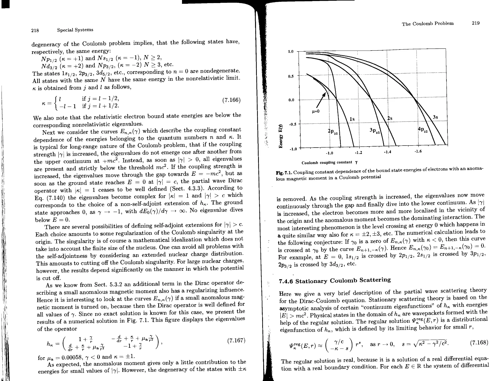
who helped me to write the computer program producing Fig. 7.1.
Graz, October 1991	Bernd Thaller

Contents
1 Free Particles ..................................................... 1
1.1	Dirac’s Approach ............................................ 2
1.2	The Formalism of Quantum Mechanics .......................... 4
1.2.1	Observables and States ............................ 4
1.2.2	Time Evolution .................................... 5
1.2.3	Interpretation .................................... 5
1.3	The Dirac Equation and Quantum Mechanics .................... 6
1.3.1	A Hilbert Space for the Dirac Equation ............ 6
1.3.2 Position and Momentum ................................ 7
1.3.3	Some Other Observables ............................ 8
1.4	The Free Dirac Operator ..................................... 9
1.4.1	The Free Dirac Operator in Fourier Space ............. 9
1.4.2	Spectral Subspaces of Ho ............................ 10
1.4.3	The Foldy-Wouthuysen Transformation ................. 11
1.4.4	Self-adjointness and Spectrum of Hq ................. 11
1.4.5	The Spectral Transformation ......................... 13
1.4.6	Interpretation of Negative Energies ................. 14
1.5	The Free Time Evolution .................................... 15
1.6	Zitterbewegung ............................................. 18
1.6.1	The Velocity Operator ............................... 19
1.6.2	Time Evolution of the Standard Position Operator .	20
1.6.3	Evolution of the Expectation Value .................. 21
1.6.4	Evolution of Angular Momenta ........................ 22
1.6.5	The Operators F and G ............................... 23
1.7	Relativistic Observables ................................... 24
1.7.1	Restriction to Positive Energies .................... 24
1.7.2	Operators in the Foldy-Wouthuysen Representation	25
1.7.3 Notions of Localization ............................. 26
1.8	Localization and Acausality ................................ 28
1.8.1 Superluminal Propagation ............................ 28
1.8.2	Violation of Einstein Causality ..................... 30
1.8.3	Support Properties of Wavefunctions ................. 31
1.8.4	Localization and Positive Energies .................. 32
1.9	Approximate Localization ................................... 32
1.9.1	The Nonstationary Phase Method ...................... 33
1.9.2	Propagation into the Classically Forbidden Region .	34
Appendix .................................................. 35
XII
Contents
l.A	Alternative Representations of Dirac Matrices ...... 35
l.B	Basic Properties of Dirac Matrices ................. 37
l.C	Commutators with Hq ................................ 37
l.D	Distributions Associated with the Evolution	Kernel	38
l.E	Explicit Form of the Resolvent Kernel .............. 39
l.F	Free Plane-Wave Solutions .......................... 39
2 The Poincare Group ............................................... 42
2.1	The Lorentz and Poincare Groups .......................... 43
2.1.1	The Minkowsky Space ................................ 43
2.1.2	Definition of the Lorentz Group .................... 44
2.1.3	Examples of Lorentz Transformations ................ 44
2.1.4	Basic Properties of the Lorentz Group .............. 46
2.1.5	The Poincare Group ................................. 47
2.1.6	The Lie Algebra of the Poincare Group .............. 48
2.2	Symmetry Transformations in Quantum Mechanics ............ 50
2.2.1	Phases and Rays .................................... 50
2.2.2	The Wigner-Bargmann Theorem ........................ 51
2.2.3	Projective Representations ......................... 51
2.2.4	Representations in a Hilbert Space ................. 52
2.2.5	Lifting of Projective Representations .............. 53
2.3	Lie Algebra Representations .............................. 54
2.3.1	The Lie Algebra and the Garding Domain ............. 55
2.3.2	The Poincare Lie Algebra ........................... 56
2.3.3	Integration of Lie Algebra Representations ......... 58
2.3.4	Integrating the Poincare Lie Algebra ............... 60
2.4	Projective Representations ............................... 62
2.4.1	Representations of the Covering Group .............. 62
2.4.2	A Criterion for the Lifting ........................ 64
2.4.3	The Cohomology of the Poincare Lie Algebra ......... 65
2.4.4	Relativistic Invariance of the Dirac Theory ........ 67
2.5	The Covering Group of the Lorentz Group .................. 67
2.5.1	SL(2) and Lorentz Group ............................ 68
2.5.2	Rotations and Boosts ............................... 69
2.5.3	Nonequivalent Representations of SL(2) ............. 70
2.5.4	Linear Representation of the Space Reflection ...... 71
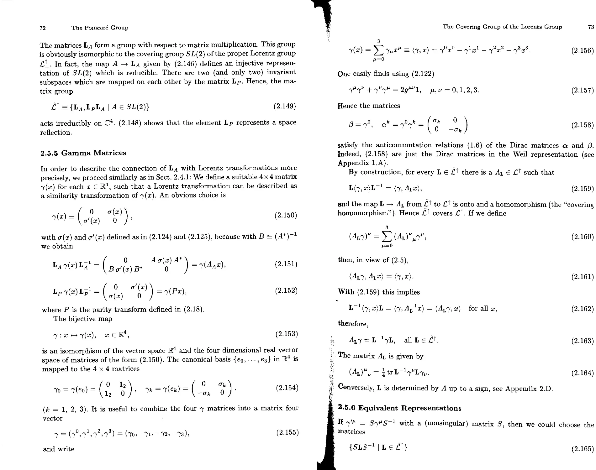
2.5.5	Gamma Matrices ..................................... 72
2.5.6	Equivalent Representations ......................... 73
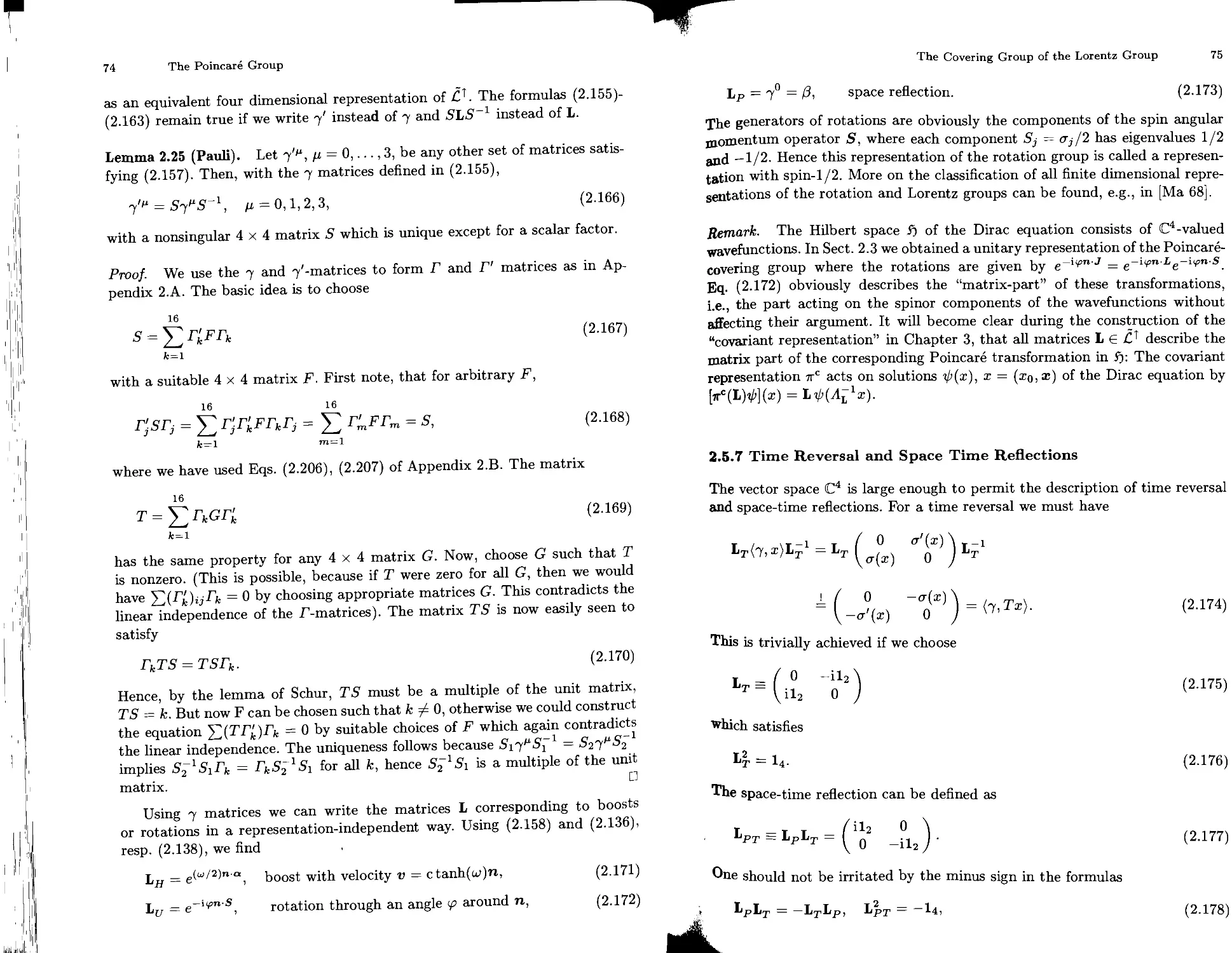
2.5.7	Time Reversal and Space-Time Reflections ........... 75
2.5.8	A Covering Group of the Full Poincare Group ........ 76
Appendix ................................................. 77
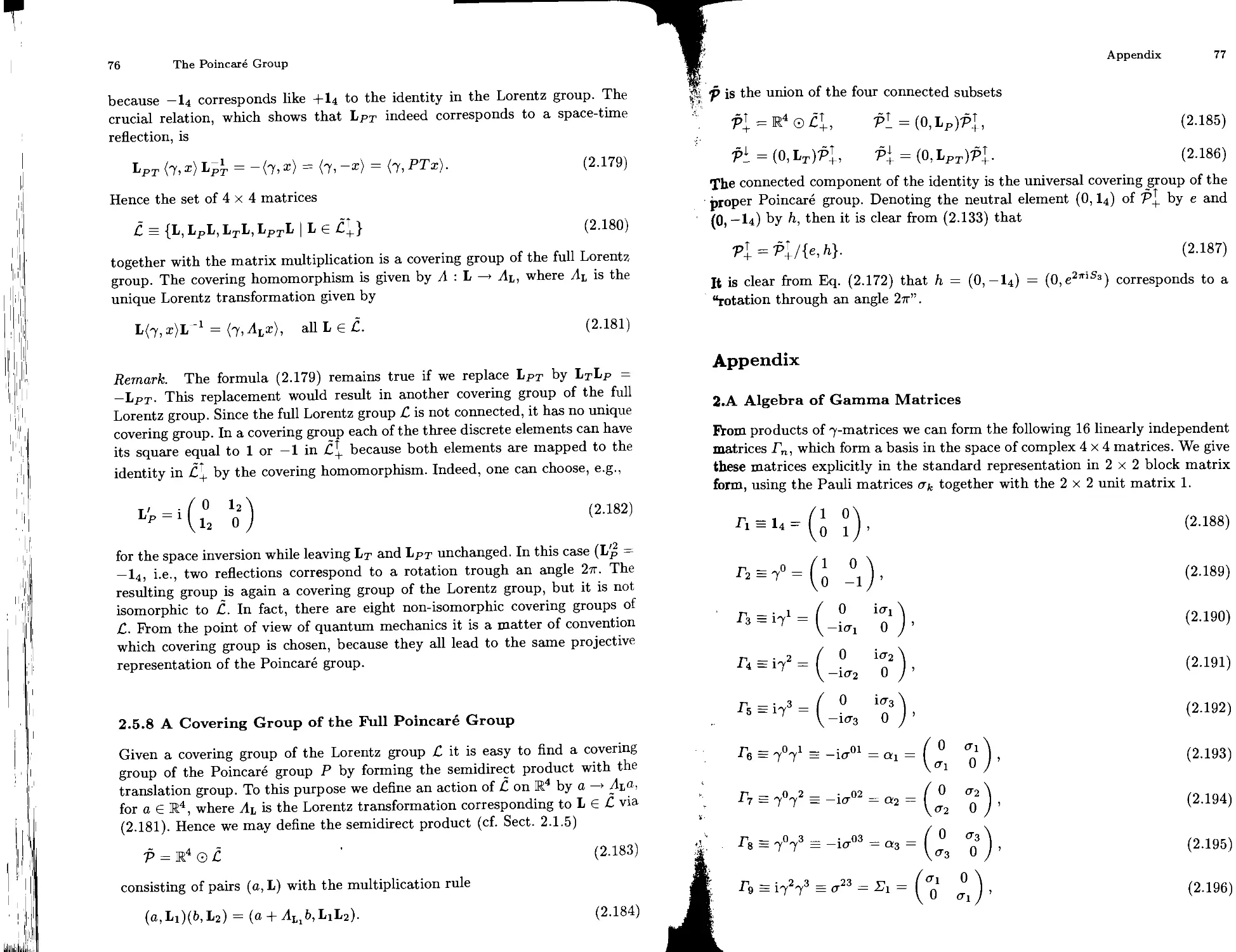
2.A	Algebra of Gamma Matrices .......................... 77
2.В	Basic Properties of Gamma Matrices ................. 78
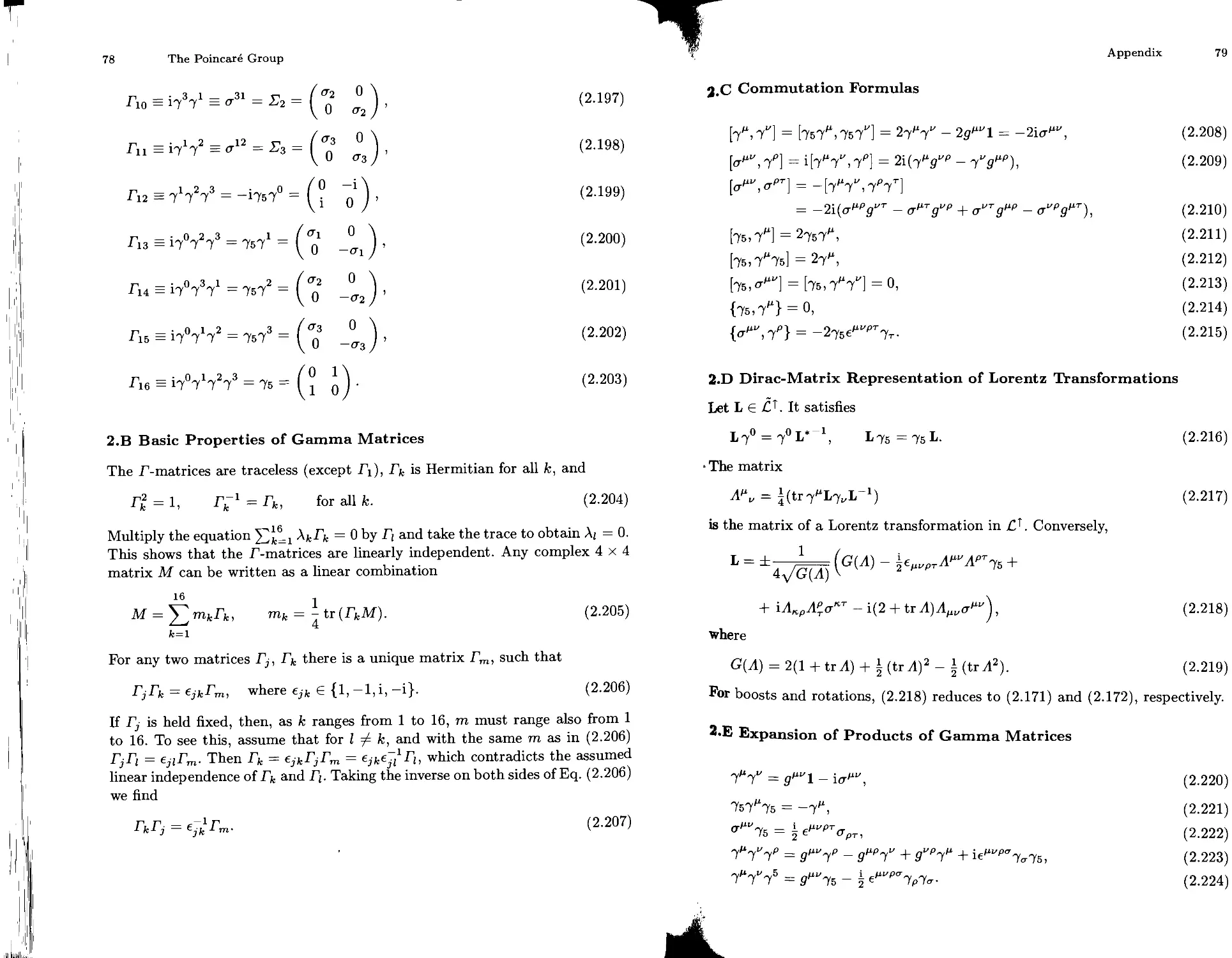
2.C	Commutation Formulas ............................... 79
2.D Dirac-Matrix Representation of Lorentz
Transformations ........................................... 79
Contents
XIII
2.E	Expansion of Products of Gamma Matrices ............. 79
2.F	Formulas with Traces ................................ 80
3	Induced Representations .......................................... 81
3.1	Mackey’s Theory of Induced Representations ................. 82
3.1.1	Induced Representations of Lie Groups ............... 82
3.1.2	A Strategy for Semidirect Products .................. 83
3.1.3	Characters and the Dual Group ....................... 84
3.1.4	The Dual Action of the Poincare Group ............... 85
3.1.5	Orbits and Isotropy Groups .......................... 86
3.1.6	Orbits of the Poincare Group ........................ 87
3.1.7	Invariant Measure and Little Group .................. 88
3.1.8	Induced Representations of the Poincare Group ....	88
3.2	Wigner’s Realization of Induced Representations ............ 89
3.2.1	Wigner States ....................................... 89
3.2.2	Wigner States for the Poincare Group ................ 90
3.2.3	Irreducibility of the Induced Representation ........ 92
3.2.4	Classification of Irreducible Representations ....... 93
3.2.5	The Defining Representation of the Little Group ...	93
3.3	Covariant Realizations and the Dirac Equation .............. 94
3.3.1	Covariant States .................................... 94
3.3.2	Covariant States for the Poincare Group ............. 95
3.3.3	Invariant Subspaces ................................. 95
3.3.4	The Scalar Product in the Invariant Subspaces ....... 96
3.3.5	Covariant Dirac Equation ............................ 97
3.3.6	The Configuration Space ............................. 98
3.3.7	Poincare Transformations in Configuration Space . .	99
3.3.8	Invariance of the Free Dirac Equation .............. 100
3.3.9	The Foldy-Wouthuysen Transformation ................ 101
3.4	Representations of Discrete Transformations ............... 102
3.4.1	Projective Representations of the Poincare Group . .	102
3.4.2	Antiunitarity of the Time Reversal Operator ........ 104
4	External Fields ................................................. 106
4.1	Transformation Properties of External Fields .............. 107
4.1.1 The Potential Matrix ................................ 107
4.1.2 Poincare Covariance of the Dirac Equation ........... 107
4.2	Classification of External Fields ......................... 108
4.2.1	Scalar Potential ................................... 108
4.2.2	Electromagnetic Vector Potential ................... 108
4.2.3	Anomalous Magnetic Moment .......................... 109
4.2.4	Anomalous Electric Moment .......................... 110
4.2.5	Pseudovector Potential ............................. Ill
4.2.6	Pseudoscalar Potential ............................. Ill
4.3	Self-adjointness and Essential Spectrum ................... 112
4.3.1	Local Singularities ................................ 112
XIV
Contents
4.3.2 Behavior at Infinity .............................. 113
4.3.3 The Coulomb Potential ............................. 114
4.3.4 Invariance of the Essential Spectrum
and Local Compactness ................................... 114
4.4	Time Dependent Potentials ............................... 117
4.4.1	Propagators ...................................... 117
4.4.2	Time Dependence Generated by	Unitary Operators .	118
4.4.3	Gauge Transformations ............................ 119
4.5	Klein’s Paradox ......................................... 120
4.6	Spherical Symmetry ...................................... 122
4.6.1	Assumptions on the Potential ..................... 122
4.6.2	Transition to Polar Coordinates	............ 123
4.6.3	Operators Commuting with the	Dirac Operator ....	125
4.6.4	Angular Momentum Eigenfunctions .................. 126
4.6.5	The Partial Wave Subspaces ....................... 128
4.6.6	The Radial Dirac Operator ........................ 129
4.7	Selected Topics from Spectral	Theory .................... 131
4.7.1	Potentials Increasing at Infinity	............ 131
4.7.2	The Virial Theorem ............................... 134
4.7.3	Number of Eigenvalues ............................ 136
5	Supersymmetry ................................................ 138
5.1	Supersymmetric Quantum	Mechanics ........................ 139
5.1.1	The Unitary Involution т ......................... 139
5.1.2	The Abstract Dirac Operator ...................... 139
5.1.3	Associated Supercharges .......................... 140
5.2	The Standard Representation ............................. 141
5.2.1	Some Notation .................................... 141
5.2.2	Nelson’s Trick ................................... 142
5.2.3	Polar Decomposition of Closed Operators .......... 143
5.2.4	Commutation Formulas ............................. 145
5.3	Self-adjointness Problems	.............................. 145
5.3.1 Essential Self-adjointness of Abstract
Dirac Operators ......................................... 145
5.3.2 Particles with an Anomalous Magnetic Moment ....	147
5.4	Dirac	Operators with Supersymmetry ..................... 149
5.4.1 Basic Definitions and Properties .................. 149
5.4.2	Standard Representation .......................... 151
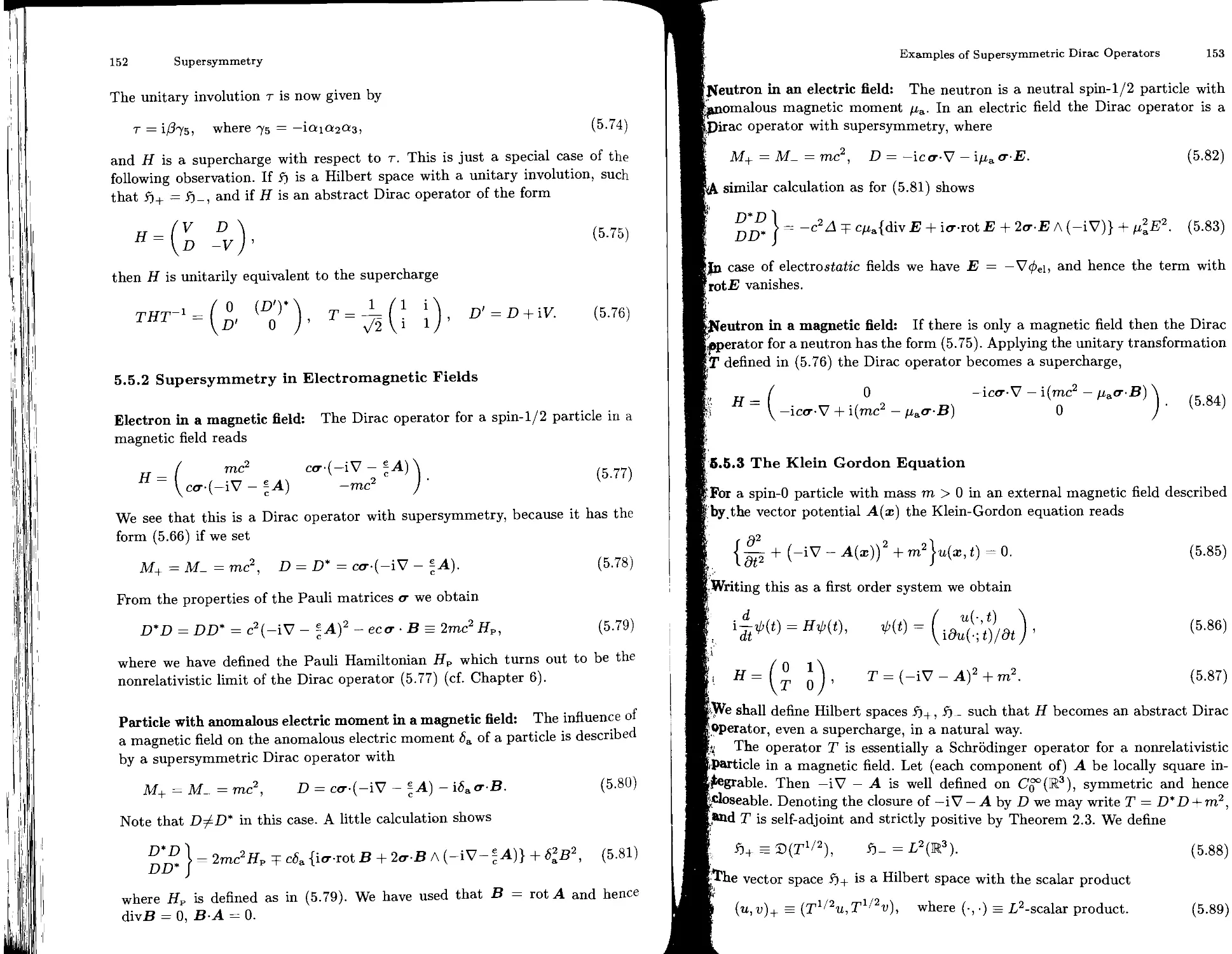
5.5	Examples of Supersymmetric Dirac	Operators .............. 151
5.5.1 Dirac Operator with a Scalar Field ................ 151
5.5.2 Supersymmetry in Electromagnetic Fields ........... 152
5.5.3 The Klein-Gordon Equation ......................... 153
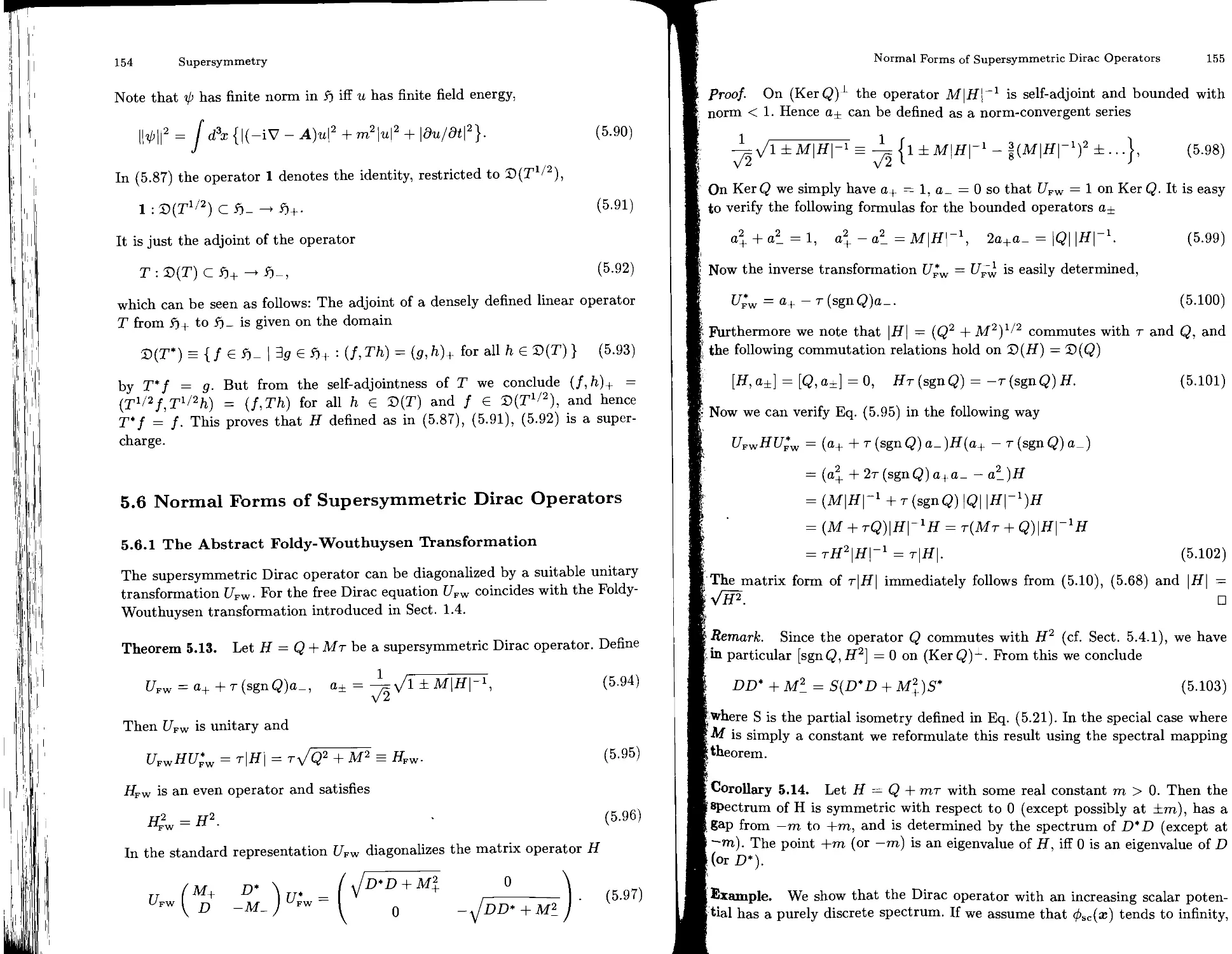
5.6	Normal Forms of Supersymmetric Dirac Operators .......... 154
5.6.1 The Abstract Foldy-Wouthuysen Transformation .. .	154
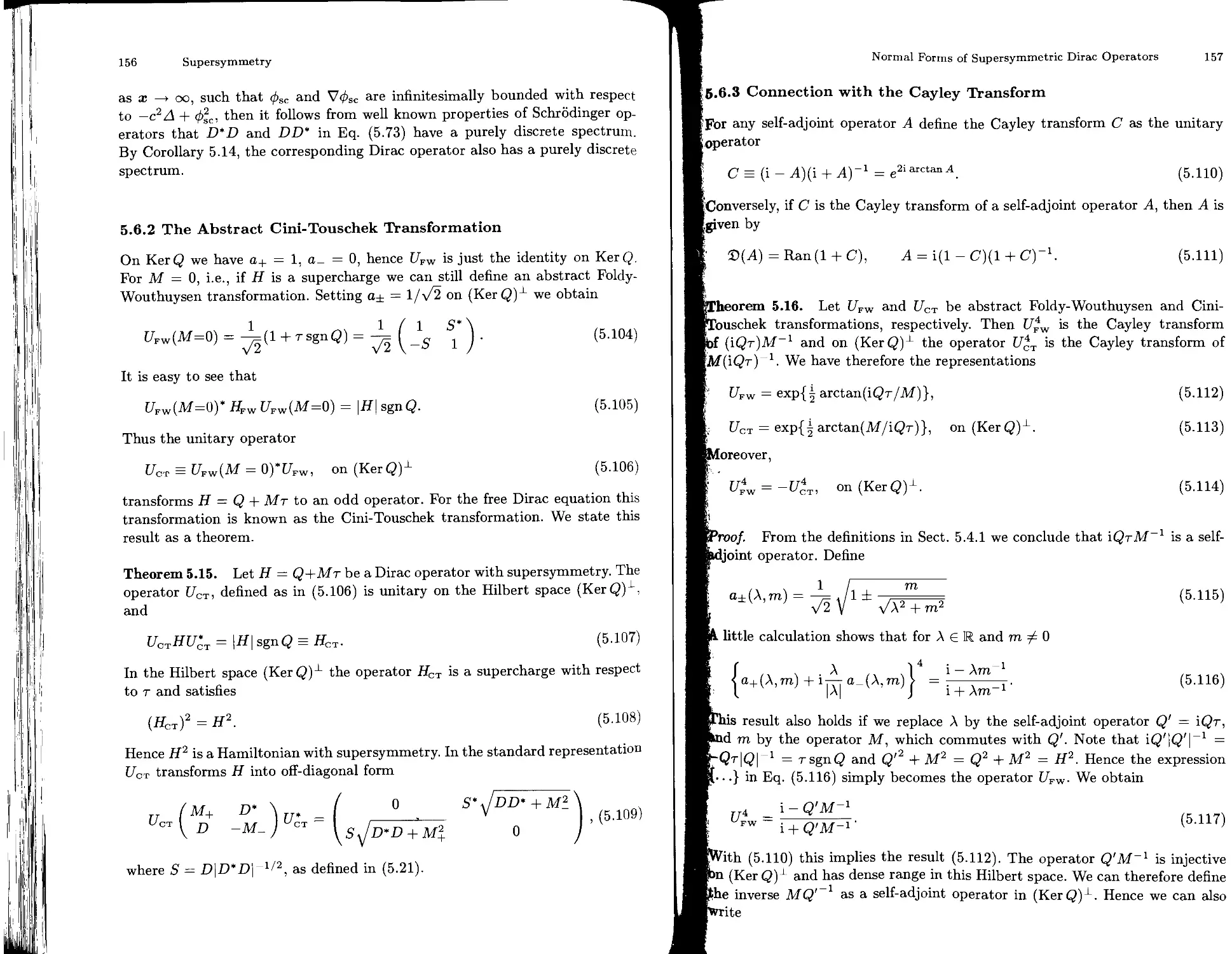
5.6.2 The Abstract Cini-Touschek Transformation ......... 156
5.6.3 Connection with the Cayley Transform .............. 157
Contents
XV
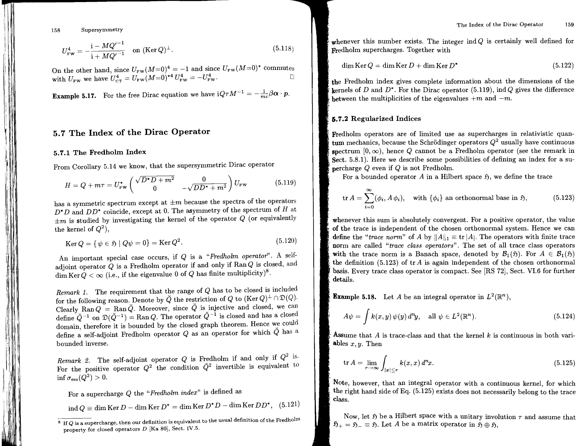
5.7	The Index of the Dirac Operator ............................. 158
5.7.1	The Fredholm Index ................................... 158
5.7.2	Regularized Indices .................................. 159
5.8	Spectral Shift and Witten Index ............................. 161
5.8.1 Krein’s Spectral Shift Function ...................... 161
5.8.2 The Witten Index and the Axial Anomaly ............... 165
5.8.3 The Spectral Asymmetry ............................... 166
5.9	Topological Invariance of the Witten Index .................. 167
5.9.1 Perturbations Preserving Supersymmetry ............... 167
5.9.2 Invariance of the Index Under Perturbations .......... 167
5.10	Fredholm Determinants ...................................... 170
5.11	Regularized Indices in Exactly Soluble Models .............. 173
5.11.1 Scalar Potential in One Dimension ................... 173
5.11.2 Magnetic Field in Two Dimensions .................... 174
5.11.3 Callias Index Formula ............................... 174
6	The Nonrelativistic Limit ........................................ 176
6.1	c-Dependence of Dirac Operators ............................. 177
6.1.1	General Setup ........................................ 177
6.1.2	Supersymmetric Dirac Operators ....................... 178
6.1.3	Analyticity of the Resolvent ......................... 180
6.1.4	Nonrelativistic Limit with Anomalous Moments	....	182
6.2	c-Dependence of Eigenvalues ................................. 183
6.2.1	Browsing Analytic Perturbation Theory ................ 183
6.2.2	The Reduced Dirac Operator ........................... 186
6.2.3	Analyticity of Eigenvalues and Eigenfunctions ........ 187
6.2.4	First Order Corrections of Nonrelativistic Eigenvalues	188
6.2.5	Interpretation of the First Order Correction ......... 188
6.2.6 Example: Separable Potential ......................... 191
7	Special Systems .................................................. 193
7.1	Magnetic Fields ............................................. 194
7.1.1 Introduction ......................................... 194
7.1.2 Dirac and Pauli Operators ............................ 194
7.1.3 Homogeneous Magnetic Field ........................... 196
7.2	The Ground State in a Magnetic Field ........................ 198
7.2.1	Two Dimensions ....................................... 198
7.2.2	Three Dimensions ..................................... 199
7.2.3	Index Calculations ................................... 200
7.3	Magnetic Fields and the Essential Spectrum .................. 202
7.3.1	Infinitely Degenerate Threshold Eigenvalues .......... 202
7.3.2	A Characterization of the Essential	Spectrum ......... 203
7.3.3	Cylindrical Symmetry ................................. 206
7.4	The Coulomb Problem ......................................... 208
7.4.1	The Hidden Supersymmetry ............................. 208
7.4.2	The Ground State ..................................... 210
XVI
Contents
7.4.3	Excited States ..................................... 211
7.4.4	The BJL Operator ................................... 214
7.4.5	Discussion ......................................... 216
7.4.6	Stationary Coulomb Scattering ...................... 219
8	Scattering States ............................................... 222
8.1	Preliminaries ............................................. 223
8.1.1	Scattering Theory .................................. 223
8.1.2	Wave Operators ..................................... 224
8.1.3 The Scattering Operator ............................. 225
8.2	Asymptotic Observables .................................... 226
8.2.1	Introduction ....................................... 227
8.2.2	Invariant Domains .................................. 228
8.2.3	RAGE ............................................... 230
8.2.4	Asymptotics of Zitterbewegung ...................... 230
8.2.5	Asymptotic Observables ............................. 232
8.2.6	Propagation in Phase Space ......................... 236
8.3	Asymptotic Completeness	....................... 239
8.3.1	Short-Range Potentials ............................. 239
8.3.2	Coulomb Potentials ................................. 240
8.4	Supersymmetric Scattering	and Magnetic Fields ............. 242
8.4.1	Existence of Wave Operators ........................ 242
8.4.2	Scattering in Magnetic Fields ...................... 244
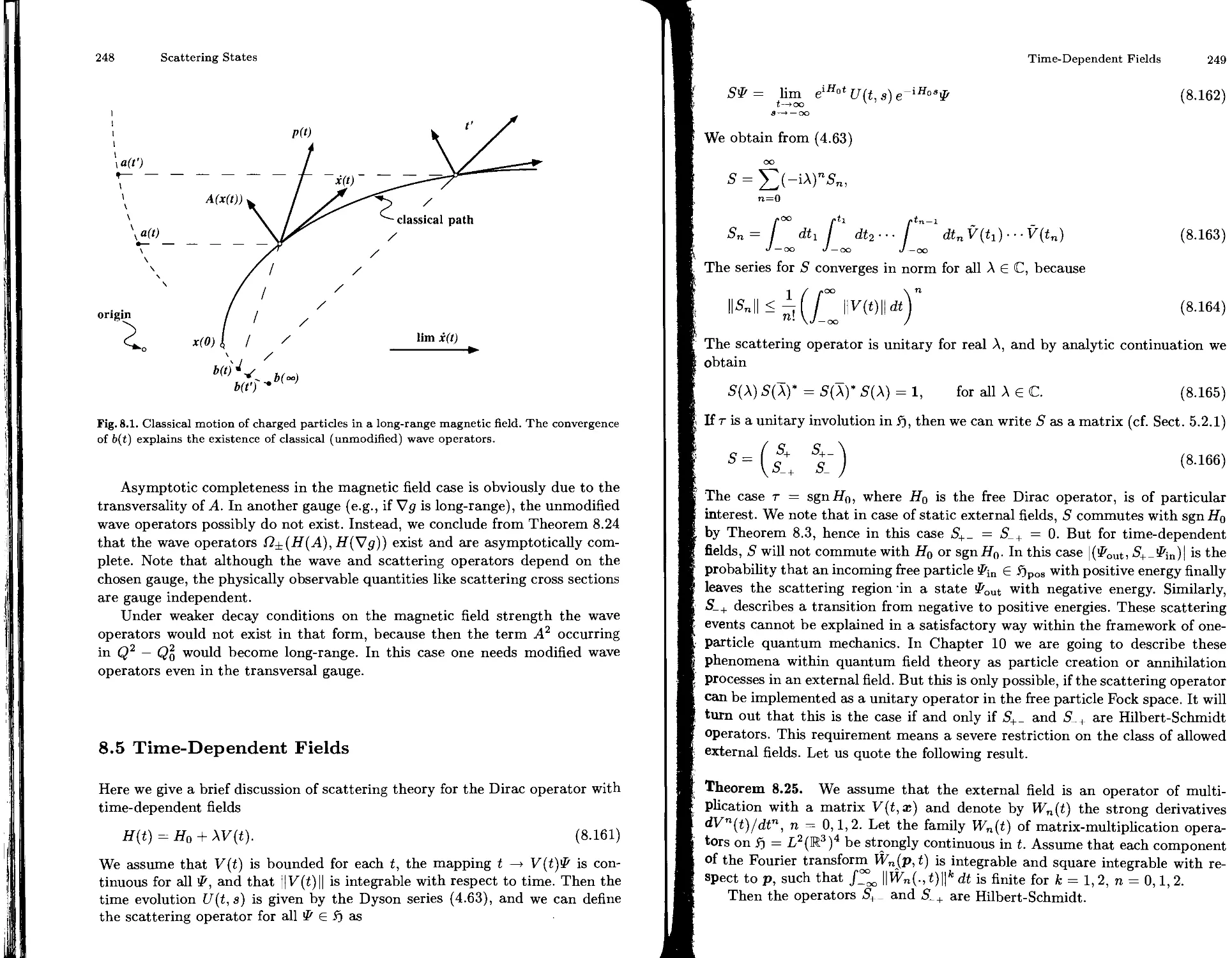
8.5	Time-Dependent Fields ..................................... 248
9	Solitons ........................................................ 250
9.1	Time-Dependent Scalar Potential ........................... 251
9.1.1	Scalar Potentials in One Dimension ................. 251
9.1.2	Generation of Time Dependence ...................... 252
9.1.3 The Miura Transformation ............................ 253
9.2	The Korteweg-deVries Equation ............................. 253
9.2.1	Construction of an Operator В ...................... 253
9.2.2	Differential Equations for the Potentials .......... 255
9.3	Inversion of the Miura Transformation ..................... 256
9.4	Scattering in One Dimension ............................... 260
9.4.1	The Scattering Matrix .............................. 260
9.4.2	Relative Scattering and the Regularized Index ...... 264
9.5	Soliton Solutions ......................................... 267
9.5.1	Solitons of the KdV Equation ....................... 267
9.5.2	mKdV Solitons in the Critical Case ................. 270
9.5.3	mKdV Solitons in the Subcritical Case .............. 272
10	Quantum Electrodynamics in External Fields ...................... 274
10.1	Quantization of the Dirac Field ........................... 275
10.1.1 The Fock Space ..................................... 275
10.1.2 Creation and Annihilation Operators ................ 277
Contents
XVII
10.1.3 The Algebra of Field Operators .................... 279
10.1.4 Irreducibility of the Fock Representation ......... 280
10.2	Operators in Fock Space .................................. 281
10.2.1 Implementation of Unitary Operators ............... 281
10.2.2 The Time Evolution ................................ 282
10.2.3 Number and Charge Operators ....................... 283
10.2.4 One-Particle Operators ............................ 284
10.3	Bogoliubov Transformations ............................... 287
10.3.1 Unitary Implementation in the General Case ........ 287
10.3.2	Even and Odd Parts of Unitary Operators .......... 287
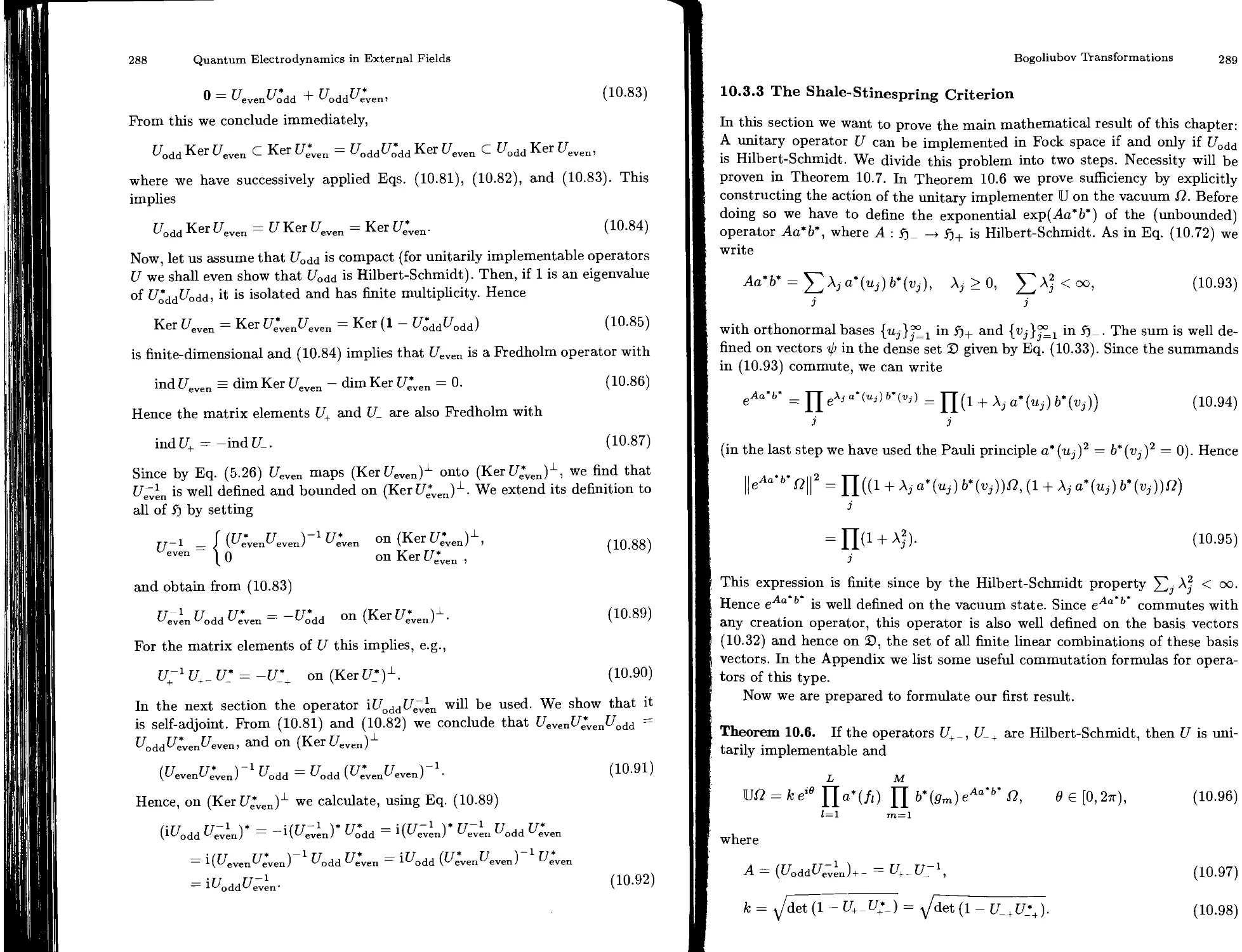
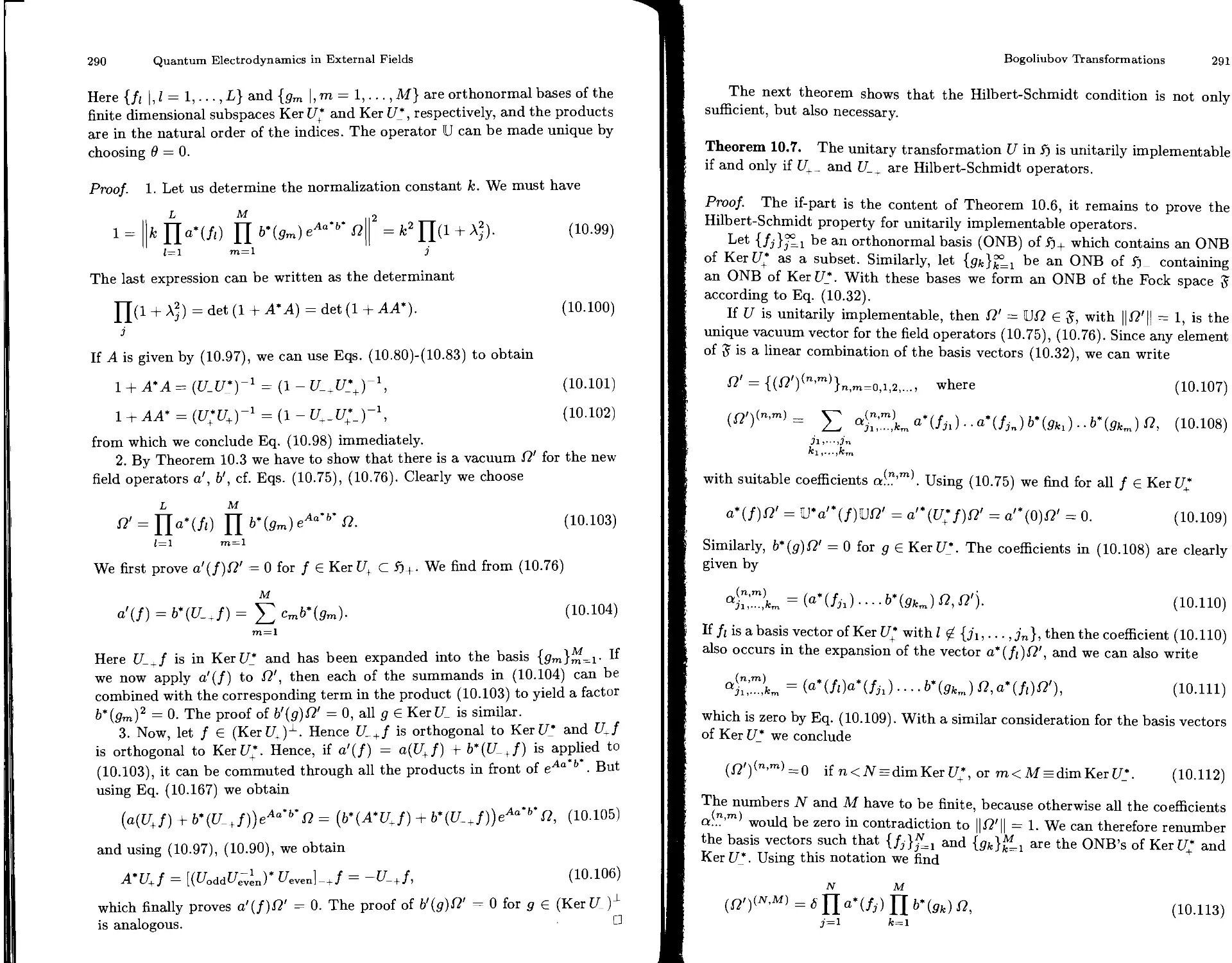
10.3.3	The Shale-Stinespring Criterion .................. 289
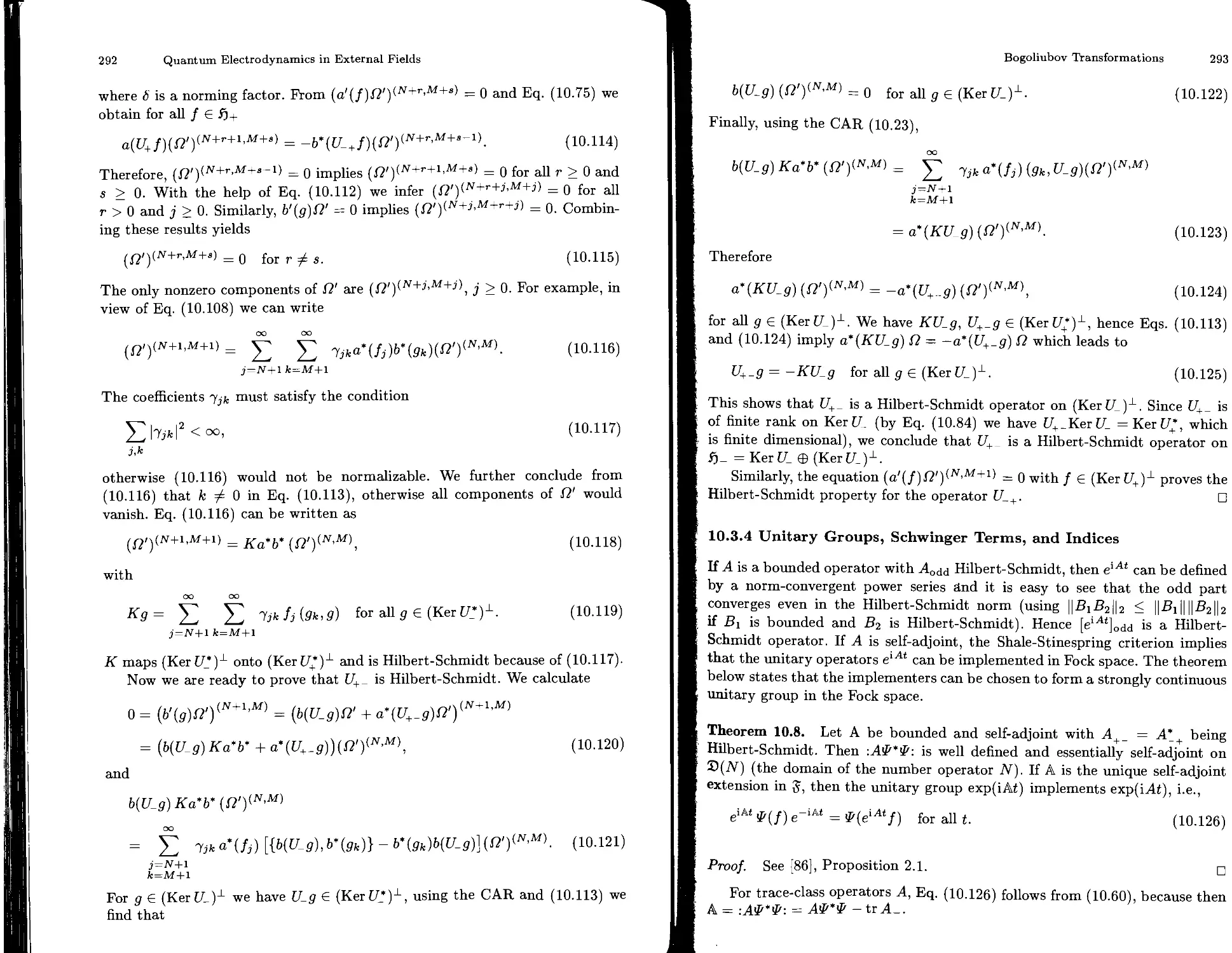
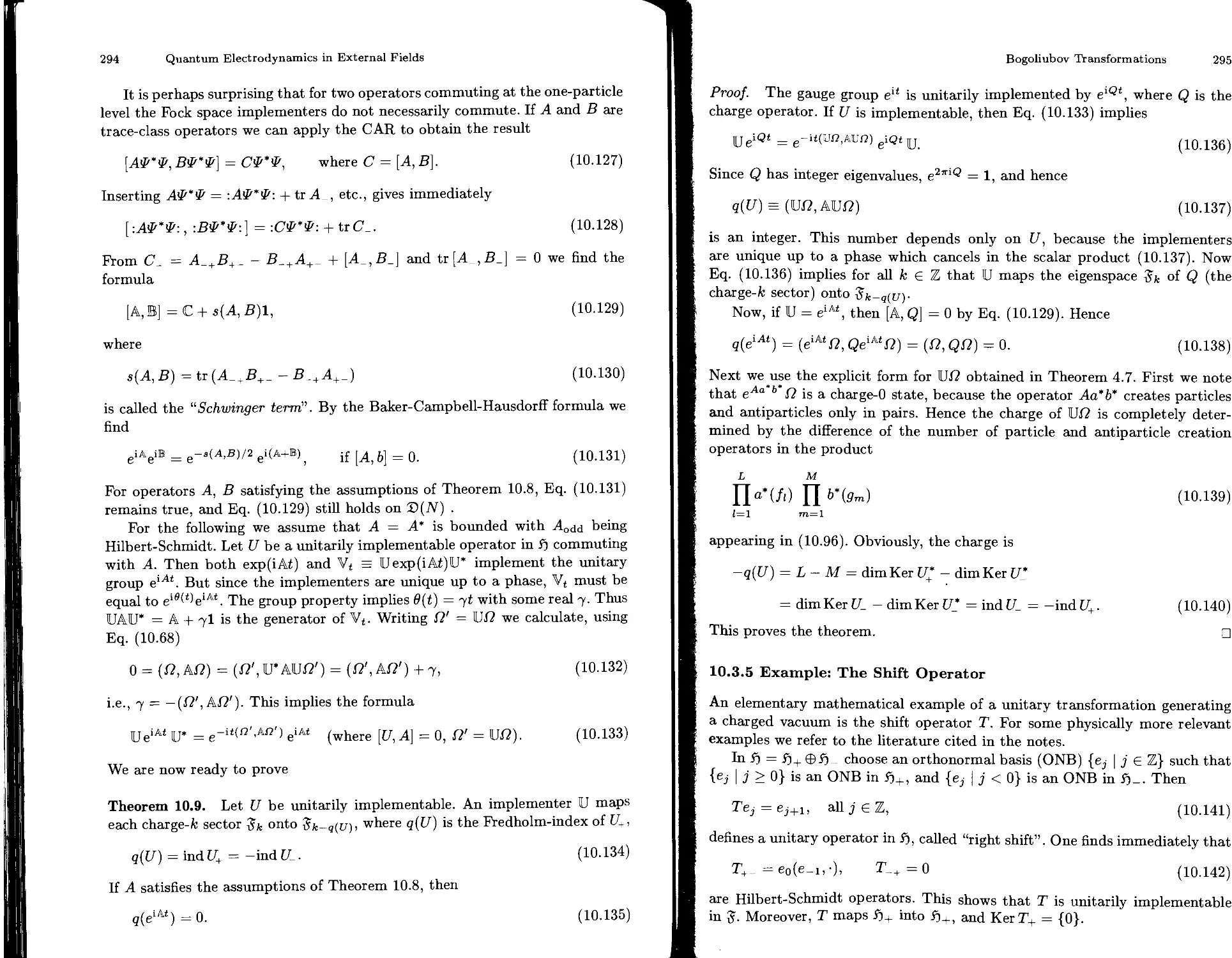
10.3.4 Unitary Groups, Schwinger Terms, and Indices ....	293
10.3.5	Example: The Shift Operator ...................... 295
10.4	Particle Creation and Scattering Theory ................. 296
10.4.1	The S-Matrix in Fock Space ....................... 297
10.4.2	Spontaneous Pair Creation ........................ 299
Appendix ................................................. 300
Notes ......................................................... 302
Books ......................................................... 321
Articles ...................................................... 325
Symbols ....................................................... 346
Index ......................................................... 353

1 Free Particles
The free Dirac equation describes a relativistic electron or positron which moves freely as if
there were no external fields or other particles. Nevertheless this equation is important for the
asymptotic description of interacting particles because in the limit of large times interacting
particles tend to behave like free ones, provided their mutual separation increases.
In Sect. 1.1 we “derive” the Dirac equation for a free particle following Dirac’s original
approach. In order to obtain a quantum mechanical interpretation we consider the Dirac
equation as an evolution equation in a suitable Hilbert space whose vectors are related to
the physical states via a statistical interpretation. We identify certain self-adjoint operators
with physical observables in correspondence to nonrelativistic quantum mechanics (Sect. 1.3).
Next we prove self-adjointness of the Dirac operator (energy observable) and determine its
spectral properties in Sect. 1.4. The time evolution is described in Sect. 1.5. In particular we
derive the evolution kernel (Feynman propagator) and show that it vanishes outside the light
cone. This implies a causal propagation of wavefunctions. We also investigate the temporal
behavior of position, velocity, spin and orbital angular momentum (Sect. 1.6).
By writing the Dirac equation as a quantum mechanical initial value problem we arrive at
a one particle interpretation which, if pushed too far, leads to some inconsistencies — even at
the level of free particles. The origin of all problems is the fact that the Dirac operator is not
semibounded. Therefore a free electron can be in a state with negative energy. Via a charge
conjugation these negative energy solutions can be identified as positive energy solutions of a
positron Dirac equation. There remains, however, the problem that there are superpositions
of electron and positron solutions in the original Hilbert space. The resulting interference
effects lead to a paradoxical behavior of free wavepackets (“Zitterbewegung”, see Sect. 1.6).
Since for free particles the sign of the energy is a conserved quantity one might think of
restricting everything to the subspace of positive energies, and choosing observables which
leave this subspace invariant. This procedure leads to the quantum analog of the classical rel-
ativistic relation between energy and velocity without Zitterbewegung (Sect. 1.7). But again
there is an unexpected difficulty. This is the localization problem described in Sect. 1.8:
Since the standard position operator (multiplication by x) mixes positive and negative ener-
gies one is forced to look for a new position operator (i.e., to reinterpret the wavefunction).
But choosing any other position observable in the positive energy subspace leads inevitably
to the possibility of an instantaneous spreading of initially localized states and therefore to
an acausal behavior. On the other hand, we could keep |V’|2 as the usual expression for the
position probability density. But then there are no localized states at all with positive en-
ergy, and hence there is no position observable in the usual sense. This problem indicates
either that the usual quantum mechanical interpretation (which is basically a one-particle
interpretation modelled on the nonrelativistic theory) is insufficient, or that “localization in
a finite region” is not a property that one single relativistic particle can have.
In Sect. 1.9 we describe an approximate localization by the “method of (non-)stationary
phase” (Sect. 1.9). In particular we estimate the probability of finding the particle at large
times outside the “classically allowed” region. This is the region of space where a particle
with a certain momentum distribution and initial localization is expected to be according to
classical mechanics. We find that the tails of the wavefunction in the classically forbidden
region decay rapidly in time. These results are needed for scattering theory in Chapter 8.
2
Free Particles
1.1 Dirac’s Approach
In this section we follow closely Dirac’s original arguments which led to the
discovery of his famous equation describing the relativistic motion of a spin-1/2
particle in R3. A deeper understanding of the origin of the Dirac equation will
be obtained on a group theoretical basis in Chapter 3.
Formally, the transition from classical to quantum mechanics can be ac-
complished by substituting appropriate operators for the classical quantities.
Usually, these operators are differential or multiplication operators acting on
suitable wavefunctions. In particular, for the energy E and the momentum p
of a free particle the substitution
Q
E —> ih—, p —> —ihV,
at
(h = Planck’s constant)
(1-1)
is familiar from the nonrelativistic theory. Moreover, (1.1) is formally Lorentz-
invariant. If applied to the classical relativistic energy-momentum relation,
E = у/c2p2 + m2c4,
(1-2)
(1.1)	gives the square-root Klein-Gordon equation
ih tp(t, x) = ^/—c2h2A + m2c4 ip(t, ж), t € R, x € R3,	(1-3)
where Л = д2/дх2 + d2/dxl + д2/дх% is the Laplace operator. The square-
root of a differential operator can be defined with the help of Fourier-trans-
formations, but due to the asymmetry of space and time derivatives Dirac
found it impossible to include external electromagnetic fields in a relativistically
invariant way. So he looked for another equation which can be modified in order
to describe the action of electromagnetic forces. This new equation should also
describe the internal structure of the electrons, the spin. The Klein-Gordon
equation
d2
—®) = (—c2h2A + m2c4) j/»(t, x)	(1.4)
with a scalar wavefunction ip was not able to do so. Moreover, a quantum
mechanical evolution equation should be of first order in the time derivative. So
Dirac reconsidered the energy-momentum relation (1.2) and before translating
it to quantum mechanics with the help of (1.1), he linearized it by writing
з
E = с aipj + f3mc2 = ca p + (3mc2,	(1.5)
i— 1
where a = (а1,а2,аз) and f3 have to be determined from (1.2). Indeed, (1.2)
can be satisfied if one assumes that a and /3 are anticommuting quantities
which are most naturally represented by n x n matrices (“Dirac matrices”).
Dirac’s Approach
3
Comparing E2 according to Eqs. (1.2) and (1.5) we find that the following
relations must hold
atak + ak&i = 2<5ifcl, i,k = 1,2,3,
ai/3 + /3ai = O, i = 1,2,3,	(1.6)
/32 = 1,
where <5,*. denotes the Kronecker symbol (<5jj, = 1 if i = fe; <5,*. = 0 if i k), 1
and 0 are the n-dimensional unit and zero matrices. The n x n-matrices a and
/3 should be Hermitian so that (1.5) can lead to a self-adjoint expression (which
is necessary for a quantum mechanical interpretation, cf. the next section). The
dimension n of the Dirac matrices can be determined as follows. From (1.6) we
conclude
tra, = tr/32aj = — tr (3ai(3 = —trail3(3 = —freq = 0,	(1-7)
where tr denotes the trace of a matrix. On the other hand, in view of a2 = 1,
the eigenvalues of cq are either +1 or —1. This together with (1.7) shows that
the dimension n of the matrices has to be an even number. For n = 2 there are
at most three linearly independent anticommuting matrices: For example, the
Pauli matrices
together with the unit matrix 1 form a basis in the space of Hermitian 2x2
matrices. Hence there is no room for a “rest energy” matrix f3 in two dimensions.
In four dimensions (1.6) can be satisfied, if we choose
^=(о -1)’	о)’ г = 1’2’3’
This “standard representation” was introduced by Dirac. Some other frequently
used representations are listed in the appendix. If one now “translates” Eq. (1.5)
to quantum mechanics one obtains the Dirac equation
= Hoi/>(t,®).	(1-Ю)
Ho is given explicitly by the matrix-valued differential expression
rr	г, , о 2	( mc2l —ihctr-VA	,,
Ho = -ihca • V + 3mc = .t _	,	(1.11)
y-inccr-V -mrl J	v '
where a = (а1,а2,аз), °- = (о'1,о'2,<’’з) are triplets of matrices. Hq acts on
vector-valued wavefunctions
(V>1 (t, ж) \
:	eC4.	(1.12)
4
Free Particles
If m = 0 (“neutrinos”), then the mass term in (1.5) vanishes and only three
anticommuting quantities at are needed. In this case it is sufficient to use 2x2
matrices. Indeed, E = ccr • p satisfies the condition E2 = c2p2 with the Pauli
matrices defined above. The corresponding two component equation
ifi W) =	 P W)	(1-13)
is called the Weyl equation. It is not invariant under space reflections and was
therefore rejected until the discovery of parity violation in neutrino experi-
ments.
If the space-dimension is one or two, then again we can use Pauli matrices
instead of Dirac matrices. In this case the Dirac equation has the form (1.10)
with
/9 d \	2
HQ = -ihc <71  -1- <72 77— + <73mc .
\ UXi UX2/
(1-14)
It is commonly accepted that the free Dirac operator, apart from some
peculiarities, describes free relativistic electrons. Chapter 1 is devoted to a
detailed description of (1.11) and the solutions to (1.10). In the following we
shall always use units with h = 1.
1.2	The Formalism of Quantum Mechanics
In this section we give an outline of the basic ideas which will guide us in our
attempt to put the Dirac equation into a quantum mechanical framework.
1.2.1 Observables and States
According to the basic principles of quantum mechanics one defines a Hilbert
space f) for each quantum mechanical system1. Every measurable quantity or
“observable” (e.g., energy, momentum, etc.) has to be represented by a self-
adjoint operator. The “state” of the system at time to is given by a vector
0(to)	£)• We assume that -0(to) is normalized, i.e., multiplied by a scalar
constant such that
IIWo) II2 = (Wo), Wo)) = 1,
(1-15)
where “(•, •)” denotes the scalar product in
1 For the basic principles of linear functional analysis in Hilbert spaces (the mathematical
background of quantum mechanics), the reader is referred to the literature, e.g [Ka 80],
[RS 72], or [We 80]. Here we assume some basic knowledge about linear operators, their
domains and adjoints, self-adjointness, spectrum and so on.
The Formalism of Quantum Mechanics
5
1.2.2 Time Evolution
If the system at time to is in the state ip(to), then at time t its state is given
by
0(t) = e~'Htip(t0),	(1.16)
where the self-adjoint operator H (“Hamiltonian”) represents the energy of the
system. According to Stone’s theorem (see [RS 72]) 0(t) is the unique strong
solution of the Cauchy problem
i^ V’W =	0(to) e Э(Я) C fj.	(1.17)
at
If Sj is a function space, then ip is often called “wavefunction”. The unitary
time evolution exp(—iHt) induces a transformation of the observables. Let A
be self-adjoint on a domain of definition :Э(А). Then
A(t) = e[HtAe~iHt	(1.18)
is self-adjoint on £>(A(t)) = exp(— iHt) £>(A).
1.2.3 Interpretation
The usual interpretation linking these mathematical objects with the results
of measurements is obtained as follows. For any self-adjoint operator A we can
find, according to the spectral theorem, a “spectral measure” x(A € B) of a
(Borel measurable) set B.
x(A eB) = [ X(A G B)dEA(X) = [ dEA(X),	(1.19)
Jr	J в
where EA(X) is the spectral family of A (see [RS 72]), and x(A e B) is the
characteristic function of B, i.e.,
*<Л£В’ = {о A | в'	<120>
The operator x(A e B) is an orthogonal projection operator2. If = 1, then
(0, x(A 6 B) i[>) is a probability measure on R.
Definition (Born’s statistical interpretation). If a quantum mechanical system
is (at some time) in the state described by ip, then
(Ф,Х(А e B)ip) = f d(ip,EA(X)tp)	(1-21)
J в
2 An orthogonal projection P is a self-adjoint operator with P2 = P, its range Ran P is a
closed subspace of the Hilbert space, 1 — P projects onto the orthogonal complement of
Ran P
б
Free Particles
(where В is some Borel set in is the probability for a measurement of the
observable represented by A to give a result in B.
Thus the only possible results of measurements are the (real) numbers con-
tained in the spectrum <r(A). Eq. (1.21) predicts the probability zero for any
value which is not in <r(A), because Е'д(А) is constant on any interval which
contains no points of er (A). If the system is in a state 0 which is an eigenvector
of A belonging to the eigenvalue Aq, then the probability of finding the value
Aq in a measurement of A is 1.
From (1.18) and the unitarity of the time evolution we find
(0,х(ЖС € 8)0) = (0(t),x(A e B)0(t)), for all t,	(1-22)
and if 0(t) = exp(—IHt) 0 is in £)(A) for all t, then we can define the “expec-
tation value”
(0,лам) = (тл0(*)).	(i.23)
According to our probabilistic interpretation this is the mean value of the
results of many measurements which are all performed on systems identically
prepared to be in the state 0.
The projection operator E = ф(ф, •) is the observable determining whether
or not a system is in the state 0. The only possible results of single measure-
ments of E are 0 (“system is not in 0”) or 1 (“system is in the state 0”). If the
system is prepared to be in the state 0, then the expectation value of E (i.e.,
the probability of finding this system in the state 0 is given by
(0,E0) = |(0,0)|2,	(1.24)
and is called the “transition probability” from 0 to 0.
1.3	The Dirac Equation and Quantum Mechanics
Here we make some of the identifications which are necessary for a quantum
mechanical interpretation of the Dirac equation. We need a Hilbert space and
some operators representing basic observables.
1.3.1 A Hilbert Space for the Dirac Equation
If we compare (1-10) and (1.17) we see that it is most natural to interpret Hq
as the Hamiltonian for a free electron. Hq is a 4 x 4-matrix differential operator
which acts on C4-valued functions of x 6 R3. We choose the Hilbert space3
$j = L2(R3) ф L2(R3) Ф L2(R3) Ф L2(R3)
3 The various notations in Eq. (1.25) are explained, e.g., in [RS 72], Sects. II.1 and II.4
The Dirac Equation and Quantum Mechanics
7
= L2(R3)4 = L2(R3,C4) = L2(R3) ® C4.	(1.25)
It consists of 4-component column4 vectors 0 = (0i, 02; 03; 04) ' . where each
component 0t is (a Lebesgue equivalence class of) a complex valued function
of the space variable x. The scalar product is given by
C 4 _______
(0,0)= / УУ(а:)0г(а:)<Йг.	(1.26)
0R3 i=1
(The bar denotes complex conjugation).
In this Hilbert space we want to define the free Dirac operator
Ho 0 = — ica • V0 + ,3mc2 0, for all 0 ё £>(Hq),	(1-27)
on a suitable domain 2)(Hq). We shall prove in Sect. 1.4.4 that Hq is self-adjoint
on
Э(Я0) = ff‘(R3)4 C f),	(1.28)
the first Sobolev space5, which is a natural domain for first order differential
operators. Now, by Stone’s theorem, Eq. (1.10) becomes a well posed initial
value problem in the Hilbert space $j.
1.3.2 Position and Momentum
Having identified Hq as the operator for the energy of a free electron, it remains
to define self-adjoint operators for the other observables. Of course, this cannot
be done without ambiguity and we know that any particular choice causes prej-
udices concerning the interpretation of the theory. This is indeed a subtle point
of the Dirac theory, as we shall see in later sections. The following definitions
are motivated mainly by the analogy to the nonrelativistic quantum mechanics
of an electron.
The operator x = (xi, X2, ®з) of multiplication by x is called “standard
position operator”. In fact, x consists of the three self-adjoint operators Xt
which are defined by
r 4
Z)(xi) = | 0 € L2(R3)4 I / У |zi0fe(a:)|2 d3x < oo}, г = 1,2,3, (1-29)
J k=i
(Xi^l(x) \
:	for 0 in this domain, and i = 1,2,3.	(1.30)
Гг04(®) /
Remember that the spectral measure x(®i € Bi) of хг is just multiplication
with the characteristic function of the Borel set В» C R. We define a projection
operator valued measure on R3 by setting
4 We write the column vector as a transposed row vector (superscript “T”).
5 [RS 78], p. 253
8
Free Particles
E(B) = x(xi e Bi) x(x2 e B2) x(x3 e в3) = x(® e B),	(1-31)
for each В = Bi x B2 x B3. Then the probability of finding the particle in the
region В C R3 is
/• 4
^,Em)= / \Mx)\2d3x,	mhV wH2,	(1-32)
Jb	k=i
and |-0(®)|2 can be interpreted as a “position probability density”. (There Eire
other possible interpretations which we shall discuss in Sect. 1.7).
The differential operator p = —iV = — i(d/dxi, д/дх2, d/dx3) (acting
component-wise on the vector -ф is called “momentum operator”. Mathemati-
cally, it can be defined as the Fourier transformation of the standard position
operator. One obvious motivation for this choice is that p generates the space
translations
(e iapip) (ж) = tp(x — a).	(1.33)
1.3.3 Some Other Observables
Furthermore we define the “angular momentum operators”
S = —j а Л a (spin angular momentum),	(1-34)
L = x Ap (orbital angular momentum),	(1.35)
J = L + S (total angular momentum).	(1.36)
By a A a we denote the three matrices г ejkioikoii, j = 1, 2, 3, where e is the
totally antisymmetric tensor
1,
Cjki = < —1,
I 0,
if (jkl) is an even permutation of (123),
if (jkl) is an odd permutation of (123),
if at least two indices are equal.
(1-37)
The spin operator S is bounded, everywhere defined and self-adjoint. In the
standard representation,
<r/2 is just the spin operator of nonrelativistic quantum mechanics. Also the
operator L is well known from nonrelativistic quantum mechanics, except that
it acts now on 4-component wavefunctions. Finally, we define the “ center-of -
energy operator”
N = ± (Hox + xH0),	(1.39)
which will play an important role as the generator of Lorentz boosts in Chap-
ter 2. All the operators Ho, p, J, and N are essentially self-adjoint on C^(R3)4
(see also Sect. 2.2.4).
The Free Dirac Operator
9
1.4 The Free Dirac Operator
Next we describe the most important mathematical properties of the Dirac
operator Hg. We prove its self-adjointness and analyze the spectrum which
consists of all possible values resulting from an energy measurement. It will
turn out that according to the Dirac equation a free particle can have negative
energies.
1.4.1 The Free Dirac Operator in Fourier Space
The free Dirac operator Hg is most easily analyzed in the Fourier space. The
Fourier transformation
(^k)(p) =-----L- [ e~ip'x tpk(x) d3x, /г = 1,2,3,4,	(1-40)
(2тг)3'2 Аз
defined for integrable functions extends to a uniquely defined unitary opera-
tor (which is again denoted by T7) in the Hilbert space L2(R3)4. Occasionally
we shall write 5rL2(R3, d3x)4 = L2(R3,d^>)4 to distinguish between the vari-
ables. The Hilbert space L2(R3,d^>)4 is often called momentum space. Any
matrix differential operator in L2(R3, d3x)4 is transformed via F into a matrix
multiplication operator in L2(R3,d^>)4. For the Dirac operator one obtains
(^Я0^-1)(р)=Ь(р)= (mc21 CtrjY	(1-41)
v	v \ca-p -тс2 1)	v 7
For each p, this is a Hermitian 4 x 4-matrix which has the eigenvalues (p = |p|)
Ai(p) = Л2(р) = -A3(p) = -A4(p) = \/ c2p2 + m2c4 = A(p).	(1-42)
The unitary transformation u(p) which brings h(p) to the diagonal form is
given explicitly by
, 4 (me2 + A(p))l + 0ca  p	a-v
U(P) =-----,	= a+(p) 1 + a_(p)0----,	(1.43)
y2A(p)(mc2 + A(p))	P
where
a±	y/1 ±mc2/A(p).	(1.44)
It may be checked that
u(p) h(p) u(p) 1 = 0 A(p),	(1.45)
where
u(p) 1 = a+(p)l -a_(p)0^~.	(1.46)
10
Free Particles
(In all these expressions a and [3 denote the Dirac matrices in the standard
representation (1.9), 1 is the 4x4 unit matrix).
From Eqs. (1-41) and (1.45) it is clear that the unitary transformation
yV = u7?	(1.47)
converts the Dirac operator Hq into an operator of multiplication by the diag-
onal matrix
(W/f0W-1)(p)=^A(p).	(1.48)
in the Hilbert space L2(R3,d^j)4. If ф = W-0 is integrable, then we can write
^х) = тЛ^[ ei₽ 1 u(p)-1 <^>(p) d3p, ^gLWjViLW)4. (1.49)
(2тг)3/2
Note that u(p)-1 ф(р) is a linear combination of the four eigenvectors of the
matrix h(p).
These eigenvectors can be chosen as simultaneous eigenvectors of the helicity
S  p, see Appendix l.F.
1.4.2 Spectral Subspaces of Ho
In the Hilbert space WZ2(1R3)4 where the Dirac operator is diagonal, see
Eq. (1.48), the upper two components of wavefunctions belong to positive en-
ergies, while the lower components correspond to negative energies. Hence we
define the subspace of positive energies $jpos C L2(R3)4 as the subspace spanned
by vectors of the type
V’pos = W”1 ±(1 + 0)Мф,	^L2(R3,d3x).	(1.50)
Similarly, the vectors
V’neg = W”1 1(1-/3)W,	-ф 6 L2(R3,d3z),	(1.51)
span the negative energy subspace Sjnes. Since fjpos is orthogonal to fjneg, we
can write
= fjpos Ф ffneg (orthogonal direct sum).	(1.52)
Every state ф can be uniquely written as a sum of фроя and t/’neg- Obviously,
Hq acts as a positive operator on 7fpos because with ф± = 1(1 ± /3)yV-0 we
have
W’pos, Hq фров) = (W-^+ , Ж1 A(-) ф+) = (ф+, A(.) ф+) > 0.	(1.53)
Similarly, Hq is negative on f)neK- The orthogonal projection operators onto the
positive/negative energy subspaces are given by
1 / H \
P...=W-,l(l±Zi)W=2(l±^).	(1.54)
The Free Dirac Operator
11
Here the operator |Л0| is given as
| Ho | = Jh% = y/-c2A + m2c4 1.	(1.55)
The square root operator may be defined as the inverse Fourier transformation
of the multiplication operator c2p2 + m2c4 in L2(R3, d3]?). Obviously we have
Hq-0pos = ±|Яо1'0ро'•	(1.56)
neg	neg	v
With sgnHo = Hq/\Hq\ we have Hq = |Ho|sgnHq (polar decomposition of Hq,
see also Sect. 5.2.3 below).
1.4.3 The Foldy-Wouthuysen Transformation
The transformation
t/FW = f-'w	(1.57)
is usually called the Foldy- Wouthuysen transformation. Obviously it transforms
the free Dirac operator into the 2 x 2-block form
UrwH0U-^ = (л/-с2Д + то2с4 О 24)=W	(1.58)
\	0	- у— с2 A + m/c1)
This should be compared to (1.3). We see that the free Dirac equation is unitar-
ily equivalent to a pair of (two component) square-root Klein-Gordon equations.
1.4.4 Self-Adjointness and Spectrum of Ho
An operator is called essentially self-adjoint, if it has a unique extension to a
larger domain, where it is self-adjoint (see [RS 72], Sect. VIII.2).
Theorem 1.1. The free Dirac operator is essentially self-adjoint on the dense
domain C^°(R3 \ {O})4 and self-adjoint on the Sobolev space
Э(Я0) = #1(R3)4.	(1.59)
Its spectrum is purely absolutely continuous and given by
ct(Hq) = (—oo, —me2] U [me2, oo).	(1.60)
Proof. From (1.53) we see that Ho is unitarily equivalent to the operator
/ЗЛ(-) of multiplication by a diagonal matrix-valued function of p, and hence is
self-adjoint on
Wo) = W1D(/3A(-)) = ^-1и“1Э(А(-)) = ^-1Э(А(.)).	(1.61)
We have used that u(p)‘ 1 is multiplication by a unitary matrix and does not
change the domain of any multiplication operator. The Sobolev space H^R3)4
is defined as the inverse Fourier transform of the set
12
Free Particles
{f e	|	(1 + |p|2)1/2/ e L2(R3,d3p)4 }.	(1.62)
By the definition of A, Eq. (1.42), this set equals D(A(-)) (for m 7^ 0). The
spectrum of Hq equals the spectrum of the multiplication operator /ЗА which
is simply given by the range of the functions Aj(p), i = 1,..., 4.
In order to prove the essential self-adjointness we first consider the free Dirac
operator on the set <S(R3)4 of (4-component) functions of rapid decrease6. The
Dirac operator with this domain will be denoted by Hq, i.e.,
D(H0) =<S(R3)4, Ноф = —ica • V Ф +/Зтс2-ф, ф e 5(R3)4.	(1.63)
The set <S(R3)4 is invariant with respect to Fourier transformations,
/•5(R3)4 = 5(R3)4.	(1.64)
Therefore, Hq is unitarily equivalent to the restriction of h(p) to <S(R3)4. Since
the restricted multiplication operator is essentially self-adjoint (its closure is
the self-adjoint multiplication operator h(p)), the same is true for Hq, and its
closure is Hq, the self-adjoint Dirac operator. The Dirac operator on the domain
Cq°(R3 \ {O})4 will be denoted by Hq. We want to show that the closure7 of
Hq equals Hq. Since we have 'D(Hq) c D(Hq), and the same relation holds for
the closures of the operators, it is sufficient to prove
£>(Йо) C ©(closure of Hq).	(1.65)
For every ф 6 <S(R3)4, we have to find a sequence -0n 6 Cq°(R3 \ {O})4 with
lim -0n = ф, Um Нофп = Ноф.	(1.66)
n—>00	n—>00
Choose f G C°°(R3) with f(x) = 1 for |ж| < 1, f(x) = 0 for |ж| > 2, and let
0 < f(x) < 1 for all x. For ф e <S(R3)4 define
0n(®) = /(n-1®) (1 - f(nx)) ф(х).	(1.67)
Clearly, -0n Cq°(R3 \ {O})4, and фп —► ф. Next we calculate
Нофп(х) - Ноф(х) = -icV’(aj) (1 - f(nx)) n 1 (a • Vf)(n~1x)	(1.68)
+ [сф(х) f(n гх) n (a • S7 f) (n®)	(1.69)
+ [f(n~1x) (1 - f(nxj) - 1]Ноф(х).	(1-70)
The norm of the first summand can be estimated by const.1||V’||, the second
summand (1.69) is bounded in norm by const.n-1/2 sup |V’(®)| because
f \ф(х)\2 n2 f)(nx)\2 d3x < sup |-0(®)|2~ У |(v/)(®)|2 d3x. (1.71)
(1.70) vanishes in norm, as n —► сю by our assumptions on f. This proves
Eq. (1.66) and hence Eq. (1.65).	□
6 [RS 72], Sect. V.3, p.133.
7 The closure of an operator is explained, e.g., in [RS 72], Sect. VIII.1.
The Free Dirac Operator
13
1.4.5 The Spectral Transformation
The spectral transform Usp of Hq is defined as the unitary transformation to
a Hilbert space Я where U^HqU^1 acts as a multiplication operator. This
Hilbert space Я is given by
Я = £2(<т(Я0),£2(52)2)2.	(1.72)
It consists of two-component functions (pi (E), g?(E)) of one single real variable
E which can only take values in <t(/Zq)- For апУ E, the values g^E) lie in
the Hilbert space L2(S2)2. This means that (for each i and E) gi(E) is a
(two-component) square integrable function on the unit sphere S2. The scalar
product in L2(S2)2 is
r 2 ______________
(ф,ф)а = / dw y^<^>a(u>)-0a(u>), all ф, ф G L2(S2)2,
a=l
(1.73)
where w — (d,<p) G S2, and da> = sind dddip. For elements g and h in Я the
scalar product is defined as
Г	2
(g,h)A= /	dE^E^E)),-	(1.74)
МВД	i=i
Next we introduce a unitary transformation
£:Z2(R3,d3p)4 — Я.	(1.75)
For ф G L2(R3,d^j)4 we use polar coordinates and write
0(p) =/(p,w), p = |p|.	(1.76)
Then the vector К.ф G Я is defined by its values [/C0](E) as follows (remember
that [K1<^](E) is a two-component function of G S2).
[К.ф}(Е,ш)
= ^/2 {E2(E2 - mV)}1/4 |(1 + sgn(E)/3) f(~(E2 - mV)1/2,o>)
ЮМЛ e>°>
=	{E2(E2 - mV)}1/4 J ) /2 • •' '	(1.77)
( ;3 ••• ), e<o.
(For the last expression we have chosen the standard representation of Dirac
matrices). The operator K. is essentially a variable substitution composed with
a projection onto upper/lower components of f. It is easy to check that K.
is unitary, thanks to the complicated factor in (1.77). Now we can define the
“spectral transform” of Hq by
Usp = KW: Е2(й3,<Йг)4 — Я,	(1.78)
and verify that U^HqU^,1 = multiplication by E, i.e.,
[[4РЗД(Я) = E[Usp^](E).	(1.79)
14
Free Particles
1.4.6 Interpretation of Negative Energies
According to Sect. 1.3.1 the free Dirac operator represents the energy of the
system described by the Dirac equation. Since the spectrum of the Dirac op-
erator has a negative part, this system can be in a state with negative energy.
Originally our intention was to describe a single free electron, for which the
occurrence of negative energies is a most peculiar fact. Moreover, the unbound-
edness of the Dirac operator provides us with an infinite energy reservoir. In
spite of various attempts there is still no commonly accepted solution for some
of the interpretational problems with negative energies.
A better understanding of the negative energy solutions can perhaps be
obtained if we consider for a moment the Dirac equation in an external field,
and the operation of charge conjugation. The Dirac operator for a charge e in
an external electromagnetic field (0ei, A) is given by
H(e) = ca  (p - | A(t, ж)) + (Зтс2 + e0ei(i, x).	(1.80)
Now consider the antiunitary transformation
Сф = исФ-	(1-81)
where Uc is a unitary 4x4 matrix with (3Uc = —UcP, and aUJc = UcOk, for
k = 1, 2, 3. In the standard representation we take Uc — (in the Majorana
representation, cf. Appendix 1A, one simply has Uc = 1)- A short calculation
shows that if -0(t) is a solution of the Dirac equation with Hamiltonian H(e),
then Cy>(t) is a solution of the Dirac equation with Hamiltonian H(-e). This
motivates the name charge conjugation for the operator C. Moreover,
C^ejC'1 =-Я(-е).	(1.82)
Thus, the negative energy subspace of H(e) is connected via a symmetry trans-
formation with the positive energy subspace of the Dirac operator H(—e) for
a particle with opposite charge (antiparticle, positron). For Сф in the positive
energy subspace of H(—e) we can interpret ^^(a:)]2 as a position probability
density. Then the equation
|^(ж)|2 = И®)|2	(1-83)
shows that the motion of a negative energy electron state ф is indeed indistin-
guishable from that of a positive energy positron. This suggests the following
interpretation: A state ф 6 fjneg describes an antiparticle with positive energy.
The problem now is that the Hilbert space Sj = L2(R3)4 contains states
which are superpositions of positive and negative energy states. But a sin-
gle particle state can hardly be imagined as a superposition of electrons and
positrons. So one might try to modify the theory by restricting everything to
the Hilbert space fjpos with the help of the projection operator Fpos defined in
(1.54). This projection operator commutes with Hq and hence with exp(—i/Zot)
so that an initial state with positive energy has positive energies for all times,
i.e.,
The Free Time Evolution
15
0(t) = e 1Hot'Ф = Ppos^(t) if and only if ф = _Ppos0.	(1-84)
For free particles this point of view has indeed some attractive features. The
main problem with it is that some observables do not leave fjpos invariant. One
might even think of interactions which, say in a scattering experiment, turn an
initial state with positive energy into a final state which has negative energy
admixtures.
1.5 The Free Time Evolution
The time evolution operator exp(—i/fot) is an integral operator in the Hilbert
space L2(R3, </3ж)4. In this section we determine the integral kernel.
If at time t = 0 the system described by the free Dirac equation is in the
state 0 = W-10, then its time evolution is given by
0(t) = Ж 1 (e чА('>‘А + е^!А('>‘0)	(1.85)
(see Sect. 1.4.1 for notation). Writing the inverse Fourier transform as an inte-
gral and expressing 0± with the help of (1-47) again in terms of 0 we obtain
the time evolution in form of an integral operator. As in Sect. 1.4.4, <S(R3)4 de-
notes the space of 4-component functions of rapid decrease, the test-functions
for tempered distributions.
Theorem 1.2. Assume 0 € <S(R3)4. Then for t / 0
0(7,®)=/ S(t,x-y)ip(y)d3y,	(1.86)
Jr3
where
S(t, x) = i(ij^ — ica • V + 0mc2) A(t, x).	(1-87)
A(t, •) is a distribution of the form
Л(''X> = S-^rPSI-cV - l*l!> +	- l*l2) + }.	<1-88)
where the remainder is continuous (6 denotes the Dirac delta function, and 0
the Heaviside step function). For |®| c|t| we have
2	( Ji (mcy/c2t2 - |ж|2^
= ЧГSgn(f) 1	lf C|fl > |a:i’	(L89)
1 0	if c|t| < I®|.
(Ji is the first Bessel function8).
8 For the definition of the Bessel functions J„, modified Bessel functions K„ and Hankel
functions see the book of Gradshteyn and Ryzhik [GR 80]
16
Free Particles
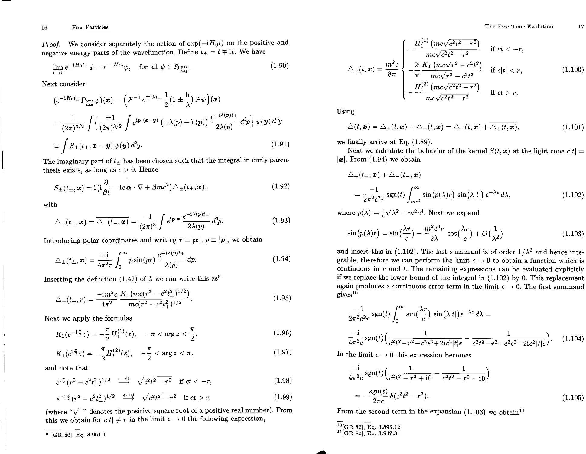
Proof. We consider separately the action of exp(— iHot) on the positive and
negative energy parts of the wavefunction. Define = t ie. We have
lim	= e	for all ib 6 Sj ₽»•.	(1.90)
c->0	nes
Next consider
1 r f -Li г	gT‘A(p)t± i
= J { J e”""’(±Aw + hw) “ад- Лв)
= / S±(t±,x - y)tf(y)d3y.	(1.91)
The imaginary part of t± has been chosen such that the integral in curly paren-
thesis exists, as long as e > 0. Hence
S±(t±, ж) = i(ij^ - ica • V + (3mc2)A±(t±, ж),	(1.92)
with
_________________________ _i f . e-‘A(p)t+
J	<L93)
Introducing polar coordinates and writing r = |ж|, p = |p|, we obtain
zpi f°°	eyiA(p)t± =	,>S“,W A(p) *	(1-94)
Inserting the definition (1.42) of A we can write this as9	
л p x -im2c K^mc^r2 - c2!2.)1/2)	(1.95)
+ +’Г	4тг2	mc(r2 — c2!^)1/2	
Next we apply the formulas	
K^e^z) =-^H^z),	-7r<argz<^,	(1.96)
K^e^z) =	-^<argz<7r,	(1-97)
and note that	
e1? (r2 — c2!^.)1/2 —y/c2!2 —r2 if ct < — r,	(1.98)
e'1? (r2 - c2!^.)1/2	y/c2!2 — r2 if ct > r,	(1.99)
(where “aA ” denotes the positive square root of a positive real number) this we obtain for c\t\ ф r in the limit e —► 0 the following expression,	. From
9 [GR 80], Eq. 3.961.1
The Free Time Evolution
17
A+(t, ж)
m2c
8tt
Using
(mcy/c2t2 — r2)
mc\/c2t2 — r2
2i Ki (rnc\/r2 — c2t2)
я- mc\/r2 — c2t2
(mc\/c2t2 — r2)
mc\/ c2t2 — r2
if ct < —r,
if c|t| < r,
if ct
A(t, ж) = A+(t, ж) + A_(t, ж) = A+(t, ж) + A+(t, ж),
(1.100)
(1.101)
we finally arrive at Eq. (1.89).
Next we calculate the behavior of the kernel S(t, x) at the light cone c|t| =
|®|. From (1.94) we obtain
A+(t+, ж) + A_(i_, ж)
—1	Г°°
= 27r2c2r sSnW J 2 sin(p(A)r) sin(A|t\) e“Ae dX,
(1.102)
where p(A) = |л/А2 - m2c4. Next we expand
• / /хч \	• Лг\ m2c3r ,Ar,
sin(p(A)r) = sin( —) -	cos( —) +
1
A2
(1.103)
and insert this in (1.102). The last summand is of order 1/X2 and hence inte-
grable, therefore we can perform the limit e —► 0 to obtain a function which is
continuous in r and t. The remaining expressions can be evaluated explicitly
if we replace the lower bound of the integral in (1.102) by 0. This replacement
again produces a continuous error term in the limit e —> 0. The first summand
gives10
-1
2тг2с2г
e-Ae dX =
о
1
1
-i	(	1	1	M
4A SgnW \c2t2 —r2 —c2e2 + 2ic2|t|e “ c2t2-r2-c2e2-2ic2|t|e / ’	(L1°4)
In the limit e -> 0 this expression becomes
4тг2с g ( ) (c2t2 — r2 + iO c2t2 — r2 — io)
2тгс 1
From the second term in the expansion (1.103) we obtain11
(1.105)
lo[GR80], Eq. 3.895.12
U[GR 80], Eq. 3.947.3
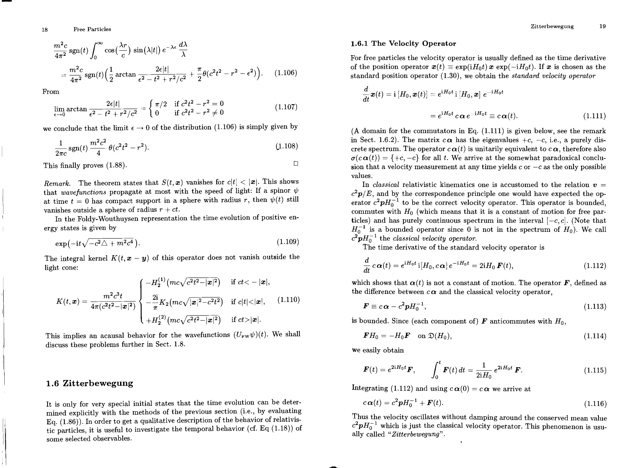
18
Free Particles
cos(t) sin(Al*l)e At T
= SgnW (I arCtan e2 - t2 + r2/^ + ^(C^2 ~r2~ g2)) • (1’106)
From
i- < 2el^l Г тг/2 ifc2i2-r2 = 0	/1107'1
c—>0	e2-t2 + r2/c2	[0 if c2t2 - г2 ± 0
we conclude that the limit e —► 0 of the distribution (1.106) is simply given by
—sgn(t) ——t?(c2t2 — r2).	(l-WS)
Z7TC	4
This finally proves (1.88).	□
Remark. The theorem states that S(t,x) vanishes for c|t| < |ж|. This shows
that wavefunctions propagatё at most with the speed of light: If a spinor -0
at time t = 0 has compact support in a sphere with radius r, then 0(t) still
vanishes outside a sphere of radius r + ct.
In the Foldy-Wouthuysen representation the time evolution of positive en-
ergy states is given by
exp (—it \/—r^A + m2c4 ).
(1.109)
The integral kernel K(t,x — y) of this operator does not vanish outside the
light cone:
' (mcy/c2t2 — \x\2^
. m2cit	2i	_______
K{t'X} = 4ir(c2t2-\x\2) j -~K2(mc^\x\2-c2t2)
I +H^ (mcy/c2t2 — \x\2)
if ct< — |ж|,
if c|t|<|ж|,	(1.110)
if ct> |ж|.
This implies an acausal behavior for the wavefunctions (I7FW0)(t). We shall
discuss these problems further in Sect. 1.8.
1.6 Zitterbewegung
It is only for very special initial states that the time evolution can be deter-
mined explicitly with the methods of the previous section (i.e., by evaluating
Eq. (1.86)). In order to get a qualitative description of the behavior of relativis-
tic particles, it is useful to investigate the temporal behavior (cf. Eq (1.18)) of
some selected observables.
Zitterbewegung
19
1.6.1 The Velocity Operator
For free particles the velocity operator is usually defined as the time derivative
of the position operator x(t) = exp(ifl’ot) x exp(—iHgt). If x is chosen as the
standard position operator (1.30), we obtain the standard velocity operator
^rx(t) = i [H0,x(t)] = elHoti [Я0,ж] e ,H,,t
at
= ca e iHat = ca(t).	(1.111)
(A domain for the commutators in Eq. (1.111) is given below, see the remark
in Sect. 1.6.2). The matrix ca has the eigenvalues +c, —c, i.e., a purely dis-
crete spectrum. The operator ca(t) is unitarily equivalent to ca, therefore also
cr(ca(t)) = {+c, —c} for all t. We arrive at the somewhat paradoxical conclu-
sion that a velocity measurement at any time yields c or — c as the only possible
values.
In classical relativistic kinematics one is accustomed to the relation v =
c2p/E, and by the correspondence principle one would have expected the op-
erator c2pHg1 to be the correct velocity operator. This operator is bounded,
commutes with Hq (which means that it is a constant of motion for free par-
ticles) and has purely continuous spectrum in the interval [—с,с]. (Note that
Hg1 is a bounded operator since 0 is not in the spectrum of Hg). We call
c^pHg1 the classical velocity operator.
The time derivative of the standard velocity operator is
ca(t) = elHot i[H0, ca] e-1Hot = 2iH0 F(t),	(1-112)
which shows that a(t) is not a constant of motion. The operator F. defined as
the difference between ca and the classical velocity operator,
F = c a — c2pHg 1,	(1.113)
is bounded. Since (each component of) F anticommutes with Hg,
FH0 = —H0F on Э(Я0),	(1.П4)
we easily obtain
/•t	1
F(t) = e21HotF, / F(t) dt = —— e2iHot F.	(1.115)
Jo	2ilfo
Integrating (1.112) and using ca(0) = ca we arrive at
ca(t) = c2pHg1 + F(t).	(1.116)
Thus the velocity oscillates without damping around the conserved mean value
c2pHg1 which is just the classical velocity operator. This phenomenon is usu-
ally called “Zitterbewegung”.
20
Free Particles
1.6.2 Time Evolution of the Standard Position Operator
The formal time derivative of x(t) in Eq. (1.111) implies
x(t) = x + f ca(t)dt.	(1.117)
Jo
Here the second summand is bounded for all finite t and thus 2) (®(t)) = £>(®)
by a standard perturbation theoretic argument. This heuristic argument is
made precise in the following theorem. We mention that in nonrelativistic quan-
tum mechanics the domain of x is not invariant under the free time evolution.
Theorem 1.3. The domain £>(a:) of the multiplication operator x is left in-
variant by the free time evolution,
2>(a:(t)) =e-'Hot^)(x) = Э(ж).	(1.118)
On this domain we have
x(t) = x+c2pH01t + ~ (e2lH°‘-l) F.	(1.119)
21л0
Proof. Formally, (1.119) is easily verified by differentiating it with respect to t,
which gives (1.116) in accordance with (1.111). The integration constant comes
from the condition ®(0) = x.
In order to prove the invariance of the domain we consider the regularization
*> s i+Тн A A °-	<L12(4
For A > 0, xx is a bounded multiplication operator which is defined everywhere
in the Hilbert space. A vector 0 is in the domain of x if and only if ||®д0||
remains bounded uniformly in A, as A —> 0.
Since also the derivative of X\ is bounded, we have ж д-0 €	whenever
0 € S(H0). On these states we can evaluate the time derivative of Xx(t),
xx(t)ip = e+'Hot i[H0,xx]e~lHot ip, for 0 e D(H0).	(1-121)
at
But the commutator extends to a bounded operator on all of f). Integrating
from 0 to t and taking the norm gives for all 0 6 0 and A > 0,
||a:A(t)0|| = ||жде“1Яо‘0||
Jo 11	1 + Ala:l	11
If, in addition, 0 is in the domain of x, then the right hand side remains
bounded uniformly, as A —► 0. Hence also exp(-iH'ot)0 is in the domain of x.
From this the equality of 2)(ж) with exp(—iH'ot)2)(a:) follows immediately. □
Zitterbewegung
21
Remark. Eq. (1.111) makes sense if applied to vectors in the domain of the
commutator [До, ®(t)]• We show that the set
Э	СЭ(®)ПЭ(Я0)	(1.123)
is dense, invariant under the free time evolution, and [Яд, ®(t)] is well defined
on 2). If 2) were not dense, then there would exist a nonzero vector f € Sj for
which
0 = (/,Я0“7) = (Яо“7,-0), а11^б2)(®).	(1.124)
Since 2)(®) is dense, (1.124) implies Hq1 f = 0 and hence f = HqHq1/ = 0.
This is a contradiction, therefore 2) is dense in Sj. The inclusion 2) С 2)(®) is
most easily seen in momentum space. Let -0 6 2)(®), i.e., J-ip 6 2)(VP). From
7-а:Я0 7 = iVph(p)-1	(1-125)
we find 6 2)(®), because the derivative with respect to p of
b(p)-. =	+	(1.126)
v 7 c2p2 4- m2c4
is bounded. This implies 2) С 2)(®) and hence 2) С 2)(®) П 2)(Яо), because the
inclusion 2) С 2)(Яо) is trivial. Finally, it is easily seen that the commutator
[Яд,®(t)] is well defined on е_1Яо*Я^“12)(®) = 2). On this domain the com-
mutator can be evaluated to give ca(t). Since the result is bounded, it can be
extended uniquely to all of
1.6.3 Evolution of the Expectation Value
Due to the third summand in (1.119) the expectation value of x(t) contains an
oscillating part We can show that this oscillation tends to zero, as t —> с».
Writing (Я8р^)(Л) = g(X) we obtain
1	1
MO =	, X777- e2iHotF^ = (ад , — e2iAt UspF^)
Z1A
= [ e2iAt £ (9iW , {U^FU-^sMX) )g dx, (1.127)
Jo-(Ho) 21Л	i=1>2
which is the (inverse) Fourier transform of an integrable function of Л. The
Riemann Lebesgue-Lemma implies that z^(t) is a continuous function of t,
vanishing as t —> oo.
The Zitterbewegung is a consequence of the negative energies. Since F
anticommutes with Ho we obtain
FFpo. = P„e8 F.	(1.128)
neg	pos	\	/
Therefore the bounded operator F maps the positive energy subspace into the
subspace of negative energy and vice versa, in particular, PposFPpos = 0. For
22
Free Particles
any state i[>pos g fjpos, which is also in the domain of x, we can form the
expectation value
(V’posG)’ ® 0pos(O) = (V’pos;-fpos®(^)-fpos V’pos)>	(1.129)
and see, that it performs no Zitterbewegung at all. A similar conclusion holds
for the negative energy states. We summarize our results in the following the-
orem.
Theorem 1.4. The expectation value of x in the state 0(t) = е~1Н°*ф, where
0 € Э(ж), is of the form
(0(t),®0(t)) = (0, {x+	+ (0,с2рЯо-1 l/))t + z^t),	(1.130)
21Ло
where z^(t), given by (1.127), is continuous in t and vanishes at infinity. If 0
is an initial state with positive (negative) energy, then the expectation value of
x in the state 0(t) performs no Zitterbewegung at all. In this case we have
(0(t), ж 0(t)) = (0, ж0) + (0,с2рЯо-1 0) t, 0 G fjpos or fjneg. (1.131)
The velocity of a negative energy particle is always antiparallel to its momentum
because (?рН^1'фпеъ = -c2p |Яо|_10пе8.
1.6.4 Evolution of Angular Momenta
We want to stress that not only x(t') shows the phenomenon of Zitterbewegung.
It is present also for example in the angular momentum operators L and S. A
little calculation shows that
L(t) = ®(t) л p = L + —лP’	(1-132)
21Ло
S(t) = ~a(t) A a(t) = S- ^V(e2iHot - 1)F A p.	(1.133)
Thus we see that orbital and spin angular momentum are not conserved because
of Zitterbewegung. In the sum J = L f S, however, the time-dependent terms
cancel, and we obtain the important result
J(t) = J,	(1.134)
which can be also verified directly from
[J,Ho]=O.	(1.135)
Zitterbewegung
23
1.6.5 The Operators F and G
Eq. (1.116) gives the connection of the а-matrices with the classical velocity.
We now give a similar relation for the Dirac matrix /3 in order to shed some
light on its physical meaning. We first calculate
i[#o,/3] =2i#0G,	(1.136)
where
G = ^-^2.	(1.137)
no
G is a bounded operator which again anticommutes with Hq, i.e.,
GH0 + H0G = 0 on Э(Я0).	(1.138)
G maps .f)pOS onto f)neg and vice versa. We see that
G(t) = e2iH(J<G, [ G(t) dt = -Д- e2iHot G.	(1.139)
Jo	2iffo
Therefore, also /3 performs a Zitterbewegung,
ТПС2
/3(t) = — +G(t).	(1.140)
-«о
The operator G describes the difference between the Dirac matrix (3 and the
operator corresponding to the classical expression
The operators F and G are closely related. From H2 = c2p2 + m2c4 we obtain
the relation
F-p + mc2G = 0	(1.142)
(i.e., the free Dirac operator is not changed if we replace ca by с^рНц1 and /3
by m^HQ1). We finally note the relations
1 - a • F + f3G = 3,	(1.143)
„2	m2c4 c2p2	F2 G	HS -	~3 <-	(1.144)
24
Free Particles
1.7	Relativistic Observables
The results of the previous section present some interpretational difficulties
which we try to overcome by choosing different sets of operators for the ob-
servables of the theory.
1.7.1 Restriction to Positive Energies
The Zitterbewegung is mathematically well understood but presents some dif-
ficulties for the interpretation of the theory. Why should a free relativistic
particle violate Newton’s second law? The origin of this difficulty might well
be that the choice of relativistic observables in Sect. 1.3 has been incorrect.
We have chosen the standard position operator x because of its simplicity.
But now we have learned that x mixes up positive and negative energy states
in a very complex manner. This effect is the origin of the Zitterbewegung. It
would be absent if there were only positive (or only negative) energies. Also
the electron-positron interpretation in Sect. 1.4.6 suggests to consider the pos-
itive and negative energy subspaces separately, 5jpos for electrons, and f)neg
(or better CTjneg, see Eq. (1.82)) for positrons. Therefore it seems to be more
natural to represent observables by operators which do not mix positive and
negative energies. So we try to replace x by the part x which leaves fjpos and
f)neg separately invariant. A little calculation shows that
SE =: Ppos*rEpos “b Pneg®Pneg ® tt F'	(1.145)
21Л0
x is obtained from x by subtracting
Fpos®-Pneg + Pneg®-Ppos =	F	(1.146)
21Ло
This is a bounded operator and hence x is self-adjoint on ®(i) = ®(a:). From
(1.111), (1.115) and (1.116) it is clear that on this domain (cf. Theorem 1.3 in
Sect. 1.6.2)
i(t) = x + c'^pH^t.	(1.147)
Hence the corresponding velocity is just the operator expected from classical
relativistic mechanics. From (1.145) it is also clear that x satisfies the canonical
commutation relations with p, since p commutes with (2iHo)~1F'.
In the same way one could restrict also the other operators which mix the
spectral subspaces:
cd = c2pH0'1,	(1.148)
0 = mc2Ho\	(1.149)
L = L--~F'p,	(1.150)
Relativistic Observables
25
S = S + -Д-F Ap = -\<?Ff\F.	(1.151)
2Шо	4
Tn (1.151) we have used the relation
8,-1„Д<>=-АГЛР + Хрлр.	(1.152)
Of course the operators Ho and p commute with the projectors Ppos and Pneg,
hence p = p, and
Ho = Ho = \/c2p2 + m2c4 Ppos - \/c2p2 + m2c4 Pneg.	(1.153)
From (1.150) and (1.151) we see that also J = J = L + S, as expected.
1.7.2 Operators in the Foldy-Wouthuysen Representation
The operator x has the interesting property that its components do not com-
mute,
c2 -
=-i-^2^,	(1.154)
where (г,к,Г) is a cyclic permutation of (1,2,3). Eq. (1.154) is very unfa-
miliar for position operators. It implies that localization in a finite region is
not a meaningful concept any longer (see Sect. 1.7.3). There is, however, an-
other position operator leaving f)pos and f)neg invariant, which has commut-
ing components and time derivative с2рЯ0-1. This is the so called “Newton
Wigner position operator” xNW. It can be obtained most easily in the Foldy-
Wouthuysen (FW) representation (cf. Sect. 1.4.3). Let x denote, as usual, the
operator of multiplication by x (acting now in the Hilbert space of the FW-
representation). We define the Newton-Wigner position operator to be the in-
verse FW-transformation of x
®nw = UFW xUp-^/.	(1.155)
We see immediately that the components (xNW)i commute with each other and
that the positive/negative energy subspaces are left invariant by ®NW, since
[®nw,Ppo.] = U^{x,±(l±0)]Uvw =0.	(1.156)
Similarly, we obtain for the time dependence
®NW(t) = ®NW + c2pH0lt.	(1.157)
A less agreeable feature of the Newton-Wigner operator is its explicit form in
the standard representation, which is obtained from (1.155) and (1.57) after
some calculation.
0	/	C2	\	c2
2iA ('“ " W^3)<“  p’p) - A(A + me=)S ''» <1168»
26
Free Particles
where A = (c2p2 + m2c4)1//2. Of course we can also define other observables
first in the FW-representation and then transform them to the standard rep-
resentation.
The following list gives the FW-representation of some important operators.
For any observable A we denote APW = UFVJ AU~„.
Pfw = P,	(1.159)
(B"0)fw = 0\/ c2p2 + m2c4,	(1.160)
(Ppo.)FW = |(l±0),	(1.161)
e о |-< 1 II s b e	(1.162)
0 c p F FW —	,	0(?FW5	(1.163)
A + mr	
1	c2	
XFW — x 1 „. Ц Epw . z.	21	P> 2iHfW	A(A + me2)	(1.164)
«S'fW ~~ S* (®FW	P)	(1.165)
^FW = ®FW Py	(1.166)
J FW = J у	(1.167)
(®nw)fw ==	(1.168)
1.7.3 Notions of Localization
There are several possible choices for position operators, each having attrac-
tive features but also disadvantages. So it seems worthwhile to describe some
requirements which are often regarded as fundamental for any position observ-
able. We consider a single particle and assume (at least for the moment) that
it can have the property of being localized in some subset В of R3. If this prop-
erty is indeed observable, then for each region В there must be a self-adjoint
operator E(B) in the Hilbert space of that particle which describes the two
possibilities of being localized either within В or outside B. Thus E(B) should
only have the eigenvalues 1 (“within B”) and 0 (“outside B”). An operator
E(B) with these properties must be a projection operator. Indeed, any observ-
able which describes whether or not a physical system has a certain property,
is a projection operator.
Our requirements are the following:
1.	For every (Borel-measurable) set В C R3 there is a projection operator
E(B) such that (-ф,Е(вуф) is the probability of finding the particle in B, if it
is currently in the state -ф, HV'II = !• The particle must be somewhere, hence
B(R3) = 1.
(1.169)
Relativistic Observables
27
2.	If the system is at the same time localized in Bj and in B? then it is localized
in Bi П В2,
E(Bi ПВ2) = B(B!)B(B2) for all Bj and B2.	(1.170)
3.	The range of E(Bj U B2) is the subspace of states which are localized in
Bi U B2. This subspace should be spanned by the vectors in E(Bj) and those
in B(B2). Hence
B(BiUB2) = B(Bi) + B(B2)-B(BinB2) for all Bi and B2. (1.171)
If Bi, B2, ... are disjoint then
B(B1 UB2U...) = ^B(Bi).	(1.172)
1=]
4.	Let U(a, R), a e R3, R 6 SO(3), be a unitary representation (Sect. 2.2.4) of
the (covering group of the) Euclidean group in the Hilbert space of the particle.
For any Borel set В in R3 the set denoted by RB + a is obtained from В by a
rotation R and a translation with the vector a. Then
E(RB + a) = U(a, R)E(B)B(a, R)*.	(1.173)
If E(B) satisfies the requirements 1-4 above, then it is the spectral measure of
a unique “position” operator q = (91,92,93). We can define spectral families
Eqi(X) = E({x € R3 I Xi < A}) and the operators
qt= [ XdEg.(X), i=l,2,3.	(1-174)
«/ —00
From (1.170) it is clear that
Bqi(A)BQfe(A) = BQfc(A)B9i(A), i,k= 1,2,3,	(1.175)
i.e., the components of q commute. Conversely, for any position operator with
commuting components we can define E(B) = x(qEB) via the spectral theo-
rem. Here x denotes the characteristic function of B.
A spectral measure on R3 cannot be associated with the operator x of
(1.145) because its components do not commute. According to this operator
the notion of “localization in a region B” has no clear meaning.
For the standard position operator E(B) = x(x € B) is simply the operator
of multiplication by the characteristic function of the set В and hence the
requirements 1-4 are trivial (cf. Sect. 1.3.2).
(ф,Е(В)-ф)= [ \^(x)\2d3x	(1.176)
J в
is the probability for finding the particle in B. According to this notion of
localization a particle is localized in В if and only if its wavefunction -ф vanishes
almost everywhere outside B.
28
Free Particles
For the Newton Wigner operator ®NW, the spectral measure
E(B) =	6 B) = x(x & B) UFVI	(1.177)
satisfies 1-4 because these statements are not affected by the unitary transfor-
mation U~^. If (i/>, Е(Вуф) = 1, then the particle is localized in B, but this
does not mean that the wavefunction ip has to be localized in B. There is a
remarkable theorem of Newton, Wigner and Wightman, which we state here in
the form needed for the Dirac theory.
Theorem 1.5. Let q = (q-L,q2,qs) be a set of self-adjoint operators in f) =
L2(K3)4 such that E(B) = x(Q € B) fulfils requirements 1-4 and in addition
5.	Bq(B) leaves fjpos and fjneg invariant, i.e.,
Eq(B)Sj pos С pos •	(1.178)
' neg	neg
Then q is the Newton Wigner operator.
Therefore, if “localization in a region B” is a meaningful concept, then the
theorem above is a strong argument in favor of the Newton Wigner operator.
There are, however, some a priori arguments against the possibility of a strict
localization in a region for particles with a definite sign of energy. These are
considered in the next section.
1.8	Localization and Acausality
The restriction to operators leaving the positive/negative energy subspaces
invariant solves the problem of Zitterbewegung. But there is another, more
subtle difficulty. This is the localization problem.
1.8.1 Superluminal Propagation
The Einstein causality requires a finite propagation speed for all physical par-
ticles. Indeed, any solution of the Dirac equation (1.10), whether it has posi-
tive energy or not, cannot propagate faster than with the velocity of light (cf.
Sect. 1.5). On the other hand, in the Foldy-Wouthuysen representation, we ex-
pect a possible superluminal spreading of the wavepackets in the corresponding
Hilbert space UFV/Sj. Thus, if we take the Newton Wigner operator (which is
just multiplication by x in the FW-representation) as a position observable,
then we have to live with an acausal propagation of initially localized particles.
This problem, which we already mentioned in Sect. 1.5, comes with all position
operators commuting with the sign of energy. This is the content of the next
theorem.
Localization and Acausality
29
Theorem 1.6. Let Sj be a Hilbert space. For every Borel set В С K3 let F(B)
be a bounded, self-adjoint operator in fj such that for all ф 6 Sj with = 1,
Р(В)ф) is a probability measure with the following properties:
i) (ф, Р(В)ф) = 1 and (</>, F(B)</>) = 0 implies (0, ф) = 0.
ii) There is a self-adjoint operator p (the generator of space translations) such
that for all a 6 R3
(e-ip'“ ф, F(B + a) e~ip a ф) = (ф, Е(В)ф).	(1.179)
Furthermore, define H = A(p), where Л is a continuous function, positive, and
not identically constant. Let ф 6 Ф with = 1.
Then for all nonempty open sets В С K3 and for all e > 0 there is a time
t € (0, e) such that
(e“iHt^, Р(В)е~1Н1ф) 0 0.	(1.180)
Proof. We give an indirect proof. Assume that
ф , F(B) e~iHt ф) = || F(B)1/2 e~iHt ф ||2 = 0	(1.181)
for all t € (0,e). From (1.181) we see that F(B) e~'Hi ф = 0. Next define for
arbitrary ф e Ф the complex function
g(z) = (0, F(B)e~iHz ф) = (фв , e~iHz ф),	(1.182)
where фв = Р(В)ф. Since
^-g(z) = -i[ Xe~iXz d(j>B ,Ен(Х)ф)	(1.183)
Jo
exists for Im(z) < 0, g is analytic in the lower half plane. Since moreover g is
continuous by the strong continuity of exp(— iHz), we can apply the Schwarz
reflection principle, g can thus be analytically continued to a holomorphic func-
tion on C. Since it is zero on the interval (0, e) of the real axis, it must vanish
everywhere,
g(z) = 0 for all z e C.	(1.184)
Now for all ф satisfying (1.181) and all ф e Ф we have
(Фв,х(а < H < ЪУф) = -^L= [dtg(t)x(t) = 0,	(1.185)
V 2тг J
where x(t) is the Fourier transform of the characteristic function of the interval
(a,b). Thus F(B)x(a < H < Ь)ф = 0. Now let B' be an open subset of В such
that the distance d of the boundaries of В and B' is nonzero. We have for
|a| < d
F(B') e~'ap x(a<H<b) ф = e~ia p F(B'-a) х(а<Н<Ъ) ф = 0,	(1.186)
30
Free Particles
since В' a с B. Next we consider for all a € K3 the function
h(a) = (фВ’,е~[арх(а < H <Ь)-ф)
= У e~'aq x(a < A(q) < b) d^B., Ep(q)i/>) = Jeiaq dp(q), (1.187)
where Ep(q) is the spectral family of p. The support of the measure dp(q) is
contained in {q e K3 | a < A(q) < b} which is compact. According to the Paley-
Wiener-Schwartz theorem, it’s Fourier transform h(a) is an analytic function.
Since h(a) = 0 for |a| < d, we have h(a) = 0 for all a. Choose a partition of
the interval [0, oo) into subintervals A^) of finite length. Then
(0, F(B') e~iap 0) = (0b- , e~iap £ x(Afe-i < H < Afe) 0) = 0,	(1.188)
for all ф and a. Hence we must have F(B' — a) 0 = 0 for all a, which is only
possible for 0 = 0.	□
In the Hilbert space = fjpos the assumptions of the theorem are easily verified
for F(B) = x(®nw € B) (the spectral measure of the Newton-Wigner operator)
and A(p) = (c2p2 + m2^)1/2. The generator of translations is the momentum
operator p = —iV, we have e,p a ®NW e~ip a = ®NW+a. Assumption i) is implied
by (1.170), ii) by (1.173).
1.8.2 Violation of Einstein Causality
Let us discuss a special case of Theorem 1.6. Take F(B) as the spectral measure
of some position operator in Sj = fjpos. As we have discussed in Sect. 1.7.3 there
are states 0 G Sj, ||0|| = 1, satisfying (0,F(B)0) = ||F’(S)0jj2 = 1, because
F(B) is a projection. One calls these states “localized in B”. Now, take a state
0 localized in a proper subset Bq of R3. Let В be another subset located far
away from Bq. If d is the distance between Bq and В then we would expect
that 0 is localized outside В at least for the time d/c (the time a light signal
needs to get from Bq to B). But the probability of finding the system in В at
time t is just given by (1.180), if H is the Hamiltonian of the system. Since this
probability is nonzero for some arbitrarily small t, we have to admit that the
system has a (small) probability of getting from Bq to В in an arbitrary short
time, thereby propagating with a superluminal speed.
Of course we expect the effects of this “instantaneous spreading” to be im-
measurably small in physically reasonable situations. Nevertheless, we cannot
neglect it in a discussion of localization properties because according to our
quantum mechanical interpretation the accuracy of measurements of one single
observable is not limited a priori. We may conclude that the notion of local-
ization as defined, e.g., in Sect. 1.7.3 is in contradiction to the principles of the
theory of relativity.
Localization and Acausality
31
1.8.3 Support Properties of Wavefunctions
If we restrict the operator x(x e B) as in Sect. 1.7.1,
x(x e B) = Ppos e B) Ppos + Pneg e B) Pneg,	(1.189)
then the result would not be a projection operator because x(x e B)2 x(x €
B). Consequently, x(x £ B) is not the spectral measure of any self-adjoint
operator. We have
x(® € B)V>) = [ {Hpos(®)!|2 + Нпее(®)||2}^,	(1.190)
which in general is different from fB с/3ж||'0(ж)||2, unless В = К3. However,
(^ро5,х(® e BjV’pos) = / IIV’post®)!)2 d3x,	(1.191)
J в
and similar for i/)neg. Therefore, also x(x € B) satisfies the assumptions of the
theorem.
Now, assume that (ippos, x(® € B)ippos) = 1 for some proper subset В of R3.
Because of (1.191), i/)pos vanishes almost everywhere outside of Bq. According
to the Dirac equation the wavefunction ippos spreads according to
^poS(t,x) =[ S(t,x - y)V’pos(y) d3y	(1.192)
(Z7Tp'z JR3
with finite speed, because the integral kernel S is zero for |a? — y| > c|t|.
This is clearly a contradiction to the infinite propagation speed required by
Theorem 1.6.
Therefore it is impossible for a wavefunction with positive energy to be
initially localized in a proper subset of R3. Any wavefunction with positive
energy has to be spread over all of space for all times. Of course, a similar
consideration is also valid for ipnei. Thus we have proven
Corollary 1.7. Let ip be an arbitrary state in fjpos (or fjneg). Then
supp(-0) = closure of {x £ R3 | i/,(ac)	0} = R3.	(1.193)
Part of this corollary can easily be shown directly. Pposip = ip implies for
the Fourier transform ф = Рф of any positive energy wavefunction a relation
between upper and lower components, namely
fфз (p) A = c<tp (<Mp)\	(1194>.
\04 (p) /	\/c2p2 + m2c4 + me2 \02 (p) /
Now if ф had support in a compact subset Bo of R3 then, according to the Paley-
Wiener-Schwartz theorem <p4,..., ф4 all had to be entire analytic functions in
p, which is impossible because of the square root in (1.194).
32
Free Particles
1.8.4 Localization and Positive Energies
We may summarize the results obtained so far as follows. If we choose fjpos to
be the Hilbert space of a free electron the observables have to be represented by
operators which leave this Hilbert space invariant. Then there are essentially
two possibilities:
a)	We can retain the interpretation of as a position probability density
even after restriction to the positive energy subspace. But then the position
is not a quantum mechanical observable in the usual sense. This is because
by Corollary 1.7 there are no strictly localized states and consequently
there is no self-adjoint operator in fjpos whose spectral measure is related
with the position probability. The probability of finding the particle in a
set В is still a well defined concept, although there are no states for which
this probability is 1 if В K3.
b)	On the other hand, we could insist on a quantum mechanical position
observable (i.e., a self-adjoint operator which leaves fjpOs invariant). But
then we have to face the violation of Einstein causality as predicted by
Theorem 1.6.
Obviously, for particles with positive energy there is no possibility of having a
relativistic notion of position, which is analogous to the nonrelativistic concept
and satisfies the causality requirements of a relativistic theory.
Fortunately, to most of the mathematical results obtained below — as well
as to practical measurements — it seems to be irrelevant which interpretation
is preferred. For the purpose of this book we keep calling (?/)(яг)|2 a position
probability density.
Difficulties with the strict localization of an electron are not quite unex-
pected. Restricting an electron to a finite region, which is necessary in order to
prepare a localized state, would require an infinite potential barrier and thus a
lot of energy so that pair production is likely to happen. But this effect cannot
be described by the Dirac equation alone.
1.9 Approximate Localization
For most purposes in quantum mechanics the strict localization properties are
irrelevant. It is often sufficient to specify an approximate localization region and
to estimate the probability of finding the particle outside. The mathematical
results of this section will be needed for Chapter 8.
Approximate Localization
33
1.9.1 The Non-Stationary Phase Method
The time evolution of a free particle with positive energy A(p) = ->/c2p2 + m2c4
can be written as
f	^(p)d*p
= (5^572 /
where we have introduced
ш =	+ c|t|, ф(р) = (x  p - A(p) t).
(1.195)
(1.196)
В We want to estimate (1.195) for large values of |®| and/or |t|. Note that the
Ж estimate |</>(p)| < 2A(p)/cis independent of w. If w is very large, small variations
Ж of p will eventually cause the exponential function exp(icu</>(p)) to oscillate very
S rapidly, so that due to frequent cancellations there is only a small contribution
to the integral. Only in the neighborhood of points with V</>(p) = 0 (“points of
I stationary phase”) the function ф changes slowly with p and hence there are no
f oscillations. For large w, the main contributions to the integral come from these
! points. If we want the integral to decay with increasing w, we have to exclude
t. these points by requiring that V</>	0 on supp</>. The following theorem makes
к these ideas precise.
e Theorem 1.8. Let К be a compact subset of Rn, and ф : Rn —-> R be к + 1
Г times differentiable on a neighborhood of K, with |V0| > e > 0 on K. Let ф
s be к times differentiable with suppi/ С K. Then there exists a constant C,
I' depending on г, ф and ф, such that for arbitrary w e R
J 1У* eiu^(p4(p)d3p| < C(l+M)“r, all r < fc.	(1.197)
Proof. By partial integration we find
[ е^ф(р)сФр=- f	. J^(PL^(p)rf3p
J	|V0(p)[2
= -Л У е1шфЮ (Т>ф) (p) d3p,	(1.198)
where Т>ф = V • (^V0/|V0|2). Repeating this procedure gives
уе^(р’(рг^)(р)а3р.	(1.199)
The function Т>гф is a sum of products of the factors
|V</>r2, Оаф, DPij), where |a| < r + 1, \f3\ < r.	(1.200)
34
Free Particles
We use the multiindex notation, a = (ai,... ,an), where a, are nonnegative
integers, |a| = 52, a,, and
Da = -----------.
9Г1 • •  d^
(1.201)
Since ф and ф are continuously differentiable, their derivatives are bounded
uniformly on K. By assumption, > e on K, hence any finite product of
the expressions (1.200) is bounded on К. We conclude that (1.199) is bounded
by const.M-r- Since the integral is regular for a> = 0, the result follows. □
1.9.2 Propagation into the Classically Forbidden Region
With the help of the preceding theorem we can control the propagation of
the wavefunction ф(х, t). For our phase function ф defined in Eq. (1.196) the
stationary points are given by
(1.202)
9
C p
x — u(p)t = 0, where u(p) = — .
A(P)
Note that u(p) is just the velocity of a classical relativistic particle with energy
A(p). For a particle with negative energy everything is analogous, only u(p) =
—c2p/X(p). Let К be a subset of JR3. The set
{ x e R3 | x/t = u(p) for some p € К }
(1.203)
describes the region in which a particle is localized according to the classical
relativistic kinematics, provided its velocity is in the set
{ и g R3 | и = u(p) with p € К }.	(1.204)
Therefore, the set (1.203) is called the “classically allowed region" for particles
with momenta in K. In the classically forbidden region the condition x/t/
u(p) for all p e suppJE0 avoids the points of stationary phase for (1.195).
Theorem 1.8 states that the wave function decays fast in this region:
Corollary 1.9. Let ф be a wavefunction with Fourier transform ф = Рф €
satisfying
supp2 C {peR3 | 0 < uq < |u(p)| }.	(1.205)
Then for each N > 0 there is a constant C/v depending only on ф such that
|| X(|®| < u0|t|/2) e^iHot ф || < CN (1 + |t|)-N.	(1.206)
Proof. The situation here is different from Theorem 1.8 because the phase
function ф depends also on ш, cf. Eq. (1.196). But for x in the ball |® I < «o|f 1/2
we have
Appendix
35
c|t| < cu < (c + uo/2)|t|,
and hence for p in suppV’,
- И > uo
|®| + c|t |	— uq + 2c
(1.207)
(1.208)
Moreover, </>(p) is infinitely differentiable on suppV> and all derivatives are
bounded uniformly in |t|. Hence the proof of Theorem 1.8 applies to this situ-
ation as well. For |®| < uot/2 and each r we can estimate ?/?(t, ж) by
const const'
(1 + МГ - (i + l< ’
Finally, the estimate
(1.209)
||x(|®| < «оИ/2)е iHot ||2
|x|<u0|i|/2	(Л “i |Я/
proves the corollary.
(1.210)
□
l(W)(p)| >
Remark. If a particle is in a state with minimum velocity larger than w0, then
after some time it will move away from the origin and the points |ж| < u0|t|/2
will belong to the classically forbidden region. According to Corollary 1.9, the
probability of finding the particle in this region decays rapidly in time. This
result is very useful in scattering theory, cf. Chapter 8.
Appendix
l.A Alternative Representations of Dirac Matrices
Most calculations with Dirac matrices can be done without referring to a par-
ticular representation. For some considerations, however, an explicit form is
useful. Here we list the most prominent representations. By a = (er1; <t?, cr3) we
denote the three Pauli matrices
(1-211)
which satisfy the properties
з
{o’ijOfc} = 28ik, [<Ti,CTfc] = 2i ^2 tikmVm-
m= 1
(1.212)
The following matrices are written in 2 x 2-block form, each entry is itself a
2 x 2-matrix.
36
Free Particles
1. Standard (or Dirac-Pauli) representation.
„	/ 1	0 \	7 0	er \	/0 1) “ I 0	- 1 )	’ “	\ er	0 ) ’	75	\ 1 0 )	’	(1.213)
2. Supersymmetric representation. _ A 0	—i \	_ ( 0	t \	f0	1 \ ( i	0 )	’ "s ~ ( er	0 J ’ ('75^s	\ 1	0 J	’	(1.214)
This representation is related to the standard representation via the unitary
matrix
t= —f1 s V2 V V’ i.e., (3S = Ts/37s-1, etc.	(1.215)
3. Weyl (or spinor) representation. oj’ “w3.0 -er J’	-1)’ and the matrix giving the relation to the standard representation is т = —f1 1 "l \/2\1 -1 )	(1.216) (1.217)
4. Majorana representation.
о _ f 0 i\	, ч _ / <7113	0	\ Pm ~ ( i 0 ) ’	— 1 n	I > \—1 " /	\ " —crl,3 /	(1.218)
( \ _	1A ( \ _ / 0	\ (Om)2 - к Q 1 ,	(T5)m - 1	0 1 	(1.219)
Again, the Majorana representation is related to the standard representation
by a unitary similarity transformation with
T ( 1 + ier2 1 - ier2 A \ — I + <T2	1 + cr2 у Sometimes also the representation with /3m replaced by в = (0 A \ 0 a2 1	(1.220) (1.221)
is referred to as the Majorana representation, corresponding to Majorana’s
original choice. In any case, the Majorana representation is characterized by the
fact that the а-matrices are real, while (3 = — /3- Hence, in this representation,
the charge conjugation C can simply be chosen as complex conjugation (cf.
Sect. 1.4.6).
Appendix
37
l.B Basic Properties of Dirac Matrices
{<*;, ak} = 2Sik, {ai, /3} = 0, (32 = 1,	(1.222)
[ai,afc] = 2(a1Qfc - <5ifc) =	(1.223)
0}	4 [ckfc,OiTn] 2	2iSkSm,	(1.224)
where	is a cyclic permutation of (1,2,3),
[Si,Sk] =i£m6ifcmSm, {S2,Sfc} = yik,	(1.225)
OiOfc = 6ik + 2ieikmSm = iSiSk,	(1.226)
5 A A = ±(A- (a- A)a),	(1.227)
(a • A)(a  B) = A  В + 2iS • (A Л B) for any vectors A, B, (1.228)
-iaia2a3=75, (7s)2 = 1,	(1.229)
{7б,Д} =0,	[75,a]=0, 75a = 2S.	(1.230)
l.C Commutators with Hq
We denote
S=~aha, L = x/\p, J = L + S,	(1.231)
К = 0(2S  L + l), Bo = —KS p = --BS  (p Л L — L Лр), (1.232)
me	me
F = ca-c2pH^1, G = /3-mc2H0\	(1.233)
IV = ^(Box + xHo) = Hox + ya = xH0 - ya,	(1.234)
A^-^p-x + x-pH^).	(1.235)
The following formal relations hold on a suitable dense domain, e.g., on
CS°(R3)4.
i[H0,p] = i[H0, J] = 0, i[H0,K] =i[H0,B0] =i[H0,S-p] = 0,	(1.236)
i[H0,a] = i[H0,F] = 2iH0F, i[H0,0] = i[H0, G] = 2iH0G, (1.237)
i[H0,a.;afc] = 2c(akpj - ajpk),	(1.238)
i[H0,L] = -i[H0,5] = —^-FAp,	(1.239)
21/ZQ
i[Ho,®] = oa, i[Ho,ca-x] = 3c2+2iHoF-x, i[H0, x2] = 2ca-x, (1.240)
i[H0,N] = ^(Hoa +aH0) = c2p,	(1.241)
i[H0,A] = (H^a-p + a-pH^1) =c2p2H^2.	(1.242)
38
Free Particles
l.D Distributions Associated with the Evolution Kernel
With A(p) = y/p2 + m2, m > 0, we define
i C . eTiA(p)t
2А(₽Л'	(L243)
l'	A(t,a?) = A+(t,a?) + A.(t,x) =	[eipx	d^p,	(1.244) 1	J	A\P)
।	where the integrals are Fourier transforms of distributions. Furthermore we
define
Aret(t,®) = 0(t)A(t,®),	(1.245)
p	Aav(t,®) =-0(-t) A(t,®),	(1.246)
Ip!	Af (t, ®) = 6»(t) A+(t,®)-ff(-t) A-(t,x),	(1.247)
|H	Af.(t,®) = 0(t) A_(t,®) — 0(—t) A+(t,®).	(1.248)
The tempered distributions A&, where к = ret, av, f, or f*, are fundamental
solutions of the Klein-Gordon equation,
/ Я2	\ -—+ A-m2 Afe(t,x) = ^(t)^(®).	(1.249) \ /
1	For a distribution A(t, x) we define
ЩЕ,р) = J‘ei^Et-px'> A(t,®)d3zdt.	(1.250)
Then
1	&±(E,p) = T2%i 0(±E) ф2 -m2),	(1.251)
I	A(E,p) = T27risgn(E)^(p2-m2),	(1.252)
(L253)
|	A,(£,p)%, J2±.o.	(1.254)
I	Fundamental solutions of the free Dirac equation are obtained from the A’s by
differentiation,
Sk(t,x) = i(i|^ ~ ia ’ + f^m) Ak(t,®), к = ret,av,f,f*,	(1.255)
(i^+ia-V-/3m)sk(t,x) = i6(t)6(x).	(1.256)
The distribution
|	SF(t,x) = -iSf(t,x)/3	(1.257)
Appendix
39
is usually called Feynman propagator (see, e.g., the book of Bjorken and
Drell [BD 64]. Feynman [Fe 61] uses the notation I+(t,x) = — Af(t,®), and
K+(2,1) = 5f(t2 - <i,®2 - ®i)Z?)- As we have seen in Sect. 1.5 the Schrodinger
picture evolution operator is given by the integral kernel
S(t,x) = i(i — — ia • V + A(t,x) = S+(t,x) + S	(1.258)
The distribution Sf(t,x) satisfies
Sf(t,x) = 0(t) S+(t, x) — 0(—t) S-(t, x),	for t 0,	(1.259)
from which we see that it is just the integral kernel of the operator
0(t) e~iHoi Ppos - 0(-t) e~iHot Pne&.	(1.260)
l.E Explicit Form of the Resolvent Kernel
The resolvent (Hq — z)-1 of the free Dirac operator Hq is defined for all
z eC\o-(H0),
((Ho - z) 1 V>)(®) = [ K{x - y,z)^(y)d3y.	(1.261)
The integral kernel К can be obtained from the well known resolvent kernel of
the Laplace operator p2 = — A because
(Ho-z)-1 = (Ho + z)(H02 - z2)-1
= (ca-p +Z?mc2 + z) (p2 -	- m2c2])	.	(1.262)
We find
1	i eife(*)l*l
K\x, z) = — (—ica • V + /Зтс2 + z) ----——
с2	' 4тг |ж|
(zy • x	• T*	\
ic —-у + cfc(z) ——- + ^mc2 + z) -——,	(1.263)
|®|2	|®|	' 4тгс2|а:|
where k(z) = y7z2/с2 — m2c2, and the branch of the square root has been
chosen such that Imfc(z) > 0.
l.F Free Plane-Wave Solutions
For p e K3 with p = (p2 + p2 + Рз)1/2 o and p / p3 we define
40
Free Particles
h_(p) =	1_____( РзP V	(1.264)
\/2р(р~Рз) \P1+W2j
For p = p3 we simply set h+(p) = (J), h_(p) = (°). Then we have
er-ph±(p) = ±ph±(p).	(1.265)
It is obvious from Sect. 1.4.1 that (with a± as in (1.44))
"p°-.±WHUW 1 ( (0)') =	and	(1.266)
^..,±(p) «w-	,) -
are eigenvectors of the matrix h(p) corresponding to the eigenvalues ±A(p),
where A(p) = (c2p2 +m2c4)1^2. Hence
wPo. ,(p,x) = <x>Cos ±(p)elp'x	(1.268)
neg’	neg ’
are generalized (i.e., not square-integrable) eigenfunctions of the free Dirac
operator Ho with positive or negative energy ±A(p). Moreover,
^poS>±(p)ei₽'x-iA(p)t, ^±(р)е^+^,	(1.269)
are “plane-wave solutions" of the Dirac equation.
The functions w are simultaneously eigenfunctions of the “helicity operator"
S-p/p which projects the spin into the direction of the momentum. The helicity
is conserved for free particles, because S  p commutes with Hq. Using (1.265)
we find
S • p
----- Wpo. (p) = I Wpos (p),	(1.270)
P neg ,_r	neg ’"r
S • p	.
---— wpos _(p) = — | wpos _(p),	(1.271)
P neg ’	neg ’
Denoting the projections onto positive/negative helicity by P±, i.e.,
P± = l(l±^-P)	(1.272)
z	p
we can write the Hilbert space as an orthogonal direct sum of four subspaces
f)pO. , = Fpo. P±f).	(1.273)
neg ’	neg
It is clear from (1.49) that the plane-wave solutions can be used to form
square-integrable wavepackets. For example, with f e Z](R3) nZ2(R3),
W,®) = (2^ L eip X“iA(p)t (P) /(P) d3p e f)pos>_ (1-274)
Appendix	41
is a square integrable solution of the free Dirac equation with positive energy
and negative helicity.
If we let the mass m tend to zero, then a±(p) —> 1/-/2, and the w’s be-
come eigenvectors of the “chirality matri'ji' ys = — iaici^as which for m = 0
commutes with the free Dirac operator
#o(m=O) = ca p = 2c755  p, [Ho(m=O), 75] = 0.	(1.275)
*75tt,neg,± “F^neg^,	^)*	(1.276)
2 The Poincare Group
In Chapter 1 the Dirac equation was defined in such a way that it automatically satisfies
the energy-momentum relation as required by classical relativistic mechanics — at least in
a particular inertial frame. According to the principles of relativity, different inertial frames
are related by Poincare transformations (Sect. 2.1). In this chapter we are going to prove
that the Dirac equation — and the quantum theory developed in Chapter 1 — is invariant
under Poincare transformations. This is perhaps obscured by the fact that the position is
represented by an operator, whereas time remains a parameter. After all, this is not quite
in the spirit of the theory of relativity, where space and time coordinates are mixed up by
Lorentz transformations.
A quantum mechanical theory is relativistically invariant if the Poincare group has a rep-
resentation by symmetry transformations. The pure states of a quantum system are uniquely
described by the one-dimensional subspaces (“rays”) of the Hilbert space. The set of all rays
forms a projective space and symmetry transformations are to be defined in this space. Hence
we are looking for a “projective representation” of the Poincar£ group.
By the Wigner-Bargmann theorem any symmetry transformation in the projective space
of states can be described as a unitary or antiunitary operator in the Hilbert space of the
system. The connectedness of the proper Poincare group implies that it has a projective
unitary representation. Antiunitary operators can only appear in representations of the dis-
crete Lorentz transformations (Sect. 2.2). Any unitary representation of a Lie group also
defines a projective representation, but it is not true that a projective representation is al-
ways given by a unitary representation (problem of lifting representations). The analysis in
Sect. 2.4 shows that under suitable assumptions (which we show to be fulfilled for the proper
Poincare group) the projective representations of a connected Lie group can be derived from
the unitary representations of the universal covering group.
A representation of the Poincare covering group is obtained as follows: On the basis of
Chapter 1 it is easy to obtain a representation of the Lie algebra of the Poincare group
in the Hilbert space of a Dirac particle. The infinitesimal generators are simply given by
the Dirac operator, the momentum and angular momentum operators and the center of
energy operator (Sect. 1.3). Exponentiating this Lie algebra representation we obtain with
the help of Nelson’s theorem a unitary representation of the simply connected Poincare
covering group. It is interesting to note that in the Hilbert space of the Dirac electron we
cannot obtain a unitary representation of the Poincare group itself (Sect. 2.3). Nevertheless,
the existence of a unitary representation of the Poincare covering group provides us with the
desired projective representation of the Poincare group and is therefore sufficient to prove
the relativistic invariance of the Dirac theory.
These results motivate a detailed investigation of the Poincare covering group. We de-
scribe its 4-dimensional representations which are most important for the Dirac theory in
Sect. 2.5. It turns out that 4 dimensions are indeed necessary for a linear representation of
the parity transform. In this context the Dirac matrices arise in a natural way.
The Lorentz and Poincare Groups
43
2.1 The Lorentz and Poincare Groups
This is a preparatory section where we define the relativistic symmetry groups
and describe some of their properties which are needed later.
2.1.1 The Minkowsky Space
An “event” is something that happens at a definite time at a definite place
(e.g., the emission of a photon, the detection of a particle, etc.). Events in
space-time are described with respect to an “inertial frame” by coordinates1
x = (ж0, ®)т ё R4, where x = (z1, x2, z3)T are the space coordinates, and
x° = ct is the time coordinate of the event. The factor c denotes the velocity
of light. It gives x° the dimension of a length. The principle of relativity states
that all inertial frames are equivalent for the description of nature. The coor-
dinate transformations I —> I' between all possible inertial frames are called
Poincare transformations.
In the vector space R4 we define the ''‘'Lorentz metric"
{y, x} = y°x° — yrxr — y2x2 — y3x3, all x,y e R4.	(2-1)
The bilinear form (•, •) is symmetric and nondegenerate2, but not positive def-
inite. With the 4x4 matrix
/1 0T \
g=(^) = (fT)=	_13J	(2.2)
(where 0 is the three-dimensional zero column vector) we can write (2.1) in the
form
4
{y,x} = yrgx = д^уцхи.	(2.3)
/i,p=0
The vector space R4 endowed with the Lorentz metric is called “Minkowsky
space".
Remark. With the help of the Lorentz metric we can associate a unique el-
ement y' of the dual space of R4 with a given vector у G R4 by writing
y'(x) = (y,x), for all x. The components of the linear form y' with respect
to the canonical basis in the dual space are (y°, — y1, — y2, — y3). Usually one
denotes by the components of the vector у in the Minkowsky space and by
Ур the components of the linear form y' in the dual space. By the summation
convention one automatically takes the sum over an index which appears twice
in ал expression, once as a lower index and once as an upper index, e.g.,
Ур = gpuyv, {y, x) = y^Xp = УрХц.	(2.4)
1 “T” denotes the transposed of a vector or a matrix. We would like to consider x a column
vector.
2 i.e.f for all у / 0 there exists an x such that (y9 я?)/0.
44
The Poincare Group
2.1.2 Definition of the Lorentz Group
Definition 2.1. A (homogeneous) Lorentz transformation of R4 is a linear map
A : R4—>R4 with
II
I
)
ll
I'
lli
I
I
I
{Ay, Ax) = (y,x) for all x, у e R4.	(2-5)
The elements of the matrix of A are denoted by A^p.
Eq. (2.5) is obviously equivalent to
ZTgZ = g, or A*pgpv AVT = gpT,	(2.6)
which consists of ten independent quadratic equations for the components of
Л, e.g.,
(А)2 - (Л^)2 - (Л20)2 - (Л30)2 = 1.	(2.7)
This implies for all Lorentz transformations
Л°о > 1 or Л°о < -1.	(2.8)
The composition of two Lorentz transformations is again a Lorentz transfor-
mation. We find
1 = —det g = —det ATgZ = —det AT det g det A = (det Л)2	(2-9)
and hence det Л = ±1 for any Lorentz transformation A. Therefore A is in-
vertible and the set of all Lorentz transformations forms a group, the “Lorentz
group''', denoted by
£ = 0(3,1).	(2.10)
I
I
Eq. (2.6) shows that only six of the 16 matrix elements of A can be chosen
independently. Therefore, six real numbers suffice to characterize any Lorentz
transformation uniquely. The set of all Lorentz transformations forms a six-
dimensional manifold. By (2.6), £ is a closed subgroup of the general linear
group and hence is a Lie group. Eq. (2.8) shows that the group manifold is not
connected.
2.1.3 Examples of Lorentz Transformations
Example 2.2	. Rotations. Let R £ SO(3), the group of orthogonal real 3x3
matrices with determinant +1. Then
0T\
R ) ’
(2-11)
is a Lorentz transformation. The rotation R = (Rik) can be most intuitively
characterized by the rotation vector = <pn where the parameter p e [0, тг)
The Lorentz and Poincare Groups
45
specifies the angle of the rotation, and the unit vector n gives the axis (the
sense of rotation is determined by the right-hand rule),
з
Rik = 6ik cos + ПгПк(1 - cos 9?) - eikmnm sin ip.	(2.12)
m=l
The set of all rotations is a subgroup of the Lorentz group. It is obviously
isomorphic to SO(3).
Remark. The group manifold of the Lie group SO(3) is connected, but not
simply connected3. This can be understood as follows. By the association of
<p to each rotation the Lie group SO(3) is mapped homeomorphically to the
ball В with radius тг in R3. However, we must identify antipodal points on
the surface of B, because they correspond to the same rotation. Obviously,
the resulting manifold is connected, but not simply connected, because there
are closed paths which cannot be continuously shrunk to a point. Take, for
example, any diameter joining two antipodal points.
The rotations around a fixed axis form a one-parameter subgroup. If we
choose the rotation angle as the parameter, then the composition of two rota-
tions is described by addition (mod 2тг) of the angles.
Example 2.3	. Boosts. With v e R3 (column vector), v=|v| < 1, define
TH =	(2-13)
Vl —
Then one can check that
(7(11) 7(v)vT \
(2-14)
7(v)v 13 +	/
is a Lorentz transformation. Here (vvT)ifc = ViVk.
Eq. (2.14) describes an “active” velocity transformation in the following
sense. Consider a free classical particle which is at rest in some inertial frame.
Thus for subsequent times ti, <2 it has the coordinates (t 1, ж), (<2, x). The boost
Л applied to these points gives («1,3/1), (-®2,2/2)- Using (2.14) we find that the
velocity of the particle after the transformation is just v.
The subset of boosts is not a subgroup of £, but it forms a submanifold of C.
Nevertheless, the set of boosts in a fixed direction v/|v| forms a one-parameter
subgroup. If we choose the parametrization
v= tanh(cu) v/|v|, cue[0,oo),	(2-15)
then the composition of two boosts with parameters and u>2 gives a boost
in the same direction with parameter cuj + cu2. Similar to the rotation vector
3 [Ch 46], Chapter II, Sects. IV and XI.
46
The Poincare Group
ip we may define a boost vector w = a>v/\v\ g R3. Therefore the manifold of
boosts is homeomorphic to R3 and hence simply connected and noncompact.
For m > 0 define the hyperboloid
MpOS = {p e R4 I {p,p} = m2, p° > 0}
= {(\/p2 + m2, p) e R4 | p e R3 }.	(2.16)
which is usually called the “mass shell”. It contains in particular the point
q = (m, 0,0,0). We associate to each p G Mpos a boost Ap which is uniquely
determined by the condition Apq = p. The transformation Ap is given by (2.14)
where v is uniquely determined by p,
v = , f	P = my(v)v.	(2.17)
y/p2 + m2
Hence the mass shell can be identified with the submanifold of boosts.
Example 2.4	. Discrete transformations. The matrices
/-1 0T\
T =	? i , PT = -14.
\ u I3 /
(2.18)
define the “discrete” Lorentz transformations. P is called “space inversion” or
“parity transform”, T “time reversal”. Together with the 4x4 unit matrix 14
the discrete transformations form a subgroup of the Lorentz group.
2.1.4 Basic Properties of the Lorentz Group
The Lorentz group £ — 0(3,1) is a Lie group with a six dimensional group
manifold consisting of four connected components
= {Я e	£ I Я°о	>	l,detA = +1},	(2.19)
Cl={Ae	C\A°0>	l,detZ= -1} = PC\,	(2.20)
= {Я 6	£ I Я°о	<	1,detя = -1} = T£?+,	(2.21)
£j+ = { A G	£ I Я°о	<	1, detЯ = +1} = PTC\.	(2.22)
The connected component of the identity £\. is a Lie subgroup, called the
proper Lorentz group. It is noncompact, because it contains the subset of boosts
which is homeomorphic to R3. It is not simply connected, because the subgroup
of rotations is not simply connected. Indeed, all group elements of C\. can be
obtained from boosts and rotations: For any A e C\ we can write
Я = Я(и)Я(<р),	(2.23)
where Я(и) is a boost with velocity v and Я(<р) is a rotation with rotation
vector <p. We find
The Lorentz and Poincare Groups
47
v’ = (Л°1,Л02,Л°з)М00,	(2.24)
and a little calculation gives the rotation matrix R in A(<^?) in terms of the
matrix elements of A,
(Л\,
Rik = \ A - (Л°о-1)^оЛ% (е3п=о(л°„)2)
Other Lie subgroups of the Lorentz group are
£+ = 4u4 = SO(3,1), £т = £^и£!.
if v = 0,
if v ф 0.
(2.25)
(2.26)
Remark. The topological properties of £^ are of central importance in quan-
tum mechanics. The multiple connectedness will force us to use representations
of the simply connected covering group (“spinor representations”) and can
be regarded as the group theoretical reason for half-integer angular momenta
(spin-1/2). The noncompactness prevents the existence of nontrivial unitary
representations in a finite dimensional space. As a consequence, the spinor
components of Dirac wavefunctions have to be transformed with the help of
non-unitary matrices.
2.1.5 The Poincare Group
The Poincare group is obtained by combining Lorentz transformations and
space-time translations.
Definition 2.5. A Poincare transformation П = (а,Л), where A e £ and
a e R4, is a mapping from R4 to R4 which is defined as
П(х) = Ax + a.
(2.27)
The set P of all Poincare transformations is a group with the composition law
(ai, Л1)(а2, Л2) — (di + Л1<12, Л1Л2).	(2.28)
Hence the Poincare group P is the semidirect product of the Lorentz group
and the group of space-time translations (i.e., the additive group R4)
P = R4 ® £.	(2.29)
The subgroup of translations is an abelian normal subgroup of P.
Remark 1. The semidirect product of two arbitrary Lie groups (Я, •) and
(T, o) can be defined if there is an action of H on T. We say that a group H
acts on a set T, if for every h E H there is a bijective map Ah'- T^T, which
satisfies
48
The Poincare Group
а)	Ae = idj- (e is the neutral element of W),
b)	Zs(Zh(t)) = Ag.h(t), for all g, h E H, and all t E 7.
Furthermore we assume that each Ah is a Lie group automorphism of 7, i.e.,
c)	Ah' 7—>7 is analytic,
d)	Ah(s ot) = TA(.s) о Ah(t), for all h e Tt, and all s, t e 7.
Then the “semidirect product” of 7 and Ti. is the Lie group 7 0 7Y which as a
set is the cartesian product
7 x H = {(t,h) | t E 7, h 6 H},	(2.30)
and on which the group multiplication is defined as
(s,g)(t,h) = (s ° Aa(t),g • h).	(2.31)
Note that in a “direct product” 7 ® "H one would have the multiplication law
(s, 9) x (L h) = (s ° t, 9 ' h).	(2.32)
Remark 2. The connected component of the identity of P is called the proper
Poincare group
7>J_=R4®ry.	(2.33)
The proper Poincare group is regarded as the fundamental symmetry group of
physics. Different inertial systems are connected by Poincare transformations.
The principle of relativity states that all laws of nature are independent of the
inertial system chosen for their description.
2.1.6 The Lie Algebra of the Poincare Group
Since the Poincare group P is a Lie group, we can introduce local coordinates,
say
q =	E R10,	(2.34)
in a neighborhood of the identity element e, to which we associate the origin
О in R10. For our choice of coordinates on P the coordinate lines qj(t) =
(0,..., t,..., 0) (with t on the j-th place) are in fact one-parameter subgroups
of the proper Poincare group P^, such that group multiplication is described
by addition of the parameters
9j(s) 0 9j(i) = 9i(s + *)•	(2-35)
There are ten one-parameter groups obtained in this way. The infinitesimal
generators, defined by
The Lorentz and Poincare Groups
49
. d , x
Aj -
t=0
(2.36)
are denoted as follows:
-Po=- |Ho
Pl, P2, Рз
Jl, J2, J3
generator of ^-translations,
generators of space translations,
generators of boosts,
generators of rotations.
The sign convention is consistent with our quantum mechanical notation in
Chapter 1. We can use the following formula for the Lie bracket of Aj and Ад,
[Aj,Afc] = ^^9j(s)9fc(t)9j(s) 1
to determine the Lie algebra,
[Pj,P* ] = [Pj,H0] = [J,-,h0] = 0,
[Nj,pfc] = -6jfeH0,	[Nj,H0] = —c2Pj,
[ j , Pfc ]	[ J j , Jfc ]	^jkm Jm,
m	m
[Ny, Nfc ] = C	[ Jj, Nfc ] = СуктпНтп'
m	m
Here J, fc, and m run from 1 to 3.
(2.37)
(2.38)
Remark 1. The last three equations in (2.38) form the Lie-algebra of the
Lorentz group. For groups of matrices the infinitesimal generators are also
given by matrices and the Lie bracket (2.37) becomes the commutator. It is
interesting to note that the Pauli matrices Nj, = ^<?k, Jfc = |<7fc satisfy the
Lorentz-Lie algebra, as can be seen immediately from Eq. (1.212).
Remark 2. The generators of symmetry transformations of a physical theory
are related to the basic observables of the theory (like energy, momentum,
center of energy, angular momentum). Conversely, the existence of self-adjoint
operators which represent the Poincare Lie algebra can be used to prove the
relativistic invariance of the Dirac theory. This strategy will be pursued in the
next sections.
50
The Poincare Group
2.2 Symmetry Transformations in Quantum Mechanics
The principle of relativity states that the behavior of physical systems should
not depend on the inertial frame chosen for the preparation and description of
the experiment. The state of any physical system S is described with respect to
a given inertial frame I in terms of coordinates x £ R4. If we prepare a system
of the same kind identically with respect to another (equivalent) coordinate
system I', then an observer in I' would describe the system exactly as before,
but this time the numbers x refer to the new frame I'. From the point of
view of an observer in the old frame I the state of S is changed during that
procedure. We say that the system S is transformed. Hence the coordinate
transformation I —> I' is reflected by a corresponding transformation in the
state space of the physical system. In the following sections we investigate, how
these transformations could be represented in the state space (Hilbert space) of
a quantum mechanical system. The predictions of a quantum theory are given
as transition probabilities (Sect. 1.2.3). Hence the basic requirement for the
invariance of a quantum mechanical theory with respect to the description in
different inertial frames is that the transition probability between two states ф
and ф should be the same as between the corresponding transformed states ф'
and ф'.
2.2.1 Phases and Rays
It is clear that there is no one-to-one correspondence between states of a physi-
cal system and vectors ф in a Hilbert space. If ф and ф are unit vectors differing
only by a complex number of modulus one, then they obviously describe the
same state, because they lead to the same observable predictions (probability
measures, expectation values). Hence all vectors in the one-dimensional sub-
space (“ray”)
ф = {Хф\Х&<С}	(2.39)
correspond to the same state. The set of all ф forms a projective space, denoted
by h-
Remark. Let фп, n ~ 0,1, 2,..., be an orthonormal basis in the Hilbert space
of a quantum mechanical system. Of course, for each n, the vectors фп and
Хпфп (with |An| = 1) represent the same state. However, the vectors ф and ф',
where
oo	oo
Ф = апфп, ^' = У2 МЖ	(2.40)
n—1	n=l
represent in general different states.
The ambiguity in the description of states complicates the description of
symmetry transformations which we are now going to define.
Symmetry Transformations in Quantum Mechanics
51
2.2.2 The Wigner-Bargmann Theorem
The transition probability from a state ф to a state ф is given by
{ф,ф) = \(ф,ф)\2,	(2.41)
where ф and ф are arbitrary unit vectors in the subspaces ф and ф, respectively.
Definition 2.6. A bijective map T:fj —> fj is called a symmetry transformation,
if for all ф, ф
{Тф,Тф) = {ф,ф}.	(2.42)
The set of all symmetry transformations forms a group with respect to com-
position. Obviously, any unitary (or antiunitary4) operator U in fj defines a
symmetry transformation U by
Цф = (Uipy.	(2.43)
The converse result is the following fundamental theorem.
Theorem 2.7 (Wigner-Bargmann). Every symmetry transformation T in is
of the form
T = U, with U unitary or antiunitary in Sj.	(2.44)
If Ui and U2 are operators with T = Ui = U2 then
U2 = e16Ui, for some в e [0,2тг).	(2.45)
In particular, the operators U satisfying (2.44) Eire either all unitary or all
antiunit ary.
2.2.3 Projective Representations
Since inertial frames are linked by Poincare transformations, we expect that
any Ротсагё transformation should correspond to a symmetry transformation
of the quantum system. We call a quantum system “relativistically invariant”, if
the Poincare group can be implemented as a group of symmetry transformations
m the projective space of states. We require this implementation to form a
‘projective representation”.
Definition 2.8. Let Q be a Lie group with unit element e. A projective represen-
tation of Q in f) is a mapping p of Q into the group of symmetry transformations
such that
4 An antiunitary transformation A is antilinear, A(oop + /Зф) = aA(ip) + /ЗА(ф), and satisfies
(Aip, Аф) = (ф, ф), whereas a unitary transformation U is linear, and (и-ф,иф) = (ф.ф).
52
The Poincare Group
a)	p(gh) = p(g)p(h), for all g,h^G,
b)	p(e) = 1 (identity in ft),
c)	gn g in G implies p(gn) -> p(g).
(We say that Un —> U if (Unip)' —> (Uip)' for all ip e $j). Each p(g), g 6 G, is
of the form p(g) = ir(g), where ir(g) is either unitary or antiunitary and тг(д)
is the symmetry transformation associated with ir(g) by (2.43). If, in addition,
d)	тг(д) is unitary for all ir(g) with p(g) = rt(g),
then p is called a projective unitary representation.
In order to prove the relativistic invariance of the Dirac theory, we have
to show that there is a projective representation of the Ротсагё group in fj.
Any projective representation is given by a set of (anti)unitary operators in the
underlying Hilbert space which are only unique up to a phase. We are going
to investigate carefully the relations between projective group representations
and their possible realizations as operators тг(<?). As a first result we note
Theorem 2.9. Any projective representation of a connected Lie group is a
projective unitary representation.
Proof. Let p be an arbitrary projective representation of a connected Lie
group. Every element g of a connected Lie group is element of a one-parameter
subgroup {h(t) | t e R}, i.e., g = h(to). Hence g is the square of the element
h(to/2). By the Wigner-Bargmann Theorem p(g) = тг(р), where ir(g) is the
square of a unitary or antiunitary operator. Hence ir(g) is always unitary. □
2.2.4 Representations in a Hilbert Space
Given a projective representation p we can choose operators 7r(<?) with p(g) =
it(g). Now Def. 2.8.a implies together with (2.45)
7Г(д)тг(h) = a>(g, h) rr(gh), all g, h e G,	(2-46)
with some suitable phase factor a>(g, h) e U(l) = {e1S | 0 6 R}. The <n’s
cannot be chosen completely arbitrary, e.g., the associativity law of the group
multiplication [fg]h = f[gh] implies for all f,g,h e G
fw(f,gh)a>(g,h), if тг(/) is unitary,
________________ (2-47)
w(/, gh) a>(g, h), if ir(f) is antiunitary.
The w’s Eire further restricted by the requirement that the operators ir(g) should
depend continuously on g. It is a difficult problem to decide whether one can
choose the operators тг(<?) with all the w’s being equal to one (Sect. 2.4.2). If
this is the case, then (2.46) becomes the usual representation property.
Symmetry Transformations in Quantum Mechanics
53
Definition 2.10. A representation тг of a Lie group Q in a Hilbert space is
a mapping тг of Q into the set of bounded linear (or antilinear) operators such
that
a)	ir(gh) = тг(<?)тг(Ь), for all g,h e Q,
b)	тг(е) = 1 (identity in Sj),
c)	gn —> g in Q implies for all и £ that тг(дп)и —► tt(<?)u in (strong
continuity).
Each тг(<?) is bounded invertible by a) and b). If, in addition,
d)	*•(£?)* = тг(5-1) = л(д)-1,
then тг is called a unitary representation.
Remark. It is well known that the Lorentz group has no finite dimensional
unitary representations except the trivial one тг(<?) = 1, all g.
Definition 2.11. A representation тг of a group Q is irreducible, if there are
no proper subspaces of Sj which remain invariant under all operators тг(<?).
Otherwise the representation is reducible.
Lemma 2.12 (Schur). A unitary representation тг of a group Q is irreducible
if and only if the only operators commuting with all тг(<?), g e Q, are scalar
multiples of the identity operator.
Proof. Almost any book on representation theory, see for example [BR 86],
Chapter 5, Sect. 3.	□
2.2.5 Lifting of Projective Representations
It is clear that every representation of a group by unitary or antiunitary op-
erators defines also a projective representation. Conversely, if for a projective
representation p there exists a representation тг with тг = p, then we say that
p admits a lifting тг (this means that all ш(д, h) = 1). The following example
shows that the lifting of a projective representation is not always possible.
Example 2.13. Let Q be the (abelian) subgroup of discrete Lorentz-transfor-
mations id, P, T, and PT defined in Sect. 2.1.3, and let Sj = C2. The projective
space of one-dimensional subspaces is the complex projective line = PC. It’s
elements are of the form
Ф = {(Az1;Az2) I A 6 C} for V» = (zi,z2) £ C2.	(2-48)
We define a projective representation of Q in by
p(F) = <71, p(T) = <72, p(PT) = a3,	(2.49)
where <7; are the Pauli matrices. Because of
54	The Poincare Group
— &ik T leikm&m	(2.50)
it is easy to verify Def. 2.8.a). The associated operators
тг(Р) = cr i, тг(Т) = <72, ir(PT) = cr3, Tr(id) = 1г,	(2-51)
do not form a representation in C2, instead we obtain from (2.50)
тг(Р)тг(Т) = iir(PT), тг(Т)тг(Р) = -i7r(PT), etc.,	(2.52)
which violates the representation property Def. 2.10.a. By Theorem 2.2 the
operators тг are determined uniquely up to a phase by the given projective
representation p. Hence we could try to repair the representation property by
multiplying each with a suitable chosen phase Ад e £7(1), i.e.,
тг'(Р) = А1СГ1, etc.	(2.53)
It is clear that тг'(Р) = fr(F) = p(P), etc. Now (2.52) can be replaced by
тг'(РМ(Т) = iAiA2A3 M(PT), MT)n'(P) = -iAiA2A3’1Tr'(FT). (2.54)
In order to obtain the representation property Def. 2.10.a) for the operators тг'
we have to require that both iAiA2A3 1 and — iAiA2A3-1 should be equal to one.
But this is clearly impossible. Hence this group has a projective representation
which cannot be lifted to a Hilbert space representation by a suitable choice of
phases.
Example 2.14. The proper Poincare group V\_ is a connected (but not simply
connected) Lie group. By Theorem 1.2 any projective representation p is pro-
jective unitary. In Sect. 2.3.4 we will find unitary operators тг in L2(R3)4 such
that тг is a projective representation of Pl. But as we shall see the operators
тг cannot be chosen to form a representation of Pl in this Hilbert space be-
cause both тг — 1 and тг = — 1 correspond to the identity transformation in P^_.
Hence there is a projective unitary representation of Pl which does not admit
a lifting. (It can, however, be lifted to a representation of the simply connected
covering group, Sect. 2.4).
2.3 Lie Algebra Representations
In the previous section we have seen that a quantum theory could have a sym-
metry group which is not represented by a group of (anti)unitary operators in
the Hilbert space of the system, because it is not possible to adjust the arbitrary
phases properly. Next, we are going to investigate the proper Рошсагё group
(the connected component of the identity) by “integrating” a representation
of of its Lie algebra. We will obtain a representation of the Poincare covering
group, but not a representation of the Poincare group itself.
Lie Algebra Representations
55
2.3.1 The Lie Algebra and the Garding Domain
We first show that a unitary representation of a Lie group defines a unique
representation of the Lie algebra in terms of self-adjoint operators.
Let тг be a unitary representation of a Lie group Q in a Hilbert space fj.
Any one-parameter subgroup /i(t) = exp(At) corresponds to a strongly con-
tinuous one parameter group of unitary operators Tr(ft(t)). By Stone’s theorem
(Sect. 1.2) we must have
тг(Л(*)) = e"iAt,	(2.55)
where the operator A is self-adjoint. Clearly, the operator A corresponds to the
Lie algebra element A.
Theorem 2.15. There is a dense linear subspace Sq (the Garding domain) of
fj which is a common invariant domain for all generators, i.e.,
®сСЭ(Л), ADgc3g,	(2.56)
whenever exp(—i At) represents a one-parameter subgroup of Q. On the Garding
domain, the Lie bracket operation is represented by i times the commutator of
the corresponding (essentially) self-adjoint operators.
Proof. The construction of the Garding domain uses the existence of a (left
invariant) Haar measure dg and the possibility of defining differentiable func-
tions with compact support on the group manifold. For ip e and f G Cfi°(g)
define
^f= [	dg,	(2.57)
Jq
where тг is any representation of Q in Sj. The integral may be considered a
Riemann integral. It extends only over the support of f. The Garding domain
®G consists of all possible linear combinations of the vectors ipj with ip G Sj
and f g Cg°(g). is dense because for all ip G Sj we can find a sequence
Фк G £>g which converges to ip, as n —> oo: Simply choose fn G Cq°(&) with
fn —> О,	У fn(g) dg = 1, for all n,	(2.58)
and such that supp(/n) shrinks to e G Q, as n —► oo. Furthermore, the Garding
domain is an invariant domain for all generators of one-parameter subgroups.
Let h(t) be any one-parameter subgroup of Q, ir(h(t)) = exp(-iAt), i.e.,
. ,	...	7r(/l(t)) — 1
АФ = 1 J™ ~ t -------- (2.59)
for all ip for which this limit exists. For ipf in the Garding domain we have
—(ф—- Ь =	-ir(g)}ipdg
мйЙЬ...
56	The Poincare Group
= У | {f(h(t)-1p) - f(g)} тг(р) ip dg,	(2.60)
where we have used the left-invariance of the Haar measure,
d(fi-1£?) = dg.	(2.61)
Let A denote the Lie algebra element corresponding to the one-parameter sub-
group h(t) = exp(At). Then 7s(t)-1 = h(—t) is generated by —A. The tangent
vector A acts as a derivation on differentiable functions f 6 Cg°(Q). A.f is again
a differentiable function in Cq°(G) and its value at g is given by
(-A/)(p)=	.	(2.62)
ai	t=0
Hence we obtain from (2.60) (by interchanging the integral sign with the limit
t 0)
iAipf = j\Af)(g)n(g)ipdg = ip&f.	(2.63)
This shows that A leaves the Carding domain invariant. (2.63) also defines a
representation of the Lie algebra of Q by operators iA in the Hilbert space,
where A is self-adjoint. Let A and В be infinitesimal generators and
7r(eAt) = eiAt, 7r(eBt) = e~iBt.	(2.64)
Then
V’tA.B]/ = V'AB/BA/ = V’AB/ - V’BA/
= iA(iB)ipf - iB(iA)ipf.	(2.65)
Hence the Lie bracket С = [A, B] defines via (2.63) an operator C which is i
times the commutator of the self-adjoint operators A and В
C = i[A,B].	(2.66)
Due to the invariance of this commutator is well defined and symmetric
on In fact, C is essentially self-adjoint on £>g because £>g is an invariant
domain for the unitary group 7r(exp(Ct)) whose generator is by construction a
self-adjoint extension of the operator C (see [RS 72], Theorem VIII.11).	□
2.3.2 The Poincare Lie Algebra
Let us assume that the Poincare group (or any group with the same Lie algebra)
has a unitary representation in some Hilbert space. According to Theorem 2.15
the ten infinitesimal generators
{ —1HO, Pfc, Jfc, —|Nfc ; A: = 1, 2, 3}	(2.67)
Lie Algebra Representations
57
of the Poincare group, which were defined in Sect. 2.1.6, correspond to self-
adjoint operators
Jk, -\Nk ; k = 1, 2, 3}	(2.68)
which are well defined on the Carding domain in the Hilbert space of the
representation.
Remark. In particular, the self-adjoint generator of time translations is de-
noted by — Ho. The minus sign is chosen for consistency with our earlier no-
tation. In this chapter we describe Poincare transformations from the “active”
point of view. Hence a time translation puts the system in the future and is
described with respect to a fixed coordinate system in R4, i.e., by an observer
which is at rest at the origin of the Minkowsky space: If this observer prepares
a system in the state ip then
тг(е“н°‘) = eiHot	(2.69)
puts this state into the future at time t. In quantum mechanics (Chapter 1),
^>(t) = exp(—is the state observed at time t. Hence exp(—iHot) de-
scribes the change seen by a human observer which (sometimes against his own
will) moves through the time towards the future (this “passive” point of view
coincides with the Schrodinger picture of quantum mechanics). It is clear that
an active Poincare transformations is the inverse of the same transformation
in the passive interpretation.
The self-adjoint operators (2.68) form a representation of the Lie algebra of
the Poincare group. From (2.38) we obtain with (2.63) and (2.66) the following
commutation relations.
[Pj,Pfc] = \Pj,H0] = [J^Hq] = 0,
lNj,Pk] = it>jkH0,	[Nj, Ho] = ic2pj,
m	rn
lNi, Nk] = ~ 52 ic\kmJm, [Jj, Nk] = 52 iejkmNm.	(2.70)
m	m
Here j, k, and m run from 1 to 3. The commutators are well defined on the
Carding domain.
The relations (2.70) are valid for all unitary representations of the Poincare
group. So far we haven’t found any. Therefore, let us consider the converse
Problem, namely to start with a representation of the Lie algebra in order to
fibd a group representation by exponentiating. In fact, it is much easier to find
a representation of the Lie algebra because the generators of symmetry trans-
formations have a direct physical meaning. The generator of time translations,
И the energy of the system, p is the momentum, J the angular momentum, and
is usually associated with the center of energy. If the given Hilbert space is
58
The Poincare Group
the state space of some physical system, then one usually has some idea how
these operators should look like.
Example 2.16. It is clear that in the Hilbert space L2(R3)4 of a Dirac electron
the time translations are generated by the Dirac operator Hq. The choice of
p and J for translations and rotations is also more or less obvious, at least
in view of the correspondence to nonrelativistic quantum mechanics. For N
we symmetrize the classical expression HqX. Hence we choose the following
operators in order to represent the Poincare Lie algebra:
p = —iV,	Ho = cap + /Зтс2,
J = x/\p — ~a/\a, N =-(HqX + xHq).	(2-71)
4	£
Obviously C^° (R3 )4 is a common dense invariant domain, on which the opera-
tors (2.71) Eire symmetric. We can verify that these operators satisfy indeed the
commutation relations (2.70) of the Poincare Lie algebra. (This requires some
commutator gymnastics using the formulas in the Appendix of Chapter 1).
Hence the operators (2.71) form a representation of the Poincare Lie algebra.
We want to stress that this representation of the Poincare Lie algebra was
obtained here by an “educated guess” and not by a derivation from a unitary
representation of the Poincare group. We shall see that a unitary representation
of the Poincare group from which this particular Lie algebra representation can
be derived does not exist5. In the next section we give a criterion for obtaining
a unitary group representation from a Lie algebra representation.
2.3.3 Integration of Lie Algebra Representations
Can we always construct a unitary representation of the whole group from the
self-adjoint representation of the generators? The answer is no.
Example 2.17. Let M be the Riemann surface of yfz. In L2(Af) consider the
operators px = —\d/dx, and py = -\d/dy. which are essentially self-adjoint
on C^°(M \ {0}) and satisfy [px,py] = 0 on this domain. Hence they represent
the Lie algebra of the abelian translation group (R2,+). The unitary groups
generated by px and py in L2(M) describe finite translations in x- and y-
direction on the Riemann surface (not on R2). Therefore exp(—iapx) exp(—ibpy)
/ exp(—ibpy) exp(—iapx), because finite translations on the Riemann surface
do not commute.
This counterexample shows that what we know so far about the operators
(2.71) representing the Poincare Lie algebra does not guarantee that these op-
erators generate a unitary representation of a Lie group. A sufficient condition
for the existence of a group representation is given in the next theorem.
5 Don’t worry! All we need is a projective unitary representation.
Lie Algebra Representations
59
Theorem 2.18 (Nelson’s Theorem). Let Ai,...,An be symmetric operators
defined on a dense linear subset Э in a Hilbert space Sj. We assume that these
operators represent the Lie algebra Lq of some Lie group Q,
A3-DcD, j = l,...,n,	(2.72)
[Aj, Afc] = Am on X), j- к = 1,... ,n.	(2.73)
7П
If the operator
n
Q = £ A2m	(2.74)
m= 1
is essentially self-adjoint on X), then there is on fj a unique unitary represen-
tation 7Г of the simply connected Lie group Q (see below), which has Lq as its
Lie-algebra. If Ai,..., An form a basis of the Lie-algebra of Q, then the group
element exp(tiAj + • • • + tnAn) is represented by
тг(е*1А^—ptnAn)	(2 75)
Remark 1. If Q is connected, then Q is the universal covering group of Q.
The universal covering group of Q can be understood as the “smallest” Lie
group which covers Q and which is simply connected. See [Ch 46] for a precise
definition. The universal covering group of the proper Poincare group will be
described explicitly in Sect. 2.5 below. In Nelson’s theorem the covering group
appears for the following reason: The representation of the Lie-algebra defines
only a local homomorphism of a neighborhood of e in Q into the group of unitary
operators in X). This local representation can only be extended uniquely to a
global representation if the group is simply connected.
Remark 2. If Q is not connected, then Q is the universal covering group of
the connected component of the neutral element in <?. In this case the theorem
above tells nothing about the representation of the “discrete” group elements
(like P, T, and PT in case of the Poincare group).
Remark 3. The essential self-adjointness of Q together with the assumptions of
the theorem imply the essential self-adjointness of the symmetric operators Ak,
for k = 1,... ,n.
60
The Poincare Group
2.3.4 Integrating the Poincare Lie Algebra
Nelson’s theorem gives a useful criterion for the possibility of exponentiating
a representation of the Lie algebra. In this section we shall prove that the
assumptions of Nelson’s theorem are fulfilled by the operators (2.71), namely,
'	that
q=1~h2+P2+J2 + ±N2	(2.76)
is essentially self-adjoint on C^°(R3)4. Hence we obtain the following result with
L	the help of Nelson’s theorem.
Theorem 2.19. The operators Ho, p, J, and N (which are well defined and
j	essentially self-adjoint on the common domain Cq°(R3)4) are the generators of a
i	uniquely determined unitary representation тг of the simply connected covering
group P'_ of the proper Poincare group.
The representation тг will be obtained in Sect. 3.3.7 in a more explicit form
|l '	and with the help of different techniques.
ll’l
'Li	Remark 1. The operators (2.71) define a representation of the covering group,
l.[	but they do not define a representation of the Poincare group itself. This can
II	be seen as follows. The subgroup of rotations around the Гз-axis is given by
|	exp(—iipJz). This implies that a rotation through 2тг (which is identical to the
। ।	neutral element in the Poincare group) transforms a vector ip into its negative,
।	e~i2’rj3V' = e~i2rrS'3e ''27rL'3ip = ел2^3з1р =	(2.77)
j ।	Here we have used
l|	e~'^L3^x) = -0(R(<p)2:),	(2.78)
I
,,1	R(<^) being the 3x3 orthogonal matrix corresponding to a rotation around
the 2?3-axis through an angle <p. This relation is perhaps familiar from the
1	nonrelativistic quantum mechanics of spinless particles. It can be verified by
showing that	—> ^(R(9?)z) is a strongly continuous one-parameter unitary
group with generator L3. Eq (2.77) now follows from
I	e~iVs3 = j cos^/2) _ 2iS3 sin((p/2).	(2.79)
I ।	where we have used the expansion exp(—iipS.3) =	together with
(2S3)2 = 1. Hence the two operators 1 and —1 both correspond to the neutral
element e of the Poincare group Pj which cannot be the case in a representation
I	(see Definition 2.10.b). Of course, 1 and —1 correspond to different elements e
[	and h of the covering group Pj (see Sect. 2.5.8).
Remark 2. A representation of the Poincare covering group which does not
I jj '	define a representation of the Poincare group itself is sometimes called a spinor
I	representation.
Lie Algebra Representations
61
Remark 3. The representation тг of Theorem 2.19 is reducible. The Hilbert
space L2(R3)4 decomposes into two invariant subspaces because all generators
commute with the sign of the energy
sgn(Ho) = Яо/^.	(2.80)
In particular, [Nj, sgn(Ho)] = 0. These invariant subspaces are just the spectral
subspaces 5jpos, fl neg corresponding to positive and negative energies, respec-
tively. (See Chapter 1).
Finally, we prove the lemma which verifies the assumptions of Nelson’s
theorem for the generators (2.71).
Lemma 2.20. The operator Q = Hq/c2 + p2 + J2 + N2/с2 defined with the
help of (2.71) is essentially self-adjoint on C^°(R3)4.
Proof. We set c = 1 for the purpose of this proof. On £> = Cfj°(R3)4 we obtain
by an elementary computation of commutators the formulas
J2 =L2 + 2L-S+l,	(2.81)
L2 = x-p2x — (x-p)(p-x),	(2.82)
2L-S = ix-p — i(a-a:)(a-p),	(2.83)
N2 = ж-р2® + m2x2 — | + ixp — i(ct-a:)(cfp) — im(a/3)-x.	(2.84)
Hence on Э we may write Q = X + Y + R, where
X ~ 2p2 + m2x2, Y = 2J2 + (x-p)(p-x), R — mif3a-x + m2 — |. (2.85)
The operator X is equal to the Hamiltonian of a harmonic oscillator in nonrel-
ativistic quantum mechanics. Hence we may define
Ak = mxk + (iy/2)pk,	(2.86)
and obtain
X = ^2 A*k A-k + (3>/2)m = 52 AkA*k ~ (3^)тп,	(2.87)
к	к
<c„||Xn/2M allies,	(2.88)
where x means either or “no *” and the cn are suitable constants > 0. In
order to prove the essential self-adjointness of Q we apply Konrady’s trick6.
First of all we define an operator
Z = kX2 on 3	(2.89)
e
[RS 75], Example 6 in Chapter X.2.
62
The Ротсагё Group
which is essentially self-adjoint for all к > 0. The operator У can be written as
a linear combination of terms of the form
BAkl Ak2 ... Akn, В bounded, n < 4.	(2.90)
From (2.88) we see that Y is bounded relative to X2. If we choose the constant к
large enough, Y will have Z-bound < 1. The operator X is even infinitesimally
bounded with respect to Z. We may use the theorem of Kato and Rellich to
conclude that Z + X + Y is essentially self-adjoint on £> (at least for к large
enough). In our next step we prove that
(Z - Д)2 < (X + У + Z)2 + const.	(2.91)
(we say A < В if (0, Aip) < (ip, Bip) for all ip G 3). A little calculation shows
(X + У + Z)2 = (X + У)2 + Z2 + 2fcX3 + 2kXYX + k[X, [X, У]]. (2.92)
Since У > О we conclude
(X + У + Z)2 > Z2 + 2fcX3 + к[Х, [X, У]].	(2.93)
or
(Z-Д)2 < (Х + У + Z)2 —2fcX3 + {—fc[X, [X,Y]\ — (ZR+RZ) + R2}.(2.94)
The operator {...} is a finite linear combination of terms (2.90) with n < 5.
Hence we conclude from (2.88) that
{...}< aX5/l2 for some a > 0.	(2.95)
This implies immediately that for all e > 0 there is a constant such that
{...}< eX3 + const(g).	(2.96)
If we choose e = 2k then (2.91) follows. Finally we use Wiist’s theorem to
conclude that X + У + Д = (X + У + Z) — (Z — Д) is essentially self-adjoint
on Э.	□
2.4 Projective Representations
2.4.1 Representations of the Covering Group
The results obtained so far are not yet completely satisfactory. We have pos-
tulated that the proper Poincare group should be a symmetry group of the
Dirac electron. Now, using Nelson’s theorem, we have ended up with a unitary
representation тг of the universal covering group Q, which defines a projective
unitary representation of Q. On the other hand, physical invariance requires a
projective representation of the symmetry group Q = Pj. and not of its cov-
ering group. Does our projective representation of Q also define a projective
Projective Representations
63
representation of Q7 (The unitary representation of Q obtained in Sect. 2.3.4
did not define a representation of Q).
In this section we show that under suitable assumptions the projective rep-
resentations of a connected Lie group Q can be derived from the unitary rep-
resentations of the covering group Q (and not from the representations of Q
itself).
Let Q be a connected Lie group. We denote its covering group by Q,
g^g/-H = {g'H\ge g},	(2.97)
W being a discrete central subgroup. The covering homomorphism p : g —> g
is defined by
p(p) = ffW.	(2.98)
If g is the symmetry group of a quantum mechanical system, then it is our
goal to find a projective representation of g in fj. We assume that every pro-
jective representation of the covering group g admits a lifting to a unitary
representation of g. Under this condition the problem is equivalent to finding a
suitable unitary representation in 5j of the covering group Q. This can be seen
as follows: Let p be a projective representation of g. Then p op is a projective
representation of g which by assumption admits a lifting, i.e.,
p(p(p)) = ’r(p), for all g e g,	(2.99)
where the operators тг(р) are unitary (because g is connected) and form a
representation of g in the Hilbert space fj. Because of p(j)i) = р(рг) we find
7г(р) = n(gh) = ft(g)ir(h),	(2.100)
hence we must have
tt(/i) = ei(Wl for all heW.	(2.101)
Clearly, the operators тг(р) are unique up to a common phase factor.
Conversely, let тг be a unitary representation of the covering group g in
fj which satisfies (2.101). The symmetry transformations тг(р) clearly form
a projective unitary representation of g. They depend, however, only on the
cosets pW because Tr(ph) = exp(i0(h))Tr(p). Hence тг defines a unique projective
representation of g given by
P(pW) = p(p(p)) = тг(р).	(2.102)
We have thus proven the following theorem.
Theorem 2.21. Let g be a connected Lie group and assume that every pro-
jective representation p of the covering group g admits a lifting, i.e., there is a
Unitary representation тг of g such that тг(р) = p(p), for all g e g. Then there
is a one-to-one correspondence between the projective representations of g and
the unitary representations of g satisfying (2.101).
64
The Poincare Group
This explains the importance of covering groups in quantum mechanics: A
group of symmetry transformations (acting on states) is usually realized as a
group of unitary operators (acting on vectors in fj) which form a representation
of the universal covering group.
2.4.2 A Criterion for the Lifting
The next theorem states that the condition of Theorem 2.21 on the projective
representations of the covering group Q can be satisfied, if the Lie algebra of
Q (or equivalently of Q) has a simple property to be defined below. For the
Poincare Lie algebra we verify this property in the next section.
Theorem 2.22 (Bargmann). Let Q be a simply connected Lie group with Lie
algebra Lg. Assume that the second cohomology group of the Lie algebra (with
coefficients in R) is trivial. Then any projective (and hence projective unitary)
representation p of Q admits a lifting.
Remark. The triviality of the second cohomology group means that for each
bilinear form в : Lg x Lg —> R satisfying
0(A,B) = -0(B, A),	(2.103)
6»([A, В], С) + 0({B, C],A) + 9([C, A], B) = 0,	(2.104)
(all А, В, C E Lg) there exists a linear form ш : Lg —> R such that
в(А,В) = w([A,B]), for all A, В e L§.	(2.105)
Proof. If p is a projective representation, then for each g e G, p(g) is a sym-
metry transformation which, by the Wigner-Bargmann theorem, is of the form
P(s) = ’’’(fl), and each operator тг(д) is unitary (because G is connected). Each
operator тг(<?) is unique only up to a phase. One first has to prove, using the
continuity property of the map g —> p(g) that the operators тг(р) can be chosen
such that the map g —> тг(<?) is strongly continuous7. Still, тг is not a represen-
tation because
7r(f?)7r(/i) = h) Aah),	(2.106)
where w is a phase factor. Note that depends continuously on (g, h) because
the maps (g,h) —> 7r(g/i), h —> tt(/i) are strongly continuous. By multiplying
each тг(<?) with a constant phase factor exp(i$) we can achieve тг(е) = 1 and
hence <v(e, e) = 1. If we can find phase factors A(g), with g —> X(g) continuous,
and
A(ffh)=<v(ff,h)A(ff)A(h), •	(2.107)
then the operators
7 see [Si 68], or [28], p.7
Projective Representations
65
’г'(р) = ЧзЫз)	(2.Ю8)
form a unitary representation of Q. To prove existence of suitable phase factors
A one uses a trick. The set Еш = Q x U(l), together with the multiplication
(g,X)(h, g) = (gh, w(g, h)Xg), all g, h € G, X, g € U(l),	(2.109)
is a Lie group8. (In order to prove the associative law for (2.109) one has to
use the property (2.47)). Now any continuous homomorphism Q —> Еш of the
form g —> (g, X(g)) would provide us with the desired phase factors. For, let 7
be such a homomorphism, then,
(3/1, A(5h)) = 7(5/1) = 7(Р)?(Л) = (ff, 4a))(h, X(h))
-(5/l,w(5,/i)A(5)A(/l)).	(2.110)
The elements in the Lie algebra LE^ are of the form (A, z), with A g Lg, and
z €	= R. Since Q is simply connected, any Lie algebra homomorphism
g : Lg —- LE^ of the form p(A) = (A, zM)(A)) defines a unique Lie group
homomorphism 7 : Q —> Еш of the form 7(5) = (5,^(5)), such that g — 7'.
The construction of g runs as follows. Choose any linear map 0 : Lg —> LE^
such that /3(A) = (A, z^(A)). In general, 0 is not a Lie-algebra homomorphism.
Therefore we define
= [0(A), 0(B)] — 0([A,B]) = (0,в(А,В)).	(2.111)
Then the real-valued bilinear form 0(A,B) satisfies (2.103) and (2.104). By
assumption, we may write 6(A,B) = w([A,B]). Define
g(A) = (0,u>(A)) + 0(A).	(2.112)
Then g is a Lie algebra homomorphism because
[g(A), g(B)\ = [0(A), 0(B)] = 0(A, В) + 0([A, B])
= (0, w([A, B])) + 0([A,B]) = g([A,B]).	(2.113)
Moreover, g(A) = (A, zg(A) + cu(A)) (A, zM(A)). This completes the proof of
Bargmann’s theorem.	□
2.4.3 The Cohomology of the Poincare Lie Algebra
The next theorem shows together with Theorem 2.22 that any projective rep-
resentation of the Poincare covering group admits a lifting.
Theorem 2.23 (Bargmann). The Lie algebra Lp of the Poincare group has a
trivial second cohomology group (with coefficients in R).
8 This is a nontrivial result. We have to use the fact that a locally euclidean group is also a
Lie group. See [176], [318]-
66
The Poincare Group
Proof. Let в be any real-valued bilinear form on Lp satisfying (2.103) and
(2.104). We have to define a linear form ш such that 0(A,B) = u?([A,B]). It
is sufficient to define ш on the basis В = {—Ho,Pfc, Jfc, — N*.; к = 1,2,3} of the
Poincare Lie algebra and extend it by linearity. A short inspection of (2.38)
may convince the reader, that any A € В can be written as the Lie bracket of
two other basis elements. Hence we define
w(A) = 0(B,C),	(2.114)
where В and C have been chosen from В such that A = [B,C]. We have to
show that this definition does not depend on the particular choice of В and C,
i.e.,
[B,C] = [D,E], implies 0(B, C) = 0(D, E).	(2.115)
It is sufficient to check (2.115) for В, C, D, E 6 B. Then the bilinearity of 0
guarantees that (2.115) holds for all В, C, D, E 6 Lp. Inspection of (2.45)
shows that for example the basis element Jj, can be written in two ways as a
commutator, namely
Jn = [J>, Jfc] = ^[Nfc,Nj],	(2.116)
where	is a cyclic permutation of (1,2,3).
c20(JhJk) =^([Nr,Nm],Jfc) = -0([Nm,Jfc],Nr)-0([Jfc,Nr],Nm)
з
= £{-efcmp0(Np,Nr) + efcrp0(Np,Nm)},	(2.117)
p=i
where (r, m, j) is a cyclic permutation of (1,2,3). Since к j we must have
к = r or к = m. If к = r then efcrp = 0. In the first sumitiand only p = j
contributes, and er, — +1. If к — m only the term with ekrp = emTj = —1
survives. Hence
c20(Jj, Jfc) = -0(Nj,Nfc) = i.	(2.118)
As a second example consider
c20(Pfc,Pf) = 0(riNfc,Ho],P>) = -0([p3,Nfc],Ho)
--^(H0,H0) =0.	(2.119)
In a similar v  we can show using (2.103), (2.104) and (2.38) the relations
0(pfc,Ho) =0(Jfc,Ho) = O,
0(Jfc,Pfc)=0(Jfc,Nfc)=O,
6»(Nj,Pfc)=0, 0(N3,p3) =0(Nfc,Pfc) =6»(Nm,pm),
6*(Nm,H0) = c2fl(J3,pfc) = c20(p3, Jfc),
0(J3,Nfc) = 0(N;,Jfc),	'	(2.120)
where (j, k, m) is a cyclic permutation of (1,2,3). We see that for ш defined as
above, we have indeed 0(B, C) = w([B, Cj), all В, C 6 Lp.	□
The Covering Group of the Lorentz Group
67
2.4.4 Relativistic Invariance of the Dirac Theory
In this section we complete the proof of relativistic invariance of the Dirac
theory. We want to show that there is a projective representation of the Poincare
group 7L in f). We only have to apply Theorem 2.21 which says that a unitary
representation of the covering group corresponds to a unique projective
representation of Q. We know already, that the Hilbert space L2(R3)4 carries a
unitary representation of the covering group (which we obtained via Nelson’s
theorem) and that the condition of Theorem 2.21 on the lifting of projective
representations is satisfied (as a consequence of Bargmann’s Theorems 2.22,
2.23). It remains to check the condition (2.101).
In Sect. 2.5 we are going to investigate the Poincare covering group in more
detail. In particular we shall see that the Poincare group P^ can be obtained
from its covering group by factoring out the discrete group {e, h} consisting of
the neutral element and an element h which corresponds to a rotation through
an angle 2тг, i.e., P^ = P^/{e,/i} (cf. Eq. (2.187)). From Sect. 2.3.4 we know
that e and h are represented by тг(е) = 1, and tt(/i) = ехр(2тп J3) = —1. Hence,
the representation тг satisfies Eq. (2.101), and Theorem 2.21 can be applied.
It follows that тг defines is a projective representation of Pj) corresponding
uniquely to the unitary representation тг of P^ obtained by exponentiating the
Poincare Lie algebra. This shows that the proper Poincare group is indeed a
symmetry group for the quantum mechanical theory of the Dirac equation.
2.5 The Covering Group of the Lorentz Group
We have shown that the Dirac theory is relativistically invariant, because the
Hilbert space of the system carries a representation of the Poincare covering
group. Here we are going to describe the covering group and its representation
in the space of Dirac spinors in some detail. We know already from Eq. (2.77)
that rotations of wavefunctions in L2(R3)4 are described by (1) transforming
the argument and (2) multiplying the components by a 4 x 4 matrix. In this
section we concentrate on the part of a Lorentz transformation acting on the
components, i.e., we consider matrix representations of £ (note that transla-
tions exp(ia • p) have a trivial matrix part). We start in the two-dimensional
spinor space C2 which is used for the description of particles with zero rest
mass. Here the matrix group SL(2) can be defined in such a way that the
isomorphism to £.\ becomes obvious. In order to obtain a representation of
the parity transformation, it will be necessary to switch to the representation
space C4.
68
The Poincare Group
2.5.1 SL(2) and Lorentz Group
The set of all complex Hermitian 2x2 matrices <7 will be denoted by H(2):
<reH(2) if and only if <7T = a,	(2.121)
where the superscript T denotes the transposed, the bar the complex conjugated
matrix. The multiplication of (each element of) a matrix in H(2) with a real
number as well as the addition of two matrices in H(2) gives a matrix which is
again in H(2). Hence H(2) is a vector space over the real numbers. This vector
space is four-dimensional because the Pauli matrices <70 = 1г, J = 1,2,3
defined in Sect. 1.1 form a basis of H(2). Using
3
= 2<5г*12, \pi,<?k] = 2i eikmaml2, i, k = 1,2,3,	(2.122)
m=l
tr<7fc=O, k = 1,2,3,	(2.123)
we see that every matrix a in H(2) has the representation
3	3
<7 = <7(2:) =	2!M<7M = ~ (tr <7<7M)<7M, with x € IR4.	(2.124)
fi=0	fi=0
Clearly, the association of x with <7(2:) e H(2) defines an isomorphism of IR4
onto H(2). Another isomorphism is given by
3	3
x —> <r'(x) = x°cr0 - xkcrk = У2	(2.125)
fc=i	M=o
It is easy to see that
det <7(2:) = det tr'(x) = (г, x), tr(x)cr'(x) = tr'(x)cr(x) = (x,x)l2,	(2.126)
where (•,•) is the invariant Lorentz scalar product. With the parallelogram
identity we find
I {det [<7(2:) + cr(y)] — det <7(2:) — det cr(y)}
= |{det [<7(2:) + <7(y)] - det [<7(2:) - <r(y)]} = (x, y).	(2.127)
Next we consider the similarity transform of <7(2:) with a complex 2x2 matrix
A,
a(x) a(y) = Acr(x) A*.	(2.128)
(A* = AT denotes the adjoint matrix). The matrix cr(y) is again Hermitian.
Its components in the basis of Pauli matrices are determined from
11	1 -3
y" = - (tr cr(y)av) = - (tr Aa(x) А*а„) = - V(tr A<7MA*<7P) 2Л (2.129)
i	1 fi=O
The Covering Group of the Lorentz Group
69
For any A we obtain in this way a linear mapping Ла'- x —> у of Ж4 into itself.
Furthermore, if we assume that det A = 1, then we find
(y,y) = det<r(t/) = det A det cr(x) det A* = det tr(x) = (x,x).	(2.130)
Because of (2.127) the mapping Ла leaves (-,-) invariant and defines therefore
a Lorentz transformation.
The set of all complex 2x2 matrices A with det A = 1 is a group with
respect to matrix multiplication. It is denoted by SL(2,C) or simply SL(2).
The vectors in the representation space C2 are usually called spinors.
Theorem 2.24. For A e SL(2) define Aa as above. The mapping A : A —> Aa
is a group homomorphism from SL(2) onto Hence
Лав = ЛАЛВ for all A, В e SL(2).	(2.131)
Both I2 and —12 are mapped onto I4,
Л1({14}) = {12,12}.	(2.132)
Therefore we may write
в1 = ЗЬ(2)/{12,-12}.	(2.133)
Proof. The kernel of the homomorphism A is given by
Z = A”1 ({14}) = {A e SL(2) I AaA* = a for all a e H(2) }.	(2.134)
Taking a = 12 we see that A e Z is unitary. Hence we have A e Z if and only
if Aa = <7 A for all <7 € H(2). Hence, A must be a multiple of 12. But since
A must also be unitary, we obtain A = +12 or A = —12. This proves (2.132).
Furthermore A = ±B if and only if Ла = Лв, which is another way of writing
(2.133).	□
The group = SL(2) is a simply connected Lie group and hence it is isomor-
phic to the universal covering group of C\.
2.5.2 Rotations and Boosts
Any matrix A in SL(2) can be written in the form
A=HU, H = (A*A)1/2, U = (A’A)1/2A.
(2.135)
(“Polar decomposition”). The square root of A* A is most easily obtained in
the basis of C2 with respect to which A* A is diagonal. Since its eigenvalues
are real and positive, the square root of A* A is the diagonal matrix H with
the square roots of these eigenvalues in its diagonal. Hence also H is Hermitian
70
The Poincare Group
and positive, det/f = 1. U is unitary. Hence H and U correspond each to a
Lorentz transformation. We consider them separately.
a)	Representation of boosts. Let H be any Hermitian 2x2 matrix with
det H — 1, i.e., H € 5'L(2). The ansatz
з
H = cosh(w/2) сто + 52 sinh(w/2) = е(ш/2)п'а',	(2.136)
fc=i
with w real and nk being the components of a unit vector, automatically satisfies
det H = 1. The matrix elements of Лн can be read off from Eq. (2.129). If we
compare this matrix with Eq. (2.14) we see that Лн is a pure boost with
velocity
— = tanh(cu)n.	(2.137)
c
b)	Representation of rotations. For any unitary matrix U € SU(2) (the group
of complex unitary 2x2 matrices with determinant 1) we may write
U = cos(<p/2) ctq — i sin(<p/2) n-ст = e-1(*’/2)n"T.	(2.138)
with <p in [0, 4tt) and n being a three-dimensional real unit vector. Again we
determine the matrix elements of Ли from Eq. (2.129). Comparison with (2.11)
and (2.12) shows that Ли is a pure rotation around the axis n through an
angle <p. If we replace ip —> <p + 2тг, then U —> — U, but Лц = Л_и. In particular
any “rotation through 2тг” is represented by — 1г 6 6'L(2).
The polar decomposition A = HU of a 5'L(2)-matrix A obviously cor-
responds to the decomposition (2.23) of proper Lorentz transformations into
boosts and rotations.
2.5.3 Nonequivalent Representations of SL(2)
When defining a correspondence between SL(2) and Lorentz transformations,
we have used the isomorphism x —> <7(2:) defined in (2.124). Let us now use the
isomorphism x —> cr'(x) of Eq. (2.125). Indeed,
<т'(x)а'(у) = В a'(x) В*, В e SL(2),	(2.139)
defines again a Lorentz transformation. What is the connection between A and
В if they correspond both to the same Lorentz transformation? With
<r'(x) = CT2 cr(x) <T2, ст(ж) = ст^ ст'(а:) ct2,	(2.140)
we calculate
ст'(у) = CT2 Aa(x) A* CT2 = (стгАстг) <т’(х) (стгАстг)* = Bcr'(x)B*.	(2.141)
The Covering Group of the Lorentz Group
71
But for all A € SL(2)
СГ2АСГ2 = (A*)-1,
hence
В = (A*)”1.
(2.142)
(2.143)
The map A —> В is a group automorphism of SL(2). The two representations
of SL(2) defined by the matrices A (“defining representation”) resp. В are not
equivalent. For equivalent representations A and A' = TAT-1 we must have
trA' = trA, all A. But with A' = (A*)-1 this condition is violated for the
matrix
/2i	0 \
\0 -i/2 J ’
(2.144)
Remark 1. The automorphism A —> В corresponds to space reflections. We
have
А(л.}-1 — РЛАР~1,	(2.145)
with P as in (2.18). In SL(2) there is no element corresponding to P, i.e., the
map <7(2:) —> <r'(x) = <72 <7(2:) <72 = ^(a:)^1 cannot be described as A <7(2:) A*
with A e SL(2).
Remark 2. Another automorphism of SL{2) is provided by A —> A.
2.5.4 Linear Representation of the Space Reflection
The considerations above show that there is no possibility of covering the full
Lorentz group with SL(2) matrices, because the space reflection P cannot be
described in this way. The fact that the space reflection P is given by the auto-
morphism A <-> (A*) 1 suggests to double the dimension of the representation
i space in order to obtain a matrix representation of P. In the linear space C4
we combine the matrices A and (A*)-1 into 4x4 matrices of the form
L/i =
A
0
0
(A*)’4
with A € SL(2).
(2.146)
The automorphism A <-> (A*) 1 can now be represented by the matrix
LP —
12 \
0 / ’
(2.147)
which satisfies
LpL^Lp1 —	— (Im) , Lp _ 14.
(2.148)
72
The Poincare Group
The matrices La form a group with respect to matrix multiplication. This group
is obviously isomorphic to the covering group SL(2) of the proper Lorentz group
C,\_. In fact, the map A —> La given by (2.146) defines an injective represen-
tation of SL(2) which is reducible. There are two (and only two) invariant
subspaces which are mapped on each other by the matrix Lp. Hence, the ma-
trix group
£T = {LA,LPLA| Леад
(2.149)
acts irreducibly on C4. (2.148) shows that the element Lp represents a space
reflection.
2.5.5 Gamma Matrices
In order to describe the connection of Lyi with Lorentz transformations more
precisely, we proceed similarly as in Sect. 2.4.1: We define a suitable 4x4 matrix
7(2:) for each x e R4, such that a Lorentz transformation can be described as
a similarity transformation of 7(2:). An obvious choice is
1 \ - ( 0
7^=^'(*)
<7(2:) \
0 / ’
(2.150)
with <7(2:) and cr'(x) defined as in (2.124) and (2.125), because with В = (A*) 1
we obtain
‘Л‘К'=(В4)1Г	(2.151)
L, T(x) I).' = ( °	a'<X>) = 7(Pz),	(2152)
\ (J I Jb I \J j
where P is the parity transform defined in (2.18).
The bijective map
7 : x <-> 7(2:), x e R4,	(2.153)
is an isomorphism of the vector space R4 and the four dimensional real vector
space of matrices of the form (2.150). The canonical basis {cq, ..., e3} in R4 is
mapped to the 4x4 matrices
70 = 7(60)=^^ q2 } ’ 7fc =	= (-CTfc 0*)’	(2.154)
(fc = 1, 2, 3). It is useful to combine the four 7 matrices into a matrix four
vector
7 = (7°,71,72,73) = (7o, -71, “72, -73),
(2.155)
and write
The Covering Group of the Lorentz Group
73
3
7(2:) =	= <7, x} = 7°а:0 — 71ж1 — .2x2 — 73a:3.	(2.156)
m=o
One easily finds using (2.122)
7'V + 7Y = 2^1, д, p = 0,1,2,3.	(2.157)
Hence the matrices
/3 = 7°, afc=7°7fc=(?	°)	(2-158)
\	°k J
satisfy the anticommutation relations (1.6) of the Dirac matrices a and [3.
Indeed, (2.158) are just the Dirac matrices in the Weil representation (see
Appendix l.A).
By construction, for every L E there is a AL e £1 such that
L(7, 2j)L-1 = (7, AL2j),	(2.159)
and the map L Al from £1 to £1 is onto and a homomorphism (the “covering
homomorphism”). Hence £* covers £T. If we define
3
(ЛлГ = £ (AJ^,	(2.160)
m-o
then, in view of (2.5),
(A/bA2^ = Ь,х)-	(2.161)
With (2.159) this implies
L-1 (7, x)L = (7, A£’12:) = (Al7, x) for all x,	(2.162)
therefore,
Al7 = L-17L, all L e £1.	(2.163)
The matrix Al is given by
(4)\ = brL-Vl^.	(2.164)
Conversely, L is determined by A up to a sign, see Appendix 2.D.
2.5.6 Equivalent Representations
If 7'M =	} with a (nonsingular) matrix S, then we could choose the
matrices
{SLS-1 I L £ £T}	(2.165)
74
The Poincare Group
as an equivalent four dimensional representation of £T. The formulas (2.155)-
(2.163) remain true if we write 7' instead of 7 and SLS~X instead of L.
Lemma 2.25 (Pauli). Let 7'M, p = 0,..., 3, be any other set of matrices satis-
fying (2.157). Then, with the 7 matrices defined in (2.155),
7'm = 57m5-1j p = 0,1,2,3,	(2.166)
with a nonsingular 4x4 matrix S which is unique except for a scalar factor.
Proof. We use the 7 and 7'-matrices to form Г and Г' matrices as in Ap-
pendix 2.A. The basic idea is to choose
16
S = ^r^Frk	(2.167)
Л—1
with a suitable 4x4 matrix F. First note, that for arbitrary F,
16	16
risrj = E rirkPrkrj = £ r^Frm = S,	(2.168)
k~ 1	m=l
where we have used Eqs. (2.206), (2.207) of Appendix 2.B. The matrix
16
T = ErfcGrk	(2-169)
*:=i
has the same property for any 4x4 matrix G. Now, choose G such that T
is nonzero. (This is possible, because if T were zero for all G, then we would
have ^,{rk)ijPk =0 by choosing appropriate matrices G. This contradicts the
linear independence of the Г-matrices). The matrix TS is now easily seen to
satisfy
ГкТ8 = Т8Гк.	(2.170)
Hence, by the lemma of Schur, TS must be a multiple of the unit matrix,
TS = k. But now F can be chosen such that к 0, otherwise we could construct
the equation ^(ТГ^Г*, = 0 by suitable choices of F which again contradicts
the linear independence. The uniqueness follows because Siy^Sf1 = 5'27м‘$2
implies	TSi for all fc, hence Sf1 Si is a multiple of the unit
matrix.	□
Using 7 matrices we can write the matrices L corresponding to boosts
or rotations in a representation-independent way. Using (2.158) and (2.136),
resp. (2.138), we find
Ья =	boost with velocity v = ctanh(cu)n,	(2.171)
Lc? = e~'vn's, rotation through an angle 9? around n,	(2.172)
The Covering Group of the Lorentz Group
75
Lp = 7° = /3, space reflection.	(2.173)
The generators of rotations are obviously the components of the spin angular
momentum operator S, where each component S, = 07 /2 has eigenvalues 1 /2
and —1/2. Hence this representation of the rotation group is called a represen-
tation with spin-1 /2. More on the classification of all finite dimensional repre-
sentations of the rotation and Lorentz groups can be found, e.g., in [Ma 68].
Remark. The Hilbert space Sj of the Dirac equation consists of C4-valued
wavefunctions. In Sect. 2.3 we obtained a unitary representation of the Poincare-
covering group where the rotations are given by e = e~l^nL e~'-en-s.
Eq. (2.172) obviously describes the “matrix-part” of these transformations,
i.e., the part acting on the spinor components of the wavefunctions without
affecting their argument. It will become clear during the construction of the
“covariant representation” in Chapter 3, that all matrices L € describe the
matrix part of the corresponding Poincare transformation in f): The covariant
representation тгс acts on solutions ip(x), x = (x0, x) of the Dirac equation by
= Ъ’ф(Л^х).
2.5.7 Time Reversal and Space Time Reflections
The vector space C4 is large enough to permit the description of time reversal
and space-time reflections. For a time reversal we must have
~Lt(,
Vх) 1 T-l
0 ) Lt
0
0 i = (7,Tx).
This is trivially achieved if we choose
(2.174)
LT = ( 0
T Ui2
—il2
0
(2.175)
which satisfies
Li
(2.176)
The space-time reflection can be defined as
0
—Иг
L — T T f ^2
= I q
One should not be irritated by the minus sign in the formulas
LpLy — —LpLp, Tpp =	I4,
(2.177)
(2.178)
76
The Poincare Group
because —14 corresponds like +I4 to the identity in the Lorentz group. The
crucial relation, which shows that Ърт indeed corresponds to a space-time
reflection, is
Ьрт	= -<7,x) =	= (i,PTx).	(2.179)
Hence the set of 4 x 4 matrices
£ = {L, LPL, LTL, LPTL | L e £T+}	(2.180)
together with the matrix multiplication is a covering group of the full Lorentz
group. The covering homomorphism is given by A : L —> Al, where Aj, is the
unique Lorentz transformation given by
L(7, r)L= (7, ALr), all L € £.	(2.181)
Remark. The formula (2.179) remains true if we replace Lp? by LpLp =
—Lpp. This replacement would result in another covering group of the full
Lorentz group. Since the full Lorentz group £ is not connected, it has no unique
covering group. In a covering group each of the three discrete elements can have
its square equal to 1 or —1 in because both elements are mapped to the
identity in £,\ by the covering homomorphism. Indeed, one can choose, e.g.,
LP = ifl0 л)	(2.182)
у 12 U J
for the space inversion while leaving Lp and Lpp unchanged. In this case (Lp =
—14, i.e., two reflections correspond to a rotation trough an angle 2тг. The
resulting group is again a covering group of the Lorentz group, but it is not
isomorphic to £. In fact, there are eight non-isomorphic covering groups of
£. From the point of view of quantum mechanics it is a matter of convention
which covering group is chosen, because they all lead to the same projective
representation of the Poincare group.
2.5.8 A Covering Group of the Full Poincare Group
Given a covering group of the Lorentz group £ it is easy to find a covering
group of the Poincare group P by forming the semidirect product with the
translation group. To this purpose we define an action of £ on Ж4 by a —> Al a,
for a 6 Ж4, where Al is the Lorentz transformation corresponding to L € £ via
(2.181). Hence we may define the semidirect product (cf. Sect. 2.1.5)
P = K4©£	’	(2.183)
consisting of pairs (a, L) with the multiplication rule
(a,Li)(b, L2) = (a + Abl5, L1L2).	(2.184)
Appendix
77
p is the union of the four connected subsets
У == R4 G ,	Pl = (0,LP)?j,	(2.185)
= (O,LT)P|,	'Pi = (0,LpT)^+-	(2-186)
The connected component of the identity is the universal covering group of the
proper Poincare group. Denoting the neutral element (0,14) of P"] by e and
(0, —14) by h, then it is clear from (2.133) that
Pi = Pl/{e, h}.	(2.187)
It is clear from Eq. (2.172) that h = (0,-14) = (0,e2,rlS3) corresponds to a
“rotation through an angle 2тг”.
Appendix
2.A Algebra of Gamma Matrices
From products of 7-matrices we can form the following 16 linearly independent
matrices Гп, which form a basis in the space of complex 4x4 matrices. We give
these matrices explicitly in the standard representation in 2 x 2 block matrix
form, using the Pauli matrices op together with the 2x2 unit matrix 1.
Г1	= 14 =	\° 1J	1			(2.188)
r2	= 7° =	/1 0 \0 -1				(2.189)
r3	= 171 =	( °	i<Ti \ 0 ) '			(2.190)
Г4	= i72 =	( ° \ -i<72	i<72 \ 0 ) '			(2.191)
r5	= i73 =	( 0 \-i<73	io-.з \ 0 ) ’			(2.192)
F6	= УУ :	= —icr01	= »i =	( ° \ <71	<71 \ 0 ) '	(2.193)
r7	= 70?2 .	= —icr02	= a2 =	( ° \<72	<72 \ 0 / ’	(2.194)
rs	= yy ;	= —icr03	= a3 =	( 0 \<73	<73 \ 0 / ’	(2.195)
r9	= i7273	= o'23 —	£1 = (	<71 0	0 <71 / ’	(2.196)
78
The Poincare Group
r10 = i7V = <r31 = s2 =	\ 0	° <T2 J ’	(2.197)
Гц = i7172 = a12 = Гз =	/ <^3 \ 0	0 A <73 J ’	(2.198)
Г12 = 717273 = -1757° =	у i	—i A 0 ) '	(2.199)
Лз = i7°7273 = 7571 = (	СГ1 0	° -<71 ) ’	(2.200)
Г14 ее i7°7371 = 7s72 = (	<r2 0	0 “<72 J ’	(2.201)
Г15 ее i7°7172 = 7573 = (	<73 0	0 -<73 J '	(2.202)
Г16 ее i7°717273 = 75 = (	0 1 1 0	) .	(2.203)
2.В Basic Properties of Gamma Matrices
The Г-matrices are traceless (except Д), Г*, is Hermitian for all k, and
Г2 = 1, Гк1 = Гк, for all k.	(2.204)
Multiply the equation ХкГк = 0 by Г; and take the trace to obtain A; = 0.
This shows that the Г-matrices are linearly independent. Any complex 4x4
matrix M can be written as a linear combination
16 1
М = ^ткГк, mk =-tr (TkM).	(2.205)
fc=l
For any two matrices Г7 , there is a unique matrix such that
Г^Гк = ejkrm, where eyfc € {1,-l,i, -i}.	(2.206)
If Гу is held fixed, then, as к ranges from 1 to 16, m must range also from 1
to 16. To see this, assume that for I k, and with the same m as in (2.206)
ГуГ; = Then Fk = ejkFjFm =	which contradicts the assumed
linear independence of Гк and Д. Taking the inverse on both sides of Eq. (2.206)
we find
ГкГ, = е^Гт.	(2.207)
Appendix
79
2.C Commutation Formulas
[7м, 74 = [757м,7574 = 27m7u - 2Р^1 = -2ia^,	(2.208)
= i[7M7^, 7P] = 2i(7V₽	- 7‘V"’),	(2.209)
[a^,apT] = -[7m747₽74
= -2i(cr'ipg,'T - сртд“р	+ aUT gpp - cr1'pgpT),	(2.210)
[75,74 = 2757m,	(2.211)
[75,7m75] = 27m,	(2.212)
[75,<tm4 = [75,7m74=0,	(2.213)
{75,7м} = 0,	(2.214)
{a^,yP} = -275ем,/₽т7т.	(2.215)
2.D Dirac-Matrix Representation of Lorentz Transformations
Let L e £T. It satisfies
L70 = 7°L*-1,	L75 = 75L.	(2.216)
The matrix
= {(t^^L1)	(2-217)
is the matrix of a Lorentz transformation in Conversely,
л"л'",5+
+ 1ЛпрЛракт - i(2 + tr Л)Л^ар^,	(2.218)
where
G(H) = 2(1 + tr Л) + I (tr Л)2 - i (tr Л2).	(2.219)
For boosts and rotations, (2.218) reduces to (2.171) and (2.172), respectively.
2.E Expansion of Products of Gamma Matrices
7M71? = g^i _	(2.220)
757m7s = -7м,	(2.221)
^75 = hM"₽T^,	(2.222)
7m7"7₽ = gpv7p - gppY + gvp'tp + ^-"^75,	(2.223)
7M7^75 = дриЪ ~ | eMI/₽<T7p7<r.	(2.224)
80
The Poincare Group
2.F Formulas with Traces
trFfc = 0, fc = 2,...,16,	(2.225)
tr Гк1} = 0, for к I, and k, I = 1,..., 16,	(2.226)
tr7M7- =45m-;	(2.227)
tri'VvV = Цд^9ра -g^sT + pMV₽),	(2.228)
tra^trp'7 =	- gupg^),	(2.229)
tr757M7^V = -4ie^₽<r,	(2.230)
tr7M1 ... 7м" = 0,	for n odd,	(2.231)
tr 7м1 ...yp”= дР1Р2 (tr7M3... 7м”) - рМ1МЗ (tr7M27M4... 7Mn)+	
+ 5M1Mn (tr7M2 ... 7м” 2), for n even.	(2.232)
3 Induced Representations
In this chapter we intend to illustrate the role of the Dirac equation in the general theory of
unitary group representations. We show that the Dirac equation arises quite naturally in a
construction of certain irreducible representations of the Poincare covering group. Besides, we
describe explicitly the behavior of wavefunctions ip(x, t) under the transformations generated
by Hoy Pi J> and N (which represent the Poincare Lie algebra, see Chapter 2).
A full classification of all unitary representations of the proper Poincare group - and hence
of all relativistically invariant quantum theories - can be obtained by the method of induced
representations. A short introduction is given in Sect. 3.1. In order to find representations
of a Lie group Q one starts with a representation of a closed subgroup /С (the inducing
representation). In a suitable Hilbert space of functions defined on the factor set Q/К, one
can then obtain an induced representation of Q in a canonical way.
The semidirect product structure of the Poincare group can be used to show that the
induced representations are irreducible, if the inducing representation of /С is irreducible.
Furthermore, all irreducible representations can be obtained in this way (Sect. 3.2). The
subgroup /С is chosen as the semidirect product of the translation subgroup and the isotropy
group (or little group), which is isomorphic to 5(7(2). For the representations which are of
interest in connection with the Dirac equation the factor set Q/К, can be identified with the
mass shell in momentum space. There is a unitary irreducible representation of the proper
Poincare group for every value of the mass and for every irreducible representation of the
isotropy group (i.e., for every spin).
The functions in the representation space of the induced representation satisfy an ad-
ditional covariance condition. If one wants to get rid of this, one can pass to the so-called
Wigner states which are functions on the mass shell with a characteristic behavior under
group transformations. A second possibility is to introduce covariant states, which behave
in a more transparent way under the action of the group. But the covariant representation
can only be defined if the inducing representation is the restriction of a representation of the
whole group.
In Sect. 3.3 we give a group theoretical “derivation” of the Dirac equation. We consider
the covariant representation characterized by spin-1/2 and nonzero mass m of the particle. In
order to define the inducing representation we start with the 4-dimensional representation of
 the Poincare covering group obtained in Chapter 2. The restriction of this representation to
the isotropy group (i.e., the inducing representation) is not irreducible in this case. The Dirac
equation can be identified as a covariant projection to an irreducible subspace. Moreover, it is
•traightforward to introduce a new representation space in such a way that time translations
generated by a local differential operator, the Dirac operator. In this picture the Foldy-
Wouthuysen transformation can be identified as the transition from covariant to Wigner
.«tates. The representation of the Poincare group obtained in this way coincides with the one
obtained in Chapter 2 by an exponentiation of the Poincare Lie algebra.
л In Sect. 3.4 we consider the problem of extending a unitary representation of the proper
E. Poincare covering group to a representation of the full Poincare group with reflections. If
№ We require that the subspaces with positive/negative energy remain invariant, then the time
К re*ersal has to be represented by an antiunitary operator. This leaves four possible unitary
К Representations of the covering group with reflections, all leading to the same projective
К representation of the full Poincare group.
82
Induced Representations
3.1 Mackey’s Theory of Induced Representations
3.1.1 Induced Representations of Lie Groups
Let Q be a separable Lie group1 with a left invariant measure dg (Haar mea-
sure). In order to define a representation of g we consider measurable functions
ф on Q with values in some (complex) Hilbert space X. The group Q acts in a
natural way on the set of these functions by left translation:
^^)ф(д) = 0(h-1p).	(3.1)
The existence of a Haar measure allows us to integrate these functions, the left
invariance states that
[ Ф(д)йд = [ Ф^гд)йд.	(3.2)
Jg	Jg
Let us assume that there exists a closed subgroup /С of Q for which a unitary
representation т in X is known.
Example 3.1. Let Q = СЛ, given by Eq. (2.149), and X = C4. Then K, =
SU(2) is a closed subgroup, which has the unitary representation r(Z7) = Lv
defined by Eq. (2.146). This representation is reducible. It is obtained as the
restriction of an irreducible (but not unitary) four-dimensional representation
of An example of an irreducible representation is provided by the “defining
representation” t(U) = U of 5'17(2) in X = C2 *.
Starting from the unitary representation т of the subgroup /С we can define
in a natural way a unitary representation of the whole group Q. This represen-
tation will act on X-valued functions ф which satisfy the subsidiary condition
ф(дк~1У) = т(к) ф(д), all g € Q and all к € K.	(3.3)
We can define a Hilbert space of functions satisfying (3.3), if there is an
invariant2 measure dp on QjK.. The factor set Q/K, consists of cosets g =
= {gk\k € /С} and by the invariance of the measure dp we have
[ f(g)di4g)=[ f(Ahg)dn(g), ail h e g,	(3.4)
Jg/к	Jg/к
where f is an arbitrary real-valued measurable function on g/К, and Лн is the
natural left action of g on the cosets g = gK € g/К.,
1 All the results of this section have a generalization to arbitrary separable locally compact
topological groups Q. Every locally compact group has at least one Haar measure. A Lie
group is always locally compact. It is separable iff it has a countable number of connected
components. (The Poincare group has four components).
2 It would be sufficient to require the quasi-invariance of the measure d/z, see, e.g., [Ma 68].
Our assumption of invariance makes the expressions look simpler and is fulfilled for the
cases we are interested in.
Mackey’s Theory of Induced Representations
83
Ah : QfK G/K, Ah(glC) = hgK (= coset of hg).	(3.5)
For X-valued functions ф satisfying the subsidiary condition (3.3) we may re-
quire the square integrability with respect to dp,
[ Ms) < °°-	(3-6)
Jg/к
This makes sense because from the unitarity of r and Eq. (3.3) it follows that
||0(з)||^ = f(g) only depends on the coset g = gK.
Remark. If f : Q —> X is continuous and has compact support in Q, then
0(/l) = [ r(g)f(hg)dg	(3.7)
satisfies (3.3) and (3.6).
The set of (/^-equivalence classes of) functions ф on Q with values in X
satisfying (3.3) and (3.6) forms a Hilbert space ЯЛ. The elements in this Hilbert
space are sometimes called “Mackey states”. The norm in 9Л is given by (3.6)
and can be derived from the scalar product
(Ф1,Ф2)= [ (Ф1(д),Ф2(д))^р,(д),	(3.8)
Jg/к
where again the integrand depends only on the coset g.
The left action (3.1) leaves this Hilbert space invariant because the function
g —> 7r(h)</>(g) = </5(/i 1<z) satisfies again the condition (3.3). Hence the left
action tt(/i) defines a linear mapping of 9Л into itself which is again denoted
by тг(/г). The unitarity of ?r(h) follows immediately from Eq. (3.4). The strong
continuity of h —> tt(/i) follows from the measurability of h —> (гр тг(Ь)ф) (see,
e.g., [HR 63], Sect. 22.20b).
Definition 3.2. The representation h —> tt(/i) in the Hilbert space Xfl is called
the representation of Q “induced” by the representation т of К.
The importance of this concept comes from the fact that for a number of
groups including the Poincare group the irreducibility of the induced represen-
tation тг follows from the irreducibility of the “inducing representation” r.
3.1.2 A Strategy for Semidirect Products
In order to determine induced representations of the Poincare group P1 we need
a closed subgroup K. Since P1 is a semidirect product R4 © £* it is convenient
to choose
К = R4 © H,
(3-9)
84
Induced Representations
where H is a subgroup of Then the factor set P^/К is simply given by
PT/K: = (R40£T)/(R40h) = £T/W.	(3.10)
For any unitary representation r of K, in a Hilbert space X the restrictions
a(a) = r(a, 1), a 6 R4, and <t(L) = t(0, L), L 6 TL,	(3-П)
are representations of the subgroups R4 and respectively. From
(a,L) = (a,l)(0,L) = (0, L)(A£’1a, 1)	(3.12)
(see (2.28)) we find
r(a,L) = a(aML),	(3.13)
tr(L)'1 a(a) f(L) = «(A^a), all (a, L) 6/С.	(3.14)
The mapping a —> 7(a) = а(Л£'1«) again defines a representation of R4. (In
the following two sections we are going to describe the map a —> 7 as the dual
action of the Poincare group). Our strategy will be to choose the subgroup Tt
such that
а(Л1)1а) = а(а) for all L E and a G R4.	(3.15)
In this case the product of representation operators simplifies to
т(а, Li) r(b, L2) = а(а + b) t^LjI^)	(3.16)
for all (a, Li) and (b, L2) €
3.1.3 Characters and the Dual Group
We start by describing the irreducible representations of the subgroup of trans-
lations which is isomorphic to the additive group R4. This is quite simple
because any irreducible representation of an abelian group is one-dimensional,
as a consequence of Schur’s Lemma: A unitary representation a of a group Q
in a Hilbert space Sj is irreducible if and only if the only operators commuting
with all the a(p) are of the form x EC. Now, if Q is abelian, all operators
a(p) commute and hence
а(з) = х(з)1,	(3-17)
where x is a complex valued function on Q. Therefore every one-dimensional
subspace of Sj is invariant under a, i.e., a is irreducible if and only if dimfj = 1-
Definition 3.3. A one-dimensional unitary representation of an abelian group
Q is called a “character”. If £ and x are characters of Q then £x defined by
£x(g) = £(з)х(9) again a one-dimensional unitary representation, i.e., a
character. The set of characters of Q endowed with this multiplication is a
group which is called the “dual group”.
Mackey’s Theory of Induced Representations
85
For each p e R4, the map xP defined by
Xp(a) = e1 M, all a G R4.	(3.18)
is a character of the translation group in the Hilbert space Sj = C. The set
ff = {xP | p € R4} with the multiplication
XPXq(a) = XP(a)x<j(a) = Xp+(J(a), all a e R4,	(3.19)
is the dual group N which in this case is again isomorphic to the additive group
R4, the isomorphism being given by
X-P-^Xp, all p e R4.	(3.20)
(For a general abelian group Q the dual group need not be isomorphic to Q).
Remark. We shall choose the inducing representation r for the Poincare group
in such a way that the representation a of R4, defined in (3.11), is of the form
a(a) = Xg(a)l,	(3.21)
for some fixed q g R4.
3.1.4 The Dual Action of the Poincare Group
Any group Q acts on itself as a group of inner automorphisms Д : Q —> G,
Ih(9) = hgh \
(3.22)
It is natural to study the action of the Poincare group on the abelian normal
subgroup R4 (the subgroup of translations). We find
Ab,L)(a>!) = (b> b) («, 1) (b, L)-1 = (Льа, 1),
(3.23)
which we can simply write as a —> A^a. Now we can also define a “dual action”
of the Poincare group on the dual group N of R4,
(jtbMXp) (a) = xP (A^a) = Хл1Р(а)-	(3.24)
Note that the action of the translation subgroup R4 on its dual is trivial, we
Ьате Am)Xp = XP for all b e R4.
Obviously, the isomorphism (3.20) preserves the action of the inner auto-
niorphism and we have the following commuting diagram
P - (p, 1)
A(p) = -f(i>,i)(p,i)
Xp
ХлъР ~ !((>,l)Xp
(3.25)
86
Induced Representations
Remark. If we choose the inducing representation r of the Poincare group
such that a(a) = уд(а)1 (cf. Sect. 3.1.2), and if we assume that Eq. (3.15)
should hold, then
Xq(a) = Xgt'Va) = Хд1д(а), all L e H, a G R4,	(3.26)
suggests to choose K. = R4 © Ti. as the subgroup whose dual action leaves the
character Xq invariant. A group with this property is called isotropy group. We
shall discuss this concept in the next section.
3.1.5 Orbits and Isotropy Groups
Let Q be a group which acts on a set M (Sect. 2.1.5), and let q G M. The set
Oq = {Ah(q) \h&g}cM	(3.27)
is called the orbit of q under the action of Q. Obviously, M is a disjoint union
of orbits. Given an orbit Oq and some p G Oq, we define
Kp = {h G g I Ah(q) = p} C g,	(3.28)
as the set of all group elements which map q onto p. Obviously, g is the union
of the subsets Kp, p G Oq. Two group elements h and к are both in Kp if and
only if
A(q) = Afc(q) or Ah-ik(q) = q,
i.e., if hr1 к is in the set
gq = {g e g I Ag(q) = q}.	(3.29)
gq is a subgroup of g, called the “isotropy group” (or “stability group”) of q
under the given action of g on M. The isotropy group of q consists of all group
elements which leave q invariant. If q' is any other point in the orbit of q, then
the isotropy group gqi is isomorphic to gq.
Example 3.4. g = M = N, the dual group of R4. From (3.24) it is clear
that R4 is a subgroup of the isotropy group of any character Xq under the dual
action of P1 on N.
The set g/gq is defined as the collection of all cosets
ggq = {gh\he gq}, geg.	(3.30)
The coset ggq coincides with Kp, where p = Ag(q). Hence the elements of the
factor set g/gq are in one-to-one correspondence to the points of the orbit Oq-
Hereby the action Ak of h G g on Oq corresponds to the left multiplication
with h on the cosets ggq:
Mackey’s Theory of Induced Representations
87
p e 0q -> AhP e oq
J.	J.	(3.31)
gQq ^Q/Qq —> hgQq E Q/Qq
The relation between factor sets and orbits is made precise in the following
theorem.
Theorem 3.5. Let Q be a separable Lie group which acts as a Lie transforma-
tion group on a manifold M (i.e., each Ah : M —> M is a diffeomorphism). Then
the isotropy group Qq of a point q E M is a closed subgroup of Q. The factor set
Q/Qq has a unique analytic structure such that Q with the action gQq —> hgQq
is a Lie transformation group on Q/Qq. Moreover, Q/Qq is diffeomorphic to the
orbit Oq, and the diffeomorphism is given by the map
gQq ~p=Ag(q).
(3.32)
Proof. See [He 78], Theorems 3.2, 4.2, and Proposition 4.3.	□
3.1.6 Orbits of the Poincare group
We fix a reference character by choosing q E IR4. The orbit of Xq under the
dual action of Q = P1 is the set
6q = {ihXq\h=(a,-L)E^}.	(3.33)
With the help of the isomorphism x it can be identified with the subset
Oq = {ALq I L E rT} = {Aq I A E £T}	(3.34)
of K4. The isotropy subgroup of Xq under the action of "P is
A = {g e PT I igXq = Xq} = {(a, L) e PT | A^q = g}.	(3.35)
The subgroup of translations is obviously a subgroup of the isotropy group and
we may write
Vq = К4 О Cq, Cq = {^EC\A^q = g}.	(3.36)
The group Cq is called the little group of the character Xq or simply the little
group of q. The dual group N = K4 is a disjoint union of the following orbits:
1)	q =	(p,0,0,0)T, p > 0	:	Oq	= {p	E	K4	|	(p,p) =	p2 ,po > 0}	= Mpos,
2)	Q =	(-p,0,0,0)T, p > 0	:	Oq	= {p	E	K4	|	(p,p) =	p2,po < 0}	= Mnes,
3)	Q =	(0, p, 0, 0)T, p>0	:	Oq	=	{p	G	K4	|	(p,p) =-p2},
4)	q=	(1,1,0, 0)T	:	Oq	=	{p	6	K4	|	(p,p) =	0,po > 0},
5)	q=	(~l,l,0,0)T	:	Oq	=	{pE	IR4	|	(p,p) =0,po < 0},
6)	Q=(0,0,0,0)T	: Oq = {0},
Ь the applications we shall deal exclusively with the orbits 1 and 2 because
this leads to a description of particles with real mass p/c = m > 0. The orbit
3 has no clear physical significance (tachyons?), the orbits 4, 5, and 6 lead to
Particles with zero rest mass.
88
Induced Representations
3.1.7 Invariant Measure and Little Group
Each orbit of the Poincare group in the character group .IV carries an invariant
measure. For q = (±^,0,0,0)T, p > 0 (i.e., for the orbits 1 and 2 above) the
invariant measure is given by
dp(p) = -—|po| = VM2 +p2.	(3.37)
Ы
The stability subgroup of q = (±д, 0,0,0)T obviously consists of all transla-
tions, all space rotations and the space reflection P, while any boost or time
reversal would change the reference character q. Hence the little group of q is
given by the following subgroup of
£, = {Ll7,L/>Ll7|C/eSC/(2)}, q = (±g, 0,0,0)T.	(3.38)
(See Sect. 2.5.4 for the relevant definitions).
Remark. The little group £<? is defined here as a subgroup of £T which is a
group of 4 x 4 matrices. The action of £q in C4 is reducible, because apart from
the unit matrix 1 also the matrix Lp = (3 commutes with all other matrices in
Cq. Hence, by Schur’s Lemma, the ‘defining representation’ (3.38) cannot be
irreducible. The matrices
Q± = |(l±/3),	(3.39)
are obviously the projections onto the two irreducible subspaces Q±C4, which
are both isomorphic to C2. The vectors in Q+C4 (Q“C4) will be called the
“even-parity (odd-parity) spinors”.
3.1.8 Induced Representations of the Poincare Group
Now we are ready to apply the results of Sect. 3.1.1 to the Poincare group
Q = P1. The closed subgroup K. will be chosen as the isotropy group IC = Pq of
a character Xg defined in (3.36). K. is precisely of the form (3.9) with H = Cq.
We choose the inducing representation т such that its restriction a to the
subgroup of translations is of the form a = xql,
r(a,L) = xq(a)<r(L), a 6 >4, L e Cq.	(3.40)
Then (3.15) is satisfied for any representation cr of Cq. Moreover, the represen-
tations т of Pq in a Hilbert space X is irreducible if and only if <r is an irreducible
representation of Cq in X. As in Sect. 3.1.1 we may hence define representa-
tions тг induced by the representations (3.40) of the closed subgroups "Pq, the
isotropy groups for the various choices of q. By Theorem 3.5 every factor set
pl/Pq = £T/£q can be interpreted as the orbit Oq of Xg (resp. q) under the
Wigner’s Realization of Induced Representations
89
dual action p —> Лър of P1. On each orbit exists a measure which is invari-
ant with respect to this action. Therefore, an induced representation of P1
can be obtained for each orbit Oq and each unitary representation cr of the
corresponding little group Cq.
The Hilbert space for the representation consists of functions defined
on Q = P1 with values in X satisfying the condition
ф ((a,L)(6,Lz)-1) = ei^’^<r(L/)0(a,L),	(3.41)
от all (a,L) G P1 and all (5, L') G Pq. The scalar product in ЭЛ9 is given by
(Ф,г])= [	(ЖЬ)л(а,Ь))х-	(3.42)
Jo, lPo|
fhe integrand depends only on the point p = Alq corresponding to the coset
a, L)Pq. In special cases we shall obtain equivalent representations with more
uniliar scalar products.
i.2 Wigner’s Realization of Induced Representations
о far we have obtained group representations in a Hilbert space of functions
rhich are defined on the group itself and satisfy the condition (3.3). This
i a rather unfamiliar situation. In order to get closer to the usual quantum
lechanical formulations, we have to construct a more handsome Hilbert space.
1 this section we describe a possible way to get rid of the subsidiary condition
13). In case of the Poincare group this will lead us to a Hilbert space of
luare-integrable functions which are defined on the mass shell.
.2.1 Wigner States
Ve consider first the general case: Let Q be a separable Lie group and let тг
e a representation of Q which is induced from a unitary representation r of
closed subgroup /С. The representation space consists of functions ф on C)
itisfying Eq (3.3). In order to eliminate this subsidiary condition we fix a
lapping s : Q/K —> Q such that s(g/C) G gK and such that the image
S = s(G/K) cG	(3.43)
i a (Borel-) measurable set3. This simply means that we choose a representa-
ive s from each coset g = gK. Any g 6 Q has the unique form
g = sk '1, where s = s(g'), and к G K.	(3-44)
Che left action (3.5) of Q on G/К defines also a natural left action of Q on S,
re write
According to the Mackey decomposition theorem such a mapping s exists on any separable
locally compact group Q with closed subgroup K. (see [305], part I, Lemma 1.1)
90
Induced Representations
= s(hgK) = slA^g) for all ,s = ,s(g) e S.	(3.45)
The measure dp.(s') = dp.(g') on S is invariant with respect to this action, cf.
Eq. (3.4).
The restriction of a function ф satisfying (3.3) to the set S defines a function
C of s 6 S. We have for all g G Q and .s = s(g)
C(s) = <?i(s), ф(д) = ф^зк^) = r(k) ф(з) = т(к) C(s),	(3.46)
and the Hilbert space fUl can be identified with the Hilbert space
2B = L2(S,dg(s);X)	(3.47)
of square integrable X-valued functions C, defined on S C Q. Here X is the
Hilbert space carrying the unitary representation r, cf. Sect. 3.1.1.
The action of тг(/г) on £(s) becomes
7rw(h)<((s) = tt(/i)</>(s) = ф(к~1з).	(3.48)
The group element h~1s belongs to the coset h~ VstC which by (3.45) has the
representative Л^1^. By Eq. (3.44) h-1s has the unique representation
h~xs = (Ah\s')k^ with some к € /С.	(3.49)
Hence we obtain with (3.3)
7Tw(/0 Ф) = т(к) ал^з) = r^h (Л,1.,)) C^-1»).	(3.50)
The operator тг(/г) acts on elements of the Hilbert space 2U which are not sub-
ject to any further restrictions. The elements in this Hilbert space are sometimes
called “Wigner states”.
3.2.2 Wigner States for the Poincare Group
Let us now apply the abstract considerations of the previous section to the
Poincare group. Our first task is to find a representative з for each coset in
Q/К. = PT/Pq. Since by Theorem 3.5 each g G can be identified with a
point p G Oq we can write s = s(p). If q = (±p, 0, 0,0), p > 0, we choose
s(p) = (0,Lp),	(3.51)
where Lp denotes the 4x4 matrix corresponding to the unique boost mapping
q to p e Oq. The matrix Lp can be determined from
ALp(q)=p,	_	(3.52)
and is Hermitian because it is of the form (2.146) with Hermitian A (see
Sect. 2.5.4). By Eq. (2.159) we have
<7,p) = LP<7,g)Lp1 = g0 bp 7° bp1,	(3-53)
where go = ±M- Using (2.216) and L* = Lp we obtain
Wigner’s Realization of Induced Representations
91
1	7°Lp1=Lp7°,	(3.54)
’Ж
and hence
1 Qobp = (7,P>7°-	(3.55)
From
(<?o + <7,P)7°)2 = 2(q0 +p0) (7,P)7°	(3-56)
we finally obtain
L = go + (7,P>7° = <7o +Po + Q -p	(3 57)
\/2<?o(?o + Po) \/2?о(?о + Po)
where the argument of the square root is always positive, because
Po = ±\/р2 + M2 f°r Qo = ±M-	(3.58)
The mapping p —> s(p) is one-to-one. It is just the homeomorphism identifying
the mass shell Oq (which is Mpos, if q<j = +p, and Mneg, if Qo = ~p) with the
submanifold of Lorentz boosts (cf. Sect. 2.1.3). For each vector ф in the Hilbert
space ЯЛ, of the induced representation we define a Wigner state C, as in (3.46).
Identifying p with s(p) we simply write
С(р) = ЖЦ), all peog.	(3.59)
Next we calculate т(з-1/г (Л^1^)) with s = (0,Lp), h — (a,L) 6 P. The action
of P on the representatives (0,Lp) is given by the action of P on p G Oq, i.e.,
^(a,L)(0, LP) = (0, Ьл1Р).	(3.60)
Hence
s’1 h (Л^Ч) = (ОЛр)-1 (a,L) (0,Ьл-1р) =	ЧЬл_1р) (3.61)
and
т(з~1 h (A^s)) - exp(i (q, Л^а)) cr(Lp 1LLyl-ip).	(3.62)
With
= (ЛЬрд,а) = (p,a)	(3.63)
and (3.50) we finally arrive at
(irw(a,L)C)(p) = ei(p’a) а^ЧЬ^КЦ^р).	(3.64)
The Wigner states C, form a Hilbert space Wq with the scalar product
(C,£) =	(C(p)>C(p))x-	(3.65)
Now the integrand depends explicitly on p (cf. Eq. (3.42)).
92
Induced Representations
3.2.3 Irreducibility of the Induced Representation
Theorem 3.6. For each orbit Oq and each irreducible representation tr of the
corresponding little group "H the induced representation (3.64) of the Poincare
group P is irreducible.
Proof. In the Hilbert space
2Uq = B2(Oq, X) L2(Oq, dp(p)) ® X	(3.66)
the translations are represented by
7rw(a, 1) = eUp’a' ® 1,	(3.67)
i.e., they act trivially on X and as a multiplication operator on L2(Oq). Let В
be any bounded operator in 2Ug which commutes with all the representation
operators 7rw(a, L). In particular, the part of В acting in B2(Og) commutes
with exp(i(p, a)) for all a G K4. Therefore4, it is an operator of multiplication
by a bounded function of p. We conclude that В must be of the form,
(BC)(p) = B(p)£(p),	(3.68)
where each B(p) is a bounded operator in X. B(, and C, can be extended to
functions on the whole group by applying (3.3). We write £(p) = <((0, Lp) and
denote the elements of K. by (a,U). Then (3.68) becomes
(BC) ((0, Lp)(a, U)1) = B(p)C((0, Lp)(n, U)’1),	(3.69)
because the action of В depends only on the coset given by p. Using (3.3) this
can be written as
pM <r(U) (B£)(p) = B(p) <r(U) C(p),	(3.70)
or
cr(U) B(p) = B(p) cr(U), all U e H.	(3.71)
Since is irreducible it follows from Schur’s lemma that
B(p) = fc(p)l,	(3.72)
where 6(p) is a bounded complex valued function. Finally, since В commutes
with all representation operators ttw(0,L), we have
B(p) = %w(0, L) B(p) ttw(O, L) 1 = В(Льр), all L 6	(3.73)
i.e., b(p) has the same value for all values of p on the orbit Oq. This shows that
В is a multiple of the identity in 2Uq. The lemma of Schur now states that the
representation тг is irreducible."	О
4 Although this result is folklore, it is mathematically highly nontrivial. One can prove it,
e.g., by noting that the generators po>..  ,рз of тг(а, 1) form a complete set of commuting
operators in L?(Oq). (See Def. IV.5.2 in [Pr 71]). Any operator commuting with a complete
set must be a function of these operators (Theorem IV.5.6 of [Pr 71]).
Wigner’s Realization of Induced Representations
93
3.2.4 Classification of Irreducible Representations
“ Theorem 3.7. Every irreducible unitary representation of P is equivalent to
a representation of the form (3.64) induced by (3.40), where tr is an irreducible
unitary representation of H. The representation tr is determined up to equiva-
lence and the orbit Oq is determined uniquely.
Proof. This theorem (together with Theorem 3.6) is a special case of more
general results of Mackey [Ma 68].	□
This result provides a complete classification of the unitary irreducible rep-
resentations of the Poincare group. In the physical applications the orbit Oq
determines the mass of the particle, while the chosen inducing representation
of the little group determines the spin of the particle. In the following we are
going to consider the representations with nonzero mass and spin-1/2.
3.2.5 The Defining Representation of the Little Group
In order to be more explicit we consider here the ‘defining’ representation
cr(L) = L (all L e 4)	(3.74)
of the little group Ti. = Cq of q = (±p, 0,0,0), p > 0. According to our results
in Sect. 3.1.7, the action of Ti. is not irreducible in the Hilbert space X = C4.
The subspaces of even and odd-parity spinors,
X± = Q±C4=C2,	(3.75)
where Q± = |(1 ± /3), remain invariant under all linear transformations in H.
The representation cr(L) = L of Ti. restricted to 3£+ (or X-) is irreducible.
Next we investigate the representation induced by tr in the Hilbert space
of Wigner states 2Uq. This representation is, like tr, reducible, and Q^slSq are
invariant subspaces: From (3.64) and the fact that all L in the little group
commute with /3 and hence with Q± we find
7rw(a, L) (Q±C)(p) = Q± irw(a, L) £(p).	(3.76)
The invariant subspace Q+Wq consists of Wigner functions with values in 3£+.
Hence ttw restricted to Q+2Uq equals the representation induced from cr+ (= tr,
restricted to 3£+). This shows that ttw acts irreducibly on Q+Wq.
For particles with nonzero rest mass, we obtain as a whole four irreducible
/ representations in the Hilbert spaces
j Wcqs=QcWqs, c, <5 = + or—,	q± = (±M, 0,0,0).	(3.77)
i The index 6 distinguishes between particles with positive (+) or negative (—)
К rest energy. The index e corresponds to two possibilities of implementing the
к parity transform. We want to stress that the spaces 2П/ do not consist of states
К With even or odd parity. The action of the parity transform is the restriction
94
Induced Representations
of 7rw(0,Lp) to Wg, and can be evaluated with the help of Eq. (3.64), using
Lp = (3. It is only at the point p = q that we find 7rw(0, Lp) ^(q) = ±^±(q)
for e 2B±.
3.3 Covariant Realizations and the Dirac Equation
3.3.1 Covariant States
Let Q be a separable Lie group, К a closed subgroup, and r a unitary represen-
tation of К in a Hilbert space X. In this section we describe a second possibility
of eliminating the subsidiary condition (3.3). Let us assume that the unitary
representation r of К is the restriction of a representation т in X of the whole
group Q. It is not necessary to assume that f (q) be unitary for those elements
g E Q which are not in /С. For any function ф on Q satisfying the condition
(3.3) we can define a new function
ikg) = т(д)ф(д).	(3.78)
This function has the nice property
’/’(^~1) = т(дк~1)ф{дк~1) = f(pfe 1)r(fe)0(q) = т(д)ф(д) = ф(д), (3.79)
i.e., ф depends only on the coset gK of g and it is sufficient to know ф on a
representative of this coset,
= ф(з) = t(s) C(s) for all h 6 gK and s = s(gK).	(3.80)
(s is the map chosen in order to define the Wigner states, see Sect. 3.2.1). We
define a Hilbert space C of functions ф defined on S = s(S//C) by introducing
the scalar product
(Ф1,ф2) =	(t(s)-1^i(s) ,t(s)-1^2(s)^ dp(e).	(3-81)
With this definition, the mapping C, —> ф defined by (3.80) is an isometric
isomorphism of 213 and C. In the new Hilbert space C a representation тгс of Q
can be defined with (3.50) as follows:
’/’(e) = f(s)C(s)
f(s) (ttw(/i)C)(s) = r{s)r(s~1h{A^s'))
= f(s)f(s- 1)f(h)f(/lh1s)<(Th1.5) = f(h)^(Zh1s),	(3.82)
i.e.,
(ttc(/i)^)(s) = f(h)^(A^s).	(3.83)
The operator 7rc(h) :€—>(£ is unitary for all h E Q whenever 7rw(fc) : 20 —> 20
is unitary for all к E K. Clearly, the representation тгс is equivalent to the
representation ttw. Hence the irreducibility of тгс depends on the irreducibility
of the restriction r of f. The elements of the representation space C are called
“covariant states” and тгс “covariant representation”.
Covariant Realizations and the Dirac Equation
95
3.3.2 Covariant States for the Poincare Group
In the following we investigate the covariant representation defined by the orbits
of q = ? i or q ~ q, where
q± = (±/i,0,0,0)T At>0,	(3.84)
and the representation
r(a, L) = e' L, all (a, L) G Pq,	(3.85)
of the corresponding isotropy group K, = Pq in the Hilbert space X  C4. (See
(3.36) and (3.38) for a definition of Pq). Clearly, r is the restriction of the
representation
f(a,L) = eu<7'a'L, all (a, L) G P\	(3.86)
to the isotropy subgroup. The representation f of P' is not unitary because
the matrices corresponding to boosts are only Hermitian (cf. Sect. 2.5). But
the restriction r of f is unitary and we can define the two representations of
pl induced by r in the two Hilbert spaces and Wq_. Both representations
are reducible because the restriction r of f is reducible in C4 (see Sect. 3.2.5).
Starting from Wigner states we define the covariant states
^(p) = f (0,Lp)C(p) = Lp<(p), all C G 2U,.	(3.87)
as in the previous section. Although the matrix Lp in (3.87) is not unitary, the
maP C(p) ~* ^(p) is unitary (isometric) from 2Uq to <£q. Here the matrix Lp
is given by (3.57). The covariant states form a Hilbert space <£q of C4-valued
functions with the scalar product
(<М2)=/ Д (Lp1^1(p),Lp1^2(p))cl.	(3.88)
Joq IPo I
The covariant representation is given by the unitary operators
7гс(а,Ь)^(р) = elCp’a' L^A^p), all (a,L) G PT and G	(3.89)
3.3.3 Invariant Subspaces
From Sect. 3.2.5 we know that the subspaces Q±Wq, with
Q± = ^(l±/3),	(3.90)
are invariant and irreducible under %w. In (3.90) /3 denotes the Dirac /3-matrix.
The Wigner states £ in the invariant subspaces satisfy
C(p) = Q^P) if C e Q±2Uq.	(3.91)
and for the corresponding covariant states -ф = Lp() we obtain
96
Induced Representations
^(p) = Lp(<?±C)(p) = (I#VMp) =	(3.92)
Therefore, also splits into the two invariant subspaces
= (LpQ±Lp1)Cq = LpQ±2Uq.	(3.93)
The corresponding projection operators are multiplication by a matrix-valued
function of p which can be obtained from (3.53),
q±(p) = lpq±l;1 = hi ± ml;1) = -h(goi ± Ы).	(3.94)
Z	ZQo
The condition
Q±(p)t/'(p) = ^(p), all ф e	(3.95)
is equivalent to
<7,p)^(p) = ±9o^(p), all Ф e Cq .	(3.96)
We want to stress that the covariant states t/>(p) are not eigenstates of the
parity matrix Lp = /3.
3.3.4 The Scalar Product in the Invariant Subspaces
Using
l;^ = ±/3l;4 MeC;,	(3.97)
and (2.216), i.e.,
l;-1,^1 = /3,	(3.98)
we obtain
(L;1^i(p),L;1vi2(p))c4 = ±(^i(p),/ty2(p))c4, for ^i, Ф2 e •	(3-99)
Hence the scalar product (3.88) in becomes Covariant states — scalar prod-
uct
(^1,^2) = ± / ^7 (^l(p), W2(p))C4,	^1,^2 e Cq 	(3.100)
Joq iPol
For ф E we obtain (using (3 = 70) from (3.96) the relation
3
(^(p), /3p0 $(p)) = (ф(р), {±9о}Ф(р)) + (ф(р), У? 7аР* ^(р))-	(3.101)
А = 1
Since the Dirac matrices 71, 72, 73 are antihermitian, the last summand is
purely imaginary, while the other expressions are real. Hence we must have
Covariant Realizations and the Dirac Equation
97
(^(p), W(p)) = ±^(Ш1Йр)), for all ip G	(3.102)
and therefore, using (3.100) and q^/p® = p/|po|,
(^) = |MI2= / d3p4H(p)||24, alMeC±.	(3.103)
Joq Po
With the parallelogram identity this finally gives
(^1,^2) = d3p^ (^i(p),^2(p))C4, all iplt e	(3.104)
3.3.5 Covariant Dirac Equation
Eq. (3.96) is a condition for the generators of the space-time translations in the
Hilbert spaces From
7rc(a, 1) t/)(p) = e1 ^P’“^(p), all ip G	(3.105)
it is clear that the operator of multiplication by po is the self-adjoint gener-
ator of time translations, whereas р*., к = 1,2,3, generate space translations.
Multiplying (3.96) from the left with 70 = (3 and using a*. = (3^ we obtain
3
Po V"(p) =	±/3g°}^(p) for all ip g	(3.106)
k~l
While this relation holds for all ip G it is clear that the domain of the
operator of multiplication by po in the Hilbert spaces consists only of those ip
for which also pQip G In all these expressions, q = q+ or q = q_, as in (3.84).
For ip in (i.e., qg = +p) and for tp G £.~ (i.e., <jo = — p) the expression
{...} in Eq. (3.106) coincides with the Dirac operator Hq/c = a  p + i3mc in
momentum space (see Sect. 1.4). Here we have identified p with me, m being
the mass of the particle. Eq. (3.96) becomes
(7,p) i>(p) — mcip(p) = 0, for ip G C++ or ip G ,	(3.107)
and is called the Dirac equation in covariant form.
Remark. For ip in C“+ or (£:+_ Eq. (3.106) leads to a Dirac operator H'g with
/З-matrix having the opposite sign. It is unitarily equivalent to Hq because
Hg = 75H075.
The argument p = (po,p) of the covariant functions ip e C* can vary on
the orbit Oq+ = {p G K4 ) Po = Vp2 + rn2c2 }. Hence
Po ^(p) =	<Xp), if G <^+1	(3.108)
98	Induced Representations
where A(p) = (c2p2 + m2c4)^/2\ Similarly,
Po^(p) =	G ^g-’	(3.109)
Therefore (3.106) defines a positive operator in and a negative operator
on .
3.3.6 The Configuration Space
Let
M = Oq+ U Oq q± = (±mc, 0, 0, 0)T, me > 0	(3.110)
be the two-sheeted mass hyperboloid and assume
^бС+фС-.	(3.111)
Hence V) is a function defined on M such that
[ d'p™ (V'(p),^(p))c4 < oo,	(3.112)
Jm Po
and such that (3.107) holds. The Hilbert space ф is the direct sum of
two P' -invariant subspaces.
The covariant functions ^(p) do not really depend on four variables, because
p is restricted to M. In order to make this explicit we define two functions
V^pos.neg ОП IK by
^(p) 4*’“W' >tpe0’-	(3.113)
P0	IV’neg(p), if P^Oq_.
The functions ^’pOS,neg are square integrable and orthogonal in the Hilbert
space L2(K3,d^,C4) = L2(R3,d^)4. The generators of space and time trans-
lations act as matrix multiplication operators on the functions <ф. After an
inverse Fourier transformation these generators will be represented by differen-
tial operators. Assume that V>pOs,neg are smooth functions in <S(R3)4, and with
x = (го, ®) = (ci, «) define
= а/гТ? / — e~1<p’I^(p)
V 87r Jm Po
=	^eiyi{e-iA(F4«(P) + ^WtKg(p)}- (3.U4)
(2тг)3/2 JH3	I	J
It is easy to see that ф is a solution of the Dirac equation because (3.107)
implies
f — е~'М{ро-а-р-Ртс}$(р}
V	po
Covariant Realizations and the Dirac Equation
99
= {i ~-----a-(-i V) - /Зтс} ip(x),
i.e.,
i 0(o?) = {—ica -V + Зтс2} ip(x).	(3.115)
For each fixed iq = ct and smooth functions "01, "02 G Ф we find for
the corresponding functions t^i, ip2 that
I d3p^ (^i(p),^2(p))c“ = / d3x(^i(x0,x),^2(jc0,xy)C4,	(3.116)
Jm Po	Jr3
i.e., the mapping —> ip extends to a unitary mapping from Ф onto
fj = L2(R3, d3a:)4. From Sect. 1.4 we know that $j decomposes into a direct
sum f) = f)Pos Ф fineg of spectral subspaces belonging to positive and negative
energies, respectively. $jpOs is the image of under the isomorphism ip —> ip,
and fjneg is the image of C" .
3.3.7 Poincare Transformations in Configuration Space
Using (3.114), the Poincare transformation (3.89) of a covariant state ip(p) can
be represented in the configuration space = L2(R3,d3a:)4 as follows.
V 8rr3 Po
~'Lip(A[1(x — a)).	(3.117)
We collect these results in the following theorem
Theorem 3.8. In the Hilbert space = L2(R3, d3a:)4 let Ho be the free Dirac
operator and denote
ip(t, x) = e~'Hot ip(x), all ip e Sj, x e R3.	(3.118)
The transformations (a, L) of the Poincare covering group P are represented
by unitary operators
ir(a,L)ip(t,x) = Lip(t',x'),	(3.119)
where (ct', x') = x' = AL1 (x — a), x = (ct, x). In particular,
100
Induced Representations
e 1Hot = тг(а, 1), where a = ( —t, 0, 0, 0).	(3.120)
The next theorem states that this representation coincides with the repre-
sentation obtained in Sect. 2.3 by integrating the Lie algebra representation.
Theorem 3.9. The infinitesimal generators of the representation
{тг(а, L)V>}(a:) = L^(Al T(a; — a))	(3.121)
of in L2(K3, d3x)4 are just the operators Hq, p, J, and N of Theorem 2.14.
Proof. As a typical example we calculate the generator of a boost in the xr
direction. The other generators can be found similarly. The (active) boost is
given by
a;0 —> x° cosh co + x1 sinhu>, г1 —> г° sinh io + x1 cosh io,
x2 —>a:2,	x?‘ —> a:3.	(3.122)
Hence, using (2.136) we find that at time a:0 = 0 the covariant representation
(3.121) of this boost is given by
{?r(0, Lh)-0}(O, ®) = e(“/2)“i^,(_a;1 sinh ш, ж1 cosh w, a;2, a:3).	(3.123)
By construction, this transformation is unitary, and we write it as exp(i w7Vi/c).
Its self-adjoint generator N\ is obtained by differentiation with respect to co,
—i ~е'ш',2,а1'ф(—х1 sinh co, x1 cosh co, a:2, a:3)
dco
= —e("/2)ai {i -y — x1 cosh co i do + a:1 sinh co i 3i j -0(...).	(3.124)
But any ф in the representation space satisfies (3.115), i.e., idoip = (Hq/c)^,
where Ho is the free Dirac operator. Evaluating (3.124) at co = 0 gives therefore
^ = -i,^-+x1I^ = ~{Hqx1+x1Hq).	(3.125)
c 2 c 2c
But this result coincides with the usual definition of N\, cf. (2.71).	□
3.3.8 Invariance of the Free Dirac Equation
The Dirac equation is invariant under Poincare transformations in the following
sense. If we apply a Poincare transformation to a solution ^(i0,«) of the Dirac
equation (3.115), then {тг(а, L)^}(a:0, «), given by (3.121), is another solution of
the Dirac equation. This is an immediate consequence of our construction of the
Dirac equation as the projection onto an irreducible subspace. It is, however,
useful to verify the invariance of the Dirac equation by a direct calculation. In
configuration space, we assume
Covariant Realizations and the Dirac Equation
101
(3.126)
| тс ip(x) = i 7м ф(х)
I’with ф being continuously differentiable in all variables. We denote x' =
K/-1(a; — a) and perform a Poincare transformation on both sides of (3.126).
ti Using the summation convention we have
Q	c)	dx^
mcMz') =Li7^ —	__^x')— =

(3.127)
Finally, using (2.163) we obtain
; . тпсЬт/)(Л 1 (i - a)) = i7A Lt/)(Л ^ai-a)).	(3.128)
.... Hence the Poincare transformed wavefunction t/)' (i) = Lt/) 1 (x — a)) is again
a solution of the Dirac equation.
Remark. In a practical calculation one wants to determine the transformed
wavefunction of an electron which is boosted with some velocity v or rotated
, through an angle <p around some axis n. Usually, only the matrix Л is given,
e.g., by Eqs. (2.11), (2.14), or (2.18), and one has to determine first the matrix L
which transforms the spinor components of ip. This can be done for any Л e £T
with the help of Eq. (2.215). If Л is already given as the product of a boost, a
rotation, and a space reflection (any Л G & can be written in this way), then
' it is easier to use the matrices L given explicitly by Eqs. (2.168), (2.169), and
(2.170) in terms of the boost-velocity v, or rotation-vector <p. In Sect. 3.4 below
we are going to show how to deal with a time-reversal or space-time reflection.
3.3.9 The Foldy-Wouthuysen Transformation
Multiplication with the matrix
	(3.129)
V 2<?o(Qo + Po)
. ® applied to Wigner states in , Q- = (±mc, 0,0,0)T, when transforming to
the covariant representation in (3.87). For Wigner states £ in Q+Wq+ ®Q~Wq_,
replace q0 in (3.129) by mcsgn(p0) and use
0C(p) = sgn(p0)C(p) = 7^<(p)-	(3.130)
КДепсе
	> T Z/ \ me2 + A(p) - fica • p
|	~	+ Л(И S8°<P°)<M
102
Induced Representations
= u(p) 1 a/^4 ssn(po) C(p),
V mr
where u(p) is the unitary matrix defined in Eq. (1.43). We obtain
1	\ z x Vmc 7, X ('«(P)V'pos(p),	ifp6O<j+,
---- /17)1 = Н.1П] ----- thlTi} = I
-7= C(p) = 4p)	V'(p) =	""'у™’	"	4+’
VIpoT	Po	I «(p)V’neg(p), ifpeO, .
(3.131)
(3.132)
Applying an inverse Fourier transformation and using PFW = У 1u(p)P we
find that a Foldy-Wouthuysen transformation maps a state ip(x) onto a state
(4PW^)(®) =	1	[ d3peipx —L= C(p).
(27T)J/2 JH3 vl^o)
(3.133)
In this way the Foldy-Wouthuysen transformation links the Hilbert space of
covariant states with the Hilbert space of Wigner states.
3.4 Representations of Discrete Transformations
We have obtained a unitary representation of the Poincare covering group pT,
but in quantum mechanics we are mainly interested in a projective represen-
tation (Chapter 2). Hence there arises some ambiguity in the representation
of the discrete transformations. For example, if we had started with the group
P'T, where the matrix Lp is replaced by Lp — iLp, and which is also a covering
group of P1, then we would have obtained the same projective representation of
P1. One could even represent the discrete group elements by antiunitary oper-
ators. In the following we describe some restrictions on the number of possible
choices which arise from mathematical and physical considerations.
3.4.1 Projective Representations of the Poincare Group
Any projective representation of the full Poincare group contains a projective
unitary representation of the proper Poincare group corresponding to a unitary
representation тг of the covering group P^. This representation has the property
(2.98), i.e.,
7t(0, ±14) S 4(1) = {eiel | 6 G K},
and from Definition 2.10.b we find
7Г(О, I4) = 1,	7Г(О, —14) = ±1-
(3.134)
(3.135)
Consider any extension of this unitary representation of Pj_ by three additional
unitary or antiunitary operators
7г(0, Lx) = 7rx, where X = P, T, or PT,
(3.136)
Representations of Discrete Transformations
103
hich describe the discrete Poincare transformations. Let us assume (for X,
ГУ = P, T, or PT)
| 7ГХ тгу = w(X, Y) 7r(0, LxLy), with Y) e /7(1),	(3.137)
К 7Г^7г(л, L) —	(a, L) L^LL^1) тг^, with wx(a,b) e£/(l), (3.138)
[where (a, L) = and hence
I (Xa, LXLLX’) = (0, Lx) (a, L) (0, I^)'1 G p\.	(3.139)
rjlext, define operators
P, 7r(Xa, LXL) = тгх7г(а, L), A G SL(2),	(3.140)
|to obtain unitary or antiunitary operators also for the Poincare transformations
|(Xa, L%L) in the other connected components (0,Lx)P+ of P. The relations
1(3.137) and (3.138) assure that the symmetry transformations
( p(a, Ль) тг(а, L), for (a, L) G P,	(3.141)
|fonn a projective representation of the full Poincare group. However, the phase
(factors are not completely arbitrary.
S First of all, we have
; тг2х = ш(Х,Х)тг(0,±и) = ±ЦХ,Х) = е1ф.	(3.142)
If irx is antiunitary, we can write it in the form
ttx = UK,	(3.143)
where U is unitary and К is the antiunitary operator of complex conjugation
in a suitable basis of the Hilbert space Sj. But then
, иф = UKUK = UUK2 = UU = U^UUU
% =U^UVU = и'е'фи = е~'1ф	(3.144)
Й shows that
I 2
= ±1, if *x is antiunitary.	(3.145)
On the other hand, if тгх is unitary we can always achieve тгх = 1 instead of
j.(3.142) by multiplying тгх with exp(—i</>/2). We also note that multiplying an
£ antiunitary operator by a phase does not change its square because
f (е'^тгу)2 = е1фиКе'фиК = е1фе~1фиКЦК = тгх.	(3.146)
ж Next, for (a, L) G Pj_ consider
 тгу тгСаЛ)^1 = шх(а,Ь)тг((0,Х) (a,L) (0,X)).	(3.147)
104	Induced Representations
Hence, if we multiply (3.147) by
Ях^а',!/)^1, (a',L')eP^,	(3.148)
we find, using the representation property
тг(а, L) тг(а', L') = тг( (a, L) (a', I/)),	(3.149)
that the phase factors a>x form a one-dimensional unitary representation of the
group
a)x(a, L) cox(a', I/) = шх ((a, L) (a1, L')).	(3.150)
But the only finite dimensional unitary representation of the proper Poincare
group is the trivial representation. Hence we find
ivx(a, L) = 1 for all (a, L) e	(3.151)
and thus
=7r((0,Lx)(a,L)(0,Lx)).	(3.152)
3.4.2 Antiunitarity of the Time Reversal Operator
As in Sect. 2.3.2 we denote the self-adjoint generators of space-time translations
by p = (H0/c,p), i.e.,
7r(a, I4) = exp(iHoa°/c — ip-a) = e^p’“\ for a e R4.	(3.153)
Theorem 3.10. If we require that fjpos and f)neg remain invariant with respect
to all transformations of a representation of the full Poincare group, i.e.,
7r(a,L) (sgnHo) 7r(a, L) 1 = sgnH0, all (a, L) e P,	(3.154)
then the time reversal (0,Ly) must be represented by an antiunitary operator
7TT, whereas the operator xp corresponding to the parity transform has to be
unitary.
Proof. Using (3.152) we find
7Гх е!<р’а> 7ГХ1 = ei(p’Xa> = ell'Xp'a'1.	(3.155)
Choose a = (ct,0,0,0). Then exp(i(p, a}) = exp(iHot). If Tx is unitary, then
by the spectral theorem
7Tx e1Hot -ttx1 = exp (i 7^-Ho ^x11),	(3.156)
whereas if ttx is antiunitary,
Representations of Discrete Transformations
105
7Гхе1Н°*7гх1 = exp(-i7rxH0 ^x1 O'
(3.157)
If X = P, then {Xp, a) = +HqI, if X = T or PT, then {Xp, a} = —Hot. Hence
ve have to choose 7rp unitary and the operators тгт and trPT antiunitary in
order to achieve тгуНотгу1 = Hq in all cases.	□
Let тг be a representation of the group P with an antiunitary time reversal op-
erator as required by the theorem. By a suitable choice of phase we can make
the unitary operator тгр satisfy тгр = 1. Furthermore, choose phases for тгр and
KpT such that 7Tp7rT = лРТ, where the square of the antiunitary operators 7rT
and 7Грт remains ±1. Hence the representations of P with antiunitary time
reversal can be labelled by (sgn7rP, sgn7rPT). There are four possible combina-
tions, (+,+), (+,—), (—,+), and ( — ,—). Each possibility obviously leads to
the same projective representation of P.
Example 3.11. In the Hilbert space of a Dirac electron,
(irpip){x) =Lpip{-x) = {3ip{-x),	(3.158)
(7i^)(®) = j3i[>{x).	(3.159)
The last equation implies together with (3.157) and 7гтНо7гт 1 = Hq
faip){t,x) = e~1Hot (тгРф'){х) = 7rTe1Hot ф{х) = (3i/>{—t,x).	(3.160)
For this choice we have sgn?rP = sgn7rPT = 1.
4 External Fields
In this chapter we introduce an external potential as an operator V of multiplication with
a Hermitian 4x4 matrix-valued function of the space-time variable x. According to their
behavior under Poincare transformations the fields can be classified as scalar or pseudoscalar,
vector potentials or pseudovector potentials, tensor or pseudotensor forces (Sects. 4.1 and 4.2).
Vector potentials describe electromagnetic forces, scalar potentials can be used as a model
for quark confinement, and tensor forces are needed to describe the behavior of particles with
anomalous electric and magnetic moments.
In order to make the Dirac operator well defined and to ensure the existence of unique
solutions for the initial value problem, the potential function V(o?) must have a certain
regularity. In Sect. 4.3 we formulate conditions establishing the self-adjointness of the Dirac
operator H = Hq + V. Concerning the local behavior, potentials with 1/r-singularities are
admitted only for coupling constants 7 less than c/2. Stronger singularities can only be dealt
with for special matrix potentials. In the case of an electrostatic Coulomb potential 7/r one
can find physically distinguished self-adjoint extensions for 7 < c (nuclear charges < 137).
The behavior of the potentials at infinity is not restricted, in contrast to the Schrodinger case.
This can be understood as a consequence of the finite propagation speed of Dirac particles.
In Sect. 4.3.4 we show that the Dirac operator in an external field has the same essential
spectrum as the free Dirac operator, provided the potential vanishes at infinity.
For static potentials the self-adjointness of the Dirac operator is sufficient to solve the
initial value problem by Stone’s theorem. For time-dependent potentials we need some addi-
tional assumptions. A short discussion of these problems is given in Sect. 4.4. The situation
is particularly simple if the time dependence is the result of a gauge or symmetry transfor-
mation.
The limitations of the theory are most clearly indicated by the Klein paradox. This phe-
nomenon occurs whenever the interaction is so strong as to cause transitions from electron
states to positron states. We show that in the presence of high potential steps the Dirac
equation has solutions which violate the principle of charge conservation. This paradoxical
situation has no completely satisfactory physical explanation within a one particle interpre-
tation.
The explicit solution of the Dirac equation with an external field is of course largely
facilitated by the presence of symmetries. Most important for applications (e.g., the hydrogen
atom) are spherically symmetric potentials, which we treat in Sect. 4.6. In this case the Hilbert
space can be decomposed into an orthogonal direct sum of partial wave subspaces, which are
the simultaneous eigenspaces of the angular momentum operators J2, J3 and the operator A
which describes the spin-orbit coupling. On each subspace the Dirac equation is equivalent
to a two dimensional system of ordinary differential equations of first order (the radial Dirac
equation). Some general results on the spectral properties of the radial Dirac operator are
reviewed in Sect. 4.6.6.
In Sect. 4.7 we present some results on the behavior of eigenvalues. We prove the rela-
tivistic virial theorem, which gives simple criteria for the absence of embedded eigenvalues
in certain regions of the continuous spectrum.
Transformation Properties of External Fields
107
^4.1 Transformation Properties of External Fields
The Potential Matrix
ff
Жл theory of particles in an “external” field is a first step towards a descrip-
-Won of a true interaction. External fields have an influence on the motion of
particles without being perturbed by the presence of particles. This is an ide-
|thlized concept because in reality the particles interact with the field generating
l^mechanism. In quantum mechanics, external forces are taken into account by
tedding to the free Hamiltonian a term describing the interaction energy.
For our purposes the external field is given by a 4 x 4 matrix-valued func-
tion V,
У(г) = (Vij(a:)) 4=i,-л , x = (ct,x),
.7 = 1,--,4
(4.1)
which acts as a multiplication operator in L2(R3)4 for each t. The potential
matrix is added to the free Dirac operator Hq to obtain the “Dirac operator in
an external field”
H = Hq + V, Ho = — ica  V + fine2.	(4.2)
,We shall require that (for each t) the Dirac operator H is self-adjoint on a
suitable domain. In particular, the matrix V(s) has to be Hermitian for all
t E R4. Regularity conditions on the functions Vl3 implying the self-adjointness
of H and the existence of a unitary time evolution will be discussed in Sects. 4.3
and 4.4.
4.1.2 Poincare Covariance of the Dirac Equation
In order to investigate the behavior of the perturbed Dirac equation under
Poincare transformations, we have to transform not only the particles, but also
the whole mechanism generating the external field.
From (4.2) we obtain the perturbed Dirac equation in covariant form if we
fnultiply i ^ip = Hip from the left with 1/3,
i’ {i<T,d> - me - Kov^)}^®) = 0, where d =	.	(4.3)
k	)	ox^ uxK
Sere we have defined (with y° = /3)
Kov(s) = 17°Н(г).	(4.4)
liPbllowing the calculation in Sect. 3.3.8, we find that a Poincare transformation
&'0’b) € 'P^ converts (4.3) into
Ж {i(7,^} - me-Vc'ov(2:)jLV’(d“1(2: - a)) = 0,	(4.5)
►here
108
External Fields
Vc'ov(a:) = LVCov(A-1(a:-a))L-1.	(4.6)
If the external field (i.e., the field generating mechanism) undergoes a Poincare
transformation, then VCov(®) must change into Vc'ov(a:), given by (4.6). From
the transformation law (4.6) we deduce with the help of Eq. (4.4) and the
relation 7°L7° = L* 1 the corresponding transformation law for the potential
matrix V.
Theorem 4.1. Assume that the function ^(г) satisfies the Dirac equation (in
Hamiltonian form) with the potential V(г). Let (a, L) £ P1. Then the Poincare
transformed wavefunction Ь^>(Л1)1(г — a)) is a solution of the Dirac equation
with the Poincare transformed potential
V'(x) = L*-1	(4.7)
4.2 Classification of External Fields
The 4x4 matrix Vcov(®) is a linear combination (with real coefficients) of the
16 /^-matrices defined in Appendix A of Chapter 2. Concerning the behavior
under Poincare transformations we can distinguish among several special cases.
4.2.1 Scalar Potential
Let <j)sc be a real-valued function of x = (ct, as). Define
Kov(z) = |<Ы*)1,	Р(®)=Жс(®),	(/3 = 7°).	(4.8)
A Poincare transformation Vcov —> Vc'ov according to Eq. (4.6) requires the
replacement
</>sc(®) —> </>8с(Л-1(г — a)), for all Л € £, a e R4.	(4.9)
We see that </>sc must behave like a scalar under Poincare transformations. The
Dirac operator with a scalar potential reads H = —ica  V + i3(mc2 + </>Sc(a:))’
i.e., <j)sc is like an г-dependent rest mass.
4.2.2 Electromagnetic Vector Potential
With the help of four real-valued functions A = (AM) = (</>ei,A) which are
arranged as a four vector we define the potential matrix
з
KovGr) = <7, A(x)) = £	(4.10)
/2=0
У(г) = </>е1(г) — a  А(г).	(4-П)
Classification of External Fields
109
Using Eqs. (4.6) and (2.159) we find that under a Poincare transformation,
. (y,A(x)) = Vcov(x)^ К'от(г) = (7,ЛЛ(Л-1(а;-а))).	(4.12)
Tn order to achieve relativistic covariance we have to assume that the external
field described by А(г) behaves in such a way that
Л(г) —> А'(г) = ЛА(Л~1(а: — a)),	(4-13)
whenever the field generating mechanism is subject to a Poincare transforma-
tion. This is precisely the behavior of electromagnetic potentialsHence, for the
applications, </>ei is an electric potential, and A is the magnetic vector potential.
The electric and magnetic field strengths which satisfy Maxwell’s equations are
given by (where X = (ct, x))
d x}
E(X) = -gradj.^eK®)------В(г) = го^А(г).	(4-14)
oct
If we perform a Poincare transformation of the electromagnetic potentials ac-
cording to (4.13), then the corresponding new field strengths E' and B' will
again satisfy Maxwells equations.
The Dirac operator (4.2) with an electromagnetic field reads
H = ca  (p — ®A(ct,a:)) — (3mc2 + e<j>e\(ct,x).	(4-15)
Here the coupling constant e has been introduced to describe the charge of the
particle.
Remark. In classical mechanics, the forces by which the field strengths act
on particles are given by the following rule (“principle of minimal coupling”):
If H(p) is the Hamilton function (energy) of a free classical particle, then
H(p — ^A(x\) + е</>е1(г) is the Hamilton function of a charged particle in the
given electromagnetic field. We see that Eq. (4.15) is obtained if we apply the
minimal coupling principle to the free Dirac operator.
4.2.3 Anomalous Magnetic Moment
With the help of six real-valued functions we form an antisymmetric 4x4
matrix F^v = — Fvfl, where p, v = 0,..., 3. Define
з
Коу(г) =	52 ^"F^Y	(4.16)
/1,^—0
к we perform a Poincare transformation Vcov -> Vc'ov, then the required be-
havior of F^v can be read off from the following calculation (where we set
= A_1(a: — a) and apply the summation convention)
h^FMI/(s') L1 = ib7ML-1L7"L-1FMI/(a;')
110
External Fields
= i(A-lypy(A-^TYF^x')
= i7V A^A^F^x') = a^F'pT(x).	(4.17)
The relativistic covariance of the Dirac equation with this kind of potential
requires Fpu to behave under a Poincare transformation like
Fpv(x) FpT(x) = AfA^F^A^x - a)).	(4.18)
Hence FpL, must be a tensor field. We can take for Fpu the “electromagnetic
field tensor”
0 —Ei —E2 —E3\
Ei 0	—B3	B2 I
E2 B3 0	— Bi I
E3 —B2 Bi 0 /
(4-19)
where Ej and Bj are the components of the electric and magnetic field
strengths.
Physically, the potential matrix given by (4.16) and (4.19) describes a par-
ticle with an additional anomalous magnetic moment. The magnitude of the
anomalous moment is given by the coupling constant ga in units of the Bohr-
magneton \e\/2mc.
For the potential matrix V in the standard representation we obtain, using
1
- 52 ^vFpv = if3a-E — 23S  B,
/2,^ — 0
and the explicit formulas of Appendix A of Chapter 2
T_	( —cr  В icr  E\
V	\-icrE cr В J '
(4.20)
(4.21)
4.2.4 Anomalous Electric Moment
As before, we use a tensor field Fpb, to define
c 3
Kov(®) = -i^ 52	(4.22)
/1,^=0
We can use Eq. (2.246) to obtain (summation convention!)
-A^vFpv = apTFp\	(4.23)
where F is the Hodge dual of F. If F is the field strength tensor (4.19), then
	/ 0	-Bl	-B2	-B3\	
BpT = ^e^F^ =	1 B1 B2	0 —Ез	E3 0	—E2 I Bi ‘	(4.24)
	\B3	E2	-Ei	0 /	
Classification of External Fields
111
Ж Hence we obtain the potential matrix
| V = 6a{if3a-B + 2(3S-E} = 6a( a En	(4-25)
*	у —1 O’ • _t> —<T •	J
which describes the energy of a particle with an anomalous electric moment in
A: an electromagnetic field. The magnitude of the anomalous moment is given by
il which again is measured in units of Bohr magnetons.
Using the Weyl representation of 75, Eq. (1.216), and of the matrix L which
corresponds to a proper Lorentz transformation, Eq. (2.146), we see that 75 is
a scalar under proper Lorentz transformations,
L75 L-1 = 75, for all L e C\.	(4-26)
But for the parity transformation (Sect.2.5.4) we have
Lp75 Lp1 = ~75-	(4.27)
We find that the Dirac equation is ZU-covariant, if the quantity Fpv in Eq. (4.22)
is a pseudotensor. However, the electromagnetic field strength tensor does not
change sign under a space reflection. Therefore the Dirac equation with the
potential (4.25) is not covariant with respect to a parity transformation.
4.2.5 Pseudovector Potential
The pseudovector potential is formed with the help of four real-valued functions
Kov(z) = 75(7, A>v(z))-	(4.28)
In order to obtain -covariance of the Dirac equation, Apv must behave as
a vector potential, as far as proper Poincare transformations are concerned.
Because of (4.27), Apv must change sign under a space reflection, if the Dirac
equation is required to be parity covariant,
Apv(a:) —> -PApv(Px).	(4.29)
For the electromagnetic vector potential we simply have, according to Eq. (4.13),
' A*) -> PA(Px).
 4.2.6 Pseudoscalar Potential
j With a real-valued scalar function </>ps of the space-time variable x we define
f Kov(a:) = |750ps(z)l,	V(a:) = &у5фр!1(х).	(4.30)
w It is clear from Eqs. (4.26) and (4.27) that under a Poincare transformation the
Ж field </>ps must behave like a scalar potential, see Eq. (4.9), except that under a
К space reflection 0ps(®) —> — Фрз(Рх).
112
External Fields
4.3 Self-Adjointness and Essential Spectrum
If Hq is the free Dirac operator and V is some potential matrix, does Hq + V
define a unique self-adjoint operator? The answer is yes, if we can prove the
essential self-adjointness of Hq + V on some convenient dense domain. The
unique self-adjoint extension is then given by the closure of Hq + V.
4.3.1 Local Singularities
The following simple theorem is based on the Kato-Rellich theorem (see, e.g.,
[RS 75], Sect. X.2) and is sufficient for many applications of physical interest.
Theorem 4.2. Let V be a multiplication operator with a Hermitian 4x4
matrix such that each component Vik is a function satisfying the estimate
|Vifc(®)| <a-^+5, all x e R3 \ {O}, i,fc = l,...,4,	(4.31)
for some constants b > 0, and a < 1. Then the operator H = Hq + V, where
Hq is the free Dirac operator defined in Eq. (1.11), is essentially self-adjoint on
Cq°(R3 \ {O})4 and self-adjoint on £>(H0) = //^(R3)4.
Proof. From Hardy’s inequality (r ~ |as|)
[ ~ \ip(x)\2 d3x < [ \V^x)\2d3x, ^eC0°°(R3),	(4.32)
Jrs 4r	./.3
we conclude the same inequality for spinor valued ф €	(R3 )4 by adding the
results for the components. Next we note that
4
| — ica-V^>(®)|2 = c2|V^>(as)|2 = c2 \®Фг(&)/дхк\2,	(4.33)
i,k = l
and find that the multiplication operator c/2r is bounded relative to ica-V.
From (4.31) we obtain for all ф € Cq°(R3)4
||Vip\\ < a|| - ica-V^|| + Ь\\ф\\ < a||H0^|| + (b + amc2)||ф||.	(4.34)
Since the possible singularity of Vik at the origin is square integrable we have
X)(V) D X>(Hq) = H1(R3)4. The operator V is symmetric since the matrix
(Kfc(®)) is Hermitian for all x. (Essential) self-adjointness of H finally follows
from the (essential) self-adjointness of Hq by the Kato-Rellich Theorem, be-
cause a < 1.	0
Remark. For the result on essential self-adjointness, a = 1 would be also
admitted by Wiist’s theorem ([RS 75], Thm. X.14). One can show that there
are matrix-valued potentials satisfying
Self-Adjointness and Essential Spectrum
113
I Vi* (®) | < -4—j—,	with e > 0 arbitrarily small,
[or which the Dirac operator is not essentially self-adjoint. In this sense the
result of Theorem 4.2 is optimal.
M.3.2 Behavior at Infinity
(Theorem 4.3. Assume that each element of the Hermitian potential matrix V
Ня an infinitely differentiable function,
I VifceC°°(R3) for all г, k= 1,...,4.	(4.35)
ИЪеп H = Hq + V is essentially self-adjoint on Cq°(R3)4.
li
[Proof. Since V is Hermitian, H = Hq+V is symmetric on (R3)4. By the ba-
[iic criterion for essential self-adjointness ([RS 72], corollary to Theorem VIII.3,
fp. 257), it is sufficient to show that (Н±1)ф = 0 for some ф € Z2(R3)4 implies
Lp = 0. The operator H ± i is an elliptic differential operator of first order with
[variable C°° coefficients. (A differential operator J2|a|<fc aa(z)Da is called ellip-
|tic at жо, if S|a|=fc aa(-Eo)p“ Ф 0 for all p 0). By the local regularity property
[of elliptic operators ([RS 75], Sect. IX.6) we conclude that any L2 solution of
I (H + i )^> = 0 is infinitely differentiable. Let ф be such a solution. Choose a
[function f e Cq°(R3) with /(г) = 1 for |г| < 1 and set fn(x) = Then we
[find
| (H + l)fnip = —ica • (V/n)^>,	(4.36)
land from(V/n)(o!)=l(V/)(^)
Г ll/nV’ll2 + н-гадн2 = ||(H + i)/n^||2 = H(v/n)<
I	< £ sup|(V/)«||<.	(4.37)
№ X
£ As n tends to infinity, we have H/nV’ll Ill’ll and with (4.37) we obtain ф = 0.
[The same argument works for a solution of (H — i )ф = 0.	□
[Remark 1. A physically interesting example of a potential which is described
|by this theorem is the constant magnetic field B(x) = (0,0, B), for which we
|;can choose А(ж) = (B/2)(—гг, zi, 0)
[Remark 2. Theorem 4.3 states that the Dirac operator is essentially self-
| adjoint on Cq° irrespective of the growth of the potential at infinity. This is
[not true for Schrodinger operators because a force field which increases too
[fest, as |as| oo, could accelerate a particle so much that it escapes to infinity
[fe a finite time. In this case the unitarity of the time evolution and hence the
114
External Fields
self-adjointness of its generator breaks down. This situation clearly cannot hap-
pen for a Dirac particle, because the relativistic bound on the velocity prevents
a finite travelling time to infinity.
4.3.3 The Coulomb Potential
An electron in the field of a point nucleus is described by the Coulomb potential
</>ei(aj) = In atomic units, 7 = e2Z/Ti, Z nuclear charge. (4.38)
I ж I
For coupling constants |^y| < c/2 (Z < 68) the Coulomb potential is covered
by the assumptions of Theorem 4.2. In this case the Dirac operator H = Hq +
</>eil is well defined and self-adjoint on X)(Hq). The restriction on 7 is quite
unfamiliar from the nonrelativistic theory. It is not only due to the method of
proof. The essential self-adjointness indeed breaks down, if |y| > c\/3/2 (Z >
118), see Example 4.17 in Sect. 4.6.6 below. Fortunately, this problem arises
only for point-like nuclei which do not occur in reality. Besides, if one takes into
account the anomalous magnetic moment of the electron, the situation changes
completely (see Sect. 5.3.2).
The following theorem covers also non-spherically symmetric potentials. We
refer to the literature cited in the notes for the proof and further information.
Theorem 4.4. Assume that the electrostatic potential V = </>eil satisfies the
condition
sup I ® 0ei(®) I < 7.	(4.39)
zeR3\{o}
Then for 7 < с\/3/2 the Dirac operator H = Hq + </>eil is essentially self-adjoint
on = Cq°(R3 \ {O}) and self-adjoint on 'S(H) = X>(7fo)- For 7 < c the Dirac
operator H, defined on X), has a self-adjoint extension H which is uniquely
characterized by the property
X)(H) C X)(|H0|1/2) or equivalently X)(H) C 3?(|V|1/2).	(4.40)
4.3.4 Invariance of the Essential Spectrum and Local Compactness
The essential spectrum cre-ss(H) of an operator H consists of all accumulation
points of cr(/f) and of the infinitely degenerate eigenvalues of H. For the free
Dirac operator Hq, the essential spectrum is clearly given by
o’ess(^fo) = cr(H0) = (—00, —me2] U [me2,00).	(4.41)
The essential spectrum is very stable under perturbations.
Self-Adjointness and Essential Spectrum
115
 Theorem 4.5. Let H and Hq be self-adjoint operators such that for one (and
Khence all) z t C \ X the operator
E (H — z)-1 — (Ho — z)~1 is compact.	(4.42)
ЯЕ»
Then <ress(Lf)	<ress(Ho).
№Proof- This is a famous theorem of H. Weyl. It is proven, e.g., in [RS 78],
Ж Thm. XIII. 14 and Corollary 1.	□
В Since the product of a compact operator with a bounded operator is com-
i pact, Eq. (4.42) implies that
((H — z)-1 — (Hq — z)'1) x(|®| < R) is compact for all R > 0.	(4.43)
Here x( | as | < R) is the (bounded) multiplication operator with the character-
I' istic function of the ball with radius R. On the other hand, if the resolvent
difference has decay at infinity, i.e., if
lim || ((H - z)-1 - (Ho -	1) X(I®| > R) || = 0,	(4.44)
n—>oc
then (4.43) implies (4.42) because
(H-z)-1-(Hq-z)-1	(4.45)
= ((H - z)-1 - (Ho - z)’1) X(I®| < R)	(4.46)
+ ((H-z)"1-(H0-z)-1)x(|®| >R)-	(4.47)
1
By (4.44), the summand (4.47) vanishes, as R —> oo, and the resolvent differ-
ence (4.45) is the norm limit of a sequence of compact operators. This implies
compactness of (4.45).
Compactness of the operator in (4.43) is almost always true and can easily
be verified. In our applications we shall even find that each of the summands
in Eq. (4.43) is compact. A self-adjoint operator H is said to have the “local
compactness property”, if the operator (H — z)~k x(|®| < R) is compact for all
R > 0, some z e C \ R and some к > 0 (if this is the case, the operator is
% compact for all z e C \ R and all fc > 0)1.
lemma 4.6. The free Dirac operator Hq has the local compactness property.
; Ь particular the operators |Ho|_*x(l®l < R) are compact for all к > 0, R > 0.
E P’’00/- Since |Ho|fc(Ho — z)~k is a bounded operator with bounded inverse,
 compactness of (Hq — z)_fex(l®l < R) is equivalent to compactness of the
operator \Hq|“k x(|®| < R)- In momentum space, |H01’ k = (c2p2 + m2c4)~fc/2
» a bounded function which vanishes, as p2 —> oo. Now the lemma follows
from the following general result: If f : [0, oo) —> C and g : [0, oo) —> C are
[Pe 83], Proposition 2.2
116
External Fields
bounded with limr too /(r) = lim,.^^ g(r) = 0, then the operator g(p2) /(г2)
is compact2.	□
Let Д’ be a Dirac operator in an external field and assume that H is self-
adjoint on a domain with the property
£>(Я) С £>(|До|1/2),	(4.48)
(cf. Theorem 4.4). Then the operator |Д0|1/2(Д — z)-1 is bounded3, and the
lemma implies compactness of
х(|Ж| < Я) (Д - z) -1 = x(kl < R) |ЯоГ1/2 IHo|1/2 (H - z)'1	(4.49)
(х(|г| < Я) |Д01”1/>2 is the adjoint of |До|”1/?2х(И < R) and hence compact).
Hence we see that Dirac operators have the local compactness property un-
der the extremely weak condition (4.48), roughly speaking, whenever they are
defined properly.
In order to show that the essential spectrum of the Dirac operator H =
Ho + V is given by (4.41) it remains to prove the decay at infinity of the
resolvent difference (4.44). If V is relatively bounded (which is the case for
Coulomb potentials), we can use the resolvent equation
(H - zy1 - (Ho - zy1 = -(H - zy1 V (Но - z)"1,	(4.50)
to simplify the condition (4.44). We obtain the following result.
Theorem 4.7. Let H = Ho + V be self-adjoint, and V be До-bounded with
lim || V (Ho - z) 1 x(|®| > R) || = 0.	(4.51)
R—* oo
Then
cress(H) = (—oo, — me2] U |mc2,oo).	(4-52)
Remark 1. Eq. (4.51) is a very weak decay condition on the potential. If V is
a multiplication operator, it is equivalent to
lim || VX(I®I > R) (Ho - zy1 || = 0.	(4.53)
R >oo
In order to prove that (4.53) implies (4.51), let /д : [0,oo) —> [0,1] be dif-
ferentiable, such that fn(r) = 0 for r < R/2, /д(г) = 1 for r > R, and
supr f’R(r) < 4/R. Then x(l®l > R) = /й(|®|) X(|®l > R) and
WV^o-zy'xW > R) ||
< || V (Ho - z)-1 ca • (V/д) (До ~ z)1 ||	(4.54)
+ II V/д (До - z)"1 ||.	(4.55)
2 [Pe 83], Proposition 2.2b.
3 This is a consequence of the closed graph theorem, see [We 80], Thm. 5.9.
Time Dependent Potentials
117
In (4.54) we have used
[(Ho - fR] = (Ho - гГЧ/я, Ho - z](H0 - zp1,	(4.56)
[Jr, Hq- z] = [Уд, ca • p] = ica • (V/д).	(4.57)
(4.54) vanishes, as R —> oo, because the norm of the matrix multiplication
operator a • (V /д) is given by
|| a  (V/д) || = sup /'(r) = £25^1.	(4.58)
ге[н/2,в]	л
(4.55) is bounded by || V x(|®| > H/2) (Hq — z) ~1 || which by Eq. (4.53) vanishes,
as R/2 —> oo. Similarly one proves that (4.51) implies (4.53).
Remark 2. Any potential matrix, with У(г) —> 0, as |as| —> oo satisfies
II Vx(|®| > R) || = sup |V(®)| —> 0, as R —> oo,	(4.59)
Н>в
and hence (4.53). But the conditions (4.51) and (4.53) are more general than
.(4.59) because they admit singularities of the potential even at large distances.
Remark 3. The condition (4.51) is not optimal, mainly because there are po-
tentials which tend to infinity, as |as| —> oo, and still (4.52) holds. In particular,
this occurs for unisotropic potentials as well as for magnetic fields in three
dimensions, see Chapter 7.
>	4.4 Time Dependent Potentials
<	4.4.1 Propagators
[If the potential matrix V is time-dependent, then the time evolution is in
(general not given by a one-parameter unitary group. Instead, we have to live
[With two-parameter families.
(Definition 4.8. A two-parameter family U(s, t), (s, t) G R2, of bounded opera-
tors in a Hilbert space Sj is called a unitary propagator, if
>	a) I7(s,t) is unitary for all s and t,
Г b) U(t,t) = 1 for all t,
‘ c) U(r,s)U(s,t) = U(r,t) for all r, s and t,
d) the mapping (s,t) —> U(s,t\i/> is continuous for all ip G Sj.
The following theorems are not specific to relativistic quantum mechanics,
therefore we quote them without proofs.
118
External Fields
Theorem 4.9. Let H(t) be a family of operators which are self-adjoint on a
common domain 3?(7f(t)) = ©q and assume that for any compact interval I
the mapping
(M)-	-1)^,	(4.60)
teR
from I x I into fj is continuous for all ip € fj. Then there exists a unitary
propagator	and if tp G ©q, then U(s,t)ip is in ©o for all t and is a
solution of the equations
i — U(t, s) ip = H(t) U(t, s) ip,	(4-61)
i-^-U(t,s)ip = -U(t,s) H(s) if.	(4.62)
OS
Proof. See, e.g., [RS 75], Theorem X.70.	□
Theorem 4.10. Let Ho be self-adjoint. The assumptions of Theorem 4.9 are
satisfied for H(t) = Ho + V(t), if V(t) is bounded and self-adjoint for each t,
and if the mapping t —> V(t)ip is continuous for all ip. In this case we have
oo	.t
U(t,s) = ^(-1)п dt,
n=0	Js
where
U(t,s) = eiHot U(t, s) , V(t) = eiHot V(t)	(4.64)
Proof. See, e.g., [RS 75], Theorem X.69.	□
4.4.2 Time Dependence Generated by Unitary Operators
The time dependence is trivial, if the Hamiltonians at different times are con-
nected by unitary transformations,
H(t + s) = e'At H(s) e~l At.	(4.65)
We assume that ©(H(0)) is left invariant by exp(—i At), all t, i.e., A is well
defined and essentially self-adjoint on this domain4. This is, e.g., the case if A
is the generator of some Poincare transformation. If U(t, s) is the propagator
generated by H(t), then
i^-e~iAsU(t + s,s)eiA3 = H(t)e~iAsU(t + s,s)eiAs,	(4.66)
dt2-- - /	1 dtnV(t1)---V(tn),	(4.63)
4 [RS 72], Theorem VIII.ll.
Time Dependent Potentials
119
which shows
e~1AsU(t + s,s)eiAs =
U(t, 0).
(4-67)
Hence the operators exp(—i At) U(t, 0), t € R form a one-parameter group of
unitary operators. We may write
e~iAtU(t,0) = e'Gt,	(4.68)
where G is a self-adjoint extension of the operator H(0) + A on 2)(H(0)). The
solution of the evolution equation with Hamiltonian H(t) and initial condition
tp(O) = y>o is hence given by
i(>(t) = eiAie~iW0)+A)^0.	(4.69)
Tn a special case, a time dependence of the more general form H(t) =
W(t,s)H(s)W(s,t), where W is a unitary propagator, will be considered in
Chapter. 9.
4.4.3 Gauge Transformations
Gauge transformations could be another trivial source of time dependence in
the Dirac equation. It is well known from the theory of electromagnetism that
the vector potential A is not uniquely determined by the field strengths. Let
F^y(x) = dpAv(x) — диАр(х) be the electromagnetic field strength tensor. We
denote x = (гм) = (ct,x) and dlt = d/dx^. If we replace AM by AM + d^g,
where g is a smooth function of x, then the field strength tensor remains
unchanged. Note that the function g may depend on time. If we write A =
(</>ei, A), then the gauge transformation becomes
Фе1 —> Фе1 + - ~,	A —> A — Vg.
c ot
(4.70)
Since only the field strength and not the potential is regarded as a physically ob-
servable quantity, this replacement should lead to an equivalent mathematical
H. description of the physical system (“gauge invariance”). In quantum mechanics,
Ж the transition from the theory in terms of AM to a theory formulated with the
я vector potential A^+d^g can be accomplished by the (possibly time-dependent)
fi unitary transformation ф(х) —> е~'я^ф(х). We find
К e~i9(-iV- A)e'9 = -iV- A + Vfl.	(4.71)
R".	(4.71) shows that two Dirac operators with different vector potentials be-
к. longing to the same magnetic field В are unitarily equivalent. Hence we obtain
 the following lemma.
В Iemma 4.11. We assume that the Dirac operator H = Ho + V is well defined
В and essentially self-adjoint on the domain X) s Cq°(R3 \ {O})4. Let g(t, •) G
В C°°(R3 \ {O}) be real-valued for each t G R. Then the multiplication operator
120
External Fields
exp(—ig)l is unitary for each t and leaves 2) invariant. The Dirac operator on
this domain is unitarily equivalent to the operator
H(t) =ei9^’’\H0 + V)e^9^ = H0 + V - ca • Vfl(t, •),
(4.72)
and if ^>(t) is a solution of the Dirac equation with the potential matrix V,
then ) ^>(t) solves the Dirac equation with the potential
V(t)=V + ^^l-ca-VS(t,-).
(4.73)
Remark. If we set V = 0 and g = l/(n|® |n) with arbitrary n > 0, then we find
that the Dirac operator with the very singular potential Е(г) = (a • as)/rn+2
is essentially self-adjoint on 2).
The unitary equivalence of quantum theories with different vector potentials
for a given field strength is the mathematical formulation of the statement
that “physics” does not depend on the “choice of gauge” (i.e., the choice of a
particular vector potential A).
4.5	Klein’s Paradox
The Dirac operator H with an external field usually does not commute with the
sign of Hq. Therefore, a particle which initially has positive kinetic energy can
be found in a state with negative kinetic energy at time t: T’1()ege_1HtPpOS 0
where PpOsneg are the spectral projections of the free Dirac operator Hq
(Sect. 1.4.2). In scattering theory with time-independent fields one can show
that at least asymptotically the sign of the kinetic energy is a conserved quan-
tity (Chapter 8). However, if the external field is time dependent or if the
potential does not vanish at infinity, a permanent transition from electron to
positron states might occur. This effect is called the Klein’s paradox. It will be
demonstrated for the one-dimensional Dirac equation (cf. Eq. (1.14)) with an
electrostatic step potential
i ^(f,	= Я(0е1) Ф^, x),
Щфе1) = -io-j — + a3 me2 + фе1(х) 1,
ox
' фо	for x > R,
</>е1(г) = measurable, bounded for x e (—R,R),
.0	for x < —R.
(4.74)
(4.75)
(4.76)
0
The asymptotic motion is described by the Dirac operator H(</>0) for parti-
cles moving to the right, and by H(0) = Hq for particles moving to the left,
respectively. The functions
Klein’s Paradox
121
y/E + me2 \ exp{~y/E2 — m2c4 (sgn E) г}
y/E — me2 ) у/4тгс (E2 — m2c4)1/4
(4-77)
w(S, x) = <73 w(E, — г),	(4-78)
fwith E e a(Ho) = (—00, - me2] U [me2,00) are eigenfunctions of H(0) in a
I distributional sense. Similarly, ш(Е — фо,х) and ш(Е — фо,х) are eigenfunctions
lof Н(фо). In this case we have E e <т(Н(фо)) = a (Ho) + фо. Let Ф, Ф e Cq°(R)
Ibave support in cr(H0) but away from ±mc2. The wavepackets of the form
ф(х) = /	{Ф(Е)ш(Е,х) + Ф(Е) w(E, x)} dE.
Г Л(я0)
(4-79)
fare dense in the Hilbert space f) = L2(R, dx)2. The mapping (Ф,Ф) —> ф
I is unitary from L2(ct(Hq), dE)2 to Sj. For the wavepackets formed with
r alone the classical velocity /pH/1 is easily seen to be a positive operator
^because a> has momentum (sgn E) |y/E2 — m2c4. Hence these states correspond
В jo particles moving to the right. Similarly the states obtained from w correspond
в to particles moving to the left. We denote the corresponding subspaces of Fj
|by Q and fj with projection operators P, P, respectively. The Klein paradox
a occurs if фо > 2mc2. In this case the positive part of <t(Hq) intersects with the
Blower part of <r(H(</>o)). Hence a particle with energies in (me2, —me2 + фо) can
E propagate on both sides of the potential step, as an electron on the left side,
If and as a positron on the right side.
E Remark. In nonrelativistic quantum mechanics, a particle with this energy can
I' propagate only at the left side (E > ф), the wavefunction decays exponentially
Kin regions with ф > E (inside the step). Therefore a particle coming in from
I the left is reflected with probability one, when it hits the potential step.
к i
J Assume фо > 2mc2 and me2 < E < ~mc2 + фо- Then H(</>ei) given by
I (4.75) has distributional eigenfunctions given by
I	z	„	f w(E,г) + Rl(E) w(E, x) for x < — R,
Г uRE,x) =	1 V Л	“	4.80)
|	v	'	{T(E)w(E - ф0,х) for x > R,	v
I / x (TY-E) &(E, x)	for x < — R,
J u2(E,x) = < )	1	~	(4.81)
E	\ш(Е — ф0,х) + Rr(E)&(E — фо,х) for x > R.
I Here the functions Rl,r(E) are called reflection coefficients, T(E) is the trans-
к mission coefficient. They satisfy for all E e (me2, —me2 + фо)
|	\T(E)\2 + \Rl(E)\2 = l, \Rl(E)\ = \R\E)\,	(4.82)
[ T(E)R^E)+T(E)Rr(E) = 0.	(4.83)
I In general the transmission coefficient is nonzero as can be seen from an explicit
I calculation of some examples (e.g., the rectangular potential step). A solution
I of the Dirac equation of the form
122
External Fields
/»—тс2+ф0
ip(t,x) = I	Ф(Е'')и1(Е,х') e~iEt dE	(4.84)
J me2
describes a wavepacket which comes from the left, moves towards the potential
step, where part of it is reflected, another part being transmitted. The trans-
mitted part moves to the right and behaves like a solution with negative energy
of the Dirac equation. Similarly, there is a resolution obtained from U2(x,E').
It describes a positron coming in from the right. When it hits the potential step
it is split into a reflected part, moving to the right, and a transmitted part,
which can be detected as an ordinary electron with positive energy at the left
side.
4.6	Spherical Symmetry
One cannot expect to find explicit solutions of the Dirac equation unless there
are some additional symmetries. The physically most important example are
spherically symmetric potentials for which the Dirac operator can be largely
simplified. The requirement of spherical symmetry restricts not only the de-
pendence on x, but also the matrix-structure of the potential.
4.6.1 Assumptions on the Potential
Definition 4.12. A spherically symmetric potential is a Hermitian 4x4 matrix
multiplication operator V which remains unchanged under a rotation in C\..
In the Hilbert space L2(R3)4 the 517(2)-rotations are represented by
e-i*’Jn!?(a!) = c-i*’S"!?(R-ia.)) 99е[0,4тг),	(4.85)
where R is the orthogonal 3x3 matrix corresponding to a rotation
The matrix V has to be rotated according to Eq. (4.7). Note that the Dirac (3-
matrix commutes with S and hence with exp(—i tpS-ri). Hence, V is spherically
symmetric, if and only if
eivSn ^(R-1®) e~ivS-n = V(®).	(4.86)
The potential matrix should be sufficiently regular, so that
X) =C^°(R3\{0})4 C3?(V).	(4.87)
The domain © consists of smooth four component functions with compact
support away from the origin 0. It is dense in L2(R3)4 and invariant under
rotations.
Condition (4.87) is fulfilled if each component of V is locally square inte-
grable onR3 \{0}.
Vij e L2)C(R3 \ {O})4, i,j=l,...,4.	(4.88)
Spherical Symmetry
123
I In this case, the operator H = Ho + V is well defined and symmetric on 3.
I It is easy to find potentials V which are spherically symmetric. First we note
| that if a scalar function ф satisfies ф(х) = фСК^х) for all rotation matrices R,
| then ф can only depend on r = |as|. Since the 4x4 unit matrix and (3 commute
К with exp(—ipS  n), we find that
I V(as) = </>sc(r)/3 +</>ei(r) 14	(4.89)
I is a spherically symmetric potential. Here we assume that </>sc and фе\ are real-
I' valued functions describing a scalar and electric potential, respectively. Another
| physically interesting example is
|	У(ж) = i(3 a • er</>am(r)	(4.90)
where again </>am is real-valued, and er = x/т. To see that (4.90) is spherically
Г symmetric we use (2.159), (2.173), with 7 = (/3, (3a) to obtain
j eivn S (3a-(R-1x)e-i,fin S = (3a-x.	(4.91)
| If we compare Eq. (4.90) with Eq. (4.20) we see that a potential matrix of this
I form can be used to describe a particle with an anomalous magnetic moment.
I If the particle has charge e and anomalous moment /ra, and if there is only
I a spherically symmetric electric field E(x) = —V</>ei(r), then, according to
I (4-20),
I V(as) = ефе1(г) -	= ефе1(г) - 1^(3—-	(4.92)
г,	г dr
j' A term like (4.90) could also be used to describe a particle with an anomalous
I electric moment in the spherically symmetric field of a magnetic monopole, see
I, Eq. (4.25).
I 4.6.2 Transition to Polar Coordinates
Г On R3 \ {0}	we	introduce polar coordinates
I;	Xi (r, i3, p}	=	r	sin33 cos p,
I	%2(r, i9, p)	=	r	sind sin p,
I	а:з(г, 3), p)	=	r	cosd,
I (The definition of p has to be extended by continuity for 27 —► 0 and is am-
| biguous on the half-plane 27 < 0, x% = 0. This is because coordinates on a
I sphere cannot be defined globally. If necessary, one has to choose another set of
J local spherical coordinates). Next we define the unit vectors in the directions
I' of the polar coordinate lines
в er = (sin 33 cos p, sin 33 sin p, cos #) = —,
r = |as| € (0,00),
19 = агссоз(2:з/|я:|) € [0, тг),
P = 7T0(-211) Sgn (2:2)
+ arctan(2J2/aq) € [—тг,тг).
124
External Fields
= (cos 19 cos p, cos 19 sin p, — sin 19) =
der
~&d'
,	1 der
ev = (-sin^, cos<p,0) = -—,
smi9 dp
For all in the Hilbert space L2(R3) we write
^(r, 19, p) = r^(xi (r,d,p), ... , гз(г, 19, ^))
We consider ip an element of the Hilbert space
T2((0, oo), dr-L2(S2)) =* L2((0, oo), dr) ® L2(S2).
(4.94)
(4.95)
(4.96)
For each r e (0, oo) the function ip(r, •) of the angular variables is square
integrable on the unit sphere S2. The mapping Ф —> ip is a unitary isomorphism
from £2(R3) onto £2((0, oo), dr) ®L2(S2).
For the Hilbert space L2(R3)4 we introduce an analogous transformation to
polar coordinates by applying the transformation (4.95) to every component of
the wavefunction. In this way we obtain the decomposition
L2(R3)4 = T2((0, oo), dr) ® T2(S2)4.	(4.97)
Similarly, the transformation (4.95) maps the domain Cq°(R3 \ {O})4 onto
Cg°(P,oo)®C°°(S2).
The decomposition of the Hilbert space into a “radial” and an “angular”
part is useful because the angular momentum operators L and J = L + S act
only on the angular part L2(S2)4 in a nontrivial way. Using the expression for
V in polar coordinates,
„ a i / a i d \
V — er я--1--et* + ev -------q I >
or г \ от sin 19 <919)
we obtain
T .	1 d . d
L “ 16,9 sin 19 dp 16*’5i9’
r 2 _____LAf- A \	1 d2
sin 19 dd \ dd J sin219 dp2'
(4.98)
(4.99)
(4.100)
where the differentiation applies to each component of the wavefunction. In
view of the decomposition (4.97) it would be more correct to write, e.g.,	=
1 ® (—\d/dp) in order to indicate that the angular momentum operator acts
like the identity in L2(0, 00, dr). Since this notation is a little bit clumsy, we
use the same letter for the'angular momentum operators L3, etc., and for their
restriction to L2(S2).
Spherical Symmetry
125
4.6.3 Operators Commuting with the Dirac Operator
We rewrite the Dirac operator on j) using polar coordinates. With (4.98) and
(4.99) we obtain
-iV = -ier|-l(erAZ),	(4.101)
where L = x A (—iV) is the orbital angular momentum. Hence we find the
following identities on Э.
—i a.  V = —i (a • er)	| a • (er A L)
= -i (a  er) £ + i (a  er) (25  L).	(4.102)
In the last step we have used the formula
(a  A) (2S  B) = iysA  В — la  (A Л B)	(4.103)
which follows easily from Eqs. (1.228) and (1.230) in Appendix l.B. Finally we
arrive at
Ho = -ic(a • er) | - 7/ЗН) + 3mc2.	(4.104)
Here we have introduced the “spin-orbit operator”
K = (3(2S-L + 1) = (3(J2 -L2 + j).	(4.105)
The operators Hq, J, L, J2 = J2 + J2 + J2, and L2 — L2 + L2 + L2 and hence
also К are all essentially self-adjoint on the domain 5) = Co°(R3 \ {O})4. We
know already that Hq commutes with each of the angular momentum operators
Jit because Hq and Jfc are generators of a representation of the Poincare group.
[Ho, J*] = 0, on j), for к = 1, 2, 3.	(4.106)
A little calculation shows
{S  L,a  er] =—a  er.	(4.107)
Hence {25 • L + 1, a • er} = 0. Since the Dirac matrix /3 commutes with 5 • L
and anticommutes with a • er we conclude that
[K,a-er]=0.	(4.108)
From (4.104) it is clear that К commutes with the free Dirac operator Hq, at
least on 5). At the same time, К commutes with rotations and hence with J2
and J3.
126
External Fields
4.6.4 Angular Momentum Eigenfunctions
The operators J2, J3, and К defined in the Hilbert space L2(S2)4 have a pure
discrete spectrum. There is a complete system of orthonormal eigenvectors
Фт .<K such that
J ,K.j = j (j 1)
2—1 3 5
J ~ 2’2’2’-'->
mj = ~j, -3 + 1, •  • ,+j,
S =	+ |), +0 + I)-
(4.109)
For each set of eigenvalues y, mj and n3 there are two orthogonal eigenvectors
K. inC°°(S2)4, hence
c d” c
(4.110)
with arbitrary complex constants c+ and c . We have
(4-111)
(4.114)
(4.115)
(4.116)
=	1 ( v i - У" if” \
=	1	( V>+l-«, Y^Y \
Y^'11) '
Here are the usual spherical harmonics. They are defined for Z = 0,1, 2,...,
and m = —I, —Z +1,..., Z, with the help of the associated Legendre polynomials
pm
eimvp/m(cos< for m > °>
(1 -s2)m/2 (a;2 -1)S
Y~m
It is well known that the T;m are the eigenfunctions of the operators L2 and
L3 (orbital angular momentum) in the Hilbert space L2(S2),
£2y;m = 1(1 + i)Y[m,- L3Ylm = mYlTn,	(4.117)
and that the Y;m form a complete orthonormal set in L2(S2). Moreover,
(Li + i L2) Y™ = ^(Z + m+l)(Z-m) T;m+1,
(Li - i L2) Yim = y/(Z-m + l)(Z + m) У™'1.	(4.118)
Spherical Symmetry
127
One can verify all the statements (4.109) - (4.118) by a direct calculation using
i the explicit forms of the angular momentum operators in Eq. (4.99).
| Remark. The functions defined in (4.112) and (4.113) are elements of
I the Hilbert space L2(S2)2. They are simultaneous eigenfunctions of the oper-
t ators L2, L3, J2 = L2 + tr  L + 3/4, J3 = L3 + <r3/2, and a • L + 1. (These
L operators are defined in an obvious way also in L2(S2)2). The corresponding
t eigenvalues are denoted by 1(1 + 1), mi, j(j + 1), mj, and - к, respectively. For
I spin and orbital momentum are parallel, I = j — 1/2 = 0,1,..., and
| к = — I — 1 = — (j + 1/2) < 0. For we have I = j + 1/2 = 1, 2,..., and
[•« = / = (/ + 1/2) > 0, hence spin and orbital angular momenta are antipar-
I allel. The functions Ф^_. however, are not eigenfunctions of L2 or L3. Such
I eigenfunctions can be obtained as special linear combinations of the Ф~с. K.,
I but the corresponding subspaces are not left invariant by Hq, because the free
1 Dirac operator does not commute with the orbital angular momentum.
| The Hilbert space L2(S2)4 is the orthogonal direct sum of two dimensional
к Hilbert spaces Kj., which are spanned by the simultaneous eigenfunctions
k к Л, and %->
|	L2(S2)4= ф ф ф	(4.119)
!	1=1,5,- mi=~i kj=±(j+1)
I -*4^ - {с+Ф+.,к. + с~Фт.к. | e C}.	(4.120)
I The functions ^^/2 satisfy
I	^^2=^/2’	<4-121)
I and hence
I	1а-егФ^. к. =+Ф^	(4.122)
Bi	’ r»I j , j	1 7Tlj	\	/
From this we conclude the following result.
Lemina 4.13. The subspaces are left invariant by the operators 8 and
ot • er. With respect to the basis	кД defined by (4.110) - (4.116)
these operators are represented by 2 x 2 matrices,
—ia • er
0 -1\
1	0 7 ‘
(4.123)
128
External Fields
1
4.6.5 The Partial Wave Subspaces
The decomposition (4.119) of the angular Hilbert space implies a similar decom-
position of L2(R3)4. Each “partial wave subspace” T2((0, oo), dr) <8>AnljiKj is
isomorphic to T2((0, oo), dr)2 if we choose the basis (Фт K , Фт K.} in Rm,,к 
For (/+, f~) e T2((0, oo), dr)2,
V>(r,d,<^) = /+(г)ф+.iK.(d,(^) + f (r)<₽m.iK.(d,^)
\ Г(г)*Д’1/2(Л»>) J
defines a vector in L2((0, oo), dr)	By the isomorphism (4.95) this
vector corresponds to Ф e L2(R3)4, where
Ф(аг) = ———• i/»(r(a5), т9(аз), tp(x)),
(4.125)
with r, d, and tp given as functions of x by (4.93). An arbitrary vector in
Cq°(R3)4 is a linear combination of the form
W = £ J	+ J	(4-126)
with coefficient functions & Co°(0,oo). Furthermore, if Ф is represented by
a sequence (gmj ), then the scalar product of Ф and Ф is given by
y»OO ________ ____________________
(Ф,Ф)= £ / {/^,Ki(r)5+iiKj.(r) + /^,Ki(r)5-i>Ki(r)}dr. (4.127)
This shows that Eqs. (4.124) and (4.125) define a unitary isomorphism be-
tween the Hilbert space L2(R3)4 and the direct sum of the partial wave sub-
spaces L2((0, oo), dr)2. From the form (4.104) of the Dirac operator we find
that the action of Hq on differentiable states is easily calculated. Note that due
to the factor r in (4.95) the operator + 1 in L2(R3) simply becomes in
T2((0, oo), dr).
Theorem 4.14. The Dirac operator with the potential
V(a:) =<^sc(r)/3 + ^ei(r)l4 + i/3a.er^am(r)	(4.128)
leaves the partial wave subspaces Cq°(0, oo)	invariant. With respect to
the basis {ф+ K} the action of the Dirac operator on each subspace
can be represented by the operator
_/mc2 + yr) + ^i(r) c{~£ + ’т} + Ф™(г)\	14 1291
+^Wam(r) -me2-<Ur)+<Mr)J
which is well defined on Cq°(0, oo)2 C L2((0, oo),dr)2.
Spherical Symmetry
129
:	The Dirac operator H on Cq°(R3)4 is unitarily equivalent to the direct sum
f of the “partial wave” Dirac operators hmj iKj,
J = mi = -i Kj = ±(l + |)
(4.130)
I lemma 4.15. H is essentially self-adjoint on£> = Cq°(R3 \ {O})4 if and only
[if all hmjtKj are essentially self-adjoint on Cg°(O, oo). If this is the case, then
| the spectrum of the corresponding self-adjoint operator H is the union of the
[spectra of self-adjoint operators
s Proof. By the basic criterion ([RS 72], corollary to Theorem VIIL3.) an op-
[ erator T is essentially self-adjoint, if and only if Ran(T±i) is dense. Assume
| that for some mj, Kj the operator hmis not essentially self-adjoint. Hence
[there is a nonzero vector f g T2(0, oo)2 in the orthogonal complement of
|Ran(hm.,K.-i),
I' (/,	=0, for all 5 6 C0°°(0,oo)2.	(4.131)
I Define Ф & L2(R3)4 as in Eqs. (4.124) and (4.125). Clearly, Ф is in the angular
| momentum subspace labelled by (j, rrij, Kj). For any Ф e Cq°(R3 \ {O})4 the
| part of Ф in this angular momentum subspace can be represented by a function
j g € Cq°(0,oo)2. From Eqs. (4.127) and (4.131) we find
|	(Ф, НФ) = (f, hm„Kjg) = (/, ig) = (Ф, i<₽),	(4.132)
S which shows that Ran (H—i) is not dense, hence H is not essentially self-adjoint.
E Conversely, if there exists a vector 0 ф Ф with
(Ф, (Н-1)Ф) = 0, for all Ф eC0°°(K3 \{O})4,	(4.133)
[ then the relation (/, hmjtKjg) = 0 must hold for all g & Cq°(0, oo)2 in any angu-
f lar momentum subspace in which the component f of Ф is nonzero (otherwise
S it is trivial). This implies that is not essentially self-adjoint.
[ The result on the spectrum follows from the fact that (H—z) 1 is unitarily
F equivalent to the direct sum of the partial wave resolvents —г)-1. Hence
| z is in the resolvent set of H if and only if it is in the resolvent set of all operators
[ Чл/	□
I 4.6.6 The Radial Dirac Operator
I We want to give a short review of self-adjointness and spectral theory of the
I radial Dirac operator which is a self-adjoint extension of
В	/ n	—r— \
I h=( dr +V(r), onC0°°(0, oo),	(4.134)
t	\Cdr U '
130 External Fields
where V is a symmetric matrix written in the form
me2 + <frSc(r) + фе1(г)	сЛ + фат{г)
+ </>am(r) -me2 - </>sc(r) + </>el(r)
(4.135)
with real-valued measurable and locally integrable functions фе1, фВс, and
Фат(р )•
Theorem 4.16. The operator h is essentially self-adjoint if and only if for some
A e C the equation hf = Xf has a solution f £ L2(0, R)2 for some R > 0, i.e.,
a solution which is not square integrable at the origin.
Proof. Ref. [467], Satze 1.4, 1.5, Korollar 5.2	□
This is a generalization of Weyl’s limit-point criterion which is familiar for
Sturm Liouville problems. It is remarkable that there is no condition for the
behavior of the potential matrix or the solutions at infinity (Sect. 4.3.2).
Example 4.17. In the case of the Coulomb potential the potential matrix has
the form
The bounded operator a^mc2 does not alter the self-adjointness properties of
h, hence we can omit it in the following consideration. It is easy to see that the
equation hf = 0 without the mass term has the solutions
/(г) = (	г", where s = ±i/k2 — y2/c2.	(4.137)
\	— s /
The solution with s negative is not square integrable at zero if and only if
y2/c2 < к2 — 1/4. Therefore, according to Theorem 4.16 and Lemma 4.15,
the Dirac-Coulomb operator H = Hq + -у/|аг| on Cq°(R3 \ {O})4 is essentially
self-adjoint, if and only if [7] < cy/3/2.
Theorem 4.18. Assume that V can be written as V(r) = Vj(r) + V/M suc^
that each component of Vj is integrable in [R, 00), for some Л > 0, V2 is of
bounded variation in [R, 00), and
lim V(r) =
>00
(4.138)
Then every self-adjoint extension of h has a purely absolutely continuous spec-
trum in (—00, a) U (b, 00).
Proof Ref. [468], Satz 2.1.
In particular, the theorem states that there are no eigenvalues embedded in the
continuous spectrum. It is interesting to see that there are situations where the
Selected Topics from Spectral Theory
131
Dirac operator has a purely absolutely continuous spectrum on the whole real
axis. This occurs for electric potentials which tend to infinity, as r —+ oo.
Theorem 4.19. Assume that the potential matrix V is of the form
\ C- -me2 + Ф<л(г) J
ф' /r\ j
lim |<£ei(r)| = oo, /	( dr < oo for some R > 0.
r->oo	JR I Ф^(г) I
(4.139)
(4.140)
P Then every self-adjoint extension of h has the whole real line as a purely abso-
* lutely continuous spectrum.
Proof. This theorem was proved in [447] under slightly more restrictive condi-
ffi- tions on фе\. These restrictions were removed in [130]. See also [135], Theorem 3
В and Remark 5.	□
* This result is very remarkable. The Dirac equation with an electrostatic har-
monic oscillator potential has no eigenvalue at all! This behavior is completely
'5 different from the Schrodinger equation, which for the potentials described in
(4.140) has only discrete eigenvalues. The curious result for Dirac operators is
related to Klein’s paradoxw (Sect. 4.5). A qualitative explanation can be given
5ч as follows. Consider the Dirac equation with a positive harmonic oscillator po-
tential фе\. For any energy E we can find an oscillating (scattering) solution
' of the Dirac equation in the region where фе\{г) — тс? > E. Note that this
5 region extends to infinity and corresponds to the classically allowed region for
a positron, which is repelled by the potential. This explains why the essential
, spectrum must be the whole real line. The absence of bound states can be un-
’ derstood as follows. If a part of the wavefunction is “inside” the potential (i.e.,
f in the “classically allowed region” for electrons at energy E, which is given by
А Фе1(г)+тс2 < E), then it can tunnel through the classically forbidden region to
% the region “outside”. The wavefunction decays exponentially in the classically
•ffi forbidden region, but the probability of penetrating into the positron region is
>. nonzero. Hence what has been an electron bound state is now a resonance in a
®. scattering process involving positrons.
ж 4.7 Selected Topics from Spectral Theory
К 4.7.1 Potentials Increasing at Infinity
Иг
К bl Theorem 4.19 we stated that the Dirac operator with a radially symmetric
electric potential фе\(г) which tends to infinity, as r —► oo has a continuous
spectrum (—oo, +00). Here we prove a similar result in a more general situation.
Me Theorem 4.20. Let Bn be a sequence of disjoint balls not containing the origin,
Mf^ith increasing radius rn —> 00, as n —> 00. Assume that in each ball, the electric
132
External Fields
potential фе\ can be approximated by a continuous differentiable function vr.
depending only on r = |аг|, such that, as n tends to infinity,
min |fn(r)| —> oo,	(4.141)
-i- f (</>ei(a:) - un(r))2d3z -+ 0.	(4.142)
rn Jb„
Then the spectrum of the Dirac operator H = Ло+0е11 consists of (—00,00).
Proof. Using Weyl’s criterion (Theorem VII.12 in [RS 72]) we have to show
that there is a sequence of orthonormal vectors jn 2?(77) such that
Ншп-юо || (H — Е)ф(™> || = 0. We choose
ф(п\Е,х) = kneiF^E^vn(r)jn(x)gn(E,x), r = |я:|.	(4.144)
The function F and the spinor g will be determined later. The function jn is a
smooth localization function with support in the ball Bn with center xn:
|LZn|irn 11	0<Jn(®)<l, foralla:- (4.145)
U, 1*^	•J-'П I ' n ,
Furthermore we assume that | Vjn(a:)| is bounded uniformly in n. Since the balls
are disjoint, the sequence Ф^ consists of orthonormal vectors (the constant
kn is chosen such that ЦФ’^Ц = 1).
(Я - Е)ф(п\х) = (—ica • V + (Зтс2 + <^е1(аг) - Е) Ф<-п\х)
= (са  (VFn) + (Зтс2 + un(r) - Е) ф(п\х)	(4.146)
+ (ф^х)-уп(г))Ф^(х)	(4.147)
+ kne1Fn {-ica • [(Vun 1 jn) gn + vn 1 jn (Vpn)j }.	(4.148)
The first summand (4.146) vanishes, if
(c F'n{E, r) + (3mc2{gn(E, x) = (F - un(r)) gn(E, x).	(4.149)
The matrix on the left side has the eigenvalues ±(c2F42 + m2c4)1/2. If n is
sufficiently large, (4.141) implies that either E — vn(r) > me2 or < —me2. An
eigenvector for the positive eigenvalue is given by the column vector (T means
“transposed”)
gn = ( (c2f;2 + mV)1/2 + me2 , 0 , c^F'n , c^^F^f.	(4.150)
In the case E — vn(r) < —me2 we choose instead
gn = (-cZ^F'n , c^F'n , 0 , (c2F42 + m2c4)1/2 + me2 )T.	(4.151)
Selected Topics from Spectral Theory
133
Hn order to fulfill Eq. (4.149) we must have
I c2F42(E,r)+m2c4= (E-un(r))2.	(4.152)
Щепсе we take
г Fn(E,r) = ^ f |(E-tn(s))2-m2c4}2ds.	(4.153)
[With these definitions (4.146) vanishes, and we obtain
[ \gn(E, r)|2 = { (c2K2(E, r) + m2c4)1/2 - me2}2 + c2F'n2(E, r)
|	=2(E-®n(r)±mc2)(£-tn(r)), if vn(r) 0.	(4.154)
^Consequently, using assumption (4.141),
.	|Ф’(”)(аг)|2 < fc2 f	d3x < const.fc2,	(4.155)
Jen Vn(r)
£ const! fc2 (r„ - I)3 < ij'₽(n,H2 < const2fc2 r3.	(4.156)
(We conclude that kn must behave like const.(rn)-3/2, as n —► oo, if we require
(||jp(n)|| = 1. Hence we can estimate (4.147) by
I ||(0ei - u„)’Z'(n)||2 < const.fc2 i (фе1(х) - vn(r))2d3x,	(4.157)
I
Rwhich tends to zero, as n —> oo, by assumption (4.142). A little calculation
((shows that
|a • Vgn(a5)|2
-(F - vn)v'n
2	_______________1 2
;	- ^n> T Л r-----------------2 + ; V - M2 - mc2 (
i	l у/(E - vn)2 - me2 r	J
I This implies the estimate
(4.158)
I
fcn IIc« • H 1 jn (Vpn)] ||2 < const.fc2
\3x.
(4.159)
By our condition (4.143) and the assumption on the balls Bn, this expression
vanishes, as n —> oo. It remains to estimate
fc2||ca- (Vun
V(vJn)2}|5n|2
= const, fc2
(W„)}2|p„|2
(4.160)
134
External Fields
Since VJn(a5) = 0 in the ball with radius rn — 1, the second integral is easily
seen to be of order k^r^, and hence tends to zero, as n —> oo. The first integral
vanishes in the limit of large n by assumption (4.143). Putting these results
together proves that (4.148) and hence also (H — Е)ф(п'> tends to zero, as
n —> oo. Hence, by Weyl’s criterion, E is in the essential spectrum of H. □
There are no bound states in an increasing electrostatic potential, as one would
expect from nonrelativistic quantum mechanics. As discussed at the end of
Sect. 4.6.6 this is a manifestation of the Klein paradox: An electron can tunnel
to a region where it can exist as a positron. Instead of a bound state we observe
a resonant positron scattering state.
Remark. Theorem 4.20 is not generally true in the presence of a scalar poten-
tial V = 0<i>sc- Scalar potentials can be attractive for electrons and positrons at
the same time. Hence the Dirac operator with a scalar potential which increases
at infinity is expected to have a discrete spectrum. This is indeed the case and
can be seen most easily with the help of supersymmetric methods (Sect. 5.6.1).
4.7.2 The Virial Theorem
We prove the relativistic virial theorem under some simplifying domain as-
sumptions
Theorem 4.21. Let V be a potential matrix such that H = Ho + V is self-
adjoint on 3?(H) C ©(Hq) П 3?(V). Furthermore, we assume that for all в > 1
D(V(6>a:)) = D(V(a:)),	(4.161)
lim	_ x .	(д.) exists for all x e R3 \ {O},	(4.162)
2?(Я) c V(x  VV).	(4.163)
Then the following relation holds for any eigenvalue E of H with corresponding
eigenfunction tp.
(ip,x • Wtp) = (tp,ca • ptp),	(4.164)
or, equivalently,
(V>, x  W i/’) = (Vs (E - (Зтс2 - V) V>)-	(4.165)
Proof. Define the dilation operator
(Ue^)(x) = 0^2-ф{0х),	(4.166)
which is unitary for real 0 > 0 and depends strongly continuously on 0. The
proof of the virial theorem follows by evaluating the expectation value of the
Selected Topics from Spectral Theory
135
immutator ((77 — E),Ug] in the state ф, which must be zero if ф is the eigen-
ictor belonging to the eigenvalue E,
((H - E) ф, ивф) - (ф, Ue(H -Е)ф) = 0.	(4.167)
is easy to see that
Ug(H - E) ф(х) = j (-ica • Vx + 0(/3mc2 + V(0x) - Е))ивф(х). (4.168)
sing the self-adjointness of —ica • V on 3}(H) — Э(Но) we find that (4.167)
pals
((/3mc2 + V(a:) - Е),Евф) - (ф, 0(j3mc2 + V(0x) - Е)ивф) = 0, (4.169)
hich is equivalent to
(фЗтс2 + V(x) - E) ф, ивф) =	ф,ивф). (4.170)
iur condition (4.161) implies for 0 > 1
э	(4.171)
> that the left hand side of (4.170) is well defined. Since 0 —> Цдф is continuous,
nd since also the limit x  VV defines an operator on Э(Н), we can perform
le limit 0 —► 1 on both sides of (4.170) to obtain
((/me2 + V(a:) - E) ф, ф) = - (x  VV ф, ф)	(4.172)
rhich completes the proof of the theorem.	□
is far as local singularities are concerned, Eqs. (4.161) and (4.163) are satisfied,
: each component of the matrix V satisfies
—g|+c2, all 0 6(1,00),* ER3\M (4.173)
» some 0o > 1, and suitable constants Ci, c2 > 0. In this case,
э э(н0) э	(4174)
®cause 1/|а:| is bounded relative to Hq.
The virial theorem provides the simplest method of proving the absence of
ttibedded eigenvalues.
'Orollary 4.22. Let V satisfy the hypothesis of Theorem 4.21. Assume in
ddition that the matrix V(x) + x- W(a5) has only non-positive eigenvalues
» all as 6 IR3 \ {O}. Then we have E < me2 for all eigenvalues E of H.
imilarly, positivity of the matrix V(35) + x  W(35) implies E > —me2.
136
External Fields
Proof. From (4.165) and the fact that (3 has the eigenvalues ±1 we conclude
immediately
E(if, if) = (if, (V + x  W 4- /3mc2)if) < me2(if, if),
(4.175)
whenever (if, (V + x • VV)^) < 0.
Remark. The Coulomb potential satisfies V + x  W = 0 and hence we con-
clude immediately that there are no eigenvalues in R \ [—me2, me2].
4.7.3 Number of Eigenvalues
Finally, we want to review some results on the number of eigenvalues in the
spectral gap. We consider the Dirac operator with an electrostatic potential
H = Hq + 7<^>eil- A simple criterion for the finiteness of the spectrum in
(—me2,me2) is given in the following theorem.
Theorem 4.23. Assume that |</>е1(аг)| < const, for |®| > Ro > 0. If
lim R i j</>ei(r, d, <^)| dr = 0, uniformly in d, ip,	(4.176)
д ’°C Jr
then the Dirac operator H = Hq + <fefl has only finitely many eigenvalues with
finite multiplicity in the interval (—me2, me2).
If 0ei does not change sign, |</>е1(аг)| < e < 2mc2 for |s| > Rq > 0, and
lim R [	^.е’У d3x = oo,	(4.177)
д-‘°° W
then the number of points (counting multiplicity) of the spectrum of the Dirac
operator in (—me2, me2) is infinite.
Proof. Ref. [278], Thms. 5 and 6.	□
Remark. It is well known [266] that the Dirac operator with the potential
<fe\(x) = 7(1 + ®2)-1 has finitely many eigenvalues in (—me2, me2), if 7 < l/8m
and infinitely many eigenvalues for 7 > l/8m.
We expect that if the potential is negative and sufficiently regular, then,
as the coupling constant 7 is increased, eigenvalues will enter the gap at the
threshold me2, move through the gap, and leave it at —me2. This is indeed
the case for the spherically symmetric rectangular potential well, for which the
Dirac equation can be solved explicitly. It is wrong for the Coulomb potential
for which there are infinitely many eigenvalues at each value of the coupling
constant (Sect. 7.4). In this case the lowest eigenvalue approaches E = 0 when
the coupling constant constant becomes 1 and the Dirac operator ceases to be
well defined. It is believed that an eigenvalue after diving into the continuous
Selected Topics from Spectral Theory
137
jipectrum at —me2 converts into a resonance for positron scattering. However,
Ejt seems to be impossible to give a physical explanation of these phenomena
^without quantum field theory. For the following we denote by 2V+ (7) the num-
Bker of eigenvalues that enter the gap (—me2, me2) at +mc2, if we increase the
[coupling constant from 0 to 7. Similarly, (7) is the number of eigenvalues
Ijeaving the gap at —me2. Klaus has proven the following result on the asymp-
totics of A^.
I
Ijjheorem 4.24. Let фе\ 6 L3(R3) П L3/2(R3), </>ei(a:) < 0. Then
К ±
L’: lim N	[ \феХ(х)\3 d3x.	(4.178)
$4 7-00 Y 37ГС3 JR3
p
if roof. Ref. [266].	□
tjlemark. All eigenvalues move from the right to the left if the coupling con-
ffiMant is increased (if V > 0 the eigenvalues enter the gap at —me2 and move to
£the right). It is not known whether every eigenvalue really leaves the gap for
|farge values of 7. One can prove, however, that infinitely many eigenvalues pass
^through any given point E in the spectral gap, as 7 —> 00. If V is radially sym-
EiBetric, this behavior occurs in each partial wave subspace. If some eigenvalue is
^Supposed to get stuck at some energy Eq, it would be passed by infinitely many
pother eigenvalues. Hence there would be degenerate eigenvalues for some val-
ues of the coupling constant, which is impossible for the radial Dirac operator.
PVe conclude that for spherically symmetric potentials the eigenvalues move
^through the gap, such that every eigenvalue also leaves the gap for sufficiently
[feigh coupling constants. It is, however, generally not true that all eigenvalues
I move one behind the other because an eigenvalue of some partial wave Dirac
Operator can (and will) be surpassed by an eigenvalue belonging to a different
ODgular momentum.
й
£,1.
5 Supersymmetry
The Dirac equation has a simple property that distinguishes it from most Schrodinger oper-
ators. This is the possibility of splitting the Dirac operator H into an “even” and an “odd”
part, H = Не-ven 4- #odd- We shall use this structure to define the concept of an abstract
Dirac operator.
The above mentioned property turns out to be closely related with the general notion
of supersymmetry. In fact, the abstract Dirac operator is a generalization of a supercharge.
Therefore this chapter gives, among other things, an introduction to the basics of supersym-
metric quantum mechanics.
In Sect. 5.3.1 we investigate the self-adjointness properties of #odd by supersymmetric
methods and treat Heven as a small perturbation. We obtain results for extremely singular
perturbations of the free Dirac operator, assuming that the dominating singularities occur in
the off-diagonal elements of the potential matrix. This is useful, e.g., for treating the Coulomb
problem with anomalous moment interactions (Sect. 5.3.2).
A most interesting special case occurs if anticommutes with (which is, e.g.,
the case for the free Dirac operator). In this case H is called a Dirac operator with super-
symmetry (Sect. 5.4). In applications, however, Dirac operators have this property only in
a few cases. These include the Dirac operator with an external (Lorentz-) scalar field, or a
magnetic field, and the Dirac operator with anomalous moments in some special external
field configurations (Sect. 5.5).
Supersymmetric Dirac operators can be brought to diagonal (or off-diagonal) form by a
unitary transformation which can be given explicitly (Sect. 5.6). This will be the most abstract
form of the Foldy-Wouthuysen (or Cini-Touschek) transformation (cf. Chapter 1). In this way
one can reduce the spectral analysis of supersymmetric Dirac operators to the analysis of
simpler operators which appear in the diagonal (or off-diagonal) of the transformed equation.
In applications these operators are related to the nonrelativistic (or ultrarelativistic) limit of
the corresponding supersymmetric Dirac operator.
A Dirac operator with supersymmetry has an essentially symmetric spectrum with re-
spect to zero. The only possible asymmetry occurs at ±mc2. A measure for the amount of
supersymmetry breaking is the index which counts the difference between the number of
eigenvalues at +mc2 and at —me2. For similar reasons one defines the spectral asymmetry
(77 invariant). The Dirac operators occurring in quantum mechanics usually do not have the
Fredholm-property and therefore it is necessary to generalize the concept of an index. Various
types of regularized indices and their relations, in particular the Witten index, are investi-
gated in Sects. 5.7 and 5.8. A useful tool is Krein’s spectral shift function, which is related
to the phase shift of an associated supersymmetric scattering problem. The Witten index,
the axial anomaly and the spectral asymmetry can be described in terms of Krein’s function.
In Sect. 5.10 we describe the connection with Fredholm determinants which can be used for
explicit calculations of the index, especially in one-dimensional systems.
It turns out that the index is remarkably stable with respect to perturbations which
preserve supersymmetry. The invariance of the regularized index under a supersymmetry
preserving perturbation satisfying a relative trace class condition is considered in Sect. 5.9.
Finally, Sect. 5.11 lists some examples of supersymmetric Dirac operators for which the
(Witten) index can be calculated explicitly.
Supersymmetric Quantum Mechanics
139
.1 Supersymmetric Quantum Mechanics
ere we describe the foundations of supersymmetric quantum mechanics in
>me detail, because these concepts play an important role in the remaining
rapters.
.1.1 The Unitary Involution r
'he abstract framework of supersymmetric quantum mechanics is given by
>me Hilbert space Ti. in which a “unitary involution” is defined. An involution
i a bounded operator т in satisfying r2 = 1. It is easy to see that if an
perator possesses any two of the properties “involutory”, “unitary” and “self-
djoint”, then it possesses the third. In the following т always denotes a unitary
and hence self-adjoint) involution, i.e.,
(5-1)
a connection with supersymmetry the operator т is sometimes called “Klein’s
perator” or “grading operator”.
Since t2 = 1, only +1 and —1 can be eigenvalues of t. In order to exclude
ivialities like т = 1, we assume in the following that the spectrum of т consists
’ both eigenvalues. We denote the corresponding eigenspaces by fj+, resp.
_. The Hilbert space Sj decomposes into an orthogonal direct sum of these
genspaces, fj = Sj+ Ф Sj-, and the operators
P± = i(l±r)
(5-2)
e the orthogonal projections onto
A simple example of a Hilbert space with a unitary involution is provided
у Sj = L2(R3)4 and т = (3, the Dirac matrix defined in Eq. (1.9). Further
camples of unitary involutions are given by у5, i/3^y5, and sgnH0 = H0/|H0|,
here Hq is the free Dirac operator.
1.2 The Abstract Dirac Operator
О be a Hilbert space with a unitary involution t. We define an “abstract
irac operator" to be a self-adjoint operator H with a domain ©(H) that is
ft invariant by t, i.e., r3}(H) = D(H).
smma 5.1. Any abstract Dirac operator H can be uniquely written as the
ttn of two operators Hodd and Heven, both well defined and symmetric on
(H) (but not necessarily self-adjoint), such that Hodd anticommutes with t,
hereas Heven commutes with r,
{Hodd, r} = rHodd + HoddT = 0 on ©(H),
[Heven, T] = rffem - Hevenr = 0 on ©(H).
(5-3)
(5-4)
140
Supersymmetry
Proof. Let P±. be the projectors defined in Eq. (5.2). Since Р±Э(Н) C 'S(H)
we can write
H = (P+HP+ + P_HP_) + (P+HP_ + P-HP+) = Heven + Hodd, (5.5)
and each summand is well defined on 3}(H). Symmetry is easily verified and the
commutation properties (5.3) and (5.4) follow from tP± = ±P±. Uniqueness is
established as follows. Let Hev and Hod be two other operators satisfying the
requirements of the lemma. Then Hev — Heven+Hod — Hodd = H — H = 0 clearly
commutes with т and hence with P±. By assumption, Hev — Heven commutes
with т and hence also T = HrjA — HoAA commutes with t. On the other hand,
Hod and Hodd both anticommute with т and hence тТ = Tt = —tT on 3}(H).
This implies T = 0, i.e., HoA — Hodd and hence Hev = Heven.	□
The symmetric operator Hodd is called the odd or fermionic part of H. and
Heven is called the even or bosonic part. In most applications Hodd and Heven
can be extended to self-adjoint operators.
An abstract Dirac operator Q for which Q = QOdd is called a supercharge
with respect to t. Thus a supercharge is a self-adjoint operator with
tD(Q) =©((?),	{t,Q} = 0 on ©((?).	(5.6)
The positive operator Q2 is usually called a Hamiltonian with supersymmetry.
It commutes with т and is therefore an even operator.
Concrete Dirac operators are given formally as a sum of a supercharge Q
and an operator V which is symmetric and even, i.e.,
7-©(V)=D(V),	[t, V]=0 onD(V).	(5.7)
Very often V is an operator bounded perturbation of Q so that H = Q + V is
self-adjoint on ©(H) = 3}(Q) (see Sect. 5.3.1).
5.1.3 Associated Supercharges
Lemma 5.2. Let Q be a supercharge with respect to r. Then the operator
Q’ = iQr, defined on ©(<?), is also a supercharge with respect to t. It satisfies
Q'2=Q\ {Q',Q} = 0 onD(Q2),	(5.8)
(Q'Y = Q, onS(Q).	(5.9)
Proof. From (5.6) it is clear that Q' is defined on ©(<?), and that iQr = —irQ
on this domain. Hence (iQr)* = (—irQ)* — iQ*r* = iQr, i.e., Q' is self-adjoint
on 2?(Q). Since Q' anticommutes with r on ©((?), we conclude that Q' is a
supercharge with respect to t. Eqs. (5.8) and (5.9) follow immediately from the
definitions.	□
The Standard Representation
141
.2 The Standard Representation
'he splitting of the Hilbert space in supersymmetric quantum mechanics makes
; natural to write operators in matrix form. A mathematical correspondence
ietween supercharges Q and closed operators D leads immediately to the polar
[ecomposition theorem and to the spectral supersymmetry of D*D and DD*.
?his result will be used below in some explicit calculations (e.g., the solution
if the Coulomb problem in Sect. 7.4).
i.2.1 Some Notation
Let т be a unitary involution in a Hilbert space f), and let f)» = F-j-fj with F-
given by Eq. (5.2). The standard representation is defined by writing tp 6 Sj =
fi+ as a column vector ip = (i/»+,^-)T, where ip+ e 5j+, and tp 6
(Here ”T” denotes the transposed of a matrix or a vector). We shall identify Sj+
and with the set of vectors of the form (0+,O)T and (0,i/>~)T, respectively.
With this notation the unitary involution т is most naturally written as
i;
’	/1	0 \
т = I	_1 I	in У, = ф	(5.10)
Дп abstract Dirac operator H is represented by the 2x2 matrix
H = P+HP++P^HP_ + P+HP +P_HP+ = ( H+	(5.11)
\ 11_I- 11— J
where, e.g.,
j P+HP^= (J H+~^ onjj+®FJD(H), etc.	(5.12)
The operator Heven (Н,1ЛЛ) is just the diagonal (off-diagonal) part of the matrix
Operator H.
For an even operator V we obtain the representation
; V = P+VP+ + F_ VP_ = (И .	(5.13)
•e., V is the direct sum of the operators V+ and V_, hence1 V is self-adjoint
essentially self-adjoint, symmetric, closed) if and only if the operators V+
Qd V_ are both self-adjoint (essentially self-adjoint, symmetric, closed) on
KKfc) c 5j±. The situation is slightly more complicated for odd operators
rhich are the subject of the next section.
[We 80], Ex. 5.43 on p. 128.
142
Supersymmetry
5.2.2 Nelson’s Trick
A supercharge Q is an odd operator, hence it is an off diagonal matrix in the
standard representation. The next lemma gives criteria for an odd operator to
be symmetric, essentially self-adjoint, or self-adjoint.
Lemma 5.3. (Self-adjointness of a supercharge). Let and Sj- be Hilbert
spaces, and assume that D+ : £>+ C —> fj- and _D_ :	C Sj+ are
densely defined closeable2 operators. On 2?+ Ф X>_ define the operator
Then
<?**
о
D*+*
(5.14)
(5.15)
D'J
0
Proof. There exists a unitary isomorphism I between the Hilbert spaces
Sj = f)+ and Я =	given by I(f,g)T =	for f G Sj+ and
g G S} - The operator Q can be written as PI, where
P=(Dn~ n ) :©-®©+
\ U -L'+ /
(5.16)
The notions closure, adjoint etc. of an operator immediately carry over to direct
sums of operators. Thus the operator P is closeable (closed) iff both D- and
D+ are closeable (closed). But from Q = PI and the boundedness of I and
f-1 = I* we conclude that Q is closeable (closed) iff P is closeable (closed)3.
We have Q* = I*P* and since I** = I we find Q** = P**I.	□
The lemma shows, that an odd operator Q is self-adjoint (i.e., Q* = Q) if
and only if D+ is closed on 3)+, and D_ = (which is equivalent to the
statement that Z>_ is closed on X>_, and D+ — Dt)- Similarly, Q is essentially
self-adjoint (i.e., Q** = Q*), if and only if D*_f = D^_ or equivalently D*f = D*_-
Q is symmetric (i.e., Q** C Q*)4, iff D** D'j_ or equivalently iff D™ C D*_.
Example 5.4. For the Dirac operator (4.15) with a magnetic field, the operator
D+=D_=D = c<r-(-iV-fA) onCg°(R3)2	(5.17)
is symmetric, if each component of A is locally square integrable. A symmet-
ric operator is always closeable. Hence Q is (essentially) self-adjoint, iff D 1S
(essentially) self-adjoint.
2 A densely defined linear operator T will be called “closeable” iff T* is densely defined. In
this case (closure of T) = T**, and (closure of T)* = T*** — (closure of T*) = T*.
3 [We 80], Ex. 5.12 on p. 96.
4 For operators A and B, the notation А С В means that A = В on X)(A), which is a subset
of X)(B)
The Standard Representation
143
From the results above it is clear that there is a one-to-one correspondence
between densely defined closed operators D and self-adjoint operators Q (su-
percharges) of the form
Q={d Dq)	(5.18)
in a larger Hilbert space. Thus we can use well known theorems for self-adjoint
operators to derive results for closed operators which are more difficult to ob-
'tain in a direct way. In an unpublished remark Edward Nelson has noticed
that one can prove in this way a theorem of von Neumann: D*D is densely
defined and self-adjoint iff D is densely defined and closed. Just note that for
 any self-adjoint Q the operator Q2 is densely defined and self-adjoint (by the
, spectral theorem). Another example where Nelson’s trick is useful is the polar
decomposition theorem for closed operators. These results are proven below
! because they are of general importance to supersymmetric quantum mechanics
and necessary for calculations performed within the standard representation.
e 5.2.3 Polar Decomposition of Closed Operators
> Theorem 5.5. If D is a densely defined, closed linear operator from 3J(Z?) C Sj+
to Sj-, then both D*D and DD* are densely defined, self-adjoint and positive,
and 3J(D*D) (resp. ®(DP*)) is a core for D (resp. D’). Moreover we can write
.D = Q^S = SQ+,	(5.19)
with the self-adjoint and positive operators
Q+ = (D*D)^2, Q_ = (DD*)^2,	(5.20)
j defined on D(Q+) =	®(Q-) = ®(-^)> ancl with the partial isometry
i 5 = f Ql'D = DQ~X on (Ker D)2-	(5.21)
I 0	on Ker D.
[Here KerD is the set {ip &	| Dip = 0} (the “kernel” of D), and “-1-”
[ denotes the orthogonal complement of a set.
1 Proof. Our proof uses Nelson’s trick. A direct proof can be found in various
j textbooks, e.g., in [Ka 80], Sects. V.3.7 and VI.2.7, or in [We 80], Theorem 7.20.
1 From D and D* we may form the operator Q as in (5-18). By Lemma 5.3, Q is
‘ self-adjoint. By the spectral theorem for self-adjoint operators, Q2 is self-adjoint
I on the dense domain
[	D(Q2) = {/ e 2)(Q) | Qf e D(Q)} = D(D*D) ® D(DD*),	(5.22)
t and positive. Moreover, Q is essentially self-adjoint on D(Q2). This proves the
[first part of the theorem. For the second part we just note that (again by
the spectral theorem) for any self-adjoint operator Q = |Q|sgnQ = sgnQ|Q|,
144
Supersymmetry
where |Q| = (Q2)1/2 is defined on £>(<?), and where sgnQ is a bounded, ev-
erywhere defined operator given by Q|Q|_ 1 = Qi1^ on (KerQ)-1 and 0 on
KerQ.	□
Remark. Note that for any supercharge given as in (5.18)
Ker Q = Ker D ф Ker D*.	(5.23)
By Nelson’s trick, the formula
Ker Q = Ker Q2 = (Ran Q)±	(5.24)
is equivalent to
KerU = KerD*D = (Ran/?*)1 = (RanD*D)\	(5.25)
KerD* = KerDD* = (RanD)1 = (RanPO*)1.	(5.26)
The operator sgnQ is a unitary map from (Ker(J)1 onto (KerQ)-1-, i.e., a
partial isometry. In the standard representation it is given by
(П <?* \
I on (Ker Q)1.	(5.27)
о и /
Thus S is unitary from (KerD)1 onto (Ker D*)1.
Corollary 5.6. (Spectral supersymmetry). The operator D*D on (Ker_D)~
is unitarily equivalent to the operator DD* on (KerD*)-1-. In particular, the
spectra of D*D and of DD* are equal away from zero,
a(DD*) \ {0} = a(D*D) \ {0}.
(5.28)
Proof. The result follows immediately from the trivial calculation
(D*D 0 \	лла (S*DD*S 0
( 0	DD*)® ~(sSnQ)Q (sgnQ)-(^ Q SD*DS
which holds on (Ker (J)1 and which shows that DD* and D*D are mapped
onto each other by the isometry S.	-
In particular, whenever A 0 is an eigenvalue of D*D with eigenvector f, then
Df is an eigenvector of DD* belonging to the same eigenvalue:
DD*(Df) = D(D*Df) = DXf = X(Df).	(5.29)
Conversely, DD*g = Xg, Ay^O, implies g e D(D*), and D*D(D*д') = X(D*g)-
Hence all eigenvectors g of DD* can be written as g = Df, with f an eigen-
vector of D*D belonging to the same eigenvalue. Furthermore, all eigenvalues
A^O of Q2 are degenerate, (/, 0)T and (0,g)T are orthogonal eigenvectors.
Self-Adjointness Problems
145
.2.4 Commutation Formulas
or any supercharge Q and any bounded continuous function f define on £>(<?)
ie operator
Qf(Q2) = I Xf(X2)dEQ(X) = f(Q2)Q.	(5.30)
ince
re conclude from (5.24) and (5.18) that the following formulas hold on S(D*)
Bsp. D(D) for any densely defined closed operator D:
< f(D*D)D* = D* f(DD*), f(DD-)D = D f(D*D).	(5.32)
5.3 Self-Adjointness Problems
5.3.1 Essential Self-Adjointness of Abstract Dirac Operators
In Sect. 4.3 we investigated singular perturbations of the free Dirac operator
ffo, in cases where the perturbation V may be considered ’’small” compared to
There are, however, important situations where the assumptions of Theo-
rem 4.2 are violated (e.g., for electrons with an anomalous magnetic moment
in a Coulomb field). In these cases we proceed as follows. Define
H0 + V = Q+W,	(5.33)
(where W = втс2 + Veven is even, and Q = ca • p + Vodd is odd (with respect
'to the unitary involution т = /3). In this section we shall obtain criteria for
,^n odd operator Q to be essentially self-adjoint. These criteria are based on
[supersymmetry rather than on perturbation theory. The crucial observation is
[that in some cases W may be considered a small perturbation of the essentially
Self-adjoint operator Q although V is not a small perturbation of Hq.
lemma 5.7. Define Q as in Lemma 5.3 and let Q be symmetric. Assume
, a) D+T)+ c D(D1*),
b) D*_*D+ is essentially self-adjoint on D+.
Then Q is essentially self-adjoint on £>+ ф ©_.
Proof. We shall use the basic criterion for essential self-adjointness5: For a
symmetric operator T the following three statements are equivalent: i) T is
(essentially self-adjoint, ii) Ker(T*±i) = {0}, and iii) Ran(T±i) is dense.
' Г
[RS 721, corollary to Theorem VIII.3.
146
Supersymmetry
Assume that for some и e fj+ and i? e fj_
Then we have for all ф e S+
(П**Н+ф,и) = (D^D'u) = ±'1(П+ф,у)
= ±i(</>, D^v) = ~(ф,и).
This means ((D1*D+ + 1)0, и) = 0 and hence
и e Ran(D*_*D+ + I)1.
(5.34)
(5.35)
(5.36)
By the essential self-adjointness of D*_* D t and the basic criterion we must have
и = 0 and hence v = 0. But this implies that ±i is not an eigenvalue of Q*.
Hence Ker(Q±i) = {0} and Q is essentially self-adjoint.	□
The same result holds if the roles of D+ and of D_ in the conditions a) and
b) of Lemma 5.7 are exchanged. Thus, if at least one of the operators D**D.
or D‘+*D_ is well defined and essentially self-adjoint, then Q is essentially self-
adjoint and by Lemma 5.3 its self-adjoint extension is given by
/ 0	D*_* \	/ 0 D* \
0 J ~ \D” 0 J ’
(5.37)
As in Theorem 5.5 we conclude that both D*_*D*_ and D^*D^_ are densely
defined, self-adjoint, and positive.
The assumptions of Lemma 5.7 are weaker than the requirement that Q2
be essentially self-adjoint. This is illustrated in the following example.
Example 5.8. (The free radial Dirac operator for Kj = 1). Let D± = D =
Cq°(0, oo) and define
D+ = ^- + -, D_ = —-y-+-.	(5.38)
dr r	dr r
These operators are closeable and they leave the domain D invariant. Hence
D*_*D+ = D D+, and D** D = D+D_. We find
D+D . =
d2
dr2 ’
D_D+ =
d2
dr2 +
(5.39)
Only D-D+ is essentially self-adjoint on D. By the lemma above Q is essentially
self-adjoint on Cq°(0, oo)2, while Q2 is not. The self-adjoint operator П*фD* is
the Friedrichs extension of D+D-, and D*_*D*_ is simply the closure of D_ D -
Together with Lemma 4.15 this example leads to another proof of the es-
sential self-adjointness of the free Dirac operator Ho on Cq°(R3 \ {O})4. This
result does not extend to the nonrelativistic Schrodinger operator —A.
Self-Adjointness Problems
147
В Now, assume that W+ and W are symmetric operators such that is
Ц form-bounded relative to D**D+, similar for W_ and D” D_. This means there
В exist constants a and b such that
t	(W+u,W+u) <a(D*_u,D+u) + b(u,u),	(5.40)
I	(W_v,W_v) <a(D*+v,D_v) + b(v,v).	(5.41)
for all и e S+ and v e 3?_. This implies, since D+ C D“ = D*_,
|	||W+u||2 < a||D+u||2 + b||u||2, forueS+,	(5.42)
(similar for W_), i.e are (operator-) bounded relative to IT. For Q as
i;. above and
s ж=(7	<543>
r
we thus obtain immediately
I' IIWil2 < M<M2 + b|M|2, all^eS+®D_.	(5.44)
л Now, if a < 1 we can apply the Kato-Rellich theorem (resp. Wiist’s theorem
for a = 1, see [RS 75], Thm. X.14) to conclude essential self-adjointness of
T = Q + W on S+ ф S_. For a < 1 the closure H = T** is self-adjoint on
®(Q**) C D(W). This domain is left invariant by r, as can be seen from (5.37).
Therefore H defines an abstract Dirac operator. We summarize our results in
• the following theorem.
) Theorem 5.9. Let Q, defined as in Lemma 1 be symmetric on some dense
[j. domain T>+®£>_. Assume that one of the operators D1*D+ on £> ( or D*£D- on
is well defined and essentially self-adjoint. Let W± be symmetric operators
> in fj±, such that W± are form-bounded relative to D*L*D+ resp. D‘+*D^ with
в form bound a < 1. Then the operator
I T=(d Do“) + (^+ W ) onD(T) = D+®D_	(5.45)
№
K> is essentially self-adjoint.
К An application of this theorem is given in the next section.
К 5.3.2 Particles with an Anomalous Magnetic Moment
 Let </>el(®) = </>ei(r), r = |®|, be a rotationally symmetric electrostatic potential.
К We denote ф'е1(г) = Нфе\{г~)/4г. Then the Dirac operator for an electron with
V anomalous magnetic moment is unitarily equivalent to a direct sum of radial
И Dirac operators (cf. Sect. 4.6.5). The radial Dirac operators are defined on the
B, basis of the following expressions
148	Supersymmetry
( тс2 + фе1(г)	с(-± + *)-Mr)\
\с(£ + г) ~ Ма</>е1(г) -тс2 + 0е1(г)	) ’
where к = ±1, ±2, .... If, for example, фе\(т) is a Coulomb potential y/r, then
</>'j(r) has a l/r2-singularity which looks very bad in view of Sect. 4.3. It will
nevertheless turn out that the existence of an anomalous magnetic moment has
in fact a regularizing influence, so that the Dirac operator, as long as fj,a y£ 0,
can be defined even for extremely singular potentials, like = exp(l/r).
We want to define with the help of T a unique self-adjoint radial Dirac
operator H in the Hilbert space L2(0, oo)2. We assume that <pei is twice contin-
uously differentiable with a possible singularity at the origin r = 0. Then the
operators
/ d	K\
D± = c (± — + -) - ^a</>'i(r)	(5.47)
\ dr	r /
are well defined on D± = C^°(0, 00) (the infinitely differentiable functions with
compact support away from 0). Moreover -D±T>± = Cq(0,oo). Hence T may be
defined on C(J°(O,00) ф Cq°(0, 00). By a partial integration we find (/, D_g) =
(D*Lf,g) = (D+f,g) = (f,D*^g) for all f and g in Cg°(0,oo). Therefore D*+ is
a closed extension of D_ and hence D” C D'+. Now we consider the operators
D**D+ and	which are well defined on C(J°(O, 00). We denote
Kff(r) = Ma</>el(r)2 + CMa {~2«	± Ф'^г) } + C2 —,	(5.48)
then, on Cq°(0, oo),
d2
D*_*D+ =D_D+ =	+ H+(r),	(5.49a)
d2
D*+*D_ = D+D_ = -c2 — + Heff(r).	(5.495)
According to Theorem 5.9, at least one of these operators, say D_D+ must be
essentially self-adjoint on Cq°(0, oo). From Lemma 5.7 of the previous section we
may then conclude the essential self-adjointness of Q. Concerning the essential
self-adjointness of the symmetric second order operators (5.36) many results
exist in the literature on nonrelativistic quantum mechanics. We shall assume
the following conditions on V:
(i) 0ei is twice continuously differentiable on (0,oo),
(ii±) Kff(r) — I?5 —	~ > f°r some real constants k, k',
(iii) Kff(r) —	—	— 5, for some real constant b.
The conditions (i), and (ii+) resp. (ii_) imply essential self-adjointness of
(5.49a) resp. (5.49b)6. They can be replaced, of course, by any other set of
sufficient conditions. Note that in general only one of the operators (5.49a),
6 see, e.g., [RS 75] p.200
Dirac Operators with Supersymmetry
149
(5.49b) is essentially self-adjoint (cf. Example 5.8). Note also that for ga 0
the conditions (i) - (iii) include rather singular potentials </>ei like
</>ei(’') = r~b, or </>ei(r) = eb/T — 1, any b > 0.	(5.50)
On the other hand, if = 0, the condition (iii) requires |</>ei(r)| < c/2r + b, at
least for « = ±1. (In fact, electrons do have a small, but nonvanishing anoma-
lous magnetic moment). Condition (iii) is needed for a perturbative treatment
of the main diagonal part of T. For this we have to check, according to The-
orem 5.31 (we may neglect the constants ±mc2 in a discussion of essential
self-adjointness)
(</>elU, фе\и) < (D*_U, D*_u) + b(u,u),
(5.51)
which can be written as
(5.52)
Using assumption (iii) this condition can be satisfied if
or
du(r)
dr
(5.54)
which is precisely Hardy’s inequality7. This shows a remarkable fact: No matter
how singular </>ei(r) is at r = 0, the Dirac operator is always well defined as
long as ga ± 0.
The Coulomb-Dirac operator with ga / 0 will be investigated further in
Sect. 7.4.5.
5.4	Dirac Operators with Supersymmetry
5.4.1 Basic Definitions and Properties
As a particularly important special case of an abstract Dirac operator we define
a “Dirac operator with supersymmetry”. It has the form
+	(5.55)
where Q is a supercharge with respect to r, and M is a positive self-adjoint
operator, which commutes with Q and т (i.e., M is an even operator),
7 see [RS 75], Sect. X.2, the lemma on p.169
150
Supersymmetry
MS(Q) С ©(<?),	[M,Q] = 0 onS(Q) cD(M).	(5.56)
rD(M) = D(M),	[M,t] = 0 on^M).	(5.57)
We assume for simplicity that M is invertible and that M and M~l are bounded
and defined on all of H, from which we conclude
M : D(M) = Sj —> $j is bijective, and MZ>(Q) = D(Q).	(5.58)
In the applications, M is usually a positive constant, the rest mass of the
particle.
Example 5.10. (The free Dirac operator). The operator Q = —ica  V, where
a is the Dirac matrix defined in (1.9), is a supercharge with respect to /3 in
the Hilbert space L2(R3)4. The Dirac operator Q + mc2/3 describing a free
electron is a Dirac operator with supersymmetry. Further examples are given
in Sect. 5.5.
Example 5.11. Let f be a bounded continuous real-valued function such that
/(A) > к > 0. For a given supercharge Q (with spectral family Eq(A)) define
the bounded operator
/+oo
/(А2)^(А).	(5.59)
-oo
Then Q + f(Q2)r is a Dirac operator with supersymmetry.
Theorem 5.12. Let H = Q + Mt be a Dirac operator with supersymmetry.
Then H is self-adjoint on 35(77) = 35(Q). The operator H2 is self-adjoint on
£>(№) = 35(<£2), and
H2 = (?2 + M2 on35(Q2).	(5.60)
Moreover, H2 is strictly positive,
(V>,H2V>) > удДф for all With IIV'II = 1.	(5.61)
Proof. The self-adjointness of H follows immediately from the boundedness of
M. Since H is self-adjoint, the operator H2 is densely defined, self-adjoint, and
positive. For all ip € 35(Q2) we may write H2ip = (Q2 + MtQ + QtM + M2)ip-
On the domain 35(Q2) C 35(Q) we find MtQ + QtM = 0, using (5.6), (5.56),
and (5.57). S>(№) equals 35((J2), since M2 is bounded. This proves (5.60). The
strict positivity of ‘H follows from (ip, H2ip) > (ip, M2ip) = ||ЛТ0||2, because
\\ip\\ =	• iiWII implies HMV'II >	1|-	1:1
The following commutation formulas follow immediately from the definitions.
MD(Q2) = X>(Q2), MQ2 = Q2M on35(<?2),	(5.62)
Examples of Supersymmetric Dirac Operators
151
№ rS(Q2) = D(<22), tQ2 = Q2t on D(Q2),	(5.63)
I	M2Q = QM2 on X)(Q).	(5.64)
Therefore Q. as well as M, commute with H2 = Q2 + M2, and we have
I	f(H2)Q = Q f(H2) onD(Q),	f(H2)M = M f(H2),	(5.65)
у for any bounded, continuous function f.
5.4.2 Standard Representation
Let H = Q + Mt be a Dirac operator with supersymmetry. In the standard
representation it has the form
f M+ D* \ H' \ D -M_ ’	(5.66)
The matrix elements of H do not commute with each other. However, from
Eq. (5.56) we obtain
D*M_ = M+D* on Э(О’), DM+ = M-D on D(D), and hence H2 can be written as	(5.67)
2_(D*D + M2	0	\ \	0	DD* + M2 J ’	(5.68)
Denoting
h2=d*d + m^,	h2_ = dd* + m2, we obtain from (5.65) by Nelson’s trick the formulas	(5.69)
f(H2)D* = D* f(H2) on D(D*), f(H2)D = D f(H2) on 2)(D). for any bounded, continuous function f.	(5.70) (5.71)
5.5	Examples of Supersymmetric Dirac Operators
5.5.1 Dirac Operator with a Scalar Field
Let V = /Зфяс be a (Lorentz-) scalar potential (see Sect. 4.1.2). Using the
"supersymmetric” representation of the Dirac matrices (see Appendix A to
Chapter 1) the Dirac operator H = Ho + V has the form (5.66), with
f м+ = M- =0, D = - iccr-V + i(mc2 + </>sc),	(5.72)
= -c2A ± ar-(V0sc) + (me2 + </>sc)2.	(5.73)
d*d
DD*
152
Supersymmetry
The unitary involution т is now given by
т = 1/3^5, where 75 = —iaia2a:3>	(5-74)
and H is a supercharge with respect to t. This is just a special case of the
following observation. If f) is a Hilbert space with a unitary involution, such
that Sj+ — and if H is an abstract Dirac operator of the form
Я=(р _DV),	(5.75)
then H is unitarily equivalent to the supercharge
ТНТГ1 = ( °	T = -~(1 D' = D + iV. (5.76)
\D 0	)	y/2 у 1 1 у	1
5.5.2 Supersymmetry in Electromagnetic Fields
Electron in a magnetic field: The Dirac operator for a spin-1/2 particle in a
magnetic field reads
H=(	,“c’...	(5.77)
yc<7-(—iV — ^A)	-mc‘ J	'
We see that this is a Dirac operator with supersymmetry, because it has the
form (5.66) if we set
Af+=Af_=mc2, D = D* = co--(-iV - ^A).	(5.78)
From the properties of the Pauli matrices tr we obtain
D*D = DD* = c2(-iV - 5A)2 - ectr В = 2mc2 HP,	(5.79)
where we have defined the Pauli Hamiltonian HP which turns out to be the
nonrelativistic limit of the Dirac operator (5.77) (cf. Chapter 6).
Particle with anomalous electric moment in a magnetic field: The influence of
a magnetic field on the anomalous electric moment <5a of a particle is described
by a supersymmetric Dirac operator with
M+ = Af_ = me2, D = c<7-(—iV — ^A) — 16acrB.	(5.80)
Note that D^D* in this case. A little calculation shows
J = 2mc2HP p c<5a {io-rot В + 2<т В Л (-iV-f A)} + ё2В2, (5.81)
where HP is defined as in (5.79). We have used that В = rot A and hence
div В = 0, B-A = 0.
Examples of Supersymmetric Dirac Operators
153
Neutron in an electric field: The neutron is a neutral spin-1/2 particle with
anomalous magnetic moment ga. In an electric field the Dirac operator is a
Dirac operator with supersymmetry, where
M+ = M_=mc2, D = —ictr-V — щл(т-Е.	(5.82)
A similar calculation as for (5.81) shows
-с2Л TCMa{divE + io-rotfl + 2o--EA(-iV)} + ^£?2. (5.83)
Jn case of electrostatic fields we have E = — and hence the term with
rot-E vanishes.
Neutron in a magnetic field: If there is only a magnetic field then the Dirac
Operator for a neutron has the form (5.75). Applying the unitary transformation
T defined in (5.76) the Dirac operator becomes a supercharge,
0	-ictr-V - i(mc2 -	\	,	,
—iccr-V + i(mc2 — pacr-B)	0	J 	\	)
5.5.3 The Klein Gordon Equation
For a spin-0 particle with mass m > 0 in an external magnetic field described
by the vector potential A(sc) the Klein-Gordon equation reads
+ (-iV--A(a:))2 + m2 ju(®,t) = 0.	(5.85)
Writing this as a first order system we obtain
!	=	(5.86)
h H=(^	T = (-iV - A)2 + m2.	(5.87)
$Ve shall define Hilbert spaces f)+, fj _ such that H becomes an abstract Dirac
Operator, even a supercharge, in a natural way.
Is The operator T is essentially a Schrodinger operator for a nonrelativistic
IParticle in a magnetic field. Let (each component of) A be locally square in-
i^egrable. Then —iV — A is well defined on Cq°(R3), symmetric and hence
ydoseable. Denoting the closure of —iV — A by D we may write T = D*D + m2,
(and T is self-adjoint and strictly positive by Theorem 2.3. We define
„ Л+=Ж1/2),	Л-=Ь2(®3).	(5.88)
rThe vector space is a Hilbert space with the scalar product
к (u, v)+ = (T1/2u,T1/2v), where (•, •) = L2-scalar product.	(5.89)
154
Supersymmetry-
Note that -ф has finite norm in Oj iff и has finite field energy,
IIV’H2 = / d3x {|(-iV — A)u|2 + m2|u|2 + |c>u/c>t|2}.	(5.90)
In (5.87) the operator 1 denotes the identity, restricted to S(T1//2),
1 : S(T1/2) C Sj- — fj+.	(5.91)
It is just the adjoint of the operator
T : D(T) C	(5.92)
which can be seen as follows: The adjoint of a densely defined linear operator
T from to is given on the domain
S(T*) = {f ESj- | Зд £ij+ : (f,Th) = (g,h)+ for all h G S(T) }	(5.93)
by T* f = g. But from the self-adjointness of T we conclude (/, h)+ =
(Tl/2f,Tl/2h) = (J,Th) for all h € £>(T) and f G ^(T1/2), and hence
T*f = f. This proves that H defined as in (5.87), (5.91), (5.92) is a super-
charge.
5.6 Normal Forms of Supersymmetric Dirac Operators
5.6.1 The Abstract Foldy-Wouthuysen Transformation
The supersymmetric Dirac operator can be diagonalized by a suitable unitary
transformation UFW. For the free Dirac equation C7FW coincides with the Foldy-
Wouthuysen transformation introduced in Sect. 1.4.
Theorem 5.13. Let H = Q + Mt be a supersymmetric Dirac operator. Define
UFW = a+ + т (sgnQ)a , a± = -~y/l±M\H\ *,
Then UFW is unitary and
ufwhu;w = t\h\ = T^Q2 + ЛР = HFW.
HFV/ is an even operator and satisfies
tt2 _ tt2
“fw	’
(5.94)
(5.95)
(5.96)
In the standard representation UFW diagonalizes the matrix operator H
t7Fw
M+
D
I U*
—M~ / FW
^D*D + M2
0
(5.97)
0
-^Jdd* + m2_
Normal Forms of Supersymmetric Dirac Operators	155
Proof. On (KerQ)1 the operator Л/|H|is self-adjoint and bounded with
norm < 1. Hence a± can be defined as a norm-convergent series
-±=,/1 ±	(5.98)
On KerQ we simply have a+ = 1, a_ = 0 so that UFVi = 1 on KertJ. It is easy
to verify the following formulas for the bounded operators a±
a2+ + a2_ = 1, a2+-a2_=M\H\~\ 2a+a_ = |<?| |H|-1.	(5.99)
Now the inverse transformation U* = is easily determined,
UFVi = a+ -t (sgnO)a_.	(5.100)
Furthermore we note that |Hj = (Q2 + M2)1^2 commutes with r and Q, and
the following commutation relations hold on D(H) — £>(<?)
[H, a±] = [<2, a±] = 0, Hr (sgnQ) = -r (sgnQ) H.	(5.101)
Now we can verify Eq. (5.95) in the following way
UFWHUFV! = (a+ + т (sgn Q) a-)H(a+ - т (sgn Q) a)
= (a^ + 2r (sgnQ) a( a._ - ai)H
= (M|H|-1+r(sgnQ)|Q||H|-1)H
= tH2\H\~1 = t\H\.	(5.102)
The matrix form of t|H| immediately follows from (5.10), (5.68) and |H| —
□
Remark. Since the operator Q commutes with H2 (cf. Sect. 5.4.1), we have
in particular [sgn<5,№] = 0 on (KerQ)-1-. From this we conclude
DD* +M2_ = S(D*D + Ml)S*	(5.103)
'where S is the partial isometry defined in Eq. (5.21). In the special case where
is simply a constant we reformulate this result using the spectral mapping
[theorem.
Corollary 5.14. Let H = Q + тпт with some real constant m > 0. Then the
spectrum of H is symmetric with respect to 0 (except possibly at ±m), has a
gap from — m to +m, and is determined by the spectrum of D*D (except at
~m). The point +m (or — m) is an eigenvalue of H, iff 0 is an eigenvalue of D
(or D*).
Example. We show that the Dirac operator with an increasing scalar poten-
tial has a purely discrete spectrum. If we assume that </>sc(®) tends to infinity,
156
Supersymmetry
as x —> oo, such that dsc and V0SC are infinitesimally bounded with respect
to —с2Л + </>2c, then it follows from well known properties of Schrodinger op-
erators that D*D and DD* in Eq. (5.73) have a purely discrete spectrum.
By Corollary 5.14, the corresponding Dirac operator also has a purely discrete
spectrum.
5.6.2 The Abstract Cini-Touschek Transformation
On Ker Q we have a+ = l,a_=0, hence UFV/ is just the identity on KerQ.
For M = 0, i.e., if H is a supercharge we can still define an abstract Foldy-
Wouthuysen transformation. Setting a± = X/yfi on (KerQ)1 we obtain
1	1 / 1	S'* \
[7FW(M=0) =-^(1 + rsgnQ) =-e= ( „ j.	(5.104)
It is easy to see that
[7fw(M=0)* Hfw C7fw(M=0) = |H| sgnQ.	(5.105)
Thus the unitary operator
UQ-, =UFW(M = 0)*[7FW, on (KerQ)-1	(5.106)
transforms H = Q + Mt to an odd operator. For the free Dirac equation this
transformation is known as the Cini-Touschek transformation. We state this
result as a theorem.
Theorem 5.15. Let H = Q+Мт be a Dirac operator with supersymmetry. The
operator Ucr, defined as in (5.106) is unitary on the Hilbert space (KerQ)1,
and
UCTHU*T = \H\ sgnQ = HCT.	(5.107)
In the Hilbert space (KerQ)1 the operator HCT is a supercharge with respect
to т and satisfies
(HCT)2 = H2.	(5.108)
Hence H2 is a Hamiltonian with supersymmetry. In the standard representation
Ucr transforms H into off-diagonal form
( M+ D* \ f 0	S* \JDD,> +M- \ D	) CT \Sy/D*D + M2	0	J \ , (5.Ю9)
where S = D\D*D\ 1//2, as defined in (5.21).
Normal Forms of Supersymmetric Dirac Operators
157
5.6.3 Connection with the Cayley Transform
For any self-adjoint operator A define the Cayley transform C as the unitary
operator
C = (i — A)(i + A)-1 = e2iarctan<	(5.110)
'Conversely, if C is the Cayley transform of a self-adjoint operator A, then A is
.given by
©(A) = Ran(l + C), A = i(l - C)(l + C)”1.	(5.111)
theorem 5.16. Let UFV/ and UCT be abstract Foldy-Wouthuysen and Cini-
?ouschek transformations, respectively. Then is the Cayley transform
if (i<5r)M-1 and on (KerQ)x the operator UfT is the Cayley transform of
kf(iQr)1. We have therefore the representations
UFW = exp{| arctan(i<5r/M)},	(5.112)
UCT = exp{| arctan(Af/iQr)}, on (Ker<5)x. [oreover,	(5.113)
tfp4w = -tfcT, on (KerQ)^.	(5.114)
'roof. From the definitions in Sect. 5.4.1 we conclude that yQtM 1 is a self-
ijoint operator. Define
a±(A,m) =
v 1 V2\ Vx2 + m2
little calculation shows that for A 6 R and m 0
f /X X .А /X xV i -	1
(5.115)
(5.116)
his result also holds if we replace A by the self-adjoint operator Q' = iQr,
ad m by the operator M, which commutes with Q'. Note that iQ'jQ' 1 =
Qr|<5|-1 = rsgnQ and Q'2 + M2 = Q2 + M2 = H2. Hence the expression
•.} in Eq. (5.116) simply becomes the operator (7FW. We obtain
i-Q'M 1
i + Q'M-1’
(5.117)
ith (5.110) this implies the result (5.112). The operator Q'M~l is injective
n (Ker Q)1 and has dense range in this Hilbert space. We can therefore define
lie inverse MQ'-1 as a self-adjoint operator in (KerQ)^. Hence we can also
rrite
158	Supersymmetry
=	on (Ker<5)±-	(5.118)
i + MQ'
On the other hand, since UFW(M=0)4 = — 1 and since f7FW(Af=0)* commutes
with UFV/ we have C4T = (7FW(Af=0)*4 C4W = ~UFVi-	□
Example 5.17. For the free Dirac equation we have iQrM-1 = —	 p.
5.7	The Index of the Dirac Operator
5.7.1 The Fredholm Index
From Corollary 5.14 we know, that the supersymmetric Dirac operator
tt n , TT* (y/D*D + m2	0	\
H — Q + тт — UFW ( q — x/DD* 4- m2 J ^FW	(5.119)
has a symmetric spectrum except at ±m because the spectra of the operators
D*D and DD* coincide, except at 0. The asymmetry of the spectrum of H at
±m is studied by investigating the kernel of the operator Q (or equivalently
the kernel of Q2),
KerQ = {ф €	| Q-ф = 0} = KerQ2.	(5.120)
An important special case occurs, if Q is a “Fredholm operator'. A self-
adjoint operator Q is a Fredholm operator if and only if Ran Q is closed, and
dim Ker Q < oo (i.e., if the eigenvalue 0 of Q has finite multiplicity)8.
Remark 1. The requirement that the range of Q has to be closed is included
for the following reason. Denote by Q the restriction of Q to (Ker Q) ±n®(Q).
Clearly Ran (J = Rant?. Moreover, since Q is injective and closed, we can
define Q1 on 0(t?-1) = Rant?. The operator Q1 is closed and has a closed
domain, therefore it is bounded by the closed graph theorem. Hence we could
define a self-adjoint Fredholm operator Q as an operator for which Q has a
bounded inverse.
Remark 2. The self-adjoint operator Q is Fredholm if and only if Q2 is-
For the positive operator Q2 the condition Q2 invertible is equivalent to
inf <7ess(Q2) > 0.
For a supercharge Q the “Fredholm index" is defined as
ind<5 s dimKerU — dimKerU* = dimKerD*D — dimKerDD*, (5.121)
8 If Q is a supercharge, then our definition is equivalent to the usual definition of the Fredholm
property for closed operators D [Ka 80], Sect. IV.5.
The Index of the Dirac Operator
159
whenever this number exists. The integer indQ is certainly well defined for
Fredholm supercharges. Together with
dim Ker Q = dim Ker D + dim Ker D*	(5.122)
the Fredholm index gives complete information about the dimensions of the
kernels of D and D*. For the Dirac operator (5.119), indQ gives the difference
between the multiplicities of the eigenvalues +m and — m.
; 5.7.2 Regularized Indices
Fredholm operators are of limited use as supercharges in relativistic quan-
 turn mechanics, because the Schrodinger operators Q2 usually have continuous
' spectrum [0, oo), hence Q cannot be a Fredholm operator (see the remark in
 Sect. 5.8.1). Here we describe some possibilities of defining an index for a su-
 percharge Q even if Q is not Fredholm.
! For a bounded operator Aina Hilbert space ft, we define the trace
OO
trA = ^2(</>i, A</>j), with {</>;} an orthonormal base in ft, (5.123)
i=о
whenever this sum is absolutely convergent. For a positive operator, the value
: of the trace is independent of the chosen orthonormal system. Hence we can
define the “trace norm” of A by ||A||i = tr |A|. The operators with finite trace
norm are called “trace class operators”. The set of all trace class operators
• with the trace norm is a Banach space, denoted by Bi(f^)- For A e Hi(fl)
s the definition (5.123) of tr A is again independent of the chosen orthonormal
1 basis. Every trace class operator is compact. See [RS 72], Sect. VI.6 for further
; details.
s Example 5.18. Let A be an integral operator in L2(Kn),
!	-&Ф = У k(x, у) гр(у) dny, all гр e L2(®n).	(5.124)
[ Assume that A is trace-class and that the kernel k is continuous in both vari-
: ables x, y. Then
j trA = lim У k(x,x)dnx.	(5.125)
Note, however, that an integral operator with a continuous kernel, for which
i the right hand side of Eq. (5.125) exists does not necessarily belong to the trace
i class.
[ Now, let й be a Hilbert space with a unitary involution r and assume that
( ft+ = ft_ = ft. Let A be a matrix operator in ft ф ft,
160
Sup ersy mmet ry
We assume that A+ + A_ is trace class in $j and denote the “supertrace” by
str A = tr (A+ + A_).	(5.127)
If A is also trace class in Sj ф f), then str A = tr A, but A need not be trace
class for (5.127) to exist. Occasionally, we denote the diagonal sum (the “matrix
trace”) of A by
mtr A = A+ + A_.	(5.128)
An analogous definition can of course be used for higher dimensional matrices
of operators. If A and В are bounded operators such that AB and BA belong to
the trace class, then the relation tr AB = tr BA holds9, while usually mtr AB
mtr В A (even for diagonal matrix operators), because the matrix elements are
operators which need not commute.
Let Q be a supercharge in А defined with the help of a closed operator
D as in Eq. (5.18). If mtrr(Q2 — z) 1 is trace class for some zeC \ [0,oo),
then we can define the '‘resolvent regularized index”
indz Q — —zstrT(<52 — z)-1 = —z1//2strr(Q — z1/2)-1.	(5.129)
Similarly, if mtrre'^ *' is trace class for some t > 0, we define the “heat kernel
regularization”
indt Q — strr e'^	(5.130)
Theorem 5.19. If exp(—Q2t) is trace class for some t > 0, then Q is Fredholm
and
indt Q = indQ (independent of t).	(5.131)
If (Q2 — z)~l is trace class for some z e C \ [0, oo), then Q is Fredholm and
indz<2 = ind<2 (independent of z).	(5.132)
Proof. Since exp(—(J2i) is trace class, we obtain
indt<5 = lie~tD'D -tretDD'.	(5.133)
The self-adjoint trace class operators exp(—tD*D) and exp(— IDD*) have a
purely discrete spectrum in [0,1]. Hence (5.133) evaluates to
indt Q =	— пгдг)..	(5.134)
9 see [Ka 80], Sect. X.1.4, or [Si 79].
Spectral Shift and Witten Index
161
where Xi (resp. /tj are eigenvalues of multiplicity mt (resp. ъ) of exp(—tD*D)
(resp. exp(—t.D.D*)). Since for trace class operators the eigenvalue 1 must be
isolated and of finite multiplicity, we conclude that the same is true for the
eigenvalue 0 of D*D and DD*. Hence 0 is not in the essential spectrum of
these operators, which proves the Fredholm property for D*D, DD* and Q2.
By the spectral supersymmetry stated in Corollary 5.6, the contributions of all
other eigenvalues cancel in Eq. (5.134). This proves the first statement. The
proof of the second statement is similar.	□
5.8	Spectral Shift and Witten Index
5.8.1 Krein’s Spectral Shift Function
Let S and T be self-adjoint, such that S — T is trace class. One sometimes
wants to know if also f(S) — /(T) is trace class, where f belongs to a suitable
class of functions which we want to determine. Assuming that f is the inverse
Fourier transform of an integrable function, we obtain by the spectral theorem
1	r°°
(5.135)
f(S) - /(T) = -= / f(p) (cipi - e’pJ ) dp.
V w J — oo
Using
eipS — ei?T = [ daipeiQpS(5-71)ei<1““)pT
Jo
we obtain
< |p| IIS - riL,
(5.136)
(5.137)
and hence the trace norm of f(S) — f(T) can be estimated by
I	ll/(S)-/(T)||1<4= Г \pf(p)\dp\\S-T\\i.	(5.138)
,	V2tt J.oo
Hence, a natural class of functions is
g = p : r _ R | y°° |/(p)| (1 + |p|) dp < oo}.	(5.139)
: Clearly, Cq°(R) C Q. Any / e Q is continuously differentiable and by the
Riemann-Lebesgue lemma f and f vanish as |x| —> oo.
' A useful technical tool for the calculation of traces (and hence of regularized
indices) is Krein’s spectral shift function £.
Theorem 5.20. Let Ti and T% be bounded and self-adjoint and assume Ti — T%
to be trace class. Then there is an integrable function ( : R -> R such that
162
Supersymmetry
/оо
£(A) dX,
-oo
/ОО
£(A) f'(X)dX, for all f&g.
c) £(A) = 0, for A to the left of <r(T1) U<7(7)3).
£ is determined uniquely a.e. by b) and c).
Proof. We give the proof for the case that Ti and T2 have finite rank r. The
general case is treated in [BW 83], Chapter 19. Let T be self-adjoint with finite
rank r, i.e.,
Т = ^Х,ф, (</>>,).	(5.140)
i—0
For any continuous function f we can write
r	/*4-00 r
tr f(T) = £ /(Ai) =	£>(A - Ai) fW dX
i=0	i=0
= [ n'(X)f(X)dX,	(5.141)
J — 00
where n' is the distributional derivative of the step function
/A+t r
— Xi) dp,.	(5.142)
n(A) counts the number of eigenvalues of T which are less than or equal to A.
Clearly, n is continuous from above, with steps at Хг of size m, if this eigenvalue
occurs m times in the sum (5.140). In terms of the spectral family of T we can
write
n(A) =trET(A).	(5.143)
Now, if T\ and T2 are of rank r, then
/+00
«(A) - n'(A)) f(X)dX
-00
= -[ (ni(A) - n2(A)) f'(X)d & mbda. (5.144)
J — 00
In the last step the boundary term from the partial integration vanishes, be-
cause nj(A) — n2(A) = 0 for IA| sufficiently large. Hence we can define
£(A) = n2(A) - Ui(A) = tr (Et2(A) - ET1(A)).	(5.145)
£ is continuous from above and vanishes for |A| > max{||7i||, ||T21|}.	□
Spectral Shift and Witten Index
163
Remark.
The equality (5.145) is not true in general. There are examples where
both sides in Eq. (5.145) are well defined but unequal (see Sect. 7.2.3).
Theorem 5.21. Let Q be a supercharge in Sj Ф and assume that the operator
mtrr(<52 +1)-1 is trace class in Sj. Then there exists a function £ : [0, oo) —» R
such that
/»OO
strr(Q2 - z)-1 = - /	£(A) (A - z)~2 dX, for z e C \ [0, oo), (5.146)
Jo
is a function on
oo) such that g defined as
s(m) =/(i/м -1), ме(0,1],
can be extended to a function in Q, then
z>OC
strr/(Q2)=/ e(A)/'(A)dA.
Jo
(5.147)
(5.148)
Proof. By Theorem 5.20 there exists a function r) such that
 -strr(Q2 + I)"1 =tr ((£»*£» +I)”1-(£»£»* +l)-1) = / 77(g) dg, (5.149)
Jo
and for g G Q we have
str-r^Q2 + l)-1) = [ г]{ц)д’{ц)ац.	(5.150)
Jo
Now the variable substitution A = — 1 + 1/g converts these integrals into
[	f т?((А + l)-1) (A + l)-2 dX,	(5.151)
Jo	Jo
[ 4(m)0'W^=- / T?((A+ l)-1) f'(X)dX,	(5.152)
Jo	Jo
Where we have set /(A) = ((A 4-1)— 1). Hence we choose £(A) = — r/((A + l) J).
Choosing /(A) = (A — z)-1 we find that </(g) = (g-1 — 1 — z) 1 can be extended
a C^-function, if z [0, 00).	□
We see that the regularized index indz Q of a supercharge can be expressed
With the help of Krein’s spectral shift function £,
. j „	Г°° z£(X)dX
ludzQ = k	(5Л63>
Similarly, indt Q can be expressed by £ as a consequence of the following theo-
rem whose proof is analogous to that of Theorem 5.21.
164
Supersymmetry
Theorem 5.22. Let Q be a supercharge and assume that mtrre sO- is trace
class for some s > 0. Then there is a unique function £ : [0, oo) —> R such that
str re =—t	£(A)e At dX, for all t > s.
Jo
If f is a function on [0, oo) such that g defined as
з(м) = /(-s'1Ы де (0,1],
can be extended to a function in Q, then
/»OO
strr/(Q2) = / £(A)/'(A)dA.
Jo
(5.154)
(5.155)
(5.156)
Remark 1. For operators of finite rank, we obtain from the proof of Theo-
rem 5.20
indQ = tr [ED.D(0) - Edd.(0)] = -£(0).	(5.157)
Again this is not generally true, because equality might fail if Q is not a Fred-
holm operator. The meaning of £(0) in the general case will be described in
Theorem 5.24.
Remark 2. If the assumptions of the Theorems 5.21 and 5.22 are both true,
then the corresponding functions £ coincide, because the integrals in (5.148)
and (5.156) have the same value for all Cq°-functions.
Remark 3. By the same arguments as above a spectral shift function can be
defined for arbitrary self-adjoint operators Hi and H2, for which the difference
[(HT —z)”1 — (H2 —z)-1] or [exp(—sHi)—exp(—SH2)] is trace class. The spectral
shift function can be interpreted as the determinant of the on-shell scattering
operator for the scattering system (Hi,H2), see Sect. 8.1.3. Consider, e.g., the
operators
d2
H2 = —-r-~, Hi=H2 + V(r), in f) = L2(0, 00).	(5.158)
drz
Under suitable conditions on the potential V we can define the scattering phase
shift r)(k} and find a finite number of eigenvalues Аг of Hi. Krein’s spectral shift
function can be expressed as
f д(х/Х)/тг,	A > 0,
^(A) = /	(5.159)
1^ооЕ/(А-А7)ЙА, a<0.
Spectral Shift and Witten Index
165
5.8.2 The Witten Index and the Axial Anomaly
In the physically most important case where Q is not Fredholm one cannot
expect the regularized indices indt Q and indz Q to be independent of t, resp.
Z. In this case one defines under the assumptions of Theorem 5.21 the “Witten
index" as
W(Q) = lim indz Q,	(5.160)
z—>0
| arg z|>e>0
whenever this quantity exists. This definition reduces to the notion of the Fred-
holm index whenever Q is Fredholm
'Theorem 5.23. Let Q be a Fredholm supercharge with mtrr(<J2 + I)-1 be-
longing to the trace class. Then W(Q) exists and
W(Q)=indQ.	(5.161)
proof. For a self-adjoint Fredholm operator H the resolvent has the Laurent
^expansion
(H-z)”1 =-|F + 5(z),	(5.162)
’Where P is the projection onto the eigenspace belonging to the eigenvalue 0 of
H (which is isolated and of finite degeneracy by the Fredholm property), and
(iS(z) is holomorphic10. Hence
’	-z((L»*L> - z)”1 - (DD* - z)”1) = P+ - P- - z(5+(z) - S_(z)) (5.163)
(where the index “+” belongs to D*D and ” to DD*). By assumption, the
operator (z) —	(z) is trace class for z € C\ [0, oo), in fact even holomorphic
In z in the trace norm. Hence in the limit z —> 0 the trace of the expression
(5.163) tends to tr (_P+ — P_) = ind Q.	□
If, instead, the assumptions of Theorem 5.22 are true, then one can try to define
the Witten index alternatively as
W(Q) = lim indtQ.	(5.164)
t—*<X
The two definitions are equivalent if Krein’s spectral shift function is assumed
to be continuous from above. This is a consequence of the next theorem and of
^Remark 2 in the previous section.
Theorem 5.24. a) Let defined under the assumptions of Theorem 5.21, be
continuous from above at A = 0. Then W(Q), defined by (5.160), exists and
 W(Q) = -e(0).	(5.165)
10The holomorphic part in the Laurent expansion of the resolvent is called the “reduced
resolvent”, [Ka 801, Sect. 1.5.3.
166
Supersymmetry
b) If £ is defined under the assumptions of Theorem 5.22 and if £ is continuous
from above at 0, then W(Q), defined by (5.164), exists and (5.165) holds.
(5.166)
Proof. We have to show that
/»OO
a str r(<?2 + a)1 + £(0) = a / {£(0) - £(A)} (A + a)-2 dX
Jo
is less than e for a sufficiently small. In (5.166) we have used (5.146) and
f°° adX
i , »	\ n -L •
(5.167)
Next we split the integral in (5.166) into + /г°°. Choose <5 small such that
|£(0) — £(A)| < e/2 for A < <5. Then the first integral is bounded by
Jo
Given this <5, choose a so small, that the second integral, which is bounded by
~2dX < e/2.
(5.168)
. 2 dX = aconst.(<5),
“Л
is less than c/2. The proof for the second statement is similar.
Finally, we define the “axial anomaly" by
A(Q) = — lim indz Q-
(5.169)
(5.170)
□
If £(oo) = Иша-юо £(A) exists, we obtain similarly as in Theorem 5.24a the
result
A(Q) = e(TO)
(5.171)
5.8.3 The Spectral Asymmetry
We consider a supersymmetric Dirac operator of the form
H = Q + mr, m > 0,
and define
r]t(H) = strsgn (H) e~tH = strm(Q2 + m2) 1/2 e +m )
/•oo	> -t(A+m2)
= m
Jo	dX VA + m2
(We have used Eq. (5.155) to obtain the last expression). The “spectral asym-
metry” can now be defined as
(5.172)
(5.173)
m2)“3/2dA.
(5.174)
Topological Invariance of the Witten Index
167
.9 Topological Invariance of the Witten Index
Perturbations Preserving Supersymmetry
st Hss =	be a Dirac operator with supersymmetry. We can decompose
r = Weven +Wodd according to Sect. 5.1.2 and write Q = (J +Wodd, M = M +
eveni. If Q and M satisfy the assumptions of Sect. 5.4.1, then H = Hss + W
ould again be a Dirac operator with supersymmetry. Among other things we
ive to verify on S(Q) the following condition.
{Q, Mr} = {Wodd, Mt} + {Q, Weven} + {Wodd, Weven} = 0,	(5.175)
hich shows that supersymmetry is very sensitive against perturbations. Usu-
ly we assume the simplest case that a supersymmetry preserving perturbation
an odd operator W = Wodd so that the summands in (5.175) vanish sepa-
ately:
sample 5.25. Let Hq be the free Dirac operator and let W = —cot  A(®) =
odd- If H = Hq + W is self-adjoint on some suitable domain (see, e.g., Theo-
then H is a Dirac operator with supersymmetry.
The following is a simple example for the fact that supersymmetry preserv-
ig perturbations need not be odd operators.
sample 5.26.
nd let
Let P be an orthogonal projection in a Hilbert space 5j+ = Sj-,
m
P
Ho =
m > 0.
(5.176)
br any real аф — m, and b^m, define
W =
aP
-1
-1
bP
(5.177)
'hen Hq + W is again a Dirac operator with supersymmetry.
•9.2 Invariance of the Index under Perturbations
ioncerning the behavior of the Fredholm index under supersymmetry preserv-
1g perturbations, we quote the following classical result which is known as the
topological invariance of the index”.
’heorem 5.27.
Sect
ith
.5.2.2)
and
Let Q be a Fredholm supercharge, and C be symmetric, odd
compact relative to Q. Then Q -\-C is a Fredholm supercharge
ind(Q + C) = indQ.
(5.178)
168
Supersymmetry
Proof. See, e.g., [Ka 80], Sect. IV.5.3.	□
Remark. For bounded Fredholm operators the topological invariance is usu-
ally stated in the following way: Two Fredholm operators have the same index
if and only if they can be joined by a continuous path (i.e., a continuous map
from [0,1] into the set of Fredholm operators equipped with the operator-norm
topology).
If Q is not a Fredholm operator, then the (regularized) index is not invariant
under a relatively compact perturbation. Instead, one can prove the invariance
under suitable relative trace class conditions.
Theorem 5.28. Let Q be a supercharge such that mtrre-4^2 belongs to the
trace class for all t > 0. Let PF be a symmetric and odd operator which is
infinitesimally bounded with respect to Q. Assume Wet(^ to be trace class
in Sj ф such that for all t > 0
j|PFe-^ || < const.t~a,	for some a < 1/2,	(5.179)
||РИе	||i < const.4 й, for some /3 > 0.	(5.180)
Then Q + W is a supercharge for which mtrre UQ+W) is trace class in Sj for
all t > 0, and
ind( (Q + PF) = ind( Q for all t > 0.	(5.181)
Proof. Let us denote Qx = Q + APF. We give a proof of this theorem under
the assumptions
е~*®х — e~tc^ is trace class for all t > 0, A g R,	(5.182)
PFe 46'1* is trace class for all t > 0, A g R.	(5.183)
It has been shown in [171], Proposition 3.4, that the conditions (5.179) and
(5.180) are sufficient to imply (5.182) and (5.183). In order to calculate the
derivative of trr(e-<<5A — e~t(? ) with respect to A we consider
1 r(e~tQx+» _	= i f ds ^re-s^ е-(^’)«2х
h V	J hJ0 ds
= -L f* dsTe-sQ2x+x (hQxW + hWQx + h2W2)e~^^Qx.	(5.184)
Jo
Using (5.183) and the boundedness of operators of the form QX1 e *®хг, v'e
easily conclude that all summands of the integrand in (5.184) are trace class-
In order to perform the limit h —> 0 we recall that for A trace class the map
В —> tr BA is a continuous linear functional on the space of bounded linear
operators. From this we conclude that
Topological Invariance of the Witten Index
169
AtrT(e-^_e^2)
uA
/*t	_	..
= -y dstr |re-s<?A (QaW + Иг(?ак"~”Й|.	(5.185)
Since the cyclicity of the trace holds for bounded operators, we regularize the
Operators Qx and W by replacing Q Qx,E = <?a(1 + eQ2)-1> anc^ ~*
(1 + eQ2)-1^- Then all operators are bounded, and Qx,e anticommutes with
f, but commutes with e~s®x. Now we can use the commutation properties and
the cyclicity of the trace to find
' trre-’«‘ (Qx,eW+ WQx,E)e^~s)Q2x = o,	(5.186)
And, by letting e —> 0,
Atrr(e-t(?A=0,	(5.187)
aA
hence
' try	) = 0 for all Л.	(5.188)
Now, since mtrre-4^2 is trace class by assumption, we conclude the same
result for mtrте and hence
indt (Q + ТУ) = trmtrre~<c?1 = indt Q.	(5.189)
□
I
The assumptions of the theorem are satisfied, e.g., if
' W(Q2 + I)-a is bounded for some a < 1/2,	(5.190)
W/Q2 + l)”^ is trace class for some/3 > 0,	(5.191)
(because
’	|| We~tQ21| = || W(Q2 + l)-“ || ||e-t(?2 (Q2 + 1)“ || < const.(5.192)
^implies (5.179), and a similar argument applies to (5.191) and (5.180).
[Remark. The theorem above is essentially a result on the invariance of the
(spectral shift function11. Hence there are analogous invariance results for the
[Axial anomaly and the spectral asymmetry.
i?lsee [56]
170
Supersymmetry
5.10 Fredholm Determinants
For practical calculations of the index in special situations, Fredholm determi-
nants are a useful technical tool.
Definition 5.29. Let A be a trace-class operator, an orthonormal base in
Sj, and denote by Mn the n x n-matrix
(Mn)M = (</>,, (1 + А)фк).	(5.193)
Then the determinant of 1 + A is defined by
det (1 + A) = lim detMn,	(5.194)
n—too
and this definition is independent of the chosen orthonormal base.
If Xj are the eigenvalues of the trace-class operator A, then, by Lidskii’s
theorem
det (1 + A) = JJ(1 + АД trA = ^Ai.	(5.195)
3 = 1	j = l
Hence the operator (1 + A) 1 exists if and only if det (1 + A) 0. The deter-
minant is related to the trace by
det(l +A) = etrln(1+A).	(5.196)
This equation can also be used as a definition of the determinant12. For ||A|| <
1, the logarithm in Eq. (5.196) is given by the power series J2^=1(—1)” 1An/n.
The importance of the determinant in the present context is due to a relation
between tr [(H2 — z)-1 — (Hi — z)-1] and the determinant of an operator to be
defined below.
Let Hi and H2 be self-adjoint operators, Hi = H2 + V, and assume that
V = vu, so that the resolvent difference can be written in the symmetric form
(H2—z)—1 - (Hi—z)-1 = (Нг-z)-1 v [1+A(z)]“1 и (H2-z)~\	(5.197)
Here and in the following the operator A(z) is defined as
A(z) = u (H2 — z)-1 u.	(5.198)
Assuming that we can apply the cyclicity of the trace, we calculate
tr {(H2 - z) 1 - (Hi - z)-1} = tr {[1 + A(z)) 1 и (H2 - z)~2 v } =
= tr{[l + A(z)]-1^^}	(5.199)
12[Ka 80], p. 524
Fredholm Determinants
171
=	In det [1 + A(z)].	(5.200)
We can verify the last step by the following formal calculation. If Xj(z) are the
eigenvalues of A(z), then (5.199) becomes
Etl+A,^)]-1	= £ -^ln[l+A3(z)] = AinJJ[i+A.(z)], (5.201)
(1Z	az	uz
and the last expression equals (5.200). In the following lemma we collect these
results and the assumptions necessary to justify the calculation above.
Lemma 5.30. Let = H2 +vu, such that z —> A(z) defined as in Eq. (5.198)
is analytic with respect to the trace-norm for z e p(H2) and such that the
operators u(H2 — zq)-1, (H2 — zo)-1t> are Hilbert-Schmidt for some z0 g Р(Я2).
Then
tr {(H2 - -z)-1 - (Hi - z)	In det [1 + A(z)].	(5.202)
Proof. See [GK 69], [274], [56].
□
The quantity det [1 + 4(z)] is called “perturbation determinant" or “Fredholm
\determinant" for the operators Hi and H2. Let us compare this result with the
[formula
i tr{(H2-z)~1-(Hi-z)-1}=	(5.203)
[	J И _ z)
[where £ is Krein’s spectral shift function for the pair Hi, H2 (see Eq. (5.145)
[and Remark 3 in Sect. 5.8.1). Assuming that £(A)/(1 + |A|) is integrable, we
[obtain
d
dz
, , r< 41 d f £(X)dX
In det [1 + A(z)] = — / —----,
dz J Л — z
(5.204)
[and
lim
z~*00
I Im z\ >0
£(X)dX
X — z
= 0.
(5.205)
Hence, under the assumption
’ Jim^ det [1 + A(z)] = 1
|Im z\>0
we conclude
Indet [1 + A(z)] = Г фЖ
J —00 A z
(5.206)
(5.207)
We can even obtain a representation of £ itself in terms of Fredholm determi-
nants. For this we assume that £(A) is a bounded, piecewise continuous function
172
Supersymmetry
of A € К. Then £ has a well known representation as the boundary value of a
complex harmonic function, namely13
|№+) + «А-И = ^ Here £(A±) = lim£_,o+ £(A ± 6). We can write 2ie	_	1	1 |A — p — ie|2 p — A — ic p —A + ic’ and find, since £(p)/(l + |p|) is integrable, |[£(A+) + £(A_)] =	(5.208) (5.209)
= — lim ( Г	_ Г	1 2тп e^0+ \J_OO p - A - ie J_oo p - A - ic J = 1	lim In det I1 +	+ ie^ 2 tri e-»o+ det [1 + A(A — ie)] = — lim arg det [1 + A(A + ie)]. 7Г e—>0 +	(5.210)
Note that | [£(A+) + £( A_)] = £(A) if and only if £ is continuous at A. We collect
these results in the following lemma.
Lemma 5.31. Assume the conditions of Lemma 5.30 and Eq. (5.206) and sup-
pose the function £(A)/(1 + |A|) to be integrable. Then
Indet [1 + A(z)] = Г J - cc If, in addition, £ is bounded and piecewise continuous on R, then I [£(*+) + £(*-)] = |	arg det [1 + A(A+ie)].	(5.211) (5.212)
Remark. Fredholm determinants turn out to be a useful tool for index-
calculations especially of one-dimensional Dirac operators. However, the con-
dition (5.206) is known to fail in higher-dimensional systems. In this case one
can still reformulate the theory in terms of modified Fredholm determinants.
This works well at least in two dimensions. See [56] for details.
Explicit examples of the index of Dirac operators in special situations will
be presented in later sections. In Sect. 7.3 we consider the index of the Dirac
operator in a two-dimensional magnetic field. In Sect. 9.4 the index of a one-
dimensional Dirac operator with a “soliton”-potential is calculated using Fred-
holm determinants. Further examples can be found in the literature cited in
the Notes.
13[Br 65], Sects. 5.3 and A.2.5.
Regularized Indices in Exactly Soluble Models
173
.11 Regularized Indices in Exactly Soluble Models
.11.1 Scalar Potential in One Dimension
the Hilbert space Sj = L2(R)2, consider the Dirac operator
Q = —i <T2dx +	ф(х),	(5.213)
here ф and дхф are bounded, real-valued functions satisfying
lim ф(х) = ф±,	(5.214)
а?—»±оо
± [	(1+х2) {\ф(х)—ф±\ + \фх(х)\} dx < 00.	(5.215)
Jo
nder these conditions it will be shown in Sect. 9.4.2 with the help of one-
mensional scattering theory, that
indz Q = И - - Д^-1	(5.216)
\-^ф2+-г	^ф1 -zi
ence, using Eqs. (5.160) and (5.170) we obtain
W(Q) = (sgn</>+- sgn</>_)/2, A(Q) = 0.	(5.217)
re summarize the zero energy properties of D*D and DD* in the following
,ble [56]:
Asymptotics of ф	Behavior at Е=0 of		W(Q)	ind Q
	D*D	DD*		
Ф- <0 < ф+	eigenvalue	-	1	1
Ф- >0> Ф+	-	eigenvalue	-1	-1
ф- =0<Ф+	resonance	-	1/2	0
ф- = о> Ф+	-	resonance	-1/2	0
ф- = о = Ф+	resonance	resonance	0	0
sgn ф_ = sgn ф+ 0	-	-	0	0
ie zero energy results follow from the observation that Af = 0 is solved by
Дх) = /(0) exp{-j\(y)dy] = О(е~ф±х),
as ж —> ±oo,
(5.218)
d A*g = 0 is solved by
g(x) = <?(0) exp| I ф(у)<1у} = О(еф±х), as x ±oo.
(5.219)
ie can also evaluate Krein’s spectral shift function using Eqs. (5.210), (9.113)
id (9.115). We obtain for all A € R
174	Supersymmetry
£(A) = i p(A - </>+) arctan_ 0(A _ ф2_) arctan
- [sgn0+ - sgP</>-], if ф_ 0 and ф+ / 0,	(5.220)
£(A) = i 0(A - </>+) arctansgn</>+, (</>_=0^</>+). (5.221)
This shows that also £(A) is independent of the local properties of the potential
and depends only on the asymptotic values (topological invariance).
5.11.2 Magnetic Field in Two Dimensions
Let Q be the Dirac operator for an electron in a -magnetic field В with
compact support in two dimensions. It is given by
2
Q = ^2c<7fc(-i5fc - Лк(а:)),
fc = l
(5.222)
in the Hilbert space L2(R2)2, where В = ЗМг — 82 A\. If we denote the flux of
В by
F = — [ Bfxjdlx,	(5.223)
2tt Jr2
then (see Theorem 7.3 below)
.	/ cn Iif F = n + e,	0 < c < 1,	.. о9.ч
mdQ = (sgnF).|n_15	=	n=1;2,3,...,	(5’224)
and (Theorem 7.4)
indz Q = W(Q) = -4(Q) = F, £(A) = 0(X)F.	(5.225)
5.11.3 Callias Index Formula
Let Q be the Dirac operator with a Higgs-field Ф in Rn, n odd. The Hilbert
space in this case is $j = L2(Rn)2pTn, where p = 2^n-1^2 is the dimension of
the spinor space over Rn. We define the Dirac operator by
D*\
0 ) ’
0
D
Q =
p
D = —i ткдк ® lm - ilP ® Ф(х).
k=0
(5.226)
D is a pm x pm matrix differential operator, and Ф is a m x m Hermitian
matrix of C°° functions. The constant p x p matrices тк, k = 1,... ,n are the
generalization of the Pauli matrices to the present case, they satisfy the algebra
-|- TkTj 2<5j/el*
(5.227)
Regularized Indices in Exactly Soluble Models
175
We assume that |Ф| is strictly positive for |ж| > Rq and asymptotically homo-
geneous of degree 0 as x —» oo. We denote
! U(x) = Ф(х)/\Ф(х)\, zeR", |г[ > Ro.	(5.228)
Then (J is a Fredholm elliptic differential operator with index given by
I / i \	f
{	“« = ^(§1)	(5-229)
Here is the sphere of radius R in Rn, centered at the origin. dU(x) is
.the matrix of differentials and (dU(x))n~1 is the (n — l)th power, where the
differentials are multiplied by exterior multiplication.
6 The Nonrelativistic Limit
In this chapter we analyze the behavior of the Dirac equation in the nonrelativistic limit and
derive the explicit form of the first order relativistic correction. There are two main reasons
for this investigation. The first is purely conceptual: It is important to see how the relativistic
theory contains the successful nonrelativistic theory as a limiting case. The second reason is
a practical one: In some cases it is useful to replace the Dirac theory by the much simpler
Schrodinger theory together with some relativistic corrections. The first order corrections can
sometimes be calculated explicitly, but it is not always necessary and is often impossible to
calculate higher order corrections or the exact solution of the Dirac equation. Besides, for a
higher accuracy we expect quantum electrodynamical effects to play a certain role (e.g., the
Lamb shift). These effects cannot be described by the Dirac equation alone.
We achieve the nonrelativistic limit by letting c, the relativistic bound for the propa-
gation speed of signals, tend to infinity. Unfortunately, the Dirac operator H(c) itself, even
after subtracting the rest mass, makes no sense for c = oo. The correct way to analyze the
parameter dependence of unbounded operators is to look at its resolvent. We shall prove
norm-convergence as c —> oo of (-H(c) — me2 — z)~1 for one (and hence all) z with Imz Ф 0.
The nonrelativistic limit of the Dirac resolvent is the resolvent of a Schrodinger or Pauli
operator times a projection to the upper components of the Dirac wavefunction. The Dirac
resolvent is even analytic in 1/c (Sect. 6.1).
From the explicit expansion of the resolvent in powers of 1/c we obtain complete in-
formation about the behavior of the relativistic energy spectrum in a neighborhood of
c = oo (Sect. 6.2). The necessary background from perturbation theory is quickly reviewed
in Sect. (6.2.1). The Rayleigh-Schrodinger perturbation series for the eigenvalue A(c) of the
resolvent determines its expansion into powers of 1/c. The corresponding expansion of the
eigenvalue E(c) of the Dirac operator is easily obtained from A(c) = (E(c) — me2 — z)"1.
It turns out that the eigenvalues of the Dirac operator are analytic in the parameter 1/c2.
We determine explicit formulas for the relativistic corrections to the nonrelativistic binding
energies. For the corrections of order 1/c2 only the knowledge of the corresponding nonrel-
ativistic solutions (Schrodinger or Pauli equation) is required. The result can be written as
a sum of expectation values which have a nice physical interpretation (spin-orbit coupling,
etc.).
We formulate the theory in terms of abstract Dirac operators in the supersymmetric
framework of the previous chapter. In this way the calculations can be performed with the
least amount of writing and the results are applicable to the widest range of concrete situa-
tions.
^Dependence of Dirac Operators
177
i.l c-Dependence of Dirac Operators
;.1.1 General Setup
nonrelativistic physics it is assumed that there is no principal bound for the
propagation speed of signals. In the theory of relativity the constant parameter
\c (the velocity of light) represents such a bound. Nevertheless we expect that the
relativistic theory is similar to the nonrelativistic one, if c is very large compared
all velocities of the system under consideration. In the nonrelativistic limit,
C should be “infinitely large” compared to the other velocities. The only way
to achieve this without restricting the consideration to motionless systems is
to allow c to be a variable parameter. The nonrelativistic limit can then be
mathematically described by letting c tend to infinity.
In this chapter we describe the dependence of the Dirac operator on c, es-
pecially in the region near c = oo. The parameter c appears in various places in
,the Dirac equation. For example, in an electromagnetic field the Dirac operator
reads
H(c) = ca 
- A(x)) + (Зтс2 + e </>ei(®)-
c /
Before defining a c-dependent abstract Dirac operator we want to make the
following two remarks:
[^Remark 1. The Dirac operator describes the energy of the electron includ-
ing its rest energy me2 (—me2 in the positron subspace). The rest energy is
la purely relativistic object (it has no nonrelativistic limit) and has to be sub-
tracted before letting c tend to infinity. Otherwise there is no possibility to get
, a nonrelativistic limit for the expression (6.1).
(6-1)
Remark 2. The factor 1/c in front of A(®) has nothing to do with relativistic
.quantum mechanics. It’s origin is the replacement p —» p — (e/c)A (i.e., the
^minimal coupling principle”) hence it would also appear in the Schrodinger
equation with an external magnetic field. So if we don’t want to “turn the
tight off”, we have to keep this factor constant in the nonrelativistic limit. For
;®mplicity, we absorb the factor 1/c and the coupling constant e into A and
Wnte henceforth H(c) = ca  (—i V — A) + /Зтс2 + V.
!/ Motivated by these considerations we make the following definition of c-
dependence for an abstract Dirac operator.
/• Let Sj be a Hilbert space with a unitary involution r, in which a supercharge
X and a strictly positive, self-adjoint operator M commuting with Q are defined
in Sect. 5.4.1. Define
/ H(c) = cQ + Mc2r + V, c > 0,
frhere V is symmetric on £>(<?) and bounded relative to Q, i.e.,
I|V/|| <a||Q/||+MIM	0<a,&
(6-2)
oo.
(6-3)
178
The Nonrelativistic Limit
Thus, if c > a, then H(c) is self-adjoint on £>(Q) by the Kato-Rellich theorem.
Moreover, we assume, that V is an even operator, i.e.,
tV = Vt on £>((?).
Hence we may conclude that H(c) with c > a is an abstract Dirac operator. In
the standard representation we may write
H(c) =
M+c2 + V+
cD
cD*
-M_c2 + V.
(6-5)
Our assumptions include in particular the Coulomb potential with an arbitrar-
ily large coupling constant.
6.1.2 Supersymmetric Dirac Operators
The operator
H0(c) = cQ + тМс2, c > 0,	(6.6)
is a Dirac operator with supersymmetry. According to Remark 1 above we
subtract the “rest energy” Me2 and investigate the convergence of Hq(c') - Me2
in the limit c —> oo. It will turn out that only the positive energy part of this
expression survives in the limit. Alternatively, in order to obtain a nontrivial
limit in the negative energy subspace, we can add the term Me2 and consider
the nonrelativistic limit of the operator Hq(c) + Me2.
The main mathematical tool for investigating the parameter dependence
of unbounded operators (which need not have a common domain of definition
for all values of the parameter) is the resolvent1. For any self-adjoint operator
A and z with Im(z) A 0, the resolvent is defined as the bounded operator
(A—z)~1. The next theorem gives an expression for the resolvent of the operator
(6.6) from which the nonrelativistic limit can be read off immediately.
We use the following notation. As in Sect. 5.1.1 we define the projection
operators
F±^(l±r).	(6.7)
M and Af-1 are bounded and commute with Q (Sect. 5.4.1). Hence the operator
(6-8)
is defined and self-adjoint on S>(Q2). Moreover, Ho,oo is a Hamiltonian with
supersymmetry (see Sect. 5.1.2). From the examples in Sect. 5.5 we see that in
typical applications H01OC is a nonrelativistic Schrodinger or Pauli operator (a
perturbation of the Laplacian).
see, e.g., [Ka 80] or [RS 72]
^-Dependence of Dirac Operators
179
Theorem 6.1. Let Hq(c) = cQ + Mc2r be a Dirac operator with supersym-
metry. Then for each z e C \ R
(Яо(с) т Me2 - z) 1 =
(p±± <6'9’
Proof. Denoting
A± = Ho(c) ±Mc2 ±z = cQ±2Mc2P± ± z,	(6.10)
we find
A+A_ = A_A+ = c2Q2 -2Mc2z- z2,	(6.11)
from which we obtain
± 2Mc2 \2M 2Mc2
Using
(Л + В)-1 = (l + Л-’В) ’Л 1	(6.13)
with
(6-12)
the result (6.9) follows immediately.	□
The operators
1 z2
2M	“ 2Г1	(6Л5)
which occur in Eq. (6.9) are bounded with norm less than 1 for c sufficiently
large (depending on z). In this case we can expand
OO
(iTTi^))-1 =£(±T±(c))n, if ||T±(c)|| < 1,	(6.16)
71 = 0
where the sum is convergent in the operator norm. As c —> oo, ||T±(c)|| —> 0,
and we obtain from (6.9) the following corollary.
Corollary 6.2. Let Bo(c) = cQ + Mc2t be a supersymmetric Dirac operator.
Then
lim (Я0(с)	-z)-1 = P± (±Boi00-z)-1.	(6.17)
180
The Nonrelativistic Limit
The limit in (6.17) is a norm-limit of bounded operators. In the standard rep-
resentation (6.17) can be written in the form
(~z cD* \ 1 = / ((2ЛГ )	- z) 1 ()\
oo	— 2ALc2- zj \	0	0/
(6.18)
resp.
lim
c—>oo
2Л7. c2 - z
cD
cD*
—2
0 0 \
0	-z) 1 J '	(6'19)
Inserting (6.16) into (6.9) gives an expansion of the resolvent of the operator
H0(c) 4: Me2 into powers of 1/c. Thus the resolvent is holomorphic in 1/c in a
z-dependent neighborhood of 1/c = 0. We extend this result to arbitrary Dirac
operators of the form (6.5) in the next section. We finally mention the following
corollary, which is immediate from Eq. (6.12).
Corollary 6.3. Let M = ml, m > 0. Then z € C is in the resolvent set of the
Dirac operator H0(c) - me2 if and only if z(l + z/2mc2) is in the resolvent set
of Ho,ж = Q2/2m.
6.1.3 Analyticity of the Resolvent
From now on we consider only the Dirac operator with rest energy subtracted.
The calculations are similar in the other case.
Theorem 6.4. Let H(c) = /f0(c) + V be defined as in (6.2)-(6.5). Then, for
Im (z)	0,
(H(c) -Me2 -z)-1 =
= (P++? I?+?v '  <6-20’
where
K(c 2) = ^H°o -z-	— J	R°°’	(6 21)
Ro. = (нж - z)-1, Нж =	+ VP+.	(6.22)
and where P+ is defined as in (6.7).
Proof. We denote
° l2M Z с2 2M
(6.23)
c-Dependence of Dirac Operators
181
and A_ as in Eq. (6.10). Hence we obtain from (6.12)
(H(c) - Me2 - z) 1 = (A_ + У)”1 = AZ1(1 + VAZ1)'1
4p++5^Wi+vp+Ko+?v^4 ' (6-24)
The last factor (...) 1 can be written as
(1 + VP+Koy-1 (1 + ~ V Ko (1 + VP+K0)^	.	(6.25)
Finally, we arrive at the result (6.20), by using the relation
K(c~2) =KO(1 + VP+K0)-\	(6.26)
□
Corollary 6.5. Let H(c) = H0(c) + V be as above. Then the resolvent
(H(c) - Me2 - z) \ Im(z) 7^ 0, is holomorphic in 1/c in a z-dependent neigh-
borhood of 1/c = 0,
oo
(H(c) - Me2-z)”1 =	— fln(z).
Ti—0
The sum converges in the operator norm. We have
Ro(z) = RocP+ = (Нж - z)-1P+,
Bi(z) = P.RX	RooP+,
R2(z) = R°° mi (z ~ (2м ~z)RooV) Mi
etc.
(6-27)
(6.28)
(6.29)
(6.30)
Proof. Since Roc is bounded for z with Imz f=- 0 the operator If (1/c2) is
analytic in 1/c2 for c sufficiently large. For any fixed z e C\R the norm of the
operator
c2 T(c) - c2 V
cQ + z
~2M
K(c-2)
(6.31)
is less than 1 for c sufficiently large. In this case the operator 1 + T(c)/c2
occurring in the last factor of (6.20) is invertible and hence (6.20) is analytic
in 1/c around 1/c = 0. From (6.21) we obtain as in (6.16) explicitly the series
expansion of the operator К(1/c2)
1 z2	1
K(c 2) = Roc +	R°° + ? 4M2 R°° + ’ ’ ’
(6.32)
182
The Nonrelativistic Limit
Inserting this in the Neumann series of the operator (1 + T(c)/c2) 1 we obtain
finally the series expansion of the Dirac resolvent. We have used the relation
l-RxKV--: Rx I -z\	(6.33)
in order to obtain the above expressions for R\ and Дг-	□
Remark. The operators Rq and R% are even (they commute with the unitary
involution r), whereas R\ is odd (i.e., anticommutes with r). More generally,
in the expansion (6.27) all operators Дг™ are even operators, and all Дг™- i are
odd. This can be seen as follows. The only odd operator occurring (6.20) is
Q/2Mc. It is also the only operator coming with 1/c, all other terms in (6.20)
either contain a factor 1/c2, or they do not at all depend on c. Therefore the
only odd terms in the expansion (6.27) are those terms which contain an odd
number of factors Q/2Mc, and these are precisely the terms containing an odd
power of 1 /с.
6.1.4 Nonrelativistic Limit with Anomalous Moments
As an example we consider the Dirac operator with an anomalous electric and
magnetic moment. This operator has been defined in Sects. 4.2.3 and 4.2.4.
The potential terms describing the interaction due to the anomalous moments
are given by Eqs. (4.21) and (4.25). In these expressions we substitute =
pe/2mc and <5a = 6e/2mc (where p and 6 are real numbers) and absorb the
constant e into </>ei and E = —V</>ei- As explained in Remark 2 of Sect. 6.1.1,
we also substitute A for (e/c)A and correspondingly В for (e/c)B. With these
conventions, the Dirac operator becomes
„ _ /me2 + V+(c) cD*(c) \
у cD(c) —me2 + V_(c) J ’
D(e) = <7-(p-A)-i^<7.(^+<5B),
V±(c) = фе1 ±	• (f E - pB).
(6.34)
(6.35)
(6.36)
Although the operators D and V± (and hence Q and V) now depend on c,
we can repeat the calculation in the previous section without changes. The
leading term Rx of the Dirac resolvent now also depends on c. We obtain the
expression
Roo(c)=	1
0\
0 7 ’
= ^D*(c)D(c)+V+(c).
A calculation similar to Eq. (5.79) gives
HP(c) = ^[(p-A)2-a-B] + ^X2
(6.37)
(6.38)
:-Dependence of Eigenvalues
183
К	- 2^[icr • rot X + 2cr • X A (p - A) + div X]
I	+ ^а-^Е-рВ) + фе1,	(6.39)
К where X = £^E + SB). Assume that the c-dependent terms are bounded
S with respect to
I	ЯР(оо)=^(р-А)2-^<т.В + ^е1.	(6.40)
S Then the resolvent equation shows convergence in the operator norm of
К	(HP(c) — г)-1 —> (Hp(oo) — z)-1, as c —> oo.	(6-41)
К Hence we consider (6.40) as the nonrelativistic limit of the Dirac operator with
, anomalous moments (6.34). Finally, we may reintroduce the factor e/c and
St obtain the “Pauli operator”
| HP = ^(p - f A)2 - (1 + p)^a • В + ефе1.	(6.42)
В The operator HP describes nonrelativistic particles interacting with an elec-
«. tromagnetic field (</>ei, A). A term of the form p • В describes the interaction
S energy of a magnetic moment p in a magnetic field. The magnetic moment p,
which is measured in units of Bohr magnetons e/2mc, is proportional to the
spin |cr of the particle,
l »=!)£&	(6-43)
• The constant in Eq. (6.43) is called «/-factor of the particle. For particles with
1 small anomalous moments like electrons the «/-factor is approximately two. This
(' has been observed experimentally before the invention of the Dirac equation. A
comparison of (6.43) with (6.42) shows that the Dirac equation gives the right
prediction: The ordinary Dirac operator (4.15) describes particles with «/-factor
exactly equal to 2. If there is an additional interaction of the form (4.21) we
	| obtain g = 2(1 + p). An anomalous electric moment gives no contribution in
•B the nonrelativistic limit.
j'l
	6.2 c-Dependence of Eigenvalues
	f 6.2.1 Browsing Analytic Perturbation Theory
Hr hi this section we state some mathematical results which are needed later. The
Ж reader is referred to the literature for the proofs of the various results2.
K< Let H be a self-adjoint operator in a Hilbert space Sj. The resolvent set p(H)
Ж is given by those complex numbers z for which the resolvent R(z) = (H — z) 1
В exists and is a bounded operator. The complement <т(Н) = C \ P(H) (the
spectrum of H) is a closed subset of the real axis. The singularities of R(z) are
just the eigenvalues of H. Let E be an isolated eigenvalue of H and let Г be
H 2 [Ka 80], [RS 78]
184
The Nonrelativistic Limit
a closed positively oriented curve which encloses A but no other part of trfH).
Then
P = — тДт / R(z)dz	(6.44)
2iri Jr
is an orthogonal projector onto the eigenspace belonging to the eigenvalue E.
The multiplicity m = dimPfj of the eigenvalue is assumed to be finite. Then
we have the following representation3, of H in Pf)
PHP = EP --- —z R(z) dz.	(6.45)
2tti J r
An eigenvalue E is called nondegenerate, if m = 1.
Now, let H(k) be an operator valued function of a (possibly complex) vari-
able к, such that the resolvent R(n,z) is analytic in к, i.e.,
R(k, z) = nnRn(z), z € C \ R,	(6.46)
n—0
where all 7?n(z) are bounded operators and the sum converges in the operator
norm, uniformly on compact subsets of p(H(0)). Assume that En is an isolated
eigenvalue of H(0), and define the closed curve Г as in (6.44). Then
Р(к) = —R(n,z)dz	(6.47)
is (for sufficiently small |«|) a projection onto an m-dimensionsal subset of R
(the orthogonal direct sum of the eigenspaces of all the eigenvalues of H(k)
lying inside Г). Obviously, P(k) is analytic around к = 0,
n— 0	1
With the help of the projection operators P(k) and Pq = P(0) we define the
unitary operator4
U(k) = (1 - (P(k) - Po)2)’1/2 (P(k)P0 + (1 - P(k))(1 - Po)) (6-49)
Note that A = (P(k) — Pq)2 commutes with P(k) and Pq. We can define the
inverse square root in Eq. (6.49) as
00 /—
(i - a)-1/2 = У2 (n2)(~л)п = l +	+	(6-50)
if ||A|| < 1 which is the case for sufficiently small |k|, because limK^0 P(k) = Po
in the operator norm.
3 [Ka 80], Sect. 1.5
4 [Ka 80], Sects. 1.4.6 and 1.6.8.
c-Dependence of Eigenvalues
185
The operator valued function U(n) is called transformation function for
P(k), because
P(k)P0 =	(6.51)
i.e., U(k) intertwines between the projections P(k) and Pq. Clearly, U(k) is
analytic in к around к = 0, from the expansion of P(k) and Eq. (6.50), we
obtain
P(k) P0 = Pq + kPiPq + k2(P2P0 + | Л2^о) + • • 	(6.52)
Similarly as in Eq. (6.45) we can define an analytic family of bounded self-
adjoint operators
Р(к)Н(к)Р(к) = —7Д7 Ф z R(k, z) dz.
2tti Jp
(6.53)
The range of the projection P(k) is generally different for each к. But with the
help of the transformation function we can define an analytic family of bounded
self-adjoint operators which is unitarily equivalent to (6.53) and which acts on
one fixed subspace Pq^.
H(k) = U(k)-1 P(k)H(k)P(k)U(k)
=	PqU(k.)~1 zR(K,z)dzU(K)P0
27Г1	Jr
= E0P0 - -L РоЩк)1 / (z - Po) P(k, Z) dz U(k)P0.
2tti	Jr
(6.54)
Hence the problem of finding the eigenvalues of H(k) near the eigenvalue Eq of
H(0) is completely reduced to the diagonalization of a self-adjoint operator in
a finite dimensional Hilbert space. Hence we can apply the following theorem
of Rellich.
Theorem 6.6. Let H(k) be a family of operators in a finite dimensional Hilbert
space, such that H(k) is analytic in a neighborhood of к = 0. Suppose that H(k)
is self-adjoint for real к and let Eq be an eigenvalue of H(0) with multiplicity m.

Then there are k < m distinct functions, E1(k), ... ,Efc(«), which are analytic
in « in a neighborhood of к = 0, and which are all eigenvalues of H(n) with
multiplicities m3, such that mj = m.
We also note that the eigenvectors of H(n) are simply given by
ф1(п) = и(к)ф10, 1 = 1, ...,m,
(6.55)
where the vectors ф10, form a basis of the eigenspace of Hq belonging to the
eigenvalue Eq. This result follows immediately from the fact that the unitary
operator U(k.) maps Pofi onto P{k)Sj. Analyticity of H and its eigenvalues
implies that there is an expansion of the form
186
The Nonrelativistic Limit
H(K) = £ Hn,	= £ e’.	(6.56)
n—0	n=0
If Eq is nondegenerate, then the first order term in the expansion of E(k), is
given by
E. = (фо,Н1фо).	(6.57)
If Eq has multiplicity m. then E1(к), j = 1,..., k, are the eigenvalues of the
self-adjoint m x m matrix
Ajk = ^,H^k0).	(6.58)
6.2.2 The Reduced Dirac Operator
We apply the general results of the previous section to the Dirac operator
H(c) — Me2. From Sect. 6.1.3 we know that the resolvent of this operator is
analytic in 1/c, and
lim (H(c) - Me2 - z)-1 =	- z)~lP+.	(6.59)
c—*oo
We assume that Eq is an isolated eigenvalue with multiplicity m of the operator
HKP-. The corresponding eigenspace Pnfj is contained in P_5j. Let Г be a
circle in C which separates Eq from the rest of cr(Ho). The projection operator
pCc)--=-~ {(H(c)-Mc2 -zf^dz	(6.60)
2tti Jr
is analytic in 1/c. We can define the transformation operator
D(i) = (1 - (P(l) - Po)2)’1/2(P(i)Po + (1 - P(i))(l - Po)),	(6.61)
which is analytic in 1/c. We shall need the first term in the series expansion of
I7(l/c)Po. From Eq. (6.52) it is clear that
lim D(1)PO = Po = lim PoP(l).	(6-62)
c—>oo	c—>oo
We are interested in the reduced Dirac operator
H(1) =	~ ^C2)P(|)P(|)
= E0P0 -	PoU^)-1 hz- Eo) (H(c) - Me2 - z)-1 dz D(i)Po (6.63)
2tti	Jr
which is bounded and self-adjoint and analytic in 1/c for sufficiently large c. In
order to obtain the series expansion of H in powers of 1/c, we note that
/(z-Eo)Po(z)dz = O, / (z- E0)Pi(z)dz = 0.	(6.64)
c-Dependence of Eigenvalues
187
This can be seen from the explicit forms of Ro, Ri given in Eqs. (6.28), (6.29)
and Cauchy’s integral formula, because
Z - Eq
Eo - z
dz = 0.
(6.65)
Therefore the first nontrivial term in the 1/c-expansion of Eq. (6.63) is given
by
Po i (z - Eo) R2(z) dzPo.
Z7T1 Jr
But from Eq. (6.30) we find
Q z — V Q
(6.66)
(6.67)
Hence, with Cauchy’s integral formula we obtain immediately
Я(|)=^Ро+с>о2|/(С-Ео)2|/Ро + ...	(6.68)
Ж Remark. It is easy to see that the expansion (6.68) contains only even powers
Ж of 1/c. As we know from the remark at the end of Sect. 6.1.3, the l/c2n+1-
ж terms in the expansion of the resolvent are all odd operators. Hence the same
Ж’ is true for the expansions of P(l/c) and hence for the series of U(l/c)Po and
PqU(1/c)*. Therefore, also in the series expansion of H(l/c) the odd powers
fj of 1/c can only occur with odd operators. But	= P+H(l/c)P+ is an
Ж even operator and hence it is anlaytic in 1/c2. It follows immediately from this
Ж observation and from Theorem 6.6 that the eigenvalues of H(l/c) are analytic
Ж in 1/c2. Using first order perturbation theory we obtain the following results.
6.2.3 Analyticity of Eigenvalues and Eigenfunctions
| Theorem 6.7. Let H(c) = cQ + тМс2 + V be a Dirac operator defined as
r in Eqs. (6.2)-(6.5). Let Eo be an isolated eigenvalue with finite multiplicity
| m of the operator HXP+, which is the nonrelativistic limit of H(c) — Me2
| (cf- Theorem 6.4). Then H(c) — Me2 has k < m distinct eigenvalues EJ(l/c2),
& J = 1,..., k, with multiplicities rrij (with rrij = m), such that each is
I analytic in 1/c2 in a neighborhood of c = oo. The corresponding eigenvectors
I	, rj: = 1,... rrij can be chosen in the form
I	=	+	</^(i)ep±55,	(6.69)
 where (^) are analytic in 1 /с2.
188
The Nonrelativistic Limit
Proof. The result follows immediately from the analyticity of Й(|) and Theo-
rem 6.6. By the remark at the end of the preceding section, the series expansion
of U(|) is of the form
U(^) = t/even(^)+ ^odd(^)	(6-70)
Eq. (6.69) follows, because the eigenvectors of НЖР+ belonging to isolated (i.e.,
nonzero) eigenvalues are in P^Sj.	□
6.2.4 First Order Corrections of Nonrelativistic Eigenvalues
Theorem 6.8. Under the assumptions of Theorem 6.7, the eigenvalues E3 of
the Dirac operator H(c) — Me2 have the expansion
E3(±) = E0 + ±E{ + O(±),	(6.71)
where the E{, j = 1,..., k, are the eigenvalues of the self-adjoint matrix
^ = (^Л.Т-Я„)^4).	(6-72)
The vectors Ф™ form an orthonormal system of eigenvectors of НЖР+
belonging to the eigenvalue Eo.
Proof. See the discussion after Theorem 6.6.	□
Remark 1. Note that all eigenvectors ф30 are in The commutation re-
lation (Q/2M)P+ = P (Q/2М) shows that only the part V- of V in is
relevant for the calculation of the l/c2-correction to the nonrelativistic eigen-
value.
Remark 2. For a nondegenerate eigenvalue Eo, i.e., Нжф0 = Еофо, with
II = 1, there is only one eigenvalue E^l/c2) = E’o+E’i/c2-!-... of 77(c) — Me2.
and Eq. (6.72) simplifies to
^. = (^Л.Т-Я)^л).	(6.73)
6.2.5 Interpretation of the First Order Correction
In the standard representation, we denote the component of ф0 e P^ij by V’o •
Let Eq be a nondegenerate eigenvalue of НЖР+ with corresponding eigenvector
V’o, i-e.,
(~^rD*D + V+U+ = Еоф+.	. (6.74)
c-Dependence of Eigenvalues
189
According to Eq. (6.73) the first relativistic correction Ei can be written in the
form
E1= (6-75)
' £ivl—	jLlvl 	'
The scalar product in (6.75) is the scalar product in
Let us now consider a special case, namely the electron in an electrostatic
potential. We have 55 = L2(1R3)4, т = (3,
V+{x) = V_{x) =	®eR3,	(6.76)
D = D* =<r p= -itr- V,	M+-= M_ = m.	(6.77)
The nonrelativistic limit of the Dirac operator H(c) — me2 is given in L2(R3)2
by the following “Schrodinger operator with spin”
Hoo = f-^-Д + фе1(х)} 12.	(6.78)
Thus the Schrodinger operator Нж describes particles with spin (i.e., two-
component wavefunctions) but the spin does not interact with the electrostatic
field.
Theorem 6.9. Assume фе[(х) is a twice continuously differentiable function of
sb. Let be a nondegenerate bound state of Hx, i.e., H^q — EqV’o", and
ll^oll = 1- Then a first approximation to the corresponding eigenvalue of the
Dirac operator ca • p + ((3 — l)mc2 + феА is given by Eq + Ei/c2, where
E1 = 4m?	- Б0)а-рф^)
=	+ a’(Wei)Ap+|(AM)}<)-	(6-79)
Proof. Inserting (6.77) into (6.75) gives
E1 = 4m2	’РФо)
= (Фо Л<7  Рфе1<7  P - E0(a  р)2}ф+)
=	= 4^2 (ФоЛ<7-РФл<7-Р - (^P2 +<M(°'-P)2}<)
=	+ ^-Р’^^-рК)-	(6-8°)
Using p = — i V we obtain
[er • p, фе1] tr  p = -i(tr  V<^ei) rr  p.	(6.81)
From the relation (1.212) we get
190
The Nonrelativistic Limit
[cr • p, фе1](Т  p = -(V<£el) • V + CT • (V</>el) A p.	(6.82)
Next we calculate
+ (V^)(V<))
= |«,[Д<МО = ± (ф+ ,2т[фе1 - Eo ,фе1]ф+) = 0.	(6.83)
This gives finally
W()	Фе1]°’-Р'Ро) = (Фо , {| И</>е1) + «Г • (V</>el) Лр}^). (6.84)
Remark. The various terms in Eq. (6.79) have a nice interpretation. The term
— (2m) 3p4 is the kinetic energy correction of order 1/c2 as expected from the
correspondence principle: In classical mechanics, the relativistic kinetic energy
as a function of the momentum is given by
у/c2p2 - m2cA - me2 = -L p2 -	1 p4 + О f	(6.85)
2m 8m3 с2 V c4 /
The second summand in Eq. (6.79), (2m)-2 tr • (V<^>ei) A p, is called spin or-
bit coupling term. It can be explained as follows. The electron has a magnetic
moment p = — (eg/2mc)S = (e/2mc)cr (the Dirac equation without modifi-
cations describes electrons with g=2). The magnetic moment interacts with an
external magnetic field, the corresponding contribution to the energy is — p -B.
According to the special theory of relativity, an observer moving with veloc-
ity v in an electrostatic field of strength E feels a magnetic field of strength
В = —E/w/c. Hence we expect that the interaction energy of order 1/c2 is
given by
p
- tr-ЕЛр.	(6.86)
2m2 c2
This is twice the spin orbit term, if we set — eE = ^фе\. But there is still
another contribution coming from the Thomas precession. This is a purely
kinematical effect in the special theory of relativity. An accelerated frame of
reference performs an additional precession with the frequency
ш = —(6.87)
2 c2
For the motion in an electric field, the acceleration is given by v = —eE/m-
The precession of the spin axis gives an additional interaction term
ш • S =	6 tr • E A p,	(6.88)
4m2 c2
which combines with (6.86) to give the spin orbit coupling term. The last
contribution to Eq. (6.79), §^2 (ДД1), is known as the Darwin term. It can be
heuristically explained as an effect related to Zitterbewegung.
c-Dependence of Eigenvalues
191
6.2.6 Example: Separable Potential
We calculate the first-order relativistic correction for the bound state of the
radial Schrodinger equation with a separable potential V. A separable potential
is an operator of finite rank. Given some v e L2 ([0, oo); dr) and 7 > 0 we assume
that V is of the form
Уф = — 7 (у, ф) v, all ф e L2([0, 00); dr),	(6.89)
where (у,ф) = v(r) ф(г^г is the scalar product in L2([0,00); dr). The
radial Schrodinger equation with orbital angular momentum I — 0 and energy
E < 0 becomes
-ф"(г) - fi (у, ф) v(r) = -е2ф(г),	(6.90)

where we have used the abbreviations
- 2m^ -4 n	.2- У ~~ t2 > 0’	e n	~>0.	(6.91) n
A Fourier transformation ф - verts Eq. (6.90) into	-> ф, where ф(к) = ^/2/тг ф(г) sin(fcr) dr, con-
k2 <j>(k) — у (n, ф) v(k) = —е2ф(к).
Hence the solution фе must satisfy
<j>e(k) = у(у,фе)йе(к),
where
we(fc) =
v(k)
e2 + k2
From (у, фе) = (у, фе) = у (у, фе) (й, ue) we find
(y,ue) = (y,ue) = 1/y.
(6.92)
(6.93)
(6.94)
This equation can be used to determine an energy e for which a square-


integrable u£ exists.
For the explicit calculation we assume that V is a “Yamaguchi potential”,
v(r) = ear, a > 0,	i.e., v(k) = л.
V тг a2 + к2
Hence we find
Therefore, with Eq. (6.94) we conclude that
e = (fi/2a)1^2 — a,
(6.95)
(6.96)
(6.97)
which is only positive for у > 2a3 (otherwise ue is not square-integrable). In this
case the radial Schrodinger equation with the Yamaguchi potential supports
Precisely one bound state фо with energy Eo,
192
The Nonrelativistic Limit
фо(г) = л/2еа(е + a)3 ue(r), Eo =	e2.
(6.98)
The normalization factor has been chosen such that ||</»o|| = 1-
With our previous notation we have
and we can use Eq. (6.73) to calculate E±,
ti
Ei = ^2 { - 7 |(w , Фо-фо/г)}2 + Ео(Фо,Фо) j
(6.100)
The separable potential discussed here can be regarded as a very simple model
of the nucleon-nucleon interaction. For a rough estimate we insert for m the
reduced mass of the proton-neutron system, me2 = 469,46 MeV, and choose
a = 1, 7 = 124,3 MeV fm-1. Then we have Eg = —2.08 MeV and Ei/c2 =
—0.13 MeV. The constants have been chosen to fit the bound state energy of
the proton-neutron system (the deuteron), E » Eo + Ei/c2 = —2.22 MeV.
We see that the relativistic correction gives a contribution of about 6% of the
nonrelativistic bound state energy.
7 Special Systems
p In this chapter we consider Dirac operators with some special external field configurations.
L We have chosen problems which permit a very detailed discussion because of an underlying
Г supersymmetric structure.
r We know already that a spin-1/2 particle moving in a magnetic field provides a canonical
r example of a supersymmetric system. Supersymmetry essentially determines the eigenvalues
₽ of the Dirac equation in a homogeneous magnetic field. A further consequence of supersym-
। metry is the equivalence of the Dirac equation with the Pauli equation for a nonrelativistic
I spin-1/2 particle in a magnetic field, but it will turn out that there are some striking dif-
I ferences to the problem without spin. A very important effect specific to particles with spin
p is the existence of eigenvalues at threshold. In two dimensions a complete solution of this
ft problem can be obtained, which relates the number of threshold eigenvalues with the flux of
t the magnetic field. Hence we obtain the index of the Dirac operator, which is not a Fredholm
& operator in this case. Hence the index differs from the Witten index, which is calculated in
| Sect. 7.2.3. In three dimensions the index always vanishes and only some specific examples
| of magnetic fields with threshold bound states are known so far (Sect. 7.2.2).
P In Sect. 7.3 we calculate the essential spectrum for Dirac operators with magnetic fields,
s A special difficulty occurs since a magnetic field which decays at infinity might require the
j introduction of an increasing vector potential. In this case one can still use the local gauge
L freedom to conclude the invariance of the essential spectrum. This result is optimal in two
| dimensions, where the spectrum is shown to be discrete for magnetic fields which do not
f vanish at large distances. In three dimensions, however, the essential spectrum seems to be
[ always the same as for the free Dirac operator, even if the field strength increases at infinity,
f Another curious effect is that in two dimensions, for magnetic fields which decay slowly at
g infinity, the spectrum consists of a dense set of eigenvalues. In this case no scattering can
к occur; there are only bound states. This can be seen most easily from calculating explicit
L examples with cylindrical symmetry (Sect. 7.3.3).
I Supersymmetry also plays a role in the Dirac Coulomb problem (Sect. 7.4). We treat
L this problem with the help of the angular momentum decomposition obtained in Sect. 4.6.
| We shoyr that the radial Dirac equation can be transformed to a supersymmetric form which
К enables us to give an almost algebraic derivation of the Coulomb eigenvalues and eigenfunc-
I tions. The solvability of the Dirac-Coulomb problem is related to the existence of a conserved
| quantity, the Biedenharn-Johnson-Lippmann operator, which is the relativistic analogue of
К the Pauli-Runge-Lenz vector (Sect. 7.4.4). We also discuss the dependence of the eigenvalues
| on the coupling constant and compare the behavior with and without an anomalous mag-
I netic moment. Finally we describe the scattering phase shifts of the Coulomb problem and
[ the supersymmetric relation between 6K and <5-«.
194
Special Systems
7.1 Magnetic Fields
7.1.1 Introduction
In any space dimension n > 2 the magnetic field strength В is described by a
2-form
B(x) = Fik(x) dxi dxk	(7.1)
i<k
satisfying dB — 0 (exterior derivative). Hence we can write В = dA, or
дА{(х) dAk(x)
Fik(x} = ------------(7,2)
with the magnetic “vector” potential (1-form)
A(x) ^PAi(x)dxi.	(7.3)
j=i
We want to stress that the vector potential is not directly observable. Therefore,
one should formulate all results under assumptions on the field strengths. Even-
tually, we shall use the gauge freedom (see Sect. 4.4.3) to make the description
as simple as possible.
Throughout this chapter we assume that each component of В is a smooth
function in C°°(Rn). In connection with the Dirac equation we are interested in
dimensions n = 2,3. For n = 3, the differential forms В and A can be identified
with vector fields
B(x) = (F23(a:),F31(a:),F12(a:)), А(ж) = (Aj(a:), A2(a:), А3(а:)), (7.4)
satisfying В = rot A, i.e., divB = 0. In two dimensions, the magnetic field
strength В = diA2 — ^Aj is simply a scalar field. This corresponds to the
three-dimensional situation B(x ) = (0,0, B^!, 2:2)) •
7.1.2 Dirac and Pauli Operators
We recall the Dirac operator with a magnetic field
( c52i=l ai(Pi - Ai) + 0ТПС2 if П = 3,
H(A) =	(7.5)
I CE)L1 ai(Pi - Ai) + СГ3ГПС2 if П = 2.
It is essentially self-adjoint on C£°(R3)4, resp. Cq°(IR2)2, even without restriction
on the growth of В or A at infinity (Theorem 4.3).
In the standard representation H(A) has the abstract supersymmetric form
H^=(mcD
Magnetic Fields
195
where
E?=i Mp. - A)
if n = 3,
(7.7)
D =
, (Pi — A) + i(p2 — A) if n = 2.
Note that D D* in two dimensions. The Pauli operator
,	( Hs(A)l -	• B, if v = 3,
Яр(Л) =
2771	( HS(A) - (l/2m)B, if v = 2,
(7-8)
can be obtained as the nonrelativistic limit of H{A) (cf. Sect. 6.1.2). Here,
Hs(A) = 2m ~ A2 denotes the Schrodinger operator for a nonrelativistic
spinless particle in a magnetic field.
The supersymmetric structure (7.6) and Corollary 5.14 immediately imply
the following result.
Theorem 7.1. The spectrum of H(A') is symmetric with respect to 0 except
possibly at ±mc2. The open interval (-tnc2,+mc2) does not belong to the
spectrum. We have
Н(А)Ф = тс2Ф if and only if
Ф = J with	= 0 (equivalently D-ф^ = 0).	(7.9)
On the other hand,
Н(А)Ф = —тс2Ф if and only if
Ф = [ 0 | with DD*ip2 = 0 (equivalently D*A — 0)-	(7-Ю)
\V>2 /
Hence in three dimensions, where D* = D, the spectrum is always symmetric,
even at ±mc2.
Remark. The use of the vector potential in quantum mechanics is sometimes
counterintuitive, because the vector potential is usually nonzero in regions
where the magnetic field strength vanishes. Consider, e.g., amagnetic field B(x)
in two dimensions with compact support and nonvanishing flux J B(x)d2x.
Clearly in this case we expect the particle to move freely once it has left the
support of B. But using Stokes law J Ads = f Bd2x, where the circulation
of A is taken along a large circle outside the support of B, we see that A(x)
cannot decay faster than	1, as |sc| —> oo. Hence the vector potential keeps
influencing the wavefunction of the particle also at large distances from the
support of B.
196
Special Systems
7.1.3 Homogeneous Magnetic Field
Supersymmetry essentially determines the spectrum of H(A) in case of a ho-
mogeneous magnetic field B(x) = (0,0, Bq), where we assume Bo > 0. For this
situation it is sufficient to consider the two-dimensional Dirac operator H(A)
with the vector potential
A(x) =	(-X2,X1).	(7.11)
With D = (—ic\ — AJ + (дг — iA2) we find
DD* = D*D + 2B0.	(7.12)
Hence the spectrum of DD* equals the spectrum of D*D shifted by 2B0.
Since D*D > 0, we have DD* > 2B<j, i.e., DD* has no spectrum in [0,2B0).
But supersymmetry implies a(D*D) = cr(DD*) except at 0, and therefore
ij(D*D) П (0,2B0) = 0. Hence the first nonzero eigenvalue of D*D can only oc-
cur at 2Bq. The same chain of arguments works for the next interval (2B0, 4Bo).
We conclude that
a(D*D'j C {0,2B0,4B0,...},	(7.13)
<t(DD*) c{2B0,4B0,...}.	(7.14)
Hence we find
сг(Н(А)) С {у/2пВо + me2, — д/2(п + 1)BO + me2 | n = 0,1,2,...}. (7.15)
In order to obtain “d” and the eigenfunctions we proceed as follows: Assume
D*Dtpo = 0 or equivalently D-фо = 0 for some -ф0 e В2(Ж2). At the same time
фо is an eigenvector of DD*, because from (7.12) we obtain DD*tl>o = 2Вофо.
This shows that 2B0 e cr(DB*) provided 0 e cr(D*D). Supersymmetry implies
that tpi = D*tp0 is an eigenvector of D*D belonging to the same eigenvalue
2B0. Applying (7.12) again we find DD*t/)i = 4BO'0i. If we proceed in this way
we obtain a sequence of eigenvectors V’n = (H’Wo, n = 0,1,2,... satisfying
D*Di[)n = 2пВофп,
ВВ*фп = 2(п+1)Вофп, тг = 0,1,2,...	(7.16)
The corresponding eigenvectors of the Dirac equation can be found by an in-
verse Foldy-Wouthuysen transformation (Sect. 5.6.1):
Я(А)U~^	= y/^nBo+^U^1	,	(7.17)
H(A)U^ ( ° ) = -у/2(^+1)BO +mc2 U~l f ° V	(7.18)
\ 'фп /	\ фп /
Hence everything depends on whether we can find a ф0 with Di/>0 = 0 or
equivalently a solution of the Dirac equation with energy me2. This will be
done next.
Magnetic Fields
197
We define an auxiliary scalar field
•X®) = ^(Xl + X2),
such that
A(x) = V Л ф = дхф), i.e., Дф(х) = B(x).
Then it is easy to verify that if Оф0 = 0 the function
ш = е^фо
satisfies
0 = De~^u> = — ie~^(c>i + ic^w
(7-19)
(7.20)
(7-21)
(7.22)
The equation
дш . дш
dxi + dx2
(7.23)
is equivalent to the Cauchy-Riemann equations. Hence ш must be an entire
analytic function of aq + iaq- There is one further restriction, namely that
= e~B°x — фо must be square integrable. Hence any polynomial in
aq + iaq gives a solution ф0 1 of Оф0 1 = 0, if we set
ф™> =e~^(^+-2) (Xl+iX2)^-i,
(7-24)
where rrij € {|,	Moreover,
(7-25)
where J3 = —i acic?2 + i ac2<?i + <тз/2 is the angular momentum of the particle.
We collect our results in the following theorem.
Theorem 7.2. The Dirac operator in two dimensions with a constant magnetic
field Bo has the eigenvalues
\/ 2nB0 + me2, — \/2(n + 1)Bq + me2, n = 0,1,2,....	(7.26)
Each eigenvalue is infinitely degenerate.
If we start with Bq < 0 the reasoning is analogous, but we obtain an eigen-
value —me2 instead of +mc2 of H(A). The missing supersymmetry at ±mc2 is
quite typical in two dimensions as we shall learn in the following section.
198
Special Systems
7.2 The Ground State in a Magnetic Field
7.2.1 Two Dimensions
The method of finding the ground state of the Dirac operator which we applied
in the last section can be used to obtain the following result
Theorem 7.3. In two dimensions, let B(x) be a magnetic field with compact
support, and denote
F = — [ B(x)d2x.	(7.27)
2tt JR2
a)	If F = n + e (where n is a positive integer, and 0 < e < 1), then +mc2 (but
not —me2) is an eigenvalue of the Dirac operator ff(A) defined in (7.5).
b)	If F = — n — e, then —me2 (but not +mc2) is an eigenvalue of H(A).
In both cases the multiplicity of the eigenvalue is n, if e > 0, and n — 1, if e — 0.
Proof. The Green function of A in two dimensions is In — p|, therefore
<KX) = Л [ 1п|х -y\B(y)d2y	(7.28)
JR2
satisfies A</>(a:) = B(x), and
ф(х) — .Г1пЫ = О(Дг), as |ai| —> oo.	(7.29)
И
We choose the vector potential A = (—д2ф, дгф), and look for a solution of
ccr • (p — А)ф = 0,	CT = (<T1,<T2).	(7.30)
Writing ш = еазфф we find that (7.30) is	equivalent to (—1- i -^-^wi(a;) = 0,	(7.31)
cr  p o? = 0 or <	\дхх	дх2/	7 ~ Ар- р2И = 0. k \UXi	VX2'	(7.32)
These equations are equivalent to the Cauchy-Riemann equations. Hence oq
(resp. u>2) has to be an entire analytic function in the variable z = aq + iaq
(resp. z = aq — ia^)- For large |z| = |аг| these functions behave as
wi(x) к е+Р1п^ф1(х) = |a:|+F^i(a:),	(7.33)
w2(x)	e~Fln^4[>2(x) = \x\~Fip2(x).	(7.34)
The Ground State in a Magnetic Field
199
If F > 0 then is square integrable at infinity and hence zero, because an
 analytic function cannot vanish in all directions, as |z| —> oo. This shows that
В ^>2=0 anci therefore only -‘me2 can be an eigenvalue of H(A). But for this we
H have to fulfill the condition
К	e L2(R2),	(7.35)
S which requires that aq should not increase faster than |a;1 6, for some 6 > 0.
В Since aq is an entire function, it must be a polynomial in xi + 1x2 of degree
В < n — 1 (resp. n — 2, if e = 0). Hence there are n linearly independent solutions
В ^>1 of Dipi = 0, namely (for e 7^ 0)
	e~<t>(xi + ix2), e~<),(x1 + ix2)2, ... , e~'t’(xi + iaq)”-1.	(7.36)
К An analogous reasoning applies to the case F < 0.	□
№ 7.2.2 Three Dimensions
p There is no analogue of Theorem 7.3 in three dimensions. Concerning the ex-
k istence of eigenvalues at ±mc2, only some examples are known so far.
S
i Example 7.4. If we had a solution of
cr • p Ф(х) = А(ж) Ф(х)	(7.37)
for some real-valued X, which satisfies
= ^ipi(x)ipi(x) / 0,	(7.38)
i~ 1
then we could find a vector potential A and a solution of cr • (p — А) Ф = 0.
First note that it follows from
3
(^^2 = E(^^2 = М2’	(™9)
2=1
that Ф satisfies
3
.	(-)
and hence
cr  А(ж) Й'(аз) = А(аз) Ф(х),	(7.41)
if we choose
(Ф, стФ}2
w - A(a,> Tshf)T	<7-42»
UL
200
Special Systems
But a solution of (7.37) is easy to find. Choose, for example,
T , .	1 +icr • x Ф } " (1 + x2)3/2 Ф°’ where Фо € C2, with (Ф0,Ф0)2 = 1. Note that 0	(Ф, er>?)2(a:) = ——{(1 - x2)w + 2(w  x)x + 2w A x}, (1 + x ) where w = (Ф0,сгФ0)2 is a unit vector in R3. We obtain а-рФ(х) =	Ф(х), 1 + xz and finally	(7-43) (7-44) (7-45)
A(a:) = 3(1 + x2) (Ф, aV)2, B(x) = 12 (Ф, аФ)2.	(7-46)
The vector field A can be obtained by stereographic projection from a parallel
basis vector field on the three-dimensional sphere. Hence the flow lines are
circles on the Hopf tori.
7.2.3 Index Calculations
Theorem 7.3 shows that for a magnetic field with compact support in two
dimensions the index of the operator
Q = ccr  (p — A) inZ2(R3)2	(7.47)
is given by
м<г=^»ч
Here F is the flux of the magnetic field, n a positive integer, and 0 < e < 1.
In three dimensions, since D = D*, the index vanishes. The operator Q is
not Fredholm, because under the assumptions of Theorem 7.3 we have (see
Remark 2 in Sect. 5.7.1 and Theorem 7.7 below)
^eSs(<22) = <Tess(H(A)2 - m2c4) = [0, oo).	(7.49)
It is interesting to compare (7.48) with the result for the Witten index.
Theorem 7.5. Under the assumptions of Theorem 7.3, we have
indz Q = F.	(7.50)
Proof. Here we only give a sketch of the proof, see the Notes for references.
One considers a suitable class of magnetic fields with a fixed value of the flux
F =	d?x and defines the Hamiltonians
The Ground State in a Magnetic Field
201
Hl = D*D, H2 = DD* = Hi + 2B(x).
(7-51)
One first shows that the interaction satisfies suitable trace class conditions,
which imply that Krein’s spectral shift function £(A) is independent of the
magnetic field in the class and depends only on the flux F (see Theorem 5.28).
Next one considers as an example the family {Вй | R > 0} of magnetic fields
with flux F, where BR(x) = А</>й(а:), and
S + I-ЬЛ, И <7?,
R > 0.
In |®|,	|x| > R,
(7-52)
We have <f>R € C2(R2) and the corresponding Hamiltonians HR, j = 1,2, satisfy
the following scaling properties,
Uf_HRU;1 =	e,H>0, j = 1,2,	(7.53)
where
Uc^(x) = V>(a:/e)/e,	all-ф e L2 (R2).	(7.54)
Let SR(X) be the on-shell scattering operator in L2(S1) which is associated
with the scattering system (HR, HR) (see Sect. 8.1). Eq. (7.54) implies
SR(X) = 5й/£(е2А), e, R, A > 0,	(7.55)
and for Krein’s function £Й(А), which is related to the S matrix by (see also
Theorem 8.4)
5Й(А) = e-21"^	for almost every A € ста.с.(Нй) = [0, oo), (7.56)
we obtain the same scaling properties,
£Й(А) = £й/£(б2 А),	e,H,A>0.	(7.57)
But since the magnetic fields BR all have the same flux F, we find that £Л(А)
cannot depend on R, hence Eq. (7.57) implies that Krein’s spectral shift func-
tion for A > 0 cannot depend on A either. From Eq. (5.153) we obtain
indzQ = £0,	(7.58)
where’ £0 is the constant value of the spectral shift function for A > 0. Hence
the regularized index indz Q does not depend on z. It is most easily calculated
m the limit z —> oo. Iterating the resolvent equation and using appropriate
Bessel function estimates one obtains, with Hq = — A,
indz Q = lim ztr [(H2 — z) r( —2B)(H2 — z)-1]
argz|>e>0
= zU?i ztr[(H0-z)-1(-2B)(H0-z)“1]
argz|>e>0
= Л/ B(x)d2x = E.	(7.59)
J®?
□
202 Special Systems
7.3 Magnetic Fields and the Essential Spectrum
7.3.1 Infinitely Degenerate Threshold Eigenvalues
The proof of the Theorem 7.3 shows that if one can find a solution ф of Лф(х) =
B(x), such that e~^ (or e+^) is a rapidly decreasing function in <S(R3), then the
eigenvalue +mc2 (or -me2) is infinitely degenerate and hence in o-ess(H(A)).
As we have seen, this is indeed the case for a homogeneous magnetic field.
In case of a cylindrically symmetric magnetic field in two dimensions
(B(x) = B(r), r = |x|) a solution of Д</>(г) = (d2/dr2 + (1 /r)d/dr)ф(г) =
B(r) is given by
ф/r) — f ds- f dtB(t)t.	(7.60)
Jo s Jo
Hence for a magnetic field with infinite flux like
B(r) ~ r6~2, for some 6 > 0, r large,	(7-61)
we find
ф(г) ~ 5~2 r6, for r large,	(7.62)
i.e., decreases faster than any polynomial in |ж|. Therefore +mc2 is in-
finitely degenerate in this case. If even B(r) —» oo, as r —» oo, then the next
theorem shows, that +mc2 is the only possible point in the essential spectrum
of the Dirac operator.
Theorem 7.6. If in two dimensions B(x) —> oo (resp. B(x) —> —oo), as |a:| -
oo, then A with A / fmc2 (resp. A —me2) is not in the essential spectrum
of the Dirac operator.
Proof. We assume B(x) —> +oo, the other case can be treated analogously.
We show that A with A / me2 is not in cress(H(A)), because for all Ф = (^)
in Cq°(R2)2 with support outside a ball with sufficiently large radius R there
is a constant C*(A) such that
|j(H(A) - A)!?|| > C(A) ||!?||.	(7.63)
In order to prove this, we choose R so large, that
B(x) > -^|A - me21(3 + 2|A + mc2|), for all |x| > R.	(7.64)
Denoting Ф = (^) = (H(A') — А)Ф, i.e.,
Ф1 = cD*V>2 — (A — mc2)ipr,
фъ = cDtpi -- (A + mc2)^,	(7.65)
we find
Magnetic Fields and the Essential Spectrum
203
P’^||2 = ^2,D*D^2) = ||(p - A)202||2 + (02,B(aJ)02)
> |A - me2 (3 + 2|A + mc2|) Ц-021|2,	(7.66)
provided supp ip2 is outside the ball with radius R. Hence
(3+ 2|A + mc2|)||^2||2 < —1—- ||0i + (A-mc2)t/q||2
[A — mcz|
= 1^Лгс2| IWI2 + 2(sgnA)Re(^,^) + |A - mc2\||^||2.	(7.67)
A 7/tC
Since
(sgnA)Re(</>i,^1) = (sgnA)Re(cD*^2,^i) - |A - mc2\ [|t/q||2
<	Ш IWi|| - |A - mc2| IIV'ill2
<	IltM Ш1 + |A + mc2| ||1M2 - |A -mc2| ||0i||2	(7.68)
we find
3 ||tM2 + IA - mc2| < I. 1 o| II2 + 2^2»	<7-69>
A TflC
Now we have either [[021| < ЦФ2Ц or ||^21| > Ц021|- In each case
II^H2 = ||0r:i2 - II-02H2 < 2maX(l, —-1-—I \\Ф\\2,	(7.70)
I IА 7TLC i I
which proves the theorem.	□
7.3.2 A Characterization of the Essential Spectrum
We want to determine the essential spectrum of the Dirac operator with a
magnetic field B(x) which tends to 0, as |x| —» 00. Our results of Sect. 4.3.4
cannot be applied, because the potential matrix need not decay at infinity. For
example, the vector potential of a two-dimensional magnetic field with infinite
flux might even increase (see the remark at the end of Sect. 7.1.2).
Theorem 7.7. In two or three dimensions, if |B(x)| —» 0, as |sc| —» 00, then
CTess(H(A)) = (-00, -me2] U [me2, 00).	(7-71)
Proof. It is sufficient to consider the essential spectrum of the operator
Du = c^a^pi - Л) = ccr • (p- A)	(7.72)
i=i
in dimensions v = 2,3, because Hl A) is unitarily equivalent to
о-за/(В2)2 + m2c4' for v = 2,	(7.73)
204
Special Systems
and
/ у/(.О3)2 + m2c4 1
\	0
0	f о
/z	for z, = 3.
-^/(Вз)2 + m2c4 1J
(7-74)
In order to prove к e cress(D^ it is sufficient to find an orthonormal sequence
of vectors Ф^ in the domain of Du, such that
lim || (7Л, -fc)^n>|| =0
(7-75)
(Weyl’s criterion). Moreover, the distance between к and <ress(Du) is less than
d, if for a suitable orthonormal sequence Ф^
||(Pp -fc)^(n)ll <d-	(7.76)
We are going to construct suitable vectors Ф<п> as follows. Let Bn = BPn(x^)
be a sequence of disjoint balls with centers x^ and radii pn. Any two L2-
functions with support in different balls are orthogonal. We use the gauge
freedom to define within these balls vector potentials Al”) which are determined
by the local properties of В in that region (unlike the original А-field). For each
n we define
Aln)(i)= [	+ (i-x(n))s) A(i-x(n))sds,	(7.77)
Jo
or, written in components (i = 1,..., v)
At(n)(a:) = У '^Fki(x^n'1 + (x - ат(п))в)(а:* - x^) sds.	(7.78)
It is easy to see that
sup |Al”)(i)| < pn sup |B(x)|.	(7.79)
хевп	хевп
Furthermore, if A is the vector potential we started with, then
A - A^ = Vg(n\ with gW e COO(R1/).	(7.80)
Finally, we choose
-Z^Cr) = 4= H j(^)^g^\x)-ikx1),	(7.81)
V- X1/ pn
where j is a localization function with the following properties:
j e	supp j С {x I M < 1}, У |j(x)|2d^ = 1.	(7.82)
It is easily verified that supp"Fl”) C Bn, and |'^'n’ll = 1- A little calculation
gives for all к 6 R
Magnetic Fields and the Essential Spectrum
205
{cr • (p - A(x)) - k} =
=	75 (1)
Pn	V2 V/ pn
-cr (х)ф(п\х).	(7.83)
Using (7.79) we obtain the estimate
||{<r-(p-A)-fc}^")||<- [ \Vj(x)\2dl'x +pn sup |B«	(7.84)
Pn J	гСВп
If |B(i)| —> 0, as |i| —> oo, then there is a sequence of disjoint balls Bn with
increasing radius pn, such that
sup \B(x)\ <	(7.85)
Pn
But then (7.84) is bounded by constant ,/pn —* 0, as n —► oo. Hence any к e R
is in the essential spectrum of Du.	□
Remark. If B(x) is bounded, then the distance from an arbitrary point
A (—me2,me2) to oess(H(A)) is less than 4\/3sup	This can be seen
as follows. Assume |B(i)| < M for all x. In the proof of the theorem above,
choose pn = p, all n, to find that (7.84) is bounded. Let j(x) satisfy (7.82)
and choose j(x) = const.cos2(tt|i|/2) for |i| < 1. Then it is easy to see that
J |Vj(a:)|2d3a: ~ 11.62. Setting p = (yi/M)1!2 we obtain the bound 4(3Af)1^2
for (7.84). Hence the distance of an arbitrary к E R to aess(Du) is less than this
constant. The distance from an arbitrary A (—me2, me2) to the next point in
cress(H(A)) is bounded by the same constant.
It is immediately clear from the proof of Theorem 7.7 that the condition
|B(r)| —> 0 can be weakened considerably. It is sufficient to require that there
is a sequence of balls with increasing radius on which В tends to zero. These
balls can be widely separated and it does not matter how В behaves elsewhere.
This result is not so typical for Dirac operators, because similar statements
are true for the nonrelativistic Schrodinger operator without spin. For Dirac
operators in three dimensions, however, the result is true under much more
general conditions. More, precisely, one defines functions
еДд) =	\DaB\’ if Г - and = \B^\-	(7-86)
and introduces the assumption
Ar: There exist a sequence of disjoint balls Bn of radii rn with rn —> oo such
that the function er(i) restricted to the union of these balls tends to zero
at infinity.
206
Special Systems
It can be seen that if (Ar) holds for some r > 2, then one of the assumptions
(Aq) or (Ai) is true. If the components of В are polynomials of degree r, then
(Ar+i) holds. The following theorem applies to this case.
Theorem 7.8. In three dimensions, if (Ar) holds for some r > 0, then
cre5S(#(A)) = (-oo, -me2] U [me2, oo).	(7.87)
It should be clear from Theorem 7.6 that this result is very specific to three
dimensions. Theorem 7.8 is very remarkable, because magnetic fields increas-
ing like polynomials are known to yield Schrodinger operators with compact
resolvent.
Finally we quote a theorem which gives criteria for the absence of eigenval-
ues in the region (—oo, —me2] U [me2, oo).
Theorem 7.9. If B(x) —> 0 and x Л B(x) —> 0, as |i| —> oo, then the Dirac
operator has no eigenvalues Л with |A| > me2.
7.3.3 Cylindrical Symmetry
In case of electric or scalar potentials which decay at infinity, the essential
spectrum mainly consists of a continuous spectrum associated with scattering
states. This is not necessarily the case for magnetic fields as can be seen most
clearly by looking at cylindrically symmetric examples.
In two dimensions, if the magnetic field strength is cylindrically symmetric,
we can pass to coordinates
r = |i|, ф = arctan—.	(7.88)
in R2 \ {O}. We denote the coordinate unit vectors by
er = -(ii,i2), e<t> = -(-®2,®i),	(7.89)
r	r
write B(x) = B(r), and choose A(i) = A^,(r)e^,, where
A^(r) = - /rB(s)sds,	(7.90)
r Jo
In this notation the flux of В is given by
F = 27Г f B(s)sds= lim (Аа(г)г)	(7.92)
Jo	r^°°
In order to obtain the Dirac operator in cylindrical coordinates we write
Magnetic Fields and the Essential Spectrum
207
<r  (p- A) = (<r  er) er • (p - A) + (er • еф) еф • (p - A).	(7.93)
Using the formulas
erp=-i^-, еф-p =	= -L3	(7.94)
Or	г оф r
and
/ 0	е~'ф\
о- • еф = i(cr • ег)<73, (tr • er) = ( i4> Q	(7.95)
we obtain
H(A) = ccr  (p — A) + a3mc2
= c(cr • er)|—i	+ i^tr3J3 - icr3A<i,(r) j + cr3mc2. (7.96)
The angular momentum operator J3 = L3 + <73/2 commutes with 77(A) and
the spinors
/	13	5	,
Xmi ~ \Ье^тз + У^) ’ а’ЬбС’ mi =±2’±2’±2’”'
form a complete set of orthogonal eigenvectors of J3 in L2(S1)2 with the prop-
erties
/be1
(<r-er)%m. = ^aei(m.+1/2)4, J 
Any function Ф(г, ф) in L2(R2)2 can be written as a sum
mi	-1^5тДг)е1(т^ + 1/2^
\ /
with suitable functions fmj and gm satisfying
[ {|ЛпДг)|2 + |</m.(r)|2}dr < oo.
(7.98)
(7.99)
(7.100)
(7.101)
The action of H (A) on Ф can be described on each angular momentum subspace
as the action of a “radial Dirac operator” hm. defined in A2([0, oo), dr)
9
me
cD
CD\}
-me2 ) \9m.)
(7.102)
with
208
Special Systems
D =	+ A^(r),	(7.103)
dr r
and 17(A) is unitarily equivalent to a direct sum of the operators hm.. A little
calculation shows
) = - Л +	- 2—-W) + Al(r) T B(r). (7.104)
DD* J dr2	r2	r	v
From (7.91) we see that if B(r)r —> oo then also A^,(r) —> oo, as r —> oo. In this
case the term A^ dominates in (7.104) the interaction at large values of r and
clearly the Schrodinger operator D*D (resp. DD*) has a pure point spectrum.
By Corollary 5.14 the same is true for the Dirac operator hmj on each angular
momentum subspace and hence for Jd(A). Let us summarize these observations
in the following theorem.
Theorem 7.10. In two dimensions, if В is cylindrically symmetric and B(r)r —>
oo, as r —► oo, then the Dirac operator 77(A) has a pure point spectrum. In
addition, if B(r) —> 0, then B(r)r —> oo implies that there is a complete set of
orthonormal eigenvectors of 77(A) belonging to eigenvalues which are dense in
(—oo, -me2] U [me2, oo).
7.4 The Coulomb Problem
The Dirac equation with the Coulomb potential (f>ei(x) = ?/|®| describes the
motion of an electron in the field of an atomic nucleus. This problem can be
solved exactly and the solutions almost perfectly agree with the experiments.
Since the hydrogen atom is fundamental to relativistic atomic physics, this
success of the Dirac equation has been one of the main historical reasons for
its quick acceptance. The exact solvability of the Coulomb problem can be
explained with the help of supersymmetric quantum mechanics.
7.4.1 The Hidden Supersymmetry
In this section we show that the Dirac operator for an electron (without anoma-
lous moment) has a hidden supersymmetric structure. We start with the radial
Dirac operator (cf. Eq. (4.129))
_/ mc2 + ?	c{-^ + ^}\	K-±1±2	(7Ю5)
and assume —c < 7 < 0. The negative sign of 7 corresponds to an attractive
Coulomb potential. By our results in Sect. 4.6.6, hK is essentially self-adjoint
on Cq°(0,oo) for all values of к, if I7) < c\/3/2. For 7 not in this range we
shall have to specify a boundary condition at zero for the wavefunctions in the
domain of hK.
The Coulomb Problem
209
We are interested in the eigenvalues and square integrable eigenfunctions in
L2((0, oo), dr)2; i.e.,
/ f \
(hK-E) = 0,	/ {\f(r)\2 + \g(r)\2} dr <oo.	(7.106)
It is useful to rearrange this system of differential equations such that the
derivatives appear in the main diagonal:
io-2 (hK - E)
1 V f о
dr	\ — 7 - гк. I r \E-mc2
—E — me2
0
(7.107)
We can even diagonalize the matrix in front of 1/r.
A-1 ( CK 7)A = c(®	°), s= -72/c2,	(7.108)
\—7 —ск I \O—sJ	1
1 A = ( -c(k+
1 V 7
&, Therefore, with
Ж:
7
—c(k + s)
(7.109)
S'
S:
( U ) = A’1 ( 1 )
\v/	\9 )
we can rewrite the eigenvalue equation (7.106) in the following form
= 0,
(7.110)
(7.111)
which is the same as
/ me2	c{ —	+	( u\ _	( u
\c{r + “} + ~ -me2 /\v/ s
For each E the matrix operator in (7.112) is a Dirac operator with supersym-
metry. We denote
Do = Do(E) = -^-+ - + ^.
dr r czs
By a Foldy-Wouthuysen transformation UFW (cf. Sect. 5.6.1) we can transform
equation (7.112) into
i/c2DJD0 + m2c4 ф = —ф,
у/c2DqDq + m2c4 ф =----
(7.112)
(7.113)
(7.114a)
(7.114b)
I


where
(7.115)
I V \ _ TJ Iй
We want to stress that the pair of equations (7.114) is completely equivalent
to the stationary Dirac equation (7.106).
210
Special Systems
7.4.2 The Ground State
It is surprisingly simple to determine a solution of (7.114). Just remember (5.25)
and (5.26): If we could find (for arbitrary E) a vector ф in Ker .Do = Ker D/D(),
then we could automatically solve (7.114a) by choosing E appropriately. Simi-
larly, ф in Ker D'o would give a solution of (7.114b). Indeed,
Е*оф=[-^ + - + ^\ф = 0	(7.116)
(dr r c2 s j
is a very simple differential equation which is solved by
V>0(r) = rse(yEo/c2s)r.	(7.117)
This solution is square integrable if and only if yE0 < 0. Since we have chosen
7 < 0 we find that we must have Eq > 0. From (7.114b) and DqDoV’o = 0 we
obtain immediately
2
o
me s
Eo =-----
К
72
C2/t2 — 72
(7.118)
From Eq > 0 we conclude that к has to be negative for this solution. Obviously,
~кЕ0/s is the smallest positive eigenvalue which can occur in (7.114b). Thus Eo
is the ground state energy of the Dirac-Coulomb problem. The corresponding
solution of the radial Dirac equation (7.106) (with к < 0 and E = Eo) is given
by
•M = n0A[fF^ ( ° = no (
go /	\ Фо /	\
уфо
-с(к + s)V>o
(7.119)
no being an appropriate normalization constant. We have used Eq. (7.109) and
UFW = 1 on Ker Q (Sect. 5.6.1).
On the other hand, a solution of the differential equation Do0 = 0 is given
by
ф(г) =	(7.120)
Because of the singularity at the origin this solution is not square integrable
for s > 1/2, or |7| < C\/k2 — 1/4, and has to be excluded. Hence Ker Do = {0}
and Eq. (7.114a) has no T2-solution for E = Eq, i.e., Eq is not an eigenvalue
of hK with к > 0.
For s < 1/2, (7.120) is square integrable if yE > 0. In this case the solution
(7.120) can only be excluded by specifying a boundary condition of the form
lim ф(г) = 0.
(7.121)
This procedure amounts to choosing a distinguished self-adjoint extension of
the operator hK for values of 7 for which hK is not essentially self-adjoint.
The Coulomb Problem
211
Remark. The system of differential equations (hK — Eo)ip = 0 has two indepen-
dent solutions which need not be square integrable. The preceding discussion
shows that for [-y| < су/к.2 — 1/4 only one of these solutions is in L2(0,e),
whereas for |7| > c^/«2 - 1/4 both solutions are square integrable at 0. At
r = oo there is always only one square integrable solution. Thus we are in
the limit point case1 at both 0 and oo, only if |7| is sufficiently small. In this
case the Dirac operator hK, defined on the set of locally absolutely continuous
functions with compact support in (0, oo) has defect indices (0,0) and hence
is essentially self-adjoint there. For |--y| > с-у/к2 — 1/4 we are in the limit cir-
cle case at 0 and hence the defect indices of hK are (1,1). Our choice of the
boundary condition (7.121) corresponds to choosing the particular self-adjoint
realization of hK on the domain
0(fiK) = {Ф & L2(0,oo)2 I each component of Ф is locally absolutely
continuous, and ё L2(0, oo)2, Ф(г = 0) = (0,0)}. (7.122)
7.4.3 Exited States
Iterating Eqs. (7.114) gives the following second order equations
(	У2 E2 1 (c2D*D0 + т2с^ф = j E2 + L- U,	(7.123a) (7.123b)
f	-у2Е2 1 (c2D0Dq + m2c4)V> = < E2 +	|	
We have used к2 = s2 + 72/c2. With Dq given as in (7.113) 2n.n 2 Г d2	«(s+l)!	27E 72E2 c2D*0D0 = C2{ - — + -^-2-^ I A —— [ ar*	J	r	czsz	(7.124a)
с2ПТуЛ d2 8(8-1)1 27E 72E2 cP0D0-C | dr2+	j 1 r 1 c2g2.	(7.124b)
Inserting (7.124) into (7.123) we obtain f 9 / d2 s(s + l)\	27E	9 ,1	, { c2	+ m2c4 I = E2^. (	\ ar*	r* /	r	J	(7.125a)
( 9 / d2 s(s — 1)\	27E	о	« { c2	+ -^-d- +	+ m2c4 I = 1	\ dr*	r* J	r	1	(7.125b)
This shows that Eq. (7.123a) can be obtained from Eq. (7.123b) by replacing
the parameter s with s + 1. Hence Eq. (7.123a) is the same as
1 See, e.g., [RS 75], Appendix to X.l. For systems of differential equations the assertions on
limit point/circle case, defect indices, and self-adjoint realizations are proven in [467]. See
Sect. 4.6.6 for related results.
212
Special Systems
(	-y2E2	1
(c2^; + т2с4)ф = |e2 + -2L_-i)2
with
d s +1 yE
D\ = ~—I-----1—Yj—FTv
dr r c2(s +1)
(7.126)
(7.127)
Again, it is easy to obtain a solution of (7.126). For E = Ey, which still has to
be determined, the equation О*ф = 0 is solved by
0i (r) = rs+1 exp ( пгЛ ,	(7.128)
\c2(s + l) J
which is square integrable for Ei > 0 (since у < 0). 0i is a solution of (7.126)
if we choose
Fi
= me2
72	1 2
c2(s + I)2 J
(7.129)
1 +
At the same time, 0i is a solution of equation (7.123a) which is identical to
(7.126). The relation between (7.123a) and the Dirac equation (7.106) is given
by the following lemma.
lemma 7.11. Let E > Eq, у < 0, s = (к2 — y2/c2)1/2. Then ф is a square
integrable solution of (7.123a) if and only if E is an eigenvalue of the Dirac
operators hK, к = ±(s2 + 72/c2)1/2, with corresponding eigenvectors given by
for к > 0,
(7.130)
f A = AC/-1 i о
P'J FW\DO0
for к < 0.
(7.131)
Proof. Any square integrable solution ф of (7.123a) is an eigenvector of D^Do
and hence of the square root operator in (7.114a). However, (7.114a) can only
be satisfied, if nE/s > 0. Since E > 0 we must have к > 0. We have seen
in Sect. 7.4.2 that ф is not in KerDg, because this set contains only the zero
vector. Supersymmetry implies that Dq0 is an eigenvector of DqDq and hence a
solution of (7.123b) with the same E (cf. Sect. 5.2.3, in particular Eq. (5.29))-
(7.114b) is solved by Еоф if and only if к < 0. It is clear from (7.110) and
(7.115) that AC/j^J turns the solutions (0,0)T resp. (O,-Dq0)t of (7.123) into
solutions of the original Dirac equation with к > 0 resp. к < 0.	□
We conclude that Ei is an eigenvalue of the Dirac operator. Ej is the smallest
parameter for which (7.126) resp. (7.123a) has a Absolution (just note that
DiDj is nonnegative). Since the solutions of the Dirac equation with E > Eo
are in one-to-one correspondence to the solutions of (7.123a), we find that there
is no further eigenvalue between Eq and E\.
The Coulomb Problem
213
The key for a complete solution of the Dirac Coulomb problem lies in the
following lemma.
; Lemma 7.12. For n = 0,1,2,..define the operators
i „ d s + n 'yE
!	dr r cz(s + n)
i If, for some п>1, ф is a L2-solution of
{	2
E2 + ^r~k
cz(s + n)z J
t then Еп-1ф is a solution of (7.133)n-i.
(7.132)
(7.133)„
I Proof. For n = 1 the result follows from the considerations above. In this
| case (7.133)i is identical to (7.126) and (7.133)o equals (7.123b). In the general
t case we introduce a supersymmetric partner of Eq. (7.133)n-i by reversing the
| order of Dn_! and namely
Г (c2^;-!^-! + m2c4)</> = E2 + -	;	)2 U
I	С- ( о	f C	1 1 J
• The operators Dn have the following crucial property
о-2 E2	„	о2 E2
’> c2-Dn_i-Dn_i — •	—= c DnD
1	C2(s + n — I)2	C2(s + n)2
i. which shows that (7.134) is equivalent to (7.133)n. Moreover,
j , *	y2E2	y2E2
? c Dn-yDn-y >	• — > 0,
j	C2(s + n— I)2 C2(s + n)2
(7.134)
(7.135)
(7.136)
and hence KerDn_i = {0}. This shows that any square integrable solution ф
of (7.134) is an eigenvector of E*_1Eri_1 belonging to a nonzero eigenvalue.
Hence, by Corollary 5.6 and Eq. (5.29), the operator Dn^iD*_1 (which occurs
in (7.133)n_i) has the same eigenvalue, and the corresponding eigenvector is
given by ф = Оп_1ф. This is true for any nonzero eigenvalues of Dn_iD*_j
and all corresponding solutions of (7.133)n_i can be obtained in this way from
solutions of (7.133)n.	□
This lemma tells us how to obtain solutions of Eq. (7.123a): Obviously, if ф is
a solution of (7.133)n with n > 2, then
V> = D1D2...Dn_i0	(7.137)
is a solution of (7-126) and hence of (7.123a). In fact, we can determine succes-
sively all solutions of (7.123a) by considering only the ground state solutions
for the fictitious problems (7.133)n. This can be seen as follows. Among all
solutions of (7.133)n the ground state has the lowest value of E. Any excited
214
Special Systems
state (i.e., a eigenvalue ol can obtain t excited state Using Eq	solution belonging to larger values of E) belongs to a nonzero ’ DnD*. Hence, by the same procedure as in the proof above, we he excited state as a solution of (7.133)n+i- Moreover, the first of (7.133)n is obviously the ground state of (7.133)n+i. . (5.26), we find the ground state solution of (7.133)n from
(-Dn)*’/’ =	4=°-	(7-138) (ar	r	c2(s + n) )
which gives
Фп(г) = 1	"s+n exp (	(7.139) \cz{s + n) J
Again, for 7 into (7.133)n	< 0, V’n is square integrable if and only if En > 0. Inserting ipn gives immediately
En = me	(	^2/c2	I-* 2h +	/ Z-	г .	(7.140) I (n + yjn2 - 72/c2 ) )
Finally, frorr (7.106). For	i Lemma 7.11 above, we find the solutions of the Dirac equation к > 0,
(KW \Pn(rb	) =	, n = 2,3,...,	(7.141)
is the unique solution of (7.106) with eigenvalue En. For к < 0 the solution of
(7.106) is given by
(fn (r)\	A.U~1 (	0
J Fw \D0D,D2.. .Dn^n/r)
n = 1,2,....
(7.142)
Of course these solutions are not normalized.
7.4.4 The BJL Operator
The explicit solvability of the relativistic Coulomb problem is related to the
existence of an additional conserved quantity. A little calculation shows that
the Dirac-Coulomb operator
H = co. • p + /Зтс2 + -Д-	(7.143)
commutes with the Biedenharn-Johnson-Lippmann (BJL) operator
B^^K^H-pmc^ + ^S-er.	(7.144)
Here we have used the usual definitions
К = /3(25 • L + l),	5=|aAa, L = x/\p,
The Coulomb Problem
215
75 = - iaia2«3, er = —.	(7.145)
The operator iRys is symmetric and commutes with H — /Зтс2 on the domain
Cq°(R3 \ {O})4, hence В is symmetric. Using Temple’s operator
Г = (ЗК-^а-ег,	(7.146)
we can rewrite В as
В = ЫГ~^КН)-	(7-147)
The operator Г appears if we write the Coulomb-Dirac operator H with the
help of Eq. (4.104) as
H = -ic(a . er) (£ + 1 - 1Г) + (Зтс2.	(7.148)
Temple’s operator Г is not symmetric, but i7sU is self-adjoint on 2>(R). Elimi-
nating H — /Зтс2 from (7.144) with the help of (7.148) we obtain the expression
В=^/35-ег(^Я-СГ(^ + |-|Г)).	(7.149)
Another form of В can be obtained if we insert К from Eq. (7.145) into
(7.144) and use
(2S- L + l)(5-p) = L2S-(L/\p-phL}.	(7.150)
Then we get
B = 2S. (^er - А(£Лр_рА1)р im^^75-	(7.151)
This shows that В is the relativistic counterpart of the Pauli-Runge-Lenz vector
П = 1ег-±(1/\р-рЩ	(7.152)
which is a conserved quantity for the nonrelativistic Coulomb problem. But
in contrast to the nonrelativistic case, the operator В is not reduced by the
angular momentum subspaces (Sect. 4.6.4), because В does not commute with
К. Instead we have
{В, К} = BK + KB = 0, on Cq°(R3 \ {O})4.	(7.153)
If Ф is an angular momentum eigenfunction as described in Eqs. (4.124) and
(4.125), with energy E and spin-orbit quantum number Kj, then BE is an
eigenfunction of H and К with eigenvalues E and — Kj. This explains the
degeneracy of the Dirac-Coulomb eigenvalues with respect to the sign of к.
Finally, we investigate the action of В on the angular momentum eigen-
functions
(7.154)
216
Special Systems
where the functions are defined in Sect. 4.6.4. The operator В has a
“radial part” which acts as a 2 x 2 matrix operator on the radial wavefunctions
and an “angular part” acting only on Ф±.	. This is best seen in the expression
(7.147). The angular part is completely contained in the factor 175. Using the
standard representation of 75, Eq. (2.203), and the explicit form of the angular
momentum eigenfunctions, Eq. (4.111), we easily obtain
75^,Kj =	(7.155)
with defined as in Eq. (7.154). Hence the operator 75 replaces the angular
momentum eigenfunctions	with	and the action on the radial
part of is given by
° -i W M
i 0 / / \ [f J ’
(7.156)
The second factor Г —	of В has only a radial part. From Eq. (7.146)
and the properties of the angular momentum eigenfunctions we easily conclude
that Temple’s operator in the radial Hilbert space L2(0,oo) is given by the
matrix
—к
7/'c
-7/c
К
(7.157)
We conclude that the action of В on radial wavefunctions j is described by
the matrix operator
b,
0
-1 0 J
-«	-7/c\ + К
7/c kJ me2
(7.158)
Hence, denoting = bKj (gj, we find with as in Eq. (7.154)
_K. + |р(г)Фт.,_.
(7.159)
If, moreover, f(E,r) and g(E,r)
define a solution of (hK — E) H j =0, then

f(E,r)\
g(E,r) J
(f(M\
-y/c J \g(E,r) J
h(E,r)\
k(E,r) J
(7.160)
is a solution of (h-K — E) ( £) = 0.
7.4.5 Discussion
The eigenstates of the Dirac Coulomb operator H are clearly labelled by the
eigenvalues к = ±1,±2,... of the operator — K, and the quantum number
n = 0,1, 2,... counting the (nondegenerate) eigenvalues of the partial wave
operator hK. Note that the angular momentum quantum number j is uniquely
determined by к,
The Coulomb Problem
217
(-к-1/2
( к - 1/2
if к < О,
if к > 0.
(7.161)
We know from Sect. 4.6.5 that hK does not depend on the angular momentum
quantum number rrij, the eigenvalue of J3. Hence each eigenvalue has the mul-
tiplicity 2j + 1 as a consequence of the spherical symmetry. For the Coulomb
problem, Eq. (7.140) shows that the energies also do not depend on the sign of
к. This doubles the multiplicity of each eigenvalue except of those with n = 0,
for which we must have к < 0. This additional degeneracy occurs because the
BJL operator commutes with H and anticommutes with K.
In the nonrelativistic limit we find from (7.140)
£	2
En-mc2-+En.T. = -	(7.162)
f.	2(n + |k|)
(. which shows that for the Schrodinger-Coulomb problem the energy-eigenvalues
? depend only on the “principal quantum number"
N = n±|«;|,	(7.163)
( which implies a much higher degeneracy than in the relativistic case. In the non-
( relativistic limit, the angular momentum operators S and L commute and are
; conserved separately. Furthermore, as c —> 00, we have /3 —> 1 on eigenstates.
Hence, if the operator К = (3(2S • L ± 1) is positive on some eigenstate (i.e.,
к < 0), this means that the spin is parallel to the orbital angular momentum
in the nonrelativistic limit, i.e., j = I ± 1/2. On the other hand, к > 0 implies
j = I — 1/2 (here I is the quantum number for the orbital angular momentum,
; cf. Eq. (4.117)). The nonrelativistic quantum numbers N, I, and j are used to
label the Coulomb eigenstates in the “spectroscopic notation” Nxj, where x is
! a letter characterizing the orbital angular momentum:
; Z = 0,1, 2,3,4,... corresponds to
x = s,p,d, f,g,....	(7.164)
Since by Theorem 6.7 there is a one to one correspondence between the rel-
ativistic eigenstates and their nonrelativistic limit, the spectroscopic notation
can also be used to formally label the relativistic states. Hence the eigenstates
of hK can be denoted as follows:
lSi/2
2S1/2 2pi/2 2рз/2
3s J/2 3pi/2 Зрз/2 3d3/2 3d5/2
etc.	(7.165)
Note that j and I differ at most by ±1/2. Clearly, the spectroscopic notation
does not distinguish between states that belong to different eigenvalues mj of
;	J3. Hence all states in (7.165) have multiplicity 2j +1, moreover, the additional
218
Special Systems
degeneracy of the Coulomb problem implies, that the following states have,
respectively, the same energy:
Npi/2 (к = +1) and (« = —1), N >2,
Nds/2 = +2) and ЛГрз/2, (« = —2) N > 3, etc.
The states lSj/2, 2рз/2, Зс/5/2, etc., corresponding to n = 0 are nondegenerate.
All states with the same N have the same energy in the nonrelativistic limit,
к is obtained from j and I as follows,
к =
I
-I - 1
if j = 1 — 1/2,
if j = 1 + 1/2.
(7.166)
We also note that the relativistic electron bound state energies are below the
corresponding nonrelativistic eigenvalues.
Next we consider the curves Лп к(у) which describe the coupling constant
dependence of the energies belonging to the quantum numbers n and n. It
is typical for long-range nature of the Coulomb problem, that if the coupling
strength |y I is increased, the eigenvalues do not emerge one after another from
the upper continuum at +mc2. Instead, as soon as |y| > 0, all eigenvalues
are present and strictly below the threshold me2. If the coupling strength is
increased, the eigenvalues move through the gap towards E = —me2, but as
soon as the ground state reaches E = 0 at |y| = c, the partial wave Dirac
operator with |«| = 1 ceases to be well defined (Sect. 4.3.3). According to
Eq. (7.140) the eigenvalues become complex for |«| = 1 and |-y| > c which
corresponds to the choice of a non-self-adjoint extension of hK. The ground
state approaches 0, as 7 —> —1, with dE0('y)/d'y -> 00. No eigenvalue dives
below E = 0.
There are several possibilities of defining self-adjoint extensions for |y j > c.
Each choice amounts to some regularization of the Coulomb singularity at the
origin. The singularity is of course a mathematical idealization which does not
take into account the finite size of the nucleus. One can avoid all problems with
the self-adjointness by considering an extended nuclear charge distribution.
This amounts to cutting off the Coulomb singularity. For large nuclear charges,
however, the results depend significantly on the manner in which the potential
is cut off.
As we know from Sect. 5.3.2 an additional term in the Dirac operator de-
scribing a small anomalous magnetic moment also has a regularizing influence.
Hence it is interesting to look at the curves E„iK(7) if a small anomalous mag-
netic moment is turned on, because then the Dirac operator is well defined for
all values of 7. Since no exact solution is known for this case, we present the
results of a numerical solution in Fig. 7.1. This figure displays the eigenvalues
of the operator

1+ r
A _L * _1_ ,, A
dr + r + ^ar2
+ r +	A
?	/’
(7.167)
for pa = 0.00058, 7 < 0 and к = ±1.
As expected, the anomalous moment gives only a little contribution to the
energies for small values of lyj. However, the degeneracy of the states with ±k
The Coulomb Problem
219
Fig. 7.1. Coupling constant dependence of the bound state energies of electrons with an anoma-
lous magnetic moment in a Coulomb potential
is removed. As the coupling strength is increased, the eigenvalues now move
continuously through the gap and finally dive into the lower continuum. As [7)
is increased, the electron becomes more and more localized in the vicinity of
the origin and the anomalous moment becomes the dominating interaction. The
most interesting phenomenon is the level crossing at energy 0 which happens in
a quite similar way also for к = ±2, ±3, etc. The numerical calculation leads to
the following conjecture: If 70 is a zero of En^(y) with к < 0, then this curve
is crossed at 70 by the curve Hn+i)_K(7). Hence £^(70) = £'n+ii-K(7o) = 0.
For example, at E = 0, lsj/2 is crossed by 2p1;-2, is crossed by ЗР1/2,
2p3/2 is crossed by 3d3/2, etc.
7.4.6 Stationary Coulomb Scattering
Here we give a very brief description of the partial wave scattering theory
for the Dirac-Coulomb equation. Stationary scattering theory is based on the
asymptotic analysis of certain “continuum eigenfunctions” of hK with energies
|F| > me2. Physical states in the domain of hK are wavepackets formed with the
help of the regular solution. The regular solution &™*(E,r) is a distributional
eigenfunction of hK, which is defined by its limiting behavior for small r,
r3, as r -> 0, s = \/«2 -72/c2.	(7.168)
The regular solution is real, because it is a solution of a real differential equa-
tion with a real boundary condition. For each E € R the system of differential
220
Special Systems
equations (hK — Е)Ф = 0 has two linearly independent solutions (in a distribu-
tional sense, not necessarily square integrable). The Jost solutions W±(E,r)
are the unique solutions satisfying the asymptotic condition
(E, r)	exp{±i(fer + pln2fcr)},	(7.169)
\ ±iy/E—me2 /
We have used the abbreviations
k = \/E2-m2c\ v =	(7.170)
c	c2k
The possible asymptotic forms of the solutions for r —> 0 or oo are easily
obtained from an asymptotic analysis of the Dirac equation. The logarithmic
phase in Eq. (7.169) is a consequence of the long-range nature of the Coulomb
potential. This is a situation quite similar to the nonrelativistic Coulomb prob-
lem. The Coulomb potential keeps influencing the particles at large distances
such that the asymptotic behavior is not comparable to the free motion. This
will be discussed further in Sect. 8.3.2.
The two Jost solutions are linearly independent and hence the regular so-
lution must be a linear combination
^(E,r) = Aj(E) W+(E,r) + Aj(E) W~(E,r).
(7.171)
Since the regular solution is real, and the Jost solutions are the complex con-
jugate of each other, we must have
<(E)=A+(E), or
AK (E)
(7.172)
The quantity 8K(E) is called the scattering phase shift at energy E. The asymp-
totic behavior of the regular solution for large r is now given by
,	( у/E+mc2 cos(fer+vln2fer+<5K(E)) \
^eg(E,r)«2|At(E)|	,_______ \	<	.
\ —y/E—mc2 sin(fcr-|-f In 2fcr+<5K(E)) /
(7.173)
Since the relativistic Coulomb problem has been solved exactly, the phase shifts
can be calculated by determining explicitly the asymptotic behavior of the
Coulomb eigenfunctions. One obtains
2iMB) = № + W) T(s-rl - if)	74)
s — iv Г(з + 1 + if)
We finally show that the difference 6K(E) — 6 K(E) is completely determined
by supersymmetry in a straightforward way. We only need to know that for any
eigensolution Фк of the Dirac operator with energy E in the angular momentum
eigenspace labelled by к, the corresponding eigensolution with —к is given by
ВФ, where В is the BJL operator defined in Sect. 7.4.4. This remains true for
the distributional eigenfunctions belonging to the continuous energy spectrum.
The action of В on the radial eigenfunctions is given by the matrix operator bK,
The Coulomb Problem
221
cf. Eq. (7.160). Comparing the asymptotic behavior as r —> 0 of bK'P[cg(E.r)
with that required for any regular solution, Eq. (7.168), we find
(ЬкФ^)(Е,г) = -^~(з+^Ф^(Е,г),	(7.175)
where &™£(E,r) is the regular eigenfunction of h_K. On the other hand, the
action of bK on the Jost solutions is easily determined asymptotically. Inserting
Eq. (7.148) into the expression (7.147) for В and omitting all terms of order
1/r we easily derive
(E,r) x (- ± i —) (	exp{±i(kr + vln2fcr)}, (7.176)
\c me/ \±iy/E—mc2J
as r —> oo. Inserting this asymptotic relation into
bKKes = AtbnW+ + A~bKW~
=	(7.177)
and using (7.172) we obtain
„2i<5_K(E) _ 7 + i(^fc/77Zc) 2i6K(E) __ K	2i6„(E)	(7 178\
^~1(кк/тс)	к + 1(ут/к)
8 Scattering States
One of the basic problems in a mathematical formulation of scattering theory is the proof
of asymptotic completeness. In this chapter we solve this problem for the Dirac equation
in a number of quite general situations. Asymptotic completeness is a statement on the
approximation of scattering states by freely evolving states and implies, e.g., the existence
of a unitary scattering operator (Sect. 8.1). We are going to prove asymptotic completeness
by time dependent methods due to V. Enss. A basic ingredient is the theory of asymptotic
observables which describes the large-time behavior of observables like position, velocity, and
the projections to positive/negative kinetic energy.
For scattering states obeying the Dirac equation the “average velocity” x(t)/t asymp-
totically approaches the classical velocity с2рЯ0~1 (without Zitterbewegung!), as |t| —> oo.
This fact is related to the observation that each of the parts of a wavefunction with pos-
itive or negative kinetic energies is conserved asymptotically. From this one can derive a
quasiclassical asymptotic localization of scattering states in phase space, which is impor-
tant for proving asymptotic completeness. All these results are true essentially whenever
the external potential decreases sufficiently fast, as |z| —> oo. In Sect. 8.3 the existence and
completeness of wave operators and the scattering operator is proven for short-range po-
tentials. Coulomb-type potentials require an asymptotic modification of the approximating
time evolution (corresponding to the logarithmic phase shift in stationary scattering theory,
Sect. 7.4.6). The form of the modifications for long-range electrostatic and scalar potentials
is given in Sect. 8.3.2.
Long-range magnetic fields are an exceptional case because of the supersymmetric struc-
ture and the gauge freedom. By supersymmetry, the scattering operators for Dirac particles
in magnetic fields are related to the corresponding nonrelativistic operators. The gauge free-
dom can be used to make the description as simple as possible. This is useful because in
general long-range potentials cannot be avoided even for magnetic fields with compact sup-
port. We show that in these cases asymptotic completeness holds without modifications in a
suitably chosen gauge and remains true for magnetic fields with a much weaker decay than
one would normally expect (Sect. 8.4). In Sect. 8.4.2 we prove the existence of an unmodified
asymptotic free time evolution for a situation where the corresponding classical trajectories
do not even have asymptotes.
Finally, we investigate time-dependent potentials in Sect. 8.5. Since we consider only
bounded potentials vanishing for large times, the scattering operator can be defined by a
Dyson series. We describe some results which will be needed in Chapter 10.
Preliminaries
223
8.1	Preliminaries
8.1.1 Scattering Theory
In the following H and Ho are self-adjoint operators. In the applications, H is
the Dirac operator with a static external field and Ho is the free Dirac operator.
Time dependent fields are discussed in Sect. 8.5. We denote by fjpp the closure
of the linear span of eigenvectors of H and by 5jcont the continuous spectral
subspace of H,
fjcont =5jcont(H) = {ф g | Ен(Х)ф) is continuous }.	(8.1)
Here Eh(X) denotes the spectral family of H. If p(A) = (V>, E'h(A)V’) is even
absolutely continuous, then we write ф g fja c', and if p(A) is singularly contin-
uous (like a Cantor function with a Cantor set of measure zero), then ф £ Sjsc'.
We shall assume that Hq satisfies 5jcont(Ho) = f?ac'(Ho) = Sj-
It is possible to distinguish geometrically between bound states and scat-
tering states as soon as H has the local compactness property (see Sect. 4.3.4).
Theorem 8.1. Assume that H has the local compactness property. Then the
vector ф g Sj is in Sjpp if and only if for all e there exists a constant R > 0 such
that
sup||x(|®| >R)e-iH^\\ < e.	(8.2)
teR
(Here x denotes the characteristic function of the indicated region). On the
other hand, ф E Sjcont if and only if for all R E (0, oo)
lim [ \\x(\x\ < R)e~lHt ф\\2 dt = O.	(8.3)
r r j0
Proof. [Pe 83], Thm.2.1.	□
A state with the property (8.2) is called a bound state. It remains within a
sufficiently large ball for all times. Eq. (8.3) says that the probability of finding
the particle in a ball of radius R vanishes in the time mean in the limit of
large time intervals. Such a state is called scattering state. By the theorem
above these geometric properties can be equivalently characterized as spectral
properties.
Scattering states can only occur if the strength of the external field tends to
zero, as |®| —> oo. In this section we are interested in the asymptotic behavior
of scattering states under certain conditions on the decay of V at infinity.
The following problems are of basic interest in any scattering theory. The first
question is whether there exist sufficiently many states ф(Р) = exp(—1Ш)ф,
which for large |t| can be approximated by solutions </>(t) of the free Dirac
equation. In fact, we want to have a solution of the Dirac equation for every
224
Scattering States
incoming asymptotic configuration1 </>(t), i.e., for every “initial condition at
t —+ — oo”. Hence we ask for conditions on the external field such that the
following statement is true.
Existence. For every asymptotic configuration exp(—1Н01)ф, with ф G
there exist scattering states ф+ and such that
lim II e'Ht ф± — e~'Hot ф || = 0.	(8-4)
t—> —OO
The states ф± are called “asymptotically free scattering states”.
The next question is whether the scattering solutions of the Dirac equation are
completely characterized by their asymptotic behavior at t —+ ±oo.
Completeness. For every scattering state ф G jjcont ^ьеге are “asymptotic
configurations” ф± such that
lim	ф — e~1Hot ф±\\ = 0.	(8.5)
t—>±oo
8.1.2 Wave Operators
It is useful to introduce the “Moller wave operators”
ф = Hq) Ф = lim e'Ht e~iHot ф, for all ф G	(8.6)
which can be defined if and only if the scattering system has the existence
property (8.4). The completeness property is easily seen to be equivalent to
Ran f2+ = Ran = f)cont.	(8.7)
A scattering system (H, Hq) for which the wave operators exist and are com-
plete is called “asymptotically complete”.
Theorem 8.2. If the wave operators S?± = S?±(H, Hq) exist, then are
isometric operators from to Ranl?± C y>cont (i.e.,	= 1 on Sj and the
operators are projectors onto Ran f2±). We have the following relations:
(8.8)
Q± £(H0) С ©(H), HJ?± = J?±H0 on £(H0).	(8.9)
Proof. See [RS 79], Sect. XI.3, or any book on mathematical scattering theory.
□
We prefer to call the approximating vectors 0(t) “asymptotic configurations” rather than
“states”, because they are auxiliary quantities and not states of the scattering system.
Preliminaries
225
Remark 1. Eqs. (8.8) and (8.9) are called intertwining relations. They imply
for any function f with integrable Fourier transform f e L1 (R)
/(H)f2± = -L [ dt f(t) eiHt fl±
v 2тг J
= 11±^= [dt f(t) eiHot = H± /(Ho), v Alt J	(8.10)
Remark 2. If asymptotic completeness holds, then the adjoint wave operators
are given by
fl*±ip = lim eiHot e-iHt Pcont for all V G S). t—»±oo	(8-11)
They map y>cont onto fj. From (8.10) we infer
/(Ho) 121 = 121/(H).	(8-12)
Remark 3. If (H, Hq) is asymptotically complete and if HQ has a purely abso-
lutely continuous spectrum (like the free Dirac operator), then the singularly
continuous spectrum of H is absent, i.e.,
j^cont = j^a.c.	(8.13)
8.1.3 The Scattering Operator
Theorem 8.3. For an asymptotically complete scattering system (H,H0) (or
if Ran I2+ = Ran 12 ) the scattering operator
Sip = H*H_ = lim eiHot e~2iHt eiHot i/> is defined for all ip e fj and unitary. Moreover, S commutes with Ho.	(8-14)
Proof. Because of Ran fl+ = Ran 11 we obtain
S* = IT H+ = Q-lfi+ = (J?;1!?-)-1 = S~\ i.e., S is unitary. Combining (8.10) and (8.12) we find	(8.15)
5/(H0) = /(H0)S. Similarly, Eq. (8.9) and its adjoint imply	(8.16)
5’T)(H0) C 3?(Ho), SH0 = H0S on D(Ho).	(8-17)
□
226
Scattering States
The scattering operator maps asymptotic configurations for t —> — oo onto
asymptotic configurations for t —> +oo. Hence it describes the connection
between the free configurations before and after the scattering process. In
a scattering experiment only the asymptotic configurations can be observed.
Eq. (8.17) expresses the conservation of energy.
Since S commutes with Hq, it is decomposable in the spectral representation
of Ho, i.e.,
[UspS^](X) = S(A)[17sp<A),	(8.18)
where each 5(A), A e &(Hq), is a unitary operator in the Hilbert space Я of the
spectral representation. For the Dirac operator, the Hilbert space Я and the
unitary transformation Usp : ft —► .ft is given in Sect. 1.4.5. S(A) is called the
on-shell scattering operator. We quote the following theorem in order to round
off our discussion of Krein’s spectral shift function in Chapter 5.
Theorem 8.4. Let (H — z)'1 — (Hq — г)-1 be trace-class and let £(A) denote
Krein’s spectral shift function for the pair (H,Hq), i.e.,
tr {(H - z)'1 - (Ho - г)’1} = - У £(A) (A - z)~2 dX.	(8.19)
Then the scattering system (H, Hq) is asymptotically complete, and the on-
shell scattering operator can be written as
5(A) =е-2^к(Л),	(8.2D)
where the “phase shift operator” K(X') is a self-adjoint trace class operator
satisfying
trH(A) = £(A), for almost every A e <t(Hq).
(8.21)
Proof. See, e.g., [BW 83], Sect. 19.1.5.	□
8.2	Asymptotic Observables
We want to describe the asymptotic behavior of selected observables under the
interacting time evolution. With the help of these results we will be able to
give a short proof of asymptotic completeness in Sect. 8.3.1.
Asymptotic Observables
227
8.2.1 Introduction
Let Q be self-adjoint, H = Hq 4 V be the Dirac operator in an external field,
and denote
Q(t) = eiHtQe~iHt.	(8.22)
We are mainly interested in the asymptotic behavior, as t —► ±oo of the Zit-
terbewegung F (Sect. 1.6), the position operator x and the operator
A = i (Hq1p • X + x  p#o-1) = Hq1p  x + £	• F,	(8.23)
which is defined and essentially self-adjoint on D(|;r|) and on C(J°(R3)4. The
operator A is (up to a factor c2) the symmetrized inner product of the classical
velocity с2рН^г with the position of the particle. The sign of A determines
whether the averaged motion of the particle is towards the origin or away from
it, and it takes into account that wave packets with negative energy move in
a direction opposite to their momentum. Therefore the spectral projections of
A characterize incoming and outgoing states just as the spectral projections of
the dilation generator D do in the nonrelativistic situation.
We have chosen the standard position operator x for a description of the
asymptotic localization of particles. We want to stress, however, that the op-
erators ®NW and x which were discussed in Sect. 1.7 differ from x only by
bounded operators so that for large times x(t)/t ~ xNW(t)/t ~ i(t)/t. There-
fore our main results (e.g., Theorem 8.17) remain true also with the other
position operators.
We shall prove the results on asymptotic observables under the convenient
assumption that (each component of) the potential matrix V(a:) is continuously
differentiable and
V(x) —» 0, and x • (W)(a;) —> 0, as |ж| —» oo.	(8.24)
This implies that V is infinitesimally Яо-bounded and Яо-cornpact, i.e., the
operator V(Hq — z)" 1 is compact for all z 6 p(Hq). Hence (Sect. 4.3.4)
£>(Я) = Э(Я0), aess(^) = 67ess(^0) = (-oo,-mc2]u[mc2,oo).	(8.25)
Occasionally we shall use further assumptions in order to simplify the proofs.
The results remain true if one includes local singularities of Coulomb type.
More precisely, we can add a singular short-range potential Hr which satisfies
(Hq - z)'1 (1 + |a?j) Kr (Ho + Kr - z^1 is compact.	(8.26)
This is essentially a condition on the decay of (1 + |ж|) Vsr(®) at infinity (see
Sect. 4.3.4).
228
Scattering States
8.2.2 Invariant Domains
The change in time of a self adjoint operator Q is given by i[H, Q(t)]. The
commutator can be defined properly, if there is a dense domain C ®(Q)
which is invariant with respect to the time evolution. As in Sect. 1.6.2 we find
that the domain of x is invariant under the time evolution in the external field.
The proof is the same as for Theorem 1.3, because the position operator x
commutes with the potential V.
Theorem 8.5. Let Э = ©(Hq) П ®(V) C D(H) be a dense subset of $j, where
V is a 4 x 4 matrix multiplication operator2. Then
e^i7/< D(|a:|n) C D(|a:|"), n = 0,1,2,...	(8.27)
and there are constants &n(^) depending only on n and if such that
|| |ж|п e-iHt ^ || < A:„(^)(l + c|t|)n, for all e ®(|a:|").	(8.28)
Proof. Clearly, S(|a:|0) = D(l) = fj is invariant under the time evolution in
the external field. We proceed inductively and assume that the result is true
for n — 1. The operator
Bx(x) = n’ wherex = И,	(8-29)
1 I AX
is bounded and has a bounded derivative. Hence it leaves invariant and on
this domain we can calculate
4 B. («(!)) - i\H. B^m)] =	(8.30)
We see that the commutator defines a bounded operator which can be extended
by linearity to all of fj. Hence for ip g Sj we find
|| BA(x) e~‘Ht V-1| = || BA(x) V-1| + [W nc || f e~iHs || ds. (8.31)
Jq 11 ^1 aX J	II
By assumption, £>(xnl) is invariant under e~'Hs. For if e Э(жп) с Х>(жп1)
this implies that all expressions on the right hand side of Eq. (8.31) are bounded
uniformly in A, as A —> 0. Hence we find e~'Ht e D(xn) and
rlfi
|| xn e~iHt V- || < |K V II + / nc || К e~iHa if || ds
Jo
flH
<|КЯ + / ncfcn-i(V’) (1 + clsl)”-1 ds
Jo
2 This is a condition on the local singularities and can be further relaxed, see [129]. It is
remarkable that this theorem needs no condition restricting the behavior of V at infinity.
The conclusion of this theorem is false in nonrelativistic quantum mechanics [371].
Asymptotic Observables
229
< II xn 01| + fcn(0) (1 + c|t|)n <	(1 + c\t\)n.	(8.32)
□
Remark. The estimate (8.28) for n = 1 shows that irrespective of the external
, field the particle cannot escape faster than with the velocity of light. Another
' consequence of the finite propagation speed is that the essential self-adjointness
of H is insensitive to the large x behavior of the potential (Sect. 4.3.2). This
' also shows up in the following corollary.
i Corollary 8.6. Let H be as above, Im z / 0, and let n, к be integers with
► n > 0, and к > 1. Then H is essentially self-adjoint on
(	© = (H- z)—fc (|ac|n) C ®(|a:|n).	(8.33)
Proof. S is dense for all к > 0, because D(|a:|n) is dense and (H — z)_fc is
( a bounded operator with injective adjoint. For ip e D(|a:|n), Imz > 0, (8.28)
) implies
( II |a:|n (H-z)-^ II = const. || dteizttkl |a:|n e~iHt ||
(	< [ dte~(Imz)ttfc-1fcn(V>)(l + ct)n < oo, (8.34)
! which shows that D C D(|aj|n). Since for к > 1
;	(H-z)S) = (Jf — z)-fc+1 ®(|я:|п)	(8.35)
. is a dense set, H is essentially self-adjoint on S by the basic criterion ([RS 72],
' corollary to Thm. VIII.3).	□
i Corollary 8.7. Let H be as above. Then the operator ||a:| e1Ht converges
weakly to zero, i.e.,
। lim | (ф, ||а:| e~'Ht ip) | = 0, for all ф G and ip G D(|a:|).	(8.36)
Hence, if C is any compact operator, we have
lim C ||®| e'Htp = 0, for all ip & ®(|®|).	(8.37)
|t|—*oo
Proof. We approximate ф by ф' e ®(|a:|) and apply the Cauchy Schwarz
inequality to obtain
|(</>, ||а:| e~iHt ip) | < \\ф - ф'\\  || ||ж| e~iHt ip || +	|| |ж|0' || • \[ф\\. (8.38)
The first summand can be made smaller than e/2 by choosing ф' appropriately.
With this ф' the second summand is smaller than e/2 for \t\ large enough. This
proves the weak convergence. The result (8.37) follows, because a compact op-
erator maps a weakly convergent sequence into a strongly convergent sequence
([RS 72], Thm. VI.ll).	□
230
Scattering States
8.2.3 RAGE
Our results on asymptotic observables are based on the following lemma which
together with Theorem 8.1 is known as the RAGE theorem.
Lemma 8.8. Let C be compact and H be self-adjoint. Then
Tim ||	/ elHt C e~1Ht РСОП‘ dt || = °’	(8-39)
where Pcont is the projector onto $)cont(H).
Proof. See, e.g., [CFKS 87], Thm 5.8.	□
8.2.4 Asymptotics of Zitterbewegung
Our results in Sect. 8.2.2 show that the operators x2(t)/t2 and A(t)/t are
asymptotically bounded. In order to calculate the limit t —► oc explicitly we
need some information about Zitterbewegung in the presence of external fields.
The time evolution of x2(t) is described by
= i[H,x2(t)] = 2c2A(t) + (F • x + x • F)(t)	(8.40)
on the dense invariant domain S = (H — z)^1X>(x2). The operator F describing
the Zitterbewegung has been investigated in Sect. 1.6. We are now going to
describe the time evolution of F and of F • x + x • F in the presence of external
fields. The results are given in the form needed for a proof of the Theorems 8.12
and 8.13 under the simplifying assumption (8.24).
Lemma 8.9. Let H = Ho + V, where V is Jf0-compact. Then the operators
F = ca — c2pH(]“1 and G = (3 — mc2!!^1 (cf. Sect. 1.6) fulfil
II f Гг<‘> P"“ dt II = “• II f P~ dt II = °- <8'41’
Proof. On S>(Hq) = ©(-ff) we calculate
F(t) = i[H, F(t)] = —2i F(t) H0(t) + i[V, F](t)
at
= -2i F(t) H + i{V,F}(t).	(8.42)
We multiply (8.42) from the right by the bounded operator H~1Pcant, integrate
from 0 to T, and divide by T. This gives
± (F(T) - FfO)') H-'P00^
Asymptotic Observables
231
—2i	1 CT
= -ZT dt F(t) Pcont + -/ dt {V, F} H-1 Pcont. (8.43)
2 Jo	T Jo
The operator {V, F} H 1 Pcont js easily seen to be compact. By Lemma 8.8
the last summand vanishes in norm, as T —> oo. Finally,
1|| (F(T)-F(0))^-1Pcont|| <	_>o, asT-^oc,	(8.44)
proves the result for F. The proof for G is completely analogous.	□
Lemma 8.10. Let ф e ®(®). Then
1 CT
lim — / eiHt(F  x + x  F)e~iHt ф dt = 0.	(8.45)
|T|—>oo T2 Jo
Proof. Since
F • x — x • F = с2(Я0 'ca  p + ca • рНф1') = icH^'a • F	(8.46)
is bounded it is sufficient to estimate the expression with F • x. We prove
(8.45) under the assumption that (1/t) ||(1 — Pcont) x(t) t/>|| —► 0, as t —► oc.
This is reasonable, because bound states are expected to stay essentially within
a bounded region. For the general case we refer to the literature cited in the
Notes. We obtain
\\± £ F(t)(l-P‘°nt)-x(t^dt\\
<~2/^tdt ||F\\ -||(1- Pcont)a:(t) V-1| •	(8.47)
Using our assumption this is easily seen to vanish as |T| —> oo. It remains to
estimate
£ F(t)P‘°*-x(t^dt\\.	(8.48)
With the help of a partial integration we find that (8.48) is equal to
^|Ц diF(i)Pcont -х(Т)ф — dtj° dsF(s)Pcont •ca(t)V’||
<\\± £ dtF(t)P™* 11.1^(7^11
+	£ t dt || dt F(t)Pcoat || • ||ca|| • ||<	(8.49)
By Lemma 8.9 and the fact that (1/P) ||as(Т)ф|| is bounded uniformly in T for
Ф £0(®) we easily conclude that (8.49) vanishes, as T -> oo.	□
232
Scattering States
8.2.5 Asymptotic Observables
We shall need the following technical results on strong resolvent convergence.
Lemma 8.11. Let Tn and T be self-adjoint in f).
a)	If there is a core So of T (i.e., a domain where T is essentially self-adjoint),
such that £>□ c S(Tn) and limn-.oo Тпф = Тф for all ф G Do, then Tn converges
to T in the strong resolvent sense, i.e., for some z G C \ R
lim (Tn — г')~1ф = (T ~ г)^1ф, all ф G Sj.	(8.50)
n—too
b)	If Tn —► T in the strong resolvent sense, then
lim /(Tn)</> = /(T)0, all ф G fj,	(8.51)
n—too
for every bounded, continuous function f.
c)	If Tn —> T in the strong resolvent sense, then
lim ET (A)</> = Ет(Х)ф, all ф G Sj,	(8.52)
n—too	n
where A is not an eigenvalue of T.
Proof. [We 80], Thms.9.16(i), 9.17, and 9.19 or [RS 72], Thms. VIII.20 and
VIII.24.	□
The following result on the asymptotic behavior of the operator A(t) cor-
responds to classical kinematics which gives
A/t=4
c2
2	9 4
X V / ТП c \
T ~	= V E2 /
(8.53)
Theorem 8.12. Let H = Ho + V, and V = Vjr + Vsr, where Vjr satisfies
Eq. (8.24) and Vsr satisfies Eq. (8.26). Then
г	(л
hm —— = 1 —
t —>oo t V
(8.54)
H2 )
in the strong resolvent sense.
Proof. We give the proof for V = Vjr. Let Нф = Еф, f bounded and contin-
uous. Then
lim f(A(t)/t) ф = lim e1<H Eit f(A/t) ф = /(0) ф
(8.55)
proves that
lim A(t)/t = 0 on (1 - Pcont)fj
|t|-»oo
(8.56)
Asymptotic Observables
233
| in the strong resolvent sense. It remains to prove (8.54) on 5jcont. Using
i Eq- (1-242), the time dependence of A(t) is given by
'	= (c2p2H~^t) +i[V, A](t)
= (1 - m2c4H 2) + m2c4(H'2 - H~2)(t) + i[V, A](t).	(8.57)
r The commutator is well defined on the domain Э = (H — z)-1S(|a:|), which is
f invariant by Corollary 8.6. The second summand in (8.57) is compact. If i[V, A]
J is also compact, then we integrate (8.57) and obtain for U t ©
Ж)-А(О)
T	v
= (1 - m2c4H 2) Pcont [
T Jo
where Ki is compact and A(0) = A. Next we apply Lemma 8.8 to find that
1 the last expression vanishes, as T —► oo. Clearly (A/T)PcontU vanishes as
; well. This implies convergence of A(T)/T on the dense set Э. Since the limit
(1 — m2c4H 2) Pcont is bounded, © is a core, and strong resolvent convergence
i follows by Lemma 8.11. However, there remains a little problem. We have
i[V, A] = iH-'p • x[H0, VjH'1 + K2
where K2 is compact. The first summand is compact whenever x[H0, Vl decays
for |as| —> oo. This is the case for electrostatic potentials, but if V is an arbitrary
' 4 x 4 matrix, then
x [Ho, V] — x [ca, V]-p + x mc2[/3, V] - ixca- (W)
,contV>,
(8.58)
(8.59)
(8.60)
might even increase at infinity so that (8.59) is not even bounded. In this case
? we define the auxiliary operator
| (H-1p • x + x  pH'1)
which is well defined on S(|a:|) and for which one can show that
;• where K3 is compact. Hence we have the result
V- - (1 - Pcont as |tH oo,	(8.63)
for tp in an invariant dense set. By the following argument this would be suffi-
cient to prove Theorem 1.2. The difference of A and A is given by
A - A = (рНц1 - pH'1) • x + В
on T>,
(8.61)
(8.62)
(8.64)
234
Scattering States
where В is bounded. Hence
<	+	(8.65)
The last summand tends to zero as \t\ —► oo. Since VH 1 is compact, the
difference
pH^1 - pH-1 = pH-'VH-1	(8.66)
is again compact and by Corollary 8.7 the first summand in (8.65) vanishes
asymptotically. Hence (8.63) implies the same result for A(t).	□
Theorem 8.13. Let H = Ho + V, and V = Vir + Kr, where Vir satisfies
Eq. (8.24) and Vsr satisfies Eq. (8.26). Then
lim	(8.67)
|t|-oo t2 \ H2 )
in the strong resolvent sense.
Proof. The proof for bound states is the same as in the preceding theo-
rem. It remains to prove (8.67) on jjcont. From Eq. (8.40) we obtain for
e (H-z)-1©^2)
x2(t) x2 2c2 f*
—	+ Уо dsA(s)^>
If*.
+ ~2 I dselHa(F • x + x  F)e~lHs ip.	(8.68)
t Jo
The last term in (8.68) vanishes as |t| —► oo by Lemma 8.10, and || (a:2/t2)ip|
decays as well. Next we estimate
4р*1Н*-(1-^)',‘“,м-	<s-6s>
The expression (8.69) vanishes, as |t| —► oo, by Theorem 8.12. Therefore
x2(t)/t2 converges on a dense set which is a core of the bounded limit op-
erator. This implies strong resolvent convergence by Lemma 8.11.	□
This result can be used to describe the behavior of states ip G jjcont more
detailed than in Theorem 8.1.
Corollary 8.14. Let H be as above and ip G .f)cont. Then
Asymptotic Observables
235
Hm ||х(|®|<Я)е 1Ht tp\\ = 0, for all R,	(8.70)
where x is the characteristic function of the indicated region.
Proof. Lemma 8.11c and the strong resolvent convergence of x2(t)/t imply for
ф e f)cont
x(®2(t)/t2 < v2)0 —> x(l - m2c4 H~2 < v2/с2) ip.	(8-71)
The characteristic function of H can be defined with the spectral theorem,
X(1 - m2c4 H 2 < v2/c2) = [ dEHW,	(8-72)
Jb
where В = {A g R | 1 — m2c4/A2 < v2/с2}. In the expression
|| x(|®| < p) e’iHt 01|
< llx(l®l < R)e~iHtx(\H\ < mc2/y/l -v2/c2)ip\\
+ || X(|®| < R)e-iHt x(\H\ > me2/y/1 — v2/c2)ip \\	(8.73)
the first summand is < e/2 for some small v. With this v we can choose |t| so
large that the second summand is < e/2 by (8.71). Hence x(l®| < R)e~iHttp
is small for large |t| which proves the corollary.	□
In the next corollary a scattering state with positive energy is asymptotically
approximated by a configuration with positive “kinetic” energy. We denote by
Ppos/neg the projectors on the positive and negative energy subspaces of fjcont.
The projectors P°os and P°eg are associated with the free Dirac operator Ho,
cf. Sect. 1.4.2.
Corollary 8.15. Let H be as above and ip g fjcont(77). Then
, lim IKT’pos-^) 0 II = , lim ||(Pn°eg-Pnce°gnt) e'Ht ф || = 0. (8.74)
|l|—>oo	|t|—»oo
Moreover, for all g g C^°(R)
lim ||(9(H)-9(H0))e-iHtV-|| =0.	(8.75)
|t|-»oo
Proof Let 0 g f), 0 g flcont, With ||0|| = \\ф\\ = 1. Then
1(0, e~1Ht 0)| < || x(l®l > R) Ф II + || X(|®| < P) e,Ht ф || < e, (8.76)
if one chooses R large enough to have the first summand < e/2 and then
takes \t\ large enough to get the second term < e/2 by Corollary 8.14. Hence
exp(-iHt)0 converges weakly to zero for 0 g У)соп‘, and if c ig any compact
operator, we have
236 Scattering States
lim C e~iHt ф = 0, for all ф € f)cont.	(8.77)
|t| —oo
Since the operator H-1 — Hq1 is compact on jjcont we obtain
ЦН-'-Н-^е-'^ф^О,	(8.78)
i.e., H0(t) converges in the strong resolvent sense to H. This implies Ppos(t) Ф
Рр°"‘ ф and дфН0(ф))ф д(Н)ф for all g E C§°, and all ф E fjcont by
Lemma 8.11 (see also the proof of Theorem 8.17 in Sect. 8.2.6).	□
Theorem 8.16. Let H be as above. Then
I Um (тг) = c2(1 -
|t|—>OO \ tlQ /	\
m2c4\
for all ф E f)cont.
(8.79)
Proof. Since Hq = c2p2 + m2c4 we have
1 - m2c4H~2 - c2P2Hq2 = m2c4(Htf2 - H~2),	(8.80)
which is compact by our assumptions on V. By the weak convergence (8.76) of
exp(—iHtfip we conclude as in Corollary 8.7
lim If (1 — m2c4H~2 — c2p2Hq2) e~'Ht ф jj = 0.	(8.81)
|t|—*oo
□
8.2.6 Propagation in Phase Space
Theorem 8.17. Let H = Hq + V, and V = Цг + Kr> where Vir satisfies
Eq. (8.24) and Vsr satisfies Eq. (8.26). Assume that f or 1 — f is a function in
C0°°(R3). Then for all ф E £cont
lim || {/(a:/t) —/(c2pH0-1) } e-iHt || = 0.	(8.82)
|t|-.oo
Denoting u(p) = c2p/ ^/c2p2 + m2c4 we have
lim \\{f(x/t)-f(u(p))}e-iHtP^^\\=0,	(8-83)
lim || {/(a:/t) —/(—u(p)) } e~iHt PnCeOgnM=0.	(8.84)
Proof. By (8.74), Eqs. (8.83) and (8.84) are equivalent to Eq. (8.82). We shall
prove this theorem for ф in the domain
© = (H - Z)-2©(z2)nPp“ntf),	(8.85)
under the assumption that Э is dense in the subspace Pp^F) of positive energy
scattering states (without this assumption the theorem is proved with the help
Asymptotic Observables
237
of an additional approximation argument). The proof for 's completely
analogous. Now, let E S, \\тр\\ — 1,
= II { /(as/*) - /(«(p)) } e“iHt II
< тНзД / 1Л9) I II { eiq'X/t - ei9'U(P) 1 II'	(8-86)
tZTT) ' J
By the Lebesgue dominated convergence theorem the integral vanishes if the
norm vanishes as |t| —> oo for any fixed q.
|| { e’9'!C/t — ei9'“(p) } e-iHt ||
< || { ейН*=/*~«(₽)] - l}e^iHtV || + || e-iq-u^eiq-x/t -	||. (887)
By the canonical commutation relations,
e-iq-u(p)eiq-x/t _ jqx/1 e~iqu(p+q/1) ,	(8.88)
ei9.[z/t-u(p)] _ e-iA(p)t eiq-x/t giA(p)t _	eit[A(p)-A(|p+q/t|)],	(8.89)
where A(p) = (c2p2 + m2c4)1/2. Since
|-t[A(p) - A(|p + q/t\)] - q  u(p + q/t)\
= |^ dsq • \u(p + sq/t) - u(p + q/t)]| < у ||Vu|| -> 0,	(8.90)
as |t| —> oo for bounded q, we find that (8.88) and (8.89) are asymptotically
equal and hence the second summand in (8.87) vanishes asymptotically. It
remains to estimate
JL || {eig-[»/*-«(₽)]	||2
= ЦУ ds els«-[!C/t-“(p)] q • [x/t — u(p) ] e~1Ht ||
< Цх/t - u(p)]e"1Htipf = ^^x/t-^pHo1]2^)^)
/1{^-2^+(?)2<‘Ф1(	<8-91)
II t	t \ IlQ / J II
From Theorems 8.12, 8.13, and 8.16, we conclude that this expression vanishes
as |t| —► oo for all e T>. This proves the theorem. It is immediately clear that
the same proof works for any function f for which Р/ or P(1 — /) is integrable,
but we shall not need this generalization.	□
Remark. This theorem expresses an asymptotic correlation between the lo-
calization of a scattering state and its velocity. If f is a smooth function with a
small support around some average velocity vq, then /(c2p/f0-1)i/> is the com-
ponent of the state il> with velocities near vq. The theorem states that this
238
Scattering States
component is localized near v^t at large times (where the localization region
spreads linearly in time: f(x/t) describes localization in a narrow cone of space-
time). Hence the scattering states asymptotically behave in a quasiclassical way.
Note that we have obtained these results for arbitrary matrix-valued potentials
and with very few assumptions on the decay of the potential at infinity.
Corollary 8.18. Under the assumptions of Theorem 8.17,
lim ||{/(®/i-c2pHo-1)-/(O)}e-i/f<V’||=O.	(8.92)
|t|—*oo
Proof. Eq. (8.92) is proven on the positive energy subspace by observing that
the first summand in (8.87) vanishes, as |t| -too.	□
Corollary 8.19. Let U be a positive energy scattering state with energies in
the interval (a,b), i.e.,
0 = \(a < H < b)ip G	me2 < a < b < oo.	(8.93)
Define ua = c(l — m2c4/a2)1/2, and similarly щ,. These are the classical ve-
locities corresponding to the energies a and b, respectively. Choose a function
g £ C^°(R) such that g = 1 on the interval [u2,u^]. Define
0(t) e~iHot P°os g(u2(p)) x(|®I <	(8.94)
Then
lim || 0(t) - e-'Ht V>||=0.	(8.95)
|tH°°
Proof. For any 6 > 0,
\\X(\x\ > 6\t\)	il>\\
= || X{\x/t - c2pH^ + B/t\ > <5) e~'Ht ф ||
<	|| f(x/t- c2pH^	||,	(8.96)
where f has been chosen such that 1 — f G C^°(R3), /(0) = 0, and f(x) = 1
for |s| > <5. The operator В is bounded, as can be seen from Eq. (1.119). Now
Eq. (8.92) implies
lim llxd®! > ^|)е^е-^0 || = 0.	(8.97)
Next we estimate
||0(t)-e-iHfV-||	(8-98)
= || { 1 - P°os g(u2(p)) x(|®| < S\t|) }	V-1|	(8.99)
<	il^P°osff(«2(p)) II • llx(l®l > <5|t|) eiHote~iHt-0 II	(8.100)
Asymptotic Completeness
239
+ II {1 - Ppos з(«2(р)) } elHt ||.	(8.101)
According to (8.97), the expression (8.100) vanishes, as |t| —► oo. The summand
(8.101) vanishes, because by Eq. (8.74),
II Pn°eg ^'тф ||=0,	(8.102)
and by Eq. (8.79),
lim || {g(u2(p)) — g(c2(l — m2c4H-2)) } e~iHt || = 0.	(8.103)
□
Corollary 8.19 can be interpreted as follows. For large times |t|, the state
^(t) can be replaced by an asymptotic configuration with positive energy, which
has the same velocity distribution as ^(t) and is initially localized in the region
|®| < 5|t| (where <5 > 0 arbitrarily small).
8.3 Asymptotic Completeness
8.3.1 Short-Range Potentials
Theorem 8.20. Let H = Hq + V be a Dirac operator with a short-range poten-
tial, i.e., V is a Hermitian 4x4 matrix-valued matrix multiplication operator
satisfying
?oo
/ \\V(Hq~z)'1x(H> R)\\dR<oo.	(8.104)
Jo
Then the scattering system (H. Hq) is asymptotically complete.
Proof. We prove that
sup || { e~lHt — e~‘Hot } e~1Hs ф || —► 0, as s —> +oo,	(8.105)
t>o
which (together with an analogous statement for negative times) is equivalent to
the completeness property: (8.105) is just the Cauchy criterion for the existence
of the limit (8.5). It is sufficient to prove (8.105) for positive and negative energy
states separately. We give the proof for a dense set © of states in This
proves (8.105) for all ф E fjp™1, because the operators in (8.105) are bounded.
We choose © to be the set of states with compact energy support away from
threshold. According to Corollary 8.19 any ф E © can be approximated at late
times s by a “well behaved” state </>(s). We choose g in (8.94) with |p| < 1,
8UPP <7 C (4u2, с2), и = ua/4 > 0. We can choose s so large that
sup )| { e~iHt - - e'H,jt }{е~1Нз ф - ф(8) } || < е/2.	(8.106)
t>0
It remains to estimate
240
Scattering States
sup II {e~iHt - e~iHot }0(s) II	(8.107)
t>0
< sup ||y e'Ht V(x)elHot </>(s)dt'||
лОО
<	/ || V(x)	P°os g(U\p)) Х(|Ж| < <5|iI) || dt'
Jo
p(X)
<	/ \\V(x)(H0 - z)-1|| II Pp°O8x(l®l <(t' + «)«) x
Jo
xe-‘A(p)(t +») (Hq _ z)9(u2(p)) x(|aj| < 6s) || dt'	(8.108)
?oo
+ / ||V(®) PpOSg(u2(p)) xd^l > (t1 + ф) || dt'	(8.109)
Jo
By assumption, (8.109) vanishes, as s —> oo. Choose 6 = u/2. Then by the
non-stationary phase method one can prove exactly as in Corollary 1.9,
|| x(l® < (t' + s)u) е-,л(р)(‘'+’) g(u2(p)) x(|®| < <$s) ||
< Cn(l + t' + s)~n,	(8.110)
for any function g with the chosen support properties. In particular, each com-
ponent of the matrix (Hq — z)g(u2(p)) satisfies the required properties. Hence
also (8.108) vanishes, as s —> oo, and it is possible to choose s so large that
(8.107) is less than e/2. Together with (8.106) this proves the completeness
property. The same estimates also apply a fortiori, if we replace exp(—iHs)
in (8.105) by exp(—iHqs). Hence the existence property (8.4) is proven at the
same time.	□
8.3.2 Coulomb Potentials
The result of the previous section is wrong for long-range potentials like the
Coulomb potential -y/|ac|. Even in classical mechanics the Coulomb force is
known to distort the asymptotic motion of a scattered particle, so that it can-
not be approximated at large times by the motion of a free particle. It is,
nevertheless, possible to describe the asymptotic motion in a simple way with
the help of a time evolution which depends only on the momentum operator.
This “modified free time evolution” is in case of an electrostatic long-range
potential given by
U(t,0) = U+(t,0)Ppos + U~(t,0)Pneg,	(8.1П)
^(CO) = eT1A(p)( exp{—i j фе\(±и(р)в) ds|.	(8.112)
Here Ppos, Pneg are the projectors on positive and negative free energy, respec-
tively, as defined in Sect. 1.4.2, A(p) = (c2p2 + m2c4)1/2, и = VA. In case of a
long-range scalar potential we may choose
Asymptotic Completeness
241
L7±(t,0)=eTi^)‘exp{Ti^ Г 0sc(±u(p)s)dS}.	(8.113)
*•	*\P) Jo	’
Remark. The form of the modified free time evolution can be understood with
the help of classical mechanics. For large times quantum mechanical wavepack-
ets behave in a quasiclassical way. This means that the time evolution can be
approximated by an expression of the form exp{—iVF(t,p)}. Here W(t,p) is
the classical action as a function of the momentum, which is given by
W(t,p) = x(t)  p + f { H(p(s),x(s)) - i(s) • p(s)} ds.	(8.114)
Jo
H(p,x) is the classical Hamilton function and (p(s),a:(s)) is the solution of
the canonical equations with boundary conditions p(t) = p, ®(0) — Xo- If the
Hamilton function is of the form
H(p, x) = у/c2p2 + m2c4 + </>ei(a:),	(8.115)
or in case of a scalar potential,
H(p,x) = xj cJp2 + (me2 + <^>sc(a:))2,	(8.116)
where the potential functions decay like -y/|aj|, then it is easy to see from
the canonical equations that i(s) and p(s) are asymptotically constant and
therefore ac(s) = u(p)s 4-0 (In s) (independent of the initial condition in space).
Inserting this into (8.114) and keeping only the terms which diverge as t —> oo
gives a function W(t, p) which approximates the classical action for large times:
W(t,p) = X(p)t + [ 0el(w(p)s) ds,	(8.117)
•/o
resp.
me2 f*
W(t,p) = X(p)t +	- / </>sc(u(p)s) ds.	(8.118)
A(P) Jo
Of course this consideration neglects the spin and the negative energy states.
Nevertheless, the following theorem is true.
Theorem 8.21	. Let фе\ (resp. </>sc) be a long-range potential satisfying
</>ei(®) = 7/|®|, for 7 e R and |sc| > Ro > 0.	(8.119)
Then the modified wave operators, defined by
ip = lim e'Ht U(t, 0) ip, for all ip e fj,	(8.120)
t—>±oo
exist and are complete, where U(t,0) is given by Eqs. (8.111) and (8.112)
(resp. (8.113)).
For a proof of this theorem see the references in the Notes.
242
Scattering States
8.4 Supersymmetric Scattering and Magnetic Fields
8.4.1 Existence of Wave Operators
We assume that H is a supersymmetric Dirac operator of the form
H = Q + тт, m E R.	(8.121)
The spectral properties of this operator are closely related to the spectral prop-
erties of a “nonrelativistic” operator Q2. We expect that a similar relationship
is true for scattering theory. The following theorem is an application of the
invariance principle of wave operators.
Theorem 8.22	. Let H = Q + тт, Hq = Qq + тт be two Dirac operators with
supersymmetry. Assume that for all 0 < a < 6 < oc and for in some dense
subset of x(a<Qo<b) fla'c'(Qo) the following condition is satisfied for к = 1,2.
il(Q<:-Qo)e“iQ»t^|| < const.(l м^)1 fc-6, 6 > 0.	(8.122)*
Then the wave operators J?±(H, Hq) exist, and
f?±(^,^o) = f?±(Q2,Qo)x(^o >O) + f?T(Q2,Qo2)x(^o<O).	(8.123)
Proof. The assumption (8.122)2 implies existence of the “nonrelativistic” wave
operators f?“r = f?±(Q2,Qo) by the following argument. First note that the
set of states ip € fja c‘(Q2) for which there exist constants a and b such that
0 = x(a < Qq < is a dense subset of fjac (Qo)- For V* in this subset we
have
lim sup || (e1^ ( e “^0< --s e^‘^°s) V’H
s->o° t>o
= lim sup II [ e1<?2‘ (Q2 -Qo)e~1<?ot tp dt1 ||
(8.124)
We have used that by (8.122)2, the integrand in the last expression decays
integrably in time. But (8.124) is just the Cauchy criterion for the existence of
f?“r. A similar argument proves existence of f?“r.
According to Theorem 5.13 there are unitary operators
U = a+ + r(sgn Q)a_, Uo = a°+ + r(sgn Q)al,	(8.125)
such that UHU* = т|Я|, and UqHU$ = t\H0\. The operators \H\ and |/fol
are functions of Q2 and Qq, respectively, and by the invariance principle the
existence of the wave operators (\H\, |Ho|) follows from the existence of f?ar.
Moreover,
Supersymmetric Scattering and Magnetic Fields
243
f2±(|H|,|H0|) = f2ar.	(8.126)
Hence we conclude the existence of
f21cl = Х?±(т|Я|, т|Я0|) = 12-1(1 + т) + f?” j(l - т).	(8.127)
It remains to show that for all ip g f>a c (Ho) we can find	such that
0 = t lirn^ \\eiHte~iHotip - ф± ||	(8.128)
< t firn^ ||е1т|я|‘е-;т1я°1‘г7о^ - иф±\\	(8.129)
+ lim ||(^o -l)e"iT|Holtl7oV>||.	(8-130)
t—>±oe
From the existence of (8.127) we conclude that (8.129) vanishes, if we choose
Ф± = u*w?uoip.	(8.i3i)
Using the explicit forms of U and Uq we can estimate the term (8.130)
\\(U ~U0)e'iT^o[tiP\\	(8.132)
< ||(a+ - a° ) е~^н°^\\ + ||(a_ - a°)	(8.133)
+ ||(sgnQ - sgnQo)e <т,Яо|(а1 ^||.	(8.134)
The operators a± are bounded functions of |H| = |flHU-1|, and a^_ are de-
fined in the same way with |Hq|. Hence we can apply the intertwining relation
Eq. (8.10),
a± f2rel = 12celal, .	(8.135)
where f2rel is either f2(el or J?Lel to conclude that (8.133) vanishes, as |t| —► oo.
Since in (8.134) the operator sgnQ is not simply a bounded function of т|Я|,
we have to be a little bit more careful. First we note that for r] = |Q0|^
|| (sgn Q -sgnQo)e'iQ'?r/||	(8.136)
< ||(Q - Qo)e-iC?o‘v-|| + IKIQI - |Qo|)	(8.137)
Here the last summand of (8.137) vanishes for ip g £>(|Qq|) in the limit |t| —► oo
because of the intertwining relations for j?—. The first summand vanishes by
assumption (8.122)i for g x(a < Qq < b)f)a c'. The set of all vectors of the
form t] = |Qo|Vs Ф € X(a < Qo < 6)£)ac' with arbitrary 0<a<b<oois
dense in fja c', hence we have shown for all ip e f)ac‘
0= lim ||(sgnQ - sgnQo) е-1,?о‘^||
= || ((Sgn Q)f2± -	(sgnQo))^||,	(8.138)
or
244
Scattering States
(sgnQ) 12” = 1?” (sgn (Jo)-	(8.139)
With the help of (8.127) we can express 1?” in terms of f?^1. Taking into
account
(sgnQ) |(1 ± r) = |(1 =F r) (sgnQ)	(8.140)
and the same result with Qo, we obtain from (8.139)
(sgn Q) f?Lel = f^el (sgn Qo).	(8.141)
But this implies almost immediately for all x 6 У)а-С-
lim |(sgnQ - sgnQo) e 1T|Ho|taflxll = 0.	(8.142)
|t|—*oo
This completes the proof of existence of Hq). In order to show (8.123)
we note that by (8.135) and (8.139)
(8.143)
Now we calculate, using (8.131)
f?±(H,H0) = u*
= ^U^I(1+t)U0 + ^U*1^1-t)U0.	(8.144)
Finally, the relation
U^(l±r)U0 = |(1±Н/|Н|) = Х(Н|О)	(8.145)
completes the proof of the theorem.	□
Remark. Instead of assuming (8.122)!, it would have been sufficient to require
vanishing of (8.136) in the limit of large times. In the applications, however, it
is usually easier to verify (8.122)i.
8.4.2 Scattering in Magnetic Fields
We know already that long-range magnetic vector potentials can occur even in
short-range situations (see the remark at the end of Sect. 7.1.2). If the potential
matrix ca-A(x) decays like | ж | ~1, a similar consideration as in Sect. 8.3.2 shows
asymptotic completeness with the modified free time evolution
U±(t, 0) = еТ1А(₽)( exp|=pi J A(±u(p)s) • u(p)	(8.146)
The form of this approximating time evolution has been obtained by replacing
the matrix ca  A(x) by ±A(±u(p)s) • u(p) on positive (or negative) energy
states. Since it is not easy to justify the asymptotic vanishing of the Zitterbe-
wegung in (8.146), we proceed as follows. We first consider the nonrelativistic
Supersymmetric Scattering and Magnetic Fields
245
problem (the Pauli equation) and then use the supersymmetric structure of the
problem (Theorem 8.22) in order to circumvent the problems with Zitterbewe-
gung. From Sect. 8.3.2 one expects that the modified asymptotic time evolution
(8.146) has to be used, whenever A(®) vanishes like 1/|®|, as |®| —> oo, which
might be even the case for magnetic fields with compact support (see the re-
mark in Sect. 7.1.2). Clearly, it is not satisfying to use a modified time evolution
in situations where particles move freely. Fortunately, asymptotic modifications
of the free time evolution can be avoided by choosing a special gauge.
In order to apply Theorem 8.22 to the Dirac operator in an external mag-
netic field we have to verify the two conditions (8.122)*,. The condition (8.122)!
is not very restrictive. It just says that we have to choose a gauge in which the
vector potential decays at infinity like <5 > 0. Since Q — Qo = -ca-A,
Eq. (8.122)i simply becomes
|| A(x) e~ip2t V>|| < const.(1 + |t|)-«	(8.147)
for suitable ф. If |A(®)| < const.(1 + |®|)-i, then Eq. (8.147) follows immedi-
ately from
II X(I®I < uo|t|) e-i₽2‘ V' II < CN (1 + |t|)-N.	(8.148)
The inequality (8.148) holds for all ф with Fourier transform ф G C^°(K3)4
having support outside the sphere with radius uq and can be obtained exactly
as in Corollary 1.9 by a non-stationary phase argument.
The condition (8.122)г is more restrictive. With
1(J2 = p2 — 2A • p + i div A + A2 — cr • B, ^Qo=P2-	(8.149)
Eq. (8.122)2 becomes
|| ( — 2A  p + i div A + A2 — cr • В) e I₽2< ф || < const.(1 + |t|)“1-6. (8.150)
It is sufficient to show this condition for ф with Fourier transform ф G C^°(K3)4
having support in |p| > uq > 0. Eq. (8.150) can be satisfied by choosing a
suitable gauge under the following assumption on the magnetic field strength.
Assumption: Let the magnetic field strength В decay at infinity, such that for
some 6 > 0
|B(®)| < const.(1 + ж|)-3/2~й.	(8.151)
From the form of the modification in (8.146) we see that a simplification
can be achieved, if we require
A(®)-® = 0.	(8.152)
Indeed, we can always find a vector potential with this property. Eq. (8.152)
Uniquely characterizes the transversal (or Poincare) gauge which in terms of
the field strength В is given by
246	Scattering States
А(ж) = I S B(xs)/\xds,	(in three dimensions)	(8.153)
Jo
or, more generally, by
Ai{x) = i s^Fki(xs)xk ds.	(8.154)
Jo k
In the transversal gauge we conclude from (8.151)
|A(®)| < const.(1 + ж1) 1,/2-й.	(8.155)
Hence the expressions div A, A2, and tr  В occurring in Q2 — Q2 are all of
short-range. The crucial long-range term is A(x)  p. It can be written as
A(®) • p = G(x) • (x Ap) = G(x)  L,	(8.156)
where Б is the orbital angular momentum, and
G(x)-= f sB(xs)ds	(8.157)
Jo
satisfies,
|G(®)| < const.(1 + »!)—3/2 ’й.	(8.158)
Using the fact that L commutes with the nonrelativistic free time evolution
exp(—ip2t) we find
|| (-2G- Z + idiv A + A2 - <r  B) e~'p2t ф ||
< 2||C?x(|®| > W)|| • ||Z|| + 2||G|| ||x(|®| < uot)||
+ || (i div A + A2 - tr • В ) x(|®| > uot) ||
+ || i div A + A2 - cr • В || ||x(|®| < uot) e.'p * ф ||.	(8.159)
For ф with ф 6 C£°(]R3)4, suppL’ C {p | |p| > Uq > 0} (the Fourier transform
of Бф has the same support properties) we can use a non-stationary phase ar-
gument to show rapid decay of ||x(|®| < uot) e-1₽ * ф || and the same expression
with Бф (cf. Eq. (8.148)). These estimates together with (8.151), (8.155), and
(8.158) prove (8.122)г. Since all assumptions of Theorem 8.22 are satisfied, we
have proven the following theorem.
Theorem 8.23. Let H = H(A) be defined as in (7.5) and Hq = H(0) be the
free Dirac operator. Assume that the magnetic field strength В satisfies (8.151)-
Then both the relativistic and the nonrelativistic wave operators exist in the
transversal gauge, and are related by (8.123).
Asymptotic completeness is equivalent to the existence of the adjoint wave
operators J?±(H(0), H(A)). Hence we simply have to exchange the roles of H
Supersymmetric Scattering and Magnetic Fields
247
and Hq in Theorem 2 in order to get conditions for the completeness of the
relativistic system, which are formulated entirely in terms of the nonrelativistic
time evolution. The proof, however, is more complicated in this case, because
the time dependence of the angular momentum has to be estimated under the
full time evolution exp(—iQ2t). Since magnetic fields are usually not spheri-


cally symmetric (in three dimensions, a singularity free magnetic field is never
spherically symmetric), L is not a conserved quantity (i.e., it does not com-
mute with exp(—i(J2t)). Nevertheless, asymptotic completeness is true under
the same decay conditions on the magnetic field strength. We only quote the
corresponding result, see the Notes for a reference to the proof.
Theorem 8.24. Let H(A) and Hq be as above and assume that the magnetic
field strength В satisfies
DyB(x) < const.(1 +	^/2 й 7,
(8.160)
for some ё > 0 and multiindices 7 with ,7] = 0,1, 2. Then the scattering system
(H(A), Hn) is asymptotically complete in the transversal gauge (8.154).
Remark. It is quite remarkable that asymptotic completeness holds without
modifications under the extremely weak decay condition (8.160). These mag-
netic fields and the corresponding potential matrix a  A have, respectively, a
much slower decay than the electric field and its potential in the Coulomb case
(where modifications have to be introduced, see Sect. 8.3.2). Even classically
long-range situations are included by our assumptions. From special examples
we know that classical paths of particles in magnetic fields satisfying our re-
quirements do not even have asymptotes. In Fig. 8.1 this situation is explained
qualitatively. For В satisfying (8.160) the classical velocity of the particles is
asymptotically constant, v — lim x{t) exists. But if we compare the asymptotic
motion of a particle in a magnetic field with a free motion, one would have
to add a correction a{t) = sc(t) — vt which is transversal to the asymptotic
velocity v and diverges for ё < 1/2 like t1/2-5. Thus В is classically long-range
for ё < 1/2 since the time evolution is not asymptotically free. The classical
paths - like parabolas - have an asymptotic direction but no asymptote. The
situation seems to be even worse than in the Coulomb problem. There the
interacting particles also cannot be asymptotically approximated by free par-
ticles, but at least the classical paths do have asymptotes. (The correction in
the Coulomb problem increases like In |t| and is parallel to the asymptotic ve-
locity). Nevertheless, the classical wave operators exist for our magnetic fields
and are asymptotically complete (see [294] for details). Existence follows from
the convergence of b(t) = x(t) —p(t)t, as t —> 00, which is indicated in Fig. 8.1.
Here p(t) = x(t) + A(x(t)) is the (gauge-dependent) canonical momentum.
Why is it, that the quantum time evolution has free asymptotes while the
classical time evolution has not? Note that the classical path finally enters
any cone with arbitrary small opening angle around the asymptotic direction.
The correction a(t) is thus asymptotically dominated by the effect of linear
spreading of wave packets in quantum mechanics.
248
Scattering States
Fig. 8.1. Classical motion of charged particles in a long-range magnetic field. The convergence
of b(t) explains the existence of classical (unmodified) wave operators.
Asymptotic completeness in the magnetic field case is obviously due to the
transversality of A. In another gauge (e.g., if Vg is long-range), the unmodified
wave operators possibly do not exist. Instead, we conclude from Theorem 8.24
that the wave operators J?±(H(A), H(Vp)) exist and are asymptotically com-
plete. Note that although the wave and scattering operators depend on the
chosen gauge, the physically observable quantities like scattering cross sections
are gauge independent.
Under weaker decay conditions on the magnetic field strength the wave
operators would not exist in that form, because then the term A2 occurring
in Q2 — Qq would become long-range. In this case one needs modified wave
operators even in the transversal gauge.
8.5 Time-Dependent Fields
Here we give a brief discussion of scattering theory for the Dirac operator with
time-dependent fields
H(t) = Ho + XV(t).	(8.161)
We assume that V(t) is bounded for each t, the mapping t —» Vis con-
tinuous for all Ф, and that ||V(t) || is integrable with respect to time. Then the
time evolution U(t, s) is given by the Dyson series (4.63), and we can define
the scattering operator for all Ф e ft as
Time-Dependent Fields
249
8Ф = lim eiHot U(t, s) e [Н:>ЯФ	(8.162)
s—> — oo
We obtain from (4.63)
OO
S = £(-iA)"5n,
n=0
ptn — i
dtr dt2-- dtnV(t1)---V(tn)	(8.163)
- OO	J — oo	J — oo
The series for S converges in norm for all A 6 C, because
-1 / лОО	\ П
\\Sn\\<-A	||V(t)H	(8.164)
n- \J-oo	/
The scattering operator is unitary for real A, and by analytic continuation we
obtain
5(A) 5(A)* = 5(A)* 5(A) = 1, for all A 6 C.	(8.165)
If т is a unitary involution in fj, then we can write 5 as a matrix (cf. Sect. 5.2.1)
s")	(8-166)
The case т = sgnH0, where Ho is the free Dirac operator, is of particular
interest. We note that in case of static external fields, 5 commutes with sgnH0
by Theorem 8.3, hence in this case 5+_ = S_+ = 0. But for time-dependent
fields, 5 will not commute with Ho or sgnH0. In this case K’Z'out; 5+_Ф[п)| is the
probability that an incoming free particle ’/'in 6 f)pos with positive energy finally
leaves the scattering region in a state !₽out with negative energy. Similarly,
S_+ describes a transition from negative to positive energies. These scattering
events cannot be explained in a satisfactory way within the framework of one-
particle quantum mechanics. In Chapter 10 we are going to describe these
phenomena within quantum field theory as particle creation or annihilation
processes in an external field. But this is only possible, if the scattering operator
can be implemented as a unitary operator in the free particle Fock space. It will
turn out that this is the case if and only if 5+_ and 5, are Hilbert-Schmidt
operators. This requirement means a severe restriction on the class of allowed
external fields. Let us quote the following result.
Theorem 8.25. We assume that the external field is an operator of multi-
plication with a matrix V(t,x) and denote by Wn(t) the strong derivatives
dVn(t)/dtn, n = 0,1,2. Let the family Wn(t) of matrix-multiplication opera-
tors on f) = L2(R3)4 be strongly continuous in t. Assume that each component
of the Fourier transform Wn(p, t) is integrable and square integrable with re-
spect to p, such that ||Wn(-, t)||fc dt is finite for к = 1,2, n = 0,1,2.
Then the operators 5+_ and 5 + are Hilbert-Schmidt.
9 Solitons
This chapter is an introduction to the theory of solitons of the modified Korteweg-deVries
(mKdV) equation, which is closely related to the Dirac equation with a time-dependent scalar
potential. The mKdV equation is a nonlinear evolution equation in one spatial dimension.
If x) is a solution of the mKdV equation, then the spectrum of the (time-dependent)
Dirac operator with the scalar potential	is time independent. The Dirac operators
at different times are unitarily equivalent if the potential evolves according to the mKdV
equation (Sects. 9.1 and 9.2).
Under suitable assumptions the potential ф can be described in terms of the “scattering
parameters”, i.e., the eigenvalues En, the bound state normalization constants cn, and the
reflection coefficient R(E). The unique connection of the scattering parameters and the po-
tential is given by the “inverse scattering transformation”. The scattering parameters R(E)
and Cn also have a simple and explicitly known time evolution if the potential obeys the
mKdV equation. Hence under appropriate restrictions the mKdV equation is an integrable
system and the scattering parameters provide a “canonical coordinate system” in which every
initial value problem can be solved explicitly, at least in principle.
Of particular importance are the refiectionless potentials (which remain refiectionless for
all times), because in this case the inverse scattering transformation is particularly simple.
The potentials obtained in this way are called soliton solutions of the mKdV equation.
This method of solving the mKdV equation is just a special example of a much more
general method valid for a large class of nonlinear equations. Historically, the first equation
treated in this way was the Korteweg-deVries (KdV) equation, originally designed for the
description of shallow water waves. It is related to a one-dimensional Schrodinger operator
which is just the square of the Dirac operator related to the mKdV equation. Hence we
expect some relationship between the solutions of the mKdV and KdV equations. Indeed,
the well known “Miura transformation” gives two KdV solutions for every mKdV solution.
In Sects. 9.1 and 9.2 we describe the connection between mKdV and KdV with Dirac and
Schrodinger operators using the Lax approach. In this framework the supersymmetric back-
ground of the Miura transformation becomes especially clear.
In Sect. 9.3 we are going to exploit supersymmetry in order to describe the solutions of the
mKdV equation in terms of the KdV solutions (i.e., by “inverting” the Miura transformation
— at least in some sense). This is possible because the underlying Dirac and Schrodinger
problems are essentially equivalent. Starting with a KdV solution V(t,x) one usually obtains
a whole family of mKdV solutions which are related to V by Miura’s transformation. We
illustrate this method by constructing the soliton solutions of the mKdV equation from the
well known KdV solitons. We also indicate how to obtain the KdV solitons by the inverse
scattering method for the Schrodinger equation (Sect. 9.5). There exist mKdV solitons which
are kink-like scalar potentials for the Dirac equation with different spatial asymptotics to the
right and left (“critical case”). In Sect. 9.4.1 we give a short introduction to the stationary
scattering theory of the Dirac equation for this situation and describe its supersymmetric
relation to the corresponding Schrodinger scattering problem. In Sect. 9.4.2 we combine the
Jost-function techniques of Sect. 9.4.1 with the results of Sect. 5.10 on Fredholm determinants
in order to calculate the regularized index ind2 Q of a Dirac operator with a soliton-like
potential.
Time Dependent Scalar Potential
251
9.1 Time Dependent Scalar Potential
9.1.1 Scalar Potentials in One Dimension
The Dirac operator with a time-dependent scalar potential ф in one space di-
mension, H(t) = —i стл-С^еЧ-стз ф(ф, x), is a supercharge in L2(R, dx)2 with respect
to the unitary involution r = iaqa-з (cf. Sect. 5.5.1). Here к = 1,..., 3, de-
note the Pauli matrices defined in Appendix 1A. After a transformation to the
representation where r is diagonal, we obtain the operator
Q(t) = —i a2dx + o-j </>(t, x)
О -дх + ф(ф,х)\ = / 0
дх + ф(г,х) о J \D о )'	( 1
This operator is of particular importance because of its striking relation to
some nonlinear partial differential equations. We assume the scalar potential ф
to be infinitely differentiable with respect to both variables (t, x) such that ф,
дхф = фх, and д2ф = фхх are bounded, i.e.,
</>6C°°(R2), д^ф 6 L°°(R2), n = 0,1,2.	(9.2)
In this case the operator <J(t) is well defined and self-adjoint for all t. The
domain of Q(t) is time invariant by the Kato-Rellich Theorem,
2?(Q(t)) = ®(Q(0)) = ®(-ia2^) = HJ(R)2.	(9.3)
Under the above conditions the existence and uniqueness of solutions of the
Dirac (or Schrodinger) equation is obtained as a consequence of Theorem 4.10.
Theorem 9.1. Let Q(t) be the one-parameter family of Dirac operators defined
above. Then there is a “unitary evolution operator” U(t,s), and if ip 6 T> =
then U(s,t)ip is in D for all t and
U(t,s)ip = Q(t)U(t,s)ip,	(9.4)
i-^U(t,s)ip = —U(t,s)Q(s)ip.	(9.5)
We define the derivative of the parameter dependent operator Q(t) by
dt 6^o	6	!
on the domain consisting of all f for which the above limit exists. In case of
our Dirac operator we simply have
= a^t(t,x).	(9.7)
252
Solitons
9.1.2 Generation of Time Dependence
The time dependence of Q takes the simplest form if
Q(t) = W(t,s)Q(s)W(s,t),	(9.8)
where W(t, s) is a unitary evolution operator. In this case the Dirac operators
at different times are unitarily equivalent, hence the spectra of Q(t) do not
depend on t.
We assume that W(t,s) is generated by a family of self-adjoint operators
B(t), such that
idtW(t,e) = B(t)W(t,s),	(9.9)
and such that the commutator [B(t),Q(t)] is densely defined. Then, (9.8) and
(9.9) imply
^ = -i[B(t),Q(t)].	(9.10)
at
In view of Eq. (9.7) it would be interesting to find an operator B(t) such that
the commutator with Q(t) is simply a matrix multiplication operator,
—	i [B(t), Q(t)] = <ti	(9-11)
where m is a suitable function which may depend of course on ф. From (9.7)
it is then clear that any time-dependent scalar potential ф satisfying
<	/>t(t, x) = m(t, x)	(9-12)
produces a family of Dirac operators Q(t), t 6 R, with a time dependence of
the form (9.8).
From Eq. (9.11) it is clear that in our standard representation — where
both Q(f) and <zi are off-diagonal matrices — the operator В must be of the
form
Comparing
-	i[B (91 - f °	i(D*B - B+D*)\	(9 14)
[	\i(DB+-B^D)	0 J	(	'
with Eq. (9.11) we find that the operators B± should satisfy
i(DB+ -B_D) = i(D*B~ - B+D*) =m(t,x).	(9.15)
The Korteweg-deVries Equation
253
9.1.3 The Miura Transformation
Simultaneously with Q(t) we may consider the “Schrodinger operator”
Theorem 9-1 also applies to this case. If the time evolution of Q(t) is governed
by Eq. (9.8), then also the time evolution of the corresponding time-dependent
Schrodinger operator (9.16) is determined by
Q2(t) = W(t,s)Q2(s)W(s,t),	(9.17)
and
= -i[B(t),Q2(t)] = -i{Q(t), [B(t),Q(t)]},	(9.18)
where {•, •} denotes the anticommutator. If B(t) satisfies (9.11) then
-i{Q(t),[B(t),Q(t)]}= (~тх^.2фт	° V	(9.19)
1 v ’ L v	'J J	у 0 mx + 2фт J
The transition
m(t, x) —> ±m3,(t,x) + 2ф(1,x)m(t, x}	(9.20)
is usually called the “Mima transformation”. The Miura transformation links
(9.12) with the corresponding equation for the potentials V± defined in (9.16),
(V±)t = ±</>м + 2фф( = ~mx + 2фт.	(9.21)
9.2 The Korteweg-deVries Equation
9.2.1 Construction of an Operator В
Next we are going to construct a particular example for the operator B(t') which
we described in Sect. 9.1.2. We assume that B± are differential operators of
the general form
B±(t) = |£(b±(t,a:)pfc+pfcb±(t,a:)),	(9.22)
Z fc=O
where p = — i dx is the momentum operator and bj are real functions which
have to be determined. But since m(t, x) and the expressions for D and D* are
real it is sufficient to look for real operators iB+. All summands in iB± are
real if the derivatives in Eq. (9.22) are of odd order. Hence we choose bj = 0,
for all even k.
Next we determine for n = 1, i.e., we make the ansatz
254
Solitons
iB± = |(ьМ+^Ь?)-	(9.23)
If we insert this into (9.15) we see that the terms containing second derivatives
cancel if and only if bf (t, x) = b^(t, x) = c{t, x). In this case
i (DB+ - В D) = схдх - сфх + cIir/2,	(9.24)
which is a multiplication operator if c(t, x) is constant with respect to x. Hence
we arrive at
B+=B^=c(t)p, W(t,s) = e~ip^c(T}dT,	(9.25)
and Eq. (9.12) becomes
</>t(t, x) = —c(t) x)	(9.26)
which is solved by
</>(t, x) = ф(х — i c(r)dr).	(9.27)
Jo
If the time dependence of the scalar potential is as given by (9.27), then the
Dirac operators at different times are unitarily equivalent. However, we could
have known this in advance, because the time-dependent translation x —> x —
J* c(r) dr is clearly a unitary transformation in L2(R)2.
Hoping for a more interesting result we turn to the case where В is of third
order:
iB± = i(b±^ + ^b± + b±^+^b±).	(9.28)
Again we calculate iDB+ — IB D and require this to be a multiplication op-
erator. We see immediately that the coefficients of the fourth order derivatives
can only vanish if bj = bg = b. But then the coefficient of dx simply becomes
bx/2. We conclude that b should not depend on x. hence b = b(t). Under this
condition we obtain
i(DB+ - B_D) = (b+ - ЬГ - ЗЬфх) d2x
+(ь+х + уь+х - b^) + (b+ - ь;)ф - ЗЬфхх) дх
+|Ьц, хх +	— Ь1х)ф — Ь1 фх Ъфххх.	(9-29)
The coefficients of the differential operators d2 and dx vanish, if
blx = ~1Ь{2ффх - фхх) = -fb^2 - фх)х	(9.30)
and hence
b^(t,x) = — 5b(t)(</>2(t,a:) - фх(Ь,х)) + c(t),	(9-31)
Ьг (t, x) = — %b(t) (</>2(t, x) + фх{1, ж)) + c(t).	(9.32)
The Korteweg-deVries Equation
255
j. Finally, using V± defined in Eq. (9.16), we arrive at
B± = -b(t)p3 ~lb(t){V±,p} + c(t)p.	(9.33)
li
| Remark. The operators B± are known explicitly for arbitrary positive odd
1 integers n in Eq. (9.22). We refer to the literature for details.
I 9.2.2 Differential Equations for the Potentials
| We insert the expression obtained for В into Eq. (9.29) and obtain with
| Eqs. (9.15) and (9.12)
I Фг = ^Ъ(Ь)(-фххх + 6ф2фх) - c(t) фх.	(9.34)
I The corresponding equation (9.21) for the potentials V± of the Schrodinger
| equation is easily determined with the Miura transformation (9.20). We collect
| our results in the following theorems.
t Theorem 9.2. Assume that ф(ф, x) is infinitely differentiable such that ф and
I дхф = фх are bounded. Assume further that ф is a solution of
I Фг + j&W(—6ф2фх + фххх) + c(t) Фх — 0,	(9.35)
t where b and c are some infinitely differentiable functions. Then the Dirac op-
I erator Q(t) — —ia2dx + <ri</>(t,a:) satisfies
I Q(t) = W(t,s) Q(s)W(s,t), for all s, t 6 K,	(9.36)
I where W is a unitary evolution operator.
I Theorem 9.3. Assume that V(t.x) is infinitely differentiable such that V and
I dxV = Vx are bounded. Assume further that V is a solution of
I Vt + ±b(t)(-6VVx + Vxxx) + c(t)Vx = 0,	(9.37)
I with b, c 6 C°°(R). Then the Schrodinger operator Hs(t) — —d2 + V(t,x)
I satisfies
I Hs(t) = W(t, s) W(s. t), for all s, t 6 K,	(9.38)
К where W is a unitary evolution operator.
I Remark 1. If we choose b(t) = 4 and c(t) = 0 we obtain from (9.35) the
| “modified Korteweg-deVries equation” (mKdV)
	</>t — 6ф2 фх + фххх = 0.	(9.39)
	and from (9.37) the “Korteweg-de Vries equation” (KdV)
256
Solitons
V±,t - 6V±V±,X + V±,xxx = 0.	(9.40)
This equation describes the time evolution of waves which are influenced by two
antagonizing effects. The nonlinear term causes a steepening of the wave which
can be compensated by a dispersion due to the third order term. Indeed, the
equation has solutions which preserve their shape. These solutions are known as
“solitons” or “solitary waves”. (Strictly speaking, only the one-soliton solution
is shape-preserving. A more precise definition of solitons is given in Sect. 9.5).
Eq. (9.40) was originally derived to describe the behavior of shallow water
waves. There are many other physical applications, e.g., in hydrodynamics,
plasma physics, acoustics, solid state physics, and elementary particle theory.
Remark 2- If ф satisfies the mKdV equation then
&(t, x) = ф^	ds, x — j c(s)ds^	(9-41)
is a solution of (9.35). A similar statement holds for the KdV equation and
Eq. (9.37). In the following we restrict our attention without loss of generality
to the simpler equations (9.39) and (9.40).
Remark 3. The Miura transformation = ф2 zp фх gives two solutions V±
of (9.37) for each solution ф of (9.35). In that case the operators W in (9.36)
and (9.38) coincide. But since the nonlinearity of (9.37) is weaker than that
of (9.35) it would be more desirable to construct solutions of the modified
equation starting with a solution of (9.37). We shall describe this procedure in
the next section.
Remark 4- The operators В and Q are called a “Lax pair" for the mKdV
equation. Since there is a Lax pair Bn, Q for every positive odd integer n
(see the remark at the end of Sect. 9.2.1), one obtains a whole set of nonlinear
equations, the “mKdV hierarchy”. The methods of this chapter can be extended
to all equations of this hierarchy.
9.3 Inversion of the Miura Transformation
We assume that we have a solution V of the KdV equation (9.40) and want to
find a solution ф of the mKdV equation (9.39), such that
V(t,x) = ф2(ф,х} - фх{1,х).	(9.42)
This will give simultaneously a second solution ф2 + фх of the KdV equation.
For each t and given V, (9.42) is a Riccati differential equation for ф. Usually,
it is solved by the substitution
Inversion of the Miura Transformation
257
^(x) = к exp{- f (j)(y)dy},	ф=-^,	(9.43)
IZ	T
where к is some constant, which in our case may depend on the parameter t.
Inserting (9.43) into (9.42) gives for ip the equation
-ipxx + v-ф = 0,	(9.44)
which is just the Schrodinger equation for zero energy. Hence everything de-
pends on whether we can choose for each time t a positive solution of (9.44)
in such a way, that — ipx/ip satisfies the mKdV equation. The main problem
here is to choose the correct time dependence. For this we recall that the time
dependence of the Schrodinger operator —d2 + V(t,s) is generated by the op-
erator
B+(t) = —4p3 - 3{V,p}.	(9.45)
Hence it seems reasonable to assume
ipt = —iB+ip = -4ipxxx + 6Vipx + 314^-	(9.46)
With (9.44) this is equivalent to the first order equation
ipt = 2Vipx - Vxip.	(9.47)
Indeed, a little calculation with ф = — ipx/ip gives
Фх “Ь Фххх
= ip'2 (ipti’x - Wip2 - ipipxt + 3ip2x + 4.ipxipxxx - ipipxxxx). (9.48)
This expression can be shown to vanish identically if one takes into account
Eq. (9.46). Hence, at least formally, ф defined in this way indeed satisfies the
mKdV equation. We still have to verify that the function ip(t,x) determined
by Eq. (9.46) is a positive zero energy solution of the Schrodinger equation for
all t, and that ф has all of the required properties (9.2). The following theorem
states that all smooth solutions of the mKdV equation can be obtained in this
way.
Theorem 9.4. Suppose V 6 C°°(K2) is a solution of the KdV equation (9.40)
such that V and Vx are bounded and such that the Schrodinger operator
—д2 + V(0, x) is nonnegative. Then
-	+ v(°,x) = 0	(9.49)
has at least one weak solution ip0(x) > 0, all x, which is in C°°(R) (but which
Heed not be square integrable). Define ip g C°°(K2) as the unique solution of
(9.47) with initial condition ip(Q,x) = ip0(x), all x e R.
a)	If ipo is unique (up to multiplication with a constant), then ф(1,ж) =
—ipx(t, x)/ip(t, x) is the unique solution of the mKdV equation (9.39) satis-
fying (9.2) and V = ф2 — фх-
258
Solitons
b)	If (9.49) has two linearly independent positive solutions V’i.o then the so-
lutions of the mKdV equation satisfying (9.2) and V = ф2 — фх form a one-
parameter family given by
Фа^,х) =	-ф„{1,х) = 1—^V’-(^ar) +	(9-50)
&)	2	2
with a g [—1,1].
Remark. A nonnegative Schrodinger operator Hs = —d2 + V(x) is called
“critical” iff Н.,ф = 0 has a unique positive solution. (This is case a in the
theorem above. It occurs, e.g., if 0 is an eigenvalue of Hs). Otherwise, Hs is
called “subcritical”. In this case there are two linearly independent solutions
of Н^ф — 0 which are not square integrable. See [174] for details.
Proof. 1) In a first step we note that the nonnegativity of the Schrodinger op-
erator at time t = 0 implies nonnegativity for all times, because Schrodinger op-
erators at different times are unitarily equivalent if the potential evolves accord-
ing to the KdV equation. (See Theorem 9.3). Nonnegativity of the Schrodinger
operator further implies existence of a positive zero energy solution by well-
known Sturm-(non)oscillation-type results1.
2)	In the second step we prove that the function ф determined with (9.46) or
(9.47) is for any t a unique solution of the zero energy Schrodinger equation.
The zero energy Schrodinger equation at time t is equivalent to the Volterra
equation
= c(t) + d(t)x + f (x-y)V(t,y)^(t,y)dy,	(9.51)
Jo
where c(t) + d(t)x with c, d g С°°(Ж) is a solution of the homogeneous equation
Фхх = 0. For each c(t) and d(t) there is a unique solution of
-	+ Vz) = 0	(9.52)
which is obtained by iterating (9.51). In particular c(0) and d(0) are fixed by
-фо- We have to show that there are unique functions c and d such that the
ф(фх) also satisfies (9.47). From (9.52) we obtain — iptxx +	= — Угф. But
the function
&(t, x) = 2V(t, х)фх(ф x) — Vx(t, x)^(t, x)	(9-53)
also satisfies — Фхх + V& = —Уф. Hence (Ф — фф) is a solution of (9.52). It is
the zero solution iff
0 = (S' - -0t)(t, o) = 2V(t, O)d(t) - Vx(t, O)c(t) - c(t),	(9.54)
0 = (Ф-ффх(ф0) = Vx(t,0)d(t) + (2V(t,0)2 - VM(*,0))c(t) -d(t), (9.55)
1 See [174].
Inversion of the Miura Transformation
259
from which c(t) and d(t) are uniquely determined given c(0) and d(0). Hence
we obtain a unique which satisfies	i-e., Eq.(9.47).
3)	We show that ф(ф,х) > 0 for all (t,x) 6 R2 if фо(х) > 0. Assume that
= 0, for all t e R. Differentiating this and using (9.47) gives
x(t) =-2V(t,x(t)).	(9.56)
Now, assume ip(t0, x0) = 0 for some (t0, ^o)- Then (9.56) has a unique solution
x(t) with x(t0) = x0. The function ^(t,x(t)) fulfills the differential equation
^(*,	= Mt, x(t)) + i(t) ipx(t, x(t))
= {2V(t,x(t)) + i(t)} фх(ф,х(ф)) - Vx(t,x(t))^(t,x(t))
=-Ух(фх(ф))ф(фх(ф))	(9.57)
which has the unique solution
x(t)) = ^(to, £q) exp{^ , М'У) dt'} = 0.	(9.58)
Hence ф(ф, •) has a zero for all t if it has a zero for some t0. Conversely, if
tp(t, •) > 0 for t = 0, then the same must be true for all t.
4)	Since ф(ф, x) is positive we can form the logarithmic derivative </>(t, x) =
—фх(ф,х)/ф(ф,х). Using [Ha 82], Corollary XI.6.5 on p. 358, we find that ф is
bounded, provided V is bounded. Since V = ф2 — фх and Vx are bounded we
obtain boundedness of фх and фхх. Hence ф satisfies (9.2).
5)	Now, assume that we have two solutions V>± of (9.49) from which we obtain
two solutions of (9.52) according to steps 1) to 4). We can form the following
general linear combination
Фа{ф, x) = | [1 - <r(t)]	(t, x) + | [1 + <z(t)] ф+ (t, x),	(9.59)
where cr : R —> [—1,1] is in C°°(R). Since ф„ is positive, our results above apply
to фа as well and we can define фа = —-ipa,x{t,x'}/фа(ф,х}. Then Eq. (9.48)
becomes
2fc2
<l>a,t - 6ф2афа,х + Фа,ххх = “Ту W(ф- , ф+) a,	(9.60)
Фа
where W(^_,^+) = ф-(дхф+) — (дхф-}ф+ the Wronskian of the two solu-
tions. Using Eqs. (9.47) and (9.52) it can be shown that the Wronskian is time
independent. Hence (9.60) vanishes for all t g R either if a = const, or if the
Wronskian W(ip-to, Ф+,о) vanishes i.e., if the two solutions are linearly depen-
dent. In the second case the solution of (9.49) is unique up to multiplication
with a constant and ф„ indeed does not depend on <j. Since фа is the general
solution of the zero energy Schrodinger equation, the corresponding function
фа is the general solution of the Riccati equation (9.42). Hence this construc-
tion gives all smooth solutions of the mKdV equation related to V via a Miura
transformation. This completes the proof of the theorem.	□
260
Solitons
9.4 Scattering in One Dimension
9.4.1 The Scattering Matrix
It is useful to have a closer look on the spectral and scattering theory for the
Dirac operator
/ n D* \
Q=\D 0 ) ’	Я = дх + ф(х).	(9.61)
We shall assume that the potential ф satisfies
lim ф(х) = ф±,	0 < ф2_ < ф2.,	(9.62)
X—>±оо
and that the limit is approached sufficiently rapidly. For example, the following
condition would be sufficient,
± f (1+z2) {|0(x)-0±| + |</>;c(z)|}dz < oo.	(9.63)
Jo
Potential functions with these properties arise as soliton solutions of the mKdV
equation, cf. Sect. 9.5 below. Supersymmetry allows us to relate the Dirac
operator Q to the following pair of Schrodinger operators
Hj = —d2 + Vj, ^=ф2 + (-1Уфх, j = 1,2.	(9.64)
Hence we can derive the spectral properties of Q from well known results about
one-dimensional Schrodinger operators with bounded potentials ф2 фх which
are asymptotically equal to the constants ф2±.
We find that Q has finitely many nondegenerate eigenvalues in the interval
(—|</>_ I, \ф_ I) and a purely absolutely continuous spectrum
<Ta.c.(<2) = (-00, U [|</>- I, oo).	(9.65)
Moreover, Q has simple spectrum in (—1</>+|, |</>_|) U (|</>_|</>+|) iff this set is
non-empty. This situation corresponds to total reflection, it does not occur if
\ф-\ = \Ф+1. The spectral multiplicity in (—oo, —1</>+|] U [|</>+|, oo) is two, corre-
sponding to the fact that we can form two orthogonal scattering solutions with
same energies, one moving to the right and one to the left (see also Sect. 4.5).
For simplicity, we restrict ourselves to the energy range E2 > ф2^ for the rest
of this section.
Let us first consider the solutions of the Dirac equation Qip = Е'ф with a
constant potential ф{х) = фо- The two linearly independent solutions are given
by
w(E, фо, x) = C(E) <
(1 \
Е-1(1к + ф0))е ’
/ E-1(ifc + фо) \ ife;
к 1	/
E > 0,
E < 0,
(9.66)
Scattering in One Dimension
261
ш(Е,фо,х) = ш(Е,ф0,х),	(9.67)
where к = (E2 — ф^)1^2, and C{E~) = у/\Е\/4лк. These solutions are oscilla-
tory and bounded for E2 > ф2. In this case w(E, ф0, x)e~lEt is a plane-wave
solution of the Dirac equation which moves to the right. Similarly, ш is related
to solutions moving to the left.
Remark. A calculation similar to Sect. 1.6 leads to the mean velocity operator
vci = pQ1 = <J2 — гфоС^'стз. With the solutions (9.66) and (9.67) we find for
the C2-scalar product
к
(ш(Е,ф0,х), ис1ш(Е,ф0,х))с2 = ±2 —	0.	(9.68)
1^1
Hence the expectation value of uci in a state given as a (square integrable)
superposition of functions w (or w) is always positive (or negative).
One defines the “Jost solutions’' of the Dirac equation with potential ф(х)
by the following boundary conditions.
1) Outgoing Jost solutions:
Ф(Е,х)х^ ш(Е,ф+,х),	Ф(Е,х)х^°° ш(Е,ф~,х).	(9.69)
2) Incoming Jost solutions:
Ф(Е,х) x^°° ш(Е,ф~,х),	Ф(Е,х)х^¥ ш(Е,ф+,х).	(9.70)
Any (distributional) eigenfunction Ф = () of Q satisfies
ф2 = Е~1Е-ф1,	= E-'D'fa,	(9.71)
= E2^,	DD*^2 = Е2-ф2.	(9.72)
Hence we can relate the Dirac-Jost solutions with the Schrodinger-Jost solu-
tions. These can be defined as the unique solutions of the following Volterra
integral equations (for later use we give these equations for complex energies z)
i y±oo
f±(z,x) = e±ik	J Sm[k±(x-y)][Vyy)^2±]f^z,y)dy (9.73)
±	1 f±o°
9f(z,x)=e+lkx-—J sin[fc±(a:—y)] [V,(?/)-</>±]g±(z,y)dy, (9.74)
where z 6 C, x 6 R, k± = k±(z) = z — ф^. The square root is defined with
the branch-cut on the positive real axis, so that link- > 0. Iterating these
equations and applying standard techniques we find that the Jost solutions f±
are analytic with respect to z G C \ [</>^_,oo). The functions and gf are
solutions of the differential equation
262
Solitons
{-d2 + Vj(x)}f(z,x) = zf(z,x).	(9.75)
For real z = X > ф2+ the Jost solutions and gf are respectively the
outgoing and incoming generalized eigenfunctions of H3 with energy A which
satisfy the boundary conditions
f±(X,x) e±ik±x, gf(X,x) Xeyik"x, k± = ^Х-ф2±. (9.76)
Comparing the asymptotic behavior of f^(X,x), E^Df^X,!), etc., where
X = E2, with the asymptotic behavior of the Dirac Jost solutions (9.69) and
(9.70) we find
(g)po.= (£~w)’	‘J92’)’	(9'77)
(£U-(я-СД	<9-78>
We can use the Jost solutions to describe a scattering process. Obviously, for
|E| > 104-1, the outgoing solution to the left, Ф, must be a linear combination
of the linearly independent solutions Ф and Ф, i.e.,
Т(Е)Ф(Е, x) = Ф(Е, x) + Rr(E)^(E, x).	(9.79)
This describes a situation, where a particle beam coming in from the right
is split into a transmitted part escaping to the left and into a reflected part
moving back to the right. Hence T(E') is called transmission coefficient, and
RT(E) is called reflection coefficient to the right. A similar consideration is valid
for particles scattered to the left, with a reflection coefficient Rl(E). Using the
Wronski determinant
1Т(Ф,!₽) = ф1(х)-ф2(х) - 'ф1(х)ф2(х)	(9.80)
and the well known facts that 1У(Ф, Ф) does not depend on x and vanishes,
whenever Ф and Ф are linearly dependent, we obtain from Eq. (9.79)
7?r(E) =-W(jF,£)/W(jF,!Zf),	(9.81)
and similarly
Rl(E) = №(Ф,Ф)/Ж(Ф,Ф), T(E) = 2iv,k+k-\E\~1/W(&,&'). (9.82)
This representation has the advantage that the Wronski determinants can be
evaluated by inserting the asymptotic forms of the solutions. The on-shell scat-
tering operator can be represented by the matrix
<O3)
Of course, similar considerations hold for the Jost solutions and дф associ-
ated with the Schrodinger operators Hj. One obtains, e.g.
Scattering in One Dimension
263
TjWfj (\x)=g^X,x) + R^X)f^X,x)
X^?°e^k+x+Щ(Х)е+'1к+х, A > 0.	(9.84)
Here Rj(X) is the nonrelativistic reflection coefficient, and T)(A) the transmis-
sion coefficient corresponding to Hj, and (with W(f,g) = fdxg — gdxf) we
obtain
= ~W(f-,g^	= W(f+,g~)	= aVFF
J W,//)’	3	3 W(f-,f+y
(9.85)
where F = X — ф^_. Because of (9.71) and (9.72) we can even relate the
two Schrodinger problems with j = 1,2 and the Dirac problem. If and gf
are the Jost solutions of the Schrodinger problem with Vi, then the correctly
normalized Jost solutions of the problem with V2 are given by
f2 = (±ifc± +	g2 = (=Fifc± + Ф±Г^д±.	(9.86)
Conversely,
= F1F + <)>±)-1DV2±, gt = (±ifc± + Ф±у1^д±.	(9.87)
For two (distributional) solutions fj(z,x) and g.j(z,x) of (—&x ~ УУхФ =
z G C, we find
W(Df1(z),Dg1(z)) = zW(/1(z),g1(z)),	(9.88)
W(D*f2(z), D*g2(z)) = zW(f2(z),g2(z)).	(9.89)
Hence we obtain
Rr,m = 4(A)’ ™вд. (9.90)
^(A) = -ik-^ф ^(Л)’
Using (9.77) and (9.78) we obtain relations between the Wronskians of the
Dirac solutions and the Wronski determinants of the Schrodinger Jost solutions.
We shall need in particular the following result, which shows that if one of the
potentials ф, ф2 ^фх is a reflectionless potential, then all three are reflectionless
potentials:
R^E2), if Е>\ф+\,
ДГ(Е) = < ______
.R2(E2), if E < ~\ф+\.
(9.91)
In order to prove, e.g., Eq. (9.91) with E < —10+|, we insert the negative-energy
parts of Eqs. (9.77) and (9.78) into (9.81). This leads to
- g2J?*f+ = W(g2~,/+)
g2 D'g2 -g2D*g£ lV(g2,gJ)
(9.92)
264
Solitons
Using the relation f±(X,x) = g±(X,x), which holds for A t R. we arrive at
Rr(E) = R2(E2) (E negative) by comparison with Eq. (9.85). Similar calcula-
tions show that Eq. (9.91) also holds with Rr replaced by Rl or T. Hence we
can represent the relativistic scattering operator in terms of the nonrelativistic
scattering operators Sj(X) (which are defined as in Eq. (9.83) with the help of
the nonrelativistic reflection and transmission coefficients)
S(E) -
Si(E2),
S^E2),
if E> |0+|,
ifE< -|0+).
(9.93)
9.4.2 Relative Scattering and the Regularized Index
In this section we calculate the index of the Dirac operator with soliton-like po-
tentials. This serves as an illustration of the techniques developed in Chapter 5.
We use the Jost solutions f±, j = 1, 2, given by the Volterra equations (9.73)
and the relation between Fredholm determinants and the index described in
Sect. 5.10. We assume Q to be of the form (9.61), with a scalar potential ф
satisfying the conditions (9.62) and (9.63).
Since we are interested in relative scattering, we write
H1=H2 + V, V =—2фх,
(9.94)
and express the solutions with the help of Green-functions associated with
H2. We obtain, as usual, the Volterra equations
/»±OO
= /^(z,®) - / g(z,x,y) V(y) f±(z,y)dy,
J X
(9.95)
for all z e C \ {<тр(Я2) U {0i}}. The integral kernel g is given by
9(z,x,y) =	* f+, ,, [ft(z,x)f2 (z,y)-f2 (z,x)f+ (z,y)].	(9.96)
W\f2 (zhf2(z))
Another fundamental solution of the equation (H2 — z)f = 0 is
(9.97)
The Jost solutions obey the Fredholm integral equations
1	r+oo
f±(z,x) =	/^(z,z) - / g(z,x,y) V(y) f±(z,y)dy.
\z)	J-00
(9.98)
The coefficient T(z) is a “relative transmission coefficient” and can be written
as
Scattering in One Dimension
265
T(z} = W(f2(z),f+(z)) =
= 11 “	/ /2"(2>г) V(x)f+(z,x)dx\ (9.99)
I W(f2 (z),f.r(z)) J	J
Similar formulas and expressions are familiar from the one-dimensional scat-
tering theory with H2 = Ho = —d%, and the generalization to the present case
is straightforward.
Our aim is to calculate the regularized index indz (Q) with the help of the
Fredholm determinant det (1 + u(H2—z)~1v), where
v(e) = |V(z)|1/2, u(e) = IV^I^sgn V(e).	(9.100)
We omit the technical proof that (Hi—z)-1 — (H-^—z)-1 belongs to the trace
class under the assumptions (9.62) and (9.63) (see [159], Thm. 2.8 for details).
One can also show that u(Hj—z)-1u is trace class. The trace of this operator
is explicitly given by (cf. Eqs. (9.97) and (5.125))
-1	f+°°
tru(Hj-z)-1v= —	/ f7(z,x)V(x)ft(z,x)dx. (9.101)
W(fj (z),f.t(z)) J-oo
Next we replace V by yV and calculate, using Eqs. (5.199), (5.200)
— In det [1 + yu(H2—z)1?.’] = tr [1 + yu(H2—z)-1v]-1 u(H2 —z)~*v =
dy
= tru(Hi — z)~1v.	(9.102)
Now, from Eq. (9.99) we find
= T(z) 1	[ f~Vff++df+\dx
W(f2 (z),ff(z)) J 1 dy J
= Wif-< n I Kv{+ A+ } dx- <9-103)
H^(/1 (z),/f(z)) J I dy J
We can use the Volterra equation (9.95) to calculate df/~/dy. If G+ denotes
the integral operator with kernel given by g (Eq. (9.96)) for у > x, and 0 for
У < x, then we can write Eq. (9.95) as
ft = ft-~lG+Vf+,	(9.104)
hence
A/+ = -G+V/+ - yG+V±f+	(9.Ю5)
or
266 Solitons
7^Л+ = -(1+7G+V)-17G+V/+ = (1+7G+V)-71+ - fi- (9.106)
Inserting this result into Eq. (9.103) we obtain
T-1пт =	V (1 +	dx =
= ш	/ /2-(l + 7VG+)-1V/+^	(9.107)
Wi (z),/i 7)) J
In order to evaluate the last integral, we consider first the expression
—7 [	dx f dyg(z,x,y)V(y) fi(z,y)h(z,x)
J — oo	j —oo
= 7 [ dy fi(z,y)V(y) / dxg(z,y,x)h(z,x)
J — OO	J у
= [ X dyf-(z,y)[yVG+h](z, y),	(9.108)
J — oo
with some suitable function h. Hence, using (9.95), we calculate
Z+oo
dx f-^tz, x) hfz, x)
-oo
= [ dxlfi(z,x)-y I dyg(z,x,y)V(y)f~(z,y)\h(z,x)
= Г" dy/r(z,y)[(l + 7VG+)h](z,y).	(9.109)
J — oo
Inserting h = (1 + -yVG+)Vf^ into (9.109), we obtain from Eqs. (9.107) and
(9.101)
d	1	/*
T ln T = Ш/ f-/ \ /+/ w / fl (‘z’Vfl (z’ dx
d7 ^V(fi (z),f1+(z)) J
= — tru(Hi— z) 7.	(9.110)
Combining this result with Eq. (9.102) we find
ln{Tdet [1 + 7u(H2~z) M) = 0,	(9.1П)
d'y
Since 7 = 0 implies Hi = H2 and
det [1 + 7u(H2—z)-1v] = det 1 = 1 = T(z),	(7 = 0)	(9.112)
we arrive at
Soliton Solutions
267
(9.113)
det [1 + u(H2-z)	= W\fl
J T(z) W(f? (z), f? (z))
Finally, we employ the supersymmetric relation between /1 and /2, namely
f^z,x) = (±ifc±-|-0±) Z>/±(z, a:),	(9.114)
and the identity W(Df~(z),Dff(z)) = zW(j\(z), ff(z)), cf. (9.88), to cal-
culate
W(fi(z),f+(z))	( Ф )(	Ф+) W(Df~(z),Df+(z))
= |(-iA: +ф_) (ik+ + ф+).
(9.115)
We can now use the results of Sect. 5.10 to obtain the regularized index
indz Q = — z — In det [1 + u^Hz—z)-^]
az
= 1 Ф+____________Ф-
2 к/<я - z
(9.116)
— zJ
and the other formulas of Sect. 5.11.1.
9.5 Soliton Solutions
As an illustration of the methods described in Sect. 9.3 we are going to construct
the soliton solutions of the mKdV equation from the well known solitons of the
KdV equation. In the next section we briefly describe the KdV solitons and
indicate how to find them. See the notes for references to the literature on that
subject.
9.5.1 Solitons of the KdV Equation
The KdV solitons are usually obtained by the inverse scattering method. The
idea is to use the connection between solutions of the KdV equation and poten-
tials for Schrodinger operators (see Theorem 9.3). Instead of solving the (non-
linear) KdV equation with initial condition V(0,e) = V(e), one first solves the
(linear) Schrodinger equation
Н5-ф(х) = -д^ф^х) + У(х)ф(х) = Х-ф(х).	(9.117)
Here and in the following the potential V is assumed to satisfy certain regularity
conditions, e.g,
[ (1 + |г|2)|У(г)|</г < oo.	(9.118)
268
Solitons
In this case the solutions ф of Eq. (9.117) in turn uniquely determine the poten-
tial V(e). The reconstruction of the potential from a certain set of “scattering
data” is the aim of inverse scattering theory. If the time dependence of the
Schrodinger operator is given by (9.38), then the data needed to determine
the potential have a simple, explicitly known time dependence. Hence we can
obtain V(t, x) (i.e., the KdV solution) at any t from the scattering data at time
t.
For the following we assume lim^ У(г) = m2, m > 0 (the limit be-
ing approached sufficiently fast). We denote by f~(X,x) the Jost solutions of
(9.117) which satisfy the boundary conditions
/±(A,e) e±ikx, k = у/A - m2.	(9.119)
If A < m2, then f+ decays exponentially for x —> +oo and for x —> —oo.
Therefore, A is an eigenvalue of Hs if and only if the f+ and f~ are linearly
dependent. In this case there is a square integrable eigenfunction which de-
cays exponentially for x —> toe and x —> — oo, and which is unique up to
normalization. The normalized eigensolution f = c±f±, where
cM/T-	(9.120)
behaves asymptotically like
f(x) c±e=F'£X, к = у/m2 — A.	(9.121)
We assume that there are N bound states with energies An, n = 1,..., N,
and denote the corresponding norming constants by c±. It turns out that the
knowledge of the “scattering data” {7?r(A), An, c+}, A > m2, n =
is sufficient to determine the potential V(e) uniquely. In order to obtain the
potentials for some given scattering data, we have to solve the Marchenko
integral equation
K(x, y) + G(x, y) + f K(x, z) G(z,y) dz = 0,	(9.122)
Jo
with
/>OO	N
G(x,y) = I Rr(X) eik(-x+v^ dk + ^,(c+)2 e-K^x+v\	(9.123)
•'-«>	n=l
where A > m2, k = v A — m2, and
«п = V m2 — Xn, 0 < к,ц < kni < • • • < «j.	(9.124)
Finally, the potential is given by
V(x) = m2 — 2dxK(x, x).	(9.125)
Now we assume that the potential depends on time, such that it is a solution
V(t, x) of the KdV equation. Then the time dependence of the scattering data
Soliton Solutions
269
is easily calculated. We know already that the eigenvalues An do not depend
on time by Theorem 9.3. Furthermore, the time dependence of a bound state
f with energy A is given by
ft = (2V + 4A)A — Vxf	(9.126)
as can be seen easily by repeating the steps leading to (9.47). Asymptotically
for x —> oo, (9.126) becomes ft = (2m2 +4A)/X and if we insert the asymptotic
form f(t,x) к, c+(t) exp(— их) we obtain an equation for c+(t) which is easily
solved. In a similar way one can determine the time dependence of the reflection
coefficient. We obtain for the time dependence of {RT(t, A), An, c+(t)}, if V(t, x)
is assumed to obey the KdV equation, the relations
RT(t, A) = Дг(0, A) e8ifc3‘,	(9.127)
An(t) = An(0), hence Kn(t) = кп(0),	(9.128)
c+(t) = 4(0)	(9.129)
The procedure above allows us to construct solutions V(t, x) of the KdV equa-
tion in a systematic way by simply assuming certain initial values _Rr(0, A),
кп, c+(0). The scattering data may be considered a set of “canonical coordi-
nates” for the KdV equation, similar to the action-angle variables of an in-
tegrable Hamiltonian system. One can solve the initial value problem for the
KdV equation by the following procedure
1.	Consider the given function V(0,e) as a potential for the one-dimensional
Schrodinger equation and evaluate the scattering data Лг(0, А), кп, c+(0).
2.	Use the time evolution of the scattering data given by Eqs. (9.127)-(9.129)
to determine the scattering data at some later time t.
3.	Finally, perform an inverse scattering transformation (Eqs. (9.122)-(9.125))
to determine V(t,x).
Essentially the same procedure works with the mKdV equation and the Dirac
equation2. In the next section we determine mKdV solutions using a different
method, which is based on the results of Sects. 9.3 and 9.4 and takes the KdV
solutions as a starting point.
By definition, a ''N - soliton solution” is a solution of the mKdV equation
which corresponds to a reflectionless potential of the Dirac equation which has
precisely N bound states. All А-soliton solutions can be obtained by an inverse
scattering transformation from N arbitrary values An, c+(0), assuming
7?r(0,A) = 0, all A > m2.	(9.130)
The resulting potentials V(t,x) are reflectionless for all times by Eq. (9.127).
Assuming (9.130) the Marchenko equation greatly simplifies and can be
solved by the separation ansatz
2 See [347], [187], [188].
270
Solitons
K(t, x,y) = -^ 4(t) Xn(t, x) e-K^,	(9.131)
n = l
which allows to determine y„- We obtain
K(t, x, x) = dx In det (Tv + C(t, z)),	(9.132)
where Fy is the N x N unit matrix, and C(t, x) = (ckn(t,x))k n=1 N with
Q„(t, x) =	e-(«k+^)^	(9.133)
Hence, using (9.125), the N-soliton solution of the KdV equation reads
V(t,x) = m2 — 2d2 In det (1дг + C(t, z)).	(9.134)
Example (The one soliton solution). For V == 1, cf s c, Ki = к, we obtain
from (9.134)
2«2
V(t, x) = m2--------------------------------------5-.	(9.135)
cosh2((4«3 — 6m2«)t — kx + | In
9.5.2 mKdV Solitons in the Critical Case
Next we are going to determine the soliton solutions of the mKdV equation,
which correspond to the KdV solitons (9.134) by Theorem 9.4. We construct
the mKdV solitons from the given numbers m2, кп, c+(0), where n = 1,..., N,
m2 > к2, Ki > k,2 >    > kn- According to Theorem 9.4, we have to distin-
guish between two cases. In this section we treat the critical case, which occurs
if hs = -d2 + V(0,z) has a zero eigenvalue Ai = m2 — к2 ~ 0. Hence we
assume «i = m.
We denote the zero energy eigensolution by /(t, x), i.e.,
Hs(t) f(t,x) = -fxx(t, x) + V(t, x) f(t,x) = 0.	(9.136)
The potential V(t,x) is connected to {«n,cn(t)j by Eq. (9.134). We write
Hs(t) = -d2x V(t,x) = P*(t)P(t), D(t) = dx + ф^, x),	(9.137)
where according to Theorem 9.4 ф is given by
</>(t, x) = -fx(t, x)/f(t, x).	(9.138)
In order to calculate ф we need not actually solve Eq. (9.136). Instead we use
the relation
ф = ( lim ф) — f ф^х ( lim ф) — i / (V_ — V+) dx, (9.139)
I	x^oo 2 J
Soliton Solutions
271
where V+ = V = ф2 — фх, and V- = ф2 + фх- Now it is our main task to
determine the supersymmetric partner potential V_(t, x). It will turn out, that
V- corresponds to a N — 1 soliton solution of the KdV equation.
From (9.121) and (9.138) we easily find
lim ф^,х) =	= ±m.	(9.140)
z—>-±oo
Using Eq. (9.90), we find that V- is reflectionless, because its supersymmetric
partner V+ is reflectionless. We conclude, that V-(t,x) is a soliton solution of
the KdV equation. It can be expressed by a formula like (9.134), if we succeed to
determine the bound state energies belonging to V_ and the norming constants
of the corresponding eigenfunctions.
Eq. (9.140) implies that the solution of _D*(t)V’ = — дх-ф + </>(t,х)ф = 0,
which is proportional to exp(J’1 </>(t, y) dy) behaves asymptotically, as x —>
±oo, like const. ехр(±к1т) and hence is not square integrable. This implies
that D(t)D*(f) has no zero eigenvalue. But since DD* and D*D are unitarily
equivalent on (Ker D) , we find that the operator DD* = — d2 + V_ has exactly
N — 1 bound states. If /+ is the eigenstate of D*D with f„(t, x) —> exp(—/tn;r),
as n Too, then
g+ = —-1- - Df+ -----------------(dx + m)e = e K-x	(9.141)
and g+ is a solution of
D(t)D*(t)g = Xng, An = m2 - к2.	(9.142)
The norming constants d+(0) of the solutions g+ can be obtained by a very
straightforward calculation:
Ю2 = 1|5пГ2 - (m - Kn)2\\Df+ Г2 = (m - «n)2(/+,D*Df+)~2
(rn «n)2A~2(c+)2 =	(4)2.	(9.143)
'fib j
We have shown that V_(t, x) is a N — 1 soliton solution of the KdV equation,
which is determined by inverse scattering theory from the N — 1 eigenvalues
An and the corresponding constants
4(0) =	4(0),	n=2,...,N.	(9.144)
Define
d+(t) =</+(0)е(4к"-6т2)‘,	(9.145)
dkn(t,x) =	(9.146)
D(t,z) = (dkn(t,x)')kn=2^N.	(9.147)
Then, as in Sect. 9.3.1, the N — 1 soliton solution V-(t,x) is given by
272
Solitons
V~(t,x) = m2 -2^1ndet(lN_i + D(t,x)).	(9.148)
If we insert (9.148) and (9.134) into (9.139) we obtain the mKdV solution
</>(t,x), which according to Theorem 9.4 is uniquely determined.
.	.	f det (ljy + C(t, x)) i	z
</>(t, x) =	m	+ dx In] -—- — -y ?.	(9.149)
'	I det (Ijv-i + D(t,x)) J	’
From Eq. (9.91) it is clear that </>(t, x) is a reflectionless potential for the Dirac
equation, hence ф is a soliton solution of the mKdV equation. If we start from a
critical Schrodinger operator D*D with N bound states, then the corresponding
Dirac operator has 2N — 1 bound states. Hence we call ф(ф, x) a 2N — 1 soliton
solution of the mKdV equation.
Example (One soliton mKdV solution). We start with the KdV soliton V =
V+ given by Eq. (9.135) and assume that we are in the critical case, i.e., m =
«4 = к. With (c^)2 = 2k we obtain V- = ф2 + фх = к2, and
ф(ф, x) = — «tanh(/t® + 2K3t).	(9.150)
9.5.3 mKdV Solitons in the Subcritical Case
Again we start from an V-soliton solution V(t, x) of the KdV equation, given
by the numbers m2, кп, c±(0), where n = 1,..., N. But now we assume that
the lowest eigenvalue of the operator Hs = — d2 + V(0,x) is strictly positive,
Ai > 0. Hence there are two linearly independent not square integrable solutions
of Няф = 0, which are given by the Jost solutions /±(im,x). These solutions
are characterized by the boundary conditions /±(im,x) —> e^mx, as i -»
±oo. Since they are not square integrable, they must diverge, as x —> Too,
respectively. Hence we find, with some suitable constants c±,
/±(i77i,®)	c±e±'£I.	(9.151)
If we now define the functions x) to be solutions of the differential equa-
tion (9.47) with initial condition t/j±(0,x) = /±(i77i,x), we find the asymptotic
behavior
ф±^,х) x^° е^х+2тЧ'>, U!±(t,x')z^a c^e=rn(xl2m2t\ (9.152)
from which we conclude the asymptotic behavior of the functions </>0-, which
are defined according to (9.50):
0±= lim ф^,х) = / ~am	(9.153)
v ’	(±771 for <7 e (-1, 1) .	V
With the help of Ф& we can define a potential Va = ф2 ± (ф</)х. The Dirac
operator Q with the scalar potential фа is related to the two Schrodinger op-
erators with the potentials Vi = V and V2 = Va via supersymmetry. A little
Soliton Solutions
273
consideration of the asymptotic behavior of solutions of the zero energy Dirac
equation shows that it has no square integrable eigensolution if </>+ and ф~
have the same sign. On the other hand Q& = 0 always has a square inte-
grable solution if ф+ = —ф~. This is obviously the case for cr e (—1,1). From
Ker Q = Ker Hs ® Ker we conclude that in this case either Hs or HP has
a zero energy eigenstate. Since, by assumption, Hs is strictly positive, we find
that the equation НРф = -ф1Х + Уа(0,х)-ф = 0 has a square integrable solu-
tion. Hence, for each cr e (—1,1) we can use the N + 1 soliton potential Va to
construct mKdV soliton solutions as in the previous section in the critical case.
Since the mKdV equation is symmetric with respect to the exchange of Vi and
V2 (this exchange corresponds to the replacement ф —> —</>), we conclude, that
(up to a sign) all these solitons have already been obtained in the last section.
From now on, it is sufficient to consider the cases cr = ±1. In this case
ф" = ф and hence Hp has no zero energy eigenstate. The eigenvalues of HP
are given by An = m2 — к2, n = 1,... ,N, and hence УД^ж) is a V-soliton
solution of the KdV equation. (It is refiectionless by Eq. (9.90)). As in the
previous section we find
(9.154)
(9.155)
(9.156)
\ erm -f- Kf. erm -f- кп /
The functions cj.n(t, x) are obtained by (9.129) and (9.133) from the given
norming constants c+(0). The mKdV solutions are now given, as in the previous
section, by Eq. (9.139),
Vait, x) = m2 — 2dx In det (1n + D(t, x)),
D(t,x) = (dj.n(f, Ж))А.1П=1 ,...,дг>
> tr \ f erm — кк erm -кп\1/2	. .
.	( det (lN + C(t,x
ф(ф, x) = erm + dx ln^ ---7-----------
'	(det (ljy + D(t,x
(9.157)
Example (Two soliton mKdV solution). Again we start with the KdV soliton
V = V-f- given by Eq. (9.135) and (Д)2 = с2 = 2k, now assuming the subcritical
case, i.e., m > к. We obtain with cr = ±1
V(t,x)	2к2 = V+(t,x) = m2	у-	-,	(9.158)
	cosh2 ((4k3 — 6m2/t)t — kx)	
V„(t,x}	2	2k2 1 = ТП	57			7, cosh2 [(4№ — 6m2/t)t — kx + | In b]	(9.159)
Фа^,х}	| = erm + Ktanh[(4«3 - 6m2«)t - и]	
	- к tanh [(4к3 - 6m2«)t - kx + | In b],	(9.160)
where b = (erm — к)/(сгт + к).
10 Quantum Electrodynamics in External
Fields
This chapter is a short introduction to the theory of the “second quantized” electron—positron
field interacting with an external classical electromagnetic field. Our discussion neglects the
existence of photons, but provides us with a simple model of quantum field theory without
divergences or ill defined expressions.
First we need a Hilbert space suitable for the description of a system consisting of an
arbitrary number of particles. The appropriate framework is given by the fermionic Fock
space. Its construction is based on the one-particle Hilbert space, which is split into an
electron subspace and a positron subspace. The Fock space is obtained as a direct sum of
tensor products of the one-particle space. It contains vectors corresponding to states with n
electrons and m positrons. There is even a vacuum state f? describing the possibility that
there is no particle at all. The basic quantities of the theory are the field operators (the
electron—positron field) which can be understood in terms of (anti-) particle creation and
annihilation operators, see Sect. 10.1.
The one-particle positron subspace is obtained via a charge conjugation from the negative
energy subspace of the Dirac operator. The many-particle theory can be formulated in such
a way that the generator of the time evolution in the Fock space has a positive spectrum.
Hence the Fock space formalism solves the problem with negative energies occurring in the
one-particle theory.
For the external field problem a nonperturbative treatment is possible, because the whole
theory is essentially determined by the corresponding one-particle problem for the Dirac
equation. All results of the second quantized theory are obtained from the corresponding
results for the Dirac equation with the help of some Fock space machinery. In the case of weak
and time independent external fields quantum field theory essentially reproduces the one-
particle theory. Everything depends on how the Dirac scattering operator (or even the whole
time evolution generated by the Dirac equation) can be implemented in the Fock space of free
particles. This restricts the class of external fields admitted for our consideration. The crucial
condition for the Fock space implementation of unitary transformations is that the parts
which mix the electron and positron subspaces are Hilbert-Schmidt operators (Sect. 10.2).
The number of particles need not be constant during the time evolution of a quantum
system in Fock space. Hence the theory is designed to describe particle creation and an-
nihilation. This phenomenon may happen whenever transitions from positive to negative
energies (or vice versa) occur in the one-particle theory. It can be shown, however, that static
fields vanishing at infinity are unable to create particle/antiparticle pairs. In this case, the
quantized theory is essentially equivalent to the one-particle theory.
In the case of time dependent fields, the implementation of the time evolution in Fock
space has no covariant meaning, and hence a consistent particle interpretation can only be
maintained asymptotically. The scattering operator is unitarily implementable for a suffi-
ciently large class of physically interesting external fields. The possibility of pair creation is
described by the vacuum expectation value of the scattering operator, see Sect. 10.4.
Finally, we briefly discuss the difficulties with defining the “spontaneous pair creation”,
i.e., a sudden change of the pair creation probability which one expects if the coupling
constant is increased beyond a critical threshold.
Quantization of the Dirac Field
275
10.1 Quantization of the Dirac Field
i 10.1.1 The Fock Space
We give a mathematically rigorous version of what is commonly known as the
I procedure of second quantization. We first need a Hilbert space which is capable
of describing states with an arbitrary number of particles and antiparticles. It
[ is convenient to choose the antisymmetrized Fock space 3 which we are going
f to describe in this section.
I 1. The one-particle subspaces. Let Sj be the Hilbert space of the Dirac equa-
| tion. We assume that Sj can be split into two orthogonal spectral subspaces of
£ the Dirac operator H.
U = U+®U-,	(10.1)
[ such that Sj+ can be interpreted as the Hilbert space for a particle. In particular
| we assume that the Dirac operator H is semibounded from below if restricted
} to f)+- For example, in case of free particles, we choose Sj+ to be the Hilbert
| space fipoS of positive energy solutions of the free Dirac equation, cf. Sect. 1.4.2.
г Similarly, let H be semibounded from above on fj_.
f In view of our considerations on the interpretation of negative energies in
F Sect. 1.4.6, we assume the existence of an antiunitary map C (the “charge
j, conjugation''1) such that the transformed Dirac operator — CHC-1 restricted
to the Hilbert space СТ)_ can be interpreted as the Dirac operator for an
i antiparticle. Then we denote
(	3'У'=^,	3(y = CSj_. •	(10.2)
1	In order to be concrete, the one-particle Hilbert spaces are both considered
f	subspaces of fj = L2(R3)4 with the ordinary scalar product, i.e., 3^9 consist of
I	four component square integrable functions f. We shall write f3(x) = f(x,s),
I	s = 1,.. ,4, where x is the space variable of the particle, s its spinor index.
|	Unlike our earlier notation the spinor index s is written as an ordinary variable
|	in order to avoid the clustering of indices in the n particle case. Furthermore
E we shall use the notation
I x = (x,s), a?eR3, {1,2,3,4}.	(10.3)
I Example: Let H = H(e), the Dirac operator in a sufficiently weak external
| electromagnetic field. In this case C is the charge conjugation as defined in
I Sect. 1.4.6, and CHtejC' = —H(—e). The Hilbert space ЗУ is the subspace
I of positive energies fjpos, and j’1’ = Cfjneg- The decomposition (10.1) clearly
к depends on the external field and so does the whole construction below. A
I difficulty arises if the field is so strong that electron bound states dive below the
в E = 0 threshold, so that particles and antiparticles cannot be simply separated
276
Quantum Electrodynamics in External Fields
by the sign of energy. In this case the splitting (10.1) has to be done in a more
subtle way.
2	. The n-particle subspaces. The Hilbert space of states describing n
particles is defined as the antisymmetrized tensor product1 of n copies of .
It can be described by forming antisymmetrized products of the one-particle
basis vectors: Let {fj | j = 1, 2,...} be a basis in Sj+. Choose n basis vectors
corresponding to the indices ji,  , jn and consider the function
-Д= V sgn (o’)/^0(2:1)/<r(j2)(a:2).../<T(j„)(a:n),	(10.4)
v 71
*	’ Permutations cr
which depends on n variables
Xi = (®i, si), Xi e R3, Si e {1,2,3,4}, i = l,...,7i.	(10.5)
Next consider functions which are finite linear combinations of the vectors
(10.4). Thet/.» are antisymmetric in the arguments x,, i.e., for arbitrary i / k
we find
-0(n)(xi,. . ,Xj, . . ,Xk, • • ,xn) = —0(n)(xi,. . ,Xk, . . ,Xj, .. ,xn).	(10.6)
Finally, define a scalar product by
(^"\^(n))„ =
n r	________________
У2 / d3xi • • • d3xn7/j(n)(a;i,.., xn)	.., xn).	(10.7)
S1,...,»„=i‘/r3"
Definition 10.1. The n-particle space 5+^ is the closure of the set of finite
linear combinations of the vectors (10.4) with respect to the norm associated
with the scalar product (10.7).
If {/,} is an orthonormal basis in Sj+, then the vectors (10.4) form an
orthonormal basis of .
Similarly, we define the Hilbert space of m antiparticles as the anti-
symmetric m-fold tensor product of 3^). The wavefunction describing m an-
tiparticles is antisymmetric in the variables yk = (yk, tk), к = 1,... ,m, where
yk is the space variable of the A'-th antiparticle, tk its spinor index.
3. Arbitrary numbers of particles. In order to be able to treat various numbers
of particles and antiparticles simultaneously, we define the Dirac field Fock
space as the direct sum
1 [RS 72], Sect. II.4.
Quantization of the Dirac Field
277
3 = ф J(n’ra), 3(n’m) ==3^n)®3£m),	(10.8)
n,m=0
where = C. The Fock space consists of sequences ф of functions
V’ = (V-’(n’m))n.m-0,i,2,.„,	(10.9)
where ф(п’т') e ^(n>m) depends on (xi,..., xn; 2/i, •  , ym) and is antisymmet-
ric in particle and antiparticle variables separately. The scalar product of the
vectors ф — (ф!п'т1) and ф = (ф(п’т^) is given by
OO
(M5 = E ^{П'т\ф{П'т})пт,	(10.10)
П,7П = 0
(^(n,m)^(n,m))nm =
E [	d3xi---d3ym'4>(n'm\xi,..,ym)<^n’m\x1,..,ym)- (10.11)
”1 r ••	— 1
The usual interpretation is the following: A normalized state ф g J describes a
physical system with a variable number of particles, the probability that there
are just n particles and m antiparticles at a given time is
П(п’т)||^т = (^(п’т)^(п’т)и.	(10.12)
A state of the form
I? = (eiA,0,0,...) g 3, AeR,	(10.13)
describes the possibility that there are no particles at all and is called “vacuum”.
10.1.2 Creation and Annihilation Operators
1.	Particles. For any f g fj+, we define in 3 the 11 particle annihilation opera-
tor" a(f), which maps each subspace 3(n+1>m) into 3^n,m\
(а(/)^)(п,т)(2:1,.. ,xn-,yi,,Ут) =
= V«+ 1E [ d3a:/(x)V’(n+1’’n)(®,2:i,..,2:n;yi,--,ym),	(10.14)
s=i JR3
where x = (ж, s) as in Eq. (10.3). Next we define the “particle creation opera-
tor" mapping	into
(a*(/)-0)<n’m)(®i, • • ,хп,У1,  - ,ym) =
= 4= E(-1)J+1 /(®j) ^(n“1’m)(si, • -, Xj,.., zn; 7/1,.., Ут). (10.15)
VH . 1
278
Quantum Electrodynamics in External Fields
(The hat indicates that the corresponding argument has to be omitted). A little
calculation shows the “canonical anticommutation relations'’ (CAR)
{a(/i),a(/2)} = {a‘(/i),a‘(/2)}=0,
{a(/i),a’(A)} = (/i./2)l,	(Ю.16)
for /1,/2 £ &+ Here (/i,/2) denotes the ordinary scalar product in T2(K3)4.
Moreover, we find that a*(f) is the adjoint of a(f),
«*(/) = (a(/))*,	(10-17)
and that a(/) and a*(f) are bounded operators on J,
\\a*m2 + M/X = (V-, {a(/),a‘(/)M5 = ||/||2 H||2.	(10.18)
For the vacuum state f? we obtain
a(/)l?=0eJ,	(a‘(/)f2)(n,m) =// for (n,m) = (1,0),	(10 ,19)
v	10 otherwise.
For any ф e 3
а(/)2^ = |ШМ/)Н = 0,	(10.20)
which shows that ip contains at most one particle in the state f. This is the
famous ‘’Pauli exclusion principle".
2.	Antiparticles. For any g E 5j we define the “antiparticle annihilation
operator"
(b(p)^)(n’m)(a:i,.., xn; .., ym) =
______ 4 /* ____________
(-l)nVm + 1 V /	[^(у)^(п,т+1)(®1, • • ,хп-,У,У1, • • ,Ут), (10.21)
t=i -I»3
and the “antiparticle creation operator"
. ,xn-,yi,  -,ym) =
L^^.i)^1 [C'p](yfc)v-(n’’n“1)(^i,..^n;yi,..,yfc,..,ym),	(Ю.22)
v k=i
where C is the charge conjugation. Note that b depends linearly on g, while the
mapping g —> b*(g) is antilinear. We find that for g, gi, g2 E Sj- the operators
b(g) and b*(g) are bounded and satisfy the CAR
{&(л),&(й)} = {&‘(л),ь‘(^)} = о,
{ЪЫ,Ь*Ы} = (Cgi,Cg2)l = (52,51)1 = ХЖ	(Ю.23)
(note that C is antiunitary!) and in addition
Quantization of the Dirac Field
279
{ax(/),bx(<7)}=0,	(10.24)
(where “x” means either or “no *”). As before,
b‘(f?) = (b(f?))*,	(10-25)
Ь(д)П = 0,	(Ь\д)П]{п’т} = for (n,m) = (0,1),	(10.26)
'	'	10 otherwise.
The equations а(/)-ф = 0, Ъ(д\ф = 0 for all f G f)+, g G Sj_, imply V’ = a J?,
with a G C, i.e., the vacuum is unique up to a constant.
10.1.3 The Algebra of Field Operators
In Sj = ф Sj- we denote the projections onto the subspaces fj± by P±. For
any f G Sj we define a “field operato^' !?(/) on the Fock space $ by
!?(/) = a(F+/) + b*(F_/).	(10.27)
Obviously,!?(/) is bounded. It annihilates a particle and creates an antiparticle.
The mapping / —> !?(/) is antilinear. The adjoint operator !?*(/) depends
linearly on / and is given by
!?*(/) = a*(F+/) + b(F_/).	(10.28)
In terms of the field operators the CAR (10.16), (10.23), (10.24) become
{Ш),Ш)} =	= 0,
Wi),^(/2)} = (/i,/2)l, all/bAefj.	(10.29)
We easily find
H(/X + H‘(/) < = WWW) = |[/II2IMI2,	(10.30)
and hence
пади = ii^‘(/)ii = ня	(Ю.31)
The mapping f —> !?(/) is often referred to as the “second quantized Dirac
field”. In a “naive” field theory, the operators !?(/) satisfying the CAR would
have been interpreted as annihilation operators. Instead Eq. (10.27) reflects
Dirac’s original idea formulated in his “hole theory”. In this intuitive picture the
vacuum I? describes the “Dirac sea”. It consists of infinitely many electrons with
negative energies which completely fill up the negative energy continuum. Hence
by the Pauli principle, only electrons with positive energies can be created. The
“annihilation”	of one of the electrons with negative energy amounts to
the creation of a “hole” in the Dirac sea. But the holes can be interpreted as
particles with the same mass, but the opposite charge, i.e., as antiparticles.
280
Quantum Electrodynamics in External Fields
10.1.4 Irreducibility of the Fock Representation
One often takes the abstract “C* algebra” generated by the field operators Ф as
a starting point. A representation of the CAR is given by some Hilbert space ®
and an antilinear mapping Ф from fj into the bounded operators in 6 satisfying
(10.29). Given Ф we define annihilation operators by writing — in analogy to
Eqs. (10.27) and (10.28) — c(/) = Ф(/) for f G fj+ and d(g) = Ф*(д) for
g G f)_. If there exists a vector 12 G 6 such that c(/)f? = d(g)Sl — 0 for all
f G fj+ and g G fj_, then f? is called the vacuum of the representation. The field
operators in the Fock space & = $ given above may be regarded as a special
representation with a vacuum vector. This representation is distinguished by
the property of being irreducible, i.e., there is no proper subspace of 3, which
is left invariant by all field operators.
Let {fj | j = 1,2,...} (resp. {gk | к = 1,2,...}) be an orthonormal basis of
(resp. fj ) In the expression
«* (/a )«’ (fj. )•••«’ (Л„) br (gkl) b* (gk.2 (gkm) П G 3	(Ю.32)
the indices can be assumed ordered, ji < .. < jn, ki < .. < km (by
the CAR, any transposition of creation operators only changes the sign).
A Fock space vector of this type can be identified in a natural way with
a state describing n particles and m antiparticles for every n, m: It is eas-
ily verified that (10.32) can be written as the product of (10.4) with an
analogous expression involving the antiparticle states Cgkl,..., Cgkm. But
these products form a basis of the Hilbert space 3+^ ® 317^, because the
fs and g's form a basis of fj. Hence the states obtained in this way for
n, m = 0,1,2,... form an orthonormal basis of the Fock space 3- The set
2? = { L’ £ 5 1 V’ a finite linear combination
of basis vectors of the form (10.32)}	(10.33)
is a useful dense domain which will be needed below for the definition of various
operators in 3-
Consider any subspace of 3 which is invariant with respect to all field op-
erators. The corresponding projection operator Pi commutes with all creation
and annihilation operators. Hence a(/)Pif2 = Pia(f)Sl = 0, for all f G fj+,
and b(g)PiS7 = 0, for all g G fj_. This implies Pi Pl = a/2, because the vac-
uum is unique up to a constant. Hence Pitp — aip for all states ip of the form
(10.32), i.e., Pi = al on a dense set. But since Pi is closed we find Pi = al on
3- (In fact, we have shown that any closed operator commuting with all field
operators is a multiple of 1). Finally, since Pi is a projection, we find a2 = a
which implies = {0} or Sj = 3- Hence we have proven
Theorem 10.2. There is no proper subspace of the Fock space 3 which is
invariant with respect to all field operators !F(/) and !F*(/), f G fj, i.e., the
Fock representation is irreducible.
Operators in Fock Space
281
The next theorem states that the irreducible representations of the CAR
with a vacuum vector are equivalent to the Fock representation.
Theorem 10.3. Let Ф(/) and Ф*(/) be another representation of the CAR
which is irreducible on a Hilbert space 6. Define
с(/) = Ф(/), d(g) = Ф*(д), for all f G Sj+ and all g G Sj-. (10.34)
The representation Ф has a vacuum vector fl' E & satisfying
c(f)fl' = 0 = d(g)fl', for all f G Sj+ and all g G f)_,	(10.35)
if and only if there is a unitary transformation U : S —» ® such that
Ф(/) =U!?(/)U’, for all fef),	(10.36)
where !₽(/) are the field operators defined in (10.27).
Proof. The unitary operator U is easily obtained by extension of the mapping
which sends the basis vector (10.32) of $ to
с*(/л) c’(/>2) • • • c*(AJ d’(5fcl) d\gk2)  • • d*(gkm) fl' G &.	(10.37)
Conversely, given U, we can obtain a new vacuum vector as f?' = U12.	□
10.2 Operators in Fock Space
10.2.1 Implementation of Unitary Operators
For any unitary operator U which leaves the one-particle subspaces Sj± invari-
ant we can define a Fock space operator as follows.
Consider the mapping
!₽(/)	all f G ft.	(10.38)
Obviously, the operators Ф(/) and Ф*(/) act irreducibly on the Fock space
and satisfy the CAR, because (/i, /2) = (Ufi,U/2). Using the assumption
USj± = ft± we find that any vector of the form
J2' = e'e fl, with arbitrary 6 G [0,2тг),	(10.39)
satisfies (10.35). Hence fl' is a vacuum vector for the new field operators Ф. By
Theorem 10.3 we conclude that there is a unitary operator U in the Fock space
such that
#(Uf) = иеди’.	(Ю.40)
Usually, one chooses 0 = 0 and hence UJ? = fl.
For the argument above it has been crucial that U leaves the subspaces ft±
invariant. The implementation of unitary operators in the general case will be
described in Sect. 10.3 below.
282
Quantum Electrodynamics in External Fields
10.2.2 The Time Evolution
In the Hilbert space fj of the Dirac equation the time evolution is described by
the unitary group exp(—iHt), where H is the Dirac operator (for simplicity, we
assume that H does not depend on time t, leaving the more general case to a
discussion in Sect. 10.4). Obviously, the time evolution leaves the one-particle
subspaces invariant, because are defined as spectral subspaces of H. Hence
we can apply the results of the preceding section and find that for each t e IR
there is a unitary operator Ut in the Fock space such that
!?(/) ВД = ^~iHt f) = Uf!?(/) u;.	(10.41)
The choice of Ut is made unique by the condition
= all t e IR.	(10.42)
It is easily verified that the operators U(, form a unitary group,
Uo = 1, UsUt = Us+t, alls,!.	(10.43)
The strong continuity of e~lHt implies the norm continuity of ^(/) by (10.31).
For f e D(H) we find, using the antilinearity of S' and (10.31),
-^-i#/)|| = |^(e-1Ht[i(e-iH'l-l) + iH]/)||
=	+	0, as h —> 0.	(10.44)
Hence S't(f) is even differentiable in t with respect to the operator norm,
^!?f(/)=i^(H/), all/e 35(H).	(10.45)
at
Using (10.27) we find that the operators
<(/) = a’(e-iHt/), b*(g) = b* (e~iHt g), f 5 H+, g e	(10.46)
are norm differentiable for f and g in 35(H),
-£<(/) = -i<(H/),	±b*t(g)=ib*t(Hf).	(10.47)
at	at
dt
Now, let i/> be a basis vector of the form (10.32). We choose the bases {/Д and
{<?*:} to be contained in the domain of the Dirac operator H. We conclude
= a*t(fjl)..a;(fjn)b;(gkl)..b;(gkm)f2
t=o	az t—0
= +a*(HfjL)..а*(ЛJb*(gkl)..b*(gkm) Q + ...
+ а‘(/л)..	) 6’ (gkl).. 6’ (gkm) П -
~ <S(fn) • • а’(Л„) b*(Hgkl )..b* (gkm
— a^f^)  .a*(fjn)b*(gkl). ,b*(Hgkm) S2.	(10.48)
Operators in Fock Space
283
This shows that the operator
H=i4 Ut
dt t=o
on 23(H) = {ф e $ | lim |(Ut-l) ф exists}
(10.49)
is densely defined, because the dense set 23 of finite linear combinations of the
basis vectors (10.32) is contained in 23(H). We conclude that Ut is strongly
differentiable on a dense set, hence Ut is a strongly continuous unitary group
and its infinitesimal generator is H. Using the CAR one can show with a little
calculation that
OO oo
W = E E( ВДПЛНЛ) - (Pi> Wg^)) ф. (10.50)
1=1 J = 1
This expression shows that И is semibounded, because — H is semibounded
from below on fj_. The operator H implements H into the Fock space. It is
sometimes called the “second quantized Dirac operator”. We collect our results
in the following theorem.
Theorem 10.4. The time evolution exp(—iHt) can be implemented as a uni-
tary group Ц = exp( -iHt) with a positive self-adjoint generator H which is
given by (10.50).
We see that the energy of a state ф in the Fock space is always positive.
The problem with the unphysical negative energies obviously has disappeared.
The negative energy states of the one-particle theory are regarded as states
of antiparticles with positive energy. Note, however, that the particles and an-
tiparticles in the system described by ф e.J do not interact with each other. Of
course this is only a rough approximation to a more complete theory involving
the quantization of the field describing the interaction. Nevertheless, the exter-
nal field theory is used in a number of situations (e.g., laser physics, heavy ion
collisions), where the external field is so strong that it dominates the behavior
of the system.
10.2.3 Number and Charge Operators
On the dense domain 2) of finite linear combinations of basis vectors (10.32)
we can define the “number operator^'
OO
лг = Е(а’(Л)а(л-) + ь*ыь(5>)),
j=i
and the “charge operator1'
Q = 'E^(fj)a(fj)-b\gj)b(gj)).
J=i
(10.51)
(10.52)
284
Quantum Electrodynamics in External Fields
Both N and Q are independent of the chosen orthonormal bases. A short
calculation shows that vectors ip of the form (10.32) are eigenvectors of both
N and Q with Nip = (n + m)ip and Qip = (n — m)ip, where n and m are the
numbers of particles and antiparticles in ip. Since these vectors form a complete
orthonormal basis we see that N and Q both have a purely discrete spectrum
and are unbounded. The eigenspace 5, of Q belonging to an eigenvalue q e Z
is called the charge-q sector.
Obviously, the charge operator Q corresponds to the identity 1 in fj in the
same way as H corresponds to H. Similarly, the number operator N corresponds
to the unitary involution т = sgn H. The unitary transformations generated by
1 in fj are the global gauge transformations f —+ е1в f, which leave the Dirac
equation invariant. In Fock space, they are implemented by exp(i(9Q).
10.2.4 One-Particle Operators
The operators H, sgnH, 1 considered above leave the subspaces fj± invariant.
Now we consider a bounded operator A : fj —+ fj which need not have this prop-
erty. Let us consider first the simplest case where A is a trace-class operator.
We define
OO OO	oo
= ^^ег,Ае})Ф*{е<)Ф(е3) = £ Ф*(Ае>)	(10.53)
i=l ) = 1
where 5^(e) = a(P+e) + 6*(P_e) is the second-quantized Dirac field, and the
form an orthonormal base (ONB) of fj. The definition does not depend
on the choice of the ONB. Writing the trace-class operator in the form2
OO
A = 52Afc(<?fc,’)/fc,	(Ю-54)
fc=i
(A* > 0 are the singular values of A and where {fk}, {gk} are ONBs in fj) and
choosing ej = fj in (10.53) we find
OO
АФ*Ф = 22 Afc Ф*(дк) *(fk).	(10.55)
fc=i
Eq. (10.31) implies immediately that the sum converges in the operator norm
and
||A’F*’F|j < 22	= Mill (the trace norm).	(10.56)
fc=i
Hence for trace-class operators A the expression АФ*Ф defines a bounded op-
erator in §. With the help of some little calculations one finds for trace-class
operators A, В the relations
2 [RS 72], Thm VI.17 (normal form of compact operators).
Operators in Fock Space
285
А*Ф*Ф = {АФ*Ф)*,	(10.57)
[АФ*Ф, ВФ*Ф] = СФ*Ф, where С = [Л, В],	(10.58)
[АФ*Ф,Ф*^)] = $/*( Af),	[АФ*Ф ,Ф(Г)] =-Ф(А*Г).	(10.59)
One can define the exponential exp(it АФ*Ф) by its norm-convergent power
series and finds
е~ИАФ’Ф =	(10.60)
Next we express АФ*Ф in terms of creation and annihilation operators. Using
Eqs. (10.27), (10.28) we find
АФ*Ф = Aa*a + Aa*b* + Aba + Abb*,	(10.61)
where the summands are defined in the obvious way: Choosing orthonormal
bases {fj j = 1,2,...} of fj+ and {gk | fc = 1,2,...} of we have
Aa*a = ^2(fi,Afj) a*{fi) a{fj) = A+a*a,	(10.62)
Aa*b* = ^(f3,Agk)a*(fj)b*(gk) = A+~a*b*,	(10.63)
Aba = ^Г{дк, A fj) b{gk) a{fj) = A_ + ba,	(10.64)
k,j
Abb* = ^(9k,Agi)b(gk)b*(gi) = A_bb*.	(10.65)
k,l
Here we denote by A+ = P+AP+, A+1 = Pt AP , etc., the matrix elements of
A with respect to the decomposition (10.1) of the Hilbert space.
It is easy to see that the operators H, N, and Q defined in the previous sec-
tion all have a vanishing expectation value in the vacuum state 12. Calculating
the vacuum expectation value (12, АФ*ФП) of the trace-class operator A, we
see immediately that only the last summand in (10.61) can give a non-vanishing
contribution
(12, Abb*Q) = ^(9fc, Agt)(12, b(gk) b* (gi)fi)
k,i
= ^2(9k,Agk) =tr A-.	(10.66)
к
Hence, if A is not trace-class, not even the vacuum belongs to the domain
of the formally defined operator АФ*Ф. In this case we have to modify the
definition (10.53). For any expression consisting of a sum of products of the
creation/annihilation operators aU) and ^(*) we introduce the procedure of
“normal ordering”: In each product all creation operators are moved to the
left of the annihilation operators. For each transposition which is necessary to
286
Quantum Electrodynamics in External Fields
perform this rearrangement the product is multiplied with a factor (—1). The
procedure is denoted by double dots, e.g.,
Abb*-. = -^9k,Agi)b*{gi-)b{gk)	(10.67)
k,l
Using the CAR we find -.Abb*: = Abb* — tr A_ and hence
(52, -.АФ'Ф.П) = 0.	(10.68)
Now we are able to relax the trace-class condition. We first consider the
operator Aa*a, assuming that A is bounded. It is easy to see that the action
on a basis vector
#" = a* (AJ'-a* (/>„)</>,	where Ф = b*(gkl)   b*(gkm) fl (10.69)
is simply given by a sum of n terms
Аа*аф = a* (Afjl) a*(fh) •  a*(Jjn) ф + ...
... + a*) a* (fj3)   a*(Afjn) ф.	(10.70)
An analogous calculation can be done for :Abb*-.. This shows that the operators
Aa*a and :Abb*: are both well defined on the dense domain (10.33).
Unfortunately, the situation is more complicated for Aa*b*. For simplicity,
let us assume that A. is a compact operator from 55- to 55+. Hence there
exist orthonormal bases {uyjylj in 55+ and {vyjySj in 55- such that
A. =	Xj>0.	(10.71)
j
(The numbers A2 are the eigenvalues of the positive operator A’_A+_). With
these bases in the definition (10.63) of Aa*b* we obtain
Aa*b* = £Хуа>у)Ь».	(10.72)
3
Using the CAR we calculate
|| Aa*b*f?||2 = AfcAy(f?, b(vk)a(uk)a*(uj)b*(vj)S2)
k.j
= £A2(52,6(Vfc)6*(Vfc)5?) = £A2.	(10.73)
fc	fc
Hence fl is in the domain of Aa*b* if and only if A£ < oo, which is equivalent
to A+_ being a Hilbert-Schmidt operator. The same consideration with A* lets
us require the Hilbert-Schmidt property also for3 A* + and hence for A .
Having defined Aa*b* on fl and noting that Aa*b* commutes with all creation
operators, we can extend the definition to all finite linear combinations of basis
vectors of the form (10.32).
3 We use the simplified notation + = (A_ + )*, etc. The reader should be careful with this
notation, because (A_ + )* =
Bogoliubov Transformations
287
10.3 Bogoliubov Transformations
10.3.1 Unitary Implementation in the General Case
Any unitary transformation U-.fy —+ Sj induces a transformation of the field
operators by
*(f) ->	= V(Uf), for all f € f). This implies for the corresponding annihilation operators	(10.74)
«'(/)= <^/) + ^(^-+/), all / € fj+,	(10.75)
b'(g) = a*(U+_g) + b(U_g), all g e ft-,	(10.76)
where U+ = P+UP-, LU = P+UP~, etc. Obviously, the new field operators
!?'(/) again satisfy the CAR (10.29).
Definition 10.5. The transformation U is called “unitarily implementable”, if
there exists a unitary operator U such that
!^'(/) = иеди*.	(10.77)
According to Theorem 10.3 the unitary implementability of U is equivalent
to the existence of a vacuum vector Q' g $ for the new annihilation operators
a'(f)ft' = b'(g)f2' = 0 all f e f)+, and all g e .	(10.78)
If such a vector exists, then it is a scalar multiple of UI2.
10.3.2 Even and Odd Parts of Unitary Operators
Here we discuss some mathematical properties of unitary operators which will
be useful later. As always we assume that f) is a Hilbert space with a unitary
involution т which induces a splitting Sj =	(Chapter 5). In the present
context we have r = sgn H but the results of this section also hold in the general
case.
Any unitary operator U in Sj can be decomposed into an even (or diagonal)
part Ueven which commutes with r and an odd (or off-diagonal) part Uodd which
anticommutes with r,
U =
U+
U^+
U+\
u- )
— Ueven 4“ Uodd •
(10.79)

The unitarity condition for U can be rewritten as
U*U	— 1 ^even^even 0 = ^even^odd	+ ^odd^odd, + ^Odd^even,	(10.80) (10.81)
UU*	= 1— t^gven ^even	+ UoddU*dd,	(10.82)
288	Quantum Electrodynamics in External Fields
0 = ^even^o’dd + ^odd^e*ven,	(Ю-83)
From this we conclude immediately,
f^odd Ker Ueven C Ker Ueven f^odd^odd Ker Ueven C C7odd Ker I7even,
where we have successively applied Eqs. (10.81), (10.82), and (10.83). This
implies
t/odd Ker Ueven = U Ker Ueven = Ker U?ven.	(10.84)
Now, let us assume that (7odd is compact (for unitarily implementable operators
U we shall even show that J7odd is Hilbert-Schmidt). Then, if 1 is an eigenvalue
of ^odd^odd, i® isolated and has finite multiplicity. Hence
Ker Ueven = Ker U^enUeven = Ker (1 - U;ddUodd)	(10.85)
is finite-dimensional and (10.84) implies that Ueven is a Fredholm operator with
ind Ueven = dim Ker (7even - dim Ker U*ven = 0.	(10.86)
Hence the matrix elements U+ and U_ are also Fredholm with
ind К = -ind CL.	(10.87)
Since by Eq. (5.26) Ueven maps (Ker(7even)± onto (Ker(7*ven)±, we find that
is weH defined and bounded on (KerU‘ven]". We extend its definition to
all of Sj by setting
TJ-1 — J (^even^even) 'even on (KeT f7even) ,	(10 881
even (0	onKe<.en ,	1	’
and obtain from (10.83)
C^even ^odd Co = “^’dd ОП (Ker	.	(10.89)
For the matrix elements of U this implies, e.g.,
U-1 U U* = -U*+ on(KerC/*)±.	(10.90)
In the next section the operator iUoddи^еп will be used. We show that it
is self-adjoint. From (10.81) and (10.82) we conclude that UevenU*venUodd =
^odd^even^even? and ОП (Ker C7even)
(U^U^r1 uodd = uodd	(10.91)
Hence, on (Ker I7e*ven)± we calculate, using Eq. (10.89)
(i^odd ^even) Hueven) ^odd i(^even) ^even ^odd ^even
i(^even^even) ^odd ^even ^^odd (^even^even) ^even
-i^odd^even-	(Ю.92)
Bogoliubov Transformations
289
10.3.3 The Shale-Stinespring Criterion
In this section we want to prove the main mathematical result of this chapter:
A unitary operator U can be implemented in Fock space if and only if (7odd
is Hilbert-Schmidt. We divide this problem into two steps. Necessity will be
proven in Theorem 10.7. In Theorem 10.6 we prove sufficiency by explicitly
constructing the action of the unitary implementer U on the vacuum Q. Before
doing so we have to define the exponential exp(Aa*b*) of the (unbounded)
operator Aa*b", where A : Sj_ —+ f)+ is Hilbert-Schmidt. As in Eq. (10.72) we
write
Aa*b* = '^Xja\uj)b*(vj), X, > 0, ^A^Coo,	(10.93)
j	j
with orthonormal bases	in fj+ and {vjin The sum is well de-
fined on vectors ip in the dense set 3? given by Eq. (10.33). Since the summands
in (10.93) commute, we can write
eAa’b' =	= JJ (1 + A> a* (u> ) b* (v> ))	(10.94)
3	3
(in the last step we have used the Pauli principle a*(uj)2 = b*(vj)2 = 0). Hence
|| ?Aa'h‘ a II2 = П((! + A, a’(uj) b*(vj))ft, (1 + Xj a\Uj) b\Vj))f2)
j
= П(! + А72).	(10.95)
This expression is finite since by the Hilbert-Schmidt property ^2 • A? < oo.
Hence eAa b is well defined on the vacuum state. Since eAa b commutes with
any creation operator, this operator is also well defined on the basis vectors
(10.32) and hence on 3?, the set of all finite linear combinations of these basis
vectors. In the Appendix we list some useful commutation formulas for opera-
tors of this type.
Now we are prepared to formulate our first result.
Theorem 10.6. If the operators U+_, U_+ are Hilbert-Schmidt, then U is uni-
tarily implementable and
l	м
W = keie Па*(Л) П b*(9™)eAa‘b‘ П, 0е[О,2тг),	(10.96)
1 = 1	m= 1
where
A = (tW7‘en)+- = U+^U-\	(10.97)
к = yZdet(l -14	) = ^/det(l - U_+U*+).	(10.98)
290
Quantum Electrodynamics in External Fields
Here {fi I, I = 1,..., L} and {gm |, m = 1,..., M} are orthonormal bases of the
finite dimensional subspaces Ker Uf and Ker Uf, respectively, and the products
are in the natural order of the indices. The operator U can be made unique by
choosing 0 = 0.
Proof. 1. Let us determine the normalization constant k. We must have
L	M	2
1 = ||^Па*(/')	= *2№+^-	(10-99)
/-“1	ТП— 1	j
The last expression can be written as the determinant
JJ(1 + A2) = det (1 + A* A) = det (1 + AA*).	(10.100)
j
If A is given by (10.97), we can use Eqs. (10.80)-(10.83) to obtain
1 + A* A = (UJT)-1 = (1 - LL+U:+)-\	(10.101)
1	+ AA* =	= (1 -	(10.102)
from which we conclude Eq. (10.98) immediately.
2.	By Theorem 10.3 we have to show that there is a vacuum fl' for the new
field operators a', b', cf. Eqs. (10.75), (10.76). Clearly we choose
l м
Я' = Па*(Л) П b*(gm)eAa'b’fl.	(10.103)
l — l	m — 1
We first prove	= 0 for f 6 Ker£7+ C We find from (10.76)
м
n'(/) = b\u_+f) = £ cmb*(gm).	(10.104)
m = l
Here lL+f is in Ker Uf and has been expanded into the basis
we now apply a'(f) to fl1, then each of the summands in (10.104) can be
combined with the corresponding term in the product (10.103) to yield a factor
b*(<An)2 = 0- The proof of b'(g) fl' = 0, all g e Kerf/ is similar.
3.	Now, let f £ (KerlT))^. Hence U_+f is orthogonal to KerU* and U+f
is orthogonal to Kerf/*. Hence, if a'(f) = a(U+f) + b*{U_+f) is applied to
(10.103), it can be commuted through all the products in front of eAa b . But
using Eq. (10.167) we obtain
(a(U+f) + b’(U J))eAa'h' (1 = (b*(A’Lf f} r b*ff)eAa'h~ fl, (10.105)
and using (10.97), (10.90), we obtain
A*U+f = [(t7oddt7e-vin)* t7even]- + / = -U_+f,	(10.106)
which finally proves a'{f)fl' = 0. The proof of b'^fl' = 0 for g e (KerCL)1
is analogous.	□
Bogoliubov Transformations
291
The next theorem shows that the Hilbert-Schmidt condition is not only
sufficient, but also necessary.
Theorem 10.7. The unitary transformation U in is unitarily implementable
if and only if . and U_+ are Hilbert-Schmidt operators.
Proof. The if-part is the content of Theorem 10.6, it remains to prove the
Hilbert-Schmidt property for unitarily implementable operators.
Let	be an orthonormal basis (ONB) of which contains an ONB
of Ker(7+* as a subset. Similarly, let {gk}kLi be an ONB of £j_ containing
an ONB of Ker Uf. With these bases we form an ONB of the Fock space $
according to Eq. (10.32).
If U is unitarily implementable, then d' = HJJ? € 5, with = 1, is the
unique vacuum vector for the field operators (10.75), (10.76). Since any element
of £ is a linear combination of the basis vectors (10.32), we can write
d' = {(12')(n’m)}n,m=o,1,2,..„ where	(10.107)
(I?')("’m) = £ a^kma\fh)..a\f3n)b\gkl)..b\gkm)d, (10.108)
with suitable coefficients Using (10.75) we find for all f e Ker Uf
a*(f)d' =	= a'*(Uff)d' = a'*(0)f2' = 0.	(10.109)
Similarly, b*(g)d' = 0 for g e KerU*. The coefficients in (10.108) are clearly
given by
= (atU^  Я, d'}.	(10.110)
If fi is a basis vector of Ker Uf with I 0 {ji,..., jn}, then the coefficient (10.110)
also occurs in the expansion of the vector a*(fi)d', and we can also write
= (<W(/h) • • • 	n,a*(fi)d’),	(10.111)
which is zero by Eq. (10.109). With a similar consideration for the basis vectors
of Ker Uf we conclude
(f7')("’Tn) = 0 if n < N = dim Ker Uf, or m < M = dim Ker IP.	(10.112)
The numbers N and M have to be finite, because otherwise all the coefficients
would be zero in contradiction to ||I2'|| = 1. We can therefore renumber
the basis vectors such that {fjjjL} and {gk}^=1 are the ONB’s of KerU+* and
Ker IP. Using	this notation we find
N	M
(1?')<^м) =	s Ц	JI (10 113)
j=l	k=l
292
Quantum Electrodynamics in External Fields
where 6 is a norming factor. From (a'(/)12')Tv~r’M~3) = 0 and Eq. (10.75) we
obtain for all f € f)~
a(U+f)(il')(N+r+1’M+s) = -b*(U ^f)(fl')<N+r’M+s l).	(10.114)
Therefore,	= 0 implies ^n^(N+r+i,M+a) = 0 for all r > 0 and
s > 0. With the help of Eq. (10.112) we infer (12')(7v+r+TM+j) = Q for all
r > 0 and j > 0. Similarly, b'(g)fl' — 0 implies (12')(-/v+T-M+r+j) = 0. Combin-
ing these results yields
(^')^+r,A/+3) = 0 for г ф s	(10.115)
The only nonzero components of 12' are (12')(7V+j>m+D, j > 0. For example, in
view of Eq. (10.108) we can write
OO oo
И"+1’м+1) = £	£ Ъка*{^Ь*(дк)(П'^м\	(10.116)
j—N+l fc—Af+l
The coefficients yjk must satisfy the condition
(10.117)
j,k
otherwise (10.116) would not be normalizable. We further conclude from
(10.116) that fc T 0 in Eq. (10.113), otherwise all components of fl' would
vanish. Eq. (10.116) can be written as
(12')<N+1'M+1) = Ka*b* {fl'^N'M\	(10.118)
with
Kg = E 12 ^jkfj(gk,g) for all g e (KerC*)A.	(10.119)
>=N+1 k=M~\
К maps (Ker IT*)-1- onto (KertT)*)-1- and is Hilbert-Schmidt because of (10.117).
Now we are ready to prove that is Hilbert-Schmidt. We calculate
0 = (b'(ff)f?')(N+1’M) = (b(U_g)Q' + a*(tf+_5)f2')(7V+1’M)
= (b(U g) Ka*b* + a(Lf_g})(fl')‘N’M'>,	(10.120)
and
b(lLg) Ka*b* (f2')<N’M>
OO
= E	[{b(U_g),b\gk)}-b*(gk)b(U_g)]^N’M\ (10.121)
j=N+l
k=M + l
For g e (Ker Cl)-1- we have ILg 6 (KertT*)-1-, using the CAR and (10.113) we
find that
Bogoliubov Transformations
293
b(LLg)	= о for all g e (Ker	(10.122)
Finally, using the CAR (10.23),
OO
b(U_g)Ka*b*(ff)^= £ 7jfe a*(/j) (fffe, U_ff)(f2')(N’M)
fc=M+l
= a^KU.g)	(10.123)
Therefore
a*(KlLg) (f?')WM) = -a*(U+_ff)	(10.124)
for all g 6 (KerLC)-1. We have KU_g, U+_g £ (КегЦ*)-1-, hence Eqs. (10.113)
and (10.124) imply a*(KU_g) Q = —a*(U+_g) (2 which leads to
U+_g = -KU g for all g 6 (KerLL)-1.	(10.125)
This shows that U+_ is a Hilbert-Schmidt operator on (KertL)-1. Since U+_ is
of finite rank on KerLL (by Eq. (10.84) we have U+UKerU_ = КегЦ*, which
is finite dimensional), we conclude that U+_ is a Hilbert-Schmidt operator on
Sj_ = Ker IL Ф (KerCC)-1.
Similarly, the equation {a'{f)iil)<'N'M+1'1 — 0 with / G (Ker U+)1- proves the
Hilbert-Schmidt property for the operator [7_+.	□
10.3.4 Unitary Groups, Schwinger Terms, and Indices
If A is a bounded operator with Aodd Hilbert-Schmidt, then e1At can be defined
by a norm-convergent power series dnd it is easy to see that the odd part
converges even in the Hilbert-Schmidt norm (using ЦВ1В2Ц2 < II ^1IIIIB2|| 2
if Bj is bounded and B2 is Hilbert-Schmidt). Hence [e1At]odd is a Hilbert-
Schmidt operator. If A is self-adjoint, the Shale-Stinespring criterion implies
that the unitary operators e1At can be implemented in Fock space. The theorem
below states that the implementers can be chosen to form a strongly continuous
unitary group in the Fock space.
Theorem 10.8. Let A be bounded and self-adjoint with A+_ = A* + being
Hilbert-Schmidt. Then :АФ*Ф: is well defined and essentially self-adjoint on
S(7V) (the domain of the number operator N). If A is the unique self-adjoint
extension in then the unitary group exp(iAt) implements exp(iAt), i.e.,
eiAt >F(f) e-iAt = !F(eM7) for all t.	(10.126)
Proof. See [86], Proposition 2.1.	□
For trace-class operators A, Eq. (10.126) follows from (10.60), because then
A = :АФ*Ф: = АФ*Ф - tr A_.
294
Quantum Electrodynamics in External Fields
It is perhaps surprising that for two operators commuting at the one-particle
level the Fock space implementers do not necessarily commute. If A and В are
trace-class operators we can apply the CAR to obtain the result
[АФ*Ф, ВФ*Ф] = СФ*Ф, where С = [А, В].	(10.127)
Inserting АФ*Ф = :АФ*Ф: + tr А_, etc., gives immediately
[:АФ*Ф:, :ВФ*Ф:] = -.СФ*Ф: + trC_.	(10.128)
From C _ = A_+B+_ — В_+A+_ + [A_,B_] and tr[A_,B_] = 0 we find the
formula
[A,B] = C + s(A,B)l,	(10.129)
where
s(A, B) = tr (A . B+ _ - B.^A, )	(10.130)
is called the “Schwinger term”. By the Baker-Campbell-Hausdorff formula we
find
eiAeiB = е-з(А,В)/2 ei(A+B), if [д у = 0	(10.131)
For operators A, В satisfying the assumptions of Theorem 10.8, Eq. (10.131)
remains true, and Eq. (10.129) still holds on 3D(7V) .
For the following we assume that A = A* is bounded with Аоси being
Hilbert-Schmidt. Let U be a unitarily implementable operator in Sj commuting
with A. Then both exp(iAt) and Vt = Uexp(iAt)U* implement the unitary
group е1Лг. But since the implementers are unique up to a phase, Vt must be
equal to e'e^elAt. The group property implies 8(t) = yt with some real 7. Thus
UAU* = A + 7I is the generator of Vt. Writing 12' = UI2 we calculate, using
Eq. (10.68)
0 = (I2,AI2) = (I2',U*AUI2') = (12', AI2') + 7,	(10.132)
i.e., 7 = —(12', AI2'). This implies the formula
UeiAt U* = e-it(nl’An''> eiAt (where [17, A] = 0, 12' = UI2).	(10.133)
We are now ready to prove
Theorem 10.9. Let U be unitarily implementable. An implementer U maps
each charge-fc sector onto	where q(U) is the Fredholm-index of U+,
q(U) = indtZ, = -indCL.	(10.134)
If A satisfies the assumptions of Theorem 10.8, then
q(eiAt)=0.	(10.135)
Bogoliubov Transformations
295
Proof. The gauge group elt is unitarily implemented by e1Qt, where Q is the
charge operator. If U is implementable, then Eq. (10.133) implies
UeiQt =	eiQt у.	(10.136)
Since Q has integer eigenvalues, e2,n<? = 1, and hence
q(U) = (Ш, AUI2)	(10.137)
is an integer. This number depends only on U, because the implementers
are unique up to a phase which cancels in the scalar product (10.137). Now
Eq. (10.136) implies for all к e Z that U maps the eigenspace Sfc of Q (the
charge-fc sector) onto dk-q(U)-
Now, if U = e1At, then [A, Q] = 0 by Eq. (10.129). Hence
q(eiAt) = (eiAtf2, QeiAtf2) = (12, QI2) = 0.	(10.138)
Next we use the explicit form for UI2 obtained in Theorem 4.7. First we note
that eAa 6 12 is a charge-0 state, because the operator Aa*b* creates particles
and antiparticles only in pairs. Hence the charge of IJ12 is completely deter-
mined by the difference of the number of particle and antiparticle creation
operators in the product
L	M
ГР(/|) IP*(<?m)	(10.139)
/=1	771=1
appearing in (10.96). Obviously, the charge is
—q(U) = L-M = dim Ker Uf - dim Ker U*
= dim Ker CL — dimKerlT* = indLL = —indl7+.	(10.140)
This proves the theorem.	□
10.3.5 Example: The Shift Operator
An elementary mathematical example of a unitary transformation generating
a charged vacuum is the shift operator T. For some physically more relevant
examples we refer to the literature cited in the notes.
In f) = f)+ ФГ)_ choose an orthonormal basis (ONB) {e3 | j e Z} such that
{e7- | j > 0} is an ONB in fy+, and {e7 | j < 0} is an ONB in f)-. Then
Tej = ej+i, all j e Z,	(10.141)
defines a unitary operator in Sj, called “right shift”. One finds immediately that
T+_ = e0(e_i,-),	T.+ = 0	(10.142)
are Hilbert-Schmidt operators. This shows that T is unitarily implementable
in Moreover, T maps fj+ into Sy+, and KerT+ = {0}.
296	Quantum Electrodynamics in External Fields
The operator T* = T-1 is the “shift to the left”. From T*e0 = e_i e
we conclude that KerT* = {eo}, i.e.,
indT+= —1.	(10.143)
Similarly one verifies KerT_ = {e_i}, KerTl = {0}, hence indT_ = 1, as
expected. We conclude from Theorem 10.9 that the unitarily implemented shift
operator T maps the vacuum into the charge-1 sector. The heuristics is of course
the following: В moves a state from the negative energies to without leaving
a hole in the Dirac sea. Hence the vacuum is turned into a single-particle state.
We can directly verify this in the following calculation. Writing
Q = £{а*(е,) a(e,) -	b(e4^)},	(10.144)
>>o
and using Eqs. (10.75)-(10.77) gives
TQT* = J2{a*(ej) a(e7) - b*(e-j) b(e_7)} — a(e0) a*(e0)
J>i
= Q - 1.	(10.145)
In particular, this implies
(TO,QTO) = (D,(Q + 1)D) = 1,	(10.146)
which is in accordance with our previous observations.
10.4 Particle Creation and Scattering Theory
The splitting of the Hilbert space of the Dirac equation into a one-particle and
a one-antiparticle space can be made explicit in the case of free particles (see
Section 1.4.2), but is extremely difficult in the presence of external fields. If the
field is even time-dependent, then also the Fock space would depend on time,
because its construction is based on the positive/negative spectral subspaces
of the Dirac operator H(t).
We assume that the hypotheses of Theorem 4.9 are satisfied, hence there is
a unitary propagator U(t, s) in f) = L2(R3)4. At some initial time, say t = 0, we
can split the Hilbert space into Sj = fj+ as in Eq. (10.1), and build a Fock
space from the vacuum 57, which is characterized by a(P+f)57 = b(P-f)57 — 0.
At time t we can write
fi = D(t,0)fj+®n(t,0)y)_,	(10.147)
and the corresponding projection operators are given by
P±(t) = U(t,0)P±U(0,t).	(10.148)
There is a vacuum vector 57t, given by
Particle Creation and Scattering Theory
297
a(P+(t)U(t,0)f)[2t = b(P-(t)U\t,0)f)Ht = 0,	(10.149)
and a Fock space given as the closure of the linear hull of the vectors
П a*(U(t, 0)/,) b’(U(t, 0)gk) Qt,	(10.150)
where {/j}~ j is a basis in Sj+ and	in F)-.
In this formulation the Fock representation depends on time while the field
operators remain unchanged (“Schrodinger picture”). This means that at each
instant of time the interpretation of particles and antiparticles changes. In order
to avoid these difficulties and to obtain a particle interpretation for all times,
one tries to describe the whole theory in a fixed Fock space. If all particles
are asymptotically free (scattering theory), then it seems to be reasonable to
choose the free particle Fock space.
We denote by 3o the Fock space associated with the free Dirac operator Hq.
Its construction is based on the splitting of the one-particle Hilbert space Sj into
f)pos and f)neg, the spectral subspaces of Ho which are defined in Sect. 1.4.2.
We obtain field operators which satisfy the CAR
{ao(/i),a3(/2)} = (/i,/2)l, /jef)po„ etc.	(10.151)
Let fj+ and be the the positive and negative energy subspaces of the Dirac
operator with an external field. We can build a new Fock space $ starting with
the splitting Sj = Г)+фГ)_. This defines field operators and CAR for interacting
particles. But now we want to describe the particles in an external field within
the framework of the original free particle Fock space 3o- For this we have to
represent the “interacting field algebra” in (Jo, i.e., we look for operators a(f),
b(g) in 3o such that
{«(/i), а* (/2)} = (/1,/2)1, /,ей+, etc.	(10.152)
One can describe interacting particles within this framework, if it is possible
to implement the time evolution exp(—iHt) of a particle in an external field
as a unitary operator in the free particle Fock space. By Theorem 10.7, it is
necessary and sufficient that the operators
Ppos exp(—iHt) Pneg, Pneg exp(-iHt) Ppos	(10.153)
are Hilbert-Schmidt. This of course restricts the class of external fields which
can be described by this method.
10.4.1 The S-Matrix in Fock Space
It is not clear whether it is always useful to implement the whole time evolu-
tion in the Fock space of free particles. Scattering theory, however, describes
asymptotically free states and the scattering operator S maps free incoming
states onto free outgoing states. Therefore the free particle Fock space So is a
natural framework for the implementation of scattering theory, at least if we
298
Quantum Electrodynamics in External Fields
assume that the operators PposSPnes and PnesSPpos have the Hilbert-Schmidt
property.
One of the most interesting phenomena which can be described as a scat-
tering process in QED is the possibility of pair creation from the vacuum. If the
scattering operator is implement able, then |(I?, SI?)|2 is the probability that a
system which is in the vacuum state for t —> —co is still in the vacuum state
for t —> +oo, i.e., after the scattering by the external field. Hence
p = 1 - 1(Г2,ЗГ2)|2	(10.154)
is the probability of pair creation from the vacuum.
Remark. Particles are usually created in pairs as a consequence of the charge
conservation. Let H — Ho + XV and assume that the scattering operator 5(A)
depends continuously (in operator norm) on the coupling constant A. (Note
that S given by Eq. (8.163) is even analytic in A). In the set F(fj+) of all
Fredholm operators on ?j+ the operator S+ (A) is therefore connected by a
norm-continuous path with the identity operator 5(0) = 1. By the topological
invariance of the Fredholm index, all operators in the same path component of
F($+) have the same index,
ind 5+(A) = ind 1 = 0.	(10.155)
By Theorem 10.9, if 5(A) is unitarily implementable, the implementer S leaves
all charge sectors invariant, q(5(A)) = 0, and therefore
SQ = QS.	(10.156)
If the external field does not depend on time, then 5 commutes with the
free Dirac operator and hence it leaves the spectral subspaces f>+,_ invariant.
Therefore, ___= 5_____H = 0, and we conclude the following theorem which
states that static external fields are unable to create pairs.
Theorem 10.1	0. Let V be a static external field such that the scattering op-
erator 5 exists and is unitary. Then 5 is unitarily implementable in Fock space
and
SI? = I?,	(10.157)
i.e., the probability of pair creation is zero.
However, a scattering operator can also be defined for time dependent fields.
Criteria for the Hilbert-Schmidt property of the operators __and 5____h are
given in Sect. 8.5, Theorem 8.25.
Theorem 10.1	1. Let H = Ho + XV (t) and let 5(A) be the scattering operator
for the pair (H, Hq). Assume that 5H__(A) and 5—ДА) are Hilbert-Schmidt
Particle Creation and Scattering Theory
299
operators for all X e C. Then the map X —♦ S(X)i/> is holomorphic on K, for any
чр which is a finite linear combination of the basis vectors (10.32).
Proof. See the Notes
□
10.4.2 Spontaneous Pair Creation
Originally, the notion of “spontaneous pair creation” should describe a jump in
the probability of pair creation if the external field strength exceeds a critical
threshold (below that threshold no pair creation is expected). However, our
considerations above give no hint for the existence of such a phenomenon within
the present framework. For static fields, the notion of spontaneous pair creation
makes no sense at all, because in this case there is no pair creation at all, no
matter how strong the external field might be. For time dependent fields the
Fock space scattering operator S depends analytically on the coupling constant
X of the external field. Therefore, also (I2,S(X)f2) is analytic in X, i.e., there
is no sudden change in the probability of pair creation if the strength of the
external field is varied.
One possibility of treating spontaneous pair creation comes from the adi-
abatic switching formalism. One considers time dependent fields with a large
probability of pair creation from the vacuum. Following Nenciu [336] we say
that a spontaneous pair creation appears, if the probability of pair creation is
still large in the adiabatic limit, i.e., if the field varies very slowly in time. Let
the potential be of the form
VAe = Хе e2‘2 V,	(10.158)
where V is a time independent potential such that the Fock space scattering
operator S(VA e) exists for all X,e > 0. It is believed there exist potentials for
which there is a critical threshold Xc, such that
(10.159)
In the “overcritical” case X > Xc, one would say that “spontaneous pair cre-
ation” occurs. The existence of the overcritical case has not been shown yet,
although some partial results were obtained (see the Notes). The discontinuity
with respect to the coupling constant X only occurs in the adiabatic limit e —+ 0.
For any fixed e > 0, the probability of pair creation is a smooth function of A,
by Theorem 10.11. If the scattering operator S(VAjo) exists for all X, then the
probability of pair creation is even zero for all X by Theorem 10.10.
Theorem 10.1	2. A static field is undercritical, if during the switching the
eigenvalues emerging from the upper (resp. lower) continuum do not reach the
lower (resp. upper) continuum.
Proof. See the Notes.	□
300
Quantum Electrodynamics in External Fields
It has been conjectured that a field is overcritical if the electron eigenvalues
dive into the positron continuum (or vice versa) during switching the field on
and off.
Appendix
We list some useful formulas with Aa*a, Aa*b*, etc., where A is bounded with
>Udd being Hilbert-Schmidt. We have
(Aa*b*)* = A*ba,	(Aba)*=A*a*b*,	(10.160)
(ЖГа)" = A*a*a,	(Abb*)* = A*bb*.	(10.161)
On the domain 3? given by Eq. (10.33) we define the exponentials
oo
eAa'b* = ^2 - (Aa*b*)n, etc.,	(10.162)
n—0
where (choosing orthonormal bases {/) | j = 1,2,...} of f)+ and {gk | k =
1,2,...} of £_)
(Aa*b*)n =
£ (/n, Agkl) • • (fjn, Agkn) a* (fh )b*(gkl) • • a*(fjn )b* (gkn) =
31 • ••in
fel...fen
£ (fh, Agkl) • - (fjn, Agkn) a* (fh) • • a* (fjn)b* (gkn )--b* (gkl). (10.163)
3i - in
k!...kn
In case of mixed creation and annihilations operators we define besides the
ordinary n-th power
(Az*a)n =
£ (fil,Afjl)--(fln,AfjJa*(fMfj1V^*(fin)a(fln) (10.164)
*1 - tn
ji •• in
the “normally ordered” operators
:(Aa*a)n: =
£	(10.165)
3i -- in
°° 1
.eAa'a:= £ —f:(Aa*a)n-. etc.,	(10.166)
n=0
Appendix
301
in which all creation operators appear to the left of the annihilation operators.
A little calculation shows the following commutation relations for all / € f)_
and g e Sj_
eAa*b', a(/). = -b*(A*/) eAa'b',	(10.167)
еАа'ь’,Ь(5)]=п*(А5)еА“'ь’,	(10.168)
[еАа*ь’,а‘(Л] = [еАа’Ь’,Ь‘(9)] = 0,	(10.169)
[eAba,a*(f)] = b(Af)eAba,	(10.170)
[eAba,b* (g)] =—a(A*g) eAba,	(10.171)
[eAba	= [eAba ,b(g)\ = 0,	(10.172)
,eA-i)a'a. a*(j) = а*(А/)-.е(А“1)а‘а:,	(10.173)
;е(А-1)а-а; а(Лу) =а(у);е(А-1)а-а;)	(10.174)
[:	, b*(g)] = [: е(А-1)а'а=, Ь(д)] = 0,	(10.175)
.e(i-A)frfr’. b*(g) =Ь,(А*д):е(1-А)ьь':,	(10.176)
: e(i-A>bb': b(Ag) = b(g): е^А}ьь':,	(10.177)
:,a(f)] = [: е^~А^ьь':, а*(/)] = 0.	(10.178)
Notes
Chapter 1
Section 1.1. The Klein-Gordon equation was already known to E. Schrodinger in 1926 but he
found it gave the wrong solutions to the hydrogen problem. (“Z.B. fuhrt das relativistische
Keplerproblem, wenn man es genau nach der eingangs gegebenen Vorschrift durchrechnet,
merkwurdigerweise auf halbzahlige Teil quanten.” [407], p. 372). Subsequently, this equation
was rediscovered by several authors [104, 145, 146, 180, 272, 277]. The Dirac equation ap-
peared first in Dirac’s paper [113]; see also [114]. Sect. 1.1 follows essentially the presentation
in Dirac’s famous book [Di 76]. Similar considerations can be found in nearly any physics
book dealing with the Dirac equation. A still very readable introduction is Pauli’s article for
Handbuch der Physik [358], or [Pa 90]. Concerning the square-root Klein-Gordon equation
Dirac remarks: “...although it takes into account the relation between energy and momentum
required by relativity, (it) is yet unsatisfactory from the point of view of relativistic theory,
because it is very unsymmetrical between po and the other p’s, so much so that one cannot
generalize it in a relativistic way to the case when there is a field present.” ([Di 76], p.255).
The bad behavior under Lorentz transformations, when external fields are introduced by
“minimal coupling”, is discussed in more detail in [434]. More about the history of the Dirac
equation can be found in the book [SW 72] and in [323, 324, 325].
Section 1.2. Some standard books on linear functional analysis as it is needed for quantum
mechanics are, for example, [Ka 80, RS 72, We 80]. There are several excellent textbooks
on the mathematical foundations of quantum mechanics, e.g., [Th 79]. More details on the
material in this section can be found in [Pr 71].
Section 1.3. The association of observables with operators is the one made implicitly in most
textbooks. Problems arising with the position observable will be discussed in Sects. 1.7 and
1.8. The choice of the standard position operator lets |V,|2 become the position probability
density. This was also an implicit motivation for our choice of Hilbert space: A normalized
state describes a particle which is “somewhere” in space with probability one.
Section 1-4- The Foldy-Wouthuysen transformation owes its name to [148]. In this paper the
authors aim at finding the transformation in presence of external fields. This results in a
formal perturbation series for the Dirac operator in the parameter 1/c2. We shall not follow
this approach here because even now there is no rigorous formulation of this method (see
the notes to Sect. 6.1). For free particles the diagonal form of Hq already appears in [369].
Further details and references are given in the notes to Sect. 5.6.
A detailed proof of the domain properties, the self-adjointness and the spectrum of the
Dirac operator (Sect. 1.4.4) is contained in [We 80], Sect. 10.6; see also [Ka 80], Sect. V.5.4.
The interpretation of the negative energy states usually involves the notion of the “Dirac
sea” which consists of the negative energy continuum filled up with electrons. The positrons
then appear as “missing electrons with negative energy”, i.e., as holes in the Dirac sea. This
heuristic explanation has surely inspired the quantum field theoretic point of view which to-
day is commonly accepted in the physics community despite the mathematical difficulties it
presents. We did not present the “hole theory” at this point because we want to stay concep-
tually within the usual quantum mechanics as long as possible. An appreciation of the hole
Notes
303
theory and its impact on physics is contained in [475]. The difficulties with negative energies
have inspired various new approaches to relativistic quantum mechanics among which we
mention a stochastic interpretation [368], an approach using an algebra of pseudodifferential
operators [95, 96], and a formulation in terms of a proper time parameter which is proposed
for spin-1/2 particles in [363, 377]; see also [126]. The proper time formalism is related to
ideas used by Schwinger [411] for calculating propagators in the presence of external fields.
The reader might wish to compare the spectral transformation of the Dirac operator given
in Sect. 1.4.5 with that for the free Schrodinger operator which is given, e.g., in [AJS 77],
Eq. (5.95). The spectral transformation Lrsp is not widely used because it is simpler to use
the “almost spectral transformation” W of Sect. 1.4.1 [386].
Section 1.5. A discussion of the time evolution kernel in the spirit of this section is given
in [367]. The most important distributions appearing in this context are discussed in the
appendix. For details see [Ja 69], Sect. IV, and [386]. The integral kernel of the operator
exp{—+ m2} is calculated, e.g., in [290], Eq. (2.13), from where we obtained our ex-
pression for K{tyx) by analytic continuation.
We did not mention the path integral representations of the evolution kernel (propaga-
tor). There are three different approaches to path integrals for particles with spin. These
constructions are based on random walk in a spinor space [239], representations of the ho-
motopy group (paths on multiply connected spaces) [410] (see also [112]), and on holonomy
[35, 364].
Section 1.6. Breit [69, 70] was the first to notice that Dirac’s velocity operator cot has the
eigenvalues +c and —c. The Zitterbewegung was discovered by Schrodinger [408] and inves-
tigated subsequently by many authors, e.g., [31, 34, 196, 224, 227, 244, 361]. Concerning the
older literature see the review article by Honl [226]. The asymptotic damping of the Zitter-
bewegung according to the Riemann Lebesgue lemma can be found in [292]. The notation
for the operators F and G is that of Enss and Thaller in [129], where the behavior of these
operators is investigated in the presence of external fields, see also Sect. 8.2.4. Ref. [129] also
contains a more general result on the invariance of the domain of the position operator. For
the Schrodinger equation the non-invariance (!) of the domain of x is discussed in [371]; see
also [128]. General techniques for defining commutators on invariant domains are introduced
in [155]; see also the discussion of Nelson’s theorem in Sect. 2.3.
Section 1.7. Concerning the huge amount of literature on relativistic observables, in par-
ticular the possible choices of position operators, we refer to the review article by Kalnay
[283]. Observables restricted to the positive energy subspace are considered in [369]; also
the Newton-Wigner operator appears in this paper for the first time. Newton and Wigner
[340] take a different point of view. Their basic assumption is that localization in a finite
region is a property which a relativistic particle with positive energy can have. They derive
their position operator as the unique operator for which this localization property satisfies
the assumptions of Sect. 1.7.3. Their approach was put on a sound mathematical basis by
Wightman [474]. This reference contains the proof of Theorem 1.5 (in fact of a more general
result).
Section 1.8. The result on causality and localization in final form is due to Hegerfeldt and
Ruijsenaars [208]. In their paper a slightly more general theorem is proven; there are also
similar results for scattering states in the presence of external fields. A similar causality
problem can be shown to arise for exponentially decaying wavepackets [207]. Instantaneous
spreading from compact regions was already shown in [206] for quite general notions of lo-
calization; cf. also [360]. Of course this result also holds for nonrelativistic systems, where
e-g- Xp) — p2/2т. For the Newton-Wigner operator and some other notions of localization
this phenomenon has been known for some time [144, 158, 362]. In fact, Newton and Wigner
[340] had already noticed the missing Lorentz invariance of their notion of localization, which
is a related problem: Take a particle which is NW-localized in a finite region of space with
respect to a particular Lorentz frame of reference. In general, the particle will not be local-
ized in a finite region with respect to another Lorentz frame related to the first by a boost.
304
Notes
The detection probability of acausal events associated with the Newton-Wigner localization
was estimated by Ruijsenaars [391], who found that this probability is practically negligi-
ble. An explicit example is given in [384]. The remarks concerning the compact support of
wavefunctions are from [445]. More recently, the assumptions, implications and meaning of
Hegerfeldt’s “paradox” were discussed in [119, 255] with the result that the effect cannot be
used to transmit signals.
Section 1.9. The results in this section are not specific to the Dirac equation. It is a quite
general phenomenon that the quantum mechanical motion is for large times close to the
motion of an ensemble of classical particles with a statistical distribution of initial positions
and momenta. More about stationary phase methods can be found, e.g., in [RS 79], Appendix
1 to XI.3, and in [Pe 83], Chap. 1.3. A more general version of Theorem 1.8 is due to
Hormander [228].
Chapter 2
Section 2.1	. Concerning the definition of Lorentz transformations and the underlying princi-
ples we mention the paper of Berzi and Gorini [50], in which a derivation of Lorentz trans-
formations is based on the principle of relativity, the homogeneity of space-time and the
isotropy of space. This paper also contains references to earlier work on Lorentz transforma-
tions. In particular, Zeeman [503] has shown that the Lorentz transformations together with
dilations form the group of causal automorphisms of space time. A one-to-one mapping т of
the Minkowsky space M onto itself is called causal ifx < у '.<=> (x° < yQ and {y — xyy — x} > 0)
is equivalent to r(x) < r(y)y for all x, y^M (neither linearity nor continuity of т is assumed).
Zeeman proved that any causal automorphism is of the form r(x) = Arx + a, with some real
r, four-vector a, and some Lorentz transformation A with A00 > 0 (for this result dim M > 2
is crucial).
In the examples of Sect. 2.1.3 and throughout the book we use the active point of view.
This means that a Lorentz transformation changes the state of the physical system under
consideration without changing the state of the observer. An alternative but equivalent inter-
pretation is the Lorentz transformation as a change of the observer: After the transformation
the system is still the same but it is seen from a different inertial frame. This “passive”
point of view would result in a different sign for the velocity or the rotation angle in the
matrix A. Similarly, while exp(—iHt) is the time evolution of a quantum particle as seen
from an observer who changes his position in time (because he is getting older), an active
time translation of a state Ф is given by exp(+i//t)’₽.
Section 2.2	. A good explanation of the relativistic invariance of a quantum system is given
in [Si 68]. As a general reference for further reading on this and related topics we also
recommend [Va 85]. The Wigner-Bargmann theorem was first formulated in Wigner’s book
([Wi 31], pp. 251-254; [Wi 59], pp. 233-236), but there the theorem is not proved in full
detail. The complete proof is due to Bargmann [29]. More on the history of this theorem and
further references can be found in [419].
Section 2.3	. The existence of a dense invariant domain for a unitary representation of a Lie
group has been shown by Garding [199]. The reader should compare our proof in Sect. 2.3.1
with the proof of Stone’s theorem (see for example [We 80], Sect. 7.6). The counterexample
in Sect. 2.4 is due to E. Nelson. It is discussed in [RS 72], Sect. VIII.5. Nelson’s theorem of
Sect. 2.4 is proved in [332]. See [155] for related results. In Sect. 2.5 we prove the essential
self-adjointness of Q using Konrady’s trick, which is described in detail in [RS 75], pp. 174"
176. In this book one can also find further possibilities of proving this result, analogous to the
various ways of proving essential self-adjointness of the anharmonic oscillator Hamiltonian.
Section 2.4	. It was again Bargmann who solved the problem of lifting projective representa-
tions [28] of Lie groups and applied these results to the Poincare group. A modern but very
abstract proof of the results in Sect. 2.4.2 can be found in [Si 68], Sect. 2.
Notes
305
Section 2.5	. This section provides an example for the use of Clifford algebras in the theory
of representations of Lie groups. The classical approach presented here is sufficient for our
purposes. See [Rii 70] for additional information on the group SL(2) and its representations;
for a classical treatment of spinors see [Co 53]. Among the more recent books on the Poincare
group we mention [KN 86]. A modern presentation of the deep results on “spin geometry”
(which are beyond the scope of this book) can be found, e.g., in the book of Lawson and
Michelson [LM 89]. The elementary proof of Lemma 2.25 is due to Pauli [357]; see also [179].
The formulas in the Appendix are obtained by lengthy calculations. See [304] from where we
took in particular Eq. (2.218) in Sect. 2.D.
Chapter 3
Section 3.1. Wigner gave a classification of the irreducible representations of the Poincare
group (the “inhomogeneous Lorentz group”) in his classic paper [477]; see also [30]. This was
the first analysis of a group with no non-trivial finite dimensional unitary representations.
Further studies of Poincare transformations including the discrete transformations were done
in a series of papers by Shirokov [421, 422, 423, 424, 425] and Joos [249]. See [182] for some
recent work on that subject. The mathematical theory of induced representations is mainly
due to Mackey [305], [Ma 68]. A systematic theory of induced projective representations in the
presence of antiunitary operators has been formulated by Parthasarathy [354] and applied to
the Poincare group. Induced representations and their application to physics are also treated
in [BR 86]. A physics book on this subject is [Oh 88].
Sections 3.2-3. The presentation of the material in these sections has been inspired in part
by [341]. Almost all the results have an analog for particles with spin other than 1/2. Details
concerning the representations for particles with higher spin can be found in the literature,
for example in the books [Co 53, VW 77, BR 86, Oh 88]. Classical papers on relativistic
wave equations are [30, 478]. See also the references in [Co 53]. Various representations of the
Poincare group and the meaning of the wave equations are investigated in [471]. However, the
higher spin equations have gone a little bit out of fashion, since Velo and Zwanziger observed
that in some cases the wavefunctions of particles with spin > 1 propagate faster than light
in an external electromagnetic field [452, 453]. The Foldy-Wouthuysen transformation can
be defined for particles with any spin as the transformation linking the covariant realization
with the Wigner realization [303]. A new interpretation of the Dirac equation, based on an
analysis of the representations of the Poincare group in stochastic phase space is attempted
in [368].
Section З.4. The results in this section are essentially due to Wigner [477]; see also [425, 479,
480].
Chapter 4
Section 4-2. Scalar potentials which increase as |ж| —+ 00 (e.g., like a harmonic oscillator) have
been used as models of quark confinement [234, 373, 374, 375, 420, 427, 433, 441]. Increasing
electrostatic potentials are known to give a continuous scattering spectrum with the Dirac
equation (see Sects. 4.6.6 and 4.7.1). The potential describing anomalous magnetic moment
coupling was introduced by Pauli; see [358], p. 157. The anomalous electric moment terms
are treated in [140, 396].
Section 4-3- The problem of self-adjointness of Dirac operators has a long history. In fact,
for some time most of the mathematical investigations of Dirac operators dealt with this and
related questions [254]. Theorem 4.2 was obtained by Kato in his book [Ka 80], Sect. V.5.4.
306
Notes
Arai [17, 18] showed that Kato’s result is optimal for matrix-valued potentials (cf. the remark
in Sect. 4.3.1). It follows from results of Weidmann [467] that the Dirac operator with a
Coulomb potential y/т is essentially self-adjoint if and only if 7 < сл/3/2 (a proof of this
fact had already appeared in unpublished lecture notes of F. Rellich in Gottingen, 1953,
“Eigenwerttheorie partieller Differentialgleichungen”). These proofs make use of the spherical
symmetry of the potential. Results of this type cannot be shown with the help of the Kato
Rellich Theorem, because the relative bound of 1/r with respect to Hq is exactly two [355].
The first part of Theorem 4.4, namely that |</>e](®)| < c-\/3/2r implies essential self-adjointness
of the Dirac operator Hq + фе}1, was proved by Schmincke [404]. In this case the domain of
the self-adjoint extension is just the domain of Ho, as shown in [286, 287]; see also [19,
265]. A new proof of this result is given in [456]. For the Coulomb potential 7/r the Dirac
operator is not essentially self-adjoint if 7 > c-\/3/2 [331, 467] (see also Sect. 4.6.6). But there
are several self-adjoint extensions. Schmincke [403] and Wiist [490, 491, 492] investigated
a self-adjoint extension in the case 7 < c, which is distinguished by the property that all
states in the domain of Dirac operator have finite potential energy. On the other hand,
Nenciu [333, 334] required that all states in the domain of the self-adjoint extension have
finite kinetic energy. Klaus and Wiist showed that the self-adjoint extensions considered
by Wiist and Nenciu are the same [270] and have the same essential spectrum as the free
Dirac operator [271]. So all these authors have contributed to the second part of Theorem 4.4.
More recently, Vogelsang investigated distinguished self-adjoint extensions for larger coupling
constants [457, 458]. In this case, however, the physical meaning of the extensions is less clear
[331] (for 7 > c or Z > 137 the radially symmetric problem displays an oscillatory limit circle
case), in particular, the behavior of the eigenvalues is ambiguous [79]. The breakdown of
self-adjointness at high nuclear charges is related to a “collapse to the center” [366], allowing
the particle to reach the singularity in a finite time.
Most of the investigations mentioned so far dealt almost exclusively with electrostatic
potentials. More general matrix-valued potentials are considered in [333] and in a series
of papers by Arai and Yamada [17, 18, 19, 498]. They prove essential self-adjointness, the
existence of distinguished self-adjoint extensions and invariance of the essential spectrum for
a class of matrix-valued potentials. Ref. [18] contains a generalization of Theorem 4.4 to a
matrix potential of the form {Зф5С + Фе\ + г/За • хф^т with al/ r-singularity. Potentials of this
type occur in the description of particles with anomalous magnetic moments. In a Coulomb
field, however, a particle with an anomalous magnetic moment would feel a 1/r2 singularity;
see Sect. 5.3.
The essential self-adjointness of the Dirac operator on a domain of functions with support
away from the origin (Theorem 4.2) shows that one cannot introduce relativistic point inter-
actions in three dimensions in the same way as in the nonrelativistic theory. The Schrodinger
operator is not essentially self-adjoint on that domain, and point interactions can be associ-
ated to its self-adjoint extensions [AGHH 88]. In one dimension, however, point interactions
can be defined also for the Dirac operator; see [170]. Further treatments of the relativistic
^-potentials can be found in [116, 117, 120, 137]. Periodic point interactions serve as an ex-
plicitly soluble model in solid state physics; see [108, 109, 110], where relativistic effective
masses are calculated.
In 1972, Jorgens [251] proved essential self-adjointness of the Dirac operator for all matrix
potentials with elements in Lfo , which shows that only the local behavior of the potential
affects the question of essential self-adjointness, and that the smoothness required in The-
orem 4.3 is not really necessary. The proof of Theorem 4.3 is a slight generalization of the
proof for Dirac operators with magnetic fields given in [212], Proposition 1.1. A similar result
appears in a paper of Chernoff [89]. It is proven there with a different method, which can be
used for Dirac operators on Riemannian manifolds; see also [90, 483]. In one dimension or for
radial Dirac operators Theorem 4-2 also follows from [133], p. 538, and [467], Theorem 5.1.
Many center Coulomb potentials are treated in [41, 203, 257, 265, 334, 457].
Section 4.4. In this section we consider only smooth gauge transformations. Gauge trans-
formations of singular magnetic vector potentials are discussed in [289] in the context of
Notes
307
Schrodinger operators. The gauge invariance of the Dirac equation is treated in [390] in
the context of the implementation of scattering theory in Fock space. The remark after
Lemma 4.11 is due to Arai [18].
Section 4-5. In 1928, O. Klein discovered oscillatory solutions inside a potential step where
a nonrelativistic solution would decay exponentially [273]. He determined the reflection and
transmission coefficients for a rectangular step potential фов(х). Subsequently F. Sauter
investigated Klein’s paradox for a smooth potential, which gave the same qualitative result,
but with a much smaller transmission coefficient [398]. Klein’s paradox is also described in
the book of Bjorken and Drell [BD 64], but in their “plane wave treatment” of the problem is
a serious error, as was pointed out first by Dosch, Jensen and Muller [121]. Bjorken and Drell
considered a solution as “transmitted” which in fact corresponds to an incoming particle.
Obviously they neglected the fact that the velocity of the transmitted wave is opposite to
its momentum (which is typical for negative energy solutions, cf. Sect. 1.5, and was already
noted by Klein). They concluded that more is reflected than comes in, which is incorrect and
contradicts, e.g., the unitarity of time evolution. Unfortunately the same error is contained
also in many papers which treat that subject on a formal level. The most comprehensive
and mathematically complete analysis of the Klein paradox up to now has been given by
Bongaarts and Ruijsenaars [59, 60]. Their goal was to treat that phenomenon in the context
of quantum field theory. They arrived at the negative conclusion that the scattering operator
for that situation cannot be implemented in the Fock space.
The one-dimensional Dirac operator with a step-like potential is of certain interest in solid
state physics, where it can be used to model the transition between two periodic structures
[110].
Scalar step potentials occur as soliton solutions of the mKdV equation (Chap. 9); see the
Notes to Sects. 9.4 and 10.3.
Section 4-6. The angular momentum decomposition of the Dirac equation is treated in most
textbooks, but usually only at a formal level. An extensive and rigorous discussion is contained
in [376]. The separation of Dirac operators in other coordinate systems is carried through in
[93, 402]. The partial wave expansion in the presence of a magnetic monopole is considered
in [262, 489]. The radial Dirac operator for an electrostatic potential is treated, e.g., in [71,
198, 381]. More general first order systems of ordinary differential equations are investigated
in [467, 468] by methods similar to those for Sturm-Liouville problems. These results can
be applied immediately to the radial Dirac operator. Lemma 4.15 is proved in [18]. The
absence of eigenvalues for increasing spherically symmetric electrostatic potentials is shown
in [130, 135, 204, 216, 447]. Further results which are relevant for the radial Dirac operator
are contained in [201, 215]. The radial Dirac operator with a scalar potential is treated in
[433] (see also Sect. 4.2.). This is a special case of a supersymmetric system; see Chap. 5.
A systematic study of the spectral theory of one-dimensional Dirac and Sturm-Liouville
operators allowing a detailed comparison of all aspects is the goal of the book [LS 91].
Section 4‘7‘ Theorem 4.20 and its proof is given in [132, 134]. In the latter paper it is
shown that essentially the same proof allows one to include an additional magnetic vector
potential which in the spheres Bn can be approximated by a gradient vector field in the
mean square sense. The paradoxical result that the spectrum in the relativistic case consists
of the whole real axis but is discrete in the nonrelativistic case poses the question in which
sense these situations are connected in the nonrelativistic limit c —+ oo. Titchmarsh [448]
studied the Dirac operator with the electrostatic potential А|ж| and showed that the analytic
continuation of the Green function has poles which for large values of c are close to the
eigenvalues of the corresponding Schrodinger operator. The question has also been treated
by Veselic [454], who showed for a large class of potentials bounded from below that the
transition from the continuous spectrum to a discrete spectrum can be interpreted in terms
of a spectral concentration. Hence it is clear that the Schrodinger bound states are turned
into resonances for the Dirac operator. This phenomenon is also treated by G. Hachem [200]
for a linearly increasing electromagnetic field.
308
Notes
The diving of Dirac eigenvalues into the lower continuum at some critical value of the
coupling constant is another source of resonances associated with the Dirac equation. This
phenomenon, which has no nonrelativistic counterpart, is of particular interest for modeling
“spontaneous pair creation” in the field of superheavy nuclei generated during heavy ion
collisions, see Chap. 9.
The techniques of describing resonances for the nonrelativistic Schrodinger equation are
based on the method of complex scaling due to Aguilar and Combes [5], [RS 78], Sect. XII.6,
and on the semiclassical analysis of Helffer and Sjostrand [214]. The two methods, if both can
be applied to a potential, give the same resonances [210]. Both approaches were applied to the
Dirac equation. R. Weder [465] and P. Seba [413] generalized the method of complex scaling
to Dirac operators. B. Parisse [352, 353] gave a definition of resonances in the semiclassical
limit and proved that the dimension of the space of resonance functions is even. Resonances
for the Dirac equation as poles of an analytically continued S-matrix have been investigated
further by Balslev and Helffer [26] with the help of stationary scattering theory. Their method
is based on an extension of the limiting absorption principle for Dirac operators (see also [455,
458], and in particular [65]).
The relativistic virial theorem was proven for the Dirac equation for the first time in
[8], p. 247ff. A more general version of Theorem 4.21 has been obtained by Kalf [252]. His
conditions include the Coulomb singularities described in Theorem 4.4. At a more formal
level the relativistic virial theorem is treated also in [68, 178, 185]. As in nonrelativistic
quantum mechanics, the virial theorem can be used to prove the absence of bound states
in the continuum [253]. A more powerful method is based on Carleman inequalities and the
unique continuation property [47, 48, 49, 63, 245]. The unique continuation property states
that solutions of the equation Hip = Xip that vanish on an open subset vanish identically.
In particular, any eigensolution with compact support is identically zero. In [63] it is shown
that the unique continuation property holds for Dirac operators Hq + V in three dimensions
with V G lJ7c2.
The spectrum of the Dirac operator — at least for potentials that are small at infinity —
is expected to consist of finitely degenerate eigenvalues in the gap (—me2, me2), with possible
accumulation points only at ±mc2 and an absolutely continuous spectrum outside. This is
also shown for a large class of potentials in [65] by a method based on the Mourre estimate
(see also [64] and the references therein).
Further results on the number of eigenvalues can be found in [266, 278, 436]. New and pre-
cise estimates are obtained by Ivrii [231]. The behavior of the eigenvalues near the threshold
to the continuous spectrum was investigated in more detail by Klaus [267].
In recent years the semiclassical point of view has become increasingly important also
for the spectral theory of Dirac operators; see, e.g., [213] (in particular pp. 266-267) and
[231, 232, 233], which are concerned with the counting of eigenfunctions in an interval. The
book [Le 90] contains a section on the asymptotic distribution, as ft —► 0, of the discrete
eigenvalues of Dirac operators. Semiclassical methods (WKB) are also employed in [317, 352,
462], treating the double (multiple) well problem. The classical limit of the Dirac equation
was treated in some detail also by K. Yajima [494, 495, 496].
Chapter 5
Section 5.1. Supersymmetry has its origin in particle physics and quantum field theory [472]
as a symmetry between bosons and fermions; see [Fe 85] for a commented collection of
relevant papers. E. Witten initiated studies of systems with a finite number of degrees of
freedom [481]; for some early applications to quantum mechanical models see, e.g., [98, 263,
395] and the references therein.
In this chapter we present “N = 1 supersymmetry”, also known as “factorization” or
“commutation methods” [106, 405]. As a method for factorizing differential operators some
“supersymmetric ideas” can be traced back literally for centuries — not under this name, of
Notes
309
course. A historical review is given in [429]. Meanwhile there are many examples of the use of
supersymmetric methods in differential geometry and quantum mechanics. Some applications
of supersymmetry to differential geometry can be found, e.g., in [61, 184, 378, 482], [Gi 84] (see
the references to Sect. 5.7). Here the index of the Dirac operator is of special importance,
because it provides a link between the analysis of operators and topological properties of
spin manifolds. Special quantum mechanical systems which have been studied with super-
symmetric methods include quantum mechanics in a magnetic field or Yang-Mills-Higgs fields
and the Coulomb problem (see the Notes to Sects. 5.5, 5.11 and Chapter 7).
Section 5.2. The standard representation described in Sect. 5.2 was used by Cirincione and
Chernoff [92] in their treatment of the nonrelativistic limit (Chapter 6). The basic commuta-
tion results in Sect. 5.2.3 are proven in [106] by different means. Nelson’s trick in connection
with the polar decomposition is described in [443]. For some background on closed operators
we refer to the books on linear operators in Hilbert spaces, e.g., [Ka 80, We 80]. The proper-
ties of the matrix elements of unitary operators in the standard representation are described
in some detail in Sect. 10.3.2.
Section 5.3. Theorem 5.31 is taken from [173], where it is applied to the problem of elec-
trons with an anomalous magnetic moment in a Coulomb potential. Implicitly, the results
of Sect. 5.3.2 were already contained in [467] (see also [468]). The first rigorous treatment of
Dirac particles with anomalous magnetic moments in singular potentials is due to Behncke
[39, 40, 41], who proved the essential self-adjointness and some spectral properties of the
Dirac operator with techniques from the theory of ordinary differential equations. These
results are extended to multi-center problems in [257]. Possible resonances in the electron-
positron problem due to anomalous moments are discussed in [32, 33]. The occurrence of
resonances seems to be indicated by the shape of the effective (energy-dependent) potential
arising after an iteration of the Dirac equation with anomalous magnetic moment.
Sections 5-4 and 5.5. The supersymmetric structure of the Dirac equation is implicit in many
investigations of the special situations listed in this section, see, e.g., [321, 385, 450, 464].
Writing the Klein-Gordon equation as a first-order system is a very natural procedure and had
already been suggested for a transparent interpretation by Feshbach and Villars [141]. A point
of view which is similar to our approach is taken in [466]. Among the further mathematical
literature on the Klein-Gordon equation we mention [300, 329, 401]. Unfortunately, we have
no occasion to discuss Dirac-type operators over Riemannian manifolds, which also provide
us with realizations of supersymmetric Dirac operators [92]; see the Notes to Sect. 5.7.
Section 5.6. Our treatment of the Foldy-Wouthuysen transformation differs from those usu-
ally found in the textbooks, e.g., [Das 73, Me 70]. The Foldy-Wouthuysen (FW) transforma-
tion was introduced in an effort to understand how the Dirac theory approaches its nonrela-
tivistic limit [148]. Independently, Pryce [369] and Tani [439, 440] found the same transfor-
mation in a different context; see also [247]. Foldy used this transformation for a systematic
“canonical” description of covariant wave equations [147]; another variant was proposed in
[88]. At that time the canonical form of the Dirac equation after an FW transformation was
considered to have significant conceptual advantages. This and the beautiful interpretation
of the relativistic correction terms arising by the FW method elicited considerable interest
in this transformation; see the references in the review article of deVries [111]. There were
generalizations [131, 279] and applications to some of the special situations listed in Sect. 5.5
[87, 348]. The FW transformation has even been considered as a Lorentz transformation.
This is not quite correct. It is not a Lorentz transformation, but in momentum space the FW
transformation is related to a Lorentz transformation to the rest frame, because it gives just
the relation between the covariant representation and the Wigner representation of Lorentz
transformations [303] (see Sect. 3.3). The generalization of the FW transformation to super-
symmetric quantum mechanics is given in [443]. A further generalization is obtained in [183]
and [75]. See also [37, 319] for some related work.
310
Notes
The Cini-Touschek transformation [91], which had already been given by Mendlowitz
[312], has been used for a discussion of the ultrarelativistic limit c —* 0 of the Dirac equation.
Other related transformations are given, e.g., in [38, 42, 311, 321, 397, 463].
Section 5.7. In this book we describe the index theory of Dirac operators on an elementary
but abstract level. In the literature, the index has been studied most extensively for Dirac op-
erators on compact manifolds. Some of our results apply to this case as well, because Dirac
operators on manifolds also have the structure of the abstract Dirac operators considered
here, see, e.g., [92]. In this context appears the famous Atiyah-Singer index theorem (see,
e.g., [BB 85, LM 89]), which links the index of Fredholm operators with certain topologi-
cal invariants (A genera). Hence Dirac operators have become an important tool in modern
geometry. Unfortunately, these topics are beyond the scope of this book. In quantum me-
chanics, index theory has been applied by Callias [82], who derived an index formula for the
Dirac operator with an external Yang-Mills-Higgs field (Sect. 5.11.3). This problem requires
the discussion of Dirac operators on open (i.e., non-compact) manifolds [10, 62]. Some im-
portant investigations studying this problem with respect to applications in quantum theory
are [9, 149, 150, 153, 217, 218, 240, 241, 242, 243, 297, 299, 344, 470], see also the review
article of Niemi and Semenoff [343]. Important mathematical contributions to index theory
on open spaces are further given in [10, 11, 13, 14, 16, 45, 55, 73, 175, 184, 320, 378, 426];
see also the books [Gi 84, Ro 88]. The Notes to Sect. 5.11 contain references for the index
problem in magnetic fields and the Yang-Mills-Higgs fields describing fermion monopole and
fermion vortex interactions. The index has also been studied with the help of supersymmetric
scattering theory (Chap. 8), e.g., [15, 56, 61, 77, 149].
Section 5.8. The connection between index theory and Krein’s spectral shift function was
found in [56, 57, 159] and in [149]; see also [61]. Our presentation mainly follows [171]. For the
connection of Krein’s spectral shift function with scattering theory, see also Sect. 8.1.3. The
spectral shift function is related to Fredholm determinants, or modified Fredholm determi-
nants; see Sect. 5.10. The axial anomaly is the origin of the breaking of the chiral symmetry
of the Lagrangian in gauge field theory with fermions; see, e.g., [67, 82, 506]. We recommend
[393] as an elementary introduction to anomalies and their occurrence in quantum field the-
ory from a mathematical point of view. For more references and applications to physics see
[BW 85]. We have introduced the Atiyah-Patodi-Singer 77 invariant or “spectral asymmetry”
following the definition of [56], which is very convenient in the present framework but differs
slightly from earlier definitions [21, 125].
Section 5.9. The topological invariance of the Fredholm index is a classical result; see, e.g.,
[Ka 80], Sect. IV.5.3. Theorem 5.28 is taken from [171], where a slightly more general result is
proven. This paper also contains the derivation of Eqs. (5.182) and (5.183) from the assump-
tions of the theorem. A similar result holds for the invariance of the resolvent regularized
index; see [56], where these results are applied to various physical problems.
Section 5.10. For the connection of Krein’s spectral shift function and Fredholm determinants,
see, e.g., [274], [BW 83]. Fredholm determinants are used to calculate the index of one-
dimensional Dirac operators in [159] and [56]; see also Sect. 9.4.2. For higher dimensional
systems, modified Fredholm determinants [Si 79] have to be used to overcome the singularity
of the Green function for x = y. This idea was used in [56] to calculate the index of the Dirac
operator in a two dimensional magnetic field. For background information on (modified)
Fredholm determinants, see, e.g., [GK 69, Si 79] and [275].
Section 5.11. The index of the Dirac operator in one space dimension with a scalar potential
is investigated in [7, 56, 66, 82, 159, 217, 218, 229, 298, 431]. We give an explicit calculation
based on stationary scattering theory (Jost function techniques) in Sect. 9.4.2. This approach
follows [159] and [56]. For the two dimensional magnetic field problem we refer to [6, 56, 57,
160, 171, 235, 264]; see also Sect. 7.2.3 and [CFKS 87] (in particular Ch. 6.4). The difference
between the L2 index and the Witten index has been related to the 77 invariant in [12]. Callias’
index formula is obtained in [82]; his results and methods are discussed and generalized, e.g.,
Notes
311
in [11, 16, 62]. As further examples of index calculations for Dirac operators we mention the
fermion-vortex system [223, 238, 470], the Yang-Mills-Higgs monopole [82, 342, 351, 469, 501]
and the instanton background field [72, 237]. The above examples are also discussed in the
review article [343].
Chapter 6
Section 6.1. Pauli was the first to study the connection between the Dirac theory and its
nonrelativistic approximation by separating the “large” and “small” components of the wave-
function [358]. For the early literature on this subject, see [51] or [BS 59]. We mention [417],
where Eq. (6.73) is derived for a special case using formal expansions of wavefunctions. Pauli’s
method was developed further in [302], still at a formal level, and more rigorously by Schoene
[406], who investigated in particular the convergence of the solutions in the nonrelativistic
limit. The spherically symmetric case is studied rigorously by Titchmarsh in [449], spherically
symmetric scattering problems are treated in [379, 380].
A completely different approach was taken by Foldy and Wouthuysen [148], who devel-
oped a formal scheme of applying successively Foldy-Wouthuysen (FW) transformations in
order to obtain operator perturbations of the nonrelativistic Pauli operator Hp of order 1/c2
and higher. In principle, this method gives an expansion of the Dirac operator into powers of
1/c2. This method became the most popular one [111] and can be found in most textbooks
on relativistic quantum mechanics. However, even the first order perturbation of Hp is so sin-
gular that it destroys completely all spectral properties of Hp. For example, all bound states
of Hp dissolve into a continuous spectrum [167]. Mathematically, one is actually forced to
consider Hp as a small perturbation of the 1/c2 term. Adding higher order corrections makes
the situation even worse. The divergence of the Foldy-Wouthuysen series for a special case
is also noted in [54]. Nevertheless, the first order corrections of eigenvalues obtained in this
formal way are correct and agree with the expressions obtained in Theorem 6.9. Therefore
it should be clear that the “operator perturbations” cannot not be taken literally. The FW
corrections are not meaningful in an operator sense and should only be considered if applied
to wavefunctions with energies in a neighborhood of the bound state energy under consid-
eration. We refer to [183] for further clarification. Attempts to understand the status of the
FW method are also made in [75, 163, 167, 282].
The resolvent approach which is presented here was suggested first by Veselic [454].
He derived the analyticity of the resolvent by perturbation theoretic arguments. A similar
approach was used by Hunziker [225] for a larger class of potentials. The explicit expansion
of the resolvent into powers of 1/c was obtained for the first time in [164] and [166]. The last
paper also contains estimates on the convergence radius of the expansion. The convergence
of solutions of the Dirac equation in the nonrelativistic limit is also considered in [92, 330].
Section 6.2. For the complicated systems in atomic and molecular physics the calculation of
relativistic corrections is of great practical importance. Many-body analogues of the Dirac
equation can be used to deduce formulas for the first-order relativistic corrections. It is
perhaps not meaningful to calculate higher-order corrections or the exact solution of the
many-particle Dirac equation, because in higher orders one expects contributions from QED
which cannot be described by the Dirac equation alone. More on the applications of Dirac-
type equations in many-particle systems can be found, e.g., in the books [Das 73], [Ma 83],
[Py 86], or in [280]. As a review of the various methods used in the perturbation theory of
relativistic corrections we recommend [281, 282].
The problem of finding relativistic corrections to bound state energies was solved rig-
orously and for a large class of potentials by Gesztesy, Grosse and Thaller [166]. Formula
(6.73) was known before only in some special cases [417, 449]. The result is folklore in the
form of Eq. (6.79), although the derivation of (6.79) had been based on heuristic and formal
arguments [148] (see also the discussion of the Foldy-Wouthuysen method in the notes to
Sect. 6.1). The approach in [166] uses perturbation theory of resolvents and the explicit 1/c2
312
Notes
expansion to obtain the result (6.73), but only in the case of nondegenerate eigenvalues. The
analyticity of eigenvalues had already been stated by Hunziker [225] without giving the proof
in the degenerate case. Theorem 6.8 for degenerate eigenvalues was proven first by Wiegner
[473]. Some essential simplifications of the method have been obtained by Grigore, Nenciu
and Purice [183], who independently gave a proof in the degenerate case. Our presentation
here follows closely their elegant exposition.
The method of finding relativistic corrections to nonrelativistic quantities by the resolvent
method is extended to the Breit-Fermi Hamiltonian for two-fermion systems in [165]. One
dimensional Dirac operators with a periodic potential are considered in [74]. In this case the
first order corrections of the energy band edges are again given by Eq. (6.72).
Relativistic corrections for the scattering matrix are derived in [75]; the scattering am-
plitude is considered in [183]. For exponentially decaying potentials the holomorphy of the
scattering matrix at fixed energy is derived in [75] in the framework of Kuroda’s stationary
scattering theory. Again, the first order correction to the nonrelativistic S-matrix can be ob-
tained explicitly. Unfortunately the resulting expression is too complicated to be reproduced
here. Ref. [183] requires a weaker decay of the potential, which implies only differentiability
of the scattering amplitude instead of holomorphy. This is, however, sufficient to obtain first
order corrections of the scattering amplitude. The nonrelativistic limit of stationary scat-
tering theory and the analyticity of resonances in 1/c is investigated in [26]. Among earlier
results on the nonrelativistic limit of Dirac scattering theory we mention the proof of strong
convergence of wave operators as c —* oo, in [493].
The explicit form of the correction terms arising from the FW method and given in
Eq. (6.79) has always been a strong argument in favor of the Dirac equation. A more detailed
discussion of their physical interpretation is given, e.g., in the book [Ro 61] (Sects. 1.7 and
IV. 22), which also contains a derivation of the Thomas precession (Appendix B).
Chapter 7
Section 7.1	. For a review of recent results in the theory of Schrodinger operators with mag-
netic fields we refer to [CFKS 87], Sect. 6.
The principle of minimal coupling is a straightforward and simple concept for the im-
plementation of magnetic fields, but it requires the introduction of an unobservable and
nonunique vector potential. A formulation of quantum mechanics which does not make use
of vector potentials was given by Grumm [194].
We want to stress that our general assumption on the smoothness of the magnetic field
is certainly too strong. Many of the results presented in this and the following sections were
proven under more general conditions in the cited literature.
We solve the Dirac equation in a homogeneous magnetic field with a supersymmetric
method which is well known for harmonic oscillators [CFKS 87], Sect. 6.3, Example la. In-
deed, the square of the Dirac operator gives a Schrodinger operator with a harmonic oscillator
potential. The reader is also referred to Sect. 7.4, where the Coulomb problem is solved by
similar methods.
An interesting example of an external magnetic field for which the Dirac equation can be
solved exactly is the (abelian) magnetic monopole. Dirac himself introduced the hypothesis
of a magnetic monopole in 1931 [115]. Since the magnetic field of a monopole (=magnetic
charge) is not divergence-free, it cannot be represented by a magnetic vector potential defined
everywhere and without singularities. Instead, the monopole vector potential has a singular
“string” extending from the location of the monopole to infinity along some path. This
corresponds to the image of a monopole as one end of an infinitely long and infinitely thin
solenoid. The infinite string of magnetic flux produces a phase shift in the wavefunction
when it is encircled (Aharonov-Bohm effect). In order to make it invisible in a scattering
experiment, Dirac had to assume the quantization condition eg/hc = n/2, where n is some
integer, g is the charge of the monopole, and e is the electric charge of the particle in the
Notes
313
field of the monopole. Hence, if at least one monopole exists, then all electric charges must be
integer multiples of an “elementary charge”. Up to now there is no experimental evidence for
the existence of a magnetic monopole but the possible explanation of charge quantization has
drawn some interest to the theoretical investigation of monopoles. Some early work on this
subject containing explicit solutions of the Dirac equation in the external field of a monopole
is [27, 202].
In 1975, Wu and Yang [488] proposed a singularity-free description of monopoles in the
mathematical framework of gauge theory. The main idea is to cover the Euclidean space by
two overlapping regions and to define for each region a vector potential with string situated
outside of its respective region. The conditions that (1) their curl equals the magnetic field
of the monopole in each region and that (2) in the overlapping region the vector potentials
are related by a smooth gauge transformation again implies Dirac’s quantization condition.
For an abelian magnetic monopole this idea exactly describes a nontrivial connection on a
principal £7(1) fiber bundle. The quantum mechanical wave functions are sections on this
fiber bundle. In [489] Wu and Yang carry out a partial wave analysis similar to the one
in Sect. 4.6. This is possible because, owing to the spherical symmetry of the problem, the
angular momentum operator J = x A (p — (e/c)A) + S + (eg/c)er is conserved [177, 291].
Wu and Yang showed that only the angular part of the wavefunction has to be a section and
they called the angular momentum eigensections “monopole harmonics”. The radial Dirac
operator for zero angular momentum (J = 0) is not essentially self-adjoint but admits a
one-parameter family of self-adjoint extensions [80, 81, 499]. In [260, 261, 262] the authors
add an infinitesimal anomalous magnetic moment in order to regularize the problem. In [100]
the abelian monopole is considered as the limit of a non-abelian S£7(2) monopole. Depending
on the chosen regularization, the Dirac equation may or may not have a bound state. For
higher partial waves the Dirac equation has only scattering solutions. The solution of the
Pauli equation with a monopole is constructed by a supersymmetric method in [101]. For a
review of further aspects of the monopole problem we refer the reader to [97]; see also [499]
and the references therein. More on the Dirac equation with non-abelian monopoles can be
found, e.g., in [81, 236, 306, 500]. See also the Notes to Sect. 5.11.
Section 7.2	. Theorem 7.3 and the method of its proof is due to Aharonov and Casher [6]; see
also [235] for related results, and Chap. 6.4 of [CFKS 87]. The result of Aharonov-Casher is
the explicit determination of the L2 index of the Dirac operator on a noncompact manifold.
The ground state solution in three dimensions (Example 7.4) was found by Loss and
Yau [296]. Their goal was to investigate the stability of matter in the presence of magnetic
fields. By a result of Frohlich, Lieb and Loss [156], the existence of zero energy bound states
implies that nonrelativistic single electron atoms collapse when the nuclear charge exceeds
some critical threshold.
The result of Theorem 7.5 is obtained in [264] using a path integral approach. The first
non-perturbative and rigorous treatment is contained in [56], Example 4.5. See [12] for a
differential geometric proof relating the difference between the L2 index and the Witten
index to the r/ invariant. Further references are [57, 160, 171]. In odd dimensions the index
is zero and one should consider instead spectral flows of families of Dirac operators [76].
Section 7.3	. Infinitely degenerate ground states in two dimensions (Sect. 7.2.3) were also
found by Avron and Seiler [23]. They discuss this phenomenon in connection with the para-
magnetic inequality (see [CFKS 87], Sect. 6.6) inf cr(H(A) + V) < inf ct(Hq + V), which they
prove for a polynomial В and arbitrary potentials V. The paramagnetic inequality is formu-
lated in [221]. It is clear that it is not true for general fields A and V, because there are
counterexamples; see [24] and the discussion at the end of [209].
Theorem 7.6 is taken from [212]. The method of proof of Theorem 7.7 has been applied
by Leinfelder [289] to the Schrodinger equation (see also [CFKS 87], Theorem 6.1) and by
Miller and Simon to the Dirac equation [313, 314]. These papers also contain the results
related to cylindrical symmetry (Theorem 7.10). The proof of Theorem 7.8 is due to Helffer,
Nourrigat and Wang. It can be found, together with a discussion of the assumptions (Ar)
and various other interesting results in [212]. Schrodinger operators which have a compact
314
Notes
resolvent under similar conditions on the magnetic field are treated in [211]. Some new results
on the number of eigenvalues were obtained by Ivrii [231, 232, 233]. Theorem 7.9 is due to
Kalf [253]. A more general result for a wide class of external fields is obtained in [49].
Section 7.4	. The eigenvalues and eigenfunctions of the Dirac-Coulomb problem are of course
well known and can be found, e.g., in the textbooks [BS 59, Ro 61, LL 82]. The Dirac-Coulomb
problem has been of central importance ever since the invention of the Dirac equation, because
it provides the basis for relativistic atomic physics. Historically, the solutions of the radial
Dirac equation for the hydrogen atom were first worked out independently by Darwin [102]
and Gordon [181].
The solution of the Coulomb problem using supersymmetric methods is due to Sukumar
[435]. Similar methods are applied in [22, 52, 99, 432, 486]. The factorization technique
presented here is quite similar to a construction for second order differential equations due
to Schrodinger [409] and Infeld and Hull [230]. A review of the history of the factorization
method (which starts in fact with Darboux, Jacobi, and Frobenius) is contained in [429].
The supersymmetric relation between the solutions with positive and negative spin-orbit
quantum number к is just the action of the BJL operator, the relativistic analog of the
Pauli-Runge-Lenz vector [Th 79]. The BJL operator is considered in a short note by Johnson
and Lippmann [246] and discussed in detail by Biedenharn [52, 53]. In his investigation,
Biedenharn uses a transformation which brings Temple’s operator Г to a diagonal form.
For the radial Dirac equation the Biedenharn transformation is essentially identical to the
transformation A defined in Sect. 7.4.1. The supersymmetric form of the Coulomb-Dirac
equation can also be found in [52]. The Biedenharn transformation has been interpreted as
the quantum analog of the Sommerfeld transformation. This is a Lorentz transformation to
a moving frame in which the classical relativistic orbits appear to be closed ellipses (in the
original reference frame the perihelion of the ellipse is advancing). In this sense the moving
frame is the “most nonrelativistic” frame for the Coulomb problem [53]. Temple’s operator
appears in [Те 48] and [307].
The Coulomb scattering phases and continuum eigenfunctions were obtained by Mott
[322]. His result for the scattering cross section contains an error; the correct form appears
in [310]. Our presentation of the Coulomb scattering problem is motivated by [487] (see also
[430]), which contains a partially group theoretic derivation of the Coulomb scattering phase
shifts. In this work the operator В was used to derive the relation between bK and Ь-к.
We also mention some other treatments of the Coulomb-Dirac problem, e.g., [25, 94, 222,
250, 293, 461]. Further investigations of the relativistic Coulomb scattering problem are [118,
122, 152, 248, 382, 484, 485].
Based on the results of Sukumar, H. Grosse [189] derived some results on the level order
for Dirac operators. He proved that the degenerate Dirac-Coulomb eigenvalues split under
a perturbation V(r) in such a way that the eigenvalue with negative к is above (or below)
the eigenvalue with positive к if AV(r) > 0 (or < 0). Similar results for a mixed scalar and
electrostatic potential are obtained in [349]. The applications of factorization methods to the
level ordering problem for Schrodinger operators are described in [36].
There are only a few other exactly solvable problems with spherical symmetry [BG 90].
Explicit solutions were obtained for a magnetic monopole field (see the Notes to Sect. 7.1)
and for the Coulomb field combined with a magnetic monopole [205]. A supersymmetric
solution of the Dirac oscillator equation (H = cat • p + /Зтсl 2 + irrtcwQci • ж) is described
in [370] (see also the references therein). The Dirac equation can also be solved for a scalar
Coulomb potential V = — flg/r [428]; one obtains the eigenvalues
l (n + д/к2 + s2/c2 ) J
Concerning the definition of the Dirac operator and the behavior of the eigenvalues for |~y | > c
see, e.g., [79, 331, 365, 366], and Sects. 4.3.3 and 5.3.2.
Notes
315
Chapter 8
Section 8.1. There are numerous mathematical books on scattering theory; see e.g. [AJS 77,
RS 79, BW 83, Pe 83], where the foundations of scattering theory and the various notions
of asymptotic completeness are treated in more detail. In particular, [Pe 83] contains more
information on the beautiful geometric characterization of bound and scattering states. The
quantum mechanical applications in these books deal almost exclusively with the Schrodinger
equation. In this chapter we describe the time-dependent geometric approach to the problem
of asymptotic completeness for the Dirac equation [129]. This approach was developed for
the Schrodinger equation by V. Enss [127]. The alternative approach of stationary scattering
theory is used, e.g., in [123, 124, 197, 328, 359, 446, 497] and, more recently, in [26]. While
the time-dependent scattering theory seems better suited to treating the existence and com-
pleteness of a scattering theory, the technically more demanding stationary approach allows
one to obtain more precise results on the spectrum, the resolvent and, e.g., resonances [26].
Finally we note that a presentation of scattering theory which is useful for the practical
calculations of physicists can be found, for example, in the books [Pi 79, Sc 79].
Section 8.2. We describe in this section the theory of asymptotic observables as developed by
V. Enss for the Schrodinger equation [128] and adapted for the Dirac equation in [129] (an
independent but closely related investigation is contained in [327]). The results are proved
in this section under some convenient restrictions. The general proofs in the presence of
an additional singular short-range field can be found in [129]. This paper also contains the
results on invariant domains and Zitterbewegung; see the Notes to Sect. 1.6. The asymptotic
observable theory for the Schrodinger equation is described in [CFKS 87, Pe 83] and [127].
Our use of asymptotic observables aims at a proof of asymptotic completeness, but there
might well be practical applications. In fact, the algebraic solution of the nonrelativistic
Coulomb scattering problem [190] is essentially based on asymptotic observables.
Section 8.3 The asymptotic completeness of the Dirac scattering system with short-range
interactions was established for the first time in the framework of stationary scattering theory;
the time-dependent proof given here is contained as a special case in [129]. The existence of
wave operators in the case of Coulomb fields was proven for the first time in [118]. Asymptotic
completeness as stated in Theorem 8.21 is proven in [326] for a more general class of long-
range electric fields. A comparatively simple proof for Coulomb-type potentials based on
the theory of asymptotic observables is given in [129, 327]. Long-range scalar potentials are
treated in [442], where the explicit form of the modification (8.113) was given for the first
time.
Section 8.4- Theorem 8.22 is taken from [444]; see also [443]. In order to appreciate the use
of Theorem 8.22 in the proof of Theorem 8.23 let us briefly discuss the direct proof given
in [295]. There is the following difficulty. In order to apply the Cook argument, Eq. (8.124),
which works well in the nonrelativistic case, one has to verify that || a-A(x) exp(— iH(0)t) ip ||
decays integrably in time for ip in a suitable dense subset of scattering states. But this is
wrong, because A(x) decays only like |x|-1/2-5, at least if we choose the transversal gauge.
Usually it is impossible to make A(x) short-range by some other clever choice of gauge (see
the remark in Sect.7.1.2).
In the literature on this subject the Coulomb gauge div A = 0 is used almost exclu-
sively instead of the transversal gauge, which is best adapted to scattering theory. Therefore,
previous results were obtained only by introducing modifications of the wave operators [46,
327].
In situations like the Aharonov-Bohm effect the free asymptotics (e.g., plane waves for the
asymptotic description of stationary scattering states) are used together with the Coulomb
gauge, although the vector potential is long-range. But in this case the calculations are
justified, because in two dimensions and for rotationally symmetric fields the Coulomb gauge
happens to coincide with the transversal gauge.
316
Notes
Asymptotic completeness is also true in relativistic and nonrelativistic quantum mechan-
ics if one adds a short-range electric potential to the magnetic field.
A discussion of classical scattering theory with magnetic fields is given in [294].
Section 8.5. For more details on the scattering theory for Dirac operators under the convenient
assumptions made in this section, see [386]. Theorem 8.25 is proven in [416]; earlier proofs
under more restrictive conditions on the potentials are given in [350, 390]. In [308, 309],
Matsui calculates the index of the operator 5ц- under conditions ensuring that S+- and S- +
are compact. The Fredholm index ind S± (if S can be implemented in Fock space, Sect. 10.3)
describes the shift of the vacuum charge during scattering (vacuum polarization) [85]. More
precisely, the implemented scattering operator maps the charge-q sector of the fermionic
Fock space onto the charge-(q — ind 5ц-) sector. For massive particles, Matsui found that
the index is always zero, whereas for massless particles, ind S± equals the instanton number
(8тг2)“1 J* F A F of the external field. See [78, 392] for some related work.
Chapter 9
Section 9.1	. For the theory of solitons of the KdV equation and its relation to the Schrodinger
equation we refer the reader to one of the excellent textbooks on that topic, e.g., [AS 81,
DEGM 82, EvH 83, NMPZ 84, Ne 85, Ma 86, Le 87, Ma 88, BDT 88, DJ 89, LS 91]. The
idea of relating a (nonlinear) differential equation to the commutator of certain operators (a
Lax pair) appears in [288]. The Lax approach for the KdV/Schrodinger equation is described
in Chap. 3 of [EvH 83] in a way similar to our presentation in Sects. 9.1 and 9.2. In [316],
Miura shows that the solutions of the KdV and mKdV equations are related by “a remarkable
nonlinear transformation”. The relation mKdV/Dirac became clear in [1], where it was shown
that for a potential which obeys the mKdV equation the eigenvalues of the Dirac operator
remain time independent. A Lax pair for mKdV equation (Theorem 9.2) was given by Tanaka
[438]. In Sect. 9.1.3 we gave a description of the Miura transformation showing its close
connection to supersymmetry. This was first exploited in [4, 106].
Section 9.2	. Besides the mKdV equation discussed here, there is another mKdV equation,
referred to as the mKdV+ equation, + 6ф2фх — фххх = 0, in which the nonlinear term has
the opposite sign. The mKdV+ equation is related to a non-self-adjoint Dirac operator with
a complex potential Q = —	+ 1(<тзКеф + ст11тф). (This operator is unitarily equivalent
to the operator considered in [346, 438]). It is obvious that the purely imaginary solutions
of the mKdV^ equation are related to the real solutions of Eq. (9.39). The connection with
the KdV equation is given by the complex Miura transformation V = ф2 ± 1фх- The mKdV+
equation has real, nonsingular, “particle-like” soliton solutions which vanish as |x| —> oo.
These solitons can be obtained with the help of inverse scattering theory from the imaginary
discrete eigenvalues of Q. In soliton theory, the mKdV+ solitons are much better known
than the kink-like solitons discussed in Sect. 9.5. The following is a short list of references
concerning the mKdV+-equation: [219, 256, 258, 276, 346, 437, 438, 451, 459].
The KdV and mKdV equations are special cases of the general AKNS-ZS evolution equa-
tions [2, 502]. There is an entire hierarchy of higher order KdV- and mKdV-type equations
for which completely analogous results can be obtained [3, 136]. The hierarchies are related
by supersymmetry [169]. Moreover, one expects that the mKdV hierarchy reduces somehow
to the KdV hierarchy in the nonrelativistic limit [383].
For many results within the Lax approach and the AKNS-formalism it is not necessary
that the generator of the isospectral transformations is self-adjoint. An example is the hy-
perbolic sine-Gordon equation where the Hamiltonian in the Lax pair is again the Dirac
operator Q, but where the operator B(t) is a non self-adjoint integral operator. There is also
an analog of the Miura transformation relating the hyperbolic sine-Gordon equation to a
KdV-type integro-differential equation [161].
Notes
317
Section 9.3	. The construction of solutions of the modified KdV equation given a solution of
the ordinary KdV equation is due to Gesztesy and Simon [172] (see also [161, 162, 169]). In
this section we closely follow their exposition. The paper [169] contains many references to
earlier work and related results. The proof of Theorem 9.4 requires some results on critical
and subcritical Schrodinger operators; see [174] for details. In [161, 169] it is shown that
Theorem 9.4 extends to the entire mKdV hierarchy. Related results on the construction of
mKdV solutions from KdV solutions are contained in [105, 460, 505], and [BDT 88], Sect. 38.
Section 9.4	. The scattering theory for the Dirac equation with an electromagnetic step poten-
tial is considered in [60]. General systems with different asymptotics to the right and left are
treated in [103]. One dimensional scattering theory for the Schrodinger equation is described
in [159]; the results pertaining to supersymmetry are also relevant for the Dirac equation.
Scattering theory for the Dirac equation with scalar potentials is treated in some detail in
[169] and [162]
In Sect. 9.4.2 we follow mainly [56, 159]; see also [339], p. 505. The result Eq. (9.116)
was first derived by Callias [82], and since then by many authors using various methods; see,
e.g., [7, 66, 217, 218, 229, 298, 343, 431].
Section 9.5. We refer to [107, 157, 259] and the textbooks on solitons and the inverse scat-
tering transform cited above for more details on the material of Sect. 9.5.1 and possible
generalizations.
The n-soliton solutions of the Dirac equation were obtained for the first time by Ohmiya
[347] and later independently by Grosse [187], using the inverse scattering transform method
(Sect. 9.5.1), which can also be applied to the Dirac equation [154, 195]. In [188] solitons of a
coupled system of mKdV equations are derived by relating them to the Dirac equation with
a scalar and a pseudoscalar potential. Ref. [186] discusses applications of the mKdV equation
to physical models of polyacethylene.
In Sects. 9.5.2 and 9.5.3 we construct the soliton solutions of the mKdV equation using the
supersymmetric method developed in [169] and [162]. These authors apply this method also
to more general soliton-like solutions of the KdV equation as well as periodic solutions and
relate it to the corresponding solutions of the KdV equation. Refs. [4, 169] and in particular
[168] (see also the references therein) also discuss singular KdV and mKdV solutions.
Chapter 10
Section 10.1. The main physical ideas about the theory of the electron-positron field inter-
acting with an external electromagnetic field are contained in papers of Feynman [142], Salam
and Matthews [394], and Schwinger [412], and are described, e.g., in the book [Th 58]. The ex-
ternal field problem in QED has gained some interest in physics for its possible application to
laser physics [315] and to heavy ion collisions [372], [GMR 85]. During these processes strong
time-dependent electric fields occur which are assumed to “spontaneously” create electron-
positron pairs out of the vacuum. The strength of the electromagnetic field excludes the
application of perturbation theory in QED. Neglecting the field created by the electron leads
to the external field problem, which is accessible to rigorous and nonperturbative methods.
More on the physics of strong external fields in QED can be found in [FGS 91]
There are several mathematical approaches to the external field problem. The method of
Capri [83] and Wightman [476] is based on the retarded and advanced Green functions and
the associated Yang-Feldman-Kallen integral equations, smeared out with a test function.
In this chapter we follow an approach by Friedrichs [Fr 52]. This method starts with an
operator of the one-particle Hilbert space and tries to obtain a physically meaningful operator
by implementing it into the Fock space, if possible. A related method is the C* algebraic
approach of I. E. Segal which is described in [58]. It was shown by Ruijsenaars [387] that the
Capri-Wightman approach and the Friedrichs-Segal approach lead to the same scattering
318
Notes
operator. Another approach based on perturbation theory and renormalization is due to
Bellissard [43, 44]; see also [386].
Among the mathematical standard textbooks on quantum electrodynamics and field
theory we mention [Fr 52, Be 66, StW 64, Jo 65, Th 80, Sch 89, BLOT 90].
We want to note that in the physics literature the field operators are treated in a different
way, with second quantized fields depending on space-time or momentum coordinates, and the
CAR formally given by {a(x),a*(t/)} = Ь(х — у). The connection between the “unsmeared”
annihilation/creation operators a(x), a*(x), etc., and the operators a(/), a*(/) defined here,
is given for example by a(/) = J f(x)a,(x)dx, etc. Hence the unsmeared field operators
are regarded as “operator valued distributions”. But while the annihilation operator a(x)
is a densely defined operator in the Fock space, the domain of the adjoint а*(ж) consists
only of the zero vector. In Fock space, a*(x) can only be interpreted as a quadratic form,
and products of unsmeared creation/annihilation operators usually have no clear meaning.
Therefore, these expressions can only be used in formal calculations; from a mathematical
point of view we prefer the “smeared” field operators. This also gives a more satisfying
physical interpretation: While a*(x) creates an “electron at the point x” (which is an ill
defined concept), a*(/) creates an electron in the state f (which has a clear meaning).
Section 10.2. This section contains mainly standard results. We want to mention that the
relativistic covariance of the theory is not quite clear at this point. If H is the Dirac operator
with an external field, then a Poincare transformation would not commute with sgn H and the
question of implementability is nontrivial (see the next section). Moreover, the transformed
Dirac operator has a different potential; hence the splitting of the one-particle Hilbert space in
positive/negative energy subspaces will be different. But then the whole Poincare transformed
theory has to be defined in a different Fock space.
One might think of describing everything in the same Fock space, for example, in the
Fock space of free particles. Here the one-particle Hilbert space is split into the eigenspaces
of sgn Hq , which are left invariant under proper Poincare transformations. Hence we can
implement the Poincare group in the same way as described in this section for the time
evolution exp(iHot). However, the interacting time evolution does not commute with sgn Ho
and hence the implementability implies restrictions on the external field (see the next section).
In particular, the interacting time evolution cannot be implemented in the free Fock space
if the field contains a magnetic vector potential. Hence the implementability of the time
evolution has no covariant meaning. It is concluded in [143] that a particle interpretation in
the Fock space has only an asymptotic meaning for particles which asymptotically become
free.
Section 10.3. A fundamental result for the theory presented here is the Hilbert-Schmidt
criterion for the implementability of a unitary transformation in Fock space. This result is
due to Shale and Stinespring [418]; proofs can be also found in [Be 66], [20, 220, 284, 388,
389, 414, 415], [Sch 89]; see also [151, 268].
The Shale-Stinespring theorem can be used to investigate the implementability of the
time evolution in the free particle Fock space [58, 284, 285, 414]. In [220] it is shown for
spin-0 particles in a static external field that the time evolution cannot be implemented
in the free particle Fock space if the external field contains a magnetic vector potential.
Ruijsenaars [386] showed this result also in the spin-1/2 case. In addition, he proves that
the interacting time evolution is not implementable for any type of interaction which is not
electric or pseudoelectric. In these cases no interaction Hamiltonian can be defined in the
free particle Fock space.
An explicit construction of the implementable unitary transformation (Bogoliubov trans-
formation) in Fock space is given by Ruijsenaars [388]. Our Theorem 10.6 is a special case of
this result. Further generalizations, suitable for treating spin-0 and spin-1/2 particles with
the same formalism, are given in [389]. In [387] these results are used to establish the connec-
tion between the formal Feynman-Dyson expansion and the unitarily implemented scattering
operator.
Notes
319
In [269], regular external fields are considered, defined by the property that the “inter-
acting” creation and annihilation operators realize a representation of the CAR in the free
particle Fock space. A field is regular if P+ — P± is a Hilbert-Schmidt operator. In [269],
conditions for static regular fields satisfying this assumption are given, and in [338] it is
shown that no static magnetic field is regular. Also Klaus and Scharf [269] give an explicit
construction of the implemented unitary operator, and they use a normal form similar to that
of Ruijsenaars to investigate the vacuum polarization [268]. This implies the possibility that
the vacuum defined by the interacting creation and annihilation operators corresponds to a
charged state in the free particle Fock space. This phenomenon occurs for (static) external
fields which are strong enough to cause transitions from electron to positron states (e.g., if
the lowest bound state reaches the negative energy subspace). The physical effect is that the
vacuum in the neighborhood of the strong field becomes charged thereby partially screening
the field (“vacuum polarization”).
Meanwhile there are several rigorous investigations of this effect. In [84, 85] the charge
q(U) of the unitarily transformed vacuum is related to the index of t7+. Matsui [308, 309]
showed that the index of the scattering operator S_|_ for massless Dirac particles in a time
dependent external field (such that Sodd is compact) is given by the instanton number of
the field. The implementation of (chiral) gauge transformations of the 2 and 2n-dimensional
Dirac theory is investigated in [86, 392], where index formulas for chiral transformations are
derived (in particular for “kink-like” transformations with nonzero winding number). A very
readable introduction to the connections of these problems with the axial (or chiral) anomaly
in quantum field theory is given in [393].
We also mention that external fields with nontrivial topology lead to models with frac-
tional charges [236]; see, e.g., [343] for a review of the applications to physics. Consider, e.g.,
a one-dimensional kink-like scalar potential with different asymptotics ±m to the right and
left (like the soliton fields of Chap. 9). It can be shown [191] that the regularized charge oper-
ator in the corresponding Fock space has half-integer eigenvalues. Moreover, the CAR in this
Fock space cannot be represented in the Fock space of particles in a constant scalar potential.
Hence this model provides an example of nonequivalent representations of the CAR. Further
investigations dealing with related problems and the implementability of gauge, axial gauge
and chiral transformations are [192, 193]. Dirac particles in one dimension on an interval
with boundary conditions (point interactions) are considered in [137, 138]. Time-dependent
problems are discussed, e.g.,’ in [139, 345].
Theorem 10.8 and the related results are taken mainly from the corresponding sections
in [86], see also the references therein. Some earlier related work on related problems is, e.g.,
[151, 301].
Section 10.4. The implementability of the scattering operator [43, 44] was shown for a class
of smooth electric and pseudo-electric fields with small coupling constants. A wider class of
time-dependent fields, for which the scattering operator of the Dirac equation is unitarily
implementable, was found in [350]. A simpler proof is given in [390] for external fields which
are smooth test functions decaying rapidly in all space and time variables. In [416] the H-S
criterion for the external field in Theorem 8.23 is proven (even under slightly more general
assumptions); see also [Sch 89], Sect. 2.5. Attempts to generalize these results to external
fields decaying more slowly in time are made in [356]. The possibilities of implementing the
whole time evolution of a system in a time-dependent external field are discussed by Fierz and
Scharf [143]. For regular fields the equivalence of various representations is shown. However,
magnetic fields are again excluded; only time-dependent electric fields are regular. Hence this
formalism cannot be covariant, and the authors conclude that a particle interpretation has
only an asymptotic meaning.
One would expect that the Klein paradox has a resolution in quantum electrodynamics.
However, the external field theory described here is not the appropriate framework for the
description of this problem because it turns out that the scattering operator for a high
potential step (> 2mc2) cannot be implemented in the Fock space [59]. It seems as if in a
320
Notes
complete treatment of the Klein paradox the interaction of electrons and positrons should not
be neglected, but I am not aware of any mathematically rigorous solution to this problem.
The proof of the analytic dependence of the scattering operator on the coupling constant,
Theorem 10.11, is due to Ruijsenaars [387] and Seipp [416]. Theorem 10.11 follows from
Theorems 2.3 and 2.4 of [387] and the observation that no branch point can arise on the
real axis [416]. The stronger version stated as Theorem 6 in [416] (see also [399]) is not
proven there, since it is not clear whether the implemented scattering operator is bounded
for complex Л in a neighborhood of the real axis. Let us finally mention [400], where the
probability of pair creation is described in the limit of large coupling constants.
The notion of spontaneous pair creation was developed to explain the phenomena during
heavy ion collisions. It is expected to occur if a superheavy nucleus (modeled by a uniformly
charged sphere) is formed with nuclear charge so large, that the 2p1/2-state has dived into the
lower continuum. Zel’dovich and Popov [504] have interpreted this resonance phenomenon
in terms of a creation process. This point of view has gained much interest in the physics
literature, see [GMR 85] for a fairly complete presentation including the earlier literature on
that subject and a comparison with the experiments.
The possible description of a spontaneous pair creation in the adiabatic limit was pro-
posed by Nenciu [336]. A review of these ideas is also given in [335]. The proof of Theo-
rem 10.12 can be found in [336]. Parts of the conjectures of the first papers are proven by
Nenciu in [337]. The intuition behind this is the following. If a strong attractive (overcritical)
potential is slowly switched on, the lowest bound state emerges from the positive spectral
subspace, is transported through the spectral gap, and finally dives into the lower continuum.
Here it becomes a positron scattering state in the absolutely continuous negative energy sub-
space. Adiabatically this scattering state has enough time to spread and hence only a small
portion of it will be transported back through the gap when the potential is finally turned off.
Thus the scattering operator belonging to the adiabatically time dependent potential maps
a state from the positive to the negative energy subspace. Thus we expect a nonvanishing
probability for pair creation in the adiabatic limit, despite the fact that for a static external
potential there is no pair creation at all. No pair creation occurs, if the field is undercrit-
ical and the ground state does not reach the lower continuum during adiabatic switching.
Hence in the adiabatic limit we expect a discontinuity of the probability of pair creation as
a function of the coupling strength of the potential.
Books
Some famous books on quantum mechanics for physicists which also contain information on
the Dirac equation are, e.g., [BS 59, Da 65, Di 76, Ei 69, Ku 62, Mb 70, Me 70, Pa 90, Sch 68,
SLT 64] (of course, this list is incomplete). Books dealing mainly with relativistic quantum
mechanics are, e.g., [BG 90, BD 64, CS 63, Das 73, Fe 61, Ke 76, LL 82, Ma 63, Pi 79, Ro 61,
Sc 79]. The applications of relativistic quantum mechanics in atomic and molecular physics
are the topic of [Ma 83, Py 86]. Nonrelativistic quantum mechanics from the mathematical
point of view is presented, e.g., in [AJS 77, CFKS 87, Pr 71, Th 79], more mathematical
background can be found in [Ka 80, RS 72, RS 75, RS 78, RS 79, We 80]. Dirac operators on
manifolds are not studied here, we refer to [Ba 81, Bl 81, CFKS 87, LM 89, Ro 88, GM 91].
The other books deal with more specialized topics and are cited in the text or in the notes.
[AGHH 88] S. Albeverio, F. Gesztesy, R. H0egh-Krohn, H. Holden: Solvable Models in Quan-
[AJS 77]	turn Mechanics, Springer Verlag, Berlin, Heidelberg, New York 1988 — Notes 4.3 W. O. Amrein, J. M. Jauch, and К. B. Sinha: Scattering Theory in Quantum Mechanics, Benjamin, Inc., Reading, Massachusetts 1977 — Notes 1.4, 8.1
[AS 81]	M. J. Ablowitz and H. Segur: Solitons and the Inverse Scattering Transform, Siam Studies in Applied Mathematics, Siam, Philadelphia 1981 — Notes 9.1
[Ba 81]	H. Baum: Spin Strukturen und Dirac Operatoren uber pseudoriemannschen Mannigfaltigkeiten, Teubner Texte zur Mathematik, Bd. 41, B. G. Teubner,
[BB 85]	Leipzig 1981 B. Boos and D. Bleecker: Topology and Analysis, The Atiyah-Singer Index For- mula and Gauge Theoretic Physics, Springer Verlag, New York, Berlin 1985 — Notes 5.7
[BDT 88]	R. Beals, P. Deift, C. Tomei: Direct and Inverse Scattering on the Line, Math- ematical Surveys and Monographs 28, Amer. Math. Soc., Providence, Rhode Island, 1988 — Notes 9.1, 9.3
[BD 64]	J. D. Bjorken and S. D. Drell: Relativistic Quantum Mechanics, MacGraw-Hill, New York 1964 — Notes 4.5
[Be 66]	F. A. Berezin: The Method of Second Quantization, Academic Press, New York, London 1966 — Notes 10.1, 10.3
[BG 90]	V. G. Bagrov and D. M. Gitman: Exact Solutions of Relativistic Wave Equa- tions, Mathematics and Its Applications (Soviet Series) Vol. 39, Kluwer Academic Publishers, Dordrecht, Boston, London 1990 — Notes 7.3
[BLOT 90]	N. N. Bogoliubov, A. A. Logunov, A. T. Oksak, and I. T. Todorov: General Principles of Quantum Field Theory, Kluwer Academic Publishers, Dordrecht 1990 — Notes 10.1
[Bl 81]	D. Bleecker: Gauge Theory and Variational Principles, Global analysis, pure and applied, no. 1, Addison-Wesley, London 1981
[Br 65]	H. Bremermann: Distributions, Complex Variables, and Fourier Transforms, Addison-Wesley, Reading, Massachusetts, 1983
[BR 86]	A. O. Barut and R. Raczka: Theory of Group Representations and Applications, 2nd edition, World Scientific, Singapore 1986 — Notes 3.1, 3.2-3
[BS 59]	H. A- Bethe and E.E. Salpeter: Quantum Mechanics of One- and Two-Electron Atoms, Academic Press, New York 1959 and Plenum, New York 1977 — Notes 6.1, 7.4
322
Books
[BW 83] H. Baumgartel and M. Wollenberg: Mathematical Scattering Theory, Akademie
Verlag, Berlin 1983 — Notes 5.10, 8.1
[BW 85] W. A. Bardeen, A. R. White (eds.): Symposion on Anomalies, Geometry, Topol-
ogy, World Scientific, Singapore 1985 — Notes 5.8
[CFKS 87] H. L. Cycon, R. G. Froese, W. Kirsch, and B. Simon: Schrodinger Operators,
Springer Verlag, Berlin 1987 — Notes 5.11, 7.1, 7.2, 7.3, 8.2
[Ch 46]	C. Chevalley: Theory of Lie Groups, Princeton University Press, Princeton 1946
[Co 53]	E. M. Corson: Introduction to Tensors, Spinors, and Relativistic Wave Equa-
tions, Blackie and Son, Glasgow 1953 — Notes 2.5, 3.2-3
[CS 63] E. Corinaldesi and F. Strocchi: Relativistic Wave Mechanics, North-Holland,
Amsterdam 1963
[Das 73] T. P. Das: Relativistic Quantum Mechanics of Electrons, Harper and Row, New
York 1973 — Notes 5.6, 6.2
[Da 65] A. S. Davydov: Quantum Mechanics, Pergamon Press, Oxford 1965
[DEGM 82] R. K. Dodd, J. C. Eilbeck, J. D. Gibbon, H. C. Morris: Solitons and Nonlinear
Wave Equations, Academic Press, New York 1982 — Notes 9.1
[Di 76] P. A. M. Dirac: The Principles of Quantum Mechanics, 4th edition, Oxford
University Press, London 1976 — Notes 1.1
[DJ 89] P. G. Drazin, R. S. Johnson: Solitons: An Introduction, Cambridge texts in ap-
plied mathematics, Cambridge University Press, New York 1989 — Notes 9.1
[Ei 69] J. A. Eisele: Modem Quantum Mechanics with Applications to Elementary Par-
ticle Physics, Wiley, New York 1969
[EvH 83] V. Eckhaus, A. v. Harten: The Inverse Scattering Transformation and the Theory
of Solitons, North-Holland, Amsterdam, New York, Oxford 1983 — Notes 9.1
[Fe 61] R. P. Feynman: Quantum Electrodynamics, Benjamin, New York 1961
[Fe 85] S. Ferrara: Supersymmetry, Vols. 1 and 2, North Holland, Amsterdam and World
Scientific, Singapore 1987 — Notes 5.1
[FGS 91] E. S. Fradkin, D. M. Gitman, S. M. Shvartsman: Quantum Electrodynamics
with Unstable Vacuum, Springer Series in Nuclear and Particle Physics, Springer
Verlag, Berlin, Heidelberg, New York 1991 — Notes 10.1
[Ft 52] К. O. Friedrichs: Mathematical Aspects of the Quantum Theory of Fields, Inter-
science Publ., New York 1952 — Notes 10.1
[Gi 84] P. B. Gilkey: Invariance Theory, the Heat Equation, and the Atiyah-Singer Index
Theorem, Publish or Perish, Wilmington 1984 — Notes 5.1, 5.7
[GK 69] I. C. Gohberg and M. G. Krein: Introduction to the Theory of Linear Nonselfad-
joint Operators, Translations of Mathematical Monographs Vol. 18, American
Mathematical Society, Providence, Rhode Island 1969 — Notes 5.10
[GM 91] J. E. Gilbert and M. A. M. Murray: Clifford Algebras and Dirac Operators in
Harmonic Analysis, Cambridge studies in advanced mathematics Vol. 26, Cam-
bridge University Press, Cambridge 1991
[GMR 85] W. Greiner, B. Muller, and J. Rafelski: Quantum Electrodynamics of Strong
Fields, TMP, Springer Verlag, Berlin, Heidelberg 1985 — Notes 10.1, 10.4
[GR 80] I. S. Gradshteyn and I. M. Ryzhik: Table of Integrals, Series and Products,
Corrected and enlarged edition, Academic Press, New York 1980
[Ha 82]	P. Hartman: Ordinary Differential Equations, 2nd ed., Birkhauser, Boston 1982
[He 78]	S. Helgason: Differential Geometry, Lie Groups, and Symmetric Spaces, Aca-
demic Press, New York 1978
[HR 63] E. Hewitt and K. A. Ross: Abstract Harmonic Analysis I, Springer Verlag, Berlin,
Gottingen, Heidelberg, 1963
[Ja 69] E. M. de Jager: Applications of Distributions in Mathematical Physics, 2nd Edi-
tion, Mathematisch Centrum Amsterdam, 1969 — Notes 1.5
[Jo 65] R. Jost: The General Theory of Quantized Fields, Amer. Math. Soc., Providence,
Rhode Island 1965 — Notes 10.1
[Ka 80] T. Kato: Perturbation Theory of Linear Operators, 2nd edition, Springer Verlag,
Berlin, Heidelberg, New York 1980 — Notes 1.2, 1.4, 4.3, 5.2, 5.9
Books
323
[Ke 76] [KN 86]	J. Kessler: Polarized Electrons, TMP, Springer Verlag, Berlin, Heidelberg 1976 Y. S. Kim and M. E. Noz: Theory and Applications of the Poincare Group, D. Reidel 1986 — Notes 2.5
[Ku 62] [Le 87]	B. Kur§unoglu: Modem Quantum Theory, W. H. Freeman, San Francisco 1962 В. M. Levitan: Inverse Sturm-Liouville Problems, VNU Science Press, Utrecht 1987 — Notes 9.1
[Le 90]	S. Levendorskii: Asymptotic Distribution of Eigenvalues of Differential Opera- tors, Mathematics and Its Applications (Soviet Series) Vol. 53, Kluwer Academic Publishers, Dordrecht, Boston, London 1990 — Notes 4.7
[LL 82]	L. D. Landau and E. M. Lifschitz: Course of Theoretical Physics, Vol. Quan- tum Electrodynamics, 2nd ed. by W. B. Berestetzki, E. M. Lifshitz and L. P. Pitajewski, Pergamon Press, Oxford 1982 — Notes 7.4
[LM 89]	H. B. Lawson, Jr. and M.-L. Michelson: Spin Geometry, Princeton University Press, Princeton, New Jersey 1989 — Notes 2.5, 5.7
[LS 91]	В. M. Levitan and I. S. Sargsjan: Sturm-Liouville and Dirac Operators, Mathe- matics and Its Applications (Soviet Series) Vol. 59, Kluwer Academic Publishers, Dordrecht, Boston, London 1991 — Notes 4.6, 9.1
[Ma 63]	W. Macke: Quanten und Relativitdt, Ein Lehrbuch der Theoretischen Physik, Akademische Verlagsgesellschaft, Leipzig 1963
[Ma 68]	G. Mackey: Induced Representations of Groups and Quantum Mechanics, Ben- jamin, New York 1968 — Notes 3.1
[Ma 83]	G. L. Malli (ed.): Relativistic Effects in Atoms, Molecules, and Solids, Nato ASI Series B: Physics, Vol. 87, Plenum Press, New York, London 1983 — Notes 6.2
[Ma 86]	V. A. Marchenko: Sturm-Liouville Operators and Applications (Operator The- ory: Advances and Applications Vol. 22), Birkhauser Verlag, Basel, Boston, Stuttgart 1986 — Notes 9.1
[Ma 88]	V. A. Marchenko: Nonlinear Equations and Operator Algebras (Mathematics and Its Applications, Soviet Series), D. Reidel Publishing Company, Dordrecht, Boston, Lancaster, Tokyo, 1988 — Notes 9.1
[Mb 70] [Me 70]	E. Merzbacher: Quantum Mechanics, 2nd ed., Wiley, New York 1970 A. Messiah: Quantum Mechanics, Vol.2, North-Holland, Amsterdam 1970 — Notes 5.6
[Ne 85]	A. C. Newell: Solitons in Mathematics and Physics, Society for Industrial and Applied Mathematics, Philadelphia 1985 — Notes 9.1
[NMPZ 84] S. Novikov, S. V. Manakov, L. P. Pitaevskii, and V. E. Zakharov: Theory of
[Oh 88]	Solitons (Contemporary Soviet Mathematics), Consultants Bureau, New York, London, 1984 — Notes 9.1 Y. Ohnuki: Unitary Representations of the Poincare group and Relativistic Wave Equations, World Scientific, Singapore, New Jersey, Hongkong 1988 — Notes 3.1, 3.2-3
[Pa 90]	W. Pauli: Die allgemeinen Prinzipien der Wellenmechanik, N. Straumann ed., Springer Verlag, Berlin 1990 — Notes 1.1
[Pe 83]	P. A. Perry: Scattering Theory by the Enss Method, Mathematical Reports, Vol. 1, Harwood, New York 1983 — Notes 1.9, 8.1, 8.2
[Pi 79]	H. M. Pilkuhn: Relativistic Particle Physics, Springer Verlag, Berlin, Heidelberg, New York 1979 — Notes 8.1
[Pr 71]	E. Prugovecki: Quantum Mechanics in Hilbert Space, Academic press, New York, San Francisco, London 1971 — Notes 1.2
[РУ 86]	P. Pykko: Relativistic Theory of Atoms and Molecules, Lecture Notes in Chem-
[Ro 61]	istry, Vol. 41, Springer Verlag, Berlin, Heidelberg, New York 1986 — Notes 6.2 M. E. Rose: Relativistic Electron Theory, Wiley, New York 1961 — Notes 6-2, 7.4
[Ro 88]	J. Roe: Elliptic Operators, Topology and Asymptotic Methods, Longmann Scien- tific and Technical 1988 — Notes 5.7
324
Books
[RS 72]	M. Reed and B. Simon: Methods of Modern Mathematical Physics I, Functional Analysis, Academic Press, New York, San Francisco, London 1972, 2nd edition 1980 — Notes 1.2, 2.3
[RS 75]	M. Reed and B. Simon: Methods of Modern Mathematical Physics II, Fourier Analysis, Self-Adjointness, Academic Press, New York, San Francisco, London 1975 — Notes 2.3
[RS 78]	M. Reed and B. Simon: Methods of Modern Mathematical Physics IV, Analysis of Operators, Academic Press, New York, San Francisco, London 1978 — Notes 4.7
[RS 79]	M. Reed and B. Simon: Methods of Modern Mathematical Physics III, Scattering Theory, Academic Press, New York, San Francisco, London 1979 — Notes 1.9, о 1
[Rii 70]	0.1 W. Ruhl: The Lorentz Group and Harmonic Analysis, Benjamin, New York 1970 — Notes 2.5
[Sc 79]	M. D. Scadron: Advanced Quantum Theory, Springer Verlag, Berlin, Heidelberg, New York 1979 — Notes 8.1
[Sch 68] [Sch 89]	L. I. Schiff: Quantum Mechanics, 3rd ed., McGraw-Hill, New York 1968 G. Scharf: Finite Quantum Electrodynamics, Springer Verlag, Berlin, Heidelberg, New York 1989 — Notes 10.1, 10.3, 10.4
[Si 68]	D. J. Simms: Lie Groups and Quantum Mechanics, Lecture Notes in Mathemat- ics 52, Springer Verlag, Berlin, Heidelberg, New York 1968 — Notes 2.2, 2.4
[Si 79]	B. Simon: Trace Ideals and their Applications, London Math. Soc. Lecture Notes Series, Vol. 35, Cambridge Univ. Press, 1979 — Notes 5.10
[SLT 64]	A. A. Sokolov, J. M. Loskutov and I. M. Ternov: Quantenmechanik, Akademie Verlag, Berlin 1964
[StW 64]	R. F. Streater and A. S. Wightman: PCT, Spin and Statistics and all that, Benjamin, 1964 — Notes 10.1
[SW 72]	A. Salam and E. P. Wigner (eds.): Aspects of Quantum Theory, Cambridge University Press 1972 — Notes 1.1
[Те 48]	G. Temple: The General Principles of Quantum Mechanics, Methuen and Co, New York 1948 — Notes 7.4
[Th 58]	W. Thirring: Principles of Quantum Electrodynamics, Academic Press, New York 1958 — Notes 10.1
[Th 79]	W. Thirring: Lehrbuch der Mathematischen Physik 3, Quantenmechanik von Atomen und Molekiilen, Springer Verlag, Wien, New York 1979 — Notes 1.2, 7.4
[Th 80]	W. Thirring: Lehrbuch der Mathematischen Physik 4, Quantenmechanik grofier Systeme, Springer Verlag, Wien, New York 1980 — Notes 10.1
[Va 85]	V. S. Varadarajan: Geometry of Quantum Theory, 2nd edition, Springer Verlag, Berlin, Heidelberg, New York 1985 — Notes 2.2
[VW 77]	G. Velo and A. S. Wightman eds.: Invariant Wave Equations, Proceedings Erice 1977, Lecture Notes in Physics 73, Springer Verlag, Berlin, Heidelberg, New York 1978 — Notes 3.2-3
[We 80]	J. Weidmann: Linear Operators in Hilbert Spaces, Springer Verlag, Berlin, Hei- delberg, New York 1980 (german edition: Teubner, Stuttgart 1976) — Notes 1.2, 1.4, 2.3, 5.2
[Wi 31] [Wi 59]	E. P. Wigner: Gruppentheorie, Vieweg, Braunschweig 1931 — Notes 2.2 E. P. Wigner: Group Theory, Academic Press, New York 1959 — Notes 2.2
Articles
1.	Ablowitz, M., Каир, D., Newell, A. C. and Segur, H., Nonlinear evolution equations
of physical significance, Phys. Rev. Lett. 31, 125-127 (1973) — Notes 9.1.
2.	Ablowitz, M., Каир, D. J., Newell, A. C. and Segur, H., The inverse scattering
transform—Fourier analysis for nonlinear problems, Studies Appl. Math. 53, 249-315
(1974) — Notes 9.2.
3.	Ablowitz, M. J., Kruskal, M. and Segur, H., A note on Miura’s transformation, J.
Math. Phys. 20, 999-1003 (1979) — Notes 9.2.
4.	Adler, M. and Moser, J., On a class of polynomials connected with the Korteweg-de
Vries equation, Commun. Math. Phys. 61, 1-30 (1978) — Notes 9.1.
5.	Aguilar, J. and Combes, J. M., A class of analytic perturbations for one-body
Schrodinger Hamiltonians, Commun. Math. Phys. 22, 280-294 (1971) — Notes 4.7.
6.	Aharonov, Y. and Casher, A., Ground state of a spin-1/2 charged particle in a two
dimensional magnetic field, Phys. Rev. A19, 2461-2462 (1979) — Notes 5.11, 7.2.
7.	Akhoury, R. and Comtet, A., Anomalous behaviour of the Witten index — exactly
soluble models, Nucl. Phys. B246, 253-278 (1984) — Notes 5.11, 9.4.
8.	Albeverio, S., On the bound states in the continuum of N-body systems and the virial
theorem, Ann. Phys. 71, 167-276 (1972) — Notes 4.7.
9.	Alvarez-Gaume, L., Supersymmetry and the Atiyah-Singer index theorem, Commun.
Math. Phys. 90, 161-173 (1983) — Notes 5.7.
10.	Anghel, N., Remark on Callias’ index theorem, Rep. Math. Phys. 28, 1-6 (1989) —
Notes 5.7.
11.	Anghel, N., L2-Index formulae for perturbed Dirac operators, Commun. Math. Phys.
128, 77-97 (1990)— Notes 5.7, 5.11.
12.	Anghel, N., The two-dimensional magnetic field problem revisited, J. Math. Phys. 31,
2091-2093 (1990) — Notes 5.11, 7.2.
13.	Anghel, N., Index theory for short ranged fields in higher dimensions, preprint (1991)
— Notes 5.7.
14.	Arai, A., Asymptotic analysis of fundamental solutions of Dirac operators on even-
dimensional Euclidean spaces, J. Math. Anal. Appl. 126, 186-208 (1987) — Notes 5.7.
15.	Arai, A., Some remarks on scattering theory in supersymmetric quantum mechanics,
J. Math. Phys. 28, 472-476 (1987) — Notes 5.7.
16.	Arai, A., On regularized indices of a class of Dirac operators on euclidean spaces,
preprint (1990) — Notes 5.7, 5.11.
17.	Arai, M., On essential self-adjointness of Dirac operators, RIMS Kokyuroku, Kyoto
Univ. 242, 10-21 (1975) — Notes 4.3.
18.	Arai, M., On essential self-adjointness, distinguished self-adjoint extension and essen-
tial spectrum of Dirac operators with matrix valued potentials, Publ. RIMS, Kyoto
Univ. 19, 33-57 (1983) — Notes 4.3, 4.4, 4.6.
19.	Arai, M. and Yamada, O., Essential self-adjointness and invariance of the essential spec-
trum for Dirac operators, Publ. RIMS, Kyoto Univ. 18, 973-985 (1982) — Notes 4.3.
20.	Araki, H., On quasi-free states of CAR and Bogoliubov automorphisms, Publ. RIMS.
6, 385-442 (1971) — Notes 10.3.
21.	Atiyah, M. F., Patodi, V. K. and Singer, I. M., Spectral asymmetry and Riemannian
Geometry. I—III., Math. Proc. Camb. Phil. Soc. 77, 43-69 (1975), 78, 405-432 (1975),
and 79, 71-99 (1976) — Notes 5.8.
326
Articles
22.	Auvil, P. R. and Brown, L. R., The relativistic hydrogen atom: A simple solution, Am.
J. Phys. 46, 679-681 (1978) — Notes 7.4.
23.	Avron, J. E. and Seiler, R., Paramagnetism for nonrelativistic electrons and euclidean
massless Dirac particles, Phys. Rev. Lett. 42, 931—934 (1979) — Notes 7.3.
24.	Avron, J. and Simon, B., A counter-example to the paramagnetic conjecture, Phys.
Lett. 75A, 41-42 (1979) — Notes 7.3.
25.	Bacry, H. and Richard, J. L., Partial group theoretical treatment for the relativistic
hydrogen atom, J. Math. Phys. 8, 2230-2233 (1967) — Notes 7.4.
26.	Balslev, E. and Helffer, B., Limiting absorption principle and resonances for the Dirac
operator, preprint Aarhus Universiteit (1991) — Notes 4.7, 6.1, 8.1.
27.	Banderet, P., Zur Theorie singularer Magnetpole, Helv. Phys. Acta. 19, 503-522 (1946)
— Notes 7.1.
28.	Bargmann, V., On unitary ray representations of continuous groups, Ann. Math. 59,
1-46 (1954) — Notes 2.4.
29.	Bargmann, V., Note on Wigner’s Theorem on Symmetry Operations, J. Math. Phys.
5, 862-868 (1964) — Notes 2.2.
30.	Bargmann, V. and Wigner, E. P., Group theoretical discussion of relativistic wave
equations, Proc. Natl. Acad. Sci. USA 34, 211—223 (1948) — Notes 3.1, 3.2—3.
31.	Barut, A. O. and Bracken, A. J., The Zitterbewegung and the internal geometry of
the electron, Phys. Rev. D23, 2454-2463 (1981) — Notes 1.6.
32.	Barut, A. O. and Kraus, J., Resonances in e+ — e~ system due to anomalous magnetic
moment interactions, Phy. Letters. 59 B, 175-178 (1975) — Notes 5.3.
33.	Barut, A. O. and Kraus, J., Solution of the Dirac equation with Coulomb and magnetic
moment interactions, J. Math. Phys. 17, 506-508 (1976) — Notes 5.3.
34.	Barut, A. O. and Pavsic, M., Quantisation of the classical relativistic Zitterbewegung in
the Schrodinger picture, Classical Quantum Gravity. 4, L131-L136 (1987) — Notes 1.6.
35.	Batenburg, P. and Schakel, A. M. J., A geometrical interpretation of spin, Modern
Phys. Lett. A. 4, 1355-1363 (1989) — Notes 1.5.
36.	Baumgartner, B., Level comparison theorems, Ann. Phys. 168, 484-526 (1986) —
Notes 7.4.
37.	Beckers, J. and Debergh, N., Supersymmetry, Foldy-Wouthuysen transformations, and
relativistic oscillators, Phys. Rev. D42, 1255-1259 (1990) — Notes 5.6.
38.	Beckers, J. and Jaspers, M., Dirac theory and its Melosh quantum mechanical repre-
sentation, Phys. Rev. D23, 499-502 (1981) — Notes 5.6.
39.	Behncke, H., The Dirac equation with an anomalous magnetic moment, Math. Z. 174,
213-225 (1980) — Notes 5.3.
40.	Behncke, H., Dirac equation with an anomalous magnetic moment. II, in: Ordinary
and Partial Differential Equations, p. 77-85, W. N. Everitt and B. D. Sleeman eds.,
Lecture Notes in Math. 964, Springer, 1982 — Notes 5.3.
41.	Behncke, H., Spectral properties of the Dirac equation with anomalous magnetic mo-
ment, J. Math. Phys. 26, 2556-2559 (1985) — Notes 4.3, 5.3.
42.	Bell, J. S., The melosh transformation and the Pryce-Tani-Foldy-Wouthuysen trans-
formation, Acta Phys. Austriaca Suppl. 13, 395-445 (1974) — Notes 5.6.
43.	Bellissard, J., Quantized fields in interaction with external fields. I. Exact solutions and
perturbative expansions, Commun. Math. Phys. 41, 235-266 (1975) — Notes 10.1, 10.4.
44.	Bellissard, J., Quantized fields in external fields. II. Existence theorems, Commun.
Math. Phys. 46, 53-74 (1976) — Notes 10.1, 10.4.
45.	Berline, N. and Vergne, M., A proof of Bismut local index theorem for a family of
Dirac operators, Topology. 26, 435-463 (1987) — Notes 5.7.
46.	Berthier, A. M. and Collet, P., Wave operators for momentum dependent long-range
potential, Ann. Inst. H. Poncare. 26, 279-293 (1977) — Notes 8.4.
47.	Berthier, A. and Georgescu, V., Sur la propriet£ de prolongement unique pour
I’operateur de Dirac, C. R. Acad. Sci. Paris Ser. A 291, 603—606 (1980) — Notes 4.7.
48.	Berthier, A. and Georgescu, V., Sur le spectre ponctuel de I’operateur de Dirac, C. R.
Acad. Sci. Paris Ser. I. 297, 335-338 (1983) — Notes 4.7.
Articles
327
49.	Berthier, A. and Georgescu, V., On the point spectrum for Dirac operators, J. Func.
Anal. 71, 309-338 (1987) — Notes 4.7, 7.3.
50.	Berzi, V. and Gorini, V., Reciprocity principle and the Lorentz transformations, J.
Math. Phys. 10, 1518-1524 (1969) — Notes 2.1.
51.	Bethe, H. A. and Salpeter E. E., Quantum mechanics of one- and two-electron systems,
in: Handbuch der Physik, Vol. 35, Atome I, p. 88-436, S. Fliigge ed., Springer, 1957
— Notes 6.1.
52.	Biedenharn, L. C., Remarks on the relativistic Kepler problem, Phys. Rev. 126, 845-851
(1962) — Notes 7.4.
53.	Biedenharn, L. C., The “Sommerfeld Puzzle” revisited and resolved, Found. Physics.
13, 13-34 (1983) — Notes 7.4.
54.	Biedenharn, L. C. and Horwitz, L. P., Chiral two-component spinors and the factor-
ization of Kramers’s equation., Found. Phys. 14, 953-961 (1984) — Notes 6.1.
55.	Bismut, J. M. and Freed, D- S., The analysis of elliptic families II. Dirac operators, eta
invariants, and the holonomy theorem, Commun. Math. Phys. 107, 103-163 (1986) —
Notes 5.7.
56.	Bolle, D., Gesztesy, F., Grosse, H., Schweiger, W. and Simon, B., Witten index, axial
anomaly, and Krein’s spectral shift function in supersymmetric quantum mechanics,
J. Math. Phys. 28, 1512-1525 (1987) — Notes 5.7, 5.8, 5.9, 5.10, 5.11, 7.2, 9.4.
57.	Bolle, D., Gesztesy, F., Grosse, H. and Simon, B., Krein’s spectral shift function and
Fredholm determinants as efficient methods to study supersymmetric quantum me-
chanics, Lett. Math. Phys. 13, 127-133 (1987) — Notes 5.8, 5.11, 7.2.
58.	Bongaarts, P. J. M., The electron-positron field, coupled to external electromagnetic
potentials as an elementary C* algebra theory, Ann. Phys. 56, 108-139 (1970) —
Notes 10.1, 10.3.
59.	Bongaarts, P. J. M. and Ruijsenaars, S. N. M., The Klein paradox as a many particle
problem, Ann. Phys. 101, 289-318 (1976) — Notes 4.5.
60.	Bongaarts, P. J. M. and Ruijsenaars, S. N. M., Scattering theory for one-dimensional
step potentials, Ann. Inst. H. Poincare A26, 1-17 (1977) — Notes 4.5, 9.4.
61.	Borisov, N. V., Muller, W. and Schrader, R., Relative index theorems and supersym-
metric scattering theory, Commun. Math. Phys. 114, 475-513 (1988) — Notes 5.1, 5.7,
5.8.
62.	Bott, R. and Seeley, R., Some remarks on the paper of Callias, Commun. Math. Phys.
62, 235-245 (1978) — Notes 5.7, 5.11.
63.	Boutet de Monvel-Berthier, A., An optimal Carleman-type inequality for the Dirac
operator, in: Stochastic Processes and their Applications, p. 71-94, S. Albeverio ed.,
Math. Appl., 61, Kluwer Acad. Publ., 1990 — Notes 4.7.
64.	Boutet de Monvel-Berthier, A., Manda, D. and Purice, R., The commutator method
for form relatively compact perturbations, Lett. Math. Phys, (to appear) (1991) —
Notes 4.7.
65.	Boutet de Monvel-Berthier, A., Manda, D. and Purice, R., Limiting absorption prin-
ciple for the Dirac operator, Ann. Inst. H. Poincare (to appear) (1991) — Notes 4.7.
66.	Boyanowsky, D. and Blankenbecler, R., Fractional indices in supersymmetric theories,
Phys. Rev. D30, 1821-1824 (1984) — Notes 5.11, 9.4.
67.	Boyanowsky, D. and Blankenbecler, R., Axial and parity anomalies and vacuum charge:
A direct approach, Phys. Rev. D31, 3234-3250 (1985) — Notes 5.8.
68.	Brack, M., Virial theorems for relativistic spin-1/2 and spin-0 particles, Phys. Rev.
D27, 1950-1953 (1983) — Notes 4.7.
69.	Breit, G., An interpretation of Dirac’s theory of the electron, Proc. Nat. Acad. Sci.
USA 14, 553-559 (1928) — Notes 1.6.
70.	Breit, G., On the interpretation of Dirac’s alpha matrices, Proc. Nat. Acad. Sci. USA
17, 70-73 (1931) — Notes 1.6.
71.	Breit, G. and Brown, G. E., Perturbation methods for Dirac radial equations, Phys.
Rev. 76, 1307-1310 (1949) — Notes 4.6.
328
Articles
72.	Brown, L. S., Carlitz, R. D. and Lee, C., Massless excitations in pseudoparticle fields,
Phys. Rev. D. 16, 417-422 (1977) — Notes 5.11.
73.	Briining, J. and Seeley, R., An index theorem for first order regular singular operators,
Am. J. Math. 110, 659-714 (1988) — Notes 5.7.
74.	Bulla, W., Gesztesy, F. and Unterkofler, K., On relativistic energy band corrections in
the presence of periodic potentials, Lett. Math. Phys. 15, 313-324 (1988) — Notes 6.2.
75.	Bulla, W., Gesztesy, F. and Unterkofler, K., Holomorphy of the scattering matrix with
respect to 1/c2 for Dirac operators and an explicit treatment of relativistic corrections,
Commun. Math. Phys. 144, 391-416 (1992) — Notes 5.6, 6.1, 6.2.
76.	Bunke, U., On the spectral flow of families of Dirac operators with constant symbol,
preprint (1991) — Notes 7.2.
77.	Bunke, U., Relative index theory, preprint (1991) — Notes 5.7.
78.	Bunke, U. and Hirschmann, T., The index of the scattering operator on the positive
spectral subspace, preprint (1991) — Notes 8.5.
79.	Burnap, C., Brysk, H. and Zweifel, P. F., Dirac Hamiltonian for strong Coulomb fields,
Nuovo Cimento 64B, 407-419 (1981) — Notes 4.3, 7.4.
80.	Callan, C. G., Jr. and Das, S. R., Boundary conditions on the monopole Dirac equation,
Phys. Rev. Lett. 51, 1155-1158 (1983) — Notes 7.1.
81.	Callias, C. J., Spectra of fermions in monopole fields - Exactly soluble models, Phys.
Rev. D16, 3068-3077 (1977) — Notes 7.1.
82.	Callias, C., Axial anomalies and index theorems on open spaces, Commun. Math. Phys.
62,	213-234 (1978) — Notes 5.7, 5.8, 5.11, 9.4.
83.	Capri, A., Electron in a given time-dependent electromagnetic field, J. Math. Phys.
10,	575-580 (1969) — Notes 10.1.
84.	Carey, A. L., Hurst, C. A. and O’Brien, D. M., Automorphisms of the canonical
anticommutation relations and index theory, J. Func. Anal. 48, 360-393 (1982) —
Notes 10.3.
85.	Carey, A. L. and O’Brien, D. M., Absence of vacuum polarization in Fock space, Lett.
Math. Phys. 6, 335-340 (1982) — Notes 8.5, 10.3.
86.	Carey, A. L. and Ruijsenaars, S. N. M., On fermion gauge groups, current algebras,
and Kac-Moody algebras, Acta Appl. Math. 10, 1-86 (1987) — Notes 10.3.
87.	Case, К. M., Some generalizations of the Foldy-Wouthuysen transformation, Phys.
Rev. 95, 1323-1328 (1954) — Notes 5.6.
88.	Chakrabarti, A., Canonical form of the covariant free particle equations, J. Math. Phys.
4, 1215-1222 (1963) — Notes 5.6.
89.	Chernoff, P. R., Essential self-adjointness of powers of generators of hyperbolic equa-
tions, J. Func. Anal. 12, 401-414 (1973) — Notes 4.3.
90.	Chernoff, P. R., Schrodinger and Dirac operators with singular potentials and hyper-
bolic equations, Pacific J. Math. 72, 361-382 (1977) — Notes 4.3.
91.	Cini, M. and Touschek, B., The relativistic limit of the theory of spin 1/2 particles,
Nuovo Cimento 7, 422-423 (1958) — Notes 5.6.
92.	Cirincione, R. J. and Chernoff, P. R., Dirac and Klein-Gordon equations: Convergence
of solutions in the nonrelativistic limit, Commun. Math. Phys. 79, 33-46 (1981) —
Notes 5.2, 6.1.
93.	Cook, A. H., On separable solutions of Dirac’s equation for the electron, Proc. R. Soc.
London. A383, 247-278 (1982) — Notes 4.6.
94.	Cordero, P., Hojman, S., Furlan, P. and Ghirardi, G. C., Algebraic treatment of non-
relativistic and relativistic equations and its relation to the theory of differential equa-
tions, Il Nuovo Cimento ЗА, 807-820 (1971) — Notes 7.4.
95.	Cordes, H. O., A pseudo-algebra of observables for the Dirac equation, manuscripta
math. 45, 77-105 (1983) — Notes 1.4.
96.	Cordes, H. O., A pseudodifferential Foldy Wouthuysen transform, Comm. Part. Diff.
Eq. 8, 1475-1485 (1983) — Notes 1.4.
97.	Craigie, N. S., Some remarkable spin physics with monopoles and fermions, Journal
de Physique. 46, C2/95-106 (1985) — Notes 7.1.
Articles
329
98.	Crombrugghe, M. d. and Rittenberg, V., Supersymmetric quantum mechanics, Ann.
Phys. 151, 99-126 (1983) — Notes 5.1.
99.	Cunningham, M. J., An 0(2,1) x 0(3) solution to a generalized quantum mechanical
Kepler problem, J. Math. Phys. 13, 1108-1112 (1972) — Notes 7.4.
100.	D’Hoker, E. and Farhi, E., The abelian monopole fermion system and its self-adjoint
extensions as a limit of a nonabelian system, Phys. Lett. B127, 360-364 (1983) —
Notes 7.1.
101.	D’Hoker, E. and Vinet, L., Supersymmetry of the Pauli equation in the presence of a
magnetic monopole, Phys. Lett. 137B, 72-76 (1984) — Notes 7.1.
102.	Darwin, C., The wave equation of the electron, Proc. Roy. Soc. (London). A118, 654-
680 (1928) — Notes 7.4.
103.	Davies, E. B. and Simon, B., Scattering theory for systems with different spatial asymp-
totics to the left and right, Commun. Math. Phys. 63, 277-301 (1978) — Notes 9.4.
104.	De Donder, T. and van den Dungen, H., La quantification deduite de la gravifique ein-
steinienne, Comptes Rendus de 1’academie des sciences. 182, 22-24 (1926) — Notes 1.1.
105.	de Jager, E. M. and Spannenburg, S., Prolongation structures and Backlund transfor-
mations for the matrix Korteweg-de Vries and the Boomeron equation, J. Phys. A.:
Math. Gen. 18, 2177-2189 (1985) — Notes 9.3.
106.	Deift, P. A., Applications of a commutation formula, Duke Math. J. 45, 267-310 (1978)
— Notes 5.1, 9.1.
107.	Deift, P. and Trubowitz, E., Inverse scattering on the line, Commun. pure appl. Math.
32, 121-251 (1979) — Notes 9.5.
108.	Detcheva, V., Kandilarov, B. D., Khristov, T. and Metodieva, M., One-dimensional
dirac equation approach to the effective mass concept in diatomic crystals, Phys. Stat.
Sol. (b). 152, 163-169 (1989) — Notes 4.3.
109.	Detcheva, V., Kandilarov, B. D., Metodieva, M. and Lungarova, M., Effective masses
in a simple relativistic energy-band scheme, Czech. J. Phys. В 39, 696-701 (1989) —
Notes 4.3.
110.	Detcheva, V., Kandilarov, B. D., Metodieva, M. and Primatarowa, M. T., Dirac equa-
tion approach to scattering from interface potential steps and existence of interface
states, Helv. Phys. Acta. 63, 908-921 (1990) — Notes 4.3, 4.5.
111.	deVries, E., Foldy-Wouthuysen transformations and related problems, Fortschr. d.
Physik. 18, 149—182 (1970) — Notes 5.6, 6.1.
112.	Dewitt-Morette, c., Elworthy, K. D., Nelson, В. C. and Sammelman, G. S., A stochastic
scheme for constructing solutions of the Schrodinger equation, Ann. Inst. H. Poincare
A32, 327-341 (1980) — Notes 1.5.
113.	Dirac, P. A. M., The quantum theory of the electron, Proc. Roy. Soc. (London). A117,
610-624 (1928) — Notes 1.1.
114.	Dirac, P. A. M., The quantum theory of the electron, II, Proc. Roy. Soc. (London).
A118, 351-361 (1928) — Notes 1.1.
115.	Dirac, P. A. M., Quantised singularities in the electromagnetic field, Proc. Roy. Soc.
133, 60-72 (1931) — Notes 7.1.
116.	Dittrich, J., Exner, P. and Seba, P., Dirac operators with a spherically symmetric
(5-shell interaction, J. Math. Phys. 30, 2875-2882 (1989) — Notes 4.3.
117.	Dittrich, J., Exner, P. and Seba, P., Dirac Hamiltonian with Coulomb potential and
spherically symmetric shell contact interaction, in: Proceedings of the conference on
order, disorder and chaos in quantum systems, Dubna (USSR) 1989, p. 209-219, P.
Exner and N. Neidhardt eds., Operator Theory: Advances and Applications, Vol. 46,
Birkhauser Verlag, Basel, Boston, Berlin (1990) — Notes 4.3.
118.	Dollard, J. and Velo, G., Asymptotic behaviour of a Dirac particle in a Coulomb field,
Il Nuovo Cimento 45, 801-812 (1966) — Notes 7.4, 8.3.
119.	Domingos, J. M. and Caldeira, M. H., Localization and noncausal behaviour of rela-
tivistic quantum particles, II Nuovo Cimento 106B, 623-626 (1991) — Notes 1.8.
120.	Dominguez-Adame, F., Exact solutions of the Dirac equation with surface delta inter-
actions, J. Phys. A: Math. Gen. 23, 1993-1999 (1990) —
330
Articles
121.	Dosch, Jensen and Miiller, Einige Bemerkungen zum Klein’schen Paradoxon, Physica
Norvegica. 5, 151-162 (1971) — Notes 4.5.
122.	Durgapal, P. and Onley, D. S., Coulomb wave expansion in electron scattering, Phys.
Rev. C24, 7-15 (1981) — Notes 7.4.
123.	Eckardt, K. J., On the existence of wave operators for Dirac operators, manuscripta
math. 11, 359-371 (1974) — Notes 8.1.
124.	Eckardt, K. J., Scattering theory for Dirac operators, Math. Z. 139, 105-131 (1974) —
Notes 8.1.
125.	Eguchi, T., Gilkey, P. B. and Hanson, A. J., Gravitation, gauge theories and differential
geometry, Phys. Rep. 66, 213-393 (1980) — Notes 5.8.
126.	Ellis, J. R., ‘Proper time’ and the Dirac equation, J. Phys. A: Math. Gen. 14, 2917-2925
(1981) — Notes 1.4.
127.	Enss, V., Geometric methods in spectral and scattering theory of Schrodinger oper-
ators, in: Rigorous Atomic and Molecular Physics, p. G. Velo and A. S. Wightman
eds., Plenum, 1981 — Notes 8.1, 8.2.
128.	Enss, V., Asymptotic observables on scattering states, Commun. Math. Phys. 89, 245-
268 (1983) — Notes 1.6, 8.2.
129.	Enss, V. and Thaller, B., Asymptotic observables and Coulomb scattering for the Dirac
equation, Ann. Inst. H. Poincare 45, 147-171 (1986) — Notes 1.6, 8.2, 8.3.
130.	Erdelyi, A., Note on a paper of Titchmarsh, Quart. J. Math. Oxford. 14, 147-152
(1963) — Notes 4.6.
131.	Eriksen, E., Foldy-Wouthuysen transformation. Exact solution with generalization to
the two-particle problem, Phys. Rev. Ill, 1011-1016 (1958) — Notes 5.6.
132.	Evans, W. D., On the decomposition method and the spectrum of the Dirac operator,
Proc. London. Math. Soc. 21, 651-673 (1970) — Notes 4.7.
133.	Evans, W. D., On the unique self-adjoint extension of the Dirac operator and the exis-
tence of the Green matrix, Proc. London Math. Soc. 20, 537-557 (1970) — Notes 4.3.
134.	Evans, W. D., Spectral Theory of the Dirac operator, Math. Z. 121, 1-23 (1971) -—
Notes 4.7.
135.	Evans, W. D. and Harris, B. J., Bounds for the point spectra of separated Dirac
operators, Proc. Roy. Soc. Edinburgh Sect. A 88, 1-15 (1980) — Notes 4.6.
136.	Falkensteiner, P. and Grosse, H., A hierarchy of systems of non-linear equations, J.
Phys. A: Math. Gen. 19, 2983-2989 (1986) — Notes 9.2.
137.	Falkensteiner, P. and Grosse, H., Quantization of fermions interacting with point-like
external fields, Lett. Math. Phys. 14, 139-148 (1987) — Notes 4.3, 10.3.
138.	Falkensteiner, P. and Grosse, H., Unitary implementability of gauge transformations
for the Dirac operator and the Schwinger term, J. Math. Phys. 28, 850-854 (1987) —
Notes 10.3.
139.	Falkensteiner, P. and Grosse, H., Fermions in interaction with time-dependent fields,
Nucl. Phys. B305, 126-142 (1988) — Notes 10.3.
140.	Feinberg, G., Effects of an electric dipole moment of the electron on the hydrogen
energy levels, Phys. Rev. 112, 1637-1642 (1958) — Notes 4.2.
141.	Feshbach, H. and Villars, F., Elementary relativistic wave mechanics of spin 0 and spin
1/2 particles, Rev. Mod. Phys. 10, 24-45 (1958) — Notes 5.4, 5.
142.	Feynman, R. P., The theory of positrons, Phys. Rev. 76, 749-759 (1949) — Notes 10.1-
143.	Fierz, H. and Scharf, G., Particle interpretation for external field problems in QED,
Helv. Phys. Acta. 52, 437-453 (1979) — Notes 10.2, 10.4.
144.	Fleming, G. N., Nonlocal properties of stable particles, Phys. Rev. 139, B963-B968
(1965) — Notes 1.8.
145.	Fock, V., Zur Schrodingerschen Wellenmechanik, Z. Physik. 38, 242-250 (1926) —
Notes 1.1.
146.	Fock, V., Uber die invariante Form der Wellen- und der Bewegungsgleichungen fiir
einen geladenen Massenpunkt, Z. Physik. 39, 226-232 (1926) — Notes 1.1.
147.	Foldy, L. L., Synthesis of covariant particle equations, Phys. Rev. 102, 568-581 (1956)
— Notes 5.6.
Articles
331
148.	Foldy, L. L. and Wouthuysen, S. A., On the Dirac theory of spin-1/2 particles and its
nonrelativistic limit, Phys. Rev. 78, 29-36 (1950) — Notes 1.4, 5.6, 6.1, 6.2.
149.	Forgacs, P., O’Raifeartaigh, L. and Wipf, A., Scattering theory, U(l) anomaly and
index theorems for compact and non-compact manifolds, Nucl. Phys. B293, 559-592
(1987) — Notes 5.7, 5.8.
150.	Forte, S., Spectral asymmetry and vacuum charge in three-dimensional closed and
open space, Nucl. Phys. B301, 69-92 (1988) — Notes 5.7.
151.	Fredenhagen, K., Implementation of automorphisms and derivations of the CAR alge-
bra, Commun. Math. Phys. 52, 255-266 (1977) — Notes 10.3.
152.	Friar, J. L. and Wallace, S. J., Alternative partial wave representations for ultrarela-
tivistic Dirac potential scattering, Phys. Rev. C25, 2583-2590 (1982) — Notes 7.4.
153.	Friedan, D. and Windey, P., Supersymmetric derivation of the Atiyah-Singer index
and the chiral anomaly, Nucl. Phys. B235, 395-416 (1984) — Notes 5.7.
154.	Frolov, I. S., Inverse scattering problem for a Dirac system on the whole axis, Sov.
Math. Dokl. 13, 1468-1472 (1972) — Notes 9.5.
155.	Frohlich, J., Application of commutator theorems to the integration of representations
of Lie algebras and commutation relations, Commun. Math. Phys. 54, 135-150 (1977)
— Notes 1.6, 2.3.
156.	Frohlich, J., Lieb, E. and Loss, M., Stability of Coulomb systems with magnetic fields.
I. The one electron atom, Commun. Math. Phys. 104, 251—270 (1986) — Notes 7.2.
157.	Gardner, C. S., Greene, J. M., Kruskal, M. D. and Miura, R. M., Korteweg-de-Vries
equation and generalizations. VI. Methods for exact solution, Commun. pure appl.
Math. 27, 97-133 (1974) — Notes 9.5.
158.	Gerlach, B., Gromes, D. and Petzold, J., Eine kritische Analyse der Ladungsdichte des
Klein-Gordon-Feldes, Z. Physik. 202, 401-411 (1967) — Notes 1.8.
159.	Gesztesy, F., Scattering theory for one-dimensional systems with nontrivial spatial
asymptotics, in: Schrodinger operators, p. 93-102, E. Balslev ed., Lecture Notes in
Mathematics 1218, Springer, 1986 — Notes 5.8, 5.10, 5.11, 9.4.
160.	Gesztesy, F., On stationary two-body scattering theory in two dimensions, in: Models
and Methods in Few-Body Physics, p. 609-629, L. S. Ferreira, A. C. Fonseca and L.
Streit eds., Lecture Notes in Physics 273 Springer Verlag, 1987 — Notes 5.11, 7.2.
161.	Gesztesy, F., Some Applications of Commutation Methods, in: Proceedings of the
Nordic Summer School in Mathematics, p. 93-117, H. Holden and A. Jensen eds.,
Lecture Notes in Physics 345, Springer, 1989 — Notes 9.2, 9.3.
162.	Gesztesy, F., On the modified Korteweg-deVries equation, in: Differential Equations
with Applications in Biology, Physics and Engineering, p. 139-183, J. Goldstein, F.
Kappel and W. Schappacher eds., Lecture notes in pure and applied mathematics, Vol.
133, Marcel Dekker, New York, Basel, Hong-Kong, 1991 — Notes 9.3, 9.4, 9.5.
163.	Gesztesy, F., Grosse, H. and Thaller, B., Spectral concentration in the nonrelativistic
limit, Phys. Lett. 116B, 155-157 (1982) — Notes 6.1.
164.	Gesztesy, F., Grosse, H. and Thaller, B., An efficient method for calculating relativistic
corrections for spin-1/2 particles, Phys. Rev. Lett. 50, 625-628 (1983) — Notes 6.1.
165.	Gesztesy, F., Grosse, H. and Thaller, B., Relativistic corrections to bound-state ener-
gies for two-fermion systems, Phys. Rev. D30, 2189-2193 (1984) — Notes 6.2.
166.	Gesztesy, F., Grosse, H. and Thaller, B., A rigorous approach to relativistic corrections
of bound state energies for spin-1/2 particles, Ann. Inst. H. Poincare 40, 159-174 (1984)
— Notes 6.1, 6.2.
167.	Gesztesy, F., Grosse, H. and Thaller, B., First-order relativistic corrections and spectral
concentration, Adv. Appl. Math. 6, 159-176 (1985) — Notes 6.1.
168.	Gesztesy, F. and Schweiger, W., Rational KP and mKP-solutions in Wronskian form,
Rep. Math. Phys, (to appear) (1992) — Notes 9.5.
169.	Gesztesy, F., Schweiger, W. and Simon, B., Commutation methods applied to the
mKdV-equation, Trans. Amer. Math. Soc. 324, 465 525 (1991) — Notes 9.2, 9.3, 9.4,
9.5.
332
Articles
170.	Gesztesy, F. and Seba, P., New analyticaly solvable models of relativistic point inter-
actions, Lett. Math. Phys. 13, 345-358 (1987) — Notes 4.3.
171.	Gesztesy, F. and Simon, B., Topological invariance of the Witten index, J. Func. Anal.
79,	91-102 (1988) — Notes 5.8, 5.9, 5.11, 7.2.
172.	Gesztesy, F. and Simon, B., Constructing Solutions of the mKdV-equation, J. Func.
Anal. 89, 53-60 (1990) — Notes 9.3.
173.	Gesztesy, F., Simon, B. and Thaller, B., On the self-adjointness of Dirac operators
with anomalous magnetic moment, Proc, of the Amer. Math. Soc. 94, 115-118 (1985)
— Notes 5.3.
174.	Gesztesy, F. and Zhao, Z., On critical and subcritical Sturm-Liouville operators, J.
Func. Anal. 98, 311-345 (1991) — Notes 9.3.
175.	Getzler, E., A short proof of the local Atiyah-Singer index theorem, Topology. 25,
111-117 (1986) — Notes 5.7.
176.	Gleason, A. M., Groups without small subgroups, Ann. Math. 56, 193-212 (1952) -—
177.	Goldhaber, A. S., Role of spin in the monopole problem, Phys. Rev. 140, B1407-B1414
(1965) — Notes 7.1.
178.	Goldman, S. P. and Drake, G. W. F., Relativistic sum rules and integral properties of
the Dirac equation, Phys. Rev. A25, 2877-2881 (1982) — Notes 4.7.
179.	Good, R. H., Properties of the Dirac matrices, Rev. Mod. Phys. 27, 187-211 (1955) —
Notes 2.5.
180.	Gordon, W., Der Compton Effekt nach der Schrddingerschen Theorie, Z. Physik. 40,
117-133 (1926) — Notes 1.1.
181.	Gordon, W., Die Energieniveaus des Wasserstoffatoms nach der Diracschen Quanten-
theorie des Elektrons, Z. Physik. 48, 11-14 (1928) — Notes 7.4.
182.	Grigore, D. R., Irreducible representations of the Poincare group including inversions,
Fortschr. d. Physik. 39, 101-130 (1991) — Notes 3.1.
183.	Grigore, D. R., Nenciu, G. and Purice, R., On the nonrelativistic limit of the Dirac
Hamiltonian, Ann. Inst. H. Poincare 51, 231-263 (1989) — Notes 5.6, 6.1, 6.2.
184.	Gromov, M. and H. B. Lawson, J., Positive scalar curvature and the Dirac operator on
complete Riemannian manifolds, Publ. Math. IHES. 58, 295—408 (1983) — Notes 5.1,
5.7.
185.	Groot, E. H. d., The virial theorem and the Dirac H atom, Am. J. Phys. 50, 1141-1143
(1982) — Notes 4.7.
186.	Grosse, H., Solitons in solid state physics, Acta Phys. Austriaca. Suppl. 26, 393-399
(1984) — Notes 9.5.
187.	Grosse, H., Solitons of the modified KdV equations, Lett. Math. Phys. 8, 313—319
(1984) — Notes 9.5.
188.	Grosse, H., New solitons connected to the Dirac equation, Phys. Rep. 134, 297-304
(1986) — Notes 9.5.
189.	Grosse, H., On the level order for Dirac operators, Phys. Lett. B197, 413—417 (1987)
— Notes 7.4.
190.	Grosse, H., Griimm, H. R., Narnhofer, H. and Thirring, W., Algebraic theory of
Coulomb scattering, Acta Phys. Austriaca. 40, 97-103 (1974) — Notes 8.2.
191.	Grosse, H. and Karner, G., Quantization in presence of external soliton fields, Phys.
Lett. 172, 231-234 (1986) — Notes 10.2, 10.3.
192.	Grosse, H. and Karner, G., Implementability of gauge transformations and quantiza-
tion of fermions in external fields, J. Math. Phys. 28, 371-375 (1987) — Notes 10.3.
193.	Grosse, H. and Opelt, G., Fractional charges in external field problems and the inverse
scattering method, Nucl. Phys. B285, 143-161 (1987) — Notes 10.3.
194.	Griimm, H. R., Quantum mechanics in a magnetic field, Acta Phys. Austriaca. 53,
113-131 (1981) — Notes 7.1.
195.	Grebert, B., Formule de trace et probleme de diffusion inverse pour I’operateur de
Dirac sur la droite reelle, C. R. Acad. Sci. Paris, S6r. I. 309, 21—24 (1989) — Notes 9.5.
196.	Guertin, R. F. and Guth, E., Zitterbewegung in relativistic spin-0 and -1/2 hamiltonian
theories, Phys. Rev. D7, 1057-1068 (1973) — Notes 1.6.
Articles
333
197.	Guillot, J. C. and Schmidt, G., Spectral and scattering theory for Dirac operators,
Arch. Rat. Meeh. Anal. 55, 193-206 (1974) — Notes 8.1.
198.	Gustafson, К. E. and Rejto, P. A., Some essentially self-adjoint Dirac operators with
sperically symmetric potentials, Israel J. Math. 14, 63-75 (1973) — Notes 4.6.
199.	Garding, L., Note on continuous representations of Lie groups, Proc. Nat. Acad. Sci.
USA. 33, 331-332 (1947) — Notes 2.3.
200.	Hachem, G., Theorie spectrale de I’operateur de Dirac dans un champ electromagne-
tique a croissance lineaire a 1’infini, These d’etat, Universite Paris-Nord (1988) —
Notes 4.7.
201.	Halvorsen, S. G. and Shaw, J. K., Spiral motion for components of a Dirac system of
limit circle type, Proc. Roy. Soc. Edinburgh Sect. A 97, (1984) — Notes 4.6.
202.	Harish-Chandra, Motion of an electron in the field of a magnetic pole, Phys. Rev. 74,
883-887 (1948) — Notes 7.1, 7.4.
203.	Harrell, E. M. and Klaus, M., On the double-well problem for Dirac operators, Ann.
Inst. H. Poincare. A38, 153-166 (1983) — Notes 4.3.
204.	Harris, B. J., Bounds for the eigenvalues of separated Dirac operators, Proc. Roy. Soc.
Edinburgh Sect. A 95, 341-366 (1983) — Notes 4.6.
205.	Hautot, A., Motion in radial magnetic fields, J. Math. Phys. 14, 2011-2017 (1973) —
Notes 7.4.
206.	Hegerfeldt, G. C., Remark on causality and particle localization, Phys.Rev. D10, 3320—
3321 (1974) — Notes 1.8.
207.	Hegerfeldt, G. C., Violation of causality in relativistic quantum theory?, Phys. Rev.
Lett. 54, 2395-2398 (1985) — Notes 1.8.
208.	Hegerfeldt, G. C. and Ruijsenaars, S. N. M., Remarks on causality, localization, and
spreading of wave packets, Phys. Rev. D22, 377-384 (1980) — Notes 1.8.
209.	Helffer, B., Effet d’Aharonov Bohm sur un etat borne de I’equation de Schrodinger,
Commun. Math. Phys. 119, 315-329 (1988) — Notes 7.3.
210.	Helffer, B. and Martinez, A., Comparaison entre les diverses notions de resonances.,
Acta Phys. Helv. 60, 992-1003 (1987) — Notes 4.7.
211.	Helffer, B. and Mohammed, A., Sur le spectre essentiel des operateurs de Schrodinger
avec champ magnetique, Ann. Inst. Fourier. 38, 95-113 (1988) — Notes 7.3.
212.	Helffer, B., Nourrigat, J. and Wang, X. P., Sur le spectre de 1’equation de Dirac (dans
R3 ou R2) avec champ magnetique., Ann. Sci. Ecole Norm. Sup. 22, 515-533 (1989)
— Notes 4.3, 7.3.
213.	Helffer, B. and Robert, D., Calcul fonctionnel par la transformee de Mellin et applica-
tions, J. Func. Anal. 53, 246-268 (1983) — Notes 4.7.
214.	Helffer, B. and Sjostrand, J., Resonaces en limite semi-classique, Memoire no. 24/25
de la SMF, Supplement du bulletin de la SMF. 114, Fasc. 3 (1986) — Notes 4.7.
215.	Hinton, D. B., Mingarelli, A. B., Read, T. T. and Shaw, J. K., On the number of
eigenvalues in the spectral gap of a Dirac system, Proc. Edinburgh Math. Soc. (2). 29,
367-378 (1986) — Notes 4.6.
216.	Hinton, D. B. and Shaw, J. K., Absolutely continuous spectra of Dirac systems with
long range, short range and oscillating potentials., Quart. J. Math. Oxford Ser. (2).
36, 183-213 (1985) — Notes 4.6.
217.	Hirayama, M., Supersymmetric quantum mechanics and index theorem, Prog. Theor.
Phys. 70, 1444-1453 (1983) — Notes 5.7, 5.11, 9.4.
218.	Hirayama, M., Topological invariants for Dirac operators on open spaces, Phys. Rev.
D33, 1079-1087 (1986) — Notes 5.7, 5.11, 9.4.
219.	Hirota, R., Exact solutions of the modified Korteweg-de Vries equation for multiple
collisions of solitons, J. Phys. Soc. Japan. 33, 1456-1458 (1971) — Notes 9.2.
220.	Hochstenbach, W. J. M. A., Field theory with an external potential, Commun. Math.
Phys. 51, 211-217 (1976) — Notes 10.3.
221.	Hogreve, H., Schrader, R. and Seiler, R., A conjecture on the spinor functional deter-
minant, Nucl. Phys. B142, 525-534 (1978) — Notes 7.3.
334
Articles
222.	Hojman, 8., Algebraic method for solving the Dirac equation with a Coulomb potential,
Il Nuovo Cimento 4A, 676-682 (1971) — Notes 7.4.
223.	Hosoda, M., Shimizu, T. and Yamakoshi, H., APS-index for the fermion-vortex system,
Prog. Theor. Phys. 76, 538-547 (1986) — Notes 5.11.
224.	Huang, K., On the Zitterbewegung of the Dirac electron, Am. J. Phys. 20, 479-484
(1952) — Notes 1.6.
225.	Hunziker, W., On the nonrelativistic limit of the Dirac theory, Commun. Math. Phys.
40,	215-222 (1975) — Notes 6.1, 6.2.
226.	Honl, H., Feldmechanik des Elektrons und der Elementarteilchen, Ergeb. d. Exakten
Naturwiss. 26, 291—382 (1952) — Notes 1.6.
227.	Honl, H. and Papapetrou, A., Uber die innere Bewegung des Elektrons. Ill, Z. Physik.
116, 153-183 (1940) — Notes 1.6.
228.	Hdrmander, L., The existence of wave operators in scattering theory, Math. Z. 146,
69-91 (1976) — Notes 1.9.
229.	Imbimbo, C. and Mukhi, S., Topological invariance in supersymmetric theories with a
continuous spectrum, Nucl. Phys. B242, 81-92 (1984) — Notes 5.11, 9.4.
230.	Infeld, L. and Hull, T. E., The factorization method, Rev. Mod. Phys. 23, 21-68 (1951)
— Notes 7.4.
231.	Ivrii, V. Y., Estimates for the spectrum of the Dirac operator, Soviet Math. Dokl. 36,
599-602 (1988) — Notes 4.7, 7.3.
232.	Ivrii, V. Y., Asymptotic behavior of eigenvalues for the two-dimensional Dirac opera-
tor with a strong magnetic field, Dokl. Akad. Nauk SSSR. 311, 1102-1105 (1990) —
Notes 4.7, 7.3.
233.	Ivrii, V. Y., Exact spectral asymptotics for the Dirac operator with a strong magnetic
field. (In Russian), Dokl. Akad. Nauk SSSR. 310, 788-792 (1990) — Notes 4.7, 7.3.
234.	Iyer, V. P. and Sharma, L. K., Scalar potentials in the Dirac equation and quark
confinement, Phys. Lett. 102B, 154-156 (1981) — Notes 4.2.
235.	Jackiw, R., Fractional charge and zero modes for planar systems in a magnetic field,
Phys. Rev. D. 29, 2375-2377 (1984) — Notes 5.11, 7.2.
236.	Jackiw, R. and Rebbi, C., Solitons with fermion number 1/2, Phys. Rev. D13, 3398-
3409 (1976) — Notes 7.1, 10.3.
237.	Jackiw, R. and Rebbi, C., Spinor analysis of Yang-Mills theory, Phys. Rev. D16, 1052
(1977) — Notes 5.11.
238.	Jackiw, R. and Rossi, P., Zero modes of the vortex-fermion system, B190. 681-691,
(1981) — Notes 5.11.
239.	Jacobson, T., Bosonic path integral for spin-1/2 particles, Phys. Lett. B216, 150-154
(1989) — Notes 1.5.
240.	Jaffe, A. and Lesniewski, A., Supersymmetric quantum fields and infinite dimensional
analysis, in: Proceedings of the Cargese Summer School, July 1987 (1988) — Notes 5.7.
241.	Jaffe, A., Lesniewski, A. and Lewenstein, M., Ground state structure in supersymmetric
quantum mechanics, Ann. Phys. 178, 313-329 (1987) — Notes 5.7.
242.	Jaffe, A., Lesniewski, A. and Weitsman, J., Index of a family of Dirac operators on
loop space, Commun. Math. Phys. 112, 75-88 (1987) — Notes 5.7.
243.	Jaroszewicz, T., Gauge anomalies and scattering theory, Phys. Rev. D34, 3141-3148
(1986) — Notes 5.7.
244.	Jehle, H., Relationship of flux quantization and charge quantization and the electro-
magnetic coupling constant, Phys. Rev. D3, 306-345 (1971) — Notes 1.6.
245.	Jerison, D., Carleman inequalities for the Dirac and Laplace operators and unique
continuation, Adv. in Math. 62, 118-134 (1986) — Notes 4.7.
246.	Johnson, M. H. and Lippman, B. A., Relativistic Kepler problem, Phys. Rev. 78, 329
(1950) — Notes 7.4.
247.	Johnson, M. H. and Lippmann, B. A., Relativistic motion in a magnetic field, Phys.
Rev. 77, 702-705 (1950) — Notes 5.6.
248.	Johnson, W. R. and Deck, R. T., Continuum Coulomb wave function, J. Math. Phys.
3,	319-324 (1962) — Notes 7.4.
Articles
335
249.	Joos, H., Zur Darstellungstheorie der inhomogenen Lorentzgruppe als Grundlage quan-
tenmechanischer Kinematik, Fortschr. d. Phys. 10, 65-146 (1962) — Notes 3.1.
250.	Josephson, J., An alternative formulation for the analysis and interpretation of the
Dirac hydrogen atom, Found. Phys. 10, 243-266 (1980) — Notes 7.4.
251.	Jdrgens, K., Perturbations of the Dirac operator, in: Proceedings of the conference on
the theory of ordinary and partial differential equations, Dundee (Scotland) 1972, p.
87-102, W. N. Everitt and B. D. Sleeman eds., Lecture Notes in Mathematics 280,
Springer Verlag, Berlin (1972) — Notes 4.3.
252.	Kalf, H., The virial theorem in relativistic quantum mechanics, J. Func. Anal. 21,
389-396 (1976) — Notes 4.7.
253.	Kalf, H., Non-existence of eigenvalues of Dirac operators, Proc. Roy. Soc. Edinburgh.
A89, 309-317 (1981) — Notes 4.7, 7.3.
254.	Kalf, H., Schmincke, U. W., Walter, J. and Wiist, R., On the spectral theory of
Schrodinger and Dirac operators with strongly singular potentials, in: Proceedings of
the Conf. Spectral Theory and Differential Equations, Dundee (Scotland), p. 182-226,
Springer Lecture Notes in Mathematics 448, Berlin, Heidelberg, New York (1974) —
Notes 4.3.
255.	Kaloyerou, P. N., Comments on the Hegerfeldt “paradox”, Phys. Lett. A129, 285-290
(1988) — Notes 1.8.
256.	Kametaka, Y., Korteweg-de Vries equation IV. Simplest generalization, Proc. Japan
Acad. 45, 661-665 (1969) — Notes 9.2.
257.	Karnarski, B., Generalized Dirac-operators with several singularities, J. Op. Theor. 13,
171-188 (1985) — Notes 4.3, 5.3.
258.	Kato, T., On the Cauchy problem for the (generalized) Korteweg-de Vries equation,
in: Studies in Applied Mathematics, p. 93-128, V. Guillemin ed., Adv. Math. Suppl.
Studies 18, Academic Press, 1983 — Notes 9.2.
259.	Kay, I. and Moses, H. E., Reflectionless transmission through dielectrics and scattering
potentials, J. Appl. Phys. 27, 1503-1508 (1956) — Notes 9.5.
260.	Kazama, Y., Electric and magnetic dipole moments of the bound system of a Dirac par-
ticle and a fixed magnetic monopole, Phys. Rev. D16, 3078-3085 (1977) — Notes 7.1.
261.	Kazama, Y. and Yang, C. N., Existence of bound states for a charged spin-1/2 particle
with an extra magnetic moment in the field of a fixed magnetic monopole, Phys. Rev.
D15, 2300-2307 (1977) — Notes 7.1.
262.	Kazama, Y., Yang, C. N. and Goldhaber, A. S., Scattering of a Dirac particle with
charge Ze by a fixed magnetic monopole, Phys. Rev. D15, 2287-2299 (1977) —
Notes 7.1.
263.	Khare, A. and Maharana, J., Supersymmetric quantum mechanics in one, two, and
three dimensions, Nucl. Phys. B244, 409-420 (1984) — Notes 5.1.
264.	Kihlberg, A., Salomonson, P. and Skagerstam, B. S., Witten’s index and supersym-
metric quantum mechanics, Z. Phys. C28, 203-209 (1985) — Notes 5.11, 7.2.
265.	Klaus, M., Dirac operators with several Coulomb singularities, Helv. Phys. Acta. 53,
463-482 (1980) — Notes 4.3.
266.	Klaus, M., On the point spectrum of Dirac operators, Helv. Phys. Acta. 53, 453-462
(1980) — Notes 4.7.
267.	Klaus, M., On coupling constant thresholds and related eigenvalue properties of Dirac
operators, J. Reine Angew. Math. 362, 197-212 (1985) — Notes 4.7.
268.	Klaus, M. and Scharf, G., The regular external field problem in quantum electrody-
namics, Helv. Phys. Acta. 50, 779-802 (1977) — Notes 10.3.
269.	Klaus, M. and Scharf, G., Vacuum polarization in Fock space, Helv. Phys. Acta. 50,
803-814 (1977) — Notes 10.3.
270.	Klaus, M. and Wiist, R., Characterization and uniqueness of distinguished self-adjoint
extensions of Dirac operators, Commun. Math. Phys. 64, 171-176 (1979) — Notes 4.3.
271.	Klaus, M. and Wiist, R., Spectral properties of Dirac operators with singular potentials,
J. Math. Anal. Appl. 72, 206-214 (1979) — Notes 4.3.
336
Articles
272.	Klein, О., Elektrodynamik und Wellenmechanik von Standpunkt des Korrespondenz-
prinzips, Z. Physik. 41, 407-442 (1927) — Notes 1.1.
273.	Klein, O., Die Reflexion von Elektronen an einem Potentialsprung nach der relativis-
tischen Dynamik von Dirac, Z. Physik. 53, 157—165 (1928) — Notes 4.5.
274.	Krein, M. G., On certain new studies in the perturbation theory for self-adjoint op-
erators, in: Topics in Differential and Integral Equations and Operator Theory, p.
107-172, I. Gohberg ed., Birkhauser Verlag, 1983 — Notes 5.10.
275.	Krein, M. G., On perturbation determinants and a trace formula for certain classes of
pairs of operators, Amer. Math. Soc. Transl. (2). 145, 39—84 (1989) — Notes 5.10.
276.	Kruzhkov, S. N. and Faminskii, A. V., Generalized solutions of the Cauchy problem for
the Korteweg-de Vries equation, Math. USSR Sbornik. 48, 391-421 (1984) — Notes 9.2.
277.	Kudar, J., Zur vierdimensionalen Formulierung der undulatorischen Mechanik, An-
nalen d. Phys. 81, 632-636 (1926) — Notes 1.1.
278.	Kurbenin, O. L, The discrete spectra of the Dirac and Pauli operators, in: Topics in
Mathematical Physics, Vol.3, Spectral Theory, p. 43-52, M. S. Birman ed., Consultants
Bureau, 1969 — Notes 4.7.
279.	Kursunoglu, B., Transformation of relativistic wave equations, Phys. Rev. 101, 1419-
1424 (1956) — Notes 5.6.
280.	Kutzelnigg, W., The relativistic many body problem in molecular theory, Phys. Scripta.
36, 416—431 (1987) — Notes 6.2.
281.	Kutzelnigg, W., Perturbation theory of relativistic corrections I., Z. Phys. D - Atoms,
Molecules and Clusters. 11, 15-28 (1989) — Notes 6.2.
282.	Kutzelnigg, W., Perturbation theory of relativistic corrections II, Z. Phys. D - Atoms,
Molecules and Clusters. 15, 27-50 (1990) — Notes 6.1, 6.2.
283.	Kalnay, A. J., The Localization Problem, in: Problems in the Foundations of Physics,
Vol. 4, P- 93-110, M. Bunge ed., Springer, 1971 — Notes 1.7.
284.	Labonte, G., On the nature of “strong” Bogoliubov transformations for fermions, Com-
mun. Math. Phys. 36, 59-72 (1974) — Notes 10.3.
285.	Labonte, G., On the particle interpretation for the quantized fields in external field
problems, Canad. J. Physics. 53, 1533-1559 (1975) — Notes 10.3.
286.	Landgren, J. J. and Reito, P. A., An application of the maximum principle to the
study of essential self-adjointness of Dirac operators. I, J. Math. Phys. 20, 2204-2211
(1979) — Notes 4.3.
287.	Landgren, J. J., Reito, P. A. and Klaus, M., An application of the maximum principle
to the study of essential self-adjointness of Dirac operators. II, J. Math. Phys. 21,
1210-1217 (1980) — Notes 4.3.
288.	Lax, P. D., Integrals of nonlinear equations of evolution and solitary waves, Commun.
Pure Appl. Math. 21, 467-490 (1968) — Notes 9.1.
289.	Leinfelder, H., Gauge invariance of Schrodinger operators and related spectral proper-
ties, J. Op. Theory. 9, 163-179 (1983) — Notes 4.4, 7.3.
290.	Lieb, E. H. and Yau, H. T., The stability and instability of relativistic matter, Commun.
Math. Phys. 118, 177-213 (1988) — Notes 1.5.
291.	Lipkin, H. J., Peshkin, M. and Weisberger, W. I., Magnetic charge quantization and
angular momentum, Ann. Phys. 53, 203-214 (1969) — Notes 7.1.
292.	Lock, J. A., The Zitterbewegung of a free localized Dirac particle, Am. J. Phys. 47,
797-802 (1979) — Notes 1.6.
293.	Lombardi, J. R., Relativistic hydrogen atom in the momentum representation, Phys.
Rev. A27, 1275-1278 (1983) — Notes 7.4.
294.	Loss, M. and Thaller, B., Scattering of particles by long-range magnetic fields, Ann.
Phys. 176, 159-180 (1987) — Notes 8.4.
295.	Loss, M. and Thaller, B., Short-range scattering in long-range magnetic fields: The
relativistic case, J. Diff. Eq. 73, 225—236 (1988) — Notes 8.4.
296.	Loss, M. and Yau, H. T., Stability of Coulomb systems with magnetic fields III. Zero
energy bound states of the Pauli operator, Commun. Math. Phys. 104, 283-290 (1986)
— Notes 7.2.
Articles
337
297.	Lott, J., The Eta function and some new anomalies, Phys. Lett. 145B, 179-180 (1984)
— Notes 5.7.
298.	Lott, J., Vacuum charge and the eta-function, Commun. Math. Phys. 93, 533-558
(1984) — Notes 5.11, 9.4.
299.	Lott, J., A proof of the axial anomaly, Commun. Math. Phys. 97, 371-379 (1985) —
Notes 5.7.
300.	Lundberg, L. E., Spectral and scattering theory for the Klein-Gordon equation, Com-
mun. Math. Phys. 31, 243-257 (1973) — Notes 5.4, 5.
301.	Lundberg, L. E., Quasi-free “second quantization”, Commun. Math. Phys. 50, 103-112
(1976) — Notes 10.3.
302.	Lowdin, P. O., Studies in perturbation theory VIII. Separation of Dirac equation and
study of the spin-orbit coupling and Fermi contact terms, J. Mol. Spectr. 14, 131-144
(1964) — Notes 6.1.
303.	Leon, J., Quirds, M. and Mittelbrunn, J. R., Group content of the Foldy-Wouthuysen
transformation and the nonrelativistic limit for arbitrary spin, J. Math. Phys. 20,
1068-1076 (1979) — Notes 3.2-3, 5.6.
304.	Macfarlane, A. J., Dirac matrices and the Dirac matrix description of Lorentz trans-
formations, Commun. Math. Phys. 2, 133-146 (1966) — Notes 2.D.
305.	Mackey, G., Induced representations of locally compact groups I, Ann. Math. 55, 101-
139 (1952) — Notes 3.1.
306.	Marciano, W. J. and Muzinich, I. J., Exact solution of the Dirac equation in the field
of a’t Hooft Polyakov monopole, Phys. Rev. Lett. 50, 1035-1037 (1983) — Notes 7.1.
307.	Martin, P. C. and Glauber, R. J., Relativistic theory of radiative orbital electron
capture, Phys. Rev. 109, 1307—1325 (1958) — Notes 7.4.
308.	Matsui, T., The index of scattering operators of Dirac equations, Commun. Math.
Phys. 110, 553-571 (1987) — Notes 8.5, 10.3.
309.	Matsui, T., The index of scattering operators of Dirac equations. 2, J. Func. Anal. 94,
93-109 (1990) — Notes 8.5, 10.3.
310.	McKinley, W. A. and Feshbach, H., The Coulomb scattering of relativistic electrons
by nuclei, Phys. Rev. 74, 1759-1763 (1948) — Notes 7.4.
311.	Melosh, H. J., Quarks: Currents and constituents, Phys. Rev. D9, 1095-1112 (1974)
— Notes 5.6.
312.	Mendlowitz, H., High-energy electron-nuclear scattering, Phys. Rev. 102, 527-529
(1956) — Notes 5.6.
313.	Miller, К. C., Bound states of quantum mechanical particles in magnetic fields, Dis-
sertation, Princeton University (1982) — Notes 7.3.
314.	Miller, K. and Simon, B., Quantum magnetic Hamiltonians with remarkable spectral
properties, Phys. Rev. Lett. 44, 1706-1707 (1980) — Notes 7.3.
315.	Mitter, H., Quantum electrodynamics in laser fields, Acta Phys. Austriaca Suppl. 14,
397-468 (1975) — Notes 10.1.
316.	Miura, R. M., Korteweg-deVries equation and generalizations I. A remarkable explicit
nonlinear transformation, J. Math. Phys. 9, 1202-1204 (1968) — Notes 9.1.
317.	Mohamed, A. and Parisse, B., Approximation des valeurs propres de certaines pertur-
bations singulibres et application a I’operateur de Dirac, preprint of the Departement
de Mathematiques, Universite de Nantes (1991) — Notes 4.7.
318.	Montgomery, D. and Zippin, L., Small subgroups of finite dimensional groups, Ann.
Math. 56, 213-241 (1952) —
319.	Moreno, M., Martinez, R. and Zentella, A., Supersymmetry, Foldy-Wouthuysen trans-
formation and stability of the Dirac sea, Modern Phys. Lett. A 5, 949-954 (1990) —
Notes 5.6.
320.	Moscovici, H. and Stanton, R. J., Eta invariants of Dirac operators on locally symmetric
manifolds, Invent, math. 95, 629-666 (1989) — Notes 5.7.
321.	Moss, R. E. and Okninski, A., Diagonal forms of the Dirac Hamiltonian, Phys. Rev.
D14, 3358-3361 (1976) — Notes 5.5, 5.6.
338
Articles
322.	Mott, N. F., The scattering of fast electrons by atomic nuclei, Proc. Roy. Soc. London.
A124, 425-442 (1929) — Notes 7.4.
323.	Moyer, D. F., Evaluations of Dirac’s electron, 1928-1932, Am. J. Phys. 49, 1055-1062
(1981) — Notes 1.1.
324.	Moyer, D. F., Origins of Dirac’s electron, 1925-1928, Am. J. Phys. 49, 944-949 (1981)
— Notes 1.1.
325.	Moyer, D. F., Vindications of Dirac’s electron, 1932-1934, Am. J. Phys. 49, 1120-1125
(1981) — Notes 1.1.
326.	Muthuramalingam, P., Scattering theory by Enss’ method for operator valued matrices:
Dirac operator in an electric field, J. Math. Soc. Japan. 37, 415-432 (1985) — Notes 8.3.
327.	Muthuramalingam, P. and Sinha, К. B., Existence and completeness of wave operators
for the Dirac operator in an electromagnetic field with long range potentials, J. Indian
Math. Soc. (N.S.). 50, 103-130 (1986) — Notes 8.2, 8.3.
328.	Najman, B., Scattering for the Dirac operator, Glasnik Matematicki. 11, 63-80 (1976)
— Notes 8.1.
329.	Najman, B., Eigenvalues of the Klein-Gordon Equation, Proc, of the Edinburgh Math.
Soc. 26, 181-190 (1983) — Notes 5.5.
330.	Najman, B., The nonrelativistic limit of the Klein-Gordon and Dirac equations, in:
Differential Equations with Applications in Biology, Physics and Engineering, p. 291-
299, J. Goldstein, F. Kappel and W. Schappacher ed., Lecture notes in pure and
applied mathematics, Vol. 133, Marcel Dekker, New York, Basel, Hong-Kong, 1990 —
Notes 6.1.
331.	Narnhofer, H., Quantum Theory for 1/r2 - potentials, Acta Phys. Austriaca. 40, 306-
322 (1974) — Notes 4.3, 7.4.
332.	Nelson, E., Analytic vectors, Ann. Math. 70, 572-615 (1959) — Notes 2.3.
333.	Nenciu, G., Self-adjointness and invariance of the essential spectrum for Dirac opera-
tors defined as quadratic forms, Commun. Math. Phys. 48, 235-247 (1976) — Notes 4.3.
334.	Nenciu, G., Distinguished self-adjoint extension for Dirac operator with potential domi-
nated by multicenter Coulomb potentials, Helv. Phys. Acta. 50,1-3 (1977) — Notes 4.3.
335.	Nenciu, G., Strong external fields in QED. Rigorous results, in: Proceedings of the
Predeal International Summer School in Heavi Ion Physics, Predeal, Romania, p.
653-690, (1978) — Notes 10.4.
336.	Nenciu, G., On the adiabatic limit for Dirac particles in external fields, Commun.
Math. Phys. 76, 117-128 (1980) — Notes 10.4.
337.	Nenciu, G., Existence of the spontaneous pair creation in the external field approxi-
mation of Q.E.D., Commun. Math. Phys. 109, 303-312 (1987) — Notes 10.4.
338.	Nenciu, G. and Scharf, G., On regular external fields in quantum electrodynamics,
Helv. Phys. Acta. 51, 412-424 (1978) — Notes 10.3.
339.	Newton, R. G., Inverse scattering. I. One dimension, J. Math. Phys. 21, 493-505 (1980)
— Notes 9.4.
340.	Newton, T. D. and Wigner, E. P., Localized States for Elementary Systems, Rev. Mod.
Phys. 21, 400-406 (1949) — Notes 1.7.
341.	Niederer, U. H. and O’Raifeartaigh, L., Realizations of the unitary representations
of the inhomogeneous space-time groups I, II, Fortschritte d. Phys. 22, 111-129, and
131-157 (1974) — Notes 3.2-3.
342.	Niemi, A. J. and Semenoff, G. W., Spectral asymmetry on an open space, Phys. Rev.
D30, 809-818 (1984) — Notes 5.11.
343.	Niemi, A. J. and Semenoff, G. W., Fermion number fractionization in quantum field
theory, Phys. Rep. 135, 99-193 (1986) — Notes 5.7, 5.11, 9.4, 10.3.
344.	Niemi, A. J. and Semenoff, G. W., Index theorems on open infinite manifolds, Nucl.
Phys. B269, 131-169 (1986) — Notes 5.7.
345.	Odaka, K. and Itoh, T., Particle picture in external fields, quantum holonomy, and
gauge anomaly, Lett. Math. Phys. 15, 297-303 (1988) — Notes 10.3.
346.	Ohmiya, M., On the generalized soliton solutions of the modified Korteweg-de Vries
equation, Osaka J. Math. 11, 61-71 (1974) — Notes 9.2.
Articles
339
347.	Ohmiya, M., The inverse scattering problem for the Dirac operator and the modified
Korteweg-De Vries equation, Osaka J. Math. 16, 249-269 (1979) — Notes 9.5.
348.	Osche, G. R., Dirac and Dirac-Pauli equations in the Foldy Wouthuysen representation,
Phys. Rev. D15, 2181-2185 (1977) — Notes 5.6.
349.	Palladino, В. E. and Leal Ferreira, P., Level order in a relativistic potential model,
Phys. Lett. B. 185, 118-120 (1987) — Notes 7.4.
350.	Palmer, J., Scattering automorphisms of the Dirac field, J. Math. Anal. Appl. 64,
189-215 (1978) — Notes 8.5, 10.4.
351.	Paranjape, M. and Semenoff, G., Spectral asymmetry, trace identities and the frac-
tional fermion number of magnetic monopoles, Phys. Lett. 132B, 369-373 (1983) —
Notes 5.11.
352.	Parisse, B., Resonances paires pour I’operateur de Dirac, C. R. Acad. Sci. Paris, Serie
I. 310, 265-268 (1990) — Notes 4.7.
353.	Parisse, B., Resonances pour I’operateur de Dirac, preprint (1991) — Notes 4.7.
354.	Parthasarathy, K. R., Projective unitary antiunitary representations of locally compact
groups, Commun. Math. Phys. 15, 305-328 (1969) — Notes 3.1.
355.	Parthasarathy, K. R., On the exact bound of the Coulomb potential with respect to
the Dirac operator, Lett. Math. Phys. 2, 413-415 (1978) — Notes 4.3.
356.	Pasztor-Kraus, J., Scattering theory in external fields slowly decaying in time, Helv.
Phys. Acta. 63, 86-106 (1990) — Notes 10.4.
357.	Pauli, W., Contributions mathematiques a la theorie des matrices de Dirac, Ann. Inst.
Henri Poincare. 6, 109-136 (1936) — Notes 2.5.
358.	Pauli, W., Die allgemeinen Prinzipien der Wellenmechanik, in: Handbuch der Physik
Vol. 5/1, Prinzipien der Quantentheorie, p. 137-168, S. Fluggeed., Sect. 4.2, Springer,
1958 — Notes 1.1, 6.1.
359.	Pearson, D. B., The Dirac operator with highly singular potentials, Commun. Math.
Phys. 57, 117-133 (1977) — Notes 8.1.
360.	Perez, J. F. and Wilde, I. F., Localization and causality in relativistic quantum me-
chanics, Phys. Rev. D16, 315-317 (1977) — Notes 1.8.
361.	Perkins, G. A., The direction of the Zitterbewegung: A hidden variable, Found. Phys.
6, 237-248 (1976) — Notes 1.6.
362.	Petzold, J., Probleme der Makrokausalitat und Teilchendichte in der relativistischen
Quantenmechanik, Annalen der Physik. 31, 372-380 (1974) — Notes 1.8.
363.	Piron, C. and Reuse, F., Relativistic dynamics for the spin 1/2 particle, Helv. Phys.
Acta. 51, 146-156 (1978) — Notes 1.4.
364.	Polyakov, A. M., in: Champs, cordes et phenomenes critiques (Les Houches), 305-368,
North Holland, Amsterdam 1990 — Notes 1.5.
365.	Popov, On the properties of the discrete spectrum for Z close to 137, Sov. Phys. JETP.
33, 665-673 (1971) — Notes 7.4.
366.	Popov, V. S., “Collapse to the center” at Z > 137 and critical nuclear charge, Sov. J.
Nucl. Phys. 12, 235-243 (1971) — Notes 4.3, 7.4.
367.	Prosser, R. T., Relativistic Potential Scattering, J. Math. Phys. 4, 1048-1054 (1963)
— Notes 1.5.
368.	Prugovecki, E., Dirac dynamics on stochastic phase spaces for spin 1/2 particles, Pep.
Math. Phys. 17, 401-417 (1980) — Notes 1.4, 3.2-3.
369.	Pryce, M. H. L., The mass-centre in the restricted theory of relativity and its connexion
with the quantum theory of elementary particles, Proc. Roy. Soc. Ser. A 195, 62-81
(1948) — Notes 1.4, 1.7, 5.6.
370.	Quesne, C., Supersymmetry and the Dirac oscillator, Int. J. Mod. Phys. A 6, 1567-1589
(1990) — Notes 7.4.
371.	Radin, C. and Simon, B., Invariant domains for the time-dependent Schrodinger equa-
tion, J. Diff. Equ. 29, 289-296 (1978) — Notes 1.6.
372.	Rafelski, J., Fulcher, L. P. and Klein, A., Fermions and bosons interacting with arbi-
trarily strong external fields, Phys. Reps. 38, 227-361 (1978) — Notes 10.1.
340
Articles
373.	Ram, В., Quark confining potential in relativistic equations, Am. J. Phys. 50, 549-551
(1982) — Notes 4.2.
374.	Ram, B. and Arafah, M., Bound-state Dirac eigenvalues for scalar potentials, Lett, al
Nuovo Cimento 30, 5-8 (1981) — Notes 4.2.
375.	Ravndal, F., A harmonic quark bag model, Phys. Lett. 113B, 57-60 (1982) — Notes 4.2.
376.	Rejtd, P. A., On reducing subspaces for one-electron Dirac operators, Israel J. Math.
9, 111-143 (1971) — Notes 4.6.
377.	Reuse, F., A new relativistic model for the hydrogen atom, Helv. Phys. Acta. 51,
157-166 (1978) — Notes 1.4.
378.	Roe, J., An index theorem on open manifolds. I, II, J. Diff. Geom. 27, 87-113, and
115-136 (1988) — Notes 5.1, 5.7.
379.	Ronveaux, A., Nonrelativistic limit of the Dirac equation in the continuum, Lett, al
Nuovo Cimento, Ser I. 4, 703-706 (1970) — Notes 6.1.
380.	Ronveaux, A., Longueur de diffusion en theorie de Dirac et de Schrodinger, C. R. Acad.
Sc. Paris, Ser. B272, 1229-1231 (1971) — Notes 6.1.
381.	Roos, B. W. and Sangren, W. C., Spectral theory of Dirac’s radial relativistic wave
equation, J. Math. Phys. 3, 882-890 (1962) — Notes 4.6.
382.	Rosen, B., Relativistic Coulomb scattering, J. Math. Phys. 4, 392-404 (1963) —
Notes 7.4.
383.	Rosenhouse, A. and Katriel, J., Isospectral transformations in relativistic and nonrel-
ativistic mechanics, Lett. Math. Phys. 13, 141-146 (1987) — Notes 9.2.
384.	Rosenstein, B. and Usher, M., Explicit illustration of causality violoation: Noncausal
relativistic wave-packet evolution, Phys. Rev. D36, 2381-2384 (1987) — Notes 1.8.
385.	Roux, J. F., Exact diagonalization of the Hamiltonian of a Dirac particle with anoma-
lous moment, interacting with an external magnetic field, J. Math. Phys. 25, 2087-2089
(1984) — Notes 5.4, 5.
386.	Ruijsenaars, S. N. M., Charged particles in external fields. I. Classical theory, J. Math.
Phys. 18, 720-737 (1977) — Notes 1.4, 8.5, 10.1, 10.3.
387.	Ruijsenaars, S. N. M., Charged particles in external fields. II. The quantized Dirac
and Klein-Gordon Theories, Commun. Math. Phys. 52, 267-294 (1977) — Notes 10.1,
10.3, 10.4.
388.	Ruijsenaars, S. N. M., On Bogoliubov transformations for systems of relativistic
charged particles, J. Math. Phys. 18, 517-526 (1977) — Notes 10.3.
389.	Ruijsenaars, S. N. M., On Bogoliubov transformations. II. The general case, Ann. Phys.
116, 105-134 (1978) — Notes 10.3.
390.	Ruijsenaars, S. N. M., Gauge invariance and implementability of the S-operator for
spin-0 and spin-1/2 particles in time dependent external fields, J. Func. Anal. 33,
47-57 (1979) — Notes 4.4, 8.5, 10.4.
391.	Ruijsenaars, S. N. M., On Newton Wigner localization and superluminal propagation
speeds, Ann. Phys. 137, 33-43 (1981) — Notes 1.8.
392.	Ruijsenaars, S. N. M., Index formulas for generalized Wiener-Hopf operators and
boson-fermion correspondence in 2N dimensions, Commun. Math. Phys. 124, 553-593
(1989) — Notes 8.5, 10.3.
393.	Ruijsenaars, S. N. M., Index theorems and anomalies: a common playground for math-
ematicians and physicists, CWI-Quarterly. 3, 3-19 (1990) — Notes 5.8, 10.3.
394.	Salam, A. and Matthews, P. T., Fredholm theory of scattering in a given time-
dependent field, Phys. Rev. 90, 690-694 (1953) — Notes 10.1.
395.	Salomonsen, P. and Holten, J. W. v., Fermionic coordinates and supersymmety in
quantum mechanics, Nucl. Phys. B196, 509-531 (1982) — Notes 5.1.
396.	Salpeter, E. E., Some atomic effects of an electronic electric dipole moment, Phys. Rev.
112, 1642-1648 (1958) — Notes 4.2.
397.	Saroia, D., Rao, K. N. S. and Rao, A. V. G., New aspects of the Foldy-Wouthuysen
and Cini-Touschek transformations, J. Phys. A: Math. Gen. 11, 1185-1190 (1978) —
Notes 5.6.
398.	Sauter, F., Zum “Kleinschen Paradoxon”, Z. Physik. 73, 547-552 (1931) — Notes 4.5.
Articles
341
399.	Scharf, G. and Seipp, H. P., Charged vacuum, spontaneous positron production and
all that, Phys. Lett. 108B, 196-198 (1982) — Notes 10.4.
400.	Scharf, G. and Seipp, H. P., Strong-Coupling Theory of the Dirac equation, Nuovo
Cimento 82A, 1-34 (1984) — Notes 10.4.
401.	Schechter, M., Wave operators for pairs of spaces and the Klein-Gordon equation,
Aequat. Math. 20, 38-50 (1980) — Notes 5.4, 5.
402.	Schluter, P., Wietschorke, P. and Greiner, К. H., The Dirac equation in orthogonal
coordinate systems. I. The local representation. II. The two-centre Dirac equation, J.
Phys. A: Math. Gen. 16, 1999-2016, and 2017-2034 (1983) — Notes 4.6.
403.	Schmincke, U. W., Distinguished selfadjoint extensions of Dirac operators, Math. Z.
129, 335-349 (1972) — Notes 4.3.
404.	Schmincke, U. W., Essential selfadjointness of Dirac operators with a strongly singular
potential, Math. Z. 126, 71-81 (1972) — Notes 4.3.
405.	Schmincke, U. -., On Schrodingers factorization method for Sturm-Liouville operators,
Proc. Roy. Soc. Edinburgh. 80A, 67-84 (1978) —
406.	Schoene, A. Y., On the nonrelativistic limits of the Klein Gordon and Dirac equations,
J. Math. Anal. Appl. 71, 36-47 (1979) — Notes 6.1.
407.	Schrodinger, E., Quantisierung als Eigenwertproblem, Annalen d. Phys. 79, 361-376
(1926) — Notes 1.1.
408.	Schrodinger, E., Uber die kraftefreie Bewegung in der relativistischen Quantenmecha-
nik, Sitzungsber. Preuss. Akad. Wiss. Berlin, Phys.-math. KI. 24, 418-428 (1930) —
Notes 1.6.
409.	Schrodinger, E., A method of determining quantum-mechanical eigenvalues and eigen-
functions, Proc. Roy. Irish Acad. Sect. A 46, 9-16 (1940) — Notes 7.4.
410.	Schulman, L. S., A path integral for spin, Phys. Rev. 176, 1558-1569 (1968) —
Notes 1.5.
411.	Schwinger, J., On gauge invariance and vacuum polarization, Phys. Rev. 82, 664-679
(1950) — Notes 1.4.
412.	Schwinger, J., Theory of quantized fields V., Phys. Rev. 93, 615-628 (1954) —
Notes 10.1.
413.	Seba, P., The complex scaling method for Dirac resonances, Lett. Math. Phys. 16,
51-59 (1988) — Notes 4.7.
414.	Seiler, R., Quantum theory of particles with spin zero and one half in external fields,
Commun. Math. Phys. 25, 127-151 (1972) — Notes 10.3.
415.	Seiler, R., Particles with spin< 1 in an external field, in: Invariant Wave Equations,
p. 165-196, G. Velo and A. S. Wightman eds., Lecture Notes in Physics 73, Springer
Verlag, 1978 — Notes 10.3.
416.	Seipp, H. P., On the S-operator for the external field problem of QED, Helv. Phys.
Acta. 55, 1-28 (1982) — Notes 8.5, 10.4.
417.	Sewell, G. L., An appropriate relation between the energy levels of a particle in a field
of given potential energy, calculated in the relativistic and non-relativistic theories,
Proc. Cambridge Phil. Soc. 45, 631-637 (1949) — Notes 6.1, 6.2.
418.	Shale, D. and Stinespring, W. F., Spinor representations of infinite orthogonal groups,
J. Math. Meeh. 14, 315-322 (1965) — Notes 10.3.
419.	Sharma, C. S. and Almeida, D. F., A direct proof of Wigners theorem on maps which
preserve transition probabilities between pure states of quantum systems, Ann. Phys.
197, 300-309 (1990) — Notes 2.2.
420.	Sharma, L. K., Mehta, S. and Iyer, V. P., Solution of the Dirac equation for the
general even power potential with application to particle spectroscopy, J. Math. Phys.
24, 2521-2527 (1983) — Notes 4.2.
421.	Shirokov, I. M., A group theoretical consideration of the basis of relativistic quan-
tum mechanics, I. The general properties of the inhomogeneous Lorentz group, Soviet
Physics JETP. 6 (33), 664-673 (1958) — Notes 3.1.
342
Articles
422.	Shirokov, I. M., A group theoretical consideration of the basis of relativistic quantum
mechanics, II. Classification of the irreducible representations of the inhomogeneous
Lorentz group, Soviet Physics JETP. 6(33), 919-928 (1958) — Notes 3.1.
423.	Shirokov, I. M., A group theoretical consideration of the basis of relativistic quan-
tum mechanics, III. Irreducible representations of the classes Po and Oq, and the
non-completely reducible representations of the inhomogeneous Lorentz group, Soviet
Physics JETP. 6(33), 929-935 (1958) — Notes 3.1.
424.	Shirokov, I. M., A group theoretical consideration of the basis of relativistic quantum
mechanics, IV. Space reflections in quantum theory, Soviet Physics JETP. 34(7), 493-
498 (1958) — Notes 3.1.
425.	Shirokov, I. M., A group theoretical consideration of the basis of relativistic quantum
mechanics, V. The irreducible representations of the inhomogeneous Lorentz group,
including space inversion and time reversal, Soviet Physics JETP. 36(9), 620-626 (1959)
— Notes 2.6, 3.1.
426.	Singer, I. M., The 77-invariant and the index, in: Mathematical Aspects of String The-
ory , p. 239—249, S. T. Yau ed., Advanced Series in Mathematical Physics 1, World
Scientific, 1987 — Notes 5.7.
427.	Smith, P. F. and Lewin, J. D., Fermions in scalar and vector potentials, Il Nuovo
Cimento 64A, 421-452 (1981) — Notes 4.2.
428.	Soff, G., Muller, B., Rafelski, J. and Greiner, W., Solution of the Dirac equation for
scalar potentials and its implication in atomic physics, Zeitschr. f. Naturforsch. A28,
1389-1396 (1973) — Notes 7.4.
429.	Stahlhofen, A., Erweiterung und neue Anwendungen der Infeld’schen Faktorisierung,
Dissertation, Institut f. Theoret. Kernphysik, Universitat Bonn, BRD (1986) —
Notes 5.1, 7.4.
430.	Stahlhofen, A. and Biedenharn, L. C., Group-theoretic approach to scattering: the
Dirac-Coulomb problem and relativistic supersymmetry., in: Proceedings of the 16th
international colloquium on group theoretical methods in physics, Varna 1987, p. 261-
267, H. D. Doebner, J. D. Hennig and T. D. Palev eds., Lecture Notes in Physics 313,
Springer Verlag (1988) — Notes 7.4.
431.	Stone, M., Zero modes, boundary conditions and anomalies on the lattice and in the
continuum, Ann. Phys. (NY). 155, 56-84 (1984) — Notes 5.11, 9.4.
432.	Su, J. Y., Simplified solutions of the Dirac-Coulomb equation, Phys. Rev. A32, 3251-
3257 (1985) — Notes 7.4.
433.	Su, R. K. and Ma, Z. Q., Confinement properties for the Dirac equation with scalar-like
and vector-like potentials, J. Phys. A: Math. Gen. 19, 1739-1743 (1986) — Notes 4.2,
4.6.
434.	Sucher, J., Relativistic Invariance and the Square-Root Klein-Gordon Equation, J.
Math. Phys. 4, 17-23 (1963) — Notes 1.1.
435.	Sukumar, С. V., Supersymmetry and the Dirac equation for a central Coulomb field,
J. Phys. A: Math. Gen. 18, L697-L701 (1985) — Notes 7.4.
436.	Tamura, H., The asymptotic distribution of discrete eigenvalues for Dirac operators,
J. Fac. Sci. Univ. Tokyo Sec. IA Math. 23, 167-197 (1976) — Notes 4.7.
437.	Tanaka, S., Modified Korteweg-de Vries equation and scattering theory, Proc. Japan
Acad. 48, 466-469 (1972) — Notes 9.2.
438.	Tanaka, S., Some remarks on the modified Korteweg-de Vries equation, Publ. RIMS,
Kyoto Univ. 8, 429-437 (1973) — Notes 9.1, 9.2.
439.	Tani, S., (in Japanese), Soryushiron Kenkyu. 1, 15 (1949) — Notes 5.6.
440.	Tani, S., Connection between particle models and field theories, I, Prog. Theor. Phys.
6, 267-285 (1951) — Notes 5.6.
441.	Tegen, R., Relativistic harmonic oscillator potential for quarks in the nucleon, Ann.
Phys. 197, 439-455 (1990) — Notes 4.2.
442.	Thaller, B., Relativistic scattering theory for long-range potentials of the nonelectro-
static type, Lett. Math. Phys. 12, 15-19 (1986) — Notes 8.3.
Articles
343
443.	Thaller, В., Normal forms of an abstract Dirac operator and applications to scattering
theory, J. Math. Phys. 29, 249-257 (1988) — Notes 5.2, 5.6.
444.	Thaller, B., Scattering theory of a supersymmetric Dirac operator, in: Differential
Equations with. Applications in Biology, Physics and Engineering, p. 313-326, J. Gold-
stein, F. Kappel and W. Schappacher eds., Lecture notes in pure and applied mathe-
matics, Vol. 133, Marcel Dekker, New York, Basel, Hong-Kong, 1991 — Notes 8.4.
445.	Thaller, B. and Thaller, S., Remarks on the localization of Dirac particles, Il Nuovo
Cimento 82A, 222-228 (1984) — Notes 1.8.
446.	Thompson, M., Eigenfunction expansions and the associated scattering theory for po-
tential perturbations of the Dirac equation, Quart. J. Math. Oxford. 23, 17-55 (1972)
— Notes 8.1.
447.	Titchmarsh, E. C., On the nature of the spectrum in problems of relativistic quantum
mechanics, Quart. J. Math. Oxford. 12, 227-240 (1961) — Notes 4.6.
448.	Titchmarsh, E., A problem in relativistic quantum mechanics, Proc. London. Math.
Soc. 41, 170-192 (1961) — Notes 4.7.
449.	Titchmarsh, E. C., On the relation between the eigenvalues in relativistic and non-
relativistic quantum mechanics, Proc. Roy. Soc. A 266, 33—46 (1962) — Notes 6.1,
6.2.
450.	Tsai, W., Energy eigenvalues for charged particles in a homogeneous magnetic field-
an application of the Foldy-Wouthuysen transformation, Phys. Rev. D7, 1945-1948
(1973) — Notes 5.4, 5.
451.	Tsutsumi, M., On global solutions of the generalized Korteweg-deVries equation, Publ.
RIMS, Kyoto Univ. 7, 329-344 (1972) —
452.	Velo, G. and Zwanziger, D., Non causality and other defects of interaction Lagrangeans
for particle with spin one and higher, Phys. Rev. 188, 2218-2222 (1969) — Notes 3.2-3.
453.	Velo, G. and Zwanziger, D., Propagation and quantization of Rarita-Schwinger waves in
an external electromagnetic potential, Phys. Rev. 186, 1337-1341 (1969) — Notes 3.2-
3.
454.	Veselic, K., The nonrelativistic limit of the Dirac equation and the spectral concentra-
tion, Glasnik Math. 4, 231-240 (1969) — Notes 4.7, 6.1.
455.	Vogelsang, V., Spektraltheorie der Diracgleichung fur Potentiale mit grofier Reichweite,
Habilitationsschrift, Universitat Gottingen (1984) — Notes 4.7.
456.	Vogelsang, V., Remark on essential selfadjointness of Dirac operators with Coulomb
potentials, Math. Z. 196, 517—521 (1987) — Notes 4.3.
457.	Vogelsang, V., Self-adjoint extensions of Dirac operators for non sperically symmet-
ric potentials in Coulomb scattering, Int. Eq. and Op. Theor. 10, 841-858 (1987) —
Notes 4.3.
458.	Vogelsang, V., Absolutely continuous spectrum of Dirac operators for long-range po-
tentials, J. Func. Anal. 76, 67-86 (1988) — Notes 4.3, 4.7.
459.	Wadati, M., The modified Korteweg-de Vries equation, J. Phys. Soc. Japan. 34, 1289-
1296 (1973) — Notes 9.2.
460.	Wahlquist, H. D. and Estabrook, F. B., Prolongation structures of nonlinear evolution
equations, J. Math. Phys. 16, 1-7 (1975) — Notes 9.3.
461.	Waldenstrpm, S., On the Dirac equation for the hydrogen atom, Am. J. Phys. 47,
1098-1100 (1979) — Notes 7.4.
462.	Wang, X. P., Puits multiples pour I’operateur de Dirac, Ann. Inst. H. Poincare 42,
269-319 (1985) — Notes 4.7.
463.	Weaver, D. L., Some formal aspects of the Melosh and generalized unitary transforma-
tions of a class of massive-particle wave equations, Phys. Rev. D12, 2325-2329 (1975)
— Notes 5.6.
464.	Weaver, D. L., Exact diagonalization of relativistic Hamiltonians including a constant
magnetic field, J. Math. Phys. 18, 306-307 (1977) — Notes 5.4, 5.
465.	Weder, R. A., Spectral properties of the Dirac Hamiltonian, Ann. Soc. Sci Bruxelles,
Ser. I. 87, 341-355 (1973) — Notes 4.7.
344
Articles
466.	Weder, R., Self-adjointness and invariance of the essential spectrum for the Klein-
Gordon equation, Helv. Phys. Acta. 50, 105-115 (1977) — Notes 5.4, 5.
467.	Weidmann, J., Oszillationsmethoden fur Systeme gewohnlicher Differentialgleichun-
gen, Math. Z. 119, 349-373 (1971) — Notes 4.3, 4.6, 5.3.
468.	Weidmann, J., Absolut stetiges Spektrum bei Sturm-Liouville-Operatoren und Dirac-
Systemen, Math. Z. 180, 423-427 (1982) — Notes 4.6, 5.3.
469.	Weinberg, E. J., Parameter counting for multimonopole solutions, Phys. Rev. D20,
936-944 (1979) — Notes 5.11.
470.	Weinberg, E. J., Index calculations for the fermion-vortex system, Phys. Rev. D24,
2669-2673 (1981) — Notes 5.7, 5.11.
471.	Weinberg, S., Feynman rules for any spin, Phys. Rev. 133, B1318-B1332 (1964) —
Notes 3.2-3.
472.	Wess, J. and Zumino, B., Supergauge transformations in four dimensions, Nucl. Phys.
B70, 39-50 (1974) — Notes 5.1.
473.	Wiegner, A., Uber den nichtrelativistischen Grenzwert der Eigenwerte der Diracgle-
ichung, Diplomarbeit, Fernuniversitat Hagen, BRD (1984) — Notes 6.2.
474.	Wightman, A. S., On the Localizability of Quantum Mechanical Systems, Rev. Mod.
Phys. 34, 845-872 (1962) — Notes 1.7.
475.	Wightman, A. S., The Dirac equation, in: Aspects of Quantum Theory, p. 95-115, A.
Salam and E. P. Wigner eds., Cambridge University Press, 1972 — Notes 1.4.
476.	Wightman, A. S., Invariant wave equations: General theory and applications to the
external field problem, in: Invariant Wave Equations, p. 1-101, G. Velo and A. S.
Wightman eds., Lecture Notes in Physics 73, Springer Verlag, 1978 — Notes 10.1.
477.	Wigner, E., On unitary representations of the inhomogeneous Lorentz group, Ann.
Math. 40, 149-204 (1939) — Notes 2.6, 3.1.
478.	Wigner, E. P., Relativistische Wellengleichungen, Z. Physik. 124, 665-684 (1947) —
Notes 3.2-3.
479.	Wigner, E. P., Normal forms of antiunitary operators, J. Math. Phys. 1, 409-413 (1960)
— Notes 2.6.
480.	Wigner, E. P., Phenomenological distinction between unitary and antiunitary symme-
try operators, J. Math. Phys. 1, 414-416 (1960) — Notes 2.6.
481.	Witten, E., Dynamical breaking of supersymmetry, Nucl. Phys. B188, 513-554 (1981)
— Notes 5.1.
482.	Witten, E., Supersymmetry and Morse Theory, J. Diff. Geom. 17, 661-692 (1982) —
Notes 5.1.
483.	Wolf, J. A., Essential self adjointness for the Dirac operator and its square, Indiana
Univ. Math. J. 22, 611-640 (1973) — Notes 4.3.
484.	Wong, M. K. F., Coulomb scattering of fast electrons, Phys. Rev. D26, 927—930 (1982)
— Notes 7.4.
485.	Wong, M. K. F. and Yeh, E. H. Y., The Dirac Coulomb Green’s function and its
application to relativistic Rayleigh scattering, J. Math. Phys. 26, 1701-1710 (1985) —
Notes 7.4.
486.	Wong, M. K. F. and Yeh, H. Y., Simplified solution of the Dirac equation with a
Coulomb potential, Phys. Rev. D25, 3396-3401 (1982) — Notes 7.4.
487.	Wu, J. S., Stahlhofen, A., Biedenharn, L. C. and lachello, F., A group theoretical
calculation of the S matrix for the Dirac-Coulomb problem, J. Phys. A: Math. Gen.
20, 4637-4652 (1987) — Notes 7.4.
488.	Wu, T. T. and Yang, C. N., Concept of nonintegrable phase factors and global formu-
lation of gauge fields, Phys. Rev. D12, 3845-3857 (1975) — Notes 7.1.
489.	Wu, T. T. and Yang, C. N., Dirac monopole without strings: monopole harmonics,
Nucl. Phys. B107, 365-380 (1976) — Notes 7.1.
490.	Wiist, R., A convergence theorem for selfadjoint operators applicable to Dirac operators
with cutoff potentials, Math. Z. 131, 339—349 (1973) — Notes 4.3.
491.	Wiist, R., Distinguished self-adjoint extensions of Dirac operators constructed by
means of cut-off potentials, Math. Z. 141, 93-98 (1975) — Notes 4.3.
Articles
345
492.	Wiist, R., Dirac Operators with strongly singular potentials, Math. Z. 152, 259-271
(1977) -— Notes 4.3.
493.	Yajima, K., Nonrelativistic limit of the Dirac theory, scattering theory, J. Fac. Sci.
Univ. Tokyo, Sec.IA. 23, 517-523 (1976) — Notes 6.2.
494.	Yajima, K., Classical scattering for relativistic particles, J. Fac. Sci. Univ. Tokyo Sect.
IA. 29, 599-610 (1982) — Notes 4.7.
495.	Yajima, K., The quasi-classical approximation to Dirac equation. I, J. Fac. Sci. Univ.
Tokyo Sect. IA. 29, 161-194 (1982) — Notes 4.7.
496.	Yajima, K., The quasi-classical approximation to Dirac equation. II, J. Fac. Sci. Univ.
Tokyo Sect. IA. 29, 371-386 (1982) — Notes 4.7.
497.	Yamada, O., Eigenfunction expansions and scattering theory for Dirac operators, Publ.
RIMS, Kyoto Univ. 11, 651-689 (1976) — Notes 8.1.
498.	Yamada, O., Notes on the essential self-adjointness of Dirac operators, Memoirs Res.
Inst. Sci. Eng., Ritsumeikan Univ. 40, 1—8 (1981) — Notes 4.3.
499.	Yamagishi, H., Fermion-monopole system reexamined, Phys. Rev. D27, 2383-2396
(1983) — Notes 7.1.
500.	Yamagishi, H., Fermion-monopole system reexamined. II, Phys. Rev. D28, 977-988
(1983) — Notes 7.1.
501.	Yamagishi, H., Magnetic monopoles and fractional Witten indices, Phys. Rev. D29,
2975-2976 (1984) — Notes 5.11.
502.	Zakharov, V. E. and Shabat, A. B., Exact theory of self-focusing and one-dimensional
self-modulation of waves in nonlinear media, Sov. Phys. JETP. 34, 62-69 (1972) —
Notes 9.2.
503.	Zeeman, E. C., Causality implies the Lorentz group, J. Math. Phys. 5, 490-493 (1964)
— Notes 2.1.
504.	Zel’dovich, Y. B. and Popov, V. S., Electronic structure of superheavy atoms, Usp. Fiz.
Nauk 105, 403-440 (1971), english translation in Sov. Phys. Usp. (USA). 14, 673-694
(1972) (1971) — Notes 10.4.
505.	Zheng, Y. and Chan, W. L., Gauge transformation and the higher order Korteweg-de
Vries equation, J. Math. Phys. 29, 308-314 (1988) — Notes 9.3.
506.	Zumino, B., Wu, Y. S. and Zee, A., Chiral anomalies, higher dimensions and differential
geometry, Nucl. Phys. B239, 477-507 (1984) — Notes 5.8.
Symbols
Symbol
Description
First occurrence
C, D	element of, not element of, subset, superset of	
u, n, \ * z T	union, intersection, difference of sets definition of a new symbol isomorphic (superscript) adjoint of an operator A complex conjugation (superscript) transposed of a matrix or vector	1.3.1
±	(superscript) orthogonal complement of a set	5.2.3
• (dot)	scalar product in R3,	1.1
	direct product, tensor product	1.3.1, 2.1.5
0	semidirect product	2.1.5
®	orthogonal direct sum	1.3.1
A	exterior product of vectors	1.3.3
14 И	modulus of a complex number z, length of a vector x	
W, И)!	norm of a state, of an operator	1.2.1
(•,•), (-,4	scalar product (in Hilbert space fj)	1.2.1, 1.4.5, 10.1.1	
(•>•),	pair of elements, n-tupel	1.1, 2.1.5
(a, 5), [a, 5), etc.	intervals of reed numbers	1.4.4
[A, B]	commutator (= AB — BA)	l.A, 5.1.2
{ДВ}	anticommutator (= AB + BA)	l.A, 5.1.2
G/H	factor set	2.4.1, 3.1.1
(y,x) = y^x^	metric in Minkowski space	2.1.1
[ф,ф)	transition probability	2.2.2
1, In	unit operator, unit matrix in n dimensions	1.1
0	zero operator	1.1
V	nabla operator	1.1
A = VV	Laplace operator	1.1
A	operator for rel. kinematics	l.C, 8.2.1
А(ж)	electromagnetic 4-vector potential	4.2.2
A(Q)	axial anomaly	5.8.2
A	part of an observable leaving fjpos invariant	1.7.1
A, Apv	vector potential, pseudovector potential	4.2
A	transformation matrix	7.4.1
A	operator in Fock space	10.3.4
a	4-vector of translations in Minkowski space	2.1.5
Symbols
347
a
a±
»(/), “’(/)
Aa*b*, etc.
В
Bo
в
B(t), B, B±
b(g), b*(g)
c
c
CT
c
Coo
0
c
c
c±
L'n
D
D0(E)
®, ®(H)
Sg
£)7
dnx
dg, dp,, dp,{g)
dEA(X)
det
8
E
E
E(B)
eaW
e
e
Grj
F
E^
F\k
F^u
FW
F
F
j(m)
vector for translations in R3	1.3.2
needed for FW-transformation	1.4.1, 5.6.1
annihilation, creation of particle in state	f	10.1.2
Fock space operators	10.2.4
magnetic field strength	4.2.2
free BJL operator	l.C
BJL operator	7.4.4
operator belonging to a Lax-pair	9.1.2
annihilation, creation of antiparticle in state g	10.1.2
charge conjugation	1.4.6, 10.1.1
Cayley tranform	5.6.3
(subscript) Cini Touschek	5.6.2
complex numbers	1.1
infinitely differentiable functions with compact support 1.3.3
Hilbert space of covariant	states	3.3.1
velocity of light	1.1
normalization constants	9.5.1
closed operator, component	of a supercharge	5.2.2
Coulomb ladder operator	7.4.1
dense set, domain of an operator H	1.2.2
Garding domain	2.3.1
differential operator	8.4.2
Volume element	1.3.1
invariant measure on group or factor set	2.3.1, 3.1.1
spectral measure	1.2.3
determinant of an operator	5.10
partial differentiation	1.1
energy	1.1
electric field strength	4.2.2
localization operator	1.7.3
spectral family of A	1.2.3
Euler’s number, neutral element of a group	2.2.3
elementary charge	1.4.6
unit vectors for polar coordinates	4.6.2
flux of a magnetic field	7.2.1
electromagnetic field tensor	4.2.3
components of magnetic field 2-form	7.1.1
Hodge dual of F	4.2.4
(subscript) Foldy Wouthuysen	1.4.3, 1.7.2
Fourier transformation	1.4.1
operator for Zitterbewegung	1.6.1
Fockspace	10.1.1
n-particle Fockspace	10.1.1
m-antiparticle Fockspace	10.1.1
nparticle/m antiparticle subspace of Fock space	10.1.1

348
Symbols
G	operator for Zitterbewegung	1.6.5
Q	Lie group	2.2.3
	isotropy group of q	3.1.5
Q	covering group of a Lie group Q	2.3.3
g	metric tensor	2.1.1
9	gauge transformation	4.4.3
9	coset gK. = {gk | к e /С} C QjK,	3.1.1
H	Dirac operator in an external field	4.1.1
H	abstract Dirac operator	5.1.2
H(2)	hermitian 2x2 matrices	2.5.1
Ho	free Dirac operator	1.1
Ho, Ho	free Dirac operator on a smaller domain	1.4.4
Hoc	nonrelativistic limit of Dirac operator	6.1.3
Hodd,even	odd and even part of an abstract Dirac operator	5.1.2	
H(e)	Dirac operator for charged particle	1.4.6, 10.1.1
H(A)	Dirac operator with magnetic field	7.1.1
HP	Pauli operator	5.3.2, 6.1.4
Hs	Schrodinger operator	7.1.1
	first Sobolev space	1.4.4
H<?’2)	Hankel functions	1.5
H(p, x)	Hamilton function	8.3.2
H	generator of ж о translation	2.1.6
H	closed subgroup, little group	2.4.1, 3.1.2
ftcont, £PPj etc	spectral subspaces	8.1.1
£)	Hilbert space	1.2.1
flpos,neg	subspaces with positive/negative energy	1.4.2
£>±	bosonic and fermionic subspaces	5.1.1
£>±	particle-antiparticle subspaces	10.1.1
H	Dirac operator in Fock space	10.2.2
h(p)	Dirac operator in momentum space	1.4.1
	radial Dirac operator	4.6.5, 7.4.1
h	Planck’s constant, usually = 1	1.1
ih,ih	inner automorphism, dual action	3.1.4
i = y<=l	imaginary unit	1.1
i, j, к	3-indices (from 1 to 3) or spinor indices (from	1 to 4)	1.1
ind , indz , indt	index of an operator	5.7
Ju	Bessel function	1.5
^ = (Л,Л,Л)	angular momentum operator	1.3.3
Jj	generators of rotations	2.1.6
j	angular momentum quantum number	4.6.4
К	complex conjugation	2.6.1
К	spin orbit operator	l.C, 4.6.5
И(А)	phase shift operator	8.1.3
Ки	modified Bessel function	1.5
K(t,x)	evolution kernel in FW representation	1.5
Symbols
349
Ker	kernel of an operator	5.2.3
К,	unitary transformation	1.4.5
К	closed subgroup, isotropy group	3.1.1
Я	spectral representation space of Hq	1.4.5
^TTlj ,Kj	angular momentum eigenspaces in L2(S2)	4.6.4
Lg	Lie algebra of a Lie group Q	2.4.2
L, Lx	Lorentz transformations in spinor space	2.5.4
Lp	4x4 matrix for the boost go —» p	3.2.2
L^R3)	Lebesgue integrable functions	1.4.1
L2(R3)	Hilbert space of quantum mechanics	1.3.1
L2(R3)4	Hilbert space of relativistic quantum mechanics	1.3.1
L	orbital angular momentum operator	1.3.3
£ = 0(3,1)	Lorentz group	2.1.2
C\, etc.	subgroups of the Lorentz group	2.1.4
£'	Lorentz covering group	2.5.4
C\ = SL(2)	covering group of	2.5.1
M	supermass	5.1.3
-^Hpos	mass shell	2.1.3
9Л	Hilbert space of Mackey states	3.1.1
m	mass of a particle	1.1
TTlj	angular momentum quantum number	4.6.4
mtr	matrix trace	5.7.2
N	number operator in Fock space	10.2.3
Nj	boost generators	2.1.6
N	center of energy operator	1.3.3
n	unit vector in R3	2.1.3
oq	orbit of q	3.1.5
0	origin in R3	1.4.4
p	parity transformation	2.1.3
p	projection onto eigenspace	6.2.1
jjcont	projector on continuous spectral subspace	8.2.3
p -1 pos,neg	projectors on positive/negative energy	1.4.2
p±	projectors on bosonic/fermionic subspaces	5.1.2
p±	projectors on particle/antiparticle subspaces	10.1.3
тут	associated Legendre polynomials	4.6.4
p	Poincare group	2.1.5
P±, etc.	subgroups of the Poincare group	2.1.5
P, P\ P\	Poincare covering group	2.5.8
P	momentum 4-vector	2.1.3
P	momentum variable, operator	1.3.2
Pt	generators of translations	2.1.6
Q	supercharge	5.1.2
Q	charge operator in Fock space	10.2.3
Q±	projectors onto irreducible subspaces	3.1.7
Q'	associated supercharge	5.1.3
350
Symbols
q = (тп, 0, 0, 0) R, Rik Rl, Rr Roo	momentum in rest system rotation matrix reflection coefficients resolvent in the nonrelativistic limit	2.1.3 2.1.3 4.5 6.1.3
R	Pauli-Runge-Lenz vector	7.4.4
R, R3	real numbers, Euclidean space	1.1
R4	Minkowski space	2.1.1
Ran	range of an operator	5.2.3
S	unitary operator occurring in polar decomposition	5.2.3	
S	scattering operator	8.1.3
S(A)	on-shell scattering operator	8.1.3
S= (S1,S2,S3)	spin angular momentum operator	1.3.3
S(t, x)	time evolution kernel	1.5
s2	two dimensional unit sphere in R3	1.4.5
SL(2)	special linear group	2.5.1
SO(3)	rotation group	2.1.3
SU(2)	special unitary group	2.5.2
5(R3)	rapidly decreasing functions (Schwartz functions)	1.4.4	
S	scattering operator in Fock space	10.3.1
s	eigenvalue of Temple’s operator	7.4.1
sgn	sign function	1.4.5, 5.1.1
str	supertrace	5.7.2
supp	support of a function	1.8.3
sup	supremum	4.3.2
T	time reversal	2.1.3
T	reflection coefficient	5.4
T	unitary right shift	10.3.5
t	time parameter	1.1
to	initial time	1.2.1
tr	trace of an operator	1.1, 5.7.2
U	unitary transformation, abstract FW-transformation 5.6.1	
U(t,s)	time evolution, propagator	4.4.1
Ue	dilation operator	4.7.2
Uvw	Foldy-Wouthuysen transformation	1.4.3
U(l)	one-dimensional unitary group	2.2.4
usp	spectral transformation	1.4.5
и	unitary transformation in Fock space	10.1.4, 10.2.1
Ut	time evolution in Fock space	10.2.2
U+, U+_, etc.	matrix elements of U in standard representation	10.2.4	
u(p)	FW transformation in momentum space	1.4.1
u(p)	classical velocity on positive energies	8.2.6
V	Cini Touschek transformation	5.6.2
V\x)	potential matrix	4.1.1
^cov	potential in covariant Dirac equation	4.1.2
Иг, Hr	long-range and short-range part of V	8.2
V	velocity vector	2.1.3
Symbols
351
w	potential matrix	5.3.1
w	related to spectral transformation of Hq	1.4.1
W(Q)	Witten index	5.8.2
W±	Coulomb-Jost solution	7.4.6
W{t,p)	classical action	8.3.2
2U	Hilbert space of Wigner states	3.2.1
X	Hilbert space for group representation	3.1.1
X	coordinate of an event in R4	2.1.1
Ж = (Я1,Я2,Яз)	coordinates in R3, position operator	1.3.2
Ж	restricted position operator	1.7.1
®NW	Newton Wigner operator	1.7.2
\rm *1	spherical harmonics	4.6.4
z	integers	10.3.4
	Zitterbewegung	1.6.3
ct, ОЦ	Dirac matrices	1.1
(3	Dirac matrix	1.1
г	Temple’s operator	7.4.4
rn	Gamma matrices	2.A
7	coupling constant	4.7.3, 7.4.1
7(z)	Dirac matrix	2.5.5
7", v = 0,1,2,3	Gamma matrices	2.5.6
75	Dirac matrix	l.A, 2.A
A	Laplace operator	1.1
A(t, •), A±, etc.	distributions associated to evolution kernel	1.5, l.D
^ik	Kronecker delta	1.1
	anomalous electric moment	4.2.4
<5K	scattering phase shift	7.4.6
^ikm, Сцурт	antisymmetric tensor	1.3.3
c	Wigner state	3.2.1
e	Heaviside step function	1.5
	polar angle	4.6.2
K, Kj	eigenvalue of spin-orbit operator К	4.6.4
	eigenvalue parameter	9.5.1
Л	Lorentz transformation	2.1.2
A.p	transformation from a rest frame	2.1.3
Ai	Lorentz transformation corresponding to L € £	2.5.5
Л	spectral parameter, eigenvalue	1.2.3
A(p), A(p)	relativistic energy as function of the momentum	1.4.1
p, V	4-indizes (ranging from 0 to 3)	2.1.1
Ma	anomalous magnetic moment	4.2.3
V	Coulomb distortion factor	7.4.6
e	Krein’s spectral shift function	5.8.1
П	Poincare transformation	2.1.5
IT, 7T(ff)	the number тг, or representation of a group	2.2.4
p(H)	resolvent set of H (= C \ cr(7L))	4.4.1
352
Symbols
p	projective representation	2.2.3
a	representation of the little group	3.1.2
a(A)	spectrum of a self-adjoint operator A	1.2.3
cress(^.)	essential spectrum	4.3.4
^a.c. (-^)	absolutely continuous spectrum	9.4.1
<T = (<71, <72 j стз)	Pauli matrices	1.1, l.A
	Dirac matrices	2.A
T	representation of isotropy group	3.1.1
T	unitary involution	5.1.1
Ф ,Kj	angular momentum eigenspinors	4.6.4
Ф	Mackey state	3.1.1
Фзс, Фе11 Фрв	potential functions	4.2
P	polar angle	4.6.2
P	rotation vector	2.1.3
x(AeB)	characteristic function	1.2.3
x(A e B)	spectral measure of an operator A	1.2.3
X(ff)	group character	3.1.3
Ф	ray in a Hilbert space	2.2.1
ад, *ад	field operators in Fock space	10.1.3
Kee	regular Coulomb wavefunction	7.4.6
ф, Ф	state, vector in a Hilbert space	1.2.1
Ф	wavefunction	1.1
Ф	covariant state	3.3.1
V>(n)	n-particle state	10.1.1
	state in $(n’rn'>	10.1.1
r?	vacuum vector in Fock space	10.1.1
Г2-	wave operators	8.1.2
U>	boost vector	2.1.3
U>	Thomas precession	6.2.5
W. W «— ' —►	generalized eigenfunctions	4.5
Index
Absolutely continuous spectrum 130, 225
Abstract Dirac operator 139
—	c-dependence 177
—	self-adjointness 145
Acausality 28
Active transformation 45, 57, 304
Adiabatic switching 299
Aharanov-Casher theorem 198
Aharonov-Bohm effect 312, 315
AKNS-ZS evolution equations 316
Analytic perturbation theory 183
Angular momentum 8, 22, 124
—	orbital 8
—	spectrum 126
— spin 8
Annihilation operator 277
Anomalous moment 182, 305
— electric 111, 123, 152
— magnetic 110, 123, 147, 153, 218, 309
Anti-unitary operator 51, 102, 104
Antiparticle 14, 275
Asymptotic completeness 224
— Coulomb 241
—	magnetic fields 247
—	short-range 239
Asymptotic configurations 224
Asymptotic freedom 224
Asymptotic observable 315
Atiyah-Singer index theorem 310
Axial anomaly 166, 319
Biedenharn transformation 314
BJL operator 214, 217, 220, 314
Bogoliubov transformation 287
Bohr-magneton 110
Boost 45, 70, 74
Born’s statistical interpretation 5
Bound state 131, 189, 218, 223, 268, 272,
275
Breit-Fermi Hamiltonian 312
Callias index formula 174
Canonical anticommutation relations 278
Carleman inequalities 308
Cauchy problem 5
Cauchy-Riemann equations 197, 198
Cayley transform 157
Center of energy 8, 49, 57
Characteristic function 5
Character 84
Charge conjugation 14, 36, 275
Charge conservation 298
Charge operator 283
Charge quantization 313
Charge sector 284
Chiral transformation 319
Chirality 41
Cini-Touschek transformation 156, 310
Classical limit 308
Classical velocity 19, 227
Classically allowed region 34, 131
Classically forbidden region 34
Closure of an operator 142
Cohomology 64, 65
Collapse to the center 306
Commutation methods 308
Compact operator 229
Continuous spectral subspace 223
Coset 82
Coulomb gauge 245
Coulomb potential 114, 130, 136,148, 208,
240, 306, 309, 314, 315
Coulomb singularity 218
Coupling constant 114
Covariant Dirac equation 97
Covariant states 94
— scalar product 96
Covering group 59, 62
— Lorentz group 69, 76
— Poincare group 60, 76, 99
Covering homomorphism 73
Creation operator 277
Cylindrical symmetry 206
Darwin term 190
Decay at infinity 116
Defining representation 93
Determinant 170
Dilation generator 227
354
Index
Dirac equation 3
—	covariant form 97
—	invariance 100
—	one-dimensional 120
— Poincare transformation 108
Dirac matrices 2, 73, 77
Dirac operator 7, 107
—	abstract 139
—	nonrelativistic limit 179
—	partial wave decomposition 128
—	resolvent 179
—	second quantization 283
—	self-adjointness 112
— spectral theory 129, 131, 308
Dirac operator with supersymmetry 149,
209
Dirac sea 279, 302
Dirac-Pauli representation 36
Discrete transformations 46, 102
Double well 308
Dual action 85
Dual group 84
Eigenvalues 130
—	number 136
Einstein causality 30
Electric potential 109
Electromagnetic field tensor 110
Electromagnetic potentials 109
Embedded eigenvalues 130, 135
Energy operator 5
Energy-momentum relation 2
Essential spectrum 114, 202
Even operator 139
Even parity spinors 88
Event 43
Evolution kernel 15
Evolution kernel 38
Evolution operator 5, 251
Exited states 211
Expectation value 6, 21
External field 107, 275
External field problem 317
Factor set 82, 86
Factorization 308, 314
Fermion-vortex system 311
Feynman propagator 39
Field — electromagnetic 109, 110
—	operator 280
—	pseudoscalar 111
—	pseudovector 111
—	scalar 108
First-order correction 188
Fock space 276
Foldy-Wouthuysen representation 25
Foldy-Wouthuysen transformation 11, 102,
154, 196, 209, 302, 305, 309
Fourier transformation 9
Fractional charge 319
Fredholm determinant 171, 264, 310
Fredholm index 158, 294, 316
Fredholm operator 158
Free Dirac operator 7, 9
Gamma matrices 72
—	commutators 79
—	products 79
—	standard representation 77
—	traces 80
Gauge invariance 119
Gauge transformation 119
Grading operator 139
Ground state 210
Garding domain 55
Haar measure 55
Haar measure 82
Hamilton function 241
Hamiltonian 5
— with supersymmetry 140, 156
Hardy’s inequality 112, 149
Helicity operator 40
Hilbert-Schmidt condition 249
Hodge dual 110
Hole theory 279, 302
Hopf tori 200
Hyperbolic sine-Gordon equation 316
Index 158, 200, 264
— Callias formula 174
—	heat kernel regularization 160
—	resolvent regularization 160
— topological invariance 167
— Witten index 165
Induced representation 83, 305
— irreducibility 92
Inertial frame 43
Infinitesimal generators 48, 100
Inner automorphism 85
Instantaneous spreading 30
Instanton 311
Intertwining relations 225
Invariance of the Dirac equation 100
Invariance of the domain 20
Invariance of the essential spectrum 114
Invariance principle 242
Invariant domain 21, 228, 303, 304
Invariant measure 88
Inverse scattering 267, 317
Involution 139
Irreducible 53
Isotropy group 86
Jost solution 220, 261
Index
355
Kato-Rellich theorem 61, 112, 251
KdV equation 255
Kinetic energy correction 190
Klein’s operator 139
Klein’s paradox 120, 131, 307
Klein-Gordon equation 2, 38, 153, 302
Konrady’s trick 61
Korteweg-de Vries equation 255
Krein’s spectral shift 161, 226, 310
Kronecker symbol 3
Laplace operator 2
Lax pair 256
Left action 82
Level crossing 219
Level order 314
Lie algebra of the Poincare group 48
Lie bracket 49
Lifting 53, 63
Limiting absorption principle 308
Little group 87, 88
Local compactness 115
Local compactness 223
Localization 26, 28, 303
Long-range potential 240
Lorentz covering group 69, 76
Lorentz group 44
Lorentz metric 43
Lorentz transformation 44, 304
Mackey decomposition theorem 89
Mackey states 83
Magnetic field 113, 119, 142, 152, 174,
190, 194, 244, 310, 312
Magnetic monopole 123, 307, 312, 314
Majorana representation 36
Mass shell 46, 91
Matrix trace 160
Minimal coupling 109, 177, 302
Minkowsky space 43
Miura transformation 253
MKdV equation 316
Modified Korteweg-deVries equation 255
Modified time evolution 240, 244
Modified wave operators 241
Momentum operator 8
Momentum space 9
Monopole harmonics 313
Monopole 312
Mpller wave operators 224
Negative energies 14, 120, 283
Negative energy subspace 10
Nelson’s theorem 58, 304
Nelson’s trick 143, 151
Neutrinos 4
Neutron 153
Newton Wigner operator 25, 303
Non-stationary phase 33, 245
Nonrelativistic limit 179
— eigenvalues 188
Normal ordering 285, 300
Number of eigenvalues 136
Number operator 283
Observable 4
— Foldy-Wouthuysen representation 25
—	restricted 24
Odd operator 139
Odd parity spinors 88
On-shell scattering operator 226
One-particle operator 284
One-particle subspace 275
Operator — closure 142
—	even/odd part 139
--- Fredholm 158
—	trace class 159
Operator valued distributions 318
Orbital angular momentum 8
Orbit 86
Orthogonal projection 5
Overcritical field 299
Paramagnetic inequality 313
Parity transform 46
Parity 93, 104, 111
Partial wave subspace 128
Passive interpretation 304
Path integral 303
Pauli exclusion principle 278
Pauli lemma 74
Pauli matrices 3, 49, 68
Pauli operator 152, 195
Pauli-Runge-Lenz vector 215
Periodic point interaction 306
Perturbation determinant 171
Phase shift operator 226
Phase shift 220
Plane-wave solutions 40, 261
Poincare group 47
—	covering group 76
-	— Lie algebra 49, 56
—	orbits 87
Poincare transformation 47, 99
Point interaction 306
Polar coordinate 123
Polar decomposition 69, 143
Position operator 26, 303
Position probability density 8, 32
Positive energy subspace 10
Potential — Coulomb 114
—	electric 134
—	electromagnetic 109
—	local singularities 112, 120
—	matrix 107
356
Index
— Poincare transformation 108
—	pseudoscalar 111
—	pseudovector 111
—	scalar 108, 134
—	spherically symmetric 122
—	step 121
Principle of minimal coupling 109
Principle of relativity 43
Projective representation 51
Projective state space 50
Propagation properties 236
Propagator 117
Proper Lorentz group 46
Proper Poincare group 48
Proper time 303
Pseudovector potential 111
Radial Dirac operator 128, 146, 207, 208
Ray 50
Reducible 53
Reflection coefficient 121, 263
Reflectionless potential 263
Regularized index 160, 265
Relativistic correction 188
Representation 53
—	classification 93
—	covariant 94
—	discrete transformations 105
—	induced 83
—	irreducible 53
—	lifting 53
—	projective 51
—	projective unitary 52
—	unitary 53
Resolvent 39, 131, 178
—	analyticity 181
Resonance 137, 307, 309
Rotation 44, 70, 74, 122
—	group 45
—	vector 44
Scalar potential 108, 151, 173, 305, 310
Scattering data 268
Scattering operator 225
—	relativistic corrections 312
—	time dependent field 248
Scattering state 223, 224
Scattering theory — completeness 224
—	existence 224
Schrodinger operator 153, 189, 195, 253
Schrodinger picture 297
Schur’s lemma 53, 84
Schwinger term 294
Second cohomology group 64
Second quantization 275
Self-adjointness 112, 306
—	ofHo 11
— supercharge 142
Semiclassical methods 308
Semidirect product 47, 83
Separable potential 191
Shale-Stinespring criterion 289
Shift operator 295
Short-range potential 227
Singularly continuous spectrum 225
Sobolev space 7
Soliton 256
Soliton solution 269
Space inversion 46
Space reflection 71, 75
Space translations 8
Space-time reflection 75
Spectral asymmetry 166, 310
Spectral family 5
Spectral measure 5
Spectral shift function 161
Spectral subspace 10
— continuous 223
Spectral supersymmetry 144
Spectral transform 13
Spectroscopic notation 217
Spectrum of Hq 11
Spherical harmonics 126
Spherical symmetry 122
Spin geometry 305
Spin-orbit operator 125
Spin-orbit term 190
Spinor 69
Spinor representation 60
Spin 8
Spontaneous pair creation 299
Square-root Klein-Gordon equation 2, 302
Stability group 86
Standard position operator 7, 227
Standard representation 3, 36, 141
Standard velocity operator 19
State 4
Stationary phase 33
Stationary scattering theory 219, 315
Step potential 120
Stochastic interpretation 303
Stone’s theorem 5
Strong resolvent convergence 232
Subsidiary condition 82
Subspace of positive energies 10
Summation convention 43
Supercharge — associated 140
— self-adjointness 142
Supercharge 140
Superluminal propagation 28
Supersymmetric Dirac operator 154, 242
Supersymmetric partner 213
Inde:
357
Supersymmetric representation 36
Supersymmetric scattering theory 242, 310
Supersymmetry 208, 308
Supersymmetry of the spectrum 144
Supertrace 160
Support 31
Symmetry transformation 51
Temple’s operator 215
Thomas precession 190
Time evolution 5, 282
—	modifications 240
—	operator 15
Time reversal 46, 75, 104
Time-dependent field 248
Topological invariance of the index 167
Trace 159
Trace class 159
Trace norm 159
Transition probability 6, 51
Translation 47
Transmission coefficient 121, 263
Transversal gauge 245
Ultrarelativistic limit 310
Unique continuation property 308
Unitarity condition 287
Unitary group 293
Unitary implementability 287
Unitary involution 139
Unitary propagator 117
Unitary representation 53
Universal covering group 59
Vacuum polarization 316, 319
Vacuum 277
Vector potential 109, 119, 194, 195
Velocity 19
Virial theorem 134, 308
Water waves 256
Wave equation 305
Wave operators 224
— modifications 241
Wavefunction 5
— Poincare transformation 101
—	support properties 31
Weil representation 36, 73
Weyl equation 4
Weyl’s theorem 114
Wigner states 90
Wigner-Bargmann theorem 51
Witten index 165
Wiist’s theorem 62, 112
Yamaguchi potential 191
Yang-Mills-Higgs monopole 311
Zitterbewegung 19, 190, 227, 244, 303
—	external fields 230