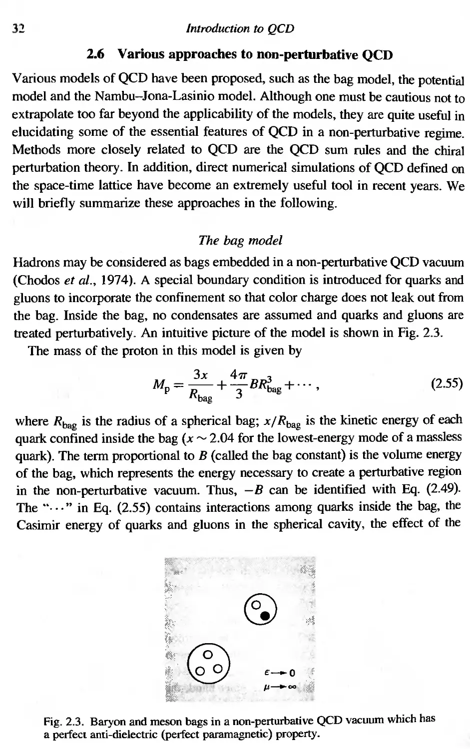
/


Text
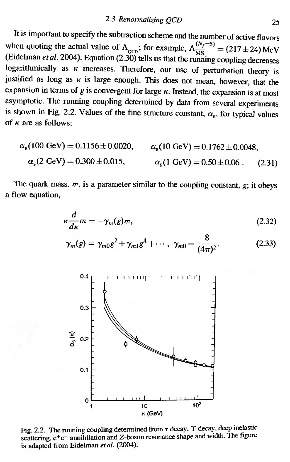
QUARK-GLUON PLASMA
From Big Bang to Little Bang
This book introduces quark-gluon plasma (QGP) as a primordial matter composed
of two types of elementary particles, quarks and gluons, created at the time of
the Big Bang. During the evolution of the Universe, QGP undergoes a transition
to hadronic matter governed by the law of strong interactions, quantum chromo-
dynamics. After an introduction to gauge theories, various aspects of quantum
chromodynamic phase transitions are illustrated in a self-contained manner. The
field theoretical approach and renormalization group are discussed, as well as the
cosmological and astrophysical implications of QGP, on the basis of Einstein's
equations. Recent developments towards the formation of QGP in ultra-relativistic
heavy ion collisions are also presented in detail.
This text is suitable as an introduction for graduate students, as well as providing
a valuable reference for researchers already working in this and related fields. It
includes eight appendices and over 100 exercises.
KOHsUKE Y AGI is a professor at the Department of Liberal Arts, Urawa University.
He has held positions at the Institute for Nuclear Study at the University of
Tokyo, Osaka University and the University of Tsukuba. He has also held several
chairs, including in the Japan Nuclear Physics Committee, the Japan-Brookhaven
National Laboratory RHIC-PHENIX Project and the International Conference on
Quark Matter. He has published 210 articles and written or edited seven books
on subatomic physics and general physics, as well as teaching the subject at
undergmduate and gmduate levels.
TETSUO HATSUDA is a professor in the Department of Physics at the University
of Tokyo. He has held positions at the University of Washington, the University
of Tsukuba and Kyoto University. He has taught subatomic physics and quantum
many-body problems at undergraduate and gmduate levels. He has published over
120 scientific articles.
Y ASUO MIAKE is Professor of Physics at the Institute of Physics, University
of Tsukuba. He has conducted research and taught at the University of Tokyo
and Brookhaven National Laboratory and the University of Tsukuba. He has
experience of teaching electromagnetism and special relativity to undergraduates
and subatomic physics to graduates. He has published over 120 scientific articles.
CAMBRIDGE MONOGRAPHS ON
PARTICLE PHYSICS
NUCLEAR PHYSICS AND COSMOLOGY 23
Genera] Editors: T. Ericson. P. V. Landshoff
1. K. Winter (ed.): Neutrino Physics
2. J. F. Donoghue, E. Golowich and B. R. Holstein: Dynamics of the Standard Model
3. E. Leader and E. Predazzi: An Introduction to Gauge Theories and Modern Particle Physics. Volume I:
Electroweak Interactions, the 'New Particles' and the Parton Model
4. E. Leader and E. Predazzi: An Introduction to Gauge Theories and Modern Particle Physics, Volume 2:
CP- Violation, QCD and Hard Processes
5. C. Grupen: Particle Detectors
6. H. Grosse and A. Martin: Particle Physics and the Schrodinger Equation
7. B. Anderson: The Lund Model
8. R. K. Ellis, W. J. Stirling and B. R. Webber: QCD and Collider Physics
9. I. I. Bigi and A. I. Sanda: CP Violation
10. A. V. Manohar and M. B. Wise: Heal'y Quark Physics
II. R. K. Bock, H. Grote. R. Fruhwirth and M. RegIer: Data Analysis Techniques for High-Energy Physics.
Second edition
12. D. Green: The Physics of Particle Detectors
13. V. N. Gribov and J. Nyiri: Quantum E/ectrodvnamics
14. K. Winter (ed.): Neutrino Physics. Second edition
15. E. Leader: Spin in Particle Physics
16. J. D. Wa]ecka: Electron Scattering for Nuclear and Nucleon Structure
17. S. Narison: QCD as a Theory of Hadrons
18. J. F. Letessier and J. Rafelski: Hadrons and Quark-Gluon Plasma
19. A. Donnachie. H. G. Dosch. P. V. Landshoff and O. Nachtmann: Pomaon Physics and QCD
20. A. Hofmann: The Physics of Synchrotron Radiation
21. J. B. Kogut and M. A. Stephanov: The Phases of Quantum Chromodynamics
22. D. Green: High P T Physics at Hadron Colliders
23. K. Yagi. T. Hatsuda and Y. Miake: Quark-Gluon Plasma
QUARK-GLUON PLASMA
From Big Bang to Little Bang
KOHSUKE Y AGI
Urawa University
TETSUO HATSUDA
Unit'ersity of Tokyo
Y ASUO MIAKE
University of TSllkuba
CAMBRIDGE
UNIVERSITY PRESS
CAMBRIDGE UNIVERSITY PRESS
Cambridge, New York, Melbourne, Madrid, Cape Town, Singapore, Siio Paulo
CAMBRIDGE UNIVERSITY PRESS
The Edinburgh Building, Cambridge CB2 2RU, UK
www.cambridge.org
Information on this title: www.cambridge.org/9780521561082
@ K. Yagi. T. Hatsuda and Y. Miake 2005
This publication is in copyright. Subject to statutory exception
and to the provisions of relevant collective licensing agreements,
no reproduction of any part may take place without
the written permission of Cambridge University Press.
First published 2005
Printed in the United Kingdom at the University Press, Cambridge
A catalog record for this publication is available from the British Library
ISBN-13 978-0-521-56108-2 hardback
ISBN-IO 0-521-56108-6 hardhack
Cambridge University Press has no responsibility for the persistence or accuracy of URLs for externa] or
third-party internet websites referred to in Ihis publication, and does nol guarantee that any content on
such websites is, or will remain, accurate or appropriate.
Contents
Preface page xv
1 What is the quark-gluon plasma? I
1.1 Asymptotic freedom and confinement in QCD I
1.2 Chira1 symmetry breaking in QCD 4
1.3 Recipes for quark-gluon plasma 5
1.4 Where can we find QGP? 6
1.5 Signatures of QGP in relativistic heavy ion collisions 9
1.6 Perspectives on relativistic heavy ion experiments 12
1.7 Natural units and particle data 14
Part I: Basic Concept of Quark-Gluon Plasma 15
2 Introduction to QCD 17
2.1 Classical QCD action 17
2,2 Quantizing QeD 19
2.3 Renormalizing QCD 22
2.3.1 Running coupling constants 24
2,3.2 More on asymptotic freedom 27
2,4 Global symmetries in QCD 28
2.4.1 Chiral symmetry 28
2.4,2 Dilatational symmetry 29
2.5 QCD vacuum structure 30
2.6 Various approaches to non-perturbative QCD 32
Exercises 36
3 Physics of the quark-hadron phase transition 39
3.1 Basic thermodynamics 39
3.2 System with non-interacting particles 43
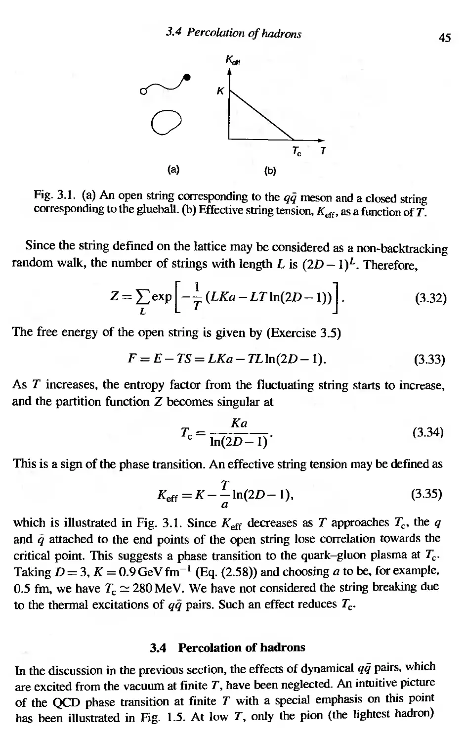
3,3 Hadronic string and deconfinement 44
3.4 Percolation of hadrons 45
3.5 Bag equation of state 46
3.6 Hagedorn's limiting temperature 50
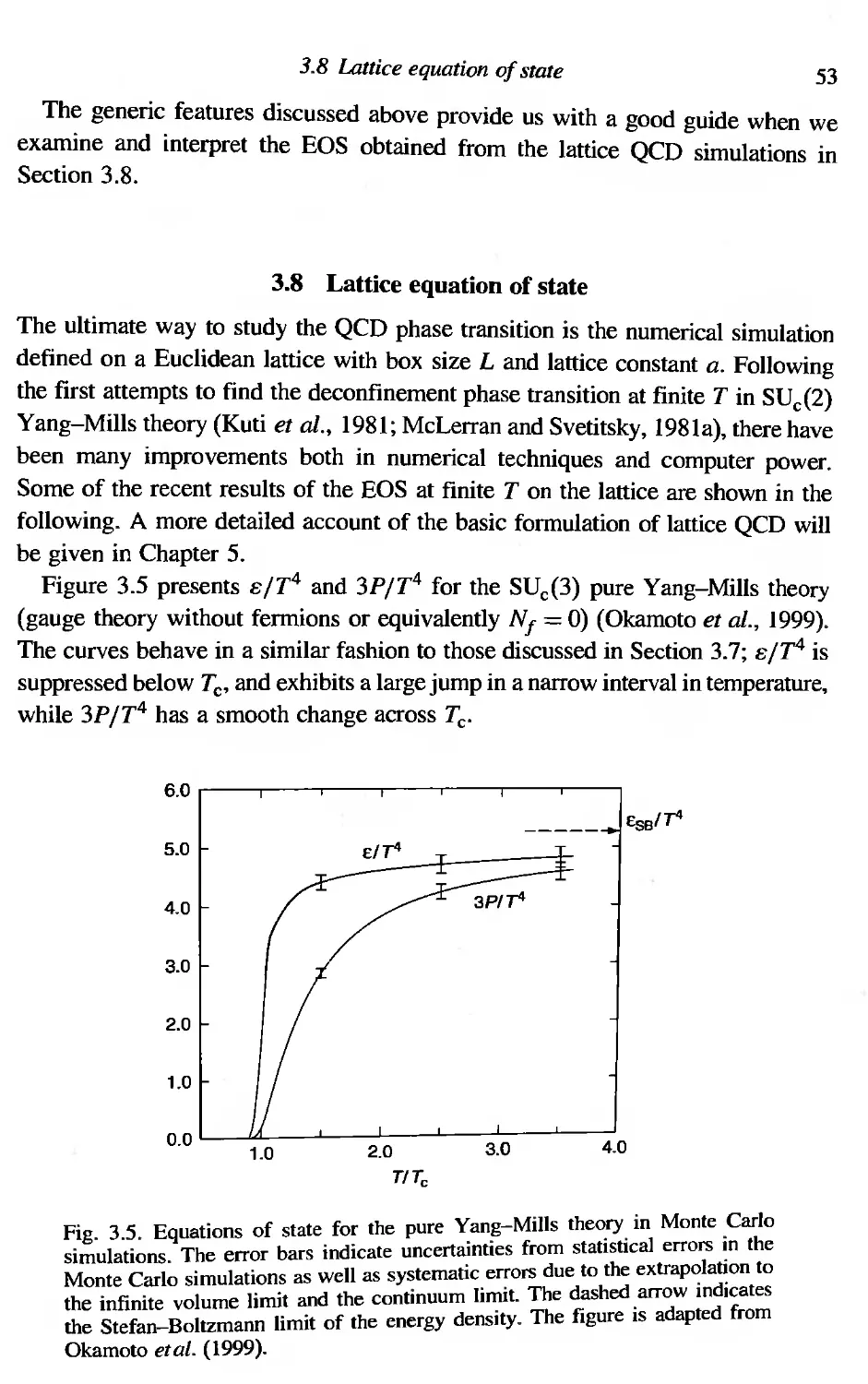
3.7 Parametrized equation of state 51
3.8 Lattice equation of state 53
Exercises 55
vii
viii Contents
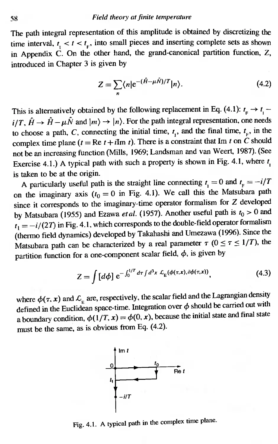
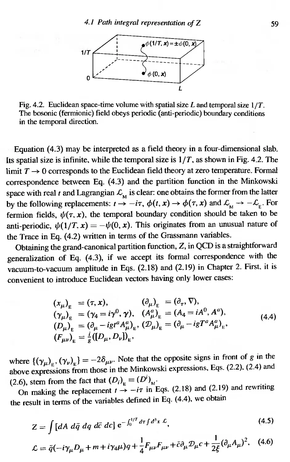
4 Field theory at finite temperature 57
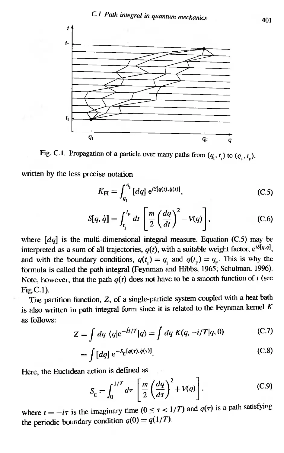
4.1 Path integral representation of Z 57
4.2 Black body radiation 60
4.3 Perturbation theory at finite T and p, 62
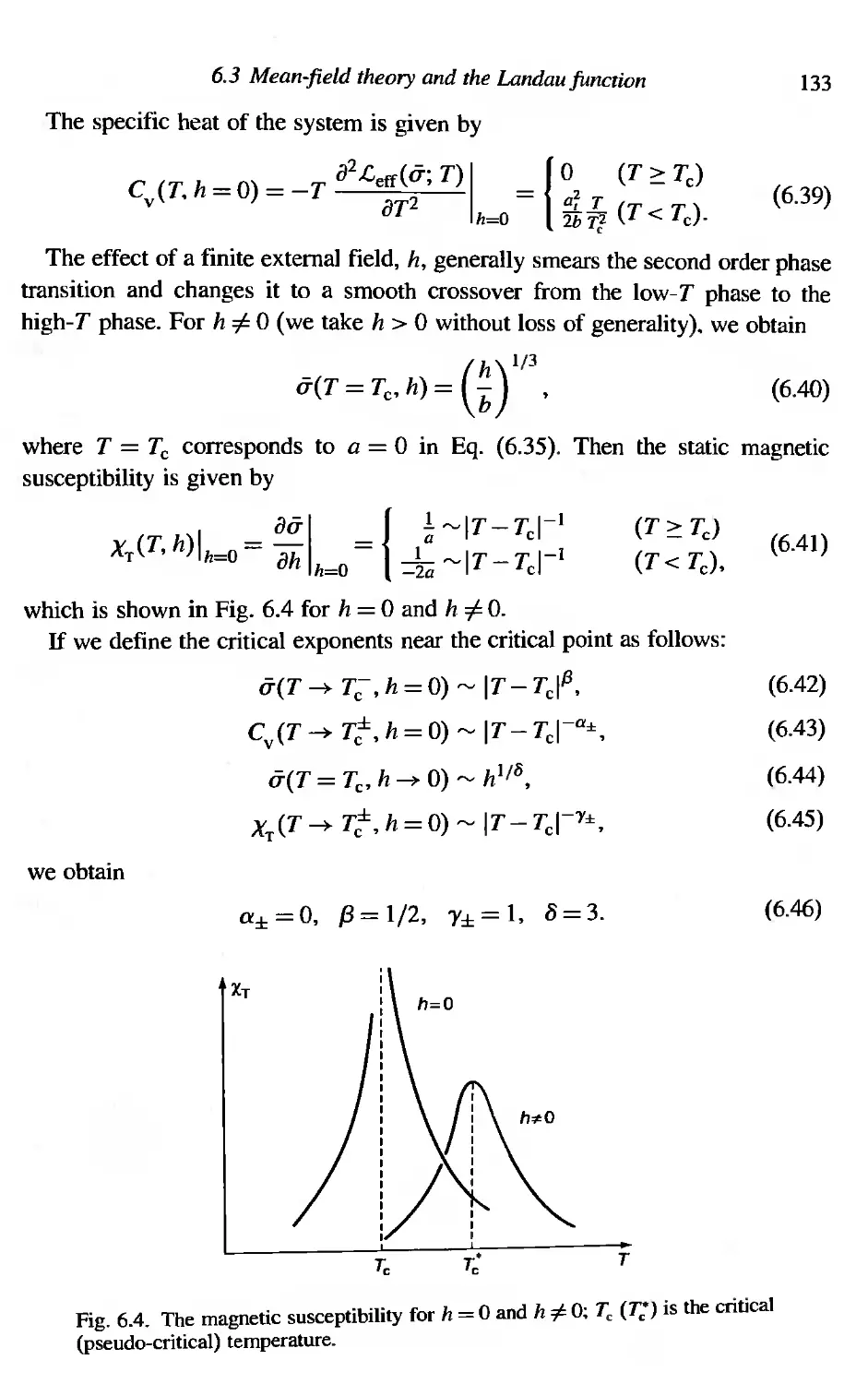
4.3.1 Free propagators 63
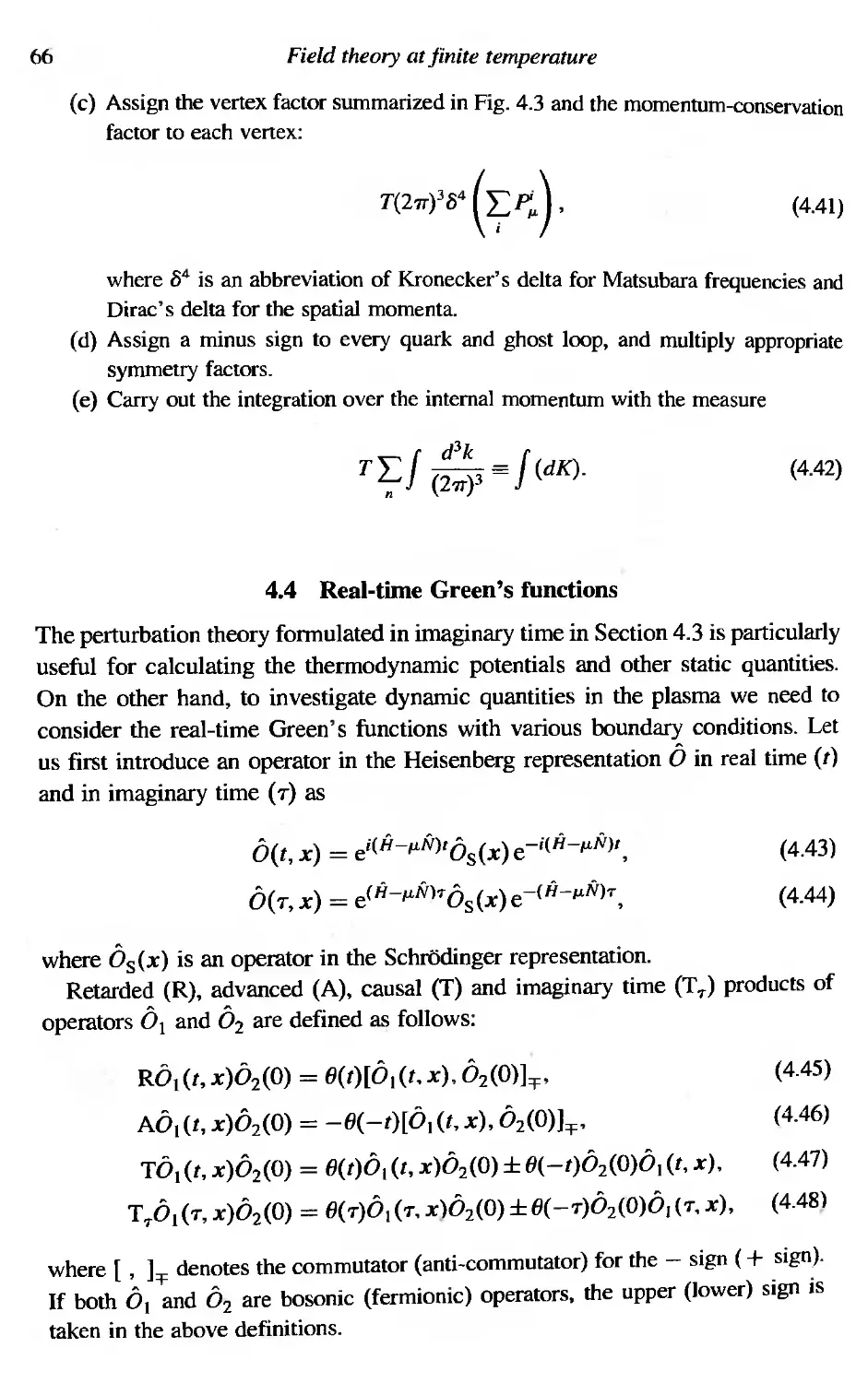
4.3.2 Vertices 64
4.3.3 Feynman rules 65
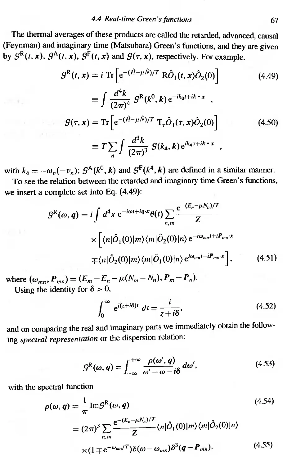
4.4 Real-time Green's functions 66
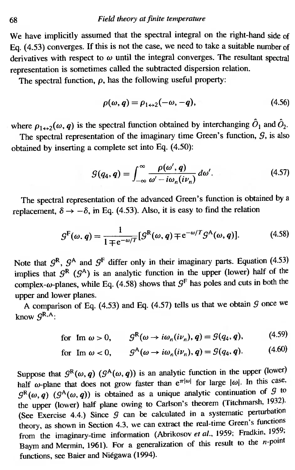
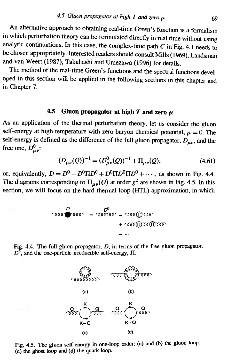
4.5 Gluon propagator at high T and zero P, 69
4.6 Quark propagator at high T and zero p, 75
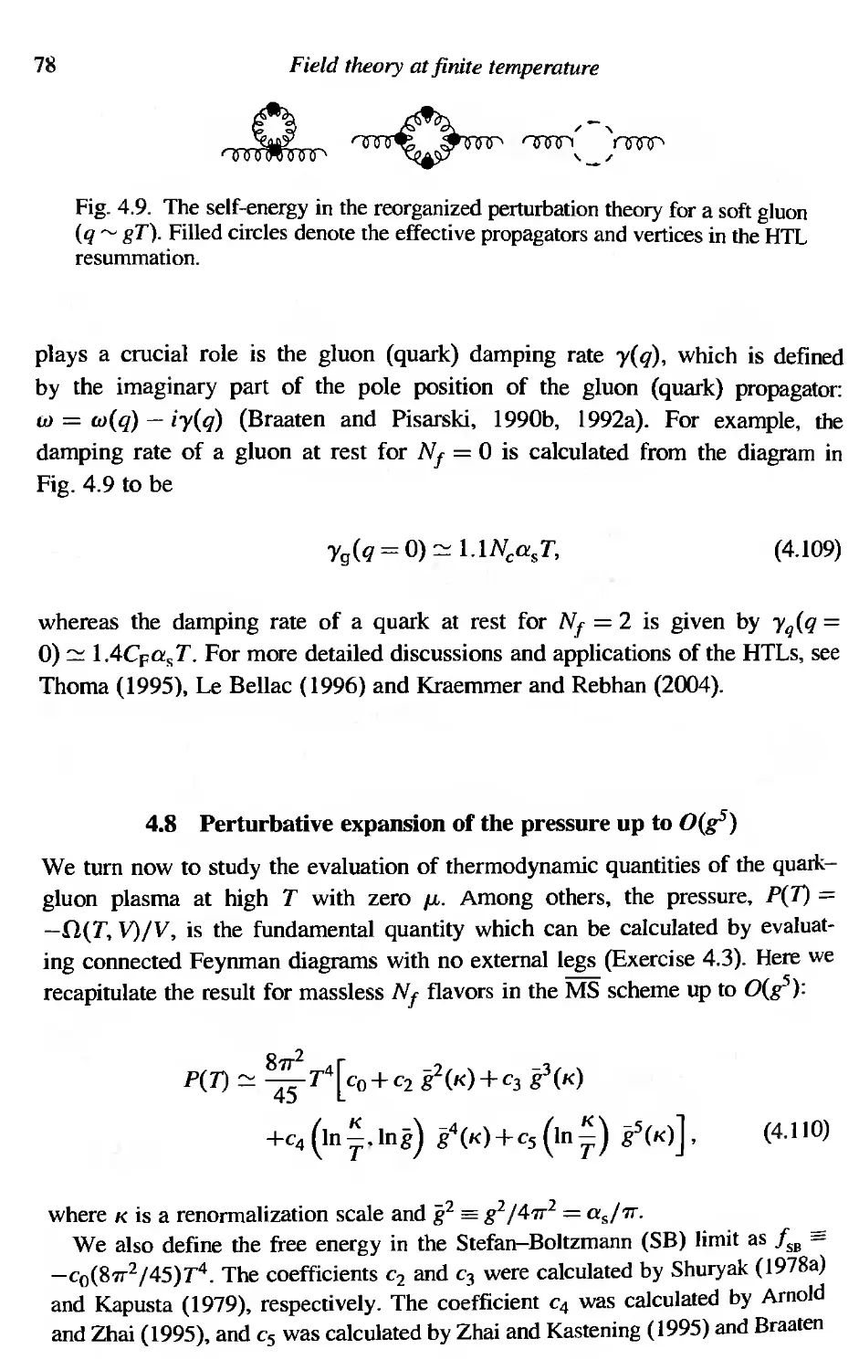
4.7 HTL resummation 77
4.8 Perturbative expansion of the pressure up to 0(g5) 78
4.9 Infrared problem of 0(g6) and beyond 81
4.10 Debye screening in QED plasma 82
4.11 Vlasov equations for QED plasma 84
4.12 Vlasov equations for QCD plasma 87
Exercises 88
5 Lattice gauge approach to QCD phase transitions 92
5,1 Basics of lattice QCD 92
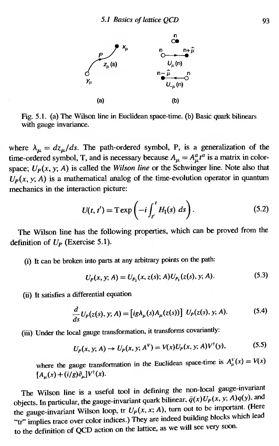
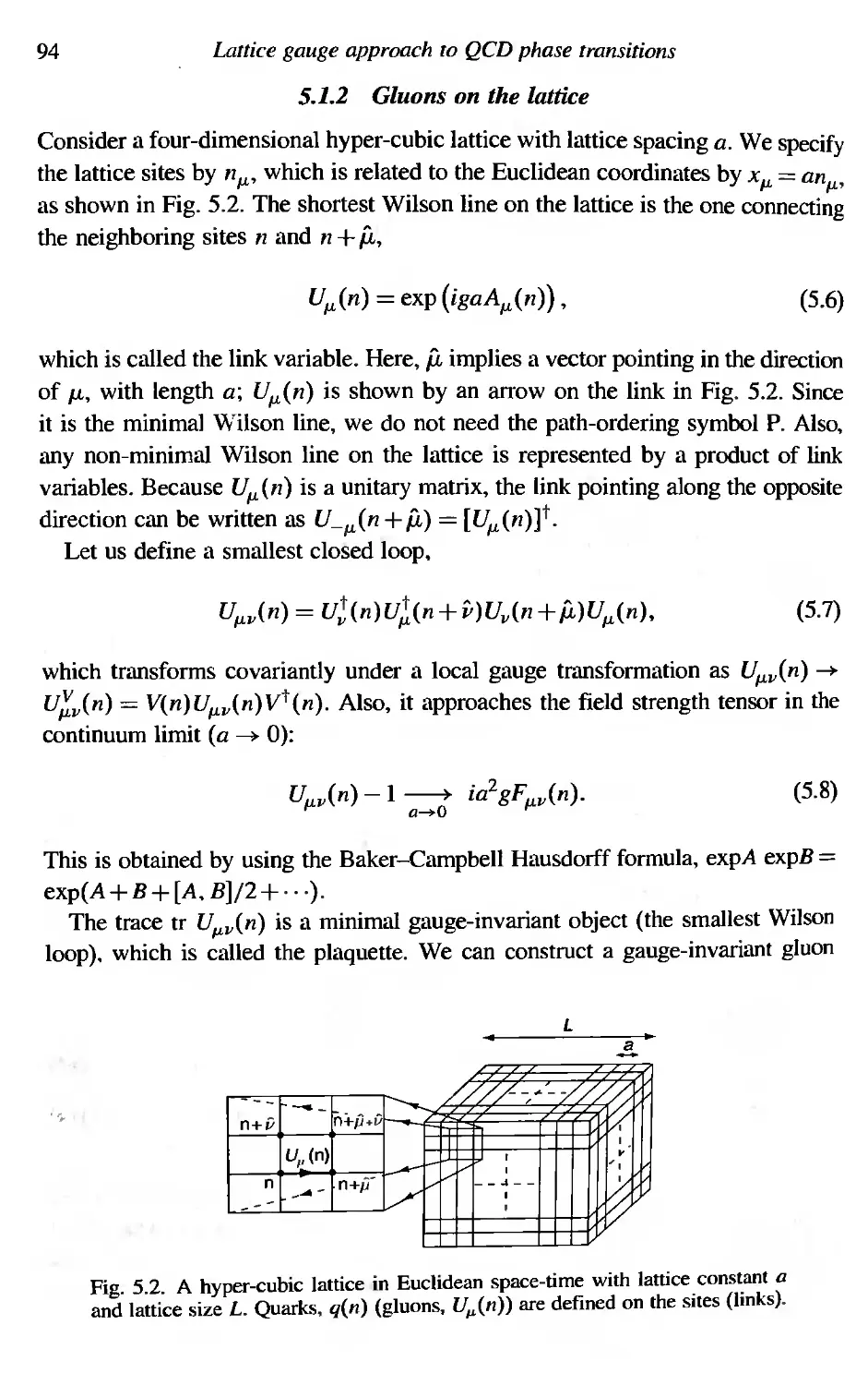
5,1.1 The Wilson line 92
5.1.2 Gluons on the lattice JI' 94
5,1.3 Fermions on the lattice 95
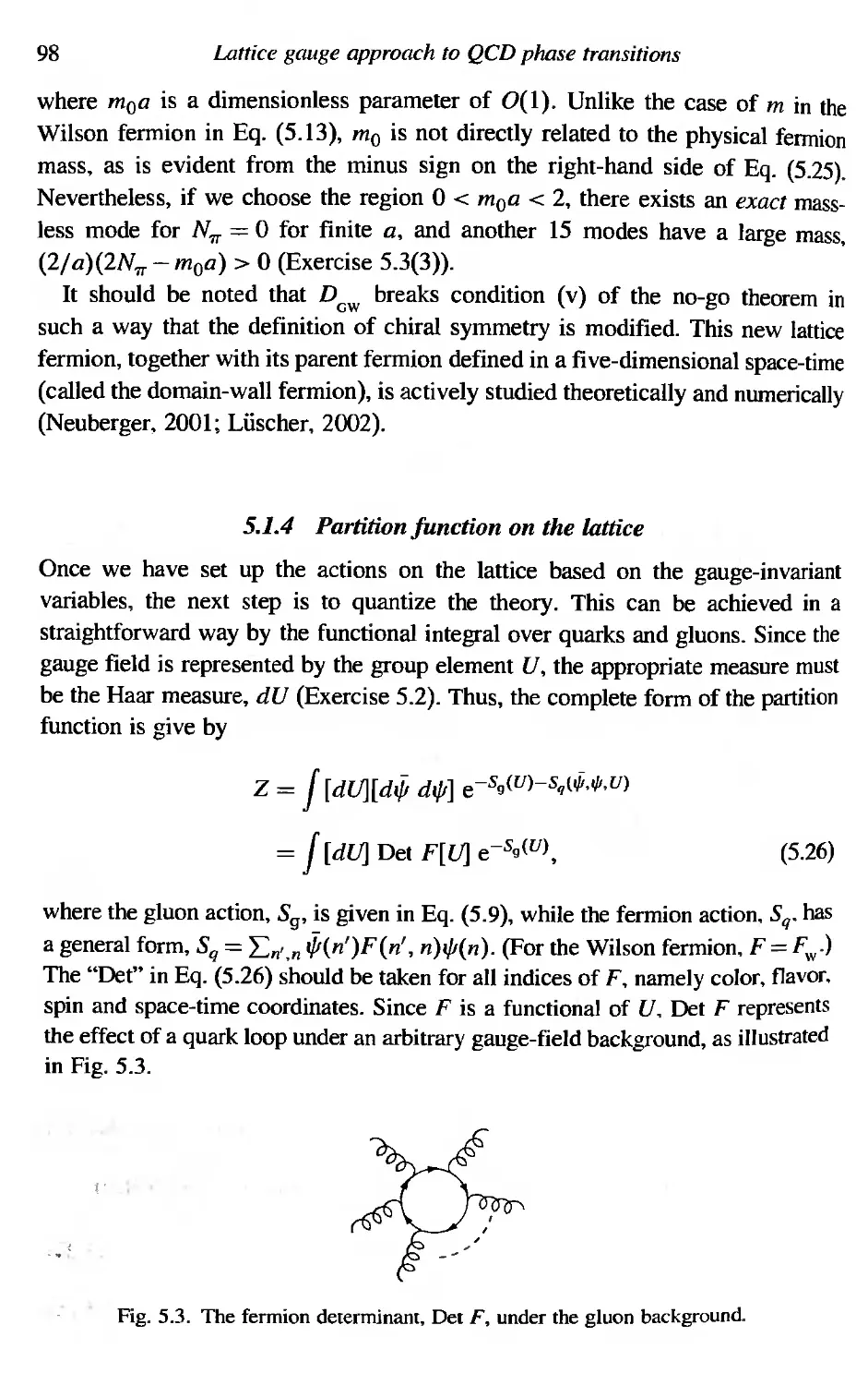
5.1.4 Partition function on the lattice 98
5.2 The Wilson loop 99
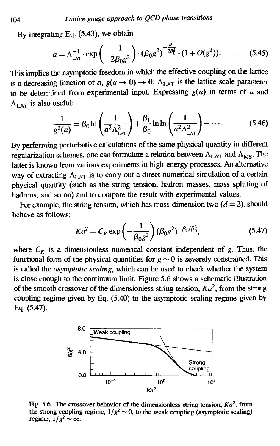
5.3 Strong coupling expansion and confinement 101
5.4 Weak coupling expansion and continuum limit 102
5.5 Monte Carlo simulations 105
5.6 Lattice QCD at finite T 109
5,7 Confinement--deconfinement transition in Nt = 0 QCD 111
5.8 Order of the phase transition for Nt = 0 115
5.9 Effect of dynamical quarks 116
5.10 Effect of finite chemical potential 117
Exercises 118
6 Chiral phase transition 122
6.1 (ijq) in hot/dense matter 122
6.1.1 High-temperature expansion 123
6.1.2 Low-temperature expansion 123
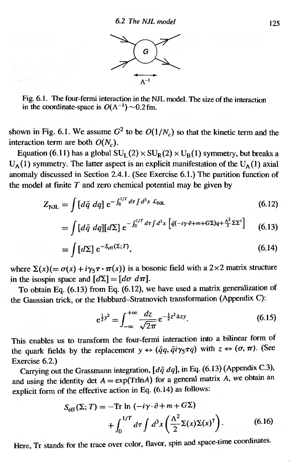
6.2 The NJL model 124
6.2.1 Dynamical symmetry breaking at T = 0 126
6.2.2 Symmetry restoration at T =f 0 127
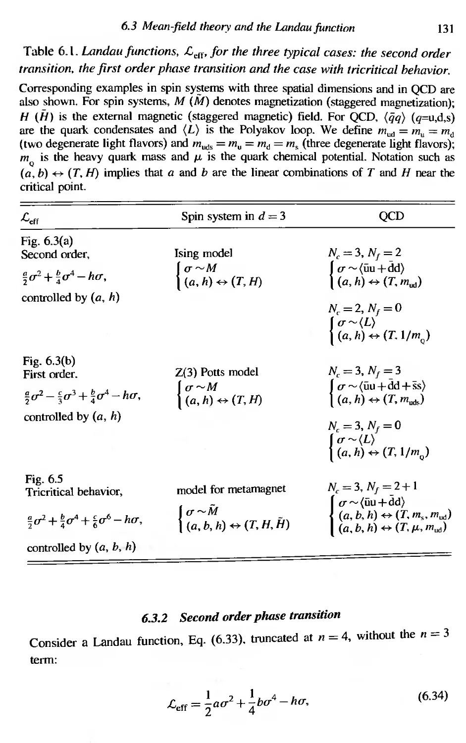
6.3 Mean-field theory and the Landau function 129
6.3.1 Order of the phase transition 129
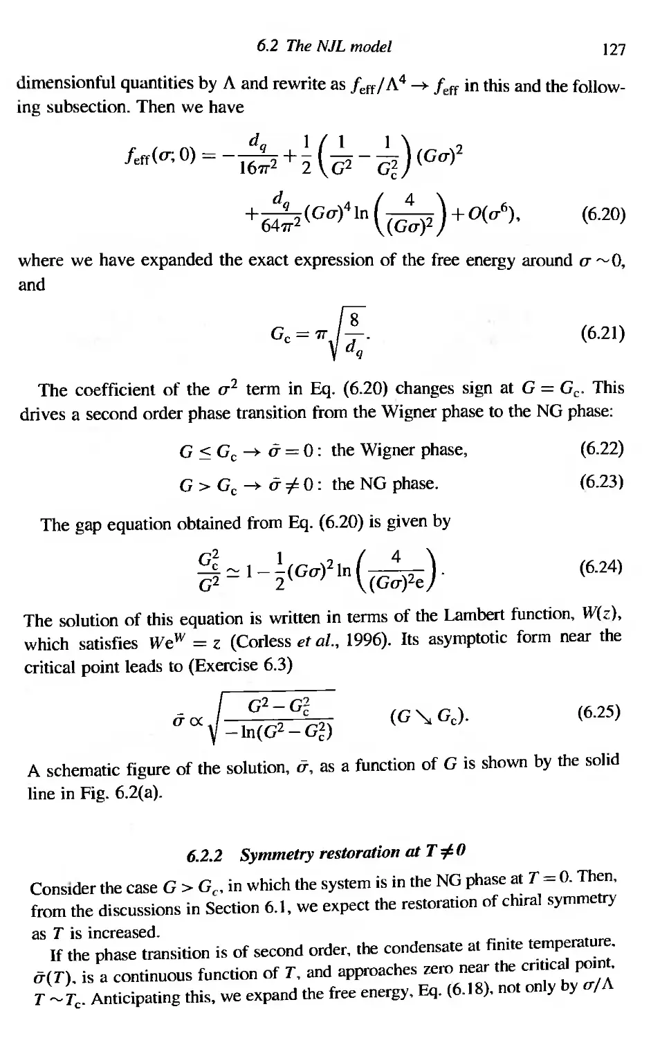
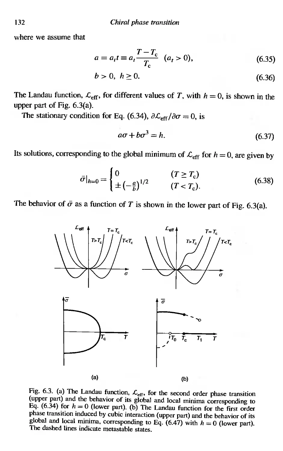
6.3.2 Second order phase transition 131
Contents
ix
6,10
6.11
6.12
6.13
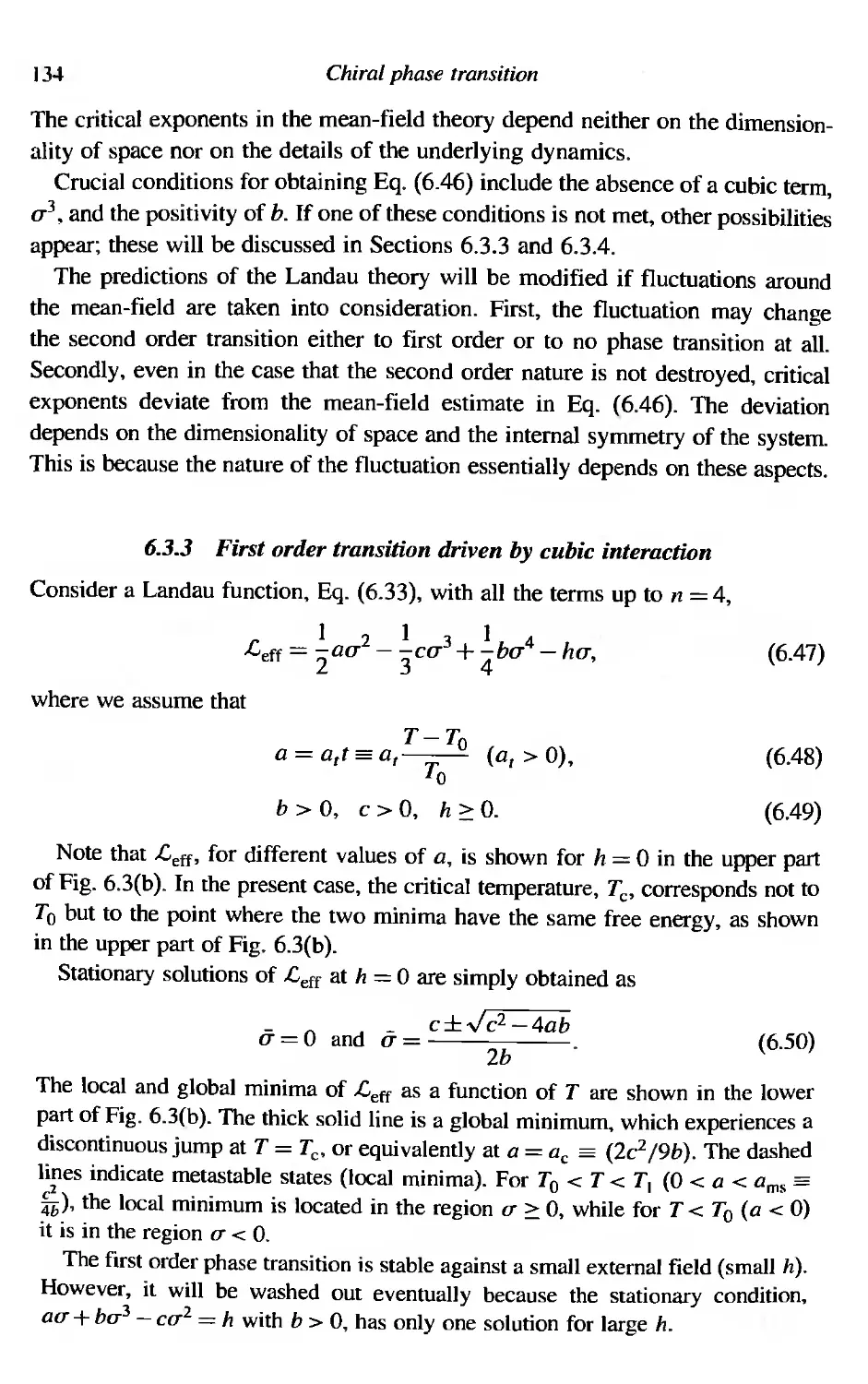
6.3.3 First order transition driven by cubic interaction
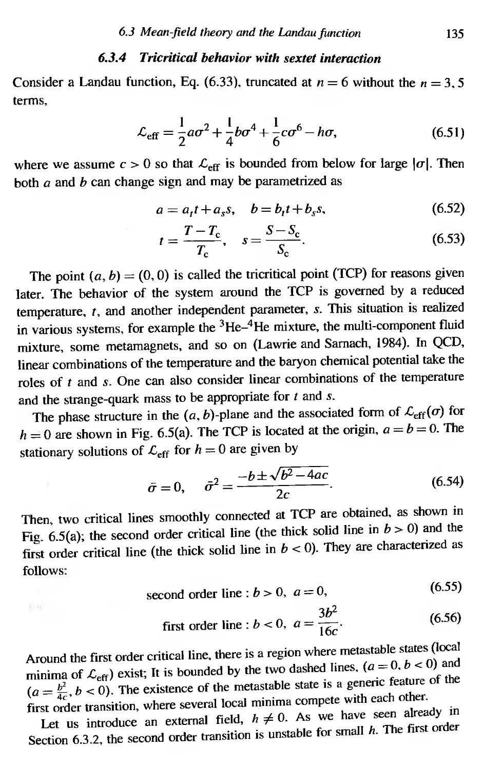
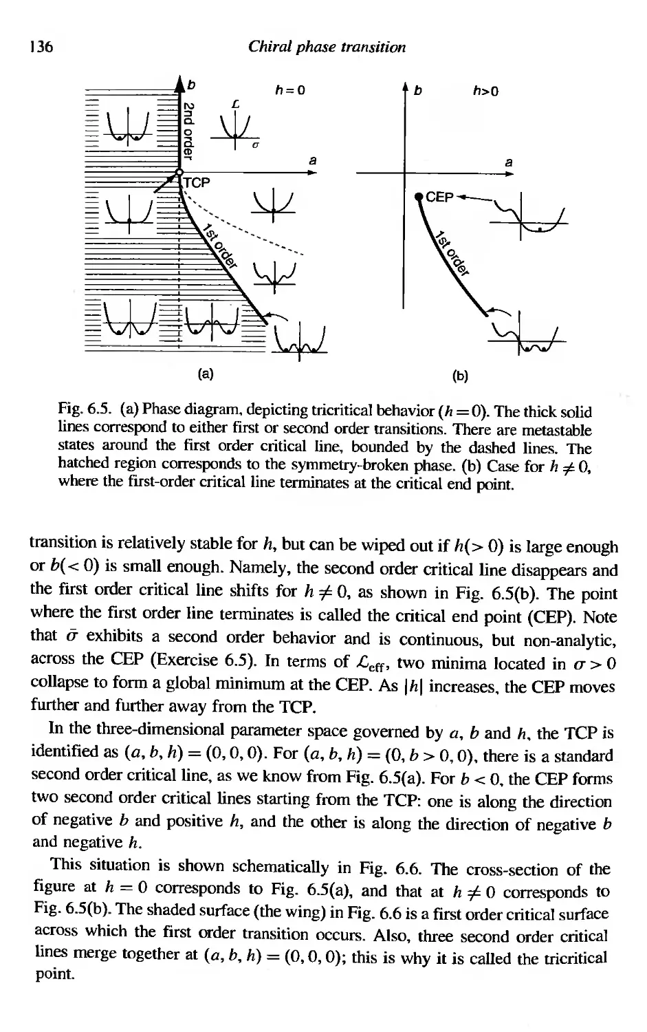
6.3.4 Tricritical behavior with sextet interaction
Spatial non-uniformity and correlations
Critical fluctuation and the Ginzburg region
Renormalization group and E-expansion
6,6.1 Renormalization in 4 - E dimensions
6.6.2 Running couplings
6.6,3 Vertex functions
6,6.4 RG equation for vertex function
Perturbative evaluation of {3i
Renormalization group equation and fixed point
6.8.1 Dimensional analysis and solution of RG equation
6.8.2 Renormalization group flow
Scaling and universality
6.9.] Scaling at the critical point
6,9.2 Scaling near the critical point
Magnetic equation of state
Stability of the fixed point
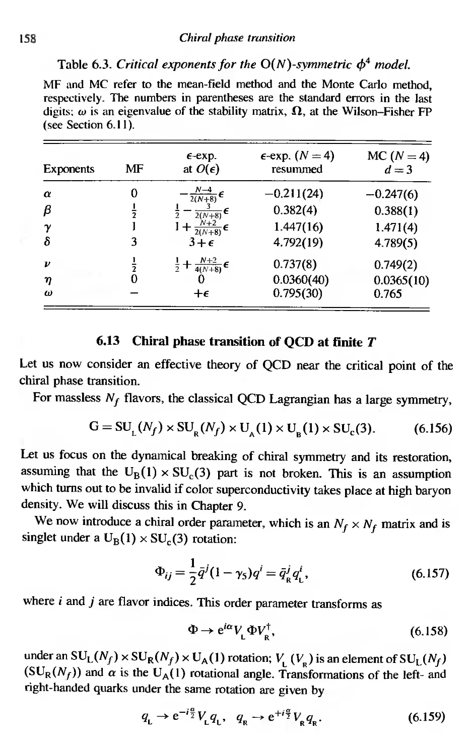
Critical exponents for the O(N)-symmetric cf>4 model
Chiral phase transition of QCD at finite T
6.13.1 Landau functional of QCD
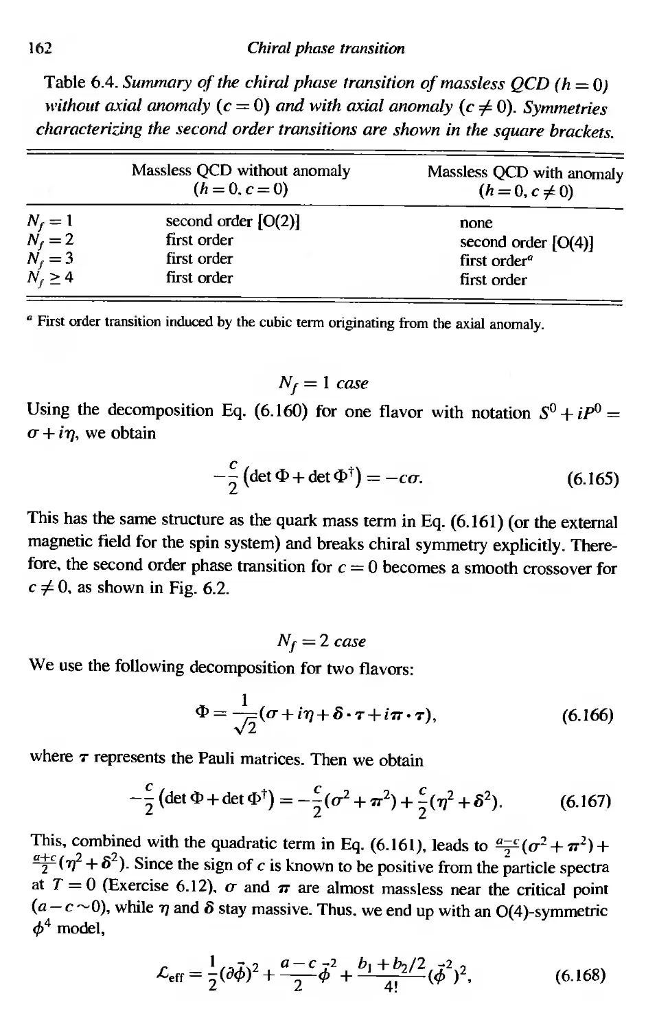
6.13.2 Massless QCD without axial anomaly
6,13.3 Massless QCD with axial anomaly
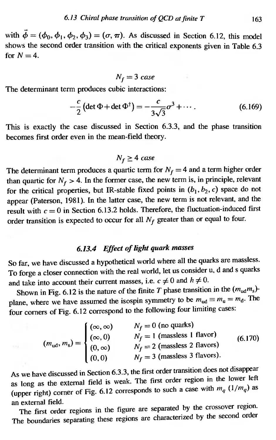
6.13.4 Effect of light quark masses
6.13.5 Effect of finite chemical potential
Exercises
134
135
137
139
141
141
143
144
145
146
147
147
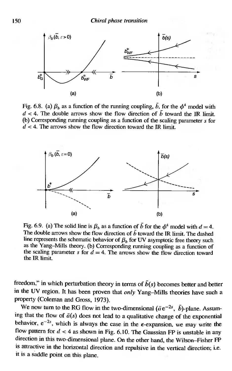
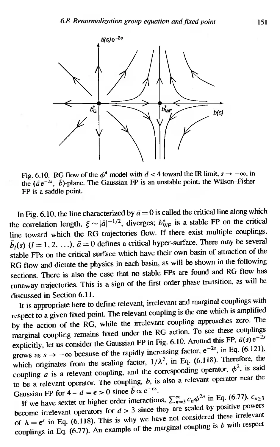
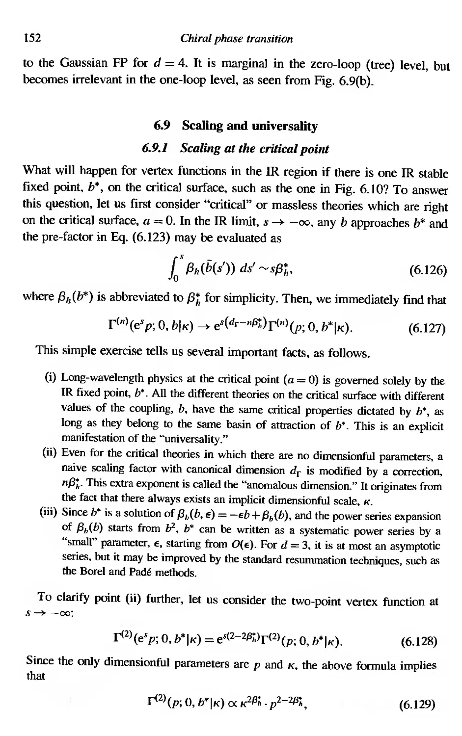
149
152
152
153
154
156
156
158
159
160
161
163
165
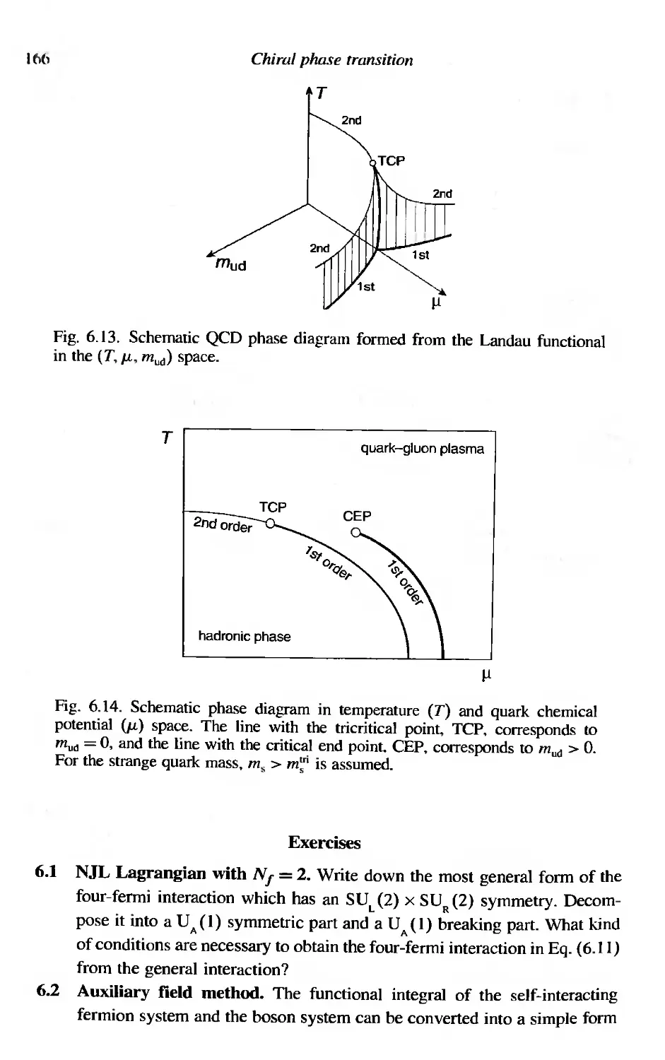
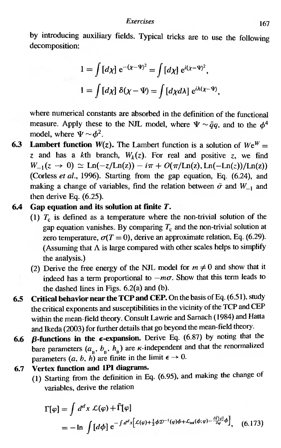
166
6.4
6,5
6.6
6.7
6,8
6.9
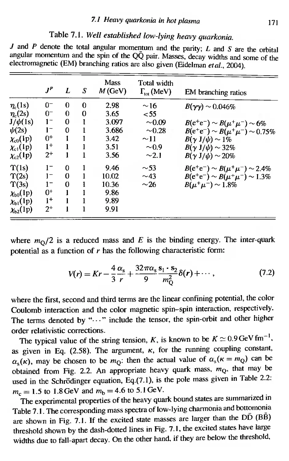
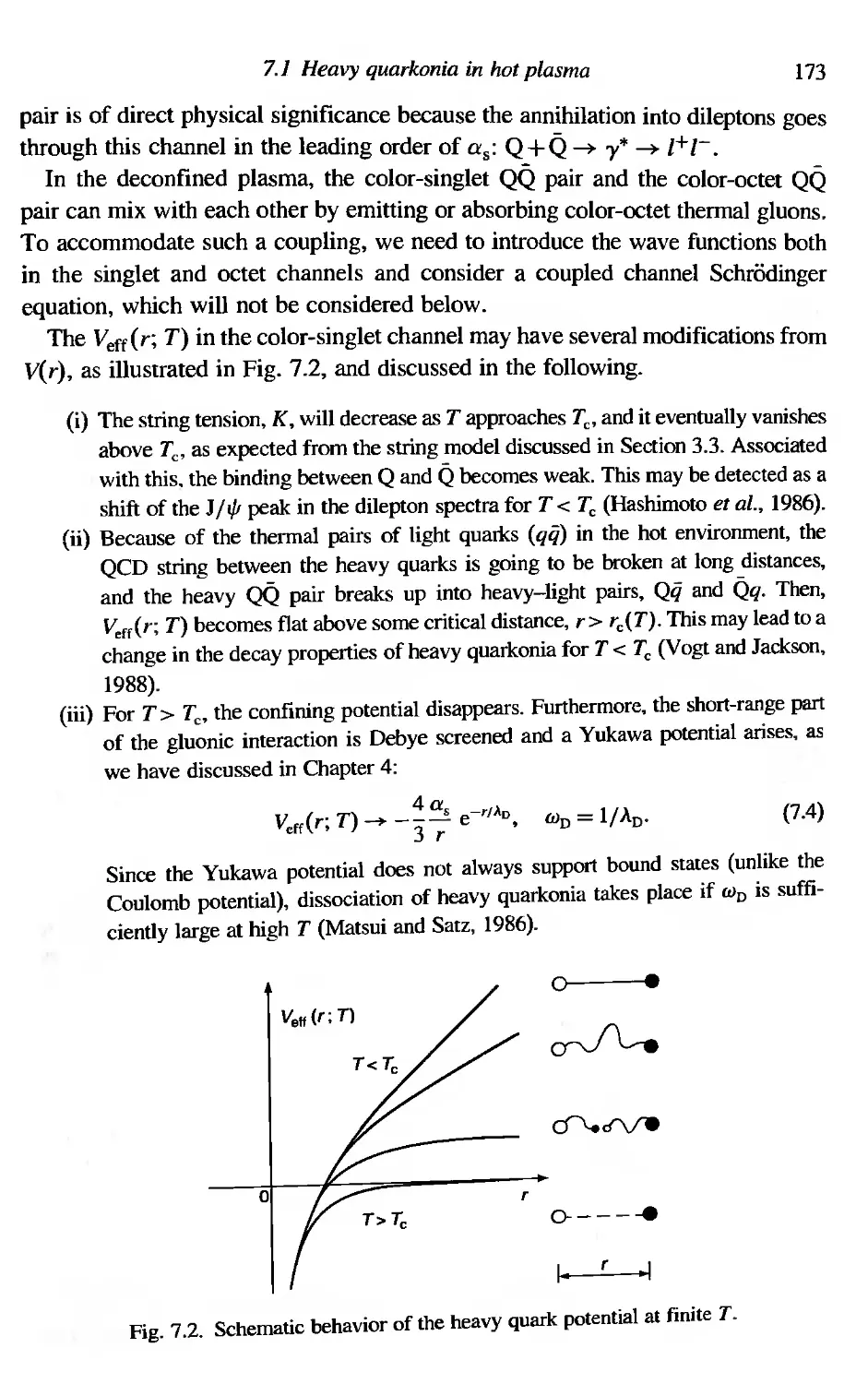
7.3
7.4
Hadronic states in a hot environment
Heavy quarkonia in hot plasma
7.1.1 QQ spectra at T = 0
7.1.2 QQ at T#O
7.1.3 Charmonium suppression at high T
7.1.4 Correlation of Polyakov lines in lattice QCD
Light quarkonia in a hot medium
7.2.1 qq spectra at T = 0
7.2.2 Nambu-Goldstone theorem at finite T
7.2.3 Virial expansion and the quark condensate
7.2.4 Pions at low T
7.2.5 Vector mesons at low T
In-medium hadrons from lattice QCD
Photons and dileptons from hot/dense matter
7.4.1 Photon production rate
7.4.2 Dilepton production rate
Exercises
170
170
170
172
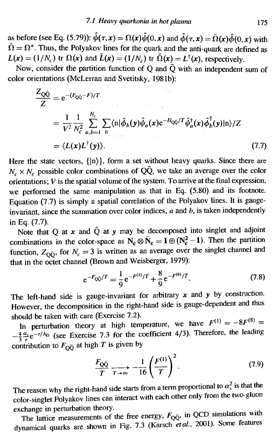
174
174
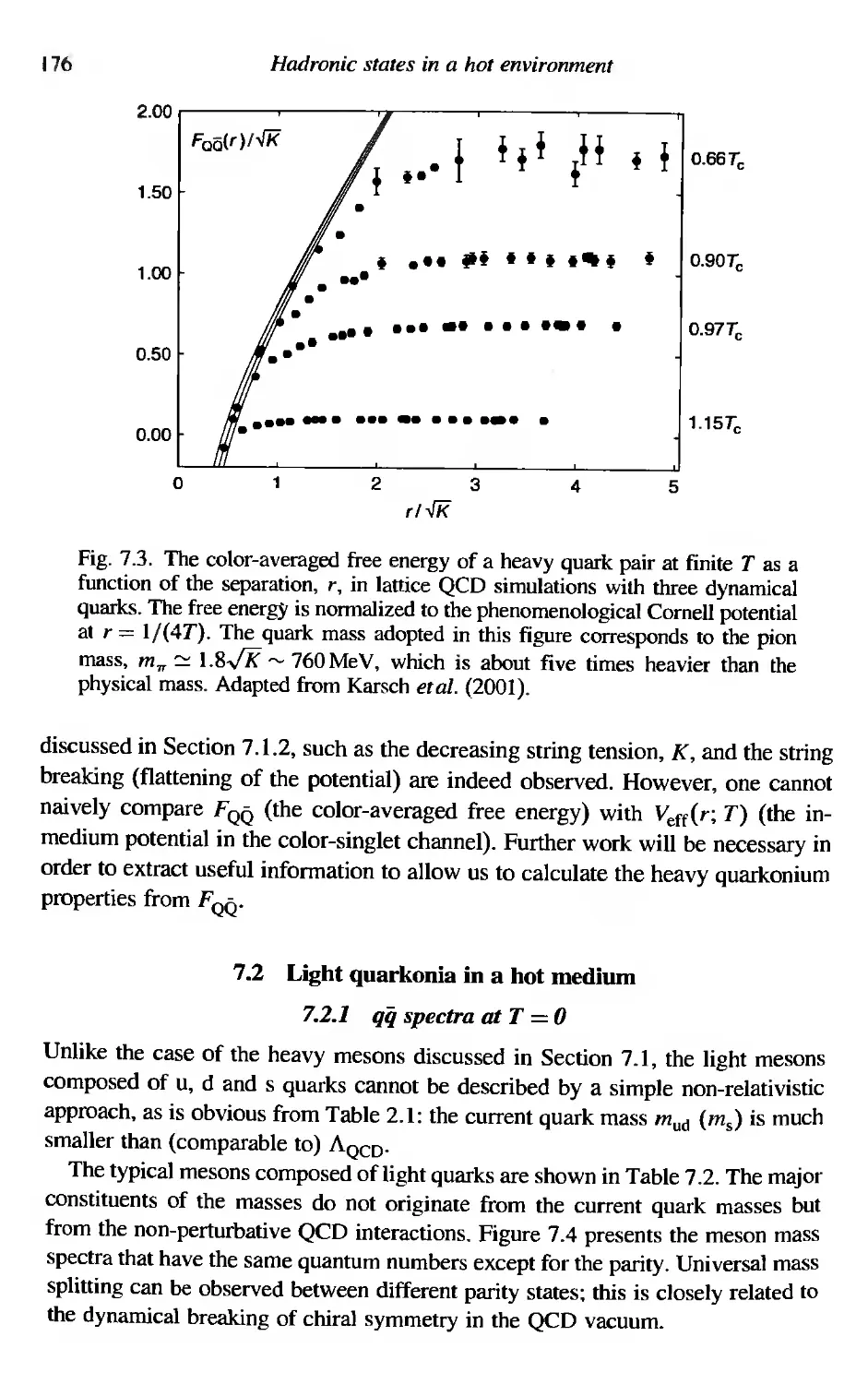
176
176
178
179
180
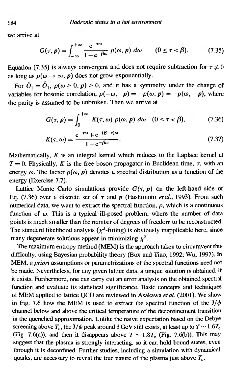
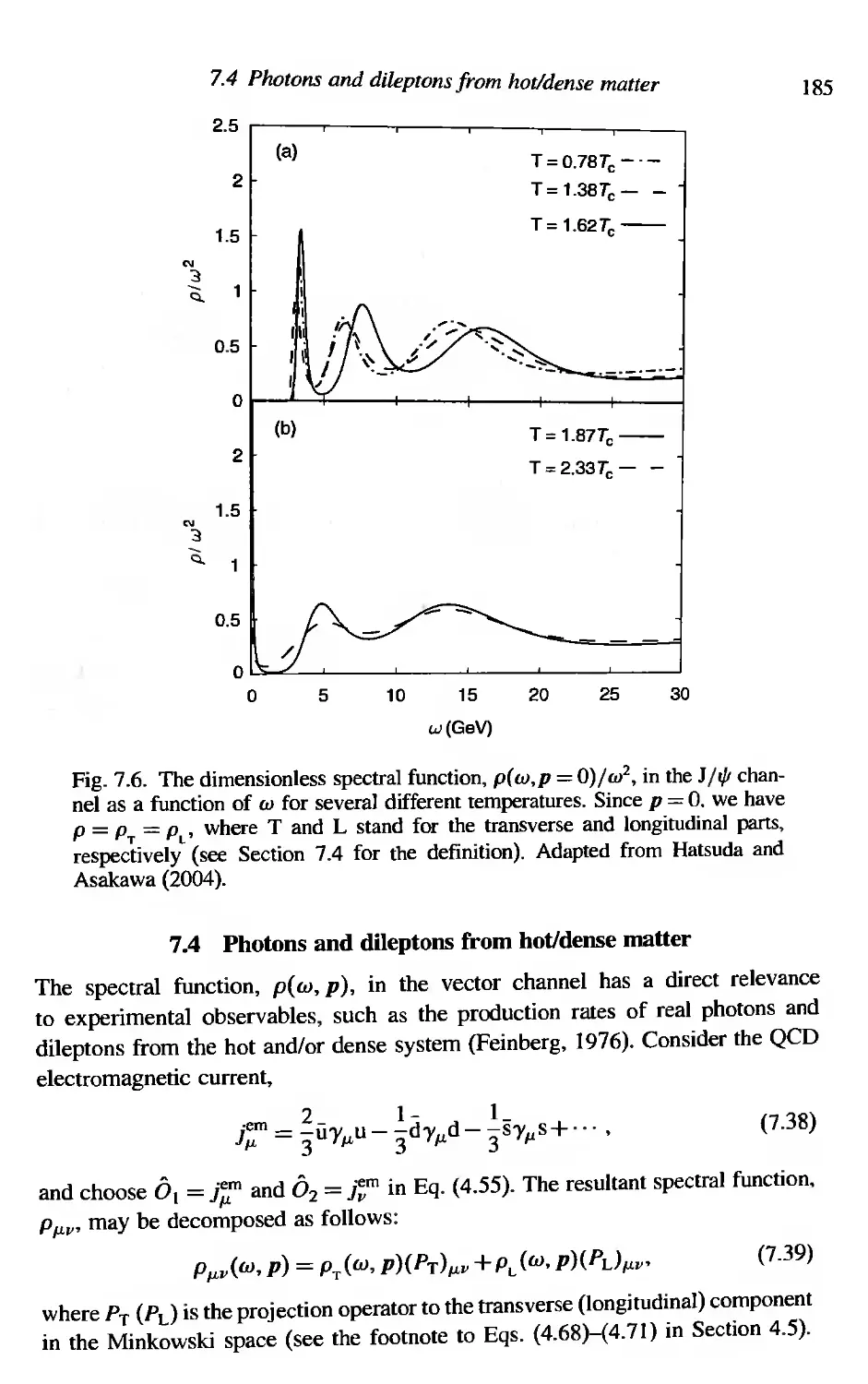
182
183
185
186
187
188
7
7.1
7,2
x
Contents
Part n: Quark-Gluon Plasma in Astrophysics
8 QGP in the early Universe
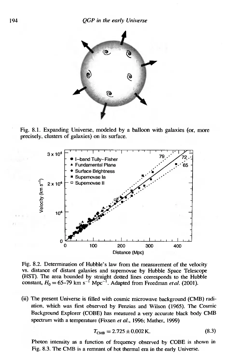
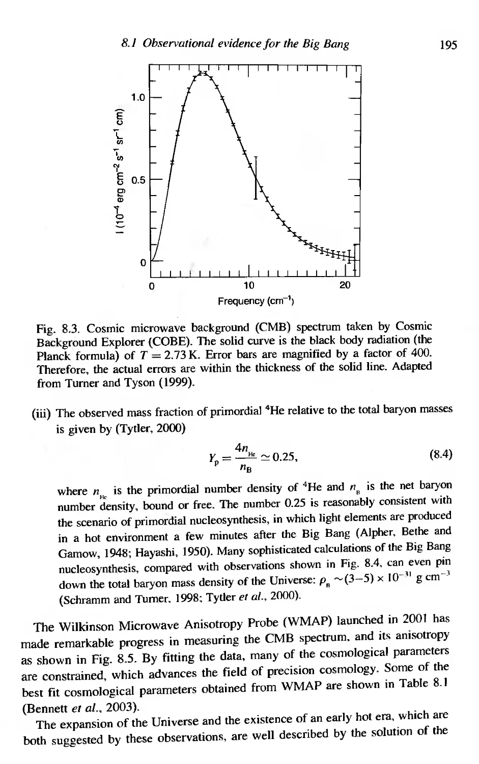
8,1 Observational evidence for the Big Bang
8.2 Homogeneous and isotropic space
8.2,] Robertson-Walker metric
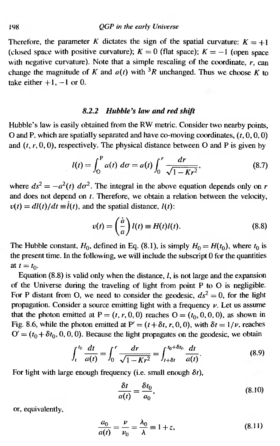
8.2.2 Hubble's law and red shift
8.2.3 Horizon distance
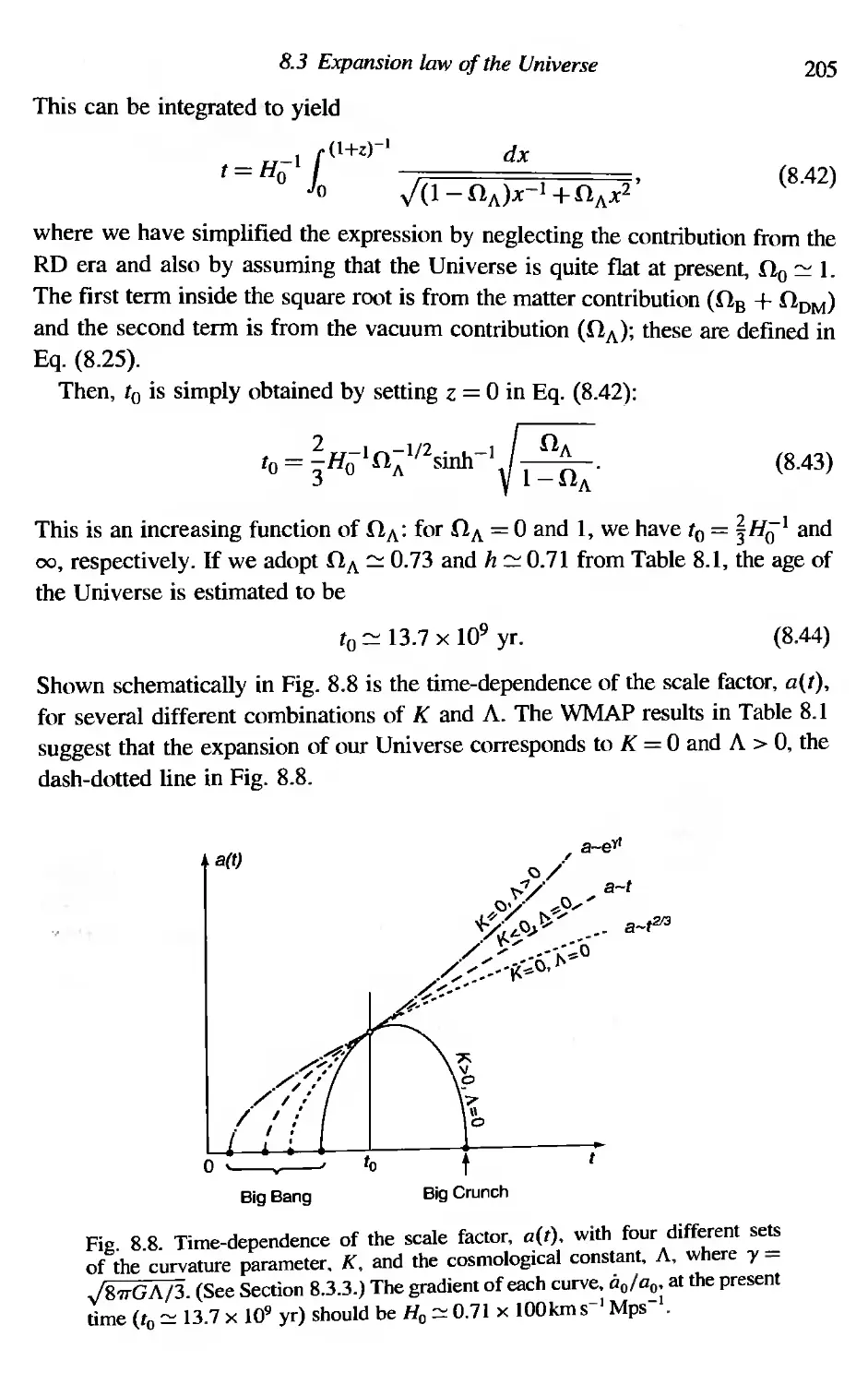
8.3 Expansion law of the Universe
8,3.] The Einstein equation
8.3,2 Critical density
8.3,3 Solution of the Friedmann equation
8.3.4 Entropy conservation
8.3.5 Age of the Universe
8.4 Thermal history of the Universe: from QGP to CMB
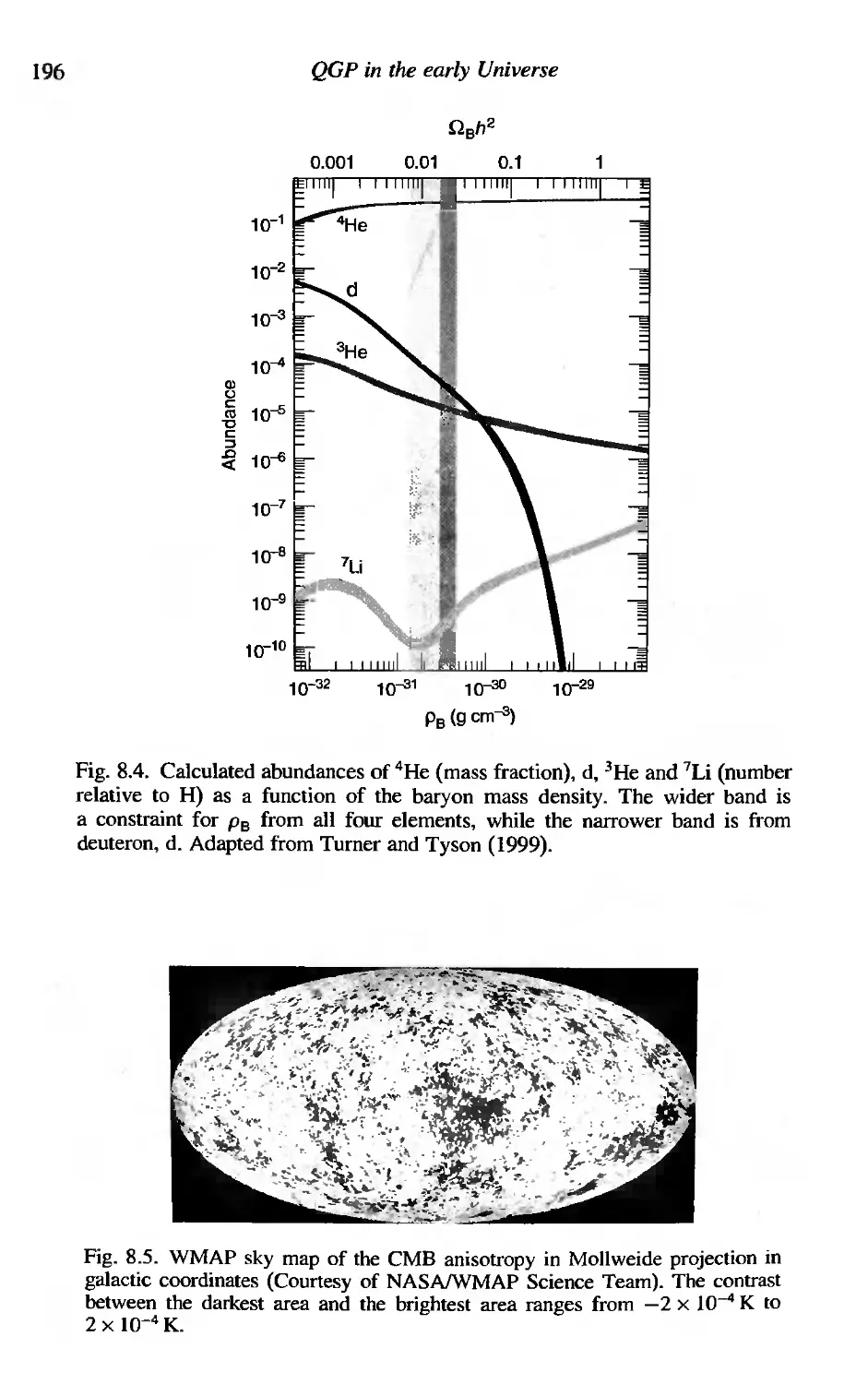
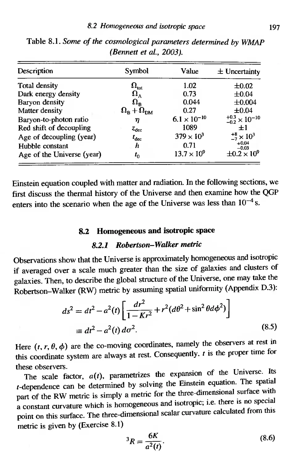
8.5 Primordial nucleosynthesis
8,6 More on the QCD phase transition in the early Universe
8.6.] t < t, (T> Tc)
8.6.2 t, < t < t F (T = Tc)
8.6.3 t > t F (T < Tc)
Exercises
191
193
193
197
]97
198
199
200
200
201
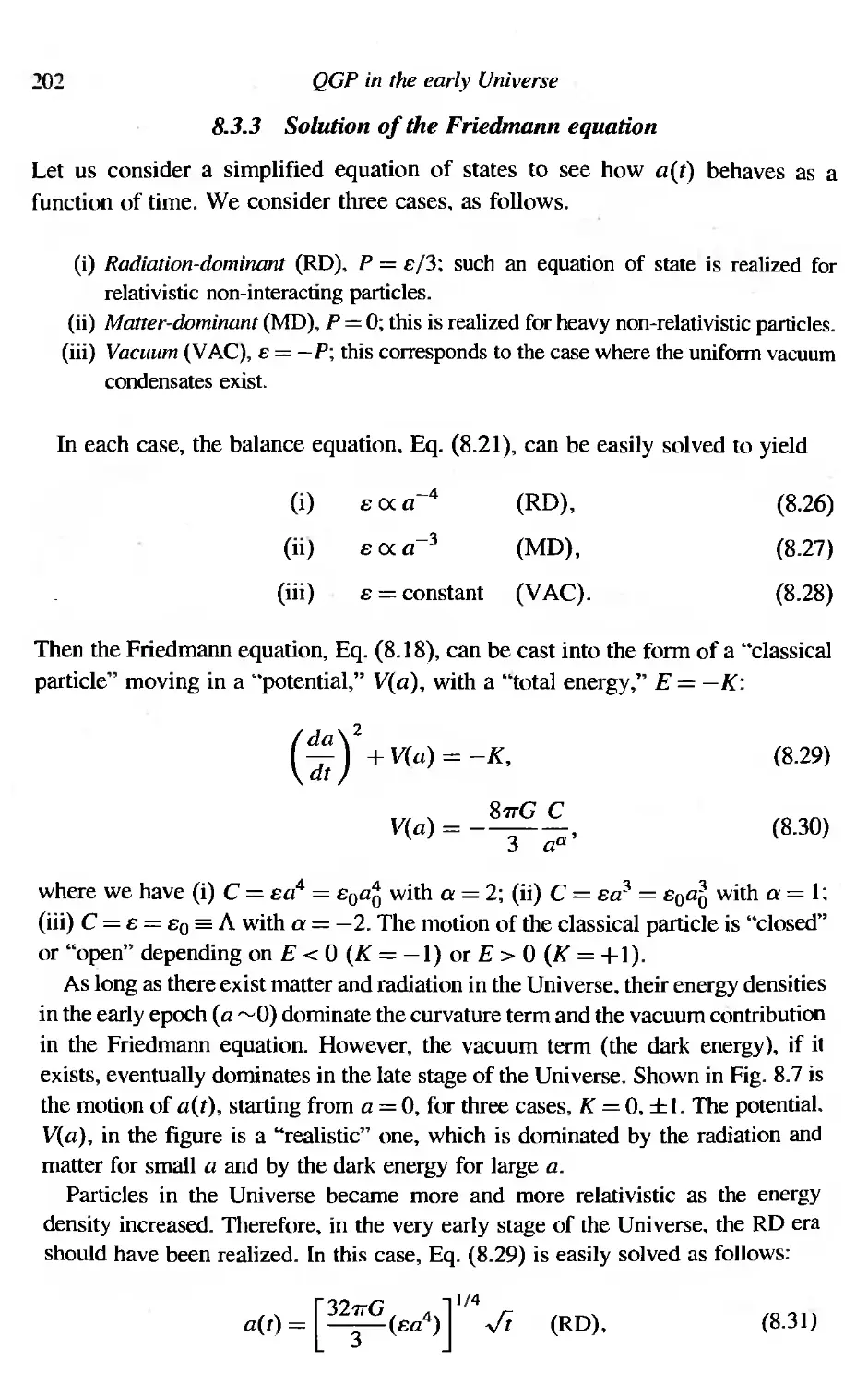
202
204
204
206
209
211
213
214
2]4
2]5
9 Compact stars
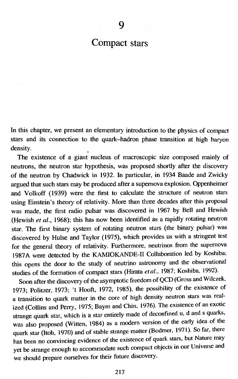
9.] Characteristic features of neutron stars
9.2 Newtonian compact stars
9.2,1 White dwarfs
9.2.2 Neutron stars
9.3 General relativistic stars
9,3.] Maximum mass of compact stars
9.3.2 Oppenheimer-Volkoff equation
9.3.3 Schwarzschild's uniform density star
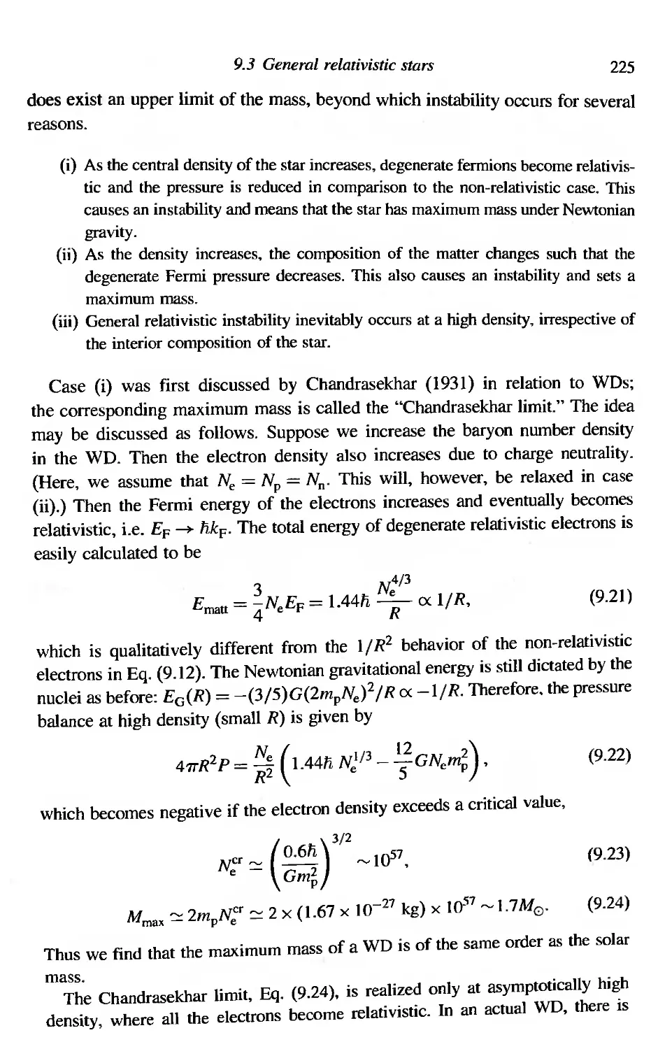
9.4 Chemical composition of compact stars
9,4.1 Neutron star matter and hyperon matter
9.4.2 u, d quark matter
9.4.3 u. d, s quark matter
9.5 Quark-hadron phase transition
9.5.1 Equation of state for nuclear and neutron matter
9.5.2 Equation of state for quark matter
9.5.3 Stable strange matter
9.6 Phase transition to quark matter
9.7 Structure of neutron stars and quark stars
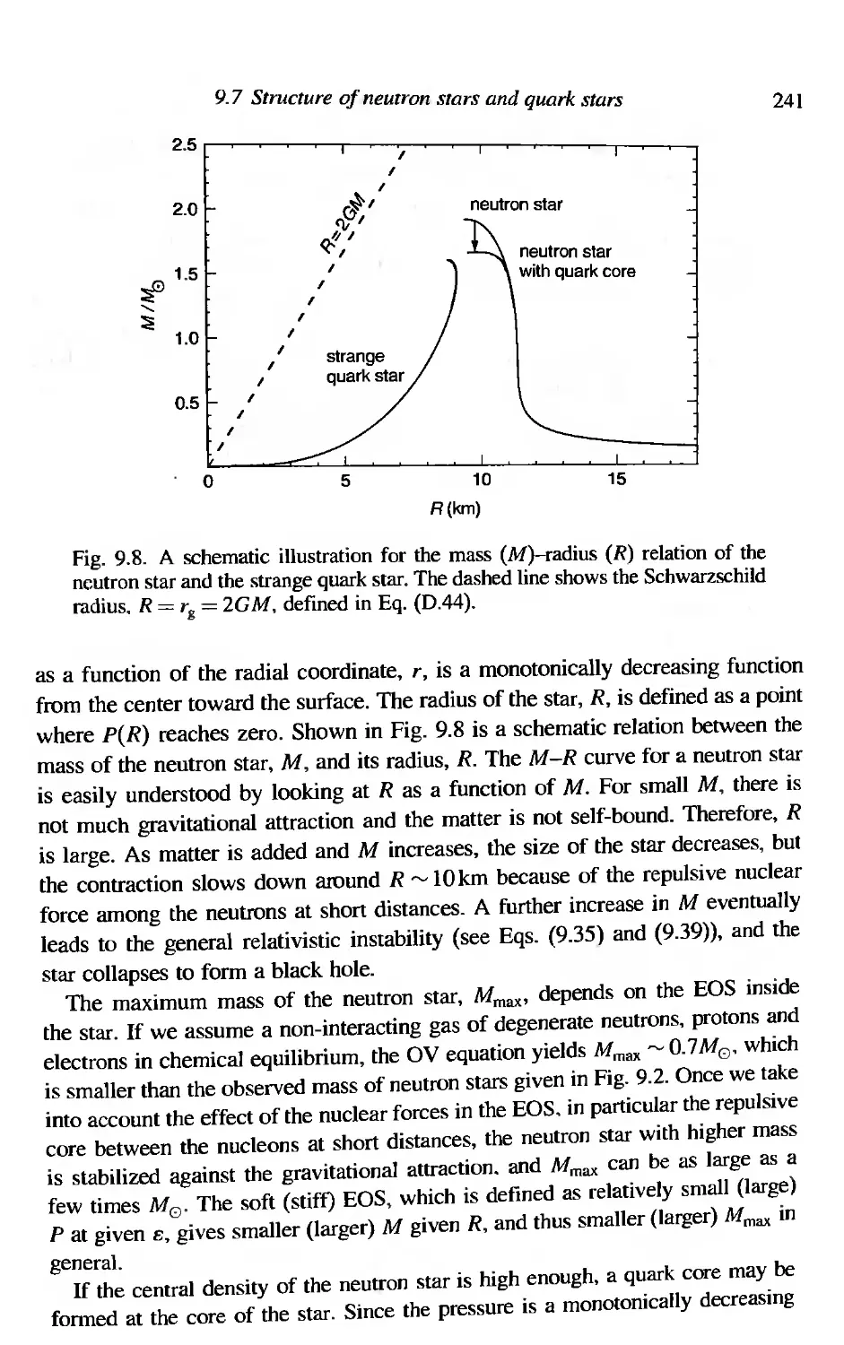
9.7.1 Mass-radius relation of neutron stars
9.7.2 Strange quark stars
9.8 Various phases in high-density matter
Exercises
217
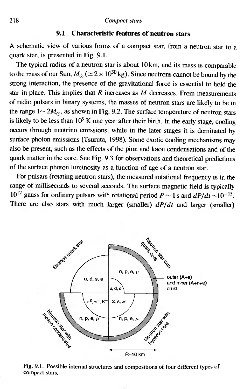
2]8
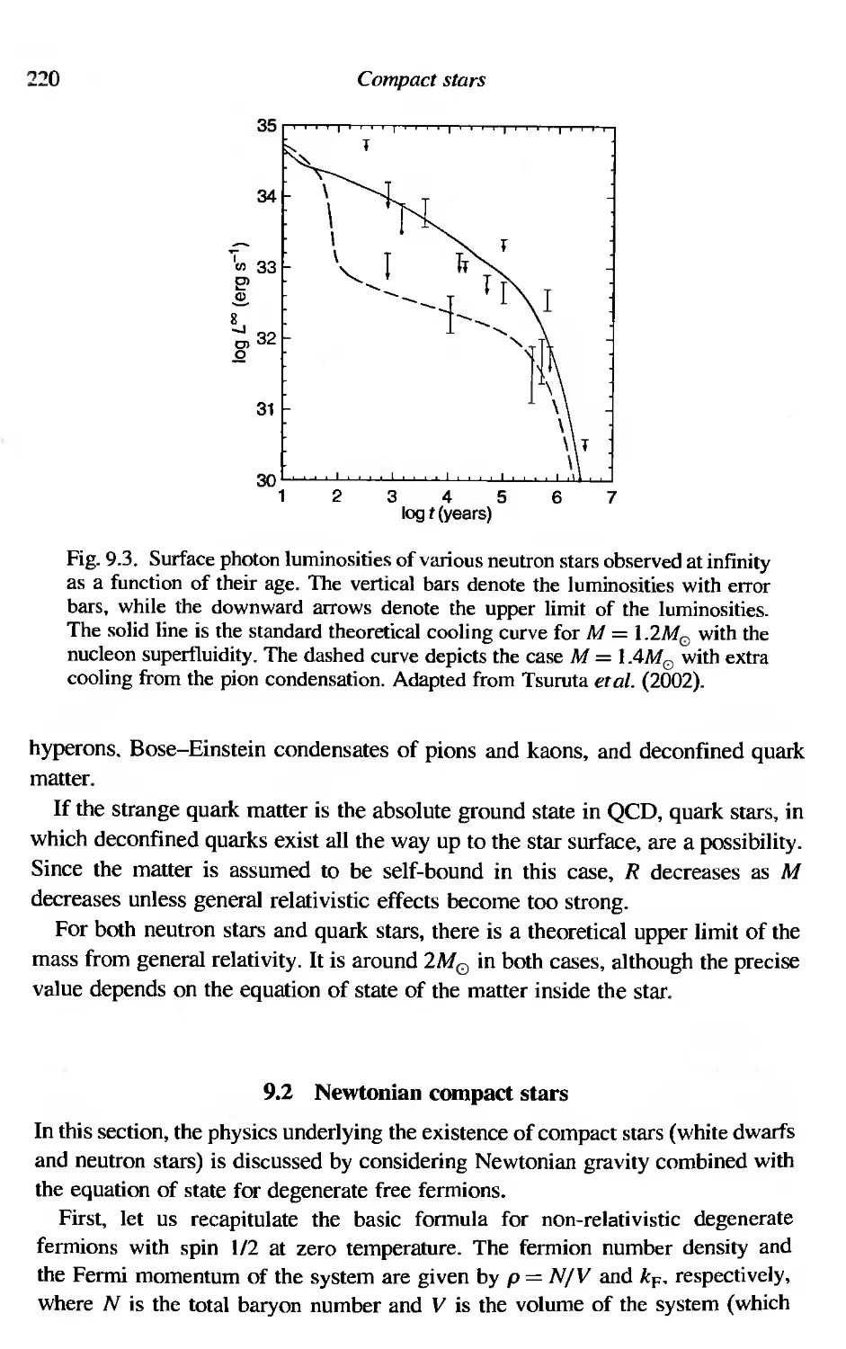
220
22]
223
224
224
226
229
229
229
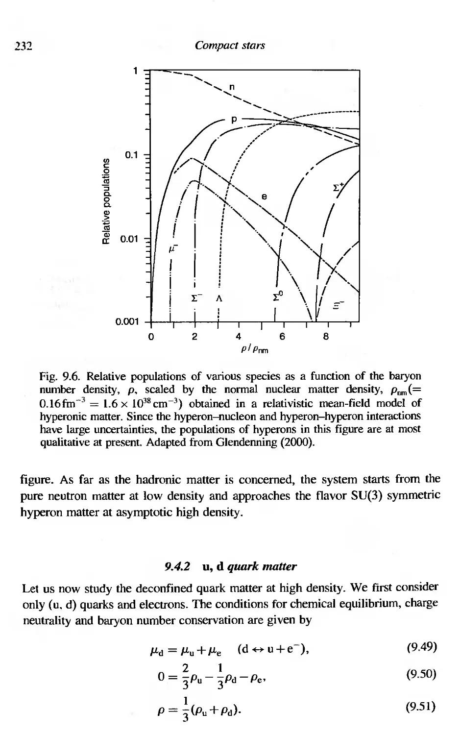
232
233
233
234
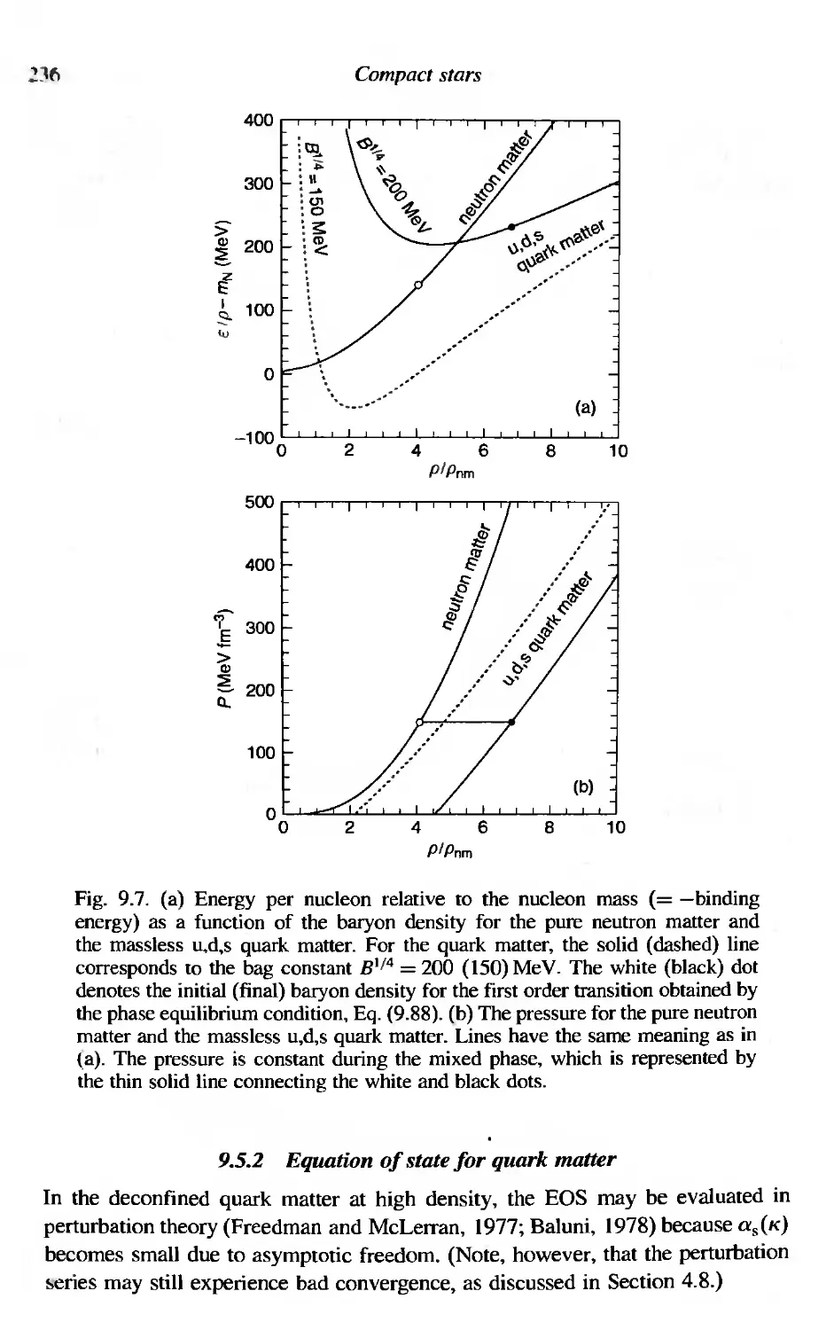
236
239
239
240
240
242
243
244
Contents xi
Part III: Quark-Gluon Plasma in Relativistic Heavy
Ion Collisions 245
10 Introduction to relativistic heavy ion collisions 247
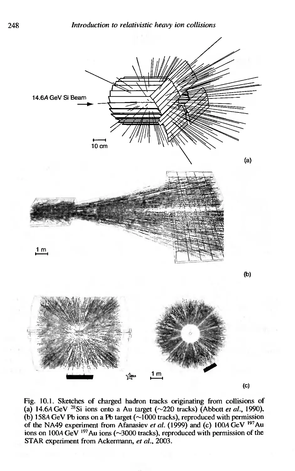
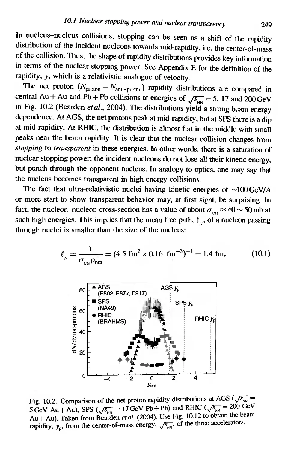
10.1 Nuclear stopping power and nuclear transparency 247
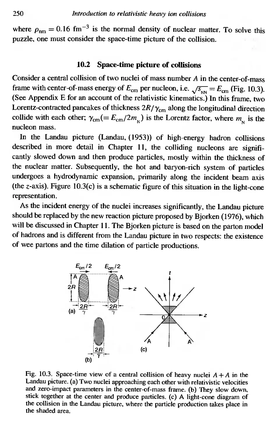
10.2 Space-time picture of collisions 250
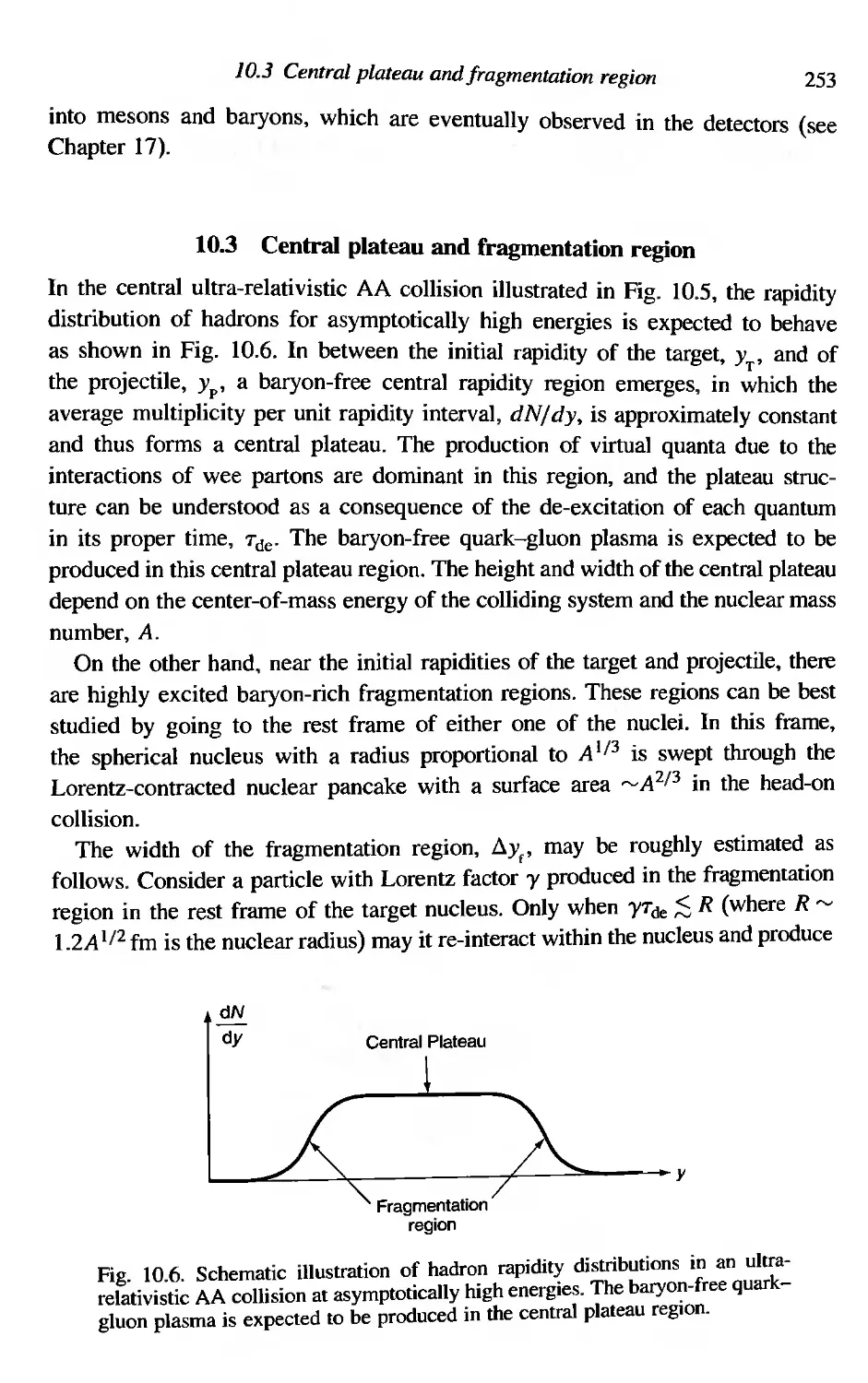
10.3 Central plateau and fragmentation region 253
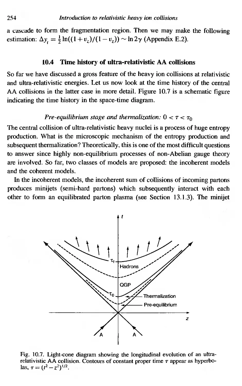
10.4 Time history of ultra-relativistic AA collisions 254
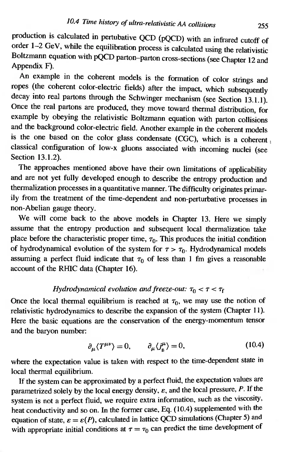
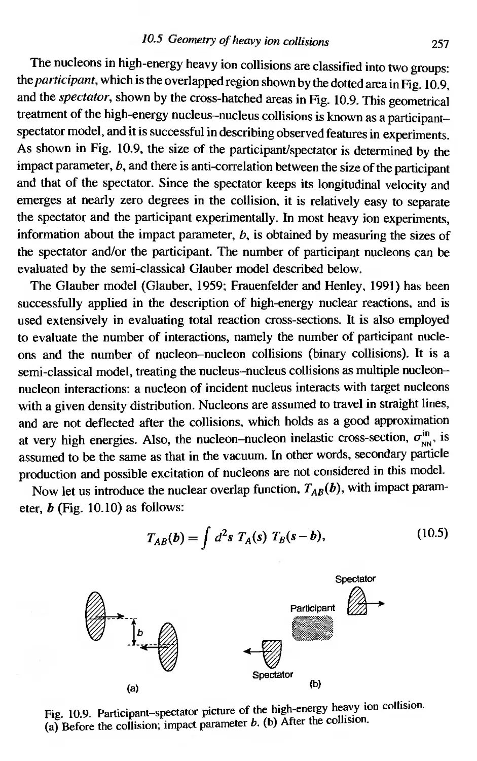
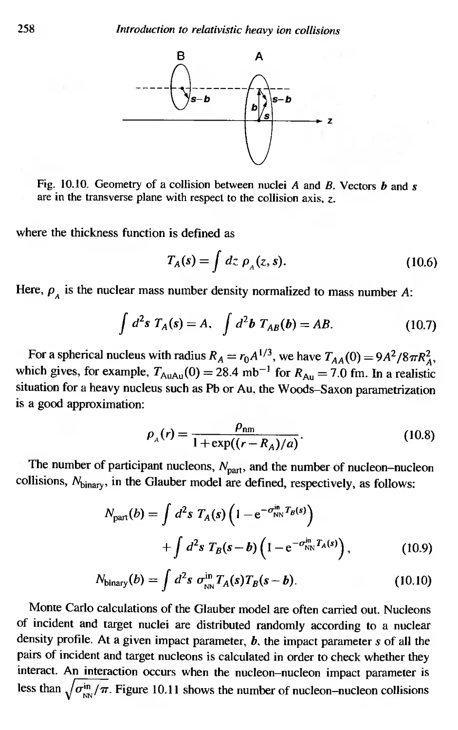
10.5 Geometry of heavy ion collisions 256
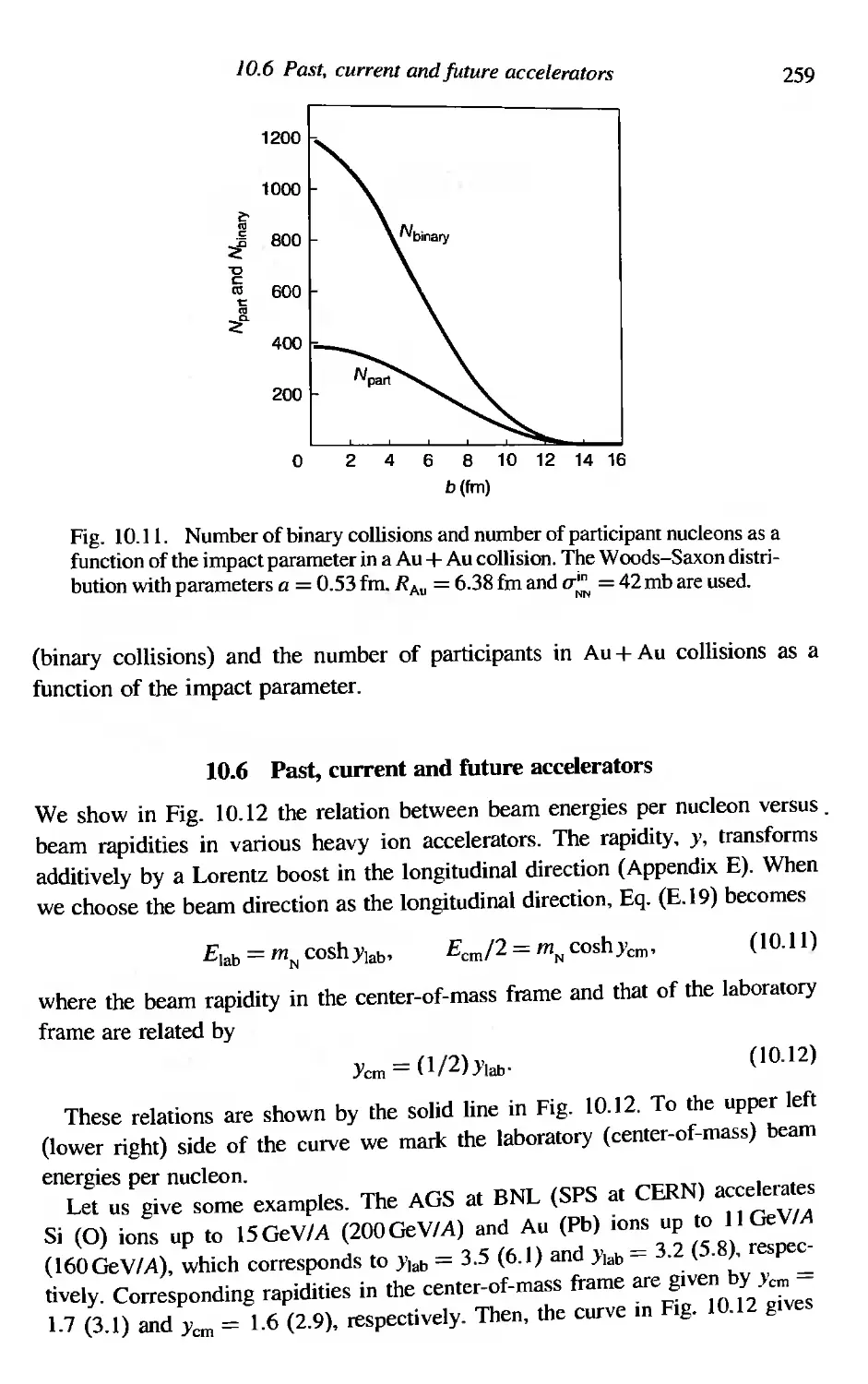
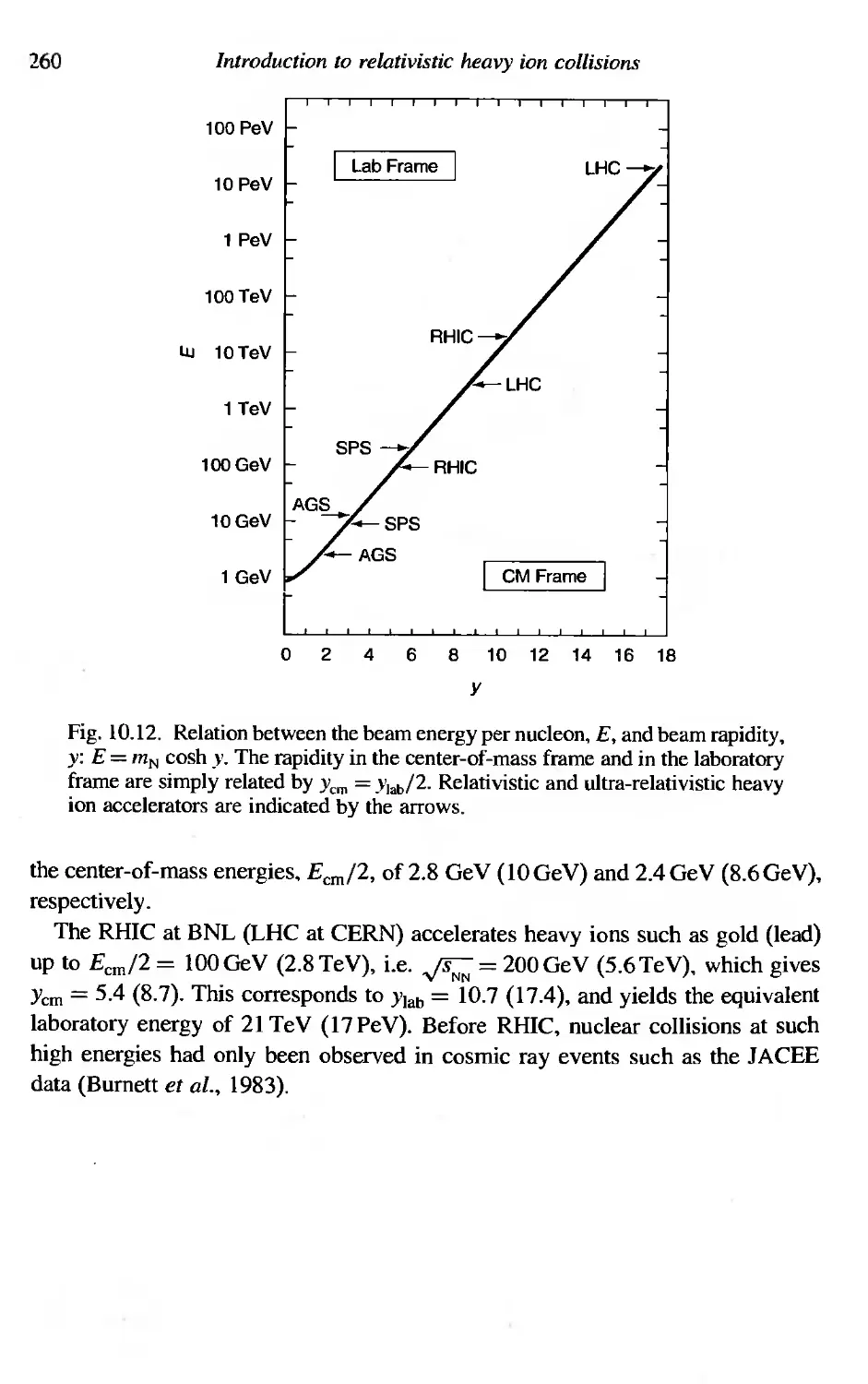
10.6 Past, current and future accelerators 259
11 Relativistic hydrodynamics for heavy ion collisions 261
11.1 Fermi and Landau pictures of multi-particle production 261
11.2 Relativistic hydrodynamics 265
] 1.2.1 Perfect fluid 265
11.2.2 Dissipative fluid 267
11.3 Bjorken's scaling solution 269
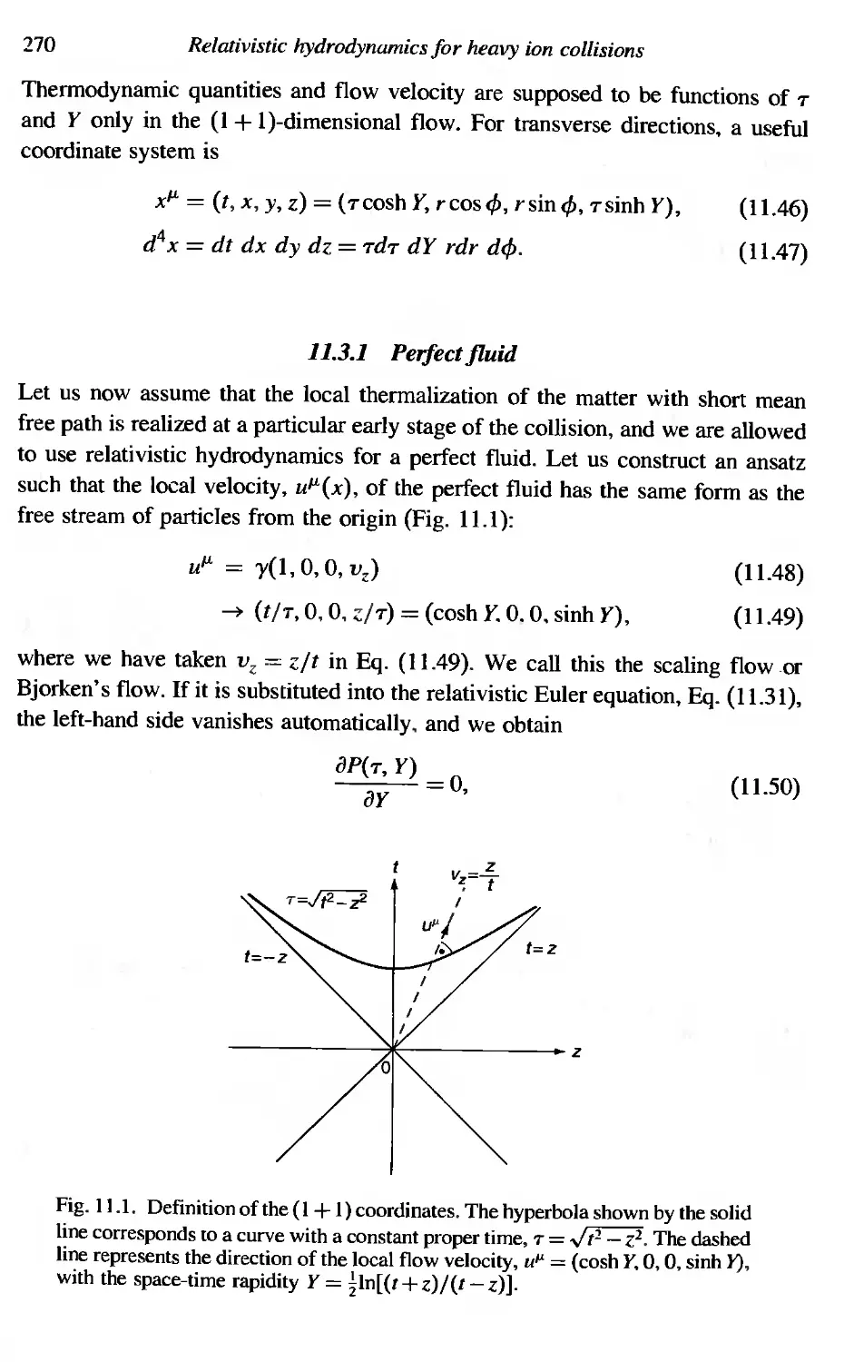
11.3.1 Perfect fluid 270
11.3.2 Effect of dissipation 273
]1.4 Relation to the observables 274
Exercises 276
12 Transport theory for the pre-equilibrium process 278
12.1 Classical Boltzmann equation 278
]2,2 Boltzmann's H-theorem 282
]2.3 Covariant form of the classical transport equation 283
12.3.1 Conservation laws 284
12.3.2 Local H-theorem and local equilibrium 285
12.4 Quantum transport theory 286
]2.4.1 The density matrix 287
]2.4.2 The Dirac equation 287
]2.4.3 The Wigner function 288
12.4.4 Equation of motion for W(x, p) 290
12.4.5 Semi-classical approximation 29]
]2.4.6 Non-Abelian generalization 293
]2,5 Phenomenological transport equation in QCD 294
Exercises 295
13 Formation and evolution of QGP 297
13.] The initial condition 298
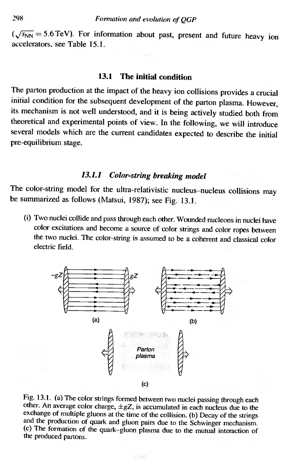
13 .1.1 Color-string breaking mode] 298
299
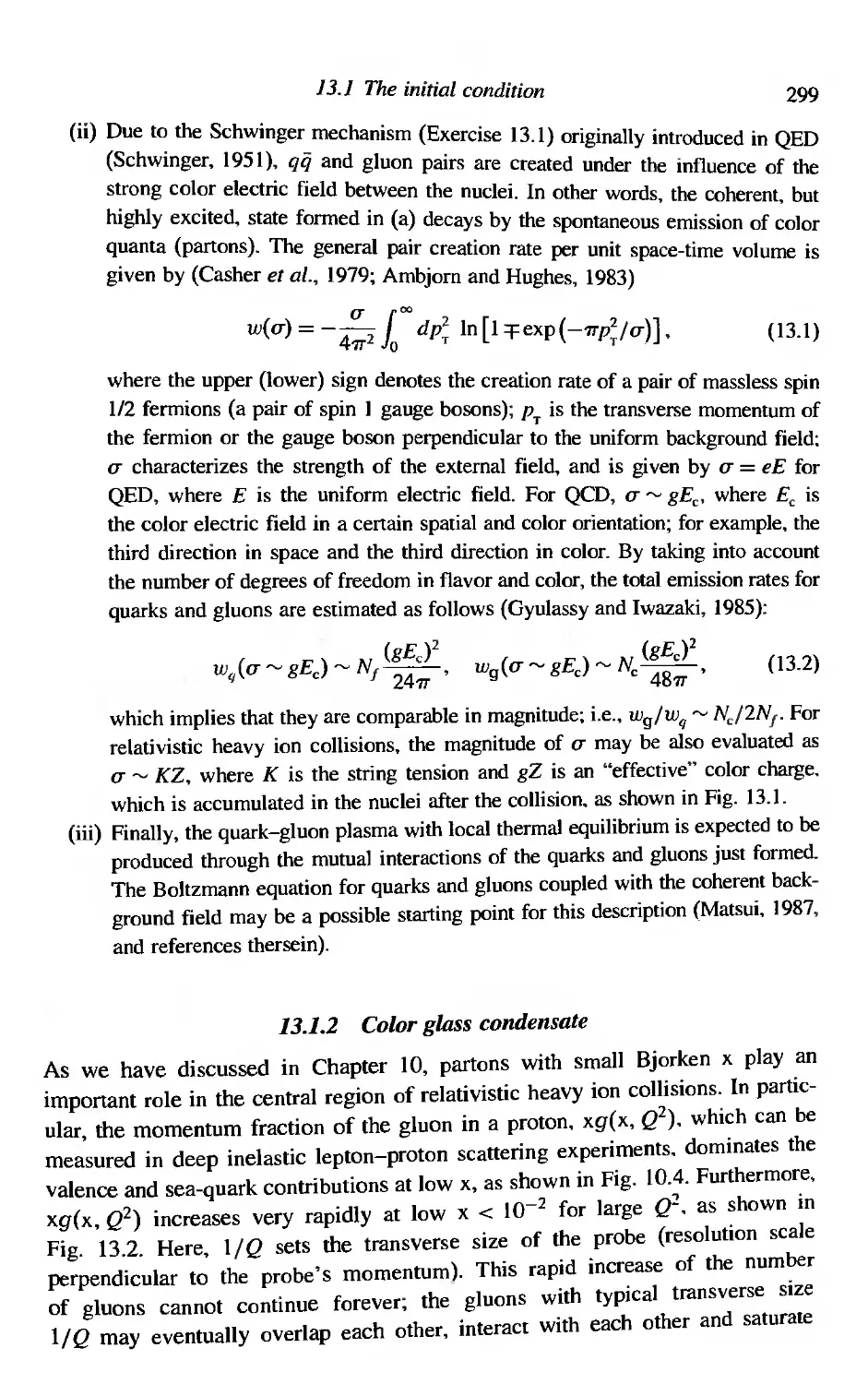
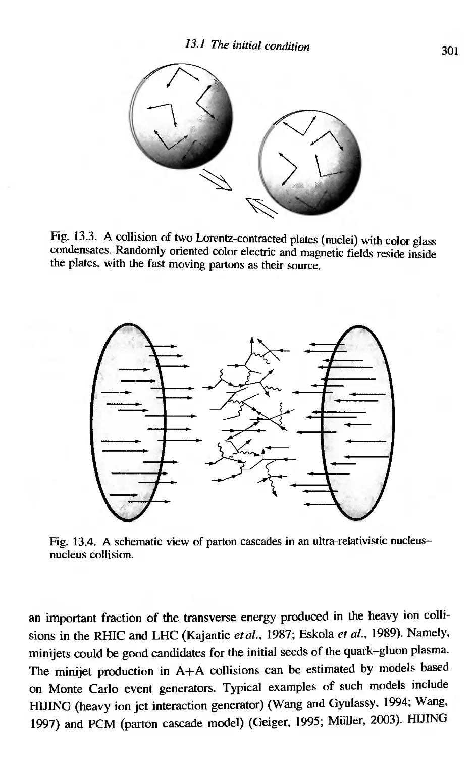
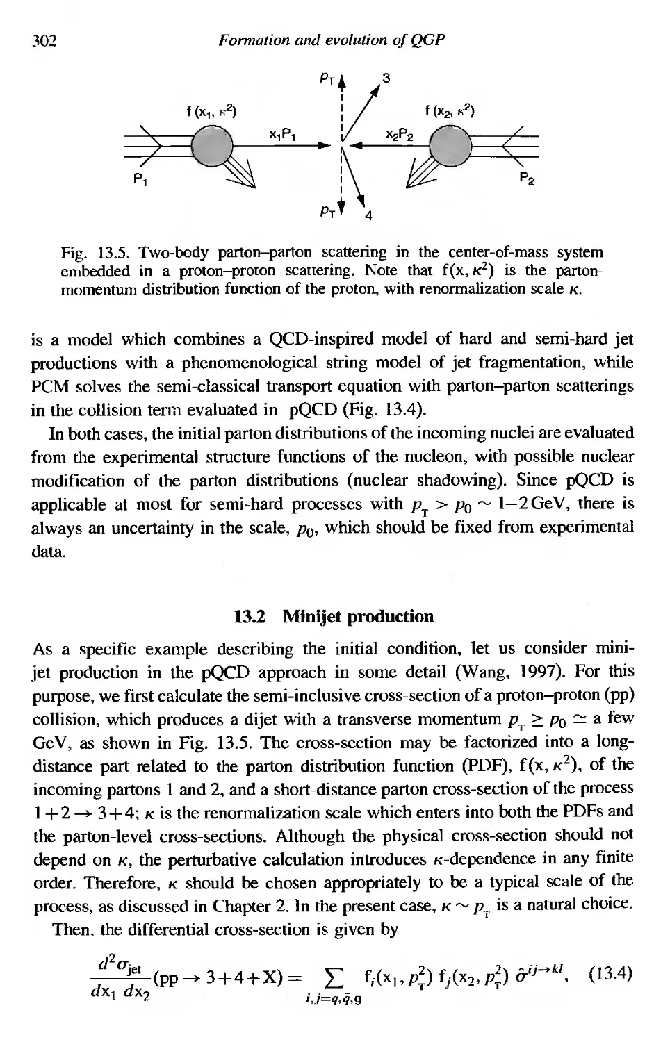
13.1.2 Color glass condensate 300
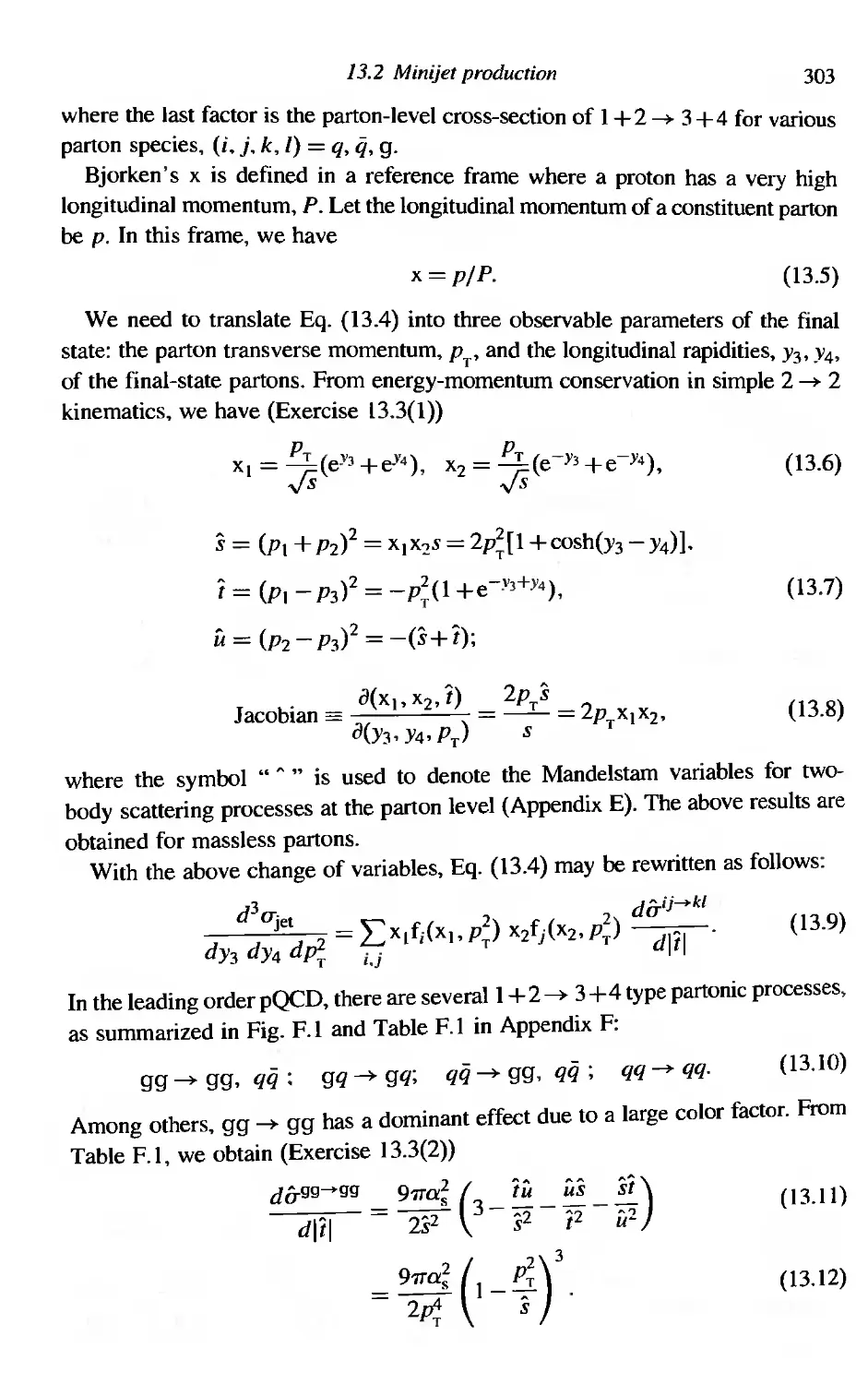
13,1.3 Perturbative QCD models 302
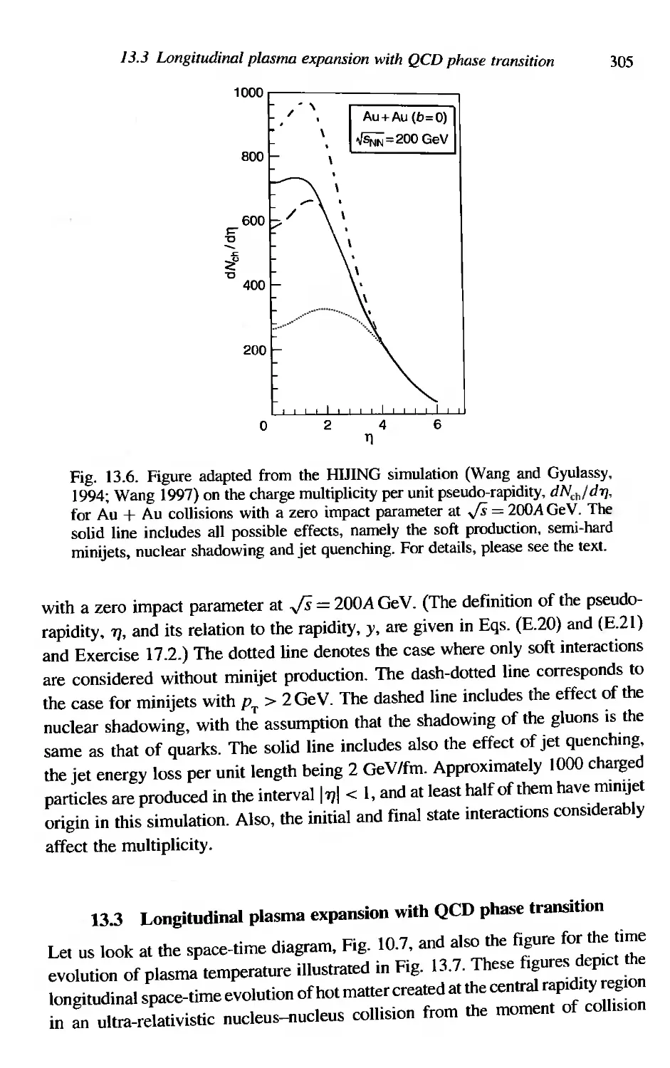
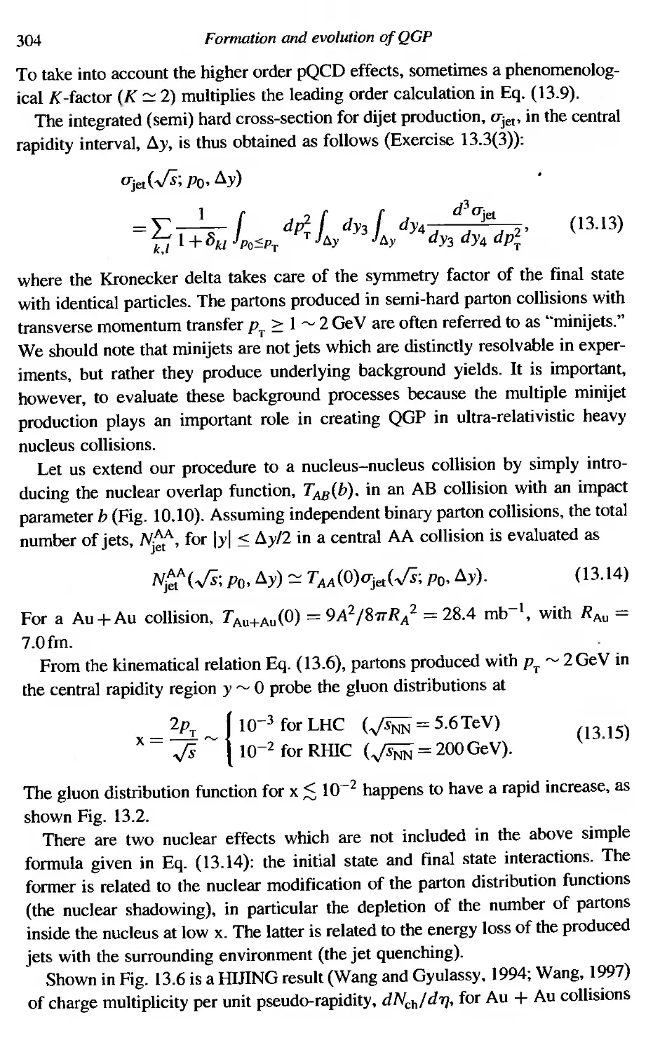
13,2 Minijet production . . 305
13.3 Longitudinal plasma expansion with QCD phase transItIOn 307
13.4 Transverse plasma expansion 309
13.5 Transverse momentum spectrum and transverse flow 311
Exercises
XII
Contents
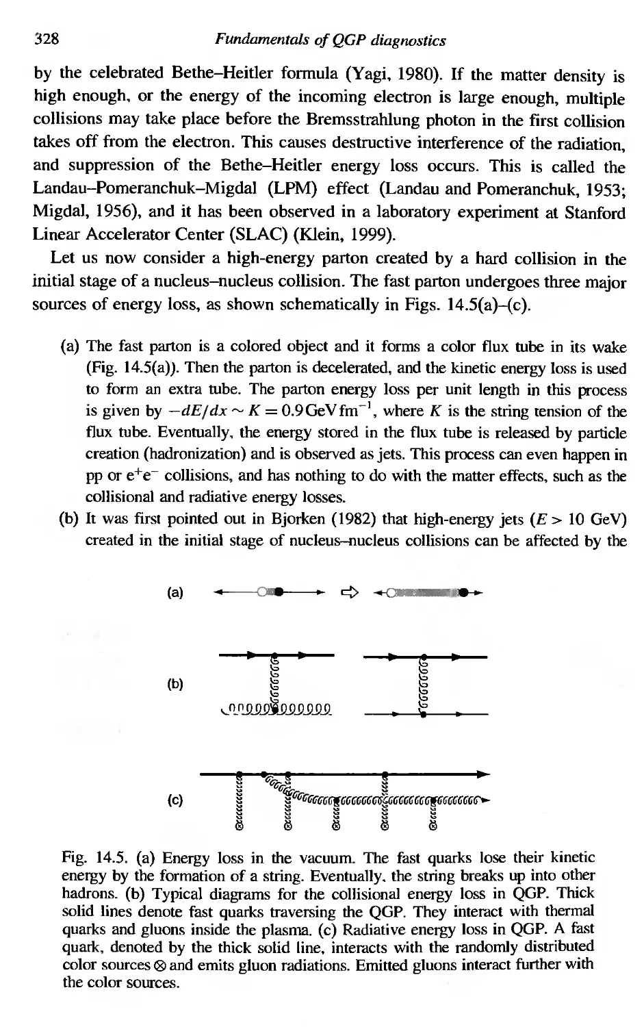
14
14.1
Fundamentals of QGP diagnostics
QGP diagnostics using hadrons
14.l.I Probing the phase transition
14.1.2 Ratios of particle yields and chemical equilibrium
14.1.3 Transverse momentum distributions and
hydrodynamical flow
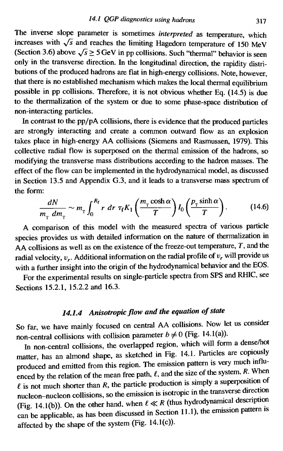
14.1.4 Anisotropic flow and the equation of state
14,1.5 Interferometry and space-time evolution
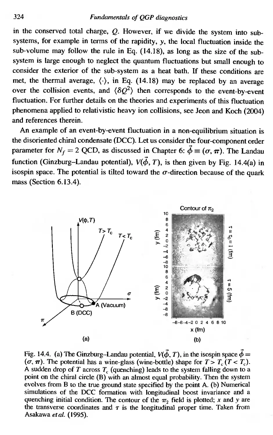
14.1.6 Event-by-event fluctuations
14.1. 7 Hadron production by quark recombination
QGP diagnostics using hard probes: jet tomography
QGP diagnostics using leptons and photons
14.3.1 Drell-Yan production of dileptons
14.3.2 1/«/1 suppression and Debye screening in QGP
14.3.3 Thermal photons and dileptons
Exercises
14.2
14.3
15
15.1
15.2
Results from CERN-SPS experiments
Relativistic heavy ion accelerators
Basic features of AA collisions
] 5.2.1 Single-particle spectra
15.2.2 Collective expansion
15.2.3 HBT two-particle correlation
Strangeness production and chemical equilibrium
1/«/1 suppression
Enhancement of low-mass dileprons
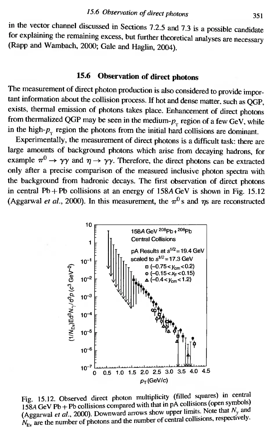
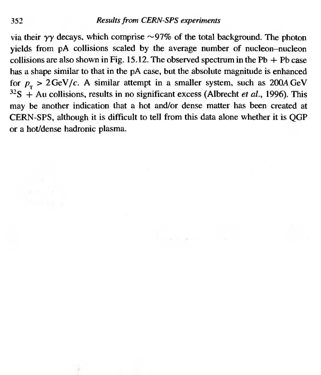
Observation of direct photons
]5.3
15.4
]5.5
15.6
16
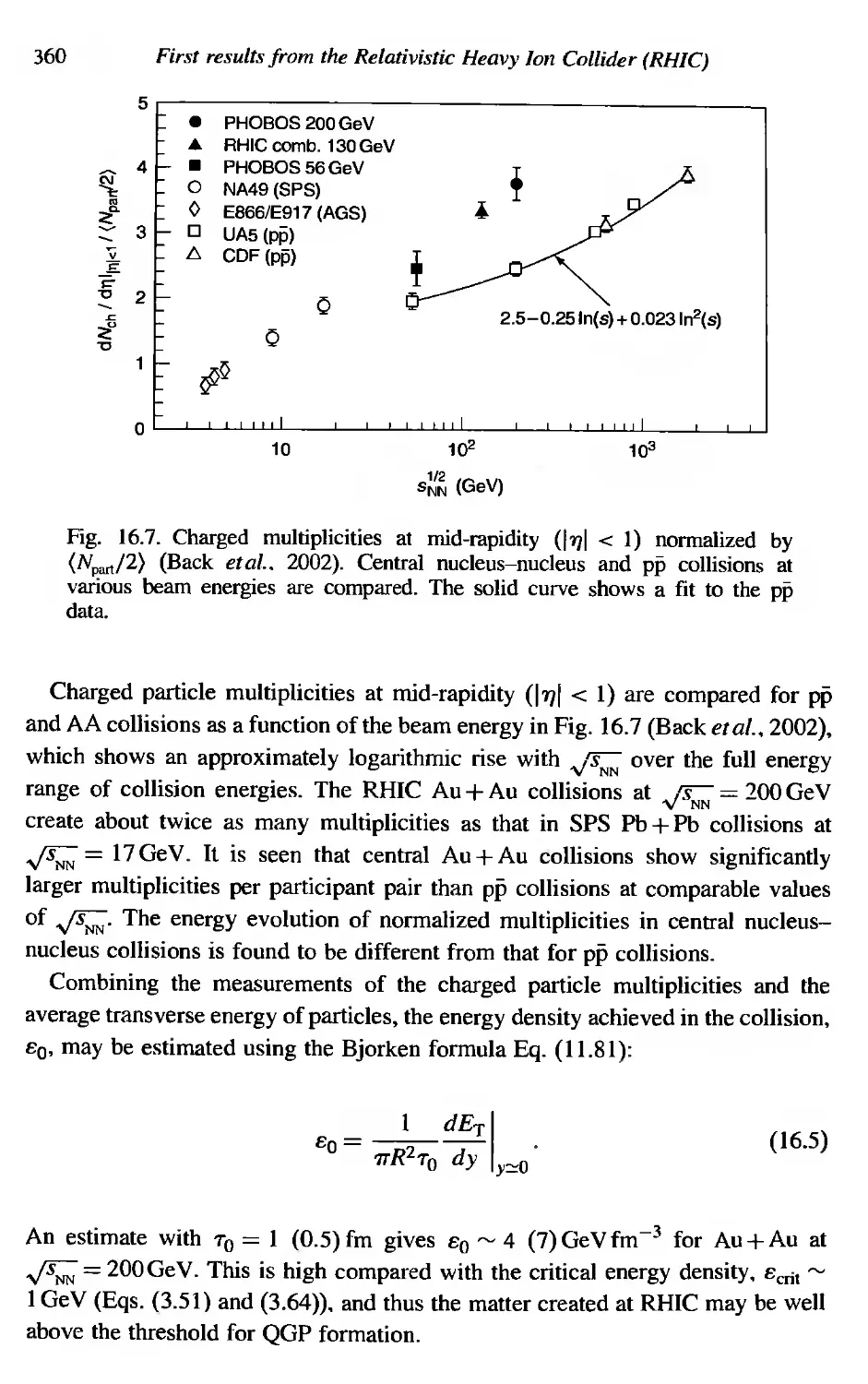
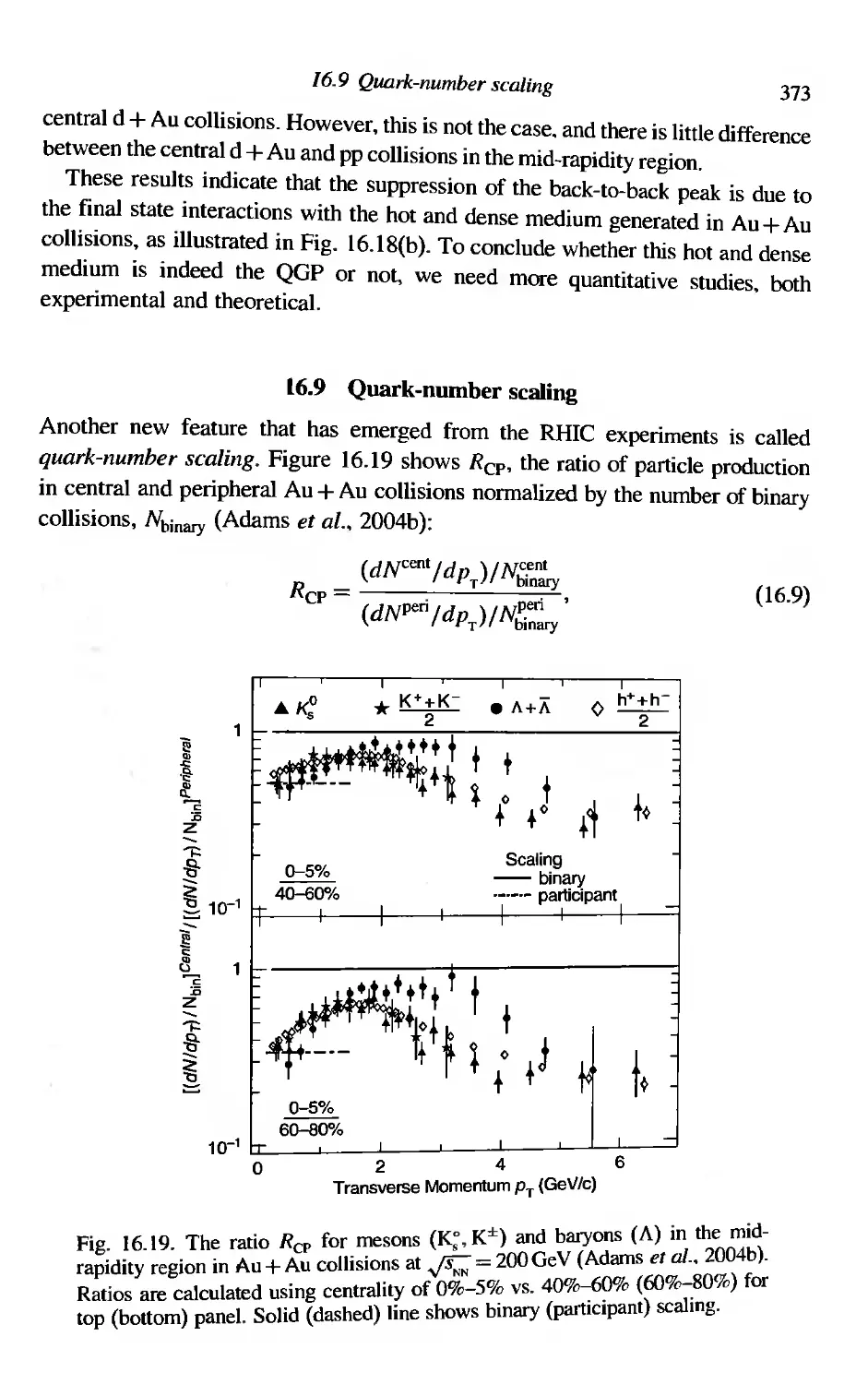
16.1
16.2
16.3
16.4
16,5
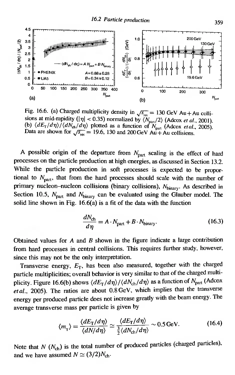
16.6
16.7
16.8
16.9
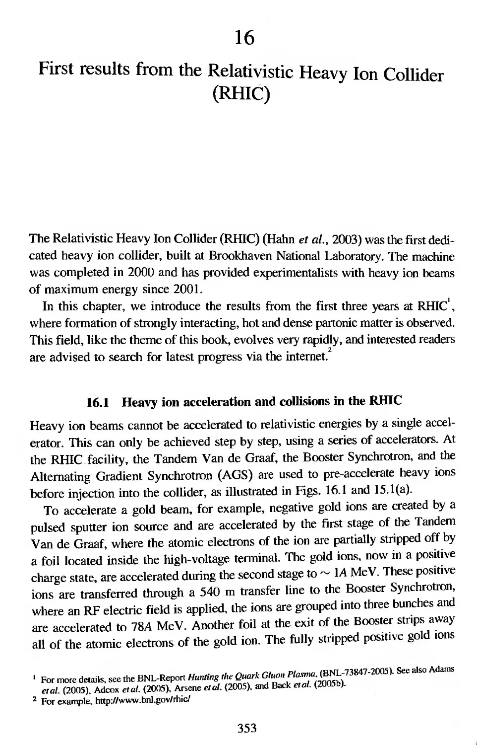
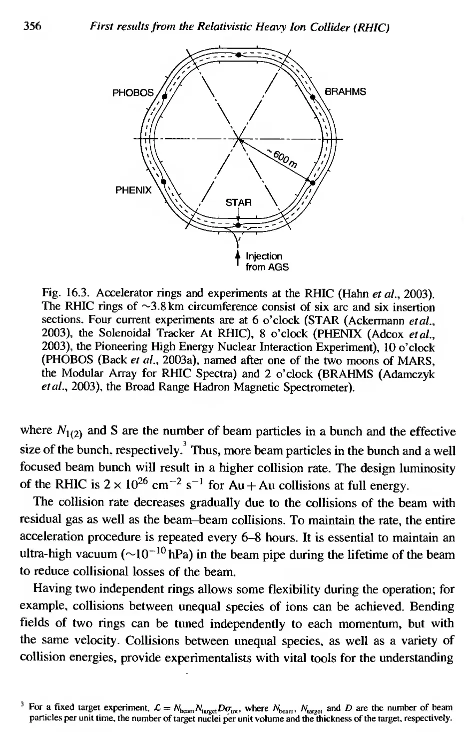
First results from the Relativistic Heavy Ion CoIlider (RHlC)
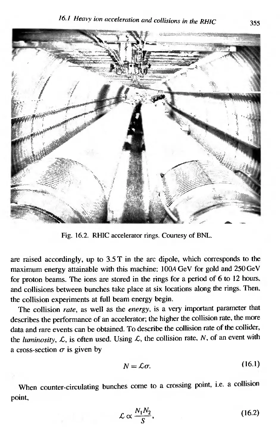
Heavy ion acceleration and collisions in the RHIC
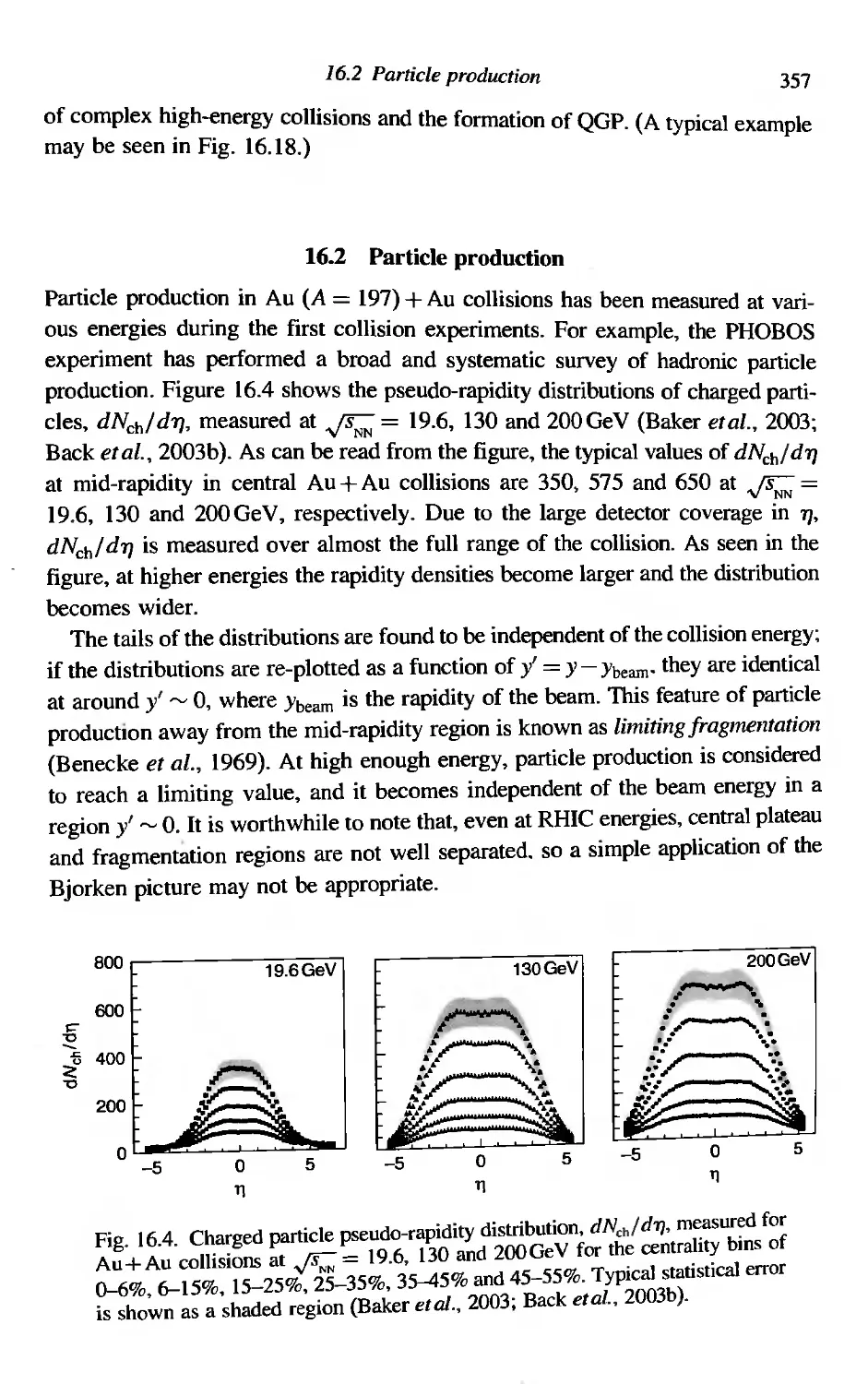
Particle production
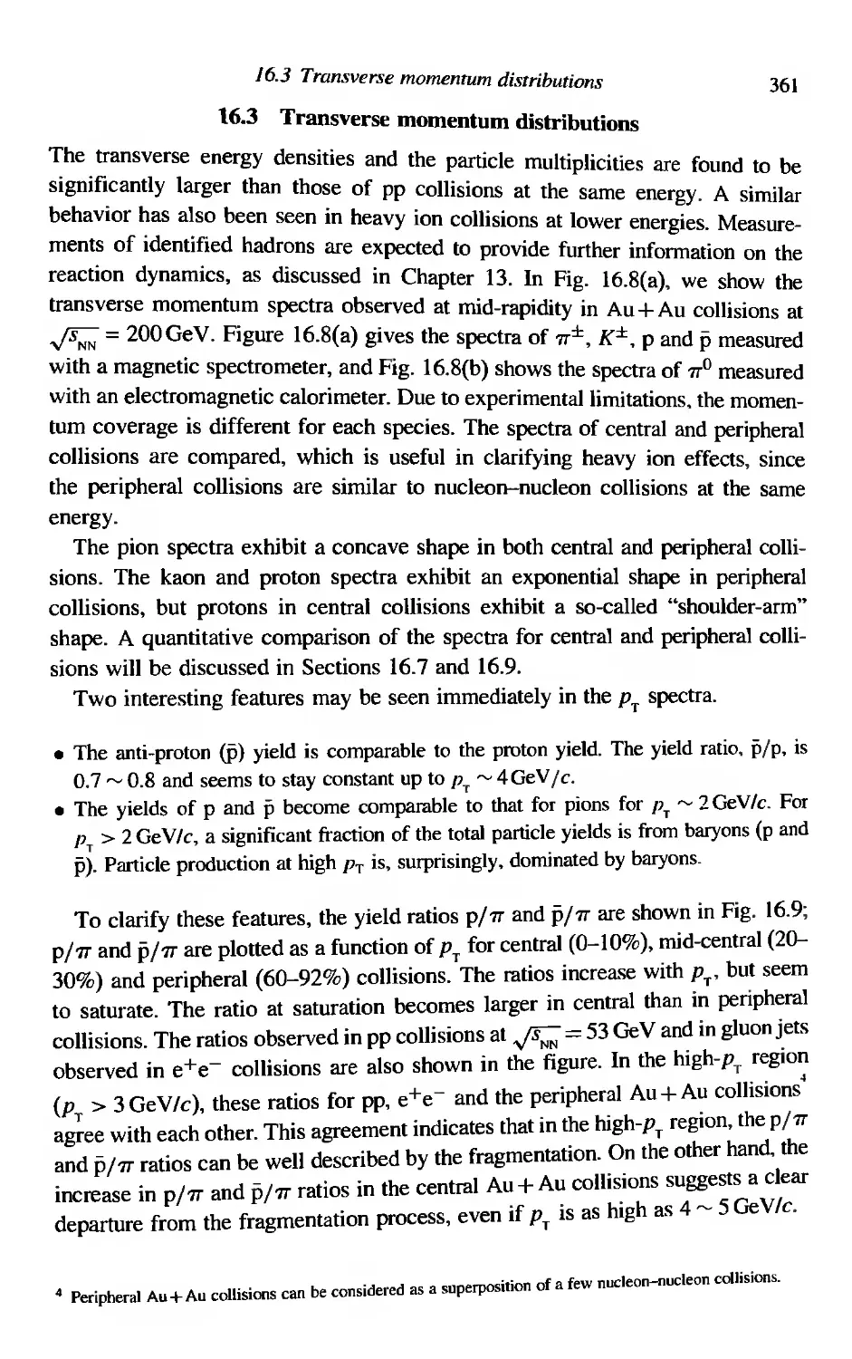
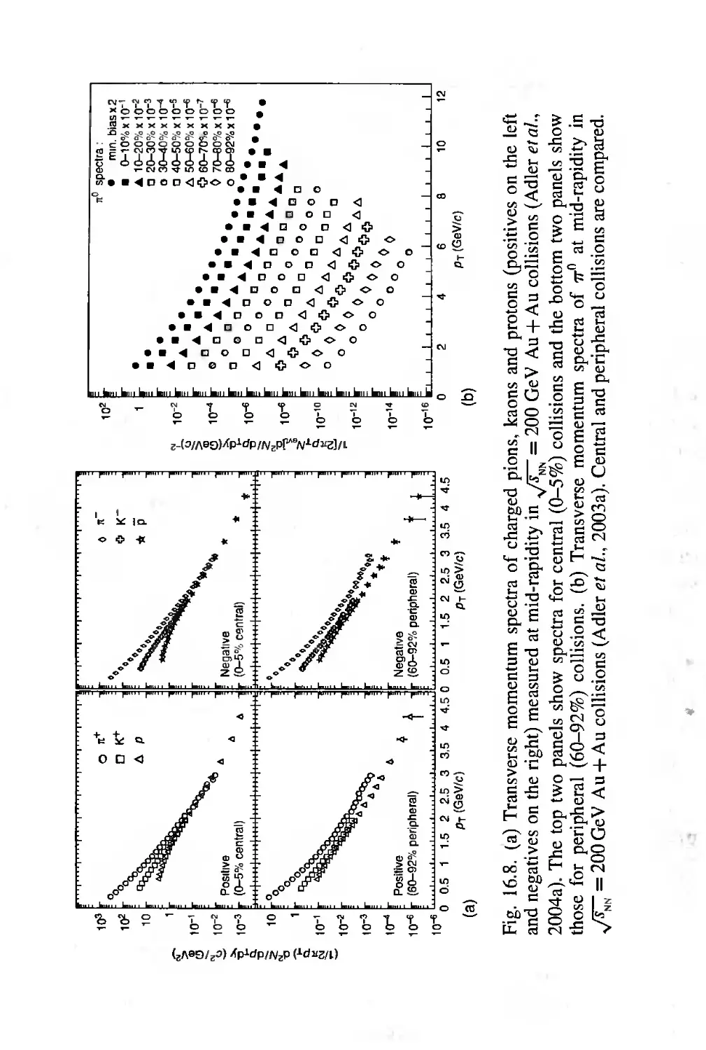
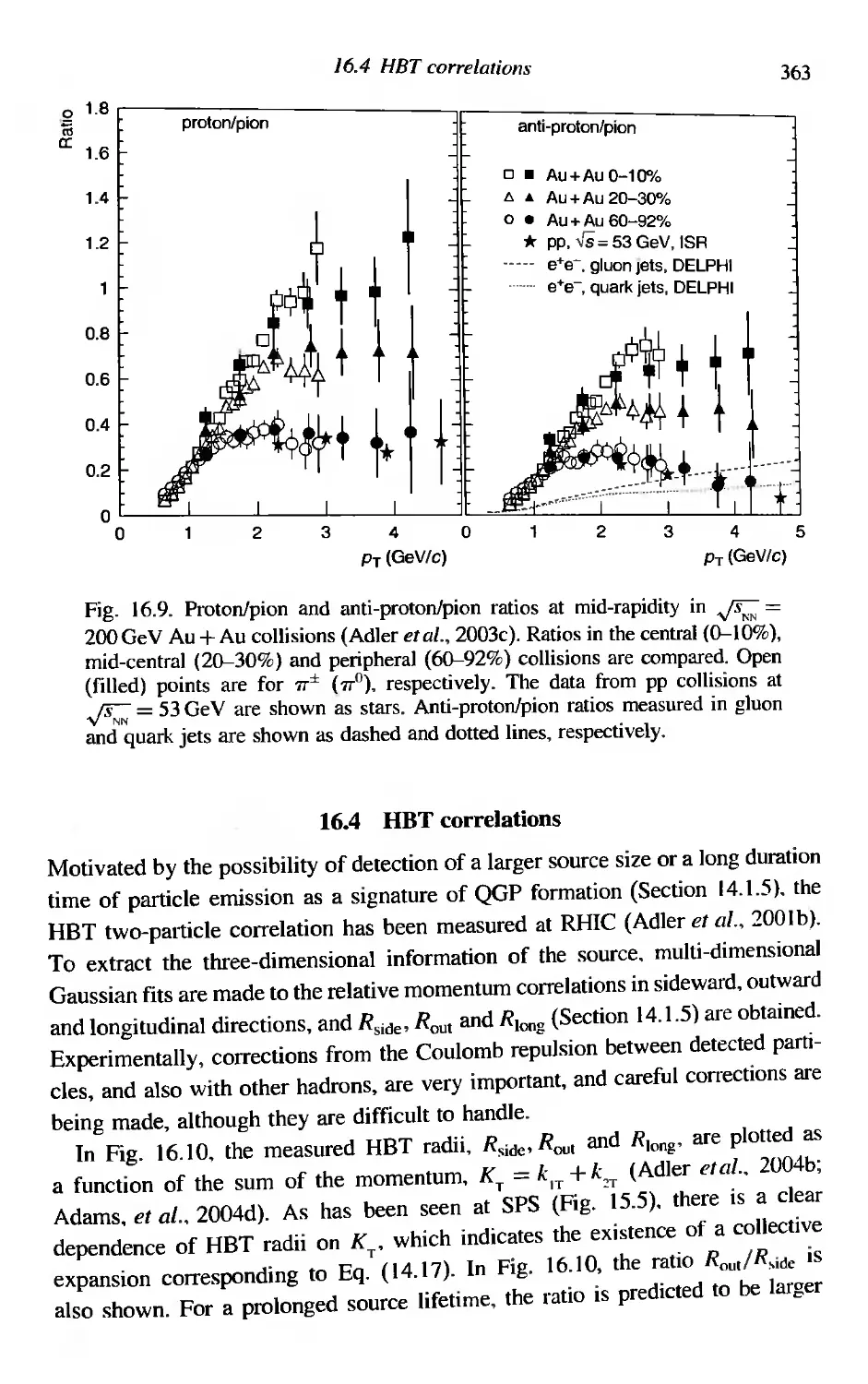
Transverse momentum distributions
HBT correlations
Thermalization
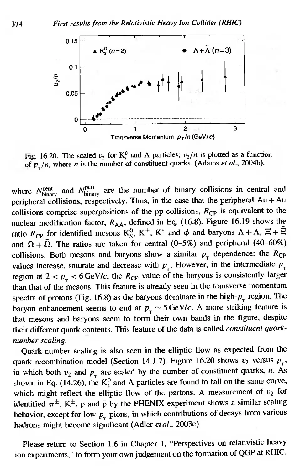
Azimuthal anisotropy
Suppression of high-P T hadrons
Modification of the jet structure
Quark-number scaling
17
17.1
17.2
17.3
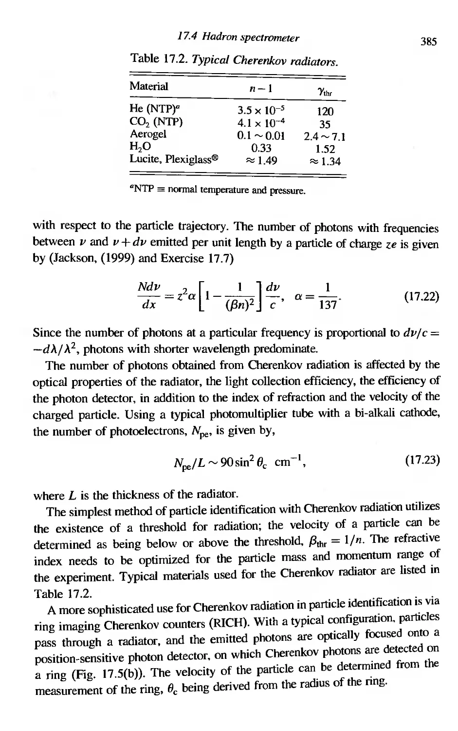
17.4
Detectors in relativistic heavy ion experiments
Features of relati vistic heavy ion collisions
Transverse energy, E
Event characterizatio detectors
Hadron spectrometer
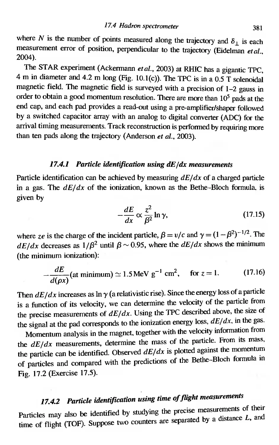
17.4.1 Particle identification using dE/dx measurements
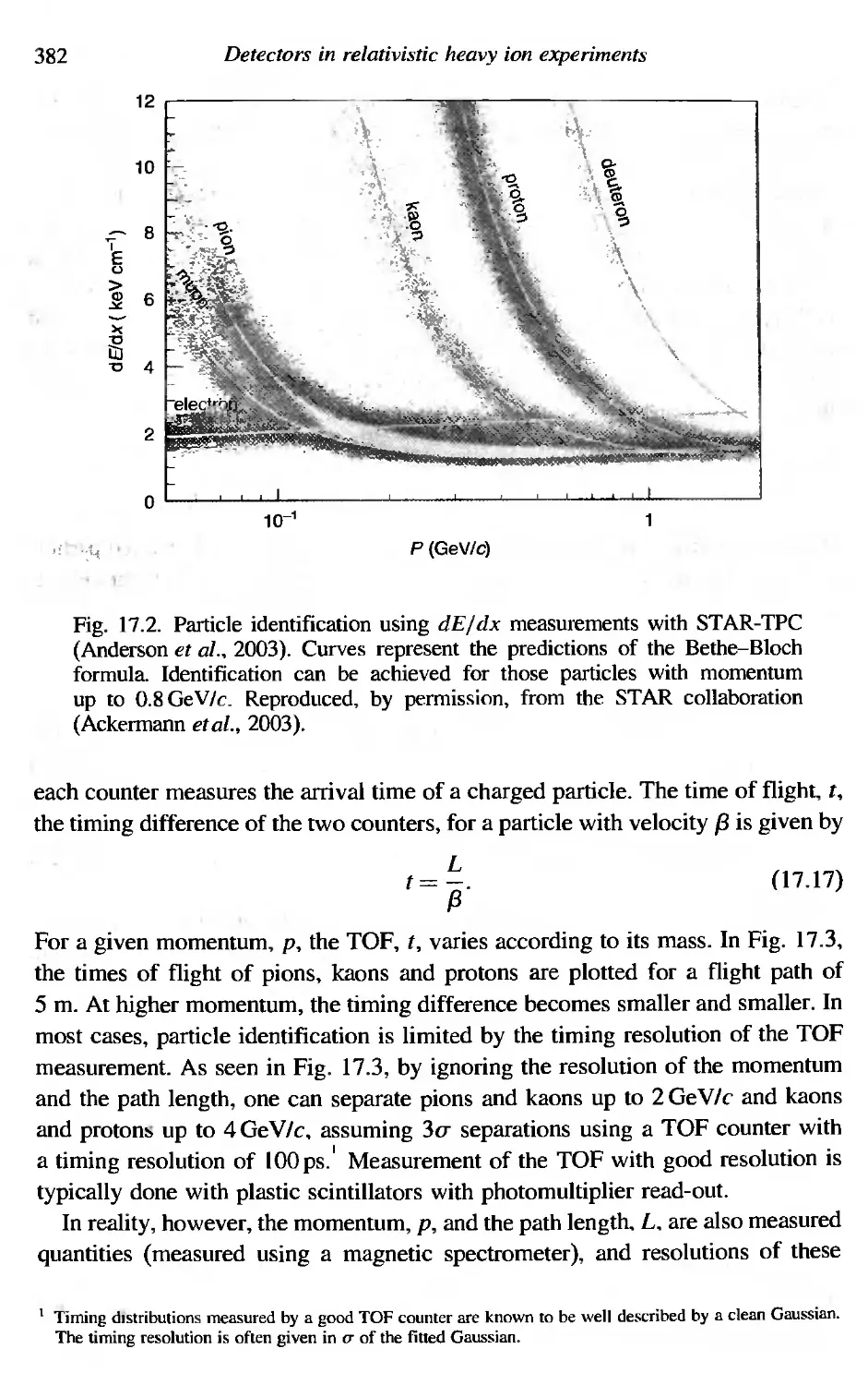
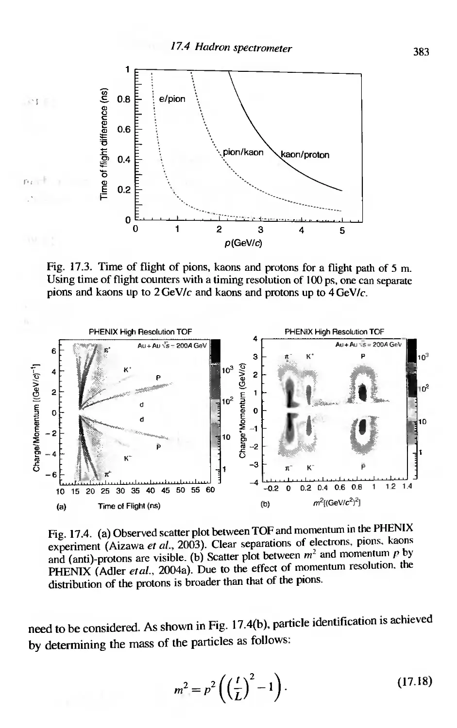
17.4.2 Particle identification using time of flight measurements
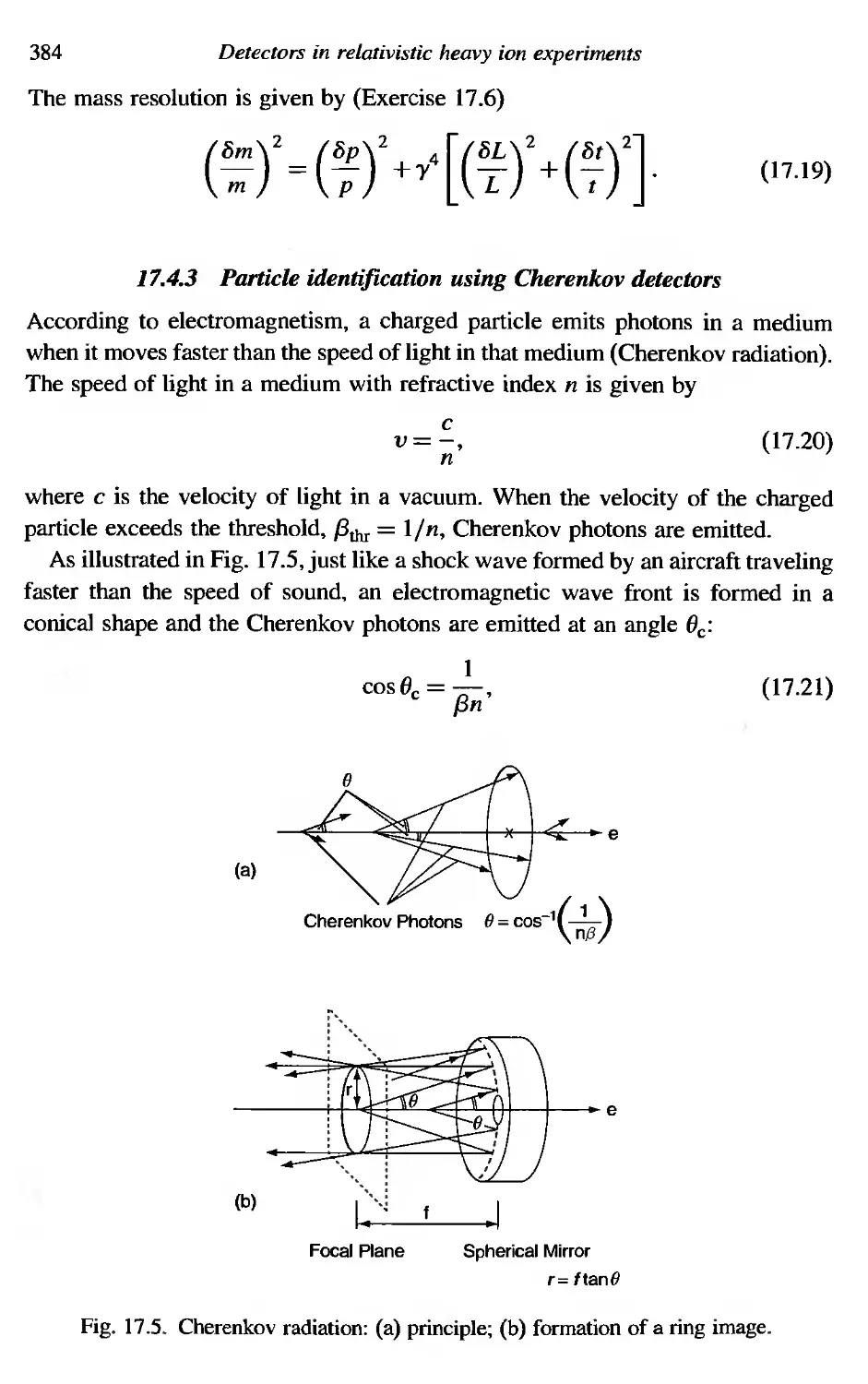
17.4.3 Particle identification using Cherenkov detectors
314
314
314
315
316
317
320
323
325
327
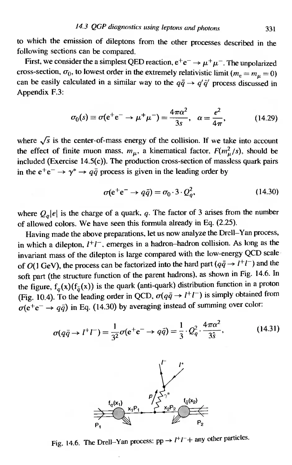
330
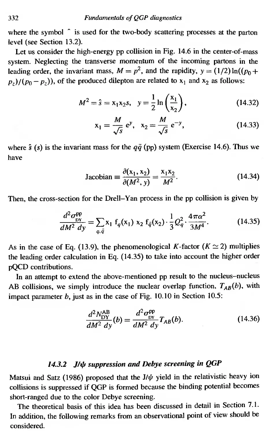
330
332
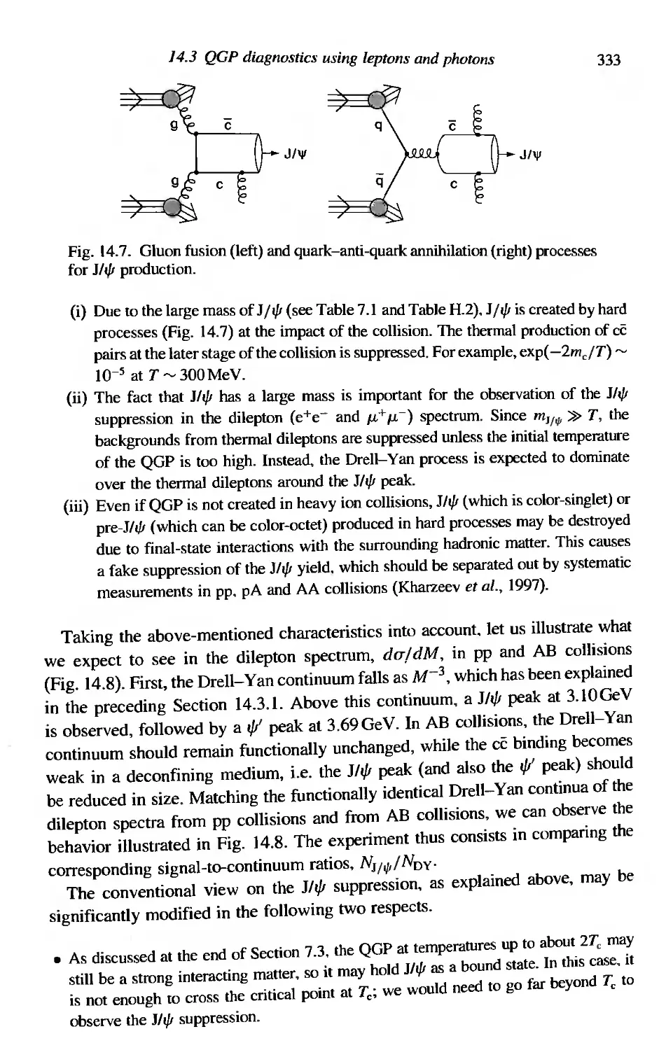
334
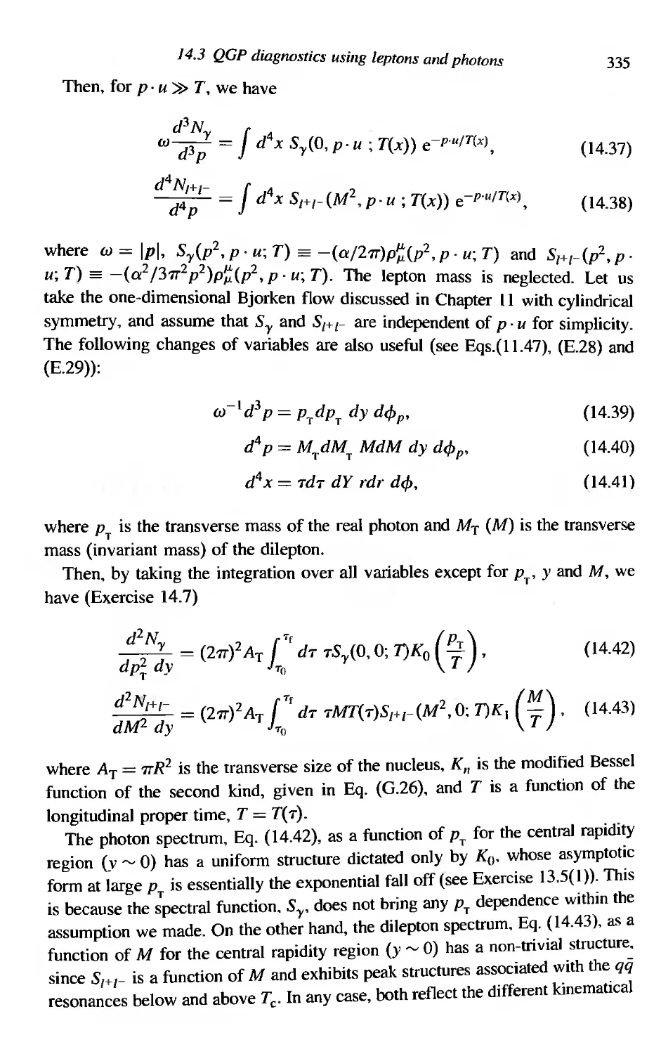
336
338
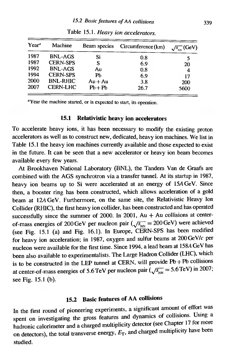
339
339
340
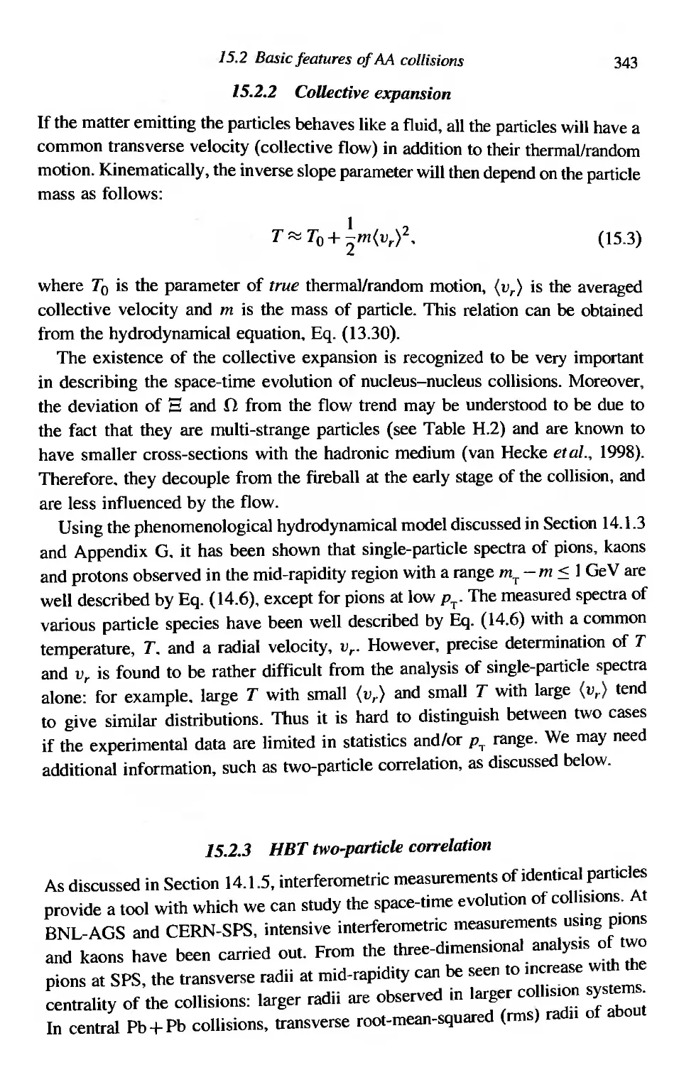
343
343
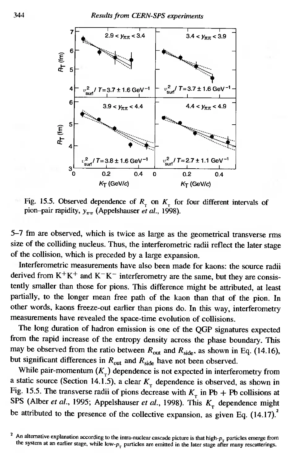
345
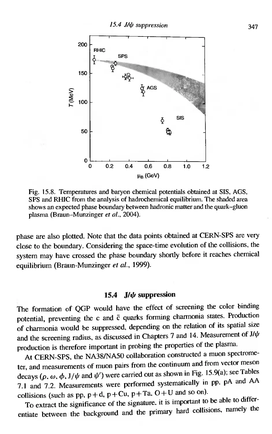
347
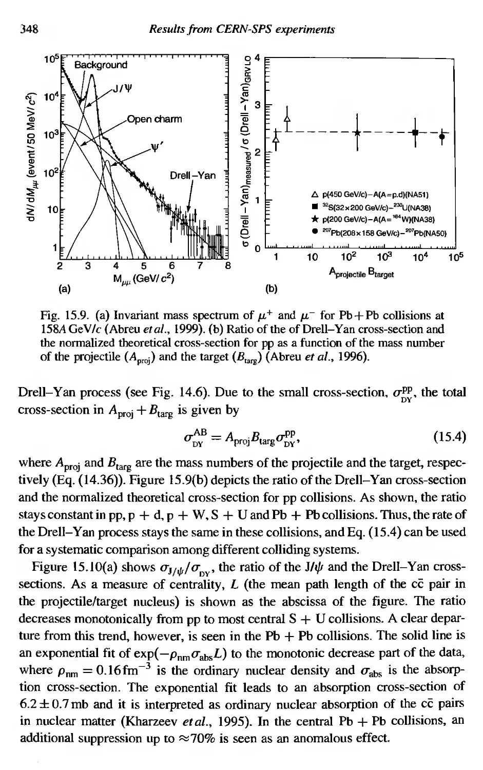
349
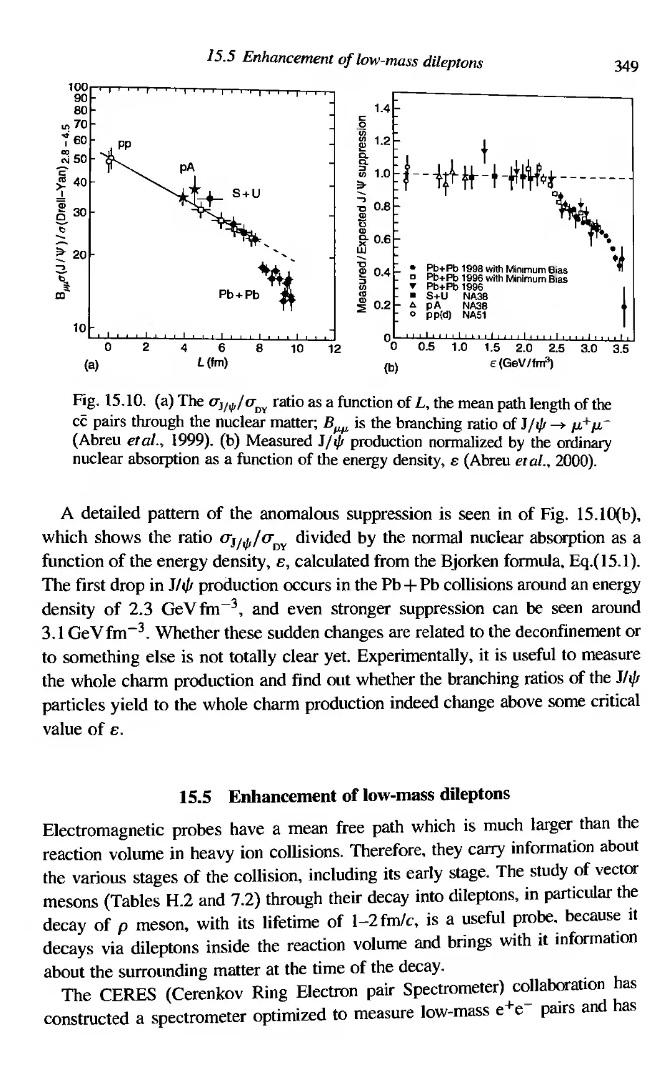
351
353
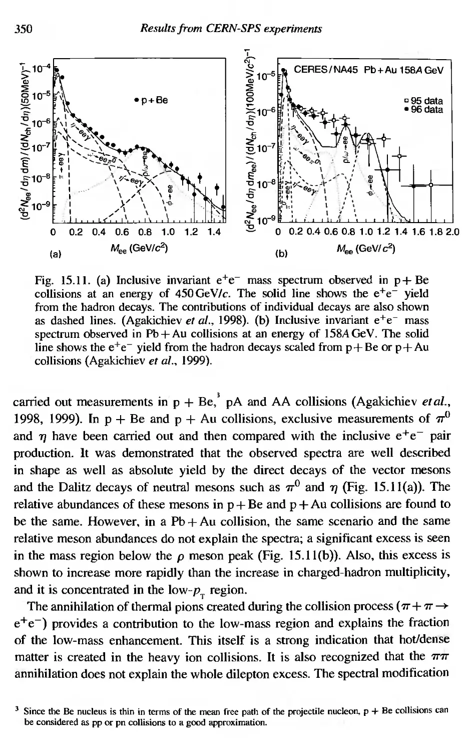
353
357
361
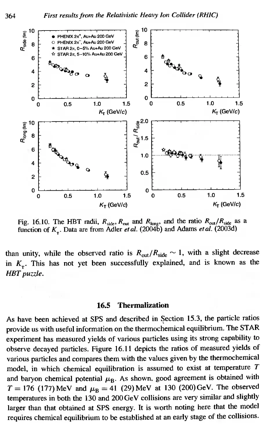
363
364
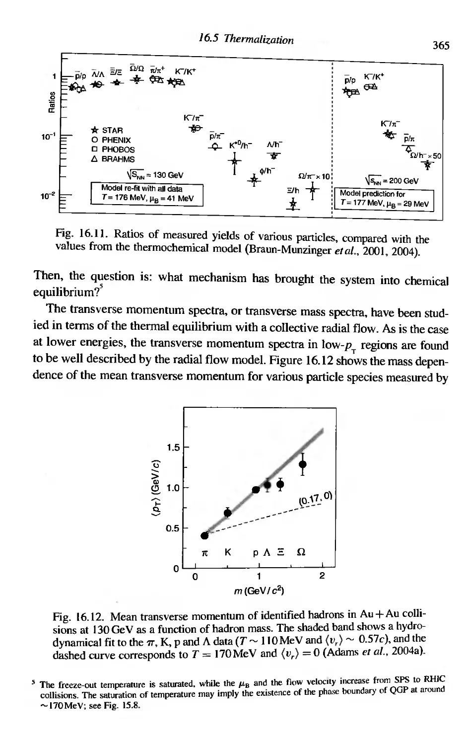
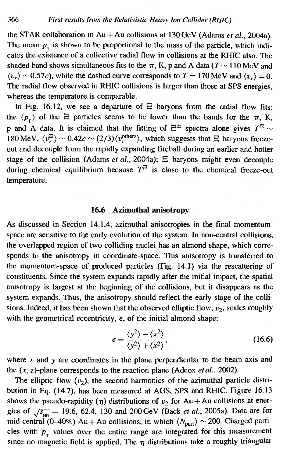
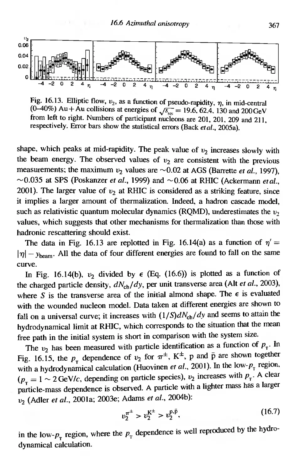
366
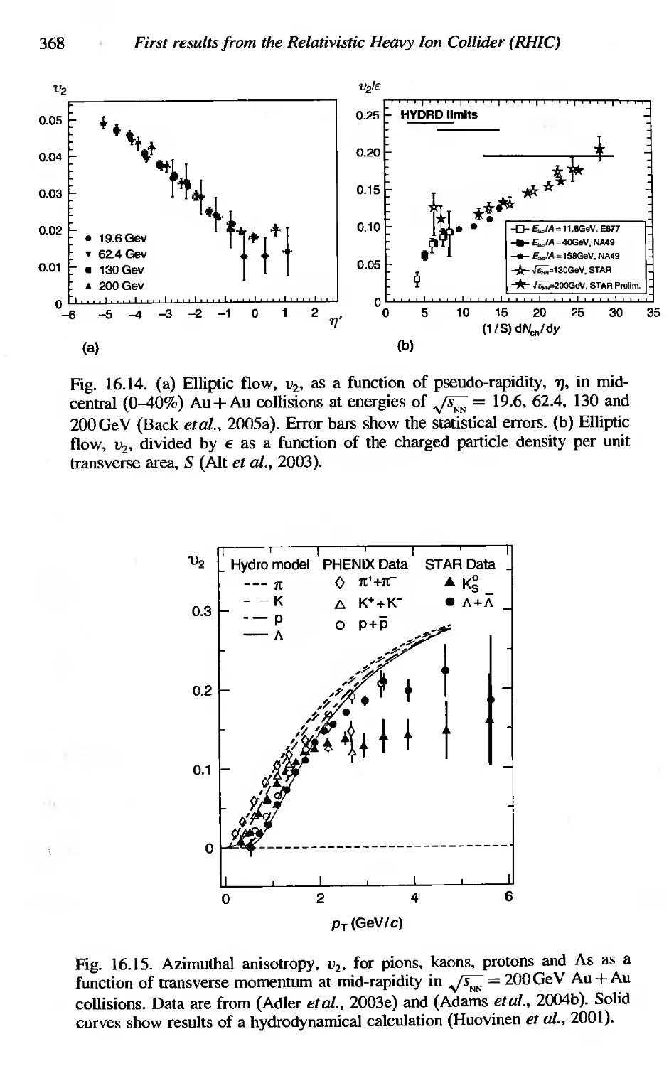
369
371
373
375
375
377
378
378
381
381
384
Contents
xiii
17.5
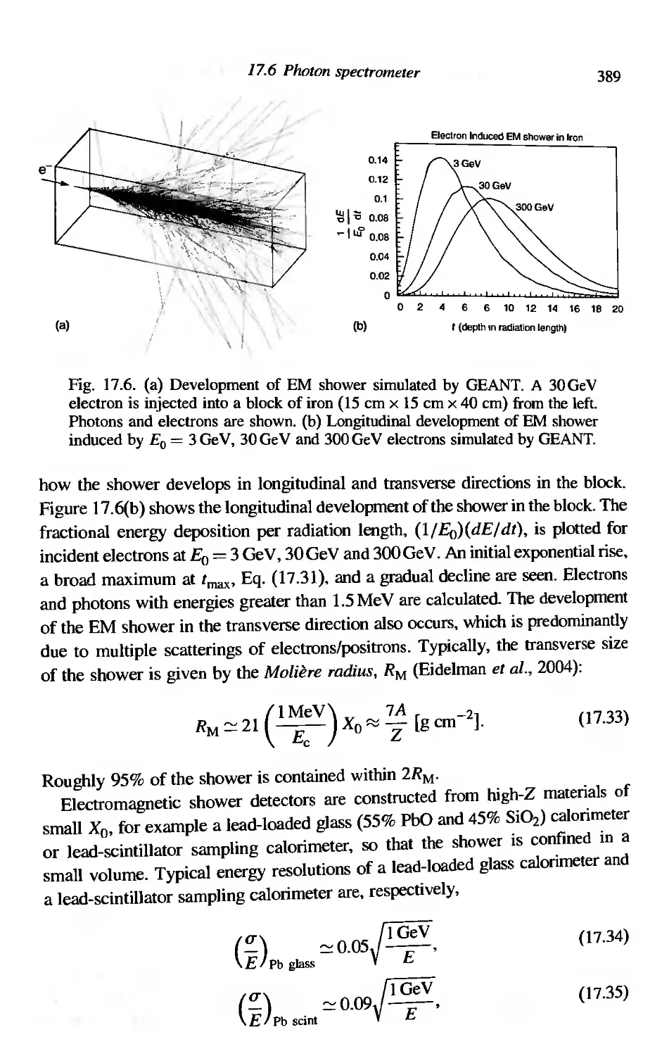
17.6
17.7
Lepton pair spectrometer
Photon spectrometer
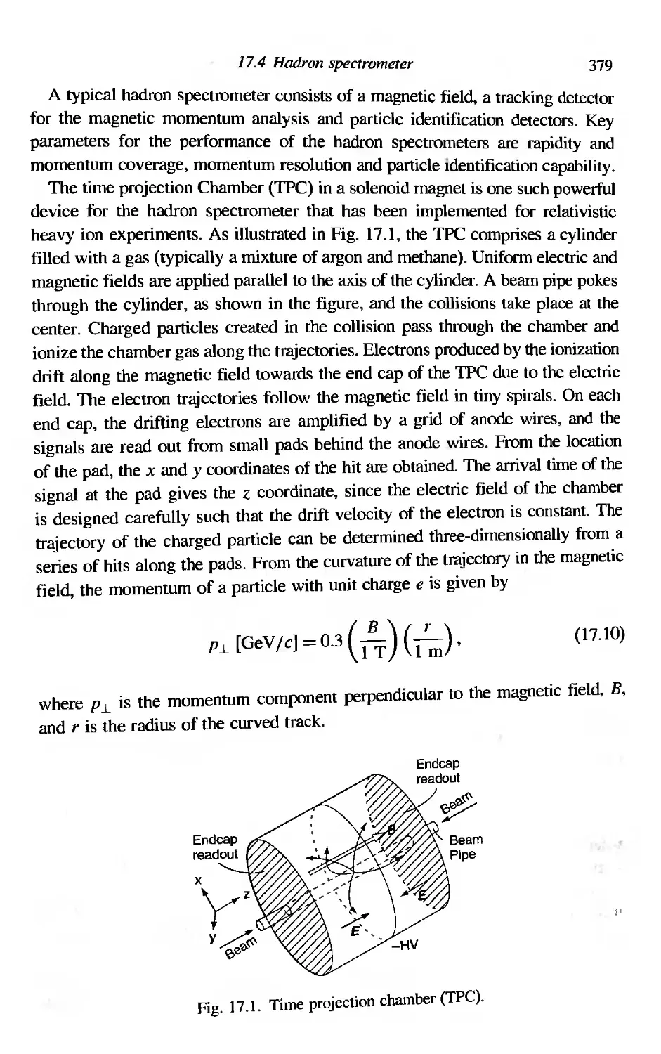
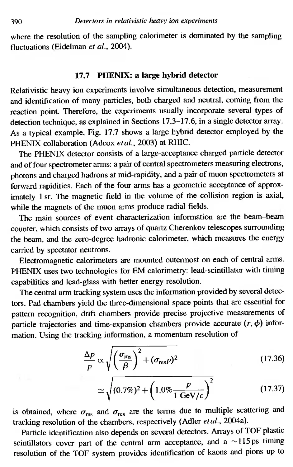
PHENIX: a large hybrid detector
Exercises
386
387
390
392
Appendix A Constants and natural units 393
Appendix B Dirac matrices, Dirac spinors and SU(N) algebra 396
Appendix C Functional, Gaussian and Grassmann integrals 400
Appendix D Curved space-time and the Einstein equation 404
Appendix E Relativistic kinematics and variables 412
Appendix F Scattering amplitude, optical theorem and elementary
parton scatterings 418
Appendix G Sound waves and transverse expansion 424
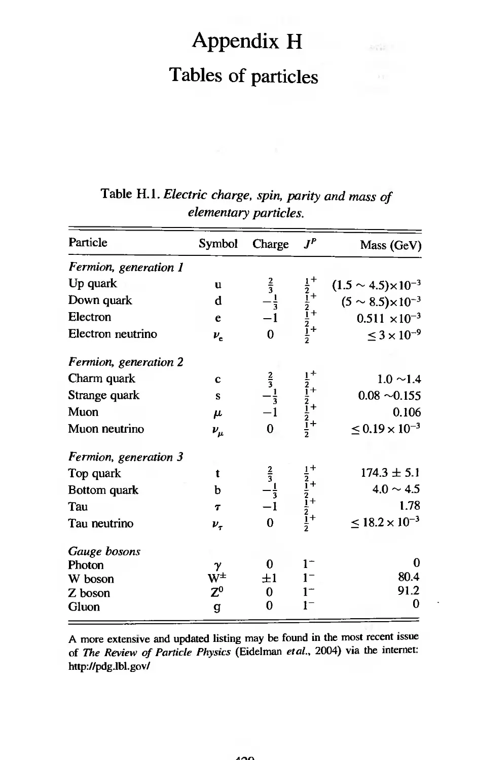
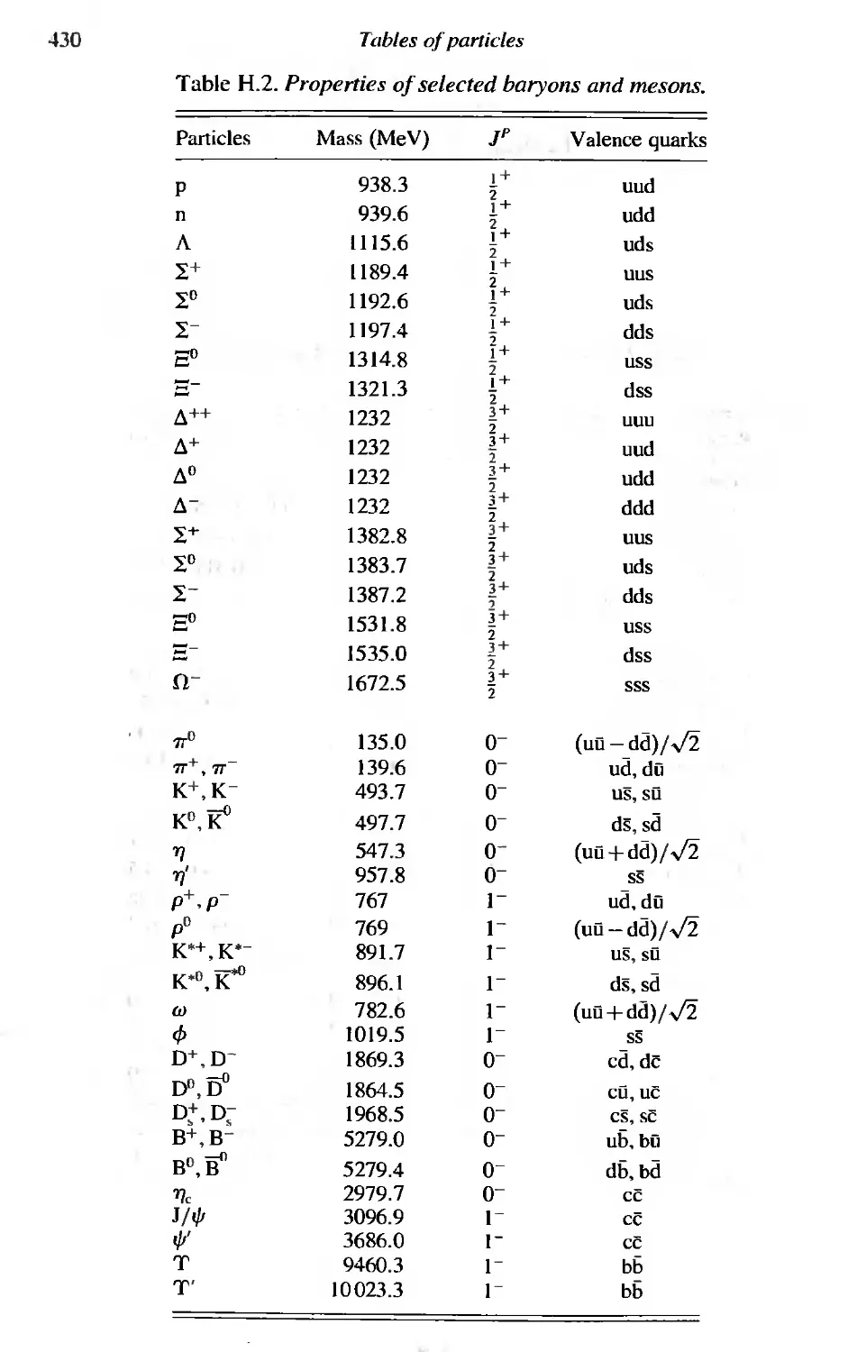
Appendix H Tables of particles 429
References 431
Index 440
Preface
Modern physical science provides us with two key concepts: one is the stan-
dard model of elementary particles on the basis of the principle of local gauge
invariance, and the other is the standard Big Bang cosmology on the basis of the
principle of general relativity, These concepts provide us with a clue which may
help us to answer the following two questions: (i) what are the building blocks
of matter? and (ii) when was the matter created? The main topic of this book is
quark-gluon plasma (QGP), which is deeply connected to these questions. In fact,
QGP is a primordial form of matter, which existed for only a few microseconds
after the birth of the Universe, and it is the root of various elements in the present
Universe,
The fundamental theory governing the dynamics of strongly interacting elemen-
tary particles (quarks and gluons) is known to be quantum chromodynamics
(QCD). QCD suggests that ordinary matter made of protons and neutrons under-
goes phase transitions: to a hot plasma of quarks and gluons for temperatures
larger than 10 12 K, and to a cold plasma of quarks for densities larger than
10 12 kg cm- 3 , The early Universe, and/or the central core of superdense stars, are
the natural places where we expect such phase transitions, It has now become
possible to carry out laboratory experiments to produce hot/dense fireballs ("Little
Bang") through high-energy nucleus-nucleus collisions using heavy ion acceler-
ators, We expect individual nucleons in the colliding nuclei to dissolve into their
constituents to form QGP,
The intention of this book is to introduce the reader who has a limited back-
ground in elementary particle physics, nuclear physics, condensed matter physics
and astrophysics to the physics of QGP, a fundamental and primordial state of
matter. In particular, the authors have in mind advanced undergraduates and begin-
ning graduate students in physics, those not only studying the above-mentioned
fields, but also those studying accelerator science and computer science. In addi-
tion, the authors hope that the book will serve as a reference text for researchers
already working in the fields mentioned above.
Chapter 1 is an introductory chapter, which illustrates the essentials of the
physics of QGP and provides a perspective on the discovery of QGP. Methodology
xv
wi
Preface
<.luite common to studies of the early structure of the Universe (the Big Bang) and
of the structure of QGP (the Little Bang) is emphasized. The text is then divided
into three parts,
Part [ provides a theoretical background in the physics of QGP and in the
QCD phase transitions. Part I may be read independently from the other Parts
in order to understand modern gauge field theories, with applications such as
color confinement, asymptotic freedom and chiral symmetry breakjng in QCD,
the basics of thermal field theory and lattice gauge theory, and the physics of
phase transitions and critical phenomena,
Part II is devoted to the implications of QGP on cosmology and stellar struc-
tures, The physics of an expanding hot Universe and of superdense stars (neutron
and quark stars) are discussed with relation to Einstein's theory of general
relativity, Appendix D is included for readers who have little knowledge about
Riemann space, Einstein's equation, Schwarzschild's solution, etc.
In Part III, the reader will find an overview of the physics of relativistic and
ultra-relativistic nucleus-nucleus collisions. This type of collision is the only
way of creating and investigating QGP and QCD phase transitions by means of
laboratory experiments. The relativistic hydrodynamics and the relativistic kjnetic
theory are introduced in some detail as guiding principles with which to investigate
the dynamics of hot/dense matter produced in the collisions. After discussing
the various experimental signatures of QGP, the fixed-target experiments are
summarized, Then we present the outstanding results achieved with the world's
first Relativistic Heavy Ion Collider (RHIC at Brookhaven National Laboratory),
for which special emphasis is put on the evidence for a QGP phase. In addition,
the special features of detectors used in high-energy heavy ion experiments are
discussed.
We have tried to cover topics ranging from fundamentals to frontiers, from
theories to experiments, and from the Big Bang and compact stars in the Universe
to the Little Bang experiments on Earth. The authors assume that the reader has
some familiarity with intermediate level quantum mechanics, the basic methods
of quantum field theory, statistical thermodynamics and the special theory of
relativity, including the Dirac equation. However, the authors have recapitulated
necessary and sufficient introductory elements from these fields, As far as possible,
the presentation is self-contained. To accomplish this, the authors have placed
key proofs and derivations in eight Appendices and also in about 160 exercises,
which may be found at the ends of each chapter.
It was not the authors' intention to provide a complete reference list for the
subject of QGP; only references which are particularly useful to students are
listed, The reader can find general and up-to-date surveys of the subject in the
recent proceedings of the "Quark Matter" Conference series: Heidelberg (1996),
Preface
xvii
Tsukuba (1997), Tori?o (1999), Brookhaven - Stony Brook (2001), Nantes (2002)
and Berkeley (2004),
Some parts of the original manuscript were used for a series of lectures given
to graduate students at the University of Tsukuba and the University of Tokyo;
the authors wish to thank the students who attended these lectures. The authors
also thank Homer E, Conzett, who carefully read parts of the manuscript and
made many grammatical and style suggestions. They also wish to express their
gratitude to our editors at Cambridge University Press, Simon Capelin, Tamsin
van Essen, Vince Higgs and Irene Pizzie, for a pleasant working relationship,
Thanks are due to many friends and colleagues, especially to Masayuki Asakawa,
Gordon Baym, Hirotsugu Fujii, Machiko Hatsuda, Tetsufumi Hirano, Kazunori
Itakura, Teiji Kunihiro, Tetsuo Matsui, Berndt Muller, Shoji Nagamiya, Atsushi
Nakamura, Yasushi Nara, Satoshi Ozaki, Shoichi Sasaki and Hideo Suganuma,
who have either provided us with data or were involved in helpful discussions.
QGP forms one of the main areas of research in the physics of QeD which
is developing rapidly, In spite of this, the authors hope this book will serve for
a long time as a good introduction to the basic concepts of the subject, so that
readers can enter the forefront of research without much difficulty.
Although this book is primarily written as a textbook for the physics of QGP,
several other teaching options in undergraduate/graduate courses are also recom-
mended.
(a) For a course on an introduction to gauge field theories, we suggest the following
sequence: Chapter 2 Chapter 4 Chapter 5 ---+ Chapter 6,
(b) For an advanced statistical mechanics and phase transition course. we suggest
Chapter 3 Chapter 4 Chapter 5 Chapter 6 Chapter 7 Chapter 12.
(c) For a course on an introduction to the applications of general relativity to cosmol-
ogy and stellar structure, Appendix D Chapter 8 Chapter 9.
(d) For an advanced nuclear (hadron) physics course, Chapter I Appendix E
Chapter 9 Chapter 10 Chapter II Chapter 13
Chapter 14 Chapter 15 Chapter 16 Chapter 17.
We would like to thank the American Astronomical Society, publishers of
The Astrophysical Journal, for permission to reproduce Figs, 8.2, 9.2 and 9.3;
the American Physical Society, publishers of Physical Reviews, Physical Review
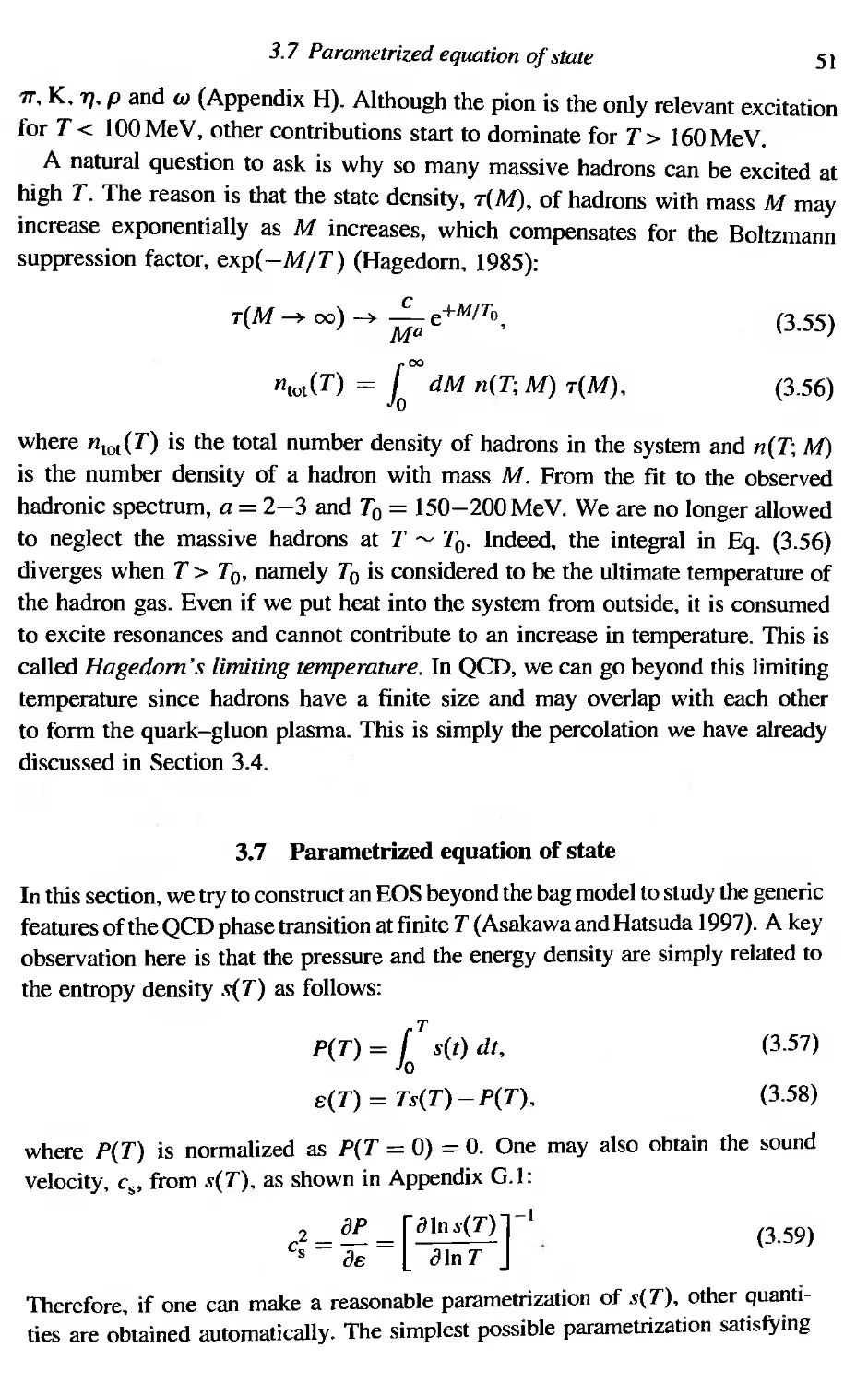
Letters and Reviews of Modem Physics, for permission to reproduce Figs. 3.4,
3.5, 4.10, 5.8, 5.9, 7.6, 8,3, 8.4. 8.10, ]3,6, 14.4(b), 15.2, 15.3, 15.12, 16.4,
16,6(a), 16.7, 16.8, 16.9, 16.12, 16,14, 16.15, 16,16, 16.18(a), 16.19. 16.20
and l7.4(b); Springer-Verlag, publishers of The European Physical Journal, for
I See Braun-Munzinger e' al. (1996), Hatsuda et al. (1998). Riccali et al. (1999), Hallman e' al. (2002). Gutbrod
et al. (2003) and Ritter and Wang (2004).
xviii
Preface
permission to reproduce Figs. 15.4, 15.5, 15.6 and 15,ll(a); Elsevier Science
Publishers B.V., publishers of Nuclear Physics, Physics Letters, Physics Reports
and Nuclear Instruments and Methods in Physics Research, for permission to
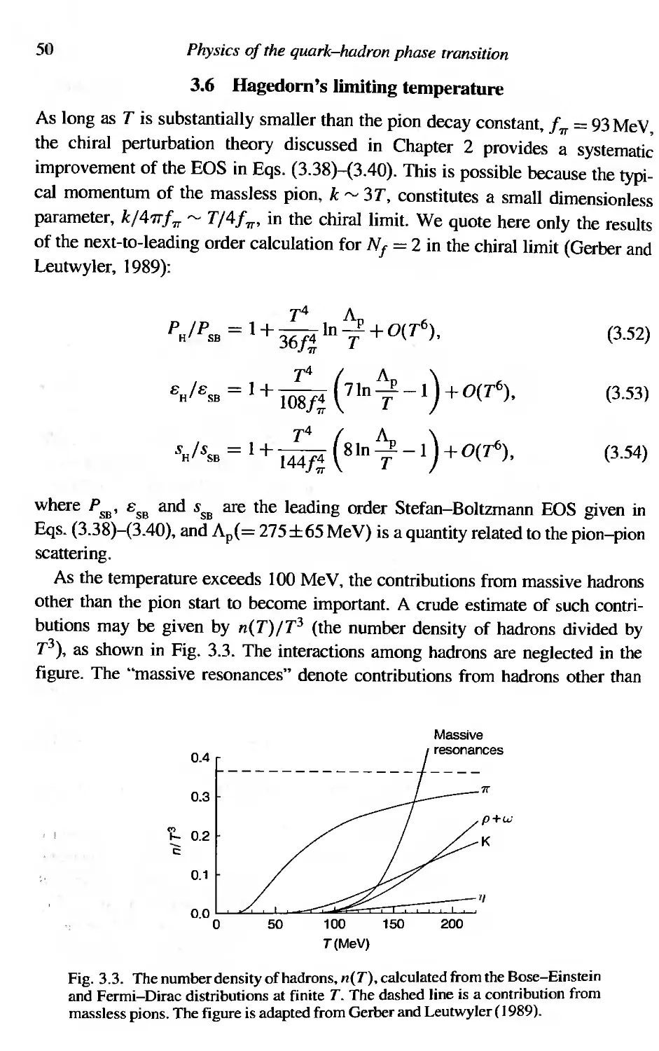
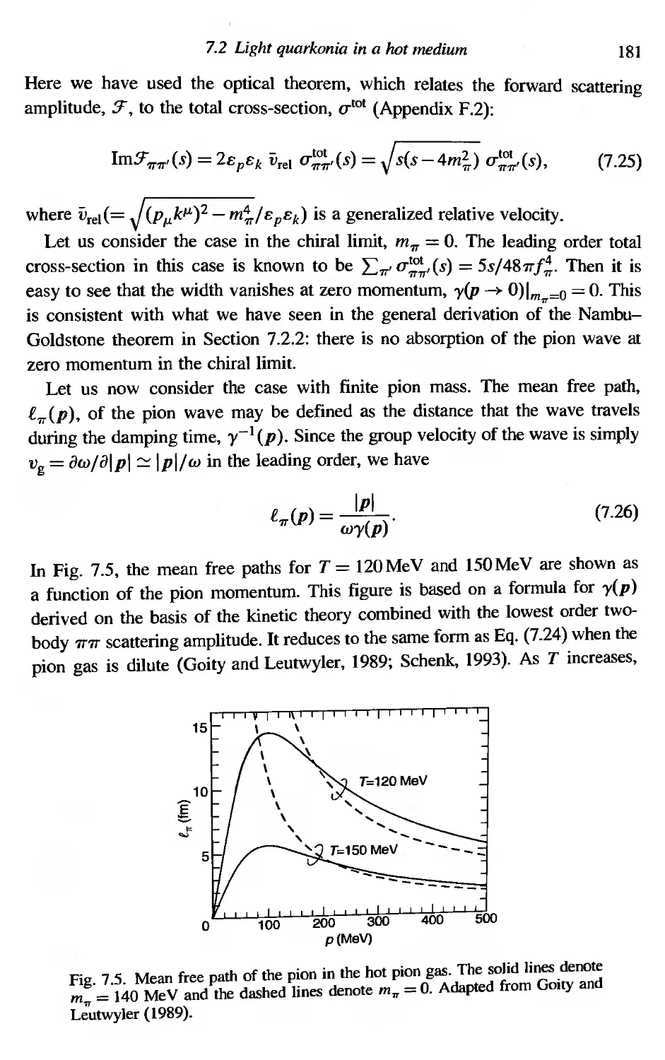
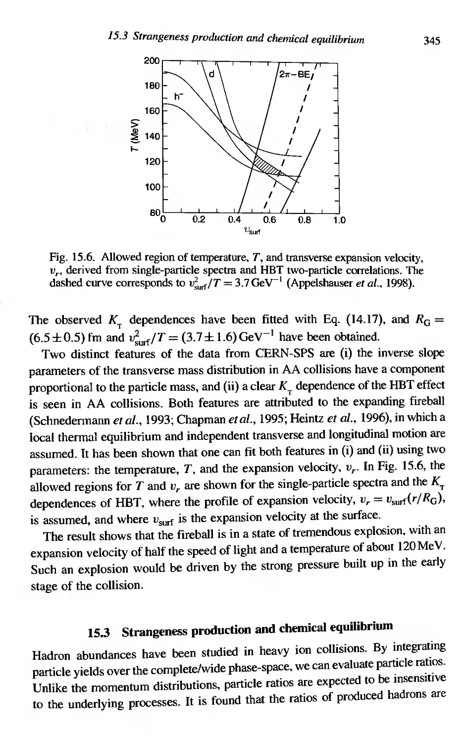
reproduce Figs, 3.3, 5,7, 7.3, 7.5, 10.1, 14.9, 15.7, 15.9, 15.10, 15.11(b), 16.3,
16,4, 16,5, 16.10, 16.11, 16,16b, 16,17, 17,2, 17,4(a) and 17.7; Springer-Verlag,
publishers of Lecture Notes in Physics and Astronomy and Astrophysics Library,
for permission to reproduce Figs. 3,6 and 9.6; the Institute of Physics, publishers
of the Journal of High Energy Physics and the Journal of Physics, for permission
to reproduce Fig, 13.2; and World Scientific, publishers of the Advanced Series
on Directions in High Energy Physics, for permission to reproduce Fig. 15.8. The
source of each figure is given in the caption, and we are grateful to the authors
for permission to reproduce or adapt their figures.
Finally, although the authors have tried to eradicate conceptual and typograph-
ical errors, they are afraid that some of them may have slipped through, A list of
typos and corrections will be posted on the World Wide Web at the following
URL: http://utkhii.px.tsukuba.ac.jp/cupbookl. The authors would be grateful if
the readers would report/send other errors/comments to this address.
The authors are proud to publish the book in 2005, World Year of Physics
(WYP2005), the centennial anniversary of Einstein's three great works on the
particle nature of light, the molecular theory of Brownian motion, and the special
theory of relativity.
1
What is the quark-gluon plasma?
In this chapter, we present a pedagogical introduction to quantum chromodynamics
(QCD), the quark-gluon plasma (QGP), color deconfinement and chiral symmetry
restoration phase transitions in QCD, the early Universe and the Big Bang cosmology,
the structure of compact stars and the QGP signatures in ultra-relativistic heavy
ion collisions, Schematic figures not exploiting any mathematical formulas are
utilized, Perspectives on discovering QGP on Earth (Little Bang) are also provided,
with an emphasis on the common methodology used to study the early Universe
(Big Bang), The issues introduced in this chapter will be elucidated thoroughly
in later chapters; the appropriate references to chapters are given in boldface.
1.1 Asymptotic freedom and confinement in QCD
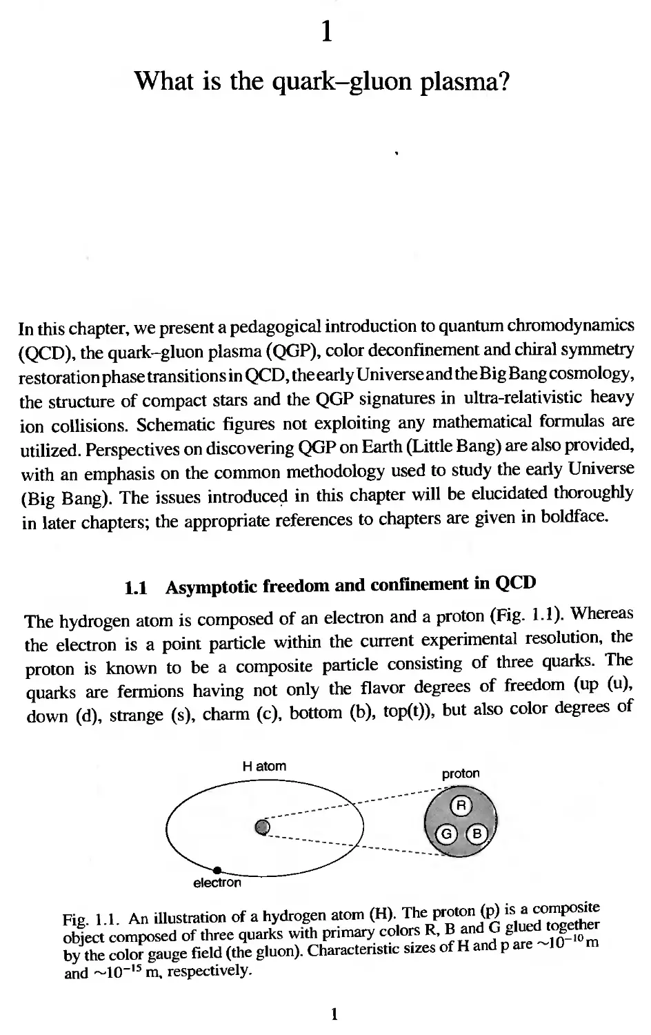
The hydrogen atom is composed of an electron and a proton (Fig. 1.1), Whereas
the electron is a point particle within the current experimental resolution, the
proton is known to be a composite particle consisting of three quarks, The
quarks are fermions having not only the flavor degrees of freedom (up (u),
down (d), strange (s), charm (c), bottom (b), top(t)), but also color degrees of
Hatom
proton
------ ----------(@'\
0::::::_______ __________
Fig. 1.1. An illustration of a hydrogen alOm (H). The proton (p) is a composite
object composed of three quarks with primary colors R, Band G glued together
by the color gauge field (the gluon). Characteristic sizes ofH and p are 1O-lOm
and 1O-I5 m, respectively.
2
What is the quark-gluon plasma?
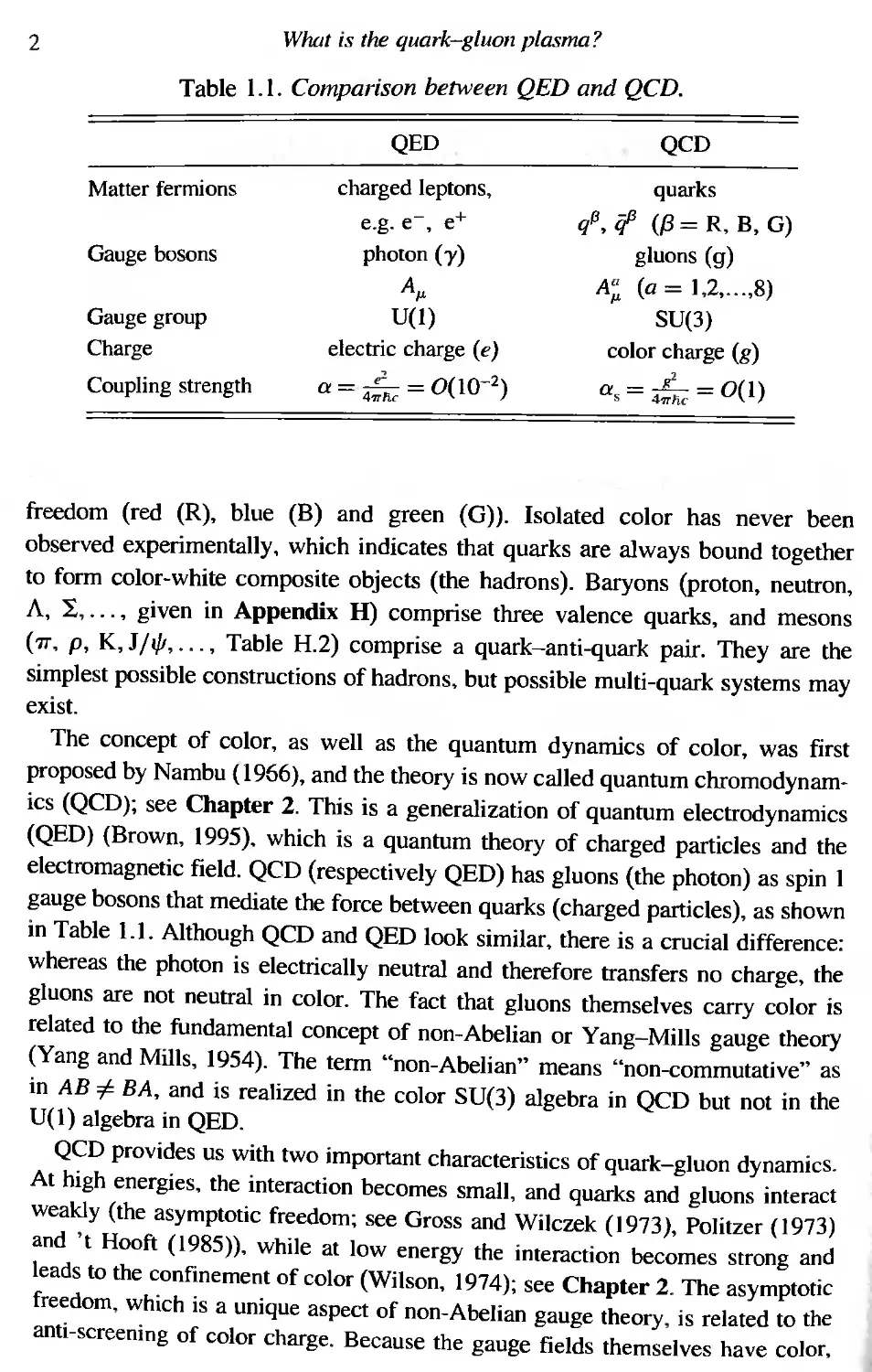
Table 1.1, Comparison between QED and QCD.
QCD
QED
Matter fermions
Gauge bosons
Gauge group
Charge
Coupling strength
charged leptons,
e.g. e-, e+
phoron (y)
AI'
U(I)
electric charge (e)
ex = = 0(10- 2 )
4wlic
quarks
q(3, if ({3 = R, B, G)
gluons (g)
A (a = ],2,...,8)
SU(3)
color charge (g)
ex =L=O ( I )
s 4w1ic
freedom (red (R), blue (B) and green (G), Isolated color has never been
observed experimentally, which indicates that quarks are always bound together
to form color-white composite objects (the hadrons). Baryons (proton, neutron,
A, "." given in Appendix H) comprise three valence quarks, and mesons
(7T, p, K,J/i/J,..., Table H.2) comprise a quark-ami-quark pair. They are the
simplest possible constructions of hadrons, but possible multi-quark systems may
exist.
The concept of color, as well as the quantum dynamics of color, was first
proposed by Nambu (1966), and the theory is now called quantum chromodynam-
ics (QCD); see Chapter 2. This is a generalization of quantum electrodynamics
(QED) (Brown, 1995), which is a quantum theory of charged particles and the
electromagnetic field, QCD (respectively QED) has gluons (the photon) as spin I
gauge bosons that mediate the force between quarks (charged particles), as shown
in Table l.l, Although QCD and QED look similar, there is a crucial difference:
whereas the photon is electrically neutral and therefore transfers no charge, the
gluons are not neutral in color. The fact that gluons themselves carry color is
related to the fundamental concept of non-Abelian or Yang-Mills gauge theory
(Yang and Mills, ]954). The term "non-Abelian" means "non-commutative" as
in AB =1= BA, and is realized in the color SU(3) algebra in QeD but not in the
U(]) algebra in QED.
QCD provides us with two important characteristics of quark-gluon dynamics.
At high energies, the interaction becomes small, and quarks and gluons interact
weakly (the asymptotic freedom; see Gross and Wilczek (1973), Politzer (1973)
and 't Hooft (1985», while at low energy the interaction becomes strong and
leads to the confinement of color (Wilson, 1974); see Chapter 2. The asymptotic
freedom, which is a unique aspect of non-Abelian gauge theory, is related to the
anti-screening of color charge, Because the gauge fields themselves have color,
1.1 Asymptotic freedom and confinement in QCD
3
a bare color charge centered at the origin is diluted away in space by the gluons.
Therefore, as one tries to find the bare charge by going through the cloud of
gluons, one finds a smaller and smaller portion of the charge, This is in sharp
contrast to the case of QED, where the screening of a bare charge takes place
due to a cloud of, for example, electron-positron pairs surrounding the charge.
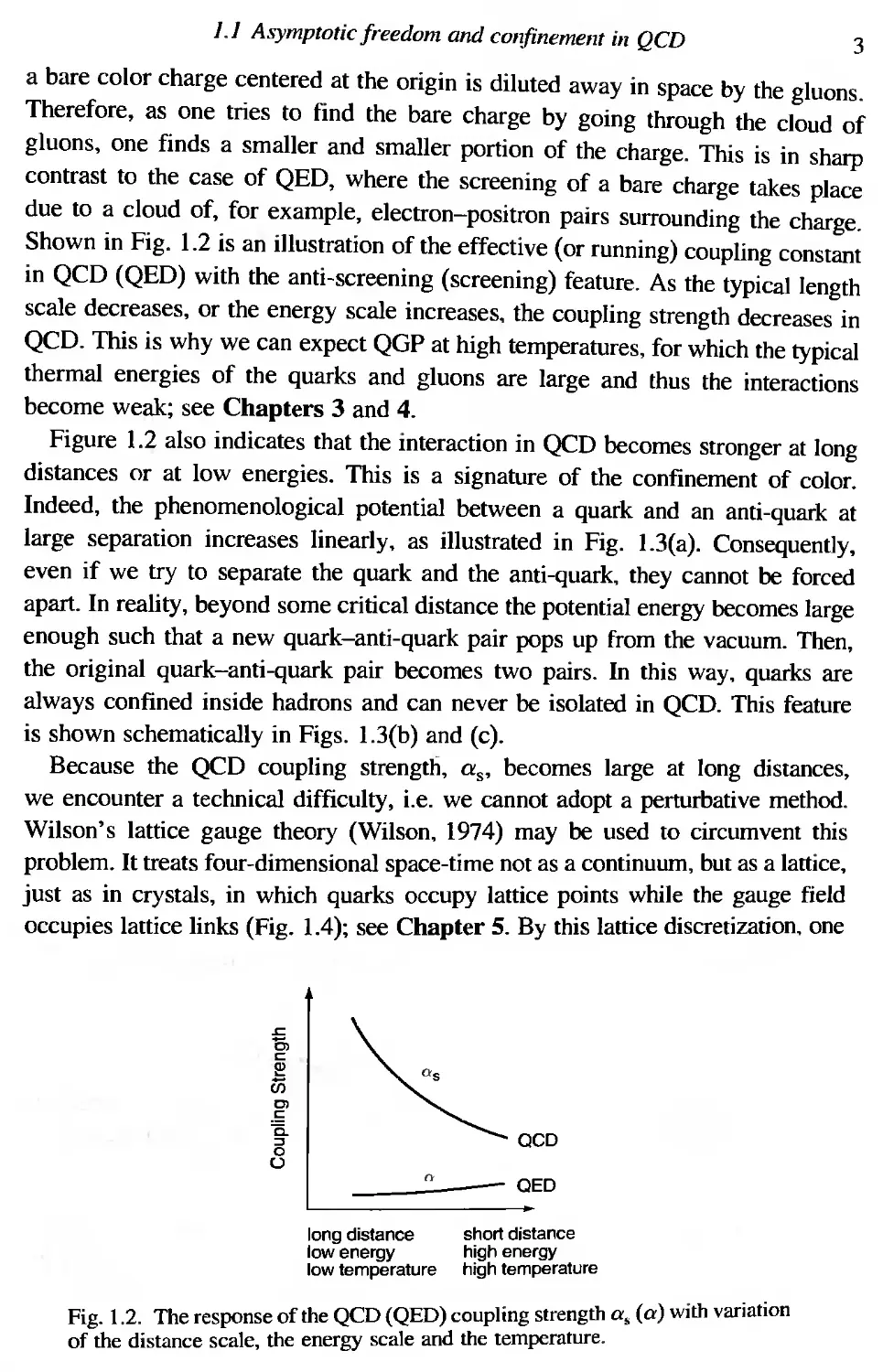
Shown in Fig, 1.2 is an illustration of the effective (or running) coupling constant
in QCD (QED) with the anti-screening (screening) feature. As the typical length
scale decreases, or the energy scale increases, the coupling strength decreases in
QCD. This is why we can expect QGP at high temperatures, for which the typical
thermal energies of the quarks and gluons are large and thus the interactions
become weak; see Chapters 3 and 4.
Figure 1,2 also indicates that the interaction in QeD becomes stronger at long
distances or at low energies. This is a signature of the confinement of color.
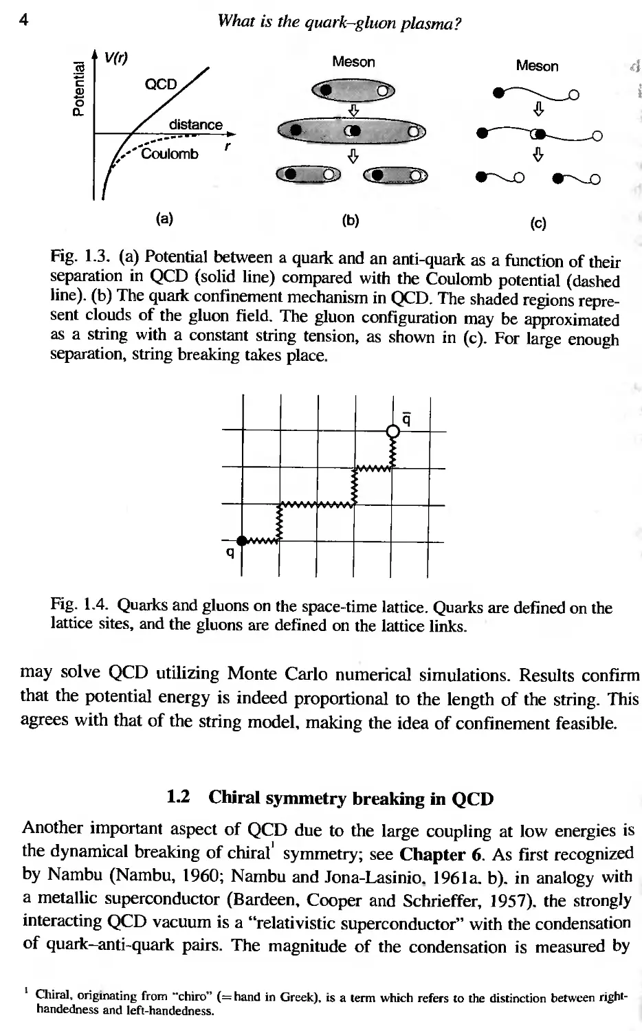
Indeed, the phenomenological potential between a quark and an ami-quark at
large separation increases linearly, as illustrated in Fig, 1.3(a), Consequently,
even if we try to separate the quark and the ami-quark, they cannot be forced
apart. In reality, beyond some critical distance the potential energy becomes large
enough such that a new quark-ami-quark pair pops up from the vacuum. Then,
the original quark-anti-quark pair becomes two pairs. In this way, quarks are
always confined inside hadrons and can never be isolated in QCD. This feature
is shown schematically in Figs, 1.3(b) and (c).
Because the QCD coupling strength, as, becomes large at long distances,
we encounter a technical difficulty, i.e. we cannot adopt a perturbative method.
Wilson's lattice gauge theory (Wilson, 1974) may be used to circumvent this
problem, It treats four-dimensional space-time not as a continuum, but as a lattice,
just as in crystals, in which quarks occupy lattice points while the gauge field
occupies lattice links (Fig. 1.4); see Chapter 5. By this lattice discretization. one
.<::
0,
<::
(;j
C>
.!:
15.
:J
o
U
" as
QCD
- QED
long distance
low energy
low temperature
short distance
high energy
high temperature
Fig. 1.2. The response of the QCD (QED) coupling strength a, (a) with variation
of the distance scale, the energy scale and the temperature.
4
What is the quark-gluon plasma?
(ij
E
Q)
(;
D..
Meson
Meson q
{!.
{),
.(!.
{),
r
(a)
(b)
(c)
Fig. 1.3. (a) Potential between a quark and an anti-quark as a function of their
separation in QCD (solid line) compared with the Coulomb potential (dashed
line). (b) The quark confinement mechanism in QeD. The shaded regions repre-
Sent clouds of the gluon field. The gluon configuration may be approximated
as a string with a constant string tension, as shown in (c). For large enough
separation, string breaking takes place,
q
q
Fig. 1.4. Quarks and gluons on the space-time lattice. Quarks are defined on the
lattice sites, and the gluons are defined on the lattice links.
may solve QCD utilizing Monte Carlo numerical simulations. Results confirm
that the potential energy is indeed proportional to the length of the string. This
agrees with that of the string model, making the idea of confinement feasible,
1.2 Chiral symmetry breaking in QCD
Another important aspect of QCD due to the large coupling at low energies is
the dynamical breaking of chiral' symmetry; see Chapter 6. As first recognized
by Nambu (Nambu, 1960; Nambu and Jona-Lasinio. 1961a. b). in analogy with
a metallic superconductor (Bardeen, Cooper and Schrieffer, 1957). the strongly
interacting QCD vacuum is a "relativistic superconductor" with the condensation
of quark-anti-quark pairs, The magnitude of the condensation is measured by
I Chiral. origmating from ..chiro" (= hand in Greek), is a term which refers to the distinction between right-
handedness and left-handedness.
1.3 Recipes for quark-gluon plasma
5
the vacuum expectation value, (ijq), which serves as an order parameter. The
masses of light hadrons are intimately related to the non-vanishing value of
this order parameter. 2 Thus, one may naturally expect, in analogy with metallic
superconductors, that there is a phase transition at finite T to the "normal" phase,
and that the condensation and the particle spectra will experience a drastic change
associated with the phase transition (Chapter 7),
1.3 Recipes for quark-gluon plasma
The asymptotic freedom illustrated in Fig, 1.2 immediately suggests two methods
for the creation of the quark-gluon plasma (QGP).
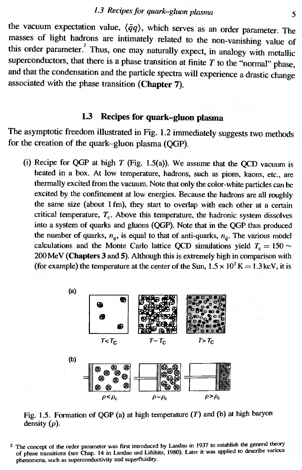
(i) Recipe for QGP at high T (Fig, 1.5(a», We assume that the QeD vacuum is
heated in a box. At low temperature, hadrons, such as pions, kaons, etc., are
thermally excited from the vacuum. Note that only the color-white particles can be
excited by the confinement at low energies. Because the hadrons are all roughly
the same size (about 1 fm), they start to overlap with each other at a certain
critical temperature, Tc' Above this temperature. the hadronic system dissolves
into a system of quarks and gluons (QGP), Note that in the QGP thus produced
the number of quarks, n q , is equal to that of anti-quarks, nil' The various model
calculations and the Monte Carlo lattice QeD simulations yield Tc = L50
200 MeV (Chapters 3 and 5). Although this is extremely high in comparison with
(for example) the temperature at the center of the Sun, 1.5 x 10 7 K = 1.3 keY, it is
(a) II
[Sl
T<Tc T-T c T>Tc
(b) BIB
8 8 .
8 41
88 8
P<Pc P-Pc P>Pc
Fig, 1.5. Formation of QGP (a) at high temperature (T) and (b) at high baryon
density (p).
2 The concept of' the order parameter was first introduced by Landau in ]937 to establish the ge aJ ory
of phase transitions (see Chap. 14 in Landau and i shitz. J980). Later it was applied to descn e vanous
phenomena. such as superconductivity and superflUldlty.
6
What is the quark-gluon plasma?
V(4). t)
T<TC
<,p>
(a)
,p
(b) Temperature
Tc
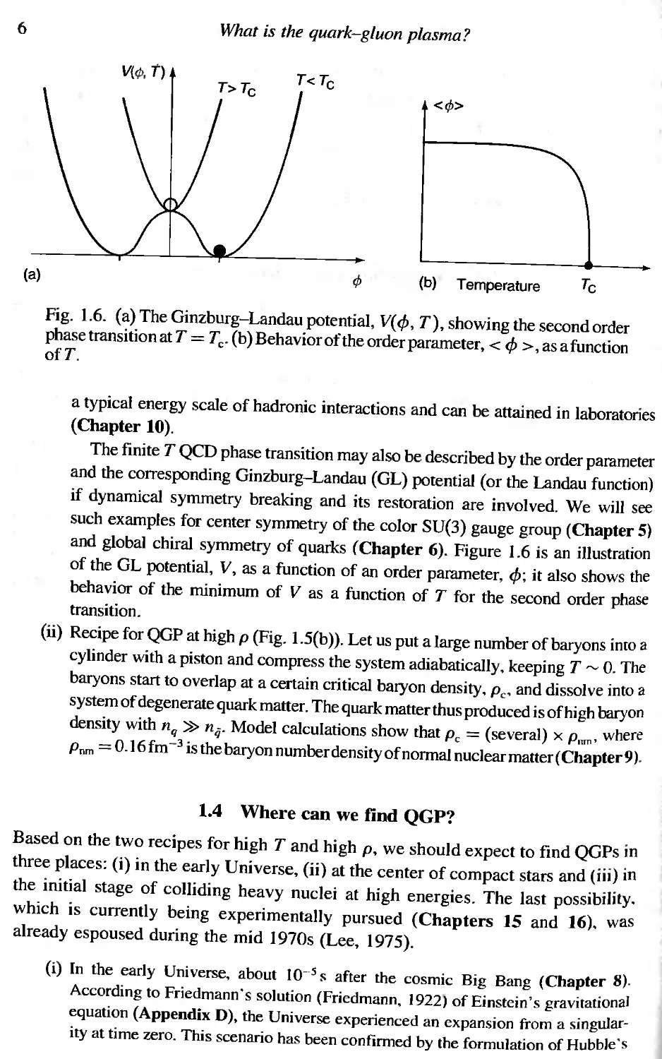
Fig. 1.6. (a) The Ginzburg-Landau potential, V( cP, T), showing the second order
phase transition at T = Tc' (b) Behavior of the order parameter, < cP >, as a function
ofT.
a typical energy scale of hadronic interactions and can be attained in laboratories
(Chapter 10).
The finite T QCD phase transition may also be described by the order parameter
and the corresponding Ginzburg-Landau (GL) potential (or the Landau function)
if dynamical symmetry breaking and its restoration are involved. We will see
such examples for center symmetry of the color SU(3) gauge group (Chapter 5)
and global chiral symmetry of quarks (Chapter 6). Figure 1.6 is an illustration
of the GL potential, V, as a function of an order parameter, cP; it also shows the
behavior of the minimum of V as a function of T for the second order phase
transition.
(ii) Recipe for QGP at high P (Fig. l.5(b)). Let us put a large number of baryons imo a
cylinder with a piston and compress the system adiabatically, keeping T O. The
baryons start to overlap at a certain critical baryon density, Pc' and dissolve into a
system of degenerate quark matter. The quark matter thus produced is of high baryon
density with nq » nij' Model calculations show that Pc = (several) x Pnrn' where
Pnrn = 0.16 fm- 3 is the baryon number density of normal nuclear matter (Chapter9).
1.4 Where can we find QGP?
Based on the two recipes for high T and high P, we should expect to find QGPs in
three places: (i) in the early Universe, (ii) at the center of compact stars and (iii) in
the initial stage of colliding heavy nuclei at high energies. The last possibility,
which is currently being experimentally pursued (Chapters 15 and 16), was
already espoused during the mid 1970s (Lee, 1975),
(i) In the earIy Universe, about 10- 5 s after the cosmic Big Bang (Chapter 8).
According to Friedmann's soIution (Friedmann, 1922) of Einstein's gravitational
equation (Appendix D), the Universe experienced an expansion from a singular-
ity at time zero. This scenario has been confirmed by the formulation of Hubble's
1.4 Where can we find QGP?
7
law for the red shift of distant galaxies (Hubble, 1929). If we extrapolate our
expanding Universe backward in time toward the Big Bang, the matter and radi-
ation become hotter and hotter, resulting in the "primordial fireball," as named
by Gamow, The discovery of T 2.73K 3 x 1O- 4 eV cosmic microwave back-
ground (CMB) radiation by Penzias and Wilson (1965) confirmed the remnant
light of this hot era of the Universe. In addition, the hot Big Bang theory explains
the abundance of light elements (d, He. Li) in the Universe as a result of the
primordial nucleosynthesis, This idea was initiated in a paper entitled "The origin
of chemical elements" by Alpher, Bethe and Gamow (I948),' which reminds us
of the book On the Origin of Species by Charles Darwin published in 1859. If
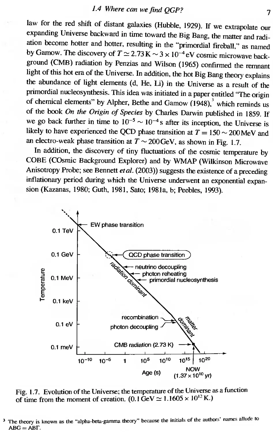
we go back further in time to 10- 5 10- 4 s after its inception, the Universe is
likely to have experienced the QCD phase transition at T = 150 200MeV and
an electro-weak phase transition at T 200GeV, as shown in Fig. 1.7.
In addition, the discovery of tiny fluctuations of the cosmic temperature by
COBE (COsmic Background Explorer) and by WMAP (Wilkinson Microwave
Anisotropy Probe; see Bennett eta/. (2003» suggests the existence of a preceding
inflationary period during which the Universe underwent an exponential expan-
sion (Kazanas, 1980; Guth, 1981, Sato; 1981a, b; Peebles, 1993).
0.1 GeV
::> 0.1 MeV
n;
Q;
c.
E
OJ
I- 0.1 keV
0.1 eV
0.1 meV
EW phase transition
<ai'
<>?6 photon reheating .
':> - primordial nucleosynthesls
<>-?...
recombination <>- '?
%i;»
photon decoupling "'"
.....
CMS radiation (2.73 K)
10- 10 10-5
10 5 10 10
Age(s)
Fig. 1.7, Evolution ofthe Universe; the temperature ofthe Vni\ rse as a function
of time from the moment of creation. (0.1 Oe V 1.1605 x 10 K.)
. .. I f the authors' names allude to
3 The theory is known as the "alpha-beta-gamma theory" because the Imt13 so.
ABG = ABr.
8
What is the quark-gluon plasma?
(ii) At the core of superdense stars such as neutron stars and quark stars (Chapter 9).
There are three possible stable branches of compact stars: white dwarfs. neutron
stars and quark stars. The white dwarfs are made entirely of electrons and nuclei,
while the major component of neutron stars is liquid neutrons, with some protons
and electrons, The first neutron star was discovered as a radio pulsar in 1967
(Hewish et ai" 1968). If the central density of the neutron stars reaches 5-10 p
there is a fair possibility that the neutrons will melt into the cold quark matter,n
shown in Fig, 1.5(b), There is also a possibility that the quark matter, with an almost
equal number of u, d and s quarks (the strange matter), may be a stable ground
state of matter; this is called the strange matter hypothesis, If this is true, quark
stars made entirely of strange matter become a possibility, In order to elucidate the
structure of these compact stars, we have to solve the Oppenheimer- V olkoff (OV)
equation (Oppenheimer and Volkoff, 1939), obtained from the Einstein equation,
together with the equation of states for the superdense matter (Appendix D).
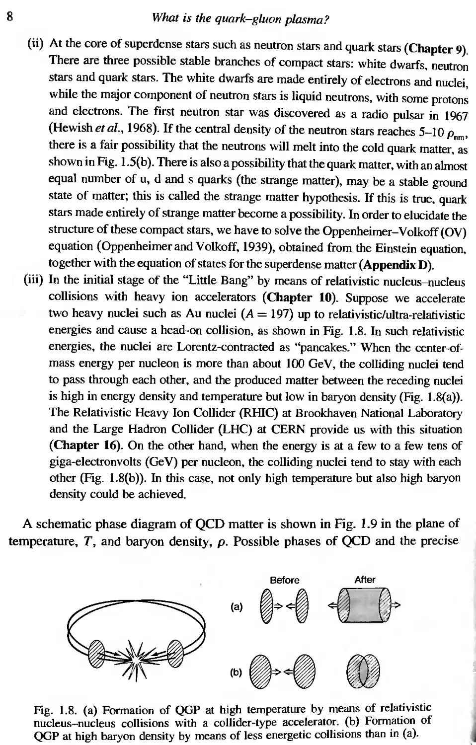
(iii) In the initial stage of the "Little Bang" by means of relativistic nucleus-nucleus
collisions with heavy ion accelerators (Chapter (0). Suppose we accelerate
two heavy nuclei such as Au nuclei (A = 197) up to relativistic/ultra-relativistic
energies and cause a head-on collision, as shown in Fig. 1.8, In such relativistic
energies, the nuclei are Lorentz-contracted as "pancakes." When the center-of-
mass energy per nucleon is more than about 100 GeV, the colliding nuclei tend
to pass through each other, and the produced matter between the receding nuclei
is high in energy density and temperature but low in baryon density (Fig. 1.8(a).
The Relativistic Heavy Ion Collider (RHlC) at Brookhaven National Laboratory
and the Large Hadron Collider (LHC) at CERN provide us with this situation
(Chapter (6). On the other hand, when the energy is at a few to a few tens of
giga-electronvolts (GeV) per nucleon, the colliding nuclei tend to stay with each
other (Fig. 1.8(b)), In this case, not only high temperature but also high baryon
density could be achieved.
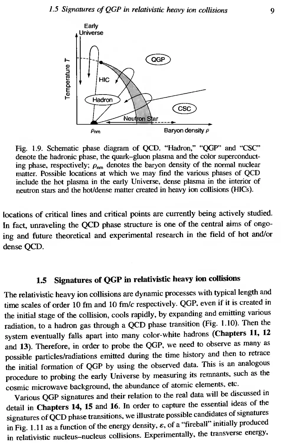
A schematic phase diagram of QCD matter is shown in Fig. 1.9 in the plane of
temperature, T, and baryon density, p, Possible phases of QeD and the precise
Before After
(a) ' I O
(b) I I (0)
Fig. 1.8, (a) Formation of QGP at high temperature by means of rela ivistic
nucleus-nucleus collisions with a collider-type accelerator. (b) FormatIon of
QGP at high baryon density by means of less energetic collisions than in (a).
1.5 Signatures of QGP in relativistic heavy ion collisions
9
Early
Universe
....
Q)
:5
Q)
c.
E
Q)
f-
@)
Pnm
Baryon density P
Fig, 1.9. Schematic phase diagram of QCD, "Hadron," "QGP" and "CSC"
?enote the hadroni phase, the quark-gluon plasma and the color superconduct-
mg phase, respectIvely; Pnrn denotes the baryon density of the normal nuclear
matter. Possible locations at which We may find the various phases of QCD
include the hot plasma in the early Universe, dense plasma in the interior of
neutron stars and the hot/dense matter created in heavy ion collisions (HICs).
locations of critical lines and critical points are currently being actively studied.
In fact, unraveling the QCD phase structure is one of the central aims of ongo-
ing and future theoretical and experimental research in the field of hot and/or
dense QCD.
1.5 Signatures of QGP in relativistic heavy ion collisions
The relativistic heavy ion collisions are dynamic processes with typical length and
time scales of order 10 fm and 10 fmlc respectively. QGP. even if it is created in
the initial stage of the collision, cools rapidly, by expanding and emitting various
radiation, to a hadron gas through a QCD phase transition (Fig. 1.l0). Then the
system eventually falls apart into many color-white hadrons (Chapters 11, 12
and (3), Therefore, in order to probe the QGP, we need to observe as many as
possible particles/radiations emitted during the time history and then to retrace
the initial formation of QGP by using the observed data, This is an analogous
procedure to probing the early Universe by measuring its remnants. such as the
cosmic microwave background, the abundance of atomic elements. etc.
Various QGP signatures and their relation to the real data wiII be discussed in
detail in Chapters 14, IS and 16. In order to capture the essential ideas of the
signatures of QCD phase transitions, we i1Iustrate possible candidates of signatures
in Fig. 1.11 as a function of the energy density, £, of a "fireball" initially produced
in relativistic nucleus-nucleus collisions. Experimentally, the transverse energy,
10
What is the quark-gluon plasma?
\
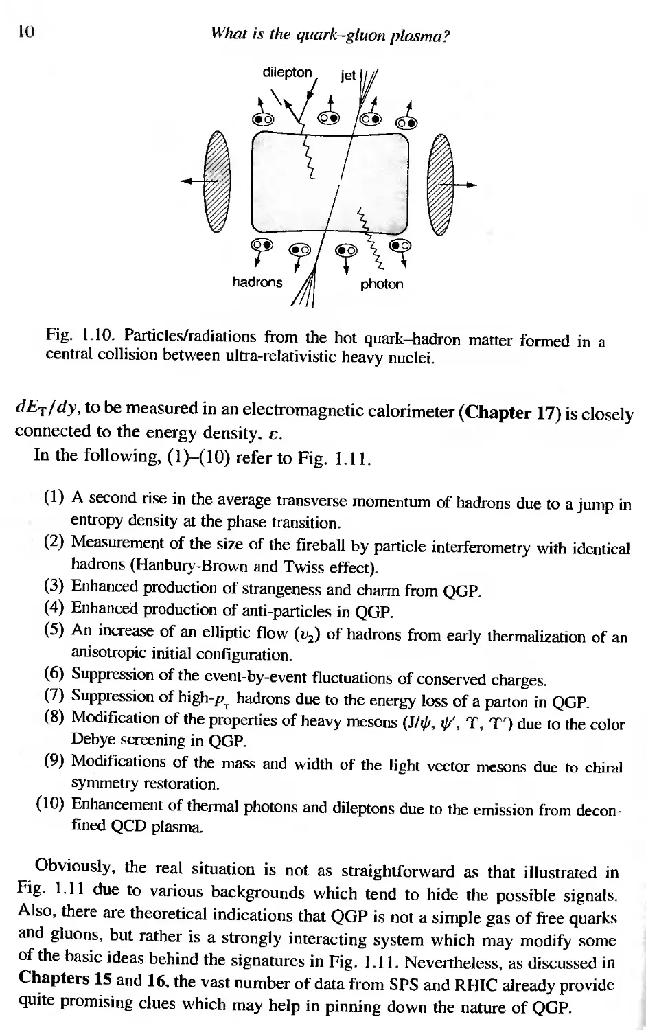
Fig, 1.10. Particleslradiations from the hot quark-hadron matter formed in a
central collision between ultra-relativistic heavy nuclei.
dET/dy, to be measured in an electromagnetic calorimeter (Chapter 17) is closely
connected to the energy density. 8,
In the following, (1)-(10) refer to Fig, l.ll.
(1) A second rise in the average transverse momentum of hadrons due to a jump in
entropy density at the phase transition.
(2) Measurement of the size of the fireball by particle interferometry with identical
hadrons (Hanbury-Brown and Twiss effect).
(3) Enhanced production of strangeness and charm from QGP.
(4) Enhanced production of anti-particles in QGP.
(5) An increase of an elliptic flow (v 2 ) of hadrons from early thermalization of an
anisotropic initial configuration.
(6) Suppression of the event-by-event fluctuations of conserved charges.
(7) Suppression of high-P T hadrons due to the energy loss of a parton in QGP.
(8) Modification of the properties of heavy mesons (JII/I, 1/1', T, T') due to the color
Debye screening in QGP.
(9) Modifications of the mass and width of the light vector mesons due to chiral
symmetry restoration.
(10) Enhancement of thermal photons and dileptons due to the emission from decon-
fined QCD plasma.
Obviously, the real situation is not as straightforward as that illustrated in
Fig. 1.11 due to various backgrounds which tend to hide the possible signals.
Also, there are theoretical indications that QGP is not a simple gas of free quarks
and gluons, but rather is a strongly interacting system which may modify some
of the basic ideas behind the signatures in Fig. 1.11. Nevertheless, as discussed in
Chapters 15 and 16. the vast number of data from SPS and RHIC already provide
quite promising clues which may help in pinning down the nature of QGP.
1.5 Signalllres of QGP in relativistic heavy ion collisions
(Pr)
(1)
r
K
It
EC
Volume
(2)
f
(3)
Ncharm, strange
1
Np,d,i'd
(4)
'1)2
(5)
r
Ec
11
(60 2 )
S
(6)
E
E
Ec
R AA (high Pr)
(7)
N heavy quarkonia
(8)
/W
e V
p,w,,p
(9)
WidIh
=>Gs
Nthermal
y,I+I-
E
'''' r . ,
Ec
Fig. 1.11. Selected observables as a function of the central energy density" in
the relativistic heavy ion collisions. They are the possible signatures of QCD
phase transitions; "is related to the transverse energy per unit rapidity. dET/dy;
"c is the critical energy above which the QGP is expected. This figure has been
adapted from an original by S. Nagamiya. For an explanation of parts (I H 10),
please see the text.
12 What is the quark-gluon plasma?
1.6 Perspectives on relativistic heavy ion experiments
The studies of the "Big Bang" by satellite observations and that of the "Little
Bang" by relativistic heavy ion collision experiments are pretty much analogous,
not only in their ultimate physics goal, but also in the ways in which the data are
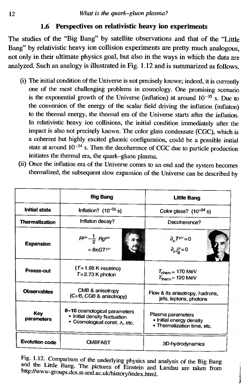
analyzed, Such an analogy is illustrated in Fig. 1.12 and is summarized as follows,
(i) The initial condition of the Universe is not precisely known; indeed, it is currently
one of the most challenging problems in cosmology. One promising scenario
is the exponential growth of the Universe (inflation) at around 10- 35 s. Due to
the conversion of the energy of the scalar field driving the inflation (inflaton)
to the thermal energy, the thermal era of the Universe starts after the inflation.
In relativistic heavy ion collisions, the initial condition immediately after the
impact is also not precis ly known. The color glass condensate (CGC), which is
a coherent but highly excited gluonic configuration, could be a possible initial
state at around 10- 24 s. Then the decoherence of CGC due to particle production
initiates the thermal era, the quark-gluon plasma,
(ii) Once the inflation era of the Universe comes to an end and the system becomes
thermalized, the subsequent slow expansion of the Universe can be described by
Big Bang Little Bang
Initial state Inflation? (10- 35 s) Color glass? (10- 24 s)
Thermalization Inflaton decay? Decoherence?
RJ1V _.1. RgJ1V i'J / ,TJ1v=0
Expansion 2
= 81tGTlw i'JJ1j '=O
Freeze-out (T=1.95 K neutrino) T chem = 170 MeV
T = 2.73 K photon 7iherm= 120 MeV
Observables CMB & anisotropy Flow & its anisotropy, hadrons,
(CvB. CGB & anisotropy) jets. leptons, photons
Key 8-10 cosmological parameters Plasma parameters
. Initial density fluctuation
parameters . Cosmological const. A. etc. . Initial energy density
. Thermalization time, etc.
Evolution code CMBFAST 3D-hydrodynamics
Fig. 1.12. omparison of the underlying physics and analysis of the Big Bang
and the Little Bang, The pictures of Einstein and Landau are taken from ..
http://www-groups.dcs.st-and.ac.uklhistory/index.html. J
1.6 Perspectives on relativistic heavy ion experiments
13
the Friedmann equation with an appropriate equation of state of matter and radia-
tion. In the case of the Little Bang, the expansion of the locally thermalized plasma
is governed by the laws of relativistic hydrodynamics originally introduced by
Landau (1953). If the constituent particles of the plasma interact strongly enough,
one may assume a perfect fluid, which simplifies the hydrodynamic equations.
(Hi) The Universe expands, cools down and undergoes several phase transitions such
as the electro-weak and QCD phase transitions. Eventually, the neutrinos and
photons decouple (freeze-out) from the matter and become sources of the cosmic
neutrino background (CvB) and cosmic microwave background (CMB). Even the
cosmic gravitational background (CGB) could be produced. These backgrounds
carry not only information about the thermal era of the Universe, but also infor-
mation about the initial conditions before the thermal era, In the case of the
Little Bang, the system also expands, cools down and experiences the QCD phase
transition. The plasma eventually undergoes a chemical freeze-out and a thermal
freeze-out, and then falls apart into many hadrons. Not only hadrons, but also
photons, dileptons and jets emerge fi'om the various stages of the expansion.
These cany information about the thermal era and the initial conditions.
(iv) What we want to know is the state of matter in the early epochs of the Big Bang
and the Little Bang. The CMB data and its anisotropy from the Big Bang is
analyzed in the following way. First we define certain key cosmological parame-
ters (usually eight to ten parameters), such as the initial density fluctuations, the
cosmological constant, the Hubble constant, etc. Then we make a detailed compar-
ison of the data with the theoretical CMB obtained by solving the Boltzmann
equation for the photons (an example of the fast numerical code for this purpose
is CMBFAST).' By doing this, we can bridge the gap between what happened in
the past to what is observed now, WMAP data provide an impressively precise
determination of many of the cosmological parameters using this method; see
Table 8.1 in Chapter 8. The strategy used in the Little Bang is similar. We first
define a few key plasma parameters, such as the initial energy density and its
profile, the initial thermalization time, the freeze-out temperatures, etc. Then a
full three-dimensional relativistic hydrodynamics code is solved to relate these
parameters to the plentiful data obtained from laboratory experiments. Such preci-
sion studies have now begun to be possible under the assumption of the perfect
fluid (Hirano and Nara, 2004),
Figure 1.13 shows a comparison between the study of the Big Bang and that
of the Little Bang from the point of view of past, present and future facilities.
COBE, launched by NASA in 1989 (SPS at CERN started in 1987), exposed
tantalizing evidence of the initial state of the Universe (heavy ion collisions).
WMAP, launched by NASA in 2001 (RHIC at BNL started in 2000), provides
better images of the newly born state and has initiated precision cosmology
4 See the CMBFAST website at http://www.cmbfast.org/.
I"
What is the quark-gluon plasma?
Big Bang
'f::i;; '
f.
r . . ..
t
.
Planck (2007-)
caSE (1989-)
. WMAP'(2Q01"
''"::';:";.:r. ,
. 1{i.;,; r\'.' :
,-' ...
' ? i ;
:: g;
:),J'.,. 007-)
.
';,;,;,'L
'
h:
"
. 'O f :ii' ';: 1t:':f( ; '."
,, : . "n"' .' :j.
P
'87-) '.
Little Bang
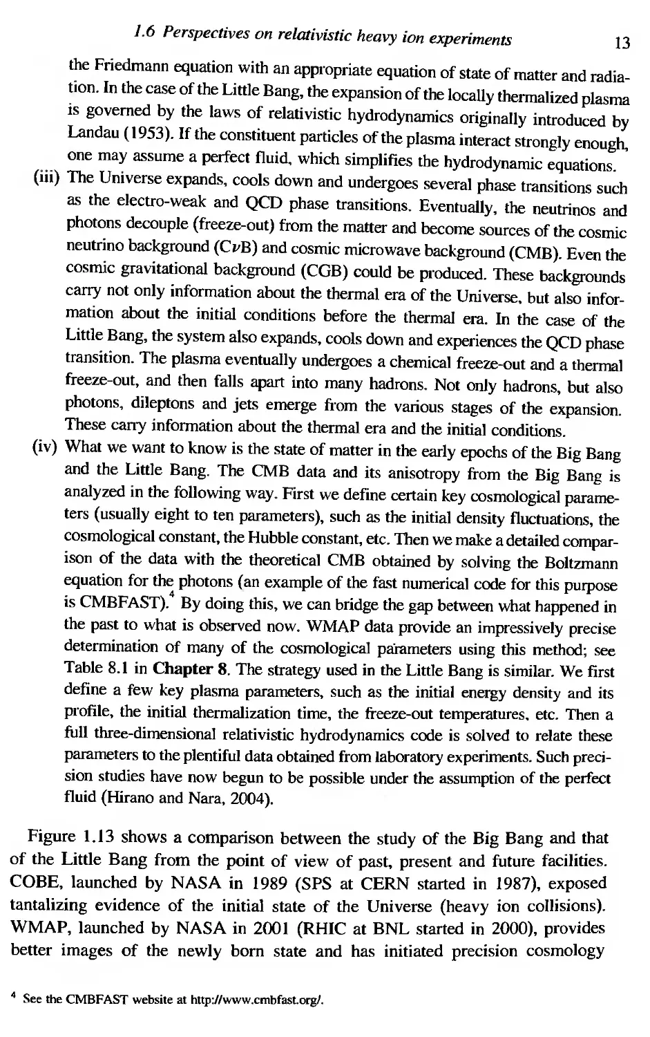
Fig. 1.13. Past, present and future facilities used to study the Big Bang and
the Little Bang. COBE, WMAP and infant images are taken from http://
map.gsfc,nasa.gov/index.htmJ (courtesy of NASAlWMAP Science Team). The
simulation picture at Planck is taken from http://www.rssd,esa.int (courtesy of
NASAIWMAP Science Team). The SPS and LHC images are CERN photos
taken from http://cdsweb.cem.ch (courtesy of CERN).
(precision QGP physics). The Planck satellite is due to be launched by ESA in
2007 (LHC at CERN is to be started in 2007); it is expected that these facilities
will shed further light on the initial conditions and the origin of dark energy
(initial conditions and the dynamics of the hot quark-gluon system).
1.7 Natural units and particle data
Throughout this book we use the natural units Ii = c = I. In addition we set the
Boltzmann constant to unity, k B = l. This unit system is described in Appendix A.
Tables of particles and their properties are given in Appendix H,
I
Basic Concept
of
Quark-Gluon Plasma
2
Introduction to QCD
In this chapter, we outline the basic concepts of quantum chromodynamics (QCD),
its classical and quantum aspects and its symmetry and vacuum structure; various
non-perturbative approaches are summarized for later purposes.
2.1 Classical QCD action
The classical Lagrangian density of QCD contains quark and gluon fields as
fundamental degrees of freedom; also, it is designed to have a local color SU c (3)
symmetry (Nambu, 1966), For a quark with mass m. the Lagrangian density is
given by
r _ -a ( ' /fJ " ) (3 I F a F ILII
NcI - q I a{3 - mV a {3 q - 4' IL" a .
(2.1)
The quark (gluon) field qa (A ) belongs to the SU c (3) triplet (octet). Therefore,
a runs from 1 to 3, while a runs from 1 to 8, Note that summation over repeated
indices is assumed unless otherwise stated.
We define /fJ == -yIL DIL' where DIL is a covariant derivative acting on the color-
triplet quark field;
DIL == aIL +igtaA .
(2.2)
Here g is the dimensionless coupling constant in QCD; the t a denote the funda-
mental representation of SU c (3) Lie algebra (See Appendix B.3). They are trace-
less 3 x 3 hermitian matrices satisfying the following commutation relation and
normalization:
I
[ta, t b ] = ifabc tC , tr(tat b ) = 2 ab.
(2.3)
18
Introduction to QCD
Explicit forms of t a and fabc (the structure constants) are given in Appendix B.3
together with some basic relations. For later convenience, we also define the
covariant derivative acting on the color-octet field:
1J 1L == OIL +igT a A .
(2.4)
Here T a are the adjoint representations of the SU c (3) Lie algebra. They are
traceless 8 x 8 hermitian matrices given by (Tahc = -ifabc. Some basic relations
of T a are also summarized in Appendix B.3.
The field strength tensor of the gluon F v is defined as
F v = aILA - avA - gfabcAtA ,
(2.5)
By introducing AIL == t a A and FILl' == t a F v' we may simplify Eq, (2.5) as follows:
-i
FILl' = alLAv-avAIL +ig[A w AI'] = -[Dw Dv].
g
(2,6)
Color electric and magnetic fields may be defined from FILl' in analogy with the
standard electromagnetic field,
Ei=F iO ,
. I 'k
B' = --"" k F )
2 '} ,
(2.7)
where "ijk is a complete antisymmetric tensor with "123 = 1. The classical equa-
tions of motion are obtained immediately from Eq. (2.1) as follows:
(ifj-m)q=O,
[Dv,Fv lL ] = gjIL or 1J bF:1L = gj1;,
(2.8)
(2.9)
where jIL = t a j1; and j1; = ijylLtaq. These are simply the Dirac equation and the
Yang-Mills equation for quarks and gluons (See Exercise 2.1).
The Lagrangian density, Eq. (2.1), is invariant under the SU c (3) gauge trans-
forma[ion (See Exercise 2.2(1»:
q(x) V(x)q(x), gAlL (x) V(x) (gAlL (x) - iaJ.,) vt (x),
(2.10)
where V(x) == exp(-iea(x)t"). To show this gauge invariance. it is useful [0
remember that FILl' and DIL transform covariantly; i.e.
FlLv(x) V(x)FlLv(x)Vt(x), DIL(x) V(x)DIL(x)Vt(x).
(2.ll)
2.2 Quantizing QCD
A small increment under the infinitesimal gauge transformation is given by
19
Bq(x) = -i(J(x)q(x),
B(gAIL(x)) = [Dw (J(x)],
(2.12)
where (J(x) = ta(Ja(x). The latter can be also written as B(gA (x)) = 1J b()h(X).
In principle, Eq. (2.1) may contain a g au g e-invariant term € FILV F Ap {)(
, ILvAp a a
Ef Bf. The existence of such a term violates the time-reversal invariance or, equiv-
alently, the CP (charge conjugation + parity) invariance. Although the meaSUre-
ment of the electric dipole moment of a neutron shows no sign of such a CP-
violating term in the strong interaction, the fundamental reason for its absence is
still not clear, and this is called the strong CP problem.
Because of the gauge invariance, terms such as A A are prohibited. As a
consequence, the gluons are massless. On the other hand, quark masses are not
consrrained by the gauge symmetry and they are indeed finite, as shown in
Table H.l in Appendix H. Moreover, quarks with different flavors (up (u), down
(d), strange (s), charm (c), bottom (b) and top (t)) carry different masses. For N f
flavors, we treat the quark field q (the quark mass m) in Eq. (2.1) as a vector
with N f components (an N f x N f matrix). In the standard model, the origin of
the quark masses is ascribed to the Yukawa coupling of quarks to the Higgs field.
However, the reason why there exist so many varieties of quark masses, ranging
from a few mega-electronvolts (MeV) to 175 GeV, is not understood,
2.2 Quantizing QCD
The classical Lagrangian density, .eel, in Eq. (2.1) does not tell us much about
the real dynamics of QCD at low energies. This is in contrast to quantum elec-
trodynamics (QED), where the Maxwell equations (as a classical limit of QED)
have wide applications in our daily lives. The basic difference between QCD and
QED is that the quantum effects become more (less) important at low energies
in QCD (QED). To see this difference explicitly, we need to quantize QCD and
to study the effects of vacuum polarizations. For a more complete discussion on
quantization and renormalization of QCD, see, for example, Ynduniin (1993) and
Muta (1998).
There are several different ways of quantizing gauge theories. In this book,
we will follow the quantization based on Feynman's functional integral (see
Appendix C), which is best suited for making a connection to the classical limit
and also for carrying out numerical simulations to study the full quantum aspects
of QCD. Another useful quantization procedure is the covariant canonical operator
formalism (Kugo and Ojima, 1979).
20
Introduction to QCD
In the functional integral method, one starts with the partition function under
an external source, J:
Z[ 1] = (0+ I 0-) J = J [dA dij dq] e i J d 4 x(£cl+1<I».
(2.13)
The physical meaning of Z[ 1] is the transition amplitude from the vacuum at
t -00 to that at t 00. The functional integration is carried out over the
c-number field, A (x), and the Grassmann fields, q"(x) and ij"(x). The external
source is defined as JCf> = iJq + ijTJ + j:'; A , where TJ and TJ are two independent
Grassmann external fields and j:'; is a c-number external field,
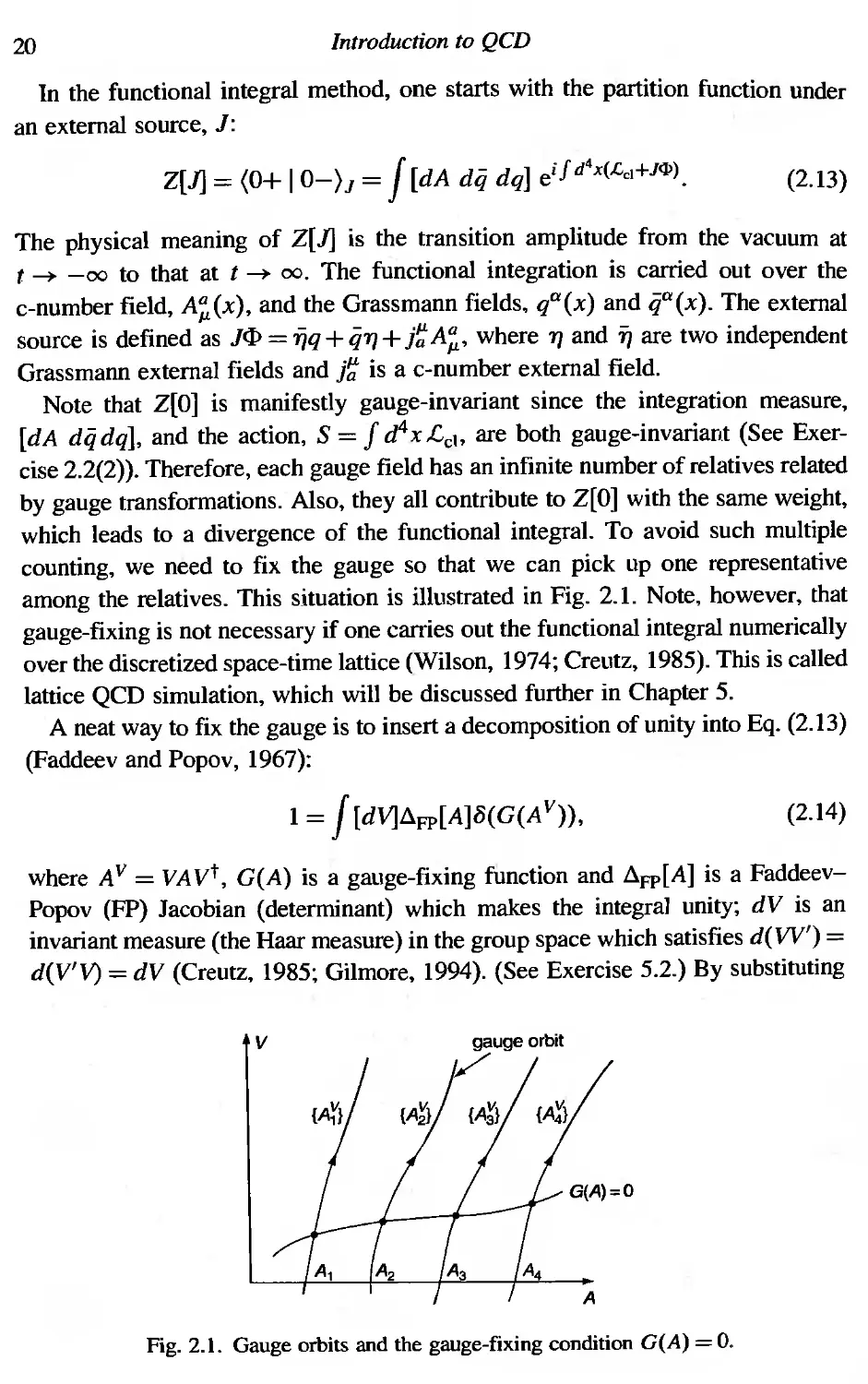
Note that Z[O] is manifestly gauge-invariant since the integration measure,
[dA dijdq], and the action, S = J d 4 x£ch are both gauge-invariant (See Exer-
cise 2.2(2)). Therefore, each gauge field has an infinite number of relatives related
by gauge transformations. Also, they all contribute to Z[O] with the same weight,
which leads to a divergence of the functional integral. To avoid such multiple
counting, we need to fix the gauge so that we can pick up one representative
among the relatives. This situation is illustrated in Fig. 2.1. Note, however, that
gauge-fixing is not necessary if one carries out the functional integral numerically
over the discretized space-time lattice (Wilson, 1974; Creutz, 1985). This is called
lattice QCD simulation, which will be discussed further in Chapter 5,
A neat way to fix the gauge is to insert a decomposition of unity into Eq. (2.13)
(Faddeev and Popov, 1967):
1 = J [dYJdFP[A]B(G(A v )),
(2.14)
where A V = VAVt, G(A) is a gauge-fixing function and dFP[A] is a Faddeev-
Popov (FP) Jacobian (determinant) which makes the integra] unity; dV is an
invariant measure (the Haar measure) in the group space which satisfies deW') =
d(V'V) = dV (Creutz, 1985; Gilmore, 1994), (See Exercise 5.2.) By substituting
v
Fig. 2.1. Gauge orbits and the gauge-fixing condition G(A) = O.
2.2 Quantizing QCD
21
the identity Eq, (2.14) into Eq. (2.13) and making an inverse gauge rotation, we
arrive at
Z[O] = (f [dVJ) x f [dA dij dq] FP[A] B(G(A)) eifd4x 'cel.
(2.15)
Note that B(G(A)) simply picks up a representative from the given gauge orbit
in Fig. 2.1. The explicit form of FP[A] is obtained from
FP[A]=det BGiAV) 1 '
V V=I
(2.16)
where the determinant is taken for both color and space-time indices.
The first factor on the right-hand side of Eq, (2.15) is the finite gauge volume
multiplied by the space-time volume, which is infinite. Since this factor has
isolated nicely and is just a multiplicative constant in Z[ 1], we may simply drop it
without affecting the vacuum expectation value of the field products (the Green's
functions ).
Choice of G is arbitrary as long as it can properly pick up representatives.
Commonly used ones are the axial gauge (G = nIL AIL with n 2 < 0), the light-cone
gauge (G = nIL AIL with n 2 = 0), the Fock-Schwinger gauge (G = .xIL AIL)' the
Coulomb gauge (G = ii Ai)' the temporal gauge (G = Ao) and the covariant gauge
G(A) = iJlL AIL - f(x) ,
(2.17)
where f(x) is an arbitrary function of space-time (Exercise 2.2(3)).
In the case of Eq. (2.17), we may further multiply the identity, I =
f[dfJe-ifZf2t, to Z[O] so that f(x) is eliminated. Here is called the gauge
parameter. The FP determinant may be exponentiated by introducing two inde-
pendent Grassmann fields, ca(x) and ca(x), called the ghost and the anti-ghost,
respectively. Then we arrive at the final form:
Z[J] = e iW11J = J[dA dij dq][dc de] eifd4x('c+JcJ>J,
_-u. {3_! a ILV
£, - q (l f/Ju{3 - mBu(3)q 4 FILl/Fa
-c iJlL1Jab c _ -.!... ( iJ IL A a ) 2.
a ILb2 IL
Although the gauge-fixed Lagrangian density, £', is no longer invariant
under the classical gauge transformation, Eq. (2.10), it has quantum gauge
invariance under the Becchi-Rouet-Stora-Tyutin (BRST) transformation, t5 BRST
(2.18)
(2.19)
22
Introduction to QCD
tBecchi et at., 1976; lofa and Tyutin, 1976); See Exercise 2.2(4), The transfor-
mations are given by
BBRSTq = -igAcq,
BBRSi= -A{aJ1. A J1.'
BBRSTAJ1. = A[DJ1.' c],
i
BBRST C = -2'gA[c, c],
(2.20)
(2.21 )
where c = c a t a and A is a space-time-independent Grassmann number. The trans-
formations in Eq. (2.20) are simply obtained from Eq. (2.12) by the replacemenl
() gAc. The BRST transformation is nilpotent, i.e. B 2 = O. Canonical q uanti-
BRST
zation of QCD can be beautifully carried out on the basis of the BRST symmetry
(Kugo and Ojima, 1979).
The standard perturbation theory employed to evaluate Z[ 1] or W[ 1] can now
be developed, starting from Eq. (2.19), by decomposing it into a free part and an
interaction part:
£ = £O+£int,
(2.22)
where £0 is obtained by setting g = 0 in £. The Feynman rules in the Euclidean
space-time with this decomposition will be given in Chapter 4. Note that Z[ 1] is
a generating functional of the full Green's function, while W[1] is a generating
functional for the one-particle irreducible (IPI) Green's functions. We may also
introduce an effective action, r[cp], by a Legendre transform, r[ cp] = W[1] - Jcp,
where cp =- B WI B J; r[ cp] is the generating functional for the I PI proper vertices.
These will be covered in more detail in Chapter 6 when we discuss the critical
phenomena associated with the second order phase transition.
2.3 Renormalizing QCD
In field theories, the quantum corrections (loops) calculated in perturbation theory
have ultraviolet divergences originating from the intermediate states with high
momenta. In renormalizable field theories, such as QCD, these divergences can
always be combined with the bare parameters of the Lagmngian and are absorbed
in the renormalized parameters.'
The energy scale at which the divergences are renormalized is caJled the
renormalization point, and is denoted by K throughout this book; K is an arbitrary
parameter. Any observables, such as the proton mass, the pion decay constant,
I Renormalizability of the QCD Lagrangian is not an accident but rather is a consequence of a large gap
between the typical QCD scale and the scale beyond QCD. Non-renormalizable terms. although they exist
in principle. become irrelevant at low energies. Note also that general non-renormalizable theories have
predictive powers as long as one has a systematic low-energy expansion: a well known example is the chiral
perturbation theory for low-energy QCD. For more details on the modern conceprs of renormalization and
effective field theories, consult Lepage (1990), Weinberg (1979), Polchinski (1992) and Kaplan (1995).
2.3 Renormalizing QCD
23
etc., do not depend on K, whereas the renormalized coupling, g, the quark mass, m,
and the gauge parameter, g, do depend on K.
The renormalization in QCD is summarized as a general statement that the
partition function defined in Eq. (2.18) can be made finite by the redefinition of
the paramelers, Namely,
Z[J B ; gB' m B , gB] = Z[J(K); g(K), m(K), g(K); K],
(2.23)
where the quantities with suffix B are bare parameters. The external field J
. ' B'
IS also regarded as one of the bare parameters. The precise relation between the
bare and renormalized quantities will be discussed in detail in Chapter 6. Since
the left-hand side of Eq. (2.23) is K-independent, Z satisfies
d
K dK Z=O.
(2.24)
The renormalization group equations for Green's functions are simply obtained
from this master equation by taking certain derivatives with respect to J.
To grasp the meaning of K in perturbation theory, let us consider the e+e-
annihilation into hadrons at a high center-of-mass energy, -,/S. The perturbative
calculation of e+e- qij for a massless quark yields the following cross-section:
[ as(K) ( as(K) ) 2 ]
u(s)=uo(s) I+CI(.JS'/K)---:;;:-+C2(.JS'/K) ---:;;:- +.... (2.25)
In this formula, uo(s) = (41Ta 2 /3s). 3. Q is the lowest order cross-section for
producing a pair of massless quarks with electric charge Qq; See Section 14.3.1.
The factor as == g2/41T (a == e 2 /41T) is the fine structure constant in the strong
(electromagnetic) interaction; Ci are dimensionless constants. It happens that cI =
1, but in general C i >2 depend on In(-,/S/K).
The cross-section is an observable and thus cannot depend on K. However, in
the perturbation theory this is guaranteed only order by order. To make the higher
order corrections behave well in Eq. (2.25). we may choose, for example, K = -'/s.
so that large logs at -,/S» K inside ci disappear. At the same time, as(K) becomes
the running coupling as(-'/s), which decreases as s increases in QCD, as will be
shown in a moment. This makes the perturbation series well behaved at high s.
As we will see in Chapter 4, the free-energy density of massless quarks and
gluons in the quark-gluon plasma at high temperature (T) has the following form:
81T 2 4 [ as(K) ( a s (K» ) 3/2
J(T) = - 45 T Jo + h ---:;;:- + h -----:;-
+ J4 (In 71': , In as(K)) ( a K) r +...] . (2.26)
24
Introduction to QCD
The factor 1(1)la,-+o is called the Stefan-Boltzmann limit, and it contains contri-
butions from a non-interacting gas of quarks and gluons, The coefficients 10,
hand h are K-independent constants, while It:::.4 depend on K through either
In(K/1T1) or Inas(K). By choosing, for example, K 1TT, we can suppress large
logs when T » K and consequently make the series well behaved, The explicit
form of Ii is given in Eqs. (4,111)-(4.115).
2.3.1 Running coupling constants
What is the behavior of the running coupling g as a function of K? This can be
answered by looking at the solution of the flow equation,
K iJg = {3,
iJK
The right-hand side is called the {3-function and may be calculated in perturbation
theory if g is small enough. All the manipulations become particularly simple if
we adopt the modified minimal subtraction scheme (MS) with the dimensional
regularization (Muta, 1998). In this scheme, {3 depends only on g and has a series
expansion of the following form (Gross, 1981; Muta, 1998)
(2.27)
(3(g) = _{3og3 - {3lg 5 +,..
{30 = ( 11- N f)
(41T)2 3 '
I ( 38 )
{31 =- 10 2--N f '
(41T)4 3
(2.28)
(2.29)
Factors {30 and {31 are subtraction-scheme-independent and are both posi-
tive for N f ::s 8. A negative (3, together with Eq, (2.27), implies that g(K)
decreases as K increases; this is called the ultraviolet asymptotic free-
dom (Gross and Wilczek, 1973; Politzer,1973; 't Hooft, 1985). Note that the
(3-function in QED is given by (3(e) = e 3 /(121T2) + e 5 /(641T4) +"', which
shows that e(K) increases as K increases. Among the renormalizable quantum
field theories in four space-time dimensions, only the non-Abelian gauge theories
are asymptotically free (Coleman and Gross. 1973).
It is a straightforward matter to extract the explicit form of g(K) in the lowest
order by taking (30 and (3). The result is as follows:
I [ (311n(ln(K2/A CD)) ]
as(K)= 41T{301n(K2/A CD) 1- {3 In(K2/A ) +,.. .
Here AQCD is called the QCD scale parameter, to be determined from experiments.
Since it is related to the integration constant of the differential equation, Eq. (2.27),
it is K-independent (Exercise 2.3),
(2.30)
2.3 Renormalizing QCD
25
It is important to specify the subtraction scheme and the number of active flavors
when quoting the actual value of A ; for exam p le, A fN/ =5) = ( 217::!: 24 ) MeV
QCD MS
(Eidelman eta/. 2004). Equation (2.30) tells us that the running coupling decreases
logarithmically as K increases. Therefore, our use of perturbation theory is
justified as long as K is large enough. This does not mean, however, that the
expansion in terms of g is convergent for large K. Instead, the expansion is at most
asymptotic, The running coupling determined by data from several experiments
is shown in Fig. 2.2. Values of the fine structure constant, as' for typicaJ values
of K are as follows:
as(lOO GeV) = O. 1l56::!: 0.0020,
a s (2 GeV) = 0.300 ::!:O,0l5,
as(lO GeV) =0.1762::!:0.0048,
a s (1 GeV) = 0.50::!:0.06 . (2.31)
The quark mass. m. is a parameter similar to the coupling constant, g; it obeys
a flow equation,
d
K-rn = -Ym(g)m,
dK
(2.32)
8
Ym(g) = Ymoi + Ymll +", , YmO = (41T)2 '
(2.33)
0.4
0.3
:g 0.2
0.1
0 10 2
1 10
,;;(GeV)
. . . d fi d "" deca y dee p inelastic
Fig 2 2 The runnIng couplIng determme rom T ecay. . ,
sca teri g, e+e- annihilation and Z-boson resonance shape and width. The figure
is adapted from Eidelman etal. (2004).
26
Introduction to QCD
Table 2.1. Running masses in the MS scheme and the
scale-independent ratios,
mu.d.s (K = I GeV) 1.35 mu,d,s (K = 2 GeV),
Running mass G
Mass ratio b
Up: mu
Down: m d
Strange: ms
1.5 to 4.5 MeV (K = 2 GeV) mu/md = 0.553 :J:0.043
5.0 to 8.5MeV (K = 2 GeV)
80 to 155 MeV (K = 2 GeV) mJmd = 18.9 :J:0.8
a From Eidelman etal. (2004).
b From Leurwyler (2001a).
Table 2.2, Running masses in the MS scheme and the
pole masses for the charm, bottom and top quarks.
Running mass G
Pole mass G
Charm: me
Bottom: mb
Top: m,
1.0 to 1.4GeV (K = mJ
4.0 to 4.5 GeV (K = m b )
175GeV (K = m,)
1.5 to 1.8GeV
4,6 to 5.1GeV
175GeV
a From Eidelman etal. (2004).
The solution of this equation in the leading order is given by
m
m(K) = 2 '
(!In(K2/A CD)rmo/ Po
(2.34)
where m is an integration constant of Eq. (2.32) and is thus K-independent (Exer-
cise 2.4). Since Ymo/2130 = 12/(33 - 2N f ), the running mass, m(K), decreases
logarithmically as K increases as long as 13 < 0, Note that m(K) is simply a
parameter of QCD and does not correspond to the pole position of the prop-
agator. Although the quarks are confined and do not have a pole in the full
non-perturbative propagator, we may introduce an on-shell mass, at least in
perturbation theory. This is called the pole mass, m po le' and it is useful in the
phenomenology of heavy quarks. The running mass and the pole mass are related
in the leading order of the perturbation theory as follows: mpol e = m(K = m)(1 +
(4/3)(a s (K = m)/7T) +... ). The running masses of light (u, d, s) quarks and their
ratios are summarized in Table 2.1. The running and pole masses of heavy (c, b. t)
quarks are summarized in Table 2,2. A more extensive and updated listing may
be found in Eidelman etal. (2004).
2.3 Renormalizing QCD
27
2.3.2 More on asymptotic freedom
The polarization of the vacuum screens (anti-screens) a test charge in QED (QeD).
The screening (anti-screening) may be interpreted as the effective charge, which
is a sum of the test charge and the induced charge, increases (decreases) as one
approaches the test charge. In terms of the dielectric constant, E, of the vacuum,
E> 1« I) corresponds to the screening (anti-screening) in analogy with dielectric
substances (Jackson, 1999).
This intuitive picture is justified either by studying the dielectric constant, E,
of the QCD vacuum under an external color electric field (Hughes, 1981) or by
studying the magnetic permeability, p" under a color magnetic field (Nielsen,
1981; Huang, 1992). Since Lorentz invariance imposes Ep' = 1, these are two
equivalent ways of seeing the same physics; namely, screening, E > I (anti-
screening, E < 1) corresponds to diamagnetism, p, < I (paramagnetism, p, > I).
Let us consider the energy density of the vacuum, Bvac, under a uniform
magnetic field, B, coupled with massless particles with a bare charge, eo, and
spin S (= 0,1/2, I). Finding the Landau levels under the uniform magnetic field
and summing over the zero-point fluctuations lead us to the following formula:
( I b(S)2 A2 ) 2_ I 2
Bvac(B):::::: - - -eo In- B = - ( ) B.
2 2 eoB 2p, B
Here A is an ultraviolet cutoff of the vacuum fluctuation and p,(B) is interpreted as
the magnetic permeability of the vacuum. (One may also introduce the magnetic
susceptibility, X(B) = 1- p,(B).) The coefficient of the zero-point fluctuation is
given by
(2.35)
(_1)2S [ 2 I ]
b(S) = ----g;;:2 (2S) - 3' '
(2.36)
which has a simple interpretation, The first term on the right-hand side of
Eq, (2.36) is from the Pauli paramagnetism related to the alignment of the parti-
cle spin along the external magnetic field, The second term is from the Landau
diamagnetism related to the orbital motion of the charged particles under the
magnetic field (Exercise 2.5). The sign factor, (_1)2s. reflects the particle statis-
tics (zero-point energy is positive for bosons and negative for fermions). This
formula indicates that the S = 1 vector boson leads to paramagnetism, f.L > I,
while the S = 0 boson and the S = 1/2 fermion lead to diamagnetism, f.L < I.
The relation between b(S) and the {3-function becomes clear if we define
an effective coupling constant, e 2 (JB) = e6le = f.Le'6, in analogy with tandard
electromagnetism, Then it is straightforward to see that Kae/aK = -b(S)e .' where
K = -J[J, which implies that b is simply the first coefficient of the {3-functIon, {3o,
defined in Eq, (2,28).
28
Introduction to QCD
To make a quantitative connection with QCD, B may be identified with the
external color magnetic field, Its couplings to the S = I and S = 1/2 fields are
generated by the gluon self-coupling and the gluon-quark coupling, respectively.
Then, after taking into account appropriate color and flavor factors (Nielsen, 1981;
Huang, 1992), we arrive at the familiar formula for asymptotic freedom,
3 N f ( I ) I ( 2N )
/3o(QCD) = -b(S= l)+-b S= - = _ 2 ll--L .
2 2 2 (47T) 3
(2.37)
Thus we find that the spin of the gluon and the gluon self-coupling make the QCD
vacuum behave like a paramagnetic substance. This result, combined with Lorentz
invariance, implies that the QCD vacuum exhibits anti-screening of color charges.
For a system at finite temperature and density, the situation changes due to the
existence of matter. In fact, quark-gluon plasma exhibits the screening of color
charges, rather than anti-screening, as will be discussed in Chapter 4.
In summary, we have found that the running coupling, g, becomes small at high
energies, and this is known as the ultraviolet (UV) asymptotic freedom, In this
case, the perturbation theory becomes more and more reliable at high energies
once an appropriate choice of K is made. On the other hand, at low energies,
g grows, and the perturbation theory is no longer reliable. This feature is the
origin of color confinement and is called the infrared (IR) slavery. UVasymptotic
freedom and IR slavery are just opposite sides of the same coin,
2.4 Global symmetries in QCD
Besides SU c (3) local gauge symmetry, classical Lagrangian density, Eq. (2.1), has
other global symmetries, such as the chiral symmetry and dilatational symmetry.
2.4.1 Chiral symmetry
Let us first introduce the left-handed and right-handed quarks as two eigenstates
of the chirality operator, 1'5' with the eigenvalues :!:: I :
I
qL = 2'(I-1'5)q,
1
qR = 2(1 + 1'5)q,
(2.38 )
For free massless quarks, the chirality is equivalent to the helicity, u.p. Now,
consider QCD with N f flavors and write the quark field as a vector with N f
components as follows:
t q = (u,d, s, .,,),
(2.39)
2.4 Global symmetries in QCD
29
Then the quark mass, m, becomes an N f x N f matrix and Lei may be decomposed
as follows:
Lei = Lei (qL , A) + LeI(qR' A) - (qL mqR +qRmqJ.
(2.40)
It is clear from this expression that Lei in Eq. (2.1) and also L in Eq. (2.19) for
m = 0 are invariant under the U L (N f ) x U R (N f ) global transformation
-o,i(I J -iAiOj
qL e LqL' qR e RqR'
(2.41)
where the oj (j = 0, 1, . . . , N f 2 - I) are space-time-independent parameters and
L,R
11. 0 = J2/N f , 11.j = 2t j (j = I".., N} -I). This is called chiral symmetry,
It is also convenient to define vector and axial-vector transformations as
-iAi oj -iAi oj 'Ys
q e v q, q e A q,
(2.42)
where 0v = 0L = OR and 0A = -OL = OR' There are two U(l) transformations in
the above: U (I), which is related to the baryon number (oj ()( a jO , (}.i = 0), and
B v A
U (I), which corresponds to the flavor-singlet axial rotation (oj = 0, (}.i ()( a jO ),
A v A
Because of Noether's theorem, which relates symmetries and conservation
laws, the vector and axial currents, Jt = q'Y",11.jq and Jt5 = q'Y", 'Y5Mq, have the
following relations (Exercise 2,6):
a'" Jt = iq[ m, 11.j]q, (j = 0, , , . , NJ - I),
a'" J 5 = iq{m, 11. j h5q, (j = I,.", NJ -I),
a'" J 5 = J2/ N f (2iij m 'Y5q - 2N f 3 :2 F!:" F;II ) ,
(2.43)
(2.44)
(2.45)
where F;II == e"'"ApF:P (e0123 = 1) is the dual field strength. tensor, As c n e
seen in Eq. (2,45), the conservation of the flavor-singlet axIal current, Jp.5' IS
broken not only by the quark mass matrix, m, but also by the quantum effect
called the axial anomaly (Bertlemann, 1996). From the functional inregral point
of view, it originates from the non-invariance ofthe path integral measure [d ij dq]
under the U/l) transformation (Fujikawa, 1980a, b). See Exercise 2.7.
2.4.2 Dilatational symmetry
Consider the scale transformation
q(x) u 3/2 q(ux), A (x) uA (ux),
(2.46)
30
Introduction to QCD
where cr is a space-time-independent parameter. Note that .eel is invariant under
Eq, (2.46) in the chiral limit (m = 0), This symmetry is, however, explicitly
broken by the quantum effect, and we arrive at
a /11-' - TI-' - P...pa pl-'V ( I ) ,,-
I-' - I-' - 2 I-'V a + + 'Ym L qmqq,
g q
where TI-'v is the energy-momentum tensor and /11-' is the dilatational current
defined by Xv pl-'. The second term on the right-hand side of Eq, (2.47) shows
that the dilatational current is not conserved if g f= 0, Since it is related to
the trace of the energy-momentum tensor, this is called the trace anomaly
(Collins et aI., 1977; Nielsen, 1977). (For a heuristic derivation, see Exercise 2.8.)
(2.47)
2.5 QCD vacuum structure
Because the QCD coupling, g, becomes strong in the IR region, quarks and gluons
interact non-perturbatively at low energies. As a result, the QCD vacuum acquires
a non-trivial structure. such as the quark and gluon condensates,
Analyses of the mass spectrum of charmoniums using QCD spectral sum rules
(Shifman et aI., 1979; Colangelo and Khodjamirian, 2001) indicate that gluons
have non-perturbative condensation:
( as puvP:;v ) (300 MeV)4.
7T I-' vac
(2.48)
This has an interesting physical consequence if it is combined with the trace
anomaly in Eq. (2.47), First, the vacuum expectation value of the energy-
momentum tensor can be written as (TI-'V)vac = -Bvacgl-'v using Lorentz
invariance, where Bvac is the energy density of the QCD vacuum. Taking the
chiral limit, m = 0, for simplicity and expanding {3(g) up to the leading order
yields
11- 2N d 3 ( as a V )
Bvac ::::::: -p pI-'
32 7T I-'V U vac
::::::: -0.3 GeV fm- 3 ,
(2.49)
Namely, the QCD vacuum has a smaller energy density than that of the perturba-
tive vacuum. Very often, one introduces the notation Bvac = -B; B is called the
bag constant for historical reasons, as explained in Section 2,6, The color confine-
ment must be related to the gluonic structure of the non-perturbative vacuum.
Although many attempts to bridge this link have been made, a satisfactory and
clear explanation remains elusive, The anti-screening nature we have encoun-
tered in perturbation theory (e < 1 and f.L > 1) is already a signature of the color
3]
con inement. In fact, the QCD vacuum may well be a perfect anti-dielectric or
eqUivalently perfect paramagnetic substance; i.e.
2.5 QCD vacuum strocture
Evac = 0, J.tvac = 00.
(2.50)
What about the quark structure of the QCD vacuum? The Gell-Mann-Oakes-
Renne (GOR) relation, which is obtained solely by chiral symmetry, yields
(ExercIse 2.9(2, 3))
f 2 2 ( - d - ) 2
7fm7fx = -m uu + d vac + O(m ),
f;m;o = -(muuu+mddd)vac+O(m2),
(2.51 )
(2.52)
Here m = (m u + md) /2 is the averaged mass of u and d quarks, f 7f( = 93 MeV)
is the pion decay constant and m7fx 140 MeV (m7fo 135 MeV) is the charged
(neutral) pion mass. Using the quark mass from Table 2.1, we obtain m(K =
I GeV) 5,6MeV, and we have
«uu+dd)/2)vac -(250MeV)3 at K=IGeV.
(2.53)
This implies that the QCD vacuum involves condensation of quark-anti-quark
pairs. It was Nambu who developed the theory of dynamical breaking of chiral
symmetry by noticing its close analogy with Cooper pairs and superconductivity
in metals (Nambu and Jona-Lasinio, 1961a, b),
Since qq( = qL qR + qR qL) is not invariant under the SU L (N f ) x SUR (N f ) trans-
formation given in Eq. (2.41), it serves as an order parameter of the dynamical
breaking of chiral symmetry, Indeed, the pattern of the dynamical chiral symmetry
breaking in a QeD vacuum is
SU L (N f ) x SUR (N f ) -+ SU/N f ),
(2.54)
where SU v (N f ) is a vector symmetry remaining in the vacuum. At extremely high
temperature, the restoration of chiral symmetry takes place, as will be discussed
in Chapter 6. At extremely high baryon density, the system exhibits a different
type of symmetry breaking pattern (the color superconductivity). which will be
discussed briefly in Chapter 9.
The energy density of the QCD vacuum as a function of the order parame-
ter looks like that given in Fig. 14.4. It has a minimum at the bottom of the
"wine bott]e" and thus breaks symmetry. The amplitude fluctuation of (ijq)
costs energy and thus corresponds to a massive excitation, called the (T-meson
(Hatsuda and Kunihiro, 2001), On the other hand, the phase fluctuation of (ijq)
costs no energy in the chirallimit and corresponds to the massless pions, The latter
statement can be made more rigorous, and is known as the Nambu-Goldstone
theorem (Exercise 2.9(] »,
32
Introduction to QCD
2.6 Various approaches to non-perturbative QCD
Various models of QCD have been proposed, such as the bag model, the potential
model and the Nambu-Jona-Lasinio model. Although one must be cautious not to
extrapolate too far beyond the applicability of the models, they are quite useful in
elucidating some of the essential features of QCD in a non-perturbative regime.
Methods more closely related to QCD are the QCD sum rules and the chiral
perturbation theory. In addition, direct numerical simulations of QCD defined on
the space-time lattice have become an extremely useful tool in recent years. We
will briefly summarize these approaches in the following.
The bag model
Hadrons may be considered as bags embedded in a non-perturbative QCD vacuum
(Chodos et aI., 1974), A special boundary condition is introduced for quarks and
gluons to incorporate the confinement so that color charge does not leak out from
the bag. Inside the bag, no condensates are assumed and quarks and gluons are
treated perturbatively. An intuitive picture of the model is shown in Fig. 2.3.
The mass of the proton in this model is given by
3x 47T 3
M =-+-BR b +,..
PR 3 ag ,
bag
(2.55)
where R bag is the radius of a spherical bag; xl R bag is the kinetic energy of each
quark confined inside the bag (x 2,04 for the lowest-energy mode of a massless
quark). The term proportional to B (called the bag constant) is the volume energy
of the bag, which represents the energy necessary to create a perturbative region
in the non-perturbative vacuum. Thus, -B can be identified with Eq. (2.49).
The ....." in Eq, (2,55) contains interactions among quarks inside the bag, the
Casimir energy of quarks and gluons in the spherical cavity, the effect of the
-
..'
ijf
;.
t::
,.:!:t
t.
f<
! fO\
!:
;
0-0
#1.--'00
Fig. 2.3, Baryon and meson bags in a non-perturbative QCD vacuum which has
a perfect ami-dielectric (perfect paramagnetic) property.
2.6 Various approaches to non-perturoative QCD 33
meson cloud surrounding the bag, and so on. The model can describe the mass
spectra of light hadrons composed of u, d and s quarks reasonably well with a
suitable choice of the bag constant. An estimate using Eqs. (2.48) and (2.49),
together with the definition B = -B vae ' yields
B (220 MeV)4.
(2.56)
This will be used in Chapter 3 to construct a schematic model of the phase
transition between the hadronic matter and the quark-gluon plasma,
The potential model
In order to describe hadrons composed of heavy quarks, such as charm and
bottom quarks, the non-relativistic Schrodinger equation with static inter-quark
potential may be a good starting point. The potential picture is justified when the
motion of the valence quarks is much slower than the typical frequency of gluons
exchanged between quarks. A typical form of the phenomenological qq potential
is the Coulomb + linear type:
a
V - ( R ) =--+KR+...
qq R '
(2.57)
where R is the distance between the quark and the anti-quark, and K is the string
tension representing the strength of the quark confinement force, Its empirical
value obtained by fitting the charmonium and bottomnium spectra (Bali, 2001) is
given by
K (0.42 GeV)2 = 0.9 GeV fm- I .
(2.58)
This value is consistent with that obtained from the Regge trajectories of light
mesons. In perturbation theory, the coefficient of the Coulomb term, -0/ R,
becomes a = 4a s /3, The ". . ." in Eq, (2.57) represents the relativistic corrections
such as the hyper-fine term, the spin-orbit term, and so on. Application of the
model to the heavy quark bound states at finite T will be discussed in Chapter 7.
There is no a priori reason to believe that the potential picture also works for
hadrons composed of light quarks (u, d, s). Nevertheless, it has a remarkable
phenomenological success in describing mass spectra and electro-magnetic prop-
erties (De Rujula et ai" 1975) if we assume that the u, d and s quarks have the
constituent masses
Mu,d 340 MeV and Ms 540 MeV. (2.59)
These are much larger than the current masses, m q , listed in Table 2. I; Mq may
be determined, for example, by fitting the magnetic moments of light baryons,
and is now believed to be an effective mass generated by the dynamical breaking
of chiral symmetry.
34
lntroduction TO QCD
The Nambu-Jona-Lasinio (NJL) model
This model is based on a Lagrangian which captures essential aspects of
chiral symmetry in QCD (Vogl and Weise, 1991; Klevansky, 1992; Hatsuda and
Kunihiro, 1994), The typical form of the Lagrangian density for Nt flavors
is given by (Nambu and Jona-Lasinio, 1961a,b)
NJ-I
.e NJL = ij(i'Yp,BP,-m)q+ g;L L [(ij,\,jq)2+(iji'Y5'\/q)2],
- j=O
(2.60)
Equation (2.60) includes the quark kinetic term and a chiral symmetric four-
fermi interaction with a dimensionful coupling constant, gNJL' The dynamical
breaking of chiral symmetry «ijq)vac f= 0) occurs when gNJL exceeds some critical
value, In addition, the constituent quark masses. Mq, in Eq, (2.59) are generated
dynamically:
Mq = 1nq - 2g NJL (ijq)vac. (2.61)
The model can be generalized to incorporate the U A (I) axial anomaly by intro-
ducing an extra term, detk,/ijk(l + 'Y5)ql + h,c., which is called the Kobayashi-
Maskawa-'t Hooft vertex ('t Hooft, 1986; Hatsuda and Kunihiro, 1994),
It is a straightforward matter to apply this model to study the restoration of
broken chiral symmetry at high temperature and/or baryon density. It is amazing
to see that this simple model captures the essential feature of the QCD phase
diagram in the real world, a point that will be discussed further in Chapter 6.
Chiral perturbation theory
Because of the dynamical breaking of chiral symmetry, the pion as a Nambu-
Goldstone boson becomes the lightest hadron. Therefore, at low energies, we may
introduce an effective description of the QCD partition function, Z[O], solely in
terms of the pions (Weinberg, 1979; Gasser and Leutwyler, 1984, 1985):
Z[O] = f [dU] e i J d 4 x(£(2)(V)+£(4)(U)+£(6)(U)+...), (2.62)
where U(x) is a field in the SU(N f ) space and is related to the pion field as
U = exp(i,\,j 7T j ) with j = I N] - l.
Each term in the effective Lagrangian is ordered in terms of the number of
derivatives and the pion mass divided by the typical scale of chiral symmetry
breaking, Ax = 47T/-rr/JNi; namely, .e(/)(U) O((m-rr/Ax)l, (B/ Axil) with /1 +
1 2 = I. Lorentz invariance, locality and chiral symmetry are the general constraints
with which we can form an explicit construction of .e(l)(l!). For example, .e(2) is
simply given by
,e(2) = tr(ap,uap,u t +htU+Uth),
(2,63)
2.6 Various approaches to non-perturbative QCD
35
where tr is taken over the flavor indices. The free parameters associated with
.cP)(U), such as f and h in Eq. (2.63), are determined by experimental inputs
order by order in the chiral expansion. Once the parameters are fixed, we can make
a systematic prediction of other physical quantities (Leutwyler, 2001b). As will
be shown in Chapter 7, this method is also useful in analyzing the thermodynamic
properties of hadrons and their interactions, although applicability is limited to
low temperatures (Gerber and Leutwyler, 1989).
The QCD sum rules
This approach relates the hadronic properties to the quark and gluon condensates
in the QCD vacuum. The method is a generalization of the Thomas-Reiche-Kuhn
sum rule in quantum mechanics, in which various spectral sum rules are derived
on the basis of the completeness of state vectors (Ring and Schuck, 2000). In
QCD, the dispersion relation and the Wilson's operator product expansion are
the basic ingredients necessary to derive sum rules (Shifman et al., 1979). For
example, the time-ordered correlation function of the electromagnetic current in
the momentum-space satisfies the subtracted dispersion relation:
I 1 00 p(s)
TI(q2) = - 2 'a ds - subtraction,
7T 0 s-q-I
where the last factor on the right-hand side is the subtraction term required to make
the integral finite: p(s) = ImTI(s) carries all the information about the hadronic
spectrum coupled to the electromagnetic current and is called the spectral function
(see Section 4.4). By taking an asymptotic expansion of both sides by l/q2 in the
deep-Euclidean region (q2 -+ -00), we may relate certain integrals of p(s) to the
vacuum condensates.
Assuming that the spectral function has a sharp resonance at low s and a smooth
continuum at high s, and taking appropriate values of the vacuum condensates,
one can extract the masses of hadrons, couplings and electromagnetic properties,
etc., with reasonable accuracy (Colangelo and Khodjamirian, 2001). Generalizing
the method to finite temperature and/or density is also possible, and is useful
to make a connection between the spectral integrals and the condensates in the
medium (Hatsuda and Lee, 1992; Hatsuda eta!., 1993).
(2.64)
The lauice QCD
A key concept of the lattice QCD approach is to discretize the Euclidean space-
time, xi (i = 1,2,3,4), into a lattice, xi = ani' where a is the lattice constant.
Then the quark field, q(n), is defined on a lattice site labeled by n and the gluon
field, U,.,,(n) = exp(iagA,.,,(n»), is defined on a !attice link la led by n and .Il-.
The lattice constant, a, serves as a natural ultravIOlet cutoff reqUIred to regularIze
the theory in a gauge-invariant manner (Wilson, 1974).
36
Introduction to QCD
The QCD partition function on the lattice may be schematically written as a
discretized form:
Z[O] = f n[dU,.(n)dq(n)dq(n)]e-[Sg(u)+S.<q,q,U)].
n,p.
(2,65)
The explicit form of the gluon action, Sy, and that of the quark action, Sq, will
be given in Chapter 5. A systematic expansion, such as the weak coupling and
strong coupling expansions on the lattice, may be developed. and one can carry
out the direct numerical integration of Eq, (2.65) using the method of important
sampling (Creutz, 1985). Because of the recent increase in computer power, as
well as theoretical developments, lattice QCD simulations have become the most
powerful technique utilized in solving QCD from first principles.
A considerable amount of work on QCD phase transition at a finite temperature
has been done on the lattice (Karsch, 2002). For example, the critical tempera-
ture, Tc, and critical energy density, Bcrit, for a system with massless u and d
quarks (N f = 2) are extracted as (see Section 3.8)
Tc 175 MeV, Bcrit I GeV fm-3.
(2,66)
We will discuss the basic notion and applications of lattice QCD in more detail
in Chapter 5.
Exercises
2.1 Classical Yang-Mills equation. Derive the classical equations of motion,
Eqs, (2.8) and (2.9) from the classical Lagrangian density, 'cel' in Eq. (2.1),
2.2 Gauge invariance.
(1) Show that 'cCI is invariant under the gauge transformation in Eq, (2.10),
(2) Show that the measure [dA][dqdq] is invariant under the gauge trans-
formation Eq, (2.10).
(3) Derive the explicit form of the Faddeev-Popov determinant, FP[A].
for the covariant gauge Eq. (2.17). What about the case for the axial
gauge?
(4) Show the invariance of'c in Eq, (2,19) under the BRST transformation
Eqs, (2.20) and (2.21).
2.3 Running coupling and scale parameter.
(1) Solve the flow equation, Eq. (2,27), in the leading order of the
l3-function, l3(g) = -l3og3, and show that Eq. (2.30), without the In In
term, is indeed the solution.
Exercises
37
(2) Derive the following relation between the renormalization scale, K, and
the QCD scale parameter in the leading order:
AQCD = K exp( -I /2(3ol).
(3) Repeat the above derivation with the next-to-leading order (3-function.
(3(g) = _(3og3 - (31g 5 ,
2.4 Running mass. Solve the flow equation, Eq. (2.32), in the leading order,
'Ym(g) = 'Ymog 2 , and show that Eq. (2.34) is indeed the solution.
2.5 Pauli and Landau magnetism. The Pauli paramagnetism arises from spin
polarization of electrons in a magnetic field, while the Landau diamag-
netism arises from the cyclotron motion of electrons in a magnetic field.
Refer to a textbook on solid state physics and derive the following relation
between the two magnetic susceptibility: XLandan = - X pauI /3 < o.
2.6 Noether's theorem. The partition function, Z[J = 0], in Eq, (2,18) must
be invariant under the change of variable q(x) -+ q' (x), Making the change
of variables, such as in Eq. (2.42), with space-time-dependent parameters,
oj (x), and demanding that Z[J = 0] is invariant under this change, derive
V,A
the partial conservation laws of vector and axial currents in Eqs, (2.43)
and (2.44). This constitutes the functional integral derivation of Noether's
theorem,
2.7 Axial anomaly. By carefully defining the Jacobian (called the Fujikawa
Jacobian) of the functional measure [dq dq] under the change of variables,
and by expanding the quark field in terms of the eigenfunctions of the
Dirac operator, iljJ, show that there appears the axial anomaly term for
the divergence of the flavor-singlet axial current, Eq. (2.45) (Fujikawa,
1980a, b).
2.8 Trace anomaly. Let us derive the trace anomaly equation, Eq. (2.47), in a
heuristic manner. (For a rigorous derivation, see Collins eta/. (1977) and
Nielsen (1977)). For simplicity, we consider the vacuum expectation value
of Eq. (2,47) in the chirallimit m = O.
(1) The partition function ofthe gauge field without gauge-fixing is given by
- -2
Z = e iW = J [dA] e -f.'rF ,
where the QCD coupling constant, g, is absorbed in the field as A ==
g Aa and Fa = g F a Show that W is related to the vacuum energy
p. p.v - p.v' .'
density, Bvac, as W = -B vac V 4 , with V 4 bemg the space-tIme four-
volume. By differentiating Z with respect to g, show that oBvaclog =
(F 2 ) I( -2Ef). . . .
(2) Renormalization group (RG) invariance of the partItIon nctI n.
Eq. (2.24), or equivalently the RG invariance of Bvac, ImplIes
38 lntroduction to QCD
KdBvacldK = (KalaK + {3a;ag)Bvac = O. Show that this relation,
together with the fact that Bvac has mass-dimension four, leads to
aBvaclag = -(41{3)(BvaC>.
(3) Due to the Lorentz invariance of the vacuum, the trace of the energy-
momentum tensor is related to Bvac as (Tt:) = 4Bvac (Section 2.5).
Combining this with the results in (I) and (2), derive the desired
relation, (Tt:) = ({312g3) (p2) = ((312g) (p2),
2.9 Nambu-Goldstone theorem and soft pion theorem.
(1) Consider the matrix element of the axial current, J 5 1'-' in Eq, (2.44):
(OIJf)7T b (k) == ifwkl'- e-ik,xljab.
Here a and b are flavor indices running from I toNJ-l; 10) is the vacuum
state normalized as (010) = 1, while the one-pion state obeys the covari-
ant norm alization, ( 7T G(k)I7T\k') = 2E(k)ljab(27T)3lj3(k_k') with
E(k) = J e + m;. The factor fw( 93 MeV) is called the pion decay
constant since the above matrix element appears in calculating the
weak decay of the pion, such as 7T- --+ J.L - + ii 1'-' Consider the chiral
limit where the current quark masses (m) are all zero, Show that
fwmw = 0 holds by using the conservation of the axial current. If
the pion exists and couples to the axial current with non-vanishing
magnitude, it implies that the pion mass is zero when m = O. This is
the simplest proof of the Nambu-Goldstone theorem, For a general
proof applicable to the system at finite temperature, see Section 7,2.2.
(2) Starting from the matrix element (OITJfl'-(x)O(Y)IO), where 0 is an
arbitrary operator at y and T is the time-ordered product (Eq, (4,47)),
deduce the following soft pion theorem in the chirallimit (m = 0):
-i
lim(7T a (k)IOIO) = -(OI[Q , 0]/0),
k-+O fw
where Q5( = J d 3 x J5'.o) is the axial charge operator. Generalize the
idea to the arbitrary matrix element, (aiT J 5 1'- (x)O(Y)I{3). and study the
subtleties when baryons are involved in the states, For further details,
consult, for example, Chap. 19 in Weinberg (1996).
(3) Consider the matrix element (7T a (k = O)IH QCD I7T b (k = 0), where
H QCD is the QCD Hamiltonian. Using the soft pion theorem twice,
derive the Gell-Mann-Oakes-Renner relation given in Eqs. (2.51)
and (2.52). Note that H QCD commutes with Q , except for the quark
mass term, J d 3 x ij(x)mq(x). Note also that we are using the covariant
normalization of the state vectors.
3
Physics of the quark-hadron phase transition
At low temperature (T) and low baryon density (p), QCD exhibits dynamical
breaking of chiral symmetry and confinement, which are both intimately related to
the non-perturbative structure of the QCD vacuum, as we have seen in Chapter 2.
On the other hand, if T and/or pl/3 are much larger than the QCD scale param-
eter AQCD 200 MeV, the QCD running coupling constant given in Eq. (2.30),
O's(K T,pl/3), becomes small, Furthermore, the long-range color electric force
receives plasma screening and becomes short-ranged, This is why the system at
T and/or pl/3 is expected to behave as a weakly interacting gas of quarks and
gluons: the quark-gluon plasma (QGP) (Collins and Perry, 1975),
The above considerations suggest that the QCD vacuum undergoes a phase change
at some values of T and p. In fact, various model approaches and numerical simula-
tions of QCD strongly indicate the existence of a transition from the hadronic phase
to the quark-gluon phase, which is relevant to the early Universe at the age of 10- 5
s where T 170 MeV 10 12 K, and the deep interior of neutron stars where p
several xPnffi 10 12 kg cm- 3 . It may also be realized at and after the impact of the
relativistic nucleus-nucleus collisions. Such experiments are conducted by using the
Super Proton Synchrotron (SPS) at the European Organization for Nuclear Research
(CERN), the Relativistic Heavy Ion Collider (RHIC) at Brookhaven National Labo-
ratory (BNL) and the planned Large Hadron Collider (LHC) at CERN.
In this chapter, we discuss the basic concepts of the quark-hadron phase tran-
sition in a hot environment (T » pl/3, AQ{D)' The phase transition in a dense
environment (pl/3 » T, A QCD ) will be discussed in Chapter 9 with respect to the
physics of compact stars.
3.1 Basic thermodynamics
In this section, we briefly summarize the basic statistical and thermodynamic rela-
tions, following standard textbooks such as the one by Landau and Lifshitz (1980).
39
40
Physics of the quark-hadron phase transition
For a statistical system in equilibrium with volume V, temperature T and chemi-
cal potentialp" we introduce the grand-canonical density operator, p, the grand-
canonical partition function, Z(T, V, p,), and the grand potential, neT, V, p,). in
the natural units k B = Ii = c = 1:
P A = .!. e-(H-p.N)/T
Z '
Z(T, V, p,) = Tr e-(H-p.N)/T
= L(nle-(H-P.N)/Tln) == e-n(T,V,p.)/T,
(3.1)
(3,2)
n
Here iI and if are the Hamiltonian operator and the number operator, respectively.
The trace, Tr, is taken over a complete set of quantum states labeled by n. Note
that Tr p = 1 holds by definition. We may also introduce an entropy operator,
S = -In p.
(3.3)
Since the thermal average of an arbitrary operator, 0, is given by (0) = Tr[pO],
the averaged energy, E, the averaged particle number, N, and the averaged
entropy. S, are given by
E=(8), N=(N). S=(S)=-Tr[plnp],
(3,4)
Equation (3.2), combined with Eq, (3.4), yields the following thermodynamic
relations:
neT, V, p,) = E - TS - p,N,
dn = -S dT - P dV - N dp"
dE = T dS-P dV+p, dN.
(3,5)
(3.6)
(3.7)
Equations (3.5) and (3.6) are obtained by the definition of S together with the
definition of the pressure, P = -dn/dVlr,/J.' Equation (3.7) which is called the
first law of thermodynamics, is an immediate consequence of Eqs, (3.5) and (3.6).
(See Exercise 3.1(1).)
To consider a system with a fixed number of particles and/or pressure, it is
useful to introduce the Helmholtz free energy, F(T, V, N), and the Gibbs free
energy, G(T, P, N), They are different from the grand potential, neT, V, p,), only
3.1 Basic thermodynamics
41
in their independent parameters, and are therefore obtained as Legendre transforms
of n(T, V, p,):
F(T, V, N) = n+p,N =E- TS,
dF(T, V, N) = -S dT - P dV + p, dN,
G(T, P, N) = F+PV,
dG(T, P, N) = -S dT + V dP + p, dN,
(3.8)
(3.9)
(3.10)
(3.11 )
Since n(T, V, p,) (G(T, P, N)) has only one extensive variable V (N), it is
linearly proportional to V (N). Then the coefficient, which is an intensive variable,
is extracted from Eq. (3,6) (Eq, (3,ll)) to give
.0 = -PV, G = J-LN,
(3.12)
The Gibbs-Duhem relation, S dT - V dP + N dp, = 0, is a direct consequence of
Eqs. (3,6) and (3.12),
For a spatially uniform system, it is convenient to introduce the energy density,
e = E/V, the number density, n = N/V, and the entropy density, s = SIV. Then,
after using Eq. (3,12), Eqs. (3.5), (3,6) and (3,7) are rewritten as follows:
-P = e-Ts-J-Ln,
dP = s dT+n dJ-L,
de = T dS+J-L dn.
(3.13)
(3.14)
(3.15)
The following relations are also useful (Exercise 3,1(2)):
T ( ainz i alnz l )
e = V aln T V,IL + alnp, V,T '
S =.!. ( 1 + ) lnz i .
Vain T V,IL
ainz i
P=T-
av '
T.IL
(3.16)
The second law of thermodynamics (the principle of increase of entropy) implies
that F(T, V, N), if its arguments are fixed, takes a minimum at equilibrium.
Similar statements also hold for G(T, P, N) and neT, V, p,). For example, consider
a system (labeled by "sys") coupled to a heat reservoir (labeled by "res") at
temperature T. Suppose that "sys + res" departs from equilibrium by a small
42
Physics of the quark-hadron phase transition
variation Esys, with V sys and N sys fixed. Because of the energy conservation,
liEsys = -liEres, and the second law of thermodynamics, liS syS + liS res :::: 0, we
find that
liFsys = li(Esys - TS sys ) = - Tli(Ssys + Sres) O.
(3.17)
Namely, the Helmholtz free energy has its minimum at equilibrium. A similar
proof holds for G (for fixed T, P, N) and for n (for fixed T, V, IL) (Exercise 3.2(1)),
One can also study the stability of a system on the basis of the second law of
thermodynamics, The resultant relations are called thermodynamic inequalities.
Among others, some useful relations are
C p C v 0, K T 0,
(3,18)
where C = TaS/aTI (C = TeS/aTI ) is the specific heat with constant
v N P N
volume (constant pressure) and K T = -(I/V)aV/apIT,N is the isothermal compress-
ibility (Exercise 3.2(2)),
If the temperature of the system approaches zero, only a few quantum states
become available in the summation in Z, which leads to the third law of thermo-
dynamics. namely S = -an/aT approaches a finite constant as T 0,
If two thermodynamic systems I and II have thermal and chemical contact with
each other, the equilibrium conditions are written as follows:
PI = P n ' r.. = r.." J.L, = ILu'
(3,19)
They are obtained by maximizing the total entropy, dS, + dS u = 0, under the
conditions that the total volume, energy and particle numbers are fixed: d"; +
d";I = 0, dEl + dEn = 0, dN., + dN." = 0 (Exercise 3.3(1)).
If chemical reactions such as A + B ++ C (or equivalently A + B - C = 0) take
place, the last condition in Eq. (3.19) should be modified. The generalized reaction
may be given by (Exercise 3.3(2))
vIA] +vzA2+'" = LVjA j =0,
j
(3.20)
where A j (j = 1, 2. . , .) distinguish the different particles and v j counts the number
of particles (with appropriate sign) participating in the single reaction. For example,
2p+2n _4HeimpliesA I =p,Az =n.A 3 = 4He and vI = Vz = 2, V3 = -1. The
condition for chemical equilibrium then becomes
LVjILj=O,
j
(3.21)
3.2 System with non-interacting particles
43
where f.L j is a chemical potential for the jth particle. This is called the generalized
law of mass action. In Chapter 9, we will consider the phase equilibrium of cold
quark matter with cold neutron matter. In this case, the reaction 3q N(nucleon)
is relevant, and chemical equilibrium is realized when 3f.L q = f.L N '
3.2 System with non-interacting particles
The grand-canonical partition function for non-interacting massive bosons with d
internal degrees of freedom is given by
ZB = n ( f e -I(E(k)-/J.)/T ) d = n (1- e-(E(k)-/J.)/T)-d
k 1=0 k
(3.22)
Here the infinite product is taken for all possible momentum states and l is
the occupation number for each quantum state with energy E( k) = J k 2 + m 2 .
For anti-particles, f.L should be replaced by -f.L. The factor ZB in Eq. (3.22) is
finite as long as f.L :'S m, The case f.L = m is related to the physics of the Bose-
Einstein condensation (BEe), which are actively studied both experimentally and
theoretically in atomic systems (Pethick and Smith, 2001),
For f.L = O. the grand potential is given by
.oB (T, V,O)
V
d J d3 k Tin ( 1 _ e -E(k)/T )
(27T)3
J d3k 1 I
-d (27T)3 3'v,k eE(k)/T _ I
7T 2
-d-T 4
90 '
(3,23)
(3.24)
----+
m=O
(3.25)
where v = iJEjiJk = kj E is the velocity of the particle. Equation (3,24) yields an
intuitive interpretation of the pressure, P( = -.oj V), to be the averaged momentum
transfer perpendicular to the unit area of a wall of the container per unit time.
Equation (3.25) is obtained by using the integral formula in Exercise 3A( I). The
black body radiation of the photon (the Stefan-Boltzmann (SBJ law) corresponds
to d = 2 (two polarization directions) in Eq, (3.25). It is straightforward to derive
the pressure, p, the energy density, 6, and the entropy density. s, from Eq. (3.25).
The grand-canonical partition function for non-interacting massive fermions
with d internal degrees of freedom is given by
ZF = n ( L e -ICECk)-/J.)/T ) d = n (I +e-CECk)-/J.)/Tt,
k 1=0,1 k
(3.26)
44
Physics of the quark-hadron phase transition
where d counts the spin and other internal degrees of freedom, For anti-particles,
f.L should be replaced by - f.L. When f.L = 0, the grand potential is written as
DF(T, V, 0) d 3 k
= -d f -Tin (I +e-E(k)jT) (3.27)
V (27T)3
f d 3 k I I
-d (27T)3 3'v,k eE(k)jT + 1 (3.28)
77T 2
-d--T 4 . (3.29)
m=O 890
This is the Stefan-Boltzmann law for fermions, The factor 7/8 in Eq, (3,29)
reflects the fact that the Bose-Einstein (BE) distribution, n B , at f.L = 0 is larger than
the Fermi-Dirac (FD) distribution, n F , at f.L = 0 for fixed E(k) (Exercise 3,4(2)):
1 I
n B (k) = e(E(k)-p.)jT _] ' nF(k) = e(E(k)-p.)jT +] .
(3.30)
3.3 Hadronic string and deconfinement
The deconfinement transition at finite T may be understood from the property of
a hadronic string, To see this, let us first remember the energy-entropy argument
relating to phase transitions at finite T (Goldenfeld, 1992), Consider the Helmholtz
free energy, F = E - TS, At low temperature, F is dominated by the internal
energy, E, i.e. the system favors an ordered state with small E, On the other hand,
at high temperature, F is dominated by the entropy factor, -TS, i.e, a disordered
state with large entropy is favored, This implies that there should be a phase
transition from the ordered state to the disordered state at a certain T.
Let us apply this argument to the string picture of hadrons (Fig. 3,1) and demon-
strate the possible existence of a deconfinement phase transition (Patel. 1984).
For simplicity, we consider an open string with string tension K. To make the
calculation tractable, we discretize the D-dimensional space into a square lattice
with lattice spacing a. The partition function of a string defined on the lattice
links is given by
( LKa )
Z = L L exp -T '
L config
(3.31)
where we have assumed that one end of the string is attached to a certain lattice
site and the sum over "config" is taken for all possible shapes of the string with
length La,
3.4 Percolation of hadrons
45
o
K"ff
KL
Te T
(a)
(b)
Fig. 3,1. ( ) An open string corresponding to the qij meson and a closed string
correspondIng to the glueball. (b) Effective string tension, Kerr, as a function of T.
Since the string defined on the lattice may be considered as a non-backtracking
random walk, the number of strings with length L is (2D - I)L. Therefore,
z= exp [- (LKa-LTln(2D-1n].
(3.32)
The free energy of the open string is given by (Exercise 3.5)
F= E- TS=LKa- TLln(2D-I),
(3.33)
As T increases, the entropy factor from the fluctuating string starts to increase,
and the partition function Z becomes singular at
Ka
Tc = In(2D-I)' (3.34)
This is a sign of the phase transition. An effective string tension may be defined as
T
K eff =K - -In(2D- I),
a
(3.35)
which is illustrated in Fig. 3.1. Since K eff decreases as T approaches Te, the q
and ij attached to the end points of the open string lose correlation towards the
critical point, This suggests a phase transition to the quark-gluon plasma at TC'
Taking D= 3, K = 0.9 GeV fm- 1 (Eq, (2,58) and choosing a to be, for example,
0.5 fm, we have Tc 280 MeV. We have not considered the string breaking due
to the thermal excitations of qij pairs. Such an effect reduces Tc'
3.4 Percolation of hadrons
In the discussion in the previous section, the effects of dynamical qij pairs, which
are excited from the vacuum at finite T, have been neglected. An intuitive picture
of the QCD phase transition at finite T with a special emphasis on this point
has been illustrated in Fig. 1.5. At low T, only the pion (the lightest hadron)
46
Physics of the quark-hadron phase transition
is thermally excited. As T increases, massive hadrons (such as K, 7}, p, w, ...)
are excited too. Since hadrons are composite particles and have finite size (for
example the pion charge radius is about 0,65 fm), the thermal hadrons start to
overlap with each other at a certain temperature so that the system becomes a
color-conductor (Baym, 1979; Celik el ai., 1980).
To make this percolation picture slightly more quantitative, let us first eval-
uate the number density of pions at finite T, n 7T (T), using the Bose-Einstein
distribution. Assuming a massless pion gas for simplicity, we obtain
f d3k 1 3t(3) 3
n 7T (T) = 3 (27T)3 ek/T -I - -;zT ,
Here the factor 3 on the right-hand side reflects three possible states (7T+, 7T-,
7T O ); t(3) 1.202 is the Riemann zeta function Un = 3), To obtain the final
expression, we have used the integral formula for /4(0) in Exercise 3.4(1),
We assume further that a single pion occupies a volume V 7T = (47T/3)R with
a radius R7T ( 0.65fm), In the percolation problem of classical inter-penetrating
spheres randomly distributed in three spatial dimensions (the continuum percola-
tion) (Isichenko, 1992; Stauffer and Aharony, 1994), the critical density of particles
multiplied by the volume of the sphere is about 0,35, which is substantially smaller
than the close-packing situation. Applying this to our case of percolation transition
from color-insulator to color-conductor, the critical temperature is given by
(3.36)
( 7T ) 1/3 0.35
n7T(Tc)' V 7T = 0,35 Tc = - ( ) - 186 MeV.
4t 3 R7T
Note that the close-packing takes place at Tcp = lATe 263 MeV. Although
Eq. (3.37) is a crude estimate based on a simple model, it may be compared with
the result of first principle lattice QCD simulations in Eq, (2.66) for N f = 2,
(3.37)
3.5 Bag equation of state
So far, we have seen how two toy models may be used to approach the critical
point from the low-T side. To describe low-T and high-T phases simultaneously,
we discuss in this section an approach based on the bag model. The basic idea of
the bag model was briefly introduced in Section 2.6.
In the following, we take the chiral limit (m q = 0) for simplicity. Then the
dominant excitation in the hadronic phase is the massless pion, while that in the
quark-gluon plasma is the massless quark and gluon. At extremely low tempera-
ture, T « A QCD , the typical momenta of pions are small and the interactions among
pions are suppressed by the powers of T/47Tf 7T (see Eq. (2.62». At extremely
high T, the typical momenta of quarks and gluons are high, and the running
3.5 Bag equation of state
47
coupling as(K '" T) becomes weak due to asymptotic freedom. Therefore, one
may assume a free pion gas (free quark-gluon gas) in the low- (high-) T limit as
a first approximation.
Pressure, energy density and entropy density of the massless pion gas are easily
obtained from the grand potential given in Eq. (3,25):
'lT 2
PH =d 7T 90 T 4 ,
'lT 2
B H = 3d 7T 90 r4,
'lT 2
S = 4d 7T -T 3 .
H 90
(3.38)
(3.39)
(3.40)
Here d 7T is the number of massless Nambu-Goldstone bosons in N f flavors, as
discussed in Chapter 2:
d 7T = N} - l.
(3.41 )
Since Eqs. (3.38)-(3.40) determine the thermodynamic properties of the system,
they are called the equations of state (EOS).
In the quark-gluon plasma (QGP) phase, we have
.,(2 4
P - d -T-B
QGP - QGP 90 '
'TT 2
B - 3d _T4+B
QGP - QGP 90 '
'TT 2
S - 4d - T 3
QGP - QGP 90 .
(3.42)
(3.43)
(3.44)
Here d is an effective degeneracy factor of the quarks and gluons in the QGP
QGP
phase:
7
d - d + -d
QGP - 9 8 q'
d g = 2 spin X (N1- I),
d q = 2 spin X 2 qij x N c x N f .
(3.45)
(3.46)
(3.47)
The factor 7/8 in Eq. (3.45) originates from the difference in statistics: see
Eqs. (3.25) and (3.29).
48
Physics of the qunrk-hadron phase transition
Table 3,1. Degeneracy factors of the "pion," d 7T , the
quark, d q , the gluon, d g , and d = d + Id fi or
QGP g 8 q
N c = 3 and with massless N f flavors.
Nt 0 2 3 4
d 7T 0 3 8 15
d g 16 16 16 16
d q 0 24 36 48
d 16 37 47.5 58
QGP
The parameter B is the bag constant previously introduced in Eq. (2,56) in
Chapter 2. It parametrizes the difference between the energy density of the
true QCD vacuum and the perturbative QCD vacuum: B = B pert - Bvac > 0,
Because of the Lorentz invariance of the vacuum at zero temperature and density,
the vacuum expectation value of the energy-momentum tensor is given by
(TfJ- lJ ) = diag(B, P, P, P) ex gfJ- lJ . Therefore, B also represents the difference in
pressure: B = Pvac - P pert ' Unless general relativity is involved, it is a matter of
convenience to put B into the grand potential of the hadronic phase or into that
of the QGP phase. We choose to put it in the QGP phase here, so that the grand
potential is normalized to be zero at T = O. In Table 3.1, d 7T and d for N c = 3
QGP
and N f = 0, 2, 3, 4 are summarized. The degeneracy factor increases by an order
of magnitude from the hadronic phase to the QGP phase due to the liberation of
color degrees of freedom.
We are now in a position to describe the phase transition in the bag model. The
pressures of the two phases are shown as a function of T, in Fig. 3.2(a). The lines
with arrows indicate the actual behavior of P. The hadronic pressure is larger
than the QGP pressure and is favored at low T because of B > O. On the other
hand, the QGP phase is favored at high T because of its large degeneracy factor,
p
E:
S
E:H
SoGP
SH
+B
-B
T
T
T
(a)
(b)
(c)
Fig. 3.2. The equations of state in the bag model at finite T with zero c emical
potential: (a) the pressure, (b) the energy density, (c) the entropy density. The
arrows show how the system evolves as an adiabatic increase of T.
49
d QGP » d7T' The critical point is obtained from the phase equilibrium condition,
Eq. (3.19), for IL = 0:
3.5 Bag equntion of state
PH (Tc) = PQGP(T c ),
(3.48)
which leads to
T 4 = 90 B
c 7T2d -d
QGP 7T
(3.49)
Using the value B l j4 220 MeV in Eq. (2.56) with N c = 3, we obtain Tc(N f = 2)
160 MeV, which may be compared with the result of first-principle lattice QCD
simulations in Eq. (2.66) for N f = 2 (Exercise 3.6),
The energy density and the entropy density as a function of T are also shown
in Figs, 3.2(b) and (c), in which sudden jumps at Tc are seen. This is the typical
behavior of the .first order phase transition, where the derivative of the grand
potential with respect to its arguments (e.g. T) is discontinuous across the phase
boundary. In the present case, the entropy density, s = iJP/iJT, is discontinuous
at T = Tc. (See Chapter 6 for more discussions on the general theory of phase
transitions. )
The latent heat, L, released at Tc is given by
L == Tc (SQGP(T c ) - SH(T c ))
= B QGP (Tc) - B H (Tc) = 4B.
(3.50)
Since L » B H (Tc), the critical energy density required to realize QGP is estimated
to be
Bcrit == B QGP (Tc) 4B 1.2 GeV fm-3,
(3.51)
which is an order of magnitude larger than the energy density of normal nuclear
matter, Bnm 0.15 GeV fm- 3 ; see Eq. (11.3).
Although the bag model seems to capture the essential feature of the phase
transition, the effects of the interactions among particles are completely neglected.
Such interactions can be taken into account in perturbative theory, at least at
extremely low T, using chiral perturbation theory, and at extremely high Tusing
perturbative QCD. The physics near the critical point, however, may well be modi-
fied by non-perturbative interactions. To consider the phenomena near the critical
point more rigorously, the lattice QCD simulations (to be discussed in Chapter 5)
and the renormalization group method (to be discussed in Chapter 6) are
necessary .
50
Physics of the quark-hadron phase rransition
3.6 Hagedorn's limiting temperature
As long as T is substantially smaller than the pion decay constant, /7T = 93 MeV,
the chiral perturbation theory discussed in Chapter 2 provides a systematic
improvement of the EOS in Eqs. (3.38)-(3.40). This is possible because the typi-
cal momentum of the massless pion, k 3T, constitutes a small dimensionless
parameter, kI4'lT/7T TI4/7T' in the crural limit. We quote here only the results
of the next-to-leading order calculation for N f = 2 in the chirallimit (Gerber and
Leutwyler, 1989):
T 4 A
PHI P SB = 1 + 36/: In -.f + O(T 6 ),
T 4 ( A )
B H /B sB =I+ 108/: 71n ; -1 +O(T 6 ),
T 4 ( A )
s Is s = 1+- 4 81n---P.-l +O ( T 6 ),
H B 144/ 7T T
(3.52)
(3.53)
(3.54)
where P SB ' B SB and SSB are the leading order Stefan-Boltzmann EOS given in
Eqs. (3.38)-(3.40), and A p ( = 275 :f:65 MeV) is a quantity related to the pion-pion
scattering.
As the temperature exceeds 100 MeV, the contributions from massive hadrons
other than the pion start to become important. A crude estimate of such contri-
butions may be given by n(T)IT 3 (the number density of hadrons divided by
T 3 ), as shown in Fig. 3.3. The interactions among hadrons are neglected in the
figure. The "massive resonances" denote contributions from hadrons other than
0.4
7T
0.3
p+w
, , 0.2 K
<:
0.1
'I
0.0
0 50
Fig. 3.3. The number density ofhadrons, n(T), calculat d om the B?se-:Einstein
and Fermi-Dirac distributions at finite T. The dashed Ime IS a conrnbutlOn from
massless pions. The figure is adapted from Gerber and Leutwyler (1989).
3.7 Parametrized equation of state
51
11', K, 71. P and w (Appendix H). Although the pion is the only relevant excitation
for T < 100 MeV, other contributions start to dominate for T> 160MeV,
A natural question to ask is why so many massive hadrons can be excited at
high T. The reason is that the state density, T(M), of hadrons with mass M may
increase exponentially as M increases, which compensates for the Boltzmann
suppression factor, exp( - M / T) (Hagedorn, 1985):
c
T ( M 00 ) - e+ M / To
Ma '
(3.55)
ntot(T) = 10'''' dM neT; M) T(M),
(3.56)
where ntot(T) is the total number density of hadrons in the system and n(T; M)
is the number density of a hadron with mass M. From the fit to the observed
hadronic spectrum, a = 2-3 and To = 150-200 MeV. We are no longer allowed
to neglect the massive hadrons at T To. Indeed, the integral in Eq. (3.56)
diverges when T> To, namely To is considered to be the ultimate temperature of
the hadron gas. Even if we put heat into the system from outside, it is consumed
to excite resonances and cannot contribute to an increase in temperature. This is
called Hagedorn's limiting temperature. In QCD, we can go beyond this limiting
temperature since hadrons have a finite size and may overlap with each other
to form the quark-gluon plasma. This is simply the percolation we have already
discussed in Section 3.4.
3.7 Parametrized equation of state
In this section, we try to construct an EOS beyond the bag model to study the generic
features of the QCD phase transition at finite T (Asakawa and Hatsuda 1997). A key
observation here is that the pressure and the energy density are simply related to
the entropy density s(T) as follows:
T
P(T) = fa s(t) dt,
B(T) = Ts(T) - P(T).
(3.57)
(3.58)
where peT) is normalized as peT = 0) = O. One may also obtain the sound
velocity, c s ' from seT). as shown in Appendix G.l:
c 2 = ap = [ alns(T) ] -1 (3.59)
s aB a In T
Therefore if one can make a reasonable parametrization of s( T), other quanti-
ties are o tained automatically. The simplest possible parametrization satisfYing
52
Physics of the quark-hadron phase transition
the thermodynamic inequality iJs(T)/iJT 0 (Eq. (3.18) and the third law of
thermodynamics s(T -* 0) -* constant is
s(T) = f(T)SH (T) + (1 - f(T))sQG/ T ),
I
fiT) = - [i-tanh «(T - Tc)/r)].
2
(3,60)
(3,61)
Here s/T) = 4d 7T ( /90)T 3 (sQGP(T) = 4d QGP ( 7T 2 /90)T 3 ) is the entropy density
of the non-interacting pion gas (the quark-gluon plasma) in the low- (high-) T
limit; s(T) exhibits a jump in the interval IT - Tc I < r.
The EOS obtained from Eqs. (3.57) and (3.58) combined with Eq. (3.60) has
several advantages over the bag EOS, Eqs. (3.38)-(3.44), in the sense that (i) the
phenomenological parameter, such as B, does not have to be introduced, and
(ii) not only the first order phase transition, but also a smooth crossover, can be
treated in a thermodynamically consistent way.
In Fig. 3.4(a), 8(T)/T 4 and 3P(T)/T" are shown as functions of T for r/Tc =
0.05 and N f = 2 (Exercise 3.7). Note that 3P/T" increases rather slowly above
Tc because P(T) is an integral of s(T) and cannot be discontinuous at Tc. On the
other hand, 8(T)/T 4 increases rapidly around Tc, reflecting a rapid increase of
s(T) at Tc' In Fig. 3.4(b), c , calculated from Eq. (3.59), is shown in the chiral
limit (the solid line). Since P (8) is a slowly (rapidly) varying function of T across
the critical point, the sound velocity slows down. This is the reason why c drops
suddenly in the narrow region IT - Tel < r. Away from Tc, C s approaches the
relativistic limit, i/-J3. The dashed line in Fig. 3.4(b) illustrates the case for finite
quark mass, where the sound velocity approaches zero at T = O.
15
o
o
(a)
0.6 - m,,=o
__h__ m,,= 140 MeV
10
0.4
0.5
1 1.5
TITc
2
0"
o
5
"1,,"
0.2
0.5
t 1.5
TITc
2
(b)
Fig. 3.4. (a) .e/T' and 3P/T 4 obtained from the parametrized entropy density,
q. (3.60), wIth r/Te =0.05 and N f = 2;!!>' == (e-3P)/T4 is shown by the dashed
Ime. (b) Sound velocity squared as a function of T with the same parametrization
for the entropy. The figures are adapted from Asakawa and Hatsuda (1997).
3.8 Lattice equation of state
53
The generic features discussed above provide us with a good guide when we
examine and interpret the EOS obtained from the lattice QCD simulations in
Section 3,8.
3.8 Lattice equation of state
The ultimate way to study the QCD phase transition is the numerical simulation
defined on a Euclidean lattice with box size L and lattice constant a. Following
the first attempts to find the deconfinement phase transition at finite T in SU c (2)
Yang-Mills theory (Kuti et al., 1981; McLerran and Svetitsky, 1981a), there have
been many improvements both in numerical techniques and computer power.
Some of the recent results of the EOS at finite T on the lattice are shown in the
following. A more detailed account of the basic formulation of lattice QCD will
be given in Chapter 5.
Figure 3.5 presents B/T4 and 3P/T 4 for the SU c (3) pure Yang-Mills theory
(gauge theory without fermions or equivalently N f = 0) (Okamoto et ai" 1999).
The curves behave in a similar fashion to those discussed in Section 3,7; B/T4 is
suppressed below Tc, and exhibits a large jump in a narrow interval in temperature,
while 3P /T 4 has a smooth change across Tc'
2.0
TITc
Fi 35 E uations of state for the pure Yang-Mills theo.ry. in Monte .Carlo
. g. I . t " q The error bars indicate uncertainties from statIstical errors m the
slmu a IOns. . d t the extrapolation to
Monte Carlo simulations as well as systematIc errors ue 0 . d' t
the infinite volume limit and the continuum li"!it. The dashed .arr w ; d I :O:
the Stefan-Boltzmann limit of the energy density. The figure IS a ap
Okamoto eta/. (1999).
6.0
5.0
4.0
3.0
2.0
1.0
0.0
1.0
Ess/T't
4.0
3.0
54
Physics of the quark-hadron phase transition
In the pure Yang-Mills theory, massive glueballs (having masses more than
I GeV) can only be excited below Tc. Therefore, Band P are suppressed much
more than those expected for the pion gas. Above Tc, the system is expected to be
in a deconfined gluon plasma. The arrow in Fig. 3.5 shows the Stefan-Boltzmann
limit, B SB /T 4 , corresponding to the non-interacting gluon gas. The deviation of
8/T4 from the arrow indicates that the gluons are interacting above Tc' Although
the order of the phase transition is not clear from Fig. 3.5, finite size scaling
analysis, in which observables as a function of the lattice volume are studied,
shows that the phase transition is of first order and thus that there is a discontinuous
jump in B (Fukugita etal. 1989, 1990). This has indeed been anticipated from a
theoretical argument concerning the center symmetry in pure Yang-Mills theories
(Yaffe and Svetitsky, 1982). We will come back to this point in Chapter 5. The
critical temperature of the phase transition turns out to be Tc/JK 0.650, with
K being the string tension (Okamoto et al., 1999). Taking the value of K given
in Eq. (2.58), we obtain
Tc(N f = 0) 273 MeV,
(3.62)
with a statistical and systematic errors not more than a few percent.
Shown in Fig. 3.6 is the result of lattice QCD simulations with dynamical quarks
(N f =1= 0) (Karsch, 2002). Quark masses employed in the figure are mu,d/T = 0.4
for N f = 2, mu,d,s/T = 0.4 for N f = 3 and mu,d/T = 0.4, ms/T = 1.0 for Nt =
"2 + I." Sudden jumps of the energy density at Tc are seen in all three cases.
N,=3
16.0
12.0
...
....
- 8.0
'"
4.0
ESS/T4
_-2----0-----.----
1"1- -. ------"-------Q--------
A 0- --- \-
1'1'---2----- \
N,=2
N,=2+1
0.0
1.0
1.5
2.0 2.5
TITc
3.0
3.5
4.0
Fig. 3.6. The energy density of QCD with dynamical ')quarks in lattice Monte
Carlo simulations. The figure is adapted from Karsch (_002).
Exercises
55
The deviations from the Stefan-Boltzmann limit are also seen at high T. The
critical temperatures extrapolated into the chirallimit (m q = 0) are found to be
Tc(N f = 2)::::: 175 MeV, Tc(N f = 3)::::: 155 MeV,
(3,63)
with at least :f: 10 Me V statistical and systematic errors at the time of writing. The
corresponding critical energy density can be read off from Fig. 3.6 as
Bcrit I GeV fin -3,
(3.64)
The behavior of the chiral condensate, (qq), on the lattice shows evidence of a
second (ftrst) order transition for N f = 2 (N f = 3). This is consistent with the
results of renormalization group analysis (Pisarski and Wilczek, 1984 ). We will
discuss the physics of chiral symmetry restoration in more detail in Chapter 6.
The amazing thing is that bag EOS as well as the parametrized EOS discussed
in the previous sections capture the essential features of the lattice QCD results
shown in this section. Finding the EOS in hot QCD is an essential step when
studying matter in the early Universe and in relativistic heavy ion collisions. The
Einstein equation (the relativistic hydrodynamics equation) determines the space-
time evolution of the hot plasma for the former (the latter), and will be discussed
more in Chapter 8 (Chapter II).
Exercises
3.1 Thermodynamic relations.
(1) Derive Eqs. (3.5)-(3.7), starting from Eq. (3.2).
(2) Derive the relations in Eq. (3.16).
3.2 Thermodynamic stability.
(1) Generalize the proof of BFsys 0 given in Eq. (3.17) to the case for
grand potential n and the Gibbs free energy G.
(2) Derive the thermodynamic inequalities. Eq. (3.18).
3.3 Phase equilibrium.
(I) Derive the conditions for phase equilibrium, Eq. (3.19), utilizing B(SI +
S ) = 0 and the first law of thermodynamics, Eq. (3.7).
(2) Derive the generalized law of mass action, Eq. (3.21), utilizing the
Helmholtz free energy, F, with fixed T and V.
3.4 Bose and Fermi integrals. Consider the following integral:
1 1 "" xn I
1;+1 (y) = r(n + 1) 0 dx (x 2 + y2) 1/2 e(x'+Y'J'/2 ::I: I '
where r( n) = (n - I)! is the gamma function.
56
Physics of the quark-hadron phase transition
( I) Taking y = 0, show that the following formula is valid for integer
n ( 2):
:!:: I :!::
In+1 (0) = -{(n)a n '
n
with a;; = 1_2 1 - n , a;; = 1. Note that {(n) is the Riemann zeta func-
tion, Un) = L:1==1 rn, with {(2) = 'TT 2 /6, {(3) = 1.202, {(4) = 'TT 4 /90,
{(5) = 1.037, .,. For n = I, an explicit evaluation shows Ii(O) = In2.
(2) Show that the factor 7/8 in Eq. (3.29) and Eq, (3.45) arises from the
ratio a: / a4" in the above formula.
(3) Derive the recursion relation, dI;+1 (y)/dy = -(y/n)I;_1 (y), Using
this, derive the high-temperature expansion of the grand potential in
terms of m/T (Kapusta, 1989):
!\(T, V,O)/V
=-d[ ; T4- m 2 + 7 : + 6;;2 (In C4:;)2 )+c)+",)
O/T, V,O)/V
=- d[ ; T4- m 2 - 5;;2 (In C:;)2 )+c)+...)
with C = 2 Y - 3/2 :::: -0.346, and y, the Euler constant. defined as
. ( n I ) 00 n {(n)
y= 11m L:--ln n =L:(-l) -=0.5772156649...
n-+oo k=1 k n=2 n
3.5 Fluctuating string at finite T. Evaluate the partition function, Eq. (3.31),
for a closed string. Consult a review (Chandrasekhar, 1943) if necessary
to obtain the entropy of the closed string.
3.6 T c in the bag model.
(1) Derive the critical temperature, Tc, in the bag model, Eq. (3.49).
(2) Taking N c = 3 and assuming that the bag constant B is independent of
N f , study the behavior of Tc as a function of N f .
3.7 EOS from entropy density. Reproduce Fig. 3.4 by using the parametrized
form of the entropy density, Eqs. (3.60) and (3.61).
4
Field theory at finite temperature
In this chapter, we summarize the basic idea of thermal perturbation theory and
its application to QCD at high temperature. We start with the derivation of the
Feynman rules at finite temperature in the imaginary-time (Matsubara) formalism.
This is necessary in order to study the static and dynamical properties of the
quark-gluon plasma.
We have assumed a non-interacting gas of quarks and gluons at high tempera-
ture to derive the bag equation of state in Chapter 3, But, in practice, properties of
the plasma constituents are modified due to QCD interactions and they develop
collective excitations such as the plasmon (gluon-like mode) and the plasmino
(quark-like mode), We derive the dispersion relation of these quasi-particles in the
plasma on the basis of the hard thermal loop (HTL) approximation and show that
they acquire effective masses of O(gI) in the hot environment. The HTL approx-
imation and the HTL resummation are two of the most important ingredients in
the development of a consistent scheme of thermal perturbation theory.
Although the thermal perturbation works well at low orders, it is known to
break down if one goes to high enough orders. This is due to the infrared property
of the magnetic part of the gluon fields. As an example of such phenomena, we
discuss the pressure of the quark-gluon plasma at high T.
An alternative approach to the study of the dynamical properties of a plasma is
the kinetic theory. in which coupled equations of "hard" plasma constituents with
"soft" collective modes are formulated and solved in a self-consistent manner.
In particular, they lead to a straightforward and intuitive derivation of the hard
thermal loops originally obtained in diagmmmatic method.
4.1 Path integral representation of Z
The transition amplitude from a state 1m) at time t I to a state In) at time t F
(the Feynman kernel) is given by _
K ( t t ) = ( nle-iH(tF-I,) 1m). (4.1)
nm p' I
57
58
Field theory at finite temperature
The path integral representation of this amplitude is obtained by discretizing the
time interval, t l < t < t F , into small pieces and inserting complete sets as shown
in Appendix C. On the other hand, the grand-canonical partition function, Z,
introduced in Chapter 3 is given by
Z = L(nle-CIf-ILN)/Tln).
(4,2)
n
This is alternatively obtained by the following replacement in Eq. (4.1): t F """* t -
I
ijT, H"""* H - JLN and Im)"""* In). For the path integral representation. one needs
to choose a path, C, connecting the initial time, t" and the final time, tF' in the
complex time plane (t = Re t+iIm t). There is a constraint that 1m t on C should
not be an increasing function (Mills, 1969; Landsman and van Weert, 1987). (See
Exercise 4.1.) A typical path with such a property is shown in Fig. 4.1, where t I
is taken to be at the origin.
A particularly useful path is the straight line connecting t I = 0 and t F = -ijT
on the imaginary axis (to = 0 in Fig. 4,1). We call this the Matsubara path
since it corresponds to the imaginary-time operator formalism for Z developed
by Matsubara (1955) and Ezawa eta/. (1957). Another useful path is to> 0 and
t) = -i/(21) in Fig. 4.1, which corresponds to the double-field operator formalism
(thermo field dynamics) developed by Takahashi and Umezawa (1996), Since the
Matsubara path can be characterized by a real parameter 7 (0:5 7:5 IjT), the
partition function for a one-component scalar field, C/>, is given by
Z = f [dc/>J e- fd lT dT f d 3 x LE(<!>(T,X),a<!>CT,x)) ,
(4.3)
where c/>( 7, x) and.c are, respectively, the scalar field and the Lagrangian density
E .
defined in the Euclidean space-time. Integration over c/> should be carried out with
a boundary condition, c/J(ljT, x) = c/>(O, x), because the initial state and final state
must be the same, as is obvious from Eq, (4.2).
1m I
0 '0
ReI
I,
-ilT
Fig. 4.1. A typical path in the complex lime plane.
4.1 Path integral representation of Z
59
1fT
o
L
Fig. 4.2. Euclidean space-time volume with spatial size L and temporal size lIT.
The bosonic (fermionic) field obeys periodic (anti-periodic) boundary conditions
in the temporal direction.
Equation (4,3) may be interpreted as a field theory in a four-dimensional slab.
Its spatial size is infinite, while the temporal size is liT, as shown in Fig. 4.2, The
limit T --+ 0 corresponds to the Euclidean field theory at zero temperature. Formal
correspondence between Eq. (4.3) and the partition function in the Minkowski
space with real t and Lagrangian LM is clear: one obtains the former from the latter
by the following replacements: t --+ -i7, c!>(t, x) --+ c!>( 7, x) and LM --+ -L E . For
fermion fields, Ij;( 7, x), the temporal boundary condition should be taken to be
anti-periodic, 1j;(IIT. x) = -1j;(0, x). This originates from an unusual nature of
the Trace in Eq, (4,2) written in terms of the Grassmann variables.
Obtaining the grand-canonical partition function, Z, in QCD is a straightforward
generalization of Eq. (4.3), if we accept its formal correspondence with the
vacuum-to-vacuum amplitude in Eqs. (2.18) and (2.19) in Chapter 2. First. it is
convenient to introduce Euclidean vectors having only lower cases:
(X,J E = (7, x), (a,J E = (aT' V),
(YI')E = (Y4 = iy O , ,,), (A )E = (A 4 = iAO, A O ),
(D,J E = (ap. -igtaA )E' (1JP.)E = (ap. -igTaA )E'
(FP.V)E = ([DI'-' DvDE'
(4.4)
where {(YP.)E' (YV)E} = -2Bp.v. Note that the opposite signs in front of g in the
above expressions from those in the Minkowski expressions, Eqs. (2.2). (2.4) and
(2.6), stem from the fact that (Di)E == (D\,. . .
On making the replacement t --+ -i7 in Eqs. (2. I 8) and (2.19) and rewfitIng
the result in terms of the variables defined in Eq. (4.4), we obtain
Z = f [dA dij dq dE dc] e- f /T dT fd', L,
I _ I 2
L = ij( -iYp.Dp. + m + iY4JL)q + 4Fp.vFp.v + COp. 1Jp.c+ 2{ (ap.Ap.) ,
(4.5)
(4.6)
60
Field theory at finite temperature
where we have suppressed the suffix "E" as well as the color and spinor indices for
simplicity . (We have introduced the quark chemical potential, JL, for completeness
in the above formula.)
The boundary conditions to be imposed are given by
q(ljT, x) = -q(O, x), ij(ljT, x) = -ij(O, x), (4.7)
AIL(I/T, x) = AIL (0, x), (4.8)
c(ljT, x) = c(O, x), c(ljT, x) = c(O, x). (4.9)
Ghost fields obey the periodic boundary condition, although they are Grassmann
fields. This is because they are introduced to exponentiate the Faddeev-Popov
(FP) determinant, which is a function of AIL being periodic in 7.
4.2 Black body radiation
Let us study how the black body radiation formula at finite T for non-interacting
quarks and gluons is obtained from the QCD partition function, Taking g = 0 in
.c of Eq. (4.6) and adopting the Feynman gauge ( = I), .c becomes
]
.co = ij( -i'}'. a + m + i'}'4JL)q - "2AlLa2 AIL +ca 2 c. (4.10)
Then, the Gaussian integmls (Appendix C) for the corresponding partition func-
tion, Zo, can be performed as follows:
[ 4 ] Nl-1
Zo ( .Jd:ta 2 ) . (deta 2 ) . [det(-i'}'. a+m)t cNf
(4.1I )
[ 4_2 ] Nl-1
1 . - NcN f
( .Jdeta 2 ) . [det(-l'}'.a+m)] ,
(4.]2)
where "det" implies the determinant in the functional space on which iI acts. and
a., = a., - JLB"4' The first, second and third hdet" in Eq. (4.11) originate from the
integrations of the gluon, the ghost and the quark, respectively. Equation (4.12)
shows explicitly that the ghost field correctly cancels the unphysical degrees of
freedom and leaves two physical polarization states of the gluon: 2 (physical
gauge fields) = 4 (full gauge fields) -2 (ghosts).
4.2 Black body radiation
We now evaluate Zo by making a Fourier decomposition of the fields as
[1 +00
cp('T, x) = V VjT n oo e i (k 4 T+k'x) CPn(k),
61
(4.13)
where cP denotes either gluon, ghost or quark fields, The factor VjT is the volume
of the Euclidean box in which the fields are defined. Note that k4 takes discrete
values (Matsubara frequencies) because the temporal direction of the box is finite,
Depending on the boundary conditions, we obtain
-k 4 == { wn = 2n'lT'T for gluon and ghost,
JI n = (2n + I) 'IT'T for quark,
(4.14)
where n takes integer values. (The minus sign in front of k4 is just a convention.)
Note also that A/L,n(k) = A/L,-n(-k) because A/L('T,x) is real.
The path integral measure is then given by
[dA dij dq dc dc] == N n dA/L .dc.dc.dij. dq
T,X
= N J n dA/L,n(k). dcn(k). dcn(k). dijn(k). dqn(k),
n,k
(4,15)
where N is a constant and J is a Jacobian associated with the change of variables
from cp( 1', x) to CPn(k). Then we arrive at
Zo = N J n [J dA/L,n(k)e- A"."(k)(w +k2)A","(k)
n,k
X J dcn(k)dcn(k) e---C"(k)(<<1,.+k 2 )c,,(k)
x J dijn(k)dqn(k)e-<1,,(k)(-'Y4(V,,-i/L)+'Y. k + m )q,,(k)]
= N' TI [( w + k 2 ) r(N;-I)
n,k
2 2 2 J 2N c N f
X [« JI n - iJL) + k + m ) ,
(4.16)
(4.17)
where N' = N x Jx (constant from the Gaussian integration),
To evaluate Eq. (4.17), we differentiate InZo with respect to E8 = Ikl and
Eq = J k 2 + m 2 , and perform the summation over n using the formula
+00 1 'IT' { coth( 'IT'aj2) for ii = 2n
nEoo a 2 +ii2 = 2a x tanh('lT'aj2) for ii =2n+1.
(4.18)
62
Field theory at finite temperature
By integrating the result with respect to Eg and Eq, we obtain
0o(T, V,JL) = -T InZo
= V J d3k [ 2(N 2 -1) ( Eg(k) +Tln ( l_e-Eg(k)/T ))
(2'77-)3 c 2
+2N c N f ( - Eq;k) _ Tln(l +e-fEikhL)/T))
+2N c N f ( - Eq;k) _ Tln(l +e-(Eik)+IL)/T))], (4.19)
In the above formula, 2(N;- I) = (spin) x (color) and 2N c N f = (spin) x
(color) x (flavor) are the degeneracy factors for the gluon and the quark, respec-
tively; Eg(k)/2 and -Eik)/2 are the zero-point energies. The terms with In
are the entropy of the free quarks and gluons. Careful treatment of integration
measure together with N and J shows that there arises no additive constant in
Eq. (4.19). (See Exercise 4,2.)
4.3 Perturbation theory at finite T and p
To go beyond the leading order, and to take into account thermal and quantum
fluctuations, we need to formulate the perturbation theory. First we decompose
the Lagrangian density into free and interaction parts:
1/T
S= fo d7 f d 3 x (,cO+,cI)=SO+SI'
(4.20)
Then, In Z can be expanded as
Z L::'=o ;h f[ de/>] (-SlY e- so
Zo f[de/>] e-so
= E ! «-s,no =exp [E ! «-Sln ],
(4.11)
(4.22)
where [de/>] is an abbreviation of the measure [dA dij dq de de]. Note that
« -S,)n)o implies the thermal average taken with respect to the free action So:
« -S,)n)o denotes the "connected" part of the Feynman diagrams of « -SI)n)O'
The linked cluster theorem assures that all the Feynman diagrams with discon-
nected parts are generated by exponentiating the connected ones (Exercise 4.3),
4.3 Perturbation theory at finite T and J.I,
63
The perturbative expansion of an expectation value of some operator 0 is
formulated in the same manner:
-s
(0) = f[d4>] 0 e
f[d4>] e- s
= I= ..!.. (0, (-SI)n)O
n=O n! Z/Zo
(4.23)
00 1
L ,(0. (-Slt)O'
n=O n,
(4.24)
In QCD, -£1 contains different powers of the coupling constant, O(g) and
0(g2), as shown later in Eqs. (4.34)-(4.36), Therefore, we need to reorganize the
expansion Eq, (4.24) further to obtain a correct expansion in terms of g,
4.3.1 Free propagators
To construct Feynman rules, we first need to define free propagators through So.
For example, the coordinate-space gluon propagator in the Feynman gauge is
given by
D v(x - y) = (A,.(x)Av(Y)o
= Zo' f [dA] A,. (x)Av(Y) e- f /r d'z[-!AA(Z)B'AA(:J]
[ jj jj f r'IT ' [ " A J]
=Zo' -- [dA]e- JO d:-IAABAA-J A A
lJJ,.(x) jj],.(y) J-O
_ [ e-fd'Z[Vd!JA) ]
- lJJ,.(x) lJJ,.(y) 1-0
= _ .!..jj4 ( X-V ) .
a 2 "
Here, the J factor introduced in the intermediate steps is an external field taken to
be zero at the end. The propagator in the momentum-space is defined through the
Fourier transform, If 4>(x) is a periodic (anti-periodic) function in r, its Fourier
transform is given by
f d3q . .
4>(r, x) = T (2'77')3 erq4T+rq-x4>(q4,q), (4.26)
where q4 = -W n or - v n according to Eq. (4.14), o si",lplicit y , c/J in t e
coordinate-space and that in the momentum-space are dtstmgUlshed only by their
argument.
For later purposes, we introduce the Euclidean 4-vectors
Qp. = (Q4, q) = (-w" or - v". q),
Qp. = (Q4 +iJ.l" q) = (-v" +iJ.l" q).
(4.25)
(4.27)
(4.28)
64
Field theory at finite temperature
Then the gluon propagator in the momentum-space in the covariant gauge becomes
D v(Q) = 2 (BlLv - (1- g) Q v ) ,
(4.29)
with Q2 = w +q2,
Carrying out similar calculations for the quark and ghost fields by introducing
the Grassmann external fields, we arrive at the following propagators in the
coordinate-space:
SO (x - y) = (q(x)q(y)o = . I B 4 (x - y), (4.30)
-Iy.a+m
I
GO(x - y) = (c(x)c(y)o = a 2 B 4 (x - y); (4.31)
and those in the momentum-space:
I
sO(Q) =
-Y4(V n - ilL) + 1'. q+m
-I -I
G°(Q) = w +q2 = Q2 '
1
y,Q+m
(4.32)
(4.33)
4.3.2 Vertices
The explicit form of the quark-gluon, gluon-gluon and ghost-gluon vertices can
be easily seen from the definition ..c l = ..c - ..co:
-..c I = +gqYlLta A q
2
-gfabc(aILA )AtA + fabcfadeAtA A A
+gfabc(alLc)At cc ,
(4.34)
(4.35 )
(4.36)
In the momentum-space, these vertices are translated into the following forms:
qqg: +gYIL(ta)ji'
ggg: +igfabc[BlLv(K -P)p +Bvp(P- Q)IL + BplL(Q- K)v)'
gggg: -l[fabefcde(BlLvB vu - BlLuB vp )
+«b, v) +->- (e, p») + «b, v) +->- (d. a»),
(4.37)
(4.38)
(4.39)
(4.40)
eeg : -igP ILfabc'
where the overall minus sign of -SI in Eqs. (4.21) and (4.23) is taken into account
in the vertices defined above,
4.3 Perturbation theory at finite T and J.I,
Propagators
'0000000'
---....---
Vertices
A
r'p
'"
a' 'c
J!
b,lI Q c,p
")(
C,p d,a
65
1
'Y.Q+m
2 Pll-(1-0 Q v)
-1
Q2
g 'Y p (ta)ji
-igPp'abc
ig f abc [opv (K- P)p+b'vp(P-Q)p+b'pp(Q- K)vl
[ 'abe f cde ( 0PP ovu -o"u 0vp) j
_g2 +face'bde(OpvOpu-opuovp)
+ fade f bce ( opv 0pu-oppovu)
Fig. 4.3. The Feynman rules in QCD at finite T. The four-momenrum is defined
as Q,. = (q4' q) = (-w n , q) for gluons (spiral lines) and ghosts (broken lines),
while Q,. = (Q4' q) = (-v n , q) and Q,. = (q4 +iJ.l" q) = (-v n +iJ.l" q) for quarks
(solid lines).
The propagators and vertices, with proper assignment of the momenta, spin and
color indices, are summarized in Fig, 4.3,
4.3.3 Feynman rules
With all the above ingredients in place, we are now in a position to write down
the Feynman rules,
(a) Draw all the topologically independent connected diagrams for given order in g.
(b) Assign the free propagator summarized in Fig. 4.3 to each internal line.
66
Field theory at finite temperature
(c) Assign the vertex factor summarized in Fig. 4.3 and the momentum-conservation
factor to each vertex:
T(27r)304 ( ) ,
(4.41)
where 0 4 is an abbreviation of Kronecker's delta for Matsubara frequencies and
Dirac's delta for the spatial momenta.
(d) Assign a minus sign to every quark and ghost loop, and multiply appropriate
symmetry factors.
(e) Carry out the integration over the internal momentum with the measure
d 3 k
T f (27T)3 == f (dK).
(4,42)
4.4 Real-time Green's functions
The perturbation theory formulated in imaginary time in Section 4.3 is particularly
useful for calculating the thermodynamic potentials and other static quantities.
On the other hand, to investigate dynamic quantities in the plasma we need to
consider the real-time Green's functions with various boundary conditions. Let
us first introduce an operator in the Heisenberg representation 0 in real time (t)
and in imaginary time (7) as
O(t, x) = ei(H-P.N)tos(X) e-i(H-p.N)t,
0(7,X) = e(H-p.NhOs(x)e-(H-p.N)T,
(4.43)
(4.44)
where Os (x) is an operator in the Schrodinger representation,
Retarded (R), advanced (A), causal (T) and imaginary time (TT) products of
operators 0 1 and O 2 are defined as follows:
RO I (t, X)02(0) = O(t)[OI (t, x), O 2 (0)]'1''
A0 1 (t, X)02(0) = -O( -t)[O( (t, x), O 2 (0)]'1''
TO I (t, X)02(O) = O(t)O( (t, X)02(O)::I:: O( -t)02(0)0( (t, x),
TTOI (7, X)02(0) = 0(7)0 1 (7, X)02(O) ::I::O( -7)0 2 (0)0 1 (7, x),
(4.45)
(4.46)
(4.47)
(4.48)
where [,] denotes the commutator (anti-commutator) for the - sign (+ sign).
'f . .
If both 0 1 and Ch are bosonic (fermionic) operators, the upper (lower) sIgn IS
taken in the above definitions.
4.4 Real-time Green's fUnl:tions
67
The thermal averages of these products are called the retarded, advanced, causal
(Feynman) and imaginary time (Matsubara) Green's functions, and they are given
by gR(t, x), gA(t, x), gF(t, x) and g(7, x), respectively, For example.
gR(t, x) = i Tr [e-(H-P,N)/T RDI (t, x)D 2 (0)] (4.49)
== J d4k 9 R ( k o k ) e-ikot+ik' x
(27T)4' ,
g( 7, x) = Tr [e-(H-P,N)/T TTDI (7, X)D 2 (0)] (4.50)
== T" J d3k 9( k k ) eik4T+ik'x
(27T)3 4, ,
with k4 = -w n ( -v n ); gA(k o , k) and gF(k 4 , k) are defined in a similar manner.
To see the relation between the retarded and imaginary time Green's functions,
we insert a complete set into Eq, (4.49):
e-(E,,-p,N,,)/T
gR(w, q) = if d 4 x e-iWt+iq'X8(t) L Z
n,m
x [(niDi (0)lm)(mID 2 (0)ln) e-iwm"t+iPm".X
=F(nID 2 (0)lm) (miDI (O)ln) eiwm"t-iPm".X] ,
where (w mn , Pmn) = (Em -En - J-t(N m -N n ), Pm -Pn).
Using the identity for B > 0,
1 00 ei(z+i1i)t dt = , (4.52)
o z+IB
and on comparing the real and imaginary parts we immediately obtain the follow-
ing spectral representation or the dispersion relation:
g R ( ) - 1 +00 pew', q) dw'
w, q - -00 w' - w - iB '
with the spectral function
I R
pew, q) = - Im9 (w, q)
7T
= (27T)3 L e-<E,,;N,,)/T (nID. (O)lm)(mID 2 (O)ln)
n,m
x (1 =Fe-wm,,/T)S(W- w mn )S3(q - Pili")'
(4.51)
(4.53)
(4.54)
(4.55)
68
Field theory at finite temperature
We have implicitly assumed that the spectral integral on the right-hand side of
Eq. (4.53) converges. If this is not the case, we need to take a suitable number of
derivatives with respect to w until the integral converges. The resultant spectral
representation is sometimes called the subtracted dispersion relation.
The spectral function, p, has the following useful property:
pew, q) = PI'''.z(-w, -q),
(4.56)
where PI<+2(w, q) is the spectral function obtained by interchanging 0 1 and O 2 ,
The spectral representation of the imaginary time Green's function, g, is also
obtained by inserting a complete set into Eq, (4.50):
1 00 p(w', q) ,
g(Q4' q) = ,. c ) dw .
-00 W -IW n lV n
(4,57)
The spectral representation of the advanced Green's function is obtained by a
replacement, B -B, in Eq, (4.53), Also, it is easy to find the relation
I
gF(W.q) = I W/T [gR(w,q)=fe-W/TgA(w,q)]. (4,58)
=fe-
Note that gR, gA and gF differ only in their imaginary parts. Equation (4.53)
implies that gR (gA) is an analytic function in the upper (lower) half of the
complex-w-planes, while Eq. (4.58) shows that gF has poles and cuts in both the
upper and lower planes.
A comparison of Eq. (4.53) and Eq. (4,57) tells us that we obtain 9 once we
know gR,A:
for 1m w < 0,
gR(W iwn(iv n ), q) = g(Q4' q),
gA(w --+ iwn(iv n ), q) = g(Q4' q),
(4.59)
(4.60)
for 1m w > 0,
Suppose that gRew, q) (gA(w, q)) is an analytic function in the upper (lower)
half w-plane that does not grow faster than e 7T1wl for large Iwl. In this case.
gRew, q) (gA(w, q» is obtained as a unique analytic continuation of 9 to
the upper (lower) half plane owing to Carlson's theorem (Titchmarsh, 1932).
(See Exercise 4.4.) Since 9 can be calculated in a systematic perturbation
theory, as shown in Section 4.3, we can extract the real-time Green's functions
from the imaginary-time information (Abrikosov et al" 1959; Fradkin, 1959;
Baym and Mermin, 1961). For a generalization of this result to the n-point
functions, see Baier and Niegawa (1994),
4,5 Gluon propagator at high T and zero IL
69
An alternative approach to obtaining real-time Green's function is a formalism
in which perturbation theory can be formulated directly in real time without using
analytic continuations. In tills case, the complex-time path C in Fig. 4.1 needs to
be chosen appropriately. Interested readers should consult Mills (1969), Landsman
and van Weert (1987), Takahashi and Umezawa (1996) for details,
The method of the real-time Green's functions and the spectral functions devel-
oped in this section will be applied in the following sections in this chapter and
in Chapter 7.
4.5 Gluon propagator at high T and zero P-
As an application of the thermal perturbation theory, let us consider the gluon
self-energy at high temperature with zero baryon chemical potential, IL = O. The
self-energy is defined as the difference of the full gluon propagator, Dp.,,, and the
free one, D ,,:
(Dp.,,(Q))-1 = (D ,,(Q»)-I +IIp.,,(Q);
(4,61)
or, equivalently, D = DO - DOIIDo + DOIIDoIID o +. ., , as shown in Fig. 4.4.
The diagrams corresponding to IIp.,,(Q) at order g2 are shown in Fig. 4,5. In this
section, we will focus on the hard thermal loop (HTL) approximation, in which
D 00
'000.000' = -
+
Fig. 4.4. The full gluon propagator, D, in tenns of the free gluon propagator,
DO, and the one-particle irreducible self-energy, II.
A
(a)
Cb)
K
Q -, Q
'000\' I'l>OO'
'-'
K-Q
(c)
K
K-Q
Cd)
Fig. 4.5, The gluon self-energy in one-loop order; (a) and (b) the g1uon loop,
(c) the ghost loop and (d) the quark loop,
70
Field theory at finite temperature
T is assumed to dominate over all the other scales in the loop. This implies that
we need to extract the contributions proportional to gZT2 in IIIL,,(Q),
As an illustration, let us consider the ghost-loop diagram, Fig. 4,5(c);
II (Q) (-)( -) J (dK) (igK IL ) (igK"H -N c ) (K = )2
J K K
- 2 N dK IL"
- g c ( ) KZ(K _ Q)2 '
(4,62)
(4,63)
where QIL = (Q4' q) = (-wI' q) and KIL = (k 4 , k) = (-w n , k). On the right-hand
side of Eq. (4.62), the first minus sign is from the definition in Eq, (4.61);
the second minus sign is from the ghost loop. To pick up the leading high- T
contribution in the integral, we have approximated KIL - QIL in the ghost-ghost-
gluon vertex by Kw Here one may wonder why we can make the approximation
K » Q even for the time component in which Q takes only discrete values,
Indeed, the approximation is justified only after making the analytic continuation
to the real frequency, iw[ --+ w. The factor -N c is from the color summation,
fabcfcba' = -NcBaa" which is obtained from the quadratic Casimir operator in
the adjoint representation, (TaTa)bc = CAB bc ' with (Tahc = -ifabc and C A = N c
(see Appendix B.3),
Mter making a similar calculation for Fig. 4,5(a) and (b) in the HTL approxima-
tion, we find that the gauge parameter, g, disappears in II :b)(Q) (Exercise 4,5).
Adding (a), (b) and (c), we obtain
4K K -4K 2 B
II(a+b+C) (Q) _ g 2 N J( dK ) IL" IL" (4,64)
IL" . - c K2(K - Q)l ,
where KIL = (k 4 , k) = (-w n , k). The contribution from the quark loop is ob£ained
in a similar way (Exercise 4.5):
(d) g2 J 8KILK" - 2K 2 S IL "
IIIL,,(Q) - 'i Nf (dK) K2(K _ Q)2 '
(4.65)
There are two remarkable features of Eqs. (4.64) and (4.65) in the HTL approx-
imation. First, II :b+C)(Q) and II J(Q) do not contain the gauge parameter,
g, and thus are gauge-independent. Secondly, they are both consen'ed in the
sense that
QILII ,,+b+C)(Q) = 0, QILII J(Q) = o.
(4.66)
4.5 Gluon propagator at high T and zero IL
71
Equation (4.66) can be easily checked by multiplying Qf.L by Eqs. (4.64) and
(4.65), using the relation K 2 - (K - Q)2 2K. Q in the HTL approximation. and
making the change of variables K - Q --+ K.
Because of Eq. (4.66), we may introduce two invariant self-energies, TIT and
TI L , as follows:
TIf.L" = TIT(PT)f.L,,+TIdPdf.L'"
(4.67)
Here the projection operators, PT,L' in Euclidean space I have the following prop-
erties:
Qf.L(PT)f.L" = Qf.L(Pdf.L" = 0,
(P T f = (Pd 2 = I, PTP L = PLP T = 0,
Qf.LQ"
(PT+Pdf.L"= Bf.L"- '(22'
QiQj
(P T )ij = Bij - ---z, (P T )44 = (P T )4j = (P T ) j4 = 0,
q
where q == Iql. Then we also have the relations
QZ I
TI L = q2 TI 44 , TIT = 2'(TIf.Lf.L - TId.
(4.68)
(4.69)
(4.70)
(4,71)
(4.72)
The gluon propagator in the HTL approximation in the covariant gauge is given by
* (Q) = (PT)f.L" + (Pdf.L" +g Qf.L Q "
Df.L" . Q2+TI T Q2+TIL Q4'
(4.73)
where we have put * preceding Df.L,,(Q) to emphasize that it is obtained in the
HTL approximation.
The evaluation of TI and TI44 proceeds as follows. For example, from
f.Lf.L
Eq. (4,64), we obtain
TI{a+b+c) = 4lNJ J , TI +b+C) = 4lN c (Iz -/11 2 ).
f.Lf.L
with
I k Z
/1 = f (dK) K2 ' h = f (dK) KZ(K-Q)z '
(4.74)
(4.75)
I The projection operators in Minkowski space can be defined in a similar way: (PT),j = -g'J - qjq j /lql2;
(PT)o; = (PT)iO = (PT)oo = 0; (Pd".+ (P T )". = -g". + q"q,./rl".
72
Field theory at finite temperature
By using the formula shown in Exercise 4.6, we can perform a summation over
the Matsubara frequency and obtain an integration with the Bose-Einstein factor
no(k) = l/(e k / T -I). For II it is easily evaluated as '
d 3 k I
II = T f (21T)3 w +k2
-2 f d3k ioo+l> I I
--+- - dk--
21Ti (21T)3 Lioo+/J 0 k - k 2 ef3 k o - I
I ( 00 T 2
= 21T 2 10 dk k no (k) = 12'
(4.76)
(4.77)
(4.78)
where we have picked up only the leading term at high T and used the integral
13(0) in Exercise 3.4, The contribution to the loop integral from the vacuum
polarization is not proportional to T 2 and is simply renormalized away. The same
result may be obtained by using Eq, (4.18) directly.
For h, we obtain
d 3 k k 2
I - TI: f -
2 - n (21T)3 (w +k2)[(wn-Wl)z+lk-qI2]
d 3 k k 2 [( 1
--+ - f (21T)3 4EI E 2 E 1 - Ez + iWI
+ (E 2 ++ E I , wl--+ -WI) no (E 2 )] ,
I )
. no (Ed
EI +E 2 +1Wl
(4.79)
(4,80)
whereE I == Ikl andEz == Ik-ql. We have again taken only the term which depends
on T, There are two contributions in Eq. (4.80) which produce a O(T 2 ) tenn. One
is a term proportional to n B (E I) + no (E 2 ) 2no (k) and the other is proportional
to no(E I ) - no (E 2 ) (E 1 -E 2 )Bn o (k)/Bk, with EI -E 2 k- (k-qcos8) =
q cos 8, Thus,
_ 1 1 00 2 1 1 [ Y Bno(k) -!n k ]
h - - ----z dk k dy . / Bk k 0 ( )
87T 0 -I y+lwl q
= !!. ( 3 _ iWl ln I wtlq+ 1 1) .
2 q lwtlq-l
(4.81)
(4,82)
Combining the equations and making the analytic continuation iw/--+ w+i with
the Minkowski four-momentum, QJL = (w, q), we obtain
* R _ -(PT)JLV + -(PdJLv +{; QJLQv
DJLv- Q2-IIT Q2-IIL Q4'
(4.83)
4,5 Gluon propagator at high T and zero IL
73
with
Q2
IIdQ) = -w q2 (l-F(w/q)),
w2 [ Q2 ]
IIT(Q) = .; 1+ q2 (l-F(w/q)) ,
F(x) == [In I : \-i7T8(1-IXi)],
(4.84)
(4.85)
(4,86)
Note that F(x) has a cut for Ixl < I and has an imaginary part in this interval; Wo
is the Debye screening mass defined as
2 1 2 2 ( I )
W D ="3 gT N C +'2N f
= ! T2
3
(QCD) ,
(4.87)
(QED).
(4.88)
In the uniform medium at rest at finite T, only the rotational invariance 0(3) in
three-dimensional space remains out of the full Lorentz invariance. Therefore, the
non-analytic ratio, such as w/q, can appear in the self-energies. This causes the
phenomenon that the two limits w --+ 0 and q --+ 0 do not commute.
Let us consider the gluons in the time-like region (w> q). The long-wave-
length limit (w = finite, q = 0) corresponds to x --+ 00, Since F(x --+ 00) --+
1+ 1/(3x 2 ) + 1/(5x 4 ) +"', we obtain
I 2 2
IIL,T(W, q = 0) = 3WD == w p l'
*DtT(w,q=O) = [w2-W lrl,
(4.89)
(4.90)
where * DE,T(Q) == [Q2 _ IIL,T(Q)]-l, This implies that the non-static gluon fluc-
tuations (both longitudinal and transverse) in the hot plasma oscillate with a
characteristic frequency (the plasma frequency), given by
1
Wpl = ,J3 w D '
(4.91)
We now consider the more general case where q is finite. The pole positions
of the gluon propagator are obtained from
Q2 = IId w , q), <i = IIT(w, q).
(4.92)
74
Field theory at finite temperature
Equation (4,92) has real solutions in the time-like region (w > q) which are called
the plasma oscillations, or plasmons. For q « CtJo,
2 2 3 2
W = W pl + sq +", (longitudinal mode),
2 2 6 2
W = W pl + sq +.,. (transverse mode).
(4.93)
(4.94)
On the other hand, for large q (wD «q« T), both modes approach the light-cone
region W q. The dispersion relations obtained above in the time-like region
(w > q) are shown by the solid lines in Fig. 4.6(a),
In the space-like region (w < q), the self-energy has an imaginary part because
F(x) in Eq. (4,86) is complex for Ixl < l. The physical origin of the imaginary
part is simple. Consider Fig. 4.7, in which a gluon with four-momentum, (w, q),
is scattered by the massless constituents inside the plasma. Because of the energy-
momentum conservation, this scattering takes place under the following condition:
W 2 _ q2 = (ko - PO)2 - (k - p)2 = -2pk (1-cos8) 0,
(4.95)
where 8 is the angle between p and k. This is a damping associated with the
energy transfer from the collective modes to the plasma constituents; it is called
the Landau damping, In the HTL approximation. the plasmons reside in the time-
like region. Therefore, they do not suffer from the Landau damping and behave
as long-lived quasi-particles, However, in higher orders, the damping takes place
through the scattering of the plasmon with other plasma constituents; this will be
discussed in Section 4,7,
3 3
2 2
W W
- wt
wpl
0 0 0 2 3
0 2 3
qlwpi qlw,
(a) (b)
Fig. 4.6. Dispersion relations for (a) gluons and (b) quarks in the hard thermal
loop approximation. T and L represent the transverse and longitudinal modes,
respectively.
4.6 Quark propagator at high T and zero IL
75
q)
(ko,k)
Fig. 4-,7, A diagram corresponding to Landau damping, where the space-like
gluon IS absorbed by the thermal constituents of the plasma.
Because of the Landau damping, the HTL propagators near the static limit
W « q (x ---7 0) up to the leading order of x are given by
* R ( ( 2 2 .7TW D W )
D L W« q, q) = q +WD+l q -],
( 2 ) -1
* R 2 .7TW D W
DT(w« q, q) = q -14q (4.97)
Equation (4,96) shows that the longitudinal gluon becomes "massive" in the static
limit (w = 0) because of the Debye screening. In the coordinate-space, this leads
to a Yukawa potential between heavy quarks, with a length scale characterized
by l/wD' This has an important implication for the properties of heavy-quark
bound states, such as J/IJ! and T in the quark-gluon plasma, as will be discussed
in Chapter 7. On the other hand, Eq, (4.97) shows that the transverse gluon is
"massless" and is long-ranged in the static limit (w = 0), but receives dynamical
screening for finite w due to Landau damping, This dynamical screening also
plays important roles in taming the singularities in the scattering processes with
the exchange of transverse gluons.
(4.96)
4.6 Quark propagator at high T and zero p.
A similar calculation in the HTL approximation can be performed for the fermion
through the diagram shown in Fig. 4,8. The quark self-energy, with QIL = (q4' q) =
(-VI' q) and KIL = (k 4 , k) = (-w n , k), with zero chemical potential, is given by
(Q) = S(Q)-1 - SO(Q)-I (4.98)
-ic F f (dK) 'Y IL ( 'Y' K)'Yp. K2(Ql+ K)2 ' (4.99)
K
. .
o O+K 0
Fig. 4.8. One-loop self-energy of a quark in the plasma.
76
Field theory at finite temperature
where C F = (N;- 1)/2N c = 3/2 is a quadratic Casimir invariant for the funda-
mental representation defined through (tuta);j = CFBij (Appendix B.3), For the
self-energy of massless fermions in QED, one simply replaces g by e and C F by
I in Eq. (4,99). The HTL approximation K» Q has been used in the numerator
in Eq. (4.99). Also, the gauge-dependent part of the gluon propagator, -(1-
)KpKv/K4, does not contribute in this approximation, (See Exercise 4.7(1).)
After evaluating the integral in the same way as we did for the gluon self-
energy and making the analytic continuation to the Minkowski space, iVI---7
qO+iB, with -iY4 = yO and QP- = (qO, q), we obtain the retarded quark propagator
in the HTL approximation, * SR(Q) = -[ y. Q - (Q)]-l, with the self-energy
(Exercise 4.7(2)) given by
(w, q) = a(w, q)y°+b(w, q)y.q,
w 2
a(w, q) = --..LF(w/q),
W
w 2
b(w, q) = --..L[l-F(w/q)].
q
(4,100)
(4.101)
(4.102)
The factor Wf is a characteristic fermion frequency in the hot plasma:
,
2 g C T 2 (QCD), (4.103)
w f =- F
8
e 2
=_T 2 (QED). (4,104)
8
The collective mode defined as a pole of * SR( Q) is called the plasmino, which is
a fermionic analog of the plasmon (Klimov, 1981; Weldon, 1982). The dispersion
relations for the plasmino for small momentum (q « wf) and large momentum
(wf «q« T) are obtained from F(x) for x ---700 and for x ---70, respectively.
The behavior of the positive energy solutions is given by
1
w wf::l::-q
3
q
(small q),
(large q),
(4.105)
(4.106)
and the negative energy solutions are obtained by making the substitution w ---7 -w.
The dispersion relation for the positive energy plasminos for a wide range of q
is shown in Fig. 4.6(b). One interesting feature is that the velocity, Vf = iJw/iJq,
of the lower branch changes sign as q increases. Note also that the non-vanishing
77
mass gap. w(q = 0) = ::I:wf, does not imply the breaking of chiral symmetry.
Indeed, the self-energy. Eq, (4,100), is proportional to ')Ill-, Therefore it is chiral-
invariant, p;, ')Is} = o. '
4,7 HTL resummation
4.7 HTL resummation
Hard thermal loops (HTLs) appear not only in self-energies, such as TI
d '" b I ' . L,T
an ....., ut a so In vertIces, Indeed, it has been shown that vertices with
n external gluons, and those with (n - 2) external gluons and two external
quarks, have HTLs of O(T 2 ) (Braaten and Pisarski, 1990a). Furthermore, these
vertices can be summarized as the HTL effective Lagrangian in imaginary time
(Braaten and Pisarski, 1992b; Frenkel and Taylor, 1992):
£ _ 2 / dO _ ')I'V I 2 / dO vAv p
HTL -w f 41T q -iv,D q +Z% tr 4 1T F Il-A (v.1})2 F Il-P'
(4,107)
where vll- = (i, v) with v 2 = 1 and J dO is an integration over the direction
of v, Also, Fll-v = F vta, and tr is taken over the color indices, Factors D and
1} are the Euclidean covariant derivatives defined in Eq. (4.4); cuf and Wo are
defined in Eq, (4,103) and Eq, (4.87), respectively. On expanding Eq, (4.107)
in terms of g and making the momentum-space representation, TIL,T and}; are
obtained in the leading order and HTL vertices are obtained in higher orders
(Exercise 4.8). An important aspect of £HTL is that it is gauge-invariant; this is
why the gauge-parameter dependence disappears in the calculation of the gluon
and quark propagators in the HTL approximation in the previous sections, Also,
£HTL is a non-local function in the coordinate-space.
For hard particles with momentum q T, the HTL contributions in .e HTL are
suppressed by powers of g compared to the classical Lagrangian, .eel' given in
Eq, (2.1). On the other hand, for soft particles with momentum q gT, .e HTL
and £eI are the same order because cuf I a (g T)2 I (g T) a and CUb I a 2
(gT)2 l(gT)2 1. Therefore, for soft particles, it is necessary to reorganize the
perturbation theory by defining effective propagators and vertices with HTLs
included; this is called the HTL resummation (Braaten and Pisarski, 1990a), It is
written schematically as
.eel = (.eel + .e HTL ) -.e HTL = .eeff -.e HTL ,
(4.108)
where .eeff defines the effective propagators and vertices, while -.e HTL avoids e
double counting of the same contributions. Historically, the HTL resummatlOn
78
Field theory at finite temperature
rom:=:
Fig. 4.9. The self-energy in the reorganized perturbation theory for a soft gluon
(q gT). Filled circles denote the effective propagators and vertices in the HTL
resummation.
plays a crucial role is the gluon (quark) damping rate y(q), which is defined
by the imaginary part of the pole position of the gluon (quark) propagator:
w = w(q) - iy(q) (Braaten and Pisarski, I 990b, I 992a). For example, the
damping rate of a gluon at rest for N f = 0 is calculated from the diagmm in
Fig. 4.9 to be
yg(q = 0) I.INcO!sT,
(4.109)
whereas the damping rate of a quark at rest for N f = 2 is given by yq(q =
0) 1.4C F O!sT. For more detailed discussions and applications of the HTLs, see
Thoma (1995), Le Bellac (1996) and Kraemmer and Rebhan (2004).
4.8 Perturbative expansion of the pressure up to O(gS)
We turn now to study the evaluation of thermodynamic quantities of the qumk-
gluon plasma at high T with zero p.,. Among others, the pressure, P(T) =
-!1(T, V)/V, is the fundamental quantity which can be calculated by evaluat-
ing connected Feynman diagrams with no external legs (Exercise 4.3). Here we
recapitulate the result for massless N f flavors in the MS scheme up to O(lf ):
811'2 [
P(T) 4jT4 cO+c2 i(K)+C3 g3(K)
+c4 (In .lng) g4(K) + C5 (In ) g5(K)] ,
(4, 110)
where K is a renormalization scale and g2 == g2/411'2 = O!s/11'.
We also define the free energy in the Stefan-Boltzmann (SB) limit as ISH ==
-CO(87T 2 /45)T 4 . The coefficients C2 and c3 were calculated by Shuryak (1978a)
and Kapusta (1979), respectively. The coefficient c4 was calculated by Arnold
and Zhai (1995), and C5 was calculated by Zhai and Kastening (1995) and Braaten
-1,8 Perturbative expansion of the pressure up to 0(g5)
79
and Nieto (I 996a), (The coefficient of g61ng was also calculated by Kajantie
etal. (2003), These coefficients are given by
21
C o = l +-N f
32 '
15 ( 5 )
C2=-"4 1+ 12 Nf '
( I ) 3/2
C3 = 30 1+ "6Nf '
C4 = 237.2 + 15,97 N f - OAlSON}
+ I S (1+ Nf)ln[g2 (l+ Nf)]
- 1:5 (I + IS2 Nf) (1- 3 2 3 Nf ) In C:T )'
( I ) 1/2
C5 = 1+ "6Nf [ -799.2 - 21.96N f -1.926N}
+ 4 S (I + Nf) (1- 3 2 3 Nf )In( 2:T ) l
(4. II I)
(4. II 2)
(4.113)
(4. II 4)
(4.115)
Naive perturbation theory using the Feynman rule given in Fig. 4.3 gener-
ates an expansion with only even powers of g for the pressure, Because of the
massless gluon propagator, such a naive expansion becomes infrared-divergent
from 0(g4), The problem is cured by reorganizing the perturbation series by
taking into account the Debye screening of the longitudinal gluon propagator.
This corresponds to a resummation of a certain set of diagrams and leads to
non-analytic terms in Eq, (4.II0), such as Ig13, g41n g and Ig1 5 . Examples of
non-analytic terms with similar physical origin are found, for example, in the
Debye-Hiickel classical theory for strong electrolytes (Debye and Hiickel. 1923)
and in the Gell-Mann-Brueckner resummation for the correlated electron system
(Gell-Mann and Brueckner, 1957).
The existence of non-analytic terms also implies that the expansion has a zero
radius of convergence and is, at most, an asymptotic series. (Roughly speak-
ing, if Fn(x) == 2:7=1 f;(x) is an asymptotic expansion of F(x) around x = 0,
Fn(x) becomes a good approximation to F(x) for x ---+ 0 with II fixed. On the
other hand, if Fn(x) is a convergent expansion, it is a good approximation to
F(x) for n ---+ 00 with x fixed,) The asymptotic nature is common in high order
terms in various problems in quantum mechanics and in quantum field theories
(Le Guillou and Zinn-Justin, 1990).
80
Field theory at finite temperature
To check the reliability of the expansion, Eq. (4,llO), let us define a dimen-
sionless ratio,
R = P(T)
- PSB(T)'
Here, P SB (T) is the pressure in the SB limit (g 0), In Fig, 4,10(a) R is shown as
a function of as == g2 j47r for N f = 4; K is chosen to be 27rT so that the dangerous
large logs in coefficients c4 and C5 are suppressed, The solid lines in Fig. 4.10(a)
denote R calculated up to O(gn) (n = 2, 3, 4, 5), It is clear that R oscillates around
R = I if as is relatively large.
Figure 4.l0(b) shows as as a function of T, obtained by solving the flow
equation, Eq. (2.27), with the two-loop f3-function, Eq. (2,29). and N f = 4. The
boundary condition of the flow equation is set to be as(K = 5 GeV) = 0.21. The
range 0.2 < as < 0.4 corresponds to IGeV > T> 0.15GeV, which is relevant
for the quark-gluon plasma accessible in relativistic heavy ion collisions at RHIC
and LHC. In this range, the perturbative expansion of P(T) oscillates extremely
rapidly, as seen in Fig. 4.IO(a), Therefore, one cannot trust the expansion literally,
In other words, the asymptotic expansion, Eq, (4,110), is reliable only for as < 0.1,
which corresponds to T> 0(10 2 ) GeV.
Despite the above fact being true for perturbation theory, non-perturbative
lattice QCD simulations (Figs, 3,5 and 3,6) indicate that the pressure does not
deviate from the SB limit by more than 20% for T> (2 - 3) x Tc' This gives us
(4.116)
2.0 0.6
0.5
1.5
0.4
i:' i:'
1.0 0.3
It <5'
0.2
0.5
0.1
00 0.1 0.2 0.3 0.4 200 400 600 800 1000
<>s (2" T) T(MeV)
(a) (b)
Fig. 4.10. (a) Solid lines show the ratio, R (perturbative pressure, peT), divided
by its Stefan-Boltzmann limit, PsB(T» calculated up to O(g") (II = 2, 3,4.5).
The dashed line is R from the [412] Pade approximant constructed from the
perturbative series. (b) Running coupling constant as a function of T with the
two-loop J3-function and N f = 4. Adapted from Hatsuda (1997).
4.9 Infrared problem of 0(1') and beyond
81
hope that further resummation of the perturbation series may lead to a reliable
result, even for T Tc' Various methods, such as the Pade approxirnants, the
optimized perturbation, the HTL resummed perturbation, etc., have been proposed
for this purpose (Exercise 4.9). Further details of these approaches are given in
Kraemmer and Rebhan (2004).
4.9 Infrared problem of O(g6) and beyond
So far we have discussed the perturbative expansion of P(T) calculated up to
O(g5), It is known that the perturbative expansion in terms of g breaks down
at O(g6), where one encounters an infrared (IR) problem, even after taking the
Debye screening of the longitudinal gluons into account.
To see this explicitly, let us examine the diagram shown in Fig. 4.11, which
was originally discussed by Linde (1980), The diagram has (I + I) loops, 21
vertices and 31 propagators. Since a possible infrared singularity arises from the
propagators with zero Matsubara frequency, W n = 0, the dominant contribution to
the pressure in Fig, 4,11 may be schematically given by
( T ) 1+1 ( I ) 31
P(2l) II T L d 3 k k 2 k 2l ,
(4,1l7)
where the IR regulator, m, and the UV cutoff, T, are introduced to make the
integral well defined. The last factor, k 2l , comes from the ggg vertex. which has
a derivative (see Eqs. (4.38)).
Depending on the number of loops, the above expression behaves as follows:
1 < 3: l1T 4 , (4,118)
1=3 : g6T 4 1n\T/m), (4.119)
I> 3: g6T4(iT/mi- 3 . (4.120)
If the gluon propagators in Fig. 4.1I(a) are all longitudinal (electric), m can be
chosen to be the Debye mass, m = mel = Wo ex gT. In this case, no IR divergence
(a) (b)
Fig. 4.11. An (1 + I)-loop diagram for (a) the pressure and (b) the gluon self-energy.
82
Field theory at finite temperature
occurs, and higher loops give higher order contributions in terms of g. If the
gluon propagators in Fig. 4,ll(a) are all transverse (magnetic), one needs to
assign a magnelic screening mass, mmag, to m, However, in perturbation theory,
mmag does not appear in O(gT), as we have seen in Eq. (4,97). Therefore, the
higher order telms corresponding to 0(gn?:6) diverge. The situation is slightly
improved if mmag appears in 0(g2T). In this case, the pressure is finite, but all
the terms for I > 3 give the same contribution to the pressure, which implies that
the perturbation theory breaks down.
The same IR problem arises in the calculation of m ag in perturbation theory.
Consider the diagram shown in Fig, 4,ll(b), which is similar to Fig. 4.l1(a)
except for the external lines. IR counting, similar to Eq, (4,1l7), shows that the
perturbation theory starts to break down at 0(g4):
I = I: iT 2 1n 2 (T/m),
I> I: g4T2(iT/m)I-I,
(4,121)
(4.122)
The IR problem of the QCD perturbation, which is closely connected to the
transverse (magnetic) sector of the gluons, has not yet been solved. It is not clear
if one can develop a systematic resummation procedure to cure this problem. An
alternative approach to the problem (Braaten and Nieto, 1996b) is to decompose
the pressure into three parts by introducing intermediate cutoffs, Ael gT and
Amag iT:
P(T)/T 4 = Pel(g; A e1 ) + Pmag(g; A e1 , Amag)g3 + Pg(g; Amag)i, (4.123)
Note that Pel contains contributions from the hard momentum (k > A",), whereas
Pmag contains those from the soft momentum (A el > k > Amag). Due to the
presence of the cutoffs, Pel and Pmag are free from the IR problem and are
calculable in any high orders of g in perturbation theory. Up to 0(g5). Pel (g) +
Pmag(g)g3 reproduces the known results, Eqs. (4,110), (4.111}-(4.115). The l t
term, Pg' is calculable only by non-perturbative methods. such as the lattIce
QCD simulations, It contains the contributions from the super-soft momentum
(Amag > k),
4.10 Debye screening in QED plasma
In this section we make a semi-classical derivation of lhe Debye screening by
takin a hot and relativistic QED plasma as an example. This approach will be
gene:'alized to lhe time-dependent case and to the case of QCD in later sec ons.
The derivation given here closely resembles the classic work of Debye and Buckel
(1923); see also Fetter and Walecka (1971).
4.10 Debye screening in QED plasma
We start with the Maxwell equation,
83
BI/FI/J.L(x) = jJ.L(x),
(4.124)
For the time-independent case, the J-t = 0 component of Eq. (4.124) reduces to
the Gauss law,
V. E(x) = -V 2 <f>(x) = l(x) = Pind(X) + Pext(X) ,
(4.125)
where Pext is Ihe charge density of an external source and Pind is the charge
density induced by the source.
We assume that the system is composed of equal numbers of electrons and
positrons in thermal equilibrium and that the temperature is much larger than the
electron mass (relativistic plasma). Then, by neglecting me' the induced charge
density can be written as the difference of "distorted" Fermi-Dirac distributions,
n:l:.(p,x), under the influence of the scalar potential <f>(x):
d 3 k
Pind(x) 2e f (211')3 [n+(p, x) -IL(p, x)],
I
n:l:.(p, x) == e(lpl:l:.et/>(x»/T + I .
(4.126)
(4.127)
The factor 2 on the right-hand side of Eq. (4.126) corresponds to the two spin
states. Use of Eqs, (4.126) and (4.127) is justified under the assumption that the
system is static and collisionless, which will be discussed in Section 4.11.
The field <f>(x) should be determined self-consistently by solving Eq. (4,126)
and Eq. (4.125) simultaneously. Assuming T» ec/J and linearizing Eq. (4.127),
we obtain
2 f d3 P dIlF(p)
Pind(x) ::::: 4e <f>(x) (277')3 ----;Jp
e 2 T 2
= --<f>(x),
3
(4.128)
(4.129)
where np == not:ld>=o is the standard Fermi-Dirac distribution and the following
integral has been used (Exercise 3.4(1»:
d3p dn (p) T 2 roo x T 2
f (277')3 --ip- = - 77'2 J o dx eX + I = -12'
(4.130)
84
Field theory at finite temperature
=(f)
+
Fig. 4.12. Debye screening of an external positive charge by plasma particles,
Then the Gauss law in Eq. (4.125) is given by
(-V2+w )cf>(x)=Pext(x) with WD= eT, (4,l3l)
where WD is simply the Debye screening mass we encountered in Eq, (4.88).
To see the physical meaning of wo, let us consider a heavy external source
located at the origin with charge Qext > 0: Pext = Qext83(x), Then, the resultant
scalar potential and the induced charge are given by
cf>(x) = ;;; e-"'DR, Pind(X) = - 1;;xt e-"'rJR.
(4.132)
This implies that a negative charge distribution is induced around the positive
source in the medium, which is shown schematically in Fig. 4.12 for an external
source with finite spatial size, The potential, V(r), between two external sources
with charge Qext and -Qext' respectively, is screened at a distance characterized
by AD = l/wD:
V(R) = - Q xt e-"'rJR.
47TR
(4.133)
A similar classical argument can be made for time-dependent plasma oscilla-
tions (Tonks and Langmuir, 1929; Fetter and Walecka, 1971). Instead of return-
ing to it here, we will consider the discussion on Vlasov equations, which allow
us to analyze more general cases,
4.11 Vlasov equations for QED plasma
Consider again a relativistic QED plasma and a space-time-dependent distribu-
tion function, n,r(p, x), with xl'- = (t, x), The Vlasov equations are a set of
4,]] Vlasov equations for QED plasma 85
equations for the distribution function of plasma particles under the slowly varying
(soft) electromagnetic field:
al/Pl/IL(X) = jind(x) + j t(x),
jind(x) = 2e f ( 3 v IL [n+(p,x) -n_(p,x)],
[vILa :l: e(E(x) + v x B(x)). V p ] n:l:.(p, x) = 0,
(4,134)
(4,135)
(4,136)
where
v,.,. = (I, v),
(4.137)
and v is the group velocity of the relativistic plasma particles, v = dE/dp =
p/lpl == p. Note also that vILai == v' ax = at +v' V.
Equations (4,134) and (4.1 36) are straightforward generalizations of Eqs. (4.125)
and (4.126), respectively. Equation (4,136) describes the motion of the particles
in the phase-space under the influence of the electromagnetic mean-field, It
corresponds to the collisionless limit of the Boltzmann equation, which will be
discussed in Chapter 12,
Equations (4.134)-(4,136) constitute self-consistent equations, Let us first solve
Eq. (4.136) by making the following ansatz similar to Eq. (4.127):
n:l:.(p, x) = nF(lpl::l: e<l>(x, v)),
(4.138)
where <I>(x, v) is a "potential function" analogous to the scalar potential, cP(x), in
the static case. Substituting Eq, (4.138) into Eq. (4,136), we obtain
v. ax<l>(x, v) = -v. E(x),
(4.139)
where the magnetic field does not contribute because v. (v x B) = O.
If the fluctuation of the distribution function, 8n:l:.(P' x) = n:l:.(p. x) - nF(p). is
small, we may write
an/p)
8nr.(p, x) ::::: ::I:e<l>(x. v)----ap'
Then the induced current in Eq. (4.135) in the same approximation is given by
jtnd(x) ::::: -w J vIL<I>(x, v). (4.141)
The potential function, <1>, in Eq, (4.139) can be solved explicitly under the
boundary condition that the mean-field vanishes in the far past:
(4.140)
nr.(p, X)IH-OO --+ nF(p).
(4.142)
go
Field theory at finite temperature
Then the solution is given by
<I>(x, v) = - L dt' v. E(t', x - vet - t'))
= - 10 00 d'T e-1hv.E(x-v'T),
(4.143)
(4.144)
where 8 is a small positive number, which has an effect equivalent to the condition
E(t -00, x) O. The integral in Eq, (4.143) is simply the work done on a
particle moving with a constant velocity, v, during the time interval -00 t.
Using E = -VA o - iJtA, the induced current, i;d, on the right-hand side of
Eq, (4.141) may be rewritten in coordinate-space and momentum-space as follows:
jfnd(X) = f d 4 y TIILV(x_ y)A,,(y) , jtnd(Q) = TIILV(Q)Av(Q), (4.145)
with QIL = (w, q).
With a useful formula,
f d4x e iQx roo d7 e-1hf(x-v'T) = if(Q). ,
10 v,Q+1B
we find
2 [ f dO vlLV V ]
TIlLv(Q) = -WD B1L08,,0 - w - . ,
471' v. Q+18
(4,146)
(4.147)
where J dO is an integration over the spatial angle of v. After this angular
integration, it is easy to see that the TIIL"(Q) derived here is equivalent to the
retarded self-energy of the photon in the HTL approximation: Eq. (4.67) with
Eqs, (4.84), (4.85) and (4.88),
As we have seen before, the two limits w 0 and q 0 do not commute:
TIILV(O, q) = -%BlLoB"o, TIIL,,(w.O) = W 18ILi8vj'
(4.148)
which are obtained directly from Eq. (4,147) by using an angular average.
J ViVj dO/(471') = Bij/3. Therefore, j d(x) = -wbBJLOAo(x) for a static field
AJL(x), while j d(X) = W 18ILiA;(t) for a homogeneous field AJL(t).
Now, substituting the above induced current into the Maxwell equation.
Eq. (4,134), with j xt = 0, we obtain
(-V 2 +wb)E(x) =0, -V 2 B(x) =0, (4.149)
for a static case. This implies that the electric (magnetic) field is screened
(unscreened) in the plasma. For a homogeneous but non-static case, we obtain
(iJ; - w I)E(t) = 0, (iJ; - w I)B(t) = o.
(4.150)
4.12 Vlasov equations for QCD plasma
87
Namely, both electric and magnetic oscillations in the plasma have the plasma
frequency, wpl' For general propagation of the electromagnetic waves with finite
wand q. we need to solve the coupled Vlasov equations (Exercise 4.10).
4.12 Vlasov equations for QCD plasma
The previous discussions on QED can be generalized to QCD. A detailed deriva-
tion of the QCD Vlasov equations with respect to the Kadanoff-Baym formal-
ism (Kadanoff and Baym, 1962) can be seen in Blaizot and lancu (2002). We
repeat only the final results here, with a special emphasis on the similarity to the
QED case.
Considering the soft gluonic mean-field interacting with the hard plasma parti-
cles (quarks and gluons), the covariant and linearized forms of the QCD Vlasov
equations are given by
[Dv, FVP.(xW = jtnd a ,
.p..a _ 2 J dO p. a ( )
J- d - -wD -v <I> x, v ,
In 47T
[v. DJC' <I>(x, vW = -v. Ea(x),
dn
Bn ::<p, x) = xg<l>"(x, v) d; '
dn
BW(p, x) = g<l>U(x, v) d; ,
(4.151)
(4.152)
(4,153)
(4.154)
(4.155)
Here n U and N U are the distribution functions for quarks and gluons, respectively;
::I:
Dp. = op. + igt a A is the covariant derivative acting on Fp.v == F vtU; and <I> =
<l>at u .
Equation (4.151) is the Yang-Mills equation with a source current, which is
analogous to the Maxwell equation, Eq, (4.134), in the QED plasma. The induced
current, jtnd a , on the right-hand side, however, receives contributions rom quarks
and gluons in the QCD plasma since they are both colored. EquatIOns (4.152)
and (4.153) are analogous to Eqs. (4,141) and (4.139), respectively. The small
fluctuation around the equilibrium distributions of quarks and gluons, Eqs. (4.154)
and (4.155), corresponds to the similar expression in Eq. (4.140).
The solution of Eq. (4,153) is inferred from Eq. (4.143), and is easily
obtained as
['XJ b
<l>U(x,v)=- 10 dTe- 8T Uab(X,X-VT)V.E (X-VT),
(4.156)
88
Field theory at finite remperarure
where U is the Wilson line defined as a path-ordered product of the gauge field,
U(x, x- VT) = Pexp ( -ig loT dt V' A(x- V(T- t))). (4,157)
Since A,...(x) = A (x)ta is a matrix and [A/L(x), A/L(Y)] =f. 0 for x =f. Y, we need
the path ordering, P. Under the local gauge transformation, we have U(x, y)
V(x)U(x, y)vt (y). Therefore, <l>a and E a transform in a covariant way,
A crucial difference between <l>a in QCD and <I> in QED is that <I>" is a non-
linear function of the gauge field because of the Wilson line, U ab . By expanding
U in terms of AIL' we have
I
. ,a = n/LV Ab + _r/L vA A b AC +,..
lmd ab v 2 abc v A '
(4.158)
Coefficients n, r and so on are equivalent to the HTL self-energies and vertices
which are generated from Eq. (4,107) (see also Exercise 4,8). Thus we have two
different but equivalent ways of deriving HTLs: the diagrammatic approach and
the kinetic theory approach. For further discussions and applications of the latter,
see the extensive review by Blaizot and lancu (2002).
Exercises
4.3
Complex time path. Consider a real scalar field defined on a complex
time, t, by cl>(t, x) = eiHtcl>(O, x) e- iHt , Define an ordered product on a
complex-time path, C, as
T c cl>(xd cl>(X2) = O(SI - S2) cl>(xd cl>(X2) + O(S2 - s,) cl>(X2) cl>(XI),
where Xl = (t l , xd and X2 = (t 2 , X2)' with t l ,2 E C. Every point r on C
is characterized by a real parameter, s, which increases uniformly as one
moves from the initial point, t I , to the final point, t F , Show that 1m t
(t E C) should not be an increasing function of s for the thermal average
of T c cl>(xd cl>(X2) to be well defined,
Grand potential in quantum mechanics. Taking a harmonic oscillator
in quantum mechanics at finite T and treating the path-integral meas e
carefully, show that there arises no additive constant to the grand potentIal,
0 0 , in Eq, (4.19).
Linked cluster theorem. Let us prove the linked cluster theorem for the grand
potential 0 = - Tin Z by using the replica trick (Negele and Orland, 1998),
(1) Derive the identity
4.1
4.2
In ( ) = lim d(Z/ZoY' .
Zo x-+o dx
Exercises
89
(2) Show that the path integral representation of (Z/Zo)l is obtained by
introducing an 1 replica of the field, c/J, namely CPa (u = 1,2, ..., I),
(Different replica fields do not interact with each other,)
(3) Show that the connected Feynman diagrams for (Z/ZO)I contain a
factor I, while the disconnected diagrams for (Z/ZO)1 contain a factor
1 2 or higher powers of I. Then prove that In(Z/Zo) has connected
diagrams only.
4.4 Carlson's theorem and retarded Green's function. The theorem goes as
follows (see Sect. 5,8 of Titchmarsh (1932)), Consider a regular function,
f(z), for Re z O. Suppose the function is bounded as If(z) 1 < Me k1zl
for Re z 0 with some constant M and k < 7T'. Suppose also that f(z) =
o for z = 0, 1,2, ' ., Then, f(z) = 0 identically, By using this theorem,
prove that the analytic continuation of the imaginary-time Green's function,
g(Q4' q), to the retarded Green's function, gR(w, q) (advanced correlation
gA(w, q)), in the upper half (lower half) w-plane is unique.
4.5 The gluon self-energy at finite T. Evaluate the diagrams in Figs, 4.5(a),
(b) and (d) in the hard thermal loop approximation and derive Eqs. (4,64)
and (4.65).
4.6 Matsubara summation.
(1) Prove the following summation formula for bosons (w" = 2n7T'T):
+00 T i I
T " f(k o = iw ) = ----: dko f(k o )- coth(k o /2T)
L.J n 271'1 C 2T
n=-OO
I 1 +ioo
= ----: dko [f(ko) + f( -ko)] /2
27T'1 -ioo
1 1 00+8 I
+----: dko [f(ko) + f( -ko)] k IT l '
27T'1 -ioo+8 e 0 -
where the contour C encircles the imaginary axis in the complex ko-
plane, and f(k o ) is assumed to have no singularities along the imag-
inary axis. The summation is separated into the vacuum part and the
T -dependent part in the last expression,
(2) Prove the following summation formula for fernllons (II n = (2n + I ) 7TT):
+00 1 1 +ioo+IL+8 1
T " f(k o = ill" +JL) = -- 2 " < dko f(k o ) e(ko-p.)IT + I
L.J 7T1 -,oo+p.+v
n=-OO
1 +ioo+p.-8 I
-----: 1 . dko f(k o ) e-(ko-p.)IT + 1
27T1 -100+p.-8
I I +ioo
+----: ,[ dko f(k o ) + _ 2 . 1 . dko f(k o ),
27Tl f r 7Tt -'00
90 Field theory at finite temperature
where r is a rectangular contour in the ko-plane: 0 - ;00 J..t - ioo --+
J..t + ;00 --+ 0 +;00 --+ 0 - ;00. The last term on the right-hand side is
the vacuum contribution, which is independent of T and J..t.
4.7 Quark self-energy at finite T.
(I) Evaluate the diagrams in Fig, 4,8 in the hard thermal loop approxima-
tion and derive Eq, (4.99); show the gauge-parameter independence of
(Q).
(2) Evaluate the integral Eq. (4.99) using the formula in Exercise 4.6 and
derive Eqs. (4,100)-(4.102).
4.8 Hard thermal loop vertices.
( I) Keeping only the leading terms in the coupling constant and making
an analytic continuation to the Minkowski space, derive the following
HTL self-energies from Eq. (4.107):
TI/LV(Q) = -w [B/LOBvO- W J : V.b iB ]'
? J dO l' ' v
(Q) = wi' 47T v.Q+;B '
where Q/L = (w, q) and vI-' = (I, v) with v 2 = l. Show further that the
above expressions are equivalent to Eqs, (4.84), (4.85) and (4.100),
(2) Expand Eq. (4.107) in terms of g and derive the general form of the
HTL vertices in momentum-space,
4.9 Pade appoximant for Euler series. The [LjM] Pade approximant of a
formal power series, f(z) = LN=OCNZ N , is defined as fez) = [LjM] +
O(ZL+M+\), with
aO+a\z+" ,+aLz L
[LjM] == M
ho+h\z+...+hMZ
The [Lj M] Pade approximant is a unique rational fraction defined up to a
common multiple such that its Taylor series up to ZL+M agrees with the
original series, fez). Consider the following integral and its asymptotic
expansion for arg(z) =f.::I::7T (the Euler series):
co -t
E(z) = 1 dt
o I +zt
::::: l-z+2! z2-3! z3+4! z4-5! z5+....
E(z) has a cut along the negative real z-axis. Therefore, the Euler seri s
has a zero radius of convergence, but it is known to be a unique asymptotiC
expansion,
Exercises
91
( I) Plot the Euler series as a function of real positive z for various values
of N, Then compare the results with E(z) obtained by numerical inte-
gration to see the asymptotic nature of the series.
(2) Construct the [M / M] Pade approximant from the Euler series for vari-
ous M and compare the results with E(z) obtained by numerical inte-
gration. The [L / M] Pade approximants with L - M ::: -I are known
to converge to E(z) for -7/' < arg(z) < 7/'. See Chap. 5 of Baker and
Graves-Morris (1996) for more details.
4.10 Dielectric constants. Define the electric flux density, D, by D = E + P,
where P is the polarization given by iJP/iJt = iind and V. P = -j d'
Then the dielectric tensor, Ek/, in momentum-space is defined through
Dk(w, q) = Ek/(w, q)E/(w, q), One may also introduce the longitudinal and
transverse components as Ekl = (B k /- ihiiI)E T +ii/i/ E L .
(I) Derive the relations between the dielectric constants, E T . L . and the self-
energies given in Eqs. (4.84) and (4.85),
n L n T
EL=I- w 2 _q2 ' ET=I- w 2 '
(2) Plot the real and imaginary parts of the above dielectric constants and
discuss the dielectric properties of the plasma in various regions of
frequency and momentum,
5
Lattice gauge approach to QCD phase transitions
In Chapter 4, we studied the propeJ.ties of QCD at high T using perturbation
theory in terms of the QCD coupling, g. Although such an approach provides
many insights into the qualitative features of the quark-gluon plasma, there are
also some drawbacks. First, perturbation theory never reveals the physics of a
phase transition, which is intrinsically non-perturbative. Also, perturbation theory
has its own problems, even at extremely high T, as we saw in Section 4.9.
A powerful method that overcomes these difficulties is the lattice QCD approach
originally proposed by Wilson (1974). The key concept is to define QCD on a space-
time lattice. This is a neat method which leads to a gauge-invariant regularization
of the ultraviolet (UV) divergences and simultaneously allows non-perturbative
numerical simulations, In this chapter we will introduce the basic concepts
oflattice QCD. Then we apply the method to the physics ofQCD phase transition.
5.1 Basics of lattice QCD
5.1.1 The Wilson line
To define the gauge field on the lattice, it is not enough to discretize the standard
QCD action. To maintain gauge invariance on the discretized space-time, we need
to use a special (yet natural) basic variable for the gauge field. It is called the link
variable.
Let us start with the gauge theory in continuous space-time and consider a path,
P, connecting Euclidean space-time points, Yp. and xp.' as shown in Fig. 5.I(a). The
path may be characterized by a coordinate, Zp.(s), parametrized as Zp.(s = 0) = Yp.
and Zp.(s = I) = xI'-' Now define the path-ordered product of the gauge field,
Up(x, y; A) = P exp (i g L dzp. AIJ.) = P exp (i g fo] ds AIJ.AIJ.)
co (i)" I )
=I:+L ds1dsz,..dsnP[A.A(SI)...A.A(sn)], (5.1
n=O n. 0
92
5,1 Basics of lattice QCD
93
Y p
n
C.
n n+j1
o---------e
Up(n)
n-j1 n
e-:------o
U_p(n)
J'Kp
/:zp(S)
(a)
(b)
Fig. 5,1. (a) The Wilson line in Euclidean space-time, (b) Basic quark bilinears
with gauge invariance,
where Ap. = dZp./ds. The path-ordered symbol, P, is a generalization of the
time-ordered symbol, T, and is necessary because A = A a t a is a matrix in color-
p. p.
space; Up(x, y; A) is called the Wilson line or the Schwinger line. Note also that
Up(x, y; A) is a mathematical analog of the time-evolution operator in quantum
mechanics in the interaction picture:
U(t, t') = Texp ( -; (HI(S) dS).
(5,2)
The Wilson line has the following properties, which can be proved from the
definition of Up (Exercise 5.1).
(i) It can be broken into parts at any arbitrary points on the path:
Up(x, y; A) = Up, (x, z(s); A)Up, (z(s), y; A).
(5.3)
(ii) It satisfies a differential equation
Up(z(s), y; A) = [igA p (s)Ap(z(s»] Up(z(s), y; A). (5.4)
ds
(iii) Under the local gauge transformation, it transforms covariantly:
Up (x, y; A) .... Up(x, y; A V) = v(x) Up (x, y; A)Vt(y), (5.5)
where the gauge transformation in the Euclideart space-time is A (x) = Vex)
[A,,(x) + (i/g)o,Jvt(x).
The Wilson line is a useful tool in defining the non-local gauge-invariant
objects. In particular, the gauge-invariant quark bilinear, ij(x)Up(x, y; A)q(y). and
the gauge-invariant Wilson loop, tr Up(x, x; A), turn out to be important. (Here
"tr" implies trace over color indices.) They are indeed building blocks which lead
to the definition of QCD action on the lattice, as we will see very soon.
94
Lattice gauge approach 10 QCD phase transitions
5.1.2 Gluons on the lattice
Consider a four-dimensional hyper-cubic lattice with lattice spacing a. We specify
the lattice sites by n", which is related to the Euclidean coordinates b y x = an
.... p. p.'
as shown in Fig. 5.2. The shortest Wilson line on the lattice is the one connecting
the neighboring sites nand n + jl,
Up.(n) = exp (igaAp.(n)),
(5,6)
which is called the link variable, Here, jl implies a vector pointing in the direction
of j.t, with length a; Up.(n) is shown by an arrow on the link in Fig. 5,2. Since
it is the minimal Wilson line, we do not need the path-ordering symbol P. Also,
any non-minimal Wilson line on the lattice is represented by a product of link
variables. Because Up.(n) is a unitary matrix, the link pointing along the opposite
direction can be written as U_p.(n+jl) = [Up.(n)]t.
Let us define a smallest closed loop,
Up.v(n) = U! (n)U (n + v)Uv(n + jl)Up.(n),
(5,7)
which transforms covariantly under a local gauge transformation as Up.v(n) ....
U:v(n) = V(n)Up.v(n)Vt(n), Also, it approaches the field strength tensor in the
continuum limit (a --+ 0):
Up.v(n) - I ia 2 gFp.v(n).
a.....O
(5.8)
This is obtained by using the Baker-Campbell Hausdorff formula, expA expB =
exp(A+B+[A, B]/2+" ,),
The trace tr Up.v(n) is a minimal gauge-invariant object (the smallest Wilson
loop), which is called the plaquette, We can construct a gauge-invariant gluon
L
-?.
--- /. / , -
---
n+ii n+jI+O ,
,
U,,(n) , .
, "
n n+ir /' ---1--
-.... - I
- - - I ::1
Fig. 5.2. A hyper-cubic lattice in Euclidean space-time with lattice cons ant a
and lattice size L. Quarks, q(n) (gluons, U,,(n» are defined on the sites (hnks).
5,} Basics of lattice QCD
.lction from the plaquette as follows:
95
2N c '" ( 1 )
Sg = ---"'"2 1- N Re tr Up.v(n)
g p c
(5,9)
---+ J tfxFb (x)2.
a O 4 p.v
Here, Lp denotes the summation over all plaquettes with a definite orientation.
namely
(5.10)
L=L L = L L
p n 1 p.<v 4 2 n 1 p.#v 4
(5.11 )
Note also that a 4 Ln :::: f d 4 x for small a,
The lattice gluon action, Sg, is not unique in the sense that one may add
arbitrary non-minimal terms which vanish in the continuum limit, a --+ 0, One
may even utilize this fact to accelerate the approach to the continuum limit. The
lattice action with non-minimal terms is called the improved action, and is useful
in obtaining precise results on a relatively coarse lattice in numerical simulations,
For more details and references, see Kronfeld (2002),
5.1.3 Fermions on the lattice
Analogous to the gluon case, we first look for the small-size gauge-invariant objects.
Up to the nearest neighbor coupling, one has three such objects (Fig. 5.1 (b)):
ij(n)q(n), ij(n + jA,)Up.(n)q(n), ij(n - jA,)U_p.(n)q(n),
(5.12)
Here one may put any ')I-matrices between ij and q without spoiling the color
gauge invariance. A special combination of the above terms is called Wilson's
fermion action,
Sw = a 4 L [ mij(n)q(n) - L Lij(n+jJ,)rp.Uin)q(n)
n p.
_.!- L (ij(n + jJ,)Up.(n)q(n) - ij(n)q(t1)) ]
2a p.
== a 4 L ij(n') (m8"'on +Dw(n'. n; r» q(n),
(5.13)
n'.n
where Wilson's Dirac operator is given by
Dw(n', n; r) = -- 2 1 L [8"'.n+iL(r+ rp.)U,..(n) - r8 n .,,,],
a p.
(5.14)
96
Lattice gauge approach to QCD phase transitions
The summation over J..t is taken for both positive and negative directions'
LIL == LIL=:I:I,:I:2,:I:3,:I:4' The f lL s are the hermitian ')I-matrices satisf y in g ft = [ ,
IL IL'
LIL = -f", and {flL' [v} = 2BlLv' They are related to the Euclidean ')I-matrices in
Eq. (4.4) as f lL = -i(')IIL)E; see Appendix B,l.
Taking the continuum limit ofEq. (5.13) with (f(x+a) - f(x-a))/2a = f'(x)+
O(a 2 ) and (f(x+ a) + f(x - a) - 2f(x))la 2 = f"(x) + O(a 2 ), we obtain
S ! d 4 xij(x) ( m_i')l.D_ ar D 2 ) Q(x).
w a O 2
(5.15)
Therefore, m corresponds to the quark mass, while the parameter r controls the
magnitude of the higher derivative term, which vanishes in the continuum limit.
The parameter r is introduced to Sw to avoid the fermion-doubling problem on
the lattice, To see this, consider the free fermion (UIL(n) = I ) and make a Fourier
transform (F.T.): S(p) = [F,T.(mB"',n +Dw(n', n; r))]-I in Eq. (5,13). Assuming
that the space-time volume is infinite, we obtain
S(p)-I = m(p) +i L plLflL'
IL>O
(5.16)
r
m(p) = m+ - L (l-cos(PlL a )),
a IL>O
(5,17)
where PIL is a continuous momentum restricted to the first Brillouin zone, -Tria
PIL 7Tla, and P IL = a-I sin(plLa). In fact S(p) is the Euclidean fermion propa-
gator on the lattice, and m(p) acts as a momentum-dependent mass.
Since sin(plLa) becomes zero for PlLa = (0,0,0,0), (Tr, 0, 0, 0), (0, Tr, Tr, Tr),
(7T, 7T, 7T, 7T), there arise 2 4 = 16 degenerate fermions for r = O. This is called
the fermion-doubling problem on the lattice, In fact, there is a no-go theorem by
Nielsen and Ninomiya (1981a, b) which is as follows,
The fermion doubling always exists, if the free fermion action on the lattice has (i) bilin-
earity in the quark field, (ii) translational invariance, (iii) herrniticity (in the Minkowski
space-time), (iv) locality in space-time, and (v) exact chiral symmetry.
For a simplified proof of the theorem using the Poincare-Hopf theorem. see
Karsten (1981),
If r =1= 0 in D w' the second term on the right -hand side of Eq. (5.17) leads to a
mass splitting of 16 fermions:
m(p) { m + ?:!:.N
m a 1T
where N 1T (= 1,2,3,4) is the number of TrS in PlLa. This implies that we.can
select only one light fermion by choosing m 0 and that all the other I: fermlons
have masses of O(lla) for positive r. The price we have to pay IS that the
(" p '" --+ 0)
ePIL --+ Tria),
(5.18)
5,1 Basics of lattice QCD 97
non-zero r breaks chiral symmetry explicitly for finite a, {'Y5, Dw} :f 0, and only
SU)N f ) x UB(I) symmetry is preserved in Sw (Exercise 5.3(1)), Namely, the
Nielsen-Ninomiya theorem is evaded by breaking condition (v).
Another method that allows us to avoid fermion doubling is the staggered
fermion formulation, in which 16 doublers are reinterpreted as four-component
Dirac spinor x four-flavors (Susskind, 1977), Again, this breaks chiral symmetry
explicitly, although some remnant symmetry, U v (NJf4) x U A (N f /4), remains.
Wilson's fermion action, Eq, (5,13), is conveniently given by
Sw = L rfr(n')Fw(n', n)rf1(n),
n' n
(5.19)
Fw(n', n) = l)n'n - K Ll)n',n+p.(r+ f,JU,..{n),
IL
(5.20)
where we have redefined the quark field as rf1 = a 3 / 2 q/"fiK, where K = [2(ma+
4r)]-1 is the hopping parameter. If the quark mass, m, is large, K is small, and
the "hopping" to neighboring lattice site is suppressed.
Since the Wilson fermion breaks chiral symmetry explicitly by r for finite a,
care must be taken when we study the chiral properties of the system, such as
the dynamical breaking of chiral symmetry, the properties of Nambu-Goldstone
bosons and the chiral phase transition at finite temperature. It would be better to
define a generalized chiral transformation which has an exact symmetry, even for
finite a, and reduces to the standard chiral symmetry for a --+ O.
Let us consider a transformation
q --+ e- i6 A YS q ,
ij --+ ije- i6A 1'5,
(5.21 )
(5,22)
Y5 = 'Y5(l-2aD Gw )'
These reduce to the standard axial rotation for a --->- O. Note that D GW is a gener-
alized Dirac operator, which is constructed such that ijDGwq is invariant under
Eq, (5.21) for finite a:
'Y5 D +D Ys =0.
GW GW
This can also be written as {rs, D Gw } = 2aDGw'YsDGW' which is called the
Ginsparg-Wilson relation (Ginsparg and Wilson, 1982),
An explicit form of D GW may be constructed as follows (Exercise 5.3(2»):
(5.23)
D = ( ]+ ) ,
GW 2a '/XtX
X == D(r=l) - mo,
W
(5.24)
(5,25)
98
Lattice gauge approach to QCD phase transitions
where moa is a dimensionless parameter of 0(1). Unlike the case of m in the
Wilson fermion in Eq, (5.13), mo is not directly related to the physical fennion
mass, as is evident from the minus sign on the right-hand side of Eq. (5.25).
Nevertheless, if we choose the region 0 < moa < 2, there exists an exact mass-
less mode for N'lf = 0 for finite a, and another 15 modes have a large mass,
(2/a)(2N'lf-moa) > 0 (Exercise 5.3(3)).
It should be noted that D GW breaks condition (v) of the no-go theorem in
such a way that the definition of chiral symmetry is modified. This new lattice
fermion, together with its parent fermion defined in a five-dimensional space-time
(called the domain-wall fermion), is actively studied theoretically and numerically
(Neuberger, 2001; Luscher, 2002),
5.1.4 Partition function on the lattice
Once we have set up the actions on the lattice based on the gauge-invariant
variables, the next step is to quantize the theory, This can be achieved in a
straightforward way by the functional integral over quarks and gluons. Since the
gauge field is represented by the group element U, the appropriate measure must
be the Haar measure, dU (Exercise 5.2). Thus, the complete form of the partition
function is give by
z = J rdUJ[d.j; drJI] e-Sg(U)-Sq(.[i,rJ;,U)
= J [dUJ Det F[UJ e-Sg(U),
(5,26)
where the gluon action, S9' is given in Eq. (5.9), while the fermion action, Sq. has
a general form, Sq = Ln',n .j;(n')F(n', n)rJI(n). (For the Wilson fermion, F = Fw')
The "Det" in Eq, (5.26) should be taken for all indices of F, namely color, flavor,
spin and space-time coordinates. Since F is a functional of U. l)et F represents
the effect of a quark loop under an arbitrary gauge-field background, as illustrated
in Fig, 5.3.
j'
*
Fig. 5.3. The fermion determinant, Det F, under the gluon background.
5.2 The Wilson loop
99
Setting Det F[ VI = constant is called the quenched approximation, in which all
the virtual quark-anti-quark excitations are ignored. A useful approximation for
the Wilson fermion is a hopping parameter expansion, in which Det F and other
quantities (such as the fermion propagator, F:;I) are expanded in a p wer series
of K, This is an expansion valid for heavy quarks since K = [2(ma +4r))-I.
The strong coupling expansion in terms of 1/ g2 and the weak coupling expan-
sion in terms of g are also methods useful for analyzing Z. We will discuss these
expansions in relation to the quark confinement and the asymptotic scaling.
5.2 The Wilson loop
Whether the QCD vacuum leads to quark confinement or not can be tested
by studying the expectation value of a non-local operator called the Wilson
loop (Wilson, 1974), Consider a situation in which a heavy quark and an
anti-quark are embedded in the non-perturbative QCD vacuum in Minkowski
space, A gauge-invariant operator for such a pair may be written as M(x, y) =
Q(x)yUp(x, y; A)Q(y). Here, Q(x) is a heavy quark with mass m Q , 'Y is an
arbitrary 'Y-matrix, and Up(x, y; A) is the Wilson line in the Minkowski space.
The mass of this pair is extracted from the correlation function,
1= (M(y', x')Mt(x, y)},
(5.27)
with Xo = Yo = 0, y' 0 = x'o = ':T > 0 and Ix - yl = R; (".) denotes the average
with respect to the QCD partition function in Minkowski space without virtual
quark loops (the quenched approximation).
In the leading order of the heavy quark mass m , the spatial momentum of
Q -
the quarks can be neglected, and the quark propagator, S(x',x) = (Q(x')Q(x)},
satisfies
['Yo (i a:' 0 - gAo(x'») - m Q ] S(x', x) = cS 4 (x' - x). (5.28)
This first order differential equation is easily solved as follows (Exercise 5.4):
is(x', x) = Up (x' ,x; AO)S3(X' - x)
X [O(Xo - xo) e -imQ(x -xo) A+ + O(xo - xo) eimQ(x -xo) A_], (5,29)
where A = (1::1:: 'Yo)/2 are the projection operators for the positive and negative
energy st tes. We adopt the boundary condition that the positive (negative) energy
quark propagates forward (backward) in time. Since I1l Q is large, the uark and
the anti-quark do not move in space and only oscillate in time under the mfluence
of Ao.
100
Lattice gauge approach to QCD phase transitions
Using Eq. (5.29), we may evaluate Eq. (5.27) as follows:
I ex trs (A_ 'Y A + y) e -2im Q 'J' (tr P e-igpcdz"A"(z» (5.30)
ex exp [ -i(2m Q + V(R)):T] , (5.31)
where C is a Minkowski contour, as shown in Fig. 5.4, Y = 'Yo'Y t 'Yo and trs (tr)
is a trace over spin (color), We have taken only the leading contribution for large
:T in the exponent in Eq. (5.31). The exponent 2m Q + V(R) is simply the total
energy of the quark and anti-quark separated by a distance R; thus, V(R) is the
potential energy (Brown and Weisberger, 1979; Eichten and Feinberg, 1981).
Making a continuation of the last factor in Eq. (5.30) to Euclidean space, we
arrive at the Wilson loop,
(W(C) == (tr P eigpcdZ"A,,) (5.32)
ex e-V(R)'J' exp[ - (KR+h+ * +.,,):T], (5.33)
where we have taken a rectangular path, as shown in Fig, 5.4, and have taken a
limit :T » R --+ 00 in Eq. (5.33).
Since VCR) is a potential between Q and Q, K i= 0 implies the existence of a
string-like linear confining potential. It also implies the area law of the Wilson
loop, (W(C) exp( -KA), where A = R x:T is simply the area inside the path C.
In full QCD, where virtual qij pairs are aJlowed, the linear rising potentia! becomes
flat at long distances because of the breaking of the string, QQ --+ (Qij)(qQ),
On the lattice, the Wilson loop is written as a product of link variables defined
on the path C:
(W(C) = (tr n UIL(n).
IinkEC
(5.34)
c
1
'J'
j
___R__
Fig. 5.4, A rectangular Wilson loop with the temporal (spatial) size ':T (R). The
contour, C, can be either in Minkowski space or in Euclidean space.
5.3 Strong coupling expansion and confinement
101
In general. the QQ potential as a function of R may be defined as
V(R)=- lim [ .!.In(W(C)} ] .
T --"00 'J' T»R
(5.35)
It is proved that V(R) cannot increase faster than R at large distances
(Seiler, 1978). The weak coupling perturbative expansion of (W(C)} in terms
of g does not show the area law in any finite orders, while the strong coupling
expansion in terms of Ilg shows the area law in the leading order (Section 5.3),
Non-perturbative numerical simulations on the lattice provide clear evidence of
the linear rising, V(R), not only in the strong coupling, but also in the weak
coupling regime in the quenched approximation, as will be shown in Fig. 5.7.
5.3 Strong coupling expansion and confinement
Let us evaluate the Wilson loop in the strong coupling limit, g --+ 00. Since Sg is
proportional to Ilg2, we can expand exp( -Sg) = I-Sg+S /2+... to obtain
] 00 I
(W(C)} = z J [dUJ tr n V,.,.(n) ::>[I(-Sg/.
linkEC 1=0 .
(5.36)
Only the three following integrals are necessary to extract a leading contribution
to (W(C)} in the strong coupling:
J t 1
dV VijV kl = liSiljjb
c
where Vij (i, j = 1,2, ..., N c ) is an SU(N c ) matrix (Creutz, 1985), (see Exer-
cise 5.2(5).) The key observation here is that all the Vs from the Wilson loop and
the V t s from (-S )1 should be paired in the leading order of II g2 in Eq. (5.36).
This means that th area inside the Wilson loop is tiled with a minimum number
of plaquettes, as shown in Fig. 5.5. Structures other than the minima! surface are
higher orders in 1 I g2 ,
J dV = l,
J dV Vij = 0,
(5.37)
00000
00000
00000
88888
Fig, 5.5. A minimum surface in wh ch t e .Wilson loop is tiled by the funda-
mental plaquettes in the strong coupling lumt.
102
Lattice gauge approach to QCD phase transitions
In the evaluation of the numerator of Eq, (5.36), each plaquette has a contri-
bution, 1/ g2, Also, each integration on the link gives a factor 1/ N c ' and the
contraction of the color indices gives a factor N c on each site, On the other hand,
Z (the denominator of Eq. (5.36)) is unity in the leading order.
Therefore, one arrives at the following formula in the lowest order of the strong
coupling expansion:
I I ( 1 ) NPI"'I ( 1 ) Nhnk
-(W(C)) -, 2" ' - .N:"iIC
N c g-->oo N c g N c
( I ) R'J'/a 2 ( InNcg2 )
= - =exp --R'J ,
N c g2 a 2
(5.38)
(5.39)
where we have used the relation N link - N site + I = N p1aq and Nplaqa2 = R'J (the
area inside C). Since it shows the area law, the confinement is proved in the
strong coupling, The linear rising potential thus obtained is give by
V(R) = KR, with Ka 2 = In(N c g 2 ).
(5.40)
If we consider higher orders of the strong coupling expansion, "rough" surfaces
should be taken into account. Nevertheless, the confining feature is stable for small
perturbations in 1/ g2. In fact. there exists a theorem that, for sufficiently large g,
the strong coupling expansion converges and exhibits confinement for all compact
gauge groups in all space-time dimensions (Osterwalder and Seiler, 1978).
An obvious question here is whether the confining feature still survives in the
weak coupling regime of QCD, For compact QED (quantum electrodynamics
formulated in terms of the U(1) link variable), the confining phase in the strong
coupling undergoes a phase change to a non-confining Coulomb phase in the weak
coupling (Guth, 1980). On the other hand, in QCD in four space-time dimensions
with N c = 3, the confining phase is expected to persist in the weak coupling
regime without phase transition. This receives strong support from numerical
simulations on the lattice. However, a rigorous and analytic proof of this feature
is still missing, and the search for this proof remains one of the most challenging
problems in quantum field theory.
5.4 Weak coupling expansion and continuum limit
Lattice QCD may be regarded as a field theory with an ultraviolet (UV) regu-
larization, i.e. the lattice cutoff in coordinate-space. To compare the predictions
of lattice QCD with observables such as the hadron masses and the critical
temperature, we need to take the continuum limit, a --+ O. If we formulate lattice
5.4 Weak coupling expansion and continuum limit
103
perturbation theory in terms of the coupling constant, g, there appear an infinite
number of vertices generated by the expansion of UJL(n) = I + igaAJ.L(n) +..,
in the gauge action, Sg' and in the measure, [dU]. Nevertheless, the theory is
known to be renormalizable, i,e. all the UV divergences in the a --+ 0 limit can
be absorbed in the coupling constant and masses, and physical observables are
independent of a (Reisz, 1989).
The lattice QCD with finite a may be alternatively regarded as an effective
field theory defined at some length scale, a, In this case, g(a) is interpreted as an
effective coupling constant defined at the scale, a, where quantum fluctuations
with wavelength shorter than a are integrated out. If a is small enough, the
perturbation theory in terms of g is reliable because of the asymptotic freedom,
g(a --+ 0) --+ 0, as will be shown shortly.
Since the lattice spacing is the only dimensionful parameter of the theory with
massless quarks. any observable on the lattice, ('), can be written in the form:
(') = a-dG(g(a)),
(5.41 )
where d is the mass-dimension of (') and G is a dimensionless function of g,
If (') is a physical quantity, such as the hadron mass or the string tension, it is
a-independent and satisfies the following equation:
d(,) ( a a )
a da = a aa - (3LAT ag (') = 0;
dg(a) 3 5
{3 (g) = -a- = -{3og - {3\g +,..,
LAT da
(5.42)
(5.43)
By integrating Eq. (5.42), we obtain
( g dg' )
G(g) = exp -d J (3LA/ g ') .
(5.44)
When a is extremely small, we may apply lattice perturbation theory.for the
short-distance part of the heavy quark potentia! to determine {3LAT' The fIrst two
terms on the right-hand side of Eq. (5.43) are known to be independent f ow
the theory is regularized (the momentum cutoff, the Pauli-Villers regularizatIOn,
.' I .' d so on ) This is called the
the lattice cutoff, the dImensIOnal regu anzatIon, an .
regularization-scheme independence of {30.1 {see Exercise 5,5; also see S ct. 5.3
of Muta (1998». Because of this, one may identify {30,1 in Eq. (5.43) wIth {30.I
given in Eq. (2.29),
104
Lattice gauge approach to QCD phase transitions
By integmting Eq. (5.43), we obtain
a = A-I 'exp ( - ) ' (f3ol)- .(1 +O(l)).
LAT 2f3og 2
This implies the asymptotic freedom in which the effective coupling on the lattice
is a decreasing function of a, g(a 0) --+ 0; A LAT is the lattice scale parameter
to be determined from experimental input. Expressing g(a) in terms of a and
A LAT is also useful:
I ( ] ) f3\ ( I )
- =f301n - +-lnln - +...,
g2(a) a 2 A2 f30 a 2 A2
L L
By performing perturbative calculations of the same physical quantity in different
regularization schemes, one can formulate a relation between A LAT and A MS ' The
latter is known from various experiments in high-energy processes. An alternative
way of extracting A LAT is to carry out a direct numerical simulation of a certain
physical quantity (such as the string tension, hadron masses. mass splitting of
hadrons, and so on) and to compare the result with experimental values,
For example, the string tension, which has mass-dimension two (d = 2), should
behave as follows:
(5.45)
(5.46)
Ka 2 = C K exp ( - f3:g 2 ) (f3ol) -{3d{3 ,
where C K is a dimensionless numerical constant independent of g. Thus, the
functional form of the physical quantities for g 0 is severely constrained, This
is called the asymptotic scaling, which can be used to check whether the system
is close enough to the continuum limit. Figure 5,6 shows a schematic illustration
of the smooth crossover of the dimensionless string tension, Ka 2 , from the strong
coupling regime given by Eq. (5.40) to the asymptotic scaling regime given by
Eq. (5.47).
(5.47)
8.0 Weak coupling
0.0
4.0
10- 1
100
Ka 2
10'
Fig. 5.6. The crossover behavior of the dimensionless string tension, Ka z , from
the strong coupling regime, 1/g' 0, to the weak coupling (asymptotic sca1ing)
regime, 1/ gZ 00.
5,5 Monte Carlo simulations
105
5.5 Monte Carlo simulations
Suppose we have a lattice with N s (Nt) sites in each spatial (temporal) direc-
tion. Then the total number of links is N; x Nt x 4, The total number of gluon
integrations, f[dV], for a moderate lattice size, N s = Nt = 32, is given by
(N; x x 4)links X 8color 3 X 10 7 .
(5.48)
This is a hopelessly large number of dimensions for standard methods of numeri-
cal integration, such as the Simpson method, the Gaussian quadrature, etc. In this
case, Monte Carlo (Me) integration, which is a statistical way of evaluating the
integral, plays a powerful role. For a rapidly varying integrand, the MC integra-
tion should be supplemented by the importance sampling (IS) to achieve better
accuracy, in which the rapidly varying part is sampled more often than the slowly
varying part.
MC integration with importance sampling in the quenched approximation
(Eq, (5.26) with Det F = I) consists of two steps.
(i) Generate a chain of gauge configurations,
UtI) --+ U(Z) --+ . . . --+ U(N),
(5.49)
where uti) is a set of link variables on the lattice, which should be arranged to
appear with a probability W[U] = Z-I exp( -Sg(U».
(ii) Use the gauge configurations generated in Eq. (5.49) to calculate the expectation
value of an arbitrary operator A(U),
] N 2
(A) = - LA(n)::I: -,
N n=1 N
(5.50)
where A(n) = A(u(n», and a statistical variance,
a Z = 2. f(A('L (A»'.
N n=1
(5.5!)
Generating a new sample, V --+ V', in (i) (which is called the updating) can be
performed by the Markov process, defined as follows:
W/[V ' ] = L: W[UJP(V --+ V');
U
(5.52)
(a) L:P(V --+ V') = I:
U'
(b) P(V --+ U') > 0 (strong ergodicity);
(c) L:W [UJ = l.
U
(5.53)
(5.54)
(5.55)
106
Lattice gauge approach to QCD phase transitions
Here, P{ V --+ V') is the probability that V' is accepted after V . We expect a unique
equilibrium distribution, W eq , to be obtained after applying many successive
updating processes to some initial distribution, W o , and hence W eq becomes a
Fixed point: Weq[V'] = Lv Weq[U]P(V --+ V'). A sufficient condition for P to
lead such an equilibrium distribution is the detailed balance:
Weq[UJP(V --+ V') = Weq[V']P(V' --+ U).
(5.56)
Typical methods for updating are the Metropolis algorithm (Metropolis et aI.,
1953) and the heat-bath algorithm (Creutz, 1985):
, { min(l, e-(Sg(V')-Sg(U)) Metropolis
P( V --+ V ) = S (V ' )
e- 9 heat-bath,
(5.57)
where we have dropped the unimportant normalization factor. It is easy to see that
both algorithms satisfy the detailed balance, Eq, (5,56), and lead to the equilibrium
"Boltzmann" distribution, Weq[U] ex e-Sg(U). In both algorithms, the updating is
carried out step by step. We start with a configuration, V, and change a single-link
variable according to the rules above. Then we go to the next-link variable, repeat
the procedure, and so on. One "sweep" corresponds to the change of all the link
variables. After many sweeps. the gauge configuration becomes a member of the
Boltzmann distribution.
For the full QCD simulation with dynamical quarks. one has to expend extra
effort in order to deal with the fermionic determinant. DetF(U). in Eq. (5.26),
Various approaches, such as the pseudo-fermion method and the hybrid MC
method, have been developed. For further details of these algorithms in full QCD
simulations, see Chap, 7 of Montvay and Munster (1997).
Readers who wish to learn more about the basics and applications of lattice
QeD should consult lecture notes (Ukawa, 1995; Gupta, 1999; Di Pierro. 2000)
and books (Creutz, 1985; Montvay and Munster, 1997; Smit, 2002). For those
who want to practice QCD MC simulations, some basic programs and tool kits
may be downloaded. I
In the following, we present some high precision results using MC simulations
in the quenched approximation.
Potential between heavy quark and anti-quark
The data in Fig. 5.7 shows a dimensionless QQ potential,
[V{R) - V(R o )] x RD.
(5.58)
I QCDF90 may be downloaded from hUp:/Icpc.cs.qub.ac.uk/cpc/: the Lattice Tool Kit ;11 Fortran 90 m.IY be
downloaded from hup:/Inio-mon.riise.hiroshima-u.3c.jpILTK/.
5,5 Monte Carlo simulations
107
3
6 { 6.0
2"" = 6.2 0-----.--<
g 6.4 t-----..o----<
Cornell pot. -
2
;j 0
I
IE' -1
-2
-3
-4
0.5
1.0
1.5
RfRo
2.0
2.5
3.0
Fig. 5.7. A dimensionless QQ potential as a function of a dimensionless
quark-anti-quark separation, RI Ro, wirh Ro being the Sommer scale defined
by Eq. (5.59). Different symbols correspond to different lattice couplings, g(a).
and hence different lattice spacings. The solid line shows an empirical Cornell
potential (linear + Coulomb type). Adapted from Bali (2001).
as a function of R/ Ro obtained by using the formula in Eq. (5.35) with MC
simulations of the Wilson loop (Bali, 2001). Note that R is the distance between
heavy quarks and Ro is called the Sommer scale, defined as
R 2 dV(R) I = 1.65,
dR R=Ro
(5.59)
Simulations with different lattice couplings, g(a), correspond to different lattice
spacings, a. The latter can be fixed, for example by taking a phenomenological
value, Ro:::: O,5fm, obtained from the bottomonium phenomenology. In Fig. 5.7.
a = 0.094fm (squares: 6/g 2 = 6.0). a = 0.069fm (circles: 61g2 = 6.2) and a =
0.05Ifm (triangles: 61g2 = 6.4).
The result ofthe MC simulations in Fig. 5.7 clearly shows that the heavy quark
potential has a linear confining part at long distance and an attractive Coulombic
interaction at short distance. The MC results agree not only qualitatively, but
also quantitatively, with an empirical linear + Coulomb potential (the Cornell
potential), shown by the solid line, VCr) = Kr - hi r + const.. with b = 0.295. The
MC results in Fig. 5.7 show no appreciable dependence on a.
Mass spectrum of light hadrolls
On the lattice, the masses of mesons and baryons may be calculated directly
without recourse to the inter-quark potentials. This is particularly imponant for
108
Lattice gauge approach to QCD phase transitions
hadrons composed of light quarks (u, d and s), in which internal motion can be
highly relativistic. Even for the heavy quark bound states. such as charmonium
and bottom onium. direct calculations of the masses are important not only in
themselves, but also in determining the current masses and the strong coupling
constant.
Hadron masses in the quenched approximation are calculated as follows.
Consider a local mesonic operator, M(x) = q(x)'}'q(x), where'}' is an arbitrary
'}'-matrix. The correlation function of such operators in Euclidean space is given by
D(7) = f d3x (M(7, x)Mt(O) IZI 2 e-m'T.
'T OO
(5.60)
Here, m (Z) is the mass (the pole residue) of the lightest bound state, which
has the same quantum number as the operator M. The integration, J d 3 x, gives
a projection onto the zero spatial momentum of the bound state. Therefore, if
the temporal extent of the lattice is infinite, the hadron mass may be extracted
from the formula m = -(1/7) In D(7)1'T_oo' In actual simulations, however, the
space-time lattice volume is finite, 0 7 Nta and 0 Ixl Nsa. Then we
need to impose certain boundary conditions, such as the ones in Eqs. (4.7)
and (4.8). Accordingly, the exponential on the right-hand side of Eq. (5.60)
becomes exp[-m7] +exp[-m(Nta -7)]. (See Chapter 7,)
Shown in Fig, 5,8 is a mass spectrum of low-lying mesons and baryons
composed of u, d and s quarks calculated by the MC simulations in the quenched
1.8
1.6
1.4
1.2 cj)
Q. K* N
E
1.0 -nE}
.
'.-0 12
0.8
K
0.6
0
+--
0.4
--'0
-hcr I
I fA
T
----. -*
A 0 -H
---(1 ·
---00 .
I C
*
I!.
. K input
o </Jinpul
00-- experiment
Fig. 5.8. Low-lying masses of mesons and baryons composed of u, d and s
quarks. Horiwntal bars are the experimental masses, while the black and white
circles are the lattice QCD data in the quenched approximation. Adapted from
Aoki etal. (2000).
5.6 Lattice QCD at finite T 109
4500
- Experiment
. 1P-1S input
4100
I I
3700
S-
O) ---- --- ----
5 ----
E 3300
----
---
2900
ISO 3S 1 IP I 3po 3P 1 3P2 (state)
'1e JI'I' he XeO XcI Xe2 (name)
2500
Fig, 5.9. Low-lying masses of charmonium (see Table 7,1). Horizontal bars are
the experimental masses; black squares are the lattice QCD data in the quenched
approximation. Each state has a classification in terms of its spin, s, orbital
angular momentum, L, and total angular momentum, J, as 2,+1 LJ. Adapted from
Okamoto eta/. (2002).
approximation (Aoki etal., 2000, 2003). Extrapolation to the continuum limit is
taken by using the data for a = 0.05 fm to 0.1 fm. (The experimental mass of
the p-meson is used to set the lattice scale.) The u-d quark mass is fixed by the
experimental pion mass. Black (white) circles are the lattice data where the s
quark mass is fixed by the experimental kaon ( -meson) mass. Simulation data
and the experiments agree within 11 %, even in the quenched approximation.
Shown in Fig. 5.9 is a mass spectrum of the cc bound states (charmo-
nium) calculated using the MC simulations in the quenched approximation
(Okamoto et ai" 2002). Extrapolation to the continuum limit is taken by using
the data for a = 0,07 fm to 0.2fm. (Splitting between the spin-averaged masses
of IS and IP states is used to set the lattice scale.) The c quark mass is fixed by
the spin-averaged mass of the IS states. Lattice data and experimental data agree
reasonably well, at least in the ground states in each of the quantum numbers.
5.6 Lattice QCD at finite T
As we have discussed in Chapter 4, field theories at finite T can be defined in a
slab with a finite temporal extent (Fig. 4.2). Let us consider a hyper-cubic lattice
with the lattice spacing a, as shown in Fig. 5.2. Then, the temperature, T, and
1\0
Lattice gauge approach to QCD phase transitions
spatial volume of the box, V, are given by
T- 1 = Nta, V = (N s a)3,
(5.61)
where Nt (N s ) is the number of temporal (spatial) sites. The zero temperature limit
corresponds to a symmetric lattice, Nt = N., -+ 00,
The link variable and the quark field satisfy the periodic boundary condition
and anti-periodic boundary condition, respectively (Eqs. (4.7) and (4.8)):
U,Jn4 + Nt, n) = U,Jn4' n), r/J(n4 + Nt, n) = -r/J(n4' n).
(5.62)
Thermodynamic relations are satisfied only when the thermodynamic limit,
V I / 3 » T, or equivalently N s » Nt, holds. Of course, Nt should be simultaneously
taken to be large, with physical temperature, T, fixed in the continuum limit
(a -+ 0).
There are two different ways to vary T on the lattice. The simplest way is to
change Nt. with a and N, fixed. This method, however, can only change T by a
discrete amount. Another way is to change a with N s and Nt fixed, assuming that
N s is large enough. Changing a is equivalent to changing the lattice coupling,
g(a): a small (large) g(a) corresponds to a small (large) a and hence to a large
(small) T. In the leading order of the weak coupling expansion, Eq. (5.45) and
Eq. (5.61) lead to
T A LAT ex p ( I )
- Nt 2{3og2(a) ,
which shows that a small variation in g2 is amplified exponentially in T. In this
method, one can change T continuously. One should note that a decrease in g (or
a) leads not only to the increase in T, but also to a decrease in V if N s . t are fixed,
as seen from Eq. (5.61). Therefore, a necessary condition for the thermodynamic
limit, V I / 3 » T, will eventually be lost for small a.
The methods explained above are sufficient for studying the thermal average of
various operators at fixed T and V. However, when we try to calculate the energy
density, 6, the pressure, P, and the entropy density, s, we need to take derivatives
ofln Z with respect to T or V, as shown in Eq. (3.16). To carry out the derivative
explicitly, the introduction of an anisotropic lattice, where the lattice spacing in
the temporal direction, aI' is different from that in the spatial direction. as, is
useful:
(5,63)
T- 1 = Nta t ,
V = (N s a s )3,
as
!:=-¥-l.
at
(5.64)
Here, l; is called an anisotropy parameter. The cost, however, is that the actions
Eq. (5.9) and Eq. (5.13) need to be modified to incorporate the anisotropy; namely,
the number of coupling constants (gl' gs' Kt and Ks) are doubled.
5.7 Confinement-deconfinemem transition in Nt = 0 QCD III
. A other.appro ch which may be taken to obtain bulk thermodynamic quantities
wlthm the IsotropiC lattice is the integral method. The pressure itself is not written
as an expectation value of some operator; however, its derivative with respect
to a set of coupling parameters, 1] (such as g, K), may be written as thermal
expectation values, Therefore, the pressure can be reconstructed as a line integral
over a path parametrized by 1]:
T T l 71 _ iJlnZ
P = -lnZ = - dTJ ----:;- +P o
V V 710 iJTJ
= -T- 1 71 d- ( iJ(Sg +Sq) )
V TJ iJ - + Po.
710 TJ
(5.65)
Assuming that the integrand is a smooth function of 1] (which is valid as long as
the lattice size is finite), the line integral does not depend on the path chosen to
connect the initial point, TJo, and the end point, TJ. The pressure obtained as an inte-
gral of the entropy discussed in Section 3.7 is an example of the integral method
with TJ = T. Once we obtain P in this method, the energy density and entropy
density are simply obtained by using the thermodynamic relations s = iJP/iJT and
6 + P = sT, as long as the system is close to the thermodynamic limit, N s » !Yr..
Note that P and 6, simulated in the quenched approximation (Fig. 3.5) and
in full QCD (Fig. 3.6), are calculated according to the integral melhod. The
figures show that the energy density increases rapidly at a temperature of around
273 MeV for N f = 0 and around 175 MeV for N f = 2. This is clear evidence
of the phase change from hadronic matter to the quark-gluon plasma associated
with the liberation of color degrees of freedom.
5.7 Confinement-deconfinement transition in N f = 0 QCD
For SU(N c ) gauge theory without dynamical quarks (N f = 0), the QCD phase tran-
sition can be characterized by a discrete symmetry, Z(N c ) (Polyakov, 1978). This
symmetry is unbroken in the confining phase at low T, whereas it is spontaneously
broken in the deconfined phase at high T. For full QCD with N f light flavors,
Z(N c ) is no longer a good symmetry, but a continuous SUL(N f ) x SUR(N f ) crural
symmetry plays a crucial role, as will be discussed in Chapter 6.
In this section, we take N f = 0 QCD and discuss the confinement-
deconfinement transition based on the Z(N c ) symmetry. To warm up, let us
first consider QED in continuous space-time at finite T and examine its gau e
structure. The key observation is that, although the gauge field. A,J 1', x), IS
periodic in the temporal direction, the gauge transformation does not hav to be
periodic. For example, consider the following aperiodic gauge transformatIon:
V('T+ liT, x) = e i6 V('T, x), (5.66)
112
Lattice gauge approach to QCD phase transitions
where e is a space-time-independent constant. The periodicity of All is preserved
under this gauge transformation as follows:
gA (T+ liT, x) = V(T+ liT, X)(gAI"(T+ liT, x) +iOll)Vt(T+ liT, x)
= gA (T, x) +0l"e = gA (T, x); (5.67)
namely, the QED action is invariant even under this aperiodic gauge transfor-
mation. On the other hand, the following non-local quantity, called the Polyakov
line, is not invariant under Eq. (5.66):
[ liT ]
L(x) = exp ig 10 dTA 4 (T,X)
V(IIT, x)L(x)Vt(O, x) =e i8 L(x).
(5,68)
(5,69)
In the same way, let us look for the structure of the aperiodic gauge transfor-
mation of the following type in SU(N c ) gauge theory:
V(T+ liT, x) =ZV(T,X).
(5.70)
Since V is an element of SU(N c ), z must satisfy
zzt = I and det z= l.
(5,71)
The condition that the gauge field, AI'" must be periodic implies that
gA (T+ liT, x) = V(T+ liT, X)(gAI"(T+ liT, x) +iOl")Vt(T+ liT, x)
= gZA (T, x)zt + iZ0l"zt = gA (T, x). (5.72)
The last equality is satisfied when
zGzt = G and z0l"zt = 0, (5.73)
where G is an arbitrary element of the group SU(N c )' Note that z, satisfying the
conditions Eq. (5.71) and Eq, (5.73), has the form
z = e 2 'ITinIN'.1 = z.l (n = 0,1,2,.." N c -1), (5,74)
where zz* = 1 and ZN c = l. Such zs form a discrete subgroup of SU(N c ) and
commute with all the elements of SU(N c )' This is called the "center" of SU(N c )'
and is written as Z(N c )'
Under the aperiodic gauge transformation, Eq. (5.70), the gauge field is periodic,
and hence the gauge action is invariant. However, the Polyakov line defined below
is not invariant:
L(x) = c tr Pexp [i g fo liT A4(T, x) dT] = tr O(x)
tr [VOlT, x)O(x)vt (0, x)] = zL(x). (5.75)
5.7 ConfiT1£ment-deconfinement transition in N f = 0 QCD 113
The transformation V in Eq. (5.70) and its action on the gauge field can be
written explicitly on the lattice. First, let us consider the gauge transformation
which is aperiodic at the temporal boundary V(n4 = Nt, n) = z, with V(n4 =f:.
Nt, n) = I. Then, applying suitable periodic gauge transformations on top of this,
a transformation of the link variables at a fixed time-slice, n4 = I, results (see
Fig. 5.10):
U 4 (n4 = I, n) -+ zU 4 (n4 = I, n),
(5.76)
Since the gauge action, Sg, on the lattice always contains the product of U 4 and
U- 4 , it is invariant under Eq. (5.76), as it should be. On the other hand, the lattice
version of the Polyakov line transforms as
1 N r -l
L(x) = - tr n U 4 (n4'x) -+ zL(x),
N c n4=0
(5.77)
Thus, L(x) acts as an order parameter associated with the Z(N c ) symmetry of the
pure gauge action. A finite expectation value of L(x) indicates the spontaneous
breaking of Z(N c ) symmetry.
Now, what is the physical meaning of L(x)? It can be interpreted as a partition
function when an infinitely heavy quark is placed in the system at point x. This
heavy quark acts as a probe to determine whether the system (without dynamical
quarks) is in the confined phase or in the deconfined phase. To see this explicitly,
let us remember that the equation of motion for the heavy quark field, ,pC 7, x) ==
e-mQT./1(7, x) (which has only the upper component of the Dirac spinor), is given
by
(i :7 +gA 4 (7, x)) ./1(7, x) =0,
(5.78)
The solution of this static Dirac equation is easily found to be
./1(7, x) = !l(x)./1(O, x),
(5.79)
1+1
- - - Q - - -z
z
z ---
Fig. 5.10. Aperiodic gauge transformation acting on the temporal link variables.
114
Lattice gauge approach to QCD phase transitiom
Table 5.1. Confinemem-deconfinement phase transition in
SU (NJ gauge theory without dynamical quarks (N f = 0).
Confined phase
Deconfined phase
T
FQ
(L)
Z(N c ) symmetry
T< Tc
00
o
unbroken
T> Tc
fini te
finite
spontaneously broken
Let us now consider a partition function with a heavy quark placed at a spatial
point x. It may be defined by using fIg (= the Yang-Mills part of the QCD
" " 2
Hamiltonian) and HQ (= Hg+ a static heavy quark):
ZQ/Zg = e-(FQ(T,V)-Fg(T,V»/T
I Nt
== - L L(nl.t,o(O, x) e- HQ / T ta(o, x)ln)/Z g
N e a=1 n
I N c ." "
= Ii L L(nle- HQ / T ljJa(IIT, x)ljJta(o. x)ln)/Z g
C a=l n
= c Tr [e- Hg / T tr O(X)] / Zg = (L(x».
Here, In) is the complete set of eigenstates of fIg, and Zg (Fg) is the partition
function (free energy) of the gauge fields without the heavy quark. The color
average factor, liNe' is introduced in the definition of ZQ for convenience.
In the confining phase, the free energy of a single quark is infinite. and therefore
(L(x» = O. On the other hand, in the deconfined phase, FQ is finite and (L(x» is
finite. Thus, (L(x» serves as an order parameter for confinement-deconfinement
transition. Refer to Table 5.1 for a summary of FQ and (L(x» in each phase.
The existence of the deconfinement transition at high temperature was discussed
within the context of the strong coupling lattice gauge theory (Polyakov, 1978;
Susskind, 1979). It was later proved rigorously that for SU(N c ) and U(N c ) lattice
gauge theory in the spatial dimension d :::: 3, there exists a phase transition to the
deconfinement phase at high temperature (Borgs and Seiler. 1983a. b).
(5.80)
2 Even with light dynamical quarks. the free energy of a heavy quark is related to the Polyakov line. This is
seen by m ing the. following replacements in Eq. (5.80): if 9 --+ if (the QCD Hamiltonian with dynamical
quarks havmg the cigenstates In}). Z9 -+ Z (the QCD partition function with dynamical quarks) and Fg -+ F
(the QCD free energy with dynamical quarks). In this case. however, fJ does not have Z(N c > symmetl)'
(Section 5.9) and (L(x» does not serve as an order parameter.
5.8 Order of the phase transition for Nt = 0
115
(L)
(L) r
I
:,
i
':
Tc T Tc T
(a) (b)
Fig. 5.11. Schematic behavior of the Polyakov line (L) for several cases.
(a) Second order transition (c = h =0). (b) Solid line: first ordertransition (c #0,
h = 0); dashed line: smooth crossover (c # 0, h > he).
Figure 5.Il presents the schematic behavior of I(L)I as a function of T. Two
cases for N f = 0 QCD may be imagined: the continuous (or second order) phase
transition, where the order parameter is a continuous but non-differentiable func-
tion at the critical point; and the first order phase transition, where the order
parameter itself is discontinuous at the critical point. Which of the two cases are
realized depends on the number of colors: second order for N c = 2 and first order
for N c = 3. The reason for this difference is discussed in Section 5.8.
5.8 Order of the phase transition for N f = 0
First, we give an heuristic argument concerning the reason why the confinement-
deconfinement transition is of first order for N c = 3 (Yaffe and Svetitsky, 1982;
Svetitsky, 1986). Let us define an effective action for the Polyakov line as follows:
Z = f [dA] e-Sg(A) f [dL] n 8 (L(x) - tr P eigJ /T A 4 (T.X)dT) (5.81)
x
== f [dL] e-Sef,(L), (5.82)
where the effective action must have Z(3) symmetry, Seff(zL) = Seff(L). Assuming
that Seff can be expanded as a Taylor series in L and its derivatives, we have a
general effective action (cf. Table 6.1),
Seff(L) / d 3 x [ ('VL*)(VL)+ VeL) J. (5.83)
a c 3 b Z 5 ) ( 5 84 )
VeL) = ZL"'L-3 Re(L )+4"(L*L) +O(L , .
where ILl z and L 3 are invariant under Z(3) because zz* 1 and z = 1. e
coefficients, a, band c, can. in principle, be fixed by performmg the A mtegratlOn
numerically, but they are left undetermined in the following discussion.
116
Lattice gauge approach to QCD phase transitions
Let us consider a real and spatially uniform L and find the minimum of the
potential, V(L). We assume that a changes sign from positive to negative as we
decrease T from a high temperature, and that the signs of band c are fixed
(b > 0 and c> 0), irrespective of the temperature. Because of the existence of
the L 3 term, V(L) is asymmetric with respect to L = O. This is why we encounter
degenerate minima at a = c?- / 4b (T = Tc) and why the first order transition
is realized, as shown by the solid line in Fig. 5. II (b). On the other hand, for
N c = 2, only even powers of L are allowed. Therefore, as long as the sign in
front of L 4 does not change across the critical temperature, we obtain the second
order transition, as shown by the solid line in Fig. 5.II(a). (There is, however,
a possibility that the first order transition is driven by the sign change of the
coefficient in front of L 4 . In this case, an L 6 term is necessary to stabilize the
system.)
The existence of the deconfmement phase transition in MC simula-
tions was first demonstrated for the N c = 2 case in Kuti et ai. (1981) and
McLerran and Svetitsky (1981a) and also in Engels et ai. (1981). Later, the ftrst
order (second order) deconfinement transition for N c = 3 (N c = 2) was firmly
established in MC simulations with ftnite scaling analysis (Fukugita et ai., 1989,
1990). Determing the order of the transition is indeed more involved than just
confirming the existence of the phase transition. Coexistence of two phases and
discontinuity of the order parameter at Tc are direct signals for the ftrst order
transition. However, on a lattice with finite volume, these signals are blurred. In
this case, the ftnite size scaling analysis, in which the lattice-volume dependence
of observables is studied, provides detailed information on the order of the
transition (Fukugita et ai., 1989, 1990; Ukawa, 1995).
5.9 Effect of dynamical quarks
In Section 5,8 we neglected the effect of dynamical quarks. Once they are
introduced, the exact Z(N c ) of the lattice action is explicitly broken. This is
because the Dirac operator contains a time-like link, U 4 (n), not associated with
its hermitian conjugate, Eq. (5.20), Therefore, U 4 (n) -)- zU 4 (n) is no longer a
symmetry. This symmetry breaking becomes small for large quark mass. Indeed,
the lowest order symmetry breaking contribution from the dynamical quarks in
the hopping parameter expansion provides the following correction to V(L) in
Eq. (5.84):
V(L) -)- V(L) - h Re(L);
(5.85)
hex K N " where K is the hopping parameter. The extra term is analogous to
the external magnetic field applied to a spin system (Banks and Ukawa, 1983).
5.10 Effect affinite chemical potential
117
It requires only simple algebra to show that there exists a critical he' where
the first order transition exists for h < he and becomes a smooth crossover
for h > he' (We have assumed c> 0, b> 0 and h > 0.) Typical crossover
behavior of the Polyakov line for h > hc is shown by the dashed line in
Fig.5.11(b).
Since Z(N c ) symmetry is badly violated by the light dynamical quarks, where
K is large, one cannot even talk about the confinement-deconfinement transition
for small quark masses. This is physically reasonable because the existence of the
qij pairs screens the color charge, even at zero temperature. Also, the potential
between heavy quarks cannot rise linearly at large distances due to the string
breaking by the qij pairs. For dynamical quarks with small masses, it is more
appropriate to talk about dynamical breaking of chiral symmetry and its restoration
at finite T, This will be extensively discussed in Chapter 6.
5.10 Effect of finite chemical potential
In this section. we consider the quark chemical potential, JL, in the lattice partition
function, Z. As we have seen in Eq. (4.6), JL is introduced in the Euclidean
Lagrangian in the continuum limit as 'cq = ijF(U; JL)q, with
F(U;JL) = -iy,D+m+iJLY4=r.D+m-JLr 4
= r 4 (o4 - i(gA4 -iJL))+r.D+m,
(5.86)
where Y (0 denotes the anti-hermitian (hermitian) y-matrices. Note that F(U; JL)
has the following property (Exercise 5.6):
[F(U; JL)]t = Y5F(U; -JL)Y5' [Det F(U; JL)]* = Det F(U; -JL). (5.87)
The final equality in Eq. (5.86) implies that the chemical potential behaves as if
it is an extra imaginary-valued gauge potential in the temporal direction: gA4 -+
g A 4 - iJL. Therefore, JL on the lattice is naturally introduced by the following
replacement in Eqs. (5.13), (5.14) and (5.20) (Hasenfratz and Karsch, 1983):
UH(n) = e:f:ia g A 4 (n) -+ e:f:o!'-UH(n).
(5.88)
Although it is formally simple to introduce the chemical potential, the Mome
Carlo simulation of QCD with finite JL has been a long standing challenge since the
first attempt (Nakamura. 1984), The reason is that the fermionic determinant. Del
F(U; JL), in Eq. (5.26) for N c = 3 is complex (Eq. (5.87» and allows a considerable
cancellation among different gauge configurations (the complex phase problem).
This requires the number of gauge configurations to increase exponentially s .the
spatial volume increases: N e cV / T , where c is a positive constant. A sImIlar
118
Lartice gauge approach to QCD phnse transitions
situation appears in MC simulations of fermions in condensed matter physics and
in nuclear physics. (For a simple example, see Exercise 5.7.)
For JL = 0, Det F(U; JL = 0) is real, but it can be either positive or negative,
Therefore. it still leads to the sign problem. However, for an even number of
flavors with degenerate quark masses, the sign problem does not appear because
we have (Det F( U; JL = 0) t f . Also, for massive quarks, m » JL, the determinant
barely changes sign and is harmless. These nice features are lost for finite JL,
There have been many approaches proposed so far to solve QCD at finite JL. An
example is the reweighting method, in which the factor Det F(U; JL)exp( -Sg(U))
is reorganized in such a way as to enhance the signal effectively. Another
approach, though limited to small JL, is to construct a Taylor expansion of Det
F(U; JL) in terms of JL and to calculate the expansion coefficients at JL = O.
Introducing the imaginary chemical potential, JL I = -iJL (which is free from the
complex phase problem), and then making an analytic continuation back to the
real JL is another possible approach. More details on these approaches may be
found in Muroya etal. (2003) and Nakamura etal. (2004). An interesting role
played by JL in the chiral phase transition will be discussed in Section 6.13.5.
Exercises
5.1 Properties of the Wilson line.
(1) Remember that the time evolution operator, U(t, t'), in the interaction
picture obeys the equation io,U(t, t') = HI(t)U(t, t'). Solve this equa-
tion to show that the solution is written in the form given in Eq. (5.2).
(2) Using the analogy between U(t, t') and the Wilson line, Up(x, y; A),
prove Eqs. (5.3) and (5.4).
(3) Prove Eq. (5.5) by discretizing Up(x, y; A) into a product of short
Wilson lines along the path z/L(s). Try to form an alternative proof by
utilizing the fact that Eq. (5.5) is a unique solution of
A/L(s)D/L(AV)Up(x,y; A V ) =0.
5.2 Haar measure. Let us consider an integral over group elements, g E G, so
that the integral is invariant under the "shift" of the integration variable on
the group manifold (the invariant integral) (Creutz, 1985; Gilmore, 1994).
The left and right Haar measures associated with the integral are defined by
f dg L f(g'g) = f dg L f(g), f d f(gg) = f dg R f(g),
respectively, where g is an arbitrary element of the group G.
Exercises
119
( I) If G is a compact Lie group in which the group elements are
parametrized by variables varying over a closed interval, (i) the Haar
measure is unique up to a multiplicative constant and (ii) the left
measure and the right measure are the same: dg L = dg R == dg. The
multiplcative constant is fixed, for example by J dg I = I. Assuming
uniqueness (i), prove property (ii).
(2) Let n be the dimension of the manifold of the compact Lie group, G,
and parametrize the group elements as g(Oi) (i = I,.,., n). Then the
invariant integral may be written as an n-dimensional integral:
f dg f(g) = N f dO J(O) f(g(O)),
where N is a normalization constant. Using the multiplicative law of
the group elements. g(O"(O, 0')) = g(O)g(O'). show that the Jacobian J
is given by
J(O) = 1 4e.t iJO"(O,O')/iJO' I -1 .
I,} /1'=0
(3) Consider a metric tensor on the group G defined as M ij = tr(LiL j ) =
tr(RiR j)' with L i = g-l (iJig), R i = (iJig)g-1 and iJ i = iJjiJO i . By study-
ing the relation between J(O) and detM, show that the alternative
representation of the invariant integral is
f dg f(g) = N f dO I 1S t MI I / 2 f(g(O»,
where N is another normalization constant.
(4) Derive the Haar measure for the U(l) and SU(2) groups.
(5) Prove the relations in Eq. (5.37) for the SU(N) group by utilizing
the invariant property of the integral. Derive general formulas for the
SU (N) integral by consulting Chap. 8 of Creutz (1985).
5.3 Dirac operators on the lattice. .
(1) Show that Wilson's Dirac operator, Dw' for r # 0 does no antl-
commute with Y5: {Y5' Dw} # O. Explain that this implies that I/1 D wl/1
breaks chiral symmetry explicitly for finite a. . . .
(2) Show that the Ginsparg-Wilson relation, Eq. (5.23), and Ys-hermlt!clty.
'V D t 'V = D are satisfied by D in Eq. (5.24).
/5 GW /5 GW" GW
(3) By analyzing
I
mo(p) = mo - - L (I - cos(pp.a»
a p.>0
I :!() Lattice gauge approach to QCD phase transitions
in a similar way to Eq. (5.18), show that mo(p):::: mo (¥p!,- --+ 0) and
mo(p) :::: mo - 2N TT /a (3p!,- --+ 'TrIa), Putting them into the definition
of D ,show that there is only one massless mode in the fermion
GW
spectrum and that a further 15 modes have positive and large masses
(2NTT - moa) as long as 0 < moa < 2.
5.4 Heavy quark propagator in the Minkowski space. By making an ansatz
S(x', x) = St(x , xo)Ss(x', x), derive an equation for St(x , xo). Solve the
resultant equation with the boundary condition that the positive (negative)
energy quark propagates forward (backward) in time.
5.5 Regularization-scheme independence of Po and PI' If we calculate
a dimensionless physical quantity, such as the short distant part of the
heavy quark potential, V(R), multiplied by R in two different regulariza-
tion schemes (for example, the dimensional regularization and the lattice
regularization), we obtain the identity
gMS (l/a) = gLA/a)Z(gLAT(a))
with
Z(g (a))=I+d l g Z (a)+d g4 (a)+....
LAT LAT LAT .
Using the definition of f3 and the expansion f3 = _f3og3 - f3lgS +.., in
. . MS LAT MS LAT
each regularIzatIon scheme, show that f3 0 = f3 0 and f3 1 = f3 1 .
5.6 Fermion determinant with chemical potential.
(I) Prove the relations in Eq. (5.87).
(2) Show that Det F(U; p.,) can be made real only for N c = 2 by using
the identity [U,,]* = uzU"uz, where Uz is the 2 x 2 Pauli matrix in the
color-space.
5.7 The sign problem. Consider a simple partition function of the form
Z= L sign(4))e- S (4>J,
14>(xJ=H}
where 4>(x) is a field variable which takes only the values ::1::1 at each point
and S is assumed to be positive. The expectation value of an operator, 0(4)),
is then written as (0) = (0(4» sign(4)))o/(sign(4>))o, where 00 is an
average with respect to the partition function without the sign factor, Zoo
(1) Show that the denominator is given by
(sign(4»)o = e-(f-fo)V/T,
where 1 (to) is the free-energy density corresponding to Z (Zo), V
is the spatial volume of the system and T is the temperature. Since
1 > 10 holds, the denominator becomes exponentially small in the
thermodynamic limit, V --+ 00,
Exercises
121
(2) To achieve good statistical accuracy in the MC simulations, the vari-
ance of sign(cf» around its mean, (sign(cf»)o, must be small enough;
see Eq. (5.50). Show that this condition is given in terms of N (the
number of MC samples) by
N» e 2 (f-foW/ T ,
which becomes extremely large for large spatial volume. This is the
core of the sign problem and the complex phase problem.
6
Chiral phase transition
As we have seen in Section 2.4.1, the QCD Lagrangian with massless quarks
is invariant under the SUdNf) x SUdNf) chiral rotation, while the operator
ijq = ijL q. + ij. qL is not invariant. Therefore, the thermal expectation value, (ijq),
is a measure (but not necessary a unique measure) of the dynamical breaking of
chiral symmetry at finite T:
(ijq) = 0: the Wigner phase,
(ijq) -=I- 0 : the Nambu-Goldstone (NG) phase,
(6.1)
(6.2)
As T increases, the qij pairing is dissociated by thermal fluctuations, and even-
tually the transition from the NG phase to the Wigner phase will take place.
This is analogous to the phase transition in metallic superconductors, where the
order parameter is the electron pairing (etet). In fact, the notion of dynami-
cal breaking of chiral symmetry was originally introduced in analogy with BCS
superconductivity (Nambu and Jona-Lasinio, 1961a.b). Also, the quark mass in
mijq, which plays a similar role to the external magnetic field. breaks chiral
symmetry explicitly.
There are several interesting questions to be answered. (i) What is the critical
temperature, Tc, of chiral phase transition? (ii) What will be the order of the chiral
transition? (iii) What will be the observable phenomena associated with the chiral
transition? We examine (i) and (ii) in this chapter, and (iii) in Chapter 7.
6.] (ijq) in hot/dense matter
Let us start with the QeD partition function:
Z = Tr [e- KQCD / T ] = e-fl(T, V,/L)/T = eP(T,/L)V/T. (6.3)
KQCD = HQCD(m q = 0) + L / d 3 x ij(m q - f.L q 'Yo)q, (6.4)
q=u,d.s....
122
123
where m" (JLq) is the quark mass (the quark chemical potential) for each flavor
and we have '
6./ (ijq) in hot/dense matter
(qq) =
oP(T,JL)
om q
(6.5)
6.1.1 High-temperature expansion
Let us evaluate the right-hand side of Eq. (6.5) for JL q = 0 and m 0 in two
extreme cases: the high-T limit and the low-T limit. q
When T is high enough, the system may be approximated by the Stefan-
Boltzmann gas of free quarks and gluons. Then, the total pressure at JL = 0 is
, q
ntten as a sum: peT) = Pgluon(T) + Pquark(T). The quark mass, mq' enters only
m Pquark(T), which has the form Lq PiT; m q ), with
J d3k
P (T m ) = 4N -Tin ( I + e-Eq(k)/T )
q , q c (27T)3
4N [ 7T 2 T4 _ m2T2
c 8 90 42 q
- 56 2 m (In ( (;;)2 ) + c) + .. . ] ,
(6,6)
(6.7)
where Eik) = (k 2 + m )1/2 and C = 2'Y- 3/2 -0.346, with 'Y 0.577 being
the Euler constant. To obtain Eq. (6.7), we have used the expansion in terms of
mq/T given in Exercise 3.4(3) for fermions.
Due to the absence of the linear term of mq in Eq. (6.7), (ijq) vanishes for
m" -4 0 (the chirallimit) at high temperature. Although we have only shown this
for a free gas of quarks and gluons, it is straightforward to see that the conclusion
is the same even for interacting quarks and gluons, as long as perturbation theory
is employed. The reason is that the quark-gluon vertex does not change chirality
(namely, the transition between qL and qR is not allowed), and thus the expectation
value of ijq = ijL qR + ijR qL vanishes in any finite order of the perturbation if
mq=O.
6.1.2 Low-temperature expansion
When T is low enough and JL" = 0, the system is composed of a weakly interacting
gas of pions, and the total pressure may be decomposed as peT) = P 1T(T) + Pvac'
We have (ijq)vac = -oPvac/om" by definition, On the other hand, P 1T(T) at low
124
Chiral phase transition
T can be evaluated using chiral perturbation theory (an Euclidean version of
Eq. (2,62») (Gerber and Leutwyler, 1989):
ePw(T)V/T = f [dUJ e- J /T d 4 x (£(2)(U)+£(4)(U)+£(6)(U)+".). (6.8)
Using the GOR relations, Eqs. (2.51) and (2,52), we can change the variable from
mq to m'IT' to obtain
( q) = 1 + iJP'IT<;) I
(qq)vac f;; iJm'IT mw O
= 1- T 2 _ ( T22 ) 2 _ 16 ( T2 ) \n ( Aq ) + O(T8),
8fl,. 6 8f'IT 9 8f;; T
where Ai = 470::1: 110 MeV) is a parameter extracted from the experimental pion-
pion scattering length in the 1=0 and D-wave channel (Gerber and Leutwyler,
1989). The O(T 2 ) contribution in Eq. (6.10) comes solely from the non-interacting
gas of the pions. Therefore, the coefficient may be alternatively evaluated in a
similar way as Eq. (6,7), with the formula given in Exercise 3.4(3) for bosons.
The low-T formula, Eq. (6.10), together with the result of high-T expansion
strongly indicate that the chiral condensate decreases as T increases and eventually
melts away at sufficiently high T, so restoring chiral symmetry. There is also a
rigorous proof in N c = 2 lattice gauge theory with massless dynamical fermions
that the restoration of chiral symmetry takes place at sufficiently high temperature
(Tomboulis and Yaffe, 1984, 1985).
In Section 6.2, we study the Nambu-Jona-Lasinio (NJL) model introduced in
Chapter 2 (Eq. (2.60)) as a low-energy model of QCD to extract the physics
behind the chiral restoration at finite T.
(6.9)
(6,10)
6.2 The NJL model
The simplest version of the NJL model (Nambu and Jona-Lasinio, 1961a, b;
Hatsuda and Kunihiro, 1994) for two-flavor (N f = 2) quarks in the Euclidean
space-time is
L NJL = ij( -iy/Ji lL +m)q- 2 2 [(ijq)2 + (ijiY5Tq)2l, (6.11)
where tq(x) = (u(x), d(x» and m = diag(m u ' md) = m .1, where we assume
the isospin symmetry, mu = md' for simplicity, Note that G is a dimensionless
coupling constant responsible for qij attraction in the scalar «I, JP) = (0,0+»
and pseudo-scalar «(1, JP) = (1, 0-» channels; A -I is a characteristic length scale
below which the qij interaction is approximated as point-like in space-time, as
6.2 The NfL model
125
)2(
--
A-I
Fig. 6.1. The four -fermi interaction in the NJL model. The size of the interaction
in the coordinate-space is O(A- I ) O.2fm.
shown in Fig. 6.1. We assume G 2 to be O(ljN c ) so that the kinetic term and the
interaction term are both O(N c ).
Equation (6.11) has a global SU L (2) x SU R (2) x UB(I) symmetry, but breaks a
U A (I) symmetry. The latter aspect is an explicit manifestation of the U A (I) axial
anomaly discussed in Section 2.4.1. (See Exercise 6.1.) The partition function of
the model at finite T and zero chemical potential may be given by
ZNJL = f [dij dq] e- Jd lT dT J d 3 x £NIL
(6.12)
= J [dij dq][d};] e - Jd lT dT J d 3 x [q(-i'Y.iI+m+G )q+ Ht]
== f[d};] e-Scff( ;T),
where };(x)(= a(x) +i')'5T.1T(X)) is a bosonic field with a 2x2 matrix structure
in the isospin space and [d};] = [da d1T].
To obtain Eq. (6.13) from Eq. (6.12), we have used a matrix generalization of
the Gaussian trick, or the Hubbard-Stratnovich transformation (Appendix C):
(6.13)
(6.14)
l y 2 1 +00 dz _lz2:f:ZY
e2 = -e 2 .
-00 ,J2ii
(6.15)
This enables us to transform the four-fermi interaction into a bilinear form of
the quark fields by the replacement y _ (ijq, ijiY5Tq) with z - (a, 'iT). (See
Exercise 6.2.)
Carrying out the Grassmann integration, [dij dq], in Eq. (6.13) (Appendix C.3),
and using the identity det A = exp(TrlnA) for a general matrix A, we obtain an
explicit form of the effective action in Eq. (6.14) as follows:
Seff(};; T) = -Tr In (-i'Y.a+m+G )
+ fo lIT dT / d 3 X ( 2 (x) (x)t).
Here, Tr stands for the trace over color, flavor, spin and space-time coordinates.
(6.16)
t::!6
Chiral phnse transition
Let us estimate the integral Eq. (6.14) with Eq. (6.16) in the mean-field approx-
imation. where the main contribution to the integral is assumed to come from
the stationary solution satisfying 8S eff /8!'(x) = O. (In the present model, this
assumption is justified if N c is large.) When the stationary solution is space-
time-independent and real, we may set !'(x) = !,t (x) = u. Then, the stationary
condition is equivalent to
afeff/au = O.
with Seff(U: T) == feff(u: T)V/T.
(6.17)
In this case, the "Tr" In part of Eq. (6.16) is simply a fermion contribution with
a constant mass, M = m + Gu, which can be evaluated in the same way as the
black body formula, Eq. (4.19):
. _ A 2 2 f d3k [ -dqE(k) ( -E(k)/T )]
feff(U, T) - T U + (21T)3 2 - dqTln 1+ e , (6.18)
where E(k) = J k2 + (m + Gu)2, and d q (= 2 spin X 2 qij x N c x N f = 24) is the
quark degeneracy factor introduced in Eq. (3.47).
The first term on the right-hand side of Eq. (6.18) is the interaction energy
originating from the four-fermion term in Eq, (6.11). The first term in the integrand
of Eq. (6.18) is simply the zero-point fermion energy, -E/2, multiplied by
the degeneracy factor, d q , for the quark and anti-quark. It can be interpreted
alternatively as the total energy of quarks in the Dirac sea, where -E and d q /2 are
the quark energy and the degeneracy factor for the quark in the negative-energy
sea, respectively. The last term ofEq, (6.18) is related to the entropy term (-Ts)
of thermally excited quarks. Thus, the free energy has the expected structure
feff = e - Ts. We define u as a [rue minimum of feff(U; T).
Equation (6.17), afeff/aU = 0, is called the gap equation in analogy with a
similar equation in BCS superconductivity. The dynamical (constituent) quark
mass, M q , and the chiral condensate, (ijq), in the chirallimi[ (m = 0) are related
to u as follows:
_ A2
Mq = Gu, (iiu+dd) = -au.
(6.19)
6.2,1 Dynamical symmetry breaking at T = 0
Let us first study how the dynamical breaking of chiral symmetry takes place in
the NJL model at T = 0 and m = 0 on the basis of Eq. (6.18).
Since the model is formulated at low energies below the scale A, we limit
the momentum integral in the region, Ikl ::: A. Furthermore, we scale all the
127
dimensionful quantities by A and rewrite as J. f A 4 --+ J. I ' n th O d h .. II
., eff eff IS an t e 10 ow-
mg subsection. Then we have
6.2 The NiL model
feff(a; 0) = - d q 2 + ( ...!... - ...!... ) (Ga)2
161T 2 G2 G
+ 6:: 2 (Ga)41n ( G:)2 ) + O(a 6 ), (6.20)
where we have expanded the exact expression of the free energy around a O,
and
G c = 1T [8 .
vd;;
The coefficient of the a 2 term in Eq, (6.20) changes sign at G = G c . This
drives a second order phase transition from the Wigner phase to the NG phase:
(6.21)
G .:::: G c --+ U = 0: the Wigner phase,
G> G c --+ u =I- 0: the NG phase,
The gap equation obtained from Eq, (6.20) is given by
G I 2 ( 4 )
-::::: l--(Ga) In - .
G2 2 (Ga)2e
The solution of this equation is written in terms of the Lambert function, W(z),
which satisfies We w = z (Corless et aI" 1996). Its asymptotic form near the
critical point leads to (Exercise 6.3)
(6.22)
(6.23)
(6.24)
a(X
G2_G
-In(G2-GD
(G"\. G c ).
(6.25)
A schematic figure of the solution, ii, as a function of G is shown by the solid
line in Fig. 6.2(a).
6.2.2 Symmetry restoration at T =I- 0
ConsIder the case G > G C' in which the system is in the NO phase at T = O. Then,
from the discussions in Section 6.1, we expect the restoration of chiral symmetry
as T is increased.
If the phase transition is of second order, Ihe condensate at finile temperature.
ii(T). is a continuous function of T, and approaches zero near the critical point,
T Tc' Anticipating this, we expand the free energy, Eq, (6.18), not only by a/A
128
Chiral phase transition
(j
(j
m*O
,/,/-----
,
,
,/
....--------
---------""
G e
(a)
G
Te
T
(b)
Fig. 6.2. Chiral condensate, ii, as (a) a function of G at T = 0 and (b) as a
function of T for G > G C' Solid lines: m = 0; dashed lines: small, but non-
vanishing, m.
but also by a/T.' Using the high-temperature expansion given in Exercise 3,4(3),
and noting that dimensionful quantities are all scaled by A as in Section 6.2.1,
we find that
d q 7 71'2 4
feff(a; T) = - 1671'2 -d qg 90 T
d
+ 4 (T 2 - T;)(Ga)2
d q 4 [ ( 1 ) ] 6
+ 6471'2 (Ga) In (71'T)2 +C +O(a),
(6,26)
where
Tc = : ( - 2 ). (6,27)
The term proportional to T 4 on the right-hand side of Eq, (6.26) represents the
Stefan-Boltzmann value for massless quarks. The coefficient of the a 2 term
changes sign at T = Tc, while that of the a 4 term is positive for T « l. This is
the behavior expected for a second order phase transition.
Note that ii(T) and the associated chiral condensate near Tc can be extracted
from Eq, (6.26) and Eq. (6,19), In particular, we have
C) { 0 (T Tc), (6,28)
qq ex: _(T2 _ TZ)1/2 (T < Tc).
A schematic figure of ii at finite T is shown by the solid line in Fig. 6,2(b),
1 The effect of Ihe momenlum cutoff on Ihe emropy part of Eq. (6.18) is O(e-A1T) and is exponentiaJly
suppressed for A » T.
6.3 Mean-field theory and the Landau function 129
As in the case for the BCS theory of superconductivity, a direct connection
between Tc and the mass-gap at zero temperature, Mo = Gii(T = 0), is derived
from the gap equation, Bfeff(u; T)IBu = 0, evaluated at T = 0 and T = Tc' For
A» u, T, we have (Exercise 6.4(1))
.J3
Tc :::: --:;;:- Mo = 0.55 Mo, (6.29)
Taking the standard value for the dynamical mass, M(T = 0) 300 to 350MeV,
we obtain Tc 165 to 190 MeV, which is consistent with the numbers obtained
in the lattice QCD simulations,
As mentioned in Section 6.1, the non-vanishing quark mass, m, plays a similar
role to an external magnetic field. In fact, the second order transition is smeared
out, as illustrated by the dashed lines in Figs. 6.2(a) and (b), which can be
demonstrated explicitly in the NJL model (Exercise 6.4(2)),
6.3 Mean-field theory and the Landau function
By expanding feff(u; T) in terms of u near the critical point, we can make a
general consideration without going into too much detail about the underlying
dynamics. There are three interesting cases (all of which appear in QCD as shown
later): the second order phase transition, the first order transition and the tricritical
behavior. In this section, we will treat the three cases in a mean-field theory by
neglecting the fluctuation of the order parameter around its mean, What happens
beyond the mean-field theory will be discussed in later sections, For a pedagogical
introduction to the phase transitions and critical phenomena in condensed matter
physics, see Goldenfeld (1992).
6.3.1 Order of the phase transition
Consider the partition function in the thermodynamic limit,
Z = e-n(K) = eP(K) V ,
where the factor liT is absorbed in the definition of nand P; K = {K f } is a set
of generalized parameters such as the temperature, chemical potential. coupling
constants, external fields and so on. We consider the cases where the pressure.
P(K), is a continuous function everywhere in the parameter space {K f }, but is
not necessarily analytic,2 Phase boundaries are defined as a point, line, surface.
etc" on which P(K) is non-analytic in anyone of the couplings, K f . Depending
2 The continuity and convexity of P(K) as a function of K can be proved explicidy in many of the examples
we encounler in the following (Goldenfeld, ]992).
130
Chiral phase transition
on the nature of the discontinuity of BP(K)jBK I across the phase boundary, the
phase transition is defined either as first order or continuous:
first order, if BP(K) is discontinuous, (6.30)
BKI
continuous, if BP(K) is continuous, (6.31)
BKI
For historical reasons, the continuous phase transition is sometimes called the
second order phase transition, and we will follow this tradition in the following.'
It is useful to introduce an order parameter field, u(x), so that the partition
function is given by
z = J [du] e-serr(a(x);K),
(6.32)
where Seff(u(X); K) is called the Landau functional. Note that u does not have
to be an elementary field of the original Hamiltonian. For example, in the NJL
model given in Section 6.2, q(x) and q(x) are the elementary fields, while lex)
is an auxiliary field introduced in the functional integral.
In the mean-field theory of phase transitions, this integral is assumed to be
dominated by a minimum of Seff(U(X); K), and the fluctuation around the mini-
mum is neglected. Furthermore, for a uniform system, Seff(U(X); K) may be
replaced by ..(',eff(U; K)V, which is a function of the space-time-independent order
parameter, u. We will call..(',eff(a; K)V the Landau function, In the following, we
study the generic feature of the phase transition by simply expanding ..(',eff(U; K)
into a power series of U as follows:
..(',eff(U; K) = 2:>n(K)u",
n
(6,33)
where an(K) is a function of the generalized parameters K. 4
In Sections 6.3.2-6.3.4, we will discuss the three typical transitions described
by Eq. (6.33). Their explicit forms and their relevance to spin systems and QCD
are summarized in Table 6.1.
3 In the old Ehrenfest's classification of phase transitions. the nth order transition corresponds to the case where
the first discontinuity appears for i)IIP(K)/iJK;'. Such a definition is, however, not quite appropriate from a
modern point of view since some derivatives diverge instead of exhibiting discontinuity. A typical example
is the specific heat of the two-dimensional Ising model.
4 We do not consider the non-analytic terms in Lcff(U; K) and Scff(U(X); K) because they are the coarse-grained
quantities obtained after integrating oU[ the .'hard" (short-wavelength) degrees of freedom with an infrared
cutoff. A. In turn, this cutoff serves as an ultraviolet cutoff when we integrate out the "soft"' (long-wavelength)
modes in Eq. (6.32).
6.3 Mean-field theory and the Landau function
131
Table 6.1. Landau functions. ..c elf . for the three typical cases: the second order
transition, the first order phase transition and the case with tricritical behavior,
Corresponding examples in spin sy tems with three spatial dimensions and in QCD are
also shown. For spin systems, M (M) denotes magnetization (staggered magnetization);
H (iI) is the external magnetic (staggered magnetic) field, For QCD, (ijq) (q=u,d,s)
are the quark condensates and (L) is the Polyakov loop. We define mud = mu = m d
(two degenerate light flavors) and muds = mu = md = ms (three degenerate light flavors);
m Q is the heavy quark mass and M is the quark chemical potential. Notation such as
(a, b) ++ (T, H) implies that a and b are the linear combinations of T and H near the
critical point.
..c eff
QCD
Spin system in d = 3
Fig. 6.3(a)
Second order,
a2+ a4-ha,
controlled by (a, h)
Fig.6.3(b)
First order.
cr - ja 3 + a4 - ha,
controlled by (a, h)
Fig. 6.5
Tricritical behavior,
c? + a4 + a6 - ha,
controlled by (a, b, h)
Ising model
{ a M
(a, h) ++ (T, H)
Z(3) Potts model
{ a M
(a, h) ++ (T, H)
model for metamagnet
{ a M
(a, b, h) ++ (T, H, iI)
N c = 3, N f = 2
{ a (iiu +dd)
(a, h) ++ (T, mud)
N c = 2, N f = 0
{ a (L)
(a, h) ++ (T. Ilm Q )
N c = 3, N f = 3
{ a (iiu +dd +ss)
(a, h) ++ (T, muds)
N c = 3, N f = 0
{ a (L)
(a, h) ++ (T, Ilm Q )
N c = 3, N f = 2 + I
I a (iiu+dd)
(a, b, h) ++ (T, t1l" mud)
(a, b, h) ++ (T, M. mud)
6.3.2 Second order phase transition
Consider a Landau function, Eq. (6.33). truncated at n = 4, without the n = 3
term:
I 2 I 4 h
..c ff = -aa + -ba - a,
e 2 4
(6,34)
132
Chiral phase transition
where we assume that
T-T c
a = att=a,- (at> 0),
Tc
(6.35)
b > 0, h:::: O.
(6.36)
The Landau function, Leff' for different values of T, with h = 0, is shown in the
upper part of Fig. 6.3(a).
The stationary condition for Eq. (6.34), aLeff/au = 0, is
au+bu 3 = h.
(6.37)
Its solutions, corresponding to the global minimum of L eff for h = 0, are given by
a!h=O = { (_ ) 1/2
(T:::: Tc)
(T < Tc).
(6.38)
The behavior of a as a function of T is shown in the lower part of Fig. 6.3(a),
Left
T=Tc
Left
T=Tc
T<Tc
u
.."
Tc
T
,'10 Tc T 1 T
(a)
(b)
Fig. 6.3. (a) The Landau function, ,(,cff' for the second order phase transition
(upper part) and the behavior of its global and local minima corresponding to
Eq. (6.34) for h = 0 (lower part). (b) The Landau function for the first order
phase transition induced by cubic interaction (upper part) and the behavior of its
global and local minima, corresponding to Eq. (6.47) with h = 0 (lower part),
The dashed lines indicate metastable states.
6.3 Mean-field theory and the Landau funcrion
The specific heat of the system is given by
133
Cv(T, h =0) = -T a2.ceff( ; T) I = { T (T Tc)
aT h=O 2bT2 (T < Tc)'
c
The effect of a finite external field, h, generally smears the second order phase
transition and changes it to a smooth crossover from the low- T phase to the
high- T phase. For h =1= 0 (we take h > 0 without loss of generality). we obtain
( h ) I/3
ii(T=Tc,h)= b .
(6.39)
(6.40)
where T = Tc corresponds to a = 0 in Eq. (6.35), Then the static magnetic
susceptibility is given by
aii l { 1 IT-T.I-l
X/T,h)lh=o= ah = ...L I T_T.c l -1
h=O -2a c
which is shown in Fig. 6.4 for h = 0 and h =I- O.
If we define the critical exponents near the critical point as follows:
(T Tc)
(T < Tc),
ii(T --+ T c -' h = 0) IT - Tcl/3,
Cv(T--+ Tz=,h=O) IT-Tel-a""
ii(T = Tc, h 0) h l / 5 ,
X/T --+ TZ=, h =0) IT- Tcl-Y"',
we obtain
a:l: =0, {3= 1/2, 'Y:I: = I, a=3.
XT
T
Tc
Tc
. b ' l ' " h 0 and h -J. O' T ( T' ) is the critical
Fig. 6.4. The magnetic susceptJ I Ity .or = T . C c
(pseudo-critical) temperature.
(6.41 )
(6.42)
(6.43)
(6.44)
(6.45)
(6.46)
134
Chiral phase transition
The critical exponents in the mean-field theory depend neither on the dimension-
ality of space nor on the details of the underlying dynamics,
Crucial conditions for obtaining Eq, (6.46) include the absence of a cubic term,
a 3 . and the positivity of b. If one of these conditions is not met, other possibilities
appear; these will be discussed in Sections 6.3.3 and 6.3.4,
The predictions of the Landau theory will be modified if fluctuations around
the mean-field are taken into consideration. First, the fluctuation may change
the second order transition either to first order or to no phase transition at all.
Secondly, even in the case that the second order nature is not destroyed, critical
exponents deviate from the mean-field estimate in Eq. (6.46). The deviation
depends on the dimensionality of space and the internal symmetry of the system.
This is because the nature of the fluctuation essentially depends on these aspects,
6.3.3 First order transition driven by cubic interaction
Consider a Landau function, Eq. (6.33), with all the terms up to n = 4,
I 2 1 3 I 4
£., ff = -aa - -ca + -ba - ha ( 6.47 )
e 2 3 4 '
where we assume that
T-T o
a = att=a,- (at> 0),
To
b > 0, c > 0, h:::,: O.
(6.48)
(6.49)
Note that £"eff' for different values of a, is shown for h = 0 in the upper part
of Fig. 6,3(b). In the present case, the critical temperature, Tc, corresponds not to
To but to the point where the two minima have the same free energy, as shown
in the upper part of Fig, 6.3(b).
Stationary solutions of £"eff at h = 0 are sim ply obta ined as
_ _ c:l:: .J c 2 -4ab
a=O and a= (6.50)
2b .
The local and global minima of £"eff as a function of T are shown in the lower
part of Fig. 6.3(b). The thick solid line is a global minimum, which experiences a
discontinuous jump at T = Tc, or equivalently at a = a c = (2c 2 /9b), The dashed
li es indicate metastable states (local minima). For To < T < T I (0 < a < ams =
), the local minimum is located in the region a:::': 0, while for T < To (a < 0)
it is in the region a < O.
The first order phase transition is stable against a small external field (small h).
However, it will be washed out eventually because the stationary condition,
aa + bu 3 - ca 2 = h with b > 0, has only one solution for large h.
6.3 Mean-field theory and the Landau function
6.3.4 Tricritical behavior with sextet interaction
Consider a Landau function, Eq. (6.33), truncated at n = 6 without the n = 3. 5
terms,
135
I 2 I 4 I 6
'ceff = -aa + -ba + -ca - ha
2 4 6 '
(6.51 )
where we assume c > 0 so that 'ceff is bounded from below for large lal, Then
both a and b can change sign and may be parametrized as
T-T.
t=
T. '
c
b = btt+bss,
S-S
s= .
Sc
(6,52)
(6.53)
a = att+ass,
The point (a, b) = (0,0) is called the tricritical point (TCP) for reasons given
later. The behavior of the system around the TCP is governed by a reduced
temperature, t, and another independent parameter, s. This situation is realized
in various systems, for example the 3He- 4 He mixture, the multi-component fluid
mixture, some metamagnets, and so on (Lawrie and Sarnach, 1984), In QCD,
linear combinations of the temperature and the baryon chemical potential take the
roles of t and s. One can also consider linear combinations of the temperature
and the strange-quark mass to be appropriate for t and s.
The phase structure in the (a. b)-plane and the associated form of 'ceff(a) for
h = 0 are shown in Fig. 6.5(a). The TCP is located at the origin, a = b = O. The
stationary solutions of 'ceff for h = 0 are given by
-2 -b::J:.-Jb 2 -4ac
a = 2c .
if =0,
(6.54)
Then, two critical lines smoothly connected at TCP are obtained, as shown in
Fig. 6.5(a); the second order critical line (the thick solid line in b> 0) and the
first order critical line (the thick solid line in b < 0). They are characterized as
follows:
second order line: b > 0, a = 0,
(6.55)
3b 2
first order line: b < 0, a = 16c '
Around the first order critical line, there is a region where metastable states (local
minima of 'ceff) exist; It is bounded by the two dashed lines, (a = 0, b < 0) and
(a = !G, b < 0), The existence of the metastable state is a g neric feature of the
first order transition where several local minima compete wIth each other.
Let us introduc an external field, h # O. As we have seen already in
Section 6,3.2, the second order transition is unstable for small h. The first order
(6.56)
136
Chiral phase transition
w
h=O
b
h>O
£
*
a
a
..-.*
.....
o%.
W W
CEP
0..,
'1i>...
(a)
(b)
Fig, 6.5. (a) Phase diagram, depicting tricritical behavior (h = 0). The thick solid
lines correspond to either first or second order transitions. There are metastable
states around the first order critical line, bounded by the dashed lines, The
hatched region corresponds to the symmetry-broken phase. (b) Case for h # 0,
where the first-order critical line terminates at the critical end point,
transition is relatively stable for h, but can be wiped out if he> 0) is large enough
or b( < 0) is small enough. Namely, the second order critical line disappears and
the first order critical line shifts for h =1= 0, as shown in Fig. 6,5(b). The point
where the first order line terminates is called the critical end point (CEP), Note
that if exhibits a second order behavior and is continuous, but non-analytic,
across the CEP (Exercise 6.5), In terms of ..c eff , two minima located in a > 0
collapse to form a global minimum at the CEP. As Ihl increases, the CEP moves
further and further away from the TCP.
In the three-dimensional parameter space governed by a, band h, the TCP is
identified as (a, b, h) = (0, 0, 0). For (a, b, h) = (0, b > 0, 0), there is a standard
second order critical line, as we know from Fig. 6.5(a), For b < O. the CEP forms
two second order critical lines starting from the TCP: one is along the direction
of negative b and positive h, and the other is along the direction of negative b
and negative h,
This situation is shown schematically in Fig, 6.6, The cross-section of the
figure at h = 0 corresponds to Fig. 6.5(a), and that at h =1= 0 corresponds to
Fig. 6.5(b). The shaded surface (the wing) in Fig. 6,6 is a first order critical surface
across which the first order transition occurs. Also, three second order critical
lines merge together at (a, b, h) = (0,0,0); this is why it is called the tricritical
point.
6.4 Spatial non-uniformity and correlations
137
b
I\)
:::J
Q.
h
a
2nd (b<O. h<O)
2nd (b< 0, h>O)
Fig. 6.6. The phase dia am in the three dimensional (a, b, h) space. A "wing"
develops from the TCP III the b < 0 regIon. The center of the wing, at h = O.
corresponds to a triple line (a line of triple points on which the three different
phases coexist).
The edge of the wing (second order critical lines formed by the CEP) in
(a, b, h)-space can be identified by the condition that £eff is "flat":
an £eff
- =0 (n = 1,2,3),
aa n
(6.57)
which may be rewritten as
a = 5ea 4 ,
10 2
b=--ea
3 '
8 5
h = -ea.
3
(6.58)
Eliminating a, we have
:1::.h = 8e ( !!... ) 5/4 = 8e ( _3b ) 5/2 (a 0, b:5 0).
3 5e 3 lOe
(6.59)
One may also define the n-critical point by introducing terms up to an in the
Landau function.
6.4 Spatial non-uniformity and correlations
Let us apply a small but spatially non-uniform external field. h(x), to a system in
d spatial dimensions. Then the order parameter acquires spatial dependence, a(x),
with x = (XI' X2,"', Xd)' In this case, we need to study the Landau functional,
138
Chiral phase transition
Seff(a(x); K). Consider the second order transition with a small spatial inhomo-
geneity and introduce the Landau functional
Self = f dd X [ CVa(x))2 + a(x)2 + a(x)4 - h(x)a(x) J. (6.60)
The local order parameter is given by
_ BlnZ
(a(x) = Bh(x) '
(6,61)
The spatial correlation of the order-parameter field, a(x), defines the dynamical
magnetic susceptibility,
_ _f ) B( a(x» ( ( _ ( _f ) ( ( _ ) ( ( -f )
X(x, X = ) = a x)a X - a X a x) ,
uh(x f
(6.62)
which is related to the static susceptibility for the uniform case, Eq. (6.41), as
XCi, x) = V. XT(T, h), where V is the spatial volume in d dimensions.
In the mean-field approximation, (a(x» can be determined by the stationary
condition, BS eff / Ba(x) = 0, For a small external field, h --+ 0, we arrive at a linear
equation for X(x, Xf):
[- V; + g-2] X(x - Xf) = B(x - Xf),
(6.63)
with the correlation length given by
{= (a + 3bU2rl/2 = { {+(T Tc) = a- I / 2 (6,64)
L(T < Tc) = (-2a)-1/2,
where if is the global minimum of the Landau function in the homogeneous case.
Eq. (6.38).
The Fourier transform of X(x - Xf) is given by
- I I
X(k) = _ ----+ ::;-.
k 2 +{:;;2 T-+T c k 2
If we define the two more critical exponents:
(6.65)
{oI=.(T --+ T:;) ex: IT- Tel-v",
x( - -, I I
X - X ) T=Tc ex: Ix _ x'l d - 2 +1J '
the mean-field theory predicts
(6.66)
(6.67)
Vol=. = 1/2, T} = 0,
(6.68)
6.5 Critical fluctuation and the Ginzburg region
For d = 3, xCi - x') has a Yukawa form,
139
( - -I ) I I I 1 - -' I "
X x-x d 3 = __e- x - x j.",
= 47T Ix-x'i '
which implies that the spatial correlation becomes long-ranged near the critical
point of the second order phase transition because g (the correlation length)
becomes large. This is not the case for the first order transition, where the
correlation length stays finite at the critical point.
(6.69)
6.5 Critical fluctuation and the Ginzburg region
In Section 6.4, we saw how a spatial fluctuation of the order parameter, a(x),
becomes long-ranged or "soft'" as the system approaches the critical point of the
second order phase transition. Since such soft fluctuations (soft modes) are easily
excited thermally, they may affect the partition function and the nature of the
second order phase transition. In the context of QCD, the pion and its chiral
partner (usually called the a-meson) correspond to these soft modes.
The effect of the fluctuations depends on the number of spatial dimensions, d,
the number of internal degrees of freedom and the symmetry of the underlying
theory. Therefore, the behavior in mean-field theory will be modified once the
fluctuations are taken into account. The results may be summarized as follows.
. For d :s: d LC (the lower critical dimension), dynamical symmetry breaking cannot
occur even if we take the limit T O. (Mennin-Wagner-Coleman's theorem
Mermin and Wagner, 1966; Coleman, 1973). This is because the fluctuation generally
becomes large as d decreases. For small d, the direction of the fluctuation is limited
in space. This tends to enhance its effect to destroy the long-range order. On the other
hand. for large d the effect of the fluctuation is diluted in many spatial directions
and becomes weak. The dimension at which the long-range order disappears is called
the lower critical dimension, d LC ' For the Ising model. which has only a discrete
symmetry, d LC = I. For models with continuous symmetry, such as the Heisenberg
model, d LC = 2.
. For d > d LC ' a phase transition at a non-zero value of T, takes place. However. the
order of the phase transition is affected by the thermal fluctuations. Even if the mean-
field theory predicts the second order phase transition. it may turn into first order due
to fluctuations (fluctuation-induced first order transition). Typical examples are the
case with multiple coupling constanIS among the order parameters and the case wIth
the coupling to gauge fields. The former example in QCD is the chiral transition with
massless three-flavors (Pisarski and Wilczek, 1984), which will be discussed later, and
the latter example in QCD is the super-to-normal transition of the color superconductor
coupled [0 thermal gluons in analogy with the metallic superconductors coupled [0
thermal photons (Halperin et aI., 1974; Amit, 1984).
140
Chiral phase transition
. Even when the effect of fluctuations is mild and the second order nature is maintained
for d > d LC ' the critical exponents may be significantly modified when d < d uc , where
d uc is the upper critical dimension. The naive perturbation theory breaks down due
to infrared divergences below d uc . As we will see, the model given in Eq. (6.60)
takes d uc = 4. The renormalization group method, combined with the E-expansion
(expansion by E = d uc - d), is one of the systematic techniques used to treat the
situation, which will be discussed in Section 6.6 in more detail.
To see how to obtain the upper critical dimension, due, let us formulate a naive
perturbation theory by taking Eq. (6,60) as an example:
z = J [da] e- Seff ,
Seff= J ddX[ (Vxa)2+ aa2+ ba4J.
We consider the case a > 0 (T> Tc) for simplicity. We introduce a dimensionless
length scale, r, a dimensionless field variable, p, and a dimensionless coupling,
b ' , defined relative to the correlation length, g = 1/,Ja:
(6,70)
(6.71)
x = gr, a 2 = g2-d p2, b ' = bg4-d.
(6.72)
Then we have
Seff= J ddrU(Vrp)2+ p2+ blp4l
The perturbative expansion is set up by treating the quartic term in p as an
interaction. Then the dimensionless expansion parameter is b', Since g becomes
large near the critical point, we obtain
(6.73)
b'=bg4-d {
(d>4)
(d < 4).
(6.74)
Namely, the naive perturbation theory breaks down for a spatial dimension less
than 4, whereas it is a sensible expansion (at least in the sense of the asymptotic
expansion) for d > 4; i.e., due = 4 in this model.
The physical reason for the breakdown of the perturbation theory is clear if one
goes back to the action before rescaling. No matter how small the coupling b is,
the soft fluctuation with "mass" a = I/1P causes severe infrared (IR) divergences
in higher orders near the critical point.
By using b ' , we may estimate the region of temperature in which the fluctuation
becomes important. The condition b ' > 0(1) is rewritten as
Itl= IT-Tel < b 2 (ford=3),
Tc at
(6.75)
6,6 Renormalization group and fE-expansion
141
where we have used the definition a = art, This characterizes the critical region
(the Ginzburg region) where the fluctuations become significant (Ginzburg, 1961).
The size of the critical region depends highly on the system: a weak coupling
BCS superconductor in d = 3 has quite a narrow critical region, whereas spin
systems and the superfluid 4He have wide critical regions (Goldenfeld. 1992),
6.6 Renormalization group and E-expansion
As we have seen in Section 6,5 for the Landau functional with quadratic and
quartic terms, Eq. (6.71), severe IR divergence is encountered near the critica1
point of the second order phase transition f.or d < 4. The renormalization group
(RG) method, together with the dimensional regularization, supply us with a
convenient way to handle this problem (Wilson and Kogut, 1974; Zinn-Justin,
2002),
In the dimensional regularization, the spatial dimension, d, is analytically
continued to non-integer values with a continuous parameter E:
d = 4 - E,
(6.76)
where E acts as a "small" expansion parameter, which will eventually be taken to
be unity.
In the following, we will outline the basic idea of the RG method based on the
E-expansion and then apply the idea to study the second order phase transition of
the cf>4 model. The method may also be used to detect a signature of first order
transitions. The chiral phase transition in QCD will be discussed in Section 6,13.
6.6.1 Renormalization in 4 - E dimensions
Let us introduce a one-component cP 4 model in Euclidean d dimensions:
z = J [dcf>B] e- Scff ,
Seff = J dd X U(d"cf>B(X»2 + a; cf>;(X) + : cf>:(X)-hB(X)cf>B(X)l (6.77)
This is equivalent to what was discussed in Eq. (6.60), with the replacements.
u(x) --+ cf>B(X), a --+ a B , b --+ b B /6 and h --+ h B . The subscript B stands for bare
(unrenormalized) parameters and field. .
The basic idea of the renormalization is to reorganize the perturbatIon them?, so
.' . h t ( h rt-distance) fluctuatIons
that the "large" contnbutIon from hlg -momen um s 0
1..2
Chiral phase transition
is absorbed in the redefinition of the parameters of the theory: For this purpose,
we introduce the folJowing redefinition:
liB = Za a, b B = Zb b K', hB(x) = Zh h(x),
(6.78)
where za b h are called renormalization constants.' The scale. K. introduced in
Eq. (6.78) is an arbitrary, dimensionful parameter, which makes the renormalized
coupling. b, dimensionless in d dimensions.
Since Eq. (6.78) is merely a redefinition of the couplings, the partition function
is invariant,
Z[h B , aB' bB] = Z[h. a. blK].
(6,79)
Our goal is to change a badly behaved perturbation series in terms of the bare
couplings (h B , aB' bB) into a better behaved perturbation series in terms of the
renormalized couplings (h, a, b).
The field cPB(x) in Eq. (6.77), which is conjugate to the bare external field,
hB(x), is simply the integration variable. We may introduce a renormalized field,
cP(x), conjugate to the renormalized external field, h(x), as follows:
cPB(x) = Zh1cP(X).
(6.80)
Note that Zh I is often defined as ..;z;j, in the literature.
Since K is arbitrary, we obtain
d
K-Z[h, a, blK] = 0,
dK
which is the master equation for the renormalization group (Brown, 1995). The
reason it is called the "group" is that the procedure used to integrate out the high-
momentum fluctuations in order to construct an effective low-energy theory forms
a group. Strictly speaking, it is a semi-group, since the procedure corresponds to
a coarse graining and is not invertible.
Since the renormalized couplings, a, band h. are defined as being associated
with the scale, K, they are implicit functions of K. Therefore. the master equation
may be rewritten as
(6.81)
(:D+f3h/ ddXh(X) Oh X» )Z[h,a,bIK]=O,
a a a
:D=K-+a Q -+Q b -
aK fJa aa fJ ab'
(6.82)
(6.83)
S Strictly speaking, we need another renormalization constant. a constant term in Scff Of "the cosmological
constant:' However. it does not appear explicitly in the following discussions.
6.6 RenormaliZtltion group and E-expansion
143
where
da db
K dK = a{3Ab, e), K dK = (3b(b, e),
dh(x) d (x)
K = h(X){3h(b. e), K = - (x){3h(b, e).
(6.84)
(6.85)
Factors {3i (i = a, b, h) in Eqs. (6.84) and (6,85) are "velocities" which control
the renormalization-group (RG) flow of the couplings as functions of K. Note that
the bare couplings do not know anything about K; d(a B , b B , hB)ldK = 0,
A few remarks are in order here. In the dimensional regularization combined
with the minimal subtraction scheme, renorrnalized couplings absorb only the
leading singularities proportional to lien for e O, In this case, the dimensionless
renormalization constants, Zi, are shown to be independent of a (Muta, 1998)
(the mass independent renormalization)6:
00 z\n)(b)
zi(b, e) = 1+ L ...!....--, (i = a, b, h),
n=1 en
(6.86)
Therefore, the "velocity" parameters, {3i' are also a-independent in this scheme.
Furthermore, by using the K-independence of the bare couplings. together with
the definition of the {3s, it may be shown that (Exercise 6.6)
(3i(b, e) = -eM ib + (3i(b) (i = a. b, h).
(6.87)
Namely. the e appears only in the first term of (3b(b. e). In the following discus-
sion, we will follow this simple scheme exclusively,
6.6.2 Running couplings
Let us introduce running couplings and running fields under the scale transfor-
mation of K:
b(s) = b(eSK). a(s) = a(eSK),
hex; s) = h(x; e-'K), cb(x; s) = (x; e"K).
(6.88)
. b" . f the form In(K 2 /a). However. such
6 The dimensionful coupling, a, can enter mto :(;, only as a com matIon 0 . . b-diagrams and do
terms, for example in the form (In K 2 )/E. are always canceled by the counter-terms 111 su
not appear.
144
Chiral phase transition
Then the flow equations, Eqs. (6.84) and (6.85), together with the (3-functions,
Eq. (6.87), may be rewritten as follows:
db(s) -
- = (3b(b(s), e),
ds
lies) = aexp (10' ds'{3a(b(S'))) '
hex; s) = hex) exp (10' ds' (3h(b(s'))) ,
;[>(x: s) = <!>(x)exp ( - fos dS'{3h(b(S')))'
(6.89)
(6.90)
(6.91 )
(6,92)
We define the initial conditions at s = 0 as b == b(O), a == li(O), h(x) == hex; 0)
and <!>(x) == ;[>(x; 0).
If we can compute {3-functions in perturbation theory, we obtain a non-
perturbative behavior of the coupling constants by integmtion from the above
formulas. The procedure may be interpreted as constructing an envelops of a set
of perturbative solutions (Ei et ai., 2000).
6.6.3 Vertex/unctions
The partition function, Z, is a generating functional of the Green's functions:
C<n)(Xl,"" x n ) = (<!>(XI)'" <!>(x n »
= Z h] ( Bh Xl) '" Bh Xn» )Z[h]Lo
(6.93)
On the other hand, the grand potential, O[ h] = -In Z[ h], is a generating func-
tional of connected Green's functions because of the linked cluster theorem
(Exercise 4.3):
(n) ( )
G c Xl,"" X n = (<!>(Xl)'" <!>(Xn»c
= - ( Bh XI) ... Bh Xn» ) O[h]lh=O
(6.94)
It is also convenient to introduce the vertex function, r, as a Legendre transform
of 0:
qrpl == O[h]+ f dd x h(x)rp(x),
BO [ h ]
rp(x) == (<!>(x» =--
Bh(x) .
(6.95)
6.6 Renormalization group and E-expansion 145
By definition, the variation of the vertex function with respect to the "classical
field," fP(x), is given by
h(x) = Br[fP] .
BfP(x)
The venex function can be formally expanded by fP(x) as follows:
;'l f d d (
r[fP] = , d xI'" d x n fP(x,)... fP(xn) r n)(xJ,..., x n ).
n=O n.
Then the expansion coefficients, r(n) (x, ' "., x n ), become one-particle irreducible
(IPI) n-point vertices. Here, "IPf' means that corresponding Feynman diagmms
cannot be separated into two parts by cutting anyone of their internal lines. Here,
"vertices" implies that all the external lines are amputated (Exercise 6.7). For
example, the two-point vertex is given schematically by
(6.96)
(6.97)
r(2) = B2r[fP] = Bh
BfPBfP BfP
(6.98)
d 2 )
=[(4)4>)-(4>>(4>)]-I=[G 2)rl= (2)C (2) '
G c G c
We see that r(2) is simply an inverse of the connected Green's function, which
is rewritten as a two-point function with two amputations of the external lines as
shown in the last equality; r(2) and r(4) for the 4>4 model are shown in Fig. 6.7,
(6.99)
6.6.4 RG equation for vertex function
Renormalization group (RG) equations for general Green's functions are the
consequence of the RG invariance of Z, i.e. Eq, (6,81), or equivalently Eq. (6.82).
By combining Eq. (6.82) with Eq. (6.93), we immediately obtain
(1) + n(3h)C<n) (XI ' .,., x n ; a, blK) = O. (6.100)
r(2) [_r 1 + [ ]
+ [ /0/ + A] + 0(11')
r(4) = [X] + [ )0( + + ] + o (if)
Fig. 6.7. An example of IPI two-point and fo r-point vertices uP. to O(b 2 ) in
the cf>4 model. Each slash indicates the amputatIOn of the externallmes.
146
Chiral phase transition
Also, Eq, (6.81) and the definition ofr imply that r[fP, a, blK] is RG-invariant;
Kdr/ dK = O. This is rewritten as
(V - (3h J dd X fP(x) BfP x) ) r[ fP; a, blK] = 0,
(V - n(3/zw(n) (xl ,.." x n ; a, blK) = 0,
(6.101)
(6.102)
Furthermore, the RG equation for the "magnetic" field, h, is obtained ITom
Eq. (6.102) and Eq. (6.96) as
[V - (3h J dd X (I + fP(x) BfP X) ) ] hex) = O. (6.103)
6.7 Perturbative evaluation of Pi
Perturbation theory in terms of the renormalized coupling constant, b, may be
formulated by rewriting the action, Seff. in Eq. (6,77) as follows:
J [ I a bK E ]
Seff = dd x 2 (a/J-<f>(x»)2 + "2 <f>2 (x) + '"4f<f>4(x) - h(x)<f>(x) + SCT' (6.104)
where SCT are the counter-terms defined by identifying the above Landau func-
tional, Seff' with that given in Eq. (6.77) and using Eq. (6.78).
To calculate the (3i in the leading order, the two-point vertex function in the
momentum-space with zero external momentum in one loop can be evaluated
from Fig. 6.7 as
1 J ddq 1 z(l)
r(2)(p=O) a+-bK E --+a
2 (21T)d q2 + a E
( b z I) ) ..
= a I- +- +fmlte terms.
161T E E
Here, the II2 factor in front of the integral is a combinatorial factor: 1/2 =
(1/4!) x4 C 2 x2 Ct. We have used the integral formula given in Exercise 6.8 to
extract the most singular part proportional to lie.
Similarly. the four-point vertex function at zero external momentum in one
loop is given by
( 3d - (I) )
r(4)(Pi=O) bKE I --bKE f , I +
2 (21T)d(q-+a)2 E
( 3b Z(I» )
= bK E 1 - + .!?.... + finite tenns.
161T E E
(6.105)
(6.106)
(6.107)
(6.108)
6.8 Renormalization group equation and fixed point 147
Here, the 3/2 factor in front of the integral is 3/2 = (1/2) x (I/4!)2 x (4 C ?)2 x
2 x 4! For an alternative way of obtaining Eqs. (6.105) and (6.107) without being
bothered by the combinatorial consideration, see Exercise 6.9,
A large correction for E --+ 0 is absorbed in za,b' and we find that
a B (I + 1:7T 2 D a, b B (I + 1 2 D bK E ,
Also, h B = h in the one-loop order. This leads to the one-loop evaluation of (3i as
(6.109)
(3a(b) = 16 2 b, (3b(b) = 1:7T 2 b 2 , (3h(b) = 0,
(6,110)
6.8 Renormalization group equation and fixed point
The vertex function, r, as well as the partition function, Z, are independent of K.
This is simply because the bare theory does not know anything about the arbitrary
scale, K. In other words, all the coupling constants in the theory conspire to hide
the K-dependence of Z and r.
If we combine this fact with a dimensional analysis, we can compare the
Green's functions with a common K but with different momenta and couplings,
Then we may study the UV and IR behavior of the Green's functions from
the RG flow of the coupling constants. In high-energy processes of elementary
particle collisions, our main interest lies in the UV behavior of the scattering
amplitude, On the other hand, in the study of the critical phenomena associated
with the second order phase transition, the long-wavelength (IR) behavior of
the various observables is of interest. In both cases, the RG analysis plays a
crucial role.
6.8.1 Dimensional analysis and solution of RG equation
Let us first count the dimension of the basic couplings and the field in d dimen-
sions:
[a]=E2, [b]=EO, [h]=E +I. [cP]=E -I, (6.1lI)
where E is a scale with the dimension of energy. Since [r[ cp]] = [W[h]] = EO. we
have
[dnJ(x)] = E( -I)n, [r(II)(x)] = E( +I)II.
Here and below, we abbreviate (XI' .,., XII) by x, for simplicity.
(6.112)
1-18
Chiral phase transition
Now we define the Green's function and the vertex function in the momentum-
space by making a Fourier transform:
(27T)dB(d J (k l +... +kn)r(nJ(k)
== f dd Xl'" dd Xne-i(k,Xl +"+k"xnJrfn) (X),
(6,1I3)
where r in the coordinate-space (the momentum-space) is specified only by its
argument, X (k), for simplicity. Then we obtain
[c(nJ(k)] = Ed-( +IJn, [r(n)(k)] = Ed-( -l)n,
(6. II 4)
The dimensions obtained in the above analysis are called the canonical dimensions.
For later use, we define the canonical dimensions of h(x), c(n)(k) and r(nJ(k) as
d
d h = 2'+1,
dG=d-( +I)n, dr=d-( -l)n.
(6,1I5)
(6, II 6)
Suppose we make a scaling of all the dimensionful quantities according to the
rule E --+ AE. Then the dimensional counting yields
r[cp,a,b IK] =r[ Adfz-I ' ,b Ix]'
r (n) ( k' a b l K ) = Adrr(nJ ( ,.!!... b 1 !5. )
, , A' A2' A '
(6, II 7)
(6. II 8)
Similar formulas to Eq. (6.118) hold for C(n)(k) by the replacement d r --+ d G .
Now let us apply this dimensional analysis to obtain a useful solution of the
RG equation, Eq, (6.102). Instead of taking the partial differential form of the RG
equation, we go back to its original form,
r[cp(x; K), a(K), b(K)IK] = r[cp(x; K'), a(K'), b(K')IK'].
(6.119)
By choosing K' = e'K(== AK) and then applying the dimensional analysis,
Eq. (6,117), we arrive at
r[cp(x), a, blK] = r[ (x; s)e- s (d/2-I J , ii(s) e- 2 .., b(s)IK].
(6.120)
Differentiating both sides of Eq. (6.119) with respect to cp(x; K) and using
Eq. (6.92), we have
r<nJ(k; a, blK)
= esdr-nJ 13"(b(s')Jds' . r(n)(ke- S ; ii(s) e- 2s , b(S)/K).
(6.121)
6.8 Renormalization group equation and fixed point 149
As m.ention d e lier, the renormalization group leads to a relation for the vertex
fu.nctlOns wIth dIfferent K. Then the dimensional analysis turns it into a relation
wIth the same K but with different momenta and couplin g s. This is clearl
in Eq, (6.121). y seen
Similar to Eq. (6.121), the solution of the RG equation for the "magnetic" field
Eq. (6.103), is given by ,
h(cp(x), a, blK)
= e sdh - J 13h(b(s'»ds' . h(iP(x; s) e- s (d/2-1) , a(s) e- 2s , b(s)IK), (6.122)
6.8.2 Renormalization group flow
Equation (6.121) can be written in a slightly different form by setting k = eSp:
r(n)(eSp; a, blK) = esdr-nJ (3h d s' .f(n)(p; a(s) e- 2s , b(s)IK), (6,123)
where s ---+ +00 (-00) corresponds to the UV (IR) limit. Physics in these limits
is essentially controlled by the running couplings, b(s) and a(s)e- 2s , on the
right-hand side,
Let us first consider the behavior of b(s), Suppose there is a coupling, b*, at
which the "velocity" vanishes, (3b(b*, E) = O. Such b* terms are called the fixed
points (FPs) of the RG flow. For example, in the lowest order in the cP 4 model,
Eq. (6.110) yields
(3b(b, E) = -Eb+{3b(b) = -Eb+Ab 2 ,
(6.124)
with A = 3/161T2. Then there arise two fixed points for E > 0 (d < 4), namely
b* = 0, b* = A-IE,
(6,125)
The former is called the Gaussian FP, b(;, and the latter is called the Wilson-Fisher
FP, bh.
As shown in Fig, 6.8(a), {3b is negative (positive) fo! 0 < b < bV,rp (bV,rp < b).
Combining this with the flow equation, db/ds = (3b(b, E), immediately implies
that the Wilson-Fisher FP is "attractive" for s ---+ -00 (IR limit) and "repulsive"
for s ---+ +00 (UV limit). The running coupling, b(s), as a function of s is shown
in Fig. 6.8(b); b(s) with any initial conditions (as long as they are positive) flows
into bV,rp in the IR limit.
For E = 0 (d = 4), two fixed points in Eq, (6.125) merge into a s ngle F at
b* = 0, This is IR-attractive and UV-repulsive. The behavior of (3(b) and b(s)
in this case are shown in Fig. 6.9. This situation is called the "IR asymptotic
freedom," in the sense that the running coupling approaches zero in the IR regio .
Uthe sign of f3(b) is opposite from that in Fig. 6.9(a) in d = 4, it is "UV asymptotIc
,3b(b, E>O)
Chiral phase transition
150
(a)
b
5
(b)
Fig. 6.8. (a) (3b as a function of the running coupling, b. for the cf>4 model with
d < 4, The double arrows show the flow direction of b toward the IR limit.
(b) Corresponding running coupling as a function of the scaling parameter s for
d < 4. The arrows show the flow direction toward the IR limit,
6 b (b, E=O)
b*
--
--
-----------
(a)
b(s)
.........................
--
---
....-....------
5
b
(b)
Fig. 6.9. (a) The solid line is {3b as a function of b for the cf>4 model with d = 4.
The double arrows show the flow direction of b toward the IR limit. The dashed
line represents the schematic behavior of (3b for UV asymptotic free theory such
as the Yang-Mills theory. (b) Corresponding running coupling as a function of
the scaling parameter s for d = 4. The arrows show the flow direction toward
the IR limit.
freedom," in which perturbation theory in terms of b(s) becomes better and better
in the UV region, It has been proven that only Yang-Mills theories have such a
property (Coleman and Gross, 1973).
We now turn to the RG flow in the two-dimensional (ae- 2s , b)-plane. Assum-
ing that the flow of a(s) does not lead to a qualitative change of the exponential
behavior, e- 2s , which is always the case in the e-expansion. we may write the
flow pattern for d < 4 as shown in Fig. 6,10. The Gaussian FP is unstable in any
direction in this two-dimensional plane. On the other hand, the Wilson-Fisher FP
is attractive in the horizontal direction and repulsive in the vertical direction; i.e.
it is a saddle point on this plane.
6.8 Renormalization group equation and fixed point
151
a(s)e- 2S
b
r .
/
Fig. 6.10. RQ flow of the cf>4 model with d < 4 toward the IR limit, s.... -00, in
the (iie- 2 " b)-plane. The Gaussian FP is an unstable point: the Wilson-Fisher
FP is a saddle point,
In Fig. 6.10, the line characterized by ii = 0 is called the critical line along which
the correlation length, lal- I / 2 , diverges; bZVF is a stable FP on the critical
l ne toward which the RG trajectories flow, If there exist multiple couplings,
bl(s) (l = 1,2. .. ,), a = 0 defines a critical hyper-surface. There may be several
stable FPs on the critical surface which have their own basin of attraction of the
RG flow and dictate the physics in each basin, as will be shown in the following
sections. There is also the case that no stable FPs are found and RG flow has
runaway trajectories. This is a sign of the first order phase transition. as will be
discussed in Section 6,11.
It is appropriate here to define relevant, irrelevant and marginal couplings with
respect to a given fixed point, The relevant coupling is the one which is amplified
by the action of the RG, while the irrelevant coupling approaches zero. The
marginal coupling remains fixed under the RG action. To see these couplings
explicitly, let us consider the Gaussian FP in Fig, 6,10. Around this FP, ii(s) e- 2 .,
grows as s -00 because of the rapidly increasing factor, e- 2 -', in Eq. (6.121),
which originates from the scaling factor, 1/>..2, in Eq, (6,1l8). Therefore, the
coupling a is a relevant coupling, and the corresponding operator, cf>2, is said
to be a relevant operator. The coupling, b, is also a relevant operator near the
Gaussian FP for 4 - d = E > 0 since jj ex e-es.
If we have sextet or higher order interactions, L::'=3 c n cf>211 in Eq. (6.77), C n ::;3
become irrelevant operators for d > 3 since they are scaled by positive powers
of >.. = e" in Eq. (6.118). This is why we have not considered these irrelevant
couplings in Eq. (6.77). An example of the marginal coupling is b with respect
152
Chiral phase transition
to the Gaussian FP for d = 4. It is marginal in the zero-loop (tree) level, but
becomes irrelevant in the one-loop level, as seen from Fig. 6.9(b).
6.9 Scaling and universality
6.9.1 Scaling at the critical point
What will happen for vertex functions in the IR region if there is one IR stable
fixed point, b*, on the critical surface, such as the one in Fig. 6.1O? To answer
this question, let us first consider "critical" or massless theories which are right
on the critical surface, a = O. In the IR limit, s --+ -00. any b approaches b* and
the pre-factor in Eq, (6.123) may be evaluated as
f f3h(b(s')) ds' sf3j" (6.126)
where f3h(b*) is abbreviated to f3j, for simplicity, Then, we immediately find that
r Cn ) (eSp; 0, blK) --+ e S (d r -nf3h) r(n) (p; 0, b*'K),
(6.127)
This simple exercise tells us several important facts, as follows.
(i) Long-wavelength physics at the critical point (a = 0) is governed solely by the
IR fixed point, b*. All the different theories on the critical sUlface with different
values of the coupling, b, have the same critical properties dictated by b*, a
long as they belong to the same basin of attraction of b*. This is an explicit
manifestation of the "universality."
(ii) Even for the critical theories in which there are no dimensionful parameters, a
naive scaling factor with canonical dimension d r is modified by a correction,
n/3;. This extra exponent is caned the "anomalous dimension." It originates from
the fact that there always exists an implicit dimensionful scale, K.
(iii) Since b* is a solution of /3b(b, E) = -Eb+/3b(b), and the power series expansion
of /3b(b) starts from b Z , b* can be written as a systematic power series by a
"sman" parameter, E, starting from O(E). For d = 3, it is at most an asymptotic
series, but it may be improved by the standard resummation techniques, such a
the Borel and Pade methods.
To clarify point (ii) further, let us consider the two-point vertex function at
s --+ -00:
r (2 )(e S p; 0, b*IK) = e'C2-213 )rC2)(p; 0, b*IK),
(6,128)
Since the only dimensionful parameters are p and K, the above formula implies
that
r (2 )(p; 0, b"jK) ex K213 . p2-213 ,
(6.129)
6,9 Scaling and universality 153
which shows explicitly that the origin of the anomalous dimension - 2{3 * .
., 11' IS
related to the existence of K.
The two-point vertex function is related to the connected two-point Green's
function as G 2) (p) = [r(2) (p) ]-1. Then, by making the Fourier transform of
I/p2- 2 13'f, in d dimensions, we have
(2) I
G c (x) x d - 2 +TJ ' TJ = 2{3h'
(6.130)
at T = Tc; TJ is one of the critical exponents defined in Eq, (6,67) in Section 6.4.
It is now identified with the anomalous dimension at the IR fixed point.
6.9.2 Scaling near the critical point
Let us now consider the case where T is slightly above Tc or, equivalently, a
is small but positive, a/K 2 « 1. In Eq, (6.121) for fixed K, s is still arbitrary.
So, we choose s so that the dimensionless ratio ii(s)e- 2s /K 2 = I is satisfied. In
Fig. 6.10, these conditions lead to an RG trajectory which starts at a point very
close to the critical line (the x-axis) and passes by the Wilson-Fisher FP. Then
the RG equation for ii(s) in Eq. (6.90) yields
s ( a ) "+ . h (2 (3 * ) -1
e K 2 Wit JJ+ = - a .
(6.131)
By taking K = I in an appropriate unit for notational simplicity, we obtain
r(n)(k; a, blI) ----)- a"+(d r -n 13 'f,)g+(ka-"+, b*),
a O
(6.132)
where g+(ka-"+, b*) == r(nJ(ka-"+; 1, b*II).
Since only the combination ka-"+ enters in the vertex function. and its Fourier
transform should be a function of xa"+, €+ (the correlation length above Tc) is
given by
€+ a-"+ (T - Tc)-"+,
(6.133)
Thus, the behavior of the correlation length is solely determined by the (3-function
at the Wilson-Fisher FP,
As given in Eq. (6.62), the dynamical magnetic susceptibilil bove Tc is
defined by the behavior of the two-point Green's function. Also, tt IS related o
the two-point vertex function, as shown in Eq. (6.99). Taking n = 2 and k = 0 III
Eq. (6.132), we have
r(2)(k; a, bll) a 2 ,,+(1-13:J g +(O, b*) (T - TcV+, (6,134)
15
Chiral phase transition
which leads to
2 - 2{3i,
Y + = - = JJ+(2-17).
2 - (3
(6.135)
6.10 Magnetic equation of state
To study the critical exponents below Tc, one should first determine the equilib-
rium value of q; as a solution of Eq. (6,122) with h = const. For this purpose, it is
convenient to take the condition if;/(Ke S )d/2-1 = I together with q;/K d / 2 - 1 « l.
These two, combined with the RG equation for if; in Eq, (6,92), lead to
2
S ( ) d-2+2fJj,
e K d / 2 - 1 '
which gives the magnetic equation of state (EOS):
h(q;, a, bll):::: q; S f(aq;-I/f3, b*),
(6.136)
(6.137)
with
B = d + 2 - 2{3i, _ d + 2 - 17
d - 2 + 2{3i, d - 2 + 17 '
(3 = I d-2+2{3i, = JJ(d-2+17).
2 2-{3 2
Let us consider the case for T < Tc with h = 0, Then the non-trivial solution
of Eq, (6.137) corresponds to a zero of f(z), which leads to
(6,138)
(6.139)
q; (-a)f3 (Tc - T)f3,
(6.140)
Therefore, {3 in Eq. (6.139) is the exponent defined in Eq. (6.42). For T = Te
(a = 0), Eq. (6.137) simply yields h q;s. Therefore, B in Eq. (6.138) is the same
as that defined in Eq, (6.44). Note that Landau's mean-field theory yields B = 3
and (3 = 1/2 with f( z) = b j 6 + z (Exercise 6,10(1».
Since the magnetic EOS obtained above is valid both below and above Tc, we
can derive a formula for the static magnetic susceptibilities, y,,=, by calculating
XT(T.O) = (iJq;jiJhh=o IT - Tel-Yo> (Exercise 6.10(2»:
y- = y+ = (3(B - I),
(6.141)
It should be noted that the first equality in Eq, (6.141) is valid only for the
one-component theory. If there is a continuous symmetry, such as in the case for
O(N) cf>4 model, 'Y- is not defined because the susceptibility always diverges due
to the contribution from the Nambu-Goldstone bosons.
6.10 Magnetic equation of stale
Table 6,2, Scaling relations obtained in the RG approach and the
definitions of the critical exponents for the one-component f/J4 model.
155
Scaling relations
a = 2 - dv
J3= v(d-2+7)
y= i{2-7)
8 = (d +2-7)(d -2+7)-1
(a+2J3+y = 2)
v = (2 - J3.(b*»-1
7) = 2J3h(b*)
Critical exponents
Cv IT-Tcl-.
(j' IT-Tcl-fJ
X T IT-Tcl-'Y
(j' hl/8
T Tc' h=O
T /' Tc, h = 0
T Tc' h=O
T = Tc, h O
g IT - Tcl--
X Ix - XI-(d-2+'1)
T Tc' h=O
T = Tc, h = 0
When (j' =1= 0 is realized for T < Tc as a solution of the magnetic EOS, the vertex
function, r[(j'], may be expanded around the equilibrium value:
r n)(x: a. blK) = ( 8 8 ( X ) .., 8 ( 8 x ) ) r[(j'(x), a, blK] 1 . (6.142)
(j' 1 (j' n q>(x)=q>
Using (j' (-a)f3 and following the same procedure as in the derivation of the
magnetic EOS, we obtain
r n)(k; a, bll) (_a)2v+d-n13g_(k( _a)-v+, b*).
(6.143)
Therefore,
JJ_=V+, Y-='Y+ = v+(2-7).
(6.144)
Again, the first equalities JJ _ = v + and 'Y _ = y + are valid only for the one-
component theory.
As a final critical exponent, let us briefly discuss u"', characterizing the singu-
larity of the specific heat. By using the definition of the specific heat together
with the behavior of r(O) below and above Tc given in Eqs. (6,132) and (6.143),
we obtain
a 2 r(0)
C v ex _ lal-(2-dv+).
aa 2
(6.145)
Therefore, we have
uoi: = 2-dv+.
(6.146)
Table 6.2 summarizes the scaling relations obtained so far using the RG method
together with the definition of the critical exponents. All the exponents are related
through the Wilson-Fisher FP.
156
Chiral phase transition
6.11 Stability of the fixed point
When there are several dimensionless couplings, b = (b l , "" b n ), the RG flow on
a multi-dimensional critical hyper-surface defined by a = 0 should be considered,
The flow is dictated by
db(s) = P(b(s), €),
ds
(6.147)
Assuming that we found a FP solution of P = 0,7 let us study the stability of the
FP. By linearizing p around the FP,
db(s) - O{3l l
- O.b(s), (0)11' = --=- _ '
ds iJbl' b=b*
(6,148)
where 0 is an n x n stability matrix which is not necessarily symmetric, Consider
the special case that 0 has n independent eigenvectors, Bl(s), with complex
eigenvalues, wI' Then one can diagonalize 0 as POp-I = diag(wI'.'" w n ),
which leads to
Bl(s) = (p. b(S))1 = e sw1 ,
(6.149)
Therefore, in the IR limit (s ---+ -(0), the fixed point, b*, is stable (unstable) on
the critical hyper-surface toward the direction of Re wI > 0 (Re wI < 0),
There are cases where no stable FP can be found and the flow pattern
has runaway trajectories. This indicates the possibility of the existence of
the fluctuation-induced first order phase transition (Jacobson and Amit, 1981;
Amit, 1984). We will encounter such a case in QCD for N f 3,
6.12 Critical exponents for the O(N)-symmetric t/J4 model
In this section, we present the critical exponents of the O(N)-symmetric cP 4
model in the €-expansion, where O(N) is a rotational symmetry in N-dimensional
internal space. This model is a generalization of that given in Eq. (6.77) to the
N-component field, J = (cPo, cPI".', cPN-I), with an O(N)-symmetric interac-
-2
tion, (cP )2:
f d [ 1 - 2 a _2 b -4 ]
Seff = d x 2(OcP) + 2cP + 4i cP '
(6,150)
The redefinition of the couplings and fields can be performed in a similar manner
to Eq. (6.78).
1 Unlike the case of a single coupling, other flow patterns, such as the limit cycle and ergodic behavior. are,
in principle. possible. We do not. however, consider these cases here.
6.12 Critical exponents for the O( N)-symmetric 4>4 model 157
We recapitulate here the result of J3-functions at one loop (Exercise 6.9(3)):
[ N +8 ]
J3b(g,e) =g -e+ g+O(i) ,
N+2
J3a(g) = g+O(i),
J3h(g) = O(i),
(6.151)
(6.152)
(6.153)
where g is defined as
Sd
g == b (27T)d '
27T d / 2
Sd == r(dj2) '
(6,154)
and Sd is the surface area of a unit sphere in Euclidean d dimensions (Exer-
cise 6.8); (27T)d originates from the measure of the momentum integmtion.
From Eq. (6.151), we immediately obtain
* 6
g = N+8 e ,
Then it is straightforward to calculate v = (2 - J3Ag*))-1 and 1] = 2J3h(g*). All
the other exponents are simply obtained by referring to the scaling relations in
Table 6.2. Since g* is O(e), the J3-functions around the fixed point, as well as
the critical exponents, have a systematic expansion in terms of e. The exponents
at O(e) obtained in this way are summarized in the third column of Table 6.3
together with the prediction of the mean-field (MF) theory in the second column.
As we have discussed before, the critical exponents of the mean-field theory
do not depend on the dimensionality of space, d, or on the internal degrees of
freedom, N. On the other hand, the e-expansion introduces corrections which
depend on both d and N.
The higher order corrections in the e-expansion show that it is, at most, an
asymptotic expansion, This implies that the series should be resummed to obtain
sensible results for e -)- l. The fourth column in Table 6.3 presents the resummed
results for the 0(4) 4>4 model with the use of a series calculated up to seven loops
(Zinn-Justin, 2001). These results agree remarkably well with the results of Monte
Carlo numerical simulations shown in the fifth column (Hasenbusch,2001).
Further details concerning the theoretical calculations of the critical exponents
of various models, and their comparison to numerical and experimental data. are
given in Pelissetto and Vicari (2002).
The result for N = 4 in Table 6.3 is particularly important for us. This is because
QCD with two massless flavors has chiral symmetry, SU L (2) x SU R (2) 0(4),
and is expected to be in the same universality class as the 0(4) 4>4 model in d = 3.
(6.155)
158
Chiral phase transition
Table 6.3. Critical exponents for the O(N)-symmetric 4>4 model,
MF and MC refer to the mean-field method and the Monte Carlo method,
respectively. The numbers in parentheses are the standard errors in the last
digits: w is an eigenvalue of the stability matrix, 0, at the Wilson-Fisher FP
(see Section 6.11).
€-exp. €-exp. (N = 4) MC (N =4)
Exponents MF at 0(1') resummed d=3
a 0 - 2(',. J I' -0.211 (24) -0.247(6)
f3 I 4 - 2(;+8) I' 0.382(4) 0.388( I)
2
'Y I ] + 2(',.:2 8 ) I' 1.447(]6) 1.47](4)
fJ 3 3+1' 4.792(19) 4.789(5)
I 4 + 4(',.;8) I' 0.737(8) 0.749(2)
II 2
7J 0 0 0.0360(40) 0.0365(10)
w +1' 0.795(30) 0.765
6.13 Chiral phase transition of QCD at finite T
Let us now consider an effective theory of QCD near the critical point of the
chiral phase transition.
For massless N f flavors, the classical QCD Lagrangian has a large symmetry,
G = SU L (N f ) x SUR (N f ) x U A (I) x UB(I) x SU c (3).
(6.156)
Let us focus on the dynamical breaking of chiral symmetry and its restoration,
assuming that the UB(I) x SU c (3) part is not broken. This is an assumption
which turns out to be invalid if color superconductivity takes place at high baryon
density. We will discuss this in Chapter 9.
We now introduce a chiral order parameter, which is an N f x N f matrix and is
singlet under a UB(I) x SU c (3) rotation:
1 . .. .
CP;j = ZiP (I - 'Y5)q' = ij q ,
(6. ]57)
where i and j are flavor indices. This order parameter transforms as
CP --+ e ia V cp V t
L R'
(6.158)
under an SUL(N f ) x SUR(N f ) x UA(l) rotation; V L (V R ) is an element ofSUdNf)
(SUR (N f» and a is the U A (I) rotational angle. Transformations of the left- and
right-handed quarks under the same rotation are given by
q --+ e-; V q q e+;'j' V q .
L L L' R R R
(6.159)
6.13 Chiral phase rransirion of QCD at finite T 159
If the dynamical breaking of chiral symmetry takes P lace the th erm I f
'" . . . . a average 0
'V IS non-vanIshmg.
A decomposition of <I> useful for later purposes is given by
NZ_I
f ).a
<I> = L <l>a -, with <l>a = Sa + iP", (6.160)
a=O -J2
Here, fa =).a/2 (a= 1,2,...,' N}-l) (AppendixB.3) and fO'=- J l/(2N f ) consti-
tute the gene tors of U (-:f) I\the fundamental representation, Note that sa (p")
are the hermItIan fields WIth N f components with even (odd) parity. For N = 2
pI,2,3 correspond to the pionic fields, 7T I ,2,3. f '
6.13.1 Landau functional of QCD
Motivated by the universality argument, we construct a Landau functional, Seff =
J dd X Leff' in terms of the order-parameter field, <1>. The general structure of Leff'
which has the same symmetries as the QCD Lagrangian and is expanded by <I>
near the critical point, is given by (Pisarski and Wilczek, 1984)
I a
L eff = - tr iJ<I>t iJ<I> + - tr <l>t <I>
2 2
+ ; (tr <l> t <l»2 + tr(<I> t <l»2
c
- '2 (det<l> + det<l> t)
I
__ tr h(<I> + <l>t), (6,161)
2
Here, "tr" and "det" are taken over the flavor indices. The first four terms on
the right-hand side of Eq. (6.161) have SUdNf) x SUdNf) x UA(I) symme-
try. The fifth term with determinant structure consists of the lowest dimen-
sional operator which preserves SUdNf) x SUR(N f ) symmetry but breaks U A (1)
symmetry, This term is a manifestation of the axial anomaly in QCD discussed
in Chapter 2, and was first introduced in Kobayashi and Maskawa (1970) and
't Hooft (1986). The last term of Eq. (6.161) originates from the quark masses.
hex diag(m u ' md' ms," .), and it breaks not only SUL( f) x SUR(N f ), bul also
U A (I) explicitly.
The <I> fields are would-be soft modes which are expected to have divergent
correlation length at the critical point if the system exhibits the second order phase
transition, The hard modes, which do not have a divergent correlation length. are
supposed to be integrated out in the path integral and affect only the coefficients
160
Chiral phase transition
t1, bl' b 2 , c and h, Whether there exist Lorentz-vector soft modes (such as the
vector mesons) or not is a non-trivial issue (Harada and Yamawaki, 2003), We
assume here that the soft modes are only Lorentz scalars,
6.13.2 Massless QCD without axial anomaly
To study the phase structure obtained from L eff step by step, let us first consider
Eq. (6.161) with c = 0 and h = 0; i.e. the case where L eff has SUdNf) x
SUR(N f ) x UA(I) symmetry,
For large values of <1>, L eff is bounded from below if b l + Ji > 0 and b 2 > 0
f
are satisfied (Exercise 6.11). Under these conditions, the phase transition driven
by the sign change of a is of second order in the mean-field theory, This is easily
seen by rewriting Eq. (6,161) with c = h = 0 in terms of sO (= <1>0) and comparing
the result with Eq. (6.34).
The order of the transition, however, may change once the thermal fluctuation
of <I> is taken into account. To see this. let us look at the 13-functions up to the
next-to-leading order given in terms of the scaled couplings, gl,2 == b l ,2 S d/(2'TT')d:
NJ+4 2 4N f 2
131 = -egl + gl + Tglg2+g2' (6.162)
2N f 2
132=-eg2+2glg2+Tg2' (6.163)
These are obtained from the one-loop effective action at the critical point, a = 0,
with the four-point vertices proportional to b l and b 2 (Exercise 6,9(4)).
Depending on the number of flavors, Eqs. (6.162) and (6.163) have different
RG flow,
N f = I case
In this case, Eq. (6.161) with c = h = 0 is equivalent to the 0(2) symmetric 4>4
model discussed in Section 6.12 with a single coupling constant, b == b l + .
It is easy to discover that the fixed point, g* = 3e/5, is IR-stable. Namely, the
phase transition is of second order and the critical exponents are those given in
Table 6.3 with N = 2,
N f 2 case
In this case, b l and b 2 are independent coupling constants, and Eq, (6.161) with
c = h = 0 has a symmetry SUdNf) x SUR(N f ) x U A (1). There are two solutions
of {31 = (32 = 0:
g* = (0,0) and g* = ( -i--e, 0 ) .
N f +4
6,13 Chiral phase transition of QCD at finite T
161
As we have discussed in Section 6.11, eigenvalues, wI, of the stability matrix.
011' (= apt! ag l ,), determine whether these fixed points are IR-stable, After simple
algebra, we obtain
I (-e, -e)
(wI' (2) = ( _ N}-2 )
e, N}+4 e
for g* = (0,0)
for g* = ( N/+4 e, 0) .
(6.164)
Since there is always a negative eigenvalue for Nt 2, we find no IR-stable
fixed point on the critical surface, which indicates that the phase transition is
fluctuation-induced first order, as discussed in Section 6,11. The RG flow in the
two-dimensional critical surface in this case is shown in Fig. 6,11. Irrespective of
the starting point of the flow in Fig. 6.11, the coupling constants are sent to the
unbounded region (either b 2 < 0 or b l +b 2 /N f < 0),
6.13.3 Massless QCD with axial anomaly
Let us considerthe case for c # 0 and h = 0, where £eff has SUdNt) x SUR(N f )
symmetry. This situation is closer to the real world since UA(l) symmetry is
.
always broken by the axial anomaly irrespective of the temperature.
Table 6.4 summarizes the orders of the phase transition for massless quarks,
h = 0, Since the number of flavors plays a crucial role, let us discuss the physics
behind Table 6.4 for different N f ,
b 2 (s)
bd s )
Fig. 6.11. Schematic RG flow of the SUL(N f ) x SUR(N f ) x UA(I) model. The
two filled circles correspond to the fixed points g* = (0,0) and g* = ( E, 0).
h II th and g near the critical point.
S In prmciple. c is temperature-dependent an may beco f me. m \he uc sm.3 er a: se to the critical point.
If so, the analyses in Section 6.13.2 are valId except or In region very
162
Chiral phase transition
Table 6.4. Summary of the chiral phase transition of massless QCD (h = 0)
without axial anomaly (c = 0) and with axial anomaly (c =I- 0). Symmetries
characterizing the second order transitions are shown in the square brackets.
N f = I
N f =2
N f =3
Nf 4
Massless QCD without anomaly
(h = O. c = 0)
second order [0(2)]
first order
first order
first order
Massless QCD with anomaly
(h=O,ctO)
none
second order [0(4)]
first order"
first order
. First order transition induced by the cubic telm originating from the axial anoma1y.
N f = 1 case
Using the decomposition Eq, (6.160) for one flavor with notation SO + ip o =
a + iT}, we obtain
c
-- (det <I> + det <l>t) = -ca,
2
(6.165)
This has the same structure as the quark mass term in Eq. (6,161) (or the external
magnetic field for the spin system) and breaks chiral symmetry explicitly, There-
fore, the second order phase transition for c = 0 becomes a smooth crossover for
c =I- 0, as shown in Fig. 6.2.
N f = 2 case
We use the following decomposition for two flavors:
I
<1>= .J2 (a+iT}+ooT+il7oT),
(6,166)
where T represents the Pauli matrices. Then we obtain
_!:. (det <I> + det <l>t) = _!:.(a 2 + 17 2 ) + !:.(T}2 + 0 2 ),
222
(6.167)
This, combined with the quadratic term in Eq, (6.161), leads to a:;C (a 2 + 172) +
a!c (7)2 + 0 2 ). Since the sign of c is known to be positive from the particle spectra
at T = 0 (Exercise 6.12). a and 17 are almost massless near the critical point
(0 - c O), while 7) and 0 stay massive. Thus. we end up with an 0(4)-symmetric
cp4 model,
I - 2 0 - C -2 hI + /2 -2 2
.c eff = 2(acp) + ----z-Cp + 4! (cp ) ,
(6.168)
6,13 Chiral phase transition of QCD at finite T
163
with 4> = (4)0,4>1,4>2,4>3) = (a, 1'1'), As discussed in Section 6.12, this model
shows the second order transition with the critical exponents given in Table 6.3
for N = 4,
N f = 3 case
The determinant term produces cubic interactions:
c c
-- (det <I>+det<l>t) = __a 3 +... .
2 3.J3
(6.169)
This is exactly the case discussed in Section 6.3.3, and the phase transition
becomes first order even in the mean-field theory.
Nt 4 case
The determinant term produces a quartic term for N f = 4 and a term higher order
than quartic for Nt > 4. In the former case, the new term is, in principle, relevant
for the critical properties, but IR-stable fixed points in (hI' h 2 , c) space do not
appear (Paterson, 1981). [n the latter case, the new term is not relevant, and the
result with c = 0 in Section 6,13.2 holds, Therefore, the fluctuation-induced first
order transition is expected to occur for all N f greater than or equal to four.
6.13.4 Effect of light quark masses
So far, we have discussed a hypothetical world where all the quarks are massless,
To forge a closer connection with the real world, let us consider u, d and s quarks
and take into account their current masses, i.e. c t= 0 and h t= O.
Shown in Fig. 6.12 is the nature of the finite T phase transition in the (mudms)-
plane, where we have assumed the isospin symmetry to be mud == mu = md' The
four corners of Fig. 6,12 correspond to the following four limiting cases:
1 (00 00) N f = 0 (no quarks)
(00: 0) N f = I (massless I flavor) (6,170)
(mud' ms) = (0,00) N f = 2 (massless 2 flavors)
(0,0) N f = 3 (massless 3 flavors),
As we have discussed in Section 6.3.3, the first order transition does not disappear
as long as the external field is weak. The first order region in the lower left
(upper right) corner of Fig, 6,12 corresponds to such a case with mq (l/m q ) as
an external field.
The first order regions in the figure are separated by the crossover region.
The boundaries separating these regions are characterized by the second order
164
Chiral phase transition
N t =2
N,=O
8
t
E
C],
0d'
<1'0
Zo<9,..
t
a
1st
N t =3
0-'- m U c:1 ----.. 00
N,=1
Fig. 6.12. Finite T phase transition of QCD in the (mUd' m.)-plane. ''TCP''
denotes the tricritical point. The filled circle and square denote possible candi-
dates in the real world.
transition, which is in the same universality class as the Ising model with Z(2)
symmetry. (See Exercise 6.13(1).)
The point separating the first order and second order transitions on the mud = 0
line is an example of the tricritical point discussed in Section 6.3.4, Let us assume
that ms is heavy around this point. Then we may write down the functional only
in terms of the light modes (a, '1T). Since the system has 0(4) symmetry in the
limit mud -+ 0, the relevant functional is given by
Leff = (a )2+ a(m , 1) J>2 + b(m;!, 1) (J>2f + (J>2)3 _ h</>o, (6.171)
where h ex mud' The tricritical point is defined as a = b = 0 with c > O. Three
second order lines meet at the tricritical point. and the wing develops to positive
and negative values of mud from the tricritical point. Using the result from
Eq, (6.59) in Section 6.3,4, the leading behavior of the wing near the tricritical
point is given by mud (m - m s )5/2 (Exercise 6,13(2».
The location of the physical quark masses in the (mud, ms)-plane is not known
exactly. It could be in the first order region, as indicated by the filled circle
in Fig. 6.12. or it could be in the crossover region, as indicated by the filled
square. Lattice QCD simulations with dynamical quarks provide some evidence
that the real world belongs to the crossover region; further confirmation with
smaller quark masses and larger volume is one of the most important issues in
lattice QCD. Table 6.5 summarizes the order of the phase transition, the relevant
symmetry of the Landau functional and the critical temperature from lattice QCD
simulations for different numbers of flavors,
6.13 Chiral phase transition ofQCD at finite T 165
Table 6.5. Summary of QCD phase transition for different numbers of flavors
with N c = 3,
Lattice data for Tc are taken from Laermann and Philipsen (2003).
N f 0 2 2+1 3
mud 00 0 5MeV 0
m, 00 00 looMeV 0
Order first second first or crossover first
Symmetry Z(3) 0(4) SUL (3) x SUR (3) SUL (3) x SUR (3)
Tc (lattice) 270MeV 170MeV 150MeV
6.13.5 Effect of finite chemical potential
Introducing the quark chemical potential (p.,) enriches the phase diagram of QCD.
Let us fix the strange quark mass, ms, to be a relatively large value corresponding
to the crossover region (i.e. the filled square in Fig. 6,12) and consider a phase
diagram in the three-dimensional (T, p." mud) space.
When mud is small, the Landau functional that describes the system takes a
similar form to the 0(4) 4>4 model given by Eq. (6.171):
£, = ( a;;' ) 2 + a(p." T) ;;.2 + b(p." T) ( ;;'2 ) 2 + .::. ( :i. 2 ) 3 _I ..J.. ( 6.172 )
eff 2 'f' 2 'f' 4! 'f' 6! 'f' 7 'f'0 ,
where h ex mud and c is assumed to be positive. Since we have two parameters,
p., and T, characterizing a and b, we may, in principle, have a tricritical point
(TCP) at a = b = h = 0, Indeed the TCP at finite T and p., was first recognized
by Asakawa and Yazaki (1989) on the basis of the NJL model discussed in
Section 6,2, and was later studied in a more general context (see, for example,
Halasz etal. (1998), Stephanov etal. (1998) and Hatta and Ikeda (2003».
Shown in Fig, 6.13 is the schematic phase structure expected from Eq. (6,172)
with ms > m ri. For mud = 0, the second order transition at low p., turns into
the first order transition at large p.,. For small, non-zero, mud, the second order
transition is smoothed out, and the TCP becomes the CEP (the critical end point).
CEPs for different values of mud form the edge of a wing starting from the TCP.
We have already seen all these features in our general discussion in Section 6.3.4,
in particular Fig. 6,6. Shown in Fig, 6,14 is a schematic QCD phase diagram in
the (T, p.,)-plane for mud = 0 (the line with the TCP) and for mud> 0 (the line
with the CEP). [t corresponds to the cross-section of Fig, 6.13 with fixed values
of mud' Finding the precise locations of the TCP and the CEP is one of the most
challenging problems in lattice QCD studies.
166
Chiral phase transition
T
2nd
mud
Fig. 6.13. Schematic QCD phase diagram formed from the Landau functional
in the (T, J1., mud) space.
T
quark-gluon plasma
hadronic phase
I.l
Fig. 6.14. Schematic phase diagram in temperature (T) and quark chemical
potential (J1.) space. The line with the tricritical point, TCP, corresponds to
mud = 0, and the line with the critical end point. CEP, corresponds to mud> O.
For the strange quark mass, m, > m ,j is assumed.
Exercises
6.1 NJL Lagrangian with Nt = 2. Write down the most general form of the
four-fermi interaction which has an SUL (2) x SUR (2) symmetry. Decom-
pose it into a U A (I) symmetric part and a U A (1) breaking part. What kind
of conditions are necessary to obtain the four-fermi interaction in Eq. (6.11)
from the general interaction?
6.2 Auxiliary field method. The functional integral of the self-interacting
fermion system and the boson system can be converted into a simple form
167
by introducing auxiliary fields. Typical tricks are to use the following
decomposition:
Exercises
1= J [dxJ e-(x-'I'? = J [dxJ ei(X-'I'?,
1 = J [dxJ B(X - '111') = J [dXdA J eiA(x-'I') ,
where numerical constants are absorbed in the definition of the functional
measure. Apply these to the NJL model, where '111' qq, and to the 4
model, where '111' 2.
6.3 Lambert function W(z). The Lambert function is a solution of We w =
z and has a kth branch, Wk(z). For real and positive z, we find
W_ I (z -7 0) ::: Ln( -zjLn(z)) - i7T + O( 7TjLn(z), Ln( -Ln(z))jLn(z))
(Corless et aI" 1996). Starting from the gap equation, Eq. (6,24), and
making a change of variables, find the relation between if and W _I and
then derive Eq. (6.25),
6.4 Gap equation and its solution at finite T.
(1) Tc is defined as a temperature where the non-trivial solution of the
gap equation vanishes. By comparing Tc and the non-trivial solution at
zero temperature, a(T = 0), derive an approximate relation, Eq. (6,29).
(Assuming that A is large compared with other scales helps to simplify
the analysis,)
(2) Derive the free energy of the NJL model for m -:j. 0 and show that it
indeed has a term proportional to -ma. Show that this term leads to
the dashed lines in Figs. 6,2(a) and (b),
6.5 Critical behavior near the TCP and CEP. On the basis of Eq. (6.51 ). study
the critical exponents and susceptibilities in the vicinity of the TCP and CEP
within the mean-field theory, Consult Lawrie and Samach (1984) and Hatta
and Ikeda (2003) for further details that go beyond the mean-field theory.
6.6 p-functions in the E-expansion. Derive Eq. (6.87) by noting that the
bare P arameters ( a b h ) are K-inde pe ndent and that the renormalized
B' B' B
parameters (a. b. h) are finite in the limit E -->- O.
6.7 Vertex function and IPI diagrams.
(1) Starting from the definition in Eq. (6.95), and making the change of
variables, derive the relation
r[cp] = J dd x £(cp)+f'[cp]
= -In J[d ] e-fdd{qCP)+!"'1:rI(CP)"'+£,nl("';CP)- "'J, (6,173)
IbIS Chiral phase transition
where £, is defined from Seff[l/>] == J dd x (£(1/» - hl/», The following
power series expansion in terms of I/> has been used: £(1/> + cp) =
£(cp) + (B£(cp)/Bcp)1/> + (1/2)1/>1)-1 I/> + £int(l/>; cp).
(2) Show that the term (Bf[cp]/Bcp)1/> on the right-hand side acts to subtract
out all the one-particle reducible diagrams, Then the resultant vertex
function, r[ cp], contains only the one-particle irreducible (1 PI) diagrams
that cannot be separated into two by cutting anyone of the propagators.
6.8 Basic integral in d Euclidean dimensions.
(1) Prove the following formula for an integral II in d-dimensional
Euclidean space:
dd q 1 J df!d 1 00 rd-I
I - - - - dr
1- J (27T)d (q2+a)1 - (27T)d 0 (r2+a)1
= !B ( 1_ ) a d22/ = Sd r(d/2)r(l-d/2) a d22 /
(27T)d 2 2' 2 (27T)d 2r(1) ,
where Sd = 27T d / 2 /r(d/2) is the area of a unit sphere in d-dimensional
space and the beta function is given by
I 00 t x - I r( )r(y)
B(x,y) = { dt t X - I (I_ty-1 = { dt = x ,
10 10 (l+t)x+y r(x+y)
(2) Show that the leading contribution to the integral for small E is given by
I 1 a f "
I = --Z- + mIte terms,
87T E
I 1 1 fi .
2 = -Z - + mite terms,
87T E
It is useful to use the following relations for the ['-function:
r(z+ 1) = zr(z),
1 1 ( 2 7T2 )
r(E)=;-Y+ Z Y +6 E+''',
( -1)1 [ I ( I [ ) ]
r(-I+E)=- -+ l+-+...+--y +O(E),
n E 2 I
where y 0,577 is the Euler constant (see Exercise 3.4(3»,
Exercises
169
6.9 One-loop fonnula for the vertex function, r[cp].
(I) Using the defillition of the vertex function given in Section 6,6.3, show
that the following formula is valid in the one-loop approximation:
r[cp] :::: Seff(h = 0) + Tr In B 2 S ren (h = 0)
2 Bcp(x)Bcp(y) ,
where Seff and Sren (= Seff-Scr) are defined in Eq. (6,104).
(2) Using the above formula, derive r(n) for the one-component 4 model
and reproduce Eqs, (6,105) and (6,107),
(3) Generalize the above results to the O(N) 4 model and derive the
f3-functions at one loop given in Eqs. (6,151), (6,152) and (6.153),
(4) Generalize the above results to the SU L (N f ) x SUR (N f ) x U A (1) model
given in Eq, (6.161) and derive the f3-functions in Eqs. (6.162) and
(6.163),
6.10 Magnetic equation of state.
(I) Derive the magnetic EOS, Eq, (6.137), in the mean-field theory with
the use of Eq. (6.34), and show that B = 3, f3 = 1/2 and f(z) = h/6+z,
(2) Derive Eq. (6,141) using the magnetic EOS, Eq, (6.137), below and
above Tc.
6.11 Stability of the effective potential. Derive the stability condition of £eff
for c = h = 0 by rewriting £eff in terms of sa and pa,
6.12 Axial anomaly and the meson mass spectra. Write down Eq. (6,161)
explicitly in terms of a, 7}, 0 and '1T. Assuming h = 0 and a - c < 0, derive
the mass spectra of these particles in terms of (a), hi, h 2 and c. Assuming
that the pion, '1T, is the massless Nambu-Goldstone boson, determine the
sign of c, Carry out a similar analysis for h #- 0 and derive the mass spectra
of a, 7}, 0 and '1T. For more details, see 't Hooft (1986).
6.13 Phase structure in the (mud' ms)-plane.
(1) By taking the line m = mud = ms in Fig. 6.12 and studying the Landau
functional for the chiral field, Eq. (6.161), with c#-O and small m,
show that the boundary between the first order region and the crossover
region is the second order line with Z(2) universality. Construct a
similar analysis for large m by taking the Landau functional for the
Polyakov line, Eqs. (5.83) and (5.85).
(2) Study the structure around the tricritical point (TCP) in Fig. 6.12 using
Eq. (6.171),
7
Hadronic states in a hot environment
The purpose of this chapter is to discuss how the properties of hadrons, in
particular the quark-anti-quark bound states, are modified when they exist in hot
hadronic plasma and in quark-gluon plasma.
In Section 7,1, we will consider heavy quarkonia, such as J / I/J and T, as
impurities inside the plasma composed of light quarks and gluons, These impu-
rities can provide various information on the plasma properties, especially the
confinement-deconfinement phase transition of the system,
In Section 7.2, we will discuss the light mesons, such as p, w and , as well as
'IT and a, in the plasma. Unlike for heavy quarkonia, light mesons are part of the
plasma and thus reflect a collective nature of the system that is intimately related
to chiral symmetry and its restoration,
In Section 7.3, we discuss a lattice QCD approach that may be taken to study
hadronic modes in a hot QCD environment on the basis of the maximum entropy
method (MEM). This provides clues on how to extract spectral properties of the
hot plasma from first principle calculations.
Section 7.4 provides emission rates of photons and dileptons from hot matter
in terms of spectral functions.
7.1 Heavy quarkonia in hot plasma
7.1.1 QQ spectra at T = 0
Consider heavy quark bound states. such as charmonium and bottomonium. Since
the masses of the charm and bottom quarks are much larger than the QCD scale
parameter, A QCD 200 MeV, the non-relativistic Schrodinger equation is a good
place to start to analyze their properties:
( 2(: /2) + v(r») W(r) = £W(r),
(7.1)
170
7,1 Heavy quarkonia in hot plasma ]7]
Table 7,1. Well established low-lying heavy quarkonia.
and P denote the total ang lar mome1!tum and the parity; Land S are the orbital
angular mom ntum and the spm of .the QQ pair. Masses, decay widths and some of the
electromagnetIc (EM) branchmg ratIos are also given (Eidelman eta/., 2004).
Mass Total width
JP L S M (GeV) rlOl (MeV) EM branching ratios
1Jc(Is) 0 0 0 2,98 16 B( yy) 0.046%
1Jc(2s) 0- 0 0 3.65 <55
1N(Is) 1- 0 1 3.097 O,09 B(e+e-) B(p.,+p.,-) 6%
o/(2s) 1- 0 I 3.686 0.28 B(e+e-) B(p.,+p.,-) 0.75%
Xco(]p) 0+ 1 1 3.42 ]] B(y 1N) ]%
Xcl(]P) ]+ I ] 3.5] 0.9 B(y 1N) 32%
Xci]p) 2+ 1 I 3.56 2.] B(y 1N) 20%
T(ls) ]- 0 ] 9.46 53 B(e+e-) B(p.,+p.,-) 2.4%
T(2s) ]- 0 I 10.02 43 B(e+e-) B(p.,+p.,-) 1.3%
T(3s) ]- 0 ] 10.36 26 B(p.,+p.,-) 1.8%
XbO(IP) 0+ ] I 9.86
Xbl(lp) 1+ ] I 9.89
Xb2(lp) 2+ ] 1 9.9]
where mQ/2 is a reduced mass and E is the binding energy. The inter-quark
potential as a function of r has the following characteristic form:
4 as 327Ta s Sl . s2
V(r) =Kr---+--cS(r)+...,
3r 9 m
(7.2)
where the first, second and third terms are the linear confining potential, the color
Coulomb interaction and the color magnetic spin-spin interaction, respectively,
The terms denoted by"..," include the tensor, the spin-orbit and other higher
order relativistic corrections.
The typical value of the string tension, K, is known to be K 0.9GeVfm- l ,
as given in Eq, (2.58), The argument, K, for the running coupling constant,
as(K), may be chosen to be mQ: then the actual value of as(K = mQ) can be
obtained from Fig. 2,2. An appropriate heavy quark mass. mQ' that may be
used in the Schrodinger equation, Eq.(7.]), is the pole mass given in Table 2.2:
me = 1.5 to 1.8GeV and mb = 4.6 to 5.1 GeV,
The experimental properties of the heavy quark bound states are summarized in
Table 7.]. The corresponding mass spectra of low-lying charmonia and boltomonia
are shown in Fig. 7.1. If the excited state masses are larger than the DO (BB)
threshold shown by the dash-dotted lines in Fig, 7.], the excited states have large
widths due to fall-apart decay. On the other hand. if they are below the threshold,
172
Hadronic states in a hot environment
4.5
M(GeV)
M(GeV)
10.5
___ _BB
=
4
=
35
35
_ _ __1212
2E.... 2£... 2E....
25
25
1p 1p
25
10
....!L..2E-
3.5
....!E....
@
(l)
@
o
@
3
15
15 @
9.5
15
JP 0-
1-
0+
1+
2+
JP
1-
0+
1+
2+
Fig. 7,1. Mass spectra of low-lying channonia and bottomonia. Dash-dotted
lines show the DD and BB thresholds.
annihilations of the heavy quarks are necessary, and the widths are suppressed
according to the Okubo-Zweig-lizuka (OZI) rule,
7.1.2 QQ at T # 0
Let us consider what will happen if we put a heavy quarkonium inside hot QCD
plasma. To simplify the discussion, we limit ourselves to a temperature satisfying
the condition T « me' so that the plasma is composed of gluons and light flavors
(u, d and s and their anti-particles) but not of the heavy flavors. Under this
assumption, we may treat the heavy quarkonium as an impurity and study its
properties as if it were a two-body problem of QQ. Similar to the idea of the
Born-Oppenheimer approximation for molecules, the "fast" motion of gluons and
light quarks in the plasma may be renormalized into T -dependent parameters of
the Schrodinger equation for slowly moving heavy quarks. In particular, changes
in Eq. (7.1) would result:
V(r) ---+ Veff(r; T), mQ ---+ mQ(T).
(7.3)
Here we have implicitly assumed that the heavy QQ pair is in the color-singlet
state and that Veff(r; T) is a potential acting in this channel. The color-singlet
7,] Heavy quarkonia in hot plasma
173
pair is of direct physical significance because the annihilation into dileptons goes
through this channel in the leading order of as: Q + Q --+ y* --+ /+ /-.
In the deconfined plasma, the color-singlet QQ pair and the color-octet QQ
pair can mix with each other by emitting or absorbing color-octet thermal gluons.
To accommodate such a coupling, we need to introduce the wave functions both
in the singlet and octet channels and consider a coupled channel Schrodinger
equation, which will not be considered below,
The Veff(r; T) in the color-singlet channel may have several modifications from
V(r), as illustrated in Fig, 7.2, and discussed in the following.
(i) The string tension, K, will decrease as T approaches Te, and it eventually vanishes
above Te, as expected from the string model discussed in Section 3.3. Associated
with this. the binding between Q and Q becomes weak. This may be detected as a
shift of the J/1/1 peak in the dilepton spectra for T < Te (Hashimoto et at., 1986).
(ii) Because of the thermal pairs of light quarks (qij) in the hot environment, the
QCD string between the heavy quarks is going to be broken at long distances,
and the heavy QQ pair breaks up into heavy-light pairs, Qij and Qq, Then,
Veff(r; T) becomes flat above some critical distance, r> re(T). This may lead to a
change in the decay properties of heavy quarkonia for T < Te (V ogt and Jackson,
1988).
(iii) For T> Te, the confining potential disappears. Furthermore, the short-range part
of the gluonic interaction is Debye screened and a Yukawa potential arises, as
we have discussed in Chapter 4:
4 as riA
Veff(r; T) - -37 e- D, llJ D = I/A D ,
(7.4)
Since the Yukawa potential does not always support bound states (unlike the
Coulomb potential), dissociation of heavy quarkonia takes place if llJ D is suffi-
ciently large at high T (Matsui and Satz, 1986).
o
o .
c)\..c{\/"e
0---....
14 .1
F . 7 2 Schematic behavior of the heavy quark potential at finite T.
Ig. ..
174
Hadronic states in a hot environment
7.1.3 Charmonium suppression at high T
Let us consider situation (iii) in Section 7.1.2 in more detail. In order to estimate
the temperature above which the heavy q arkonium fails to be a bound state, let
us compare the Bohr radius, rB' of the QQ pair with the Debye screening length,
AD = w O I . If the former is smaller than the latter, the short-range part of the
potential is effectively Coulombic and can support bound states, even for K = O.
If the former is larger than the latter, the Debye screening prevents the formation
of the bound states, We have already derived the QCD Debye mass in the lo west
order perturbation theory in Chapter 4 (Eq,(4.87)): WD = gT -yl Ncf3 + N f /6. The
Bohr radius, rB' of a hydrogen atom is 1/(m e o:), where me is the electron mass
and 0: is the QED fine structure constant. Replacing me by the reduced mass,
mQ/2, and 0: by 40:./3, we obtain rB = 3/(2mQO:s)' Thus, the condition that the
bound state disappears, rB > AD' is rewritten as
{ 0,16 GeV
T> 0.15 x mQ-Ja;,
0.46 GeV
(charm)
(bottom),
(7.5)
where we take N f = 3 and have used the central values of the pole mass from
Table 2.2: me = 1.65 GeV and mb = 4.85 GeV. For the coupling, we have taken
O:s(K = 27TT) 0.4 for T 200 MeV,
The above estimate is, at most, qualitative, Nevertheless, it is interesting to see
that charmonium suppression takes place at a temperature close to Tc obtained
from the lattice QCD simulations shown in Eq. (3.63), On the other hand, the
bottomonium may survive to higher temperature. To construct a more quan-
titative discussion of the fate of the heavy quarkonia at finite T, we require
non-perturbative knowledge of Veff(r; T) calculated, for example, in lattice QCD
simulations; this is discussed in Section 7,1.4. An alternative way of calculating
the quarkonium spectrum directly on the lattice will be discussed in Section 7.3,
7.1.4 Correlation of Polyakov lines in lattice QCD
On the lattice, the potential between heavy quarks at finite T can be defined
through the correlation function of the Polyakov lines separated by a distance r.
To define this correlation, let us first introduce the field operator for an infinitely
heavy quark, , and for an anti-quark, ci> = (f,c, where C denotes charge conjuga-
tion. In Euclidean time, ci> and satisfy the Dirac equations
(i : T +8 A 4(T,X») (f,(T,X) =0, (i : T +8A4(T,X») ci>(T,X) =0, (7.6)
where A4 = t a A 4 and A4 = i a A 4 , with t a and i a = _(t a )*, are both generators of
SU(N c ) (Exercise 7.1). The solution of this static Dirac equation is easily found,
7.1 Heavy quarkonia in hot plasma 175
before (see Eq, (5.79)): (T,X) = D,(x) (O.x) and c1>(T,X) = O(x)c1>(O,x) with
D, = D,*. Thus, the Polyakov lines for the quark and the anti-quark are defined as
L(x) = (l/NJ tr D,(x) and L.(x) = (l/N c ) tr O(x) = Lt(x), respectively.
Now, consider the partition function of Q and Q with an independent sum of
color orientations (McLerran and Svetitsky, 19S1b):
Z -
QQ = e-(FQQ-F)/T
Z
N c
V 2 N2 L L(nlc1>I1(Y) a(x)e-HQQ/T (x)c1> (Y)ln)/z
c a,b=t n
= (L(x)Lt(y).
(7.7)
Here the state vectors, {In)}. form a set without heavy quarks. Since there are
N c x N c possible color combinations of QQ, we take an average over the color
orientations; V is the spatial volume of the system, To arrive at the final expression.
we performed the same manipulation as that in Eq. (5.S0) and its footnote,
Equation (7.7) is simply a spatial correlation of the Polyakov lines. It is gauge-
invariant, since the summation over color indices, a and b, is taken independently
in Eq. (7,7).
Note that Q at x and Q at y may be decomposed into singlet and adjoint
combinations in the color-space as N c @N c = 1 ffi (N; -1). Then the partition
function, ZQQ' for N c = 3 is written as an average over the singlet channel and
that in the octet channel (Brown and Weisberger, 1979):
-F. - / T 1 -F(I)/T S _F(8)/T
e QQ = -e +-e '
9 9
(7.S)
The left-hand side is gauge-invariant for arbitrary x and y by construction.
However, the decomposition in the right-hand side is gauge-dependent and thus
should be taken with care (Exercise 7.2).
In perturbation theory at high temperature, we have F(!) = _SF(8J =
-r;'-e-r/AD (see Exercise 7.3 for the coefficient 4/3). Therefore, the leading
contribution to F QQ at high T is given by
FQQ I ( F(IJ ) 2
_ __ _ (7,9)
T T--HXJ 16 T
The reason why the right-hand side starts from a term proportional to a; is that the
color-singlet Polyakov lines can interact with each other only from the two-gluon
exchange in perturbation theory.
The lattice measurements of the free energy, FQQ' in QCD simulations with
dynamical quarks are shown in Fig, 7.3 (Karsch etal., 2(01). Some features
176
Hailronic states in a hot environment
2.00
FQQ(r )/-.fK
t.. f f t f i + + + 0.66T c
1.50
1.00
t ... tH .. t ., t t
0.90T c
... .. ... ... .
0.97T c
0.50
... .. ... ..- .
1.15T c
0.00
o
2
3
4
5
r / -.fK
Fig. 7.3. The color-averaged free energy of a heavy quark pair at finite T as a
function of the separation, r, in lattice QCD simulations with three dynamical
quarks. The free ener is nOmlalized to the phenomenological Cornell potential
at r = Ij(4T). The quark mass adopted in this figure corresponds to the pion
mass, m" 1.8.JK 760 MeV, which is about five times heavier than the
physical mass. Adapted from Karsch etal. (2001).
discussed in Section 7,1.2, such as the decreasing string tension, K, and the string
breaking (flattening of the potential) are indeed observed, However, one cannot
naively compare FQQ (the color-averaged free energy) with Veff(r; T) (the in-
medium potential in the color-singlet channel). Further work will be necessary in
order to extract useful information to allow us to calculate the heavy quarkonium
properties from FQQ'
7.2 Light quarkonia in a hot medium
7.2.1 qq spectra at T = 0
Unlike the case of the heavy mesons discussed in Section 7.1, the light mesons
composed of u, d and s quarks cannot be described by a simple non-relativistic
approach, as is obvious from Table 2.1: the current quark mass mud (ms) is much
smaller than (comparable to) AQCD'
The typical mesons composed of light quarks are shown in Table 7.2. The major
constituents of the masses do not originate from the current quark masses but
from the non-perturbative QCD interactions. Figure 7.4 presents the meson mass
spectra that have the same quantum numbers except for the parity. Universal mass
splitting can be observed between different parity states; this is closely related to
the dynamical breaking of chiral symmetry in the QCD vacuum.
7.2 Light quarkonia in a hot medium
Table 7.2. Low-lying neutral mesons composed of light quarks.
J, P and I denote the total angular momentum, the arit and " .
M sses, decay widths and some of the electroma g nJic ( M ) b the I h s?spm, espectI ely.
(Eldelman et ai.. 2004). ranc 109 ratIos are gIVen
177
JP I M (MeV) r tot (MeV) EM branching ratios
7T o 0 I 134.98 7,7 x 10- 6 r(2y)::: 7.6eV
7J 0- 0 547.8 1.2 x 10- 3 r(2y) ::: 0.46 keY
7f (958) 0- 0 957,8 0.2 r(2y) ::: 4.3 keY
10(600) or a 0+ 0 400-1200 600-1000 r(2y) 5 ke V
pO(770) I- I 769 151 B(e+e-)::: B(p,+/-c)::: 4.5 x 10- 5
w(782) 1- 0 783 8.4 B(e+e-) B(p,+p,-) 8 X 10- 5
4>(1020) 1- 0 1019 4.3 B(e+e-)::: B(p,+p,-) 3 X 10⁻⁴
a l (1260) 1+ 1 1230 250-6()Q
11(1285) J+ 0 1282 24
II (1420) 1+ 0 1426 56
1.5
-'1 ]
..!!L. ...!J...
tiJ
K* KK
...!!.... w
....!L ----L!S.
1.0
:;;-
CD
::!!;
0.5
_._._._._.!!:. ..
2....
o
0+ - 0-
,--,+
JP
Fig. 7.4. Mass spectra of typical low-lying mesons. Possible chiraJ multiplets are
paired, for example the 7T-meson versus the a-meson. and the p-meson versus
the ai-meson, Dash-dotted lines indicate the 7r7T, 7TK and KK thresholds.
In the finite-T medium, with the condition mu.d « T « me' there are many
thermal excitations of light qij pairs. Namely. the light quark onium constitutes
part of the medium, unlike the heavy quarkonium, which is an impurity. This
leads to the idea that the study of the light quarkonia at finite T is the study of
collective excitations of the finite T medium,
17R
Hadronic states in a hot environment
There exist several methods that calculate the collective properties of the hot
QCD medium; for example, effective theories, such as the Nambu-Jona-Lasinio
model, the low-T expansion with the chiral perturbation theory, the in-medium
QCD sum rules and so on. Among others, a promising approach is the first
principle QCD simulations combined with the maximal entropy method, which
will be discussed in Section 7.3.
7.2.2 Nambu-Go/dstone theorem at finite T
Consider N f massless quarks and define a retarded correlation of the flavor axial
current, J p. = ij'Yp.'Ystaq, and the pseudo-scalar density, pb = iji'Ystbq (a and b
in the following denote flavor indices running from I to NJ - I):
n b(t,X) == e(t)([J p.(t,x), pb(O)]),
(7.10)
Taking the total divergence of the left-hand-side and integmting over the four-
volume, we obtain
f d 4 x iJp.n b(t,x) = ([Q , pb(O)]) = -i ( q) 8 ab . (7.11)
f
Here, Qs(t) = J d 3 x Jfp.=o(t,x) is an axial charge which is conserved for massless
quarks and is therefore time-independent.' If the chiral symmetry is dynamically
broken, the thermal average on the right-hand side is non-zero, This implies
that there should be a massless mode coupled to both the axial current and the
pseudo-scalar density; otherwise the left-hand side is zero after integmtion,
To see the existence of this massless mode explicitly, let us introduce the spec-
tral representation of n b (see Section 4,4 for the general spectral decomposition):
n ab ( ) = / d4q -;qX l +oo d ' p b(w',q)
J1. t,x 4 e w , (7.12)
(271') -00 w' - qo - i8
Substituting this into Eq. (7,11), we obtain
lim 1 +00 dw, qOpgb(W', 0) = (ijq) 8 ab (7.13)
qo--+o -00 W' - qo - i8 N f '
The left-hand side is non-vanishing only when the spectral function has the
followmg singularity at zero energy:
pgb(w, 0) = C8(w)8 ab + P ular' (7.14)
where C = -(ijq) / N f . The delta function singularity corresponds to the N} - 1
Nambu-Goldstone massless pions in hot matter.
I The basic commmalion relalion is S(xo - yo)[q' Aq(x), q' Bq(y» = S'(x- y)q'[A, B]q, where A and Bare
any matrices characterizing the internal degrees of freedom.
7.2 Light quarkonia in a hot medium
179
Although the theorem predicts massless excitation with no width at zero
momentum, the dispersion relation, w = w(q), for finite q can be different from
its vacuum relation, w = Iql; w(q =1= 0) may even become complex (the thermal
width). Once we introduce small quark masses, the pion is assigned a finite mass
and it also has a finite thermal width, even at q = 0,
7.2.3 Virial expansion and the quark condensate
If the temperature of the system is low compared to the pion mass, T < mw. the
dominant thermal excitations in the hot plasma are the pions, as seen in Fig. 3.3.
Furthermore. the pion gas at low T is dilute, so that the expansion in terms of the
pion number density (the virial expansion) is a sensible way to estimate physical
quantities. In particular, the leading order virial expansion for thermal average of
an arbitrary operator, Q, is given by
". J d3 k . b
(0) (O)vac + L 3 (7T a (k)1017T (k»n (k: T)
a (271') 2E:k B
- I J d3 k a a. .
(O)vac- J;; (27T)32E:k (OI[Qs' [Qs,O]]lO)nB(k, T).
(7.15)
(7.16)
In obtaining Eq, (7.16), the soft pion theorem (Exercise 2.9) is used to evaluate
the matrix element. Note also that we use the covariant normalization for the one-
pion state, which is why we have a covariant volume element, d 3 k/«27T)32E:k)
(Exercise 7.4), For the realistic case, mu md « ms, a takes values from I to 3.
while for hypothetical N f degenerate flavors, a takes values from I to N1- I. We
have neglected the finite quark mass in the matrix element, but we have retained it
in the Boltzmann factor, because the latter is exponentially sensitive to the quark
mass,
Applying the lowest order virial expansion to the quark condensate, we obtain
c ) N 2 - I T 2
..!!!!..- 1- 2-zBI(m w /T).
(ijq)vac 12N, fw
(7.17)
Here, B, is defined by
d 3 k T 2
J n (k; T) = -B 1 (m 1T /T),
(27T)32E:k B 24
in which E:k = (k 2 +m;)1/2, B, (0) = I and BI (00) = O. If we take massless pions
for N f = 2, we recover the first correction of O(T 2 ) in Eq. (6.10) in Chapter 6.
(7.18)
180
Hadronic states in a hot environment
7.2.4 Pions at low T
Let us now consider the dispersion relation of the pion at low temperature with
reference to the virial expansion. Information concerning the pion properties inside
the hot plasma is all buried in its in-medium propagator,
[ 2 2 ] -1
D 1T (w,p)= w -ep+ (w,p) ,
(7.19)
where e p = (p2+m )1/2 and is the pion self-energy in the medium which has
both real and imaginary parts.
Consider the case « e p ' which should be satisfied when T« m 1T . In the
lowest order of the virial expansion, the dispersion relation of the pion is given by
(ep'p)
w = e -.
p 2e p
] d 3 k
=e p -- 2 L J (2 )32 :T 1T1T ,(s)n B (k;T).
e p 1T'=-rr'J.-r 'TT ek
(7.20)
(7,21)
Here :T1T7T' (s) is the forward scattering amplitude of a pion ('TT) with momentum p
and another pion inside the medium ('TT') with momentum k. Also, s = (PI' +klL)2.
Note that :T is related to the invariant 'TT'TT scattering amplitude, M, as follows:
:T 1T7T ,(S) = M1T1T' 1T7T'(S, t = 0); see Appendix F.
First we consider the modification of the real part of the dispersion relation.
This takes place in the leading order of :T 1T7 ,.(s) in the chiral expansion, which
leads to L1T' :T 1T7T ,(S) = -m;/ if, + o(Sl, m ) (Exercise 7.5). Then, the mass shift
of the pion in the leading order may be given by
m 1T (T) 1 T 2
- = 1 + -281 (m 1T /T).
m 1T 48 f1T
(7.22)
The mass shift is positive, but by no more than a small percentage. even at T m 1T ,
For degenerate Nrflavors, the coefficient 48 in Eq, (7.22) should be replaced by
24 N f - For higher order calculations, see, for example, Toublan (1997),
Next we consider the damping rate of the pion in the medium, This is related to
the imaginary part of the self-energy. By defining w = Re w(p) - iy(p)/2, and
taking the imaginary part of Eq. (7.20), we obtain (Goity and Leutwyler, 1989;
Leutwyler and Smilga, 1990)
y(p) = L: f ( d3k ) 1 vrel u ,(s) n (k; T)
1T' 2'TT - B
f d3k /
=L: ()32 "s(s-4m;)u ,(s)nB(k;T).
1T' 2'TT e pek
(7.23)
(7.24)
7,2 Light quarkonia in a hot medium
181
Here we have used the optical theorem, which relates the forward scattering
amplitude, :1', to the total cross-section, u tot (Appendix F.2):
Im:1'.".".,(s) = 2E:pE:k v re l u ':",(s) = J s(s-4m;) u ':",(s),
(7.25)
where V re l(= J (pp- k p-)2 - m"."./E:pE:k) is a generalized relative velocity.
Let us consider the case in the chiral limit, m". = O. The leading order total
cross-section in this case is known to be L".' u ':",(s) = 5s/487rj;. Then it is
easy to see that the width vanishes at zero momentum, y(p --+ O)lm".=o = O. This
is consistent with what we have seen in the general derivation of the Nambu-
Goldstone theorem in Section 7.2.2: there is no absorption of the pion wave at
zero momentum in the chiral limit.
Let us now consider the case with finite pion mass, The mean free path,
£".(p), of the pion wave may be defined as the distance that the wave travels
during the damping time, 1'-1 (p). Since the group velocity of the wave is simply
v g = iJw/iJlpl Ipl/w in the leading order, we have
£ (P)= ,
". w1'(p)
(7.26)
In Fig. 7.5, the mean free paths for T = 120MeV and 150MeV are shown as
a function of the pion momentum. This figure is based on a formula for y(p)
derived on the basis of the kinetic theory combined with the lowest order two-
body 7T7T scattering amplitude, It reduces to the same form as Eq, (7.24) when the
pion gas is dilute (Goity and Leutwyler, 1989; Schenk, 1993). As T increases,
15
10
,J'
5
200 300
p(MeV)
Fig. 7.5. Mean free path of the pion in the hot pion gas. The solid lines .denote
m = 140 MeV and the dashed lines denote m". = O. Adapted from GOllY and
L;utwyler (1989).
o
100
400
500
IK!
Hatlronic states in a hot environment
resonances heavier than the pion are also excited (Fig. 3.3). Therefore, the solid
curves should be considered as an upper bound of the mean free path.
7.2.5 Vector mesons at low T
So far, we have discussed the pion at low T, We generalize this to vector
mesons such as p, w, 4> and their axial-vector partners, As long as the chiral
symmetry is dynamically broken in the vacuum, vector and axial-vector mesons
have different spectra, as shown in Fig. 7.4. However, as T increases, the thermal
pions mix vector and axial-vector mesons and thus tend to restore the broken
symmetry.
To observe the above-mentioned mixing explicitly, let us consider the retarded
correlation functions of the vector and axial-vector currents in degenerate N r
flavors:
n V == i(RJ (x).T:(y),
rrA == i(RJ;J.L(x)J V<y».
(7.27)
Taking the lowest order virial expansion of the above correlation functions, and
using the soft pion theorem twice (Exercise 2,9(2)) with the commutation relation,
L:[Q5' [Q5' RJ (x)J (y)]] = 2N f (RJ (X)J:(Y) -RJ;J.L(X)J v(Y))' (7.28)
c
we arrive at the following formulas:
rr v :::: (1 - e)rr ac + en ac'
rrA :::: (1 - e)rr ac + err ac'
N f T 2
e = 12 l; BJ (mw/T), (7.31)
By taking the imaginary parts of Eqs. (7,29) and (7.30), we find that the in-
medium spectral functions in the vector and axial channels are simply a mixture
of those at zero temperature (Dey et aZ., 1990). Therefore, the resonance positions
are not modified in the lowest order of the virial expansion plus soft pion theorem,
whereas the residues of the resonances are modified, The latter can be character-
ized by the in-medium decay constants, For example, those for the p-meson and
the pion are given by
(7.29)
(7.30)
( Nf T 2 )
fp.w(T) = fp.w' 1- 24 fir B. (mw/ T ) .
The mixing among different channels without shift of the resonance posi-
tions is a general feature at low temperature applicable to all hadrons (Exercise
(7.32)
7.3 In-medium hadrons from lattice QCD
183
7.6). Of course, the situation will change as T increases, where the interac-
tion among hadrons, and even the quark structure of hadrons, are not negligible
(Pisarski, 1982; Hatsuda and Kunihiro, 1985, 1994). For example, the scalar (u)
and pseudo-scalar (71') mesons are going to degenerate and become massless at the
second order critical point of the massless N f = 2 QCD discussed in Chapter 6.
The fate of vector mesons, such as p, w and 4>, around the critical point is also of
particular interest and is actively studied in various approaches (Brown and Rho,
1991, 1996; Hatsuda eta/., 1993; Harada and Yamawaki, 2003). A key issue is
whether the chiral symmetry restoration is associated with the softening of the
vector-meson spectra or not; it is related to the dilepton emission rate from the
hot plasma, as discussed in Sections 7.4 and 15.5.
7.3 In-medium hadrons from lattice QCD
The first principle lattice QCD simulations provide us with an extremely useful
tool with which to study finite T QCD, as we have seen in Chapters 2, 5 and 6.
The method also provides useful information on hadron properties below and
above the QCD phase transition, as we will see in this section.
Let us first consider the spectral function, p(w,p), defined in Eq. (4.55).
This is related to the imaginary part of the retarded Green's function, SR(t,x),
in Eq. (4.49): 0 12 should be chosen to produce the hadronic states we are
interested in. We ssume a correlation of bosonic operators for simplicity. Then,
for the vector mesons, 0 1 is chosen as: cilLc for J/I/J; silLs for the 4>-meson;
!(u'YlLu-d'YlLd) for the pO-meson; and !(u'YlLu+d'YlLd) for the w-meson. Note
that O 2 has the same structure, with the Lorentz index f.L replaced by II. Both
the real-time (retarded) and imaginary-time (Matsubara) correlations can be
reconstructed from p(w,p) through the spectral representations Eq. (4.53) and
Eq. (4.57).
Let us now introduce an imaginary-time correlation in a mixed representation:
G(r, p) = J d 3 x S(r.x)e- iP ' X ,
(7.33)
where the Matsubara correlation. S(r,x), is defined in Eq. (4.50). On using
Eq. (4.57) and carrying out the Fourier transform with an identity (w" = 2117TT),
e-;WIIT e- XT
T..... - (0 r < f3),
x-iw - l_e- x / T
" n
(7.34)
184
Hadronic states in a hot environment
we arrive at
+00 e -TW
G(r,p) = 1 -(3w p(w,p) dw
-00 1 - e
(0 S r < 13).
(7.35)
Equation (7,35) is always convergent and does not require subtraction for r =1= 0
as long as p(w --+ 00, p) does not grow exponentially,
- -t
For 0 1 = 0 1 , p( W 0, p) 0, and it has a symmetry under the change of
variables for bosonic correlation, p(-w, -p) = -pew, p) = -pew, -p), where
the parity is assumed to be unbroken. Then we arrive at
+00
G(r,p)=fo K(r,w)p(w,p)dw (Osr<f3),
e- TW + e-«(3-T)W
K(r.w) = (3
1 - e- W
(7.36)
(7.37)
Mathematically, K is an integral kernel which reduces to the Laplace kernel at
T = O. Physically, K is the free boson propagator in Euclidean time, r, with an
energy w, The factor p( w, p) denotes a spectral distribution as a function of the
energy (Exercise 7.7).
Lattice Monte Carlo simulations provide G(r, p) on the left-hand side of
Eq. (7.36) over a discrete set of rand p (Hashimoto etal., 1993). From such
numerical data, we want to extract the spectral function, p, which is a continuous
function of w. This is a typical ill-posed problem, where the number of data
points is much smaller than the number of degrees of freedom to be reconstructed,
The standard likelihood analysis (x2-fitting) is obviously inapplicable here, since
many degenerate solutions appear in minimizing X2.
The maximum entropy method (MEM) is the approach taken to circumvent this
difficulty, using Bayesian probability theory (Box and Tiao, 1992; Wu, 1997), In
MEM, a priori assumptions or parametrizations of the spectral functions need not
be made. Nevertheless, for any given lattice data, a unique solution is obtained, if
it exists. Furthermore, one can carry out an error analysis on the obtained spectral
function and evaluate its statistical significance, Basic concepts and techniques
ofMEM applied to lattice QCD are reviewed in Asakawa etal. (2001). We show
in Fig, 7.6 how the MEM is used to extract the spectral function of the J / '"
channel below and above the critical temperature of the deconfinement transition
in the quenched approximation. Unlike the naive expectation based on the Debye
screening above Te, the J / '" peak around 3 Ge V still exists, at least up to T 1.6T e
(Fig. 7.6(a», and then it disappears above T l.8Tc (Fig, 7.6(b». This may
suggest that the plasma is strongly interacting, so it can hold bound states, even
through it is deconfined. Further studies, including a simulation with dynamical
quarks, are necessary to reveal the true nature of the plasma just above Tc'
(a)
2
1.5
'"
:3
Q..
0.5
0
(b)
2
1.5
'"
:3
Q..
0.5
0
0 5
7.4 Photom and dileptons from hot/dense matter
2.5
185
T=0.78T c -.-
T= 1.38T c - -
T= 1.62Tc-
T = 1.87T c -
T=2. 33T c- -
10
15
w(GeV)
20
30
25
Fig. 7.6. The dimensionless spectral function, p(w,p = 0)lw 2 , in the J/'" chan-
nel as a function of W for several different temperatures. Since p = O. we have
P = P T = P l ' where T and L stand for the transverse and longitudinal parts,
respectively (see Section 7.4 for the definition). Adapted from Hatsuda and
Asakawa (2004).
7.4 Photons and dileptons from hot/dense matter
The spectral function, p(w, p), in the vector channel has a direct relevance
to experimental observables, such as the production rates of real photons and
dileptons from the hot and/or dense system (Feinberg, 1976), Consider the QCD
electromagnetic current,
.em 2_ 1- L
ilL =3u'YlLu-3d'YlLd-3s'Yl's+".,
and choose 0 1 = j m and O 2 = j m in Eq, (4.55). The resultant spectral function,
Pl'v' may be decomposed as follows:
(7.38)
PILV(W, p) = PT(w, P){PT)ILV + P L {w, p){Pdl'v'
(7.39)
where P T (Pd is the projection operator to the transverse (longitudinal) component
in the Minkowski space (see the footnote to Eqs. (4.68)-(4.71) in Section 4.5).
[86
Hadronic states in a hot environment
From the definition, it is easy to see that
-P = 2P T +P L , (7.40)
ui _ p2
P L = Poo' (7.41)
p
The coefficients on the right-hand side of Eq. (7,40) simply reflect the fact that
there are two polarization states in the transverse mode, whereas there is only one
polarization state in the longitudinal mode, Also, Eq. (7.41) implies that P L (w =
Ipl, p) = 0 owing to the absence of a massless mode coupled to jom in QCD.
7.4.1 Photon production rate
From Fig. 7.7(a), we obtain the transition amplitude from an initial hadronic state
Ii) to the final hadronic state If) + a single real photon:
si. A ) = -ie J d 4 x e ipx t: A)(p)(fljfm(x)li),
(7.42)
where the photon has momentum pI' = (w = Ipl, p), a polarization, A, with t: )
being the polarization vector. The above formula is only valid in the lowest
order of the electromagnetic interaction, but is valid in all orders of the strong
interaction.
The production rate of real photons from a thermalized initial state is defined
as the number of photons emitted per unit time and unit spatial volume, Ry =
d4Nyld4X. We have
I d 3 1
R = - J p - '" e-(E i -IL N ;J/T l s(A) 1 2 .
y J d 4 x 2w(27TP Z L;-- Ii
f,I,A
(7.43)
All possible final states are summed and the thermal average (with temperature,
T. and chemical potential, 11,) is taken for the initial state. Putting Eq. (7,42) into
Fig. 7.7. (a) Transition from a hadronic initial state to a final state by emitting an
on-shell photon. (b) Similar process except for the emission of a vit1ual photon
decaying into dileptons.
7.4 Photons and dileptons from hot/dense matter
187
E ( 7 43 ) d . " (A)* (A) .
q, , an usmg L..A BIL Bv = -gILl' together with the translation invariance
of the system, we end up with the following simple formula:
d 3 Ry a p (lLI= Ipl,p)
lLI- =--
d 3 p 27T ew/T-l
!:. PT(lLI= Ipl,p)
7T e w / T - I
(7,44)
where a = e 2 I (47T) I I 137. (Equation (7 AI) is used in the second equality.) This
is essentially the optical theorem (Appendix F.2), in which the photon emission
rate is related to the imaginary part of the electromagnetic correlation function
at lLI = Ipl, It is natural that only the transverse part of the spectra! function, P ,
appears in the final expression for the production of the on-shell photon. T
7.4.2 Dilepton production rate
A general formula for dilepton production rate is obtained in a similar way to the
case for real photons (Feinberg. 1976; Weldon, 1990). The only difference is that,
in the present case, the emitted photon is off-shell. From Fig. 7,7(b), we find the
transition matrix element, from the initial hadronic state, Ii), to the final hadronic
state, If), plus a lepton pair, t+t- (such as e+e- and f-L+f-L-), as follows:
Sfi(PI,P2) = -i [U(PI)YILV(P2)] f d 4 x e ipx (fU m(x)li).
(7.45)
Here, pi = (E I , PI) and P = (E 2 , P2) are the four-momenta of a lepton and its
anti-particle; qIL = (lLI, p) = P: + P; is the total momentum of the lepton pair.
which is time-like, p2 == lLI 2 _p2 > 0, The factor I/p2 is from the virtual photon
propagator, and eUYIL v is the electromagnetic current of the outgoing lepton pair.
The production rate of the dilepton from a thermalized initial state is defined
as follows:
_ f d3 PI f d3 P2 I L e-CE;-ILN;)/TIStd2
R l + l - - f d 4 x 2EI (27T)3 2E 2 (27T)3 Z t.;
f 4 d 4 R/+ l -
= d P -----;p;p'
Now we put Eq. (7.45) into Eq. (7.46) and use the following relation:
f d3 PI f d3 P2 LIL,,(PI' P2) (27T)4 4(p - PI - P2)
2EI (27T)3 2Et (27T)-
I 2 ( ' 2 )
= -(PILPV - P 8ILv)F1 mi /p .
67T
(7.46)
(7.47)
(7.48)
188
Hadronic states in a hot environment
Here, F is a kinematical factor defined by F(x) = (I + 2x)(1 - 4x)I/20{l- 4x),
which is derived in Exercise 14.5, and LI'-II is a leptonic tensor,
LI'-II(PI' P2) = . ]u.(P)'YI'-Vr(P2)][U'<PI )'Yllvr(P2)]*
s,r
4 [ I'- II + II I'- (p 2 ) 1'-11 ]
= P1P2 P1P2 - I'P2- m l g ,
(7.49)
where the summation is taken over spin (s and r); see Appendix B. We arrive at
the final formula, as follows:
d 4 R l + l - = _(X2 p (lrJ,P) F(m2/p2)
d 4 p 37T 2 p2 e w / T -I I
ex 2 (2PT+pJ(lrJ,p) F( 2/ 2)
37T 2 p2 ew/T -1 m l P ,
(7,50)
This is again regarded as an optical theorem (Appendix F.2), in which the dilepton
emission rate is related to the imaginary part of the electromagnetic correlation
function with off-shell four-momentum (Exercise 7,8). Unlike the case of produc-
tion of the on-shell photon, both P T and P L contribute to dilepton production.
Note that Eqs. (7.44) and (7.50) are valid, irrespective of the nature of the initial
state: either the hadronic phase or the quark-gluon plasma, The spectral functions
calculated on the lattice, as in Section 7.3, are a useful first principle input to
the production rate of photons and dileptons. In actual heavy ion collisions, the
temperature and chemical potentia! vary in space and time, Therefore, we need
to combine the "local" production rate obtained in this section with the hydrody-
namical evolution to predict realistic spectra. This approach will be discussed in
Section 14.3.3,
Exercises
7.1 Dirac equation for charge-conjugate field. Derive the Dirac equation for
the field, c$, in Eq. (7.6), Use the definition of the charge conjugation,
c$ =.frc = C.fr*, with C = i'Y 2 'Y 0 .
7.2 Gauge-dependent potential at finite T. By rearranging the color summa-
tion over (a, b) in Eq. (7.7) into color-singlet and adjoint combinations,
express e-F(I) IT in terms of the spatial correlation of !1(x). Show that the
result is gauge-dependent.
7.3 Projection operators in color-space.
(1) Consider the two spin 1/2 particles with total spin operator, S = Sl + S2'
Show that the matrix element of St' S2 is given by (SI" s2h=o = -3/4
for the spin singlet state and (SI' s2h=I = 1/4 forthe spin triplet state,
189
Then derive the projection operator, P, to the singlet state and the triplet
state:
Exercises
1 I
Ps=o = 4(1 -4s I 'S2), PS=I = 4(3+4s l .S 2 ),
(2) Let us generalize the above formulas for a particle in the fundamental
representation, c, of SU(N c ) and an anti-particle in the fundamental
representation, N c ' of SU(N c )' The total color operator is defined as
T a = tf + f (a = 1,2,.." N; -I). with fa = _t a *, Since N c 0N c =
1 EB (N -1), the color states of two particles belong either to color-
singlet or color-adjoint representations. Considering (T a )2 and its trace,
derive the following relation:
{ NZ_I
-
tff = Nc
2N c
(singlet)
(adjoint).
Then derive the projection operators:
P I (1 2N a-a ) P I ( 2 a-a
singlet = 2 - ctl t 2 ' adjoint = N 2 Nc -1 +2N c t l t 2 ).
N c c
Generalize this to the two particles that belong to the fundamental
representation, N c ' (See the Appendices of Brown and Weisberger
(1979) and Nadkarni, (1986a, b) for more details.)
7.4 Leading order virial expansion. Confirm Eq, (7.15) by taking into
account the covariant normalization of the state vector (see Exercise 2,9),
(1T a (k)l1T b (k) = 2Bkc5abv, where V is a volume of the three-dimensional
space. Note that the sum of discrete momenta and the momentum
integration are related: Lk IV = f d 3 kl(21T)3.
7.5 '1T'1T scattering amplitude.
(1) Show that the general1T1T scattering amplitude in N f = 2 is given by
Mab....cd(s' t, u) = A(s, t, u)c5 ab c5 cd + A(t, S, u)c5 ac c5 bd + A(u, t, s)c5 ad c5 bc '
where s, t and u are the Mandelstam variables, with s + r + u = 4m;..
and a, b, c and d are the isospin indices.
(2) Using Eq, (2.63), show that A(s, t, u) = (s - m;)1 i1:r in the leading
order of the chiral expansion. Then, taking the forward limit t = 0,
show that
, m;
L:.'Tmr,(s) = L:Mab....ab(S' 0, 4m;;.-s) = -fl'
u' b 1T
(3) Generalize the above formulas for the case of degenerate Nt flavors.
190 Hadronic states in a hot environment
7.6 Mixing of hadronic correlations at finite T. Derive the mixing formula,
similar to Eqs. (7.29) and (7.30), in other channels such as the scalar and
pseudo-scalar channels. Generalize the analysis to baryonic correlations by
consulting Leutwyler and Smilga (1990).
7.7 Uadronic spectral functions. To obtain a rough idea about the shape,
G( 7, p), as a function of 7 in Eq. (7.36), consider a pole plus a continuum
form of the spectral function:
p( CLI, P = 0) = CLl n , [a B( CLl 2 - m 2 ) + b O( CLI- CLIO)] ,
where n is a positive integer, m is the pole position and CLIO is a
continuum threshold. Note that a and b are the constants which char-
acterize the pole residue and the continuum height, respectively. This
simple parametrization is commonly used in the QCD sum rules
(Colangelo and Khodjamirian. 2001). Derive the corresponding correlation
function, G( 7, P = 0), and study its 7-dependence. Which region of 7 is
dominated by the pole and which region is dominated by the continuum?
7.8 R-ratio and the spectral function. Using the optical theorem (Appendix
F.2), show that the R-ratio in the e+e- annihilation in the vacuum is related
to the p as follows:
( u(e+e- ---+ hadrons) 47T 2 ,, )
R s) == = __pr(s ,
u(e+e- ---+ f-L+f-L-) S I'-
where s == W2 _p2,
II
Quark-Gluon Plasma in Astrophysics
8
QGP in the early Universe
In tills chapter, we discuss the implications of the quark-gluon plasma (QGP) and
the quantum chromodynamics (QCD) phase transition on the history of the early
Universe. First, we summarize the basics of Big Bang cosmology and the general
theory of relativity. Then we discuss the thermal history and the composition of
matter in the Universe (Kolb and Turner, 1989: Peebles, 1993), The QCD phase
transition, which took place at 10- 5 to 10- 4 s after the Big Bang, will be explained
in some detail by using the bag equation of state coupled with the Einstein
equation.
8.1 Observational evidence for the Big Bang
It is now widely accepted that the Universe started out as an initial hot stage some
10 10 years ago and that it is continuously expanding, even today (Fig. 8.1). There
are three key observations supporting this Big Bang scenario:
(i) Hubble's law (Hubble, 1929), which states thatthe velocity, v, of a distant galaxy
or star relative to the Earth is proportional to its distance, I, from the Earth:
v=Hox/, (8.1)
Ho = 100h km S-I Mpc-I = (9,78h- t x 10 9 year)-I,
where 1 pc (parsec) = 3.09 x lO I3 km = 3,26 light years (Appendix A.2). The
factor Ho is called the Hubble constant. and results from the Hubble Space
Telescope (HST) Key Project yield (Freedman et al., 2001)
h =0.72:f:0.08.
(8.2)
The determination of this number. which has been based on the observation
of various distant objects up to 400Mpc, is shown in Fig. 8.2. If we. cce t
the "cosmological principle" (that no observer occupies a preferred posItIOn m
the Universe), Eq. (8.1) applies to any two observers in the Universe, and thus
indicates that the Universe is expartding (Fig. 8.1).
193
194
QGP in the early Universe
"' ,,
1
..
'
/
.,.'--
<- ,
Fig. 8.1. Expanding Universe, modeled by a balloon with galaxies (or, more
precisely, clusters of galaxies) on its surface.
'(3
o
Q;
>
10 4
. I-band Tully-Fisher
.. Fundamental Plane
. Surface Brightness
· Supernovae la
o Supernovae II
3x 10 4
I", 2x 10 4
E
o
o
100
200 300
Distance (Mpc)
400
Fig, 8.2. Determination of Hubble's law from the measurement of the velocity
vs. distance of distant galaxies and supernovae by Hubble Space Telescope
(HST). The area bounded by straight dotted lines corresponds to the Hubble
constant, Ho = 65-79 km S-I Mpc-'. Adapted from Freedman etal. (2001).
(ii) The present Universe is filled with cosmic microwave background (CMB) radi-
ation, which was first observed by Penzias and Wilson (1965). The Cosmic
Background Explorer (COBE) has measured a very accurate black body CMB
spectrum with a temperature (Fixsen et at., 1996; Mather, 1999)
T CMB = 2.725 :i: 0.002 K.
(8.3)
Photon intensity as a function of frequency observed by COBE is shown in
Fig. 8.3. The CMB is a remnant of hot therma1 era in the early Universe.
8. J Observational evidence for the Big Bang
195
1.0
E
<>
-L
en
.,
en
')'
E 0.5
<>
C)
Q;
"i
0
::.
0
10 20
Frequency (em-I)
Fig. 8.3. Cosmic microwave background (CMB) spectrum taken by Cosmic
Background Explorer (COBE). The solid curve is the black body radiation (the
Planck formula) of T = 2.73 K. Error bars are magnified by a factor of 400.
Therefore, the actual errors are within the thickness of the solid line. Adapted
from Turner and Tyson (1999).
(iii) The observed mass fraction of primordia] 4He relative to the total baryon masses
is given by (Tytler, 20(0)
4n
Y p = 0.25,
nB
where n H , is the primordial number density of 4He and n. is the net baryon
number density, bound or free. The number 0.25 is reasonably consistent with
the scenario of primordial nucleosynthesis, in which light elements are produced
in a hot environment a few minutes after the Big Bang (Alpher, Bethe and
Gamow, 1948; Hayashi, 1950). Many sophisticated caJculations of the Big Bang
nucleosynthesis, compared with observations shown in Fig. 8.4, can even pin
down the total baryon mass density of the Universe: p. (3-5) x 10-" g cm- J
(Schramm and Turner, 1998; Tytler et al., 2000).
(8.4)
The Wilkinson Microwave Anisotropy Probe (WMAP) launched in 2001 has
made remarkable progress in measuring the CMB spectrum, and its anisotropy
as shown in Fig. 8.5. By fitting the data, many of the cosmological parameters
are constrained, which advances the field of precision cosmology, Some of the
best fit cosmological parameters obtained from WMAP are shown in Table 8.1
(Bennett et aI., 2003).
The expansion of the Universe and the existence of an early hot era, which are
both suggested by these observations, are well described by the solution of the
196
QGP in the early Universe
OJ
"
c:
co
'C
c:
L>
«
Q B h 2
0.01 0.1
10- 1
10- 2
10-3
10-4
10- 32
10-31 10-30
PB (9 cm-3)
10- 29
Fig. 8.4, Calculated abundances of 4 He (mass fraction), d, 3He and 7Li (number
relative to H) as a function of the baryon mass density. The wider band is
a constraint for PB from all four elements, while the narrower band is from
deuteron, d. Adapted from Turner and Tyson (1999).
Fig. 8.5. WMAP sky map of the CMB anisotropy in Mollweide projection in
galactic coordinates (Courtesy of NASAlWMAP Science Team). The contrast
between the darkest area and the brightest area ranges from -2 x 10- 4 K to
2 X 10- 4 K.
8.2 Homogeneous and isotropic space
Table 8.1. Some of the cosmological parameters determined by WMAP
(Bennett et at., 2003),
197
Description Symbol Value ::I:: Uncertainty
Total density Otol 1.02 ::1::0.02
Dark energy density OA 0.73 ::1::0.04
Baryon density Os 0.044 ::1::0,004
Matter density Os + 0DM 0.27 ::1::0,04
Baryon-to-photon ratio 7J 6.1 x 10- 10 g: x 10- 10
Red shift of decoupling Zdec 1089 ::1::1
Age of decoupling (year) t dec 379 X 10 3 x IQ3
Hubble constant It 0.71 +0.04
Age of the Universe (year) 13,7 x 10 9 -0.03
to ::1::0.2 X 10 9
Einstein equation coupled with matter and radiation, In the following sections, we
first discuss the thermal history of the Universe and then examine how the QGP
enters into the scenario when the age of the Universe was less than 10- 4 s.
8.2 Homogeneous and isotropic space
8.2.1 Robertson-Walker metric
Observations show that the Universe is approximately homogeneous and isotropic
if averaged over a scale much greater than the size of galaxies and clusters of
galaxies. Then, to describe the global structure of the Universe, one may take the
Robertson-Walker (RW) metric by assuming spatial uniformity (Appendix 0.3):
ds 2 = dt 2 - a 2 (t) [ 2 + r 2 (d0 2 + sin 2 Ode/i) ]
I-Kr
== dt 2 _ a 2 (t) du2. (8.5)
Here (t, r, 0, cfJ) are the co-moving coordinates, namely the observers at rest in
this coordinate system are always at rest, Consequently. t is the proper time for
these observers.
The scale factor, aCt), parametrizes the expansion of the Universe. Its
t-dependence can be determined by solving the Einstein equation, The spatial
part of the RW metric is simply a metric for the three-dimensional surface with
a constant curvature which is homogeneous and isotropic; i.e. there is no special
point on this surface, The three-dimensional scalar curvature calculated from this
metric is given by (Exercise 8.1)
3 6K
R--
- a 2 (t)'
(8,6)
198
QGP in the early Universe
Theret'llre, the parameter K dictates the sign of the spatial curvature: K = + I
(closed space with positive curvature); K = 0 (flat space); K = -I (open space
with negative curvature). Note that a simple rescaling of the coordinate, r, can
change the magnitude of K and aCt) with 3R unchanged, Thus we choose K to
take either + I, - I or 0,
8.2.2 Hubble's law and red shift
Hubble's law is easily obtained from the RW metric. Consider two nearby points,
o and p, which are spatially separated and have co-moving coordinates, (t, 0, 0, 0)
and (t, r, 0, 0), respectively, The physical distance between 0 and P is given by
I(t) = ( aCt) dO' = a(t) [' h ,
-0 -0 l-Kr 2
where ds 2 = -a 2 (t) dO' 2 , The integral in the above equation depends only on r
and does not depend on t. Therefore, we obtain a relation between the velocity,
vet) = dl(t)ldt ==i(t), and the spatial distance, I(t):
(8.7)
vet) = ( ) I(t) == H(t)/(t).
The Hubble constant, Ho, defined in Eq. (8.1), is simply Ho = H(t o ), where to is
the present time. In the following, we will include the subscript 0 for the quantities
at t = to.
Equation (8.8) is valid only when the distance, I, is not large and the expansion
of the Universe during the traveling of light from point P to 0 is negligible,
For P distant from 0, we need to consider the geodesic, ds 2 = 0, for the light
propagation. Consider a source emitting light with a frequency II. Let us assume
that the photon emitted at P = (t, r, 0, 0) reaches 0 = (to, 0, 0, 0), as shown in
Fig. 8.6, while the photon emitted at P' = (t+ 8t, r, 0, 0), with 8t = 1/11. reaches
0' = (to + 8t o , 0, 0, 0), Because the light propagates on the geodesic, we obtain
(8.8)
f to dt (r dr f to+/ito dt
t aft) = 10 vl- Kr 2 = t+/it a(t) '
For light with large enough frequency (i.e. small enough 8t),
8t 8to
aft) 00
(8,9)
(8.10)
or, equivalently,
ao_II_Ao_
-----=1+"',
aft) 110 A
(8.11)
8.2 Homogeneous and isotropic space
199
Fig. 8.6. Light traveling from point P to point 0 under the effect of the red shift
due to the expansion of the Universe.
where A (Ao) is the wavelength of the emitted (received) light; z is the red shift
of the light emitted in the past at time t « to) and observed at to (the Doppler
effect),
If the Universe is expanding, ao > a(t), and hence z> l. After some algebra,
corrections to the simple Hubble law, Eq. (8,1), can be derived for small z:
1 2
z-"2(I+ q o )Z +.,,=Holo,
(8,12)
where qo (= -ao/(aoHJ)) is the deceleration parameter. If z is very small, z v
and Eq. (8,1) is recovered.
8.2.3 Horizon distance
The horizon distance is defined as a length scale which specifies the causally
connected region. Suppose that light emitted at t = 0 with the co-moving coordi-
nate, r H , is observed at time t with a co-moving coordinate, r = O. Then,
"dt (rH(t) dr
10 a(t) = 10 .JI - Kr 2 '
Therefore, the horizon distance, lH(t), is given by
(8.13)
i rH (') dr
1 (t) == a(t)
H . 0 vl-Kr-
i t dt i a(l> da
= a(t) - = a(t) -.
o a(t) 0 a 2 H
As we will see in Eq. (8.31), a(t) is proportional to "fi in the radiation-dominant
era of the early Universe. Then, we have lH (t) ex t in this era,
(8.14)
200
QGP in the early Universe
8.3 Expansion law of the Universe
So far, we have not calculated the t-dependence of the scale factor, a(t). This is
determined by the general theory of relativity coupled with matter and radiation,
i,e, the Einstein equation.
8.3.1 The Einstein equation
The Einstein equation relates the space-time curvature to the energy momentum
tensor (Appendix D,2):
I
G/-,v == R/-,v - "2 Rg /-,v = 81TG T/-,v.
(8,15)
Here, R/-,v and R are the Ricci tensor and scalar curvature, respectively; G is the
gravitational constant; T/-,v is the total energy-momentum tensor, which contains
not only terms originating from the matter and the radiation, but also the term
Ag/-"" where A is the cosmological constant. (See Exercise 8.2.)
The energy-momentum tensor must satisfy the covariant conservation law
(Exercise 8.3):
V/-,T =0,
(8.16)
where V implies the covariant derivative defined in Appendix D,l, Let us introduce
a parametrization of T IL v consistent with the spatial homogenity and isotropy:
T/-' v = diag(e(t), -P(t), -P(t), -P(t».
(8.17)
Because of the homogenity, e and P are functions of t only. Note that e (P) is
naturally interpreted as a local energy density (the local pressure) at a given time.
The left-hand side ofEq. (8,15) can be rewritten by using the explicit form of
the RW metric, Eq, (8.5), as shown in Appendix D.3. In particular, GOo = 81TGe
leads to
H2 = ( ) 2 = 81TG e _ K . (8.18)
a 3 a 2
This is an equation for the expansion velocity, iI, and is called the Friedmann
equation. Combining GOo = 81TGe and G i i = -81TGP, an independent equation
for the acceleration a is obtained, as follows:
a 41TG
= -T(e+3P).
Another combination yields an equation which does not contain a:
d(ea 3 ) da 3
-+P-=O.
dt dt
(8.19)
(8.20)
8.3 Expansion law of the Universe 201
This is a balance equation between the total energy in a co-moving volume
element and the work done, dE = -P dV. Equation (8,20) can also be obtained
from \If.LT o = O. nly two of the above three equations are independent. In
the fl llowmg, we will take the Friedmann equation, Eq. (8.18), and the balance
equatIOn, Eq, (8.20), as the independent equations. Note that the balance equation
can be rewritten in a form useful for later purposes:
de 3
da = - (e+P), (8.21)
8.3.2 Critical density
Dividing both sides of the Friedmann equation. Eq, (8.18), by H 2 , we obtain
K e
k=-=--I=O-1
H 2 a 2 e c '
(8.22)
where the critical density defined by e c = 3H 2 /87rG sets a boundary between the
closed Universe and the open Universe:
O>I<===}k>O
0=1 <===}k=O
0<1 <===}k<O
(closed space),
(flat space),
(open space).
(8.23)
The critical density of the present Universe, eco, is given by
3R 2
e 0 = = 1.88h 2 X 10- 29 g cm-3
c 81TG '
(8.24)
which is a tiny number. Observations, in particular the WMAP results in Table 8.1,
indicate that 0 0 is close to unity, indicating a flat Universe. Since II -!l I grows in
time (as we will see in Section 8.3.3), it implies that 0 must have been extremely
fine tuned to be unity in the very early stages of the Universe, A possible resolution
of this flatness problem, together with other cosmological problems, are given
by the hypothesis of the inflational Universe (Kazanas, 1980; Guth, 1981; Sato,
1981a, b; Peebles, 1993).
Note that 0 0 may be decomposed into three components as following:
.no =!lB+!lDM+OA'
(8.25)
where OB ::::::: 0.04 is the baryonic contribution, !lDM 0,23 is the contribution
from non-baryonic dark matter and !lA 0.73 is the contribution from the dark
energy (see Table 8.1.) The latter two factors are the major components of the
present Universe; unraveling their origin is one of the biggest challenges in current
cosmology and particle physics.
202
QGP in the early Universe
8.3.3 Solution of the Friedmann equation
Let us consider a simplified equation of states to see how a(t) behaves as a
function of time. We consider three cases. as follows.
(i) Radiation-dominant (RD), P = e/3; such an equation of state is realized for
relativistic non-interacting particles.
(ii) Matter-dominant (MD), P = 0; this is realized for heavy non-relativistic particles.
(iii) Vacuum (V AC), e = -P; this corresponds to the case where the uniform vacuum
condensates exist.
In each case, the balance equation, Eq. (8.21), can be easily solved to yield
(i) -4 (RD), (8,26)
eex.a
(ii) e ex. a- 3 (MD), (8.27)
(iii) e = constant (VAC). (8.28)
Then the Friedmann equation, Eq. (8.18), can be cast into the form of a "classical
particle" moving in a "potential," V(a), with a "total energy," E = -K:
( da ) 2
dt + V(a) = -K,
8'1TG C
V(a) = -3 aa '
(8.29)
(8.30)
where we have (i) C = ea 4 = eoari with a = 2; (ii) C = ea 3 = eoa with a = I;
(iii) C = e = eo == A with a = - 2. The motion of the classical particle is "closed"
or "open" depending on E < 0 (K = -I) or E > 0 (K = +1),
As long as there exist matter and radiation in the Universe. their energy densities
in the early epoch (a O) dominate the curvature term and the vacuum contribution
in the Friedmann equation. However, the vacuum term (the dark energy), if it
exists, eventually dominates in the late stage of the Universe. Shown in Fig. 8.7 is
the motion of a(t), starting from a = 0, for three cases, K = 0, ::I: I. The potential.
V(a), in the figure is a "realistic" one, which is dominated by the radiation and
matter for small a and by the dark energy for large a.
Particles in the Universe became more and more relativistic as the energy
density increased. Therefore, in the very early stage of the Universe. the RD era
should have been realized. In this case, Eq. (8.29) is easily solved as follows:
[ 32'1TG ] 1/4
aCt) = (ea4) -.Ii
(RD),
(8.31 )
8.3 Expansion law of the Universe
203
V (a)
c:
Q)
c.
o
Flat 0
'C
Q)
<J)
o
C3
a
)\=0
RD
MD
VAC
Fig. 8.7, Classical mechanical picture of the motion of a(t).
where ea 4 = constant in the RD case. This equation also implies that
3 I
e = - _ 2 (RD). ( 8.32 )
32170 t
As the Universe expanded and a(t) increased, the RD era, with a(t) ex t l / 2 , turned
into the MD era, wi th a(t) <X p/3. Eventually, it will experience exponential
growth, a(t) <X exp( J 87TGA/3 t), in the V AC era for A > 0,
Suppose that the energy density in the RD era is described by the black body
spectrum of massless particles with temperature T. Then we obtain (from results
in Section 3.2)
7T 2
e = d eff -T4,
30
( . 7 . )
deff = dk + gd F '
where i labels the particle species (leptons, photons, quarks, gluons etc.), Then
Eq. (8.32) reduces to
T [ :5 ] 1/4 1 (RD). (8.35)
= 167T G deff ..ji
If the number of species is large, the Universe would have expanded quickly. and
hence T decreased rapidly.
It should be noted that Eq, (8.34) is approximate, even in the RD case, in the
sense that different species may have different temperatures depending on the
time when a given species decouples from the system. In such a case, d eff should
be replaced by
(8.33)
(8.34)
[ i ( Ti ) 7 i ( Ti ) ]
d eff = dB T 4 + gd F T 4 ,
where T, is the temperature for species, i, and T is the photon temperature,
(8.36)
.204
QGP in the early Universe
8.3.4 Entropy conservation
As we have discussed in Chapter 3, the energy density and pressure can exist
in a vacuum, whereas the entropy must vanish at zero T due to the third law of
thermodynamics. Therefore, entropy is sometimes a very useful tool for counting
the effective number of degrees of freedom in the system,
Let us consider a simplified situation where p, « T. This is not unrealistic in
the early Universe when T was quite high. In terms of the unit co-moving volume,
V = a 3 , the balance equation, Eq, (8.20), is given by
dE+PdV =0,
(8.37)
where E = e V = ea 3 , This, together with the thermodynamic relations TS =
E + PV (Eq. (3,5)) and TdS = dE + PdV (Eq. (3.7)), immediately imply the
conservation of the total entropy in the volume:
I
0= dS = d(sa 3 ) -7 sex 3'
a
(8.38)
where s is the entropy density, s = S/V.
If the system contains independent "thermal" components with temperature
Ti' not only is the total entropy conserved, dS = d(Li Si) = 0, but also each
component is conserved, dS i = 0, This is because the covariant conservation
of the energy-momentum tensor in each component, "V"Ti" = 0, gives each
balance equation, The entropy density for the relativistic particles in this case is
given by
d s 27T2 3
s= eff-T,
45
s [ i ( Ti ) 3 7 i ( Ti ) 3 J
deff = dB T + gd F T .
(8.39)
(8,40)
8.3.5 Age of the Universe
The RD era ended at about 10 12 s ( 3 x 10⁴ year) after the Big Bang, a time which
is negligible when compared with the present age of the Universe. Therefore, to
estimate the age of the Universe, to, from the Einstein equation, we can safely
neglect the contribution from the RD era. Let us start with the Friedmann equation,
Eq, (8.18), divided by ao:
d(a/ao)
dt
87TG e ( .::. ) 2
3 ao
K
-2'
a o
(8.41)
8.3 Expansion law of the Universe
This can be integrated to yield
205
-I 1 (\+Z>-I dx
t=Ho
o V (1-OA)rl+OAx2'
where we have simplified the expression by neglecting the contribution from the
RD era and also by assuming that the Universe is quite flat at present, 00 l.
The first term inside the square root is from the matter contribution (OB + 0DM)
and the second term is from the vacuum contribution (OA); these are defined in
Eq. (8.25).
Then, to is simply obtained by setting z = 0 in Eq, (8.42):
2
- _ R - Io - I / 2 . nh -I
to - 0 H A Sl .
3 1- 0A
(8.42)
(8.43)
This is an increasing function of 0A: for OA = 0 and I, we have to = HOI and
00, respectively. If we adopt 0A 0,73 and h 0,71 from Table 8.1, the age of
the Universe is estimated to be
to 13.7 x 10 9 yr,
(8.44)
Shown schematically in Fig. 8,8 is the time-dependence of the scale factor, a(t),
for several different combinations of K and A. The WMAP results in Table 8.1
suggest that the expansion of our Universe corresponds to K = 0 and A > 0, the
dash-dotted line in Fig. 8.8.
aft)
a-eyt
,
<::>/
'>'/' , a-t
{rCJ/ J/
/ c>'" .._._ a_t2/3
./ /' ....-;"'0
.-t.{:::.....j< '" c.
.."
Big Bang
Big Crunch
Fig. 8.8. Time-dependence of the scale factor, aY), with four different se
of the curvature parameter. K, and the cosmologIcal constant, A, where 1'-
..j87TGA/3 . (See Section 8.3.3.) The gradient of each curv ; ao/a ; at the present
time (to 13.7 X 10 9 yr) should be Ho 0.71 x 100kms Mps .
206
QGP in the early Universe
8.4 Thermal history of the Universe: from QGP to CMB
Let us briefly summarize the history of the Universe from the early epoch to the
present time by decomposing it into several stages (see Fig, 1.7),
Early epoch: T> me I Ge V
Up until the point at which the temperature of the Universe cools to I GeV,
several phase transitions in grand unified theories and in electroweak theory have
already taken place. At the time when T me' heavy particles, such as weak
bosons (WI, Zo), the Higgs boson, the heavy quarks (t, b and c) and the heavy
lepton (7), have already decayed into lighter quarks, leptons and gauge bosons.
Quark-gluon plasma: me > T> T QCD 170 Me V
This is the region of initial temperature which the relativistic heavy ion collision
experiments at RHIC and LHC may reach. Major thermal components of the
Universe are given by
quarks: u, d. s, ii, d, s;
leptons: e-, p,-, e+, p,+, Ve,/.L,T' Ve,/.L,T;
gauge bosons : g (gluon), l' (photon).
QCD phase transition: T TQCD (t 1O- 5 -IO-4s)
The hadronization (the conversion of the colored states to the color-singlet hadron
states) takes place at this point. For example, 3q -7 B (baryon), 3ij -7 B (anti-
baryon), qij -7 M (meson), gg -7 G (glueball) and so on. After this conversion is
finished and the temperature becomes smaller than the pion mass, m 1T 140MeV,
and the muon mass, m/.L = 106 MeV, most of the hadrons disappear either by decay
or annihilation, and a small amount of protons and neutrons with TJ = nB/ny ::::
6 x 10- 10 (Table 8,1) remain. Here, nB and ny are the net baryon number density
and the photon number density, respectively. Muons also decay into photons
through p,-+p,+ -+ 21'.
Eventually, for m/.L > T> me, non-relativistic nucleons and relativistic leptons
and photons are left in the Universe:
- + -
p, n, e , e , Ve,/.L,T' Ve,/.L,T' 1'-
(8.45)
Neutrino decoupling: T I MeV ( t O.l-l s)
As the Universe further expands and cools, the Hubble expansion rate exceeds the
reaction rate of neutrinos through weak interactions. Then the neutrinos decouple
8.4 Thermal history of the Universe: from QGP to CMB
207
from other components. This decoupling temperature can be estimated as follows.
First, the typical neutrino reaction rate is given by
r = ( nO" V ) T3 G 2T2 - G 2 T 5
II II F - F '
(8.46)
Here, v (:::: c) is the relative velocity of the neutrino and other particles and
n <X T 3 is the number density of particles in the plasma to interact with the
neutrino. The factor 0" II G T 2 is a typical cross-section of the neutrino in a
thermal environment, with G F = (292.80GeV)-2 being the Fermi constant. (The
T -dependence of the cross-section can be obtained from simple dimensional
analysis: 0"11 G x (energy)2 G x T 2 . ) By takin g the ratio of f ll with the
Hubble constant, H, in the RD era (H = J (87r/3)Ge <X -VGT4) , we obtain
f ll G T5 ( 2- ) 3
H -VGT4 1 MeV ,
(8.47)
where Newton's constant, G = (1.2211 x 10¹⁹GeV)-2 (Appendix A.2), is used,
Thus, the neutrino decouples from other particles for T smaller than approximately
I MeV.
Once the neutrino decoupling occurs, the original thennal distribution is frozen
and the number of neutrinos in a unit co-moving volume is conserved. Let us
consider a unit co-moving volume, a 3 , and a volume in momentum-space, d 3 p.
Since the particle number after decoupling is conserved, we obtain
a 3 d 3 p nll(p, T) = (d)3d 3 p' nll(p', T'),
(8.48)
where T < T' < I MeV. The wave number is red-shifted according to the expan-
sion, so that p = (d la)p'. Noting that the distribution function for a massless
particle is a function of the ratio piT, we thus obtain
" ( ,a' )
nll(p, T) = nll(p , T ) = nil p. T -;; ,
(8.49)
which leads to
adec I
T = T dec - <X -,
a a
Although the distribution function has a thennal form even below the neutrino
decoupling, it does not mean that the particles interact with each other.
For later purposes, we define TII as the neutrino "temperature" after the decou-
piing. Then, Eq. (8,50) and the conservation of entropy imply that
I 1
TII <X -, SII <X nil <X )'
a a
(8.50)
(8.51)
:!08
QGP in the early Universe
Photon reheating: T < me = 0.51 MeV (t lOs)
Shortly after the neutrino decoupling, the temperature drops below the electron
mass and electrons and positrons (e- and e+) start to disappear via e- +e+ 2y.
Simultaneously, the number of photons increases, and the photon temperature
(hereafter defined as T) starts to deviate from Tv'
Let us evaluate the ratio T/Tv at the end of this reheating. Before the e+e-
annihilation, but after the neutrino decoupling, the entropy density for e-, e+ and
y is given by (see Section 3.2)
( 7 ) 27T2 II 27T 2
s '" = 2 + - x 2 x 2 - T 3 = -, - T 3
'Y+ e 8 45 2 45 '
(8.52)
On the other hand, after the e+e- annihilation, we have
27T 2
s =2.-T 3
'Y 45'
(8.53)
Due to separate entropy conservations in the electromagnetic and neutrino sectors,
we obtain
( II ) 1/3
(aT)after = 4" (aT)before'
(aTv)after = (aTv)before = (aT)before'
(8.54)
where we have used the fact that T = Tv before the reheating. Thus we obtain
( T ) ( II ) 1/3
- = - 140l
Tv after 4 -. .
(8.55)
At which temperature is this ratio indeed realized? To answer this question, we
need to include the electron mass, me, to evaluate the entropy density in Eq. (8.52).
Then we find that the above ratio is satisfied only when the temperature is smaller
than about me/lO (Exercise 8.4).
Recombination: T = Tree 4000 K
After the e+e- annihilation has been completed, there stilI remains a tiny fraction
of electrons, so that the net electric charge of the Universe is zero: ne-/ny =
np/ ny 10- 9 -10- 10 . However, once the temperature falls below 4000 K, recombi-
nation of the electrons and the protons occurs quickly to form hydrogen (e - + p -
H + 'Y), and the local charge neutralization of the Universe takes place. Note
that roughly 25% of the baryonic matter is in the form of ex particles, which are
8.5 Primordial nucleosynthesis
209
composed of two protons and two neutrons. The neutralization of ex into 4He atoms
takes place around 8000 K because of the relatively high ionization energy of 4He.
Photon decoupling: T = T dec 2700 K
As the temperature falls further, the collision rate of photons with atoms through
Thomson scattering becomes smaller than the Hubble expansion rate. Then the
photon decouples from the matter, as previously occurred for neutrinos. After this
decoupling, the Universe becomes optically transparent.
Cosmic background radiation: T« T dec
At the present time, the Universe is filled with black body photons and neutrinos,
which are the remnant of the hot era in the early Universe. As we have already
discussed in Section 8.1, accurate measurements of the CMB and its fluctuation
became available thanks to COBE and WMAP. Although the cosmic neutrino
background (CvB) radiation has not yet been observed, we expect the following
temperature from the discussion given above:
Tvo = ( :1 ) 1/3 T CMB 1.95 K. (8.56)
Correspondingly, the number densities of CMB and CvB are
'(3) 3 -3
nCMB = 2---;;-TCMB 410 cm , (8.57)
'IT-
H(3) 3 3 )
nCvB = 6. 4 'IT 2 T va = OncMB' (8.58
where we have used the integral formula in Exercise 3.4. Note that the six degrees
of freedom for CvB originate from the three generations of left-handed neutrinos
and their anti-particles.
The energy density of CMB+CvB at the present time is given by
By+v+v.o = [2+ x2x3x ( :l Y / 3] ; MB
7.80 x 10- 34 g cm -3, (8.59)
which is more than four orders of magnitude smaller than BcO in Eq. (8.24).
8.5 Primordial nucleosynthesis
In the epoch between the QCD phase transition (T QCD 170 MeV) and the
neutrino decoupling ( l MeV), protons and neutrons are equilibrated by the
210
QGP in the early Universe
weak interaction. Their relative abundance is dictated by the neutron-proton mass
difference. Q = m n - mp = 1.3 MeV:
( :n ) = e-Q/T,
p eq
where the chemical potentials of the electrons and the neutrinos are assumed to
be negligible. At T = Tn :::: 0.8 MeV, the weak interaction rate, such as p+e- ++
v e + n, becomes smaller than the Hubble expansion rate. Then the neutron-to-
proton ratio is fixed and the neutron freeze-out takes place. After this freeze-out,
neutrons decay (n --+ p + e- + v e ) slowly with a lifetime of about 900 s. When
T reaches Td:::: 0.07 MeV. the formation of d (deuteron), 3H, 3He, 4He, 7Li and
7Be takes place according to the following reaction chains (Fig. 8.9):
(8.60)
p + n --+ d + y,
d+p--+3 He + y , d+d--+ 3 H + p . d+d--+ 3He+n,
3 H +d--+ 4 He+n, 3 H + 4 He --+ 7Li+y,
3He + n --+ 3H + p, 3 He + d --+ 4He + p, 3He + 4He --+ 7Be + y,
7Li+p --+ 4He+ 4He, 7Be+n --+ 7U+p. (8.61)
Since most of the neutrons are eventually used to form 4He, it is relatively easy
to estimate the primordial abundance of this element at the time of the neutron
freeze-out (nn/np)T=T n :::: 1/6. Until nucleosynthesis begins, this ratio is decreased
a little by the neutron decay from 1/6 to 1/7. Then, assuming all the neutrons are
exhausted to form 4 He, the mass fraction of the primordial 4 He is given by
4. nn/2 2(nn/n p )
Y p ::::-= =0.25,
nn + np 1 + (nn/n p )
(8.62)
which is consistent with the observed number Eq. (8.4). Detailed numerical calcu-
lations of the primordial nucleosynthesis show that one can predict the abundance
of the light elements reasonably accurately as a function of the baryon density,
Fig. 8.9. Major nuclear reactions in the Big Bang nucleosynthesis (BBN).
8.6 More on the QCD phase transition in the early Universe
211
10°
Hi '
10- 2
10
10-4
g 10-5
1cr
.E 10- 7
«
10-5
10- 9
10- 10
10- 11
10- 12
10- 13
0.1
3
Time (min)
10
30
Fig. 8.10. The mass fraction of 4He and the number abundance (relative to H)
of the other light elements during the first hour after the Big Bang. Note that
'YJ = 'lBlny and N v denote the baryon-to-photon ratio and the number of light
neutrino species, respectively. Adapted from Schramm and Turner (1998).
nB' or the baryon-to-photon ratio, 7) == nBlny. The time history of the primordial
nucleosynthesis in the first hour of the Universe is shown in Fig. 8.10. Most of
the light elements are produced during the first three minutes (Weinberg. 1977).
As shown in Fig. 8.4, by comparing the resultant abundance and the observation
of primordial light elements, we obtain
P B = (3 - 5) x 10- 31 g cm- 3 ,
n Bo h 2 0.02.
(8.63)
(8.64)
This indicates that in order to guarantee the flatness of the present day Universe,
(no I), the baryon cannot be a major component.
8.6 More on the QCD phase transition in the early Universe
Let us now return to the epoch of the QCD phase transition and examine the effect
of phase transition on the time history of the Universe. Since the scale factor. a.
is small, the Universe is radiation-dominant, and the curvature term proportional
to K can be neglected. Then the balance equation, Eq. (8.21), and the Friedmann
equation, Eq. (8.18) yield
a B J81TG (8.65)
=- 3(E'+P) = 3E'.
212
QGP in the early Universe
To make an analytical study of Eq. (8.65) possible, we adopt the bag equation
of state (the bag EOS) discussed in Section 3.5. This EOS has a strong first
order phase transition which does not necessarily reflect the true nature of the
QCD phase transition summarized in Tables 6,4 and 6.5. Nevertheless, it is good
enough as a first step in the description of the general features of the time history
of the Universe at the time of the QCD phase transition. To perform more realistic
studies, Eq. (8.65) may be solved numerically by taking the parametrized EOS in
Section 3.7 and the lattice EOS in Section 3,8.
Now, the bag EOS in the QGP phase is given by
'IT 2
E:QGP = dQGp 30 T 4 + B,
(8.66)
'IT 2
P QGP = dQGp 90 T 4 -B,
sQGP = (E:QGP +P QGp)jT,
The effective number of degrees of freedom is given by
21
dQGp = 16+ 2Nf+ 14.25 = 51.25 (N f = 2),
(8.67)
(8.68)
(8.69)
in which 14.25 is a contribution from the photons and leptons (e:i:, /L:i:, ve./-L,'" Ve,/-L.T)'
We take N f = 2 from now on for simplicity.
The bag EOS in the hadronic phase with N f = 2 is composed of massless pions
together with photons and leptons:
'IT 2 3
E: =d -T 4 =3P =-s T, (8.70)
H QGP30 H 4H
where
d H = 3+ 14.25 = 17.25.
(8.71)
As we have discussed in Section 3.5, phase equilibrium is achieved when P QGP =
PH at T = Tc, which gives
'IT 2 4
B = (dQGp - d H ) 90 Tc = Lj4,
r - sQGP(T c ) _ d QGP _ 51.25 3
= sH(T c ) - d"; - 17.25 - .
As the temperature decreases and reaches Tc, the Universe experiences the
coexistence of the QGP phase and the hadronic phases for a certain period of
time for the EOS with the first order phase transition. During this period, the
temperature of the system is fixed at Tc because the liberation of the latent heat,
L, compensates for the cooling of the system due to the expansion. The energy
(8.72)
(8.73)
8.6 More on the QCD phase transition in the early Universe 213
density of this mixed phase may be parametrized by the volume fraction factor,
f(t), as follows:
B(t) = B/Tc)f(t)+BQGp(Tc)(l- f(t)) , (8.74)
where f(t) takes the values 0 (I) at the start (end) of the co-existence. Note that
the time scale of the expansion of the Universe at the epoch of the QCD phase
transition is 10- 5 _10- 4 s, which is many orders of magnitude larger than the time
scale of the strong interaction (l0-23-1O-22s). Therefore, the expansion of the
Universe is an adiabatic process, and we can safely neglect, for example, the
supercooling at the time of the phase transition. (For more discussions on this
point, see, for example, Kajantie and Kurki-Suonio (1986) and Kapusta (2001).)
This feature is already assumed in Eq. (8,74), where we use a fixed temperature,
Tc, for BH.QGp on the right-hand side. Even if the phase transition is not first order,
but is second order or a smooth crossover, the analysis based on Eq. (8.74) still
provides us with a good idea of the time history of the temperature, T(t), and the
scale factor, a(t), as long as the entropy density experiences rapid change.
For later purposes, we define the typical time scale, A, of the QCD phase
transition as follows:
( 8'1TGB ) -1/2 ( 170 MeV ) 2
A = = (78 f.Ls) Tc (8.75)
where I f.Ls = 10- 6 s and we adopt 170 MeV as a typical value of Tc.
8.6.1 t < t l (T> Tc)
With the bag EOS, Eqs. (8.67) and (8.68), the second equality in Eq. (8.65) yields
a differential equation for B(= BQGp):
-dB = J8'1TG dt. (8.76)
4,J6( B-B) 3
By introducing a variable X = J (r - I )/3r(Tc/T)2, this can be cast into a simple
form, dX/dt = (2/A) -JI +X2 . Then we obtain
( T(t) ) 2 1 (8.77)
T; = V 3";' sinh (2t/A)'
On the other hand, the first equality in Eq. (8.65) yields
a(t) _ (8.78)
a - T(t)'
,
where a is simply defined as the scale factor when the phase transition starts to
I
take place: a, = a(t = t,) and 1'(t = t,) = Tc'
21
QGP in the early Universe
Equation (8.77) shows that the temperature decreases as Ij../i at early times
and then turns into the form exp( - 2t j A) for large t due to the existence of B.
The onset time of the phase transition, t l , is obtained from Eq. (8.77) as follows:
A (R -l -l
CI = -In - + 1 +-
2 3r 3r
::: 18 /Ls (for Tc = 170 MeV).
(8,79)
(8.80)
8.6.2 '1 < , <'F (T = Tc)
During the mixed phase, Eq. (8.65) and Eq. (8.74) l ead to
a j -1 r:::-: 3
a 3(;S-f) =A y4(1-f)+ r-l '
This is solved analytically as follows (Exercise 8.5):
(8.81 )
1 [ ( 3 t-t ) ]
f(t) = 1- - ( - tan 2 I -tan- I -J4r-l -3 , (8.82)
4r-l) 2 r-l A
a(t) [ ( 3 t-t I )] 2/3
- = (4r)I/3 sin I +sin- I -
a(t I ) 2 A .j4;.
The mixed phase ends at f(t p ) = I, which yields
t - t = +A 2 [ tan-I -J4r-l -tan-1 -J3 ]
p I 3
::: 17 J.1S (for Tc = 170 MeV).
(8.83)
(8.84)
(8.85)
The scale factor at the end of the transition is given by
a ( t ) = r l / 3 a(t ) = 1.44 a(t ) ,
p , ,
(8.86)
which is obtained either from the solution given in Eq. (8.83) or from the conser-
vation of the total entropy. s(t I )a 3 (t,) = s(t p )a 3 (t p )'
8.6.3 , > 'p (T < Tc)
After the phase transition, the temperature of the Universe starts to decrease again,
following the standard law in the radiation-dominant era. With the EOS for the
hadronic phase in Eq. (8.70), the second equality of Eq. (8.65) for B (= B H )
becomes
-dB = J87TG dt.
4.,fiB 3
(8.87)
Exercises
215
350
Tc
300
> 250
'"
..... 200
150
100
o
10
"t, t F
20 30 40
t(J.lS)
50
Fig. 8.11. Temperature, T, of the Universe as a function of the age, t, around the
epoch of the QCD phase transition. Typical scales used are Tc = l70MeV and
A = 78 jJ.s. Compare this figure with that in the relativistic heavy ion collisions,
Fig. 13.7.
This may be rewritten as dY/dt = A-I by introducing a change of variable,
Y = (r J) (Tc/Tf, which gives
( TX) Y
I /12t-t F '
+V r=T A
(8.88)
On the other -hand, the first equality in Eq. (8.65) yields a(t)/a F = Tc/T(t), as
before.
Shown in Fig. 8.11 is the time-dependence of the temperature of the Universe
with the first order QCD phase transition discussed in this section. Extension
to a more realistic case with smooth crossover between the hadronic phase and
the quark-gluon plasma can be easily achieved by taking the parametrized BOS
discussed in Section 3.7. As long as the energy density and the entropy density
have increase rapidly around the (pseudo) critical point, the qualitative behavior
of T(t) is unchanged from that given in Fig. 8.11. (See Exercise 8.6.)
Exercises
8.J Three-dimensional curvature. Derive the relation between the three-
dimensional scalar curvature. 3 R, and the scale parameter, a, given in
Eq. (8.6). Remember that the four-dimensional scalar curvature. R. in
Eq. (D.26) reduces to _3 R if we neglect the t-dependence of aCt). For
more details. see Sec. ]] I in Landau and Lifshitz (1988).
216 QGP in the early Universe
8.2 Geodesic equation. A point particle moving under the gravitational field
is governed by the following geodesic equation:
X A + r A XJ-LXV = 0
J-LV '
where X A ( T) is the particle coordinate as a function of the proper time,
T, and the dot denotes the derivative with respect to T. This is equivalent
to the statement that any tangent vectors on the geodesic line, which
are the four-velocities of the particle, XA( T) are parallel to each other in
curved space-time. Assuming a weak gravitational field, show that the
above geodesic equation and the Einstein equation, Eq. (8.15), reduce to
Newton's equation of motion X A + iJ4>N/iJX>" = 0 with the scalar potential
4>N == (goo - 1)/2 and the Poisson equation, V 2 4>N = 47TGB, respectively.
8.3 Bianchi identit)'.
(I) Derive the identity, Eq. (D.ll), and the Bianchi identity, Eq. (D.12),
in Appendix D starting from the Jacobi identity acting on an arbitrary
vector, AU.
(2) Prove the symmetry property of the Ricci tensor, RJ-Lv = RvJ.L' in
Eq. (0.14).
(3) Using the Bianchi identity and making appropriate contractions. prove
that V J-L GJ-L v = 0, where G J-LV is defined by Eq. (8.15).
8.4 Photon reheating. Evaluate the entropy density, Sy+ex, in Eq. (8.52) before
the photon reheating by taking into account the electron mass, me' Assum-
ing entropy conservation, relate the photon temperature, T, to the neutrino
temperature, Tv' Plot T/Tv as a function of me/T and ascertain when the
ratio Eq. (8.55) is approximately satisfied.
8.5 Mixed phase and QGP volume fraction. Solve Eq. (8.81) in the mixed
phase and derive the time-dependence of the volume fraction, f(t), given
in Eq. (8.82) and the scale factor, a(t), given in Eq. (8.83).
8.6 Realistic EOS and expansion of the Universe. Generalize the parametrized
EOS, Eqs. (3.57) and (3.58) with Eqs. (3.60) and (3.61) by taking into
account the contributions from leptons and photons. By using the EOS,
solve the balance equation + Friedmann equation, Eq. (8.65), numerically.
Plot T as a function of t, and compare the result with that of Fig. 8.11.
9
Compact stars
In this chapter, we present an elementary introduction to the physics of compact
stars and its connection to the quark-hadron phase transition at high baryon
density.
The existence of a giant nucleus of macroscopic size composed mainly of
neutrons, the neutron star hypothesis, was proposed shortly after the discovery
of the neutron by Chadwick in 1932. In particular, in 1934 Baade and Zwicky
argued that such stars may be produced after a supernova explosion. Oppenheimer
and V olkoff (1939) were the first to calculate the structure of neutron stars
using Einstein's theory of relativity. More than three decades after this proposal
was made, the first radio pulsar was discovered in 1967 by Bell and Hewish
(Hewish et ai., 1968); this has now been identified as a rapidly rotating neutron
star. The first binary system of rotating neutron stars (the binary pulsar) was
discovered by Hulse and Taylor (1975), which provides us with a stringent test
for the general theory of relativity. Furthermore, neutrinos from the supernova
1987A were detected by the KAMIOKANDE-II Collaboration led by Koshiba;
this opens the door to the study of neutrino astronomy and the observational
studies of the formation of compact stars (Hirata etai.. 1987; Koshiba. 1992).
Soon after the discovery of the asymptotic freedom of QCD (Gross and Wilczek.
1973; Politzer, 1973; 't Hooft, 1972, 1985), the possibility of the existence of
a transition to quark matter in the core of high density neutron stars was real-
ized (Collins and Perry, 1975; Baym and Chin, 1976). The existence of an exotic
strange quark star, which is a star entirely made of deconfined u, d and s quarks,
was also proposed (Witten. 1984) as a modern version of the early idea of the
quark star (ltoh, 1970) and of stable strange matter (Bodmer, 1971). So far, there
has been no convincing evidence of the existence of quark stars, but Nature may
yet be strange enough to accommodate such compact objects in our Universe and
we should prepare ourselves for their future discovery.
217
218 Compact stars
9.1 Characteristic features of neutron stars
A schematic view of various forms of a compact star, from a neutron star to a
quark star, is presented in Fig. 9.1.
The typical radius of a neutron star is about 10 km, and its mass is comparable
to the mass of our Sun, M0 (:=: 2 x 10 30 kg). Since neutrons cannot be bound by the
strong interaction, the presence of the gravitational force is essential to hold the
star in place. This implies that R increases as M decreases. From measurements
of radio pulsars in binary systems, the masses of neutron stars are likely to be in
the range I 2M 0 , as shown in Fig. 9.2. The surface temperature of neutron stars
is likely to be less than 10 9 K one year after their birth. In the early stage, cooling
occurs through neutrino emissions, while in the later stages it is dominated by
surface photon emissions (Tsuruta, 1998). Some exotic cooling mechanisms may
also be present, such as the effects of the pion and kaon condensations and of the
quark matter in the core. See Fig. 9.3 for observations and theoretical predictions
of the surface photon luminosity as a function of age of a neutron star,
For pulsars (rotating neutron stars), the measured rotational frequency is in the
range of milliseconds to several seconds. The surface magnetic field is typically
10 12 gauss for ordinary pulsars with rotational period P 1 sand dP/dt 1O-15.
There are also stars with much larger (smaller) dP/dt and larger (smaller)
?;-
9>
<:f
'1f
outer (A+e)
and inner (A+n+e)
crust
h'%,
"\9 "l'1
'" '0
0o? ".s-
°0 ""
"0.: .
is>o?
is'
"<>",
R-10 km
Fig. 9.1. Possible internal structures and compositions of four different types of
compact stars.
9, J Characteristic features of neutron stars
PSR J0437 -4715
PSRJ1012+5307
PSR J1045-4509
PSRJ1713+07
PSR 81802-07
PSR J1804-2718
PSR 81855 + 09
PSR J2019 + 2425
o
219
PSR 81518+49
PSR 81518+49 companion
PSR 81534+ 12
PSR 81534+ 12 companion
PSR81913+16
PSR 81913+ 16 companion
PSR82127+11C
PSR 82127 + 11C companIon
PSR 82303 + 46
PSR 82303+46 companion
2
3
Neutron star mass (Me)
Fig. 9.2. Neutron star masses from radio pulsars in binary systems (double
neutron stars, neutron star - white dwarf stars and neutron star - main sequence
stars). The vertical solid and dashed lines denote M/M0 = 1.35::1::0.04. Taken
from Thorsett and Chakrabarty (1999).
magnetic field, 1015 (10 9 ) gauss. A sudden spin up of the rotation associated
with a subsequent relaxation to the normal rotation has been observed, and is
called the glitch. This phenomenon may be related to the internal structure of
neutron stars, in particular the superfluidity of the neutron liquid.
The outer crust of neutron stars is solid; it is composed of heavy nuclei forming
a Coulomb lattice in a sea of degenerate electrons. As the pressure and density
increase toward the inner region. electrons tend to be captured by nuclei and, at
the same time, neutrons drip out from the nuclei, so that the system is composed of
neutron-rich heavy nuclei in a Fermi sea of neutrons and electrons. Eventually. the
nuclei dissociate into a neutron liquid and the system becomes a degenerate Fermi
system composed of superfluid neutrons and a small fraction of superconducting
protons and normal electrons. When the baryon density becomes more than a
few times the normal nuclear density, one may expect exotic components such as
220 Compact stars
35
T
34 \
\
\
'", 33 \
E' '-... ..... ---I-
-
8
32 '1 1 \
.Q
31 \
\
\ T
\
30
1 2 3 4 5 6 7
log t (years)
Fig. 9.3. Surface photon luminosities of various neutron stars observed at infinity
as a function of their age. The vertical bars denote the luminosities with error
bars, while the downward arrows denote the upper limit of the luminosities.
The solid line is the standard theoretical cooling curve for M = 1.2Ma with the
nucleon superfluidity. The dashed curve depicts the case M = lAMa with extra
cooling from the pion condensation. Adapted from Tsuruta eral. (2002).
hyperons. Bose-Einstein condensates of pions and kaons, and deconfined quark
matter.
If the strange quark matter is the absolute ground state in QCD, quark stars, in
which deconfined quarks exist all the way up to the star surface, are a possibility.
Since the matter is assumed to be self-bound in this case, R decreases as M
decreases unless general relativistic effects become too strong.
For both neutron stars and quark stars, there is a theoretical upper limit of the
mass from general relativity. It is around 2Mo in both cases, although the precise
value depends on the equation of state of the matter inside the star.
9.2 Newtonian compact stars
In this section, the physics underlying the existence of compact stars (white dwarfs
and neutron stars) is discussed by considering Newtonian gravity combined with
the equation of state for degenerate free fermions.
First, let us recapitulate the basic formula for non-relativistic degenerate
fermions with spin 112 at zero temperature. The fermion number density and
the Fermi momentum of the system are given by p = N/V and k F . respectively,
where N is the total baryon number and V is the volume of the system (which
221
is later identified as the volume of the com p act sta r) I The d . .
. . . correspon mg Fermi
energy IS given by (Exercise 9.1)
9.2 Newtonian compaa Slars
E F = rh = ( 37T 2 l!.. ) 2/3
2m 2m V (9.1)
The total n rgy of the degenerate system is obtained as an integral of the kinetic
energy, 1i k 12m, up to the Fermi energy:
3
Etot = - NE F .
5
The corresponding pressure is given by
(9.2)
P= _ aE tot = p E
av 5 F'
(9.3)
The white dwarfs (neutron stars) exist as a result of the balance between the
pressure, P, of degenerate electrons (neutrons) and the gravitational pressure.
9.2.1 White dwarfs
Although the masses and radii of white dwarfs (WDs) vary, the characteristic
values are
M M0' R IO-2R0'
(9.4)
where the mass and the radius of the Sun (M 0 and R 0 ) are given by
(Appendix A.2)
M0 = 1.989 X 10 30 kg, R0 = 6,960 X 10 5 km.
(9.5)
Matter inside a WD is composed of electrons and nuclei such as 4He, 12C and
16 O. The relative fraction of the nuclei depends on the density of the WD. The
typical interior temperature of observed WDs is 10 6 - 7 K. Sirius B was the first
star identified as a WD. It is companion to a main sequence star, Sirius A. The
mass and radius of Sirius B are known to be M 1.03M 0 and R 8.4 x 10- 3 R0'
respectively.
To evaluate the electron density, consider a WD with M = M0 and R = 10- 2 R0'
The mass density of this star is given by
M ( M ) 6 6-3
e = - = - x 10 = 1.41 x 10 g cm ,
V V 0
(9.6)
I Throughout Chapter 9. we use p for the number density and E for the mass or energy density. following the
standard convention in nuclear physics.
"1
Compact stars
The corresponding electron number density, which is equal to the proton number
density due to charge neutrality, is given by
( 6/2 ) 30-3
Pe = P p = mp = 0.42 x 10 cm ,
(9.7)
where we have assumed that the number of protons equals the number of neutrons
and the mass density of the star is dominated by the nucleon mass, which is 2000
times heavier than the electron mass.
Since the electron density is so high, the averaged inter-electron distance, a, is
an order of magnitude smaller than the Bohr radius in the oxygen nucleus:
a = ( 4; pe) -\f3 0.83 X 10- 10 cm
a
< aBe60) = ; = 6.6 X 10- 10 cm, (9.8)
where a B = fi/(mea) is the Bohr radius of a hydrogen atom. This implies that
most of the electrons in a WD are not bound to the nucleus. The nuclei themselves
form a lattice structure to prevent mutual Coulomb repulsion, and the electrons
form a Fermi sea.
The electrons can be well approximated by a degenerate Fermi gas, since the
Fermi energy of the electron is much larger than the typical temperature of a WD:
fi2
E e = -(37T 2 p )2 f 3 200 keY
F 2me e
»T 106-7 K (O.I-I) keY.
(9.9)
Now, what would be a general relation between M and R for WDs? Such a
relation is obtained by the pressure balance. First, we consider the Newtonian
gravitational energy of a star with a uniform density, which is given by
3GM 2
EdR) = -5 ' (9.10)
On the other hand, the total energy of the matter composed of nuclei and electrons
with electromagnetic interactions is given by
3
Emau(R)= miNi+5Ne +"" (9.11)
,
where i denotes possible species inside the WD such as the nucleus and the
electron; mi (N i ) is the mass (number) of each species.
The second term on the right-hand side of Eq. (9.11) is the energy of the
degenerate electrons. The main contribution to the third term. denoted by"...,"
is the Coulomb energy among the nuclei forming a lattice structure.
9.2 Newtonian compact stars
223
The energy Ematt(R) for fixed R is dominated by the energy of the nuclei in
the first term of Eq. (9. II), while the pressure of the matter P = -oE l o V
, matt matt'
is dominated by the degenerate electrons in the second term. In other words, the
mass of the WD is determined by baryons, whereas the stability is dictated by
electrons, This was first recognized by Fowler (1926), immediately following the
development of Fermi-Dirac statistics in 1926.
Neglecting the binding energy of the nuclei, the proton-neutron mass difference
and the Coulomb corrections, we may write
fi2 N. 5 / 3
Emau(R) 2N e mp+ 1.1--;-,
me R
where mp is the proton mass and we have used charge neutrality and isospin
symmetry, N n = N p = N e ,
Because the electron energy increases as II R 2 for small R, and the gravitational
energy decreases as -II R for large R, there is always a minimum of the total
energy, Etot(R) = Emau + EG' as a function of R for fixed N e , The minimum is
determined by the pressure balance:
oE 2fi 2 N. 5 / 3 3 GM 2
=-1.1---=-+--=0. (9.13)
oR me R3 5 R2
(9.12)
This immediately leads to a mass-radius relation as follows:
M 1 / 3 R = 1.2 ( ) ( : ) ( m /3 ) 0.8 X 10 20 gl/3 cm. (9.14)
where we have eliminated N e by using N e MI(2m p )' This is a remarkable
relation in the sense that the properties of the macroscopic star given on the
left-hand side are dictated by the fundamental constants in Nature, such as G and
fi, on the right-hand 'side. If we adopt M = M0 2 X 10 33 g, we have
R 0.6 X 10 4 km 1O- 2 R 0 _ (9.15)
This is consistent with the observation given in Eq. (9.4).
9.2.2 Neutron stars
The typical mass and radius of a neutron star are given by
M M0' R (1-2)xlO-5R0' (9.16)
and the internal composition comprises mainly neutrons with a small ad:ixture
of protons and electrons. Typical internal temperatures are less than 10 K one
year after their birth.
22
Compact stars
Because the radius is small ( 10 km), the averaged mass density is quite high:
e ( )0 xI014-15 1014-15gcm-3, (9.17)
Assuming that the neutron star is composed only of neutrons, the neutron number
density is given by
Pn = = 10 38 - 39 cm- 3 = (0.1-1) fm- 3 , (9.18)
m n
This should be compared with the nuclear matter density, Pnm = 0.16fm- 3 : the
neutron star density is so high that all the nuclei dissolve into its constituents
(except for the low-density outer surface). Namely, the neutron star is a giant,
neutron-rich nucleus.
The Fermi energy of the neutron corresponding to the density interval in
Eq. (9.18) is given by
fi2
E = -(37T2Pn)2/3 (50-200) MeV, (9.19)
2m n
This is much larger than the internal temperature (T < 10 9 K 0.1 MeV). There-
fore. the neutrons are well approximated by a degenerate Fermi liquid.
The mass-radius relation for a neutron star is estimated in the same way as that
for a WD if we assume uniform and degenerate neutron matter and Newtonian
gravity. Taking into account the fact that both the energy and pressure of the
system originate from the neutrons in the present case, an equation similar to
Eq. (9.14) results:
M I /3 R 3 7 ( .!. ) ( fi2 ) ( ) 10 17 gl/3 cm (9.20)
-. G m n m /3 .
Using M = M0' we find R 10 km, which is consistent with the observation
given in Eq. (9.16),
9.3 General relativistic stars
In this section, we discuss the effect of general relativity on the structure of
compact stars by looking at the Oppenheimer-Volkoff equation for static and
spherically symmetric stars.
9.3.1 Maximum mass of compact stars
Equations (9.14) and (9.20) show that the mass, M, of a compact star grows
without an upper bound as its radius, R, decreases. However, in reality, there
9.3 General relativistic stars
225
does exist an upper limit of the mass, beyond which instability occurs for several
reasons.
(i) As the central density of the star increases, degenerate fermions become relativis-
tic and the pressure is reduced in comparison to the non-relativistic case. This
causes an instability and means that the star has maximum mass under Newtonian
gravity.
(ii) As the density increases, the composition of the matter changes such that the
degenerate Fermi pressure decreases. This also causes an instability and sets a
maximum mass.
(iii) General relativistic instability inevitably occurs at a high density, irrespective of
the interior composition of the star.
Case (i) was first discussed by Chandrasekhar (1931) in relation to WDs;
the corresponding maximum mass is called the "Chandrasekhar limit." The idea
may be discussed as follows. Suppose we increase the baryon number density
in the WD. Then the electron density also increases due to charge neutrality.
(Here, we assume that N e = N p = N n . This will, however, be relaxed in case
(ii).) Then the Fermi energy of the electrons increases and eventually becomes
relativistic, i.e. E F --+ fik F , The total energy of degenerate relativistic electrons is
easily calculated to be
3 N:/ 3
Emau = -NeEF = 1.44fi - ex l1 R ,
4 R
which is qualitatively different from the II R 2 behavior of the non-relativistic
electrons in Eq. (9.12). The Newtonian gravitational energy is still dictated by the
nuclei as before: EG(R) = -(3/5)G(2mpNe)2 I R ex -II R. Therefore, the pressure
balance at high density (small R) is given by
47TR2p = (1.44fi N /3 _ 2 GNem ), (9.22)
(9.21 )
which becomes negative if the electron density exceeds a critical value,
( ) 3/2
cr O.6fi 1057
N e - G 2 '
mp
M 2m N cr 2 x ( 1.67 X 10- 27 kg) X 10 57 1.7M Q .
max- pe-
Thus we find that the maximum mass of a WD is of the same order as the solar
(9.23)
(9.24)
m .
The Chandrasekhar limit, Eq. (9.24), is realized only at asymptotically hIgh
density, where all the electrons become relativistic. In an actual WD, there is
226
Compact stars
a more stringent constraint bound originating from (ii). As the electron Fermi
energy increases, it eventually exceeds the threshold of an inverse l3-decay:
e-+Z (Z-l)+v e ,
(9,25)
where Z denotes a nucleus with an electric charge, Ze, Then the electrons are
absorbed in the nuclei and the Fermi energy of the electrons is reduced. The typical
Q-values for such processes in WDs are 13,37 MeV, 10.42 MeV and 4.64 MeV for
12C, 16 0. and 28Si, respectively. Because of the reduction of relativistic electron
pressure due to this "neutronization" the WD becomes unstable above the central
energy density, 10 9 - 10 g cm 3 , The corresponding maximum mass is M0' as
shown in Fig. 9.4.
So far, we have discussed only the instabilities arising from cases (i) and (ii),
which are relevant to WDs. For neutron stars, the general relativistic effect is
more important, and the bound originating from case (iii) is most relevant to set
the maximum mass and density. This will be discussed in Section 9.3.2.
9.3.2 Oppenheimer- Volkoff equation
To describe the static and spherically symmetric stars in general relativity, we
start with the Schwarzschild metric (Appendix D.4):
ds 2 = ea(r) dt 2 - eb(r) dr 2 - r 2 (d0 2 + sin 2 0 dfjJ2), (9.26)
2
neutron ........
stars ".
.....
0 '. '.
1
strange
quark
'nm stars
0
6 8 10 12 14 16 18
log 'cent (g cm-3)
Fig. 9.4. Compact star mass, M. as a function of its central energy density,
8eent. The energy density of the normal nuclear matter is shown by
8nm( 2.7 X 10'4 g cm- 3 ). The solid lines depict branches satisfying the neces-
sary condition for stability; see Eq. (9.35).
9.3 General relativistic stars
227
together with the energy momentum tensor of a perfect fluid (Section 11.2),
T/.LV = (P+e)u/.Lu V _pg/.L V , (9.27)
where u/.L is the fluid four-velocity with the normalization gl-Lvu/.L u v = I.
Then the Einstein equation reduces to (Appendix D.S):
dM(r) 2
- = 47Tr e(r),
dr
_ dP(r) = GeM ( 1- 2GM ) -1 ( I + ) ( I + 47Tr3p ) ,
dr r 2 reM
(9.28)
(9.29)
where M(r) is the mass inside radius r. Equations (9.28) and (9.29) are the
first order coupled differential equations originally derived by Oppenheimer and
Volkoff (1939); they are called the "OV equations."
The OV equations can be solved together with the equation of state (EOS),
P = P(e), and the initial conditions. M(r = 0) = 0 and e(r = 0) = e cent ' The
pressure decreases uniformly from the center of the star to the surface. The radius
of the star, R, is defined at the point where per = R) = O. The gravitational mass
(or simply the mass) of the star, M, is given by
R
M = 10 47Tr 2 e(r) dr,
which contains the contribution from the matter and the gravitational field, and
their mutual interactions,
We define the binding energy of a neutron star as the difference of M and the
total mass of the nucleons in free space:
(9.30)
-13 == M -mNA,
(9.31 )
where mN is the nucleon mass and A is the total baryon number of the star;
A = f jO(r)A dr dO dt/J
R ( 2GM(r» ) -1/2
= fo 47Tr 2 p(r) 1- r dr.
where we have used the relations A = e(a(r)+b(r))/2 r 2 sin e. jl-L(r) == u/.Lp(r).
with ul-L = (g;;,I/2 = e- a (r)/2, 0, 0, 0), for the Schwarzschild metric. Using realis ic
EOSs of hadronic matter, we obtain 13/ A = 50-100 Me V for neutron stars wIth
M = (l-I.S)M o (see Sect. 3.14 in Glendenning (2000». . . .
A crucial difference between the Newtonian star and the relatIvIstIC star stems
from the existence of the last three factors on the right-hand side of Eq. (9.29).
(9.32)
(9.33)
2:!8
Compact stars
In particular. the factor (1-2GM(r)/r)-1 is related to the change of metric,
Assuming that the limit e(r --+ 0) is regular, we have I - 2GM(r)/rI H o > 0
from Eq. (9,28). Then Eq. (9.29) tells us that P(r) decreases monotonically as
r increases from the center of the star, If2GM(r)/r approaches unity, the pressure
gradient, dP/dr, becomes so large that P goes to zero quickly and vanishes at
r = R, which defines the surface of the star, Therefore, 1- 2GM(r)/r is always
positive inside the star.
The gravitational red shift of a photon emitted from the surface of the neutron
star is given by (Exercise 9.2)
z = Pe -I = ( goo (00) ) 1/2 -I = ( 1- 2GM ) -1/2 _ I.
Po goo (R) R
(9.34)
On inserting characteristic values for the mass and radius of the neutron star
(M '::::. M0 and R'::::. IOkm). we obtain z '::::. 0.2; i.e. the effect of general relativity
is not negligible for neutron stars. (The upper limit of z is 2, as will be shown in
Section 9.3.3.) Although the metric changes substantially over the macroscopic
distance from the center of the star to the surface, its change in the microscopic
scale is negligibly small. Therefore, one can always take a local Lorentz frame to
calculate the EOS, P(r) = P(e(r»,
The existence of pressure on the right-hand side of Eq. (9.29) is a source of
the limiting mass with a genuine relativistic origin. In the Newtonian star. the
pressure acts only to support the system against gravitational collapse. In the
relativistic star, however, the pressure can act to destabilize the star. In fact. as
the mass of the star increases, the gravity compresses the matter and P increases.
The right-hand side of Eq. (9.29) tells us that the increase of P further increases
the pressure gradient and thus decreases the size of the star. Eventually the star
becomes unstable, and suffers from gravitational collapse to become a black hole.
A necessary condition for the stability of compact stars can be shown to be as
follows (see Harrison et al. (I965) and also Chap. 6 of Shapiro and Teukolsky
(1983»:
dM
->0.
d Been!
(9.35)
Namely. the mass of the stable star should increase as the central energy density
increases. This is a necessary, but not sufficient, condition for stability. Whether
the star is truly stable or not should be examined by studying the vibrational
modes of the star. If there is a tachyonic mode with an imaginary frequency, the
star is unstable, even if Eq. (9.35) is satisfied. White dwarfs and neutron stars
shown by the solid lines in Fig, 9.4 belong to the truly stable branch.
9.4 Chemical composition of compact stars
229
9.3.3 Schwarzschild's uniform density star
If we assume the existence of a star with uniform enero y densit y ( ) =
.. eo. B r BeenI'
we c n solve th OV e uatI.ons analytIcally. The assumption of uniform density
(the mcompresslble flUid) IS unphysical because the speed of sound violates
causality, C s = dP/ds = 00, Nevertheless, we can learn something about the
general structure of the compact stars, as well as the relativistic upper bound on
2GM/R in an analytic manner.
If the density is uniform, Eq. (9.28) reduces to
_ 4'71' 3
M(r) - 3Scenlr . (9.36)
Then, Eq. (9.29) is given by
dP
(P + scent)(3P + Scent)
which is easily solved as
4'71'G
3
r dr
1- 8 ?TGs cent r 2 /3'
(9.37)
P(r) JI-2G(M/R)(r/R)2 -JI-2G(M/R)
Scent 3 J I - 2G(M/ R) - J I - 2G(M/ R)(r/ R)2'
The numerator is always positive. but the denominator can change sign for a
certain value of r. Assuming that P(r) is not singular and is positive everywhere
inside the star, such a singularity can be hidden away only when the denominator
at r = 0 is positive:
(9.38)
Pffi GM 2GM 8
3 I---l>O -<-.
R R 9
This upper limit turns out to be correct, even for a star with non-unifonn
energy density, as long as several reasonable conditions are met as follows:
(i) s(r> R) = 0; (ii) M is fixed; (iii) 2GM(r)/r < I; and (iv) ds(r)/dr O. For
the proof, see Sect. 11.6 of Weinberg (1972). The above upper limit also implies
that the red shift for the light emitted from the surface of the star satisfies z < 2
via Eq. (9.34).
(9.39)
9.4 Chemical composition of compact stars
We now discuss the possible forms of high density matter in chemical equilibrium
inside the compact stars,
9.4.1 Neutron star mLltter and hyperon matter
Although the main ingredient of a neutron star is the neutron. there are other
species mixed in the system because ofthe strong and weak interactions. First, pure
230
Compact stars
neutron matter is unstable against the l3-decay n p+e- + v e . After the decay,
the electron-neutrino leaves the star without experiencing many interactions,2
while protons and electrons remain in the star and form a degenerate Fermi liquid
together with the neutrons. The equilibrium configuration of n, p and e-, which
we call the standard neutron star matter, is determined by the following three
conditions: chemical equilibrium, charge neutrality and the conservation of total
baryon number. These may be given as
f-Ln = f-L p + f-Le
(n ++ p+e-),
(9.40)
(9.41)
(9.42)
P p = Pe'
P = Pn+Pp'
These are the general conditions which should be satisfied, no matter what kind
of interactions take place, as long as they conserve charge and baryon number.
If we adopt the non-interacting Fermi gas model for a degenerate fermion
system, the chemical potential, f-L, and the fermion number density, P, are simply
related to the Fermi momentum, k F . Therefore, it is easy to find, for example the
proton fraction in a neutron star for a given baryon density. p. Indeed, Eq, (9.40)
is given by
Jk2+m 2 = Jk2+m2 + Jk2+m2
n n p pe e'
(9.43)
where k n = (37T2Pn) 1/3 and kp = (37T2pp) 1/3 = (37T 2 Pe)1/3 = ke (see Fig, 9.5(a).
For simplicity, let us neglect the proton-neutron mass difference, m n - mp
1.3 MeV, and the electron mass, me:::: 0.51 MeV, which are small compared with
the Fermi energy. Then, the proton-to-neutron ratio is given by
[ 3 2/3 ] -3/2
P p 1 m n
- - 1+ -
Pn - 8 C7T 2 pJ
(9,44)
This is a monotonically increasing function of Pn that approaches the asymptotic
limit, 1/8, from below (Exercise 9.3). In the same approximation, the electron
Fermi momentum is given by
m ( 37T 2 p I m3 ) 2/3
k-k--.!'. n n
e - p - 2 1 + (37T2Pn/m )l/3 .
As the neutron density increases, the electron chemical potential increases
and eventually exceeds the muon mass: ke > mr-< = 106MeV. Then, the Fermi
(9.45)
2 This is true only for the cold neutron star. At the time of formation of the neutron star in the supernova
explosion, the temperature of the system is high enough such that the neutrinos interact rather strongly with
matter. This leads to the formation of the neutrino sphere. inside which neutrinos are effectively confined.
9.4 Chemical composition of compact stars
231
n
m n Iln IIp
(a)
(b)
d s
Ile I . .
Ilu Ild
me
(c)
Fig. 9.5, .Matter under chemical equilibrium and charge neutrality conditions in
the Fcrm gas model. Shaded areas show the occupied states. (a) The neutron star
matter wIth n. p and e-; (b) n, - and A in hyperon matter; (c) the composition
of the uds quark matter with finite strange quark mass, ms'
surface of the electrons becomes unstable against the decay e- -+ IL - + iJ I-' + lJ e .
Neutrinos produced in this reaction escape from the star, while muons stay and
form a degenerate Fermi system. At the same time, the process n -+ p + IL + iJ I-'
also becomes available. Then the chemical equilibrium, charge neutrality and the
conservation of baryon number for n, p, e- and IL - are given by
ILn = ILp + ILe' ILe = ILl-"
Pp = Pe+PI-"
P = Pn + Pp'
(9.46)
(9.47)
(9.48)
If we assume a non-interacting Fermi gas, these equations can determine the
composition of all species once Pn is given.
As the baryon density increases further, not only the excited states of the
nucleon but also baryons with strange quarks (hyperons) enter into the game. This
is because the Fermi energy of the neutron exceeds the threshold of the neutron-
decay into hyperons, See Fig. 9,5(b). Which hyperon appears first depends on the
hyperon-nucleon interactions; typically, - and A may appear at 2-3Pnm' where
Pnm = 0.16 fm- 3 is the normal density of nuclear matter (see Section 9.5.1).
Shown in Fig. 9.6 is an example of the relative populations of various species
as a function of the baryon number density, p. Interactions among baryons are
taken into account in the relativistic mean-field theory (Glendenning, 20(0). The
deconfinement of the hadronic matter into quark matter is not considered in this
232
Compact stars
0.1
--.....
.......... n
..........
.....
.....
"'" "'" ..------..----------
p --,
""..-' /--
.J' //
'/rf' ! ,
/ , . ""..1-"-,, e 1/ 1:+
Ii"" -"_
i I i"".. ';'"
. : " -
r I j ""i\ "-fy(/
I i I\./ "-
" 1:- A 1: 0 \ I
. I
, \
'"
c
o
:;
c-
o
c-
Q)
>
0.01
0.001
o
2
4 6
pi Pnrn
8
Fig. 9.6. Relative populations of various species as a function of the baryon
number density, p, scaled by the normal nuclear matter density, Pnrn(=
0.16fm- 3 = 1.6 x 10 38 cm- 3 ) obtained in a relativistic mean-field model of
hyperonic matter. Since the hyperon-nucleon and hyperon-hyperon interactions
have large uncertainties, the populations of hyperons in this figure are at most
qualitative at present, Adapted from Glendenning (2000).
figure. As far as the hadronic matter is concerned, the system starts from the
pure neutron matter at low density and approaches the flavor SU(3) symmetric
hyperon matter at asymptotic high density,
9.4.2 u, d quark matter
Let us now study the deconfined quark matter at high density. We first consider
only (u. d) quarks and electrons. The conditions for chemical equilibrium, charge
neutrality and baryon number conservation are given by
JLd=JLu+JLe (d_u+e-),
2 1
0= 3Pu - 3 Pd -Pe'
1
P=3(Pu+Pd)'
(9.49)
(9.50)
(9.51 )
9.5 Quark-hadron phase transition
233
By using the formula for non-interacting massless quarks (see Exercise 9.1 with
k F = J.L), we immediately obtain
J.L u ::: 0.80 J.Ld'
(9.52)
Thus, the Fermi energy of the d quark is slightly higher than that of the u quark.
This is different from the situation of neutron matter, where nand p have quite
different Fermi energies, as shown in Fig, 9.5(a). The difference originates from
the relativistic nature of quark matter.
9.4.3 u, d, s quark matter
Next we consider quark matter with (u, d, s) quarks and electrons. Elementary
processes which induce chemical equilibration are as follows:
d++u+e-,
s++u+e-,
(9.53)
(9.54)
(9.55)
d + u ++ u + s,
where we have not written neutrinos explicitly since they escape from the system
and do not develop the chemical potential in cold quark matter. The equilibrium
conditions are given by
J.Ld = J.Lu +J.Le'
(9.56)
(9.57)
(9.58)
J.Ls = J.Ld'
I 2
0= -3(Pd +Ps)+3Pu -Pe'
1
P = 3(Pu +Pd +Ps)'
For massless u, d and s quarks, Eqs. (9,56) and (9.57) become
(9.59)
J.Lu = J.Ld = J.Ls' J.Le = O.
(9.60)
Namely, the massless quark matter is charge neutral by itself without leptons,
If we have finite m s ' Ps becomes smaller than Pu,d' Then the electrons become
necessary to make the system charge neutral, as shown in Fig. 9.5(c).
9.5 Quark-hadron phase transition
In Section 3.4, we estimated Tc for the deconfinement transition using the perco-
lation model. The same idea can be applied to the system at finite baryon density
23.J
Compact stars
(Baym, 1979). If we use an "effective" radius, R N , of the nucleon, the close-
packing density becomes
Pcp = ( 4'77' R3 ) -I { 2.4 Pnm for R N =0.86 fm
3 N 12 Pnm for R N =O,5 fm .
(9,61 )
Here, RN = 0.86 (0.5) fm corresponds to the charge radius of the proton (hard
core radius of the nuclear force).
Since the central baryon density of neutron stars may reach several to ten
times the value of Pnm' the transition to quark matter as well as the hadron-quark
mixed phase may be possible inside the star, Unfortunately, finite density QCD
on the lattice at zero T is not available yet because of the complex phase problem
discussed in Section 5.10. Therefore, the studies at finite baryon density have so
far been limited to a hybrid model with the "realistic" equation of state (EOS) for
hadronic matter at low densily and the "phenomenological" bag EOS for quark
matter at high density.
To study the phase transition in such a hybrid model at T = O. let us first
summarize the basic relations among the pressure. P(f-L)(= -O(f-L. V)/V), the
energy density, 8(p), the chemical potential. f-L, and the baryon number density,
p, By simply taking T = 0 in Eqs. (3.13)-(3.15) and replacing n by p. we obtain
z 0(8/ p) 0(8/ p)
P=f-LP-8=P -=--,
op op- 1
OP 08
P = Of-L ' f-L = op '
(9.62)
(9.63)
The incompressibility modulus, X, is defined as follows:
X ",,9 0P =9!.... ( pZ O(8/P) ) ,
op op op
(9.64)
It is often useful to define the binding energy per nucleon:
'B E 8
--=--m =--m
A A N P N'
where E is the total energy of the matter without gravity, A is the total baryon
number and m N is the nucleon mass,
(9.65)
9.5.1 Equation of state for nuclear and neutron matter
Baryons are strongly interacting through the nuclear force in high density matter,
Therefore it is a difficult task to extract information about high density matter by
extrapolating from the known nuclear properties at Pnm' Nevertheless, a number of
235
many-body techniques have been developed to attack the problem, which include
non relativistic po ential approaches and relativistic field theoretical approaches
(Helselberg and Hjorth-Jensen, 2000; Heiselberg and Pandharipande, 2000).
Instead of going into detail regarding this developing field, we adopt a
phenomenological parametrization of the EOS for matter composed of protons
and neutrons (Heisel berg and Hjorth-Jensen, 2000), It contains several parame-
ters which can be fixed by the known nuclear properties and by the results of
sophisticated many-body calculations. An example of the parametrized binding
energy per nucleon is as follows:
9.5 Quark-hadron phase transition
_! _ e H _ -x+2+iJ 2
A - P -m N -avol'x, I +xiJ +a sym .x'Y'(xn-x p ) ' (9.66)
(x = ..£.. = x n +x p ' x n = , x p = .!!R... ) .
. Pnm Pnm Porn
The corresponding pressure is given by PH = p 2 iJ(e H I p)liJp. Actual values of the
parameters are given by
a vo l = -15.8 MeV, a sym = 32 MeV,
Pnm = 0.16 fm- 3 , iJ = 0,2, 'Y = 0.6.
(9.67)
(9.68)
In Eq. (9.67), -a vo l is the binding energy of the nuclear matter (xn = x p ) at the
saturation density, Pnm' where 131 A takes its maximum; a sym is the symmetry
energy which provides a difference between the neutron matter (x p = 0) and the
nuclear matter. Since a sym > 0, the binding energy. 131 A, has a maximum only
at P = 0 for x p = 0, Namely, the pure neutron matter cannot be bound by the
nuclear force alone (Exercise 9.4).
The parameters iJ and 'Y are fixed by fitting the EOS obtained in the non-
relativistic calculation with modem two-body nuclear forces, relativistic correc-
tions and the correction from the three-body nuclear force. The incompressibility
modulus for nuclear matter at P = Pnm is given by
X = 18a vo l 200 MeV. (9.69)
nm I + iJ
which is consistent with the empirical value. In Figs. 9.7(a) and (b). the EOS of
the pure neutron matter, x p = 0, is shown as a function of the baryon density..
For later purposes, we recapitulate the numerical values of the saturatIon
density, Pnm' and the corresponding energy density, e nm . for nuclear matter:
Pnm = 0.16 fm- 3 =0.16 x 10 39 cm- 3 , (9.70)
e = 015 GeV fm- 3 = 2.7 x 10 14 g cm- 3 . (9.71)
nm .
1JfI
400
300
s;-
O> 200
E
I 100
'"
0
-100
0
500
400
? 300
.E
>
0>
200
It.
100
0
0
Compact stars
:1:11
::i;.
:11
,
:",
:0
:
'<I>
\<
..e\
AS -,,'ii" .-
\}P' ". ...
o.\}'O' .......
-....--........
........
...............//
(a)
2
4 6
plPnm
8
10
Fig. 9.7. (a) Energy per nucleon relative to the nucleon mass (= -binding
energy) as a function of the baryon density for the pure neutron matter and
the massless u,d,s quark matter. For the quark matter, the solid (dashed) line
corresponds to the bag constant 8 1/4 = 200 (150) MeV. The white (black) dot
denotes the initial (final) baryon density for the first order transition obtained by
the phase equilibrium condition, Eg. (9.88). (b) The pressure for the pure neutron
matter and the massless u,d,s quark matter. Lines have the same meaning as in
(a). The pressure is constant during the mixed phase, which is represented by
the thin solid line connecting the white and black dots.
9.5.2 Equation of state for quark matter
In the deconfined quark matter at high density, the EOS may be evaluated in
perturbation theory (Freedman and McLerran, 1977; Baluni, 1978) because lI!s(K)
becomes small due to asymptotic freedom, (Note, however, that the perturbation
!.eries may still experience bad convergence, as discussed in Section 4.8.)
9.5 Quark-hadron phase transition
237
The pressure of the non-interacting quarks with mass, m, at finite chemi-
cal potential, JL, and at zero temperature is easily evaluated from Eqs, (3,27)
and (3.28):
[ d ]
P(JL) = - T f In (1 + e-(E(k)-It)/T )
(2'77) T=O
d 3 k I
= f (2'77')3 3 vok {}(JL-E(k))
= JL4 [ kF ( '1- 5m2 ) + m 4 In ( 1 +kF/JL )]
4'77'2 JL 2JL2 2 JL4 mlJL
I 4 (1 3m2 )
1 JL - It' +."
-x 3
4'77'2 k4 4k F _ 2k F +... )
F 5m 7m 3
(m «JL)
(k F «JL).
(9,72)
(9.73)
(9.74)
(9,75)
Here, E(k) = (k 2 +m 2 )1/2, and k F = (JL2_m 2 )1/2 is the Fermi momentum of the
quark.
The total pressure of the quark matter in the leading order p(O) is the sum of
Q
the pressure from each flavor and the bag constant:
p O) = -B+ L P q ,
q=u,d,s,...
(9.76)
where Pq is defined by Eq. (9.74) with JL, m and k F replaced by JL q , mq and kqo
respectively,
The corresponding energy density and baryon number density are given by
B O) = B- L(Pq+JLqPq).
q
(0) _ ! _ ! '" OPq
P - 3 L Pq - 3 L.. 0" '
q q r-q
(9.77)
(9.78)
respectively, where we have assumed that the bag constant. B. is independent of
the chemical potential.
The pressure and energy density (PQ and B Q ) with leading as corrections are
written in a particularly simple form if all the quarks are massless (m q = 0):
P = -8+ L JL: (1-2.e) = !(B -48),
Q q 4'77'2 3 Q
(9.79)
::!3H
Compact stars
where g2 = g2/47r 2 = as/7r, In terms of the quark density Pq, the pressure, the
energy density and the chemical potential may be rewritten as follows:
P = -B+ (7r2p )4/3 ( I + g -2 )
Q L 47r 2 q 3'
q
E: = B+ ( 7r2p )4/3 ( 1 + g2 )
Q L 47r 2 q 3'
q
JL q = (7r 2 pq)1/3 (1 + g2),
(9.80)
(9,81)
(9.82)
These equations show that the leading as correction for massless quarks is repul-
sive in the sense that the quark-quark interactions increase the energy density and
pressure.
Although different t1avors decouple up to O(a s )' and the pressure can be written
by a sum of each species as shown above. this is no longer true for higher orders,
For example, the pressure with common chemical potential, JL q = JL, with mq = 0,
up to D(a;) in the MS scheme is given by (Fraga et at., 2001)
N f JL4
P =-B+-
Q 47r 2
[ 2 ( 2 ( ' 2Nf ) K ) 4 J
X 1 - 2g - G + N f In g + 11 - '3 In p: g ,
(9.83)
where G:::: lOA - 0.536N f + N f In N f and K is the renormalization point.
In the following, we neglect mu,d,s altogether to make the discussion as simple
as possible. Also, the as correction is within the large uncertainty of the bag
constant, B; we therefore neglect it for simplicity,
The energy per baryon for the quark matter, E:Q/p - m N , and the pressure, P Q ,
are shown in Figs. 9,7(a) and (b) for mq = 0 and as = O. For the canonical value
B1/4:::: 200 MeV introduced in Chapters 2 and 3, the quark matter becomes more
bound than the neutron matter for P > several x P nm , as can be seen from the
solid lines in Fig. 9.7(a). This leads us to consider the possibility of a hybrid
star where the quark matter core is surrounded by the neutron matter mantle
(Collins and Perry, 1975; Baym and Chin, 1976).
On the other hand, if B is sufficiently small, the quark matter, with an
approximately equal number of u, d and s quarks, may even become a stable
and self-bound system (the strange matter). Then, a strange quark star (strange
star) in which the whole interior of the system is made of strange matter may
occur.
9.6 Phase transition to quark matter
239
9.5.3 Stable strange matter
There may exist either a stable (Bodmer, 1971; Farhi and Jaffe, 1984;
Witten, 1984) or a meta-stable (Chin and Kerman, 1979; Terazawa, 1979) state
of matter with large strangeness. Within the bag EOS in Eqs. (9,80)-(9.82), it is
easy to derive a range of the bag constant which allows the stable strange matter
(Exercise 9.5):
147 MeV < B < 163 MeV,
(9.84)
The upper limit is obtained by requiring that the binding energy, 'B / A, of the
strange matter at its saturation point (PQ = 0) is larger than 8 MeV (which is
the binding energy of the most stable nucleus, Fe), The lower limit is obtained
from the condition that the 'B / A of the u,d quark matter without strangeness is
less than 8 Me V. The latter is necessary for the stability of the ordinary nuclei
against the decay into the u,d quark matter by the strong interaction, Under
normal circumstances, the rate of decay from ordinary nuclei to strange matter is
negligible. This is because many u and d quarks must be simultaneously converted
to s quarks for the decay, which involves higher orders in the weak interaction,
If the condition in Eq. (9.84) is met, stable strange matter results with the
following properties:
EQ = 4B 2.4 Enm' (9,85)
I ( 47Tl B ) 3/4
P = 'iT 2 2.5 Pnrn' (9.86)
JLq = e 2B Y/4 310 MeV, (9,87)
where we have used the upper limit of B in Eq. (9.84) to evaluate the numbers.
9.6 Phase transition to quark matter
Let us study the phase transition from the hadronic matter to the quarl< m.at er
with finite baryon density at zero temperature. Although it is not entirel real.ls IC,
we assume that the hadronic matter is composed only of neutrons for slmphclty.
Also, let us assume that the quark matter is composed of massless non-interacting
u, d and s quarks.
In this situation, the charge neutrality is automatically satisfied without leptons
both in the hadronic and quark phases, and the equilibrium conditions, Eq. (3.19),
at T = 0 reduce to
PH = P Q (= Pc), JL H = JL Q (= I-Lc)'
(9.88)
2 O
CompaCT Slars
Here, JL H1Q ) = oeH(Q/op are the baryon chemical potentials evaluated In the
hadronic matter (the quark matter), In practice, we have
JL H = JLn' JL Q = JLu + JLd + JL s = 3JLq, (9.89)
The characteristic feature of the phase transition dictated by Eq. (9,88) is anal-
ogous to that at finite T, discussed in Section 3.5, In fact, we have one-to-one
correspondence if we replace T by JL and s by P in Fig. 3,2 and plot PH (JLn = JL)
and P Q (JLq = JLI3), etc, as a function of JL. As in the case at finite T, the phase
transition is of first order. The baryon density, P = oP/OJL, has a discontinuity
from Pel to Pc2 at JLc'
Alternatively, the determination of Pcl(c2) may be carried out by the double
tangent method, which is a variant of the standard Maxwell construction in
the liquid-gas phase transition (Reif, 1965). The basic idea is to start with the
thermodynamic relation at the critical point,
e=JLcp-Pc'
(9.90)
This is a straight line in the (e, p)-plane and is simultaneously tangential to the
two curves eH(p) and eQ(p). Then the points of contact give the critical densities,
PeI(c2)' One may construct a similar double tangent in the (e/ p, p- I )-plane simply
by dividing Eq. (9.90) by p. The white and black dots shown in Fig. 9.7 correspond
to the critical densities thus obtained. (see Exercise 9.6,) The pressure, P(p), stays
constant at Pc in the interval Pel < P < Pc2'
In a realistic situation with a finite s quark mass and with beta-equilibrium,
electrons are not negligible, either in the hadronic phase or in the quark phase.
Then, we need to consider not only the baryon chemical potential, but also the
charge chemical potential in the phase equilibrium conditions in Eq, (9,88). This
may lead to a smooth crossover from the hadronic matter to the quark matter
instead of a sharp first order transition (Glendenning, 1992). To describe this
situation. however, it is necessary to obtain detailed information of the mixed
phase, in particular the surface tension of the quark-hadron interface (Glendening,
2000) .
9.7 Structure of neutron stars and quark stars
9.7.1 Mass-radius relation of neutron stars
Ordinary neutron star matter, which is composed of neutrons with a small fraction
of protons and electrons, is not a self-bound system. Therefore, gravity plays an
essential role in the formation of neutron stars. Once we have the equation of
state, P = P(e), obtained using theoretical and/or empirical information, the OV
equations, Eqs. (9.28) and (9,29), are easily solved numerically. The pressure, P,
9.7 Structure of neutron stars and quark stars
1.5
'-
::!;
2.5
,
,
,
&'
'1i'
</!,'
,
,
,
,
,
,
,
,
,
,
,
,
241
neutron star
10
R(km)
15
2.0
1.0
0.5
Fig. 9.8. A schematic illustration for the mass (M)-radius (R) relation of the
neutron star and the strange quark star, The dashed line shows the Schwarzschild
radius, R = rg = 2GM, defined in Eq, (D.44).
o
5
as a function of the radial coordinate, r, is a monotonically decreasing function
from the center toward the surface, The radius of the star, R, is defined as a point
where peR) reaches zero, Shown in Fig. 9.8 is a schematic relation between the
mass of the neutron star, M, and its radius, R. The M-R curve for a neutron star
is easily understood by looking at R as a function of M, For small M, there is
not much gravitational attraction and the matter is not self-bound. Therefore, R
is large, As matter is added and M increases, the size of the star decreases, but
the contraction slows down around R IOkm because of the repulsive nuclear
force among the neutrons at short distances. A further increase in M eventually
leads to the general relativistic instability (see Eqs. (9.35) and (9.39», and the
star collapses to form a black hole.
The maximum mass of the neutron star, M max , depends on the EOS inside
the star, If we assume a non-interacting gas of degenerate neutrons, protons and
electrons in chemical equilibrium, the OV equation yields M max 0.7M 8 , which
is smaller than the observed mass of neutron stars given in Fig. 9.2. Once we take
into account the effect of the nuclear forces in the EOS. in particular the repulsive
core between the nucleons at short distances, the neutron star with higher mass
is stabilized against the gravitational attraction. and M max can be as large as a
few times M 8 , The soft (stiff) EOS, which is defined as relatively small (large)
P at given B, gives smaller (larger) M given R, and thus smaller (larger) M max in
general.
If the central density of the neutron star is high enough, a quark core may be
formed at the core of the star. Since the pressure is a monotonically decreasing
2..2
Compact stars
function from the center, without discontinuity, there will be a sharp discontinuity
in baryon density. as long as we adopt the single-component phase equilibrium
condition in Eq. (9.88). In this case, the neutron matter mantle is floating on
the quark matter core, which is similar to the phase separation between oil and
water. If we consider the equilibrium conditions for multi-component chemical
potentials (such as the baryon and charge chemical potentials), there is a chance of
a smooth crossover from the quark core to the neutron matter through the mixture
of the two phases, as mentioned at the end of Section 9,6. In any event, as long
as the quark core (or other exotic components such as hyperons, pion and kaon
condensations etc.) exists, the EOS becomes soft in comparison to the ordinary
neutron star matter. Then the maximum mass of the neutron star is reduced, as
indicated schematically in Fig, 9.8,
9.7.2 Strange quark stars
Let us consider a situation in which the strange quark matter is the absolute
ground state of matter and is self-bound even without gravity. In this case, the M,
R relation becomes qualitatively different from that for neutron stars, as shown
schematically in Fig, 9.8. The mass of the star essentially scales like M ex R 3
for small R since the gravitational effect is relatively weak in such a region. The
general relativistic effect becomes significant as M increases, and eventually the
star becomes unstable at M = M max '
For the bag EOS, P = (E - 4B) /3 (which is valid even with the interactions up
to O( as) as long as the quarks are massless), the profile of the star is completely
dictated by a single parameter, B, Since the pressure is zero at the surface, the
energy density jumps abruptly from Esurf = 4B to the vacuum, Namely, the strange
quark star has a very sharp edge in density at the surface, It is also possible that
it has a crust composed of ordinary nuclei separated by a vacuum from the bare
strange matter surface (Madsen, 1999).
For the bag EOS, the OV equations are made dimensionless by introducing the
following barred dimensionless variables (Witten, 1984):
- r M
P=P, E=B, r= -JGij ' GM= -JGij '
(9,91)
By numerical integration of the dimensionless OV equations, we obtain M max =
0.0258 and the corresponding values R = 0.095 and Bcent = 19.2 (Exercise 9,7).
This leads to
( 155 MeV ) 2
M max :::: 1.78M(') B1/4
(9.92)
9.8 Various phases in high-density matter
243
The corresponding radius and the central energy density are given by
R 9 5 ( 155 MeV ) 2 ( 155 MeV ) 4
-. BI/4 km, Scent:::: 10 BI/4 Bnm' (9.93)
Here we have taken B 1 / 4 = 155 MeV as a typical value for the bag constant of
the absolutely stable strange matter (see Eq. (9.84»,
9.8 Various phases in high-density matter
If there is some attractive channel between the fermions near the Fermi surface
the system may undergo a phase transition to superconductivity or superfluidit;
in three spatial dimensions (Shankar. 1994). This is indeed the case in the
neutron star matter, where the attraction between the neutrons in the (5, L, J) =
(spin, orbital angular momentum, total angular momentum) = (I. I. 2) channel
leads to the condensation of 2S+1 LJ = 3P 2 Cooper pairs (the neutron super-
fluidity). (Hoffberg et aI" 1970; Tamagaki, 1970) Also, the attraction between
the protons in the (5, L, J) = (0,0,0) channel leads to the condensation of
ISO Cooper pairs (the proton superconductivity). For more details on nucleon
superfluidity and its implication to the physics of compact stars, see Kunihiro
etal, (1993),
In the quark matter, the long-range gluonic attraction between the quarks in
the color anti-triplet (3) channel leads to the color superconductivity (CSC) with
the condensation of 1 So Cooper pairs (Bailin and Love, 1984; Iwasaki and lwado,
1995; Alford et al., 1998; Rapp et al.. 1998). An interesting symmetry breaking
pattern in the N f = 3 massless QCD at high density is given by
SU c (3) X SU L (3) X SUR (3) X U a (I) -+ SU c + L + R x Z(2),
(9.94)
where the SU c + L + R implies a simultaneous rotation of color and flavor. This is
called the color-flavor locking (CFL). For more details on the color superconduc-
tivity and its implication to the physics of compact stars, consult Alford (2001)
and Rajagopal and Wilczek (2001).
Other than the superfluidity and superconductivity, the condensations of pions
('1T0 and '1T-) (Migdal. 1972; Sawyer and Scalapino, 1973) and of kaons (K-)
(Kaplan and Nelson, 1986) have been studied extensively. Unlike the case of the
Bose-Einstein condensation of dilute atomic gases (Pethick and Smith, 2001).
strong interactions of the pion and kaon fields with the nucleons are essential in
the meson condensation processes. For more details, see Kunihiro etal. (1993)
and Lee (1996).
The exotic phases discussed above have various implications. not only on the
bulk structure, but also on the rotation and cooling of the compact stars. Readers
Compact stars
interested in such phenomenological consequences should consult Heiselberg and
Hjorth-Jensen (2000) and Weber (2005).
Exercises
9.1 Degenerate Fenni gas. Consider a non-interacting gas of spin 1/2 fermions
(the Fermi gas). Show that the fermion number density, p, and the Fermi
momentum, k F , are related as follows:
d 3 k k 3
P = 2 L _kF (2'1Tp = 3;2 .
9.2 Gravitational red shift.
(I) Calculate the Schwarzschild radii (rg = 2GM) of the Sun (M 0 2
x 10 30 kg) and of the Earth (M Earth 6 x 10 24 kg), (Answer: about 3km
and 9 mm, respectively.)
(2) Derive Eq. (9.34) using the Schwarzschild metric Eq, (D.42),
9.3 Proton fraction in neutron star matter. Derive the exact expression
ppl Pn without assuming that m n - mp and me are small. (See Sect. 11.4 in
Weinberg (1972).)
9.4 Nuclear equation of state. Plot Eq. (9.66) with the parameter set
Eqs, (9.67) and (9.68) as a function of pI Pnm for several different values of
the proton-to-neutron ratio, PplPn' and confirm that the nuclear (neutron)
matter is self-bound (not self-bound).
9.5 Bag constant and dense matter. Derive the lower and upper limits of the
bag constant given in Eq. (9.84) for mq = 0 and as = O.
9.6 Quark-hadron phase equilibrium. Take the EOS for the pure neutron
matter in Eq, (9.66) and that for the u,d,s quark matter in Eq. (9.81) with
as = O. Apply the double tangent method, Eq. (9.90), and confirm the
critical densities given in Fig. 9,7,
9.7 Quark star and scaling solution. Rewrite the OV equations and the
bag EOS in terms of the barred quantities in Eq. (9.91) and solve the
coupled equations numerically to obtain if max = 0.0258, R = 0.095 and
Been! = 19,2.
III
Quark-Gluon Plasma
in
Relativistic Heavy Ion Collisions
10
Introduction to relativistic heavy ion collisions
From the discussion in Chapter I, especially Figs, 1.5 and 1.8. we can expect that
a quark-gluon plasma is formed by either compressing or heating the hadronic
matter. Relativistic heavy ion collisions are thought to provide us with each of
these situations. At a few to a few tens of giga-electronvolts per nucleon. the
colliding ions stop each other and high baryon densities could theoretically be
achieved. At much larger energies, the heavy ions pass through each other, and
the region in the middle is high in temperature but low in baryon density. In this
chapter, we provide an overview of the basic and simplified pictures of relativistic
and ultra-relativistic heavy ion collisions as an introduction to Part III.
10.1 Nuclear stopping power and nuclear transparency
In an attempt to explain production multiplicity, we present sketches of nucleus-
nucleus collisions illustrating emitted hadron distributions in (a) AGS, (b) SPS
and (c) RHIC experiments in Fig. 10.1. The particle multiplicities in nucleon-
nucleon collisions are known empirically to increase as In .jS (Fig. 16.7), where
s is a Mandelstam variable (see Appendix E) and .jS corresponds to the total
energy in the center-of-mass frame. In head-on nucleus-nucleus collisions (often
called central collisions), almost all the nucleons are involved in the reaction and
contribute to the particle production equally. Then the particle multiplicities will
scale as A, and those in central Pb + Pb collisions will be approximately 200
times larger than proton-proton collisions at the same energy per nucleon.
In high-energy heavy ion collisions, Lorentz-contracted nuclei collide with each
other and many nucleon-nucleon collisions with secondary particle productions
take place. Incoming nucleons lose their kinetic energies in these collisions.
converting the energy into other degrees of freedom. The amount of energy
lost during the collisions depends on the thickness of the nuclei and also the
collision energy. The degree of energy loss is called the nuclear stopping power,
247
248
Introduction to relativistic heavy ion collisions
t--I
10cm
14.6A GeV Si Beam
----
l" .J J
--... . ..
, :;'t- ... / -'-
---::=-
1m
t--I
(b)
Ji
\,
1
1',.-
......
*"
1m
t--I
(c)
Fig. 10,1. Sketches of charged hadron tracks originating from collisions of
(a) 14.6A GeV 28Si ions onto a Au target ( 220 tracks) (Abbott er aI., 1990).
(b) I S8A Ge V Pb ions on a Pb target ( 1000 tracks), reproduced with permission
of the NA49 experiment from Afanasiev et al. (1999) and (c) 100A GeV 197 Au
ions on 100A GeV 197 Au ions ( 3000 tracks), reproduced with permission of the
STAR experiment from Ackermann, er aI., 2003,
10.1 Nuclear stopping power and nuclear transparency
249
[n nucleus-nucleus collisions, stopping can be seen as a shift of the rapidity
distribution of the incident nucleons towards mid-rapidity, i.e, the center-of-mass
of the collision. Thus, the shape of rapidity distributions provides key information
in terms of the nuclear stopping power. See Appendix E for the definition of the
rapidity, y, which is a relativistic analogue of velocity.
The net proton (Nproton - Nanti-prolon) rapidity distributions are compared in
central Au + Au and Pb + Pb collisions at energies of ..;s;;; = 5, 17 and 200 GeV
in Fig. 10.2 (Bearden etal., 2004). The distributions yield a strong beam energy
dependence, At AGS, the net protons peak at mid-rapidity, but at SPS there is a dip
at mid-rapidity. At RHIC, the distribution is almost flat in the middle with small
peaks near the beam rapidity. It is clear that the nuclear collision changes from
stopping to transparent in these energies, In other words, there is a saturation of
nuclear stopping power; the incident nucleons do not lose all their kinetic energy,
but punch through the opponent nucleus. [n analogy to optics, one may say that
the nucleus becomes transparent in high energy collisions.
The fact that ultra-relativistic nuclei having kjnetic energies of 100GeVIA
or more start to show transparent behavior may, at first sight, be surprising. In
fact, the nucleon-nucleon cross-section has a value of about U NN R:: 40 50 mb at
such high energies. This implies that the mean free path, fN' of a nucleon passing
through nuclei is smaller than the size of the nucleus:
f = = (4.5 fm 2 x 0,16 fm-3)-1 = 1.4 fm,
N uNNPnm
(10.1)
80 · AGS AGS yp
(E802. E877, E917)
i: :St ) : TRH'T
.."fy ..:.. i i
'020 iff : :
. .c . t i
-.-.! :
o
-4
4
FI ' g 10 2 C om p arison of the net proton rapidity distributions at AGS ( =
. .. ( r.--200GeV
5GeV Au+Au), SPS ( = I7GeV Pb+Pb) and RHIC '\Is..:-
Au+Au ) Taken from Bearden eta/. (2004). Use Fig. 10.12 to obtaI I n the beam
. r.- of the three acce erators.
rapidity. yp' from the center-of-mass energy, '\Is..,
250
lntroduction to relativistic heavy ion collisions
where Pnm = 0.16 fm- 3 is the normal density of nuclear matter. To solve this
puzzle, one must consider the space-time picture of the collision,
10.2 Space-time picture of collisions
Consider a central collision of two nuclei of mass number A in the center-of-mass
frame with center-of-mass energy of Ecru per nucleon, i.e. ..;s;;;; = Ecm (Fig, 10,3),
(See Appendix E for an account of the relativistic kinematics,) In this frame, two
Lorentz-contracted pancakes of thickness 2R/ 'Ycm along the longitudinal direction
collide with each other; 'Ycm(= Ecm/2lnN) is the Lorentz factor, where inN is the
nucleon mass.
In the Landau picture (Landau, (1953» of high-energy hadron collisions
described in more detail in Chapter II, the colliding nucleons are signifi-
cantly slowed down and then produce particles, mostly within the thickness of
the nuclear matter. Subsequently, the hot and baryon-rich system of particles
undergoes a hydrodynamic expansion, primarily along the incident beam axis
(the z-axis), Figure 1O.3(c) is a schematic figure of this situation in the light-cone
representation,
As the incident energy of the nuclei increases significantly, the Landau picture
should be replaced by the new reaction picture proposed by Bjorken (1976), which
will be discussed in Chapter 11. The Bjorken picture is based on the parton model
of hadrons and is different from the Landau picture in two respects: the existence
of wee partons and the time dilation of particle productions.
Ecm /2 Ecm/2
};lnnmn_jA -z
_LI_mnm_1
--' 2R'-- ---: 2R;-
(a) ----::y ----::y
U
i2R!
-:1"-
(b)
z
Fig. 10.3. Space-time view of a central collision of heavy nuclei A + A in the
Landau picture. (a) Two nuclei approaching each other with relativistic velocities
and zero-impact parameters in the center-of-mass frame. (b) They slow down,
stick IOgether at the center and produce particles. (c) A light-cone diagram of
the collision in the Landau picture, where the particle production takes place in
the shaded area.
10.2 Space-time picture of collisions 251
1.0
qs K 2 =10GeV 2
0.8
1: 0.6
qv
x 0.4
0.2
9
0 0.8 1.0
(a) (b) x
Fig. 10.4. (a) Production of low-momentum gluons (g) and sea-quarks (q,) from
the al nce quarks (qJ.. (b). Parton distribution function, f(x), in the proton
multIplted by X (the longItudInal momentum fraction of the parton) at the renor-
malization scale K 2 = 10 GeV 2 . Note that U v and d v denote the valence u quark
and the valence d quark. respectively.
As has been well established by the deep-inelastic lepton-hadron scattering
experiments, the nucleon is composed of valence quarks and the wee partons
(gluons and sea-quarks). Wee partons have a much smaller momentum fraction
(x) of the nucleon compared with the valence quarks, and the number of wee
partons increases as x approaches zero. This is illustrated in Fig. 10.4,
The wee partons may be considered as vacuum fluctuations which couple to the
fast-moving valence quarks passing through the QCD vacuum (Bjorken, 1976).
Alternatively, the wee partons may be regarded as part of a coherent classical
field created by the source of fast partons, which is called the color glass conden-
sate (Iancu and Venugopalan, 2004). Because of its non-perturbative nature, the
typical momentum, p, of the wee partons is of order AQCD ( 200MeV), which
characterizes the strong interaction scale of QCD. Since nucleons and nuclei are
always associated with these low-momentum wee partons, the longitudinal size
of hadrons or nuclei, /)"z, can never be smaller than 1 / p I fm owing to the
uncertainty principle at ultra-high energies, as shown in Fig, 1O.5(a):
I
/)"Z - I fm. (10.2)
p
As a consequence, the two incoming nuclei in the center-of-mass frame before
the collision wear the "fur coat of wee partons" (Bjorken, 1976) of typicaJ
size 1 fm, while the longitudinal size of the wave function of a valence quark is
2R/'Ycm' Therefore, the wee partons are expected to playa vital role at ultra-high
energies which fulfil the condition
2R
'Yem > 1 fm '
(10.3)
252
G,m 12
Ecm /2
Introduction 10 relativistic heavy ion collisions
- -
r-ATI-h------ A
Ih _h_:_n_ - z
II II
---..-- ---..-
(a) -11m -11m
R
o z
(b)
z
(c)
Fig. 10.5. Space-time view of the central AA collisions in the Bjorken picture.
(a) Two nuclei approach each other with ultra-relativistic velocities and zero-
impact parameters in the cemer-of-mass frame. (b) They pass through each other,
leaving highly excited matter with a small nel baryon number (shaded area)
between the nuclei. (c) A light-cone diagram of the collision in the Bjorken
picture; the highly excited matter is fonned in the shaded area.
After the head-on collision of two beams of partons, many virtual quanta and/or
a coherent field configuration of the gluons will be excited, as shown schemat-
ically in Fig, 1O.5(b). It takes a certain proper time, Tde (de-excitation or de-
coherence time), for these quanta to be de-excited to real quarks and gluons. The
de-excitation time, Tde' would typically be a fraction of I fm ( I/AQCD)' or it
could be much less than I fm, The state of matter for 0 < T < Tde is said to be in
the pre-equilibrium stage.
Since Tde is defined in the rest frame of each quantum, it experiences Lorentz
dilation and becomes T = Tde'Y in the center-of-mass frame, where 'Y is the Lorentz
factor of each quantum. This implies that slow particles emerge first near the
collision point, while the fast particles emerge last, far from the collision point
(Fig. 1O.5(c). This phenomenon, which is not taken into account in the Landau
picture, is called the inside-outside cascade.
The real partons produced during the de-excitation process interact with each
other and constitute an equilibrated plasma (quark-gluon plasma). We define
TO (>Tde) as a proper time within which the system is equilibrated, as schemat-
ically shown in Fig. IO,5(c); TO depends not only on the basic parton-parton
cross-section but also on the density of partons produced in the pre-equilibrium
stage, One would expect that TO is of order I fm or some fraction of I fm,
The highly excited matter thus produced cools down and then hadronizes
10.3 Central plateau and fragmentation region
253
into mesons and baryons, which are eventually observed in the detectors (see
Chapter 17).
10.3 Central plateau and fragmentation region
In the central ultra-relativistic AA collision illustrated in Fig. 10.5, the rapidity
distribution of hadrons for asymptotically high energies is expected to behave
as shown in Fig. 10.6, In between the initial rapidity of the target, Y T ' and of
the projectile, Y p ' a baryon-free central rapidity region emerges, in which the
average multiplicity per unit rapidity interval, dN/ dy, is approximately constant
and thus forms a central plateau. The production of virtual quanta due to the
interactions of wee partons are dominant in this region, and the plateau struc-
ture can be understood as a consequence of the de-excitation of each quantum
in its proper time, Tde' The baryon-free quark-gluon plasma is expected to be
produced in this central plateau region. The height and width of the central plateau
depend on the center-of-mass energy of the colliding system and the nuclear mass
number, A.
On the other hand, near the initial rapidities of the target and projectile, there
are highly excited baryon-rich fragmentation regions. These regions can be best
studied by going to the rest frame of either one of the nuclei. In this frame,
the spherical nucleus with a radius proportional to A 1/3 is swept through the
Lorentz-contracted nuclear pancake with a surface area A2/3 in the head-on
collision.
The width of the fragmentation region, Yf' may be roughly estimated as
follows, Consider a particle with Lorentz factor 'Y produced in the fragmentation
region in the rest frame of the target nucleus. Only when ')ITde ;S R (where R
1.2A 1/2 fm is the nuclear radius) may it re-interact within the nucleus and produce
dN
dy
Central Plateau
y
Fig. 10.6. Schematic illustration of hadron rapidity distributions in an ultra-
relativistic AA collision at asymptotically high energies. The baryo -free quark-
gluon plasma is expected to be produced in the central plateau regIOn.
25
Introduction to relativistic heavy ion collisions
a cascade to form the fragmentation region. Then we may make the following
estimation: Yf = ! In «I + v-J/(l- vJ) In2y (Appendix E.2).
10.4 Time history of ultra-relativistic AA collisions
So far we have discussed a gross feature of the heavy ion collisions at relativistic
and ultra-relativistic energies. Let us now look at the time history of the central
AA collisions in the latter case in more detail. Figure 10.7 is a schematic figure
indicating the time history in the space-time diagram.
Pre-equilibrium stage and thermalization: 0 < T < TO
The central collision of ultra-relativistic heavy nuclei is a process of huge entropy
production, What is the microscopic mechanism of the entropy production and
subsequent thermalization? Theoretically, this is one ofthe most difficult questions
to answer since highly non-equilibrium processes of non-Abelian gauge theory
are involved. So far, two classes of models are proposed: the incoherent models
and the coherent models.
In the incoherent models, the incoherent sum of collisions of incoming partons
produces minijets (semi-hard par10ns) which subsequently interact with each
other to form an equilibrated parton plasma (see Section 13.1.3). The minijet
Fig. 10.7. Light-cone diagram showing the longitudinal evolution of an ultra-
relativistic AA collision. Contours of constant proper time 7" appear as hyperbo-
las, 7" = (12 _Z2)'/2.
10.4 Time history of ultra-relativistic AA collisions
255
production is calculated in pertubative QCD (pQCD) with an infrared cutoff of
order 1-2 GeV, while the equilibration process is calculated using the relativistic
Boltzmann equation with pQCD parton-parton cross-sections (see Chapter 12 and
Appendix F).
An example in the coherent models is the formation of color strings and
ropes (the coherent color-electric fields) after the impact, which subsequently
decay into real partons through the Schwinger mechanism (see Section 13.1.1),
Once the real partons are produced, they move toward thermal distribution, for
example by obeying the relativistic Boltzmann equation with parton collisions
and the background color-electric field, Another example in the coherent models
is the one based on the color glass condensate (CGC), which is a coherent I
classical configuration of low-x gluons associated with incoming nuclei (see
Section 13.1.2).
The approaches mentioned above have their own limitations of applicability
and are not yet fully developed enough to describe the entropy production and
thermalization processes in a quantitative manner. The difficulty originates primar-
ily from the treatment of the time-dependent and non-perturbative processes in
non-Abelian gauge theory,
We will come back to the above models in Chapter 13, Here we simply
assume that the entropy production and subsequent local thermalization take
place before the characteristic proper time, TO' This produces the initial condition
of hydrodynamical evolution of the system for T> TO' Hydrodynamical models
assuming a perfect fluid indicate that TO of less than 1 fm gives a reasonable
account of the RHIC data (Chapter 16),
Hydrodynamical evolution and freeze-out: TO < T < Tf
Once the local thermal equilibrium is reached at TO, we may use the notion of
relativistic hydrodynamics to describe the expansion of the system (Chapter II).
Here the basic equations are the conservation of the energy-momentum tensor
and the baryon number:
Up. (TP.V) = 0, up. U:) = 0, (lOA)
where the expectation value is taken with respect to the time-dependent state in
local thermal equilibrium.
If the system can be approximated by a perfect fluid, the expectation values are
parametrized solely by the local energy density, B, and the local pressure, . If he
system is not a perfect fluid, we require extra information, such as the VIS OSlty,
heat conductivity and so on. In the former case, Eq. (lOA) supplemented wIth the
equation of state, B = B(P), calculated in lattice QCD simulations (Chapter 5) and
with appropriate initial conditions at T = 'To can predict the time development of
256
Introduction to relativistic heavy ion collisions
the system until it undergoes a freeze-out at T = Tf. The most interesting part of
the physics is in this period, TO < T < Tf, where the evolution of the thermalized
quark-gluon plasma and its phase transition to the hadronic plasma take place.
Freeze-out and post-equilibrium: Tf < T
Eventually, freeze-out of the hadronic plasma happens at the proper time, Tf. The
freeze-out is defined by a space-time hyper-surface, where the mean free time of
the plasma particles becomes larger than the time scale of the plasma expansion
so the local thermal equilibrium is no longer maintained. One can think of two
kinds of freeze-out: the chemical freeze-out (after which the number of each
species is frozen while the equilibration in the phase-space is maintained) and the
thermal freeze-out (after which the kinetic equilibrium is no longer maintained),
The chemical freeze-out temperature must be higher than that of the thermal
freeze-out, Also, these temperatures depend on the hadronic species in principle,
Even after freeze-out, hadrons can still interact in a non-equilibrium way which
may be described by the Boltzmann equation at the hadronic level.
10.5 Geometry of heavy ion collisions
The geometric aspects of high-energy heavy ion collisions play an important role
in collision dynamics. The de Broglie wavelength of the nucleons in high-energy
nucleus-nucleus collisions is much shorter than the size of the nucleus. Then
the description of the collision using the impact parameter, b, becomes a good
starting point. Figure 10.8 illustrates a distant collision, a peripheral collision and
a central collision. In the distant collision (b> 2R), due to the electromagnetic
interactions between the colliding nuclei, the projectile or the rarget nucleus may
break up. As the impact parameter, b, decreases, the strong interaction produces
a sudden rise in inelastic reactions once two colliding nuclei have overlapped
geometrically.
I:e 1I1<'R
(a) (b) (c)
':1-
Fig. 10.8. Illustration of high-energy nucleus-nucleus collisions: (a) a distant
collision, (b) a peripheral collision and (c) a central collision. Dotted areas denote
participant regions and cross-hatched areas denote spectator regions.
10.5 Geometry of heavy ion collisions
257
The nucleons in high-energy heavy ion collisions are classified into two groups:
the participant, which is the overlapped region shown by the dotted area in Fig. 10,9,
and the spectator, shown by the cross-hatched areas in Fig. 10.9. This geometrical
treatment of the high-energy nucleus-nucleus collisions is known as a participant-
spectator model, and it is successful in describing observed features in experiments.
As shown in Fig, 10.9, the size of the participant/spectator is determined by the
impact parameter, b, and there is anti-correlation between the size of the participant
and that of the spectator. Since the spectator keeps its longitudinal velocity and
emerges at nearly zero degrees in the collision, it is relatively easy to separate
the spectator and the participant experimentally. In most heavy ion experiments,
information about the impact parameter, b, is obtained by measuring the sizes of
the spectator and/or the participant, The number of participant nucleons can be
evaluated by the semi-classical Glauber model described below,
The Glauber model (Glauber, 1959: Frauenfelder and Henley, 1991) has been
successfully applied in the description of high-energy nuclear reactions, and is
used extensively in evaluating total reaction cross-sections. It is also employed
to evaluate the number of interactions, namely the number of participant nucle-
ons and the number of nucleon-nucleon collisions (binary collisions). It is a
semi-classical model, treating the nucleus-nucleus collisions as multiple nucleon-
nucleon interactions: a nucleon of incident nucleus interacts with target nucleons
with a given density distribution, Nucleons are assumed to travel in straight lines,
and are not deflected after the collisions, which holds as a good approximation
at very high energies. Also, the nucleon-nucleon inelastic cross-section, u :' is
assumed to be the same as that in the vacuum. In other words, secondary particle
production and possible excitation of nucleons are not considered in this model.
Now let us introduce the nuclear overlap function, TAB(b), with impact param-
eter, b (Fig. 10.10) as follows:
TAB(b) = f d 2 s TA(s) TB(s-b), (10.5)
n f b
--
Spectator
Participant i-
Spectator
(b)
(a)
Fig. 10.9. Participant-spectator picture of the high-energy he ,:y ion collision.
(a) Before the collision; impact parameter b. (b) After the collISIOn.
258
Introduction to relativistic heavy ion collisions
B A
mnG;::-;__--- .
z
Fig. 10.10. Geometry of a collision between nuclei A and B. Vectors band s
are in the transverse plane with respect to the collision axis, z.
where the thickness function is defined as
TA(s) = f dz p/z, s).
(10,6)
Here, PAis the nuclear mass number density normalized to mass number A:
f d 2 s TA(s) = A. f d 2 b TAB (b) = AB.
(10,7)
For a spherical nucleus with radius R A = r o A I / 3 , we have TAA(O) = 9A2/8nR'i,
which gives, for example, TAuAu(O) = 28.4 mb-] for R Au = 7.0 fm. In a realistic
situation for a heavy nucleus such as Pb or Au. the Woods-Saxon parametrization
is a good approximation:
( ) Pnm
P A r = l+exp«(r-RA)la)
(10.8)
The number of participant nucleons, N part , and the number of nucleon-nucleon
collisions, N binary , in the Glauber model are defined, respectively, as follows:
Npart(b) = f d 2 s TA(s) (I _e-U NTB(S»)
+ f d 2 s TB(S-b)(l-e-U NTA(S»),
Nbinarib) = f d 2 s U :TA(S)TB(S-b).
Monte Carlo calculations of the Glauber model are often carried out. Nucleons
of incident and target nuclei are distributed randomly according to a nuclear
density profile. At a given impact parameter, b. the impact parameter s of all the
pairs of incident and target nucleons is calculated in order to check whether they
interact. An interaction occurs when the nucleon-nucleon impact parameter is
less than J u in In . Figure 10.11 shows the number of nucleon-nucleon collisions
NN
(10.9)
(10.10)
10.6 Past, current and future accelerators
259
it 800
'C
c:
"i: 600
"
<.C-
400
200
o 4 6 8 10 12 14 16
b(fm)
Fig. 0.] ] . N mber of binary collisions and number of participant nucleons as a
functIon of the Impact parameter in a Au + Au collision. The W rods-Saxon distri-
bution with parameters a = O.53fm. R Au = 6.38 fmand CT = 42mb are used.
(binary collisions) and the number of participants in Au + Au collisions as a
function of the impact parameter.
10.6 Past, current and future accelerators
We show in Fig. 10.12 the relation between beam energies per nucleon versus.
beam rapidities in various heavy ion accelerators. The rapidity, Y, transforms
additively by a Lorentz boost in the longitudinal direction (Appendix E). When
we choose the beam direction as the longitudinal direction, Eq. (E. 19) becomes
E 1ab = m N COShYlab'
Ecm/2 = m N coshYcm'
(1O.1l)
where the beam rapidity in the center-of-mass frame and that of the laboratory
frame are related by
Ycm = 0/2) Ylab'
(10.12)
These relations are shown by the solid line in Fig. 10.12. To the upper left
(lower right) side of the curve we mark the laboratory (center-of-mass) beam
energies per nucleon.
Let us give some examples. The AGS at BNL (SPS at CERN) accelerates
Si (0) ions up to 15GeV/A (200GeV/A) and Au (Pb) ions up to II GeV/A
(160GeV/A), which corresponds to Ylab = 3.5 (6.1) and Ylab = 3,2 (5.8), respec-
tively. Corresponding rapidities in the center-of-mass frame are given by Ycm =
1.7 (3.1) and Ycm = 1.6 (2.9), respectively. Then, the curve in Fig, 10.12 gives
260
100 PeV
10PeV
1 PeV
100 TeV
UJ 10TeV
1 TeV
100 GeV
10 GeV
1 GeV
Introduction to relativistic heavy ion collisions
o 2 4 6 8 10 12 14 16 18
Y
Fig, 10.12. Relation between the beam energy per nucleon, E, and beam rapidity,
y: E = inN cosh y. The rapidity in the center-of-mass frame and in the laboratory
frame are simply related by Ycm = YbJb/2. Relativistic and ultra-relativistic heavy
ion accelerators are indicated by the arrows.
the center-of-mass energies, Ecm/2, of2.8 GeV (10 GeV) and 2.4GeV (8.6GeV),
respectively.
The RHIC at BNL (LHC at CERN) accelerates heavy ions such as gold (lead)
up to Ecm/2 = 100GeV (2.8 TeV), i.e. ..;s;;.= 200GeV (5.6TeV), which gives
Ycm = 5.4 (8.7). This corresponds to Ylab = 10.7 (17.4), and yields the equivalent
laboratory energy of 21 TeV (17PeV). Before RHlC, nuclear collisions at such
high energies had only been observed in cosmic ray events such as the JACEE
data (Burnett et ai., 1983).
11
Relati vistic hydrodynamics for heavy ion collisions
Relativistic hydrodynamics provides a simple picture of the space-time evolu-
tion of the hot/dense matter produced in the central rapidity region of relativistic
nucleus-nucleus collisions. It allows us to describe, without going into detail
about any microscopic model, all stages of the expansion of matter from, possi-
bly, the quark-gluon plasma, through a hadronization transition and freeze-out.
With reference to relativistic hydrodynamics, we compare two reaction pictures
developed to describe relativistic and ultra-relativistic nucleus-nucleus collisions:
the Landau picture and the Bjorken picture. We will emphasize the importance
of particle multiplicity and entropy in accessing the conditions of the early stages
of matter evolution.
11.1 Fermi and Landau pictures of multi-particle production
In 1950, Fermi published a paper entitled "High energy nuclear events"
(Fermi, 1950), which was the first to suggest an ingenious method of applying
thermodynamics to multiple meson production in high-energy collisions. The
method proposed was based on the assumption that in a collision of high-
energy nucleons all of the energy appears at the instant of the collision in a
Lorentz-contracted small volume due to the strong interactions (see Fig. 10.3).
Fermi proposed that one could then use a statistical method to calculate the
multiplicities and spectra of the produced particles. Landau (Landau, (1953):
Belensky and Landau, 1955) reexamined Fermi's original idea. arguing that one
does not expect the number of finally emitted particles (mesons) to be determined
only by the equilibrium condition at the instant of the collision. That is, the
system is strongly interacting even after the collision, and the number of particles
becomes definite only when the interaction among them becomes small. It was
Landau who first introduced relativistic hydrodynamics to describe the expansion
stage of the strongly interacting matter. The original papers by Fermi and Landau,
..,,,,
262
Relath'istic hydrodynamics for heavy ion collisions
as well as other pioneering papers, are collected in Kapusta et al. (2003). See also
Blaizot and Ollitrault (1990), Csernai (1994) and Rischke (1999) for extensive
discussions of the idea applied to relativistic heavy ion collisions.
Let us consider a central (zero-impact parameter) relativistic collision of two
equal nuclei of mass number A in the Landau picture (Fig. 10.3). We define the
total energy of the system in the center-of-mass frame, W cm , as follows:
W cm == AEcm = 2Am N 'Ycm'
(11.1 )
Then the initial energy density, 8, is calculated by dividing W cm by the Lorentz-
contracted volume of the nucleus, V:
W cm 2Am N 'Ycm 2
8=-= - 28nm'Ycm'
V Vrest/'Ycm
where 8nm is approximately the energy density of the nuclear matter,
Am N -3
8nm== - =0.15 GeV fm ,
V rest
and V rest is the volume of the nucleus at rest,
47T 3 47T 3
V rest = 3'R = 3roA (ro 1.2 fm).
Similarly, the initial baryon number density is given by
2A 2A
P - - - - 2Pnm'Ycm'
V Vrest/'Ycm
where Pnm is the baryon number density of the normal nuclear matter:
A -3
Pnm == - =0.16 fm .
V rest
(11.2)
(11.3)
(11.4)
(I 1.5)
(11.6)
Landau described the collision process as follows (the quote is from Belensky
and Landau, (1955)).
(i) When two nucleons collide, a compound system is formed, and energy is released
I
in a small volume V subject to a Lorentz contraction in the transl'erse direction.
At the instant of collision, a large number of "particles" are formed; the "mean
free path" in the resulting system is small compared with its dimensions, and
statistical equilibrium is set up.
(ii) The second stage of the collision consists in the expansion of the system, Here the
hydrodynamic approach must be used, and the expansion may be regarded as the
motion of an ideal fluid (zero viscosity and zero thermal conductivity). During
I The word "transverse" here implies "longitudinal" in the notation of the present book.
II.] Fermi and Landau pictures of multi-particle production 263
the process of expansion the "mean free path" remains small in comparison with
the dimensions of the system, and this justifies the use of the hydrodynamics.
Since the velocities in the system are comparable with that of light, we must use
not ordinary but relativistic hydrodynamics. Particles are formed and absorbed
in the system throughout the first and second stages of the collision. The high
density of energy in the system is of importance here. In this case, the number
of particles is not an integral of the system, on account of the strong interaction
between the individual particles,
(iii) As the system expands, the interaction becomes weaker and the mean free path
becomes longer. The number of particles appears as a physical characteristic
when the interaction is sufficiently weak. When the mean free path becomes
comparable with the linear dimensions of the system, the latter breaks up into
individual particles. This may be called the "break-up" stage. It occurs with a
temperature of the system of the order T "" p.,e-, where p., is the mass of the pion.
(All temperatures are in energy units.)
By replacing "nucleons" by "nuclei" in item (i) and "break-up" by "freeze-out"
in item (iii), we can also apply the above descriptions to the relativistic nucleus-
nucleus collisions. In this case, item (i) corresponds to Figs. 1O.3(a) and (b) and
items (ii) and (iii) correspond to Fig. 1O.3(c). Treating the system as an ideal fluid
is an assumption and needs to be examined carefully by microscopic calculations
of the transport coefficients such as the viscosities and heat conductivity. In the
following, we refer to a "perfect fluid" instead of an "ideal fluid."
If we accept the assumption of the perfect fluid, only an equation of state of
matter is necessary for a hydrodynamic description of the system. Let us assume
that the energy density, e, and the pressure, P, of the fluid (which is mainly
composed of pions) produced in the relativistic heavy ion collision obey the
following familiar relation in black body radiation:
1
P=-e. (11.7)
3
Further assuming that the baryon chemical potential, JL B , is negligible compared
with the temperature, T, the thermodynamic relations, Eqs. (3.13) and (3.15) in
Chapter 3, yield
Ts=e+P, T ds=de,
(11.8)
where s is the entropy density. On combining Eg. (11.7) and Eg. (11.8), we
immediately obtain T ex sl/3 and e ex s4/3, which yields
sex e 3 / 4 , T ex e l / 4 . (11.9)
The results, as expected, coincide with the relations of Stefan-Boltzmann's law
discussed in Section 3.5.
264
Relativistic hydrodynamics for heavy ion collisions
Since the initial energy density is written as e ex 'Y;m ex E m according to
Eqs. (ll.l) and (11.2), the initial entropy density shortly after the impact is given
by
s ex e 3 / 4 ex E 2.
(11.10)
By definition the perfect fluid has no viscosity and does not produce entropy.
Therefore. the total entropy of the system, S, stays constant during the course of
the hydrodynamical expansion. Also, the number density of the produced particles
(pions), n 1T , is proportional to s according to the black body formula, and hence
the total number of pions produced is N 1T ex S. Therefore we can relate N 1T at the
time of the freeze-out to the initial entropy density as follows:
N 1T ex sV ex E 2Vrest/'Ycm ex AE r; ex AEI b4, (11.11)
where we have used the relation Ecm ex El ;; (from Appendix E). This expression
implies a slow growth in production multiplicity with the incident energy. It also
shows that the heavy nuclei are much more effective in particle formation than
protons.
Detailed evolution of matter in both the longitudinal and transverse directions
can be studied by solving the relativistic hydrodynamic equation with the equa-
tion of state Eq. (11.7), This predicts a non-isotropic phase-space distribution of
produced particles as a result of the hydrodynamical expansion. which takes place
predominantly in the longitudinal direction. reflecting the initial conditions of the
longitudinally compressed hadronic matter.
A necessary condition for the applicability of the Landau picture to central
relativistic nucleus-nucleus collisions is that the nucleons in the front part of each
of the colliding nuclei must lose all their kinetic energy in the center-of-mass
frame while traversing the other nucleus. This demands that the average energy
loss of these nucleons per unit length be greater than the critical value given by
( dE ) = Ecm/ 2 2 ( ) 2 GeV fm- I (l1.12)
dz cr (2R/'Ycm) - 10 GeV '
where we have taken R = 7 fm (the radius ofthe Au nucleus). Although Eq. (l1.l2)
yields a number comparable to the typical size of the energy loss in QCD. such as
the string tension, K = 0.9 GeV fm- 1 , for Ecm < 10 GeV, it becomes too large to
be attainable for ultra-relativistic energies such as Ecm 200GeV at RHIC. We
conclude that the Landau picture must break down since the required stopping
power becomes too large. Furthermore, in contrast to the Fermi and Landau
approaches, the thickness of the colliding nuclei cannot become infinitely small
in the ultra-relativistic regime due to the presence of wee partons, as discussed in
Section 10.2. Before discussing Bjorken's scaling, which can cure these problems,
let us first study the basics of relativistic hydrodynamics.
11.2 Relativistic hydrodynamics
265
11.2 Relativistic hydrodynamics
11.2.1 Perfect fluid
Suppose that the local thermal equilibrium is established at a certain stage of the
collision. If the mean free path of constituent particles, i. is sufficiently shorter
than the length scale characterizing the system, L (i.e. the Knudsen number is
much smaller than unity, K n = if L « I), then the later evolution of the system
until the freeze-out may be described by relativistic hydrodynamics.
In particular, the perfect fluid is the ideal situation for perfect isotropy to be
maintained according to an observer moving with the same local velocity of
the fluid because the mean free paths and the times are so short. In this case, the
energy-momentum tensor of the fluid is diagonal in the local rest frame of the
fluid:
[ e(x) 0 0 0 ]
I-''' ( = 0 P(x) 0 0
1 x) - 0 0 P(x) 0 '
o 0 0 P(x)
(l1.l3)
where e(x) is the local energy density and P(x) is the local pressure. Equa-
tion (11.13) is simply Pascal's law, which implies that the pressure exerted by
a given portion of fluid is the same in all directions and is perpendicular to the
area on which it acts. Recall that Tij dfj = P dfi is the ith component of the force
acting on a surface element, dj, whence Tij = pfJij.
We then proceed to consider a fluid moving with a four-velocity, ul-'(x), defined
by
ul-'(x) = rex) (I, v(x)) ,
(11.l4)
where rex) = 1/ ) 1- v 2 (x) and with the normalization
ul-' (x) ul-' (x) = 1.
(IUS)
Note that ul-' is related to the four-velocity in the local rest frame, :"= (I, o. 0, 0),
by the Lorentz transformation as follows:
o
ul-' = AI-' " u" .
(11.l6)
Then we have
AI-'o= ul-'.
(l1.l7)
('6
Rela/il'istic hydrodynamics for heavy ion collisions
Also. the normalization of the four-velocity leads to gl-''' AP I-'A U v = gPU, which
yields
APjA U j = APoA u o _ gPU = uPuu _ gpu.
(11.18)
In consequence. the energy-momentum tensor of a fluid in motion with velocity
/II-' is given by
o
TI-''' = Al-'pAv U TPu= Al-'oA"oe + Al-'iAViP
= (e+P)ul-'uV _gl-'vp.
(I 1.19)
(11.20)
Alternatively. we could derive Eq. (11.20) by simply covariantizing Eq. (I1.13).
Now we are in a position to determine the motion of the fluid by using the
conservation of the energy-momentum and the baryon number:
iJl-'TI-'V = 0,
iJl-'j = O.
Here. the baryon number current, i (x), is given by
iBI-' (x) = n B (x) ul-' (x),
(11.21 )
(11.22)
(11.23)
where the baryon number density, n B (x), is defined in the local rest frame of the
fluid.
The conservation laws, Eqs. (11.21) and (11.22), contain five independent
equations, while the equation of state relating e and P provides an extra equation.
By solving these six equations, we determine, for a given initial condition, the
space-time evolution of six thermodynamical variables: e(x), P(x), n B (x) and
three components of the flow vector, vAx), vix) and vz(x).
To extract a scalar equation, we first contract Eq. (11.21) with the four-velocity,
u"iJl-' [(e + P) ul-'u" - gl-''' P] = O.
Since the normalization, Eq. (IUS), leads to
(11.24)
uviJl-'u" = 0,
( 11.25)
Eq. (11.24) is reduced to
ul-'iJl-'e + (e + P) iJl-'ul-' = O.
(11.26)
We then use the thermodynamic relations de = Tds+JLBdn and e+P = TS+JL B l1
given in Eqs. (3.13) and (3.15) together with the baryon number conservation,
Eq. (11.22). Then we have
iJl-' (suI-') = 0,
( 11.27)
J 1.2 Relativistic hydrodynamics
which implies that the entropy current is conserved:
267
sP- (x) = S (x) uP- (x).
(11.28)
In other words, the fluid motion is adiabatic and reversible. This conclusion is
natural because we are considering a perfect fluid with zero viscosity and zero
thermal conductivity.
A second set of equations is obtained from the transverse projection of
Eq. (11.21):
(gpv - upuv)op-TP-V = 0,
(11.29)
which is reduced to
- P+ P+ + =Q
( 11.30)
An alternative way of obtaining the same equations is to combine the spatial
and temporal components of Eq. (11.21) and use u i = uOv i , which results in
(Exercise 11.1)
ov I - v 2 [ OP ]
-+(v.V)v=-- VP+v- .
at e+P at
(11.31)
This is a relativistic generalization of the Euler equation. In the non-relativistic
case, the right-hand side is -(VP)jp, where p is the mass density.
The basic equations of relativistic hydrodynamics for a perfect fluid are the
"continuity equation" for the baryon number density, Eq. (11.22), the "energy
equation," Eq. (11.26), or equivalently the "entropy equation," Eq. (11.27), and the
"Euler equation." Eq. (11.31). These equations are supplemented by the equation
of state (EOS), which relates e with P and describes the fluid motion starting
from a given initial condition.
11.2.2 Dissipative fluid
If the fluid is dissipative, the energy-momentum tensor, Eq. (11.20), the baryon
number current, Eq. (11.23), and the entropy current, Eq. (11.28), must be modi-
fied to include additional terms, which contain the derivatives of the flow velocity
and the thermodynamical variables:
1'P-" = (e + P)uP-U V _ PgP-V + T IlV ,
j = nBuP-+v ,
Sll = suP- + u ll ,
(11.32)
(11.33)
(11.34)
268
Relativistic hydrodynamics for heavy ion collisions
Note that TP-v, v and uP- are the dissipative parts. The dissipative hydrodynamical
equations are derived from ap-Tp-v = 0 and ap-j = o.
When we have the dissipative corrections, the definition of the flow velocity,
uP-, becomes more arbitrary. Among various possible definitions, the Landau-
Lifshitz (LL) definition (Landau and Lifshitz, 1987) and the Eckart definition
are useful. In the former (latter), uP- is identified as an energy (particle) flow
defined from Tp-v (j ). The LL definition is more convenient for application to
the central rapidity region in the ultra-relativistic heavy ion collisions, since the
baryon number density is small in this region. In the local rest frame of the LL
definition (u i = 0), we have T Oi = 0, and also we define TOO == e and J-o == n.
B
These lead to the following constraints in the general Lorentz frame:
up- TP-v = 0, up-v = o.
(11.35)
It is known th t retaining only the linear order of the dissipative quantities in
the entropy current, uP-, violates causality, and acausal propagation of information
takes place. Therefore, to construct a consistent relativistic and dissipative hydro-
dynamics, we need to go beyond the linear order, as developed in the theories by
Miiller (1967) and Israel and Stewart (1979). Readers who are interested in such
theories should consult Rischke (1999) and Muronga (2002), and references cited
therein.
With the above reservations, we will discuss further the approach in linear order
to find a physical meaning of the dissipative terms in Eqs. (11.32)-(11.34). For
this purpose. we define a second-rank tensor perpendicular to the flow velocity
as follows:
IIp-V = g P-V - uP-uv U llP-v = 0 1lP- = 0
. ' IL ' P, .
(11.36)
Also, it is convenient to introduce a longitudinal derivative (aU) and a transverse
derivative (ad as follows:
ap- = all +a'{,
all = uP-(u. a), ai = ai-' - uP-(u. a).
( 11.37)
(11.38)
Starting from up-avTP-v = 0, adopting a similar procedure to that used to
derive Eq. (11.27) in the perfect fluid, and using Eq. (11.35), we arrive at
(Exercise 11.2( 1 »
ap-sP- = -VB' a 1. ( 7 ) + Ti-'vai uV,
ui-' = _ [.La vi-'
l' B'
(11.39)
(11.40)
11.3 Bjorken's scaling solution 269
The explicit forms of TI-'V and /l B can be uniquely obtained by assuming (i) that
they satisfy the constraints Eq, (11.35), (ii) that they are the functions of the first
order derivative 0l-'U V ' and (iii) that the right-hand side of Eq. (11.39) must be
positive semi-definite because the second law of thermodynamics indicates that
there is an increase in entropy due to dissipative effects, 0l-'sl-' 2: O.
Leaving the derivation as an exercise (Exercise 11.2(2)(3)), we recapitulate the
results here:
TI-'V = 1] [oiuv + o ul-' - I-'V(o J.' U)] + l' I-'V(o 1- . u),
/II-' = K ( .::L ) 2 01-' ( MB ) .
B e+P J. T
(11.41)
01.42)
The shear viscosity, 1](2: 0), is a coefficient of the traceless part of the viscosity
tensor, TI-'V, while the bulk viscosity, l' (2: 0), is a volume effect corresponding to
the trace part of the viscosity tensor. Note that K (2: 0) denotes the heat conduction
which corresponds to the energy flow taking place even without the particle flow
(Exercise 11.2(3».
Finally, the relativistic generalization of the Navier-Stokes equation. which
dictates the flow with dissipative effect, is obtained from
pvop.TI-'V = 0,
(11.43)
with P = I, 2, 3 (Exercise 11.2(4»). Since some part of the initial energy is
converted into the extra entropy, the dissipation generally slows down the expan-
sion of the hot fluid,
11.3 Bjorken's scaling solution
As we have discussed in Section 10.2, owing to the inside-outside cascade.
the produced quanta in an ultra-relativistic heavy ion collision materialize far
downstream of the target. Namely, the reaction volume is strongly expanded
in the longitudinal beam direction (z-axis), as shown in Fig, 10.5. In the first
approximation, it is therefore reasonable to drop the transverse spatial dimension
(x, y) and to describe the reaction in (I + I) dimensions, z and t. It is then useful
to transform the coordinate system from the Cartesian coordinates (t. z) to the
proper time, T, and the space-time rapidity, Y (Fig. 11.1):
t = Tcosh Y,
I t+z
Y= -In-,
2 t-z
Z = Tsinh Y.
(I 1.44)
( 11.45)
T = .Jt 2 _Z2 ,
270
Relativistic hydrodynamics for heavy ion collisions
Thermodynamic quantities and flow velocity are supposed to be functions of T
and Y only in the (I + I)-dimensional flow. For transverse directions, a useful
coordinate system is
xl-' = (t, x, y, z) = (nosh Y, rcoslfJ, rsinlfJ, TSinh Y),
d 4 x = dt dx dy dz = TdT dY rdr dlfJ,
(11.46)
(11.47)
11.3.1 Perfect fluid
Let us now assume that the local thermalization of the matter with short mean
free path is realized at a particular early stage of the collision, and we are allowed
to use relativistic hydrodynamks for a perfect fluid, Let us construct an ansatz
such that the local velocity, ul-'(x), of the perfect fluid has the same form as the
free stream of particles from the origin (Fig, 11.1):
ul-' = y(l, 0, 0, v z )
(t/T, 0, 0, Z/T) = (cosh Y. O. 0, sinh Y),
(1I.48)
(11,49)
where we have taken V z = z/t in Eq. (11.49). We call this the scaling flow -or
Bjorken's flow, If it is substituted into the relativistic Euler equation, Eq. (11.31),
the left-hand side vanishes automatically, and we obtain
iJP( T, Y)
=0
iJy ,
(11.50)
v =f
z
Fig. 11.1, Definition of the (I + 1) coordinates, The hyperbola shown by the solid
line corresponds [0 a curve with a constant proper time, T = ..j (2 - Z2 , The dashed
line represents the direction of the local flow velocity, ul' = (cosh Y, 0, 0, sinh}j,
with the space-time rapidity Y = tln[(t + z)/«( - z)].
11.3 Bjorken's scaling solution 271
where we have used the transformation law
( l; ) ( cosh Y - sinh Y ) ( 1... )
fz = - sinh Y cosh Y ia . (11.51)
q ation (11.50). implies that the pressure does not depend on the space-time
rapIdIty and hence IS constant on the hyperbola in Fig, 11.1. Since Y transforms
as Y Y - tanh -I Vbnost under the Lorentz transformation (Appendix E), it also
implies that the pressure, P, is boost-invariant. 2
By using the relations valid for the scaling flow,
o 1
u o/L = - o/Lu = - ( 11.52 )
IL OT' IL T'
the "entropy equation," Eq. (11.27), for the perfect fluid reduces to the simple
form:
os( T, Y)
OT
S(T, Y)
(11.53)
T
This is easily solved to give
( Y) = s( TO' Y)TO
S T ,
T
(11.54)
where TO is an initial proper time. Similarly, the ""energy" equation, Eq. (I 1.26),
reduces to
08
OT
8+P
(11.55)
T
So far, we have not used the equation of state, and hence the above equations
are valid irrespective of the detailed structure of matter. To attain further insights
into the solution of the scaling expansion, let us consider a simple form of the
equation of state with I-t B = 0:
P= A8, A= c;,
(11.56 )
where C s is a numerical constant with the meaning of the speed of sound. C s =
.JOP/08 , For an ideal and relativistic gas, P = 8/3 and C s = lj,J3, Combining
Eq. (11.56) with the thermodynamics relations, Ts = 8 + P and dP / dT = s, we
also see that
s=a T 1 /\
P=A8= TI+I/A
] +1/A '
( 11.57)
2 In local thermal equilibrium. P( T) is parametrized by the local temperature, T. and local bary,?n ch mic '
pOlenlial, P-B' as P(T) = P(T(T, Y),/LB(T, Y» Namely. T and IL B . d.o not have to be boost-mv ,::,':
principle. However, in the central rapidity region of the ultra-relatiVistic regime. as shown In Fig. ..
have I.L B O. and hence T becomes boost-invariant.
272
Relativistic hydrodynamics for heavy ion collisions
where a is a constant independent of T (Exercise 11.5). Then the solutions of the
hydrodynamic equations become
TO
s( T) = So-, (11.58)
T
( TO ) I+A
8(T)=80 --; , (11.59)
T(T) = To ( r, (11.60)
where So' 80 and To are the values at the initial time, TO' The energy density and
pressure decrease faster than the entropy under the scaling expansion of the fluid.
Now let us extend our studies on the physical meaning of Eqs. (11.58) and
(11.59) (Matsui, 1990), Consider a slice of fluid contained in the region sand-
wiched by two stream lines:
5v
Iz151T'
(11.61)
where 5v: « I. Since the longitudinal thickness of this slice is 5z = 1 5v z ' the
volume occupied by this fluid element is given by
5V = 7T'R 2 .1. 5v z ,
(11.62)
where 7T'R 2 is the transverse area of the nucleus, Then the total entropy contained
in this expanding volume is given by
5S = s5V = 7T'R 2 . sl .13v z = 7T'R 2 , solo .13v z , (11.63)
where we have used T::::: t for z ::::: 0 and Eq. (11.58), Since the right-hand side
of Eq. (11.63) is independent of time, the total entropy in this expanding fluid
element is a constant of motion.
Next we calculate the internal energy contained in the volume 5v by using
Eq. (11.59):
2 ( to ) A
13E = 813V = 7T'R ' 80 1 0 .13v z t ' (11.64)
This implies that the internal energy contained in the expanding fluid element is
not conserved. The missing part of the internal energy has been converted into the
longitudinal flow energy of the adjacent fluid cells by the pressure exerted during
the volume expansion. This can be understood better if we rewrite Eq. (11.55) in
the following form:
d(T8) =_p ( 11.65 )
dT '
A more realistic analysis of the scaling hydrodynamics with an EOS incorpo-
rating the QCD phase transition will be discussed in Chapter 13.
11.3 Bjorken's scaling Solulion
273
11.3.2 Effect of dissipation
To see the. effect of. the dissipative corrections to the results in Section 11.3.1,
let us consIder he fIrst order corrections, 'TI-'V and VB' given in Eqs. (11.4l) and
(11.42), respectIvely. In the (1 + I)-dimensional flow with Eq. (11.49), we obtain
I-' 1
01- u l-'=-'
'T
UI-'0i =0,
(I 1.66)
together with Eq, (11.52), Then the non-zero components ofthe dissipative correc-
tions are given by (Exercise 11.3(1))
00 ( 4 Y ) sinh2 y
'T = - 3 7J +!> -;;-'
'T 33 = _ G7J+() cos 2 Y ,
03 ( 4 Y ) sinh Y cosh Y
'T =- 3 7J +!> 'T '
vI-' = O.
B
(I 1.67)
(11.68)
(11.69)
(11.70)
Namely, the shear and bulk viscosities always appear in the combination 7J+(,
and there is no heat conduction current.
Substituting these in the Navier-Stokes equation, Eq. (I 1.43), we see
that Bjorken's flow is indeed satisfied as long as P and the viscosities are
Y -independent and thus boost-invariant (Exercise 11.3(2). The entropy equation,
Eq. (11.39), for the dissipative fluid can then be cast into the following form
(Exercise 11.3(3)):
os s 1 7J+(
-=--+--
O'T 'T 'T 2 T
= - (1- R;l('T)),
'T
(11.7!)
(II. 72)
where Re is an effective Reynolds number defined by
[ 7J+( I
R- ('T)=-'-'
e S T'T
(I 1.73)
which is a measure of the relative importance of the dissipative term (the second
term on the right-hand side of Eq, (I 1.71» over the inertial term (the first term on
the right-hand side of Eq, (11.71». Since the former has an opposite sign to he
latter, the dissipative term tends to slow down the dilution of the entropy density.
274
Reilitil'istic hydrodynamics for heavy ion collisions
Note that for large (small) viscosity, R;I becomes large (small).' Furthermore,
R. is .J function of T: for the relativistic plasma with c = 1/3, both the viscosity
and the entropy density are proportional to T 3 . Therefore, R;I ex: (TT)-I T- 2 / 3 .
We can also derive the energy equation with dissipative corrections from
tI"0p.TP." = 0 as follows (Exercise 11.3(3)):
08 8+P I ( 4 )
-=--+- -7)+( .
OT T T 2 3
(11.74)
The right-hand side of this equation can also be rewritten using the same Reynolds
number, Re( T), as given in Eq. (11.73) when I-t B = 0 is satisfied.
The above analyses are, at most, qualitative, To study the realistic effects of
dissipation, it is not enough to take simple equations such as Eqs. (11.71) and
(11.74). As we have mentioned in Section 11.2.2, we must take into account the
second order corrections of the dissipation.
11.4 Relation to the observables
Let us construct the relations between the early-time entropy density, so' and
the early-time energy density, 80' to the observables such as the emitted particle
number per unit rapidity, dN/dy, and the observed transverse energy per unit
rapidity, dET/dy, at Tf in the central AA collisions (Baym et at., 1983; Bjorken,
1983; Gyulassy and Matsui, 1984).
First, we simply assume that the momentum-space rapidity of an observed
particle (Appendix E) can be identified with the space-time rapidity, y, of a
fluid element to which the particle belonged at the time of freeze-out, Tf' Since
the volume element on the freeze-out hyper-surface at T = Tf is (7TR 2 )Tf dY for
(I + I )-dimensional expansion, we have
dN 2
- = TTR . Tfllf,
dy
(11.75)
where Ilf = Il(Tf, Y = y) denotes the number density of the constituent particles.
Let us further assume the following relation between the entropy density and the
number density of particles in the relativistic plasma:
s = {n,
(11.76)
3 At high temperature, the shear viscosity in QCD is evaJuated as T}cx T 3 /(a;lna;') (Baymefal..1990;
Arnold et at.. 2003). Therefore. 7]/ s increases slowly as T increases, while its behavior near Tr;; is not precisely
known.
275
where .g = 3.6 (4.2) for an .ideal gas of bosons (fermions) at high temperature
(Exercl.se 11.4). Then, by usmg the fact that ST is a constant of motion during the
expansIon of the perfect fluid, Eq, (11.58), we have
11.4 Relation to the observables
{ dN
So = 7TR2 TO dy ' 01.77)
which relates the initial entropy to the final particles produced. This equation also
implies that
dN 2/3+lJ
dy ex: A ,
(11.78)
if the initial entropy density depends on A as So ex: A lJ .
Similarly, the total energy produced per unit rapidity is given by
dE 2 ( TO ) A
- = TTR '80TO' - ,
dy Tf
where we have used Eq. (11.59). With the relation dET/dyly=o = dE/dylv=o, we
find -
(11.79)
1 dE T I ( Tf ) A
80 = 7TR2 TO dy y=O' TO
On the other hand, Bjorken (1983) first derived an estimate for the case of free
streaming:
(11.80)
1 dET I
80,Bj = 7TR2-r, d y .
o y=o
The factor (Td To)A is a measure of the energy transfer due to the work done
by the pressure during the hydrodynamical expansion, Therefore, in an attempt
to estimate the early energy density, 80' using Eq, (11.80), we need information
about the freeze-out time, Tf' in addition to the dET/dy data (Exercise 11.5),
Another way to estimate 80 is to use Eq. (11.77) for the early entropy
density and convert this to the energy density by using the equation of state
(Gyulassyand Matsui, 1984). Consider the simple equation of state, P = A8.
given in Eq. (11.56). Because of Eq. (11.57), we have
I
8 = sl+A,
(1 +A)a A
(11.81)
( 11.82)
Then, by using Eq, (11.77), we obtain
I ( { dN ) I+A
80 = (I + A)a A 7TR2 To dy
(11.83)
276
Relativistic hydrodynamics for heavy ion collisions
This formula tells us that we can estimate the initial energy density, 80, by
the observed particle number per unit rapidity in the central rapidity region
(Exercise 11.5).
Two remarks are in order before closing this chapter. First, hydrodynamics
itself cannot tell which value we should take for the initial conditions, i.e. the
initial time, TO (the time when the local thermalization is reached), and the spatial
profile of the temperature and baryon chemical potential at TO' Therefore these
parameters are usually adjusted to fit the final observables. A more fundamental
approach would be to calculate the initial conditions from microscopic theories
without assuming thermal equilibrium, This includes attempts such as the parton
cascade model, the color-string model and the color glass condensate model,
which will be discussed in Chapter 13. The second remark concerns the use ofthe
realistic equation of state with QCD phase transitions and also the effect of the
transverse expansion of the plasma, which will be discussed further in Chapter 13.
Exercises
11.1 Relativistic Euler equation. Derive the relativistic Euler equation,
Eq. (11.31), by evaluating vi(op.TP.O) - oJLTJLi = 0,
11.2 Relativistic Navier-Stokes equation.
(I) Derive the equation for the entropy current, Eq, (11.39), for a dissipa-
tive fluid.
(2) Derive the dissipative tensor, TJLV, Eq. (llAl), in the first order inho-
mogeneities of u JL , Derive the energy-momentum tensor in the local rest
frame of the Landau-Lifshitz definition with the flow velocity (u i = 0),
and study the physical meaning of the shear and bulk viscosities in this
frame.
(3) Derive the dissipative vector, pJL, given in Eq. (11.42). Taking a frame
B. .
where particle flux is zero (nBu' + p = 0), show that the energy flow,
T Oi , is reduced to
-K [ VT- VP ] ,
8+P
in the first order inhomogeneities of up.,
(4) Derive the Navier-Stokes equation from t::.pvop.Tp.v = 0 and Tp.v in
Eq. (11.41).
11.3 Dissipative flow.
(I) Derive the explicit form of the viscosity tensor, Eqs. (11.67)-(11.69)
and the heat conduction current, Eq. (11.70), for Bjorken's flow,
Eq. (11.49).
Exercises
277
(2) Show that Bjorken's flow satisfies the Navier-Stokes equation,
Eq. (11.43), as long as P and the viscosities are boost-invariant.
(3) Derive the entropy and energy equations. Eqs. (11.71) and (II. 74) for
a dissipative fluid, keeping in mind that the viscosities, 7) and (, can
still be a function of T,
11.4 Model equation of state.
(I) Show that g == sin in Eq. (11.76) takes the value 3.6 (4.2) for an
ideal gas of massless bosons (fermions) at finite temperature with zero
chemical potential. Consult Chapter 3 for help in evaluating the entropy
density and number density,
(2) Show that the following relation holds for an ideal gas of massless
quarks and gluons at high temperature in equilibrium:
4 d 7 d I : : :
s 271' g+g q
g = - = - 3 = 3,98 (N f = 3),
n 45((3) d g + "4 d q 4.02 (Nt = 4),
4.20 (N f = 00),
where d and d are the degeneracy factors given in Table 3.1.
g q .
11.5 Initial energy density in AA collisions. Estimate the early energy densIty,
80( TO = 1 fm), in ultra-relativistic Au + Au central collisions applying the
three different formulas in Eqs. (11.80), (11.81) and (11.83). Assume that
dN/dy = 1000 and dETldy = 500MeV x dNldy at y = O. Also use R =
7 fm, g =4, A = c = 1/3, Tf =8 fm and a = 4d QGP 71' 2 190 with d QGP = 37 in
Table 3.1.
12
Transport theory for the pre-equilibrium process
We begin this chapter with a summary of the classical kinetic theory, namely
the Boltzmann transport equation and the Boltzmann H-theorem (Huang, 1987).
We then present an essential idea of deriving relativistic and quantum mechanical
transport theory for a non-Abelian quark-gluon system on the basis of the Wigner
function and the semi-classical expansion. The quark-gluon transport theory is
one of the possible approaches used to describe the pre-equilibrium stage of the
ultra-relativistic heavy ion collisions, as will be discussed further in Chapter 13.
12.1 Classical Boltzmann equation
In order to describe a non-uniform system of many classical particles, let us
introduce a one-particle distribution function, f(x, p, t). We do not consider spin,
or any other internal degrees of freedom, for simplicity, We assume that, although
the particles obey classical mechanics, they are identical and indistinguishable.
The function f(x, p, t) describes the number density of particles at time, t, in the
phase-space volume, d 3 x d 3 p, at the phase-space point, (x, p).
The particle density and current can be expressed in terms of f(x, p, t) as
follows:
n(x, t) = f d 3 P f(x, p, t),
j (x, t) = f d 3 P V f(x, p, t) ,
(12.1)
iJe(p) p
v----
- iJp - s'
(12.2)
where v is the single-particle velocity, with s = J p2 + m 2 .
The change in distribution with time takes place through two different processes,
the drift and the collision:
( ) = ( ) drift + ( ) collision'
(12.3)
278
12.1 Classical Boltzmann equation
The contributions on the right-hand side can be described as follows.
(i) The. drift te m describes the change in particle distribution through the single-
partIcle motion of the particles flowing into and out of the phase-space volume
at (x, p):
279
( ) . =-(voVx+FoVp)J,
dnft
(12.4)
where v and F(x) are the velocity and the external force, respectively. This is
simply a result of the classical equation of motion for independent particles.
(ii) The collision term describes the change in f through kicking-in (gain) and
kicking-out (loss) processes due to the particle collisions in the phase-space
volume at (x, p):
( ) .. =Cgain-Closs,
CoUISlon
( 12.5)
where
C - f d 3 d 3' d 3' (1 ' 2 ' 12)f [Z] ( , , )
gam-2 pz PI pzw --->- x'PpPz,t,
Closs = f d 3 pz d 3 p; d 3 p; w(12--->-1'2')f!ZI(x,PI,Pz,t).
Here we have considered only the elastic binary collisions, as shown in Fig. 12.1.
Note that w(12 --->- 1'2') d 3 p; d 3 p; is the transition rate for two particles with
momenta (PI' pz) to be scattered into the range (P'I' P;) (p; +d , P; +dP;).
The detailed balance relation is then given by
w(12 --->- 1'2') = w(I'2' --->- 12),
(12.6)
which follows from the time-reversal and rotational invariance of the two-body
scattering (Exercise 12.1).
It should be noted that f[ZI(x, PI' Pz, t) is a two-particle distribution function
which is propOltional to the probability of finding one particle at (x, PI) and
another particle at (x, pz), at time t. The factor 1/2 in front of the gain and loss
terms reflects the fact that the two-particle "state" with momentum (p; ,p,) is
indistinguishable from the "state" with (p,, ) because of the identical nature of
the particles.
: ::
Fig. 12.1. Elastic binary scattering of identical particles with transition rate w.
280
Transport theory for the pre-equilibrium process
A crucial step taken by Boltzmann in 1872 was the "Strosszahl Ansatz." in
which the correlation between the two particles before the collision is neglected
and the two-particle distribution is reduced to a product of the one-particle distri-
butions:
f[2](x, PI' P2' t) = f(x, PI' t)f(x, P2, t).
(12.7)
Combining this ansatz with Eq. (12.3), we arrive at the celebrated non-linear
integro-differential equation, due to Boltzmann:
(fr+v o Vx+F. Vp)f(X,P.t) = c[f]' (12.8a)
C [J] = J d 3 P2 d 3 P; d 3 P; w(12 -* 1'2')
x [f(x, P;, t)f(x, P;, t) - f(x, PI' t)f(x, P2' t)], (l2.8b)
where P == PI' The differential cross-section, dO', is related to the transition rate
as follows:
VI2 dO' = w(12 -* 1'2') d 3 P; d 3 P;,
(12.9)
where V12 = I vI - v21 is the flux factor per collision. With 0 defined as a scattering
solid angle between the initial and final relative momenta, PI - P2 and P; - P;,
we have
c[f] = J d 3 p2 J dO v12 ( : ) Ul'h - flh).
(12.10)
Here, the shorthand notation, fi == f(x, Pi' t), is used. Note that most of the
integmls, f d 3 P; d 3 P;, on the right-hand side of Eq. (12.8b) can be carried out
due to implicit 8-functions in w representing the conservation of both total energy
and total momentum. This is why the integration over the final states reduces to
that for the solid angle, f dO, in Eq. (12.10).
The well known Maxwell-Boltzmann distribution for equilibrium systems is
derived as a unique stationary solution of the transport equation. To see this,
consider a uniform and stationary system with nO external force, and define the
corresponding distribution as f MB (p). For such a system the left-hand side of
Eq. (12,8a) vanishes, Therefore, fMB(P) must satisfy c[fMBJ = o.
We can prove that the necessary and sufficient condition for C[f MB ] = 0 is
the following relation, which should be valid for any combination of momenta
satisfying f1'. + P; = PI + P2 (Exercise 12.4(3»:
f MB (PI )f MB (p;) = f MB (PI )f MB (pz).
(12.11)
12.1 Classical Boltzmann equation
28]
w. by taking the logarit m of Eq. (12,11), we find that InfMB(p) is an
addItive and a conserved quantity. Therefore, it is written as a linear combination
of the single-particle energy and the momentum:
InfMB(p) =a+b o 8(p)+b.p,
(]2.12)
where a, b o and b are constants to be determined by the averaged quantities of
the system. For example, for non-relativistic particles with averaged momentum
Po, the particle density, n, and the pressure parametrized as P = nT lead to the
standard Maxwell-Boltzmann distribution (Exercise 12,2):
J: (p) = n e-(p-Po)2/2mT (12.13)
MB (2'TT'm1)3/2
Let us discuss briefly the relaxation time approximation, which is useful for a
qualitative study of the transport equation. Suppose that the system is not far from
the local equilibrium distribution satisfying c[feq(x, p, t)] = 0 (note that feq is not
necessarily the Maxwell-Boltzmann distribution, f MB ). One may then linearize
the right-hand side of the transport equation and approximate it as follows:
c[f] _ f-feq .
T
(12.14)
Here, T characterizes the typical time scale for the system to relax to the local
equilibrium distribution. It may be estimated by the mean free time between the
collisions,
I
T=-,
nO'tot v
where O'tot is an averaged total cross-section of the binary collision. v is the
averaged relative velocity of particles and n is the averaged particle density in
the system, Note that e == (nO'tot)-1 is simply the mean free path, which is the
average distance traversed by a particle between two successive collisions. (See
Exercise 12.3 for more on the connection between T and the linearized collision
term, C[j].)
The reason why T acts as a relaxation time may be easily understood by
considering the example of the spatially uniform distribution without external
force. In this case. the solution of the transport equation with the relaxation time
approximation is given by
f(p, t) = f MB (p) + (J(p, 0) - f MB (p») e- t / T , (]2.16)
which shows that the system approaches the equilibrium distribution with a typical
time scale T.
Let us end this section with a remark concerning the derivation of the Boltzmann
transport equation from the equations of motion for many interacting particles.
(12.15)
282
Transport theory for the pre-equilibrium process
In general, the exact equations are the coupled integro-differential equations for
the multi-particle distribution functions:
f[j](x,. X2' ..., Xj' PI' P2' ..., Pj' t),
(12.17)
where j runs from I to N (the total number of particles), The coupled equations
have a hierarchical structure in which f[j] is related to f[HI], This is called the
Bogoliubov-Born-Green-Kirkwood- Yvon (BBGKY) hierarchy. The Boltzmann
transport equation is obtained by truncating this hierarchy by retaining only the
slowly varying degrees of freedom and replacing f[2] by a product of f(ll,
according to the Strosszahl Ansatz.
12.2 Boltzmann's H-theorem
Associated with the time variation of the one-particle distribution function,
f(x, P, t), we may introduce the following entropy density and entropy current:
sex, t) = J d 3 P f(x, P, t)(l -lnf(x, p, t)),
s (x, t) = J d 3 P V f(x, P, t) (I-lnf(x. p. t)),
(12.18)
(12.19)
The Boltzmann entropy, Set), and the associated H-function for a non-equilibrium
system, are defined by the spatial integration of sex, t):
S(t) == -H(t) = J d 3 x sex, t),
(12.20)
The time variation of sex, t) and the entropy flow are related as follows:
as + v.s = - J d3p C[j] Inf,
at
(12.21)
where we have used the transport equation, Eq. (12.8a), and we have assumed
that the surface integral vanishes at infinity. For a local equilibrium system with
C[j] = 0, Eq. (12,21) becomes an equation for the conservation of the total
entropy, Set).
Let us rewrite the collision integral on the right-hand side of Eq, (12.21) for
a genera] non-equilibrium situation. Interchanging the variables (PI' P2' p; , p;),
using the symmetry properties of the scattering probability w(12 -+ 1'2') =
w(21 -+ 2'1') = w(I'2' -+ 12), we arrive at the following expression (Exer-
cise 12.4(1»:
dS 1 f
dt = 8 d 3 x d 3 p. d 3 p2 d 3 p; d 3 p; w(l2-+ 1'2')
x (f2' fl' - hf. )(In(f2' f,,) -In(hf.)) ::: O.
(12.22)
12.3 Covariant fonn of the classical transport equation
283
The inequality is due to the relation (x - y)(ln x - In y) 2: 0 together with the
positivity of the transition rate, w. Thus, we find that the entropy (the H-function)
increases (decreases) in time, and dSjdt = 0 is satisfied only when the local equi-
librium condition, h f1' = hf1 (or equi valentIy C[j] = 0), is met. This constitutes
the statement and the proof of Boltzmann's H-theorem.
The theorem implies that an approach to thermal equilibrium is associated
with entropy production (dSjdt 2: 0), and that its rate is controlled by the
particle collision, C[j]. The origin of the irreversibility of the Boltzmann
equation is the Strosszahl Ansatz, Eq, (12,7), for the binary system before
the collision in the BBGKY hierarchy, Once the collision has taken place,
correlations between the particles are established, which invalidates the ansatz. If
the Strosszahl Ansatz is introduced after the collision in the BBGKY hierarchy,
the sign in front of the collision term is reversed, and the associated entropy
decreases in time, (See, for example, Cohen and Berlin (1960).)
12.3 Covariant form of the classical transport equation
The transport equation discussed in Section 12.2 is applicable to both non-
relativistic and relativistic particles. For the latter case, however, it is more
convenient to rewrite the equation in a covariant form (de Groot et al., 1980).
First, we introduce a distribution function as a function of xl-' = (t, x) and
pI-' = (pO = e(p), p):
f(x, p)lpo=e(p) == fix, p. t).
( 12.23)
By using this notation, the particle-number current, the energy-momentum
tensor and the entropy flow are written, respectively, as follows:
f d3p
rex) = popl.Lf(X,p),
d 3
TI-'V(x) = f ; pi-' pV f(x, p),
d 3 p
sl.L(x) = f popl.Lf(X,p)(I-lnf(x,p»,
(12.24)
(12.25)
(12.26)
They are related to the quantities in the previous Section 12.2 as follows:
(12.27)
( 12,28)
rex) = (n(x, t), j(x, t»,
sl.L(x) = (s(x, t), sex, t» .
:!H
Transport theory for the pre-equilibrium process
In Eqs. (12.24)-(12.26), d 3 p/po == d 3 p is a Lorentz-invariant volume element
satisfying the following identity:
d 3 p
_ = d 4 p (}(pO)8(p2 _ m 2 ),
2 p o
(l2.29)
We obtain a covariant form of the transport equation by multiplying po and both
sides of Eq. (l2.8a):
(pJ1.a + FJ1.(x, p)a ) f(x, p) = C [J],
(12.30)
with
C[J] = J d 3 p2 d3p d3p w(I2 1'2') Ul,h, - fil2).
(l2.31)
Here we have introduced the Lorentz-invariant collision term and the invariant
transition rate:
C[j] = p0C[j],
(12.32)
(12.33)
w(12 1'2') = ele2e e; w(12 1'2'),
The external force, FJ1.(x, p), in Eq. (12.30) is defined as
FJ1.(x. p) = (pov. F, pO F).
(l2.34)
For the Lorentz force in classical electrodynamics, we have F = q(E + v x B),
where q is the electric charge of classical particles. In this case, using the relations
F Oi = E i and 2Fij = EijkBk, where FJ1.V(x) is the field strength tensor of the
electromagnetic field, we find
FJ1.(x, p) = -qFJ1.V(x)pv'
(12.35)
and also
pJ1.FIL(X, p) = 0, a FIL(x, p) = o.
(12.36)
12.3.1 Conservation laws
Microscopic conservation of energy, momentum and other quantum numbers is
related to macroscopic conservation laws through the following theorem Consider
some conserved quantity, X(x, p), which satisfies
A == (x] +X2) - (XI' + X2') =0,
(12.37)
12.3 Covariant form of the classical transport equation 285
with the definition Xi = X(X, Pi)' Then the following relation holds:
J d 3 p X(x, p) C[j] (12.38)
= J d 3 PI d 3 p2 d 3 pI' d 3 p2' w(12 1'2') Ud2' - fl12) A = 0,
where we have applied a similar step as in proof ofthe H-theorem (see Eq. (12,22)
and Exercise 12.4(2)).
Using the Boltzmann transport equation and the relation a FP-(x, p) = 0 after
the partial integration, we arrive at the macroscopic conservation laws for X = 1
and X = pP- as
ap-jP-(x) = 0, avTp-V(x) = O.
(12.39)
These equations correspond to number conservation and energy-momentum
conservation, respectively,
12.3.2 Local H-theorem and local equilibrium
It is obvious from the proof of the H-theorem in Section 12.2 that the theorem is
valid even locally:
ap-sP-(x) = - J d 3 p C[j]lnf 2: 0,
(12.40)
This leads to the definition of the local equilibrium, ap-sP-(x) = 0, or equivalently
f(x, pdf(x, P2) = f(x, p;)f(x, p;).
(12.41)
As before, this is easily solved by writing
Inf(x, p) = a(x) +bp-(x)pP-,
(12.42)
which leads to a local form of the Boltzmann distribution:
fa (x, p) ex e-(p"u"(x)-p-(x))/T(x). (12.43)
Here we have introduced a "local" chemical potential, J.L(x), a "local" temperature,
T(x), and a "local" velocity, up-ex), with up-uP- = 1 so that five parameters a
and bP- (J.L = 0, 1,2,3) are given by five independent parameters T, J.L and u as
a(x) = J.L(x)fT(x) and bP-(x) = uP-(x)fT(x). ., _
So far we have not taken into account the Bose or Fermi statIstICS In the
collision erm, except for the factor 1/2 in front of the expression ori.gi ating from
the identical nature of the particles. The Bose-Einstein (BE) statIstICS and the
28b
Transport theory for the pre-equilibrium process
Fermi-Dirac (FD) statistics may be easily incorporated in the collision term by
the following substitution:
IU - 1.12
1..12,(1 :1:/.)(1 :l:fz) - (I :1:/1')(1 :1:/2,)/.12'
(12.44)
where + (-) is for BE (FD) statistics.
The solution of the local equilibrium condition is again easy to solve, and
finally we obtain
] I
IBE(FD) (x, p) = (21Th)3 e(p,,-U"-(X)-IL(X»/T(x) =F I '
where we have determined the overall constant by demanding that the integra-
tion of f d3 p f (x, p) in the global equilibrium situation yields the correct
BECFD)
definition of the particle number density, n (see Chapter 3).
Once the local equilibrium is established, Eq. (12.45), together with the defini-
tion of the particle current and the energy-momentum tensor in Eqs. (12.24) and
Eq. (12.25), lead to
(12.45)
r = nulL, TILv = (e+P)uILuV _PgIL V ,
(12.46)
where n, e and P are defined as f 1 d 3 p, f pOI d 3 p and f (v. p)1 d 3 p, respec-
tively (Exercise 12.5),
Equation (12.46), together with the conservation laws, Eq. (12.39), thus provide
a basis of the hydrodynamics for the perfect fluid discussed in Section 11.2.1. In
terms of the Boltzmann equation, this is a leading order of the Chapman-Enskog
asymptotic expansion (de Groot et ai" 1980) in which the ratio of the mean free
path and the spatial non-uniformities of the system act as a small expansion
parameter. The dissipative hydrodynamics discussed in Section 11.2.2 is obtained
as the next-to-leading and higher orders of this expansion.
12.4 Quantum transport theory
The classical transport theory is a consequence of the classical equations of motion.
Similarly, the quantum transport equation may be derived from the quantum
Heisenberg equations (Kadanoff and Baym, 1962; de Groot etat., 1980).
In the following, we will outline the derivation of the transport equation of
quantum Dirac particles moving in a c-number electromagnetic mean-field as
an example (Vasak erat" 1987). The derivation contains the essential ideas of
the quantum transport theory with a gauge field and its relation to the classical
transport equation. Generalizations to the case with a c-number non-Abelian gauge
12.4 Quantum transport theory
287
field are much more tedious. but the basic ideas are similar (Elze and Heinz,
1989; Blaizot and Iancu, 2002).
In the following, we will write n explicitly, unless otherwise stated, so that we
can make a direct connection to the classical transport theory.
12.4.1 The density matrix
We will work in the Heisenberg picture. where quantum operators evolve in
time while the state vectors remain time-independent. An ensemble average of a
Heisenberg operator, A(t), over a mixed state is defined as:
(A(t» = LPm(mIA(t)lm) = Tr[pA(t)],
(12.47)
m
where the density matrix, p, is given by
p=Llm)Pm(ml,
( 12.48)
m
with (mll11) = l. Note that the probability is positive semi-definite and is normal-
ized to unity (Pm::: 0 and Lm Pm = I).
Note that the ensemble (1m) } does not have to be a complete set or an orthonor-
mal set. The density matrix, p, satisfies the relations
Tr p = I, Tr p2 ::: I.
( 12.49)
The density matrix for a pure state (Pm = 8mn) is characterized by p2 = P or.
equivalently, Tr p2 = l.
In the following, an ensemble average over a certain unspecified mixed state
is always denoted by the bracket (A(t».
12.4.2 The Dirac equation
A quantum Dirac particle with charge q moving under a c-number Abelian field.
AIL(x), obeys the Dirac equation:
(iny. D - m)lJ;(x) = O. I[,(x)(ifiy. D t + m) = 0, (12.50)
where the covariant derivatives are given by
D a + .q A ( ) Dr =a t -iCJ.A (x),
IL = IL 'fi IL x , IL IL fi IL
and the ordinary derivatives are defined as
(12.51)
a
aIL == axIL '
+--
. a
a == axIL '
(I 2.52)
288
Transport theory for the pre-equilibrium process
The Dirac equation is gauge-covariant in the sense that the same equation holds
after the local gauge transformation
IJ; -+ IJ;' = ei't,AIJ;, AIL -+ A = AIL - aIL A,
(12.53)
There is a back-reaction of the Dirac particles on the c-number Abelian field.
After the ensemble average, it is described by
avFVIL = q( ,fr-yILIJ;).
(12,54)
12.4.3 The Wigner function
A quantum analogue of the classical distribution function, f(x, p), is the Wigner
function, W(x, p). It was originally introduced by Wigner (1932) to study quantum
corrections to the thermodynamic quantities in many-particle systems. If it is
integrated over p (x), the particle "density" in the coordinate (momentum) space
is obtained. Therefore, it is a kind of distribution function in the phase-space.
However, W(x, p) cannot really be interpreted as the probability density since it
is not always positive.
For a quantum Dirac particle with spin 1/2, one may define the Wigner function
as follows:
W"{3(x,p) = f (2 )4 e- iPY / Ii (,fr{3 (x+D IJ;" (x-D),
(12.55)
where a and /3 are the spinor indices. In the above equation, p is a momentum
conjugate to the relative coordinate, y, of the two operators. Therefore, it represents
a local momentum of the particle defined at the center-of-mass located at x.
An apparent problem with Eq, (12.55) is that it is not gauge-covariant because
it is defined through the non-local product of operators. Fortunately, we have
already discussed the solution in Chapter 5: inserting the Wilson line between the
fermion operators cures the problem. Namely,
W,,{3(x, p) = f (2 )4 e- iPY / Ii (,fr{3(x+)U(x+, L)IJ;,,(L», (12.56)
U(x+, x_) = exp [ -i* i:+ AIL(z) dZIL] , (12.57)
where Xci == x -:1:.yj2. Note that U(x+, x_) is defined on a straight line connecting
x_ and x+:
(+ AIL(z) dZIL=ylL t AIL(X- +SY) ds.
(12.58)
12.4 Quantum transport theory 289
The factor W a /3(x, p) in Eq. (12,56) has now become gauge-invariant because the
phase rotation of the Dirac fields is completely canceled by the gauge transfor-
mation of the Wilson line. If AIL(x) is not a c-number field but a quantum field,
U must be replaced by the path-ordered product, as discussed in Chapter 5.
As a 4 x 4 matrix in the spinor space, W has the following property:
Wt(x,p) = yOW(x,p)yo.
(12.59)
Suppose we decompose W(x, p) into 16 independent y-matrices (Appendix B.l):
W = WS+Y5WP+YILWt+iYILY5Wf+ uILvw.r.
(12.60)
Then, Eq. (12.59) implies Wi (i = S, P, V, A, T) are all real (but not necessarily
positive). The induced source current on the right-hand side of Eq. (12,54) is
obtained from W(x, p) as
jI'-(x) = (lfrylLlJ;)
= J d 4 p tr[yILW(X, p)] = 4 J ctp wt(x, p),
(12.61 )
where tr is over spinor indices.
Finally, to get an intuitive feeling for the Wigner function in the momentum-
space, let us derive its explicit form for non-interacting fermions (we take 1i = I for
simplicity). Using the mode expansion of the free Dirac field given in Appendix B.
it is straightforward to show that (Exercise 12.6)
Wfree(x. p)
= J d3k [8 4 (p_ k)A+(k)n+(k) -8 4 (p+k)A_(k)(l- n_(k»]
(27T)32t:k
= (27T)-3(y. p+m)8(p2_m2) x [O(po)n+(p) +O(-po)(n_(-p)- 0], (12.62)
where Aofo(P) =p m. The distribution function, nofo(k), is the standard Fermi-
Dirac distribution for particles and anti-particles, and it is related to the expectation
value of the number operators in the covariant normalization as follows:
(b (k)bs(q» = 2t:k(27T)38rs83(k - q)l1+(k),
(d r (k)dl(q» = 2t:k(27T) 38 r/ J3 (k - q)(l -tL(k»,
(12.63)
(12.64)
where r and s are spin indices,
290
Transport theory for the pre-equilibrium process
12.4.4 Equation of motion for W(x,p)
To derive an equation of motion for W(x, p), let us first consider the response
of Ifr/3UlJ;u under the variations of x and y, Allowing ax to act from the left, and
making use of the fact that U(x+, -c) is defined on the straight line, yields
iha [Ifr/3(x+)U(x+,x_)lJ;u(x_)]
- . t
= 1J;/3(x+)lhDp.(x+)U(x+, L)lJ;u(X_)
+1fr/3(x+)U(x+, :c)ihDp.(:c)lJ;u(x_)
+qlfr/3(x+) [yv 10 Ids Fp.v (x - +Sy) ] U(x+, x_)lJ;u(x_). (12,65)
A similar equation holds for ihaM Ifr/3UlJ;u]. Combining the results, we find that
[1" (p+ hax) -m] W(x,p)
= ihq [10 Ids (l- s) e i (s-lf2)1i!J. ] 1'p. Fp.v (x) a; W(x, p)
n
= zq[iMM) + jl(M)]yI-'Fp.v(x)a;W(x,p),
(12.66)
(12.67)
(12.68)
where we have used the relation Fp.v(x + z) = e z . ax Fp.v(x) and the spherical Bessel
functions, jn(z), with jo(z) = Z-I sinz and h(z) = z- 2 sinz-z- 1 cosz.
Note that I::. in Eq. (12.68) is defined as the following differential operator:
1
I::.=Zax.ap'
(l2.69)
where the x-derivative acts only on Fp.v(.t), while the p-derivative acts only on
W(x, p).
Combining pp. (an in Eq, (12,66) with jl (jo) in Eq. (12.68), the above equation
of motion for W(x, p) may be rewritten as follows:
(1',K-m)W(x,p) =0,
(12.70)
where
KJ1. == lIP. + -hVP., I
II' P" - Jqj,(M)F'" (xJa:;.
Vp. = a - qMM)FP.V(x)af"
(12.71)
with [Vp.> IIJ1.] = O.
12.4 Quantum transport theory 291
.Equatio (12.70) .is t e basic equation for the Wigner function of quantum
Dirac partIcles movIng In a c-number Abelian fiel d So " ar h d
. , , I., we ave ma e no
approxImatIOns. Therefore, Eq. (l2.70) contains the same information as the
original Dirac equation.
For l ter .purposes, it is useful to derive the second order form of Eq, (12.70)
by multlplymg '}'. K + m from the left. Using the identity'}' '}' = g - ia we
obtain p. v p.v p.v'
( K 2 - m 2 - aP.V[KI'-' Kv]) W(x, p) = 0,
(l2.72)
12.4.5 Semi-classical approximation
What is the relation between the classical transport equation derived in
Section 12,3 and the transport equation given in Eq, (l2.70)? To construct a
close connection between the two, let us expand jo(z) and jl (z) in Eqs. (12.71)
in terms of z and keep only the lowest order. Then we obtain
nIL = Pp. + O( ),
Vp. = a - qFILV(x)a + O( 2).
(12.73)
(12.74)
This expansion is justified when -l» fi, or, more precisely,
Xp- Pw» fi,
(12.75)
where X F (Pw) is a typical length (momentum) scale over which FP.V(x) (W(x. p»
has a sizable variation in the x-space (p-space). In other words, the field strength
and Wigner function should be smooth enough in coordinate space and momentum
space, respectively, for this " -expansion" to be valid. We may wonder about the
connection between the -expansion and the strict fi-expansion. Since fi and .1
enter into Eqs, (12.71) in different ways. the two expansions are different. In the
following. we will adhere to the -expansion, and we call it the "semi-classical
expansion."
Let us decompose the transport equation into two types of equations, starting
from Eq. (l2.72). Up to the lowest order in , we find [Kp.- Kv]::::: ifiqFILV' By
adding Eq. (12.72) and its adjoint, and using Eqs. (12.73) and (12.74), we obtain
the "constraint equation:"
fi2 fi
(p2 _ m 2 )W _ 4(a - qFp.V(x)a )2W = 4qFILV(x){alLv, W}. (12.76)
292
Transport theory for the pre-equilibrium process
The constraint equation tells us that the on-shell condition, p2 = m 2 , which
we have assumed in the classical transport equation, is violated by the quantum
effects.
By taking the difference of Eq. (12.72) and its adjoint, and using Eqs. (12.73)
and (12.74), we obtain an independent equation from Eq, (12.76), namely
the"transport equation"
ih(p. ax - qpp.pLV(x)a )w = qFP.V(x)[Up.v, WJ.
(12,77)
The left-hand side has exactly the same structure as the classical transport equation,
Eq. (12.30), while the right-hand side describes the effect of spin on the transport.
Since the particles interact only through the c-number Abelian field, the collision
term does not appear in Eq, (12,77); namely, Eq, (12.77) corresponds to the
Vlasov equation for Dirac particles.
For p2 = m 2 to be a good approximation, not only should the condition
Eq, (12,75) be met, but also the gradient and spin-dependent terms in Eq. (12.76)
should be small compared with (p2 + m 2 ) W(x, p), In physical terms, Fp.v(x) and
W(x, p) must be slowly varying functions in any oftheir arguments. Also, qFp.v(x)
itself must be small.
Even if all the above conditions are satisfied, Eq. (12,77) still yields coupled
equations for Wi (i = S, P, V, A, T) after the decomposition, Eq, (12.60). To
simplify the equation further, let us assume that W has the same spinor structure
as W free in Eq, (12,62), with the distribution functions (27T)-3 11io (p) replaced by
fio(X, p):
W(x, p) = ('Y' p + m)l3(p2 - m 2 )[B(pO)f+(x, p) + B( -pO)(f_(x, -p) - I)].
(12.78)
This obviously satisfies the constraint equation, (p2 - m 2 ) W = O. The factor
f+(x, p), for pO > 0, can be interpreted as a distribution function for positive-
energy particles. On the other hand, f_(x, -p), for po < O. corresponds to the
distribution for negative-energy particles, which implies, according to hole theory,
that f_(x, p) for pO> 0 is interpreted as the distribution for anti-particles.
Substituting Eq. (12,78) into Eq. (12.77) and working out the commutator on
the right-hand side, we finally obtain
(p. ax T qpp. Fp.v(x)a;) fio(X, p) = 0,
(12.79)
where p02 = p2 + m 2 . The sign in front of the second term reflects the opposite
charges carried by the particle and the anti-particle. The induced current obtained
12,4 Quantum transpol1 theory
from Eq, (12.78) is given by
293
rex) = 2 f ( 3 U+(x, p) - I-(x, p)],
(12.80)
where we have neglected a space-time-independent constant. The overall factor
of 2 on the right-hand side corresponds to the spin degrees of freedom. Equa-
tions (12,79) and (12,80), together with Eq. (12,54), constitute the "derivation"
of the Vlasov equation in the leading order of the semi-classical expansion.
For Dirac particles coupled to the quantum gauge field, the transport equation
still has a similar form to Eq. (12.70), with U(x+, .c) replaced by the path-
ordered product. An important difference from the c-number gauge field is that
FlLv(x) should be placed inside the ensemble average on the right-hand side of
Eq. (12.70). This generates the correlation of photons and Dirac particles, which
leads to coupled equations analogous to the BBGKY hierarchy. The collision term
is expected to emerge from the truncation of this hierarchy, as in the classical
case. For more details on the QED transport equations, see Vasak etal, (1987).
12.4.6 Non-Abelian generalization
A transport equation for quarks under a c-number non-Abelian field is derived in
a similar way to the Abelian case, although the derivation is much more tedious.
The Wigner function with the non-Abelian field is defined, with 1i = l, as
w:Z(x, p) = f ( 4 e- ipy ([i/if3 (x+) U(x+, x)MU(x, x_)/fI,,(x_)]o), (12.81)
where a: and f3 (a and b) indicate the spinor (color) indices, Note that U is the
path-ordered product,
U(x+, L) = Pexp ( -ig i:+ AIL(z) dz/l), (12.82)
where AIL = AO to. The path ordering is required because the AIL do not commute
with each oth:r due to their matrix structure in the color-space. Under the local
gauge rotation /fI(x) --+ /fI' (x) = V(x)/fI(x), the Wigner function transforms covari-
antIy:
W(x, p) --+ Vex) W(x, p) v t (x),
(12.83)
. . b e derived in a similar
The constraint equatIon and the transport equatIon can .'
way as in the Abelian case. The expansion parameter in the non-Ab han case IS
written as 11 = (1/2)Dx' 0p' where DIL is the covariant derivative, Takmg only the
294
Transport theory for the pre-equilibrium process
D( 0) terms, and neglecting D( apa p W) and D( apDx W), the transport equation is
given by
. [ )] i { /LV V
I p.Dx, W(x,p -zg ppF (x),apW(x,p)}
I [ /LV ]
= 4 g u/LvF (x), W(x,p) .
02,84)
This becomes a non-Abelian generalization of the transport equation in
Eq. (12.77). Also, from a constraint equation similar to Eq. 02.76), the on-shell
condition, p2 = m 2 , is shown to be satisfied only when the spatial and momentum
variation of F/LV(x) and W(x, p) are small and gF/LV(x) itself is small. (Here the
spatial variation should be defined in terms of the covariant derivative, Dr)
The Yang-Mills equation with the back-reaction from the induced quark current
is given by
[Dv.FV/L(x)] = gt Q f d 4 p tr[yVtQ W(x, p)] = gjl'-(x),
(12.85)
where tr is taken over color and spin indices.
12.5 Phenomenological transport equation in QCD
When the non-Abelian QCD plasma is locally color-neutral, the induced color
current, rex), and F/Lv(x) in Eq, (12.85) vanish. Then, we may write down
phenomenological transport equations for the number distributions of quarks and
gluons as follows:
p/La/LJi(x, p) = ('i[f],
(12.86)
Here, Ji(X, p) are the distribution functions for quarks (i = q), anti-quarks (i = ij)
and gluons (i = g). The right-hand side is the collision term, which represents
not only the 2 --+ 2 binary collisions (such as the diagrams shown in Fig. El in
Appendix F), but also the decay processes (such as g --+ gg, g --+ qij and q --+ qg)
and the fusion processes (such as gg --+ g, qij --+ g and qg --+ q).
The quark-number current and the energy-momentum tensor are defined,
respectively, as follows:
j (x) = f d;: pP [fq(x, p) - Jij(x, p)],
T/LV(x) = f : p/L p v [Jq(x.p)+Jij(x,p)+fg(x,p)].
(12.87)
(12.88)
In an attempt to solve the phenomenological transport equation. Eq. (12.86),
and to describe the time evolution of the parton distributions during the early
Exercises
295
pre-equilibrium stage of ultra-relativistic nucleus-nucleus AA collisions, we need
to introduce further assumptions. First, to justify the use of perturbative QCD
in the collision term, a phenomenological cutoff parameter should be intro-
duced to remove the soft processes, Also, the initial parton distribution functions,
fi=q.q,g(x, p), of the colliding nuclei, AA, must be modeled by using the exper-
imental parton distribution function of a nucleon and its nuclear modification.
The parton cascade model (Geiger and Miiller, 1992; Geiger, 1995; Miiller, 2003)
is a typical approach which solves the phenomenological transport equation for
quarks and gluons by taking into account the points discussed above,
Exercises
12.1 Detailed balance. Using the time-reversal invariance and the rotational
invariance, deduce the detailed balance relation for the transition rate,
Eq. (12.6).
12.2 Maxwell-Boltzmann distribution.
(1) Calculate the particle density, n, the mean energy, the mean momentum
and the pressure, P, using 1 MB (p) in Eq. (12.12), Then relate a, ho
and b to the temperature, T, the particle mass, m, the particle density,
n, and the mean momentum, Po, to derive the Maxwell-Boltzmann
distribution in Eq. (12.13),
(2) Consider the case with a force F(x) = - Vc/J(x). Show that the equi-
librium solution of the Boltzmann equation in this case is given by
f. ( ) = no e-[(p-po)'j2m+</>(xJ]jT.
eq x, p (2mnT)3j2
12.3 Relaxation time approximation. Take the collision term C(j] in
Eq, (12.10) and linearize it by taking only the first order terms of
[j Ii = Ii - li,eq' Pick up a loss term proportional to h.eq x [j II and estimate
the relaxation time, 7, in Eq. (12.15).
12.4 Boltzmann's H-theorem.
(l) Deduce the second law of thermodynamics, Eq. (12.22), by using the
symmetry properties of the transition rate, w, and by making a change
of integration variables, PI' P2, p; and p;.
(2) Deduce the master equation for the conservation law, Eq. (12.39), by
following the same procedure as that in (1). . .
(3) Show that Eq, (12.11) is a necessary and sufficient conditl?n for the
vanishing collision term C(f. ] = 0 by taking the followmg step :
(i) If Eq. (l2.11) is satisfied,MC[fMB] = 0 follow ; (ii ..C[JMB] = IS
equivalent to aiMB/at = 0 by the Boltzmann equatIOn; (111) aiMB/at - 0
2<16 Transport theory for the pre-equilibrium process
leads to dSjdt = O. where S is the Boltzmann entropy; (iv) dSjdt = 0
leads to Eq. (l2.1l) because of the H-theorem Eq. (12,22).
12.5 Relation to hydrodynamics. Confirm Eq. (12.46) by first defining the
scalar quantities jlLuIL, uILuvT ILv and gILVT ILv , and then evaluating those in
the local rest frame, U = O.
12.6 Wigner function for equilibrium system. By substituting the mode expan-
sion of the Dirac field (Appendix B.2) into the definition of W(x, p)
(Eq. (12.55» and using Eq, (12.29), confirm that the Wigner function for
non-interacting fermions, Wfree(x, p), has the form of Eq. (12,62),
13
Formation and evolution of QGP
As discussed in Chapter 10, the formation of quark-gluon plasma in ultra-
relativistic heavy ion collisions begins with the production of a large number
of partons (quarks and gluons) in hard or semi-hard processes and/or in the
de-exitation of the soft classical field in the initial stage, The resultant many-
parton system passes through the space-time evolution and eventually undergoes
a transition to a system composed of color-singlet hadrons. In describing this
time evolution and making connections with the final experimental observables,
we must utilize the relativistic hydrodynamics, assuming local equilibrium. as
discussed in Chapter 11, or the relativistic transport model with collision terms,
as discussed in Chapter 12.
At RHIC and LHC, the initial temperature, To, of the hot and dense parton
system (QGP), provided that it is in a thermal equilibrium, is expected to be
higher than the critical temperature of the QCD phase transition (Tc 170MeV).
When the QGP cools to Tc, hadronizaton starts, and a drastic decrease in
the entropy density takes place because the color degrees of freedom in the
hadronic system are confined as latent degrees of freedom. The hadronic gas thus
produced continues to expand and cool until a freeze-out transition results, where
the mean free path of hadrons exceeds the space-time size of the system. The
transverse expansion and flow of the system superimposed on the longitudinal
expansion reflect the equation of state of the matter. Observable consequences of
the collective transverse flow include a blue shift of the transverse momentum
spectrum of emitted hadrons at the freeze-out stage.
In this chapter, we focus on the central collisions of heavy nuclei such
as Au + Au (A = 197) in the ultra-relativistic regime, Relevant accelerators
for such experiments are the Relativistic Heavy Ion CoIlider (RHIC) at BNL,
with an energy of .fi = (100 + 100) GeV/nucleon (.jSNN = 200GeV), and
the Large Hadron Collider (LHC) at CERN, with .fi = (2.8 + 2.8) TeVlA
?Q7
298
Formation and evolution of QGP
(JSNN = 5.6 TeV). For information about past, present and future heavy ion
accelerators, see Table 15,1,
13.1 The initial condition
The parton production at the impact of the heavy ion collisions provides a crucial
initial condition for the subsequent development of the parton plasma. However,
its mechanism is not well understood, and it is being actively studied both from
theoretical and experimental points of view. In the following, we will introduce
several models which are the current candidates expected to describe the initial
pre-equilibrium stage,
13.1.1 Color-string breaking model
The color-string model for the ultra-relativistic nucleus-nucleus collisions may
be summarized as follows (Matsui, 1987); see Fig. 13,1.
(i) Two nuclei collide and pass through each other. Wounded nucleons in nuclei have
color excitations and become a source of color strings and color ropes between
the two nuclei. The color-string is assumed to be a coherent and classical color
electric field.
gZ
Ef
-gZ
(a)
(b)
i
Parton
plasma
t
(e)
Fig. 13.1. (a) The color strings formed between two nuclei passing through each
other. An average color charge, :!:gZ, is accumulated in each nucleus due to the
exchange of multiple gluons at the time of the collision. (b) Decay of the strings
and the production of quark and gluon pairs due to the Schwinger mechanism_
(c) The formation of the quark-gluon plasma due to the mutual interaction of
the produced partons.
13.1 The initial condition 299
(ii) Due t the Schwinger_mechanism (Exercise 13.1) originally introduced in QED
(Schwmger, 1951), qq and gluon pairs are created under the influence of the
s ong col r electric field between the nuclei. In other words, the coherent, but
highly exctted, state formed in (a) decays by the spontaneous emission of color
q anta (partons). The general pair creation rate per unit space-time volume is
gIVen by (Casher et al., 1979; Ambjorn and Hughes, 1983)
w(u) = - 4: 2 [0 dp; In [I 'fexp( -1Tp;/U)] , (13.1)
where the upper (lower) sign denotes the creation rate of a pair of massless spin
1/2 fermions (a pair of spin I gauge bosons); PT is the transverse momentum of
the fermion or the gauge boson perpendicular to the uniform background field;
u characterizes the strength of the external field, and is given by u = eE for
QED, where E is the uniform electric field. For QCD, u gEe' where Ee is
the color electric field in a cenain spatial and color orientation; for example, the
third direction in space and the third direction in color. By taking into account
the number of degrees of freedom in flavor and color, the total emission rates for
quarks and gluons are estimated as follows (Gyulassy and Iwazaki, 1985):
(gEe)2
W ( u g E ) N f -
q e 241T '
(gEe)2
wg(u gEe) N e - 8 '
4 1T
(13.2)
which implies that they are comparable in magnitude; i.e., wg/w q NJ2N f . For
relativistic heavy ion collisions, the magnitude of u may be also evaluated as
u KZ, where K is the string tension and gZ is an "effective" color charge.
which is accumulated in the nuclei after the collision. as shown in Fig. 13.1.
(iji) Finally, the quark-gluon plasma with local thermal equilibrium is expected to be
produced through the mutual interactions of the quarks and gluons just formed.
The Boltzmann equation for quarks and gluons coupled with the coherent back-
ground field may be a possible starting point for this description (Matsui, 1987,
and references thersein).
13.1.2 Color glass condensate
As we have discussed in Chapter 10, partons with small Bjorken x play an
imponant role in the central region of relativistic heavy ion collisions. In partic-
ular, the momentum fraction of the gluon in a proton, xg(x, Q2). which can be
measured in deep inelastic lepton-proton scattering experiments. dominates the
valence and sea-quark contributions at low x, as shown in Fig. 10.4. Furthermore.
xg(x, Q2) increases very rapidly at low x < 10- 2 for large Q2. as shown in
Fig. 13.2. Here, I/Q sets the transverse size of the probe (resolution scale
perpendicular to the probe's momentum). This rapid increase of the num er
of gluons cannot continue forever; the gluons with typical transverse sIze
I/Q may eventually overlap each other, interact with each other and saturate
300
Formation and evolution of QGP
20
,,2=20 GeV 2
15
'"
'"
.g; 10
x
,,2=200 GeV2
5
,,2=5 GeV 2
0-4
10- 3
10- 2
10- 1
x
Fig. 13.2. Gluon distribution function, xg(x, K 2 ), of the proton measured in
the deep inelastic electron-proton scattering; K is taken to be the momentum
transfer, Q, to the proton in this case. Adapted from the data of the HI and Zeus
Collaborations (Nagano, 2002),
(Gribov et at., 1983; Mueller and Qiu, 1986). In other words, the gluons form a
classical coherent field configuration called the color glass condensate (CGC), as
reviewed in lancu and Venugopalan (2004). The saturation scale, Qs' is defined
in a self-consistent way as follows (Exercise 13.13.5):
Q 2 ( r.2 ) X g (x, Q;)
s as s 7TR2 '
(13,3)
where R is the radius of the mother hadron. For a nucleus, g(x, Q2) should be
replaced by the gluon distribution in nuclei, g A (x, Q2) Ag(x, Q2), and R should
be replaced by the nuclear radius, R A = roA 1/3, Therefore, Q; increases as A 1/3.
and thus the saturation of the gluons is easier to see in heavy nuclei than in
protons,
In the CGC picture (Fig. 13.3), the relativistic nucleus-nucleus collisions are
described as a time development of the soft classical field, with the source
created by fast moving partons randomly oriented in color-space (McLerran and
Venugopalan, 1994a, b), Although the model describes the initial state just before
and after the collision, it remains an open question how the decoherence from the
classical field to the parton plasma takes place.
13.1.3 Perturbative QCD models
In high-energy AA collisions, hard or semi-hard parton scatterings in the initial
stage may result in a large amount of jet production. In particular, the multiple
minijets, whose typical transverse momentum is a few GeV, could give rise to
\'"
\. "'
\.,,,/ r, .
13,} The initial condition
301
$
/\.
?" , .}-
.
Fig. 13.3. A collision of t o Lorentz-contracted plates (nuclei) with color glass
condensates. .Randomly one ted color electric and magnetic fields reside inside
the plates. wIth the fast movmg partons as their source,
-
-
Fig. 13.4, A schematic view of parton cascades in an ultra-relativistic nucleus-
nucleus collision.
an important fraction of the transverse energy produced in the heavy ion colli-
sions in the RHIC and LHC (Kajantie etal.. 1987; Eskola et aI., 1989). Namely,
minijets could be good candidates for the initial seeds of the quark-gluon plasma.
The minijet production in A+A collisions can be estimated by models based
on Monte Carlo event generators, Typical examples of such models include
IDJING (heavy ion jet interaction generator) (Wang and Gyulassy, 1994; Wang,
1997) and PCM (parton cascade model) (Geiger, 1995; Miiller, 2003). HIJING
302
Formation and evolution of QGP
>
f (X1. ,_2)
X'P 1
PT. 3
V : f (X2. K2)
· PLP
PT. 4
<
P,
P2
Fig. 13.5. Two-body parton-parton scattering in the center-of-mass system
embedded in a proton-proton scattering, Note that f(x, K2) is the parton-
momentum distribution function of the proton, with renormalization scale K.
is a model which combines a QCD-inspired model of hard and semi-hard jet
productions with a phenomenological string model of jet fragmentation, while
PCM solves the semi-classical transport equation with parton-parton scatterings
in the collision term evaluated in pQCD (Fig. 13.4).
In both cases, the initial parton distributions of the incoming nuclei are evaluated
from the experimental structure functions of the nucleon, with possible nuclear
modification of the parton distributions (nuclear shadowing). Since pQCD is
applicable at most for semi-hard processes with P T > Po 1-2GeV, there is
always an uncertainty in the scale, Po, which should be fixed from experimental
data.
13.2 Minijet production
As a specific example describing the initial condition, let us consider mini-
jet production in the pQCD approach in some detail (Wang, 1997), For this
purpose, we first calculate the semi-inclusive cross-section of a proton-proton (pp)
collision, which produces a dijet with a transverse momentum P T 2: Po :::: a few
GeV, as shown in Fig, 13.5. The cross-section may be factorized into a long-
distance part related to the parton distribution function (PDF), f(x, K 2 ), of the
incoming partons I and 2, and a short-distance parton cross-section of the process
I + 2 --+ 3 + 4; K is the renormalization scale which enters into both the PDFs and
the parton-level cross-sections, Although the physical cross-section should not
depend on K, the perturbative calculation introduces K-dependence in any finite
order. Therefore, K should be chosen appropriately to be a typical scale of the
process, as discussed in Chapter 2. In the present case, K P T is a natural choice.
Then. the differential cross-section is given by
d 2 ujet ) " ( 2 ) f ( ' ) "ij-+kl
-(pp--+ 3+4+X = L.. f i x"P T j X2'P; U ,
dXj dX2 i,j=q,ij,g
(13.4)
}3,2 Minijet production
303
where the last factor is the parton-level cross-section of 1 + 2 3 + 4 for various
parton species, (i. j. k, I) = q, ij, g.
Bjorken's x is defined in a reference frame where a proton has a very high
longitudinal momentum, P. Let the longitudinal momentum of a constituent parton
be p. In this frame, we have
x = pfP,
(13.5)
We need to translate Eq. (13.4) into three observable parameters of the final
state: the parton transverse momentum, P T ' and the longitudinal rapidities, Y3' Y4,
of the final-state partons. From energy-momentum conservation in simple 2 2
kinematics, we have (Exercise 13.3(1))
XI = Js (e Y3 +e Y4 ), X2 = Js (e- Y3 +e- Y4 ), (13.6)
S = (PI + P2)2 = xlxZs = 2p;[1 +cosh(Y3 - Y4)]'
'i = (PI - P3)2 = -p;(l + e- Y3 + Y4 ) ,
U = (P2 - P3)2 = -(s+ 'i);
(13,7)
. a(XI,x2''i) 2P T s
JacobIan == = - = 2P T X IX2'
a(Y3'Y4'P T ) S
where the symbol "A" is used to denote the Mandelstam variables for two-
body scattering processes at the parton level (Appendix E), The above results are
obtained for massless partons.
With the above change of variables, Eq. (13.4) may be rewritten as follows:
d 3 dirij-+kl
Ujet '" Z ) f ( 2 ) _ (139)
2=L.,. X l f i(Xt.P T X2j X 2,P T d l 'i l ' .
dY3 dY4 dPT i,j
In the leading order pQCD, there are several 1 + 2 --+ 3 +4 type partonic processes.
as summarized in Fig. F.l and Table F.l in Appendix F:
gg gg, qij: gq --+ gq; qij gg, qq; qq qq.
Among others, gg gg has a dominant effect due to a large color factor. From
Table F.l, we obtain (Exercise 13.3(2»
dir gg -+ gg 97Ta 2 ( 'iU uS s'i )
s 3 -----
dl'il = 2S2 - :5 2 (2 LiZ
_ 97Ta; ( I _ p; ) 3
- 2 s
T
(13.8)
(13.10)
(13.11)
(13.12)
304
Formation and evolution of QGP
To take into account the higher order pQCD effects, sometimes a phenomenolog-
ical K-factor (K::: 2) multiplies the leading order calculation in Eq, (13.9).
The integrated (semi) hard cross-section for dijet production, OJet. in the central
rapidity interval, Y, is thus obtained as follows (Exercise 13.3(3)):
Ojet(.JS; Po, y)
1 f 2 1 1 d3Ujet
=I:- dp dY3 dY4 2 '
k,l I + [hi PO PT T 6.y 6.y dY3 dY4 dP T
(13.13)
where the Kronecker delta takes care of the symmetry factor of the final state
with identical particles. The partons produced in semi-hard parton collisions with
transverse momentum transfer P T :::: I 2 Ge V are often referred to as "minijets,"
We should note that minijets are not jets which are distinctly resolvable in exper-
iments. but rather they produce underlying background yields. It is important,
however, to evaluate these background processes because the multiple minijet
production plays an important role in creating QGP in ultra-relativistic heavy
nucleus collisions.
Let us extend our procedure to a nucleus-nucleus collision by simply intro-
ducing the nuclear overlap function, TAB(b), in an AB collision with an impact
parameter b (Fig. 10.10). Assuming independent binary parton collisions, the total
number of jets, A, for lyl ::: yl2 in a central AA collision is evaluated as
A(-J'S; Po, y)::: TAA(O)Ujet(-J'S; Po, y).
(13,14)
For a Au+Au collision, TAu+Au(O) = 9A2/87TRi = 28.4 mb- 1 , with R Au =
7.0fm.
From the kinematical relation Eq, (13.6), partons produced with P T 2 GeV in
the central rapidity region Y 0 probe the gluon distributions at
2P T { 10-3 for LHC (.JSNN = 5.6 TeV)
x = ,JS 10- 2 for RHlC (.JSNN = 200 GeV),
(13,15)
The gluon distribution function for x 10- 2 happens to have a rapid increase, as
shown Fig. 13.2.
There are two nuclear effects which are not included in the above simple
formula given in Eq. (13.14): the initial state and final state interactions. The
former is related to the nuclear modification of the parton distribution functions
(the nuclear shadowing), in particular the depletion of the number of partons
inside the nucleus at low x. The latter is related to the energy loss of the produced
jets with the surrounding environment (the jet quenching),
Shown in Fig. 13.6 is a HIJING result (Wang and Gyulassy, 1994; Wang, 1997)
of charge multiplicity per unit pseudo-rapidity, dNch/dTJ, for Au + Au collisions
13.3 Longitudinal plasma expansion with QCD phase transition
1000
305
/.- '.
800
200
600
I='
'C
-J
'C
400
o
2
4
T1
6
Fig. 13.6. Figure adapted from the HIJING simulation (Wang and Gyulassy,
1994; Wang 1997) on the charge multiplicity per unit pseudo-rapidity, dN /dTJ,
for Au + Au collisions with a zero impact parameter at ,JS = 200A Ge V. The
solid line includes all possible effects, namely the soft production, semi-hard
minijets, nuclear shadowing and jet quenching. For details, please see the text.
with a zero impact parameter at .JS = 200A GeV. (The definition of the pseudo-
rapidity, 71, and its relation to the rapidity, y, are given in Eqs. (E.20) and (E.21)
and Exercise 17.2.) The dotted line denotes the case where only soft interactions
are considered without minijet production. The dash-dotted line corresponds to
the case for minijets with P T > 2 GeV. The dashed line includes the effect of the
nuclear shadowing, with the assumption that the shadowing of the gluons is the
same as that of quarks. The solid line includes also the effect of jet quenching,
the jet energy loss per unit length being 2 Ge V Ifm. Approximately 1000 charged
particles are produced in the interval I 711 < I, and at least half of them have minijet
origin in this simulation. Also, the initial and final state interactions considerably
affect the multiplicity,
13.3 Longitudinal plasma expansion with QCD phase transition
Let us look at the space-time diagram, Fig. 10.7, and also the figure for the time
evolution of plasma temperature illustrated in Fig, 13.7, These figures depict the
longitudinal space-time evolution of hot matter created at the central rapidity region
in an ultra-relativistic nucleus-nucleus collision from the moment of collision
304
Formation and evolution of QGP
To take into account the higher order pQCD effects, sometimes a phenomenolog-
ical K -factor (K 2) multiplies the leading order calculation in Eq. (13.9),
The integrated (semi) hard cross-section for dijet production, Ujel' in the central
rapidity interval, Y, is thus obtained as follows (Exercise 13.3(3)):
Ujet(,JS; Po, y)
I f 2 1 1 d3 Ojet
=L- dp dY3 dY4 2 '
k,/ I + Ski Po:5cP T T 6.y 6.y dY3 dY4 dP T
(13.13)
where the Kronecker delta takes care of the symmetry factor of the final state
with identical particles. The partons produced in semi-hard parton collisions with
transverse momentum transfer P T 2: I 2 GeV are often referred to as hminijets."
We should note that minijets are not jets which are distinctly resolvable in exper-
iments, but rather they produce underlying background yields. It is important,
however, to evaluate these background processes because the multiple minijet
production plays an important role in creating QGP in ultra-relativistic heavy
nucleus collisions.
Let us extend our procedure to a nucleus-nucleus collision by simply intro-
ducing the nuclear overlap function, TAB(b). in an AB collision with an impact
parameter b (Fig. 10.10). Assuming independent binary parton collisions, the total
number of jets, A, for lyl :S yl2 in a central AA collision is evaluated as
t(,JS; Po, y) TAA(O)Ojet(,JS; Po, y).
(13,14)
For a Au+Au collision, TAu+Au(O) = 9A2/87TRi = 28.4 mb- 1 , with R Au =
7.0fm.
From the kinematical relation Eq. (13.6), partons produced with P T 2GeV in
the central rapidity region Y 0 probe the gluon distributions at
2P T { 10-3 for LHC (.JSNN = 5.6 TeV)
x = .JS 10- 2 for RHIC (.JSNN = 200 Ge V),
(13,15)
The gluon distribution function for x ;S 10- 2 happens to have a rapid increase, as
shown Fig. 13.2,
There are two nuclear effects which are not included in the above simple
formula given in Eq. (13.14): the initial state and final state interactions. The
former is related to the nuclear modification of the parton distribution functions
(the nuclear shadowing), in particular the depletion of the number of partons
inside the nucleus at low x. The latter is related to the energy loss of the produced
jets with the surrounding environment (the jet quenching).
Shown in Fig. 13,6 is a HIJING result (Wang and Gyulassy, 1994; Wang, 1997)
of charge multiplicity per unit pseudo-rapidity, dNch/dTf, for Au + Au collisions
13.3 Longitudinal plasma expansion with QCD phase transition
1000
305
/ '.
800
200
..................
............
600
I='
'C
-J
'C
400
o
2
4
I]
6
Fig. 13.6. Figure adapted from the HIJING simulation (Wang and Gyulassy,
1994; W ang 1997 n the harge multiplicity per unit pseudo-rapidity, d N eh / dT},
for Au + Au collisIOns wIth a zero impact parameter at ,JS = 200A GeV. The
solid line includes all possible effects, namely the soft production, semi-hard
minijets, nuclear shadowing and jet quenching. For details, please see the text.
with a zero impact parameter at .JS = 200A GeV. (The definition of the pseudo-
rapidity, TJ, and its relation to the rapidity, y, are given in Eqs, (E.20) and (E.21)
and Exercise 17,2.) The dotted line denotes the case where only soft interactions
are considered without minijet production. The dash-dotted line corresponds to
the case for minijets with P T > 2 GeV. The dashed line includes the effect of the
nuclear shadowing, with the assumption that the shadowing of the gluons is the
same as that of quarks. The solid line includes also the effect of jet quenching,
the jet energy loss per unit length being 2 Ge V1fm. Approximately 1000 charged
particles are produced in the interval I TJI < 1, and at least half of them have minijet
origin in this simulation. Also, the initial and final state interactions considerably
affect the multiplicity.
13.3 Longitudinal plasma expansion with QCD phase transition
Let us look at the space-time diagram. Fig. 10,7, and also the figure for the time
evolution of plasma temperature illustrated in Fig. 13.7. These figures depict the
longitudinal space-time evolution of hot matter created at the central rapidity region
in an ultra-relativistic nucleus-nucleus collision from (he moment of collision
Jot)
Formation and evolution of QGP
350
300
:> 250
Q)
.... 200
Tc
150
t't c
100
o 10
t'tH
20 30
't(lm)
,'t,
40 50
Fig. 13.7. Time evolution of the temperature of hot matter with a first-order
QCD phase transition (solid line) at Tc = 170MeV created in the central region
of an ultra-relativistic heavy nucleus-nucleus collision. The initial temperature
is taken to be Ii) = 2Tc at To = 0.5 fm. and the freeze-out time is given by
TH/Tc = 5.9, as shown in Eq. (13.19). Compare this figure with that in the early
Universe. Fig, 8.11.
to the "freeze-out" stage. We assume that the initial temperature, To, at time
l' = 70 = 0,1 1 fm is large enough to produce the quark-gluon plasma, To > Tc'
Assuming local thermal equilibrium. the quark-gluon phase expands according
to the laws of relativistic hydrodynamics discussed in Chapter II. It is natu-
ral that one-dimensional (longitudinal) expansion dominates initially because of
the anisotropic initial condition shown by Fig. 1O.5(b) in the Bjorken picture.
Superimposed on this motion is a transverse expansion, which will be discussed
in Section 13.4. The longitudinal expansion of QGP obeys the simple scaling
solution given in Section 11.3,1:
S070 Z
S=-, V"7=-.
l' - t
This is independent of the specific form of the equation of state, and expresses
entropy conservation and a linear growth of the co-moving volume with time. The
expansion causes cooling of the plasma according to Eq. (11.60). and T reaches
the critical temperature, Tc, of the QeD phase transition at 7 = 7c' If we assume
the Stefan-Boltzmann formula for the QGP entropy, Eq, (3.44), the temperature
in this QGP period behaves as
( 7. ) 1/3
T=Tc (1'0<7<1'0>.
l'
In the scenario of the first order phase transition, as described by the bag model
in Chapter 3, the system becomes a mixture of QGP and hadronic plasma during
the phase transition. As we have done for QCD phase transition in the early
(13.16)
(13.17)
13.4 Tramverse plasma expansion 307
Universe (Section 8.6), let us introduce the volume fraction of the hadronic phase
J( T), in the mixed phase, Then we have '
SeT) = SH (T)J(T) +SQGP (I - J(T» = SOTO . (13.18)
T
where s" (sQGp) is the entropy density in the hadronic (QGP) phase. Equa-
tion (13.18) determines the T-dependence of J(T) uniquely (Exercise 13.4(1». If
we adopt the Stefan-Boltzmann formulas, Eqs. (3.40) and Eq. (3.44), together
with Table 3.1, the lifetime of the mixed phase is given by the ratio
T" = sQGP = d QGP = { 12.3 (Nt = 2)
(13.19)
Tc sH d.". 5,9 (Nt = 3),
Important consequences of the QCD phase transition are (i) to slow down
the cooling of the system considerably and (ii) to produce a (longitudinally)
large volume of a hot hadronic gas at T = Tc. The above-mentioned features
are qualitatively true as long as the entropy density experiences a rapid change
around T = Tc, and they are not limited to the first order phase transition (Exer-
cise 13.4(2». The point is that the decrease of the entropy density in a small
interval of T has to be compensated for by a time-consuming expansion of the
system so as to conserve the total entropy.
After the phase transition is over at T = T H , the interacting hadron plasma
undergoes a hydrodynamic expansion. The entropy conservation still govems
T( T) in this hadronic period. If we assume the simple Stefan-Boltzmann formula,
Eq, (3.40), we obtain
T = Tc ( ;, ) 1/3 (T" < T < Tt>. (13.20)
Eventually, the mean free path of the hadrons exceeds the space-time size of the
system, and the local thermal equilibrium is no longer maintained. This is when
hadron breakup occurs (the "freeze-out" shown by Tf in Figs. 10.7 and 13.7).
13.4 Transverse plasma expansion
A transverse hydrodynamic expansion (the r-direction in Fig. 1O.5(b» is caused
by a transverse pressure gradient which is significant near the transverse edge of
the system (r R) (Bjorken, 1983; Blaizot and OlIitrault, 1990; Rischke,. 19 9).
Therefore, the interior parts of the hot matter initially und rgo only a 10n Jtudmal
one-dimensional expansion in the z-direction. In the meanttme, a rarefactton wave
is created at the transverse edge. The rarefaction wave is a flow where the fluid
is continually rarefied as it moves, i.e. the energy density of the fluid element
decreases as it moves. A boundary of the rarefaction wave (the wave front)
308
Formation and evolution of QGP
r I Hadrons
c!, Rarefaction
front(r: rrt)
R
z
Fig. 13.8. Geometry of the fluid expansion. The rarefaction fronts described by
Eq, (13.21) are shown by the dashed lines.
propagates inwards at the velocity of sound, c s ' in the local rest frame of the fluid.
Since C s is determined from iJPjiJe, as expressed by Eqs. (G.4) and (3,59), the
transverse expansion is sensitive to the equation of state P = Pee). Note that the
velocity of sound becomes small near the QCD phase transition. This is because
the pressure stays almost constant across the transition while the energy density
changes rapidly (see Fig. 3.4).
The rarefaction front that started at the edge travels inward and moves a distance
C s T = cs -J t 2 - Z2 by time t, for given z, Therefore, the wave front lies on the
curve shown by the dashed line in the (z, r)-plane in Fig. 13,8:
rrf = R - c s Jt 2 - Z2 ,
(13.21)
where C s is assumed to be a constant. For r < rrf' the information that the colliding
nuclei are of finite size and that a boundary exists has not been received. The
characteristic time scale, TT' for the transition from one-dimensional expansion to
three-dimensional expansion is estimated to be
R
T =-,
T C s
( 13.22)
For the Au + Au collision, we obtain T =./3,7 = 12 fmjc, If we have QCD
T
phase transition, an ordinary rarefaction front finds it hard to propagate in the
QGP-hadron mixed region because the velocity of sound, c s ' is small there. This
tends to make TT even longer.
In an attempt to make the above-mentioned discussion more quantitative, we
have to solve the hydrodynamical equations with transverse expansion. The basic
equations in the case of cylindrical symmetry are given in Appendix G.2. in which
the radial coordinate, r, and the radial velocity, V p are essential variables, It is
also convenient to introduce a transverse rapidity, a. as follows:
_I I I +v r
a=tanh vr=-ln-,
2 I-v,.
(13.23)
13.5 Transverse momentum spectrum and transverse flow 309
which is analogous to the longitudinal space-time rapidity, Y, defined in
Eq, (11.44).
13.5 Transverse momentum spectrum and transverse flow
To see the observable consequences of the transverse flow of hot matter, let us
consider the transverse momentum spectrum of hadrons emitted from the hot
matter on the basis of hydrodynamic calculations so far developed. We follow
the longitudinal-boost-invariant scenario. The invariant momentum spectrum of
hadrons (Appendix E.3) emitted at freeze-out is given by a local thermal distri-
bution, f(x, p), with the freeze-out temperature, Tf' boosted by a local velocity
field, u JL , at the freeze-out hyper-surface, kf (Cooper and Frye, 1974):
d 3 N d 3 N i
E- = f (x, p) pJL dIlL'
d 3 p mTdm T dy dcf>p I,
where pJL is parametrized as Eq. (E.19) in Appendix E.2 (see also Eq. (E.28»
and dIJL is a normal vector to the hyper-surface, If (see Chap. I of Landau
and Lifshitz (988)). The local thermal distribution, f(x, p), is the one given by
Eq. (12.45):
(13.24)
1 1
f(x, p) = (27TP e(p"u"(x)-JL(x»/T(x) Of l ' (13.25)
The rapidity and the transverse mass are denoted by y and mT' respectively
(Appendix E.2):
Y = ln ( E+Pz ) , m = Jp2+m2 ,
2 E - Pz T T
and cf>p from Eq. (13.24) is the angle of p in cylindrical coordinates. If the e re
degeneracies, such as the spin and isospin, the degeneracy factor pre-multIplies
the right-hand side of Eq. (13,24). . .
A cylindrical thermal source expanding in both the longItudinal (z) and t s-
verse (r) directions with boost-in variance in the z-direction leads to the followmg
qualitative formula for the transverse mass spectrum:
m K. ( "') 10 ( p),
m dm 27T 2 T
T T
where V f is the spatial volume of the cylinder at . the reeze-out, Kn (In) is the
modified Bessel function of the second kind (the ftrst kind) and
m cosh Ci f P sinh Cif
T i: _ T
'" == T ' <"P = '£
'f f
(13.26)
( 13.27a)
(13.27b)
310
Formation and evolution of QGP
Here. Tr and ar are, respectively, the temperature and the transverse rapidity
(Eq. (13.23» at the freeze-out. To obtain the simple qualitative formula given in
Eq. (I3.27a), we have assumed (i) the Boltzmann distribution with m T » T and
JL(x) = O. (ii) the instant isotherm freeze-out on an r-independent hyper-surface,
IO(z) == tf(Z) = J 71 + Z2 , and (iii) T and a are r-independent. Assumption (iii) is
a rather drastic one, (See Eq. (G.24) and its derivation given in Appendix G.3.)
For m T P T » Tf with non-zero transverse flow, the arguments of K l and 10
are large, so we can utilize the asymptotic forms of Knam (0) and In(t p (0)
to simplify Eq. (13,27a) further (Exercise 13.5(1); Schnedermann etal., 1993):
err + Vr
Tf Tf -.
I-v r
dN -m j T.'ff
-"""""e T f,
m dm
T T
(13,28)
The inverse slope for m T P T » Tf is therefore larger than the original tempera-
ture by a blue shift factor (see Fig, 13.9), which implies that a rapidly expanding
source shifts emitted particles to higher momenta, Such an m-independent asymp-
totic limit is achieved for m T larger than I GeV (2 GeV) or more for the pion (the
proton), In this region, however, non-hydrodynamic power-law contributions to
dN/(m T dm T ) (such as the recombination of soft and semi-hard partons and the
fragmentation of hard partons) become important.
For moderate values of m T , the particle mass, m, tends to flatten the slope or
equivalently to increase the effective temperature as m increases, This can be seen
by defining the effective freeze-out temperature as
-r;ff = - [ -..!!......In ( )] -1
f dm m dm
T T T
(13.29)
m
u
VJ
[J)
g
,
,
,
,
,
,
,
,
,
,
v,= 0',
<: 1 1-
"tJ{3
IE
o
m,--m
Fig. 13.9. Transverse mass spectrum (l/my)dN/dmy with a transverse flow of
v, = 0.5 (solid line) and without a transverse flow (dashed line)
Exercises
311
Ad pting Eq. (13.27a) and taking the limits m» Tr, m »P T and Tr» mv;
(whIch correspond to Kn(i;nr (0) and In(i;p 0). we obtain (Exercise 13.5(2»:
ff I 2
r _Tr+2mVr' 03.30)
The formula shows that the heavier the particles, the more they gain
momenta/energy from the flow velocity, and hence the effective temperature
becomes large.
In an actual analysis of the slope of the spectrum of emitted hadrons, one should
use the formulas with fewer approximations, as given in Appendix G.3, instead
of the crude one given in Eq, (13.27a), Also, we must be careful to take into
account additional pions originating from the decay of resonances. for example
pO 'TT+ 'TT- , W 'TT+ 'TT 0 'TT- , l:1 N 'TT, and so on. In contrast to the case of the
transverse expansion of the thermal source, these pions contribute to raising the
total pion yield at low m T ,
Single-particle spectra observed in the BNL-AGS, CERN-SPS and BNL-RHIC
experiments will be discussed in Chapters 14, 15 and 16 with reference to the
approach presented in this chapter.
Exercises
13.1 Schwinger mechanism of particle creation. Following the steps given
below, derive the creation rate of e+e- pairs under a uniform electric
field. E. in the z-direction. For more details, consult Casher etal. (1979).
Glendenning and Matsui (1983) and Gyulassy and Iwazaki (1985).
(I) Consider the total energy of a positron created at Z = 0 with longitudinal
momentum P L and transverse momentum P T : show that P = (eE;:f-
m 2 with m 2 = P 2 +m2.
T' T T e _
(2) By studying the positron and the electron penetratmg from z = 0 to
Z =::I::z with P ( z ) = 0 through the Coulomb potential baITier, show
C L C "}
that the Gamow factor is given by P = exp( -'TTm;/ eE).
(3) Show that the persistence probability of the vacuum is given by
1(0; t = +0010: t = -(0)1 2 = exp [ . L In( 1- P) ]
spm,:.I.pt'P,.
By rewriting the sum in integral form by taking the mesh size Pf =::
2'TT/L, oP y = 2'TT/L and 8t = 'TT/m T , and taking l:1z = 2m T /eE, wIth [-
the size of the spatial volume, derive
1(0; t = +0010; t = -(0)1 2 = exp(-w f d 4 x)
312
Formation and evolution of QGP
with
eE [ 00 2 [ ( 7Tm; )]
w= ------,,- dp In 1-exp -- .
47T- 0 T eE
(4) Generalize the above formula to the qij production in QCD, where the
quarks have non-Abelian color charge. The interaction between q and
ij just produced tends to reduce the production rate. This effect is not
considered in the above formula. How should this effect be taken into
account?
13.2 Gluon saturation. The saturation scale given in Eq. (13.3) may be obtained
from the condition u x n 1, where u is a typical parton cross-section,
Ci s / Q2, and n is the number of gluons per unit transverse area and unit
rapidity, (dNgluon/dY)/(7TR2).
(I) First derive the relation Y = Yhadron -In(l/x) + In(m/P T ), where Y is
the rapidity of a massless parton with a transverse momentum PT' x
is the Bjorken variable of the parton and Yhadron is the rapidity of the
mother hadron with mass m.
(2) Derive Eq. (13.3) by showing that the number of gluons is related to
the gluon distribution function as follows:
dNgluon = g dx = xg dy,
13.3 Parton kinematics.
(I) Derive the kinematical relations Eqs, (13,6)-(13.8) with the help of
Sect. 17.4 of Peskin and Schroeder (1995),
(2) Derive the differential cross-section of the 99 --+ 99 process given in
Eq. (13.12) by using the relations r+ u = -s = -ru/p 2 obtained from
T
Eq. (13.7).
(3) Derive the range of integration for P , Y3 and)'4 in Eq. (13.13).
13.4 Duration of the mixed phase.
(1) Show that, for the Stefan-Boltzmann gas. the hadron fraction, f( T), in
Eq, (13.18) is given by
( Tc ) r
f(T) = 1-- -,
T r-l
where r == d QGP /d 7T ,
(2) Using Eq. (13.16) and the parametrized entropy density for smooth
crossover, Eqs. (3.60) and (3.61), plot T as a function of T with the
initial condition T( T = 0.5 fm) = 2Tc'
EXErcises
313
13.5 The transverse mass spectrum.
(I) Verify Eq, (13.28) by using the asymptotic form of the modified
B essel fun ctions: Kn{i; -4 (0) -4 J'TT/(21;) e- g and 1,,(1; -4 00) -4
J l/(2'TT1;) e+(
(2) Show that Eq. (13.29) determines the "local"' slope of the m T spec-
trum and indeed has the meaning of the effective temperature. Then,
carry out the derivative and rewrite the results using Ih = I. and
K; = -(1/2)(Ko + K 2 ). Finally. derive Eq. (13.30) under the condi-
tions given in the text. Note that 1 0 (1; -4 0) = 1 + e /4 + O(t;4) and
II (I; -4 0) = 1;/2 + O(t;3).
14
Fundamentals of QGP diagnostics
We have illustrated the various signatures of QGP proposed in Fig. 1.11 in
Chapter I, In Chapters 15 and 16. the signatures will be discussed in more
detail in comparison with experimental results obtained from relativistic heavy
ion accelerators. This chapter complements those chapters by summarizing the
fundamentals of QGP diagnostics by means of hadrons, jets, leptons and photons,
14.] QGP diagnostics using hadrons
The QGP formed in nucleus-nucleus collisions with a space-time volume of
0(10 4 ) fm 4 eventually cools and hadronizes into hot hadronic gas. The final-state
hadrons are the most abundant and dominant source of information about the
early stage of the collisions; however, they suffer from the final-state interactions,
which partially mask the early information. In this section. we discuss what we
can learn from these remnant hadrons.
14.1.1 Probing the phase transition
As discussed in Chapters 3 and 13, the most significant feature of the QCD phase
transition is a drastic change in the numbers of degrees of freedom. For example,
for N f = 2, the hot hadron gas has only three light degrees of freedom (7T+, 7T O
and 7T-), while the QGP has about 37 degrees of freedom (quarks and gluons);
see Table 3.1. This is reflected as a rapid change in elT 4 or slT 3 across the
critical temperature.
The experimental transverse energy, dET/dy, the hadron multiplicity, dNldy,
and the average transverse momentum, (P T ), roughly correspond to 8, sand T,
respectively (see Sections 11,4 and 13,5). Therefore, a plot of (P T ) as a function
of dET/dy or dN/dy may show characteristic correlations reflecting the QCD
equation of state (van Hove, 1982).
314
14.1 QGP diagnostics using hadrons 315
During the phase t ansition from QGP to the hadron plasma, the total amount
of the entropy, SlOta)' IS conserved for a perfect fluid (see Chapter II):
S =s V -s V
total QGP QGP - H H'
(14.1)
where V QGP (sQGP) and V H (SH) are the volume (entropy density) ofthe QGP and the
hadron plasma, respectively. Since entropy density is proportional to the number
of degrees of freedom. and sQGP is much larger than SH' we have
V H » V QGP '
(14.2)
Thus. the QCD phase transition induces an increase in the size of the hadronic
gas (Lee, 1998). A possible means of studying this inflation is identical particle
interferometry, which will be discussed in Section 14.1.5.
14.1.2 Ratios of particle yields and chemical equilibrium
In high-energy hadron collisions, qij pairs are created by hard collisions in which
heavy flavors are suppressed due to their masses. According to a systematic study
(Wroblewski, 1985). ss yields are only 10-20% of uii or dd yields, This situation
may change, however, if secondary interactions take place between the produced
particles in heavy ion collisions.
If QGP is created, ss pairs are produced via gluon fusion; the threshold energy of
99 ---'> ss is about 200 Me V, while the typical thermal energy of a massless gluon is
about 3T. Then the chemical equilibrium among gluons and quarks (u, d, s) could
be established, and an enhanced yield in strange and multi-strange particles should
be bserved, In particular, the probability of forming anti-hyperons by combining
ii, d and s quarks would be greatly enhanced compared with that in nucleon-
nucleon collisions; this serves as a signature of QGP (Rafelski and Miiller, 1982;
Letessier and Rafelski, 2002).
On the other hand, in the hot non-QGP hadronic matter, strangeness production
is only slightly enhanced because (i) the threshold energy is large for creat-
ing kaons (K) and hyperons (Y) and (ii) the cross-sections of strange-particle
production from non-strange particles are small, (For example. the Q-value for
'TT'TT --+ KK is about 700 MeV. Also, the cross-section of 'TTN --+ K+Y, where
Y denotes a hyperon. is as small as 1 mb.) Detailed calculations via the rate
equations show that the strangeness equilibration time greatly exceeds the reaction
time of heavy ion collisions,
Analysis performed on the ratios of the produced hadrons in relativistic heavy
ion collisions reveals that they are well described by a simple statistical model
316
Fundamentals of QGP diagnostics
(Cleymans and Satz, 1993; Braun-Munzinger etal" 1999). For a uniform fireball
in chemical equilibrium, the particle number density, n i , is given as an integral
over the particle momentum, p:
f d3 P I
ni = d i (21TP exp[(E i - ILi)/TJ::I:: I '
(14.3)
where di' p, E i , ILi and T are spin degeneracy, momentum, total energy, chemical
potential and temperature, respectively. The + (-) denotes BE (FD) statistics,
The chemical equilibrium is given by ILi = IL B B i - ILsSi - ILI/[, where B;, S;
and I[ are the baryon number, the strangeness and the third component of the
isospin quantum numbers of particle species i, respectively. With this model,
only two parameters, the temperature, T, and the baryon chemical potential, IL B ,
are independent, and it has been shown that the ratios of particle production are
explained well. To account for the incomplete strangeness equilibration, a factor
called the strangeness fugacity, ys' has also been introduced in order to describe
the experimental data better.
The temperature obtained from the analysis of the number ratios reflects the
stage of the chemical freeze-out, After this, no more particles are produced,
but there are still collisions among hadrons exchanging energy and momentum.
Finally, the mean free path becomes comparable to the size of the system, and
then the particles flyaway. This is called the kinematical freeze-out or the thermal
freeze-out. Observed kinematical distributions of hadrons reflect the stage of this
kinematical freeze-out.
For experimental results on chemical equilibrium from SPS and RHlC. see
Sections 15.3 and 16.5.
14.1.3 Transverse momentum distributions and hydrodynamicalflow
Transverse momentum spectra have been measured for various particle species,
not only in nucleus-nucleus collisions but also in pp or pA collisions at various
energies. The spectra are usually presented in terms of an invariant cross-section,
as given in Eq. (E.28). It is known that the single-particle spectra are well described
by an exponential in m T or mT-m rather than in P T in the region P T < 2 GeV/c:
d 3 u I d 2 u
E -=-- exp(-m 11). (14.4)
d 3 p 21Tm T dm T dy T
This phenomenon is called m T scaling (Guettler etal" 1976; Barkte etal"
1977), and the inverse slope parameter, T, in Eq, (14.4) is shown to be common
to various particles (such as pions. kaons and protons) in high-energy pp/pA
collisions;
pp/pA: T7T T K Tp 150 MeV.
( 14.5)
14.1 QGP diagnostics using hadrons
317
The inverse slope parameter is sometimes interpreted as temperature, which
increases with ..;s and reaches the limiting Hagedorn temperature of 150 MeV
(Section 3.6) above ..;s 2: 5 Ge V in pp collisions. Such "thermal" behavior is seen
only in the transverse direction, In the longitudinal direction, the rapidity distri-
butions of the produced hadrons are flat in high-energy collisions, Note, however,
that there is no established mechanism which makes the local thermal equilibrium
possible in pp collisions. Therefore, it is not obvious whether Eq, (14.5) is due
to the thermalization of the system or due to some phase-space distribution of
non-interacting particles.
In contrast to the ppjpA collisions, there is evidence that the produced particles
are strongly interacting and create a common outward flow as an explosion
takes place in high-energy AA collisions (Siemens and Rasmussen, 1979). This
collective radial flow is superposed on the thermal emission of the hadrons, so
modifying the transverse mass distributions according to the hadron masses. The
effect of the flow can be implemented in the hydrodynamical model, as discussed
in Section 13.5 and Appendix G.3, and it leads to a transverse mass spectrum of
the form:
dN i Re ( mTCOSha ) ( PTSinha )
- m r dr TfKI 10 .
m dm TO T T
T T
A comparison of this model with the measured spectra of various particle
species provides us with detailed information on the nature of thermalization in
AA collisions as well as on the existence of the freeze-out temperature, T, and the
radial velocity, V r . Additional information on the radial profile of V r will provide us
with a further insight into the origin of the hydrodynamical behavior and the EOS.
For the experimental results on single-particle spectra from SPS and RIDC, see
Sections 15.2,1, 15.2.2 and 16.3.
(14.6)
14.1.4 Anisotropic flow and the equation of state
So far, we have mainly focused on central AA collisions, Now let us consider
non-central collisions with collision parameter b =I- 0 (Fig. 14.1(a»,
In non-central collisions, the overlapped region. which will form a denselhot
matter, has an almond shape, as sketched in Fig. 14,1. Part cles are copi usly
produced and emitted from this region, The emission pattern IS very much mflu-
enced by the relation of the mean free path, e, and. the .siz of the system. R.. e
e is not much shorter than R, the particle productIon IS sImply a superpos tlOn. 0
., .' ., the transverse dIrectIon
nucleon-nucleon collisions, so the emISSIOn IS IsotropIC In . .
(Fig 14.1(b)). On the other hand, when e« R (thus hydrodynamical descnptI n
can e applicable, as has been discussed in Section 11,1), the emission pattern IS
affected by the shape of the system (Fig, 14,I(c»).
JI8
Fundamentals of QGP diagnostics
t
2R
!
(a) , ,
, ,
b-+-!
,tl
'0/
-- -
¥ .......
(b) I \
f R
'0/
-- .-
--- -
-- .-
-- ......
,I<' ......
(c) f« R
x
rh
-qr P.
Py
P'
Fig. 14.1. Non-central (b # 0) relativistic/ultra-relativistic nucleus-nucleus colli-
sions. (a) Transverse view. (b) The almond shape of the paIticipant region
(shaded) produces isotropic transverse distributions because f?;:. R, whereas (c)
it produces non-isotropic (elliptically distributed) flows because f « R. PT =
(P., Py> is a transverse momentum vector.
14.1 QGP diagnostics using hadrons
319
In the hydrodynamical picture, the pressure gradient, V P, generates a collective
flow: see, for example. Eq. (11.31). In the almond-shaped region, the pressure
gradient is expected to be steeper in the direction of the impact parameter, b,
and the collective flow will be developed in this direction. Thus, the particle
production will have an elliptical azimuthal (cf» distribution (Fig. 14.1(c)); see
Ollitrault (1992, 1993). Since the pressure gradient is closely related to the EOS,
it is important to measure the elliptic flow in order to detect the existence of the
QGP pressure in the early stage,
If the phase transition is of first order, the pressure stays constant during the
phase transition. This results in a vanishing sound velocity, C s = -.lap/at: , which
is referred to as a "softening" of the EOS. The collective expansion velocity will
be reduced significantly if softening occurs. The study of collective motion in
the final state of the produced hadrons is expected to provide key information
about the equation of state (Hung and Shuryak, 1995). The effect of the phase
transition on the collective flow has also been demonstrated by hydrodynamical
calculations (Rischke, 1996).
Experimentally, the azimuthal distribution of particle emission is analyzed with
respect to the reaction plane in terms of a Fourier expansion as follows:
d 3 N d 2 N ( 00 )
E = 1 + L 2vllcos(n(cf>- cJ.:>r)] ,
d P 27rP T dP T dy n=l
where cf> is the azimuthal angle of the particle and cJ.:>r is the azimuthal angle of
the reaction plane in the laboratory frame (Fig. 14.1). The first two coefficients in
the Fourier decomposition are called the directed and elliptic flows, respectively.
Namely, VI quantifies the strength of the directed flow, whereas v quantifies the
strength of the elliptic flow; it is easily seen that vI = (coscfJ) and V = (cos2cf»
(Exercise 14.1).
Since the orientation of the reaction plane is not known in the experiment, the
first task of the analysis is to determine the reaction plane in each collision. If
the angular distribution is dominated by the anisotropic flow, as describe by
Eq. (14.7), then the azimuthal angle of the reaction plane can be determmed
independently for each harmonic of the flow as follows:
(11) I ( -I LiWiSinllcf>i )
cJ.:>r=-tan '
n Li Wi cos ncf>i
where the sum goes over the ith particles and Wi is the weight. The transverse
A h ., ood g ular reSO-
momentum of the particle, P T ' is often used for Wi' c .levIng. a g an
lution to determine the reaction plane is one of the key Issues 10 the measurements.
If the resolution deteriorates, the observed effects become small, particularly. for
higher harmonics, and systematic errors become large because larger correctIons
are needed.
(14.7)
(14.8)
320
Fundamentals of QGP diagnostics
Two-particle azimuthal correlations are also used as a tool to study the
anisotropic flow. If they are due to the azimuthal correlation of each particle with
respect to the reaction plane, as in Eq. (14.7), the azimuthal angle difference of
all the pajrs shows the following distribution:
dN pair ( ;.. 2 )
- ex 1 + L 2vncosnilcp ,
dilcp n=1
(14.9)
where ilcp = CPI - CP2' Note that, with this method, it is not necessary to determine
the reaction plane in each event. On the other hand, the observed effect is small
since it is proportional to v ,
Caution is needed in this type of flow analysis because there are other sources
of azimuthal correlations. First, because the total transverse momentum of all
the particles is zero, there is a back-to-back correlation among these momenta.
The HBT effect, which will be discussed in Section 14.1.5, creates an azimuthal
correlation at an angle corresponding to Splp Rip. Resonance decays. such
as .l --+ p'IT and p --+ 'IT'IT, also generate an azimuthal correlation among those
products according to the decay kinematics. Final-state Coulomb and strong inter-
actions among particles also produce small modifications. These effects should
be evaluated quantitatively, which is often a very complicated process.
For experimental results on anisotropic flows from SPS and RHIC, see
Section 16.6.
14.1.5 Interferometry and space-time evolution
The interferometry of identical particles was originally introduced as optical
intensity interferometry by Hanbury-Brown and Twiss (1956) and independently
as a Bose-Einstein correlation in particle collisions by Goldhaber etal. (1960).
The method (now called the HBT interferometry) has become a useful tool
in the study of the space-time structure of extended sources in astronomy,
particle physics, nuclear physics and condensed matter physics (Baym, 1998;
Weiner, 2000; Alexander, 2003).
Let us consider two identical Bose particles. for example pions. which are
emjtted at points a and b and detected at points A and B. as shown in Fig. 14.2(a),
The space coordinates of a. b, A and B are denoted by xI' x2, X I and X 2 . respec-
tively, The observed particle momentum at A (B), within the uncertajnty relation,
is denoted by k[ (k 2 ), There are two possibilities for this process in quantum
mechanics: either, the particles fly from a to A and b to B (the solid lines), or the
particles fly from a to Band b to A (the dashed lines), Since the two particles are
identical, and the two possibilities cannot be distinguished. there is an interference
term in the transition probability originating from Bose-Einstein statistics.
14.1 QGP diagnostics using hadrons
321
C 2
--.- eA
a...... K
XI --___ /,// XI> k l
....>,...
................. ...........
b . / ---.....
.%'2 ..... . B
2
l!.k
X 2 .k:!
(a)
(b)
Fi . 14.2. (a) Two identical Bose particles (for example pions) are emitted at
pomts and b nd are detected at points A and B. (b) Typical shape of the
correlatIon functIon, C 2 . Space-time size can be measured as the width of the
correlation function.
To relate this idea to experimental observables in high-energy collisions, let us
consider the quantity '\}I)2 = (k I' k21x t, X2), which is a transition matrix element
between the two-particle state located at xl and x2 at the time of emission and
the two-particle state with momenta k) and k 2 at the time of detection. Then. we
find immediately that
1'\}Il212 = 2 2 Ie-ik, 'x'e- ik2 'X2 +e- ik , 'x2e-ik2 'x'i z
I
= V2 (l +cos(.:1k. .:1X)) ,
where .:1k = k) - k 2 , .:1x = xI - x2 and V is the spatial volume of the system.
This shows that the probability of having particles with momenta close to each
other (.:1k 0) is enhanced due to the Bose-Einstein statistics.
Assuming that the particle sources are distributed in space according to a
distribution function, p(x), and that the particle emissions from different points
are incoherent, the probability of observing k J and k z is given by
(14,10)
(14.11)
1 f 3 3 1 1 2
P(k l , k 2 ) = 2 d Xl d X2 p(Xt)p(xz) '\}I12 '
where the factor 1/2 on the right-hand side is due to the identical nature of the
particles, which reduces the integration over Xl and Xz by half. Similarly, the
probability of observing a particle k i (i = 1,2) is given by
(14.12)
P(k;) = f d3xi p(x;)I'\}I;l2,
where '\}Ii = (k;lx;) = (l/.J\!)e-iki,xi, .
Suppose d 6 N/(d 3 k l d 3 k 2 ) and d 3 N/d 3 k i are the two-particle and one-partl.cle
phase-space densities, respectively, observed in experiments. Then the correlatIon
(14.13)
322
Fundamentals of QGP diagnostics
function, C 2 , and the distribution function, p, are related as follows (Exer-
cise 14,2):
_ d 6 N/(d 3 k 1 d 3 k 2 ) _ 2P(k l ,k 2 ) _ _ 2
C 2 = (d3N/d3k])(d3N/d3k2) - P(kdP(k 2 ) -I + Ip(.:1k) I , (14.14)
where p(k) is the Fouriertransform of p(x) with the normalization p(O) = l.
If the source distribution is a simple Gaussian, p(x) ex exp( _!X2 / R 2 ), the
correlation function, C 2 , is given by (see Fig. 14,2(b)
) ' 2
C 2 =I+Ae-(Ak-R.
(14.15)
The parameter A is introduced for a better fitting of the data. If the particle source
is completely incoherent (chaotic), A is expected to be unity. Therefore, A is often
called the "chaoticity."
Note that .:1k and .:1x in Eq. (14.11) can be handled separately in three-
dimensional directions, The hot matter produced in the high-energy heavy ion
collisions is cylinder-shaped along the beam axis, and the three spatial direc-
tions of .:1k are often taken as outward, sideward and longitudinal, as shown in
Fig, 14.3. The inverse widths of the C z correlation in the outward, sideward and
longitudinal directions provide the source sizes along these directions, namely
Rout, R side and R 1ong ' respectively (the Bertch-Pratt parametrization),
As shown in Eq. (14.2), either an inflation of hadronic gas or an extended
emission of hadrons is expected when the QGP is formed. particularly for the first
order phase transition. Using the three-dimensional interferometry technique. it is
OUTWARD
SIDEWARD
LONGITUDINAL
DIRECTION OF PARTICLES
BEAM AXIS
Fig. 14.3. Three-dimensional analysis of the HBT correlation with the Bertch-
Pratt parametrization. "Longitudinal" is the direction of the beam axis; "outward"
is perpendicular to the beam axis and is toward the direction of the particles;
"sideward" is the direction perpendicular to both the longitudinal and outward
directions.
14.1 QGP diagnostics using hadrons 323
proposed t at detection of the QGP formation by means of the extended lifetime
can be carned out using the ratio of Rout and RSide (Rischke and Gyulassy 1996-
Pratt, 1984, 1986; Bertch 1989): ' ,
RoutiRside> I. (14.16)
The correlation function only depends on the relative momentum k - k
d' . d 'I 2,
an IS In ependent of the sum of the momentum, k[ +k2' for the static source
given in Eq, (14.15). However, if there is a collective expansion, as discussed in
Section 13.4, there is a strong correlation in phase-space between the momentum
and space coordinates. (See, for example, Fig. 14.1.) In such cases, the correlation
function depends on the pair momentum, K T = kIT +k2T' With a source expansion
of V r = vsurf(r/ R) (Chapman etal" 1995; Heintz etat., 1996), the transverse size,
RT' is given by
R _ RG
T- J l+mTV;urf//
where m T = J Kf + m 2 and m is the mass of the particle. T is the temperature,
RG is the geometrical root-mean-squared radius of a Gaussian source distribution
and v,urf is the expansion velocity at the surface.
For experimental results on HBT interferometry from SPS and RHIC, see
Sections 15.2.3 and 16.4.
(14.17)
14.1.6 Event-by-event fluctuations
It is not only the observables obtained after averaging over whole collision events
that reflect the equilibrium and non-equilibrium properties of the matter created
in relativistic heavy ion collisions but also the event-by-event fluctuations.
One example of a fluctuation observable in a thermal equilibrium situation is
the charge fluctuation, (SQ2) = (Q2) - (Q)2, If we use the classical Maxwell-
Boltzmann (MB) distribution to evaluate the thermal average, we easily obtain
(SQ2)MB = q2(N ch ), where q is the particle's electric charge and N ch is the
number of charged particles. Since the particles in the hadronic (QGP) phase
have charge :f: 1 (:f:! or :f: ), the fluctuation in QGP is relatively suppressed
(Asakawa et at.. 200b; Jeon nd Koch, 2(00). Indeed, within the ME distribution
and with N f = 2, we obtain (Exercise 14.3)
(SQ;)MB I (SQ P)MB _ (14.18)
= -, - 24'
Sw 6 SQGP
where Sw (SQGp) is the entropy of the ion (q a.rk-gluon) gas. ince the ma ter
created in the heavy ion collisions compnses a fInIte system. there IS no fluctuatIOn
324
Fundamentals of QGP diagnostics
in the conserved total charge, Q. However, if we divide the system into sub-
systems, for example in terms of the rapidity, y, the local fluctuation inside the
sub-volume may follow the rule in Eq, (14,18), as long as the size of the sub-
system is large enough to neglect the quantum fluctuations but small enough to
consider the exterior of the sub-system as a heat bath, If these conditions are
met, the thermal average, (,), in Eq. (14.18) may be replaced by an average
over the collision events, and (SQ2) then corresponds to the event-by-event
fluctuation, For further details on the theories and experiments of this fluctuation
phenomena applied to relativistic heavy ion collisions, see Jeon and Koch (2004)
and references therein.
An example of an event-by-event fluctuation in a non-equilibrium situation is
the disoriented chiral condensate (DCC). Let us consider the four-component order
parameter for N f = 2 QCD, as discussed in Chapter 6: 4> == (0', 1T). The Landau
function (Ginzburg-Landau potential), V(4), T), is then given by Fig. 14.4(a) in
isospin space. The potential is tilted toward the O'-direction because of the quark
mass (Section 6,13.4).
V(cj!,T)
T>Tc
(a)
u
' ; : ; : :t:2 ., I ....
4 I "''''--J.- <'''''''' "
I If:: \,"( ;fl-:-! 6'
>--2 1 :; ""'tt /J '!!..
I";' "". ,;
t f <'. 1 ';'-
4 I ':£:-:
2 , '. '\.
>- ;( '!. . i i i
-8 '.>. ,- .:0::'": ','.,,'
J
-8-8-4-2 0 2 4 6 B 10
x (fm)
(b)
Fig. 14.4. (a) The Ginzburg-Landau potential, V(cP, T), in the isospin space cP =
(u, 'IT). The potential has a wine-glass (wine-bottle) shape for T> Tc (T < TJ.
A sudden drop of T across Tc (quenching) leads to the system falling down to a
point on the chiral circle (B) with an almost equal probability. Then the system
evolves from B to the true ground state specified by the point A. (b) Numerical
simulations of the Dee formation with longitudinal boost invariance and a
quenching initial condition. The contour of the 7T 2 field is plotted; x and yare
the transverse coordinates and T is the longitudinal proper time. Taken from
Asakawa et al. (1995).
14.1 QGP diagnostics using hadrons 325
At high T the chiral symmetry is restored, while at zero T the true ground state
is at point A in Fig, 14,4(a). When we cool the system rapidly (quenching) from
high to low T, the order_parameter may choose any direction on the "chiral circle"
and will disorientate (c/J) (point B) with respect to the QCD vacuum (point A).
This DCC eventually decays into the vacuum by emitting a particular combination
of pions, depending on the location of B. Assuming that all the directions of the
disorientation are equally probable, one finds that the probability, P, ofthere being
an event with the ratio f= N.,rJ/(N;r+ +Nwo + N w -) (Exercise 14.4) becomes
1
P(f) = IT
2vf
(14.19)
This is quite different from the Gaussian distribution centered around f = 1/3
obtained from the incoherent pion emission. In particular. the probability of f
being small for the DCC case is quite large: J .OI P(f) df = 0.1. Shown in
Fig. 14.4(b) is a result of numerical simulations for a classical chiral field, J(t, x),
obeying the equation of motion of the 0(4) model with a quenching initial
condition (Asakawa et at., 1995), Boost invariance in the longitudinal expansion
is assumed to incorporate the Bjorken picture. The growth of large DCC domains
with time can be seen.
The disoriented chiral condensate may be closely connected to the so-called
"Centauro event" found in cosmic showers at Mt Chacaltaya Observatory
in Bolivia (Lattes et al., 1980), where many charged pions but (almost) no
neutral pions were observed. Spinodal decomposition in material science
(Cahn et al., 1991) and a roll-down transition of an inflaton field in the inflation-
ary cosmology (Linde, 1990) also closely resemble the DCe. For more detailed
discussions on the DCC, see the reviews by Rajagopal (1995), Bjorken (1997),
and Mohanty and Serreau (2005).
14.1.7 Hadron production by quark recombination
Transverse distributions of produced hadrons observed in high-energy e+e- or
pp collisions show characteristic distributions: these comprise an exponential
distribution at low P and a flatter one at high P , corresponding to soft and hard
T T
collisions, respectively. .
A well established mechanism for the production of high-P T hadrons IS the frag-
mentation of parent partons (Sterman et al.. 1995; Ellis et al., 1996).. Consider a
parton, i, with momentum Pi which hadronizes into a hadron, , wIth momen-
tum P = ZPi' Here, z( < 1) is the momentum fraction of h relative to the arent
parton, The fragmentation function, Di h' is defined such that Di-+h( ) dz IS the
number of hadrons of type h with momentum ZPi < P < (Z+dZ)Pi In a parton
J26
Fundamentals of QGP diagnostics
of type i with momentum Pi' The factorization theorem in QCD for the inclusive
single-particle production process is given by (Sterman et al., 1995)
d 3 a" 1 ] dz d 3 a;
E- d 3 = L z E i- d 3 Di....,,(Z),
P i 0 Z Pi
(14.20)
where E, d 3 ai / d 3 Pi is the production cross-section for a parton of type i with
momentum Pi = p/z. The fragmentation function, Di....,,(z), for various combi-
nations of i and h has been studied in detail in e+e-, pp and pp collisions (see,
for example, Kniehl eta/. (2001»). Reflecting the fact that E i (d 3 a;/d 3 p;) has a
power-law fall off for high Pi, the high-P T hadron spectrum exhibits a power-law
behavior.
A mechanism which can be important for hadron production at intermediate P T
is quark recombination/coalescence (see, for example, Fries etal. (2003), Greco
etal. (2003) and Hwa and Yang (2003), and references therein). In this picture,
quarks and anti-quarks of thermal and/or minijet origin combine to form mesons
(M) and baryons (B). This process may become particularly important in nucleus-
nucleus collisions because a number of minijets and thermal partons are expected
to be produced in comparison to the pp collision, as discussed in Chapter 13. In a
simplified version of the recombination model. the production rates of the mesons
and baryons are evaluated as follows:
d 3 N I
E- 3 M ex r pI-' dl.. l dx w(r; xp ) w(r; (l-x)p ) 14> (x)1 2 , (14.21)
d P fIr roT T M
d 3 N I I-x
E ex ( pI-' d11-' 1 dX l dx'
d P fIr 0 0
X w(r; xP T ) w(r; x' PT) w(r; (I - x - X')PT) I4>B (x, x')r (14.22)
Here, w(r; p) and w(r; p) are phenomenological phase-space distributions of
constituent quarks and anti-quarks, where r Elf; x and x' are the light-cone
momentum fractions of the constituent quark, and 4> M ( 4> B) is the light -cone wave
function of the meson (baryon); If denotes the hyper-surface on which the recom-
bination takes place. (Compare the above expressions with the thermal emission
of hadrons given in Eq. (13.24),) If we take an equal fraction of the light-cone
momentum (x = 1/2 for mesons and x = x' = 1/3 for baryons), we obtain the
following approximate relations:
d 3 N M 2
E- 3 C M W (p /2),
d P T
d 3 N B 3
E--:s- C B w (P T /3),
dp
(14,23)
where CM(B) correspond to the coalescence probabilities for mesons and baryons,
respectively.
/4.2 QGP diagnostics using hard probes: jet tomography 327
The momentum of the parent parton (constituent quark) is larger (smaller) than
that of the produced hadron in the fragmentation (recombination). For example,
consider the production of a meson with P T = 5GeV Ic. In the parton fragmen-
tation. the parent parton needs to have a momentum in excess of 5 GeV/c (p Iz
with z < I), while in recombination the constituent quarks are required to hav a
momentum of only 2.5 GeVIc on average. Therefore, consIdering the steep fall
off of the quark momentum distribution, there may be a region of P T where the
recombination process dominates the fragmentation. Furthermore, for such a P T
region, the yield ratio of baryons to mesons would be enhanced because the P T
of the baryons (mesons) comes ITom the sum of three (two) quarks.
In the quark recombination picture. the azimuthal anisotropy of the produced
hadrons reflects the anisotropy of the constituent quarks and anti-quarks. For
simplicity, let us assume that quarks and anti-quarks have a pure elliptic flow:
w ex I + 2V2,q cos 24>,
(14.24)
where v2.q is the strength of the elliptic flow of the quarks and anti-quarks, and
4> is the azimuthal angle. According to Eq. (14,23), the invariant distribution of
mesons is given by
d 2 N,
M ex [l +2v2 qcos24>f 1 +4v2 q cos 24>,
d4> PTdP T ' '
(14.25)
for V2,q « 1. With a similar manipulation for the baryons, we have
V2,M(P T ) 2V2.iPT/2), V2,B(P T ) 3V2.q(PT/3). (14.26)
Thus, the strengths of the elliptic flow for mesons and baryons are scaled according
to the number of constituent quarks (quark number scaling) (Molnar and Voloshin,
2003). An experimental observation of this type of scaling property should provide
a test for the recombination picture.
For the experimental results from RHIC related to the recombination picture of
hadron production, see Section 16.9.
14.2 QGP diagnostics using hard probes: jet tomography
A fast charged particle, for example an electron passing through a.tter, loses
its kinetic energy due to collisions with atomic electrons and nucleI vIa e e.ctro-
. f ene rgy loss' the collIsIOnal
magnetic interactions, There are two mam sources 0 . d
source and the radiative source (Jackson, 1999). The former is due to the tw bo y
scattering of the fast particle with the matter constituents. while the latter IS due
to the Bremsstrahlung (braking radiation) during the collisions v.: ith the at.ter. A d t
d . t and I ts rate IS dIctate
high energies, the radiative energy loss becomes omman,
328
Fundamentals of QGP diagnostics
by the celebrated Bethe-Heitler formula (Yagi, 1980). If the matter density is
high enough, or the energy of the incoming electron is large enough, multiple
collisions may take place before the Bremsstrahlung photon in the first collision
takes off from the electron, This causes destructive interference of the radiation,
and suppression of the Bethe-Heitler energy loss occurs. This is called the
Landau-Pomeranchuk-Migdal (LPM) effect (Landau and Pomeranchuk, 1953;
Migdal, 1956), and it has been observed in a laboratory experiment at Stanford
Linear Accelerator Center (SLAC) (Klein, 1999).
Let us now consider a high-energy parton created by a hard collision in the
initial stage of a nucleus-nucleus collision. The fast parton undergoes three major
sources of energy loss, as shown schematically in Figs. 14,5(a)-(c).
(a) The fast parton is a colored object and it forms a color flux tube in its wake
(Fig. 14.5(a»). Then the parton is decelerated, and the kinetic energy loss is used
to form an extra tube. The parton energy loss per unit length in this process
is given by -dEfdx K = Q,9GeVfm- 1 , where K is the string tension of the
flux tube. Eventually. the energy stored in the flux tube is released by particle
creation (hadronization) and is observed as jets. This process can even happen in
pp or e+e- collisions, and has nothing to do with the matter effects, such as the
collisional and radiative energy losses.
(b) It was first pointed out in Bjorken (1982) that high-energy jets (E> 10 GeV)
created in the initial stage of nucleus-nucleus collisions can be affected by the
(a)
--0.------+- <> ..-:::.. ...
.
t; '6
'"
'- o.n j)j)j)jj)j)j)j)j)jt
(b)
!i
666666 G666666"6G6666G
(c)
Fig. 14.5, (a) Energy loss in the vacuum. The fast quarks lose their kinetic
energy by the formation of a string. Eventually. the string breaks up into other
hadrons. (b) Typical diagrams for the collisional energy loss in QGP, Thick
solid lines denote fast quarks traversing the QGP. They interact with thermal
quarks and gluons inside the plasma. (c) Radiative energy loss in QGP. A fast
quark, denoted by the thick solid line, interacts with the randomly distributed
color sources I8i and emits gluon radiations. Emitted gluons interact further with
the color sources.
/4.2 QGP diagnostics using hard probes: jet tomography 329
collisions ,:"ith soft particles (E T) in QGP, This collisional energy loss in QGP
ca.n be. estl ted by the scattering processes shown in Fig. 14.5(b), where the
thl k hnes I ply a high-energy quark. The final result for the energy loss per
umt length wIth the hard thermal loop effects discussed in Chapter 4 is given by
(Thoma, 1995)
- C z 7Ta;T z (I + d )In (a D .
(14.27)
In Eq. (14.27), a is a constant of 0(1); C z , the quadratic Casimir invariant (see
Appendix B.3), is given by C z = C F = (N; - 1)/2N c = 4/3 for the quark and
C z = C A = N c = 3 for the gluon; CtJ D = (1 + Ntl 6 )I/Z g T is as defined in Eq. (4.87).
As a rough estimate of the magnitude of the energy loss of a high-energy quark, let
us put T =0.3GeV and a, =0,2, Then, -dE/dx 0.3 GeV/fin for E=50 GeV.
This is less than the vacuum energy loss in (a) and does not provide the major
part of the in-medium energy loss.
(c) The radiative energy loss with the non-Abelian LPM effect, Fig. 14.5(c), has been
considered as an alternative to and more efficient mechanism than the collisional
energy loss discussed in (b) (Baier etaZ., 2000; Gyulassy etaZ., 2004). In the
system created in the relativistic nucleus-nucleus collisions, the plasma is rather
thin, in the sense that high-energy partons interact with soft plasma constituents
only a few times before escaping from the hot/dense zone. Furthermore, the
plasma itself is expanding as a function of time. Taking these effects into account
in the (I + I)-dimensional Bjorken expansion, we obtain an approximate formula
for the radiative energy loss, I1E, of a fast parton ejected along a direction
perpendicular to the beam axis (Accardi et aZ., 2003):
9 ( I dN ) ( 2E 3 )
I1E ( L ) -C,7Ta3 _.-J! Lln -+-+." .
4 - , AT dy CtJ L 7T
(14.28)
Here, AT = 7TR z is the transverse size of the nucleus, L ( R) is the path length
of the jet, and dNg/dy is the number of gluons produced in the central rapidity
region. For a Au + Au collision at RHIC with = 200 GeV, dNg/dy 2000.
Then, by assuming T = 0.3 GeV, a, = 0.2 and L = 5 fin, we have I1E/ L
1.2 GeV/fm for a fast quark with E = 50 GeV. This exceeds the vacuum energy
loss in (a) and is likely to be detected if the QGP is formed in the heavy ion
collisions,
The interaction of fast partons and matter is not directly observable but is
indirectly reflected in the cluster of hadrons Gets), particularly in he leading .h gh-
p hadrons. First, the single-particle spectra of high-P T hadrons m A colhs ons
ay be depleted relative to the superposition of the pp collisions if the m-medlum
energy loss is at work. Since the high-energy jets in hard processes in a 2--2
330
FundamenraLs of QGP diagnostics
collision are produced back-to-back, the absence of the 180 0 correlations of high-
Pr hadrons is also an indication of either the extinction of one of the jets or the
detlection of jets inside the matter. For non-central collisions, the initial geometry
of the system just after impact has an almond shape in the transverse direction,
as discussed in Section 14.1.4, Then the jet energy loss should have an azimuthal
angle dependence, since the path length of the fast parton is different for different
azimuthal angles. Different hadron species (p, p, 71', K, cp, ...) may also provide
detailed information about the properties of energy loss in matter.
The ultimate aim of these studies is to unravel the detailed spatial and temporal
structure of QGP, thus it is called jet tomography (Gyulassy etal" 2004). lt may
be also called JET Uet emission tomography) in analogy to positron emission
tomography (PET). These studies are applicable not only for the fast parton, but
also for heavy quarks and high-energy photons, One promising approach is to
study the interplay between the dynamics of the soft plasma particles and the high-
energy partons: this is the hydro + jet model (Hirano, 2004), which is a simulation
of relativistic hydrodynamics combined with jet production, fragmentation and
quenching.
For experimental results on jets from RHIC, see Section 16.7.
14.3 QGP diagnostics using leptons and photons
Leptons and photons can probe the interior of hot plasma because, unlike hadrons,
they do not suffer strong final-state interactions. This is why they are called
"penetrating probes." There are three sources of leptons and photons in relativistic
heavy ion collisions: the initial hard collisions between partons, the thermal
production in the hot plasma and the decay of the produced hadrons, The thermal
photons and dileptons are particularly important in extracting information from
the hot/dense matter (Feinberg, 1976; Shuryak 1978b). Dileptons also can be used
to study the production of various neutral vector mesons. such as p. w, cp, JfI/I,
1jI' and T (Tables 7,1 and 7.2).
In the following subsections, we discuss the Drell- Y an production of dileptons,
the JIIjI suppression in a hot environment, and thermal photons and dileptons from
an expanding plasma,
14.3.1 Drell-Yan production of dileptons
Dileptons via virtual photons (y*) can arise from the initial hard collisions
between partons in the colliding nuclei. This is known as the DreJl-Yan mech-
anism (Drell and Yan, 1970, 1971), and it is well evaluated by means of the
perturbative method. We should thus treat Drell- Yan production as a reference
14.3 QGP diagnostics using leptons and photons
331
to which the emission of dileptons from the other processes described in the
following sections can be compared.
First, we consider the a simplest QED reaction, e+e- --+ JL+ JL-, The unpolarized
cross-section, ao, to lowest order in the extremely relativistic limit (me = m = 0)
can be easily calculated in a similar way to the qij -+ q'i/ process discu:Sed in
Appendix F.3:
47Ta 2
ao(s) == a(e+e- -+ JL+JL-) = '
e 2
a=-
47T'
(14.29)
where -JS is the center-of-mass energy of the collision. If we take into account
the effect of finite muon mass. mw a kinematical factor. F(m /s), should be
included (Exercise 14.5(c», The production cross-section of massless quark pairs
in the e+e- --+ y* --+ qij process is given in the leading order by
a(e+e- --+ qij) = ao' 3. Q ,
(14.30)
where Qqlel is the charge of a quark, q. The factor of 3 arises from the number
of allowed colors. We have seen this formula already in Eq. (2.25).
Having made the above preparations, let us now analyze the Drell- Yan process,
in which a dilepton, l+ /-. emerges in a hadron-hadron collision. As long as the
invariant mass of the dilepton is large compared with the low-energy QCD scale
of D( I Ge V), the process can be factorized into the hard part (qij --+ /+ /-) and the
soft part (the structure function of the parent hadrons), as shown in Fig. 14.6. In
the figure, fix)(fij(x» is the quark (anti-quark) distribution function in a proton
(Fig, 10.4). To the leading order in QCD, a(qij --+ /+/-) is simply obtained from
a(e+e- --+ qij) in Eg. (14.30) by averaging instead of summing over color:
I _ _ 1 , 47Ta 2
a(qij --+ /+ r) = 3 2 a(e+e --+ qq) = "3' Qq' '
(14.31)
. 14 6 The Drell-Yan P rocess: pp -+ 1+1-+ any other particles.
FIg, ..
332
Fundamentals of QGP diagnostics
where the symbol A is used for the two-body scattering processes at the parton
level (see Section 13,2),
Let us consider the high-energy pp collision in Fig. 14.6 in the center-of-mass
system, Neglecting the transverse momentum of the incoming partons in the
leading order, the invariant mass, M = p2, and the rapidity, y = (1/2) In«po +
pz)f(po - pJ), of the produced dilepton are related to x] and x2 as follows:
2 A I ( XI )
M =s=xlx2s, y=-ln - ,
2 x2
_ M _\' _ M _y
xI - -JS t:', x2 - -JS e ,
(14.32)
(14.33)
where s (s) is the invariant mass for the qq (pp) system (Exercise 14,6). Thus we
have
. a(x], X2) xI x2
J acoblan == 2 ) - ----z'
a(M , y M
(14.34)
Then, the cross-section for the Drell- Y an process in the pp collision is given by
d 2 a Pp I 47Ta 2
= "X I f (x ]) X 2 f-(x 2) .-Q2,-.
dM2 dy L.:. q q 3 q 3M 4
q,q
( 14.35)
As in the case of Eq. (13.9), the phenomenological K-factor (K:::::: 2) multiplies
the leading order calculation in Eq, (14.35) to take into account the higher order
pQCD contributions,
In an attempt to extend the above-mentioned pp result to the nucleus-nucleus
AB collisions, we simply introduce the nuclear overlap function, TAB(b), with
impact parameter b, just as in the case of Fig, 10.10 in Section 10,5:
d2N,AB d 2 a Pp
( b ) - T ( b )
dM2 dy - dM2 dy AB '
(14,36)
14.3.2 JII/J suppression and Debye screening in QGP
Matsui and Satz (1986) proposed that the JfI/I yield in the relativistic heavy ion
collisions is suppressed if QGP is formed because the binding potential becomes
short-ranged due to the color Debye screening,
The theoretical basis of this idea has been discussed in detail in Section 7.1.
In addition, the following remarks from an observational point of view should be
considered.
14.3 QGP diagnostics using leptons and photons
333
J/IV
J/\jI
Fig. 14.7. Glu0.n fusion (left) and quark-anti-quark annihilation (right) processes
for JIIjI production.
(i) Due to the large mass of J/1jI (see Table 7.1 and Table H.2). J/1jI is created by hard
processes (Fig. 14.7) at the impact of the collision. The thermal production of cc
pairs at the later stage of the collision is suppressed. For example, exp( - 2mJT)
10- 5 at T 300 MeV.
(ii) The fact that JIIjI has a large mass is important for the observation of the JIIjI
suppression in the dilepton (e+e- and f.L+,.c) spectrum. Since mjf.p» T, the
backgrounds from thermal dileptons are suppressed unless the initial temperature
of the QGP is too high. Instead, the Drell- Y an process is expected to dominate
over the thermal dileptons around the J!IjJ peak.
(iii) Even if QGP is not created in heavy ion collisions, J!IjJ (which is color-singlet) or
pre-JII/! (which can be color-octet) produced in hard processes may be destroyed
due to final-state interactions with the surrounding hadronic matter. This causes
a fake suppression of the JIIjI yield, which should be separated out by systematic
measurements in pp, pA and AA collisions (Kharzeev et al., 1997).
Taking the above-mentioned characteristics into account. let us illustrate what
we expect to see in the dilepton spectrum, dajdM, in pp and AB collisions
(Fig, 14.8). First, the Drell- Y an continuum falls as M- 3 , which has been explained
in the preceding Section 14.3,1. Above this continuum, a JIIjJ peak at 3.IOGeV
is observed, followed by a 1jI' peak at 3.69 GeV. In AB collisions, the Drell-Yan
continuum should remain functionally unchanged, while the cc binding becomes
weak in a deconfining medium, i.e, the J!IjJ peak (and also the 1jI' peak) should
be reduced in size. Matching the functionally identical Drell- Yan continua of the
dilepton spectra from pp collisions and from AB collisions, we can observe the
behavior illustrated in Fig. 14,8, The experiment thus consists in comparing the
corresponding signal-to-continuum ratios, NJ/o/J/N Dy .
The conventional view on the JIIjI suppression, as explained above, may be
significantly modified in the following two respects.
. As discussed at the end of Section 7.3, the QGP at temperatures up to about 2Tc may
still be a strong interacting matter, so it may hold J!IjJ as a bound state. In this case. it
is not enough to cross the critical point at Tc; we would need to go far beyond Tc to
observe the JIIjI suppression.
334
Fundamentals of QGP diagnostics
da/dM
J/IjI
10- 2
10-4
'/ I
2
3
4
M(Gev)
Fig. 14,8. Dilepton spectrum as a function of the invariant dilepton mass, M(M
2GeV). The solid (dashed) line is due to pp (nucleus-nucleus) collisions, both
have been shifted to match the Drell- Y an continuum of the pp collision.
. At high energies, such as at RHIC or LHC, the JIIjI suppression due to Debye screen-
ing may be overcome by the production of JIIjI by the recombination of primordially
produced c and C. Thermal excitation of charm quarks is rarely allowed, as we
mentioned before. However, those produced in primary hard processes may interact
with other plasma constituents. and some of them recombine into JIIjI particles at
the hadronization stage. This process may lead to a JIIjI enhancement rather than a
suppression (Braun-Munzinger and Stachel, 2001; Thews etal., 2001).
For experimental results on JIIjI particles from SPS, see Section 15,4.
14.3.3 Thermal photons and dileptons
General formulas for the photon and dilepton emission rates from hot matter at
rest with a fixed temperature, T, have been given in Eqs, (7.44) and (7.50) in terms
of the spectrum function, p (w, p). It is convenient for later purposes to choose
the variables p2(= w 2 - p2), wand T and to express the spectral function as
p = p (p2, w; 1). Now we are in a position to extend the results in Section 7.4 to
the hot matter in a hydrodynamical expansion with a local four-velocity, u lL . We
apply the local Lorentz transformation to take into account the emission from fluid
elements with different local velocities. This is equivalent to the replacements
w --+ p' u in the spectral functions and in the thermal factors in Eqs, (7.44) and
(7.50). Note that p2 is Lorentz-invariant and thus is not changed.
14.3 QGP diagnostics using leptons and photons
Then, for p' u » T, we have
335
d 3 N
w d 3 p Y = f d 4 x Sy(O,p.u; T(x) e-p.ujT(xJ,
d 4 N/+ l _ f 4
7P = d X S/+/_(M 2 ,p'u; T(x» e-P'ujT(xJ,
(14.37)
(14.38)
where w = Ipl, Sy(p2, p' u; T) == -(a/2'lt')p (p2, p. u; T) and S + _ ( 2 .
u; T) == -(a 2 /3'lt'2 2 ) 1-' ( 2 . ) . 1/ P ,p
'. PI-' P ,p' u, T . The lepton mass IS neglected. Let us
take the one-dimensIOnal Bjorken flow discussed in Chapter II with cylindrical
symmetry, nd assume that Sy and Sl+/- are independent of p' u for simplicity.
The followmg changes of variables are also useful (see E q s. ( 11.47 ) ( E 2 8) d
(E.29): ' . an
- I d 3 d
w p = P T P T dy d4>p'
d 4 p = M dM MdM d ) ! d'"
T T 'Pp'
d 4 X = TdT dY rdr d4>,
(14.39)
(14.40)
(14.41)
where P T is the transverse mass of the real photon and M T (M) is the transverse
mass (invariant mass) of the dilepton,
Then, by taking the integration over all variables except for P T ' y and M, we
have (Exercise 14.7)
d 2 N y 2 l Tr ( p )
d2d- = (2'lt') AT dT TSy(O, 0; T)Ko ....I. ,
P T Y TO T
d 2 N l +/- 2 l Tr 2 ( M )
dM2 dy = (2'lt') AT TO dT TMT(T)SI+I-(M ,0: T)K( T '
(14.42)
(14.43)
where AT = 'It'R 2 is the transverse size of the nucleus, Kn is the modified Bessel
function of the second kind, given in Eq. (G,26), and T is a function of the
longitudinal proper time, T = T( T).
The photon spectrum, Eq. (14.42), as a function of P T for the central rapidity
region (y 0) has a uniform structure dictated only by K o ' whose asymptotic
form at large P T is essentially the exponential fall off (see Exercise 13,5(1». This
is because the spectral function. S'}" does not bring any P T dependence within the
assumption we made. On the other hand, the dilepton spectrum, Eq. (14.43). as a
function of M for the central rapidity region (y 0) has a non-trivial structure.
since S/+l- is a function of M and exhibits peak structures associated with the qij
resonances below and above TC' In any case, both reflect the different kinematical
336
Fundamentals of QGP diagnostics
p,ro
I
+-
'C
t>
'C
M,+/-
Fig. 14.9. A schematic illustration of the dilepton emission from various sources,
Taken from Satz (1992),
region of the same in-medium spectral function, p . Therefore, simultaneous
studies of these emission rates will be important.
For experimental results on dileptons and photons from SPS, see Sections 15.5
and 15.6.
Before closing, we show in Fig. 14.9 a schematic figure of the dilepton yield
from the relativistic heavy ion collisions. The thermal (Drell-Yan) dileptons
dominate in the low (high) invariant mass region. The resonant structures, such as
P, w, cp, JIIjI, 1jI', T and T', are sitting on top of the background, The medium
modifications of these peaks (enhancement, suppression, shift and broadening)
can supply useful information on the structure of the hot matter created in the
collisions (Alam etal., 1996; Rapp and Wambach, 2000; Gale and Haglin. 2004),
Further discussions on these points, together with the data from CERN-SPS. are
given in Sections 15,4, 15,5 and 15,6 in Chapter 15.
Exercises
14.1 Elliptic flow. Derive the relations VI = (coscp) = (Px/P T ) and v2 =
(cos2cp) = (p;/p - p;/p ).
14.2 HBT correlation for fermions. Derive the correlation function, C 2 , for
two identical fermions, such as electrons and protons.
Exercises
337
14.3 Charge fluctuations. Derive the charge fluctuations in Eq. (14.18) assum-
ing the Maxwell-Boltzmann distribution. What are the numbers if we use
Bose-Einstein and Fermi-Dirac distributions?
14.4 DCC formation. Derive the probability distribution, Eq. (14.19), for the
DCC formation. Identify the physical origin of the difference between this
and the Gaussian probability distribution for incoherent pion emission.
14.5 Cross-section for e+e--+p,+p,- process.
(1) Referring to the calculation of the process, qij -+ q'tj' (with mq = 0 and
mq' =P 0), given in Appendix F.3 (Fig. F.2), prove that the spin-averaged
QED amplitude for e+e- -+ p,+p,- (with me = 0 and mIL =P 0) in the
tree level is given as IMI 2 = 2e 4 fz- [(m - u)2 +(m - t)2+2m s].
(2) Show that the differential cross-section in the center-of-mass frame
results in
: Icm = :: ( 1 - 4:; Y/2 [ (1 + 4:; ) + (1 - 4:; ) cos 2 e l
(3) By integrating over e and C/>, show that the total scattering cross-section
is given by
14.7
47m 2
u(e+e- -+ p,+p,-) = -F(m;/s),
3s
with F(x) == (1 +2x)(l-4x)I/2e(I -4x).
Drell-Yan kinematics. Derive Eqs.(l4.32)-(14.34) in the center-of-mass
system of the pp collision. Note that the transverse momenta of the incom-
ing quark and anti-quark, as well as that of the outgoing virtual photon,
can be neglected in the leading order.
Thermal photon and dilepton spectra. Assuming cylindrical symme-
try, derive Eqs,(14.42) and (14.43) by taking into account Eq. (G.18)
with a = 0 and then performing Y -integration in the interval (-00, +00)
and M -integration in the interval (M, +00). Use the indefinite integral
T
f dg gKoW = -gK I W.
14.6
15
Results from CERN-SPS experiments
As shown in Chapter 5, phase transitions from hadrons to the QGP can be
studied quantitatively in lattice QCD simulations. The critical temperature at
which the transition to the QGP phase occurs is estimated to be 170 MeV.
There are a number of proposed signatures of QGP, as discussed in Chapters I
and 14. However, the nucleus-nucleus collisions involve complex dynamical
phenomena which do not allow us to make straightforward comparisons between
the predictions and the experimental data. In this respect, we need to collect all
the possible experimental data available from the nucleus-nucleus collisions and
analyze them carefully before drawing any conclusions about the properties of
matter formed during the collision. In other words, it is essential to carry out
systematic experimental studies for the progress in QGP physics.
Heavy ion programs have been carried out at BNL-AGS (Alternating Gradient
Synchrotron), with heavy ion beams of energy lIA-15AGeV, and at CERN-
SPS (Super Proton Synchrotron), with beam energy 40A-200A GeV. In these
experiments, a collective behavior of nucleus-nucleus collisions was discov-
ered, and the understanding of the collision dynamics in terms of space-time
evolution and thermal/chemical equilibrium became possible. Furthermore,
several anomalies have been reported, such as the anomalous J/I/J suppression
(Abreu etaZ., 1996, 1999,2000), the enhancement oflow-mass dilepton production
(Agakichiev etaZ., 1998, 1999) and the enhancement of multistrange baryon
production (Andersen et ai., 1998). Evidently, nucleus-nucleus collisions are
qualitatively different from a superposition of nucleon-nucleon collisions.
In this chapter, we present a review of the existing data, obtained mainly from
CERN-SPS experiments.
"'")0
J 5.2 Basic features of AA collisions 339
Table 15.1. Heavy ion accelerators.
Year" Machine Beam species Circumference (Ian) .JS;;;;' (GeV)
1987 BNL-AGS Si 0.8 5
1987 CERN-SPS S 6.9 20
1992 BNL-AGS Au 0.8 4
1994 CERN-SPS Pb 6.9 17
2000 BNL-RHIC Au + Au 3.8 200
2007 CERN-LHC Pb+Pb 26.7 5600
"Year the machine started, or is expected to start, its operation.
15.1 Relativistic heavy ion accelerators
To accelerate heavy ions, it has been necessary to modify the existing proton
accelerators as well as to construct new, dedicated, heavy ion machines. We list in
Table 15.1 the heavy ion machines currently available and those expected to exist
in the future. It can be seen that a new accelerator or heavy ion beam becomes
available every few years.
At Brookhaven National Laboratory (BNL), the Tandem Van de Graafs are
combined with the AGS synchrotron via a transfer tunnel. At its startup in 1987,
heavy ion beams up to Si were accelerated at an energy of 15A Ge V. Since
then, a booster ring has been constructed, which allows acceleration of a gold
beam at 12AGeV. Furthermore, on the same site, the Relativistic Heavy Ion
Collider (RHIC), the first heavy ion collider, has been constructed and has operated
successfully since the summer of 2000. In 2001, Au + Au collisions at center-
of-mass energies of 200 Ge V per nucleon pair (,JS;; = 200 Ge V) were achieved
(see Fig. 15.1 (a) and Fig. 16.1). In Europe, CERN-SPS has been modified
for heavy ion acceleration; in 1987, oxygen and sulfur beams at 200 GeV/c per
nucleon were available for the first time. Since 1994. a lead beam at 158A GeV has
been also available to experimentalists. The Large Hadron Collider (LHC), which
is to be constructed in the LEP tunnel at CERN, will provide Pb+Pb collisions
at center-of-mass energies of 5_6TeV per nucleon pair (,JS;;= 5.6TeV) in 2007;
see Fig. 15.1 (b).
15.2 Basic features of AA collisions
In the first round of pioneering experiments, a significant amount of effort was
spent on investigating the gross features and dynamics of collisions. Using a
hadronic calorimeter and a charged multiplicity detector (see Chapter 17 for more
on detectors), the total transverse energy, ET' and charged multiplicity have been
studied.
340
Results from CERN-SPS experiments
. .
__ -- __n__ _..""'
.
.
/
':i :;, : ,c,:'; "., '; :<,, :,' A ' ..'
;.,
, >" \. .,'
..: >. : >i "'. . - <G .
.- _ ..o." ." .;'- 1 '1."
. a ' ,v-'! ....-.
., .'l'If 'A,..y-,IIf=:'::Y". '
. ,.£/... .
>...-- ,, / ,..- , -
;; -' .
:. ..' P . . '. ,. "II1II
_._.r..
...,.,...... "I,.. - -
'. . , ' ,
QJ.: - ,
- " --
, .... -.
f :: :'; : TO<
. . .";..
. .... .'
' \5 ,.
. ". _M ...
: .;.
" . . -
'," -.' .
:1 ; _ " ;
(a)
(b)
Fig. 15.1. Centers of relativistic heavy IOn research. (a) Brookhaven National
Laboratory; (b) CERN. See also Fig. 16.1. (Courtesy of BNL and CERN.)
The energy density, eo, was evaluated as a basic quantity of the collision, using
Bjorken's formula, Eq. (11.81):
I dE T I (15.1)
eo = nR2TO dy y",o'
Taking TO as I fmlc and R as the nuclear radius. a measured dET/dT} of 450GeV
in Pb + Pb collisions at CERN-SPS leads to a value for eo as large as 3 GeVfm- 3 .
Although this is a crude estimate, there is a good chance that CERN-SPS has
already provided us with a doorway to the new regime, the quark-gluon plasma,
15.2.1 Single-particle spectra
The m T distributions for identified hadrons around the mid-rapidity region have
been intensively studied in nucleus-nucleus collisions at BNL-AGS and CERN-
SPS, In Fig, 15.2, the shapes of m T distributions are compared for pions, kaons
and protons from 158A Ge V Pb + Pb collisions (Bearden et at., 1997). Invariant
cross-sections are P lotted as a function of m - m, where m = J p'2 + m 2 and m
T T T
are the transverse mass and the rest mass of the particle, respectively, The m T
distributions are found to be exponential, except for a 10w-m T region of pions.
A steeper component of the pions for mT - m < 0.2GeV is known to contain
contributions from the decay of the resonances such as /1. The distributions
are limited to m T - m ::: 1 GeV due to the experimental limitations of particle
identification. For neutral pions (no), however, the m T distributions are extended
to m T - m 4 GeV, as shown in of Fig, 15,2(b) (Aggarwal et ai" 1999). The 7TOS
are reconstructed in their two-gamma decay channel using an electromagnetic
calorimeter. The local slope of the spectrum, 7iocal' is shown in the inset of
J 5.2 Basic features of AA collisions
....
....
....
10
o
0.5 1.0 0 0.5
mT-m(GeVlc 2 )
(a)
_104
'>
10 3
"'" 10 2
.0
.s 10
",ct
'C
iB 10-1
1.0
341
10 7
_ 280 0
>
OJ
:!: 240
. -:::
\J-
... 160
,_ 0.5 m: , 1.5 2.0 2.5 3.0
"m
,
...,
t
10 6
10 5
2 3
mT- m(GeVlc 2 )
4
(b)
Fig. 15.2. (a) Transverse mass distributions for pions, kaons and protons from
158A GeV Pb + Pb collisions. The dashed lines represent the exponential fits
(Bearden et aI., 1997). (b) Transverse mass distributions of neutral pions. Data
are taken from Aggarwal eral. (1999).
Fig. 15,2(b). High statistical measurements and wide coverage in m have revealed
I T
the concave shape of the spectra,
Note that the distributions for the proton and anti-proton are flatter than those
for pions and kaons. To compare their slopes, the distributions are fitted to the
function
£ d 3 u ex ex p ( _ mT )
d 3 p T '
where T is the inverse slope parameter. For pions, the range of the fitting is chosen
as m T - m > 0.25 GeV in Fig. 15,2(a) to exclude the steeper component. Inverse
slope parameters are obtained for pions, kaons and protons of both charges and
plotted as a function of particle mass in Fig. 15.3, where they are compared in pp
(.JS;:; = 23 GeV), S + S (.JS;:; = 19.4GeV) and Pb + Pb (.JS;:;= 17.2GeV)
collisions in the mid-rapidity region. While in pp collisions the inverse slope
(15.2)
I A flatter component in the high-p region is also observed in pp collisions. A deviation from the exponential
falloff above 2GeV/c is underst60d in terms of hard scatterings with a partonic structure of hadrons. Such
hard scattering is also expected in AA collisio in the igh-PT region. Thus.. the concave shape o e
pion spectra may not only be due to the col1ecuve expansIOn. but also to the eXistence of hard scattennos.
particularly in high-p, regions.
342
Results from CERN-SPS experimencs
0.3
....
./ -
-./
K
/ __-i
- / ,--
f.::-=-,...----+
p
1.0 0
m (GeV/c2)
....
.--- -
/
/ -
- / .--t------t
/ _1
!---+------r
:;-
OJ
i:' 0.2
0.1 ,,+
o
K+
"
K-
0.5
is
1.0
0.5
Fig. 15.3. Inverse slope parameter, T, as a function of the particle mass,
m. They are compared at mid-rapidity in pp, S + Sand Pb + Pb collisions
(Bearden et aI., 1997).
parameters are independent of particle species (T7/' T K Tp), which is known
as the m T scaling, they are found to be different in AA collisions (T7/' < T K < T p )'
Figure 15.3 suggests that the inverse slope parameters are proportional to the
mass of the particles, and this effect becomes larger in Pb + Pb than in S + S
collisions. While the parameters for pions are similar to those for pp collisions,
the slopes of heavier particles become flatter in AA collisions. Such behavior
has been further tested with other particle species, as shown in Fig. 15.4, where
inverse slope parameters of deuterons, n, E and c/J are plotted in addition to pions,
kaons and protons. The parameters of these particles are roughly proportional to
the mass of particles, except for nand E particles,
0.5
d
o NA49
o NA44
0.4 WA 97
>-
OJ 0.3
j::' t n -+ Q +
"
0.2 @
I1:J
0.1
0 0.5 1.0 1.5 2.0
m (GeV /c 2 )
Fig. 15.4. Inverse slope parameter, T, plotted against panicle mass, m
(Antinori et al., 2000).
15.2 Basic features of M collisions
343
15.2.2 Collective expansion
If the matter emitting the particles behaves like a fluid, all the particles will have a
common transverse velocity (collective flow) in addition to their thermal/random
motion, Kinematically, the inverse slope parameter will then depend on the particle
mass as follows:
I
T To+ 2'm(v r >2.
(15.3)
where To is the parameter of true thermal/random motion, (v r > is the averaged
collective velocity and m is the mass of particle. This relation can be obtained
from the hydrodynamical equation, Eq. (13.30).
The existence of the collective expansion is recognized to be very important
in describing the space-time evolution of nucleus-nucleus collisions. Moreover,
the deviation of E and n from the flow trend may be understood to be due to
the fact that they are multi-strange particles (see Table H.2) and are known to
have smaller cross-sections with the hadronic medium (van Hecke etaZ., 1998).
Therefore. they decouple from the fireball at the early stage of the collision, and
are less influenced by the flow.
Using the phenomenological hydrodynamical model discussed in Section 14.1.3
and Appendix G. it has been shown that single-particle spectra of pions, kaons
and protons observed in the mid-rapidity region with a range m T -m:S I GeV are
well described by Eq. (14.6), except for pions at low PT' The measured spectra of
various particle species have been well described by Eq. (14,6) with a common
temperature, T. and a radial velocity, V r . However, precise determination of T
and v r is found to be rather difficult from the analysis of single-particle spectra
alone: for example. large T with small (v r > and small T with large (v r > tend
to give similar distributions. Thus it is hard to distinguish between two cases
if the experimental data are limited in statistics and/or P T range. We may need
additional information, such as two-particle correlation, as discussed below.
15.2.3 HBT two-particle correlation
As discussed in Section 14.1,5, interferometric measurements of identical particles
provide a tool with which we can study the space-time evolution of collisions. At
BNL-AGS and CERN-SPS, intensive interferometric measurements using pions
and kaons have been carried out. From the three-dimensional analysis of two
pions at SPS, the transverse radii at mid-rapidity can be seen to increase with the
centrality of the collisions: larger radii are observed in larger col1isiO. systems.
In central Pb + Pb collisions, transverse root-mean-squared (rms) radII of about
344 Results from CERN-SPS experinumts
7 d' 3.4 < Y"'t < 3.9
6
". -'. t
....
....
ct 5 ...... . -".
-..--,
4 ,,2 I T=3.7:!: 1.6 GeV- 1 v;u,l T=3.7:!: 1.6 GeV- 1
surf
6 3.9 < Y"'t < 4.4 4.4 < Y"'t < 4.9
5
ct 4
v;u/ T =3.8:!: 1.6 GeV- 1 vs / T=2.7:!: 1.1 GeV- 1
3
0 0.2 0.4 0 0.2 0.4
KT (GeVlc) KT (GeVlc)
Fig. 15.5, Observed dependence of R T on K T for four different intervals of
pion-pair rapidity, y."..". (Appelshauser et aI., 1998).
5-7 fm are observed, which is twice as large as the geometrical transverse fillS
size of the colliding nucleus, Thus, the interferometric radii reflect the later stage
of the collision, which is preceded by a large expansion.
Interferometric measurements have also been made for kaons: the source radii
derived from K+K+ and K-K- interferometry are the same, but they are consis-
tently smaller than those for pions, This difference might be attributed, at least
partially, to the longer mean free path of the kaon than that of the pion. In
other words, kaons freeze-out earlier than pions do. In this way, interferometry
measurements have revealed the space-time evolution of collisions.
The long duration of hadron emission is one of the QGP signatures expected
from the rapid increase of the entropy density across the phase boundary. This
may be observed from the ratio between Rout and RSide' as shown in Eq. (14.16),
but significant differences in Rout and R side have not been observed.
While pair-momentum (K T ) dependence is not expected in interferometry from
a static source (Section 14,1.5), a clear K T dependence is observed, as shown in
Fig. 15.5, The transverse radii of pions decrease with K T in Pb + Pb collisions at
SPS (Alber et al., 1995; Appelshauser et ai" 1998). This K dependence might
T 2
be attributed to the presence of the collective expansion, as given Eq. (14,17).
2 An alternative explanation according to the intra-nuclear cascade picture is that high-P T particles emerge from
the system at an earlier stage. while low-P T particles are emitted in the later stage after many rescatterings.
15.3 Strangeness production and chemical equilibrium
345
:>
OJ
140
....
120
100
80 0
0.2
0.8
1.0
Vsurf
Fig. 15:6. Allowe region o temperature, T, and transverse expansion velocity,
v" denved from smgle-partIcle spectra and HBT two-particle correlations. The
dashed curve corresponds to v;"'rf/T = 3.7 Gey-l (Appelshauser et al., 1998).
The observed K T dependences have been fitted with Eq. (14.17), and RG =
(6.5 :::1:0.5) fm and v urf/T = (3.7:::1: 1.6) Gey-l have been obtained.
Two distinct features of the data from CERN-SPS are (i) the inverse slope
parameters of the transverse mass distribution in AA collisions have a component
proportional to the particle mass, and (ii) a clear K T dependence ofthe HBT effect
is seen in AA collisions. Both features are attributed to the expanding fireball
(Schnedennann et aI., 1993; Chapman etat., 1995; Heintz et at.. 1996), in which a
local thermal equilibrium and independent transverse and longitudinal motion are
assumed. It has been shown that one can fit both features in (i) and (ii) using two
parameters: the temperature, T, and the expansion velocity, V r . In Fig. 15.6, the
allowed regions for T and v r are shown for the single-particle spectra and the K T
dependences of HBT, where the profile of expansion velocity, V r = Vsurf(r/ R G ),
is assumed, and where vsurf is the expansion velocity at the surface.
The result shows that the fIreball is in a state of tremendous explosion, with an
expansion velocity of half the speed of light and a temperature of abour 120 Me y,
Such an explosion would be driven by the strong pressure built up in the early
stage of the collision,
15.3 Strangeness production and chemical equilibrium
Hadron abundances have been studied in heavy ion collisions. By integrating
particle yields over the complete/wide phase-space, we can evaluate cJe ra i s.
Unlike the momentum distributions, particle ratios are expected to be Insensitive
to the underlying processes. It is found that the ratios of produced hadrons are
346
Results from CERN-SPS experiments
+
'"
!.::
I
I '"
"" ---
1Cl:
I
8
-.-
"Sl
<
.-
I I
.!:
C)(/] C)(/)
-.--.-
I
.c:
<
...
+
-
<
+
<
< .;:-
+ III
< < III +
- I
< r I III
. -!- -=- -9
.!S.
C\J
I
c:
-
I +
III a
_ (I]
". c: +
--- .
<I)
o
10- 1
Q)
C3
1'"
'"
a.
9" c.
iCi
"-1
-+-
10- 2
.
'C
1:0
10-3
t
Model. T=168MeV
. Experiment
Fig. 15.7. Hadron abundance ratios. A comparison is given between the chem-
ical equilibrium model (horizontal bars) and experimental ratios (filled circles)
(Braun-Munzinger et al., 1999).
well described by a simple statistical model (Eq. (14.3)), in which a temperature,
T, and a baryon chemical potential, J.LB, play central roles,
The measured particle ratios at CERN-SPS and the model calculations are
compared in Fig. 15.7. The effects of resonance decays and excluded volume
corrections are included in the model calculation. As seen in the figure, this
simple model fits the experimental ratios reasonably well, and a temperature of
about 170 MeV and a baryon chemical potential of about 270 MeV are obtained.
It is very intriguing that the abundances of the multi-strange particles also show
the signs of chemical equilibrium. Since they have small cross-sections with the
medium, they would not have enough time to reach chemical equilibrium if they
are only produced by hadronic interactions.
Here we note the difference between chemical and thermal freeze-out. During
the evolution of the collisions, the temperature of the system decreases due to
the expansion. Chemical freeze-out comes first, after which matter composition is
frozen. Particles still undergo elastic collisions until the thermal freeze-out, after
which no further collisions among particles take place. Thus, the temperature for
chemical freeze-out should be higher than that for thermal freeze-out. Indeed,
the latter extracted from the single-particle spectra and HBT measurements is
120-140 MeV (Fig. 15.6). while the former. calculated from a statistical fit, is
about 170 MeV.
Similar analyses have been carried out for heavy ion collisions at lower beam
energies; the obtained parameters are plotted in Fig, 15.8, where the theoreti-
cal expectation of the phase boundary between hadronic matter and the QGP
J 5.4 1/1/1 s!lppression 347
200
RHIC
2 - 0 SPS
150 '<}
:;;- AGS
Q)
100
t--
Q SIS
50
0
0 0.2 0.4 0.6 0.8 1.0 1.2
Ils(GeV)
Fig. 15.8. Temperatures and baryon chemical potentials obtained at SIS, AGS.
SPS and RHIC from the analysis of hadrochemical equilibrium. The shaded area
shows an expected phase boundary between hadronic matter and the quark-uluon
plasma (Braun-Munzinger et al.. 2004). b
phase are also plotted, Note that the data points obtained at CERN-SPS are very
close to the boundary. Considering the space-time evolution of the collisions. the
system may have crossed the phase boundary shortly before it reaches chemical
equilibrium (Braun-Munzinger et aI., 1999).
15.4 JII/J suppression
The formation of QGP would have the effect of screening the color binding
potential, preventing the c and c quarks forming channonia states. Production
of channonia would be suppressed, depending on the relation of its spatial size
and the screening radius, as discussed in Chapters 7 and 14, Measurement of JII/1
production is therefore important in probing the properties of the plasma.
At CERN-SPS, the NA38/NA50 collaboration constructed a muon spectrome-
ter, and measurements of muon pairs from the continuum and from vector meson
decays (p. w. 4>, J/1/1 and 1/1') were carried out as shown in Fig. 15.9(a); see Tables
7.1 and 7.2. Measurements were performed systematically in pp, pA and AA
collisions (such as pp, p+d, p+Cu, p+Ta. 0+ U and so on).
To extract the significance of the signature. it is important to be able to differ-
entiate between the background and the primary hard collisions, namely the
348
Results from CERN-SPS experiments
10 5
Background
9 4
>
a:
'"
"2
'"
'i 3
Qj
e.
\:)
2
:E
E
"2
1
I
Qj
e.
\:) 0
l:>. p(450 GeVlc)-A(A p.d)(NA51)
. "S(32. 200 GeVlc)- 2JOU(NA3B)
* p(200 GeVlc)-A(A= "'W)(NA3B)
. 207pb(20B.15B GeVlc)- 2O'Pb(NASO)
c-
o
:>
'"
:;;:
a
'"
'E
'"
! 10 2
3:.
'tJ
'tJ
10
10 2
10'3
10 4
10 5
Aprojectile Btarget
(a)
(b)
Fig. 15.9. (a) Invariant mass spectrum of JL+ and JL- for Pb+Pb collisions at
158A GeV/c (Abreu etal., 1999). (b) Ratio of the of Drell-Yan cross-section and
the normalized theoretical cross-section for pp as a function of the mass number
of the projectile (A pcoj ) and the target (B targ ) (Abreu et al., 1996).
Drell- Y an process (see Fig. 14.6). Due to the small cross-section, O' , the total
cross-section in Aproj + Btarg is given by
AB_A B PP
O'DY - proj targO'DY'
(15.4)
where A proj and Btarg are the mass numbers of the projectile and the target, respec-
tively (Eq. (14.36)). Figure 15.9(b) depicts the ratio of the Drell- Y an cross-section
and the normalized theoretical cross-section for pp collisions, As shown, the ratio
stays constant in pp, p + d, p + w, s + U and Pb + Pb collisions. Thus, the rate of
the Drell- Yan process stays the same in these collisions, and Eq. (15.4) can be used
for a systematic comparison among different colliding systems.
Figure 15.IO(a) shows O'J/r/J/O'DY' the ratio of the J/Ifr and the Drell-Yan cross-
sections, As a measure of centrality, L (the mean path length of the cc pair in
the projectile/target nucleus) is shown as the abscissa of the figure. The ratio
decreases monotonically from pp to most central S + U collisions. A clear depar-
ture from this trend, however, is seen in the Pb + Pb collisions. The solid line is
an exponential fit of exp( -PnmO'absL) to the monotonic decrease part of the data,
where Pnm = 0.16fm- 3 is the ordinary nuclear density and O'abs is the absorp-
tion cross-section. The exponential fit leads to an absorption cross-section of
6.2 ::l:: 0.7 mb and it is interpreted as ordinary nuclear absorption of the cc pairs
in nuclear matter (Kharzeev et ai" 1995), In the central Pb + Pb collisions, an
additional suppression up to 70% is seen as an anomalous effect.
15.5 Enhancement of low-mass dileptotlS
349
100
90
80 1.4
'" 70 "
0
'"f 60 '"
m 1.2 t
50 a.
a. l-itIH¥I\!..,-
'2 1.0
40 s+u,
30 :;; 0.8
{!j
CD
20 0.6
. - ..(
..., "C . Pb+Pb 1998 with Minimum Bias
'\ !!! 0.4 D g: g g with Minimum BIas
Pb+Pb ii1 .. t
'" <11 . S+U NA38
0.2 .. pA NA38
0 pp{d) NAS1
10
00 ,. ,
0 2 4 6 8 10 12 0.5 1.0 1.5 2.0 2.5 3.0 3.5
(a) L(lm) (b) E (GeV 11m")
Fig, 15.10. (a) The uJ/oJI/u Dy ratio as a function of L, the mean path length of the
cc pairs through the nuclear matter; B"" is the branching ratio of J/I/I --> p.,+p.,-
(Abreu etal., 1?99). (b) Me sured IN production normalized by the ordinary
nuclear absorptIon as a functIOn of the energy density, I> (Abreu era/., 2000).
A detailed pattern of the anomalous suppression is seen in of Fig, 15.10(b),
which shows the ratio uJ/I/Ju Dy divided by the normal nuclear absorption as a
function of the energy density, 8, calculated from the Bjorken fonnula, Eq.(l5.1).
The first drop in J/I/; production occurs in the Pb + Pb collisions around an energy
density of 2.3 Ge V fm - 3 , and even stronger suppression can be seen around
3.1 Ge V fm- 3 . Whether these sudden changes are related to the deconfinement or
to something else is not totally clear yet. Experimentally, it is useful to measure
the whole charm production and find out whether the branching ratios of the JII/I
particles yield to the whole charm production indeed change above some critical
value of 8,
15.5 Enhancement of low-mass dileptons
Electromagnetic probes have a mean free path which is much larger than the
reaction volume in heavy ion collisions, Therefore, they carry infonnation about
the various stages of the collision, including its early stage. The study of vector
mesons (Tables H.2 and 7,2) through their decay into dileptons, in particular the
decay of p meson, with its lifetime of 1-2fmlc, is a useful probe. becaus it
decays via dileptons inside the reaction volume and brings with it infonnatJOn
about the surrounding matter at the time of the decay.
The CERES (Cerenkov Ring Electron pair Spectrometer) collaboration has
constructed a spectrometer optimized to measure low-mass e+e- pairs and has
350
Results from CERN-SPS experiments
CERES/NA45 Pb+Au 158AGeV
10-5
:;;:
o
o ,
"
:;;10-£ ': ,+ +..J...
:. i.p. , -f=T.
.c. I I \
o10-7 I: ;",19)-\
.,{ '6G
Em i :\, \.
10-8 :m: :"''e j:.': ''
:: \
10-9: 1
:!:!. 0 0.20.40.60.81.01.21.41.61.82.0
Mee (GeVl c 2 )
c 95 data
. 96 data
"i... 1 0'"
>
Q)
10- 5 "
t
10-6\ p
;! i' '6 09 ;', .
::9..10- 7 I :....._....\ .
- I .... ......' _
E m I .......::.e , y>
'tJ t I ,--\
..g10-8 t=:: \ ; ;....
_ I \ \" \ (IJ
m I \ //\ \ t
:f 10-9: )i '- 'i"
.E.. " \
.p+Be
o
0.2 0.4 0.6 0.8 1.0 1.2 1.4
Me. (GeV/c 2 )
(b)
(a)
Fig. 15.11. (a) Inclusive invariant e+e- mass spectrum observed in p + Be
collisions at an energy of 450GeV/c. The solid line shows the e+e- yield
from the hadron decays. The contributions of individual decays are also shown
as dashed lines. (Agakichiev et al., 1998). (b) Inclusive invariant e+e- mass
spectrum observed in Pb + Au collisions at an energy of 158A GeV. The solid
line shows the e+e- yield from the hadron decays scaled from p+ Be or p+Au
collisions (Agakichiev et al., 1999).
carried out measurements in p + Be,' pA and AA collisions (Agakichiev eta/.,
1998, 1999), In p + Be and p + Au collisions, exclusive measurements of 7T O
and T{ have been carried out and then compared with the inclusive e+e- pair
production. It was demonstrated that the observed spectra are well described
in shape as well as absolute yield by the direct decays of the vector mesons
and the Dalitz decays of neutral mesons such as 7T O and T{ (Fig. 15.11(a), The
relative abundances of these mesons in p + Be and p + Au collisions are found to
be the same, However, in a Pb + Au collision, the same scenario and the same
relative meson abundances do not explain the spectra; a significant excess is seen
in the mass region below the p meson peak (Fig. 15,ll(b», Also, this excess is
shown to increase more rapidly than the increase in charged-hadron multiplicity,
and it is concentrated in the low-P T region,
The annihilation of thermal pions created during the collision process ( 7T + 7T -+
e+e-) provides a contribution to the low-mass region and explains the fraction
of the low-mass enhancement. This itself is a strong indication that hot/dense
matter is created in the heavy ion collisions. It is also recognized that the 7T7T
annihilation does not explain the whole dilepton excess. The spectral modification
3 Since the Be nucleus is thin in terms of the mean free path of the projectile nucleon, p + Be collisions can
be considered as pp or pn collisions to a good approximation.
15.6 Observation of direct photons
351
in the vector channel discussed in Sections 7.2,5 and 7.3 is a possible candidate
for explaining the remaining excess, but further theoretical analyses are necessary
(Rapp and Wambach, 2000; Gale and Haglin, 2004).
15.6 Observation of direct photons
The measurement of direct photon production is also considered to provide impor-
tant information about the collision process. If hot and dense matter. such as QGP,
exists, thermal emission of photons takes place, Enhancement of direct photons
from thermalized QGP may be seen in the medium-P T region of a few GeV, while
in the high-P T region the photons from the initial hard collisions are dominant.
Experimentally, the measurement of direct photons is a difficult task: there are
large amounts of background photons which arise from decaying hadrons, for
example 7T O -+ yy and TJ -+ yy. Therefore, the direct photons can be extracted
only after a precise comparison of the measured inclusive photon spectra with
the background from hadronic decays, The first observation of direct photons
in central Pb + Pb collisions at an energy of 158A GeV is shown in Fig. 15.12
(Aggarwal et aI., 2(00). In this measurement, the 7T 0 s and 7jS are reconstructed
10
158A GeV 208Pb+ 208Pb
11 ,.
11 oA """" M .'. ,.. G,'
10- 1 =""",.'. m""
c (-o.75<Ycm<0.2)
1: I t ; : =:::fl
Q) 10- 2
(9
'"
",0. 10-3
'tJ
/--
<: 10-4 a?
'"
'tJ
t
w 10-5
t .
10-6
10- 7 0.5 1.0 1.5 2.0 2.5 3.0 3.5 4.0 4.5
0
PT(GeV/c)
. I ., (f ' l l d uares) in central
FI ' g 15 12 O bserved direct photon multIp IClty I e sq b I )
. .. . . h . A Irs'ons ( opensym os
158A Ge V Pb -j- Pb collisions compared wIth t at m p co. 1..1 that Nand
(Aggarwal et al., 2000). Downward anowsbshO uPr::/ II :i: terespeclvelY,
N Ev are the number of photons and the num er 0 cen '
352
Results from CERN-SPS experiments
via their 'Y'Y decays. which comprise 97% of the total background. The photon
yields from pA collisions scaled by the average number of nucleon-nucleon
collisions are also shown in Fig. 15.12. The observed spectrum in the Pb + Pb case
has a shape similar to that in the pA case, but the absolute magnitude is enhanced
for P T > 2GeV Ie. A similar attempt in a smaller system, such as 200A GeV
32S + Au collisions, results in no significant excess (Albrecht et ai" 1996), This
may be another indication that a hot and/or dense matter has been created at
CERN-SPS, although it is difficult to tell from this data alone whether it is QGP
or a hot/dense hadronic plasma.
16
First results from the Relativistic Heavy Ion Collider
(RHIC)
The Relativistic Heavy Ion Collider (RHIC) (Hahn et ai" 2003) was the first dedi-
cated heavy ion collider, built at Brookhaven National Laboratory. The machine
was completed in 2000 and has provided experimentalists with heavy ion beams
of maximum energy since 2001.
In this chapter, we introduce the results from the first three years at RHlC',
where formation of strongly interacting, hot and dense panonic matter is observed,
This field, like the theme of this book, evolves very rapidly, and interested readers
are advised to search for latest progress via the internet. 2
16.1 Heavy ion acceleration and collisions in the RHIC
Heavy ion beams cannot be accelerated to relativistic energies by a single accel-
erator. This can only be achieved step by step, using a series of accelerators. At
the RHIC.facility, the Tandem Van de Graaf, the Booster Synchrotron, and the
Alternating Gradient Synchrotron (AGS) are used to pre-accelerate heavy ions
before injection into the collider, as illustrated in Figs. 16,1 and 15.l(a).
To accelerate a gold beam, for example, negative gold ions are created by a
pulsed sputter ion source and are accelerated by the first stage of the Tandem
Vande Graaf, where the atomic electrons of the ion are partially stripped off by
a foil located inside the high-voltage terminal. The gold ions, now in a positive
charge state, are accelerated during the second stage to lA MeV. These positive
ions are transferred through a 540 ill transfer line to the Booster Synchrotron,
where an RF electric field is applied, the ions are grouped into three bunches and
are accelerated to 78A MeV, Another foil at the exit of the Booster strips away
all of the atomic electrons of the gold ion. The fully stripped positive gold ions
I For more details, see the BNL-Report Hunting the Quark Gluoll Plasma. (BNL-73847-2005). See also Adams
etal. (2005). Adcox etal. (2005), Arsene etal. (2005), and Back eta/. (2005b).
2 For example, http://www.bnl.gov/rhic/
353
354 FirST results from the Relativistic Heavy Ion Collider (RH/C)
Proton
Linac
Alternating Gradient
Synchrotron
Stripper Foil
Pulsed Sputter Ion
Source
Tandem Van de Graaf
Fig, 16.1. Configuration of the accelerator facility of the RHIC (Hahn etal.,
2(03). Acceleration of a gold beam is carried out step by step using a chain
of accelerators: the Tandem Van de Graaf, the Booster Synchrotron, the Alter-
nating Gradient Synchrorron and the Relativistic Heavy Ion Collider. See also
Fig, 15.1(a).
are injected into the AGS, where the three bunches of gold ions are accelerated
further to 1O.8A GeV, which is the required injection energy for the RHIC. The
three bunches of gold ions from the AGS are injected into the two 3.834 km
long RHIC rings called the blue ring and the yellow ring (Fig. 16.2), where they
circulate in opposite directions. By repeating this process, each ring contains 60
bunches of ions; each bunch contains about 10 9 gold ions, The filling of both
rings takes a few minutes,
The two RHIC rings are non-circular concentric superconducting magnet rings,
located in a common horizontal plane and intersecting one another at six locations
along the ring. Each ring consists of three inner and three outer arcs, with six
intersection regions in between (Fig. 16.3), There are 396 superconducting dipole
magnets and 492 superconducting quadrupole magnets to guide and focus the ion
beams into well defined orbits in each beam pipe. Together with other correction
magnets, there are 1740 magnets in total. The magnets are cooled to :S 4.6 K by
circulating supercritical helium supplied by a gigantic 24.8 kW refrigerator system.
The injected bunches of ions from the AGS at an energy of 1O.8A GeV are
accelerated by electric fields in an RF cavity, Two RF cavities are implemented
in each ring. On increasing the energy of the ions, the magnetic fields of the rings
16.1 Heavy ion acceleration and collisions in the RHIC
355
..... :-
(
)!'
':'
"
','
"
........ ".
\' .
1
"\ ,.;
.
{
" ii' - ':"
y .. .......-4,,_. '< "II
\. ft _
. .t _.-'1"" ....._
.'t
, ".,
if:.;. ,:.:;ifF
r - .
.. , t';,
\:"
Fig. 16.2. RHIC acceleralOr rings. Courtesy of BNL.
are raised accordingly, up to 3.5 T in the arc dipole, which corresponds to the
maximum energy attainable with this machine: 100A GeV for gold and 250GeV
for proton beams. The ions are stored in the rings for a period of 6 to 12 hours.
and collisions between bunches take place at six locations along the rings. Then.
the collision experiments at full beam energy begin.
The collision rate, as well as the energy, is a very important parameter that
describes the performance of an accelerator; the higher the collision rate, the more
data and rare events can be obtained. To describe the collision rate of the collider,
the luminosity, £, is often used, Using £, the collision rate. N, of an event with
a cross-section u is given by
N=£u,
(16.1)
When counter-circulating bunches come to a crossing point, i.e. a collision
point,
N(N 2
£()(-
S '
(16.2)
356 First results from the Relativistic Heavy Ion Collider (RHIC)
t Injection
from AGS
Fig. 16.3. Accelerator rings and experiments at the RHIC (Hahn et al., 2003).
The RHIC rings of 3.8 km circumference consist of six arc and six insertion
sections, Four current experiments are at 6 o'clock (STAR (Ackermann eta/.,
2003), the Solenoidal Tracker At RHIC), 8 o'clock (PHENIX (Adcox eta!.,
2003), the Pioneering High Energy Nuclear Interaction Experiment), 10 o'clock
(PHOBOS (Back et al., 2003a), named after one of the two moons of MARS,
the Modular Array for RHIC Spectra) and 2 o'clock (BRAHMS (Adamczyk
eta!., 2003), the Broad Range Hadron Magnetic Spectrometer).
where N 1 (2) and S are the number of beam particles in a bunch and the effective
size of the bunch. respectively.' Thus, more beam particles in the bunch and a well
focused beam bunch will result in a higher collision rate. The design luminosity
of the RHIC is 2 x 10 26 cm - 2 S -I for Au + Au collisions at full energy.
The collision rate decreases gradually due to the collisions of the beam with
residual gas as well as the beam-beam collisions. To maintain the rate, the entire
acceleration procedure is repeated every 6-8 hours. It is essential to maintain an
ultra-high vacuum ( IO-lOhPa) in the beam pipe during the lifetime of the beam
to reduce collisional losses of the beam,
Having two independent rings allows some flexibility during the operation; for
example, collisions between unequal species of ions can be achieved. Bending
fields of two rings can be tuned independently to each momentum, but with
the same velocity. Collisions between unequal species, as well as a variety of
collision energies, provide experimentalists with vital tools for the understanding
3 For a fixed targer experiment. £ = NtJc:lmNtllTs,ctDCT,OI' where N hcam . Nlargc, and D are the number of eam
particles per unit time, the number of target nuclei per unit volume and the thickness of the target, respectively.
16.2 Particle production 357
of complex high-energy collisions and the formation of QGP. (A typical example
may be seen in Fig. 16,18.)
16.2 Particle production
Particle production in Au (A = 197) + Au collisions has been measured at vari-
ous energies during the first collision experiments. For example, the PHOBOS
experiment has performed a broad and systematic survey of hadronic particle
production. Figure 16.4 shows the pseudo-rapidity distributions of charged parti-
cles, dNch/dTJ, measured at -JS;;, = 19.6, 130 and 200GeV (Baker etal., 2003;
Back etal., 2003b). As can be read from the figure, the typical values of dNch/dTJ
at mid-rapidity in central Au + Au collisions are 350, 575 and 650 at .;s;;; =
19,6, 130 and 200GeV, respectively. Due to the large detector coverage in TJ,
dNch/dTJ is measured over almost the full range of the collision. As seen in the
figure, at higher energies the rapidity densities become larger and the distribution
becomes wider.
The tails of the distributions are found to be independent of the collision energy;
if the distributions are re-plotted as a function of y' = Y - Ybeam' they are identical
at around y' 0, where Ybeam is the rapidity of the beam. This feature of particle
productIon away from the mid-rapidity region is known as limiting fragmentation
(Benecke et aI., 1969). At high enough energy, particle production is considered
to reach a limiting value, and it becomes independent of the beam energy in a
region y' 0, It is worthwhile to note that, even at RHIC energies, central plateau
and fragmentation regions are not well separated. so a simple application of the
Bjorken picture may not be appropriate.
800
19.6GeV
130GeV
200 GeV
." -..
:.,, ..
::.... ....::..
:: '"
..' .,.r "'. :-:.
" -J'!!
600
200
""
:z." 400
'0
o
-5
5
-5
o
11
5
o 5 -5 0
11 11
. ., d . tr ' b 0 . d N / d'YI measured for
Fig 16 4 Charged partIcle pseudo-rapIdIty IS I U on, ch .,, . . f
Au+Au'collisions at ,JS;;; = 19.6, 130 and 200GeV for the centra lt bms 0
0-6%,6-15%, 15-25%,25-35%,35-45% and 45-55%. Typical statIstIcal error
is shown as a shaded region (Baker etaJ., 2003; Back etal., 2003b).
358 First results from the Relativistic Heavy Jon Collider (RHJC)
PHOBOS Preliminary
30 ...... HH + + + + + + ;200GeV
g 20 ..?''' f+++ ++ + + + ++ 130GeV
:;; .r.
't'
-
-} 10......... tt + + 4> i i ... '" 19.6GeV
[:,.
o
e+e-
ODA pp/pp
..'" PHOBOS
o
200 400
N part
Fig. 16.5. Total charged multiplicity normalized by (N part /2) as a function of
N part (Back eta!.. 2003c). Data are shown for A;; = 19.6, 130 and 200GeV
Au + Au collisions.
By integrating the measured dNcb/dTJ distributions, we obtain the total charged
multiplicities as a function of the centrality of the collisions. This provides impor-
tant clues for the mechanisms of particle production. The centrality is character-
ized by the number of participant nucleons, which is evaluated in each collision
as described in Section 17.3, The total charged multiplicities normalized by the
participant nucleon pair, (N part /2), are shown against N part in Fig. 16.5 (Back
eta!., 2003c), As is clearly seen in the figure, the normalized total charged multi-
plicities are almost constant from peripheral (small N part ) to central (large N part )
collisions, In other words, the particle production per participant nucleon is the
same, The participant nucleon is often called a wounded nucleon, and this feature
of particle production is known as the wounded nucleon model from studies in
proton-nucleus and pion-nucleus collisions (Busza et al., 1975).
Figure 16.5 clearly demonstrates that the wounded nucleon model also holds in
relativistic heavy ion collisions, On closer inspection, however, we see that there
is a slight tendency toward an increase in Neb / (N part ) wi th N part at higher energies,
i.e. 130 and 200 GeV. This tendency is more visible in particle production in
the mid-rapidity region. shown in Fig. 16.6(a), where the charged multiplicity,
dNcb/dTJ, at ITJI < 0.35 normalized by (N part /2) is shown as a function of N part
(Adcox et aI" 2001); pp and pp data are also plotted for comparison. The observed
centrality dependence does not simply scale with N part ' but shows a steep initial
rise from pp to N part 150 and then a slow increase with N part '
16.2 Particle production
4.5
4
6i 3.5
") 3
:::: 2.5
€ 2
1.5
:s. 1
0.5
o
o
- (dN ch I dll)=A Npan+ B N b1nary
. PHENIX A=0.88z0.28
-UA5 B=0.34+0.12
50 100 150 200 250 300 350 400
N par1
(a)
359
_ 1.0
>
"
Q.
1 0.8
T-6
0.6
200 GeV
19.6GeV
o
100
200
300
(b)
N".
ig. 16.6. .(a) C? rged multiplicity density in,p;;:= 130 GeV Au+Au colli-
sIons at mid-rapIdIty (1171 < 0.35) normalized by (N pnn /2) (Adcox et al., 2001).
(b) (dE T /d17)/(dN ch /d17) plotted as a function of N pnrt (Adcox etal., 2005).
Data are shown for .JS;; = 19.6, 130 and 200 GeV Au + Au collisions.
A possible origin of the departure from N parl scaling is the effect of hard
processes on the particle production at high energies, as discussed in Section 13.2.
While the particle production in soft processes is expected to be propor-
tional to N parl ' that from the hard processes should scale with the number of
primary nucleon-nucleon collisions (binary collisions), Nbinary' As described in
Section 10.5, N parl and Nbinary can be evaluated using the Glauber model. The
solid line shown in Fig. 16.6(a) is a fit of the data with the function
dN cb
- = A . N parl + B. Nbinary'
d7J
(16.3)
Obtained values for A and B shown in the figure indicate a large contribution
from hard processes in central collisions. This requires further study, however,
since this may not be the only interpretation.
Transverse energy, ET' has been also measured, together with the charged
particle multiplicities; overall behavior is very similar to that of the charged multi-
plicity. Figure 16.6(b) shows (dET/d7J) /(dN cb /d7J) as a function of N part (Adcox
etal., 2005). The ratios are about 0,8 GeV, which implies that the transverse
energy per produced particle does not increase greatly with the beam energy. The
average transverse mass per particle is given by
( ) _ (dET/d7J) (dET/d7J) 0.5 GeV.
m T - (dN/d7J) (dNcb/d17)
(16.4)
Note that N (Neb) is the total number of produced palticles (charged particles),
and we have assumed N:::: (3/2)N cb '
360 First results from the Relativistic Heavy 1011 Collider (RHIC)
5
. PHOBOS 200 GeV
... RHIC comb. 130GeV
4 . PHOBOS 56 GeV
0 NA49 (SPS)
0 E866/E917 (AGS)
3 0 UA5 (pP)
v D. CDF(pp) ,
:E
?
'C 2 0
-} 2.5-0.25In(5) + 0.023In 2 (5)
'C 0
O
0
10
10 2
5 (GeV)
10 3
Fig, 16.7. Charged multiplicities al mid-rapidity <1'1)1 < 1) normalized by
(N part /2) (Back eta/.. 2002). Central nucleus-nucleus and pp collisions at
various beam energies are compared. The solid curve shows a fit to the pp
data.
Charged particle multiplicities at mid-rapidity (1771 < 1) are compared for pp
and AA collisions as a function of the beam energy in Fig. 16.7 (Back etal., 2002),
which shows an approximately logarithmic rise with ,JS;;; over the full energy
range of collision energies. The RHIC Au + Au collisions at ,JS;;; = 200 Ge V
create about twice as many multiplicities as that in SPS Pb + Ph collisions at
,JS;;; = 17 Ge V. It is seen that central Au + Au collisions show significantly
larger multiplicities per participant pair than pp collisions at comparable values
of ,JS;;;, The energy evolution of normalized multiplicities in central nucleus-
nucleus collisions is found to be different from that for pp collisions.
Combining the measurements of the charged particle multiplicities and the
average transverse energy of particles, the energy density achieved in the collision,
80, may be estimated using the Bjorken formula Eq. (11.81):
I dET I
80 = 7TR2 70 dy y:o:o'
(16.5)
An estimate with 70 = I (0.5) fm gives 80 4 (7) Ge V fm -3 for Au + Au at
,JS;;; = 200 GeV. This is high compared with the critical energy density, 8 cr it
1 GeV (Eqs, (3.51) and (3,64»), and thus the matter created at RHIC may be well
above the threshold for QGP formation.
16.3 Transverse momentum distributions
361
16.3 Transverse momentum distributions
The transverse energy densities and the particle multiplicities are found to be
significantly larger than those of pp collisions at the same energy. A similar
behavior has also been seen in heavy ion collisions at lower energies. Measure-
ments of identified hadrons are expected to provide further information on the
reaction dynamics, as discussed in Chapter 13, In Fig. 16.8(a), we show the
transverse momentum spectra observed at mid-rapidity in Au + Au collisions at
.;s;;;; = 200 GeV. Figure 16.8(a) gives the spectra of '7T:!:, K:i:, P and p measured
with a magnetic spectrometer, and Fig. l6.8(b) shows the spectra of '7T 0 measured
with an electromagnetic calorimeter. Due to experimental limitations. the momen-
tum coverage is different for each species. The spectra of central and peripheral
collisions are compared, which is useful in clarifying heavy ion effects, since
the peripheral collisions are similar to nucleon-nucleon collisions at the same
energy.
The pion spectra exhibit a concave shape in both central and peripheral colli-
sions. The kaon and proton spectra exhibit an exponential shape in peripheral
collisions, but protons in central collisions exhibit a so-called "shoulder-arm"
shape. A quantitative comparison of the spectra for central and peripheral colli-
sions will be discussed in Sections 16.7 and 16.9,
Two interesting features may be seen immediately in the P T spectra.
. The anti-proton (p) yield is comparable to the proton yield. The yield ratio, p!p, is
0.7 0.8 and seems to stay constant up to P T 4GeV !c.
. The yields of p and p become comparable to that for pions for P T 2 GeVlc. For
P T > 2 GeV/c, a significant fraction of the tota} particle yields is from baryons (p and
p). Particle production at high PT is, surprisingly, dominated by baryons_
To clarify these features, the yield ratios p/'7T and p/'7T are shown in Fig, 16.9;
p/'7T and Pf'7T are plotted as a function of P T for central (0-10%), mid-central (20-
30%) and peripheral (60-92%) collisions. The ratios increase with T' bu seem
to saturate. The ratio at saturation becomes larger in central than In penpheral
collisions. The ratios observed in pp collisions at ..;s;;;, = 53 Ge V and in gluon j.ets
observed in e+e- collisions are also shown in the figure. In the high-P T region
(p > 3 GeV/c), these ratios for pp, e+e- and the peripheral Au+A collisions.
ag;ee with each other. This agreement indicates that in the high-P T regIOn, the p/'7T
and p/'7T ratios can be well described by the fragmentation. On the other hand, the
increase in p / '7T and p / '7T ratios in the central Au + Au collisions suggests a clear
. f . h' g h as 4 5 GeV/c
departure from the fragmentation process, even I P T IS as I. '
. . f few nucleon-nucleon collisions.
4 Peripheral Au + Au collisions can be considered as a superposition 0 a
E 1;; ;; :
. XJoCXX)(X)()()( .
.. g g .
E:i: '1 n % :: ..
Q) ....N VLi"JCC.....ttI
gfii. ....COD<:IOOO:.-: D 0
J::: .....COC<]
.....DOD <:I
.....coo<:l<}
.....COD <:I<} 0-
.....COC<]<}OO
.....coo<:l<}OO
.....DOD<:I<}OO
.....cOc<:lOoo
.....coo<:l<}OO
.....DOC<:l<}OO
.....000<:100.0
.....COD<]<}OO
.....COD<:I<}OO
.....C0C<:l<}OO
; b
b
'-('"1"S),{p1dPIN,P!"'"N'duz1I L
.. .......
I , . +-
"',e.
<> 0 i< . ...
.- '1;....
f 00..
8.
J>. g.
I "
,:0. 0 ": 0.0. 00 ; -i
m "' .".
> " 0.0. 0000 0- i;
0.0. 00 : 00 cf
I 000 g
00 0 z_
.. -<>-
+ "'t:: "- .. ...
00 <1 .. ..
I /-- I
m 1j Q)o?
i:i? >'"
;0>
00
0<1' , 00
S!
'"
o
o
1> b b
.... _ N <'>
, , ,
9
.... 1
(,/lSSI,') ,{p1dPIN"P ('duZI')
] .5
0) .2 8-
-5 E
s::::::...... Q.) 0.. 0
o a u
C/j __ 0....0 Q.)
. ;g 'g
. . ......... s::::::
R;:::: E "'.
8 gC :5
s::::: ::s 0 t.o-. 8
E«..oo_
8+]
o.::S; -E.
] « 0..';:
C':I;:> C/j Q.)
",0) ;gEo..
g 00 2]
ro 0 : s::::: d
g =a E e
;g II U 0 ;::
.9 6: z E e
o.. l.IjQ) .
"\j I
s:::::8
1-<--...... C/jO
]a ag
5 -f
og.u,-...t:s
'i8e
...... "'0 f.j::., I-<
:E :a
C/j ' $
E"O 0..'-
::s Q.) VJ:::::
5 8.
E '" ..c ""'.-
08 ", ::g
E"",.!!i U
QJ I ::s
b/)"'O«
g;?"C: o.. +
en QJ 0...... ::s
a-5 <C
g 0..-&;>-
B"5 0
-" > Q) c..o
00 . I-<
JZ II
<:: "" 0) 6:
. --g 8 0 z
C':IN-5
..
"
"'\<,
0-
"-
;e:
'"
..
'"
'"
M-
"
LI"!
"'\<,
'" 0-
"-
'"
o
a
'"
..
'"
'"
M"
tq
"'\<,
'" 0-
"-
Q 1.8
to
c: 1.6
1.4
1.2
0.8
0.6
0.4
0.2
0
0
16.4 HBT correlations
363
proton/pion
anti-proton/pion
o . Au+Au 0-10%
'" .. Au + Au 20-30%
o . Au + Au 60-92%
* pp, ; 53 GeV, ISR
+ t t A .; tJ
---.............. .
__ _ ..."r................. T"
2
3 4 0
PT (GeV/c)
2
345
PT (GeVlc)
Fig. 16.9. Proton/pion and anti-proton/pion ratios at mid-rapidity in .;s;;; =
2 GeV Au + Au collisions (Adler etal., 2003c). Ratios in the central (0--10%),
mId-centra! (20--30%) an pe pheral (6<!-92'10) collisions are compared. Open
(fIlled) pomts are for 71' (71'), respectIvely. The data from pp collisions at
.;s;;; = S3 GeV are shown as stars, Anti-proton/pion ratios measured in gluon
and quark jets are shown as dashed and dotted lines, respectively.
16.4 HBT correlations
Motivated by the possibility of detection of a larger source size or a long duration
time of particle emission as a signature of QGP formation (Section 14.1.5). the
HBT two-patticle correlation has been measured at RHlC (Adler et al., 200Ib).
To extract the three-dimensional information of the source. multi-dimensional
Gaussian fits are made to the relative momentum correlations in sideward, outward
and longitudinal directions, and R side ' Rout and R 10ng (Section 14.1.5) are obtained.
Experimentally, corrections from the Coulomb repulsion between detected parti-
cles, and also with other hadrons, are very important, and careful corrections are
being made, although they are difficult to handle.
In Fig. 16.10. the measured HBT radii, R side ' Rout and R 1ong ' are plotted as
a function of the sum of the momentum, K T = kIT + k", (Adler etal.. 2004b;
Adams, et al.. 2004d). As has been seen at SPS (Fig. 15.5), there is a clear
de p endence of HBT radii on K which indicates the existence of a collective
T'
expansion corresponding to Eq. (14.17). In Fig, 16.10, the ratio Rout/ R,idc is
also shown, For a prolonged source lifetime, the ratio is predicted to be larger
364 FirsT re.wlTsfrom the Relativistic Heavy Jon Collider (RHIC)
;[ 10 . PHENIX21t+.Au+Au200GeV ;[ 10
" o PHENIX 2.-, Au+Au 200 GeV =-
.., 8 8
rt * STAR 21[. 0-5% Au+Au 200 GeV
6 -tr STAR 21t. 5-10% Au+Au 200 GeV 6 ff
ff ac>
4 "o 4
a
2 2 +
0 0
0 0.5 1.0 1.5 0 0.5 1.0 1.5
K T (GeWc) K T (GeV/c)
;[ 10 2.0
'" rr:. ii1
c 8
0 1.5 t-
o:
'\ 0: 0
6 ----:: Q_m _.uhui.m_uu
<4 1.0
4
.. <4
2 0.5
0 0
0 0.5 1.0 1.5 0 0.5 1.0 1.5
K T (GeV/c) K T (GeV/c)
Fig. 16.10. The HBT radii, RSide' R ou , and R Iong ' and the ratio Rout/Rside as a
function of K T . Data are from Adler eta!. (2004b) and Adams eta!. (2003d)
than unity, while the observed ratio is Rout/ R side 1, with a slight decrease
in K T . This has not yet been successfully explained, and is known as the
NBT puzzle.
16.5 Thermalization
As have been achieved at SPS and described in ection 15.3, the particle ratios
provide us with useful information on the thermochemical equilibrium, The STAR
experiment has measured yields of various particles using its strong capability to
observe decayed particles, Figure 16.11 depicts the ratios of measured yields of
various particles and compares them with the values given by the thermochemical
model, in which chemical equilibration is assumed to exist at temperature T
and baryon chemical potential f..lB' As shown. good agreement is obtained with
T= 176 (177)MeV and f..lB =41 (29)MeV at 130 (200) GeV, The observed
temperatures in both the 130 and 200 Ge V collisions are very similar and slightly
larger than that obtained at SPS energy. It is worth noting here that the model
requires chemical equilibrium to be established at an early stage of the collisions.
16.5 Thermalization
365
10- 1
'"
.Q
a;
II:
pip IOK"
* STAR
o PHENIX
o PHOBOS
b. BRAHMS
=130GeV
Model re-fit with all data
T = 176 MeV, lie = 41 MeV
"'n-
iI7 _
pln-
--0- K+O'h- Nh-
t I;
-+
"'n-
"'t> pin
h-x50
T
nix-x 10
=.Ih t
..:t
=200GeV
Model prediction for
T = 177 MeV. lie = 29 MeV
Fig. 16.11. Ratios of measured yields of various particles, compared with the
values from the thermochemical model (Braun-Munzinger eta/., 2001, 2004).
Then, the question is: what mechanism has brought the system into chemical
equilibrium?'
The transverse momentum spectra, or transverse mass spectra, have been stud-
ied in terms of the thermal equilibrium with a collective radial flow. As is the case
at lower energies, the transverse momentum spectra in low-P T regions are found
to be well described by the radial flow model. Figure 16.12 shows the mass depen-
dence of the mean transverse momentum for various particle species measured by
1.5
" +
:>
'" 1.0 .
. __ 0; 7-,0)
t::
.s .
0.5 .- -
It K pA - n
0 2
0 1
m (GeV I c 2 )
Fig. 16.12, Mean transverse momentum of identified hadrons in Au+Au colli
sions at 130 Ge V as a function of hadron mass. The shaded band shows a hydro
dynamical fit to the 7T, K, P and A data (T 110 Me V and (v,) 0.57 ), ; g; )
dashed curve corresponds to T = 170MeV and (v,) = 0 (Adams et a., .
. d th flow velocIty increase from SPS to RHJC
S The freeze-out temperature is saturated. whll the JJ..B an. e f th hase boundary of QGP at around
collisions. The saturation of temperature may Imply the eXistence 0 e p ,
-170MeV; see Fig. 15.8.
366 FirSI results from the Relalivi."lic Heavy Jon Collider (RHJC)
the STAR collaboration in Au+Au collisions at 130GeV (Adams et aI., 2004a).
The mean P T is shown to be proportional to the mass of the particle, which indi-
cates the existence of a collective radial flow in collisions at the RHIC also. The
shaded band shows simultaneous fits to the 7T, K, P and A data (T 1I0 MeV and
(v r > 0.57c), while the dashed curve corresponds to T = 170 MeV and (v r > = O.
The radial flow observed in RHIC collisions is larger than those at SPS energies,
whereas the temperature is comparable.
In Fig. 16.12, we see a departure of E baryons from the radial flow fits:
the (P T > of the E particles seems to be lower than the bands for the 7T, K.
p and A data. It is claimed that the fitting of E:i:: spectra alone gives T=
180MeV, (v > 0.42c (2/3)(v therS), which suggests that E baryons freeze-
out and decouple from the rapidly expanding fireball during an earlier and hotter
stage of the collision (Adams et a!., 2004a): E baryons might even decouple
during chemical equilibrium because T= is close to the chemical freeze-out
temperature,
16.6 Azimuthal anisotropy
As discussed in Section 14.1.4, azimuthal anisotropies in the final momentum-
space are sensitive to the early evolution of the system. In non-central collisions,
the overlapped region of two colliding nuclei has an almond shape, which corre-
sponds to the anisotropy in coordinate-space. This anisotropy is transferred to
the momentum-space of produced particles (Fig. 14.1) via the rescattering of
constituents. Since the system expands rapidly after the initial impact, the spatial
anisotropy is largest at the beginning of the collisions, but it disappears as the
system expands. Thus, the anisotropy should reflect the early stage of the colli-
sions. Indeed, it has been shown that the observed elliptic flow, Vb scales roughly
with the geometrical eccentricity, E, of the initial almond shape:
(l) - (x 2 )
E-
- (y2) + (x2) ,
(16.6)
where x and y are coordinates in the plane perpendicular to the beam axis and
the (x, z)-plane corresponds to the reaction plane (Adcox eta!" 2002).
The elliptic flow (V2), the second harmonics of the azimuthal particle distri-
bution in Eq. (14.7), has been measured at AGS, SPS and RHle. Figure 16.13
shows the pseudo-rapidity (17) distributions of V2 for Au + Au collisions at ener-
gies of = 19.6,62.4,130 and 200GeV (Back eta!" 2005a). Data are for
mid-central (0-40%) Au + Au collisions, in which (N part ) 200. Charged parti-
cles with P T values over the entire range are integrated for this measurement
since no magnetic field is applied, The 17 distributions take a roughly triangular
16.6 AzimuthaL anis01ropy
367
''2
: -r6r61
0 2 4 0 2 4 0 2 4 0 2 4
Fig. 1 .13. Elliptic t1 v.:, v 2 ' as a function of pseudo-rapidity, 1], in mid-central
( 01'o) Au:-Au collIsIons at energies of ..;s;;. = 19.6,62.4. 130 and 200GeV
from I ft to nght. Numbers of participant nucleons are 201, 201. 209 and 211,
respectIvely. Error bars show the statistical errors (Back et al., 2005a).
shape, which peaks at mid-rapidity. The peak value of V2 increases slowly with
the beam energy. The observed values of V2 are consistent with the previous
measurements; the maximum V2 values are 0.02 at AGS (Barrette et aI., 1997),
0.035 at SPS (Poskanzer et al., 1999) and 0.06 at RHIC (Ackermann etal.,
2001). The larger value of V2 at RHIC is considered as a striking feature, since
it implies a larger amount of thermalization. Indeed. a hadron cascade model,
such as relativistic quantum molecular dynamics (RQMD), underestimates the V2
values, which suggests that other mechanisms for thermalization than those with
hadronic rescattering should exist.
The data in Fig. 16.13 are replotted in Fig. 16.14(a) as a function of 1]' =
1171- Ybeam' All the data of four different energies are found to fall on the same
curve.
In Fig. 16.14(b), v2 divided by € (Eq. (16.6)) is plotted as a function of
the charged particle density, dNch/dy, per unit transverse area (Alt et al., 2003),
where S is the transverse area of the initial almond shape. The € is evaluated
with the wounded nucleon model. Data taken at different energies are shown to
fall on a universal curve; it increases with (1/S)dN ch /dy and seems to attain the
hydrodynamical limit at RHIC, which corresponds to the situation that the mean
free path in the initial system is short in comparison with the system size.
The v2 has been measured with particle identification as a function of PT' In
Fig. 16.15, the P T dependence of V2 for 71'''', K"', P and p are shown toge her
with a hydrodynamical calculation (Huovinen eT al., 2001). In the low-P T regIOn,
(p = I 2 GeV/c, depending on particle species), v2 increases with PT' A clear
p ticle-mass dependence is observed. A particle with a lighter mass has a larger
V2 (Adler et aI., 2001a; 2003e; Adams et aI., 2004b):
1T'" K'" > V2 P'P ,
V2 > v2
(16.7)
in the l ow- p reu;on where the P dependence is well reproduced by the hydro-
T tr , T
dynamical calculation.
368 First results from the Relativistic Heavy Ion Collider (RHIC)
"2 V2 'E
,
0.05 +. 0.25 HYDRD limits
"t :t 0.20 t-
0.04 -"H"
0.03 0.15 *t +-
-Ii<
-ttl+(t
0.02 0.10 . . -0- &.r,JA = 11.8GeV, E817
. 19.6 Gav . ___ /Ac4OGeV. NA49
. 62.4 Gav -+- /A =158GeV. NA49
0.01 . 130 Gav 0.05 *- JS;;;;=130GeV, STAR
. 200 Gav .... JS;;;F200GeV. STAR Prelim.
0 0
-0 -5 -4 -3 -2 -1 0 2 r( 0 5 10 15 20 25 30 35
(1 IS) dNch'dy
(a) (b)
Fig. 16.14. (a) Elliptic flow, V2' as a function of pseudo-rapidity, 7], in mid-
central (0-40%) Au+ Au collisions at energies of -JS;;; = 19.6, 62.4, 130 and
200GeV (Back etal., 2005a). Error bars show the statistical errors. (b) Elliptic
flow, V2' divided by € as a function of the charged particle density per unit
transverse area, S (Alt et at., 2003).
1)2
0.3
Hydro model
--- 1t
--K
-- P
-A
PHENIX Data STAR Data
o 1t++7L ... K _
.6. K++K- . A+A
o
0.1
0.2
o
o
2
4
6
PT(GeV/c)
Fig. 16.15. Azimuthal anisotropy, V2' for pions, kaons, protons and As as a
function of transverse momentum at mid-rapidity in -JS;;; = 200 Ge V Au + Au
collisions. Data are from (Adler etal., 2003e) and (Adams etaf., 2004b). Solid
curves show results of a hydrodynamical calculation (Huovinen et af., 2001).
370 First results from the Relativistic Heavy Ion Collider (RHIC)
. 200 GeV Au+Au. Central
. 200 GeV Au+Au. Peripheral
- TAB scaled pp
1.6
10-'
. Au+Au, Central lJ. d+Au, min-bias
1.4 . Au+Au, Peripheral
10- 2 1.2 l-iJtjUfl t- I ----
'"
CJ
10-3
Mo. rr.:1i 0.8 td t t t t
:!2 10'"
?-
'C
lU 0.6
10- 5
0.4 .++++++++++++tttttt
10- 5 0.2
10- 7 0 2 4 6 8 10 0
0 2 4 6 8 10
(a) PT (GeVlel (b) PT (GeVlel
Fig. 16.J6. (a) Transverse momentum spectra of 1£0 measured in 200 GeV Au+Au
central (0- 10%) and peripheral (80-92%) collisions (Adler et at., 20OJa, b). Solid
curves indicate 1£0 spectra measured in 200 GeV pp collisions (Adler et at., 2003d),
which are scaled by the number of primary nucleon-nucleon collisions in heavy
ion collisions. (b) The nuclear modification factor, RAA' in central and peripheral
Au + Au collisions compared with the ratio R dA in minimum-bias d + Au collisions
(Adler et al., 2003a, b; Adcox et at., 2005) . The shaded boxes show the systematic
errors. Both collisions are measured at an energy of.JS;;; = 200 GeV.
where O'AA (P T ) and O'NN(P T ) are the P T distributions from AA and pp collisions,
respectively, and (Nbinary) is the number of primary nucleon-nucleon collisions.
In the experiment, (Nbinary) is estimated for central and peripheral collisions from
trigger cross-sections using the Glauber model (see Section 10.5).
The ratios observed by the PHENIX experiment in central and peripheral
Au + Au collisions are shown in Fig. 16.16(b), compared with the ratios observed
in minimum-bias d + Au collisions at .;s;;;; = 200 Ge V. It is found that the
ratios in the central Au + Au collisions are less than unity, but in the d + Au
collisions and the peripheral Au + Au collisions the ratio reaches unity in the
high-momentum region. Consistent results are reported from the other experiments
(Arsene et aZ., 2003; Back etaZ., 2003d).
This depletion in central Au + Au collisions is striking. The production of high-
P T hadrons is known to be enhanced in pA collisions compared to that in the
scaled pp collisions; due to multiple initial elastic collisions, a random walk of
partons in the transverse momentum enhances the production of high-P T hadrons.
16.8 Modification of the jet structure
0.8
371
0.6
<y.
J 0.4
. + t \ J
,',
0.2
0.°0
2
4 6
PT(GeV/c)
8
10
Fig. 16.17. R AA from neutral pions for 200GeV central Au+Au collisions
together with differ nt heoretical calculations with the jet energy loss (dashed,
dash-dotted and solId Imes). The shaded box denotes a systematic error in the
data. Adapted from Adcox etal. (2005).
This effect is known as the Cronin effect (Cronin etaZ., 1975) and is well studied
in pA collisions up to 800 GeV.
If the particle production is due to soft processes, it should scale as the number
of participant nucleons. In the low-PT region, where the particles are produced
via soft processes, the ratio should scale as the number of participant nucleons,
N part ' rather than Nbinary' In this case, R AA is recalculated and 0.2 is obtained.
In contrast. in the very high-P T region, where particle production is due to hard
processes, the particle production should scale as Nbinary' and the value of R AA
should be unity if there is no nuclear effect at all, Typical theoretical estimations
of R AA are illustrated in Fig. 16.17, together with the observed data in central
Au + Au collisions. Assuming that there is an energy loss of partons in the medium
created in the collisions (Section 14.2), one may explain the observed RAA- There
are different calculations for the energy loss in the medium, which are based on
different assumptions. Without the energy loss, the ratio is shown to increase with
P T ' and becomes unity in the high-P T region.
16.8 Modification of the jet structure
As discussed above, RHIC has opened the door to the study of hard scattering
in AA collisions. Inspired by the discovery of the high-P T suppression, detailed
analysis of the jet structure has begun.
The method is as follows: partons fragment into jets of hadrons in a cone along
the direction of the original parton. Among all the hadrons in the jets. a high-P T
hadron (called a leading particle) is likely to be aligned along the original direction
372 First results from the Relativistic Heavy 1011 Collider (RHIC)
of the parton. Assuming that high-P T hadrons represent the hard-scattered parton,
an angular correlation of produced hadrons relative to the direction of the parton
can be defined,
However, there are other sources of such angular correlations. In particular,
the elliptic flow discussed in Section 16.7 is found to be important, even in the
high-P T region. The elliptic flow characterized by dN/ dcP ex 1+ 2V2 cos(2cP) leads
to an azimuthal correlation dN/d6.4> ex 1+ 2V2 cos(26.4» (see Eq. (14.7)), where
4> is the azimuthal angle relative to that of the reaction plane and 6.4> is the
azimuthal angle difference of two particles.
Azimuthal angular correlations of charged particles relative to a high-P T particle
(4 < P T < 6 GeV/c) in 200GeV Au+Au collisions are compared in Fig. 16.18
with those seen in central d + Au and pp collisions at the same energy, Constant
components and correlations due to the elliptic flow are subtracted in this plot.
Peaks at 6.4> 0 (nearside peak) are clear in both Au + Au and d + Au colli-
sions, and are very similar to that seen in pp collisions. This is typical of a jet
produced by a parton fragmentation process.
On the other hand, the counter-peak at l:J.4> 180 0 (back-to-back peak) disap-
pears in central Au + Au collisions, while it shows a typical dijet event in both
central d + Au collisions and in pp collisions. Therefore, a clear difference is found
between the central Au + Au and the d + Au collisions. If the suppression of the back-
to-back peak in the Au + Au collisions is due to initial state effects, independent of
the matter created after the collisions, the same effect should also be observed in the
0.3
h+ + h-
:c
0.2
1
C>
..,
;f0.1
* Au + Au Central
. d + Au Central
- pp Minimum Bias
IJ
=ff]=
IJ
= =
(b)
(a)
Fig. 16.18. (a) The comparison of two-particle azimuthal angular correlations
of charged particles for central Au + Au, central d + Au and pp collisions at
.JS;;; = 200 GeV (Adams eta/., 20OJa: Adler eta/., 2003), where N'riggcr is the
number of high-P T particles. (b) Back-to-back correlations in Au+Au (upper)
and d + Au (lower) collisions.
16.9 Qunrk-number scaling
373
central d + Au collisions. However, this is not the case. and there is little difference
between the central d + Au and pp collisions in the mid-rapidity region.
These results indicate that the suppression of the back-to-back peak is due to
the final state interactions with the hot and dense medium generated in Au + Au
collisions, as illustrated in Fig. l6.18(b). To conclude whether this hot and dense
medium is indeed the QGP or not, we need more quantitative studies, both
experimental and theoretical.
[6.9 Quark-number scaling
Another new feature that has emerged from the RHIC experiments is called
quark-number scaling. Figure 16.19 shows R cp , the ratio of particle production
in central and peripheral Au + Au collisions normalized by the number of binary
collisions, N binary (Adams et at., 2004b):
( dN cent / d p ) / N,c.ent
R = T bm , (16.9)
cp (dNperi/dpT)/N
""
.@-
:is
Z
-
-;::
.g.
;g 10- 1
"
-
-;::
.g.
!
... * K+;K- . A+A
_ +++t t t
W.f-c.- . . TIT*f,+t 0 t
+ +0
h+ +h-
O
+, +9
0-5%
40-60%
Scaling
- binary
._._.- participant
,.j, ++tt t
ff""P' .tw+!o+ t
._.- T+ 1 + +0 +J
h
0-5%
60-60%
10- 1
6
o
2 4
Transverse Momentum P T (GeVlc)
( OKlo) and baryons (A) in the mid-
Fig. 16.19. Th ratio Rcp for. esons K" =200GeV(Adamsetal.,2004b).
rapidity region m Au + Au colhslO S at -.rs;;; S ClI 40 m -tiO% ( 60%-80%) for
d . trahty of 0%- YO vs. -/0
Ratios are calculate u mg cen d) r h s binary (participant) scaling.
top (bottom) panel. Sohd (dashe me s ow
374 First results from the Relativistic Heavy Ion CoUider (RHIC)
0.15
& K (n=2)
. A+A (n=3)
0.1
.!:
0.05
0
.....-. · t! t jt j j
...
.-
.....,...____...........__..........______............______..h...............________.h.......h
o
1 2
Transverse Momentum PTln (GeV I c)
3
Fig. 16.20. The scaled V z for K? and A particles; vz/n is plotted as a function
of PT/n, where n is the number of constituent quarks. (Adams et at.. 2004b).
where N [;, ry and N : ry are the number of binary collisions in central and
peripheral collisions, respectively. Thus, in the case that the peripheral Au + Au
collisions comprise superpositions of the pp collisions, Rcp is equivalent to the
nuclear modification factor, RAA' defined in Eq. (16.8). Figure 16.19 shows the
ratio Rcp !or identified mesons K , K:I:. K* and 4> and baryons A + A, :8 + :8
and 0 + 0. The ratios are taken for central (0-5%) and peripheral (40-60%)
collisions. Both mesons and baryons show a similar P T dependence: the Rcp
values increase, saturate and decrease with PT' However, in the intermediate P T
region at 2 < P T < 6 GeV/c, the Rcp value of the baryons is consistently larger
than that of the mesons. This feature is already seen in the transverse momentum
spectra of protons (Fig. 16.8) as the baryons dominate in the high-P T region. The
baryon enhancement seems to end at P T 5 GeV/c. A more striking feature is
that mesons and baryons seem to form their own bands in the figure, despite
their different quark contents. This feature of the data is called constituent quark-
number scaling.
Quark-number scaling is also seen in the elliptic flow as expected from the
quark recombination model (Section 14.1.7). Figure 16.20 shows v2 versus P T "
in which both v2 and P T are scaled by the number of constituent quarks, n. As
shown in Eq. (14.26), the K? and A particles are found to fall on the same curve,
which might reflect the elliptic flow of the partons. A measurement of V2 for
identified 77':1:, K:I:, P and p by the PHENIX experiment shows a similar scaling
behavior, except for low-P T pions, in which contributions of decays from various
hadrons might become significant (Adler etal., 2003e).
Please return to Section 1.6 in Chapter l, "Perspectives on relativistic heavy
ion experiments," to form your own judgement on the formation of QGP at RHIC.
17
Detectors in relativistic heavy ion experiments
Experimental detector systems used in relativistic heavy ion experiments are simi-
lar to those used in high-energy particle physics experiments, where collisions
among elementary particles, such as pp or e+e- collisions, are studied. Detector
systems can be categorized into the hadron spectrometer, the lepton pair spectrom-
eter and the photon spectrometer, and most of the heavy ion experiments consist
of combinations of these detector systems. The technologies used in these systems
are similar to the high-energy particle physics experiments: a major difference in
heavy ion experiments is the large multiplicity of particles and the requirement
of the impact parameter information.
In this chapter we discuss the features of relativistic heavy ion collisions and
the detectors used in heavy ion experiments.
17.1 Features of relativistic heavy ion collisions
In central heavy ion collisions, particle multiplicities and particle densities at the
detector are much larger than those in pp collisions at the same energy. Tracking
and particle identification devices often do not work. or the information becomes
confused. when there are more than two particles passing through one cell of the
detector. Detector systems used in heavy ion experiments have to be designed in
such a way that high-multiplicity events can be handled properly.
Another important requirement for heavy ion experiments is impact parameter
information. Since a nucleus is an extended object, the geometry of the colliding
nucleus plays an important role. In central collisions, two colliding nuclei overlap
geometrically, and most of the incoming nucleons are involved in the collisions,
while in peripheral collisions, a small fraction of colliding nuclei overlap. and a
smaller number of nucleons are involved in the collisions (see Figs. 10.8 and 10.9).
The space-time evolution of collisions may be different in central and peripheral
collisions. Thus, it is important to sort various observables by the number of
375
376
Derectors in relativistic heavy ion experiments
participant nucleons or by the impact parameter of the collisions. This information
is often called the centrality of the collisions.
In pp collisions, which can be considered as an elementary process of high-energy
nucleus-nucleus collisions, more particles are produced in collisions with higher
beam energies; the produced particles are mostly pions. From earlier measurements
of pp collisions, it is known that the number of particles produced does not increase
proportionally to the center-of-mass energy ofthe collision, but scales as
(N) <X In -j'S,
(17.1 )
where (N) is the average number of multiplicity and s is a Mandelstam variable
(see Eq. (E.4) in Appendix E). The particles are uniformly distributed between the
rapidities of colliding nucleons, as illustrated in Fig. 10.6. Since the rapidity gap
of the colliding nucleus scales very weakly with the collision energy, the rapidity
density, dN/dy, also increases logarithmically with s, as shown in Fig. 16.7:
dN
- <xln-j'S.
dy
(17.2)
In central heavy ion collisions, most of the incoming nucleons are involved in
the collision. For a zeroth order estimation, let us assume that nucleus + nucleus
collisions are a simple superposition of pp collisions. In Pb + Pb collisions, for
example, 200 nucleons in the Pb nucleus collide. Even with the assumption
that an incoming nucleon collides with other nucleons only once, the particle
multiplicities in a central Pb + Pb collision are 200 times larger than those in pp
collisions. At BNL-AGS, we have 12 GeV per nucleon (.JSNN of 4.8 GeV) and a
charged particle density of dNch/dy 150. At CERN-SPS, we have 150GeV per
nucleon (.JS;; 17 GeV), dNch/dy 270, and, atBNL-RHIC, .JS;; 200GeV,
dNch/dy 700 (see Fig. 16.4). Detectors such as hadronic spectrometers trace
individual tracks of particles and analyze their momentum and particle species, If
more than two tracks pass through an element of the detector, it becomes difficult
to reconstruct them. Thus, the minimum element of the detector should be small
enough to reconstruct events with high multiplicity. Detectors for nucleus-nucleus
collisions should be capable of handling high particle densities according to its
expected multiplicities.
The number of charged particles per unit solid angle, dNch/dO, can be evalu-
ated from the rapidity density:
dN ch I dN ch I dN ch
dO = 21T sin e """dif 21T sin 2 e dy .
(17.3)
where the approximation dy dTJ and the relations dTJ = -de/sin e, dO =
21T sin e de are used, For the definition of pseudo-rapidity, 71, see Eq. (E,20). In
17.2 Transverse energy, E T 377
the study of QGP formation in heavy ion collisions, it is important to measure
the particle production at mid-rapidity (y 0), namely at 8cm 90° .
In collider experiments, 8cm = ab and the dNch/df! shows a minimum at
8em = 90° according to Eq. (17.3). Thus, measurements of particle production at
around 8crn = 90° are relatively easy in collider experiments (Exercise 17.1). On
the other hand, for those experiments at BNL-AGS and CERN-SPS, the collisions
occur with a target at rest in the laboratory frame, in which Oem # ab' The
laboratory angle corresponding to Oem = 90° can be evaluated as
8 lab = 2tan- 1 (e- Ybe ,m/ 2 ),
(17.4)
where Ybearn is the rapidity of the beam. Mid-rapidity corresponds to ab 20° and
8 lab 6° at AGS and SPS energies, respectively. Due to the relativistic effects, the
products of the collisions are focused in small forward angles in the laboratory,
where the particle density becomes high.
17.2 Transverse energy, E T
High particle density suggests that measurements of total energy flow are easier
than those for individual particles. The transverse energy flow, in particular,
provides us with a suitable measure of the amount of center-of-mass energy
available in the nuclear reaction for the production of particles in a heavy ion
collision experiment, and it is connected with the energy density achieved in the
collision (Eq. (11.81)).
Actually, we obtain the transverse energy, E T , by measuring the distribution
of the energies of emitted particles, 6.E i , weighted by sin 0; with respect to the
incident beam axis (Appendix E.2) as follows:
E T = L6.E i sin8 j = L( ET);'
(17.5)
Since the pseudo-rapidity, 71, of a produced particle, Eq. (E.20), and its derivative
with respect to 8 are given by
71 = -In ( tan ) , dTJ = - 0 8 '
2 sm
dE T /d8 as a function of the angle 8 is converted into a distribution in pseudo-
rapidity 71:
(17.6)
dE T . dE T . 2 dE
_=-smO -=-sm 0 dO '
dTJ dO
d . . b ' dE / d TJ is measured with a
Experimentally the transverse energy IStn utlOn, T '. .
segmented calorimeter, an analog of a heat m suri g device. PartIcles entenng
a segment, i, covering a range around 8; deposIt theIr energy, E;.
(17.7)
378
Detectors in relativistic heavy ion experiments
The transverse energy pseudo-rapidity density, dET/dTJ, which approximately
equals dET/dy at extremely relativistic energies, E T » m (Exercise 17,2), plays
an important role in analyzing the experimental data from SPS and RHIC.
17.3 Event characterization detectors
It is important to sort data by the centrality of the collisions. For this purpose,
most heavy ion experiments are equipped with special detectors, These devices
are called event characterization detectors,
The centrality of collisions can be determined either by the size of the spectator
or by the size of the participant. According to the participant-spectator model
(Section 10.6.1), the beam spectator comes out at 0 0° with respect to the beam
axis. A hadronic calorimeter located at 0 0°, a zero-degree calorimeter, is often
used to detect the spectator. The energy measured by the zero-degree calorimeter,
E ZDC , is given by
E ZDC = EbeamNbs,
(17.8)
where E beam is the beam energy per nucleon and N bs is the number of nucleons
in the beam spectator; see Fig. 10.9 (Exercise 17.3), For collisions of nuclei both
with mass number A, the total number of participant nucleons, N part ' is given by
N part = 2(A - E ZDC / E beam ).
(17,9)
To measure the size of the participant, a hadronic calorimeter. an electromagnetic
calorimeter or charged particle multiplicity counters at mid-rapidity are imple-
mented. Signals from these detectors are propOltional to the number of partici-
pant nucleons. In order to reduce the effect of fluctuations, a larger acceptance
is required. Both the zero-degree calorimeter and the detectors al mid-rapidity
provide the required information on the centrality of collisions,
17.4 Hadron spectrometer
Hadron spectrometers measure the momenta and determine the particle species of
charged particles. They provide momentum and rapidity distributions for a large
variety of identified particles. Particles with short lives can be observed through
detection of their decay products; for example, the momentum and rapidity distri-
butions of </J mesons can be studied by detecting their decay products, K+ and
K-, Also correlation among these observables can be studied with hadron spec-
trometers if the acceptance of the detector is properly designed. If the acceptance
of the detector is large enough, the thermal and chemical analyses of produced
particles can be studied on an event-by-event basis,
17.4 Hadron spectrometer
379
A typical hadron spectrometer consists of a magnetic field, a tracking detector
for the magnetic momentum analysis and particle identification detectors. Key
parameters for the performance of the hadron spectrometers are rapidity and
momentum coverage, momentum resolution and particle Identification capability,
The time projection Chamber (TPC) in a solenoid magnet is one such powerful
device for the hadron spectrometer that has been implemented for relativistic
heavy ion experiments, As illustrated in Fig. 17.1, the TPC comprises a cylinder
filled with a gas (typically a mixture of argon and methane). Unifonn electric and
magnetic fields are applied parallel to the axis of the cylinder. A beam pipe pokes
through the cylinder, as shown in the figure, and the collisions take place at the
center. Charged particles created in the collision pass through the chamber and
ionize the chamber gas along the trajectories, Electrons produced by the ionization
drift along the magnetic field towards the end cap of the TPC due to the electric
field, The electron trajectories follow the magnetic field in tiny spirals. On each
end cap, the drifting electrons are amplified by a grid of anode wires, and the
signals are read out from small pads behind the anode wires, From the location
of the pad, the x and y coordinates of the hit are obtained. The arrival time of the
signal at the pad gives the z coordinate, since the electric field of the chamber
is designed carefully such that the drift velocity of the electron is constant. The
trajectory of the charged particle can be determined three-dimensionally from a
series of hits along the pads. From the curvature of the trajectory in the magnetic
field, the momentum of a particle with unit charge e is given by
]JJ. [GeVjc] =0.3 CB T ) ( /m )'
(17.10)
where p J. is the momentum component perpendicular to the magnetic field, B,
and r is the radius of the curved track.
x
yZ
Y/#-
'Oil,
Endcap
readout
Endcap
readout
Fig. 17.1. Time projection chamber (TPC).
380 Detectors in relativistic heavy ion experiments
Table 17.1, Radiation length. Xo. and critical energy,
EcfEq. (17.28)), for various materials (Eidelman et ai., 2004),
p is the density 'of the material.
p Xo Xo/p Ec
Material Z (g em- 3 ) (g em- Z ) (em) (MeV)
Hiliquid) I 0.071 61.28 866,0 364.0
He(liquid) 2 0.125 94,32 756.0 250,0
C 6 2.2 42.70 18.8 111.0
AI 13 2.70 24.01 8,9 56.0
Fe 26 7.87 13.84 1.76 29.0
Pb 82 11.35 6.37 0.56 9,6
Water 1.0 36.08 36,08
Air (7.2) 0,0012 36.66 30420.0 95.0
Track reconstruction is usually carried out via a series of position measurements
along the trajectory of the track. The error of the curvature can be given by
(Sk)2 = (Sk mu1t )2 + (Skpos)2,
(17,ll)
where the curvature k = l/r, Sk mu1t is the error due to the multiple scattering
of particles in the chamber and Skpos is the error from the measurements of hit
positions (Exercise 17.4). The angular deviation due to the multiple scattering can
be approximated by
Z ( IGeV/C ) fPL
Sk mult 0,016 L{3 P V X;;- '
(17.12)
where L is the length of material traversed, p is the density and Xo is the radiation
length of the material. Here Xo is given in mass per unit area, the length being
given as Xo/ p. The radiation length of the material is approximately given by
(Table 17.1)
7l6.4A -2
Xo= Z(Z+I)ln(287/JZ) gcm ,
(17,13)
where Z and A are the atomic number and the mass number of the material,
respectively,
The contribution due to position error can be reduced by taking many measure-
ments along the trajectory. For a large number of uniformly spaced measurements,
the error is approximated by
S 1- {TiO
Skpos ()( L2 V N"+4 '
(17,14)
17.4 Hadron spectrometer
381
where N is the number of points measured along the trajectory and S.L is each
measurement error of position, perpendicular to the trajectory (Eidelman etal.,
2004).
The STAR experiment (Ackermann etal., 2003) at RHIC has a gigantic TPC,
4 m in diameter and 4.2 m long (Fig. 1O.I(c»). The TPC is in a 0.5 T solenoidal
magnetic field. The magnetic field is surveyed with a precision of 1-2 gauss in
order to obtain a good momentum resolution, There are more than 105 pads at the
end cap, and each pad provides a read-out using a pre-amplifierlshaper followed
by a switched capacitor array with an analog to digital converter (ADC) for the
arrival timing measurements. Track reconstruction is performed by requiring more
than ten pads along the trajectory (Anderson et aI., 2003).
17.4.1 Particle identification using dE/dx measurements
Particle identification can be achieved by measuring dE/dx of a charged particle
in a gas. The dEl dx of the ionization, known as the Bethe-Bloch formula. is
given by
dE Z2
- - ()( -In 'Y
dx /32 '
where ze is the charge ofthe incident particle, /3 = v/e and 'Y = (1- /32)-1/2. The
dE/dx decreases as 1//32 until /3 0.95, where the dE/dx shows the minimum
(the minimum ionization):
(17.15)
dE ., ) 1 5M V -I 2 fi I
--(atrmmmum::::. e g cm, orz=.
d(px)
Then dE / dx increases as In 'Y (a relativistic rise), Since the energy loss of particle
is a function of its velocity, we can determine the velocity of the partIcle. from
the precise measurements of dE/dx. Using the TPC described above, he SIze of
the signal at the pad corresponds to the ionization energy los , d /dx, m. the gas.
Momentum analysis in the magnet, together with the velocIty mforma lOn from
the dE/dx measurements, determine the mass of the parti le, From ItS mass,
the particle can be identified. Observed dE/dx is plotted agamst the momentu
of particles and compared with the predictions of the Bethe-Bloch formula m
Fig. 17.2 (Exercise 17,5),
(17,16)
17.4.2 Particle identification using time of flight measurements
Particles ma y also be identified by studying the precise measure ents ° L f thei d r
ated b y a dIstance , an
time of flight (TOF), Suppose two counters are separ
382
12
10
'I 8
E
u
>
CD 6
-"
'<
-c 4
2
0
-': ":l-{
Detectors in relativistic heavy ion experiments
,
;\
.-"\-"
:.:
"A
< f'.
"J'.-;>
.;\.. .
'; t'i; . ''';';. . .:'
"W . ........ . t
w r. i.:
I">!(, .- _
" ' ' ,.
. , , :{; .
>.. . " ";'xi:;;: ,, .,:; . <
. - }
.:-" .;..
r,:' '
t\
.. ; %
:;t %
'.J<
'-. ......
f ....-...:
:\
-\
\.
..,.....::."'"
10- 1
P (GeV/c)
Fig, 17.2. Particle identification using dE/dx measurements with STAR-TPC
(Anderson et al., 2003). Curves represent the predictions of the Bethe-Bloch
formula. Identification can be achieved for those particles with momentum
up ro 0.8GeVk Reproduced, by permission, from the STAR collaboration
(Ackennann eta/., 2003).
each counter measures the arrival time of a charged particle. The time of flight, t,
the timing difference of the two counters, for a particle with velocity {3 is given by
L
t= {j'
(17.17)
For a given momentum, p, the TOF, t, varies according to its mass. In Fig, 17.3,
the times of flight of pions, kaons and protons are plotted for a flight path of
5 m. At higher momentum, the timing difference becomes smaller and smaller. In
most cases, particle identification is limited by the timing resolution of the TOF
measurement. As seen in Fig, 17.3, by ignoring the resolution of the momentum
and the path length, one can separate pions and kaons up to 2 GeV/c and kaons
and proton up to 4GeV/c, assuming 30' separations using a TOF counter with
a timing resolution of 100 ps.' Measurement of the TOF with good resolution is
typically done with plastic scintillators with photomultiplier read-out.
In reality, however, the momentum, p, and the path length. L. are also measured
quantities (measured using a magnetic spectrometer), and resolutions of these
I Timing distributions measured by a good TOF counter are known to be well described by a clean Gaussian.
The timing resolution is often given in u of the fitted Gaussian.
r. ,
U)
.E- 0.8
'"
<J
c:
0.6
'6
.E
.'2' 0.4
""
'0
'"
E 0.2
i=
0
0
17.4 Hadron spectrometer
383
e/pion
'\ :: on
.. ..
-'-
2 3
p(GeV/c)
Fi . 17 :3. Tim of flight of pi?ns, a ns and protons for a flight path of 5 m.
smg time of flIght counters with a tlmmg resolution of 100 ps, one can separate
pIOns and kaons up to 2 GeV/c and kaons and protons up to 4 GeV/c.
U. 4
:;
g 2
0
E
..
-2
::;
CD
-4
.:!1
(,)
PHENIX High Resolution TOF
f. : . r.' Au+Au-.'S-200AGeV
>: K'
. P
.''':' -
d
r-,
,'\ x.
6
-6
10 3 ¥
'" 2
CJ
El
10 2 2
c
0
o
::; -1
10 ..
-2
(,)
-3
10 15 20 25 30 35 40 45 50 55 60
(a) Time 01 Flight (ns)
4
5
4
PHENIX High Resolution TOF
3
Au+Au-.s=200AGe" 1_
'I;.. K. P 10 3
.!:
,-'-- r.t -
t I.} 1 10
\I J l
JC K- P
-4
-0.2 0 0.2 0.4 0.6 O.B
(b) m2[(Gevtc 2 )2]
1 12 1.4
Fig. 17.4. (a) Observed scatter plot between TOF and momentum in the PHENIX
experiment (Aizawa et al., 2003). Clear separations of electl'ons, pions. kaons
and (anti)-protons are visible. (b) Scatter plot between m 2 and momentum r by
PHENIX (Adler eta/., 2004a). Due to the effect of momentum resolution. the
distribution of the protons is broader than that of the pions.
need to be considered. As shown in Fig. 17.4(b), particle identification is achieved
by determining the mass of the particles as follows:
m 2 =p2 ((if -I).
(17.18)
384
Detectors in relativistic heavy ion experiments
The mass resolution is given by (Exercise 17,6)
C: Y = C: Y +y4[ Ct Y +( t Y].
(17,19)
17.4.3 Particle identification using Cherenkov detectors
According to electromagnetism, a charged particle emits photons in a medium
when it moves faster than the speed of light in that medium (Cherenkov radiation).
The speed of light in a medium with refractive index n is given by
c
V=-,
n
(17.20)
where c is the velocity of light in a vacuum. When the velocity of the charged
particle exceeds the threshold, {3thr = l/n, Cherenkov photons are emitted.
As illustrated in Fig. 17.5, just like a shock wave formed by an aircraft traveling
faster than the speed of sound, an electromagnetic wave front is formed in a
conical shape and the Cherenkov photons are emitted at an angle (}c:
I
cos(}c =-,
{3n
(17,21)
e
(a)
Cherenkov Photons B = cos- l ( .6)
",
: - ,
.
(b) "' i' ...j :.1
Focal Plane
Spherical Mirror
r= ftanB
Fig, 17.5. Cherenkov radiation: (a) principle; (b) formation of a ring image.
17.4 Hadron spectrometer
Table 17,2. Typical Cherenkov radiators.
385
Material n-I
'Ythr
He (NTP)a 3.5 x 10- 5 120
CO 2 (NTP) 4.1 x 10- 4 35
Aerogel 0.1 O.OI 2.4 7.1
H 2 O 0.33 1.52
Lucite, Plexiglass@ "=' 1.49 "='1.34
aNTP == normal temperature and pressure.
with respect to the particle trajectory. The number of photons with frequencies
between v and v + dv emitted per unit length by a particle of charge ze is given
by (Jackson, (1999) and Exercise 17.7)
Ndv 2 [ I ] dv 1
dx = z a I - ({3n )2 ' a = 137 '
(17.22)
Since the number of photons at a particular frequency is proportional to dvlc =
-d>"1 >..2, photons with shorter wavelength predominate.
The number of photons obtained from Cherenkov radiation is affected by the
optical properties of the radiator, the light collection efficiency, the efficiency of
the photon detector, in addition to the index of refraction and the velocity of the
charged particle, Using a typical photomultiplier tube with a bi-alkali cathode,
the number of photoelectrons, N pe ' is given by,
NpelL 90sin 2 (}c cm- 1 ,
(17.23)
where L is the thickness of the radiator.
The simplest method of particle identification with Cherenkov radiation utilizes
the existence of a threshold for radiation; the velocity of a particle can be
determined as being below or above the threshold, {3thr = I/n. The refractive
index needs to be optimized for the particle mass and momentum range of
the experiment, Typical materials used for the Cherenkov radiator are listed in
Table 17,2,
A more sophisticated use for Cherenkov radiation in particle identification is via
ring imaging Cherenkov counters (RICH), With a typical configuration. particles
pass through a radiator, and the emitted photons are optically focused onto a
position-sensitive photon detector, on which Cherenkov photons are detected on
a ring (Fig, 17.5(b», The velocity of the particle can be determined from the
measurement of the ring, ()c being derived from the radius of the ring,
386
Detectors in relativistic heavy ion experiments
17.5 Lepton pair spectrometer
Many hadrons have short life times, so they do not reach the detector before its
decay. These hadrons can be measured by detecting their decay products. Among
many decay channels of these hadrons, their decay into leptons is useful, despite
its smaller decay probability; since leptons do not suffer strong interactions, they
may escape from the dense hadronic gas, carrying information about their parent
particles; see Section 14.3.
The lepton pair spectrometer is designed to detect lepton pairs of e + e - , IL + IL -
or elL from leptonic decays of hadrons such as </J and Jlt/J (Chapter 15) and the
Drell- Y an process (Chapter 14). The spectrometer utilizes a magnetic field for
the momentum measurements together with tracking and particle identification
detectors. From the measured momenta and mass of two leptons, we can calculate
the invariant mass, ml2:
mI2 = (PI +p2f,
(17.24)
where PI and P2 are the four-momenta of each lepton. For every observed lepton
pair, ml2 is calculated and a histogram of ml2 can be obtained. (See Fig. 15.9(a)
as an example of the invariant mass distribution for a IL + IL - pair.) If the pair is
produced via a two-body decay of a hadron with mass mh, the ml2 value of the
pair will be mh giving a peak in the histogram. If it is not from a two-body decay,
the histogram of m)2 shows a broad distribution forming a background to the
peak at ml2 = mho The shape of the background is determined by the inclusive
distribution of the lepton. One can distinguish the peak and the background from
the difference in the shape if the peak is sharp enough. 2 The width of the peak
is determined by the momentum resolution of the measurement and also by the
decay time of the mother hadron (natural width),
One of the key issues in designing the lepton pair spectrometer is the particle
identification due to the small signal /background ratio, The signals from the
lepton pairs of higher mass or the leptonic decay of the short lived hadrons (such
as J/t/J) are small. Branching ratios of leptonic decays are much smaller than the
hadronic decays, Compared with these small signals, copious pions are produced.
and thus background due to the pions becomes a key issue.
As an example of electron detection, the major background processes are '1T 0 --+
yy followed by photon conversion (y --+ e+e-) in a detector and '1T 0 --+ ye+e-,
In collisions at RHIC, one out of 1 05 10 6 electron pairs is from the leptonic
decay of hadrons. Thus the background subtraction is a sensitive task. Cherenkov
counters or electro-magnetic calorimeters are often used to identify electrons.
2 There are several ways to evaluate the background from independent measurement/analysis: (i) comparison
with pairs of the same charge. for example, p.,+J.L- vs p.:t:p.:t:. (ii) background from artificial creation of pairs
by mixing events.
17.6 Photon spectrometer
387
Electron identification for the lepton pair S pe ctrometer al . .
b . . so reqUIres extra caution
ecause t rejection of charged pions is important. However, there is a limi
t the abIlIty of the. detector to reject pions; usually, the detector misidentifies
pIOns as electrons WIth a probabili ty of 10 3 Delta ray " f .
. . emISSIOn 0 charoed pIOns
n a Chere kov counter .produces fake signals. Thus the electron ide ification
IS o ten c rr ed out by vanous combinations of particle identification detectors.
Smce It IS necessary to detect both le p tons from the decay the t
f h . ' accep ance
o t e d te tor IS another important issue, A typical opening angle. 8 , of two
leptons IS gIVen by 12
8)2 = 2 cos- I
p2
T
m +p2 -4m 2 '
T
(17.25)
where PT is the transverse momentum of the mother hadron and m is the mass
of the lepton. (The momenta of the two leptons are assumed to be the same for
simplicity.) In the case of P T mh» m, we have 8)2 90°. If mh» P T , m, we
have 0 12 180°. Thus, it is important to have a large acceptance detector for the
lepton pair measurements.
17.6 Photon spectrometer
The measurement of direct photons in high-energy heavy ion collisions is one of
the most challenging experiments. In order to measure direct photons, the subtrac-
tion of photons from neutral pions and electron conversions has to be carried out
carefully. The direct emission of photons ( l 00 Me V) from the QGP phase may
be visible if the lifetime of the QGP is long enough and/or the temperature of the
QGP is high enough, despite the huge background from neutral pions and other
particles (Section 15.6).
To measure high-energy photons in the laboratory, an electromagnetic calorime-
ter is often used. Electrons or positrons with energies above 100 MeV lose energy
through Bremsstrahlung, in which a large fraction of the energy is emitted as
photons. For photons with energies above 100MeV, the major interaction with
matter is the pair production. in which energetic electron-positron pairs are
produced. If the original electron/positron or photon has an energy large enough.
these processes, Bremsstrahlung and pair production in turn, result in a cascade.
or showers. of electrons, positrons and photons (electromagnetic (EM) shower),
An intuitive picture of the EM shower can be given by simple cascades; suppo e
we begin with an energetic photon with energy Eo. On average, the photo Ill
convert into an electron-positron pair after traversing matter for one radIatIOn
length, X o , of Eq, (17.13).
388
Detectors in relativistic heavy ion experiments
The average energy of the produced electron and positron is Eo/2. Then, after
another one radiation length, each electron and positron will radiate a photon, which
carries half the energy of the electron/positron on average. In this manner, after t
radiation lengths, the total number, N, of shower members (electrons, positrons and
photons) increases as 2 t , and each ofthe member has energy E(t):
E
E(t) -.!!.. (17.26)
2 t
The shower develops until the electron/positron energy becomes too low to radi-
ate photons. After that, the electron/positron loses its energy through ionization
process (Eq. (17,15)), For simplicity let us assume the development stops imme-
diately, at
E(t) Ec,
(17,27)
where Ec, the critical energy, is defined as
( )ionizalion = ( )Brems: (17.28)
as given in Table 17.1. Thus, the shower will reach a maximum and then cease
abruptly. The maximum will occur at t = t max :
Eo
E{tmax) = - = Ec, (17.29)
2 1 m3x
which yields
t rnax ex In (E o / Ec)'
(17.30)
The assumption of the immediate cessation at t max is certainly overly simplified:
in reality, it stops gradually, and a semi-experimental formula of t max for electron-
induced and photon-induced showers are given as
t x In (E o / Ec) - 0,5 for electron-induced,
ttrlx In (E o / Ec) + 0.5 for photon-induced.
(17.31)
(17.32)
The measurement of the number of charged particles in the shower provides
information about the incident energy since the number of particles is proportional
to the incident energy.
A quantitatively accurate calculation of the EM shower development can be
achieved using a Monte Carlo simulation code such as GEANT.' Figure 17.6(a)
shows the simulation of an EM shower by GEANT. An electron at an initial
energy of Eo = 30GeV is injected to a block of iron (15 cm x 15 cm x40cm). One
can see many photons (dotted lines) and electrons (solid lines) in the shower and
3 GEANT is the Detector Descriplion and Simulation Tool, CERN Program Library Long Write up W5OJ3,
from Ihe CERN Application Software Group, Geneva, Switzerland.
17.6 Photon spectrometer
(a)
\ !
389
Electron Induced EM shower in Iron
0.14
0.12
0.1
I:c 0.08
-ILlY 0.08
0,04
0.02
(b)
o 2 4 6 6 10 12 14 16 18
, (depth In radiatIon length)
Fig. ]7.6. (a) Development of EM shower simulated by GEANT. A 30GeV
electron is injected into a block of iron (]5 cm x 15 cm x 40 cm) from the left.
Photons and electrons are shown, (b) Longitudina] development of EM shower
induced by Eo = 3 Ge V, 30 Ge V and 300 Ge V electrons simulated by GEANT.
how the shower develops in longitudinal and transverse directions in the block.
Figure 17.6(b) shows the longitudinal development of the shower in the block. The
fractional energy deposition per radiation length, (I/Eo)(dE/dt), is plotted for
incident electrons at Eo = 3 Ge V, 30 GeV and 300 Ge V. An initial exponential rise,
a broad maximum at t max ' Eq, (17.31), and a gradual decline are seen. Electrons
and photons with energies greater than 1.5 MeV are calculated. The development
of the EM shower in the transverse direction also occurs, which is predominantly
due to multiple scatterings of electrons/positrons. Typically, the transverse size
of the shower is given by the Moliere radius, RM (Eidelman et al., 2004):
( 1 MeV ) 7A -2
RM 21 ----g;- Ko Z [g em ].
(17.33)
Roughly 95% of the shower is contained within 2RM'
Electromagnetic shower detectors are constructed from high-Z materials of
small Ko, for example a lead-loaded glass (55% PbD and 45% SiD 2 ) calorimeter
or lead-scintillator sampling calorimeter, so that the shower is confined in a
small volume, Typical energy resolutions of a lead-loaded glass calorimeter and
a lead-scintillator sampling calorimeter are, respectively,
U ) JIGeV
( _ 0.05 '
E Pb glass
u JIGeV
_ 0.09 -,
(E )Pb scint E
(17.34)
(17,35)
390
Detectors in relativistic heavy ion experiments
where the resolution of the sampling calorimeter is dominated by the sampling
fluctuations (Eidelman et al., 2004),
17.7 PHENIX: a large hybrid detector
Relativistic heavy ion experiments involve simultaneous detection, measurement
and identification of many particles, both charged and neutral, coming from the
reaction point. Therefore, the experiments usually incorporate several types of
detection technique, as explained in Sections 17.3-17,6, in a single detector array,
As a typical example, Fig. 17,7 shows a large hybrid detector employed by the
PHENIX collaboration (Adcox eta/., 2003) at RHIC.
The PHENIX detector consists of a large-acceptance charged particle detector
and of four spectrometer arms: a pair of central spectrometers measuring electrons,
photons and charged hadrons at mid-rapidity, and a pair of muon spectrometers at
forward rapidities. Each of the four arms has a geometric acceptance of approx-
imately I sr. The magnetic field in the volume of the collision region is axial,
while the magnets of the muon arms produce radial fields.
The main sources of event characterization information are the beam-beam
counter, which consists of two arrays of quartz Cherenkov telescopes surrounding
the beam, and the zero-degree hadronic calorimeter. which measures the energy
carried by spectator neutrons.
Electromagnetic calorimeters are mounted outermost on each of central arms.
PHENIX uses two technologies for EM calorimetry: lead-scintillator with timing
capabilities and lead-glass with better energy resolution.
The central arm tracking system uses the information provided by several detec-
tors. Pad chambers yield the three-dimensional space points that are essential for
pattern recognition, drift chambers provide precise projective measurements of
particle trajectories and time-expansion chambers provide accurate (r,4» infor-
mation. Using the tracking information, a momentum resolution of
6.p
-cx
p
( U ms ) 2 2
73 + (uresP)
(0.7%)2+ ( 1.0% P ) 2
I GeV Ie
(17,36)
(17.37)
is obtained, where urns and u res are the telms due to multiple scattering and
tracking resolution of the chambers, respectively (Adler etal., 2oo4a).
Particle identification also depends on several detectors. Arrays of TOF plastic
scintillators cover part of the central arm acceptance, and a 115 ps timing
resolution of the TOF system provides identification of kaons and pions up to
.. ....
;/<,;.:. .. y... ... ...
,:
Fig. 17.7
392
Detectors in relativistic heavy ion experiments
3 GeV/c and protons up to 4GeV/c, For electron identification, the information
from a RICH detector and that from the EM calorimeter are combined to identify
electrons at the background level of 10 4 over a wide range in momentum.
The first part of each muon arm following a thick hadron absorber contains three
stations of cathode strip tracking chambers. The back part of each arm consists
of panels of streamer tubes alternating with plates of steel absorber, The pion
contamination of identified muons should be below one part in 104, leading to a
high degree of confidence in particle identification, as is the case with central arm
electron identification. The excellent momentum resolution of identified tracks in
the muon arm yields a mass resolution of 100 MeV for J/I/J--+ p,+p,- (Abkawa
eta/., 2003).
Exercises
17.1 Hadron yield. Estimate dNc/df! for Pb+Pb collisions at energies of
rs-=5.6TeVand rs-= 17 GeV.
'V-NN 'V-NN
17.2 Pseudo-rapidity. Calculate the difference, 7} - y, between the pseudo-
rapidity and the rapidity, Confirm 7} > y. Hint: : = = Jl + ;: > 1.
17.3 Zero-degree calorimeter. Evaluate the effects of the participants in a
zero-degree calorimeter.
17.4 Errors in track construction with magnetic spectrometer. Using
Eqs, (17,12) and (17,14), describe a typical p/p behavior as a function of p.
17.5 Minimum ionization. Confirm an approximate value of the minimum
ionization, dE/d(px), given by Eq. (17.16) in the case of STAR experiment
shown in Fig. 17.2. The drift gas (NTP) is a mixture of 90% Ar and 10% CH 4 .
17.6 Mass resolution in TOF. Derive Eq. (17.19).
17.7 Cherenkov radiation. For relativistic charged particles of z = I in water
(Aerogel),
(1) calculate the number of Cherenkov photons emitted per centimeter of
path in the visible region (A = 400 750 nm),
(2) Calculate the energy loss per centimeter and confirm that it is
much smaller than the minimum ionization loss Eq, (17.16) of about
1.5 MeV cm- 1 .
(3) Explain the relation Eq, (17.23),
17.8 EM shower. Compare the qualitative results expressed in Eqs, (17.29)-
(17.33) with the quantitative calculations represented in Fig, 17.6.
Appendix A
Constants and natural units
A.I Natural units
Throughout this book we use the natural units h = c = I:
h -= 2: = 6,5821 x 10- 25 GeV s = 1, I
c = 2.9979 X 10 8 m s-I = l.
(A.I)
These units have the following consequences. First, [c] = [L] [Tr I; i.e.
[L] = [T], where the symbol [X] implies the dimension of X. Also, £2 =
rc? + m 2 c 4 leads to
[E] = [m] = [p].
(A.2)
Furthermore, [h] = [E][T] gives
[E] = [m] = [L]-1 = [Tr l ,
(A.3)
Therefore [m], or equivalently [E], can be chosen as a single independent dimen-
sion in natural units. It is customary in high-energy physics to speak of mass,
momentum and energy in terms of giga-electronvolts (GeV), and to measure
length and time in units of (GeV)-I.
Next we adopt the rationalized Heaviside-Lorentz system of units for electro-
magnetic interactions, where the MKSA constants 1"0 and 1-'-0 are set to unity. and
the 47T factors appear in the force equations rather than in the Maxwell equations.
The fine structure constant in the quantum electrodynamics, a, is defined as
follows:
e 2 e 2 I
a---- -
- 47Thc - 47T - 137.04'
(A.4)
393
394
Constants and natural units
Table A.I. Transformation among different units in h = c = k B = I.
[J] [MeV] [g] [em-I] [K]
I J I 6.2415 X 10 12 1.1127 X 10- 14 3.1630x 1()23 7.2430 x 10 22
I MeV 1.6022 x 10- 13 I I. 7830 X 10- 27 5.0677 X lOw 1.1605 X lOw
I g 8.9876 X 10 13 5.6096 X 10 26 I 2.8428 X IcP 7 6.5096 X 10 36
I cm- I 3.1615xlO- 24 1.9733 x 10- 11 3.5177x 10- 38 I 2.2290 X 10- 1
IK 1.3807 x 10- 23 8.6173 X 10- 11 1.5362 X 10- 37 4.3670 1
The pion Compton wavelength in natural units is given by
h I 1 -1
X 7T = - = - - MeV 1.41 fm,
m 7T e m 7T 140
Prom (AI), we obtain a useful numerical relation, namely
hc = 197.33 MeV fm 200 MeV fm,
where I fm (femtometer) = I x 10- 15 m,
A typical hadronic cross-section is of order
U' X2 = (hc)2 (200)2 MeV 2 fm 2 2 fm 2 = 20 mb
7T (m7T c2 )2 (140)2 MeV2 '
where 1 b (barn) = 10- 28 m 2 = 100fm 2 and I mb = 0.1 fm2.
The mass of the proton (p), neutron (n) and electron (e) are known to be
mp = 938.27 MeV I c 2 = 1.6726 x 10- 24 g,
m n = 939.57 MeV le 2 = 1.6749 x 10- 24 g,
me = 0,51 10 MeV le 2 = 9.1094 x 10- 28 g,
(A5)
(A6)
(A7)
(A8)
(A9)
(A 10)
We often set k B = 1 together with h = e = I in studying relativistic thermody-
namics, where k B is the Boltzmann constant:
k B = 8.6173 X 10- 14 GeV K- 1 = l.
Then we have
I GeV = 1.1605 x 10 13 K,
(All)
(AI2)
A.2 Frequently used units in astrophysics
A.2 Frequently used units in astrophysics
The gravitational constam, G, is given by
G = 6,673(10) X 10- 11 m 3 kg-I S-2
= 6.707(10) x 1O- 39 hc ( G;2 V ) -2 (AI3)
where the numbers in the parentheses depict errors in the last two digits.
The Planck mass in natural units is defined as
395
mplanck = ( )! = G- 1 / 2
1.221 X 10 19 GeV = [1.616 x 10- 20 fmr l . (AI4)
Other units used in astrophysics are defined as follows.
I AU = 1.4960 X 10" m.
. I AU (astronomical unit) is defined as the average distance between the earth and the
sun:
. I Iy (light year) is defined as the distance traveled by light in one year:
I ly = 9.461 X 10'5 m,
(A.15)
(A.16)
where 1 yr = 3.156 x 10 7 S.
. 1 pc (parsec) is defined as the distance at which half the major axis of the earth's orbit
subtends an angle of one second:
Ipc=3.086x 10¹⁶ m =3.262Iy.
The solar properties (mass, radius and luminosity) are as follows:
M0 = 1.989 X 10 30 kg,
R0 = 6.960 X 10 5 lan,
I 26 W
L0 = 3,85 x 0 .
(A.I7)
(AI8)
(A.l9)
(A20)
Appendix B
Dirac matrices, Dirac spinors and SU(N) algebra
B.t Dirac matrices
In the (1 + 3 )-dimensional Minkowski space with the metric gl"v = diag( 1, -1,
-I. -I), the Dirac matrices satisfy the relations:
{1'IL, 1'V} = 2g 1LV , (1'IL)t = 1'01'IL1'0,
(B. 1)
It is also convenient to define
1'5 = i1'°1'I1' 2 l = 1'5 = (1'5) t ,
i
u lLV = "2 [1'IL, 1'T
(B.2)
(B.3)
In the standard Dirac representation, we have
1'0 = G l ), 1'j = ( _:j d)' 1'5 = ( ) , (B.4)
where Uj are the Pauli matrices,
U I = ( ), u2 = e i), u 3 = G l ) , (B.5)
Some useful relations for the Dirac matrices are as follows:
1'1L1'1L = 4,
1'.\1'IL1'.\ = -2-y1",
1'.\1'IL1'V 1'.\ = 4g1"v,
/if) = A. B - iUlLvAILB v .
(B,6)
(B.7)
(B.8)
(B.9)
396
8.2 Dirac spinors
Some trace identities are given by
tr (1) = 4, tr (yP,yV) = 4g1LV,
tr (odd powers of 'f,l,2,3) = 0,
tr (yI"yVyAyP) = 4(gP'v gAp _ glLAgvp + gILPgVA),
tr (ylLyVyAyPyS) = 4i E ILVAp ,
where the totally anti-symmetric tensor EILVAp is defined by
p,vAp _
E - -Ep,vAp' E0l23 = 1.
397
(B.IO)
(B.ll)
(B.I2)
(B. 13)
(B. 14)
In the four-dimensional Euclidean space with the metric fJ lLV = diag(l, 1, 1, 1),
we define the y matrices as
( . ) ( . 0 i )
yp, = Y4 = lY ,y ,
E
which satisfy the relations
{(yp,)E' (YV)E} = -2fJ lLv , (yp,): = -(yp,)E'
It is also convenient to define Hermitian y matrices by
rp, = -i(yP,)E' Lp,= -rl'-'
which satisfy
{rl'-' rv} = 2fJp,v' rJ = rw
B.2 Dirac spinors
The Dirac equation without interaction is given by
(iyP,01L - m)W(x) = (i - m)W(x) = 0,
where the solution is decomposed as
(B.15)
(B.I6)
(B.17)
(B.18)
(B.19)
W(x) = L: f d3: [hs(p)us(p) e- ipx +d;(p)v.,(p) e iPX ]. (B.20)
s=l,2 (21T) 2e p
with e = J p2 + m 2 and = wtyO; s(= 1,2) denotes the +1/2 and -1/2 spin
p .' .
projections along a chosen quantization aXIs.
398
Dirac matrices, Dirac spinors and SU(N) algebra
The anti-commutation relations of the creation and annihilation operators are
(bs(p), b:.(p')} = (dip), d;.(p')} = (27T)32e p lJ ss .lJ 3 (p- p'),
. . t, 3,
('I'a(t, X), 'I'/3{t, X)} = lJ a /3lJ (X - X),
(B.21)
(B.22)
where a and 13 are spinor indices and all other anti-commutators vanish,
One particle state with a momentum, p, and a spin orientation, s, created by
the creation operator in Eq. (B.21) has a covariant normalization
(p, sip', s') = (27T)32e p lJ ss .lJ 3 (p - p'),
(B.23)
The normalization and the spin sum of the Dirac spinors u and v are given by
u;(p)u,.(p) = 2e p lJ ss " v;(p)vs'(p) =2e p lJ ss "
L us(p)us(p) =p+m,
s=I,2
L vip )vs(p) = p - m.
s=I,2
(B.24)
(B.25)
For more properties of l' matrices and Dirac spinors, see App, A of
Pokorski (2000), in which the same definitions are adopted.
B.3 SU(N) algebra
Let 'Ja (a = I"", N 2 - I) be the Hermitian generators of the SU(N) group, They
satisfy the Lie algebra
['J a , 'Jb] = ilabc'J c ,
(B.26)
where labc is the structure constant being totally anti-symmetric in its indices,
Note that ('Jb)2 commutes with every generator 'Ja and is called the quadratic
Casimir operator.
For N = 2, labc reduces to the anti-symmetric tensor, Eijk' with E123 = l. For
N = 3, the non-vanishing components of labc are given by
/123 = l,
/147 = -/156 = 1246 = 1257 = 1345 = -1367 = 1/2,
1458 = 1678 = Ji/2.
(B.27)
In the fundamental representation, 'Ja is written by the N x N matrices t a as
a I
t = -A.a.
2
(B.28)
B.3 SU(N) algebra
399
where Aa for N = 2 reduce to the Pauli matrices ui given in Eq. (B.5), while
those for N = 3 reduce to the Gell-Mann matrices given by
( 0 1 0 ) ( 0 -i 0 ) ( I 0 0 )
Al = 1 0 0 , A 2 = i 0 0 , AJ = 0 -1 0 ,
000 000 000
( 0 0 1 ) ( 0 0 -i ) ( 0 0 0 )
A4 = 0 0 0 , As = i 0 0 ,At; = 0 0 1 ,
100 000 010
( 0 0 0 ) ( 1 0 0 )
A7 = 0 0 -i , As = 0 I 0
o i 0 0 0 -2
Some useful relations of t a for general N are as follows:
(B.29)
( a b ) _I",
tr t t - "2vab'
tf.;ftl = (8il jk - 8ij kl) ,
N 2 -1
(tata)ij = CF ij' with C F = IN'
. ..,-a' . tt b (N 2 I ) X ( N2 - 1) matrices
In the adjoint representatIon, J IS wn en y -
T a as
(B.30)
(B.31)
(B.32)
(Tahc = -ifabc'
(B.33 )
which satisfy the relations
tr(TaT b ) = N ab'
(TaTa)bc = C A 8 bc , with C A = N.
(B.34 )
(B.35)
Appendix C
Functional, Gaussian and Grassmann integrals
C.t Path integral in quantum mechanics
Consider a quantum mechanical particle at position q in one spatial dimension.
The transition amplitude of the particle at an initial position q = qI to a final
position q = qF is given by the Feynman kernel:
K FI =- K(qF' t F Iq" t) = (qFle-iif(tF-tI)lq),
(C.l)
where if = T + V is the Hamiltonian operator and T (V) is the Hermitian kinetic
(potential) operator. By dividing the interval t F - t[ into n equal steps of length
E =- (t F - tI)ln and inserting the complete set of states J dqlq)(ql = I, we obrain
n-I
KFJ = lim J n dq (q Ie-ire e-iVelq )." (q Ie-irE e-iVelq). (C.2)
n-+oo I F n-I I J
1=1
Here we have used the Trotter formula to decompose the exponential operator
(Schulman, 1996):
lim [ (e- AE e-BEt - (e-CEY ] = 0,
n--+ 00
(C.3)
where A = it, B = iV and C = A+B = iiI.
Introducing another complete set in momentum space, J dplp) (pi = l, and
assuming that T = p2 12m and V = V(q), we have
K F1 = lim J 11 dq ( ) n/2 eiELj ,[ 1'( Qr:j-, )2 -V(qJ-I)J. (CA)
n--+oo 1=1 I 21TH
Here, (plq) = e- ipq 1.J27i and the Fresnel integral, r :: dz exp( -iaz 2 12) =
(21Tlia)I/2, are used. Note also that qo =- qI and qn =- qF' Sometimes. Eq. (C.4) is
400
C.} Path integral in quantum mechanics
401
IF
II
ql
qF
q
Fig. C.\. Propagation of a particle over many paths from (q t ) to (q t )
I IF' F .
written by the less precise notation
K FI = l qF [dq] eiS[q(t),q(t)],
qI
( C.5)
S[q,q] = (Fdt [ ( r-V(q»). (C.6)
where [dq] is the multi-dimensional integral measure. Equation (C.5) may be
interpreted as a sum of all trajectories, q(t), with a suitable weight factor, eiS[q,q],
and with the boundary conditions, q(t I ) = q\ and q(t F ) = qF' This is why the
formula is called the path integral (Feynman and Hibbs, 1965; Schulman. 1996).
Note, however, that the path q(t) does not have to be a smooth function of t (see
Fig.C.!).
The partition function, Z, of a single-particle system coupled with a heat bath
is also written in path integral form since it is related to the Feynman kernel K
as follows:
Z = f dq (qle-ifITlq) = f dq K(q, -iITlq, 0) (C.7)
= f [dq] e-SE[q(T),q(T)]. (C.8)
Here, the Euclidean action is defined as
SE = tiT dT [ ( r +V(q»). (C.9)
where t = -iT is the imaginary time (0:"5: T < liT) and q(T) is a path satisfying
the periodic boundary condition q(O) = q(II T ).
402
Functional, Gaussian and Grassmann integrals
C.2 Functional integral in field theory
We recapitulate the functional integral formula for the spin 0 scalar field and spin
1/2 fermion fields. For detailed derivations of these formula using the bosonic and
fermionic coherent states, consult Negele and Orland (1998) and Pokorski (2000),
C.2.] Scalar field
Field theory is simply many-body quantum mechanics. Therefore, the partition
function, Z, for a real scalar field, 4>, at finite temperature is obtained by replacing
q( 1') in Eq. (C.8) by 4>(1', x), where x is a spatial label of the field, Then we
immediately obtain
Z = J [d4>] e-SE1</>,a</>J,
liT
SE = 10 d1' J d 3 x £/4>(1',x),a4>(1',x)),
(C.W)
(C.Il)
with the periodic boundary condition
4>(0, x) = 4>(I/T, x).
(C.12)
These equations correspond to Eq, (4.3) in Chapter 4.
C.2.2 Fermionfield
The fermion operator, W, reflects the Pauli exclusion principle as given by
Eqs.(B.21) and (B.22). Therefore, the fermionic functional integral is defined over
variables 1/1(1', x), which anti-commute with each other, unlike the classical vari-
ables, 4>(1', x), which commute with each other, Such I/1s are called the Grassman
variables, The functional integral over independent Grassmann variables 1/1 and 1/1
is given by
Z = J [d,ji dl/1] e- sE1oji ,I/1,aoji,aI/11, (C.B)
[ liT J
S = d-r d 3 x£ (,ji(1',x),I/1(1',x),a,ji(1',x),al/1(1',x)), (C.I4)
E 0 E
with the anti-periodic boundary conditions originating from the unusual nature of
the trace over Grassmann variables,
1/1(0, x) = -1/1(I/T, x), ,ji(0, x) = -,ji(l/T, x).
(C.I5)
C.3 Gaussian and Grassmann integrals
C.3 Gaussian and Grassmann integrals
Basic Gaussian and Grassmann integrals are as follows:
/ +00 e- ax2 / 2 _
-00 -J27i - -./G'
J dz*dz e-blzl2 = !
27ri b'
J dld e- c €€ = c,
403
(C.16)
(C.l7)
(C.18)
Here, x (z) is a real (complex) number, and l and are anti-commuting Grassmann
numbers ({ , l} = 0, and 2 = t = 0); a and b are assumed to be real, positive
numbers, while c is an arbitrary complex number. Equation (C.17) can be deduced
by rewriting the integral in terms of the real and imaginary parts of z or in tenns
of t!Ie polar coordinates of z, Equation (C.18) can be deduced by noting that
e- cU = 1- cl and J d = iJ/iJ (integral = derivative) for Grassmann variables.
Generalization of the above results to the case of multiple variables is
straightforward. For x = (XI' . . . , x n ), z = (Zl, . . . ,zn)' = ( l' .", n) and
= (ll,"', In)' with { b l} = {lb ld = { k' ll} = 0, we obtain
J n dXl _l'xAx 1
1=1 ..fi7i e 2 = .JdetA '
J U n dzidZI -'z*Bz - ---.!......
-e - ,
27ri det B
1=1
(C.19)
(C.20)
n
J U d 1 d l e-'i C € = det C.
1=1
Here, A is a non-singular and real-symmetric matrix whose eigenvalues: ai' satisfy
a > 0 for all L- B is a non-singular complex matrix whose complex eIgenvalues,
b l obtained by'the bi-unitary transformation (UBV t ) satisfy Re b l > 0 for alII; C
i:'an arbitra complex matrix with no conditions. Note that B an C do not h.ave
to be Hermi an matrices. In field theories, the label "f" summanzes all posslb h le
. . t and "det" denotes t e
indices including spin, flavor, color, space-tIme pomts, e c"
determinant for all these indices.
(C.21)
Appendix D
Curved space-time and the Einstein equation
D.I Non-Euclidean space-time
In the general curvilinear coordinates with xM = (xo, xl, x 2 , x 3 ), the invariant
distance, ds, is expressed in terms of a symmetric metric, gM"(x), as follows:
ds 2 = gM"(x) dx M dx".
(D. I)
Once the coordinate system is given, the associated metric can be calculated in
a unique way. If it is in the Minkowski space-time, the metric reduces to
gp,v(x) ---+ 17 M " = diag( +1, -I, -I, -I).
(D.2)
The contravariant vector, AM(x), transforms in the same way as dx M under the
general coordinate transformation xM = xM(x'}:
ox M ,
AM(x) = ----,A "(x').
ox"
(D.3)
Contravariant tensors such as AM"A... (x) are defined in a similar way with respect to
each space-time index. The covariant vectors and tensors are defined by lowering
the space-time indices using the metric gM'" for example AM(x) == gM"A"(x). In
particular, the metric gM"(x} is a covariant tensor.
Note that gM"(x) can be diagonalized, at least locally, since it is a real symmetric
matrix, When the result of the diagonalization gives one positive eigenvalue and
three negative eigenvalues. the corresponding space-time is called the Riemann
space, in which the following relation is satisfied: det gM"(x) == g(x} < O.
Einstein's equivalence principle is simply the statement that one may take the
flat metric, 17 M ", locally so that the effect of gravity is canceled out at a given
point. However. taking the flat metric globally is not possible in the curved space-
time under the gravitational field. The invariant volume element under the general
coordinate transformation is J-g(x) d 4 x.
404
D.l Non-Euclidean space-time
405
Vectors defined at two different points, x and x', can be compared only by
moving the vector at x to the point x' by parallel transport. In other words, the
naive derivative of a vector, 0ILAv(x), is not a tensor. The covariant derivative,
defined by taking into account the parallel transport, is given by
VAA IL = (gV lLoA - rVAIL)A v , VAAIL = (gP-vOA + r )AV, (0.4)
where the latter relation is obtained by requiring that V IL and OIL are the same
operation if they are acting on a scalar such as AILAIL; r v is called the Christoffel
symbol.
Useful relations with the covariant derivatives obtained from Eq. (0.4) are
VA(AILB v ) = (VAAIL)Bv+AIL(VABv), (0.5)
V AglL v = O. (0.6)
From Eq. (D.6), we can derive an explicit form of the Christoffel symbol in
terms of the metric tensor:
r v = gAP(OlLgvp + ovgPIL - 0pglL v )' (0.7)
All the components of r v vanish if the space-time is flat. Note that the Christoffel
symbol is not a tensor. Also, r A = OIL In A.. .
The covariant derivative acting on general tensors IS defined In the same way
as Eq. (D.4), For example,
VAA lLv = (gPlLgu"OA - gu"r P AIL - gPlLrAv)Apa, VAAlL v = gILPVAA pv ' (0,8)
The covariant derivatives do not commute with each other:
[V w Vv]A U = (V IL V v - VvVIL)A U = R U f3lLv Af3, (0.9)
h R u is called the Riemann-Christoffel curvature tensor. By explicit ca]cu-
were f3lL v
lation,
R U = ° r u - ° r u f3 + r u A rA vf3 - r':,Ar f3'
f3lLv IL vf3 v IL IL
Note that R U = 0 everywhere is a necessary and sufficient condition for the
f3lL v
global flatness of space-time, V [V. V ]] = O.
From the Jacobi identity [V w [V v ' VA]] + [V v ' [VA' V IL ]] + [A' W v
we obtain
(0.10)
R u f3lL v + R ulL v f3 + R uv f31L = 0
(0.11)
and the Bianchi identity,
U + VR u -0
VARuf3ILV + VILR f3vA v f3AIL - .
(0.]2)
406
Curved space-time and the Einstein equation
Furthermore, the following symmetry properties follow from the definition of
R a {3p,v:
R a {3p,v = -R{3ap,v = -R a {3vp, = Rp,va{3'
(D. 13)
These relations reduce the number of independent components of R a {3p,v from 256
to 20.
The Ricci tensor, Rp,v, and the scalar curvature, R, are simply defined as
Rp,v = Rap,va = Rvp,' R = RP,p,.
(D.14)
D.2 The Einstein equation
The Einstein tensor, G p,v' is defined by
1
Gp,v == Rp,v - "2 g p,v R ,
From the Bianchi identity and Eq, (D,S), we can prove
VA GAp, = O.
(D.15)
(D.16)
In terms of G p,v' Einstein's equation is given by
G p,v = 87TGTp,v'
(D.17)
where G is Newton's constant given by Eq. (A.13) and Tp,v is the total energy-
momentum tensor of the matter, the radiation and the vacuum,
The coefficient 87TG is obtained by demanding that the Einstein equation,
Eq. (D.17), should reduce to the Poisson equation for the Newtonian potential,
V2cPN = 47TGe, in the limit of a weak gravitational field and in non-relativistic
kinematics. In that case, we have goo:::::: 1 + 2cPN and Too:::::: e, where e is the
energy density of matter (Exercise 8.2).
The Einstein equation, Eq, (D,17), relates the curvature of space-time, repre-
sented by the gravitational field (left-hand side), to the energy-momentum of all
other kinds of particles and fields that exist in the space-time (right-hand side).
Note that Tp,v is often written as a sum of the matter + radiation contribution and
the vacuum contribution by introducing the cosmological constant A:
Tp,v = Tp,v + Agp,v.
(D.18)
Note that the covariantly conserved energy-momentum tensor should appear
on the right-hand side of the Einstein equation because of the identity Eq, (D.16);
namely,
A - A
VAT p,=VAT p,=0.
(D,19)
D.3 The Robertson-Walker metric
407
The Einstein equation is non-linear in terms of the metric, g vex), so that the
principle of superposition does not hold. '"
When the metric takes a diagonal form, g",v = 0 (p. t= v), a useful fonnula for
R",v and R can be derived. For this pUrpose, let us first parametrize the diagonal
components as follows:
g",,,,=e,,,exp(2F,,,), eo=+I, e;=-1 (i=I,2,3),
(D.20)
where summation over repeated indices is not taken and will not be taken in the
following expressions, With this parametrization, the explicit calculation shows
that the non-zero components of the Ricci tensor become (see Sect. 92 in Landau
and Lifshitz (1988)):
R",v = L [(iivFa)(ii",Fv) + (iivF",)(ii",Fa)
a#(""v)
-(ii",Fa)(iivFa) - ii",iivFa] , (IL =1= v), (D.21)
R",,,, = L [(ii",F",)(ii",Fa)-(ii",Faf-ii",ii",Fa]
a#",
+ L e",e a e 2 (F,,-F a ) x [ (iiaFa)(iiaF",)-(iiaF",)2-iiaiiaF",
a#",
-(iiaF",) L iiaFf3 ] ' (D.22)
f3#(""a)
D.3 The Robertson-Walker metric
The Robertson-Walker metric, Eq. (8.5), reads as follows:
ds 2 = dt 2 - a 2 (t) [ I r2 + r 2 (dfP+sin 2 (} d 4 l)] , (D.23)
which leads to
2 2 22'2(}
g = , &Jo=-a 2 r, g</J</J=-a r SIn .
gtt = I, rr l-Kr 2
(D.24)
and hence
a F: = In(ar), F</J = In(ar sin (}).
"'=0 F =In 2 ' 0
"t ,r vl-Kr- .
22 we arrive at the following relatIons:
Substituting these into Eqs, (D.21) and (D. ),
[ a i12 K ] (D,26)
R = -6 - + 2' + 2 '
a a a
(D.25)
408
Curved space-time and the Einstein equation
o a
Ro=-3-,
a
. [ a 0.2 2K ]
R'.=- -+2-+-
I a a 2 a2
[ '2 K ]
GOo = 3 :2 + a 2 '
. a 0. 2 K
G'.=2-+-+-
, a a 2 a 2
(i = 1,2,3),
(i=I,2,3).
(D.27)
(D.28)
(D.29)
(D.30)
D.4 The Schwarzschild metric
Let us find a static and isotropic solution of the Einstein equation, Eq. (D.17).
Using spherical coordinates (r, (), cp), we may express the metric in a standard
form (the Schwarzschild metric) :
ds 2 = ea(r) dt 2 _ eb(r) dr 2 - r 2 (d(}2 + sin 2 () dtfi),
_ a(r) _ b(r) _ 2 _ 2. 2 ()
gtt - e ,grr - -e , gee - -r ,gt/>t/> - -r SIn ,
(D.31)
(D.32)
where the off-diagonal part of the metric can be always eliminated by coordinate
transformation; a(r) and b(r) should be determined from the Einstein equation.
From Eq, (D.20), we have
Ft = a(r)/2, Fr = b(r)/2, Fe = Inr, Ft/> = In(rsin(}).
(D.33)
Then, by using Eqs. (D.21) and (D.22), non-vanishing components of the Ricci
tensor and the scalar curvature are given by
( a" a' a,2 a'b' )
R O =e- b -+-+---
o 2 r 4 4 '
( a" b' a'2 a'b' )
R l =e- b ---+---
I 2 r 4 4 '
. ( a' - b' I ) I
R'i=e- b 2;-+ r 2 - r 2 '
-h ( 11 2(a' - b') a,2 a'b' 2 ) 2
R=e a + +---+- -"
r 2 2 r 2 r-
where i = 2, 3 and the prime (') indicates the derivative with respect to r.
(D.34)
(D.35)
(D.36)
(D.37)
D.4 The Schwarzschild metric 4
09
. In consequence, the non-zero components of the Einstein equation are ex p licitl y
gIVen by
o -b ( h' 1 ) 1
G 0 = e - - - + - = 87TGT O
r r Z rZ 0'
1 -b ( d I ) I
G I = -e - + - + - = 87TGT 1
r r Z rZ I'
i I -b ( " d-b' d 2 db' ) .
Gi=--e a +-+--- = 87TGT'.
2 r 2 2 "
(0.38)
(0.39)
(0.40)
Now let us put a spherical object with a total gravitational mass M and a radius
R in the vacuum. Since T = 0 for r> R, we can integrate Eqs. (0.38) and (0.39)
to find
eb(r)= ea(r)=cz(l-cdr),
1- cdr'
(0.41)
where Cl,2 are the integration constants. Note that C2 can be absorbed in the
redefinition of time: -JC2t t, On the other hand. Cl is related to GM by the
Newtonian potential, ch, = - G M / r at r 00, and the metric
2GM Cl
goo = 1+2ch, = 1-- = 1--,
r r
(0.42)
Therefore, we obtain CI = 2GM. As a result, the metric is expressed as
ds 2 = ( 1 _ ) dtZ - d - ?(dfP + sin 2 Odqi) ,
r l-:.B.
r
(0.43 )
which is known as the Schwarzschild solution of the Einstein equation outside
the star. Here, rg is called the Schwarzschild radius or the gravitational radius,
defined by
rg == 2GM.
(0.44)
We may also integrate Eq. (D.38) to obtain
M = foR 47T?T dr = foR 47Tr 2 e(r) dr. (0.45)
. h h d . d . 0 er 47Tr 2 dr instead of the
Note that the integration on the fig t- an Sl e IS v . .
. 4 eh(")/2r 2 dr This IS because
space-volume element obtained from the metnc, 7T .
M contains the field energy of gravity as well as the energy of matter.
410
Curved space-time and the Einstein equation
D.S The Oppenheimer-Volkoff (OV) equation
In order to calculate the internal structure of a static and spherically symmetric
star, we need the energy-momentum tensor, T , parametrized, for example, by
the perfect fluid form (see Eq, (9.27)):
T = diag(e(r), -per), -per), -per)).
(D.46)
We assume that the equation of state (EOS), which relates the energy density and
the pressure at each r, is known to be
P = P(e),
Then the Einstein equations, Eqs. (D.38)-(D.40) become
( b' I ) I
e- b --- +- = 87TGe,
r r 2 r 2
e -b ( a' + .!.. ) _ .!.. = 87TG P,
r r 2 r 2
e- b ( " a' -b' a'2 a'b' )
- a +-+--- = 87TGP.
2 r 2 2
(D.47)
(D.48)
(D.49)
(D.50)
We have four equations, so we can solve the four unknown functions a(r),
b(r), per) and e(r), Let us introduce a function M(r):
e-b(r) == 1- 2GM(r) . (D.51)
r
Outside the surface of the star, the Schwarzschild solution, Eq. (D.43), should be
valid such that M(r) is related to the gravitational mass M:
M(r R) = M,
By substituting Eq. (D.51) into Eq. (D.48), we obtain
dM(r) 2
- = 47Tr e(r),
dr
or its integral form
(D.52)
(D.53)
r
M(r) = Iv 47Tr 2 e(r) dr. (D. 54)
In order to obtain the pressure gradient, dP/dr, let us differentiate Eq. (D.49)
and eliminate a" by using Eq, (D,50). In addition, the elimination of b' and a'2
using Eqs. (D.48) and (D.49) results in
dP(r) e+P,
- = a.
(D.55)
D,5 The Oppenheimer-Volkoff(OV) equation 411
Combining this with Eq. (0.49) and Eq. (0,51), we finally arrive at the following:
_ dP(r) _ Ge(r)M(r)
dr - i2
x ( 1- 2GM(r) ) -1 ( 1+ p(r) ) ( 1+ 4 7T?P(r» ) . (0.56)
r e(r) M(r)
This is called the Oppenheimer-Volkoff (OV) equation (Oppenheimer and
Volkoff, 1939; Tolman, 1939).
To obtain the numerical solution of the profile of a star, we solve the fust order
differential equations, Eqs. (D.53) and (0.56), together with the EOS, Eq, (0.47).
The initial conditions for the differential equations are given by
.711(0) = 0 and e(O) = ecent.
(0.57)
The radius, R, of a star with central energy density ecent is defined by the condition
per = R) = O. Then the total mass of the star is obtained by Eq. (0.54) with
r=R.
In the Newtonian limit, we may neglect the gravitational radius and the pressure
on the right-hand side of Eq, (D.56). Then, we arrive at
_ ( dP(r) ) Ge(r)M(r) (0.58)
dr NR i2
which shows a balance between the internal pressure and the gravity acting on a
small volume element located at distance r.
Appendix E
Relativistic kinematics and variables
E.1 Laboratory frame and center-of-mass frame
Consider the following reaction with a two-body initial state:
a+b c+d+e+...,
(E.l)
and call a the projectile and b the target particle. In the laboratory frame (the
target rest frame), the target is at rest and the projectile strikes it with an energy
E 1ab and a momentum plab. After the collision, the particles in the final state, c,
d, e,..., are usually moving. In the center-of-mass frame, which actually means
the center-of-momentumframe, the sum of the momentum vectors of all particles
in the initial state and that in the final state vanish. Namely, the two frames are
defined as follows:
. Laboratory frame
p b = 0, E b lab = mb'
(E.2)
. Center-of-mass frame
p m+p m = p m+pc:?+p m+... =0,
(E.3 )
where mb is the rest mass of particle b. In the center-of-mass frame, both particles,
a and b, in the initial state approach each other with equal but opposite momentum.
Only the energy available in the center-of-mass frame can be used to produce
new particles or to excite internal degrees of freedom.
In order to obtain the relation between the energies in the laboratory and center-
of-mass systems, we utilize Lorentz invariance. We define the following Lorentz
scalar quantity, s, which is one of the Mandelstam variables:
s == (Pa + Pb)2 == (Pa + Pb)J.L (Pa + Pb)J.L ,
(EA)
412
£.1 Laboratory frame and center-of-mass frame
where P ( ) . h ti 413
a Ph IS t e our-momentum of th . I
. II e partlC e a ( b ) B y d fi "
same In a coordinate systems. . e tnltIon, s is the
Consider a relati vistic collision between two . .
Using Eqs. (E,2)-(E.4), we obtain partIcles wIth the same rest mass m.
I laboratory frame I
I center-of-mass frame I
m
.
plab
a
m
.
plab
b
m
---
Pa cm
m
----
pcrn
b
. Laboratory frame
p: b = (£Iab, ioo),
P oo = (m, 0),
s == (Po + Pb)2 = (p: b + p b)2
= (E 100 + mf - (i ab )2 = (£100 +m)Z _ [(£lab)2 _m 2 ]
= 2mE Iab + 2m 2
(E.5)
. Center-of-mass frame
p m = (£cm /2, pcrn) ,
p rn = (ern /2, _pcrn),
s == (Po + Pb)2 = (p rn + p'(,")2 = (grn)2.
(E.6)
By equating Eq. (E.5) and Eq. (E.6), we obtain
E 1ab = (E cm )2 _ m.
2m
(E.7)
With E 1ab » m, which corresponds to an extremely relativistic or ultra-relativistic
case, the energy E cm (= -JS) becomes
-JS = E cm .J2mElab ,
(E.8)
Equation (E.8) shows that the center-of-mass energy which is useful for produc-
ing new particles increases only as the square root of the laboratory energy in
relativistic energies. This is the reason why we have to construct relativistic
collider-type accelerators.
In addition to s in Eq. (E.4), we define twO other Mandelstam variables (square
of four-momentum transfer) as follows:
t == (Pa - Pc)2 , U == (Pa - Pd)2 ,
(E.9)
414
Relativistic kinematics and variables
y=lanh- 1 [3
4
3
2
-2
-3
-4
Fig, E.l. Rapidity y = tanh- I {3 plotted against {3.
for the two-body reaction of a+h c+d, The three variables s, t and u are not
independent:
s+t+u = m +m +m;+m ,
(E. 10)
E.2 Rapidity and pseudo-rapidity
In relativistic mechanics, the addition law of the velocities moving along, for
example, the z-axis is non-linear:
VI +v2
v=-
l+
c 2
or {3 = {31 +{32 ,
1+ {31{32
(E.ll )
where (3 == vie = v. Let us introduce a function y == y({3) so as to make the
addition law of y linear in y under the condition Eq. (E.ll) for {3. Recalling the
following addition law:
tanh- I {3 ::I: tanh- I {3 = tanh- 1 {31 ::I:{32
I 2 I ::I: {31{32 '
(E. 12)
£.2 Rapidity and pseudo-rapidity
415
we obtain
y=tanh- l {3 = ln , (E. 13)
whi h .w call the rapidity, y. For small{3, we have y {3; i.e., the rapidity is a
relatIvIstIc analogue of the velocity. As shown in Fig. E.l, the rapidity increases
without bound as the particle velocity approaches the velocity of light. Since
{3 = P:/ E, Eq. (E.13) may also be expressed as follows:
y=tanh- I {3= ln E+pz
2 E - Pz '
(E. 14)
where Pz indicates the momentum component along the z-axis (longitudinal
momentum). A Lorentz boost along the longitudinal axis from a frame S to a new
frame S' thus changes the rapidity in a simple additive way:
y' = y +tanh- I {3,
(E.15)
where {3 is the velocity of S' with respect to S. Consequently, a particle distribution
expressed as a function of y has a shape that is invariant under such a boost.
The transverse momentum, PT' and the longitudinal momentum, Pz' of a particle
having rest mass m and momentum vector p = (Px' P)" pz) are given by
PT = J + P; = Ipl sin 0, Pz = Ipl cos 0,
(E.16)
where 0 is the polar angle of the vector p with respect to the z-axis. By using
these variables we define the transverse mass. m T , as
m2 = p2 +m2;
T T
E 2 = p:+m 2 .
" T
(E.l7)
Then the rapidity, y, in Eq. (E.l4) can be rewritten as follows:
E+p-
y = In---".
m T
(E.l8)
The four-momentum, pI', is thus conveniently parametrized as
= (E,Px,py,pJ = (mTcoshY,PTcos4>p' PTsincPp' mTsinhY). (E.19)
This parametrization is valid also for an off-shell time-like particle if we define
m2 = p2.
Next we define the pseudo-rapidity, 17:
17= -In (tan D .
(E.20)
416
Relativistic kinematics and variables
From Eq. (E,14), if the particle masses are negligible, i.e. E 2 = p2 + m 2 :::: p2, we
have
1 p+p II+cosO ( 0 )
y:::: -ln = -In = -In tan- = TJ.
2 p - Pz 2 I - cos 0 2
Therefore, at extremely high energies (E» m), the rapidity, y, and the pseudo-
rapidity, TJ, are equivalent. The pseudo-rapidity is useful because it can be deter-
mined directly from the particle production angle, e, measured with respect to the
beam axis in experiments.
(E.21)
E.3 Lorentz-invariant differential cross-section
Let us derive the Lorentz-invariant phase-space factor. A transformation of a four-
momentum, (E, Px' Py' pz), in the S frame to a four-momentum, (E', p , p , p ),
in the S/ frame moving with velocity {3 along the z-axis relative to S is
[ : l - [ - {3 l [ l
p - 0 0 I 0 Py'
p -,,{3 0 0 " Pz
where" == (1- (32)-t = Ejm is the Lorentz factor. Then, we obtain
E' =" (E - (3pz), P: = Px' p = Py' p =" (pz - (3E). (E.23)
Using the fact that E 2 - p - p - p = m 2 and that, for Px, Py fixed, Pzdpz =
E dE, we have
(E,22)
dp _ ,,(dpz-{3 dE) _ dpz
E' - ,,(I-{3lf)E - E '
(E.24)
so that
d 3 p' = dp dp dp dpx dpy dpz _ d 3 p
E' E' E - E
This can be also obtained directly from the following identity:
(E.25)
d 3 p
_ = d 4 p e(po)8(i _m 2 ), pO = E.
2 p o
Then the Lorentz-invariant differential cross-section for producing a particle of
momentum p lying in the phase-space element d 3 p and energy E is given by
E(d 3 uj d 3 p). The transverse momentum, PT' the azimuthal angle, CPp, and the
rapidity, y, of the produced particle are related to p as follows:
d _ dpz
dpx dpy = dcpp PTdPT' Y - E '
(E.26)
(E.27)
£.3 Lorentz-invariant differential cross-secrion
417
where Eq. (E.14) and dE/dpz = Pz/E are used. Thus we obtain
d 3 a d 3 a d 3 a d 3 a
E-=E
d 3 p dpx dpy dpz PTdPT dy dcP p mTdm T dy dcP p '
For the production of a time-like virtual particle with four-momentum pi" and
m 2 == p2, it is also convenient to define the cross-section,
a a d 4 a
d 4 p dpo dpx dpy dpz mTdm T mdm dy dcP p
(E.28)
(E.29 )
Appendix F
Scattering amplitude, optical theorem and elementary
parton scatterings
F.l Scattering amplitude and cross-section
The S matrix for the transition from a state la) to a state
(Weinberg, 1995)
113) is given by
(f3ISla) = (f3la) + i(f3ITla),
A 4 4
(f3ITla) =' (27T) 8 (Pa - P(3)Ma-+{3'
(F.l )
(F.2 )
where T is the transition operator (oS = I + iT) and M a -+{3 is the corresponding
invariant amplitude.
For the process I + 2 --+ 3 + 4 + . , , + n, the invariant differential cross-section,
dU a -+{3' is given by
I M a -+{3 1 2 (27T)484(Pa - P(3)
du = df3 (F.3)
( 28 1 )( 28 2)i'rel
IM a -+{312(27T)484(Pa - P(3)
= ,
2 J (s-(ml-m2)l)(s-(ml +m2)Z)
with
n d3p.
df3 =' n ] 3 .
j=328j(27T)
Here the Lorentz-scalar flux factor is defined a s
Vrel = J (PI' pz)2 - mim / (8182)' (F.6)
which reduces to the relative velocity, IVI - v21, for collinear collision of the initial
particles, Note that ml and m2 are the masses of the initial particles. and s is one
of the Mandelstam variables, S = (PI + pz)2 (see Eqs. (EA) and (E.9). The total
cross-section is obtained by u t = J du, with appropriate symmetry factors for
identical particles in the final state.
(F.5)
418
F.3 Parton scattering amplitudes
419
F.2 Optical theorem
The conservation of probability, or equivalently the unitarity of the S-matrix
"t" A A A A
(S S = I), leads to a constraint, -i(T - Tt) = TtT. By taking the forward matrix
element of this relation, we have
-I f 2 44
1m Ma a - 2 df3 I M a -+f3 I (27T) 8 (Pa - Pf3)
(F.7)
= 28 I 82 Vrel u ot
(F.8)
= J (s - (ml - m2)2)(s- (ml +m2)2) u ot. (F.9)
This is called the optical theorem, which relates the imaginary part of the forward
scattering amplitude to the total cross-section.
Note that for two-to-two scattering (I + 2 --+ 3 + 4), both 1m M a -+ a and u:: JI
depend only on s.
F.3 Parton scattering amplitudes
For two-to-two (I + 2 --+ 3 + 4) scattering, the invariant amplitude M (we drop
the suffix a and f3 for simplicity) is a function of the Mandelstam variables, sand
t, defined in Eqs,(EA) and (E.9). Also, the differential cross-section Eq. (FA) is
rewritten as
da
dltl
I 2
[ ] [ ] IM(s, t)1 .
167T s-(m\+m2l s-(m\-m2)2
(F.IO )
The Feynman diagrams for the two-to-two parton scatterings in the tree level
are shown in Fig.F.!. These processes are calculated either by hand or by using
automatic computation programs such as GRACE (Yuasa etal" 2000), compHEP
(Pukhov et aI" 1999) and O'Mega (Moretti et al., 2001),
As a simple illustration, let us consider the cross-section for the process
q{kl' SI' i} + q{k 2 , s2' k} --+ q' {PI'S;, j} + q' {P2' s;, I},
(F.ll)
which is shown in Fig, F.I(a) and Fig. F.2. Here, q and q' are quarks with
different flavors, (k l ,k 2 ,PI,P2) are the quark momenta, (SI,S2'S;.S;) are the
quark spins and (i, k, j, 1) are the quark colors, This is a process quite similar to
e+e- --+ J.t + J.t - , except for the color factors. The tree-level amplitude, M, in the
Feynman gauge is given by
( ')3 2
M = tjl tfi [it (PI' s;) Y IL V (P2' sm [v (k 2 , S2) ylLu (k l , Sl)]' (F.12)
s
where s = (k l +k2)2 and t a =},a /2 are the generators of the SU(3) color gauge
group (see Appendix B),
420 Scattering amplitude, optical theorem and elementary parton scatterings
>:<
I
J<
(b1)
(b2)
I
(e)
x:c
(d)
, 001 000
. . .
.£
.
(e)
::r xx
(I)
Fig, F.l. Feynman diagrams for two-to-two parton scattering and production in
the lowest order. O(g2).
q q'
kl.s, PI'S:
mq " ,if mq'
CD -ig-,v -igr" CD
@ t@ I@
mq '}f
k"s,
q
Fig. F.2. The lowest-order Feynman diagram for qij -+ q'ij'. The factors needed
to compute the amplitude are shown. The encircled letters give the color indices
of the particles and run from 1 to 3 for quarks and antiquarks, and from I to 8
for gluons. Energy-momentum conservation gives k l +k 2 = PI + P2'
F.3 Parton scattering amplitudes
421
The squared amplitude, IMI2, defined by summing (averaging) over final
(initial) states in color and spin is related to M as follows:
IMI2 == I LL IMI2
( 2 x 3 ) ( 2 x 3 ) .
spms colors
g4
= 36s 2 . T4 .tr [( PI +mq')y1L (P2 - m q ,) Yv]
xtr[(t2 +mq) ylL (tl -m q ) y V ],
(F,13)
(F,14)
In Eq. (F.l3), the summation over spins is taken for Sl, S2, s;. and s , and the
summation over colors is taken for i, j, k and t. In Eq. (F,14), "tr" is taken only
for the Lorentz indices. Also, the color part is abbreviated to
T - t aabb
4 = jltkitiktlj'
(F.15)
where the summation over repeated indices is assumed and we have used the
hermiticity t a = (ta)t, To carry the spin sum in Eq, (F.13), the completeness
relations (see Appendix B). have been used:
L o/a (p, s) 1J;{3 (p, s) = (p::f:m)"'{3'
spin
(F.16)
where + (-) on the right -hand side corresponds to 0/ = u (0/ = v).
Note that T4 is evaluated by using the normalization with respect to the color
trace, tr( t a t b ) = sab /2:
I 8
T4 = tr (tat b ) tr (tbt a ) = 4: L I = 2.
a=1
(F.17)
The trace for Lorentz indices in Eq. (F.14) can be carried out straightforwardly
using the properties of gamma matrices (see Appendix B):
tr[(fi:2 + mq)YILUI - mq)yv]
= 4 (k llL k 2v + k Iv k 21L - (k i ' k 2 + m )glLv) .
Let us consider a situation in which the incoming parton, q, is nearly massless
(m q = 0), while the outgoing parton, q', has a finite mass (m q , #- 0). This covers
processes such as uii (or dd) --+ ss, ce. Then, the energy-momentum conservation
k 1 +k2 = PI + P2 leads to
s == (k l +k2)2 = (PI +P2)2 = 2k l .k 2 = 2m , +2(Pl' pz),
t == (k 1 - PI)2 = m -2(k i .PI) = m , -2(k 2 , P2),
u == (k l - P2) = m , -2(k l 'P2) = m , -2(k 2 ' pd.
(F.18)
(F.19)
422 Scattering amplitude. optical theorem and elementary parton scatterings
Table F.l. Two-parton scattering and production sub-processes in the lowest
order perturbative QCD.
The associated matrix elements squared, IMI2, divided by 167T 2 a; and their values
at Oem = 90° are also shown. The initial (final) colors and spins are averaged
(summed). Note that q(ij) and 9 denote massless quark (anti-quark) and gluon,
respectively (Fig.F.l); q and q' denote distinct flavors. All the quark masses are
taken to be zero,
Process
At 8em = 90°
Fig.F.I
IMI2 J(l61T 2 a;)
q ij --+ q'ij'
qq' --+ qq'
qij' --+ qij'
qij --+ qij
qq --+ qq
gg --+ qij
qij --+ gg
qg --+ qg
gg --+ gg
(a)
(bl)
(c)
(a)(c)
(bl)(b2)
(d)
(d)
(e)
(t)
4/ 2 +,,2
9 --;r
45 2 +"2
9 ---;r
4 s2+u 2
9(2
( ,1+,,2 + s2+u 2 ) _ !t
9 s2 ,2 27s1
( S2+u2 .'{2+t2 ) _ i
9 i 2 +"2 27 ut
1 (2+"2 3 ,2+u 2
(; ----m- - "8 ---;r-
32 P+ll2 8 ,2+u 2
27 -;;;- - 3"-.r
45 2 +"2 5 2 +u 2
- 9 + ----,r-
(3- - - )
0.222
2,22
2.22
2.59
3,26
0.146
1.04
6.11
30.4
r-
Using Eqs. (F.17)-(F.19), Eq. (F.14) is rewritten as
4
IMI2 = 3 s2 .2.32. [(k 2 , PI)(k l . P2)+(k l . pd(k 2 . P2)+m ,(kl .k 2 )]
2 2 4 I [( 2 ) 2 ( 2 ) 2 2 ]
=167T a s ' 9 s2 mq,-u + Inq,-t +2m q ,s,
where as = g2/(47T). If the mass of q' is negligible, we obtain
2 2 2 4 u 2 + t 2 du 7Ta 2 4 u 2 + t 2
IMI = 167T as' 9 ' dTtf = s/ ' 9
(F.20)
(F.21)
The tree level amplitude, IMI2J{l67T 2 a;), is listed for massless quarks
in Table F.l for all the lowest order processes at O(g4) shown in Fig. F.l
(Combridge et ai" 1977; Ellis et ai" 1996). In the center-of-mass system, we
have the relations
s=4IkJ2, t = -21k1 2 (I -cosOcm)' u = -2IkI 2 {l +cosOcm),
where IkJ == Ikll = Ik 2 J, Therefore, for large angle scattering, we find
- = t = u = -21k1 2 at Oem = 90°.
2
(F.22)
(F.23)
423
Table F.2, Virtual-photon production through two-parton processes in the
lowest order petturbative QCD,
The associated matrix elements squared, IMI2, divided b y 1 67T2a.a Q 2 are S h o
2 S t.j wn,
,:,here a. = j(47T) and Qq' e is the electric charge of a quark with flavor q
(I.e, Qq IS either 2/3 or -1/3) are given. The initial (final) colors and spins are
averaged (summed). All the quark masses are taken to be zero. For real-photon
production, s + t + u = O.
F.3 Parton scattering amplitudes
Process
Fig.F.3
IMI 2 /(161T2a.a )
At Oem = 90°
qij gy.
qg..... qy.
(a)
(b)
,2+ u 2+25(5+1+U)
9 tu
I 5 2 +u 2 +21(5+I+U)
-3 su
0.889
0.833
=t:
3<
(a)
XA
(b)
Fig. F.3. The lowest order Feynman diagrams for single-photon production.
Substituting Eq, (F.23) into the third column of Table F.I, allows us to evaluate the
relative importance of the processes at Oem = 90°: this is shown in the right-most
column. The cross-section of the gg elastic scattering is prominently large,
The single-photon production by the two-body parton-parton scattering at
O(g2) can also be calculated from the diagrams in Fig, F.3. and the results are
shown in Table F.2.
Appendix G
Sound waves and transverse expansion
G.t Propagation of sound waves
In order to discuss the propagation of sound in matter with a relativistic equation
of state, we consider a small fluctuation in a uniform perfect fluid, whose energy-
momentum tensor is given by Eq, (11.20). If we keep only the terms which are
of first order with respect to the amplitude of the fluctuations, we have
-roo 8e, T iO (e+P) vi' Tij -gij8P,
(G.!)
where 8 denotes a small adiabatic change of the thermodynamic quantities. Substi-
tuting Eq. (G. I) into the equations of motion, Eq. (11.21), we obtain
Me
-at+(e+P) V.v = 0, (e+P) at+ V8P=O. (G.2)
Eliminating v, we find
a 2 8e
- - V 2 8P = O. (G.3)
at 2
Let us assume a fluid with zero baryon density, Then we have 8e = (ae/ap)8P,
and Eq. (G.3) reduces to the wave equation describing the propagation of a small
pressure fluctuation with the velocity of sound:
2 ap alnT
C s = ae = alns . (G.4)
This follows from the thermodynamical relations, Eqs, (3.14) and (3.15), For a
simple equation of state such as P = Ae, we have C s = .JX (see Eq. (11.56).
G.2 Transverse hydrodynamical equations
Let us assume that two colliding nuclei have a zero-impact parameter (b = 0) and
that the colliding system is axially symmetric with respect to the collision axis,
We employ cylindrical coordinates (r, cP, z), where z is the coordinate along the
A",A
G.2 Transverse hydrodynamical equations
425
collision axis and r == J x 2 + y2 = Z = 0 is the collision poi t. In addition, we
define the longitudinal proper time, 7 = -J t 2 - Z2 , To obtain the boost-invariant
solutions in the longitudinal direction, we generalize the Bjorken flow, Eq, (11.49),
to the following form:
ufJ- = (up Un U"', U z ) = R ( !..., Vr (7, r), 0, ) , (G.5)
I-v; 7 7
where the overall factor on the right-hand side is obtained from the normalization
ufJ-ufJ- = I. We define the transverse rapidity a as follows:
a=tanh-Ivr= ln l+v r ,
2 I - v r
(G.6)
which gives cosha=l/ Jl-v; and sinha=vr/ Jl-v; , Together with
Eq, (lIA5), we then find
UfJ- = cosh a (cosh Y, tanh a, 0, sinh Y) ,
(G.7)
In the present framework of the two-dimensional expansion of a fluid, the
identities in Eq. (11.52) are modified to
a a
ufJ-afJ- = cosha-+sinha-,
a7 ar
afJ-ufJ- = .!.. [ .!!-. (7rcosha) + (7rSinha) ] .
7r a7 ar
(G.8)
(G.9)
Then the entropy equation. Eq. (11.53), is generalized to
.!!-. (7rscosh a) + (7rssinh a) = 0,
a7 ar
This is independent of the specific form of the equation of state,
Another equation necessary to determine the transverse acceleration of the fluid
can be obtained from Eq, (11.30):
(G. 10)
- p+ p+ + =
together with Eqs. (G.8), and (G,9), In particular, for an equation of state such as
that given in Eqs. (11.56) and (11.57), we may reduce Eq, (G.lI) to
(G,lI)
a a
_ (T sinh a) + - (Tcosha) = O.
a7 ar
(G.12)
426
Sound waves and transverse expansion
Eqs. (G,IO) and (G.12) provide us with a basis to determine the boost-invariant
cylindrical expansion for the equation of state, P = Ae,
G.3 Transverse mass spectrum
Let us consider the emission of hadrons. Their transverse mass spectrum is
dictated by the Cooper-Frye formula, Eq. (13.24) (Cooper and Frye, 1974) with
the transverse expansion (Ruuskanen, 1987; Heinz et ai" 1990), We assume that
the freeze-out takes place on X f , which is a three-dimensional hyper-surface
specified by the cylindrical coordinate system:
X O == tdr, z), Xl = r cos cP, X 2 = r sin cP, X 3 = z.
(G.B)
A normal vector, dX JL , to the surface is then given by (see Chap, I in Landau and
Lifshitz (1988))
ax v ax A axp
dX JL = EJLvAp--- dr dcP dz
ar acP az
( axo ax o aX O )
= I, -a; cos cP, -a; sin cJ>, -a;: rdr dcJ> dz,
(G.14)
(G.15)
The four-momentum of the emitted hadron may be expressed in terms of the
momentum-space rapidity, y, and the transverse mass, m T , as in Eq. (E.19) in
Appendix E.2, Thus, we obtain
[ aXo aX O ]
pJLdX..= m coshy-p c os ( cP-cP p )--m sinhy- rdrdcPdz.
r T T ar T
(G. 16)
The expansion flow velocity, uJL, is obtained as a generalization of Eq, (G,7)
to the case of cP #- 0:
u JL = (u t ' U X ' u Y ' u z ) = cosh a (cosh Y. tanh acos cPo tanh a sin cP, sinh Y), (G,17)
Then we have
pl'-uJL/T = mcosh(Y - y) - I'cos (cP-cPl') ,
(G.18)
with
_ mTcosha
m= T '
p sinh a
t: _ T
!'p= T
(G.19)
G.3 Transverse mass spectrum
427
For a local thermal distribution of Eq. (13.25), the invariant momentum spec-
trum is thus given by an integration over the freeze-out hyper-surface, f:
d 3 N d 3 N
E-=
d 3 p mTdm T dy dq;p
m 00
= L(=t=t+ 1 ( dz r dr en{/L/T-(;mcosh(Y-y»)
(2 'IT) n=1 h f
x [( COSh Y - sinhy a ,o ) Io(g ) _ P T a o II (g ) ] . (G.20)
az p m T ar p
The integration over q; is carried out by making use of the modified Bessel
functions of the first kind, Iv(g), defined in Eq. (G,25), The upper (lower) sign
in (=t=y+ 1 corresponds to the boson (fermion),
Let us make further integrations over q;P and y. The former integration is
trivial. As for the latter, we assume that the detector system has full y-acceptance
and shift the integration variable y to y - Y, Then the result is expressed by the
modified Bessel function of the second kind, Kv(g), defined in Eq, (G.26):
dN m 00
- = ---2 L(=t=t+ l l dz r dr en(/L/T)
mTdm T 'IT n=1 If
x [ (COSh Y - sinh y a O ) K l (ngm)Io(ng p )
P a o ]
-....:!...-Ko(ngm)II(ng p ) ,
m ar
T
(G.21)
The boost-invariance in the longitudinal direction implies T = T(r, 7), p, =
p,(r, 7) and a = a(r, 7) . Let us fu rther parametrize the freeze-out hyper-surface as
o(r, z) = (f(r, z) = J 7i(r) + Z2, Then, we have a o /az = z/ J 71 + Z2 = tanh Y
and a o/ar = (d7ddr)/coshY, Knowing dz = 7coshYdY. we may integrate
over z to obtain
dN
m dm
T T
m 00 1 Rf 1)
---22Y max L(=F)n+1 rdr 7dr)enC/L/
'IT n=1 0
X [Kl (ngm)Io(ng p ) - :: ; Ko(ng m )II (ng p ) J ' (G,22)
428
Sound waves and transverse expansion
If we further assume an instant freeze-out independent of r at 7f = const, the
second term inside the bracket of Eq. (G,22) vanishes. Note that the volume of
the cylindrical matter at the freeze-out, V f , is given by the following integral:
(R f
V f == 2Y max . 27T 10 r 7f(r) dr, (0.23)
If we further assume that (i) m T » T (i.e, the dominance of the n = I term),
(ii) an instant isotherm freeze-out takes place on an r-independent hyper-surface,
IO(z) == tf(z) = J 7; + Z2 , and (iii) T and a are r-independent, Eq, (G,22) reduces
to a crude but a simple formula,
V f m eJ.l.dTf .KI( m)IO ( ),
m dm 27T 2 T P
T T
(G.24)
where Tf, J.Lr and af are the temperature, chemical potential and the transverse
rapidity at the freeze-out.
Finally, we recapitulate the integral representations of the modified Bessel
functions of the first kind, I,,( , and of the second kInd, K,,( ):
I (21T
I,,(g) = 27T 10 dtjJ cos(vtjJ) el;cos<l>, (G.25)
I 1 +00
K,,( ) = 2' -00 dy cosh(vy) e-I;coshy. (G.26)
Appendix H
Tables of particles
Table H.l. Electric charge, spin, parity and mass of
elementary particles,
Panicle Symbol Charge JP Mass (Ge V)
Fermion, generation 1
Up quark u z 1+ (1.5 4,5)x 10- 3
3 f+
Down quark d I (5 8.5)x 10- 3
-3 2"
Electron e -I !+ 0,511 x 10- 3
Electron neutrino lie 0 f+ ::: 3 x 10- 9
2"
Fermion, generation 2
Charm quark c 2 1+ 1.0 1.4
3 2"
Strange quark s I 1+ 0,08 0.155
-3 2"
Muon I-L -1 1+ 0.106
2"
Muon neutrino lip. 0 1+ ::: 0,19 x 10- 3
2"
Fermion, generarion 3
Top quark t 2 1+ 174.3 :f: 5.1
3 f+
Bottom quark b I 4,0 4.5
-3 2"
Tau T -I 1+ 1.78
2"
Tau neutrino liT 0 1+ ::: 18.2 x 10- 3
2"
Gauge bosons
Photon 'Y 0 1- 0
W boson W :f:l 1- 80.4
Z boson ZO 0 1- 91.2
Gluon 9 0 1- 0
A more extensIve and updated listing may be found in the most recent issue
of The Review of Particle Physics (Eidelman etal., 2004) via the internet:
http://pdg.Ibl.gov/
-t30 Tables of particles
Table H.2. Properties of selected baryons and mesons.
Particles Mass (MeV) JP Valence quarks
938.3 1+ uud
P 2"
939.6 1+ udd
n V+
A 1115.6 2" uds
+ 1189.4 1+ uus
V+
o 1192.6 ? uds
- 1197.4 1+ dds
?
2° 1314.8 1+ uss
1:
-- 1321.3 ,+ dss
1:
l1++ 1232 :!+ uuu
?
l1+ 1232 3+ uud
1:
l1 0 1232 3+ udd
1:
l1- 1232 3+ ddd
1:
+ 1382.8 3+ uus
1:
o 1383.7 3+ uds
1:
- 1387.2 3+ dds
?
2° 1531.8 3+ uss
1:
1535.0 3+ dss
- 1:
n- 1672.5 3+ sss
1:
nO 135.0 0- (uil-dd)/.J2
7T+,TT- 139.6 0- ud,dil
K+,K- 493.7 0- uS,sil
KO, 497.7 0- dS,sd
TI 547.3 0- (Uil+ dd)/.J2
TI' 957.8 0- SS
p+,p- 767 1- ud,dil
pO 769 1- (uil-dd)/.J2
K*+, K*- 891.7 I- us, sil
K*o, 896.1 1- dS,sd
w 782.6 1- (uil+dd)/.J2
4> 1019.5 1- SS
D+,D- 1869.3 0- cd,dc
DO,ff 1864,5 0- cil,uc
D ,D;:- 1968,5 0- cs, sc
B+,B- 5279.0 0- ub,bil
BO, B" 5279.4 0- db,bd
Tic 2979.7 0- cc
IN 3096.9 1- cc
11/ 3686.0 1- cc
T 9460,3 1- bb
T' 10023.3 1- bb
References
Codes, for example hep-phl0310274 in Accardi et al. (2003), refer to the article in the e-print archive,
http://www.arxiv.orgl.
Abbott, T. el al. (1990). E802 Collaboration. Nucl. Instrum. and Meth. A290, 41.
Abreu, M. C. et al. (19%). NA50 Collaboration. Nuel. Phys. A610, 404c.
(I999). NA50 Collaboration. Phys. Lett. B450, 456.
(2000). NA50 Collaboration. Phys. Lett. B477, 28.
Abrikosov. A A, Gor'kov, L. P. and Dzyaloshinskii, 1. E. (1959). Sov. Phys. JETP 9,636.
Accardi. A et al. (2003). hep-phl0310274.
Ackermann, K. H. et al. (2001). STAR Collaboration. Phys. Leu. 86,402.
(2003). STAR Collaboration. Nuel. Instrum. and Meth. A499, 624.
Adamczyk. M. et al. (2003). BRAHMS collaboration. Nucl. Instrum. and Meth. A499, 437.
Adams, J. et al. (2003a). STAR Collaboration. Phys. Rev. Lett. 91, 72304
(2003b). STAR Collaboration. Phys. Rev. Leu. 91. 172302.
(2003c). STAR Collaboration. Phys. Rev. Lett. 90, 032301.
(2003d). STAR Collaboration. Phys. Re.'. Lett. 93, 012301.
(2004a). STAR Collaboration. Phys. Rev. Lett. 92, 182301.
(2004b). STAR Collaboration. Phys. Rev. Lett. 92, 052302.
(2004c). STAR Coliaboration. Phys. Rei'. Lett. 92,062301.
(2004d). STAR Collaboralion. Phys. Rev. Lett. 93. 012301.
(2005). STAR Collaboration. Nuel. Phys. A757, 102.
Adcox, K. et al. (2001). PHENIX Collaboration. Phys. Rev. Leu. 86, 3500.
(2002). PHENIX Collaboration. Phys. Re.'. Leu. 89, 212301.
(2003). PHENIX Collaboration. Nuel. Instrum. and Meth. A499,469.
(2005). PHENIX Collaboration. Nucl' Phys. A757, 184.
Adler, C. et al. (200Ia). STAR Collaboration. Phys. Rev. Lett.87, 182301.
(200lb). STAR Collaboration. Phys. Rev. Lett. 87. 082301.
(2003). STAR Collaboration, Phys. Rev. Lett. 90, 082302.
Adler. S. S. et al. (2003a). PHENIX Collaboration. Phys. Rev. Lett. 91. 072301.
(2003b). PHENIX Collaboration. Phys. Rev. Leu. 91, 072303.
(2003c). PHENIX Collaboration. Phy... Rev. Letl. 91. 172301.
(2003d). PHENIX Collaboration. Phys. Rev. Lett. 91,241803.
(2003e). PHENIX Collaboration. Phys. Rev. Lett. 91, 182301.
(2004a). PHENIX Collaboration. Phys. Rev. C69. 034909.
(2004b). PHENIX Collaboration. Phys. Rev. Lett.93, 152302.
Afanasiev, S. el al. (1999). NA49 Collaboration. Nuel. Inst/'Um. and Meth. A430, 210.
Agakichiev. G. et al. (J998). CERESINA45ffAPS Collaboralion. Eur. Phys. J. C4. 231.
(1999). CERES Collaboration. Nucl. Phys. A661. 23c.
Aggarwal. M. M. et al. (1999). W A98 Collaboration. Phys. Rev. Lelt. 83. 926.
(2000). W A98 Collaboralion. Phy.,. Rev. Lett. 85, 3595.
Aizawa, M. et al. (2003). PHENIX Collaboration. Nucl. Instrum. alld Meth. A499, 508.
Akikawa. H. et al. (2003). PHENIX Collaboration. Nucl' Instrum. and Meth. A499, 537.
Alam.1.. Sinha, B. and Raha, S. (J996). Phys. Rept. 273, 243.
Albel, T. et al. (1995). NA35 and NA49 Collaboration. Nucl. Phys. A590, 453c.
431
432
Refereoces
Albrecht, R. et al. (1996). W A80 Collaboration. Phys. Rev. Lett. 76, 3506.
Alexander, G. (2003). Repr. Prog. Phys. 66, 481.
Alford, M. G.. Rajagopal, K and Wilczek, F. (1998). Phys. Lett. B422, 247.
(2001). Ann. Rev. Nuc/. Parr. Sci. 51. 131.
Alpher, R. A, Bethe, H. A and Gamow, G. (1948). Phys. Rev. 73, 803.
All. C. et al. (2003). NA49 Collaboration. Phys. Rev. C68, 034903.
Ambjorn, J. and Hughes, R. J. (1983). Ann. Phys. 145,340.
Amit, D. J. (1984). Field Theory, the RenormaUzation Group and Critical Phenomena. Singapore: World
Scientific.
Andersen, E. et al. (1998). WA97 Collaboration. Phys. Lett. B433, 209.
Anderson, M. et al. (2003). Nucl' Instrum. and Meth. A499, 659.
Antinori, F. et al. (2000). W A97 Collaboration. Eur. Phys. J. C14, 633.
Aoki, S., et al. (2000). CP-PACS Collaboration. Phys. Rev. Lett. 84, 238.
(2003). CP-PACS Collabration. D67, 034503.
Appelshauser, H. et al. (1998). NA49 Collaboration. Eur. Phys. J. C2, 661.
Arnold, P. and Zhai, C. (1995). Phys. Rev. D51, 1906.
Arnold, P., Moore, G.D. and Yaffe, L.G. (2003). JHEP 0305, 051.
Arsene, I. et al. (2003). BRAHMS Collaboration. Phys. Rev. Lett. 91 072305.
(2005). BRAHMS Collaborarion. Nuc/. Phys. A757, 1.
Asakawa, A and Hatsuda, T. (1997). Phys. Rev. D55, 4488.
Asakawa, M. and Yazaki, K. (1989). Nucl. Phys. AS04, 668.
Asakawa, M., Huang, Z. and Wang, X-No (1995). Phys. Rev. Letl. 74, 3126.
Asakawa, M., Heinz, U. W. and Muller, B. (2000). Phys. Rev. Letl. 85, 2072.
Asakawa, M., Hatsuda, T. and Nakahara, Y. (2001). Prog. Part. Nucl. Phys. 46, 459.
Back, B. B. et al. (2002). PHOBOS Collaboration. Phys. Rev. Lett. 88, 022302.
(2003a). PHOBOS Collaboration. Nuc/. Instrum. and Meth. A499, 603.
(2003b). PHOBOS Collaboration. Phys. Rev. Letl. 91, 052303.
(2003c). PHOBOS Collaboration, nucl-exl0301017.
(2003d). PHOBOS Collaboration. Phys. Rev. Lett. 91, 072302.
(2005a). PHOBOS Collaboration, Phys. Rev. Letl. 94. 122303.
(2005b). PHOBOS Collaboration. Nuc/. Phys. A757, 28.
Baier, R. and Nic!gawa. A (1994). Phys. Rev. D49, 4107.
Baier. R., Schiff, D. and Zhaharov, B. G. (2000). Ann. Rev. Nuc/. Part. Sci. SO. 37.
Bailin. D. and Love, A (1984). Phys. Rept. 107, 325.
Baker, G. A Jr. and Graves-Morris, P. (1996). Pad" Approximants, 2nd edn. Cambridge: Cambridge
University Press.
Baker, M. D. et al. (2002). PHOBOS Collaboration. Phys. Rev. Letl. 88, 022302.
(2003). PHOBOS Collaboration Nucl. Phys. A715, 65c.
Bali, G. S. (2001). Phys. Rept.343, 1.
Ba1uni, V. (1978). Phys. Rev. DI7, 2092.
Banks, T. and Ukawa, A (1983). Nuc/. Phys. B225, 145.
Bardeen, J., Conper, L. N. and Schrieffer, J. R. (1957). Phys. Rev. 108, 1175.
Barrette, J. et al. (1997). E877 Collaboralion. Phys. Rev. C55, 1420.
Barkte, J. et al. (1977). Nucl. Phys. B 120. 14.
Baym, G. (1979). Physica 96A, 131.
(1998). Acta Phys. Polon. B29, 1839.
Baym, G. and Chin, S. A (1976). Phys. Lett. 62B, 241.
Baym, G. and Mermin, J. (1961). J. Math. Phys. 2, 232.
Baym, G.. Friman, B. L., Blaizot, J.-P., Soyeur, M. and Czy , W. (1983). Nuc/. Phys. A407, 541.
Baym, G., Monien, H., Pethick, C. J. and RavenhaH, D. G. (1990). Phys. Rev. Lett. 64, 1867.
Bearden, I.G. et al., (1997). NA44 Collaboration. Phys. Rev. Lett. 78. 2080.
(2004). BRAHMS Collabration. Phys. Rev. Lett. 93, 102301.
Becchi, c., Rouet. A and Stora, R. (1976). Ann. Phys. 98, 287.
Belensky, S. Z. and Landau, L. D. (1955). Ups. Fiz. Nauk. 56, 309; reprinted (1965) in Collecred Papers of
L.D. Landau, ed. D. T. ter Haar. New York: Gordon & Breach, p. 665.
Benecke, J., Chou, T. T., Yang, CoN. and Yen, E. (1969). Phys. Rev. 188. 2159.
Bennett, C. L. et al. (2003). WMAP Collaboration. Astrophys. J. Suppl. 148, I.
Bertch, G. (1989). Nucl. Phys. A498, 173c.
Bertlemann, R. (1996). Anomalies in Quanlum Field Theory. Oxford: Oxford University Press.
Bjorken, J. D. (1976). In Currenl Induced Reactions, Lecture NOles in Physics vol. 56. New York: Springer, p. 93.
(1982). htt p :lnibrary.fnal.govlarchive/test-preprintlfermilab_pub_82_059_I.shtml
(1983). Phys. Rev. D27, 140.
(1997). Acta Phys. Polon. B28, 2773.
Referen£es
433
Blaizot, J.-P. and Iancu, E. (2002). Phys. Rept. 359, 355.
Blaizol, J.-P. and OIlilrault, J.- Y. (1990). In Quark-Gluon Plasma, ed. R.C. Hwa. Singapore: World Scientific,
p.393.
Bodmer, A. R. (1971). Phys. Rev. D4, 1601.
Bornbaci, I. (2001). In Physics of Neutron Star Interiors, Lecture NOles in Physics vol. 578. New York:
Springer.
Borgs, C. and Seiler, E. (1983a). Nuc/. Phys. B215, 125
(1983b). Commun. Math. Phys. 91, 329.
Box, G. E. P. and Tiao, G. C. (1992). Bayesian Inference in Statistical Analysis. New York: John Wiley and
Sons.
Braaten, E. and Nieto, A. (1996a). Phys. Rev. D53, 3421.
(l996b). Phys. Re.. Lett. 76, 1417.
Braaten, E. and Pisarski, R.D. (1990a). Nuc/. Phys. B337, 569.
(1990b). Phys. Rev. D42, 2156.
(1992a). Phys. Rev. D46, 1829.
(1992b). Phys. Re\'. D45, 1827.
Braun-Munzinger, P. and Stachel, J. (2001). Nuc/. Phys. A690, 119.
Braun-Munzinger, P., Specht, H. J., Stock, R. and Stocker, H., eds. (1996). Quark Matter '96 Nuc/. Phys.
A610, Ie.
Braun-Munzinger, P., Heppe, I. and Stachel, J. (1999). Phys. Lett. B465, 15.
Braun-Munzinger, P., Magestro, D., Redlich, K. and Stachel, J. (2001). Phys. Lett. B518, 41.
Braun-Munzinger, P., Redlich, K, and Slachel, J. (2004). In Quark-Gluon Plasma 3, eds. R. C. Hwa and
X. N. Wang. Singapore: World Scientific, p. 491.
Brown, L. S. (1995). Quantum Field Theory. Cambridge: Cambridge University Press.
Brown, G. E. and Rho, M. (1991). Phys. Rev. Lerr. 66, 2720.
(1996). Phys. Rept. 269, 333.
Brown, L. S. and Weisberger, W. I. (1979). Phys. Rev. D20, 3239.
Burnett, T. H. et al. (J 983). Phys. Rev. Lett. 50, 2062.
Busza, W. et al. (1975). Phys_ Rev. Lett. 34, 836.
Cahn, R. W., Haasen, P. and Kramer, E. J., eds. (1991). Phase Transformations in Material Science and
Technology, vol. 5. New York: Weinheim.
Casher, A., Neuberger, H. and Nussinov, S_ (1979). Phys. Rev. D20, 179.
Celik, T., Karsch, F. and Satz, H. (1980). Phys. Lett. B97, 128.
Chandrasekhar, S. (1931). Astrophys. J. 74, 81.
(1943). Rev. Mod. Phys. 15, I.
Chapman, S., Nix, J. R. and Heinz, U. (1995). Phys. Rev. C52, 2694.
Chin, S. A. and Kerman, A. (1979). Phys. Rev. Lett. 43, 1292.
Chodos, A., Jaffe, R. L., Johnson, K., Thorn, C. B. and Weisskopf, V. F. (1974). Phys. Rev. D9, 3471.
Oeymans, J. and Satz, H. (1993) Z Phys. C57, 135.
Cohen, E. G. D. and Berlin, T. H. (1960). Physica 26, 95.
Colangelo, P. and Khodjamirian, A. (200 I). In At the Frontier of Particle Physics/Handbook of QCD. vol. 3,
ed. M. Shifman. Singapore: World Scientific, p. 1495.
Coleman, S. (1973). Commun. Math. Phys. 31, 259.
Coleman, S. and Gross, D. J. (1973). Phys. Rev. Lett. 31, 851.
Collins, J. C. and Perry, M. J. (1975). Phys. Rev. Lett. 34, 1353.
Collins, J. c., Duncan, A. and Joglekar, S. D. (1977). Phys. Rev. D16, 438.
Combridge, L., Kripfganz, J. and Ranft, J. (1977). Phys. Lett. B70, 234.
Cooper, F. and Frye, G. (1974). Phys. Rev. DI0, 186.
Corless, R. M. et al. (1996). Adv. Compo Math. 5, 329.
Creutz, M. (1985). Quarks. Gluons and Lattices. Cambridge: Cambridge University Press.
Cronin, J. W. et al. (1975). Phys. Rev. DU, 3105.
Csernai, L. P. (1994). Introduction to Relativistic Heavy Ion Collisions. New York: John Wiley & Sons.
De Groot, S. R., Leeuwen, W. A. van and Weert, Ch.G. van (1980). Relativistic Kinetic Theory. Amsterdam:
North-Holland.
De Rujula, A.. Georgi, H. and G1ashow, S. L. (1975). Phys. Rev. D12, 147.
Debye, P. and Huckel, E. (1923). Z Physik 24, 185.
DeGrand, T., Jaffe, R. L., Johnson, K. and Kiskis, J. E. (1975). Phys. Rev. DI2, 2060_
Dey, M., Eletsky, V. L. and Ioffe, B. L. (1990). Phys. Letr. 8252, 620.
Di Pierro, M. (2000). From Monte Carlo Integration TO Lattice Quantum Chromodynamics: An Introduction.
Lectures at the GSA Summer School on Physics on the Fronlier and in the Future, BatavIa, IlImms;
hep-latlOOO900 I.
Orell, S. D. and Yan, T.-M. (1970). Phys. Re.. Lett. 25, 316.
(1971). Ann. Phys. 66, 578.
434
References
Ei, S-1.. Fujii. K_ and Kunihiro, T. (2000)_ Ann. Phys. 280, 236.
Eichten, E- and Feinberg, F. (1981). Phys. Rm D23 2724.
Eidelman. S. et al. (2004)_ Particle Dara Group. Ph)'s- Lelt. B592, I.
Ellis, R- K.. Stirling, W. J. and Webber, B. R. (1996). QCD and Collider Physics. Cambridge: Cambridge
Universi[y Press.
Elze. H. T. ,md Heinz, U. (1989). Phys. Rept. 183, 81.
Engels. J.. Karsch, F., Satz. Rand Montvay, I. (198]). Phys. Letl. BIOI, 89.
Eskola. K. J., Kajantie, K. and Lindfors, J. (1989). Nucl' Phys. B323, 37.
Ezawa. R, Tomozawa, Y. and Umezawa, H. (1957). Nuom Cimento 5, 810.
Faddeev. L. D. and Popov, V. N. (1967). Phys. Lett. 25B, 29.
Farhi. E. and Jaffe. R. L. (1984). Phys. Rev. D3O, 2379.
Feinberg, E. L. (1976). Nuovo Cim. A34. 391.
Fermi, E. (1950). Prog. Theor. Phys. 5. 570.
Fetter, A. and Wa1ecka, J. (1971). Quantum Theory of Many-Particle Systems. New York: McGraw-Hili.
Feynman, R. and Hibbs, A. R. (1965). Qualllum Mechanics and Path IllIegrals. New York: McGraw-HilL
Fixsen. D. J. et at (1996). Astrophys. J. 473. 576.
Fowler, R. H. (1926). Mon. Not. Roy. Astra. Soc. 87, 114_
Fradkin, E. S. (1959). Sov. Phys. JETP 9,912.
Fraga. E. S.. Pisarski, R. D. and Schaffner-Bielich. J. (2001). Phys. Rev. D63, 121702_
Frauenfelder, R and Henley. E. M. (1991). Subatomic Physics. New York: Prentice.
Freedman, B. A. and McLerran. L. D. (1977). Phys. Rev. D16. 1169.
Freedman, W. L. er al. (2001). Astrophys. J. 553, 47.
Frenkel. J. and Taylor, J_ C. (1992). Nue/. Phys. B374, 156.
Friedmann. A (1922). Z. PhYs. 10,377.
Fries, J. B.. MiJlIer, B., Nonaka. C. and Bass, S. A. (2003). Phys. Rev. C68, 044902.
Fujikawa, K. (l980a). Phys. Rev. D21, 2848.
(1980b). Phys. Rev_ D22, 1499.
Fukugita, M., Okawa. M. and Ukawa, A. (1989). Phys. Rev. Letl. 63, 1768.
(1990). Nuc/. Phys. 8337, 18 I.
Gale, C. and Haglin, K. L. (2004). In Quark Gluon Plasma 3, eds. R. C. Hwa and X. N. Wang. Singapore:
World Scientific, p. 364.
Gasset, J. and Leutwyler, H. (1984). Ann. Phys. 158, 142.
(1985). Nuc/. Phys. B250, 465.
Geiger. K. (1995). Phys. Rept_ 258. 237
Gell-Mann. M. and Brueckner, K. A. (1957). Phys. Rev. 106, 364_
Gerber, P. and Leutwyler, H. (1989). Nue/. Phys. B321, 387.
Gilmore, R. (1994). Lie Groups, Lie Algebras and Some of Their Applicatiolls. New York: RE Krieger
Publishing.
Ginsparg, P. H. and Wilson. K. G. (] 982). Phys. Rev. D25. 2649.
Ginzburg, V. L. (1961). SOl'. Phys. Solid State 2.1824.
Glaubet. R. J. (1959). Lectures on Theoretical Physics, vol. I. New York: Interscience, p_ 315.
Glendenning. N. K. (1992). Phys. Rev_ D46, 1274.
(2000). Compact Stars: Nuclear Physics. Particle Physics and General Relati,'ity. 2nd edn. New York:
Springer - Verlag.
Glendenning, N. K. and Matsui, T. (]983). Phys. Rev. D28, 2890.
Goity, J. L. and Leutwyler, H. (1989). Phys. Letl. B228, 517.
Goldenfeld, N. (]992) Lectures on Phase Transitions and the Renormalization Group. Frontiers in Physics 85.
New York: Addison-Wesley.
Goldhaber, G., Goldhaber, S., Lee, W-Y. and Pais, A. (1960). Phys. Rev. 120, 300.
Greco, V_, Ko. C. M. and Levai, P. (2003). Phys. Rev. Lett. 90. 202302.
Gribov, L. V., Levin. E. M. and Ryskin, M. G. (1983). Phys. Rept. 100, 1.
Gross, D. J. (1981). In Methods in Field Theory. eds. R. Balian and J. Zinn-Justin. Singapore: Wotld Scientific.
Gross. D. J. and Wilczek, F. (1973). Phys_ Rei'. Lett.3O, 1343.
Gueuler, K. et al. (1976). Phys. Letl. 64, III.
Gupta, R_ (1999). In Probillg the Standard Model of Particle Interactions. vol. I, eds. R. Gupta, A. Morel, E.
de Rafael and F. David. Amsterdam: Elsevier.
Gutbrod. H.. Aichelin, J_ and Wemer, K.. eds. (2003). Quark Matter '02. Nue/. Phys. A7I5, Ic.
Guth, A. H. (1980)_ Phvs_ Rev. D2I. 2291.
(1981). Phys. Rev_ D23, 347.
Gyulassy, M. and Iwazaki, A. (1985). Ph\'s. Letl. B165. ]57.
Gyulassy, M_ and Matsui, T. (1984). Phy . Rev. D29, 419.
Gyulassy, M_, Vitev, I., Wang, X-N_ and Zhang, B-W. (2004). In Quark-Gluon Plasma 3, eds. R. C. Hwa and
X. N. Wang. Singapore: World Scientific, p. 123.
References
435
Hagedorn, R. (1985). Lecture Notes Phys. 221, 53.
Hahn. H. et al. (2003). Nue/. Instrum. and Meth. A499, 245.
Halasz. M. A.. Jackson, A. D., Shrock. R. E., Stephanov, M. k and Verbaarschot. J. J. M. (1998). Phys. Ret'.
D58, 096007.
Hallman, T. J.. Kharzee, D. E., Mitchell, J. T. and Ullrich, T., eds. (2002). Quark Matter '01. Nuc/. Ph\'s.
A698, Ie. .
Halperin. B. I., Luhensky, T. C. and Ma, S.-K. (1974). Phys. Rev. Letl. 32, 292.
Hanbury-Brown. R. and Twiss, R. Q. (1956). Nature, 178, 1046.
Harada. M. and Yamawaki, K. (2003). Phys. Rept. 381, I.
Harrison, B. K.. Thorne, K. S., Wakano, M. and Wheeler, J. A. (1965). Gral'itation TheoTl' and Gravitationa/
Collapse. Chicago: University of Chicago Press. .
Hasenbusch. M. (2001). J. Phys. A34, 8221.
Hasenfratz, P. and Karsch, F. (1983). Plzys. Letl. B125, 308.
Hashimoto, T.. Hirose, K.. Kanki, T. and Miyamura, O. (1986). Phys. ReI'. Letl. 57. 2123.
Hashimoto, T., NakanlUra, A. and Stamatescu, I. O. (1993). Nucl. Phys. B400. 267.
Hatsuda. T. (1997). Phys. Rev. D56, 8111.
Hatsuda, T. and Asakawa, M. (2004). Phys. Rev. Letl. 92, 012001.
Hatsuda, T. and Kunihiro, T. (1985). Phys. Rev. Letl. 55 158
(1994). Phys. Rept. 247. 221.
(2001). nucl-th/01l2027.
Hatsuda. T. and Lee, S. H. (1992). Phys. Rev. C46, 34.
Hatsuda. T., Koike, Y. and Lee, S. H. (1993). Nue/. Phys. B394, 221.
Hatsuda. T., Miake, Y., Nagamiya, S. and Yagi, K.. eds. (1998). Quark Maller '97. Nucl. Ph\'s. A638.1e.
Halla. Y. and Ikeda, T. (2003). Phys. Rev. D67, 014028. .
Hayashi. C. (1950). Prog. Theor. Phys. 5, 224.
Heeke, H. van, Sorge, H. and Xu, N. (1998). Phys. Rev. Lett. 81, 5764.
Heintz, U., Tomasik, B.. Wiedemann. U. A. and Wu, Y.-F. (1996). Phys. Lett. B382, 181.
Heinz, U.. Lee. K. S. and Schnederrnann, E. (1990). In Quark-Gluon Plasma. ed. R. C. Hwa. Singapore:
World Scientific. p. 471.
Heiselberg, H. and Hjorth-Jensen. M. (2000). Phys. Rept. 328, 237.
Heiselberg, H. and Pandharipande. V. (2000). Ann. Rev. Nuc/. Part. Sci. 50. 481.
Hewish. A., Bell, S. J., Pilkington. J. D. H., Scott, P. F. and Collins. R. A. (1968). Nature 217,709.
Hirano, T. (2004). J. Phys. G30, S845.
Hirano, T. and Nara, Y. (2004). J. Phy... G30, S1139.
Hirata, H. et al. (1987). KAMIOKANDE-II Collaboration. Phys. Ret'. Letl. 58, 1490.
Hoffberg, M., Glassgold. A. E., Richardson, R. W. and Rudernlan. M. (1970). Phys. Rev. Lett. 24, 775.
(1982). Phys. Lett. 1I8B. 138.
Hove. L. van (1982). Phys. Lett. 1I8B, 138.
Huang. K. (1987). Statistical Mechanics. New York: Wiley.
(1992). Quarks. Leptons & GGHge Fields, 2nd edn. Singapore: World Scientific, chap. 12.
Hubble, E. (1929). Proc. Natl Acad. Sci. (USA) 15, 168.
Hughes, R. J. (1981). Nucl. Phys. B186, 376.
Hulse, R. A. and Taylor, J. H.. (1975). A.trophys. J. L5I. 195.
Hung. C. M. and Shuryak. E. V. (1995). Plzys. Rev. Letl. 75, 4003.
Huovinen. P., Kolb, P. F.. Heinz. U., Ruuskanen, P. V. and Voloshin. S. A. (2001). Phys. Letl. B503, 58.
Hwa, R. C. and Yang. C. B. (2003). Phys. Rev. C67, 034902.
lacobson, H. H. and Amit, A. D. (1981). Ann. Phys. 133,57.
lancu, E. and Venugopalan, R. (2004). In Quark-Gluon Plasma 3. eds. R. C. Hwa and X. N. Wang.
Singapore: World Scientific, p. 249.
lofa. M. Z. and Tyulin, I. V. (1976). Theor. Math. PhYs. 27, 316.
Isichenko. M. B. (1992). Rei'. Mod. Phys. 64, 961.
Israel, W. and Stewart, J. M. (1979). Ann. Phys. 118.341.
ltoh, N. (1970). Prog. Tlzeor. Phy... 44, 291.
Iwasaki, M. and Iwado, T. (1995). Phys. Lett. B350. 163.
Jackson. J. D. (1999). Classical Electrodynamie.., 3rd edn. New York: John Wiley & Sons.
Jeon, S. and Koch, V. (2000). Phys. Rei'. Lett. 85. 2076.
(2004). In Quark-Gluon Plasma 3, eds. R. C. Hwa and X. N. Wang. Singapore: World Scienlific, p. 430.
Kadanoff, L. and Baym, G. (1962). Quantum Statistical Mechallics. New York: Benjamin.
Kahrzeev, D.. Lourenco, C.. Nardi, M. and Staz. H. (1997). Z. Phy... C74. 307.
Kajantie, K.. Landshoff, P. V., Lindfors. J. (1987). Phy... Rev. Letl. 59.2527.
Kajantie. K., Laine. M., RunmlUkainen, K. and Schroder, Y. (2003). Phys. R,,'. D67. 105 008.
Kaplan, D. (1995). Lectures Gi\'ell at 7th Summer School in Nuclear Physics SYllulletnes, Seattle, USA;
nucl-th/9506035.
436
References
Kaplan, D. B. and Nelson, A. E. (1986). Phys. Letl. B175, 57.
Kapusta, J. I. (1979). Nucl. Phys. B148, 461.
(1989). Finite-Temperarure Field Theory. Cambridge: Cambridge University Press.
(2001). In Phase Transitions in the Early Universe: Theory and Observations, eds. H. J. de Vega,
I. Khalatnikov and N. Sanchez. New York: Kluwer.
Kapusta, J.. Miiller, B. and Rafe1ski, J. (2003). Quark-Gluon Plasma: Theoretical Foundations: An Annotated
Reprint Collection. Amsterdam: Elsevier Science.
Karsch, F. (2002). Lecture Notes Phys. 583, 209.
Karsch, F.. Laermann, E. and Peikert, A. (2001). NucL Phys. B605, 579.
Karsten, L. H. (1981). Phys. Letl. 104B, 315.
Kazanas, D. (1980). Astrophys. J. Lett. 241. L59.
Kharzeev, D., Lourenco, c., Nardi, M. and Satz, H. (1997). Z. Phys. C74, 307.
Kharzeev, D. and Satz, H. (1995). In Quark-Gluon Plasma Z, ed. R. C. Hwa. Singapore: World Scientific,
p.395.
Klein, S. (1999). Rev. Mod. Phys. 71, 1501.
Klevansky, S. P. (1992). Rev. Mod. Phys. 64, 649.
Klimov, V. V. (1981). Sov. J. Nucl. Phys. 33, 934.
Kniehl. B. A., Kramer, G. and Potter, B. (2001). Nud Phys. B597, 337.
Kobayashi, M. and Maskawa, T. (1970). Prog. Theor. Phys. 44, 1422.
Kolb, E. W. and Turner, M. S. (1989). Early Universe, Frontiers in Physics, vol. 69. New York: Perseus
Books.
Koshiba, M. (1992). Phys. Rept. 220, 229.
Kraemmer, U. and Rebhan, A. (2004). Rept. Prog. Phys. 67, 351.
Kronfe1d, A. S. (2002). In At the Frontiers of Particle Physics: Handbook of QCD, vol. 4, ed. M. Shifman.
Singapore: World Scientific.
Kugo, T. and Ojima, I. (1979). Prog. Theor. Phys. Suppl. 66, I.
Kunihiro, T.. Muto, T., Takatsuka. T., Tamagaki, R. and Tatsumi, T. (1993). Prog. Theor. Phys. Suppl. 112, 1.
Kuti, J., Polonyi, J. and Szlachanyi, K. (1981). Phys. Lett. B98, 199.
Laerrnann, E. and Philipsen, O. (2003). Ann. Rev. Nuc/. Parr. Sci. 53, 163.
Landau, L. D. (1953).lzv. Akad. Nauk SSSR 17, 51; reprinted (1965) in Collective Papers of L. D.Landau, ed.
D. T. ter Haar New York: Gordon & Breach, p. 569.
Landau, L. D. and Lifshitz, E. M. (1980). Statistical Physics, 3rd edn. Oxford; Pergamon.
(1987). Fluid Mechanics, 2nd edn. Oxford: Pergamon.
(1988). Classical Theory of Fields, 6th edn. Oxford' Pergamon.
Landau, L. D. and Pomeranchuk, I. J. (1953). Dokl. Akad. Nauk. SSSR 92, 92.
Landsman, N. P. and van Weert, G. W. (1987). Phys. Rept. 145, 141.
Lattes, C. M. G., Fujimoto, Y. and Hasegawa, S. (1980). Phys. Rept. 65, 151.
Lawrie, I. and Sarnach, S. (1984). In Phase Transitions and Critical Phenomena, vol. 9, eds. C. Domb and
J. Lebowitz. New York: Academic Press, p. 1.
Le Bellac. M. (1996). Thermal Field Theory. Cambridge: Cambridge University Press.
Le Guillou, J. C. and Zinn-Justin, J. (1990). Large-order Behaviour of Perlurbation Theory. Current
Physics-Sources and Comments, vol. 7. Amsterdam: Elsevier Science.
Lee, C. H. (1996). Phys. Rept. 275, 255.
Lee, T. D. (1975). Rev. Mod. Phys. 47. 267.
(1998). In T. D. Lee: Selected Papers. 1985-1996. eds. H.-C. Ren and Y. Pang. New York: T&F STM,
p.583.
Lepage, G. P. (1990). In From Actions to Answers (TASI '89). eds. T. DeGrand and D. Toussiant. Singapore:
World Scientific, p. 483.
Letessier, J. and Rafelski, J. (2002). Hadrons and Quark-Gluon Plasma. Cambridge: Cambridge University
Press.
Leutwyler, H. (2001a). Nucl. Phys. Proc. Suppl. 94, 108.
(2001b). In At the Frontier of Particle Physics/Handbook of QCD, vol. 1, ed. M. Shifman. Singapore:
World Scientific, p. 271.
Leutwyler, H. and Smilga. A. V. (1990). Nuc/. Phys. B342, 302.
Linde, A. D. (1980). Phys. Lett. B96, 289.
(1990). Parlicle Physics and Inflationary Cosmology. New York: Harwood.
Luscher, M. (2002). In Theory and Experiment Heading for New Physics: Proceedings of the International
School of Subnuclear Physics (Subnuc/ear Series. vol. 38), ed. A. Zichichi. Singapore: World Scientific.
McLerran, L. D. and Svetitsky. B. (198Ia). Phys. Len. B98, 195.
(l98Ib). Phys. Rev. D24, 450.
McLerran, L. D. and Venugopalan, R. (1994a). Phys. Rev. D49, 3352.
(1994b). Phys. Rev. DSO, 2225.
Mather, J. C. et al. (1999). Asrrophys. J. 512, 511.
References
437
Madsen. J. (1999). Lecture Notes Phy.,. 516, 162.
Matsubara, T. (1955). Prog. Theor. Phys. 14. 351.
Matsui, T. (1987). Nucl. Phys. A461. 27c.
(1990). In Proceedings of the Second Symposium on Nuclear Physics: Intermediate Energy Nuclear
Physics, ed. D. P. Min. Korea: Han Lim Won, p. 150.
Matsui, T. and Satz, H. (1986). Phys. Lett. B178, 416.
Merrnin, N. D. and Wagner, H. (1966). Phys. Rev. Lett_ 17, 1133.
Melropolis, N., Rosenb]uth, A. W., Rosenbluth., M. N., Teller, A. H. and Teller, E. (1953). J. Chem. Phys. 21,
1087.
Migda1, A. B. (1956). Phys. Rev. 103, 181 I.
(1972). Nucl. Phys. A210, 421.
Mills. R. (1969). Propagators for Many Particle Systems. New York: Gordon and Breach.
Mohanty, B. and Serreau, J. (2005). hep-ph/054154.
Molnar, D. and Voloshin, S. A. (2003). Phys. Rev. Lett. 91, 092301.
Montvay, I. and Munster, G. (1997). Quantum Fields on a Lattice. Cambridge: Cambridge University Press.
Moretti, M., Ohl, T. and Reuter, J. (2001). hep-ph/0102195.
Mueller, A. H. and Qiu, J-W. (1986). Nucl. Phys. B268, 427.
Muller, B. (2003). Int. J. Mod. Phys. E12, 165
Muller, I. (1967). Z. Phys. 198, 329.
Muronga, A. (2002). Acta Phys. Hung. Heavy Ion Phys. 15, 337; nuc\-th/0105046.
Muroya, S., Nakamura, A., Nonaka, C. and Takaishi, T. (2003). Prog. Theor. Phys. 110, 615.
Mula, T. (1998). Foundation of Quantum Chromodynamics: An Introduction to Perturbative Methods in
Gauge Theories, 2nd edn. Singapore: World Scientific.
Nadkami, S. (1986a). Phys. Rev. D33, 3738.
(1986b). Phys. Rev. D34, 3904.
Nagano. K. (2002). J. Phys. G28, 737.
Nakamura, A. (1984). Phys. Lett. B149, 391.
Nakamura, A. et al., eds. (2004). Prog. Theor_ Phys. Suppl. 153, I.
Nambu, Y. (1960). Phys. Rev_ Lett. 4, 380.
(1966). In Preludes in Theoretical Physics, in Honor of Weisskopf. V. F., eds. A. de-Shalit, H. Feshbach
and L. van Hove. Amsterdam: North-Holland, p. 133.
Nambu, Y. and Jona-Lasinio, G. (196Ia). Phys. Rev. 122, 345.
(196Ib). Phys. Rev. 124,246.
Negele, J. W. and Orland, H. (1998). Quantum Many-particle Systems. New York: Harper Collins.
Neuberger, H. (200]). Ann. Rev. Nuc/. Part. Sci. 51, 23.
Nielsen, H. B. and Ninomiya. M. (198Ia). Nuc/. Phys. B185, 20; erratum ibid., p. 541.
(]98Ib). Nucl. Phys. B193, 173.
Nielsen, N. K. (1977). Nucl. Phys. B120, 212.
(1981). Am. J. Phys. 49, 1171.
Okamoto, M. et al. (1999). CP-PACS Collaboration. Phys. Rev. D60, 094510.
(2002). CP-PACS Collaboration. Phys. Rev. D65, 094508.
Ollilrault, J. Y. (1992). CP-PACS Collaboration. Phys. Rev. D46, 229.
(1993). Phys. Rev. D48, 1132.
Oppenheimer, J. R. and Volkoff, G. (1939). Phys. Rev. 55, 374.
Osterwalder, K. and Seiler, E. (1978). Ann. Phys. 110,440.
Patel, A. (]984). Nuc/. Phys. B243, 41 I.
Paterson, A. J. (1981). Nucl. Phys. B190, 188.
Peebles, P. J. E. (1993). Principles of Physical Cosmology. Princeton: Princeton University Press.
Pelissetto, A. and Vicari, E. (2002). Phys. Rept. 368, 549.
Penzias, A. A. and Wilson, R. W. (1965). Astrophys. J. 142,419.
Peskin, M. E. and Schroeder, D. V. (]995). An Introduction to Quantum Field Theory. Reading, MA: Perseus
Books.
Pethick, C. and Smith, H. (2001). Bose-Einstein Condensation in Dilute Gases. Cambridge: Cambridge
University Press.
Pisarski, R. D. (1982). Phys. Lett. Bll0, 155.
Pisarski, R. D. and Wilczek, F. (1984). Phys. Rev. D29, 338.
Pokorski, S. (2000). Gauge Field Theories, 2nd edn. Cambridge: Cambridge University Press.
Polchinski, J. (1992). In Recent Directions in Particle Theory: From Superstrings and Black Holes to the
Standard Model (TASJ'92), eds. J. Harvey and J. Polchinski. Singapore: World Scientific, p. 235.
Politzer, H. (1973). Phys. Rev. utt.30, 1346.
Polyakov, A. M. (1978). Phys. utt. B72, 477.
Poskanzer, A. M. et al. (1999). NA49 Collaboration. Nucl' Phys. A661, 341c.
438
References
Pratt. S. (1984). Phys. Rev. Lett. 53, 1219.
(1986). Phys. Reo'. D33. 1314.
Pukhov. A. et al. (1999). hep-ph/9908288.
Rafelski, J. and MUlIer, B. (1982). Phys. Rev. Leu. 48, 1066.
R, agopal. K. (1995). In Quark-Gluon plasma 2, ed. R. C. Hwa. Singapore: World Scientific, p. 484.
(2001). In At the Frontier of Particle Physics: Handbook of QCD, ed. M. Shifman. Singapore: World
Scientific.
Rajagopal. K. and Wilczek, F. (2001). In At the Frontiers of Particle Physics: Handbook of QCD, vol. 3, ed.
M. Shifman. Singapore: World Scientific, p. 2061.
Rapp, R. and Wambach, J. (2000). Adv. Nucl. Phys. 25. I.
Rapp. R., Schafer, T., Shuryak. E. V. and Velkovsky. M. (1998). Phys. Rev. Lett. 81, 53.
Reif. F. (1965). Fundamentals of Statistlcal and Thermal Physics. London: McGraw-HilI.
Reisz, T. (1989). Nuc/. Phys. 8318,417.
Riccati, L.. Masera. M. and Vercellin, E., eds. (1999). Quark Matter '99. Nuc/. Phys. A661, Ic.
Ring, P. and Schuck, P. (2000). The Nuclear Many-body Problem. Berlin: Springer-Verlag.
Rischke. D. H. (1996). Nucl. Phys. A610, 88c.
(1999). In Hadrons in Dense Matter and Hadrosynthesis, eds. J. Cleymans, H. B. Geyer and F. G. Scholtz.
Lecture Notes in Physics vol. 516. Berlin: Springer, p. 21.
Rischke. D. H. and Gyulassy, M. (1996). Nucl' Phys. A608, 479.
Ritter, H. G. and Wang, X.-N., eds. (2004). Quark Matter '04. J. Phys. G30, 633.
Ruuskanen, P. V. (1987). Acta Phys. Pol. B18, 551.
Sato, K. (198Ia). Mon. Not. Roy. Astron. Soc. 195,467.
(198Ib). Phys. Lett. B99. 66.
Satz, H. (1992). Nucl. Phys. A544. 371.
Sawyer. R. F. and Scalapino, D. J. (1973). Phys. Rev. D7. 953.
Schenk, A. (1993). Phys. Rev. D47, 5138.
Schnedermann, E.. Soli frank, J. and Heinz, U. (1993). Phys. Reo'. C48, 2462.
Schramm, D. N. and Turner, M. S. (1998). Reo'. Mod. Phys. 70. 303.
Schulman, L. S. (1996). Techniques and Applications of Path Integration. New York: Wiley.
Schwinger. J. (195 I}. Phys. Rev. 82. 664.
Seiler, E. (1978). Phys. Rev. DJ8, 482.
Shankar, R. (1994). ReI'. Mod. Phys. 66. 129.
Shapiro. S. L. and Teukolsky. S. A. (1983). Black Holes. White Dwarfs and Neutron Stars: The Physics of
Compact Objects. New York: John Wiley & Sons.
Shifman. M. A., Vainstein. A. I. and Zakharov, V. I. (1979). Nuc/. Phys. B147, 385, 448.
Shuryak, E. V. (l978a). Sov. Phys. JETP 47. 212.
(1978b). Phys. Left. B78. 150.
Siemens, P. J. and Rasmussen, J. O. (1979). Phys. Rev. Lett. 42, 880.
Smit, J. (2002). Introduction to Quantum Fields on a Laftice. Cambridge: Cambridge University Press.
Stauffer, D. and Aharony, A. (1994). Introduction to Percolation Theory, revised 2nd edn. London: Taylor
and Francis.
Stephanov, M. A., Rajagopal, K. and Shuryak, E. V. (1998). Phys. Rev. Lett. 81,4816.
Sterman. G. et al. (1995). ITEQ Collaboration. Rev. Mod. Phvs. 67, 157.
Susskind, L. (1977). Phys. Rev. D16, 3031. .
(1979). Phys. Rev. D20, 2610.
Svetitsky, B. (1986). Phys. Rept. 132. I.
Takahashi, Y. and Umezawa, H. (1996). Int. J. Mod. Phys. 810, 1755.
Tanlagaki, R. (1970). Prog. Theor. Phys. 44, 905.
Terazawa, H. (1979). INS-Rep.-336. Tokyo: University of Tokyo.
Thews, R. L.. Schroedter, M. and Rafelski, J. (2001). Phys. Reo'. C63. 054905.
Thoma. M. H. (1995). In Quark-Gluon Plasma 2, ed. R. C. Hwa. Singapore: World Scientific. p. 51.
't Hooft, G. (1972). Unpublished.
(1985). Nucl. Phys. 8254, II.
(1986). Phys. Repr. 142, 357.
Thorsett. S. E. and Chakrabarty. D. (1999). Astrophys. J. 512, 288.
Titchmarsh, E. C. (1932). The Theory of Functions. Oxford: Oxford University Press.
Tolman. R. C. (1939). Phys. Rev. 55, 364.
Tomboulis, E. T. and Yaffe, L. G. (1984). Phys. Rev. Lett. 52, 2115.
(1985). Commun. Math. Phys. 100, 313.
Tonks, L. and Langmuir. I. (1929). Phvs. Rev. 33, 195.
Toublan. D. (1997). Phys. Rev. D56, 5629.
Tsuruta, S. (1998). Phys. Rept. 292. I.
Tsuruta, S., Teter, M. A.. Takatsuka, T., Tatsumi, T. and Tamagaki, R. (2002). Astrophys. J. 571, L143.
References
439
Turner, M. S. and Tyson, J. A. (1999). Rev. Mod. Phys. 71, S145.
Tytler, D. et al. (2000). Physica Scripta T85, 12.
Ukawa, A. (1995)_ In Phenomenology and Lattice QCD: Proceedings of the 1993 Vehling Summer School,
eds. G. Kilcup and S_ Sharpe_ Singapore: World Scientific.
Vasak, D.. Gyulassy, M. and Elze, H. T. (1987). Ann Phys. 173,462.
Vogl, U. and Weise. W. (1991)_ Prog. Part. Nucl. Phys. 27, 195.
Vogt, R. and Jackson, A. (1988). Phys. Lett. B206, 333.
Wang, X.-N. (1997). Phys. Rept. 280, 287.
Wang, X.-N. and Gyulassy, M. (1994). Compo Phys. Comm. 83, 307.
Weber, F. (2005). Prog. Part. Nuel. Phys. 54, 193.
Weinberg, S. (1972) Gravitation and Cosmology: Principles and Applications of the General Theory of
Relativity. New York: John Wiley & Sons.
(1977). First Three Minutes. London: Deutsch and Fontana.
(1979). Physica A96, 327.
(1995). The Quantum Theory of Fields, Vol I: Foundations. Cambridge: Cambridge University Press.
(1996). The Quantum Theory of Fields, Vol 2: Modern Applications. Cambridge: Cambridge University
Press.
Weiner, R. M. (2000). Phys. Rept. 327, 249.
Weldon, H. A. (1982). Phys. Rev. 026, 2789.
(1990). Phys. Rev. 042, 2384_
Wigner, E. (1932). Phys. Rev. 40, 749.
Wilson, K. (1974). Phys. Rev. 010, 2445.
Wilson, K. G. and Kogut. J. B. (1974). Phys. Rept. 12,75.
Witten, E. (1984). Ph,'s. Rev. 030, 272.
Wroblewski, A. (1985). Acra Phys. Pol. B16, 379.
Wu, N_ (1997). The Maximum Enrropy Method. Berlin: Springer.
Yaffe, L. G. and Svetitsky. B. (1982). Phys. Rev. 026. 963.
Yagi, K. (1980). Nuclei and Radiations. Tokyo: Asakura.
Yang, C. N. and Mills, R. L. (l954). Phys. R..,. 96, 191.
Yndurain, F. J_ (1993). Theorv of Quurk and GluOl. Interactions. New York: Springer.
Yuasa, F., et al. (2000)_ Prog: Theor. Suppl. 138, 18.
Zhai, C. and Kastening, B. (i995). Phys. Rev. 052, 7232.
Zinn-Justin, J. (2001)_ Phys. Rept. 344, 159_
(2002). Quantum Field Theory and Critical Phenomena, 4th edn. London: Oxford University Press.
adjoint representation, 18, 399
AGS, 338
Alternating Gradient Synchrotron, see AGS
analytic continuation, 68, 89
anisotropic lattice, 110
anisotropy parameter, 110
anomalous dimension. 152
anti-hyperons, 315
anti-screening, 2, 30
aperiodic gauge transformation, III
area law, 100, 102
asymptotic freedom. 2, 24
IR,I49
UV,I50
asymptotic scaJing, 104
asymptotic series, 79
AU (astronomical unit), 395
auxiliary field method. 166
average transverse momentum, 314
axial anomaly, 29
azimuthal angular correlations. 372
azimuthal anisotropies, 366
azimutha1 distribution of particle emission, 319
{3-function. 157
background subtraction, 386
bag constant, 30. 32. 48
bag EOS, 212
bag model, 32, 46
Baker-Campbell-Hausdorff formula, 94
balance equation, 201
bare parameters, 22
baryon, 2
chemical potential, 346
free, 253
rich, 253
basin of attraction, 151
BBGKY hierarchy, 282
BCS superconductivity, 4, 122
beam-beam counter, 390
Bertch-Pratt parametrization, 322
Bethe-Bloch formula, 381
Bianchi identity, 405
Index
Big Bang, 1,6,193
binary collisions, 279
Bjorken flow, 270, 335
Bjorken formula, 275, 340,
348, 360
Bjorken picture, 250
B jorken' s x, 303
black body radiation, 60
black hole, 228
blue shift, 297, 310
Bohr radius, 174
Boltzmann entropy, 282
Boltzmann equation, 280
Boltzmann H-theorem. 283
boost invariance, 271
Bose-Einstein distribution, 44
bottomonium (T). 107, 108, 170
BRST transformation, 21
bulk viscosity, 269
canonical dimensions, 148
Carlson's theorem, 68, 89
Casimir operator, 70, 398
Centauro event, 325
center -of-mass frame, 259
center symmetry, 54, 112
central collisions, 247, 256, 358, 375
central plateau, 253
centraJ rapidity region, 253
centraJity, 358
of collisions, 376, 378
CERES collaboration, 349
Chandrasekhar limit, 225
chaoticity, 322
Chapman-Enskog expansion, 286
charmonia states. 347
charmonium (J/",), 170
suppression, 174
chemical equilibrium, 230, 316, 346
chemical potentia1, 40
Cherenkov counter, 387
Cherenkov radiation, 384
440
chiral condensate, 124
chiral perturbation theory, 34
chiral phase transition, 122, 158, 162
chiral symmetry, 29
dynamica1 breaking, 126
restoration, 10, 127
SUL (N j ) x SUR (N j ), 159
chiraJity operator, 28
Chrisroffel symbol, 405
closed Universe. 201
coherenl models. 255
collective elliptic flow, 10
collective excitation, 177
collective expansion, 343
collective flow, 319, 343
collective radial flow, 317, 366
collision parameter, 317
collision term, 278
color
Coulomb interaction, 171
Debye screening, 10, 332
degrees of freedom, 2
electric field, 299
glass condensate, 251, 255, 300
magnetic interaction, 171
octet pair, 173
singlet pair, 172
string picture, 298
strings and ropes, 255
SU,(3), !7
color superconductivity, see CSC
color-flavor locking (CFL), 243
co-moving coordinates. 197
compact star, 8, 218
compHEP,419
complex phase problem. 117, 234
confinement, 2
confinement-deconfinement transition, 114
confining phase, 102
constituent masses, 33
constituent quark-number sca1ing, 374
constraint equation, 291
continuous phase transition, 130
continuum limit, 94, 102
contravariant tensors, 404
Cornell potential, 107
correlation length, 138, 139
Cosmic Background Exp]orer (COBE), 7, 194, 209
cosmic background radiation, 209
cosmic gravitational background (CGB), 13
cosmic microwave background (CMB), 7,
13,194
cosmic neutrino background (CJJB), 13, 209
cosmologica] constant, 200, 406
cosmological parameters, 195
cosmological principle, ] 93
Coulomb phase, 102
counter term, 146
covariant, 404
derivative, 200, 405
covariant transport equation, 284
CP invariance, 19
Index
441
critical baryon density, 6
critical density of the Universe, 201
critical dimension
lower (dLe>, 139
upper (dud, 140
critica1 end point, 136
critica1 exponents, 133, 134, 155
critica1 fluctuation, 139
critica1 hyper-surface, 151
critica1 region, 141
critica1 temperature,S, 55, 306, 338
Cronin effect, 371
crossover, 52, 104
CSC, 9, 243
current masses, 33
curvilinear coordinate, 404
Dalitz decays, 350
dark energy, 201
DCC, 324
de Broglie wavelength, 256
Debye screening, 75, 82, 174
Debye screening mass, 73, 84
de-coherence time, 252
dE/dx, 381
deep inelastic scattering, 251, 299
de-excitation time, 252
degenerate electrons, 221
degenerate Fermi pressure, 225
density matrix, 287
detailed ba1ance, 106, 279
dilatational current, 30
dimensional ana1ysis, ]47
dimensiona1 regularization, 141
Dirac matrices, 396
direct photons, 387
dispersion relations, 74
dissipative fluid, 267
distant collision, 256
domain-wan fermion, 98
double langent method, 240, 244
Drell- Yan mechanism, 330
drift term, 278
dynamica1 breaking of chiral symmetry, 31
dynamical quarks, 116
dynamica1 screening, 75
e expansion, 141
early epoch, 206
early Universe, 6
Eckart frame, 268
effective field theory, 22, 103
Einstein equation, 200
Einstein equivalence principle. 404
Einstein tensor. 406
electromagnetic calorimeter, 350, 387
electromagnetic current, 185
electromagnetic probe. 330
electromagnetic shower, 387
electron identification, 387
elliptic flow, v" 366
elliptical azimuthal ("') distribution, 3] 9
442
energy density. 360
energy-momentum tensor. 200, 265
enlropy. 40
entropy productIOn. 254
EOS. 47, 234. 308
equations of state, .'iee EOS
Euclidean space-time, 58
Euler conslant 1', 123
Euler equation, 267
Euler series. 90
event characterization detector. 378
expanding firebaU, 345
expanding Universe, 193
expansion
high-temperature, 123
low-temperature, 123
Faddeev-Popov delerminant. 20
Fermi gas model, 230
Fermi-Dirac distribution. 44
fermion doubling problem, 96
Feynman diagrams, 419
Feynman functional integral. 19
Feynman kernel, 400
Feynman rules, 65
final state interactions, 314, 373
fine structure constant. a, 393
finite size scaling, 54. 116
first law of thermodynamics, 40
first order phase transition. 306
first three minutes, 211
fixed point, 149
Gaussian. 149
stability, 156
Wilson-Fisher, 149
flatness problem, 20 I
flavor degrees of freedom, I
flavors, 19
flow. 297
fluctuation
charge. 323
event-by-evenl, 10, 323
forward scattering amplitude, 180
ITagmentation region, 253
frame
center-of-mass. 247,412
laboratory, 412
target-rest, 412
free streaming, 275
freeze-out. 256. 263. 307
chemical, 256, 316
kinematical, 316
thermal. 256, 316
Friedmann equation, 200
full QeD. 100
fundanlental representation, 17, 398
fur coat of wee partons. 251
gap equation, 126. 127
gauge boson, 2
gauge parameter, 21
gauge transformation, 18
Index
Gaussian integral, 60, 403
GEANT, 388
Gell- Mann malrices, 399
Gell-Mann-Oakes-Renner relation, 31
generalized law of mass action, 43
geodesic, 198,216
ghost. 21
Gibbs-Duhem relation. 41
Gibbs ITee energy, 40
Ginsparg-Wilson relation, 97, 119
Ginzburg region. 139, 141
Ginzburg-Landau potential, 6
Glauber model. 257. 359
gliICh. 219
gluon
action. 95
distribution function. 304
fusion. 315, 333
GRACE, 419
grand-canonical partition function. 40
grand potential, 40
Grassmann field, 20
Grassmann variables. 402
gravitational collapse. 228
gravitational constant, G. 395
gravitational mass, 227
gravitational radius, 409
gravitational red shift. z. 228
Green's function, 21. 144
advanced, 67
cau.al (Feynman), 67
connected, 144
imaginary time (Matsubara). 67
retarded, 67
If -function, 282
Haar measure, 20. 98, 118
hadron, 2
multiplicIty, 314
hadron speclrometer, 378
hadronic calorimeter, 378
hadronic gas. 307
hadronic string, 44
hadroniz3Iion. 206. 297
Hagedorn lemperature. 51. 317
Hanbury-Brown and Twiss effect. see HBT
hard process. 297, 371
hard thermal loop (HTLI
approximation, 69
effeclive Lagrangian, 77
resummation. 77
HBT, 10, 320. 343, 363
HBT puzzle. 364
head-on collisions. 247
heat conduction. 269
heavy ion acceleration, 339
heavy ion collider. 353
heavy mesons, 176
heavy quarkonium, 172
Helmholtz free energy, 40
high-PI hadrons, 329
HIJINU. 301
hopping. <)7
paramelcr, '/7
expansion. 99
Hubbard-Stratnovich transformation, 125
Hubble constant. 193
Hubble Space Telescope (HST), 193
Hubble's law, 7, 193, 198
hybrid star, 238
hydrodynamica1 evolution, 255
hyperon matter, 231
idea1 fluid, 263
ill-posed problem, 184
impact parameter. 256, 304, 375
-information, 375
importance sampling, 105
inclusive cross-section. 302
incoherent models, 254
incompressibility modulus, 234
inflation, 7. 20 I
inflational Universe, 7, 201
inflational cosmology, 325
infrared (lR) problem. 81
infrared OR) slavery, 28
initial state effects. 372
in-medium decay conslants, 182
in-medium propagator, 180
in-medium spectral functions, 182
inside-{)utside cascade, 252
integral
Fresnel. 400
Gaussian, 403
Grassmann, 403
integral method, III
interferometry
correlation function C 2 , 322
of identical particles, 320
measurements. 344
invariant cross-section, 316
invariant integra1, 118
invariant momentum spectrum, 309
inverse slope, 310, 341
parameter, 316
Ising model, 164
JII/1 suppression. see charm onium suppression
JACEE, 260
Jacobi identity, 405
jet
fragmentation, 302
production. 300
quenching, 10. 304
structure. 371
tomography, 330
K -factor, 332
KAMIOKANDE-Il,217
kaon condensation, 243
Knudsen number, 265
A Qeo , 24, 252
laboratory frame, 259
Index
443
Lambert function. We;:), 127, 167
Landau damping. 74
Landau diamagnetism, 27
Landau function, 6, 130
Landau functional, 130
Landau picture, 250, 262
Landau-Lifshitz frame, 268
Landau-Pomeranchuk-Migdal (LPM) effect, 328
Large Hadron Collider, see LHC
large particle multiplicity, 375
latent heat, 49
lattice gauge theory, 3
lattice QCD. 92
simulations. 183
lattice scale parameter, 104
lattice spacing, 94
leading particle, 371
lepton pair, 386
spectrometer, 386
LHC, 8, 339
Lie algebra, 17, 398
light mesons. 176
limiting fragmemation, 357
linear confining potential, 171
link variable. 92, 94
linked cluster theorem, 62
Uttle Bang, I, 8
local equilibrium, 286
loca1 H-theorem, 285
local rest frame, 265
longitudinal expansion, 297
momentum, 4]5
Lorentz boost, 415
Lorentz-contracted nuclei, 247
Lorentz dilation, 252
Lorentz factor. 250
Lorentz-invariant differential cross-section, 416
Lorentz transformation, 265
luminosity, 355
magnetic equation of state, 154
magnetic screening mass, 82
magnetic susceptibility
dynamical, 138
static. 133
Mandelstam variable, s. t, u, 247, 4]2, 413
Markov process, 105
mass-independent renormalization. 143
mass resolution. 384
mass shift, 180
Matsubara frequencies, 61
matter dominance. 202
maximum entropy method (MEM). 170, 184
Maxwell construction, 240
Maxwell-Boltzmann distribution, 280
mean field theory, 129
mean free path, 181.249.281
mean free time. 281
measurements of time of flight. 381
medium modification. ] 70
Mermin-Wagner-Coleman theorem, 139
meson, 2
444
metastable states, 135
metric, g".(x), 404
mid-rapidity, 249
mid-rapidity region, 340
minijet. 254. 300, 304
producrion.302
minimal subtraction, 143
minimum ionization, 381
Minkowski space-time, 59
mixed phase, 213, 306 _
modified minima1 subtraction (MS), 24
Moliere radius, 389
Monte Carlo (Me) event generator, 301
Monte Carlo (Me) integration, 105
m T distributions, 340
m T scaling, 316
multiple scattering of particles, 380
multiplicity, 247
multi-strange particles, 346
muon pairs, 347
Nambu-Jona-Lasinio (NJL) model, 33. 124, 166
Nambu-Goldstone bosons, 47
Nambu-Goldstone massless pions, 178
Nambu-Goldstone phase, 122
Nambu-Goldstone theorem, 38
natural units, 14, 393
Navier-Stokes equation, 269
,,-critical point, 137
neutral vector meson, 330
neutrino astronomy, 217
neutrino decoupling, 206
neutrino sphere, 230
neutron
drip, 220
freeze-out, 210
matter, 231, 236
superfluid, 220, 244
neutron star, 8, 219, 224
maximum mass, 242
mantle, 243
quark core, 242
Nielsen-Ninomiya theorem, 96
non-Abelian,2
non-centra1 collisions, 317, 366
non-isotropic transverse flow. 317
norma1 nuclear matter, 262
nuclear modification factor, 369
nuclear overlap function, 257, 304
nuclear shadowing, 302
nuclear stopping power, 247
nucleosynthesis, 210
number of binary collisions, 258
number of participants, 258
0(4) symmetry, 164
O'Mega,419
O( N)-symmetric <1>_ model, 156
one-particle distribution function, 278
one-particle irreducible (IPI) diagrams, 167
one-particle irreducible (I PI) vertices, 145
open Universe, 201
Index
operator product
advanced (A), 66
causal (T), 66
imaginary time (T T)' 66
retarded (R), 66
Oppenheimer-Volkoff (OV) equation, 224, 227,411
optica1 theorem, 181, 187,419
order parameter,S, 31
OZI rule, 172
<1>_ model, 141
Pad!! approximant, 90
pair creation rate, 299
parsec, 193
participant, 257
nucleons, 358, 378
participant..,;pectator model, 257
particle density, 375
particle identification detectors, 379
particle identification devices, 375
particle multiplicities, 375
partition function, 20
parton
cascade model (PCM), 295, 301
distribution function, 302
model. 250
path integral, 400
Pauli matrices, 396
Pauli paramagnetism, 27
penetrating probes, 330
percolation model, 46, 233
perfect fluid, 263, 265
peripheral collision, 256, 358, 375
pertubative QCD (pQCD), 255
phase equilibrium, 42, 49, 239
phase transition
continuous. 115, 130
crossover, 117
first order, 49, 115, 130, 134
fluctuation-induced first order, 139, 156. 161
order. 115, 129
second order, 115, 130
PHENIX collaboration. 390
pholon
production rate, 186, 187
reheating. 208
speclromeler, 387
pion condensation. 243
Planck, 14
Planck mass, 395
plaquette, 94
plasma frequency, 73
plasma oscillation, 74. 84
plasmino, 76
plasmon, 74
plastic scintillators, 382
Polyakov line, 112, 174
precision cosmology, 14
pre-equilibrium, 254
pre-equilibrium stage, 252
primordial fireball, 7
primordial _ He, 195,210
primordial nuc1eosynthesis, 7, 195,210
projection operators, 71
propagation of sound in matter, 424
proper time, 269
proton superconductivity, 243
pseudo-rapidity, (1), 377,415
pulsar, 8, 218
pure Yang-Mills theory, 53
QCD, 2, 17
coupling strength, a" 3
phase transition, 165, 297
sca1e parameter, AQCn, 24
sum rules, 35, 190
vacuum,S, 27
QED,2
QGP,I
signatures, 9
quantum chromodynamics, see QCD
quantum electrodynamics, see QED
quantum transport equation. 286, 292
quark and g]uon condensaIes, 30
quark coalescence, 326
quark condensate. 4, 179
quark constituent mass, 126
quark number scaJing, 327, 373
quark recombination. 326
quark star, 8, 218
quark-gluon plasma, see QGP
quenched approximation, 99
p meson, 349
R-ratio, 190
radiation
dominant, 202
length, 380
radio pulsar, 2] 7
rapidity, y, 249,415
rapidity distribution, 249
rarefaction
front, 308
wave. 307
rationaJized Heaviside-Lorentz system of units, 393
real time Green's functions, 66
red shift, z, 199
regularization scheme independence, 103
relativistic Boltzmann equation, 255
relativistic heavy ion accelerators, 339
Relativistic Heavy Ion Collider, see RHIC
relativistic hydrodynamics, 261, 265, 306
relaxation time, 295
approximation, 281
relevanl coupling, 15]
relevant operator, 15]
renormalization, 23
renormaJization constant, 142
renormalization group, 23, ]4]
equation for vertex function, 145
flow equation, 24, 144
master equation, 142
renormalized parameters, 22
resonance decays, 320
Index
445
retarded correlation, ] 78
reweighting method, 118
Reynolds number, 273
RHIC, 8, 339, 353
Ricci tensor, 200, 406
Riemann-Christoffe] curvature tensor, 405
Riemann space, 404
Riemann zeta function, 46
Ring Imaging Cherenkov Counters, RICH, 385
Robertson-Wa1ker (RW) metric, 197,407
running coupling, 143
u meson, 139
sca1ar curvature, 406
scale factor, a(t), ]97
scaJing relation, 155
Schwarzschild metric, 226, 408
Schwarzschild radius, 409
Schwarzschild solution, 409
Schwinger mechanism, 255, 299
screening, 3
second law of thermodynamics, 4], 42
self-energy
gluon, 69
quark, 75
semi-c1assica1 expansion, 291
semi-group, 142
semi-hard parton collision, 304
semi-hard process. 297
shear viscosity, 269
sign problem, 118, 120
signallbackground ratio, 386
Sirius B, 221
soft mode, 139
soft pion theorem, 38
softening of EOS, 319
Sommer sca1e, 107
sound velocity,S], 424
space-time rapidity, 269
specific heat, 133
spectators, 257
spectra1 function, 35, 67, 183
spectral representation, 67,
]78,183
spinodal decomposition, 325
SPS, 338
staggered fermion, 97
STAR experimenl. 381
Stefan-Boltzmann (SB) law, 43, 263
strange matter, 8, 238
strange quark matter, 8
strange (quark) star, 238
strangeness fugacity, 316
string
breaking, 176
tension, 33, 17]
strong coupling expansion, 99
slrong coupling limit. 10 I
Strosszahl Ansatz. 280, 282
structure constants, 18. 398
SU(N) group. 398
subtracted dispersion relation, 68
446
Super Proton Synchrotron, see SPS
supercooling. 213
supernova 1987 A. 217
suppression
of high- P T hadrons. 369
of JII/1 production, 332
sweep, 106
symmetry energy, 235
tensors. 404
thermal emission of dileptons. 331
thermal photons and dileptons, 10
thermalization.254
thermodynamic limit, 110
third law of thermodynamics, 42
time projection chamber. see TPC
tOIaI charged multiplicities, 358
TPC. 379
track reconstruction, 380
tracking detectors, 375, 379
transport equation
classicaL 278
non-Abelian. 293
phenomenological, 294
quantum, 286
transverse energy, 274, 314, 377
transverse energy distribution, d E T / d'fJ, 377
transverse expansion, 297.
306, 308
transverse flow, 309
transverse hydrodynamic expansion, 307
transverse mass spectrum, 309
transverse momentum. 303
transverse momentum spectra, 361
transverse rapidity, 308, 425
tree-level parton scatterings. 4]9
tricritical point (TCP). 135
Troller formula, 400
Index
U A(II symmetry, ]59
ultraviolet (UV) asymptotic freedom, 28
universality. 152
updating, 105
vacuum energy, 37
vacuum expectation value, 21
vacuum fluctuation. 27
vacuum polarization, 19
valence quarks. 251
vector mesons, 182, 347
velocity of sound. 308
vertex function, 144
virial expansion, ] 79
Vlasov equatIOns, 84, 87, 292
volume fraction factor, 2 I3
weak coupling expansion. 99
wee partons, 250, 25]
white dwarfs, 220, 221
Wigner function, 288
Wigner phase, 122
Wilkinson Microwave Anisolropy Probe (WMAP),
7, ]95
Wilson action, 95
Wilson line, 88, 93, 118
Wilson loop, 93, 100
Wilson operator, 95
wing, 137
wounded nucleon model, 298, 358
Yang-Mills equation, 18
Yang-Mills field, 2
Yukawa potential, 173
Z(3) symmetry, ]]]
Z( NC> symmetry, ] 15
zero-degree calorimeter, 378