/


Text
LECTlJRES CaN
FOURIER INTE:GRALS
BY
Salomon Bochner
vVITH AN A{}'rHOR'S SUPPLEMENT ON
Monotonic Functions,
Stieltjes Integrals,
and Harmonic Anaiysis
TRANSLATED FROM tl HE ORIGINAL BY
Morris Tenenbaum
and
Harry Pollard
PRIN CETON, NE\V JERSEY
PRINCETON UNIVERSITY PRESS
1959
Copyright @ 1959, by Princeton Unlvers1ty Press
All Rights Reserved
L. C8 Card 59-5589
Printed in the United States of America
TRANSLATORS t PREFACE
In undertaking this translation of Bocbr rls
classical book and its supplement (Monotone
Funk 1onenl Stieltjessche Integrale und harmon1sche
Analyse, Mathemat1sche .Anna.len, Volume 108 (1933),
pp. 378-410), our main purpose was to make generally
a.vaila.ble to the present generation. of group-
theor sts and praotitioners in distributions the
historical and concrete problems wbich gave rise
to these disoiplines. Here can be four.ii the
theory of positive definite functions, of the
generalized FOllI'1e%' integral, and even forms of
the important theorems conoerning the reciprocal
of Fourier transforms.
The translators are grateful to proressor
Bochner for r.ds encouragement in this work and
for his many valuable suggestions.
Morris Tenenbaum
Harry Pollard
Cornell University
CHAPTER I:
1 .
2 .
3
4.
5.
CHAPTER II:
6..
7.
8.
9.
1 o.
CONTENTS
BASIC PROPERTIES OF TRIGONOME'I'RIC INTEGRALS..............
Tr1gonometr c Integrals Over Finite Inte vals..........
Trigonometric Integrals Over Infinite Intervals........
Order of Magnitude or Trigonometric Integra15.... .....
Uniform Convergence o:C Trigonometric I!ltegrals..........
The Cauchy Principal Value or Integrals................
REPRESENTATION - AND SUM FORMULAS....................
A General Representation Formula.......................
The Dirichlet Integral and Related Integrals....... ... · ·
The Fourier Integral Formula............_...............
11 YfjL I1 Jr() 1lJL . . . . . .. . . . . . . . . . . . .. .. . .. . · . · · · . . . · 0 · · · · ·
The Poisson rnmm t1on Formula..v... ....-. ,........... .
'"
CHPATER III: THE FOURIER INTIDRA:L THEOfill-1.. · · · · " · .. · · · · . .. ,. · · · · · · · · · ·
'1. The Fourier Integral Theorem and the Inversion Formulas
'2. Trigonometric Integrals with e-x.....................
13 . The Absolutely Integrable Funct1ons. iJ'heir Fal tung
arld Their S , 'In1n1ftt ion. · . · · · . · · · · · · · · · · · · · · · · · · · · · · · · · ·
Trigonometric Integrals with Rati nal Funotions........
m 1 i _X
lr1gonometr c Integrals w th e .................c...
Bessel FiJ...'T1otions............. . . . . . . · . . . . . . . . . . . . · · It · · · ·
14.
15.
16.
17.
CHAPTER r:v:
18.
i9.
20.
21.
CHAPTER V:
22.
23.
24.
25.
26.
27 ·
CHAPTER VI:
28.
29.
30.
31 .
32.
33
34.
CHAPTER VII:
35.
36.
37.
38.
Evaluation of Certain Repeated Integrals...............
STJ:EI.tTtffiS ...................-.................
The Flm.ction Class $ ............. '" · · · · .. · · . · · · · · -- · · · · ·
Sequences of Functions of $ 0........,................
Positive-Definite Functions............................
Speotral Decomposition of Pos1t1ve-Der1n1te Functions.
An Appl cation to Almost Periodic Functions.........
OPERATIONS WITH FUNCTIONS OF THE CLASS t) <:>. · · · · · · · · · · · ·
The Que s t1on. . . . . . . . . . . · . . . · . . · .. . . . . · · · . · . · . . . · · . · . · · · .
MuJ.. tip11ers. · . . · . · . · . . · · . · . . · . . · . . · . .. · · . .. · · · · · · . . · · · · · .
ferent1ation and Integration........................
The Difference-Ddfferential Equation...................
TI1e Integl.al Eq'l1ation......... · · . . . . · · · · · · · · . · .. · · . . · . . · .
Systems of Ecluat1ons. · · · . · · . . . . . . . . .. . . . · . . · . · . . · . · · . . · .
G ZED TRIGONOMETRIC INTEGRALS...................
Definition of the Generalized Trigonometric Integrals..
Further P lculars About the Functions of 3 k. · · · · · · · ·
Further Particulars About the Functions of' k. · · · · · · · ·
()Il"e Il () ....................................
1;jLj)JLjL J: . . . . . . . . · . . . . . . . . . . . . . . . · . · . . . · . . · · · . . . . . . . .
e 1;()1? lStttlfL1;jl() .. . · · · · · · · · · · · · · · · · ... · · · · · · · · · . · · · . · ·
F"t1nctlonal Ecltta1;ions.. · · · · · . . · · · · . · · · · · . · . . · · · . . . · . . . · .
AN IC AND HARMONIC FUNCTIONS................;.....
!.8place Ir11;egrals..............,.................... . . . .
Union of Laplace Integrals..........._.... .....It......
Rej)resentat1on of Given Functions by Laplace IntegraJ..s.
Continuation. Harmonic Funct1QBS'9.. .... ...........
Page
1
.
1
5
10
13
18
23
23
27
31
35
39
46
46
51
54
63
67
70
74
78
78
85
92
97
104
104-
108
114
120
130
134-
138
138
145
153
160
166
173
178
182
182
189
1 9Ja.
202
CONTENTS
Page
i39. Bounda.ry Value Problems for Harmonic Functions.......... 208
CHAPTER VIII: QUADRATIC INTEGRABILrTY...... ....................... 214
4 o. The Par eva.l EQua.tion.................................... 21 4-
$41. The Theorem of-Plancberel............................... 219
42 . 1W1kel TraIlsfoI'!I.i..........,...... . . . . . . . . . . · . · . . . . . . . . · · · · 224
CHAPTER IX:
S43.
144.
S45.
S1l.6.
FUNnTIONS OF S VPJrr ABTt .........................
Trigonometric Integrals in Several Variables............
The Fourier Inte al Theorem......................... ..
tt'l1e mr1chlet Inl.legra.J....................,................
The Poisson tion Formula...................... ....
231
231
239
240
...
255
APP:EIIDIX. . . . . . . . . . . . . . . . .. . . . . .. .. . · . . . . . . . . . . . . . . . ,. . . · . · · . · · · . · · · · · .. · · 2 64
Concernir.g FU.llCt:tOI1S of Real Variables... . . . . . · . . .. . . . . . It 264
Measurablli tv. . . .. II . . . c . . . . .. . .. . .. . . . .. . . . .. . . . . . . . . . . . . . . . . 264
.,
S1 Jtb 1l1ty. II .. ;I . . . . .. . . . . . . . . . . . . . .. . . . . . II . . . . . . .. . . . . · · · .. . 266
D1:rf'arentlab11i ty. . .. . . . . . . . . .. . . .. . . . . · · .. · .. · · · · · · . · · · · · · .. 270
Approximation in the Mean............................... 271
Complex Valued Ftu ct1ona................................ 276
E:x'tension of Functions.. . . . . . . . . . . . . · · · · · · · . · · · · · · · · · · · · 277
S1 t1on of Repeated Integrals......................... 279
AJmB - Q,UorrATIONS................................................... 2 81
MQNOTONIC FUNCTIONS, STIELTJES INTEDRALS AIID HARMONIC ANALYSIS...... 292
I:
1 .
2 .
3.
II:
4.
5.
III:
6.
7.
i8.
9.
In.tI'Oduction. . . . . 4 . . . . . . . . . . .. . . .. . . . . . . · . . . . . . . · . · · . . . . · 292
MONOTONIC FlTNCTIONS.......................................
Definition of the Monotonic Functions.........c........
Conti.r1u1 ty Intervals.................... · · · · · .. · · · · · .. ·
Sequences of Monotonio Funct1ons.Q.....................
S TJE8 II RA1.,5.....................................
Definition and Impol ant Properties....................
Uniqueness and Limi t Theorems..........................
{)rqJ[C; 1\1l j[ ][ .........................................
Fourier-8t1eltjes Integrals............................
Uniqueness and 1 t Theorems......................,...
Positive-Definite Functions............................
Spectral Decomposition of Square Integrable Funot1or ..
295
295
299
303
307
307
312
316
316
320
325
328
S'Y}(B()!.S - .......................... II . . . . . . . . . . . .. · . . . . . . .. · . . . . · . . 3 32
CHAPTER I
BASIC PROPERTIES OF TRIGONOME:TRIC INTIDRALS
1. Trigonometric Inte rals Over Finite Interva.ls
1. We denote as trigonometric L tegrals expressions of the form'
b
(1) (a) '" J f(x) cas ax dx
a
or
(2 )
b
tl1 (a) '" J f (x) sin ax d..""{
a;
It 1s frequently more convenient to use the exponential factor e iax in
place of the trigonometric factors cas ax and 8in ax. The trigonometric
integral will then read
b
J(a) '" J f(x) e 1ax dx 1
a
For typographical s npl1fication we shall always denote the flli ct1on e i ;
by e ( ) . Hence 've shaJ.l write J (a ) as
b
J(a) = J f(x)e(ax) dx ·
a
(3 )
It 1s also customary to denote trigonometric integrals as our1er integrals
[1J because J. J. Fourier provided the first incentive to the study of
these integrals [2].
1 We shall also rrequently use the symbols r, H, J to denote respectively
the gamma funct1on, the HaP el function and the Bessel function. These
speoial uses at times 'will be evident from the context.
,
2
CHA.PTBR I. TRIGO!i<»lli RIC INTEGRALS
Whenever the contra.ry 1s not evident .from the context, a, "number"
will be a complex number) and a t ction a complex function of a real vari-
able. A function f (x) 1-.'111 therefore be an expression of the form
f 1 (x) + if 2 (x) where f 1 (x) and f 2 (x) are real valued functions as
usually defined. For dealing with such functions J cf. ...4.ppendix 12. We
shall assume once and for all that each function which occurs 1 er an in-
tegral sign, will first of all be integrable on each finite 1nterval and
we sh l take as a basis the integral concept of Lebesque. Thus we assume
that, automa't1cally, any given function is measurable (Lebesgue) in its
entire extent and "summable It (Lebesgue) in every finite interval.
2. If. the limits or integration So a...'t"J.d b ere the same :fOl) the
integrals (1) to (3), then
J (a) :: t (ex) + itV( a )
,
and
2 (Q) = J (ex) + J ( -ex ) ;
21 Q) = J(a) - J(-a)
.
.Because of the similarity in construction of (a) and \fI(a), we shall
frequently prove a statement for onJ.y one of the three integrals, and when
the transfer is obvious one, assume its correctness for the other two.
Since, in addition,
e ( -() ) :::: (a ); 1/1 ( -a ) ;: -ll/(a)
'1d 1
J ( -0: ) = J 1 ( a ) 1
where
b
.J 1 (a:) = J :f' (x ) e (ax) dx
a
with the function f,(x) fe x ) , it will suffice ror the study of the
functions 4) (a); tlF (0;) and J (a) to limit ourselves to one or the half
.
lines ex 0 or Q o. As a rule, we shall favor the right half line.
3. At least one of the two limits of the definite integral with
which we shall be concerned, will in general, be 1n.f1n1 te . rr'o simplify
writing, we shall omit the upper integration limit when its value 1s + ,
and the lower' limit when its value is - 00. The integral
J f(x) cos ax dx
o
I The crossbar means !Jconjugate-complex lf .
1. FINITE INTERVALS
3
will therefore extend, for example, over t.1-)e int8rval [ 0, co J', and the
integral
(4 )
J f(x)e(a:x) d.x
over the interval [- co, co J .
4. A basic property of the trigonometric integral8 with which we
shall immediately concern ourselves is that they become, "in general lJ ,
arbitrarily s l for large values of a. In this section we shall restrict
ourselves to the case where the limits of integration are finite, and OQly
to a disoussion of the integral (3).
If -the function t(x) ha.s no qualifications a.tta.ched to j.t J then
the integral (3) is merely a speci&l case of (4). Tbe integral (3) becomes
(4) if, outside of (a, b) J the function f (x) :1.s extended by me&YJ.s of
zero values; i.e., if f(x) 1s extended, by means of the stipulation
Uf(x) = 0 if' x:l (a, b) Ii, to a ftL.'1.ctlon defined in [- 00, 0:>]. This
assertion is not true, howeve , if f(x} has restrictions assigned to it.
For example, if it is required that r(x) be dlrferentiable, then (3) is
a. special case of (4.) only if r (x ) vanishes for x:: a and x: b;
since only then is the new function which arises by asslgnL zero values
outside (a, b) differentia.ble in [- 00, co] ( of. Appendix 8). .And if
f(x), after its extension in [- I ] is intended to be continuously
differentiable, then not only must it be continuously differelltiable In
(a., b) but the f\:nct1on and its der ivat1ve must also both va.r sh for
x c a and x b.
Our assertion states that 2
(5)
J (a) -) 0 as a -) toe.
If f(x) is d1:r.ferent1able in (a, b) and if we denote by M, a bound of'
f(x) and a.lso of
b
J Ifl(x)ldx
a
,
then it t ollows from
1 ( I }.L) will mean the interval ).. { x ; (At1 J the interval
A < x < . Mixed bI ackets will aJ..so Be employed so that (A., ] will mean
). x < .
2 We shall write for the limit, with no difference in meaning, either
l:1mf( )=h or f(;)-)h.
4
CHft.P'TER I. TRIGONO il?rRIC INTFl3RAI,S
fT ( a )
b
r
'" Ia r:f(b)e(ab) - f(a)e(aa)} - :ta J fl (x)e(o:x) dx
a.
that
(6 )
f J (a ) i s: 314
. - 1&1
and from this (5) fOllows.
If we write
c
J(a) '" r +
\.J
a
b
r '" J 1 (cd -t J 2 (a:)
,-,'
c
and (5) is valid for J 1 (Q) arrl J 2 (a)t then i is evidently also
valid for. J (Q ). A similar reasoning would apply if more 1tervals 'V/ere
involved. . Herlce (5) is va..lid for a pieceYJise differeDtiable rDncti.on, l.n
particular for a piecewise constan.t function (!:step fur.lct1on").
13:," a limiting process It is 1l.OW possible to prove that (5) is
valid for any (integrable) function. Let f (x) G.rld f 1 (x) be two func-
tions such that
(7)
b
r I f (x) - f 1 (x) I d:x S; E
J
a
Then for the corresponding integrals J(cr) and J 1 (a), one has
b
!J(a:) - J 1 (ex) I '" J (f(x) - f 1 (x) )e(ax) dx
a
b
r I f (x) - f 1 (x) I dx €
J
.
.....
0,
Let (5) be satisfied for f 1 (x). ?£nce there exists &1 aCE) such that
for fa I > a (€ )
I J 1 (rt ) i € ·
Therefore for laJ aCe),
I J (Ct ) I t J 1 (a) I + I J (a) - : I (Q) i 2 E ·
2. INFINITE INTERVALS
5
But to each (integrable) fur.Lction f (x)
a step-function f 1 (x) which sa.t:tsfies
it folloW's that:
For each funotion 1 f(x)
b
J f(x )e(OOt) dx -> 0
a
and to each e.., one can specify
(7), (Appendix 10). From this
as
a-)
+ co
-
.
An BJ'lalof(ou8 relation also holds for the f'unct1ons t (ex) and 1/1 (a ) [3] .
5 · We observe that J (a) 1s a oontinuous .function, and this
fact can be p ved as follows:
b
IJ(a + p) - J(a) I J If(x) Ile(px) - 11dx M(p)
a
b'
r I f' (x ) f dx - I
..J
a
wbel e M (p ) is the maximum of: I e ( px) - 1 I in the interval (a, b). But
if p -) 0" then M(p) -) o. - t(a) and tV(o:) are also continuous
functions I cf. 2 2 .
2. Tr onometric Integrals Over rnriIrlte Intervals .
1. We say that the f\mct1on g (x) is integrable in [a, co], if
the integral
A
J g(x) dx
a
approaches a. :finite limit as A -) co. 'We denote this limit by
(1 )
Jg(x) dx ·
a
We shall also say that the 1ntegraJ. (1) Hexists" or that it uconvergesJt.
' 1
Since the function f(x) occurs 1.mder the integral sign, it will be
tacitly assumed, as agreed to in our previous statement, that it is in-
tegrable.
2 Paragraph 2 of the present section is meant. .Each section is divided
into several paragraphs. A simple number denotes a paragraph, and a. round
bracketed number a. formula. Therefore (5) denotes the formula (5). If
tbe paragraph or formula 1s quoted from other sections, then the rrumber of
the section is stated in advance. Thus 51, 3 denotes paragraph 3 of 51,
511 (9), the formula (9) or 51.
6
CF.APTER I. TRIGONOMEI'RIC INTOO-P S
Whenever a function g(x) has e.. certein property in 5. sub-
interval (A, ooJ or [- 00, B] of its interval cf definition, then we
shall also say that it has this property as x ----) 00 or as x ---) - o
Since for eacb A > a, the integral (1) along 1-11th
(2) jg(x) dx
A
either converges or does not converge, it follows that the function g(x)
is integra.ble in [a" co) if it is integrable a.s x -) co.
It is a ba.sic pro rty of the Lebesgue integral, that in a finite
terva.l, each in.tegrable .funct.ion is aJ. so absolutely int.egrable. Hence
each of the ction8 considered heretofore is, each firdte 1nte val
a.bsoltltely integrable. The same assertlon, hotlever, carmot be made if the
inteI'Val of i... tegra tion is inr:LJjp te . If g (x ) i5 integrable as x ->
in the sense af our def it1on, then tg(x)1 rwed not be also integrable
as x ---) 00; although the converse does hold. Next, if f(x) 1s
absolutely integrable in [a, J then because If (x) sin axl If(x)i,
the l.l'1tegral
(3 )
1l1(a).. !r(x) sin ax dx
a
converges for all values of 0: . Again 111 (ex) -) 0 as a -> + 00. This
is deducible from
I A
I"'(a) I 1!,; I [ f(x) sin ax dx
+ !If(X) I dx ·
A
Si..?'lce the second integral orl the right is independent of Q, it can be
made, by a suitable choice of A, smaller than E:. With A fixed., the
first integral will become sm ller than E for tat a(€)c Hence for
lat a(E:)
....
11If(a) I 2£ ·
Corresponding assertions are valid for . (a) and J (a ).
For example, let !'(x) = e- kx , k > 0 and a = 0, and let us
calculate J(a), the simplest of the three. From
A
r e-(k-ia)x dx
...J
o
' J ( ', - e-kAe<aA) )
oK - l a
I
2 . I FINITE INTEFrJ ALS
7
one obtains, by letting A -) IXJ, s.nd by separating the real and imaginary
p ts
(4 )
f e -kX k
I E cos ax dx =:T -4 .. ;
k + a 2
o
r - y...."'{ i
j e S' n ax dx ;
(\
v
0:
--
-I:. 2
..K ..... (1,
9
Both expressions actually approach zero 8.8 a -) t 00 [ 4] .
As regards behavior at infL ty I an imp:>rtant cla8.,;J of 1 u...YJ.Gtions
which need not be absolutely integra.ble are monotonic functions. Let. the
(re.a.l v'alued) functlo11 f(x) converge monotonically to zero as :x ---) ce,
i.e., let it be monotonic in a cel")tain interval (A, 00] 1 and IJcnvergent to
zero a.s x -> 00. Since we aJ.ready have at 0\Jr comma.nd integrals ovel-
rL te intervals, we can assume, therefore, that the PQL t x: A co-
incides with the initial point x = a. A f1mctlon monotonic in La, go]
wtlch converges to zero as x -) is, in its entire J:' 1'"J.ge, either
positive a...'1d -decreasing, or negative and increas1.ng- Since a.n increaslrlg
function becomes, by a change of sign' l a decrea.sing one] we need consider
only the decreas1r one.
2. We shall need the fallowing theorem of alysis; the 80-
called second mean value theorem of integration. If, in the in'L5rval
(So, b), the function (p (x) is continuous, and the function p (x ) is
positive and monotonically deoreasing.. then in the futerval (6., b) there
is a value c between a and b for which
b
- J p{x )q>(x) dx ==
a
c
p(a.) J (p(x) d.x ·
a
In particular, let q> (x) ;: sin ax, ex > o. From
c
J sin ax dx 2
Ct
a
it follows tha.t
. (5)
b I
r p(x) sin ax d.x: I 2,I?(a.)
I a
J va I
.
Now in (a, ooJ, let the function p(x) decrease monotonically to zero,
FTom
(6 )
A'
J p (x) 81.:1. ax d.x:
.A
2
Ct peA)
a > 0,
8
CF.APTER I.. 1'RIGONOME'llRIC Th"'TEGRALS
in conjurlction .;ith the fact tl1at p(A) > 0 as A --) 00, it follows
that the integral
vr(a) r p(x) sin ax dx
J
a
is convergent f.or a > 0. We can now allow A' in (6) to become infinite,
B.nd we have
J I .
P \x;
'A
I
S jIl CtX dx
""
peA)
Hence it follows that tl1(a:) -) 0 as a -> co. Surnme..rizing J we formu-
late the following theorem.
IrHEOP 1. If in La) ooJ, the function f(x) under
consideratio!l, as x -> 00; e1.ther
1. is absolutely integrable, or
2. converges monotonically to zero,
then the integrals (a), w(a)J J(a) exist for
;. all a or
2 . all a:l 0 J
a.nd converge to zero as a -) ! eo [ 5] .
The re trict10n Q:I () J made under 2 applies only to (Q; ) and
J(o:). For a ft.l12ction decreasing monotonically to zero, it is not nec-
essary that the integral
!f(X) dx,
a
which should represent the vall:!:e (0 ) 01' J (0 ), converge (for example
f (x) 1 Ix ) .
Now let f(x) be representable in the rorm
f(x) = g(x) sin px
,
where p is a constant, and g(x) approaches zero monotonically. By
means of the relation
2tV(a) = J g(x} CDS {a - p}x dx - J g{x} cos {a + p}x dx
a a
,
one recognizes again that, with the possible exceptions of a = p and
2 .
INFINITE INTERVALS
9
ex = - p, the integral 1/1(a)
The same assertion holds for
exists and oonverges to zero as a---)
+ co.
-
rex) = g(x) cas px
,
and more generally for
r(x) = g(x) s (px + q)
,
where p and q are constants.
THEORDi 1a.. The assumption 2 in Theorem 1 can be
generalized by setting
f(x) = g(x) sin (px + q)
,
where p and q are constants, and g(x') approaches
zero monotonically as x -> OIJ. However, the in-
tegrals need not converge for the values a I: :!: P [5] .
TEEORTIM 1 b. A .further gener 1zat1on of the theorem
resul ts if the factor COB ax or sin ax in (a )
and -It (a ) , 1s replaced by cos a (x - t) or
sin a(x - t), where t is an additional cODBtant
[5] ·
'1'h1s generalization can be just:tfied by the transformation
Y :;II x - t.
3. Analogous statements are valid ror a le:ft haJ.f line
[- co, b], and .for the entire interval [- Q), 00 J . We call the integral
J g(x) dx
convergent it both ihtegrals
J g(x) dx
o
o
and J g{x) ax
converge. In this sense, we shall later on a.ttach to the t\.1nctlon f{x),
the special integral
E(a) '" .;; J f(x)e(- ax) dx
and qenote 1 t as the ( Fourier ) transform [6] ot: :r (x ) . The integraal E (ex )
1 0
CHAPrER I. TRIGONCMBn'RIC INTEnRALS
1s therefore normalized somewhat d1f'f'erently from the 1ntegraJ. J (a ) ,
namely
J(a) = 2tt E(- a)
From the above, we see tha.t E(a) exists for all a r 0, and converges
to zeI'O as 0: -) :t 00, provided rex) is e1the!. absolutely convergent or
approaches zero monotonically not only as x ---) ro but also as x ---) -
4. If a. > 0, then the integral
J sin ax dx
x
a
falls \l..-r}der Theorem " because in the interval (a., 00] I the function
rex) = l/X decrea.ses monotonically to zero. On the other hand f(x) is
not integra.ble in the interval [0, a], and therefore not in [0, co).
Although the whole integrand x- 1 sin ax is regular there, and hence the
integra.l
tl1(o:) = r sin ax dx
'-I X
o
exists for all a, yet Wl/(a) is not convergent to zero a.s ex -) 00. The
transf'ormat1on ax = , ex > 0 yields for example
J sinxax dx = J SU:.1 d
o 0
.
Hence tIf(a) is constant for ex > 0, and this constant, as we sha.11 see
later L1 4. , 3 is different fron1 zero.
3. Order of Magnitude of Trigonometric Integrals
1 . T116 question arises whether an assertion can be made with
regard to the rapidity with vhich (0; ) a!ld 111 (ex ) decrease to ,zero as
a -) 00. AccordL"1g to Lebesgue, If the function f{x) is only kno,,-'Il to
be (a.bsolutely) integrable, no sta.tement of this kind CaJl be made even if
the :1n.terval happens to be fint te . Rather 1 it can be shown that these
integrals can. decrease to zero arbitrarily 310wly (7]. The 51 tua tion
changes however, if more precise information about the funct.1on f(x) is
available · It f (x ) 1s monotonically decreasing 1...t'l ( a, b) or mono-
tonically dec e.9Igil'..g to zero 111 (S" 00], then by 2, (5), there exists a.
oonstant A, such that for a > 0
3 . CRIER OF MAGNITUDE
'''(a} I A a- 1
1 1
which can be written with the familiar Landau symbol
( 1 )
1lI(a) = 0(a- 1 )
.
We recall the meaning of this symbol. Let <p ( ) > 0 as -) 00.
Then r(t) = O( (t)] states that the quotient
f(, )/q>(£)
is bounded. as t -> co; ar.td f( ):; o[q>( )] states that it approaches
zero · It .f ( ) = 0 [ <p ( ) ].t · and f 1 ( ) :::: 0 [ <p 1 ( ) ] , where q> ( f) q> 1 (t ),
and if h( ) and h, ( ) are bO\hLded as -) co, then fh + f 1hl = O(cp,).
Analogous statements are valid for the a-relation.
If f (x) is differentia.ble, then (1) is va.lid for an interval
(a., b), cf. 1, (6); if .r(x) has an a.bsolutely integrable derivative und
approaches zero a.s S -) 00, then (1) is valid for an interval [a., co].
The la.st sta.tement can be verified by means of the usual partial integra-
tion formula (Appendix 8):
J f(x)sln axdx.. f(a)cos aa + J tl(x)cos axdx
a a
.
2 . Tha.t (,) holds on the one ha.nd for monotonic and on the other
hand for differentiable functions 1s no aocident. There is in fa.ct the
following connection between them. If one knows that (1) holds for mono-
tonically decreasing functions, then it follows immediately th t it also
holds for monotonically increasing functions, and t At it holds generally
tor functions which can be represented as linear combinations (with complex
ooefficients) of monotonic funotions. We sha.1l denote, as usual, these
last funotions as functions of bounded variation . For our purposes, we
shall not need the "true" concept of bounded variation. It will be
sufficient for us to show directly, that each function which ha.s an a.bso-
lutely integrable deriva.tive is of bounded variation in the sense stated
above. Since if' f{(x) + 1 f {x) is absolutely integrable, f{ (x) and
f (x ) e also I we need to prove our assertion only for real valued f1l..Tlc-
tlons. Let rex) have an integrable derivative in (a, b). Then we can
set
b b
f(x) '"' f(b) + J it'B>I ; fl(n d - J Jf'(tll f'O) d
x x
(2 )
a: f (b) + h 1 (x) - h 2 (x ) ·
12
CHAPTER I. TRIGONOMEI'RIC I urIDRALS
Both runctions h,(x) and h 2 (x), which still depend on the parameter b,
are monotonically decreasing since the integrands are Ilon-negative. If
one is dealing with the interval (a, 00], and 1.f f' (x) itself is abso-
lutely L'1tegrable, then one applies (2) ror some fixed b in [a, co]. As
x -) 00, the limit on the right slde of' (2) exists, and hence also the
limit o f(x). We denote this limit by ( ). If, therefore, with x
rued in (2), we now let b -> 00, we obtain
r (x) = f ( Q.')) + h 1 (x) - h 2 (x ) 1
f'(x}
(8, b)
with h 1 (x) and b 2 (x) monotonically dec:r.eas1.ng functions; and with the
parameter b in these functions hav1:1g now the value + 00, Q.E.D. Also,
11m b, (x) := 11m h 2 (x) = 0 as x -> 00. If therefore l' (x ) decreases
to zero as x -) co, one can then represent f(x) as the difference of
two mortotor c runct10ns which also decrease to zero [8].
3. The inquiry can be extended to include the case in which
has infinite discontinuities at isolated points. In an 1ntal al
& d for any c, let
f (x) ::::
g(x)
Jx-cl tl
where g (x) is of bounded variation and 1s a posi t:t ve rn.unber < 1.
One oan then easlly show that
b
J
a
f ( x) CQS axdx ::::
sin
o ( I a t - )
We shall not, however, prove this [91.
4 . Let the function f (x ) be differentiable in (- 00 1 co J , and
togethel'-' vlith ita derivatives be absolutely integra.ble. Since f I (x) is
absolutely integrable, the integral
x
g(x) : J f I (s) d
exists, and since g'(x) = f'(x), we have f(x) = g(x) + c. As x --) - ,
g (x) -) o. If now c were i- 0, then f ex) could not be absolutely
integrable as x -> - 00. Hence :r (x) = g (x) , and in particular
f(x) -) 0 as x -) - 00. If we now put
if I ( ) d '" c,
,
then
4 . UNIFORM CONVERGENCE
rex) = c, -Jfr( ) d .
x
1 3
Again we obtain c, =- 0, and hence f(x) -> 0 also as x -) - . Let
us now consider the transform
E(a) = I f f(x)e(- ax) dx
1t.....
.
By partial tntegrat1on, we have
1aE(a) = 1- J f' (x)e(- ax) dx
2rc
Applying Theorem 1 ( cf. also 2, 3) to the integrand f t (x ) instead of to
f (x) 1 we see tha.t iaE (a ) converges to zero as Ct -) co J 1. e · J
E(er) ;: 0 ( I a 1- 1 )
.
If the function f' (x) has in its turn an a.bsolutely integrable deriva.tive,
then by the same reasoning, one obtains
laE(a) = o( 'a ,-1 )
and therefore
E(a) = o( lal- 2 )
Continuing in this manner, we obtain the fpllo'W'IIlS general theorem:
If the function f (x ) is k-times differentiable in
,
[- 1 ], k = 0, 1, 2, ..., and together with its
first k derivatives, 1s absolutely integra.ble, then
for its transform we have
E(a) = o( lal- k )
.
4. Uniform Convergence of Trigonometric Integrals
1. Consider the convergent LYltegral
J g(x, ) dx
a
which depends on a parameter ).,. The integral is called tL.J.1formly
I,
By the o-th derivative or a runction, ve mean the runctlon itself.
14
..
CHAPrER I. TRIGONOMETRIC IN'rEnRADS
convergent J 1£ to each € , one can find an A ( e ), such that for A > A ( € )
and ror all considered values A
J g(x, ) dx e
A
An analogous definition is valid for an integral extending over [- 00, 00] I
c-r . 2 , 3.
Un1.form convergence will occur if there exists an. absolutely in-
tegrable fUnction 7 (x) for whtoh (g(x,). ) I < r 1 (x) I. Hence
TEEORBM 2. For an a.bsolute y integra.ble function f' (x),
the integral 2, (3) I 18 'U.Diformly convergent for all
a... If f(x) -> 0 monotonicaJ.ly a.s x -) «J, then
the un.1f01'm convergence for I a I a o (> 0) follows
trom S2, 2.. A s1m1lar statement is va.lid for "(Q) .
More generally, if
f(x) = g(x)sin(px + q)
and g(x) -) 0 monotoId c ally , then t(a) and 1]I(a)
81'e 111'l1formly oonvergent in each .interval (cx 1 ' cx 2 )
which doee not contain the points a s: + p and a = - p.
The same a.ssertion" moreover, holds for the general
integral:
{1} J f(,)C)cos a(x - t} dx; J f(x)sin a(x - t) dx ·
a a
Furthermore J eaoh of these integrals, in each interval
in which it converges un1:romly, is a continuous func-
tion or Ct-
Tbe last statement 1s easily verified. Consider an a-interval
in wb10h the function
s,+n
\fI'n(a) · J :f'(x)s1n ax dx
a
converges UlUtorm1,. to 1If(a} as n -) QQ. Since tVn(a) 1s continuous
everywhere 1n a, cf. 1, 5, the 11m1.tL function t/I (a ), by a well known
tbeo m, .18 also continuous in this interval. A similar sta.tement 1s \'al1d
for the other integrals.
2 . Uniformly convergent integrals can be differentia.ted and in..--
tegrated under the integral sign with respect. to the parameter, in accordance
4. UNIFOffiJI CONVERGENCE
15
-wi th the f oll'o\\r1.ng rule s (1 0] :
a) If a f'1J...Ylction g(x, ).) is cont1nuous for a x < CXJ and
o A \ 1 ' a.ru1 if the integral
G(),,) '" J g(x >..) d.x
a
oonverges uniformly, then the function G(A.) is continuoU8 in (x o ' 1).
b) Also
)..,1 [ ).,1 -1
J G (>..) d)" .. J J g (x, >..) d>.. J 1dx
AO a AO
c) Moreover, if the function g(x, ) i different-iabla at
every point with respect to A, and if the ...mct1on
g),,(x, ),,) = Og( ),,}
is itself continuous and has 8 uniformly convergent integral, then the
function G()..) 1s differentiable, and
G' (),,) - J g)" (x, ),,) dx ·
a
3. As a first application, we shall integrate the first equa-
tion of 2, (4) with respect to c¥ between the limits 0 and a. This
gives
(2 )
J e -kx sin x ax dx '" arc tan i
o
k > 0 .
For fixed 0: > 0 the integral on the left is un1f'ormly convergent in
o k < CD as seen .from the relation
J e: kx
-A sin axdx
A
-kA
2 e 2 1
a A -aA
.
Hence by (a)
J S x dx.. 11m J e- kx s x dx = 11m arc tan
o k ->0 0 k.-)O
.
But this last limit, since k > 0, has the value ;(/2. Therefore [11]
16
CHAPTER I. TRIGON<J4E'rRIC INTmRALS
(3)
J S x dx If
= 2 '
o
and hence
(4)
J 8 X WI: '" II
.
We shall frequently use the aboVe rules tacitly- On ocoasion,
we shall employ them under more general. cond1tions than those formulated
above. But 1n tMs event, only the evaluation of some def1n1te integrals
vUl be 1nvol ved, of which no essential use will be made subsequently.
4. (4) and 2J 4, we nave [ 12]
{ 1 , a> 0
(5) 1. J s j,.n dx '" 0, a · 0
J( X
-1, a < 0 .
In t1U.s case, one speaks at a discontinuous integral. The integral
(6)
D(A) = 1 J sin x cos u dx
1C X
can be reduoed to the above J 1.f one sets
(7)
2 sin x cos x · sin(1 - k)X + S (1 + )x
.
A simple separat1.on of cases yields the v&lues
(8 )
{ "
D( ) . 1/2,
1 ,
f 1 > 1
1).1 * 1
III < 1
.
The integral (6) is called the D1.r1chlet discontinuous factor . If C08 AX
is replaced bJ' sin AX, then the integrand becomes an odd :funct.ion, and
the integral 1nsorar as it converges, vanishes. SummariziDg we have for
' I , 1
(9)
l J Sin x e(u) dx :II D(A)
Jt x
.
Fo:r p > 0 and real a, the transformation x. pt gives
(10)
1 f 1n p% e(ox) dx =- D(.2:)
. x
,
and the more general trans:fonnat1on x. p ( - t) g1 ves
4 . UNIFORM CONVERGENCE
17
( 11 )
1. J sin (x-t) e ( O'X) dx :; D (.2. )e ( at )
1t X - t p
.
Mul tiplying (9) by e (- A.a), and taking the real part ,one ob-
taina for the integral
h(A)
= 1. J sin x oos ).,(x - a) dx
1t X
the value
(1'2)
h(A) D(X) 005 a
..
We are now in a po8 t1on to ca.lculate the vaJ.ue of -che llltegr-al
H( ) &: 1. J sin x sin A(x-a) dx
3t X x-a
.
Since h{h) results from H(A.) by formal d:lfferenti.9.tlon, we shall make
use of the rules under 2. The integral H ( A. ) , 18, by Theorem 2 I unirrormly
convergent .for all A, since the :factor sin x(x - a) 1s absolutely in-
tegra.ble &S x -) :t 00. The integl"al h(A.), by Theorem 2, converges
uniformly in each closed interval which does not contain the points + 1
and - 1. Therefore, with the possible exoeption of the points ... 1 and
- 1, the function H( ",). is differentiable and
H 1 (x) = h(A.)
.
Since H( ) is continuous everywhere" it follows that
A. X
R(1..) ,. R(O) + J h(;\.) d1.. .. J h(1..) d1..
o 0
,
and hence by (8) and (1 2 )
HeA,) c s a ,
sin xa
a. '
sin a.
s.
accordU1g as
A 1 J
IAt 1,
A -, .
For the special ca.se a = 0, the integral
1. J sind> X
1t X.
B:1l1 ).x d.x
x
,
in the same intervals, haa the va.l ues
1, " - 1.
In: particular
( 1 3 )
CHAPl'ER I. TRIGON C INTmRAL5
J ( S x ) 2 dx . 1
.
16
Making use of (7), we obtain [1 3 ]
(14 )
* J ( S x ) 2 COS dx =
r 1 _ ill,
2
1>.1 2
o
,
IA-J 2 1P
Integration with respect to x from 0 to , gives for > 0
( 15)
* J ( s x ) 2
sin ).x dx :=
x
l2
). - T'
o A. 2
1 , 2 X
In particular
( 16)
3
J ( s x ) dx = i
Continuing this process, one would find, in general, for integI'a.l p 2,
that the ct on
C p ( ).) = J ( s x ) p COS ).x dx
vanishes outside ot a sufficiently large interval (namely for t >.1 p).
We note fiPAlly that
(17)
, (18)
. J ( 8 X ) 4 dx =
.
5. The Cauchy Principal Value of r.nte als
1. Let c be a. given interior point in an interval (a, b),
and rex) a. function with the following property. For (su.ff'lc1ently small)
e > 0, let f(x) be integrable in the intervals (a, c - €) and
(c + €, b), and let the sum
c-e
J f(x) dx
b
+j
f(x) <Ix
a c+e
approach a limit as e -) o. We denote this limiting vulue a.s the Cauchy
yrinc1pal value of the integral
5 . CAUCHY PRINCIPAL VALUE
b
J r (x) dx ·
a
19
If' r(x) is l tegra.ble in the neighborhood of the point c, arid hence
ir.ltegrable in the entire interval (a, b) I then the C8. 1 1Chy principal va.lue
exists and equals the usual value of the integra.l A similar defirLition
is valid if more than one singula.r point exists, namely POint9 el ' ..., C k 1
and also if the L tegrat1on limit a or b is not finite. A special case
of the Cauchy prinoipal value occurs when the point c by chance coincides
with the end point aj tha.t 1s :r (x ) 1s integrable for € > 0 ill the
interval (a. + E:, b) 1 and
b
r
""1m J f(x) dx
E .1 _) 0
a+€
exists. - If rex) is integl'lable in each finite interval, and
N
11m J rex) dx
N -)co -N
exists, then it 1s also customary to speak of the Cauchy principal value
of the integral
J i' ("";) dx
.
In this case,
,.,
the individual integrals ,
J
o
and
o
J
do not need to converge.
2 The integrals
b
cp (0:) : J ' r(x) cas QX dx,
. x - t
a
,(a)
b
I
a
f(x) S:Ul ax dx
x - t
,
are of especial interest. Hera t is a point of the interval (a} b) 8J1C.
f(x) is, first of all, integrable. First let t = 0, a = - 1, b = 1. The
integral ,,(a) then exists in the usual sense. The existence of <p(a) 1s
tied up with the question of the l1mitL,g value of
1
f'
1im I
s -) 0 v
€
f(x) - f{-x) cos ax dx
x
.
It exists if the function
r ( x) - f(-x)
g( X):II: -
x
20
CHAPTER I. TRIGONOMETRIC II\fTFGRALS
is integrable in [0, 1). In this event, it is also true by Theorem 1 that
cp (a) -) 0 as I a I -) 00
We observe that g(x) 1s integrable in [0, l}J if f(x) is by chance
continuously d1f:ferentiable, 5i.nee by the definition of the derivative
.. f (x) - f ( -x)
11m - 2x - = f'(O)
x -)0
Hen.ce g( x) is even continuous at the cr1 tical point x = o.
For t f 0, one obta.u15, mor-e generally, that the integrals
(a ) and V (0: ) exis.t, whenever the .function
fJt+x) - f(t-x)
x
is integrable in some interval 0 < x xo. And this function will be
integrable, 1.f again f(x) is by chance continuously differentiable.
3. AS Hardy ha.s shown in detailed investigations [14], one can
operate with Cauchy principal values largely as with ordinary integrals.
Consider, for example, the principal value of
( 1 )
"'(0:) =
1+8.
J
1 -8,
rex) sin ax dx
x - 1
where f'(x) is a continuously di.f:ferentlable function. 'vlrit1ng it a.s
a a
sin a J f'(l+X) - f'(l-X) C08 ax dx + COB ex J [f'(l+X) + f'(l-X)] B1 ax dx ,
o X 0
one recognizes that .. (ex) is differentiable. arrying out the differentia-
t1on a simple transformation leads to
V I (a) =-
1+8.
J
1-a
x f(x) COB ax dx
x - 1
.
In other words, the value of t' (0) results from dif'ferent1ating (1) lUlder
the integral sign. Tbe same assertion also holds for
cp (a)
1+a
= J
1-a
f(x) COB ax dx
X - 1
.
5. CAUCHY PRINCIPAL VALUE
21
We will apply this L. order to ca.1culate the value ot:
tjI(a) r sin ax dx
= '0 (1 _x:2 )x
We divide the integral into the three sums
1-a
J
o
l+a
+J
1-a
+ J '" 1V 1
1+a
+ t11 2 + 1]13
,
with 0 < a < 1. As we have just seen, 1]12 1s dirferent1able arbitrarily
often under the integral sign. The same holds for tJl 1 . Formally d1.f'f-
erent1a.t1ng tJl 3 once or twice, we obtain the integrals
J cpa ax dx
1 X
1+a -
or
- J x siD. <Ix
1+a 1 -: X
.
Rn- Th 2 therefore r,., ( ) r ..." and .r," ( rw ) for a J. 0 exist
J.JJ '&'.QUI, , ." a or CJ...I...L ex, ¥' i
and are continuous, and
J/f r (a) '" J C08, dx,
o 1 - X
1l1ff(a)
::; - J x sill ax dx
, _ x 2
o
.
Hence for a > 0,
t(a) + ...II(a) '" J s ax dx =
o
The general solution of thj.s d:1fferent1.a1 equation is
(2 )
'" (a) ::& i + A sin a + B cos ex '
where A and B are oonstants. Since tl1(a) 1s continuous everywhere,
by letting ex -> 0, (2) has the value B:: - 1C/2. Similarly by letting
a -) 0 in t f (0) = A cos a - B sin a, we obta.in
A '" I 1 x2
Now writing £or the last integral
2 2
.[ 1 X + .[ 1 x +f 1 x2 '
22
CHAPTER I.' TRIGONOMETRIC INrEJRALS
there results
1
A :: 0 + -r:: log 3
c:
1
-2'
lo g 2 + 1
2 - 1
= 0
A simple tra..J.sformatlon yields fL"'la11 y (1 5 J for a > 0, a > 0:
J sin ax dx = (1 - cos aa),
(a2_x 2) 2a 2
o
J C08 ax dx:;: It 6111 a.a
a '2. _ x 2 2a
o
,
(3)
J x sin x cL :=
a'- - XC
o
1t:
-2'
cas a.cx
.
4. Thes.e integrals could have been calcula.ted more quickly by
complex L tegrationfo In. a similar m8..&. 1ner, the following formula. (16), can
be obta.ir.i.oo, also for B > 0 arId 0 < R( A) < 2:
r V x .- 1 A ( rYV ) "\ I") Jx A.-1 e -ax
(4) J &a 2 - :; dy '" - 1 ; all.-CCe(aa) + e{x 1C/2) - a 2 x 2 dx
o - 0 +
r Iv - 1 ( )
(5) y e dy
V o a- + y
J 1-.-1 -ax
- 1 i a -2e-aae( r./2) + e(x 1C/2) x 2. e dx
o a - x
.
5. For later needs, we shaJl now prove that the real part of
a -x
(6 ) J e ex > 0
X + IE" dx,
-ex
converges, a.s E-) 0, to the principal value of
(7 )
f o: -x
dx
x
.
-a
The real part of the dllference of (7) and (6) amounts to
a
€ 2 J e -x - eX .
x x 2
o
dx
2
+ €
1
.
And since x- 1 (e- X - eX) is bou.a.ided in (0, a), its absolute value is
smaller than a constant times
e 2 J 1 dx = <:.
2 2 2
o x + e
.
CHAPTER II
REPRESENT.ATION - AND SUM FORMULAS
6. A General RepreseIltation Fo
1. Let K( $ ) and f( ) be given functions In the L'1.terva.l
[- 00, ex)]. Under sui table cond! tions, the integl"aJ..
(1) rn(X)=Jr(X+ )K( )d
exists for n > no. Letting n -) «) under the integral sign, we may
expect to obtain
(2 )
rex) J K( ) d ".
11m fn(x)
n ->co
41
Tha.t 1s
(2 1 )
rex) JK( ) df. 11m J r ( x + i) K(C) d ·
n-)oo
We call this relation a re:eresentat1on of the, funotion r(x) EL.. means of
the kernel K( I ). We can a.lso write for (1)
(3 )
or
(4 )
t'n(X) '" n J r(x ... f )K(n ) d ,
rn(x) '" n J f( )K[n( - x») d ·
The relation (2) 1s to be expected only it' r ( ) ls contir.1uous at x:; .
But a representation is still possible in the neral case where r(e)
has the right and left limits f{x + 0) and f(x - 0). In this case, the
expression (2) 1s to be replaced by
(5)
o
r(x + 0) !K(E) dE + r(x - 0) J K( ) d '"
o
1im fn(x)
n -)00
23
24
CHAPrER II. REPRESENTMION - AND SUM FOR1vHJ.LAS
If K(f) is even, i.e., K(- ) K( ), &nd if iD addition
(6 )
r
J K( ) d ::0 1 ,
then it reads 1
(7 )
;.. [f (x + 0) + r (x - 0)] = 1im J f ( x + ) K ( ;) d
c n _)00 I
.
THEORm 3 (17j. For the validity of (5) at points x
for WhiO!l r(x + 0) and i-(x - 0) exist, one of the
two follo1fTil1g e..3s1.lrnpti(j lS is suf.ficient.
(a) f( ) is bo\u1.ded, It--( t ) J G, and K( )
is absolutely integrable.
(b) f( ; is absolutely integrable.. K( ) is
absolu ely integrable d bounded, and K( )
o ( I ) -1) G.d I j -> co.
PROOP 0 SetJc.ing
it 13 evident that r., (x)
i
f}(t) f( ) for x, and 0 for < A,
also satisfies aS8 pt1on (a) or (b) Hence
(5) reads
(B)
f (x + 0) J K (;) d :: lit.'1 r l' ' \ x + ) K ( £) d
o n -)00 1..10
S1mlla:rly one obta.L s
(9)
o 0
r(x - O)JK( ) d '" 11m Jf(A + )K( ) d ·
n ,-)00
Conversely, (5) 1s a consequence of (8) and (9). It is) therefore I
sufficient to prove formulas (8) and (9), and since they are symmetrically
constructed, we need concent,rate on only one of them. We choose (8).
PROOF OF (a). The integral fn(x) exists for all n. J..J8t
cp(n) '" J [ f (x + A ) - r(x + 0)] K( ) d
o
Then, fora A > 0
P..
t q> (n) I r
-J
o
r(x
+1
n
) - f(x + 0)
IK( >I dg + 2G J !K( ) I dg
A
.
T If f K( t )d =I 0, then it can be normalized by mulUp1ying K( t) by
a consta.YJ.t.
6 . A GENERAL REPRESENTATION FORMULA
25
Since K( ) 1s absolutely integrable, the second term on the right can be
ma.de, a. suitable choice of AI smaller than an arbitrary number E > o.
The first term is
A
6{n) J IK(nld
o
,
where 8(n) denotes the upper limit of It.(x + t) - f(x + 0)1 in the in-
-1
terval 0 < t An . But w th A fixed, the length of this interval be-
comes arbitrarily small v1.th n-', and by the definition of the limit
r(x + 0), 8 (n) also becomes arbitrarily small. Therefore for fixed A,
the :r1:rst term is sm ll er than E for n n(£). Hence Icp(n) I E + £ =-
2 E for n n( t ) . Expressed in another way
cp(n) -> 0 as n -> 00
PROOF OF (b). Fot' 0) 0, ve write
o
n J r(x + t)K(nt) dt · n J + nJ = (x) + (x)
o a c
.
Since the 11m1 t rex + 0) exists, f (x + ) is bounded in a certa,in in-
terval 0 < c. If for this c, one sets the .function :rex + ) equal
to zero outside or this interval, and momenta.1'lly denotes the resulting
function by t(x + t), then 8n(X) agrees with the corresponding ex..
pression (3). Now using the proo:.r of (a)" we obtain as n -) 00
(x) -> :rex + 0) J K(t) d ·
o
We must st:1U show th&t (x) e.x1.sts for n > no" and that (x) -) 0
as n -).,. For Q t < 00, we have nt pc. S1nce nc -) -. and
K(t):II 0(111- 1 )
,
there exists, for n > no' an €n with en -) 0, such tha.t
Therefore
to (x)
IK(nt>! < En(nl)-',
In/c t € IC -1 [f(x + t)Jdt,
follows.
o < co
and hence our assertion in regard
2. The Fajer kernel [18}
(10)
2
IC( t) .. ( )
26
CHAPTER II. REPRE5 ATION - & D surlt FOffi.l1JLAS
ha.s special significance. The corresponding repr-esentat1on becomes, pro-
vided r(x) 1s bounded or absolutely integrable,
2
( 1 , ) f (x + 0) + f (x - 0) = 1 i n 1 J f ( t:. \ l S in ll.- x ) 1 d t
2 ,i 1m . .} r ; _ x I "
n -> .J
M01 generally) one has for p > 1
( 12 )
r(x+o) +
rex-a) =
1im
n -)0';
1 -D J [ 1 P
n L f ( ) sin n ( -x) I d
O n - x I
1 J
,
where
p
C p ,. J ( s 5 ) ds
If P = 1, i.e.} if
( 1 3 )
K ( ) =..!. sin.
1( ;
,
then (12) is the so-called Fourier integral formula , which must be treated
separately since it does not come under Theorem 3, cf 85
3. We shall ow prove an important cri erion for the case of the
Fejer kernel. Let f( ) be absolutely integrable, and the value of f(x)
finite. If we set
r (sin n s )2
I [f{x + E) - f(x)) 2 dt
oJ 7f n
o
== ! + J = gn(X) + hn(x)
o B
,
then
1( I h-. (x ) I r it: (x+ ) L d + r Jf (x) l d 1 0 J I f (x + ) i d + 1% (x) 1
J.l - J 5 n 2 5 n 2 no.... B n5
Hence
( 14)
11m h n (x) = 0
n--)oo
for fL"'{ed 5 .
To evaluate gn(x), we introduce the function
F( ) == J If (x + 5) - f(x)1 d
o
;
and assume for the point x under consideration, that
S1. DIRICHLET INTFDRAL
27
(15 )
11'( ) -> 0 as -) 0 .
Making use of the inequality
I s x
2
< 1 + X
x > 0
,
(which can be easily proved by considering the two. cases 0 < x 1 and
1 < x) ,one obta.ins
(16) 8
I (x) t J nF' (s )dg u
o (1+n }2
B
n8 1 J 1 n 2
13 F( 8) + 2 T F{ ) - 3 d ·
(1+no)2 0 (l+n )
If, in addition, we take (15) into consideration and make use of the
relation
8
J
a
n 2 d r
( 1 +nt ) 3 J (1 +x ) 3
o
i
:: -
2
I
we rind from (16) that for each € > 0, there is a e, such that
(17 )
nm f (x) t € ·
n -)00
Since E can be made arbitrarily small, it rolleve from (14) and (17) tt t
(x) + hn(x) -) 0
Hence at each point x for which (15) is valid, we have
2
f(x) = 11m 1- r f(g \ [ sin n( -x) ] d .
1tn J ) - x
n ->co
(1 a)
But Lebesgue has proved that for any a.rbitrary (irltegrable) f'u.n0tion f(x),
(15) is valid for almost all points x (19). We have, therefore}
THEO 4. For an absolutely integrable fUIlctlon
f{x), the representation (18) exists for almost
all points x of the entire In.terval [1 9 J .
7 . The Dirichlet Integ1'8. and Bela tad Integral
,. Let f(x) be a given function in (0,00), fih1ch is positive
and monotonically decreasing. We denote its limit at the enj point x.. 0,
as is usual, by f(+ 0). For arry p, 0 < p 1, the kernel
28
CF.APTER II. REPRESENTATION - AND SUM FORMtrLAS
( 1 )
K(x) =
sin X
x P
does not fa.ll under Theo em 3. However, by Theorem 1, the integrals
(2 )
F(n) = J f(E) s1n dx ,
o x P
exist for s.ll n > o. \c/e shall now show that the relation
(3 )
'1
11m F(n) "" 1'(+ 0) I 31n p X dx,
o x
n -) 00
,
is also true. Let
t(n) '" F(n) - 1'(+ 0) I s px dx .
o
Then
A
t(n) = J [f{ )-f(+O) ] S pX dx
o
= .,(n)
+ [J ...!... f(! )sin x dx - J ...l....r {+o )sin x dx ]
x P n x P
A A
+ .2 (n)
By 2} (5)
t ... 2 (11) I I ' f ( A ) + f (+ 0) ] f (+ 0 )
- AP t n - AP
Hence for 8111 table A, t "2 (n) J €. But wlth A fL"{ed, I V 1 (n)! E Tor
n no' a. resuJ t which can -be a.rrived at in a manner similar to tha.t used
in evaluating the first term III the proof of Theorem 3, assumption (a).
From this ('3) ollows.
2 . In. particular, we obtain for p:;: 1 .
(4 )
i'(+ 0) '" 11m : If(X) sinnx dx
n -)00 .\ 0 x
.
If the function
finite 1.nterva2
[a, J .. Renee
f(x) 1.3 positive and mQnotor ca.lly decreasiD...g lrl t.he
( o} .9.).. then 1 t can be extended by zero valu(-;s in
(5 )
a.
f.::- 0) lirB r i' (x) sin ill{ dx ,
II -)t.O 1! J n
o
a > 0
7 · DIRICELEI' IN'l1JOCtRAL
29
This formula 1s valid in particular for r(x):: 1, and therefore also for
f(x) = 0, where c is a.rry arbitrary constant. Further, if it holds for
f,(x) and r2(X) then it also holds for f,(x) + f 2 (x). The following
theorem now follows easily.
THEORl!M 5. The relatlon (5) ls valid for each runc-
tlon of bounded variation.
COROLLARY. For 0 < a < 2 1t
a
· (6) 0.. 11m * J f(x) ( 1 X - ) ' sin nx dx .
n ->00 0 sL 2"
This result follows from Theorem 1, slllce the factor of sin roc 1s in-
tegrable. With the addition of (5) and (6), we have [20]
a
1'(+ 0).. 11m. J r(x) sin dx,
n -)00 0 sin 2'
(7 )
o < a < 2n
.
3. We return to the function f(x) speoified in (1). For the
kernel
(8 )
K(x) == cos x
x P
,
0< P < "
one obta.ins
(9)
11m J f( )K(x) dx = fJ+ 0) J K(x) d.x
n -)00 0 0
.
We have, foI' the present, removed the value p:= " because for this value,
K(x) is not integrable in the neighborhood of the point x = o. But it is
indeed possible t.o remove this point by introducing, for fixed a > 0, the
kernel: K(x) = x-' cos x for x a and = 0 or x < a. Then (9)
again holds. To prove this, 'toTe proceed just as we did 1n 1. However for
the component ..., (n), a slight change 1s necessary. It will now read
A
*, (n) =- J [ f( ) - f(+ O)]K(X) dx J
a
and here again, one finds that it becomes arbitrarily small with n- 1 If
(9) is valid for the kernels K,(x) d K 2 (X), then it will also be valid
for K:;: K 1 + . Bringing in Theorem 3, assumption (a), one finds that
(9) is valid for each kernel, which, as x ---) , can be written as
30
CIIAPTER Ir. lmPRESENTATION - Attt> SUM FORMULAS
( '0)
K(x) 2 C08 X + b sin x + H(Y)
x P Jrq
,
where p > 0, q > 0 ar.d H(x) is absolutely integrable as x ----.;> I
and instead of requll-ing that f(x) be positive and monotonically de-
oreasing, it 1s possible to allow f(x) to be a :f'unct1on of bounded va.ri-
atiorl 1.1"l (0.. col. For example, one may a.llow f{x) to have an. absolutely
integrable derivative in [0, 00].
In partioula.r, ea.ch f"u.nctioll Ko (x) has the p operty {1 a)"
W'hlch as x --) 0)1 admits an asymptotic e:xpar:sion
( 1 1 )
9 0 ( c + s'1 &2 ) sin x ( bl
Q# o + + ... + -- , b +-
x P X x x q 0 x
b 2
+ - +
x 2
. .. )
vi th P > 0
m(v) > - 1).
and q > 0 (a.s f'or example the resel function J (x) for
'V
By this 15 meant that for each m > 0, the difference
m m
-. a 0
K (x) _ cas x \. J.l sin x }' 'Il
· x P xJ.l - x q L Xll
o =o
1 O(x -m-l )
1as the order o magnitude as
Hence Ko(X) -> 0 as x -) 00,
x -> 00.
and the integral
(12 )
K,(x) = JKo( ) d
x
exists, and is a function of the same character as Ko(x}. This fact 1s
recognized without difficulty by the formula (r > 0, a =I 0)
J e \ (XI ) d ;:: _ 1 (ax) + r J r ,8 ( a ) de
r 'Ia x r w Er+ 1
X x
.
One can. thus repeat the process (12) , resuJ. ting in .runctlons
(13)
K.... + 1 (x) J KIJ. ( ) d ,
x
t4 = 0" " 2 1 ...
I
- . all of which are s 111\1 l a:r in character to Ko (x ) ·
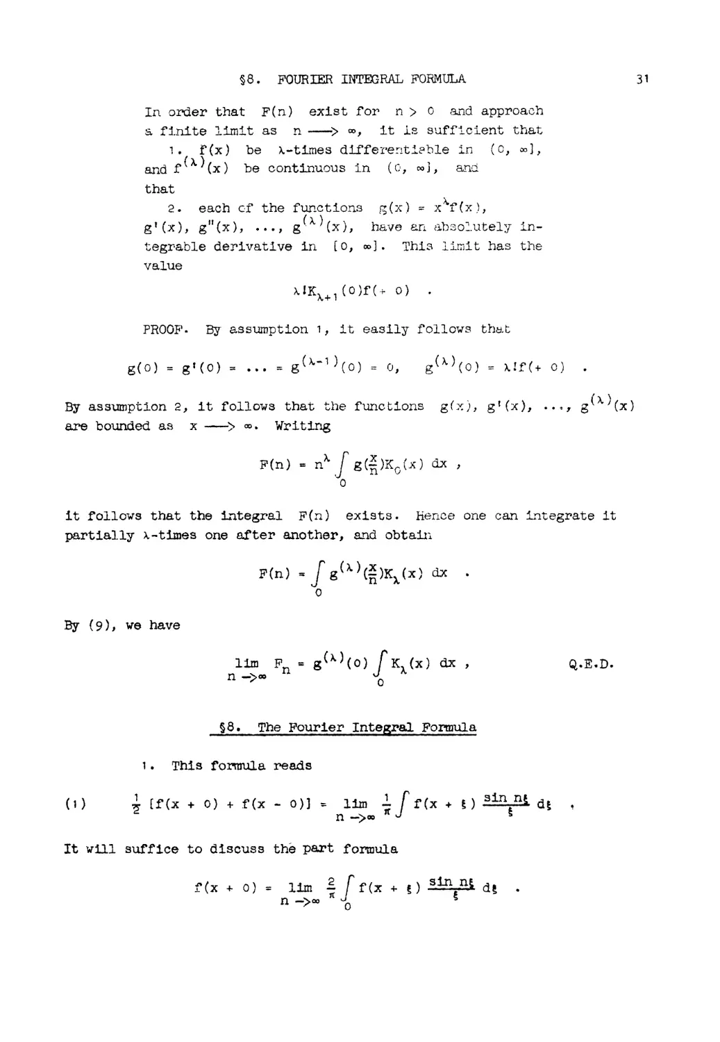
'rHEOR1!M 6. For A = " 2, 3, ... , we consider the
integral
F(n) =' J .f( )x o(x) dx
()
8. FOURIER INTEGRAL FOfu'1ULA
31
In order that F(n) exist for n > 0 &ld approach
s. flnite limit as n -) 00, it 1s sufficient tha.t
1. r (x ) be A.-times differe!"lti?ble in ( 0, 00),
and f ( A. ) (x ) be contiL'1UOUS in ( 0, 00 ] , aI1.'j
that
).
2. each of the functions g(x) = x f(x),
g t (x), glJ (x), ..., g (A. ) (x), have an c1b30 .utely in-
tegrable derivative in (0, 00]. This limit has the
value
A.IKA.+1 (O)f(+ 0)
PROOF. By assumption 1, it easily follows th t
g ( 0) = g r ( 0) ::= _.. = g ()...-1 ) ( 0) = 0, g ( A. ) ( 0) = A.! f (+ 0)
By assumption 2, it follows that the functions g(x), gt(x), ..: g( )(x)
are bounded as x -) 00. Writing
F(n) = n A J g( )KoCx) dx ,
o
it rollovs that the L tegral F(n) exists. Hence one C L tegrate it
partially A-times one after another, obtalll
F(n) = j g(A,)( X )K (x) dx
n A.
o
.
By (9), we have
11m Fn = g()..)(O) !KA(X) dx ,
n ->00 a
Q.E.D.
8. The Fourier Inte al Formula
1. This formula reads
( 1 )
[rex + 0) + rex - 0)] = 11m J r(x + ) sin n d£
n -)00
,
It will suffice to discuss the part formula.
r(x + 0) = 11m * J f(x + ) sin n d
n ->00 0
.
32
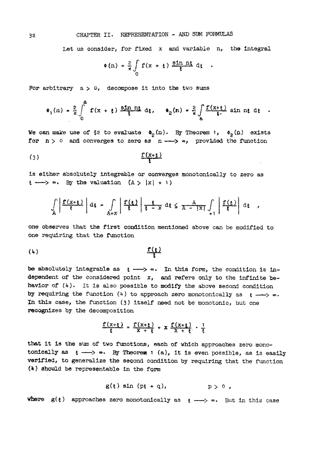
CHAPTER II. REPRESENTATION - AND SUM FORMULAS
Let us consider, for rixed x and variable n, the integral
e (n) .. J r(x + n s n _ d£ .
o
For arbitrary' a > 0, decompose it into the two Sums
a
.1(n).. J r(x + ) s n! d ,
o
. (n) ;t: J r(x+ ) sin nt d
2 tt
S.
.
We can make use of 2 to evaluate 6 2 (n). By Theorem 1 J 41 2 en) exists
for n > 0 and converges to zero as n --) , provided the !'unction
(3 )
f(?,f)
is either absolutely integrable or converges monotonically to zero as
t -> . By the valuation (A > Ixl + 1)
Jl f( +f) I d£ .. J f )
A A+x'
: x dg J I r f. ) d f
+1
1
one observes that the first condition mentioned above can be modified to
one requiring that the function
(4)
!Jfl
be absolutely integrable as -> 00. In this form, the condition is in-
dependent of the considered point x, and ref'ers only to the 1I:tf'1n1te 'be-
havior of (4). It is also possible to modify the above second condition
by requ.1raing the f1.U1ct1on (4) to a.pproach zero monotonica.lly as t -) co.
In this case, the function (3) itself need not be monotonic, but one
reoognizes by the decomposition
f(x+ ) = f(x+ ) + x f(x+l) .
X + + £-
that it 13 the sum of two functions, each of which approaches zero mono-
toniCally as -> co. By Theorem 1 (a), it 1s even possible, as 15 easily
ver1f'1ed" to generalize the second condition by requiring that the .function
(1t.) should be representa.ble in the form
g( ) sin (p + q),
p > 0 I
wbare g{ ) a.pproaches zero monotonically as -) 00. But in this case
8. FOURIER INTEGRAL FOm.HJT..,A
33
the integral 2(n) need not exist for n = + p.
We must still state conditions under which the relation
11m 1(n) = f(x + 0)
n -)00
holds. In 7J we became acquainted with the most L port t of tb se con-
ditions} namely that f(x + ) be of bounded variation in the interval
o < < H. 1ale sha.ll not, however, enter into a discussion eX- still o'ther
conditions which are deduced in the theory of FOUr'ier SeriBf:. Suroma.r1z1I.lg.,
we have the followiP.g4
TBEORB}l! 7 [21]. If the function f ( ) is of
bounded variation in the neighborhood of t:he poL'"1t
x, then the formul
(5 )
(f(x + c) + f(x - 0)] = 11m 1 J f( ) sin n( -x) d
n -)00 1t - X
is valid, provided the function t( ) not only as
-) 00, but also as £ -) - t», fulfills one of
the following condltlona:
a) it 1s a.bsolutely integrable
) it 1s monotonically convergent to z ro, or
more generally, is representable in the fo m
g(t) 81n(p + q), where g( ) converges mono-
tonically to zero.
Rm . It is obviously possible to generalize condition 6) by
requiring that the function (4) or g ( ) be represellt.able as a linear
oombination of f ctionB converging monotonically to zero. This repre-
sentation is possible, for example, if the function in question converges
to zero a.s -) 00, a...1'ld has an absolutely integra.ble derivative. A
kind of special case o condition e) is therefore the followir :
r ) it converges to zero and ha.s an a.bsolutely in-
tegrable derivative, or the function g(g) has
these properties.
Hardy [22] has ShOwil tha.t the requ1reement that (1,.) ha.ve an abso-
lutely integrable derivative as -) 00 1s equivalent to the require-
ment that -1fj (g) be absolutely integrable as -> oc.
EXAMPL:ES.. 1. r(X) a X- 1 sin x. Then by 4, 4, for n '
3Jt.
CHAPrER II. :REPRESENTATION - AND SUM FORMULAS
*J f( ) S ( -x) d . s ., f(x) .
2. rex) = COB x. Then by 4, , for n > 1
1; J f (t) au: n d = 1 = f(o) .
3- rex) a -lac for x > 0 and ;: 0 ror x < o. Then by 4, 3
e
* J f( t) sin n t d, 1 n k > 0
1: - arc tan 1G I .
& 1':
As n -? co, the right side actWfily has the limit , rf(+ 0) ... f(- o)J.
2"
4. By our theorem I far $Xample, the
11m 1 [ .1- .in n(J-x d£,
n -)00 Jt 0 i P t - x
O<p<1
,
exists for x 0 and = x- P for x > 0, and = 0 for x < o.
2 . THE<>.R]M 8. If r (x ) has the same infinite be-
havior as in Theorem 7 , and if, for sLmost all x
in the interval (&, b), the expression
(6 )
J f(t) sin n( -x d
K - X
is convergent as n -> co,
1s, tor almost all ;x in
t (x ) .
then the limit function
(a, b), identical with
PROOF. We decompose (6) into the terms
b a
[ + J + I oa B, + B 2 + B3
.
If'in (6) f(x) is repla.ced by zero in (a, b), B 2 and B3 results.
Hence 1;>y Theorem 7 J B 2 + B3 converges to zero for a. l x in [s, b).
Therefore, by the hypothesis, the xpression
b
tn (n x) -= 1. J t(.} sin n( -x) dt
....., 2t t -x
a
is convergent for almost all x in (a l b) as n -> 00. It remains to
9 . WIENER FORMULA
35
show that it converges to rex). We form
2n
",(n, x) = n ! q>(v, x) dv
o
Since we can interchange the order of integration with respect to v and
(Appendix 7, 10), we obtain
b 2
,It ( ) = ...!... J f ( & ) [ sin n ( -x ) ] d t
n, x n _ x
a
.
If q>(n) is bour...ded tor 0 < n < 00, and attains a lir.1it as n -) 00,
then
n
1/I(n) = -fiJ cp(v) dv
o
approaches the same limit; as per a general theorem (Appendix 17) 0 For
this reason
11m (n, x) = 11m (n, x)J
n -> 00 J
for almost a.ll x in (a, b) . But by Theorem 4, 11m .. (n, x) =- f'(x) for
a.lmost all x in (a, -b); hence also 11m (n, x) $ rex) ror almost all
x in (a, b) .
9. The Wiener Formula [23]
1. Recently, Norbert Wiener has compared the formula
11m J f'(fi)K(X) dx = f'(+ 0) J K(x) dx
n ->00 0 0
with the case where n -) o. Aasuming that the "mean value" of the fu..11C-
t10n r{x)
(1 )
x
9)l {f) -= 11m f f ( ) d
x -)CX)
o
exists (and is finite), the Wiener formula then reads
(2 )
11m ! :rCE)K(X) ax = IDl{f) ! K(X) dx
n -) 0 0 a
.
36
CHAPTER II. REPRESENTATION - AND SUM FORMULAS
THEOREM 9. For the validity of (2), the following
assumptions are sufficient:
1) that K(x) be differentiable in (0, 00],
and that there be a constant H such that
(3 )
I x 2 K (x ) I H for 1 X < co .
2) that there be a. constant G such that
(4)
x
J I f ( ) IdE G for 0 < x <... ·
o
PROOF. Subtra.cting from the given function f(x) its mean value,
there results a. new £'unction which aga1I1 satisfies 2, and whose mean value
vanishes, i.e.,
(5 )
x
11m J f(t) d =: 0
x ->00 0
.
Since formula (2) holds for each constant !'unction f(x), and is "addltive H J
it 1s sufficient to prove our theorem for Jnot1ons satisfying (5). How-
ever, two preliminary remarks are required for the actual proof.
a ) Introducing the function
. (6)
x
.(x) = r tf(t)1 d ,
.J
o
and taking (4) into cons ide ra.t ion, we obtain for 0 < A < E
B B B
f jf(x) L dx .. J dt t( ) - teA) + 2 J t( ) d.x G + 2G J dx {3G .
x 2 7 B A 2 x 'B ? - A
A A A A
Hence also
(7)
f J1f(x>l dx 1Q:
2 - A
A x
.
By (3), we find for A 1, with x a n
(8) J f(%)K(X) dx
A
) Introducing the funotion
9 · WIENER FOFJ.fJLA
t { tin
fn(t) = I f(E) dx = t ¥ {" f(x)
37
dx}
and making use of (4) and (5), we obtain
(9)
'.n (t ) I Gt
a.nd
11m tn(t) = 0
n -) 0 t
Also, (5) implies as follows. To each
to determine an no > 0 such that for
8)0 and
o < n no'
> 0, it 1s possible
and for t > a.
I t n (t ) t 1) t ·
We are now ready for the proof 1 tself . Beca.use of (5) we need
show that
(10)
J f(*)K(X) dx
o
converges to zero a.s n -) O. Let an £ > 0 be given. Decomposing the
integral (1 0) into the terms
A
J and J
o A
we determine, by rea.son of (8), a r:1.xed A 1 such that
JI € ·
AI
We now set
A A A
(11) J = J K(x) d n(x) .. tn(A)K(A) - J tn(x)K' (x) dx
o G 0
ay (9), there is an n, such that for 0 < n n 1
Itn(A)K(A) I £: ·
There still remains the right side integral in (11). We decompoae it into
a. A
J + J ·
o a
38
CHAPTER II. REPRESENTATION - AND SUM FORMULAS
On the one hand, by (9)
a a
r Ga. r i KI (x), dx
v v
0 , 0
,
which can be made smaller than e for a suitable fLxed a. On the other
hand, for this a and for
T) '" *'{ fAx I K' (x) I dx ]-1
,
we determine an no in accordance with observation f3 Then
A A
J T) J X IK' (x) I dx €
a a
Hence for 0 < n rrdninruUJ (no' n,)
.
J f ( )K(x) dx € + € + € + E '" 4e ,
o
thus completing the proof.
For example, if f(x) is a bounded function whose mean value
exists, then
11m r f(x) s1n 2 nx dx = !!R(f)
n -) 0 1£...) nx 2
o
.
From this, one easily rinds the following:
2. It. r(x) 1s a. T 1ven function in (- 00, co], then by its
"mean alue" ) we shall/understand the limit
,
(12 )
x
in (f) = 11m J f ( f) dt
x -)00 -x
insofar a.s this 11mlt exists. If f(x) ha.s such a. mean value, arxl 1s
boUDded, say, then
(13)
11m 1. J fCX.) ,S1n 2 nx dx '" !In (f)
n -)0 n rrx 2
.
10. POISSON SUMMATION FORMULA
39
10. The Poisson Summation Formula [24J
1. Let the function f' (x) be defined for all x - We form the
transformation'
(1 )
q> (a) .. J f(x )e(2nax) dx
Then the Poisson formula reads (here a and k are integers)
(2 )
+00
L
a=-oo
+OQ
q>(a) c I' f(k)
k=-oo
.
Before proving (2) ur.rder suitable a.ssumptions for f{x), we shall forma.lly
deduce from it certain other formulas. Until further notice, A and
will be any two positive numbers for which
All == ,-
. Replacing f(x) by f(X)' there results from (2)
(3 )
+00 +00
.fi.:I 'P(aA-) ",.J;L f(kl!)
-co -Q)
.
Let t be any number in the interval 0 t < 1. We consider the function
F(x) = .f(tJ.L + x), and denote its transform by (a). Hence
t (aA-) .. J f (tJ,! + x)e (2..:aA-x) dx .. e (- 21!a:t)q> (aA-)
,
and (3) becomes thererOl"e
(4 )
+ +
.fi: I e (- 21!at)q> (aA-) '" .r; L f (tlJ. + kjJ.)
.
-00
-
Now let f(x) be a. function defined in the interval (0, Q:)]. We
introduoe the integrals
(5 )
.(a) = 2 J f(X)COS(21tCXX) dx
o
,
(6 )
X{a) '" 2 f rtx)-s1n(2Jtax) dx
o
.
1
This transformation 15 normalized somewhat dirferently from the proper
transformation E(a), of'. 2, 3-
40
CHAPTER II. REPRESEri ATION - .AND SUM FORMULAS
If the function f(x) is exter1ded the intervp (- 00, 0] so as to be-
come an even function, then q>(a) = v(a) and one obtairu;
..;.; { ,(0) 00 t (a:l..) }
+ 2 L CQS (21!o:t ) .
a=1
I '
\ 7 ) f .f (tl-L ) 00
-L r
t
,- f(k + t ) + f(k - \ '
=..JJ,l + l "t . .
U } J J
k=1
For exam e, this gives for t: 0 fuJd
,
t =
2'
the special cases
(8) 5{V(O) + 2 J;,'HaA)} =,r;; {f(O) + 2 k%1 f(k.d} ,
( 0'
" )
.r \1 ex } \' ( 1 )
.Ji: i '+' ( 0) + 2 J (-1) V( a)., ) = 2fi; f (k + "2) fl
l a= 1 k= 0
.
But if the f"unc.tion f(x) 1s extended by an odd function, then. q>(o;) = lX(Q),
arJd one obtains by (4)
00 { 00 ,
(10) 2 b. I sin 21£at · x(a).,) ...rv: f(t.d + L [f(kjJ. t.d - f(kl-L - t fl )] }
a=l k 1
For t = 0, -I:.heI'e seems to be a contradiction because the left side has
the value 0 and the right side the value -J-; f (O ) . This discrepancy J
h Never, disappeare when one r alizes that after completion or r(x), the
entire function b s two limits or opposite sign at be pOlnt t = o For
this l eason the valus 0 is to be ll.t.J.derstood for f (0). -Replaci.. }"
n by /2 and 2 ; and modifying somewhat the Bing indices} one
obtain3 fer t = 1/4
( 1 1 \
\ )
00
-hI (-1)aX[(a+ )A]
a=O
ro
,.. -;--, >
= ";,L
L-J
1<=0
k ( 1 \
( ... 1 ) f ( k + 2 ) j.j. I
2 c: No", fo):} the proof itself 0 We shaJ..l assume j.r1... this paragraph
that each fur!ction f(x) has the limits f(x + 0) and f(x - 0) at each
pol nt x, and that at each Stich point} the value of the functioIl is
"
[f(x + 0) + f(x - 0)]. If, therefore, for example, a function g(x) is
given in an in.terval ( 0, p) where p is 8.!"_ integer J and if for the
10. POISSON SUMMAi'ION FORMULA
41
purpose of applying (2), it 1s extended by zero values to a function f(x)
defined everywnere, then the expression
p-1
.} (g(o) + g(p») + L g(k)
,
1s to replace the right sum in (2).
Further, 1...1'). this para.graph we call a series
( 12 )
+00
I All
-00
convergent, 1r the part.1al sums
(13)
n
sn = I All
-n
a.pproaches a limit as n -) co. Ana.logously, we ca.ll an integral extend-
ing over the whole interval (- ao, co] I convergent if its Cauchy pr1n 1pa.1
value exists, cf. 5, 1.
Hence for integers a and integers p > 0,
(14 )
p+1/2 I
J f (x)e (2 sta.X) dx
-p-1/2
= Jt / 2 ( f f (x + k» ) e ( 2 nax) dx
-1/2 -p
.
If the series
( , 5 )
+co
L f(x + k)
-0:)
1 1
converges un1.formly in the irlterval - 2 X < 2' ca.ll g(x) the limit
function, then the expression on the right of (14) is convergent as
p -> 00. Hence the expression' on the left is also, 1. ell I the integral
(a) exists and
1 /2
cp (ex) = J g (x )e ( 2 1CCXX) dx
-1/2
.
From this it follows tha.t
n 1/2
I cp(ex) = J g(x) S1n3gn: )1fX dx
-n -1 /2
.
42
CHAPTER II. REPRESENTATION - AND SUM FORM1JLAS
If furthermore g(x) 1s of bounded variation, th D the right side con-
verges to g(o) as n ---) 00, cf. 1, 2. Hence the left side al o con-
verges, &nd if one now inserts the value of g(O)J (2) results. Applying
a formal transformation stated in 1, we obtain
THEOREM 1 o. Far the valid.i ty of forrouJ a, (4), 1 t is
sufficient th t tbe s9ries
( 16)
+00
') f (x + tf,.L + k )
Z
k==-oo
converge uniforml:,.'7" irl
( 17)
1
- 2 S X < 2 1
and tbat its sum be of bOl illed variation jB this in-
terva.l. Both series in (4) are, under this hypothesis,
themselves convergent.
3. We shall now have two special cases reducible to this
criterion.
a) Let the function f(x) be po it1ve, monotonically decreasing
to zero and integra.ble L the interval £ - 2 x < 00. For k J and
x - 1, we then ha.ve
k k-l
r(x+k) J r(x+ )d J f( )d
k-l k-2
and hence for p J, an.d arbitrary r > 0
p+r
I r(x + k) J r( ) d
p k-2
.
Therefore the series
( ; 8 )
00
I r(x + k)
k=l
converges uniformly irl - 1 x < 00. Moreover, since all terms ot'" the sum
are mOIlot,orlically decrAasing, the fun.c'tlon representing the sum lS 9.1so
monotonically decreasing.
b ) Let the function f (x) be d1.f'ferentlabJ.e 5..11 1 he inte va.l
S10. POISSON SUMMATION FOft FJLi\.
l 3
J - , x < , and let the integrals
(19 )
r f(t) d;
J
.t ... j
and
(.
I Iff ( )! -; ;
,
£ .... 1
be fi r; te. Hence
j m
l f(X+k)
m+ 1
r
I f(x + ) d
)
p
I r'
L I J
p . 0
( f (x -i- k) - f ( X .t- k -r ) J d
If we now set) for 0 s < , 1
Ir(x + k) - f(x + k + )f =
/
.J
0"
f' (x + k + it) d'1
1: J.. 1
('
I If' (x T- 11)1 d'! ,
k
we obtain
m m+l
I f(x + k) - I f(x + t) d
p p
m k+l
\ I Iff (x + ; ) I
=> 'k
m+ 1
{ F' , f ' I (x
C. TI -;; I + ,)! d"
,
-
r,
,e
and from this there f ally results
m
\'
L f (x + k)
p
m+l m 1
£ f(x + s) d 1+ £ jr:(x + Tj)1 dTj
Because of
series (18)
by f 1 (x).
( 1 7) as 'the
the convergence of the integrals ( 9)j this implies that the
conver"ges uniformly L. the interval (1 7) We denote its sum
If r,(x) 1s real, then f 1 (x) - f, (c) aL be represented in
dif erence or the monotonic functions
0:1 x
II
1 0
Ift( +k)1 ! fJ( +k)
2
d
If ( ) t 1. i -t and 1m .. t t 1 ill
f 1 X is not real, J.len l.,S rea-L. ag..J..noJry pa.r s separa e .y w
have such a representation each.
From t s observat1on r we reach the following conclusion. ·
.,
THEOREM 10a. For the validity of formula (4), it is
s ficient that f (x) be of bounded v&y.iation in a.
finite interval and satis£y one of the following con-
ditions both as x -) Q) and as ._> - :
44
CHlLPTER IIo REPRESElf:IA:rION - AND S1jt YOill'1U1JAS
1) i G is rnonotonie ann e.bsol 1 .ltely in G grable
2 ) it is irltegraule c1J1d 11as absollYte.l_y in-
tegrable derivative.
Bo.tl1 sel. 1es in (4) al'e autouatics.lly conv'3 '"tgent [25}.
PJ.1-Y"T'{K IN REG-ARD TO :=:.
T3.-lE- funr:;tlon 1 ex ) t8elf need not be
x. Thus, for exa.'1rple,t the funct.ion
absolutely ir t-3grable 8.3 x --->
-1 r--
X 31.n '" x Gomes under 2 0<
ID 8V1PLES .
1 T ' b +- 1m ... .. t ..; f / " _ -= , I ' is t - L "-- J6 fo " a
. ne etjl.- cni:). app.l.J..ca ..J..011 0.-- } _ ...l"JUu..J.,
[26]
-
Fix
+00
)
L-J
-.:;0
- 2 I
e -k 1\ I X =
+00
\i 2
\ -k :X1t
L e
- 0',)
It :resu2 ts frolJl the relatlon
r _ 2
i e e(o; ) J s =
I ...
....1
i -a' /4-
'" 11' e
which we sball prove later, 15, (9).
2 II If f (x) = e - px , p > () J then by .' (L)
-.v(Q)
.- --- p-- ,
. , 2
P - 4.- t 211:0: )
x(u) .-
2 ( i: l -""I
, - . '-- I
2 . 0
p + (2 1t:Q:' ) '-
r7j ('T) b.I1d. ( O j) ve obtain the formulas (27]
(r.n )
; '- ...
..--.
. '\
-:'1.
cosb
IJj.l
(i + t) · S:L'1l1- 1 = p + 2
00
..._J
d::..1
cas 2 naG
.:J
p'-
p
+ ( 2 1!Ct;\ ) 2
,
(21 )
1
,",
-:11rJ-."'r1
1
P (- -
2
\
... ,
tJ .
'"' inh - I
.')
.E ::;
'2 2
I
0:=1
ain 2 C}:t
2
P
:) ITa A
, \ .)
+ (2 1tCt;" )-
One notes that the second CP,..I) be obtained from the
,":1 .t Y. C" .J-
.... .J...- 1.. ......... '""",
by cifferen 1at1on
"" j +- h y:.,..) <'""1"""',0 .-..,.. - r'\
N _ I,.,: .. J. t: .... ) . . I, l. \.,'
o < 'L < j. :i'O:!'"
t. They are valid for p > 0, \ > 0, > C J A = 1,
3peo1al values o the paremeter} numerous well 10WD
obtaL.'1.ed. For eX8.lTIple 1 1r t = 1 /4, we ob"te tn from (2 1 )
i'orrrrwlas caLi be
( Pu lif\ 00
1 T ) 2 I (-1 )&3 21£(2 p +1 ) .
2)" e + e ;:: p 2 .
. I : 2
i3 O + l2j(\2 +1 )A..i
, o. POISSON SUMMATION FORMULA
45
From this one can derive the formula [28]
(22 )
+00
L
k=-oo
( ) -1 +00
e 2knq ... e- 2knq '" d q I
k;:;-co
( \ -1
e + e - )
3. With the aid or (20) and (21)1 the followL trigonometric
integrals can be evalua.ted [29].
J eWx e -<ox sin (1)
- x cos ax dx = _Q ,
e nx e- n e a + 2 cas 00 + e
o
- 1t < w <
,
r eIDX ..... e -wX 1 e a. + e- a
sin ax dx = _ 2 '
'.)0 e 1tX - e -1(X e a + 2 CDS (J) + e
- 1\ < (j,) < n
J
J cos (.OX sin aX dx
e 1tX _ e- nx
o
1 erA - e-ex
= 4 em + e + e a + a-a
,
J sin ax dx == coth _ 1
e 2 1tX _ 1 'to -- 2a
o
function
4. As a last application or the Poisson formula , we consider the
-8
r (x) :: X for 0 < x < QO, 0 < s < + 1. Hence, cf. , 2: 1
x (Ct) = 2 J f'\ sin 2 'faX dx = 2 r ( 1 - s) COB 1 /2 s 1(
x S (2 1C(X ) 1 -6
o
We have therefore by (11)
(23 )
00
\' n , -8
L (-1) '" (3.) COB 1 51fT' (1
o (2n+1)5 J(
0:>
)2: (_1)n
- s -
o (2n+ i ) 1 -8
,
which is a special case of the functional equation for the Dirichlet .
L-function [30 J . Al though the function just considered does not come under
Theorem , Os., nevertheless the a.pplication of the sUlmnation form"J.la. 1s
justifiable. We rem.ark without proof the rOllov1..rJ.g. As far as the be-
havior of rex) outside a finite interval 1s concerned, it is sufficient
tor the va.lidity of (10), that f(x) approach zero monotonically as
x -) 00. As fa.r a.s its behavior in a finlte interval is concern.ad it is
sufficient for the validity of (4) that r(x) be of 90undnd va...t a iat1on in
4 the neighborhood of the "lattice po1nts n t + k , k := 0, t 1, :t 2, ....,
and otherwise be integrable only.
CHAPTER III
t"fHE .F'OURIER INTIDRAL 'l'IIEOIID
11. The Four-leI' Integra.l Theorem and the InveY.f;lon FOI"'nTulas
1. We denote the fOI tua
(1 )
1 r f " 0) f, / X
2' ,x + .+
o)J '" : .J daJ f( ) cos Q( - xj d
o
as a Fourier L tegral theorem.
TImOR Jl. It is sufficient for the validity of (1),
that f( ) be of bounded va.riation in the neighborhood
of x, and that one of the rollow1ng conditions be
.fulfilled not only as -) + OJ, but also as
1
f -)
- 00.
1) f( ) be absolutely integrable}
2) f ) be a.bsolutely integrable and
con"v.ergent monotonically to zel'O, or more
representable in the form- g( ) 8L (p£ +
g ( ; ) approaches zero monotonically [31].
f ( s ) be
generally be
q), where
In case 2), the integra] with respect to a, 1s
a. CS.11chy princlps.l-value \-lith at most two singular
points.
PROO:f\'. Writing the integral on the right of (1) in the form
(2 )
n
11m J daJ f( ) C03 Q( - X) d
n -)ro · 0
T """'" ..... -..... ... ...
I-c is, therefore.' suffj.cierlt for example,
1. as --.--> 00 ar.J:i satisfs" corlditlon <0 as
tlldt f (x) satisfy r;iJndit ion
-> - x.
46
1 1. INVERSION FORMULAS
47
and interchar ir .the order of integration with re8pect to a and ,
we obtain
(3 )
11111 J f( ) sin n( E-X) dg
t - X
n >oc
Because of Theorem 7, it 1s necessary only' to show that this L1'}terchange of
the order Gf lntegrat10n is admissible. Formula, (1) is additive; i.e.,
if it holds for fl( ) and f (s), the it also holds for f j (;) + f 2 (;).
For its proof, we can therefore assume that f( ) vanishes outside of a
half line [a, 00).
PROOF of 1). By hypothesis, f( f) is abso2.u.tely integrable.
Hence because
!f( ) cos a( - x)1 f( )
the equality
n n
I do: J f ( ) COS 0: ( - x) d = J d f f ( ) COS 0: ( - x) da
C! a a iJ
i8 valid or each finite interval (0, n) by a basic general theorem
(Appendix 7 J 1 0) J Q'.E .D.
PROOF of 2). For finite numbers a} nJ a, b,
n b
J daI
a .s.
f(;; cos a( - x) d
b n
= J d J f ( ) COB a ( - x) do:
a a
follows from 1) - For fixed x, it is here admissible to allow b -> co
provided the integral
qJ (a) :- r f ( ) co 8 a (f - x) d f.
d
a
1s 1formly convergent in a a n. In fact if we set
b
<!>b(a) :. j f( ) cas a{ - x) d
a
,
then
n n
r (o:) do: -> r q>(o:) da
J v
a a
.
48
CHAPTER III. THE FOURIER IN'.l'm-RAL T"rlEOREM
We now apply Theorem 2. IT f (£ ) a.pproaches zero monotonically, then ea.ch
interva.l (€, n) for which 0 < e < n, is suitable as an a-interval.
We" therefore.. then have
n
J da J fr ( ) C()S 0: ( - x) d t = J t ( ) sin n ( -::) d - J f f ( f) sin e ( -x) d t
f - x - X
£ a a s
Since ( - x)-1f( ) is, together with t-'r(,}, also absolutely in-
tegrable as -) 00, it follows by Theorem 2 a.gain, that the second in-
tegral on the right 1s continuous in E , and hence converges to zero as
E -) o. Thererore the integra.l on the left has a. limit a.s € -) o.
This limit is
(4 )
n
11m J da J r( ) 008 cx( - x} d = J f( ) sin n( -x) d
E - X
€ -)0 E: a a.
Q.E.D..
In the more general case where f( ) = g( ) sin (Pf + q), P > 0,
it is necessary to interchange the order or integration in the repeated
L. tegral
( [e + In )
u p+e
da J f ( )008 0: ( - x) d
a
It then appears tha.t a limit exists as € -> 0, and this limit equals
the expression on the right ot (4), Q.E .D.
2 · For the sake of brevi ty I we shall W1:'1 te f (x ) in place of
, i (rex + 0)'+ r(x - 0)]. If the question of convergence 1s disregarded,
then (1) be interpreted as follows. Each "random" .function der1ned
in [- 00, CD} may be written in the form
(5b)
f(x) = J [0 (CX)C05 ax + S(a),in ax] da
o
where
(5a) C(a) '" J f(t )C05 a d , Sea) · J r( )s1n o:tde
Formula. (5b) 1s the. ffharmonic analysis" of the function f (x ); - the
rep sentat1on of the .function as Hsums tt of cosines and sines. If now
11. INVERSION FORMULAS
49
f(x) ls, in part1cular l even [f{- x) = rex)] or odd [f(- x) - rex)],
then S (a) :a 0 01' C (a) · o. Thus one obtains the pair of formulas
(6a)
C(a) .. J f(t)cos a d
o
(6b )
f(:x) =< J C (0 )cos xacIa
o
(7a)
8(a) .. J f(t)sin oEdt
o
(7b)
f'
rex) .. J S(a)sin xada 0
o
By substitution, there results
(8 )
f(x) .. J da cos xa J f(t)cos otdg
o 0
or
(9 )
rCx) .. J cIa sin xa J f(E )sin otdt
o 0
Let and J.l be arry two numbers whose product is 2/ : c Mul t1plication
or C (a ) by ),u /2, transforms (6) into the symmetrical pa.ir of formulas
(10)
,(a) .. A. fret )cos atdt,
o
rex) .. 11 J t(a)oos xaoo
o
.
Simllarly one obtains from ( 1 )
(11 )
x(o) .. A. J r(t )sin atdt,
o
f(x) .. 11 J x(a)sin xoda
a
.
In what tollows, we shall denote the passage from (6a) to (6b) a.s an in-
version or (6a) I and shall call the second the inverse (or also the con-
verse [32]) of the firstj similarly in the case of (7). By" Theorem 11,
there follows immediately
THEOREM 11a. The inversion of (6a) and (7a) is
admissible provided the .f'unct1on f ( ) I defined
in [ 0, co]) satisfies 1) or 2) of Theorem 1 1 as
£ -) CD, and 1s of bounded variation in the
ne18hborhood of x.
50
CHAPTER III. THE FOURIER INTEDRAL THEOREM
By inversion of $2, (4), we obta,1ri for example
(12 )
r cos xa d rY _ J( e - kx
2 u. .... 2K '
\J k + 0:
o
J a s xa do = 2! e- kx .
k 2 2 2
o + a
If t(x) s x , then by 4, (6),r C{a) 1 for 0 < a < 1 and = 0
for a > 1; hence actually
r C (a )008 o:xda
u
o
1
= r cos axda = rex)
..)
o
.
3- If rex) is given 1n [- I ], the pair of relations (5)
can also be interpreted a.s a pair of inversions, after introducing "complex"
notation at any rate. Consider the transform of r{x)
(13)
E(a) '" in r f( )e(- a ) d
...J
,
Then, cf. the proof of Theorem 1 1,
n
J E{a)e(xa) da +
a
-0
J E(a)e(xa) da
-n
n
=J
[E(a)e(xa) + E(-a)e(-xa)] da
C1
n
'" J da J f( )cos a(e - x) d£
a
"and following theorem ensues.
"
T.HEORiM 11b. If r( t) 'satlsf'.1es 1) or 2) of
Theorem 11 not only as e > co, but also as
t -) - co then (1 3) may be converted to
(14)
f'(x) '" J E(a)e(xa) da
This converse holds for points x in whose
neighborhood f (x) 1s of boUI't.rled variation pro-
vided one interprets the i11tegraJ. (1 4) in a
suita.ble manner as a Cauchy principal-value.
4. Of. interest is
, 2 . TRIGONOMm'RIC INTEJRALS WITH e -x
51
THEOREM 12. If' r( ) behaves at infinity as
specified (espeoially:lf f ( ) is absolutely in-
tegrable) and if the integral
J E(a)e(ax) da
converges for almost all x in an interva.l
(a, b) - perhaps as a Cauchy principal-value -,
then the limit .function 1s, f'or almost all x
in (a, b) identical with :rex).
PROOF. By the assumed property a.t infinity, we have
n ,
J E(a)e(xa) da = J f( ) sintni ; ) d
-n
.
Now apply Theorem 8.
12.
Trigonometric Integrals with
-x
e .
The formulas [a > 0, 0 < J.L < 1 )
(1 )
J xJ.l.-1 S CO in s ax dx = r (J.1) C08 1C
a sin J.1 2"
o
which can be consolidated in one as
("2 )
J xl1-1 e (- ax) dx os I' (11) e (- 11 )
a JJ
o
,
originated with Euler (34]. Here r(J,1) denotes the Euler ganma. f'u.nct1on
(3 )
r(....) = J e -xx l1 - t dx
o
.
-The formulas of Fresnel are important special cases of (1),
(4)
. J cos x = J sin x dx = -2...1' ( )"' J i .
0 5 05 .J2
We shall discuss these separately la.ter on. Formula (2) also results trom
[k > 0, - co < ex < 00, 0 < }.L < co]
5
CHAPl"ER III. THE FOURIER RAL TBEOR1!M
J e- -1e(- ax) ax. r(p.)
o (k 1a)
by letting k -) o. Here
(5 )
(k + 1a)1& . J k 2 + a 2 ... e(... 81'0 tan ),
.f( < .... tan a < 1{
- QI,I,-C 1C ·
We s 1')Q]] , however, not prove (5) [35].
2. There 1'esu1 ts by inversion of (,) [k > 0, JI. > 0]
(6 )
reu) J da · {
2. (k+ia)....
-kT JI.-1
e --x I
x > 0
o
I
x < 0
.
Hence [-36]" by changing the a 18na of and x,
(7}
r(...) J _e(ax) da. {
2. (k-1a) ekxlxlJI.-1,
o
,
x > 0
x < 0 .
.
Substituting a + q for 0, one easUy finds that both relations are valid
also for such complex k tor which Ii (k) > o. OnlY' then one mus t set
(8) (k + 1a) . Ik + 1a1 e ( i.1 arc tan a + (k» ) .
I ft(k)
This result can a1s<?_ be obt Ained by' analytic continuation, and the formula
is, 1n tact, valid tor complex J.L with It( ) > o.
3. I£ in
(9)
J e-nee- ) dx · 1C 11a '
o
iR(k) > 0
we replace a by a - p and ex + p and then add, we obtain
21 J a-lexe(_ ax)oos x dx 1 + 1
p ::aa_p_ a a+p- 1.k
o
.
Integration with respect to p between 0 and p gives, tor 0 < p < a,
21 -1i e-kxe( _ ax) Sin x pX dx . log ( + p - 1k . ex - 11<: )
J' -" - :!k a - 1.1<:
o
, 2 . TRIGONOMEl'RIC INTEJRALS WITH e -x
53
where the imaginary part of the logarithm 1s to be taken between - ../2
and 1C/2. Letting k -) 0, and taking the real part we obtain for
o < ex < t3 or 0 < t3 < a
(10)
J a ax sin x <Ix = log I : g I
o
Integrating (9) with respect to k gives [a > 0, b > 0]
J -ax -bx
e ; e e(- ax) <Ix D log b + la
a + :La
o
.
Hence follows [37]
(11 )
J e-ax X - e-bx
cos ax dx.:= log
o
b 2 + a 2
a 2 2
+ ex
( '2)
J -ax -bx
e - e sin ax dx =
x
arc tan.2 - arc tan !:
a a
.
o
For positive nuniPers a, x and , we have by (3)
(13)
r(l-I) (x + a )-1-1 .. J e -(x+a )Z z l-l-l dz
o
.
'";:;
Multiply by e-kxe(_ ax), k > 0, and integrate v1th respect to x between
o and co. One can interchange the order or integration in the repeated
right integral to obtain
(14 )
J -kx ( ' J -a.z -1
r( ) e e -ax) dx = e Z dz
o (x+a) 0 Z + k + la
.
If a t- 0 I
one obtains
one can even consider the case where
[a. > 0,. > 0, k 0, a 0]
k .....;.... > 0 .
A1 together,
(15 )
J -kx { Ja J ..az { }
r() e CO'S x dx e z + k dz
1-1 0 Cx+a)1-I sin · 0 (Z+k) 2 + a
.
(16 )
4. The Presnel integral
J.. p. J sin x dx
1( 0 .JX
54
CHAPTER III. THE FOURImt INTFDRAL THEOR»i
can be evaluated "directly II by making use of 1 1, (, 1 ) with "':: J.1 [ 38] .
Setting rex) x- 1 / 2 , we obtain
(11 ),
x(a) = rf J ain Ctl d = X(1) ;: f(a)J
" 1i .JQ
o
Henoe also f (a) = x (a )J , and therefore
(18 )
x (Ct) (1 - J2) :: 0
.
By the decomposition
J 8in x dx
o .JX
00
= L
k=O
(2k+ 1 ) Jt
£ sin x ( .J x , ... 1 ) dx
.JX+1C
2 2f
J
one recognizes that J > 0, arn therefore beoause of (1 7), X (ex) :f o.
Hence (, - J2) . 0 1'ollows from (, 8 ), 'and because J > 0, it follows that
J = 1. One can trea.t the cosine integral in a similar manner only here
the proof that J > 0 is somewha.t mor-e complicated. The proof rests on
the ract that the fUnction x- 1 / 2 is its one cosine -- or sine-transform.
Many other such "selt reciprocal" functions exist [39 J ·
13 . The Absolute Inte£a.ble Functions .
Their F tung The Summation .
...
1. We shall now consider all. those functions f (x ) which are de -
fined and are absolutely integrable in {- GO, GO]. We denote the tota.lit of
such functions by O. Since we require ot a function of 3 0 only inte-
grability in the infinite region, we shall disregard its behavior on a. null
I
set. In particular, we shall regard two f1.U1ctions of lY 0 as identical, if'
the functions have the same value almost everywhere in (- 00, 1 . If f (x )
,
is a function of 3 0' then the following also belong to tj 0: f (- x), f { x ) ,
g (x )f (x ) where g (x ) 1s bounded (integrable ll1 the fitrl. te l egion), in
particular the function e(u)f(x) where A is rea.l: and in addition the
function f(x + A.). Moreover the class 6 0 is linear.
2 . We call a collection of fUnctions linear if elf 1 + c 2 f 2 :ts
an element or the collection, where 01 and c 2 are any two (complex)
oonstants, and f, and f 2 are elements of the collection. In particular,
for each constant 0, cf" is also a..:.'1 element of the collection.. 1-!here f
is an element of the collection.
Moreover, fY 0
of. :functions .f n (x), n ==
is closed in the following sense. If' a sequence
1, 2, 3, ... of o is convergent in the
, 3 · ABSOLurELY INTEnRABLE FUNCTIONS
55
integrated mean; i.e., if
(1 )
11m J Ifm(x) - fn(x>! dx .. 0
m ->00
n -)00
J
then there is exactly one function f(x) of fi: 0 towards which it I converges
in the sense that
(2 )
11m J If(x) - fn(x>! dx "" 0
n ->00
of. Appendix , 1 .
3 · Let f, and f 2 be two given functions of 0 to For
brevity, we set
(3 )
J If 1 (x)! dx = C p
i = 1 , 2
.
We now make f'ull use of Fubini 1'8 theorem, of. .hppandix 7 , 10. Tbe function
(4.)
g{x, y) = f,{y)f 2 (x - y)
is a measurable function of th9 variables (x, y). For each point y in
which f'1 (y) is finite
Jig (x, y) I dx = I f 1 (y) 1 J I f 2 (x - y) I dy .. If i (Y) I · C 2
.
Therefore
j d::r Jig (x, y) I dx "" C 2 J I f 1 (y) I dy = C 1 C 2
Hence the function g(x, y) is absolutely integrable over the whole (x, y)
plane. Therefore the integral
(5 )
J g(x, y) dy .. J 1', (y)f 2 (x - y) dy
exists :tor almost all x, and is again ,-'. . J.'i.l tion of o. Moreover it
is inde p endent or the order of f and r because
1 2
(6 )
J l' 1 (y)1' 2 (x - yo) dy '" J f 2 ( f\ )f , (x
11) d!i
.
If for . two :functions in
all x, then the function
----
[- 00', 00], the inter : ,8 (6) exif1ts for almost
... .1. " ._""
56
CHAPTER III. THE {i'OURIER INTIDRAL THEORE .t
fi J f 1 (y)f 2 (X - y) dy
(1)
is called the Falt of f 1 and f 2 [40]5 If f1!x) and f 2 (X) are
functions of 3 0 , then their Faltung exists, and likewise belongs to fio.
4. To each function of O' we attach its transform E(a)
(8 )
E(a) = J f(x)e(-ax) dx
,
and denote the total1tI of these functior E(a) by o. In order that
a function E(a} belong to O' it 1s necessary that it be bounded
(9 ),
2lfIE(a)1 .f If(x)1 dx
}
that it be continuous (Theorem 2), and that it approach zero as. ex -) :!: 00
(Theorem 1). The class o is moreover linear: t? clf, + c 2 f 2 belong
c,E1 + c 2 E 2 - If E(a) belongs to O' then the following do also:
E(-a), (a), E(a + x) and e(Aa)E(a), real. They are the transforms
o.f f( -x), r( -x ) , e (-,,-x )f(x) and fix + A). If functions of i) 0 con-
'verge in the integrated meap then owing to
.2 If IE (0:) - (0: ) I J If (x) - f n (x ) I · I e ( -ax ) I dx J 1 f (x) - f n (x ) I dx
I
their transforms are uniformly convel"agent in - 00 < a < 00.
THEOP 13. -The Fa.l tung of functions of 5 0 COl"\re-
sponds to the multiplication of their transforms.
PROOF. Since
J{ J f(x)e(-ax) dx '" 4: 2 J dx J ft (y)e(-ay)f 2 (x-y)e(-a(x-y» dy ,
and since for fixed a, the ftIDct10ns f 1 (y )e ( -ay ) and f 2 ( 1) )e ( -aT) ) be-"
long to 3 0' - we can interchange the order of integra.tion to obtain
(10)
E (ex) = E 1 (ex )E 2 (a ) ·
Within the class 0' the functions can therefo re by multi-
plied arb trarily. We also" remark tha.t the transform E 1 (a )E 2 ( ex) belongs
to the function
(11 )
1 3. AB8OLtJ'l'ELY INTIDRABLE FUNCTIONS
f f,(y) r 2 (y-xJ dy = i;J f,(y+X) f 2 (YJ dy
57
5. By det1n1t1on, each function of iY 0 is attached to exactly
one funct10n of o. It is an important fact, tha.t the converse 1s a1 o
valid.
THEOREM 14. Two functions of 0 which have the
same transforms are identical [41].
< '
PROOF. To r{x) = f 1 (x) - f 2 (x) belongs E(a) = E,(a) - E 2 (a).
Now let E(a):i o. 'rhen
J E(a)e(ax) da E 0
.
Hence by Theorem 12, f(x) == o.
The one-to-one relation between functions or 0 and 0 w1ll
be expressed by the symbolic formula
(12 )
:r(x):... J e(ax)E(a) da
.
\ '
We call tMs formula, wholly independent or whether or not the integral
converges I a. representation of f (x ) · We shall also speak or the function
(13)
J e(ax)E(a) do
I
bY' which we shall mean the well determined function of 3 0' whose trans-
form agrees with the riven function E'(a) of o. We say that the repre-
sentation of rex) converges if the integral (13) is convergent for almost
all x. We then write, by Theorem 12
(14 )
f(x) = J e(ax)E(a) da
.
6. Let q>'(a) be a given continuous function in
the following properties: 1) (-a) = (a), 2) (o) = 1,
absolutely integrable, and 4) the function .
[- 00, co]
3) <pea)
with
1s
(15 )
K(x) = -h J e(ax)cp(a) do
1s absolutely integrable (and therefore a function of 3 0 ), bounded and
at1nf'inityequalto o(lx)-'). - It ls easllyseenthat q>(a) 1sthe
transrorm of 2 KK(x), and more generally that cp C R ) 1s the transform
of 27tnK(nx), i.e.,
58
CHAPTER III. THE FOURIER INTEX}RAL THEOR»1
(R) -.. n J e( -ax )K(nx) dx ·
Hence by 2) I it tollows that
(16) J K( ) dt .. 1 ·
2
The functions e- 1a I" e-(l and cp(a);: 1 - la I for fa I 1
and = 0 for let I > 1 are examples of funotions satisfying the given
cond1tions. The corresponding funct:1.ons 'K(x) are
, 1
;( 1 + x7J. '
x 2
-(-)
1 2
e
2,J;
and
( s r
,
ot. 1 2 (9); 1 5 , ( 9) and 4 , ( 1 4 ) ·
Now let rex) be any function of ij 0' and E(a) its trans-
form. The Faltung of f(x) and -2" (nx) corresponds to the transform
<p(*>E(a). If, now, cp(E> 1s absolutely integrable and E(a) bounded,
then the product is also absolutely integrable. Hence tor almost all x
(17)
f ( )E(a)e(ax) d.a .. n J f( )K[n(x - t)] dt
.
By' Theorems 1 and 2, the left side 1s convergent and continuous for all x.
The right side is likewise convergent and continuous tor alJ. x; this
easily follows from the faot that f( ) 1s absolutely integrable, and
that K(x), because of (15), 1s bounded and uniformly continuous for all
x. In regard to the latter, ct'. the remarks in 4. Two oontinuous func-
tions which agree almost everywhere, agree point for point. The rela.ti n
( 1 7) 1s therefore valid tor all points x. ,Therefore by (16) and Theorem
3, a.t each point x for whioh r(x + 0) and rex - 0) exist, we have
(18 )
(f(x +,0) + f(x - 0)]- = 11m J \p(E)E(a)e(ax) da
n -)co
.
By (1), we can a.lso write for < 1 8 )
(19) [f(x + 0) + f(x - 0)].. 11m J tp(fi) da J f( ) cos a(x - ) d
n -)co 0
.
Letting now n -> co under the integral sign, formula 1 1, (,) results;
but this extension of the limit is inArlm1 sslble because for the validity
of the last fomula, bounded varia.tion in the neighborhood of x was
assumed. However, we may view the &ituat1on in the follow.1ng manner.
1
Formula , 1, (1) can still be ma.1ntained tor absolutely integrable functions
1 3 . ABSOLUTELY INTEnRABLE FUNCTIONS
59
t (x) for points x at which the requirement of bounded variation 1s not
fulfilled, provided that ordinary convergence of the 1ntegr be replaced
by "sunmabllity" with the aid of a convergence producing factor ,(ex)
The factor can be of very general nature; in the two special cases
cp(a) = e -Ia I and cp (ex) = e -a 2 , the integral (19) 1s called a Sommerf'el
integral [42].
7. Theorem 13 can be employed for the calcula.tion of definite
..
integrals.
THEOREM 15. Let f 1 (x) and f 2 (x) be given
f"w1ctions o-r B o. In order that the relation
(20 )
2 J( J E, (a )E 2 (ex ) e (ax) dex .. J f, (y)f 2 (x - y) dy
hold for all x, it is suff:1.cient that one of the
following conditions be fulfilled:
1) The f"w1ctlon E 1 ( )E 2 (a ) be absolutely in-
tegrable and the r ht side of (20) represent a
't
continuous function.
2) One of the functions f 1 (x) and f 2 (x)
have an absolutely integrable derivative.
PROOF of 1). This half of the theorem has already been proved
and used in 6. We repeat the proof briefly. By Theorem 12 I (20). holds
for almost all x. Since the functions on both sides of it are continu-
ous, it holds for all x without exception.
PROOF of 2). Because of Theorem 1 1 b, 1 t 1s sufficient to prove
that the right side of (20) is differentia.ble. We may a.ssume I from the
hypothesis, that r 2 (x) is the function which has an absolutely in-
tegrable derivative. We set
2J(q>(X) = J f, (y)f (x - y) q,y
and form, for an arbitrary a, the integral
x X
2Jf J Ip( ) d '" J d J f 1 (y)f ( - y) dy ·
a a.
One can interchange the order of integration on the right, to obta.in
60
CBJ\.l III THE FOURIER INTEJRAL THEO
-;r
./'.
J :t"1 (Y) dy J f:1(g, - y) d '" J 1'1 (y)1' 2 (x - y) dy - J 1'1 (y)f'2(a - y) dy
,
0..
= 2nf(x) - 2 (a)
.
lie:nce the Pal t1.L.J..g :f (x) is the integral of' a function cp (x), Q.E:JD.
If f 1 (x) d r-' 2 (x) both vanish for x < 0, then its Fa.ltung
:.so V'8.l1.iahr s; for x > 0; it has the value
(21 )
X
1 f '"
i
2-ii ;
o
f,(y)f 2 {x - y) dy
.
The .first ps-Z't of tbe above assertion 1s also va.lid 11' more functions are
fal tet one after tl ,8 other 0 More generally, if :for v::: 1, 2, ..., n,
f v (x) ::;: 0 fOJ." X 7:.....> then the Faltung :: 0 t )r x x, + x 2 + .. e + xne
II sirni181:t? rem k is valid ti' the "< II sign is r 6placed by the I,> n sign.
All of these rules .;ill 'be made use of in what follows.
8 . From
J Sin p e(O' ) d = 0
for
fal > p > 0
1
one ob-cains -
n sin
rR Pv
(22 )
oJ -
1
e (v ) d = 0
fo!
Icri P1 + P2 + w.. + Pn
,
w in particular, cr. 4, 4
l
(23 )
(i " siD. P; \
,.. - - ;
; f
\ - i
o( J ) d ::: 0
.for
J cr I > np > 0
provided one faltet together 0he functions
to the n functions
f (x)
v
of
'"'0
correspondiI\.
sin p Ct
\I
a
of
-0 o.
By 12! 6, we obtain i43],' for
m(k ) > 0, IJ. > 0, 'Ii := '.t -.., Il
v \I
1 3 . ABSOLUTELY I Trfl.1}RI\.BLE FlJNCTIONS
61
(24 )
2- J ' -- e (ax), do = 0
2n 1
(k 1 + ia ) . . (k n + ia) I.
for x < 0
,
and
-kl"'x X
( 25) 2- J e (ax) do: _ = 6 c: . f e - (k 2 - k 1 )y y tl 1 -1 ( X -v u ) 6.1 2 -1
2 "It !-I 1 jJ 2' dy
(k 1 + la ) (k 2 + ia ) r (Ill ) r ( IJ. 2) 0
for x > O. By 12, (6) and 12, (7), we obtain, f.or 9l (k) > 0, J.l > 0,
aI'ld x> 0
kx
..!.. j e(ax) da = e J e-2kyy -1(y _ X)Il-1 dy
2 (k2+a2) r 2 ( ) x
[44J
.
For = 1, we obtain the already known formula of 11, (12) ,
91(1» 0,
(27 )
...!... f e ( ax) da :::: ...!... e - 1- I x , - < x < 00
2 , J2 + 8 2 2,t I 00
.
More generally I we obtain, :for integers > 0,
(28)
2. r cos ax do: _ e - x !-I\,1 I' (2f1-r-1 ) (2X )r
1f -b (£ 2 +0: 2 )jJ - 2 2 j.1-1 r (jJ) /::0 r(r+1 )r(j.I-r) t 2j.1-r-1
by computing the integral on the right of (26), for x > o. If for x < 0,
the function (27) is raJ. tat n-t1.mes one after another with the function of
12, (6) for various values of k and [45], we obtain ( (k ) > 0,
\I
m(t) > 0, > 0, x < 0]
v
(29 )
2.... J r l e(ax} dcz
21£ 2 n 1 J1
(, +o')(k+1a) ...( +1a) n
n
= e 'X IT 1
2l n IJ
1 (J+k ) Y
v
.
B1 12 (6), and 12, (7), we obtain ror x > 0 [46]
(3q)
..l.. r 6(001:) cIa '" ekx J e- 2ky yp-l (y - x)a-1 dy
21f v (k+ia)P (k-ia)G r( p)r (a) X
If p + 0' > , ,one can a.lloYl x -) 0, and obtain
62
CHAPTER III. THE FOURIER INTEnRAL THEORM4
(31 )
J da -21t r(p+a-l)
(k+ia)P(k-ia)a - r(p)r(a)(2k)p+a-l
By the transformation a = k tan x and the substitution a + p - , = P
and a - p :: q, we obtain (p > 0, arb 1 trary q)
· 1 2 cosP-'x cos qx dx" 1 2 cosP-'x e(qx) dx =
-rc/2 -1(/2
1( r(p)
2 P - 1 p( p+l+ g)r( p+1-Q )
2 2
From this, we obtain by inversion, for p > ,
{ cosp- 1 o,
..l.. J r (p)e (xa ) I::
2 P r( P+ +X )r( P+ -x ) 0,
tad
- 2
(at >
9. The following remark will be of use later on.
If the functions r( ) and E(a) are interchanged in Theorem 12,
and small changes are made in normalization, the following results. If
the function E (a ) is absolutely 1nte rable, and if' the function
.t'(x) = J e(xa)E(a) do:
belongs to 0 (i.e., it is absolutely integra.ble), then the function
_ 2 1 r e(- ax)f'(x) dx
1( \oJ
agrees with E(a) for a.J.most all 0:. If, in particular , E(ex) is also
continuous," then for all a
E(a) ,. it J e(- ax)f'(xJ dx
,
and E{o:), as the transform of f(x) is a function of
'"
'" o.
Hence each function '1 (a) defined 1n [- CO, co], which is two
times differentiable, and which together w th its both derivatives is ab-
solutely integrable, is contained :in the class o. In partioular, there-
fore, each function 7 (a) 1s in this cla.ss which is two times differentiable
and vanishes outside of a finite interval. Since for the function
(32 )
K,(x) '" J e(xah(a) do:
,
ve obta.1n, by an,appropria.te application of 3, 4, the valuat1ol).
.
1 4 . IN'rPItRALS WITH RA:I'ION..4L FUNCTIONS
63
K (x) = 0 ( 'x \ -2 )
r
,
it follows that K]' (x) 1s a function of o. We note aga.in that
r(a) = -J- ! e<- ax)K (x) d.x
_1f, r
.
If 1(a) has r absolutely integrable derivatives, r 2, then
by 3, 4
(33 )
K (x) := 0 ( I x, -r)
r
.
If for r 1, the ftmctlons
(34 )
aP,.{a),
.
p :::: 0, 1, ..., r,
are a.bsolutely
(32 ), we obtain
function K (x)
'1
K; P ) (x) ., J e(xa)( 1.0: )P;da} do,
integrable, then?y application of' 4, 2, (c) to the LTl.tegral
the result without assuming differe!ltlabUity that the
is r-times continuously differentiable, and
(35 )
p == 0, 1,
..., r
It in addition, the first two derivatives of the function (34) are absolute-
ly integrable (which happens, for eXWJple, if' l' (a) v13.Il.1.shes outside of 8-
finite interval), then by the above, the ftmctiqns (35) Ctre likewise ab-
solutely integrdblo.
14. Trlgonome rlc Integrals with Rational Functions
1 0 In or er trla.t a rational f'unCt:tOI1 come under "! 1, it is nec-
essary and sufficient that the degree or the numerator be smaller tharl the
degree of the derlominator, and that no real poles exist. - By 12,t (6)
and 12, (1), the transform
(1 )
1 J e(-ax) dx
21t X - 1k
is known for arry complex number k. It is, for m (k) > 0,
(2 )
o for (:t > 0
and
ieko; :tor ex < ()
I
and for (k) < oJ
(3 )
- ie ka for a > 0
and 0 fox- a < 0
.
64
CHAPTER III. THE FOURIER INTEXJRAL THEOREM
BrJ FaltUli...g J or more sirr:ply by d1..fferent.iation with respect to k J one Gail
compute from this the transform of (x - ik)-n, n = 1, 2, ... J a
partial fraction decompositlcn, one can obtain from this, in principle, the
tran.sform of every rational fl.U1ct1on. For example, one thus obtains for
a > 0, formtua 11, (12), but this time more generally for ffi(k) > o.
By integration w th respect to a, of the first expression thereL , there
results
(4 )
, r s in ax
1( J o xCi+k 2 ) dx =
1 (1 _ e ak )
2k 2
.
2. The partial fraction decomposition is burdensome. It is
possible in certain special cases to proceed difrerently. For example,
setting k = re( ), - ; < < 1 in 11, (12), and separating reals and
ima.ginaries, we obtain
.l I 4
It' X
o
cos ax dx
+ 2r 2 x 2 cas 2 + r 4
= 1 e -ro cos cp sin(cp + ra sin qJ)
2r 3 sin 2
,
1 r
J ;4
2
X cos ax dx
=
1"'\ 2 4
+ 2r x cas 2 + r
1 e-ro cos cp s1n(cp - ro sin <'P)
2r sin 2cp
In pa.rticular, :If 1t [a > 0, r > 0]
qI == 4'
ro
1 J cos ax dx J2 e - [ cos ( ) + sin ( fi ) ]
1{ 4 4"- = 4r 3 .
o X + r ..
By d1f'ferentlatlon with respect to a, it follows that
1. J x sin ax dx - -1- e
0 x 4 + r 4 - 2r 2
rex
- -
./2S1n( )
Numerous other integrals can be evaluated in this manner [41 J .
3. The residue theory gives the most practical method to follow.
If rex) is rational, z = x + Ii, then
r
j f ( x )e ( -ax) dx
has the va:_ue
r) i ;:. /-
e.. 1( L...l :. ,
for a < o}
- 2 rciER- )
for a > c.
1 4. INTIDRALS 'WITH RATIONAL FUNCTIONS
Here l:R+ is the sum of the residues of the fUI1CtloIl
f(z)e(-az)
65
for those poles which lie in the half plane y > 0,
those poles which lie in the lower half plane. If
and
f(x)
LR- the sum for
is even, then
, [ ' 1
- f(x) COB ax dx = lER+ = - 1ER- ,
1tJ
o
and if f (x ) is odd, then
1 r f(x) sin (xx dx = ER+ = m-,
1t J
o
()...) i o.
obtain
For example, let us select the'simplest case; (z):
If ( ).) > 0, and if x is replaced by a, ex by
(5 )
r e(cxx) _ { 0
a - da - 2 1e( x)
J
for x < 0
for x > 0,
and if ( ) < 0.. we obtain similarly
(6 )
J e (ax) da = { - 2 1tie ( ).,x )
a - 0
for x < 0
for x > 0 .
These results are in agreement-with the value (2) or (3) of 1
we shall make an application which will be useful to us later.
any function f (x ) of & 0 and denote 1 ts transform by q> (a ) .
functions on the right of (5) and (6) likewise belong to 3 0 '
for (A) 0" a function of i3 0 which we denote by g (x),
transform agrees with
(1 )
cp(a)
1( 0:-).. )
.
,It has the value
x
e (>..x) J e (- >..x 1 )f (x 1 ) dx 1 ' or
ex > 0,
ex > o.
z - ,
- x,
and
we
From this
Consider
Since the
there is)
whose
e (Ax) J e (- >..x 1 )f (x 1 ) dx 1 '
X
according as
;J ( ) > 0 or
-0( ) < 0
.
This process can be repeated For each integer p > 0, there is a func-
.t1on (x ) of 00 whose transform agrees with
66
CHAPTER III. THE FOURIm{ INTIDR THEOREM
(8)
<p (a)
(1(a->-.»)p
Hence
(9)
(x) ;: e ( AX )f p (x ) ;
where :fp (X) has the value
x xl
J dx l !
(10)
dx 2
x '"'
p-
r
Of .. I
J
X p _ 1
dx p _ 1 I
e ' - AX ) f ( x ) dx
\ P P P
,
or
(11 ) (- 1)P J dx, J dx 2 ... J dx p _ 1 I e(- A.Xp)f(x p ) dX p I
x Xl X P _ 2 X p _ 1
according as (A» 0 or (A.) < o.
4. For k > 0, a pa.rtial act1on decomposition yields
( 1 ... \
\ j J
2 J a-lex.. r e- Y .. J e-Y
1 2 ax = '.. y k1 ay - y _ ki dy J
a 1 + X 0 0
a result which is also evidently val1.d for l (k) > o. We now set
k = € + ai, a > 0 and € > 0, and write for the first integral on the
right
2a
J
o
-y
e
Y - Q +
r -y
dv + e d y
€ 1 J Y - a +--n
20:
SeparatL. the real part on both sides of (13), and allovln.g E -) 0, then
there results for a > OJ cf. 5, 5
J r J
2 in ax dx = I e dy _ e dy
o ' -+- x 2 va Y + a Y - a
,
where for the second integral on the right, we have to take the Cauchy
principle va111e" If now we introduce the function
11 Y ::
r -i
d
v
... log Y
(logarithmic integral of Y), it is possible to write for th s [48]
15.
TRIGONOMmrRIC INTmRALS WITH
_X2
e
67
('4)
J sin ax , [ -Q Ct ex a _ex ]
dx = _ 2 e Ji e - e 11 .
1 + x 2
o
D'....fferentiating, we obtain
(15 )
r x cos ax dx '" _ [ e -ex .t 1 e ex + 6 a .t 1 e -a ] .
J 1 + x 2
o
By inversion, we obta.in the rela.ted formula.s
J eX J1 e -x cos ax dx '"
o
log a - ex i
1 + (1.2
- log Ct - ex
J e-xli eX cos ax dx =
. 1 + a,2
o
915.
Trigonometric Integrals with
_x 2
e
(1 )
We start from the equality
J e- x2 dx '" .r; ·
o
Its simplest direct proof prooeeds in the following well known manrJSr. We
denote the :tntegra.l by J . Then
J2 .. J e- y2 dy J e- x2 dx = J J e-<x2+y2) dx dy ,
o 0 0 0
and by the
introduction of polar coordinates
2 1(/2
J2 · J e -r r dr J dip
o 0
J(
:a "i
.
Letting x = y A > 0, and then differentiating repeatedly with respect
to A, we obtain
(2)
J e _;..y2 d.y .. i ..r;; ;..-1 /2
o
2n+1
l' y2ne-Ay2 d1' . :;- 1 · . ";n. (2n-1) ;.. - 2
C
68
CHAPTER III. THE FOURIER INTIDRAL THEOREM
We shall now calculate the integral
(3 )
J e -x2
cos 2 bx dx
o
by a procedure which can also be used in ms.n.y more dif'ficul t cases. We
make use of the series expansion
CG
cas 2 bx '"' L (-
o
n x 2n (2b)2n
1 ) { 2n ) !
.
"-
Inserting it in (3), and then integrating termwlse, one obtains by (2)
00 2 00
_ 2 1 J;""\ (_ l)n 1 · 3 ... (2n-1) 2 n b2n = 1. \ (_ l)n b 2n
L 1 · 2 ... · 2n 2 n 2 L 1 · 2 ... n
o 0....
1 ,- _b 2
::: - '\I 1( e
2
It 1s still necessary to justify the interchange just used of series
summation and integration over an infinite interval. Set
n X 2v (2b)2V
cos 2 bx = I (- 1 )" + Rn (x )
( 2v ) J .
0
Then by the above
r e-x 2 cos n 2v 2
(4 ) 2 bx d.x '"' .r;-I (- 1 )v b + J Rn(x)e- x d.x .
J -vr
0 v=O 0
But now by Taylor's theorem, for a sui table e between 0 and 1 ,
' I R (x> ! = ( -1 )n+1 (2bx)2n+2cos ( e2bx) x2n+2(2b)2n+2
-b 1 · 2 · ... · (2n+2) 1 · 2 ... · (2n+2)
, Hence by (2)
I '\ 2 1 b 2n + 2
I { (x )e -x dx "2..r; (n+ 1 ) I
Therefore the remainder term approaches ze o as n --) , and we have [50]
r x 1 _b 2
e - 2 COS 2bx dx = - .r; e
J 2
o
(5 )
.
15..
TRIGONOMETRIC INTEGRALS WITIf
_x 2
e
69
Differentiating this equation repeatedly with respect to b, and making
use of (2)" there results ( 5 1] for k = (0) J 1, 2, 3 , ...
r x 2k e _x 2 cas 2bx dx
v
o
.. e _b 2 J (x+bi )2k ; (x-bi )2k e _x2 dx
o
(6 )
r X 2k-l e -x2
sin 2bx dx =
J
o
e -b2 J (x+bi)2k-l - (x_b1)2k-l _x2
21 e d.x
o
.
,
There is also a relation for the integral
cp (b )
J _x2
= e
o
sin 2bx dx
,
namely
cpr (b) + 2b<p(b) = - J .:L [ e- x2 cas 2bX ] dx =
odx
.
Therefore
b
= e -b2 J b2 b 2
cp(b) e db + ce-
o
.
From the fact that <p(O) = 0, we have c = 0, and henoe [52]
f
(7 )
b
J 2 e - b2 J A2
a-X sin 2bx dx = e fJ dfj
o 0
.
By a simple trarlSformat1on of the variable, one obtains from (5) 1 for
. '> 0
(8 )
a 2
I e->..x 2 cos (Xx dx = fi e- TI ,
o
- and from it
(9)
J '2
e-A.x e(- ax) dx
0;2
n - TI
= - e
A.
.
By 12, (3), for k 0 and f..l > - 1
1 = 1 J yli e -(X 2 +k 2 )y dy
(x 2 +k 2 ) +1 ( )
r fJ.+1 0
.
From this follows [53]
(10)
C1IA.PTER III. THE FOURIER IIfl'J!nRAL THEOREM
1 ( 2 (1,2 )
J ..r; J J.1 -- - ky +1JV
008 ax dx 1t Y 2 e Y dy .
o (X 2 + 1f )11+ 1 '" 2I'(1J+1) 0
70
.l '
for J.L = 0
.{;f J Y -1 / 2 e -( k2y + i;) dy = me e -I 0: I k ,
o
This gives,
(11 )
aoo (by substituting '1:11 x 2 , k 2 = p, 0 2 2' 4q)
J e- px2 - dx '" i fl e -2 ../pq
_ 0
(12 )
for p > 0 and q > o. The integral on the left 1s, for :fixed p > 0,
conveI'gent and defined for a.l.l complex q w1th positive real part, and
as can easily be SbOVIl, 1s an analytiO function in q. There:fore by. the
principle of analytic continuation, ( 1 2) is also valid for q = p + !ex
with p > o. Hence if one now sets p:a 1, and as can be justified,
allows p -) 0, one obtains for ex > 0
I e- x2 e (-7) dx .. ..r; e- ./2a e(- "/20: ) ·
(13)
One obtains sim.11arly [54]
, 1
(14) J e- #' e(- o:x 2 ) dx = J ik (1 - i) e- &(1+1)
o
.
1 6. Bessel Funotions
In the theory' ot cylindrical functions, there 1s a large number
of trigonometric integra.ls, the most important of which will be sta.ted
tt
here. We :ref'er to the basic work ot G. N. Watson, Theory of Bessel Func-
t1oM, Cambridge 1922: quoted as "watson If, for notations and proofs.
For the :Bessel function of a.rrs complex order, the following re-
lation 1s valid, m (,,) > - [55]
( 1 )
( / ) v J 1 v"!-1/2
J (x) 2 x 2 (1 _ t 2 ) cos xt dt
v -r; r (\1+1 /2) 0
.
One obta.ins by inversion, 9l (v) > - 1 /2,
,6. BESSEL FUNCTIONS
71
J .r; 2 v-1/2
J ( y y P { v+1 { 2 ) (, - a ) , o < a < 1
(2 ) Jy(X) cas ax dx =
I
0 l 0 I , < a < t»,
or writing 1t somewha.t differently [a > 0, b > 0, m (v) > - 1/2]
( 3 } '" J J v (ax )
cos bx dx =
XV
o
,-- 2 2 v-1/2
1f (a - b )
2 V r(v+1/2)a v
I
b < a
o
,
b > 8..
For 9t(v) > 0, a > 0, b > 0, we have {55a.]
( 4- ) J J v (ax )E,(bx) dx '"
o
1 "e(v arc sin b/a) b < a
Ja 2 J
_ b 2
-v
a V e(1C / 2 + v 1( / 2) ( b + J b 2 - a 2 ) J b > a.,
/b 2 2
- a
and
,
- e(v arc sin b/a)
v
,
b < a.
J J (ax)
(5 ) v. e (bx) dx =
o
-v
a"e ( v v 1C / 2 ) (b J 2 2 )
- + b - a I
b > a.
Important special ca.ses obtained from the above ("Weber D1scont1nuous In-
tegrals 11) are
(6 )
J Jo(ax) CDS bx dx = 1
o J a. 2 - b 2
or 0,
(1 )
J Jo(ax) sin bx dx '" 0 or 1
o 2_
,
acoording as b < a or b > a.
For integers n, one obtains [56]
J ( ) ( - , ) n J2 1( X
2n+1/2 x 0=
1
J P2n(t) cos xt dt
o
72
CHAPTER III. THE FOURIER INTIDRAL THEOREM
1
J 2n + 3 !2(X) = (- l)n J¥ J P2n+l (t) sin xt dt ,
o
where Pm (t) are the Legemre pol:y"nomia.ls.
More general than (3) are the following .formulas [9 (v) > - 1 /2,
z any complex number] [57]
J J v { a J x 2 + z2}
o ( Jx 2 + z2 ) v
cos bx dx
(8 )
. ( Ja 2 - z b2 ) V-l/2
= A a- v J V _ 1 /2 { J a2 + b 2 }
,
:for b < . 1 and = 0 for b > 8.. The special. case y = 1 /2 gives
(a > 0, b-;) -0)
.' · · J sin ( a J x 2 + 2 2 ) cos bx d.x =
o J x 2 + z'2
J 0 ( z J e. 2 - b 2 )
,
b < a
o
,
b > a.
The :function ex -\I J v (Q ) is an even function of ex. By (2) and
4, (11), one obtains by Faltung, for the expression
(9)
r sin p(a-t) J,,(a)
da I
...J a - t (x"
the value [58]
( 1 0 )
1-v J P 2 v-1/2
2 1C cos ty · ( 1 - y) . dy or
r(v+l/2) 0
Jv{t)
1(
tV
,
according as 0 < D < 1
FBre m(v) > - 1/2 and t is any real number.
From the formula [m( + v) > - " z any number] [59)
or 1 < p ·
1f
fn} J!l+ (Z)Jv_ (z) = -hJ J Il + v (2Z cos Q/2)e (v - 11 Q/2)e(- Q) dQ,
-1t
one obtains by inversion that
16. BESSEL FUNCTIONS
73
( 1 2.) J J IJ.+ (z )J y_ (z )e (t ) d
= J
l
J + (2Z C08 t/2)e(v - t/2)J
J..L_V
for
o
,
for
It I < 1t
It I > 1t.
Hence in particular [60]
( 13 )
J JIJ.+ (x)Jy_ (x) d " JIJ.+v(2X) ·
There are two inte g rals or the Hankel function H(l )(x)
\I '
[- 1/2 < m(v) < 1/2, X > 0] [61]
(14) H(1 )(x) = r(1/2-v) · (x!2.)y [1 + e(- 2V1()] J (t 2 - 1 )V-l/2. e (xt) dt ,
v 1 1
(15 )
H ( 1 ) (x) :; 2 (X /2 ) - v J e (xt ) d t .
v 2 v+1 / 2
i .r;- r (1 /2-v) 1 (t -1 )
The corresponding integrals for H( 2 ) (x) are obtained by interchanging 1
and - 1.
This implies (61]
(16 )
J (x) - 2<X/2 )2- J ' sin xt dt
v -..r; r(l /2-v) 1 (t2._1 )y+ 1 !
,
(17 )
y (x) = 2(X/2 )-v J cos xt dt
v - J; !"(1 /2-v) (t 2 _1 )V+1 / 2 ·
1
For the runction
Ky ( z) = Itie ( It ) · H 1 ) (iz ) ,
we have
[ m ( v) > - 1 /2] [62]
(18 )
K (x) :: 2 V r(v+l/2) J COB xu du.
y ..r;- XV 0 (U 2 +i )V+1 / 2
For example, there results by inversion (63]
(19 )
J Ko (t) cos at dt " 11
o 2 .j 1 + 0 2
.
CBA.Pl'ER III. THE FOURIER INTIDRAL THEOREM
. Ih add 1 t10n we have the fo rmula
(20 )
J Ko(t> sin at dt =
o
arc sinh x
J 1 + a,2
1 7 . Evaluat on of Certa.in Repeated Integrals
Let e (xyz ) be a function def.1ned and absolutely integrable in
the whole (xyz)-space. Let
(1 )
E(a) = Iff t(xyzle [a{x + y + z)] dx dy dz
"
be a f1.U1ction of ;t 0; indeed ..Let it be the transform of a function.
'VI (I) of is o. Further, let D( ) be a given function in an interval
s IJ. which is itself two times differentiable, and which, together
with its first derivative, vanishes at the end points of the interval,
(2 )
D(A) = D' ()..,) ::: D( ) = Dr (1-1) = 0 .
Outside of (A., J..L), we extend it by zero values, and denote this new func-
tion by F (t ). Call its transform Eo (a ) . By partial integration, two
times, of
J F ( )e (- ex ) d g = in f F ( )e (- ex ) d
A
,
it follows that Eo(a) == O( 1at- 2 ). Hence Eo(a) 1s absolutely integrable
in (- 00 , co].
We shall now compute the integra.l
(3 )
J = Iff (xyz)F(x + y. + z) dx dy dz ·
Substitute
(4 )
F(x + y + z) = !Eo(a)e[ex(x + y + z)] da
.
Since not only t(xyz) - but also Eo(a) is absolutely integra.ble, one can
interchange the order o integration and obtain
(5 )
J = J E (a)E(a) dex
.
11 . REPEATED INTEnRALS
75
Hence by Theorem 1 5
J .. -h J F(y) tV(- y) dy ·
THEOffE:4: 16 [64]. Let the function t (xyz) be defined
and absolutely integrable 1n the whole (xyz)-space,
and let the function
E(a) .. JJJfI(xyz)eCtl(x + y + z)] dx dy dz
be the transform of an absolutely integrable function
1If(z), 1.e.,
E (a) .. -h J tV ( )e (- tl ) d t .
tV(U = JE(a)e( a) da ·
For ea.ch function D( e) defined and bounded in an
interval X IJ, we have
. JJJ fI(xyz)D(x + y + z) dx dy dz
A.<x+y+z<
(6 )
= ..L f 1li(- y)D(y) dy
21f
A.
.
For the special case D( ) = 1, we obtain
(7)
JJJ fI (xyz> dx dy dz
A.<x+y+ Z(J.l
1 J Jl
:: -
" 21C
1]1 (- y) dy .
PROOF. We have a.lready proved the theorem for the case where
D( ) is two times differentiable in (A., IJ) and the boundg,ry conditions
(2) hald. If D(£) 1s bounded in (A, ), then it is possible "to specify
a set of runctions which has the above special structure, is uniformly
bounded, tDn( )1 G, and converges to D(£) for almost all in
()." ). 'We shall not howeveI' prove this assertion. The relation (6) holds
for each such function Dn ( ). By a general convergence theorem [Appendix
7, 8], one can then allow n -) co under the integral sign on both sides
of (6). Hence (6) is also valid for this lindt function D( ), Q.E.D.
EXAMPLES. In the examples which follow, the space integral is
..
to extend. over the parallel layer
< X + Y + Z < .
76
CHAPTER III. THE FOURIER INTEGRAL THEOREM
1. Let [a > 0, b > 0, C > OJ or more generall-y 9t (a) > 0,
ffi (b) > 0, 9t ( c) > 0 ]
-1
t(xyz) = { (a 2 + x 2 )(b 2 + y2 )(c 2 + z2)}
Then by 1 3 , (21)
E{a)::: j ' e(ax) d.x J e(ay) dy j e(az) dz = L e-laICa+b+c)
a 2 + x 2 b 2 + y2 c 2 + z2 abc
.
Therefare
tV (- y)
7(3 J - I ex I (a+ b+ c) ( ) d
= --- e e - ya a
aba
:?rc 3 a + b + c
= ------ .
abc (a+b+c)2 + y2
Hence
rrr dx dy dz _
JJJ (a 2 +x2)(b 2 +y2)(c 2 +z 2 )
N(x+y+Z(J.L
rc 2 { arc tan
abc a+b+c
- arc tan
A.
} ,
a+b+c
!J r (a+b+c)2 + (x+ y +z)2 2
- dx dy dz =
(a2+x2)(b2+y2)(c2+z2) ahc
).,(x+Y+Z(tl
(a + b + c) ( - A) .
2 . Let [a > 0, b > 0, c > 0]
t(xyz) =
_a2x2_b2y2_c2z2
e .
Then by 15, (9)
JJJ
x<x+y+Z(
_a2x2_b2y2_c2z2 f 2y2
e D(x + y + z) d.x dy dz = c e-P. D(y) dy",
)..
where
1 _ 1 1 1
---+-+-.
p2 a 2 b 2 c 2
3 · Let [k > 0, a > 0, b > 0, a > 0]
(xyz )
-k ( x+ y +z ) a-l b-1 0-1
= e x y z ,
fQr
x > 0, y > 0, Z > 0
= 0
,
for other values.
Then for j..L > A. 0
$1 1 . REPEATED INTEGRALS
77
e- k (X+y+z)x a -'yb-1 z C-1 D (x + y + z) dz
<x+y+z<
= r(a)1'(b)r(c) f e-ky y a+b+C-1 D (y) dy .
r (a+b+c) A
Stnce the actual region of integration on the le t 1s also a bounded point
set, one can allow k -> 0, and obtain
rrr a-1 b-1 c-' D( )
JJJ x Y z X + Y ..... z dx dy dz
<x+y+z<
,.'
OJ.!
= l' (a)1' (b)1' (0) J ya+b+c-l D(y) dy .
r (a+b+c ) A
CHAPTER IV
STIELTJES INTEnRALS
18. Th Function Class
1e We recall the concept of the Stieltjes Integral [65]. Let
x (a) be a contL""luous function and t (a) be a monotonically lncreasing
function in. a finite interval a. 0; b. The last function need not be
continuous, but it should have a well determined value at each point. Take
any arbitrary set of numbers
a. ::: a o < 0: 1 < cx 2 < ,... < cx n - 1 < <Xn = b 1
and form the sum
n-l _
X(t1,,>[,(a,,+1> - ...(o:,,>}
,,=0
C¥v Boy a v + 1 .'
If the interval (a", CX V + 1 ) becomes sufficiently small, then this sum
differs from a well determined limit by an arbitrarily small value. One
denotes the limit by
(1 )
b
J x (0: >dt (0: >
a
and calls it a Stieltjes integral. If' ,(a) is d1i'ferentla.ble, then
b b
(2 ) J X (a )d" (0: ) = r X (a ) V ' (a) da I
J
a a.
and if '+' 1 (ex) and *2 (0:) differ only by a constant, then
b b
(3 ) r x (0: )d V 1 (0:) = f X(Ct)dt (a) .
J c
a a
78
5' 8. THE FlJNCTION CLASS \
79
The usual rules of calculation apply; in particular
b
J dt (ct) = ... (b) - 'i (a )
a.
,
b b
(4 ) If x(a)d'¥(Q)f J J X (a ) ! d... ( a) Max t x «) I .. [ (b ) - 1f;{a)]
.
a a.
If x(ex ) 1s differentiable, then one obtains by pa:rtial integration
b b
(5 ) J x (a )d'¥ (a) .. x (b ) V (b) - x ( a. ) t (a ) - J x I (ct }v (ct) da
a a
If x( , a) 1s continuous in the rectangle a a b, o S 1' then,
as can be verified without difficulty, the following rule 1s valid
1 b b 1 1
(6) J d J x(t, a)dv(a) '" J [J x( , a)d ] d,(a).
o a a o
It states that the order of integration with respect to a and may be
interchanged.
2 . In addition, we define
b
(7) J x(a)d.(a),. 11m J x(a)d.(o:) ,
a b-)oo So
fnsora as the right ha.rxi limit exists, and analogously for the lower limit
- co. The same rules for ca.loulating proper integrals comes over to
improper ones, and the partial integration rormula is val1d provided
-,X(a)t(a) approaches a limit a.s a -) 00 or a -) - 00. It is sufficient
tor the existence of the integral (7), that X(a) and ,(a) be bo1.1D.ded.
For example, if t(a) :La monotonic and bounded.. then the limit
t (co) 11m.. (a )
->DO
exists, and by (4), for B > A
B
If x (ex )d.. (a ) I G [ .. (co) - . (A) ]
A
(8 )
,
r\
v
CHltP 'l' t:< IV. 3Tm:r_J.r r;-c£s JJ\"r GP y _/---,
where
( H \ 1-,
J) ".."
,
\ ..,.
...
cenctes a bOlli d o
x(a).
l\f:te rw ar d s
13
can also be rep aced in
+ XI.
l. If two functions *, (a) and w 2 (a) defined in [- 00, 00],
devi t f om one another only at pOjflts of discontinuities, the if the
lntegral
(9 )
r
J X(o;) d\V(a)
conve:rges fOl 'v (a) '¥ 1 (0:), it 8.1so converges for v (a) = *2 (0:) J and
the value in both cases is the same. We can therefore always assume fo
the second fUI1.ct1on r(a) tll the integral (9) that its value is normalized
at each point by the relation
1
v(o:) = 0 [*(a + 0) + (a - 0)]
.::...
h.. By a distriblltion fUl'lction, we mean a function which is de-
fined in [- 00, 00], is bounded and mOI1;oton1cally increasing, an.d for which
V(a) = (V(a + 0) + V(a - o)J
1
ever:,rwher€ e We call two dlstriblltions equivalent and write
v, (a) X V 2 (a ) ,
if these functions difrer only by a constwlt
V, (a) = V 2 (a) + C
We shall frequently make U3e of the inequality
J
(10) I I e(ax) dV(a)
v (0) ) - V(b),
a
J e(xa) dV(a)
V(a) - v(- 00) .
For each distribution unctlon yea), the integral
( 1 1 )
:f(x) = J e(xa) dV(a)
exists for all x. Two equivalent distribution functions V(a) yield the
On the other hand we do not make the usual assumptIon
v( (0) - v( - 00) ;: 1
because we cannot use it.
1 8. TEE FUNCTION CLASS
81
same function f (x ). We denote the totality of the thus defined funct.ions
(11 ) as the flU1otion class . We sha.ll give, in 21, a nd1rect II cha.rac-
terization of these functions.
I.f f 1 and f 2 are two functions . of $, and eland c 2
positive constants, then c 1 f, + c 2 f 2 is also a function of $. To
belongs each function of' 3 0 whose transform E(a) 1s' p081 1ve (more
exa.ctly: not negative), and a.bsolutely integrable. In fact, we only have
to set
ex
V(a) :; J E(I3) dl3
.
Each function of' is bounded
(12 )
I f (x ) I f' ( 0) = V (co) - V (- co)
,
and "hermi t1an It I 1. e .
(13)
f (- x) ;; :r (x )
.
If V(a) 1 in a certain normalization of the additive constarlts, is odd J
then
J e(xcx) dV(a) = J cos'(xcr) dV(a)
.
Therefore f (x) 1s a real even f'unction, and hence
(14 )
f ( 0) ::: 2V (00 )
.
Conversely, if' f (x ) 1s real, then by the :rorrnula. (1 £3) proved below, one
finds tl}a.t in the normalization V{ 0) = 0, the .function V(a) is odd, and
therefore, in pavt1cular, sat sfies (14).
5. If one sets
n
(15) fn(x) '" J e(xa) dV(a)' I
-n
then
t f (x) - f n (x ) I [ V (co) - V (n )] + [V (- n) c.. V (- co)] .
Hence in [- co, QOJ, the sequence (15) converges uniformly to rex) as
n -) ()(). Moreover, since I as is easily seen, f n (x ) 1s un.1.rormly con-
tinuous, therefore f (x ) 1s also un1:rormly continuous.
82
CHAPrER IV. STIELTJES INTIDRALS
6 · -Let g ( f) be a continuous :function of 3 0 . Set
R{a, p) = f g( )e( a) d
.
-p
Then by (6)
! g( )f n ( ) d = JTJ. R(a, p) dV(a)
-p -n
1s valid for the !'unction (1 5 ) · Since f n (x ) converges unif'ormly to f (x )
and since R(a, p) is bounded
IR(a, p}1 J Ig( )1 d =
,
it is perm1.salble to let n go to 00, and
P r-o
· J g( )f( ) d = J R(a, p) dV(a) ·
-p
A.s p -) co, R(a, p) converges uniformly to
r g.( t )e ( ex) d
J
in each f te a-interval. -For each a > o one easily finds, therefore
a a
J R(ct, p)dV(a) -) J [Ig( )e( a)d ]dV«X)
-a -a
.
On the other hand, it follows from (8) that
-a
J + JR(a, p) dV(a) C{lV(oo) - V(a)] +
a
1
(V(- a) - v(- oo)]J ,
and the right side becomes arbitrarily small ror sufficiently large a.
Hence it follows from all this that
( 16 )
J g( )f( ) d = I[J g( )e( a) de] dV(a)
,
.
Now' .r eplacing g( ) by g(x - ) and denoting the tX':J.nsform of g( )
by . (ex ) ,
r
g(£) - I e(;a)t(a) ,
\..;
1 8. THE FUNCTION CLASS
83
we obtain the Faltung rule
(17 )
2\: J g(x - £ )f(£) d = J e(xa)t(a) dV(a)
.
1 · THEORF}( 1 7 [ 66] · Formula (1 1 ) has a. converse and 1 t is
( 18)
Q)
V(p) - V(o) =- Um h J :rex) e(- xlx- 1 dx
Q) -)00
-<D
.
PROOF. For fixed p, set
(19 )
Q{a) = V(a + p) - yea)
.
Since V(a) approaches a lim1 t as a -) : 00, therefore
(20 )
Q(a) -) 0 as a -) : co .
Furthermore Q(a) 1s absolutely integrable, since , the integral
b
J IQ(a) I da -
a
haa the value
! Q(a) da = ![V(b + a) - V(a + a)] da
a 0
and, theref'ore, oonverges to zero provided a and b both go to + GO
( or - 00).
'We have,
[e(-px)-1]f(x) = J e[(a-p)x] dV(a) - J e(ax) dV(a)
= J e(ax) dV(a+p) - J e(ax} dV(a)
= nl ... [ e(nx)Q(n) - e(-nx)Q(-n) - f: ixe(ax)Q(a) da ] 1
and thererore
84
,
CHAPTER IV. 8TIELTJES INTEGRALS
(21 )
f (X) i: .f(x) e(-px) - 1 = j e(ax) Q, (a) da
p - Dc
.
Now using Theorem 1 1 b, we have
Q( ) = yep) - v(o)
1
= 11m 21C
(j) -> ex>
ill
J
f (x) ,
p
-(J.)
Q.E.D.
We 00nclude immediately rrom Theorem 17, the important
THEORB}l1 1 8 . Two tunc tions or a.re (then and)
only then identical, if their distribution func-
tions are equ valent.
8. The following theorem is significant.
THEOREM 1 9. Let
f' (x) = J e (xex) dV (ex ) ,
and g(x) = r e(xa) dW(a)
J
be .functions of , and let V(cx) be continuous.
The Stieltjes integral
(22 )
u (13) = J V ( 13 - ex) dW (ex )
is a continuous distribution function, d the
corresponding f1.IDctlon F(x) of has the value
f(x)g(x).
PROOF. By 2., the integral (22) is convergent and boilllded for
all f3. If' 13 2 > t3 1 , then V( f3 2 - ex) V( t3,' - ex) and therefore U( )
is monotonically increa.sing. The continuity of U( ) follows easily
from the combination of facts- that VCr) is continuous and that the limit
a
U ( ):: 11m J V ( - a-f dW (a )
a ->00
, -a
takes pla.ce Ul11rormly in each t3-1ntervaJ..
We now consider alongside the functions (1 9) and (21), the
correapond functions
, 9. SEQUENCES OF FUNCTIONS OF
85
(23)
p ( t3) = u (t3 + p) - U (13) = J Q. ( t3 -. ex) dW (ex )
,
(24 )
F p (X )
_ F(x) e(-px) - 1
-ix
= I e ( I3x ) P (t3) dt3
.
If the integral ( 3) is substituted for p( ) in (24), and the or er of
L.'1tegra.tlon with respect to a and P. then interchanged (an intercbange
permissible by the same considerations which were employed in (16), and
indeed now justified because of the contir ility and absolute integrability
of Q(1)), we obtain
Fpe x ) = J [J e(xl3)Q.(13 - a) dt3 ] dW(a)_
= r e (xa ) f (x) dW (a) = f (x) g (x )
... p p
.
Returnir to the de 1n1tion of fp
and
F
p'
there results
(25.)
F(x) = f(x)g(x)
9. If the assumptio;rl that V (a ) is cOli.tinn01.lS is dI 0pp d, then
Theorem 19 and its proof are still valid, but an er & sjon of the concept
of the Stieltjea integral (1) is then required. to include the case where
x(a) 1s also discontirluouS. A1. though we sha.ll not make this expansion}
we shall in 19, 5 prove by other means that the product of any two fmlc-
tions or $ is again a function of .
10. The definition and properties of the Stieltjes integral (1)
carries over immediately to the case where tea) 1s not monotonic, but
more generally is of bounded variation. We could generalize the class of
functions to the class or integrals
l' (x) = J e (xa) de (a )
in wP..1ch the 1L.1'1derlying rtmction (a ) can be interpreted as the difference
of two dlstr butlon functions. Many properties of the $ functions would
be preserved, a.s for example Theorems 1'J - 19. However the investiga.tions
in the paragraphs which follow are substantially based on the $ func-
tions, so that we shall hereafter concentrate on such functions only.
19. Sequences of Functions of
1. Let it be known of a sequence o:f distrlbut1.on functions
86
CHAPrER IV. STIELTJES IN'I'mRALS
(1 )
V 1 (O), V 2 (a), V 3 (Gt), ....
that it is convergent on a point set
(2 )
ex l' Q2 ' a 3' ...
which is everywhere dense,
11m Vn(a y ) = TV'
n -)(0
(v = 1, 2,3, ...),
and that it 1s uniformly bounded
(3 )
!Vn(a) I M ,
(n: 1,2, 3, ...).
The totality of values of 't" v is of itself also monotonically increasing,
i.e., if a < (1", then T Tv. Since the avo are by assumption every-
where dense, the TV determine uniquely, as one finds without difficulty,
a distribution function V(a) which has the fullowing property. For each
a, V(a + 0) is the lower bound of the numbers 1" for such 'V for which
v
ex is larger than 0:; and correspqndingly V(a - 0) 1s the upper bound
\I
of the numbe s v for such v for which (x" 1s smaller than ex. It is
also evident tha.t
(4)
IV(cx) I M
.
We shall show that the relation
(, )
V(a) = 11m Vn(a)
n ->ao
holds a.t every point of continuity of V{a). Pick an arbitra:ry- ex. For
Q < ex"
.vn(a) Vn(cx v ) ;
therefore
TIm Vn(Q) IIm Vn(O:v) = 1"
n ->00 n _)00 v
.
The left side of the inequality is independent of v;
-rv can stand for which 0: < Qv. But since V(a + 0)
of such T v' we have
on the right s de any
is the lower bo\L.'1d
IIm Vn(a) V(a + 0) .
n -)00
Similarly J one obtains
19. SEQUENCES OF FUNCTIONS OF
87
V(a - 0)
11m
V(a)
.
n ->00
Hence
11m
V ( a - 0) V n (Ct) .L .Lm V n (a) V ( ex ... 0)
n -)00 n -)00
But e..t a contlnuity point a, V(a - 0) :: V(a + 0). Hence a l fOUl'" terms
01-' the inequality are equal to one another} a result wh1ch 1S sY::lonymous
with (5).
If ve are given dJ-stribution f\mctions 'In (a) J r.:. :; 1, 2 J ...,
and V(a ) J B.}'ld if relation. (5) holds at all pvln at--.a- which V (a. ) 1-
continuous, then the sequence V n (a ) 1s said to cOi1verge _ to V (a ) . Since
twa distribution functions which agree as their common po1r s of con-
tinuitYt also agree at all other points, it follows that the limit func-
tion of a conver'gent sequence V n (a) 1s unique.
THEOREr,f 2 0 .
n = 1J 2, 3,
tion Vo(a),
rr the distribution functions Vn(c)J
..., converge to a distribution func-
and if
(6 )
11m V n ( :!:co) = V 0 ( oo )
n -)00
then the :f1lIlctions f n (x ) of $ belonglng to them
converge at each pojnt x to the function fo(x)
of $ which belongs to Vo(a) [67].
PROOF. For fixed a > 0 and for n = 0, 1, 2, ..., set
a
l' n (x) = J e (xa:) dV n (a: )
-a
-a
+ J + J '" :fn{x, a) + J.(X' a) + Pn(x, a)
a
,
where a is selected L'J. such a way that Vo(a) 1s continuous at a = + a
and a = - a. Therefore
(7 )
11m Vn(a) = vo(a) ,
n -)00
lL Vn(-a) = Vo(-a) ·
n -)00
Hence as J.'1 -> 00
11m Ifo{X) - fn(x)1 A(x, a) + B(x a) + C(x, a)
,
a6
CHAPTER IV. 5T1ELTJES INTEnRALS
where
A(x, a} = IIi tfo{x, a) - fn(x, a) I, B(x, a) · IIm 1Po - Pn l ,
C (x, a) s: 11iii , - 1 .
On the one hand, ve have
a.
:fn(x, a} :r e(xa}Vn(a) - e(-xa>Yn(-a} - 1x J e(xa)vn(a) da
-8.
,
and because of (7) and the convergence of vn(a) to Vo(a), it follows
that ( ot. Appendix 7, 8)
A(x, a,) = 0
.
On the other hand
IB(x, &)1 'Pol + !Ii 1Pnl Vo( } - Vo(a) + IIm [Vn( } - Vn(a)] ,
and because ot (6) and (7), it :rollows that
IB{x, a)1 2 [Vo(oo) - vo(a)] ·
Therefore, tor a given . > 0, we can choose aq. a so large that
IB(x, a)1 E. A corresponding assertion is valid for C(x, a). Hence
for each E
IIi Ifo(X) - fn(x)1 2c ·
,
From this it follows tbat
.
to(x) # 1im fn(x)
rl ->00
Q.E.D.
2. By assumption (6), it tollows very easily that the V n (a)
are uniformly bounded
(8 )
IV n (a) I M ..
(n = 1, 2, 3, ...) .
But one must not replace a.ssumption (6) :tn Theorem 20, by the weaker
assumption (8).. 8,S can be seen from the following counter example:
Vn(a) = 0 for ex < nand. 1, 'tor a > n. Hence fn(x):a e(nx),
V 0 (ex) . 0, and the:retore t 0 (x) c: o. Note that in this example the
sequence f n (x) not only fails to converge to fa (x) but it :rails to
converge at all. Now, this is not an accidental phenomenon, and the
following assertion can be made in fact.
1 9 .- SEQUENCES OF FUNCTIONS OF
89
3 · If the V n (ex ) are Ull.1£ormly bounded, and oonverge to V 0 (ex) I
and if the f n (x) converge to a. continuous function F(x), then
F (x) :: f 0 (x ) ·
We proceed to prove this statement-
Bw 181 7, we have for fixed p,
f (x) e{-px) - 1 = J e(xa) dW n (a),
n - 1X
(n = 0, " 2, .. _ ) I
where the functions
a
Wn(a) =J [V n (t3 + p) - V n (t3)] d
o
are again distribution functions. By "iteration", one finds for the
functions
2
8n (x) .. f n (:x) { e (:pfJ ':" 1 )
,
the relation
(9)
'"
gn(X) = J e(xo:) (a) da ,
where the runct10ns
En(a) = Wn(a + p) - Wn(a)
are absolutely integrable. By (8), it rollows that, ct. 18, (12), I
(10)
t f n (x ) t 2M -
Hence the runc t ions , gn (x ) belong to 3 0' and since the (a) are also
absolutely integrable, (9) states, cf. 13, 9, that (a) s the trans-
form of (x ). Because of the convergence o f' n (x ) to F (x ) , the con-
vergence of (x )' to
G(x)
2
= F (x) { e ( - px) c- 1 )
- iX
follows. Since by (1 0 ) J the gn (x ) are uniformly bounded, therefore for
a > 0 ( of. Appendix 1 0 )
a
J 18n(x) - G(x)! dx -> 0
-a
.
90
CHAPTER Dr. STIELTJES INTEGRALS
And because
4M
I (x)t -"2 '
x
f G (x ) f s: 4M
7
,
one also easily finds tha.t
J I {x) - G{x)/ dx -) 0
.
Hence for the transform . (a ) of G (x ) , we have
t (a) =
11m En(a) ·
n ->00
But by the convergence of Vn(a)
it follows that
to V 0 (a. ) and its uniform bOundedness,
EO(a) = lim En(a) ·
n -)00
From this, we obtain successively: Eo(a) = .(a), go (x) = G(x), ro(x) = F(x).
4. THEOREM 21 [68]. Ii'thef'unctions fn(x) of ,
n = 1, 2, 3, .. & ; are uniformly bounded
(11 )
1 f n (x ) I M ,
and converge, for. all x, to a continuous limit
function rex), then the following assertions are
valid:
1) The function f(x) likewise belongs to m.
ay (11), one can normalize, after 18, (12), the
additive oonstants L the distribution functions
V n (a) of f n (x) in such a. way that the V n (a)
are also unit o!"rllly b01L."1.ded
(12 )
fVn(a)f N e
2) There 1s at least Olle .such normalization in
which the V n (ex) are convergent, and
3) If in any such normaJ.ization the V n (a) con....
verge, then its limit function 1s equivalent to the
distribution function of f(x).
PROOF of 1). Let the V n (a) be given in a normalization (12).
W'e take on the a-axis any countable set of evaryvhere dense n\m1bers (2),
and detel L e by the well known diagonal argument a subsequence
1 9. SEQUENCES OF FUNCTIONS OF
91
(, 3 )
V n (0:), V n (a), V n (ex), ...
1 1 "2 3
which converges at all these points. By 1, therl3 is a distribution .f1..L. c-
tion yea) such that
V(a) = l V n (a) .
k -)00 k
Since by assumption, the set f n (x) as a subset or fn(x), converges to
k
rex), it follows by the proof in 3 that r(x) is a function o , and
V(a) is its distribution function.
('4 )
PROOF of 2). .We take a fixed point a o
continuous. We can add to the V n (0:) cons tan.t s
at which V(a.)
8n so that
is
V(a o ) :::
lL V n (a o )
n -)00
and the new functions V n (a) continu.e to be uniformly bounded. We claim
that they are also convergent to V(a). If not, there would be a point
ex = at which V(a.) is continuous and at which the set "'vn (13) would
not converge to V(f3). We could then, using the arguments employed in
the proof of 1)" specify a subsequence
(16 )
V rn (ex), \i m (a), V m (ex), .OD
123
which would converge to a distribution f\1nct.1.on D(a), but vTithout con-
verging to \T(f3) at the point a = . Again referring to the proof of
1)) since tJ(a) 'Were a distribution function of f(x), there would bs
a constant c such that
(17 )
U(a.) = V(a) +' C
therefore, U I ) would be continuous a.t ex = a o ' a.r1d hence
\a I
(,8) U(a ) lim V m (0: 0 ) .
\ 0 k -)00 k
By (15) aIld (18), U" , V( a ). or! the other band by ( 1 7 )
cro ) ::;.
, 0 '
U(cx ) :: V(a o ) + c .
0
Therefore c = 0,
tinuous as a = 8,
a = . But because
assumption that the
i.e.} U(a) = V(a). Furthermore, U(a) is also 00D-
and thus the sequence (16) s convergent to U(f!» at
of U( ) = V( ) this is a contradiction to the
subsequence (16) does not converge to V( ) at a = .
PROOF cf 3)8 This proof follows L ediately from 3.
92
CHAP IV. STIELTJE5 INTEGRALS
5. THEOREM 22. The product of' two functions of
is a function of .
PROOF. Let f'(x) and g(x) be any two functions of' . If
q> (x ) 1s some function of which has a. continuous distrib1.1tion function,
then by Theorem 19, cp(x)f(x) 1s also a function of with continuous
d1-stribution f1.U1ct1on. Repeated application of Theorem 19 results ill
cp (x ):f (x )g(x)
a.lso belonglllg to . Now by 1 5, (4)
x'-
- 4n 2 J
e = e(xa) dV(a)
,
where
f32
a - 2
V(a) " .£.. J e n d/3
.[;0
,
and thererore the function
x 2
- 4n 2
e f(x )g(x)
1s conta.ined in . But now consider this function for va.riable values of
n. As n ---) 00, this get converges to r(x)g(x). It is moreover uni-
formly bounded; hence by Theorem 21, f(x)g(x) 1s also a function of . .
20. Posit1ve-Deru1ite Functions
r
1. We call a function f(x) positive-definite [69] if 1) it is
continuous in the flni te region, and is bounded in [- 00, co], 2) it 1s
"hermitian", 1.e.,
(, )
r ( -x ) = f (x)
and 3) it sat1sries the following conditions: For any points x" x 2 ' ...,
, (m == 1, 2 J 3, ...) I and any numbers P, J 1'2' ..., Pm
(2 )
m m
L L
= 1 v= 1
f(x - x )p p- 0
I! v fJ v ..
2. Each function of is posit1ve-deflnite. Property 1) 1s
20. POSITIVE-DEFINITE FUNCTIONS
93
already known and 2) is easily verified. In regard to 3) 1 the le:rt side
of' (2) has the value
J (cd dV(a)
where
m m
(a) .. I I
SJ=l v=1
e([x il - x ]a)p P- =
,.. 'V V
m
L
=,
2
e(x a)p
I-L j.i
£ 0
,
and 1s therefore actually c.
3. Conversely, we sha.1.1 now sbow that each positive-definite
function r(x) belongs to ,. We shall .first prove this for all pos1tlve-
definite functions r (x) which happen to belong to 3 0'
rex) - J e(xa)e(a) da
.
In addition to f(t),
in [- 00, oed. For each A > 0,
let g ( ) be a given continuous function
the expression
A A
J J f' (x - y)g (- x Ji( - y) dx dy
-A -A
1s non-negative. In fact, by the definition of the Rlem8Jk integral, it
is the limit, a.s n -> co, of
n-1 n-1
h 2 I I
( h - vh)g(- h)g(- vh),
(h
A
= -
n
) ,
J..L=-n v=-n
and because of the assumpt on of the positlve-definiteness of f( ), this
double sum 1s o. If further g ( ) is also a.bsolutely integrable J
g(t) - J e(xa)r(a) do
I
then by allowing A -) CD, we obtain
J J r(x - y)g(- x) gl- y) dx dy 0
Denoting by F ( ) the Fa! t'W1g of the f'mct1ons f.( i ), g ( ) and g ( - ) ,
all three of which belong to 5 0' we have
(3 )
.
94
CH)...PT}4 rv". S'r TRT IT J IN'l'EGRALS
( 2 1f ) 2 F ( ) = J J f ( - ,". Y ) g (X ) g ( - y) dx dy
,.....
I I f(g + X - y)g(- X)g(- y) d dy
J .....
The transform of F(g) has tbe value jr(a)12E(a) If r(a) is in
addi tiO'::l also absolutely integrable, then since F ( ) is a cor:.tinuous
:rurlction" we have by 'rheorem 5
F ( ) = J e ( 0: ) i r (0: ) 1 2 E (a) do:
,
and in particular
("'I ?
F(O) = J Ir(a)!'-E()') drx
But since, by (3), F(o) 0, we conclude as follows. The transform E(a)
or rex) 1s such that ror each absolutely integrable runctlon r(a) of
;to
(4 )
r f r (0;) 1 2 E(a) da 0
v
The tr8..L"1sform of r ( ... x ) is E mc . SL"'1ce f ( - x ) ::: f (x ) , therefore
( a ) = E(a), and hence E(a) is real. Moreover, it follows by (4) that
E (Ct) 0 for all x. If' 1 t were not so, there w0111d be an interva.l
(xo > Ct > Ct, in which E(a) were < o. A fur.L(;tion I' (cx) which 1s two
timee differentiable and which vanishes outside of ((Xo' 0:,) is a func-
t ion of :t 0 · But for such a function
J Ir(a)1 2 E(o:) da < 0
in contradiction to (4). - We shall now sho'tV hat E(o;) is absolutely
integrable Consider the .functiorl
2
fn{x) = :m Jf'( ) ( S ( - » ) d -
2n
J e (xo:) ( 1 - J ! ) E (a) do:
-2n
.
Since f( ) is bounded, there is a,constant A such that Ifn(O)1 A.
Hence, because E(a) 0, it followe for 2n > a, that
20. POSITIVE-DEFINITE FUNCTIONS
95
a
J (1 -:J%l) E(a) da A
-a
,
and by allowing n -) 00, that
a
J E(a) da A
-a
.
Dna now replaces a by 00, Q...E.D. But if the transform E(a) of f(x)
is positive and absolutely integrable, then f(x) 1s a function of ,
cf. 1 8 , 4.
4. Let f(x) be any positive-definite function, and let 1(0)
be positive and absolutely integrable. Consider the product
F(x) = f(x) I e(xo)y(a) da
.
F(x) 1s likewise positive-definite. In f act, the boundedness and con-
tinuity o:f F(x) and the relation F( - x ) = F(x) are at once verified.
Moreover
I F(xj.L - Xv )pj.L = f [ If (x - xv)e (xj.La )pj.L · e (xva )Pv ] r (ex) da ,
,v=1 ,v
and since the cornered bracket is 0, the whole expression is there-
fOI'e also o. In particular, the functions
x 2
-' -
n
fn(x) = f(x)e
J
(n) 0)
,
belong to the functions F(x). These functions are thererore positive-
- definite, and since they belong to i1 0' they are, as already shown,
f'unctlons of $. Furthermore, they are uniformly bou... ed, and converge
to f(x) as n ---) . By Theorem 21, therefore, f(x) is also a runc-
t10n of . We have thus proved
THEOREM 23 (69]. In order that a f'u..71C t ion belong
to class , it 1s necessary' and sufficient that
it be positive-definite.
t:;,
-"'.
One can state exactly for which p the functions
96
CHAPrER IV. STIELTJES INTEDRALS
(5 )
I ' P
f (x) J:: e - x I ,
P
(0 < p < 00)
,
belong to , and for which t:hey do not. For p -: 1 and p:. 2, the
transforms of (5) are positive B.P..d a.bsolutely integrable. Hence the func-
tions themselves B.re in . We shall show below that they will also be-
long tc if' 0 < p < 1 [7 0 ], but will not if 2 < p < 00 [71J. Ttley
a.re llkewise poaltive-deflnite if' , < p < 2, but the proof of this
assertloIl is somewhat troublesome and we shall, therefore, not give it
[72].
Let 'llS derlote the trans.form of (5) by E (a). Therefore
p
1! E (a) '/ d.x = J cos (xa) -xo dx
== - e (.,. xa) l' (x) . e .
p :2 ,., p
0
We obts-in by partial LYJ.tegrat1on for 0 < p < 1
r' ( P -1 - ]
1l a E p (a) = J sin (xa). pX e - J. dx
o
The factor of sin xa 1s positive aJ.l.d monotonica.lly decreasing. Since
r si... (xa) · g (x) dx
I.J
o
nla [
= I / in (xex). ' g ( 2 !f + x )
n=O 0
( (2n+l )1{
- g . - +
a
x) ] dx
J
it follows that E (a) is non-negative for a > o As in 3., the absolute
p
integrability of E (a) now :follows because of the boundedness and con-
p
tinuity of f (x). Hence f p (x) 1s a :runct1on of ror 0 < p < 1.
l,ot E(ex) be the transform of a. function rex) of 3 0 . If
(.x) ls p-titnes differentia.ble, and if the derivatives up to the pth order
also beloog to \'J 0' then the transf' OI'lll of f (p ) (x ) 13 (1a )P:E (ex ) . One
Y 4 ecognizes from this the i'ollowing. If a. fu...'J.ction r(x) of g has 2n
, , 0
absolut.ely integrable deriva.t1 'les a... if the function r \ 2n) (x.) is con-
tL uous ar bounded, then the f ction. f(x) is positlve d fL te if and
orrly if the runction (- 1 )n r (2n)(x) so 1s. For p > 2 (5) has two
derivatives which are absolutely integrable, 00ntiln.lous and bounded. Be-
cause f (O) = 0, - f {xj is not a function of ¥ since such a function
bas !.1 value > 0 for x = 0, unless 11: ve..niehes J..dentlcally. lienee fOI'
p > 2;
(;; \ of a t f t .6 f
\/1 v no a unc on 0
.
21. SPECTRAL DECOMPOSITION
97
21. Spectral Decomposition of Positive-De f inite Functions .
An Application to Almost Periodic Functl ns
1. A G1str1bution f'unctiO!l "'v(a) ha.s at most a cav.ntable number
of discontinuous points , but these can pile up in any m&h er on the a-axis.
'We denote them in some sequence by
(1 )
AO' )." "'2' ...
and the corresponding function jumps by
a .
v
Thus
(2 )
a = V( + 0) - V( - 0)
v v v
,
and
(3 )
I all V (00) - V (- 00)
'V
.
It is possible to write V(a) a.s the sum of two distribution functions
(4 )
V(a) = Sea) + D(a)
so that . S(a) is oontinuous and D(a) consists only of the jumps of
V(a). Indeed, the function D(a) is defined in an unique manner by the
property that at each continuity point ex of' V(a), it is equal to the
S1J1D of the jumps of V (a ) lying to the left of ex ,
i'
(5 )
D(a) = I all
Av<a
.
Therefore
D( + 0) - D(). - 0) = V(A + 0) - V( - 0)
V 'V 'V 'V
.
If V(a) is continuous, then D(a) o. The other extreme oocurs when
8(a) = constant.-
2 . We write the function
rex) = J e(xa) dV(a)
in the form
f(x) = g(x) + hex)
,
98
CHAPT' R Ill. S:rIELTJES Il\'TEGHAIS
where
(6 )
g (x) :.: (' e (xa) dD (a )
...J
and
(7 )
h(x) = I e(xa) dS(a)
.
'rbe elements g(x) and h{x) are t.hemselves .fuIlctions of . For eaoh
corltinuous and bouIlded f\J.nction x (0: )..
f' ,\
J X(o;) cD(a) = L x(A.v)a v ·
v
Hence in particular
(8 )
g(x) = )' a e(A. x)
!-..J v 'V
V
Canyersely each exponential series o the form (8) in which the
real numbers and the a v positive numbers with convergent sums
A are
v
I a v
1
11
1s a f'unction of the form (6). D(a) needs only to be determined as
follows. If a is different from all A, then (5) holds; for the re-
\I
main1ng point.s
D(a) = [D(a + 0) + D(a - o)J
.
3. If S(a) is consta.n.t outside of a finite interval, the11 by
18, (6)
1.O
m J h(x) dx '" J s am d3(a)
-<.0
.
If a < 0 and b > 0, then by 1 8, ( 8 )
J a
I J + [ S (Xm d3(u) 3(00) ba,S(b) + s(a)_-a (-)
,
and by 1 8, (4)
21. SPECTRAL DECOMPOSITION
99
b
J
a
sin ac.o dS (0: )
am
S (b) - S (a) .E (b, a)
,
where € (b, a), because of the cont1nu1 ty or S (ex ) ,
arbitrarily small by choosing suitable values of b
can be made
and a. Hence
(.U
11m J h(x) dx = 0
en -)00 -0)
,
or in the notation or 9, 2
(9)
9R(h(x») = 0
.
.But if Sea) does not vanish outside of a :f1n1te 1nterva.1, then we con-
sider the functions
n
(x) '" J e(xa) dS(a)
-n
.
ay what has just been proved
IDl ( (x )} = 0 .
If a set of functions 1 each of which has a "mean value" J converges tU11-
fonnly in [- 00, 00], then the, limit function also has a "mean value"
which can be calculated by taking the limit. Hence (9) is valid for the
most general funotion (7). Since' h (x)e (- AX) has the continuous distr1-
'but1on function Sea + A); the following is also valid
(10)
Wl{h(x)e(- u») = 0
.
On the other hand.
(e(Ox») = ID2(1) =
IDl (e ( px ) ) = 0,
p .J 0
.
The following assertion is therefore valid for the function
( 1 1 )
n
(x) .. I ave( vx)
o
.
(Sn(x)e(- x)} = 0 for A 1 AV' v = 0, " ..., n and = a v for
1 00
CHAPTER IV. STIELTJES INTEGRALS
= . Since as
l'
(8) in (- oo 00] "
n -> 00,
we have
the functions (11) converge -uniformly to
( i 2 )
{ 0 for A. } v :::: 0, 1 , 2, . . to
{g(x )e(- AX)} \I
=
I a ror A. = A. .
v v
l
'ya therefore obtain r)y (t 0) and ('2)
THEORP}.1 24. For each funct10Il
f (x) =: r e (x a: ) dV(a)
J
,
the !ollovring relat10P. holds for all real
IDl {f (x )e (- } x) 1 :: V ( + 0) - 'V (A. - 0) .
4. II" r(x) is positive-de?1.nite, then ffi''J is too. By
Theorem 19J -the product hex )liTx) is a !11.GCtl011 of , whose distribution
function 16 aga.in continuous. By (9), it therefore follows that
(1 3 )
Wl({h(X)f2) ::; 0
:;1_
00,
co],
5. Let 4 i (t) be s. given contirJ.uou3 f'LlJ.l.ction, bounded in
with the property that the limit
T
( 14 ) f (x) '" ",11m iT J' q> (t )qi ( t - x j dt '" !Ill t (q> (t ) q> (t - x) )
.... -)ca -T
exists uni:to!i1:ll.y LYJ. ear;h finite j -L te!.val. Oria ea.sily f1ndg that f (x)
is bounded and continuous, and that for each c
(" )
IDe t (q; (t )q, ( t - x 7 . ;:: ill' t (q> (t + C ) q1 rt + c - xl ) .
In the laB t \."6 may put c:= x. Hen.(.:.c
( -- X l =: an"lr {q; ft )<p (t + x») - an + ( ( t )7y-rt-:-'xr} f (x )
v
Moreove-r 1.f L'P!. (1 5 ) ,
then sum OV9r and
X 18 ree Glaced rb x
.. tl U.
V; we obta 1 il
... 'X
a.!.!l
t"'>
....,
bv
eo
X , ,,
e.J:ld we
{ 1 \rg, j 21
L .f (x - x v ) p IJ.P: -' !!1t t i q> (t + X IJ. ) P ! " J f- 0
,v:l t =1
21. SPECTRAL DECOMPOS1"TION
1 01
Hence f (x ) .is pos1 tl ve-def1n1 te ·
Setting as before
(1 6 )
f(x) = g(x) + h(x)
,
we shall compute
a( ) == Bnu (g(-ll)e(- xu)) = Bnu (f(u)e(- A.u»)
Its value 1s
a().) =
11m l
200
co ->00
/' [ 11m J T ip(t )<p(t
v r - oo -
-00 ' -T
u)e(- A.u) dt] du
.
Since the inner limit in each interval - 00 u CJ)
permissible to terchange the limit with respect to
gration with respect to u. Therefore
is uniform, it 1s
t and the inte-
( 17)
T r (I) ]
a(),.) '" 11m 1111 -k J cp(t) l in J q>(t - u)e(- A.u) du dt
co -)00 T -)00 - -T -0)
.
We now make a further assumption in regard to (t), namely that for each
A, the limit
c( ) :I:
11m .l..
20>
CD -)ca
(o+t
J qI ( )e (- )" E) dE ii
-c.u+t
'Ii>
gn {<p ( t )e (- A. ) J
exists un1£ormly with respect to all t
the oonjugate-complex, and replacing by
[- , m). Passing over to
- u, there results
1im .l
':>(1)
(.Q -)00 -
w
J <p(t - uJ e(- II.u) du '" e(- >..t) c(>..]
-0,) _
.
Hence
")
2(0
ru
r,
J t u)e(- U) du : e(- t)c ( X ) + £(t, m)
,
-(1)
where the er .eor term
tor a.ll t in [- ,
€(t,
t:OJo
1))) converges uniformly to zero, as
Substl tut1ng this in (1 7 ), we have
w -) 00,
102
CHAPTEE IV. STIELTJES INTIDRALS
1
11m 2:r
T -)00
T
J (t)e(- t) dt
-T
= IC(A)1 2 .
a(A)
= c().) ·
Those values of >- for which a (A ) or c ( ). ) vanishe:3 , are the "particu-
lar oscil1atlons ll of the function r(x) or cp(t). It follows from what
has just been proved that both ftL. ct1ons have the same 1Ieigenva.lues"
A.v' and that the amplitudes belonging to th m a" = a( v) and 0)1. o(l.y)
are connected by the relation
a = I e 1 2
" v
.
Substituting the special value x = 0 in (16) and going back to the
de:r1n1tion of' f(x) and g(x), we obtain
!1Jl£l (t)12} .. I Ic,,1 2 + h(O)
v
.
Because h(O) 0, the Bessel inequality
I Icv 1 2
v
iN (Icp(t) 1 2 }
,
therefore holds for the function (t). There was actually no need for
this lengthy dis u8s1on in order to deduce this inequality; it could have
been obtained d'1rectly with greater simplicity. But our method of deduc-
tion enables us to deoide for which functions (t), the Parseval '
equation
L I c v l 2 '" !In(I (t)12}
v
1s valid. Our criterion states: h(O) = 0, and since h(x) is positlve-
definite, it follows by 18, (12) that
h (x) :: 0
.
An application will be made of this presently.
As is well known, the Parseval equation is valid for periodic
functions. More generally, it is valid for the almost periodic functions
of H. I Bohr, a statement which we shall prove. From the der1n1tlon of al-
most periodic functions [73], the following properties, which we shall
aSS'UIne a.s mown, are obtained in a I lat1vely simple marmer: 1) A functior
q> (t) which is almost periodic, fulfills all the above conditions; and
the function t (x) as derIDed 1.'1 (14) 1s likewise aJ..most periodic.
21. SPECTRAL DECOMPOSITION
, 03
2) Sums, products, and a uniform limit in (- co, co]
functions are again almost periodic functions. 3)
periodic function F(x).t the mean value
of almost periodic
If, for an almost
IDl(IF(x)1 2 }
vanishes, then F(x) = o.
We can now reason as folloW's [74 J . Since tbe function e (,,"x)
is almost periodic for real , therefore by 1) and 2), the function
hex) =:; rex) - g(x) = f{x) - \' a e(1\. x)
L v v
v
is almost periodic. By (1 3) the "mean value II of I h (x) 1 2 1s zero. F nce
by 3)
h(x) _ 0
;
Q..E.D.
CHAPTER V
OPERATIONS WITH FUNCTIONS OF THE CLASS 0
.22 . The Q1lestlon [75 J
constant
1. Let us consider, for any real number f>a
1
a pa ' the d1.fferenoe-different1al equation
and any (complex)
(A)
r s
I I
p=O 0'=0
a y ( p ) (x + 6 ) = f (x )
pa a-
.
If all 8 a a.re equal to each other (i. e . , s:: 0), and say equal to zero ,
there results the pure differential equation:
(B)
cx:Cr)Cx) + c r _ 1y Cr-1 )'.. ,+ ... + coY ex) 0: fex)
.
On the other hand, if r = 0, there results the pure difference equa.tion
(0) &oy(x + 8 0 > + a,y(x + 6 1 ) + ... + &sy(x + 6 8 ) = rex) ·
The eas1est case of (0) is the one 111 which the spans
metical sequence, the simplest perhaps when 8" = a.
equation becomes
6 a .form an ari th-
In this case, the
(D)
&QY(X) + 8 1 Y(X + 1) + ... + asy(x + s) · f(x) ·
.
A special case of (A) which is worthy of notice, and which em-
braoes (B) 1s
1 We recall that the zero derivative of a funotion is understood to be the
function itself, that ls, y(O)(x). y(x).
Also compare with the ob8e atlon in 13.
1 04
22 0 THE QUESTION
105
1E)
y(r){x) +
r-l S
I I
p=o 0'=0
a y(p)(x + 8 ) = f(x),
pa a
(r 1)
Equation (C) is not a special case of (E)j and we shall see later that
equation (E) even' r"r arbitrary large r and arb1.trary 5 is simpler
ri
thaI1 (D).
For brevity, we shall frequently denote any one of our equa 1ons
by
( 1 )
Ay = f (x) ,
and the functional Ay will denote the left side of whichever eq ation
we consider.
2 . We call a. f'unct1on y (x ) r-times d ferentlable in B 0' if
it is defined in [- 00 , 00]" has deriva.tives. to (at least) the rth order ,
and, together with its first r derivatives 1s absolutel integra.ble . If
the transf'orm of y (x ) is denoted bY' q> (a ) I then by 3, 4, the transform
of y(p)(x); p = 0, 1, ..., r, has the value (1a)P (a). In other words,
if the representation
(2 )
y(x) - J q>(a)e(xa) da
is formally differentiated p-times, then ':-he result is the "correct"
representation
y(p)(x) - J (1cx)Pq>(a)e(xa) deL
.
Hence ollows, cro '3, 4,
(3 )
y(p)(x + B) - J (1a)Pe(Ba)cp(a)e(xa) da
1
and therefore. fOl'" each f"unctlon y(x) whicrl is r-timea differentiable in
3 0 we obtain
(4 )
Ay - J G (a )cp (a )e (xa) do:
I
where G (a ) stands for the function
(5 )
r s
I I s.pa(1a)Pe(B l1 a)
p=O a=O
.
1 06 CHAPrER V. . OPERATIONS WITH FUNCTIONS OF THE CLASS It 0
If the contr 1s not expressly emphasized, ve shall consider
the function G(a) only for real values - co < ex < co. We call it the
chara.cteristic function of equation (A). The function G (a ) can also be
interpreted as the Uoperator" belonging to the operation Ay, i.e., if
within the function class {1 0' a function y (x) r-times d1.fferentiable
in 3 0 passes over to a function Ay, then a very simple operation in
the function class :to' namely the multiplica,tion or <p(a) y G(o:),
corresponds to this change over. Hence we shall also say that Ay has
resul tad from y (x ) by "mul tiplica tion " with the t1 m ul tiplier " G (a ) ,
cf'. 2 3 , 1.
There are still other opera.tions Ay, to some extent more
general ones, which correspond ID the x o-domain, to the multiplication
by a suitable operator G (ex). For example, let
(F)
Ay .. A.Y{x) - -h J y{t )K{x - t) dt
,
where A. is a constant, and K( ) is a fixed absolutely integrable func-
tion in [- co, ]. If the transform of K( ) 1s denoted by rea), then
.
a' ct1on (2) goes over into a function (4) with
(6 )
G(ex) = - 1(0:)
.
All types of operations considered thus far are contained in the general
operation
r S m n
Ay if I I apaY(p)(x +8a) + dn I I bl!vJ y{I!){ ... c.ov)Kj.lV(X - )-dt ,
p= 0 a= 0 J.1= 0 v= 0
.....
where a pa and b v are arbitrary constants, 8 0 and ill r real constants,
and K ( ) absolutely integrable functions. If the transform of the last
fJ.V
functions are denoted by 7 v(O:), then the opera.tor belonging to 1t reads
r s m n
I I a pa (10: )Pe ( 6 aO:) + I I bj.l v (10: )I!e (c.ovO:),. I! v (0:)
p=o a=O =o v=o
.
However ve shall not consider our operator in versions of this or similar
gunera11 ty. Our purpose is to show how" for a g1 ven function l' (x ) of
0' one can solve (1) for y (x ) by means of (4); and the versions A to
F will offer ample opportunity to describe the method o solution and its
advantages.
2. In the present chapter we stipulate that a :function y(x)
shall be So solution of (1) 1£ it 1s r-times dif'ferentiable in . 3 0 ,
22. THE QUESTION
107
[r 1s the order of the 1 highest derivative o y(x) actually occurring in
Ay], and sa.tisfies (1) in [- 00, 00]. If
(7 )
(x) - J E (a )e (xa) da
and if (2) is a solution of (1), then we have by (4)
(8 )
G(a)q>(a) == E(a)
.
The question as to whether at least one solution exists can be separated
from the question as to how many solutions exist. Since the operation
Ay 1s additive
A(C,Y, + c 2 Y 2) == C,AY, + C 2 AY 2 '
the general solution of (1) can therefore be obtained out of. a particular
solution by addir to the latter any solution of the homogeneous e uation
(9)
Ay == 0 .
3. The hom?geneous equation 1s settled immediately since it
corresponds to the relation
('0)
G(a)cp(a) ::: 0
.
"
Ir now G(a) is different rrom zero in (- co, 00], then it follows that
(1 1 )
cp(a) == 0
.
This means that (9) has only the trivial solution
y (x) = 0
.
If G(a) does vanish at points of [- ooj 00), then the trivial solution
remains the only one, if the zero points of G(a), - that 1s the values of
a for which G(a) = 0 -, are nowhere dense, as for instance if they are
isolated. Because in this case, (11) is valid for an everywhere dense set
of values of a, and since q>(a) as a function or to is continuous,
therefore (11) must be vali. throughout. - The f'unction (5) is an analytic
function of the variable a. Hence its zero points are isolated, and
thererore the general equation (A), in its homogeneous case, has no
solution (in our sense). - If we 'admit "solutionstf other than those
stipulated here then the homogeneous equation may well have some. In the
case of equation (B) say, if the (complex) zeros A of the polynomial
p
Cr(i )r + c r _ 1 (iT)r-1 +
... + C = 0
.. 0
" 08 CHAPrER V. OPERATIONS WITH FUNCTIONS OF THE CLASS 3 0
are all simple, then the to:tality of all "solut:tons" are the expressions
Cle( 1x) + C2e(A ) + ... + Cre(A )
for arbitrary- constants C p ' but these solutions, by what we have just
proved, could not possibly have the property of beir.g r-t1mea d1f'f'erentla.ble
in 3 0 . There is a d1fterence however in the case of (F). Here G(a)
can be oonstant in intervals, and when this occurs there are indeed solu-
tions of the homogeneous equation. We shall return to this later, cf. 26.
4. Let us consUlar the non-homogeneous case (A). At most one
solution can exist. For a solution to exist, the following two con-
ditions, by reason of (8), must be satisfied
,) the function
(a) * G(a)-l E (a)
must be a f'unct1on of o' i.e., r(x) can be f1mult1plied" by G(a )-1
(ct. the next par8gI' pb).
2) It l' > 0, then the funct1.on y(x) of 0 belonging to
<P (ex ) mus be r-t1mes dti'ferent18,ble 1n 3 0 .
These oond1tions are not only necess&r1, but also sufficient.
Fo!' if' they are sat1sfied l then the function
y(x) - !G(a,.!.1 E (cc)e(xa) da
1s a solution of (A) as can be verified by substitution. We have the
problem, therefore, of stating criteria for the f'u1t 1'1me nt of these con-
ditions.
2 3 . Mul t1pliers
1. Let
(1 } rex) - J E(a )e(xa,> da
be a given function. By a mult1"plier of E(a) or of r(x),
continuous .function r (ex) defined in - CIa < a < which is
tuted that the .function r(a)E(a) again belongs to o. We
denote the function
we mean a
so const1-
shall also
(2 )
f'
J r (0: )E{a )e(xa) da ,
by
ref]
.
2 3 · MULTIPLIERS
1 09
We shall say further that we have "multiplied U r (x ) by r (ex ), and if'
rea) can be written in the form G(a)-1, we shall call the function
G(a) a "divisor" of rex).
shall call
If r (ex )
r(a)
is a mu.ltiplier for all functions of :lo'
a. (generaJ.) multiplier (of the class 0 or
then we
i)o).
then l'
2. IT r,
= c 1 r 1 + c 2 r 2
and r 2 are multipliers and
1s also a Multiplier,
c,
&1.d
°2
constants,
ref] = c,r 1 (f] + c 2 r 2 [fJ ·
Moreover the product r P1 P 2 of two general multipliers is again a
general mul tlplier,' and we have namely
r [f] = r 1 (r 2 [f]) c I" 2 (1' 1 [f]) ·
3 . In part1cu.lar
r(a) = c;
r[f) = c:t"'(x)
belong to the general multipliers; for real )." also the function
rea) = e(Aa) : rrfJ = f(x + ). If an infinite series
(3 )
c1a( ,a) + c2e( 2a) + v o + cne( nQ) + ...
1s g1 van in which the n are arb1 tra....ry real numbers I 8..r.d the en
arbitrary complex numbers, then for each n the partial sum
(4 )
l (a)
n
== \'
L
v:::: 1
eve (J.tva)
is a (genel a.1) multiplier:
(5 )
[f]
n
= )
L...'
v=1
c f (x + )
v v
.
If the series
co
I Ic" I
\'=0
converges, then on the or...e ha..1'ld the series (3) is absolutely and un:if'or-LI1ly
convergent - we denote its sum by H(a) -, and on the other hand it
follows from
11 0
CHAPTER V. OPERATIONS WITH FUNCTIONS OF THE CLASS
.....
(y 0
J I +p[f] - (r] I dx nf Ie" I J If(x + !!v I dx
v==n+ 1
n
L
IC"I :J If(x)1 dx
,
v=::n+l
that the series (5) converges in the integrated mean (cr. 13, 2). Its
limit function F(x) ag 1n beloD,gs to i}o. The transform of F(z) 1s
equal to the value of the limit of the tra.Dsform or (5). Tbe transform of
(5) is (a)E(a)} and since Hh(a) converges to H(a) it follows
that H(a)E{a). 1s the transform of F(x). But f(x) can now be any
function of lYo. We bave the result thererore, that the sum R(a) of an
absolutely convergent series (3) 1s a general multiplier, and that
H[f] = F
t!
If [for a function f(x) of gol, the series
00
I
v=o
c t: (x + J.1 )
\I 'V
converges ror almost all XJ
a bqunded function, then its
H[r] (cf. Appendix 11).
4 . .Let
..
\
\
aa 1s the case, t:or example, when f(x) is
sum is identical '-lith F(x ) a.. d herlce with
(6)
s
G(a) = Y ao-e(t\,-a)
a=O
be a given exponential polynomial with arbitrary real 5a and-complex a o .
Under a specifiable restriction! the function G(a)-1 is expandable in an
absolutely convergent series of the rorm (3). This restriction states that
G(a) shall be essentially d1frerent from zero, i.e., that a constant
s > 0 exist such that
(7 )
IG (a) I S > 0,
(- 00 < ex < co)
.
That this cond1tion is necessary follows tmmediately, because the relation
00
IH(ed I I Ie)
o
23. MULTIPLIERS
1 1 1
implies that the funotion H(a) is bounded. Tl1at the condition is also
-sufficient 1s not difficult to prove. Ho"rever> in ordel to avoid gow..g
far afield, we shall here briefly discuss only the special case that G(a)
can be wrl t ten in the form
(8)
k
G (a) = as IT [e «(I)x a ) - AX ]
X=1
wIth real OOx i 0 and complex
occurs if in G (ex ) , the spans
8a = a8. One can then set: k
be different rom one another)
polynomial
)"x
S
a
= s'"
(76) . In particular'} thls special case
form an arithmetical progression, say
illX ::: 5, and the A.x (which 11.eed not
then the complex zero points of the
are
s
I
a=O
a ",C1
(j
.
If a Ax has the absolute value 1,
Ax = e (CDX )' and the number a = t3
then for a suitable real
is a zero point of G(a).
(3)
But if
(9)
fA.xl i 1
f'or x = 1, 2) ..., k
,
then each individual
hence G(a) 1s also
,
therefore, condition
then the rurJ.ct:ton
factor of (8) is essentially different rrom zero;
essentially dirferent from zero. the case -of (8)
(7) 1s equivalent to condition (9). If IAt I 1,
,.
[e(wa) _ A]-l
has the a.bsolutely convergent expansion
co
I, ne(_ (1 + n)63a)
n=O
or
00
I J... -1 - ne (P..CDCl )
n=O
.
Such an expansion 1s an absol'utely convergent series of the form (3). The
product of two (and therefore of' several) absolutely convergent series of
the form (3) is again an absolutely convergent series of this form. The
product series results if we multiply term by term and then collect such
terms in which the same exponential e ( a:) occurs. Hence under assumption
(9), 1 e., under assumption (7), the reciprocal of the function (8) is in-
deed expandable in an absolutely convergent series (3).
5 · By Theorem 1 3, the product of two functions of :t 0 is again
a function of X o. Therefore each function r (ex ) of ;t 0 is a mul tip11er.
We recall the observations of 13, 9. If KT(x) is the function of o
, 1 2 C v. OPERATIONS WITH FUNCTIONS OF THE CLASS ir 0
belonging to r(a), then for the function def'1ned in 1
r (f J - J E(o:)r (o:)e (xo:) do:
we have by the Faltung rule of 13, 4
ref] .. bJ f( )I<T(x - ) d
.
6 $ The function
r (0: ) 1
== r
a -
is the transform of the function
r 21tie- x
K,.(X) == 1 0
,
x > 0
x < 0
.
J
In particular
K" (x) = 0 ( Ix l-r) 1
(r > 0)
.
This same estimate 1s valid for the kernel which belongs to (a + 1 )-1 .
7 . let 1" (ex ) be a function r--tl.mes differentiable, r 2, a...TJi
for a. suitable constant c, let
rea) = E. + R(a)
a
outside of' an interval - A a A, where the function H(a) together
with its first r-derivatives, is absolutely tegrable. The function
r (a) - ex 1
is r-times differentiable, and aince it has the form
- ci ( )
-( 1) + Ha
a a-
outside of [- A, A]
absolutely integrable-
it, together with the first derivatives, 1s
1
It is tbere.fore a fu.. ct1on of 0' and the
., For the purpose of t1ds chapter l we depend principally on this fact.
We could ha.ve, therefore" aSB1JII1ed :rrom the outset that r(a) 1s two times
diffeI'erltiable, instead of' making the ee more troublesome hypothesis
that there is a number r 2 Buoh that r (ex ) is r-t1mes differentiable.
But by the introduction o -the letter r, certain practical relations re-
8ul t, as for example the relation (, 0) soon to :follow. While we shall not
require this 1mmed1ately, we shall need it in the next chapter though.
23. MULTIPLIERS
11 3
associated kernel has the order of magnitude 0 ( Ix 1-1'). Hence the function
r(o) itselr 1s also a function of :to; therefore it is a multiplier, and
we have for the kernel belonging to it
(10)
Kr (x) ;: 0 ( I x I-:P ) ·
8. For what follows we need the following lemma. Let F (cx) be a
. given r-t1mes dirferentlable function in an interval (al' O 2 ) - One can con-
struct a. function r*(a) which is defined and is r-tlmes d1.fferent1able in
[- 00,00], agreeing with r(a) in (a 1 , Ct 2 ), and vanishing outside of a
certain finite interval (a" cx 2 ) - naturally with c¥, < a, and c¥2 < a
(Appendix 14). This extension of r(a) to r*(a) come about by the ad-
joining of a bell shaped extension piece on the i.ef't end point cx, and on
the right end point 'C¥2 or r(a). One can even prescribe that the numbers
a, and 0: 2 be arbitraI'ily near to a, and a 2 respectively-
9. Let the funotion (1 ) and 8.11 interval (a 1 , a 2 ) be given.
That function in 0; which agrees with E(cx) in (cx" ( 2 ) and otherwise
vanishes, is in general not a function of 1: 0' becs'W)e it is in general
not a continuous function.' If one therefore cuts out a continuous piece
from a function of <to (i.e., out of the group of oscillations of a func-
tion of {; 0 ) , then this piece. need not again be a function of 0 (i. e . I
it need not again form the ()scl1lation group of a function of fJ 0). But
tor many problems, it is important to be able to "isolate" a finite piece
of a function E (ex). This "isolation" can be accomplished, provided thE1
cut is not carried out too sharply on both 11ntarval ends ex, and a 2 . For
as a{ is laid close to Q1 on its left and a close to Q2 on its
right, there is a !unct1on rea) which has the value 1 in (a 11 ( 2 ),
vanishes outside of (a{, a ), and in [- 1 ] has derivatives up to a
previously assigned order r 2. The product r (a )E(a) is a function of
st o which agrees with E(a) in (a 1 , cx 2 ) and vanishes outside of the
int & rval (a{, a ). For the function of 3 0 belongj.ng to it, ve have
(11 )
r[!'] = :h J Kr( )!'(x - t) d
,
where Kr ( ) has the order of magnitude 0 ( 1 x r-r ) . One can even construct
the function r(a} in such a way that it has derivatives of arbitrary
higher order (Appendix 1 5 ). Then
(12 )
Kr (X) = 0 ( I x I - r ) I
(r = " 2, 3, ...)
,
and by reason of (11), many "smoothness properties rt of f' (x) will ca:rry
1
And for each function of X 0'
contin ty is a necess condition.
. ' 11 4. CHAPTER V. OPERATIONS WITH FUNCTIONS OF THE CLASS ft 0
oven.. to the function r(f'] obtained f'rom j:c" see for instance 24, 1.
1 o. Let
(13) '1'1' 1'2' ..., TX' ...
be a finite set of real numbers which differ from one another. For each
index x, we can determine a multiplier r x(D:) which is differentiable
arbitrarily often, which has the value 1 in some (suCf'iciently small)
neighborh od of 1"x and which vanishes outside of a (somewhat larger)
closed tnterval, the latter lliterval not clud1ng any of the other points
( 1 3 ) . The mu1 tipl1er
ro(a} '" 1 - I rx(a)
x
is differentiable arbitrarily often, has the property that it vanishes in
./
a certain neighborhood of' each point (1 3) and has the value 1 outside of
a (aut'ficiently large) finite interval.
". Let a fun.ction (1) be given. Two continuous functions
r 1 (a) and r 2 (a) which differ from one another only at such points a
for which E(a) = 0, are either both multipliers of (1) or neither of them
is. We call them "equivalent It in regard to (,).
12. If the transform of (1) vanishes outside of a rinite in:
terval (a" b)" then by Theorem 12
(14 )
b
f(x) = J E(a)e(xa) da
a
.
If r(a)
(a, b),
1s a ct1on defined and r-t1mes
then
(r 2)
differentiable in
(15 )
b
J r(a)E(a)e(xa} da
a
is again a fu.. ction of fj o. For if one extends r(a) to a ct1on r*(a)
which is defined and r-times differentiable in (- CiJ, 00], and which
vanishes outside of a finite interval, then rea) and r*(a) are equiva-
lent as regards (14), and (15) is then the. function r*[f]. r*[f] can
also be ,vritten 1rl the .fo:r-m (11) where * (x) = a ( Ix I-:r).
t :t. Dirferentiation and Integration
1. If K (x ) is r-t1mes dif'f'erent1able in 6 0 and f (x ) belongs
24. DI}f NrIATION AND INrEJ'Pw.\TI Ol'.j
11 :>
to 50' then the function
g(x)
1 ( Kf '.s;.1 \ ">..
::.- ,t. I L \. x - ' G. t
1t'u . I -'.
1s also r-times c.i.fferentiable in B" 0) 9.nd tndee(
a (p ) ( x ) = J K (p ) ( J \ ( X - t '\
o .. 21t \ .1.,:>i
d ,
o s.;
::> 1'1
As 1s easily seen, it 1s sufficient to prove this 8..3.3ec' ,ion fOT") t he '_;8.se
r = 1. The fU nctlon
h (x) = . J( I K I ( )f (x - ) d = 2\ J f (T) )K: (,\ - 11) d'1
is by 13, 3 a function or 3 0 . As has already b0en shown in the proof of
Theorem 1 5, 2
x
J hex) dx '" g(x) - g(x o )
Xo
,
Dd therefore h(x) = g'(x), Q.E.D.
2 . To each function f (x ) there 1.8) for eacll integer r > 0,
. ,
an rth integral, i.e., a function Fr(x) such that F r)(x):;; f(x).. The
function F r (x ) is unique excepting for a r8Jldom addi ti ve polJ7110mlal of
(r-l )th degree in x. !le call a function f(x) .r-.times i.Iltegra.ble 3 0
if r (x) belongs to 50' and the ad.d1tlve polynoml£tl 1!1 ? (x) ca.n be
selected in such a. wa.y that Fr(X) together ..pith de vativ F P ) (x) J
o p r, belon:s to tY 0' i. e .... F r (x ) ls r-tiIT18s differentiable 1£1
Oll In 3, h we showed that if' r(x) 1s l-time integrable in 3 0 , then
the integral F 1 (x ) is unique and has the value
(, )
x
J r(x) dx = - J f(x) dx
x
More generally the following is valid. If f(x)
0 J then F r (x ) is unique and has the value
18 r-tin;es int.egrable in
.
X Xl
.r dx 1 J
dx 2
x
r-2
r
J
X r _ 1
dx1>_l J
f (X l <) dx r
- . .
= ( - l)r J dx 1 J
X x,
dX 2
,...
e.. J
X r ...
-t:!.
f'
dx r _ 1 I
v
X tt _ 1
.f.' (X r ) d.x r
1 1 6
CHAPTER V
'JPl1:-q...i\:1 1 IONS W f:lrH :Fj"TJ'] i)rJ'IOHS OF i1IiE 0:1-1'\35 ( r-
',J
'I'he pr'oof is 'very simple. \{e Pl'O'.rC j t sa:y for r::; '2. By h:ypotb 18ls
F:2 (x ) belongs t.o [T 0 and is the integr'8.1. 02.."} the flillC t ion F (x) ::: f (x ) )
hence P2(x) is unique &ld has the value (1). Now F 2 (X) as the in-
tegral of - F 2 (x) is a.gain un1ql1E-1 and e l) ts fr'om F 2 ex) 1.n the same wa;l
as F (x ) results f:t'orn f (x ) . II'her-ef'oz'e
"".(
x .. - 1
F 2 (:x ) r dx, I I . dx- / .2 r J ( ) d..;{r>
, f ,X.""\ ) .- \-1 ) J dx J.. \ 2 . 1
.J '2 - "I
,.. . c.
X x,
THEOF.Er '2 5
If the i'u.D.c t10n
(2 )
(' r. ) f .
f . ) - . 17' ( .... R X I'; 1 da
.. \ A I _I VJ , \.4 I
is r-times dif':Cerentit3,-Dle in 0: 0' therl
, ".< )
..);
r(p)(x) . I (ia)PE(a)e(:xc] do:,
p = 0, 1, ..., r.
Conversely if a function
(4)
....
(x) - I (la)rE( )e(xa) da
v
exists {i.e., if (la)4 1s a multiplier of
then f (x ) is r-times dif'ferentlable in 3 0
hence f (r ) (x) = cp (x ) ) .
E (a ) ),
(and
PROOF. The fi1"1st part of the theorem has already been proved in
3, 4, and used many times previously. The second part is more difficult.
We shall pre-require the followir two theorems which are also useful of
themselves.
THEOREM 26. If E(a) varlishes outside of a :r1nite
ulterval (A, B)... then rex) is differentiable
arbi trarily of tan in 0 ·
PROOF.
from 4, 2, c) .
That :r(x)
Indeed
Is differentiable arbitrarily often rollows
B
f (p ) (x) =.r (10: )PE(a)e (xo:) do:,
A
p = 0, 1, 2, ...
.
ADd that these derivatives belong to 3 0 follows from 23, 12.
24. DIFFERENTIATION AND INTEGRATION
l '
I t
THEOREM 27. If E(e:) vanishes in an interval [A, BJ
wh:Lch contains the point a = 0 (A < 0 < B), then
f (x) is integrable arbitrarily often in. 0' and
the pth integral has the form
(5 )
F (x) -., J E(a) e(xa) da
P ( ia ) P
.
PROOF. Since together with E(a),
in (A, B], it 1s surflc1ent to prove that
in if 0 and tha.t this integral has the value
gCx) ... J El ) e(xa) da
also
f(x)
(la)-'E(a) vanishS5
is 1-times integrable
(6 )
.
The f ct1on (1 )-1 is regular oustlde of [A, B]. Therefo e
in [- oe, co] a function r{a) can be found (cr. Appendix 16) which is
two times differentiable, and outside of [A, B] agl")ees with (iex )-1.
This function is a multiplier by 23, 7, and since in regard to E(a),
it 1s "equivalent" with (ia)-', cf. 23, 11, the function (6) exists in
any case, and indeed g(x) = ref). We still bave to prove that g(x) 1s
differentiable and that g' (x) ::: f (x), and it suffices to prove only that
it is differentiable in o. For if this is 80, then the derivative, by
the first part of Theorem 25, has the transform (1a)r(a)E(a) = E(a) ar
hence gl(X) = f(x). Set
r 1 Ca) .. 21( -1Y
r 2 (a)
1
=
21. ( a+ 1J
and write
rea) = r 1 (a) + r 2 (a) + f 3 (a) ·
Then correspondingly
g(x) = r,[£l + r 2 (fJ + r 3 (fJ = g, + g2 + g3 ·
Outside of [A, B], we have
r 3 (a) = rea) - r 1 (0) - r 2 (d) :=
1
ia(a 2 +1 )
,
and there£ore by 13, 9 the associated kernel K3 (x ) is l-times diff-
erentiable in 0 · Hence by 1. g3 (x ) is also 1 -times dif'f'erentiable in
ffo. Furthermore by 23 6
11 8 CF-PYfER V.. OPERATIONS WITH FUNCTIONS OF THE CIJtSS
, U o
2g t (x) = J e- f(x - ) d
c
= e-x J e-!)f(- !)) dlj
-x
,
from which we obtaL by differentiation (Appendix 8)
2g{ (x)
X J xx
e- e- r(- ) d + e- e f(x) =
-x
- 2g 1 (x) + f (x )
J:16nce g{ (x ) is a. function or 0 An analogous reasoning 1s valld also
for g2 (x ) Therefore Theorem 21 j.B proved.
\ia can now prove finally Theorem 25. In accor-dance v:ith 23, 10,
we attach to the single point 1: 0, the multipliers r 1 (a) Dd
ro(a) = 1 - P,Jaj, and set
fX = rx(f], x = rx[ ]'
(x ::: 0, 1)
Then f fa + f,: = o + 1. By Theorem 26, f 1 (x) is d1fferen iable
arbitrarily often il1 B 0' Yld 'We have
(7 )
f (r ) (x) = q> (x)
1 1
.
By Theorem 27 1 there is a runct10n Fo(x)
of tr
o
such that
(8 )
F r ) (x) =' <Po (x )
.
By compa.ring (7) and ( 8 ) 1 we iI1.fer z that q> (x ) is the rth deri va ti ve of' a
certain function. g(x) = 1'1 (x) which 1s r..t1mes dif'ferentiable in &" 0 II
We must still show that g(x) f(x). rr the transform of g(x) is de-
noted by ,F(a); then as has already been proved, (ia)rF(a) is the trans-
form of tp (x ). By comparLYlg it with (4), we have actually F (a) = E (a).
3. The t e content of Theor m 25 can be expvessed as follows.
In order that the flmctiOIl (2) be l"1-times d1.ff'erentiable in tJ 0' it 1s
necessary &'J.d. sufficient that (Ia )r E (Q; ) belong to Z 0 · If"' the roles of
f (:x) and cp (x) - are 1.11.terchanged, one ca..Yl also make .the i'ollowing state-
ment. In order tha.t (2) be r-tiraes integrable in 3 0 , it is necessary
and sufficient that (1a)-r E (a) belong to zo' i.e.) that a function
(a) or :t 0 exist for which
( ' \
Q'
,,/ I
E( ) = (1a)r (a)
.
The f'unct1ons E(u) and (a)" as functions of :.lo" are continu:)us.
Therefore, tf fer given E (ex ) there is to exist such a rUL'l.ctton (0;),
$24. D lilft: 'T IATION AND INTIDRATION
119
we must ha.ve E( 0) :: o. But this requirement is not sufflcierlt.. By
Theorem 27, it is 3uffic1ent for example, that E(a) vanish tn 3.."'1. en-
tire neig. borhood of a cO.
4. The function
(10)
e (- XX)1' (x)
1
(A real)
,
has the trant1form E (0: + ).,). If' (1 0) j.s r-times differentiable in 3 0 ,
then the rth derivative has the epre entat1on
J (1ct)l"E(0: + ).)e (xa) do:
The product of the rth deriva.tive with e(A.x) has then the representation
( , 1 )
,[ (1(0: - 1»)r E (o:)e(xo:) da
.
Hence there exists a runction with the representation (11). Conversely
one finds: rr a runction (1 t) exists, then (10) is r-tirnes dif ere!ltiable
in a . A simila.r statement holds for integration. We have theref'ore
o
the follow1r theorem.
IrHEOREM 2 U . Le t
"
f(x) I E(a)e(xa) da
.j
be a given function. In ord9r that a runct10n
with the representatioll
(1(0: - »rE(a)e(xo:) da
or
J (1(e: - J.. ))-rE(o:)e (xo:) do:
exist, it is necessary and s rlclent that the
functlorl e (- \x)f (x ) be r-times dttferent1able
or tntegrable in <Y o.
5. Let it be knOwl1 of two functions f 1 (x) and
that their tra.n.sforms agree i.a the neighborhood of a point
the .function
f 2 (x )
Ci -::: A.
of oJ
For
(12 )
e(- Ax)f, (x) - e(- Ax)f 2 (x)
the transform vanishes in the neighborhood of 0: = o. Rence by Theor'em
1 2 0 CHAPTER V. OPERATIONS WITH FUNCTIONS OF THE CLASS 3 0
27 (12) is integrable arbitr}a.rily of'ten in 00. This easily implies as
follows.
If the transforms E 1 (a) and E 2 (a) of tW0 fUGctions f 1 (x)
and f 2 (x) agree in the neighborbocd of a point a::; A)
E 1 (0:) = E 2 (a ) ,
[ (A < a A), (A a < B)]
and if a function with, the representation
r r ( J\. ) J -r E1 (a)e (xa ) do.
J tooL a ""
exists, then there also exists 8. ;function with the representation
J (i(a - A. ) ) - r E2 (ex ) e (xa ) da .
25. The D1fference-D1fferantial Eguation
1. t.rhe characteristic function G(a:) of the general equation
(A ), cf. 22, 1, can have a finite or a countably i.nfirlite 11umber of zeros.
If zeros exist, we denote them arbitrarily by
(1 )
1' 'r 2 , .fI., '{x' ...
al their multiplicities by
I 1"\ )
\.::
£" £2' ..., X' ... ·
The wJltiplic1ty of the zeros will enter into our observations in the
following mBJ1..ner. In each neighborhood (Ax, Bx) of' '"ex which conta.ins
no other zeros.
(3 )
G(a) = (i(a - Tx)}tXG*(a)
I
11here in (Ax' Bx)' G*(a) dif'f'ers from zero and is dii-ferentiable
,
arbltral'11y often. .Actually we will require the existence of derivatives
only up to a. specifiable order r 2.
THEOREM., 29. Irl. order that equa.tion (A) have a solu-
tion, it is necessary that the runct10n
(4 )
e(- TXX )f(x)
be ix-times integrable in 3 0 for al x, i.e.) that
all functloI1S
25. THE DIFFERENCE-DIFFERENTIAL EQUATION
121
(5 )
-£
(i(a - 1"X») (a)
belong to X o.
..
T:1 , '\
if 1!.\CX;
24, 4.
P..EMARK. For example, the given nAcessary condition is fulftlled
vanishes in a neighborhood or each zero xJ cf. Theorem 27 and
PROOF. If (A) is solvable, then there exists a function (a)
o:f J: 0 .f or which
(6 )
G(a):p(a) = E(a)
.
We select a zero point "'x and consldel"1 a multiplier rx(a) which
vanishes out8ide or (Ax' Bx) d has the value 1 in a smaller neighbor-
hood of TX Then, cr. (3)
(7 )
IX
(i(a - 1"x») G*(a)r*(a) (a) = r*(a)E(a) .
The functions
(8 )
r *(a )E(a)
and
G * (a) · [ r * (a )cp (a ) )
both belong to x o ' the last 't1Y 23, 12. The relation (7) says therefore,
.ex
that (8) has the divisor (i(a - 1"x)) , and since by construction of
r*(a), (8) agrees with E(a) in a certain neighborhood of TX' hence
by 24, 5 E(a) must also of necessity have this divisor, Q.E.D.
2. To obtain also sufficient conditions :tor the solvability of
(A), we observe that by 22, 4 in conjunction with Theorem 25, it is nec-
essary and sufficient for the solvability of (A), that the lnct1ons
(9 )
(ia)PG(a)-l E (a)
belDng to t 0 for p = 0, 1, ..., r.
3. \ole now insert a lemma.
LEMMA. Let P 0, q p + 2, m an integer 0
and 0: 0 > o. Let g(a) and h(a) be two given
functions in <10 a < which are m-times con-
tinuously differentiable, and together with the
flrsr, m derivatives bounded"
1 22 CHAPrER V. OPERATIONS WITH FUNCTIONS -OF THE CLASS 3 0
Ig(1l )(ex) I M,
Ih(Io1)(a)J { M,
..,
O m .
Moreover let the fUnction
Aaq + a q - 1 g(a)
dllrer from zero 1n (a o ' ooJ, where A =I 0 ia a
consta.nt.
Then the function
(10)
rea) aPb(a)
Aaq + a q - 1 g(a)
together with its first m derivatives, is abso-
lutely integrable in Coo' eo]"
,
PROOF. We write
rea) = 1 h(a) _ 1 k(a)
a q - p A + a- 1 q(a) a q - p
.
By hypothesj 5, k (a) is a bounded, cont1nuous ftU1ction.
q - p 2, 1" (a ) 1s therefore absolutely integrable in
m = 0, therefore, the proof is t1n1shed. For m 1,
erentiate rea), and set for tb derivative
BeCatlSe
[ 0: 0' 00]. For
one can dif':r-
a P1 h 1 (a)
q1 q - 1
A 1 a + Q 1 g1(a)
wh re P, = P + q, ql ;; 2q, A, c A 2 and h, (a) and S1 (ex ) are certain
detailed expressions from which one can e slly see that these functions
have m - 1 cont:lnuouB and bounded deriva.tives, and that the denominator
of (11) differs from zero in (a o ' ]. S ce P 1 0 and q1 P, + 2,
the quantities P" q,', m, a: m - 1 ,__Ct o ' _81 (a), h 1 (a), A 1 again satis.fy the
hypothesis or the theorem. It is evident therefore, that the proof of
the conclusion can be arrived at by induction from m - 1 to m, Q,.E.D.
We will now treat equa.tlons (E), (B), (C) and (A) in this order.
The first three are special cases of (A), to be sure, but we will also
obtain special statements in return.
(11 )
r 1 (a) =a
4. Equation (E).
Since the exponential funct1.on e (8a ) is bound.ed for real 8 I
the order of magnitude of the chare ter1st1c function
. 25.. TEE D ll'!i' CE-DIFFERENTIAL EQUATION
123
G(a)
:;; (lo;)r
r-1 s
+ L I
p=o 0=0
a (ia)r e (8 a)
pO' a
13 determmed, as ex -) ::;:. f:O} by the highest term a r . There is, "there-
fore an c Ol such that for lal a o
IG(a) Mla!r .
In partieular, G(a) f 0 for )a! ':x 0 , & d tbelefore f}{a)
, .... 1
as a.n e.D.Rlytic turH}tlon, can have onJ.y a fLJite rnJI!1ber of eJ.'v9.
We assuwe for the time be1r that no eel zorOB all eXist.
We shall prove h"l tbis case, that t:he fu.nctions
( 12 )
J. 'U' ( 1""# ) = ( 4 ) Pt"t f- ,-1
/oj. \... .J..(:l {;i \ ',4. }
P
are geaaral multipliers
cases 1. 0 p r -
can be applied directly
h(a) = i P ,
for 0 p r. For its :proof we distir -u.ish three
2 . 2 . p;:; r - 8..&,Y}Q 3 C 0: r 10 rl'be above lemma
-r
in cas ,. In it we set p p, q r I A ;:;: 1. 1
_ g(a) :::
1
r-1
a
r-1 s
\ ).
L LJ
p=O 0'%0
a ( ia ) P e (5 a)
po a
The derivative of each order of g(a) is bounded in (0 <) Cil) ex < sJO
because the derivative of each order of a- e(oa): 0 13 t5elf bo ed.
Hence by the corollary Hp(Q), together with all derivatives, especially
with the f:trst two derivatives, is absolutely integrable in lao' 00]. The
same assertion also holds as ex -> - 00. Therefore H (ex) is a multi-
p
plier... It is not possible to employ the lemma. directly in case 2. But
one very easily finds tha.t it ca.rr be applied to the dif'tference
-1 (a) - fa
and. then orlly f: 3, 7 need be considered. IIi ca. e 3 ';J put
r 1"
= (let) G (a) - ( 10: )
l-Ir ( Ct ) G (ex ) = 1 - Gf a) - -
and we ea...", wrl te
r-l S
(a) = 1 - I I
p=O a=O
a H (a)e(t> a)
per p C1
Since the
o p r
Hp (0: ) haye already been recognized as mul tip11ers for
- 1: it therefore follows that (a) is also a. multiplier, 23, 2.
1
\-le re:c&ll tha.t .in general G(a) 1.5 cor...sidered only for real values of ex c
1 2Jt. CHAPl'ER V. OPERATIONS WITH FUNCTIONS OF THE CLASS 3 0
THEOREM 30. For the 501 vabll;t ty of (E) J the gi van
necessary condi.t1on in Theorem 29 1s a.lso sufficient.
In partioular, if the characteristic runction has
no zeros at all, then a solution always exists, and
one can write for the solution
(13 )
y(x) = iKJK(f.)f(X - f.) d;
,
where
K(f.) a J G(a)-le(xa) da
.
5 · PROOF. If there are no zeros at all, the assertion follows ro
what has just been proved, and it may even be supplemented as £o11ows. De-
note by Kp (X) # the function of 3 0 belonging to Hp (a), 0 p r - 1.
Hence by our observations, 1 t fol1'oW5 that
(14 )
y(p)(x) .. -hI Kp(f. )f(x - t) dt
.
But because Hp (x) = (lex) PI\, (<X) J
only (1 3 ), but also
therefore
K (I) :a K(P)(t).
p
Hence not
y (p ) (x) = ..L J ' K (p ) (f )1' (x - I) dl,
21t
(0 S; p r - 1)
is valid.
6. If' now G (ex ) has points (1) as zeros, then by the hypothesis
or the theorem, the functions
-I
(15) (i(a - x)} (a)
are in . 0 a:ocl we have to prove, of. 2, that the functions
(16 )
(la)PG(a)-1 E (a) ,
O p r ,
&.leo belong to 1:0. We attach multipliers r, (a), I'2(a), ... and ro(a)
to the zero points (1) in accordance with 23, 10, and set
(17 )
Ex(a) s: T'x(a)E(a) ,
x = 0, 1, 2, ...
.
S ce E(a) = Eo(a) + E 1 (a) + ..., it will be 'sufficient to prove that
the functions
(18 )
(ia )PG{a )-'Ex (ex) ,
OS;p I' ,
belong to 0" .p or X - 0 1 2 . 'D or X l ' the proof fO l lows
o - 1 1 1 ...
25. THE D J.lC'14' C E-DIFFERENTIAL EQUATION
, 125
at once by 23, 12, if for (18) one writes
-l
( lex ) PG.. (a ) -1 [r 'X (0: ) ( 1 ( a - or x ) } (ex ) ] .
If x = 0, we make use of the fact tha.t Eo (ex) vanishes in the neighbor-
hood of each zero of G (a ) .. We alter G (ex ) in these neighborhoods in
such a way that the new function which we call Go (ex) vanishes nowhere,
and 1s two times differentia.ble.. Because
(1a)PG o (a)-'E o (a) = (1a)PO(a)-'E o (a),
p :=: 0, 1, ..., r
it is sufficient to prove that the functions
Hp(a) = (ia)PG o (a)-1 ,
p -= 0, 1, . ., r .J
are multipliers. If 0 p r - 1 1 the proof proceeds exactly as it. did
for the functions ('2), that is again by the use of tbe lemma under 3, and
by considering that
G(a) :: Go(a)
outside of a certain finite interval. In regard to (a), we note that
the function
r-1 s
(ar+ L e.paHp(a)e(t>aa) - 1
p=O a=O
1s zero outside of a finite interval; therefore by 23, 5 it is a multi-
plier.. and consequently (a) 1s also a multiplier, Q,.E.D.
7. For example l consider the equation
y(x) _.2. [y(x + 1) + y(x - 1)1 - ytf(x) == f(x)
2
.
Here
Q(a) = 1 + a 2 - c cos a
.
If, for example lei < 1,
solution for each f{x)
then G(ex) has no zeros.
of 3 O,and indeed
There is therefore a
y(x) .. -h J K( )f(x - ) d
,
where
1 26 C HA.. l'.EH v. OPERATIONS WITH FUNCTIONS OF THE CLASS 0
K(x) = J e xa) da
1 + a - c cos a
.
On the other hand.. if' c = 1, G (0: ) has a zero of mul t1p11ci ty J,:; 2 at
he origin. nce there exists a solut:1on then OI11y then, 'if' f (x)
is (at least) two times integrable in 3 0 .
8. Equation (B).
In this special case of (E)
r
G(a) '" I C p (1.a)P ·
p=o
'We assume that the complex zeros of th:1s polynomial are all single and de-
note them 'by
A 1" ... I r ·
For the existence of a solution or (B), 1 t 1s necessary and sufficient by
Theorem 30.. that for each real zero A" SO tazt as such zeros .occur at
p
all, the function
(19 )
x
e ( ),. p x) f e (- ). P )f ( ) d t
belong to
B ·
o
If this happens one can also write for (19), cf. 24, 2,
(20 )
- e(>..px) J e(- ),.p )f( ) ds
x
For dlsplay the solution effectively, consider the partial fraction de-
composition of G(a)-1
!' A
(21 ) , I p
G «(1& j = l.( a- ) .
p=1 P
It correspond to splitting.
r
y(x) = I ApY p (x ) ,
p o
where
Yp(X) - J E ( a) e(xcx) da
if a-X ) .
, p
25. THE D .u.'.tt .J:!1{EN CE-DIFFERENTIAL EQUATION
127
By 14, 3, Yp(X) has the value (19) if (Ap) > 0, the value (20) jf
( p) < 0; the values (19) and (20) common if ( p) = o.
If' among the complex zeros of G(o:), multiple ones occur, then
the mora general expression
L ,P:.. /I
e .o
{l(a-A ») .t
p, J, p
replaces the pa.rtial traction decomposi t10n (21 ). Correspondir.agly, if a
solution exists, it has the form
y(x) = I Ap1Yp.t(X)
(J, J,
,
where by '4, 3 and 24, 2 and 4, Yp,t(x) has the value (19) for
. (x p) 0 and the val ue (20) f'or ;s (). p) 0, provided the integral with
respect to . 1s taken as all 1, -fold in ( 1 9) and ( 20 ) .
9. }Squ.a:Lion (C} Q
Here irrrln1teJy m y zel-aos of G(a) can oocur. In order that a
solution exist, the hypothesis of Theorem 29 must be satisfied for each
individual zero point.
In the lmpleBt case for' example
(22 )
Y(X+8) - y(x) = f(x)
8
we have
G(o:)
= e (80' ) -=-l
8
.
21C
This function has zeros at trY, v 0, I} ! 2, ...
fore, if a solution of (22) is to exist, all the functions
.
There-
e ( - ¥ yx) rex),
v == 0, + 1, ! 2 , tI..
must first of all be integrable irl fJ o.
But in contrast to equation (E), in the case of equation (C)
the reQuirement mad6 in Theorem 29 1s not suf'flclent for solvability a The
assertion cannot even be made tr t the equation is always solvab:e if
G(a) .is every\lhere d1-ffererlt from ero. For example, if
s
G (0:) '-< I a.a e (8 aO:)
a=O
1 28 CHAPTER V. OPERATIONS WITH FUNCTIONS OF THE CLASS 3
o
and the 8 0 are irrationally related to eacl1 other, then it is possible
tor G(a:) to be never literally zero in - co < ex < co and yet to become
"a.rbitrarily sma11f! at "almost periodic" intervals. If (C) is to be
solvable for arbitrary f(x), then by 22, 4, the function G(a)-l must
be a general multiplier. But if G(a) becomes ar.bitrar11y small, then
G(a )-1 becomes arbitrarily la.rge, mea.nL'1g that it rIoes I10t remain bOill'J.Cied
in [- 00, CXJ].. It can be shown however [which "we will not undertake here]
that each general multiplier must be bounded of necessity.
It is not so however, if' G(cx) is essentially d1fre nt from
zero. By 23, 4, the following theorem is namely valid.
TEEOREM 31 & For the solvability of (C), it is
suf:t'icient tha.t G (a ) be essentially different
from zero l i.e., it satisfy a relation
IG(a)( s> 0,
(- 00 < Ct < 00)
.
10. Equation (A).
Let it be known of the function
(23 )
r s
G (0:) "" L I a pa (10: )Pe (8 aO:)
p=O a=O
,
that the u pr inc1pal part If
(24 )
8
,,(0:) .. L e.. ra S(8 a O:)
ct=o
satisfies the relation
(25 )
ir(a)! s > 0,
(- CD < ex < co)
One can then set
{ r-l S e (6 a) }
G (0:) ; r (0: ) (10: ) r + I I a p c/ 1 0: ) P '}' ( ) "",. (0: )G 1 (0:)
p=O 0=0
.
Each function
e ( 8 (fa )
,. ( a )
together with all its erivat1ves ls, by (25), bounded. Therefore G 1 (a}
has at most a finite number of zeros with well determined finite multi-
plicities. If no zeros at all exist, then in a manner entirely similar to
25. THE DIFFERENCE-D ll'f4' TIAL EQUATION
129
that of equation (E), one concludes that the ftulct10na
{ict)PG,{a)-1 ,
o p r
"V ( ) -1
are general mul t1p11ers . Since I '-4r
also are the functions
is also a general mu1tipl1er so
(ia)PG(a)-1 = r{a)-l (1a)PG,(a)-',
o ps;r ·
Furthermore I if the t'unction G l' (a) does have zeros I then. the procedure
used-for equation (E) can still be applied, and II one considers tha.t
G 1 (a) has the same zeros with the same multiplicities as G(a); the
following theorem ensues.
THEOREM 32. If the IfprinC:Lpal part" (24) of the
chara.cteristic function (23) is essentially
different from zero, then the hypothesis or Theo-
rem 29 is also sufficient for the solvability of
(A) .
11 . If the assumption (25) is dropped altogether, the following
remark can still be made.
THEOREM 33" If the given function .f(x) is so
constituted that its transform E(a) vanishes
outside of an interval (a, b)
(26 )
b
rex) = J E(a)e(xa) da
a.
,
then it is sufficient for the solvability or (A),
that the hypothesis of Theorem 29 be satisfied in
regard to the zeros of G(a) which fall in the
interval (a, b).
REMARK. In regard to the zeros of G(a) which fall outside of'
(a, b), the given condition of Theorem 29, by the remark to Theorem 29,
is satisfied by the function (26) of' itself.
PROOF. IT no zeros at all are contained 1n the interval (a, b),
then the functions
(1a ) PG (a ) -, E (0: ) ,
o p r ,
13°
(' "f.X 1'\ P'T'"'K: El "') ;.;-
WI l.3.£"U... . \. t..
OPE.HATIONS lJl"TF .pv Crr1IONS OIi"' THE CLASS iJ 0
by 23... 12, be:long to O' ar i 01- 1 1> qUa.t1.0:tl is the1 1 efore solvable. rbe
case j , which zer03 are present s 8bttlGQ by the same aTtif1ce as was
used in 6 tl
26. The In egral EQuation
,. Let us con ider the ul'tegral equation (F) previously 111tro-
duced in 2
("/ ')
, I _
. 1 t\
A.\T \ X) - - J K ( )v (x - ) d =: f (x) ·
21t .....
In. tnis case
(.") )
\ "-
( .\ - -
\j o / - ,'\,
.. r(a)
,-{here
, \
r ,CL)
denotea the transform of
K( I.
. . ,
In tho homogeneou case, f(x) 0, a non-Grivlal solution ex-
ists only 1.1' there is an entire a-interval tn whtch G (c;) vw..ishes. In-
deed each function
y(x) - J qJ(a)e(xa) da
sa.tisfies (,) whose transform vanishes every'Jlhere Wher\8 G (0: ) is different
from zero If: therefore G(o:) van:i..shes among other thingsJ in 8J1 interval
A a B, ar..d if V (a) is two times differentiable in this interval,
and vardshes on the interval ends along with the first derivative, then
the function
B
J v(cx )e(xc:) do
A
1s a solution of (1).
If is looked at as a parameter, 8 those valu s of A, ror
which 8. non-tri v1.al solution of the hom.ogeneous equati.on exis ts, L .te:r)-'
preted as eigenvalues of the equation, then the tGtal1 y of eigenvalues
consists of those numbers for which the equation
7(a} :: ).,
holds in &""1. entlre ex-interva.l. Since each group of dlsjo1nt interva ls on
the straight line is countable, there is at most a countably inf1r te
number oj eigenvalues. Howe vel" there 1s no n.eed at all to ha.ve an eigen-
value. Ra.ther if i (a) in the most lit.eral sellsa is Jirefs.-w.a..r", namely
analytic, then there 1s generally no eigenvalue at all because in hat
S26. THE INTEnRAL EQUATION
1 31
case r (a ) cannot be constant in an interval.
2. We remark that '1 (ex) is certainly analytic if there is a
constant a > 0 such that
K(x) = Q(e- a1xt )
as IxJ ---> 00. I is not difricult to show, although we shall not
attempt it, that the tegral
1 (a:) = -h J K ( )e (- a: ) d
then converges for a.ll complex values of the strips
I (a:) I < a
,
and rOIws,an analytic function there, which together with all its deriva-
tives, is bounded in each partial strip 1 (a)1 a o < a.
3 . If' K ( ) is "herm! t1an n, i. e . I K ( - t ) ::; K ( )? then ,. (a )
Is real, and only real eigenvalues enter the picture.
4. We sha.ll now COlls1der the non-homogeneous equa.tion (1). For
a given 0, G(a) 1s either nowhere zero, as for example in the case
where I I > Maxlr(a)l, or the zeros all lie in a fL 1te terval since,
because r (a) -) 0 as la t -) tX),
11m [A - rea») = A 1 0
Jal -)00
.
THEOREM 34. For a given A I 0, it is sufficient
for the solvability of' (1), that r(a) be two
times differentiable, be absolutely integrable to-
gether with the first two derivatives, and that one
of' the following three conditions be satisfied.
1) G{a) is nowhere zero.
2) G(a) has (what is always the case 1 rea)
is analytic) only a finite number of zeros x with
well determined finite multiplicities 'x' and the
.f'w1ction
e(- 'txx)f(x)
is lx-times integrable in 3 0 for each zero x.
3) It is possible GO specif'y a finite number of
finite intervals Ax a Bx with the following
properties. Each zero of G(a) is contained in the
interior of one of the intervals, and the transform
132 CHAPTER V. OPEFATIONS WITH FUNCTIONS OF THE CLASS o
E(a) or f(x) vanishes in this inteI"val.
REI'If 1{ IN RBJAIID TO ASSUMPTION 2. By the assumptloIl that at
each of the f1r tely many points x at which G(a) v&ushes, a zero
with rnultiplicity Ix be displayed) we mean that in a certa1rl !leighbor-
hood of x it is possible to set
\ I X
G(a) ; fi(a - TX j } G*(a) ,
whel"e G (a) is different from zero and i two time8 differentiable.
PROOF OF 1). oocause )"-(a) 1s ecn:-,inUOU3, G(cx) 13 essen-cially
dii:ferent from zero. Setting
-1
G -::;
1
;.. - r (ex )
= 'I + _ yea)
A. A.[A-r(a)J
-= .1. + 't-"\ (Q; )
).. '"
,
we ha"tle the 1"esu1 t that "A. (a), toget.her wj Lh the first two derivatives
with respect to u is absolutely integrable, and 1s therefore a multi-
plier" 0 SettL""1g
K ( ) = J -d ?' (a) ,,--6 e ( £ a) da
A ( ( . ,
A A-y,a)j
,
we obta.in
y (x) '" { f (x) + d 1C r K). ( )f (x - ;) d
v
.
For small values of A- 1 the solving kernel K A (;) can be developed in a
power series in the usual manner.
PROOF OF 2). The proof of the case where finite number of
zeros with firD_te multiplicity 1s considered follows exactly as it did in
25, 5.
PROOF OF 3). This case is even simpler than 2. Changing the
ction G(a) in the intervals (Ax' Bx) to a twice differentiable
function Go (a ) which vB..L"1ishes nowhere (cf. Appendix 16), we see that
G o (a)-1 is a multiplier. And beca.use G(a) and Go(cx) are "equ1.valent tf
in regard to f(x), 0f. 23, 11, it follows that
y(x) - I Go(a)-'E(a)e(xa) da
is a solution or our. equation, Q. E.D.
5 . "Ie shaJ.l now consider a very special integral equation
occurring in the literature hich does not come urlder (1), the equation
2.6. THE INTEGRAL EQUATION
133
namely [77]
(3 )
l J J ,(t) { }
Y t (x) ::: 2" t Y (x + t) - y (x - t) d t ,
o
where J 1 (t) denotes the Bessel funct on of the first order. Writir ror
the right side
2 1 . f O J 1 (-t ) 1 r J 1 (t )
, _ t y(x --t) dt - 2 t y(x - t) dt J
o
it is evident that it consists of two cumbinations or y(x) wlth func-
tions of &0. If we introduce a would-be representation
"
y (x) -- r cP (a ) e (xa) da
J
then we obtain a HrepresentationU of the equation (3) itself', if an the
right side we inseI)t
y (x :!: t) '" J q> (a )e C:!: ta)e (xa) da
and interchange the integrations w::.th respect to t and a.. The pel""l-
missibillty of this interchange was established in the proof or Tbeorem
13. In fact the content of Theorem 13 is essentially identical with the
,
statement that this interchange is admissible. In this way the relation
(4 )
J laq> (a)e (xa) da .- J r (a)<\I (a)e (xa) da
is obtained where
-y (ex )
j J (t) j J 1 (t)
= 2. 1 [e(o;t) - e(- at)) dt :: i t sL at dt
2 t .
o 0
Setting v = 1 in '6, (5), we obta
1 (0;)
. r
!
I
=
I
i
\.
ia for 0 a 1
,
i
a+ J a,2-1
for
, a < 00
,
and in addition
r(- a) = - ,,(a)
.
, 134
CR.4.PTER V. OP !{ATIONS WITH FUNCTIONS OF THE' CLA,.'3S u: 0
From (4) , it fol1o "3 that
(ia - r(a)J {a) : 0
.
The factor in front or (a) var she3 tor- - 1 a 1, and 19 different
from zero for other values of a. From this fact, It 1s very easily seen
that the totality of solutions of (3) corls1sts exaetJ:y of those fUJ.l.ctions
of o whose transforms var sh for jaf> 1.
27. System .t Equations
1 Ii We consJ..aer the system of ci.fferen..ti.iS.l 0quations
( 1 )
m
\i
y (x) - L at-lvYv(x) + .f (x),
'V B l
IJ -- 'J, 2, . 0 , m
where f j..L (x ) are f'tL."'1ctions of g: o. By a 't solut,ion tt, we mean a
functions y 1 (x ), ."., Y m (x ) which are 1 -time dif.ferentlable in
sat151 the system of equations in [- , j.1 A cbaracteristic
G(a) ga ul plays a. r"Ole in the question of its solvability, and
the polynomial of the mth degree
iu - a 11 - 8 12 . . . -a'ttl I
... a 21 iex - tt 22 . . . - a 2m
G(a) :s . I
. .
. . I
- 1 - 2 . . . 1 - m
a
'l'HEOREM. 35. In orelal'» that the system (1) have a
solution, one of the follow1r two conditions 1s
Sll:t'fic1ent.
1. The chara.cteristic function G (a) have no
zeros.
2. At each zero '"x of G(e) witl1 multiplicity
A .., ) the !W1C t ions
I\.
e (- "[' x x)f (x),
J.
j.!:: 1,.2, ..., m
be lx-times integrable in 3 o.
There is always one solution at most.
f
It 1s sQfficient to assume that the 1 (X) belong to o'
ent1able , and satisfy the system of equations. The derlvat:lves
than of themsel ves functions ot 3 0 by reason of equation (1).
,
system of
...
3 0 , and
function
it is
are differ-
y I are
JJ.
2 7 · SYSTEMS OF FJ:(UATIONS
135
REMARK. In case 2., as contrasted with equation (A) cf.
Theorem 29; the g1 ven condi tlon is not necessary. This can be seen by an
example. Consider the equations
y (x ) = 1 [ y 1 (x) + y 2 (x)] + f 1 (x)
y (x ) = - 1[y,(x) + Y2(X)] + r 2 (x) .
Hare
ia - i - 1 2
G(et) = = - a .
1 1a + 1
Hence G(a) has a two-f'old zero at the point
twice and q(x) 1s once differentiable in 50'
is solvable for the functions
a; = o. But if p(x) 1s
then the equation system
f 1- (x) = p ff (x) + q 1 (x ) I
f'2(X) I: p"(x) - ql(X) .
Its solution is
y 1 (X) = 21p (x) + p r (x) + q (x )
y 2 (x) = - 2ip (x) + p f (x) - q (x ) .
But the functions f 1 (x ) and r 2 (x) are two times llltegrable in i} 0 onlY'
if q (x ) is one time integrable in iY 0; however this does not bold if
for example
2
q(x) = ( s x )
since
J q (x) dx I- 0
,
of. 3 , 4 .
PROOF. Set, for Jl:;;: 1, 2, ...J m
(3 ) f (X}-JE (a}e(xa) da
IJ. 1J.
(4 ) Y (x) - J q> (a)e(xa) do: .
Jl J.L
Substituting in (1 )" we obtain the equations
1 36 CHAPTER V. OPERP..TIONS WITH FUNCTIONS OF THE CLASS go
(5 )
lam ( Ci )
"YJ..t' J
m
) a. <p (a) -.: E (a),
L-.J Jl v v Il
v=1
J.l .- 1, 2 } ..... m .
DenotL1'1g the algebraic complement of the determinant (2) by
follows by (5) that
G (a),
/-LV
1'0
(6 )
In
G(a}<pv(a) '" I
=: 1
G (o:)E (a),
v tl
v =
1, 2,
. . . :
IDe
Hence for all
0:,
a art rom the (isolated) zeros of
G(O: j '\.
"\ /
(7 )
tp (0:)
V
m
= )
'--.J
=1
G (a)
{a } EJ-1 (0:) ,
v =
1,2, ...; m .
Therefore there can be only orle solution at most.
Assume now that the hypotheses or the theorem are fulfilled.
Then by 25J 4-6, the runctions
(ia)P
G (0: ) E (ex )
belong to 0 for 0 p m. But since the polynomials G;..a. v (a) are.3.t
most of degl"1ee (m - ,), it follows that the rig t sum in (7) 18 a func-
t:1on of 0' and that the f1..L.'1.ctioll y v (x) of 3 0 belonging to it is
dif'ferentlable in o. It is verif'iable at once by substitution that th€
yv(x) thus obtained, actua.lly form a solution, Q.E.D.
2. The proceedir s just described can be employed in the solu
t10n of very genera.l systems of f1..U1ct1onal equations. We shall treat one
more in extenso, namely the system of difference-equations
(8)
y (x + B ) :=
fJ.
m
) s'1I'f.'Y V (X) + f (x),
L_I ,... v 1.1
v ,
jJ. = 1, 2,
. .. . ,
m !
with arbitrary real differences
5 .
The cbaractcristic functioIl reads
e(o"a) - all - 8 12 . . . - a'rn
,
- tl. 21 e (8 2 <x) - 8. 22 .. . . - a 2m
( ...., ) I ,
\ ;/ U' ai ::: .. . ..
. . .c
e . .
- 1 - .2 e (6mCl ) -
2 7 . SYSTEMS OF EQUATIONS
131
It is an expression of the form
(10)
m
I aa e «(I) act )
(1=0
witb r.ea.l expor...ents aa- We now make the a.ssumption that the expression
does not vanish :tdentlcally. Tras a.lways occurs for example if all 5tJ.
ha.ve one and the same sign, say 8J.L > o.
THEOREM 36. If the characteristic fLmction G (0:)
1s essentially different from zero
(1 1 )
IG(a)t S> 0,
(- < a < 00)
,
then the system (8) has a solution.
PROOF. Introducing representations (3) and (4) we obtain
e (8 ex)q> (c:)
I.! J..L
111
I
11=1
aJ,lVcpv(cx) =
E (0:)
I..L
.
From this, equations (6) and (7) again follow, provided G 18 under-
J..LV
stood to be the algebraic complement of' (9). Since further G(a) has
only isolated zeros even if (11) 1s not satisfied, there is again only one
solution. If now assumption (11) is satisfied, then G(a)-l is a multi-
plier. Since the G (a: ), as exponential polynomials of the form (1 0),
J,lV
are multipliers, it follows that runct10ns (7) in the present meaning of
the letters occurr:L.Jg there, aIae conta.ined in 0' and the f\IDct1ons of
3 0 belonging to them form a solution of (8).
3. If assumption (11) is dropped, then as in 25, 11, one can
state a sufficient condition for its solvability, whenever all the trans-
.forms E (0:) vanish outside of an interva.l .6. ( ex B. It reads tha.t for
- -
each zero '!"x of G(a) lying 111 (A, B) with multiplicity ex> the
r ctions e(- xx)r (x), = " 2, .. , rn, shall be lx-times integrable
in o.
CHAPTER VI
GENERALIZED TRIGONOMRrRIC INTIDRALS
28. Definition of the Generalized Trigonometric Integral
1. In the previous chapter, we had to limit ourselves to such
Jr'solutions n of the functional equations under COlls1deration which along
with the required derivatives were absolutely integrable as x ---) .
We shall now take into consideration functions of a mo e gener l behavior
in the 1..r£1n1te domain.
Let k = 0, 1,
totality o the functions
and after division by
for which
....
2, ... . We denote as functions class, k
r(x) which a.re integrable in the f1... te re ion ,
are absolutely, integrable as x -:> :t 00, i.e.,
(1 )
1 -1
.f I f (x ) I dx + J
-1
f )
dx+J
1
f(x)
x k
dx
is finite . It is evident that irk is contained in 5 k + 1 , arId that ea.ch
function which as x ---) ! 00 does not grow stronger than a power
Ixl l (t 0, 1, 2, ...), is contained in J+2. Since
1 / , / 1
2 1 + Ixl k ,
for
Ix I 1
, s::
2}xl k -
1 +
1 1
Ixl k Ixl k 1
for
Ixl 1
1
the requlrement that (1) be finite 1s equivalent to tl1e requirement that
J If (x ) I (x) dx
be finite, where :Cor brevity \ve have set
138
28. GENERALIZED TRIGONOMEYrRIC INTEnRALS
139
(2 )
Pi (x) = 1
!C 1 + Ixt k
.
From the above, it is at once recogxU.zed that the functions cla.ss i;k is
additive. We shall frequently make use of the fact that along w1:th r(x),
also r (x + ) belongs to k; 'also f (x )g (x ) if g (x ) 1s bounded
(and integrable in the finite region).
2. In what follows, the letter k will be used only to
designate the class 1.ndex. It in certain explicit observations, the vaJ. e
of k will be limited to k = 1, 2, 3, ... or k = 2, 3, ..., it will
be understood that the case k = 0 or k = 0, 1 can be completed easily,
and th1.s compl tlon will then be left to the reader.
3. let cp(a) and tea) be two given functions continuous in
a finite or 1nt1n1te interval [A, B]. We call cp (a) and i' (a) u k _
equivalent It in the considered interval, or for short "equivalent ", and write
k
q>(o:) X yea)
or shorter
<p(a) :::=< t(a)
,
if the difference <pea) - tea) Is a. polynomial of the (k-1 )th degree in
a. 1 IT k = 0, equivalent 1s no different from identical. The k-
equivalence has the three propeI'tles of an equality:
1) cp(Ct) >< q>(cx)
2) q>(a) tea) implies ,(a) >< cp(a}
3) (a) tea) and t(a) X(a) implies (Q) X(a).
The following observation 1s verry important. If q>(a) and tea) are
equivalent in the adjacent interva.ls . [A, OJ.. [0, B], they need not be
equivalent in [ A, B] for k 2, even if the functions themselves are
continuous. For the polynom1.sJ.s pea) and Q(a) by which cp(a) and
tea) differ in [A, C] and re, B] need not be identical in spite of
the continuous union at a = C. But if the two intervals [A, C 1 ] and
[C 2 ' BJ, C 2 < C 1, overlap, then pea), Q(d) are identical and cp(a),
t (0; ) are equivalent in [A, B].
4. Let us consider a function f (x ) of u 0 whose transform
E(a) of Zo we shall hereafter denote by E(a, 0). By E(a, k), k 1,
we shall mean the k-th integral of E(a, 0) to within the unique k-
equivalence, i.e.,
., By a polynomial of the (k-1 )th degree, we mean a polynomial of degree
(k - 1) at most.
140
CHAPTER VI. GENERALIZED TRIGONOMm'RIC INTID-RALS
(3 )
E(k)(cz, k) ::: E(a, 0)
If in particular we set
a
E(er, k) = J E(I3, k - 1) dl3
o
,
then by the substitution
E(a) = fi J :r(x)e(- ax) dx
and by the interchange- of the order or integration, success vely for
k :: 1, 2, 3, ..., we obtain
J e(-ax) - hk(ax)
E (a, k) = l f (x ) k dx
21C (-ix)
,
where
k-1
_ _ \' (_1t)x
h k (t ) L x J' ·
x=o
Since however hk(ax) is a polynomial of degree (k - ,) in a, we have
(4) 21CE(a, k) J :rex) e(-ax) - (ax) dx + ( J1 + J ) f(x)k e(- ax) dx .
-1 (-ix) 1 (-ix)
Setting for brevity
k-1
I
XeO
x
(-lax)
X I
for Ix I '
,
(4 1 ) = (a, x)
o
for Ixl > 1
8.hd Lo = 0, we can write
(5 )
k J e(-ax) -
E(a, k) >< 1( r(x) k dx
(-ix )
.
AB 1s recognizable b-y (4), the integral on the right is now also absolutely
convergent if f(x) belongs to tyk This motivates the following
definition-
28. GE r:ERALlZED TRIGONOME'l'RIC rTIT'IDRALS
1 41
Let f(x) be
've mean the function of
.
degree (k 1). We shall
t e value of the index k
write E(a), (a), etc.
a :rune tion of 3 k. By the k-tr a.nsfortn of f (x )
Q determined by (5) to within the polynomial of
denote it by E(a, k), 0(a, kJ, etc., and if
1s fixed by the content, then ' e shall also
them r
The totality.of all k-transforrns will be denotej by Zk.
If a function of 3 k 1s considerea as a functic))l of i} k+£'
. then for the trarlsforms E(a, k) and E(a, l{ + £) belonging to
tLure i , as one may easily ver .:T J the ..Lrl1pol"Jtant relatloIl
n.... ,
j,
(6 )
k f )
17 ' k ) '-../ I. £ f a
-.. Q , >..---...1...:1 I.,
k + .t)
The class
t,
K
is aclditive:
r - c, f\ +
(' 1-
-2 2
1 " - l i"' J ,-, -j .; 0
lJJ:"...I. - V
k
E(a, k)
"---'"
,-.... C 1 E 1 ( , k) +
(., 4' l:v k )
v2 .;J2 \ u. J
If the first term on the right of (4) is denoted by 2 (a) and the
second by 2n a), then the function
1
(k)(a) " :he f f(x)e(- ax) dx
-1
18 a O-transform, and the 1'lUlction 1]1 (a ) is likewise contained in :t o.
Hence both are continuous and converge to a as a ---) 00. By the well
known formula. (for an arbitrary k-times continuously differentia.ble func-
tion ib (0:) )
a
, r ( A ) k - 1 K. (k ) ( Q ) d A
{k -1 )! J a - fJ 'II
o
one concludes withol..lt difficulty that (a) = o( lalk) as a -) + 00. It
therefore follows that each function E(a, k) is continuous, and
k
(a)
'-./
---.,.
,
(7 )
k
E(a, k) = o( la I.) as a -) 00
5. A first justification for the introduction o the k-trans-
forms is ofrered by the following theorem.
THEOREM 37. If the k-transforms or two fuJlctlons of
3k agree (i.e., are k-equivalent), then the functions
are identical [79J.
PROOF. Consider the dif'ference :ftmction
142
CHAPl'ER VI. GJSnJ!itlAI,I TRIGON RIC IN'l'R}RALS
k (a) s (a + k) - ( ) (a + k - 1) + ... + (- 1 )k( ) (a)
.
It va.n1s00e for a. polynom1a1 or degree (k - 1); hence
Ak (a, x) . 0
where (a, x) is defined by ( 4' ). On the other hand
ke(_ ax) = e(- x)[e(- x) - 1}k
.
It therefore tollows from (5) that
AkE(a l k) .. J g(x)e(- ax) dx
,
where
(8 )
k
( ( ) ( e (-x _ ) li 1 )
g x) = r x
ThfJ f1.mctlon g(x) belongs to I; 0 and l\kE(a" k) 1s its O- ransform.
If now two f'lUlctions r(x) have equivalent k-trans:forms" then tIre corre-
spondL f1.mctions g (x ) have the same O-transform and are identical by
Theorem 14. But then the fWlctlons .f(x) are also identical, Q,.E.D.
If we are given a f'tu1ctiorl f(x) and its k-transforro E(a)
then the fact, of their belor 1ng together will be denoted by the symbolic
rela.tlon 1
rex) - J e(xa)dkE(a)
We also call this relation or its right side a "representation H of f{x).
Cf. S31 in regard to the possible "convergence It of this representation to
l' (x) .
1
If it were not for typographical considerations, we should have written
k
J e (xa) d E(a)
da k - 1
instead o.f
J e{xa)dkE(a)
.
,28. GENERALIZED TRIGONOMRrRIC INTmRAL8
143
6 . One easily finds
a(-ax) - Ln(a,x)
( a) r c
I 2 ax-:::
(:L )
( J ' + j i'"\ ) 6(-0;), I- e( x) -.2 dx + 2 r dx:2
. ( -L"'<) v (.,.!x)
\ 0 1 ' ,
/ sin £ X ) 2
.. 4 J \ ; dx - 2 '" 2\a I · ; - 2 ·
o
Hence for f(x) =
E(a: 1 2) x
1
2 fa!
From (6) there follows more generally for k
. ) 1 1 ' - I k-'
E (a, k >< 2 (k-1 J" 1 a - ,
where by
171 k
we mean, botll here and in what follows, tha.t fun.ctlon which has the value
1 k fO!1 r > 0 and t11e value - 7 k for r < C..
For' r (x) :::: x;.L, 8: 0, 1, 2, ... ,
and
-
k + 2)
we have
k
J e ( -ax) - T.. (ax)
i - dx
(_ix) k -
k
1 J..L r e C -ax) - I'k-J,L
J (-n )1<:-fJ. dx..
2nE(Ci J k)
--.-
----...
---.,....-
.-....
Therefore
( ) '-" 1 1 1 ;:; , k-I-L-1 .
E ex, k .-- - 1k
2 - -, }T
Let f (x ) be a fUl1ctio11 of iY k i ,. real and (0: ) the k-transform of
f (x) · e (-rx ) . Then
J e (- (a-or)x) - e( 1:X )L.k(a,x)
21!t (ex ) f (x ) k dx
(-ix ) ,
J e(- (a-T)x) - (a:-,.,x) J (a- ,x) - e(TX) (a:,X)
f (x ) li- dx + f (x ) k l dx
(-ix) (-ix)-
rrhe second integral is a polynomial of degree (k - 1) 1n ex. Hence
k
t(a)XE(a - , k)
(1 C )
144
I
CHAPrER VI. GENERALIZED TRI9-QNOMm'RIC INTmRALS
where E(a, k) denotes the k-transform of rex). In particular, f'or
k T 2, x Jl e(1'x) has the k-transform
(11 )
1 1 " , k-J.1-1
2" rt1c -J.l-1 )! a - If
.
7- Let real numbers T" 'f 2 , ..., "'n be given which differ from
one another, and alsp complex numbers c . The function
J.1V
(12 )
k-2 n
l' (x) = I I CJ.l yxJ.l e ('f yx ),
=o v::o
(k 2)
belongs to i) k.
(with exponents
We call each such function Co trivial function of 3k
1" ). Its k-transform amounts to
v
(13)
k-2 n
I I
J.1= 0 v= 1
c
JJv
lJ.1 l ex _ or Ik- -l + P(a)
(k -J.1-1 )1 y
,
where P (a) is any polynomial of degree (k - 1). We call each function
(13) a trivial function of ::t k (with exponents 'f v ). The function (1 3 )
has the following property. In ea.ch of the n + 1 intervals
,[- 00,1",], ['[,11"2)' ..., [T n _ 1 , 't n ], [Tn' ooJ ,
it is equal to a polynomial of degree k - 1. . The polynomials are con-
tinuously joined a.t the points 1'v' yet their deriva.tives are not. The
x-th derivative, = 1, 2, ..., k - 1, has the jump
. 1 k -A.-1
3>'11 :: C k ->.-l,v
at the point v.
ay the inverse formula
c v = (- i) _ _1,v
one can obtain &1Y prescribed jumps of the derivatives at the POLnts Ty
through suitable va ues of the constants c v. Therefore the totality of
the trivial functions of Z k consists of all those functions in a which
are composed in the stated manner, of f1nitely many contLnuously joined
polynomial pieces of degree (k - 1). - A trivial function of t k can also
be characterized as follows. The runct10n is continuous, and if finitely
many suitable a-points are removed, the runctlon is k-t1mes continuously
29. FUNCTIONS OF iJ k
145
differentiable and the k-th derivative vanishes.
29. Further Particulars About the :Functions of k
1. We call a sequence of functions in t) k
(1 )
r 1 (x )" .f 2 (x ), f 3 (x ) , ...
k-conver ent or k-conver ent to f(x) (also in ok) if, cf. 28, (2),
(2 )
11m J If'm(x) - fn(x)1 Pk(x) dx ; 0
m ->00
n -)00
or
(3 )
11m J If'n(x) - f'(x)1 PJc:(x) dx = 0
n ->00
.
.-
A function cp (x ) then and only then belongs to k if cp (x ) (x ) belongs
to 3 0 . Relation (2) states that the functions fn(x)Pk(X) are o-con-
vergent, and relation (3) states that they are o-convergent to f(X)Pk(x).
By 13, 2, the following 1s therefore valid. If a sequence (1) is
k-convergent, then there 1s a certain function r(x) of 3k - we call it
the k-limit of (1) - towards which it k-converges. Each function f(x)
of Bk is the k-limit of functions of f) O ' perhaps of the "severed"
functions
(5 )
fn(x) = { f(x) for lx' n
0 for I x f > n .
2. For the function
f dx
P(ll);: + ,
(l+lxl k )(l+IX-rtl k 2)
(4 )
we have
(6 )
P ( T)
C k
1 + JT]l k
where c k is a constant dependent only on k. Writing the tntegra1 (5)
in the form
-146
CHAPI'ER VI. GENERALIZED TRIGONOMETRIC INTEGRALS
(''( )
r dx
J (1+iX-Y1r k )(1+txl k +2)
,
it 1s immediately seen tha.t it is bO'lk ded in 11, and for say tl > 1, the
valuation (6) results li the limits of integration of' (7) are llecompo&ed
into the three intervals
1
- 00 < x 2" 'r},
T} x 1},
3
2!1 x<oo
.
3 Let rex) be a. function of B k - Beca.use of (6)
I i f' h )! p ( 1'1) d 'I C k J If' (1] )Pk h)! d T)
,
and :tr.t a.fter substitution of the integraJ.. (5), the order of integration is
interchanged on the le1:.t with respect to x and Tt (Appendix 7, , 0 ),
there results
J dx J rI Ir(T1) i dT} J
1{ J Y k + 2 C k I f ( T) ) i 11< ( 11) d 11 ·
1 + Ix! . + Ix- f
Hence the function
(8 )
\"P (x) r f (x+ ) ds
- J 1 + 1 ! k +2
=I 1
f( Tj) dT}
+ rX-11I k +2
is a f'unction of 3 k' and what is more
(9)
J \<p(x)II1c(x) dx ckJ If(x)!I1c(x) dx
.
4. we deduce from this the following theorem
TBEOR»1 38. Let the dsquence r, (x ), f 2 (x ) ,
f (x), ... be k-convergent to fo(x). With a
.)
function K( t) for which
('0)
-1
t K ( ) I A (1 + 't I k+2 )
I
we form the functions
(11 )
g." (t) = in J f v (x - t )K( t) d£ = -k J f v (x + t )K( - t) dt
,
v = 0, 1, 2, 3, ... .
S29. FUNCTIONS OF k
Then the gv (x ) are likewise :functions of _3 k and
the sequence g,(x), 82(x), 83(x), ... is k-con-
vergant to go (x ) ·
14'7
PROOF. Because
./ h... J If'y(x+ )1
I gy (x ) I 2 2C 1 + I I k + 2
,
it "follows by 3 that the g,,(A) belong to ok-
In consaquence of
A J Irn(x+ ) - fo(x+t)1
I _(x) - g o (x)1 -- dg
2. 1 + I J k +2
,
the 1n.equal1ty
(12) J I (x) - go(X)\Pk{X) dx k J Ifn(X) - f;(x)!Pk(X) dx
holds because ot 3. Hence the asserted convergence behavior results.
THEOREM 39. Let f(x) be a f'1m.ctlon of k and
K( t) a function which satisfies (1 0). We consider,
say for n == 1, 2 I 3, ... the .functions belonging
likewise to ok (by Theorem 38)
(13 ) f n (x) '" J f (: x + ) K( ) d .
These functions are k-convergent to the f1L.'1ction
f"
(14 ) :r * (x) =0 f (.x) · J K ( ) d t
1.e. ,
(15 ) r
11m J 11' n (x) - f * (x ) , (x) dx ::: 0
n .-)co
In particular
(16)
X 1
lbn J !fn(x) - f.(x)1 dx = a
n ->(X)
Xo
is valid for finite numbers xo' and x,.
i 48
CHAPTER VI. GENERi\LIZED TRIGONOMETRIC INTEGRALS
PROOF. We shall make use (without proof) of the following theo-
rem of Lebesgue [80]. rr f(x) is llltegrable in (A, B), then
b
11m J f If ex) - f (x + ;) r dx = 0
-) 0 a
,
for. A < a < b < B. It expresses the fact that each L tegrable function
possesses a certairl ltcontL uity in the mean".
. Let r(x) be a function or k. By the theorem just stated,
b
11m r If' (x) - f' (x + E) I Pk (x) dx -. 0
-) 0 J a
for every two finite numbers a, b. On the other band
a
1im J I f (x + £)1 Pk (x) dx '" 11m r I l' (x + £) I Pk (x) d.x = 0
b ->00 a -)-00 J
b
and it is fo without dif icu1ty that this limit relation holds uni-
formly for all ; in each interval I ( o. Fram this, e obtain the
result that the function
(17)
8( ) = J If(x) - :r(x + £ )1I1!(x) dx
converges to zero a.s -) o.
Let o be a fixed number > o. For varlable n, eet
( 8 )
r nK(n ) for I t o
( )=i
l 0 for I I > o "
and
(19)
( ) = nK \ n ) .. Kn ( ) ·
We set correspondingly 1
(x) = jf'(X + ) ( ) d , hn(x) = Jf(X" f:) !(f) d
g*(x) = f(x) J ( ) d , h*(x) = f'(X) j ( ) d
1
The functions g* (x ) and h* (x ) also depend on n.
29. FUNCTIONS OF 3k
149
so that
fn(x) - f*(x) = (X)." g*(x) + (x) .. h.(x) .
Since
J It'n - f*IPk dx J !gn - g*lPJ..c dx + J I - h*l11< dJt ,
it is 8 f1c:1ent f'or the proof of (15) to show tha.t
(20)
11m J Ihn - h*IPk dx 0
n --)eo
and
(21 )
J I - g*ll1c dx Tj( o)
)
where '1 o) is independent of n and approa.ches zero as o -:'> 0. B1
(1 0) J it fQJ.lows that
(22 )
I (;)I
A
An
+ IE t k + 2
where
(23 )
11m ;: 0 .
n ->00
By 3.
J r (x)lpk(x) dx Ck J If(xt}lpk(x) dx
J Ih*(x) 1I1<:(x) dx J !f(x) 1I1<:(x) dx · I 1 + : "jk+2 J
and because of (23), (20) follows. Further, denoting the upper limit of
the runct10n 6( ) defined by (17) in the interval - o o' by
£( o), we hav
J ISn - g*l1\: dx JJ If(x + ) - f(x)111c(:x)I 1(dl dx d
o
J 8( )r ( )1 d e( o). nJ IK(n )! d =
-£0
.'"'
E( O) · J IK(;)! d = T}( o)
Q.E.D.
150
CHAPrER VI. GENERALIZED TRIGON()M]H'RIC INTmRALS
5. If f(x) and f'(x) both belong to 3 k , then
(24 )
f (x) = 0 ( I x I k ) ,
(x -> co)
.
For if this relation did not held say as x -> + 00, then there would be
a number A > 0, and a set of points
( 5 )
1<X,<X 2 (X 3 <...->OO I
such that
(26 )
If(xv)1 Ax
.
We can assume that
(27 )
XV+l
- x 1 ,
v -
v = 1, 2, 3 , ...
,
[otherwise one takes a suitable subset of' (25)J. By the finiteness of
(28 )
J Jfl( )L dx
1 x
it follows easily that
x +1
"
J
x
v
(f'(x)t dx
::: 0 ( )
"
.
Now if Xv x x" + 1, then
X +1
v
If(x) - f(xv)1 J
Xv
If r (x) I dx :. 0 (x k )
v
.
,
therefore by (26) there 1s a "0 suoh that for ,,> v o '
If(x») 1 Ax k 1 Ax k
- 2 v "= 1i'
tn the interval
Xv x Xv + 1 ·
Because or ( 27 ), we would now ha.ve
2 9. F'UNCTIOI 8 Oli t; k -
"j c- '\
. , i
X +1
'V
r J!.W.l. dx \' r
J - I
, v=1 X
\.'
l li dx " OQ
ill cQntradictlon. to the a.as'Umpt1on tha.t f (X) belongs to k.
6. We call r (x) r-t1mes diffel"'ent1able :tn iJ k li the
derivatives f I (x), fU {x}; ..., r (r) (x) exist and together with f (x)
belong to tyke We call f(x) r-times integrable in ijk if the k-th In-
tegraJ. of f (x) can be so normalized that it is 1"- t,imes differentir.ble
in i1 k ·
7. Let K(t) be r-times differentiable... and together with the
fir-at r-derivatlves satisfy (1 0). lJ."he fur.ctlon
g(x) = -J;. J K( )f(x
\
- )
d : L J f( f )K(x ... s) dg
c:;..1r
,
formed w1th a. function f (x ) of 3 k' is r-times differentlab"l.e in i1 k'
and what is more
g(p)(x)" fiJK(p)( )f(X - i) dt J
p == 0, 1, 2, ..., r .
The proof can be limited to the caso r == 1.; indeed it 1s suf.flc1.ent to
show that the ction (belonging to Ok)
hex) '" -hJK'( )f(X - ) dt." f«Jf( )K'(X - d d
1s the derivative of g(x). We form the function
x x
cp (x) "" J h (I}) d!} '" i. J dTj J f ( )K' (Tj - ) d
o 0
Interchanging the integrations with respect to a.nd ( of. the ob-
servations U1 3. for the am"i ssib111ty or this interc e)J we obt
cp(x) '" J f'( )K(x - ) d - in! f(i)K(O - ) d .. g{x) - g(0) ,
Q.E.D.
-
Moreover, 1.f r(x) is r-times differentiable in i1 kJ then be-
cause of
f (p ) (x) -.. 0 ( I x I )
,
P :I 0, 1, 2:J c.., r - 1 ,
152
CHAPTER ,rI. GENERALIZED TRIGONOMETRIC INTIDRALS
we obtain by p-t1mes partial integration, cf. 5,
g (p ) (x) .. J K (t )f' (p ) (x - ) d ,
p = 0, 1, ..., r .
8. If f (x.) belor-...gs to 3 0 , then of tl1e fUJlction
x
F(x) - r f (t) d
J
Xo
one can in general only assert that it 1s bOi ded; therefore it belongs to
2. Over against this "\ole sha.ll show the followi.r.g. If f(x) belongs to
3 k , k 1, then F(x) belongs t ,2 k+1. Since a constant iJelongs to
k 1' k 1, it does not matter which fixed value is selected for xo.
We therefore take say Xo o. Further it ts sufficient to show that the
n1.1Il1bers
n
.. J JF :{ 1 dx ,
1 X
n ::
1 ,...
j' c.,
3, ...
and correspondingly the numbers
-I
J J F(x ) l dx
txl k +l
-n
are bounded. If one sets
V +1
a. v : J 'f'(x)! dx
v
,
then because of the membership of f{x) in iY kJ the neries
(29 )
8,
a o + -r:
,K
an
+ G
;K
a 3
+--,.:
K
oJ
+ ...
:La convergent. But for x tJ. +) 1 , o ,
IF{x) I I a = F .
v
ycO
Therefore
3°. FUNCTIONS OF . 153
k
n F
L -m .
=1 J.1
Tbls yields
n
I ova", ,
v=o
where for 'V 1
CG
I +1 f"
c =
v
cvtJ v
and Co -:= C 1 · :Beca.use of the convergence of (29), is therefore bounded.
3 (\. Fu.J: ther P tlcuJ.ars About the Fu."1ctions of' -! k
... . LJ ..aI ') to,
1 Let us recall 28J 3. If the lnct1on sete n(Q), tn(a)
c011verge in l . < ex < B.. to the functiol"'.2 'a), -?(a), and if (fo}:") :rued
k)
q>n. (0:) X "n (ex) ,
D = 1) 2, 3, "..,
then
cp(a) ::=:: ,(a)
.
If namely tr!6 polynomials of degree (k..")
'P n (<X) - "-n (a )
converge in [A, Bl as n --> 00, then the 11m1t fi.Jnction is a.lso a. poly-
nomial of this type. This follows if k fixed po.tnts a l' Q 2' ... 1 O:k
are seleoted, and 1.n the Lagrange interpola.tion f.ormu.1.a.
(<pu (ax )-t n (aX) )Q(a)
<pn(a) - .n(a)::a ) 1f ,
X 1 (a-ax)nf ax)
k.
a(c): IT (a - ax)
X==l
one a.llows n -> co on both 81O.es.
We hold an arbitrary point
For any ruD,ctl011 t (Q) in (A" Bj I
a 0 of the i.t. terval [}.\! B}
we sh l understand by
fixed.
ex
- r t (a) da
(r)
154
CHAPTER VI.. GENERALIZED TRIGONOMETRIC INTEGRALS
the definite r-th integral of t (ex ) in the normalization
0: a 1 Ct r _ 2
J da,'J ... J
a o 00 a o
a
r-l
da r _ 1 J
C¥o
(ar) da r
.
In particular therefore
0:
r ill (0:) da
( 1 )
a
= r (a) da
..,)
o
.
For k 1) the formula of partial integration
a a
I X (a ) '" t (cd da .. X (0: h (a) - f X t( a. h- (C1.) do: - X ( 0: 0 h- (0: 0 )
(i ) (1 )
is valid.
We can also write for thie
a
r
( ,J)
1
X (a ) V I (ex) da ::::::: x (ex ).. ( ex) -
a
I
(1 )
x' (a ) \(1 (ex) da
For general k, tbe analagous formula reads
Q k a
(1) r x(ah(k)(a) da x(ah'(o:) + )' (-lfC k ) J x(r)(ct)v(a) da
( k) r ';;"', r ( r)
.
We leave its verification, by differentiating both sides k-ttmes, to the
reader.
Now let ... (a)
differentiable function.
be a continuous ana ex (a ) a k-times continuously
We then constder the f\ln0tlop
(2 )
k
q(a) x(a).(Q)
k
\
+ L
r= 1
a
(-1 )r (k ) r X (r ) (a ) V (0:) da
r ( )
determinec. to w1thLYl a. polynomial of degree (k - , ). r:r '¥ (0:) 1s also
k-timeg continuol..lsly differer1tlable, then by (,)
30. FUNCTIONS OF k'
155
(3 )
k ex
cp(a) X J x(a).(k)(a) da
(k)
,
for which we can write more incisively
(4 )
cp (k) (a) = X (0:). (k) (ex)
.
In analogy to (3) and (4), we write, 1f only continuity or ,(a) is
1
assumed l
(5 )
k a
cp(a)X J X(a)dk (a)
(k) .
or
(6 )
k(a) = x(a)dk (a)
,
and agree that each 01' the symbolic relations (5) and (6) is only another
way of writing (2).
If x(a) = 0, then it follows by (2), for any (a), whatsoever,
k
q>(a);:;< 0
(7 )
.
We also r1te ror this
(8 )
dkcp(a) w 0
,
so that this rel tion is equivalent to the relat:ton
dk<P (ex) := Qdk.. (ex)
J
where t(a} 1s an ar bltrary continuous function. The following observa-
tion 1s very important. If an everywhere continuous function (a)
satlsf es (8) in two adjoining intervals [A, CJ, rC I Bl, it does not
f ollow that it satis fies (8) in the whole interval [A, B]. It is
T
If' i t W l e n.ot for typographica.l considerations, we shoula. have -.-11'1 tten.
instead of (5)
k a
cp(a)>< r
v
(k)
Cf. also the .footr ote on page 1 42 ·
X(a) dk (a)
de: -1
.
156
CHAPr"'"',d{ VI. GENERltLlZED TRIGON Ofvlm.; RIC INTmHALS
ot.herwise however if the intervals overlap, cf. 28} 3. A trivial func-
tion E(a) or k with exponents 1' T2' ..., n is character zed by
the fact that it is continuous, ar satisries th relation
,
eKE (, ) ::: G
ill each ()f the intervals
(- 00, 1(1)' [1"1'
"C J, .c... [,. l ' 'f ], l-. , ooJ ..
i:: . n- n n
....
jfl
fill1ctlons in
1 )
&J.d
2 )
Let (a), .(a), x(a) & d
(A, B] for which
d km ( a' = x ( a)dk ( a )
"t"n ) . n .. Tn '
(a)j *n(a), xn(a) ba given
n ::::: i J 2, 3, ...
Q)n(a) -) .;p(a), fn(a) -> ,,(ex)
" (r) ( ,.,, ) _ ) X (r ) ( rv ) k
"'n \AI "'" r : 0 , 1 1 :2 , ...,
u..rdformly in each subinterval (. I I B') of [A, Bl 8,3 n -) 00.
Tllen tbe relation
(9)
dk (a) = x(a)dk.(a)
also holds. For by (1)
k Ct
(10) Ipn (a) :=::: r X n (a )dkt n (a) ,
(k')
and by (2), the left side or the right side is convergent to
ex
!pea) or J' X(a)dkt(a)
(k)
.
Henc by (1)
( 11 )
k ex
cp (a) X I x (a )d k . (a )
(k)
.f
Q.E.D.
4. If the cticns
ea.ch subinterval (A t 1 B I) of
defL ed by the relation
*n(a:) converge uniformly to
fA} BJ, and:1I the function$
)ir(a)
in
( )
((>n\Ct ,
are
dk _(a) = X(a)dk'n(a)
,
'30. FOHCTION5 OF X k
157 -
then the C;>n (ex) oan be no 1zed in sucn a way that they converge uni-
formly to a limit function cp (a) in each interva.l (A I, B f) for which
( 9) holds, sa.y by the stj.pul.a.t1on
a
CPn (0:) '"' J x (0: )d k "- n (a )
(k)
5. The following associative law holds
X, (0:){x 2 (a)d kt (a)}= {Xl(a)X2(a) kv(a)
,
and it is to be understood as follows. Let -(a) be continuous a.nd
Xl (ex) and x 2 (a) k-times continuously differentiable. Set x(o;) =
x, (a)x 2 (a). If the functions 1l1(a), t(a), cp(a) are determined by the
relations
d a) = x 2 (a)d k ,(a)
dk.(a) Xl (a)dkt(o:J
dk (O) a X(o)dk,(a),
then
(12 )
dkt (ex) = dkCP (ex)
,
i.e. J
k
t (a) q> (a)
.
If t(a) is k-t1mes continuously differentiable the a.ssertion
reduces to
X,{ X 2 t(k>} = {X 1 X 2 }t(k)
and is trivially correot. In the general case, there is in each subinterval
(A', BI) of [A, B], by the Weierstrass approximation tbeoI-em, a. sequence
of k-times continuousl,. differentiable functions t n (a) wh1.cb converge
uniformly to .. (0 ) as n -) co. In the relatiorJ.8
(13 )
dIrvt n (0) =
dko)n (c:) =
d.kcpn (a) =
X 2 (0: )dkt n (ex)
X, (a )dk,."n (o)
x(D: )dktn (0)
one can by (4) normalize the functions n (a), t n (a) and CPn (ex) in such
8 way that in each subinterval (An, B n ) of (A', B'], they converge
t1111.rormly to "'(a), tCa) and ,(ex). Since the tn(ex) are k-times
158
CHAPTER VI. GENERAL!ZED TRIGONOMRrRIt INTEDRALS
continuously differentiable, we have
t(k)(a) :: cp(k)(a)
n n
,
and by (1"> the validity of (12) in (AU, Bit) follows. But this last in-
terval can be an arbitrarily large subinterval of (A, B).
6. If' in a subinterva.l [a., b] of [A, Bl, the function x(a)
is different from zero, then x(a)-l is continuously differentiable just
as often as x (ex ) 1 tseli'. Mut1plying both sides of
(14) dkCP (0) = x (ex )d k . (ex)
by x(a)-1 and applying the associative law to the right side, we obtain
x(a)-ldk (a) = dkt(a)
-
In particular, from the relation
(14 1 )
G(a)dkE(a) :: 0
we obtain the relation
k
E(a) 0
in each interval in which G(a):I o. If therefore E(a) is the k-trans-
form of f(x), and if G(a), apart from a finite number of points
1' ..., Tn' Is different from zero in [- , ], then as a consequence
of (14 1 ), f(x) is a trivial function of 3k with exponents TV' cf. 28, 7-
1. Let A < At < Aft < B" < B' < B. Let .(0:) be continuous in
[A, B] and dk,(a) = 0 in (A', B'). Let x,(a) and x 2 (a) be k-times
continuously differentiable in (A, B) and x, (ex) = x 2 (a) in [A, Aft J
and (B" I B]. For the functions q>1 (ex) and CP2 (a) defined by
dk n(a) = Xn(a)dk.(a) .
n :; 1, 2,
we have
k
<P, (ex) X <1>2 (ex), A < Q < B ·
For the :runction (b{a) = <p,(a) - <P 2 (a:) satisfies the relation
dk.(a) = Xl (a) - x 2 (a) dk.(a)
,
30. FUNCTIONS OF :t k
159
alld therefore
( 'j 5 )
dk (a) == 0
-n LA: A"] J [A t, B I J, [B ft , B]. Since these intervals overlap, and to-
gether yield the interval [A, B], it follows that (15) 1s also valid
in r A, BJ..
8. Setting for l = 1} 2, 3, ...
- I '
W\u)
a
j"
I
-- { /)
, (a) da ,
(a) ==
a
('
I
I
.J
( ) ,
y (0:) dc,
,
it follows by (14), if
that
X(a)
-t I k \ ..
.i..S \ +i )-v:lmes
ontinu.ously diffel'entlable J
dk+£t(a) : X(a)dk+t (a)
.
This relation also can be proved most quickly if . (c) is approx.L ated
by k-times continuously differentiable functions n{a), ir n(a) is
defined by (13) and then n is allowed to become infinite.
9. If the functions f n (x) of 3k k-converge to r(x), then
their k-transforms En (a) are convergent in suita.ble. 110rrnalization to the
k-tran.sform E(a) of' f(x), a.nd indeed lmirormly in each finite interval.
On the ot.her hand, each function f(x) of 3k can be represented a.s 8
k-lirnlt of f"ilTlctlons fn(x), each of which belongs to o' cf. 29, ,.
Je shall make two appllcat10ns from the above.
lC'e. Let us denote the k-transforms of r{:x) and f(x + ).,) by
E(a, k) a.lld <b(a, k) . Then
( 1 6 ) d k f k) e(>vcx)dkE(a, l{ )
\a, =
I f "'- ...,
n a.e. i..1 1 II
f(x)
belongs to
0-
aoJ
then
(a J 0) = e ( i\.u: )E (a, 0)
J
and by 8., (16) follows.
k-lj.rni.t or f1JJlctiollS of
In the general case, we represellt
0' and make n -> co in
f(x)
as the
dk n(a, k) = e( a)dkEh(a, k)
11. THEOREM 40. With a function r(:x) o:r k and
a fU.Ilct1oIl K ( ) for wh.L h
160
CHAPTER VI. GENERALIZED TRIGONOMErRIC mrEnRAI.3
(17 )
-,
IK (t ) I A( 1 + I t k+2 )
,
we form the function
(18 )
g(x) = h J f( )K(x - t) d
,
wh1.oh s.lso belongs to 5k. Between the k-trans-
torms E(a) aDd t(er) of rex) and g(x),
there is the relation
(19 )
dk (a) c 1(a)d k E(a)
,
where r(a) denotes the O-transform of K(!).
(That 1 (a ) is k-t1mes continuously differentiable
follows from 13, 9.)
PROOF. If f (x ) even belongs to t} 0' ( 19) 18 the Fal tung rule
of 1 3. For general r (x ) 1 we consider functions f 11 (x ) of' i} 0 which
are k-convergent to f (x) . The correavonding functions (x ) , which
likewise belong t 3 oJ a.re by Theorem 38, k-convergent to g (x). Hence
( 1 9 ) results from
dk.n(a) = 1(a)dk (a)
by letting n"---) =.
3'. Convergence Theorems
1. THEORJiM 41. 'Let . (a ) be absolutely integra.ble
in [- 00 , 00]. Then the function
(1 )
g(x) '" J e(xa)t(a) da
,
sinoe it is bounded, is contained in 3 2 ; its
2-transfonn E(o) is two times differentiable, a...T1.d
5atls ies the relation
E J1 (a) =- t(a)
PROOF. We shall need only the special case, and therefore s-hall
only prove this part, in which t(a:} vanishes outside of a fL te in-
terval. However the general case can be deduced from the special one
without difficulty, if one'makes use of the fact that the functions
31. CONVERGENCE THEOmMS
161
n
l3n(x) - f e(xa) (a) do:
-n
are 2-convergent to g(x).
The .f\mct1on
1 r e(-xa) - L 2 (a,x)
v(t3 , a) .:= 2iCJ e(xt3) 2 dx,
- x
for fixed , 1s the 2-transfo of e(x ). There ore by 28, b
( J a) = i la - 1 + A( ) + aB( )
The coefficients A(!3) and B( ) are continuo'u.s since 1/1( , Q) is
continuous in f3 for a: a: 0 and say for ex:: ,. By introducing the
ft1nction
(a, ) ==
r ex - t3 for ex >
1
o
tor a: <
,
we obtaill
( , 0:) = (a, ) + A( ) + + a(B( ) - )
If one now substitutes ( ,) in
f e(-ax) - L 2
E(a) X fi g (x ) _ x 2 dx
and (as is permissible) interchanges the order or integration, one obtains
ex
E(o:) >:;: J ( )111(13, 0:) d13 xJ (a, t3) (/3) dt3 = J (0: - 13) ( ) d
.
F.ence E(a) is actua.+ly the second integral of (ex).
2, THEOREM 42. let the function f (x ) of iY k
be such that its k-transform E(a) is k-times con-
tinuously differentiable not only on a left half
line (- (XJ, a o ]' but also on a right half line
[bo' co]. For a < a o ' b o < b, we define the
genera ized integral
b
J(x, a, b) = J e(xa)dkE(a)
a
162
CHAPTER Vi. GENERALIZED TRIGONOME1rRIC INTmJRALS
by the expression
k-1
e(xb) I
I'=o
(- 1x f E (k-r-1 ) (b) - e(xa)
k-l
\ (- 1x fE(k- r -l ) (a)
I-J
r=o
(2 )
b
+ (- 1x)k J e (XCI )E(o) do
a.
.
Then :in rega.rd to the limit va..Lue
(3 )
11m J(x, - A, A)
A -)00
the following assertion holds.
If this limit exists for almost all
an interval (x o ' x,), then its value
r(x) for almost all x in (x o " x 1 )
x in
a.grees with
(81].
REMARK. Our definition of the generalized integral J(x J a, b)
is such that it has the following properties.
i) If E(a) is k-t1.mes differentiable throughout (not rlec-
easar11y continuously), then
b
J(x, 8., b) =J e(xa )E(k) (a) da .
a
2) For a I < 8,0' b o < b l
(4 J J(x, aI, b') = J(x, a, b) + J{x, aI, a) + J(x, b, b ' ) .
3 ) If, in particular, E(a) has its k-th derivative equal to
zero in [- GO, a o ] and [bo' 00], (and thus 1s o on ea.ch of the half
lines), then
J(x, ai, a.) = J(x, b, b ' ) = 0
.
Hence the runct10n
(5 )
F(x) = J(x, a, b)
is independent of the special values of' a and b. In part1c'ular, '9
have a...150
(6 )
F(x) = 11m J(x, - A, A)
A -)00
.
31. CONVERGENCE THEOREMS
163
PROOF. For the a.ctual proof, we first introdllce the following
theorem.
3. THEOREM 43- If' the k-transform E(a)
has its k-th derlvat1ve equal to zero in
and [bo' 00], then
of f (x )
(- 00, a. J
o
(7 )
rex) 11m J(x, - A, A)
A -)00
,
(and therefore, among other things, f(x) is
differentiable arbitrarily often).
PROOF. Set
J(x, a, b) = t(x) + (- ix)kg(x)
where t (x) means the "trivial" part of the f\L.Y).ct1on (2), and
b
g(x) '" J e(xa)E(a) da
a
.
Since g(x) 15 bounded, the function F(x) de ined by (5) or (6) is
conta.ined in 3k+2. We now examine the (k+2 )-transforrn (a) of F(x). In
the interval a < a < b, the part of (a) resulting from t(x), 1s
equivalent to zero, cf. 27, 7. Hence
k+2 J k e ( -ax) - J e ( -ax) - +2
t(a) ' (- ix) g(x) +2 dx = g(x) d.x
(-ix ) k +2 'I (-ix )2
k +2 J e(-ax) - L 2 k+2
::::=:: g (x ) 2 dx > f]/(a)
(-ix )
,
where "'(ex) means the 2-tranaform or g(x).
But by Theorem 41
tJr"(a) = E(ex)
.
Consequently
k"t-2 ex
t (0:) - r E (a) do:
(2 )
1
a(Ct(b
.
Now since (8" b) an be an arbitrarily large interval, and since E(a)
1s the k-transf'orm of f(x), it follows by Theorem 37 that f(x) and
F (x ), considered as functions of iJ k+2 1 agree · But this says that the
164
CHAPTER VI. GENERALIZED TRIGONOMEl'RIC INTIDRALS
functions f(x) and F(x) are identical.
4. We can now prove Theorem 42. Consider in (- 00, ooJ, a
function rea), (k+2)-times continuously d.ifferentiable and vanishing
outside of a rin1te interval (- ao' ao)' whjch is even [1( a) rea)],
monotonically decreasing in 0 a < 00 ap has the value when a = o
The function
K(s) => J e( Cth(cd do
is such that
-1
I K( ) C (1 + I t k+2 )
and
2\c JK(;) d = ,(0) =
The ftmctlon
f'n(X) := J f( )K[n(x - ;)] d;
has a k-Lransform En(a) which by Theorem 4q satisfies the relation
dkEh(et) = ,( )d (a)
and therefore has the following three propert es.
1) (a) is k-times continuously dllferentiable o"u.tside of
(a o ' b o )' and
k)(a) = r( )E(k)(Ct) .
2) In a suitable normalization, (ex) is urliformly convergent
to E(a), as n -) 00, in ea.ch fw.ite a-interva.l [because r(a/n)->
1(0)]. The derivatives of En(a) are likewise convergent to the corre-
sponding derivatives of E(a) at each point a = a < a o and ':¥ = b > bo.
3) OUtside of the 1.ntervals (- c¥on, aon)
k)(a) .. 0
.
Beca.use of 3), we have by Theorem 42
(8 )
fn(x)::: 11m In(x, - A, A) 1
A -)00
where In(x, a, b) denotes the expression (2) formed with En(a), i.e.,
31. CONVERGENCE THEOREMS
165
(9) fn(X) '" In(x, - A, 'A) +(jA + I) e(xah'( )E(k)(a) da
if A > - s.o and A > b o . Now let x be a fixed point III (X o ' Xl) a.t
which the limit (3) exists, i.e., at which the integral
( 1 0)
f [e{xa)Bf(a) + E(- xa) (- a)} da
A
is convergent. renote (for fixed x) the integrand by q; (a ). Therefore
1 0) has the value
R '" J !pea) da
A
.
Next consider the quantity
= J q>(a h(*) da .. In <p(a h( ) da
A A
.
We assert that
( , 1 )
11m l\t == H ·
n -)00
For its proof, we introduce the function
R(a) .. J q>(a) "da
a
I
Ct A ,
and d note the max1m'UID value of IH',,) I by M. Than
., - [ HI (a h(fi) de» .. r( )H(A) + ; I R(edr I HO da
.
From this we obta.in (11) because
'1 ( ) R(A) -) 'l(O)R(A) '" , · R(A) '" H
and
I R(a )r I ( %) da M I [ - r I ( ) ] da t-1 · r ( 0) ·
Recalling that r(- a} = yea), (11) states that the second term in
'I 66
r"' a Ii. D TE 'r' "f' '"
v r.&.t1.I '.). \. v...!..
GENERALIZE.D T RT GONOfvlETRIC INTEGPJ\LS
J(x, - A, A) + ( (A r ) e<XCt)E(k)(CX) da
, J ,..
'\
},
is the limit of the corresporLding righ term in (9). Moreover beca.use of
2 ) 5 the first te:rrn 1s the 11m! t of thE1 cOl"aresponding first term. We have
s.howr therefore that for almost all -x jXl (x o ' xl)
11m fn(x) -
n -)00
lim J(x - A, A)
I\. ->00
But 8:LY}. e by Theorem 39, the seque11ce f n (x ) converges in the mea.n. to
rex), the limit
11.m f (x)
n . 11.
->
so far as it exists for almost all x in (x o ' x,), is identical with
f(x;! [Appendix 11], Q.E.D.
32. Multipliers
The additional observations of this chapter will be similar in
m y respects to those of the previous chapter. Hence we shall often
content ourselves with short hints and suggestions, and shall entirely
suppress trivial generalizations from k 0 to arbitrary k.
For the following paragraphs, ere 23.
1 .
Let
(1 )
f' k
r(x) - I e(xa)d E(a)
J
be a given function of' iY k . By a mult1Elier of'
a k-tlmes continuously differentiable ctlon
the function
E(a) or f(x), we mean
r(2) which is such that
( 2 " )
\ I
t (ex;
a
r
.J
tk)
r {ex )dkE (0; )
agaL1'1. belongs to Zk. We shall again denot.e the f'u... ctlon of k be-
longlng to i (0 ) by
ref]
(0
If r (a ) is a ge!l.eral muJ_ tlpller of the class v k (or:t k ) , then for
brsvlty we speak of it also as a k-multiplier . If r, and r 2 are
mul t1.p11ers 1 then r = c 1 r" + c 2 r 2 is 8.1so a :nul tipller, a.:.'1.d
32 . MULTIPLIERS
167
ref] = ctr,[f] + c 2 r 2 [f] ·
the associative law ( 30, 5), the product r of two k-mult1p11ers r,
and 1'2 is again a k-multip11er, and
rff] = r,(r 2 [fJJ = r 2 [r,[f]] ·
2. 30, 10, e(Na) is a k-mult1p11er: r[r(x)] r(x + ).
Hence a finite series of the form
(3 )
c1e( 1a) + c2e( 2a) + ... + cne( na) + ...
...
is a k-multlplier. 'We shall show tha.t an inrinite series of this form
is then certainly a k-multipl1er, if both series
(4 )
00
L I C v I,
y=1
Q)
I lJ.LylklCyl
v=1
converge. It 1s easy to verify the inequality
k
1 < 2k
1 + I X-j..L I k - , t xi"
and if we a.lso take into account the finiteness of the series (4) then,
when putting
-1
I1r(t) = (1 + ttt k )
,
ve obtain
L I C v 1I1<: (x - y) C n l1<: (x)
vs::n+l
and where C n is a nmnbeI' dependent only on n, for which
11m C n = 0
n ->00
In the notation of 23, 3
168
CHAPl'ER VI. GENERALIzm:> TRIGONOMEl'RIC INTHZRALS
n:.p
J I +p[f] - [r] 1P.k dx L
v=-n+ 1
Icv I ! Ir(x + I!v) 1P.k(x) dx
n
<;, J If (x ) I L,
n+1
Icvl (x - !-Iv) dx On! If(X)!I1c(x) d.x
.
Hence the sequence of functions
[f] - r e (xa ) Hn (ex )d k E (0: )
v
1s k-convergent. We dellote its k-limit by
F(x) - J e (xa )dkt> (0:)
By 30, 9
k ex
t(a)x l1nJ !F'n(a)dkE(O:)
n -)00 ( '\
k)
and therefore by 30, 4
dk (a) c H(a)dkE{a)
Hence H(et) 1s a multiplier of the arbitrary !'unction rex) of i'J k '
If the functio!l
(5 )
s
G(o:) c I aa e (80'a)
a=O
is essentially different from zero,
(6 )
IG(a)1 S) 0,
(- < ex < 00)
,
then it C be expanded in an absolutely convergent series of the form
(3). The function
(7 )
dk(G(a)-t)
do k
can be written as the auot1.ent of two functions of the type (5). The
denominator has the value G(a)k, and is also essentially diffeI-ent from
32. MULTIPLIERS
169
zero. There:fore the function (7) can also be expanded irl an absolutely
convergent exponential series. AJ3 is known from the theor"j of aJ.C1oat
periodic functions (and as can also be ahown directly without difficulty),
the develoPment of (7) results from the devalopmon'L of' G(a)-1 by k-t1.mes
formal d11'ferent1at1on (82 J J and it therefore reads
Oi:)
I (1 v fc",s{.,."C%) ·
v=1
This series is absolutely qonvergent, b t that me&r that the second series
(4) also converges. We have therefore shown that for arbi trarll:y large
k, the function G(a)-l 18 a k-multlplier.
3. The O-transfom of a. f1..1.'1.ct1on K( ) which satlsfies the
relation
(e )
., -1
IK{ )I A(1 + isl A + 2 )
1s "by Theorem 40, a k-multip11er. S11Ch O-tr&1.sforms are on the one hand,
the funct1ol1S
(9)
1
a _ 'i '
1
a + !
.
on the other hand all such furlctions whioh with the rirst k + 2 der1va-
t ves B.1 e absolutely integrable 1 and generally (k+2 )-times con inuously
differentiable unctl0nB rea) which outside of an interval
- A a A, can be written as
n
r (a) := + H(a) ,
where c is a constant a.nd R(a) along with the first k + 2 deriva-
tives is a.bsolutely integra1Jle.
The observa.tions of 23, 10 carry over verbatim if IImultipliar"
is replaced by "k-multipl1er ff . On the other hand the observations of
. '
23, 11 are to be mod11:ied as follows. let (1) be a given function. Two
k-t1mes continuously d1.fferent1able f'unctions f 1 , r 2 which dif'fer from
each other only for suoh points a Ul whose neighborhood
dkE(a) = 0
I
are either both multipliers of (1) or neither of them a.re. We call them
tf equivalent n 1... regard to (1).
For k 1, the result of 23, 12 can be maintained 1n the
fOllow1ng way. Let "a. function E(a) of X k ha.'le the property tbat outside
t 70
CHAPTER VI. GENERALI TRIGONOMErRIC INTEGRALS
of a finite inter-val (a o' b o ) the r'01atioJl
dkE(a) :: 0
holds, i e., both in (- 00, aoJ, ar D1 [Do' 00]. I£t
(k+2 )-times d J -r fel"':entiable run t1.on in a eloaed irlter'val
a < a o ' b o < b Then there is ex ctlJ one ictlon (a)
3atisfies the relation d k 4>(O:) '" 0 outside of (8. 0 ' b o )'
r*(a) be a given
(a, b) J
of '\ Nhich
.K
and the relation
c. k .... ( \ :' _ 1 '* (I'V )d k (a ) .,
, y a I ,..... oW
in [ a, b] It
( 1 0)
( 1 1) -
( 12 )
(13 )
4. TEEOREM 41 . Let f (x ) be a function of t5 k
and.
T.f' ( (V )
.......J' I
its k-trfuiefolw.
.. \
I '
. I
f' (-.,. ,
.... A I
If
is r-tlmes differentiablo In
B1.r' then
..
f(P)(x) - J e(xa)(ia)PdkE(a),
p = 0, 1, 2, ...) r.
2 ,
,
Conversely) if a function
r ' p k
(x) I e(xa)(ia) d E(a)
J .
exists (i.e., if (ia)r is a m111tiplier of' E(a»,
tbe f'(x) is r-ti!'Des differentlabJ.e L i1 k (and
hence r(r){x);::: (x».
3) If dKE(c) = 0 outside of a finite j terval
(a o ' b o )' then f(x) is dlffel'lenti.able 8rbltraril J r
often in fj k' and hence by 1.,
f (p ) (x) = J e (xa )( ia ) P dkE (a ) ,
4) If dkE(a) = 0 inside an interval lao' boJ
which contains the point. a == oJ then. f(x) 13 in-
tegrable arbitrarily often in 5 k , and the rth in-
tegral F (x) ha.s the representa.tion
p
p :: 1, 2J 3, or..
F p (x) - J e (xo: )(ia) -PdkE(a)
RE . Formula (10) or (13) is to be understood in such a
manner that the k-trans.form t (0:) 01" the function standing on the lef't
satisfies the relation
32. MULTIPLIERS
111
C14 )
dKt(a) = (ia)PdkE(a)
or
( 15 )
(la)Pdk (a) ? dkE(a)
.
PROOF OF 1). It 1s sufricient to limit on self to the case
r :;I: 1, and indeed to prove for the k-transform E, (?) or 1'r (x) that
(16 )
dkE,(a) = iadkE(a)
,
.
Hence
J e(-ax) -
21fE,(0)X fl(X) (_ix)k dx
.
Considering that 1f(x) = oClxt k ), cf. 29, 5, we obtain by a judioious
partial integration and a slight calculation following it
1
21( E, (o)>=::::::- J
-1
d ( e(-ax) - (aIX» )
r (x) ax k ' dx
( -ix )
(J-' + f ) f(x) £X ( : ) dx
J e ( -ax) - . J e ( -ax) - + 1
)::::: 10 f(x) (_ix)k dx - io f(x) (_ix)k+' dx
.
Therefore
a
E, (o)X 10 E(o) - 10 J E( ) d
o
which 1s merely another way of writing (1 6 ) .
PROOF OF 3). Let r(a) be (k+2 )-times d1:fterentiable, equal
to one in (a o - £, b o + E), and equal to zero outside of a finite in-
terval. We denote by K ( ) the f'unct1on of iY 0 belonging to 1 t · By
Theorem 40, the function
172
CHAPTER VI. GENERALIZED TRIGONOMEl'RIC IN'I'mRllLS
(17 )
rCf] · JK( )f(X - ) d
is on the ona hand identical with rex); on the other h , by 29, 7,
d1fferent1.able arbitrarily often in .
PROOF OF 4). Let a o < a < 0 < b < b o . One can find a f""Ll.nct1on
r(a) which is {k+2 )-times differentiable, and which agrees with (1a )-1
outside of [a; b]. The conclusion now follows as in the proof of Theorem
27, making use or 3- and 29, 7.
PROOF OF ). The conclusiorl is reached_ L'rl a. manner analogous
to Theorem 25. Indeed we introduce successively the functions r (ex),
It
r o (a), f K , K Fo(x), g(x), and the k-transforrn F(a) of g(x). g(x)
is the r-th integral of (X), and it must be proved that r(x) is also
an r-th i tesral of (x). For this it must be shown that
h(x) a g(x) - rex)
is a polynomial in x of degree
8mOtL ts to R(a) F(a) - E(a),
(r - ,). The k-tr srOI of h(x)
and there is also the relation
(18 )
(ia)rdkH(a) = 0
.
By 30, 6, h(x) 1s a. trivial ftlIlction of 3 k' and therefore dif'fer-
entiable arbitrarily often in i1 k . Because of the already proved
assertion 1); it follows by (18) that h(r)(x) vanishes, Q.E.D.
5. In a manr r analogous to Theorem 28 &m 24J 5, we arrive
a.t the following. In order that a function
. +r
F(x) - J e (xa) (1 (0: - >..)}- dkE(a)
exist, it 15 rJ3cesaary" and sufficient that 0 (- x)f (x) be r-t1mea
differentiable Ol iIltegra.ble in g k ("'" ls va.lid for d1ffel nt1ation,
- for integration). What is more
. ( )
F (x) = e ( AX ) [ e (... X) f (x ) J ..-
or
7
r\
F(x) = e(u:) J e(- u)f(x) d.x .
(r)
If tbe k-tr n f'orms
E , ( a ) and E { () \
2 \ I
aJjd if' a f"Unc: tlon
&re k-equivalent in the
-
n51.ghbo'rh0 'Xl of' a. poln.t a "
33. O OR EQUATIONS
173
J e(xa) (i(a - A.)}-rd 1 (a)
exists, then there also exists a funotion
J e(xa) (l(a - A.)}-rd 2(a)
.
33. Operator Equations
1. Let G(a) be k-times continuously differentiable in
[- 00, a.]. By a. solution of the equation
(1 )
G(a)dkq>(a) = 0
we mean a function <p (0 ) of Z k whioh satisfies it, or the function of
k belonging to it, that is the function
y(x) - J e(xa)dkq>(a)
(2 )
.
2. If G(a) has no (real) zeros, then by 30, 6, there 1s no
solution l.e., there 1s only the solution y(x) = 0). If it has only a
finite number of zeros
(3 )
""1' ..., 'fy' ..., 1'n '
then only functions of the form
(4 )
n
y(x) = I yv(x)
v=l
with
(5 )
y v (x) ::::
k-2
e ( T v X ) I
;....=0
c x
\1J.1. '
v =
1, 2, ..., n
can occur.
The following is a more pTeclse statement. If the zeros (3)
have multiplicity
(6)
l 1 ' ..., t, ..., /, ,
v n
then the general solution of (1 ) b s the form
1 74
CHA.PrER VI. GENERALIZED TRIGONOfvJETRIC INTEGRALS
n m
( e ( 1" "x ) 'V )
(7) y(x) = L I c x ,
VIl
\1=1 I-L=O
where
mv = min (1 - 1, k - 2), v :;: 1 , 2, . . . , n ,
v
and the eVil are arbitrary constants. For example, 1r r is an
v
arbitrary k- Jlt1plier, then together with q;(a)J
ex
d" (a) :::=:: f I' \I (a )dkqJ (a)
(k)
is also a. solut1or=. of (1). Now if' r ( ) 1!1so1ates" the zero 1" from
v v
the other zeros, and if' <p(a) is the k-tra.nsform of (4), then according
to the structure of the trivial functions discussed in 28, 7 J q> (Q) is
\I
the k-transf'orm of y v (x). Hence each component y v (x) 1s by itself' a
solution. Conversely, together w:tth the y (x), y(x) 1s also a solution.
v .
There remains, therefore, only to d1.scu s for whj_ch c the function (5)
v
is a aolution. By hypothesis
(9 )
tv
G (a) { i ( Q - ,. y ) ) G i(. (ex ) ,
G*(a) i 0
in the neighborhood of' Q::t '(. From this it follows easily that the
relation G(a)dk \I(a) = 0 isVsynonomous with t relation
£
(i(a - T )} vdk (a) 0
v 'Y
('0) ,
.
,...
B1 32, 5, yv(x) is, then d only then, a solution of (10) if the
t -th derivative of e(- T x)y (x) v Jshes. From this (7) follows.
v v v
3. If x(a)) x = 1, 2, 3, ..., are solutions of (1) which
converge un1.forrnly' in each fll1ite interval to a function 'P (a), then
the latter is also a solution. If therefore G(a) has infinitely many
non repetit1ve zeros
( , 1 )
T 1 , 't 2 ,
-
3' ... I
11m l't I a CO
'V
V ->00
with well determined multiplicities
( 12 )
t 1, £2 ' l3' ... ,
33. OPERATOR EQUATIONS 1 75
then the functions
X m
( e (T v X ) ''V
(13) y x (x) = I I c ( x ) Xli ) X = 1, 2, 3, . . . ,
VJ.1 J
v=1 \ J.1=o
and each k-l1mit of
each solution y(x)
prove the converse,
31, 4, & d consider
such functions belong to the solution. Conversely,
can then be k-approxtmated by functions (13). To
let 1(a) and K( ) be functions as defined in
the functions
4'
Yp(X) "' f y(e )K(p(x - » de
.
By Theorem 3 9, they k-converge to y (x ) as p -) 00. Since
dk<Pp (0:) "' r ( ) dkq; (a) ,
we ha.ve
( 1 4 )
G(a:)dkqJp(O:) ,. 0
But GW
( 1 5 ) d kcp p (ex) = 0
outside of an interval (a p ' b p ). Moreover for each solution of (14)
which satisfies (15), it follows just as in the case of lLLitely many v'
that it is a trivial function of the form (, 3) - with exponents l' in
\I
the interval (s'pl b p ) -. Q.E.D. If only such solutions are desired
"Ahose tre.nsforms outside of a. finite interval (a, b) are equivalent
o zero, and if no Ty has the value a or b, then the totality of
the :runctions (1 3) result, formed with those T which lie in the ill-
y
terval (a, b).
4. r:r tha zeros of G(a) are of a more complicated character,
then the total! ty or sol utlons. of (1) cannot be so easily described.
If, .for instance, G(a) vanishes in an interval [so' boJ, then
t.he following belong to the solutions: each f\LT1.ct1on (13) with exponents in
the interval (so' b o ] and each k-11m1t of such functions, but for ex-
ample also each function
(16 )
b
(- 1x)k J 1(0:)e(xo:) do:
a
with a o < a, < b < bo' provided ., (o) is two times differentiable, and
together with the rst derivative vanishes for a = a and a = b
176
CHAPTER VI. GENERAllIZED TRIGONOMRrRIC If\. RALS
[because (1 6) is then a function of fi 'k \lhose k-transform a.grees with
., (ex ) 1 a11d 1s therefore equivalent to zero for Q < a 8.l!d b < ex].
5. For a. given funct1011
(1'1) f(x) - J e(xa)dkE(a)
we now consider more generally the non-homogeneous equation
(18 )
G(a)dk {Q) = dkE(a)
.
If' CPo (a) is a. part1c1..1lar solution of (18), then the general solution of
(1-8) is obtained by adding to CPo (a) any solution of (1). We shall there-
for-e, orJ.y inquire f'urtber whether some one solution of (18) exists.
6. We assume that G(a} bas a. 1n1te or a cOUa."1tably 1n:r1n1te
ri\.1lDber of zeros (11) with mul tipliclty ('2). As in 25, 1, one shows the
following. In. order that (18) have a srolut1on, it is nec.essary that the
function
(19 )
e(- 'txX)f(X)
be j, -times irltegrable in 3 k for all .x, 1. e.., that all functions
a
r {Ha - 'fx)}-JXdkE(a)
(k)
belong tIc k 0
.
In particular, let
(20 )
G(a) = (1cx)r +
r-1 s
I L
p=o a-o
a (1a)Pe(5 ex)
pa C1
,
for r 1 j or more genera.lly let
r s
(21) G(a) = L Is.pa<1a)Pe(8 a a)
pcO (1=0
-
for r 0 , where the "principal part If
8
7(a) = I ae(eaO:)
aso
i 3 3. OPERATOR EQUATIONS
177
is essentially different from zero,
(22 )
11 (a) I S > 0 ,
(- GO < a < 00)
.
By the same lemma and s.nalogous observations as in 25, one shows
the following. If G(a) has no zeros whatsoever, then the functions
(ia)PG(a)-l
I
p = 0, 1, ..., r,
are k-mu1t :p11ers, and there exists a solution. y(x) which is actually
differentiable r-t1JIJes in k. In the case of (20) , the followL'1g is
again valid as in 25, 5,
y (p ) (x) = it J K( P ) (t )t' (x - ) d ,
Co
p = 0, 1, ..., r.
More generally if G(a) ha.s a .finite number ot zero , then the above neo-
essary condition 1s also sufficient for the existence of a solution y(x)
whicll is r-times differentiable L 3 k a But it 1s determined onl:y- to
within an a.rbitr ry additive function of the form (7). For ea.ch rtmcti<?n
(7) is differentiable arbltra:i."ily often (therefore especlaJ.ly r-times) in
3k.
If assumption (22) 1s not made in (21), then analogous to Theo-
rem 33, the following is valid. If E (Q ) 1s equ.1 vB lent to zero oU.tslde
of 8. finite L terval (a, b), thsn for the existence of' a. solut,lon
r-tlmes differentiable in iY k , it is 31.:tffi'cient that the &bove necessB...."'7
condition be satisfied in regard to the zerv3 of G(a) falling ill the in-
terval (a, b). But by (3), the erbitrary solution of 1) jolr d to a
partiuulal") solution of (18) need not nOt! be a tl a iv1.al fWlct1on.. But if
only such solutions of (18) are desired hose only trivial k-tr form is
equivalent to zero outside of (8., b), tharl only t:e1'r1al functions i.ilth
exponents in (a, -0) are added.-
7. In a.ccorda.. ce with the 1nteg:(al equatior.l examined in 26, we
ow consider the case
G(a) == A - yea)
..
"
1rlhe!'e A. is 8, "?9Jrameter and "1 (a' is the (J-t:,rB.r1sform of a. function K( )
which satisfies the valuat on
-1
'K{ )I A(l + 1 lk+2)
.
If k 2, there are a.lwa.ys "eigenvalues", 1 e., numbers A.,_
for whicb (1) is solv8,ble. Wha.t 1s mOI19, e&ch value of' lea) 13 B.n
eigenvalue. For example if a = Is a zero of G(a), then y(x) = e( x)
178
CHAPTER VI. GENERALIZED TRIGONOMF1I'RIC INTmRALS
Is a. solution of (1). This can be recognized by the rela.tion
e ( TX) - :h- J e ( ,. )K (x - ) d = G ( T) · e (-rx )
If 7 (Ct ) 1s anal:yt1c, as for example if'
K ( t) :a 0 ( e -a I t I ) ,
a > 0 ,
then for each eigenvalue :\', G(a) has finitely many zezaos (3) with mul ti-
pl.1c:lty (6), &rJd. moreover the eigen functions are given by (7).
Concerning the non-homogeneous equation, the rolloving is va.l.1d,
simllarly as in 2 6 I . For the sol vab111ty of "
(A - 1(a»dk (a) . dkE(a)
ror a given )." 0, it is sufficient that 1 (0) ..be (k+2 )-times differ-
entiable and be s.bsolutely integrable together with the K... 2 deriva-
tives, and that one or the following conditions be satisfied.
1) G (a ) 1s nowhere zero _
2) G(cx) has (what 1s alwa.ys true of analytic G(a:») only
finitely many zeros x with mult pllc1ty J x ' and for each x, the
f\1nct1on
e(- ,.xx)f(x)
is "x-times integrable in i; k-
3) F1n1.tely ma.ny intervals Ax Q 1\ can be specified of
the f*ollow1ng oharaoter. Each zero of GCa} is contained in the interior
of one ot the intervals I and in ch of these intervals E (a) X' o.
In the case of 1), we have aga1.n as in S26, the representation by
means of the sol vUlg kernel-
34. Functional atlons
tions
3 k"
,. If the given funotion f(x) vanishes in ane of the equs.-
(A) - (F) of $22 (homogeneous c&se)1 or more generally belongs to
and 1.f the given function IC( t ) satisfies a valuation
-1
IK(t)t A(1 + It1k+2)
( 1 )
in case (F), then one can inquire about those solutions which are r-t1mes
diJferentiable in 3 k - Here it can be assumed that the index k is
fixed, or it can be permitted to be arbitrarily large. If k is fixed,
the equation
(2 )
934. FUNeJrIONAL EQU/f"'""IONS
G(a)dk (a) : dkE(a}
179
holds for the k-transform, and the r-eaults of the previous paragraph are,
basica.lly, results concerr ng the functional equatlon
(3 )
AY == f (x )
belongir to ( ). The results become considera.bly more significa... t if
the index k is not held fixed.
By the :ru.. ctrlon cla.ss we shall mean the union of all runctlon
cla.sses 3 k , so that each function of 3 belongs to a certain cla.s8 , 3 k e
All functions therefore belong to which increase more weakly than a
power I x i m :Cor a sufficiently large m ·
Let f(x) now be a function of i), and in the case of eq1..1B,tion
( ,), let
(4 )
-1
IK( )I (1 + I ,n) ,
n- 1" 2,3, ... ..
By a olutlon of (3), we mea.n a function y (x) which satisfies it and
which 1s r-tL-n8s differentiable in , 1.e., it, together 'tilth the first
r-derivat1ves" belongs to -
2. THEOREM 45. The equation
(5 )
y(r)(x) +
r- s
I L
p:zO 0=0
a y(p)(x + & ) ;
pU C1
f (x ) I
r 1
,
always has a solution. This solution 1s un1.que to
within an arbitrary additive function of the form
(6 )
n
\'
)
L
\IS 1
I -1
. V
( e(TvX) CV X )
,
where the numbers 'r 1 , ...J Tn are the zeros of
G(a) and whose multiplicities are the J 1" ... I "n
(83].
The same statement is valid for the general
equation
r s
(7) I r ap (p)(x + 8(1) ; f(x) , r 0
p=o a o
180
CHAPTE:R VI. GENE:RALIZED TRIGONOMIDrRIC INTBnRALS
(8 )
",henever
s
I 8 ra e(8 a CX) 3 > 0,
0'-0
'(-00< a( (0)
PROOF. let t(x) be contained in is k · Set
0
k 1 a: k + J, 1 + J 2 + ... + J +- 2 ,
0 n
and consider a fixed k k 1 . By 29, 8, the t'unction
e(- "xX )f(x)
1s Ix -times integr abl e in -l!t k for each X. Hence by 33, 6, our equa-c1on
has a. solut:lon in 6 k. Since k k 1, min. (A" - '!, k - 2) := t" . 1.
Therefore the solution is unique to within an bitrary add1tlv function
-of the form (6). And since the special value of k does not enter the
structure of (6), all solutions have thus been obta1Iled; Q,.E.D. - If no
zeros at all of G(a) exist in (5), then one can again write
:r ( P ) (x) = i. J K (p ) ( to )r (x - to) d t
,
p = 0, 1,2 1 ..., r -
One can ga h r from th1$ representation, that not only the membership of
f (:7 ) GO a. class g k 1s transm1 tted "to y'(x) 1 but also tha.t otner more
intima-t;e properties of r (x ) £4 trar sm1 tted to y (p ) (x) , 0 p r ... 1,
and due to
r-1
y(r}(x) = f{xj - pr
s
\ a, y ( p ) (x + 8 )
L pa a
a=o
also to y (r) (x ) . For example, if' y (x) is bounded, unif"ormly continu-
ous, of bounded total variation, tc.: then y(p)( ): 0 p r, is also
bounded.. t1!:dformly continuous, of' bounded total var1a- ion, 9rc. If
f (x) ::: O{ I x: n), then the same vaJ.uatlon hold'3 Gi ; ", fo :Y t 'e ":[ (p ) x). If
f(x) 1s most periodic, so also 1s the y(p)(x). - The f: e ob-
servatior.s can also be made for the more genera.l eqU!'t '.on" (7), but we sha.ll
Dot purs 1 .le this subject further.
1;.f. Yi9S tr ctlo.a (8) S" no t sa t1sfied by (7), but the trt-i..t1sfo:r. .2f.
the ven f\1Ilct.ion f(x) 1s equivele11t to zero .£ s1de ?f a f1 :.ite_:L.I'1ter -
val (a, b), then again at least a, E'olut.ion 18t ;1e_aFE
solut12.- n 2! the homogene e ua.t1os :...£ !!!! t descr1oed....e. -: JnPl-X . as JE. "
Thecrtem L' 5, u..."1less one limits oneself to su h SOl1: t:t0ns wl108e 'cransforms
.... '. ---------.
are likewi e eoUivale t to zero o tslde of (a, b)g
34. FUNCTIONAL EQUATIONS
181
3. The sta.tement of Theorem 45 is va.lid, for fixed ).. =I 0, also
for the integral equation
xy(x) - J y( )K(x - ) d = f(x)
,
provided K( t ) satisfies (4) and G ( ) has only finitely many zeros '(
"
with well determined multiplicity tv; conditions whlch are rulfilled, for
example-l if
t K ( ) I Ae -a I g I
,
A > 0) So > 0
A well known example 1s [84
K(t) = 21Ce- 1tl
,
in which case
(9)
In this case
xy(x) - I e-Ix- Iy( ) d 0= f(x)
>--(a) =
2
G(a) = A.
2
1 + (1.2
- ,
1 + a. 2
The numbers >-- 2 are e1genv8.1ues.. . 1'he eQ.ua.tion
A.
= 0
1 + a. 2
2
yields
I 2 -
0= J '"
and these zeros are both s1mple
the totality of funct:tons of lY)
The totality or elgenfunctlons (out of
consists therefore of the Jnctlons
( . n-- :-:)..- \ ( .. J I X )
C 1 8 J --x-- x } + c 2 e \
IT f (x) belor s to B, -:he non-bomogen8ous equation (9) always has a
solution (in ). The solution y(x) must belong to the lowest class
k in wh.i h f (x) 1s alI>oady contained, e.; cept when )., is '1. eigen-
value. IT f(x) is bcunded, y(x) ne8d not lil<e\1:tse be bounc:ede
4. We shall not, in the pr sBrl b&pt€r, go into the system of
functional equations. But in. the next ctlapter, W5 shall hb.ve the oppeJr-
tunity to examine cerGain special 8Y3 t :al1S a f}, conCipete conneation.
CHAPTER VII
ALYTIC AND F ONIC FL CTIONS
35. Laplace Integrals [85l
1. We shall examine anaJ.ytic functions of a complex variable.
As frequently done, we denote the complex variable by
S ::. CJ + it,
<1 = m(s),
t = (s)
By a strip [A, ], we mean all the points of the complex plane for which
A < a < . It 1s also admissible to have A: - 00 or = , in which
case a left half or a right half plane or the whole plane is involved. r::!iy
("'1' J.1 j ) we shall always mean a real closed sub-strip of fA., !lJ,
(A. <)A 1 a 1 ( ).
2. In 0 < ex < 1 let E(a) be a given functj.on integrable in
every f'1n1 te interval. IT the Int gr.s.l
( 1 )
J eaaIE(a)! da
o
converges rOl a certa.in a 0' then since ror C1 a 0
integral
a °oa
eO e I the
(2 )
rea) = J e 8a E(a} da
o
converges absolutely and ormly for m (s) a 0 . It is easy to show
that the f\1nct1on
n
fn(s) = J esaE(a) da ,
o
n= 1, 2,3.1 ....,
is eveI1'Where dirterentia.ble. Therefore it 1s analytic, and indeed
182
3'. LAPLACE Th"TEGRALS
183
n
fri(s) ,. J aeS (a) da
o
.
Since the sequence of an8J.ytic :functions f n (8 ) corlverges un.1formly a.s
n -> 00 to the .function f(s} in the open region fR(s) < a o ' it
follows by 8 general theorem that the latter f\k ct1cn is likewise analytic
there. Beca.use of
11m a1!eua-aoa =- 0,
a -)0
a < C1 0' r IS 1, 2 3, ...,
the integral
J aes (a) da
o
1s absolutely and U1'li£ormly convergent in each partial half plane
It (s) 0', «00). It 1s the limit of the sequenoe f' (B) and by a. general.
theorem, it has therefore the value r'(s). More generally
(3 )
t>(r) (s) ." J ares (a) da
o
,
r :w 1, 2, 3, ...
,
where the integral on the right oonverges absolutely and unlf'ormly for ea.ch
r in each partial halt plane m: (5) O' 1 ·
We call the int.egra.l (2) a Laplace 1ntegral (in the narrower
sense ) .
It is possible to give a. simple formula or the upper limit p.
ot all numbers Go for which (1) is i'1n1te. And indeed Jl ha.s the value
a
m 1 f IE(a)1 da
a ->e» a
o
or
Dii J IE(a) I da
a ->co
a
J
according as J.1 < 0 or IJ. > o. In wbat follows, we shall not discuss
questions of f'unct1.on theory of tl:1s k1.nd.
3- For any a < min. (a o ' 0), consider the absolutely integrable
funotions
R(a) a e (a) £or a 0, 2; 0 for a < 0
K(a) . ea(X tor a 0" a 0 for a < 0 .
Their Fal tung.. of. 1 3, 3, is zero foI' Q < Q and
184
CHAPTER VII. A. ALYTIC AND HARMONIC FUNCTIONS
ex
1 J e a f3 E (J3 ) e CJ (a - t3) d
2n
o
0;
1 aCt J ( )
= e E d
o
for a) o. And since the Faltung is likewise absolutely integrable, cf.
13, 3, it follows that
(4 )
J e a a. I E ( 0: , 1)! do:
o
is rinite, where
(5 )
a
E ( a. , 1) J E ( ) dl3
o
From
Q:
J ea (a) da
o
a
ea (a, 1) - er J ea (a, 1) da
o
,
it follows, sL ce both integrals converge as a ---) 00, that eCJ {a, 1)
also converges as a -) OQ. By (4), this 11mi t must vanish, 1. e . ,
(6)
j e cra E ( ex , 1) = 0
a _),'t"
With the aid of (6) and (4), we have by partial integration or (2), the
Laplace integral
- f.' 8 ) '" J e era']: (a, 1) da
o
.f
m(s) < in(CJo' a)
By induction one obta.ins tor r = '1, 2 J 3, ...
(7) (- 1 )1") r(s) J Sa r) da 91(8) < m.L.J. ( cr 0 ' 0)
s = e E(a, ,
0
where
a
E(a, r + 1 ) = r E(f3, r) d II == 1 , 2, 3
1
v
0
Conversely, if E(a) is difrerent able} then the f'ortr.1.Jla
S35. LAPLACE INT"EnRALS
,85
- sf(s) =' J eS 1 (0) da + E(o)
o
,
m(s) < min(a o ' 0)
,
is valid, provided the integral on the right converges absolutal"1. In.-
ductively one finds that if the integrals
J es (a)(a) da
o
,
(s) < win(a o ' 0) ,
a :: 1, 2, ..., r
,
conveIige absolutely, then if 9((5) < min(C1 o ' 0)
(7') (- 1 )r[srf(s) + sr-l (O) - sr-2Ef (0) + G.. + (- 1 )r-'E(r-I )(O)]
r sa ( r )
= leE \ · I (ex) da
J .
o
4. For the integrals
o
(. esaE(a) da
..J
,
there are analogous observations to those made tbus far: 1nBte ...d of the
half plane [- l») 00]' substitute the half plane [Go' 00], and replace
min(a o ' 0) by max(oo' .0).
Through the combination of both kinds, we obtain Laplace -
tegrals (L'1. the wider sense) of the form
(7")
f(s) '" r eS (a) da
""
If the integral (7") con.verges absolutely for cJ = , and C1:: j.l, "- < ,
then by the decomposition
o
.f=J +J J
o
one recognizes that it converges absolutely and uniformly (A, J, and
represents an analytic runct1ono For arbitrary r we have
r(r)(a) = r Qre (a) da
....'
,
where the integral on the rlght cOll.verges a.bsolutely and uniformly 1r.L eael1
sub strip (A 1 , 1).
186
CHAPI'ER VII. ANALYTIC AND HARMONIC Ic'UNCTIONS
In the sende of 13,
(8)
ecae(Ct) - 2\( J f(c + It)e{- at) dt
1s valid for each c !!! ;\. < c < !J.. cT'.o.srefcre-L if two Lapla.ce integrals
of ..an lytic function f' (s ) are lmown , '\-lhose a4.missibla strips have
connnon interior poL11.ts, then the function E(a-) .!!1'.lBt be the same bO'Gh
t1me (by Theorem 14). It is dif'ferent, however, if the strips lie 011t-
side one anothel"'- 1I'hu. for example, the funct10rl f(s) = 8- 1 has in the
strips [- } 0], (oJ ], the different Laplace integrals
- J esada ,
o
o
r
J
sa d
e a
If one considers that E(a) and
bounded variation, then for each point a
of bounded va.riation, and for < c < ,
e a ( c: ) are s1mul taneously of
1:-1 "Those neighborhood E(cx) 1s
one finds the inverse formulas
(9)
f(s) = J eS (a)
d:::r J
E(a+O) + E(a o) 1
2 =2;tI
c+1°o
J l'(s)e- SCt da
c-ico
1
where the la.st integral is to be taken as the principsJ. value of
c+ 1ft...
11m J
A -)CXJ c-:tA
o
If x = e a , the pair of formulas (9) becomes
('0)
reS) = J cp(x)x S - 1 dx ,
o
(x+o) + (x-o) 1
2 = 21tI
+ioo
J
f(s )x- S ds
c-iO)
Here x > 0, x-a == e- s log a,
are named a.f'ter MellL'1 [85].
that for s = A and s =
and log x is real. These inverse formulas
The convergence assumption or <p(x) states
with < c < , the 1ntegr8
J cp(x)X S - 1 dx
o
converges ab olutely. This occurs, for example, if (x), as x -) 1
ha. h o(x - -£ ),
S t e order of magnitude and as x -> 0, the o er of
'35 · LAPLACE INTmRALS
187
( - ""t.
magnitude 0 x . ), E > f).
5 · ExB.l!fples ot the inverse formula.
1. The best known 1s [m (5) > 0, C > 0, x > 0]
r -x B-1
r(s) = J e x dx,
a
c+1°o
a-X = 2:1 J res )x- S ds
c-l
.
The second formula., after having been established for x > oJ may also
be cla1med rOI' 91 (x) > o.
2. (x) X P (1 + x)-q, 0 < p < q. The first integral in (10)
oonverges for - p < a < q - p, erA irneed
t(s) =: J X P (1 + x)-qx s - t dx = J x P + S - 1 (1 .... x)-q dx & 1 I'{S + P _ }r( q - P - s
r { q j
o 0
Hence
0+100
(11) r(q)xP(l + :x)-q .. 2:1 J r(a + p)r(q - p - s)x- a ds, - p < c < q - p.
0-100
In particular q = 2p, C 0 gives
r(2p):x P (1 + x)-2p .. -hi J Ir(p + it)!2 cos(t log :x) dt ,
o
using the fact that r(p - it) c r ( p + it).
3 · cp (x) .. ( 1 - .x )q-1 for 0 < x < 1, and a: 0 for x > 1;
q > OiJ
1
t{a) .. .f
o
(1 - x)q-l x S-1 dx = r(r)r{s)
1"' s+q )
Hence £or C > 0
( 1 2 ) 2 1
0+100
J
c-1°o
. J (f3J__ x -5 ds IC
ffi+CiJ
1 ( , _ X ) Q-1
P\q )'
for 0 < x < 1
l
o
for < x <
If q:: 1, coo obtains the important formula. [0 > 0]
188
CHAPTER VII. ANALYTIC AND HARMONIC F'UNCTIONS
c+1°o r 1 ft OJ:} o < X < 1
, J -8 t
21tI L- ds == 1/2 f'or X =
s
c-ioo 0 for 1 < X < 00
.
II' q is a positive integer > 1, we have
1
21t'I
c+1°o
r
v
c-1°o
x-a ds
=
s ( S + 1 ) ... ( s +q -1 )
( 1 -x )q-l
( q-1 )!
for
O<X 1
P
4. q> (x) e ( log ) for o < x 1 , and = 0 for x > 1 ·
,
p > - 1. Hence
1 p
f(s) =J S...1 ( log j ) dx '" J e- Y (S-l )yPe- Y dy =' J e-YSyP dy
x .
0 0 0
But for 91(s) > 0, this is
o
for
1 x < co
r(p+ 1 )
p+l
S
lIenee for p > - 1, C > OJ 1;1e have
r ( log ) p
c+1°o I
1 r -8 -P { p+l )
.x ds
-T = I
2 1t:L J p+l
c-ico s l 0
:for 0 < x < 1
for 1 < X < 00
.
6. We now make, without proof, a few assertionsCconcerning
ordinary (not necessal"al1y absolute) convergence or a Laplace integral
.
(13)
res) '" J eSDE(a) da
o
If the integral O the right converges at a point s a o ' or oruy
oscillates between finite 11mi ts J then it is li..\1.irormly cor vergent Ltl each
bounded, closed point set of the half plane ffi(S) < ao and thererore
represents an ar lytlc function there. The relations (3), (7) and (7')
retairl validity, and the analogue to the above un.1queness theorem a.gain
holds (85]"
The integral (13) is a. special case of tbe integral
36. UNION OF LAPLACE INTIDRALS
189
(: 14 )
r esod«» (a )
J
o
;
where t (et) is of bounded variation in each f*lnite interval (u: It), and
the integra.l :ts to be taken in the Stiel tjes sense [8'7 j c Tile jntegl'als
(14) 1nol e the richlet series which arise if the function (Q) 1s
piecewise constant and has only isolated j'lImP points. By 8.11 eXtEH1.'iion, the
above assertion9 about the .1.ntegral (13) a.re valid rOi' the lnteg:.c a a.l (14 )',
and include the c,?rresponding Bsserticn. for D:Lrlchlet serIes.. .1;jJ1Y" other
statments can be car 1ed over from Dirichlet series to the Integral (14).
For example, there 1s the theorem that for monot.one (a) the :cL1.t (J -= u.
of the convergence abscissa is a slr ar po t of the represented func-
tion. In addition the summation theories. of M. Riesz J tile theorems about
the order of ID.3.gT'1itude of the represented f'unction, etc.
We nt1on that theorems or Abel1 ard Tauber1an characte
have been carried over from pow r series to I place integrals (13) (88),
and also that frequently the distribution of thG (complex) zer08 G lnc-
tiona has been investig ted which can be represented by integrals or the
form
J e (sa )E(a) da J
J k saE(a) da ,
and by correspondingly mOl e gerleral Stieltjes integrals f 89) . We observe
further that under suitable a.ssumptions concerning E(a), asyroptotic
developmellts [90 J can be set up for Laplace integrals (1 3) which are of.
importance ror various questions of analysis arrl in the theory of prob-
ability.
We point out in. clos,ing, tr. a.t as a rule we shall 1.L de sta.nd by
Lapla.ce integrals only the above absolutely convergent integrals, treated
L", extenso.
36. Union of Laple..co eIntegrals_ 191]
1 . If two Laplace integra.ls
f (s) r eS (a) da
'V v V
J
'V ::a 1,
,
have 8, stl ip [a l' v 2 ] in common, then.
(\
f 1 (S)f 2 (s) .. J eSO''E(a) da
1s valid there, whel")e by l:rheorem 1 3
, 90
CHAP'l1ER VII. ANALYTIC AND Hf RMONIC FUNCTIONS
e a (a) .. J e at3 E 1 (13 )e CI (a -/3 )E 2 (a - t3) d/3
Hence
( 1 )
E (a) >= r E 1 (f3 )E 2 (ex - t3) dl3
v .
and it 1s part of th0 assertion that th last integra is converg9nt (for
almost all ex ) · If f 1 and f 2 E' La.pla.ce illtegrals in. the narrower
sense, then the S holds for their Faltung, l e.J
("'\
f,(s)f 2 (s) .. J .::s (a) da
o
where
11"\ )
,.::.
()
( ,-v ) - - J E ( ' E ' ) d
.t,;,J \.4 4 1 ...P, 2 ta - t3
o
Example [9 ].
For t.he Bessel function J (a), we have
(3 )
J e sa ex /.I J /.I (ex) cia = £ \Ii> "!..!. & . 21.1
,r;- -"( 1 +3 2 )J..t+1 / 2
o
if f1 < 0, > - 1/2. From this it. follows if > - 1/2J 'V > - '/2,
fS < 0, that
a
J i1 J I! (6 )( a - tI)" J v ( ex - 8) d6 =
o
r( +l/2)r(V+l/2)2 + 1
r -;;:- · 2 ;':1
c.::
..J !f
c+i
J
0-1«>
e-sO:ds
(1 +8 2 ) +V+1
= -.!..._ r. (I-l-'- {s L!'("j' /2) al!+V+ 1 /2 J (a) .
r;;- .r p,+v+ 1 + '1+' /2-
I4t/ Jt
Ir = v = 0, we have
(4)
a
.f
o
( r;- 1./2 ( ) J
J o (a)J o a - ) d .J . J I a = s n a
v 2 1,'2
.
2 · In the Mellin maP..ner :Jf vri tlr , 35, ( 1 0 ), the Fal tung rule
(1) cOrre3I}Oooa to the formula
(r. )
.. ,.I
t'n 7 y. ) = r :>(", ,'" ) rr, i ' ) \ 21-
.,.. \.... . , y 1 '., 'f 2 \[ v.
\.... , .". eJ
3641 UNION OF LAPLACE IN'l'"EDRALS
1 91
EXAMPLES .
1 .
x-a
q> 1 (X) = ,
(1 +x) 1-a
x-
2(X) m ('+X)8- '
gives by example 2 of 35, in the strip r r) or (a, 6] with
La,
Q < 0 < 'f, f3 < 0 < 6,
f 1 (8) = r ( s-a: t ( "1 -S f 2 (s) 2: l' (s -f3 ) l' (5 -s )
l' to -t3 ) .
r 1-a ) ,
Now in the common strip [Ma... (a, ), M1n(1, B)]
(6 )
q>(X) S J y-a · x- t3 .Qz = x- f3 J y-6-a-1 dy
o (1+y)r-a: Y- (1+X/y)B-f3 y 0 (1+y)r-a:(x+y) 8 -
and
(7)
f(a) = (s)f (s) = r(a-a)r a-f3)r r-a)r(8-a)
-, 2 r r-a ) r 8- )
.
These strips contain the stra.ight line a = o. As is easily established,
q1 (x ) 1s a. differentiable i''U1lct,1on, arJd ileDOe
8-0-1 d
c:> (1) = { (,:y) r+ 8 -a:f3 =
r (6-a)r (r-t3 )
r (r+5-a-a )
,
f(it) = r( t-a)r(1t- )r l-lt)r(8-it)
r ( ., -ex )1' -(3 )
By 35, (10), we obt -n for x. 1, C = 0 [93]
(8) 2\c J r(it - a)r(it - p)r(r - It)r(e - it) dt =
r( r-a) r(5-a )1'(7- f3 )r(8-f3 )
r( '}'-5-a-f3)
2 Starting with
( ) -a -x
qJ, X =. X e ,
cp (x) = x- e-X
2
,
one finds for c > Max(a, )
(9 )
1
21(1
c+ioo
r r(s - a)r(s - )x-s ds
o
c-ico
("\ .
= x- 13 J yl3- a -l e -y-x/y dy
o
.
1 92
CHAPTER VII. ANALYTIC MID HP.f 10!'IIC FUNCTIONS
I f' . ., ]
_ eSpeCl6._ .y
a = f3 ;: 0, C > 0,
we obtain
( , 0 )
1 r , 1t) 2 -c-it dt
_ 2 T'\C-} oX
1(..;
:"1 .
, - y -x IV d".
:I:;:; J C\ 'c..:::JI-
J '-' Y
'.)
.
3- Itlfferent Faltung rO -ul8S are obtained if 8 product
f, (c it)f 2 (c - it) is formed in place of the product r,(c + it)r 2 (c + it}.
From
'"'
f , (c it) J e(at)eacE,(a) da,
r'" (c -
'2 .
...... \
...i-l.i/
'" f e(at)e-a:c E2 (- a) do
,
there results by Faltung
( 1 1) e -ex C J e 213 1 (13 }E? (13 - a) dl3 - 7!: ! f', (c + 1 t )f 2 (c - it)e (- ta) d t
.
If the illnct10T.l on the left is by cha.tlce differentiable in el, then there
re na ts , if a is now replaced by 2a I and by + ex
(12) i;c J f 1 (0 + It)i'2 (0 - l.t)e(- 2ta) dt '" J e2f3 , (13 + a)E 2 (t\ - a) dl3
= J X 2C - 1 tp, (xe a )<P2 (xe -a:) dx
o
.
4 . Far t > 0, consider the theta. function
( 13 )
ocs
,,(t). L
n=--
_1( 2 n 2 t
e
.
Starting with
J e st e-1C 2 n 2 t dt .. -
o
8 -
1
2 2 J
1( n
9t(a) < 0
1
we rind for the partial sums
"'n(t) =
n
I
v=-n
2 2
-Jt' \of t
e
I
the relation
36. UNION OF LAPLACE INT:EXIRAI.,S
1 93
Jest""n (t) dt .. -
o
n
Is
-n
1
22'
- 1C "
R(S) < 0
Let s = 0 < o. As n -> 00, the series on the right on the one hand,
converges to a finite number, and on the other haD the pos tive L tegrand
eat\)' n (t ) converges monotonica.lly increasing to e t1t (t ) . H6nce by a
general theorem (Appendix 7, 9], the lat-ter function is also integra.ble in
(0,. 00], and
J est..,.(t,> dt
o
00
- - > 1 ?2"
L....J S - 1t n
n=-e,:)
,.
As is well known, the series on the r:!.ght has the value
(14 )
f(s)
= _ ct .J8
.fS
and we have therefore found the Laplace integral for this function
(15 )
r(s) .. J est..,.(t) dt I
o
91(8) < 0
But now (14) satisf'ies the dif'ferential equation
(16 )
f(S)2 - 2f'(S) - i r(s) + = 0
If ve make use of the formula
= - J e t dt
o
,
(s) < 0
J
,
and apply :roregoing sta.tements then from the Lapla.ce integral (15) we can
deduce a Laplace 1ntegral for the left side o:f (1 6 ), valid in 9l (s) < o.
By the uniqueness theorem, the integrand o-r the Laplace integral must
vanish and this leads to the relation
t
r (-r)".(t - ,.) d-r - 2t".(t) + ,,"r(t) - 1 = 0
J
o
.
This 'surprising relation :for the the a function (1 3 ), which can also be
1 91t.
CHAPI'ER VII. .AN.ALYTIC AND HARMONIC FUNCTIONS
verl1.i.ed directly, has been discovered st.rangely er10ugh only recelltly r 94 J ,
and a.l though it hed bean found: in another 'May, 1 twas soorl a.fterwa.rds
,\rar1f'1ed 1n the manner' here described. It is not an isolated formula.. IT
the Laplace 1r tegral
(' ,...,
f(s) :2 j e E(a) de
o
satisfies an algebraic d1f'ferential equation
(s, f, fl, f".t ...) = 0
,
vhere (s, f, i 1 , of", .. ) 1s a pOlynomial of the arguments s, t:, :fa,
rff 1 ...: then the function E(a) satisfies an integral differential
equation of the above'tT e [95].
37. tRe Bentatjon of Given FUnctions by Lap e Integrals
1. A .function f (s) 1 analytic in [A., ]"
class if k' k n 0, 1, 2 , ..., if for each sub-st.rip
constant K = K(\" 1) such tt t .
sh13.l1 belong to
[l1' 1]' tbere is a
I .
(1 )
J !f(a + it)iI1r{t) dt K ,
.
where, 'as in. the previous chapter,
(2 )
(t) =
1
1 {. Itl k
.
We require, therefore, that the function f(a + it), as a fDrlction of
t, fluniformly in (J !t , belong to iY k.
THEOREM 46. In [A, tJ,], let f(5) be a function
of 3 k. In ea.ch sub-strip ().1' j!1)" there is"
for each €, aT> 0, such that
...
(3 )
1£ (8 ) I € It' k tor
ft > T
,
ar..d
(4 )
( IT + 1;) If(a + 1t)! (t) dt €
.
PROOF. For a. function g(z) of the var1.able z::: X + iy 1
analytic in Ix1 < r, Iyl < r, let
.
31 · REPRESENTATION BY LAPLACE INTEnRAL8
195
f f Ig(z) I dx dy G
-r -r
.
Then
Ig(O)'
1tr
.
.b or from
21(g(0) = J2.fC g(pe ilp ) dcp
o
,
O< <r
,
we ha.ve
2:1(
21( pig (0 ) I Jig ( pe iqr ) I p dcp
o
1
O(p(r,
.and from this, by lntegratlon with respect to p between 0 and r, we
obtain
.r 2_
"r 2 I g ( 0 ) I J J
o 0
...
Ig(re 1p )lp dp d G
.
We introduce a sub-strip ( 1 - r, 1 + r) of [ , ] enolosing the sub-
strip (A 1 , 1). By hypothesis, we have for this sub-strip
J !fea + it)!I1<:{t) dt K 1
.
For the f-unctlon
(5 )
1l 1 +r
x(t) = J Ifea + it) I da
1-r
,
we obta:tn
· J x{t )I1<:{t) dt K 2
.
Henoe there is, for each €, a. To > 0, such that
(6 )
J X{ ) dt II:r 2 e
T t
o
196
CHAPl'ER VII. ANAUTIC AND HARMONIC FUNCTIONS
It' r is suff1ciently small, it :follows for t > To + r, that
(7)
t+r
J x(t) dt .r 2 Et k
t-r
.
1'here:rore for t > To + r and fS in (),1' jJ 1 )
(8 )
f f Ir(a + :tt + + I'll d dl1 . 1Ir 2 et k
-r -r
Because
(9)
r r
.r 2 It (IJ + 1 t ) I J J If (a + :tt + t + I'll d t d'l
-I' -r
,
it follows that
Ir(s)1 et k ror t > To + r
The inequality (3) has thus been proved tor the upper half plane. The
proof proceeds &T1al ogoualy for the l wer half plane.
.
By (Bl, in conjuJlct1on with (5), and f'or sufficiently small r,
.
it follows that
r r
JCr 2 f f «(J + it) I Px: (t) I1c (t) J J I r (0' + it + t + 11'\) I d t d'1
-r -r
s: I1c(t) f -x(t + 'I) dTi 2 f x(t +T) )Px:(t + 'I) d'1
-r -r
From this in conjunction with (6) J we obtain
J
T +r
o
I (a + 1t)I -(t) dt { 2
.hJ{ - -:2
1fr
! d'1 J
-r T
o
X( )Pk( ) d = £f
J
where :ror fixed r, £ t becomes arbitrarily .small along with €. From this
and from the corresponding observations for the lower ha.lf plane} ( 4 )
follows.
DEDUCTION. To each closed rectangle lying in [ J ]
37 . REPRESENTATION BY LAPLACE IIiTEDPJ(LS
197
1 a "JJ. 1 '
ttl T
,
ther is for each E, a 8 such that
J If(s + lor) - 1'(5 1 :I- h)i h) d'r E
for every two points s, s' of the rectangle .for which t s - S J I o.
2. THEOREM 47. In [A., ], let .i(s) be a runction
of 3 o. The function
(10)
c+ 100
E(a) J f(s)e-as de,
- 2:i
c -100
A. < c <
is independent of c, and for all s L. [ A., J.1.],
the inverse
(1 1 ) l' (s) .. J e s (0:) do:
holds. The integral (11) is absolutely convergent.
PROOF. Since
c+ co
J 1'(5 )e-O: 8 ds '" 1e -O:C J f(e + it )e( - ext) dt
c-lao
,
the integral (1 0) is absolutely convergent for each c. The independence
of c resul ts from the Cauchy theorem for
c 2 +iT C 1 +iT cl""I+iT C -iT
2
J f(s)e-QS ds - J = J r
, ,
J
c -iT c -iT c,+1T c -1.T
2 1 1
and by (3) I the two integrals on the r:1ght are convergent to zero as
T -) 00, provided 01 and c 2 are fixed. - The :ru.nct1on r(a + it)
has a o-tr lsform E(a, a) tor each a. Hence
E(a, a) = ea (Q)
It 1s therefore natural to write,. in the sense of 13,
f(s) - J eS (o:) dcx
198
CHAPl'ER VIr. ANALYTIC AND HARMONIC FUNCTIONS
and to speak of E (ex ) as the o-transtorm of the analytic function f' (s ) .
Since f(s), 8S a function of t, is dirferentlable, it follo s from
Theorem"b that we have equality ('1) in a literaJ. sense. It 15 easy
to see that (11) is absolutely convergent. We prove it t'or a": a,.
Choose a a 2 in the interval 0 1 < 0'2 < J.L. Then.
(C1 -a )a.... ( )
E( , a) = e 1 2 -- a 2 , a
1
"
and since E( O 2 , a), as a function of X 0' 1s bounded, E (a 1" ex) is
absolutely integrable in [0, co]. A B 1",11 a.r sta.tement i8 valid in
,
[- , oj, Q.E.D.
In order that the integral (1 1 ) be a. Lapla.oe integl"al in the
narrower sense:
(12 )
E{a) = 0 for a < 0
,
it is necessary that the quantity
(13 ) J(a} :: J !f'(a + it) I dt
be bounded s a-) - 00. It is a.lready suf'ficient that ror eacb £ > 0
( 1JJ )
J(a) = o(e-E:O')
,
a -> - Q)
.
For axample, if (14) 1s satisfied, then it is at once seen from the re-
lation
-CIa r
E(a) = rea + it)e(- at) dt
21t J .
,
that (12) holds. Conversely, if (12) holds, then if'
6 :a G, - a, one writes
a < tr 1 < J.L,
f' {a + U) .. J e -81 C¥ I E (C¥ )e a 1 C¥ e (at) da
o
.
Hence, by the FaJ. tung rule,
f (cy + 1 t' ) = 1'( J f' ( a 1 + 1 d I) 2 2 8 d,. I
+ (t-T)2
from whioh follows
21CJ(a) J If(a 1 + i-r)1 d " J ---S :: 2ttJ(C 1 )
8 2 + rr 2
Q
3 7 · REPRESENTATION BY L. LACE I'NTEnRALS
199
Therefore J (a ) 15 also ,8 monotonically decreasing fUl1ction as a -> - co.
3. THEOREM 48. In [)., f..L], let f (s) be a func-
tiOll of k. Denote the k-tr ansforms belonging to
the functions f «(1 + it), ). < a < , by-.
E(a, a) = E(a, a, k). There 1s a function E(a) =
E{cx, k) which we shall call the k-transform of
f" ( s ) ( in [ A" - ] ), stloh tha. t
(15 )
k
d E(a, ex)
= eaadkE(a)
,
(A. < (j < )
.
According to tljis J one ca..'1 wrl te
,
f(s) - J escxdkE(a)
Two flIDCtions of tbe same class in [ , ) whose
tra.nsfort.J1s are equivalent, a.re identical.
PROOF. It can be assumed for the proof that [A, ] is not the
whole plane [- «') ,] (otherwise the theorem results from the fact that
the wbole pla.i1e C6 t: be covered by t110 overlarping ha.lf planes), 8.11d that
[A, ] d :'es not ccnta.1n the pOlllt a = 0 (for example, if the fW1C, tion
f,(s) c f(s + a), Cor any real a, sa isf1es the theorem in [ + a
. + a], t11en. f(;s) atl.a:{ .;; it :. tha strip [)." ,.1]). Undor. thes
assumptions the ction
(16 )
res)
s k
is conta..Dled L'1
J beca.use theIl a valua.tion
o
15 I = J a 2 + t 2 ;:: A (1 + I t I )
exists j..n 1 - ffi \ s) !J.,. We now set
T
E T ((" a) = -1-. ) " f'(a+1t [ e(- at) - T:-. (a, t) ] dt
2n -T (-It) k --k
J
l{il ( a ,
..L
T
a ' I ' (_1)k J .C'(O'+it) -(C1+1t)a
- ;--- - e dt
-T (a+it)
.
Then
k ( k
d F . " ex ) o.a d 'nr ( J , Q: )
d J'V k - := e k
.:..
,
200
CHAP'11ER VII. ANALYTIC AND HARMONIC FUNCTIONS
for whlchwe n also write
dkET(a, a) = eaadkHr(a, a)
If T:-> 00 J tl1e functions Et r ( fJ, 0) A.l1d Hy ( (j: a) &76 uniformly con-
vergent in ea.ch fin.ite a-irlte.rva.lj the first indeed to E(u} a)J the
aecond to a function which apart from 81 j agrees v1th ths o-trans orm
of (16). There actually is, therefore, a ctlon E(a) for which (15)
holds, Q,.E.D.
4.
By suitable exten.sioll, many properties of the k-trans:form
in the previous chapter are also valid in the case of ar lyt1c
TItUS, for axample, E(o: + ) 19 the k-tran.s:form of.' e-A.Sf(s)_
and the k-tr'a-nsform (ex ) of f (s + A) satisfle the relation
established
f1mctions.
rea.l --:1
dk (a) = e adkE(a)
By a trivial function or
k J
we mean a function (with real
't' )1
v
( 17 )
k-2 n
I I
J-L'=O v=1
T S
C e Y sUo
'Vj.l
Its k-trans orm amounts to
k-2 n
I I
J..1= 0 v='
C (-1 )t.L t a _ fk-il- 1
v (k -J.L-1 ) 1 -r '" I
,
and it 1s again characterized by having, after the omission of the points
"'1' ..., Tn of the a-axis, ,a vanishing k-th derivative.
If outside of a fl te interval
to zero, then agafn for a < a o ' b o < b,
(a o' bo)' E(a)
we ha.ve
18 equl valent
k-1 k-1
f (s) · e bS L (-1 )JlE (k-j.l-l ) (b )sl! - e SS I (-1 )IJ.E(k-IJ.-1 ) (8. )sJl
=o .o
b
+ (- s)k J eS (a) dQ
a
.
1
The trivial functions now defined agree for a == 0 with those derined
in 28, 7.
37 · REPRESENTATION m LAPLACE INTIDRALS
201
5. If E(a) is equivalent to zero on a half line [- 00, a];
and if the function 1'(s} was given orig :tna1 1y 1n an interval [A., i-1J:
with >.. > - 00, then there exists an analytic contin-uatlon of r(s) 111
(- , J which likE!wlse belongs to rt k. It can be assumed for the proof
th8.t a 0 - otherwise we consider e- S 8,r(s) instead of f(s) - and tha.'
A < 0 - otherwise we consider -r(s + :\ + E), € > C, instead of f(s)-.
By the proof of Theorem 48, we obtained the resul t tlJat the k-tran8.form
E (a ) of' l' (s ) in a aui table normalization, equalled in [ }" J 0], apart
/
from sign, the o--transform of' the function (1 6 ) . Assuming this normaliza-
tion, then
11m ea (a) = 0
a -)-co
f'or x < a < 0, and since E(a) in (- co, 0] 1s a polynomial and, there-
fore E(a) must vanish there. Hence the function (16) exists in (- co, !-1J,
and is there a function of 3 o. Our assel tion concerning t(s) itself
follows rrom this.
If ' a 0 at the outset, then ill [- 00 < a j.L), we have by 2
J Jl'(a+1 )L dt K(J! )
la+iti X ,
.
From this it easily follows that the runctlon
J ( (I) .. J ! f «J + 1 t ) I p>!{ (t) d t
satisfies the valuation
(19)
J(O') = o(lal k )
,
a -> - 00
Conversely, if -r (s) . belongs to k in 1- 00, ], B.I1d for each € > 0
satisfies the valuation [more general than (1 9 ) J
J(a) =: o(e- Ea )
,
cr -) - 00
,
then, as can be recognized with the help or (16), dkE(a); G for a < o.
If in [- , ooJ, i.e., in the whole plane, a rwlctlon f{s) 1s
analytic and belongs to a k' and if it has the valuation, -tor each € > 0,
J(a) a o(e E fa!)
-not only as a -> 01) but also as a -) - 00, then dkE(Q) = 0 for
202
CHAP 1ER \lII. A1 .ALYTrC AL'ID HAR11l0NIC. FUNCi£iIONS
a < 0 ffilQ 0 < a. Hence f{s) is luentically zero for k = 0 and k =
and is ti polynomial of (at most) degr-ee (k - 2) for k 2. 'filis theo-
rem is a gerleralization of the basic tneor-em of Liouville that an every-
where analytic and b01.IDded function 1s a constant " Since a bo\mded '-7ntire
function r (s ) 1s contained in &.2 J and
J If. (0' + it) I P2 ( t) d t K
,
it follo-ws by our gene al theorem t:b..at r (s ) 1s a polynom _al of degree
0, i.e., a constant.
3A. Contirluat1on. Harmonic F1h'1.ct1ons
1. We now consider harmonic fLUJctions
u(s) = u(oJ t)
which are l egular in a strip [A., 'a].
harmonic functions as complex valued,
It will be profitable GO fix the
i.e., as fUnctions
u{S) = u, (as t) + iu 2 (a) t}
ihere :rro1Il the outset, the real components u l (a, t) and u 2 (a, t) ha.ve
no ar lJtlcal com1ection with on other.
.
2. A function u(s) in fA, ] shall belong to class
to each sub-strip ( " 1) there 1s a constant K = K( l' 1)'
IT k ' if
sttch tha. t
( 1 )
J !u(a, t)I (t) dt < K
.
Here again the proof 1'3 the same as in 3 'T . There j 8 a T SUC l that for
a glven ( 1 J ' 1) ar.d i'or each £,
(2 )
\, U (3 ) I s: € I t I k
,
It 1 > T
J
....nd
(3 )
-T
,'"
I
I
I · ) t I'
T I ulo !Pk t) d
I",.:
T
v
From thJ..3 it fol.iows again, f"or a. giVe!l rectangJ.e
t
(4 )
,!;-..,;.
4 { a { .. ,
f - . I
It! T
38. HARMONIC FUl'iCTIONS
203
that for each E there exists a 8
ctangle for which tat - ai s 8,
such that for eveP'3 two points of the
It' - t1 8
J lu(a', t J + ..) - u(a, t + .r) I ( or) d... €
We say of this last property that
of [ A, ].
. \
U\g
is k-continuous in he llttel-1or
3. Let the left and point 3 ). be a. fin.ite numba:p, a.nd let
a boundary function u(t) of be class k be given, to whic.h the .func-
tion 11 (C!, t) k-oonverges as cr -> }..:
J !u(t) - u(a, t)!I1«t) dt -) 0 as a --> A.
We say that the ruIlct10n u( <1; t) joins itself' k-con.t1nuously to the
boundary value u(t) as a --> )".. In orjer that s ch a. boundary fU!1ction
eXJ..st, it is necessary and slli'f'1cient that the functions u( a, t) be
k-convergent as a ---> X, i.e., cr. 29, 1,
,...
11111 J i u ( r; l' t) - u Ca 2 ' t) I I1< (t) d t :z; 0
a -> ;..
}
G 2 ->"-
Whenever such a boundary function u(t) exists, if' we extend the function
u(a, t) on the straight line a: by putting u( , t) = u(t), then
the k-cont1nuit as der1ned above will also hold L a strip which includes
the left botL. ary lL e
x a 1 « ) ,
- C!Q < t < ex,
If is finite, s ilar considerations na.t.ur lly apply to
a -> .
4. For an harmonic .f'1mction u(x, y) in lxf r, IY\ r, we
ha.ve
r 2 au ( 0 J 0 )
dX
21C
- - : J '
n pU(p cos , p sL )cos d ,
o
o < p r 4
.
Integrating with respect to
p between
o 8.J.J.d
"'''1
1. :1
we obtain
(5 )
_ / au' 0 0 )
dX
r r
3 r J
/- ,
3 I
n-r J
-r -r
I 'U (x, y) I cL"'{ dy
Now let
u( a J t)
be a f\.mction oJ-
<-t k
in
[ \'.,
1
j
To each
204
CHAPrER VII. ANALYTIC fu""fD HARMONIC Filllc..?L' ()NS
,
..
(A,1 J 1 ), it is possible to sp"3cify a larger gub--st.r 1p
+ r)& Then for all (a, t) in ( " )
1 I I
r r
dU ( 0' , 1J I 3 J r 1 ( ) I d
oa 3 J U (J + , t + 'T1 I '; t..l 11
n-r -r-r
sub-strip
("'1 - r,
-it"
With the aid of the function
valuation
x( t)
f01.IDd in the proof ur 'l't'ec)l")em
I
40,
the
r I Oll ( 11 , t ) I I Pk (t ) d t { K 1 ...
. ) i da I ;'-
I.. 1 (j ,
is fou.nd wi thOllt dif:ricul ty . 'rbat is, the d ::p1 Va ti. ve of u ( fJ, t) wi th
respect to ° J is likewise a JIlction of ('i, in [A J u1. SL'1.ce the
K
lette s x and y ca..l'1 be interchsnged l.n (5).. tne SaJDe assertions ror
the de i va. ti va o:C "..l ( (J, t) with respect to t carl also be deduced. Bllt
slX:.c0 a partlal der1.vat:.ve of' B.!1Y higher order arises by a succession of'
imple di f6rentiatlon9J it follows that all partial de ivatives of
u (a, ,- t } with r.espect to (J and t, likewise be] ong to t k in [A., ]..
This applies in particular to an analytj. :function
f ( s) ::: U. ( S )- + 1 v ( s )
which belongs to i'5 k in [A., ]. Its first derivative
( .. ,
bJ
of
dS
=_l ( dU + i EY )
dt ot
,
also belongs to k the:. e and therefore also ea.ch highel' deriva.tive. The
transforms or the derivatives of f(s) can be determined at once by (6)
with t:he US9 of Theol m 44, 1. Hence
r(r)(s) _ r esaardkE(a)
J
.
5. On the other ha.nd, the integral
s
F(s) = J f(s) ds
So
(where So is a point of lA, ]) need not belong to
k 1, it belongs to k+l and for k = 0 to i\ k+2.
So = 00J that 1s So real, we have
k. However for
For, on putting
38. HARMONIC FU CTIONS
205
C1 t
F{a + it) .. J :res) ds + 1 J :reO' + it) dt '" A(e) + qJa(tJ
°0
-
v
By 29, 8, the function qia(t) belongs to ; k+1 or k+2' and 1"01"
x k + 1 or · k + 2, satisfies the valuation
J I 'P 0'( t )i:px (t) dt K in ( "1' 1) ,
and the :rune t:ion A ( 0' ) is bounded in 1 a 1 e
The :following is add1t1onaJly of interest. rr p(a + it) be-
longs to ff k on a single interior 1 straight line a = Cl O ' then it be-
longs to rt k in the whole strip [A., J..L J · For example, if one sets
F(a + it) = F{a o + it) + v(a, t)
:for (] in A, CJ Ill' then it 1s sufficient to show tha.t
J It(a, t>IPJc(t) dt K(A 1 , , )
But th1.s folloW's from
C1
It (a, t)! J l:r( + it)! d!
0'0
J Theorem 44, 4), the folloving assertion results immediately.
I:f inside an interval (a, b) which contains the zero point: a < 0 < b,
.the k-trans:rorm E(a) of f (s)' is equivalent to zero, t11en in lA, j..l J ,
f(s) is integra.ble arbitrarily often in l1 k e
6. To each harmonic function u (<1, t) J there is a conjugatA in
each simply connected region, and therefore in particular in ea.ch str.1p
[A., ]. It is determined, to within a real additive constant, as a solu-
,
tion of the equations
av
at
au
=-,
dO'
ov
- ::
00'
au
-
T The assertion is also valid for a str.a.1ght bourldaI"J. I:f, by chance,
...U(tJ., t) of k joins itself k-continuously to a bouruiary value u(t)
as a -) A, and 1r u(t) is integrable in k' tben the integral of
f (8) in a. suitable normalization of the addit:tve constants is contained
in R- k , and a.s tj -) A. I likew:tse joins itself' k-contlnuously to a.
bou..'1dar'Y val u.e .
206
CHAPrER VII IJ J.1LALy'lJ:rC AND HARMONIC FTTNCTIONS
If (qo' to) is a point of the st ip, then
v(a, t)
t
+ / (' dU ( a .f T) d ....
::: v(cr} t ) .
o \J dO'
to
One recognizes from this, just as in the case or the integral of & analy-
tic .function, that v «(f 1 t) belongs in any case to g k+ i or 3 k+2 .
And from
a
v ( a, t) = V ( a 0' t) -}. J ( , 't) d g
a .
o
,
one recognizes that v(a, t) belongs to 3k in [A., J,j] provided it be-
longs to 3 k on a single straight lirle a = rJ 0 ·
If u( a J t} is real, and belongs to t k in [;..., ]*,
u(a, t) is, in [A., ], the real part of an ana-lytle !unction
which belongs at least to k+2. Writing, if heed be, k for
we can fix u( (j, t) as the real part of a function f( 9) of
(7 )
f(s) - J eSO:dkE(a) .. J e(to:)eaa:dkE(a)
,
folloW's
l' {s J - (- l)k J e (to: )e -aO:dkET="--a)
.
Hence if we p'ut
(7 1 )
u( a, t) ", J e(ta )dkE(a, 0:)
,
then
(8 )
dkE(a, a) _ eoadkE+(a) + e-aadkE-(a)
,
where
(9)
2E+ (a) = E (a ) ,
2E-{a) = (- 1)k E {_ a)
In pB..!.--t1cular; II k::: 0
E(a; a) = ea +(a) + e-a -(a)
.
then
f(s)
k + 2,
k From
.
i38. HARMONIC FUNCTIONS
207
It tor' k 2 I a. £unction
g(s) - J eaadkt(a)
is introcluced which differs trom f(s) by an imaginary conatantc and
therefore has the same" real part, then analogous to (8)
( 1 0)
dkE(a , a) = e adkt+(a) + e-aadk -(a)
.
And since 41 (a ) - E(a) is the k-transform of a c nsta.nt, we obtain
(11 )
t+(a) X E+(Q} + a:ral k -"
t-(a) X E-_{a) + bral k - 1
,
and herein the numbers a and b are certain CO!lstants. According
to (8), the representation of the runction E(o, a) by two runct ons
E+ (ex) and E- (a) independent;)f' a 1s therefore not entirely unique.
But we assert that if there 1s a representation (1 0) besides the rapre.
sentatlon (8), a ccmnection (11) necessarily exists. Setting
D+(a) = t+(a) - E+(a),
D-(a) = t-(a) - E-(a)
,
it then follows from (8) and (10) that
e 2aa d k D+(a) = _ dkD-{a)
,
and therefore
(12 )
( e 2a,a 2a a )
_ e 2 dkD+( ) = 0
tor any two numbers 0:" a 2
a simple zero at the point
20: 1 CX 20'2 a
in [A, ]. If a, f a 2 , e - a
a 11& o. Therefore (12) implies
lad k D+(ex) =: 0
has
Hence D+ (a) is a tr1.v1a1 £unction of k and indeed it is the trans-
form of a function whose derivative vanishes, therefore the tr81lBform of a
cons tant . A similar result 1s valid tor D- (a ) . Therefore
k-1
D+(a) X a{al ,
k-1
D-(a) X bral
,
Q.E.D.
7 . Taking (8) into consideration, the transforms of the partial
der1 vati vas ot u (a, t) are obt&1ned by formal partial d1£ferentiation of
(1 1 ). This .follows from the fact that every partial derivative of u(a, t)
can be expressed by the real or imaginary part of a certain derivative of
208
CHAPTER VII. ANALYTIC AND HARMONIC FUNCTIONS
res), and that the tr sform of every derivative of f(s} results from
formal differen iation of (7).
8. For the imagina17 part of r(s), that 1s for the conjugate
v(o, t) of u( , t), we bave
kT':'l . )
d {t1, a ==
_ ieaadkE+(a) + le- Ga d k E-(a)
In pa.rticular, if < 0 < Il, then acco! ing to (8) and (9)
E ( 0, a.> X E + (0:) + E- (ex ) (E (a:) + (- 1) k E (- a) J
E( 0,
, '--"" t iE + ( )
aJ - Ct +
iE- (a) 1. [- iE(a) + 1 (- 1 ) k E ( - a ) ]
2
Two real vB.Piable fUnctior'J.3 U (t ) and v (t ) of J k ought to be denoted
e..s cOlljugate , if their k-transfortns tl> (a) and 1/f(a.), with tbe aid of a
suitable functiorl E(a), stCJXld to one another in the relation
2 (ex) = E (a:) + (- 1) k E (- a) ,
21V( ex) = - iE (a) + i (- 1 ) kE (- a J
.
We shall not proceed further in the study of conjugate functions [971.
9. rr the tixnct10n u{a, t) joins itsel k-continuously to
a function u("" t) as a -) A., then the transform E(a, a) goes over
to the tranuform E(A, a) continuously. ay 30, 9, (8) is therefore also
valid for a::)... An a.naJ..ogous remark is valid as a -) J.i.
If the analytic function :res) joins itself k-cont,lnuously to a
f"I.lIlC tion f"\ (t) as a -) A. J then
It.
f (t) J e (:\.+It )adkE(a)
39. Boundary Valu Problems for Harmonic Functions
1. In a strip (A, l, let a real harmonic function u(a, t)
be given, where A. and J.l, until further tlotlce, are finite numbers.
We say "t,r t the func1;1on u( a.. t) belongs to the f\u1.ct1on elass in
[:\.J ] 1 if it belongs to k for a certain k. If for ufflciently
large k, u(a, t) joins itself k-continuously to the boundary val-u.e
u(}.., t} as C1 -) x, then we say that u( G, t) belongs to ;Y in
()", J.L]. An ana.logous remark .1s valid ror a:: J.L.. T"he assumption tha.t
u.(a; t) belr)p.g to in ("A, ) 1s supposed to signif'y that for
su ficiently ldrge k, a k-continuous jolping takes place at the bo ary
value rlot o;l1y as cr - A. but -:Usa as a -) J.1. In this sense, ror
example, the statemeIlt that the function
39 · BOUNDARY V.ALUE PROBLEMS
209
( 1 )
2
d (a,t)
oadt
likewise belongs to ( ) ) is to be understood as follows.
According to 38; 1: not only is the fUIlct10n (1) contained 1n k in
[A, ], but also a suitable k = k l exists which if necessary can be
larger than the k needed untIl now, such that (1) by approximation of a
to ffi1d J is k-convergent to two limit functions. We shall denote
them purely gj TIbollically by
a 2 u ( '\'" t )
OC1dt
,
a2U( , t )
(j a t
For what fellows, there will be no restriction of generalness if'
we set A = 0, = 1.
THEOREM 49- If the harmonic function u(a, t)
of joins itself k-continuously to the value
zero at both boundary lines, then it is identically
Zf9ro.
PROOF. Since
(2) dkE(o, a) = euadkE+(a) + e aad -(a)
1s also valid for the voundary value a 0, therefore
(3 )
dkE+(a) + dkE-(a) = 0
(4 )
e+adkE+(a) + e-adkE-(a) = 0
From this it follows that
(5 )
(i - e 2a )d k E+(a) = 0
Hence
(6 )
a:dkE+(a) = 0
Because
(7)
2E+(a) = E(a:),
2E-{a) .- (- 1 ) k E ( _ a)
,
we obtain
(8)
adkE(a) = 0
210
CHAPTER VII 0 ANALYTIC AND HARMONIC FUNCTIONS
But E(a) was the k-trans.form or the f1mct1on
(9)
f(s) = u(a l t) + 1v(a, t)
I
and C8) says that the derivative of r(s) vanishes. Hence res) is a
c-onstant. Therefore u(a, t) 1s a constant, and because o the k-
oontinuous a.pprox at1on of u( 0, t) to the value zero, this constan.t
vanishes, Q.E.D.
A generalization of Theorem 49 is the following.
THEOREM 50. Let
m d +vU m o +vu
(10) I I b
A U a . , A U =
0 J..LV oa otV 1 Jlv da dt'V
J,1, v=o IJ., v=o
be two given funct10nals with real constant co-
efficients aJ,1V' bl-Lv. Let it be known of a. func-
tion of ty, harmonic in [0, 1], that it dis-
plays the following behavior at the boundary.
,. The harmonic function
ub(a J t) » Aou(a, t)
1s contained in i! even in ( 0, 1], and what is
more
( , , ) U o ( 0, t) = 0
2 . The ha.rmonic function
u,{a, t) = A 1 u(a, t)
15 conta.1ned in 3 even in [0, 1], and what 1s
more
( 1 3 )
U 1 (1, t) :: 0 .
Then u(a, t) 1s the real part of a. trivial func-
tion, i.e., of a funct on
n .1,,-1
I I
y-= 1 = 0
,. s
c sJ4 e v
,."" I
l'
Y
real
.
(12 )
REMARK. The proof '.1111 suggest that the given functlonals
539. BOUNDARY VALUE PROBLEMS.
211
AO u, A 1 U Cap. be fiXed in a considerably more general form than that ot
(10). However we shall not discuss this matter further.
.PROOF.' For 0 < a < 1 J we write
u(a, t) - J e(ta)d (a, a)
I
where (2) and (7) are valid. The function AoU J:ias the "differential"
eaap+(a)dkE+(a) + e-aap-(a)dkE-(a)
,
where
;p+ (a ). 2: all vi v a l1 + v ,
,,,
P-(a) ,. I
IJ.,Y
(- 1) a 1"a +V
t.1v
.
By (1 1 ) wa have therefore
(14 )
P+(a)dkE+(a) + p-(a)dkE-(a) . 0
.
Correspondingly, 1 t follows from (1 2 )
(15 )
eOQ+(a)dkE+(a) + e-aQ-(a)dkE-(cx) = 0 ,
where the polynomial Q resul ts . from the polynomial P by replaoing
&IJ. " by b J.t v · Again using (7) , it follows from (1 4) and (1') that
(16 )
G(a)dkE(a) II: 0
where
G(a) . eaQ+(a)P-(a) - e-a Q (_ a)P+(a)
.
It is easy to see that G(a) ha.s at moat a finite number of zeros
. .
T 1 , ..., Tn with well determined multiplicities 1", ..., 'n. It there-
tore folloWs :from (16) that u(a, t) is the real part ot (13), Q.E.D.
We havre not proved and do not claim that each function (13)
actually gives a solution. For which values ot the constants c a
j4Y
solution actually results 1s best established directly, tor given concrete
functions (1 0 ), by ver1ty1.ng the boundary conditions (11) and (12) in the
expression (1 3 ) .
EXAMPLE. In a cert problem of hydronamics (98]
AOU . U,
OU
AU. qu - - .
1 da
212
CHAPTER VII. ANALYTIC AND HARMONIC FUNCTIONS
Then P+(a) = 1, P-(a) = 1, Q+(a) = q - a, Q-(a) = q + a. Hence
G{a) = e (q - a) - e-a(q + a) = q(e a - a-a) - a(e a + a-a) .
This function a.lways has the zero -r = 0 which 1s simple if q -I 1 and
t efold if' q = 1. Its contribution to the function (1 3) has the form
Co if q i 1, and because of the first boundary condition, this real
part must vanish. Hence there results no oontribution at all to the
function u itself. For q =, on the contrary, the contribution to
( 1 3) has the value
Co + c,a + °2 82
.
IT for complex constants Co I c l' c 2 ' the real part is taken
and both boundary conditior are verified or it, there results the con-
tribution
Aa + Bat
to the solution u, where A and B
In order to discover further zeros of
G(a) = 0 in the form
are arbitrary real constants.
G(a), we writ the equation
( 1 7 )
tan het
ex
1
= -
q
The function on th left has the value for
zero aa a ---) 00. In [o, ) it is monotonic.
vanished, we would have
a = 0 and converges to
For where its derivative-
4a = -e 20 _ e- 2a
aUt for a > 0, this equality cannot be true since 40; < e 2a - e -2a .
Further the runction on the left of (17) is even. We have therefore the
result that for q 1, G(a) has no additional zeros; for q> 1, it
has two symmetrical zeros
1'2 = l' > 0, 1',.. ;: - ,. < 0
j
both o which are single. For the real pa.rt of
c e1'S + C e-1'5 ,
3 4.
there results an expression
e a(a.l cos Tt + bi sin 1't) + e--r a Ca 2 cos Tt + b 2 sin 1't)
Condition (11) reads
39. BOUNDARY VALUE PRO:BI.;ENS
(a 1 + B. 2 ) cos -rt + (b, + b 2 ) sin 1't == 0 .
From this it follows that a 2 = - a 1 :: - a, b 2 = - b = - b. Hence
1
213
u = (e1' - e- a)(a cos t + b sin -rt)
Thie fWlction satisfies condition (12) for any a and b, and thus all
solutions of our problem have been found.
3. The result of Theorem 50 brings the question closer whether
ror given functions o(t), ,(t) of J, there 1s an harmonic function
U ( C1, t) of lJ in [ 0, 1] which satisfies the non-homogeneous boundary
conditions
"-ou(o, t) = o(t)
A,U(l, t) = l(t) ·
Since a discussion of this question is somewhat lengthy we shall disregard
it.
4 1> Consider the real part u( a, t) of a function f (s ) whioh
belongs to ii' in [- 00, 0], and has a k-transform which for a < 0 1s
,
equivalent to zero. Let it now be required of a runct10n u( a, t) that
AoU belong to in [- 00, 0), ap..d that for a = 0, the boundary con-
dition AOU = 0 be satisfied. Hare ""ou is a functional 'as in Theorem
5 o. Again we obtain the relation
p+(a)dkE+(a) + P-(a)dkE-(a) = 0
And if (7) and the specia.l assumption concernip..g E (a ) are considered,
there results
P+(a)dkE(a) = 0 ror a > 0
therefore again only the real part of an expression (1 3 j is eligible, 1-There
now the v are the non-negative zeros of the polynomial P+(a).
1 #
Such an harmonic function
requiring that it belong to
large k) the filnction
u ( C1 , t) can be characterized "directly" by
g in (- 00, 0], and that for sufficiently
J(a) = J lu(a, t)I (t) dt
satisfy for each € > 0, the valuation
J(a) = o(e-£a),
a -> - 00
CHAPTER VIII
QUADRATIC INTEnRABILITY
'40. Tbe Parseval EQ.uat1on
1 . By the ola.ss t} k' k Jr& 0, 1, 2, ..., we understood the
totality ot those functions f(x) -for which the funotion
f(x)
1 + ixl k
Is absQlutely integrable in [- GO, 00]. }&1or k =: 0, 1, 2, we shall have
occasion to consider the totality" of those functions f(x) for which
t(X)2
1 + Ix 1 2 k
18 absolutely 1ntegrable in [- co, GO]. We shall denote this function class
by iS , and tor accurate distinction we shall also write g instead
or t; k. In particular , if 1s the ;otallty of those functions -for
which
J I f (x ) 1 2 dx
1s finite.
If tr(x) 1 2 is integrable over certain f'1n1te intervaJ., then
.Ir (x ) I 1s also integrable there, but not conversely. Tb1.s fa.ct is
1llust:rated by the Schwarz inequality
(b _ a) (l,f(X)' dx ) 2 [b If(x)1 2 dx
.
But nevertheless, eacb function of iT is not therefore already con-
tained 111 \) as the ollow1ng counter example demonstra.tes. For
n a 1, 2, 3, ... let
214
q.o. THE PARSEVAL EXtUATION
215
f(x)
-1
s: n
in n<x<n+1
,
and :: 0 ror' x 1. This function is contained in 0: but not in 3 .
By 3 2 we mean the totality of those functions which belong
1 2
not only to 3k bu also to k · .
For functions of 3 we shaJ.l make use of the following facts,
of which the basic ones will have to be stated without proof [99].
2 . The sum of two functions of is again a. function of
. The product of t'W.o functions of' lJ 1s absolutely integrable in.
[- co, 00), and what is more, the Schwarz inequality
IJ f(x)g(x) dxl 2 J If (x) 1 2 dx · J Ig(x)!2 dx
holds. Hence
J I f (x) + g (x ) 1 2 dx J (I f 1 2 + I g 1 2 +- 2 I fg I) dx 2 J ( If 1 2 + 1 g 1 2 ) dx
.
In particular, if
J If(x) - g(x)1 2 dx €,
Jlg(x) _h(x)!2 dx E
,
then
J If (x) - hex) 1 2 dx 4e
.
3 . From
(1 )
11m J l:f n (x) - :f (x ) 1 2 dx = 0
n ->00
,
it always follows that
(2 ) .
11m J !fm(x) - f n (x)1 2 dx = 0
m ->co
n ->00
.
ConveI'selY.f if' a. sequenoe o functions f n (x ) of a converges
in the quadratic mean, i.e., sa.tisfies (2), then there 1s a f'mct1on rex)
- 2
of a to which 1 t converges in the quadratic mean, 1. e. 1 for which (1)
is satisfied. This function f(x) (apart from a null set) is urdque.
Let fn(x}, cpn(x) be two given sequences of functions of 3
which converge to the f"unct1ons f (x ), cp (x) in the quadratic mean. In
216
CHAPTER VIII. . QUADRATI INTEnRABILITY
order that the functions rex) and cp(x) agree., it 1s necessary and
sufficient that
11m f Ifn(x) - n(x)12 dx :It 0
n ->00
.
If (1) holds, and if the sequence in (X) oonyerges a.lmost every-
where, in the usual sense, to a function q> (x ) , then 1: (x) =. "" (x ) .
From (1) we. obtain
11m f If' n (x ) 1 2 dx .. fir (x)l2 dx
n ->00
4. To each t'unct1on fex) of: 3 , there .1s' a. sequence of
functions f' n (x ) of' 3 6 2 for which
.
11m J t r n (x) - r (x ) 1 2 dx .. 0
n ->00
.
One sets, say
. { f(X o )
f n (X) =
for
Ixl n.
for
Ix I > n
The tJa.pprox1!!1stlonf'ul!ct1or..a" fn(x) of 3 2, 8.S just constru.cted; a.re
SaCrA zero outside of a. finite interval.. But still fur'ther flregulari ty
properties rr can be required of the approximation t'unctiona. We shall use
the f'act that there are functions f n (x), each or wh1.ch has, in a finite
number "of' finite intervals, a. constant value in each and otherwise
vanishes ("step f'unction"). Such a function :Ls eo ipso bounded.
5 · For each function of 3 , ve have
11m J I l' (x) - l' (x + t) 1 2 dx -- a
I -)0
It f (x ) belongs to "3 2 and is bounded: f (x) G, then (3) follows
rrom 1 :r (x) - f (x + t) 1 2 = I t (x) - f (x + t) I · I l' (x) - r (x + ) t
2G)t(X) - f(x + )I in conjunction with
(3 )
.
11m J 11'(x) - r(x + t)! dx = 0
->0
of. the beginning of the proof ot: Theorem 39.
For an arbitrary function of' B 1 (3) now f'ollows by the
approx1mat1on property established in 4 1 through the valua.ti.on
..,.
S4.0. THE PARSEVAL EXtUATION
217
J If(x) - f(x + )12 \fn(x) - f(x)1 2
+ Itn(x + t) - f(x + )12 + Ifn(x) - fn(x + )12
6. The object ot this pa.Fagraph is the following theorem.
THEOREM 51 [100]. For each function
f(x) - J e(xo:)E(a) da
of
12
o
(The Parseval equation)
J IE(a)1 2 da =;;J If(x)!2 dx
(4 )
is valid.
PROOF. For each :f\1nction f (x ) of _ , the :f\1nct1on f (x )
f(x.- '1) with y held fixed,. is by 2. absolutely integrable in
- 00 < x < co. We now consider the :f\1nction
g(x) '" fn J f(e ) f. ( e - x ) de
tor all (and not only -r:Jr almost all ) values x in [- co I 00]. It is
bo'UI1ded
Ig(x>l2 4: Jlf(t)12 dt. Jlf(E)1 2 de ,
and continuous. The latter follows from
tJ2
4. 2 'g(x) - g(x + y)l2 (J If(e)1 If( - x) - f(e - x - y)1 dE)
J 11'(t)1 2 dt · J If(e) - 1'(, - y)j2 dE ,
in corJ.junot1on with (3).
If f(x) 1s contained in ij 2, then by the Faltung rule,
g(x) 1s a :f\1nctlon of 6 and its transform amounts to IE(a:) 1 2 0 But
we have already proved in 20, 3 (at the verry end) that if the transform
of a bo'UI1ded :f\1nctlon of 36 is not negative, tha it is absolutely in-
tegrable. Therefore, b;r Theorem 15) 1) J sines g (x ) is COlltinUOU8 fer-
all x,
g(x) = J IE(a) 12 (xo:) do:
From this (4) results for x = o. Q.E.D.
218
CHAPrER VIII. QUADRATIC INTEG-RABILITY
7. If' two functions f,' (x) and f 2 (X)
s1dered, one obtains 1 by 'applyil1g (l ) to ).f 1 + f' 2
Sllbtracting
of 2 are con-
and Af, - f 2 and
>.. j El (a )E 2 (a) da + A. J E 1 «(1, )E 2 (a) da
= 2 J 1', (x)1'2 (x) d.x + 2\ J 1'1 (X)1'2 (x) dx
By means of' the speci.:rlcatlons A. = 1 and A::; 1, one finally obtains
(5 )
IE, (a)E 2 ( eX ) d.x = 211{ J £'1 (x)f 2 (x) dx
.
If f 2 (x) 1s replaced by f 2 (Y - x)J there results
(6 )
jE 1 (a)E 2 (et)e(ya) da == fi!1'1(X)1'2(y - x) d:x
.
,
i.&."'1 particular
, (7)
JE 1 (Q)E 2 (a) da == 1{ J1'1(X)f2(- x) d.x
8. Let :r(x) be a given function c
rorm E{a) = E(a, 1), we have
12
1 · For its 1-trans-
E(a + e) - E(a - e) .. fn! f(x) 2 5 ex e(- ax) dx
,
and therefore by Theorem 51
J IE(a + E) - E(a - e)J2 do:; ! If(x)12 5.L'1. 2 €X d.x
€X 2
.
If therefore a. "mean value tt exists for the .function
of 9, 2, then
t:)
Ir(x)t in the sense
(8 )
1im J IE(a + €) - E(a - e:)1 2 da = IDl { I:r(x)1 2 }
E -)0
.
E(a, 2)
If f (x)
of f(x),
belongs to. 3 2 .. then for the 2-tra.nsform E(a);::
one obtains in a simila.r manner
J \E(a + e) - 2E(a) + E(a - e)1 2 da = hJ \f(x)!2 ( B1n ¥ ) 4. d.x
With the aid of 4, (18), we obtain from this, insofal) as the rt mean va.lue"
'.J
of I f ex ) 1"" exists in the sense or 9, 2,
41. THEOR1!M OF PLANCHEREL
219
11m J IE(a + €) - 2E(a) + E(a - e)12 da = IDl { tt(X)1 2 }
E ->0 E
4-1 The Theorem of Plancherel
1 . THEOREM 52: Each function f (x ) of 3 1s "'
attached to a function F(a) or tj in a re-
versibly que manner with the following properties-
If f' (x) "belongs to iJ 2 , then F (a ) 1s the
o-transform or :f(x}. If f(x) is an arbitrary
funotion of 3 , and if the functions
(1) fn(x) - J Fn(a)e{xa) do
of t) 2 satisfy the rela.tion
(2 )
J Ifn(x) - f(x)l2 dx -) 0 ,
(n -) co)
,
then
(3 )
J IFn(a) - F(a)1 2 da -) C
1
(n -) 00)
Henoe
J IF(a)l2 da '" '2\( J If(x)1 2 dx
PROOF. 1st rex) be an a.rbitrary function or g . Consider
any funotions (1) whatever o 3 2 for which (2) holds. By Theorem 5 1
(4 )
21( J IFm{o) - Fn(a) 1 2 da '" J !fm(x) - fn(x) 1 2 dx
!lence
(5 )
J IFm(a) - F n (a)1 2 da -) 0,
(m, n -> 00)
By (5) there 1s a funotion F (a) of 3 for which
(6 )
J IFn(a) - F{a)1 2 da -) 0,
(n -) co)
From
2 It J I F n ( a') ,2 do · J I f n (x ) 1 2 dx
220
CHAPrER -VIII" QU.A.DR&I-IC INTIDJRABILr:rY>
a.nd
J 1Fn (ex) 1 2 do: -> J IF(o:) 1 2 dO',
J !f n (x)1 2 dx --> J !f(x)!2 dx
(4) now follows.
We still have to show that the .furlct1on F(a) is L'1dependent of
the special approximation sequence (2), and that the functions F(a)
whioh be10ng to two different functions 1:' (x ) J differ f raom 0118 another.
Consider an approximation sequence
gn(x) - J Gn(o:}e(xo:) da
along with (,). om
(7 ) 211 J ! F n (0:) - G n (0: ) 1 2 do: =. J I f n (x) .. &n (x ) 1 2 cix - > 0, (m I n, - > co)
it follows tha.t the "limit f\mctlon" or the sequence G n (ex) actttally agrees
with F{a). fJ.'hU5 the independence of' the fu..Y}ction F(cx) of the special
approximation sequence has been shown.
2
In this wa.y, eEl..oh :runction of t 0 1s attached to a veIl de-
termined function F(a) which we call tIle ..E.IBJ1Cherel transform of f(x).
In part1<?ular, if orJ£) sets
ta{X) z:
J f(x)
,
L 0
for
Ixl < a
for
Ixl > So
J
then the -fun t1ons group f a. (x) 1s convergent to f (x ) in the quadratic
mean as a -) 00. lienee the functions
a
F (a) :;.1_ J r f (x ) {3 (- xa) dx
a 21t
-a
are convergent to F(a) in the quadratic mea.n. as a --) co. We signify
this fact by the I lat1on
(8 )
F ' -. )
\ J.
:= J.m.
2- J f(x )e(- xa) dx
21t
In particular, it the eA-press1on
a
-h J f(x}e(- xo:} dx
-a
5 )f.1. THEORBM OF PLANCHEREL
221
converges as a -> oo at aJ..most all points or an a-interval, then the
limit f1lnct1on is identical with F(o:). The attaching of. the Plancherel
transform to the f\mctions of 5 is an additive one. In particular
2. J IFn(a) - F(a)1 2 da = J Ifn(X) - f(x)j2 d.x
1s va.lid for arJ:f two functions r (x) and f n (x ) of 3 ·
2. It follows from this tha.t if a sequence of functions fn(X)
2
of ty 0 1s convergent to f (x) in the quadratic mean, then the sequence
of Plancherel transfOI'mB belonging to them
(9 )
Fn(a) = t.m. h!fn(x)e(- xa) dx
is also convergent to the function (8).
3. If f(x) and g(x) have the same transform F(cx), then
by (4)
JJf(X) - g(x)!2 dx = 21t! IF(a) - F(a)1 2 da = 0
,
and therefore f (x) = g (x) . Hence dU-:ferent transforms belong to dif'ferent
funotions. Thus Theorem 52 has been proved completely.
4. - THEOREM 53. Eaob f'unc,tion F(a) of 3
is a Plancherel transform" and the f1m.ction of
w ch it 1s the transform is in turn
(10) f(x) .. t .m. J F(a )e(ax) cia ..
.
The relat:tons ( 8) and (, 0) therefore are each an
inverse of the other [1 01 ] .
REMARK. By multiplying :l;'(a) by ./2;, the pair ot formulas
(8) and (10) become
g(a) = J.m. ! f(x)e(ax) dx
'\J 2. 1{
(11 )
.1 !
r(x) = J.m. g(x)e(- xa) da
" 21£
Also for x > 0 I a > 0 I we obtain the pair of formulas
(12) c(a).. t.m. If J f(x) cos ax dx,
o
f(x) '" .tom. If J c(a) cos xa da ,
o
222
-
CHAPrER VIII. QUADRATIC :rNT:EX}RAB Il"Y
(13) s (a) = .t .m. fl I f( ) sin ax dx,
o
rex) '" ,t.m. fl I sea) sin xa da
o
PROOF. We must show that (8) is a consequence of (10). Since
by an interchange of the functions 2.p (- ex), r (x ) 1 the pair or formulas
(8), (10) become the pair (10), (8), it 1s sufficient to prove that (10)
is a consequence of (8). If' r (x ) 1s a step f'urlction f n (x) in
accordance with 40, 4, then actually by Theorem 12 (apa.rt from finitely
! ,
many values x )
f n (x) = J Fn (a)e (ax) da = .t .m. I Fn (a)e (ax) da
From this (1 0) follows by allowing n -> 00, and by considering the
.
statement in 2. with the functions 2J(F(- ex), rex) interchanged, Q.E.D.
5. As in 40, 7 J the following relations are obta.ined
J F, (a )Ji' 2 (a) da = i;; If, (x )f 2 ( x) dx
JF,(a)F 2 (a)e(ya) da '" -hI f,(x)f 2 (y - x) dx
.
AS an a.pplication" we determine the solut.1ons wh1.ch are con-
tained in ts: , of the equation [102]
f(x) = l f Sin t [f(x + t) + f(x - t)] dt
1f t
-0
.
Since s t also belongs to , we obtain from the Plancherel trans-
form F(a) of rex), the necessary.and surficlent condition
F(a) = F a) I s t [e(cxt) + a(- at)] da = F(a) J Sin \OOS at dt
o 0
.
Therefore
F(a)6(a) :& 0
where 8(a) = 0 ror JaJ < 1 and 6(a) = 1 for lal> 1. Hence the
general solution reads
1
rex) .. J F(a)e(ax) da
-1
where F(a) is any quadratic integrable funotion. The real solutions are
1 1
f(x) = J A(a) cos ax da + J Il(a) sin ax da ,
a 0
1
41. TBEOREX O PLANCHEP
.... l.. .J
where ). (a ) BJ"J.! JI. (0 ) are a.rI¥ real quadratic integ:rable functions.
6. Each f'lmct1on of belcngs to <1 # For- tllC fun tion
,
rex) ·
is the product ot' two functions of i; "1d is thel"efore abeolutel'y in-
tegrable. If r(:x:) belongs to ii , than the f"lL'1.ct1on::-
{ e(x)
fn(x) sa
a
for
Ix I < n
for
Ix I > n
are on the orJ.e hand convergent to r (x) 111 the q1.lB.drat10 mean, and on the
other hand l-convergent to rex) . From the latter} 1t follO{ 8 for t11e
. l-transforms of the f""unct1ons in (x)" f(x) 1 tha.t
(14 )
Fn(a, l)-)E(a" 1)
and because of (6) it follows from tr..e first that
a a
J Fn( ) d -) J F( } d
o 0
Since fn(X) belongs to iT 2
( 1 5 )
En(a, 1) - Eh(O, 1) + fa Fn( ) d
o
&.'1d t'rom (1 4) and (1') follows
a
E (a, 1) = E ( 0, 1) + J F( 13) dp
o
.
Since 11" r (:x ) belongs
to 1 2
o '
the integra.ls
(j1 + y(X) --Ii dx
converge, therefore
J e(-ax) -I,,(a,x) J ( )
2JCE(a" 1) t(x) -- _ .1x .. dx >< t(x) e 1X - 1 dx
From th1s, the following theorem results.
THEORBK 54. For the Plaachel"el transform of s
function f(x) of i} " we have the relation [103]
224
CHA..PTER VIII 0 Q,UADHfl.TIC INTIDRABILI'lY
(15' )
F ( ex) = -& 211( J f (x) 1 - i -ax) dx
If f(x) - is even or odd, then one C& also write
for (1 5 ' )
d 1 J sin ax
F(a) = aa (x) X dx
o
or
F(a)
:: d_ 1 r f (x) , - cos ax dx
CIcx rt J x
o
1- A partial generalization of the theorems of this paragraph
reads as follows [104].
Consider a function f(x) for which
J \f(x)IP dx
is finite. If 1 < P 2, then the derivative
( 16) .
T:'I ( ) --1- d If ' ) 1 - e( -ax ) d
.r ex - 21t 00 {X rx . x
exists and has a finite integral
. --E-
(17) 1 IF(a)IP-1 da
Hence
f(x) = ix J F(a) axlx- 1 da
For two functions :r(x) with equal p, the follow:tng 1.3 a'i o valia l1 05].(
1 :f 1 (t)F 2 (t) dt " 1 :f 2 (t )F 1 (t) dt
But it 1s to be observed that for 1 < p < 2, not ever-i Il.1rlction p(a)
for which (17) is :flrlite occurs as a transf'orm, 1 "e., stams in the l -
lat10n (16) to a suitable function r(x).
42. Hankel Transform
In the present paragraph, all functions are real and defined on
"'"
the half line [ 0, DC)). We COtmt them as belonging to B their
square 1s integrable in ( 0, ocJ.
,. Let g(t) be 9. function of 3 and let g(t) o. The
42 . F.ANKEL TF.ANSFORM.
225
!'unction
( 1 )
C(lg(Y) '" ; / get) dt
o
is also contained in
2
;y 0 and satisfies
(2 )
f cpg(y)2 dy <;; 4 J g(t)2 dt
o 0
To pI.Ove this, let us consider for fixed a > 0, the f'unct1ons
Fa,(Y) '" f get) dt,
a.
a(Y) = Fa.(Y)
...
rr P. > a,
A
r
J
a.
2
a(Y) dy =
A
-J
a.
A
Fa,(y)2d '" - * Fa,(A}2 ... 2 J a,{y)g(y) dy
a
/ 2 J [ A 1 1 /2 f A ] 1/2
i!: ta.(y)g(y) d"f 2 J a,(y}2 dy J g(y)2 dy' ·
a a.J L 8.
From this it follows, by squari..'1g the outermost terms of the inequaJ.1tYJ
and then removing a common factor} that
ft. A
J 4\a.{y)2 dy 4J g(y}2 dy 4Jg(t)2 dt
a a 0
Let b and B be two fixed numbers with B > b > o. Then for 0 < 8, < b
(3 )
B
J t a (y)2 dy 4 J g(t)2 dt
b 0
.
BU.t in each fixed interval (b, B), the .f'unctlon
to g{Y) as a. -) Q. F nce by (3)
B
J tpg(y)2 dy 4'j g(t)2 dt
b 0
I .
a\Y)
is convergent
By lett:tng b -> 0, B -> (0, (2) reeu1ts, Q.E.D.
2 . Now' consider the ti.mct1on
226
CHAPTER VIII. QUADRATIC INTEDRABILITY
l/a
"'g(8.) '" J get) dt
o
Hence
.!. . (1 ) l J 1 get) dt = q> (y)
y g\j y
o
From this, with the aid of the variable transformation y
1
= -,
ex
one finds
J 'g G Y dy .. J "'g(o:)2 do: 4 J g(t)2 dt
o y 0 0
Finally by means of the variao e transformation t = , one obtains
or
for the function
Xg(O:) = J ¥l dt
1 /a.
the relation
ex
Xg(O:) = J ) d-r
o
. -
Hence again by (2)
JXg(o:)2 do: 4 J i;: Y d-r.. 4 J g(t)2 dt
o 0 T 0
3 · THEOREM 55
Bessel function
[ 1 06] .
J"y(t),
For m ( v) - 1
the function
form with the
s (t) r t 1 / 2 J (t)
v v
,
and hold y fixed.
Then the reciprocity formulas
(4 )
F(a) ;::: r Sv (ax)f (x) dx,
v
o
:r(x) =< J SV (XQ )FCo:) do:
o
hold, ar are to be understood in the following
sense.
1) For an arbitrary f'unction f(x) of ;\ ,
the fUGct10n
(5 )
Fn (0:)
n
= r :\, (o:x ):r (x) dx
..J
o
142. HAIIEL SFOHM
227
1s again conta1ned in t; provided n > 0, and
the sequence Fn (a) 1s convergent in the quadratic
mean as n ----) 00. The 11m1 t function
(6) F(a) · ".m. J Sv(ax):f'(x) dx
o
is naturally again'R ctlon or u;.
.. 2 ) . The rela.tion
(7) J R(a)2 da .. J :f'(x)2 dx
o 0
holds.
3 ).
The reciprocal relation
(8 )
1'(x) .. l.m. J Sv (xa)F(a) da
o
holds.
RF.MARK .
with (12) of 41.
If
1
v · - 2'
then Sv(t).. If cos t,
and (4) agrees
PROOF of 1}.
lstence of a constant
Together with the proof, we sha.ll show the ex-
0, 1ndepe ent or rex); such that
J F(a)2 da c J 1'(x)2 dx
O. 0
Beca.use Sf (v) - i, the function Sy (t) is bounded in finite intervals.
And because or the asymptotic behavior of Jy(t), we can set
(9)
.
Sv (t) .. J; cos (t - i - ¥ ) + R (t )
,
where
I R ( t ) I A for t 1
and
IR{t)1 ( B
- t:
for t > l' .
We now introduce the three functions
..
(10) 1 (a ) ::: J, .m. If J cos( ax - i - ¥)r(X) dx
,
0
1 I ex .
2 (ex ) = j R(ax )1'(x) dx, t 3 (a ).. J R (ax) l' (x ) .
0 1/a.
228
CHAPTER VIII. QUADRATI0 TIn'EnRABJLITY
Beoa.use or
cos( ax - * - "J 2 1{) .. C08 ax cos( + 1()+ sin ax sin ( .. \/:) .
and by trJe reaul t8 ot the previous parag!'aphs _' the right 1ntegr.aJ. in (1 0 )
actually exists, and the tore
( , 1 )
J .,(a)2 da .0, J f(x}2 d.
o 0
Further
1 fa;
I &2 (cr ) I A J · I f (x ) I ax,
o
1. 3 (0-)1 J Ir(x}1 dx
1/a
,
and by the auxill1ary cons1derat1or..s in 2., the f\L t1ons 1 2 (a ) and
.3 (a) are functions of i) . VJ.bey satis.fy certa.in estimates
(12 )
J .p(a} da C p J f(x)2 dx .
o 0
(p := 1, 2)
But now
., (0:) .. .2(a) + .3(a} - .4.m. J Sy(ooc}r(x} dx .
o
we have thus proved that the integral (6) exists. By (1 1) and (12),
a valuation (9) holds tor the function
F(a) = t, (a) + 4>2(0:) + t 3 (cx) .
The funotion F(a) is oalled the (v-th) Hankel tr '1Srorm of
the funotion f (x ).
PROOF of 3). Let t(X), fn{x)j n = 1, 2, 3, ... be given func-
tions of · Consider t1:e1r Hankel tran3fol"ms
Fn(a) '" ,t.m. J S,,(ax}fn(X) d.x .
o
F{a) · ,.'m. J S/wc).f(x) dx .
o
and with them, torm the tunotions
8.n(x} .. .I.m. J S,,(xa)Fn(a) 00,
o
g(x) .. J .111. J S" (m )F( ) do:
o
.
42 . HANKEL TRA.,."lSFORM
229
By (9), it follows that
J IF(a) - F n (a)1 2 da C! l.r(:x) - f n (X)\2 dx
o 0
Jig (x) - 8n (x ) 1 2 dx S; c J IF (a) - F n (ex ) 1 2 dcx
o 0
Therefore if gn(X) = :fn(x), then
J Ig(x) - f'n(x)j2 dx <; c 2 J If'(x) - f'n(x)!2 dx
o 0
,
ram which the following immediately results. If for a sequence of func-
tions the inverse formula (8) holds, and if these .functions converge in
the quadratic mean, then the inverse formula a.1so holds for the limit
function.
On the other hand, we find directly that the inverse formula is
valid for the linear combination c 1 r 1 + c 2 1' 2' and in particular for the
difference r 1 - f 2' provided 1 t holds for f 1 a.nd f 2 ·
. .
The inverse formula is valid for the function
X V + 1 / 2 for 0 < x < A
fA (x) :It
o for A < x < 00
In fact
a \1+1 /2 F (a)
A
-J
o
aA
(ax)Y+1 Jy (ax) dx = J
o
aA
t V + 1 J ( ) d ::: 1
'" a
\I+1J ( )
v+1
o
== a V A V + 1 J (etA)
\1+1
Hence
! S v (ax)F(Q) da = J (ax)1/2J (ax)A- 1 / 2 A v +'J (aA) do:
v \1+1
o 0
::: x' / 2 A '" +, J J (ax)J ( aA) dcx
v \1+1
o
,
which, by a formula about Bessel functions [107), 1s actually fA (x).
The inverse formula is therefore also valid for the function
230
CHAPTER VIII. QUADRATIC INTIDRABILITY
v + 1/2
fb(x) - ra(x) which has Ghe va]ue x in the intervgl (a, b) and
vanishes O hel {ise. CODse uently, it is also valid for he fLmction
11 i h h ' h I v V-r t /2 in . t . i t -
l C as e va ue Cp n conseCU,lve n erva s
X p < .x < Xp+l' P -= 0: 1., ..., n - 1, - the are constan 3 -, and
va.:nishes otherwise. Each f\Ul.ct1on cp (x ) whlch has t.he val 8 ir an
interval (a, b) a.nd vanishes otherwise, can nC) .t{ be approximated as
accurately as one wlsbes through the last functions considered. Fer the
interval (a, b) Cffil be sUbdivided in sufficiently many equal parts
i' ,- b d f ... d b th 1 -+- i v + 1 /2 '\
\X p ' XP+l j, ana c p can e e e e restr c on CpX p , '.
Hence the converse function 15 valid also for q>(x); h9nee also for each
tep iunction; bence also for each :fUl1.ction of l .
PROOF of 2). It can be assumed that f'(x) vanishes outside of
a finite interval [0, aJ. (The general case follows easily from ttds
by extending the limit.) Hence
a tl
( 1 3) f f (x ) 2 dx '" J f (x ) 2 dx c J f (x) [ .t. m. J S v (ax ) F (a) dO' ] d..'{
o 0 0 0
If the functions q>n (x) of converge to cp (x ) in the quadratic
tiJean, then
a
J f (x )q> (x) dx =
o
a.
1im J f (x )<pn (x) dx
n -)00 0
P nce the last integral in (13) has the value
llm fn F CQ:) [ J a Sv(ax)f(x) dX ] da =
n ->00 '0 0
n
11m J F(a)2 da
n -)00 c
Q.E.D.
CHAPTER IX
FUNCTIONS OF SEVERAL VARIABI..ES
43. Trigonometric Integrals in Several \Tc;.riables
1. We shall consider in the present chapter (complex valued)
functions of several (real) variables. The number of variables wD_l al-
ways be denoted by k. By an interval, ve shall alwarys mean a point set
( 1 )
8.xS;Xx hx'
x = 1,2, ...., k
For each funct10Il occ"urring under a k-fold integ:-al, vIe a.gain tacitly
assume that in each finite interval of its rar e of defjr tion, it 1s
integrable in the sense of Lebesgue (the interval is called finite if the
numbers 8x, hx are all finite). Far brevity', in place of
(2 )
° 1 b k
J ... J F(x 1 , ..., x k )dx 1 ... dxk
a 1
,
we shall also write
(3)
b
J F (x l' 0", x k ) dx
a
,
and co respondingly for
oc.
I
Q"\
'00 (ff(X"
...J
-00
. . . ,
X k )dx 1 ... dx k
00 00
or J .. 0 I
o c'
F (x l' ,..., X k )clx 1 ..." dx k '
-Oo..t
also vrrite
(4 )
I F(x 1 , o. 0, x k ) dx
or
J F (x 1; 0", X k ) dx
o
231
232
CHAPTER IX. FUNCTIONS OF SEVERAL VAR I.Am.
Other letters, as for example a" ..., a kJ a instead or the letters
x l' ..., X k , X, will a.ppear in an obvious manner.
We cs.1l the integral (4) convergent ir the (2k) -:rold or the
k-told limit of the integral
(5 )
b
J F(x" ..., x k ) dx
a
or
c
J F(x l' ..., X k ) d:x
o
ex1.ets a.S &x -'} - ao and 'hx -) + 00 or a.s C x -) + 00. We shall
denote this limit as the value of the integral in question. We call the
integral (4) absolutely convergent, if the integral in question conveI'ges
for the function I F(x l' ..., X k ) I. We shall say that the integral
. J F(x" .... x k ) dx
exists as a Cauchy principal va.lue, if' the k-fold limit of the integral
A
J F (x" ..., x k ) ax
-A
exists as A -> + 00.
It .the .function F can be written in the rorm
k
F{x 1 , ..., x k ) = IT Fx( x)
X=1
,
then the integral (4) is convergent, absolutely convergent, or convergent
as a Cauchy prinoipal value, if for ea.ch individual x, the (simple) in-
tegral
J Fx (x) dx or J Fx (x) dx
o
1s oonvergent, a.bsolutely convergent, or convergent as a Cauchy principal
va.lue .
2 . In the main we will consider a f'unctlon f (x l' ... I x k )
which is defined and ab8011 tely integrable in the whole space. Then the
trigonometric integral
elk) = 1 k J r (x l' .... x k)8 ( -I axx x )
(21t) x
E(a 1 '
. . . ,
dx
exista for all a. We shall denote it as the ( Fourier ) transform of .
43. IN'.I'F.nRALS IN 5:E\TERAL VARlftJ3lES
233
It is very easy to see that the transform 18 bounded and cant 1nUO'l1.8 .
Fur-ther it is convergent to zer.o as
lex 1 I + ... + t Ct k \ -> 00
However we shall not use this ac
3. If
f (x l' ...) x k ) = IT fx (Xx )
x
and each individual f'actol :C x (x) 1s a.bsolutely integrable in [- 00, ],
then
where
E ( ex l' ..., CX k ) .. IT E.x (Ct X )
X
, ("\
Ex(a)::: J ! x(x)e(- ax) dx "
For example, in the interval 0 t I < nx '
2
in I1xXx \ e(-
2 CXXX x ) (1 I r I \
1 fn II ,:Xx I
(6 ) ( 2 1( ) R ) dx ;:: - - ,
Xx I1x n ,
J X l
x "2 'X
a... for other values (a" .. -I a k ) the integral is o. Further if > 0
(1 )
?
J -l:xB.xXx --lI:xCtxXx
e dx
?
ax-
-1 J4Zx -
k/2 Bx
IT .Jax. e
x
4 . More generally the integra.l
r -r.x A. 8..xA.xXx -lExaxxx
J(a, a):; e 1 dx
,
can be computed from the above provided the quadratic form in the 8xA. is
symmetric and positive der lte. Indeed we shall show that it has the
value (108)
W(a, a) c nk/2 e P / 4
.[D
I
where
234
CHAPl'ER IX. FUNCTIONS OF SEVERAL VARI A'R'{.1t'$
D(a) ,.
1
D(a)p(a, ex) =
o
el,
cx,
a 11
. . .
Ct k
a,k
a'l
. . .
a,k
c . .
. . .
. .
. .
. . . . . . .
.
.
.
.
.
.
.
.
.
.
.
.
1
. . .
Ct k °k1
. . .
Qkk
Thus we claim the identity
,
(8 )
J(a, a) : W(a, a)
.
Beca.use
(9)
L 8x>.Xxx>. A I
x, X
,
A > 0
,
the integral J(a, Ct) is absolutely integra.ble. Hence one can a.pply to it
arbitrary coordinate transformations with continuous partial derivatives.
The affine transformation
( 10)
Xx = L "x}..Y).
A.
with positive determinant
A::: I 1x 1
gives on the one h d
I8x>.XxX). + 1Lax
X"" x
= L'hx}..Yx Y ). + f'xYx
'X. A. X
where
b X = )a. r 'V"
'" L JJV J.1X I VA..
v
f'x = La f.! i J.lX
J.!
,
and on the other hand
(11 )
J(a, ex) =: J(b, t3) · 6.
.
But now by fo! as in the theory of determinants, we have
D(b) = D( a) · 6. 2 1
D(b)p(b, a) c D(a)p(a} aj . 2
,
and therefore
( 12 )
W(a, a) =: Web, ) · 6.
43. INTEnRALS IN SEVERAL VARI ABTRS
235
But the transformation (1 0) can now be determined in such a way that
Jbx Xxx ..
.
In this speoial case, however, the relation
J(b, ) = W(b, )
holds because of (7). (11) and (12), (8) now also follows.
( 13)
5. TEEOREM 56 [, 09] . If the absolutely integrable
fi1nct ion r (x l' .. ., x k ) depends only on the quantity
r .. J x + ... + X , 1.e.,
f (x l' ..., Xk) .. q> ( J x + ... + X )
,
then the fi1nct1on
(14) .T(a" ..., ).. !f(X 1 , ..., xk)e( - { xXx) dx ,
in th e same "ray de pends only on the quantity
a .. J a + ... + a . The k-fold integ.ral (, 4) can be
expressed by a single 1nt gra1
(15 )
(2n )k/2 J k/2
J(a) .. a(k-2)72 q>(p)p J(k_2)/2(a p ) dp ,
o
where J (t) denotes the Bessel function of the
-th order.
If in addition the q t1ty
( 16 )
222
s = a = a, + ... + a k
is introduced, then one finds ['10]
1. For k = 2m + 2
, 1 7 )
,T(a) .. (- , )m1(m+'2 2m + 1 d m m ! cp(p)pJo(..[sp) dp
ds 0
,
and
2. For k = 2m + 1
236
CHAPTER IX. F'l)"RCTIONS OF SEVERAL VARI ART."R S
( 18 )
J(a)
d ID r
:::: (- 1)mJtm22m+l - mJ C'$(p)cos(J"sp) dp
ds
o
PROOF. Hold ax f'ued and consider B-1! ol-.tbogon.al transfo!J[lJation
Yx '" IOxA,XA,
A.
1.n the integral (14) with the detel'I11lna...YJ.t "t- 1 J in whi.ch
O · O . · () -r.t
1 1. 1 2 · .... · '" 1 k - '-" 1
; ... ; a,
2 .K
Then in particular
\:2 \i
ex = 2! 1
X 'X
axxx = J a · Y, ·
If after the transformation we write Xtt instead of Y K' we obtain
+ ....
\
+ x J e (- ax 1) dx
,
( 19)
<T(a,: ..., CXl\) = J cp (J x
so that J actually depends only on ex.
Let F (x l' ..., X 1 {) be deperlCient only on thF3 dis ta..'1r:e r. If
the integral
!F(X" ..., x k ) dx
is evaluated by first integrating for fixed r, over
2 2
sphere xi + ... -+- X k = r, and then between 0 and
to r, we obtain the value
the (k-1) dimensional
+ 00 wlth l espect
CDk J F(r )r k -, dr
o
,
whe:re denotes the (k-l) dimensional content of the unit sphere
X 2 + + X 2 _ - 1
1 .... k
.
Therefore
(20)
2 1(k / 2
=- r(k/2)
,
143. INTEXJ.RALS IN SEVERAL VARIAB."LES
237
a relation which 1s valid also for k. 1. In this case the assumpt1.on in
regard to F(x 1 ) says that it 1s an even :runctiOI1.
Now let k 2. The integrand of the integral (T 9) depends only
on :1.: 1 and
P '" J JC + ... + x
.
For fixed x 1 ' the other vari8,bles run through the whole (k-1) dimenslonsJ.
space. Henc& by the observation jus t set :f orth
J(a) ,. -t f dx,.J CJ) (J :x + p2)e(_ ax,)pk-2 dp ·
o
(x 1 J p) plane, the integral is to extend over the upper half plane
In polar coordinates
In the
p o.
X, IC r COB 9,
p = r sin e.. J
r lies between the limits 0 and 00, and e between 0 and 1(. Hence
J(a} a _, J <per )Jc-'K(ar} dr
o
where
It
K(t} · J e(- t cos 9 )(sin e )k-2 de
o
But now, at'. 16 J (1)
I Y Jt
J (t) .. ('/2t) J e(- t cos s}(sin 9)2'\1 de
v r(V+,j2)r(ij2) 0
From this and (20), (15) results; which is also valid for k - 1. Then
J_ 1 !2(t) cos t
One gains (17) and (18) from (15), if in (15) the expression
Jp(a p ) ( _2 ) md m
aP = -0 dam
( J -m (.rs p ) )
sp-m
is inserted for p-
k - 2
2 -A
This expression results from the substitut.ion
238
CHAPrER IX. FtJNCTIONS G.b' SEVERAL VARIABLES
of x = sp in the formula
JE(X) _ _ 1 d
;p - x dX
( J;:;_ 1 (X) )
'" X p - 1
EXAMPLE. For odd k, u > oJ
( 2 1 )
1 J e -U J X +. · .+X - 1 (Ct 1 X 1 +. · · -'- ct 0k) dx
(2 J( ) k
k+l
- -2"- r ( k + 1 ) -
Zl 2 ,U
=
( 2 2 2 ) , (k +l )! 2
u +a 1 + · · · -rCX k
is obtained very easily from (18). The same relation is obtained from
( 1 7) for even k by mear.lS of the form: 11 a
(' -Up ( ) u
I e pJ a ap dp = ' 3
o Ju 2 + 80 2
which results from differentiation of r 1 .. .. ]
l , : I
J e-UPJo(a p ) dp - -
J u 2 + a 2 ,
0
6 . Again the Fal tU.l1g rule holds Let
f 1 (x l) ..., X k ) J
f 2 (X 1 , ...., k)
be two given absolutely integrable functlons witl1 an equal D1.1.'11ber of
variables. Then there exists the k-fold integral
1 !"I
K If 1 (y 1) ... 1 Y k )f 2 (x 1 - Y l' ...,
(21l') J .
x - - y \ d y
.:{ k/
ror almost all points of the k-dimens1onal x-space, Qnd the resulting
function (the "raltur.a.gH)
f (x l' ..., X k )
is again absolutely integrable. The proof proceeds just a3 t did i the
case ; 1, cf. 13, 3, because the theorem of Fubi used in the case
= 1, in regard to the interchange of the 'Jr er of integration LL a two-
fold integral is still correct if each of the variables x and y rurls
through not a linear interval but a k-fold Llterval (cf. AppendL 7, 10).
In a similar way the proof carries over t at the Faltung of absolutely
integr8:ple f.unctions cvrrespoI1...ds to the mul ti plication or the transforms
'4. FOURIER. . I 'l':mRAL
239
E (a l' ..., ok) s: E, (ex 1 J ..., 0k) (a, I ... 1 ct k ) ·
Thus for example, the transforw of the function
( 3 ! (x.x-Yx) ) \ 2 dy
\ "2 \Xx-\Vx)
(22 )
1 r IT 1
k J t {y 1 ... 1 Yk}
(21f) x A
ha.s in the interval 0 f Qx r < nx, the ,"alue
( 1 - 1:;1 )
E ( Cl l' ..., Cl k ) II -JC.
x
and the value 0 for other (ex l' ... J a k ); while the transform of the
(22 ' )
function
(23)
J - I1x (xx-Yx)
:r (y l' ... J Y k ) e dy
has the value
k/2
,1'( E(a 1 ,
-J n 1 ... n k
2
ax
- 1/41: -
'XI1.x.
. . . ,
Clk)e
44. The Fourle:r L'1.tegral Theorem
,. Let cp ( l' ..., k) be a. g1 van bounded funotion, and
K(e 1 , ...., t k ) a given absolutely integra'Me function in the "octant 11
( , )
o < x < 00 J
.
x = 1, 2, ..., k
.
For simpl1f1eatlon we assume
(2 )
I K ( t' ... . k") d : 1
o
For each system of positive numbers
n:: (nt' ..., ),
nx > 0 ,
there exists the quar ity
(3 )
= { ( ,
. . ,
l. )
J:'. I ' t
n:- K, =- l' ..., k) d
.K I
240
CHAPTER IX. FUNCTIONS OF SEVERAL VARIABLES
If now, the (k-fold) limit exists for the runction !
(4)
( ,
cp + 0, ..., + 0) =
1im q> ( t l' · c., k)
x-) 0
,
then the (k-fold) limit
(5 )
11m
n ->co
x
also exists, and its value amounts to (4). For its proof, we can restrict
ourselves to the case
(6 )
cp(+ C.. ..., + 0) = 0
We divide the octant (i) into a finite interva.l
(7 )
o < x < a..t.
,
and its exterior. Correspondingly, we divide the integral (3) into the
S '\JIll
.."
P 11 + l ·
If we denote a bound of q> by M, then I I M times t:he integral of
IKI over the exterior. Hence , \.1Il1.f'ormly in n, is a.rbitrarily
small if' only the B-x are sufficiently large 0 Further I P n I the
upper limit of the funct1.on CTJ (t l' ..., t k ) in the interval
o< < B.x
11x
times the integral
J IK( l' ..., k)1 d
But beca.use of' (4) J this upper limit becomes arbitra.rily small for fixed
as nx ---> , and from this it follows that the limit (5) exists and
has the value ( 6 ) .
\
From this the folloving generalization or Theorem 3, a) 1s found
v1thout difficulty.
THEOREM 57 (112]. Let f(x 1 , ..., x k ) be a given
bounded function, and K( l' ..., k) be a given
absolutely integrable function in the whole space,
for which
(8 )
J K( l' ..., k) d .,
44. FOURIER INTEnRAL
241
As n -) co the function
K
J f ( x,
,
+ -
n 1
· · · J
Xk+ ) K( 1' ..., fk)d
(9)
., n 1 ... I t( t T' "'1 tk )K(n, (x, - t,). .... (Xk - k» dt
18 convergent to at each point vhere f 1s con-
tinuous. More generallY'J it converges at each point
a.t whIch the 2 k limits
(10)
f(X 1 t 0, ...1 X k + 0)
exist, to the "mean value ll
(11 )
k L f (x ,. 0, ..., X k to) ·
2. For the relation
(H ) E(a" ..., ) .. (2:)k f :r(x" ..., )e { - OXXx ) dx ,
the inverse formula
f(X" ..., x k ) !E(a" ..., )e( «XxXx) da
holds. We shall establish orlter1a ror its va11dlty. It tor absolutely
integrable t , the integral (12) ls subat1 tuted 1n
(13 )
(14 )
n
J E(a" ..., ) ( ) GrxXx ) da
-n \ x
and the order of integration interchanged, ve obtain
1 J sin n4 -£x)
;c fel" ..., tk) Xx - Ix dt
.
The queat1.on arises under what conditions this integral converges to
r (x" ..., X k ) as nx -) 00. However we shall lea.ve the ex8lIdna.t1on of
this question for the next paragra.ph, and shall now make another sta.tement.
Let us form v1tb the absolutely integrable fUnct10n f, the
expression (22) of 43, and denote it by f n - According to (22'), tl1e
integral (13), formed with the transf'orm of tn' amounts to
242 '
CHAPTER IX. FUNCTIONS OF SEVERAL VARIABLES
( 15 )
n
J E(cx"
-n
· · · J elk) IT
X
( 1 - I I ) e ( r axx x )
da
Substi tuting the integral (12) herein, and inte:rchanging tbe order of in-
tegration, the flli ctlon f n results after a slight adjustment. Hence the
inverse formula (13) is valid for f n . By Theorem 57, we now obtain the
following theorem.
THEOREM 58. r:c f(x 1 , ..., X k ) is absolutely in-
tegrable and bounded, then the inverse formula (13)
holds at each point at which f is continuous (or
more generally has the limit (11 )), provided the in-
tegral (13) is interpreted as the limit of the in-
tegral (15) as Dx ---) 00, i.e., provided the in-
tegral (13) is summed by the method of the k-
dimensional arithmetic mean.
If the limit of (15) exists, and at the same time the integral
(13) exists as a Cauchy principal value, then by a general theorem of
s ation related to the method of arithmetic mean, the two values are
equal to one another [Appendix 18]. Therefore from Theorem 58, we obtain
the following.
THEOREM 59. If f(x 1 , ...J X k ) 1s absolutely in-
tegrable and bounded, then the inverse formula (13)
holds at ea.ch point at which the integral (13) ex-
ists as a Cauchy principal value and f(x 1 , ..., xk)
is continuous (or more generally has the limit (1; ).
3. The following theorem is of a totally different kind.
THEO 1 60. If f(x" ..., x k ) and E(a 1 } ..., Qk)
are both absolutely integrable, therl the inverse
formula (13) holds for almost all Xc
Since for absolutely integrable E, the integral
( 1 3) represents a contin.uous function, therefore f,
after correction if need be on a point set of measure
zero, is a continuous function, and for continuous f,
(13) is valid everywhere.
If f is absolutely integrable and bounded, then,
at any rate, E 1s absolutely integrable if it is of
UIliform sign, E o.
44 . FOURIER INTEJRAL
243
PROOF. Let f and E be both absolutely integrable. The func-
tion tn. considered in 2. has the value (15),. S:tr:.ce E is a.bsolutely 1-11.-
tegrable, for fixed X, the integral (15) is convergent o the integral
(i 3 ) On the other hand, by T"neol m 57 I f n is convergen.t to f, if f
is knOt\rrl to be contlrlUOUs a....'1.d bounded. Thus, for 8.'bsolutely integr'able E,
the i verse formula certaiP y holds if f is also continuous and bo ded.
!D the gener l case where only absolute integrability 1s knOwrl of rex)}
we irltroduce the fUJ."lction, for f'1xed :b > 0
( 16 )
Fh (x l' ""., X k )
h
1 r
:::
h 1 · · · h k .)
. 0
f (4 1 -+- t l' ,.., X k +
t k ) dt
It is known from the theory of L t8gratlon that the function (16) is con-
tinuous (Appendix 9). lo Bover it is bOlL ed
('\
h 1 ... h k I }f'h I J J f ( t 1 J ...) £ k) r d
If a oonstant facto 1s disregarded, (16) is the Faltu! of the fur ct1on
f with that furlCtion which haa the value in the interval
- hx < t x < 0 and vanishes otherwise. The fu..'lotion, F h , the efore, ls
also absolutely L tegrable. Its transform computes easily to
(Ct l' ..., (,)'k) == E ( a l' ... J a k )8 h ( a 1 '
\
... ., C k J
,
where
= IT e (CXxh.x) - 1
B h (0: l' ..., a k ) X W x hx
.
Beca.use
( 17 )
18h (ex l' ..., a k ) J 1 ,
the transform 'is likewise absolutely L.'1.tegrable. lienee by the special case
already esta.blisbed we DB.ve
( 1 8 ) F h (x l' ...: X k) .. J (0:" ..., O:k) e ( tl K X K ) d c::
tor all x. Relation (13) in the general case will be deduced from this
by a passage to a limit.. We let h K '-> 0; for "Th1ch 5h converges to
1. Moreover sincs (17) is valid d because of the absolute integrability
of E, the right side of (18) is convergent to the rig t side of (13) as
hx -) 0.. On the other hand, we know from the theory of integl at1on if
in (16) the numbers hx a.re say, eq-ual to one anothej"',
244
CHAPTER IX. FUNCTIONS OF SEVERAL \TARIABI.E8
h, = h 2 = ... = h k = h ,
and the common vaJ.ue h is
function Fh is convergent
for almost all x.
allowed to decre&se to
to f for almost all
zero, that then the
Xe Hence (13) holds
and let
Now let
E o.
f be B bsolutely integrable W..Q bounded; If' I G,
We gather immediately from (22) of 43J that likewise
If!:' G
for all I1x >
valid for r n
obta.in.
0, By the observatioI13 1 2, the inverse formula is noy
a.t 8J.1 points. If 1 t is applied to the origin. x-v '- 0,
A.
we
n
f E(Cl 1 ,
-n
· a · J
IT ( I I \
a k ) X 1 - I'lx - ) da G
It fixed numbers B.x > 0 are now taker'l, then because E 0,
1 a E ( a l' ..., a k ) g (1 - I:: I ) d(x }; G
..f 1 -4 f
...LS V8......,.I...Q or
11x > 8-x.
By allow:f..r1..g I1.x -) 00,
we obtain
a
J f"'I
E(a1 0 '; a k ) da G
-a
And. sinoe the numbers '< can be arbitrarily large, this sa rs that E 18
absolutely llltegrable, Q.E D.
4. T s presents the question of how to recognize f r a giverl
f1.J1lction f whether 1 its tra.nsform is absolutely 111.tegrable. Delicate
criteria. do not seem to be kno-wn. But e.. ra.ther obvious cri.tsy'ion [11 3] is
the follC"wing. Tbe f lctiC'n f nas the 3K' de1')lvatlves
(19)
P 1 + .. · ... +Pl
d Af'
J.. ......____
PI", Pk
oX 1 · .. .. dX-,_
1'..
,
o PY,. 2
..J.1d these 2r6 '20nt -in l,:.0'U.S, a.bsolutely L,ltegrable J !..1.IlQ convergent. tc zer>(' a.s
I x ! + ".. - I X-t, I -) GO
I I ,r..
44 . FOURIER:rnTEDRAL
245
(For the highest derivatives: Px I: 2, the decreasing to zero part can be
abandoned, and certain discontinuities can also be a.llowed.) - For i!"\ the
expression for the transform
1 .. .
of the function (19) is formed and integrated partia.lly, there results
apart from a constant factor, the function
(20)
P,
c¥,
. .. a, E
K
.
Since the functions (19) are absolutt31y i.ntegrable, the functions (20) are
bounded. Hence the function
(1 + I c¥ 1 1 2 ) ... (1 + I CX k 1 2 ) .. ]
1s also bounded. Therefore E is absolutely integrable.
5. An application (114). By the inverse of (21), 43, we ob-
tain for u > 0
(21 )
e-u J a +...+a = r ( )U J e(l:x xx) dx
k +l k +1
2"" ( 22 22""
· U +x,+...+X k )
By a Faltung, we find for u > 0, U 1 > 0
-(u+U!) J a +.. .+a
(22) e
r ( k;' ) UI r
= k + 1 J F (X l' ..., X k ) e ( Lx Xx) dx
n:
,
where
"
F (x 1 I · · · ,X k ) = J
( 2 2 J. 2
( U +y 1 +. · · . Yk]
dy
. 1l( : "1 'J P5
'.) n 2 ... "t.:..
( U ' ... + (x 1 _oy, ) c + · 10 · + (x k - Y k) ]}
.
By the combinat1.on of (21) and (22), with the aid of Theorem 61 which
follows, there results
u + u i
=
, ,2 2 2 , ( k + 1 j / 2
[(u+u J +X 1 +...+X k J
r ( k; 1 ) UU I
F (x l' P.., X k )
(k+l )/2
1C
Iii
246
CHAPTER IX. ""'UNCTIONS OF SEVE-HAL VARIABLES
Iutegrating with res ect to u t
froIL
,., t
......
to
00,
we obtain
1
-- ..:- -A 2 <r{ k - 1 ) /2
[ {u+u 1 r +X .;. · · · +X k ]
(23)
.. l' I . 2U J ; - 2' · '2 '(k+1 )'1'2 ,. dy 2 4 - -2" (Y-1 )/2
1£\ I (u +1,+-. o+Yk] (u' 'T"(x:-Y, )--+.. e+(Xk-Yk) 1" ·
6. THEOREM 61. If two absolutely integrable f'1.:u:.ctions
have the same t ansform, then they are identical (al-
most everywhere).
PROOF CI The difference of' both fur1Ctions has the null transform,
and by Tbeorem 60, theMfor-e J this difference likewise has the value
zero]
,.., "'=' --
..6..u.
.., . In Theorem 58, we have summed the inverse integral by the
method o tbe arithmetic mean. A rather mean1ngf 1 il convergence crlter10n
is arrived at, if one sums the 1.nverse integra.l in the "fifay that one forms
the Hspherica.l" partial sums
(24 )
fR(X , ...J
X k )
I
Kn
E ( o;
J
!
... Qk)e(LxQxxx) da
F re K R me8.J g tbe volume
? T,2
a 1 -,- ... + cx k .. t
Inserting (12), there results
(25 )
f R "" C 1 J f ( X 1 + l' "", X k -I- k ) P. R ( l' ..., k) d
,
where
r e(- Extxax) da
.
,
a.nd c, (later c 2 , c 3 ' ..0) denotes a oonstant dependent only on tbe
dimerlsion k II
If for brevity we set
44. FOURIER INTmRAL .
247
t c £ + ... +
and
k - 2
J.L = ,
2
we obtain by Theorem 56
R R
c , J k / 2 c2 -k J rlJ.+1J (r)
= 1 I J (tr) dr ;::: dr
IJ. f..l
0 0
Rt
., C2 -k J [,.f.L+'J"f.L+' (,.) ]
o
Jl+l
'" C 2 ( ) J" + 1 ( R )
For fixed X, we now introduoe the function of one variable
(26 )
F( ) .. J f(x, + A11 ..., Jt k + ) dw ,
-1 S
where S means the un1 t sphere A. -+- ... + { = 1, and dID denotes the
(k-1) dimensional element of volume of th1.a sphere, and (J)k_'i 1.ts volume.
F( ) is therefore the mean value of f on the sphere of radius around
the fixed point (x l' ... I X k ). For example, for k = 2
21t
F(t) .. -h J f(x, + COS . x 2 + t ain cp) dq>
o
If' in (25), we integra.te for absolutelI" integrable f, f1.r'st over the
sphere of radius t, and then over the variable t from 0 to 00 , we
obta:1n
(27 )
f R (X " ..., X k ) II: C r F(t )R +1tJlJ (Rt) dt
3 , + 1
.. 03 J F ( ) t l1 J"I1+1 (t) dt
o
.
THEORHM 62. In order that the partial integral
(28) f R (X 1 , ..., X k )
converge, for absolutely integrable f, to a
248
CHAPTER IX. F1JNCTIONS OF SEVERAL VARIABLES
finite number as R ---> 00, it 1s sufficient that
the spherical mean value F(t) defined by (26) be
of the following character. I we denote by the
quantity (k-2)/2 when k is even, and the quantity
(k-l )/2 when k is odd, then the f"unction F(t) is
A.-times continuously differentia.ble in ( 0, 00 J , and
each of the functions
get) = tA.F(t), gt(t), g"(t), ..., g(A)(t)
has an absolutely 1ntegrabl derivative 1n [0, 00].
The limit of (28) has the value
F(O) 11m F(g)
,-)0
RE}t1ARK. The following 15 to be noticed in regard to the ex-
istence of the unct1on F(E). The runction f( l' ..., fkW is by
assumption integrable everywhere in finite intervals. Introducing spheri-
cal polar coordinates around the point (x l' ..., x k ), there l'\esul ts by
the theorem of Fubini (Appendix 7, 10), tha.t the integra.l (26) exists for
almost all positive , and represents an integrable function in finite
intervals. And our convergence condition demands that the function F( e ) J
after suitable modification on a null set, fulfill the given assumptions.
PROOF. By a. suitable application of Theorem 6 to (27), we ob-
tam the res1.1lt that the limit o:f (28) exists and has the value
C4 F (O) ·
That the constant c4" which is independent of r, ha.s the va.lue 1 is
obtainable frdm Theorem 60, since or instance for the function
- (x + . . . + x )
I: e
the corresponding value F(O) must come out.
8. We record without details, the OUov1ng theorem.
THEOREM 63- Theorems 52 and 53 and the definitions
underlying them are also valid for funct10na of
k-variables [115].
We need only replace dx everywhere by dx 1 ... dx k . The par-
ticulars to' Theorems 52 and 53 were so set up that they can be ca.rried
45. DIRICHLEr INTIDRAL
2.49
over to the k-dlmenslonal case by the esults o the present chapter.
45 , The Dirichlet Integral
1 . In the closed "octant rt
( t )
o Xx < 00,
x -- 1, 2 , .., k
..
let a non-negative function f(x" ..., x k ) be derL ed at all oli ts. e
shall defirle b T recurrellce what ve ean '\-vTben we denote this f....u1l ticn 8..S
monotonicaJ l:r dec!' e.sLDg by pr ,"ceed1ng rrom k - 1 to .
-Por- k;=: 1, we apply the usua1 d f'lnition
+' ( t ) +,/et ) " 0
J.,;," - .L\ l L
I -
if
s:
1 - I
l\ssume the de.fir.i tlon is already known for functiorls of k - 1 varl.iablea.
Then we call the function f (x l' ..., X k ) monotonically decreasing) if
for each value x k = kJ the function
(2 )
f(JC" ..., X k - 1 ' ;k)
and for e7ery two values ;k < £1:, the function.
( ":l \ g (x 1 ' xk_' ) f (x 1 ' X k - 1 ' £k ) -tt(x x k _ 1 ' , ,
\..JJ . . . , = · · ,. J - "\\'1' . . , ,'- )
K
1s non-negative 8....t1d montonically decrea.s1ng 1 in the oct&YJ.t
O Xx <00
,
x == 1,
. . . ,
K - 1
Let a furlction cp (x l' ..., x k ) be 4 0 irl (1) &.11.d have a finite
lnteg:pal there. rrl1en the function
f' (x l' ... J X k ) ! q:> (y l' ..., Yk) d:J
x
is monotonically decreasing. For k:;: 1, this can be seen irrmlediately.
For k 1, it can be obtained inductively by conside -;l1'.g that tbe flL. ction
(2) b91ongir to it has the for
lOne can raise the object1o to this defir tion; that it depends on the
sequence of the variables. W1thout er aging in a discussion or tbis defi-
nition, we 1<smark tha.t the results which follow wouJ.d ho1d all the more
if we assumed tbat the a.bove monotonic defiDition should be satisfied in
every fixed sequence of the variables [116].
250
CHAPTER IX. FDNC'!'IONS OF SEVERAL VARIABLES
J ...
x,
J [ Jill (y 1 · .... l' k-1' "k) dTl k ] dy 1 ... dy k-1
X k _ 1 t k
and the tunot1on (3) belonging to it has the form
J ... f [ ! III (y l' .... Y' k-l' Tlk) d'lk ] dy 1 ... dy k -1 ·
Xl X k _ 1 t k kl
2. THEORBM 64. Let f be a gJ.ven non-negative,
monotonicall,. decreasing runct1a 'l in (1), and fox-
x · 1, ..., k in the (one d1mension&l) interval
(4 )
(0 ) ax Ix b x '
let (Xx) be a :rutlctlon such that ror all tx in
(4 )
(, )
IX
o "J
Ax
Then for the integral
b
J ,. J r(x l .
a
A.x(t) dt C x ·
..., x k ) TI x(xx) dx ,
x
the valuation
(6 )
o J ,f(&l' ..., ) IT C x
x
holds.
PROOF. For k = 1,
integral c81cul us., of. S 2, 2.
set
this is the second mean va.lue theorem ot the
We shall now reason trom k - 1 to k. We
b 1 b k _ 1 k-1
J(x) =J ... f r(x1 ..., x x _,' x) II AX(X X ) dx 1 ... dx k _ 1 .
&, -1 X= 1
Then by (5 )
(7) J ,. J J(x) (x} dx .
S45 . DIRICHLEr INTPDRAL
251
Beca.use (2) 18 monotonic and because we have assumed our theorem a.s already
proved for k - 1, therefore
(8 )
k-1
o J(x) (a1' '.., -1' x) IT ex
X:a'
.
Hence J (x ) 1s, 1tl particular" non-negat1 va. On the otber ha.nd
b 1
J(E k ) - J(f.k) .. J
.a,
. . .
b k _ 1
J
-1
k-l
g (x l' ... J X k _ 1) II
X=l
(xx) dx 1 ... dx k _ 1
.
Since therefore OUI' theorem is already proved for k - 1 variables, we
have
J( k) J( k) ror t k k
Hence J (x ) is monotonically deoreasing. By (7) therefore
o J J( )ck I
and by (8), (6) :follows, Q,.E.D.
3- Sinoe the function sin x/x 1s integrable in (0, 00], there-
fore
Jf.
o
sin x dx
x
lies below a. bo'W1d independent of . Moreover, a.s one can ea.sily convince
oneself J this expression 1s positive for all .. For a:l: 21Ol1}
m a " 2, 3, ..., and b &, we have by 2
b
a J sin x dx 1 Max J sin x dx _ 8. 2
.x a t
a a
.
There 1s therefore a numerical constant B > 0, such that for
a = 2J(tD,
m -- 0.. 1,2, 3, ...
and t a
o I
sin x dx B
x a m + 1
a
2-52
CHAPTER IX FUNCTIONS OF SEVERAL VARI.ABLES
If therefore the function :f in (1) is non-negative and mono--
tonically decreasing, and if
(9)
ax 2 1
m x -= 0 , 1: 2 , 3 , ... 1
then by Theorem 64, for the L tegral
J(a, b)
b
=J
sin x
.p ( \ TT K d
.L xl' .. *' X k I 11 x x
K
a
K
subject to bit L aft' we have t:he valuation
( 1 0 j
Al<
o < IJ(a, b) I < ( ) (
- - m 1 + 1 ".. m k + 1 )
in which A denotes a numerical constant and I\: a bound of' the £'unction
f..
Let 2k numbers Px' G x be given, and non-negative integers
m X such that
( 1 1 )
Px 2m x Jt,
ax 2m'X. ,
x = 1, 2, ..., k
In the expression J(a, b), set the value (9) for
e:tther Px or ax .for b x . In this way there result 2 k
all of which satisfy (10). If these integrals are provided
signs, and then added, we obtain the i..l1tegral J ( p, (]). f:;J
(11), therefore, the valuation
a XJ and
ir.L t e gr al s ,
with suitable
assumption
2 k AK
I J ( p , a) I ( m 1 + 1 ). . . (ID k + 1 J
...
1s valid.
From this it is recognized without difficulty 011at the integral
( 2 ) k J sin Xx
n f(x j , ..., X k ) IT Xx' dx
o x
is convergent for each non-negative, monotonically decreasing function f.
And tblS convergence is uniform for all functions f which satisfy a
common valuation
I f ( X 1" ..., X k ) I ;; K
Because of this last assertion, the integral
45. DIRICl1LNi' INTEGRAL
253
( 2 ) k J ( Xl x k ) 11 3m Xx
- f -, ..., - ---
t( n 1 n,.. - x x
o ... / X I
dx
uniformly in t n x ' nX> 0, is approximable by :in 8xpression
( ; t J
o
( Xl
f -,
n,
X k ) sin Xx
..., - II '- dx
n, -i( x
.K X
T.r lth 3 "'\ J..ic1en '. ..LY arge 1'. . 3ut r.t.I. .1.J Q x "hA J. ' d J. ..L X Gn , {- n '.i 8v-"\ _ L ,r 83 S L!1 n
., ... u.J. -:..... 1 ."1 ""X : h,... ......... - .... .._ _d'a....; - _.-
converges, as r ---) 00, to
( 12 )
f(+
0, ...,
' . _ [.; n
v J I
. .1.1
Px
r. (" sin Xv
c I __
)T ,j Xx
x 0
dx
x
..
where r(+ oJ . c. J + 0) denGtes the limit of the function f(x 1 ., ..., x k )
. as XX -> o. We assume the existence of this _imit W"tt lout. engaging in
the question whether it does not follow out of the monotonic assumption.
For arbitrarily large PXJ the second ractor in (12) differs rbitrarily
little from 1. From this we obtain the followlng theorem.
THEOREM 65 [116]. If jn (1) the function
f(x" 7..' X k ) is non-negative, bounded and
monotof'.ically deereasing, the!! the relation
11m ( ) k J f(x 1 ,
l1x->oo 0
. . . ,
IT sin I1x. Xx
x k ' - dx ::;; f (+ 0, ..., + 0)
X Xx
....
holds.
4. In (1) let the function. f be continuous, convergent to
zero as
Ix, I + Ix 2 J + ... + Ixkl ---> 00
and have the derivative
F = f
xl. · X k
which in (1). is continucus a.nd abso111tely integrable. We shall show that
in (1), f can then be represented as the difference of two functions]
each of which in (1) 1s non-negative, bounded and monotonically decrea3ir
We introduce the functions F , and F, the first of which agrees wit.h
2
254
C1i UTER IX. FTJNCTIONS OF SEVERAL VARIABLES
F wherever
agrees with
F 0 . and vanishes otherw-1se, and the second conversely
(F ! wherever F" 0 and vanishes otherwise. Hence
F _11' :e F
1 .. 2
The functions
f p '" J F p ( 1' ..., t k ) d ,
x
p = 1, 2
,
are non-negative, bounded and monotonically decreasing, and we wish to
show that the f1lODtion
g : f 1 - f 2
has the value (- 1 )k . In fact,
(13)
g (8. 1 '
· · · J
) = JF( l' ..., k) d
a.
On the other hand
(14 )
b 1
J ... J fx, .. .x k ( 1) ..., k) d 1 ... d k
8 1
..
equals a. sum
(15 )
L!: f(c" ..., C k )
where each ex bas either the value Box or the value b x ' and the tet'm
r(a l , ..., ) has the coeff o1ent (- 1)k. Th 8 result is easily ob-
tained if (1 4) 1.s 1ntegra.t out. By the asS'UJriptlon concerning r , all
oomponents of (15) to within
( - 1) k f (a l' ..., )
are convergent to zero as bx -> I and on the other hand (1 4) is then
convergent to (13). From this our assertion follows.
5 . THEOREM 66. If the function f (x l' ..., X k )
1s continuous 1n the whole space, 1s oonvergent to
zero as
Ix, I + ... + txkl --->
and 1£ 1.t has the derivative
S 6. POI8.30N atJMMATION FORMULA
2"
t'
X 1 · · · x k
wh1ch is continuous and absolutelY integrable in
the whole space, then
J II sin I1x Ix
rex" ..., x k ).. 11m fe x , + &,. ..., x k +' £k) It£x - de
x
Moreover, 1£ f'(x 1 , ..., x k ) is absolute1y- in-
tegrable, then for
.
E (a 1 1 ... I Cl k )::: .' k J f ( t I' ..., I k )e ( Ex ax ex) de
(2 J( )
the inverse rormula
(16 )
r (x l' ..., X k ) .. f E (ell' ..., °k)e ( Xx <Xx) do
holds, where the last integral 1s to be taken as
a Cauchy pr1nc1pal value.
rem 65.
integral
PROOF. The first part of the theorem follows rom 4. and Theo-
TOe second part then follows considering that the va.lue of the
n
J Rea" ..., 0k)e(l:x0XXx) do:
-n
amounts to
J IT sin n.x (xx-Ix).
f ( £ " ... , t k ) 11 Xx _ t) de
'X. x
.
)46.
The Poisson 81) .q t1on Formula
.
, · If the quantity <p(n 1 , ..., n k ) is defined for all frlattice
points", i.e., for all cOlDb1nat1.ons of posit1ve and negative integers,
tben the sum
(1) ..
r q> (n 1 , ..., )
n
18 to extend over &1.1 these la.ttice points. We oall the series (1)
256
CIjAPTER IX. FUNCTIONS OF 3KJER.AL VP..RIABLES
cODvergent and denote its SlL.'TI b J T W t If the partl-3.1 sums
n 1 n k
,---, I
(2 ) Sn n ::- 2_, ( Vk)
q:>\v.. · · .. J
--1... k I
-n -n k
1
converge to If as fl....<. -) x.
'Vle shall c01131dep only such fnnctioJ:18 for which) first of all}
tbe integ al
( 3 )
CD (fi 1 '
l \
...., l.k)
!
J
-"" ($
.i \ j'
X ) c ( r' \' , X ) dx
..'J _ 1 __\.:::)1t... U I
-;: ). X X
Gx.ists as a Sauchy p:r.incipal v?lue Fer tbis it ;..3 suffieient out not
necessary that f be absolu"CelJ' 1ntegra.ble.
The Poisson f0rmulr in k vctriaol.es (in its sImplest fcrm)
reac1s
(4 )
I f(m" .. 0 OJ 1I1c) r qJ(n 1 ,
ill [l
· . ., n l )
K
If k 1, this formula becomes formula (2) of 10.
The question of tl1e val Ldity of (L \ em bra res the question as to
whether the two series occurring in (4) are convergent d as to whether
there is equality between their S1L S. \he !_8\..lk at it f)rinc. ipaJl:r as a
question of the equality of both sums, rand therefore, as regards con-
vergence of the series", i,.re will have DC h8sitation to make assurnptions
explicitly..
1 5 \
\ J
THEOREM 67 [117]. In ol'der that (Ii) ;-lold J the follow-
ing assumptions are sufficient:
(a) The function f(x" ...., X k ) '09 unique y de-
:fined at all po1.nts, be bounde:::i and .:.ntegrable tn
flllite intervals: and be contir.!.uolU3 at. 'ChI:: 1attice
points.
Cb ) The series
F (x l' 0 0 0 1 x k ) = I f' (x 1
ill
+ m"
.. · .. J X.,
K
-1- m k .'
be uniformly convergent on the base lntej va L J :
(6 )
1 1
-2 < 2 '
x ;: 1) ....., k
S46. POISSON SUMMATION FORMULA
257
- Under the present assumptions, the integral (3)
exists and what is more
(1 )
qI(n" ..., n k ) x J F(t" ..., tk)e(21CI:X t'X) dt ·
J
(c) The series
( 8 ) I <p (n l' ..., n k )
n
be convergent.
REMARK. For example, assumption. (a) is tben satisfied if f
continuous everywhere, and assumption (0) 1r there are constants G > 0
and "1 > 0 such that
is
(9)
frf G(x;
+ ... +
k
- 2 - 11
x )
Concerning a.ssumption (0"), it is in a certain sense dispensable. In fa.ct l
we shall prove the following. If' assumptions (a) and (b) are satisfied,
then the series (8) is convergent by a.ri thmetlc mea11S, and (4) holds.
Under convergence by arithmetic means) we herewith underst&nd that the
series
( 1 0)
n 1 -1
1 )
(J ==
n 1 · · · n k n 1 · · · n k .
v =0
t
. . .
n k -1
\ '8
Lv, · · · Y k
\lk=o
,
formed with the pa..rtial 8tLrus (2) of ( 8 ) , is conv:ergent as I1x -) 00. -
If assumption (c) enters, then the assertion or our theorem results from
Jhe fo:tlo'Wing fact (Appendix '8). I.f a. series ( 8) on the one hand con-
verges, and on the other hand 6 summable by arithmetio means, then both
"suman are equal to each other.
PROOF. The function F(x l} ..., X k ) 1s bounded in the interval
(6) and continuous at the point ( 0, ..., 0) . The first follows because
the function f is bounded in finite intervals, and the series (5) is
uniformly convergent in (6). The second follows because .each term of the
series (5) is continuous at the point (0, ..., 0) and the series (5) 1s
un1f'ormly convergent.
Because of (7), we obtain :from (2) and (1 0 ) 1 if use is made of
elementary formulas of trigonometric sums (118J, that
258
CHAPTER IX. :FUNCTIONS OF SEVERAL VARIABLES
( 11 )
2
f sin r.:ilxt x
a :: F( 1 J ...", I k ) IT -- <. d
n 1 · · .. u 4 ? t
--x J 'X I1.x S l.!i 1( j.:x
Owing to
F( 0, ... I 0) .. I f (m 1 , "') !J1,j()
m
,
the proof now results from the following theorem-
THEOREM 68 [119). I:f the funct10n F( " ...., k)
18 bOUL-1O.ed ffild continuous at the po1rlt ( 0 J ...., 0),
then the expression (11) is convergent to
F(O>, . ., 0)
as n,,-) 00.
,..
PROOF. Let 0 be a. sufficiently small number > o. We divide
the irrte:ryal ( 6) into the small 1.rY .erva.l
( 12 )
-- 8 < x < 0 ,
x:: 1, ...} k
,
and L. to the "exterior" of' this interval which '\\'"e shall denote by w. We
use the act that for arbitrary n
( 1 3 )
1 I Q
J £:. sin 2 1Cn t
!a d& =
. 2
-1/2 n sin 1(
,
and therefore
2
r II sin 1t'nx x
I ? d c 1
. -x nxsin- X
Now
(-0 1 /2 \
\ -{/2 + If} )
s1n 2 1Cnt
'=>
n S1n'-1C
d
1
s1n 2 1fC
1/2
J s1rl2nn d£ 1
s1n 2 1(0
-1/2 n
,
46. POISSON SUMMATION FORMULA
2.59
and therefore beoause of (1 3 )
(14 )
11m
n ->co
8
J S1n2.nt
dl = 1
n S1n 2 gt
-8
Hence also
(15 )
5
lim In
n. ->00
- -5 X
S1n 2 "Ilx 1 x
dt c: 1
2
I1xsin "t x
We now divide the integral (11) into tl1e two terms
8
(16) I + J
-5 9{
Denoting 8. boW1d of F by G:1 the second te taken absolutely 1s
S1n 2 2fD...&
G In ? x dt
w x l1x,sin -Ix
,
and because of" (1") and (1'), it is convergent to zero aa I1x -> co. Be-
cause of the cont1nu1. tJ" of the f\mctlon F ( e l' ..., t k ) at the point
(0, ..., 0), and b'1 tAk1\1g (14) 1nto oonsideration, the first sum in (16),
un11'ormly in 1\ I differs ror suf:f1c1ently small 6 arbitrarily little
from
5 2
J sin -I1x t x
F(O, ..., 0) II 2 d&
_& X nx s1n -t x
I
and because o (15) I it is oonvergent to F( 0, ..., 0) as n x -> ... Hence
our theorem fOllows.
2. Consider now an arbitrary affine transf'ormation
(17 )
Y A. '" I 8. AX X X
X
I
A. c 1, ..., k ,
with positive determinant
D = I a l x I
260
CHAPrER IX. FUNCTIONS OF SEVERAL -\fARIiL.T-{[..tES
If a fUnction. f(x 1 , . ..S x k ) is continuous and satisfies (9) for distant
poL ts, then (9) is also valid for the furlction
g (x 1) -.. 7 X k ) f (y i' .. , Y k )
There 1s a cop.nectlon between. the quaI".;.tit1e
( 18 )
, , J "'.p'
cp n 1; ..., ilk)::S .... t Y i )
· · ., Yk)e 12n Y' n v ) dy
\ X X,
and
... (t " ... 1 t k ) = J g (x t' ..., xk)e ( 2 nit 0" X ) dx ,
\ X f
which readily shows if (17) is substituted j l (18). In fact
q>(n" ..., n k ) .. D · ,( 8x1I1x' ..., aX,kn x ) ·
If by chance the function (tl'
terva.l J then by Theorem 67
...J t,)
.i{
v lishes oULside o a finite in-
D · 2> ( I a 1 n" ' ..., L: a x1 !\ )
n x x
\ pI )
= L ..!.. \ m l' ....).
m
If the inverse transformation to (17)
':""I
Xx = Ax A. YA.'
A.
x 1, 2, ..., k
,
1s now llltroduced, there results
( 1 9 )
D · I t ( I 8x , ,
n ,x
· · ., I axk''\ )
x
= Lg ( I A,xll1x' "'J IAkx ) ' ,
m X X
which is a generalization [120] or 10, (3).
3. The Poisson summation formula admits numerous applications,
and its significance for a.na.lytic number theory 1s consta..rltly rising [1201.
A classic application 1s the deduction of the relations for the theta
'6. POISSON SUMMATION fORMULA
261
functions in several variables, but we shall not diSC 8 it s We bring up
only one other app11ca t10n (12 1 ], of the :formula (1 9 ), which 1s surprising ·
IT we set
g(x 1 1 · · ., X k ) == II ( sin 1£Xx ) 2
](Xx
'X.
then
,(t, , ..., t k ) ;: II ( 1 - I t x I \
)
x .
provided a.l1 belong to the interval
,
o Itx I < 1
,
x 1., 2, ->.,. k
For a.ll otbe (t 1 , ...., ).. t = o. For the special value m 1 :::: ...e :c::
::: 0, the right term of (19) has the value 1" All other terms arc in
eny case non-negati'f,te.
Beoause
(20 )
g(o, ...,0):;: 1
:
the right side of (1 9) bas a value 1. Further
(21 )
.(0, ...,0):: 1.
If thel)erOre 0 < D < 1) then the express1.on
( \' " )
.. L 1 , ".., L a. x
x X
must be dl:fferent rrom zero :for a system or integers (n." ..., n k ) whIch
do not vanish completely or what is equivalent to it, that for these nx
\.' &. n. I < 1
fA P K I
j
p ::;:: " 2, ...., k
But now let D have exactly the value 1. For 1 /2 < A. < 1" :rarm the
numbers
a; ) = ).aX1
(22 ) p -;;;: 'j 3" k
) L- . . . )
= a 1
XP
262
CH&.urrER IX. FUNCTIONS OF SEVERAL VARIABLES
The determ1Jlant D belonging to it lies in the in.te "a.l ( , 12 1]. HerJ.ce
,.. ( )
by the proofs just given, there are integers nx"-J wtlich do not all
vanish, and numbers e ().) in the inteP'"val ( 0 J 1 j such tha.t
p
(23 )
I a,j ) >')
'X
e().,)
p ,
p :: 1, 2"
. .. ., k
But beca.use Z-or variable t J the ds cer t i), 18 bOllnded b-31ow an.d all
r"l.
coef'ricients of (23) are bounded above} there is by the theory of linea..Y!
equatlons> a bo1.l'O.d K :L'"1.depen.d8nt 0:1 . f\)r' whi.ch
1n;)"J! K
Sjllce moreover th n " ) are .L tegers) then by the Jtbur a1J
dra-v:er u pr.inciple" for each sequence of ValubS ). \:ibich converge to .1,
. ( ) ( » )
the corr sponding sat of nu ber systems \n 1 'J ...J n k . must contaj
OI"',.e W:b.iCIl occurs 1nf1n1 tely oft en I! We ca.ll it (n 1 J ...., r';'k). ]Por this
system, we now ha.ve
t
I ,n;( I
.-J i
X
(24 )
, .
, \' !
I axpr<x I
p := 2, J>.., k
< ,
,
we have thererore gained the following theor m c
To each quadra.tic ma.trix of l'eal numbel"}3 B.x P with
th detel ant +', there ts a. fjystem of integers
(n 1 · £ ., ) \o1hich do not all y.:u-.&.1sh, :for which the
inequalities (24) hold.
Instead of the index p:-:. 1) one n.a.tural1y t;an de3ignat any L"'1riex
p = 2, 31 .., k in the system (24)
A. ma.trix l8x p I 1s called 8.11 exce t.1( rJ. matrix.) ...
'\' ax
L_I P
X
, ,
ter
8nch 3 tam
'..... ;'t
'.IJ.
.Lltegers
D,..",
h
not
imul tarleausly \ra..t1ishing ror a.t least
one
p ";
r {'j )
to" ''''x
';e c0nside!' the r-slation (19'; rOl' tl e trlatrlx
'a I
I xp'
itself, and
S46. POISSON SUMMATION FORMULA 263
not for the a.uxiliary matrix 1 a. ) 1 ; va then sat D.. 1. Our matrix is
then and only then an except:1.onal matriX, if on the left of (1 9) the member
(21) only is different from zero. And for this it 1s again necessary and
sufficient that only th6 term (20) be dirferent from zero on the right of
(19). And for th1s it 1s again necessary and sufficient that .for each
syst.em o :lrltegeI'S I1x which do not all vanish, there be a p:: p (n x )
for which
I1\pl\
'X.
s an integer differelit rrom zero
APPENDIX
CONCERNING JrUNCTIONS OF REAL 'Vlill IABI,"RS
We have need of concepts and theorems about functions o real
variables wr ch cannot as yet be found in general textbooks on infinitesimal
calculus. For this rea.son we shall assemble sundry information a.bout this
matter, and use as a basis, the text of c. Carath odory, Vorles1L en uber
ree11e F1.u1,ktionell, 2nd Edition, 1927 (quoted in "' hat follows by "Carath n).
MEASURABILITY
. L t A be a. glven point set in the k d;1..merlSiona1 Cartesian
space k' (k 1, 2, 3 .. ). (In the sense or Lebesgue), the set is
either meHsUl'1able or non-measurable. In the fil')St case, a. w911 determ.lned
meaS1lI'e mA, 1:1 assigrled to it. For this measure, a non-negative !lumber
\-rith the irH lusj on of 0 and + 00 1s spaoified. If mA ;:: 0, we say that
the set is 8. r.lull set. In place of the expr-ess1on" non the point set B
with the exceptiorl. of a 11Ul1 set If, we may also say, "aJ.most. everywhere in
B". In order to operate wit11 ni.J.11 sets, it is e sentlal that the luL1.on of
finitely 01- countably nfinite . null sets be again a null set as th y
are.
2 . If an ar.rLTle transformation
k
\
Xx - a xo + L
A.=1
ax).. x A.
,
x = 1,
n .,
c:., ..., K
J
is carried cut, eaah measurable point set goes over to a measurabl poL t
set, and the me a. sure number is multiplied by the absolute value of the tl'aal1S-
formation determin& t. It is evident therefore that null sets go over into
null sets (C rath. 335 Theorem 2).
3 · OIl a measura.ble point set
let 'us e:rect in the (x" ..., x k ; Y,)
264
A in t,11e (x 1 ' ...}
space, the cylinder
X k )
spa.ce 7
APP:ENDIX
265
- 1 < 'Y, < 1
Tbd_s cylinder is agaL measurable (with the measure eqc to 2 · m(A»;
cr Carath. 315j,Theorem'. the tr 8formation Xx = xx; Y1 = J1
and by' letting N -> a: (the limit set of mea.auratle point sets is also
mea.sura.ble ), we obta..1.n the result that the c;rl1nder l, 1 :
- co < '1 1 < ex)
1s also measurable.
that the crylll1der
""
By induction from
A,
t
to
t 1- 1,
we obtaL finally
- < Y'A. < 00
}.. :; 1 J 2 1 ...:1 1
erected on the base A in the space (x" ..0' X k ; Y,J ..., Y J ),
wise measurable. If A was a (k-d1mensional) nul.l set, then Al
a (k+j)-d1mensional null set.
4.. Let f (x l' .. J x k ) be an arbitrary fW1ctlon defined on a
measurable point set E of 9t k . For the present, we envisage real numbers
a.s values o:r the f1mct1on in the interva.l - f + 0). To d15ti sh
between measura.ble and non-measurable 1 ctlor.\.6 i.t is sufficient for ex-
ample for the measurability of f tha.t for each real. 8... ea.\. h subset Ma.
of E for which
1s like-
is also
f (x " ..., x k ) > a
be measurable. In conjunction with 3 and 2 , the f.ollowing then ea.sily
results.
J..r r(x 1 , ..., xk) 1s measurable in 9(k' then it is also
measurable as a ction of the (x" ..., x k ; Y" ..., yJ)-space. If
J :: k, then by 2, the rtmction
f(y, - x" Y2 - x 2 ' ..., Yk - X k )
is also mea.surable in B1 k + k .
5. S'UItW) d.1ffererlces, and products of measura.ble rtmctions, and
(by the characterization given in 4) the square root of a non-negative
measurable f1mct1on are sJ..sc measurable. We use these results to arrive
at the rolloving.
If r snd g are measurable functions, then
J r2 + g2
266
APPENDIX
is Also a measurable fUnction (hence in the special case g - 0, the fUnc-
tion ! f t) 18 measura.ble.
If' f 1 and f 2 are mea.surable functions h"'1 9t k' then
( 1 )
f 1 (x l' ..., X k ) · f 2 (y 1 - X l' ....., Y k - X k )
is measurable in fn k + k -
Let (x) be measurable on E. For real c, \-18 def1rJ.e f c (x)
as follows. Let .fc(x) = f(x) :Cor those points for which f(x) C &"1.d
let f c (x) 3IC c for those points for wtt..1ch f(x) > c. T'nan f' c (x) is
also measurable as is evident from the r lation
c = f ; Q - J ; C t
. sImilar conclusion is
1s l"epla.ced by the rr< rt
fined 80 that fab = f
C b for those points
meaaurJable ..
val:td if, in the de:f1J.1i tion of f,
v
sign. t.1ore generally if :For a <
for those points for which a r
for which f < a or f > b; then
the u> n sign.
b, :f ab 1s de-
b, and f - == a
a.b
r ab is again
6. A defi...-.ution due to Carath. 1s the rolloving. Two f'unctions
f aJ.ld qi defined on the same point set a.re called HequivaleIlt If II they
agree a.l1nost everyr..rhere. SUIIlS 1 products and l1m1 t f'unct1ons or equivalent
functions are again equivalent. 15qui valent f'unctions ar simultaneously
measura.ble. By 3-5 we a.rrive at the following. If the functions f 1 and
f 2 defined 111 9t k are equivalent to the f'unctiofiS Ct>, and CP2' then
(1) 18 equIvalent to
tp 1 (x" ..., X k ) - CP2 (y 1 - X l'
\.
Y ...)
· · · k - .Ak /
S TJrvltfiABTI,ITY
7 · .Among the f'unctiona mea.s1JI'able on A_, the OJ.leR ,{hieh are
summabJe playa 3pecial role. In the text we have avoided the term
f1 st:mm8.hle ", and used. instead the more .fami118.1"3 name 'i 1.rltegrable" e We now,
however, make the following observation. If the poLDt set is bounded, then
the two terms have exactly the same meaning. But _f A is 1J..;. bOUrlded,
then "summable ff s.nd "absolutely L"'1.teg! ablen mear1 the same. Hence the term
not .absolutely integrable which OCGU! 1 S frequently in the text d05S not fall
under the concept "summabillt y U as used by Carath. To preserve the reBt icted
usage of Carath., ,.,e sha.ll herea.f'ter in this appendix use the term S1JIm11a,-
b111ty. The :following theorems are valid (Carath. 414-445)..
APPENI1IX
267
1) To ea.ch ftL. ct1on f wh10h 1s 8 1 11T1t1JA-b le on E,. there corre-
sponds a finite number
Jfdx
E
vh.1ah is called the integral of rover 11: · ( If
under tIle integral sign 18 to be replaced by dx 1
mes.su--na.ble and b01lJ.J.ded (for example ir :r = c)} and
mea.sure, than f i summable a..1'J.d
k 2s then the dx
d.x k -) If :f is
E has a fi.nite
(c ell: O J dx' - C .. mE
\J
E E
2) Equivalent functiolLa are a taneou81y 5ummahl , ar yield
the Sa.'1JB val1..1.es for th integral.. .AJIlong the f1mCtiol18 equi valsn.t Co a.
s ble one, there are always ctlons which finite (at each point
o E)..
3) In order tr1B.t f be 8 1.mJ'ftA.b le, it .1s I1..8cessa....-rry and surficient
that f' itself' be measurable and If I be summable.. Hence
( ,... ,
c J
'Jrdx
E
flrl dx
u
E
-
4) If for the aummable !'unct on r 1 e11 e uiva.lent on£; exists
whcse values lfe in ths interve.J.. (g, G), then
(3 )
g' DiE Jfdx G. mE
E
,
(Carath. 406 neorem 3).
Il1 particular if
f} 0
.:t.
and wBasur ble then
(4)
rfdx O
, -
v
E
and
>-2
5 ) If' f 1 a...JJJ. f 2
are finite GvD2t tS,
a.re f j 1n..tte 8.!ld s"Lt ble f\l!.iCtioll3" arJd J-. 1
then J-. 1 r 1 + A. 2 f 2 is : Jri1l1'\Ab J.e · Fu.rttler
J ()" 1', + 2f ) ax '" )., J f 1 dx +
E E
"
:t_ I f9 dx
- v -
E
J..:f in particular, f 2 - f - f 1 ' then 1.,.'1 conj"unction wi th (4), the :rollowir.g
reaul ts . If f 1 f and f 1 &a. r are 81 m -ab le) then
266
APPENDIX
Jf, dx Jfdx
E E
A s 1m1J ar conclusion is valid if "<11 is replaced by u>". Hance it
follows, if -r and q) are s lnnmAb le and l.rf CJ>, that
{fdx
J dx
E
6) If' f 1s finite and s lDmnAb le, and q> 1s bounded ( 'qJ I G)
and measurable, then f'cp 1s measura.ble. It also follows from the ahove
that
(5 )
J f dx G J If I dx
E E
This last relation 18 a generaJ.izat1on of (2) and (3).
7 ) Ir f l' t 2' f 3' ... measura.ble functions and
Ifni cp
,
n = 1 2, 3) ...,
vhere cp 1s S 'lJmm.e-b le 1 and if the sequence of :t\mctions f n 15 convergent,
then "
11m r t n dx .. J 11m :r n dx
n->co En
In pla.ce or the assumption that the sequence of functions r converges
n
everywhere l it 1s suf:ric1ent to assume that it converges a.lthost everywhere.
For if at non-convergent points.t the functions a.re repla.ced by zero values,
then the new s nc6 oonverges everywbere, o e can now use 6 and 7.2).
.
8 ) Tbe assumption 7) will be sat1s:Cied if
t n
where g is s 11n'1ftLQ.b le and the are measurable and unirormly bounded
in n and convergent almost everywhere. In this case, therefore
J.1m r d:JC"Jg 11m dx
n--)tm 'E E .n ->00
APPENDIX
2-69
In particular, if E has a finite measure (sa.y 1s bounded), tllen one can
set g::, and obtain
11m J dx J 11m dx
n -->00 E E n. ->eo
.
9) If the f\m.ct1ons f n are s 1JmmA.b le and inorease monotonically
to f, and if the integral of' f n is bourlded; then f 19 8J.sc summa.ble.
In this case
11m J f'n dx J 11m f'n cL-.;:
Il ->00 E E
1 0 ) Let the functions :r ( 1" l' ... J 1'k) be sumrnable 1:1.1 m k 10
Divide tIle varia.bles 't'x arbitrarily into two groups, and call one
x" ..., ; the otber Y 1 , ..., Yl1.' (m + n = k). Then there is a. null
set e of m n such that the repeated integral
J
m- -e
n
dyJ fdx
H1m
exists. Its value is
r £d ,.
J
mm+n
rr the variables x are divided arbitrarily into groups
Z 2f = (,. 1{ l' -r. 2 ' .101O, .k )
1!
1{ = 1, 2, 1O.., P
k 1f 1, k 1 + k 2 + .... + = k ,
then there is a. :rtmct1on cp ( or l' ..., 1"k) which ':8 equivalent to
f ( or 1 J .101O, or k ) and :ror which the integral
(1)
J dz 1 J dZ 2
Jtk mk
1 2
· .. J tVd z p
9t k
p
exists; (Caratb. 551 and 554 only formulates the case for
p = k;
k = k = ... = k = 1
1 2 -p
,
270
APPENDIX
but too proof follows l1.terally for arbitrary k1(). The value or (7) 1s
I cpd't
gtk
,
whioh 1n turn agrees again w1th
f'
J fd-r ·
mlr
Let the function f ( 1" 1 .". 1 't'k) be measurable 111 9t k" In order
that it be also 3 nmmAb le Ll'l 9l ok ' the follarwing l quirements are suff'ic1ent:
1. that a .function ... exist which is equivalent to :r, 2. that there be
a majorant of t( cp It f ), poas1.bly the function <¥ = f" I 1.tselI, and
3. that there be a variable grouping z of sU.cb 8. kind that the in°tegra.l
1{
(7) ex1.sts. Ttds important collection of theorems 1 vh1ch goes ba.ck to
Fub1n.1, 1s the basis for the operations with integrals. We have frequently
r ferred to it ill the text, especially for the proof of the Fa.ltung rule..
In the proof of the FaltULJg rule, parts 5 s...T1d 6 (of this appendix) are
employed in oodit1on.
DIFFER3NTIABILITY
iDterval
8 . Let
[a , b].,
f (x) be representable, on a. f!n.1 t'3 or inf°ini t6 ; J.rJ.8C1.A.
in the form
x
f(x) .. C + J f,( ) d
a
,
'Where f 1 (x) 1s mea.surable in r 8., b]. The f\mcticn f (x ) is c.ont 11lUOl!S ,
and at almost a.l1. points of" [a., b]) possesses a d.€l"lvative L"rl the usual
sense "h1.oh 1s equivalent to !'"', (x). In the text, vIe C8....11ed such a function
:r(x) simply differentjAble and the function f,(Y) its de.! tlve . If
among the fimct1.ons equivalent to f 1 (x), there is a cont:L."1.U01A; OIle (thsre
can be at most one such), then f(x) 1s called cont:LnUO"tls:y diffe e:.ttifible,
and by the derivative of :f(x) we mae.J:l onJ.y the GOntirluous fln1.0tioll f" (x).
t
If th:ls last f'tL. otion is different.iable (1.t1 tha above sen..s :');. then f(x) is
c.a11. -t1mes ';1 rterentiable. It is ea.sy to extend om" n1G,-"kY1.ng to ,f"\!no-
tions :r(.x) wtdcb va call r....tirrJes differentia.ble or r-tjJJ1es contiIll101.lS:Y
d.1:r!'erentlable.
If' .f(x) and g(x) are both di:r:rarentiable 1.n (8., b), then
APPENDIK
271
r(x)g(x) :La also differentiable in (a, bj, e.nd the derivative of the
last function is equtvalent to fg' + lt g .. Tne ro:rmula. :for partial in-
tegrat1.on
b b
f f'g' dx .. f(b)g(b) - .f(a)g(a) - J .f'g ell:
& 8
is also valid.
9" Let cp (x 1.1 ... I x k ) be aummabll:: in Wk. Ccnsidar the
qua.. tlty
,
It' (.6.) = I <y (x 1 ; · ., x k ) dx
\J
a
for a:o arb1.trary it'\terval.
A : < Xx < f3 x
x:: :.f 2, ...... k
'l1})e f\mc t.1on
Chapt. IX).
F(b) is a totally continuous inter-q-a,l f'lL'"1ct1oY.l (Caratb..
Hence the expression.
1
.,.
1
1 "
- ;....., i> (x; -,- 11 1 , '
J.-k tJ
o
· .. · J
Ak
J- , "- ,
J..ik ;
dh
*'"
say -ror
h-> 0
h, h 2 = ... = : b J is convergent to (x1' . ., x k )
for almo t all (x" . . x k ) (Car th 446, Theorem 3).
as
ltPPROXIMATION IIi r.['HE I AJ
100 T t r(x, j · ": x k ) DO summable irl '''i k.
one can deterroin.e a .30nt:.trn.1O'Us P...lflCtl\x:l r (x 1) · ., X k )
o tsjde a f'iIUt0 'Gerv&l, such tlldt
To 0s..ch f. > 0,
wb.ich var::i he$
rl.f- :dx<
v
Since a contirru./')ui! :01l1ctlon. 0f t.t.d.s kjJ".rl can be a'pp! -jx1mated 9..rbitI a.rtly
closely by a. .fU!2ctj ori lhi..ch al'Wa rs hR a. Qr...st8.1 t. valu.e in .finitely J;;9..J.V
1ni;9 S parallel to the axes, and otheI is6 varGBhs8 (step ctiQn))
there is to ea.ch € > 0, a step fun0ticn -tf" ror wb.ich
(8 )
J If - *! dx <
272
APPEl\4"T)D:
11. Let f n , n = 1, 2;
be summable in k. From
(9)
('
lim J I f m - f n I d.x ::= 0
m ->00
n ->00
the existence of a summable 11ll1ctlon f follow8 for whi h
( 10)
11m r!:f' - :f n ! dx "" c
n -)00 '"'
Any two furlc;t1.ons f whic.h sa tisf:r (1 0) are equivalent to each other, If
( 1 0) bolds, and the functions :r n coriverge to 'P almos t every'whe:??e on a
point set E, then f and <v are 0quivalent i.n E.
If the f'unctl.or18 f n (x) are 8Ul11D1llble on E and as n -> 00
converge a.lmost everywhere to a. f1U1ction :r(x) whioh 1s 11.kev/ise summable,
and if the r n have a summable major8..t.."1.t say, then
( , i )
1:bn J I f - f n I dx "" 0
n --)00 E
11a. The proo s which we shall produce ror the theorems j 10.,
and 11. utilize, to a considerable extent, the theories developed l11
Carath.
Let a sequence of functions f n (x) be g1.ven whien !:, tj_z3'rj (9).
For any measurable point set E of k' we consider the qu;.s.llt.,j ties
(12 )
f"\
J (E) = J :f dx
n n
E
Hence
IJm(E) - In(E)i s; J l1"m - 1'1'.1 dx
,
and the sequence (12) 1s there:rore convergent as n -> 00.
this linUt by
.
IT we denote
J(E)
1
Twie have the more precise result 1?hat to each E , there exists an n sucb
that
(13 )
I J (E) - J n (E) I ; ,
for &11 point sets E.
APPENDIX 273
We now make the following assertion. There 1s a s 1'11'ntDflb le :func-
tion rex) such that, a.ne.l OgoUB to (12),
(14 )
J(E) = J f' dx
E
In order that such a :runctlon f(x) exist, t .is necessary and sufficient
that the quantity J(E) have the :rollowing two properties (cr. Carath.,
Chapter IX) z
a) J (E 1 ... E 2 ) s; J (E 1 ) + J (E 2 )
f3) to each € > 0, there is a. 0 > 0 such that
f J (E ) f s: € for mE B
Property a) 1s verifiable 1mmed1ately. Because o-r the summab1l1 ty" of' f n (x),
the property ) a:pplies to the quantity J n (E), and because of (1 3 ) , the
property carries over from In(E) to J(E). - We shall 8hov that the f'unc-
tlon rex) thua obtained sa.tisf.1es (1 0 ) . By (1 2) and (1 4 ) J we have
(15 )
1m J f'n dt = J f dt
n ->00 E E
In particular, 1.f any interval
Xx S;Xx+hx.'
X =\1,2, ..., k
is taken for E, and the :funct on8
h
F 1 r -P ( )d
nh = h , ... J .I. n Xl + , ..., X k + k
o
( 16)
F b =;::
h ,
1
h
J f(x, + ,. ..., x k + £k) dg
o
. . .
introduced., then
( 17 )
11m Fn.....,(x" ..., X k ) = Fh(x" ..., x k )
n ->(1)
Wi th the .J..1d of the theorem of Fub.1n1, we obtain
274
APPFJ-IDL\
11
J '" IF F ' - ,... 1 r d ,..... .p ( + t. :x + t \ f , . dx
:un - nh i ,-f j !.L ID A 1 !:r1' ...., -k ski - n
o
J It's:
f_ t ax
.u. .
If we now let 111 -o:> , we b8.ve that to each €o, there.A.3 !4 1 n. such
that the ?unction
(18 )
ro. t ?'
\"A .b ' ... -, ,
. t
· .. .) X k ) _A I f h - F nh {
satisfies
(19 )
I G h dx <,;; e:
Tor all coaibl.ua.tions of the quantities h > o. If' by chance
D' 1 = .. l"\- = h" tber the non-negati-ve .flJ.L"1.ction G h OOII'"..rerges to the
runctlon
G ==
tOP _ .p.
t.... .....n
f'O:t s.J.m.ost all x Su h -) 0; w..d (10), vh1ch n.rust bE; still pl Ved,
will have been attained vhen we sho-: t t the l:!.mit or (19) is
(20 )
(';
IGd.x €
v
By 7: 8) > this is cel-tainly true .if all the fU11cti.on
of an interval
f'1
\..1"......
.lj
V<sh outside
(21 )
-P X,. P ,
J..
and inside the interval satisfy ths common relet.ion
G h k
JJl the gen.el-'al ca.ss., we changG the f"Llnct;ion G by t1lis me8...Tl8 to a. f'unc-
.u
tion Ghp wb.ioh iB r&placad by zero v&luss outside of (2 1 )) a.nd b:v the
value p e ieI here inside (2 1 ) where it exceeds the valuf:7 p. One sees
.ilrm.e(tta te 11' t.b.a. t the 1 imi t f\mc t.:Lon
G...; 1im G ph ;.
1-' h -) 0
AP IX 215
which now sat1.sf1es (20), increases monotonica11y to Gasp -> co. By
7, 9) therefore
Um JGpdx=JGdx E
P ->co
r, -:-=\ D
Iq', . ..t!i . .
From
J I f - gl dx J I f -
1» t
....1""' t
.....
dx + r Ig - f I dx
\. n
J
it is evident that there car! be onlv one ction f which 5at s ies (10).
QI
If' (1 0) holds and the functions
where on E, then the functions f - f n
every"vlbere.. If one sets
:f n converge to
are convergent to
almost every-
f - q> almost
G h = If - r 1 / h l ,
the above ment1op d corolla.ry concerning G b res'ults, r..amely that :t:r
(22 )
J G h dx E
E
then
. (23)
J If - 't> I dx 10
E
.
Because of (1 0 ), the quantity
l nce (23) holds for € = 0,
other almost everywhere on E.
assertion iLL 11
€ in (22) can be taken arbltrarily small.
and r &Ld are tbere ore eq.ual to each
In a. 31milar' manner, one proves t11e last
For the proof or 10. one first introduces the unction fn(x)
which va.nis:hes outside the lllterval ,- n Xx n ,has the' value r1 where
f (x) nJ has the value - n where f (x) - n., and otbel _se a.grees
with f(x). It 1s evident that
1 f (X') :- -, (x ) I l:r I
_4!
and on the other hand that
11m
n ->00
t f' (x " ( 'I - 0
t.... AI - l.n J"..j,
,
216 APPENDIX
for al s all x
'1"';'- >} · 7 ) '
:_; I;, ,
th8 efore, for each
€
there ts 11.
n.
such that
(21 )
J If - fnl dx .;;.
We new fo i.'tl . he functions Fn..."'l in a.ccordance \rti-cb (16) ar..d with theIn, the
.fu..n.c tlon.s
''1
\.'
-;"1
... .'
ff n - Fool
h no
ThE: fl::.ttutio!LS G r1 -'l2J1.:tsh 011tside of a.. irrtel-ve.1 j.nd.ependent of h. Irl-
side these ::11ter.vals they a.r l U,} f ormly bOUJ."lded, and moreovel-, rare alrno st
all x,
Ij G h == 0
b ->0
I '1; 8);- tl-l2:' e is thr: refore a. suitable h stich :.hat
(25 )
r
( G rl_./ £
I h u..A 'T.'"
J '" -!to
From (24) 8o:...-K1 (25), it follows f'or the funct _on
q> = Fnh '
continuous and vaJiishing outside of a finite irlte7v ,.l, that
r'
,
J
!.f - q>1 dx
E
2
COMPLEX VALUED Fill CTIONS
12" Let
f (x 1 J ... X k ) f 1 (x l' · ., X k ) + j..f 2 ( X 1 J ..., X k )
be a given function on E
f aummable or measurable,
where f 1 and
jJ fl. a.nd f 2
fro are real valued. We ca..11
c
11_ summable or measurable..
.Prom
I .p I I :f 2 + .p2 , .p I J I
1.L .J 1 .1. 2 J. 1 ! + , r 2 1
it fol:Lows that
I f .
I !
.iu alsa slir.uillB.ble or mea. u.1 8.ble.
The obseryatioIlS or 1 to 7, 3) car::'7 ove fa1.rly easily. Only
APPENDIX
277
the relation
(26)
J f dxj J Ii'I dx
E I
1s not trivial. The following however is trivial
IJ f d.x
E
= Jf1 dx... 1Jf'2 dx J I f 1 1 d.x
E E E
+1 1f'2 i dx 2J !f'1 dx
E E
For the proof of the more exact relation (26), it may be assumed that
E :: ffi k. If it were not, f can be extended outside of E by zero vallles.
If r is constant on an interval AI and otherwJ_se vanishes, then the
correctnes s of (26) 1s evident. Further, if the valid1 ty of (26) is
known for o functioDB f and g,' each of which vanishes wherever the
other 1s difrerent from zero, then (26) is readily seen to hold ror the sum
f + g. Hence (26) holds ror each step function. For each €, a step
function
.. = ., + 1'"
'2
can now be determined such that
J 1f'1 - .11 dx €, J 1f'2 - t 2 1 dx €
From
J (f' - t) dxl <;,J If', - .1 1 ax + J If 2 - t 2 1 dx
,
and
I J (If I - Iv J) dx I J If' - . I dx
,
Wf;:; obtain., by letting € -) 0." the val.1dity of (26) for each complex
valued runct:ton f.
Everything which follows thereafter carries over without diffi-
culty to complex valued functions.
:EXTENSION OF FilliCTIONS
13. Let two points f3,,., be g1 veri on the a axis, and numbers
b 0 ; p = 0, 1, ..., r - 1. Then there is an analytic runction in ( , 7),
p P
actually a polynomial P(a) for which
r-.. A
c:. f ",
AfPENllIJ{
. )
P {O' f \ .,
. .) c 0
'" p'
p(p)('t) :-; C ,
. # P
p .: 0, 17
">...
...., .I.
..
........ ; .
See for instance Ae A. Markoff, r;j f':" reD.zep...re(;bnur -, I.eipzig, 1896.
i 4 . Let r (a) be a giverl (r-1 )..-.ti..11eS contLnuously dU-ferenttable
funotion .in 8.t"'1 lnteryaJ.. ( B , r) j B.Lld 13 t, .., J gl veri numbers for which
, < 1 7 < ,? 10 By 13- there is 111 (B t, fj) all d.r).Lllyti f1z.Lction. 't3 (a )
which together i.;ith its r.... 1 derivatives, va.r.L She3 for a:::; f3 t, and
!'O1? a = tj j oL s continuously -fi l;!l r (a ) . Sim1.l8.: : J:y t.here is ,1.n ( 'f, r t )
an analytic runction r" (a) wtlicb ha.s 001 analogo-u.s :Jfjhavj.or for tbe points
., r and 7. If to the f'unct:.Ol1. pieces .r p' r, r I' one adds the function
values zero on the ilJ.tervals [-00, f3 t) a.nd [., t, -to ], t.her'a raesul ts a
function G(a) which 1s (1:-1 )-t 1:rte s corltinuously differer...tiable in the
entire interval [-a'J, 00].. If the f1.mction r(a) is actU13.11y r-tl.mes
differentiable (in the sense o:f 8.) in (f3, 7), the:l the function G(a)
1s also in [- OOj ].
1 5 . In p&rtlcula.r 1 if the rune tion P (a )
..
c then it is even possible to {e the functions
say by selecting
llas 'tbe constant vali.l6
r '" aPn r monotoniG y
p r
_ ( !:-f3 . . ) 1
-x
r s ce
fj
>
_ ( x -7 f_ \ i'
\ x-r ,
r - ce
7
In this case, one can even construct the functions r t3 and rcr as mono-
tonic function pieces in such & way that the result11 function G(a) bas
derivatives of arbitrarily high order. However we sh.:s.ll not. d::t scuss this
question furcther.
16. If two functions P(a) and Q(a) are given, each r-times
dif'I er-ent1a.ble on two halr 1 j..nes (- \x), t3 f) !U1d (.., " + J , then by 1 3 ·
they can be extended to a. rilllotion H(o:) which J8 !'-=ti;iles dirferentiable
III (- t:r:. 9 (X}]. One can even demand of the function B(a) that. it d1.ffer
f-rom. Z6.PO Lt1. (8 " 7'), pro\rided only P ( f) # 0 and Q{ 7 ') :f. o. One
than cOl1.cei ves this e.xteIlsion by-ought about by means of 8. polynomial P (a ) ,
possibly. :in accordance with 13- From tha outset, ?(,'Z) C tn have fL"'1itely
m&a. zeros in ( " .., t ] . We sha.ll n.ow modify P (a ) ::.11 such s. w y that
the al tered function is again r-timas differerltie..ole in the neighborhood
of ea.ch of its zeros, but is di.fferent fr om zero tbere. For the 9.ke of
simplicity, we assume that a. selected ze:a.")o has the va,}.ue a o = o. In E...
defL te ne ghborhood which contains no further zeros of P(a), one can
write
P(a) = caP(1 + f(a) + 19(a»)
p > 0
1
APPENDIX
279
where f' (a ) and g (a )
1s taken absolutely < 1
are polynomials with real coeffioients and
on a subinterval
f(a)
7)
lal cx 1 ( < 1/2)
of' ur neighborhood. We add to P(a) that ot1.on which in (27) haa the
value
2 2 r+l
01 (a - a )
I
,
and vanishes otherwise. T'ne extended f'unction 1s r-t1mes contl:ruou.sly
dif'ferentiable, aP..d apart from a fa.ctor c, can be written in ( 7) as
r+l
a P (1 + fea») + l[a P g(a) + (a - 0 2 ) ]
Sirlce the real part vani,shes only for ex = 0, while the .1ma.ginal part 1.3
f 0, the hL ct1on has no zerOE in (27).
SUI-.1MATION OF REPEATFJ) I:NTEJ-RALS
17. If an integrable .f1111ct1.on q> (0:), defirled:!..n ( 0, 00]
approa.ches a limit cp as a: -> 00 , then the f"unction
(28 )
ex
(Q) = J q> ( ) dl3
o
also oonverges to <p a.s a -> 00. Th1.s :ract 1.a recognized without difri-
culty, ir the substit1..1tioI!
q>(a) = <p + €(o;) e:{cr) --> 0
1.8 cons1.dered in (28)..
1 8 e Let an integrable function
(29 )
(I)(Ct, ,
\
. .. ., Ct k J
be given in the octant
O< <a)
x ::-; 1, ..., k
which converges to a limit BZ
Ct...... --> 00.
;.
The l1mc t1 On
280
APPENDIX
(30)
I (a " ..., Ct k ) =-
. a
!
1
a
r 'il ( P l' ... J P k) d.fO
a'\.,. . I
A-
C
d09S not thell need to conv'6rge a.s --
1s not bounded :1...1'1 the entire octant). But if
li.1'dt 1'18S the same value c:>.. I have produced
a pap?r Ll the Mathe tischen ZeltschrifG 35,
that tl1G st1Ii1D1a.tion mean value
(provided cp (Ct 1: ..... 'I elk)
it does corwerge, then its
a proof cf this statem& t in
122/6, 1932. It is true
t) ::
n 1 · .. · n k
1
fI..-x. - 1
"
\ (V1:' . )
n k L
vx=o
Y k J
n..
I
is t! ated instead of the in.tegra.l mear: va.i ue (30). However- tbs a g1.::.ment
th6::'e1n ca.rries over very ea.s1ly to (30).
Now let .. (r l' ..., Yk) be a lc.tiorl defirled and 1n.tegl'\a.ble
in the whole 7x-space, and let the integra:
(31 )
CP(l}i' .,', fjk) = J ,(r" H, rk) dr
-(3
r.tS.ve a limit as t.\ ---> GO. If we insert (3 1) in ("30) 1 we obtain
(32 )
a I f\ f \
J IT f 1 - ) ' V ( ;3 l' ... 1 f3 k) dt3
..:a X \ '
If'therefore (32) also approachea a limit, then the t1-rO limits agree..
F<EMARKS - QUO'rATIONS
1. A basic b1 tor1cal-genet1c introduotion to the theory of
trigonometric integrals appea s n the TInzyklopdd e der mathematischen
Wissenschs1'ten" Article II A 12, b:v' H.. Burkha.:r""<it errtj.tled, Trigonometrlsche
Reihen. und Integrale (to about 1850). Irl thta connection, Chapt. V es-
pecially, "Da.s Fouriersche Integral n should be ccnsidered. We shall
quote this :fundamental orIginal work in what :follows, brle1--1y by
HBurkhard t U
along with pagas or formula. number". In part1cluar, we shall y'efer to
"Burkhal1(lt n in cases of :r'JemarkRble specia.l integrals beca.l1se of its S()1.l1;
referencez. Prior to tlJ8 e.n,f....Yclopedia 8.l'Licle $ the sarne autnar 1r!lti.r:tlly
mgde a very comp ehensive oollection of material in the Jatu esb6ric t car
Deuts he Mathematiker-Vereird_g i X, 1 and 2, 1909, under the title:
Entwicklungen nach oszilierenden Funktionen Q Integration der Differ-
entialgleichungen der ma.themattschen Physik, wh1.ch a.lso consider'ed ex-
haustively, smongst others, the occurrence of Fourier L tegrals in physics.
Yet this report is still not arranged systematically from a mathematical
poitlt of view, and moreover because of its considerable size eot easy to
use.
The oldest textbook concern:L't'J.g :B"ourier lntegra.l (R.nd ill Gsrte.in
-respects the only one up to year 1931) is O. SC':hlomlicl1, An.al"::rcische
Stildien, second addition, Leipzig; 181 e.
A remar able cO Gribution to the stor of FOl ier i teg Js 18
g: .ven by Ao Pr:ingsheim, esptJej.ally t.o the q1.1.estion l egaroing t 11e extent t.o
which ti16 name of F01lr::.el'1 irJ:egrals C&11. be legItimately t:.1.sso'JiatGd ii th
J-. J. Fou:rie!' in. con.nect. i_on 1,11 ti1 he Four-ier 5Jltegra.1 theorem y Jc)...hrE.3berlcbt
d.er Ieuts0hen 4a.thematlke:r'- /8r8.ln].gung 16, 2 -1 6, 1 907, and ill '-; o flJ le c:. tio!'t
'\-r:t tb the v alidi ty of the 1 Lr-ll t Cif tne F'ourj er integra.l .rO:rnn) 8. > la tl"2 e !:U:...1'J.
68, 307-408, 1910. We shall quote the ] L work by
281
282
REMA.RYJj - QUOTATIONS
uPrL sheim In
It contains the first exact criteria for tbe validity or the
Four1.er integral formula and the Fourier integral theorem. It was ampli-
fied later in a supplement which appeared in Math. Aru 4 71, 289-298, 1912.
\fe quote it in what follows by
"Pringsheim lIt!
The results of Pringsheim, aud later additional generalizations
by other writers are completely reproduced in the textbook of L4 Tonelli,
Serie trlgonomctriche Bologna 1928. e quote it hereafter, especially
pp. 402- 4 33, by
flTonelli"
We stlll name in addition the book by E. W. Hobson, Theory of
FUIlctions of a Real Variable, 2nd Edition, Vol. 2, 19'26, quoted hereafter
by
"Hobson ,
-, especially Chapter X, where the theory of Plancherel trans-
rormat1ons and summation theories ax-a treated at great length a
Long before Pr)1ngsheim, the first precise result concerning the
validity of the Fourier integral formula., and indeed concerning usummabilityl
instead of dlre t convergence vas advanced by A. Sommerfeld in his disserta-
tion: TIber die w11lkUI-lichen Funktionen in der mathematlschen Physik,
K5nigsberg, 1891.
The book, Fourier Integrals ror Practical Application, by George
A. Campbell and Ronald M. Foster, Bell Telephone Lab., New York, 1931, con-
tains a very varied selection of definite Fourier integrals.
At the proper place, we shall quote additional citations.
2. Cf. Burkhardt, p. 1085, 6. The complex manner of writing
originated witb A. Cauchy, Burkhardt, p. 1086.
3 · This theorem is mown under the name of the Riema.rm.-Lebesgue
lemma. The theorem has been proved for Riemann integrable functions by
B. Riemann, Uber die Darstellbarkeit einer wll1kUr11chen Funktlon durch
eine tr1gonometrische Reibe, Works, 2nd Edition, p. 253-255, and for
general :functions by H. Lebesgue, Lecons sur les st1rles trigonometriques,
Paris, 1906, p. 61.
RlIttARKS - QUOTATIONS
283
4. The integrals (4.) are, "the only case which can be settled
by the d1 ct calculatiQn of the indefinite integral and the insertion of
the limit," of. Bijrkhardt, p. 1098.
, · Pringshe1.m I.
6. The name, "transform" goes back in the la.st analysis to
Cauchy, see Burkhardt, p. 109 8 , although Cauchy speaks of the f!reciprocal lJ
function.
1. H. Lebesgue, Bulletin de la Societe mathematique de France,
38, 1 84 to 2 00, 1 9 1 o.
8. If a funotion is or bounded variation on a r te or in-
fln.ite interval, then it can be' represented as the difference of two
bounded monotonic functions. It is customary to consider this problem
in the theory of real functions only in the case of a finite interval;
nevertheless the case where the interval is infinite is very easily ob-
tained for it, cr. for example Tonelli, p. 411, footnote.
9. The theorem stems from G. Darboux, M moire sur l'approxi-
mation des Fonctions de tr s g ands nambres, Journ. de Math. 3rd Series,
4, '5-56, 1818, - cf. say the representation by Tonelli, ppt/ 226-228. -
For more general theorems, cf. say A. Haar, fiber asymptotische Entwlcklung
von Funktionen, Math. Ann. 96, 69-101, 1921; in addition the works of
Du Bois - Reymond and Hardy, quoted under [20].
10. Cf. say Ch.-J. de 1a Va11 e Pouss , Co s d1analyse, sixth
edition, Vol. II, 1928, p. 30.
11. Formula (3) stems from J. Fr. Pfaff and L. Mascheroni, cf.
Burkhardt, p. 1123. - Concerning the different methods for the evaluati.on
of this formula, cf. A. Berry, Messenger of Mathematics, Series 2, 37,
61-2, 1907, and E. L. Nanson, the same, 113-4.
12. Formula (5) first appears in G. Bidone &'Ld .T. J. Fourier,
formula (8) in Fourier, cr. Burkhardt, p. 963.
In regard to the d1scont uity factor, cf. [64].
13. Formulas (1 3) all.d (14) stem originally from Ph. Kelland and
J. enger, cr. Burkhardt, p. '121.
14. G. H. Hardy, Proceedings of the London Mathematical Society,
Series (1), 23, 16-40, and 55-91, 1901/2; 35, 8i-l07, 1902/3; Series (2),
7, 181 -208, 1 9 0 8/9.
15 · Formula (3) and more general ones 8.1 e due to Cauchy.
16. Formulas (4) and (5) are from L. p. Gilbert, M moires
couronn es de IfAcad e R. des Sciences de Bruxelles, XXX 1, 1-52, 1861.
284
RE1I.iARKS - QUOTATIONS
'1. For literature, cr. Artic] II C 11 by E F lb and O. Szasz,
pp. 1239/ 4 3 in the R kloplidie der mathetlatischen Wisse.p Ghaften., and
Hobson, Chapter 'lII.
18. For the naming after L. Fej r, fo [4?j
:9. H Lebes le, cited in [3J, p. 12! 4. - 1e S& 6t p. 95-96,
ror the prcor also of Theorem 4 and indeed for a t lction which var 5hes
utside of a r1r te 1nte! al.
20.. This basic fOJ a 1s due to P. G. Lejeune..Dirichlet and
1snamed afterIilin, cr. Burkhardt, p. 1036/8, - P. duBcis-Reymond and
G. H. HarJ3" ha.ve investigated the Dirichlet ihtegral for t.:ue case \{her-s
the f nction f(x) itself 3howed s1ngularit1 at x = G.
'2 1. Pringshelm 1
22 . P.J'U101L.''1ced in pr1ng3 heim II.
23. Tbe "Wiener" formula n in the general word1JIg of 'rbeorern 9 is
ap}-18.J'ently r16V 0 Only formula (1 3) occurs ill Wiener - cf.. H.. WieLer, Math.
Zeitac 1ft 24, 575-616, 1926 - and the corresponding formula with the
kernel
sin 4 nx
3 4
fiX
lllStead of
sin 2 nx
"\
nxc..
f N. Wiener, Journal of Mathematics and Physics, 5, 99-121J 1926, in
'particu"l.dr 1. Our proofs of Theorem 9 are a generalization of a proof by
Wiener for formula. (13) L.Y). N. Wiener, Journal of the London Mathematj.cal
Society 2, 118-123, 1927. A note of S. Bochner ar G. H. H8I , the same
1, 240-2 t Pr} led the way to the la.st note, in which the \ilener formula wa.s
t xpressed a.s such for trie first time.. In Wiener it occurred only
implici.tly. t{. Jacob" the same 3, 182-187, 1928, gave a general i za.tion.
of rormuJa (13) -L1. another direction.
24. To il8In9 th9 rormula exclusively after S. D.. Poisson 1s
h ly justifiable! ere khardt, p. 1339/42.
253 or Theorems 10 and lOa cf. say J. R. Wilton, Journ. of
th INndon Mathema ical Society, 5, 276-280, 1930.
26. By Cauchy; Burkhardt, p. 1341.
27. C1:. 00 SChlOmilch, Beitrage zur Theor1e del" bestinnnten
Integrale, Jana 1843, p. 20. For a prevlo similar rormula by Pfaff, c .
Burkhardt, p. 939.
28. By Poisson, cf. Burkhardt, p. 1341, formula (1713).
29. By- Poisson, cf. Burkhardt, p. 1130/31. For an evalu.a.tion,
RI!NARKS - QUOTATIONS
28,
of - say 8chlOmilch, cl ted 1n (27], 6 rr.
30. Formula (23) 18 by C. J. Ma. 1ms ten, ct. Burkhardt, p. 942,
formula (45").
y
3 1. Pringshe1m. I. - Our assumptions 1) and 2) are indispensable.
There are very beautiful criteria by Pringsheim, H. W. Yuong, H.. H&."m
among others, for which we refer to the representation by Tonelli, where
additional literature 1s also quoted.
32. cr. oitation in [6].
33- P. S. de Laplace gave Formula (12)? cf. Burkha.rdt, p. 1100/01.
34. cr. Burkhardt, p. 115.
35 · For a proof. of (5) and for allowing k ---:;;> 0, o:f.. sa.y G.
F. Meyer, Vorlesungen uber die Theorle der bestlmmten Integra.le, Le1pzig,
1811, p. 164-188.
36. Formula (6) ste from Cauchy; Burkhardt, p. 1110/11.
37- Cf. Burkhardt, p. 1119/20.
38. This proof stems principally from Fourier, cf. Bul"khardt,
p. 1117.
39. Cf. the summarizing paper of G. H. Hardy E. C. T1tch-
marsh, Quarterly Journal of Mathematlc , Oxrord Series 1, 196-231, 1930.
40. Instead of ''FaltlliJgH, one can also say "compo::;ltion".. For
the story of the concept of. Gc Doetsch, t arbllck uber Gegenstand und
Methode der Funktionalanalysis, Jahresbericht der Deutschen Mathemat1ke
VereL igur , 3 , 1-30, 1927, especially from p. 19-
41. A generalization of the theoI em by S. Polla.rd, Proceedings
of the LoD on Mathematical Society, Series (2), 25, 451-468, 1926; M.
Ja?ob, Mathematlsche Annalen 97, 663-674, 1927, and A. Zygmund, the same
99, 562-589, 1928.
42 . Cf. Sommerfeld, c1.ted in [i]. Jr.h f ,1I ther specia.l csse
(a) = t - fa I for lal < 1 and = 0 fo iai>', st essentially
rrom L. Fejer, Mathematische Annalen 58, 51-69, 190 who applied this
summation method to Fourier series. 1 e summation for a general ! ction
<p (a ) stems :from G. H. Hardy, Tra..'1sa.'Jtlons of the C1?Jnbridge Philosopb.1cal
Society XXI, 431, j 912 . Hardy t s :functions cp (ex) ...rae more specJ.a1 than
ours, but in return, the rosul t is applicable D.Ot only to functions f (x)
which are absolutely integx'able as x -) : 00. In addition to the
representa.tion by Hobson in regard to CesAro-s l1itfD1 "b tllty for arbitrary-
exponents, cr. the work of M Jacob, Bulletin International de l' Acad mie
Polonaise de Cracov e, Series A: Sciences math t1queB, p. 40-74 , 1926,
and Mathematlsche Ze1tschrift 29, 20-33, 1928; S. Pollard, Proceedings of
286
RF.MARKB - QUOTATIONS
the Cambridge Philosophical Soc et7, XXIII, 373-382, 1927.
43. Formula (24) stems from Cauchy" cf. Meyer cited in [35],
p. 205-208.
44. By E. Catalan, Burkhardt, p. . i 1 05.
45. Formula (29) and a generaliza.tion of it has been found by
D1r1chlet, cr. Burkhardt, p. 1114.
46. FormuJ.as (3 0 ), (31) and (32) stem f"rom Cauchyl Burkhardt,
p. 8'0 to 851.
47. cr. M er, oited in [35], p. 310-313-
48. Formula. (, 4.) stems trom Q. SchlOmilch and A. de Morgan,
c . Burkhardt, p. 1145-47. - Our proor 1s in principle the one by G. H.
naroy, Proce ed 1 11g s of' the London Ma.thematical Society, Series (1), 35,
81-103, 1902/03., espec1sJ.ly p. 96. - Fo a .ft1nctl.on theory proof by L.
KFonacker see his Vorlesungen l Vol. 1, Best1mmte Integrale, 1 894,
p. 1 99-2 1 4 .
49. C:f., for example, G. H. Hardy, Transactions of the Cambridge
Philosophical Society) 21, 39-86, 1912.
50. By Laplacej Burkhardt, p. 1126-1127. -
5 , · By Ca.uchy; Burkhard t , p. 1 1 28)' f'ormula ( 95 1 ).
52. AftSI' A. M. LegeDdre; Burkhardt, p. 1142-43.
53. After Q. Schlomilch; Burkhardt, p. 1154.
54. For :formulas (13) and (14) cf. Meyer, cited in (35],
p. 286-289 and p. 319-324.
55. By E. c. J. von Lonnnel; lIlatson, p. 48. The inverCilon in-
tegral is contained in a general integral .formula of H. Weber and P.
3chatheltl1n; Wat8on p 389-415.
55a. By H. Weber; Watson, p. 405.
56. ByL. Gegerilia.uer; Watson, p. 50, :E'ormula (3).
57 · By N. J. Sonine & Gegenbauer; Watson, p. 415, :rormula (1).
58. E. G. Gallop; Watson, p. 422.
59. Of. Watson p. 150, formula (1).
60. Formula (i 3) is contained in a general :E'ormula of s.
F..amanujan; watson, p. 4"49. Numerous other (not necessarily related to
Bessel fUnctions) Fourier integrals and inversions of such integrals stem
from Raman.ujan. Tbes are distributed in various papers of his collected
works (0011ected PapeI's of s. R& anujan, Cambridge, 1927) We shall meet
several later in 35.
RDtARK8 - QUOTATIONS
287
61. By F. G. Mehler and Sonine; Watson, p. 169-170.
62. . A. B. BaSset; Watson, p. 172.
63 - Formula.s (, 9) erA. (20) go back to O. Heavisid1e; Watson"
p. 388.
64.. :Dirichlet I s appli.ca.tion of t11e discontln.uity factors forma
the source or'this theorem, cr. 4, 4; for the svaluation or certa
de.finite iIltegrals, cf' - Burkhardt" p. 321 --13 2. }4'orm'Ula (7) or our
theorem stems f'rom D:Lriohlet, the ener.al formula. ste1D.S from 3chlomiloh,
cited in [1]1 p. 160-181.
65 <t Conce:r-nir..g this, cr - sa.y o. Perron; Die Lehre von de!1
KettGnbl ichen, 2r 1 cl 1929, p. 362-367
66.
C p
.L .
POI L vy CalCll1 des Probabil1tt1ft, 1925, p.
.63-172..
67. The same, p. 192-195.
68 · 'Ithis 15 an important theorem in probability theory by jJ"
Uvy, t,he same> p.. 1 97 f'f., and previously in. Cornrte9 renduB de ].! academie
des 3cienc 8 de Par18 115, 854-856, 1922. Cf. also M. Jacob, the 9 e,
188, 54 -543, 754-7571 1929- The proofs or the heorem are by G. P61ya,
Math€7118.t sche ZeitBchr1:ft 18, 96-108, 1923, SJ:ld by "1.. P. Cantinell:l;
Rendi. o tl del Circolo matematico di Palermo, 521 416, 1928.
69. TIlS de£inition of the concept of the posit1ve-d fir t6
:Cunct.:t::Jns and the f\lrther cODJJidera.t1on of such filllcti0nsj' but r.ot our
Theorem 23 L the :flLll extent, stems from M. Matblas, Mathew..at1scbe
Zeit cr ift, 16, ;0;-125, 1923- Precadj it was a note by F. Bernstein,
Mathemat1sche 1 n len, 85, 155-159 1922.
70a P61ya, cited in (68]$
71. :Ma. tt.d.as , ci tad in J 69 J . The spee 18.1 case p = 4. va.s trea. too
pr Yi01l3J_y .in another manner by F. Bernstein; Mathe 1.t,i3che .Alli lerl; 79,
265--268 J 1918.
72. Levy. cited in [66)", p. 252-277.
73- Cf. H. Bor , Acta Mathematica, 45 1 29-127 j 1925.
74. This proo is essent1.ally that of N. Wiener, ProceediP.gs
or the London Mathematical Society; Series (2), 2?, 483-496, 1928.
75 · For the considerations of this chapter arill the corresponding
part of the next chapter J I have been stimulated by the paper of N. Wiener"
The C rational Calculus, thematlsche Annalen, 95, 5?7-585, 1926.
76.. In ! ga.rd to the general case, cr. my note: Beitra.g zur
absoluten Konverganz fastper od18cher Fourierreihen, Jah e8ber1cht der
Deutschen Mathematiker-Vereinigung, 39, 52-54, 1930.
288
REMARKS - QUOTATIONS
77. G. H. Ifardy and E. C. Tltchmarsh, Proae ed 1 11g s of the London
Mathemat cal Sooiety, Series (2), 23, 1-26, 1925, and a correction, the
same 24: XXXI to XXXIII, 1925 (Records for February 1 925 ) . In addition
by the same authors, the same 30, 95-106, 1930, and E. Hopf', Journal of the
London Mathematical Society, 4, 23-27, 1929.
78,. Generalized Fourier integrals have been examined q1.rl.te
S)1St8llat1.cally for the first time by H. HahnJ c:f. the work in Acta Mathe-
matica, 49, 301 353, 1926 and Sitzungsberichte der Akademie der W ssen-
schaften in W en, Mathematlsch-Naturw1ssenschaft11ohe Klasse, Section II,
134, 449 to 410, 1925. 80mevhat later, general:Lzed Fourier integrals 'Were
examined by N. Wiener 1 01 too in [ 2 3 J, but methodically different .from H.
Hahn. - Both these authors have carried through the generalization nearly /
to the extent of our class 3 2 ; I gave a generalization or higher f1mo'tion
classes in Mathemat1scbe Annalen, 97, 635-662, 1927. - An extension o
Fourier integ!'als for the purpose of the extension of the theorem of
Planoherel, or. 40 and 41, was discussed by I. c. Burkhill, Proceedings
of the London Mathematical Society, Series (2)1 25, 513-529, 1926.
79. For general1zet1on of the uniqueness theorem in addit.1on
to the generalized Fourier-:L""1tegrals by Hahn, Wiener and Burkhill, cf.
M. Jacob, Mathematisohe Annalen, 100, 278-294, 1928.
80.. Lebesgue, c1.ted in [3], p. 15-16.
81. For theorems proper concerning convergence at isolated
powts, cf. [31], especially H. F..ahn cited in [78].
82. H. Bohr, oited in [73].
83. This result stems rrom Erh. S hmidt, Matllematische Annalen,
70, 499-524, 1911. G. HOheisel examined a generalization of the Schmidt
method for the case where the Cl pa are polynomials in x, Matbematische
Zeitschrift, 35-99, 1922.
84. E. Picard, Annales de l'Ecole Normale S rieure, 3rd S r1es,
28, 313 to 32 , 191'.
85. For literature for this and the following paragraphs, c .
Doetsoh, Qited [40].
86. For more general criteria or the validity of the inverse
to la ar its summation, and for tbe examples which follow, cr. es-
.pec1a11y G H. Hardy, Messenger of Mathematics, 47, ;78..189; 1918. The
remarka.ble example 2) stems from G. Ramanujan, the same, 46, 1 c-18, 1915,
especially formula (2).. I.. c. Burkh1ll treated the case where both inverse
fo as are Btieltjes integrals, Proceedings of the Cambridge Philosophioal
Society, 23, 356-360, 1926.
RBMARK8 - QUOTATIONS
289
87 . T. V. StachO, Mathemat1.scb.e 'UIld 1\at'\IrW1. s n5cha.rtl1.che
Ber1chte SUS Ungarn, 33, 20-32, 1926.
88. G. Doetsch, 81tzungsberichte der Pre1.1ssichen J\kademie dar
W1ssenschaften, Pbys- them. Klasse, 1930, x.
89. Ct. G. POly-a, Journal FU.r die rake urA angewaI1dte Mathe-
matik, 158, 6-18, 1927, and E. C. Titchmarsh, Proceedj s of the London
Mathematical Society, Series (2), 25, 283-302, 1925.
90. Doetsch, cited in [40] and p , cited irl [9].
91. For this paragraph in all ita partic 1 .aars J cr. Doetsch,
cited in [40], and ill addition G. H. P'ABordy, Messenger o£ Mathematics, 49,
8'-91, 1920; 50, 165-171, 1921.
92 . For formula (3) J see G. N. \alatson.. The Theory or Bes sel
Functions, C bridgeJ 1922, p. 386.
93- Cf E. T. Wh1ttaker ' and G. N. Watson, A Course of Modern
Analysis, 3rd Edition, 1920, p. 289.-
94. F. Bernstein, c . citation in [91J.
95 ) Cf. once more G. Doetso:h, t lat!;.' 1IWS.t.ische ZaitscrJ.11ift, 32,
,87-599, 1930.
96. The theorem stems from Hj. Mellin (but he proved it u..11der
ver!9' narrow a.ssumptions) and from. H. Hamburger &!.d !VI. F""u,iiwara.. Cf.
Doetsch, cited in [40] and Haar, cited in [9].
97 . The oldest systemB.tic competent study of conjugate trigo.....
nometr:lc 1ntegl als vas o. Beau, Untersuchungerl auf dem Geblete der
t11.g0n0metrischen Reiban und trigonometrischen L tegra.le, Lelpzig, 1883.
For a more recent work, cf. E. C. Tltchmarsh, Proceedings of the London
Mathematical Society, Series (2), 24, 109-130 1924, d JOU1 al of the
London Mathema.t1cal Society, 5, 89-91., '1930.
98. A.. Weinstein, Rendioont:l delle R.. Accademia Nazionale dei
L1noel Classe d1 Sc1enze fis:1.che,. matenlat1c11e e :n tura.le.1 Ed. \1, Series
68., 1. Sem- 1927 a...-:td Comptes Rendus des eances de 11Acad mie des Sciences
de Paris _, 184.. 479-499, 1 927" aru1 pa.p'9r'8 :rrom tbG fiI.ath91ILJJ.tisch&n Seminar.
der Hamburgischen UI1.iversitat, 5, 263-264.. 1928. .... For the SOl\ltioll
itsell, c:f. a.ga Jn . G" Hoheisel; J 11reEbe icLt der Deutschen Math3ma:tiker-
Vereinigung, 3 J 54-58, 1930.
99v This thaorem st.ems fI \.xn E.. Fls0h61-: F. Riesz JI Iii Re"don,
and. its extension to infinite intarvals by 'P1.a. ltallJ..a For a c0l'llPrebe:!1:siva
representation c:f. Hobson , p. 246-249,
1000 The content of Theorclms 51 ";Jo 55 stemn :from lYio Plancharel,
Rendioont1 del Circolo Matemat1co di PaLerm0) 301 289 339, ;910 nd
90
REMARKS -' QUOTATIONS
Proceedings of the T ndon Mathematical Society, Series (2), 24, 62-10,
1925 & The origL'"1al Planctrerel Theory is very genera.l. The observatior
for the spec.1a.l case of the Fourier &.. d F .J<el integrals were specialized
by E. (). 'itctm: rsh, P:r'ocoeding9 of the Cambridge Philosophical Soc1ety
11, 63--473, 1923 (ar1.d s. 0o:r*rectiqn in 12, 1924), eJ'Kl Journal of the
London Mathemati.ca.l Society', t,, 195-196, 1927. rme ase o tt.!e Fourier
integral was treated 6nBw by F. Rlesz in Acta litterarum ac cientl&rum
(Soie!ltiarum matema.ticaruro.), SZeged, 3., 235-241 1927.
101c Me Plancherel, E. C. Titchmarsh among others; cr. [31],
. a.nd liobson, p. "'('.1S-75 1 ; gave crit(:Jria for the cor.:.vergence of L tegra.ls in
the USll'3.1 sellse.
1 0;2 =
'-' f: . ..,
v u-
H.. HrJ.... y E"
C rJl j t t" \-r-... ""'.''' h
a _. vjJLUC.. .;,) ,
,.::1ted in [77].,
1 03.. I. G. Burk :.l: studied the case where the difrerentia.l
.f (x) ax wars e'placed :in the integral (, 5 r) by t"be mOl e general dq> (x),
of. citation in [861; 8J..80 similarly j_n the case o:f' the Ha.nkel integral.
For this, cr. s. IZ1..!lni.\ T '1e IEohoku Me..thematical JOllr!lal, 29; 266-277, i928.
104.. Eoo C.. 'rl tcroa.rah, Proceedings of' the IJOndon Mathematicf1.J.
Soe ie ty J Serle 8 ( ;),; 23) 2 79 -28 1) '! 925 2.11d J"ourna.1 or the Lond on ! the-
tical Society; 2, :4d-i50 19 7; A. c Berry, Aru als of Math maticsJ
Se -r.i ..... '"1S-; n" r-...q ...... 8"'1"\ ;;,-.,Q . :-,\-- 1 r' f' ""', c... c Hcb -' o """ '7 4 ; r"71. 7
J......Dt., -=-, )C, .c. t-.::;::.)'.... .\U. t....5\ -uJ'J, 1;1.:) .. - '-' .. 10-' . )..j 4.'&', p. ,' -'j .
105. Fore generCLliza ion.s, er.. G. H. FJJ.rdy nd E- c" 'r1_-:: l1l rsb_"
Journal or the London Mathematical Society, 6, 44-48, 1930.
lo6
f'
v. .
( 100 J a n.d I.. C.. Burkldll, cited ia [j o ] ,
_ 'OX) 11 tera-
t.l.Jl e Qonce rrd n g the toplc pr 1 :Lor to Plancherel cf' 0 \.-in tgOIl 1 '.j:: te.j jJ'1.. [92] co
For gener 11z5tions or the FOi ler integral heorcms baS8G ou uther than
'H8.P..kel kernels, cr.. M.. H. Stone.) rliat!3ematische ZeitscmJift,_ 28 J 654-676,
"''''''oA
! )__ r... .
0 7 ..... 'f r i . f 9 ' J - 4 06 .p 1 ( 0 \
1 !. liI. v' at. s on" c oa JIi 2 , P . ,.. ormu a 0 J ..
1 08 :E'b13 proof by E. Gzuber, t-fon.a.tshefte .fi.ir llfa.thdmatik und
P TS .,. k , 2 , 1 1 9- -; 2lt , 1 A 9 1 .
109 For k 2, 3, by Poisson Caucl J Durkhardt J p. ii65-
11 73 · Tne theorem. is also n.ot new Tor }( arb! tra.ry.
110. Bv Poissoz: and Ca.-!.lchy , B-urkhardt, p. 1164 ..
-
1 1 1 . cr. \4'atson , clted in { 92 ] , Coopt. 13. .7.
1 1 :2 it Cf. [171.
1 i 34 G.f. Ch.. Hoo lUntz, Mathematische c\r..na.len: 90, 279- 291, 1923
and Sltzur 3berichte der Berliner Mathematischen GeselJschaft 1925, p. 81-93.
1 i 4.. 1,1. 'I'homson Lc'l'd Kel V:t r J.1 Pa.pers on Rlectrost#-1.tics a...
- QUOTATIONS
291
Magnetism, Second Edition, 188 , p. 112-125.
115. Of. A. C. Be , cited in r104].
116. Our defin1t on of monotone ctions of several variables
should amount essentially- to that by G" H. Hardy, Quarterly Journal of
Mathematics, 37, 55-60, 1905/06. For 11 erature conceI ng the subject
and for analogues to our Theorem 65 in the case of repeated FOUl ler series}
cf. H. Hahn, Theorle dsr reellen Funktionen J Bd. I" Berlin 1 92 1 J p. 539....
547, Hobson, p. 702-711, and Tonelli, Chapter LX.
11.. 'TIle POiSSOfi summation ormuJ..a. in 36veral varIables '\-18,8
first studied by Ch. H. MUntz, cited in. [113], then by L. I. Mord ll, of" 4'
[120]. For the present criteria a...YJ.d genera.lizc.:.tions, cf'. my note in
Mathemat1sche Ar en 106, 56-63? 1932-
118. For tl"ia fomula, inclu.di.ng f'Ol11iU]_a. ('f3), of. say TOflsllJ j
p. 487.
119.
variables. Cf' .
This is a theorem conce !g Fourier series in several
TOIlell1; p. 486-500.
.120!t Considerable f'urther generaliza.tions than (1 9) pl 'y clf late
an. Import.ant role in aI'...al:rtlc number theory For 11 tara ture j cf. L.. I.
Mordell, Proceedings of he London Mathematic l Society, Series 2; 32,
501-556, 1931.
i21c C. L. S egel, Mathematische Ar alen, 877 36-3t, 1922-
MONo'rONIC FUNCTIONS, S'rIELTJES IN!rIDHALS
AND HARMONIC ANALYSIS
Inrp"RODUC'fr ON
Conslde1" tbe totality of all monotonically increasing' f"uIlct1ons
of variable 0 It:L8 known trJB.t for this f'unction class the following
notions of equality and convergence are very appropriate. (fwo :runctions
are ca.lled "'essent1ally equal l1 II thfqy a.gree at their points of continuity 0
A sequence of functions fn(x) Is called "essentially convergent H 1.f there
exists a I1unction fo(x) such that at each point of continuity or fo(x)
the sequelloe or numbers f n (x) converges to the number fa (x) . The im-
portance of these concepts of equality and convergence consists in the fact
that the following compactness theorem is then valid. Each inrLnite set of
2
uni.f'ormly bounded :functions contains 8..£."1 essentially convergent su.bsequence ,
and the limit .function o:f an essentially convergent sequence remains un-'
changed if each .function of the sequence 1s repluced by ffil essentially equal
one.
'rhe compactrless theorem can be formulated more profltably if the
point ftmctiorls f(x) are repla.ced by intey'Val .t"lmctions f(x; y) := f(y) -
f (x ) . .Arl interval 1s ca.lled a cant inul"cy in.ter al of the f'une tion f (x; y)
if small changes of the boundaries of the interval produce little c.hange in
the flln.ction value itself. Correspon.dingl )f -one def rles the concepts
"essentia.lly equaJ" &"1.d. nessel1ti.s.lly 6Q.ul"traienc {T frhe compa -cness theorem
will therl read as foll.ows v EaCr1 inf:Ln:.. TJ("1 set of unif:H"1nly bounded (norl-
negativf:3, 8Aiditive) 1n.t rval f'ltr':'0tio:l3 contai.l1;3 [ 8sser:tia.lly cOTl.vergent
subsequence) fuY),d t:te lim:tt :tv.rJ.ccion (,)t' E...l. 0s:1ent."1-.s1iy converige:nt sequence
remaiJ"'J.8 unctanged if eaoh lune ti.c:u .:;C t.hL SGql1enC f; .1_9 replaced by a....Tl
essentially 9Qual or1e..
Irhe -:)(3..8ic advaIlta.ge
,-,,-"
u..l
t 1118
Q': j ' . :' __./roa ( h -tc, r '.......... t. -'-i,....... CO n'l""' a ""' tn ss
...;- _ .....,'j ..1..-""> I.... l-,;t. L.L.C ; J:.l \.... J.'J
1
or rnonotoJlica.lly decreas iP..g .
2
This :..'heorem is usually n8.ll1ed aftc2-- s. Hel1Y1 S_I.tzur sberichte jeri
Wiener l aq,emie [Proceedings of the Vienna cademy] ;21 (J921)J p. 265-297-
The terms "essent'ially equal Jf an.d riessentia.1J_y convergent. f are d1..1.a to A.
Wintner., SpeKtraltbeorie der 1JIlendlicheIl 1at -' zen, 1929, p. 77"
292
STIELTJES INTinRA.I.3
293
theorem and other facts about :L. terva.1 funot:Lons and the Riema.n-St1eltjbs
1nteg s15J oonnected with them oan be carried ove verb&t for ct1or
of severa.l varia,bles, although the dlsoont1nuity crAra.cter of the interval
fUnctions in the case o:f more variables 13 considerably more complicated
than in the case of one variable. It will be evident trom the results of
this work that this formula.tion is an appropriate one.
A theorem or Four1er-Stlaltjes integra.ls usefUl 1n probability
the0I'1 1s the rollowing. Ii: foI' a sequenQe of monotonic funotions Vn(cr),
the corresponding "oharacteristic functions Ie
f n (x)
00
= f
eixCtdV (a)
n
-<»
oonverge uniformly in ea.ch .fin.1te x-interval, then the fUnctions Vn{a) ara
esaentis.lly convergent. We shall prove this theorem not only ror several
variables, but shall 0.180 rrea it from the requirement of tL."'1if'orm convergence.
It will be sufficient that the functions f n (x) converge or aJ..most all x
ana at the or1gi..'1. In addition we shall give a necessa..-ry- and su...-f'f1clent
condition that a. functioIl can be vritten 4 in the .form
00
r(x):: r eixccdV"Ccr}
'J
--!JO
.
Br reason of it, we shall then be able to formulate and prove, LTl
an espec 1A."Y lUCid mB.Ilt.ier, a theorem. of Norber:t Wiener on spectra.l &t'1B.ly-
sis of a rather general kind of funct1on Let g(x) be a square Lntegra.ble
function (of one variable). If this .tunctlon is also sq11are integrable in
the 1r 1n1te region, then Pl charel has shown that it C be represented
by a Fourier integral
g(x) - J eixcxr(a) da
If, however, it 1s not square integra.ble L the lnfln.i te reg1on but 1n.-
stead 1s periodic or more generally almost periodic ill it entire domain,
then it possesses a Fourier series
3 The theory or St1eltjes integrals in several variables was rirst
systematioally investigated by J. R8don J wiener Berichte 122 (t,13), Cf.
also A. Kolmogoroff, Untersuchungen i.lber den Integralbegrl.fr-, ]\fa.t b Annalen
103 (1930), p. 6'4-696.
4 For functions of one variable 1 t ha.s already boeal gi ven in the author t 5
Vorlesungen uber F our1er scbe Integrale, I 81pzig, Akademische Verl gesell-
scha.ft, 1932, in particular Chapter IV. In what follows we shall quote this
book by "Fourier Integrals tt .
294
STlELTJES INTEDRALS
\ ixa
g(x) - e Yr(a y )
v
The "speotral intensity" or g(x) is that interval .function which in the
one C8se 'belongs to the (morlotonic) .function
a
V(a) = J I r (a)/2 cia ,
o
and in the other to the funotion
Cl
V(a) = I
a =0
'V
Ir(a )1 2
v
In both cases;J it is a bounded, J!1onoton.tc .function. If in addition one in-
troduces tha .function
(0,1)
co
f(x) = J e1.xa dV (a)
-00
,
'then in the one case 1 ve have
00
f(x) = J g(x + I) g{ J dt
-m
,
and in the other
(0,2 )
T
f(x) "" 1im '* f g(x + t ) g( e) de
T ->(0 '- -T
NoW' N. Wiener? has proved the :rolioving result (and also generalized it to
several variables). If g(x) is an arbitrary square integrable .function in
the finite regj.on, regarding whose behavior in the infinite region it is
known only that the (f1nite) ".1 t (0,2) erlsts for all x, then one can
assign to it in a mean.1ngful m&nIler, a bounded monotonic .function V(a) &s
its spectral :function. More prec.1sely stated, this assignment means that
the relation (0, 1) holds for almost aJ.l x (and oorrespondingly for more
variables) between the fal tunga-function r (x ) and the spectral .function
V(a). Due to t'\ very- or1g1.na.l ('unpublished-) idea of M. Riesz, we sh8J..l re-
place the convergence denominator 2T in the integraJ.. (0, 2) by an arbit1'a.ry
"-
5 N Wiener, Acta Mathematics 55 (1930)., pp.117-258.
STIELTJES INTEnRALS
,- £"\ 5
C:;1
positive monotonically increasing :runction p (t ) for which
11m pl +1) = 1
rn :--,.."'" P" TT
.L -,. ......
.
That is, we shall prove the existence o:f the spGctral f1.mct .cn -v( :r} under
the more genera1 6 assumption that the I1ndt
,.. I \
v!,X) ..
l m
T -->ro
1
p ('r;
T
r g(x + ) g(D d
tj
-T
exists :rOI' all At> Even the ex19tence o this limit will be needed only ior
a discrete sequan.ce or values 111;) crt2 T), ... . This very comprehen.sive
formulation of the Wiener theorem has the merit that it also includes the
Plancheral ca.se when p (T) E 1. It therefore can be looked a.t> L'1 its way,
aB actual generalization o the Fourier integral formul .
I . MONOTONIC FUNCTIONS
1. DEFINITION OF THE MONOTONIC FUNCTIO
1 . 1. We take 85 a. basis a Euolidean apace o:f s.everal dimensions.
We shall denote It:s d1m.ension number by k, and &n. 1IJ.dex which takes on
the values 1 to k, by X. A point of ttds space will be denoted by
a, ..., a 1 , ..., x, y ... etc., and ts individual components by
upper a.ccents. :fIence
q> (a) I q> (a t I Ct n I ...: a (k ) )
and
cp(a:(X))
denote one and the same f'unct1on.
The coordinate system or the space is fixed. By an interva.l we
mean the point set
(1" 11)
a(X) x(x) < (x)
x 1: ..., k
.
The vsJ.ues - co aDd. + CD will also be m1 t tad 7 for the numbers a ( X. ) and
t:J (x ) if they are interval boundar1.es. Consequently the whole spa.ce, which
ve denote b1' m I also belongs to the :lI1tervals; a.s well as all ftocta.nt.s n ,
u:P..alf spaces It , "parallel slices n, ate. JlS 8 rule "'N"e shall denote &L in-
terval by the letter , arId the interval (1, 11) sometimes more precisely
6
A beg1nn1rsg of this generalization which goes back to M_ Jacob, can al-
ready be found in N. Wiener, Ope cit.
..,
I IT a left interval boundary:ts -., then the sign < III (1, 11) is to
be replaced by < . -
296
STIKLTJES INTEDRALS
by the symbol (a; ).
Besides the intervals, we shall consider 1 when the contrary is
not expressly stressed, 0J11;l EfU.ch point sets which can be expressed as
the sum of :r:L. tely (disjOUlt) intervals. By a point set, we shall .
si.tnR1y mean a set oona ituted 111 suoh a manner . It is not difficult to see
that sums and differences, union and tersectlon or two po t sets (of our
k' nq ) are aga.b. point eets (of our kind.).
1 .2 e To each bounct 111terval , it 15 possible to assign a
well determined number ,( ) which has the following two properties.
I. Additivity , i.e-, if
=' 1 + 2'" ..
+ . ,
n
then
<r ( ) .. ( 1) + q> ( '2) + ... + <P ( n) ·
II. (Bounded) mon t(Y.oio1ty , i.e., there is a constant 1 such
that
( 1 · 21 )
,0 tp ( ) M
We shall denote such functions q>(Z5.), and only BUCh 8 as einterva.1
funotions.
If orJB represents a bounded point set as a. sum or intervals
Z5y1 in two different ways, then by the additivity property the number
. Icp( v)
v
is ind.ependent of the speoial deoalltpOs1tion used. For this reason, the
range of def'irrl. t10n of the fimction <p ( ) can. be extended to bounded point
sets , in such a way- that the above two properties a.! preserved, 1..e.,
( 1, 22) cp (vt. .v) = J , cp( ) 1
and
(1 ,23 ) o <p( ) M ,
g We shall turn in a later statement to interval f\m.ct1ona of d1.t'f'erent
algebraic signs.
STIELT IN'l'PnRALS
297
vhere 14 is the same number as in (1, 21) _ The tarm. "monotonic tt which
appears in Property II can be justified as follows. Let l! 1 C 2. \ By I,
cp ( ,) + cP ($ 2 - $ 1) = q> ( 2 )
Beoause of n we hence have
( , ) S cp( 2} if 1 ( 2 '
and this 1s a relation of monotinio1ty literally-
ndt the empty set and for the empty set define
everything thus far asserted remains valid
1.3. It 1s nov also possible to expend the range of d 1 tioil
of' cp ( ) to unbounded point sets. Let be an arbitrary poL11.t et. We
take a monotonic sequence of es 2B n vh:tch converge to Eft aJ:1...d consider
the int o rsectlon3
We note thet it' we 00-
( ) as zero, then
= 'U"$
n n
Since
cP (\Un) :;. "P ( n+ 1 ) fil
the limit
(1 031 )
11m q> ( n)
exists. Indeed it ha.s -che important property that for hmmded $ 1:t agrees
with the original value ($), and as 1s easily seen, it- is independent of
the special choice of the sequence o cubes. For this reason, as is easily
ver1.f1ed, it the ntmibe!' q') ( ) is' def1rJ.ed by the 11m! t (1, 31) the laws
(1, 22), (1, 23) and (1 7 24) remain. in for e.
1 4. For eaoh cube we have
q>( ) + cp{w - ) :: (Ji)
By the definition or
folloving. To each
cp(m),
e > 0,
in conju...'rJ.otiotl with (1, 2 1 :-), 1;e obtairl the
there :ts a cube such that
o q>( ) 5. £ if ( (st",:ill)
1 · 5.
Let q>(a) be a' point nmctiO!l (which has & i-1!1..ique va.lue
For each bounded 1ntervaJ. (1, 11), we form the s'um con-
.
2 k te!"i:!S
So t each point).
s1sting of' the
298
8TIELTJEB Th'.l:.OORALS
( 1 ,'1 )
1
I (- 1) € 1 + · · · Hk 'P ( (X) + EX { ct ( X) _ _ p ( X) »
E: X = 0
.
For example if k == 2 , it becomes
q>( I.1 f3") - q>(a', 13 1f ) - q>( IJ an) + <p(a r , ( 11 )
.
,
and for general k it becomes
t' /(k)
t · .. ct (k) ... dr'
dk d (k)
(k J d1 t ...... I
4< .. d1
,
whenever the partial de:t)1vatives under the integrsJ. sign ex1.st and happen
to be continuous. We denote the expression (1 , 51) by
( 1, 52)
q>(a; )
or also by
(1, 53)
<p( )
It is easy to .recognize that this Tunct:lon q>{ ) has the property 1 above.
If in addition it possesses prope II which we interpret as an assumption
on the geneI&a.ting function <p (a), then we call q> (a) a. monoton1.c (point)
function and (1, 52) or (1, 53) the corresp nd1ng interval function.
1 .6. For each interval :runctlon 9 q> ( ) 1 there exists a monotonic
function to which it belongs. If, for exampl , one assigns to each point
a the ttoctant n
x (x) < a (x )
x .. 1.1 2, ..., k
,
and denote it by
( " 61)
l>l (a) _ {( Ct t :
alt
,
(k)
..., ex )
,
then
I .. 62 \
\ ( } I
q>( r{a)
,
l
as can easily be ver 1ed, is suoh a. f'lL."'lction.
Besides tl1is function} there are stLl1 other point functions to
it.hleh q>( ) belongs nut we f)!lall show that t1:e t.L.'1ct1on (1) 62) because
9 We reca..ll t.ha.t by interval funr.:tion ile mean only the kind described in
1 J 2.
STJELTJES I1fJ.TmRALS
299
of a certain uniqueness propertY', 1.8 exceptional. By t .4, l.t has, tor ex-
ample" the following property. If' for a. fixed x, the component a(X)
1s allowed to decrea.se to - co, then the f\mction 18 un1.formly oonvergent
to zero regardlea,s of the values ot the other components. We oall a .func-
tion of' this kind normalUed . Conversely let cp(a) be a normalized fUnc-
tion. If 1n the sum (', 51) , the point is held .fixed, and all the
component,s a(x) are allowed to decrea.se to - co, then all elements of
the sum, apart from <p ( .f, 13 n, ... I f} (k ) ), go to zero. That 1s
( ) = ltm (aj ) ·
ct (x) ->-fJO
But since
11m (a; ) - ( ( »
a (x) ->-00
1
it follows that q>( ) agrees with fUnction cp( ( ») defined in (1... 62).
We sball, a.s a rule, assume that the monotonic fUnctions are
normalized ·
2. CONTINUITY rnTERVALB
2 . 1. For each bounded interval (1, 11), ve consider for each
(sufficiently small) E > 0, the interior interval
: sex) + € x(X) < b(X) - E
E
the surrounding interval
r · a!X) _ € x(X) < b(X) + E
.. €.
&-,(1 the boundary layer
X. 1, ..., k ,
x. 1, ..., k 1
@S. £ = 9[ E - lJ €
For each terval function we have
(2) 11)
,( €) ,( ) (WE)
We call the ct1on q> ( ) continuous in , - and s. con-
tinuity interval at: Q)( ), - if the limit relations
(2, 12)
11m ( €)' ( ) = 1im ,(WE) ,
£ ->0 € ->0
3QO
STIELTJES rnTIDRALS
which are equivalent to he single relation
11m
€ ->0
cp( ) ;:: 0
£
hold.
2 2 .. We call a system o.f intervals every1.fhere dense, :Lr to each
bounded int rval of the space J thQre are int6rva19 of the system whose
oorner points differ arbitrarily little from the corner poirlts of .. )' and
ve call it fi...'rJ.ely meshed 1r in. addition; we can 3ubdiYide each inter-va} of'
the system in other :U1terva..ls of t:he system of arbi trar:L1J small diame"ter £
THEOREM 1. A ong tbe CO'tl:lilion contlrlclty intervals of
finitely or ol.4YJtably lJ'lfinitely many interval u..."'1C -
t1onB, there is a finely meshed system.
PROOli'. Let q> ( ) be atl interval function and x a fixed index.,
For an arbltra....ry number 7 (x ) J we denote by. (r (X) ) the !"J8J.f space
x(X) < r(X) ,
and we f[)l he function of one variable
( r. 2 '" \
c., I)
q;( ()'(X»))
By (i, 24) ! .1 t is monotonically inCreclSL1'1g:, Ei.r l1erlce
coun.tably ruany d1.scontiJluity points w We denote these
(x ) ( )
i, ., 7r-, ;
I Co.
possesses at most
bv
(2, 22)
Ir therefore /' (x) dir e- 5 from the
to each a > oJ there 1s at:. E > ()
th&. B O'ler the parallel sl:!.ces
cotlIltably ma.rry num be:r 1 2
Ruo h that the value of
(2, 22), then
Q(W) is les!3
Iv "\
\..... I
7
WT. E: <.
X ", C' \
x' '< 1 i\.J +
We form the val'ues (2, 22) for each x, and cfJ....ll the (1£-1 )-d1menaional
hyperplanes
x(x) :::: -y(X)
'V
J
the exceptional planes of qJ ( ) or q> (a ) ·
k
If' for a bounded J..nterval" none or the 2 ccr'n_ rg fa.lls :tIl t? n
exc.eptional. plan.e, or what P.J110U!ltS-. to the same thing, if n.o end point of
the interval .falls :1n a..11. exceptional planff I then -to ea.ch 11 > 0, one can
,determ1n a boundary layer G.\e of' the 111terva.l, for wr ch cp({]€) ft.
Helioe ea.ch such interval 1s a. continuity int rval. The assertion of our
STIELTJES mI'EDRALS
301
theorem thererore results immediately from the ract that the exceptional
planes of countably many interval ot1ons are likewise counta.ble, Q.E.D.
By means of the representation (1, 62), one finds that each
(nol 1zed) monotonic function cp (ex) is continuous at all points which do
not lie in an exceptional plane. Hence
TI-IEOR&."ti\1 2. Except for the points of"l cOW1tably many
planes parallel to the axes each monotonic ction
(a) is continuous.
.' 3
... . .
We call two interval functions (01' the corresponding mono-
tOl1.iC rune :.:tons) "essentiallY equal " or only " unessent1ally dllf'erent " i.f
each c?ntinuity interval of one func ion is also a continuity interval of
the other, and their values agree in the continuity intervals.
It is easy to prove
THEOREM 3. If two interval rune tions agree in an
everywhere dense interval system, they are essentially
equal.
By Theorems 1 and 3, one concludes
as one would desire or any equality concept,
property: IT q>1 and q>2' and 2 and q>3
so also are 1 and 3.
2 · 4 . For the broadening of our equal 1 ty concept, we shall utilize
a result of H. Hahn, and introduce for the remainder or this section , wholly
arbitra point sets m of our spaces 1D3tead of only such point sets
which are the sums of finitely many intervals.
Let ..( ) be a non-nega.tive bounded function which is defined
\
for all bounded intervals , and ha.s the :following property. If an in-
terval is divided into (disjoint) intervals '1' ..., n' then
that our equality concept, just
does possess the transitive
are essentially equal, then
(2, 41)
t(vt v)
n
I
1'=1
t( v )
where the sum on the 1ght is assumed to be bounded.
Now let [) be an arb1 trary open point set. We consider the dis-
joint intervals l' ..., n which together nth their boundaries are con-
tained in () · We :then form the sum
30i!
5TIELTJES INTEnRALS
n
I .( v)
vel
ana. take the upper l1m1:t of'this sum. We denote this upper I1m.1.t by CP(D).
If ID1 15 now an a.rbitrary point set we understand by q>(IDl) the lower bound
or ( iJ ) for all open point sets (j containing . This set runct10n
q>(91l) is what H. Hahn calls So floontent ,,1 o. It has amoDg others the pr'operty
that for each sequence of mutually dj.sjoint Borel sets v 'We have
(? v )
== '\ <p{ )
L v
· 'V
In particular our intervals are Borel sets. For example, since the interval
(1, 11) 1s the intersection of the open point sets (n = 1, 2, 3, ...)
a(X) _1 < x( ) < ('X)
n
x.... 1, ..., k
,
we bave among others
(t v) - vt 1 ( v)
I
thlit 13 the .function q> ( ) is an interval .function (in our sense).
Let t ( ) be an arb! trary interval .function (in our sense). - By
the proced1L. just described, th&re 1s attached to 1t a well determined con-
tent whicb we ca.ll its dom1.n8nt function . It is important to note that
the two interval f\mct1ons t ( ) and <p ( ) are essentially equaJ... In
fact, -because of the addit1vity of ...( ) it is ea.sy to verif'y, in the no-
tat10n or 2.1; that
(2 , 4E)
q>( E) t{ '> cp(it° e )
is valid f'or each bounded interval . If now is a continuity interva.1.
of <p( ), then (2, 12) 1s valid and (2, J1-2) implies
<p( ) == t( )
,
as claimed.
1<5' H. , R l1e Funktlonen, Springer 1921, p. !j.53 8lJd 448. In defining
the ,senerating .function t( ), H. Hahn views the intervals as closed, and
not Just left sided closed as are ours, of. 1.1., but this difference is of
no eonsequenoe. We remark that we w111 continue to assume that an interval
is left sided closed as heretofore.
STIELTJES INTmRALS
303
It two erval tunct10ns '1 ( ) and t2( ) are essentiallJ'
equal then- their dominant tunct10ns tp, ( ) and '2 (a) . are identically
equal. For the proof it is sufficient to show that for arry open set C
(2, 43)
CP1 (0) 11\ '2 (D) ·
By definition, <1>1 (-D) is the upper limit of
n
I .1( V)
v=1
for disjoint inte1'Vals v \{hich with their closure are (,. onta.1.ned 1..'1 .
Now, this upper limit remains unchanged ti !I1 addi.tion '\.;e require 01:" the
intervals v that they be continui ty interva.ls of .. 1 ( ) · For on the
basis of observations made in 2.2, we can associate with each interval v
..,
a oontinuity interval v of '1 ( ) in such a manner that it encloses _
v but differs from it arbitrarily little and that the union of these v
is decomposable into disjoint continuity intervals of .1( ). A similar
rea.soning applies to q> 2 ( () , and since t 1 ( ) and ... 2 ( ) are equal L.'1
ccntinui ty intervals, (2, 43) now results. Conversely if q> 1 (gn) and
t1>2 (IDl) are identical, then t 1 ( ) and t 2 ( ) are essentially equal because
they are both essentia.lly equal to CP1 (sm). The t"'oliow1n8 theorem 18 the -
fore va.lid.
THEO 4. In order that two interval functions be
essentially equal, it 1s necessary and sufficient that
their dominant functions be identical.
2 .. 5 It We make in our k-d1mensional space 9t an orthogonal tr#&1s-
-
ormat on and denote the naw coordinates by X, the whole space of the new
ooordinates by m, the intervals in 9i by , and poin sets in it by .
If an interval function ,( ) in and an interval function
x( ) in ;t are given, there 1s from the outset no measure by which to ...
equate the f'1.mct.ions to each other. But by introdu.ct1oD. of domlnant :Cunc-
tions, we CCL by Theorem 4 generalize our def1r0.tion of equality as ollows.
1fe call the f1h ct.lona t( f) and x('5) essent1al.l equal , if their dominant
:rtmctlons are identical. T.his "equality-It also possesses the property or
tra.tlsit1v1ty ·
3. SEQTJENCES OF MONOTONIC FUNCTIONS
3 · 1. Let a sequence of interval functions
(3.. 11) cp 1 (Z5) I cp ( J), <1>3 ( ), ...
. 3 011.
S'1'IEUl'JB8 IIf1'J!nRALS
"be given vb1ch 1s oonstituted, as follOW-s. There is an additional function
,( ) sucb that the sequence (3, 11) converges to cp( ) in e h oont1nmty
inteM'8J. of cp( ). EveI7 other tunct.1on .( ) which stands in the same
relat:1on to the sequence (3, 11) as the function .( }, is eVidently,
only unessent1ally different .rrom this latter function. The sequence
( 3, 11) 18 then Called essen.t1 ILJ '] I convergent and the function 'P ( ) 1 ts
l1m1t ct1on.
THEOREM 5. If each function q>n( )' in an essentially
convergent sequence (3, 11) # 1s replaced by a function
In( ) 1.messent1ally d1f:ferent then the new sequence
1s l1lcev1se essentiall,- convergent and the I1m1t func-
tion 1s the same.
-
PROOF. Let o be a continu1t7 interval ot cp ( ) and a
o n continuity interval of all functions <pn( ) aDd .n( ) and cp( ).
If C o' then
-
cpn( ) 11: .n( ) 'n( o) I
and hence
<p( ), 11m 'n( o)
n
-
. But since the intervals are eveI'JVhere dense, :Lt fUrther follows from
this that
cP (ii o ) J.!!!1 In ( o) ·
n->-
Similarly one .t'1nds
IIi t n ( o) qJ( o) ..
n->ao
and there.tore that
<P ( o):a: 11m In ( o) ·
n ->00
Q.E.D.
3 · 2 · THEOREN 6. From eaoh sequence of :f\mct1ons
( 3, 11) which is 'l1I11foI'Dlly bounded,
q»n( ) M ,
STIELTJES IIf.rPnRALS
3°'
1t 18 poss1bls'to choose a.subsequence which is
essentially convergent.
And 1r the original sequence itself is not
essentially convergent, then it conta.1ns two
essent1ally convergent subsequences whose I1m1t
functions are not, essentially equal.
PROOF. We oonsider all such bounded intervals , where all the
coordinates or all corner points are ratj.onal numbers. The totality of the
intervals fi is a. finely meshed system. Since the number of these inter-
vals is countable ,one can choose a subsequence
(3, 21)
CPDp( )
-
wbich converges on the intervals . The f\mct1on
(3, 22)
.( ) - 1 . ( )
evidently has the property
. t ( I v ) - I
v-, v=1
-
t( y)
-
Starting with t( ) we .form Q)(IDl) ju.st as ve did in (2.4). That 1.5, tp(C)
is the upper l1ndt of'
n
I .( v)
v-,
- -
.. for disjoint intervals :J 1 , ..." n which w1.th their closure are cont a5t\Ad
in .D and CP(ID ) is the lower limit of q>(C) for all open sets c con-
ta:L..1"Jing . This f'unctlon cp (9R) is again a. content in the sense that the
statements of H. Hahn I'emain suitably in .force 11' the generating f'unct1.on
t( ) is defined on a f1nely meshed interval system 5 only"
or the interval f'unot:lon cp ( ) thus gained , ve shall show tbat
the sequence (3, 21) converges essentially to it. Let be a, bountied in-
-
terval and (! E an inscribed interval. There 1s an interval 1 of our
ystem sucb that Ci£ 1s oontaj.ned wholly in the 1llterior or 1 and 5,
is contaL'1.ed wholly in the inter1.or of Z\. If', 1n addj.t1.on, one :J.nsSl'ts &11
-
open set between (f E and 1' one .finds that
,( £) .( 1) .( )
3-06
8TIE[,TJ]5 INTEGRALS
-
S 1m:11 l,. theN 18. an interval 2 between and € sUOh that
-
!( ) t( 2) ( E)
Since
t( ,) \PDp ( ) nm \PDp (. ) "'( 2) ,
we have
'I
\P ( E) " 11m Ip (ij) ITiii <P ( ) <p ( (E ) ·
Ir 3 s now a. cont1.nui ty interval ot cp ( ) , then (2, 11) 1s valid. Hence
Ip ( ) ., 11m Ip ( ) ,
thus prov:1ng the first p8.I't of our theorem.
I:r the entire sequence does not conve e essentially then there
is a oontinuity interval o of the above function q>( ), in which the
sequence CPn ( o ) does not converge to <p (.i1 0) , (otherwj.se <p ( ) would be
the l1m1.t f'Wlct1on ot the sequence). There is therefore in a.r:rs ca.se, an-
other subsequence which converge in the interval. 0' but I\ot to q> ( o) ·
From this we now choose a. subsequence wh1.ch is essentially convergent but
its limit function 19, in , o' different from cp( o)' Q,.E.D.
3. 3. If a. sequenoe - q>n ( ) converges essentially to a function
q>{ ), then it is not necessary for the total variation <pn(m) to con-
verge to the total variation q>(m). But if this also occurs, then we call
the sequence. compactly oonvergent .
3 · 4 . For a 81 ven E > 0, one can determine a (sufficiently
large) cube m I in which q> ( ) is continuous, such tha.t
(3,41) ,
cp(9i - m) E
t
If now fPn(Zi) converges essentially to <p( ), then
11m n( ) = ( )
11 - >co
'l'hus, for the J:1elation
11m n( ) = ( )
n -)co ...
to hold it is necessa:I!7 and suffic1erlt tha.t
8TIELTJES INTEGRALS
307
( 3 .. 42)
'ffi CPn (9t - ) < €
n -)CIO
We have therefore the following criterion. In o rq er that an essentiall y
.
conve nt equence converge compactlY it is neces8 and sufficient that
to each 6 > 0.. there exist a cUbE? , for which the inequalities (31 41)
and (3, 42) hold.
- "1
II · STIELTJES INTOORALs
4 . DEFINITION AND IIvtPORrrANT PROPERTIES
4.1.. Let a monotonic ruIlct:lon <p(a) with its corresponding in-
terva.l function tp ( ) be given; also an everywhere defined continuous
£unction .. (a ) which 1s bounded throughout, 1. e. J
(Jt., 11)
Jt(a)1 H ,
and a point set which for the present, ve assume 1s bounded. Since the
function t(a) is un:lrormly continuous on each bounded point set it 1s
possible to der1ne 11 in the obvious manne!', following the Riemann procedure,
the Stleltjes L tegra1
(4, 12)
J = f ,(a )dcp(a)
ij
into finitely many disjoint intervals
y
y a point a v ' then the StDD
and takes
If one breaks up m
tram each interval
( , 13)
n
I = I ,(a v )cp( v)
v=l
differs from a certain limit value by an arbitrary small amo'W1t l provided
..
only that the maximum dil.}meter of the interval y is sufficiently small.
This limit value is actually the value of the integral (4, 12).
The following rules o.f computation are valid:
(4, 14)
J ldlp(a) = cp(jp)
$
,
(la., 15)
J c,(a )dcp(a)
$
= c f ... (a )dcp(a)
SU
,
1 1
J. Rad.on, ope C1t 3 . The f'unction 'tea) can also be complex valued.
308
STIEIll'JES RALS
(4, 16)
J 'f{a )dcp (cd
m
I J .. (a )dq> (cd
u:-:.1 '.13
t.!
1.f
m
\1
= )
L
J.1==1
jJ. 1
( 4 , 17) J.. 1 ( )dq> (a) J "2 {a )dcp (O! )
tf '1 (a) t (a )
I I
( 4 , 1 8 ) I r t (a )dcp (a ) ,Gcp ( )
I v$ -
if It(a)1 G ,
(4, 19)
J I '"'
. ... (a )dq> ( a ) I J I.. (a ) I d,+, (a ) ,
t
and
( 4 , 1 0 ) J ( 2:>+." ) dcp (a) .. L J V v dq> (a ) ,
$ 'V \I
where the summation, in the last equality, C q also extend ove infinitely
.ma.ny terms, provided the series
I>¥
\.'
converges un.i.rorrnly in "
4 . 2 . By (4, 1 5) and ( 4 , 1 6 ) , one can subsequently determine an
.estimate of the diffel-aence of the integral (4., 12) a...t1d the appro:ximat1.ng
sums ( 4 , 1 3 ) .. If 0 denotes the maximum diameter or the interva.l , and
v
if (1)(8) denotes a bound :for the oscillation of' cp(a) for any two points
of $ of maxtmu distance 8, then
IJ - Ef m(5) ($)
4.3. If in addition the :function q>(a) :ls dependent on a
parameter , t =- "(0, ) and 1s unirormly convergent in (a, ) then
(4, 31)
J{}.,) .. J tea, )dql(a)
'P
S'lIELTJE3 !Nl'.EX}R.A.'LS
. 309
is un1to1'll17 c<)nvergen't in . In. :re.ct I
l.r (>"1) - J (>"2 ) I . J ,. (a, )., 1) - . (a, >"2) I dq> (a )
G( 1' A. 2 )cp($)
where
G( 1' ).2) =- supremum I t(a" A. 1 ) - t(a, ""2) I ,
ex E -
IT :\. stands for several ordinary parameters and takas on the
values of an interval 1! ot the -8pace then, since J(A) is cont1nuo ,
the Riemann integNU
( 4 I 32)
J J(>..) dA.
2
I
exists. We are go1ng to show that the integrations with r&spect to A. and
a can be interchanged, so that (4, 32) has the value
(4, 33)
[ ,(a, >..) d>.. ] dq>(a)
If S is divided into disjoint intervals " of' suf:f1clantly small
diameter, then (4.. 32) osn be approximated by 8 sum
(4, 3Ja.)
n
I J(>..y)m( y)
yea 1
in which y 18 & point of )3 v and m( y) the Euclidean volume or 2 \I-
BT (4, 31), (4, 3 ) has the value
I [ ! t(a >"y )m(1!y) ] dcp(a)
" 'V. 1
But the :tntegrand
(4, 35)
n
r. .. (a A.y )m(1! y )
310
STIELTJES INTEGRALS
is now an approximation sum of the quantity
1 ,(a, i..) di.. = J(>..) ,
2
and since .(ex, ) is uniformly continuous, the differenoe
A t1ties (4, 35) and '(4, 36) 1s, by 4.2, smaller than an
of a. Our assertion then follows from
(4, 36)
pea) of the
e Lfldependently
r J
J p(a)dq>(a)! £cp($)
'P I
sets .
the limit
4 . It- . We sha.ll now derine tbe integra.l (4., 12) for general point
We introduce the point set n as in 1. 3 and d f'l.na (4, 12) by
"
1im J t(a)dq>(a)
n ->(1)
n
r
That the limit exists and is indepe!'.dent of the special sequence- 'n
.follows from
J ,(a)dq>(a) -J So Hcp($n+p - n) So H<p{!It - .!p n )
$n+p n
In partioular, the integral formed over the whole space
J ... (a )dq> (a)
m
exists. We will write ror this
J Her )dq>(a)
witbout specifying the pointset over which to integrate.
It is easy to see that the ru es in 4. 1 remB in valid for general
.
\-le now introduce t,.Jo "theorems of' identif'icat1on".
4.5. Let v(a) be a non-negative function, Lebesgue integra.ble
over the whole space. Then as is well kno'tm, the Lebe gue integral
(4, 51)
q>( ) .. J v(a) da
$
5TIELTJE5 - INTBnRALS
311
1s an al function (according to. our detirdt1on), arsd what is more
,,(,) . ,18 :«b801utely continuous, by which we mS&1 tbat to ea.oh E there
is a &: such that
,(,) E
it
m(,) 8 .
. Converse1.y, if an 1nterval function <p( ) is absolutely continuous, then
it is representable in the form (l4., 51). The first "theorem of identifica-
tion" states that in the last case, the St1eltjss :L'ltegrsJ.
( It , 52)
f t(a)dcp( )
,
is equal to the Lebesgue integra.l
J tea )v(a), da
.
It 1s sufficient to prove this assertion tor bounded t\. We approximate
(4, 52) by a sum (4, 13) and note that
t(a,,)cp(ZI,,) - J t(a)v(a) da) I J It(a v )" t(a)j · v(a) da
C).,'
v
r.v
"'v
ID (!)} f v (a) da /I) (!) )cp ( v )
v
,
where Q) (5 ) is defined a.s LL 4.2:. Our a.ssertion "then follows.
4 .6. Let <p (a ) now be a general monotonic ftmctlon and
a non-negative continuous bounded function. The function
.(a)
..
(4., 61)
xc,!!) = I.(a)dCP(a)
$
,
[which agrees with cp(,> if t(a):: 1 JJ 1s an interval :funet1on, and our
second "theoI'em o-r 1dent1.f1cat1on tf reads as follows. If Y (a) is an.other
continuous bounded function, then the integrals
( 4 I 62 f
J !(-a )dx(a)
$
312
STIELTJES Il1T.I!1tRALS
and
(i , 63)
J [r{a)t{a)]d<p(cr)
\U
ar equal to each other. For its proof. we make use of the following con-
clusion from the :Mlles of computation in 4. 1. Between the upper and lower
l1m1ts of t(d) in $, there is an in between value fo such that
J t(a)d<p(a) = "'olfl(\U)
'Hence or bounded: $, ea.ch approximation sum
n
I
1'=1
!" (a )x ( )
\I 11
.,.
o£ (4, 62) can be written in the form
(4, 64)
n
I 'l(av)"'vlfl( v)
v==1
,
where tv 1s an in between value of t (ex ) in '0 -I.' · Because of the uniform
oontinuity of ,(0), (4, 64) itself d:t:rfers arbltrar11y little from the sum
n
I 'f (a v )t{a v )X( v)
v=l
,
which-is itself an approximation sum of (4, 63), Q.E.D.
5 · UNIQUENESS AND LIMIT THEORENS
5. 1 ·
q>2( )
THEOREM 7. If the interval f'tmctions <p 1 ( ) and
are essentially equal, then
f ...(a )d<p1 (a) '" J tea )dC!l2 (a) -.
PROOF. Because of Theorem 1 and by reason of the def1n1 t ons ,
the integrals
STIELTJES INTEnRALS
313
(5, '1)
J tea )dcp, (a)
1
J tea )dCP2 (cd
can be a.pproximated aI ' bltrarily closely by S11ms
(5.. 12)
n
I t(a v )cp, ( v) ·
va:'
n
I t(av)T2( V)
'lac: 1
,
in which the intervals v are common continuity intervaJ..s of <1>1 ($) ar.d
2 ( ) · But these sums a-re equal term :rOt" term; "therefore thfj Ltegra.lS
(5, 11) are also equal.
5 · 2 · It aan now be shown tr t our L."1t$gl a1S are independent or
the spec1aJ. coordinate system.
GENERALIZATION OF THEOREM 1. If the given inteI'V'sl
functions <P 1 ( ) and Cf'2 ( ) a.re essentially equal
in different ooordinate systems, then
'2 ( ).
J t(a)dCP1 (a) · J t(a)dCP2(a)
PROOF. Let cp(R) be a cQDlDon doin1nant function of '1 ( ) and
By Theorem 1 J we ha.e left to show only that
J t(a)dq>(a) - J ..(a)dcp(a)
But the proof of this fact proceed.s l entirely analogously, &8 it does for
the inv8r'1ance of' the Riemann integral under orthogonal transformations.
We sha.ll onl,.. sketch its proor. We a.pproximate the left 1ntegral by a sum
(" 21)
n
I t(a".)q>( ,,)
,,-1
I
which 1s held t1xed and in which the y are cont:1nuity intervals. It is
n poas-:tble to introduce an a.pproximating 811m.
(51 22)
m
L
J1 1
- -
t(a lA )cp( )
-
in which the max1mal diameter of J1 1s sutt1c1ently l, and whioh is
such that the expre ssions (5, 21) and (5, 22) dif.fer b7 a," quantity whose
absolute vsJ.ue is (D{ & ) (m ) where Q) (5 ) 1s defined as in 4.2.
314
STIELTJES ll'ffllGRALS
5.3.
t10n
THEORm,f 8.
tea)
Ii' for each continuous bounded func-
J t(a )d(j), (a) = J t(a: )d(j)2 (a)
,
then the interval functions (1)1 (zs) and <1'2 ( ) are
essentially eqUal.
PROOF. Let be a bounded interval and EE: an inscribed in-
terval. Then there evidently exists a. continuous function v(a) for which
v(a) = 1
if a C E€
if ex ( m -
'"oJ
II a C - E
€
v(a) = 0
o v(a) 1
By the rules of computation in 4. 1
!V(a)d<i'1(a) = (j),( ) - ",(j),( - Ee)
J v(a)dq>2(a) = <P 2 (:;s) - "2q>2( - Ee)
o 1 1 ,
o 2 1
By- subtraction, there results
1<1>, (ZJ) - tl>2(Z5) I <l>1( - E€) + q>2( - Ee)
If therefore 1s a common continuity interval of <1>1 ( ) and CP2( )'
then a.s £ -> 0, 'we ha.ve
cv, ( ) - <P2( ) = 0 ,
Q.E.D.
5 .4. TEEOmM 9. 12 If the interval functions
(5, 41)
(1)1 ( ), <P2( )' q>3( )'
(, # 42)
converge compactly to a fu:h.ct1on cp 0 ( ) , then
1im J t(a)dq>m(a) :: J t{a)dCVo{a)
m -)()O
.
12 For k. 1 due to Helly, Ope c1t.
3TIELTJES INTOORAL8 31 5
PROOF. Because of the compactness ot the convergence, it 1s
sufficiently large, the integral
(5, 43)
I t(a )d<P m (a)
.v
differs sufficiently little f om
J ...{ex )d'1'm (a)
unif'oru1ly :for m = 0, 1, 2, 3, ... Let now be a common continu1 ty
interval of the functions CPo' q>1' <P 2 , (f)3' ... w:r 1ch can be divided into
arbitrarily fine intervals or the same kind. By the evaluation in 4.2, the
integral (5, l4-3) can be approximated u.n.iformly for m = ,-0, 1, 2, 3, ....
by a sum
n
I = I /p(a" )cpm(ij'.)
m v'1
But for :rixed i5"
11m
m ->(1)
I I ·
m 0
Bence our assertion olloW2.
12 )
5.5. THEOREM 10. Let a sequenoe (5, 41 be given.
If for each bounded continuous function ,(a), the number
t m ., J tea )dCJ>m(a)
converges to a (f.LJ.1ta) number '0' then the sequence
(,,41) is essentially eonvergent.
PROOF. If t (a) - 1, then t m = <Pm ( 9i) and therefore the
sequence (5, ..1) 1s un1.formly bounded. Let CPlllp (a), by Theorem 6, be any
essentially convergent subsequence, and denote the limit function by (a}.
From the proof of' Theorem 9, we infer" for each cont.inuous f'unction v(a)
which vanishes outside a bour.LCied intDr"/al, that
V o = 11m J v(a)dq> (a) = J v(a)dxp(a)
IT now So second subsequence
X q (a) J then also
<Pm (a)
q
converges essentially to a function
316
STIELTJES INTEnRAL8
V o = J v(a)dXq(a)
By comparing the two, we have
J v(a)d (a) = J v(a)dXq(a)
.
Hence by the proof of Theorem 8, we infer..that X p and X q are essentially
equal. By the second part of Theorem 6, the sequence ( 5, h 1) is therefore
essentially convergent, Q.E.D.
III. HARMONIC ANALYSIS
6. FOURIER-STIELTJES INT?X}Rr\LS
6. 1. Let ex and x be two POUlts of our (k-dimensional) space.
For the DJ.1Dlber
It
L a(tc)x(l<)
It= 1
which OCC11rS frequently we introduce a shortened nota.tion..
ax ·
We shall denote monotordc flmctions in what follows by V(a), W(a), U(a),
etc., and call them distribution f"une-tions . To each distribution function
V(a;), we a.ttach the f"unction
(6, 11)
f (x) = J euadV(a)
,
and call it the characteristic f"unct1on belonging to V(a). It is defined
at all points of the x-space. a characteristic f"unction we shall (simply)
mean a f"unction f(x) which can be determined by means of a distribution
f"unction in the marmer specified.
In particular, for non-negative functions v(a), tegrable over
9t, the functions
J euav(a) da
,
belong to the characteristic functions.
6.2. The characteristic functions are
1. positive-additive, i.e., if :r, and f 2
functions, then c 1 f 1 + c 2 f 2 1s also a characteristic
c 1 0 and 02 0;
are characteristic
function, where
317
2 . bounded, and what is more
(6, 21)
If(x)1 reO) .. v(m)
,
3. "hermitian", i.e.)
( 6 , 22)
f ( - x ) ,: f(x)
,
and
4 . uniformly contL't1uous.
This last proper y comes about in the following manner. If w1th
.cubes W n , vhich converge to n 1 O!le forms the :runctions
(6, 23)
fn(X) ,. J eixadV(a)' ,
W n
then by 4. 3, each of them is uniformly continuous. And because
If - fnl J
9t -"H
n
leixa!dV(a) = v(m - w )
n
,
it fOllpws that they converge uniformly to f.
6.3. We will base our analysia on the fact that the relation
(6, 31) g(>..) = J eHav(a) da
has the Fourier inverse relation
(6, 32)
v(a) = 1 k J e- 1a >"g( >..) d>..
(2tt)
and this holds in the following specifIc setting. Assume that the given
.
:runction v(a) is absolutely integrable in 91. Therefore the integrand on
the right of (6, 31) exists and the transform g(A) 1s a. continuous bounded
:runct1on. Now, assume further that this :runction g(A) is; for its part,
also absolutely integrable in 9t. Then the integral on the right of (6, 32)
represents a. bounded continuous :runction, which we denote, for the moment,
by v,(a). A theorem from the theory or Fourier integrals'] now states
that :for almost all a, the f\mctions v 1 (cc) and v(a:) agree. If the
original :runction v(a) is therefore mod1f'ied, U need be, on a set of
measure zero, [a modification which does not ch&1ge the integral (6, 31),
, 3
,
"Fourier Integrals" Theorem 60.
318
STIELTJ:ES JJf.l1'.PJ}RALS
1.Et J the value or the :rut1ction g(a)] then for &! points a, (6, 32)
results ·
6.4. .THEOREM 11. Let
(6, 41)
r (x) = r eixadV(a)
v
be a g1.ven general. characteristic f\mctlon, and
( 6 I 42)
g(!) c r el av(a) cia ,
v
a.bsolutely
space.
Then
(6 43)
t k J rex - )g(O de = J eixlXv(a}dV(a)
(2. )
REMAP.K.. By 6.3, v (a ) ltsel:f is continuous and bOlL.1'lded. f],'here-
fo.re the integral on the right of (6, 43) is, a.ccording to our dafiv...1t1on,/
a St1eltjes integraJ... By 4.6, the :rut1otlon
W( ) '" J v(a)dV(a)
C\.;
"\
is a distribution :rut1ct1on, and our theoI-em is eql..1ivalent with that sta.te-
ment that the function on the left of (6, 43) 1s its characte lstlc f\ul0-
tlon.
PROOF.. F7 4. 3 # ror :rued .x and bounded interval 53 of_
the A.-space ve have
(6,44) 1 k J t'n(X - ).)g(A} d). '" J e ixa [ 1 k J e- 1Aag ().)dJ.. ] dV(a)
(21() Q . w: (2.)
n
tor each approximating funct10n (6, 23) of f{x). But since .for large 2
the expression 1n braokets differs but little from
,.
1 k J e- 1aA g(A) dA ;; v(a)
(21C )
uniformly in a it follows, bY' (6, 44) that
1 i J rn(x - A)g(A) dA .. r e 1xa v(a)dV(a) .
(21t) 'ti_
n
STIELTJE8 INTEnRALS
319
We now let n -> -.
THEORD1 12. Let V(a) be a given distribution fUnction,
and v(a) a non-negative, continuous, bounded f'unotlon
integrable over the whole spaoe.
The f\mction
W(I5) ... J v(13 - <t)dV(a)
is again non-negative, continuous, bounded and integrable
over R, and the product of the characteristio f\mct1ons
1'(X) .. J eixadV(a),
g(x) .. J eixav(a) da
is again a characteristic function, namely
(6,51)
1'(X )g(x) ... J eixaw(a) da
.
PROOF. Take 8 cube of the a-space and a oUbe ot the
t3-space each converging monotonically to the whole spa.ce. The - f\mctlons
W n (l3) ... J v(,s - a)dV(a)
are non-negative, cont1nuous, bounded and monotonically increasing to
w( ). Therefore Y (p) J.s non-negative. From
Iw( ) - wn( )1 G · V(tft - )
(where G denotes $ bOUDd of v(a», it follows that w n ( ) oonverges
'Wlirormly to w ( ) · Hence w ( ) is continuous and bounded. Further
{ w n (l3) dt! '"' .( [{ v(t! - a) df5 ] dV(a)
<;, J [ J V(B - a) dB ] dV(a) .. f v(l3) d" · V(IJt) ·
From this it fOllows, as n ---> J that
J w(l5) dB <;, J v(l3) df5 · V(9t) ,
.
320
STIELTJES INTEX}RALS
from which we infer that w(t3) is integra.ble over the whole- space.
'We have in addition
(6 52) .( e1xI3Wn( ) dti : { [.( el( -ex)Xv( - ex) dl3 ] eixadV(ex)
;
and since for all ex out of
m 1 ." J a i (13 -a )x.., (1'1 - ex) dl'l '" J ai( I'I-a )x v ( 13 - ex) d/3 "' g (x)
." B
m
un.iformly, there results by (6, 52)
(6, 53)
J e1.X w!l ( ) dl3 · g(x) · r eixexdV(a)
.
Now since
I a 1x W n ( t3 ), W (f3 )
I
.y
and w(t)) 113 integrable over m, one can allow n -) 00 under the in-
tegral sign in the lert or (6, 53). The res1il t 1s (6, 51).
6.6. We shall make use or the :fact that if
v(t3) = e
k
· I
K=1
( ( K) )2
then the function
g(x) "' J eixexv(ex) dex
has the value
- 1/4
k
I
tc= 1
(x ( j( ) ) 2
.k/2e
7 · UNIQUENESS AND LIMIT TEEOREMS
7 · 1 · THEOffi1.1 13. If' the dlstr:tbut1on funotions V 1 (a)
and V 2 (a) are essentially equal, then their character-
istic fUnctions are identically equa..l,
STIELTJES .w'r RALS
f eUadV, (a) · f e 1xa dV 2 (a)
321
.
PROOF. Follows from Theorem 7.
THEORHK 114.. Conversely, if the f\mc 1ons
f, (x) = f eixadV, (a),
f 2 (x) · f e:1xadV 2 (a)
are identically equal (because of their cont1nu1t,. it
is already sufficient -ror tins requirement that they
agree for an everywhere dense set of points), then their
distribution ct1ons are essentially equal.
Expressed dif'ferently-, the attaobnent of the distri-
bution functions and characteristic functions is an
uniquely reversible one.
PROOF.
f(x) ii f 2 , set
We form the equation (6, 43) for f(x) == f 1 and
x = 0" and equate the right sides. This gives
J v(a)dV 1 (a) .. f v(a)dV 2 (a)
for &ll functions v(a) which satlaf7 the assumptions of Theorem 11. But
to these functions belong all those funct10na which possess partial de-
111-
r1vatlves up to the 2 kth order and vanish outside a bounded interval.
Now the f\mot1ons v(a) which occur in the proof of Theorem 8 may be pre-
sumed to have deriva.tives of arbitrarily high order and we can now rea.son
as we did for' Theorem 8.
7 · 2. THEORm-t,? If the functions
(7, 2')
Vl( )' V2( )' V3( )J
converge compactly to a function Vo( ), then the
functions
(7, 22) fm(X).. J eixadVm{a)
m = 1, 2, 3, ...
converge 'UIlti'ormly in each finite x-interval to
(7. 23)
fo{X) .. J eixadVo{a)
1 4
UFourier Integrals I', 144. Jt. .
322
8'!IELTJES IN'1.'.FDRAL8
PROOF. In the proo ot Theorem 9, we replace .. (a) by tbe fUno-
tion e ixa , and nOte that then all valuations hold unitormly in each
bounded x-interval.
THEO 16. C0I?-ve:rsely it the sequence (7 I 22), 1s
u:n1tormly bounded 1-'1 XI i.e.,
(7, 24)
Ifm(x)1 M
and tor a)mo st all x converges to a l:1m1t f * (x ),
then the sequence ( 7, 21) is essentia.lly convergent.
If one denotes this limit f'unotion by Vo(a), then
(7, 25)
r*(x) = fo(x)
ro almost all x.
REMARK. Because
(7, 26)
Ifm(x)1 fm(O) :II vm(m) ,
assumption (7, 24) Is eqw.valent to .
(7, 27)
Vm( ) M ·
Beoause fm(O) 111 Vm( )' this condition is then alwa.Y's satisfied if the
sequence (7, 22) also converges at the po1nt x = 0 (to a f1n1 te number);
in partioular therefore 1.f the !'unctions (1, 22) converge for a.ll x.
7.3- PROOF. At first we make the additional aS51.1D1Ption that the
sequence (7" 21) is essentially convergent to a function V 0 · Because or
tMs fact.. we shall show that (7, 25) is valid. We take the !'unctions
v(a) and g(x) from 6.6} and form with them the :functions
(7, 31 ) Fm(X) == fm(x)g(x)
(7, 32 ) F * (x) ;:;; f*(x)g(x)
(7, 33 ) wm( ) .. J v( - ex )dVm(a)
m = 0, 1,2, 3, ...
m = 0, 1, 2 3, ...
By' Theorem. 1 2 ,
(7,34) Fm(x).. J e m(O) da
m:: 0, 1,2, 3, ...
STIELTJES J.D'.1'mR.ALS
323
and. by hypothesis
(7, 35)
11m. Fm(x):: F*(X)
m ->m
for Almo st all x
-
.
For each common continuity interval of all V m (a). we have
11m J v( - a)dVm(a) .. J v(1'I - a)dVo(a)
m ->00
.
Further
r Ir«(3 - a)dVm(a) 8M
$.,
8t-
1
where
9t - .
means, for fixed p , the max 1 mn1l or v ( P - ex)
Since & beoomes a..rbltrarlly small :for large .;.) ,
for all a in
there results
(7 36)
11m v ( ) · wo( ) ·
m ->co m
By (7, 24)
IFm{x)1 Mg(x) ,
and since g(x) is integrable over the whole spa.ce, we have fl m (7, 35),
by a theorem of Lebesgue) that
(7, 37)
1iJa r IF m (x) - F * (x ) I dx =" (;
tn -:>co J
.
Making llse of ths first half of Theorem 12 we :have by 6..4, the converse to
(7, 3lt.) namely
w (a) = 1 J e-iaxp (x) dx
m (21(' ) k m
.
By (7, 36) and (7, 37) ar..d by letti...'1g m -). GD, there I s1.1ltS
1 J -lax , )
vo(a) = k e F* x dx ·
(21C )
The converse or this reads
F*(x) .. r euawo(a) da
v
for ost all x ,
32
STIEUl'JES £l'rl ' 5JRALS
or dU:rerently written, cf. (7, 32) and (7, 34),
f*(x)g(x) · fo(x)g(x)
for almost all x.
"
And since g(x) 0# (7, 25) results.
We noW' assume as given only the hypothesis or the theorem. If
the sequence Vm.(a) were not essentially convergent, then there would be
two subsequences wh1.ch. would converge to two essentially different functions
V 1 (a) and V 02 (a). By the same proofs would
f'.(x) .. J e ixa dV 01 (a)
for almost all x
...
"and
f'*(x) = J e ua dV 02 (a)
for a.lmost all x
.
Therefore would
J e1xadV (a) = J eixadV (a )
01 02
for almost all x
in contradiction to Theorem 1 4 .
7 · 4 · T1IEOR'PK 11. If' the functions
f'm (x) · J eixadV m (a)
oonverge, tor almost all x, to a continuous function
r * (x), then the sequence V m (a ) is compactly con-
vergent to a function Vo(a), and hence
:r * (x) D: :r 0 (x )
for all x
PROOF. Since the assumptions or Theorem 16 are satisfied, the
sequence Vm(a) is essentially oonvergent to Vo(a), and hence
f * (x) := f 0 (x ) ror almost all x . . Since now :r * (x ) is continuous by
hypothesis and fo(x) is continuous from the outset, it follows that
f' * (x) - f 0 (x ). :for all x. In particular if' x = 0, we have
11m J dVm(a) = J dVo(a)
m->oo
,
and thus the compactness of the convergence results.
We are now in the position to prove the following theorem.
S'I'IELTJES INTEnRALS
325
" -18. The 'product of two arbitrary- cha.racter-
18tl0 functions s a characteristic function. .
PROOF. Let us call the given functions f, (x) and f 2 (X). With
the functions v(a) and g(x) or 6.6, ve form the functions
v n (a) .. Jcv(na', na II , ..., na (k ) )
(7, '1)
( X' XU x(k) )
gn(X) · g 11' 11' ..., n ·
Then again the relation
(x) .. J eixavn(a) da
holds, and the pair of' .functions vn(a), 8n(X)' satisf'y Theorem 12. If
we apply this theorem first to the functions r 1 and gn and subsequently
to the funotions r 2 and f1 we find that the function
( 7 I 52)
8n (x)f 1 (x):r 2 (x)
1s a characteristic tunct1on. AB n -> f», the sequence (1, 51) 1s con-
v rgent to the oontinuous function f 1 (x )f 2 (x ) · Hence by Theorem 1 7, the
last function is also a characteristic tunct1on.
S8. POSITIVE-DEFINITE FUNCTIONS
8. 1. We call a functioll r (x ), which is de:rined for all points
of our space, pos1t1ve-def1nite if it
1. is bounded and continuous,
2. 1s "hermitian", i.e.,
(8, 11)
f{ - x J : rex)
I
3. satisfies the f'ollow1ng decisive condition . For arIy' points
x 11 x 2 ' ..., (m ::; 2, 3, 4. , ...) and any numbers p, J P 2 I ..., Pm
(8, 12)
m m
I I
J.1=1 1'=1
f (x - x )p p 0
J.! "J.I. v -
.
From 3, in conjunction with the continuity of f (x ) , we obta.in
the following. For each fimction p (x ), continuous in a bounded interval ,
3 6
STIELTJES INTEnRALS
(8 1 "13) J J f(x - y)p(;Jt)PCY1 dx dy 0
(the integral is a 2k-d1mena1onal one)" This 1nequall ty results if the
integral (8, 13) 1s approx1ma.ted by a suitable Rie sum to which (8 1 12)
1s applicable. I£ p (x ) 1s continuous a.nd absolutely intsg:rable in the
whole space, then a.s -> m we have by ( 8, 1 3 ) ,
(8, 14)
J J r(x - y)p(x) j)(y; dx dx c
"
8.2. Each characteris.tic i'unction
f(x) .,. IeuC&'dv(a)
1s -pos1t1ve-def'1nite. In :fact properties 1" arAi 2. are lm.awn to us. In
l"egard to j s, the left side of' (8, 12) has the value
J T(a)dV(a)
,
Whel&f)
m
T{a).. L
f.1==1
m
L
'IoJ_1
..-,
1(X -Xv)a
e PJ.1
1 m
= 1 1
ixa (2
e !1 P I
,.. tJ.l
i
'- 0
<If:.
,
and is tlterefore o.
But the converse 1s also valid, namely that each positive-
definite funotion is a characteristic function.
TBEOP 19. In order that a runct10n f(x) 8.rl t,e
written in the form
J eixadV(a)
I
it 1s necessary and suf 1clent that it be posit1ve-
definite.
PROQF. Let rex) t:he:refore be posit1ve-def'1rdte. We have to
sbow that it is a cha.rs.cteristic function. We sha1l assume at first that
t(x) is also absolutely integrable over m" With each contlnuous runc-
t10n g(x) absolutely integrable over !t 1 we can then form the function
STIELTJES INTJinP
327
p,e) = 1 k JJ f( - x - y)g(X) g{- y) dx dy
(21( )
= 1 1i. J J f(t + X - y)g(- X) g(- yJ dx dy
(21t )
.
It is easy to see that it 18 continuous, and by (8, 14) tha.t
(8, 21)
F( 0) 0 .
Further F( )
:1.8 absolutely integrable oveI. 91. 15 If one tOrm3
(8, 22)
E{a) = 1 k J e-1.xa f (x) dx
(2")
ao:l
(8, 23)
:r(a) = 1 J e- 1XQ g(X)dx
(2 ) k
,
then as 1s easily Camputed 14
Ir(a)\2 E (a).. 1 1i. J e-UaF(t )d(t)
(21t)
In addition, if r(a) is a.bsolutely integrable, the converse, cf. 6.4,
F(U = J e 1ta \F(a)\2 E (a) da
is valid. Since F{ t )
of (8, 21), tor t = 0,
18 continuous, it is: valid for all potnts.
-
we obtain
Because
(a,. 24)
I IF(a)1 2 E(a) cia 0
By (8, 11), E(a) is reaJ., and since to the functions rea), which can be
formed with the aid o-r (8, 23) by means or an absolutely integrable con-
tinuous function g(x), also belong those functions which differ -rrom zero
at a prescribed point C¥o and vanish outside of a. pl1lescribed neighborhood
of a o ' it therefore follows from (8, 24) that
E(a) 0
But if the f\mct1on r{x), as in our case, 1s absolutely L tegrable and
15 "Fourier Integrals It $43.3.
328
8TIELTJES INTmRALS
bounded and the .twIct1on E(a) defined by (8; 22) is non-negative, then'3
E(a) is also integrable over the whole space. Hence the converse to
(8, 22),
f(x) = J e1x (a) da
holds. Therefore, as we asserted, f'(x) 1s a characteristic fUnction.
Let r(x) now be an arbitraI7 positive-def1n1te f'unction. It is
easily verifiable that for each fUnction r(a), positive and integrable
over 9i , the f'unct1on
(8, 25) f(x) J e 1xa r (a) da
is also poaitive-def1n1te. But the functions
(8, 26) f(x)Sn(x)
also belong to the functions (8, 25), where (x) is the function (1, 51).
Moreover the function (8, 26) is absolutely LTltegrable. It is therefore,
by the proofs already given, a characteristic function. Further as
n -> 00, the sequence (8, 26) converges to the continuous fUnction rex).
By Theorem , 7, this la.st f\mct1on 1s therefore also a characteristic one,
Q.E.D.
9. SPECTRAL DECOMPOSITION OF SQUARE INTEGRABLE FUNCTIONS
9 · 1. Let g ( £ ) be a square integrable fune t10n in 91 . Then
one can form the f\mct1on
1'(x) '" J g(x + ) g(U d
Hence
11'(x)l2 J Ig(x + )l2 ds · J Ig( )12 dt = 1'(0)2
,
and f (x ) is therefore bounded. Furthel"
/f(x) - f(x 1 >1 2 "J Ig(x + e) - g(x 1 + )/2 dg · J Ig(c)/2 de
If x is held fixed, then by a theorem on square integrable functions l the
first factor on the right is convergent to zero as xl -> x. Hence f(x)
1s oontinuous. Because
STIELTJES IIfl'".EBRALS
329
1(- x1 '" ! i(- x +. j g( ) d '" ! g{t} g(t + x) dt = rex)
..
it follows that .t(x) is hermitlan. Moreover
rex - y) c f g(x - y + ) g(n d '" J g{x + t) g{y + t) dt
,
-
and therefore
m m 'm J
I L f'(Xj./. - Xv )Pj./.p; '" J L g(XI! + t )p", f ' 2 dt 0
=1 v 1 a1
.
Hanoe, taking everything into consideration, f{x) lu poalt1ve-de.f1n1te
and by Theorem 19, is there.fo1 representable L-,. the f'om
f'(x) '" J aixadV(a)
,
(or. the Introduction). This statement can now be considerably generaJ..1zeKi.
9.2. THEORBM 20. Let a function g( i) which is square
integrable over each botL ed interval possess the
following properties. 'I'here exists
1 . A sequence or bou..T1ded doma.1na
G 1 , G 2 , G 3, ...
which converge monotoIU.ca.lly to 91 such that rOI' each
two the distance be vieen their boundaries is 1.
2. a sequence or positive numbers
C l' 02' .c 3 ' ...
for which
(9, 21)
.. 1m Cn+1 1
.L - =
c '
n ->CD n
such that the f'unct1ons
(9, 22)
Fn(x) '" J g(x + ) g{ } dt
G n
330
STlELTJES :m:rJ!X}RA!..S
converge, as n -) 00, to So finite limit function
(9, 23)
F(x) =- 11m Fn(x) ,
n ->co
..
for all x (or for almo st &11 x and for .x = 0).
Then there exists a d1st 1but1on function V(a)
such that
(9, 24)
F(x) = J eixadV(a)
tor ost all x
.
PROOF. We set
(I)
{ g(:) 1f' t C G n
if e G n '
and consider the tunct10ns
(9, 25)
f'n(x) '" .J- J (x + t ) (t) de
n
.
For a. fixed x we denote by those points which are at a distance less
than Ix I from a boundary point of G n (where Ixl denotes the distance
of the point x :from the origin), and by those points which from a
point of Hn are at a distance less than Ixl.
If we take into aooount the actual domain or integration for
the expression (9, 25) ve obta.1n
c !f'n(X) - F n (x)1 2 J \g(x + t)\2 dt · J \g(t)1 2 de
,
and i'ran this that
If'n(x) - Fn(x}1 .J- J Igh)1 2 dt
nK.n
.
-..
We have assumed that the two domains G n have a border distance 1. If
now p denotes a :rixed whole ntmiber 2 I X I, then
Xn C G n + p - G n _ p
.
.Hence
STIELT u'ES INTEtrRALS
3 ":t..
_ t
J
Ig( )\2 d ( J
G n + p
- r
v
G
n-p
Therefore
If' n (x) - F n (x)1 Cr;+.p -' J Ig(t)t2 dt
on C n + D
.... G n + p
C n - p _ L r !g( j!2d
C n C n _ p J
ti n _ p
.
But by our assumption
11m c 1 Jig ( ) 1 2 d =
n -)go n+p G
]'n:;:p
F(O)
c
11m n+p =. 1
c
n -)0) n
.
Hence
ltm Ifn(x) - F (x)t : 0
n ->co
For the same points therefore for which (9, 23) is valid, it 1s also true
that
F(x) = 11m fn(x)
n ->QO
But the :ru..Tlctlons rn(x) are by 9.1, chara.cteristic f'unctioI" . F.J3nca our
assertion (9, 24) is now an immediate consequence or Theorem 16.
.
332
SYMBOLS
SYMBOLS
o
3k
3
{J I
in{
. . . . . . . . . . . . . . . . . . . . . . . . . . . . . . . . . . . . . . . . .
. . . . . . . . . . . . . . . . . . . . . . . . . . . . . . . . . . . . . . . .
. . . . . . . . . . . . . . . . . . . . . . . . . . . . . . . . . . . . . . . . .
g:2
k
. . . . . . . . . . . . . . . . . . . . . . . . . . . . . . . . . . . .
}
. . . . . . . . . . . . . . . . . . . . . . . . . . . . . . . . . . . . . . .
,
.to
k
r[ J
O( ), 0 (
'-I k
and
. . . . . . . . . . . . . . . . . . . . . . . . . . . . . . . . . . . . . . . . . .
. . . . . . - . . . . . . . . . . & . . . . . . . . . . . . . . . . . . . . . . .
. . . . . . . . . . . . . . . . . . . . . . . . . . . . . . . . . .
. . . . . . .
. . . . . . . . . . . . . . . . . . . . . . . . . . . . G . . . . . . . . . . . .
)
. . . . . . . . . . . . . . f . . . . . . . . .
. . . . . . . . . . .
. . . . . . . . . . . . . . . . . . . . . . . . . . . . . . . . . . . . . . . .
k
'-/
...-....
. . . . . . . . . . . . . . . . . . . . . . . . . . . . . . . . .
INDEX
assoc1a.ti va law. . . . . . . . . . . . . . . . . . . . . . . . . . . . . .
botltUied variation.............................
oharacteristic functions
() ()]) 1;() fS....................... 0 . . . . .
of'distributions............,.............
# special........................
compactly convergent..........................
conjugate .ft1nctiona...........................
continuity, interval of.... ..................
difference -- differential equation,
def1ni t10n of If . . . . . . . . . . . . . . . . . . . . . . . . . . .
138,
178,
, 08,
Page
35,
'4
, 94
209
216
38
81
56
140
166
1 0
143
139
80,
151.
1 0
1 05, 1 31l.
317
318
306
208
299
Ddr10hlet d1scontuluOUS factor................
, generalization of.....a............ 74
distribution funct1ons............. ..........
, convergence of..................
distribut1()n fUnctions in several variables...
U Dlv1sion l1 , UT'\-t ' visor If .
JJ . . . . . . . . . . . . . . . . . . . . . . . .
doII1ir1arlt function............................_
equi valent. . . . . . . . . . . . . . . . . . . . . . . . . . . .. . . . . . . .
"equivalent" mult:lp11ers......................
essentially equal... . . . . . . . . . . . . . . . . . . . . . . . . . .
]? jLr}i; J? JL................................
ELJL a . . . . . . . . . . . . . . . . . . . . . . . . . . . . . , . . . . .. .
jlr}Et fJl1 ci.. . . . . . . . . . . . . . . . . . . & . . . . . . . . . . .
FTesnel 1....Tltegra.ls............... Go . . " . ,. . . . . . . . .
hemitlan.. f'un.ot1on... . . . . . . .., . . . . .. . . . . . . . . e . . . .
JEr11i "CLJL 1:jL()Il.......................... v . .
Interval of continuity........................
80,
56,
81,
104
16
77
80
87
316
108
302
139
114
301
51
189, 237
300
51
92
295
299
:
.
Inversion; Inversion formulas...".. . . '. · · · .. · · . · · ·
.
"JCfI()JL!L1:jl()Il'I. . · . .. · · · . · · . . . · . .. · · · · .. .. · · · · · · · · · · · . ·
lc--()() \1()\lfS . . . · . . . . . . . . . . · . . · . . . · . · . · . . · · . · · · ·
k-cont1nuous bounda values....................
]c" ()Il" EtIl . ; . . . · · . · .. · · . · . · · .. · · · · . . · .'. · · · . . · ·
k--eq'U1 va.lent. . . . .. . & . .. . . . . . . . . . . . . . # . . . . e . . · . . . . .
1c () . . . . . . . . .. . . . . . . . . . . . . . . . . . . .. . .. . . . c ..
linear class of function8. ....................4
Uouville J theorem of."... .. · · .. · · · · · · · · · .. · · · · · · · · ·
ft.. n .
P! " \l ... c . e .. . . . . .. . . . . .. . . . . . . . . .. . .. e . . . .
JLJLjLr} () \JJL . . .. . G . 5 . . . .. . . . . . .. .. . .. . . . . . . . . ·
" Multi 1 .1 .. i " ,' t .f --"
p -Lea. vorl ; ml ..p.L..L.sr. to . .. . .. . . . . . . · .. · . .. .. .. ·
no:rmal1zed furlctiorH5..4O..... '" . .. . . . . . · .. . . . · . · . . . . ·
C>}) c)J? . . .-. . .. . , . . '" . . . . . . · .. . . . .. . . . .. . .. . . . . . . t ·
operator equa.tion.... . . . . . . .. . . . . .. . . . .. . · · .. . . . · . .
pos1t1ve-definite runctiona.....o..... .........
--.q
, in several var1able6 .... ...
self-reciprocal unct1on5................ .c ...
"W
"Solution if of a rutlct1.onal equatj.on.. It . .. . . . . .. . .
SoIllDBrfeld Integra...L...... f> . . . .. . .-.. . . .. . . .. . . . . . . . . ..
Theta functions, a functional quation or.......
tf 1 ..t ..., n .p,.- t
,, . lLL (} ()rl..............................
unessent1ally d1fferent ...8............ .......
Weber d1Bcont1nuo 8 integrals...................
3"33
__ Page .
46 - 49
113
203
203
145
139, 199
141, , 99
54
201
35 - 38
186
t 08 .1 .66
299
106
17,
92
325
1=\4-
,
1 06-.1, 179
;9
193
1 4lt I 200, 209
301
Of. 71